Processing math: 2%

Compact Muon Solenoid
LHC, CERN

Visit us: CMS Public Website, CMS Physics ; Contact us: CMS Publications Committee

CMS-EXO-23-006 ; CERN-EP-2024-095

Review of searches for vector-like quarks, vector-like leptons, and heavy neutral leptons in proton-proton collisions at $\sqrt{s}=$ 13 TeV at the CMS experiment

CMS Collaboration

27 May 2024

Physics Reports 1115 (2025) 570

Abstract: The LHC has provided an unprecedented amount of proton-proton collision data, bringing forth exciting opportunities to address fundamental open questions in particle physics. These questions can potentially be answered by performing searches for very rare processes predicted by models that attempt to extend the standard model of particle physics. The data collected by the CMS experiment in 2015--2018 at a center-of-mass energy of 13 TeV can be used to test the standard model with high precision and potentially uncover evidence for new particles or interactions. An interesting possibility is the existence of new fermions with masses ranging from the MeVns to the TeVns scale. Such new particles appear in many possible extensions of the standard model and are well motivated theoretically. New fermions may explain the appearance of three generations of leptons and quarks, the mass hierarchy across these generations, and the nonzero neutrino masses. In this report, the results of searches targeting vector-like quarks, vector-like leptons, and heavy neutral leptons at the CMS experiment are summarized. The complementarity of current searches for each type of new fermion is discussed, and combinations of several searches for vector-like quarks are presented. The discovery potential for some of these searches at the High-Luminosity LHC is also discussed.

Links: e-print arXiv:2405.17605 [hep-ex] (PDF) ; CDS record ; inSPIRE record ; Physics Briefing ; CADI line (restricted) ;

Figures
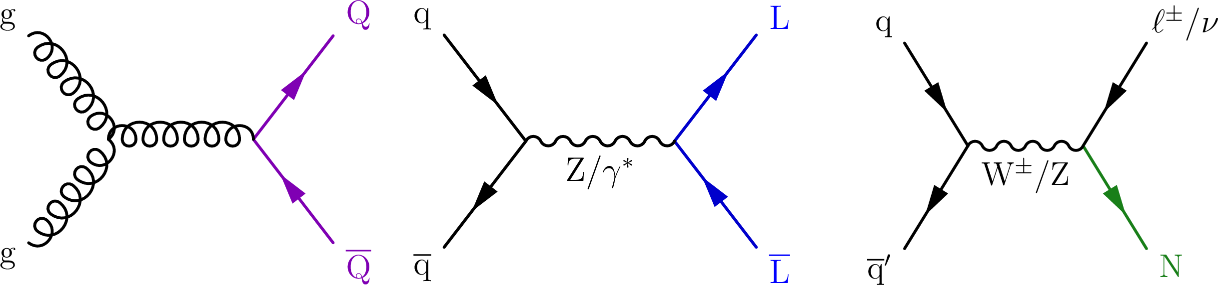
png pdf	Figure 1: Representative Feynman diagrams showing the production of VLQs (Q, left), VLLs (L, middle), and HNLs ($\mathrm{N}$, right) in proton-proton collisions.
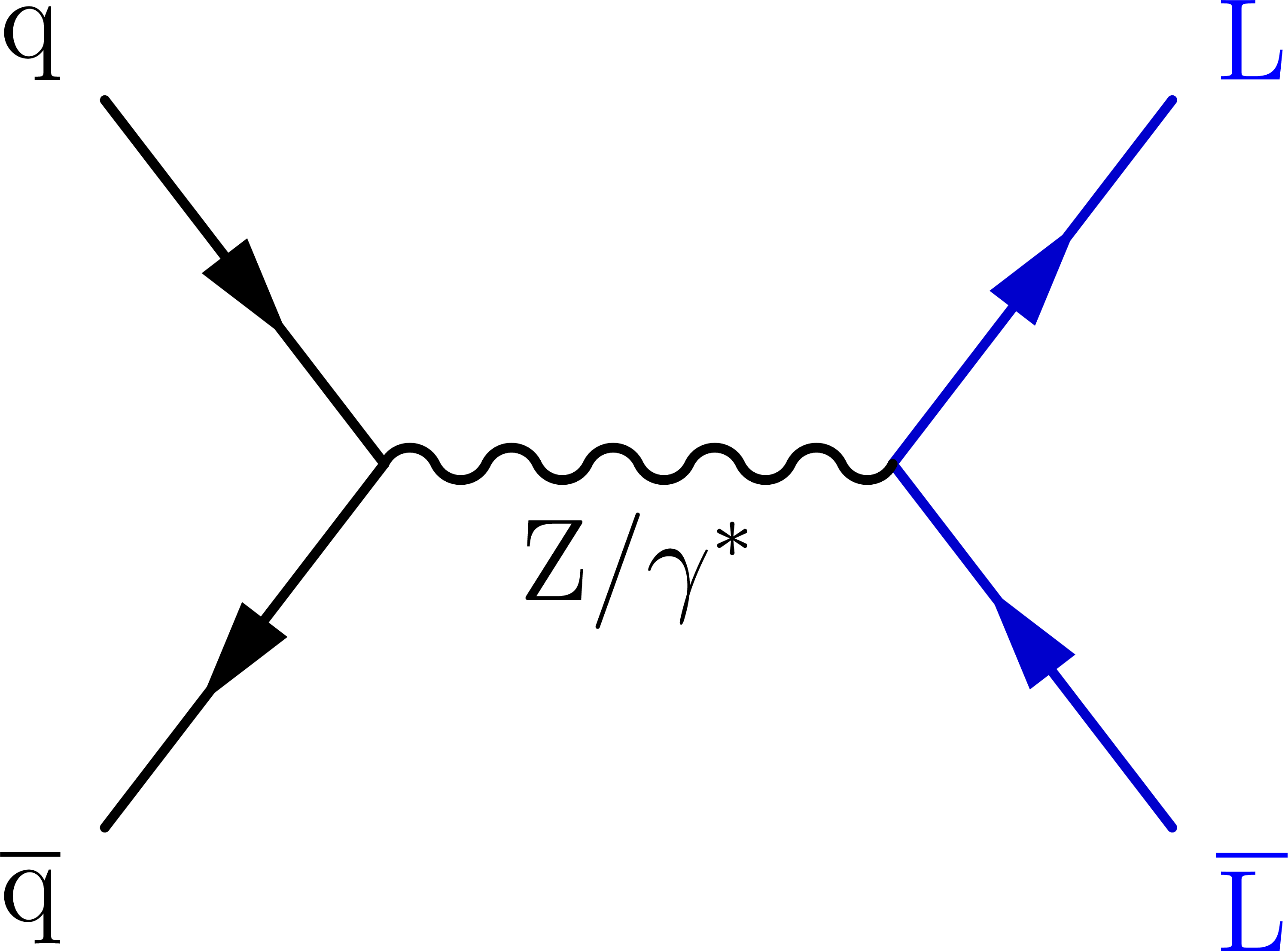
png pdf	Figure 1-a: Representative Feynman diagrams showing the production of VLQs (Q, left), VLLs (L, middle), and HNLs ($\mathrm{N}$, right) in proton-proton collisions.
png pdf	Figure 1-b: Representative Feynman diagrams showing the production of VLQs (Q, left), VLLs (L, middle), and HNLs ($\mathrm{N}$, right) in proton-proton collisions.
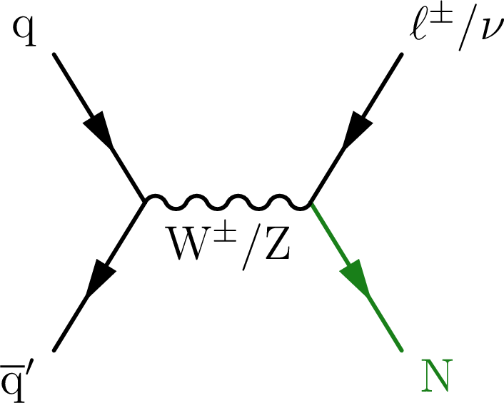
png pdf	Figure 1-c: Representative Feynman diagrams showing the production of VLQs (Q, left), VLLs (L, middle), and HNLs ($\mathrm{N}$, right) in proton-proton collisions.
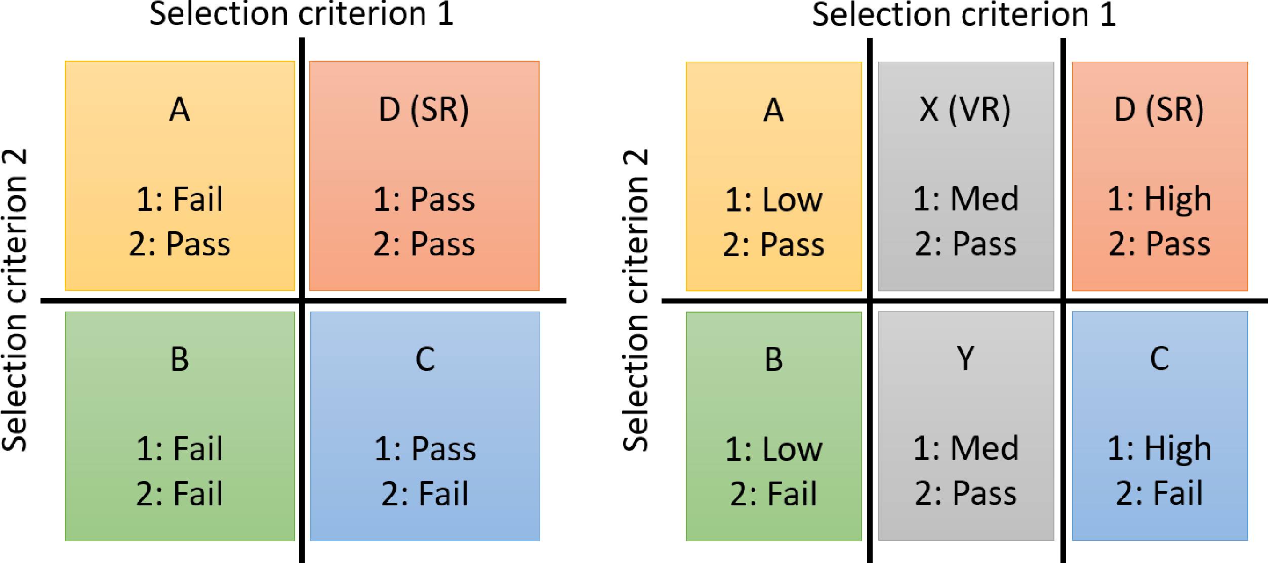
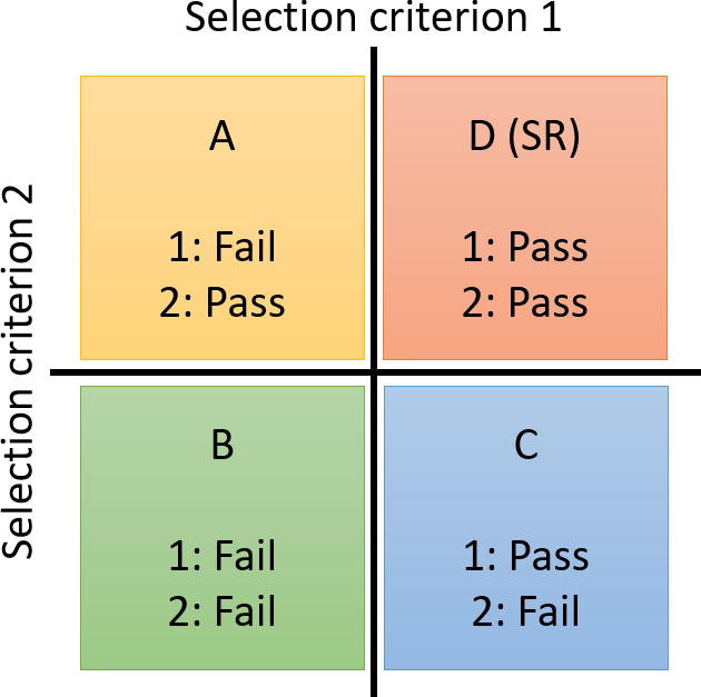
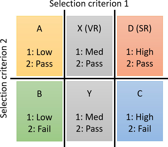
png pdf	Figure 2: Examples of either four (left) or six (right) selection regions used in the ABCD background estimation method. The region for which both criteria are satisfied is the SR. Expanding beyond four regions provides at least one ``validation region'' (VR).
png	Figure 2-a: Examples of either four (left) or six (right) selection regions used in the ABCD background estimation method. The region for which both criteria are satisfied is the SR. Expanding beyond four regions provides at least one ``validation region'' (VR).
png	Figure 2-b: Examples of either four (left) or six (right) selection regions used in the ABCD background estimation method. The region for which both criteria are satisfied is the SR. Expanding beyond four regions provides at least one ``validation region'' (VR).
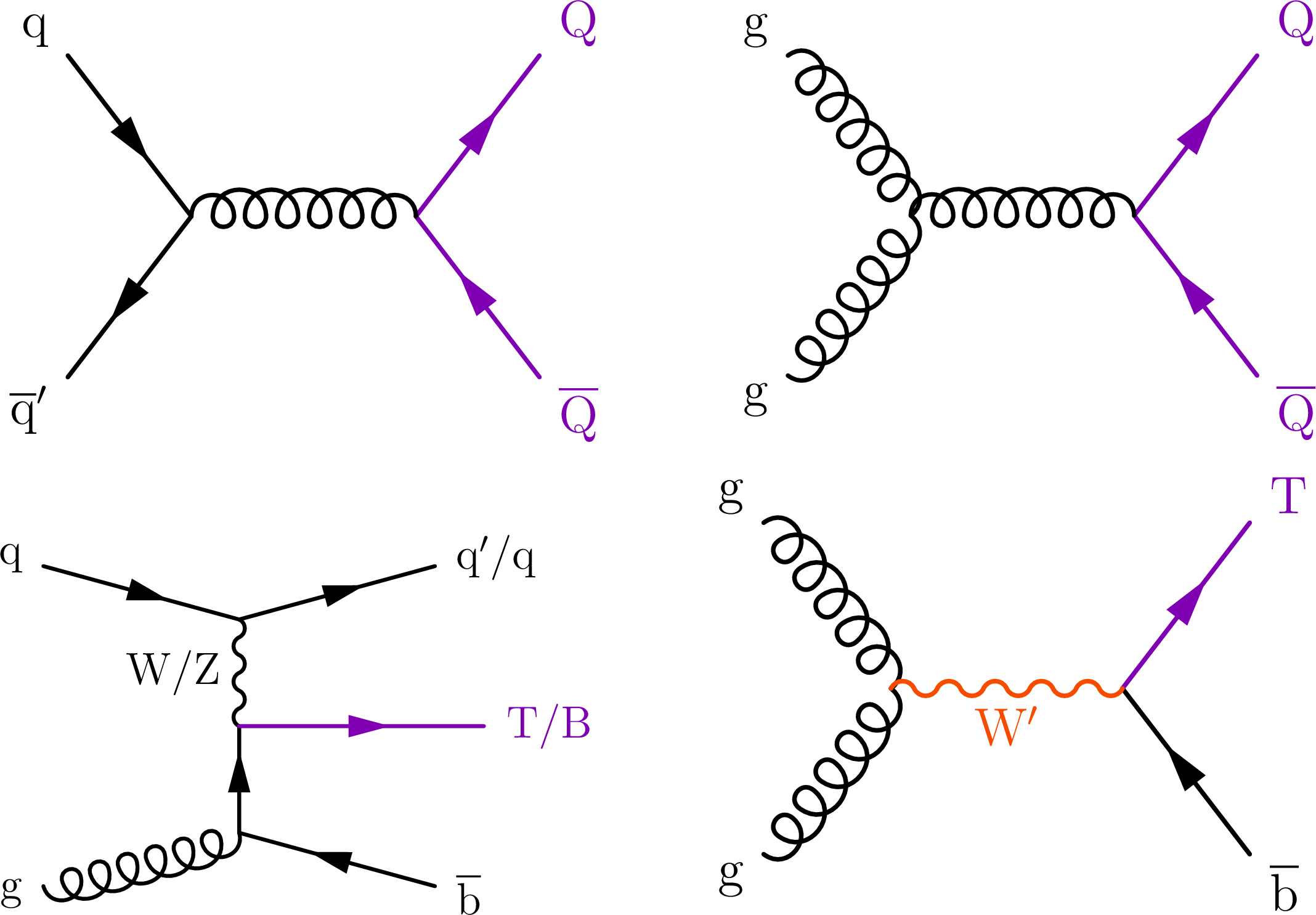
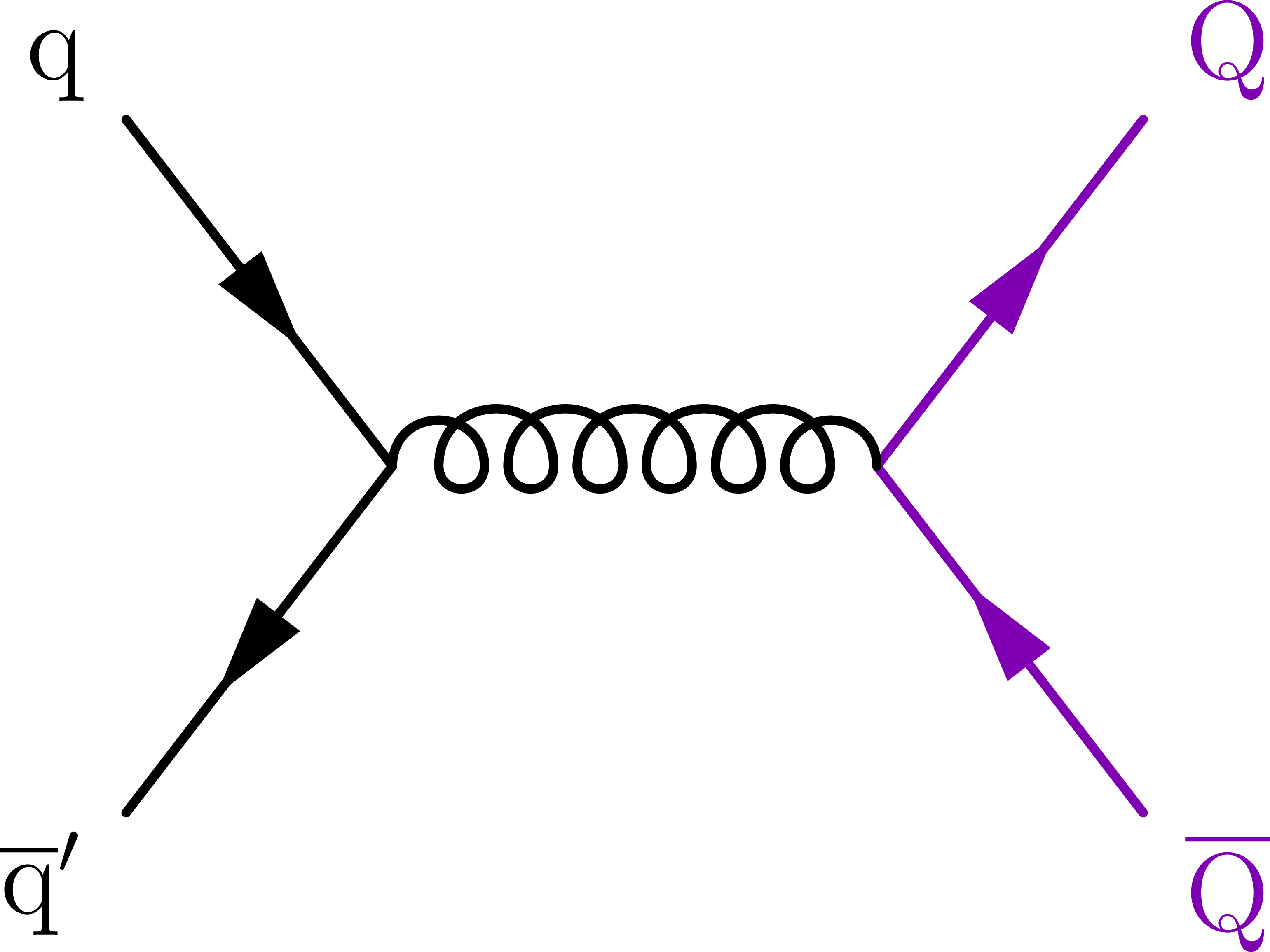
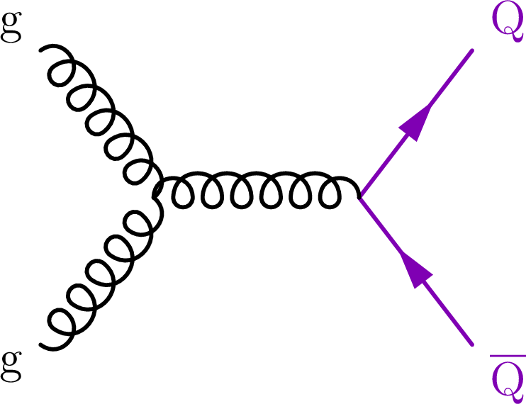
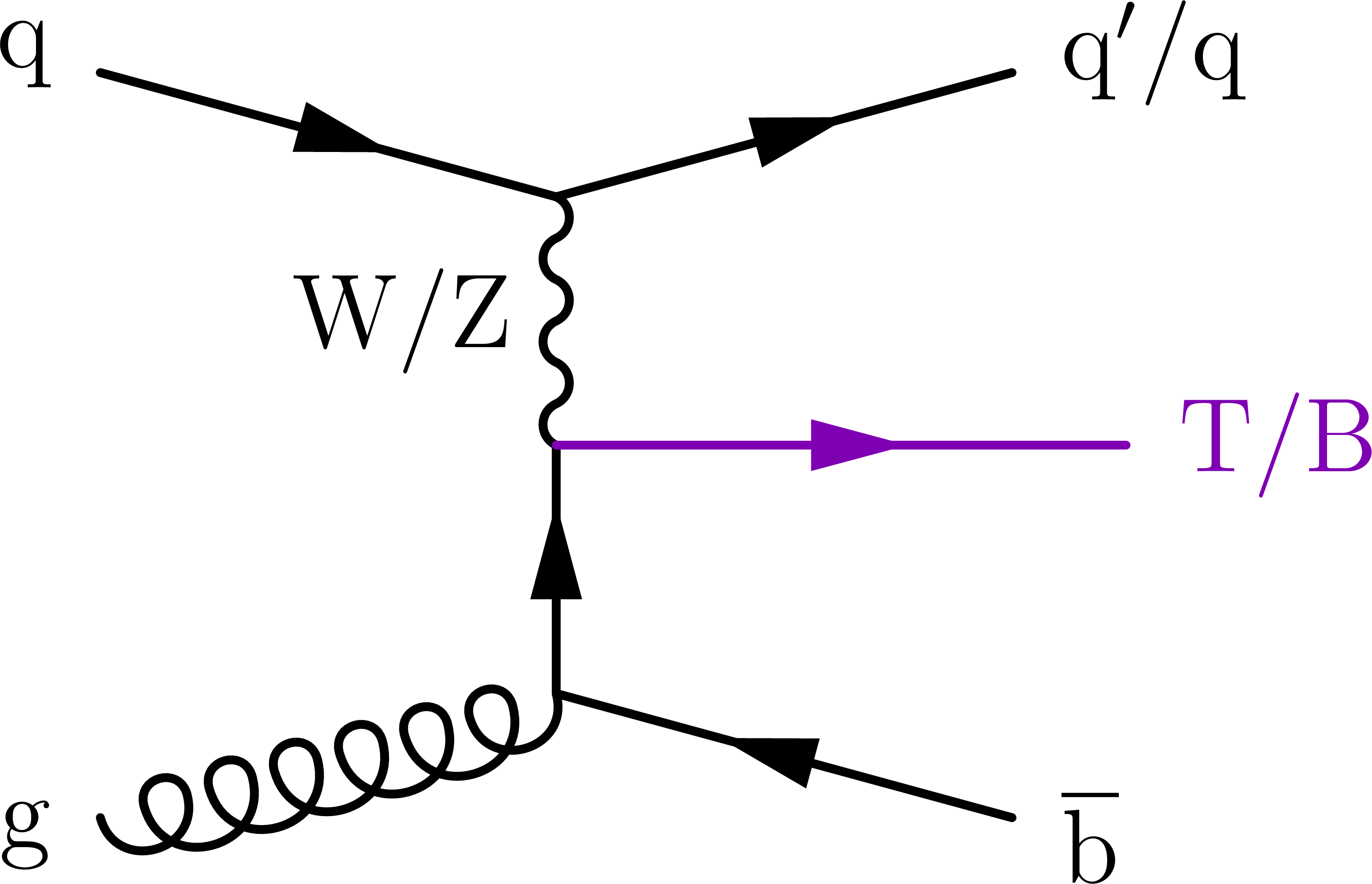
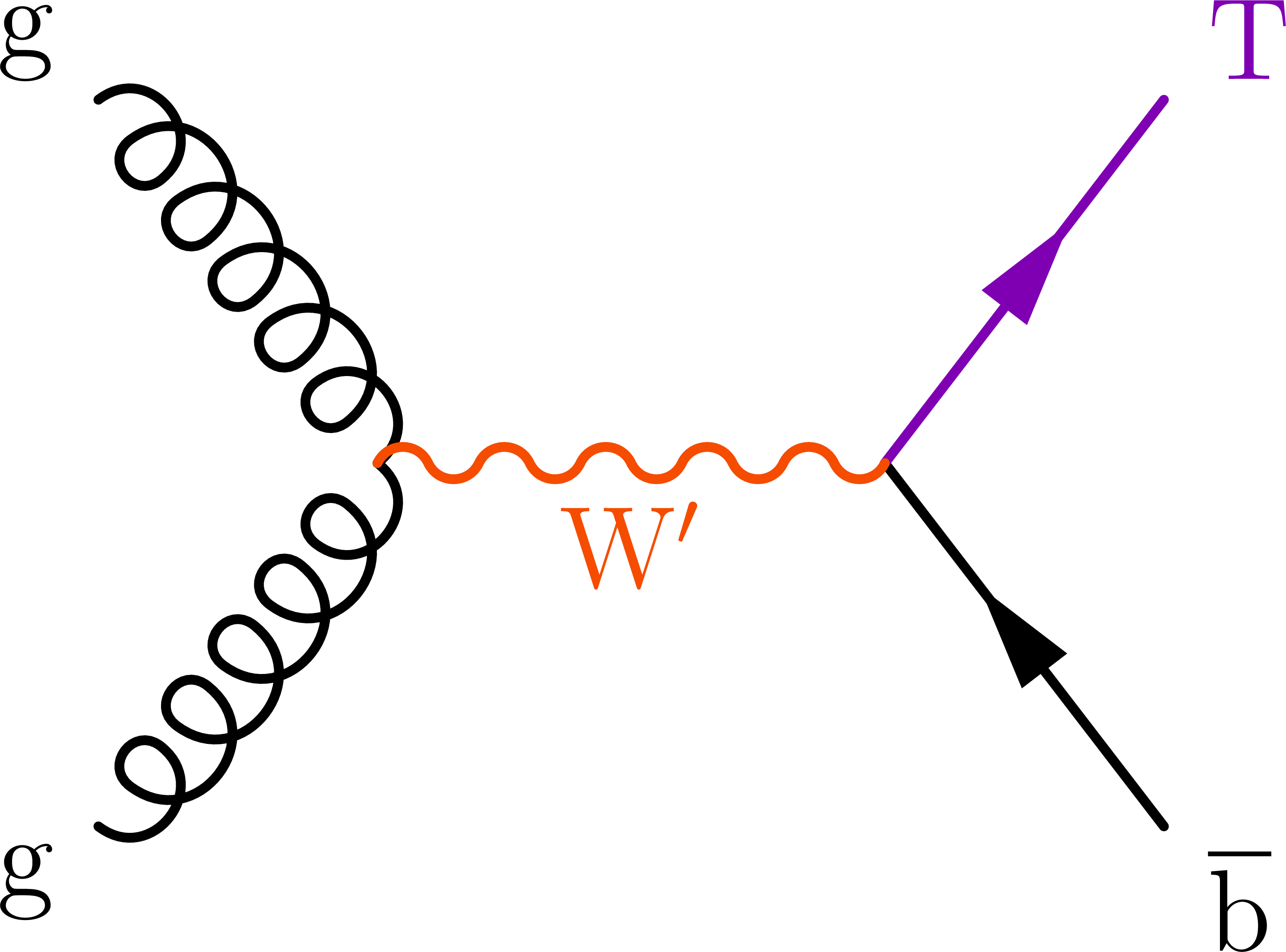
png pdf	Figure 3: Representative LO Feynman diagrams for pair production of VLQs via the strong interaction (upper row) and single production of VLQs via EW processes (lower left) or via new interactions (lower right). Here, Q stands for either VLQ flavor.
png pdf	Figure 3-a: Representative LO Feynman diagrams for pair production of VLQs via the strong interaction (upper row) and single production of VLQs via EW processes (lower left) or via new interactions (lower right). Here, Q stands for either VLQ flavor.
png pdf	Figure 3-b: Representative LO Feynman diagrams for pair production of VLQs via the strong interaction (upper row) and single production of VLQs via EW processes (lower left) or via new interactions (lower right). Here, Q stands for either VLQ flavor.
png pdf	Figure 3-c: Representative LO Feynman diagrams for pair production of VLQs via the strong interaction (upper row) and single production of VLQs via EW processes (lower left) or via new interactions (lower right). Here, Q stands for either VLQ flavor.
png pdf	Figure 3-d: Representative LO Feynman diagrams for pair production of VLQs via the strong interaction (upper row) and single production of VLQs via EW processes (lower left) or via new interactions (lower right). Here, Q stands for either VLQ flavor.
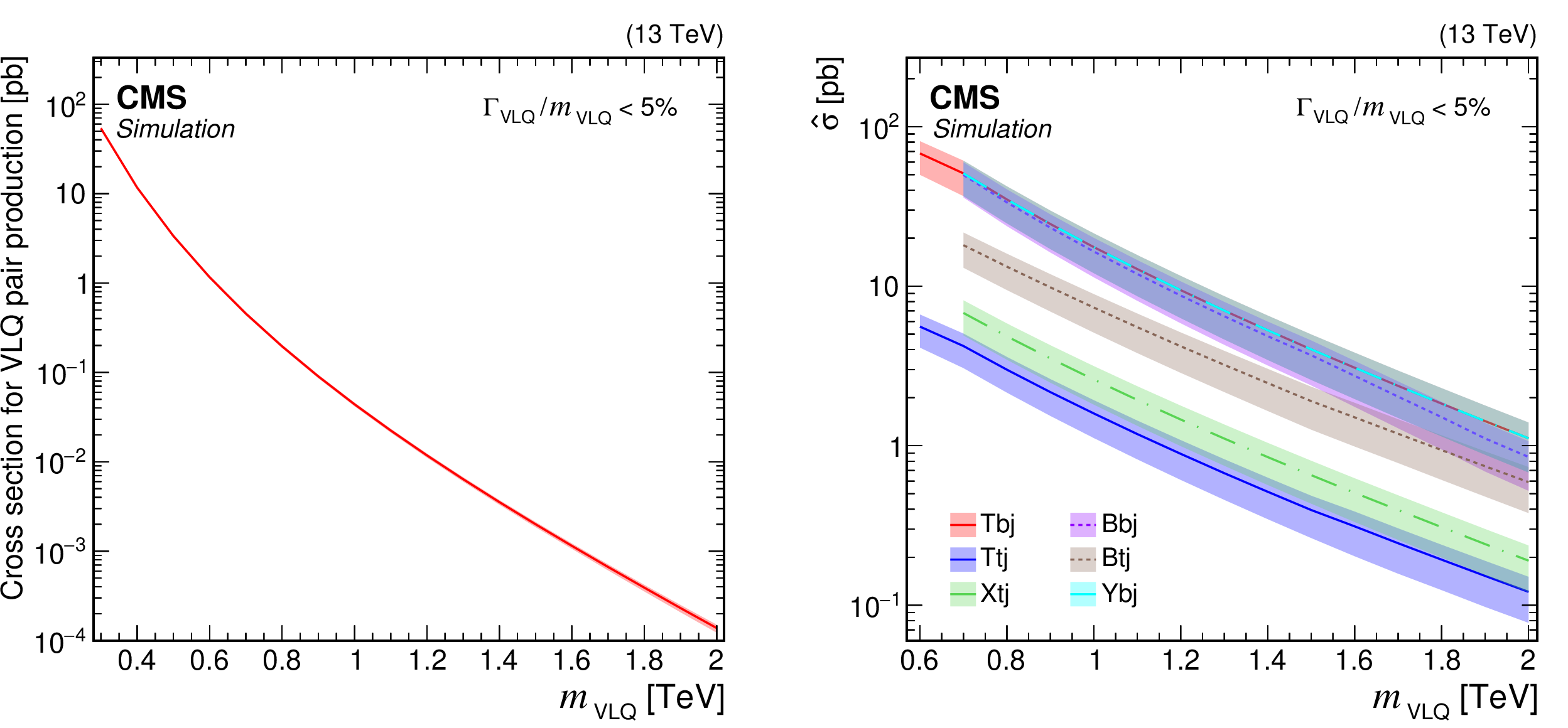
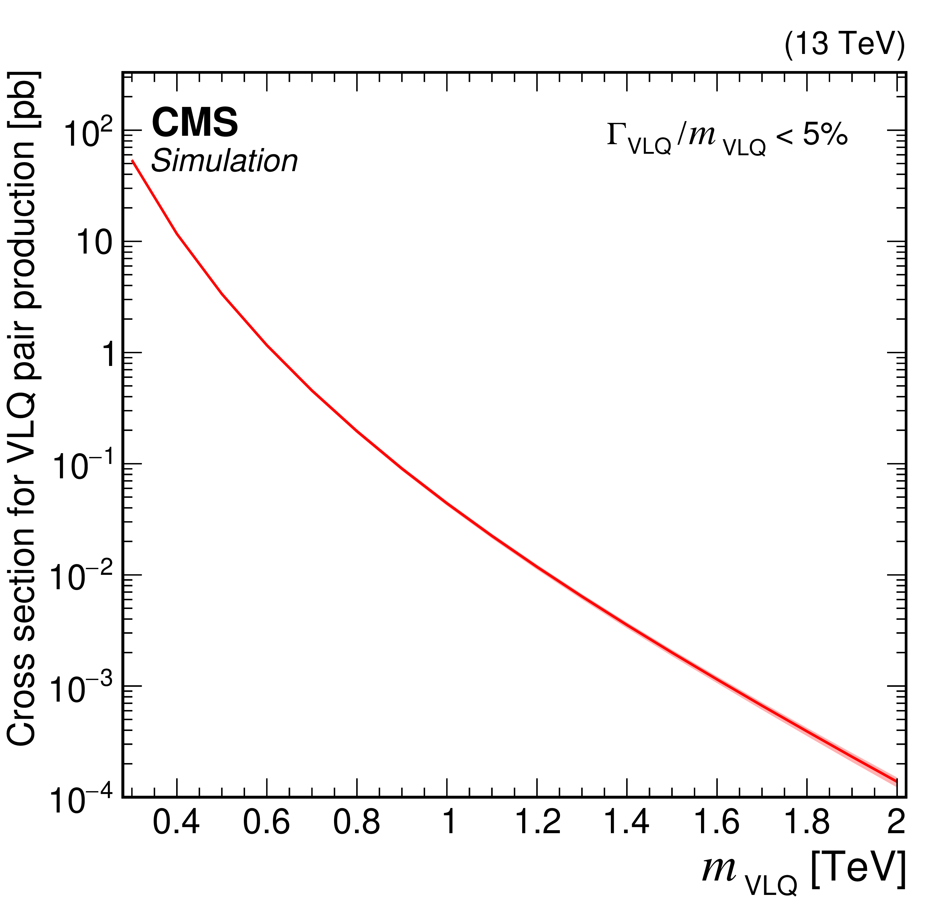
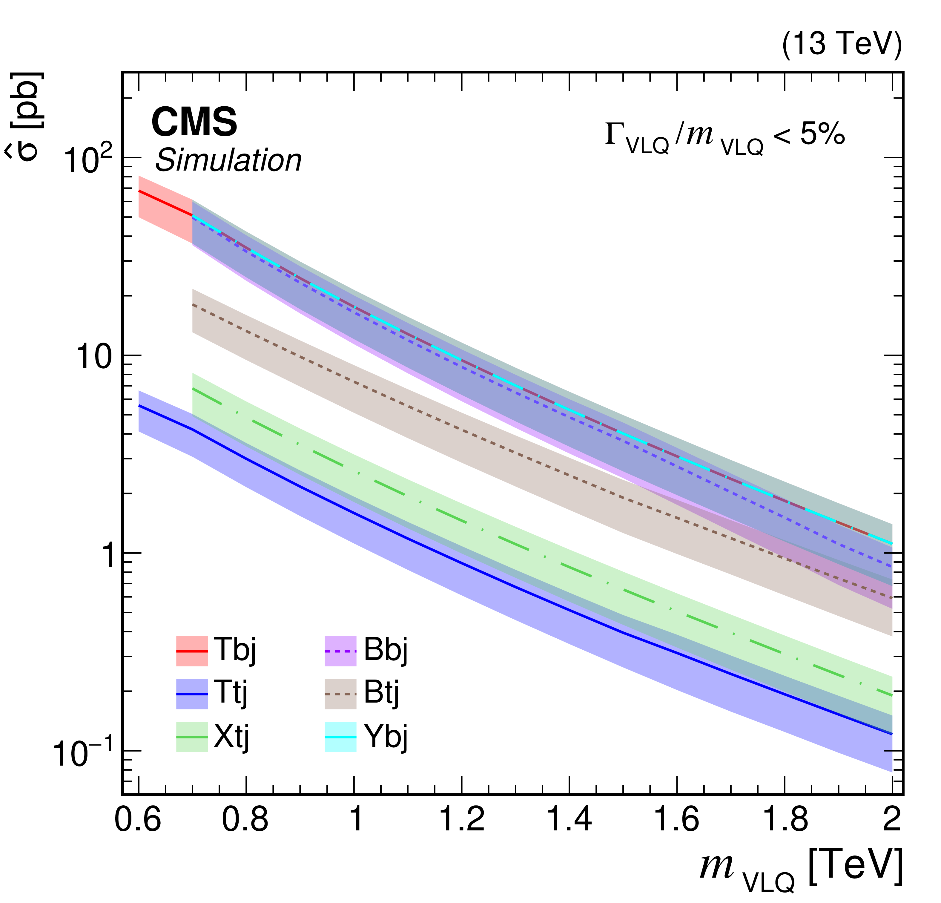
png pdf	Figure 4: Cross sections for the production of VLQs at $\sqrt{s}=$ 13 TeV as a function of the VLQ mass. Pair production cross sections via the strong interaction are computed to NNLO, using the models and tools from Refs. [127,128,129] (left). Reduced cross section $\hat{\sigma}$ for single production via the EW interaction is computed at LO in EW in the NWA using the models and tools from Refs. [130,128,118,131] (right). The shaded bands indicate PDF, renormalization scale, and factorization scale uncertainties associated with the predictions.
png pdf	Figure 4-a: Cross sections for the production of VLQs at $\sqrt{s}=$ 13 TeV as a function of the VLQ mass. Pair production cross sections via the strong interaction are computed to NNLO, using the models and tools from Refs. [127,128,129] (left). Reduced cross section $\hat{\sigma}$ for single production via the EW interaction is computed at LO in EW in the NWA using the models and tools from Refs. [130,128,118,131] (right). The shaded bands indicate PDF, renormalization scale, and factorization scale uncertainties associated with the predictions.
png pdf	Figure 4-b: Cross sections for the production of VLQs at $\sqrt{s}=$ 13 TeV as a function of the VLQ mass. Pair production cross sections via the strong interaction are computed to NNLO, using the models and tools from Refs. [127,128,129] (left). Reduced cross section $\hat{\sigma}$ for single production via the EW interaction is computed at LO in EW in the NWA using the models and tools from Refs. [130,128,118,131] (right). The shaded bands indicate PDF, renormalization scale, and factorization scale uncertainties associated with the predictions.
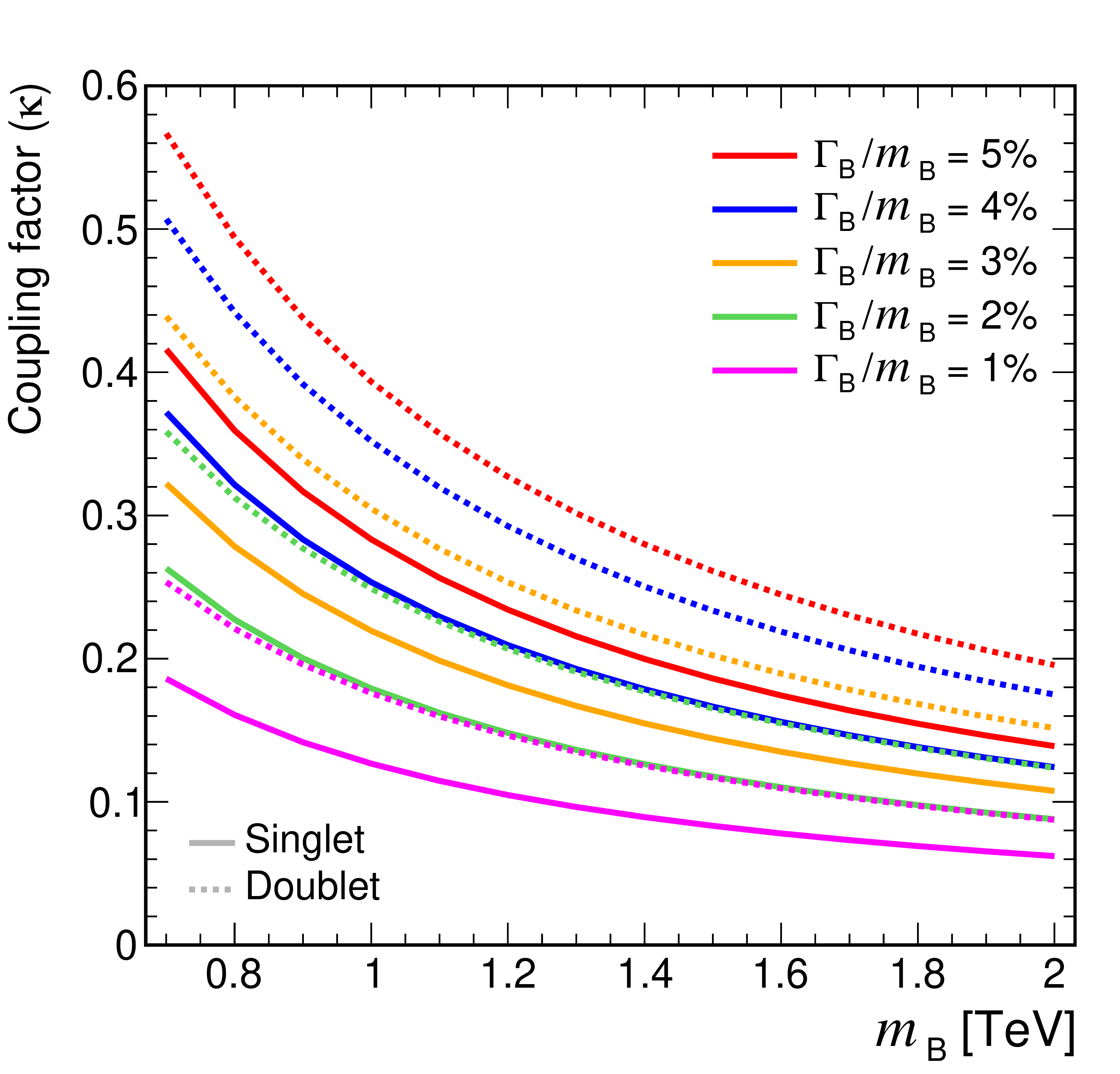
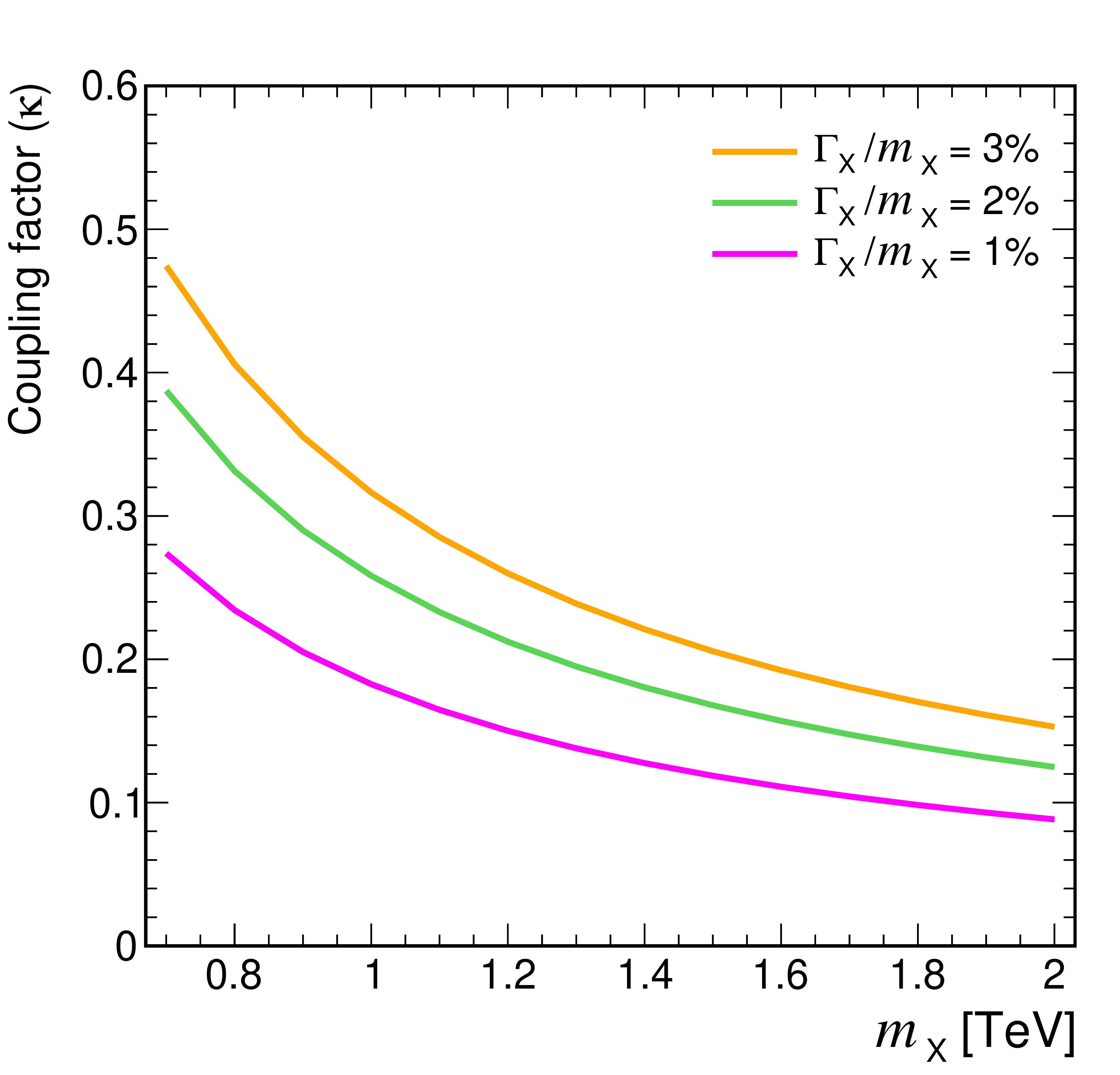
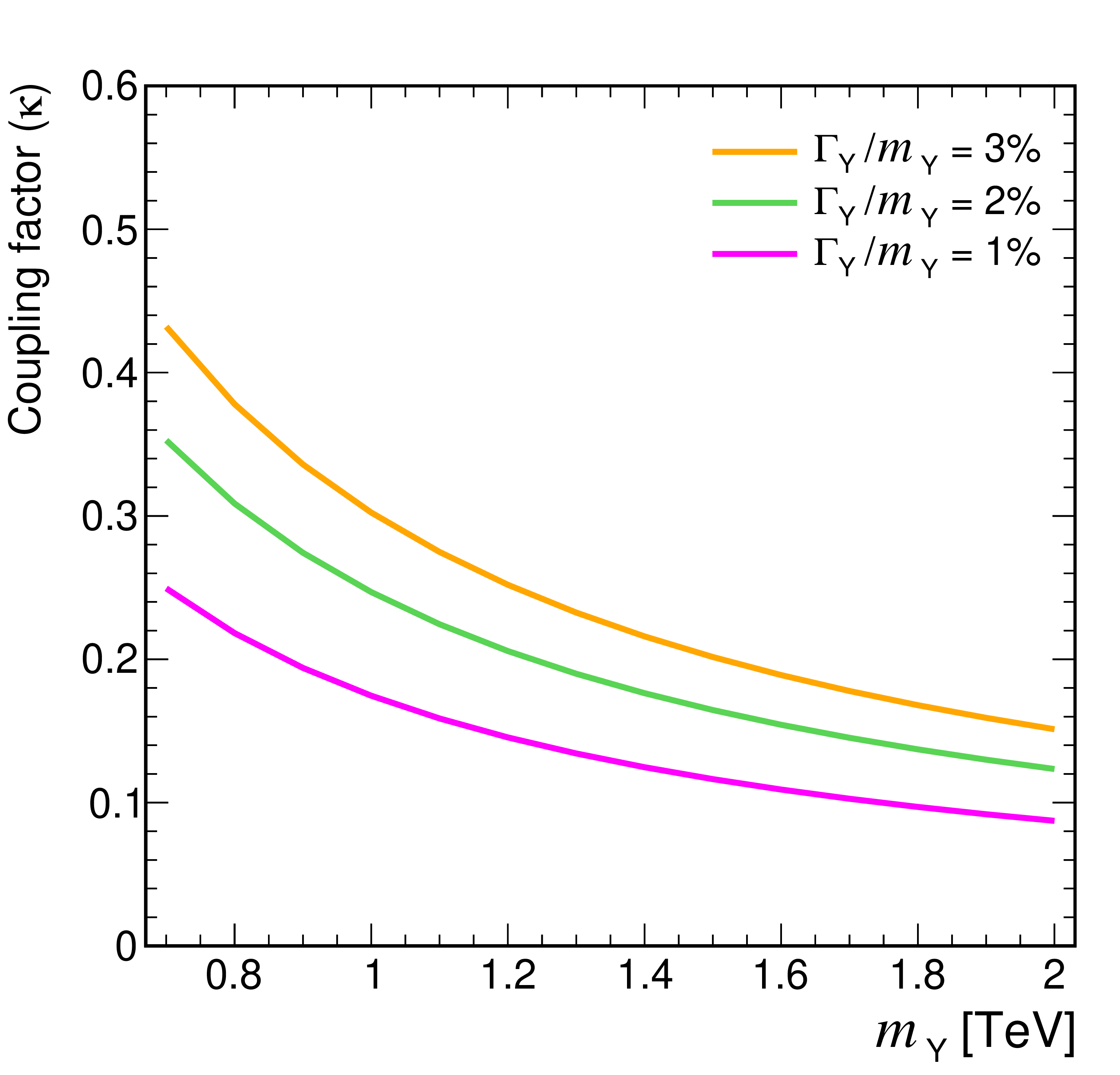
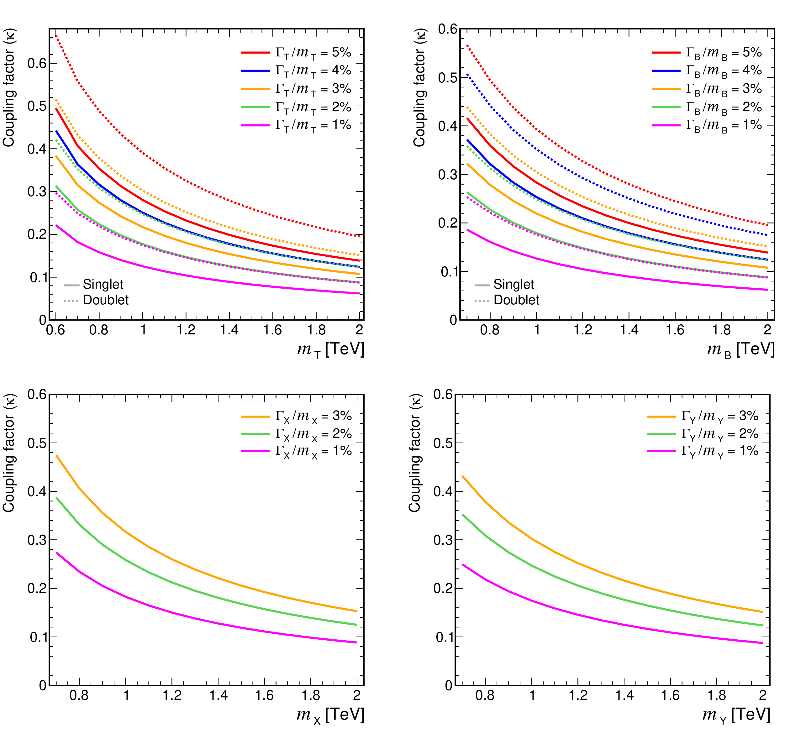
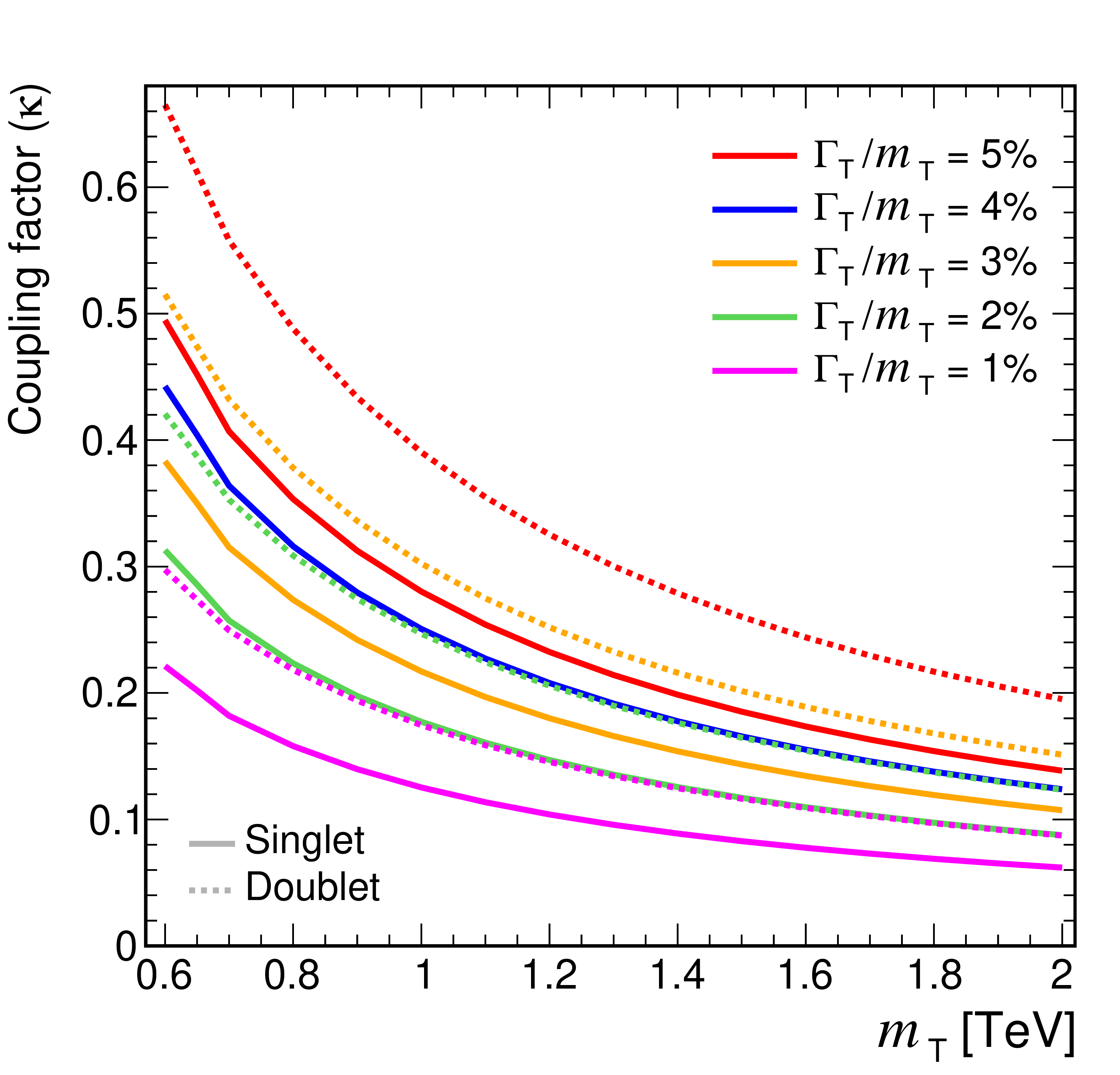
png pdf	Figure 5: Coupling factors for single VLQ production via the EW interaction in the narrow-width approximation as a function of the VLQ mass, using the models and tools from Refs. [130,128,118,131]. Coupling factors in single production of T (upper left), B (upper right) in the singlet (solid lines) and doublet (dashed lines) scenarios. Coupling factors in single production of $\mathrm{X}_{5/3}$ (lower left), $\mathrm{Y}_{4/3}$ (lower right) in doublet scenarios.
png pdf	Figure 5-a: Coupling factors for single VLQ production via the EW interaction in the narrow-width approximation as a function of the VLQ mass, using the models and tools from Refs. [130,128,118,131]. Coupling factors in single production of T (upper left), B (upper right) in the singlet (solid lines) and doublet (dashed lines) scenarios. Coupling factors in single production of $\mathrm{X}_{5/3}$ (lower left), $\mathrm{Y}_{4/3}$ (lower right) in doublet scenarios.
png pdf	Figure 5-b: Coupling factors for single VLQ production via the EW interaction in the narrow-width approximation as a function of the VLQ mass, using the models and tools from Refs. [130,128,118,131]. Coupling factors in single production of T (upper left), B (upper right) in the singlet (solid lines) and doublet (dashed lines) scenarios. Coupling factors in single production of $\mathrm{X}_{5/3}$ (lower left), $\mathrm{Y}_{4/3}$ (lower right) in doublet scenarios.
png pdf	Figure 5-c: Coupling factors for single VLQ production via the EW interaction in the narrow-width approximation as a function of the VLQ mass, using the models and tools from Refs. [130,128,118,131]. Coupling factors in single production of T (upper left), B (upper right) in the singlet (solid lines) and doublet (dashed lines) scenarios. Coupling factors in single production of $\mathrm{X}_{5/3}$ (lower left), $\mathrm{Y}_{4/3}$ (lower right) in doublet scenarios.
png pdf	Figure 5-d: Coupling factors for single VLQ production via the EW interaction in the narrow-width approximation as a function of the VLQ mass, using the models and tools from Refs. [130,128,118,131]. Coupling factors in single production of T (upper left), B (upper right) in the singlet (solid lines) and doublet (dashed lines) scenarios. Coupling factors in single production of $\mathrm{X}_{5/3}$ (lower left), $\mathrm{Y}_{4/3}$ (lower right) in doublet scenarios.
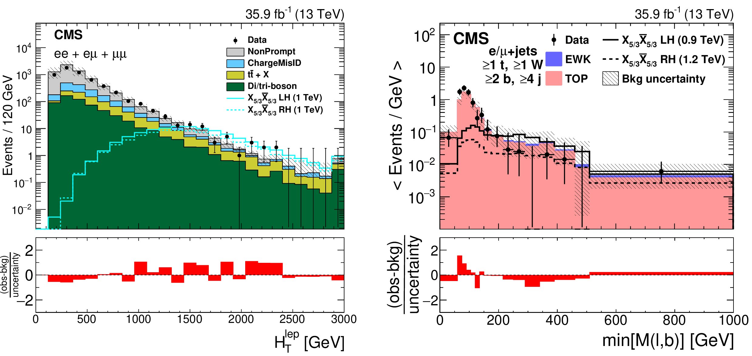
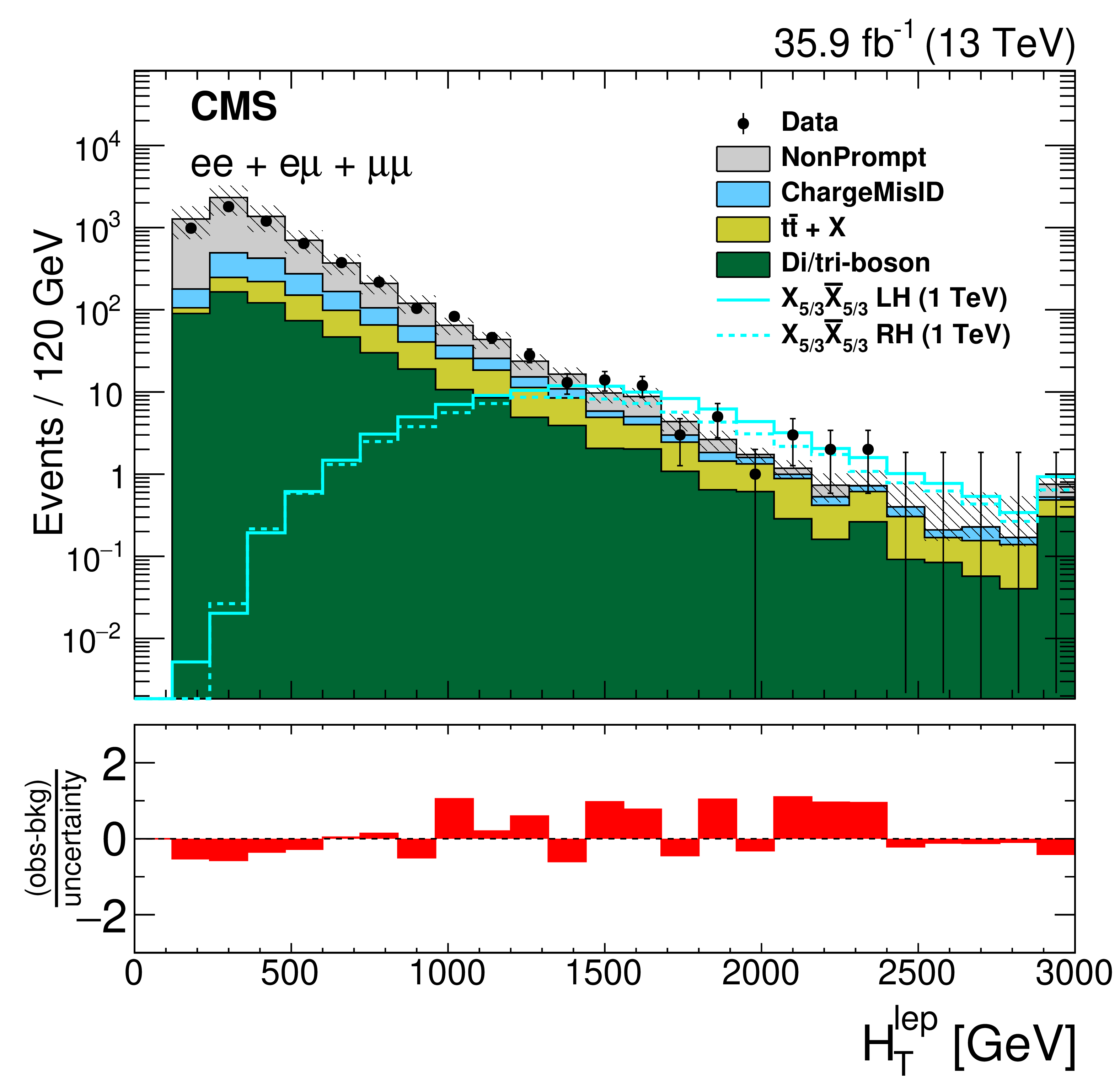
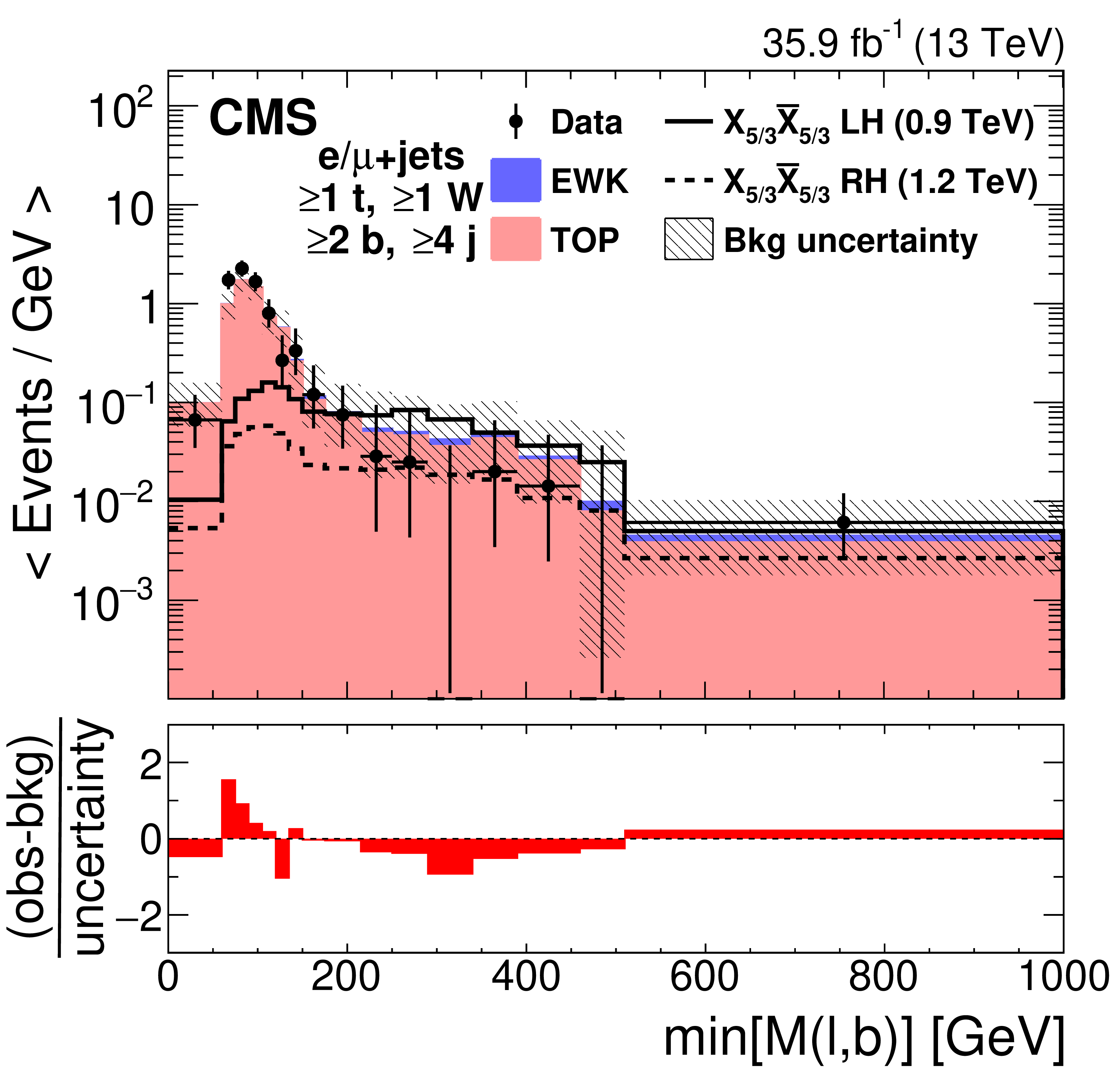
png pdf	Figure 6: Distributions of observables used to maximize the ${\mathrm{X}_{5/3}} {\mathrm{X}_{5/3}}$ signal significance for the SSDL (left) and single-lepton (right) final states. The left figure shows the $H_{\mathrm{T}}^{\text{lep}}$ distribution after the SS dilepton selection, Z boson and quarkonia lepton invariant mass vetoes, and the requirement of at least two small-radius jets in the event, for a combination of $\mathrm{e}\mathrm{e}$, $\mathrm{e}\mu$, and $\mu\mu$ channels. The right figure shows the $\min M(\ell,\mathrm{b})$ distribution in events with $\geq$1 t-tagged jet, $\geq$1 W-tagged jets, and $\geq$2 b-tagged jets for the combined electron and muon samples in the SR. The distribution has variable-size bins such that the statistical uncertainty in each bin is less than 30%. The lower panel in each plot shows the difference between the observed and the predicted numbers of events divided by the total uncertainty. Figures taken from Ref. [143].
png pdf	Figure 6-a: Distributions of observables used to maximize the ${\mathrm{X}_{5/3}} {\mathrm{X}_{5/3}}$ signal significance for the SSDL (left) and single-lepton (right) final states. The left figure shows the $H_{\mathrm{T}}^{\text{lep}}$ distribution after the SS dilepton selection, Z boson and quarkonia lepton invariant mass vetoes, and the requirement of at least two small-radius jets in the event, for a combination of $\mathrm{e}\mathrm{e}$, $\mathrm{e}\mu$, and $\mu\mu$ channels. The right figure shows the $\min M(\ell,\mathrm{b})$ distribution in events with $\geq$1 t-tagged jet, $\geq$1 W-tagged jets, and $\geq$2 b-tagged jets for the combined electron and muon samples in the SR. The distribution has variable-size bins such that the statistical uncertainty in each bin is less than 30%. The lower panel in each plot shows the difference between the observed and the predicted numbers of events divided by the total uncertainty. Figures taken from Ref. [143].
png pdf	Figure 6-b: Distributions of observables used to maximize the ${\mathrm{X}_{5/3}} {\mathrm{X}_{5/3}}$ signal significance for the SSDL (left) and single-lepton (right) final states. The left figure shows the $H_{\mathrm{T}}^{\text{lep}}$ distribution after the SS dilepton selection, Z boson and quarkonia lepton invariant mass vetoes, and the requirement of at least two small-radius jets in the event, for a combination of $\mathrm{e}\mathrm{e}$, $\mathrm{e}\mu$, and $\mu\mu$ channels. The right figure shows the $\min M(\ell,\mathrm{b})$ distribution in events with $\geq$1 t-tagged jet, $\geq$1 W-tagged jets, and $\geq$2 b-tagged jets for the combined electron and muon samples in the SR. The distribution has variable-size bins such that the statistical uncertainty in each bin is less than 30%. The lower panel in each plot shows the difference between the observed and the predicted numbers of events divided by the total uncertainty. Figures taken from Ref. [143].
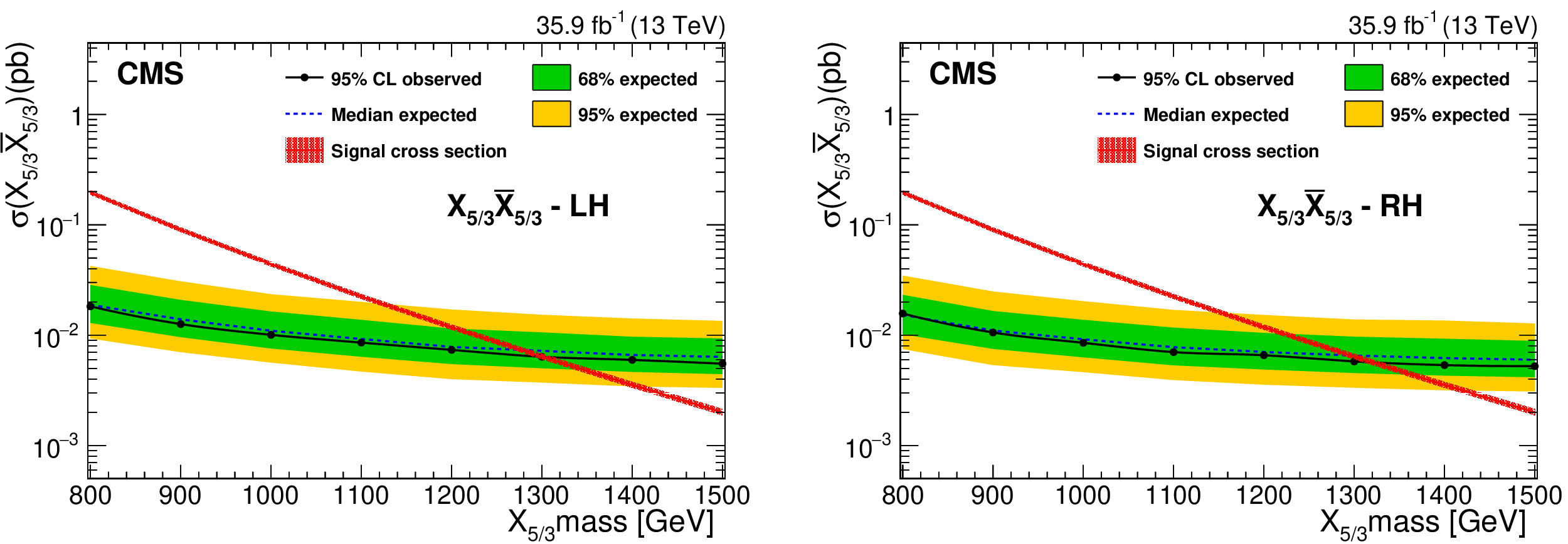
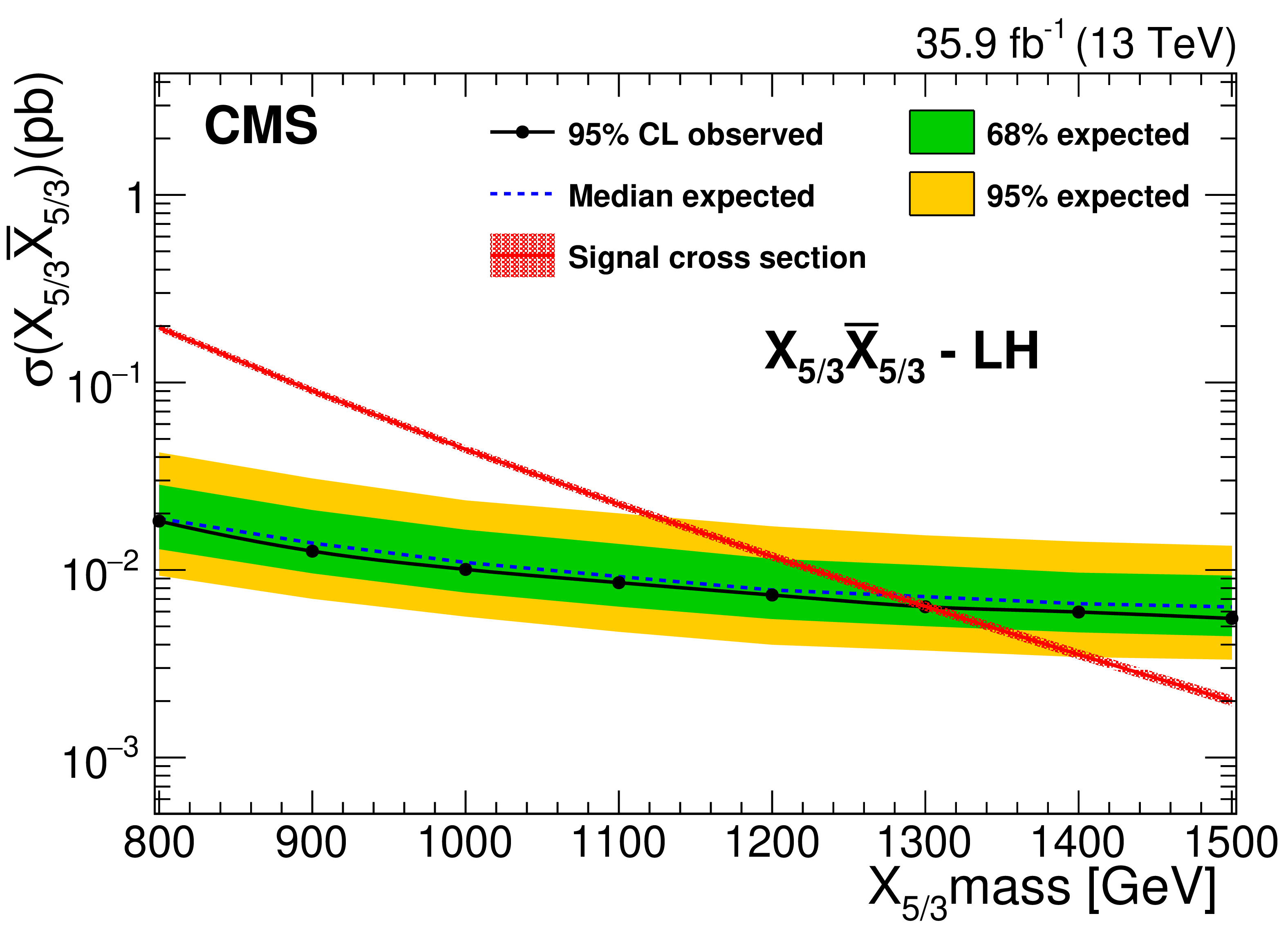
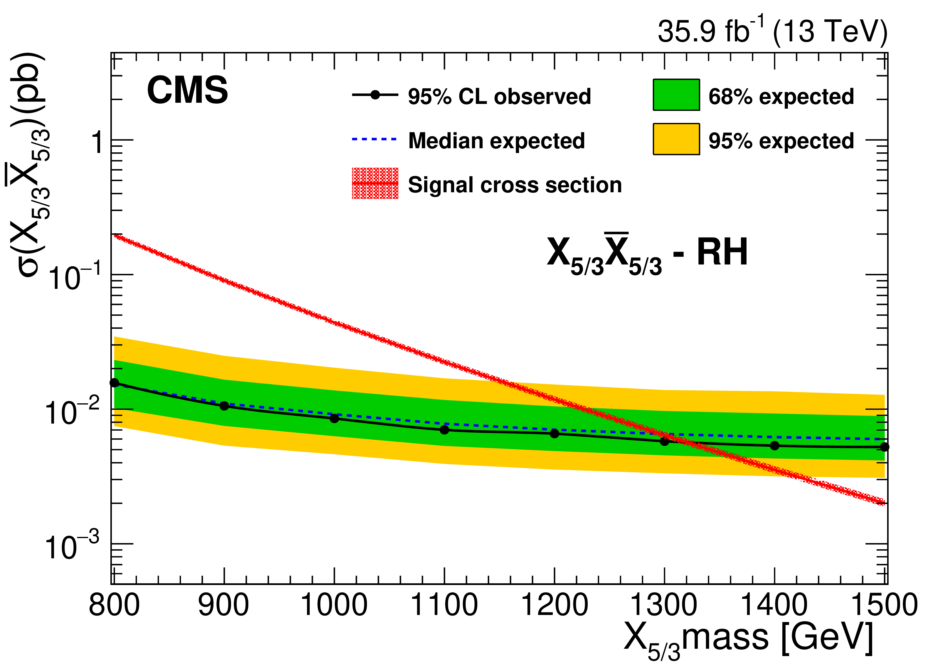
png pdf	Figure 7: Expected and observed cross section upper limits at 95% CL for an LH (left) and RH (right) $\mathrm{X}_{5/3}$ as a function of its mass, after combining the SS dilepton and single-lepton final states. The theoretical uncertainty in the signal cross section is shown with a band around the theoretical prediction. Figures adapted from Ref. [143].
png pdf	Figure 7-a: Expected and observed cross section upper limits at 95% CL for an LH (left) and RH (right) $\mathrm{X}_{5/3}$ as a function of its mass, after combining the SS dilepton and single-lepton final states. The theoretical uncertainty in the signal cross section is shown with a band around the theoretical prediction. Figures adapted from Ref. [143].
png pdf	Figure 7-b: Expected and observed cross section upper limits at 95% CL for an LH (left) and RH (right) $\mathrm{X}_{5/3}$ as a function of its mass, after combining the SS dilepton and single-lepton final states. The theoretical uncertainty in the signal cross section is shown with a band around the theoretical prediction. Figures adapted from Ref. [143].
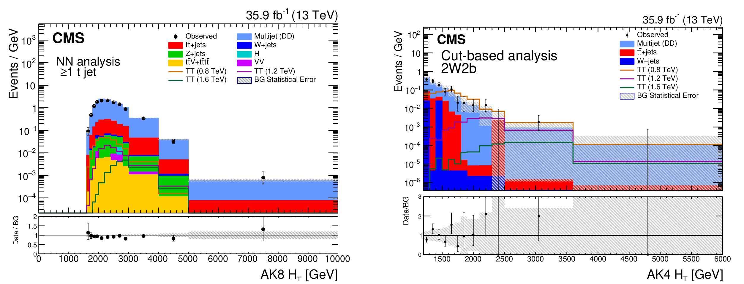
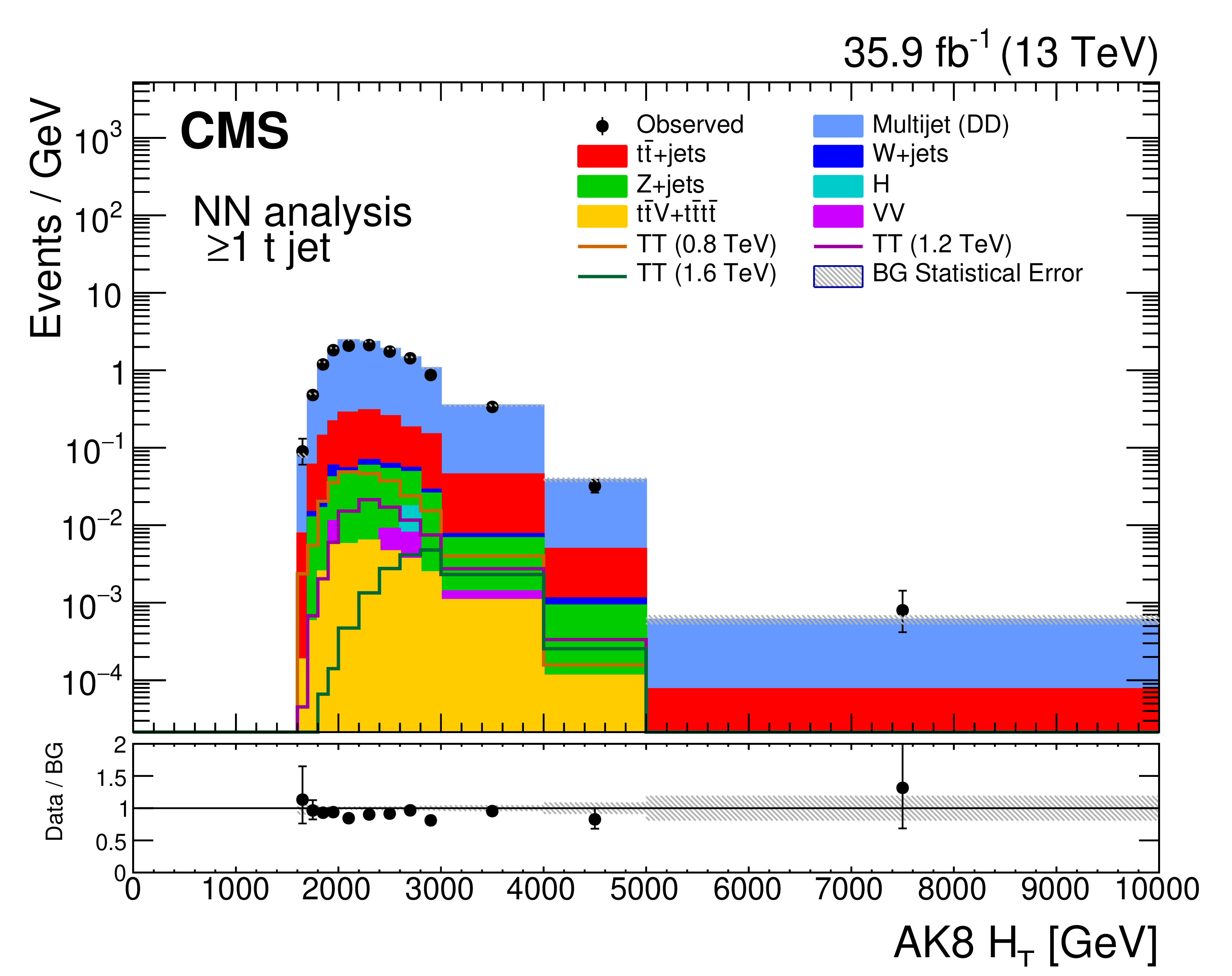
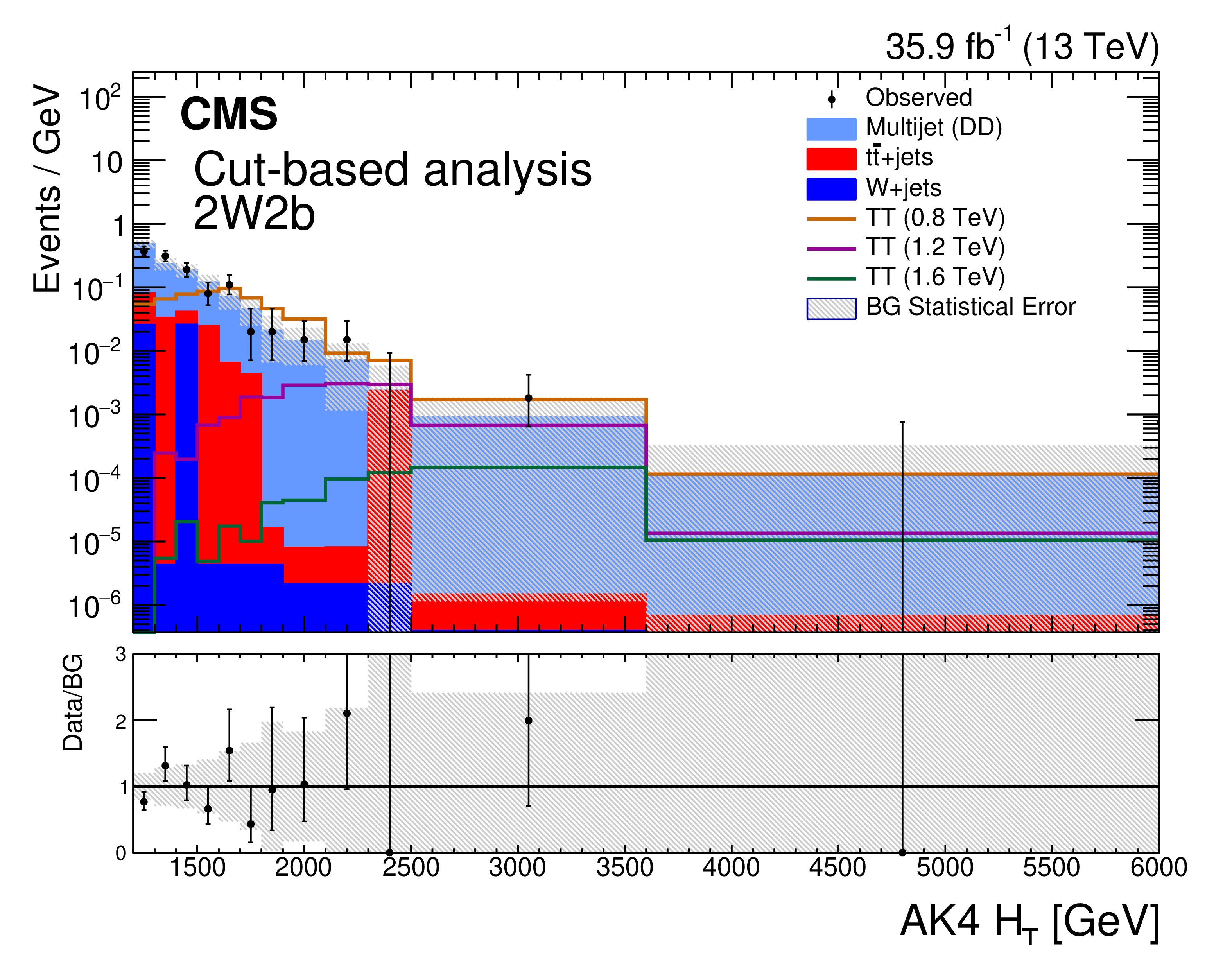
png pdf	Figure 8: Distributions of $H_{\mathrm{T}}$ in a combination of SRs in the NN-based approach, inclusive in $\geq$1 t tags (left), and in the SR with two W-tagged and two b-tagged jets in the selection-based approach (right). The lower panels show the ratio between observed data and the background estimate. Figures taken from Ref. [140].
png pdf	Figure 8-a: Distributions of $H_{\mathrm{T}}$ in a combination of SRs in the NN-based approach, inclusive in $\geq$1 t tags (left), and in the SR with two W-tagged and two b-tagged jets in the selection-based approach (right). The lower panels show the ratio between observed data and the background estimate. Figures taken from Ref. [140].
png pdf	Figure 8-b: Distributions of $H_{\mathrm{T}}$ in a combination of SRs in the NN-based approach, inclusive in $\geq$1 t tags (left), and in the SR with two W-tagged and two b-tagged jets in the selection-based approach (right). The lower panels show the ratio between observed data and the background estimate. Figures taken from Ref. [140].
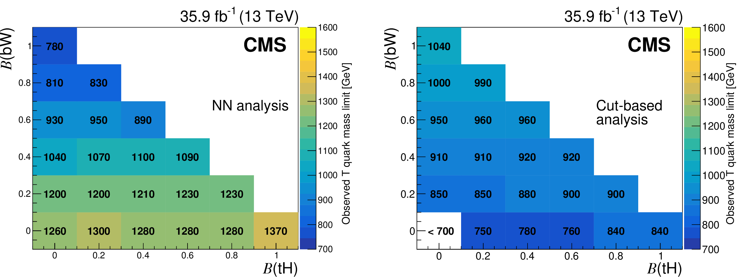
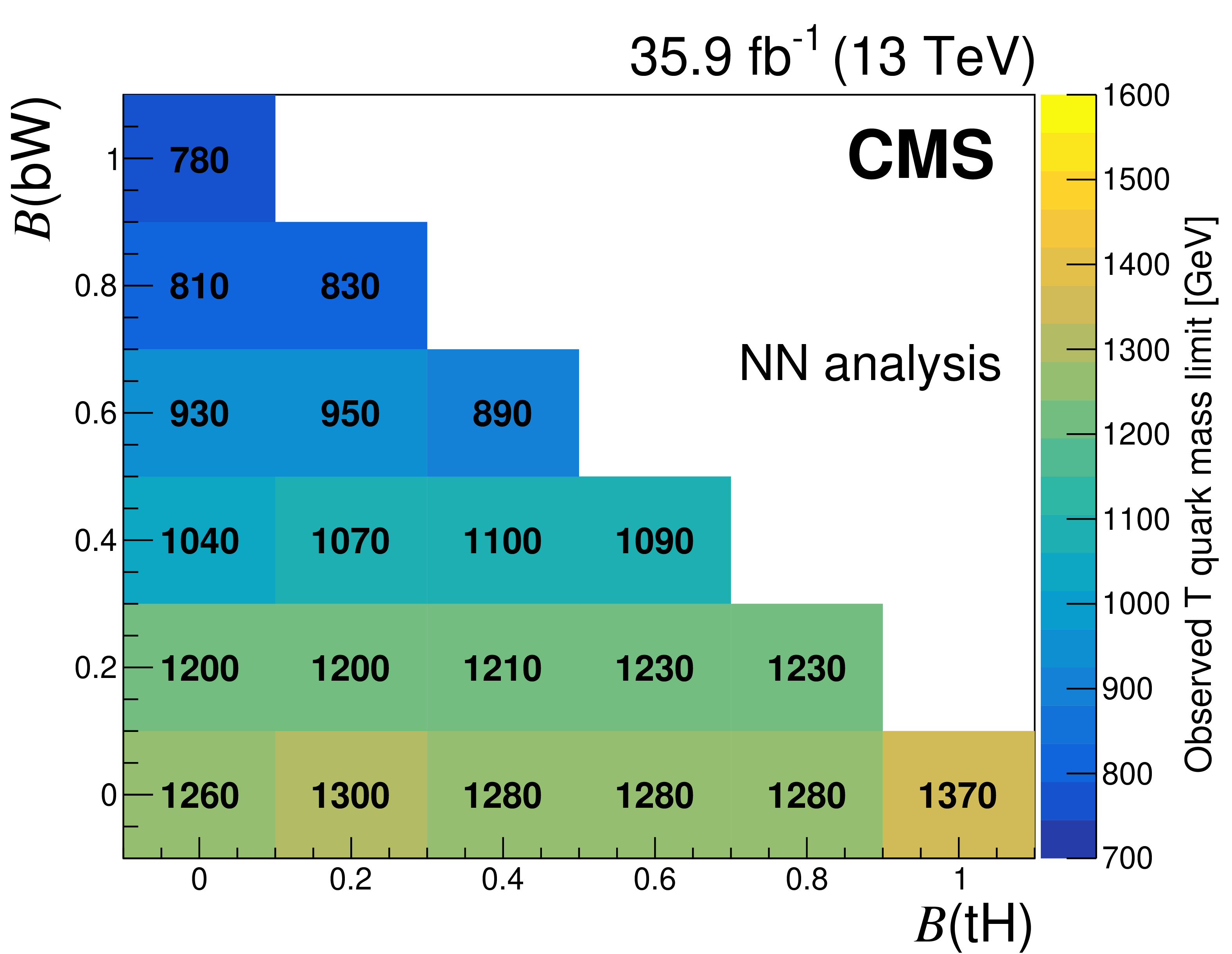
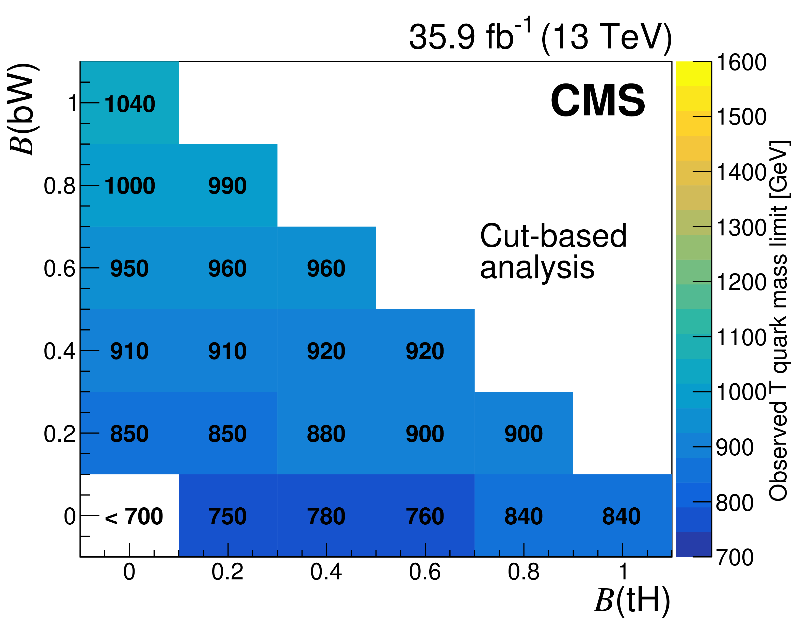
png pdf	Figure 9: Observed lower limits at 95% CL on the T quark mass as functions of the T quark branching fractions to $\mathrm{t}\mathrm{H}$ and $\mathrm{b}\mathrm{W}$, using the NN-based (left) and selection-based (right) approaches. Figures adapted from Ref. [140].
png pdf	Figure 9-a: Observed lower limits at 95% CL on the T quark mass as functions of the T quark branching fractions to $\mathrm{t}\mathrm{H}$ and $\mathrm{b}\mathrm{W}$, using the NN-based (left) and selection-based (right) approaches. Figures adapted from Ref. [140].
png pdf	Figure 9-b: Observed lower limits at 95% CL on the T quark mass as functions of the T quark branching fractions to $\mathrm{t}\mathrm{H}$ and $\mathrm{b}\mathrm{W}$, using the NN-based (left) and selection-based (right) approaches. Figures adapted from Ref. [140].
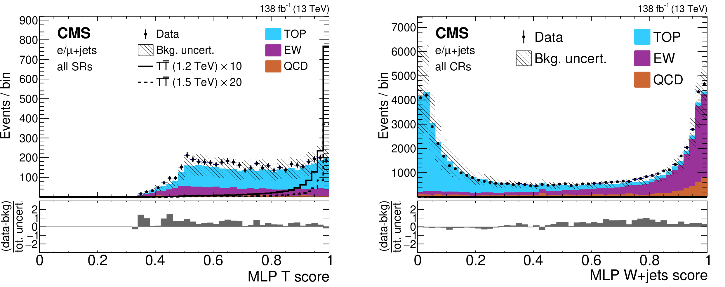
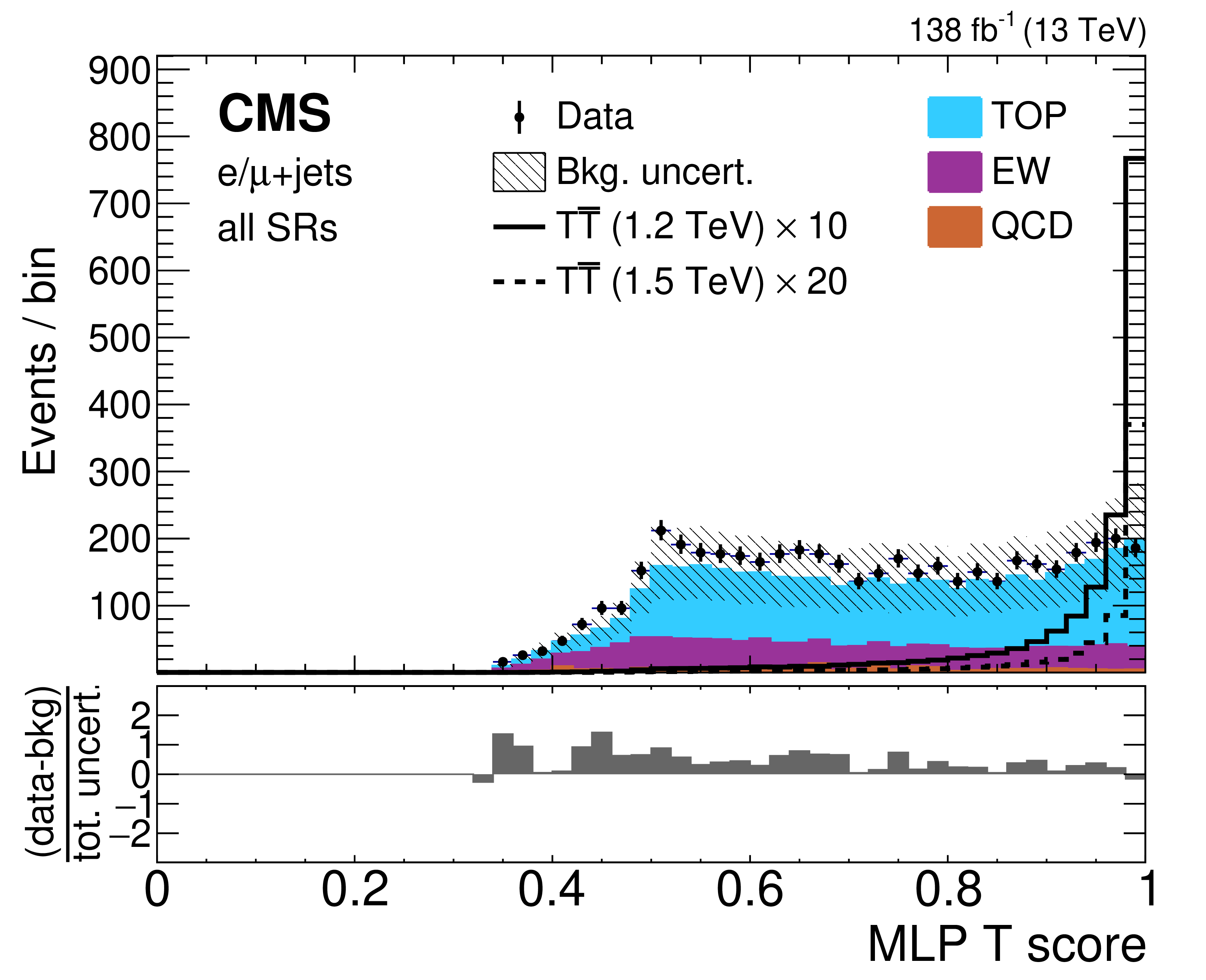
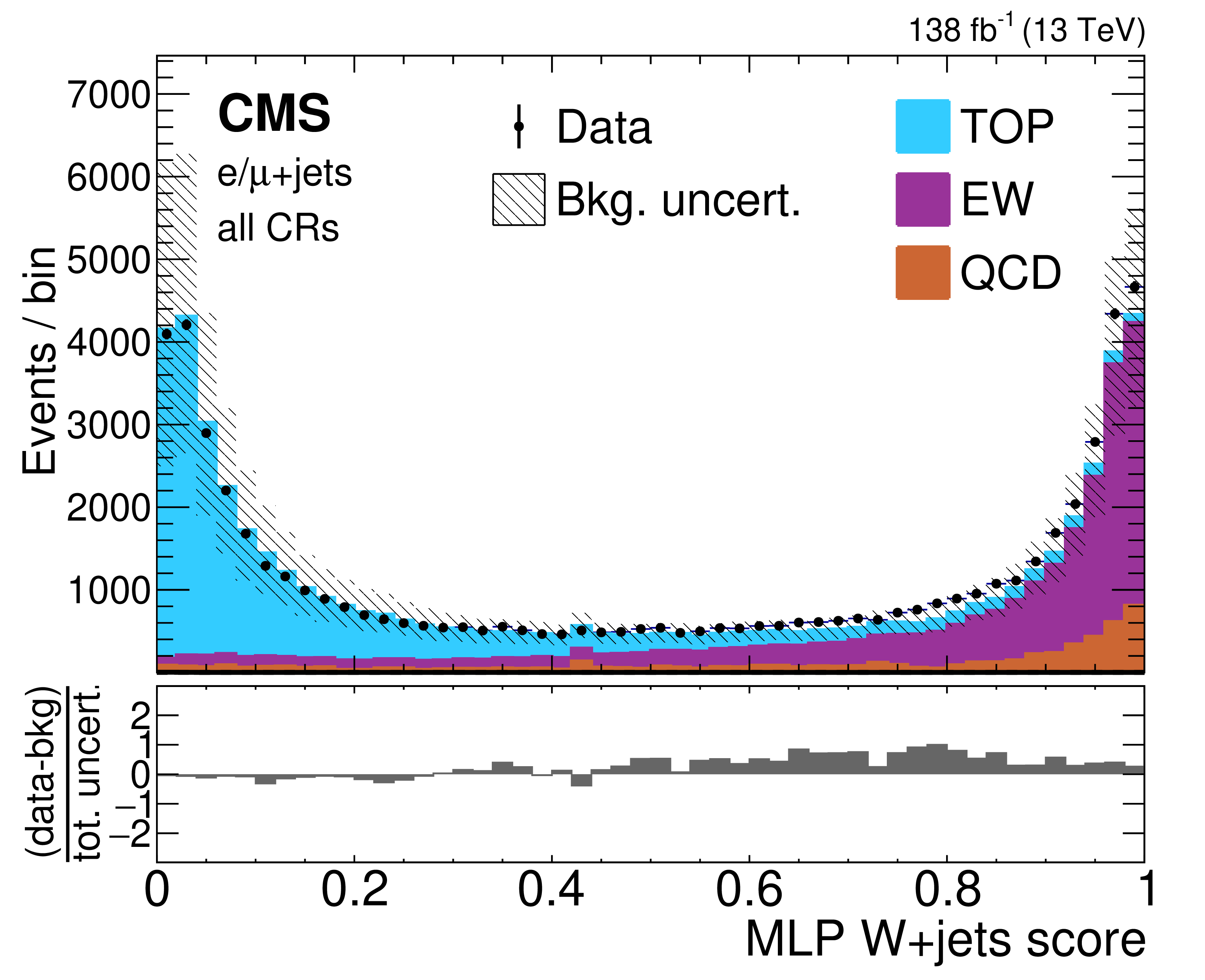
png pdf	Figure 10: Example single-lepton channel ${\mathrm{T}} \overline{\mathrm{T}}$ NN output distributions of the T quark score in the inclusive SR (left) and the W+jets score in the CRs (right). The observed data are shown using black markers, predicted ${\mathrm{T}} \overline{\mathrm{T}}$ signals with a T mass of 1.2 (1.5) TeV in the singlet scenario using solid (dashed) lines, and backgrounds using filled histograms. Statistical and systematic uncertainties in the background estimate before performing the fit to data are shown by the hatched region. The lower panels show the difference between the observed data and the background estimate as a multiple of the total uncertainty in both sources. The signal predictions in the left distribution have been scaled for visibility by the factor indicated in the figure. Figures taken from Ref. [141].
png pdf	Figure 10-a: Example single-lepton channel ${\mathrm{T}} \overline{\mathrm{T}}$ NN output distributions of the T quark score in the inclusive SR (left) and the W+jets score in the CRs (right). The observed data are shown using black markers, predicted ${\mathrm{T}} \overline{\mathrm{T}}$ signals with a T mass of 1.2 (1.5) TeV in the singlet scenario using solid (dashed) lines, and backgrounds using filled histograms. Statistical and systematic uncertainties in the background estimate before performing the fit to data are shown by the hatched region. The lower panels show the difference between the observed data and the background estimate as a multiple of the total uncertainty in both sources. The signal predictions in the left distribution have been scaled for visibility by the factor indicated in the figure. Figures taken from Ref. [141].
png pdf	Figure 10-b: Example single-lepton channel ${\mathrm{T}} \overline{\mathrm{T}}$ NN output distributions of the T quark score in the inclusive SR (left) and the W+jets score in the CRs (right). The observed data are shown using black markers, predicted ${\mathrm{T}} \overline{\mathrm{T}}$ signals with a T mass of 1.2 (1.5) TeV in the singlet scenario using solid (dashed) lines, and backgrounds using filled histograms. Statistical and systematic uncertainties in the background estimate before performing the fit to data are shown by the hatched region. The lower panels show the difference between the observed data and the background estimate as a multiple of the total uncertainty in both sources. The signal predictions in the left distribution have been scaled for visibility by the factor indicated in the figure. Figures taken from Ref. [141].
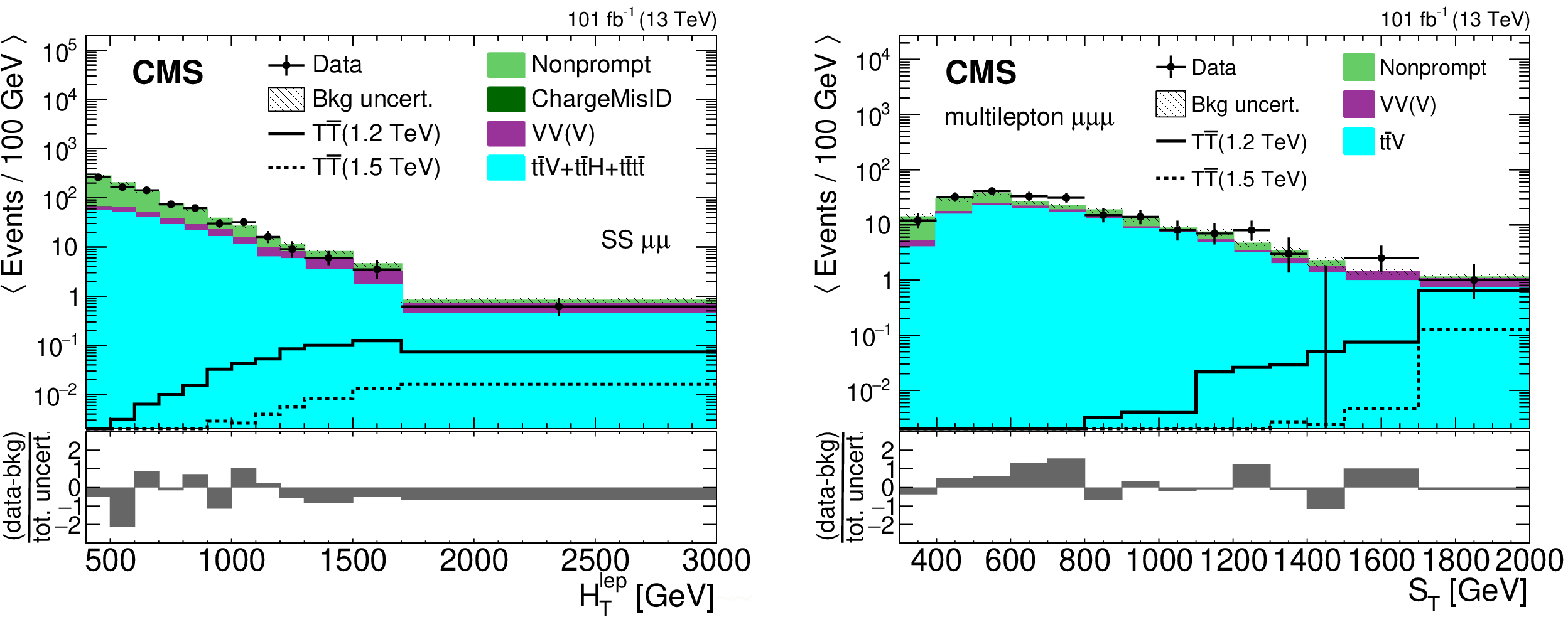
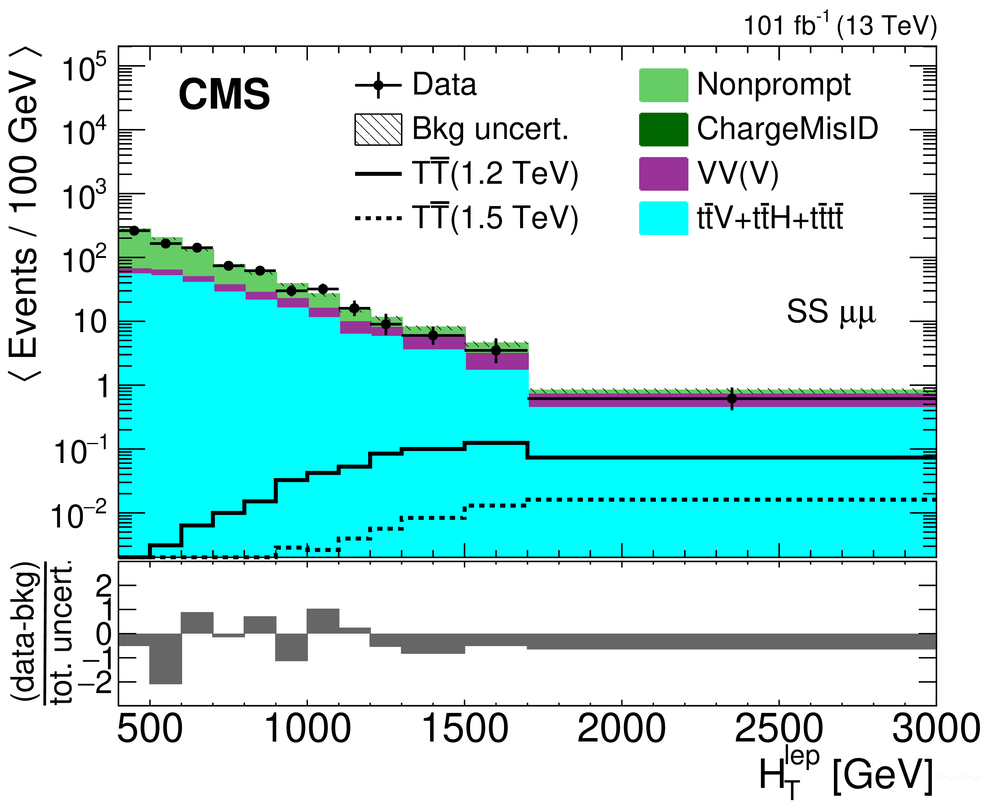
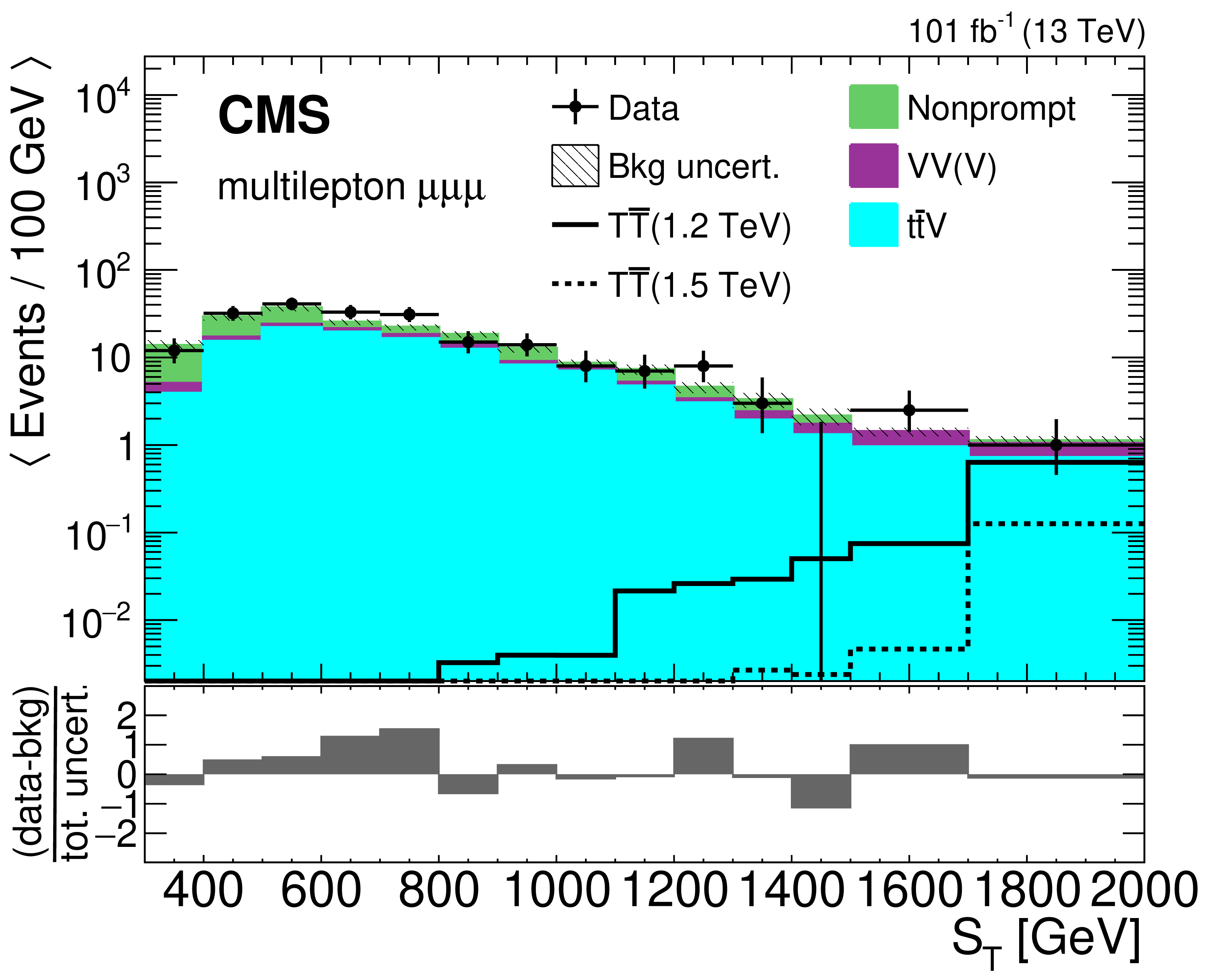
png pdf	Figure 11: Template histograms of $H_{\mathrm{T}}^{\text{lep}}$ in the $\mu\mu$ category of the SS dilepton channel (left) and $S_{\mathrm{T}}$ in the $\mu\mu\mu$ category of the multilepton channel (right). The observed data from 2017--2018 (combined for illustration) are shown using black markers, the predicted ${\mathrm{T}} \overline{\mathrm{T}}$ signal for a mass of 1.2 (1.5) TeV in the singlet scenario using solid (dashed) lines, and the postfit background estimates using filled histograms. Statistical and systematic uncertainties in the background estimate after performing the fit to the observed data are shown by the hatched region. The lower panels show the difference between the observed data and the background estimate as a multiple of the total uncertainty from both sources. Figures adapted from Ref. [141].
png pdf	Figure 11-a: Template histograms of $H_{\mathrm{T}}^{\text{lep}}$ in the $\mu\mu$ category of the SS dilepton channel (left) and $S_{\mathrm{T}}$ in the $\mu\mu\mu$ category of the multilepton channel (right). The observed data from 2017--2018 (combined for illustration) are shown using black markers, the predicted ${\mathrm{T}} \overline{\mathrm{T}}$ signal for a mass of 1.2 (1.5) TeV in the singlet scenario using solid (dashed) lines, and the postfit background estimates using filled histograms. Statistical and systematic uncertainties in the background estimate after performing the fit to the observed data are shown by the hatched region. The lower panels show the difference between the observed data and the background estimate as a multiple of the total uncertainty from both sources. Figures adapted from Ref. [141].
png pdf	Figure 11-b: Template histograms of $H_{\mathrm{T}}^{\text{lep}}$ in the $\mu\mu$ category of the SS dilepton channel (left) and $S_{\mathrm{T}}$ in the $\mu\mu\mu$ category of the multilepton channel (right). The observed data from 2017--2018 (combined for illustration) are shown using black markers, the predicted ${\mathrm{T}} \overline{\mathrm{T}}$ signal for a mass of 1.2 (1.5) TeV in the singlet scenario using solid (dashed) lines, and the postfit background estimates using filled histograms. Statistical and systematic uncertainties in the background estimate after performing the fit to the observed data are shown by the hatched region. The lower panels show the difference between the observed data and the background estimate as a multiple of the total uncertainty from both sources. Figures adapted from Ref. [141].
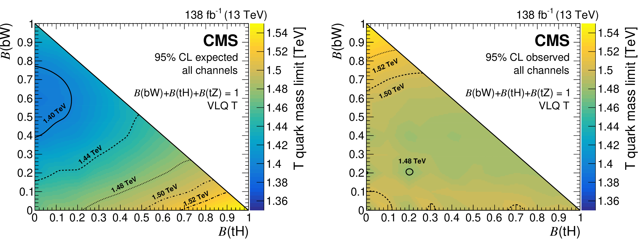
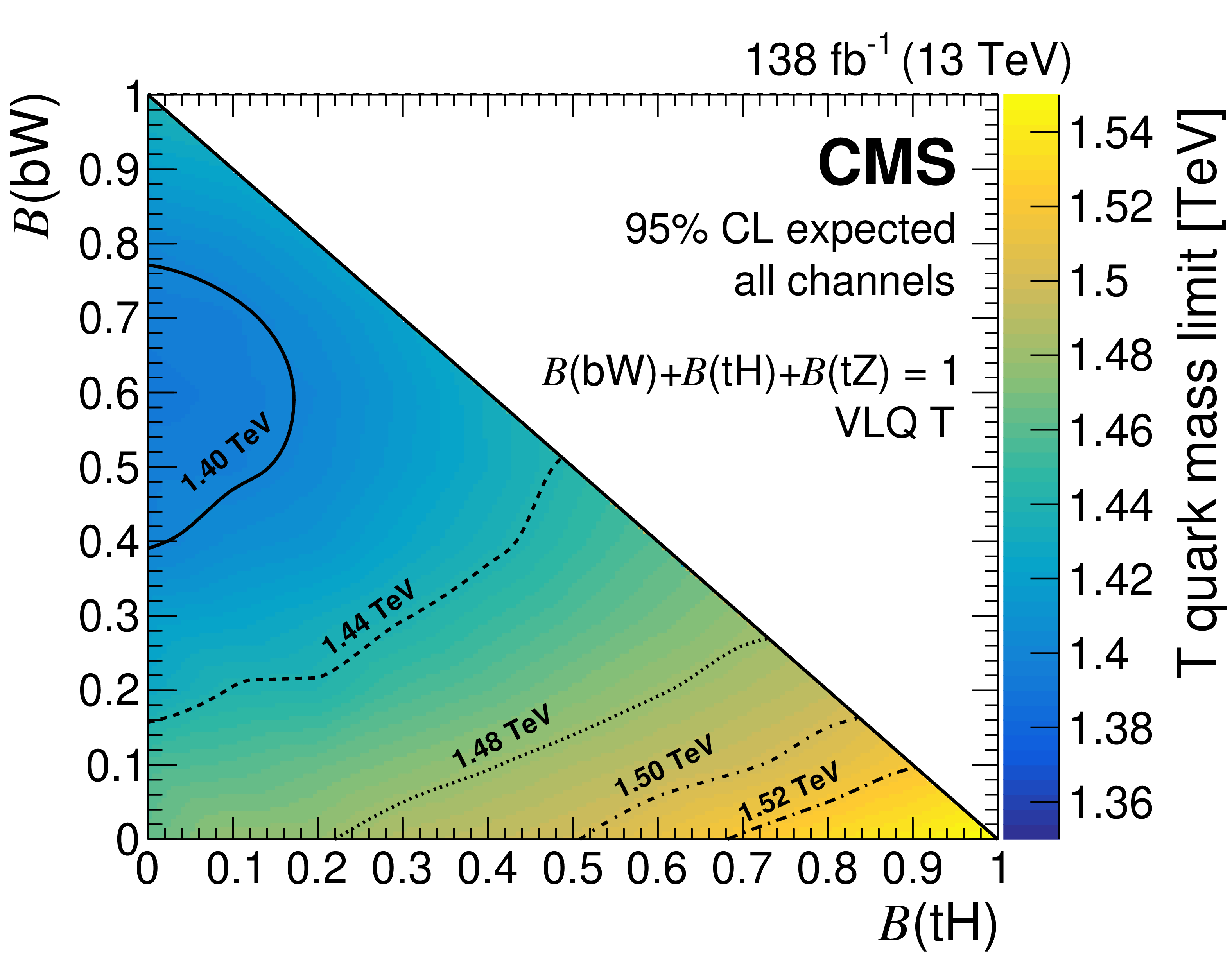
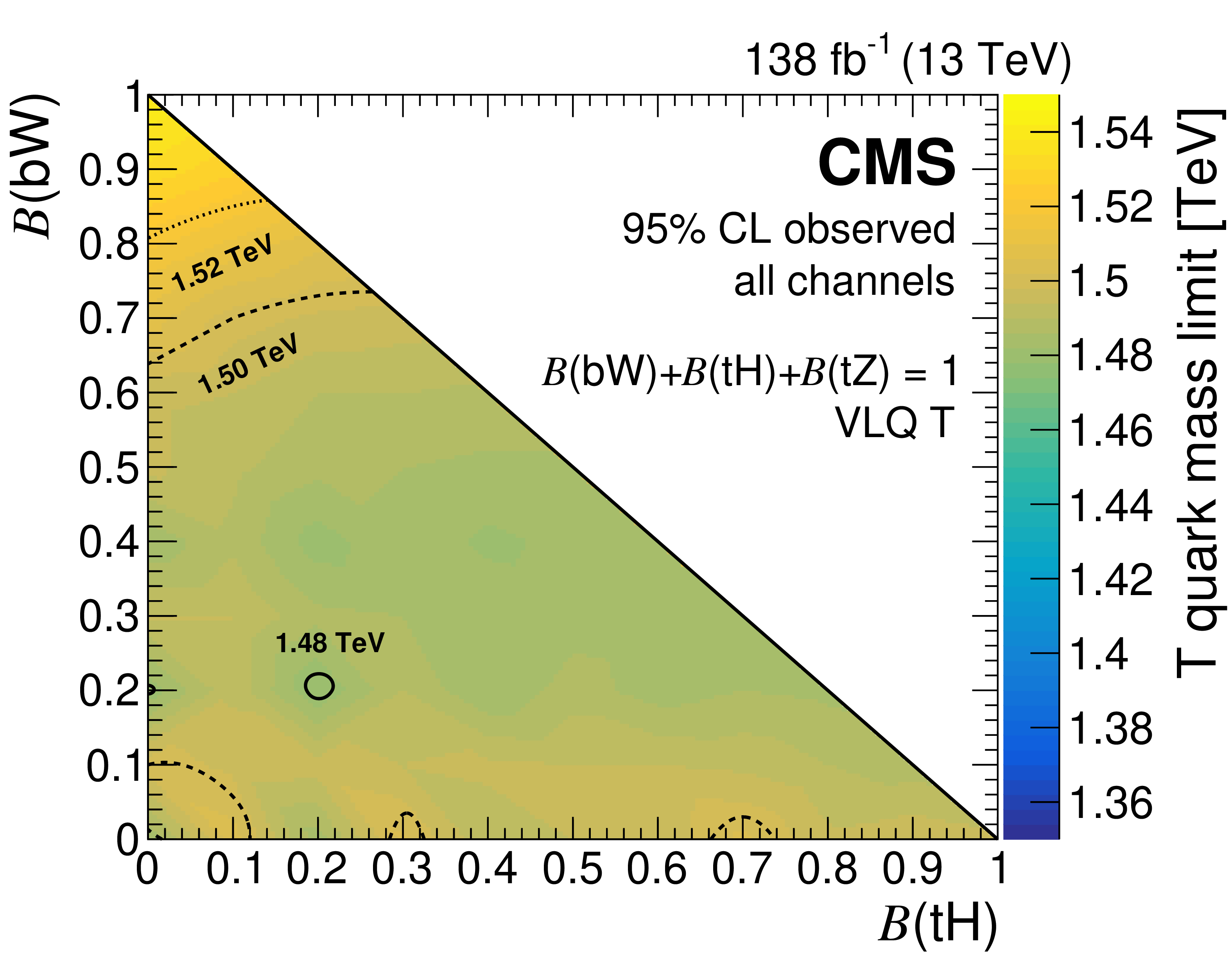
png pdf	Figure 12: The 95% CL expected (left) and observed (right) lower mass limits on pair-produced T quark masses, from the combined fit to the three leptonic channels, as functions of their branching fractions to Higgs and W bosons. Mass contours are shown with lines of various styles. Figures adapted from Ref. [141].
png pdf	Figure 12-a: The 95% CL expected (left) and observed (right) lower mass limits on pair-produced T quark masses, from the combined fit to the three leptonic channels, as functions of their branching fractions to Higgs and W bosons. Mass contours are shown with lines of various styles. Figures adapted from Ref. [141].
png pdf	Figure 12-b: The 95% CL expected (left) and observed (right) lower mass limits on pair-produced T quark masses, from the combined fit to the three leptonic channels, as functions of their branching fractions to Higgs and W bosons. Mass contours are shown with lines of various styles. Figures adapted from Ref. [141].
png pdf	Figure 13: The 95% CL expected (left) and observed (right) lower mass limits on pair-produced B quark masses, from the combined fit to the three leptonic channels, as functions of branching fractions to Higgs and W bosons. Mass contours are shown with lines of various styles. Figures adapted from Ref. [141].
png pdf	Figure 13-a: The 95% CL expected (left) and observed (right) lower mass limits on pair-produced B quark masses, from the combined fit to the three leptonic channels, as functions of branching fractions to Higgs and W bosons. Mass contours are shown with lines of various styles. Figures adapted from Ref. [141].
png pdf	Figure 13-b: The 95% CL expected (left) and observed (right) lower mass limits on pair-produced B quark masses, from the combined fit to the three leptonic channels, as functions of branching fractions to Higgs and W bosons. Mass contours are shown with lines of various styles. Figures adapted from Ref. [141].
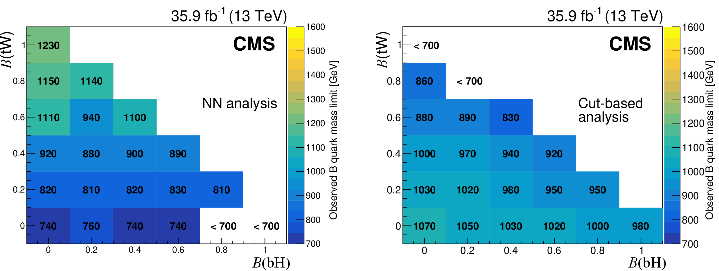
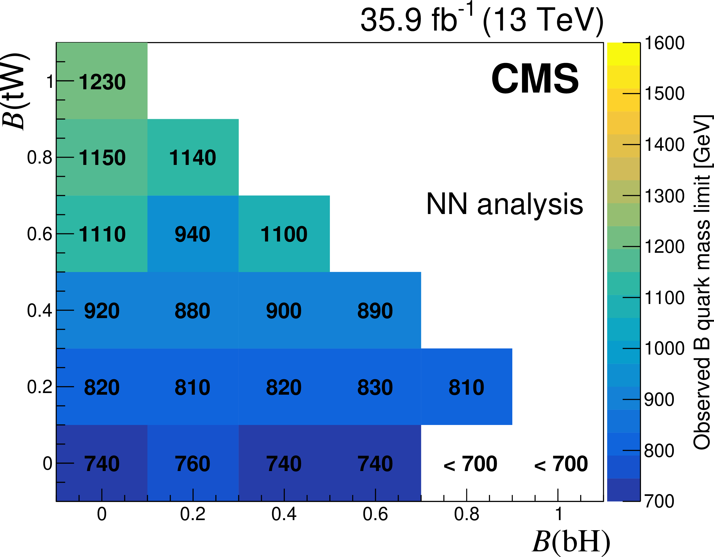
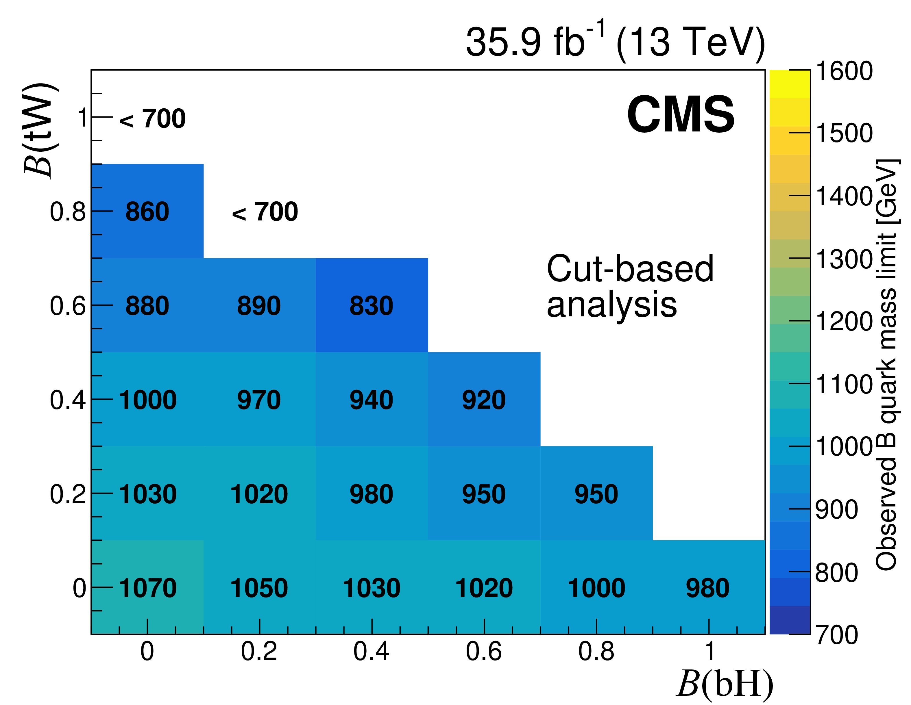
png pdf	Figure 14: Observed lower limit at 95% CL on B quark masses as a function of the branching fractions to $\mathrm{b}\mathrm{H}$ and $\mathrm{t}\mathrm{W}$, for the NN-based (left) and selection-based (right) approaches of the search for ${\mathrm{B}} \overline{\mathrm{B}}$ production in the all-hadronic final state. Figures adapted from Ref. [140].
png pdf	Figure 14-a: Observed lower limit at 95% CL on B quark masses as a function of the branching fractions to $\mathrm{b}\mathrm{H}$ and $\mathrm{t}\mathrm{W}$, for the NN-based (left) and selection-based (right) approaches of the search for ${\mathrm{B}} \overline{\mathrm{B}}$ production in the all-hadronic final state. Figures adapted from Ref. [140].
png pdf	Figure 14-b: Observed lower limit at 95% CL on B quark masses as a function of the branching fractions to $\mathrm{b}\mathrm{H}$ and $\mathrm{t}\mathrm{W}$, for the NN-based (left) and selection-based (right) approaches of the search for ${\mathrm{B}} \overline{\mathrm{B}}$ production in the all-hadronic final state. Figures adapted from Ref. [140].
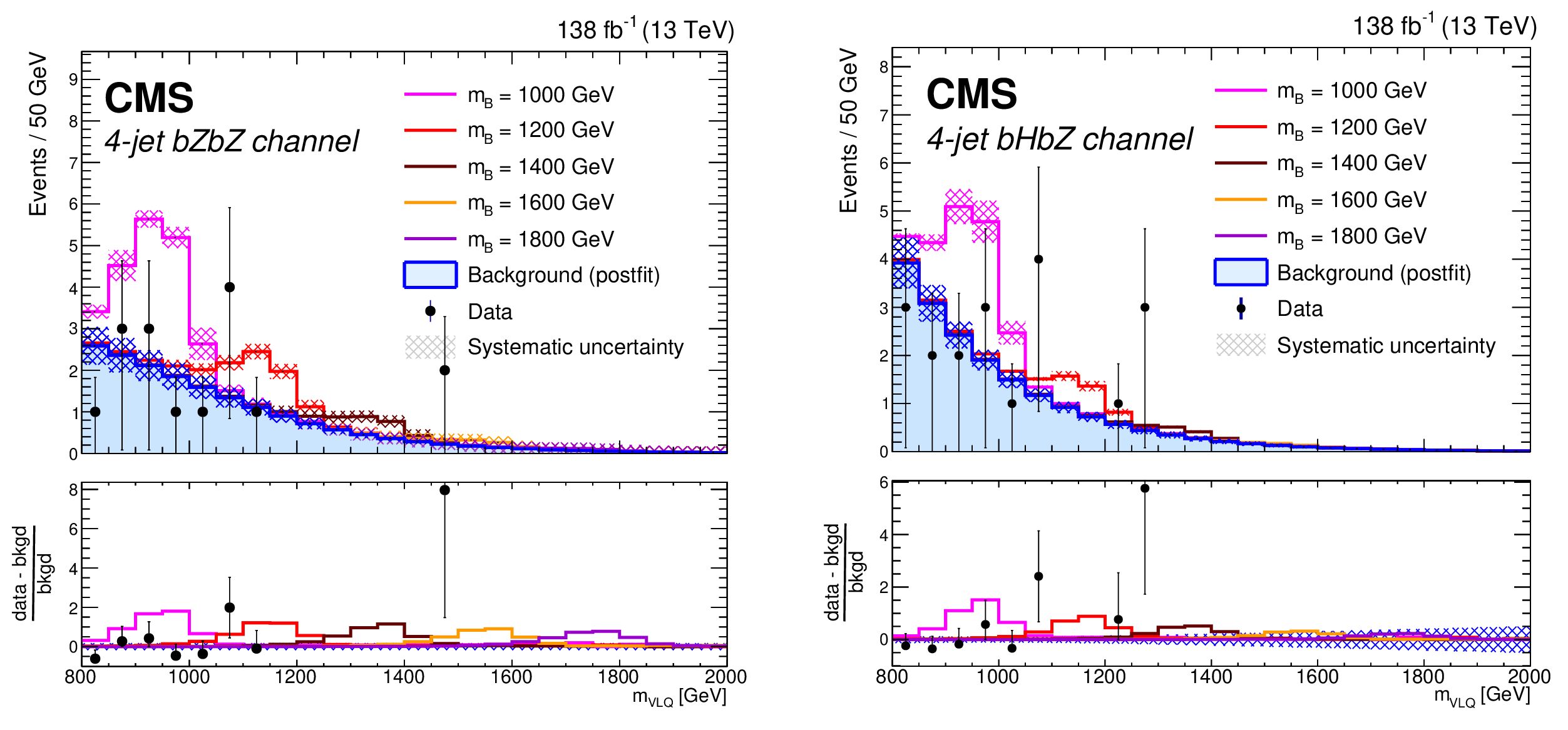
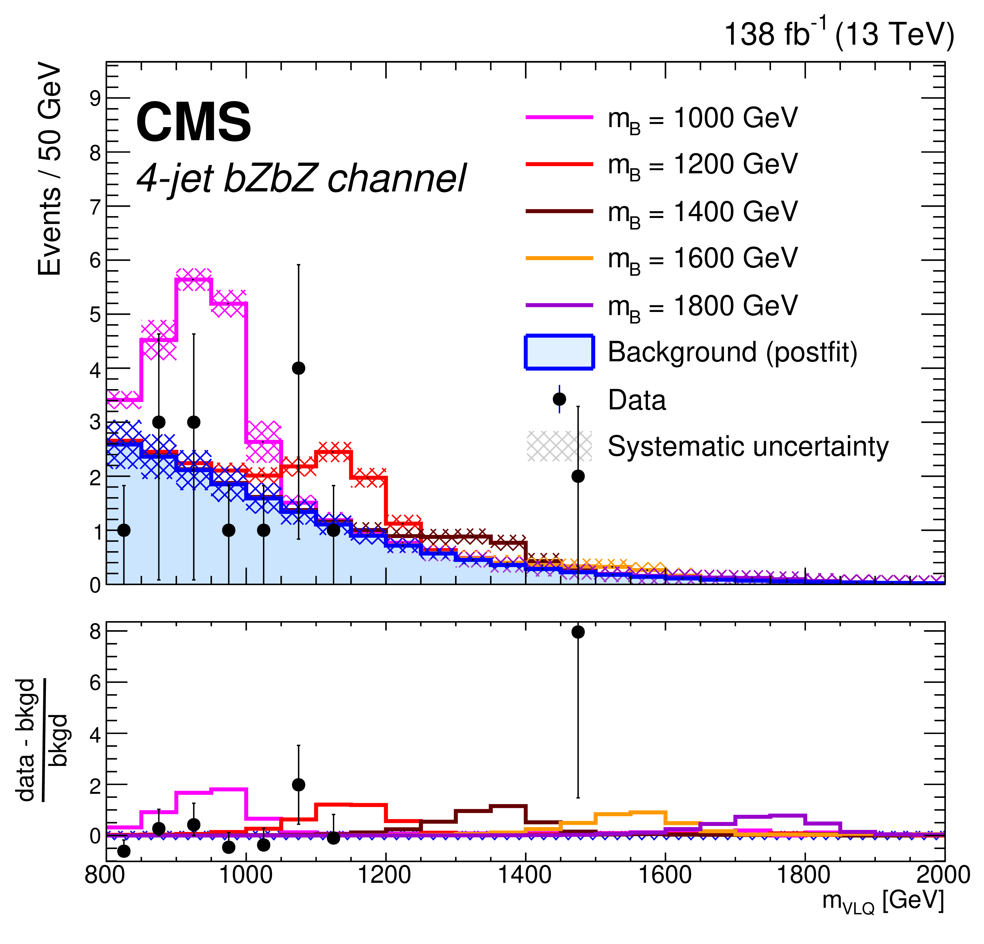
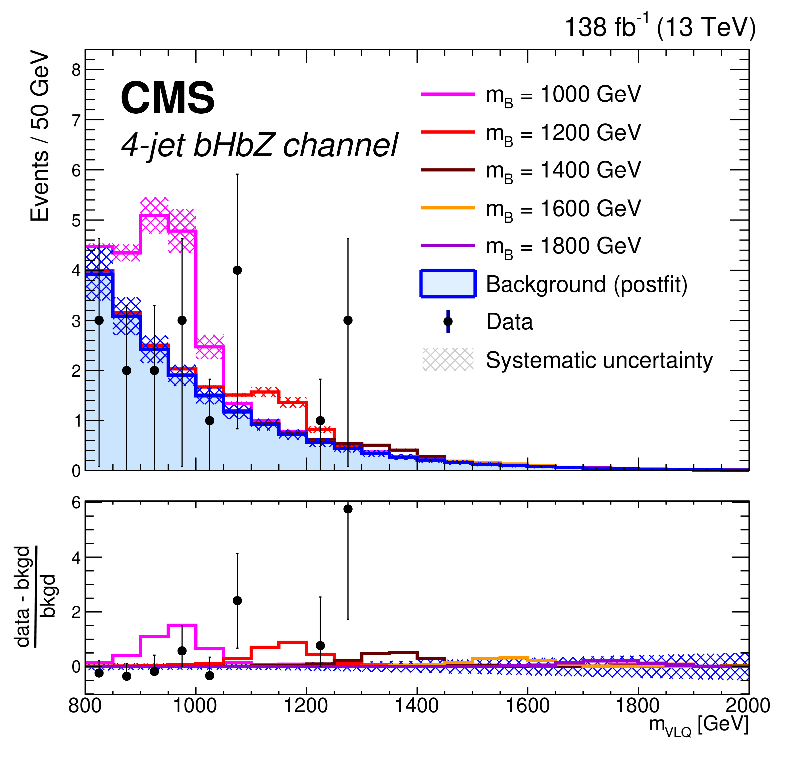
png pdf	Figure 15: Distributions of the reconstructed VLQ mass for expected background (blue histogram), signal plus background (colored lines), and observed data (black points) for events in the hadronic four-jet $\mathrm{b}\mathrm{Z}\mathrm{b}\mathrm{Z}$ category (left) and the leptonic four-jet $\mathrm{b}\mathrm{H}\mathrm{b}\mathrm{Z}$ category (right) in the search for ${\mathrm{B}} \overline{\mathrm{B}}$ production. Five signal masses are shown: 1000 GeV (pink), 1200 GeV (red), 1400 GeV (orange), 1600 GeV (yellow), and 1800 GeV (green). The signal distributions are normalized to the number of events determined by the expected VLQ production cross section. The hatched regions indicate the total systematic uncertainty in the background estimate. The lower panels show the difference between the observed data and the background estimate as a multiple of the background estimate. Figures taken from Ref. [142].
png pdf	Figure 15-a: Distributions of the reconstructed VLQ mass for expected background (blue histogram), signal plus background (colored lines), and observed data (black points) for events in the hadronic four-jet $\mathrm{b}\mathrm{Z}\mathrm{b}\mathrm{Z}$ category (left) and the leptonic four-jet $\mathrm{b}\mathrm{H}\mathrm{b}\mathrm{Z}$ category (right) in the search for ${\mathrm{B}} \overline{\mathrm{B}}$ production. Five signal masses are shown: 1000 GeV (pink), 1200 GeV (red), 1400 GeV (orange), 1600 GeV (yellow), and 1800 GeV (green). The signal distributions are normalized to the number of events determined by the expected VLQ production cross section. The hatched regions indicate the total systematic uncertainty in the background estimate. The lower panels show the difference between the observed data and the background estimate as a multiple of the background estimate. Figures taken from Ref. [142].
png pdf	Figure 15-b: Distributions of the reconstructed VLQ mass for expected background (blue histogram), signal plus background (colored lines), and observed data (black points) for events in the hadronic four-jet $\mathrm{b}\mathrm{Z}\mathrm{b}\mathrm{Z}$ category (left) and the leptonic four-jet $\mathrm{b}\mathrm{H}\mathrm{b}\mathrm{Z}$ category (right) in the search for ${\mathrm{B}} \overline{\mathrm{B}}$ production. Five signal masses are shown: 1000 GeV (pink), 1200 GeV (red), 1400 GeV (orange), 1600 GeV (yellow), and 1800 GeV (green). The signal distributions are normalized to the number of events determined by the expected VLQ production cross section. The hatched regions indicate the total systematic uncertainty in the background estimate. The lower panels show the difference between the observed data and the background estimate as a multiple of the background estimate. Figures taken from Ref. [142].
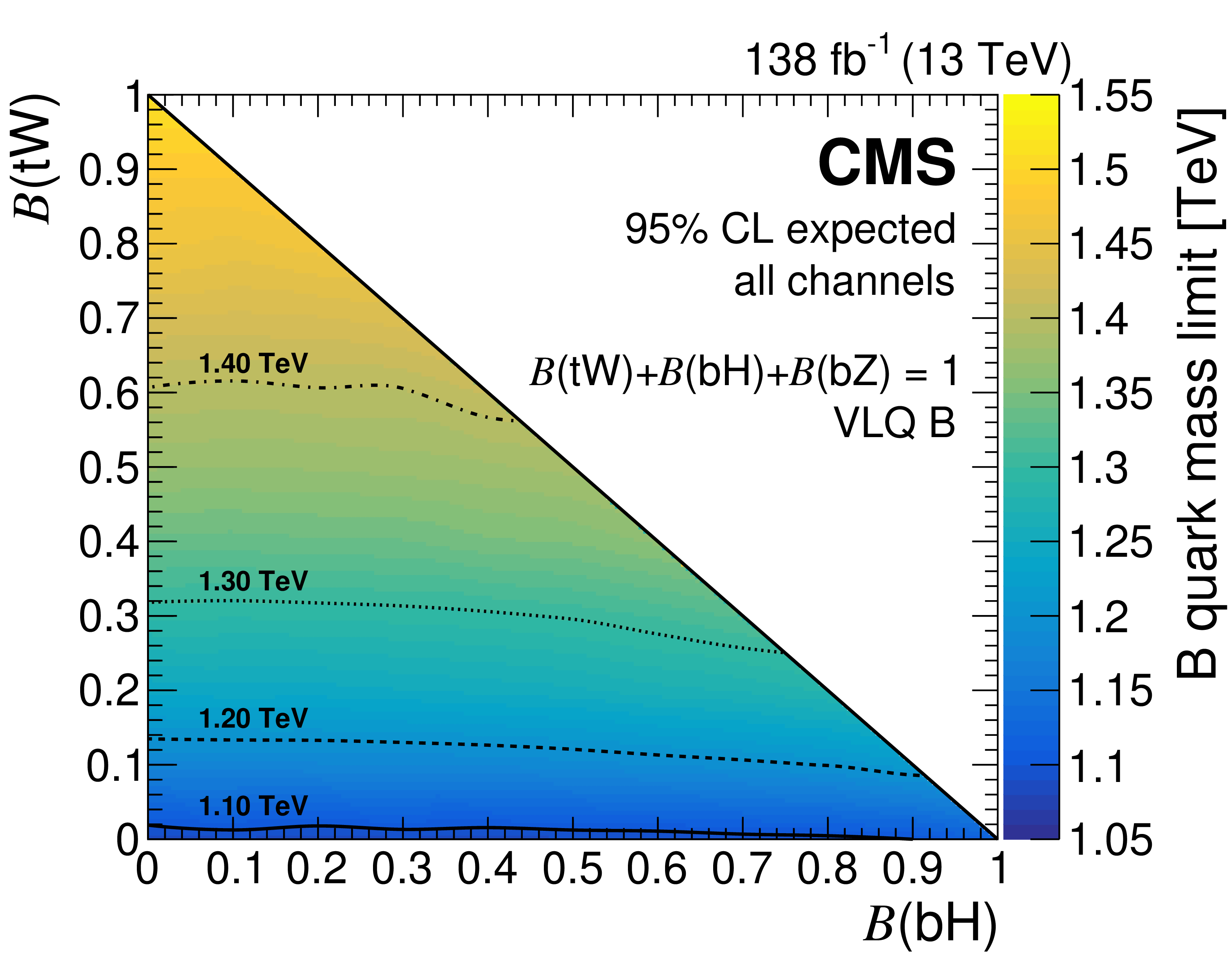
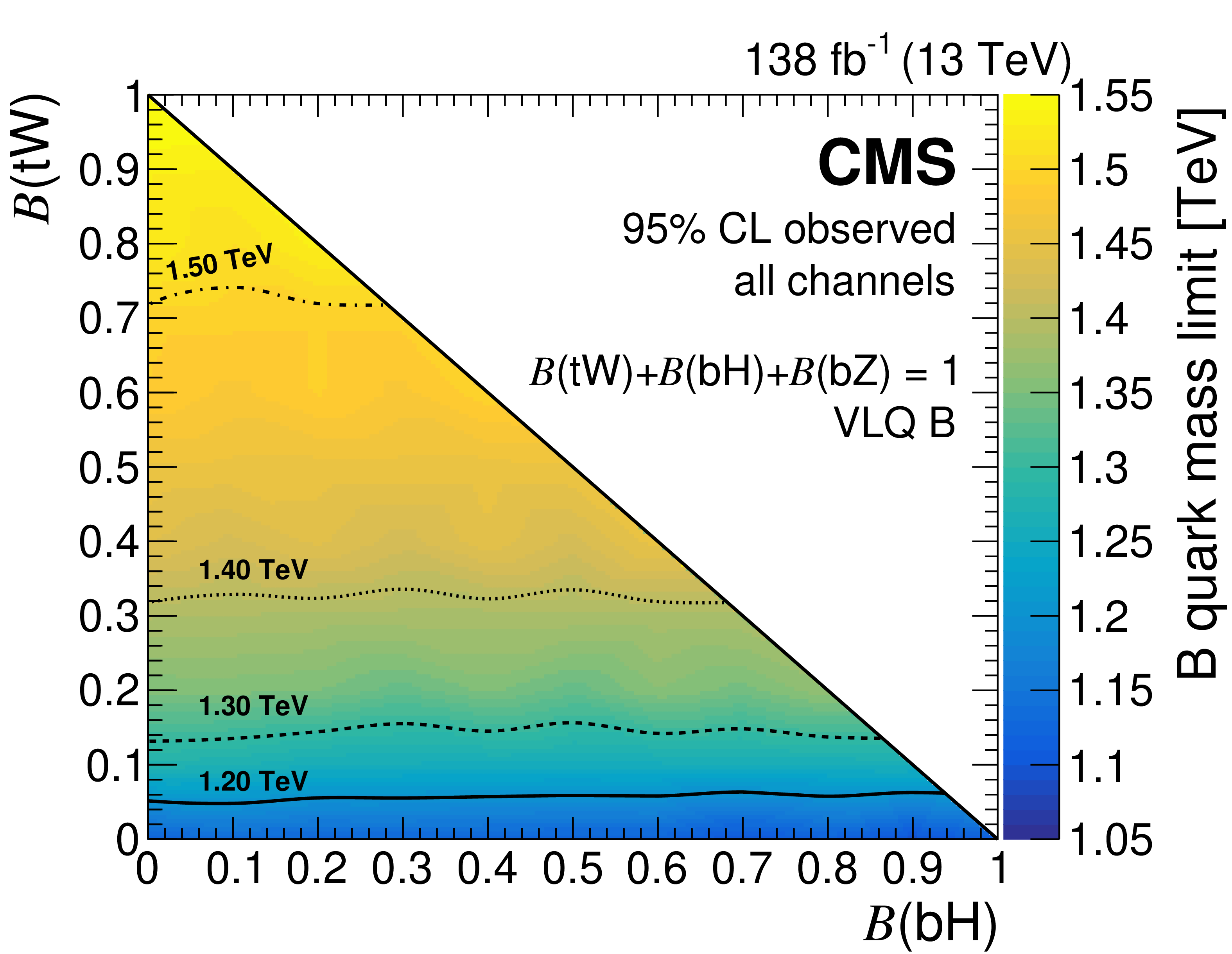
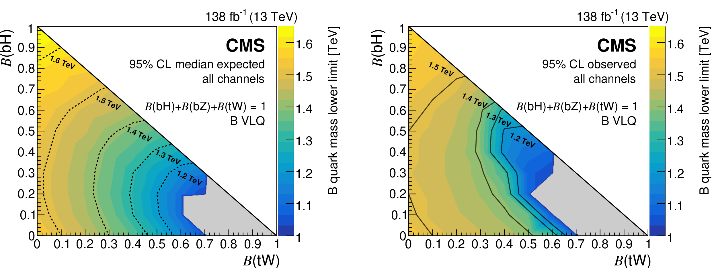
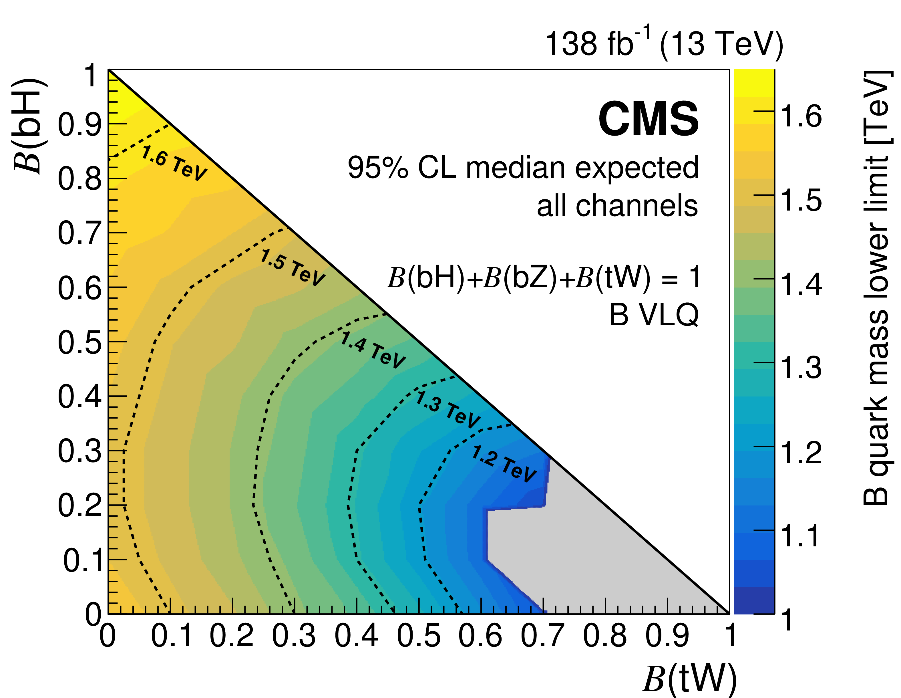
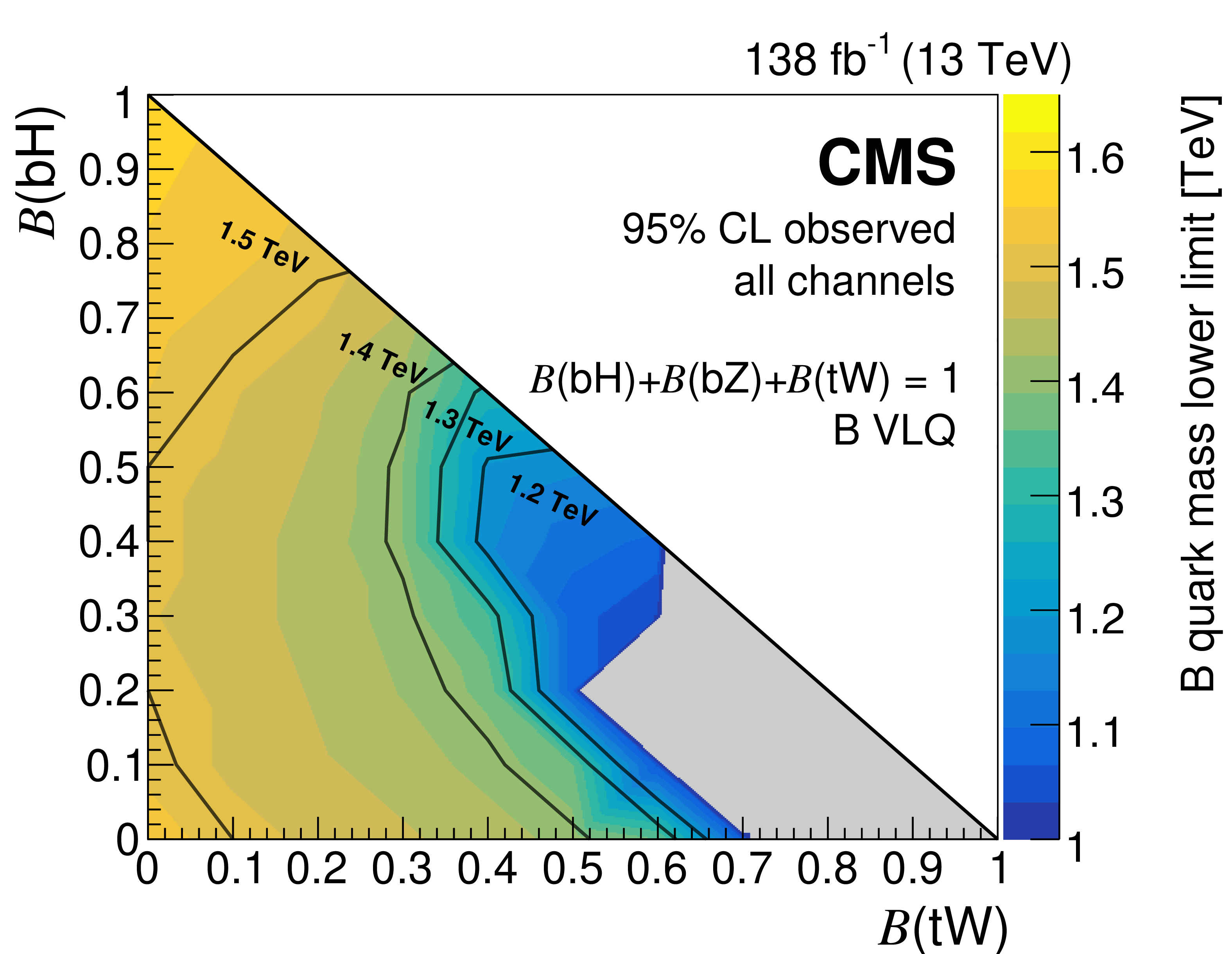
png pdf	Figure 16: Expected (left) and observed (right) lower limits on the B quark mass at 95% CL from the combination of the full Run 2 hadronic and OS dilepton channels, as a function of the branching fractions $\mathcal{B}({\mathrm{B}} \to\mathrm{b}\mathrm{H})$ and $\mathcal{B}({\mathrm{B}} \to\mathrm{t}\mathrm{W})$, with $\mathcal{B}({\mathrm{B}} \to\mathrm{t}\mathrm{W})=1-\mathcal{B}({\mathrm{B}} \to\mathrm{b}\mathrm{H})-\mathcal{B}({\mathrm{B}} \to\mathrm{b}\mathrm{Z})$. Results in the grey region, where the lower limit is less than 1.0 TeV, are omitted. Figures adapted from Ref. [142].
png pdf	Figure 16-a: Expected (left) and observed (right) lower limits on the B quark mass at 95% CL from the combination of the full Run 2 hadronic and OS dilepton channels, as a function of the branching fractions $\mathcal{B}({\mathrm{B}} \to\mathrm{b}\mathrm{H})$ and $\mathcal{B}({\mathrm{B}} \to\mathrm{t}\mathrm{W})$, with $\mathcal{B}({\mathrm{B}} \to\mathrm{t}\mathrm{W})=1-\mathcal{B}({\mathrm{B}} \to\mathrm{b}\mathrm{H})-\mathcal{B}({\mathrm{B}} \to\mathrm{b}\mathrm{Z})$. Results in the grey region, where the lower limit is less than 1.0 TeV, are omitted. Figures adapted from Ref. [142].
png pdf	Figure 16-b: Expected (left) and observed (right) lower limits on the B quark mass at 95% CL from the combination of the full Run 2 hadronic and OS dilepton channels, as a function of the branching fractions $\mathcal{B}({\mathrm{B}} \to\mathrm{b}\mathrm{H})$ and $\mathcal{B}({\mathrm{B}} \to\mathrm{t}\mathrm{W})$, with $\mathcal{B}({\mathrm{B}} \to\mathrm{t}\mathrm{W})=1-\mathcal{B}({\mathrm{B}} \to\mathrm{b}\mathrm{H})-\mathcal{B}({\mathrm{B}} \to\mathrm{b}\mathrm{Z})$. Results in the grey region, where the lower limit is less than 1.0 TeV, are omitted. Figures adapted from Ref. [142].
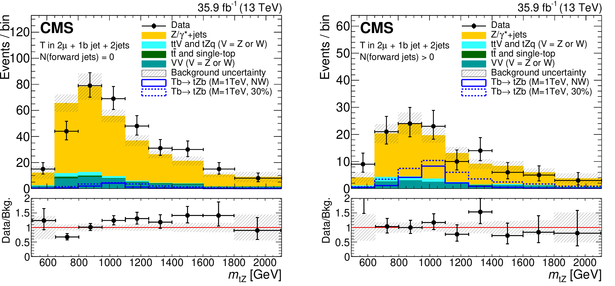
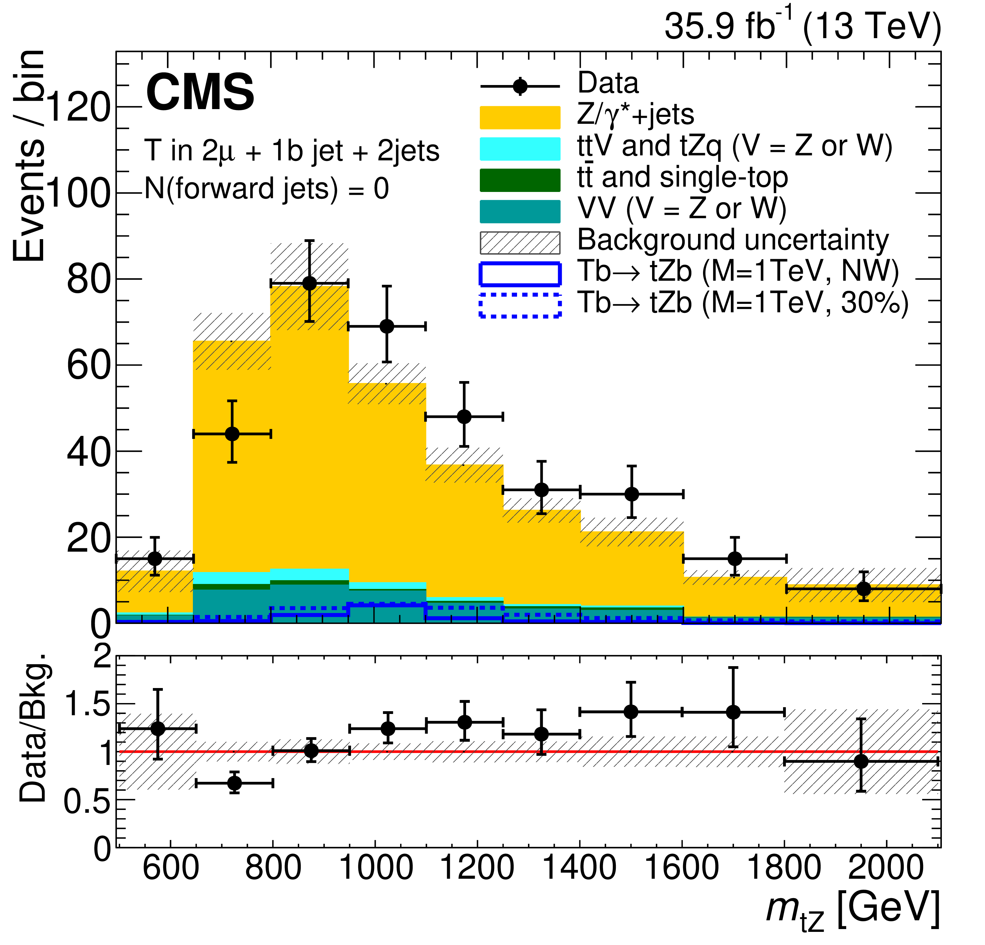
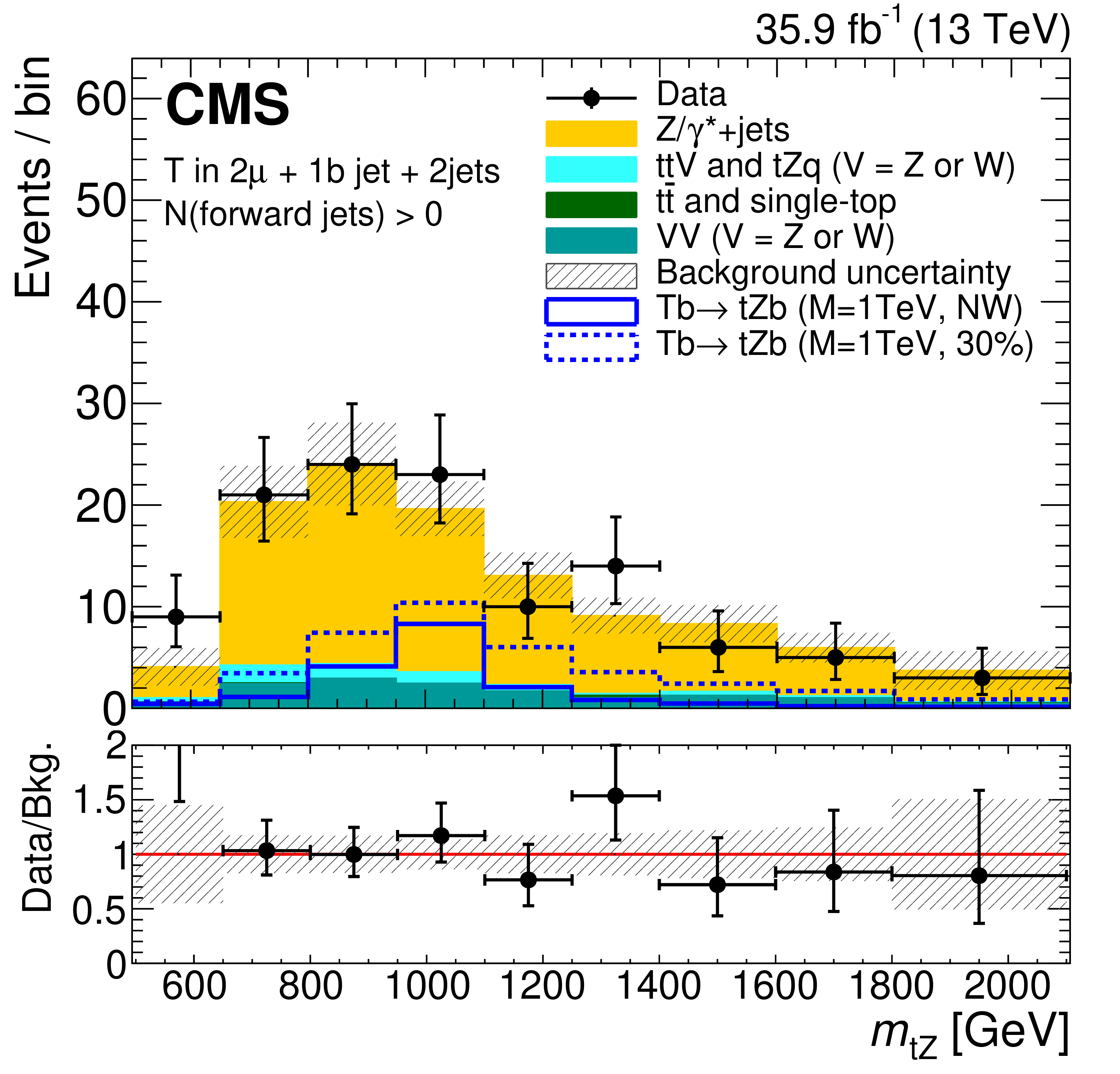
png pdf	Figure 17: Distributions of the reconstructed T quark mass, $m_{\mathrm{t}\mathrm{Z}}$ for the observed data, the background estimates, and the expected signal for the two categories where the singly produced T quark is reconstructed in the resolved topology for events with the Z boson decaying into muons and no forward jets (left) and at least one forward jet (right). The background composition is taken from simulation. The expected signal is shown for two benchmark values of the width, for a T quark produced in association with a b quark: NWA and 30% of the T quark mass. The lower panel in each plot shows the ratio of the observed data to the background estimation, with the hatched band representing the uncertainties in the background estimate. Figures taken from Ref. [144].
png pdf	Figure 17-a: Distributions of the reconstructed T quark mass, $m_{\mathrm{t}\mathrm{Z}}$ for the observed data, the background estimates, and the expected signal for the two categories where the singly produced T quark is reconstructed in the resolved topology for events with the Z boson decaying into muons and no forward jets (left) and at least one forward jet (right). The background composition is taken from simulation. The expected signal is shown for two benchmark values of the width, for a T quark produced in association with a b quark: NWA and 30% of the T quark mass. The lower panel in each plot shows the ratio of the observed data to the background estimation, with the hatched band representing the uncertainties in the background estimate. Figures taken from Ref. [144].
png pdf	Figure 17-b: Distributions of the reconstructed T quark mass, $m_{\mathrm{t}\mathrm{Z}}$ for the observed data, the background estimates, and the expected signal for the two categories where the singly produced T quark is reconstructed in the resolved topology for events with the Z boson decaying into muons and no forward jets (left) and at least one forward jet (right). The background composition is taken from simulation. The expected signal is shown for two benchmark values of the width, for a T quark produced in association with a b quark: NWA and 30% of the T quark mass. The lower panel in each plot shows the ratio of the observed data to the background estimation, with the hatched band representing the uncertainties in the background estimate. Figures taken from Ref. [144].
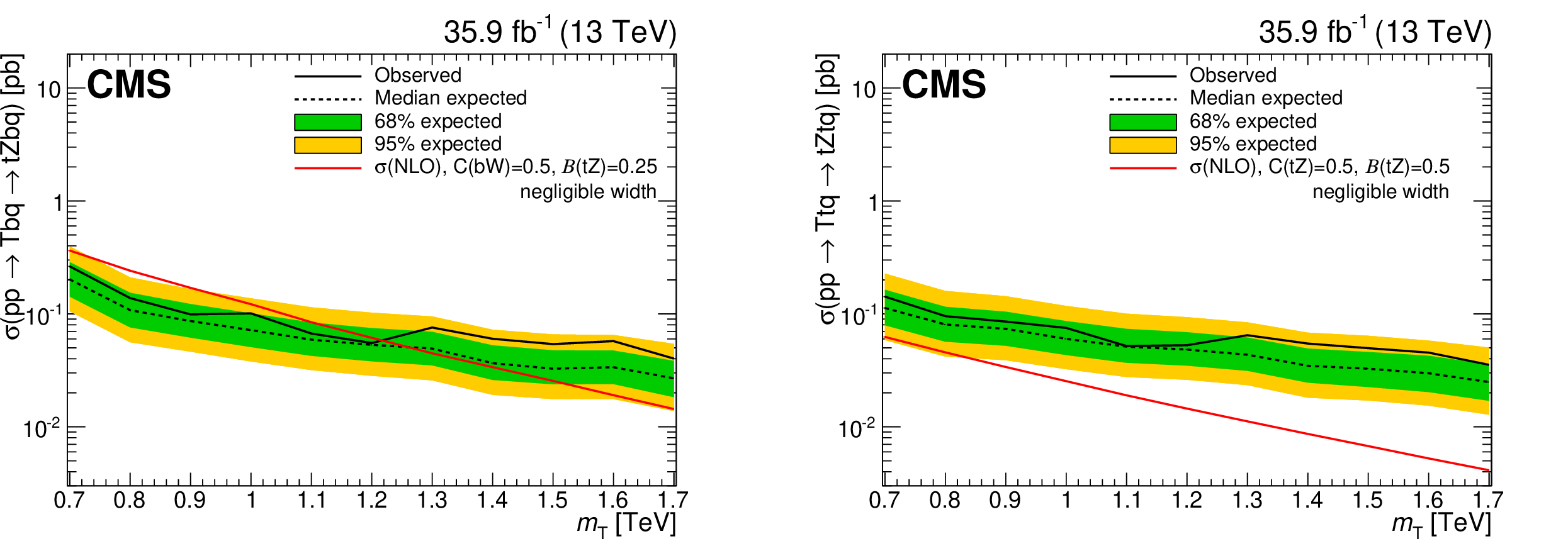
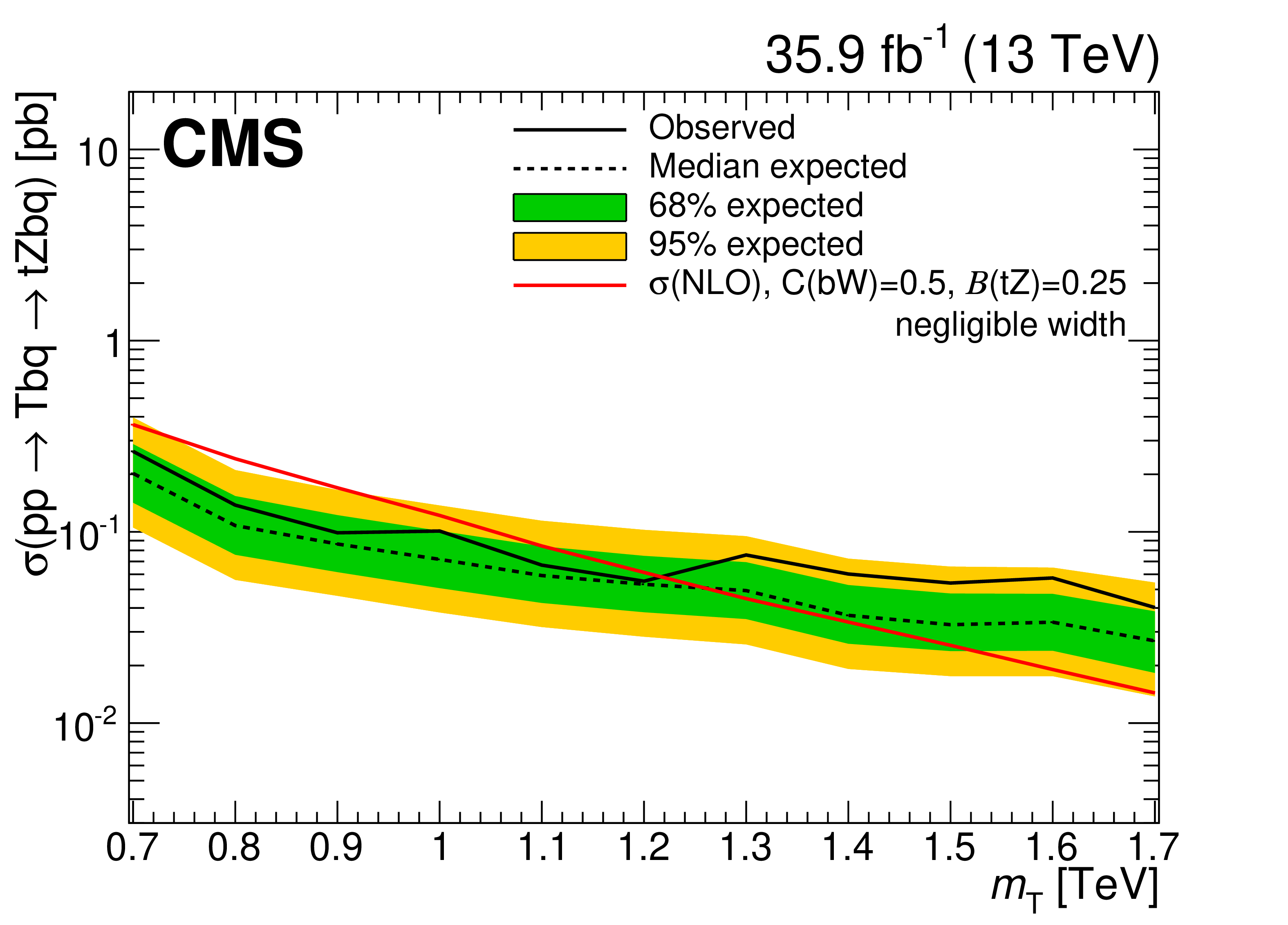
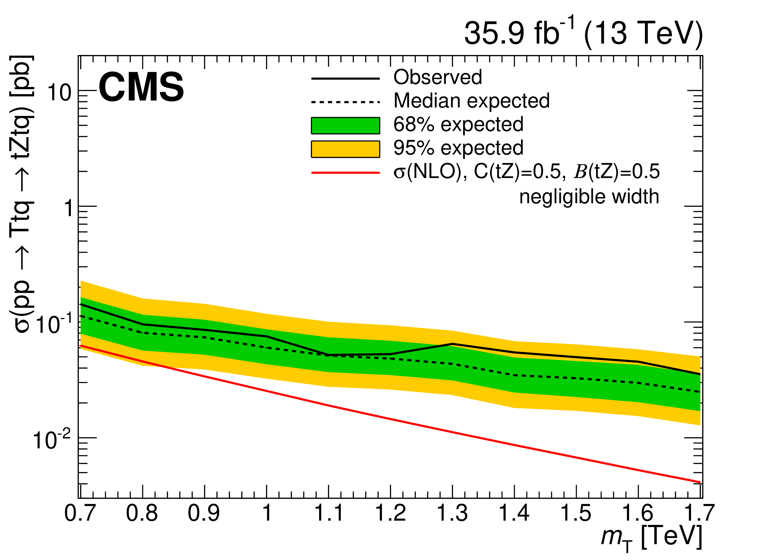
png pdf	Figure 18: Observed and expected upper limits on the product of the cross section and branching fraction for singlet LH T quark (left) and doublet RH T quark production (right) in association with a b quark and a t quark, respectively, in the NWA hypothesis. The T quark decays to $\mathrm{t}\mathrm{Z}$ with a branching fraction $\mathcal{B}({\mathrm{T}} \to\mathrm{t}\mathrm{Z})$ of 0.25 (0.5) for the left (right) figure. The red lines represent theoretical cross sections calculated at NLO in perturbative QCD, whereas the inner (green) band and the outer (yellow) band indicate the regions containing 68 and 95%, respectively, of the distribution of limits expected under the background-only hypothesis. Figures taken from Ref. [144].
png pdf	Figure 18-a: Observed and expected upper limits on the product of the cross section and branching fraction for singlet LH T quark (left) and doublet RH T quark production (right) in association with a b quark and a t quark, respectively, in the NWA hypothesis. The T quark decays to $\mathrm{t}\mathrm{Z}$ with a branching fraction $\mathcal{B}({\mathrm{T}} \to\mathrm{t}\mathrm{Z})$ of 0.25 (0.5) for the left (right) figure. The red lines represent theoretical cross sections calculated at NLO in perturbative QCD, whereas the inner (green) band and the outer (yellow) band indicate the regions containing 68 and 95%, respectively, of the distribution of limits expected under the background-only hypothesis. Figures taken from Ref. [144].
png pdf	Figure 18-b: Observed and expected upper limits on the product of the cross section and branching fraction for singlet LH T quark (left) and doublet RH T quark production (right) in association with a b quark and a t quark, respectively, in the NWA hypothesis. The T quark decays to $\mathrm{t}\mathrm{Z}$ with a branching fraction $\mathcal{B}({\mathrm{T}} \to\mathrm{t}\mathrm{Z})$ of 0.25 (0.5) for the left (right) figure. The red lines represent theoretical cross sections calculated at NLO in perturbative QCD, whereas the inner (green) band and the outer (yellow) band indicate the regions containing 68 and 95%, respectively, of the distribution of limits expected under the background-only hypothesis. Figures taken from Ref. [144].
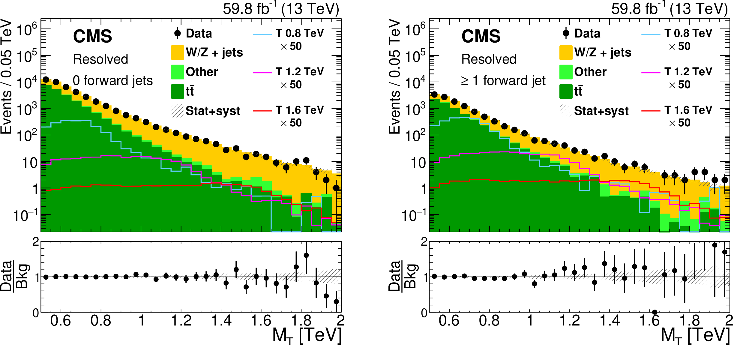
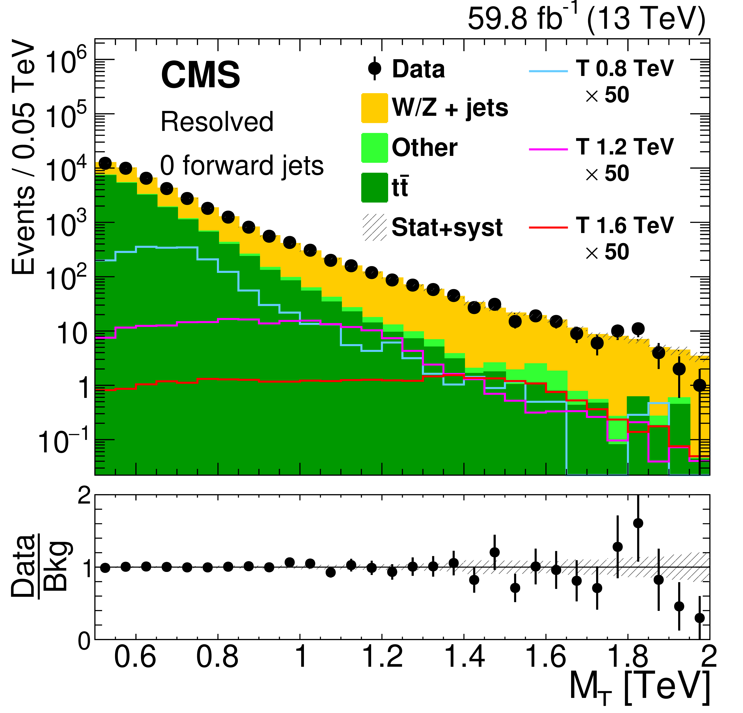
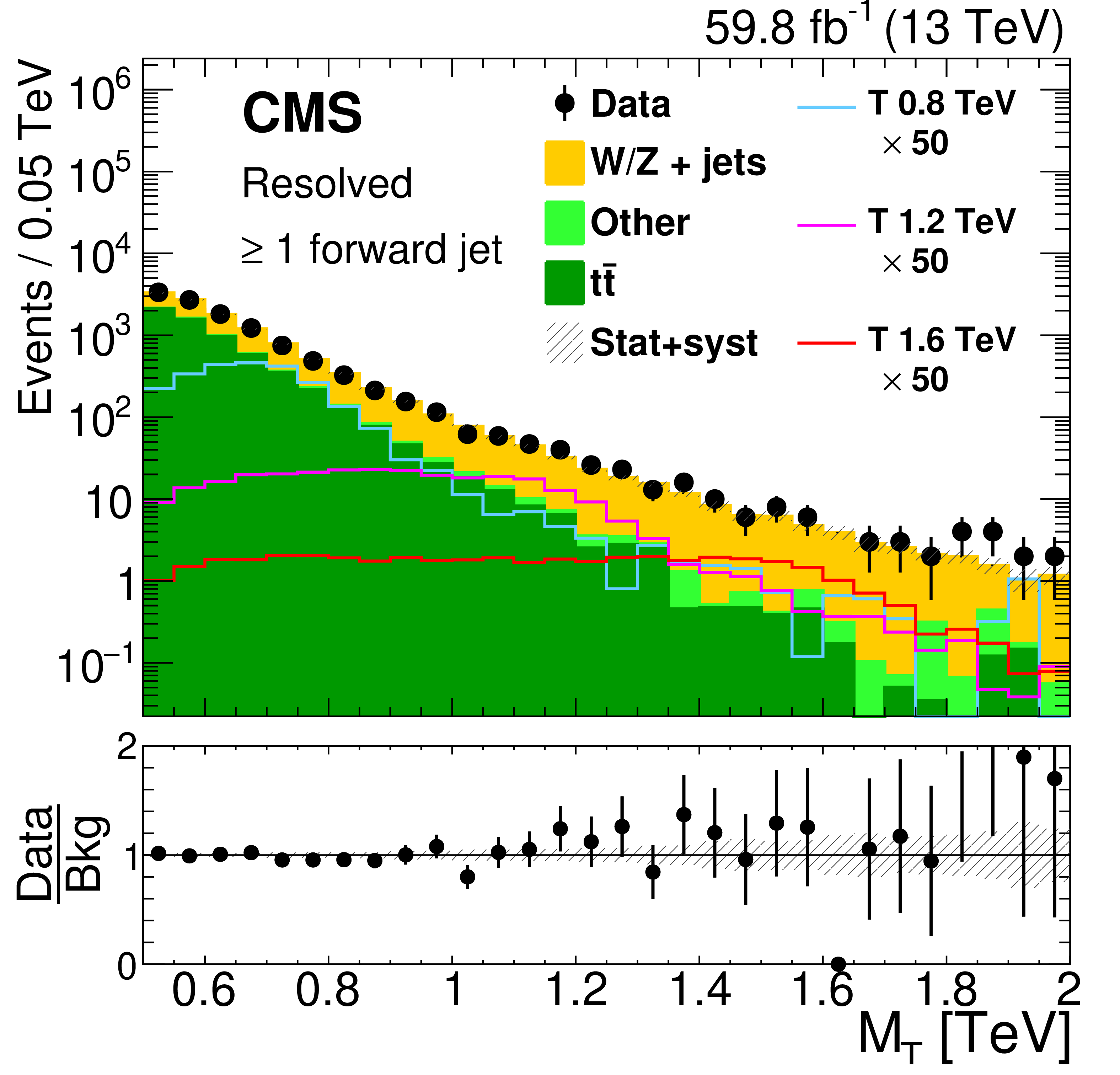
png pdf	Figure 19: Distributions from the 2018 data set of the transverse mass of the reconstructed top quark and ${\vec p}_{\mathrm{T}}^{\kern1pt\text{miss}}$ system, for the selected events in the resolved categories, for events with no forward jet (left) and at least one forward jet (right). The distributions for the main background components have been determined in simulation with SFs extracted from CRs. All background processes and the respective uncertainties are derived from the fit to data, whereas the distributions of signal processes are represented according to the expectation before the fit. The lines show the signal predictions for three benchmark mass values (0.8, 1.2, and 1.6 TeV) for a T quark of a narrow width. Figures taken from Ref. [146].
png pdf	Figure 19-a: Distributions from the 2018 data set of the transverse mass of the reconstructed top quark and ${\vec p}_{\mathrm{T}}^{\kern1pt\text{miss}}$ system, for the selected events in the resolved categories, for events with no forward jet (left) and at least one forward jet (right). The distributions for the main background components have been determined in simulation with SFs extracted from CRs. All background processes and the respective uncertainties are derived from the fit to data, whereas the distributions of signal processes are represented according to the expectation before the fit. The lines show the signal predictions for three benchmark mass values (0.8, 1.2, and 1.6 TeV) for a T quark of a narrow width. Figures taken from Ref. [146].
png pdf	Figure 19-b: Distributions from the 2018 data set of the transverse mass of the reconstructed top quark and ${\vec p}_{\mathrm{T}}^{\kern1pt\text{miss}}$ system, for the selected events in the resolved categories, for events with no forward jet (left) and at least one forward jet (right). The distributions for the main background components have been determined in simulation with SFs extracted from CRs. All background processes and the respective uncertainties are derived from the fit to data, whereas the distributions of signal processes are represented according to the expectation before the fit. The lines show the signal predictions for three benchmark mass values (0.8, 1.2, and 1.6 TeV) for a T quark of a narrow width. Figures taken from Ref. [146].
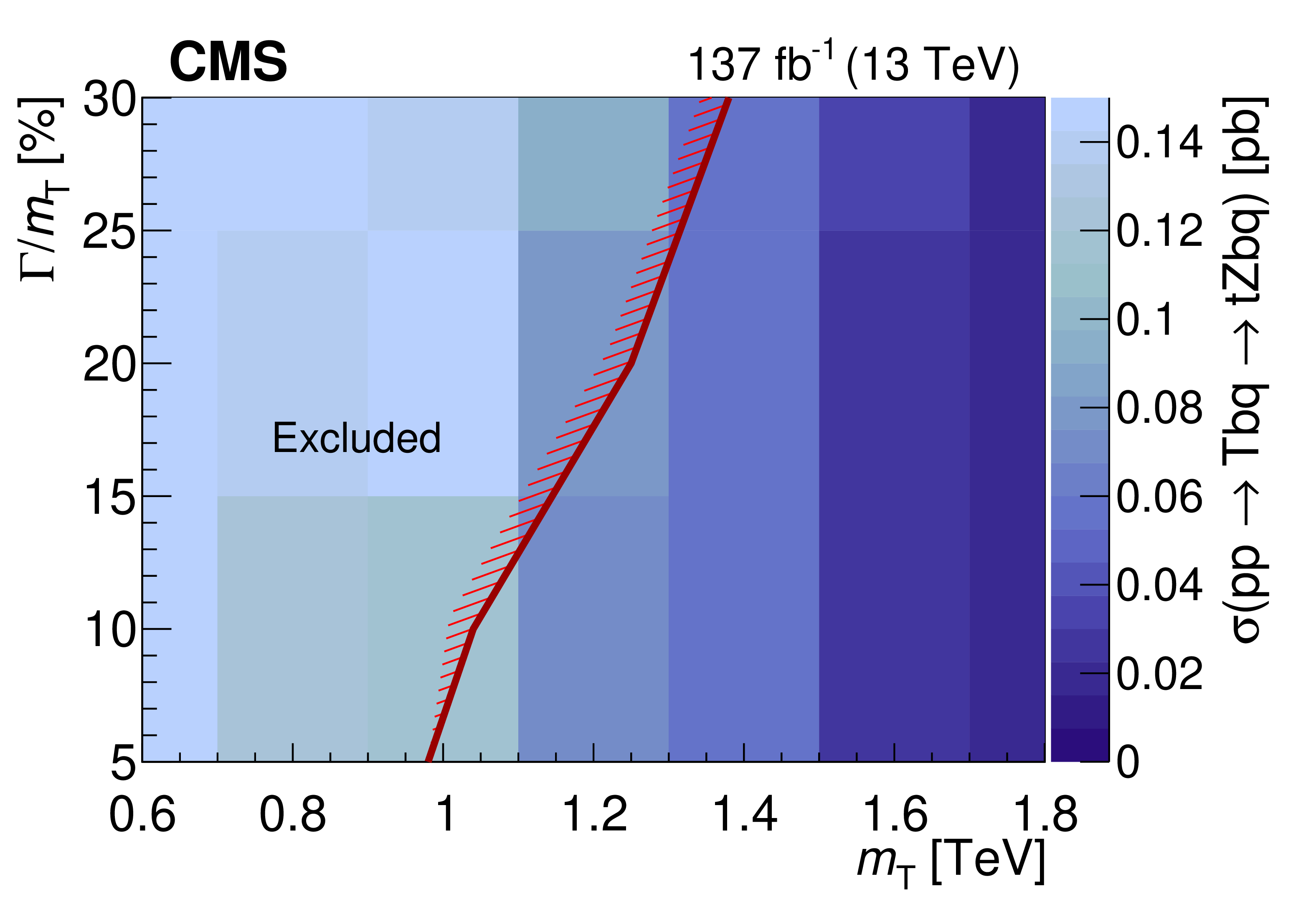
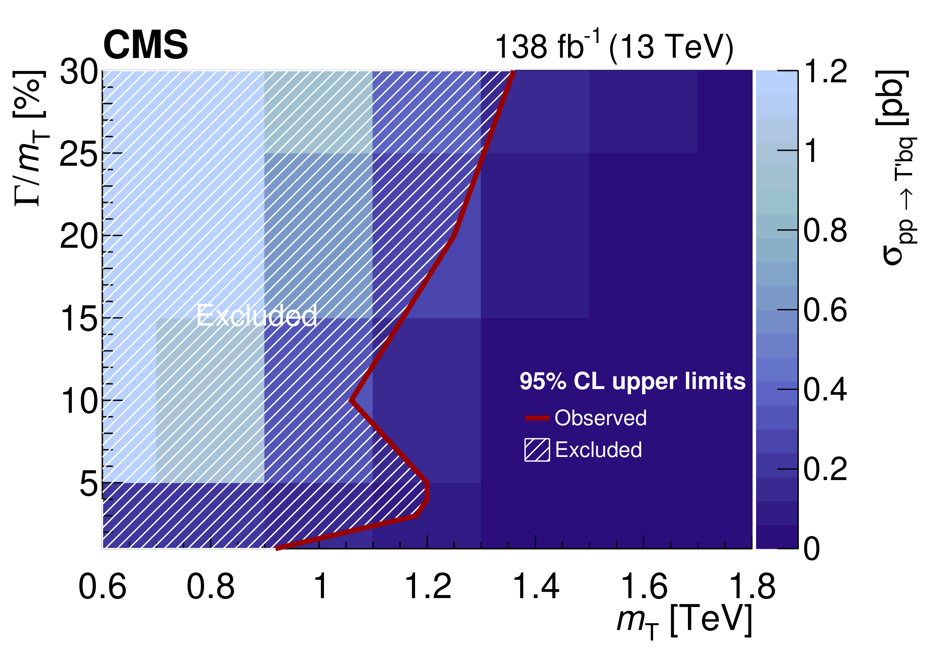
png pdf	Figure 20: Observed 95% CL upper limit on the product of the single production cross section for a singlet VLQ T quark and the ${\mathrm{T}} \to\mathrm{t}\mathrm{Z}$ branching fraction, as a function of the T quark mass $m_{{\mathrm{T}} }$ and width $\Gamma$, for widths from 5 to 30% of the mass. A singlet T quark that is produced in association with a bottom quark is assumed. The solid red line indicates the boundary of the excluded region (on the hatched side) of theoretical cross sections multiplied by the T branching fraction. Figure taken from Ref. [146].
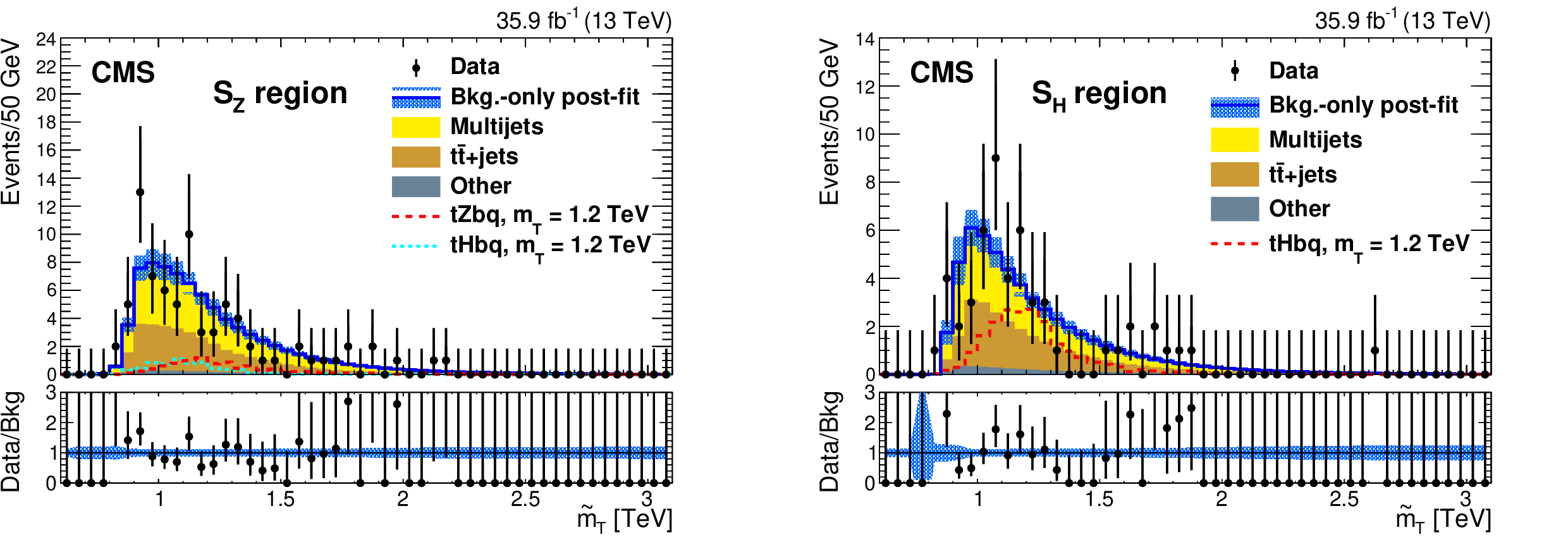
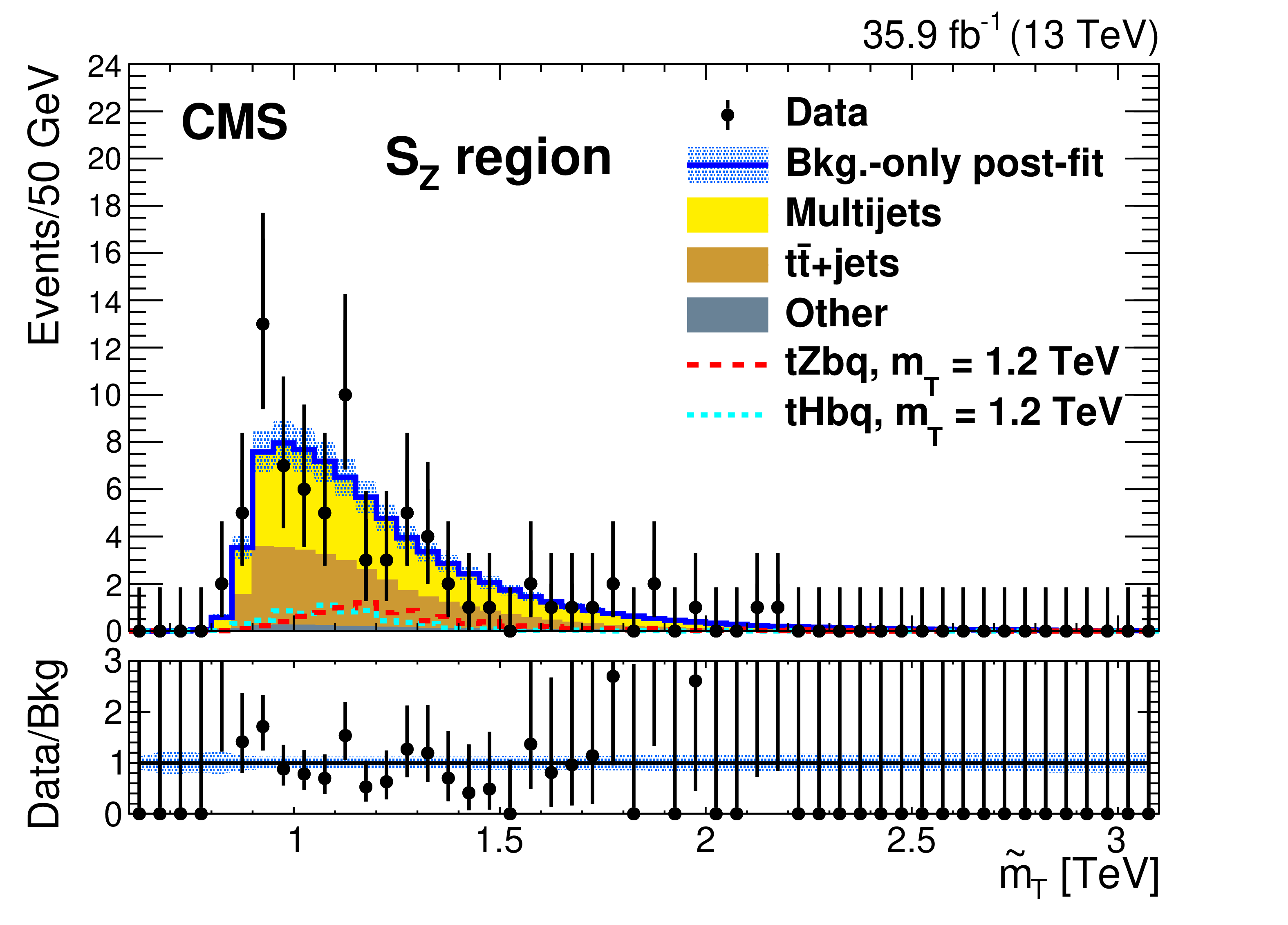
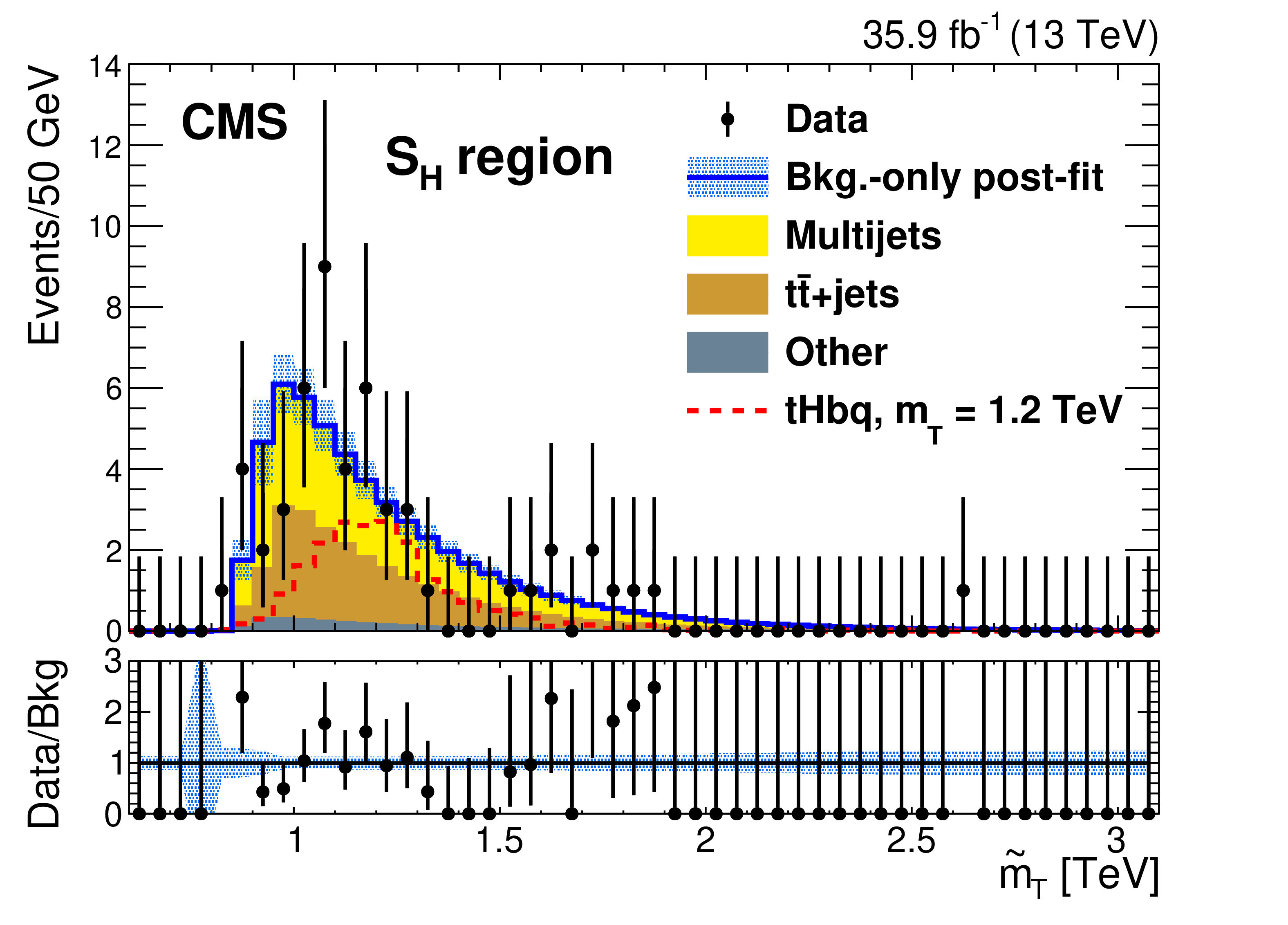
png pdf	Figure 21: Background-only postfit distributions of $\widetilde{m}_{{\mathrm{T}} }$, the adjusted T mass sensitive observable defined in Ref. [145], of the observed data for the SR of the ${\mathrm{T}} \to\mathrm{t}\mathrm{Z}$ (left) and ${\mathrm{T}} \to\mathrm{t}\mathrm{H}$ (right) channels, respectively, for the high-mass search. The dashed red histogram in each case represents an example signal for the $\mathrm{t}\mathrm{Z}\mathrm{b}\mathrm{q}$ or $\mathrm{t}\mathrm{H}\mathrm{b}\mathrm{q}$ process with a T quark mass of 1.2 TeV and a relative width of 30%. The lower panels of the plots display the ratio of observed data to the fitted background for each bin. The error bars on the data points correspond to the 68% CL Poisson intervals, whereas the light blue band in each ratio panel represents the relative uncertainties in the fitted background. Figures taken from Ref. [145].
png pdf	Figure 21-a: Background-only postfit distributions of $\widetilde{m}_{{\mathrm{T}} }$, the adjusted T mass sensitive observable defined in Ref. [145], of the observed data for the SR of the ${\mathrm{T}} \to\mathrm{t}\mathrm{Z}$ (left) and ${\mathrm{T}} \to\mathrm{t}\mathrm{H}$ (right) channels, respectively, for the high-mass search. The dashed red histogram in each case represents an example signal for the $\mathrm{t}\mathrm{Z}\mathrm{b}\mathrm{q}$ or $\mathrm{t}\mathrm{H}\mathrm{b}\mathrm{q}$ process with a T quark mass of 1.2 TeV and a relative width of 30%. The lower panels of the plots display the ratio of observed data to the fitted background for each bin. The error bars on the data points correspond to the 68% CL Poisson intervals, whereas the light blue band in each ratio panel represents the relative uncertainties in the fitted background. Figures taken from Ref. [145].
png pdf	Figure 21-b: Background-only postfit distributions of $\widetilde{m}_{{\mathrm{T}} }$, the adjusted T mass sensitive observable defined in Ref. [145], of the observed data for the SR of the ${\mathrm{T}} \to\mathrm{t}\mathrm{Z}$ (left) and ${\mathrm{T}} \to\mathrm{t}\mathrm{H}$ (right) channels, respectively, for the high-mass search. The dashed red histogram in each case represents an example signal for the $\mathrm{t}\mathrm{Z}\mathrm{b}\mathrm{q}$ or $\mathrm{t}\mathrm{H}\mathrm{b}\mathrm{q}$ process with a T quark mass of 1.2 TeV and a relative width of 30%. The lower panels of the plots display the ratio of observed data to the fitted background for each bin. The error bars on the data points correspond to the 68% CL Poisson intervals, whereas the light blue band in each ratio panel represents the relative uncertainties in the fitted background. Figures taken from Ref. [145].
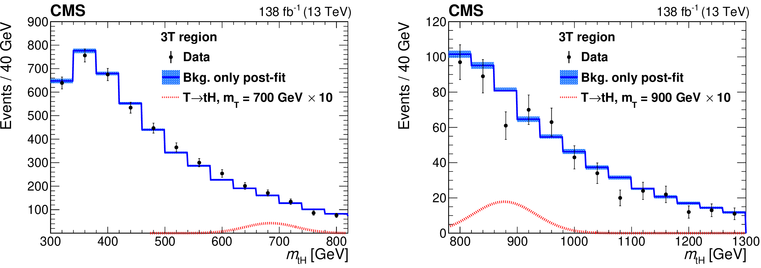
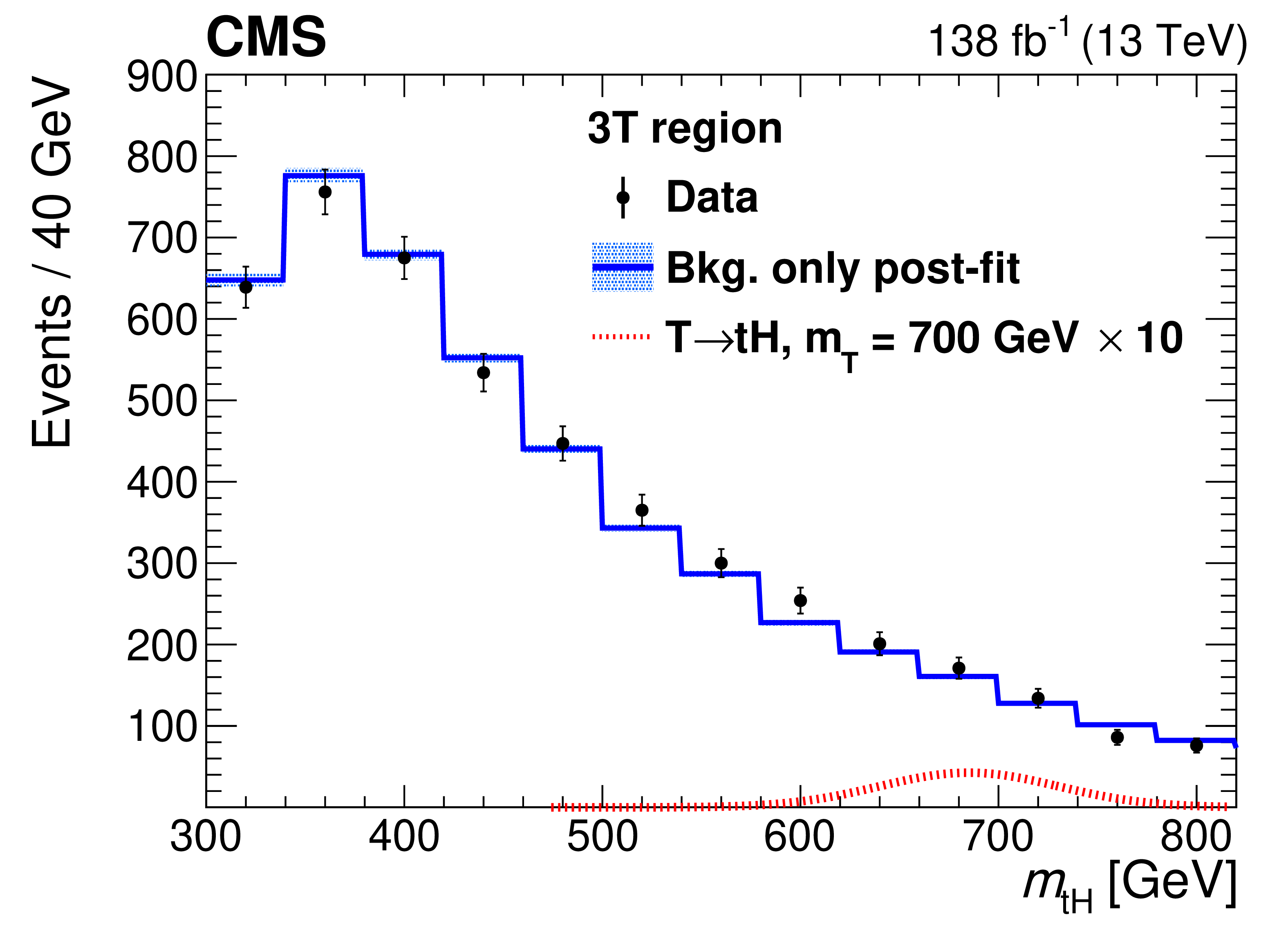
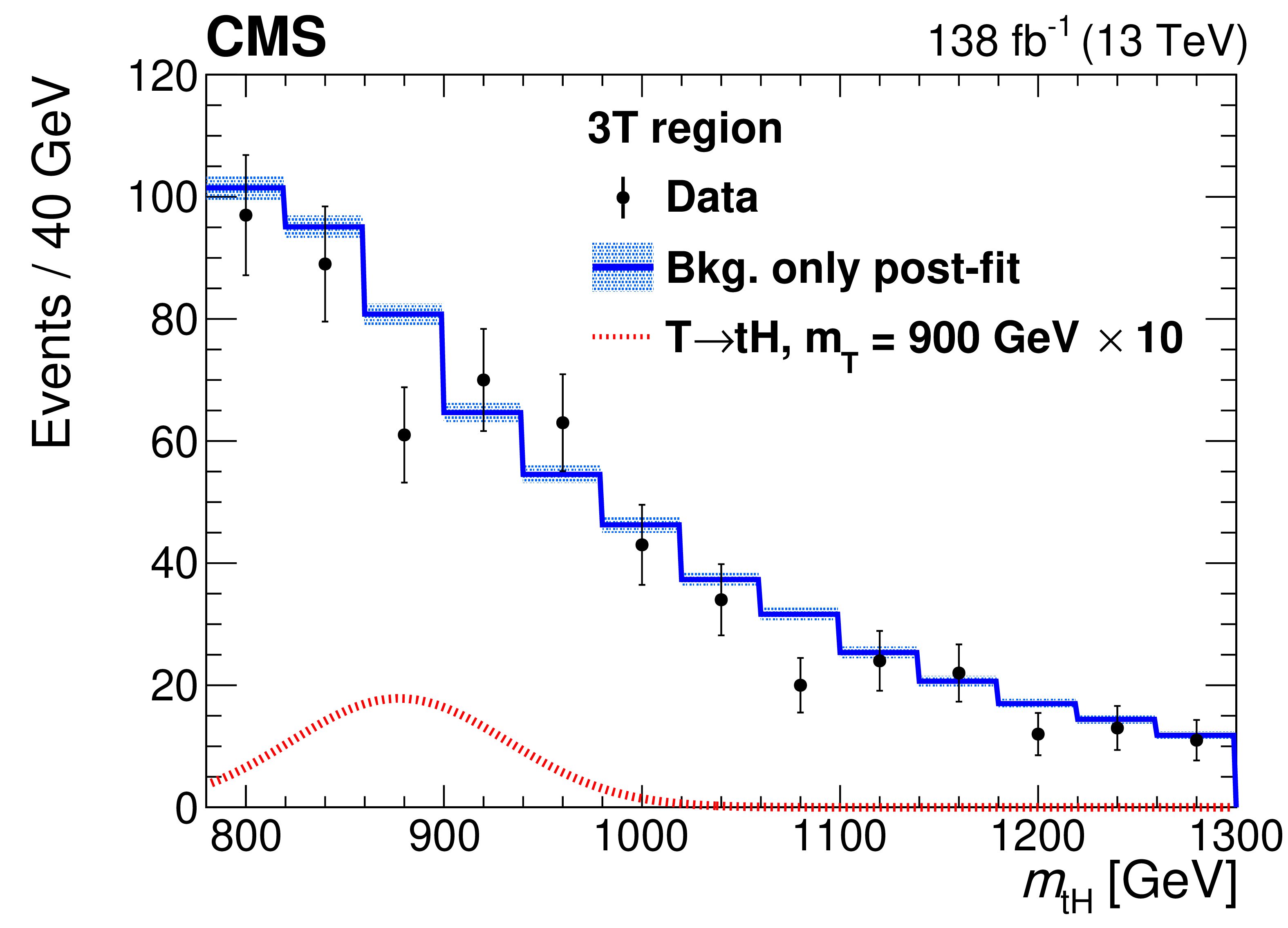
png pdf	Figure 22: Background-only postfit five-jet invariant mass distributions for the SR for the low-mass (left) and high-mass (right) selections. The shaded blue region represents the uncertainty in the fitted background estimate. The expected signal distributions (scaled for visibility) for a 700 GeV and a 900 GeV T quark are shown as red dashed lines for the low- and high-mass selections, respectively. Figures adapted from Ref. [148].
png pdf	Figure 22-a: Background-only postfit five-jet invariant mass distributions for the SR for the low-mass (left) and high-mass (right) selections. The shaded blue region represents the uncertainty in the fitted background estimate. The expected signal distributions (scaled for visibility) for a 700 GeV and a 900 GeV T quark are shown as red dashed lines for the low- and high-mass selections, respectively. Figures adapted from Ref. [148].
png pdf	Figure 22-b: Background-only postfit five-jet invariant mass distributions for the SR for the low-mass (left) and high-mass (right) selections. The shaded blue region represents the uncertainty in the fitted background estimate. The expected signal distributions (scaled for visibility) for a 700 GeV and a 900 GeV T quark are shown as red dashed lines for the low- and high-mass selections, respectively. Figures adapted from Ref. [148].
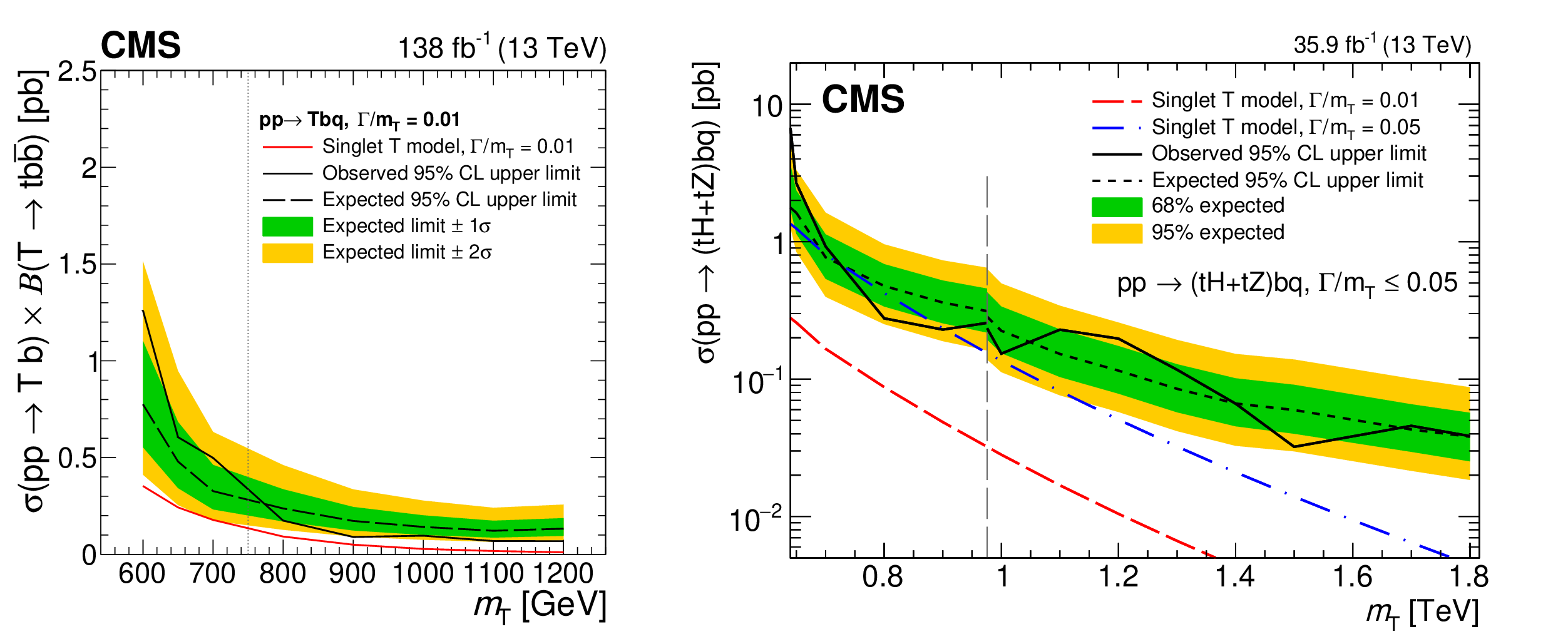
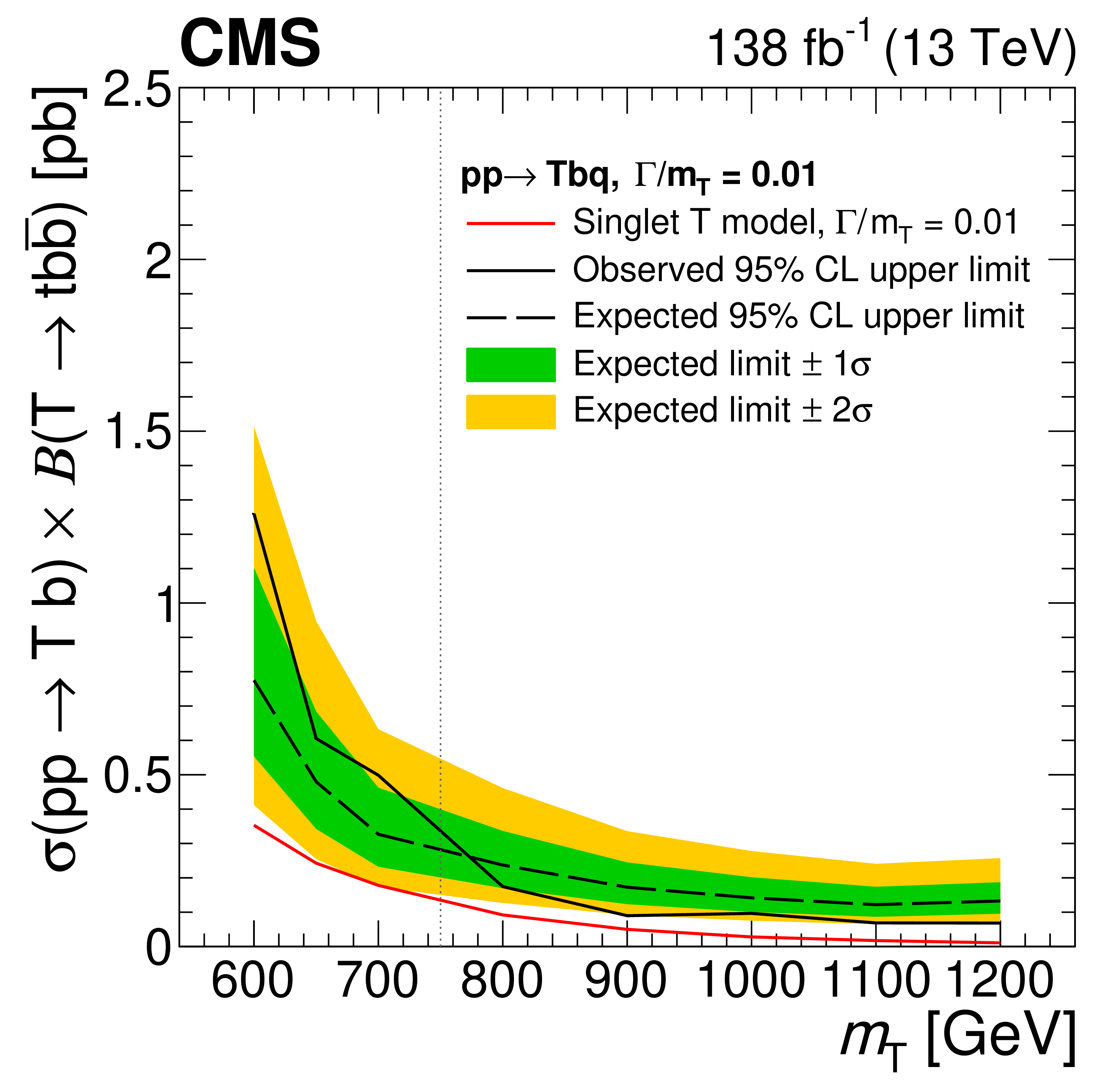
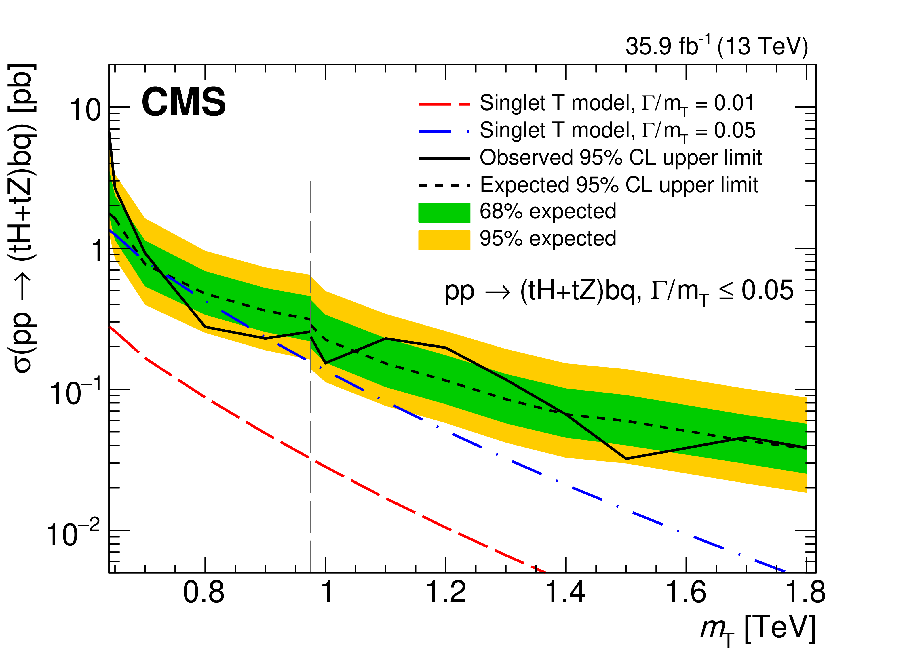
png pdf	Figure 23: Observed and median expected upper limits at 95% CL on the cross sections for single T quark production associated with a b quark, for the sum of $\mathrm{t}\mathrm{H}\mathrm{b}\mathrm{q}$ and $\mathrm{t}\mathrm{Z}\mathrm{b}\mathrm{q}$ channels, as a function of the assumed values of the T quark mass. The inner (green) band and the outer (yellow) band indicate the regions containing 68 and 95%, respectively, of the distribution of limits expected under the background-only hypothesis. The left figure corresponds to the analysis strategy described in Ref. [148], based on the five-jet invariant mass reconstruction of the T. The figure on the right corresponds to the analysis strategy in Ref. [145], which employs different reconstruction algorithms for the low- and high-mass searches. The vertical dashed lines represent the crossover point in sensitivity for the low-mass and high-mass selections. Figures adapted from Refs. [148,145].
png pdf	Figure 23-a: Observed and median expected upper limits at 95% CL on the cross sections for single T quark production associated with a b quark, for the sum of $\mathrm{t}\mathrm{H}\mathrm{b}\mathrm{q}$ and $\mathrm{t}\mathrm{Z}\mathrm{b}\mathrm{q}$ channels, as a function of the assumed values of the T quark mass. The inner (green) band and the outer (yellow) band indicate the regions containing 68 and 95%, respectively, of the distribution of limits expected under the background-only hypothesis. The left figure corresponds to the analysis strategy described in Ref. [148], based on the five-jet invariant mass reconstruction of the T. The figure on the right corresponds to the analysis strategy in Ref. [145], which employs different reconstruction algorithms for the low- and high-mass searches. The vertical dashed lines represent the crossover point in sensitivity for the low-mass and high-mass selections. Figures adapted from Refs. [148,145].
png pdf	Figure 23-b: Observed and median expected upper limits at 95% CL on the cross sections for single T quark production associated with a b quark, for the sum of $\mathrm{t}\mathrm{H}\mathrm{b}\mathrm{q}$ and $\mathrm{t}\mathrm{Z}\mathrm{b}\mathrm{q}$ channels, as a function of the assumed values of the T quark mass. The inner (green) band and the outer (yellow) band indicate the regions containing 68 and 95%, respectively, of the distribution of limits expected under the background-only hypothesis. The left figure corresponds to the analysis strategy described in Ref. [148], based on the five-jet invariant mass reconstruction of the T. The figure on the right corresponds to the analysis strategy in Ref. [145], which employs different reconstruction algorithms for the low- and high-mass searches. The vertical dashed lines represent the crossover point in sensitivity for the low-mass and high-mass selections. Figures adapted from Refs. [148,145].
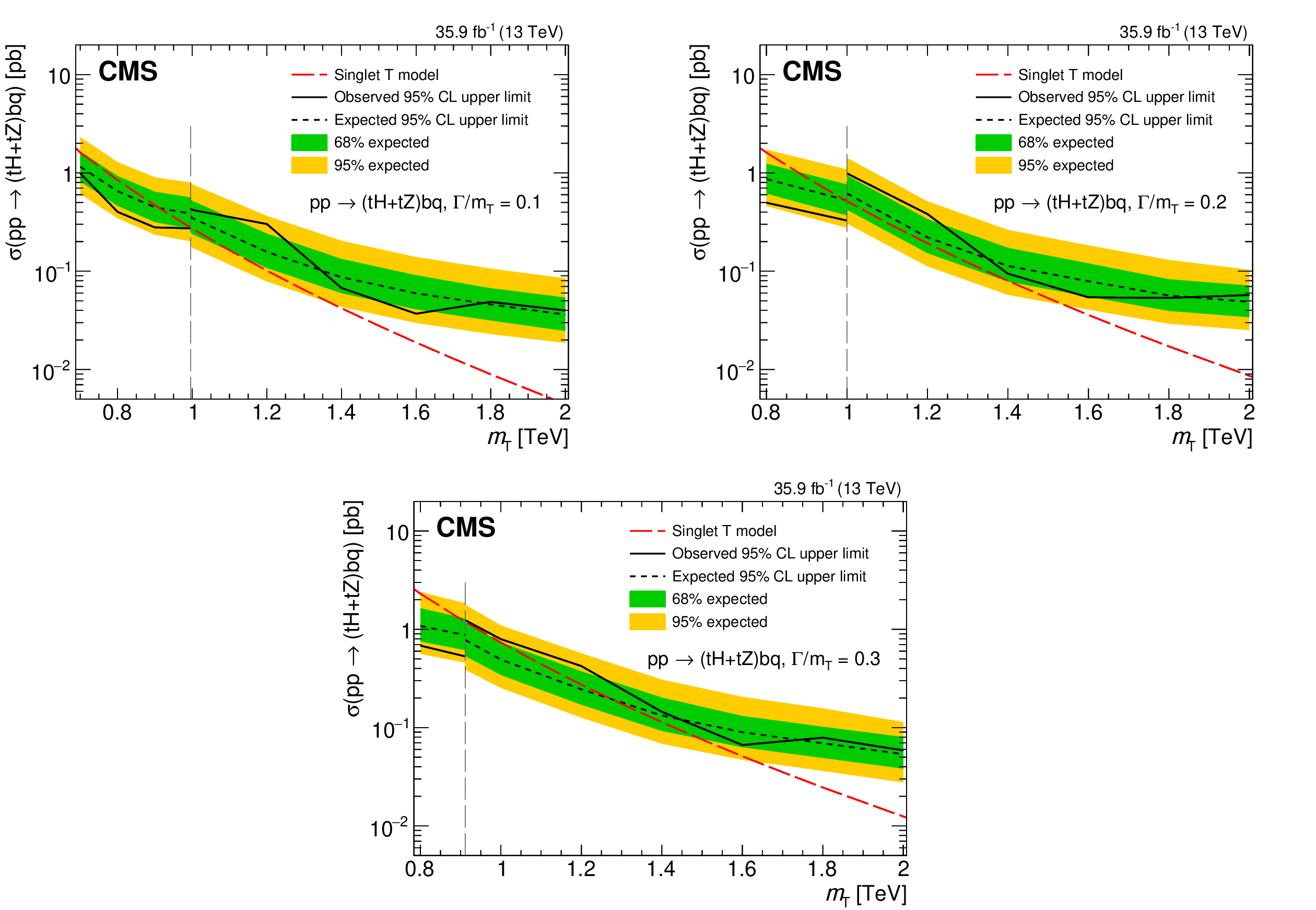
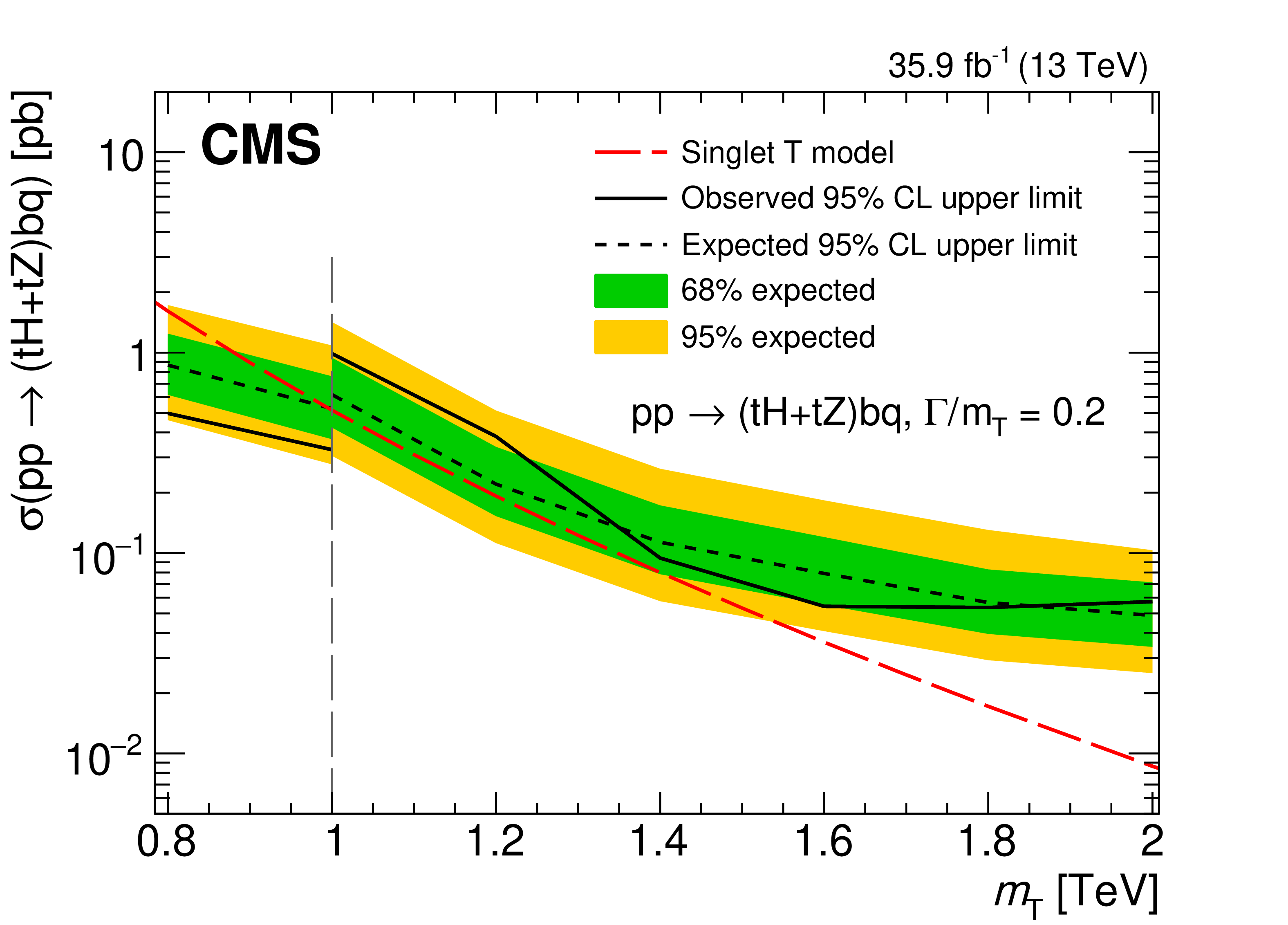
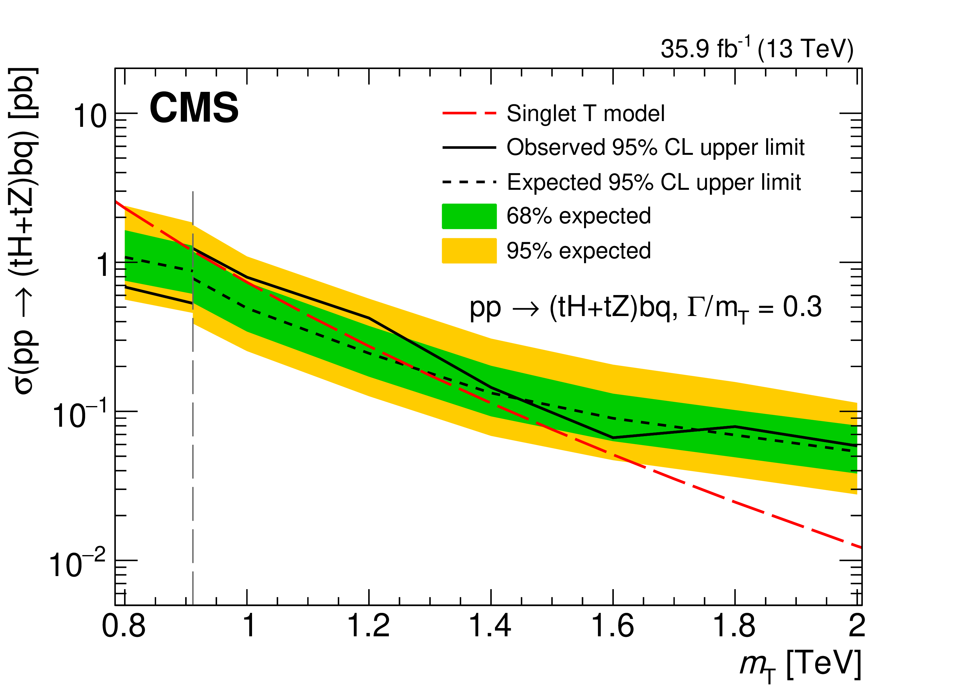
png pdf	Figure 24: Observed and median expected upper limits at 95% CL on the cross sections for single T quark production associated with a b quark, for the sum of $\mathrm{t}\mathrm{H}\mathrm{b}\mathrm{q}$ and $\mathrm{t}\mathrm{Z}\mathrm{b}\mathrm{q}$ channels, as a function of the assumed values of the T quark mass. The inner (green) band and the outer (yellow) band indicate the regions containing 68 and 95%, respectively, of the distribution of limits expected under the background-only hypothesis. The results are given for relative widths of $\Gamma/m_{{\mathrm{T}} }=$ 10 (upper left), 20 (upper right), and 30% (lower). The vertical dashed lines represent the crossover point in sensitivity for the low-mass and high-mass selections. Figures adapted from Ref. [145].
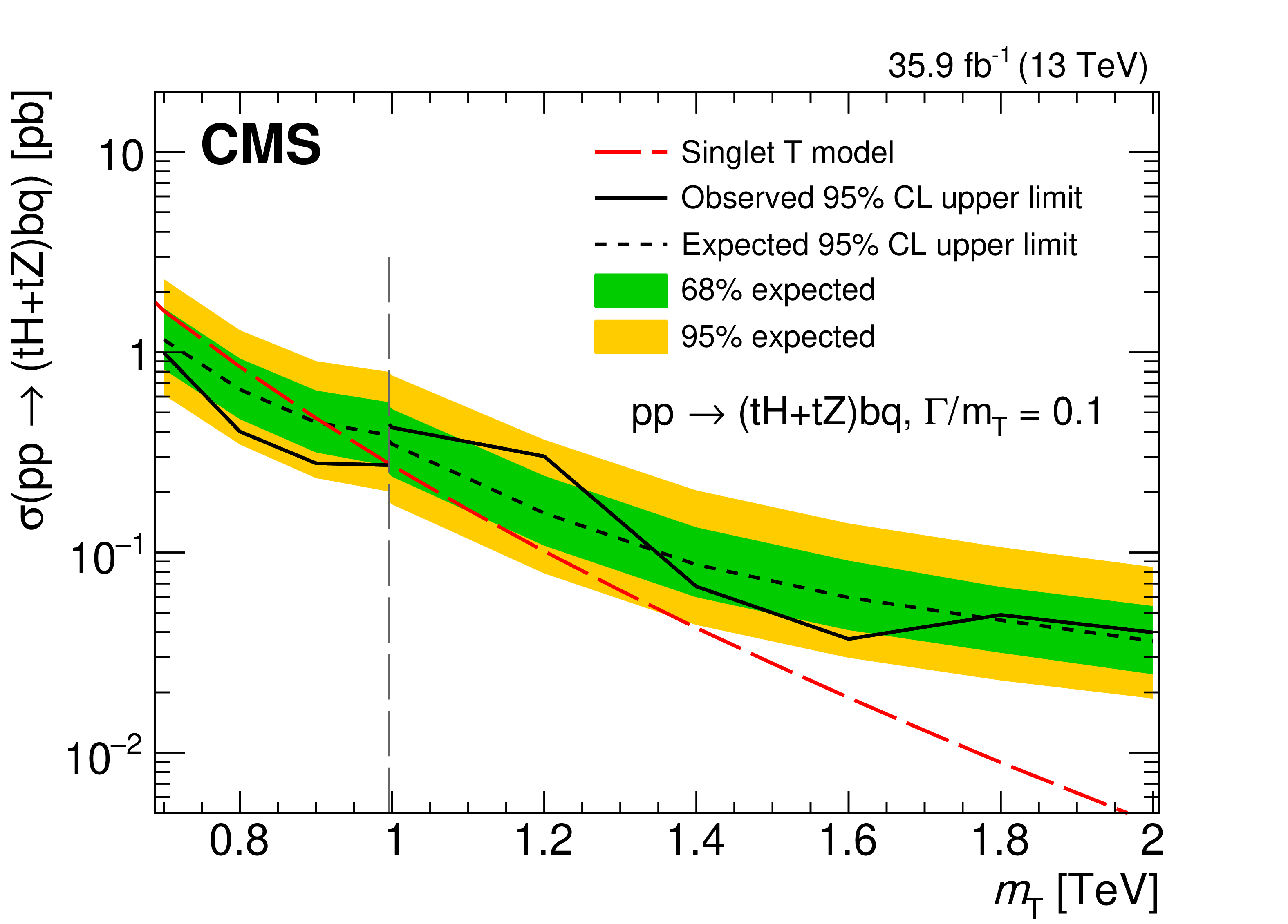
png pdf	Figure 24-a: Observed and median expected upper limits at 95% CL on the cross sections for single T quark production associated with a b quark, for the sum of $\mathrm{t}\mathrm{H}\mathrm{b}\mathrm{q}$ and $\mathrm{t}\mathrm{Z}\mathrm{b}\mathrm{q}$ channels, as a function of the assumed values of the T quark mass. The inner (green) band and the outer (yellow) band indicate the regions containing 68 and 95%, respectively, of the distribution of limits expected under the background-only hypothesis. The results are given for relative widths of $\Gamma/m_{{\mathrm{T}} }=$ 10 (upper left), 20 (upper right), and 30% (lower). The vertical dashed lines represent the crossover point in sensitivity for the low-mass and high-mass selections. Figures adapted from Ref. [145].
png pdf	Figure 24-b: Observed and median expected upper limits at 95% CL on the cross sections for single T quark production associated with a b quark, for the sum of $\mathrm{t}\mathrm{H}\mathrm{b}\mathrm{q}$ and $\mathrm{t}\mathrm{Z}\mathrm{b}\mathrm{q}$ channels, as a function of the assumed values of the T quark mass. The inner (green) band and the outer (yellow) band indicate the regions containing 68 and 95%, respectively, of the distribution of limits expected under the background-only hypothesis. The results are given for relative widths of $\Gamma/m_{{\mathrm{T}} }=$ 10 (upper left), 20 (upper right), and 30% (lower). The vertical dashed lines represent the crossover point in sensitivity for the low-mass and high-mass selections. Figures adapted from Ref. [145].
png pdf	Figure 24-c: Observed and median expected upper limits at 95% CL on the cross sections for single T quark production associated with a b quark, for the sum of $\mathrm{t}\mathrm{H}\mathrm{b}\mathrm{q}$ and $\mathrm{t}\mathrm{Z}\mathrm{b}\mathrm{q}$ channels, as a function of the assumed values of the T quark mass. The inner (green) band and the outer (yellow) band indicate the regions containing 68 and 95%, respectively, of the distribution of limits expected under the background-only hypothesis. The results are given for relative widths of $\Gamma/m_{{\mathrm{T}} }=$ 10 (upper left), 20 (upper right), and 30% (lower). The vertical dashed lines represent the crossover point in sensitivity for the low-mass and high-mass selections. Figures adapted from Ref. [145].
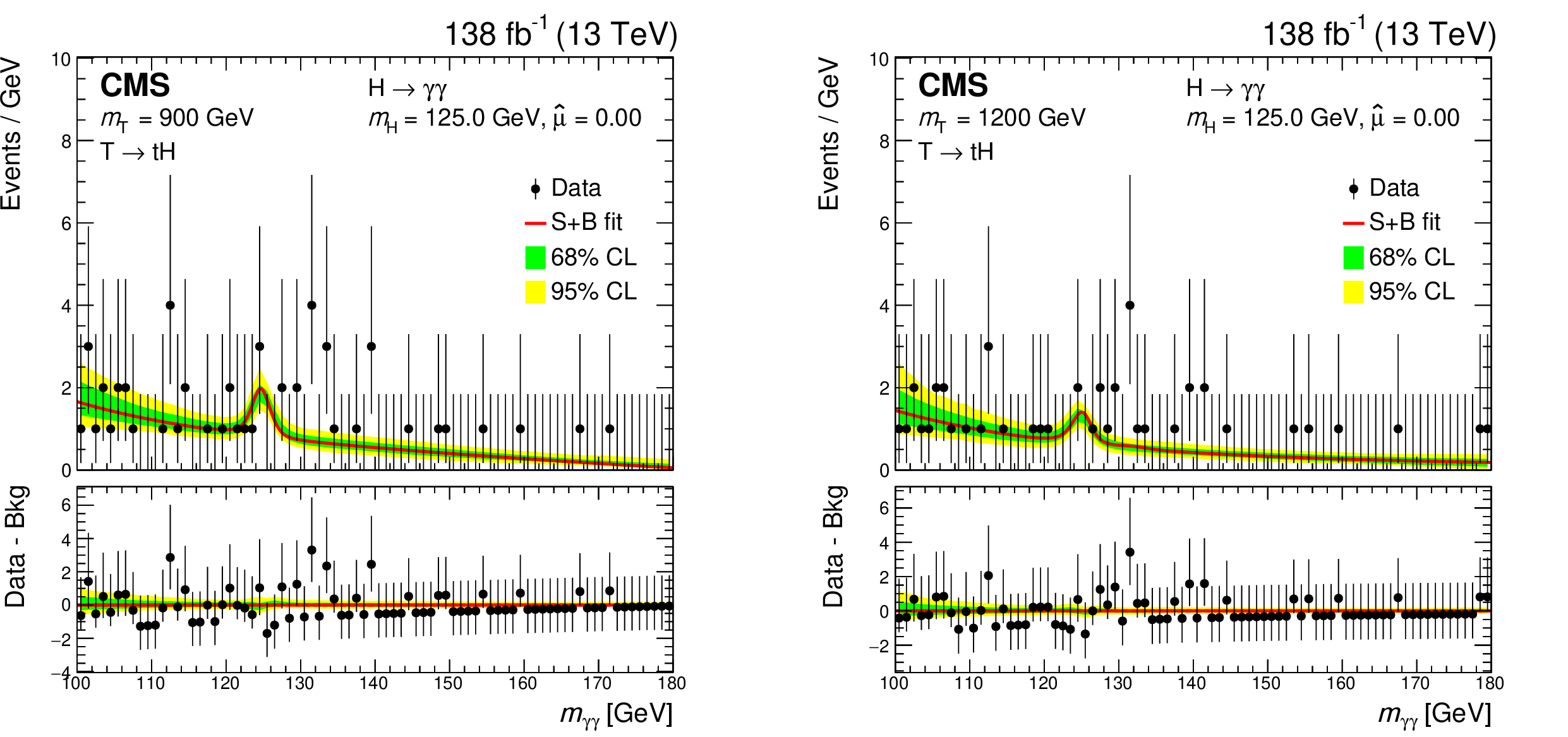
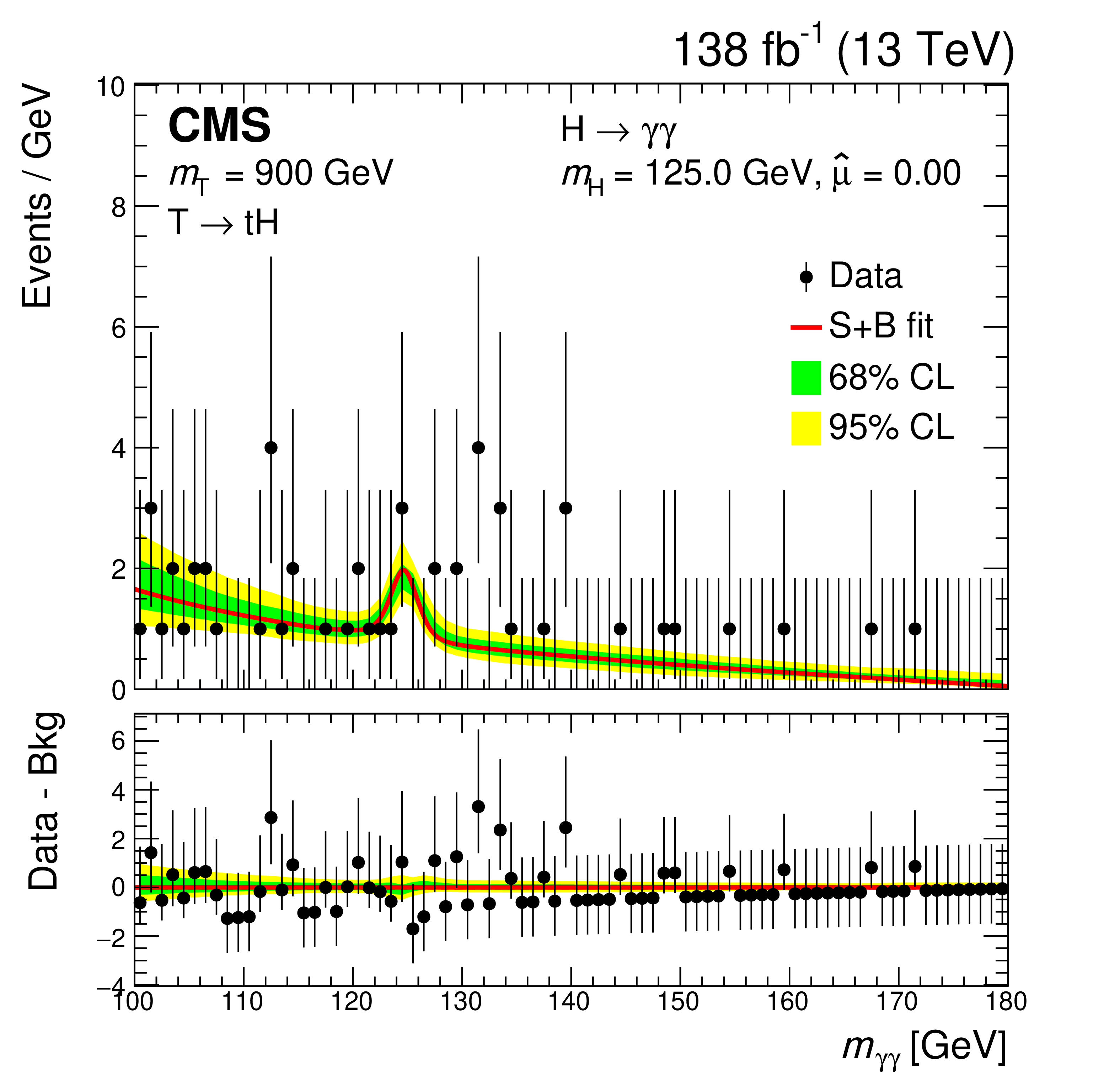
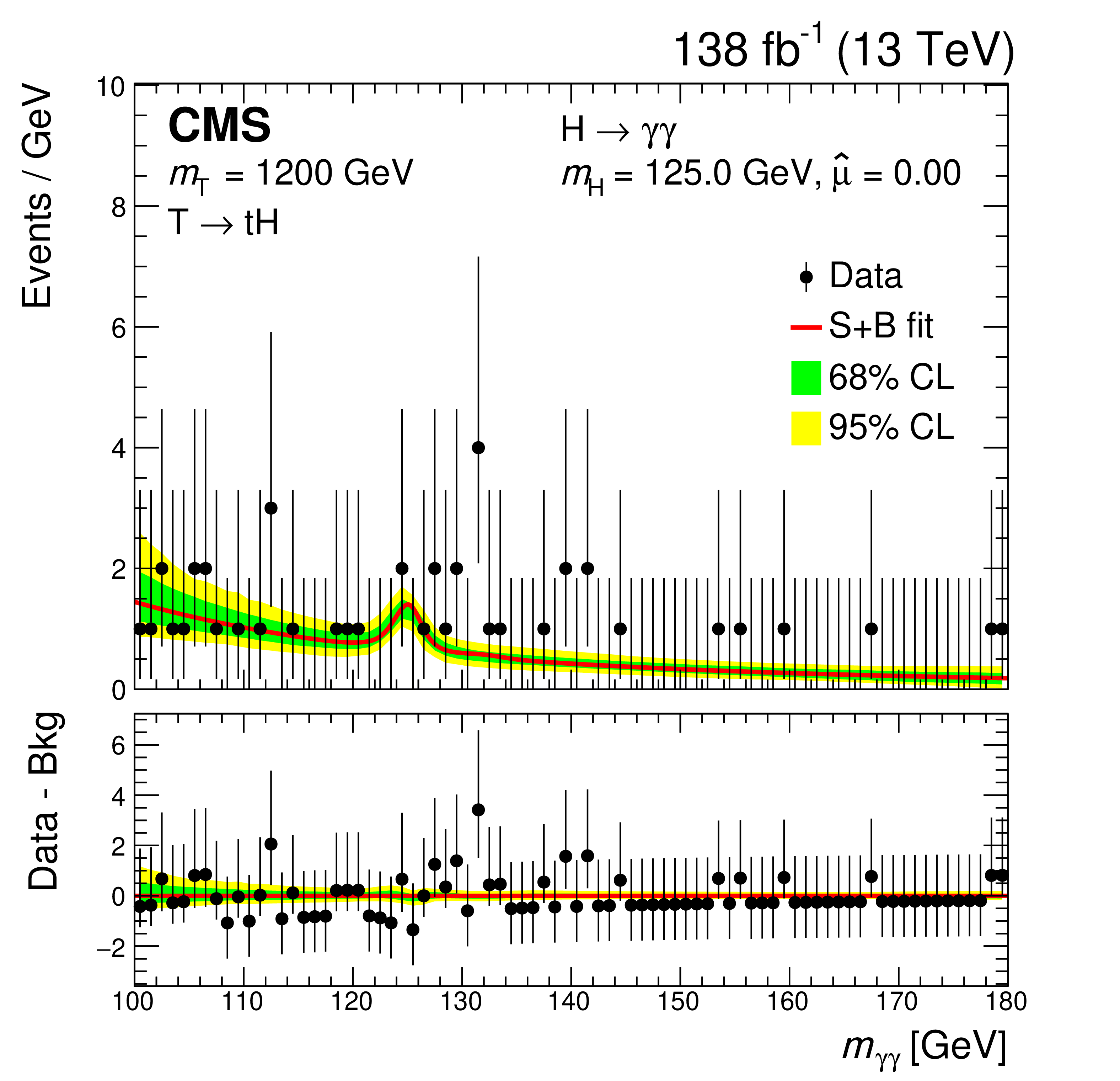
png pdf	Figure 25: Distributions of the observed data (black dots) and $m_{\gamma\gamma}$ signal-plus-background model fits (red line) for a T quark signal with $m_{{\mathrm{T}} }$ of 900 (left) and 1200 GeV (right), combining the leptonic and hadronic channels. The green (yellow) band represents the 68 (95)% CL interval in the background component of the fit. The peak in the background component shows the considered irreducible SM Higgs boson contribution ($\mathrm{g}\mathrm{g}\mathrm{H}$, VBF, VH, ${\mathrm{t}\overline{\mathrm{t}}} \mathrm{H}$, and $\mathrm{t}\mathrm{H}$). Here, $\hat{\mu}$ is the best fit value of the signal strength parameter $\mu$, which is zero for the two $m_{{\mathrm{T}} }$ values considered. The lower panel shows the residuals after the subtraction of the background component. Figures adapted from Ref. [147].
png pdf	Figure 25-a: Distributions of the observed data (black dots) and $m_{\gamma\gamma}$ signal-plus-background model fits (red line) for a T quark signal with $m_{{\mathrm{T}} }$ of 900 (left) and 1200 GeV (right), combining the leptonic and hadronic channels. The green (yellow) band represents the 68 (95)% CL interval in the background component of the fit. The peak in the background component shows the considered irreducible SM Higgs boson contribution ($\mathrm{g}\mathrm{g}\mathrm{H}$, VBF, VH, ${\mathrm{t}\overline{\mathrm{t}}} \mathrm{H}$, and $\mathrm{t}\mathrm{H}$). Here, $\hat{\mu}$ is the best fit value of the signal strength parameter $\mu$, which is zero for the two $m_{{\mathrm{T}} }$ values considered. The lower panel shows the residuals after the subtraction of the background component. Figures adapted from Ref. [147].
png pdf	Figure 25-b: Distributions of the observed data (black dots) and $m_{\gamma\gamma}$ signal-plus-background model fits (red line) for a T quark signal with $m_{{\mathrm{T}} }$ of 900 (left) and 1200 GeV (right), combining the leptonic and hadronic channels. The green (yellow) band represents the 68 (95)% CL interval in the background component of the fit. The peak in the background component shows the considered irreducible SM Higgs boson contribution ($\mathrm{g}\mathrm{g}\mathrm{H}$, VBF, VH, ${\mathrm{t}\overline{\mathrm{t}}} \mathrm{H}$, and $\mathrm{t}\mathrm{H}$). Here, $\hat{\mu}$ is the best fit value of the signal strength parameter $\mu$, which is zero for the two $m_{{\mathrm{T}} }$ values considered. The lower panel shows the residuals after the subtraction of the background component. Figures adapted from Ref. [147].
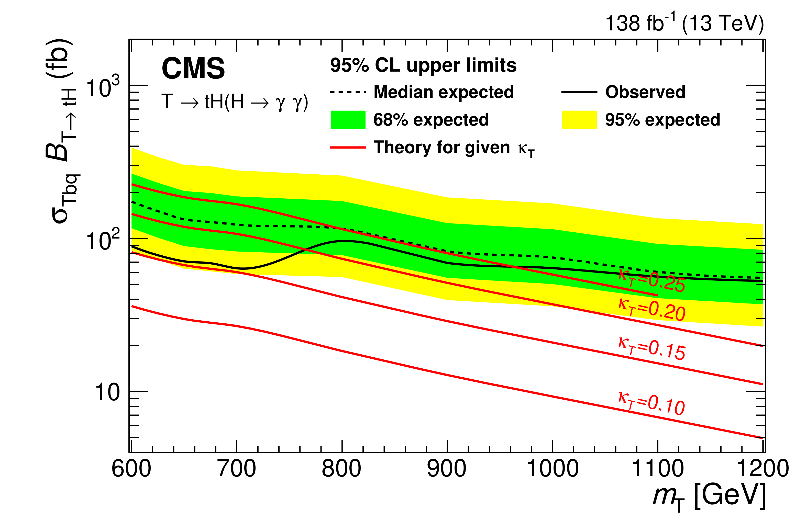
png pdf	Figure 26: Expected (dotted black) and observed (solid black) upper limits at 95% CL on $\sigma_{{\mathrm{T}} \mathrm{b}\mathrm{q}}\mathcal{B}({\mathrm{T}} \to\mathrm{t}\mathrm{H})$ are displayed as a function of $m_{{\mathrm{T}} }$, combining the leptonic and hadronic channels. The inner (green) band and the outer (yellow) band indicate the regions containing 68 and 95%, respectively, of the distribution of limits expected under the background-only hypothesis. The theoretical cross sections for the singlet T production with representative $\kappa_{{\mathrm{T}} }$ values fixed at 0.1, 0.15, 0.2, and 0.25 (for $\Gamma/m_{{\mathrm{T}} } < 5%$) are shown as red lines. Figure adapted from Ref. [147].
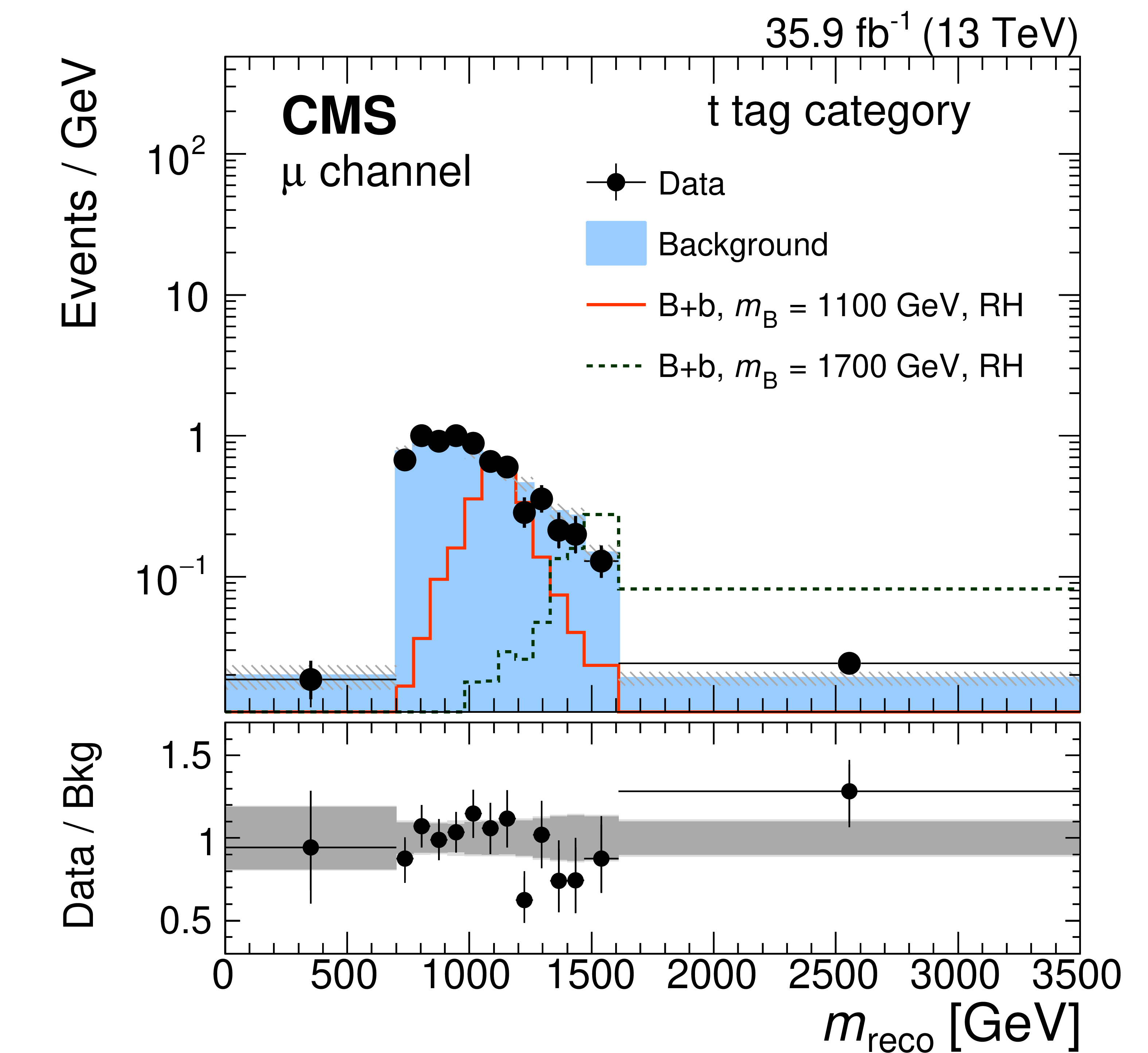
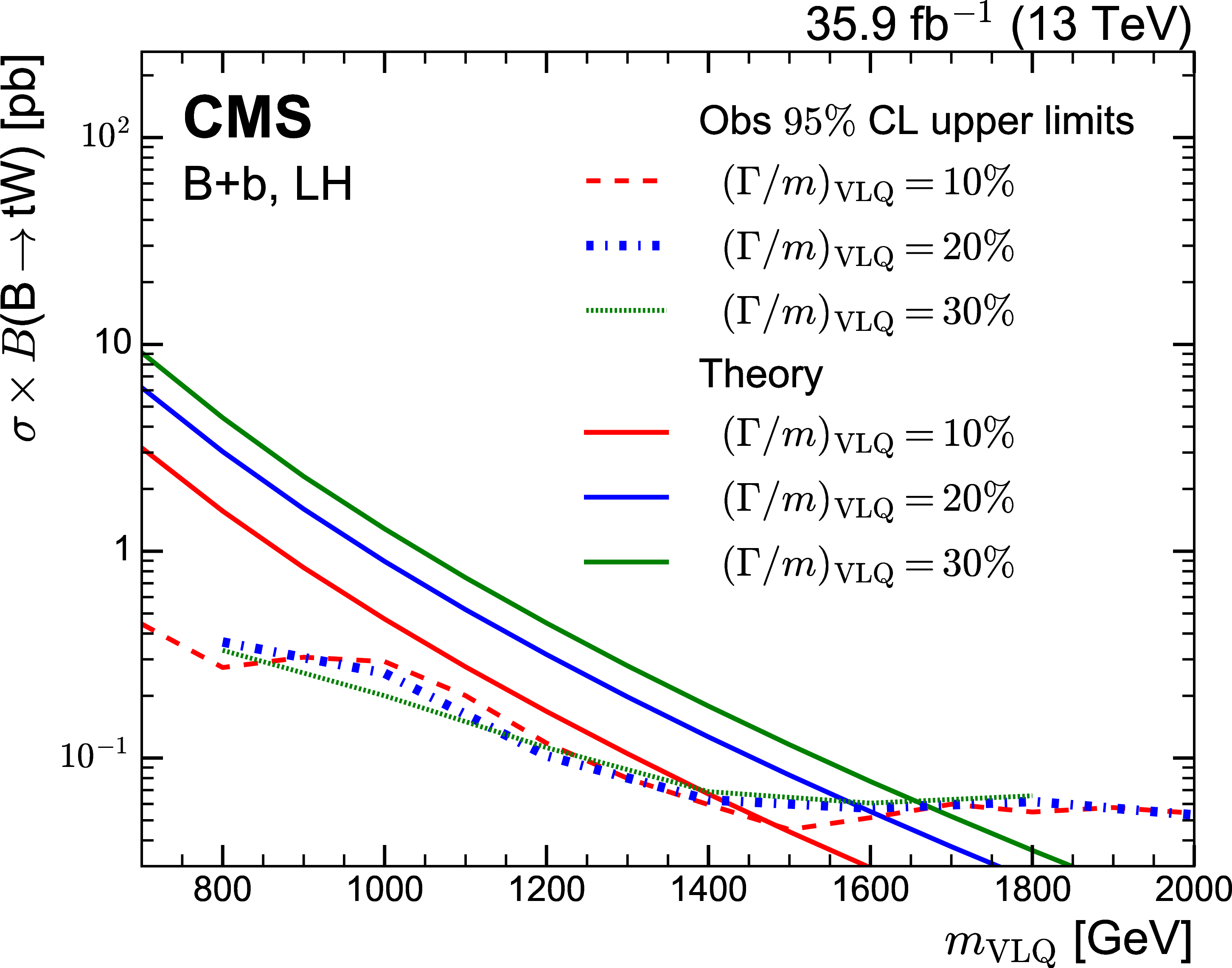
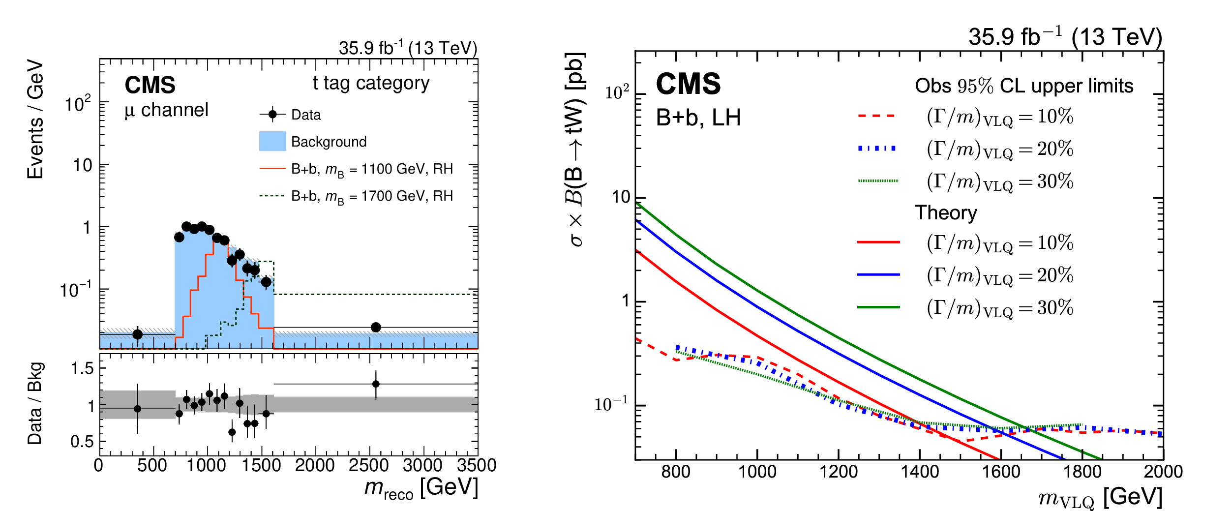
png pdf	Figure 27: The distribution in the reconstructed B quark mass in events with one t-tagged jet and a forward jet, where the SM background is obtained from a CR without a forward jet (left). The product of the observed upper limits on the cross section and $\mathcal{B}({\mathrm{B}} \to\mathrm{t}\mathrm{W})$ as a function of $m_{\text{VLQ}}$ for different relative decay widths of the B quark (right), for single B quark production in association with a b quark. Figures taken from Ref. [151].
png pdf	Figure 27-a: The distribution in the reconstructed B quark mass in events with one t-tagged jet and a forward jet, where the SM background is obtained from a CR without a forward jet (left). The product of the observed upper limits on the cross section and $\mathcal{B}({\mathrm{B}} \to\mathrm{t}\mathrm{W})$ as a function of $m_{\text{VLQ}}$ for different relative decay widths of the B quark (right), for single B quark production in association with a b quark. Figures taken from Ref. [151].
png pdf	Figure 27-b: The distribution in the reconstructed B quark mass in events with one t-tagged jet and a forward jet, where the SM background is obtained from a CR without a forward jet (left). The product of the observed upper limits on the cross section and $\mathcal{B}({\mathrm{B}} \to\mathrm{t}\mathrm{W})$ as a function of $m_{\text{VLQ}}$ for different relative decay widths of the B quark (right), for single B quark production in association with a b quark. Figures taken from Ref. [151].
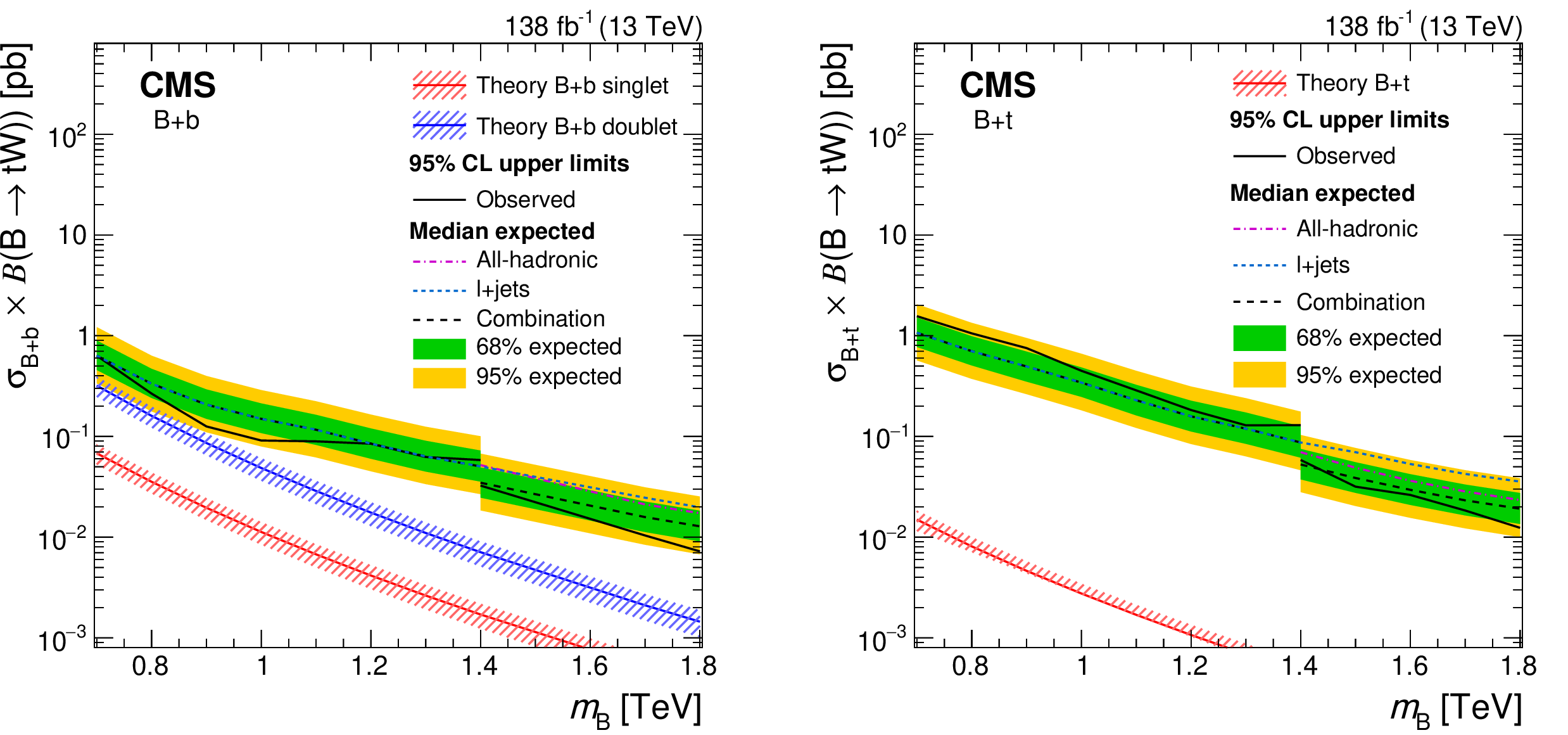
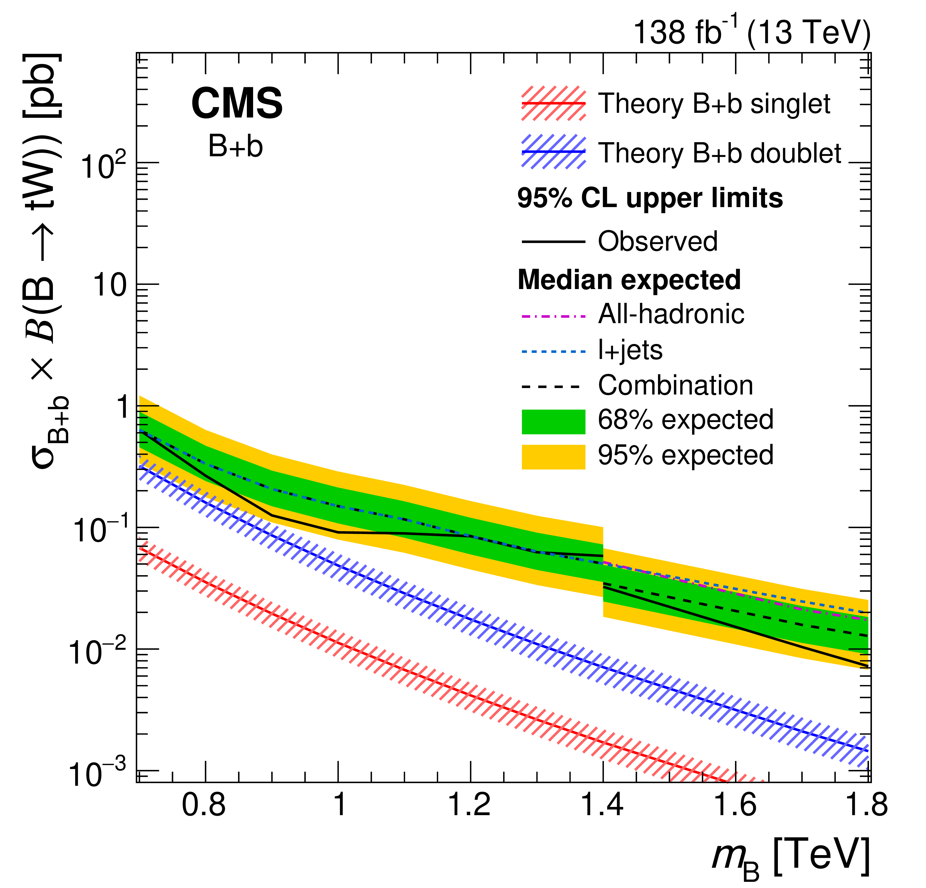
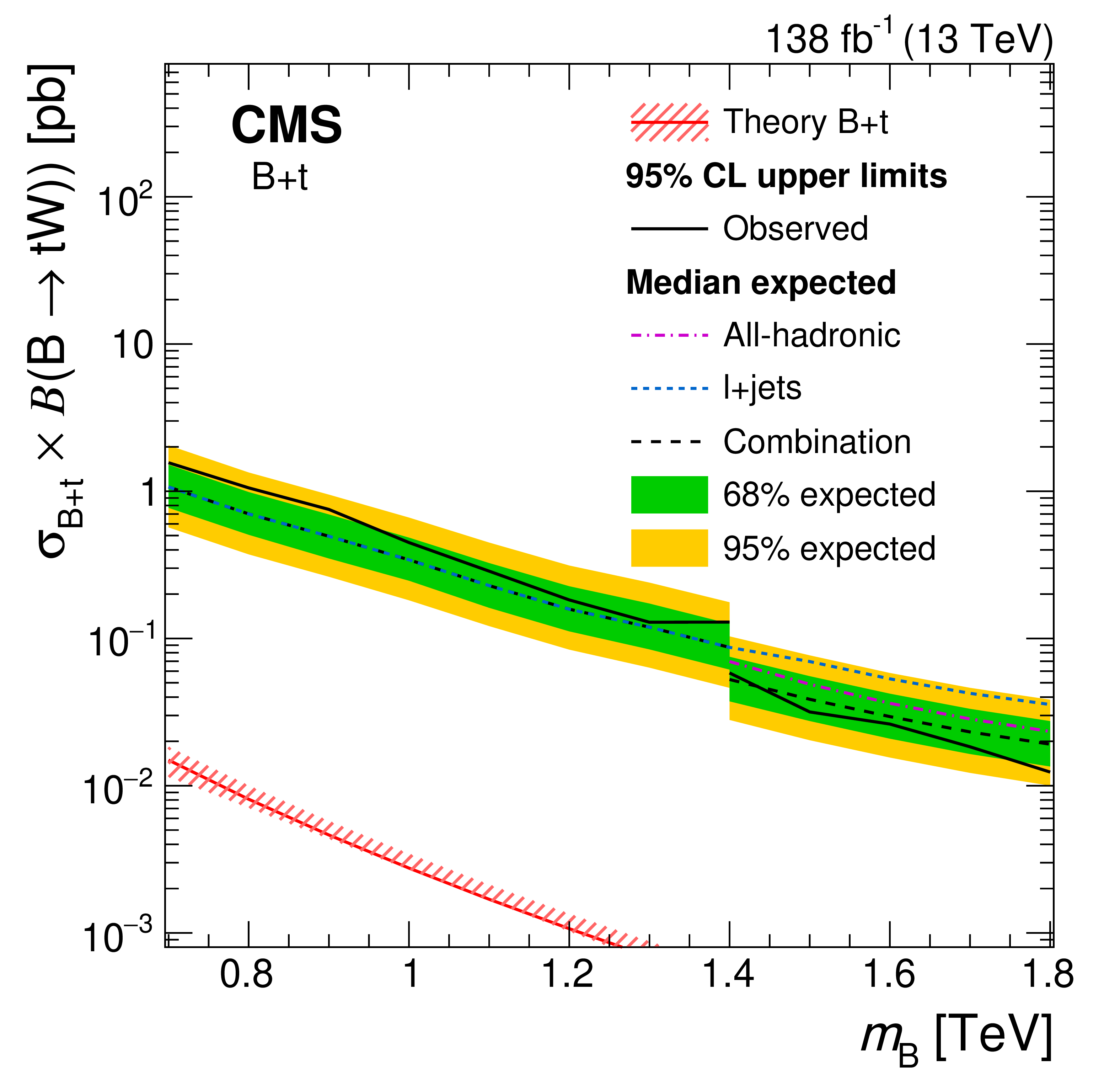
png pdf	Figure 28: Upper limits on the product of the production cross section and branching fraction to $\mathrm{t}\mathrm{W}$ of the $\mathrm{b}\mathrm{b}$ (left) and $\mathrm{b}\mathrm{t}$ (right) production modes at 95% CL. Colored lines show the expected limits from the $\ell$+jets (dotted) and all-hadronic (dash-dotted) channels, where the latter start at B masses of 1.4 TeV. The observed and expected limits from the combination are shown as solid and dashed black lines, respectively. The inner (green) band and the outer (yellow) band indicate the regions containing 68 and 95%, respectively, of the distribution of the limits expected under the background-only hypothesis. The theoretical cross sections are shown as the red and blue lines, where the uncertainties due to missing higher orders are depicted by shaded areas. Figures adapted from Ref. [153].
png pdf	Figure 28-a: Upper limits on the product of the production cross section and branching fraction to $\mathrm{t}\mathrm{W}$ of the $\mathrm{b}\mathrm{b}$ (left) and $\mathrm{b}\mathrm{t}$ (right) production modes at 95% CL. Colored lines show the expected limits from the $\ell$+jets (dotted) and all-hadronic (dash-dotted) channels, where the latter start at B masses of 1.4 TeV. The observed and expected limits from the combination are shown as solid and dashed black lines, respectively. The inner (green) band and the outer (yellow) band indicate the regions containing 68 and 95%, respectively, of the distribution of the limits expected under the background-only hypothesis. The theoretical cross sections are shown as the red and blue lines, where the uncertainties due to missing higher orders are depicted by shaded areas. Figures adapted from Ref. [153].
png pdf	Figure 28-b: Upper limits on the product of the production cross section and branching fraction to $\mathrm{t}\mathrm{W}$ of the $\mathrm{b}\mathrm{b}$ (left) and $\mathrm{b}\mathrm{t}$ (right) production modes at 95% CL. Colored lines show the expected limits from the $\ell$+jets (dotted) and all-hadronic (dash-dotted) channels, where the latter start at B masses of 1.4 TeV. The observed and expected limits from the combination are shown as solid and dashed black lines, respectively. The inner (green) band and the outer (yellow) band indicate the regions containing 68 and 95%, respectively, of the distribution of the limits expected under the background-only hypothesis. The theoretical cross sections are shown as the red and blue lines, where the uncertainties due to missing higher orders are depicted by shaded areas. Figures adapted from Ref. [153].
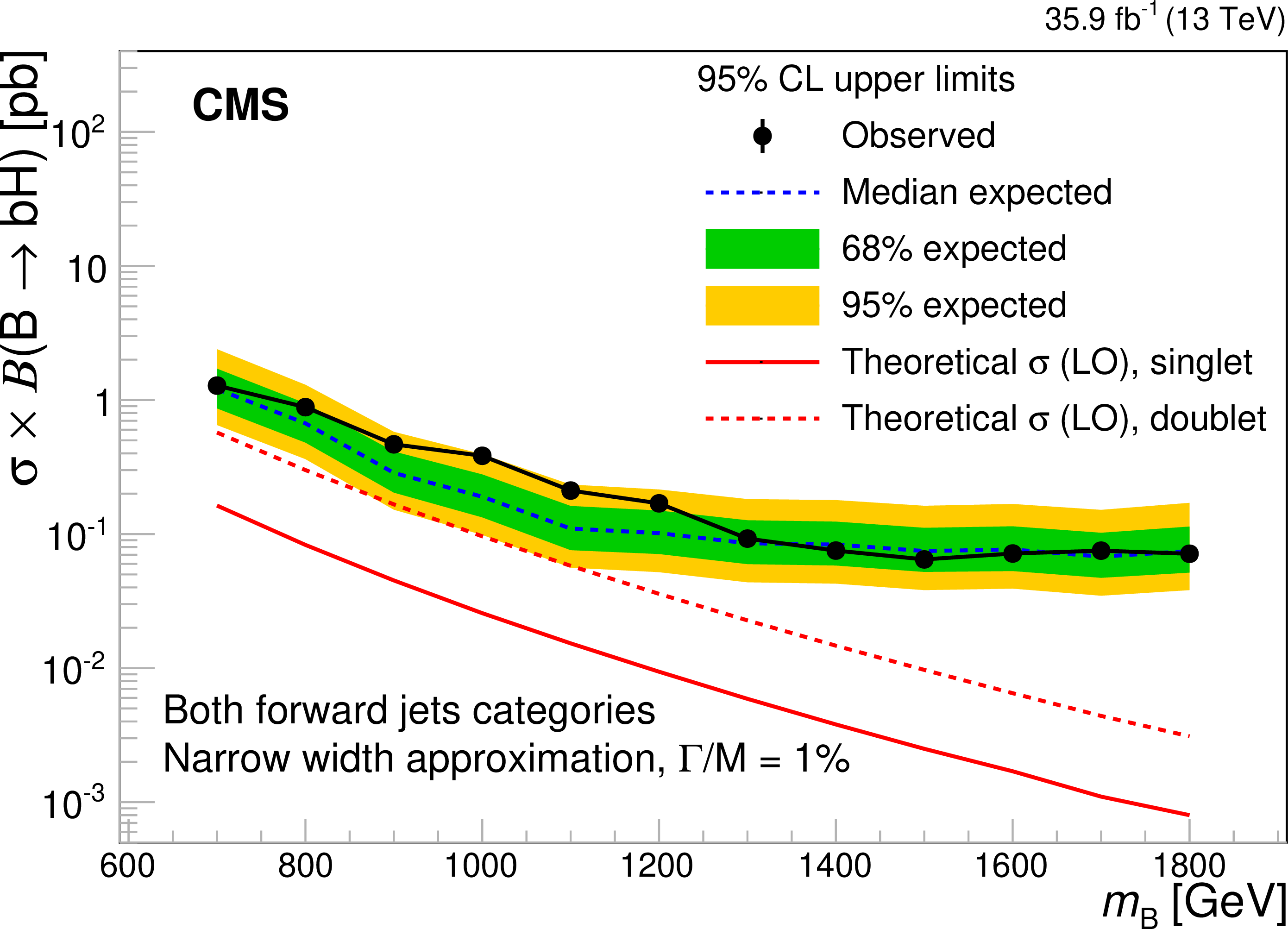
png pdf	Figure 29: Observed and expected 95% CL upper limits on the product of the B quark production cross section and branching fraction to $\mathrm{b}\mathrm{H}$, as a function of the signal mass, under the NWA. The results are shown for the combination of 0 and $>$0 forward-jet categories. The continuous red curves correspond to the theoretical expectations for singlet and doublet models. Figure taken from Ref. [150].
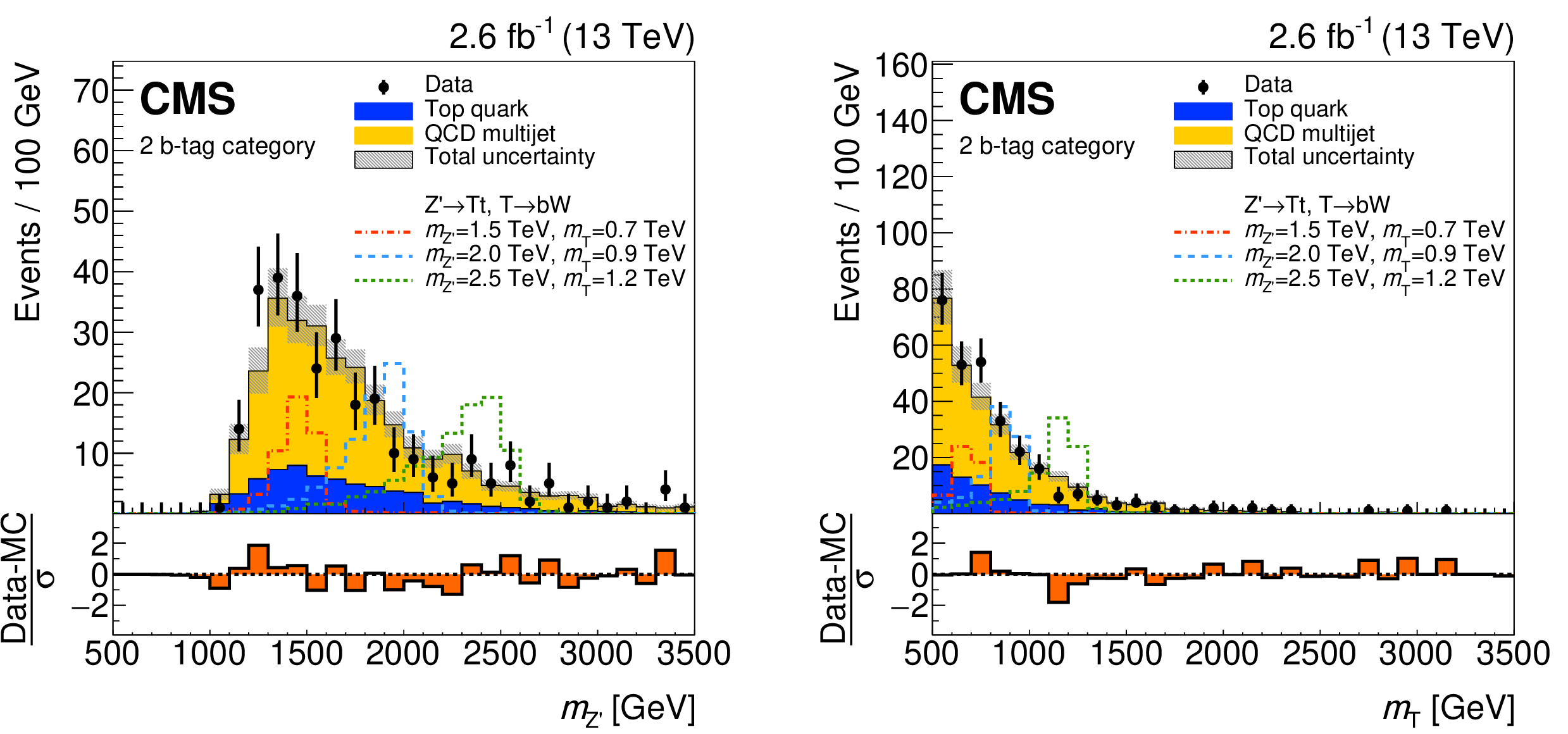
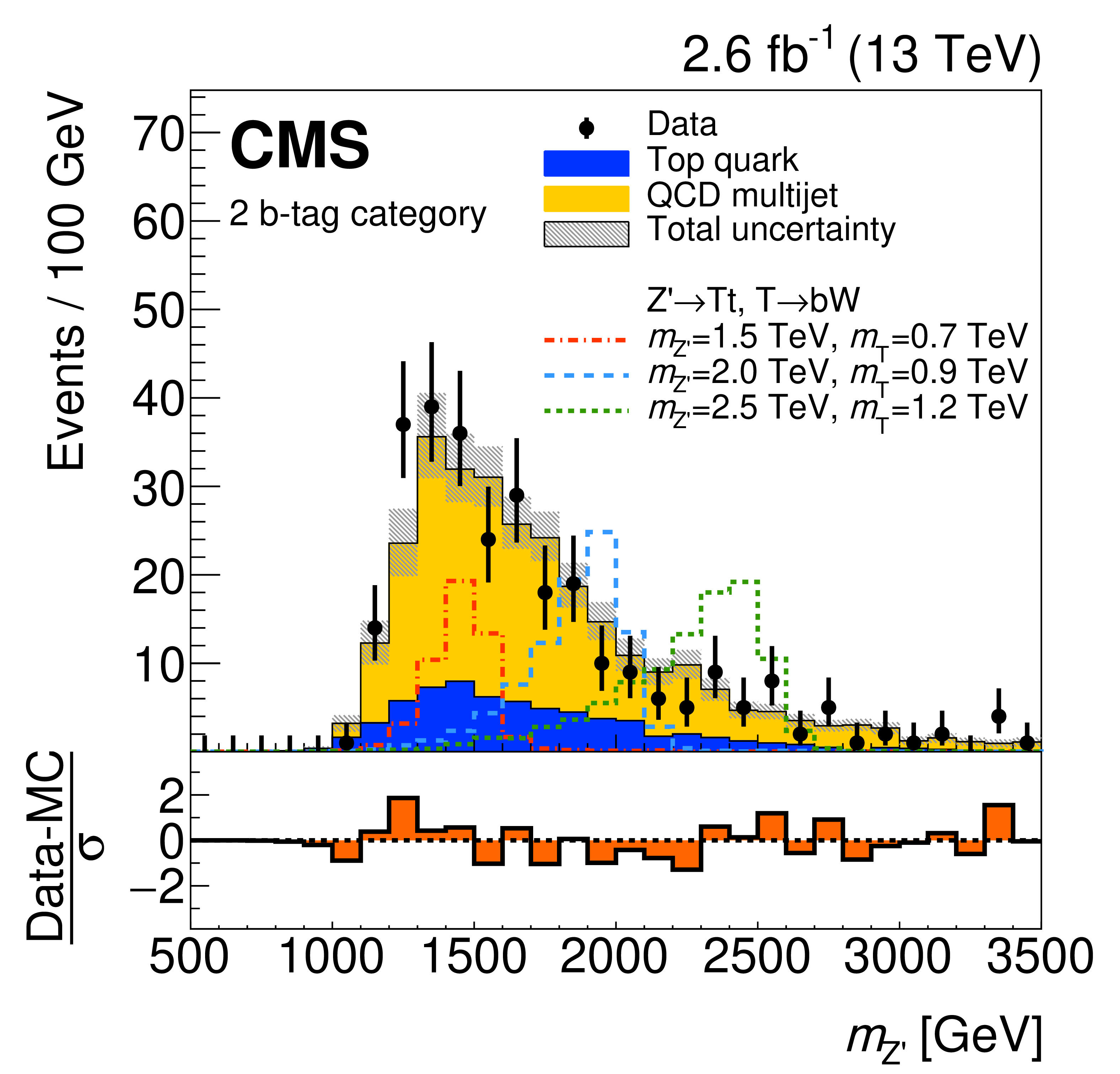
png pdf	Figure 30: Reconstructed $m_{\mathrm{Z}^{'}}$ (left) and $m_{{\mathrm{T}} }$ (right) distributions obtained in a search for $\mathrm{p}\mathrm{p}\to\mathrm{Z}^{'}\to{\mathrm{T}} {\overline{T}}$ in the all-hadronic final state. The $\mathrm{Z}^{'}$ boson is reconstructed using a t-, a W-, and a b-tagged jet, whereas the T quark is reconstructed using the latter two jets. The lower panels show the difference between the data and the estimated backgrounds divided by the sum in quadrature of the statistical uncertainties in data and backgrounds, and the systematic uncertainties in the estimated backgrounds. Figures adapted from Ref. [154].
png pdf	Figure 30-a: Reconstructed $m_{\mathrm{Z}^{'}}$ (left) and $m_{{\mathrm{T}} }$ (right) distributions obtained in a search for $\mathrm{p}\mathrm{p}\to\mathrm{Z}^{'}\to{\mathrm{T}} {\overline{T}}$ in the all-hadronic final state. The $\mathrm{Z}^{'}$ boson is reconstructed using a t-, a W-, and a b-tagged jet, whereas the T quark is reconstructed using the latter two jets. The lower panels show the difference between the data and the estimated backgrounds divided by the sum in quadrature of the statistical uncertainties in data and backgrounds, and the systematic uncertainties in the estimated backgrounds. Figures adapted from Ref. [154].
png pdf	Figure 30-b: Reconstructed $m_{\mathrm{Z}^{'}}$ (left) and $m_{{\mathrm{T}} }$ (right) distributions obtained in a search for $\mathrm{p}\mathrm{p}\to\mathrm{Z}^{'}\to{\mathrm{T}} {\overline{T}}$ in the all-hadronic final state. The $\mathrm{Z}^{'}$ boson is reconstructed using a t-, a W-, and a b-tagged jet, whereas the T quark is reconstructed using the latter two jets. The lower panels show the difference between the data and the estimated backgrounds divided by the sum in quadrature of the statistical uncertainties in data and backgrounds, and the systematic uncertainties in the estimated backgrounds. Figures adapted from Ref. [154].
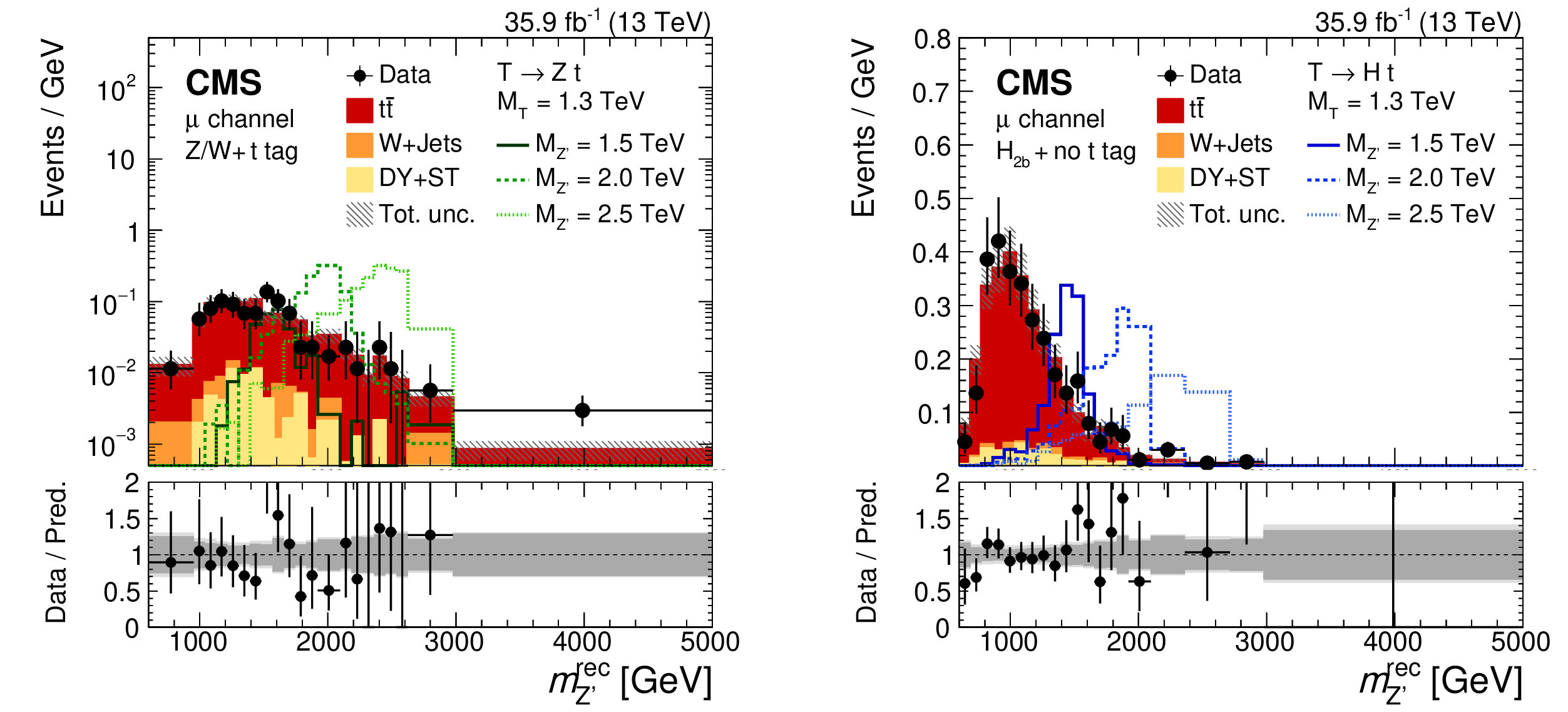
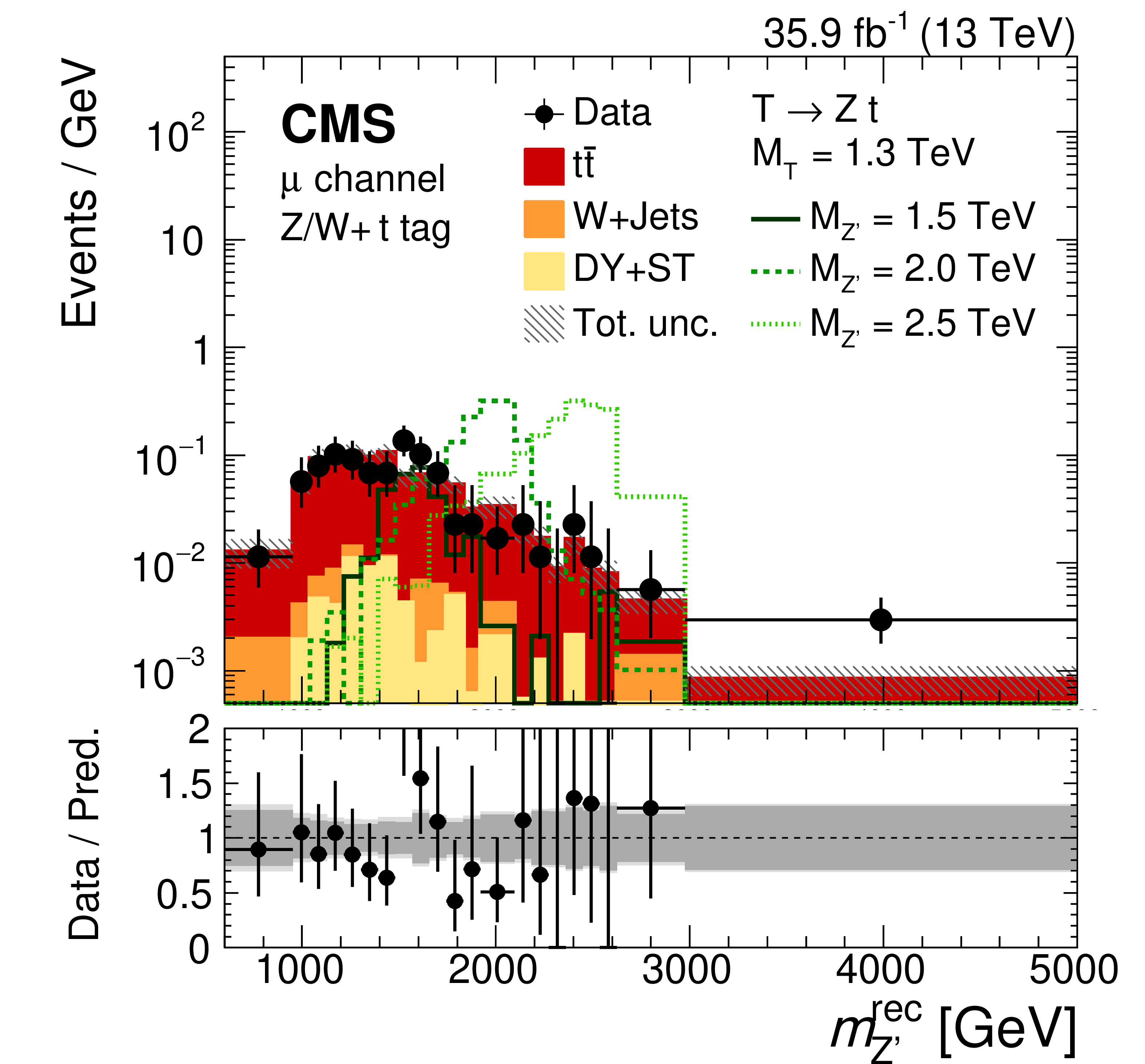
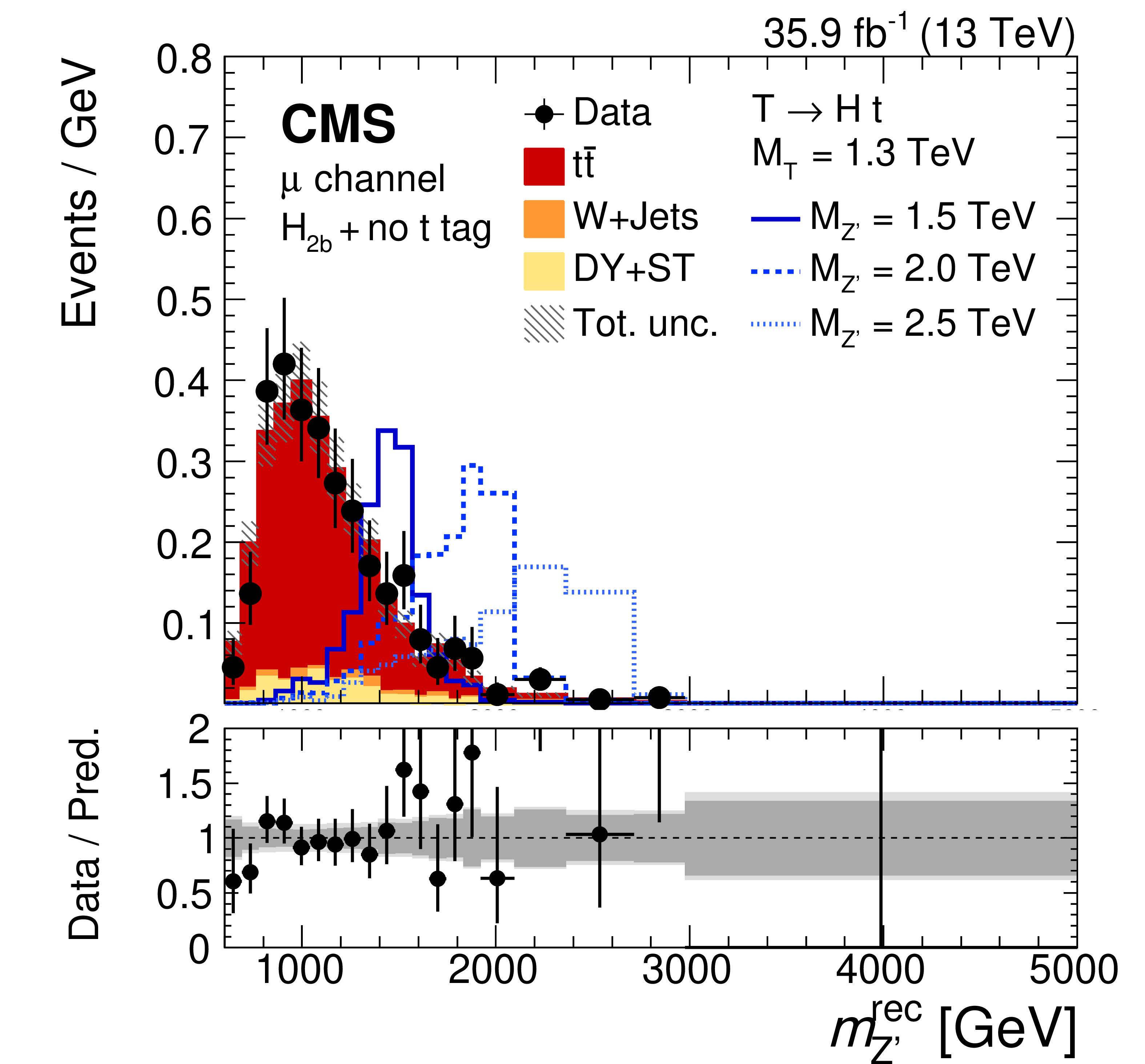
png pdf	Figure 31: Reconstructed $m_{\mathrm{Z}^{'}}$ distributions obtained in a search for $\mathrm{p}\mathrm{p}\to\mathrm{Z}^{'}\to{\mathrm{T}} {\overline{T}}$ in the $\ell$+jets final state, in events with a V- and a t-tagged jet (left) and in events with an H-tagged jet (right). The lower panels show the ratio of the observed data to the background prediction. Figures adapted from Ref. [155].
png pdf	Figure 31-a: Reconstructed $m_{\mathrm{Z}^{'}}$ distributions obtained in a search for $\mathrm{p}\mathrm{p}\to\mathrm{Z}^{'}\to{\mathrm{T}} {\overline{T}}$ in the $\ell$+jets final state, in events with a V- and a t-tagged jet (left) and in events with an H-tagged jet (right). The lower panels show the ratio of the observed data to the background prediction. Figures adapted from Ref. [155].
png pdf	Figure 31-b: Reconstructed $m_{\mathrm{Z}^{'}}$ distributions obtained in a search for $\mathrm{p}\mathrm{p}\to\mathrm{Z}^{'}\to{\mathrm{T}} {\overline{T}}$ in the $\ell$+jets final state, in events with a V- and a t-tagged jet (left) and in events with an H-tagged jet (right). The lower panels show the ratio of the observed data to the background prediction. Figures adapted from Ref. [155].
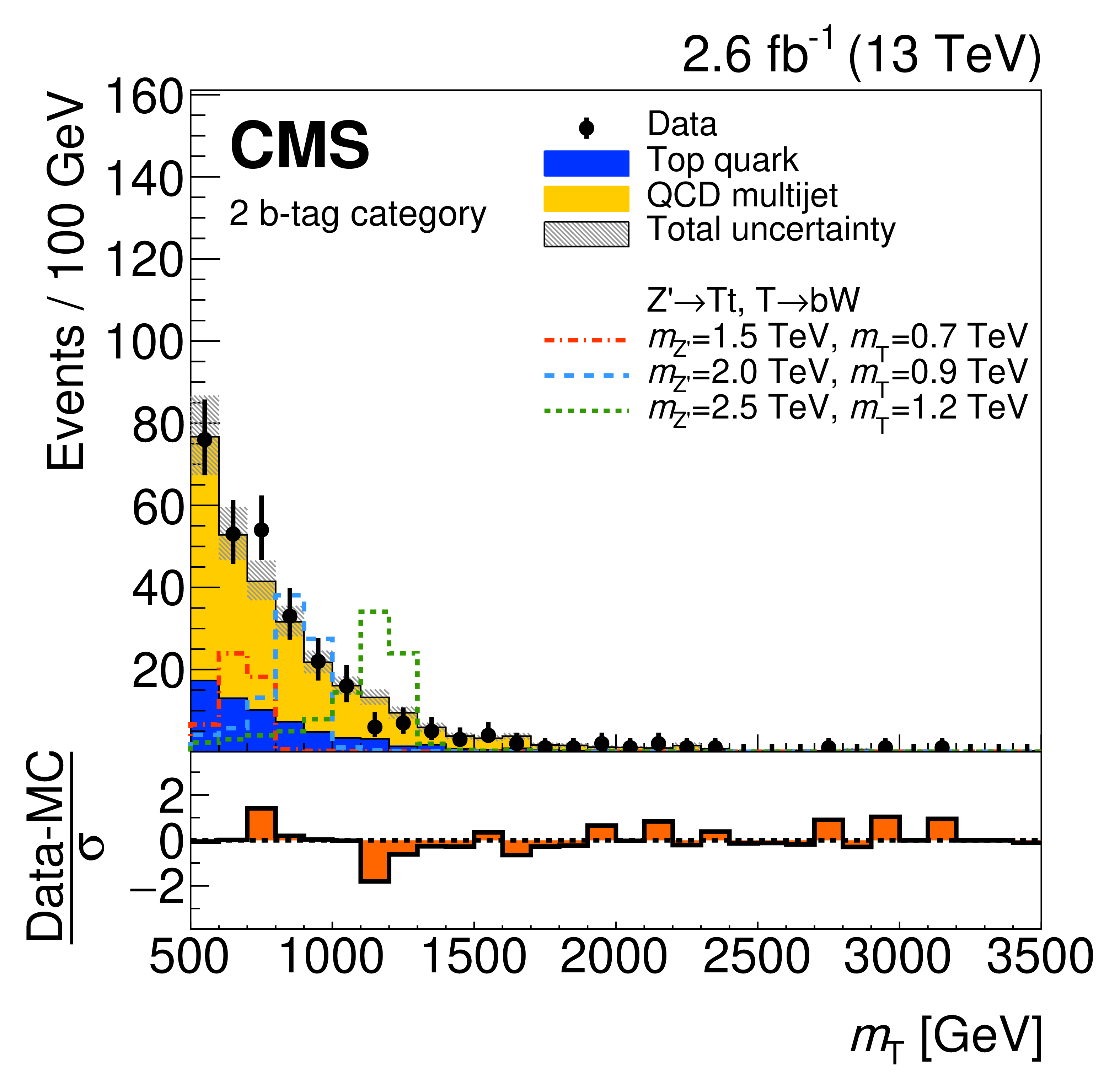
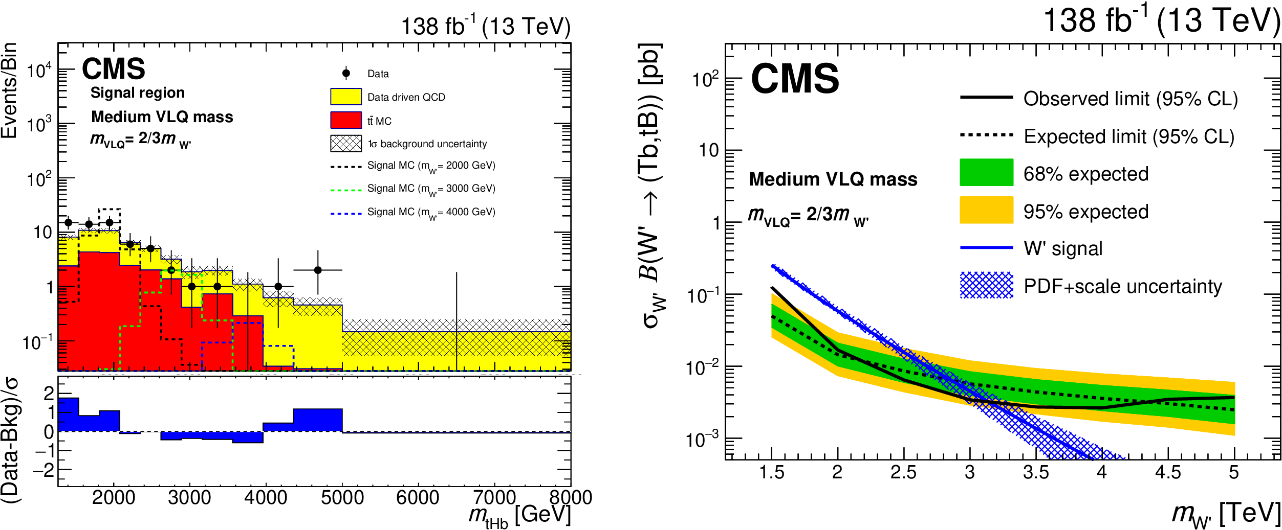
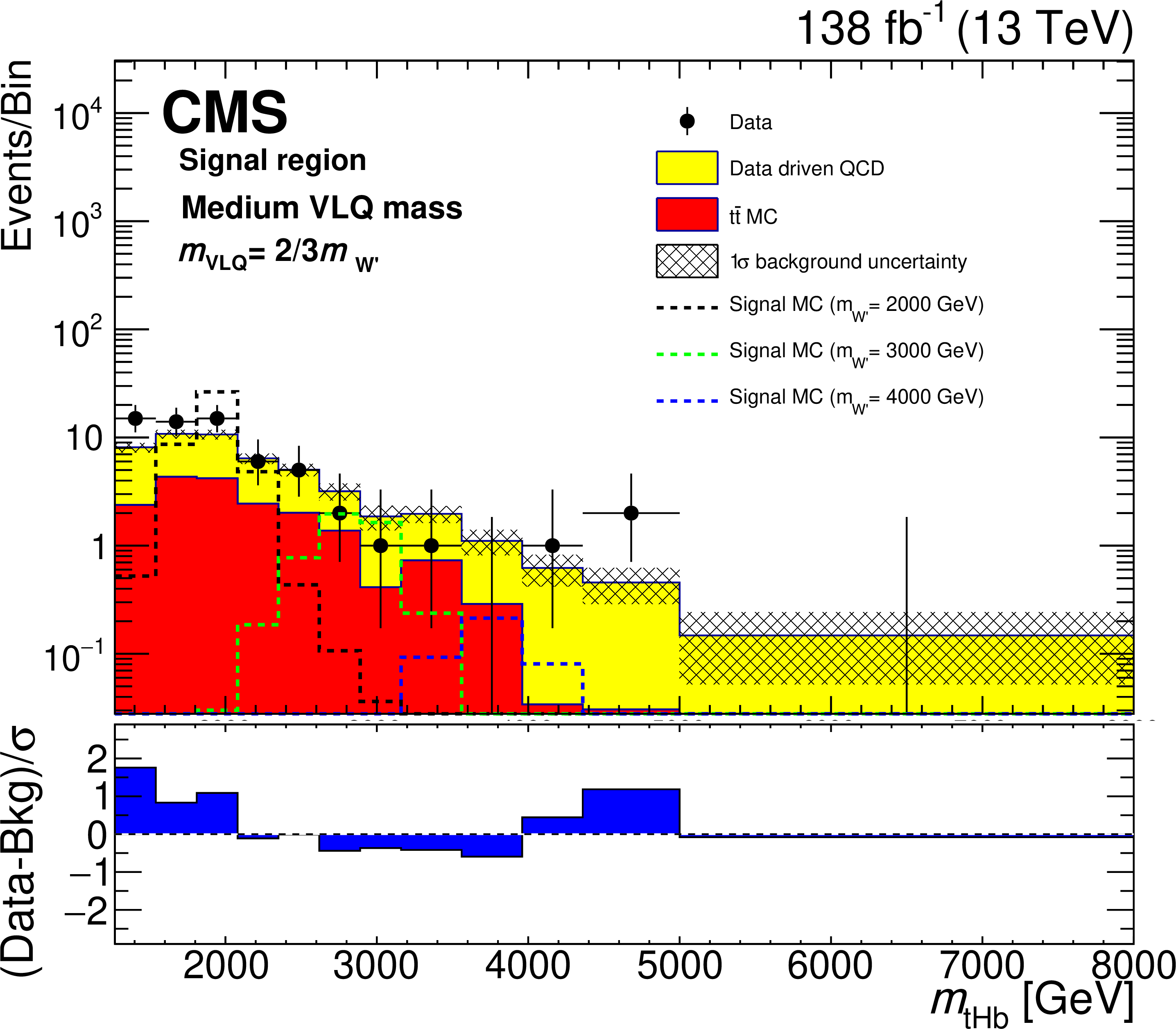
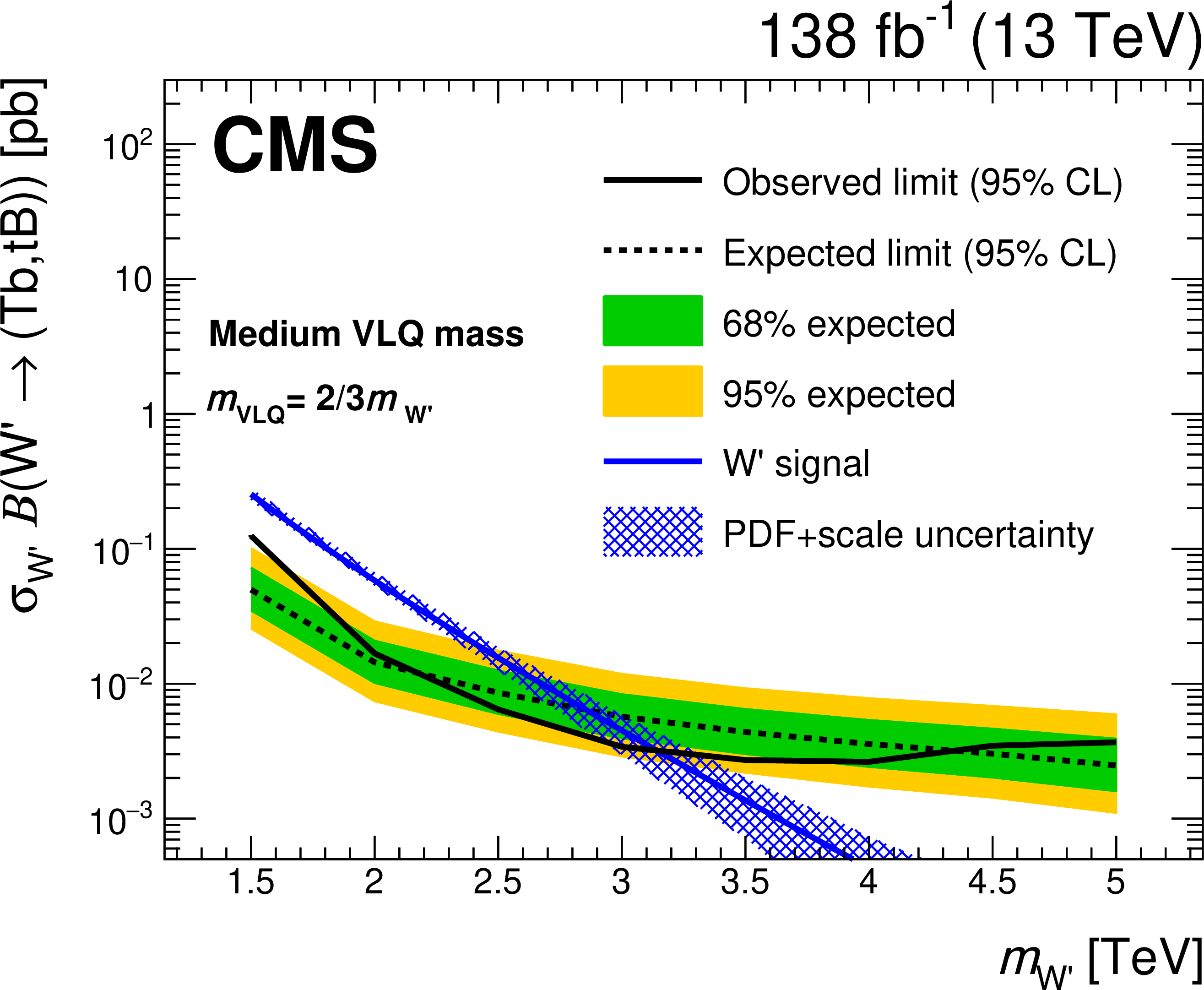
png pdf	Figure 32: Reconstructed $\mathrm{W^{'}}$ boson mass distributions obtained in a search for $\mathrm{p}\mathrm{p}\to\mathrm{W^{'}}\to{\mathrm{T}} \overline{\mathrm{b}}/{\mathrm{B}} \overline{\mathrm{t}}$ in the all-hadronic final state, in events with a t-, H- and b-tagged jet (left). Upper limits at 95% CL on the product of the cross section and branching fraction for the production of a $\mathrm{W^{'}}$ boson with decays to ${\mathrm{T}} \overline{\mathrm{b}}$ and ${\mathrm{B}} \overline{\mathrm{t}}$ (right). Figures adapted from Ref. [157].
png pdf	Figure 32-a: Reconstructed $\mathrm{W^{'}}$ boson mass distributions obtained in a search for $\mathrm{p}\mathrm{p}\to\mathrm{W^{'}}\to{\mathrm{T}} \overline{\mathrm{b}}/{\mathrm{B}} \overline{\mathrm{t}}$ in the all-hadronic final state, in events with a t-, H- and b-tagged jet (left). Upper limits at 95% CL on the product of the cross section and branching fraction for the production of a $\mathrm{W^{'}}$ boson with decays to ${\mathrm{T}} \overline{\mathrm{b}}$ and ${\mathrm{B}} \overline{\mathrm{t}}$ (right). Figures adapted from Ref. [157].
png pdf	Figure 32-b: Reconstructed $\mathrm{W^{'}}$ boson mass distributions obtained in a search for $\mathrm{p}\mathrm{p}\to\mathrm{W^{'}}\to{\mathrm{T}} \overline{\mathrm{b}}/{\mathrm{B}} \overline{\mathrm{t}}$ in the all-hadronic final state, in events with a t-, H- and b-tagged jet (left). Upper limits at 95% CL on the product of the cross section and branching fraction for the production of a $\mathrm{W^{'}}$ boson with decays to ${\mathrm{T}} \overline{\mathrm{b}}$ and ${\mathrm{B}} \overline{\mathrm{t}}$ (right). Figures adapted from Ref. [157].
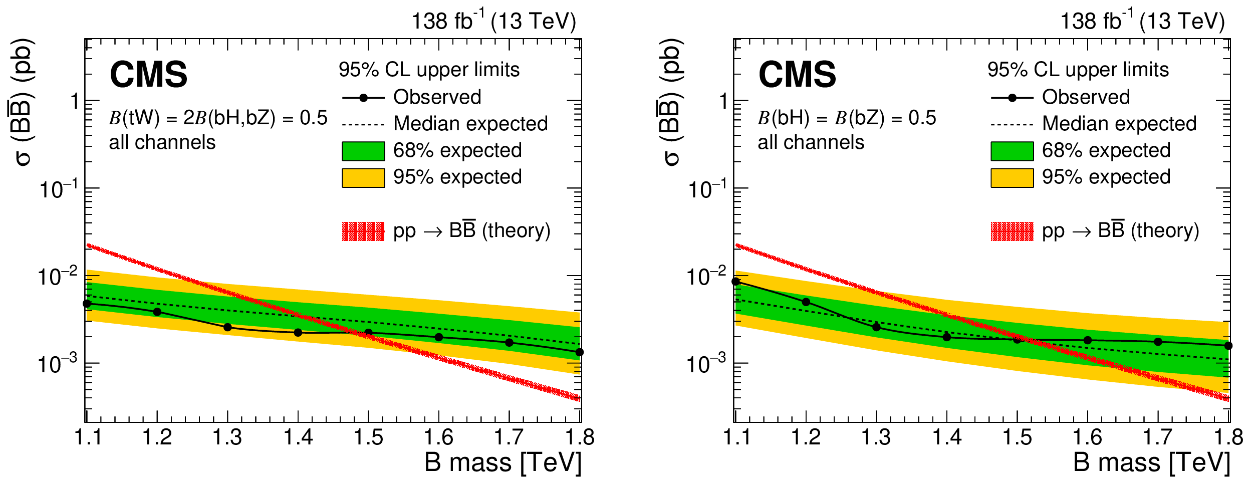
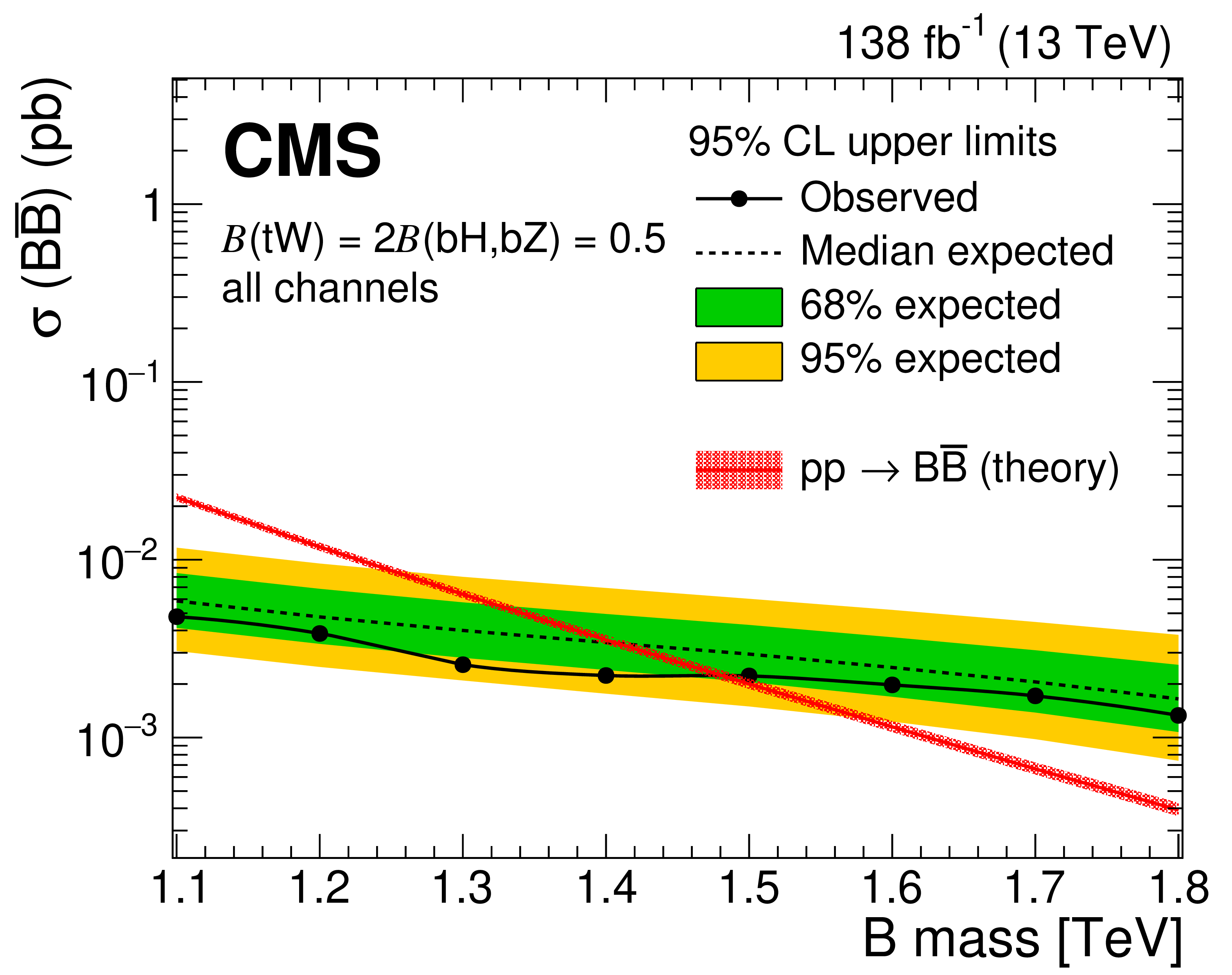
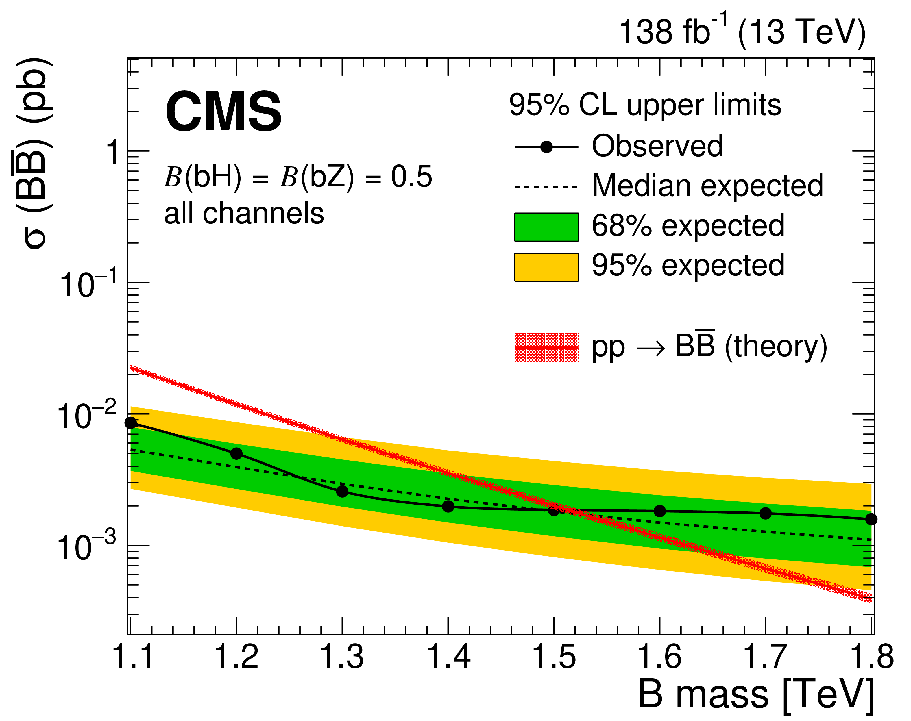
png pdf	Figure 33: Observed (solid lines) and expected (dashed lines) 95% CL upper limits on ${\mathrm{B}} \overline{\mathrm{B}}$ production as a function of the B quark mass for the singlet (left) and doublet (right) branching fraction scenarios, from the combination of two searches for ${\mathrm{B}} \overline{\mathrm{B}}$ production. Predicted cross sections are shown by the red line surrounded by a band representing energy scale and PDF uncertainties in the calculation.
png pdf	Figure 33-a: Observed (solid lines) and expected (dashed lines) 95% CL upper limits on ${\mathrm{B}} \overline{\mathrm{B}}$ production as a function of the B quark mass for the singlet (left) and doublet (right) branching fraction scenarios, from the combination of two searches for ${\mathrm{B}} \overline{\mathrm{B}}$ production. Predicted cross sections are shown by the red line surrounded by a band representing energy scale and PDF uncertainties in the calculation.
png pdf	Figure 33-b: Observed (solid lines) and expected (dashed lines) 95% CL upper limits on ${\mathrm{B}} \overline{\mathrm{B}}$ production as a function of the B quark mass for the singlet (left) and doublet (right) branching fraction scenarios, from the combination of two searches for ${\mathrm{B}} \overline{\mathrm{B}}$ production. Predicted cross sections are shown by the red line surrounded by a band representing energy scale and PDF uncertainties in the calculation.
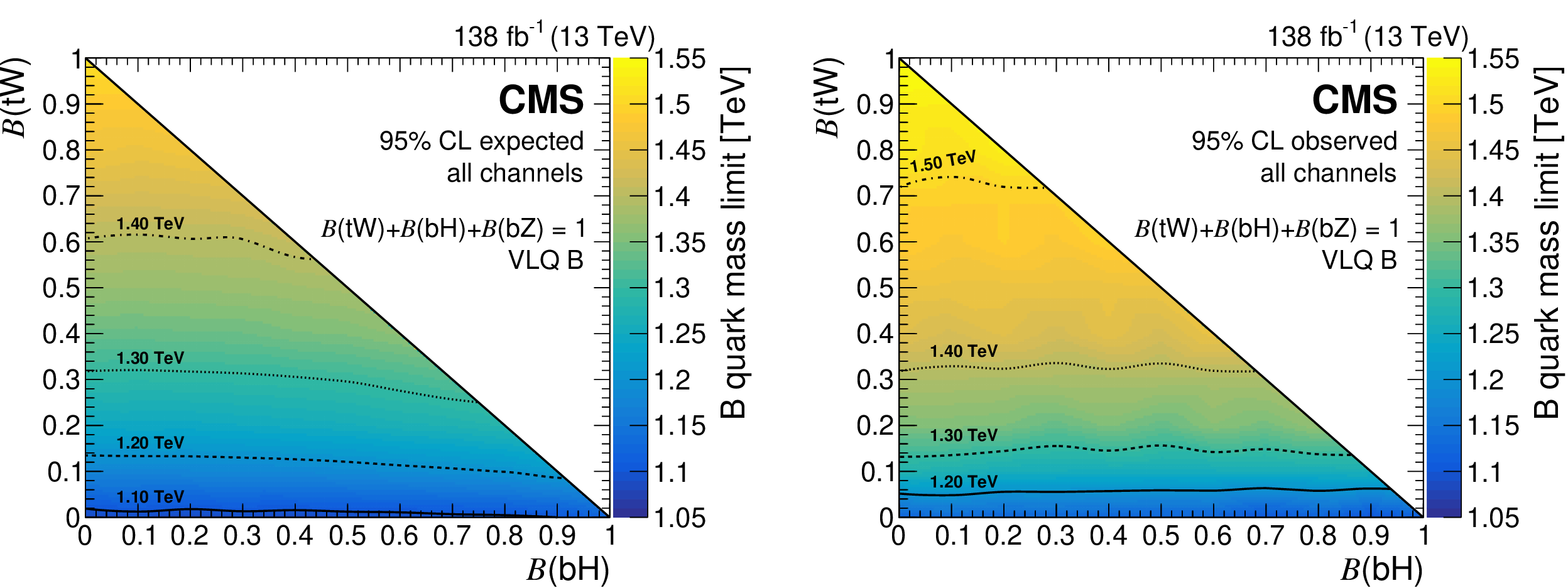
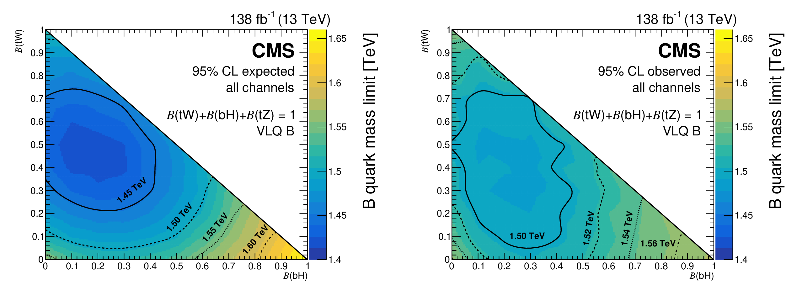
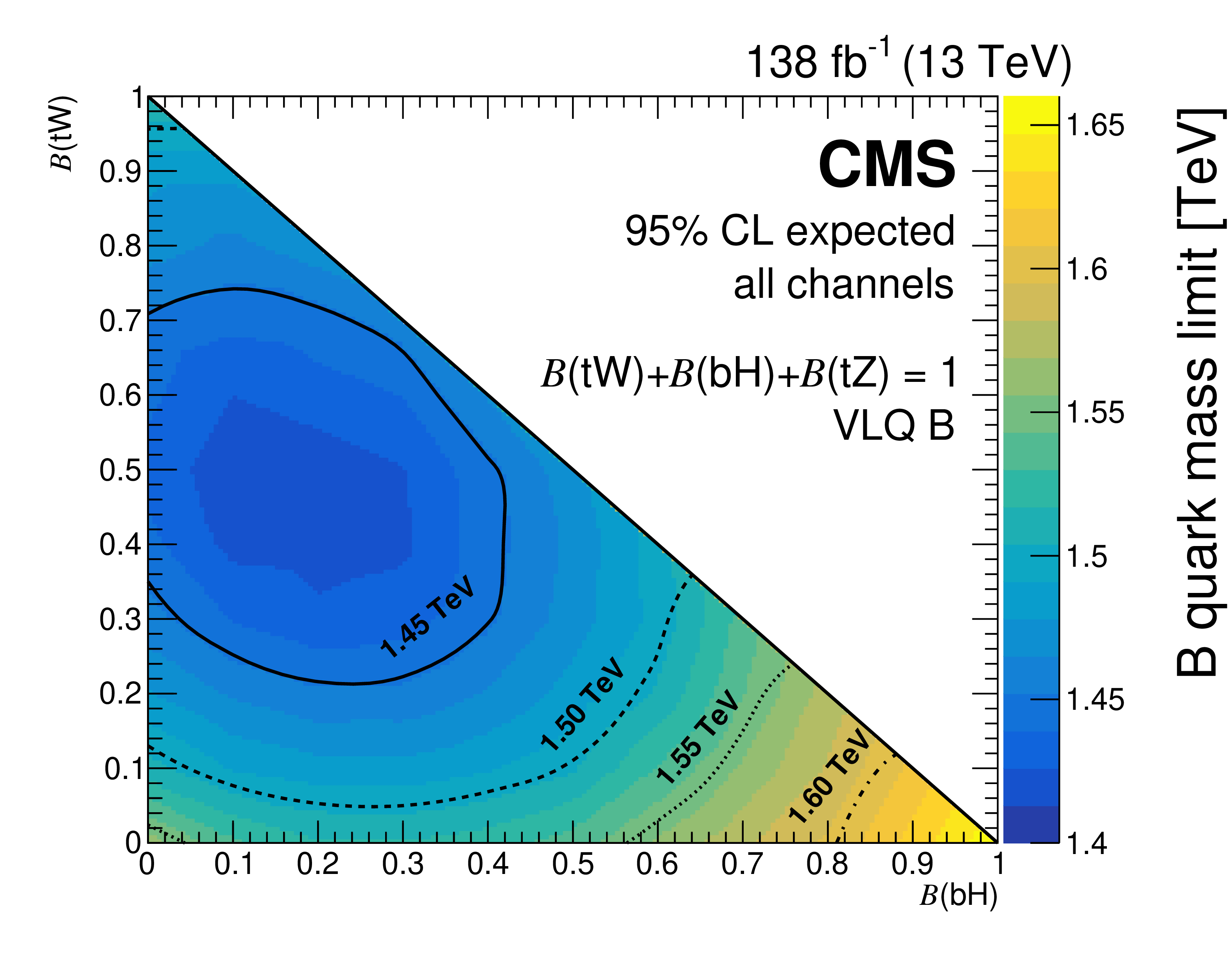
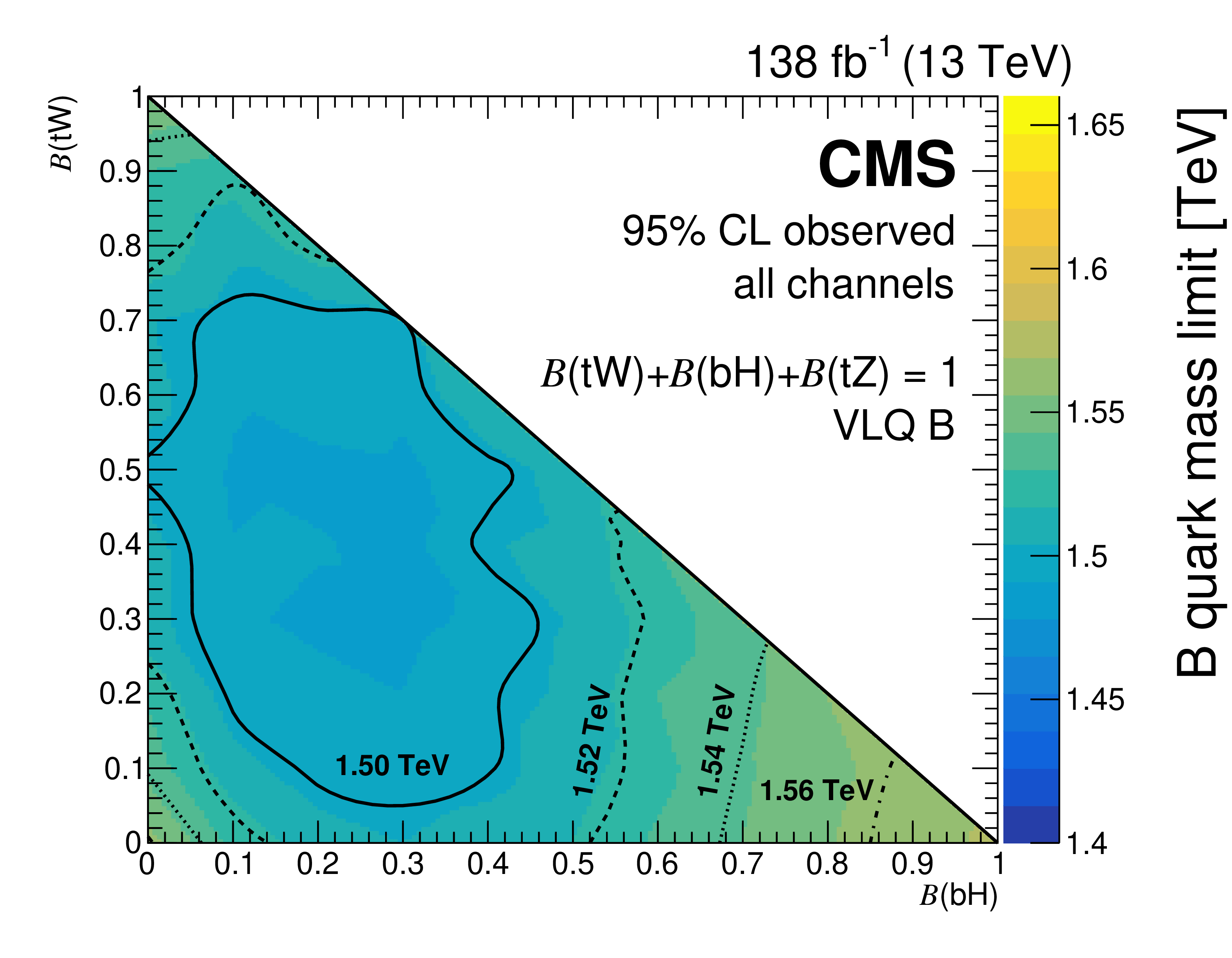
png pdf	Figure 34: Expected (left) and observed (right) lower limits on the B quark mass at 95% CL from the combination of two searches for ${\mathrm{B}} \overline{\mathrm{B}}$ production. The limits are shown as a function of the branching fractions $\mathcal{B}({\mathrm{B}} \to\mathrm{b}\mathrm{H})$ and $\mathcal{B}({\mathrm{B}} \to\mathrm{t}\mathrm{W})$, with $\mathcal{B}({\mathrm{B}} \to\mathrm{t}\mathrm{W})=1-\mathcal{B}({\mathrm{B}} \to\mathrm{b}\mathrm{H})-\mathcal{B}({\mathrm{B}} \to\mathrm{b}\mathrm{Z})$.
png pdf	Figure 34-a: Expected (left) and observed (right) lower limits on the B quark mass at 95% CL from the combination of two searches for ${\mathrm{B}} \overline{\mathrm{B}}$ production. The limits are shown as a function of the branching fractions $\mathcal{B}({\mathrm{B}} \to\mathrm{b}\mathrm{H})$ and $\mathcal{B}({\mathrm{B}} \to\mathrm{t}\mathrm{W})$, with $\mathcal{B}({\mathrm{B}} \to\mathrm{t}\mathrm{W})=1-\mathcal{B}({\mathrm{B}} \to\mathrm{b}\mathrm{H})-\mathcal{B}({\mathrm{B}} \to\mathrm{b}\mathrm{Z})$.
png pdf	Figure 34-b: Expected (left) and observed (right) lower limits on the B quark mass at 95% CL from the combination of two searches for ${\mathrm{B}} \overline{\mathrm{B}}$ production. The limits are shown as a function of the branching fractions $\mathcal{B}({\mathrm{B}} \to\mathrm{b}\mathrm{H})$ and $\mathcal{B}({\mathrm{B}} \to\mathrm{t}\mathrm{W})$, with $\mathcal{B}({\mathrm{B}} \to\mathrm{t}\mathrm{W})=1-\mathcal{B}({\mathrm{B}} \to\mathrm{b}\mathrm{H})-\mathcal{B}({\mathrm{B}} \to\mathrm{b}\mathrm{Z})$.
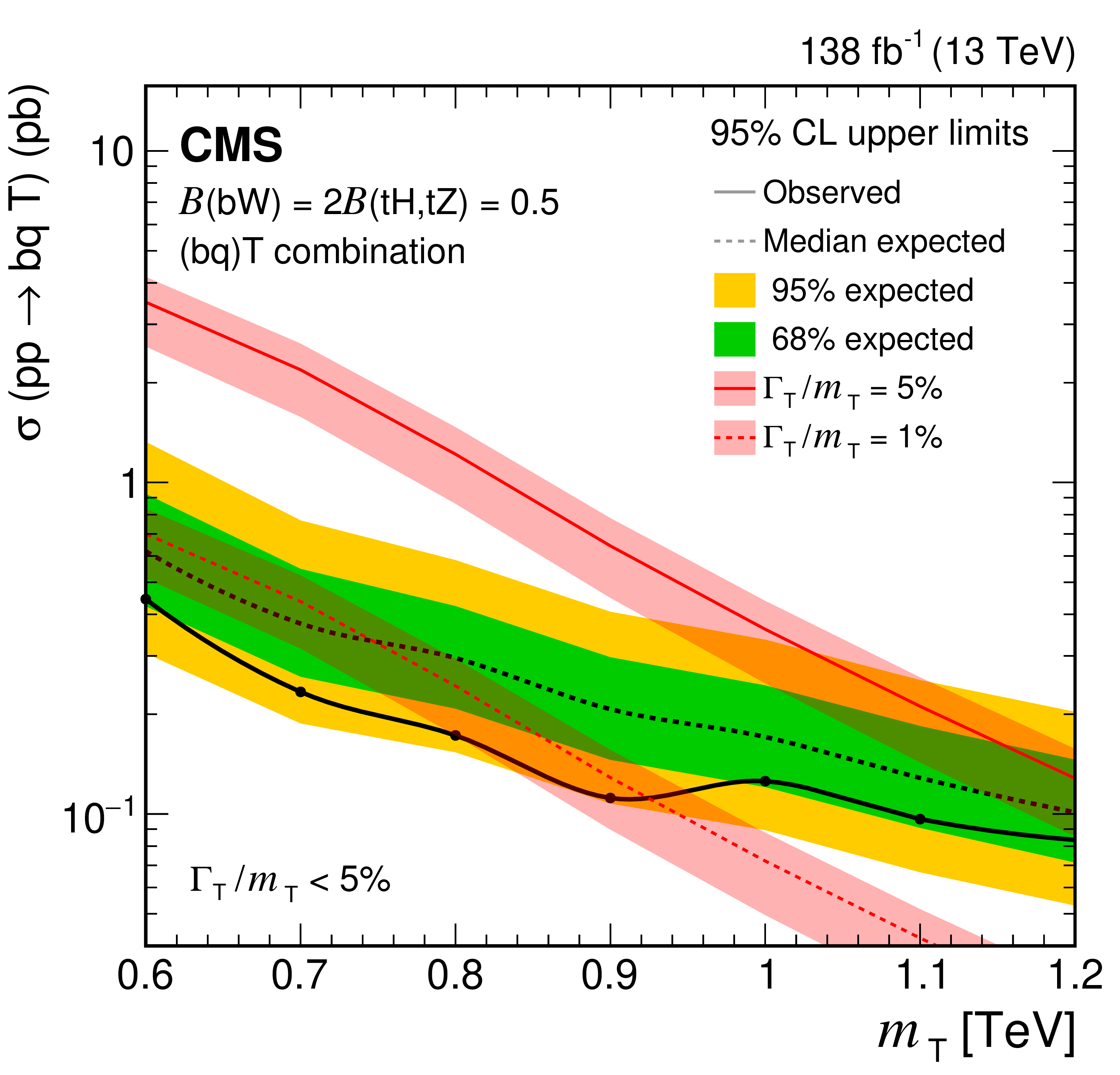
png pdf	Figure 35: Observed and expected 95% CL upper limits on the production cross section of a single T quark in association with a b quark in a singlet scenario, versus the T quark mass. Theoretical predictions for relative widths of 1 and 5% of the mass are shown as red solid line and red dashed line, respectively.
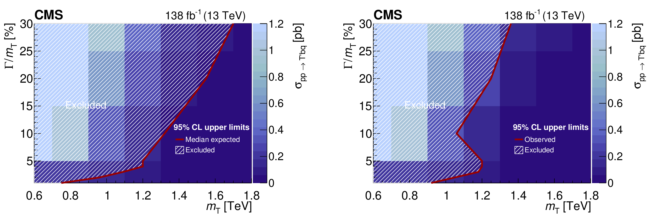
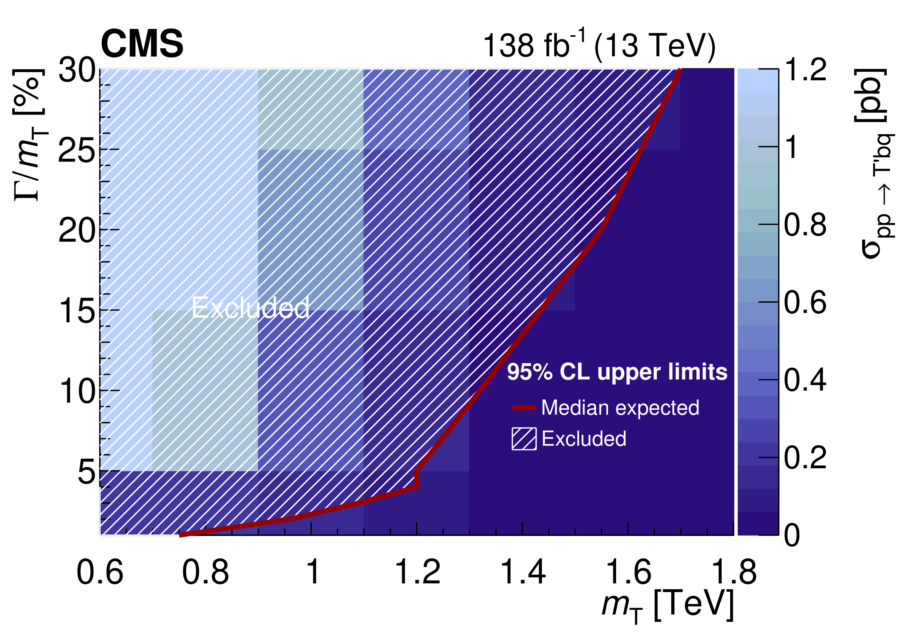
png pdf	Figure 36: Expected (left) and observed (right) 95% CL upper limits on the product of the single-production cross section and the ${\mathrm{T}} \to\mathrm{t}\mathrm{Z}/\mathrm{H}$ branching fraction for a singlet T quark, as a function of the T quark mass $m_{{\mathrm{T}} }$ and width $\Gamma$, for relative widths from 1 to 30% of the mass. A singlet T quark that is produced in association with a b quark is assumed. The solid red line indicates the boundary of the excluded region (hatched area) of theoretical cross sections.
png pdf	Figure 36-a: Expected (left) and observed (right) 95% CL upper limits on the product of the single-production cross section and the ${\mathrm{T}} \to\mathrm{t}\mathrm{Z}/\mathrm{H}$ branching fraction for a singlet T quark, as a function of the T quark mass $m_{{\mathrm{T}} }$ and width $\Gamma$, for relative widths from 1 to 30% of the mass. A singlet T quark that is produced in association with a b quark is assumed. The solid red line indicates the boundary of the excluded region (hatched area) of theoretical cross sections.
png pdf	Figure 36-b: Expected (left) and observed (right) 95% CL upper limits on the product of the single-production cross section and the ${\mathrm{T}} \to\mathrm{t}\mathrm{Z}/\mathrm{H}$ branching fraction for a singlet T quark, as a function of the T quark mass $m_{{\mathrm{T}} }$ and width $\Gamma$, for relative widths from 1 to 30% of the mass. A singlet T quark that is produced in association with a b quark is assumed. The solid red line indicates the boundary of the excluded region (hatched area) of theoretical cross sections.
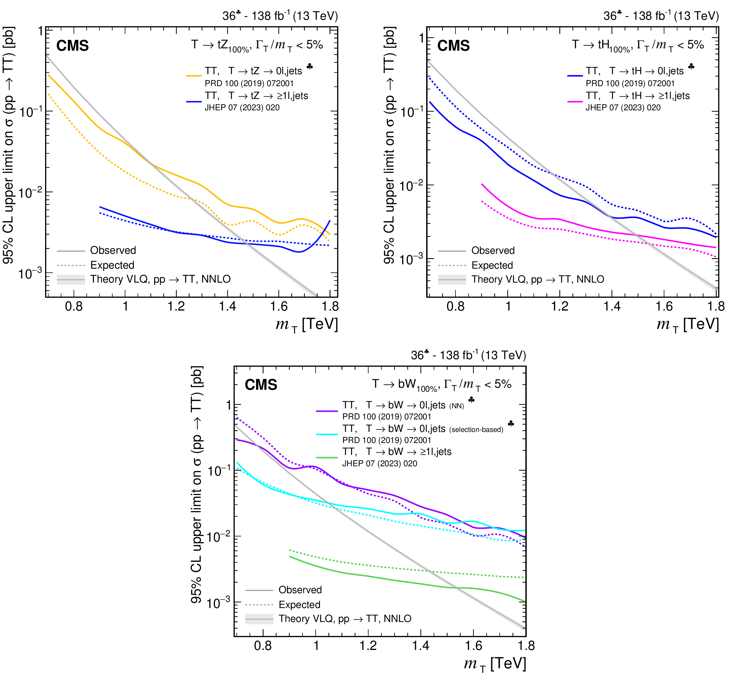
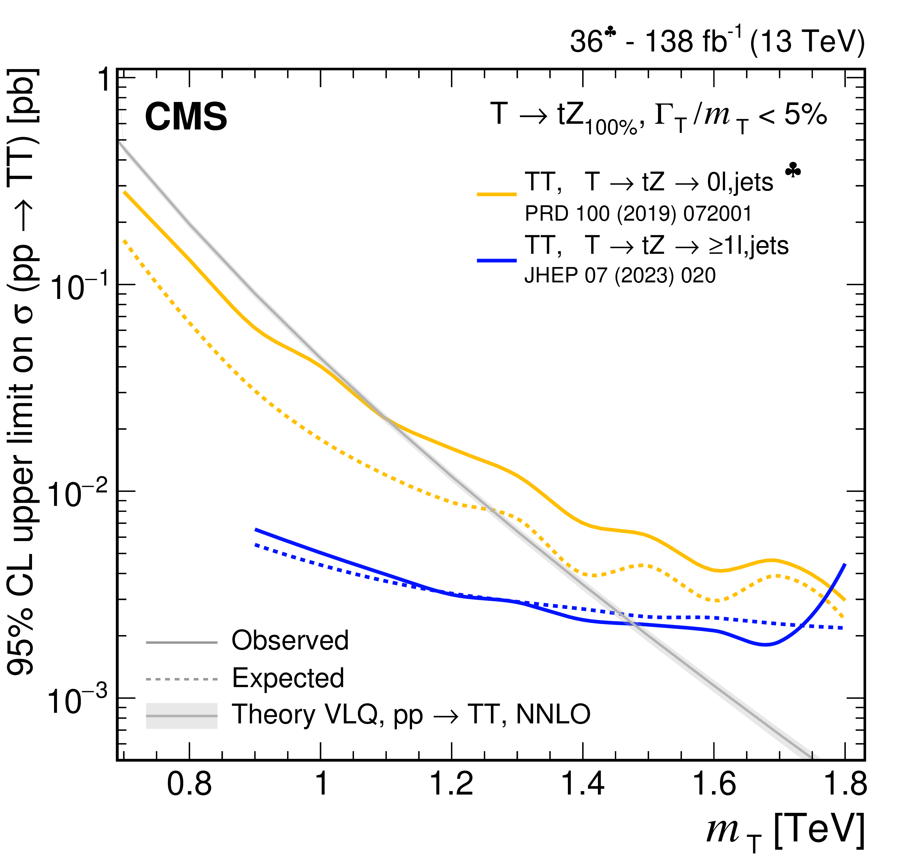
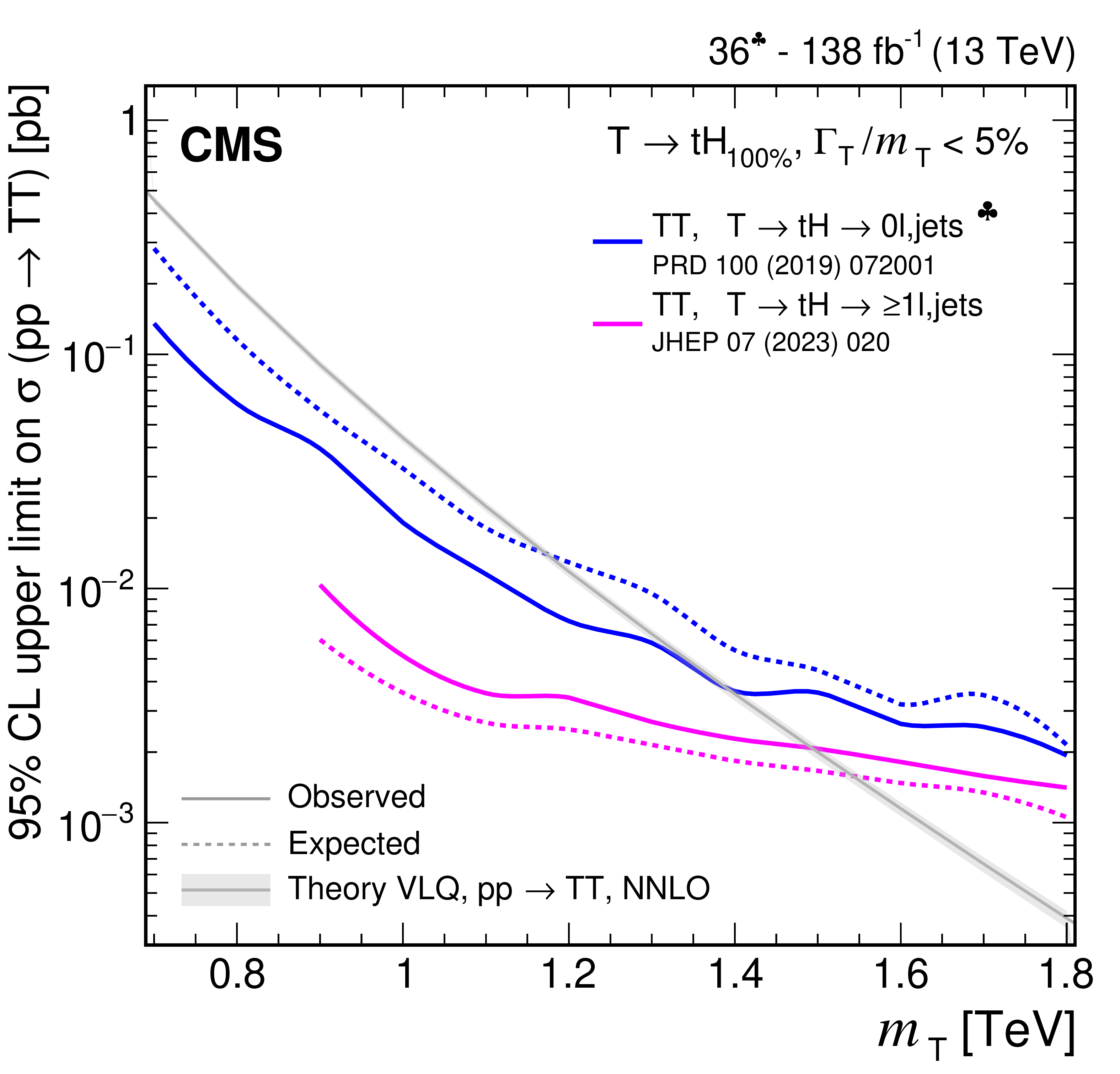
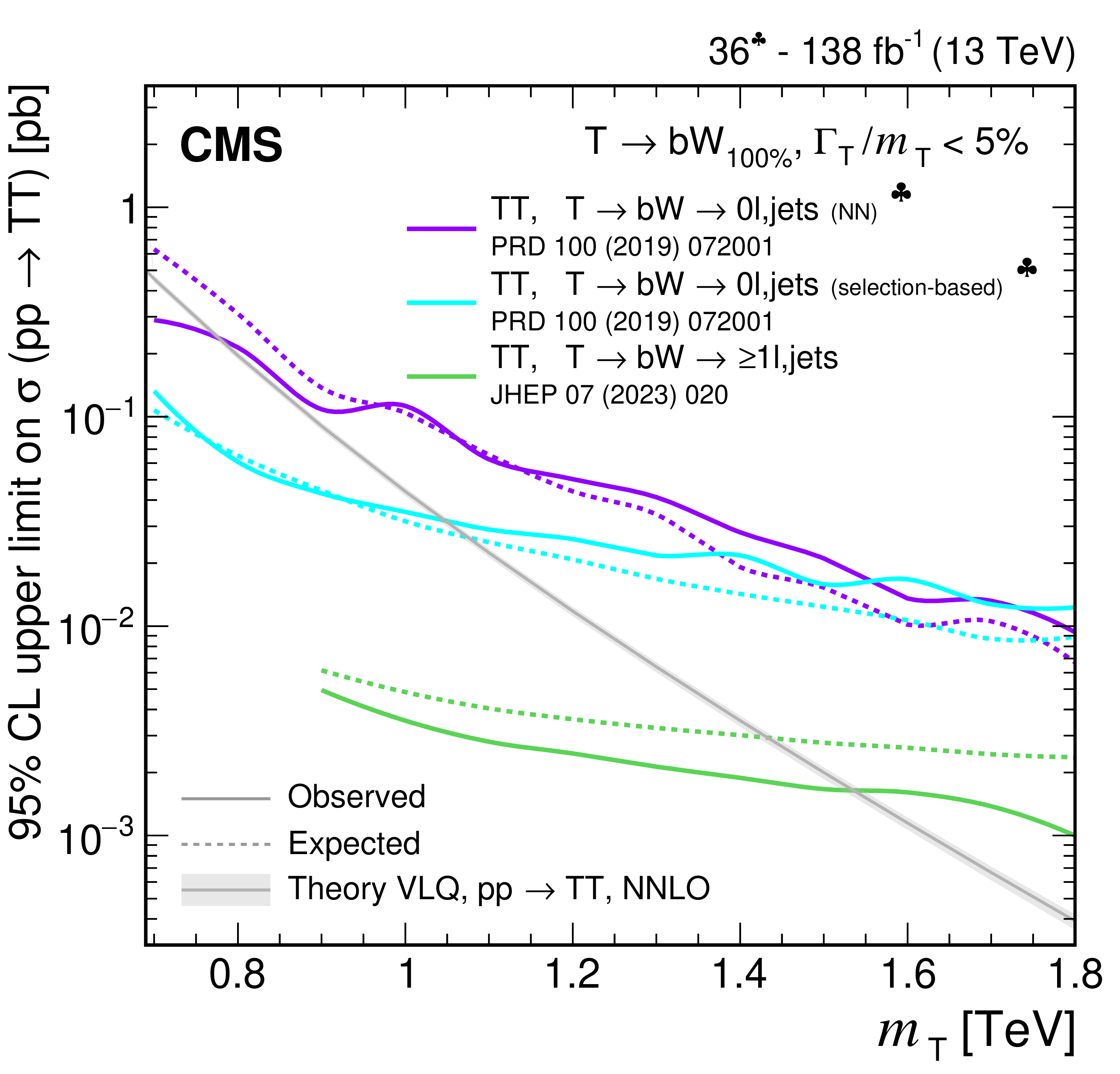
png pdf	Figure 37: Observed and expected 95% CL upper limits on the production cross section of a pair of vector-like T quarks decaying to $\mathrm{t}\mathrm{Z}$ (upper left), $\mathrm{t}\mathrm{H}$ (upper right), and $\mathrm{b}\mathrm{W}$ (lower), as a function of the T quark mass, obtained by different analyses: 0$\ell$+jets (NN, selection-based) [140], and $\geq$1$\ell$+jets [141]. A theory prediction at NNLO in perturbative QCD of the pair production cross section in the NWA is superimposed. Searches using data corresponding to an integrated luminosity of 36 fb$^{-1}$, rather than the full Run 2 integrated luminosity of 138 fb$^{-1}$, are indicated with a spade symbol in the legend.
png pdf	Figure 37-a: Observed and expected 95% CL upper limits on the production cross section of a pair of vector-like T quarks decaying to $\mathrm{t}\mathrm{Z}$ (upper left), $\mathrm{t}\mathrm{H}$ (upper right), and $\mathrm{b}\mathrm{W}$ (lower), as a function of the T quark mass, obtained by different analyses: 0$\ell$+jets (NN, selection-based) [140], and $\geq$1$\ell$+jets [141]. A theory prediction at NNLO in perturbative QCD of the pair production cross section in the NWA is superimposed. Searches using data corresponding to an integrated luminosity of 36 fb$^{-1}$, rather than the full Run 2 integrated luminosity of 138 fb$^{-1}$, are indicated with a spade symbol in the legend.
png pdf	Figure 37-b: Observed and expected 95% CL upper limits on the production cross section of a pair of vector-like T quarks decaying to $\mathrm{t}\mathrm{Z}$ (upper left), $\mathrm{t}\mathrm{H}$ (upper right), and $\mathrm{b}\mathrm{W}$ (lower), as a function of the T quark mass, obtained by different analyses: 0$\ell$+jets (NN, selection-based) [140], and $\geq$1$\ell$+jets [141]. A theory prediction at NNLO in perturbative QCD of the pair production cross section in the NWA is superimposed. Searches using data corresponding to an integrated luminosity of 36 fb$^{-1}$, rather than the full Run 2 integrated luminosity of 138 fb$^{-1}$, are indicated with a spade symbol in the legend.
png pdf	Figure 37-c: Observed and expected 95% CL upper limits on the production cross section of a pair of vector-like T quarks decaying to $\mathrm{t}\mathrm{Z}$ (upper left), $\mathrm{t}\mathrm{H}$ (upper right), and $\mathrm{b}\mathrm{W}$ (lower), as a function of the T quark mass, obtained by different analyses: 0$\ell$+jets (NN, selection-based) [140], and $\geq$1$\ell$+jets [141]. A theory prediction at NNLO in perturbative QCD of the pair production cross section in the NWA is superimposed. Searches using data corresponding to an integrated luminosity of 36 fb$^{-1}$, rather than the full Run 2 integrated luminosity of 138 fb$^{-1}$, are indicated with a spade symbol in the legend.
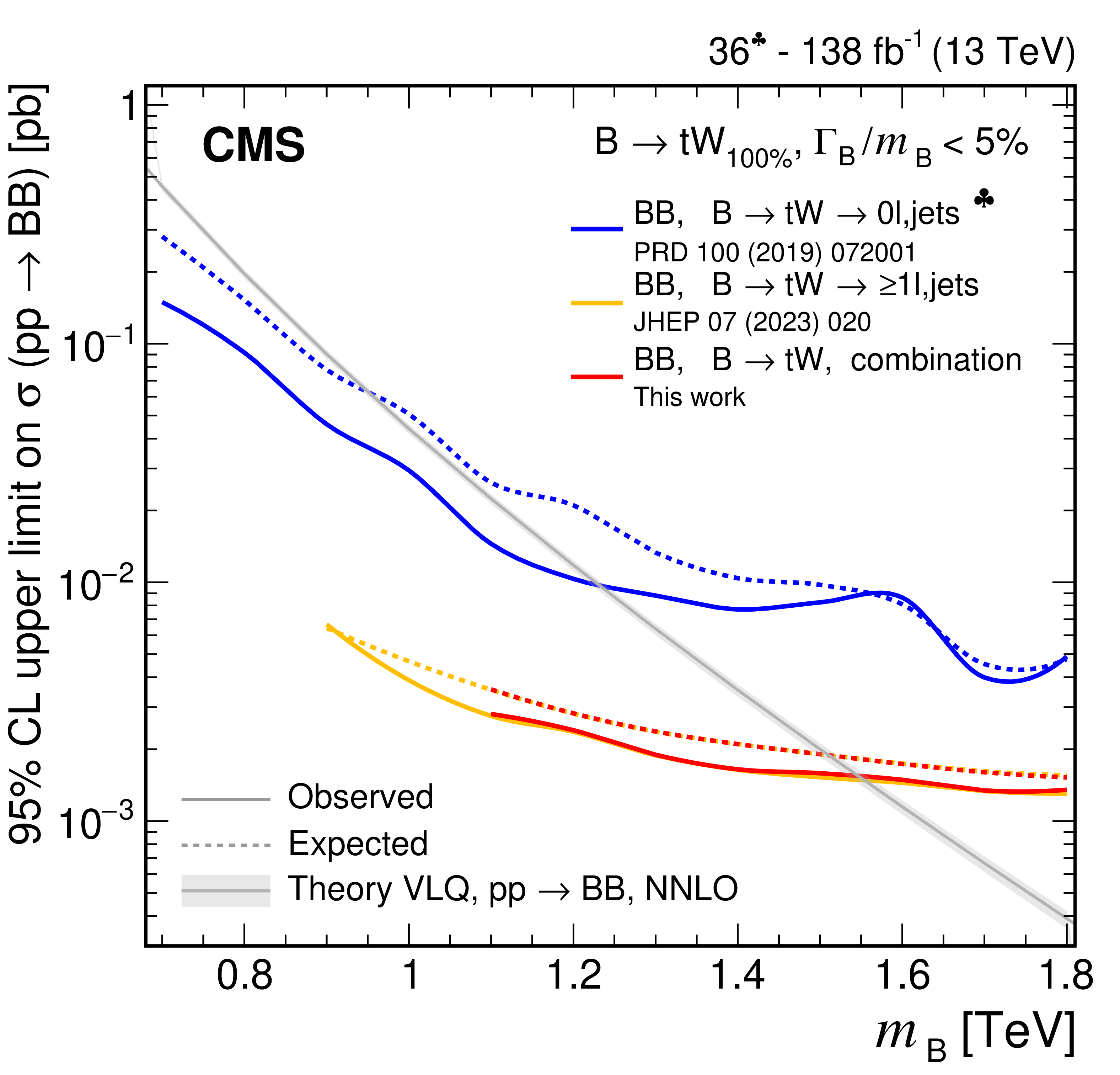
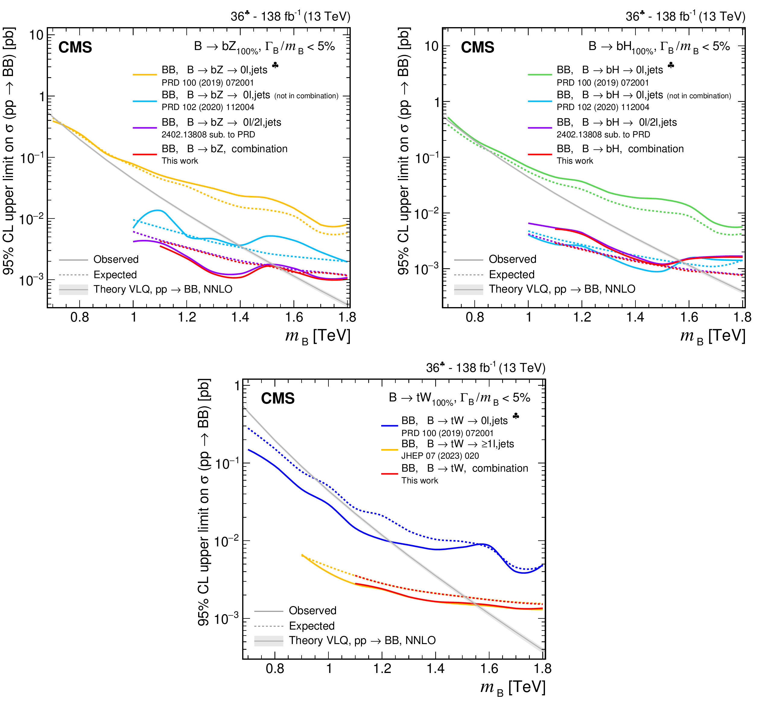
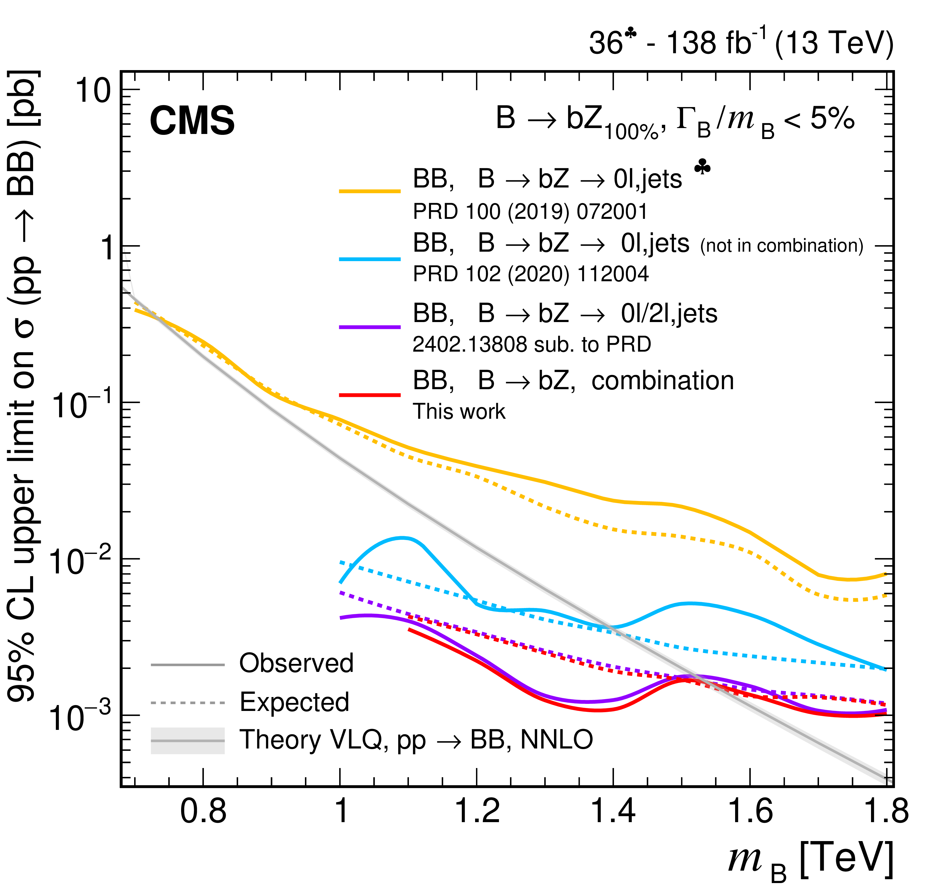
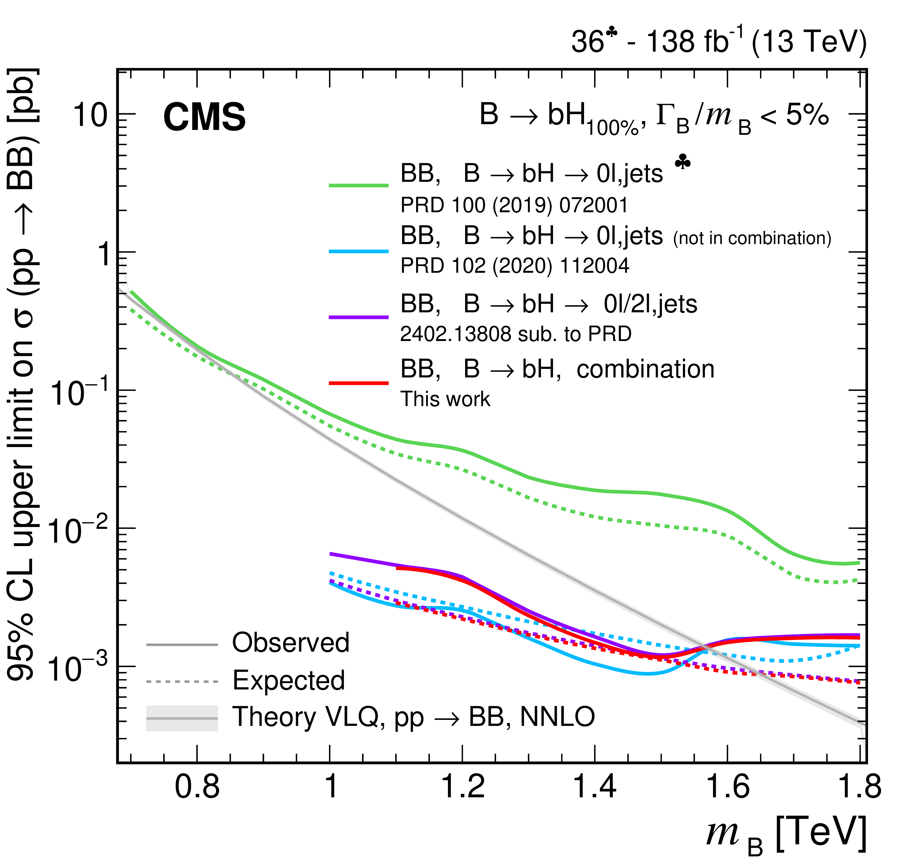
png pdf	Figure 38: Observed and expected 95% CL upper limits on the production cross section of a pair of vector-like B quarks decaying to $\mathrm{b}\mathrm{Z}$ (upper left), $\mathrm{b}\mathrm{H}$ (upper right), and $\mathrm{t}\mathrm{W}$ (lower), as a function of the B quark mass, obtained by different analyses: 0$\ell$+jets (NN) [140], 0$\ell$+jets [159], $\geq$1$\ell$+jets [141], 0\ell/2$\ell$+jets [142], and the ${\mathrm{B}} \overline{\mathrm{B}}$ combination of Section 6.5.1. A theory prediction at NNLO in perturbative QCD of the pair production cross section in the NWA is superimposed. Searches using data corresponding to an integrated luminosity of 36 fb$^{-1}$, rather than the full Run 2 integrated luminosity of 138 fb$^{-1}$, are indicated with a spade symbol in the legend.
png pdf	Figure 38-a: Observed and expected 95% CL upper limits on the production cross section of a pair of vector-like B quarks decaying to $\mathrm{b}\mathrm{Z}$ (upper left), $\mathrm{b}\mathrm{H}$ (upper right), and $\mathrm{t}\mathrm{W}$ (lower), as a function of the B quark mass, obtained by different analyses: 0$\ell$+jets (NN) [140], 0$\ell$+jets [159], $\geq$1$\ell$+jets [141], 0\ell/2$\ell$+jets [142], and the ${\mathrm{B}} \overline{\mathrm{B}}$ combination of Section 6.5.1. A theory prediction at NNLO in perturbative QCD of the pair production cross section in the NWA is superimposed. Searches using data corresponding to an integrated luminosity of 36 fb$^{-1}$, rather than the full Run 2 integrated luminosity of 138 fb$^{-1}$, are indicated with a spade symbol in the legend.
png pdf	Figure 38-b: Observed and expected 95% CL upper limits on the production cross section of a pair of vector-like B quarks decaying to $\mathrm{b}\mathrm{Z}$ (upper left), $\mathrm{b}\mathrm{H}$ (upper right), and $\mathrm{t}\mathrm{W}$ (lower), as a function of the B quark mass, obtained by different analyses: 0$\ell$+jets (NN) [140], 0$\ell$+jets [159], $\geq$1$\ell$+jets [141], 0\ell/2$\ell$+jets [142], and the ${\mathrm{B}} \overline{\mathrm{B}}$ combination of Section 6.5.1. A theory prediction at NNLO in perturbative QCD of the pair production cross section in the NWA is superimposed. Searches using data corresponding to an integrated luminosity of 36 fb$^{-1}$, rather than the full Run 2 integrated luminosity of 138 fb$^{-1}$, are indicated with a spade symbol in the legend.
png pdf	Figure 38-c: Observed and expected 95% CL upper limits on the production cross section of a pair of vector-like B quarks decaying to $\mathrm{b}\mathrm{Z}$ (upper left), $\mathrm{b}\mathrm{H}$ (upper right), and $\mathrm{t}\mathrm{W}$ (lower), as a function of the B quark mass, obtained by different analyses: 0$\ell$+jets (NN) [140], 0$\ell$+jets [159], $\geq$1$\ell$+jets [141], 0\ell/2$\ell$+jets [142], and the ${\mathrm{B}} \overline{\mathrm{B}}$ combination of Section 6.5.1. A theory prediction at NNLO in perturbative QCD of the pair production cross section in the NWA is superimposed. Searches using data corresponding to an integrated luminosity of 36 fb$^{-1}$, rather than the full Run 2 integrated luminosity of 138 fb$^{-1}$, are indicated with a spade symbol in the legend.
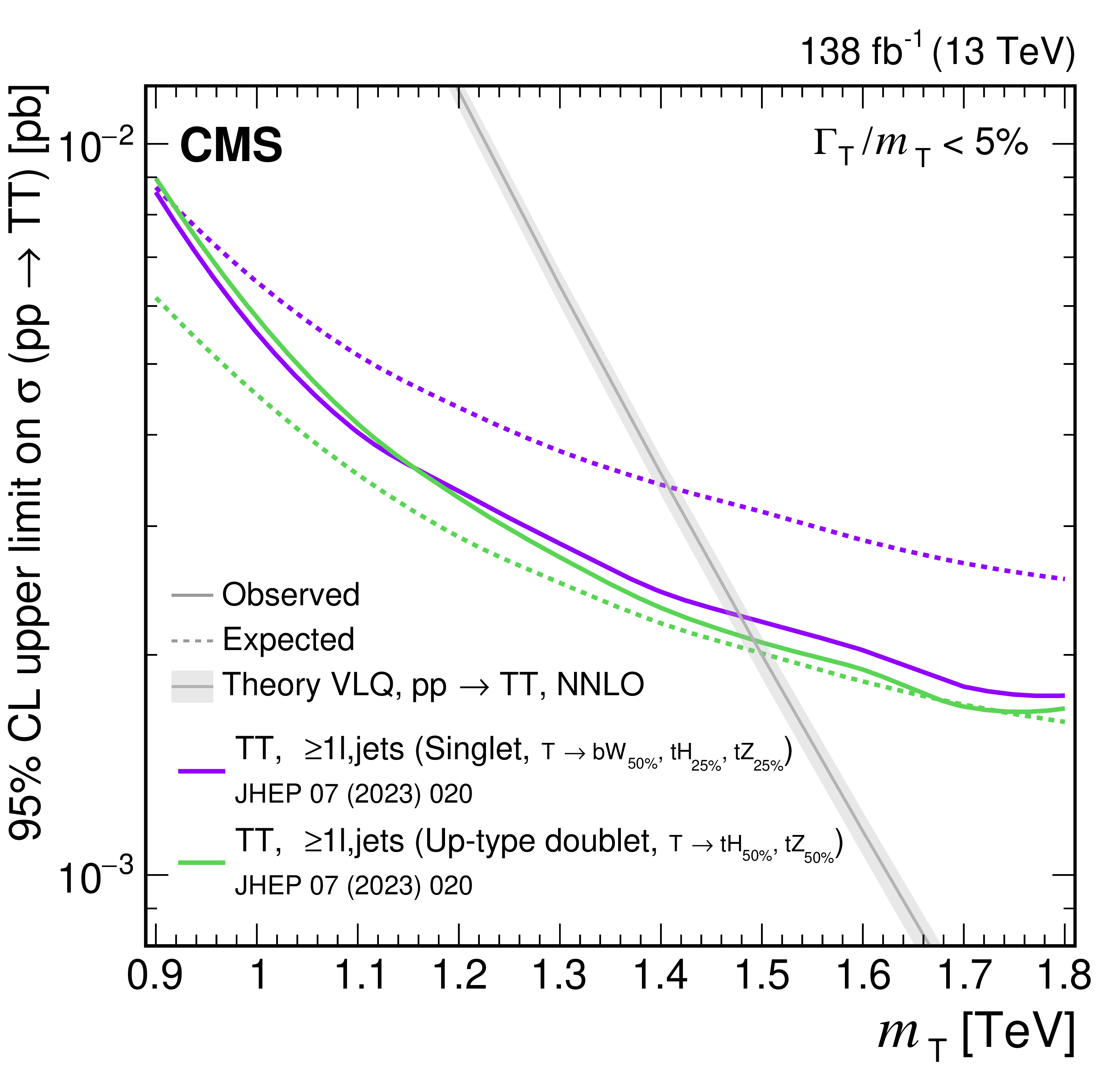
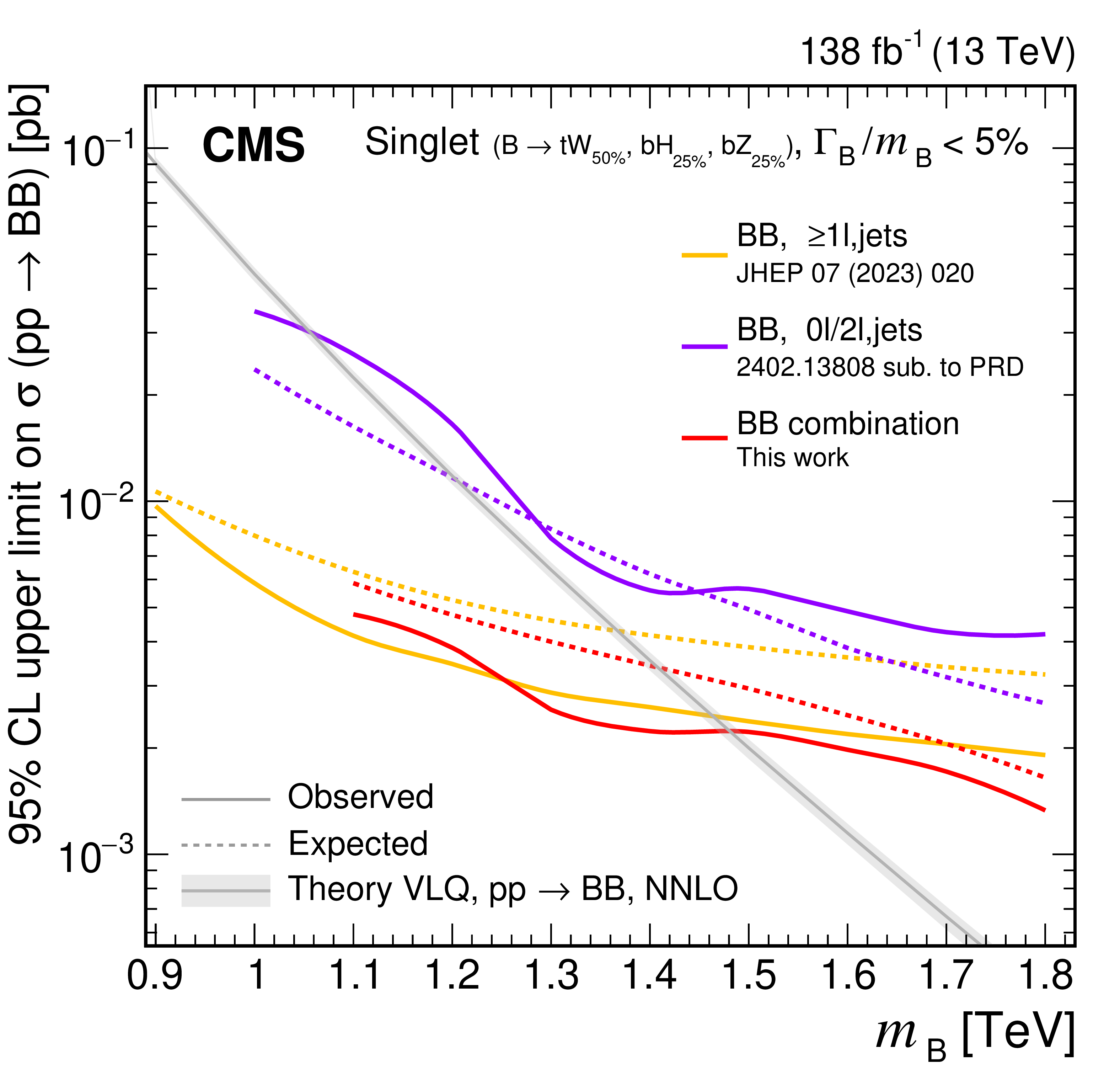
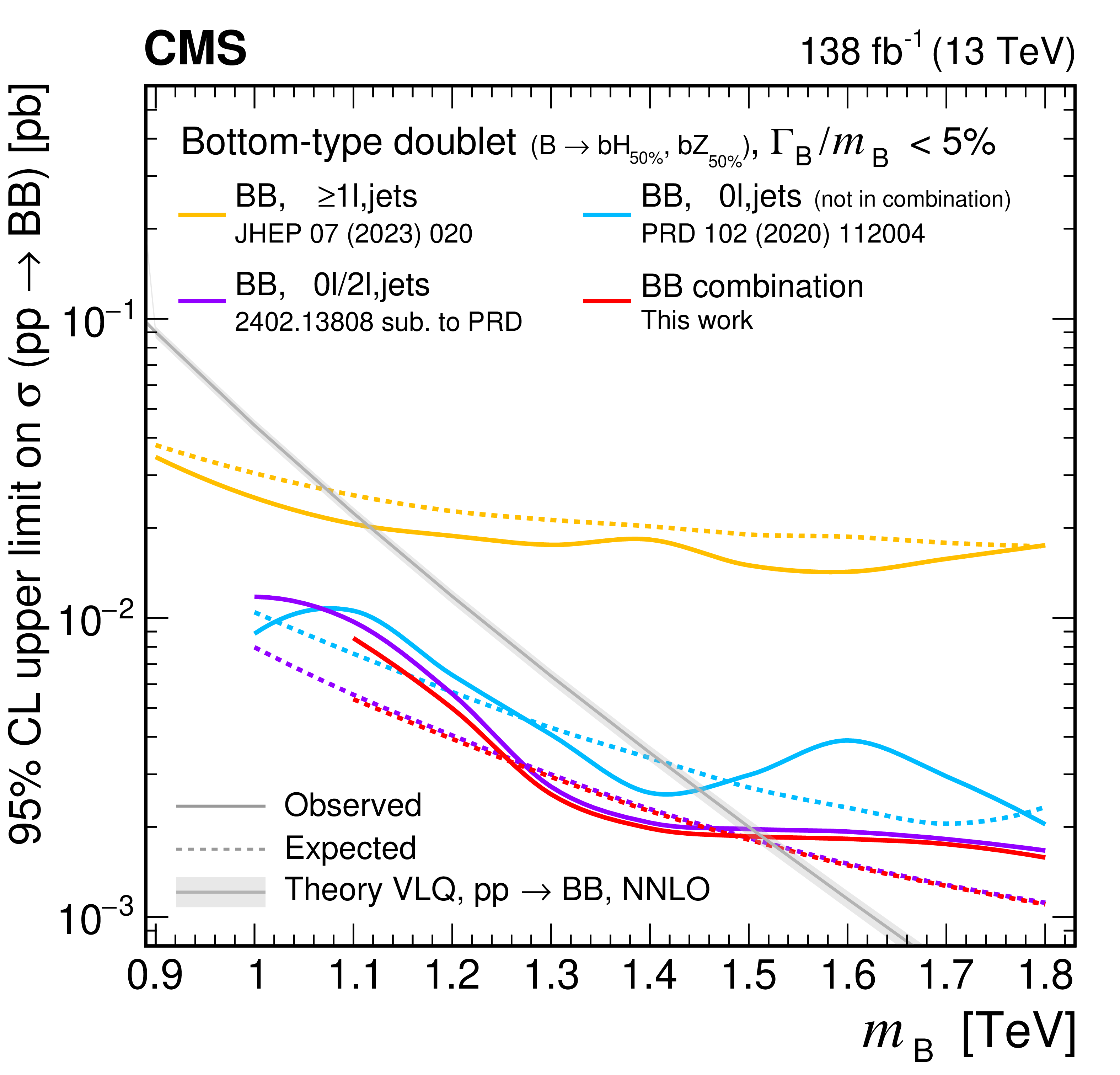
png pdf	Figure 39: Observed and expected 95% CL upper limits on the production cross section of a pair of vector-like T or B quarks, as functions of their mass, obtained by different analyses: 0$\ell$+jets [159], $\geq$1$\ell$+jets [141], 0\ell/2$\ell$+jets [142], and the ${\mathrm{B}} \overline{\mathrm{B}}$ combination. A theory prediction at NNLO in perturbative QCD of the pair production cross section in the NWA is superimposed. Branching fractions of a singlet (upper and lower left panel) and doublet (upper and lower right panel) are assumed.
png pdf	Figure 39-a: Observed and expected 95% CL upper limits on the production cross section of a pair of vector-like T or B quarks, as functions of their mass, obtained by different analyses: 0$\ell$+jets [159], $\geq$1$\ell$+jets [141], 0\ell/2$\ell$+jets [142], and the ${\mathrm{B}} \overline{\mathrm{B}}$ combination. A theory prediction at NNLO in perturbative QCD of the pair production cross section in the NWA is superimposed. Branching fractions of a singlet (upper and lower left panel) and doublet (upper and lower right panel) are assumed.
png pdf	Figure 39-b: Observed and expected 95% CL upper limits on the production cross section of a pair of vector-like T or B quarks, as functions of their mass, obtained by different analyses: 0$\ell$+jets [159], $\geq$1$\ell$+jets [141], 0\ell/2$\ell$+jets [142], and the ${\mathrm{B}} \overline{\mathrm{B}}$ combination. A theory prediction at NNLO in perturbative QCD of the pair production cross section in the NWA is superimposed. Branching fractions of a singlet (upper and lower left panel) and doublet (upper and lower right panel) are assumed.
png pdf	Figure 39-c: Observed and expected 95% CL upper limits on the production cross section of a pair of vector-like T or B quarks, as functions of their mass, obtained by different analyses: 0$\ell$+jets [159], $\geq$1$\ell$+jets [141], 0\ell/2$\ell$+jets [142], and the ${\mathrm{B}} \overline{\mathrm{B}}$ combination. A theory prediction at NNLO in perturbative QCD of the pair production cross section in the NWA is superimposed. Branching fractions of a singlet (upper and lower left panel) and doublet (upper and lower right panel) are assumed.
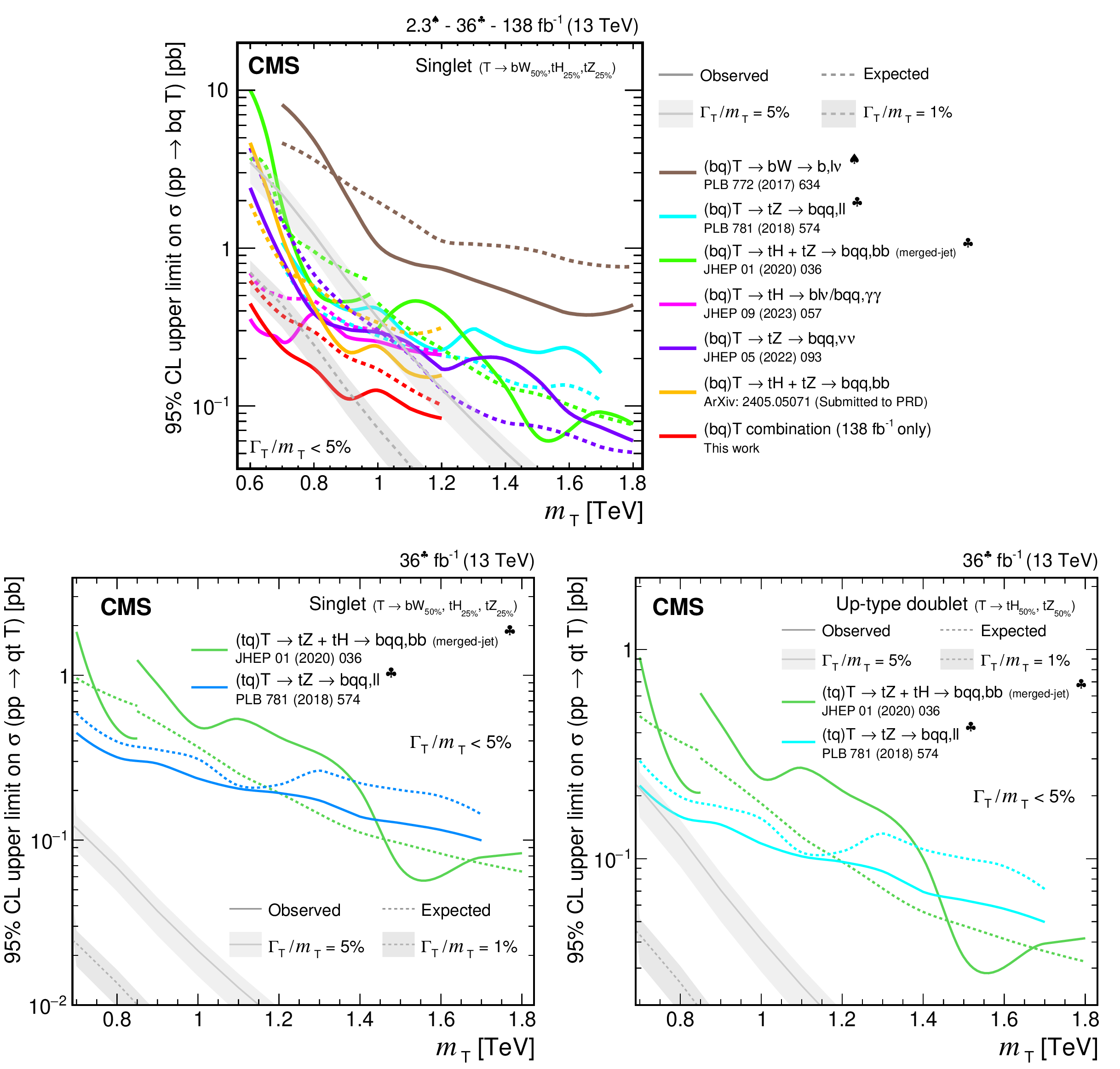
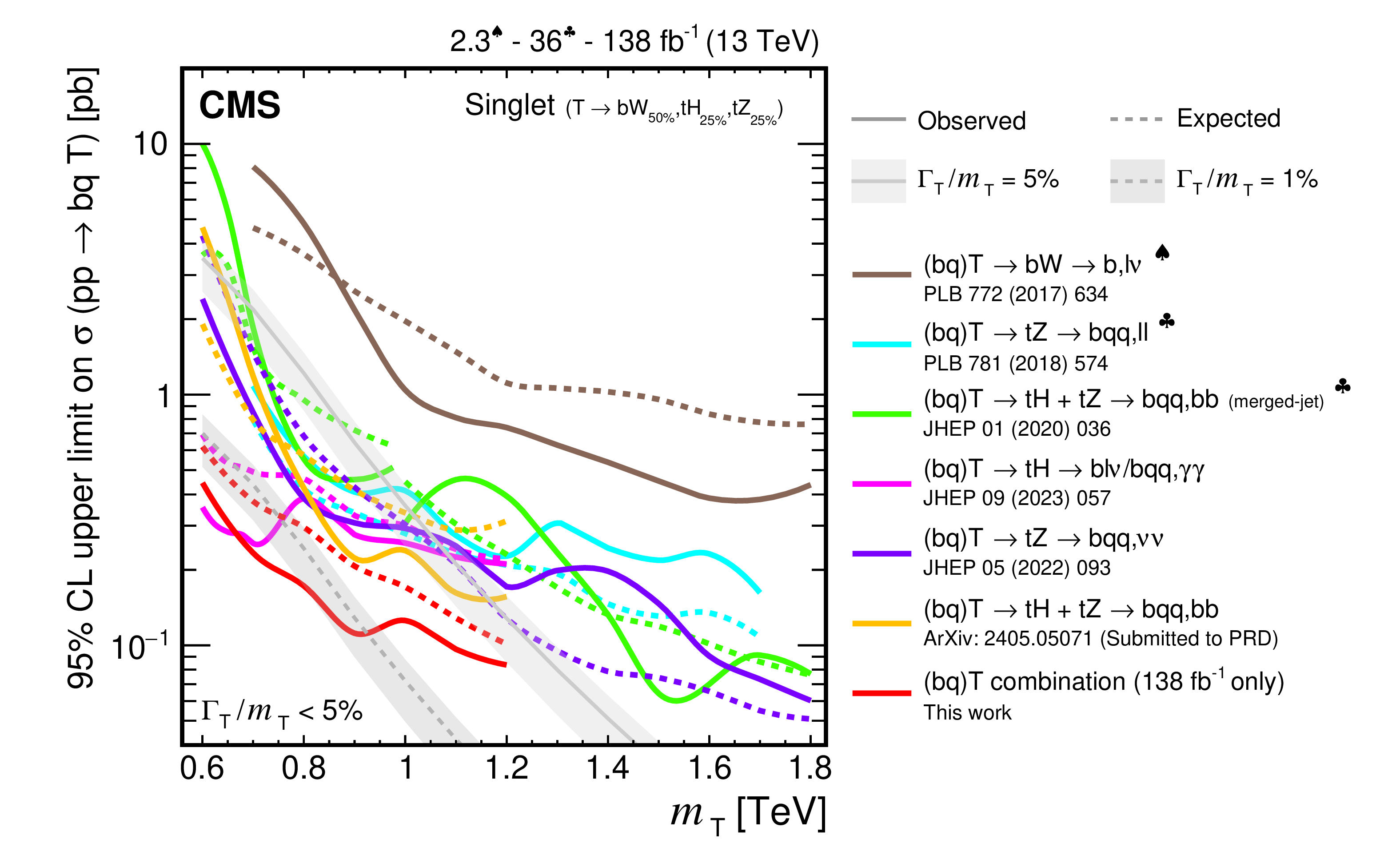
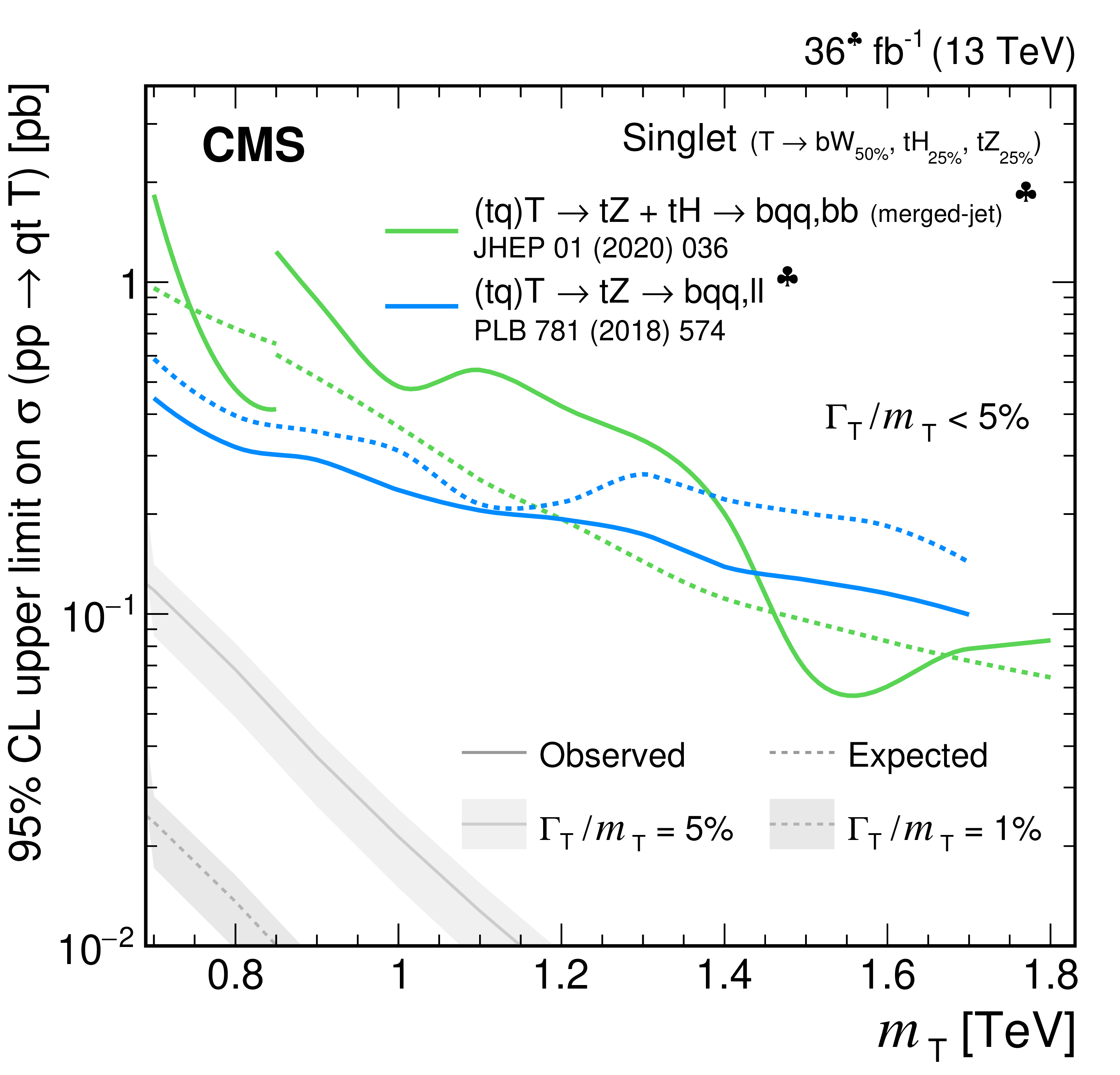
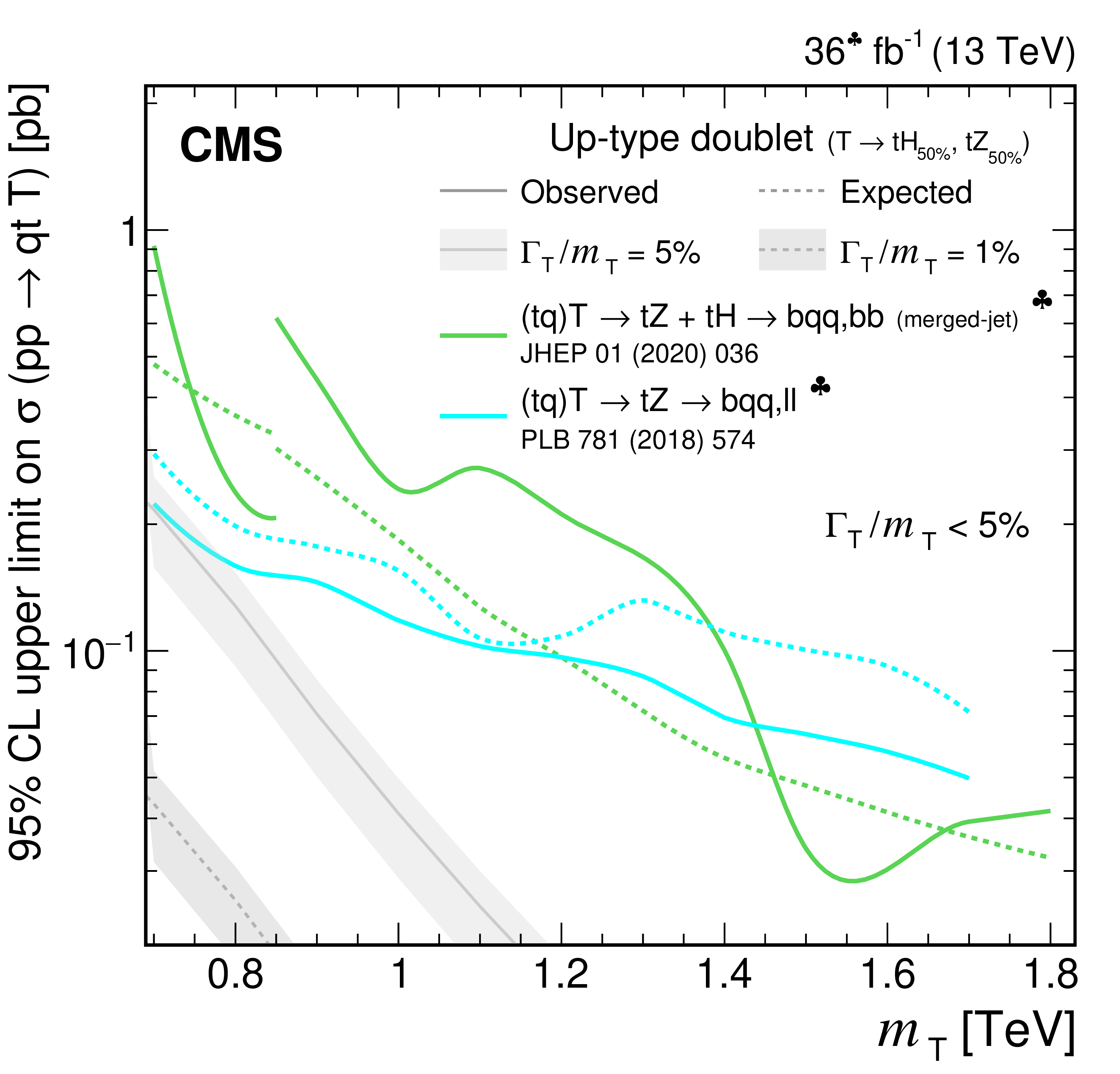
png pdf	Figure 40: Observed and expected 95% CL upper limits on the production cross section of a single T quark in association with a b quark (upper) or a t quark (lower row) in a singlet (upper and lower left) and doublet (lower right) scenario, versus the T quark mass, obtained by different analyses: ${\mathrm{T}} \to\mathrm{b}\mathrm{W}\to\mathrm{b}\mathrm{q}\mathrm{q}\,\ell\nu/\mathrm{b}\ell\nu\,\mathrm{q}\mathrm{q}$ [149], ${\mathrm{T}} \to\mathrm{t}\mathrm{Z}\to\mathrm{b}\mathrm{q}\mathrm{q}\,\ell\ell$ [144], ${\mathrm{T}} \to\mathrm{t}\mathrm{H}+\mathrm{t}\mathrm{Z}\to\mathrm{b}\mathrm{q}\mathrm{q}\,\mathrm{b}\mathrm{b}$ (merged-jet) [145], ${\mathrm{T}} \to\mathrm{t}\mathrm{H}\to\mathrm{b}\ell\nu/\mathrm{b}\mathrm{q}\mathrm{q}\,\gamma\gamma$ [147], ${\mathrm{T}} \to\mathrm{t}\mathrm{Z}\to\mathrm{b}\mathrm{q}\mathrm{q}\,\nu\nu$ [146], ${\mathrm{T}} \to\mathrm{t}\mathrm{H}+\mathrm{t}\mathrm{Z}\to\mathrm{b}\mathrm{q}\mathrm{q}\,\mathrm{b}\mathrm{b}$ [148], and the single T quark combination of Section 6.5.2. Only the three analyses using the full Run 2 data set are included in the single T quark combination. Two theory predictions at LO in perturbative QCD are superimposed, corresponding to different VLQ widths. Searches using data corresponding to an integrated luminosity of 2.3 fb$^{-1}$ and 36 fb$^{-1}$, rather than the full Run 2 integrated luminosity of 138 fb$^{-1}$, are indicated with a heart and spade symbol, respectively, in the legend.
png pdf	Figure 40-a: Observed and expected 95% CL upper limits on the production cross section of a single T quark in association with a b quark (upper) or a t quark (lower row) in a singlet (upper and lower left) and doublet (lower right) scenario, versus the T quark mass, obtained by different analyses: ${\mathrm{T}} \to\mathrm{b}\mathrm{W}\to\mathrm{b}\mathrm{q}\mathrm{q}\,\ell\nu/\mathrm{b}\ell\nu\,\mathrm{q}\mathrm{q}$ [149], ${\mathrm{T}} \to\mathrm{t}\mathrm{Z}\to\mathrm{b}\mathrm{q}\mathrm{q}\,\ell\ell$ [144], ${\mathrm{T}} \to\mathrm{t}\mathrm{H}+\mathrm{t}\mathrm{Z}\to\mathrm{b}\mathrm{q}\mathrm{q}\,\mathrm{b}\mathrm{b}$ (merged-jet) [145], ${\mathrm{T}} \to\mathrm{t}\mathrm{H}\to\mathrm{b}\ell\nu/\mathrm{b}\mathrm{q}\mathrm{q}\,\gamma\gamma$ [147], ${\mathrm{T}} \to\mathrm{t}\mathrm{Z}\to\mathrm{b}\mathrm{q}\mathrm{q}\,\nu\nu$ [146], ${\mathrm{T}} \to\mathrm{t}\mathrm{H}+\mathrm{t}\mathrm{Z}\to\mathrm{b}\mathrm{q}\mathrm{q}\,\mathrm{b}\mathrm{b}$ [148], and the single T quark combination of Section 6.5.2. Only the three analyses using the full Run 2 data set are included in the single T quark combination. Two theory predictions at LO in perturbative QCD are superimposed, corresponding to different VLQ widths. Searches using data corresponding to an integrated luminosity of 2.3 fb$^{-1}$ and 36 fb$^{-1}$, rather than the full Run 2 integrated luminosity of 138 fb$^{-1}$, are indicated with a heart and spade symbol, respectively, in the legend.
png pdf	Figure 40-b: Observed and expected 95% CL upper limits on the production cross section of a single T quark in association with a b quark (upper) or a t quark (lower row) in a singlet (upper and lower left) and doublet (lower right) scenario, versus the T quark mass, obtained by different analyses: ${\mathrm{T}} \to\mathrm{b}\mathrm{W}\to\mathrm{b}\mathrm{q}\mathrm{q}\,\ell\nu/\mathrm{b}\ell\nu\,\mathrm{q}\mathrm{q}$ [149], ${\mathrm{T}} \to\mathrm{t}\mathrm{Z}\to\mathrm{b}\mathrm{q}\mathrm{q}\,\ell\ell$ [144], ${\mathrm{T}} \to\mathrm{t}\mathrm{H}+\mathrm{t}\mathrm{Z}\to\mathrm{b}\mathrm{q}\mathrm{q}\,\mathrm{b}\mathrm{b}$ (merged-jet) [145], ${\mathrm{T}} \to\mathrm{t}\mathrm{H}\to\mathrm{b}\ell\nu/\mathrm{b}\mathrm{q}\mathrm{q}\,\gamma\gamma$ [147], ${\mathrm{T}} \to\mathrm{t}\mathrm{Z}\to\mathrm{b}\mathrm{q}\mathrm{q}\,\nu\nu$ [146], ${\mathrm{T}} \to\mathrm{t}\mathrm{H}+\mathrm{t}\mathrm{Z}\to\mathrm{b}\mathrm{q}\mathrm{q}\,\mathrm{b}\mathrm{b}$ [148], and the single T quark combination of Section 6.5.2. Only the three analyses using the full Run 2 data set are included in the single T quark combination. Two theory predictions at LO in perturbative QCD are superimposed, corresponding to different VLQ widths. Searches using data corresponding to an integrated luminosity of 2.3 fb$^{-1}$ and 36 fb$^{-1}$, rather than the full Run 2 integrated luminosity of 138 fb$^{-1}$, are indicated with a heart and spade symbol, respectively, in the legend.
png pdf	Figure 40-c: Observed and expected 95% CL upper limits on the production cross section of a single T quark in association with a b quark (upper) or a t quark (lower row) in a singlet (upper and lower left) and doublet (lower right) scenario, versus the T quark mass, obtained by different analyses: ${\mathrm{T}} \to\mathrm{b}\mathrm{W}\to\mathrm{b}\mathrm{q}\mathrm{q}\,\ell\nu/\mathrm{b}\ell\nu\,\mathrm{q}\mathrm{q}$ [149], ${\mathrm{T}} \to\mathrm{t}\mathrm{Z}\to\mathrm{b}\mathrm{q}\mathrm{q}\,\ell\ell$ [144], ${\mathrm{T}} \to\mathrm{t}\mathrm{H}+\mathrm{t}\mathrm{Z}\to\mathrm{b}\mathrm{q}\mathrm{q}\,\mathrm{b}\mathrm{b}$ (merged-jet) [145], ${\mathrm{T}} \to\mathrm{t}\mathrm{H}\to\mathrm{b}\ell\nu/\mathrm{b}\mathrm{q}\mathrm{q}\,\gamma\gamma$ [147], ${\mathrm{T}} \to\mathrm{t}\mathrm{Z}\to\mathrm{b}\mathrm{q}\mathrm{q}\,\nu\nu$ [146], ${\mathrm{T}} \to\mathrm{t}\mathrm{H}+\mathrm{t}\mathrm{Z}\to\mathrm{b}\mathrm{q}\mathrm{q}\,\mathrm{b}\mathrm{b}$ [148], and the single T quark combination of Section 6.5.2. Only the three analyses using the full Run 2 data set are included in the single T quark combination. Two theory predictions at LO in perturbative QCD are superimposed, corresponding to different VLQ widths. Searches using data corresponding to an integrated luminosity of 2.3 fb$^{-1}$ and 36 fb$^{-1}$, rather than the full Run 2 integrated luminosity of 138 fb$^{-1}$, are indicated with a heart and spade symbol, respectively, in the legend.
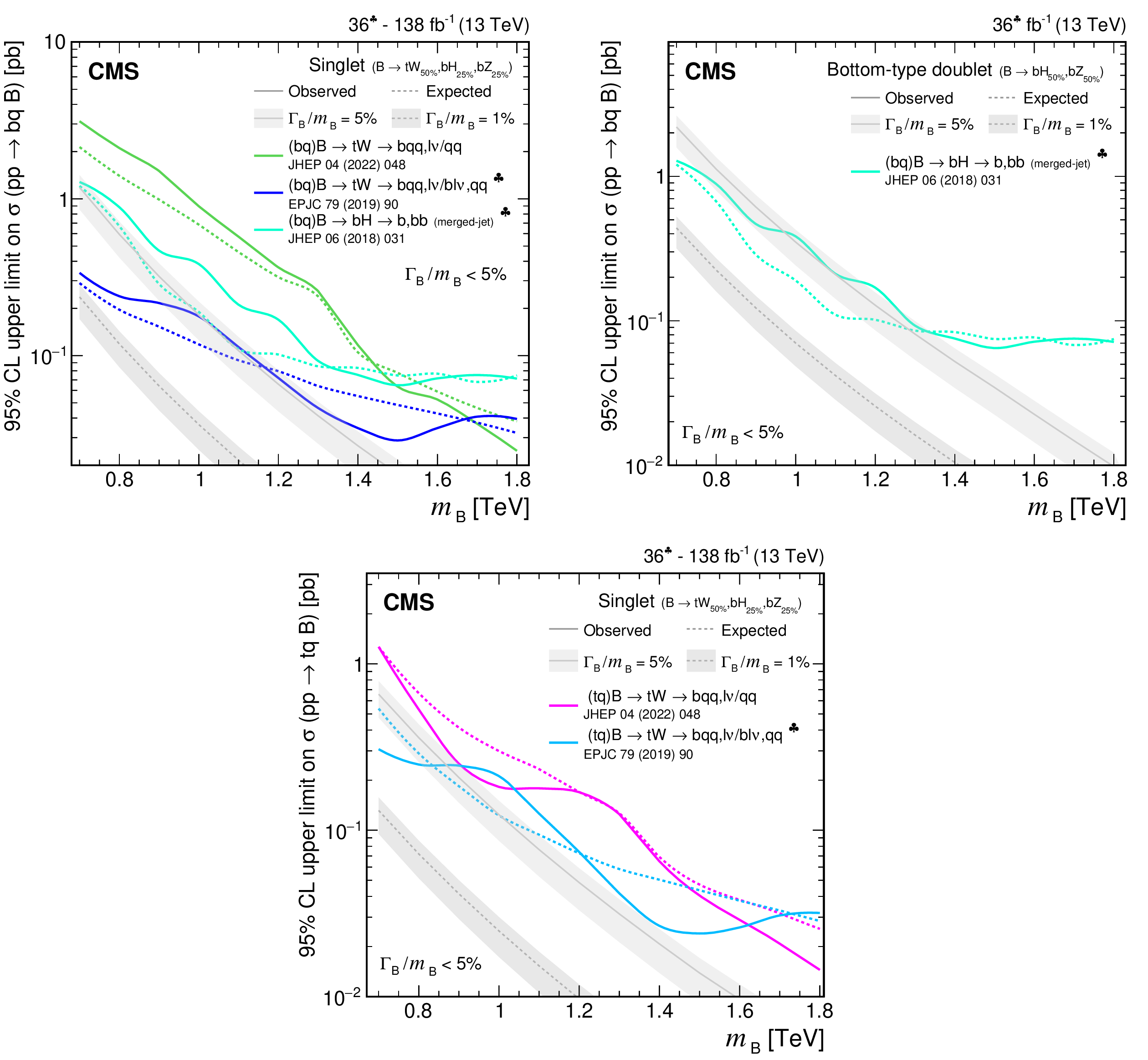
png pdf	Figure 41: Observed and expected 95% CL upper limits on the production cross section of a single B quark in association with a b quark (upper row) or a t quark (lower) in a singlet (upper left and lower) and doublet (upper right) scenario, versus the B quark mass, obtained by different analyses: ${\mathrm{B}} \to\mathrm{t}\mathrm{W}\to\mathrm{b}\mathrm{q}\mathrm{q}\,\ell\nu/\mathrm{q}\mathrm{q}$ [153], ${\mathrm{B}} \to\mathrm{t}\mathrm{W}\to\mathrm{b}\mathrm{q}\mathrm{q}\,\ell\nu/\mathrm{b}\ell\nu\,\mathrm{q}\mathrm{q}$ [151], and ${\mathrm{B}} \to\mathrm{b}\mathrm{H}\to\mathrm{b}\,\mathrm{b}\mathrm{b}$ [150]. Two theory predictions at LO in perturbative QCD are superimposed, corresponding to different VLQ widths. Searches using data corresponding to an integrated luminosity of 36 fb$^{-1}$, rather than the full Run 2 integrated luminosity of 138 fb$^{-1}$, are indicated with a spade symbol in the legend.
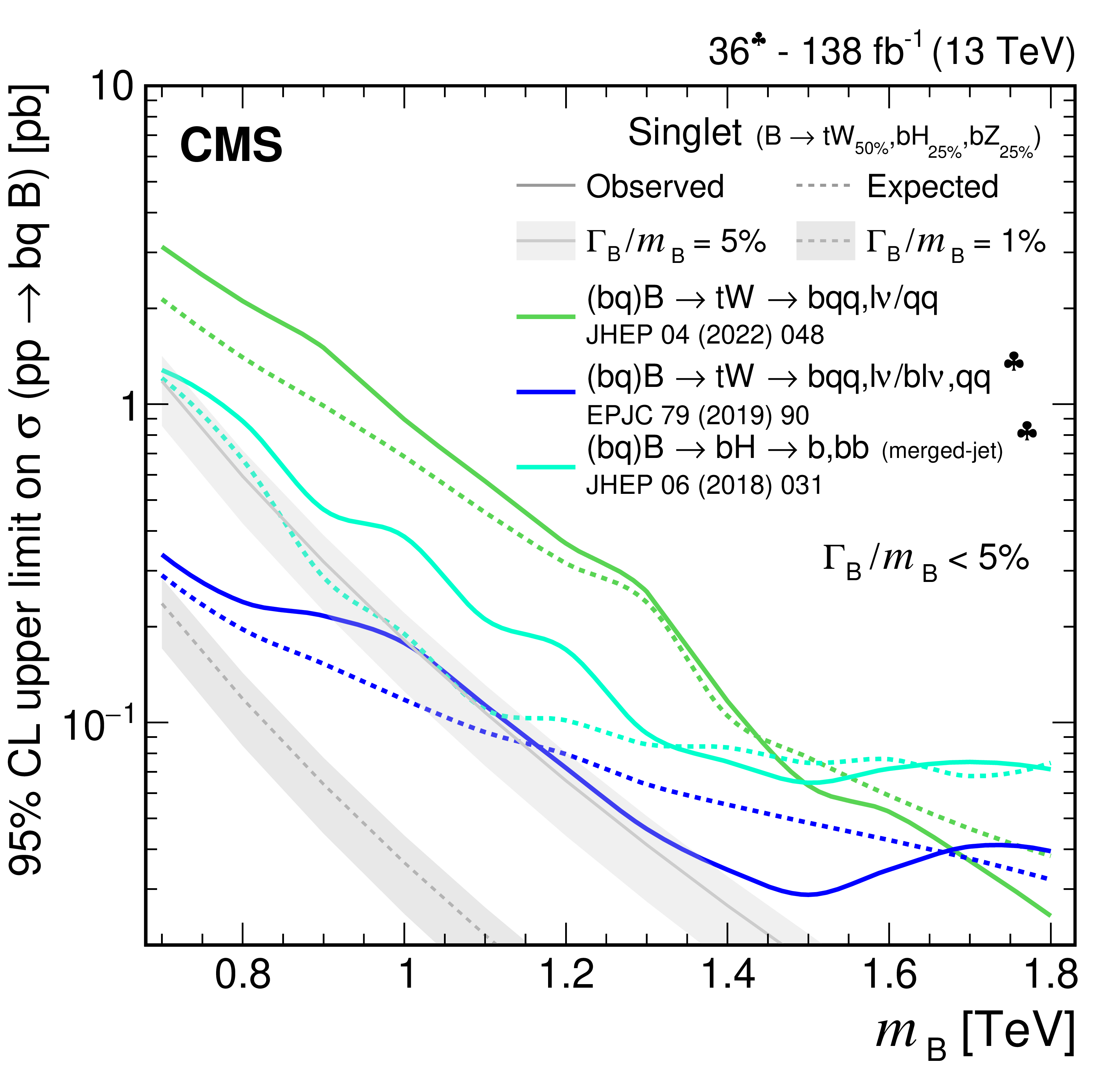
png pdf	Figure 41-a: Observed and expected 95% CL upper limits on the production cross section of a single B quark in association with a b quark (upper row) or a t quark (lower) in a singlet (upper left and lower) and doublet (upper right) scenario, versus the B quark mass, obtained by different analyses: ${\mathrm{B}} \to\mathrm{t}\mathrm{W}\to\mathrm{b}\mathrm{q}\mathrm{q}\,\ell\nu/\mathrm{q}\mathrm{q}$ [153], ${\mathrm{B}} \to\mathrm{t}\mathrm{W}\to\mathrm{b}\mathrm{q}\mathrm{q}\,\ell\nu/\mathrm{b}\ell\nu\,\mathrm{q}\mathrm{q}$ [151], and ${\mathrm{B}} \to\mathrm{b}\mathrm{H}\to\mathrm{b}\,\mathrm{b}\mathrm{b}$ [150]. Two theory predictions at LO in perturbative QCD are superimposed, corresponding to different VLQ widths. Searches using data corresponding to an integrated luminosity of 36 fb$^{-1}$, rather than the full Run 2 integrated luminosity of 138 fb$^{-1}$, are indicated with a spade symbol in the legend.
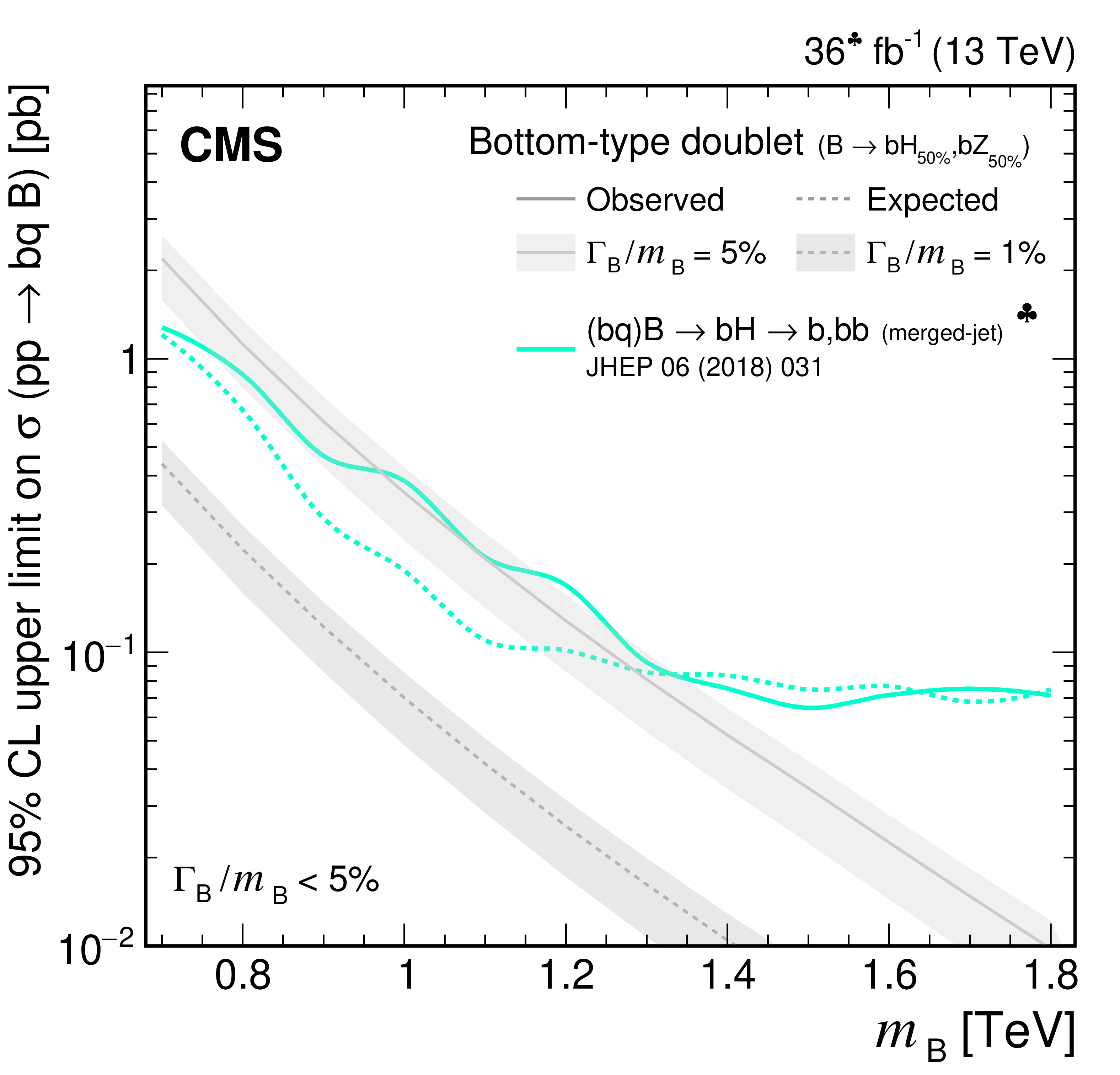
png pdf	Figure 41-b: Observed and expected 95% CL upper limits on the production cross section of a single B quark in association with a b quark (upper row) or a t quark (lower) in a singlet (upper left and lower) and doublet (upper right) scenario, versus the B quark mass, obtained by different analyses: ${\mathrm{B}} \to\mathrm{t}\mathrm{W}\to\mathrm{b}\mathrm{q}\mathrm{q}\,\ell\nu/\mathrm{q}\mathrm{q}$ [153], ${\mathrm{B}} \to\mathrm{t}\mathrm{W}\to\mathrm{b}\mathrm{q}\mathrm{q}\,\ell\nu/\mathrm{b}\ell\nu\,\mathrm{q}\mathrm{q}$ [151], and ${\mathrm{B}} \to\mathrm{b}\mathrm{H}\to\mathrm{b}\,\mathrm{b}\mathrm{b}$ [150]. Two theory predictions at LO in perturbative QCD are superimposed, corresponding to different VLQ widths. Searches using data corresponding to an integrated luminosity of 36 fb$^{-1}$, rather than the full Run 2 integrated luminosity of 138 fb$^{-1}$, are indicated with a spade symbol in the legend.
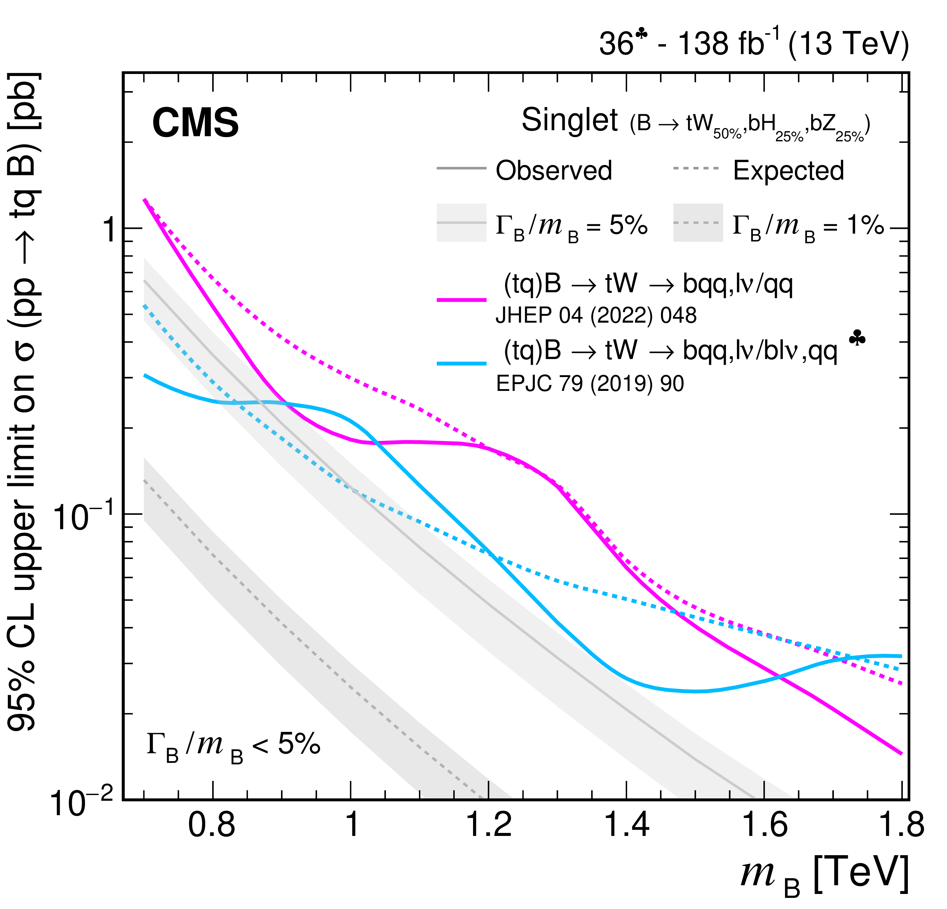
png pdf	Figure 41-c: Observed and expected 95% CL upper limits on the production cross section of a single B quark in association with a b quark (upper row) or a t quark (lower) in a singlet (upper left and lower) and doublet (upper right) scenario, versus the B quark mass, obtained by different analyses: ${\mathrm{B}} \to\mathrm{t}\mathrm{W}\to\mathrm{b}\mathrm{q}\mathrm{q}\,\ell\nu/\mathrm{q}\mathrm{q}$ [153], ${\mathrm{B}} \to\mathrm{t}\mathrm{W}\to\mathrm{b}\mathrm{q}\mathrm{q}\,\ell\nu/\mathrm{b}\ell\nu\,\mathrm{q}\mathrm{q}$ [151], and ${\mathrm{B}} \to\mathrm{b}\mathrm{H}\to\mathrm{b}\,\mathrm{b}\mathrm{b}$ [150]. Two theory predictions at LO in perturbative QCD are superimposed, corresponding to different VLQ widths. Searches using data corresponding to an integrated luminosity of 36 fb$^{-1}$, rather than the full Run 2 integrated luminosity of 138 fb$^{-1}$, are indicated with a spade symbol in the legend.
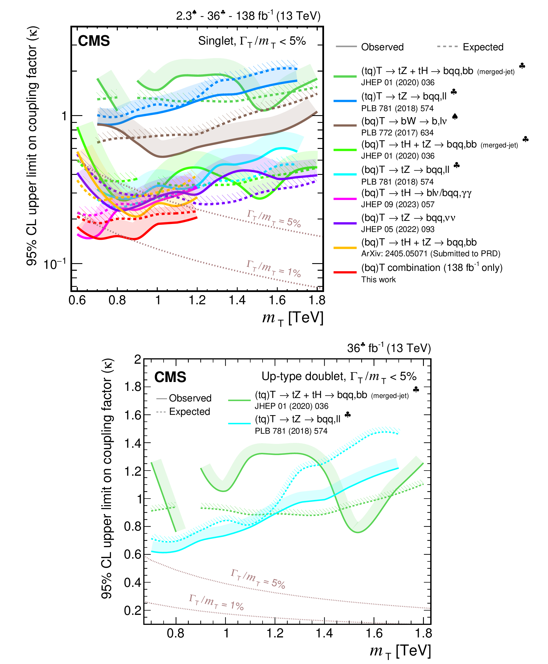
png pdf	Figure 42: Observed and expected 95% CL upper limits on the coupling strength $\kappa$ for single T quark production in a singlet (upper) and doublet (lower) scenarios as functions of the T quark mass, obtained by different analyses: ${\mathrm{T}} \to\mathrm{t}\mathrm{H}+\mathrm{t}\mathrm{Z}\to\mathrm{b}\mathrm{q}\mathrm{q}\,\mathrm{b}\mathrm{b}$ (merged-jet) [145], ${\mathrm{T}} \to\mathrm{t}\mathrm{Z}\to\mathrm{b}\mathrm{q}\mathrm{q}\,\ell\ell$ [144], ${\mathrm{T}} \to\mathrm{b}\mathrm{W}\to\mathrm{b}\mathrm{q}\mathrm{q}\,\ell\nu/\mathrm{b}\ell\nu\,\mathrm{q}\mathrm{q}$ [149], ${\mathrm{T}} \to\mathrm{t}\mathrm{Z}\to\mathrm{b}\mathrm{q}\mathrm{q}\,\ell\ell$ [144], ${\mathrm{T}} \to\mathrm{t}\mathrm{H}\to\mathrm{b}\ell\nu/\mathrm{b}\mathrm{q}\mathrm{q}\,\gamma\gamma$ [147], ${\mathrm{T}} \to\mathrm{t}\mathrm{Z}\to\mathrm{b}\mathrm{q}\mathrm{q}\,\nu\nu$ [146], ${\mathrm{T}} \to\mathrm{t}\mathrm{H}+\mathrm{t}\mathrm{Z}\to\mathrm{b}\mathrm{q}\mathrm{q}\,\mathrm{b}\mathrm{b}$ [148], and the single T quark combination of Section 6.5.2. Only the three analyses using the full Run 2 data set are included in the single T quark combination. Two theory predictions at LO in perturbative QCD are superimposed, corresponding to different VLQ widths. Searches using data corresponding to an integrated luminosity of 2.3 fb$^{-1}$ and 36 fb$^{-1}$, rather than the full Run 2 integrated luminosity of 138 fb$^{-1}$, are indicated with a heart and spade symbol, respectively, in the legend.
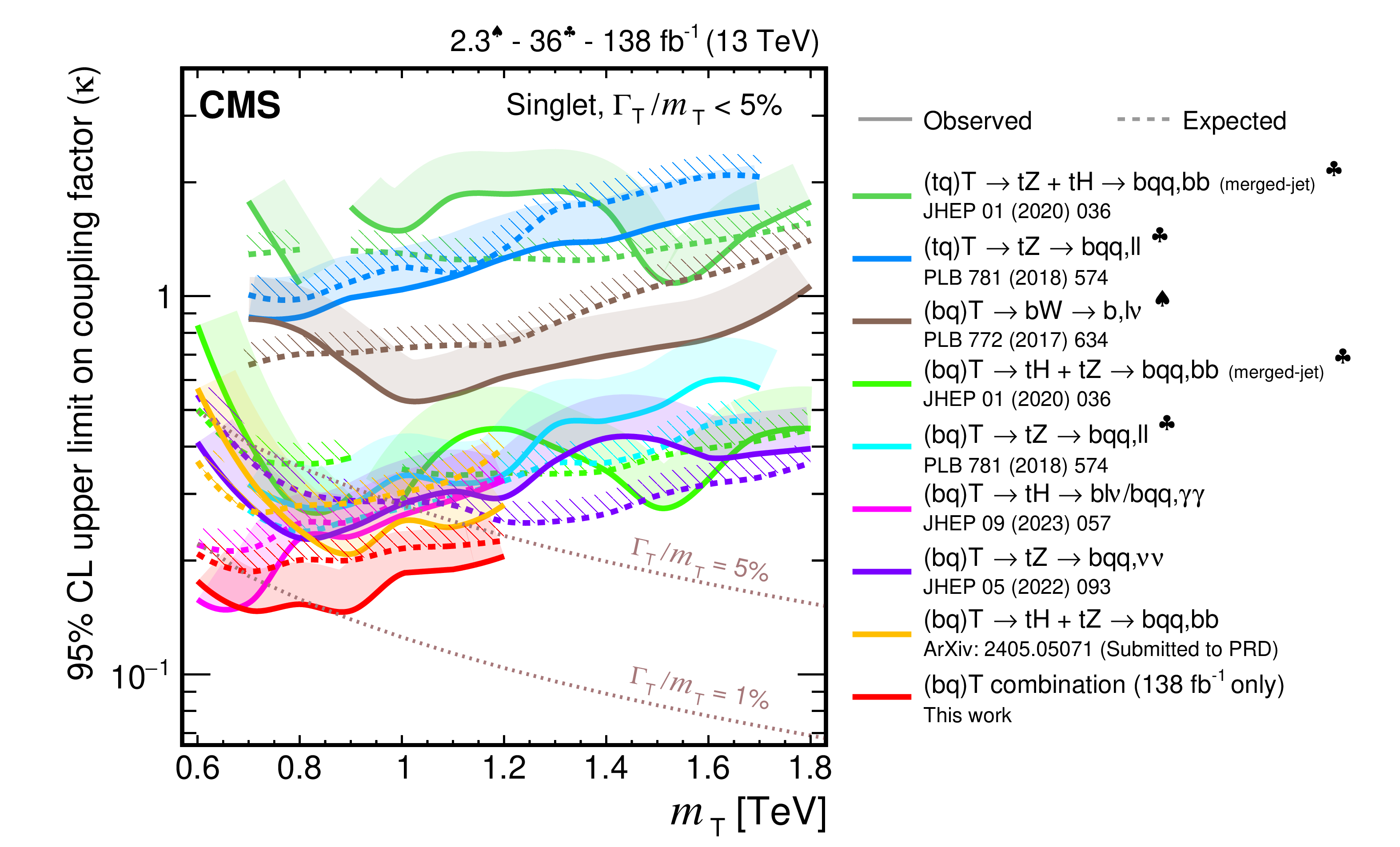
png pdf	Figure 42-a: Observed and expected 95% CL upper limits on the coupling strength $\kappa$ for single T quark production in a singlet (upper) and doublet (lower) scenarios as functions of the T quark mass, obtained by different analyses: ${\mathrm{T}} \to\mathrm{t}\mathrm{H}+\mathrm{t}\mathrm{Z}\to\mathrm{b}\mathrm{q}\mathrm{q}\,\mathrm{b}\mathrm{b}$ (merged-jet) [145], ${\mathrm{T}} \to\mathrm{t}\mathrm{Z}\to\mathrm{b}\mathrm{q}\mathrm{q}\,\ell\ell$ [144], ${\mathrm{T}} \to\mathrm{b}\mathrm{W}\to\mathrm{b}\mathrm{q}\mathrm{q}\,\ell\nu/\mathrm{b}\ell\nu\,\mathrm{q}\mathrm{q}$ [149], ${\mathrm{T}} \to\mathrm{t}\mathrm{Z}\to\mathrm{b}\mathrm{q}\mathrm{q}\,\ell\ell$ [144], ${\mathrm{T}} \to\mathrm{t}\mathrm{H}\to\mathrm{b}\ell\nu/\mathrm{b}\mathrm{q}\mathrm{q}\,\gamma\gamma$ [147], ${\mathrm{T}} \to\mathrm{t}\mathrm{Z}\to\mathrm{b}\mathrm{q}\mathrm{q}\,\nu\nu$ [146], ${\mathrm{T}} \to\mathrm{t}\mathrm{H}+\mathrm{t}\mathrm{Z}\to\mathrm{b}\mathrm{q}\mathrm{q}\,\mathrm{b}\mathrm{b}$ [148], and the single T quark combination of Section 6.5.2. Only the three analyses using the full Run 2 data set are included in the single T quark combination. Two theory predictions at LO in perturbative QCD are superimposed, corresponding to different VLQ widths. Searches using data corresponding to an integrated luminosity of 2.3 fb$^{-1}$ and 36 fb$^{-1}$, rather than the full Run 2 integrated luminosity of 138 fb$^{-1}$, are indicated with a heart and spade symbol, respectively, in the legend.
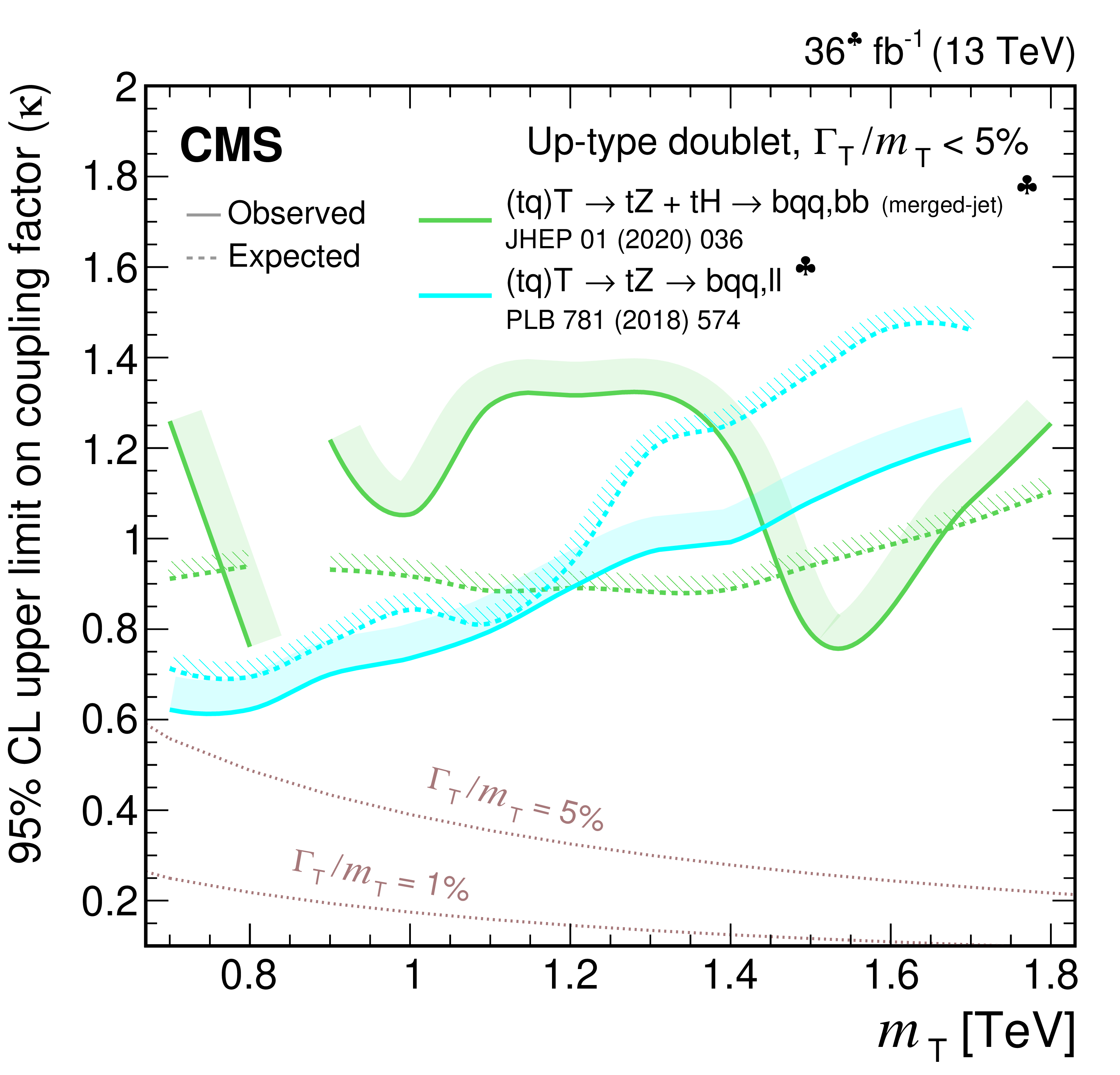
png pdf	Figure 42-b: Observed and expected 95% CL upper limits on the coupling strength $\kappa$ for single T quark production in a singlet (upper) and doublet (lower) scenarios as functions of the T quark mass, obtained by different analyses: ${\mathrm{T}} \to\mathrm{t}\mathrm{H}+\mathrm{t}\mathrm{Z}\to\mathrm{b}\mathrm{q}\mathrm{q}\,\mathrm{b}\mathrm{b}$ (merged-jet) [145], ${\mathrm{T}} \to\mathrm{t}\mathrm{Z}\to\mathrm{b}\mathrm{q}\mathrm{q}\,\ell\ell$ [144], ${\mathrm{T}} \to\mathrm{b}\mathrm{W}\to\mathrm{b}\mathrm{q}\mathrm{q}\,\ell\nu/\mathrm{b}\ell\nu\,\mathrm{q}\mathrm{q}$ [149], ${\mathrm{T}} \to\mathrm{t}\mathrm{Z}\to\mathrm{b}\mathrm{q}\mathrm{q}\,\ell\ell$ [144], ${\mathrm{T}} \to\mathrm{t}\mathrm{H}\to\mathrm{b}\ell\nu/\mathrm{b}\mathrm{q}\mathrm{q}\,\gamma\gamma$ [147], ${\mathrm{T}} \to\mathrm{t}\mathrm{Z}\to\mathrm{b}\mathrm{q}\mathrm{q}\,\nu\nu$ [146], ${\mathrm{T}} \to\mathrm{t}\mathrm{H}+\mathrm{t}\mathrm{Z}\to\mathrm{b}\mathrm{q}\mathrm{q}\,\mathrm{b}\mathrm{b}$ [148], and the single T quark combination of Section 6.5.2. Only the three analyses using the full Run 2 data set are included in the single T quark combination. Two theory predictions at LO in perturbative QCD are superimposed, corresponding to different VLQ widths. Searches using data corresponding to an integrated luminosity of 2.3 fb$^{-1}$ and 36 fb$^{-1}$, rather than the full Run 2 integrated luminosity of 138 fb$^{-1}$, are indicated with a heart and spade symbol, respectively, in the legend.
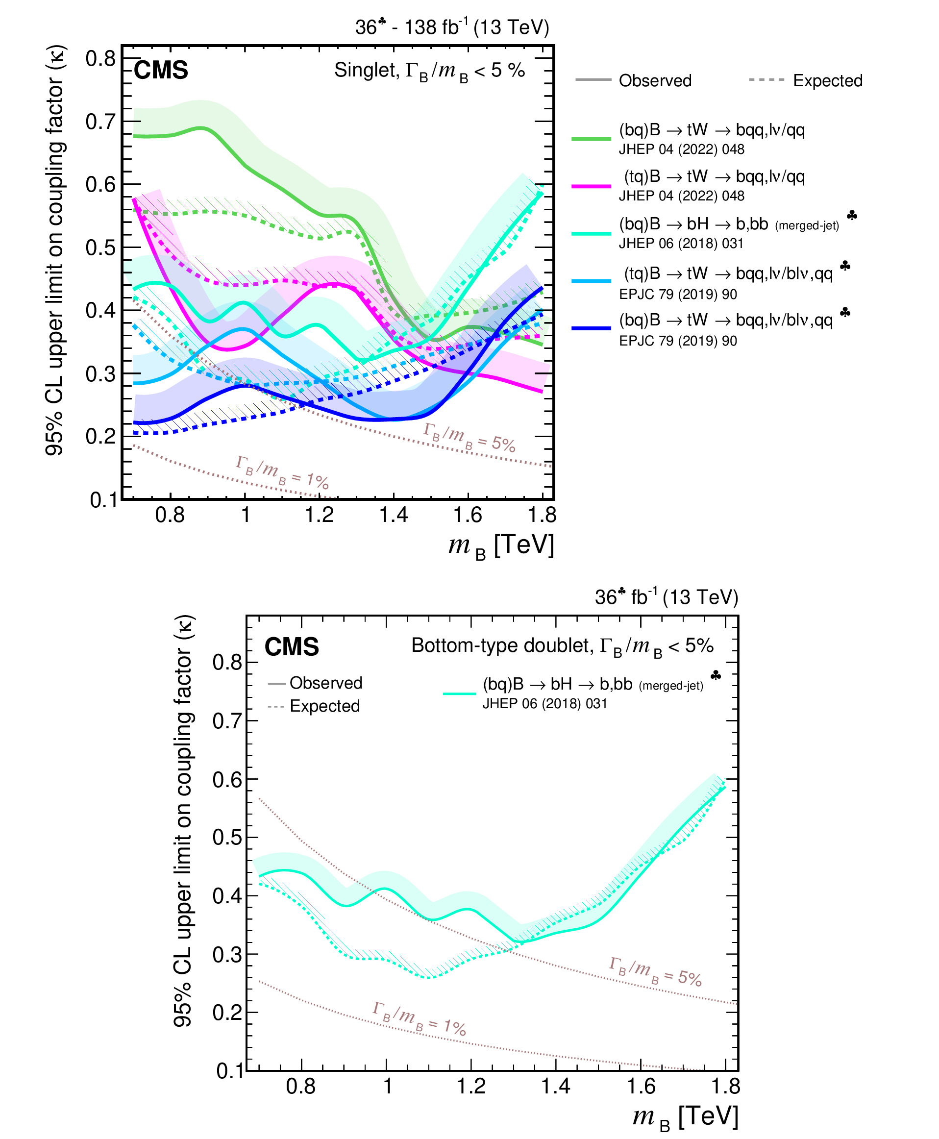
png pdf	Figure 43: Observed and expected 95% CL upper limits on the coupling strength $\kappa$ for single B quark production in a singlet (upper) and doublet (lower) scenarios as functions of the B quark mass, obtained by different analyses: ${\mathrm{B}} \to\mathrm{t}\mathrm{W}\to\mathrm{b}\mathrm{q}\mathrm{q}\,\ell\nu/\mathrm{q}\mathrm{q}$ [153], ${\mathrm{B}} \to\mathrm{b}\mathrm{H}\to\mathrm{b}\,\mathrm{b}\mathrm{b}$ [150], and ${\mathrm{B}} \to\mathrm{t}\mathrm{W}\to\mathrm{b}\mathrm{q}\mathrm{q}\,\ell\nu/\mathrm{b}\ell\nu\,\mathrm{q}\mathrm{q}$ [151]. Two theory predictions at LO in perturbative QCD are superimposed, corresponding to different VLQ widths. Searches using data corresponding to an integrated luminosity of 36 fb$^{-1}$, rather than the full Run 2 integrated luminosity of 138 fb$^{-1}$, are indicated with a spade symbol in the legend.
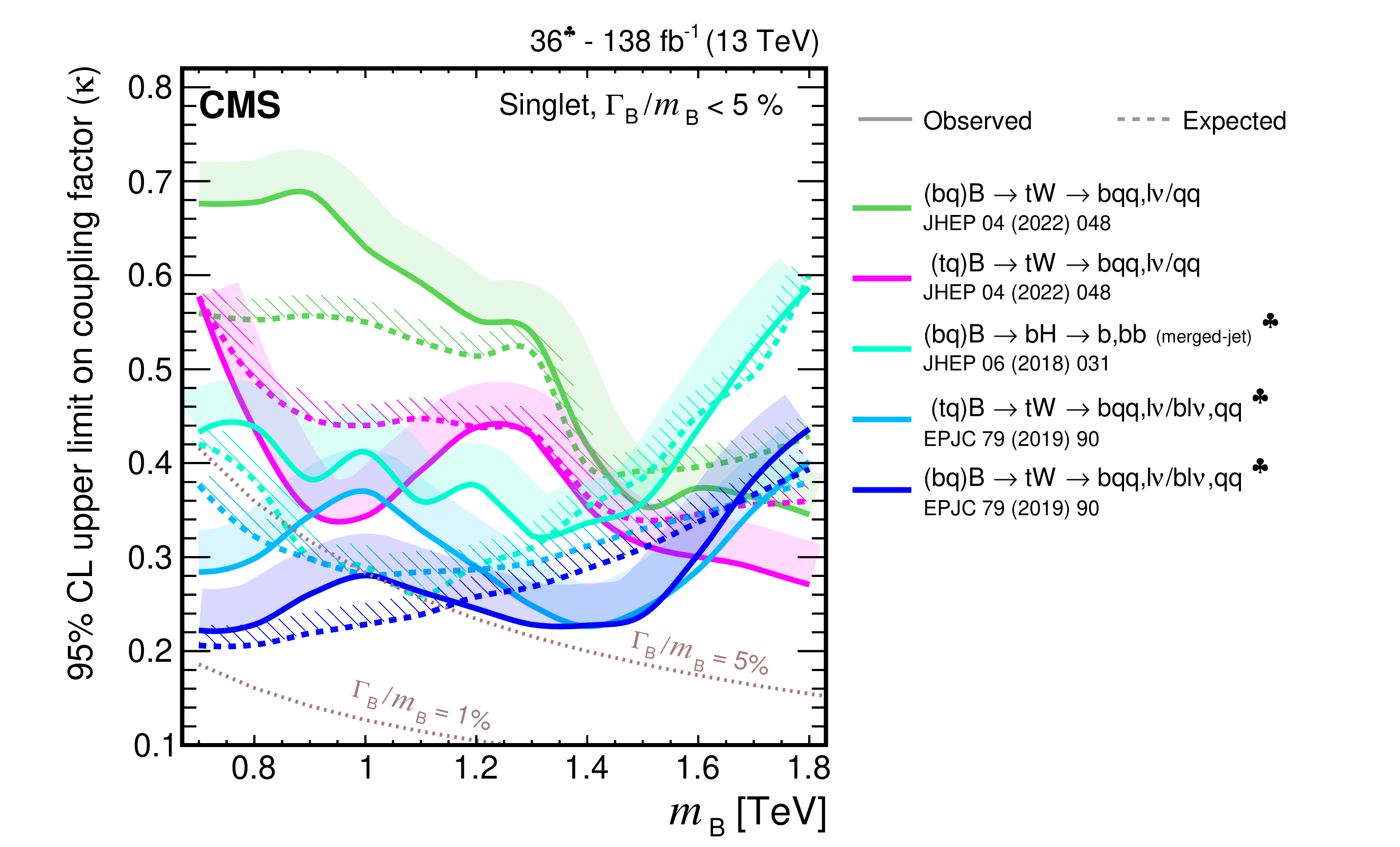
png pdf	Figure 43-a: Observed and expected 95% CL upper limits on the coupling strength $\kappa$ for single B quark production in a singlet (upper) and doublet (lower) scenarios as functions of the B quark mass, obtained by different analyses: ${\mathrm{B}} \to\mathrm{t}\mathrm{W}\to\mathrm{b}\mathrm{q}\mathrm{q}\,\ell\nu/\mathrm{q}\mathrm{q}$ [153], ${\mathrm{B}} \to\mathrm{b}\mathrm{H}\to\mathrm{b}\,\mathrm{b}\mathrm{b}$ [150], and ${\mathrm{B}} \to\mathrm{t}\mathrm{W}\to\mathrm{b}\mathrm{q}\mathrm{q}\,\ell\nu/\mathrm{b}\ell\nu\,\mathrm{q}\mathrm{q}$ [151]. Two theory predictions at LO in perturbative QCD are superimposed, corresponding to different VLQ widths. Searches using data corresponding to an integrated luminosity of 36 fb$^{-1}$, rather than the full Run 2 integrated luminosity of 138 fb$^{-1}$, are indicated with a spade symbol in the legend.
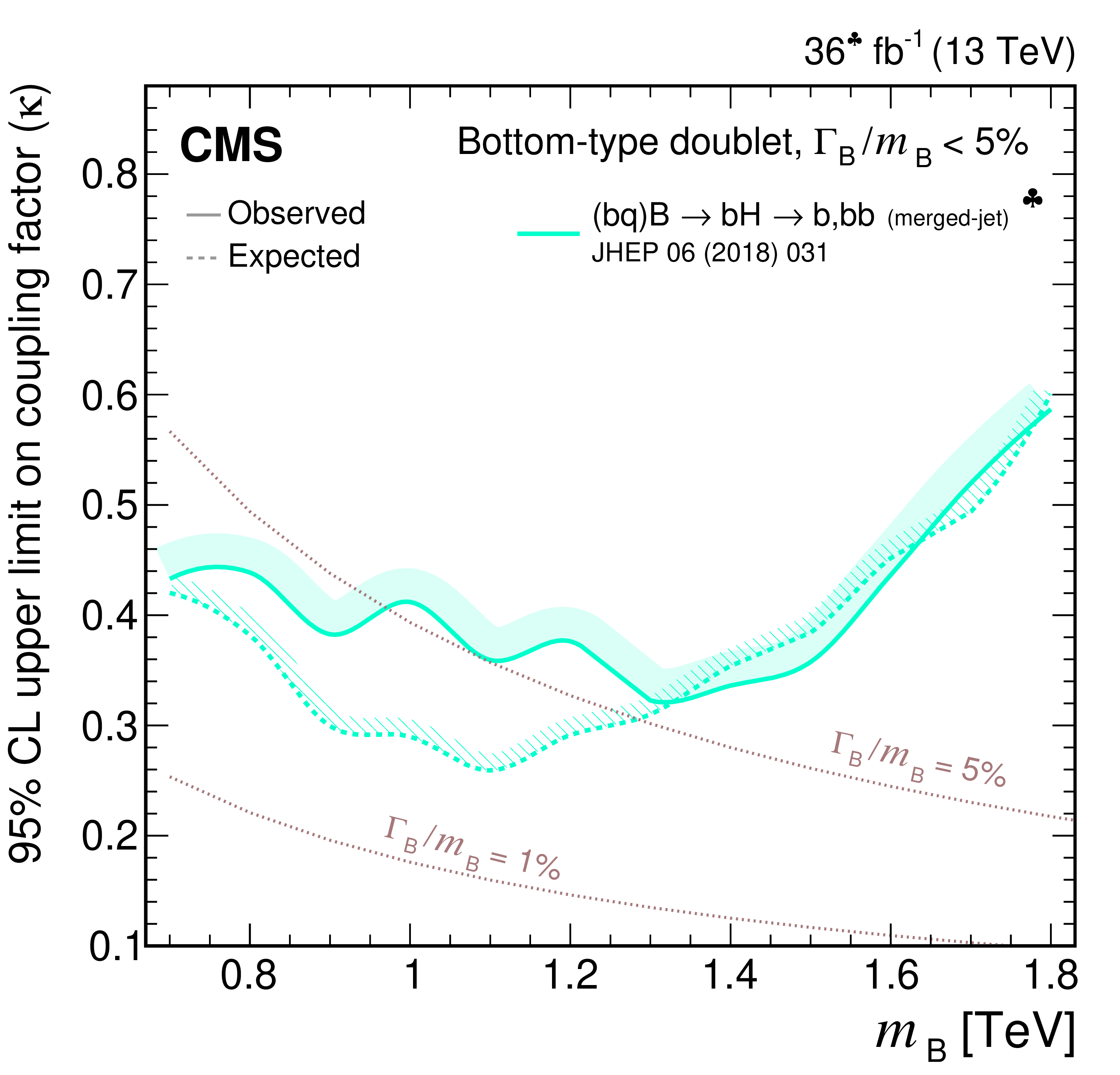
png pdf	Figure 43-b: Observed and expected 95% CL upper limits on the coupling strength $\kappa$ for single B quark production in a singlet (upper) and doublet (lower) scenarios as functions of the B quark mass, obtained by different analyses: ${\mathrm{B}} \to\mathrm{t}\mathrm{W}\to\mathrm{b}\mathrm{q}\mathrm{q}\,\ell\nu/\mathrm{q}\mathrm{q}$ [153], ${\mathrm{B}} \to\mathrm{b}\mathrm{H}\to\mathrm{b}\,\mathrm{b}\mathrm{b}$ [150], and ${\mathrm{B}} \to\mathrm{t}\mathrm{W}\to\mathrm{b}\mathrm{q}\mathrm{q}\,\ell\nu/\mathrm{b}\ell\nu\,\mathrm{q}\mathrm{q}$ [151]. Two theory predictions at LO in perturbative QCD are superimposed, corresponding to different VLQ widths. Searches using data corresponding to an integrated luminosity of 36 fb$^{-1}$, rather than the full Run 2 integrated luminosity of 138 fb$^{-1}$, are indicated with a spade symbol in the legend.
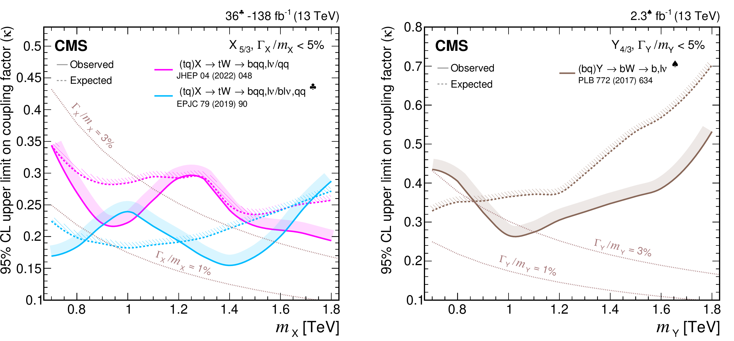
png pdf	Figure 44: Observed and expected 95% CL upper limits on the coupling strength $\kappa$ for single $\mathrm{X}_{5/3}$ (left) and $\mathrm{Y}_{4/3}$ (right) production as functions of the VLQ mass, obtained by different analyses: ${\mathrm{X}_{5/3}} \to\mathrm{t}\mathrm{W}\to\mathrm{b}\mathrm{q}\mathrm{q}\,\ell\nu/\mathrm{q}\mathrm{q}$ [153], ${\mathrm{X}_{5/3}} \to\mathrm{t}\mathrm{W}\to\mathrm{b}\mathrm{q}\mathrm{q}\,\ell\nu/\mathrm{b}\ell\nu\,\mathrm{q}\mathrm{q}$ [151], and ${\mathrm{Y}_{4/3}} \to\mathrm{b}\mathrm{W}\to\mathrm{b}\,\ell\nu$ [149]. Searches using data corresponding to an integrated luminosity of 2.3 fb$^{-1}$ and 36 fb$^{-1}$, rather than the full Run-s2 integrated luminosity of 138 fb$^{-1}$, are indicated with a heart and spade symbol, respectively, in the legend.
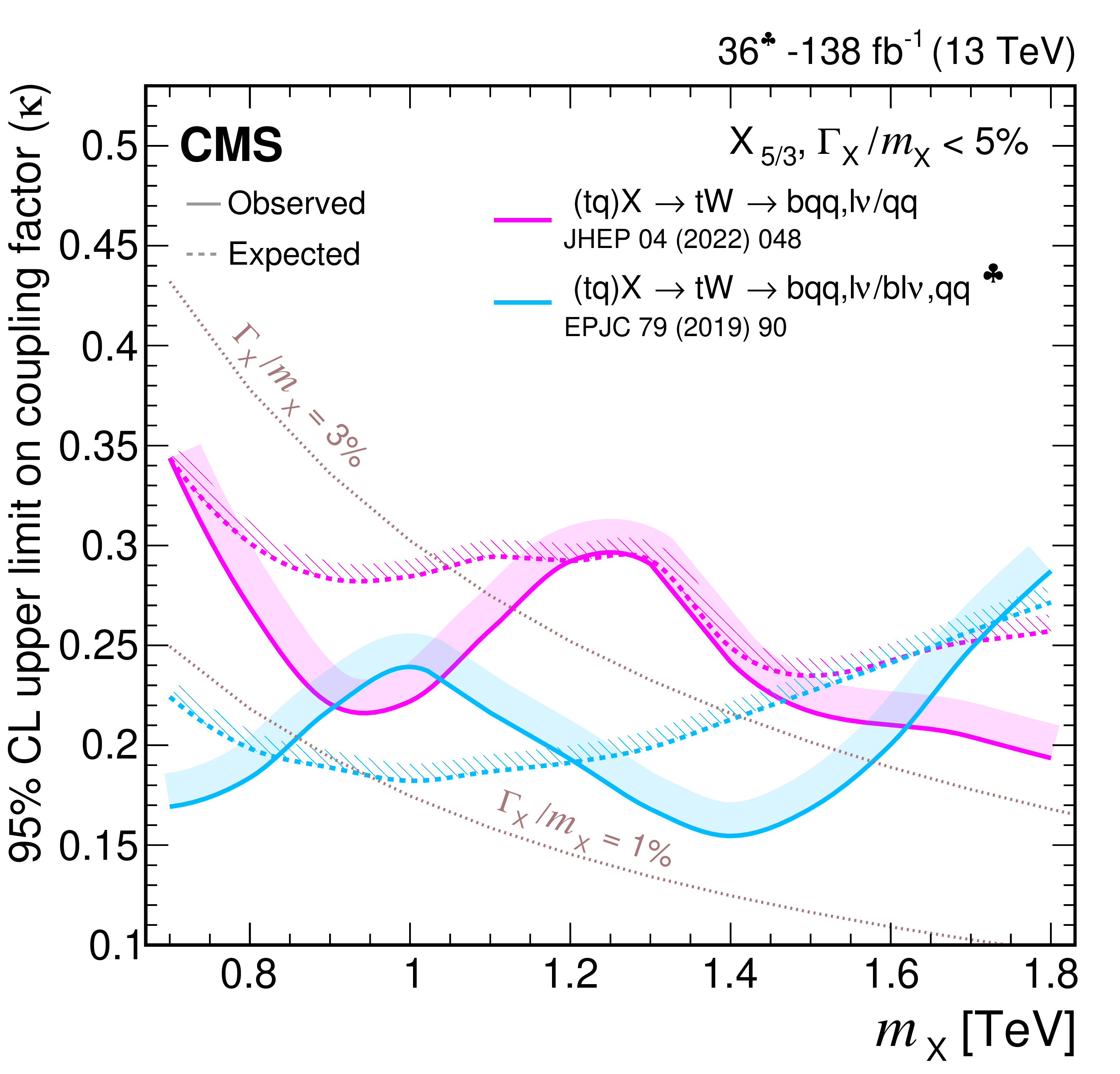
png pdf	Figure 44-a: Observed and expected 95% CL upper limits on the coupling strength $\kappa$ for single $\mathrm{X}_{5/3}$ (left) and $\mathrm{Y}_{4/3}$ (right) production as functions of the VLQ mass, obtained by different analyses: ${\mathrm{X}_{5/3}} \to\mathrm{t}\mathrm{W}\to\mathrm{b}\mathrm{q}\mathrm{q}\,\ell\nu/\mathrm{q}\mathrm{q}$ [153], ${\mathrm{X}_{5/3}} \to\mathrm{t}\mathrm{W}\to\mathrm{b}\mathrm{q}\mathrm{q}\,\ell\nu/\mathrm{b}\ell\nu\,\mathrm{q}\mathrm{q}$ [151], and ${\mathrm{Y}_{4/3}} \to\mathrm{b}\mathrm{W}\to\mathrm{b}\,\ell\nu$ [149]. Searches using data corresponding to an integrated luminosity of 2.3 fb$^{-1}$ and 36 fb$^{-1}$, rather than the full Run-s2 integrated luminosity of 138 fb$^{-1}$, are indicated with a heart and spade symbol, respectively, in the legend.
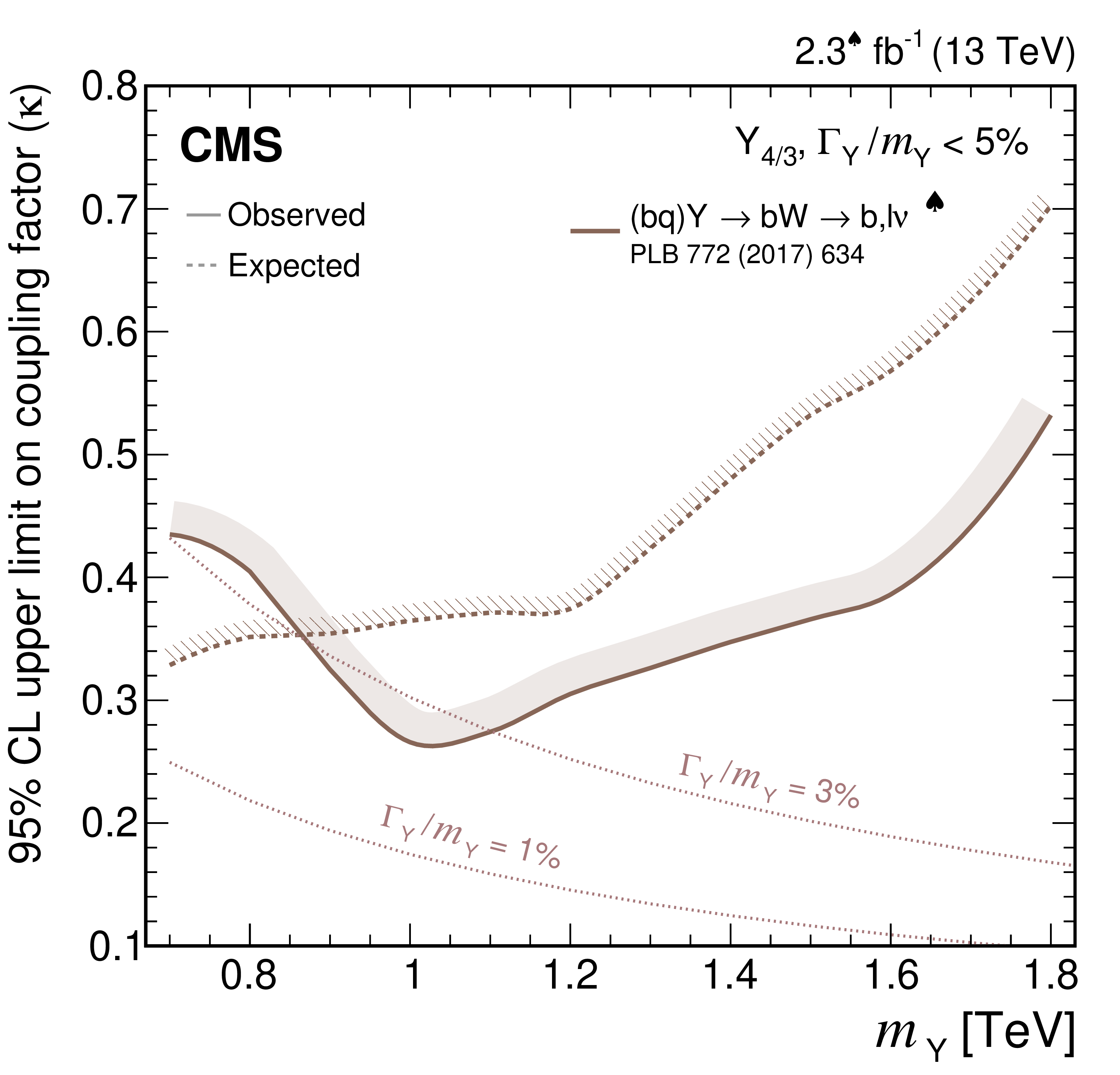
png pdf	Figure 44-b: Observed and expected 95% CL upper limits on the coupling strength $\kappa$ for single $\mathrm{X}_{5/3}$ (left) and $\mathrm{Y}_{4/3}$ (right) production as functions of the VLQ mass, obtained by different analyses: ${\mathrm{X}_{5/3}} \to\mathrm{t}\mathrm{W}\to\mathrm{b}\mathrm{q}\mathrm{q}\,\ell\nu/\mathrm{q}\mathrm{q}$ [153], ${\mathrm{X}_{5/3}} \to\mathrm{t}\mathrm{W}\to\mathrm{b}\mathrm{q}\mathrm{q}\,\ell\nu/\mathrm{b}\ell\nu\,\mathrm{q}\mathrm{q}$ [151], and ${\mathrm{Y}_{4/3}} \to\mathrm{b}\mathrm{W}\to\mathrm{b}\,\ell\nu$ [149]. Searches using data corresponding to an integrated luminosity of 2.3 fb$^{-1}$ and 36 fb$^{-1}$, rather than the full Run-s2 integrated luminosity of 138 fb$^{-1}$, are indicated with a heart and spade symbol, respectively, in the legend.
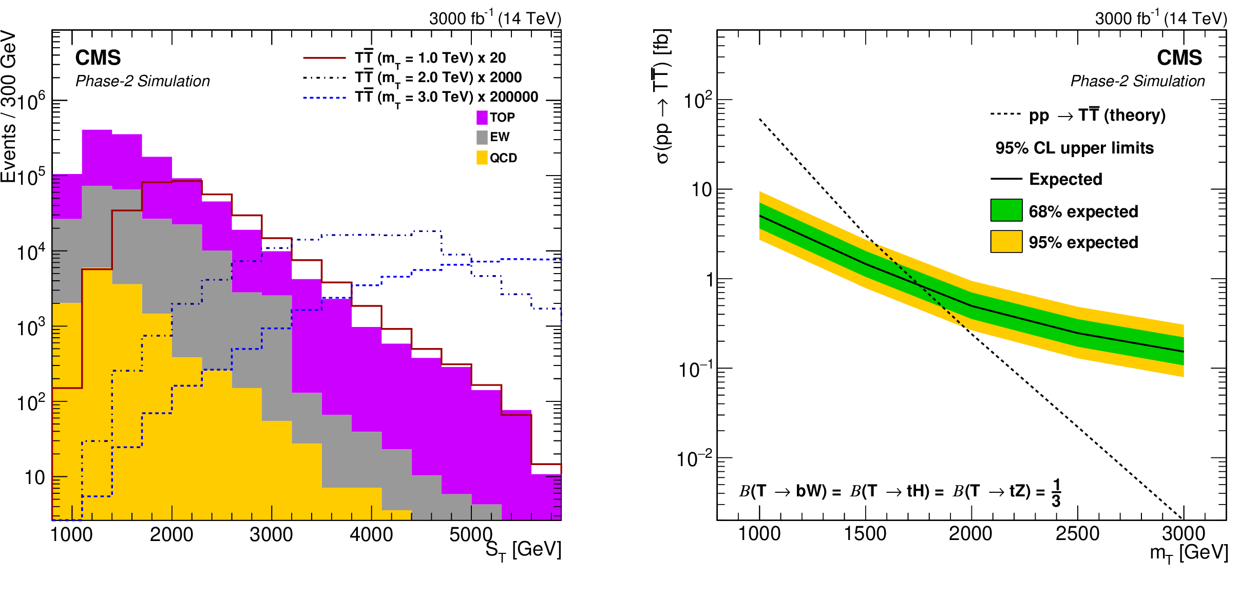
png pdf	Figure 45: Distributions of the $S_{\mathrm{T}}$ observable for signal and background processes (left), with signal distributions scaled by factors of 20, 2000, and 200\,000, depending on the T quark mass, and expected upper limits at 95% CL on the ${\mathrm{T}} \overline{\mathrm{T}}$ production cross section (right). The inner (green) and the outer (yellow) bands indicate the regions containing 68 and 95%, respectively, of the distribution of limits expected under the background-only hypothesis. Figures adapted from Ref. [170].
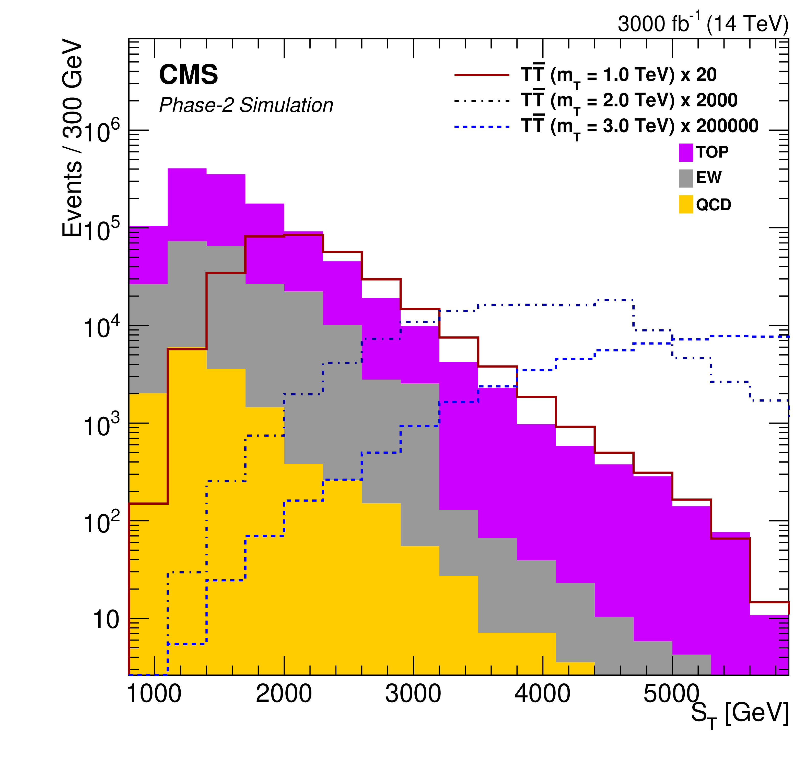
png pdf	Figure 45-a: Distributions of the $S_{\mathrm{T}}$ observable for signal and background processes (left), with signal distributions scaled by factors of 20, 2000, and 200\,000, depending on the T quark mass, and expected upper limits at 95% CL on the ${\mathrm{T}} \overline{\mathrm{T}}$ production cross section (right). The inner (green) and the outer (yellow) bands indicate the regions containing 68 and 95%, respectively, of the distribution of limits expected under the background-only hypothesis. Figures adapted from Ref. [170].
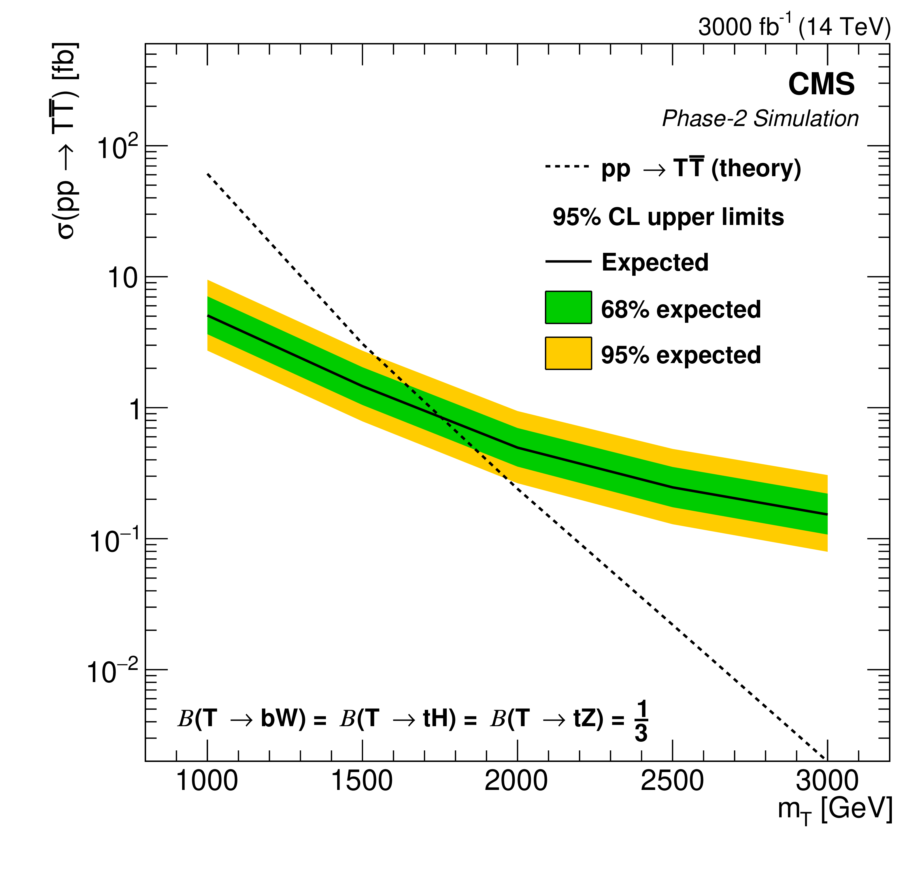
png pdf	Figure 45-b: Distributions of the $S_{\mathrm{T}}$ observable for signal and background processes (left), with signal distributions scaled by factors of 20, 2000, and 200\,000, depending on the T quark mass, and expected upper limits at 95% CL on the ${\mathrm{T}} \overline{\mathrm{T}}$ production cross section (right). The inner (green) and the outer (yellow) bands indicate the regions containing 68 and 95%, respectively, of the distribution of limits expected under the background-only hypothesis. Figures adapted from Ref. [170].
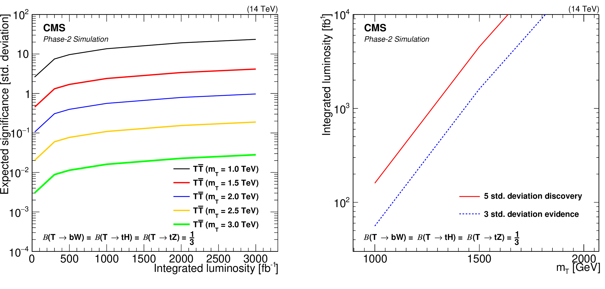
png pdf	Figure 46: Expected significances for T quark pair production as a function of the integrated luminosity at the HL-LHC, assuming equal branching fractions for ${\mathrm{T}} \to\mathrm{b}\mathrm{W}$, $\mathrm{t}\mathrm{Z}$, $\mathrm{t}\mathrm{H}$ decays (left). Discovery potential at three and five standard deviations for T quark pairs, as a function of the T quark mass and the integrated luminosity (right). Figures adapted from Ref. [170].
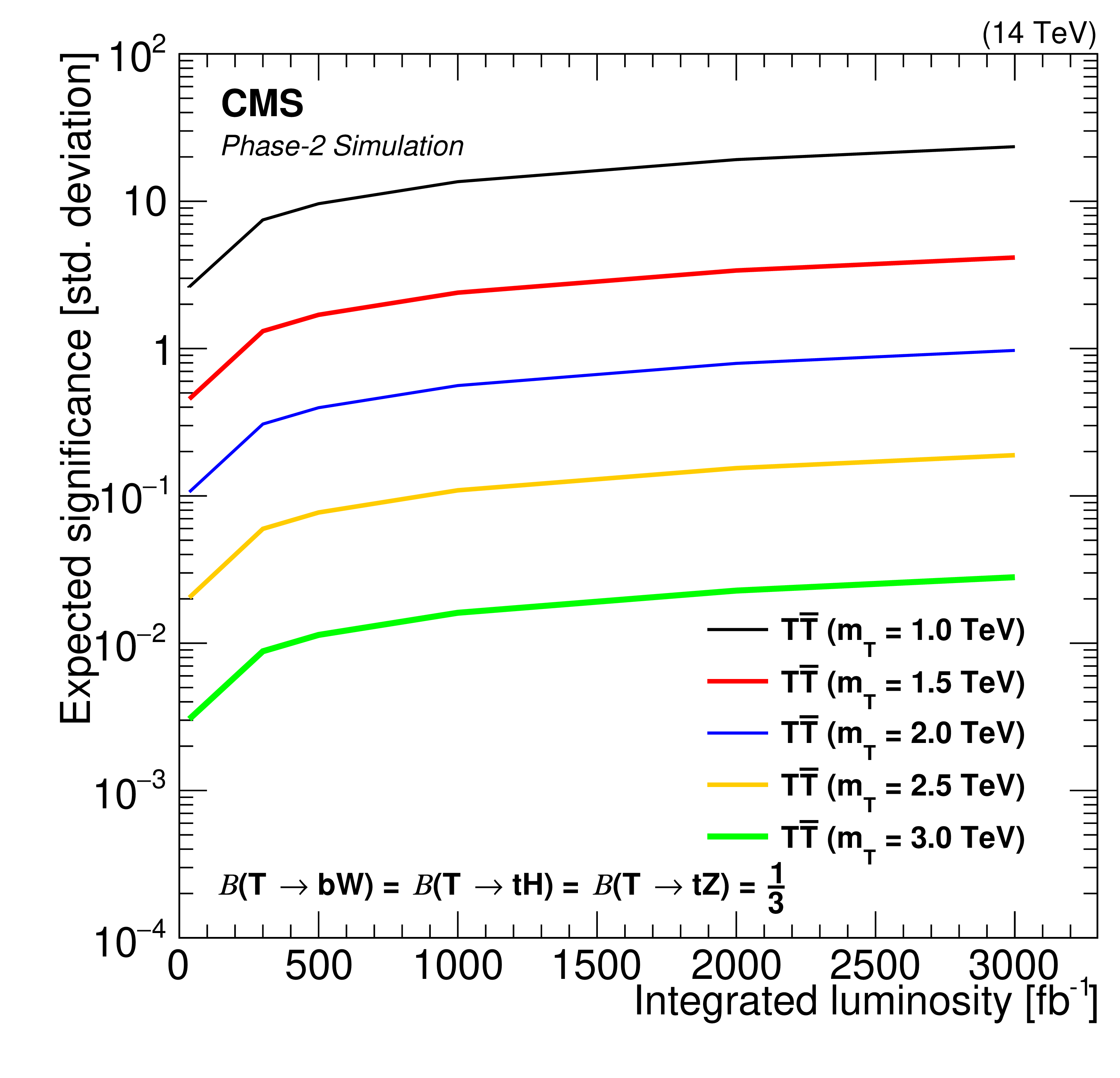
png pdf	Figure 46-a: Expected significances for T quark pair production as a function of the integrated luminosity at the HL-LHC, assuming equal branching fractions for ${\mathrm{T}} \to\mathrm{b}\mathrm{W}$, $\mathrm{t}\mathrm{Z}$, $\mathrm{t}\mathrm{H}$ decays (left). Discovery potential at three and five standard deviations for T quark pairs, as a function of the T quark mass and the integrated luminosity (right). Figures adapted from Ref. [170].
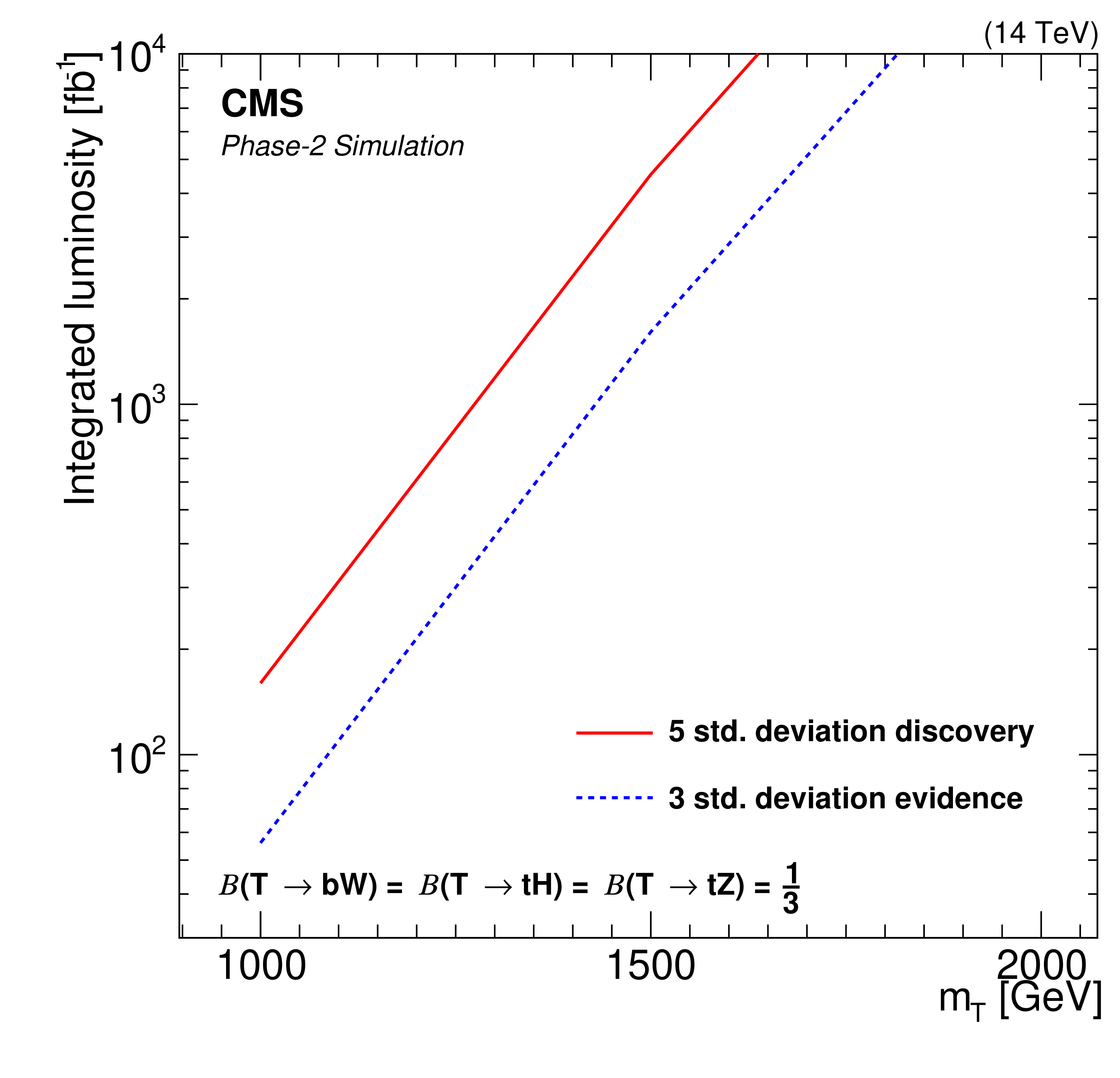
png pdf	Figure 46-b: Expected significances for T quark pair production as a function of the integrated luminosity at the HL-LHC, assuming equal branching fractions for ${\mathrm{T}} \to\mathrm{b}\mathrm{W}$, $\mathrm{t}\mathrm{Z}$, $\mathrm{t}\mathrm{H}$ decays (left). Discovery potential at three and five standard deviations for T quark pairs, as a function of the T quark mass and the integrated luminosity (right). Figures adapted from Ref. [170].
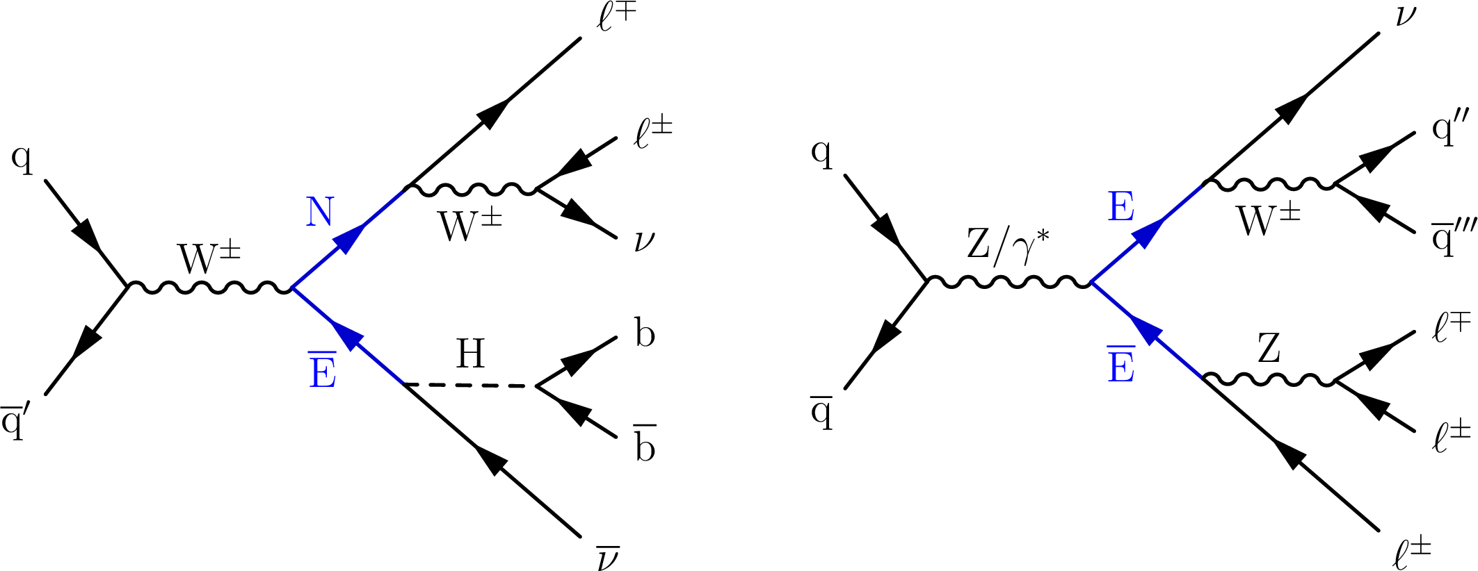
png pdf	Figure 47: Example processes illustrating production and decay of doublet (left) and singlet (right) VLL pairs at the LHC that result in multilepton final states.
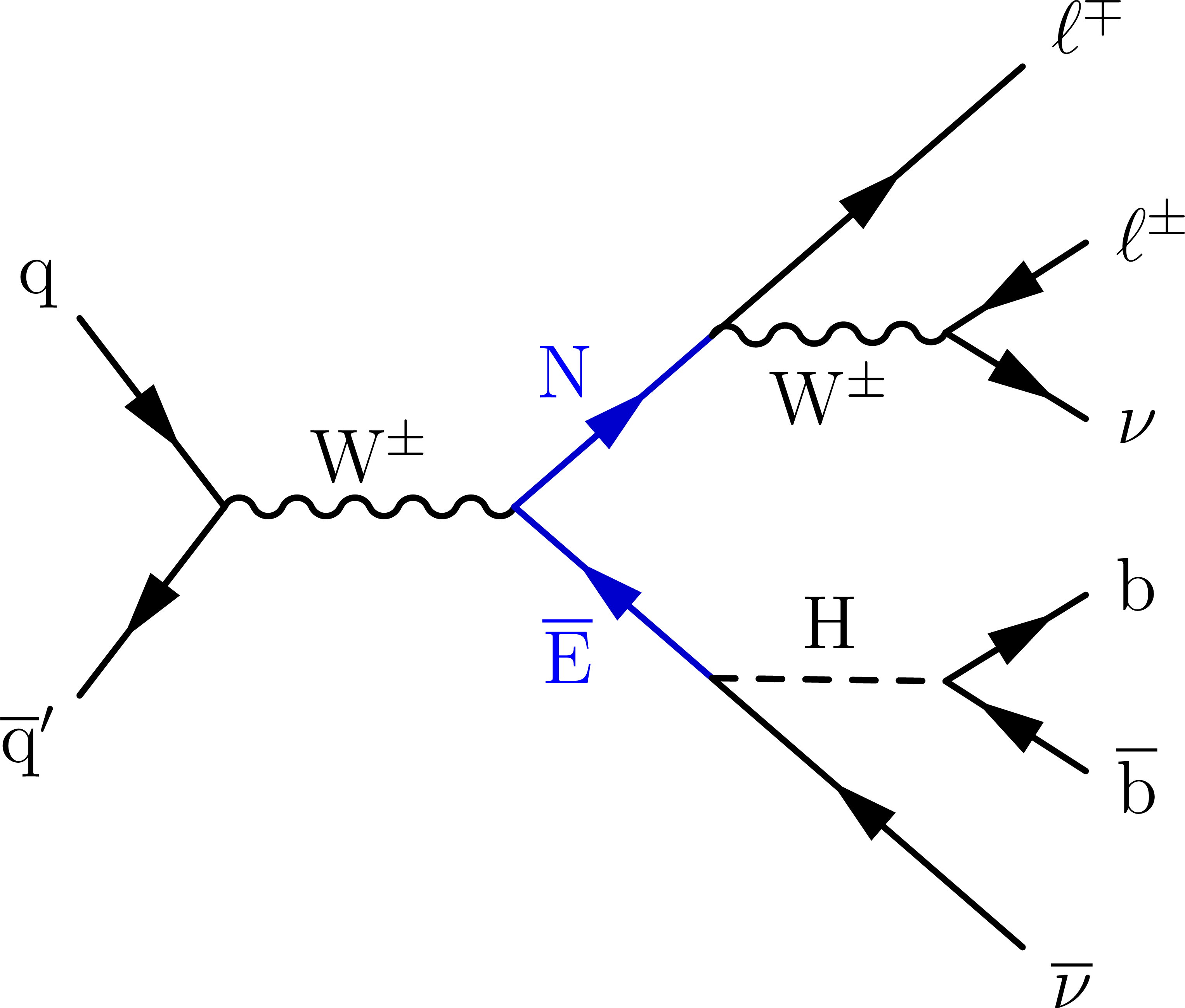
png pdf	Figure 47-a: Example processes illustrating production and decay of doublet (left) and singlet (right) VLL pairs at the LHC that result in multilepton final states.
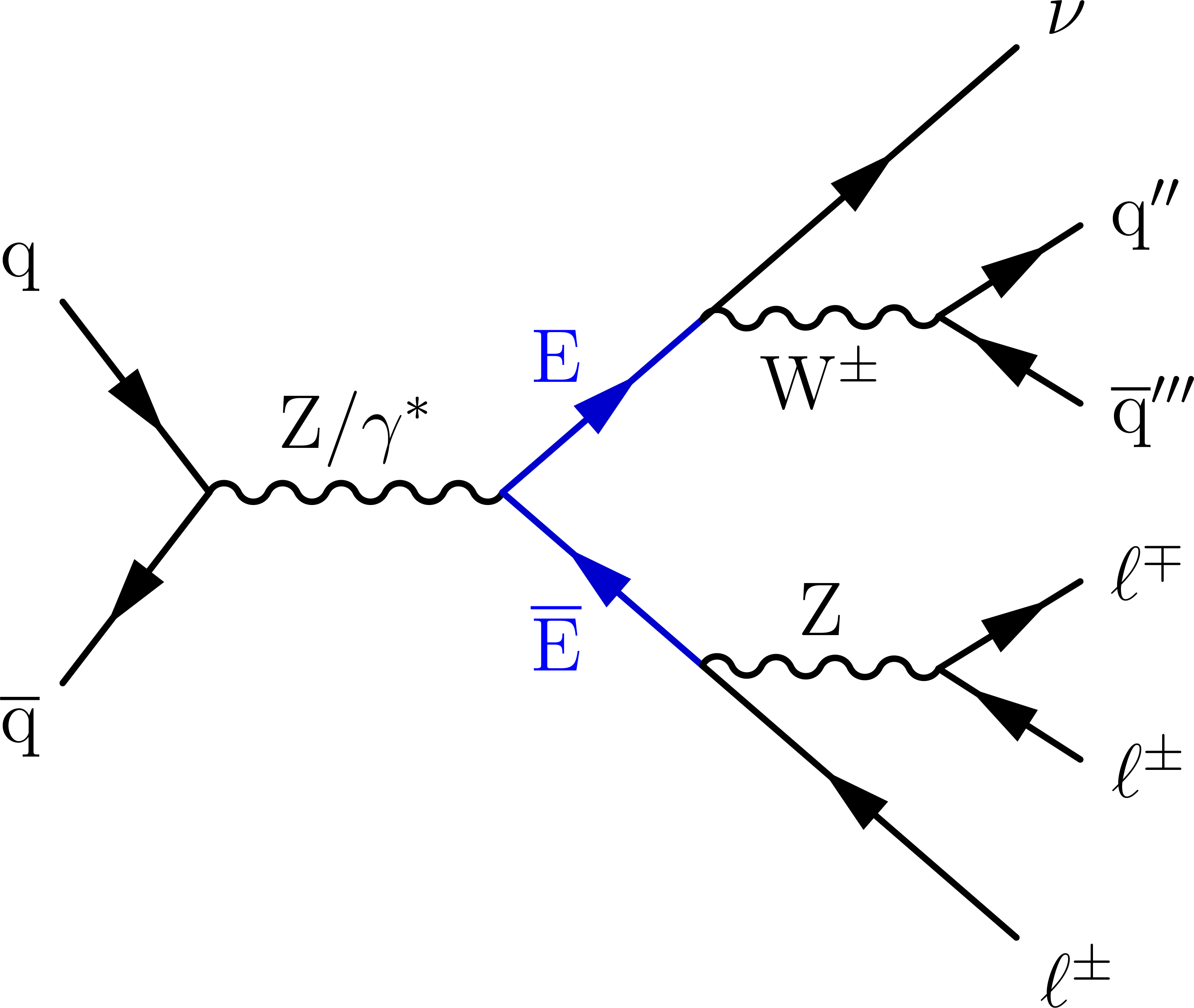
png pdf	Figure 47-b: Example processes illustrating production and decay of doublet (left) and singlet (right) VLL pairs at the LHC that result in multilepton final states.
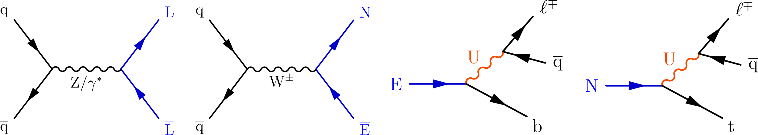
png pdf	Figure 48: Example diagrams showing $s$-channel EW production of VLL pairs through SM bosons, as expected at the LHC (left two diagrams). In these diagrams, L represents either the neutral VLL, N, or the charged VLL, E. The VLL decays are mediated by a vector leptoquark U (right two diagrams). In the 4321 model, these decays are primarily to third-generation leptons and quarks.
png pdf	Figure 48-a: Example diagrams showing $s$-channel EW production of VLL pairs through SM bosons, as expected at the LHC (left two diagrams). In these diagrams, L represents either the neutral VLL, N, or the charged VLL, E. The VLL decays are mediated by a vector leptoquark U (right two diagrams). In the 4321 model, these decays are primarily to third-generation leptons and quarks.
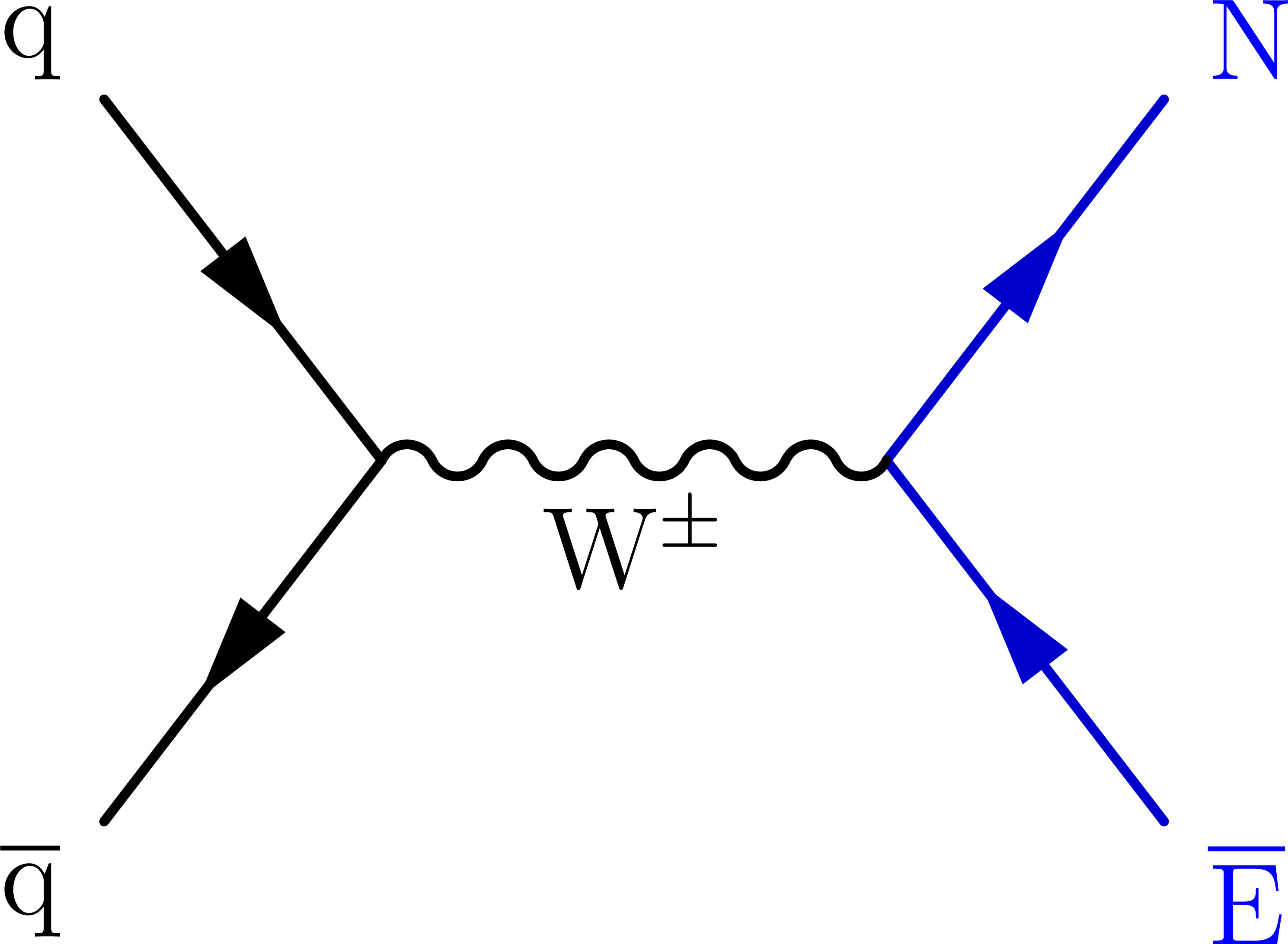
png pdf	Figure 48-b: Example diagrams showing $s$-channel EW production of VLL pairs through SM bosons, as expected at the LHC (left two diagrams). In these diagrams, L represents either the neutral VLL, N, or the charged VLL, E. The VLL decays are mediated by a vector leptoquark U (right two diagrams). In the 4321 model, these decays are primarily to third-generation leptons and quarks.
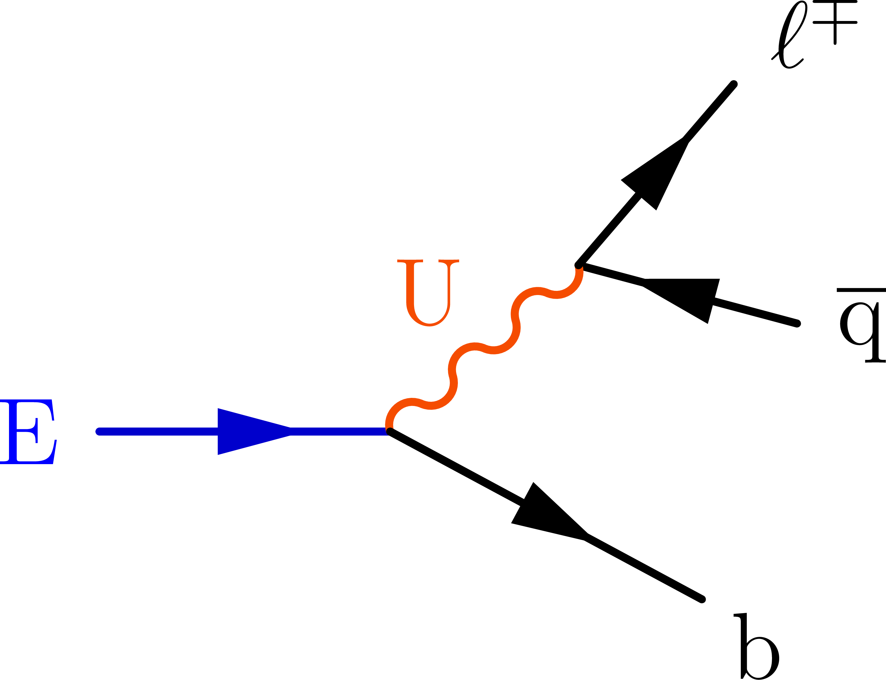
png pdf	Figure 48-c: Example diagrams showing $s$-channel EW production of VLL pairs through SM bosons, as expected at the LHC (left two diagrams). In these diagrams, L represents either the neutral VLL, N, or the charged VLL, E. The VLL decays are mediated by a vector leptoquark U (right two diagrams). In the 4321 model, these decays are primarily to third-generation leptons and quarks.
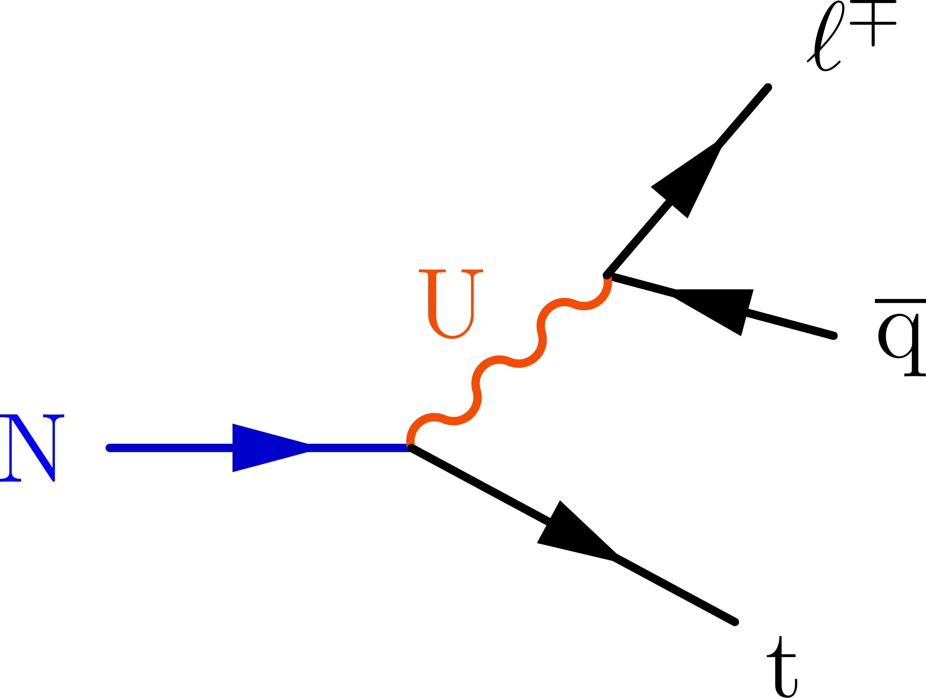
png pdf	Figure 48-d: Example diagrams showing $s$-channel EW production of VLL pairs through SM bosons, as expected at the LHC (left two diagrams). In these diagrams, L represents either the neutral VLL, N, or the charged VLL, E. The VLL decays are mediated by a vector leptoquark U (right two diagrams). In the 4321 model, these decays are primarily to third-generation leptons and quarks.
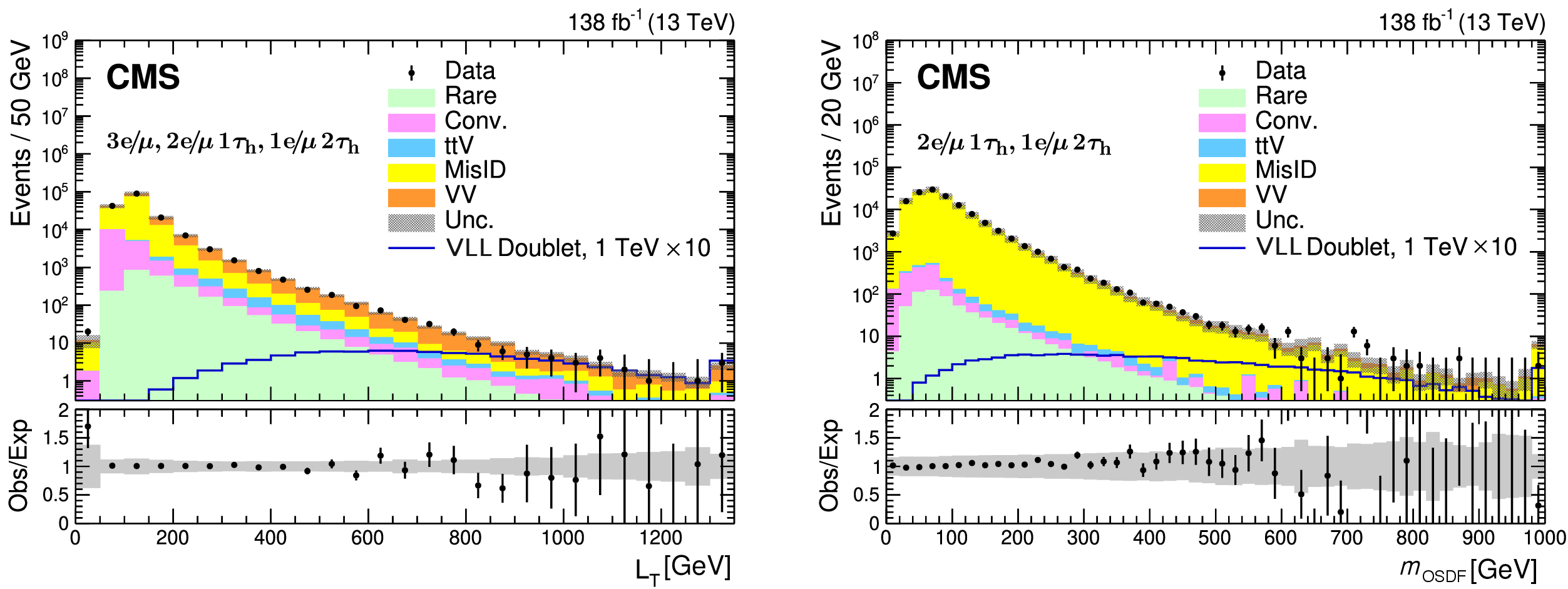
png pdf	Figure 49: The $L_{\mathrm{T}}$ distribution in 3$\mkern1mu\mathrm{e}\mkern-2mu/\mkern-3mu\mu$, 2 $\mkern1mu\mathrm{e}\mkern-2mu/\mkern-3mu\mu1\tau_\mathrm{h}$, and 1 $\mkern1mu\mathrm{e}\mkern-2mu/\mkern-3mu\mu2\tau_\mathrm{h}$ events (left), and the invariant mass distribution of the OS different-flavor ($m_{\text{OSDF}}$) light lepton and tau lepton pair in 2 $\mkern1mu\mathrm{e}\mkern-2mu/\mkern-3mu\mu1\tau_\mathrm{h}$ and 1 $\mkern1mu\mathrm{e}\mkern-2mu/\mkern-3mu\mu2\tau_\mathrm{h}$ events (right). The rightmost bin contains the overflow events. The lower panel shows the ratio of observed events to the total expected background prediction. The gray band on the ratio represents the quadratic sum of statistical and systematic uncertainties in the SM background prediction. The expected SM background distributions and the uncertainties are shown after fitting the data under the background-only hypothesis. For illustration, an example signal hypothesis for the production of vector-like leptons coupled to third-generation SM leptons in the doublet scenario for a VLL mass of 1 TeV, before the fit, is overlaid. The signal yield is scaled by a factor of 10 for visualization purposes. Figures adapted from Ref. [204].
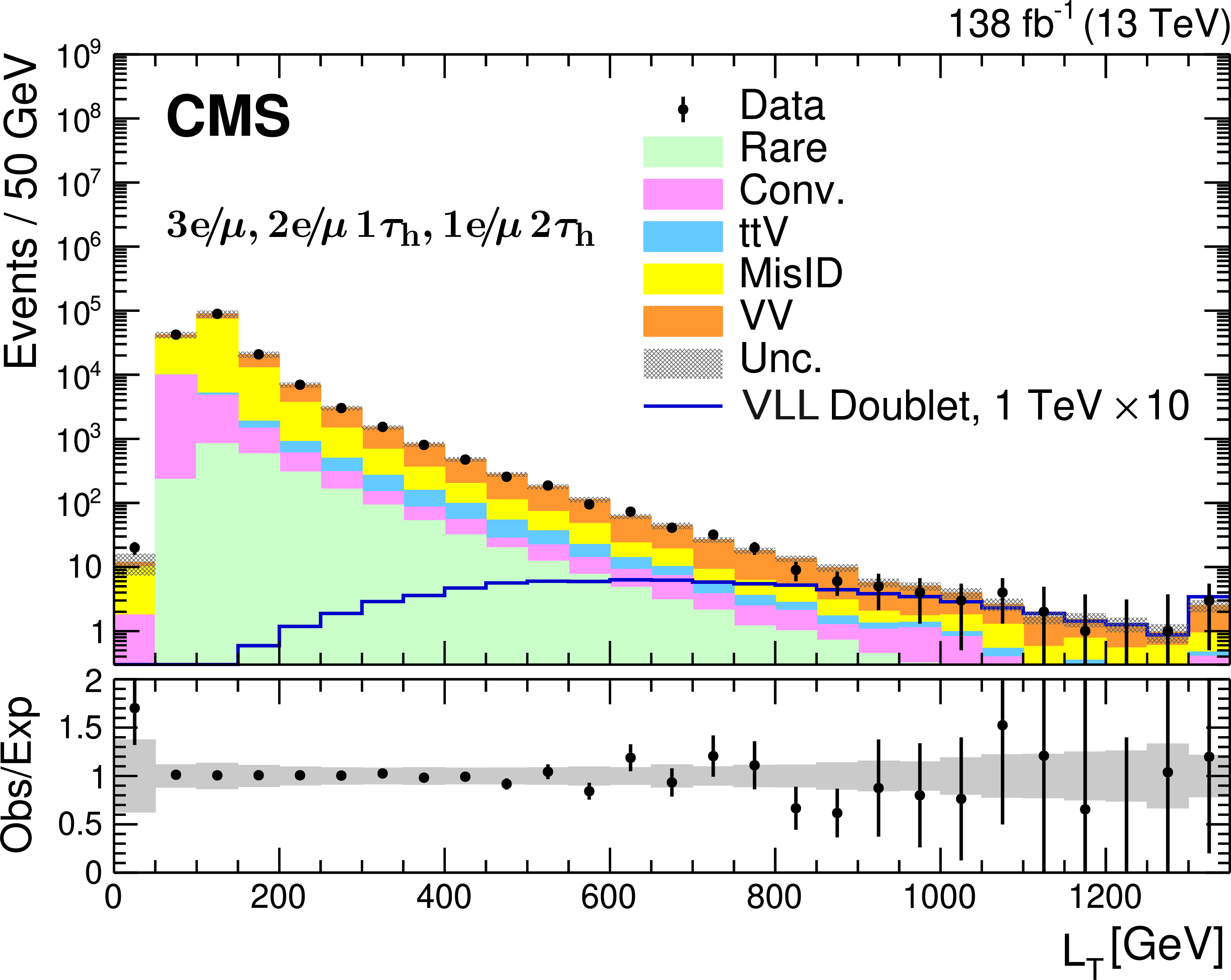
png pdf	Figure 49-a: The $L_{\mathrm{T}}$ distribution in 3$\mkern1mu\mathrm{e}\mkern-2mu/\mkern-3mu\mu$, 2 $\mkern1mu\mathrm{e}\mkern-2mu/\mkern-3mu\mu1\tau_\mathrm{h}$, and 1 $\mkern1mu\mathrm{e}\mkern-2mu/\mkern-3mu\mu2\tau_\mathrm{h}$ events (left), and the invariant mass distribution of the OS different-flavor ($m_{\text{OSDF}}$) light lepton and tau lepton pair in 2 $\mkern1mu\mathrm{e}\mkern-2mu/\mkern-3mu\mu1\tau_\mathrm{h}$ and 1 $\mkern1mu\mathrm{e}\mkern-2mu/\mkern-3mu\mu2\tau_\mathrm{h}$ events (right). The rightmost bin contains the overflow events. The lower panel shows the ratio of observed events to the total expected background prediction. The gray band on the ratio represents the quadratic sum of statistical and systematic uncertainties in the SM background prediction. The expected SM background distributions and the uncertainties are shown after fitting the data under the background-only hypothesis. For illustration, an example signal hypothesis for the production of vector-like leptons coupled to third-generation SM leptons in the doublet scenario for a VLL mass of 1 TeV, before the fit, is overlaid. The signal yield is scaled by a factor of 10 for visualization purposes. Figures adapted from Ref. [204].
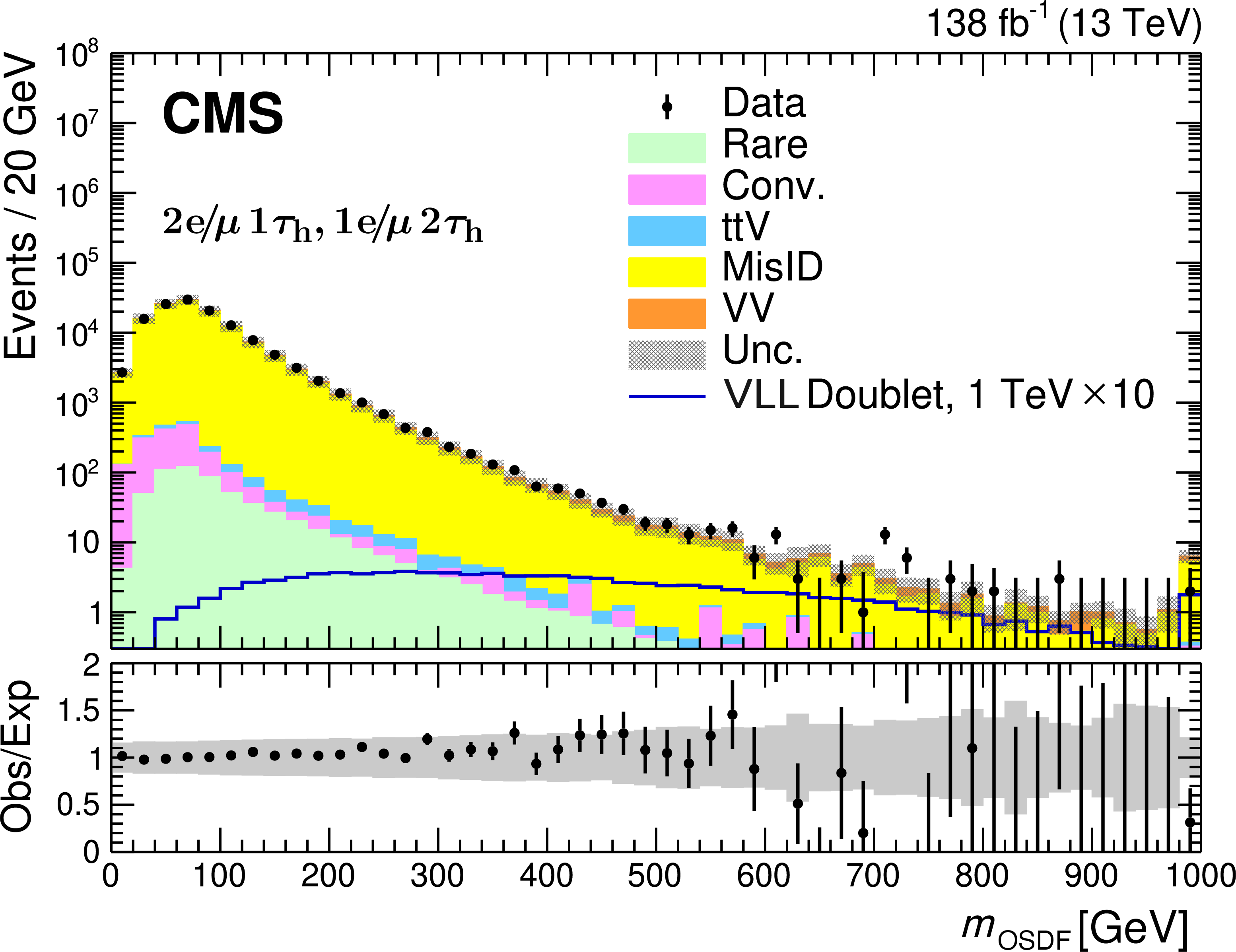
png pdf	Figure 49-b: The $L_{\mathrm{T}}$ distribution in 3$\mkern1mu\mathrm{e}\mkern-2mu/\mkern-3mu\mu$, 2 $\mkern1mu\mathrm{e}\mkern-2mu/\mkern-3mu\mu1\tau_\mathrm{h}$, and 1 $\mkern1mu\mathrm{e}\mkern-2mu/\mkern-3mu\mu2\tau_\mathrm{h}$ events (left), and the invariant mass distribution of the OS different-flavor ($m_{\text{OSDF}}$) light lepton and tau lepton pair in 2 $\mkern1mu\mathrm{e}\mkern-2mu/\mkern-3mu\mu1\tau_\mathrm{h}$ and 1 $\mkern1mu\mathrm{e}\mkern-2mu/\mkern-3mu\mu2\tau_\mathrm{h}$ events (right). The rightmost bin contains the overflow events. The lower panel shows the ratio of observed events to the total expected background prediction. The gray band on the ratio represents the quadratic sum of statistical and systematic uncertainties in the SM background prediction. The expected SM background distributions and the uncertainties are shown after fitting the data under the background-only hypothesis. For illustration, an example signal hypothesis for the production of vector-like leptons coupled to third-generation SM leptons in the doublet scenario for a VLL mass of 1 TeV, before the fit, is overlaid. The signal yield is scaled by a factor of 10 for visualization purposes. Figures adapted from Ref. [204].
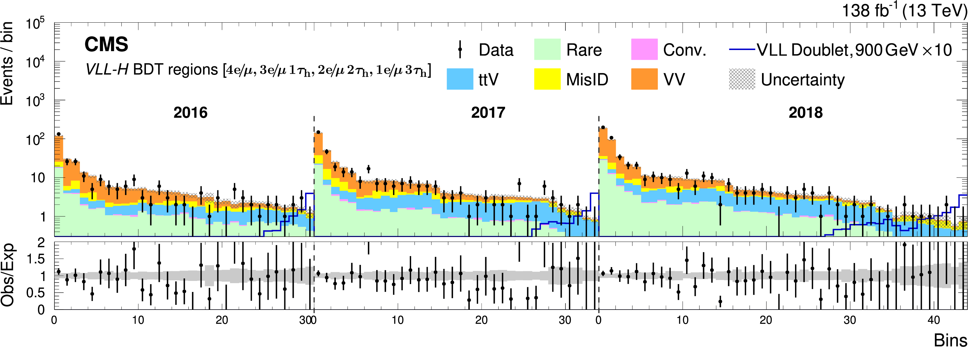
png pdf	Figure 50: The \textitVLL-H BDT regions for the four-lepton channels for the full Run 2 data set. The lower panel shows the ratio of observed events to the total expected background prediction. The gray band on the ratio represents the quadratic sum of statistical and systematic uncertainties in the SM background prediction. The expected SM background distributions and the uncertainties are shown after fitting the data under the background-only hypothesis. For illustration, an example signal hypothesis for the production of the vector-like leptons coupled to the third generation SM leptons in the doublet scenario for a VLL mass of 900 GeV, before the fit, is overlaid. The signal yield is scaled by a factor of 10 for visualization purposes. Figure adapted from Ref. [204].
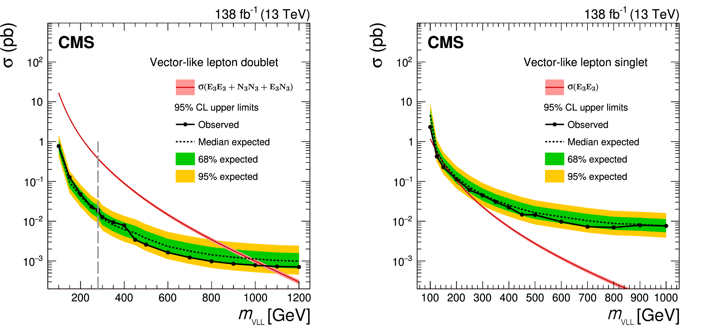
png pdf	Figure 51: Observed and expected upper limits at 95% CL on the production cross section for the vector-like leptons coupled to third-generation SM leptons in the doublet model (left) and singlet model (right). For the doublet vector-like lepton model, to the left of the vertical dashed gray line, the limits are shown from the model-independent scheme, while to the right the limits are shown from the model dependent BDT regions. For the singlet vector-like lepton model, the limit is shown from the model-independent scheme for all masses. Figures adapted from Ref. [204].
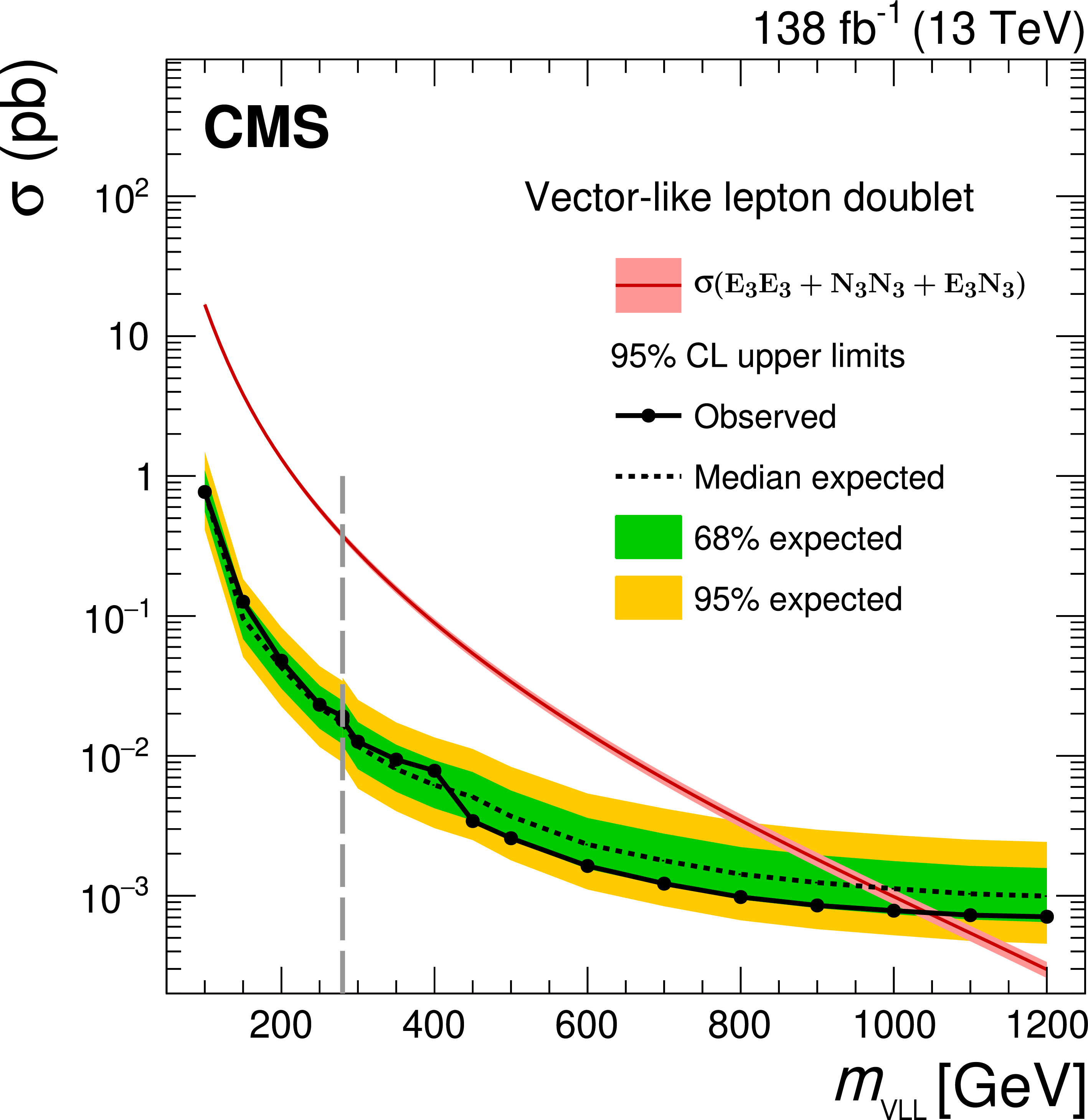
png pdf	Figure 51-a: Observed and expected upper limits at 95% CL on the production cross section for the vector-like leptons coupled to third-generation SM leptons in the doublet model (left) and singlet model (right). For the doublet vector-like lepton model, to the left of the vertical dashed gray line, the limits are shown from the model-independent scheme, while to the right the limits are shown from the model dependent BDT regions. For the singlet vector-like lepton model, the limit is shown from the model-independent scheme for all masses. Figures adapted from Ref. [204].
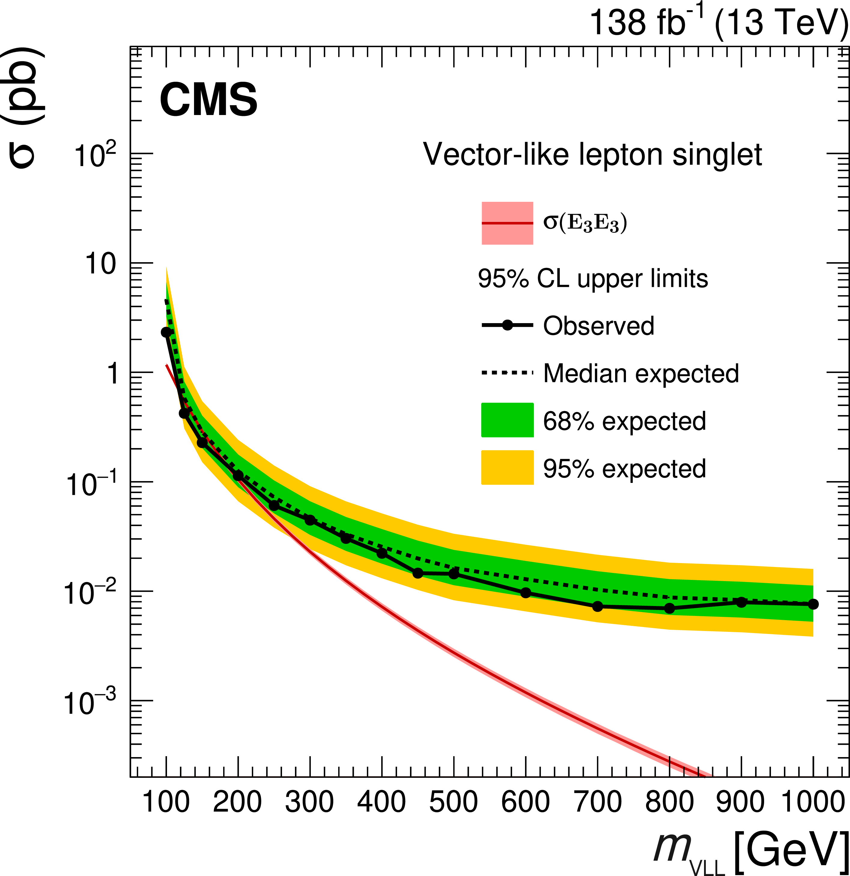
png pdf	Figure 51-b: Observed and expected upper limits at 95% CL on the production cross section for the vector-like leptons coupled to third-generation SM leptons in the doublet model (left) and singlet model (right). For the doublet vector-like lepton model, to the left of the vertical dashed gray line, the limits are shown from the model-independent scheme, while to the right the limits are shown from the model dependent BDT regions. For the singlet vector-like lepton model, the limit is shown from the model-independent scheme for all masses. Figures adapted from Ref. [204].
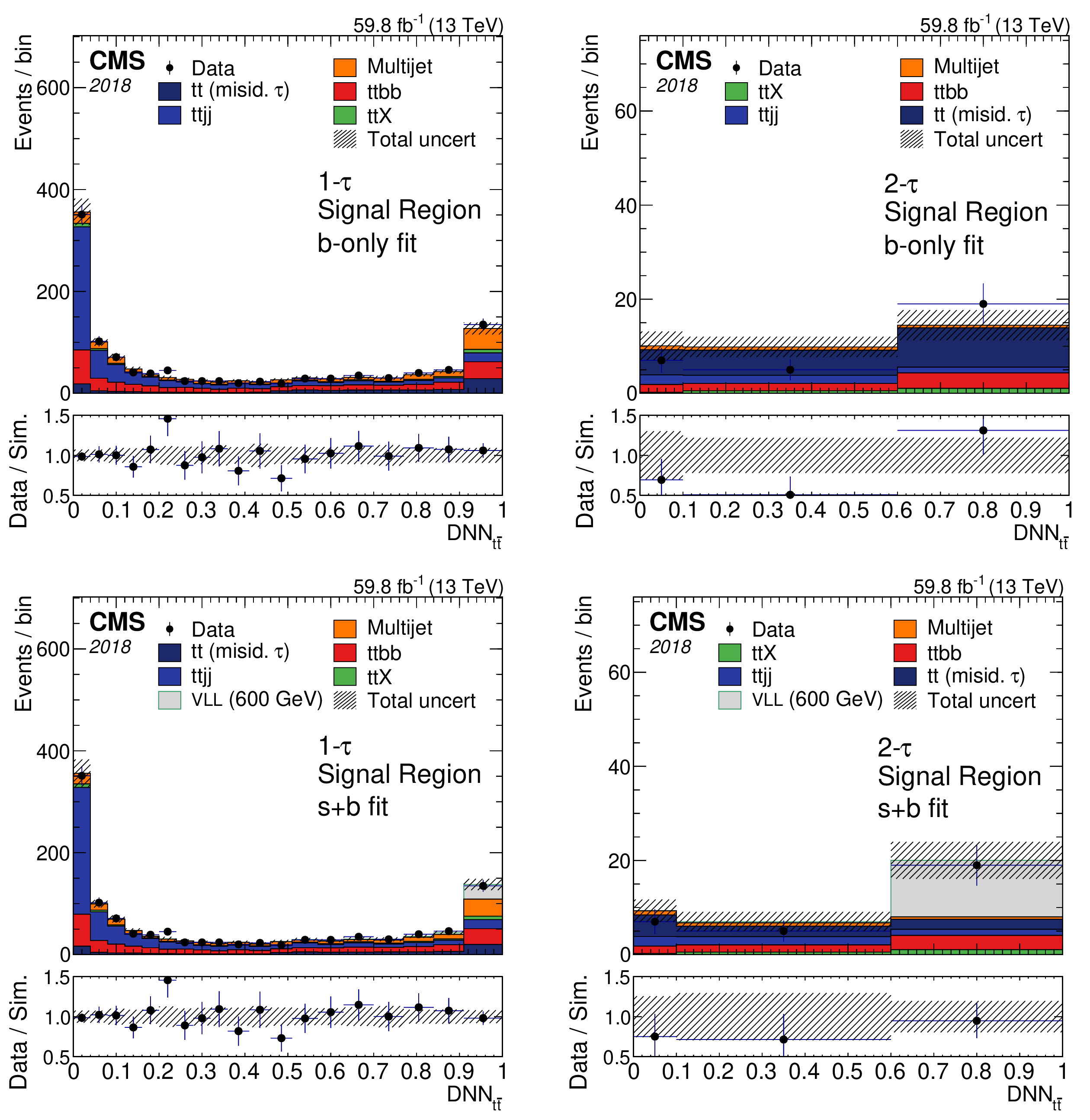
png pdf	Figure 52: Postfit distributions for the 2018 data set in the 1$\tau_\mathrm{h}$ (left) and 2$\tau_\mathrm{h}$ (right) channels. The upper row shows the background-only fit and the lower row shows the fit including the signal. Not shown here, but included in the fit, are the 2017 data and the 0$\tau_\mathrm{h}$ channel. Figures taken from Ref. [205].
png pdf	Figure 52-a: Postfit distributions for the 2018 data set in the 1$\tau_\mathrm{h}$ (left) and 2$\tau_\mathrm{h}$ (right) channels. The upper row shows the background-only fit and the lower row shows the fit including the signal. Not shown here, but included in the fit, are the 2017 data and the 0$\tau_\mathrm{h}$ channel. Figures taken from Ref. [205].
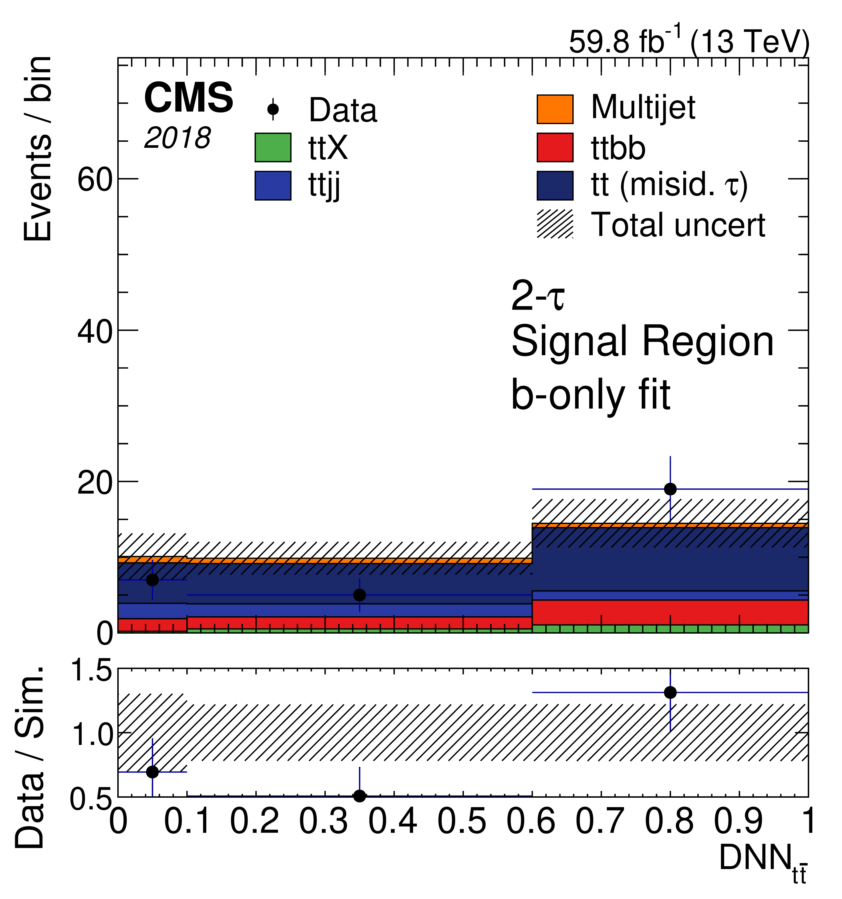
png pdf	Figure 52-b: Postfit distributions for the 2018 data set in the 1$\tau_\mathrm{h}$ (left) and 2$\tau_\mathrm{h}$ (right) channels. The upper row shows the background-only fit and the lower row shows the fit including the signal. Not shown here, but included in the fit, are the 2017 data and the 0$\tau_\mathrm{h}$ channel. Figures taken from Ref. [205].
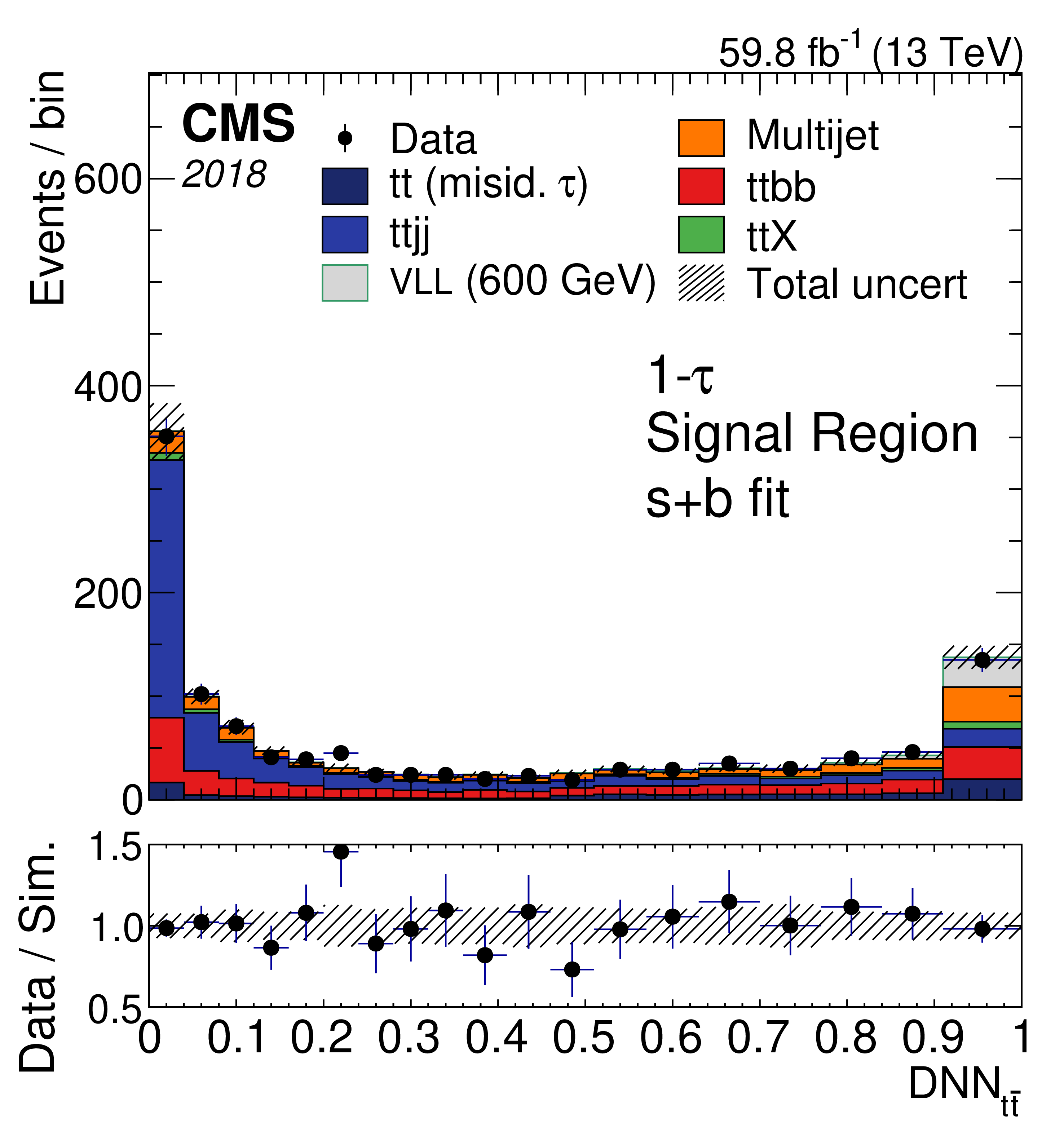
png pdf	Figure 52-c: Postfit distributions for the 2018 data set in the 1$\tau_\mathrm{h}$ (left) and 2$\tau_\mathrm{h}$ (right) channels. The upper row shows the background-only fit and the lower row shows the fit including the signal. Not shown here, but included in the fit, are the 2017 data and the 0$\tau_\mathrm{h}$ channel. Figures taken from Ref. [205].
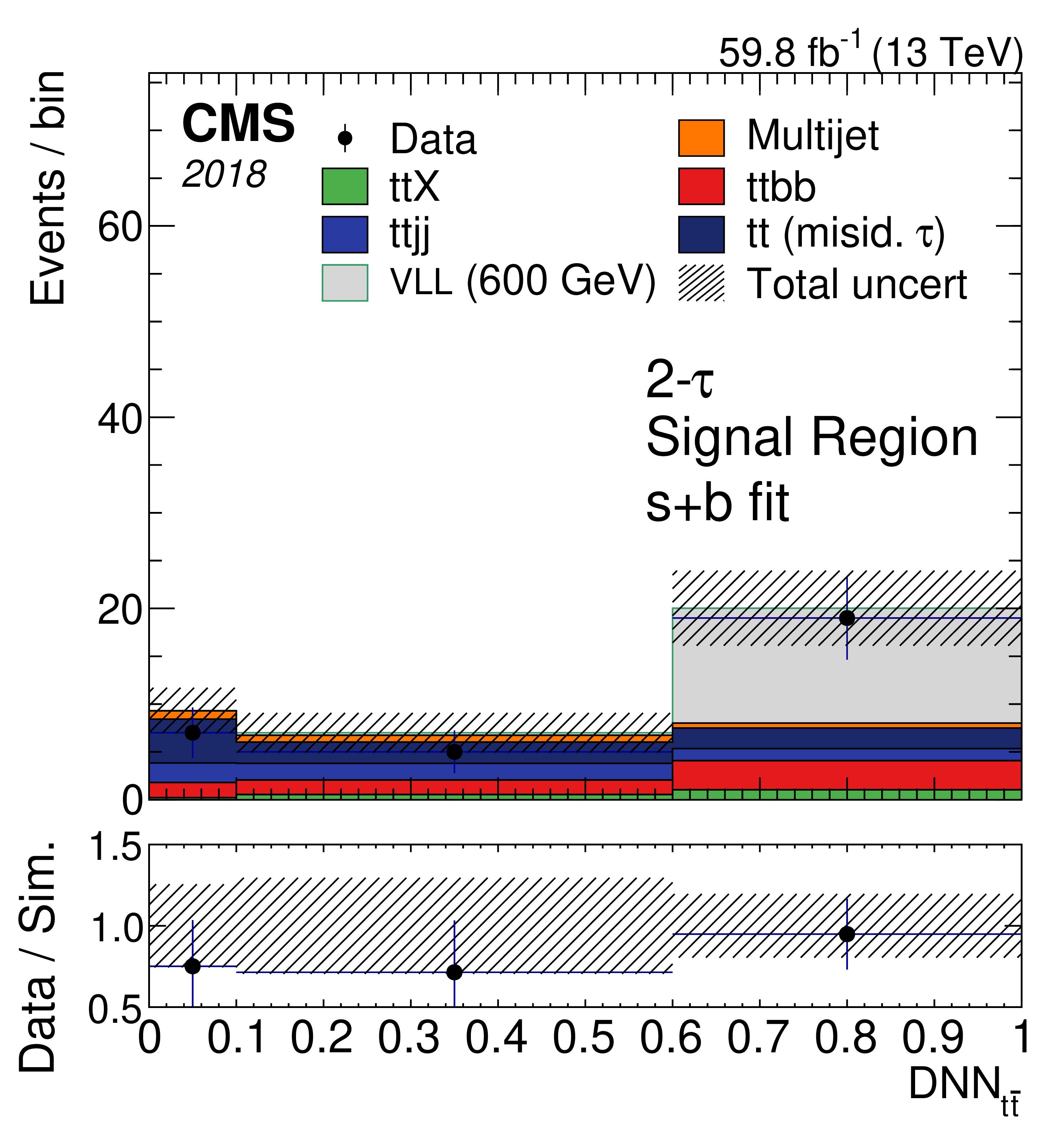
png pdf	Figure 52-d: Postfit distributions for the 2018 data set in the 1$\tau_\mathrm{h}$ (left) and 2$\tau_\mathrm{h}$ (right) channels. The upper row shows the background-only fit and the lower row shows the fit including the signal. Not shown here, but included in the fit, are the 2017 data and the 0$\tau_\mathrm{h}$ channel. Figures taken from Ref. [205].
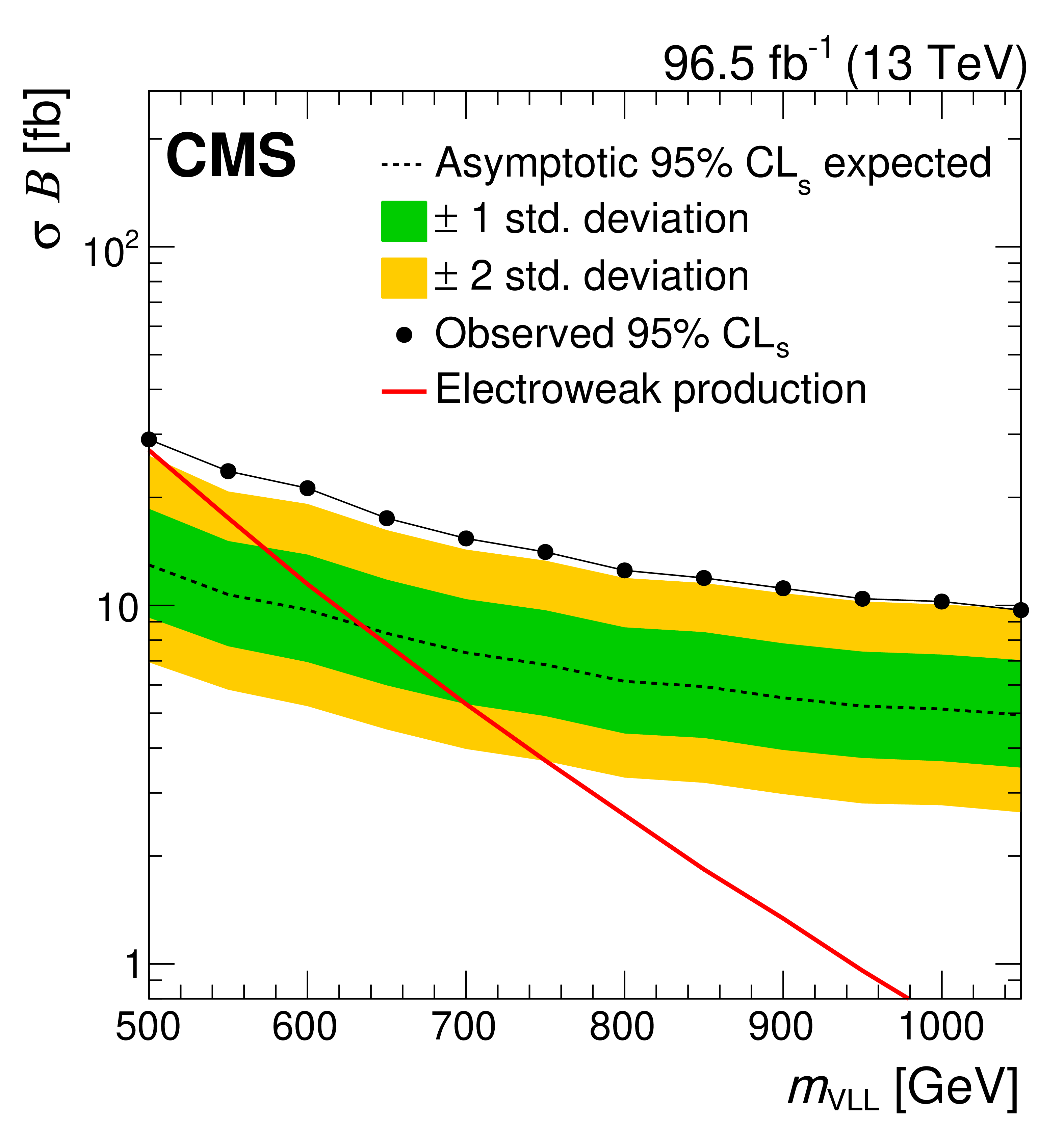
png pdf	Figure 53: Expected and observed 95% CL upper limits on the product of the VLL pair production cross section and the branching fraction to third-generation quarks and leptons, combining the 2017 and 2018 data and all $\tau_\mathrm{h}$ multiplicity channels. The theoretical prediction in the 4321 model for EW production of VLLs is also shown. Figure adapted from Ref. [205].
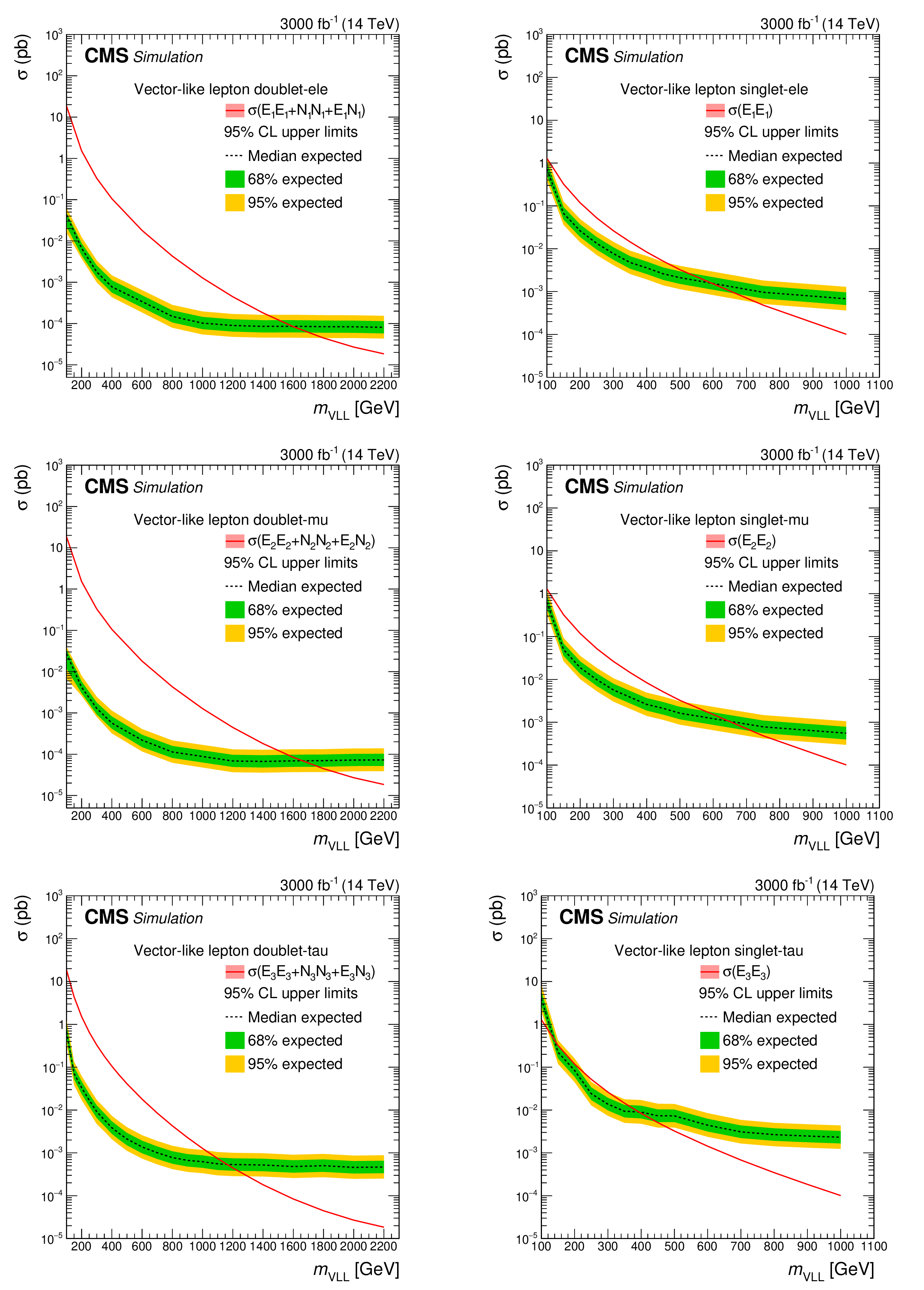
png pdf	Figure 54: Expected HL-LHC exclusion limits for vector-like leptons coupled to first-generation (upper row), second-generation (middle row), and third-generation SM leptons (lower row) in the doublet model (left) and the singlet model (right). For both models, limits are calculated using $L_{\mathrm{T}}+p_{\mathrm{T}}^\text{miss}$ from the model independent SRs for all masses.
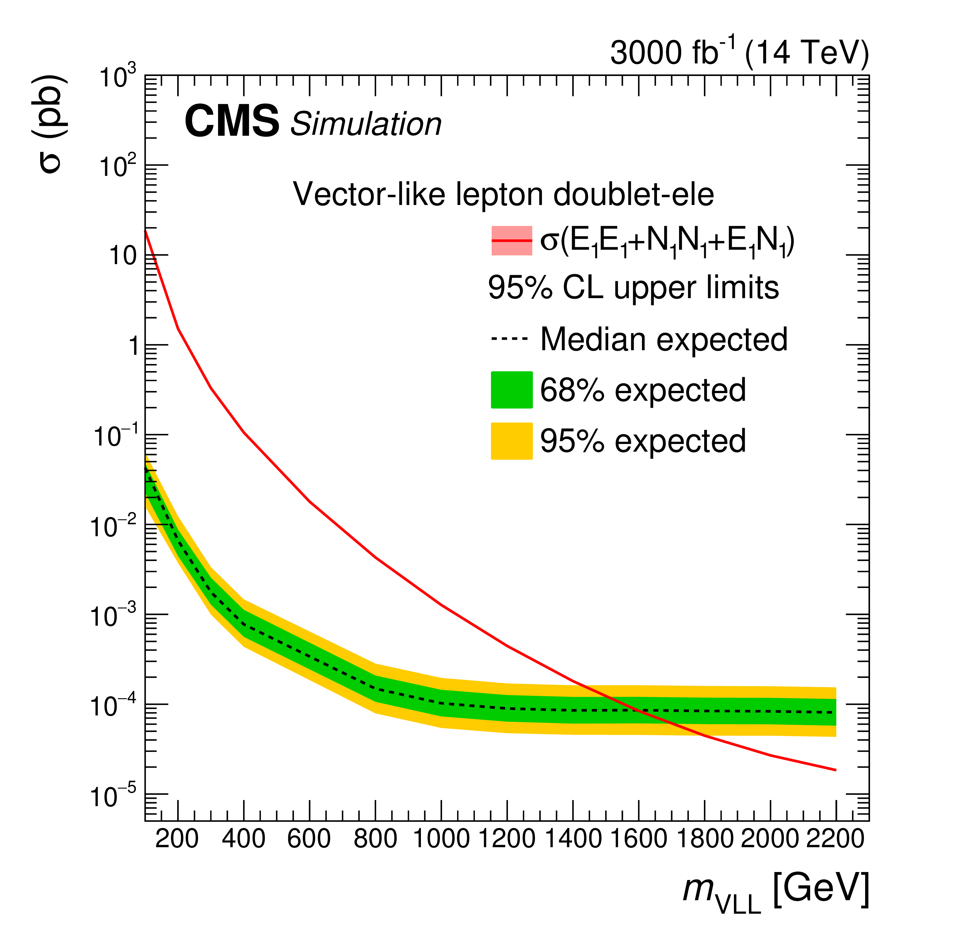
png pdf	Figure 54-a: Expected HL-LHC exclusion limits for vector-like leptons coupled to first-generation (upper row), second-generation (middle row), and third-generation SM leptons (lower row) in the doublet model (left) and the singlet model (right). For both models, limits are calculated using $L_{\mathrm{T}}+p_{\mathrm{T}}^\text{miss}$ from the model independent SRs for all masses.
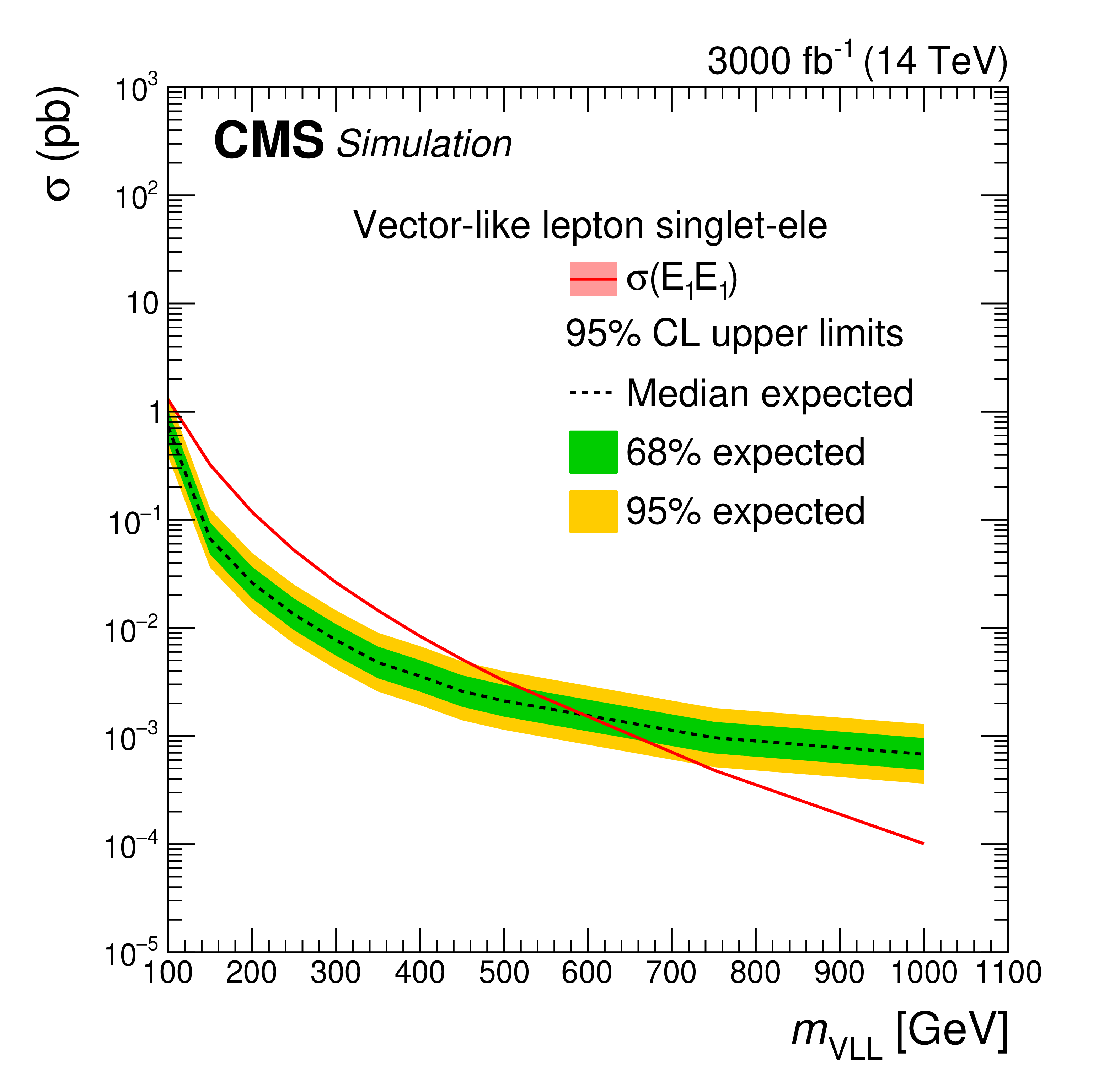
png pdf	Figure 54-b: Expected HL-LHC exclusion limits for vector-like leptons coupled to first-generation (upper row), second-generation (middle row), and third-generation SM leptons (lower row) in the doublet model (left) and the singlet model (right). For both models, limits are calculated using $L_{\mathrm{T}}+p_{\mathrm{T}}^\text{miss}$ from the model independent SRs for all masses.
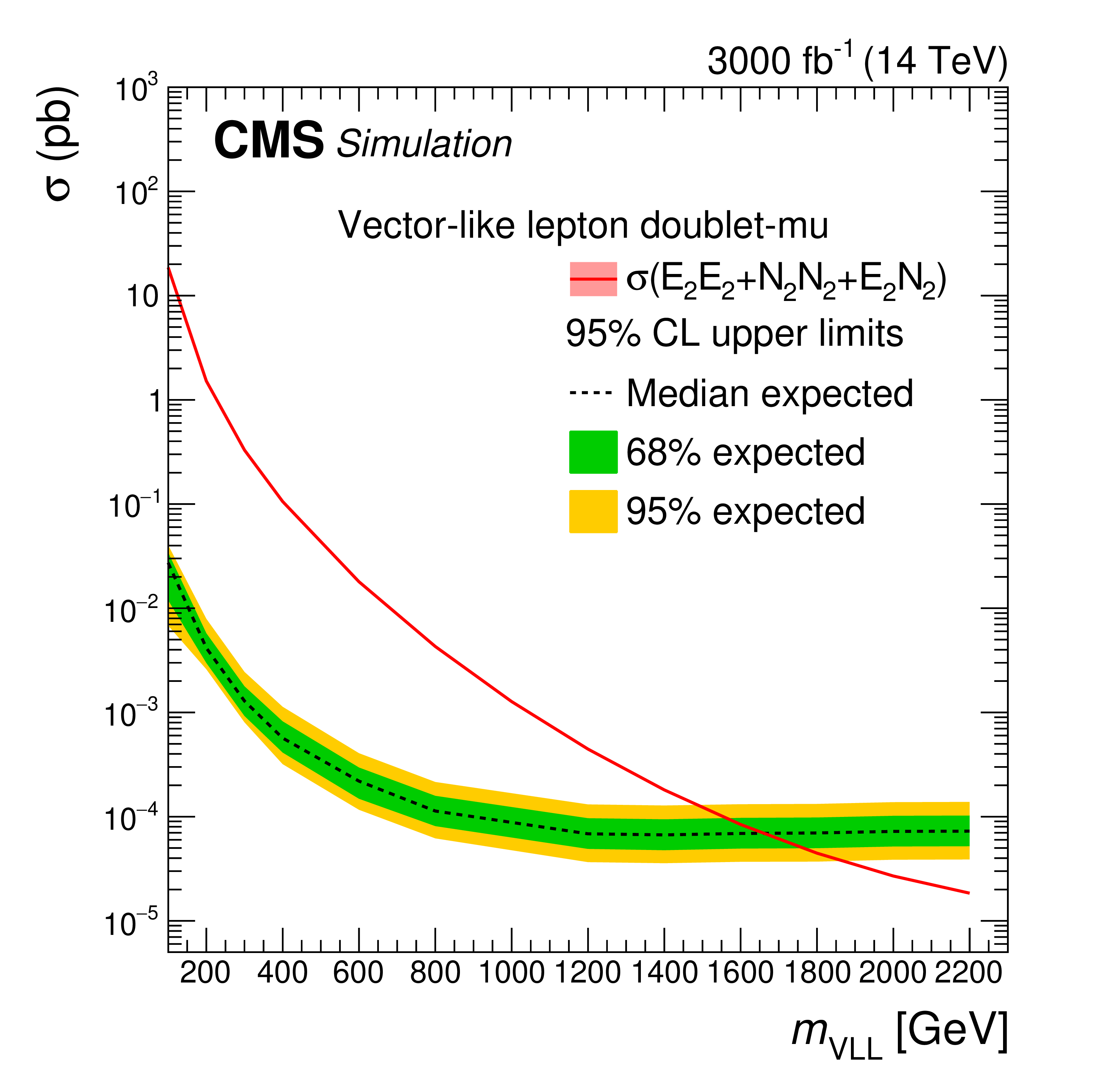
png pdf	Figure 54-c: Expected HL-LHC exclusion limits for vector-like leptons coupled to first-generation (upper row), second-generation (middle row), and third-generation SM leptons (lower row) in the doublet model (left) and the singlet model (right). For both models, limits are calculated using $L_{\mathrm{T}}+p_{\mathrm{T}}^\text{miss}$ from the model independent SRs for all masses.
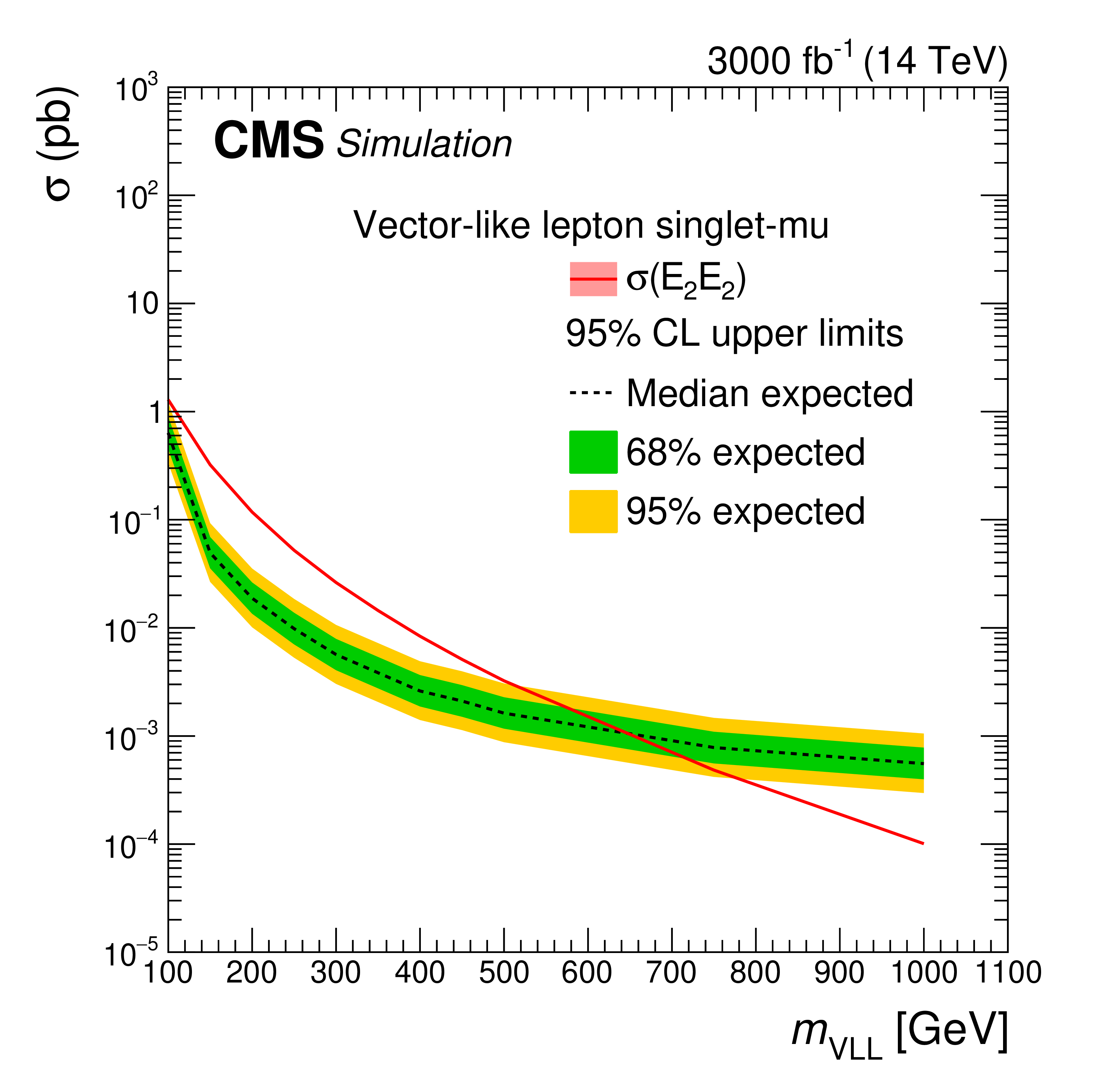
png pdf	Figure 54-d: Expected HL-LHC exclusion limits for vector-like leptons coupled to first-generation (upper row), second-generation (middle row), and third-generation SM leptons (lower row) in the doublet model (left) and the singlet model (right). For both models, limits are calculated using $L_{\mathrm{T}}+p_{\mathrm{T}}^\text{miss}$ from the model independent SRs for all masses.
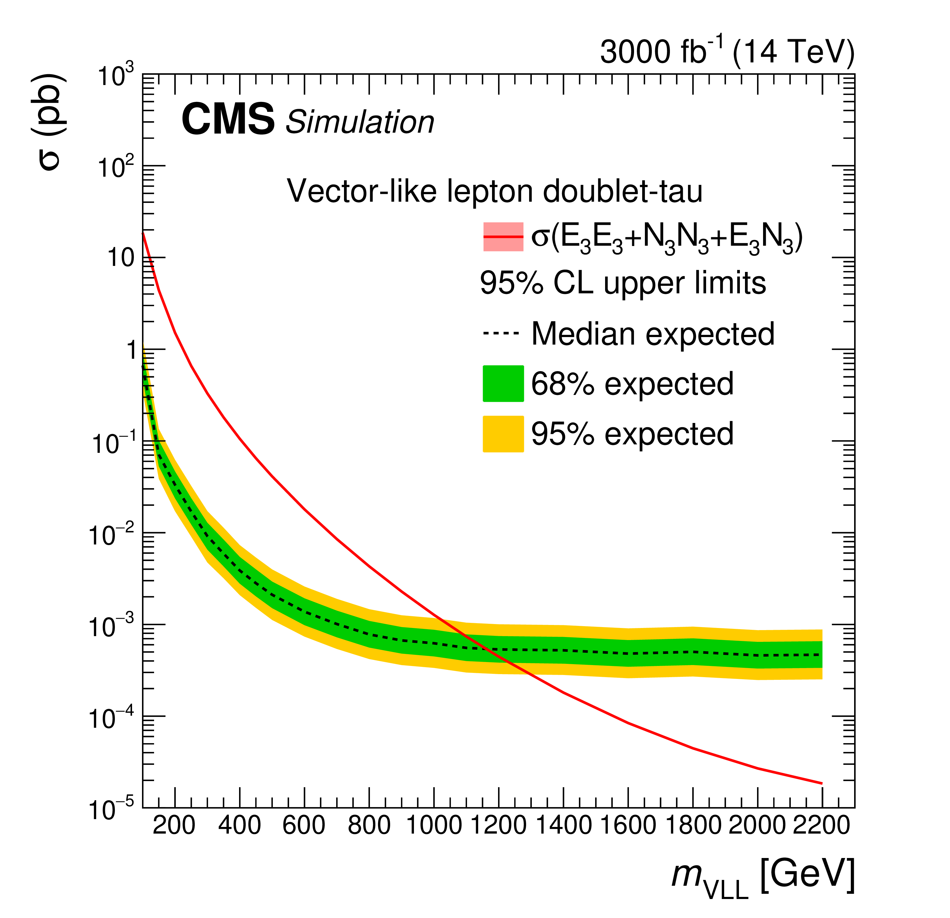
png pdf	Figure 54-e: Expected HL-LHC exclusion limits for vector-like leptons coupled to first-generation (upper row), second-generation (middle row), and third-generation SM leptons (lower row) in the doublet model (left) and the singlet model (right). For both models, limits are calculated using $L_{\mathrm{T}}+p_{\mathrm{T}}^\text{miss}$ from the model independent SRs for all masses.
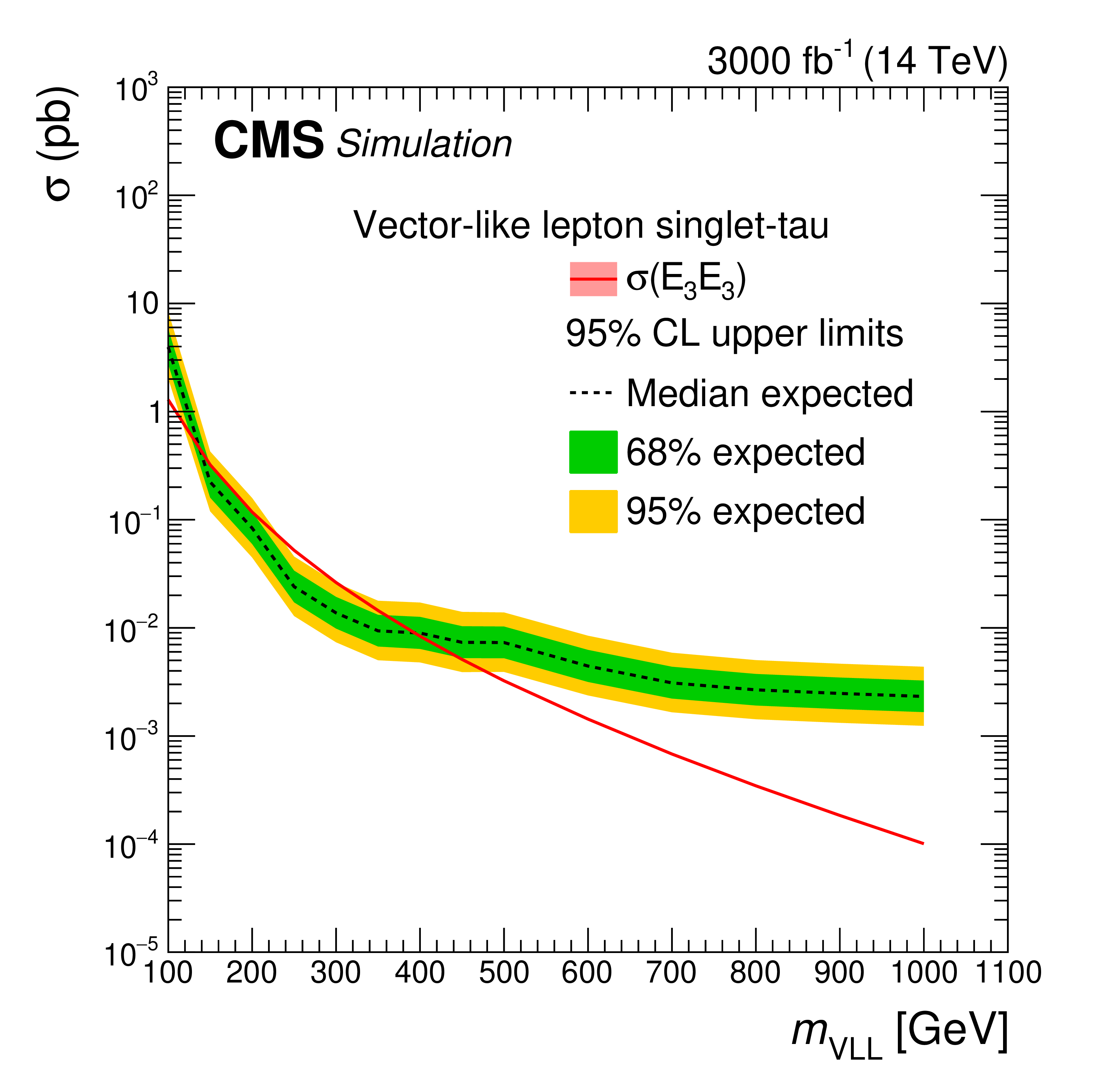
png pdf	Figure 54-f: Expected HL-LHC exclusion limits for vector-like leptons coupled to first-generation (upper row), second-generation (middle row), and third-generation SM leptons (lower row) in the doublet model (left) and the singlet model (right). For both models, limits are calculated using $L_{\mathrm{T}}+p_{\mathrm{T}}^\text{miss}$ from the model independent SRs for all masses.
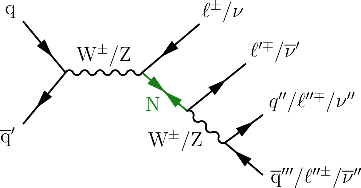
png pdf	Figure 55: Representative Feynman diagram of a Majorana HNL, labeled as $\mathrm{N}$, produced through the decay of a W or Z boson.
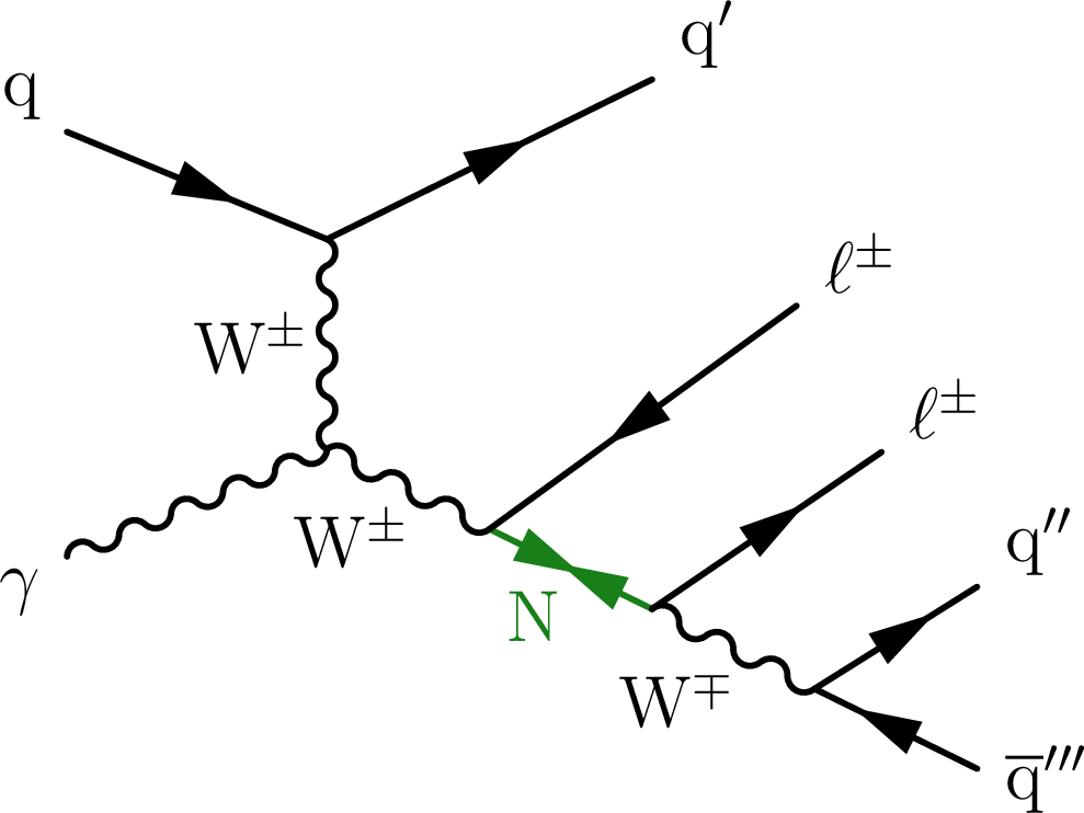
png pdf	Figure 56: Representative Feynman diagram of a Majorana HNL, labeled as $\mathrm{N}$, produced through the $\mathrm{W}\gamma$ fusion process and with two charged leptons and jets in the final state.
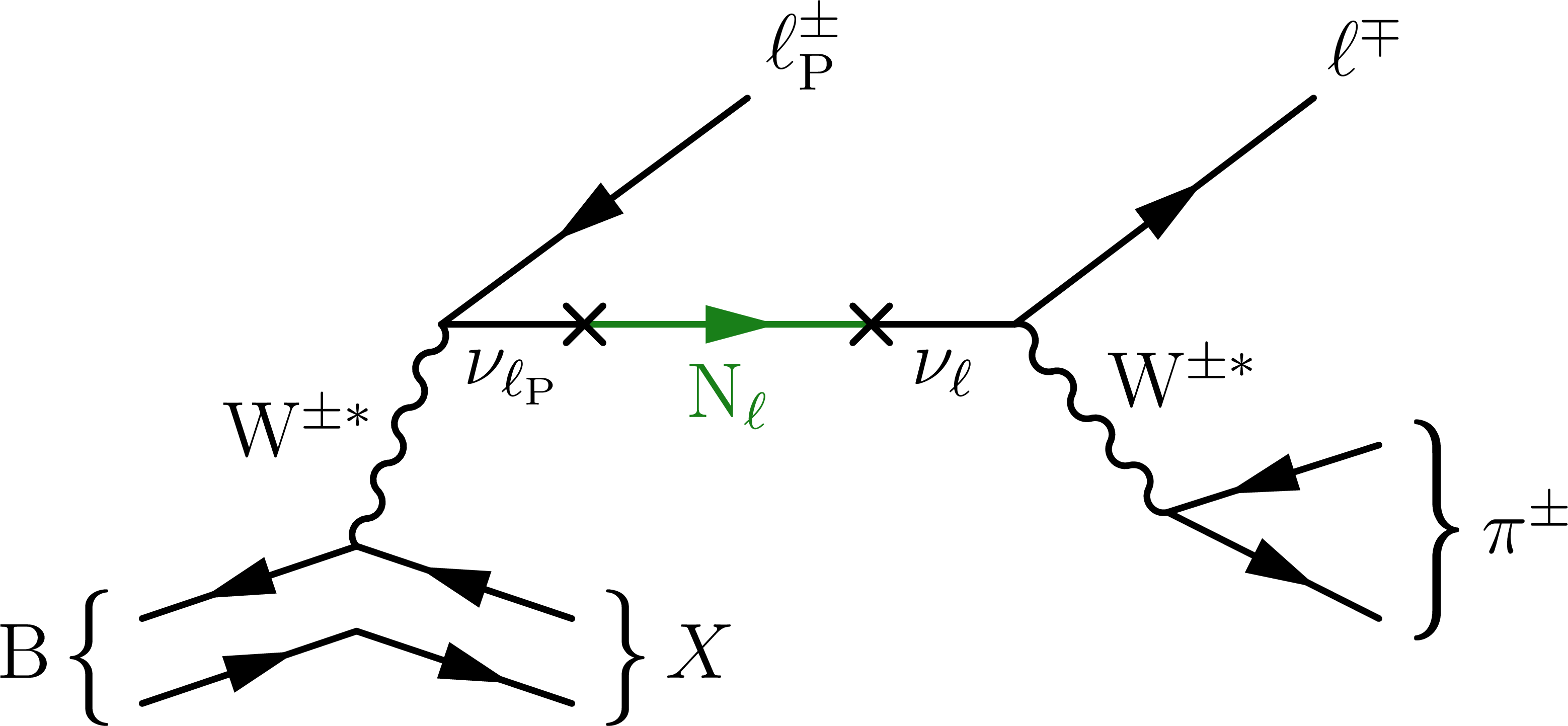
png pdf	Figure 57: Representative Feynman diagram showing the semileptonic decay of a ${\mathrm{B}}$ meson into the primary lepton ($\ell_{\mathrm{P}}$), a hadronic system ($\mathrm{X}$), and a neutrino, which contains the admixture of an HNL. The HNL propagates and decays weakly into a charged lepton $\ell^{\pm}$ and a charged pion $\pi^{\mp}$.
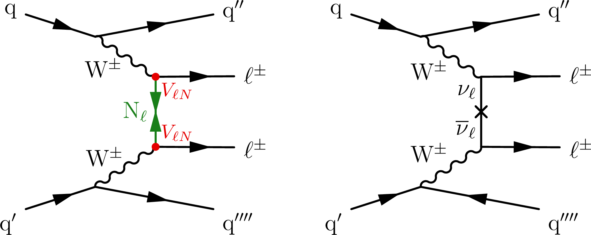
png pdf	Figure 58: Example Feynman diagrams of VBF processes with heavy Majorana neutrino production (left) and processes mediated by the Weinberg operator (right).
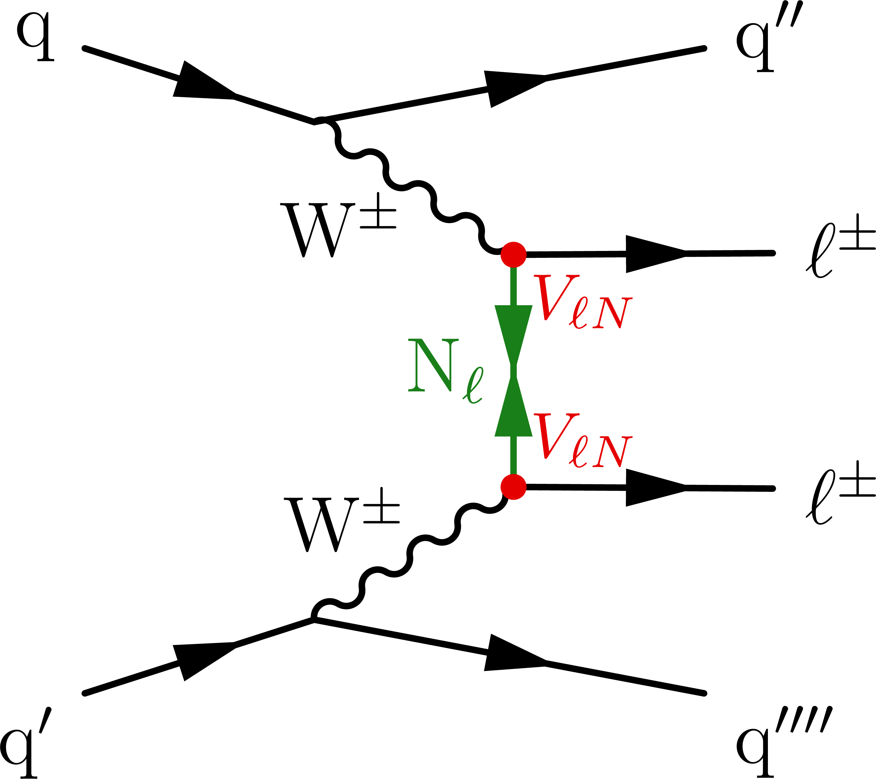
png pdf	Figure 58-a: Example Feynman diagrams of VBF processes with heavy Majorana neutrino production (left) and processes mediated by the Weinberg operator (right).
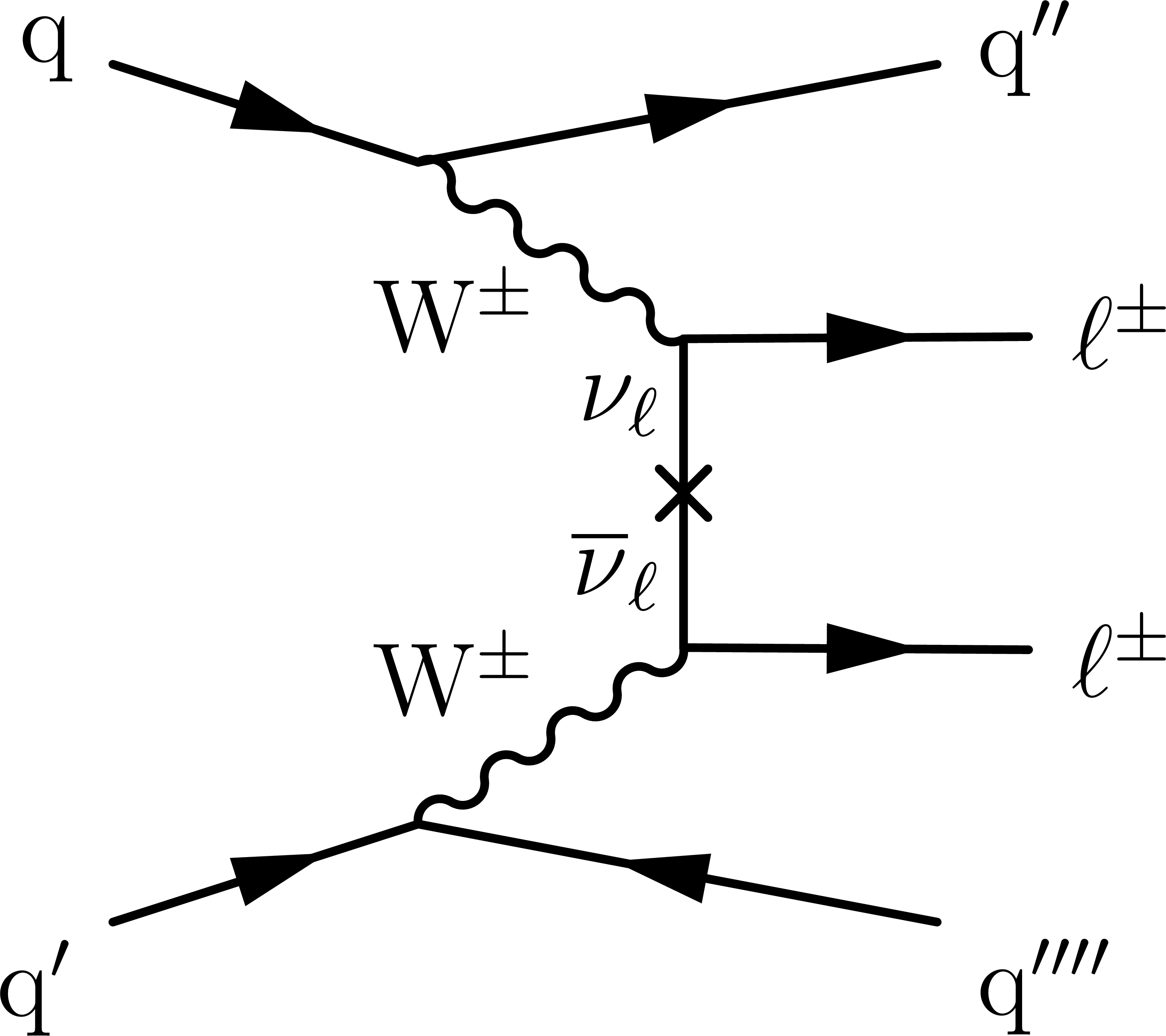
png pdf	Figure 58-b: Example Feynman diagrams of VBF processes with heavy Majorana neutrino production (left) and processes mediated by the Weinberg operator (right).
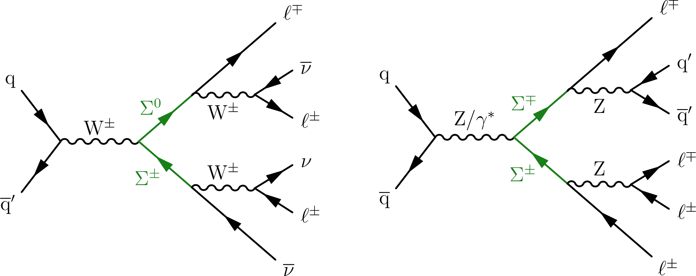
png pdf	Figure 59: Example Feynman diagrams illustrating production and decay of $Type III$ seesaw heavy lepton $\Sigma$ pairs at the LHC that may result in multilepton final states.
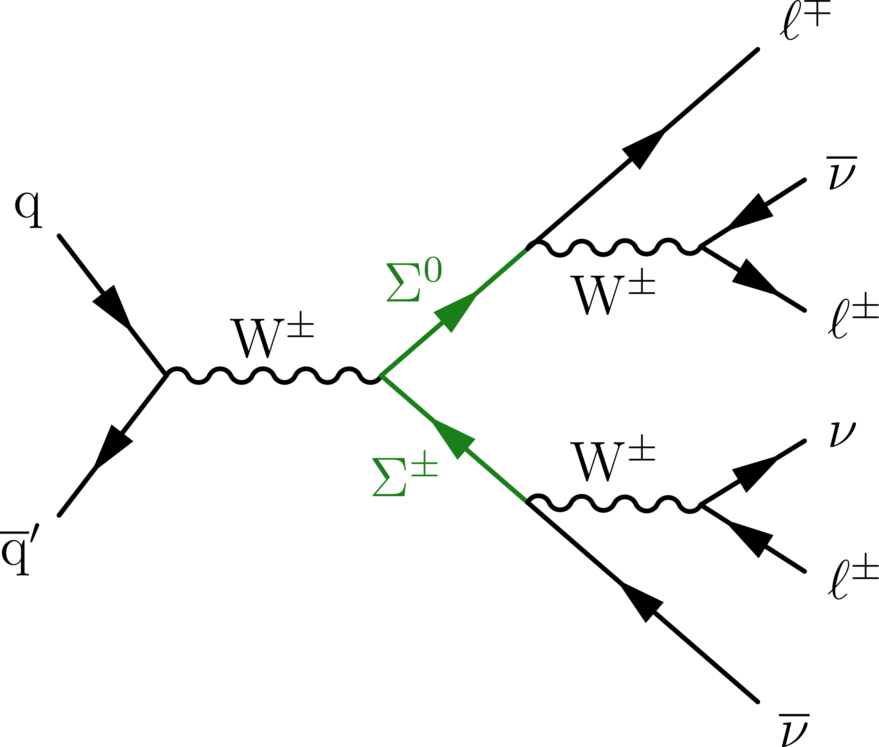
png pdf	Figure 59-a: Example Feynman diagrams illustrating production and decay of $Type III$ seesaw heavy lepton $\Sigma$ pairs at the LHC that may result in multilepton final states.
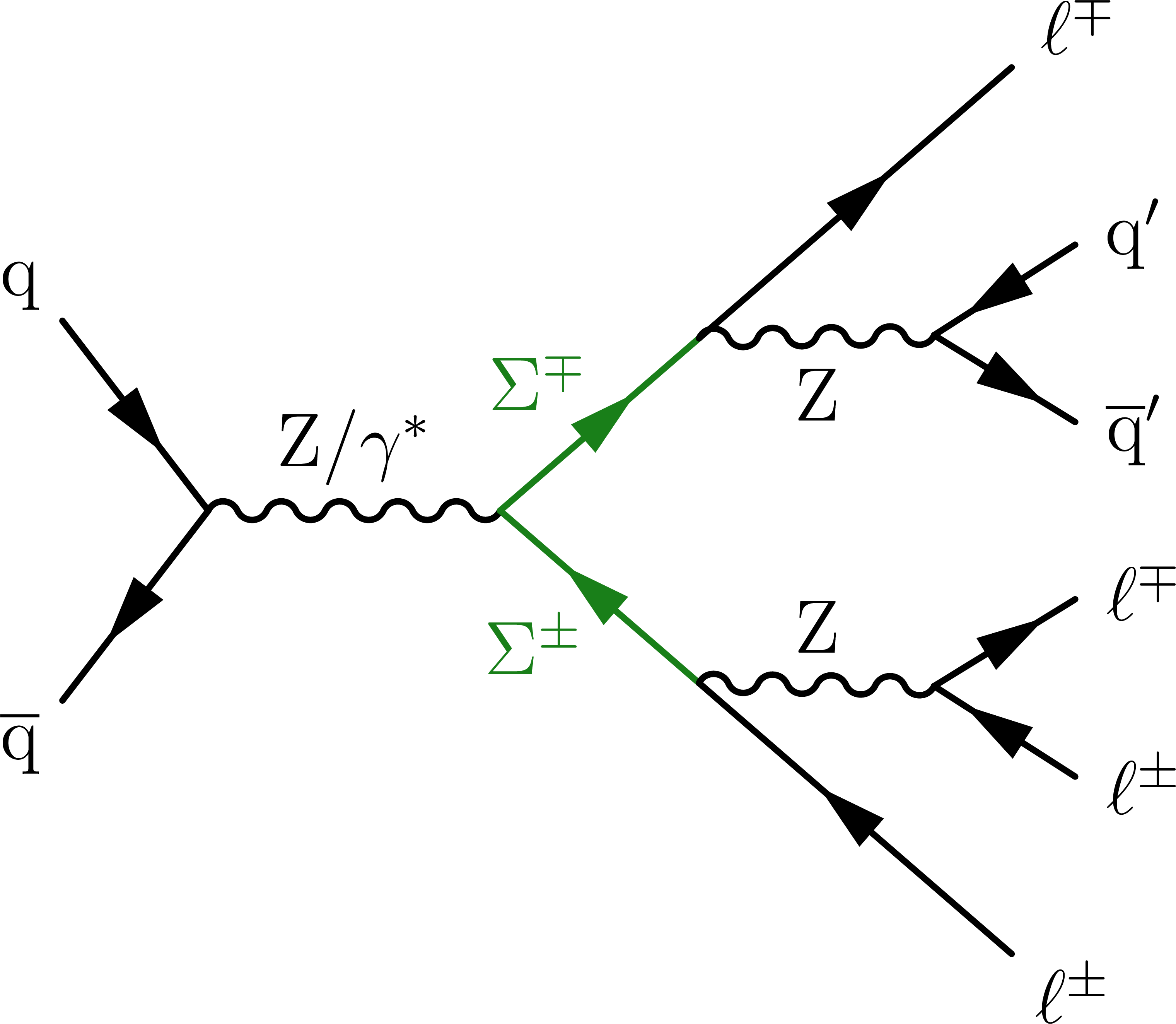
png pdf	Figure 59-b: Example Feynman diagrams illustrating production and decay of $Type III$ seesaw heavy lepton $\Sigma$ pairs at the LHC that may result in multilepton final states.
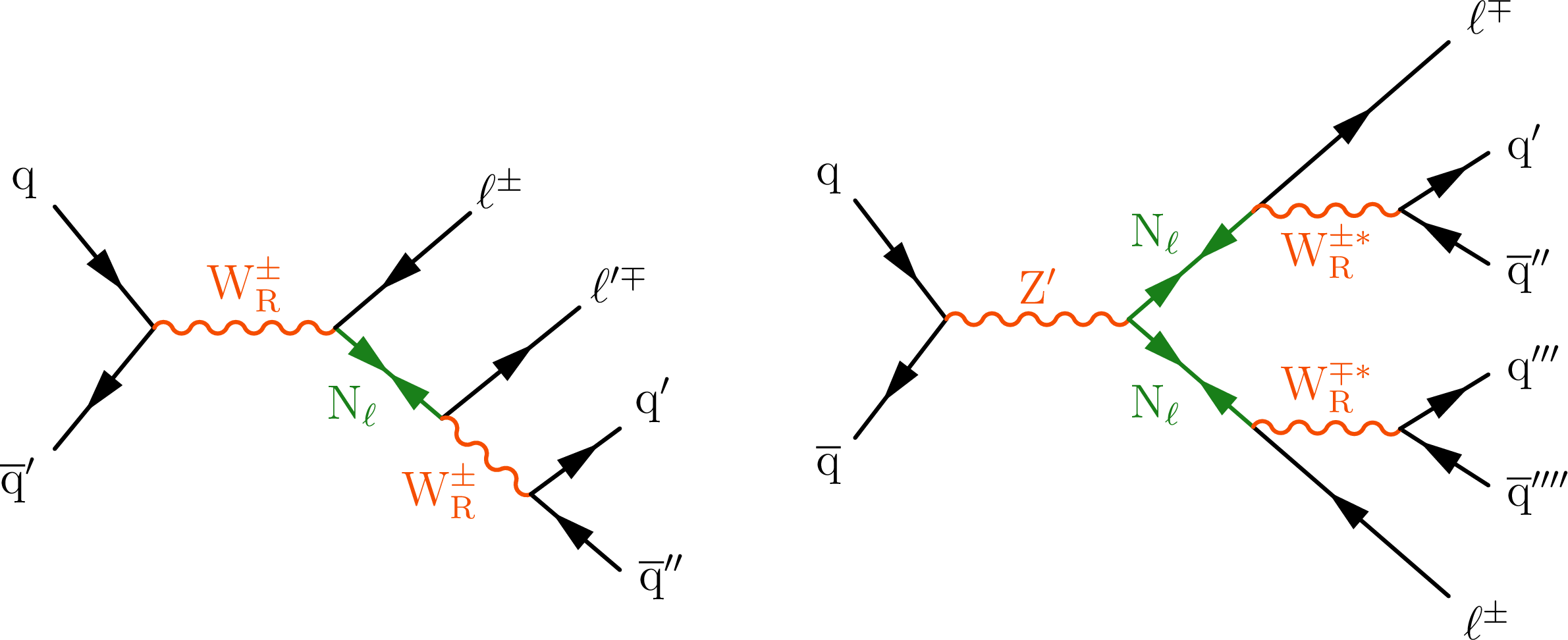
png pdf	Figure 60: Representative Feynman diagrams for the production of a heavy Majorana neutrino, labeled as $\mathrm{N} \ell$, via the decay of a $\mathrm{W_R}$ (left) and $\mathrm{Z}^{'}$ boson (right).
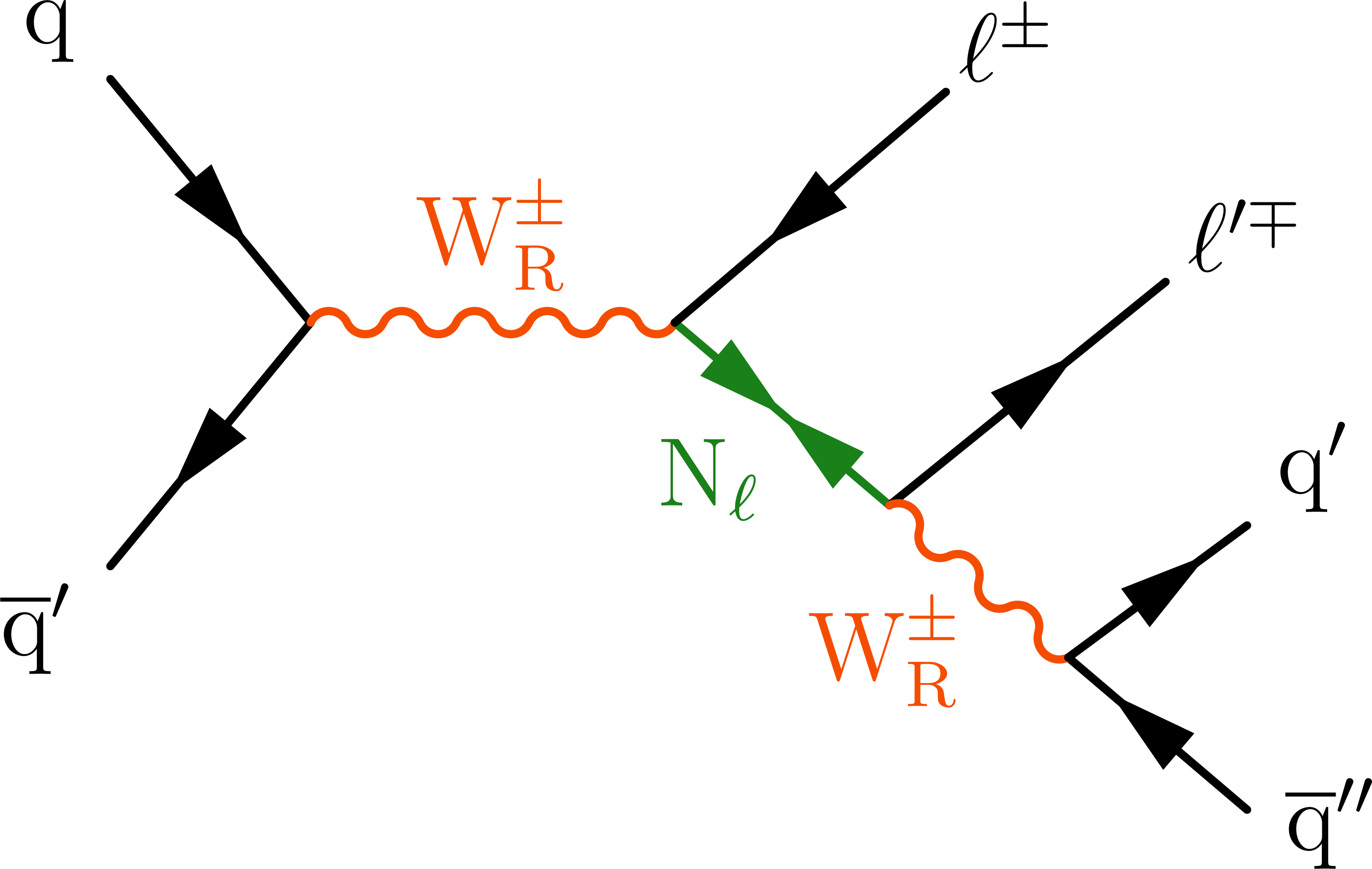
png pdf	Figure 60-a: Representative Feynman diagrams for the production of a heavy Majorana neutrino, labeled as $\mathrm{N} \ell$, via the decay of a $\mathrm{W_R}$ (left) and $\mathrm{Z}^{'}$ boson (right).
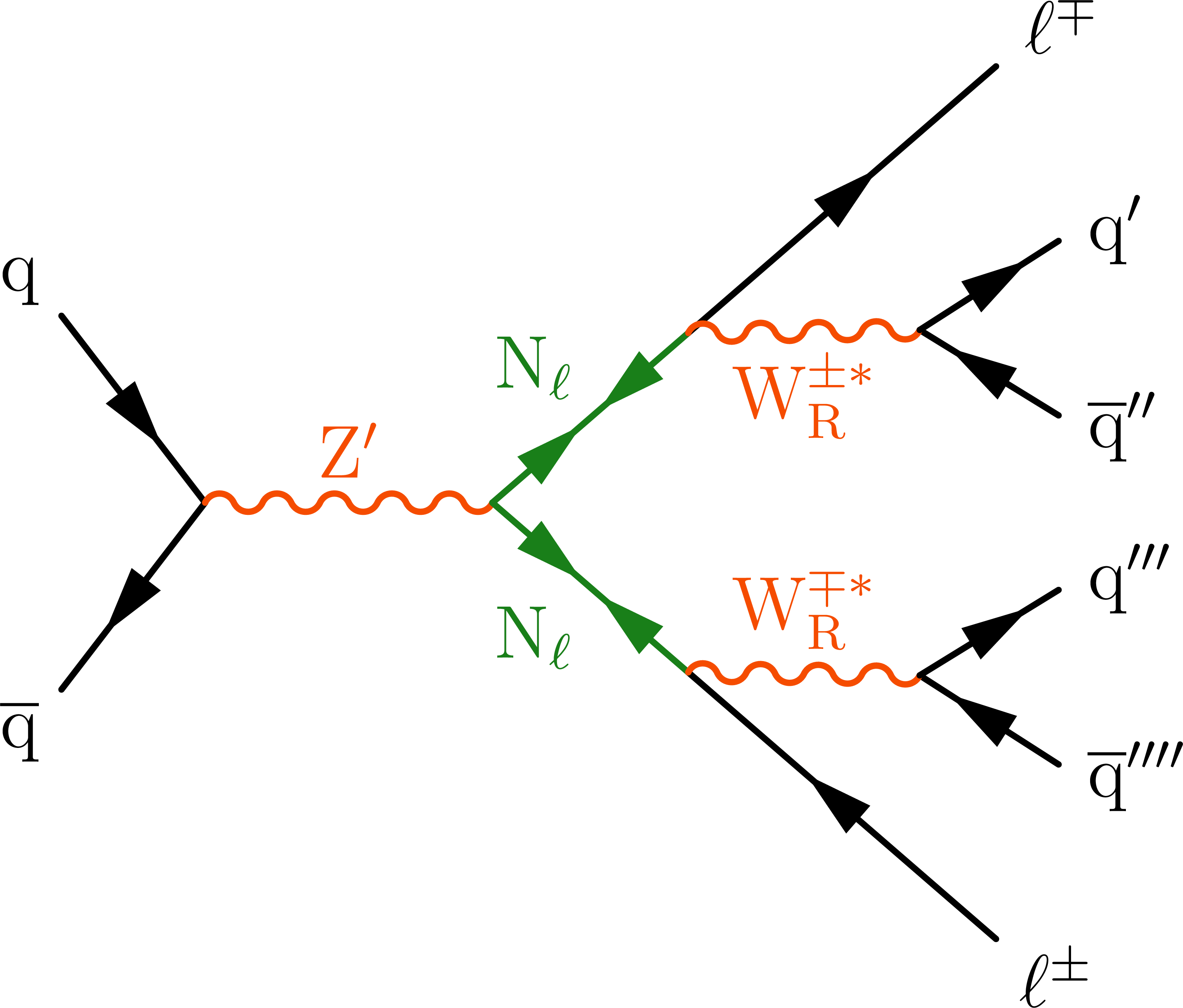
png pdf	Figure 60-b: Representative Feynman diagrams for the production of a heavy Majorana neutrino, labeled as $\mathrm{N} \ell$, via the decay of a $\mathrm{W_R}$ (left) and $\mathrm{Z}^{'}$ boson (right).
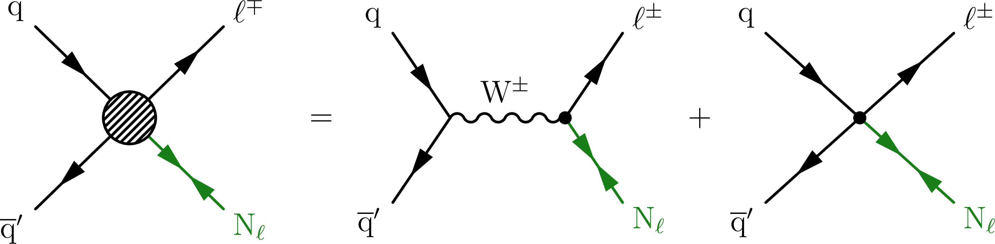
png pdf	Figure 61: The fermion interaction as a sum of gauge (center) and contact (right) interaction contributions.
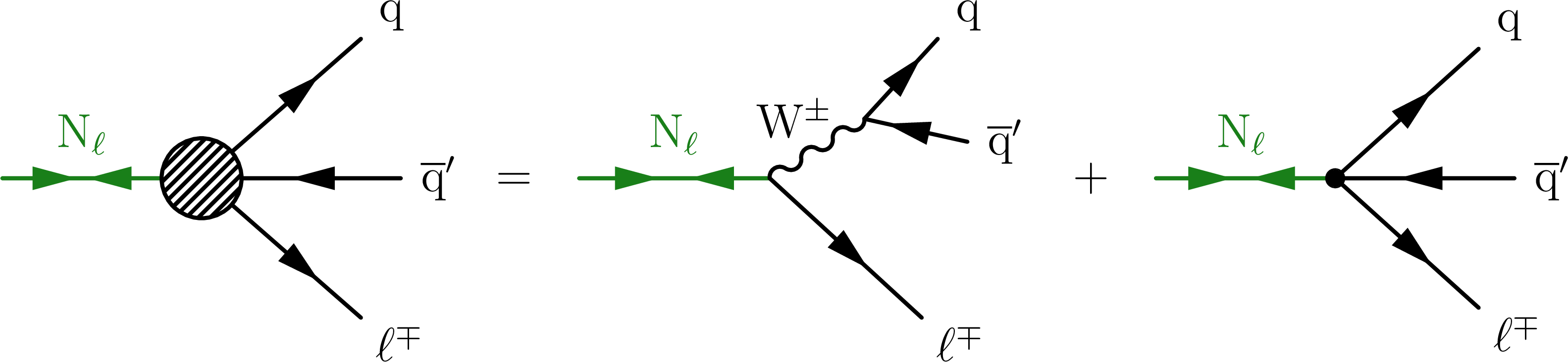
png pdf	Figure 62: Example diagrams for the decay of a heavy composite Majorana neutrino to $\ell\mathrm{q}{\overline{\mathrm{q}}{\prime}}$.
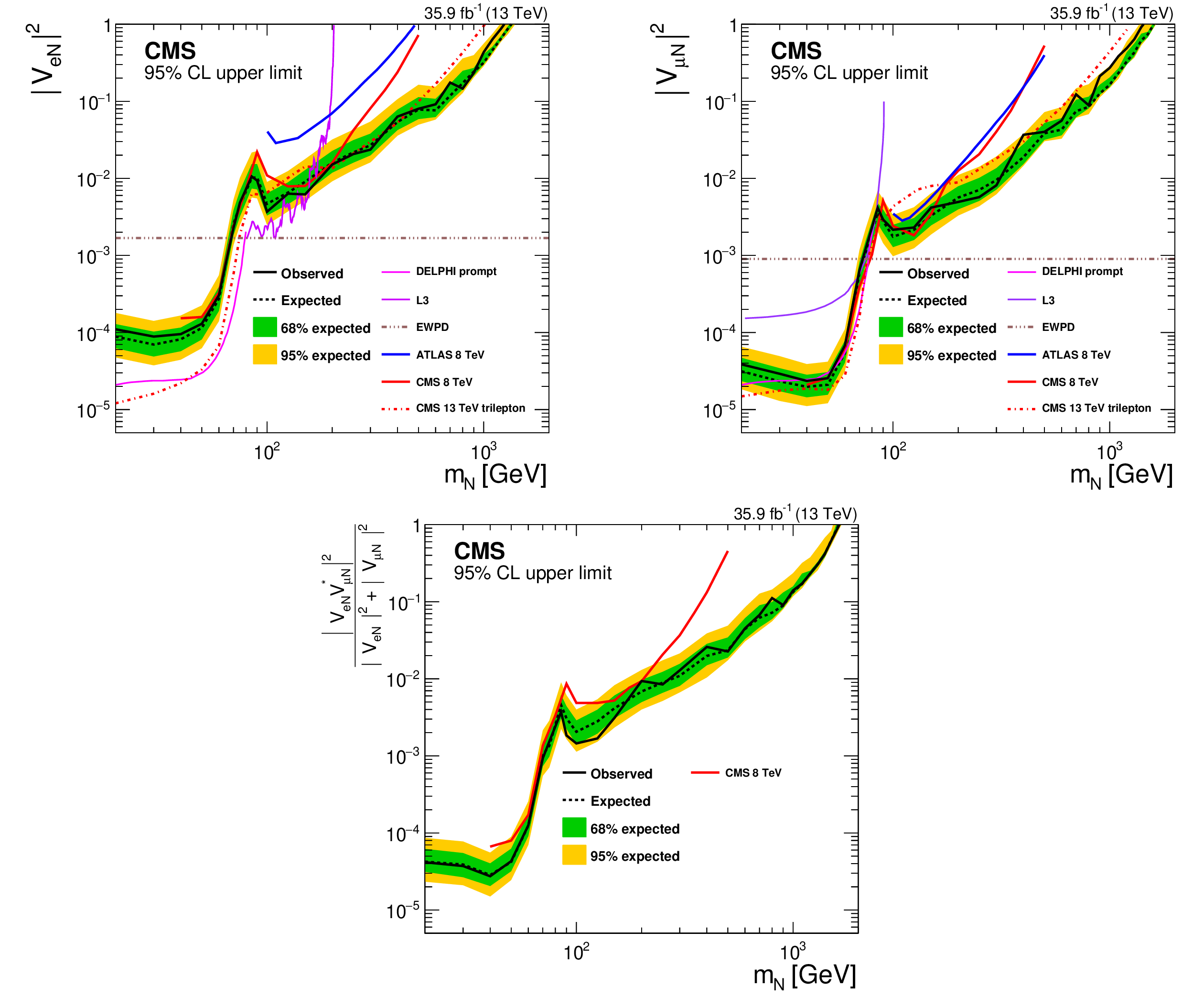
png pdf	Figure 63: Expected (observed) upper limits at 95% CL shown with a dashed (solid) black line, derived on heavy neutrino mixing parameters $|V_{\mathrm{eN}}|^{2}$, $|V_{\mathrm{\mu N}}|^{2}$, and $| V_{\mathrm{eN}}V_{\mathrm{\mu N}}^\ast|^2/(|V_{\mathrm{eN}}|^2+|V_{\mathrm{\mu N}}|^2)$ as functions of the HNL mass. The dashed brown line in the upper two figures shows constraints from Electroweak Precision Data (EWPD) [254] on the $|V_{\mathrm{eN}}|^{2}$ and $|V_{\mathrm{\mu N}}|^{2}$ parameters. The lower figure, reproduced from Ref. [252], does not show the corresponding EWPD limits. The upper limits from other direct searches at the DELPHI experiment [255], the L3 experiment [256,257], and the ATLAS experiment [258] are superimposed. Also shown are the upper limits from the CMS experiment at $\sqrt{s}=$ 8 TeV using the 2012 data set [253] with a solid red line, and the search in the trilepton final state [259] based on the same 2016 data set as used in this analysis with a dashed red line. Figures adapted from Ref. [252].
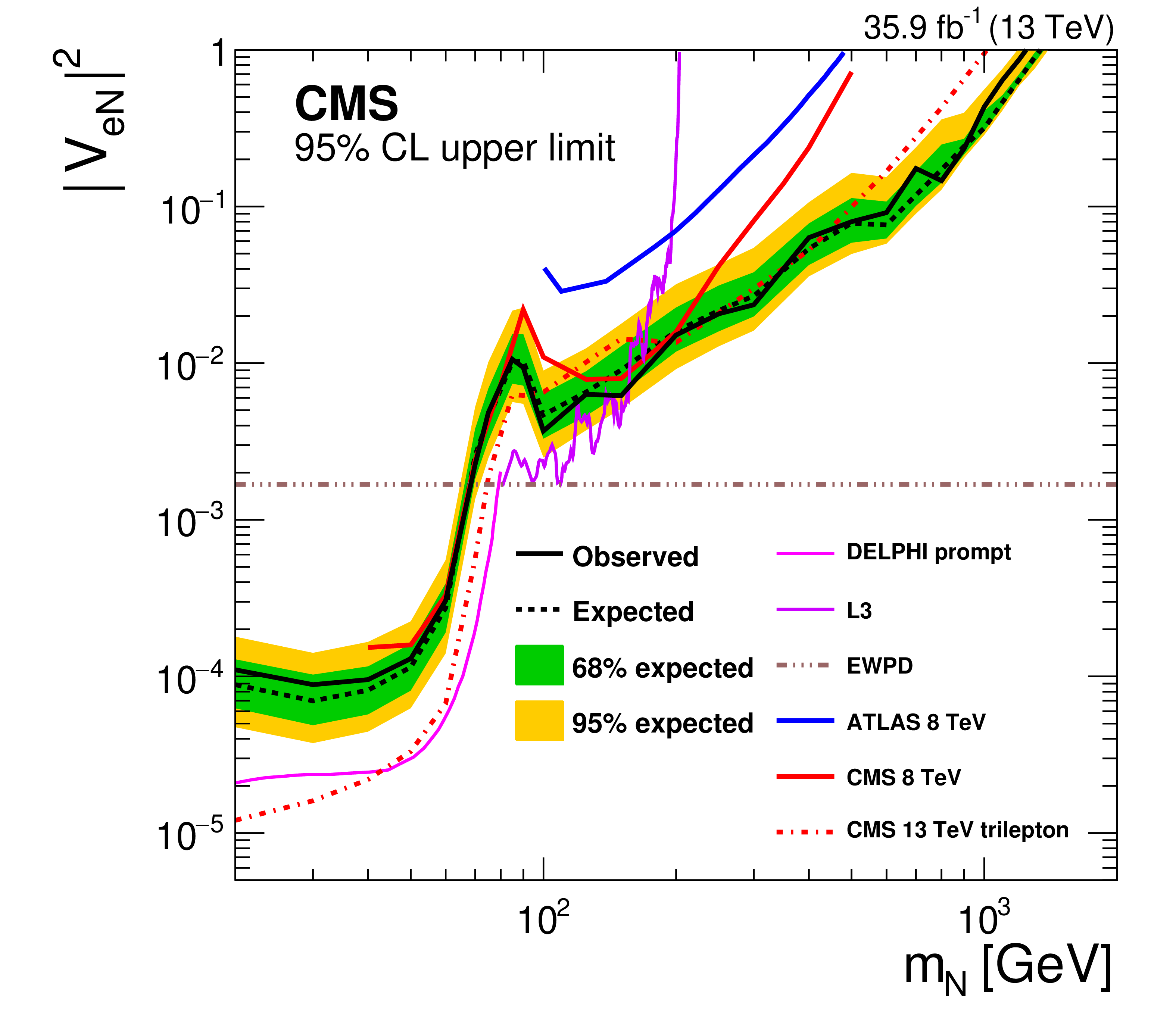
png pdf	Figure 63-a: Expected (observed) upper limits at 95% CL shown with a dashed (solid) black line, derived on heavy neutrino mixing parameters $|V_{\mathrm{eN}}|^{2}$, $|V_{\mathrm{\mu N}}|^{2}$, and $| V_{\mathrm{eN}}V_{\mathrm{\mu N}}^\ast|^2/(|V_{\mathrm{eN}}|^2+|V_{\mathrm{\mu N}}|^2)$ as functions of the HNL mass. The dashed brown line in the upper two figures shows constraints from Electroweak Precision Data (EWPD) [254] on the $|V_{\mathrm{eN}}|^{2}$ and $|V_{\mathrm{\mu N}}|^{2}$ parameters. The lower figure, reproduced from Ref. [252], does not show the corresponding EWPD limits. The upper limits from other direct searches at the DELPHI experiment [255], the L3 experiment [256,257], and the ATLAS experiment [258] are superimposed. Also shown are the upper limits from the CMS experiment at $\sqrt{s}=$ 8 TeV using the 2012 data set [253] with a solid red line, and the search in the trilepton final state [259] based on the same 2016 data set as used in this analysis with a dashed red line. Figures adapted from Ref. [252].
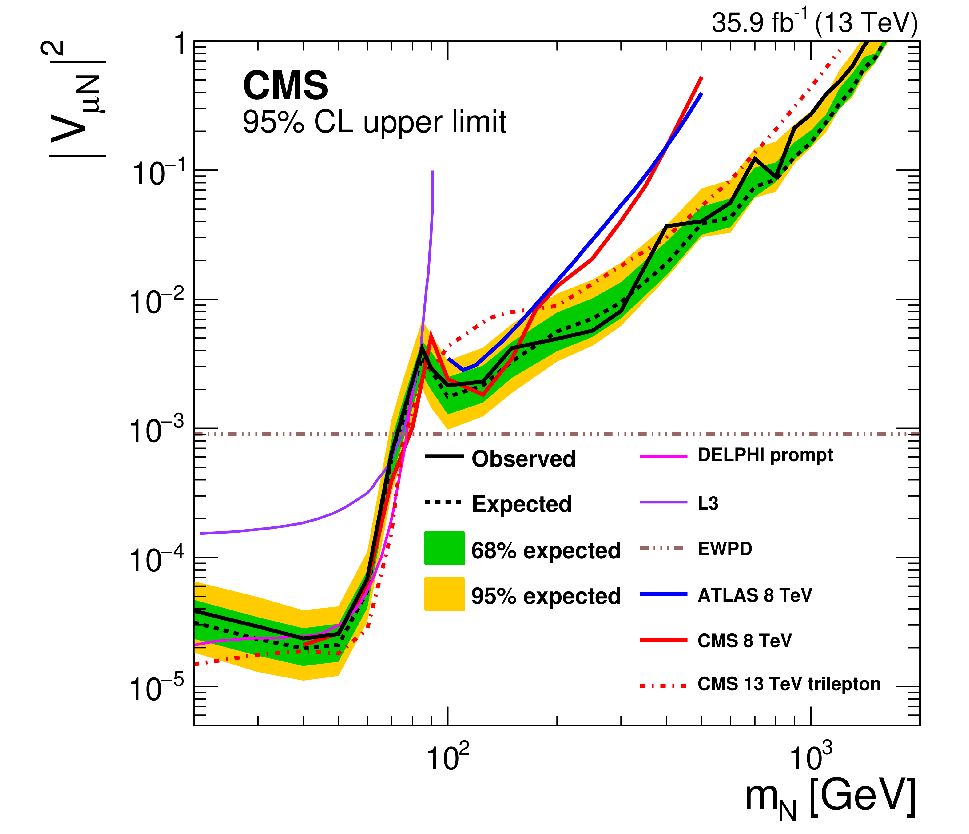
png pdf	Figure 63-b: Expected (observed) upper limits at 95% CL shown with a dashed (solid) black line, derived on heavy neutrino mixing parameters $|V_{\mathrm{eN}}|^{2}$, $|V_{\mathrm{\mu N}}|^{2}$, and $| V_{\mathrm{eN}}V_{\mathrm{\mu N}}^\ast|^2/(|V_{\mathrm{eN}}|^2+|V_{\mathrm{\mu N}}|^2)$ as functions of the HNL mass. The dashed brown line in the upper two figures shows constraints from Electroweak Precision Data (EWPD) [254] on the $|V_{\mathrm{eN}}|^{2}$ and $|V_{\mathrm{\mu N}}|^{2}$ parameters. The lower figure, reproduced from Ref. [252], does not show the corresponding EWPD limits. The upper limits from other direct searches at the DELPHI experiment [255], the L3 experiment [256,257], and the ATLAS experiment [258] are superimposed. Also shown are the upper limits from the CMS experiment at $\sqrt{s}=$ 8 TeV using the 2012 data set [253] with a solid red line, and the search in the trilepton final state [259] based on the same 2016 data set as used in this analysis with a dashed red line. Figures adapted from Ref. [252].
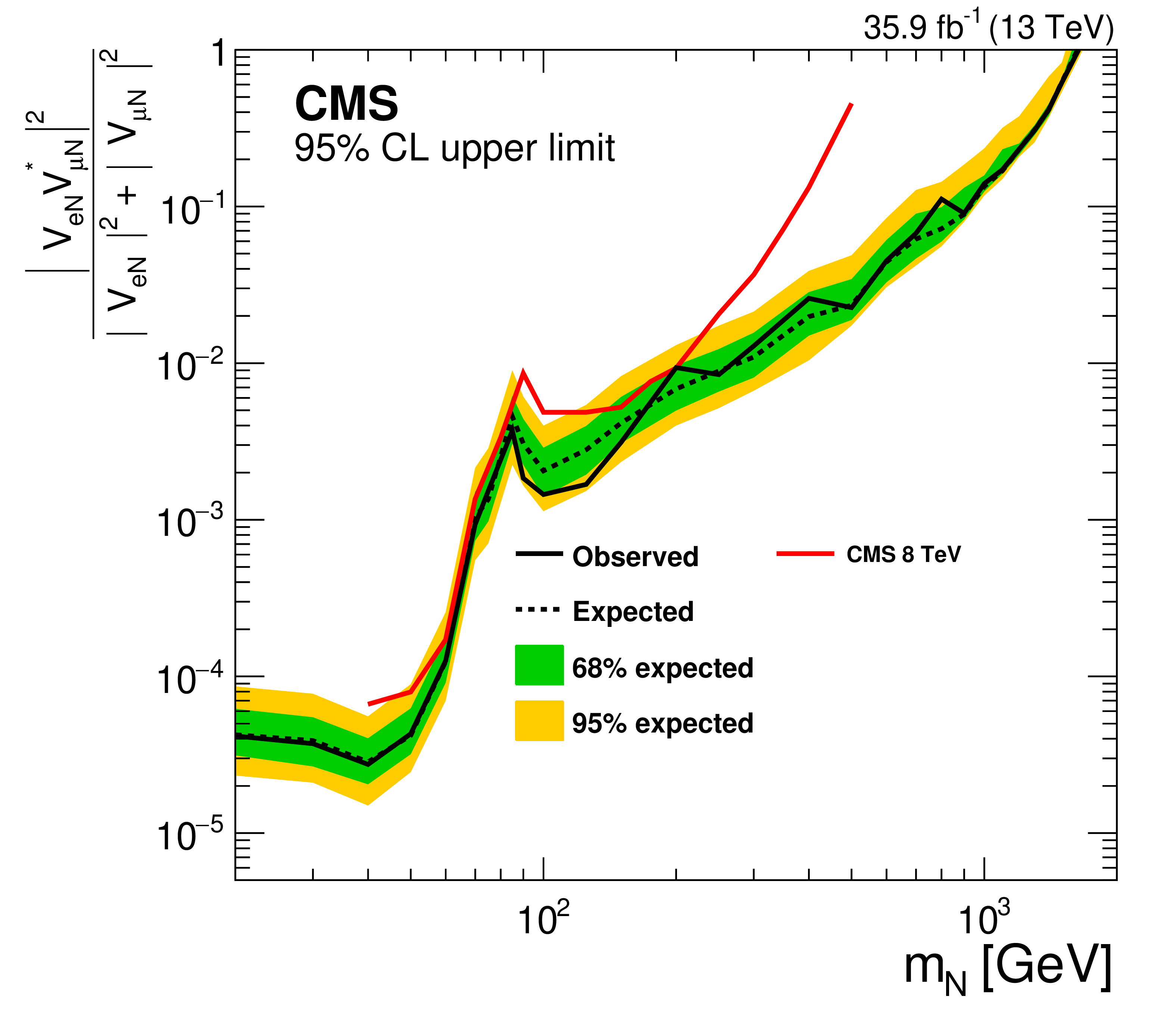
png pdf	Figure 63-c: Expected (observed) upper limits at 95% CL shown with a dashed (solid) black line, derived on heavy neutrino mixing parameters $|V_{\mathrm{eN}}|^{2}$, $|V_{\mathrm{\mu N}}|^{2}$, and $| V_{\mathrm{eN}}V_{\mathrm{\mu N}}^\ast|^2/(|V_{\mathrm{eN}}|^2+|V_{\mathrm{\mu N}}|^2)$ as functions of the HNL mass. The dashed brown line in the upper two figures shows constraints from Electroweak Precision Data (EWPD) [254] on the $|V_{\mathrm{eN}}|^{2}$ and $|V_{\mathrm{\mu N}}|^{2}$ parameters. The lower figure, reproduced from Ref. [252], does not show the corresponding EWPD limits. The upper limits from other direct searches at the DELPHI experiment [255], the L3 experiment [256,257], and the ATLAS experiment [258] are superimposed. Also shown are the upper limits from the CMS experiment at $\sqrt{s}=$ 8 TeV using the 2012 data set [253] with a solid red line, and the search in the trilepton final state [259] based on the same 2016 data set as used in this analysis with a dashed red line. Figures adapted from Ref. [252].
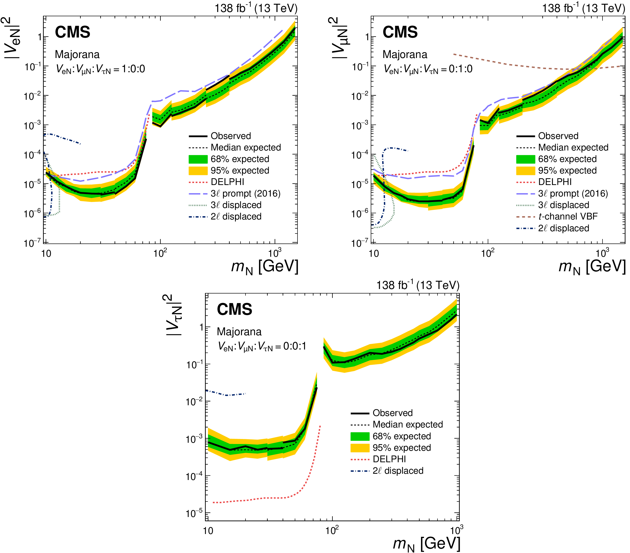
png pdf	Figure 64: Expected (observed) upper limits at 95% CL derived on heavy neutrino mixing parameters $|V_{\mathrm{eN}}|^{2}$, $|V_{\mathrm{\mu N}}|^{2}$, and \mixparsq$\tau \mathrm{N}$ as functions of the HNL mass $m_{\mathrm{N}}$. No exclusion limit is evaluated for the range 75 $< m_{\mathrm{N}} <$ 85 GeV, where HNL production through W boson decays has a resonance and the analysis strategy changes from using the low- or high-mass region. The area above the solid (dashed) black curve indicates the observed (expected) exclusion region. The upper limits from other direct searches at the DELPHI experiment [255] and the CMS experiment [259,261,262,263] are superimposed. Figures taken from Ref. [260].
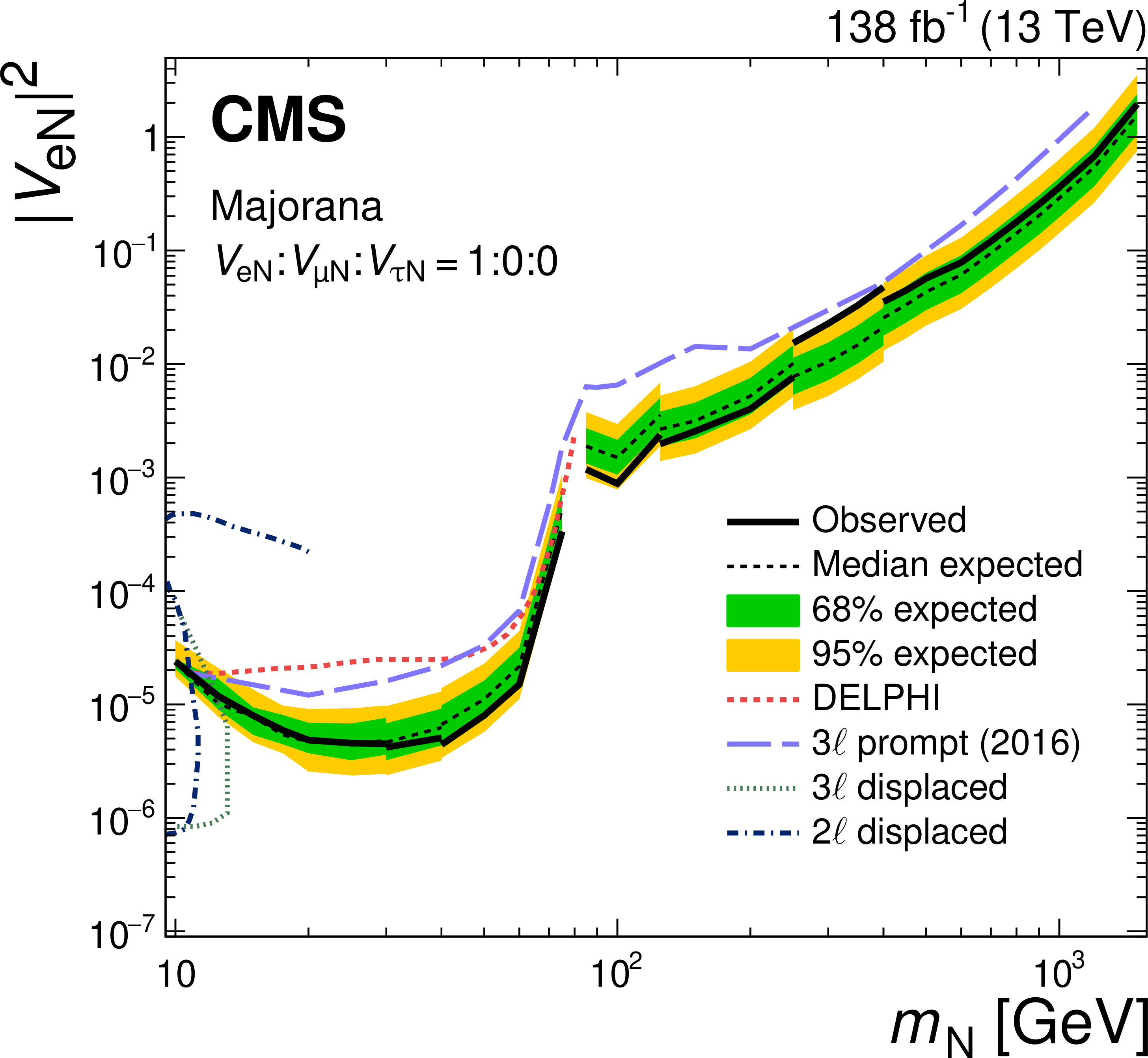
png pdf	Figure 64-a: Expected (observed) upper limits at 95% CL derived on heavy neutrino mixing parameters $|V_{\mathrm{eN}}|^{2}$, $|V_{\mathrm{\mu N}}|^{2}$, and \mixparsq$\tau \mathrm{N}$ as functions of the HNL mass $m_{\mathrm{N}}$. No exclusion limit is evaluated for the range 75 $< m_{\mathrm{N}} <$ 85 GeV, where HNL production through W boson decays has a resonance and the analysis strategy changes from using the low- or high-mass region. The area above the solid (dashed) black curve indicates the observed (expected) exclusion region. The upper limits from other direct searches at the DELPHI experiment [255] and the CMS experiment [259,261,262,263] are superimposed. Figures taken from Ref. [260].
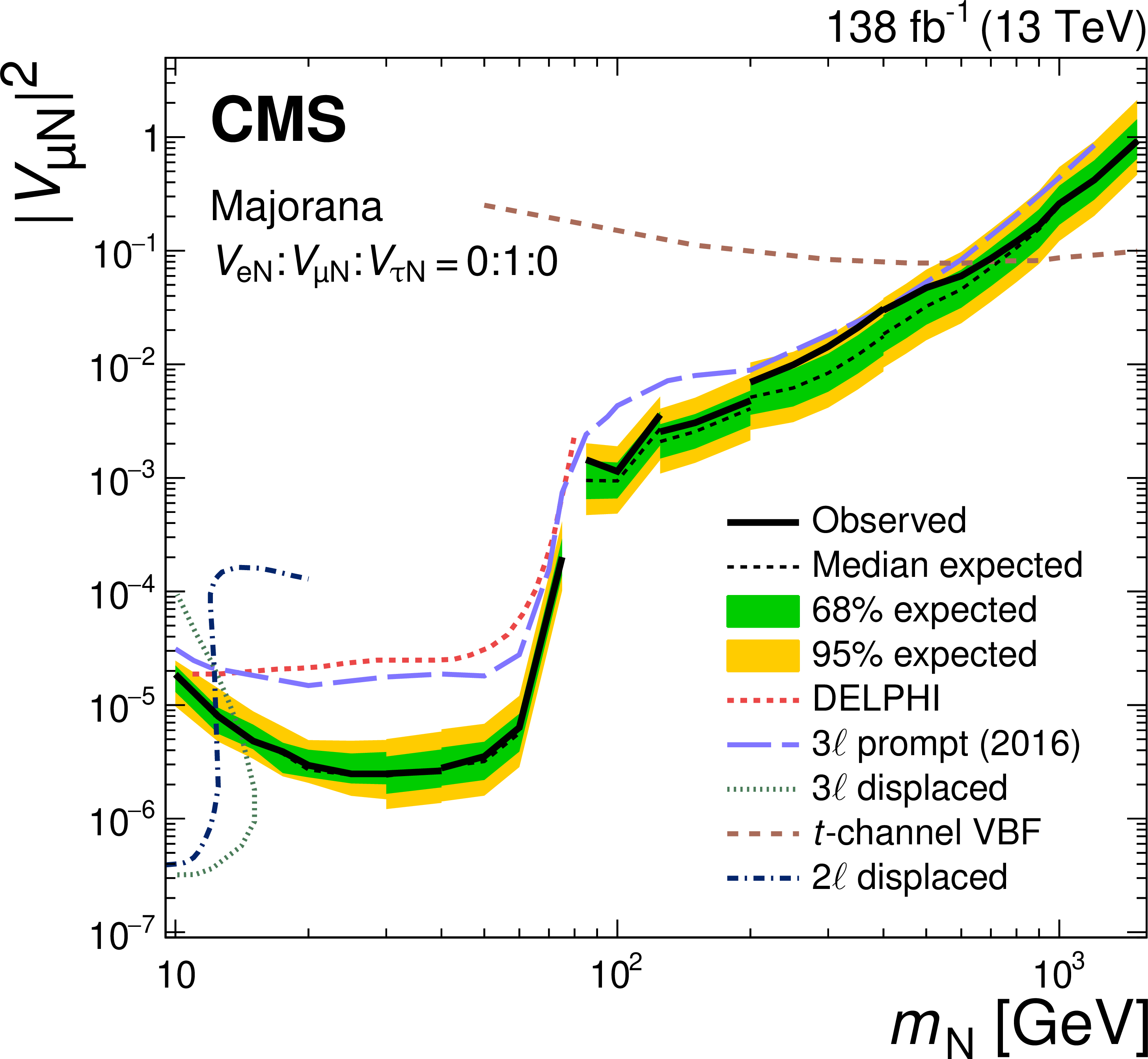
png pdf	Figure 64-b: Expected (observed) upper limits at 95% CL derived on heavy neutrino mixing parameters $|V_{\mathrm{eN}}|^{2}$, $|V_{\mathrm{\mu N}}|^{2}$, and \mixparsq$\tau \mathrm{N}$ as functions of the HNL mass $m_{\mathrm{N}}$. No exclusion limit is evaluated for the range 75 $< m_{\mathrm{N}} <$ 85 GeV, where HNL production through W boson decays has a resonance and the analysis strategy changes from using the low- or high-mass region. The area above the solid (dashed) black curve indicates the observed (expected) exclusion region. The upper limits from other direct searches at the DELPHI experiment [255] and the CMS experiment [259,261,262,263] are superimposed. Figures taken from Ref. [260].
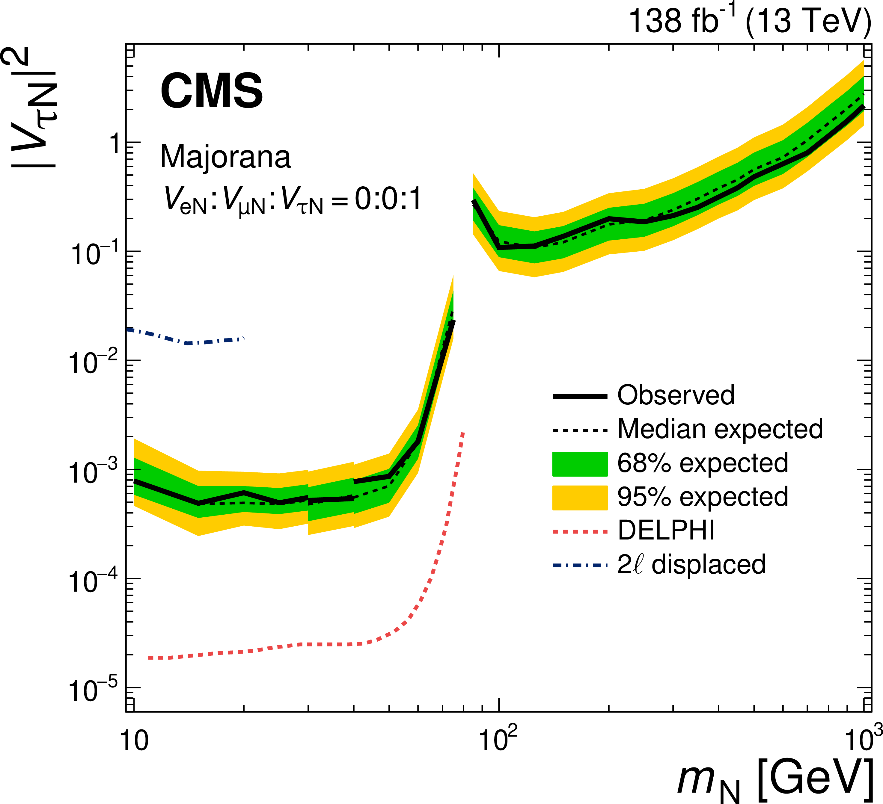
png pdf	Figure 64-c: Expected (observed) upper limits at 95% CL derived on heavy neutrino mixing parameters $|V_{\mathrm{eN}}|^{2}$, $|V_{\mathrm{\mu N}}|^{2}$, and \mixparsq$\tau \mathrm{N}$ as functions of the HNL mass $m_{\mathrm{N}}$. No exclusion limit is evaluated for the range 75 $< m_{\mathrm{N}} <$ 85 GeV, where HNL production through W boson decays has a resonance and the analysis strategy changes from using the low- or high-mass region. The area above the solid (dashed) black curve indicates the observed (expected) exclusion region. The upper limits from other direct searches at the DELPHI experiment [255] and the CMS experiment [259,261,262,263] are superimposed. Figures taken from Ref. [260].
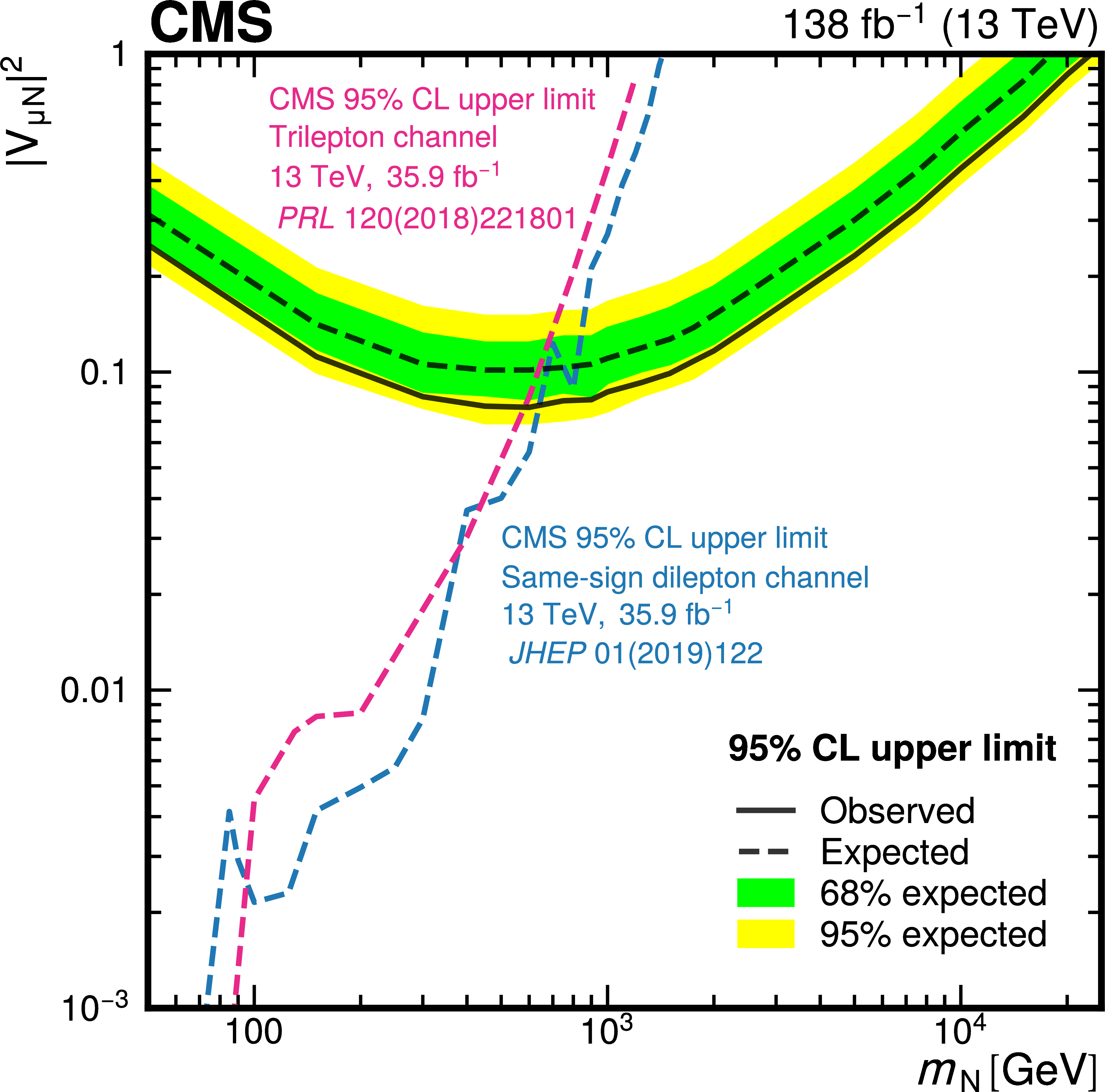
png pdf	Figure 65: Upper limits on $|V_{\mathrm{\mu N}}|^{2}$ at 95% CL as a function of $m_{\mathrm{N}}$. The black dashed curve shows the median expected upper limit, while the inner (green) band and the outer (yellow) band indicate the regions containing 68 and 95%, respectively, of the distribution of limits expected under the background-only hypothesis. The solid black curve is the observed upper limit [262]. The red dashed curve displays the observed upper limits from Ref. [259], while the blue dashed curve shows the observed upper limits from Ref. [252]. Figure adapted from Ref. [262].
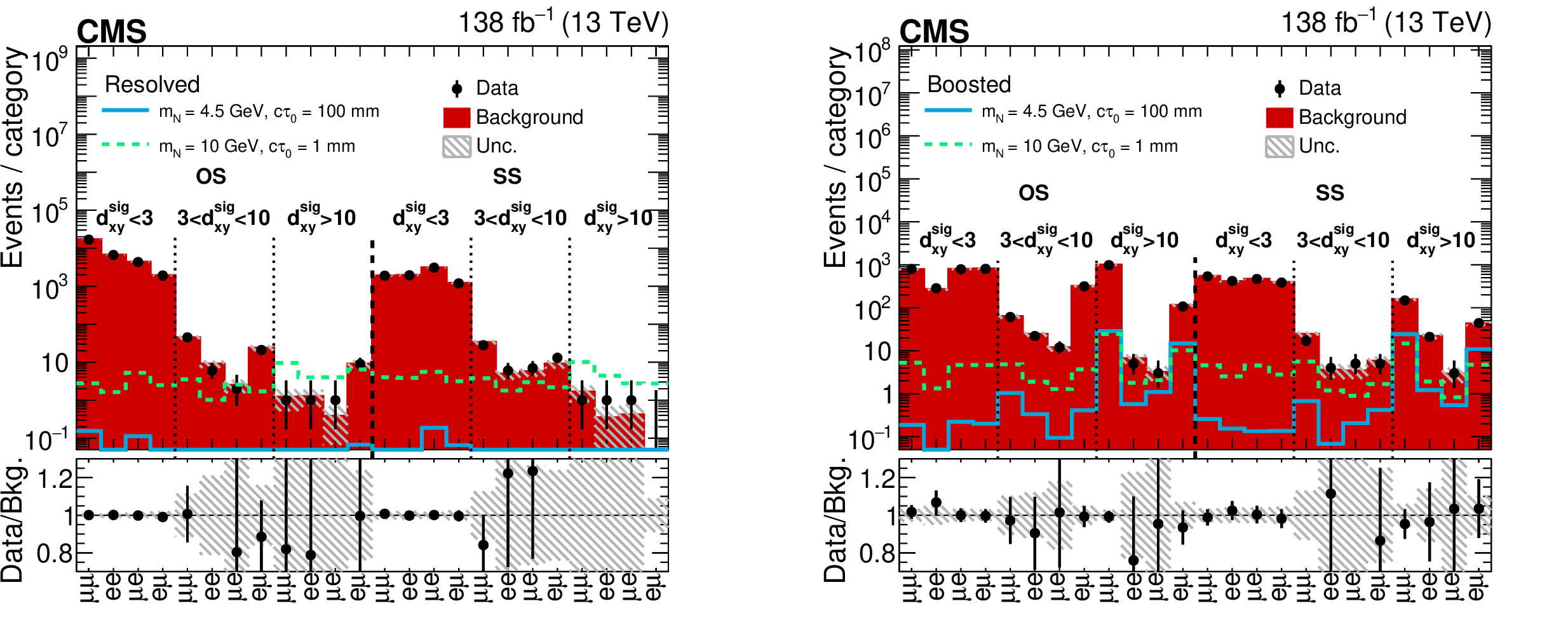
png pdf	Figure 66: Expected and observed background yields in 48 categories for resolved (left) and boosted (right) events. Two benchmark HNL scenarios are overlaid with masses of 4.5 and 10 GeV, and proper decay lengths of $c\tau_{\mathrm{N}}=$ 100 and 1$\,\text{mm}$, respectively. The $d_{xy}^{\text{sig}}$ quantity is the significance of the impact parameter of the second lepton track. Figures taken from Ref. [263].
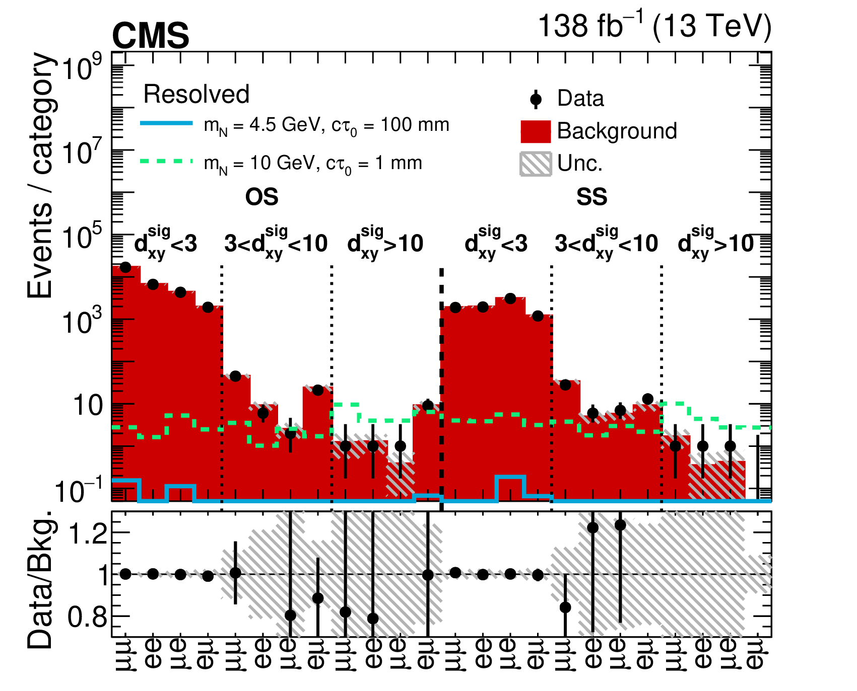
png pdf	Figure 66-a: Expected and observed background yields in 48 categories for resolved (left) and boosted (right) events. Two benchmark HNL scenarios are overlaid with masses of 4.5 and 10 GeV, and proper decay lengths of $c\tau_{\mathrm{N}}=$ 100 and 1$\,\text{mm}$, respectively. The $d_{xy}^{\text{sig}}$ quantity is the significance of the impact parameter of the second lepton track. Figures taken from Ref. [263].
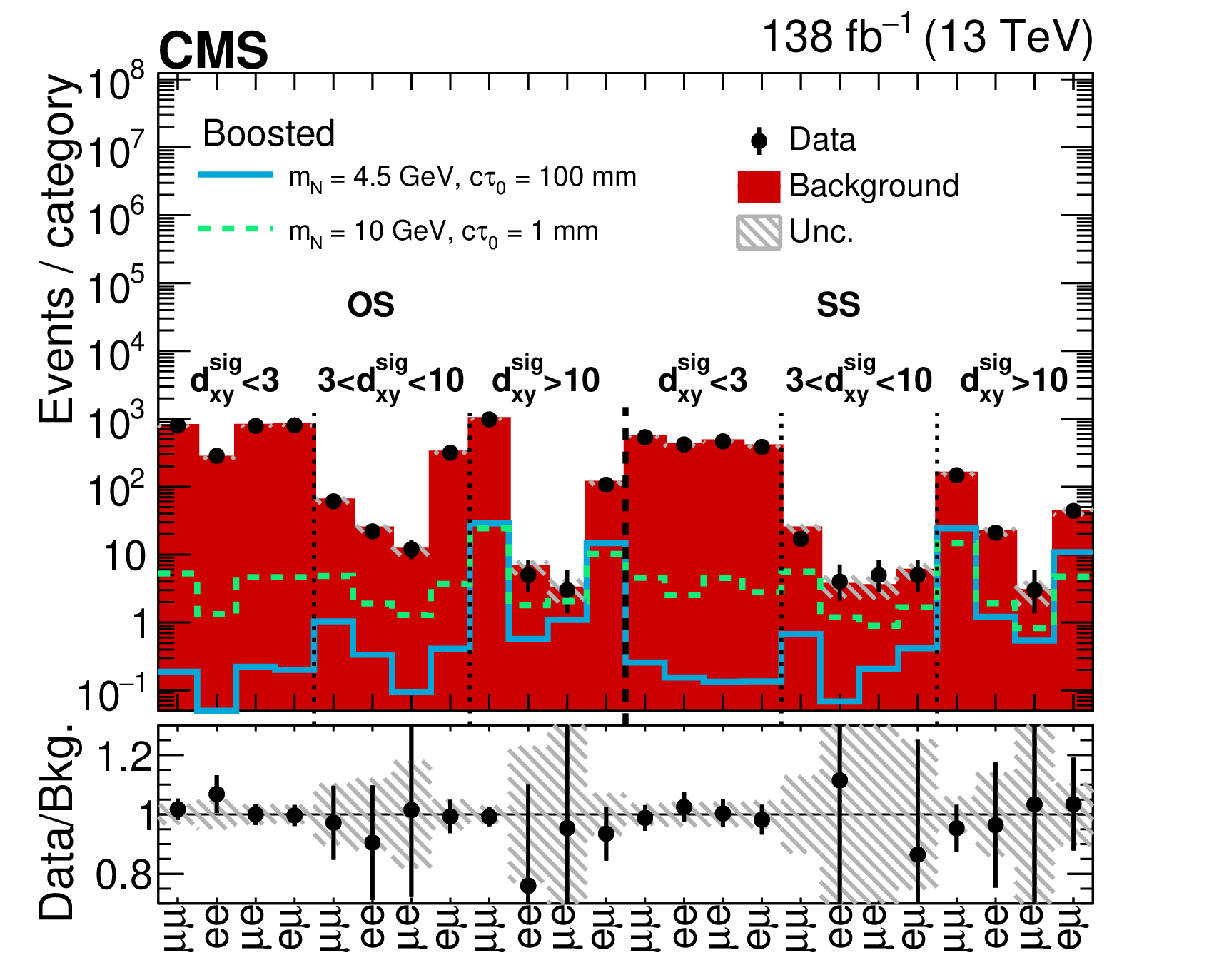
png pdf	Figure 66-b: Expected and observed background yields in 48 categories for resolved (left) and boosted (right) events. Two benchmark HNL scenarios are overlaid with masses of 4.5 and 10 GeV, and proper decay lengths of $c\tau_{\mathrm{N}}=$ 100 and 1$\,\text{mm}$, respectively. The $d_{xy}^{\text{sig}}$ quantity is the significance of the impact parameter of the second lepton track. Figures taken from Ref. [263].
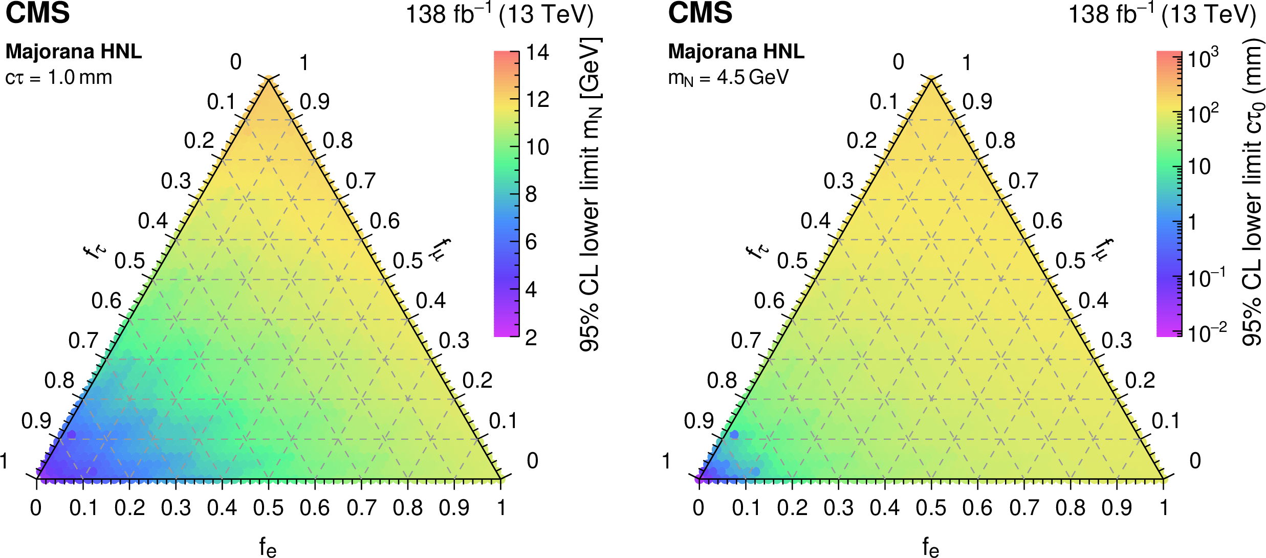
png pdf	Figure 67: Observed 95% CL lower limits on the mass (left) and the proper lifetime (right) for Majorana HNL production with $c\tau_{\mathrm{N}}=1\,\text{mm}$ and $m_{\mathrm{N}}=$ 4.5 GeV, respectively, as functions of the relative coupling strengths to electrons ($f_{\mathrm{e}}$), muons ($f_{\mu}$), and tau leptons ($f_{\tau}$). Figures adapted from Ref. [263].
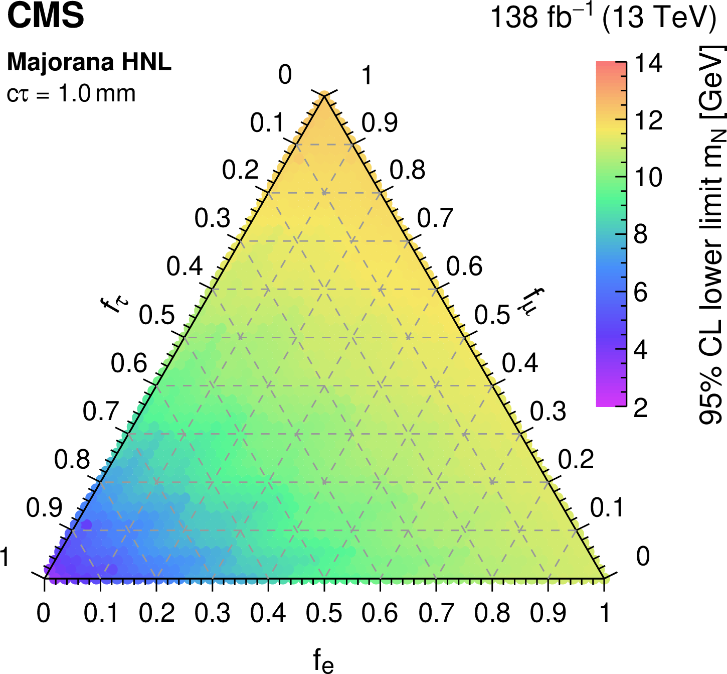
png pdf	Figure 67-a: Observed 95% CL lower limits on the mass (left) and the proper lifetime (right) for Majorana HNL production with $c\tau_{\mathrm{N}}=1\,\text{mm}$ and $m_{\mathrm{N}}=$ 4.5 GeV, respectively, as functions of the relative coupling strengths to electrons ($f_{\mathrm{e}}$), muons ($f_{\mu}$), and tau leptons ($f_{\tau}$). Figures adapted from Ref. [263].
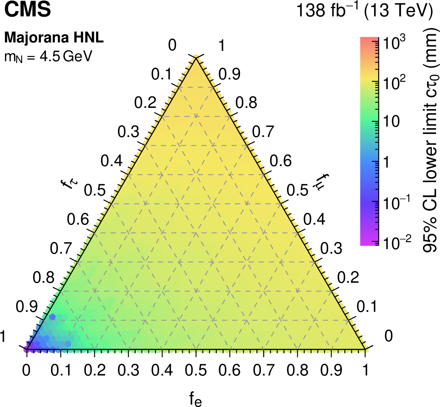
png pdf	Figure 67-b: Observed 95% CL lower limits on the mass (left) and the proper lifetime (right) for Majorana HNL production with $c\tau_{\mathrm{N}}=1\,\text{mm}$ and $m_{\mathrm{N}}=$ 4.5 GeV, respectively, as functions of the relative coupling strengths to electrons ($f_{\mathrm{e}}$), muons ($f_{\mu}$), and tau leptons ($f_{\tau}$). Figures adapted from Ref. [263].
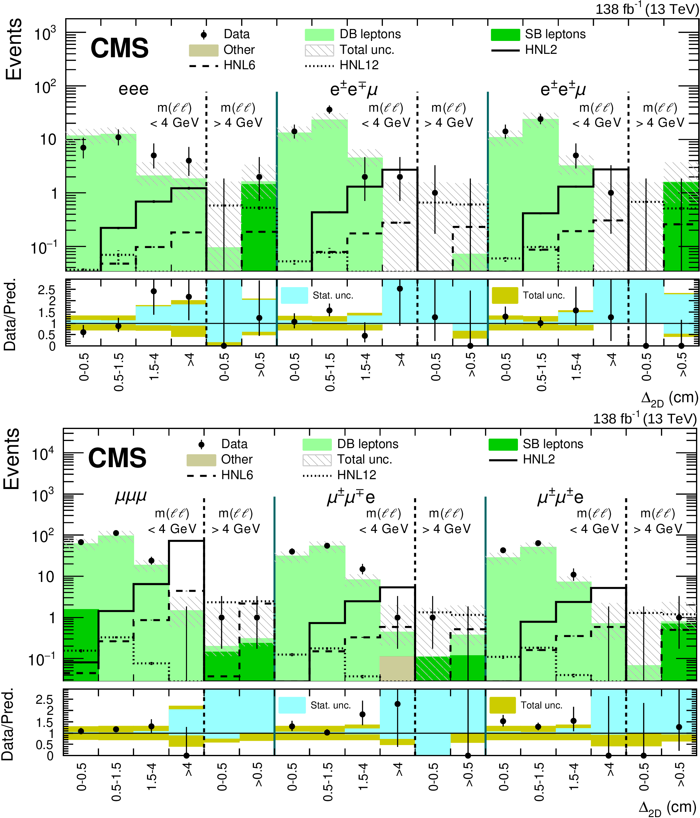
png pdf	Figure 68: Comparison between the number of observed events in data and the background predictions (filled histograms) in the SR for $\mathrm{e}\mathrm{e}\mathrm{X}$ (upper) and $\mu\mu\mathrm{X}$ (lower) final states. The hatched band indicates the total systematic and statistical uncertainty in the background prediction. The lower panels indicate the ratio between the observed data and the prediction, where missing points indicate that the ratio lies outside the axis range. Predictions for signal events are shown for several benchmark hypotheses for Majorana HNL production: $m_{\mathrm{N}}=$ 2 GeV and |V_{\mathrm{\ell N}}|^{2} =$0.8$\times$10$^{-4} $(HNL2),$ m_{\mathrm{N}}= $6 GeV and$ $|V_{\mathrm{\ell N}}|^{2} =$ 1.3$\times$10$^{-6}$ (HNL6), $m_{\mathrm{N}}=$ 12 GeV and |V_{\mathrm{\ell N}}|^{2} = $1.0$\times$10$^{-6} $ (HNL12). Small contributions from background processes that are estimated from simulation are collectively referred to as ``Other''. Figures taken from Ref. [261].
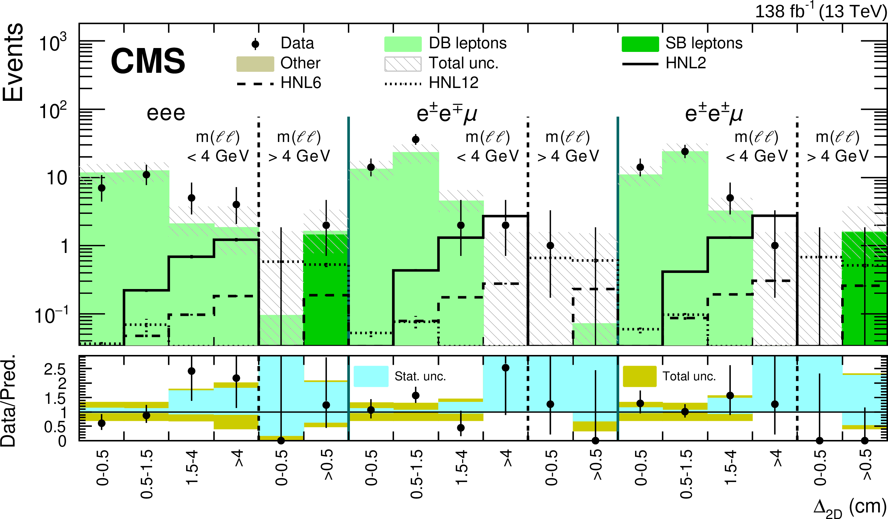
png pdf	Figure 68-a: Comparison between the number of observed events in data and the background predictions (filled histograms) in the SR for $\mathrm{e}\mathrm{e}\mathrm{X}$ (upper) and $\mu\mu\mathrm{X}$ (lower) final states. The hatched band indicates the total systematic and statistical uncertainty in the background prediction. The lower panels indicate the ratio between the observed data and the prediction, where missing points indicate that the ratio lies outside the axis range. Predictions for signal events are shown for several benchmark hypotheses for Majorana HNL production: $m_{\mathrm{N}}=$ 2 GeV and |V_{\mathrm{\ell N}}|^{2} =$0.8$\times$10$^{-4} $(HNL2),$ m_{\mathrm{N}}= $6 GeV and$ $|V_{\mathrm{\ell N}}|^{2} =$ 1.3$\times$10$^{-6}$ (HNL6), $m_{\mathrm{N}}=$ 12 GeV and |V_{\mathrm{\ell N}}|^{2} = $1.0$\times$10$^{-6} $ (HNL12). Small contributions from background processes that are estimated from simulation are collectively referred to as ``Other''. Figures taken from Ref. [261].
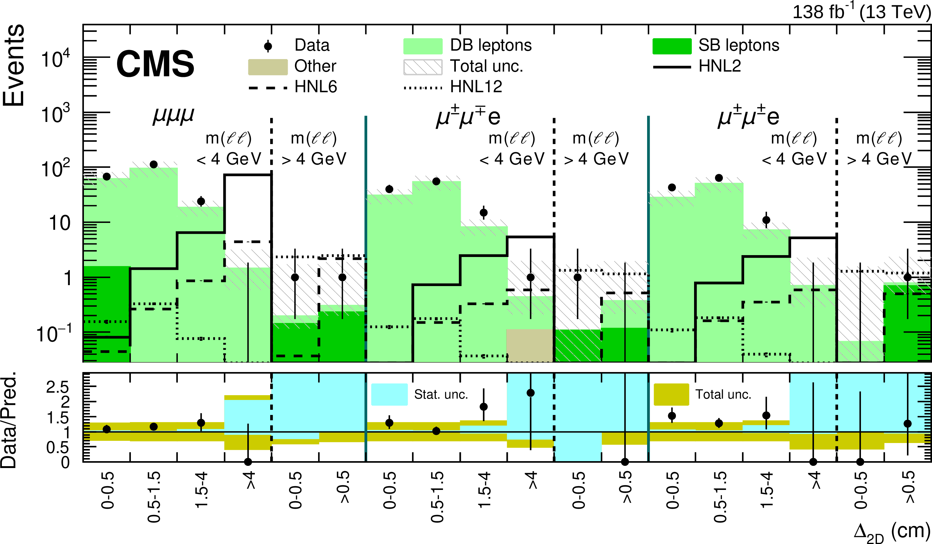
png pdf	Figure 68-b: Comparison between the number of observed events in data and the background predictions (filled histograms) in the SR for $\mathrm{e}\mathrm{e}\mathrm{X}$ (upper) and $\mu\mu\mathrm{X}$ (lower) final states. The hatched band indicates the total systematic and statistical uncertainty in the background prediction. The lower panels indicate the ratio between the observed data and the prediction, where missing points indicate that the ratio lies outside the axis range. Predictions for signal events are shown for several benchmark hypotheses for Majorana HNL production: $m_{\mathrm{N}}=$ 2 GeV and |V_{\mathrm{\ell N}}|^{2} =$0.8$\times$10$^{-4} $(HNL2),$ m_{\mathrm{N}}= $6 GeV and$ $|V_{\mathrm{\ell N}}|^{2} =$ 1.3$\times$10$^{-6}$ (HNL6), $m_{\mathrm{N}}=$ 12 GeV and |V_{\mathrm{\ell N}}|^{2} = $1.0$\times$10$^{-6} $ (HNL12). Small contributions from background processes that are estimated from simulation are collectively referred to as ``Other''. Figures taken from Ref. [261].
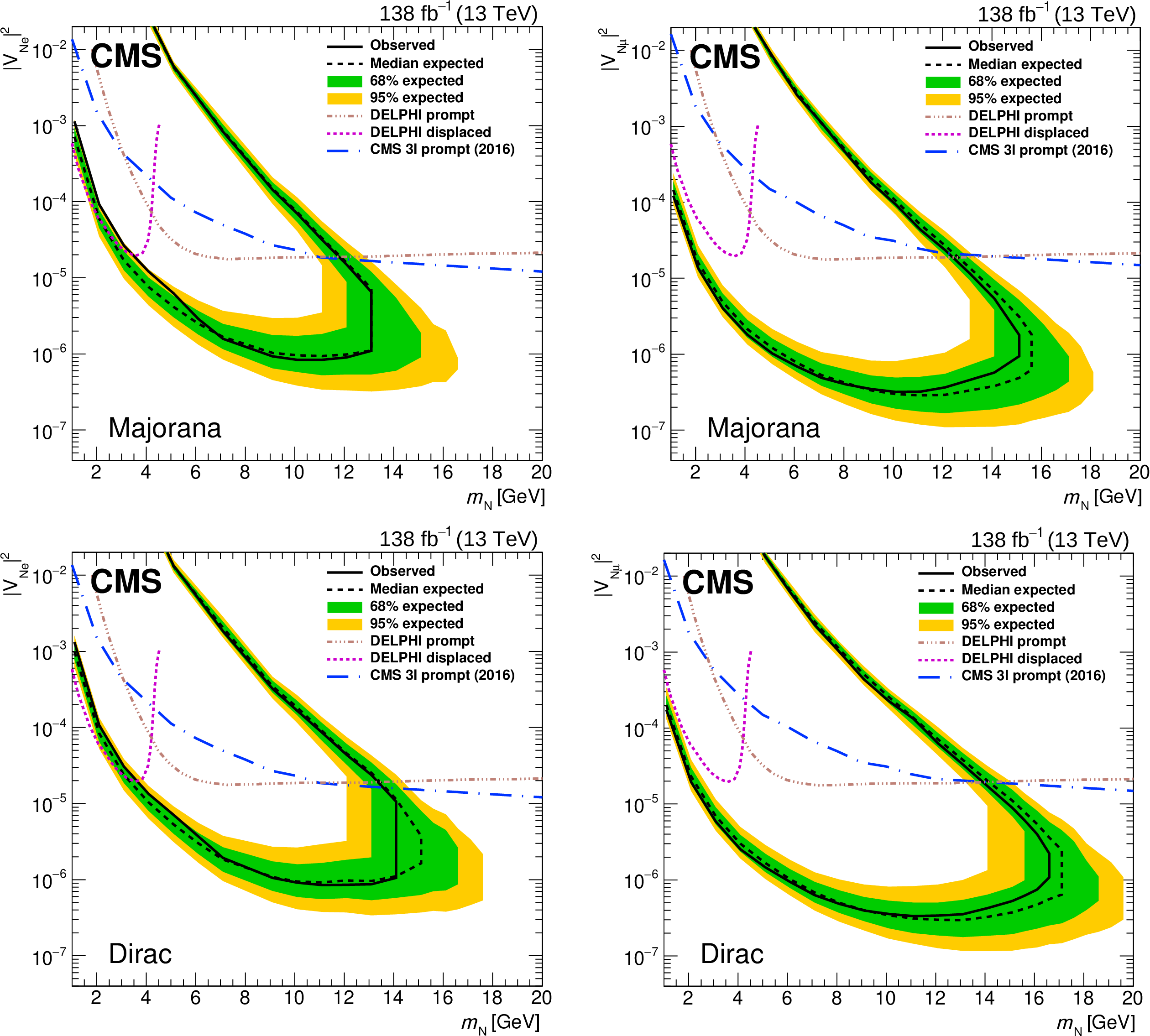
png pdf	Figure 69: The limits at 95% CL on $|V_{\mathrm{eN}}|^{2}$ (left) and $|V_{\mathrm{\mu N}}|^{2}$ (right) as functions of $m_{\mathrm{N}}$ for a Majorana (upper) or Dirac (lower) HNL. The area inside the solid (dashed) black curve indicates the observed (expected) exclusion region. Results from the DELPHI [255] and the CMS [259,252] Collaborations are shown as upper limits, i.e.,, the area above the curves indicates the respective observed exclusion region. Figures adapted from Ref. [261].
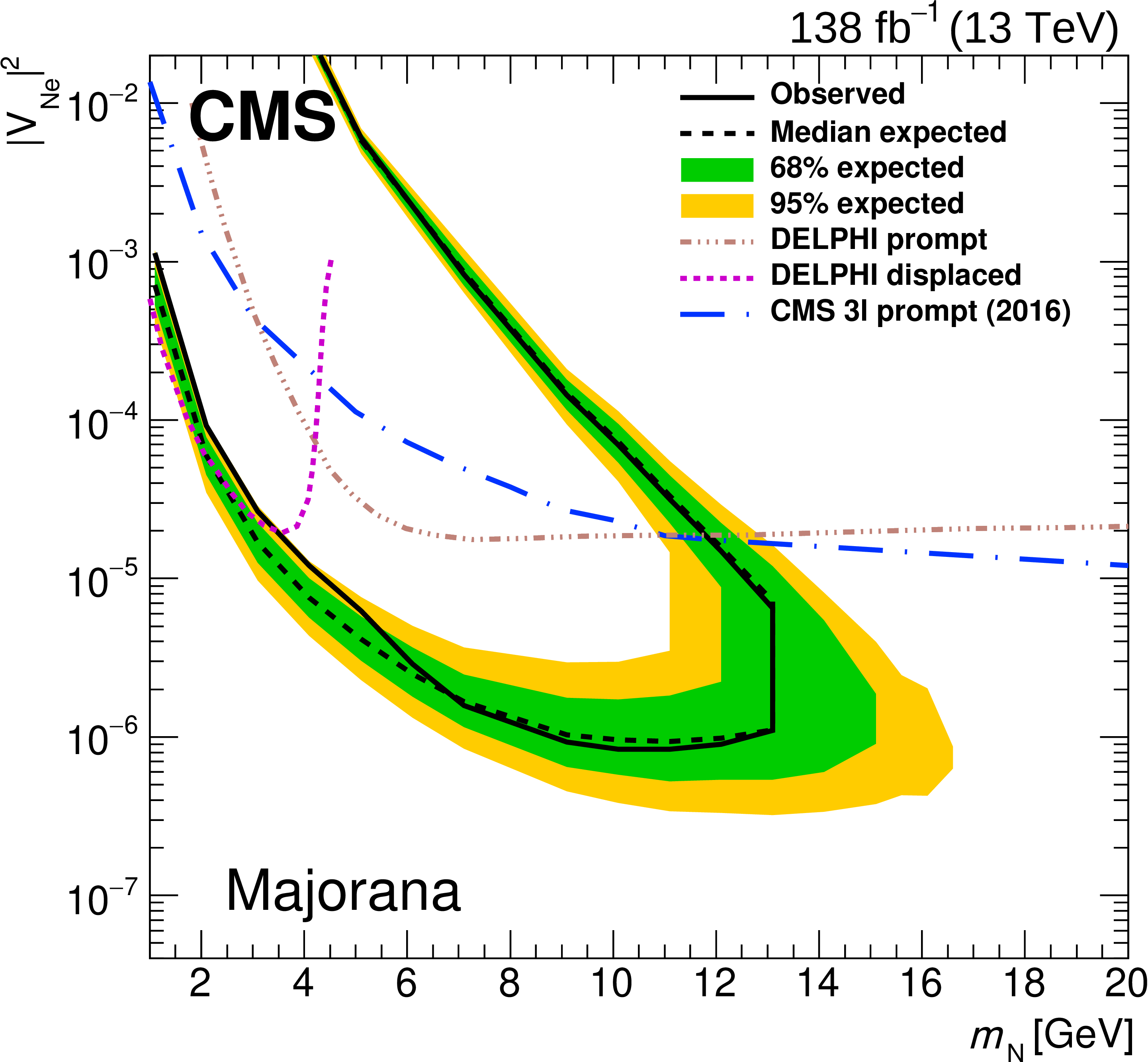
png pdf	Figure 69-a: The limits at 95% CL on $|V_{\mathrm{eN}}|^{2}$ (left) and $|V_{\mathrm{\mu N}}|^{2}$ (right) as functions of $m_{\mathrm{N}}$ for a Majorana (upper) or Dirac (lower) HNL. The area inside the solid (dashed) black curve indicates the observed (expected) exclusion region. Results from the DELPHI [255] and the CMS [259,252] Collaborations are shown as upper limits, i.e.,, the area above the curves indicates the respective observed exclusion region. Figures adapted from Ref. [261].
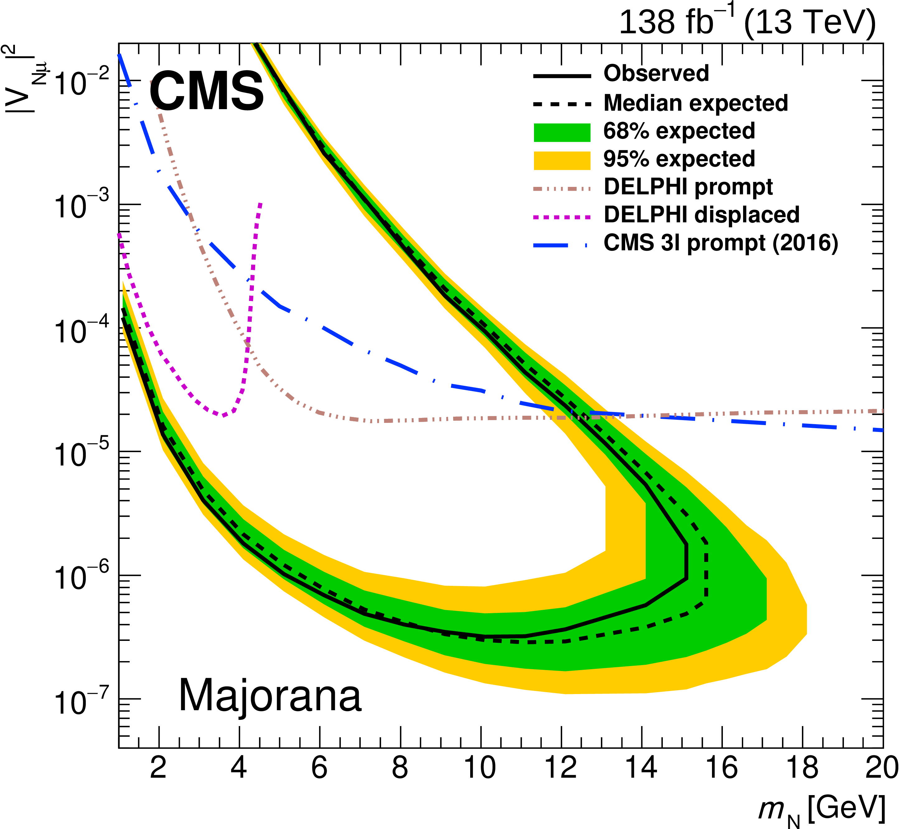
png pdf	Figure 69-b: The limits at 95% CL on $|V_{\mathrm{eN}}|^{2}$ (left) and $|V_{\mathrm{\mu N}}|^{2}$ (right) as functions of $m_{\mathrm{N}}$ for a Majorana (upper) or Dirac (lower) HNL. The area inside the solid (dashed) black curve indicates the observed (expected) exclusion region. Results from the DELPHI [255] and the CMS [259,252] Collaborations are shown as upper limits, i.e.,, the area above the curves indicates the respective observed exclusion region. Figures adapted from Ref. [261].
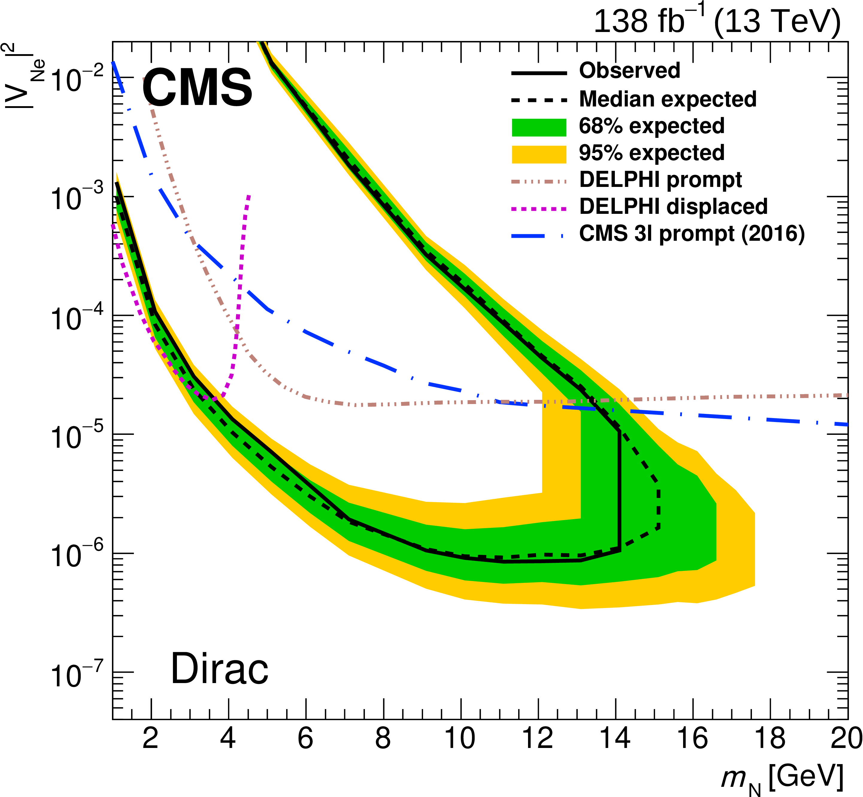
png pdf	Figure 69-c: The limits at 95% CL on $|V_{\mathrm{eN}}|^{2}$ (left) and $|V_{\mathrm{\mu N}}|^{2}$ (right) as functions of $m_{\mathrm{N}}$ for a Majorana (upper) or Dirac (lower) HNL. The area inside the solid (dashed) black curve indicates the observed (expected) exclusion region. Results from the DELPHI [255] and the CMS [259,252] Collaborations are shown as upper limits, i.e.,, the area above the curves indicates the respective observed exclusion region. Figures adapted from Ref. [261].
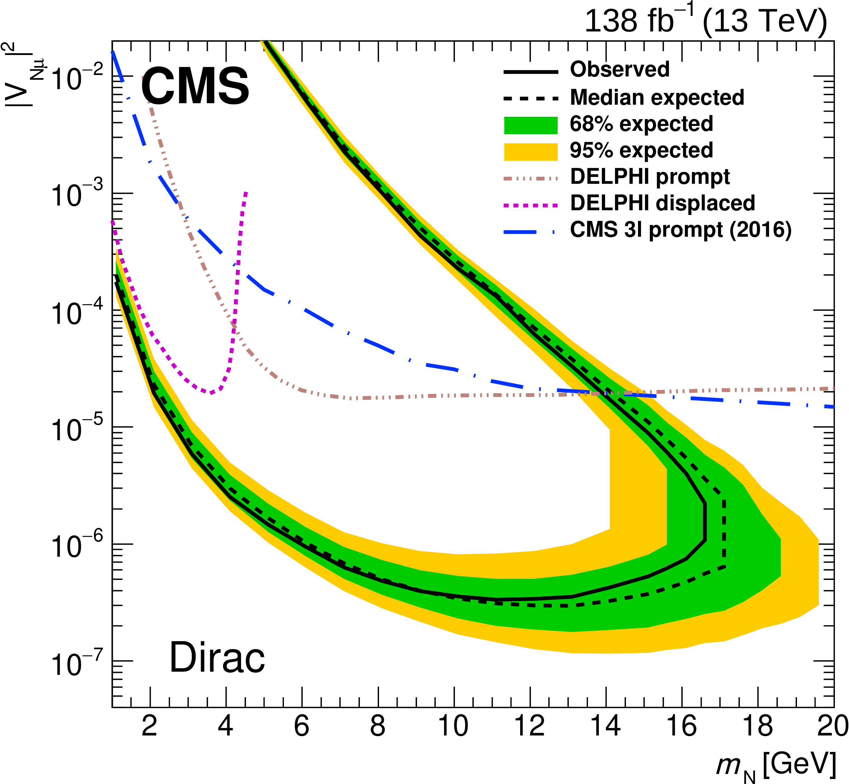
png pdf	Figure 69-d: The limits at 95% CL on $|V_{\mathrm{eN}}|^{2}$ (left) and $|V_{\mathrm{\mu N}}|^{2}$ (right) as functions of $m_{\mathrm{N}}$ for a Majorana (upper) or Dirac (lower) HNL. The area inside the solid (dashed) black curve indicates the observed (expected) exclusion region. Results from the DELPHI [255] and the CMS [259,252] Collaborations are shown as upper limits, i.e.,, the area above the curves indicates the respective observed exclusion region. Figures adapted from Ref. [261].
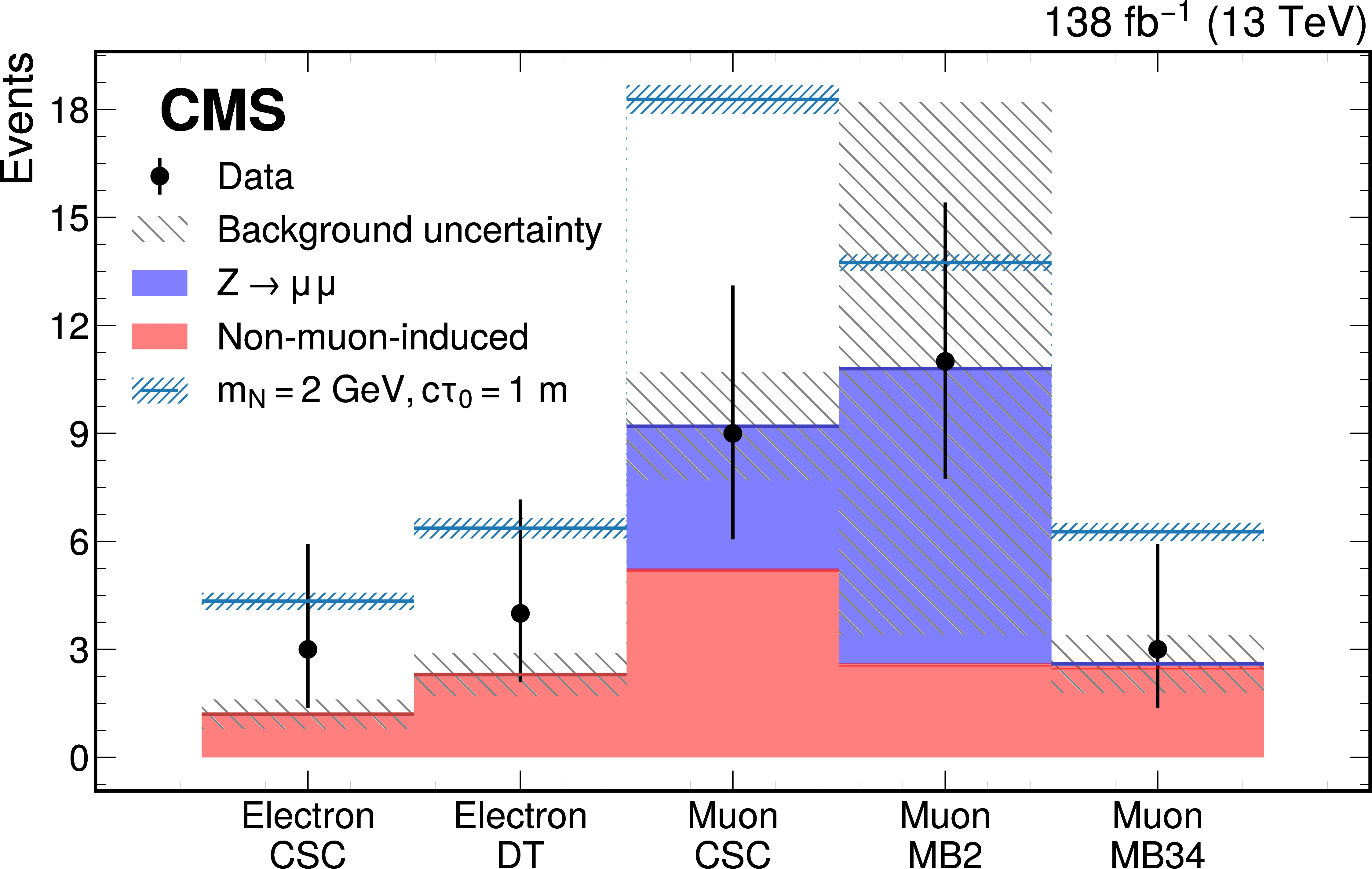
png pdf	Figure 70: Expected and observed number of events in the SR of different event categories. Signal yields of a Majorana HNL with a mass of 2 GeV and with a proper decay length of 1 m are overlaid on top of the expected background estimated using the ABCD method. Figure taken from Ref. [270].
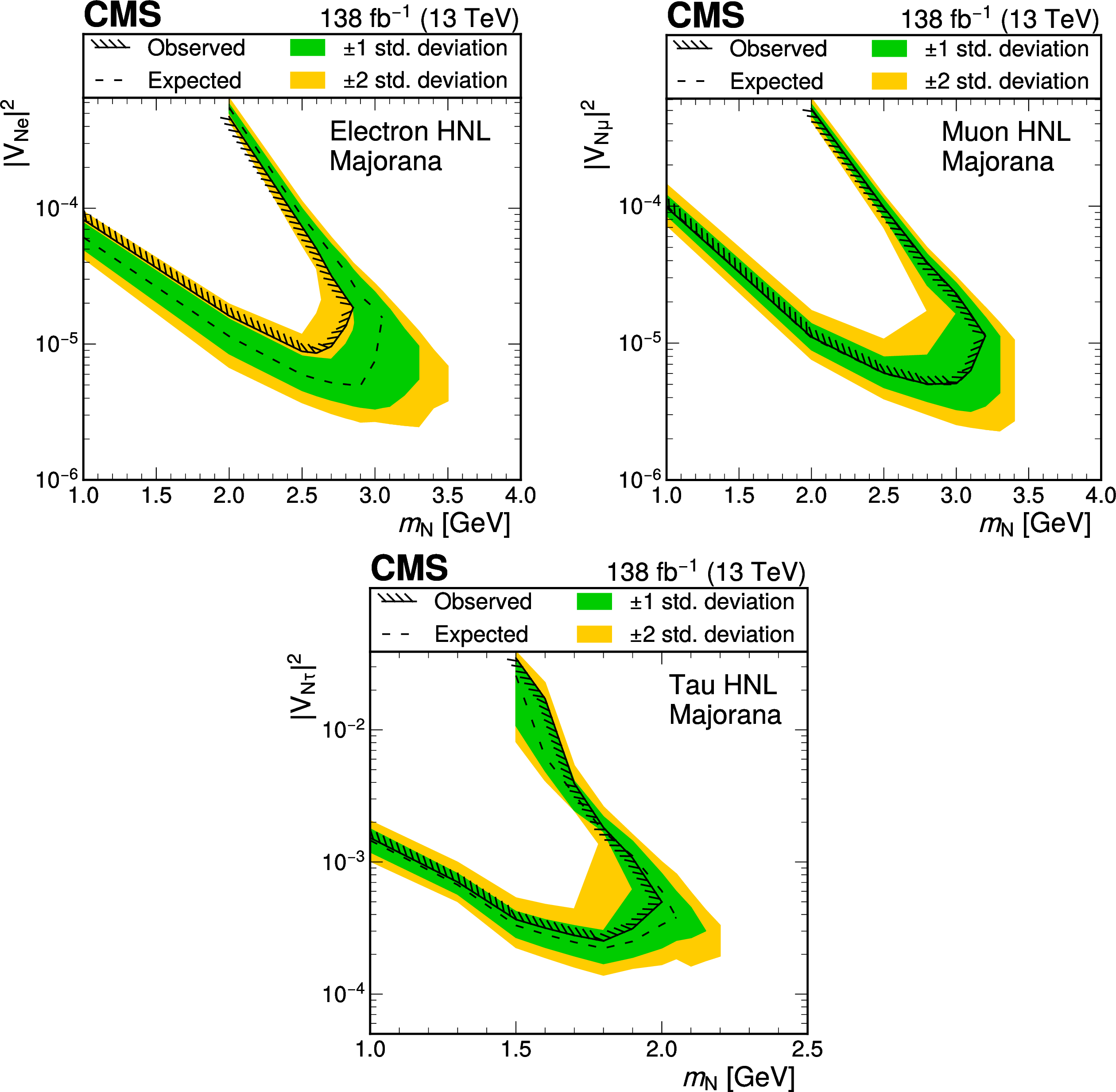
png pdf	Figure 71: Expected and observed upper limits at 95% CL on Majorana HNL production as functions of the HNL mass ($m_{\mathrm{N}}$), and assuming mixing of the HNL with only one generation. The limits are shown for pure electron mixing (upper left), pure muon mixing (upper right), and pure tau neutrino mixing (lower). The limits in the tau neutrino mixing scenario are obtained by combining the results from the electron and muon decay channels of the tau lepton. Figures adapted from Ref. [270].
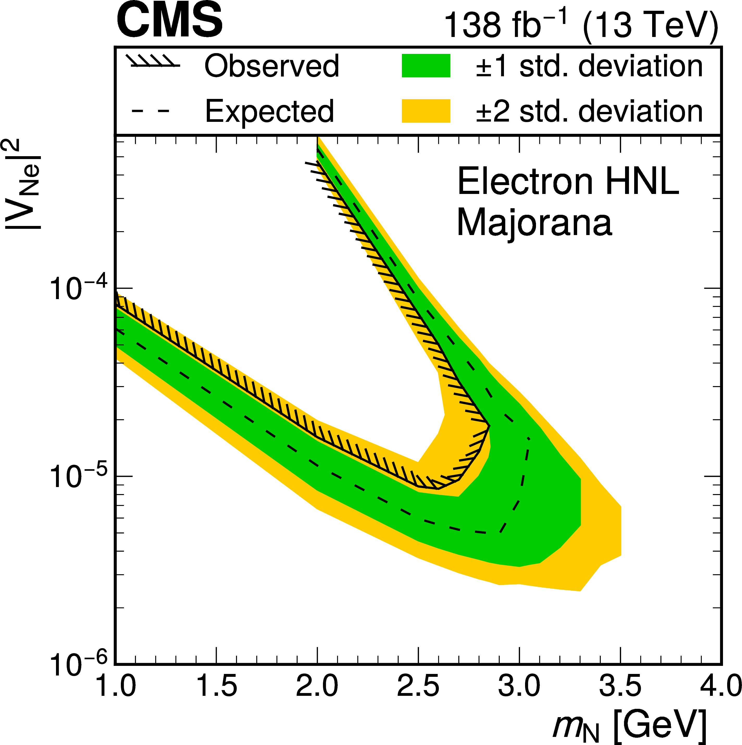
png pdf	Figure 71-a: Expected and observed upper limits at 95% CL on Majorana HNL production as functions of the HNL mass ($m_{\mathrm{N}}$), and assuming mixing of the HNL with only one generation. The limits are shown for pure electron mixing (upper left), pure muon mixing (upper right), and pure tau neutrino mixing (lower). The limits in the tau neutrino mixing scenario are obtained by combining the results from the electron and muon decay channels of the tau lepton. Figures adapted from Ref. [270].
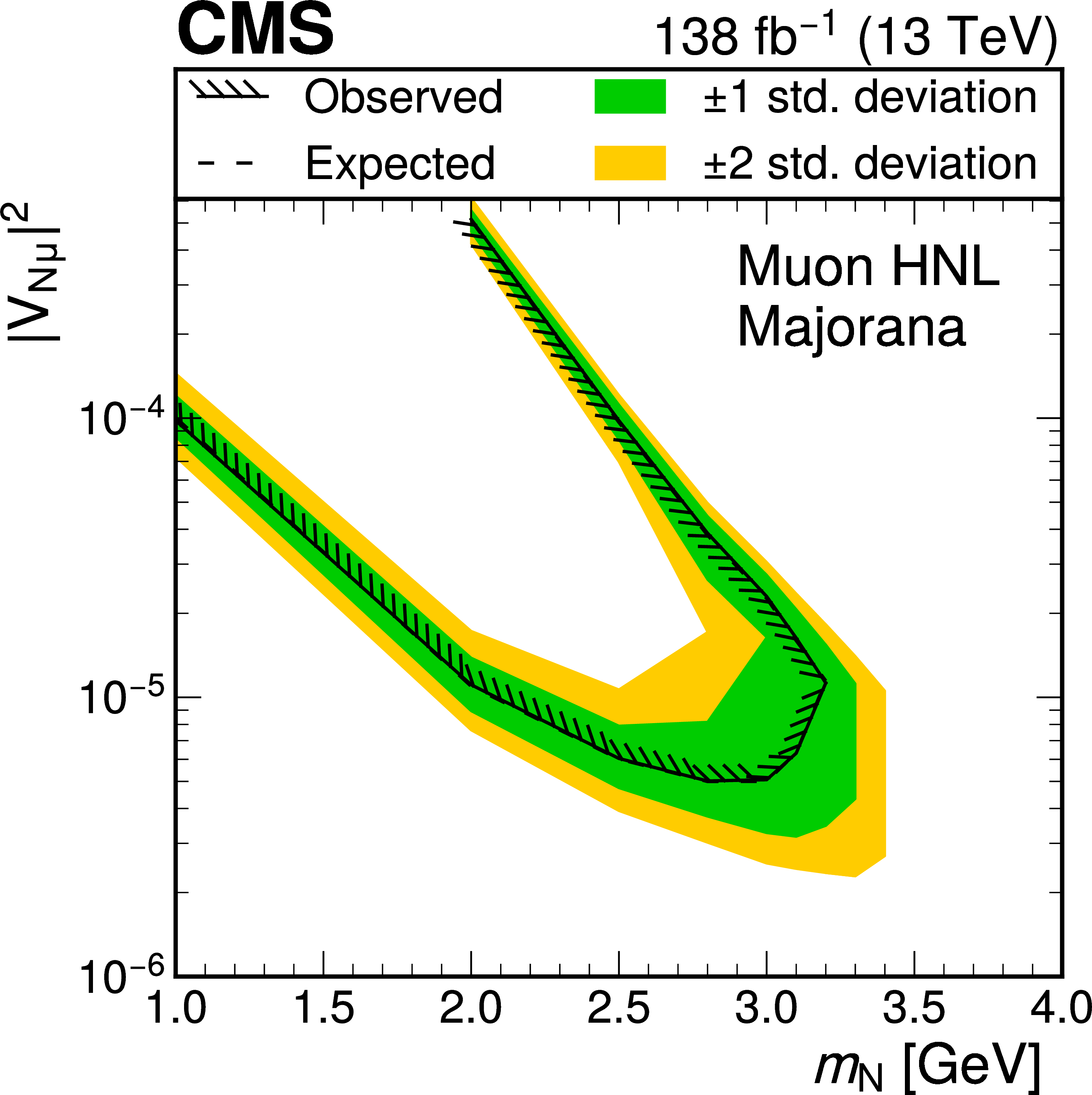
png pdf	Figure 71-b: Expected and observed upper limits at 95% CL on Majorana HNL production as functions of the HNL mass ($m_{\mathrm{N}}$), and assuming mixing of the HNL with only one generation. The limits are shown for pure electron mixing (upper left), pure muon mixing (upper right), and pure tau neutrino mixing (lower). The limits in the tau neutrino mixing scenario are obtained by combining the results from the electron and muon decay channels of the tau lepton. Figures adapted from Ref. [270].
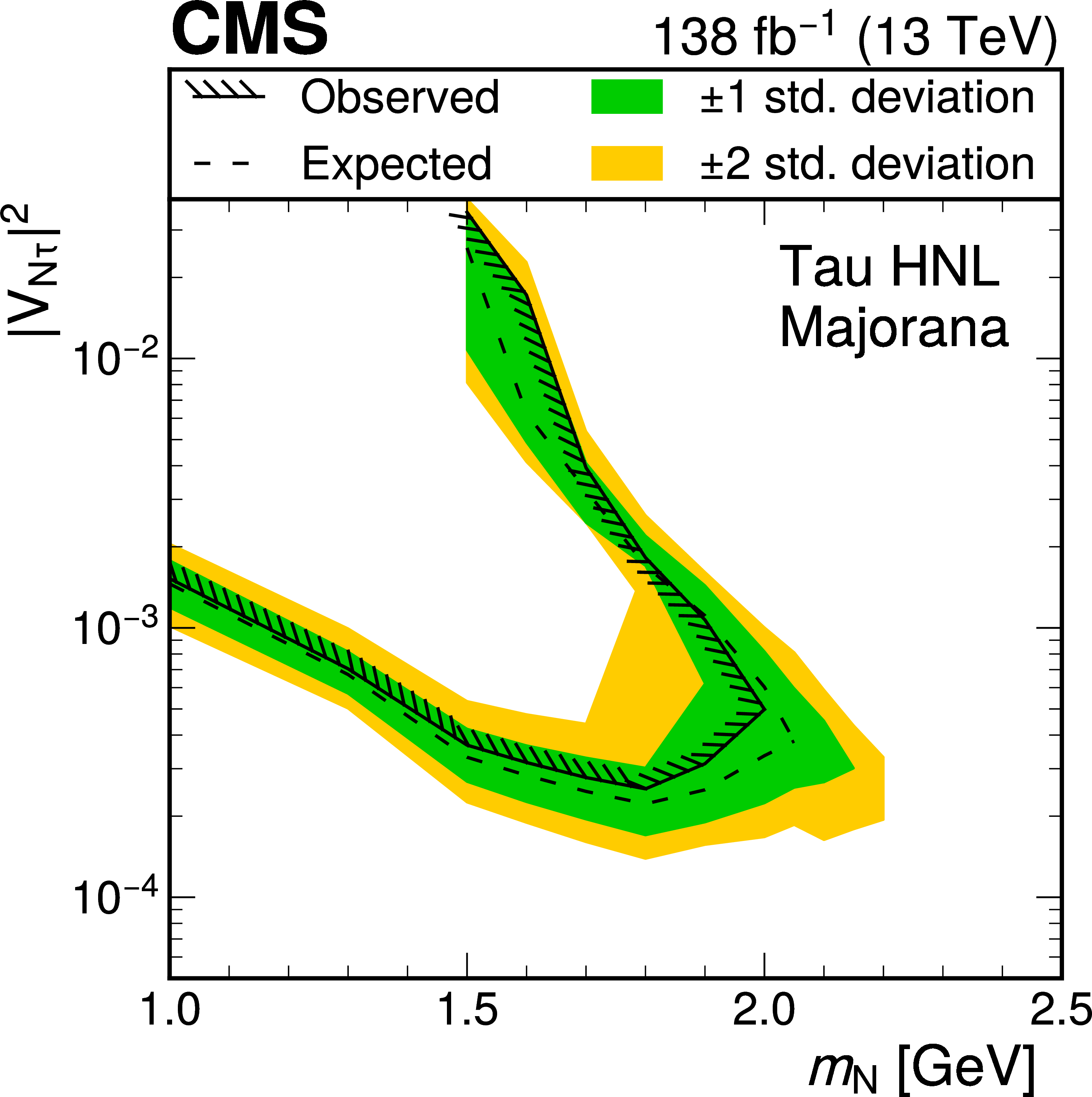
png pdf	Figure 71-c: Expected and observed upper limits at 95% CL on Majorana HNL production as functions of the HNL mass ($m_{\mathrm{N}}$), and assuming mixing of the HNL with only one generation. The limits are shown for pure electron mixing (upper left), pure muon mixing (upper right), and pure tau neutrino mixing (lower). The limits in the tau neutrino mixing scenario are obtained by combining the results from the electron and muon decay channels of the tau lepton. Figures adapted from Ref. [270].
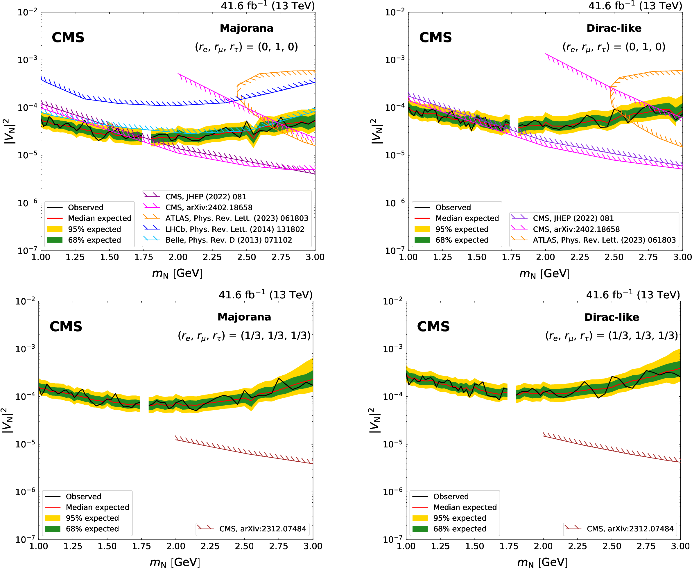
png pdf	Figure 72: Expected and observed limits at 95% CL on $|V_{\mathrm{N}}|^{2}$ as functions of $m_{\mathrm{N}}$, in the Majorana (left column) and Dirac (right column) scenarios. The limits are shown for the mixing scenarios $(r_{\mathrm{e}},r_{\mu},r_{\tau})=(0,1,0)$ (upper row) and $(r_{\mathrm{e}},r_{\mu},r_{\tau})=(1/3,1/3,1/3)$ (lower row). Results from the CMS [261,270,263], ATLAS [265], LHCb [276], and Belle [277] Collaborations are superimposed for comparison. The mass range with no results shown corresponds to a vetoed region around the $\mathrm{D^0}$ mass. Figures taken from Ref. [220].
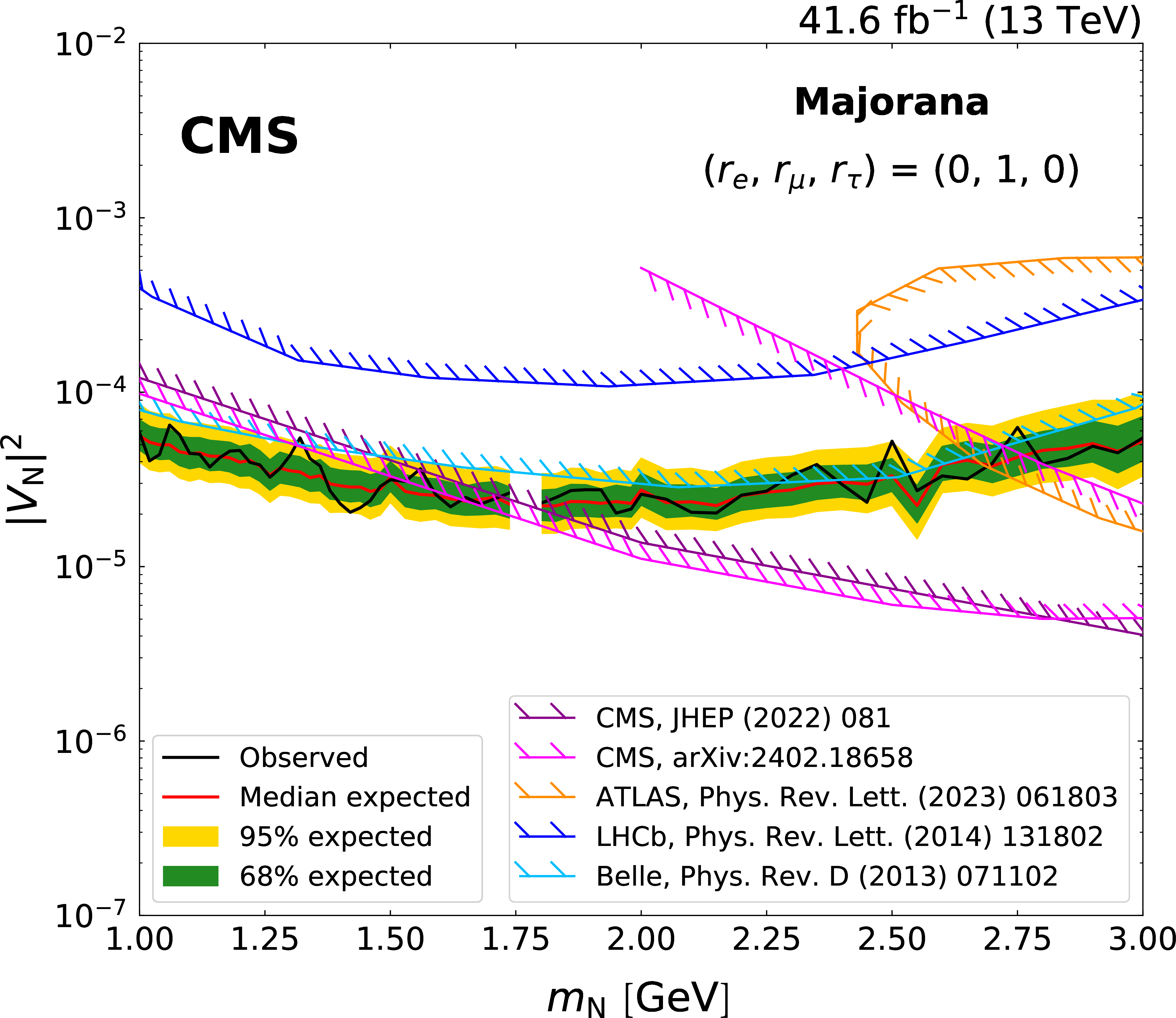
png pdf	Figure 72-a: Expected and observed limits at 95% CL on $|V_{\mathrm{N}}|^{2}$ as functions of $m_{\mathrm{N}}$, in the Majorana (left column) and Dirac (right column) scenarios. The limits are shown for the mixing scenarios $(r_{\mathrm{e}},r_{\mu},r_{\tau})=(0,1,0)$ (upper row) and $(r_{\mathrm{e}},r_{\mu},r_{\tau})=(1/3,1/3,1/3)$ (lower row). Results from the CMS [261,270,263], ATLAS [265], LHCb [276], and Belle [277] Collaborations are superimposed for comparison. The mass range with no results shown corresponds to a vetoed region around the $\mathrm{D^0}$ mass. Figures taken from Ref. [220].
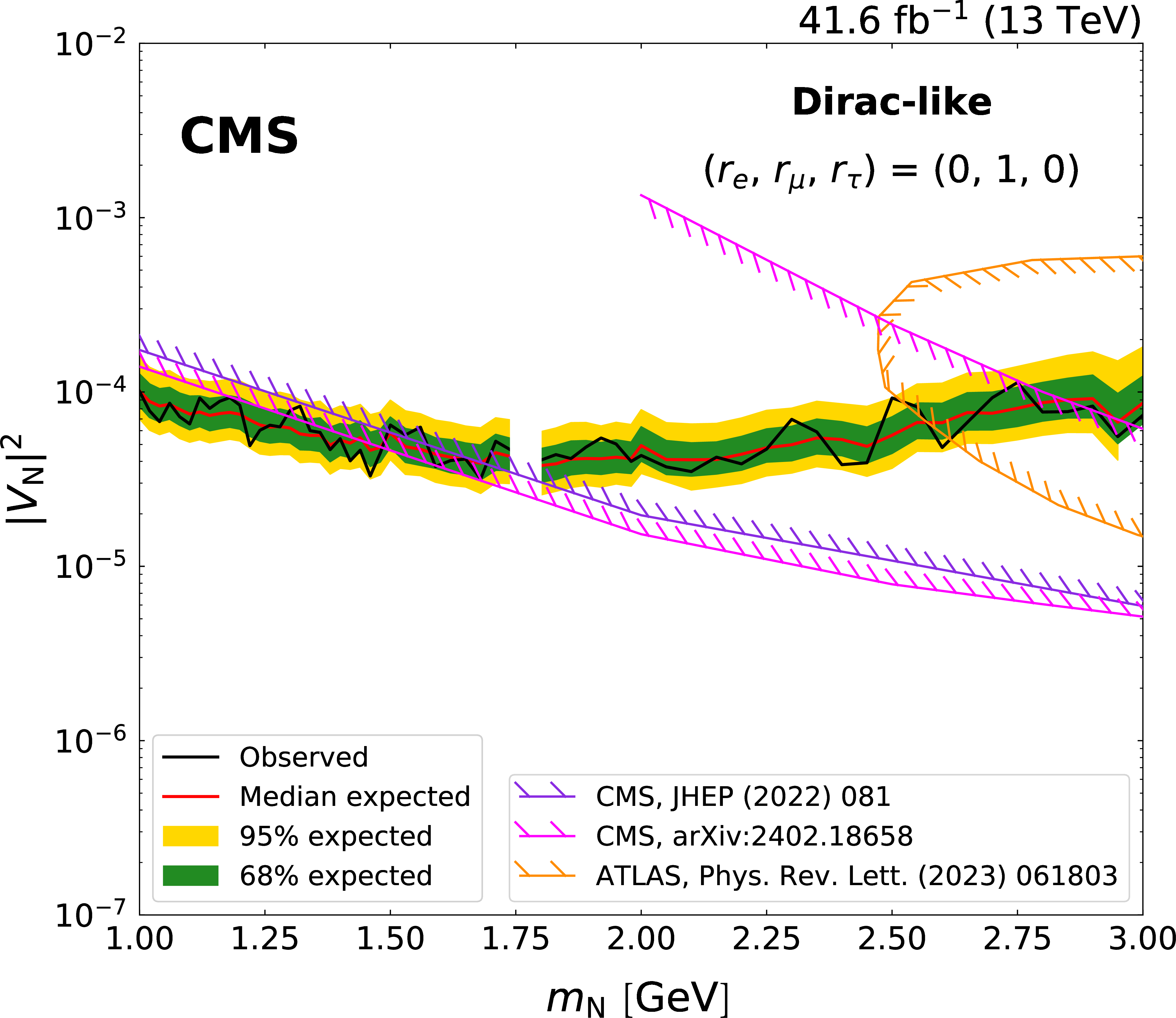
png pdf	Figure 72-b: Expected and observed limits at 95% CL on $|V_{\mathrm{N}}|^{2}$ as functions of $m_{\mathrm{N}}$, in the Majorana (left column) and Dirac (right column) scenarios. The limits are shown for the mixing scenarios $(r_{\mathrm{e}},r_{\mu},r_{\tau})=(0,1,0)$ (upper row) and $(r_{\mathrm{e}},r_{\mu},r_{\tau})=(1/3,1/3,1/3)$ (lower row). Results from the CMS [261,270,263], ATLAS [265], LHCb [276], and Belle [277] Collaborations are superimposed for comparison. The mass range with no results shown corresponds to a vetoed region around the $\mathrm{D^0}$ mass. Figures taken from Ref. [220].
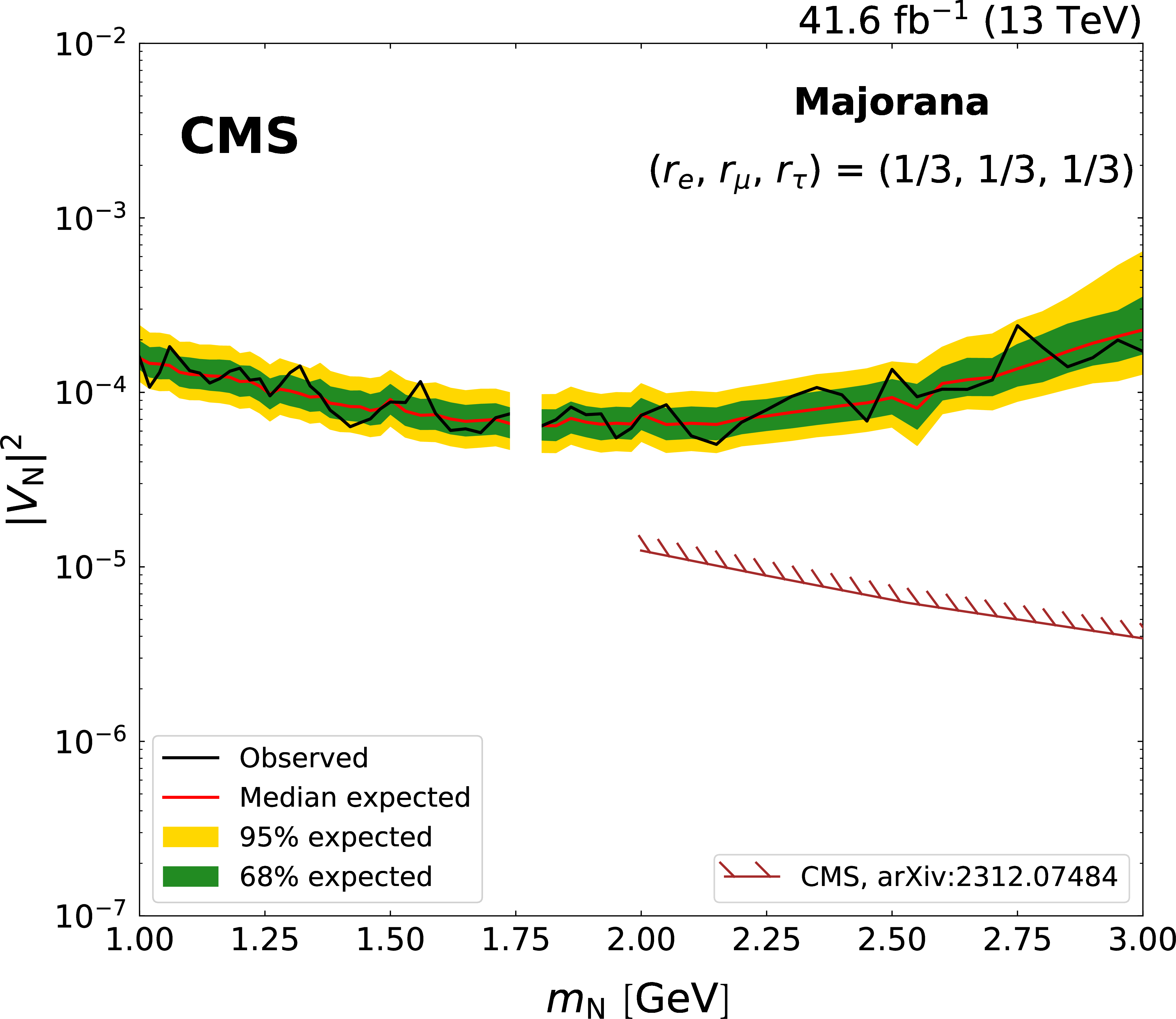
png pdf	Figure 72-c: Expected and observed limits at 95% CL on $|V_{\mathrm{N}}|^{2}$ as functions of $m_{\mathrm{N}}$, in the Majorana (left column) and Dirac (right column) scenarios. The limits are shown for the mixing scenarios $(r_{\mathrm{e}},r_{\mu},r_{\tau})=(0,1,0)$ (upper row) and $(r_{\mathrm{e}},r_{\mu},r_{\tau})=(1/3,1/3,1/3)$ (lower row). Results from the CMS [261,270,263], ATLAS [265], LHCb [276], and Belle [277] Collaborations are superimposed for comparison. The mass range with no results shown corresponds to a vetoed region around the $\mathrm{D^0}$ mass. Figures taken from Ref. [220].
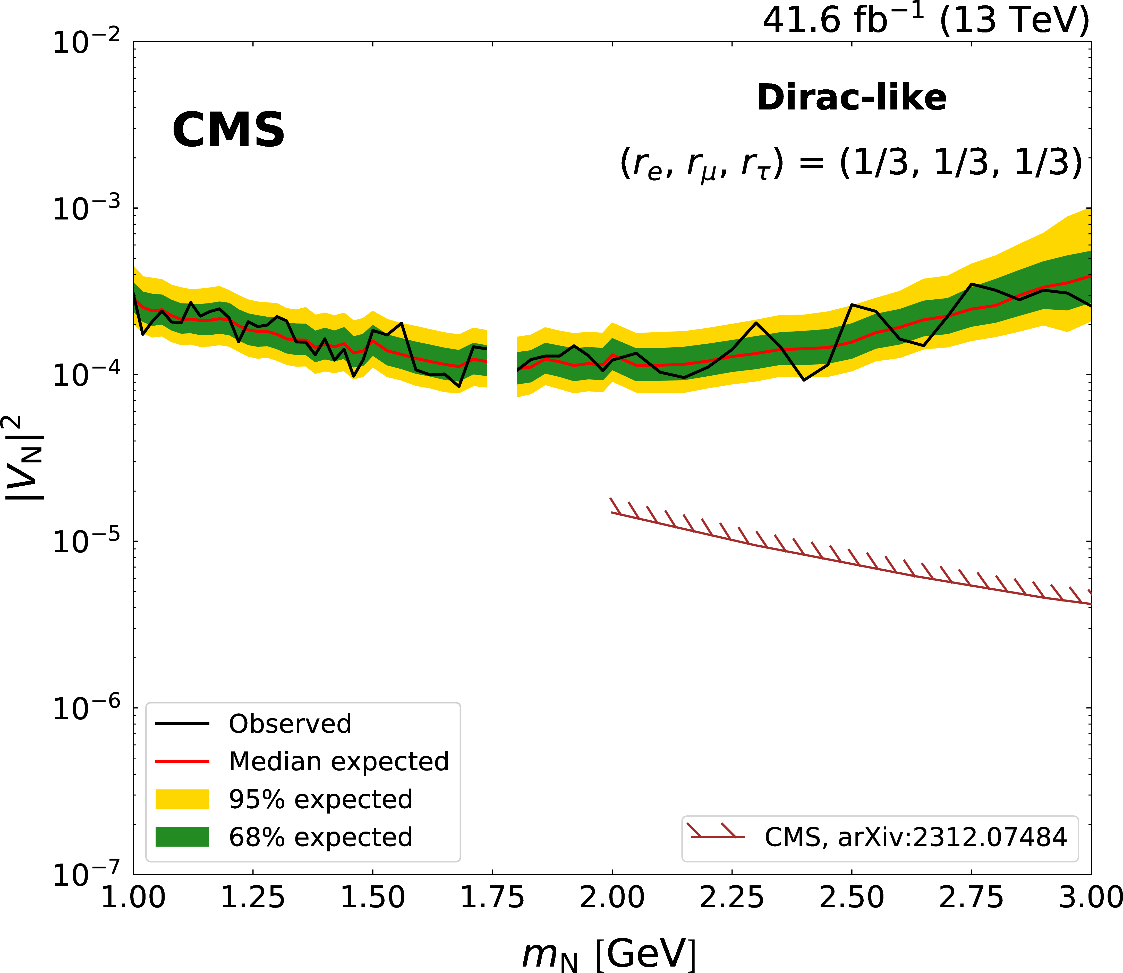
png pdf	Figure 72-d: Expected and observed limits at 95% CL on $|V_{\mathrm{N}}|^{2}$ as functions of $m_{\mathrm{N}}$, in the Majorana (left column) and Dirac (right column) scenarios. The limits are shown for the mixing scenarios $(r_{\mathrm{e}},r_{\mu},r_{\tau})=(0,1,0)$ (upper row) and $(r_{\mathrm{e}},r_{\mu},r_{\tau})=(1/3,1/3,1/3)$ (lower row). Results from the CMS [261,270,263], ATLAS [265], LHCb [276], and Belle [277] Collaborations are superimposed for comparison. The mass range with no results shown corresponds to a vetoed region around the $\mathrm{D^0}$ mass. Figures taken from Ref. [220].
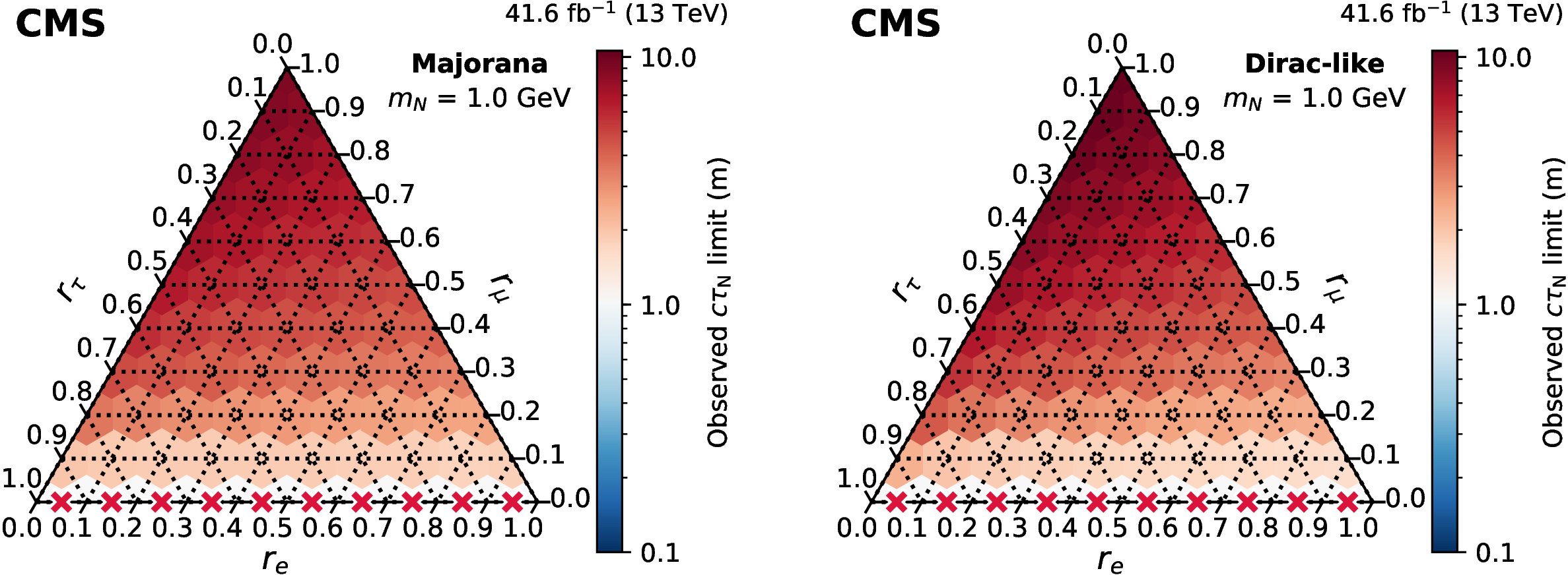
png pdf	Figure 73: Observed limits at 95% CL on $c\tau_{\mathrm{N}}$ as a function of the mixing ratios $(r_{\mathrm{e}},r_{\mu},r_{\tau})$ for $m_{\mathrm{N}}=$ 1 GeV in the Majorana (left) and Dirac (right) scenarios. The red crosses indicate that there is no exclusion found for that point. The orientation of the value markers on each axis identifies the associated internal lines on the plot. Figures taken from Ref. [220].
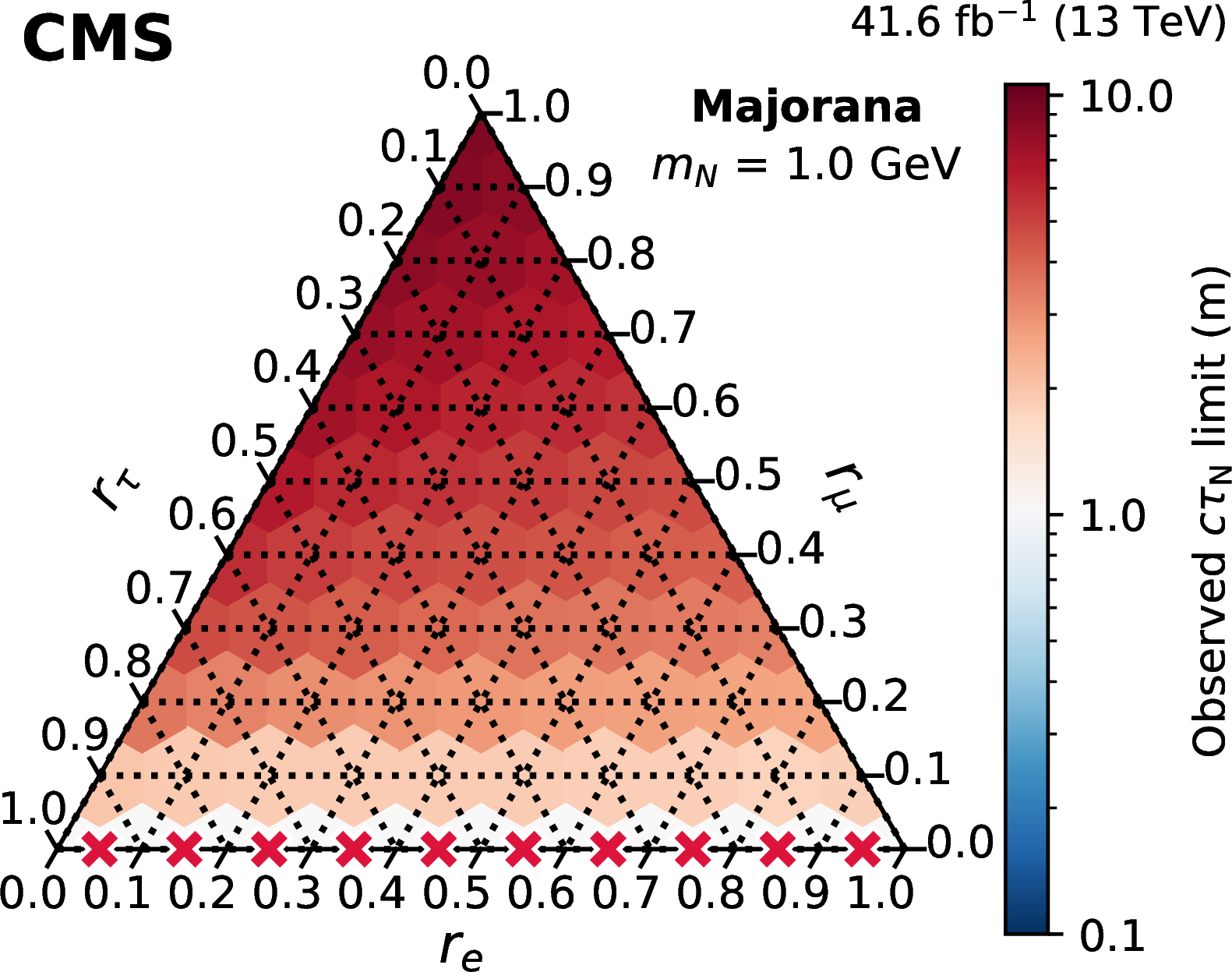
png pdf	Figure 73-a: Observed limits at 95% CL on $c\tau_{\mathrm{N}}$ as a function of the mixing ratios $(r_{\mathrm{e}},r_{\mu},r_{\tau})$ for $m_{\mathrm{N}}=$ 1 GeV in the Majorana (left) and Dirac (right) scenarios. The red crosses indicate that there is no exclusion found for that point. The orientation of the value markers on each axis identifies the associated internal lines on the plot. Figures taken from Ref. [220].
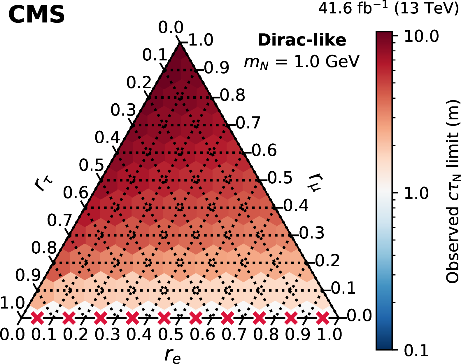
png pdf	Figure 73-b: Observed limits at 95% CL on $c\tau_{\mathrm{N}}$ as a function of the mixing ratios $(r_{\mathrm{e}},r_{\mu},r_{\tau})$ for $m_{\mathrm{N}}=$ 1 GeV in the Majorana (left) and Dirac (right) scenarios. The red crosses indicate that there is no exclusion found for that point. The orientation of the value markers on each axis identifies the associated internal lines on the plot. Figures taken from Ref. [220].
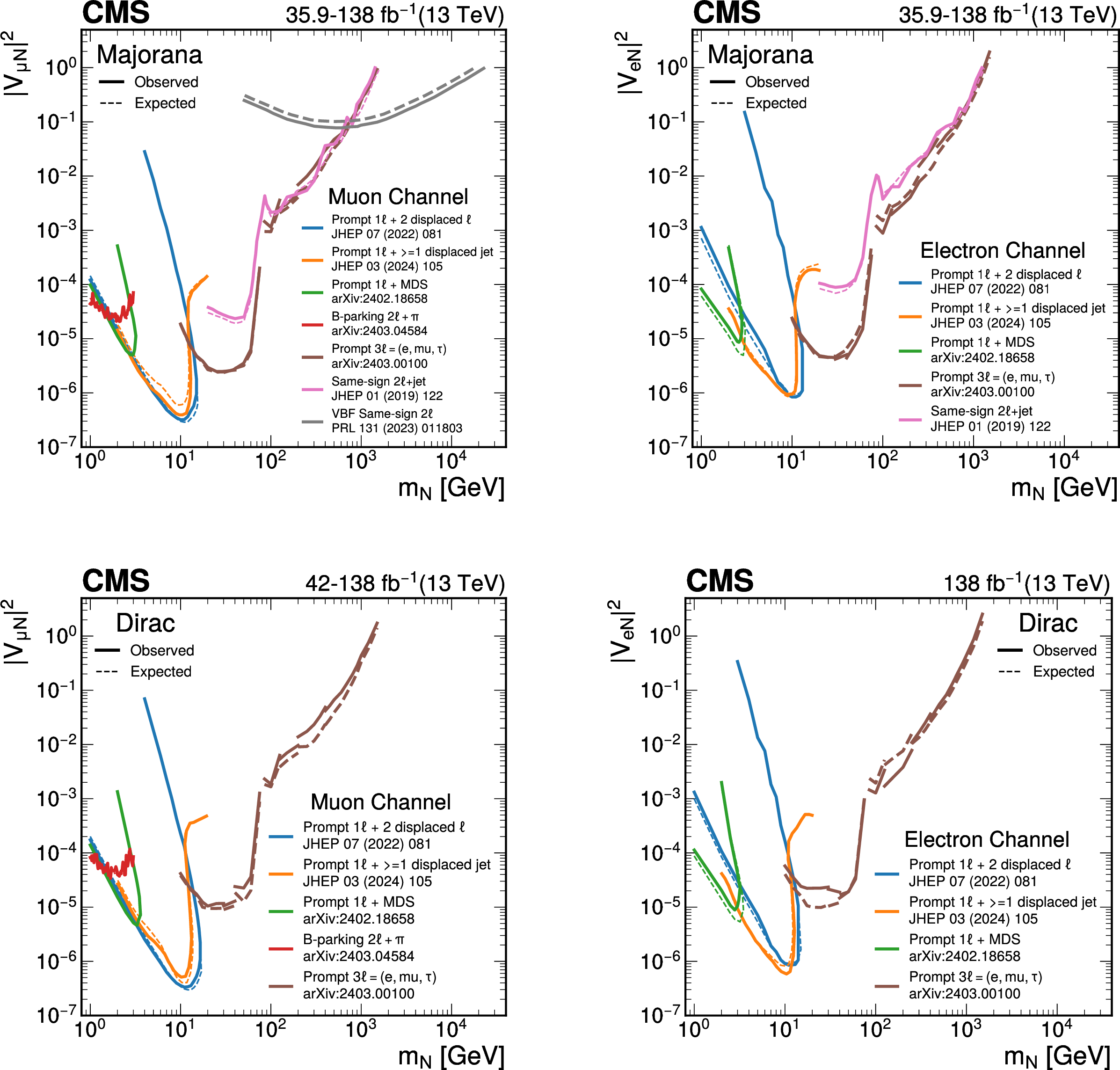
png pdf	Figure 74: Summary of searches at the CMS experiment for long-lived HNLs in the $Type I$ seesaw model. The observed limits at 95% CL on the mixing parameter \mixparsq\ell$\mathrm{N}$ as a function of the HNL mass $m_{\mathrm{N}}$ are shown, for Majorana and Dirac HNLs (upper and lower row, respectively), and in the muon and electron channel (left and right column, respectively).
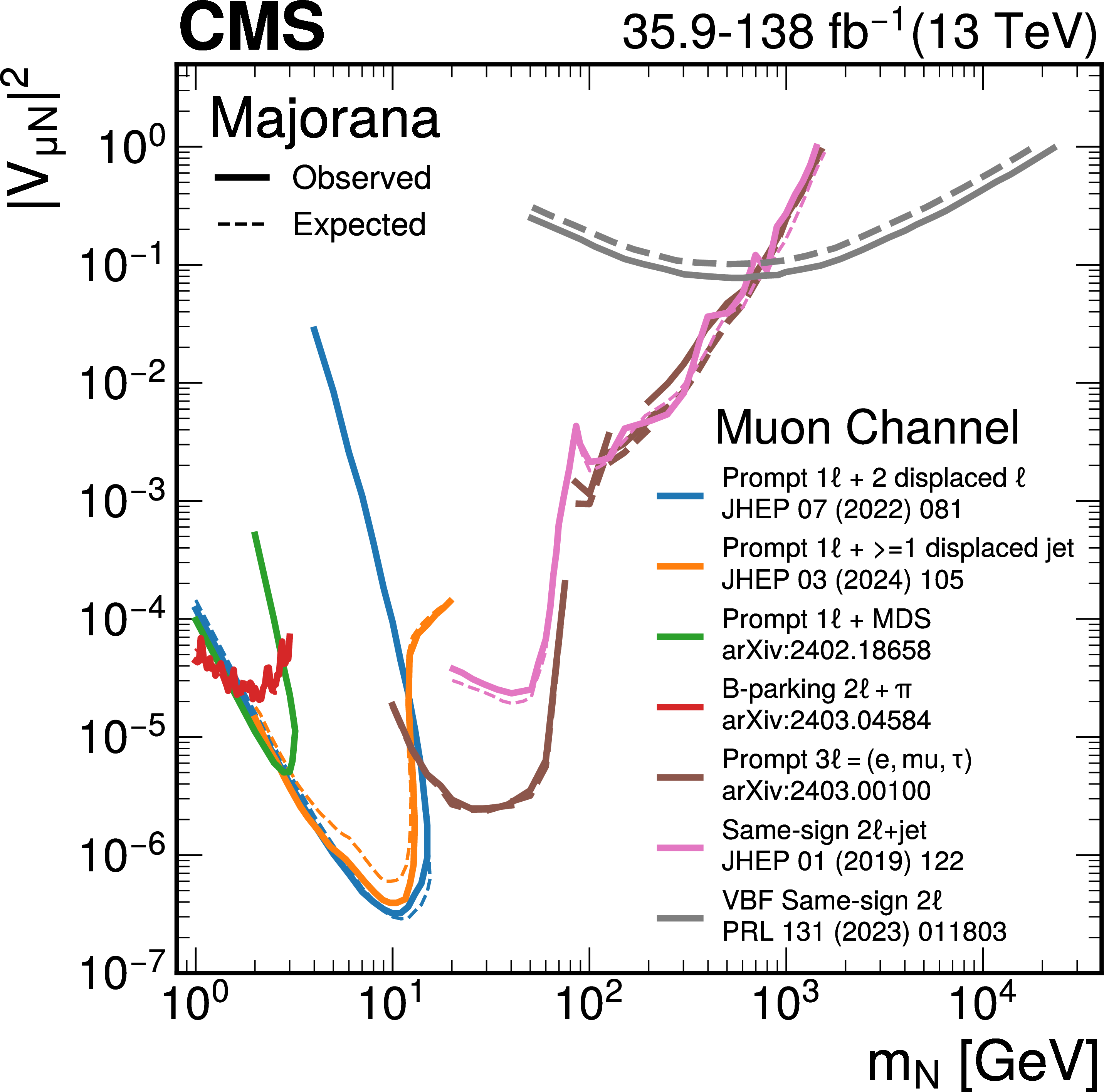
png pdf	Figure 74-a: Summary of searches at the CMS experiment for long-lived HNLs in the $Type I$ seesaw model. The observed limits at 95% CL on the mixing parameter \mixparsq\ell$\mathrm{N}$ as a function of the HNL mass $m_{\mathrm{N}}$ are shown, for Majorana and Dirac HNLs (upper and lower row, respectively), and in the muon and electron channel (left and right column, respectively).
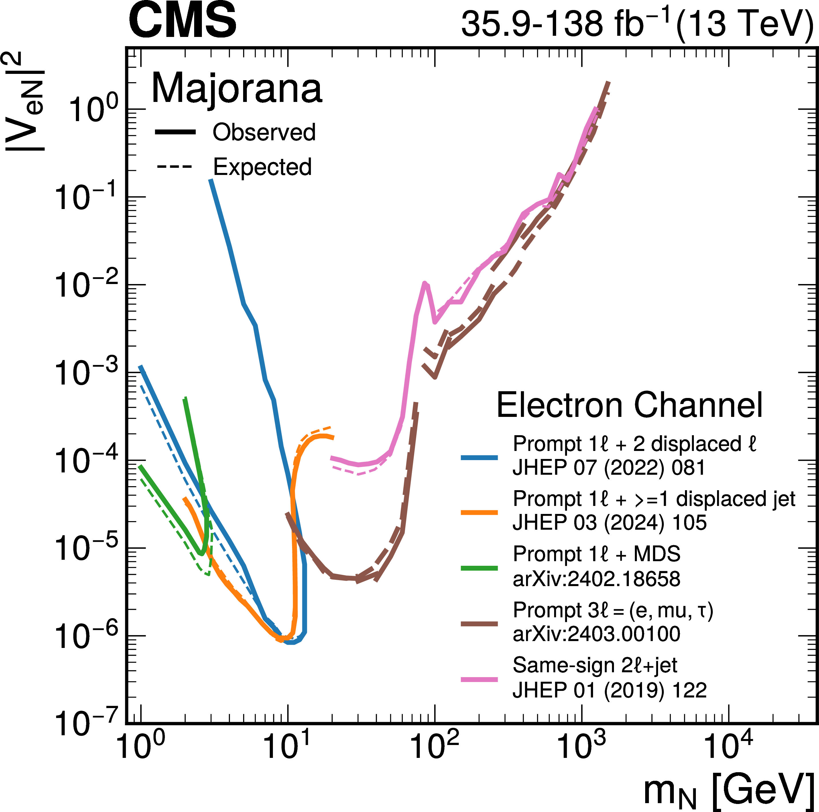
png pdf	Figure 74-b: Summary of searches at the CMS experiment for long-lived HNLs in the $Type I$ seesaw model. The observed limits at 95% CL on the mixing parameter \mixparsq\ell$\mathrm{N}$ as a function of the HNL mass $m_{\mathrm{N}}$ are shown, for Majorana and Dirac HNLs (upper and lower row, respectively), and in the muon and electron channel (left and right column, respectively).
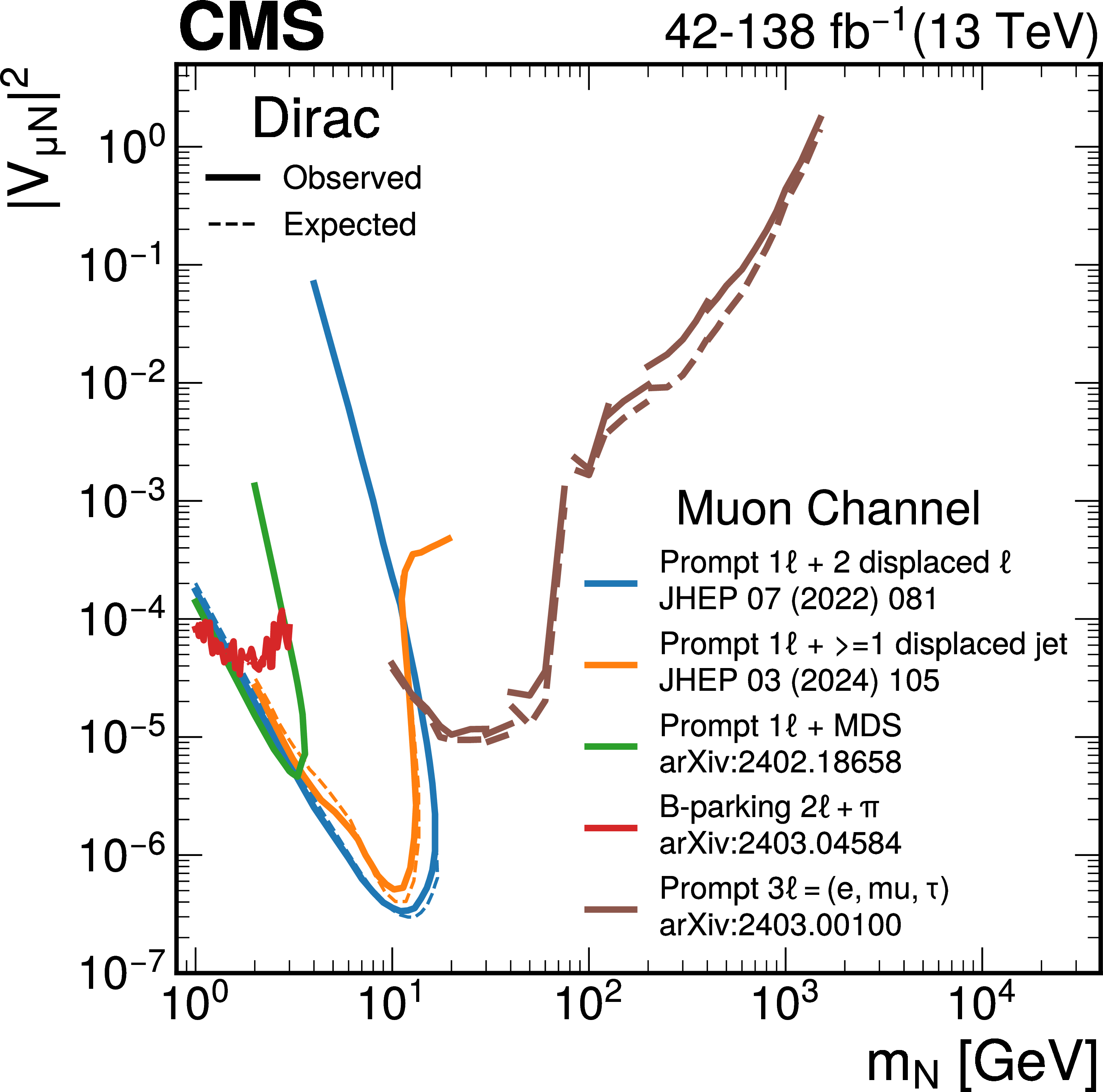
png pdf	Figure 74-c: Summary of searches at the CMS experiment for long-lived HNLs in the $Type I$ seesaw model. The observed limits at 95% CL on the mixing parameter \mixparsq\ell$\mathrm{N}$ as a function of the HNL mass $m_{\mathrm{N}}$ are shown, for Majorana and Dirac HNLs (upper and lower row, respectively), and in the muon and electron channel (left and right column, respectively).
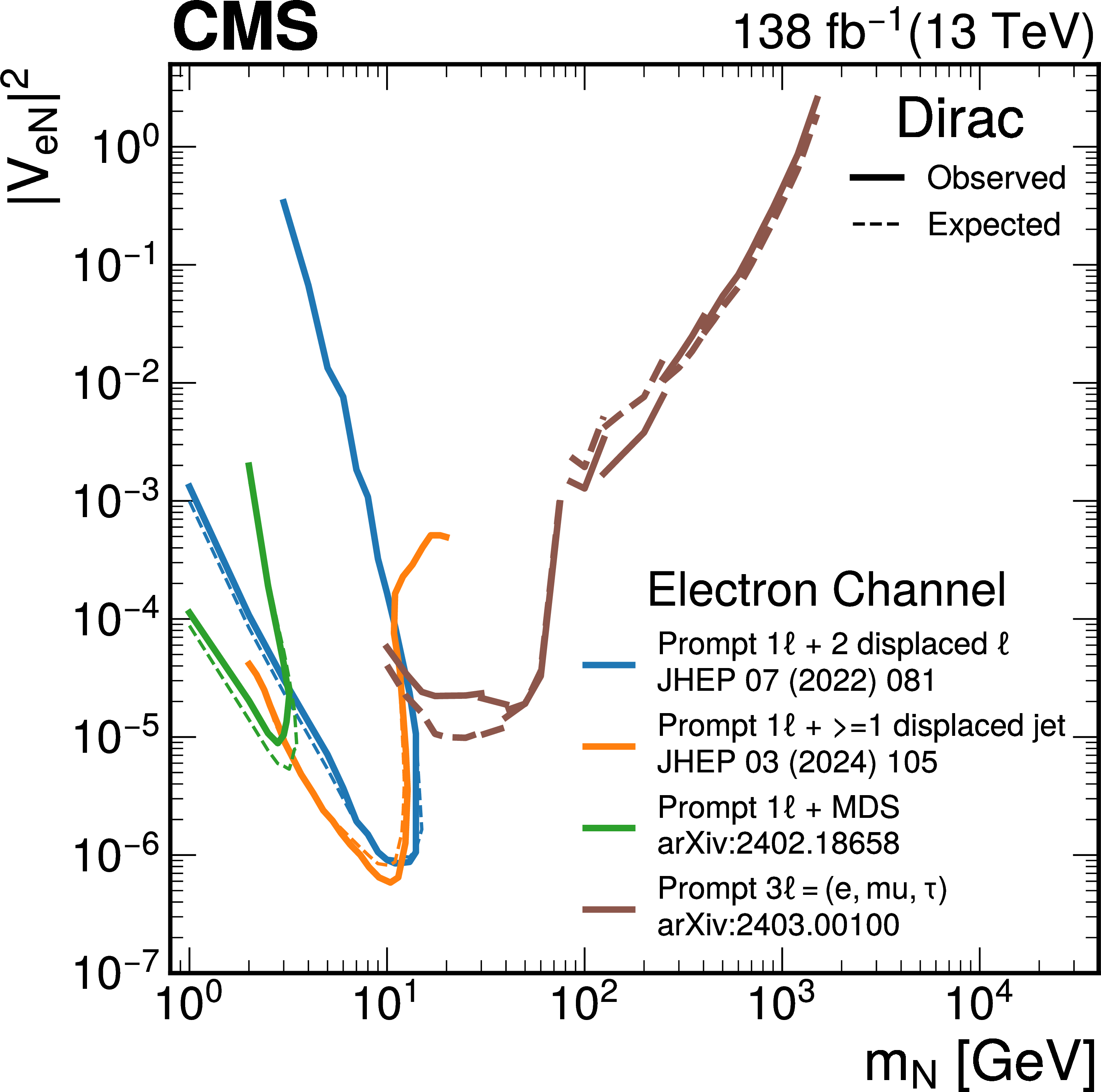
png pdf	Figure 74-d: Summary of searches at the CMS experiment for long-lived HNLs in the $Type I$ seesaw model. The observed limits at 95% CL on the mixing parameter \mixparsq\ell$\mathrm{N}$ as a function of the HNL mass $m_{\mathrm{N}}$ are shown, for Majorana and Dirac HNLs (upper and lower row, respectively), and in the muon and electron channel (left and right column, respectively).
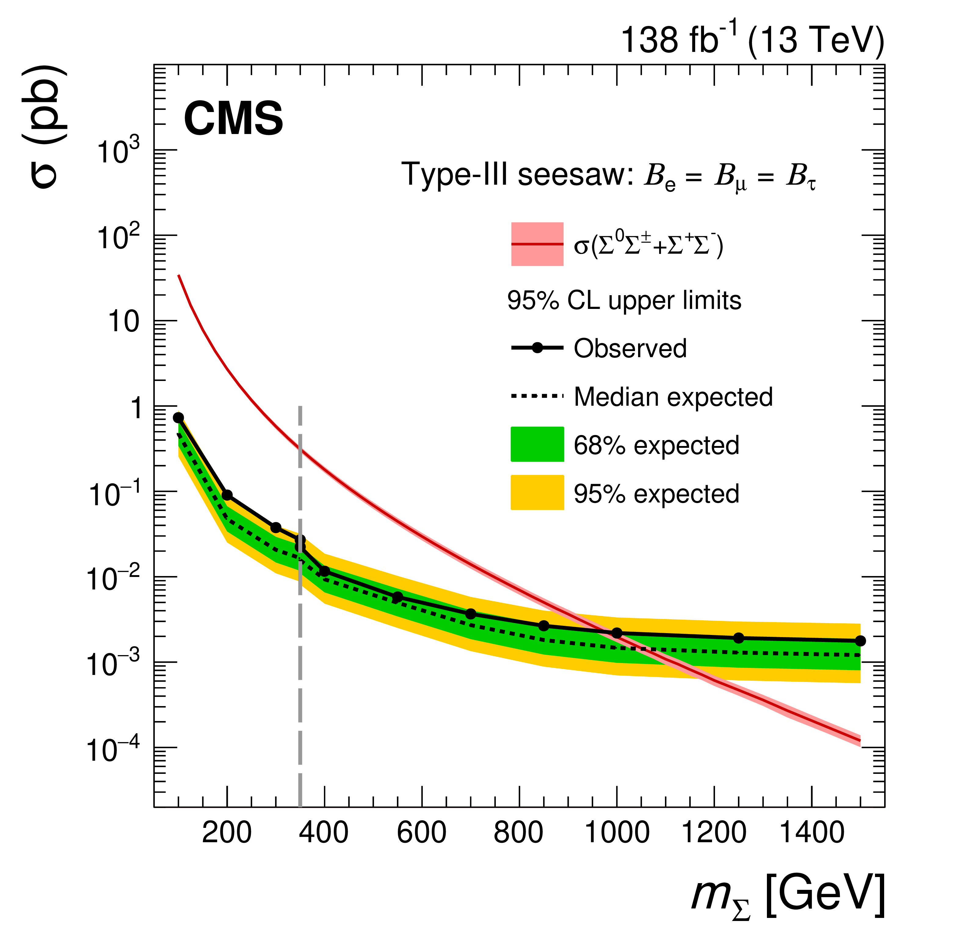
png pdf	Figure 75: Observed and expected upper limits at 95% CL on the production cross section for $Type III$ seesaw HNLs in the flavor-democratic scenario using the model-independent schemes and the BDT regions. To the left of the vertical dashed gray line, the limits are shown from the model-independent SR, and to the right the limits are shown obtained using the BDT regions. Figure adapted from Ref. [204]. Production cross sections for the signal model are calculated at NLO plus next-to-leading logarithmic precision, assuming that the heavy leptons are SU(2) triplet fermions [60,61].
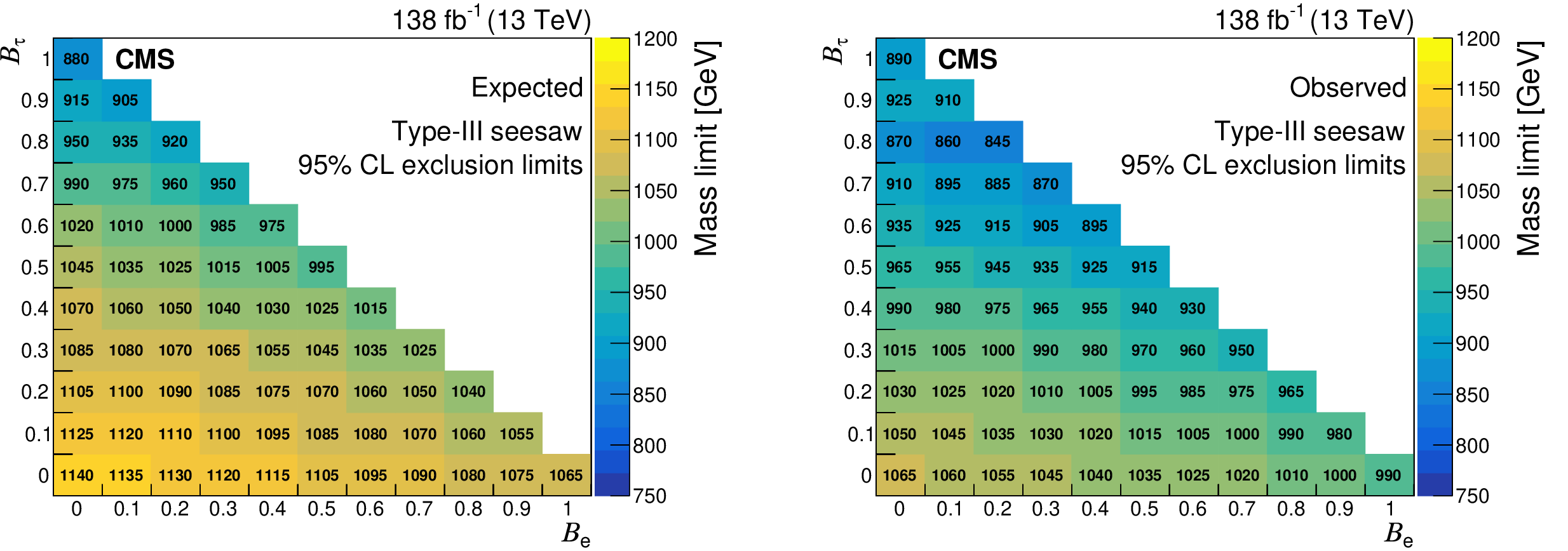
png pdf	Figure 76: Expected (left) and observed (right) lower limits at 95% CL on the mass of $Type III$ seesaw HNLs in the plane defined by $\mathcal{B}_{\mathrm{e}}$ and $\mathcal{B}_{\tau}$, with the constraint that $\mathcal{B}_{\mathrm{e}}+\mathcal{B}_{\mu}+\mathcal{B}_{\tau}=$ 1. For $\mathcal{B}_{\tau}\geq$ 0.9, these limits are obtained using the high mass BDT trained assuming $\mathcal{B}_{\tau}=$ 1, and for the other decay branching fraction combinations, the limits use the $\mathcal{B}_{\mathrm{e}}=\mathcal{B}_{\mu}=\mathcal{B}_{\tau}$ BDT. Figures adapted from Ref. [204].
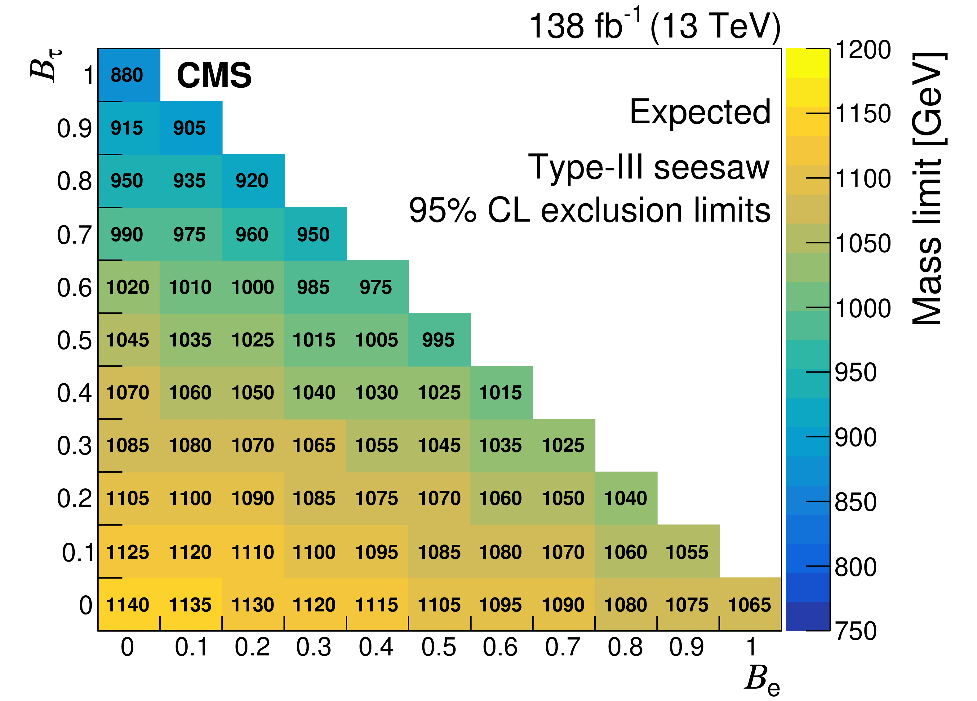
png pdf	Figure 76-a: Expected (left) and observed (right) lower limits at 95% CL on the mass of $Type III$ seesaw HNLs in the plane defined by $\mathcal{B}_{\mathrm{e}}$ and $\mathcal{B}_{\tau}$, with the constraint that $\mathcal{B}_{\mathrm{e}}+\mathcal{B}_{\mu}+\mathcal{B}_{\tau}=$ 1. For $\mathcal{B}_{\tau}\geq$ 0.9, these limits are obtained using the high mass BDT trained assuming $\mathcal{B}_{\tau}=$ 1, and for the other decay branching fraction combinations, the limits use the $\mathcal{B}_{\mathrm{e}}=\mathcal{B}_{\mu}=\mathcal{B}_{\tau}$ BDT. Figures adapted from Ref. [204].
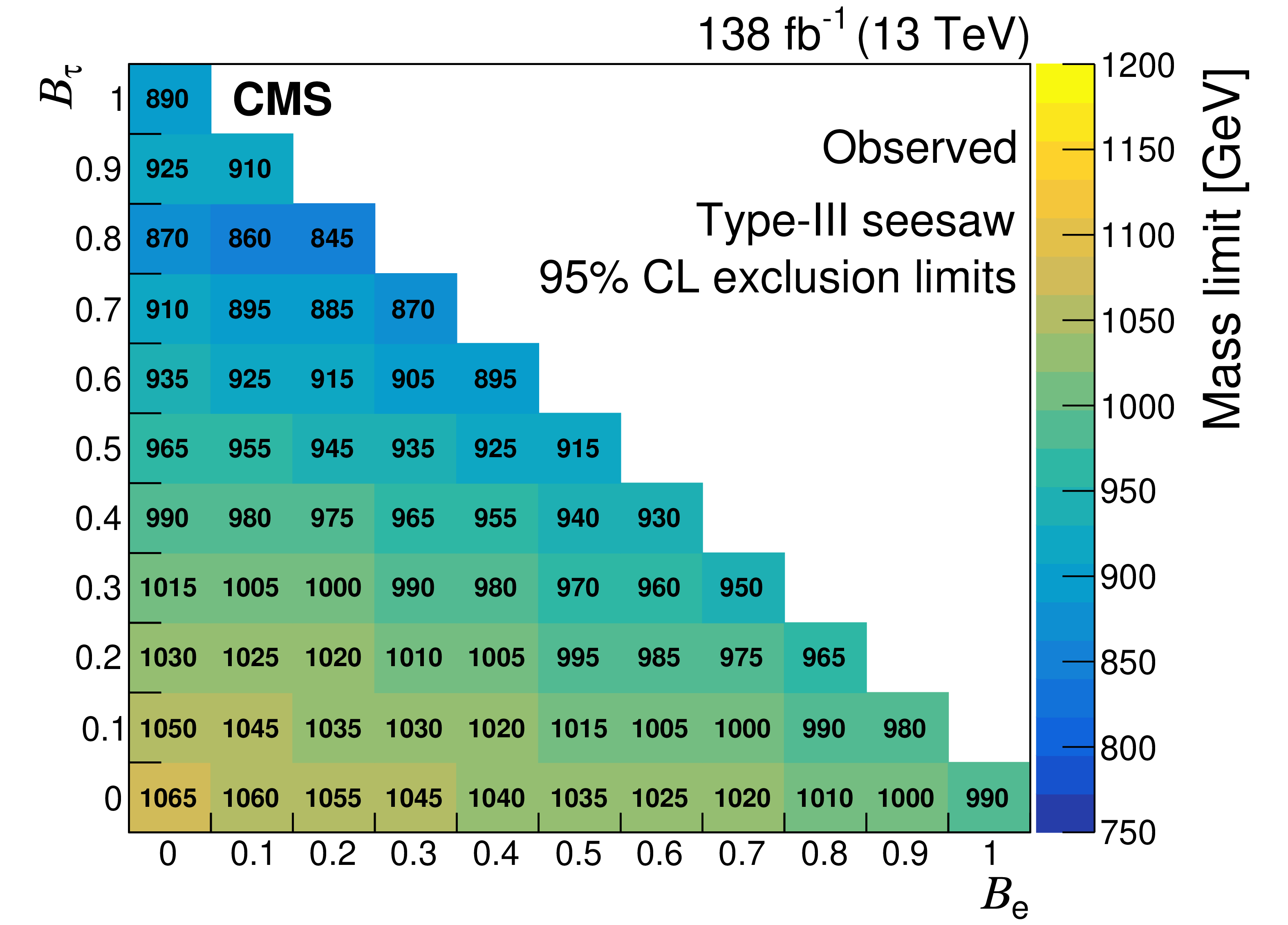
png pdf	Figure 76-b: Expected (left) and observed (right) lower limits at 95% CL on the mass of $Type III$ seesaw HNLs in the plane defined by $\mathcal{B}_{\mathrm{e}}$ and $\mathcal{B}_{\tau}$, with the constraint that $\mathcal{B}_{\mathrm{e}}+\mathcal{B}_{\mu}+\mathcal{B}_{\tau}=$ 1. For $\mathcal{B}_{\tau}\geq$ 0.9, these limits are obtained using the high mass BDT trained assuming $\mathcal{B}_{\tau}=$ 1, and for the other decay branching fraction combinations, the limits use the $\mathcal{B}_{\mathrm{e}}=\mathcal{B}_{\mu}=\mathcal{B}_{\tau}$ BDT. Figures adapted from Ref. [204].
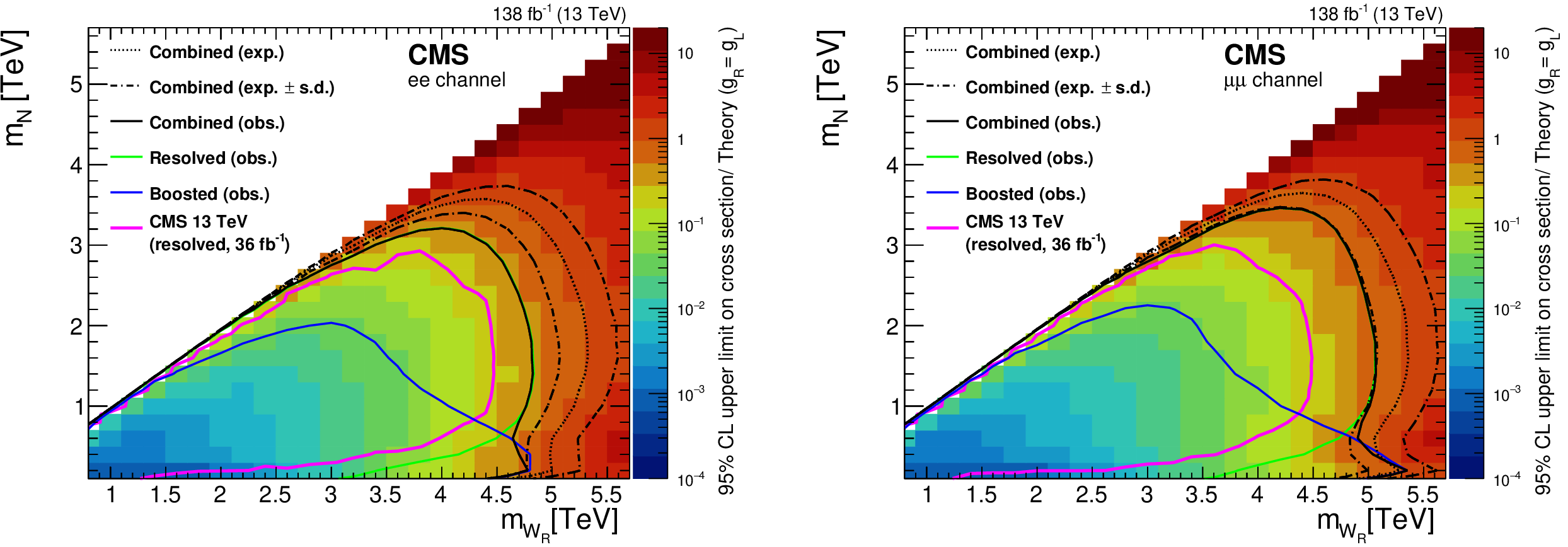
png pdf	Figure 77: The observed upper limits at 95% CL on the product of the production cross section and the branching fraction of a right-handed $\mathrm{W_R}$ boson divided by the theory expectation for a coupling constant $g_{\text{R}}$ equal to the SM coupling of the $\mathrm{W_R}$ boson ($g_{\text{L}}$), for the electron channel (left) and muon channel (right). The observed exclusion regions are shown for the resolved (solid green), boosted (solid blue), and combined (solid black) channels, together with the expected exclusion region for the combined result (dotted black). The dash-dotted lines represent the 68% coverage of the boundaries of the expected exclusion regions. The observed exclusion regions obtained in the previous search performed by the CMS Collaboration [284] are bounded by the magenta lines. The biggest improvement may be seen in the $m_{\mathrm{N}} <$ 0.5 TeV region, where the new boosted category greatly improves the sensitivity with respect to the previous result. Figures adapted from Ref. [281].
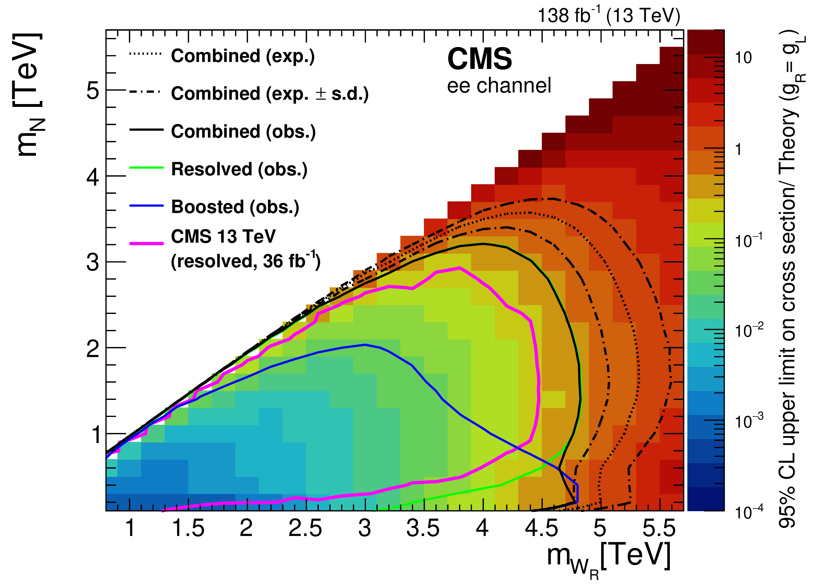
png pdf	Figure 77-a: The observed upper limits at 95% CL on the product of the production cross section and the branching fraction of a right-handed $\mathrm{W_R}$ boson divided by the theory expectation for a coupling constant $g_{\text{R}}$ equal to the SM coupling of the $\mathrm{W_R}$ boson ($g_{\text{L}}$), for the electron channel (left) and muon channel (right). The observed exclusion regions are shown for the resolved (solid green), boosted (solid blue), and combined (solid black) channels, together with the expected exclusion region for the combined result (dotted black). The dash-dotted lines represent the 68% coverage of the boundaries of the expected exclusion regions. The observed exclusion regions obtained in the previous search performed by the CMS Collaboration [284] are bounded by the magenta lines. The biggest improvement may be seen in the $m_{\mathrm{N}} <$ 0.5 TeV region, where the new boosted category greatly improves the sensitivity with respect to the previous result. Figures adapted from Ref. [281].
png pdf	Figure 77-b: The observed upper limits at 95% CL on the product of the production cross section and the branching fraction of a right-handed $\mathrm{W_R}$ boson divided by the theory expectation for a coupling constant $g_{\text{R}}$ equal to the SM coupling of the $\mathrm{W_R}$ boson ($g_{\text{L}}$), for the electron channel (left) and muon channel (right). The observed exclusion regions are shown for the resolved (solid green), boosted (solid blue), and combined (solid black) channels, together with the expected exclusion region for the combined result (dotted black). The dash-dotted lines represent the 68% coverage of the boundaries of the expected exclusion regions. The observed exclusion regions obtained in the previous search performed by the CMS Collaboration [284] are bounded by the magenta lines. The biggest improvement may be seen in the $m_{\mathrm{N}} <$ 0.5 TeV region, where the new boosted category greatly improves the sensitivity with respect to the previous result. Figures adapted from Ref. [281].
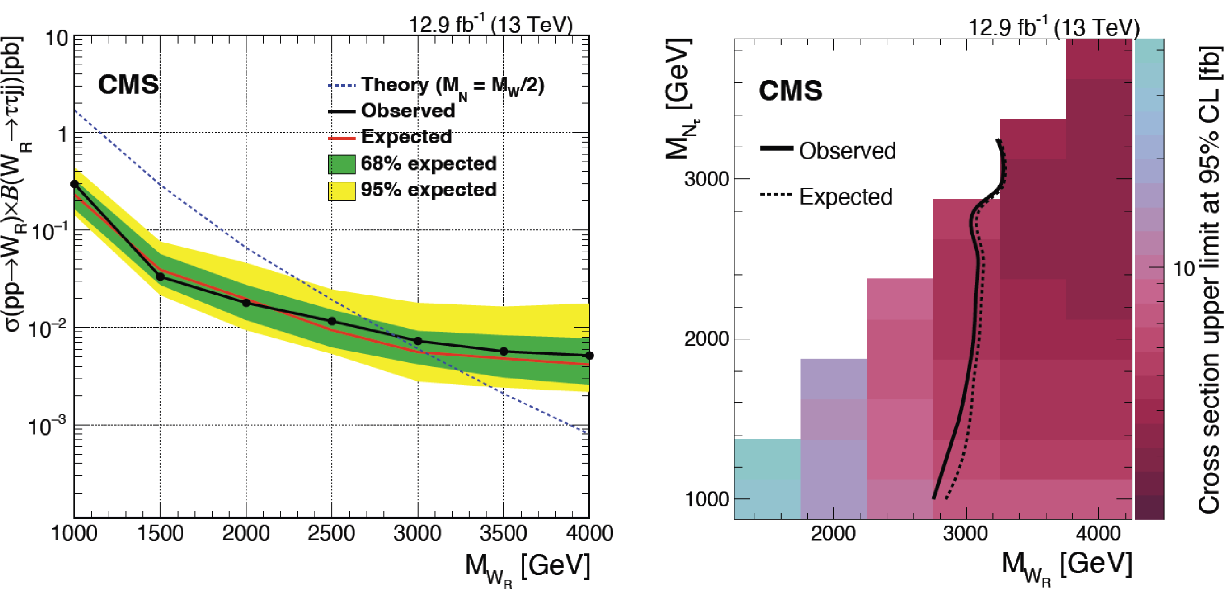
png pdf	Figure 78: Observed and expected limits at 95% CL on the product of cross section and branching fraction, obtained from the combination of the $\mathrm{e}\tau_\mathrm{h}$ and $\mu\tau_\mathrm{h}$ channels (left), and the observed and expected upper limits at 95% CL on the production cross section as functions of the mass $m_{\mathrm{W_R}}$ of the $\mathrm{W_R}$ boson and the mass $m_{{{\mathrm{N}}{\tau}} }$ of the HNL (right). The inner (green) band and the outer (yellow) band in the left figure indicate the regions containing 68 and 95%, respectively, of the distribution of limits expected under the background-only hypothesis. The dashed dark blue curve in the left figure represents the theoretical prediction for the product of the $\mathrm{W_R}$ boson production cross section and the branching fraction for decay to a $\tau$ lepton and RH neutrino, assuming the mass of the RH neutrino to be half the mass of the $\mathrm{W_R}$ boson. Figures taken from Ref. [285].
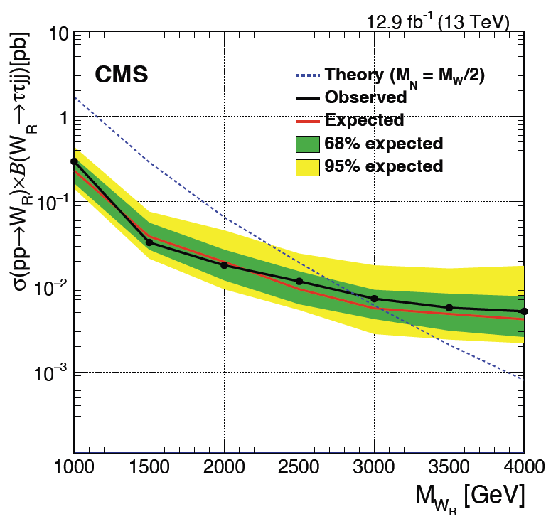
png	Figure 78-a: Observed and expected limits at 95% CL on the product of cross section and branching fraction, obtained from the combination of the $\mathrm{e}\tau_\mathrm{h}$ and $\mu\tau_\mathrm{h}$ channels (left), and the observed and expected upper limits at 95% CL on the production cross section as functions of the mass $m_{\mathrm{W_R}}$ of the $\mathrm{W_R}$ boson and the mass $m_{{{\mathrm{N}}{\tau}} }$ of the HNL (right). The inner (green) band and the outer (yellow) band in the left figure indicate the regions containing 68 and 95%, respectively, of the distribution of limits expected under the background-only hypothesis. The dashed dark blue curve in the left figure represents the theoretical prediction for the product of the $\mathrm{W_R}$ boson production cross section and the branching fraction for decay to a $\tau$ lepton and RH neutrino, assuming the mass of the RH neutrino to be half the mass of the $\mathrm{W_R}$ boson. Figures taken from Ref. [285].
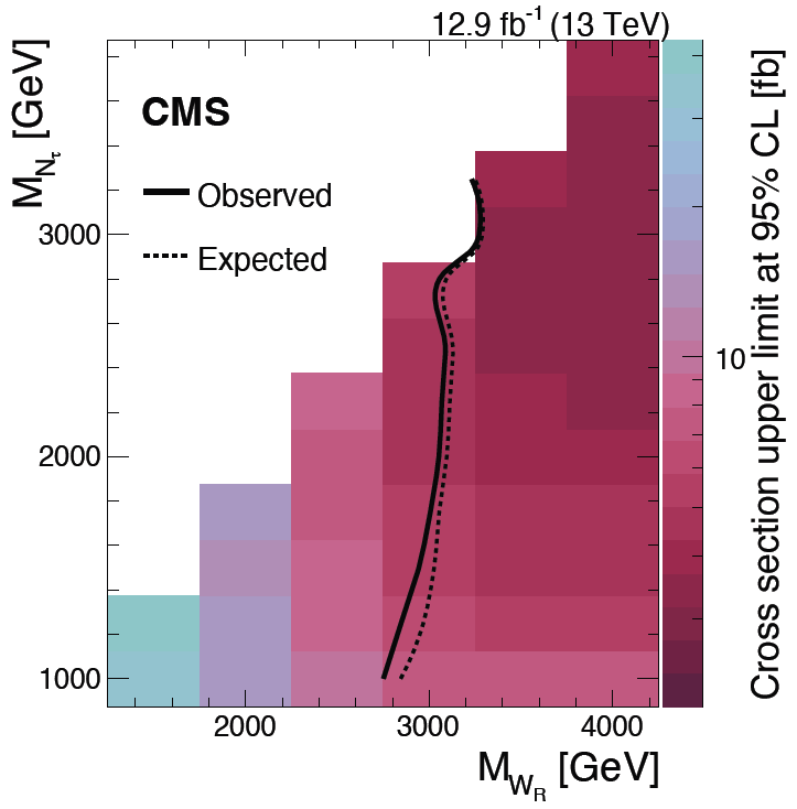
png	Figure 78-b: Observed and expected limits at 95% CL on the product of cross section and branching fraction, obtained from the combination of the $\mathrm{e}\tau_\mathrm{h}$ and $\mu\tau_\mathrm{h}$ channels (left), and the observed and expected upper limits at 95% CL on the production cross section as functions of the mass $m_{\mathrm{W_R}}$ of the $\mathrm{W_R}$ boson and the mass $m_{{{\mathrm{N}}{\tau}} }$ of the HNL (right). The inner (green) band and the outer (yellow) band in the left figure indicate the regions containing 68 and 95%, respectively, of the distribution of limits expected under the background-only hypothesis. The dashed dark blue curve in the left figure represents the theoretical prediction for the product of the $\mathrm{W_R}$ boson production cross section and the branching fraction for decay to a $\tau$ lepton and RH neutrino, assuming the mass of the RH neutrino to be half the mass of the $\mathrm{W_R}$ boson. Figures taken from Ref. [285].
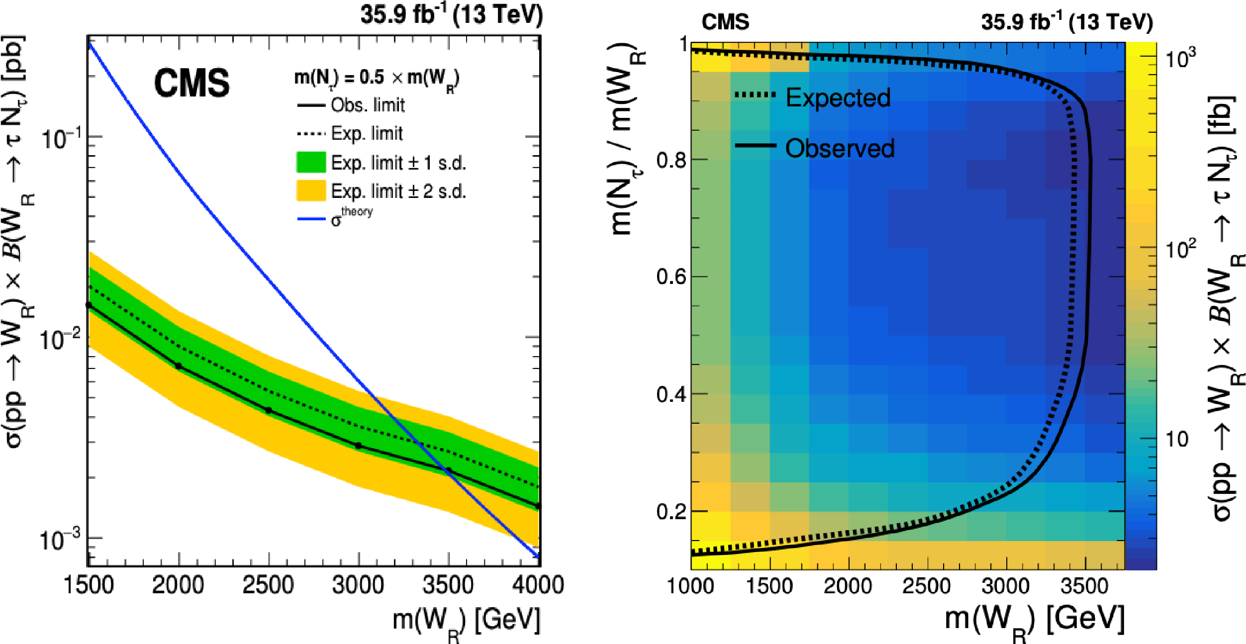
png pdf	Figure 79: Upper limits at 95% CL on the product of the cross section and the branching fraction for the production of $\mathrm{W_R}$ bosons decaying to {$\mathrm{N} \tau$ as function of the $\mathrm{W_R}$ boson mass (left). The observed (expected) limit is shown as solid (dashed) black lines, and the inner (green) band and the outer (yellow) band indicate the regions containing 68 and 95%, respectively, of the distribution of limits expected under the background-only hypothesis. The theoretical cross section is indicated by the solid blue line. Expected and observed limits at 95% CL on the product of the cross section and the branching fraction for $\mathrm{W_R}\to{{\mathrm{N}}{\tau}} \tau$ as a function of $m_{\mathrm{W_R}}$ and $m_{{{\mathrm{N}}{\tau}} }/m_{\mathrm{W_R}}$ (right). Figures taken from Ref. [286].
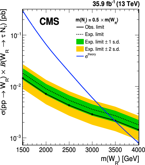
png	Figure 79-a: Upper limits at 95% CL on the product of the cross section and the branching fraction for the production of $\mathrm{W_R}$ bosons decaying to {$\mathrm{N} \tau$ as function of the $\mathrm{W_R}$ boson mass (left). The observed (expected) limit is shown as solid (dashed) black lines, and the inner (green) band and the outer (yellow) band indicate the regions containing 68 and 95%, respectively, of the distribution of limits expected under the background-only hypothesis. The theoretical cross section is indicated by the solid blue line. Expected and observed limits at 95% CL on the product of the cross section and the branching fraction for $\mathrm{W_R}\to{{\mathrm{N}}{\tau}} \tau$ as a function of $m_{\mathrm{W_R}}$ and $m_{{{\mathrm{N}}{\tau}} }/m_{\mathrm{W_R}}$ (right). Figures taken from Ref. [286].
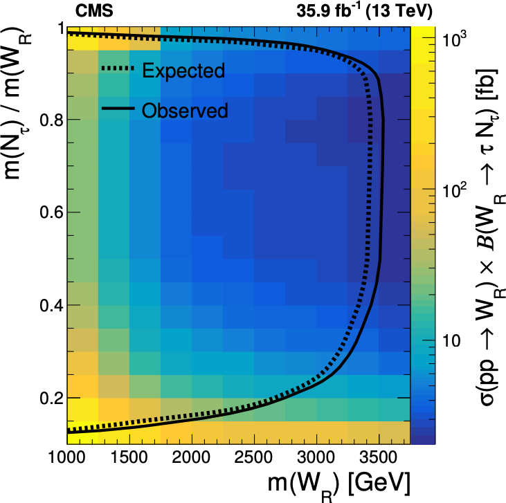
png	Figure 79-b: Upper limits at 95% CL on the product of the cross section and the branching fraction for the production of $\mathrm{W_R}$ bosons decaying to {$\mathrm{N} \tau$ as function of the $\mathrm{W_R}$ boson mass (left). The observed (expected) limit is shown as solid (dashed) black lines, and the inner (green) band and the outer (yellow) band indicate the regions containing 68 and 95%, respectively, of the distribution of limits expected under the background-only hypothesis. The theoretical cross section is indicated by the solid blue line. Expected and observed limits at 95% CL on the product of the cross section and the branching fraction for $\mathrm{W_R}\to{{\mathrm{N}}{\tau}} \tau$ as a function of $m_{\mathrm{W_R}}$ and $m_{{{\mathrm{N}}{\tau}} }/m_{\mathrm{W_R}}$ (right). Figures taken from Ref. [286].
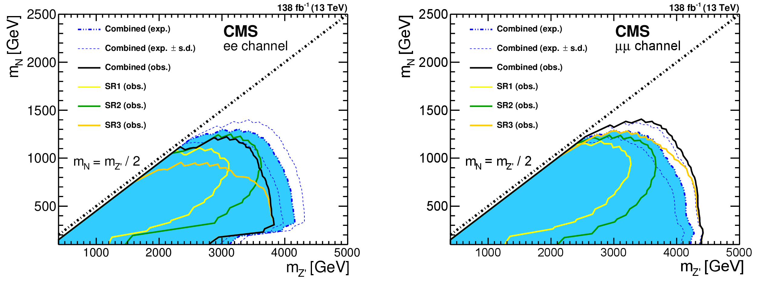
png pdf	Figure 80: The observed and expected exclusion limits in the $m_{\mathrm{N}}$--$m_{\mathrm{Z}^{'}}$ parameter space, in the dielectron channel (left) and the dimuon channel (right). Figures adapted from Ref. [289].
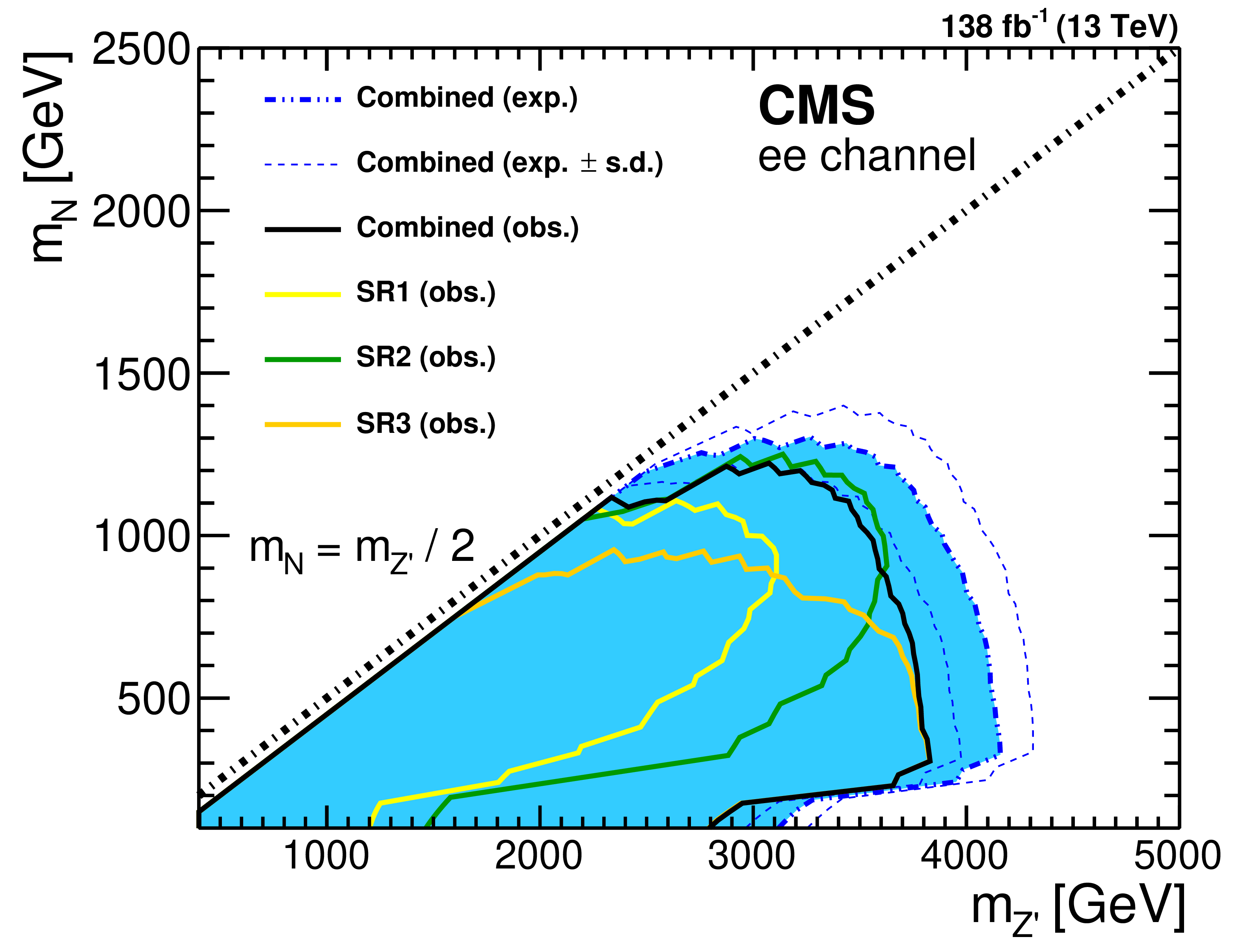
png pdf	Figure 80-a: The observed and expected exclusion limits in the $m_{\mathrm{N}}$--$m_{\mathrm{Z}^{'}}$ parameter space, in the dielectron channel (left) and the dimuon channel (right). Figures adapted from Ref. [289].
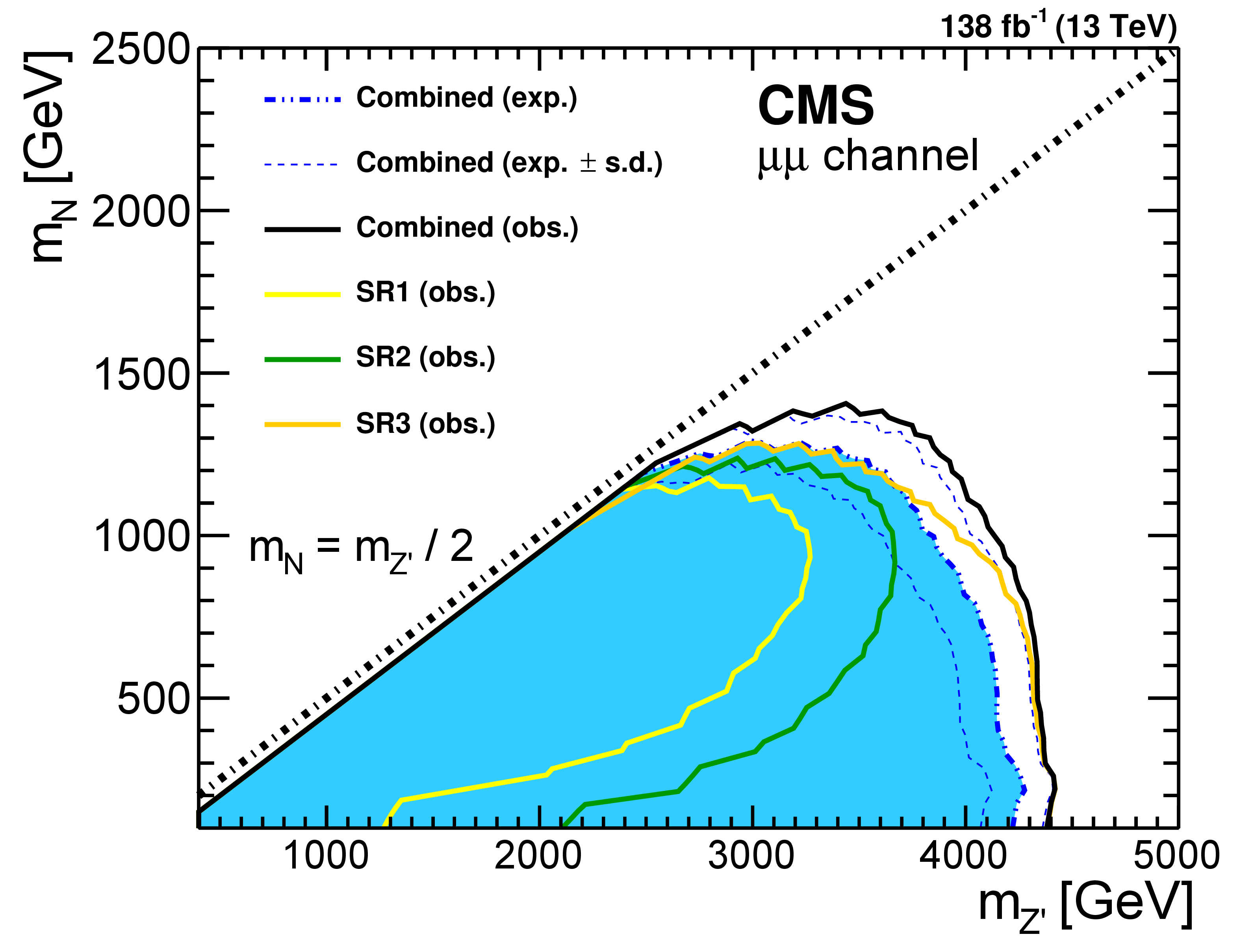
png pdf	Figure 80-b: The observed and expected exclusion limits in the $m_{\mathrm{N}}$--$m_{\mathrm{Z}^{'}}$ parameter space, in the dielectron channel (left) and the dimuon channel (right). Figures adapted from Ref. [289].
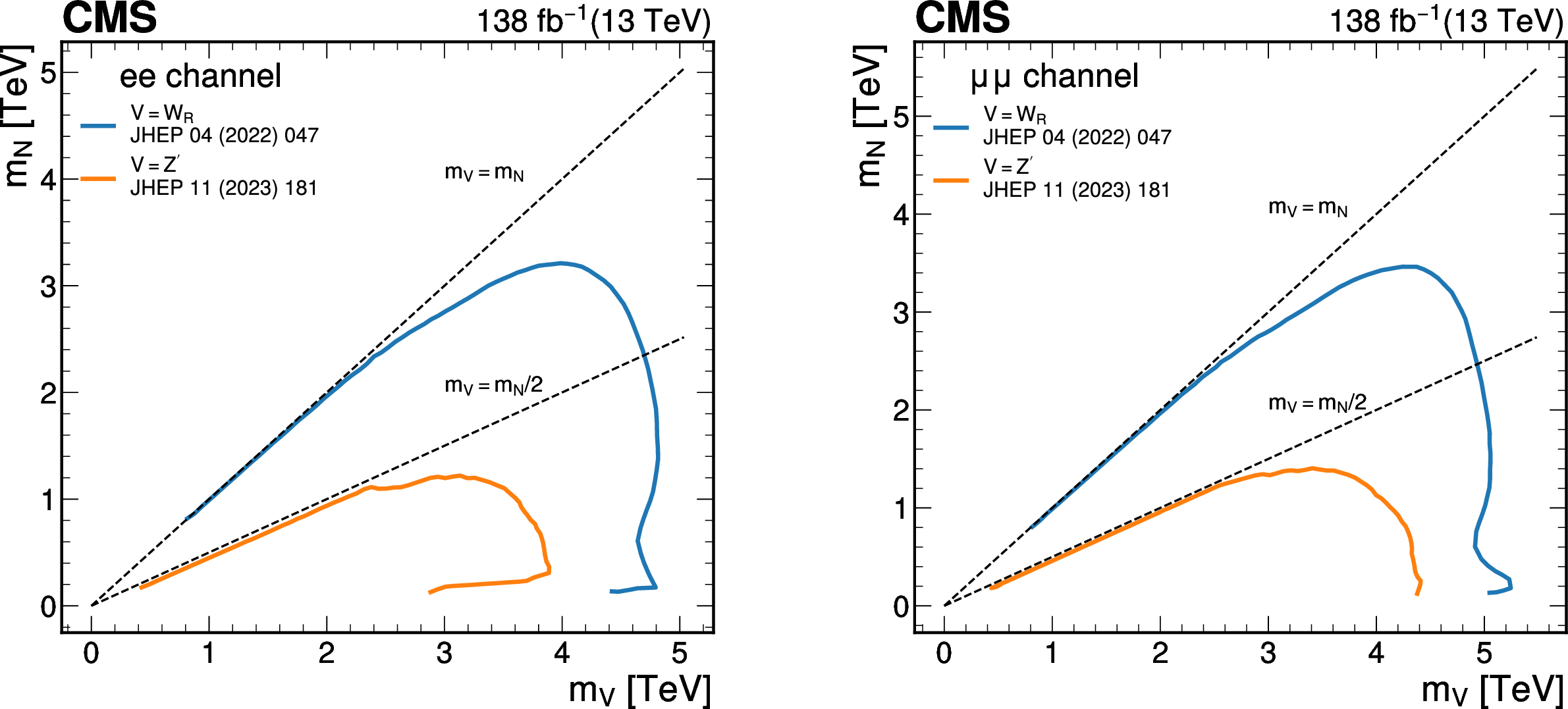
png pdf	Figure 81: Summary of searches at the CMS experiment for Majorana HNLs in the context of the LRSM model. The observed limits at 95% CL in the two-dimensional $m_{\mathrm{N}}$--$m_{\mathrm{V}}$ plane are shown in the electron and muon channel (left and right, respectively).
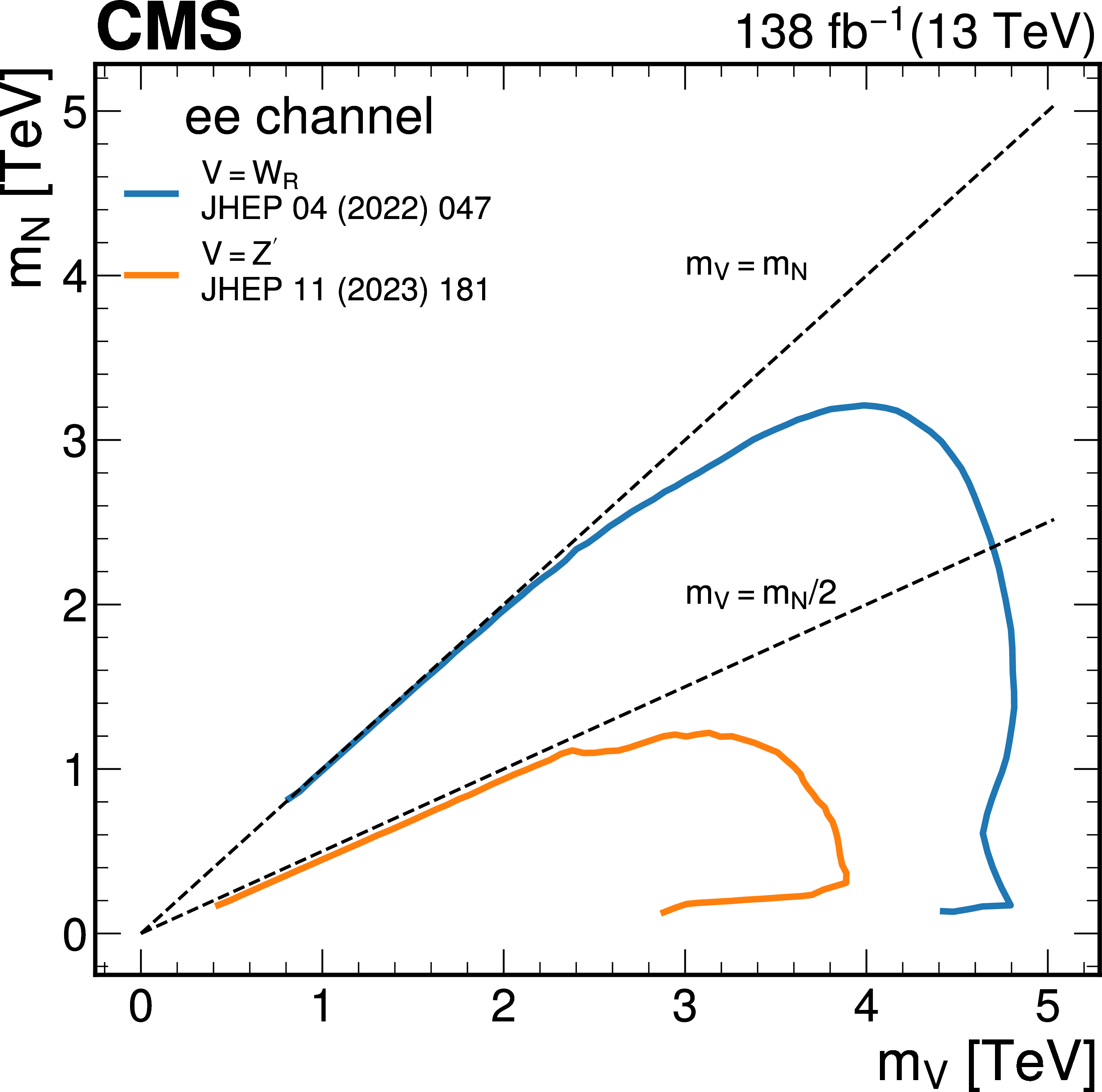
png pdf	Figure 81-a: Summary of searches at the CMS experiment for Majorana HNLs in the context of the LRSM model. The observed limits at 95% CL in the two-dimensional $m_{\mathrm{N}}$--$m_{\mathrm{V}}$ plane are shown in the electron and muon channel (left and right, respectively).
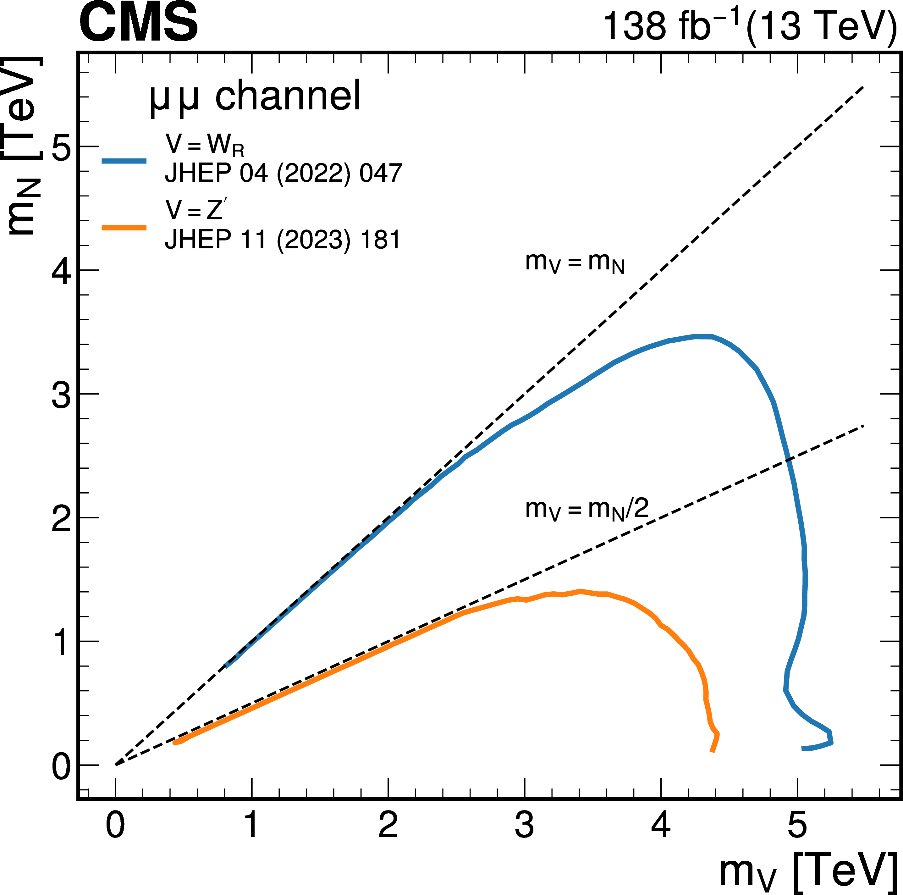
png pdf	Figure 81-b: Summary of searches at the CMS experiment for Majorana HNLs in the context of the LRSM model. The observed limits at 95% CL in the two-dimensional $m_{\mathrm{N}}$--$m_{\mathrm{V}}$ plane are shown in the electron and muon channel (left and right, respectively).
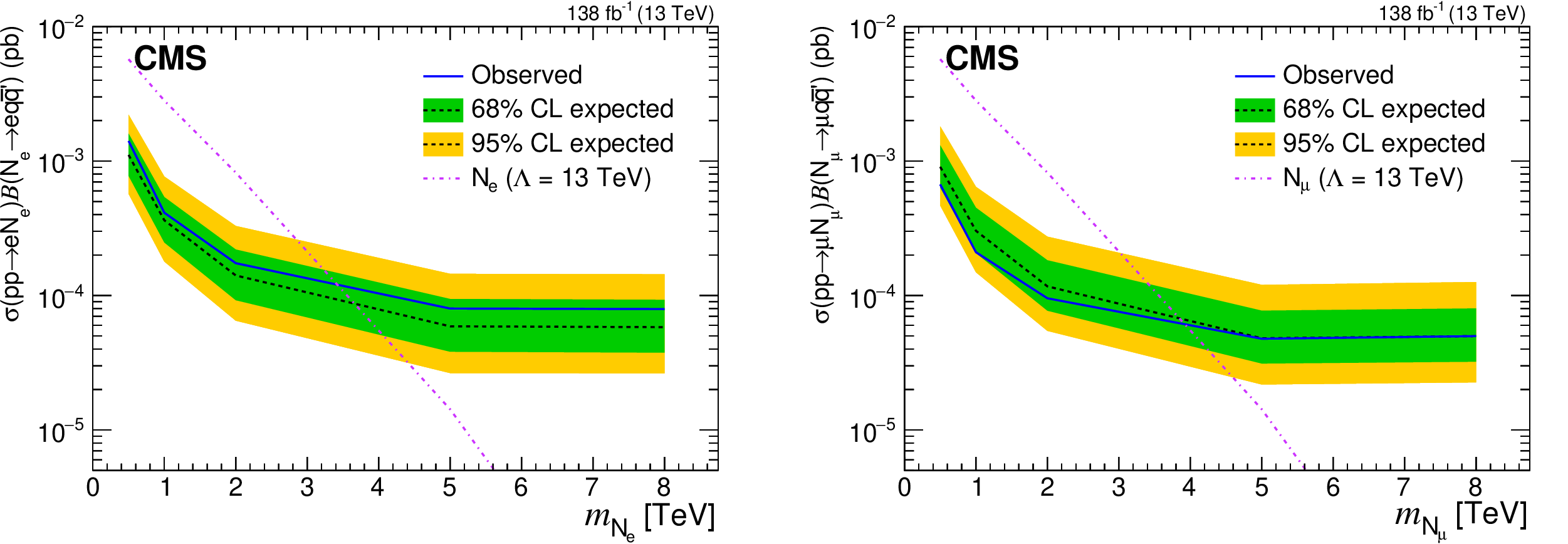
png pdf	Figure 82: Expected (dashed black) and observed (blue solid) exclusion limits for the $\mathrm{e}\mathrm{e}\mathrm{q}{\overline{\mathrm{q}}{\prime}}$ (left) and $\mu\mu\mathrm{q}{\overline{\mathrm{q}}{\prime}}$ (right) channels in the search for heavy composite Majorana neutrinos. The inner (green) band and the outer (yellow) band indicate the regions containing 68 and 95%, respectively, of the distribution of limits expected under the background-only hypothesis. Figures taken from Ref. [290].
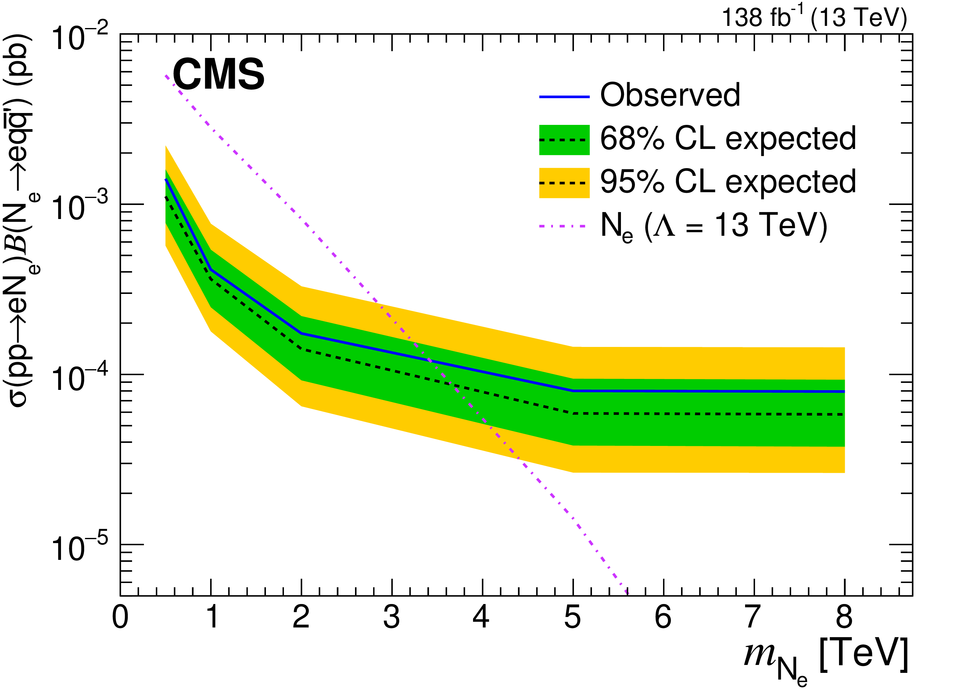
png pdf	Figure 82-a: Expected (dashed black) and observed (blue solid) exclusion limits for the $\mathrm{e}\mathrm{e}\mathrm{q}{\overline{\mathrm{q}}{\prime}}$ (left) and $\mu\mu\mathrm{q}{\overline{\mathrm{q}}{\prime}}$ (right) channels in the search for heavy composite Majorana neutrinos. The inner (green) band and the outer (yellow) band indicate the regions containing 68 and 95%, respectively, of the distribution of limits expected under the background-only hypothesis. Figures taken from Ref. [290].
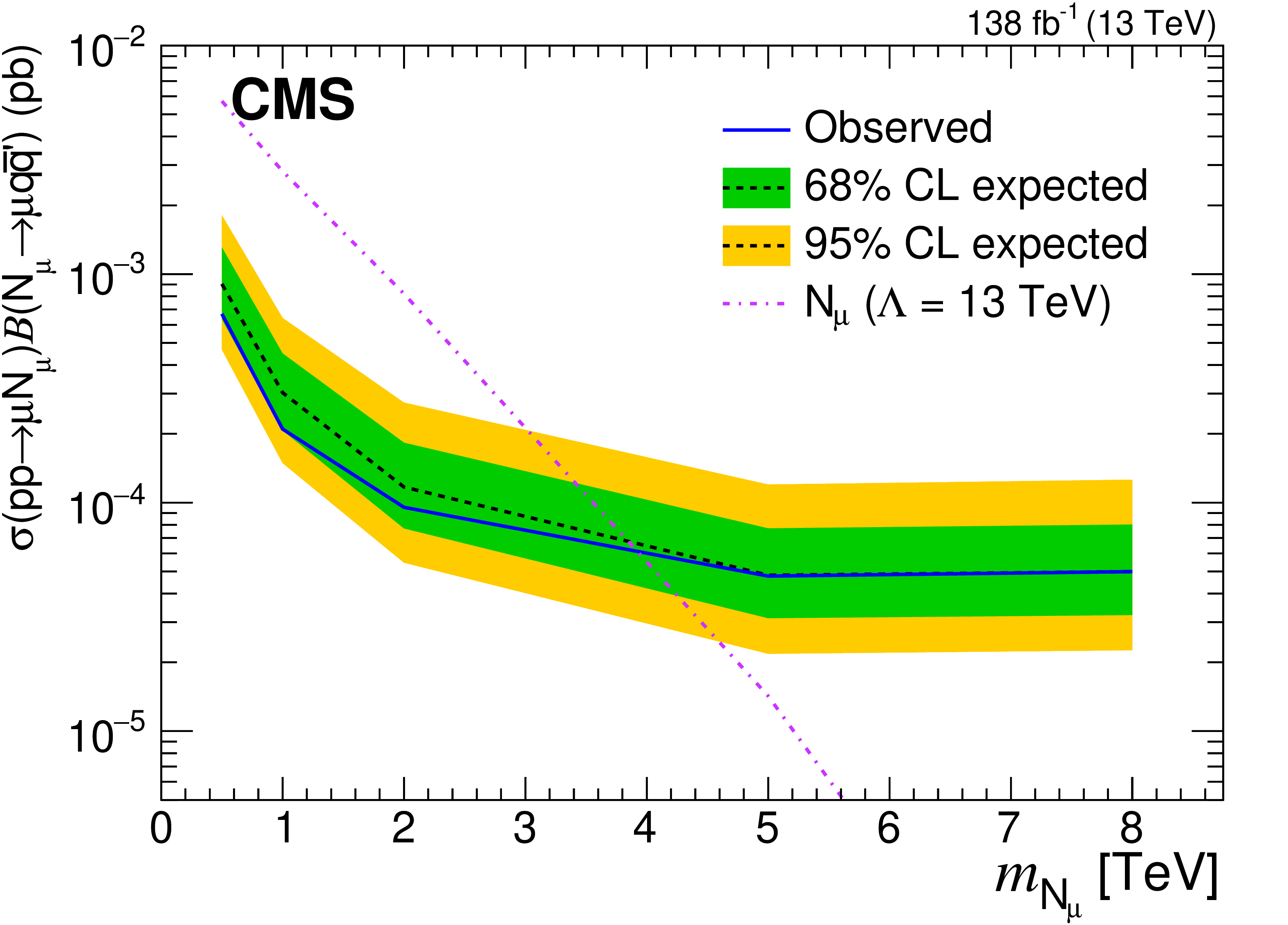
png pdf	Figure 82-b: Expected (dashed black) and observed (blue solid) exclusion limits for the $\mathrm{e}\mathrm{e}\mathrm{q}{\overline{\mathrm{q}}{\prime}}$ (left) and $\mu\mu\mathrm{q}{\overline{\mathrm{q}}{\prime}}$ (right) channels in the search for heavy composite Majorana neutrinos. The inner (green) band and the outer (yellow) band indicate the regions containing 68 and 95%, respectively, of the distribution of limits expected under the background-only hypothesis. Figures taken from Ref. [290].
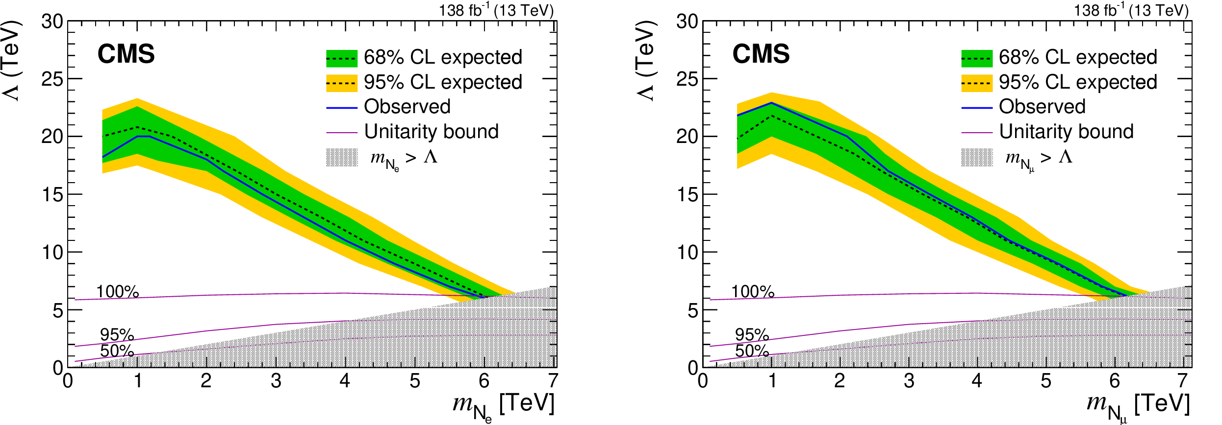
png pdf	Figure 83: Expected (dashed black) and observed (blue solid) exclusion limits for the $\mathrm{e}\mathrm{e}\mathrm{q}{\overline{\mathrm{q}}{\prime}}$ (left) and $\mu\mu\mathrm{q}{\overline{\mathrm{q}}{\prime}}$ (right) channel in the two-dimensional plane $m_{{{\mathrm{N}}{\ell}} }$--$\Lambda$. The solid violet lines represent the fraction of simulated events that satisfy the unitarity condition in the EFT approximation [292] with the various percentages considered. The inner (green) band and the outer (yellow) band indicate the regions containing 68 and 95%, respectively, of the distribution of limits expected under the background-only hypothesis. Figures taken from Ref. [290].
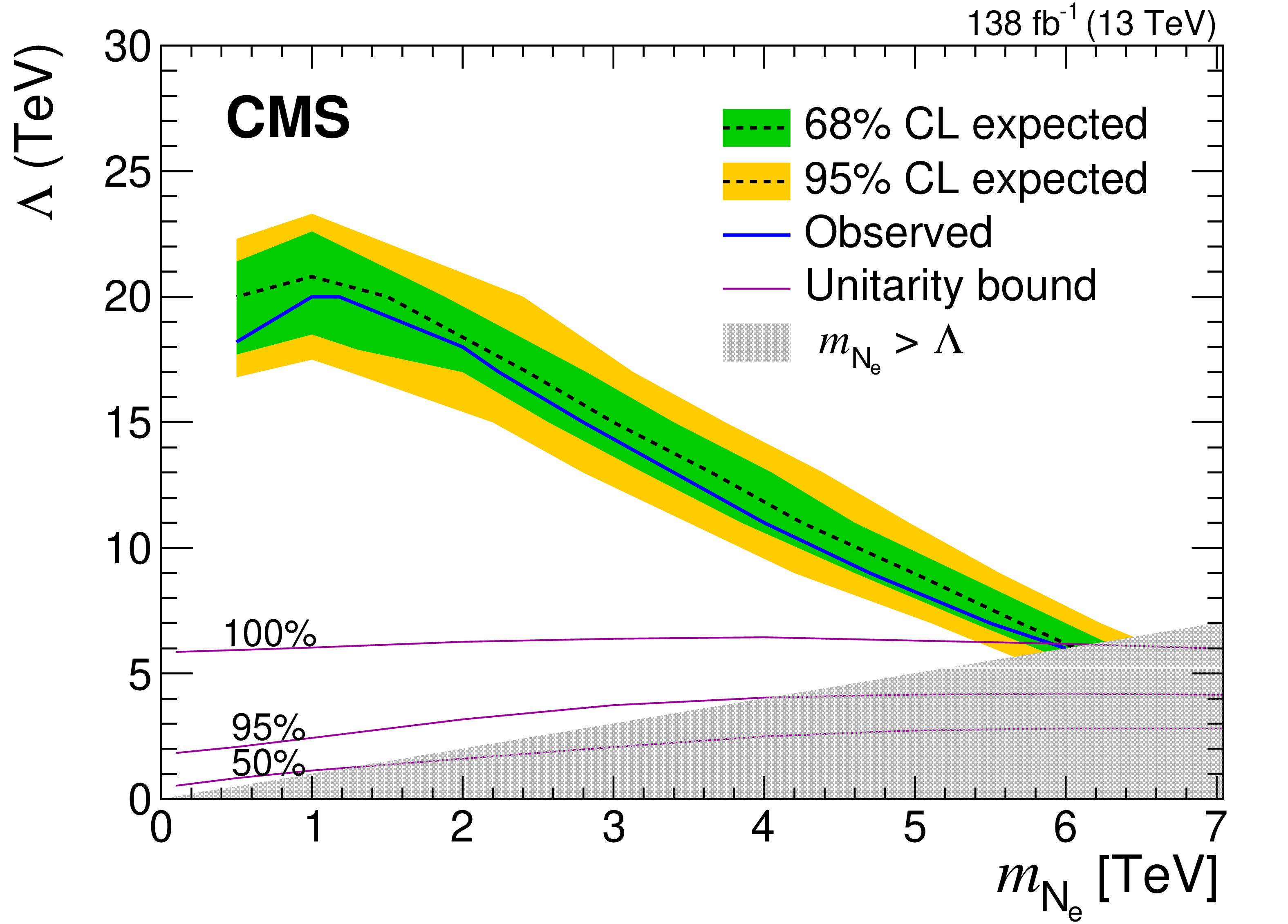
png pdf	Figure 83-a: Expected (dashed black) and observed (blue solid) exclusion limits for the $\mathrm{e}\mathrm{e}\mathrm{q}{\overline{\mathrm{q}}{\prime}}$ (left) and $\mu\mu\mathrm{q}{\overline{\mathrm{q}}{\prime}}$ (right) channel in the two-dimensional plane $m_{{{\mathrm{N}}{\ell}} }$--$\Lambda$. The solid violet lines represent the fraction of simulated events that satisfy the unitarity condition in the EFT approximation [292] with the various percentages considered. The inner (green) band and the outer (yellow) band indicate the regions containing 68 and 95%, respectively, of the distribution of limits expected under the background-only hypothesis. Figures taken from Ref. [290].
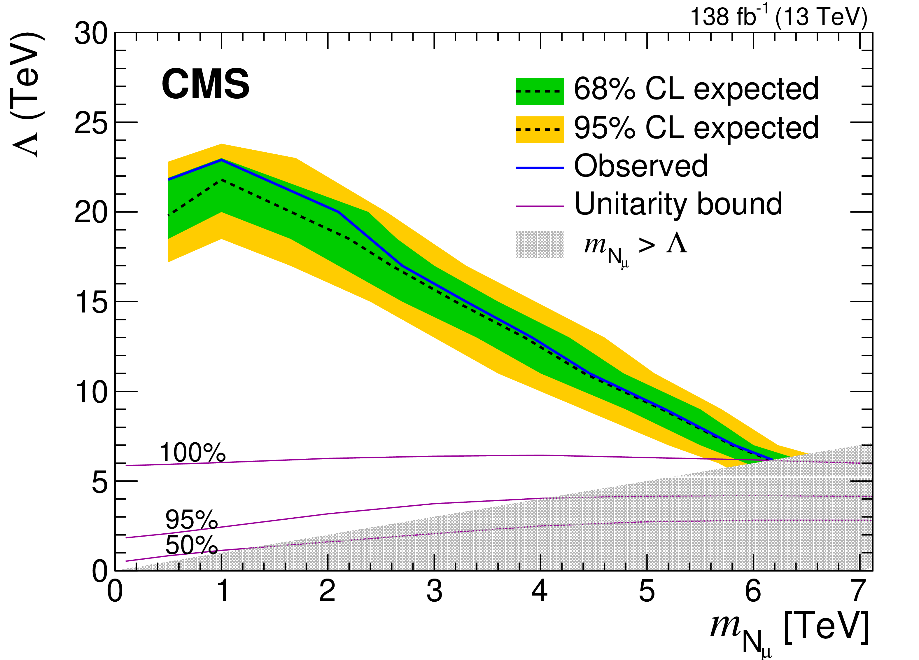
png pdf	Figure 83-b: Expected (dashed black) and observed (blue solid) exclusion limits for the $\mathrm{e}\mathrm{e}\mathrm{q}{\overline{\mathrm{q}}{\prime}}$ (left) and $\mu\mu\mathrm{q}{\overline{\mathrm{q}}{\prime}}$ (right) channel in the two-dimensional plane $m_{{{\mathrm{N}}{\ell}} }$--$\Lambda$. The solid violet lines represent the fraction of simulated events that satisfy the unitarity condition in the EFT approximation [292] with the various percentages considered. The inner (green) band and the outer (yellow) band indicate the regions containing 68 and 95%, respectively, of the distribution of limits expected under the background-only hypothesis. Figures taken from Ref. [290].
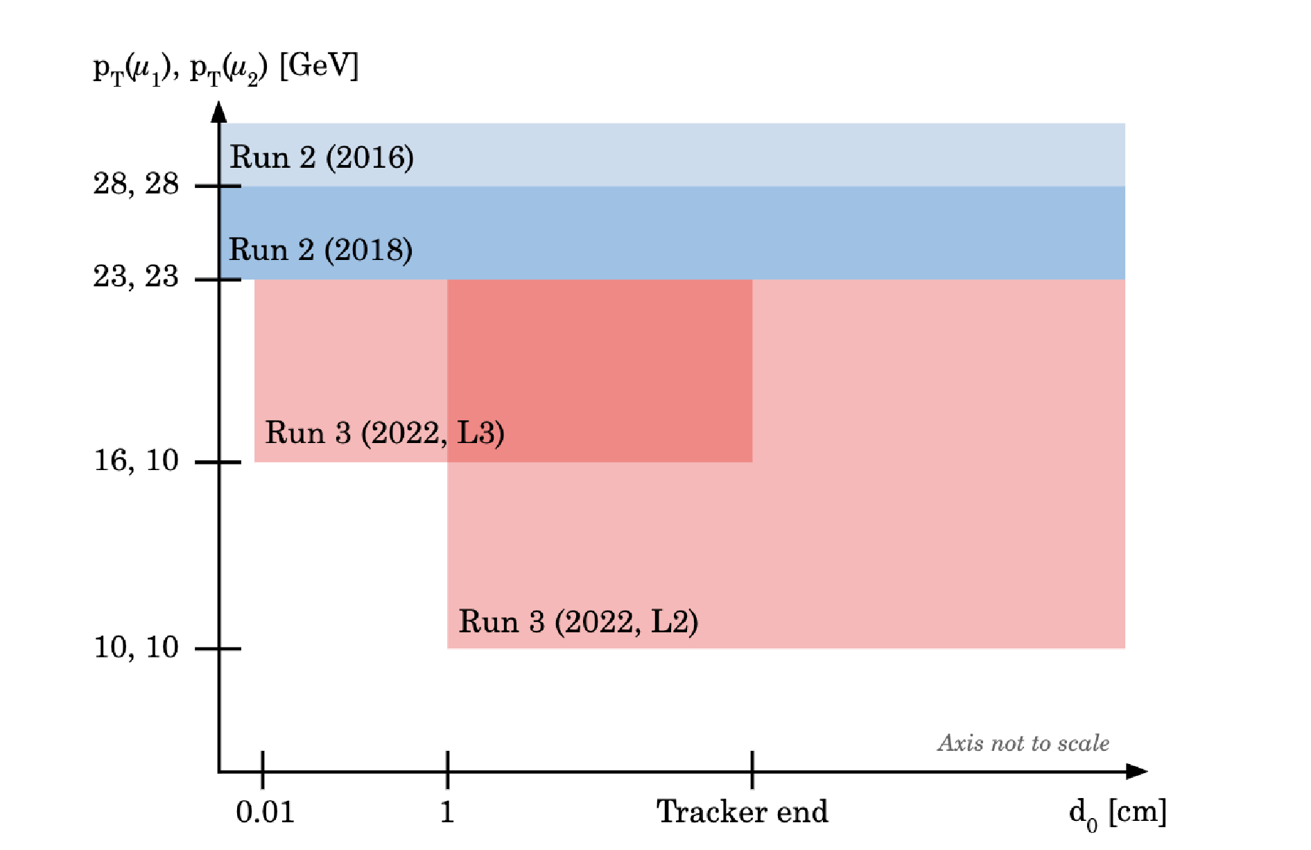
png pdf	Figure 84: Coverage in the ($p_{\mathrm{T}}$, $d_0$) plane for displaced leptons with the 2016 and 2018 triggers, and the new Run-3 triggers, indicated in light blue, dark blue, and red, respectively [293]. Here, $d_0$ is the impact parameter of the charged lepton track with respect to the PV in the transverse plane.

Tables
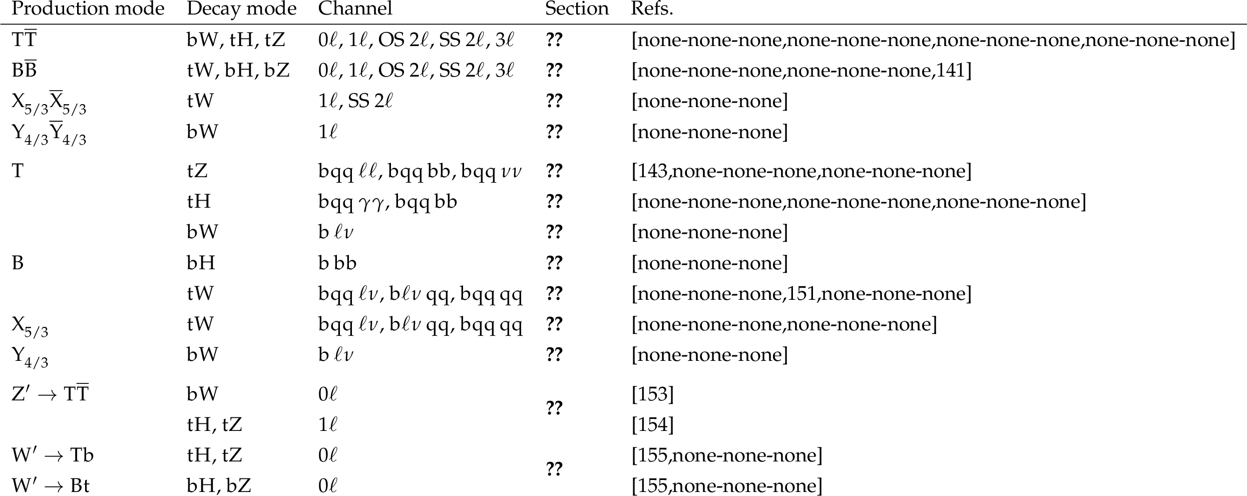
png pdf	Table 1: List of VLQ searches performed by the CMS experiment grouped by production mode. In this table, \ell denotes an electron or a muon. Additional jets in the final state are not explicitly listed in the table. The 0\ell channels correspond to the all-hadronic final state. For the 2\ell channels, it is indicated whether the leptons have opposite-sign (OS) or same-sign (SS) charges. For single VLQ searches, the channels are indicated through the decay products of the W, Z, and Higgs bosons, and t quarks.
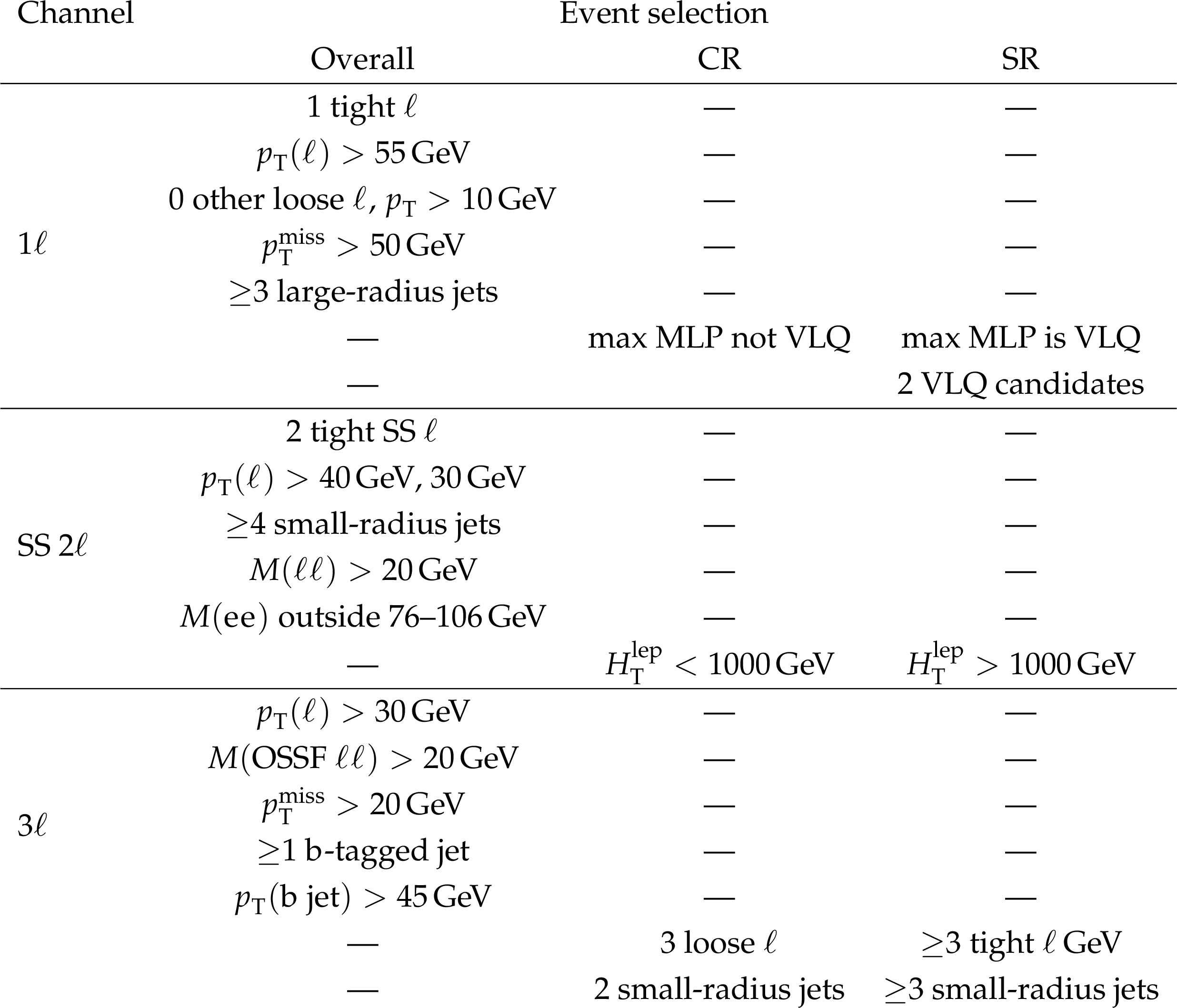
png pdf	Table 2: Summary of event selection criteria for the primary CRs and SRs in the three leptonic search channels. The phrase ``max MLP'' refers to the largest score from the single-lepton multilayer perceptron network. Table taken from Ref. [none-none-none].
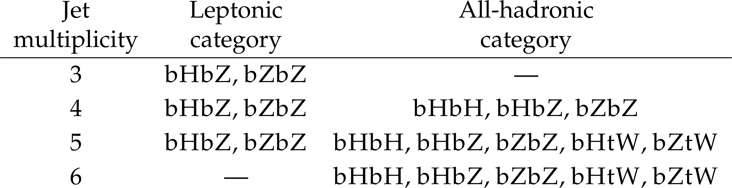
png pdf	Table 3: Summary of channels considered for each category and jet multiplicity in the search for ${\mathrm{B}} \overline{\mathrm{B}}$ production that specifically targets ${\mathrm{B}} \to\mathrm{b}\mathrm{Z}$ and ${\mathrm{B}} \to\mathrm{b}\mathrm{H}$ decays. Table adapted from Ref. [142].

Summary

In this report, the physics program of the CMS experiment has been summarized for searches for physics beyond the standard model (SM) in the context of models that introduce vector-like quarks (VLQs), vector-like leptons (VLLs), and heavy neutral leptons (HNLs). Each of these three model classes provides a complementary perspective on the origin of mass of fundamental particles. The VLQs extend the SM with nonchiral partners of SM quarks, and the searches focus on VLQs that couple to the third-generation quarks. The VLLs, introduced in a class of models that can be particularly sensitive to leptonic anomalies, correspond to an analogous extension of the leptonic sector of the SM. These searches target charged-lepton partners. The HNLs provide yet another perspective on the interplay between chirality and neutrino mass-generating mechanisms, and produce distinct prompt and displaced signatures in the detector. These searches probe unexplored areas of parameter space in several models beyond the SM, using Run 2 proton-proton collision data sets collected by the CMS detector during the years 2015 to 2018 corresponding to an integrated luminosity of up to 138 fb$^{-1}$. Two new statistical combinations of searches for VLQs have been performed. Pair production of B quarks with mass below 1.49 TeV is excluded at 95% confidence level for any third-generation decay of the B quark. Single production of T quarks in the narrow-width approximation is excluded at 95% confidence level for T quark masses below 1.20 TeV. No evidence for physics beyond the SM has been observed, and stringent exclusion limits on new fermion masses and couplings have been placed. One search for VLLs, detailed in Section 8.3, shows a modest excess of the observed data over the background-only prediction that requires further investigation using more data. No VLQ and HNL searches report excesses. Using projections in the context of the future High-Luminosity LHC (HL-LHC) and the corresponding upgrades to the CMS detector, an increased discovery reach of new fermions well into the TeVns energy domain is expected. Although the environment of the HL-LHC with many simultaneous collisions will present new challenges for particle reconstruction and identification, searches for new fermions will benefit from the increased collision energy, unprecedented integrated luminosity, and the planned detector upgrades. Many of the searches presented in this report rely on identifying jets from the decays of massive SM particles, or feature high-pseudorapidity jets from $t$-channel or vector boson fusion production modes. The expansion of the tracker volume and significant upgrades of the endcap calorimeter and muon detectors will provide improved jet reconstruction and identification at high pseudorapidity in the HL-LHC era. There are still unexplored regions of parameter space in various models beyond the SM involving VLQs, VLLs, and HNLs within reach of the LHC, that can yield a first glimpse of new physics in the near or longer term. This includes considering nonminimal VLQ extensions such as decays of VLQs to scalar or pseudoscalar bosons, exploring VLQ production modes such as electroweak pair production, and expanding the searches for VLQs assuming a finite decay width. Manifestations of VLLs in other models and final states than currently probed may also be considered, involving final states with muon detector shower signatures, final states with highly Lorentz-boosted decay products, or vector boson fusion modes of VLL pair production. Future runs of the LHC will bring great opportunities to explore new model phase spaces, detector upgrades will provide improved particle reconstruction, and continued efforts in innovating analysis techniques will further enhance the potential to discover new physics.

References
1	A. Hebecker	The standard model and its hierarchy problem(s)	in Naturalness, string landscape and multiverse: A modern introduction with exercises, Springer International Publishing, Cham, 2021 link
2	Super-Kamiokande Collaboration	Evidence for oscillation of atmospheric neutrinos	PRL 81 (1998) 1562	hep-ex/9807003
3	SNO Collaboration	Measurement of the rate of ${\nu_{\!\mathrm{e}}+\mathrm{d}\to\mathrm{p}+\mathrm{p}+\mathrm{e}^-}$ interactions produced by $^8$B solar neutrinos at the Sudbury Neutrino Observatory	PRL 87 (2001) 071301	nucl-ex/0106015
4	L. Randall and R. Sundrum	A large mass hierarchy from a small extra dimension	PRL 83 (1999) 3370	hep-ph/9905221
5	G.-Y. Huang, K. Kong, and S. C. Park	Bounds on the fermion-bulk masses in models with universal extra dimensions	JHEP 06 (2012) 099	1204.0522
6	R. Contino, D. Pappadopulo, D. Marzocca, and R. Rattazzi	On the effect of resonances in composite Higgs phenomenology	JHEP 10 (2011) 081	1109.1570
7	D. Greco and D. Liu	Hunting composite vector resonances at the LHC: naturalness facing data	JHEP 12 (2014) 126	1410.2883
8	A. Falkowski, D. M. Straub, and A. Vicente	Vector-like leptons: Higgs decays and collider phenomenology	JHEP 05 (2014) 092	1312.5329
9	J. A. Aguilar-Saavedra, R. Benbrik, S. Heinemeyer, and M. Pérez-Victoria	Handbook of vectorlike quarks: Mixing and single production	PRD 88 (2013) 094010	1306.0572
10	R. Mohapatra and G. Senjanović	Neutrino mass and spontaneous parity nonconservation	PRL 44 (1980) 912
11	J. Schechter and J. Valle	Neutrino masses in $\mathrm{SU}(2)\otimes\mathrm{U}(1)$ theories	PRD 22 (1980) 2227
12	R. Foot, H. Lew, X.-G. He, and G. C. Joshi	See-saw neutrino masses induced by a triplet of leptons	Z. Phys. C 44 (1989) 441
13	CMS Collaboration	The CMS experiment at the CERN LHC	JINST 3 (2008) S08004
14	CMS Collaboration	Performance of the CMS Level-1 trigger in proton-proton collisions at $\sqrt{s}=$ 13 TeV	JINST 15 (2020) P10017	CMS-TRG-17-001 2006.10165
15	CMS Collaboration	The CMS trigger system	JINST 12 (2017) P01020	CMS-TRG-12-001 1609.02366
16	CMS Collaboration	Particle-flow reconstruction and global event description with the CMS detector	JINST 12 (2017) P10003	CMS-PRF-14-001 1706.04965
17	CMS Collaboration	Technical proposal for the Phase-II upgrade of the Compact Muon Solenoid	CMS Technical Proposal CERN-LHCC-2015-010, CMS-TDR-15-02, 2015 CDS
18	CMS Collaboration	Performance of photon reconstruction and identification with the CMS detector in proton-proton collisions at $\sqrt{s}=$ 8 TeV	JINST 10 (2015) P08010	CMS-EGM-14-001 1502.02702
19	CMS Collaboration	Electron and photon reconstruction and identification with the CMS experiment at the CERN LHC	JINST 16 (2021) P05014	CMS-EGM-17-001 2012.06888
20	CMS Collaboration	ECAL 2016 refined calibration and Run2 summary plots	CMS Detector Performance Note CMS-DP-2020-021, 2020 CDS
21	CMS Collaboration	Performance of the CMS muon detector and muon reconstruction with proton-proton collisions at $\sqrt{s}=$ 13 TeV	JINST 13 (2018) P06015	CMS-MUO-16-001 1804.04528
22	M. Cacciari, G. P. Salam, and G. Soyez	The anti-$k_{\mathrm{T}}$ jet clustering algorithm	JHEP 04 (2008) 063	0802.1189
23	M. Cacciari, G. P. Salam, and G. Soyez	FASTJET user manual	EPJC 72 (2012) 1896	1111.6097
24	CMS Collaboration	Jet energy scale and resolution in the CMS experiment in ${\mathrm{p}\mathrm{p}}$ collisions at 8 TeV	JINST 12 (2017) P02014	CMS-JME-13-004 1607.03663
25	D. Bertolini, P. Harris, M. Low, and N. Tran	Pileup per particle identification	JHEP 10 (2014) 059	1407.6013
26	CMS Collaboration	Pileup mitigation at CMS in 13 TeV data	JINST 15 (2020) P09018	CMS-JME-18-001 2003.00503
27	CMS Collaboration	Identification of heavy-flavour jets with the CMS detector in ${\mathrm{p}\mathrm{p}}$ collisions at 13 TeV	JINST 13 (2018) P05011	CMS-BTV-16-002 1712.07158
28	E. Bols et al.	Jet flavour classification using DeepJet	JINST 15 (2020) P12012	2008.10519
29	CMS Collaboration	Performance of the DeepJet b tagging algorithm using 41.9 fb$^{-1}$ of data from proton-proton collisions at 13 TeV with Phase 1 CMS detector	CMS Detector Performance Note CMS-DP-2018-058, 2018 CDS
30	CMS Collaboration	Performance of reconstruction and identification of $\tau$ leptons decaying to hadrons and $\nu_{\!\tau}$ in ${\mathrm{p}\mathrm{p}}$ collisions at $\sqrt{s}=$ 13 TeV	JINST 13 (2018) P10005	CMS-TAU-16-003 1809.02816
31	CMS Collaboration	Identification of hadronic tau lepton decays using a deep neural network	JINST 17 (2022) P07023	CMS-TAU-20-001 2201.08458
32	CMS Collaboration	Performance of missing transverse momentum reconstruction in proton-proton collisions at $\sqrt{s}=$ 13 TeV using the CMS detector	JINST 14 (2019) P07004	CMS-JME-17-001 1903.06078
33	CMS Tracker Group Collaboration	The CMS Phase-1 pixel detector upgrade	JINST 16 (2021) P02027	2012.14304
34	CMS Collaboration	The Phase-2 upgrade of the CMS barrel calorimeters	CMS Technical Proposal CERN-LHCC-2017-011, CMS-TDR-015, 2017 CDS
35	CMS Collaboration	The Phase-2 upgrade of the CMS muon detectors	CMS Technical Proposal CERN-LHCC-2017-012, CMS-TDR-016, 2017 CDS
36	CMS Collaboration	The Phase-2 upgrade of the CMS endcap calorimeter	CMS Technical Proposal CERN-LHCC-2017-023, CMS-TDR-019, 2017 CDS
37	CMS Collaboration	A MIP timing detector for the CMS Phase-2 upgrade	CMS Technical Proposal CERN-LHCC-2019-003, CMS-TDR-020, 2019 CDS
38	CMS Collaboration	The Phase-2 upgrade of the CMS Level-1 trigger	CMS Technical Proposal CERN-LHCC-2020-004, CMS-TDR-021, 2020 CDS
39	CMS Collaboration	The Phase-2 upgrade of the CMS data acquisition and high level trigger	CMS Technical Proposal CERN-LHCC-2021-007, CMS-TDR-022, 2021 CDS
40	CMS Collaboration	Expected performance of the physics objects with the upgraded CMS detector at the HL-LHC	CMS Note CMS-NOTE-2018-006, 2018 CDS
41	CMS Collaboration	Precision luminosity measurement in proton-proton collisions at $\sqrt{s}=$ 13 TeV in 2015 and 2016 at CMS	EPJC 81 (2021) 800	CMS-LUM-17-003 2104.01927
42	CMS Collaboration	CMS luminosity measurement for the 2017 data-taking period at $\sqrt{s}=$ 13 TeV	CMS Physics Analysis Summary, 2018 CMS-PAS-LUM-17-004	CMS-PAS-LUM-17-004
43	CMS Collaboration	CMS luminosity measurement for the 2018 data-taking period at $\sqrt{s}=$ 13 TeV	CMS Physics Analysis Summary, 2019 CMS-PAS-LUM-18-002	CMS-PAS-LUM-18-002
44	J. Alwall et al.	The automated computation of tree-level and next-to-leading order differential cross sections, and their matching to parton shower simulations	JHEP 07 (2014) 079	1405.0301
45	T. Sjöstrand, S. Mrenna, and P. Z. Skands	A brief introduction to PYTHIA8.1	Comput. Phys. Commun. 178 (2008) 852	0710.3820
46	P. Artoisenet, R. Frederix, O. Mattelaer, and R. Rietkerk	Automatic spin-entangled decays of heavy resonances in Monte Carlo simulations	JHEP 03 (2013) 015	1212.3460
47	F. del Aguila and M. J. Bowick	The possibility of new fermions with ${\Delta i=0}$ mass	NPB 224 (1983) 107
48	P. M. Fishbane, R. E. Norton, and M. J. Rivard	Experimental implications of heavy, isosinglet quarks and leptons	PRD 33 (1986) 2632
49	P. M. Fishbane and P. Q. Hung	Lepton masses in a dynamical model of family symmetry	Z. Phys. C 38 (1988) 649
50	I. Montvay	Three mirror pairs of fermion families	PLB 205 (1988) 315
51	K. Fujikawa	A vector-like extension of the standard model	Prog. Theor. Phys. 92 (1994) 1149	hep-ph/9411258
52	N. Kumar and S. P. Martin	Vectorlike leptons at the Large Hadron Collider	PRD 92 (2015) 115018	1510.03456
53	P. N. Bhattiprolu and S. P. Martin	Prospects for vectorlike leptons at future proton-proton colliders	PRD 100 (2019) 015033	1905.00498
54	L. Di Luzio, A. Greljo, and M. Nardecchia	Gauge leptoquark as the origin of ${\mathrm{B}}$-physics anomalies	PRD 96 (2017) 115011	1708.08450
55	L. Di Luzio et al.	Maximal flavour violation: a Cabibbo mechanism for leptoquarks	JHEP 11 (2018) 081	1808.00942
56	M. Bordone, C. Cornella, J. Fuentes-Martín, and G. Isidori	A three-site gauge model for flavor hierarchies and flavor anomalies	PLB 779 (2018) 317	1712.01368
57	A. Greljo and B. A. Stefanek	Third family quark-lepton unification at the TeV scale	PLB 782 (2018) 131	1802.04274
58	C. Cornella et al.	Reading the footprints of the ${\mathrm{B}}$-meson flavor anomalies	JHEP 08 (2021) 050	2103.16558
59	V. Brdar, A. J. Helmboldt, S. Iwamoto, and K. Schmitz	Type-I seesaw mechanism as the common origin of neutrino mass, baryon asymmetry, and the electroweak scale	PRD 100 (2019) 075029	1905.12634
60	B. Fuks, M. Klasen, D. R. Lamprea, and M. Rothering	Gaugino production in proton-proton collisions at a center-of-mass energy of 8 TeV	JHEP 10 (2012) 081	1207.2159
61	B. Fuks, M. Klasen, D. R. Lamprea, and M. Rothering	Precision predictions for electroweak superpartner production at hadron colliders with resummino	EPJC 73 (2013) 2480	1304.0790
62	P. Nason	A new method for combining NLO QCD with shower Monte Carlo algorithms	JHEP 11 (2004) 040	hep-ph/0409146
63	S. Frixione, P. Nason, and C. Oleari	Matching NLO QCD computations with parton shower simulations: the POWHEG method	JHEP 11 (2007) 070	0709.2092
64	S. Alioli, P. Nason, C. Oleari, and E. Re	A general framework for implementing NLO calculations in shower Monte Carlo programs: the POWHEG box	JHEP 06 (2010) 043	1002.2581
65	T. Melia, P. Nason, R. Röntsch, and G. Zanderighi	${\mathrm{W^+}\mathrm{W^-}}$, ${\mathrm{W}\mathrm{Z}}$ and ${\mathrm{Z}\mathrm{Z}}$ production in the POWHEG box	JHEP 11 (2011) 078	1107.5051
66	P. Nason and G. Zanderighi	${\mathrm{W^+}\mathrm{W^-}}$, ${\mathrm{W}\mathrm{Z}}$ and ${\mathrm{Z}\mathrm{Z}}$ production in the POWHEG -box-v2	EPJC 74 (2014) 2702	1311.1365
67	J. M. Campbell and R. K. Ellis	MCFM for the Tevatron and the LHC	in Proc. 10th DESY Workshop on Elementary Particle Theory: Loops and Legs in Quantum Field Theory (LL): Wörlitz, Germany, 2010 link	1007.3492
68	S. Frixione, G. Ridolfi, and P. Nason	A positive-weight next-to-leading-order Monte Carlo for heavy flavour hadroproduction	JHEP 09 (2007) 126	0707.3088
69	S. Alioli, P. Nason, C. Oleari, and E. Re	NLO single-top production matched with shower in POWHEG: $s$- and $t$-channel contributions	JHEP 09 (2009) 111	0907.4076
70	E. Re	Single-top ${\mathrm{W}\mathrm{t}}$-channel production matched with parton showers using the POWHEG method	EPJC 71 (2011) 1547	1009.2450
71	Y. Gao et al.	Spin determination of single-produced resonances at hadron colliders	PRD 81 (2010) 075022	1001.3396
72	S. Bolognesi et al.	On the spin and parity of a single-produced resonance at the LHC	PRD 86 (2012) 095031	1208.4018
73	I. Anderson et al.	Constraining anomalous ${\mathrm{H}\mathrm{V}\mathrm{V}}$ interactions at proton and lepton colliders	PRD 89 (2014) 035007	1309.4819
74	A. V. Gritsan, R. Röntsch, M. Schulze, and M. Xiao	Constraining anomalous Higgs boson couplings to the heavy-flavor fermions using matrix element techniques	PRD 94 (2016) 055023	1606.03107
75	NNPDF Collaboration	Parton distributions for the LHC run II	JHEP 04 (2015) 040	1410.8849
76	NNPDF Collaboration	Parton distributions from high-precision collider data	EPJC 77 (2017) 663	1706.00428
77	CMS Collaboration	Event generator tunes obtained from underlying event and multiparton scattering measurements	EPJC 76 (2016) 155	CMS-GEN-14-001 1512.00815
78	CMS Collaboration	Investigations of the impact of the parton shower tuning in PYTHIA8 in the modelling of $\mathrm{t} \overline{\mathrm{t}}$ at $\sqrt{s}=$ 8 and 13 TeV	CMS Physics Analysis Summary, 2016 CMS-PAS-TOP-16-021	CMS-PAS-TOP-16-021
79	CMS Collaboration	Extraction and validation of a new set of CMS PYTHIA8 tunes from underlying-event measurements	EPJC 80 (2020) 4	CMS-GEN-17-001 1903.12179
80	S. Höche et al.	Matching parton showers and matrix elements	in Proc. HERA and the LHC: A Workshop on the Implications of HERA for LHC Physics: Geneva and Hamburg, 2004 link	hep-ph/0602031
81	R. Frederix and S. Frixione	Merging meets matching in MC@NLO	JHEP 12 (2012) 061	1209.6215
82	GEANT4 Collaboration	GEANT 4---a simulation toolkit	NIM A 506 (2003) 250
83	S. D. Ellis, C. K. Vermilion, and J. R. Walsh	Recombination algorithms and jet substructure: Pruning as a tool for heavy particle searches	PRD 81 (2010) 094023	0912.0033
84	A. J. Larkoski, S. Marzani, G. Soyez, and J. Thaler	Soft drop	JHEP 05 (2014) 146	1402.2657
85	Y. L. Dokshitzer, G. D. Leder, S. Moretti, and B. R. Webber	Better jet clustering algorithms	JHEP 08 (1997) 001	hep-ph/9707323
86	M. Wobisch and T. Wengler	Hadronization corrections to jet cross-sections in deep inelastic scattering	in Proc. Workshop on Monte Carlo Generators for HERA Physics: Hamburg, 1998 link	hep-ph/9907280
87	J. Thaler and K. Van Tilburg	Identifying boosted objects with ${N}$-subjettiness	JHEP 03 (2011) 015	1011.2268
88	J. Dolen et al.	Thinking outside the ROCs: Designing decorrelated taggers (DDT) for jet substructure	JHEP 05 (2016) 156	1603.00027
89	CMS Collaboration	Identification of heavy, energetic, hadronically decaying particles using machine-learning techniques	JINST 15 (2020) P06005	CMS-JME-18-002 2004.08262
90	CMS Collaboration	Measurement of differential cross sections for top quark pair production using the lepton+jets final state in proton-proton collisions at 13 TeV	PRD 95 (2017) 092001	CMS-TOP-16-008 1610.04191
91	CMS Collaboration	Measurements of $\mathrm{t} \overline{\mathrm{t}}$ differential cross sections in proton-proton collisions at $\sqrt{s}=$ 13 TeV using events containing two leptons	JHEP 02 (2019) 149	CMS-TOP-17-014 1811.06625
92	J. Wong	Search for pair production of vector-like quarks in leptonic final states in proton-proton collisions at 13 TeV at the CMS detector in the LHC	PhD thesis, Brown University, 2022 CERN-THESIS-2022-038
93	R. A. Fisher	On the interpretation of $\chi^2$ from contingency tables, and the calculation of ${P}$	J. R. Stat. Soc 85 (1922) 87
94	R. Barlow and C. Beeston	Fitting using finite Monte Carlo samples	Comput. Phys. Commun. 77 (1993) 219
95	J. S. Conway	Incorporating nuisance parameters in likelihoods for multisource spectra	in Proc. 2011 Workshop on Statistical Issues Related to Discovery Claims in Search Experiments and Unfolding (PHYSTAT ): Geneva, 2011 link	1103.0354
96	T. Junk	Confidence level computation for combining searches with small statistics	NIM A 434 (1999) 435	hep-ex/9902006
97	A. L. Read	Presentation of search results: The $\text{CL}_\text{s}$ technique	JPG 28 (2002) 2693
98	G. Cowan, K. Cranmer, E. Gross, and O. Vitells	Asymptotic formulae for likelihood-based tests of new physics	EPJC 71 (2011) 1554	1007.1727
99	CMS Collaboration	The CMS statistical analysis and combination tool: combine	Submitted to Comput. Softw. Big Sci, 2024	CMS-CAT-23-001 2404.06614
100	W. Verkerke and D. Kirkby	The RooFit toolkit for data modeling	in Proc. 13th International Conference on Computing in High Energy and Nuclear Physics (CHEP ): La Jolla CA, 2003 eConf C0303241 MOLT007	physics/0306116
101	ATLAS and CMS Collaborations, and LHC Higgs Combination Group	Procedure for the LHC Higgs boson search combination in Summer 2011	Technical Report CMS-NOTE-2011-005, ATL-PHYS-PUB-2011-11, 2011
102	K. Agashe, R. Contino, and A. Pomarol	The minimal composite Higgs model	NPB 719 (2005) 165	hep-ph/0412089
103	M. Perelstein	Little Higgs models and their phenomenology	Prog. Part. Nucl. Phys. 58 (2007) 247	hep-ph/0512128
104	S. P. Martin	Extra vectorlike matter and the lightest Higgs scalar boson mass in low-energy supersymmetry	PRD 81 (2010) 035004	0910.2732
105	J. A. Aguilar-Saavedra, D. E. López-Fogliani, and C. Muñoz	Novel signatures for vector-like quarks	JHEP 06 (2017) 095	1705.02526
106	S. Zheng	Minimal vectorlike model in supersymmetric unification	EPJC 80 (2020) 273	1904.10145
107	O. Eberhardt et al.	Joint analysis of Higgs boson decays and electroweak precision observables in the standard model with a sequential fourth generation	PRD 86 (2012) 013011	1204.3872
108	R. Contino, T. Kramer, M. Son, and R. Sundrum	Warped/composite phenomenology simplified	JHEP 05 (2007) 074	hep-ph/0612180
109	C. Bini, R. Contino, and N. Vignaroli	Heavy-light decay topologies as a new strategy to discover a heavy gluon	JHEP 01 (2012) 157	1110.6058
110	M. Chala, J. Juknevich, G. Perez, and J. Santiago	The elusive gluon	JHEP 01 (2015) 092	1411.1771
111	G. F. Giudice, C. Grojean, A. Pomarol, and R. Rattazzi	The strongly-interacting light Higgs	JHEP 06 (2007) 045	hep-ph/0703164
112	A. De Simone, O. Matsedonskyi, R. Rattazzi, and A. Wulzer	A first top partner hunter's guide	JHEP 04 (2013) 004	1211.5663
113	O. Matsedonskyi, G. Panico, and A. Wulzer	Top partners searches and composite Higgs models	JHEP 04 (2016) 003	1512.04356
114	D. Marzocca, M. Serone, and J. Shu	General composite Higgs models	JHEP 08 (2012) 013	1205.0770
115	A. Pomarol and F. Riva	The composite Higgs and light resonance connection	JHEP 08 (2012) 135	1205.6434
116	J. A. Aguilar-Saavedra	Identifying top partners at LHC	JHEP 11 (2009) 030	0907.3155
117	A. Deandrea et al.	Single production of vector-like quarks: the effects of large width, interference and NLO corrections	JHEP 08 (2021) 107	2105.08745
118	B. Fuks and H.-S. Shao	QCD next-to-leading-order predictions matched to parton showers for vector-like quark models	EPJC 77 (2017) 135	1610.04622
119	G. Cacciapaglia et al.	Next-to-leading-order predictions for single vector-like quark production at the LHC	PLB 793 (2019) 206	1811.05055
120	J. A. Aguilar-Saavedra	Mixing with vector-like quarks: constraints and expectations	in Proc. 1st Large Hadron Collider Physics Conference (LHCP ): Barcelona, 2013 EPJ Web Conf. 60 (2013) 16012	1306.4432
121	A. Banerjee et al.	Phenomenological aspects of composite Higgs scenarios: exotic scalars and vector-like quarks	in Proc. 2021 US Community Study on the Future of Particle Physics (Snowmass ): Seattle WA, 2021 link	2203.07270
122	A. Banerjee, D. B. Franzosi, and G. Ferretti	Modelling vector-like quarks in partial compositeness framework	JHEP 03 (2022) 200	2202.00037
123	G. Cacciapaglia, T. Flacke, M. Park, and M. Zhang	Exotic decays of top partners: Mind the search gap	PLB 798 (2019) 135015	1908.07524
124	R. Benbrik et al.	Signatures of vector-like top partners decaying into new neutral scalar or pseudoscalar bosons	JHEP 05 (2020) 028	1907.05929
125	J. A. Aguilar-Saavedra, J. Alonso-González, L. Merlo, and J. M. No	Exotic vectorlike quark phenomenology in the minimal linear $\sigma$ model	PRD 101 (2020) 035015	1911.10202
126	B. A. Dobrescu and F. Yu	Exotic signals of vectorlike quarks	JPG 45 (2018) 08LT01	1612.01909
127	M. Czakon, P. Fiedler, and A. Mitov	Total top-quark pair-production cross section at hadron colliders through $\mathcal{O}({\alpha_\mathrm{S}}^4)$	PRL 110 (2013) 252004	1303.6254
128	O. Matsedonskyi, G. Panico, and A. Wulzer	On the interpretation of top partners searches	JHEP 12 (2014) 097	1409.0100
129	M. Czakon and A. Mitov	TOP++: a program for the calculation of the top-pair cross-section at hadron colliders	Comput. Phys. Commun. 185 (2014) 2930	1112.5675
130	J. M. Campbell, R. K. Ellis, and F. Tramontano	Single top production and decay at next-to-leading order	PRD 70 (2004) 094012	hep-ph/0408158
131	A. Carvalho et al.	Single production of vectorlike quarks with large width at the Large Hadron Collider	PRD 98 (2018) 015029	1805.06402
132	C. Degrande et al.	UFO---the universal FeynRules output	Comput. Phys. Commun. 183 (2012) 1201	1108.2040
133	ATLAS Collaboration	Search for single production of a vectorlike T quark decaying into a Higgs boson and top quark with fully hadronic final states using the ATLAS detector	PRD 105 (2022) 092012	2201.07045
134	M. Buchkremer, G. Cacciapaglia, A. Deandrea, and L. Panizzi	Model-independent framework for searches of top partners	NPB 876 (2013) 376	1305.4172
135	CMS Collaboration	Search for vector-like charge 2/3 T quarks in proton-proton collisions at $\sqrt{s}=$ 8 TeV	PRD 93 (2016) 012003	1509.04177
136	CMS Collaboration	Search for pair-produced vectorlike B quarks in proton-proton collisions at $\sqrt{s}=$ 8 TeV	PRD 93 (2016) 112009	1507.07129
137	CMS Collaboration	Search for vector-like light-flavor quark partners in proton-proton collisions at $\sqrt{s}=$ 8 TeV	PRD 97 (2018) 072008	1708.02510
138	CMS Collaboration	Search for pair production of vector-like quarks in the ${\mathrm{b}\mathrm{W}\overline{\mathrm{b}}\mathrm{W}}$ channel from proton-proton collisions at $\sqrt{s}=$ 13 TeV	PLB 779 (2018) 82	1710.01539
139	CMS Collaboration	Search for vector-like quarks in events with two oppositely charged leptons and jets in proton-proton collisions at $\sqrt{s}=$ 13 TeV	EPJC 79 (2019) 364	1812.09768
140	CMS Collaboration	Search for pair production of vector-like quarks in the fully hadronic final state	PRD 100 (2019) 072001	1906.11903
141	CMS Collaboration	Search for pair production of vector-like quarks in leptonic final states in proton-proton collisions at $\sqrt{s}=$ 13 TeV	JHEP 07 (2023) 020	2209.07327
142	CMS Collaboration	A search for bottom-type vector-like quark pair production in dileptonic and fully hadronic final states in proton-proton collisions at $\sqrt{s}=$ 13 TeV	Submitted to Phys. Rev. D, 2024	2402.13808
143	CMS Collaboration	Search for top quark partners with charge 5/3 in the same-sign dilepton and single-lepton final states in proton-proton collisions at $\sqrt{s}=$ 13 TeV	JHEP 03 (2019) 082	1810.03188
144	CMS Collaboration	Search for single production of a vector-like T quark decaying to a Z boson and a top quark in proton-proton collisions at $\sqrt{s}=$ 13 TeV	PLB 781 (2018) 574	1708.01062
145	CMS Collaboration	Search for electroweak production of a vector-like T quark using fully hadronic final states	JHEP 01 (2020) 036	1909.04721
146	CMS Collaboration	Search for single production of a vector-like T quark decaying to a top quark and a Z boson in the final state with jets and missing transverse momentum at $\sqrt{s}=$ 13 TeV	JHEP 05 (2022) 093	2201.02227
147	CMS Collaboration	Search for a vector-like quark ${{\mathrm{T}} ^\prime\to\mathrm{t}\mathrm{H}}$ via the diphoton decay mode of the Higgs boson in proton-proton collisions at $\sqrt{s}=$ 13 TeV	JHEP 09 (2023) 057	2302.12802
148	CMS Collaboration	Search for production of single vector-like quarks decaying to ${\mathrm{t}\mathrm{H}}$ or ${\mathrm{t}\mathrm{Z}}$ in the all-hadronic final state in ${\mathrm{p}\mathrm{p}}$ collisions at $\sqrt{s}=$ 13 TeV	Submitted to Phys. Rev. D, 2024	2405.05071
149	CMS Collaboration	Search for single production of vector-like quarks decaying into a b quark and a W boson in proton-proton collisions at $\sqrt{s}=$ 13 TeV	PLB 772 (2017) 634	1701.08328
150	CMS Collaboration	Search for single production of vector-like quarks decaying to a b quark and a Higgs boson	JHEP 06 (2018) 031	1802.01486
151	CMS Collaboration	Search for single production of vector-like quarks decaying to a top quark and a W boson in proton-proton collisions at $\sqrt{s}=$ 13 TeV	EPJC 79 (2019) 90	1809.08597
152	CMS Collaboration	Search for a heavy resonance decaying to a top quark and a W boson at $\sqrt{s}=$ 13 TeV in the fully hadronic final state	JHEP 12 (2021) 106	2104.12853
153	CMS Collaboration	Search for a heavy resonance decaying into a top quark and a W boson in the lepton+jets final state at $\sqrt{s}=$ 13 TeV	JHEP 04 (2022) 048	2111.10216
154	CMS Collaboration	Search for a heavy resonance decaying to a top quark and a vector-like top quark at $\sqrt{s}=$ 13 TeV	JHEP 09 (2017) 053	1703.06352
155	CMS Collaboration	Search for a heavy resonance decaying to a top quark and a vector-like top quark in the lepton+jets final state in ${\mathrm{p}\mathrm{p}}$ collisions at $\sqrt{s}=$ 13 TeV	EPJC 79 (2019) 208	1812.06489
156	CMS Collaboration	Search for a $\mathrm{W^{'}}$ boson decaying to a vector-like quark and a top or bottom quark in the all-jets final state	JHEP 03 (2019) 127	1811.07010
157	CMS Collaboration	Search for a $\mathrm{W^{'}}$ boson decaying to a vector-like quark and a top or bottom quark in the all-jets final state at $\sqrt{s}=$ 13 TeV	JHEP 09 (2022) 088	2202.12988
158	CMS Collaboration	Search for vector-like T and B quark pairs in final states with leptons at $\sqrt{s}=$ 13 TeV	JHEP 08 (2018) 177	1805.04758
159	CMS Collaboration	A search for bottom-type, vector-like quark pair production in a fully hadronic final state in proton-proton collisions at $\sqrt{s}=$ 13 TeV	PRD 102 (2020) 112004	2008.09835
160	S. Banerjee et al.	Phenomenological analysis of multi-pseudoscalar mediated dark matter models	JHEP 07 (2022) 111	2110.15391
161	A. Carvalho	Gravity particles from warped extra dimensions, predictions for LHC		1404.0102
162	CMS Collaboration	Measurements of Higgs boson production cross sections and couplings in the diphoton decay channel at $\sqrt{s}=$ 13 TeV	JHEP 07 (2021) 027	CMS-HIG-19-015 2103.06956
163	H. Voss, A. Höcker, J. Stelzer, and F. Tegenfeldt	TMVA, the toolkit for multivariate data analysis with ROOT	in Proc. 11th International Workshop on Advanced Computing and Analysis Techniques in Physics Research (ACAT ): Amsterdam, 2017 PoS (ACAT2017) 040	physics/0703039
164	P. D. Dauncey, M. Kenzie, N. Wardle, and G. J. Davies	Handling uncertainties in background shapes: the discrete profiling method	JINST 10 (2015) P04015	1408.6865
165	T. Lapsien, R. Kogler, and J. Haller	A new tagger for hadronically decaying heavy particles at the LHC	EPJC 76 (2016) 600	1606.04961
166	J. P. Araque, N. F. Castro, and J. Santiago	Interpretation of vector-like quark searches: heavy gluons in composite Higgs models	JHEP 11 (2015) 120	1507.05628
167	D. Liu, L.-T. Wang, and K.-P. Xie	Prospects of searching for composite resonances at the LHC and beyond	JHEP 01 (2019) 157	1810.08954
168	A. Deandrea and A. M. Iyer	Vectorlike quarks and heavy colored bosons at the LHC	PRD 97 (2018) 055002	1710.01515
169	N. Vignaroli	New $\mathrm{W^{'}}$ signals at the LHC	PRD 89 (2014) 095027	1404.5558
170	CMS Collaboration	Search for a vector-like quark T decaying to ${\mathrm{b}\mathrm{W}}$, ${\mathrm{t}\mathrm{Z}}$, ${\mathrm{t}\mathrm{H}}$ in the single lepton final state at the HL-LHC	CMS Physics Analysis Summary, 2022 CMS-PAS-FTR-22-002	CMS-PAS-FTR-22-002
171	DELPHES 3 Collaboration	delphes 3: a modular framework for fast simulation of a generic collider experiment	JHEP 02 (2014) 057	1307.6346
172	X. Cid Vidal et al.	Report from working group 3: Beyond the standard model physics at the HL-LHC and HE-LHC	CERN Report CERN-LPCC-2018-05, 2019 link	1812.07831
173	P. W. Graham, A. Ismail, S. Rajendran, and P. Saraswat	A little solution to the little hierarchy problem: A vectorlike generation	PRD 81 (2010) 055016	0910.3020
174	M. Endo, K. Hamaguchi, S. Iwamoto, and N. Yokozaki	Higgs mass and muon anomalous magnetic moment in supersymmetric models with vectorlike matters	PRD 84 (2011) 075017	1108.3071
175	J. A. Aguilar-Saavedra	Heavy lepton pair production at LHC: Model discrimination with multi-lepton signals	NPB 828 (2010) 289	0905.2221
176	K. Kong, S. C. Park, and T. G. Rizzo	A vector-like fourth generation with a discrete symmetry from Split-UED	JHEP 07 (2010) 059	1004.4635
177	R. Nevzorov	E$_{6}$ inspired supersymmetric models with exact custodial symmetry	PRD 87 (2013) 015029	1205.5967
178	I. Doršner, S. Fajfer, and I. Mustać	Light vector-like fermions in a minimal ${SU(5)}$ setup	PRD 89 (2014) 115004	1401.6870
179	A. Joglekar and J. L. Rosner	Searching for signatures of E$_{6}$	PRD 96 (2017) 015026	1607.06900
180	P. Schwaller, T. M. P. Tait, and R. Vega-Morales	Dark matter and vectorlike leptons from gauged lepton number	PRD 88 (2013) 035001	1305.1108
181	J. Halverson, N. Orlofsky, and A. Pierce	Vectorlike leptons as the tip of the dark matter iceberg	PRD 90 (2014) 015002	1403.1592
182	S. Bahrami et al.	Dark matter and collider studies in the left-right symmetric model with vectorlike leptons	PRD 95 (2017) 095024	1612.06334
183	S. Bhattacharya, P. Ghosh, N. Sahoo, and N. Sahu	Mini review on vector-like leptonic dark matter, neutrino mass, and collider signatures	Front. Phys. 7 (2019) 80	1812.06505
184	K. Agashe, T. Okui, and R. Sundrum	Common origin for neutrino anarchy and charged hierarchies	PRL 102 (2009) 101801	0810.1277
185	M. Redi	Leptons in composite MFV	JHEP 09 (2013) 060	1306.1525
186	R. Dermíšek and A. Raval	Explanation of the muon $g{-}$ 2 anomaly with vectorlike leptons and its implications for Higgs decays	PRD 88 (2013) 013017	1305.3522
187	E. Megí as, M. Quirós, and L. Salas	${g_{\mu}-2}$ from vector-like leptons in warped space	JHEP 05 (2017) 016	1701.05072
188	J. Kawamura, S. Raby, and A. Trautner	Complete vectorlike fourth family and new ${U(1)^\prime}$ for muon anomalies	PRD 100 (2019) 055030	1906.11297
189	G. Hiller, C. Hormigos-Feliu, D. F. Litim, and T. Steudtner	Model building from asymptotic safety with Higgs and flavor portals	PRD 102 (2020) 095023	2008.08606
190	Muon $g {-} 2$ Collaboration	Final report of the E821 muon anomalous magnetic moment measurement at BNL	PRD 73 (2006) 072003	hep-ex/0602035
191	Muon $g {-} 2$ Collaboration	Measurement of the positive muon anomalous magnetic moment to 0.46\unitppm	PRL 126 (2021) 141801	2104.03281
192	L3 Collaboration	Search for heavy neutral and charged leptons in $\mathrm{e}^+ \mathrm{e}^-$ annihilation at LEP	PLB 517 (2001) 75	hep-ex/0107015
193	R. Dermíšek, A. Raval, and S. Shin	Effects of vectorlike leptons on ${\mathrm{h}\to4\ell}$ and the connection to the muon $g{-}$ 2 anomaly	PRD 90 (2014) 034023	1406.7018
194	R. Dermíšek, J. P. Hall, E. Lunghi, and S. Shin	Limits on vectorlike leptons from searches for anomalous production of multi-lepton events	JHEP 12 (2014) 013	1408.3123
195	CDF Collaboration	Measurement of the ratio $\mathcal{B}(\mathrm{W}\to\tau\nu)/\mathcal{B}(\mathrm{W}\to\mathrm{e}\nu)$ in ${\mathrm{p}\overline{\mathrm{p}}}$ collisions at $\sqrt{s}=$ 1.8 TeV	PRL 68 (1992) 3398
196	\DZERO Collaboration	A measurement of the ${\mathrm{W}\to\tau\nu}$ production cross section in ${\mathrm{p}\overline{\mathrm{p}}}$ collisions at $\sqrt{s}=$ 1.8 TeV	PRL 84 (2000) 5710	hep-ex/9912065
197	LHCb Collaboration	Measurement of forward ${\mathrm{W}\to\mathrm{e}\nu}$ production in ${\mathrm{p}\mathrm{p}}$ collisions at $\sqrt{s}=$ 8 TeV	JHEP 10 (2016) 030	1608.01484
198	ATLAS Collaboration	Test of the universality of $\tau$ and $\mu$ lepton couplings in W-boson decays with the ATLAS detector	Nature Phys. 17 (2021) 813	2007.14040
199	LHCb Collaboration	Test of lepton flavor universality by the measurement of the ${{\mathrm{B}^0}\to \mathrm{D}_{s}^{*-}\tau^{+}\nu_{\!\tau}}$ branching fraction using three-prong $\tau$ decays	PRD 97 (2018) 072013	1711.02505
200	Belle Collaboration	Measurement of the $\tau$ lepton polarization and ${R(\mathrm{D}^{*})}$ in the decay ${\overline{\mathrm{B}}\to\mathrm{D}^{*}\tau^{-}\overline{\nu}_{\!\tau}}$ with one-prong hadronic $\tau$ decays at Belle	PRD 97 (2018) 012004	1709.00129
201	LHCb Collaboration	Measurement of the ratio of the ${\mathrm{B}^0}\to\mathrm{D}^{*-}\tau^{+}\nu_{\!\tau}$ and ${\mathrm{B}^0}\to\mathrm{D}^{*-}\mu^{+}\nu_{\!\mu}$ branching fractions using three-prong $\tau$-lepton decays	PRL 120 (2018) 171802	1708.08856
202	Belle Collaboration	Measurement of $\mathcal{R}(\mathrm{D})$ and $\mathcal{R}(\mathrm{D}^{*})$ with a semileptonic tagging method	PRL 124 (2020) 161803	1910.05864
203	CMS Collaboration	Search for vector-like leptons in multilepton final states in proton-proton collisions at $\sqrt{s}=$ 13 TeV	PRD 100 (2019) 052003	CMS-EXO-18-005 1905.10853
204	CMS Collaboration	Inclusive nonresonant multilepton probes of new phenomena at $\sqrt{s}=$ 13 TeV	PRD 105 (2022) 112007	CMS-EXO-21-002 2202.08676
205	CMS Collaboration	Search for pair-produced vector-like leptons in final states with third-generation leptons and at least three b quark jets in proton-proton collisions at $\sqrt{s}=$ 13 TeV	PLB 846 (2023) 137713	2208.09700
206	CMS Collaboration	Performance of b tagging algorithms in proton-proton collisions at 13 TeV with Phase 1 CMS detector	CMS Detector Performance Note CMS-DP-2018-033, 2018 CDS
207	V. Mikuni and F. Canelli	ABCNet: an attention-based method for particle tagging	Eur. Phys. J. Plus 135 (2020) 463	2001.05311
208	M. Fukugita and T. Yanagida	Baryogenesis without grand unification	PLB 174 (1986) 45
209	S. Davidson, E. Nardi, and Y. Nir	Leptogenesis	Phys. Rept. 466 (2008) 105	0802.2962
210	P. Minkowski	${\mu\to\mathrm{e}\gamma}$ at a rate of one out of $10^9$ muon decays?	PLB 67 (1977) 421
211	M. Magg and C. Wetterich	Neutrino mass problem and gauge hierarchy	PLB 94 (1980) 61
212	R. N. Mohapatra and G. Senjanović	Neutrino masses and mixings in gauge models with spontaneous parity violation	PRD 23 (1981) 165
213	J. Schechter and J. W. F. Valle	Neutrino decay and spontaneous violation of lepton number	PRD 25 (1982) 774
214	T. Asaka, S. Blanchet, and M. Shaposhnikov	The \PGnMSM, dark matter and neutrino masses	PLB 631 (2005) 151	hep-ph/0503065
215	A. Datta, M. Guchait, and A. Pilaftsis	Probing lepton number violation via Majorana neutrinos at hadron supercolliders	PRD 50 (1994) 3195	hep-ph/9311257
216	T. Han and B. Zhang	Signatures for Majorana neutrinos at hadron colliders	PRL 97 (2006) 171804	hep-ph/0604064
217	F. del Aguila, J. A. Aguilar-Saavedra, and R. Pittau	Heavy neutrino signals at large hadron colliders	JHEP 10 (2007) 047	hep-ph/0703261
218	P. Bhupal Dev, A. Pilaftsis, and U.-k. Yang	New production mechanism for heavy neutrinos at the LHC	PRL 112 (2014) 081801	1308.2209
219	D. Alva, T. Han, and R. Ruiz	Heavy Majorana neutrinos from ${\mathrm{W}\gamma}$ fusion at hadron colliders	JHEP 02 (2015) 072	1411.7305
220	CMS Collaboration	Search for long-lived heavy neutrinos in the decays of ${\mathrm{B}}$ mesons produced in proton-proton collisions at $\sqrt{s}=$ 13 TeV	JHEP 06 (2024) 183	CMS-EXO-22-019 2403.04584
221	B. Fuks et al.	Majorana neutrinos in same-sign ${\mathrm{W}^{\pm}\mathrm{W}^{\pm}}$ scattering at the LHC: Breaking the TeVns barrier	PRD 103 (2021) 055005	2011.02547
222	B. Fuks et al.	Probing the Weinberg operator at colliders	PRD 103 (2021) 115014	2012.09882
223	S. Weinberg	Baryon- and lepton-nonconserving processes	PRL 43 (1979) 1566
224	C. Biggio et al.	Global bounds on the Type-III seesaw	JHEP 05 (2020) 022	1911.11790
225	A. Das and S. Mandal	Bounds on the triplet fermions in type-III seesaw and implications for collider searches	NPB 966 (2021) 115374	2006.04123
226	A. Abada et al.	Low energy effects of neutrino masses	JHEP 12 (2007) 061	0707.4058
227	A. Abada et al.	${\mu\to\mathrm{e}\gamma}$ and ${\tau\to\ell\gamma}$ decays in the fermion triplet seesaw model	PRD 78 (2008) 033007	0803.0481
228	R. Franceschini, T. Hambye, and A. Strumia	Type-III seesaw mechanism at CERN LHC	PRD 78 (2008) 033002	0805.1613
229	Y. Cai, T. Han, T. Li, and R. Ruiz	Lepton number violation: Seesaw models and their collider tests	Front. Phys. 6 (2018) 40	1711.02180
230	S. Ashanujjaman and K. Ghosh	Type-III see-saw: Phenomenological implications of the information lost in decoupling from high-energy to low-energy	PLB 819 (2021) 136403	2102.09536
231	S. Ashanujjaman and K. Ghosh	Type-III see-saw: Search for triplet fermions in final states with multiple leptons and fat-jets at 13 TeV LHC	PLB 825 (2022) 136889	2111.07949
232	J. C. Pati and A. Salam	Lepton number as the fourth `color'	PRD 10 (1974) 275
233	R. N. Mohapatra and J. C. Pati	`Natural' left-right symmetry	PRD 11 (1975) 2558
234	W.-Y. Keung and G. Senjanovic	Majorana neutrinos and the production of the right-handed charged gauge boson	PRL 50 (1983) 1427
235	A. Maiezza, M. Nemevšek, F. Nesti, and G. Senjanović	Left-right symmetry at LHC	PRD 82 (2010) 055022	1005.5160
236	O. Mattelaer, M. Mitra, and R. Ruiz	Automated neutrino jet and top jet predictions at next-to-leading-order with parton shower matching in effective left-right symmetric models		1610.08985
237	J. C. Pati, A. Salam, and J. A. Strathdee	Are quarks composite?	PLB 59 (1975) 265
238	O. W. Greenberg and C. A. Nelson	Composite models of leptons	PRD 10 (1974) 2567
239	E. Eichten and K. Lane	Dynamical breaking of weak interaction symmetries	PLB 90 (1980) 125
240	E. Eichten, K. D. Lane, and M. E. Peskin	New tests for quark and lepton substructure	PRL 50 (1983) 811
241	H. Harari	Composite models for quarks and leptons	Phys. Rept. 104 (1984) 159
242	H. Terazawa, K. Akama, and Y. Chikashige	Unified model of the Nambu--Jona--Lasinio type for all elementary-particle forces	PRD 15 (1977) 480
243	N. Cabibbo, L. Maiani, and Y. Srivastava	Anomalous Z decays: excited leptons?	PLB 139 (1984) 459
244	U. Baur, M. Spira, and P. M. Zerwas	Excited quark and lepton production at hadron colliders	PRD 42 (1990) 815
245	U. Baur, I. Hinchliffe, and D. Zeppenfeld	Excited quark production at hadron colliders	in Proc. Workshop From Colliders to Super Colliders: Madison WI, 1987 Int. J. Mod. Phys. A 2 (1987) 1285
246	O. Panella and Y. N. Srivastava	Bounds on compositeness from neutrinoless double $\beta$ decay	PRD 52 (1995) 5308	hep-ph/9411224
247	O. Panella, C. Carimalo, Y. N. Srivastava, and A. Widom	Neutrinoless double $\beta$ decay with composite neutrinos	PRD 56 (1997) 5766	hep-ph/9701251
248	O. Panella, C. Carimalo, and Y. N. Srivastava	Production of like sign dileptons in ${\mathrm{p}\mathrm{p}}$ collisions through composite Majorana neutrinos	PRD 62 (2000) 015013	hep-ph/9903253
249	S. Biondini et al.	Complementarity between neutrinoless double beta decay and collider searches for heavy neutrinos in composite-fermion models		2111.01053
250	R. Leonardi et al.	Hunting for heavy composite Majorana neutrinos at the LHC	EPJC 76 (2016) 593	1510.07988
251	F. del Aguila and J. A. Aguilar-Saavedra	Electroweak scale seesaw and heavy Dirac neutrino signals at LHC	PLB 672 (2009) 158	0809.2096
252	CMS Collaboration	Search for heavy Majorana neutrinos in same-sign dilepton channels in proton-proton collisions at $\sqrt{s}=$ 13 TeV	JHEP 01 (2019) 122	CMS-EXO-17-028 1806.10905
253	CMS Collaboration	Search for heavy Majorana neutrinos in ${\mu^\pm\mu^\pm}+$jets events in proton-proton collisions at $\sqrt{s}=$ 8 TeV	PLB 748 (2015) 144	CMS-EXO-12-057 1501.05566
254	J. de Blas	Electroweak limits on physics beyond the standard model	in Proc. 1st Large Hadron Collider Physics Conference (LHCP ): Barcelona, 2013 EPJ Web Conf. 60 (2013) 19008	1307.6173
255	DELPHI Collaboration	Search for neutral heavy leptons produced in Z decays	Z. Phys. C 74 (1997) 57
256	L3 Collaboration	Search for isosinglet neutral heavy leptons in $\mathrm{Z^0}$ decays	PLB 295 (1992) 371
257	L3 Collaboration	Search for heavy isosinglet neutrino in $\mathrm{e}^+ \mathrm{e}^-$ annihilation at LEP	PLB 517 (2001) 67	hep-ex/0107014
258	ATLAS Collaboration	Search for heavy Majorana neutrinos with the ATLAS detector in ${\mathrm{p}\mathrm{p}}$ collisions at $\sqrt{s}=$ 8 TeV	JHEP 07 (2015) 162	1506.06020
259	CMS Collaboration	Search for heavy neutral leptons in events with three charged leptons in proton-proton collisions at $\sqrt{s}=$ 13 TeV	PRL 120 (2018) 221801	CMS-EXO-17-012 1802.02965
260	CMS Collaboration	Search for heavy neutral leptons in final states with electrons, muons, and hadronically decaying tau leptons in proton-proton collisions at $\sqrt{s}=$ 13 TeV	Submitted to JHEP, 2024	CMS-EXO-22-011 2403.00100
261	CMS Collaboration	Search for long-lived heavy neutral leptons with displaced vertices in proton-proton collisions at $\sqrt{s}=$ 13 TeV	JHEP 07 (2022) 081	CMS-EXO-20-009 2201.05578
262	CMS Collaboration	Probing heavy Majorana neutrinos and the Weinberg operator through vector boson fusion processes in proton-proton collisions at $\sqrt{s}=$ 13 TeV	PRL 131 (2023) 011803	CMS-EXO-21-003 2206.08956
263	CMS Collaboration	Search for long-lived heavy neutral leptons with lepton flavour conserving or violating decays to a jet and a charged lepton	JHEP 03 (2024) 105	CMS-EXO-21-013 2312.07484
264	ATLAS Collaboration	Search for heavy neutral leptons in decays of W bosons produced in 13 TeV ${\mathrm{p}\mathrm{p}}$ collisions using prompt and displaced signatures with the ATLAS detector	JHEP 10 (2019) 265	1905.09787
265	ATLAS Collaboration	Search for heavy neutral leptons in decays of W bosons using a dilepton displaced vertex in $\sqrt{s}=$ 13 TeV ${\mathrm{p}\mathrm{p}}$ collisions with the ATLAS detector	PRL 131 (2023) 061803	2204.11988
266	NA62 Collaboration	Searches for lepton number violating $\mathrm{K^+}$ decays	PLB 797 (2019) 134794	1905.07770
267	CMS Collaboration	A deep neural network to search for new long-lived particles decaying to jets	Mach. Learn. Sci. Tech. 1 (2020) 035012	CMS-EXO-19-011 1912.12238
268	R. Frühwirth	Application of Kalman filtering to track and vertex fitting	NIM A 262 (1987) 444
269	CMS Collaboration	Search for long-lived particles decaying in the CMS endcap muon detectors in proton-proton collisions at $\sqrt{s}=$ 13 TeV	PRL 127 (2021) 261804	CMS-EXO-20-015 2107.04838
270	CMS Collaboration	Search for long-lived heavy neutral leptons decaying in the CMS muon detectors in proton-proton collisions at $\sqrt{s}=$ 13 TeV	Accepted by Phys. Rev. D, 2024	CMS-EXO-22-017 2402.18658
271	CMS Collaboration	Recording and reconstructing 10 billion unbiased b hadron decays in CMS	CMS Detector Performance Note CMS-DP-2019-043, 2019 CDS
272	CMS Collaboration	Enriching the physics program of the CMS experiment via data scouting and data parking	Submitted to Phys. Rept, 2024	CMS-EXO-23-007 2403.16134
273	CMS Collaboration	Test of lepton flavor universality in ${{\mathrm{B}^{\pm}}\to\mathrm{K^{\pm}}\mu^{+}\mu^{-}}$ and ${{\mathrm{B}^{\pm}}\to\mathrm{K^{\pm}}\mathrm{e}^+\mathrm{e}^-}$ decays in proton-proton collisions at $\sqrt{s}=$ 13 TeV	Accepted by Rept. Prog. Phys, 2024	CMS-BPH-22-005 2401.07090
274	K. Prokofiev and T. Speer	A kinematic and a decay chain reconstruction library	in Proc. 14th International Conference on Computing in High-Energy and Nuclear Physics (CHEP ): Interlaken, Switzerland, 2004 link
275	P. Baldi et al.	Parameterized neural networks for high-energy physics	EPJC 76 (2016) 235	1601.07913
276	LHCb Collaboration	Search for Majorana neutrinos in ${{\mathrm{B}^{-}}\to\pi^{+}\mu^{-}\mu^{-}}$ decays	PRL 112 (2014) 131802	1401.5361
277	Belle Collaboration	Search for heavy neutrinos at Belle	PRD 87 (2013) 071102	1301.1105
278	CMS Collaboration	Search for heavy lepton partners of neutrinos in proton-proton collisions in the context of the type III seesaw mechanism	PLB 718 (2012) 348	CMS-EXO-11-073 1210.1797
279	CMS Collaboration	Search for evidence of the type-III seesaw mechanism in multilepton final states in proton-proton collisions at $\sqrt{s}=$ 13 TeV	PRL 119 (2017) 221802	CMS-EXO-17-006 1708.07962
280	CMS Collaboration	Search for physics beyond the standard model in multilepton final states in proton-proton collisions at $\sqrt{s}=$ 13 TeV	JHEP 03 (2020) 051	CMS-EXO-19-002 1911.04968
281	CMS Collaboration	Search for a right-handed W boson and a heavy neutrino in proton-proton collisions at $\sqrt{s}=$ 13 TeV	JHEP 04 (2022) 047	CMS-EXO-20-002 2112.03949
282	C. Brust et al.	Identifying boosted new physics with non-isolated leptons	JHEP 04 (2015) 079	1410.0362
283	E. Gross and O. Vitells	Trial factors for the look elsewhere effect in high energy physics	EPJC 70 (2010) 525	1005.1891
284	CMS Collaboration	Search for a heavy right-handed W boson and a heavy neutrino in events with two same-flavor leptons and two jets at $\sqrt{s}=$ 13 TeV	JHEP 05 (2018) 148	CMS-EXO-17-011 1803.11116
285	CMS Collaboration	Search for third-generation scalar leptoquarks and heavy right-handed neutrinos in final states with two tau leptons and two jets in proton-proton collisions at $\sqrt{s}=$ 13 TeV	JHEP 07 (2017) 121	CMS-EXO-16-023 1703.03995
286	CMS Collaboration	Search for heavy neutrinos and third-generation leptoquarks in hadronic states of two $\tau$ leptons and two jets in proton-proton collisions at $\sqrt{s}=$ 13 TeV	JHEP 03 (2019) 170	CMS-EXO-17-016 1811.00806
287	K. Huitu, J. Maalampi, A. Pietil ä , and M. Raidal	Doubly charged Higgs at LHC	NPB 487 (1997) 27	hep-ph/9606311
288	G. Barenboim, K. Huitu, J. Maalampi, and M. Raidal	Constraints on doubly charged Higgs interactions at linear collider	PLB 394 (1997) 132	hep-ph/9611362
289	CMS Collaboration	Search for $\mathrm{Z}^{'}$ bosons decaying to pairs of heavy Majorana neutrinos in proton-proton collisions at $\sqrt{s}=$ 13 TeV	JHEP 11 (2023) 181	CMS-EXO-20-006 2307.06959
290	CMS Collaboration	Search for a heavy composite Majorana neutrino in events with dilepton signatures from proton-proton collisions at $\sqrt{s}=$ 13 TeV	PLB 843 (2023) 137803	CMS-EXO-20-011 2210.03082
291	CMS Collaboration	Search for a heavy composite Majorana neutrino in the final state with two leptons and two quarks at $\sqrt{s}=$ 13 TeV	PLB 775 (2017) 315	CMS-EXO-16-026 1706.08578
292	S. Biondini, R. Leonardi, O. Panella, and M. Presilla	Perturbative unitarity bounds for effective composite models	PLB 795 (2019) 644	1903.12285
293	CMS Collaboration	Search for long-lived particles decaying to final states with a pair of muons in proton-proton collisions at $\sqrt{s}=$ 13.6 TeV	JHEP 05 (2024) 047	CMS-EXO-23-014 2402.14491
294	A. Das, Y. Gao, and T. Kamon	Heavy neutrino search via semileptonic Higgs decay at the LHC	EPJC 79 (2019) 424	1704.00881

Compact Muon Solenoid LHC, CERN

© Copyright CERN 2024 for the benefit of the CMS Collaboration