

Compact Muon Solenoid
LHC, CERN
| CMS-TAU-20-001 ; CERN-EP-2021-257 | ||
| Identification of hadronic tau lepton decays using a deep neural network | ||
| CMS Collaboration | ||
| 20 January 2022 | ||
| JINST 17 (2022) P07023 | ||
| Abstract: A new algorithm is presented to discriminate reconstructed hadronic decays of tau leptons ($ \tau_\mathrm{h} $) that originate from genuine tau leptons in the CMS detector against $ \tau_\mathrm{h} $ candidates that originate from quark or gluon jets, electrons, or muons. The algorithm inputs information from all reconstructed particles in the vicinity of a $ \tau_\mathrm{h} $ candidate and employs a deep neural network with convolutional layers to efficiently process the inputs. This algorithm leads to a significantly improved performance compared with the previously used one. For example, the efficiency for a genuine $ \tau_\mathrm{h} $ to pass the discriminator against jets increases by 10--30% for a given efficiency for quark and gluon jets. Furthermore, a more efficient $ \tau_\mathrm{h} $ reconstruction is introduced that incorporates additional hadronic decay modes. The superior performance of the new algorithm to discriminate against jets, electrons, and muons and the improved $ \tau_\mathrm{h} $ reconstruction method are validated with LHC proton-proton collision data at $ \sqrt{s} = $ 13 TeV. | ||
| Links: e-print arXiv:2201.08458 [hep-ex] (PDF) ; CDS record ; inSPIRE record ; HepData record ; Physics Briefing ; CADI line (restricted) ; | ||
| Figures & Tables | Summary | Additional Figures & Tables | References | CMS Publications |
|---|
| Figures | |

png pdf |
Figure 1:
Decay mode confusion matrix. For a given generated decay mode, the fractions of reconstructed $ \tau_\mathrm{h} $ in different decay modes are given, as well as the fraction of generated $ \tau_\mathrm{h} $ that are not reconstructed. Both the generated and reconstructed $ \tau_\mathrm{h} $ need to fulfil $ p_{\mathrm{T}} > $ 20 GeV and $ |\eta| < $ 2.3. The $ \tau_\mathrm{h} $ candidates come from a $ \mathrm{Z}\to\tau\tau $ event sample with $ m_{\tau\tau} > $ 50 GeV. Decay modes with the same numbers of charged hadrons and one or two $ \pi^{0} $s are combined and labelled as ``$ \pi^{0} $s''. |
png pdf |
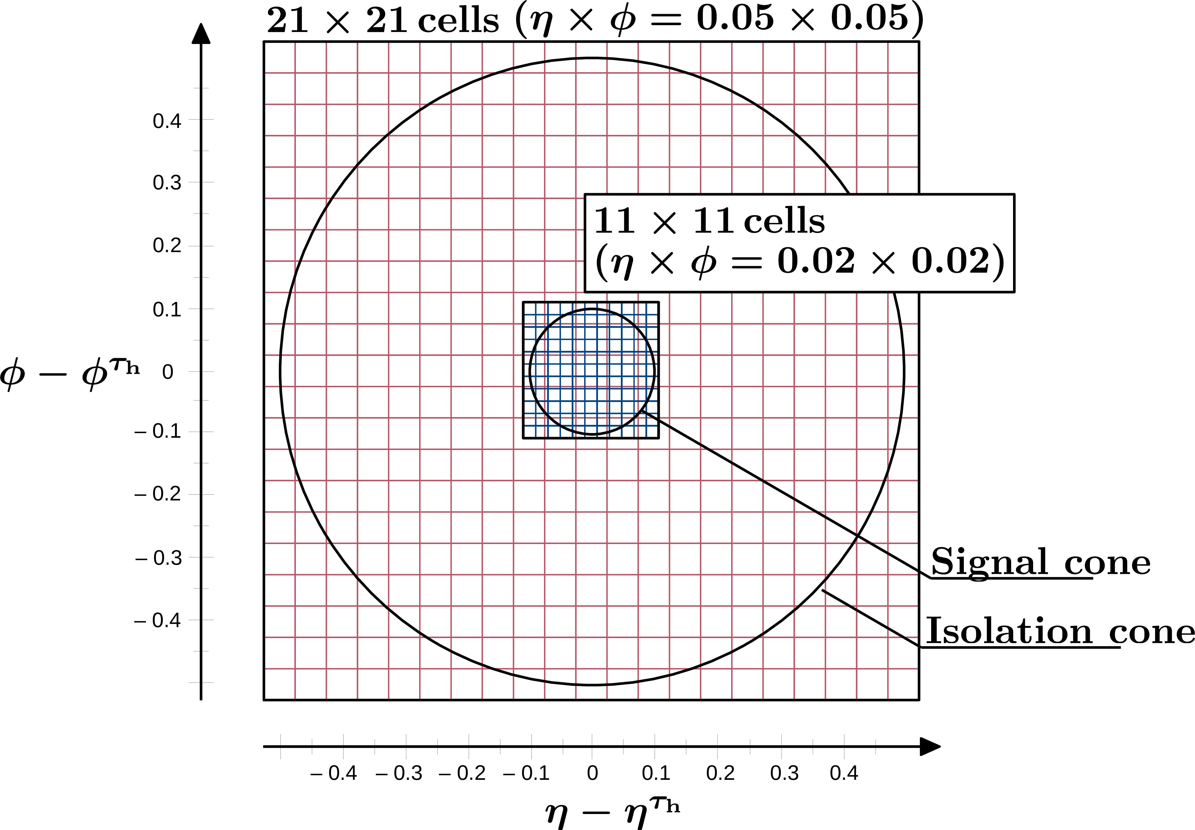
Figure 2:
Layout of the grids in $ \eta-\phi $ space around the reconstructed $ \tau_\mathrm{h} $ axis used to process the particle-level inputs for the convolutional layers of the DNN. The inner grid comprises 11 $ {\times} $ 11 cells with a grid size of 0.02 $ {\times} $ 0.02 and contains the signal cone with a radius of 0.05--0.1, which is defined in the $ \tau_\mathrm{h} $ reconstruction (the charged hadrons and $ \pi^{0} $ candidates used to reconstruct the $ \tau_\mathrm{h} $ candidate need to be within the signal cone). For high-$ p_{\mathrm{T}} $ quark and gluon jets, the finer grid is also able to resolve the dense core of the jet. The outer grid comprises 21 $ {\times} $ 21 cells with a grid size of 0.05 $ {\times} $ 0.05 and contains the isolation cone with a radius of 0.5 that is used to define higher-level observables that correlate with quark or gluon jet activity. |

png pdf |
Figure 3:
The DNN architecture. The three sets of input variables (inner cells, outer cells, and high-level features) are first processed separately through different subnetworks, whose outputs are then concatenated and processed through five fully connected layers before the output is calculated that gives the probabilities for a candidate to be either a $ \tau_\mathrm{h} $, an electron, a muon, or a quark or gluon jet. The subnetwork for the high-level inputs consists of three fully connected layers with decreasing numbers of nodes, taking 47 inputs and yielding 57 outputs. The features of both the inner and outer cells are input to complex subnetworks. In the first part, the observables in each grid cell are processed through a set of fully connected layers, first separately for electrons/photons (containing both the features for PF electrons and electrons from the standalone reconstruction), muons (similarly containing both features from PF and standalone muons), and charged/neutral hadrons, passing through three fully connected layers each. The outputs are concatenated and passed through four additional fully connected layers, yielding 64 outputs for each cell. The grids are then processed with convolutional layers, which successively reduce the size of the grid. For the inner cells, there are hence 5 convolutional layers that reduce the grid from 11 $ {\times} $ 11 to a single cell; for the outer cells, there are 10 convolutional layers that reduce the grid from 21 $ {\times} $ 21 to a single cell. The numbers of trainable parameters (TP) for the different subnetworks are also given for the different subnetworks. |
png pdf |
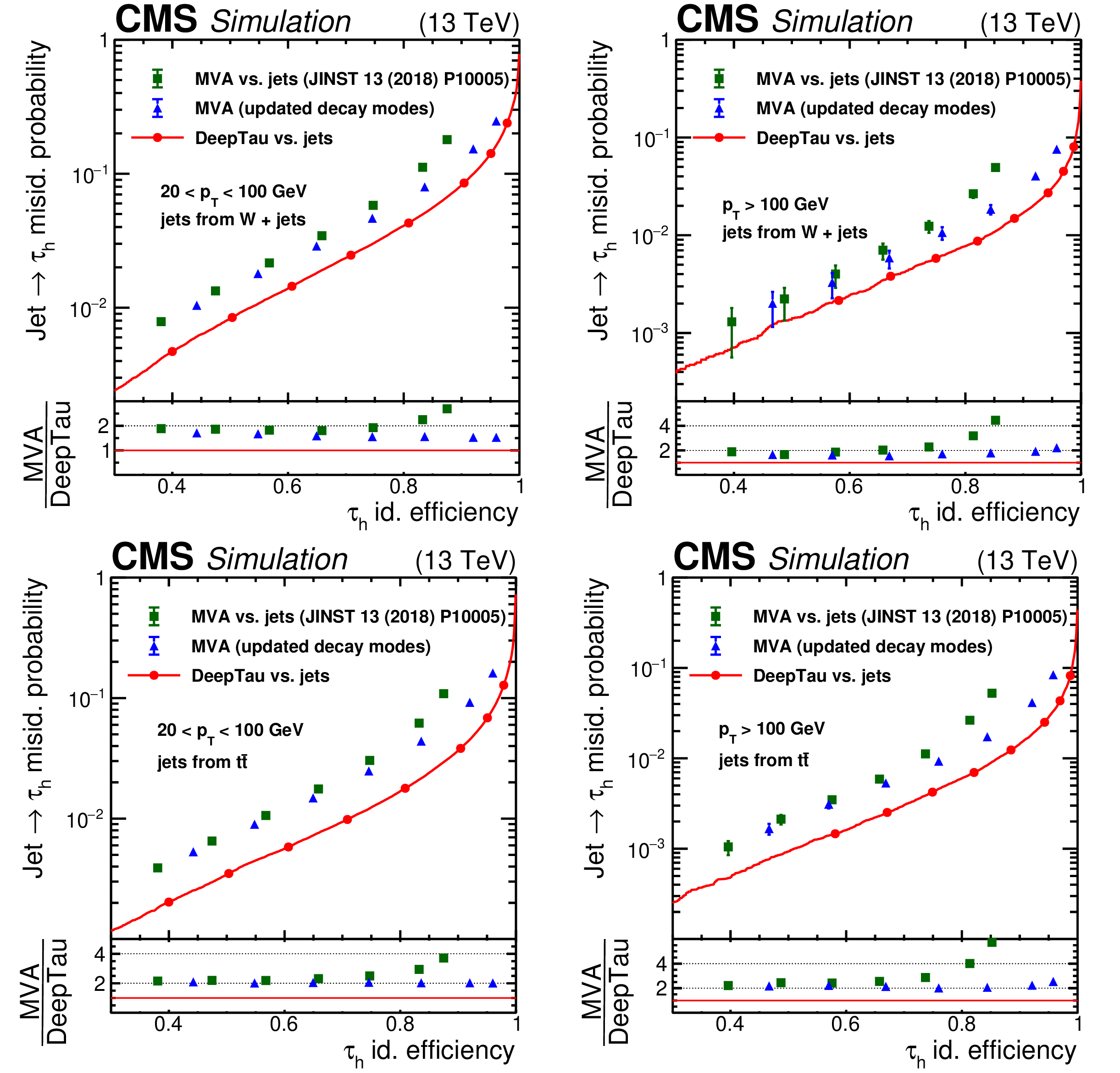
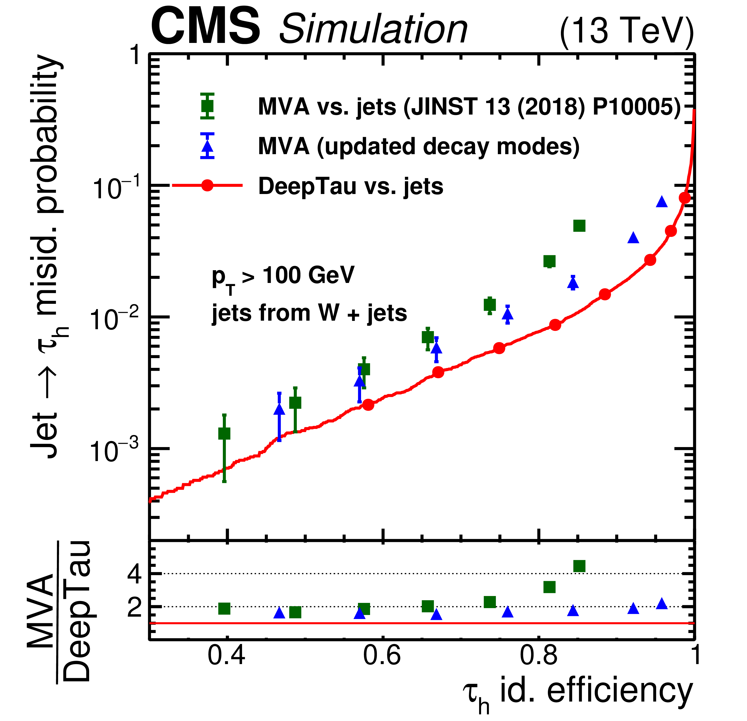
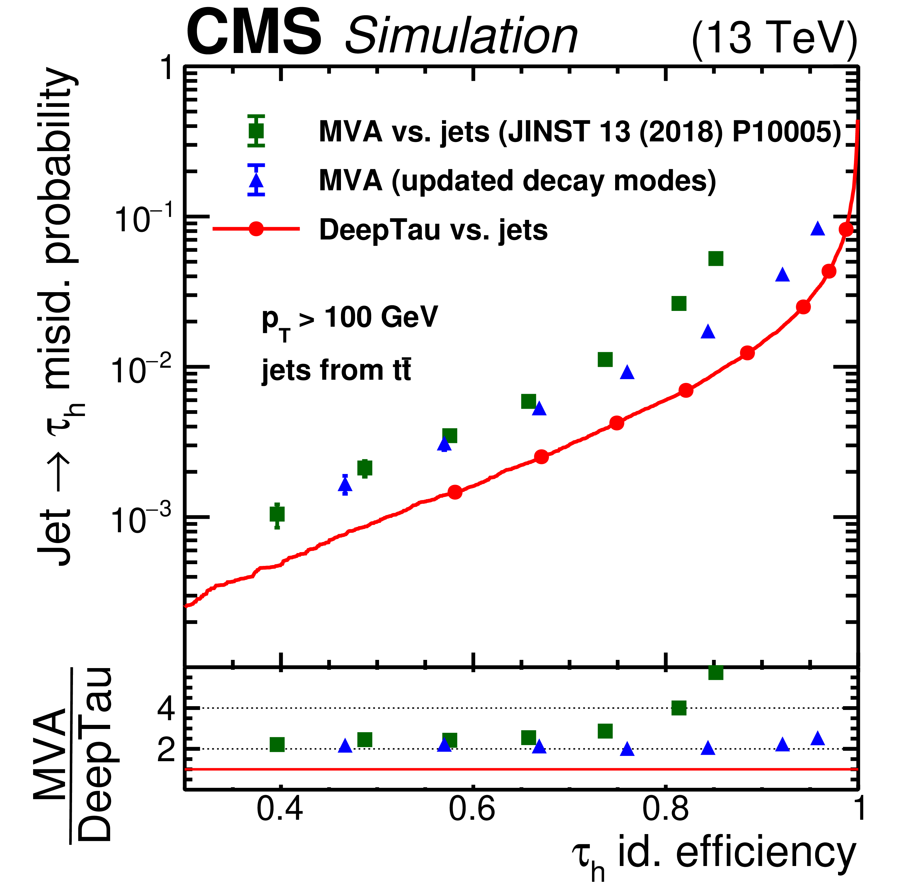
Figure 4:
Efficiency for quark and gluon jets to pass different tau identification discriminators versus the efficiency for genuine $ \tau_\mathrm{h} $. The upper two plots are obtained with jets from the W+jets simulated sample and the lower two plots with jets from the $ \mathrm{t} \overline{\mathrm{t}} $ sample. The left two plots include jets and genuine $ \tau_\mathrm{h} $ with $ p_{\mathrm{T}} < $ 100 GeV, whereas the right two plots include those with $ p_{\mathrm{T}} > $ 100 GeV. The working points are indicated as full circles. The efficiency for jets from the W+jets event sample, enriched in quark jets, to pass the discriminators is higher compared with jets from the $ \mathrm{t} \overline{\mathrm{t}} $ event sample, which has a larger fraction of gluon and b-quark jets. The jet efficiency for a given $ \tau_\mathrm{h} $ efficiency is larger for jets and $ \tau_\mathrm{h} $ with $ p_{\mathrm{T}} < $ 100 GeV than for those with $ p_{\mathrm{T}} > $ 100 GeV. Compared with the previously used MVA discriminator, the DEEPTAU discriminator reduces the jet efficiency for a given $ \tau_\mathrm{h} $ efficiency by consistently more than a factor of 1.8, and by more at high $ \tau_\mathrm{h} $ efficiency. The additional gain at high $ p_{\mathrm{T}} $ comes from the inclusion of updated decay modes in the $ \tau_\mathrm{h} $ reconstruction, as illustrated by the curves for the previously used MVA discriminator but including reconstructed $ \tau_\mathrm{h} $ candidates with additional decay modes. |

png pdf |
Figure 4-a:
Efficiency for quark and gluon jets to pass different tau identification discriminators versus the efficiency for genuine $ \tau_\mathrm{h} $. The upper two plots are obtained with jets from the W+jets simulated sample and the lower two plots with jets from the $ \mathrm{t} \overline{\mathrm{t}} $ sample. The left two plots include jets and genuine $ \tau_\mathrm{h} $ with $ p_{\mathrm{T}} < $ 100 GeV, whereas the right two plots include those with $ p_{\mathrm{T}} > $ 100 GeV. The working points are indicated as full circles. The efficiency for jets from the W+jets event sample, enriched in quark jets, to pass the discriminators is higher compared with jets from the $ \mathrm{t} \overline{\mathrm{t}} $ event sample, which has a larger fraction of gluon and b-quark jets. The jet efficiency for a given $ \tau_\mathrm{h} $ efficiency is larger for jets and $ \tau_\mathrm{h} $ with $ p_{\mathrm{T}} < $ 100 GeV than for those with $ p_{\mathrm{T}} > $ 100 GeV. Compared with the previously used MVA discriminator, the DEEPTAU discriminator reduces the jet efficiency for a given $ \tau_\mathrm{h} $ efficiency by consistently more than a factor of 1.8, and by more at high $ \tau_\mathrm{h} $ efficiency. The additional gain at high $ p_{\mathrm{T}} $ comes from the inclusion of updated decay modes in the $ \tau_\mathrm{h} $ reconstruction, as illustrated by the curves for the previously used MVA discriminator but including reconstructed $ \tau_\mathrm{h} $ candidates with additional decay modes. |
png pdf |
Figure 4-b:
Efficiency for quark and gluon jets to pass different tau identification discriminators versus the efficiency for genuine $ \tau_\mathrm{h} $. The upper two plots are obtained with jets from the W+jets simulated sample and the lower two plots with jets from the $ \mathrm{t} \overline{\mathrm{t}} $ sample. The left two plots include jets and genuine $ \tau_\mathrm{h} $ with $ p_{\mathrm{T}} < $ 100 GeV, whereas the right two plots include those with $ p_{\mathrm{T}} > $ 100 GeV. The working points are indicated as full circles. The efficiency for jets from the W+jets event sample, enriched in quark jets, to pass the discriminators is higher compared with jets from the $ \mathrm{t} \overline{\mathrm{t}} $ event sample, which has a larger fraction of gluon and b-quark jets. The jet efficiency for a given $ \tau_\mathrm{h} $ efficiency is larger for jets and $ \tau_\mathrm{h} $ with $ p_{\mathrm{T}} < $ 100 GeV than for those with $ p_{\mathrm{T}} > $ 100 GeV. Compared with the previously used MVA discriminator, the DEEPTAU discriminator reduces the jet efficiency for a given $ \tau_\mathrm{h} $ efficiency by consistently more than a factor of 1.8, and by more at high $ \tau_\mathrm{h} $ efficiency. The additional gain at high $ p_{\mathrm{T}} $ comes from the inclusion of updated decay modes in the $ \tau_\mathrm{h} $ reconstruction, as illustrated by the curves for the previously used MVA discriminator but including reconstructed $ \tau_\mathrm{h} $ candidates with additional decay modes. |

png pdf |
Figure 4-c:
Efficiency for quark and gluon jets to pass different tau identification discriminators versus the efficiency for genuine $ \tau_\mathrm{h} $. The upper two plots are obtained with jets from the W+jets simulated sample and the lower two plots with jets from the $ \mathrm{t} \overline{\mathrm{t}} $ sample. The left two plots include jets and genuine $ \tau_\mathrm{h} $ with $ p_{\mathrm{T}} < $ 100 GeV, whereas the right two plots include those with $ p_{\mathrm{T}} > $ 100 GeV. The working points are indicated as full circles. The efficiency for jets from the W+jets event sample, enriched in quark jets, to pass the discriminators is higher compared with jets from the $ \mathrm{t} \overline{\mathrm{t}} $ event sample, which has a larger fraction of gluon and b-quark jets. The jet efficiency for a given $ \tau_\mathrm{h} $ efficiency is larger for jets and $ \tau_\mathrm{h} $ with $ p_{\mathrm{T}} < $ 100 GeV than for those with $ p_{\mathrm{T}} > $ 100 GeV. Compared with the previously used MVA discriminator, the DEEPTAU discriminator reduces the jet efficiency for a given $ \tau_\mathrm{h} $ efficiency by consistently more than a factor of 1.8, and by more at high $ \tau_\mathrm{h} $ efficiency. The additional gain at high $ p_{\mathrm{T}} $ comes from the inclusion of updated decay modes in the $ \tau_\mathrm{h} $ reconstruction, as illustrated by the curves for the previously used MVA discriminator but including reconstructed $ \tau_\mathrm{h} $ candidates with additional decay modes. |
png pdf |
Figure 4-d:
Efficiency for quark and gluon jets to pass different tau identification discriminators versus the efficiency for genuine $ \tau_\mathrm{h} $. The upper two plots are obtained with jets from the W+jets simulated sample and the lower two plots with jets from the $ \mathrm{t} \overline{\mathrm{t}} $ sample. The left two plots include jets and genuine $ \tau_\mathrm{h} $ with $ p_{\mathrm{T}} < $ 100 GeV, whereas the right two plots include those with $ p_{\mathrm{T}} > $ 100 GeV. The working points are indicated as full circles. The efficiency for jets from the W+jets event sample, enriched in quark jets, to pass the discriminators is higher compared with jets from the $ \mathrm{t} \overline{\mathrm{t}} $ event sample, which has a larger fraction of gluon and b-quark jets. The jet efficiency for a given $ \tau_\mathrm{h} $ efficiency is larger for jets and $ \tau_\mathrm{h} $ with $ p_{\mathrm{T}} < $ 100 GeV than for those with $ p_{\mathrm{T}} > $ 100 GeV. Compared with the previously used MVA discriminator, the DEEPTAU discriminator reduces the jet efficiency for a given $ \tau_\mathrm{h} $ efficiency by consistently more than a factor of 1.8, and by more at high $ \tau_\mathrm{h} $ efficiency. The additional gain at high $ p_{\mathrm{T}} $ comes from the inclusion of updated decay modes in the $ \tau_\mathrm{h} $ reconstruction, as illustrated by the curves for the previously used MVA discriminator but including reconstructed $ \tau_\mathrm{h} $ candidates with additional decay modes. |
png pdf |
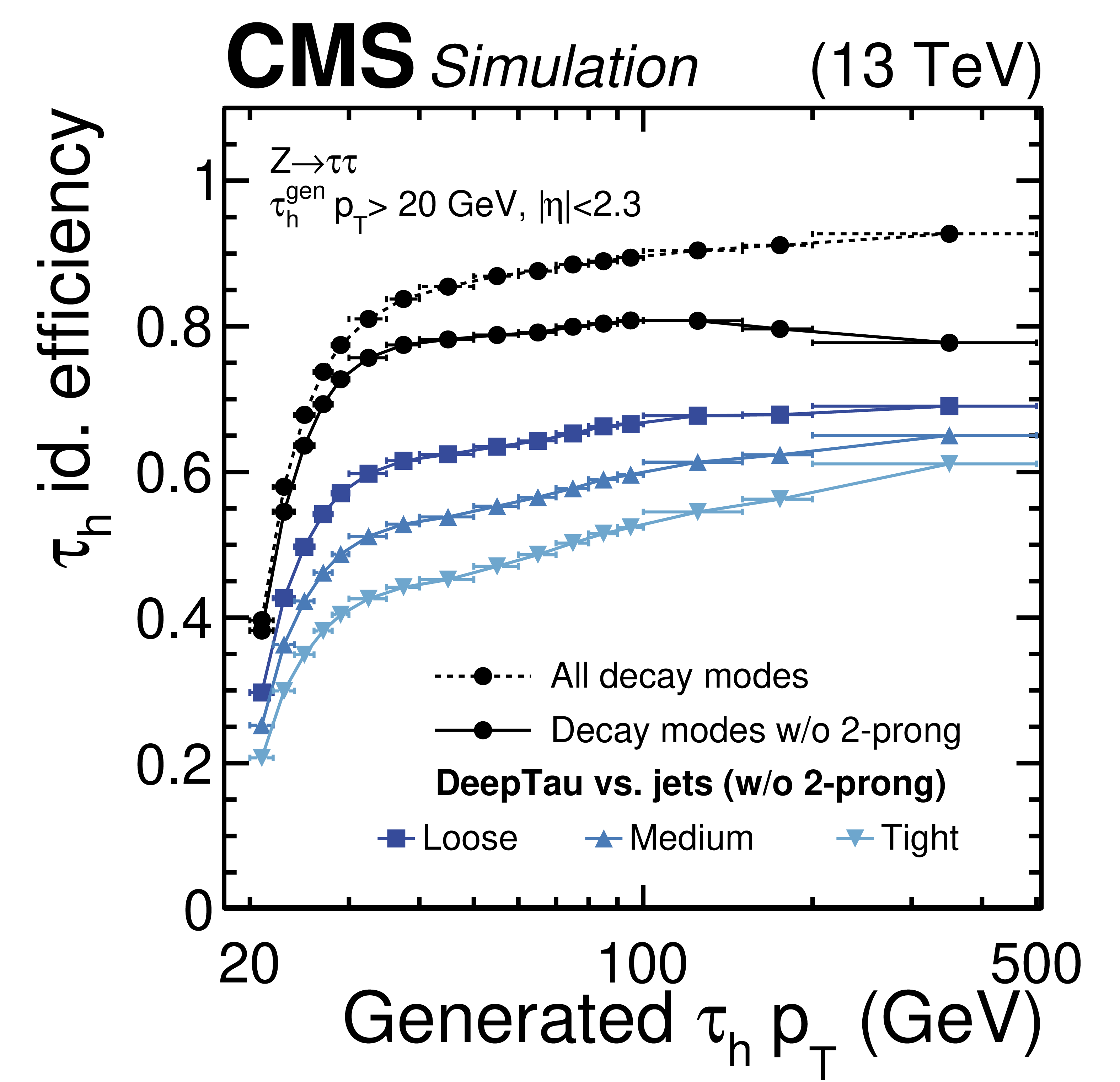
Figure 5:
Efficiencies for simulated $ \tau_\mathrm{h} $ decays with $ |\eta| < $ 2.3 to pass the following reconstruction and identification requirements: to be reconstructed in any decay mode with $ p_{\mathrm{T}} > $ 20 GeV and $ |\eta| < $ 2.3 (black dashed line), to be reconstructed in a decay mode except for those with missing charged hadrons (labelled ``2-prong'' and shown as full black line), and to be reconstructed in a decay mode except the 2-prong ones and to pass the Loose, Medium, or Tight working point of the $ D_\text{jet} $ discriminator (blue lines), obtained with a $ \mathrm{Z}\to\tau\tau $ event sample. The efficiencies are shown as a function of the visible genuine $ \tau_\mathrm{h} p_{\mathrm{T}} $ obtained from simulated decay products. |

png pdf |
Figure 6:
Efficiency for electrons versus efficiency for genuine $ \tau_\mathrm{h} $ to pass the MVA and $ D_\mathrm{e} $ discriminators, separately for electrons and $ \tau_\mathrm{h} $ with 20 $ < p_{\mathrm{T}} < $ 100 GeV (left) and $ p_{\mathrm{T}} > $ 100 GeV (right). Vertical bars correspond to the statistical uncertainties. The $ \tau_\mathrm{h} $ candidates are reconstructed in one of the $ \tau_\mathrm{h} $ decay modes without missing charged hadrons. Compared with the MVA discriminator, the $ D_\mathrm{e} $ discriminator reduces the electron efficiency by more than a factor of two for a $ \tau_\mathrm{h} $ efficiency of 70% and by more than a factor of 10 for $ \tau_\mathrm{h} $ efficiencies larger than 88%. Furthermore, working points (indicated as full circles) are now provided for previously inaccessible $ \tau_\mathrm{h} $ efficiencies larger than 90%, for a misidentification efficiency between 0.3 and 8%. |

png pdf |
Figure 6-a:
Efficiency for electrons versus efficiency for genuine $ \tau_\mathrm{h} $ to pass the MVA and $ D_\mathrm{e} $ discriminators, separately for electrons and $ \tau_\mathrm{h} $ with 20 $ < p_{\mathrm{T}} < $ 100 GeV (left) and $ p_{\mathrm{T}} > $ 100 GeV (right). Vertical bars correspond to the statistical uncertainties. The $ \tau_\mathrm{h} $ candidates are reconstructed in one of the $ \tau_\mathrm{h} $ decay modes without missing charged hadrons. Compared with the MVA discriminator, the $ D_\mathrm{e} $ discriminator reduces the electron efficiency by more than a factor of two for a $ \tau_\mathrm{h} $ efficiency of 70% and by more than a factor of 10 for $ \tau_\mathrm{h} $ efficiencies larger than 88%. Furthermore, working points (indicated as full circles) are now provided for previously inaccessible $ \tau_\mathrm{h} $ efficiencies larger than 90%, for a misidentification efficiency between 0.3 and 8%. |

png pdf |
Figure 6-b:
Efficiency for electrons versus efficiency for genuine $ \tau_\mathrm{h} $ to pass the MVA and $ D_\mathrm{e} $ discriminators, separately for electrons and $ \tau_\mathrm{h} $ with 20 $ < p_{\mathrm{T}} < $ 100 GeV (left) and $ p_{\mathrm{T}} > $ 100 GeV (right). Vertical bars correspond to the statistical uncertainties. The $ \tau_\mathrm{h} $ candidates are reconstructed in one of the $ \tau_\mathrm{h} $ decay modes without missing charged hadrons. Compared with the MVA discriminator, the $ D_\mathrm{e} $ discriminator reduces the electron efficiency by more than a factor of two for a $ \tau_\mathrm{h} $ efficiency of 70% and by more than a factor of 10 for $ \tau_\mathrm{h} $ efficiencies larger than 88%. Furthermore, working points (indicated as full circles) are now provided for previously inaccessible $ \tau_\mathrm{h} $ efficiencies larger than 90%, for a misidentification efficiency between 0.3 and 8%. |
png pdf |
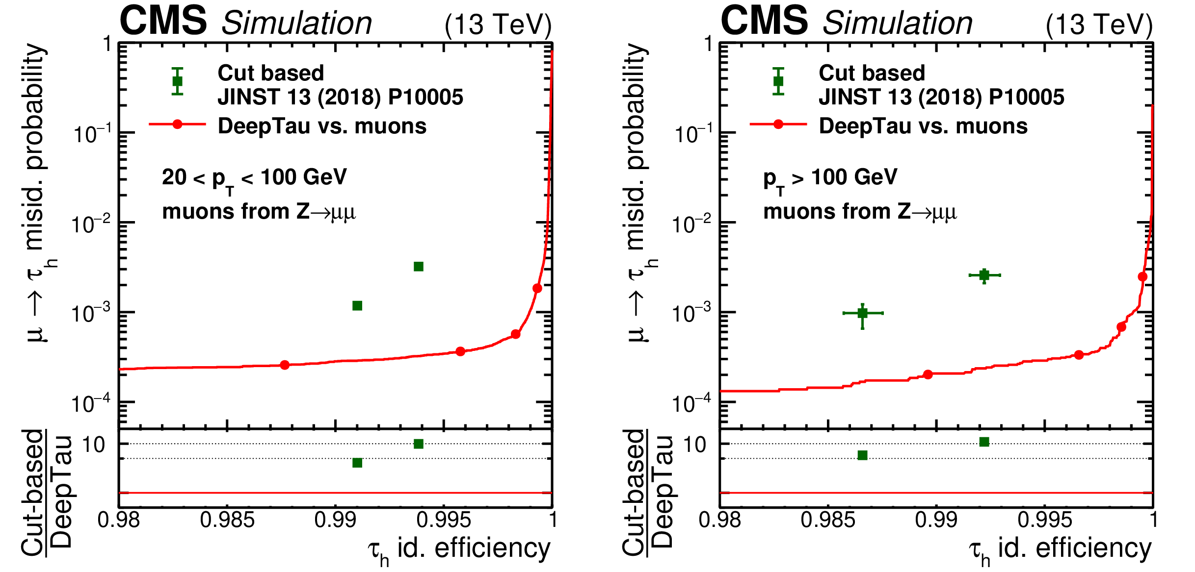
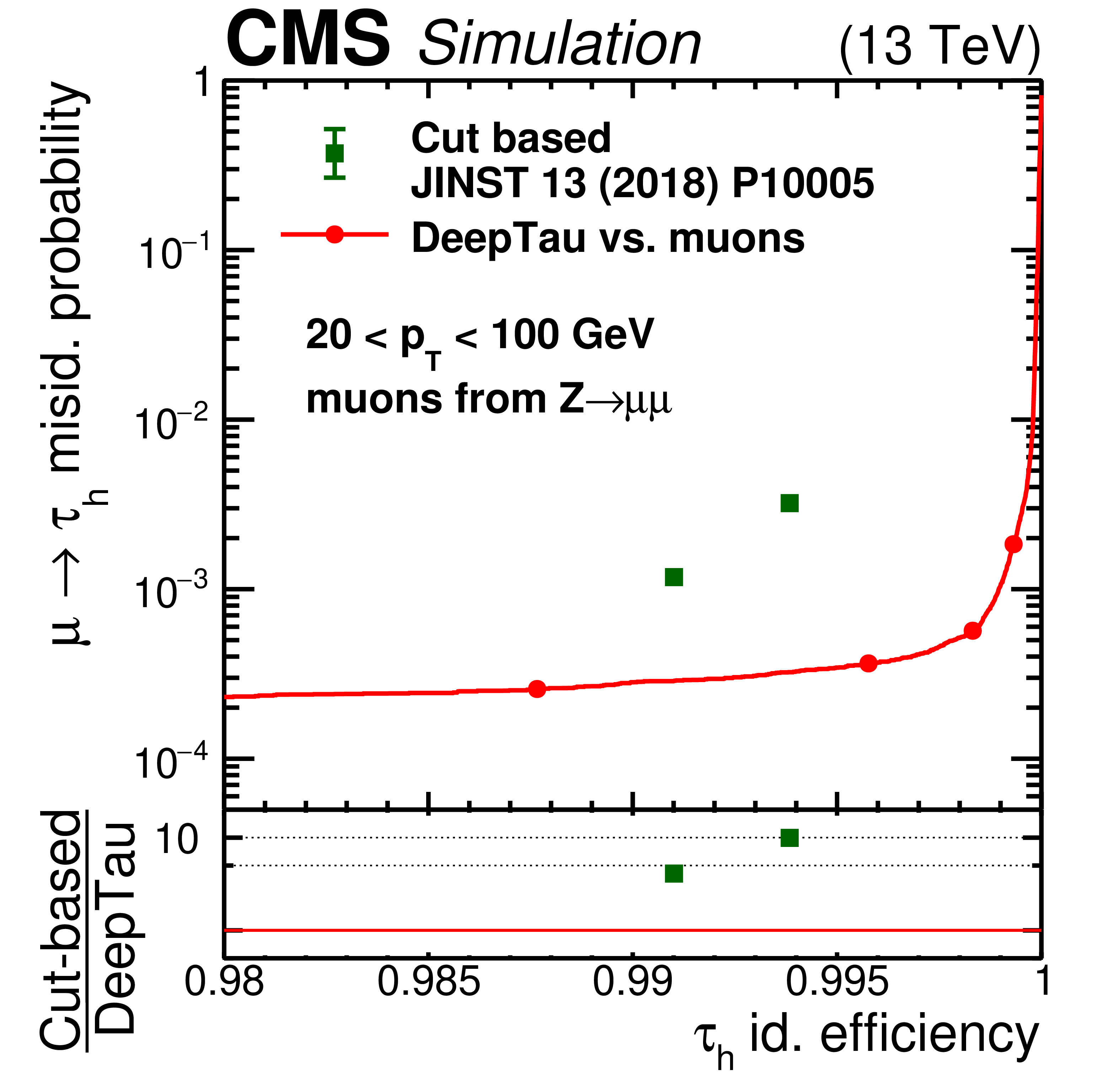
Figure 7:
Efficiency for muons versus efficiency for simulated $ \tau_\mathrm{h} $ to pass the cutoff-based and $ D_\mu $ discriminators, separately for muons and $ \tau_\mathrm{h} $ with 20 $ < p_{\mathrm{T}} < $ 100 GeV (left) and $ p_{\mathrm{T}} > $ 100 GeV (right). The four working points are indicated as full circles. Vertical bars correspond to the statistical uncertainties. In both $ p_{\mathrm{T}} $ regimes, the $ D_\mu $ discriminator rejects up to a factor of 10 more muons at $ \tau_\mathrm{h} $ efficiencies around 99%, and it leads to an increase of the $ \tau_\mathrm{h} $ efficiency for a similar background rejection by about 0.5%. |
png pdf |
Figure 7-a:
Efficiency for muons versus efficiency for simulated $ \tau_\mathrm{h} $ to pass the cutoff-based and $ D_\mu $ discriminators, separately for muons and $ \tau_\mathrm{h} $ with 20 $ < p_{\mathrm{T}} < $ 100 GeV (left) and $ p_{\mathrm{T}} > $ 100 GeV (right). The four working points are indicated as full circles. Vertical bars correspond to the statistical uncertainties. In both $ p_{\mathrm{T}} $ regimes, the $ D_\mu $ discriminator rejects up to a factor of 10 more muons at $ \tau_\mathrm{h} $ efficiencies around 99%, and it leads to an increase of the $ \tau_\mathrm{h} $ efficiency for a similar background rejection by about 0.5%. |

png pdf |
Figure 7-b:
Efficiency for muons versus efficiency for simulated $ \tau_\mathrm{h} $ to pass the cutoff-based and $ D_\mu $ discriminators, separately for muons and $ \tau_\mathrm{h} $ with 20 $ < p_{\mathrm{T}} < $ 100 GeV (left) and $ p_{\mathrm{T}} > $ 100 GeV (right). The four working points are indicated as full circles. Vertical bars correspond to the statistical uncertainties. In both $ p_{\mathrm{T}} $ regimes, the $ D_\mu $ discriminator rejects up to a factor of 10 more muons at $ \tau_\mathrm{h} $ efficiencies around 99%, and it leads to an increase of the $ \tau_\mathrm{h} $ efficiency for a similar background rejection by about 0.5%. |

png pdf |
Figure 8:
Data-to-simulation scale factors for genuine $ \tau_\mathrm{h} $ to be reconstructed as $ \tau_\mathrm{h} $ candidates and to pass the Loose, Medium, and Tight working points of the $ D_\text{jet} $ discriminator as a function of the $ \tau_\mathrm{h} $ candidate $ p_{\mathrm{T}} $ (left). Vertical bars correspond to the combined statistical and systematic uncertainties in the individual scale factors. The red hatched bands indicate the uncertainties for $ p_{\mathrm{T}} > $ 40 GeV, obtained from a combination of the individual measurements. The right plot shows the data-to-simulation scale factors for the $ \tau_\mathrm{h} $ candidates with $ p_{\mathrm{T}} > $ 40 GeV to pass the Medium $ D_\text{jet} $ working point as a function of reconstructed $ \tau_\mathrm{h} $ decay mode. The efficiencies are obtained with 2018 data and the according simulated events using a likelihood fit to the distribution of the reconstructed $ m_\text{vis}(\mu, \tau_\mathrm{h}) $. The scale factors are shown separately for data taken in 2016, 2017, and 2018 (and the corresponding simulated events) and for the four main $ \tau_\mathrm{h} $ decay modes. |

png pdf |
Figure 8-a:
Data-to-simulation scale factors for genuine $ \tau_\mathrm{h} $ to be reconstructed as $ \tau_\mathrm{h} $ candidates and to pass the Loose, Medium, and Tight working points of the $ D_\text{jet} $ discriminator as a function of the $ \tau_\mathrm{h} $ candidate $ p_{\mathrm{T}} $ (left). Vertical bars correspond to the combined statistical and systematic uncertainties in the individual scale factors. The red hatched bands indicate the uncertainties for $ p_{\mathrm{T}} > $ 40 GeV, obtained from a combination of the individual measurements. The right plot shows the data-to-simulation scale factors for the $ \tau_\mathrm{h} $ candidates with $ p_{\mathrm{T}} > $ 40 GeV to pass the Medium $ D_\text{jet} $ working point as a function of reconstructed $ \tau_\mathrm{h} $ decay mode. The efficiencies are obtained with 2018 data and the according simulated events using a likelihood fit to the distribution of the reconstructed $ m_\text{vis}(\mu, \tau_\mathrm{h}) $. The scale factors are shown separately for data taken in 2016, 2017, and 2018 (and the corresponding simulated events) and for the four main $ \tau_\mathrm{h} $ decay modes. |

png pdf |
Figure 8-b:
Data-to-simulation scale factors for genuine $ \tau_\mathrm{h} $ to be reconstructed as $ \tau_\mathrm{h} $ candidates and to pass the Loose, Medium, and Tight working points of the $ D_\text{jet} $ discriminator as a function of the $ \tau_\mathrm{h} $ candidate $ p_{\mathrm{T}} $ (left). Vertical bars correspond to the combined statistical and systematic uncertainties in the individual scale factors. The red hatched bands indicate the uncertainties for $ p_{\mathrm{T}} > $ 40 GeV, obtained from a combination of the individual measurements. The right plot shows the data-to-simulation scale factors for the $ \tau_\mathrm{h} $ candidates with $ p_{\mathrm{T}} > $ 40 GeV to pass the Medium $ D_\text{jet} $ working point as a function of reconstructed $ \tau_\mathrm{h} $ decay mode. The efficiencies are obtained with 2018 data and the according simulated events using a likelihood fit to the distribution of the reconstructed $ m_\text{vis}(\mu, \tau_\mathrm{h}) $. The scale factors are shown separately for data taken in 2016, 2017, and 2018 (and the corresponding simulated events) and for the four main $ \tau_\mathrm{h} $ decay modes. |

png pdf |
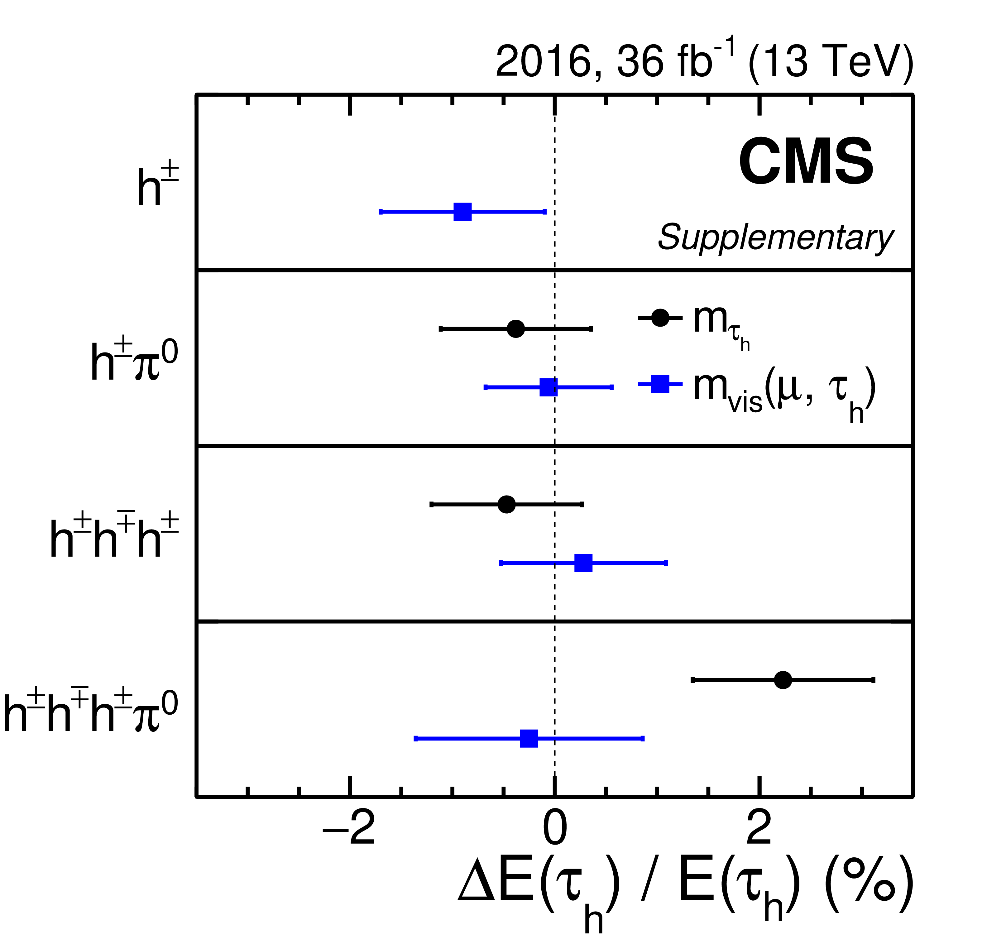
Figure 9:
Relative difference between $ \tau_\mathrm{h} $ energy obtained in data and simulated events for the four main reconstructed $ \tau_\mathrm{h} $ decay modes for the 2018 data set. The results are obtained from fits to the distribution of either the reconstructed $ m_\text{vis}(\mu, \tau_\mathrm{h}) $ (blue lines) or $ m_{\tau_\mathrm{h}} $ (black lines). The horizontal bars represent the uncertainties in the measurements. The measured values are consistent with no shift of the $ \tau_\mathrm{h} $ energy scale between data and simulation, with the largest difference amounting to 1.5 standard deviations. |

png pdf |
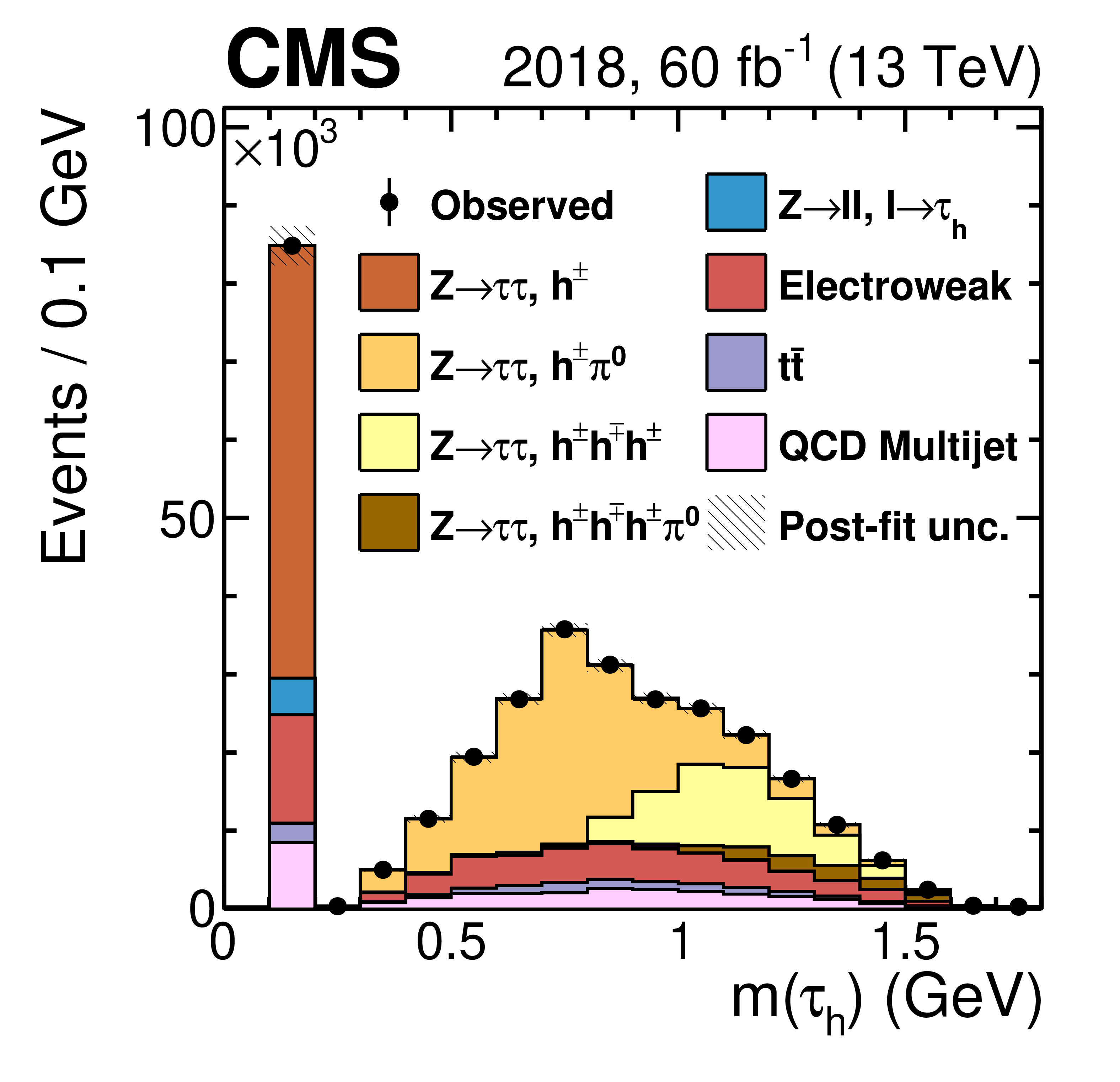
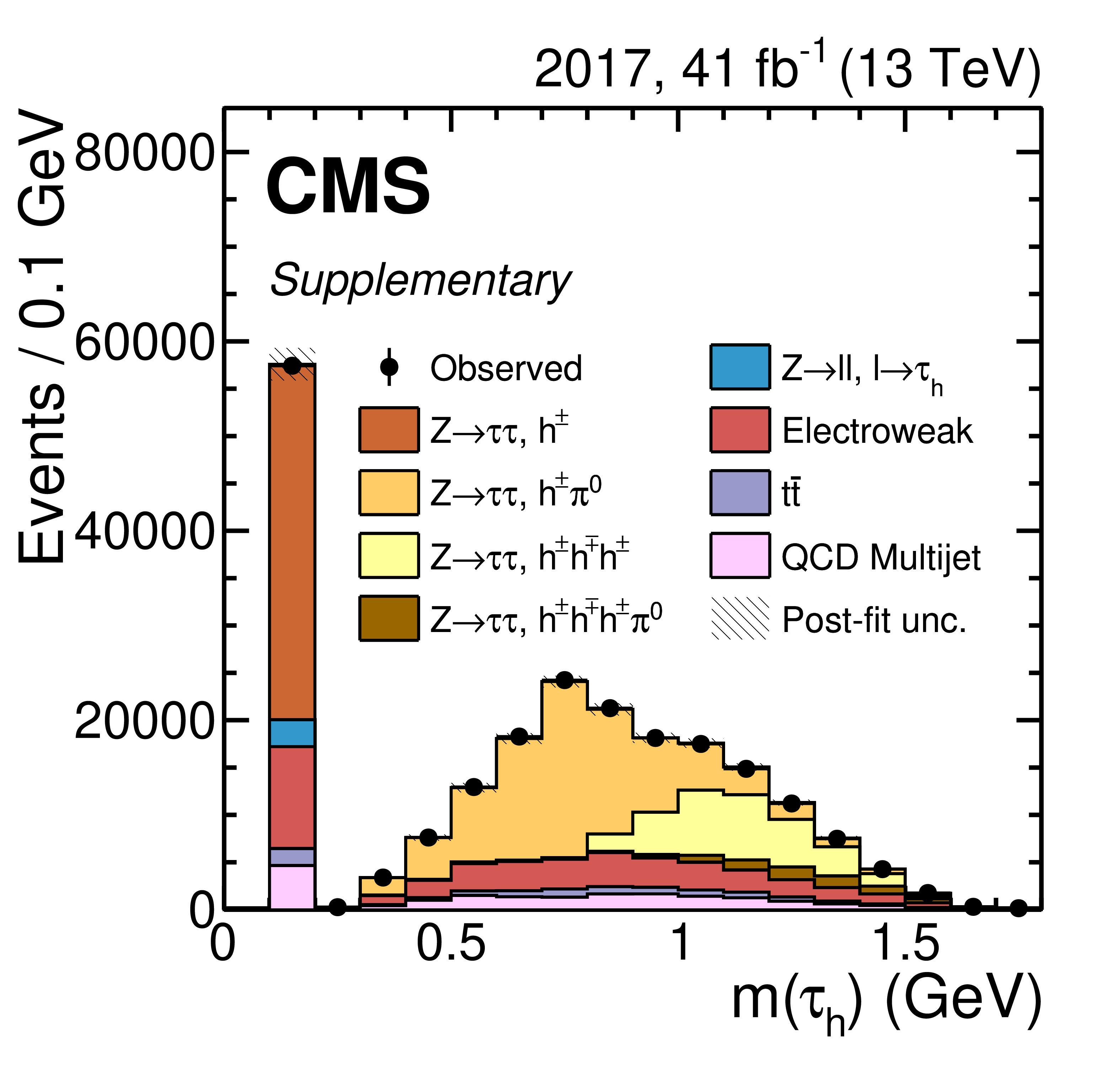
Figure 10:
Distribution of the reconstructed visible invariant mass of the $ \mu\tau_\mathrm{h} $ system, $ m_\text{vis}(\mu, \tau_\mathrm{h}) $ (left) and of the visible invariant $ \tau_\mathrm{h} $ mass (right). Vertical bars correspond to the statistical uncertainties. The event selection corresponds to the one in the measurement of the $ \tau_\mathrm{h} $ reconstruction and identification efficiencies and uses the Tight working point of the $ D_\text{jet} $ discriminator. The distributions incorporate all measured scale factors and energy corrections and are scaled to the outcome of a maximum likelihood to the observed data with the $ \mathrm{Z}\to\tau\tau $ contribution freely floating. The electroweak background combines contributions from single top quark, diboson, and W+jets processes as well as $ \mathrm{Z}(\to\tau\tau) $+jets events where the reconstructed $ \tau_\mathrm{h} $ originates from a jet misidentified as a $ \tau_\mathrm{h} $ candidate instead of one of the produced tau leptons. In the $ m(\tau_\mathrm{h}) $ distribution, the $ \mathrm{Z}\to\tau\tau $ contributions are shown separately for the different $ \tau_\mathrm{h} $ decay modes. |

png pdf |
Figure 10-a:
Distribution of the reconstructed visible invariant mass of the $ \mu\tau_\mathrm{h} $ system, $ m_\text{vis}(\mu, \tau_\mathrm{h}) $ (left) and of the visible invariant $ \tau_\mathrm{h} $ mass (right). Vertical bars correspond to the statistical uncertainties. The event selection corresponds to the one in the measurement of the $ \tau_\mathrm{h} $ reconstruction and identification efficiencies and uses the Tight working point of the $ D_\text{jet} $ discriminator. The distributions incorporate all measured scale factors and energy corrections and are scaled to the outcome of a maximum likelihood to the observed data with the $ \mathrm{Z}\to\tau\tau $ contribution freely floating. The electroweak background combines contributions from single top quark, diboson, and W+jets processes as well as $ \mathrm{Z}(\to\tau\tau) $+jets events where the reconstructed $ \tau_\mathrm{h} $ originates from a jet misidentified as a $ \tau_\mathrm{h} $ candidate instead of one of the produced tau leptons. In the $ m(\tau_\mathrm{h}) $ distribution, the $ \mathrm{Z}\to\tau\tau $ contributions are shown separately for the different $ \tau_\mathrm{h} $ decay modes. |
png pdf |
Figure 10-b:
Distribution of the reconstructed visible invariant mass of the $ \mu\tau_\mathrm{h} $ system, $ m_\text{vis}(\mu, \tau_\mathrm{h}) $ (left) and of the visible invariant $ \tau_\mathrm{h} $ mass (right). Vertical bars correspond to the statistical uncertainties. The event selection corresponds to the one in the measurement of the $ \tau_\mathrm{h} $ reconstruction and identification efficiencies and uses the Tight working point of the $ D_\text{jet} $ discriminator. The distributions incorporate all measured scale factors and energy corrections and are scaled to the outcome of a maximum likelihood to the observed data with the $ \mathrm{Z}\to\tau\tau $ contribution freely floating. The electroweak background combines contributions from single top quark, diboson, and W+jets processes as well as $ \mathrm{Z}(\to\tau\tau) $+jets events where the reconstructed $ \tau_\mathrm{h} $ originates from a jet misidentified as a $ \tau_\mathrm{h} $ candidate instead of one of the produced tau leptons. In the $ m(\tau_\mathrm{h}) $ distribution, the $ \mathrm{Z}\to\tau\tau $ contributions are shown separately for the different $ \tau_\mathrm{h} $ decay modes. |
png pdf |
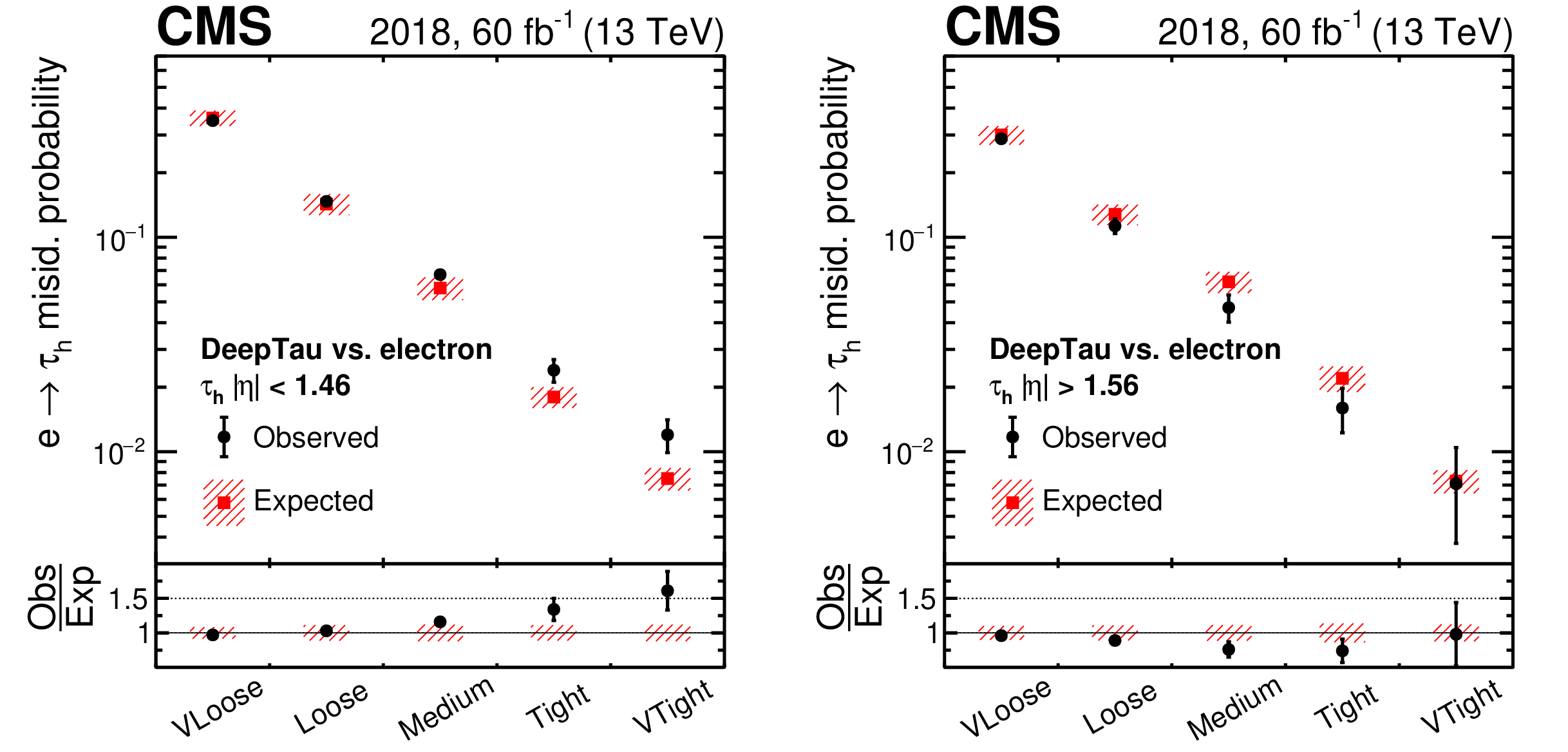
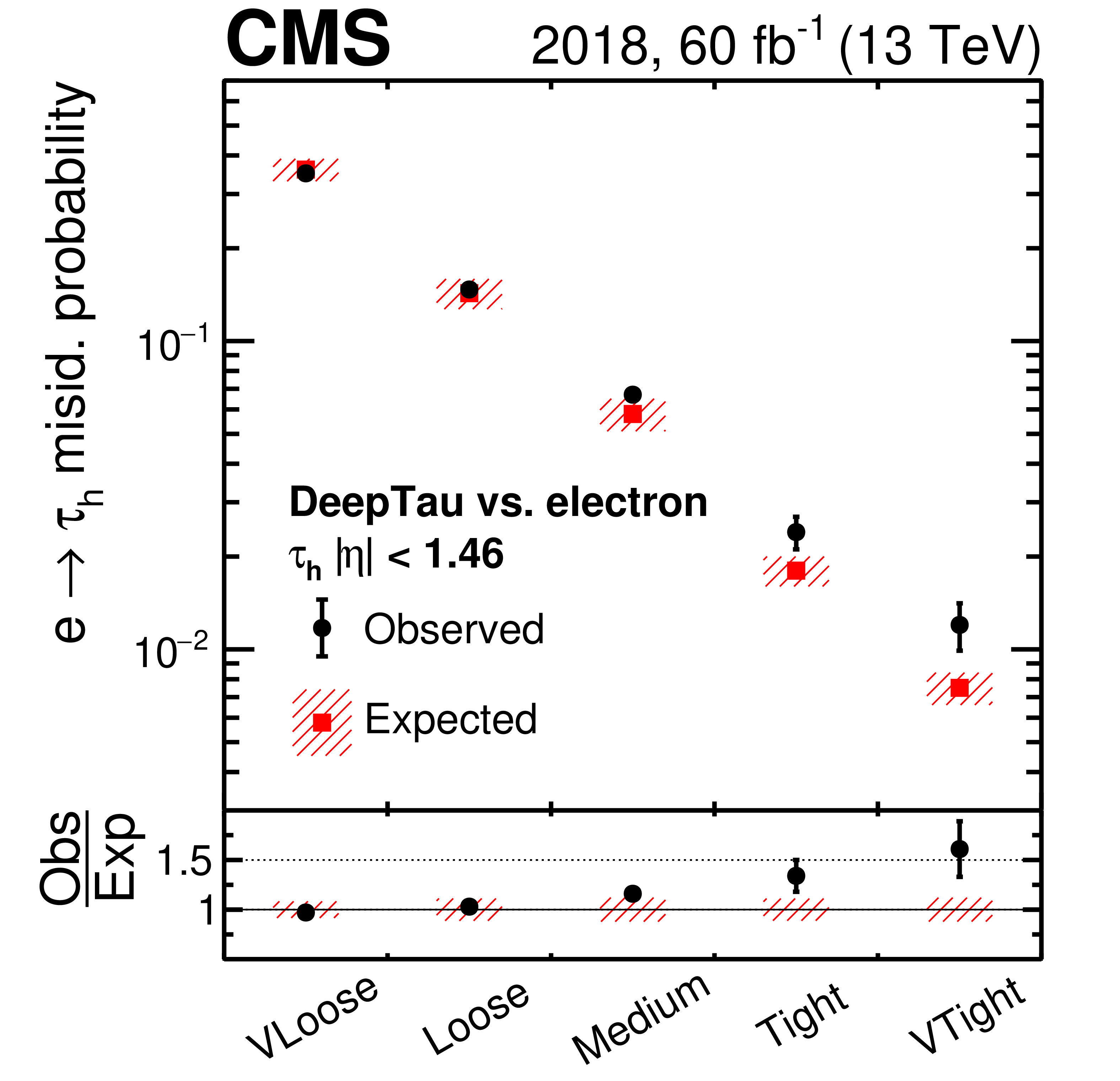
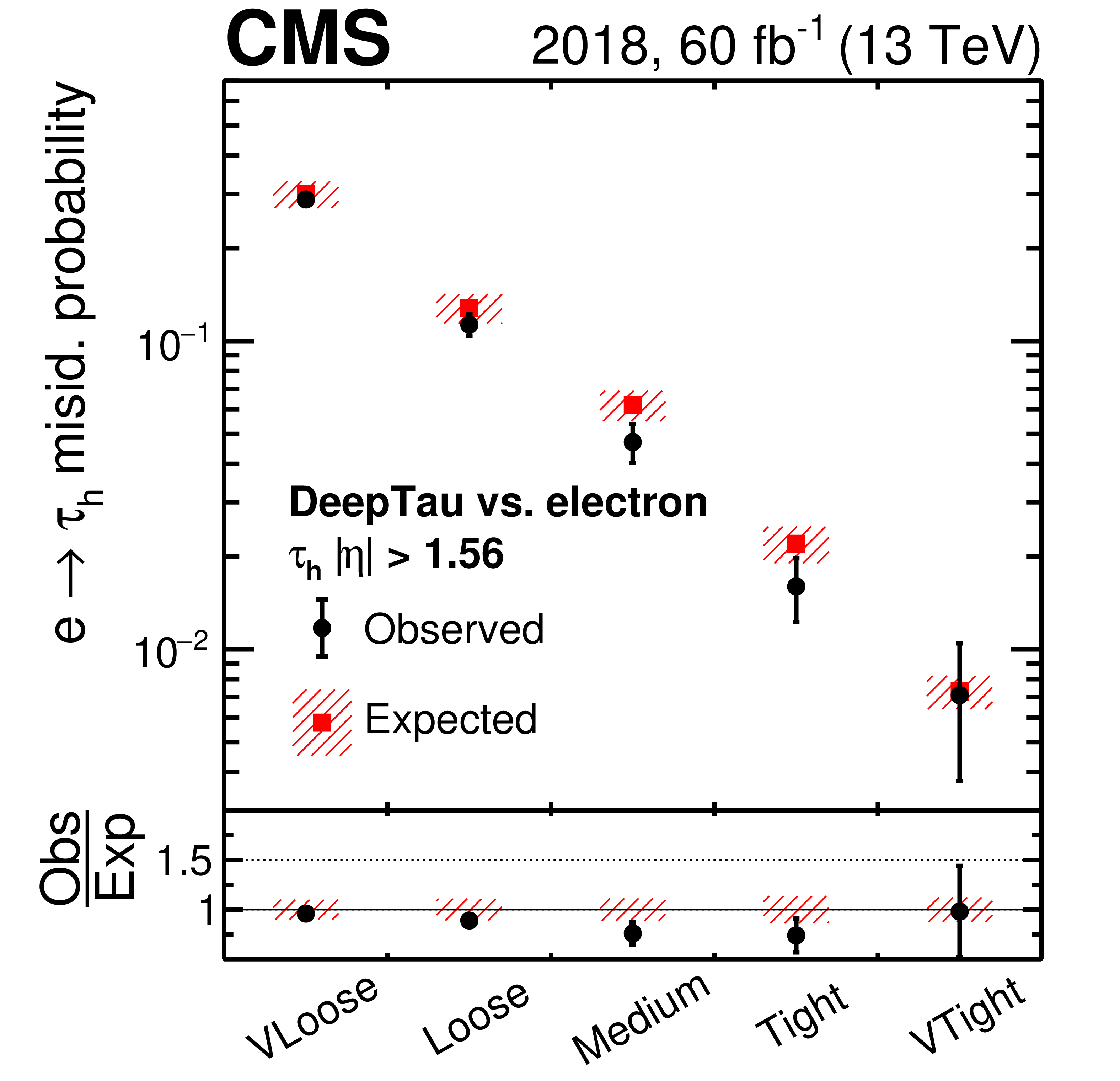
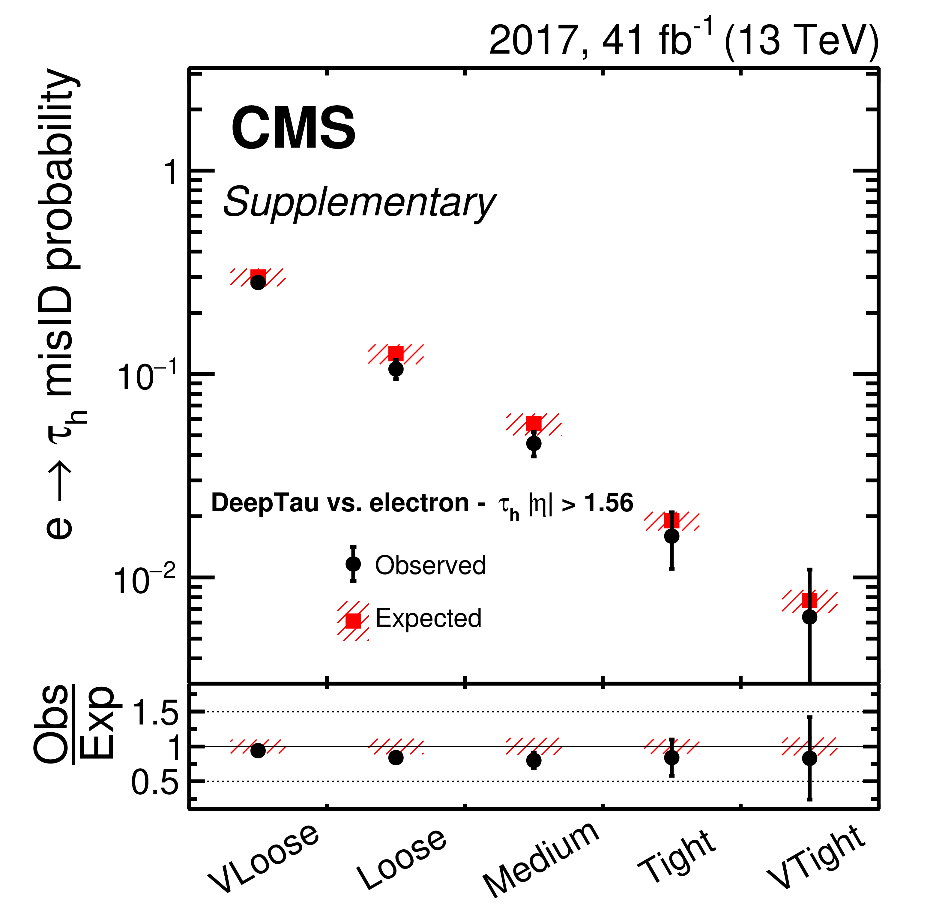
Figure 11:
Observed and expected efficiencies for electrons to pass different $ D_\mathrm{e} $ working points. Vertical bars correspond to the combined statistical and systematic uncertainties in the individual scale factors. The electrons are required to be reconstructed as a $ \tau_\mathrm{h} $ candidate and to pass the medium $ D_\text{jet} $ working point. The efficiencies are shown separately for electrons with $ |\eta| < $ 1.46 (left), corresponding to the ECAL barrel region, and $ |\eta| > $ 1.56 (right), corresponding to the ECAL endcap regions. |
png pdf |
Figure 11-a:
Observed and expected efficiencies for electrons to pass different $ D_\mathrm{e} $ working points. Vertical bars correspond to the combined statistical and systematic uncertainties in the individual scale factors. The electrons are required to be reconstructed as a $ \tau_\mathrm{h} $ candidate and to pass the medium $ D_\text{jet} $ working point. The efficiencies are shown separately for electrons with $ |\eta| < $ 1.46 (left), corresponding to the ECAL barrel region, and $ |\eta| > $ 1.56 (right), corresponding to the ECAL endcap regions. |
png pdf |
Figure 11-b:
Observed and expected efficiencies for electrons to pass different $ D_\mathrm{e} $ working points. Vertical bars correspond to the combined statistical and systematic uncertainties in the individual scale factors. The electrons are required to be reconstructed as a $ \tau_\mathrm{h} $ candidate and to pass the medium $ D_\text{jet} $ working point. The efficiencies are shown separately for electrons with $ |\eta| < $ 1.46 (left), corresponding to the ECAL barrel region, and $ |\eta| > $ 1.56 (right), corresponding to the ECAL endcap regions. |

png pdf |
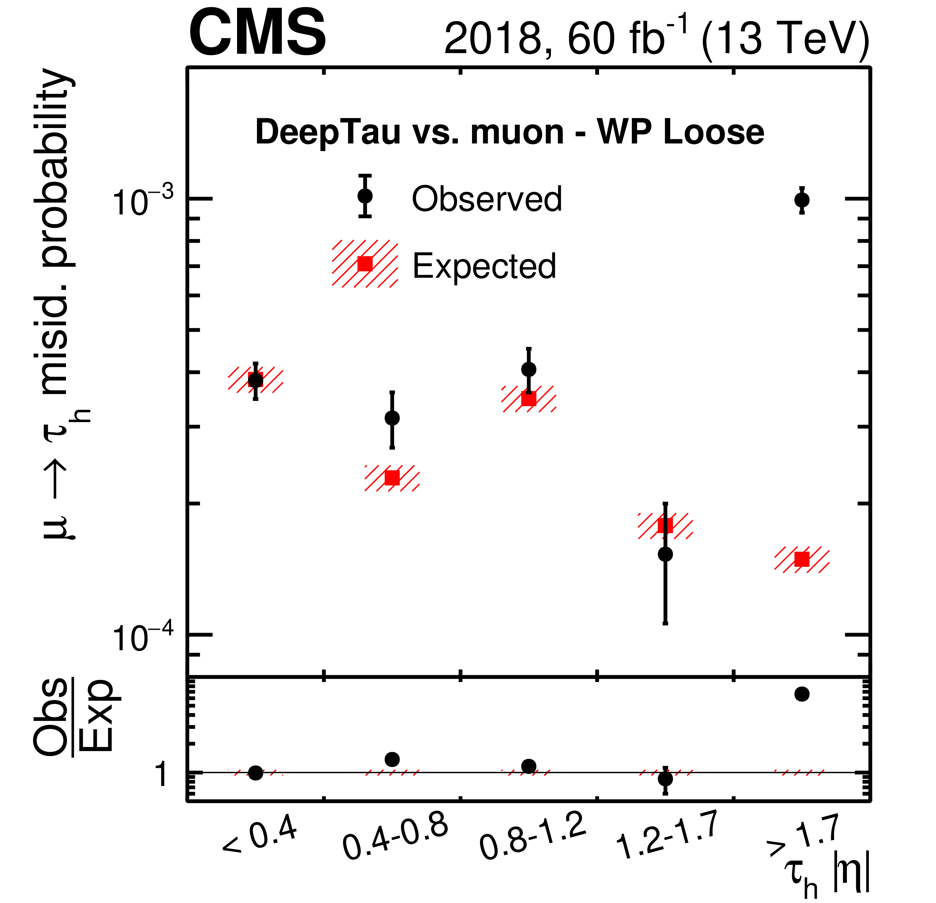
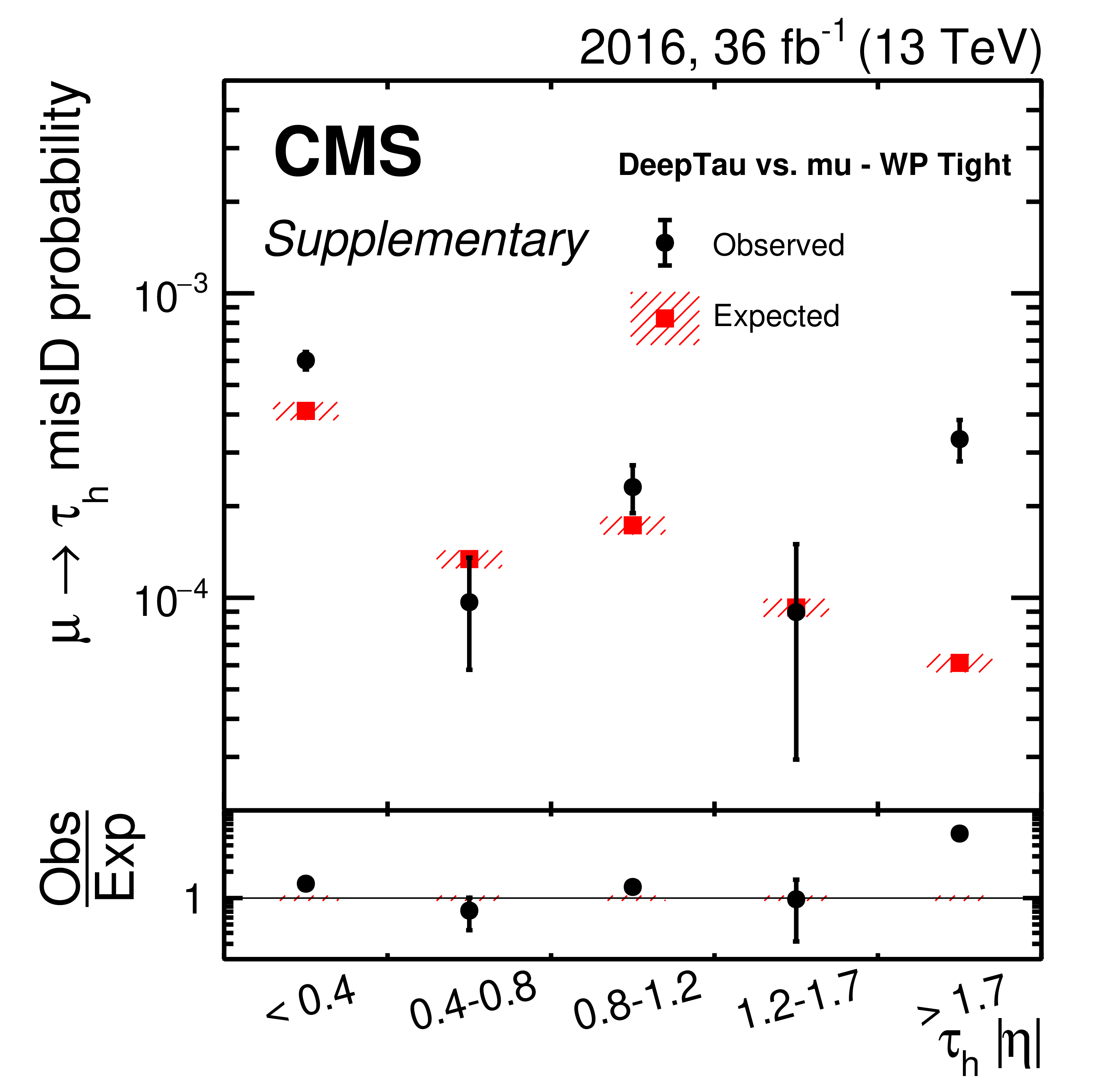
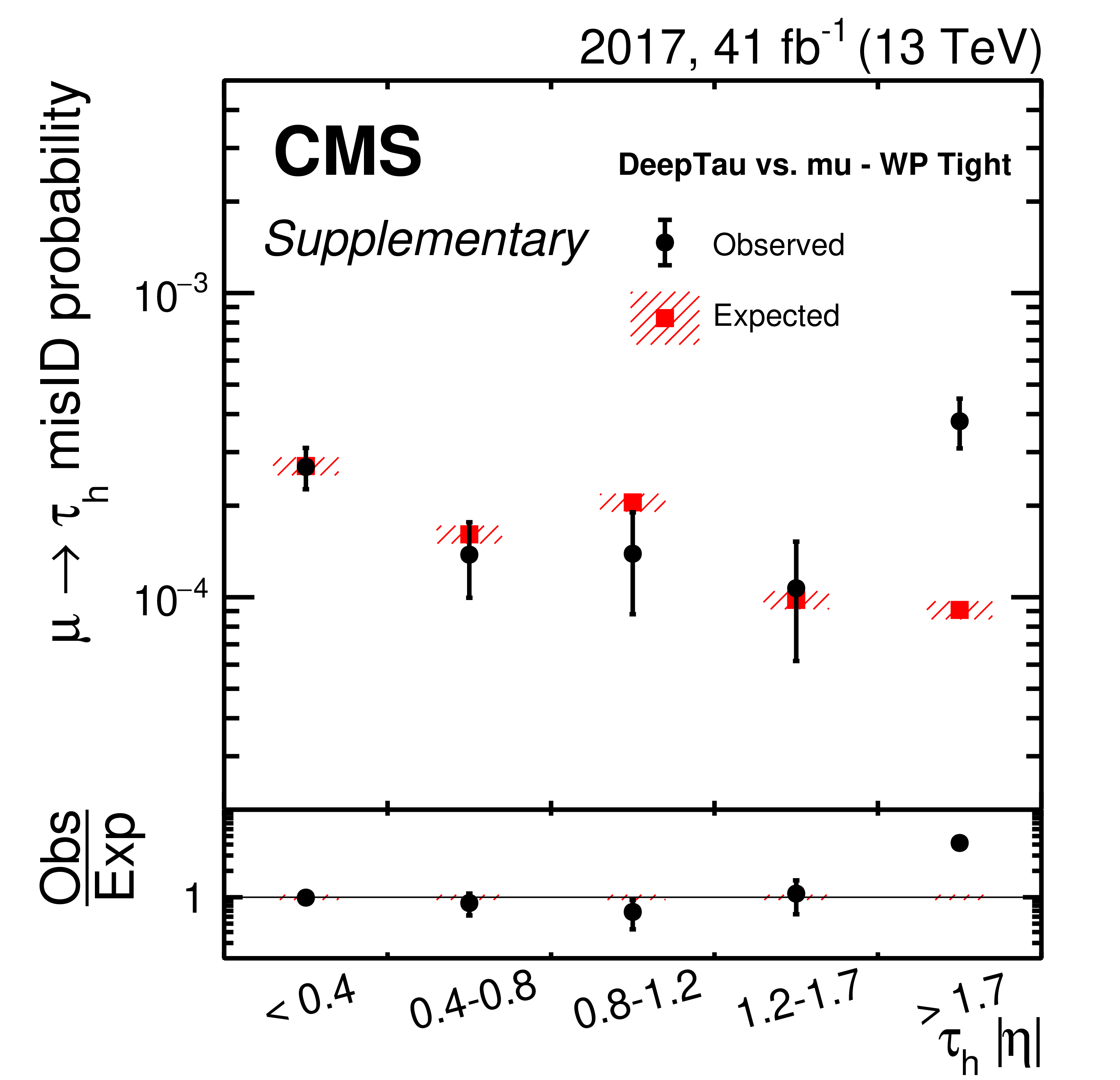
Figure 12:
Observed and expected efficiencies for muons to pass the loose (left) and tight (right) $ D_\mu $ working points. Vertical bars correspond to the combined statistical and systematic uncertainties in the individual scale factors. The muons are required to be reconstructed as $ \tau_\mathrm{h} $ candidates and to pass the Medium $ D_\text{jet} $ working point. The efficiencies are shown for several bins in $ |\eta| $. |
png pdf |
Figure 12-a:
Observed and expected efficiencies for muons to pass the loose (left) and tight (right) $ D_\mu $ working points. Vertical bars correspond to the combined statistical and systematic uncertainties in the individual scale factors. The muons are required to be reconstructed as $ \tau_\mathrm{h} $ candidates and to pass the Medium $ D_\text{jet} $ working point. The efficiencies are shown for several bins in $ |\eta| $. |

png pdf |
Figure 12-b:
Observed and expected efficiencies for muons to pass the loose (left) and tight (right) $ D_\mu $ working points. Vertical bars correspond to the combined statistical and systematic uncertainties in the individual scale factors. The muons are required to be reconstructed as $ \tau_\mathrm{h} $ candidates and to pass the Medium $ D_\text{jet} $ working point. The efficiencies are shown for several bins in $ |\eta| $. |

png pdf |
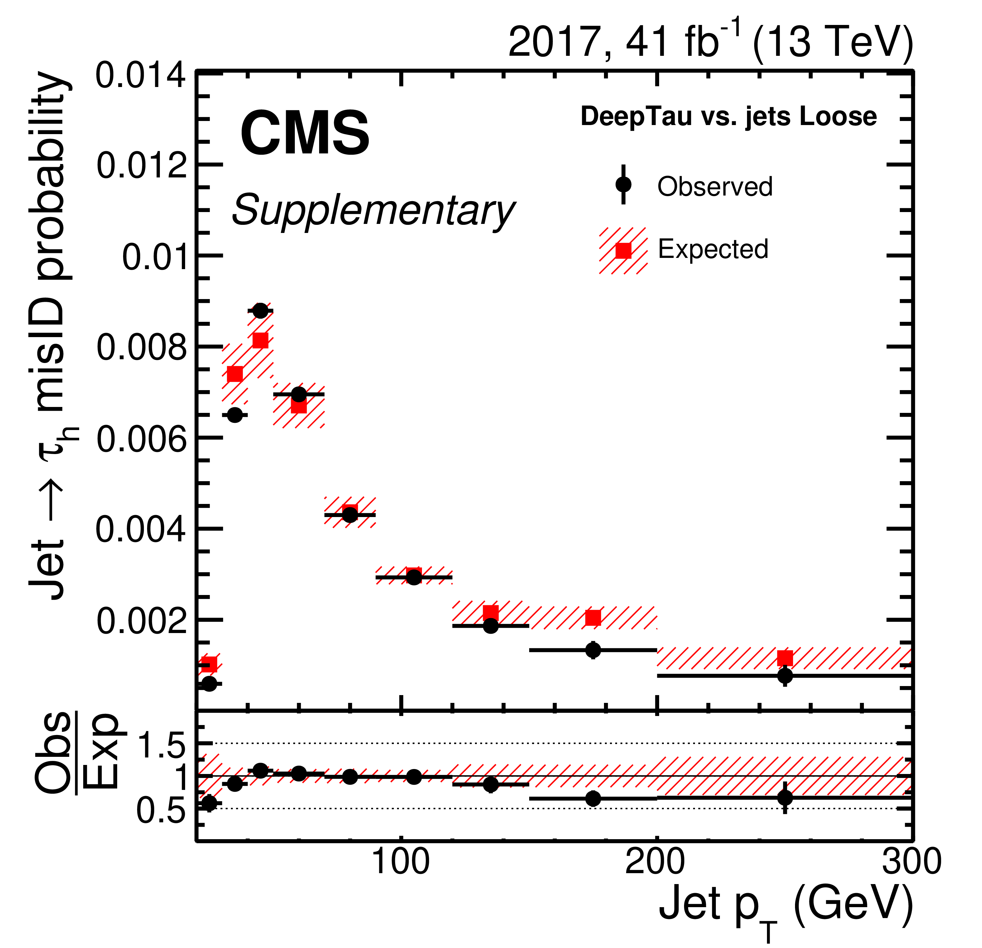
Figure 13:
Observed and expected efficiencies for quark and gluon jets with $ |\eta| < $ 2.3 to be reconstructed as $ \tau_\mathrm{h} $ candidates with $ p_{\mathrm{T}} > $ 20 GeV and to pass the loose (left) and tight (right) $ D_\text{jet} $ working points. The efficiencies are shown as a function of reconstructed jet $ p_{\mathrm{T}} $ and are obtained with data recorded in 2018 and the corresponding simulated events. The shaded uncertainty band includes contributions from the limited number of simulated events and from uncertainties in the jet energy scale and the $ p_{\mathrm{T}}^\text{miss} $ description. Besides the statistical uncertainty in the observed events, the error bars in the ratio of data to simulation also include uncertainties from the subtraction of events with genuine $ \tau_\mathrm{h} $ candidates, electrons, or muons. The efficiency first rises with $ p_{\mathrm{T}} $ near the 20 GeV threshold because it becomes more likely for a jet to give rise to a reconstructed $ \tau_\mathrm{h} $ candidate that passes this threshold. For higher $ p_{\mathrm{T}} $, the particle multiplicity in a quark or gluon jet increases with $ p_{\mathrm{T}} $. Therefore, the jets become easier to distinguish from genuine $ \tau_\mathrm{h} $ candidates and the probability for quark or gluon jets to pass the $ D_\text{jet} $ discriminator decreases with $ p_{\mathrm{T}} $. |

png pdf |
Figure 13-a:
Observed and expected efficiencies for quark and gluon jets with $ |\eta| < $ 2.3 to be reconstructed as $ \tau_\mathrm{h} $ candidates with $ p_{\mathrm{T}} > $ 20 GeV and to pass the loose (left) and tight (right) $ D_\text{jet} $ working points. The efficiencies are shown as a function of reconstructed jet $ p_{\mathrm{T}} $ and are obtained with data recorded in 2018 and the corresponding simulated events. The shaded uncertainty band includes contributions from the limited number of simulated events and from uncertainties in the jet energy scale and the $ p_{\mathrm{T}}^\text{miss} $ description. Besides the statistical uncertainty in the observed events, the error bars in the ratio of data to simulation also include uncertainties from the subtraction of events with genuine $ \tau_\mathrm{h} $ candidates, electrons, or muons. The efficiency first rises with $ p_{\mathrm{T}} $ near the 20 GeV threshold because it becomes more likely for a jet to give rise to a reconstructed $ \tau_\mathrm{h} $ candidate that passes this threshold. For higher $ p_{\mathrm{T}} $, the particle multiplicity in a quark or gluon jet increases with $ p_{\mathrm{T}} $. Therefore, the jets become easier to distinguish from genuine $ \tau_\mathrm{h} $ candidates and the probability for quark or gluon jets to pass the $ D_\text{jet} $ discriminator decreases with $ p_{\mathrm{T}} $. |

png pdf |
Figure 13-b:
Observed and expected efficiencies for quark and gluon jets with $ |\eta| < $ 2.3 to be reconstructed as $ \tau_\mathrm{h} $ candidates with $ p_{\mathrm{T}} > $ 20 GeV and to pass the loose (left) and tight (right) $ D_\text{jet} $ working points. The efficiencies are shown as a function of reconstructed jet $ p_{\mathrm{T}} $ and are obtained with data recorded in 2018 and the corresponding simulated events. The shaded uncertainty band includes contributions from the limited number of simulated events and from uncertainties in the jet energy scale and the $ p_{\mathrm{T}}^\text{miss} $ description. Besides the statistical uncertainty in the observed events, the error bars in the ratio of data to simulation also include uncertainties from the subtraction of events with genuine $ \tau_\mathrm{h} $ candidates, electrons, or muons. The efficiency first rises with $ p_{\mathrm{T}} $ near the 20 GeV threshold because it becomes more likely for a jet to give rise to a reconstructed $ \tau_\mathrm{h} $ candidate that passes this threshold. For higher $ p_{\mathrm{T}} $, the particle multiplicity in a quark or gluon jet increases with $ p_{\mathrm{T}} $. Therefore, the jets become easier to distinguish from genuine $ \tau_\mathrm{h} $ candidates and the probability for quark or gluon jets to pass the $ D_\text{jet} $ discriminator decreases with $ p_{\mathrm{T}} $. |
| Tables | |

png pdf |
Table 1:
Decays of $ \tau $ leptons and their branching fractions ($ \mathcal{B} $) in % [60]. The known intermediate resonances of all the listed hadrons are indicated where appropriate. Charged hadrons are denoted by the symbol $ \mathrm{h}^{\pm} $. Although only $ \tau^{-} $ decays are shown, the decays and values of the branching fractions are identical for charge-conjugate decays. |

png pdf |
Table 2:
Input variables used for the various kinds of particles that are contained in a given cell. For each type of particle, basic kinematic quantities ($ p_{\mathrm{T}}, \eta, \phi $) are included but not listed below. Similarly, the reconstructed charge is included for all charged particles. An estimated per-particle probability for the particle to come from a pileup interaction using the pileup identification (PUPPI) algorithm [61] is labelled as PUPPI. A number of input variables that give the compatibility of the track with the primary interaction vertex (PV) or a possible secondary vertex (SV) from the $ \tau_\mathrm{h} $ reconstruction are denoted as ``Track PV'' and ``Track SV''. |
png pdf |
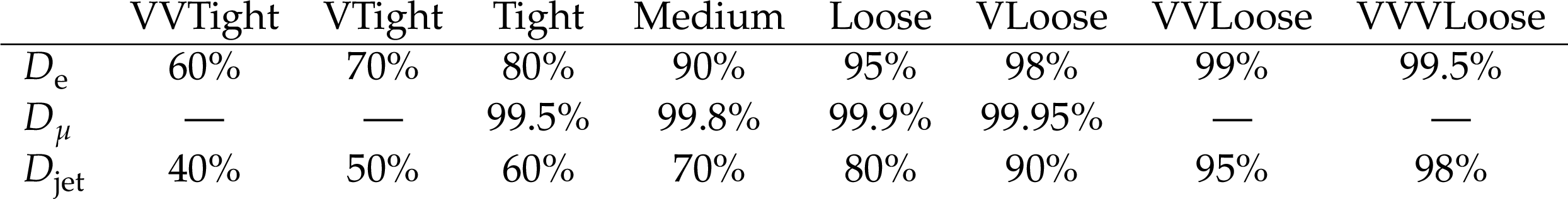
Table 3:
Target $ \tau_\mathrm{h} $ identification efficiencies for the different working points defined for the three different discriminators. The target efficiencies are evaluated with the $ \mathrm{H}\to\tau\tau $ event sample for $ \tau_\mathrm{h} $ with $ p_{\mathrm{T}} \in $ [30, 70] GeV. |
png pdf |
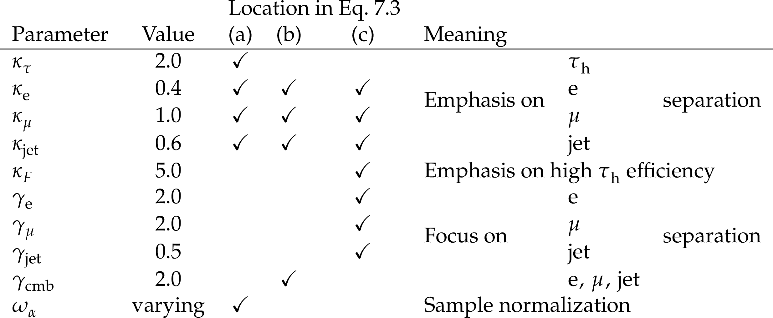
Table A1:
Parameters used in the definition of the loss function for the training of the DEEPTAU algorithm. |
| Summary |
| A new algorithm has been introduced to discriminate hadronic tau lepton decays ($ \tau_\mathrm{h} $) against jets, electrons, and muons. The algorithm is based on a deep neural network and combines fully connected and convolutional layers. As input, the algorithm combines information from individual reconstructed particles near the $ \tau_\mathrm{h} $ axis with information about the reconstructed $ \tau_\mathrm{h} $ candidate and other high-level variables. In addition, an improved $ \tau_\mathrm{h} $ reconstruction algorithm is introduced that increases the overall efficiency of the reconstruction by explicitly considering the $ \tau_\mathrm{h} $ decay mode with three charged hadrons and a neutral pion, and by applying looser quality criteria for the charged hadrons in the case of three-prong $ \tau_\mathrm{h} $ decays. The performance of the new $ \tau_\mathrm{h} $ identification and reconstruction algorithms significantly improves over the previously used algorithms, in particular in terms of discrimination against the background from jets and electrons. For a given jet rejection level, the efficiency for genuine $ \tau_\mathrm{h} $ candidates increases by 10--30%. Similarly, the efficiency for genuine $ \tau_\mathrm{h} $ candidates to pass the discriminator against electrons increases by 14% for the loosest working point that is employed in many analyses. Following its superior performance, CMS physics analyses with tau leptons will significantly increase their sensitivities when using the new algorithm. The superior performance of the algorithm is validated with collision data. The observed efficiencies for genuine $ \tau_\mathrm{h} $, jets, and electrons to be identified as $ \tau_\mathrm{h} $ typically agree within 10% with the expected efficiencies from simulated events. The agreement is similar to the one observed with previous algorithms and confirms the improvements. |
| Additional Figures | |

png pdf |
Additional Figure 1:
Decay mode confusion matrix for high-$ p_{\mathrm{T}} \tau_\mathrm{h} $. For a given generated decay mode, the fractions of reconstructed $ \tau_\mathrm{h} $ in different decay modes are given, as well as the fraction of generated $ \tau_\mathrm{h} $ that are not reconstructed. The generated $ \tau_\mathrm{h} $ needs to fulfil $ p_{\mathrm{T}} > $ 100 GeV whereas the reconstructed $ \tau_\mathrm{h} $ is required to fulfil $ p_{\mathrm{T}} > $ 20 GeV. Both the generated and reconstructed $ \tau_\mathrm{h} $ need to fulfil $ |\eta| < $ 2.3. The $ \tau_\mathrm{h} $ candidates come from a $ \mathrm{Z}\to\tau\tau $ event sample with $ m_{\tau\tau} > $ 50 GeV. Decay modes with the same numbers of charged hadrons and one or two $ \pi^{0} $s are combined and labelled as ``$ \pi^{0} $s''. |

png pdf |
Additional Figure 2:
Data-to-simulation scale factors for genuine $ \tau_\mathrm{h} $ to be reconstructed as $ \tau_\mathrm{h} $ candidates, to fulfil additional loose pre-selection criteria discussed in the paper, and to pass the loose, medium, and tight working points of the $ D_\text{jet} $ discriminator as a function of the $ \tau_\mathrm{h} $ candidate $ p_{\mathrm{T}} $ for the 2016 data set. Vertical bars correspond to the combined statistical and systematic uncertainties in the individual scale factors. The red hatched bands indicate the uncertainties for $ p_{\mathrm{T}} > $ 40 GeV, obtained from a combination of the individual measurements. |

png pdf |
Additional Figure 3:
Data-to-simulation scale factors for genuine $ \tau_\mathrm{h} $ to be reconstructed as $ \tau_\mathrm{h} $ candidates, to fulfil additional loose pre-selection criteria discussed in the paper, and to pass the loose, medium, and tight working points of the $ D_\text{jet} $ discriminator as a function of the $ \tau_\mathrm{h} $ candidate $ p_{\mathrm{T}} $ for the 2017 data set. Vertical bars correspond to the combined statistical and systematic uncertainties in the individual scale factors. The red hatched bands indicate the uncertainties for $ p_{\mathrm{T}} > $ 40 GeV, obtained from a combination of the individual measurements. |
png pdf |
Additional Figure 4:
Relative difference between $ \tau_\mathrm{h} $ energy obtained in data and simulated events for the four main reconstructed $ \tau_\mathrm{h} $ decay modes for the 2016 data set. The results are obtained from fits to the distribution of either the reconstructed $ m_\text{vis}(\mu, \tau_\mathrm{h}) $ (blue lines) or $ m_{\tau_\mathrm{h}} $ (black lines). The horizontal bars represent the uncertainties in the measurements. The measured values are consistent with no shift of the $ \tau_\mathrm{h} $ energy scale between data and simulation, with the largest difference amounting to 1.5 standard deviations. |

png pdf |
Additional Figure 5:
Relative difference between $ \tau_\mathrm{h} $ energy obtained in data and simulated events for the four main reconstructed $ \tau_\mathrm{h} $ decay modes for the 2017 data set. The results are obtained from fits to the distribution of either the reconstructed $ m_\text{vis}(\mu, \tau_\mathrm{h}) $ (blue lines) or $ m_{\tau_\mathrm{h}} $ (black lines). The horizontal bars represent the uncertainties in the measurements. The measured values are consistent with no shift of the $ \tau_\mathrm{h} $ energy scale between data and simulation, with the largest difference amounting to 1.5 standard deviations. |

png pdf |
Additional Figure 6:
Distribution of the reconstructed visible invariant mass of the $ \mu\tau_\mathrm{h} $ system, $ m_\text{vis}(\mu, \tau_\mathrm{h}) $ for the 2016 data set. Vertical bars correspond to the statistical uncertainties. The event selection corresponds to the one in the measurement of the $ \tau_\mathrm{h} $ reconstruction and identification efficiencies and uses the Tight working point of the $ D_\text{jet} $ discriminator. The distributions incorporate all measured scale factors and energy corrections and are scaled to the outcome of a maximum likelihood to the observed data with the $ \mathrm{Z}\to\tau\tau $ contribution freely floating. The electroweak background combines contributions from single top quark, diboson, and W+jets processes as well as $ \mathrm{Z}(\to\tau\tau) $+jets events where the reconstructed $ \tau_\mathrm{h} $ originates from a jet misidentified as a $ \tau_\mathrm{h} $ candidate instead of one of the produced tau leptons. |

png pdf |
Additional Figure 7:
Distribution of the visible invariant $ \tau_\mathrm{h} $ mass for the 2016 data set. Vertical bars correspond to the statistical uncertainties. The event selection corresponds to the one in the measurement of the $ \tau_\mathrm{h} $ reconstruction and identification efficiencies and uses the Tight working point of the $ D_\text{jet} $ discriminator. The distributions incorporate all measured scale factors and energy corrections and are scaled to the outcome of a maximum likelihood to the observed data with the $ \mathrm{Z}\to\tau\tau $ contribution freely floating. The electroweak background combines contributions from single top quark, diboson, and W+jets processes as well as $ \mathrm{Z}(\to\tau\tau) $+jets events where the reconstructed $ \tau_\mathrm{h} $ originates from a jet misidentified as a $ \tau_\mathrm{h} $ candidate instead of one of the produced tau leptons. The $ \mathrm{Z}\to\tau\tau $ contributions are shown separately for the different $ \tau_\mathrm{h} $ decay modes. |

png pdf |
Additional Figure 8:
Distribution of the reconstructed visible invariant mass of the $ \mu\tau_\mathrm{h} $ system, $ m_\text{vis}(\mu, \tau_\mathrm{h}) $ for the 2017 data set. Vertical bars correspond to the statistical uncertainties. The event selection corresponds to the one in the measurement of the $ \tau_\mathrm{h} $ reconstruction and identification efficiencies and uses the Tight working point of the $ D_\text{jet} $ discriminator. The distributions incorporate all measured scale factors and energy corrections and are scaled to the outcome of a maximum likelihood to the observed data with the $ \mathrm{Z}\to\tau\tau $ contribution freely floating. The electroweak background combines contributions from single top quark, diboson, and W+jets processes as well as $ \mathrm{Z}(\to\tau\tau) $+jets events where the reconstructed $ \tau_\mathrm{h} $ originates from a jet misidentified as a $ \tau_\mathrm{h} $ candidate instead of one of the produced tau leptons. |
png pdf |
Additional Figure 9:
Distribution of the visible invariant $ \tau_\mathrm{h} $ mass for the 2017 data set. Vertical bars correspond to the statistical uncertainties. The event selection corresponds to the one in the measurement of the $ \tau_\mathrm{h} $ reconstruction and identification efficiencies and uses the Tight working point of the $ D_\text{jet} $ discriminator. The distributions incorporate all measured scale factors and energy corrections and are scaled to the outcome of a maximum likelihood to the observed data with the $ \mathrm{Z}\to\tau\tau $ contribution freely floating. The electroweak background combines contributions from single top quark, diboson, and W+jets processes as well as $ \mathrm{Z}(\to\tau\tau) $+jets events where the reconstructed $ \tau_\mathrm{h} $ originates from a jet misidentified as a $ \tau_\mathrm{h} $ candidate instead of one of the produced tau leptons. The $ \mathrm{Z}\to\tau\tau $ contributions are shown separately for the different $ \tau_\mathrm{h} $ decay modes. |

png pdf |
Additional Figure 10:
Observed and expected efficiencies for electrons to pass different $ D_\mathrm{e} $ working points for the 2016 data set. Vertical bars correspond to the combined statistical and systematic uncertainties in the individual scale factors. All considered electrons are required to be reconstructed as a $ \tau_\mathrm{h} $ candidate and to pass the medium $ D_\text{jet} $ working point. The efficiencies are shown for electrons with $ |\eta| < $ 1.46, corresponding to the ECAL barrel region. |

png pdf |
Additional Figure 11:
Observed and expected efficiencies for electrons to pass different $ D_\mathrm{e} $ working points for the 2016 data set. Vertical bars correspond to the combined statistical and systematic uncertainties in the individual scale factors. All considered electrons are required to be reconstructed as a $ \tau_\mathrm{h} $ candidate and to pass the medium $ D_\text{jet} $ working point. The efficiencies are shown for electrons with $ |\eta| > $ 1.56, corresponding to the ECAL endcap regions. |

png pdf |
Additional Figure 12:
Observed and expected efficiencies for electrons to pass different $ D_\mathrm{e} $ working points for the 2017 data set. Vertical bars correspond to the combined statistical and systematic uncertainties in the individual scale factors. All considered electrons are required to be reconstructed as a $ \tau_\mathrm{h} $ candidate and to pass the medium $ D_\text{jet} $ working point. The efficiencies are shown for electrons with $ |\eta| < $ 1.46, corresponding to the ECAL barrel region. |
png pdf |
Additional Figure 13:
Observed and expected efficiencies for electrons to pass different $ D_\mathrm{e} $ working points for the 2017 data set. Vertical bars correspond to the combined statistical and systematic uncertainties in the individual scale factors. All considered electrons are required to be reconstructed as a $ \tau_\mathrm{h} $ candidate and to pass the medium $ D_\text{jet} $ working point. The efficiencies are shown for electrons with $ |\eta| > $ 1.56, corresponding to the ECAL endcap regions. |

png pdf |
Additional Figure 14:
Observed and expected efficiencies for muons to pass the loose $ D_\mu $ working point for the 2016 data set. Vertical bars correspond to the combined statistical and systematic uncertainties in the individual scale factors. All considered muons are required to be reconstructed as $ \tau_\mathrm{h} $ candidates and to pass the Medium $ D_\text{jet} $ working point. The efficiencies are shown for several bins in $ |\eta| $. The disagreement in the last bin is discussed in the paper. |
png pdf |
Additional Figure 15:
Observed and expected efficiencies for muons to pass the tight $ D_\mu $ working point for the 2016 data set. Vertical bars correspond to the combined statistical and systematic uncertainties in the individual scale factors. All considered muons are required to be reconstructed as $ \tau_\mathrm{h} $ candidates and to pass the Medium $ D_\text{jet} $ working point. The efficiencies are shown for several bins in $ |\eta| $. The disagreement in the last bin is discussed in the paper. |

png pdf |
Additional Figure 16:
Observed and expected efficiencies for muons to pass the loose $ D_\mu $ working point for the 2017 data set. Vertical bars correspond to the combined statistical and systematic uncertainties in the individual scale factors. All considered muons are required to be reconstructed as $ \tau_\mathrm{h} $ candidates and to pass the Medium $ D_\text{jet} $ working point. The efficiencies are shown for several bins in $ |\eta| $. The disagreement in the last bin is discussed in the paper. |
png pdf |
Additional Figure 17:
Observed and expected efficiencies for muons to pass the tight $ D_\mu $ working point for the 2017 data set. Vertical bars correspond to the combined statistical and systematic uncertainties in the individual scale factors. All considered muons are required to be reconstructed as $ \tau_\mathrm{h} $ candidates and to pass the Medium $ D_\text{jet} $ working point. The efficiencies are shown for several bins in $ |\eta| $. The disagreement in the last bin is discussed in the paper. |

png pdf |
Additional Figure 18:
Observed and expected efficiencies for quark and gluon jets with $ |\eta| < $ 2.3 to be reconstructed as $ \tau_\mathrm{h} $ candidates with $ p_{\mathrm{T}} > $ 20 GeV and to pass the loose $ D_\text{jet} $ working points. The efficiencies are shown as a function of reconstructed jet $ p_{\mathrm{T}} $ and are obtained with data recorded in 2016 and the corresponding simulated events. The shaded uncertainty band includes contributions from the limited number of simulated events and from uncertainties in the jet energy scale and the $ p_{\mathrm{T}}^\text{miss} $ description. Besides the statistical uncertainty in the observed events, the error bars in the ratio of data to simulation also include uncertainties from the subtraction of events with genuine $ \tau_\mathrm{h} $ candidates, electrons, or muons. The efficiency first rises with $ p_{\mathrm{T}} $ near the 20 GeV threshold because it becomes more likely for a jet to give rise to a reconstructed $ \tau_\mathrm{h} $ candidate that passes this threshold. For higher $ p_{\mathrm{T}} $, the particle multiplicity in a quark or gluon jet increases with $ p_{\mathrm{T}} $. Therefore, the jets become easier to distinguish from genuine $ \tau_\mathrm{h} $ candidates and the probability for quark or gluon jets to pass the $ D_\text{jet} $ discriminator decreases with $ p_{\mathrm{T}} $. |

png pdf |
Additional Figure 19:
Observed and expected efficiencies for quark and gluon jets with $ |\eta| < $ 2.3 to be reconstructed as $ \tau_\mathrm{h} $ candidates with $ p_{\mathrm{T}} > $ 20 GeV and to pass the tight $ D_\text{jet} $ working points. The efficiencies are shown as a function of reconstructed jet $ p_{\mathrm{T}} $ and are obtained with data recorded in 2016 and the corresponding simulated events. The shaded uncertainty band includes contributions from the limited number of simulated events and from uncertainties in the jet energy scale and the $ p_{\mathrm{T}}^\text{miss} $ description. Besides the statistical uncertainty in the observed events, the error bars in the ratio of data to simulation also include uncertainties from the subtraction of events with genuine $ \tau_\mathrm{h} $ candidates, electrons, or muons. The efficiency first rises with $ p_{\mathrm{T}} $ near the 20 GeV threshold because it becomes more likely for a jet to give rise to a reconstructed $ \tau_\mathrm{h} $ candidate that passes this threshold. For higher $ p_{\mathrm{T}} $, the particle multiplicity in a quark or gluon jet increases with $ p_{\mathrm{T}} $. Therefore, the jets become easier to distinguish from genuine $ \tau_\mathrm{h} $ candidates and the probability for quark or gluon jets to pass the $ D_\text{jet} $ discriminator decreases with $ p_{\mathrm{T}} $. |
png pdf |
Additional Figure 20:
Observed and expected efficiencies for quark and gluon jets with $ |\eta| < $ 2.3 to be reconstructed as $ \tau_\mathrm{h} $ candidates with $ p_{\mathrm{T}} > $ 20 GeV and to pass the loose $ D_\text{jet} $ working points. The efficiencies are shown as a function of reconstructed jet $ p_{\mathrm{T}} $ and are obtained with data recorded in 2017 and the corresponding simulated events. The shaded uncertainty band includes contributions from the limited number of simulated events and from uncertainties in the jet energy scale and the $ p_{\mathrm{T}}^\text{miss} $ description. Besides the statistical uncertainty in the observed events, the error bars in the ratio of data to simulation also include uncertainties from the subtraction of events with genuine $ \tau_\mathrm{h} $ candidates, electrons, or muons. The efficiency first rises with $ p_{\mathrm{T}} $ near the 20 GeV threshold because it becomes more likely for a jet to give rise to a reconstructed $ \tau_\mathrm{h} $ candidate that passes this threshold. For higher $ p_{\mathrm{T}} $, the particle multiplicity in a quark or gluon jet increases with $ p_{\mathrm{T}} $. Therefore, the jets become easier to distinguish from genuine $ \tau_\mathrm{h} $ candidates and the probability for quark or gluon jets to pass the $ D_\text{jet} $ discriminator decreases with $ p_{\mathrm{T}} $. |
png pdf |
Additional Figure 21:
Observed and expected efficiencies for quark and gluon jets with $ |\eta| < $ 2.3 to be reconstructed as $ \tau_\mathrm{h} $ candidates with $ p_{\mathrm{T}} > $ 20 GeV and to pass the tight $ D_\text{jet} $ working points. The efficiencies are shown as a function of reconstructed jet $ p_{\mathrm{T}} $ and are obtained with data recorded in 2017 and the corresponding simulated events. The shaded uncertainty band includes contributions from the limited number of simulated events and from uncertainties in the jet energy scale and the $ p_{\mathrm{T}}^\text{miss} $ description. Besides the statistical uncertainty in the observed events, the error bars in the ratio of data to simulation also include uncertainties from the subtraction of events with genuine $ \tau_\mathrm{h} $ candidates, electrons, or muons. The efficiency first rises with $ p_{\mathrm{T}} $ near the 20 GeV threshold because it becomes more likely for a jet to give rise to a reconstructed $ \tau_\mathrm{h} $ candidate that passes this threshold. For higher $ p_{\mathrm{T}} $, the particle multiplicity in a quark or gluon jet increases with $ p_{\mathrm{T}} $. Therefore, the jets become easier to distinguish from genuine $ \tau_\mathrm{h} $ candidates and the probability for quark or gluon jets to pass the $ D_\text{jet} $ discriminator decreases with $ p_{\mathrm{T}} $. |

png pdf |
Additional Figure 22:
Expected misidentification probabilities for quark- or gluon-induced jets from W-plus-jets production to be reconstructed in any of the $ \tau_\mathrm{h} $ decay modes and pass various working points of the DeepTau vs.\ jets discriminant. The misidentification probabilities are shown as a function of the generated jet $ p_{\mathrm{T}} $. |
png pdf |
Additional Figure 23:
Expected misidentification probabilities for jets from $ {\mathrm{t}\overline{\mathrm{t}}} $-plus-jets production to be reconstructed in any of the $ \tau_\mathrm{h} $ decay modes and pass various working points of the DeepTau vs.\ jets discriminant. The misidentification probabilities are shown as a function of the generated jet $ p_{\mathrm{T}} $. |

png pdf |
Additional Figure 24:
Correct charge assignment probability as a function of the generated $ \tau_\mathrm{h} p_{\mathrm{T}} $. Reconstructed $ \tau_\mathrm{h} $ are required to pass the medium $ D_\text{jet} $ working point. The blue points represent the selection most commonly used in analyses, where reconstructed $ \tau_\mathrm{h} $ decay modes with missing charged hadrons (2-prong) are not considered. The black points represent the case where these $ \tau_\mathrm{h} $ decay modes are considered. For $ p_{\mathrm{T}} \lesssim $ 100 GeV, the correct charge identification probability is close to 100%. For increasing $ p_{\mathrm{T}} $, the probability drops to 90% (at $ p_{\mathrm{T}}\approx $ 1 TeV). The red points show the specific case where 3-prong taus are reconstructed in a decay mode with a missing charged hadron. The correct charge assignment probability is $ {\approx}2/ $ 3, compatible with the expectation that the hadron that is not reconstructed or identified is not correlated with the $ \tau_\mathrm{h} $ charge. |
| Additional Tables | |

png pdf |
Additional Table 1:
Efficiencies for genuine $ \tau_\mathrm{h} $, quark- or gluon-induced jets, electrons, and muons to pass the working points defined for the three different DeepTau discriminants. The target $ \tau_\mathrm{h} $ efficiencies are evaluated with an $ \mathrm{H}\to \tau\tau $ event sample for $ \tau_\mathrm{h} $ with $ p_{\mathrm{T}}\in $ [20,100] GeV. The misidentification efficiencies for quark- or gluon induced jets are evaluated with jets from an inclusive W-plus-jets event sample with reconstructed $ \tau_\mathrm{h} $ in the same $ p_{\mathrm{T}} $ range. The efficiencies for genuine electrons (muons) are evaluated with an inclusive $ \mathrm{Z}\to\mathrm{e}\mathrm{e} $ ($ \mu\mu $) event sample, again using electrons (muons) that give rise to a reconstructed $ \tau_\mathrm{h} $ with $ p_{\mathrm{T}}\in $ [20,100 ] GeV. While the efficiencies for genuine $ \tau_\mathrm{h} $, electrons, and muons are generally representative also for different samples and $ p_{\mathrm{T}} $ ranges, the efficiencies for quark- or gluon-induced jets strongly depend on the jet flavour and $ p_{\mathrm{T}} $. For this reason, these numbers, which are integrated over the $ p_{\mathrm{T}} $, $ \eta $, and jet flavour spectra, are given for illustrative purposes only. |
| References | ||||
| 1 | CMS Collaboration | Observation of the Higgs boson decay to a pair of $ \tau $ leptons with the CMS detector | PLB 779 (2018) 283 | CMS-HIG-16-043 1708.00373 |
| 2 | CMS Collaboration | Search for Higgs boson pair production in events with two bottom quarks and two tau leptons in proton--proton collisions at $ \sqrt{s}= $ 13 TeV | PLB 778 (2018) 101 | CMS-HIG-17-002 1707.02909 |
| 3 | ATLAS Collaboration | Cross-section measurements of the Higgs boson decaying into a pair of $ \tau $-leptons in proton-proton collisions at $ \sqrt{s}= $ 13 TeV with the ATLAS detector | PRD 99 (2019) 072001 | 1811.08856 |
| 4 | ATLAS Collaboration | Search for resonant and non-resonant Higgs boson pair production in the $ {\text{b}\bar{\text{b}}\tau^+\tau^-} $ decay channel in pp collisions at $ \sqrt{s}= $ 13 TeV with the ATLAS detector | PRL 121 (2018) 191801 | 1808.00336 |
| 5 | ATLAS Collaboration | Test of CP invariance in vector-boson fusion production of the Higgs boson in the $ \text{H}\rightarrow\tau\tau $ channel in proton-proton collisions at $ \sqrt{s} $ = 13 TeV with the ATLAS detector | PLB 805 (2020) 135426 | 2002.05315 |
| 6 | CMS Collaboration | Search for additional neutral MSSM Higgs bosons in the $ \tau\tau $ final state in proton-proton collisions at $ \sqrt{s}= $ 13 TeV | JHEP 09 (2018) 007 | CMS-HIG-17-020 1803.06553 |
| 7 | ATLAS Collaboration | Search for charged Higgs bosons decaying via H$ ^{\pm} \to \tau^{\pm}\nu_{\tau} $ in the $ \tau $+jets and $ \tau $+lepton final states with 36 fb$ ^{-1} $ of pp collision data recorded at $ \sqrt{s} = $ 13 TeV with the ATLAS experiment | JHEP 09 (2018) 139 | 1807.07915 |
| 8 | CMS Collaboration | Search for an exotic decay of the Higgs boson to a pair of light pseudoscalars in the final state with two b quarks and two $ \tau $ leptons in proton-proton collisions at $ \sqrt{s}= $ 13 TeV | PLB 785 (2018) 462 | CMS-HIG-17-024 1805.10191 |
| 9 | CMS Collaboration | Search for a heavy pseudoscalar Higgs boson decaying into a 125 GeV Higgs boson and a Z boson in final states with two tau and two light leptons at $ \sqrt{s}= $ 13 TeV | JHEP 03 (2020) 065 | CMS-HIG-18-023 1910.11634 |
| 10 | CMS Collaboration | Search for lepton flavour violating decays of a neutral heavy Higgs boson to $ \mu\tau $ and e$ \tau $ in proton-proton collisions at $ \sqrt{s}= $ 13 TeV | JHEP 03 (2020) 103 | CMS-HIG-18-017 1911.10267 |
| 11 | CMS Collaboration | Search for a low-mass $ \tau^+\tau^- $ resonance in association with a bottom quark in proton-proton collisions at $ \sqrt{s}= $ 13 TeV | JHEP 05 (2019) 210 | CMS-HIG-17-014 1903.10228 |
| 12 | CMS Collaboration | Search for charged Higgs bosons in the H$ ^{\pm} \to \tau^{\pm}\nu_\tau $ decay channel in proton-proton collisions at $ \sqrt{s} = $ 13 TeV | JHEP 07 (2019) 142 | CMS-HIG-18-014 1903.04560 |
| 13 | ATLAS Collaboration | Search for heavy Higgs bosons decaying into two tau leptons with the ATLAS detector using pp collisions at $ \sqrt{s}= $ 13 TeV | PRL 125 (2020) 051801 | 2002.12223 |
| 14 | CMS Collaboration | Search for direct pair production of supersymmetric partners to the $ \tau $ lepton in proton-proton collisions at $ \sqrt{s}= $ 13 TeV | EPJC 80 (2020) 189 | CMS-SUS-18-006 1907.13179 |
| 15 | CMS Collaboration | Search for heavy neutrinos and third-generation leptoquarks in hadronic states of two $ \tau $ leptons and two jets in proton-proton collisions at $ \sqrt{s} = $ 13 TeV | JHEP 03 (2019) 170 | CMS-EXO-17-016 1811.00806 |
| 16 | ATLAS Collaboration | Searches for third-generation scalar leptoquarks in $ \sqrt{s} $ = 13 TeV pp collisions with the ATLAS detector | JHEP 06 (2019) 144 | 1902.08103 |
| 17 | CMS Collaboration | Performance of tau-lepton reconstruction and identification in CMS | JINST 7 (2012) P01001 | CMS-TAU-11-001 1109.6034 |
| 18 | CMS Collaboration | Reconstruction and identification of $ \tau $ lepton decays to hadrons and $ \nu_\tau $ at CMS | JINST 11 (2016) P01019 | CMS-TAU-14-001 1510.07488 |
| 19 | CMS Collaboration | Performance of reconstruction and identification of $ \tau $ leptons decaying to hadrons and $ \nu_\tau $ in pp collisions at $ \sqrt{s}= $ 13 TeV | JINST 13 (2018) P10005 | CMS-TAU-16-003 1809.02816 |
| 20 | ATLAS Collaboration | Identification and energy calibration of hadronically decaying tau leptons with the ATLAS experiment in pp collisions at $ \sqrt{s}= $ 8 TeV | EPJC 75 (2015) 303 | 1412.7086 |
| 21 | ATLAS Collaboration | Reconstruction of hadronic decay products of tau leptons with the ATLAS experiment | EPJC 76 (2016) 295 | 1512.05955 |
| 22 | Y. LeCun et al. | Backpropagation applied to handwritten zip code recognition | Neural Comput. 1 (1989) 541 | |
| 23 | Y. LeCun et al. | Handwritten digit recognition with a back-propagation network | in Advances in Neural Information Processing Systems 2, Morgan Kaufmann, 1990 link |
|
| 24 | Y. Lecun, L. Bottou, Y. Bengio, and P. Haffner | Gradient-based learning applied to document recognition | Proc. IEEE 86 (1998) 2278 | |
| 25 | V. Innocente, Y. F. Wang, and Z. P. Zhang | Identification of tau decays using a neural network | NIM A 323 (1992) 647 | |
| 26 | ATLAS Collaboration | Identification of hadronic tau lepton decays using neural networks in the ATLAS experiment | ATLAS PUB Note ATL-PHYS-PUB-2019-033, 2019 | |
| 27 | CMS Collaboration | Identification of heavy-flavour jets with the CMS detector in pp collisions at 13 TeV | JINST 13 (2018) P05011 | CMS-BTV-16-002 1712.07158 |
| 28 | ATLAS Collaboration | Identification of jets containing b-hadrons with recurrent neural networks at the ATLAS experiment | ATLAS PUB Note ATL-PHYS-PUB-2017-003, 2017 | |
| 29 | ATLAS Collaboration | Deep sets based neural networks for impact parameter flavour tagging in ATLAS | ATLAS PUB Note ATL-PHYS-PUB-2020-014, 2020 | |
| 30 | E. Bols et al. | Jet flavour classification using DeepJet | JINST 15 (2020) P12012 | 2008.10519 |
| 31 | CMS Collaboration | Identification of heavy, energetic, hadronically decaying particles using machine-learning techniques | JINST 15 (2020) P06005 | CMS-JME-18-002 2004.08262 |
| 32 | CMS Collaboration | HEPData record for this analysis | link | |
| 33 | CMS Collaboration | The CMS experiment at the CERN LHC | JINST 3 (2008) S08004 | |
| 34 | CMS Collaboration | Particle-flow reconstruction and global event description with the CMS detector | JINST 12 (2017) P10003 | CMS-PRF-14-001 1706.04965 |
| 35 | M. Cacciari, G. P. Salam, and G. Soyez | The anti-$ k_{\mathrm{T}} $ jet clustering algorithm | JHEP 04 (2008) 063 | 0802.1189 |
| 36 | M. Cacciari, G. P. Salam, and G. Soyez | FastJet user manual | EPJC 72 (2012) 1896 | 1111.6097 |
| 37 | CMS Collaboration | Pileup mitigation at CMS in 13 TeV data | JINST 15 (2020) P09018 | CMS-JME-18-001 2003.00503 |
| 38 | CMS Collaboration | Jet energy scale and resolution in the CMS experiment in pp collisions at 8 TeV | JINST 12 (2017) P02014 | CMS-JME-13-004 1607.03663 |
| 39 | CMS Collaboration | Performance of missing transverse momentum reconstruction in proton-proton collisions at $ \sqrt{s} = $ 13 TeV using the CMS detector | JINST 14 (2019) P07004 | CMS-JME-17-001 1903.06078 |
| 40 | CMS Collaboration | Performance of the CMS muon detector and muon reconstruction with proton-proton collisions at $ \sqrt{s}= $ 13 TeV | JINST 13 (2018) P06015 | CMS-MUO-16-001 1804.04528 |
| 41 | CMS Collaboration | Performance of electron reconstruction and selection with the CMS detector in proton-proton collisions at $ \sqrt{s} = $ 8 TeV | JINST 10 (2015) P06005 | CMS-EGM-13-001 1502.02701 |
| 42 | CMS Collaboration | Performance of the CMS Level-1 trigger in proton-proton collisions at $ \sqrt{s} = $ 13 TeV | JINST 15 (2020) P10017 | CMS-TRG-17-001 2006.10165 |
| 43 | CMS Collaboration | The CMS trigger system | JINST 12 (2017) P01020 | CMS-TRG-12-001 1609.02366 |
| 44 | J. Alwall et al. | The automated computation of tree-level and next-to-leading order differential cross sections, and their matching to parton shower simulations | JHEP 07 (2014) 079 | 1405.0301 |
| 45 | J. Alwall et al. | Comparative study of various algorithms for the merging of parton showers and matrix elements in hadronic collisions | EPJC 53 (2008) 473 | 0706.2569 |
| 46 | R. Frederix and S. Frixione | Merging meets matching in MC@NLO | JHEP 12 (2012) 061 | 1209.6215 |
| 47 | P. Nason | A new method for combining NLO QCD with shower Monte Carlo algorithms | JHEP 11 (2004) 040 | hep-ph/0409146 |
| 48 | S. Frixione, P. Nason, and C. Oleari | Matching NLO QCD computations with parton shower simulations: the POWHEG method | JHEP 11 (2007) 070 | 0709.2092 |
| 49 | S. Alioli, P. Nason, C. Oleari, and E. Re | NLO single-top production matched with shower in POWHEG: s- and t-channel contributions | JHEP 09 (2009) 111 | 0907.4076 |
| 50 | S. Alioli, P. Nason, C. Oleari, and E. Re | A general framework for implementing NLO calculations in shower Monte Carlo programs: the POWHEG BOX | JHEP 06 (2010) 043 | 1002.2581 |
| 51 | E. Re | Single-top Wt-channel production matched with parton showers using the POWHEG method | EPJC 71 (2011) 1547 | 1009.2450 |
| 52 | J. M. Campbell, R. K. Ellis, P. Nason, and E. Re | Top-pair production and decay at NLO matched with parton showers | JHEP 04 (2015) 114 | 1412.1828 |
| 53 | T. Sjöstrand et al. | An introduction to PYTHIA 8.2 | Comput. Phys. Commun. 191 (2015) 159 | 1410.3012 |
| 54 | S. Alioli, P. Nason, C. Oleari, and E. Re | NLO Higgs boson production via gluon fusion matched with shower in POWHEG | JHEP 04 (2009) 002 | 0812.0578 |
| 55 | NNPDF Collaboration | Parton distributions for the LHC Run II | JHEP 04 (2015) 040 | 1410.8849 |
| 56 | NNPDF Collaboration | Parton distributions from high-precision collider data | EPJC 77 (2017) 663 | 1706.00428 |
| 57 | CMS Collaboration | Extraction and validation of a new set of CMS PYTHIA8 tunes from underlying-event measurements | EPJC 80 (2020) 4 | CMS-GEN-17-001 1903.12179 |
| 58 | N. Davidson et al. | Universal interface of TAUOLA technical and physics documentation | Comput. Phys. Commun. 183 (2012) 821 | 1002.0543 |
| 59 | GEANT4 Collaboration | GEANT 4---a simulation toolkit | NIM A 506 (2003) 250 | |
| 60 | Particle Data Group , P. A. Zyla et al. | Review of particle physics | Prog. Theor. Exp. Phys. 2020 (2020) 083C01 | |
| 61 | D. Bertolini, P. Harris, M. Low, and N. Tran | Pileup per particle identification | JHEP 10 (2014) 059 | 1407.6013 |
| 62 | I. J. Goodfellow, Y. Bengio, and A. Courville | Deep Learning | MIT Press, Cambridge, MA, USA, 2016 link |
|
| 63 | S. Ioffe and C. Szegedy | Batch normalization: Accelerating deep network training by reducing internal covariate shift | 1502.03167 | |
| 64 | et al. | Improving neural networks by preventing co-adaptation of feature detectors | G.~E. Hinton, 2012 link |
1207.0580 |
| 65 | et al. | Dropout: A simple way to prevent neural networks from overfitting | N.~, 2014 Srivastava J. Mach. Learn. Res. 15 (2014) 1929 |
|
| 66 | K. He, X. Zhang, S. Ren, and J. Sun | Delving deep into rectifiers: Surpassing human-level performance on ImageNet classification | link | 1502.01852 |
| 67 | T.-Y. Lin et al. | Focal loss for dense object detection | TPAMI 42 (2018) 318 | 1708.02002 |
| 68 | T. Dozat | Incorporating Nesterov momentum into ADAM | in Conference Track Proceedings, 4th International Conference on Learning Representations (ICLR), 2016 link |
|
| 69 | D. P. Kingma and J. Ba | Adam: A method for stochastic optimization | in Conference Track Proceedings, 3rd International Conference on Learning Representations (ICLR), 2015 | 1412.6980 |
| 70 | CMSnoop | Keras | Chollet et al., 2015 | |
| 71 | M. Abadi et al. | TensorFlow: Large-scale machine learning on heterogeneous systems | 2015. Software available at link |
|
| 72 | CMS Collaboration | Measurements of Higgs boson production in the decay channel with a pair of $ \tau $ leptons in proton-proton collisions at $ \sqrt{s} $ = 13 TeV | Submitted to Eur. Phys. J. C, 2022 | CMS-HIG-19-010 2204.12957 |
| 73 | CMS Collaboration | Measurement of the Higgs boson production rate in association with top quarks in final states with electrons, muons, and hadronically decaying tau leptons at $ \sqrt{s} = $ 13 TeV | EPJC 81 (2021) 378 | CMS-HIG-19-008 2011.03652 |
| 74 | CMS Collaboration | Search for singly and pair-produced leptoquarks coupling to third-generation fermions in proton-proton collisions at $ \sqrt{s} = $ 13 TeV | PLB 819 (2021) 136446 | CMS-EXO-19-015 2012.04178 |
| 75 | CMS Collaboration | Precision luminosity measurement in proton-proton collisions at $ \sqrt{s} = $ 13 TeV in 2015 and 2016 at CMS | EPJC 81 (2021) 800 | CMS-LUM-17-003 2104.01927 |
| 76 | CMS Collaboration | CMS luminosity measurement for the 2017 data-taking period at $ \sqrt{s} = $ 13 TeV | CMS Physics Analysis Summary, 2018 CMS-PAS-LUM-17-004 |
CMS-PAS-LUM-17-004 |
| 77 | CMS Collaboration | CMS luminosity measurement for the 2018 data-taking period at $ \sqrt{s} = $ 13 TeV | CMS Physics Analysis Summary, 2019 CMS-PAS-LUM-18-002 |
CMS-PAS-LUM-18-002 |
| 78 | G. Cowan, K. Cranmer, E. Gross, and O. Vitells | Asymptotic formulae for likelihood-based tests of new physics | EPJC 71 (2011) 1554 | 1007.1727 |
| 79 | CMS Collaboration | Measurements of inclusive W and Z cross sections in pp collisions at $ \sqrt{s}= $ 7 TeV | JHEP 01 (2011) 080 | CMS-EWK-10-002 1012.2466 |
|
|
Compact Muon Solenoid LHC, CERN |
|

|

|

|

|

|