

Compact Muon Solenoid
LHC, CERN
| CMS-PAS-LUM-18-002 | ||
| CMS luminosity measurement for the 2018 data-taking period at $\sqrt{s} = $ 13 TeV | ||
| CMS Collaboration | ||
| May 2019 | ||
| Abstract: The calibration of the luminosity measurement by the CMS experiment in the 2018 proton-proton data taking at $\sqrt{s} = $ 13 TeV is described. The principal calibration is derived from the analysis of the van der Meer scan program in CMS taken during LHC fill 6868. In addition, the performance and stability of the CMS luminometers are also evaluated using emittance scans taken throughout the course of the year. The systematic uncertainty in the absolute calibration from the van der Meer scan is derived with a precision of 2.1%, with the dominant contribution to the uncertainty arising from the $x$-$y$ nonfactorization of the beam shape. The total systematic uncertainty, including terms from stability and linearity effects, is 2.5%. | ||
| Links: CDS record (PDF) ; inSPIRE record ; CADI line (restricted) ; | ||
| Figures | |
png pdf |
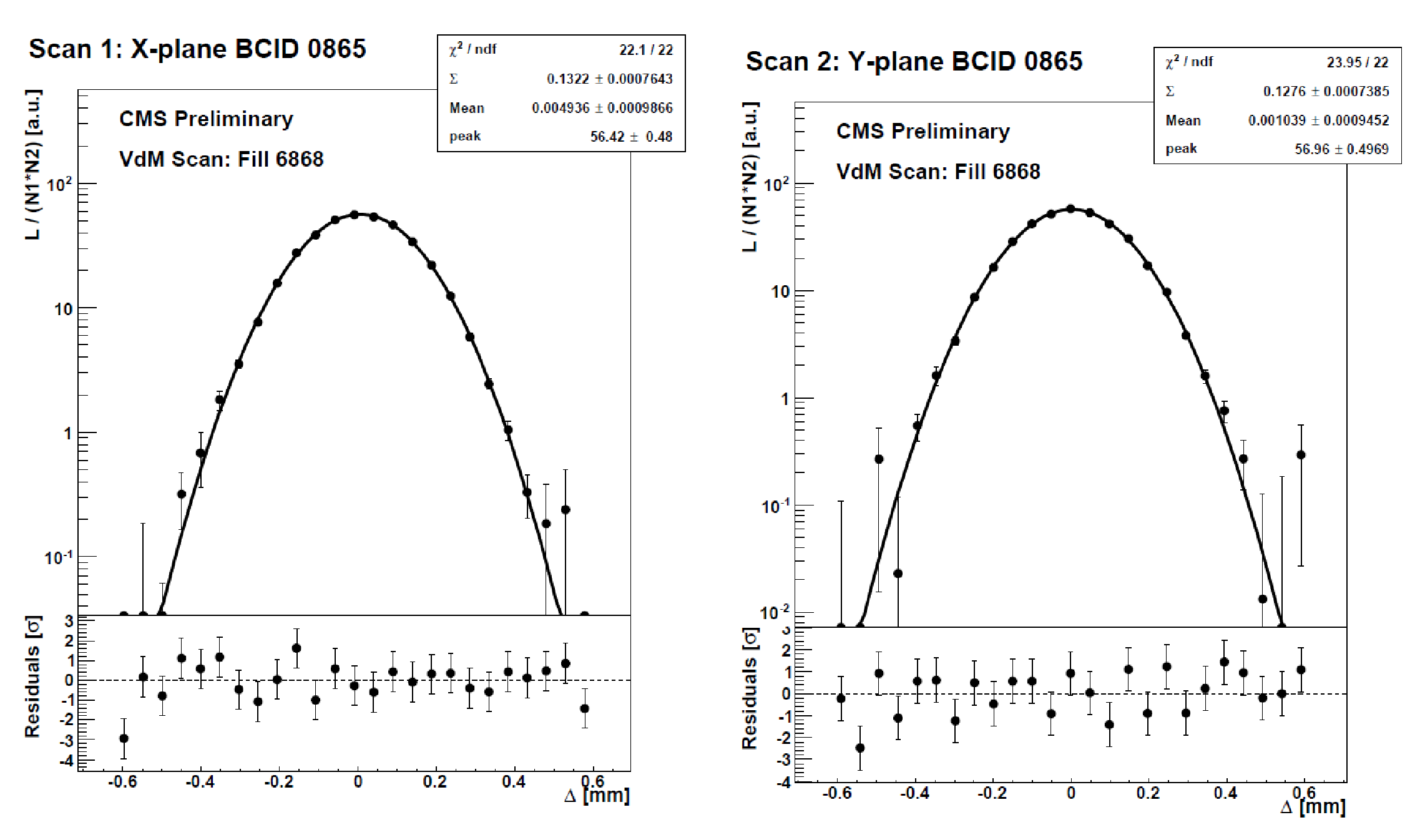
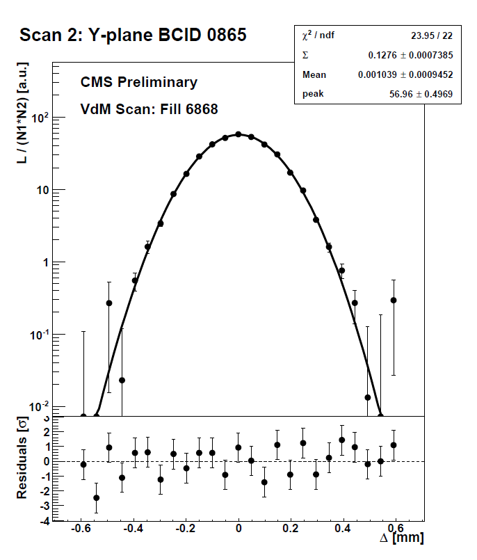
Figure 1:
Normalized rates and the resulting fitted single Gaussian scan curves as a function of the beam separation ($\Delta $) for a single bunch (BCID 865) as recorded by PCC for a scan in the $x$ (left) and $y$ direction (right). Background subtraction and the corrections described in the text have been applied to the raw data before the fit. |

png |
Figure 1-a:
Normalized rates and the resulting fitted single Gaussian scan curves as a function of the beam separation ($\Delta $) for a single bunch (BCID 865) as recorded by PCC for a scan in the $x$ direction. Background subtraction and the corrections described in the text have been applied to the raw data before the fit. |
png |
Figure 1-b:
Normalized rates and the resulting fitted single Gaussian scan curves as a function of the beam separation ($\Delta $) for a single bunch (BCID 865) as recorded by PCC for a scan in the $y$ direction. Background subtraction and the corrections described in the text have been applied to the raw data before the fit. |
png pdf |
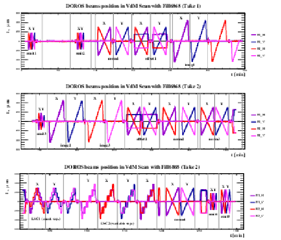
Figure 2:
Relative change in beam positions measured by the DOROS BPMs during the 2018 scan program for the two individual beams in the horizontal $x$ and vertical $y$ planes, as a function of the elapsed time from the beginning of the program. The top row shows the portion of the scan program before the alarm at CMS, while the bottom two rows show the scan program after the alarm. |

png pdf |
Figure 2-a:
Relative change in beam positions measured by the DOROS BPMs during the 2018 scan program for the two individual beams in the horizontal $x$ and vertical $y$ planes, as a function of the elapsed time from the beginning of the program. The row shows the portion of the scan program before the alarm at CMS. |

png pdf |
Figure 2-b:
Relative change in beam positions measured by the DOROS BPMs during the 2018 scan program for the two individual beams in the horizontal $x$ and vertical $y$ planes, as a function of the elapsed time from the beginning of the program. The row shows the scan program after the alarm. |

png pdf |
Figure 2-c:
Relative change in beam positions measured by the DOROS BPMs during the 2018 scan program for the two individual beams in the horizontal $x$ and vertical $y$ planes, as a function of the elapsed time from the beginning of the program. The row shows the scan program after the alarm. |

png pdf |
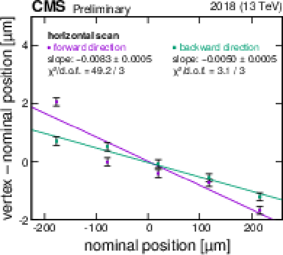
Figure 3:
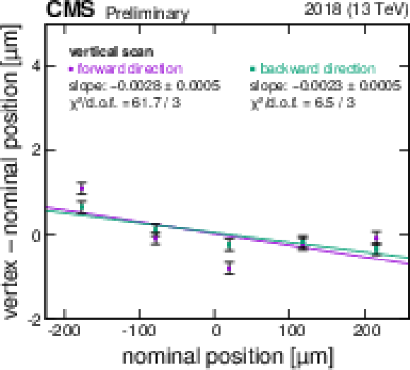
Difference between reconstructed luminous region position and nominal beam separation, as a function of the nominal beam separation, in the constant separation LSC scans. Left: scan in the $x$ plane, for the forward (purple) and backward (green) scan directions. Right: same for the $y$ plane. The plots are fitted with a straight line to derive the correction. |
png pdf |
Figure 3-a:
Difference between reconstructed luminous region position and nominal beam separation, as a function of the nominal beam separation, in the constant separation LSC scans, in the $x$ plane, for the forward (purple) and backward (green) scan directions. The plot is fitted with a straight line to derive the correction. |
png pdf |
Figure 3-b:
Difference between reconstructed luminous region position and nominal beam separation, as a function of the nominal beam separation, in the constant separation LSC scans, in the $y$ plane, for the forward (purple) and backward (green) scan directions. The plot is fitted with a straight line to derive the correction. |
png pdf |
Figure 4:
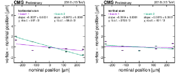
Length scale calibration scan, using the variable separation procedure, for the $x$ (left) and $y$ (right) direction of beam 1 (purple) and beam 2 (green), respectively. The difference between the reconstructed luminous region position and nominal beam separation, as a function of the nominal beam separation, is shown. The line is a linear fit to the data. Errors are of statistical nature. |
png pdf |
Figure 4-a:
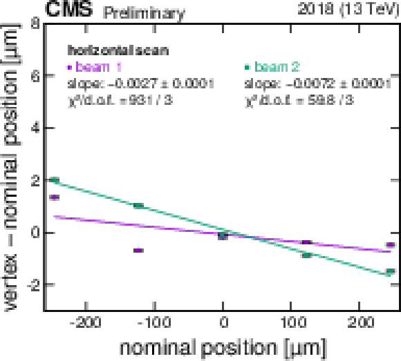
Length scale calibration scan, using the variable separation procedure, for the $x$ direction of beam 1 (purple) and beam 2 (green), respectively. The difference between the reconstructed luminous region position and nominal beam separation, as a function of the nominal beam separation, is shown. The line is a linear fit to the data. Errors are of statistical nature. |
png pdf |
Figure 4-b:
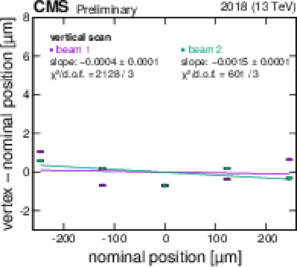
Length scale calibration scan, using the variable separation procedure, for the $y$ direction of beam 1 (purple) and beam 2 (green), respectively. The difference between the reconstructed luminous region position and nominal beam separation, as a function of the nominal beam separation, is shown. The line is a linear fit to the data. Errors are of statistical nature. |
png pdf |
Figure 5:
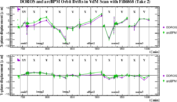
Results of the orbit drift measurement in $x$ (top) and $y$ (bottom), during the first half of the scan program after recovery from the fire alarm at CMS. The dots represent the beam position measured at the times when the beams are head-on before, during, and after each scan, as given by the DOROS BPM and arc BPMs in $\mu$m. The lines are the interpolations used to provide the orbit drift correction for each scan step. |
png pdf |
Figure 6:
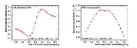
Left: An example of beam-beam deflection estimates as a function of nominal beam separation for BCID 1601. Right: an example of the dynamic-$ {\beta ^{*}}$ effect on the rate as a function of the beam separation corrected for the beam-beam deflection for BCID 1601. |
png |
Figure 6-a:
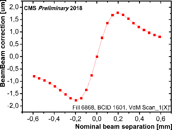
An example of beam-beam deflection estimates as a function of nominal beam separation for BCID 1601. |
png |
Figure 6-b:
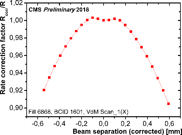
An example of the dynamic-$ {\beta ^{*}}$ effect on the rate as a function of the beam separation corrected for the beam-beam deflection for BCID 1601. |
png pdf |
Figure 7:
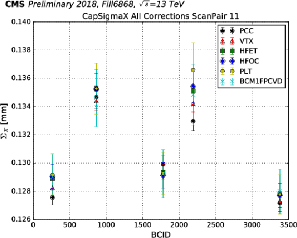
Convolved beam width $\Sigma _{x}$ measured in a normal VdM scan for the four online luminometers (HFET, HFOC, PLT, and BCM1F) along with PCC and vertex counting, shown for the five bunch crossings available for PCC and vertices. The measurements from all detectors agree within the statistical uncertainty. |
png pdf |
Figure 8:
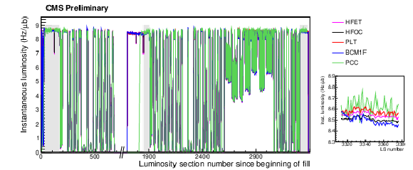
Instantaneous luminosity for the five independent luminometers during the VdM scan fill, showing the general agreement between all five luminometers through all the scans. The period during which CMS was off because of the alarm has been removed. The inset shows a zoom in on one of the periods with stable luminosity, in which the slightly different absolute scales of the different luminometers can be observed. The three gray shaded rectangles indicate the periods used to calculate the total integrated luminosity for the cross-detector comparison. |

png pdf |
Figure 9:
Decrease in HFOC efficiency in 2018 due to aging in the HF. The blue points show the efficiency in the HFOC luminosity measurement, relative to the efficiency at the time of the VdM scan (purple line), as a function of the total integrated luminosity since the beginning of Run 2 in 2015. The red line is a linear fit to the data. Errors shown are statistical. |

png pdf |
Figure 10:
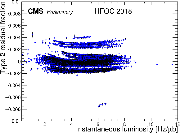
Left: HFOC afterglow correction type 1 residual fractions as a function of instantaneous luminosity. The residual fraction is given by the ratio of the luminosity of the first empty bunch immediately following a colliding bunch to the luminosity of the colliding bunch, after all corrections (including the nonlinearity effect) are applied. Right: Type 2 residual fractions as a function of instantaneous luminosity. These are given by the ratio of the luminosity of the second and following empty bunches after a colliding bunch to the luminosity of the colliding bunch. |

png |
Figure 10-a:
HFOC afterglow correction type 1 residual fractions as a function of instantaneous luminosity. The residual fraction is given by the ratio of the luminosity of the first empty bunch immediately following a colliding bunch to the luminosity of the colliding bunch, after all corrections (including the nonlinearity effect) are applied. |
png |
Figure 10-b:
Type 2 residual fractions as a function of instantaneous luminosity. These are given by the ratio of the luminosity of the second and following empty bunches after a colliding bunch to the luminosity of the colliding bunch. |
png pdf |
Figure 11:
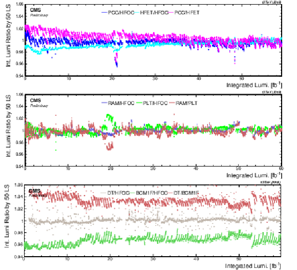
Stability comparisons for different pairs of luminometers across the 2018 data set: (top row) PCC, HFOC, and HFET; (middle row) RAMSES, PLT, and HFOC; (bottom row) DT, BCM1F, and HFOC. Periods where an individual luminometer has known detector issues have been removed. |

png pdf |
Figure 11-a:
Stability comparisons for different pairs of luminometers across the 2018 data set: PCC, HFOC, and HFET. Periods where an individual luminometer has known detector issues have been removed. |

png pdf |
Figure 11-b:
Stability comparisons for different pairs of luminometers across the 2018 data set: RAMSES, PLT, and HFOC. Periods where an individual luminometer has known detector issues have been removed. |

png pdf |
Figure 11-c:
Stability comparisons for different pairs of luminometers across the 2018 data set: DT, BCM1F, and HFOC. Periods where an individual luminometer has known detector issues have been removed. |
png pdf |
Figure 12:
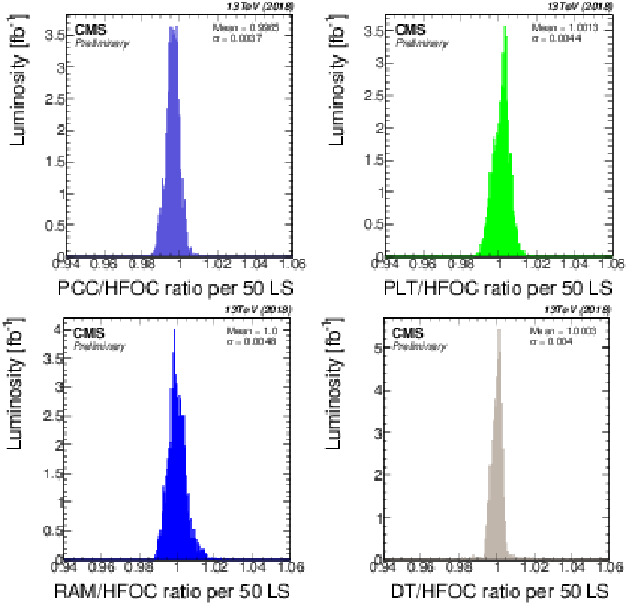
Ratio histograms for different pairs of luminometers: (top left) PCC/HFOC, (top right) PLT/HFOC, (bottom left) RAMSES/HFOC, (bottom right) DT/HFOC. For PCC/HFOC, PLT/HFOC, and DT/HFOC, known problematic regions have been excluded. |
png pdf |
Figure 12-a:
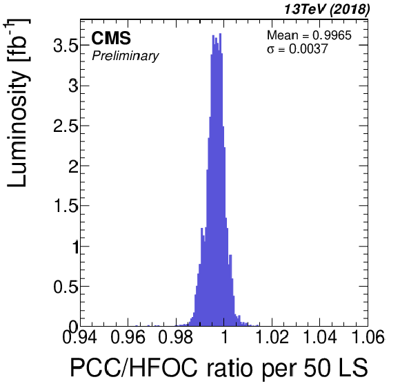
Ratio histograms for different pairs of luminometers: PCC/HFOC. Known problematic regions have been excluded. |
png pdf |
Figure 12-b:
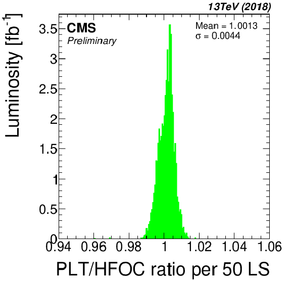
Ratio histograms for different pairs of luminometers: PLT/HFOC. Known problematic regions have been excluded. |
png pdf |
Figure 12-c:
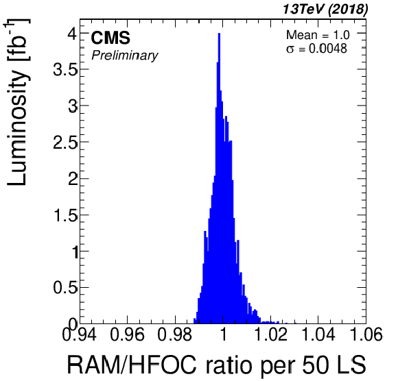
Ratio histograms for different pairs of luminometers: RAMSES/HFOC. |

png pdf |
Figure 12-d:
Ratio histograms for different pairs of luminometers: DT/HFOC. Known problematic regions have been excluded. |
png pdf |
Figure 13:
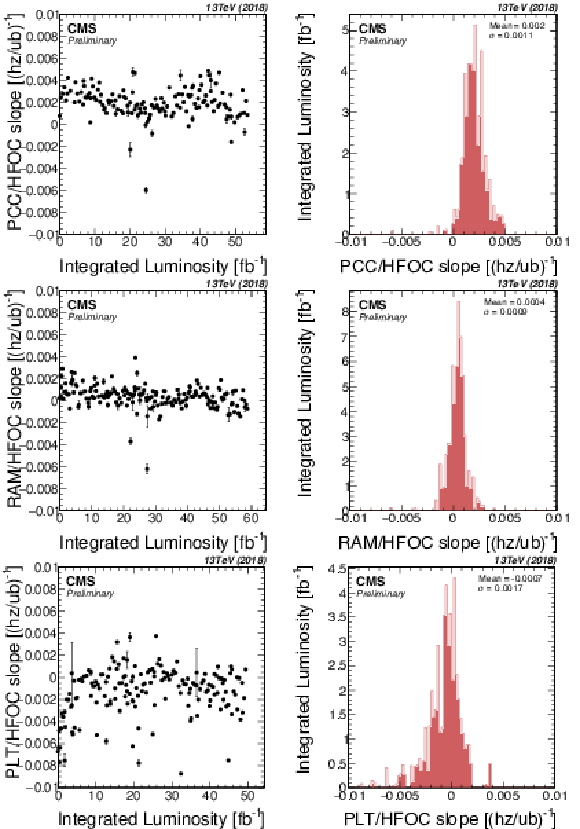
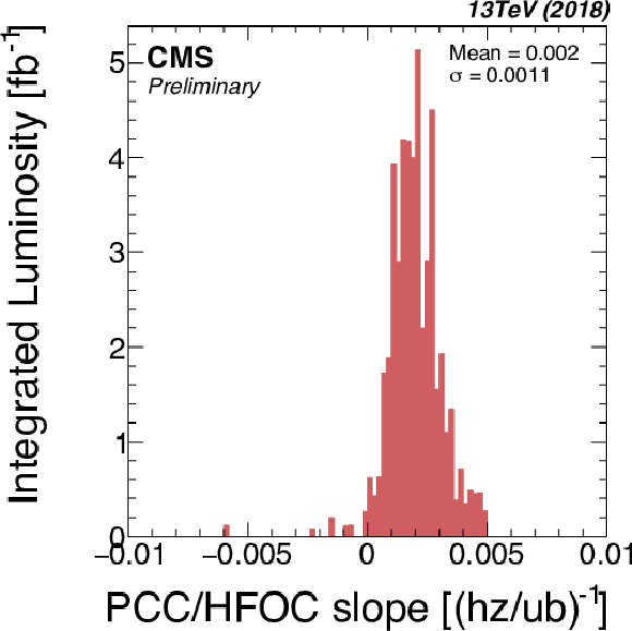
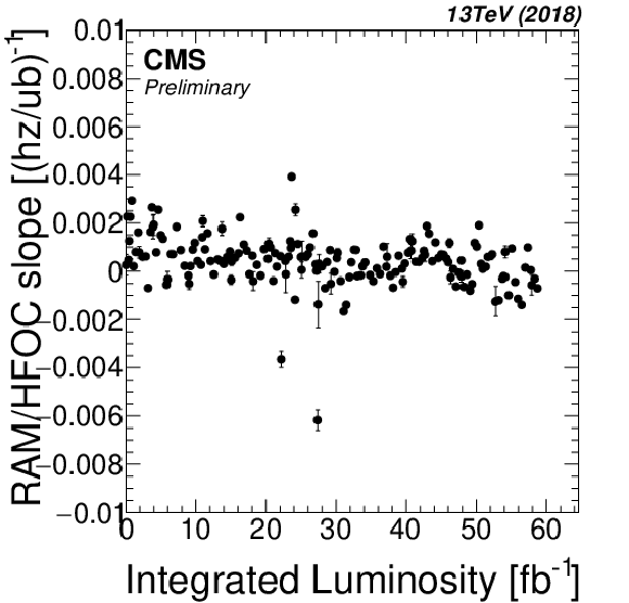
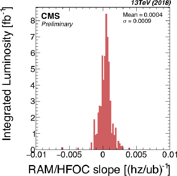
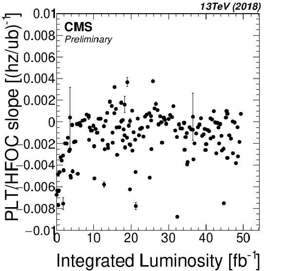
Results of the linearity studies for all 2018 fills for three different detector pairs: (top row) PCC/HFOC, (middle row) RAMSES/HFOC, (bottom row) PLT/HFOC. The left column of plots shows the slopes of linear fits per fill as a function of integrated luminosity over the course of 2018. The right plot shows the same slopes but binned and weighted according to the luminosity in that fill. |

png pdf |
Figure 13-a:
Results of the linearity studies for all 2018 fills for three different detector pairs: PCC/HFOC. RAMSES/HFOC. PLT/HFOC. |
png pdf |
Figure 13-b:
Results of the linearity studies for all 2018 fills for three different detector pairs: (top row) PCC/HFOC, (middle row) RAMSES/HFOC, (bottom row) PLT/HFOC. The left column of plots shows the slopes of linear fits per fill as a function of integrated luminosity over the course of 2018. The right plot shows the same slopes but binned and weighted according to the luminosity in that fill. |
png pdf |
Figure 13-c:
Results of the linearity studies for all 2018 fills for three different detector pairs: (top row) PCC/HFOC, (middle row) RAMSES/HFOC, (bottom row) PLT/HFOC. The left column of plots shows the slopes of linear fits per fill as a function of integrated luminosity over the course of 2018. The right plot shows the same slopes but binned and weighted according to the luminosity in that fill. |
png pdf |
Figure 13-d:
Results of the linearity studies for all 2018 fills for three different detector pairs: (top row) PCC/HFOC, (middle row) RAMSES/HFOC, (bottom row) PLT/HFOC. The left column of plots shows the slopes of linear fits per fill as a function of integrated luminosity over the course of 2018. The right plot shows the same slopes but binned and weighted according to the luminosity in that fill. |
png pdf |
Figure 13-e:
Results of the linearity studies for all 2018 fills for three different detector pairs: (top row) PCC/HFOC, (middle row) RAMSES/HFOC, (bottom row) PLT/HFOC. The left column of plots shows the slopes of linear fits per fill as a function of integrated luminosity over the course of 2018. The right plot shows the same slopes but binned and weighted according to the luminosity in that fill. |

png pdf |
Figure 13-f:
Results of the linearity studies for all 2018 fills for three different detector pairs: (top row) PCC/HFOC, (middle row) RAMSES/HFOC, (bottom row) PLT/HFOC. The left column of plots shows the slopes of linear fits per fill as a function of integrated luminosity over the course of 2018. The right plot shows the same slopes but binned and weighted according to the luminosity in that fill. |

png pdf |
Figure 14:
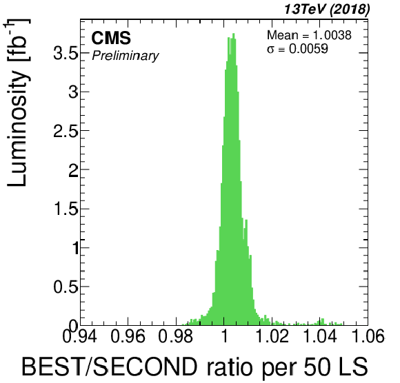
Stability tests done between the best and second-best luminometer in the priority list. Left: Ratio as a function of time. Right: Histogram of ratio values, weighted by luminosity. The standard deviation of the histogram is taken as the resulting systematic uncertainty. |

png pdf |
Figure 14-a:
Stability tests done between the best and second-best luminometer in the priority list: Ratio as a function of time. |
png pdf |
Figure 14-b:
Stability tests done between the best and second-best luminometer in the priority list: Histogram of ratio values, weighted by luminosity. The standard deviation of the histogram is taken as the resulting systematic uncertainty. |
png pdf |
Figure 15:
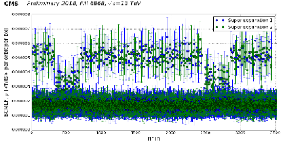
Background measured in the two "super separation'' periods by the BCM1F detector. The top band corresponds to colliding bunches, which have beam-induced background from both beams. The middle band contains bunches which are filled in one beam but not the other, so there is only a beam-induced contribution from one beam. The bottom band contains bunches which are not filled in either beam, so this corresponds to the detector noise. |
png pdf |
Figure 16:
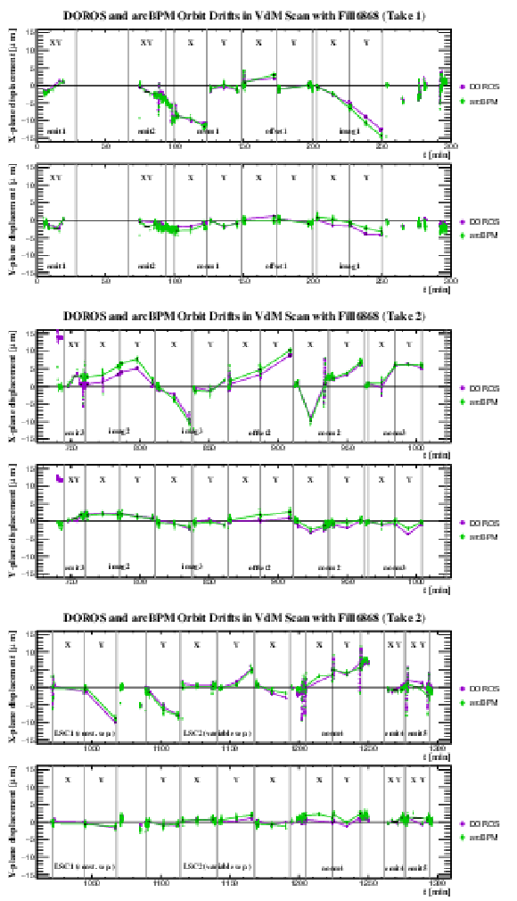
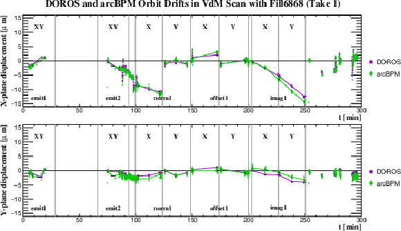
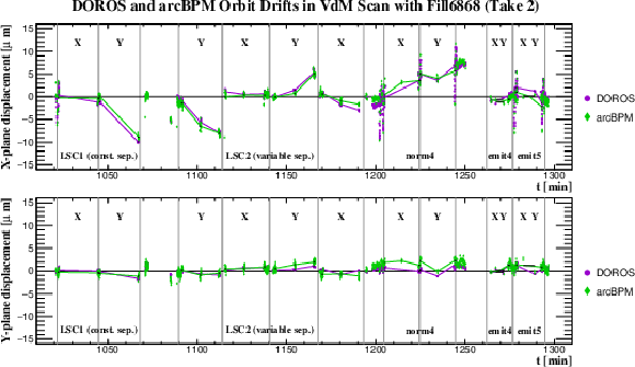
Results of the orbit drift measurement. The top pair of plots covers the time range before the alarm at CMS, the middle pair covers the first part of the time after the alarm, and the bottom pair covers the last part of the scan. In each pair the $x$ drift is shown in the top panel and the $y$ in the bottom panel. The dots represent the beam position measured at the times when the beams are head-on before, during, and after each scan, as given by the DOROS and arc BPMs in $\mu$m. The lines are the fits used to provide the orbit drift correction for each step of the scan. |
png pdf |
Figure 16-a:
Results of the orbit drift measurement in the time range before the alarm at CMS. The $x$ drift is shown in the top panel and the $y$ in the bottom panel. The dots represent the beam position measured at the times when the beams are head-on before, during, and after each scan, as given by the DOROS and arc BPMs in $\mu$m. The lines are the fits used to provide the orbit drift correction for each step of the scan. |

png pdf |
Figure 16-b:
Results of the orbit drift measurement in the first part of the time after the alarm. The $x$ drift is shown in the top panel and the $y$ in the bottom panel. The dots represent the beam position measured at the times when the beams are head-on before, during, and after each scan, as given by the DOROS and arc BPMs in $\mu$m. The lines are the fits used to provide the orbit drift correction for each step of the scan. |
png pdf |
Figure 16-c:
Results of the orbit drift measurement in the last part of the scan. The $x$ drift is shown in the top panel and the $y$ in the bottom panel. The dots represent the beam position measured at the times when the beams are head-on before, during, and after each scan, as given by the DOROS and arc BPMs in $\mu$m. The lines are the fits used to provide the orbit drift correction for each step of the scan. |
png pdf |
Figure 17:
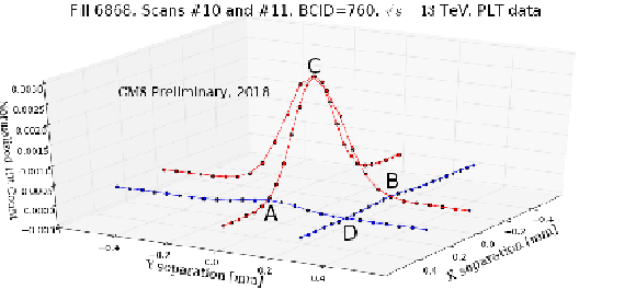
The beam separation vs. rate (normalized by beam currents) for BCID 760 from the PLT data. The red and the blue lines represent the regular VdM and the offset scans, respectively. At the points A, B, C, and D, the same point is sampled in two different scans. This makes compatibility checks possible. |
png pdf |
Figure 18:
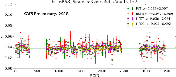
The $\rho $ correlation parameter obtained from the offset scan analysis for each BCID for PLT, BCM1F, HFET, and HFOC. |
png pdf |
Figure 19:
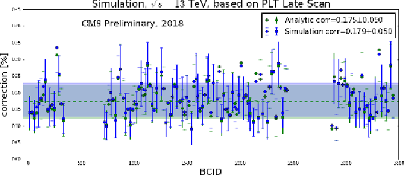
The corrections using the offset scan analysis obtained from analytic calculation and simulation are compared to validate the simulation method. The plot shows this comparison for single Gaussian shapes fitted on the PLT data in the late scan. The dashed lines and colored bands indicate the overall average and its uncertainty, respectively, for the two methods. |
png pdf |
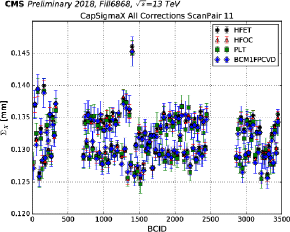
Figure 20:
Convolved beam width ($\Sigma _{x}$) measured in a normal VdM scan for all colliding bunches for all online luminometers (HFET, HFOC, PLT, BCM1F pCVD). The measurements from all detectors agree within the statistical uncertainty. |
png pdf |
Figure 21:
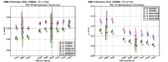
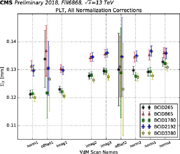
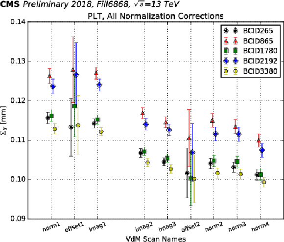
Convolved beam width measured by PLT in the $x$ (left) and $y$ (right) dimension ($\Sigma _{x}$ and $\Sigma _{y}$) after all normalization corrections have applied for the five bunch crossings with PCC data available. The uncertainty shown is statistical. The beam size increases in the $x$ direction and decreases in $y$ over time. |
png pdf |
Figure 21-a:
Convolved beam width measured by PLT in the $x$ dimension ($\Sigma _{x}$ and $\Sigma _{y}$) after all normalization corrections have applied for the five bunch crossings with PCC data available. The uncertainty shown is statistical. The beam size increases in the $x$ direction over time. |
png pdf |
Figure 21-b:
Convolved beam width measured by PLT in the $y$ dimension ($\Sigma _{x}$ and $\Sigma _{y}$) after all normalization corrections have applied for the five bunch crossings with PCC data available. The uncertainty shown is statistical. The beam size decreases in the $y$ direction over time. |
png pdf |
Figure 22:
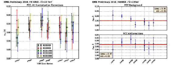
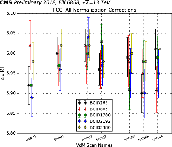
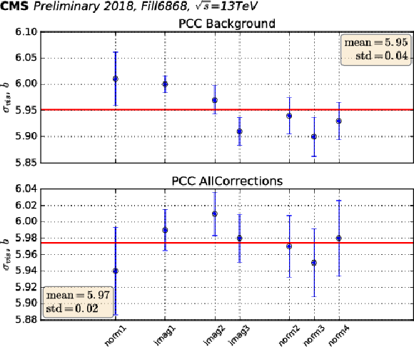
Left: Measured PCC visible cross section for all VdM scans, for the five bunch crossings with pixel data available. The uncertainty shown is statistical. Right: The measured visible cross section for each scan, together with the weighted average (red line), with only the background correction applied (top) and with all corrections applied (bottom). |
png pdf |
Figure 22-a:
Measured PCC visible cross section for all VdM scans, for the five bunch crossings with pixel data available. The uncertainty shown is statistical. |
png pdf |
Figure 22-b:
The measured visible cross section for each scan, together with the weighted average (red line), with only the background correction applied (top) and with all corrections applied (bottom). |
png pdf |
Figure 23:
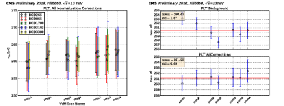
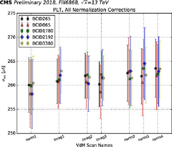
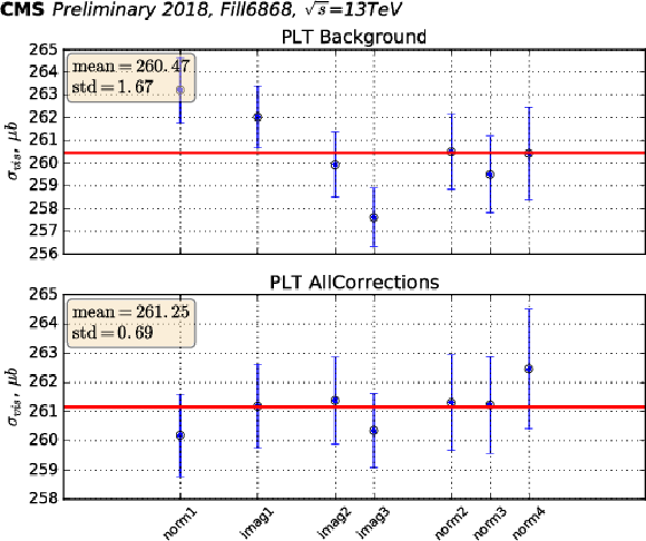
Left: Measured PLT visible cross section for all VdM scans, for the five bunch crossings with pixel data available. The uncertainty shown is statistical. Right: The measured visible cross section for each scan, together with the weighted average (red line), with only the background correction applied (top) and with all corrections applied (bottom). |
png pdf |
Figure 23-a:
Measured PLT visible cross section for all VdM scans, for the five bunch crossings with pixel data available. The uncertainty shown is statistical. |
png pdf |
Figure 23-b:
The measured visible cross section for each scan, together with the weighted average (red line), with only the background correction applied (top) and with all corrections applied (bottom). |
png pdf |
Figure 24:
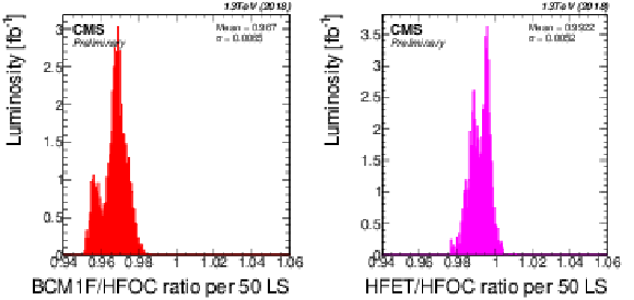
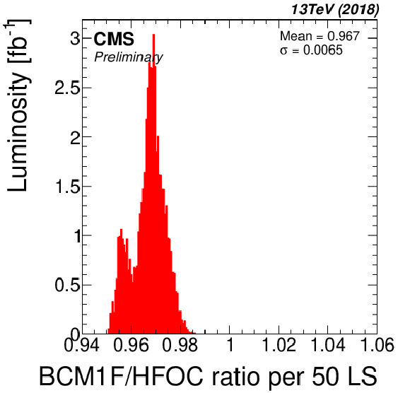
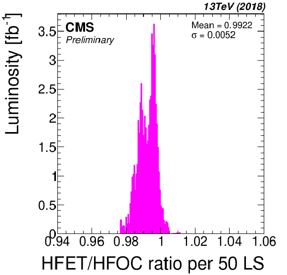
Ratio histograms for different pairs of luminometers: (left) BCM1F/HFOC, (right) HFET/HFOC. For HFET/HFOC, known problematic regions have been excluded. |
png pdf |
Figure 24-a:
Ratio histograms for different pairs of luminometers: BCM1F/HFOC. |
png pdf |
Figure 24-b:
Ratio histograms for different pairs of luminometers: HFET/HFOC. Known problematic regions have been excluded. |

png pdf |
Figure 25:
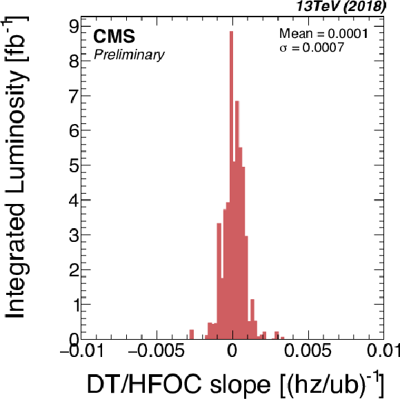
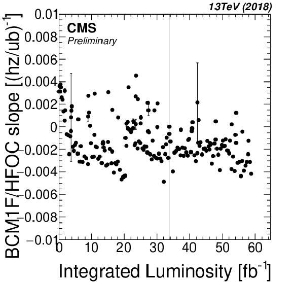
Results of the linearity studies for all 2018 fills for three different detector pairs: (top row) DT/HFOC, (middle row) BCM1F/HFOC, (bottom row) HFET/HFOC. The left column of plots shows the slopes of linear fits per fill as a function of integrated luminosity over the course of 2018. The right plot shows the same slopes but binned and weighted according to the luminosity in that fill. |

png pdf |
Figure 25-a:
Results of the linearity studies for all 2018 fills for three different detector pairs: DT/HFOC. The plots shows the slopes of linear fits per fill as a function of integrated luminosity over the course of 2018. |
png pdf |
Figure 25-b:
Results of the linearity studies for all 2018 fills for three different detector pairs: DT/HFOC. The plots shows the slopes of linear fits per fill as a function of integrated luminosity over the course of 2018, binned and weighted according to the luminosity in that fill. |
png pdf |
Figure 25-c:
Results of the linearity studies for all 2018 fills for three different detector pairs: BCM1F/HFOC. The plots shows the slopes of linear fits per fill as a function of integrated luminosity over the course of 2018. |
png pdf |
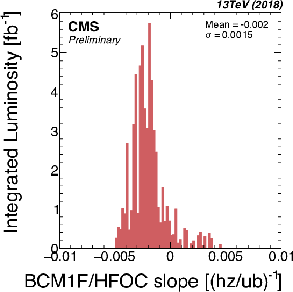
Figure 25-d:
Results of the linearity studies for all 2018 fills for three different detector pairs: BCM1F/HFOC. The plots shows the slopes of linear fits per fill as a function of integrated luminosity over the course of 2018, binned and weighted according to the luminosity in that fill. |
png pdf |
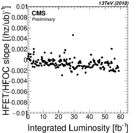
Figure 25-e:
Results of the linearity studies for all 2018 fills for three different detector pairs: HFET/HFOC. The plots shows the slopes of linear fits per fill as a function of integrated luminosity over the course of 2018. |

png pdf |
Figure 25-f:
Results of the linearity studies for all 2018 fills for three different detector pairs: HFET/HFOC. The plots shows the slopes of linear fits per fill as a function of integrated luminosity over the course of 2018, binned and weighted according to the luminosity in that fill. |
| Tables | |

png pdf |
Table 1:
Summary of measured visible cross sections for the individual luminometers, where the results have been averaged over all bunches and scans. The "bunch spread'' column is determined from the standard deviation of the individual bunch-to-bunch uncertainty, averaged over all scans. The "bunch uncertainty'' column shows the overall bunch-to-bunch uncertainty, equal to the spread divided by the square root of the number of bunches. |

png pdf |
Table 2:
Summary of measured integrated luminosity during stable periods in the VdM fill. The third column indicates the difference between the luminosity and the average. |

png pdf |
Table 3:
Summary of cross-detector comparisons. For each pair of detectors compared, each of the following is considered: the mean of the ratio between the two luminosity measurements, the standard deviation (SD) of the per-fill luminosity ratios, the mean of the slopes between the two measurements, and the standard deviation of the per-fill slopes. For PCC/HFOC, PLT/HFOC, DT/HFOC, and HFET/HFOC, problematic regions are excluded, as described in the text. |
png pdf |
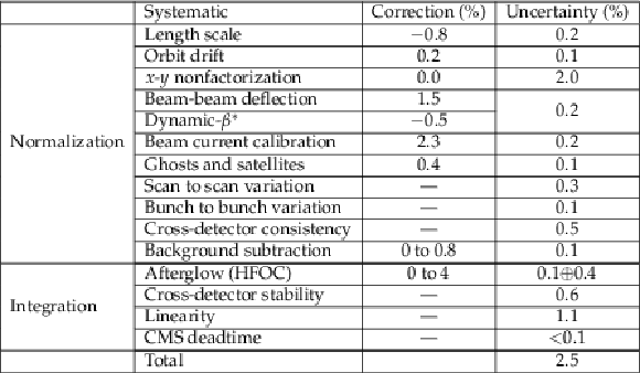
Table 4:
Summary of the systematic uncertainties entering the CMS luminosity measurement for $\sqrt {s}=$ 13 TeV pp collisions collected in 2018. When applicable, the percentage correction is shown. |
| Summary |
|
The analysis of the van der Meer (VdM) scans performed by the CMS Collaboration in summer 2018 for the calibration of CMS luminometers to the absolute luminosity scale for proton-proton (pp) collisions at $\sqrt{s} = $ 13 TeV has been presented. Table 4 summarizes the final corrections and systematic uncertainties considered in this analysis. The systematic uncertainties are divided into "normalization'' uncertainties; that is, the uncertainties arising from the luminosity calibration in the VdM scan procedure, and "integration'' uncertainties, which are the uncertainties arising from the detector operations over the course of the 2018 run. The dominant uncertainty contributing to the luminosity scale calibration, as described in Sections 4 and 5, is from the $x$-$y$ nonfactorization of the colliding proton bunch densities. All normalization uncertainties are treated as uncorrelated, giving a total of 2.1% in the luminosity scale calibration. The integration uncertainty of 1.3% includes the detector-specific uncertainties discussed in Section 6 and the cross-detector stability and linearity uncertainties covered in Section 7. In addition, the uncertainty in the integrated luminosity due to the deadtime of the CMS DAQ system is smaller than 0.1%. The integration and normalization uncertainties are treated as uncorrelated. In summary, the total uncertainty in the luminosity measurement in 2018 is 2.5% for CMS data recorded in pp collisions at $\sqrt{s}=$ 13 TeV. |
| References | ||||
| 1 | CMS Collaboration | The CMS experiment at the CERN LHC | JINST 3 (2008) S08004 | CMS-00-001 |
| 2 | P. Lujan | Performance of the Pixel Luminosity Telescope for luminosity measurement at CMS during Run 2 | PoS 314 (2017) 504 | |
| 3 | M. Hempel | Development of a novel diamond based detector for machine induced background and luminosity measurements | PhD thesis, DESY, Hamburg | |
| 4 | CMS Collaboration | The CMS trigger system | JINST 12 (2017) P01020 | CMS-TRG-12-001 1609.02366 |
| 5 | S. van der Meer | Calibration of the effective beam height in the ISR | CERN-ISR-PO-68-31 | |
| 6 | CMS Collaboration | CMS luminosity based on pixel cluster counting - Summer 2013 update | CMS-PAS-LUM-13-001 | CMS-PAS-LUM-13-001 |
| 7 | CMS Collaboration | CMS luminosity measurement for the 2016 data taking period | CMS-PAS-LUM-17-001 | CMS-PAS-LUM-17-001 |
| 8 | CMS Collaboration | CMS luminosity measurement using 2016 proton-nucleus collisions at $ \sqrt{s_\text{NN}} = $ 8 TeV | CMS-PAS-LUM-17-002 | CMS-PAS-LUM-17-002 |
| 9 | CMS Collaboration | CMS luminosity measurement for the 2017 data-taking period at $ \sqrt{s} = $ 13 TeV | CMS-PAS-LUM-17-004 | CMS-PAS-LUM-17-004 |
| 10 | ATLAS Collaboration | Luminosity determination in pp collisions at $ \sqrt{s} = $ 8 TeV using the ATLAS detector at the LHC | EPJC 76 (2016) 653 | 1608.03953 |
| 11 | ALICE Collaboration | Measurement of visible cross sections in proton-lead collisions at $ \sqrt{s_{\rm NN}} = $ 5.02 TeV in van der Meer scans with the ALICE detector | JINST 9 (2014) P11003 | 1405.1849 |
| 12 | LHCb Collaboration | Precision luminosity measurements at LHCb | JINST 9 (2014) P12005 | 1410.0149 |
| 13 | CMS Collaboration | Description and performance of track and primary-vertex reconstruction with the CMS tracker | JINST 9 (2014) P10009 | CMS-TRK-11-001 1405.6569 |
| 14 | CMS Collaboration | CMS luminosity measurement for the 2015 data taking period | CMS-PAS-LUM-15-001 | CMS-PAS-LUM-15-001 |
| 15 | C. Barschel et al. | Results of the LHC DCCT calibration studies | CERN-ATS-Note-2012-026 PERF | |
| 16 | D. Belohrad et al. | The LHC fast BCT system: A comparison of design parameters with initial performance | CERN-BE-2010-010 | |
| 17 | M. Gasior, J. Olexa, and R. Steinhagen | BPM electronics based on compensated diode detectors --- results from development systems | Conf. Proc. C 1204151 (2012) 44 | |
| 18 | M. Zanetti | Beams scan based absolute normalization of the CMS luminosity measurement | CERN-Proceedings-2011-001 | |
| 19 | M. Klute, C. Medlock, and J. Salfeld-Nebgen | Beam imaging and luminosity calibration | JINST 12 (2017) P03018 | 1603.03566 |
| 20 | W. Kozanecki, T. Pieloni, and J. Wenninger | Observation of beam-beam deflections with LHC orbit data | CERN-ACC-NOTE-2013-0006 | |
| 21 | A. Babaev | Beam-dynamic effects at the CMS BRIL van der Meer scans | JINST 13 (2018) C03028 | |
| 22 | R. Alemany-Fernàndez et al. | Cross-calibration of the LHC transverse beam-profile monitors | in Proceedings, 8th International Particle Accelerator Conference (IPAC 2017), Copenhagen, 2017 | |
| 23 | A. Jeff et al. | Longitudinal density monitor for the LHC | PRST Accel. Beams 15 (2012) 032803 | |
| 24 | A. Jeff | A longitudinal density monitor for the LHC” | PhD thesis, Liverpool University | |
| 25 | C. Barschel | Precision luminosity measurement at LHCb with beam-gas imaging | PhD thesis, RWTH Aachen University | |
| 26 | A. S. Fisher | Expected performance of the LHC synchrotron-light telescope (BSRT) and abort-gap monitor (BSRA) | LHC Performance Note 014 | |

|
Compact Muon Solenoid LHC, CERN |

|

|

|

|

|

|