

Compact Muon Solenoid
LHC, CERN
| CMS-PAS-LUM-17-004 | ||
| CMS luminosity measurement for the 2017 data-taking period at $\sqrt{s} = $ 13 TeV | ||
| CMS Collaboration | ||
| June 2018 | ||
| Abstract: The calibration for the luminosity measurement by the CMS experiment for the 2017 proton-proton LHC run at $\sqrt{s} = $ 13 TeV is described. The principal calibration is derived from the analysis of the van der Meer scan program in CMS taken during LHC fill 6016. In addition, the performance and stability of the CMS luminometers are also evaluated using emittance scans taken throughout the course of the year. The systematic uncertainty in the absolute calibration from the van der Meer scan is derived with a precision of 1.5%, with the dominant contributions arising from the $x$-$y$ correlations of the beam shape and the scan to scan variation. The total systematic uncertainty, including terms from stability and linearity effects, is 2.3%. The uncertainty for the special low-pileup run at the end of 2017 is also evaluated and found to be 1.7%. | ||
| Links: CDS record (PDF) ; inSPIRE record ; CADI line (restricted) ; | ||
| Figures | |
png pdf |
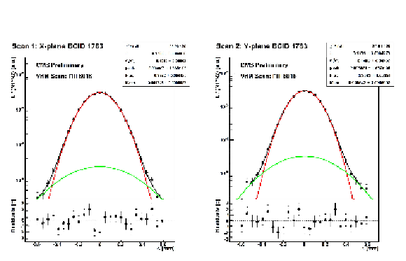
Figure 1:
Normalized rates and the resulting fitted double Gaussian scan curves as a function of the beam separation ($\Delta $) for a single bunch as recorded by PLT for a scan in the $x$ (left) and $y$ direction (right). Background subtraction has been applied to the raw data. |
png pdf |
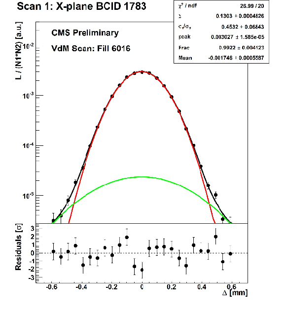
Figure 1-a:
Normalized rates and the resulting fitted double Gaussian scan curves as a function of the beam separation ($\Delta $) for a single bunch as recorded by PLT for a scan in the $x$ (left) and $y$ direction (right). Background subtraction has been applied to the raw data. |
png pdf |
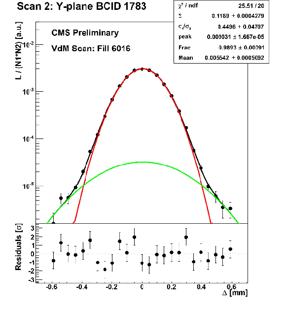
Figure 1-b:
Normalized rates and the resulting fitted double Gaussian scan curves as a function of the beam separation ($\Delta $) for a single bunch as recorded by PLT for a scan in the $x$ (left) and $y$ direction (right). Background subtraction has been applied to the raw data. |

png pdf |
Figure 2:
Relative change in beam positions measured by the DOROS BPMs during the 2017 scan program for the two individual beams in the horizontal $x$ and vertical $y$ planes, as a function of the elapsed time from the beginning of the program. The gray vertical lines delimit individual scans. |
png pdf |
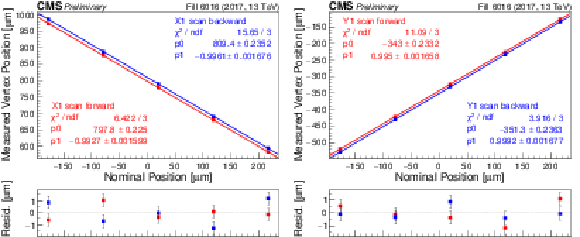
Figure 3:
Reconstructed beam spot position as a function of the nominal beam separation in the constant separation LSC scans. Left: scan in the $x$ plane, for the forward (red) and backward (blue) scan directions. Right: same for the $y$ plane. The plots are fitted with a straight line to derive the correction. |

png pdf |
Figure 3-a:
Reconstructed beam spot position as a function of the nominal beam separation in the constant separation LSC scans. Left: scan in the $x$ plane, for the forward (red) and backward (blue) scan directions. Right: same for the $y$ plane. The plots are fitted with a straight line to derive the correction. |

png pdf |
Figure 3-b:
Reconstructed beam spot position as a function of the nominal beam separation in the constant separation LSC scans. Left: scan in the $x$ plane, for the forward (red) and backward (blue) scan directions. Right: same for the $y$ plane. The plots are fitted with a straight line to derive the correction. |
png pdf |
Figure 4:
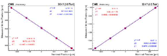
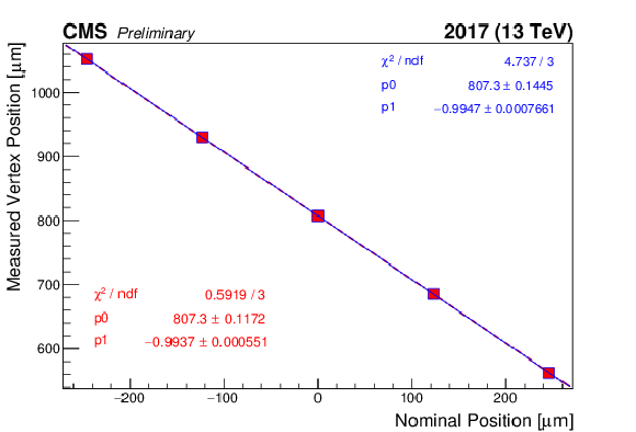
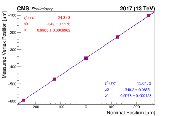
Length scale calibration scan, using the variable separation procedure, for the $x$ (left) and $y$ (right) direction of beam 1 (red) and beam 2 (blue), respectively. Shown is the measured displacement of the luminous centroid as a function of the expected displacement based on the corrector bump amplitude. The line is a linear fit to the data. Errors are of statistical nature. |
png pdf |
Figure 4-a:
Length scale calibration scan, using the variable separation procedure, for the $x$ (left) and $y$ (right) direction of beam 1 (red) and beam 2 (blue), respectively. Shown is the measured displacement of the luminous centroid as a function of the expected displacement based on the corrector bump amplitude. The line is a linear fit to the data. Errors are of statistical nature. |
png pdf |
Figure 4-b:
Length scale calibration scan, using the variable separation procedure, for the $x$ (left) and $y$ (right) direction of beam 1 (red) and beam 2 (blue), respectively. Shown is the measured displacement of the luminous centroid as a function of the expected displacement based on the corrector bump amplitude. The line is a linear fit to the data. Errors are of statistical nature. |
png pdf |
Figure 5:
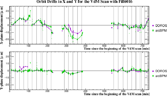
Results of the orbit drift measurement in $x$ (top) and $y$ (bottom). The dots represent the beam position measured at the times when the beams are head-on before, during, and after each scan, as given by the DOROS BPM and arc BPMs in $\mu$m. The lines are the fits used to provide the orbit drift correction for each scan step. |
png pdf |
Figure 6:
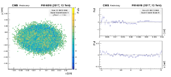
Pull distributions using the model defined in Eq. 7, called previously the "Super Double Gaussian'' model. The pull is defined as the difference between the number of measured vertices and the number of vertices predicted by the fit, divided by the statistical uncertainty of the measurement. These plots show the results from the scan constraining beam 1 in $x$. Left: 2-D pull distribution as a function of $x$ and $y$ position. Right: 1-D projections of the 2-D pull distribution, in slices of constant radius (top) and constant azimuthal angle (bottom). |

png pdf |
Figure 6-a:
Pull distributions using the model defined in Eq. 7, called previously the "Super Double Gaussian'' model. The pull is defined as the difference between the number of measured vertices and the number of vertices predicted by the fit, divided by the statistical uncertainty of the measurement. These plots show the results from the scan constraining beam 1 in $x$. Left: 2-D pull distribution as a function of $x$ and $y$ position. Right: 1-D projections of the 2-D pull distribution, in slices of constant radius (top) and constant azimuthal angle (bottom). |

png pdf |
Figure 6-b:
Pull distributions using the model defined in Eq. 7, called previously the "Super Double Gaussian'' model. The pull is defined as the difference between the number of measured vertices and the number of vertices predicted by the fit, divided by the statistical uncertainty of the measurement. These plots show the results from the scan constraining beam 1 in $x$. Left: 2-D pull distribution as a function of $x$ and $y$ position. Right: 1-D projections of the 2-D pull distribution, in slices of constant radius (top) and constant azimuthal angle (bottom). |
png pdf |
Figure 7:
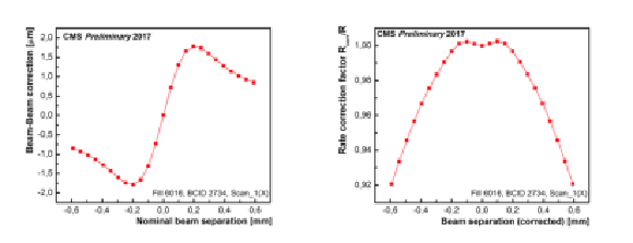
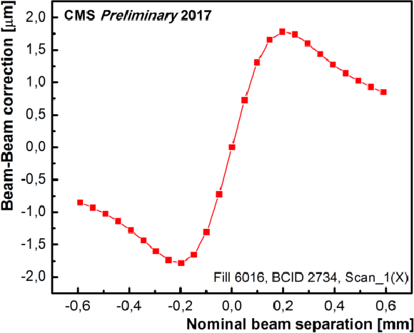
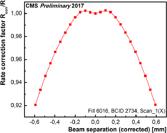
Left: an example of beam-beam deflection estimates as a function of nominal beam separation. Right: an example of the dynamic-$ {\beta ^{*}}$ effect on rate as a function of the beam separation corrected for the beam-beam deflection. |
png pdf |
Figure 7-a:
Left: an example of beam-beam deflection estimates as a function of nominal beam separation. Right: an example of the dynamic-$ {\beta ^{*}}$ effect on rate as a function of the beam separation corrected for the beam-beam deflection. |
png pdf |
Figure 7-b:
Left: an example of beam-beam deflection estimates as a function of nominal beam separation. Right: an example of the dynamic-$ {\beta ^{*}}$ effect on rate as a function of the beam separation corrected for the beam-beam deflection. |
png pdf |
Figure 8:
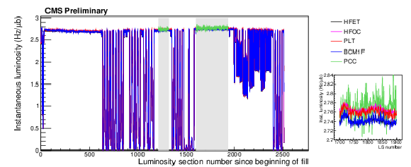
Instantaneous luminosity for the five independent luminometers during the VdM scan fill. The inset shows a zoom in on one of the periods with stable luminosity, in which the slightly different absolute scales of the different luminometers can be observed. The two gray shaded rectangles indicate the periods used to calculate the total integrated luminosity to determine the rescaling. |
png pdf |
Figure 9:
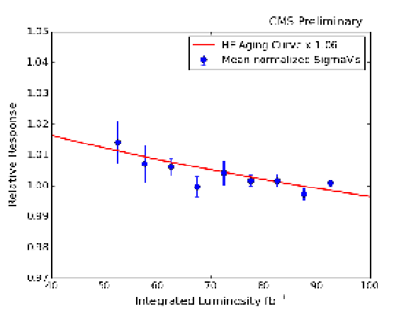
The red curve shows the aging model for the HF, derived from studies on the HF PMTs and fibers and parameterized with a function. The blue points show the average, uncorrected visible cross section derived from emittance scans as a function of integrated luminosity; the smaller uncertainties observed towards the end of the year are because of smaller variation in the ${\sigma _{\text {vis}}}$ from the individual emittance scan results. Both are scaled arbitrarily to the same scale. Errors shown are statistical. |

png pdf |
Figure 10:
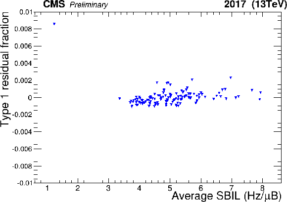
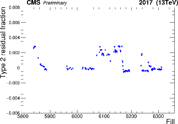
Left: HFET correction Type 1 residual fractions (remaining luminosity in empty bunches after corrections) as a function of average SBIL, after the nonlinearity effect is corrected. Right: Type 2 residual fractions as a function of fill. |
png |
Figure 10-a:
Left: HFET correction Type 1 residual fractions (remaining luminosity in empty bunches after corrections) as a function of average SBIL, after the nonlinearity effect is corrected. Right: Type 2 residual fractions as a function of fill. |
png |
Figure 10-b:
Left: HFET correction Type 1 residual fractions (remaining luminosity in empty bunches after corrections) as a function of average SBIL, after the nonlinearity effect is corrected. Right: Type 2 residual fractions as a function of fill. |

png pdf |
Figure 11:
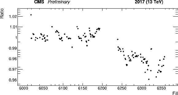
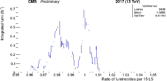
Example of stability comparison for BCM1F/HFET. Left: ratio of the measured luminosity values as a function of fill over the course of 2017. Right: luminosity-weighted binned histogram of the BCM1F/HFET luminosity ratio. |
png |
Figure 11-a:
Example of stability comparison for BCM1F/HFET. Left: ratio of the measured luminosity values as a function of fill over the course of 2017. Right: luminosity-weighted binned histogram of the BCM1F/HFET luminosity ratio. |
png |
Figure 11-b:
Example of stability comparison for BCM1F/HFET. Left: ratio of the measured luminosity values as a function of fill over the course of 2017. Right: luminosity-weighted binned histogram of the BCM1F/HFET luminosity ratio. |

png pdf |
Figure 12:
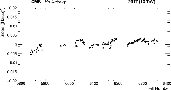
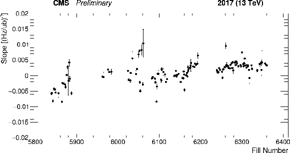
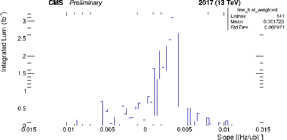
Example of linearity comparison for PLT/HFET. Left: slopes of linear fits to the luminosity ratios as a function of average SBIL versus fill number. Right: luminosity-weighted binned histogram of the slopes. |
png |
Figure 12-a:
Example of linearity comparison for PLT/HFET. Left: slopes of linear fits to the luminosity ratios as a function of average SBIL versus fill number. Right: luminosity-weighted binned histogram of the slopes. |

png |
Figure 12-b:
Example of linearity comparison for PLT/HFET. Left: slopes of linear fits to the luminosity ratios as a function of average SBIL versus fill number. Right: luminosity-weighted binned histogram of the slopes. |

png pdf |
Figure 13:
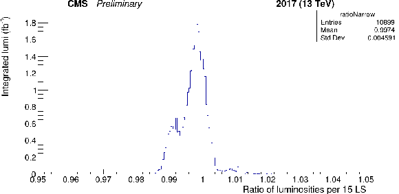
Stability comparison for HFET/PCC, as in Fig. 11. Left: ratio of the measured luminosity values as a function of fill over the course of 2017. Right: luminosity-weighted binned histogram of the HFET/PCC luminosity ratio. The overall stability systematic uncertainty is derived from this comparison. |

png |
Figure 13-a:
Stability comparison for HFET/PCC, as in Fig. 11. Left: ratio of the measured luminosity values as a function of fill over the course of 2017. Right: luminosity-weighted binned histogram of the HFET/PCC luminosity ratio. The overall stability systematic uncertainty is derived from this comparison. |
png |
Figure 13-b:
Stability comparison for HFET/PCC, as in Fig. 11. Left: ratio of the measured luminosity values as a function of fill over the course of 2017. Right: luminosity-weighted binned histogram of the HFET/PCC luminosity ratio. The overall stability systematic uncertainty is derived from this comparison. |

png pdf |
Figure 14:
Linearity comparison for PLT/PCC, as in Fig. 12. Left: slopes of linear fits to the luminosity ratios as a function of average SBIL versus fill number. Right: luminosity-weighted binned histogram of the slopes. The overall linearity systematic uncertainty is derived from this comparison. |
png |
Figure 14-a:
Linearity comparison for PLT/PCC, as in Fig. 12. Left: slopes of linear fits to the luminosity ratios as a function of average SBIL versus fill number. Right: luminosity-weighted binned histogram of the slopes. The overall linearity systematic uncertainty is derived from this comparison. |
png |
Figure 14-b:
Linearity comparison for PLT/PCC, as in Fig. 12. Left: slopes of linear fits to the luminosity ratios as a function of average SBIL versus fill number. Right: luminosity-weighted binned histogram of the slopes. The overall linearity systematic uncertainty is derived from this comparison. |
| Tables | |
png pdf |
Table 1:
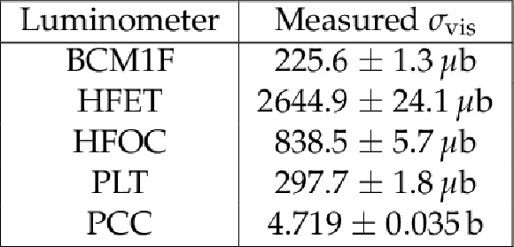
Summary of measured visible cross sections for the individual luminometers, where the results have been averaged over all bunches and scans. The uncertainty shown includes the effect of the variation among scans; the statistical uncertainty in ${\sigma _{\text {vis}}}$ for a single scan (after all bunches have been averaged over) is typically approximately 0.1%. |

png pdf |
Table 2:
Summary of measured integrated luminosity during stable periods in the VdM fill. The third column indicates the difference between the luminosity and the average; a correction equal to the inverse of this difference is then applied to rescale the ${\sigma _{\text {vis}}}$ of the luminometer to the average. |

png pdf |
Table 3:
Summary of cross-detector comparisons. For each pair of detectors compared, each of the following is considered: the mean of the ratio between the two luminosity measurements, the standard deviation of the per-fill luminosity ratios, the mean of the slopes between the two measurements, and the standard deviation of the per-fill slopes. |
png pdf |
Table 4:
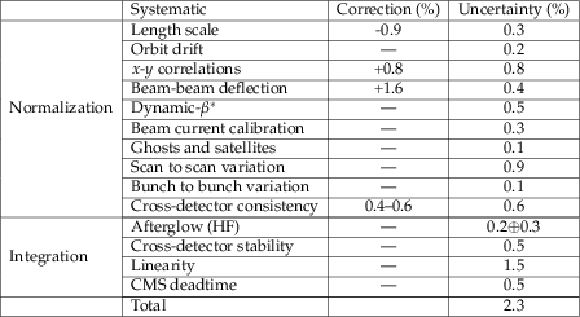
Summary of the systematic uncertainties entering the CMS luminosity measurement for $\sqrt {s}= $ 13 TeV pp collisions. When applicable, the percentage correction is shown. |
| Summary |
|
The analysis of the van der Meer (VdM) scans performed by the CMS Collaboration in July 2017 for the calibration of CMS luminometers to the absolute luminosity scale for proton-proton (pp) collisions at $\sqrt{s}= $ 13 TeV has been presented. Table 4 summarizes the final corrections and systematic uncertainties considered in this analysis. The systematic uncertainties are divided into "normalization'' uncertainties; that is, the uncertainties arising from the luminosity calibration in the VdM scan procedure, and "integration'' uncertainties, which are the uncertainties arising from the detector operations over the course of the 2017 run. The dominant uncertainties contributing to the luminosity scale calibration, as described in Section 4, are from the length scale calibration and the $x$-$y$ correlations of the colliding proton bunch densities. All normalization uncertainties are treated as uncorrelated, giving a total of 1.5% in the luminosity scale calibration. The integration uncertainty includes the detector-specific uncertainties discussed in Section 6 and the cross-detector stability and linearity uncertainties covered in Section 7. In addition, an uncertainty of 0.5% in the deadtime estimate of the CMS DAQ system is included affecting the recorded integrated luminosity. The integration and normalization uncertainties are treated as uncorrelated. In summary, the total uncertainty in the luminosity measurement in 2017 is 2.3% for CMS data recorded in pp collisions at $\sqrt{s}=$ 13 TeV. |
| References | ||||
| 1 | CMS Collaboration | The CMS experiment at the CERN LHC | JINST 3 (2008) S08004 | CMS-00-001 |
| 2 | P. Lujan | Performance of the Pixel Luminosity Telescope for luminosity measurement at CMS during Run 2 | PoS 314 (2017) 504 | |
| 3 | M. Hempel | PhD thesis, DESY, Hamburg | ||
| 4 | CMS Collaboration | The CMS trigger system | JINST 12 (2017) P01020 | CMS-TRG-12-001 1609.02366 |
| 5 | S. van der Meer | Calibration of the effective beam height in the ISR | CERN-ISR-PO-68-31 | |
| 6 | CMS Collaboration | CMS luminosity based on pixel cluster counting - Summer 2013 update | CMS-PAS-LUM-13-001 | CMS-PAS-LUM-13-001 |
| 7 | CMS Collaboration | CMS luminosity calibration for the pp reference run at $ \sqrt{s}= $ 5.02 TeV | CMS-PAS-LUM-16-001 | CMS-PAS-LUM-16-001 |
| 8 | CMS Collaboration | CMS luminosity measurement for the 2016 data taking period | CMS-PAS-LUM-17-001 | CMS-PAS-LUM-17-001 |
| 9 | ATLAS Collaboration | Luminosity determination in pp collisions at $ \sqrt{s} = $ 8 TeV using the ATLAS detector at the LHC | EPJC 76 (2016) 653 | 1608.03953 |
| 10 | ALICE Collaboration | Measurement of visible cross sections in proton-lead collisions at $ \sqrt{s_{\rm NN}} = $ 5.02 TeV in van der Meer scans with the ALICE detector | JINST 9 (2014) P11003 | 1405.1849 |
| 11 | LHCb Collaboration | Precision luminosity measurements at LHCb | JINST 9 (2014) P12005 | 1410.0149 |
| 12 | CMS Collaboration | CMS luminosity measurement for the 2015 data taking period | CMS-PAS-LUM-15-001 | CMS-PAS-LUM-15-001 |
| 13 | C. Barschel et al. | Results of the LHC DCCT calibration studies | CERN-ATS-Note-2012-026 PERF | |
| 14 | D. Belohrad et al. | The LHC fast BCT system: A comparison of design parameters with initial performance | CERN-BE-2010-010 | |
| 15 | M. Gasior, J. Olexa, and R. Steinhagen | BPM electronics based on compensated diode detectors --- results from development systems | Conf. Proc. C1204151 (2012) 44 | |
| 16 | M. Zanetti | Beams scan based absolute normalization of the CMS luminosity measurement | CERN-Proceedings-2011-001 | |
| 17 | A. Valassi and R. Chierici | Information and treatment of unknown correlations in the combination of measurements using the BLUE method | EPJC 74 (2014) 2717 | 1307.4003 |
| 18 | M. Klute, C. Medlock, and J. Salfeld-Nebgen | Beam imaging and luminosity calibration | JINST 12 (2017) P03018 | 1603.03566 |
| 19 | W. Kozanecki, T. Pieloni, and J. Wenninger | Observation of beam-beam deflections with LHC orbit data | CERN-ACC-NOTE-2013-0006 | |
| 20 | A. Babaev | Beam-dynamic effects at the CMS BRIL van der Meer scans | JINST 13 (2018) C03028 | |
| 21 | A. Jeff et al. | Longitudinal density monitor for the LHC | PRST Accel. Beams 15 (2012) 032803 | |
| 22 | A. Jeff | PhD thesis, Liverpool University | ||
| 23 | C. Barschel | PhD thesis, RWTH Aachen University | ||

|
Compact Muon Solenoid LHC, CERN |

|

|

|

|

|

|