

Compact Muon Solenoid
LHC, CERN
| CMS-HIG-16-043 ; CERN-EP-2017-181 | ||
| Observation of the Higgs boson decay to a pair of $\tau$ leptons | ||
| CMS Collaboration | ||
| 1 August 2017 | ||
| Phys. Lett. B 779 (2018) 283 | ||
| Abstract: A measurement of the coupling strength of the Higgs boson to $\tau$ leptons is performed using events recorded in proton-proton collisions by the CMS experiment at the LHC in 2016 at a center-of-mass energy of 13 TeV. The data set corresponds to an integrated luminosity of 35.9 fb$^{-1}$. The $\mathrm{ H }\to \tau \tau$ signal is established with a significance of 4.9 standard deviations, to be compared to an expected significance of 4.7 standard deviations. The best fit of the product of the observed $\mathrm{ H }\to \tau \tau$ signal production cross section and branching fraction is 1.09$^{+0.27}_{-0.26}$ times the standard model expectation. The combination with the corresponding measurement performed with data collected by the CMS experiment at center-of-mass energies of 7 and 8 TeV leads to an observed significance of 5.9 standard deviations, equal to the expected significance. This is the first observation of Higgs boson decays to $\tau$ leptons by a single experiment. | ||
| Links: e-print arXiv:1708.00373 [hep-ex] (PDF) ; CDS record ; inSPIRE record ; HepData record ; CADI line (restricted) ; | ||
| Figures | |
png pdf |
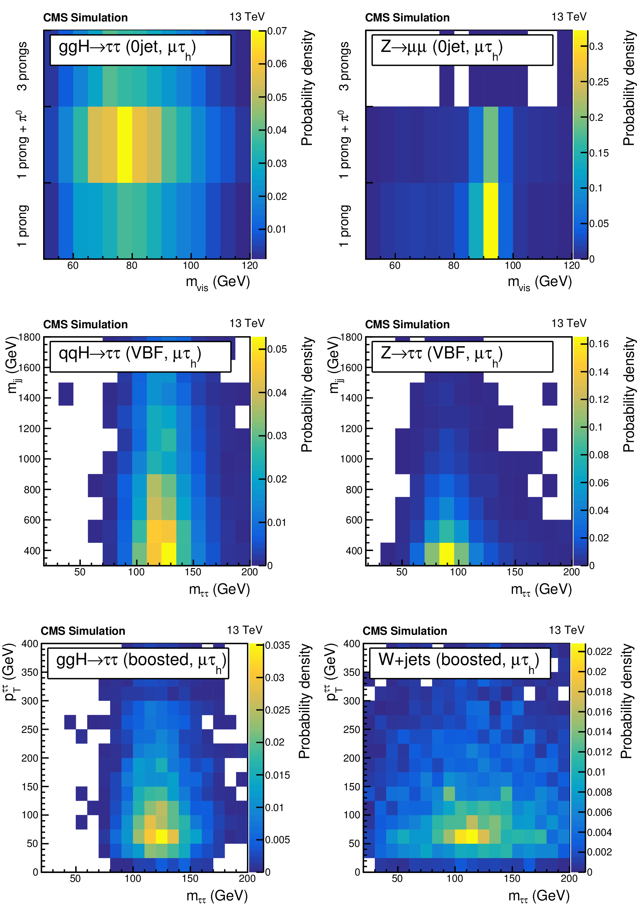
Figure 1:
Distributions for the signal (left) and for some dominant background processes (right) of the two observables chosen in the 0-jet (top), VBF (center), and boosted (bottom) categories in the $\mu {\tau _\mathrm {h}} $ decay channel. The background processes are chosen for illustrative purpose for their separation from the signal. The $\mathrm{ Z } \to \mu \mu $ background in the 0-jet category is concentrated in the regions where the visible mass is close to 90 GeV and is negligible when the $ {\tau _\mathrm {h}} $ candidate is reconstructed in the 3-prong decay mode. The $\mathrm{ Z } \to \tau \tau $ background in the VBF category mostly lies at low $ {m_\mathrm {jj}} $ values whereas the distribution of VBF signal events extends to high $ {m_\mathrm {jj}} $ values. In the boosted category, the W+jets background, which behaves similarly to the QCD multijet background, is rather flat with respect to $ {m_{\tau \tau }} $, and is concentrated at low $ { {p_{\mathrm {T}}} ^{\tau \tau }} $ values. These distributions are not used as such to extract the results. |

png pdf |
Figure 1-a:
Distribution of the $ {m_\text {vis}} $ observable for the signal in the 0-jet category and the $\mu {\tau _\mathrm {h}} $ decay channel. |

png pdf |
Figure 1-b:
Distribution of the $ {m_\text {vis}} $ observable for the $\mathrm{ Z } \to \mu \mu $ background in the 0-jet category and the $\mu {\tau _\mathrm {h}} $ decay channel. The background is concentrated in the regions where the visible mass is close to 90 GeV and is negligible when the $ {\tau _\mathrm {h}} $ candidate is reconstructed in the 3-prong decay mode. |
png pdf |
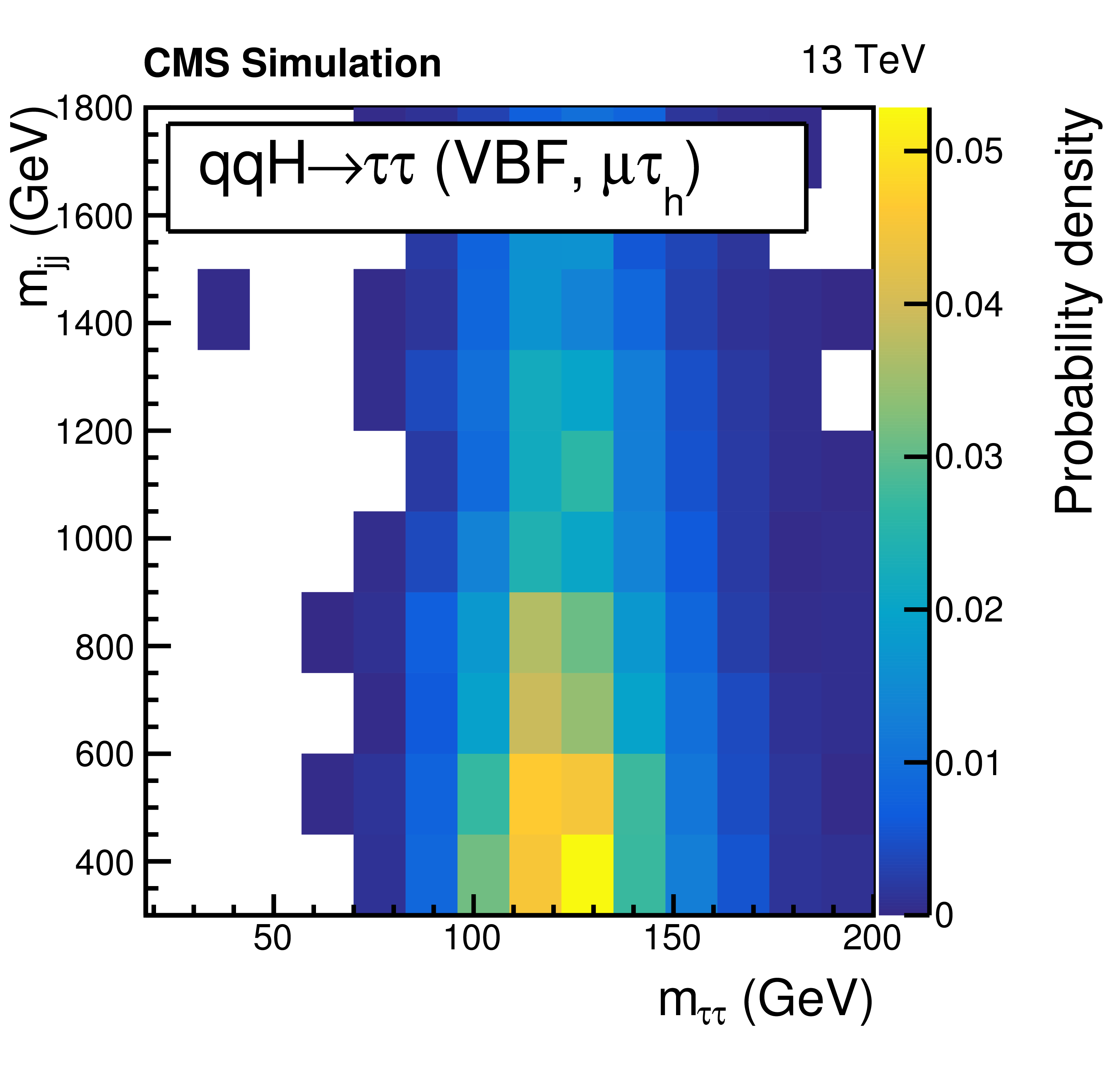
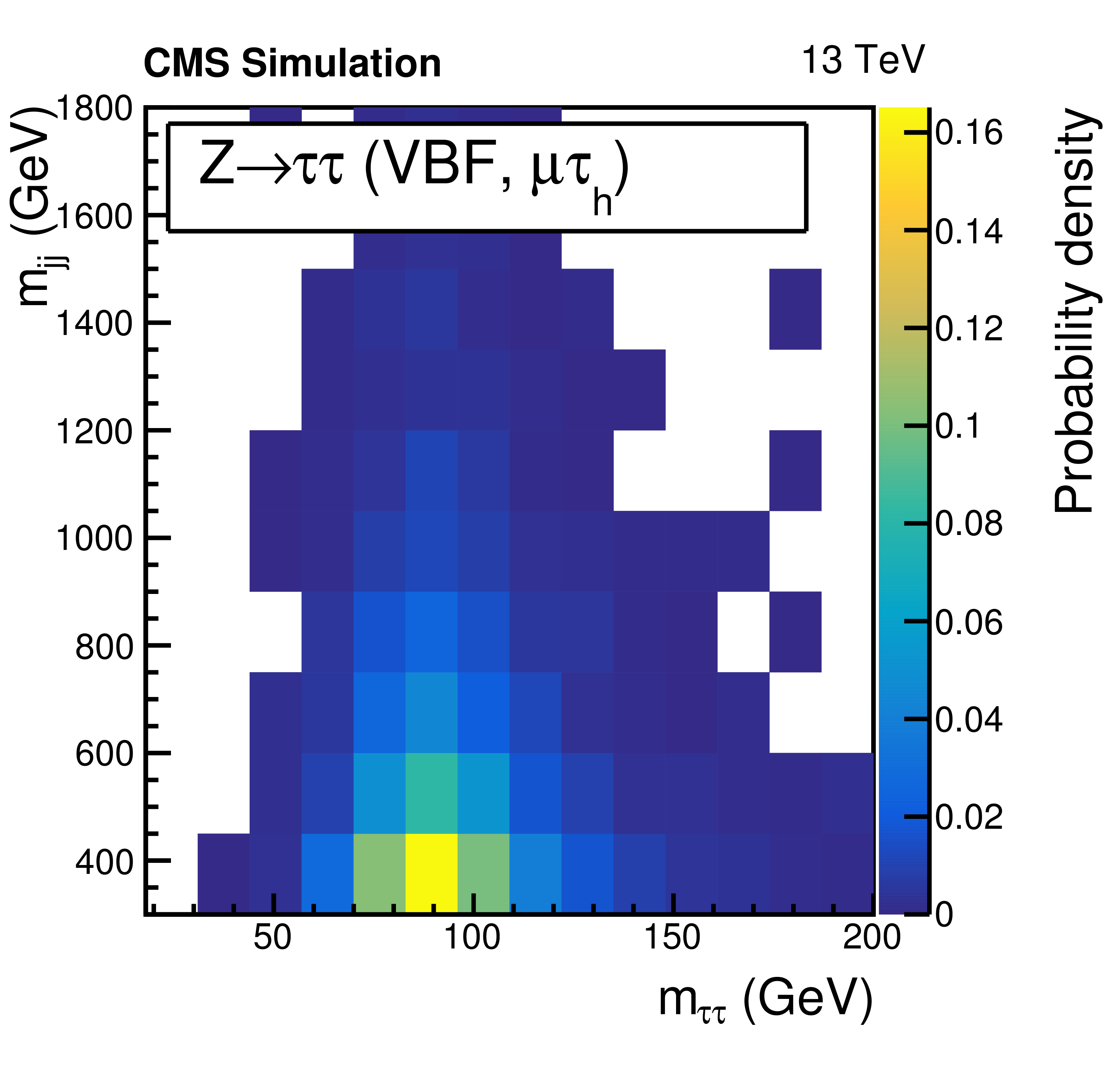
Figure 1-c:
Distribution of the $ {m_{\tau \tau }} $ observable for the signal in the VBF category and the $\mu {\tau _\mathrm {h}} $ decay channel. |
png pdf |
Figure 1-d:
Distribution of the $ {m_{\tau \tau }} $ observable for the $\mathrm{ Z } \to \tau \tau $ background in the VBF category the W+jets background in the boosted category and the $\mu {\tau _\mathrm {h}} $ decay channel. The background mostly lies at low $ {m_\mathrm {jj}} $ values whereas the distribution of VBF signal events extends to high $ {m_\mathrm {jj}} $ values. |

png pdf |
Figure 1-e:
Distribution of the $ {m_{\tau \tau }} $ observable for the signal in the boosted category and the $\mu {\tau _\mathrm {h}} $ decay channel. |

png pdf |
Figure 1-f:
Distribution of the $ {m_{\tau \tau }} $ observable for the W+jets background in the boosted category and the $\mu {\tau _\mathrm {h}} $ decay channel. The background behaves similarly to the QCD multijet background, is rather flat with respect to $ {m_{\tau \tau }} $, and is concentrated at low $ { {p_{\mathrm {T}}} ^{\tau \tau }} $ values. |
png pdf |
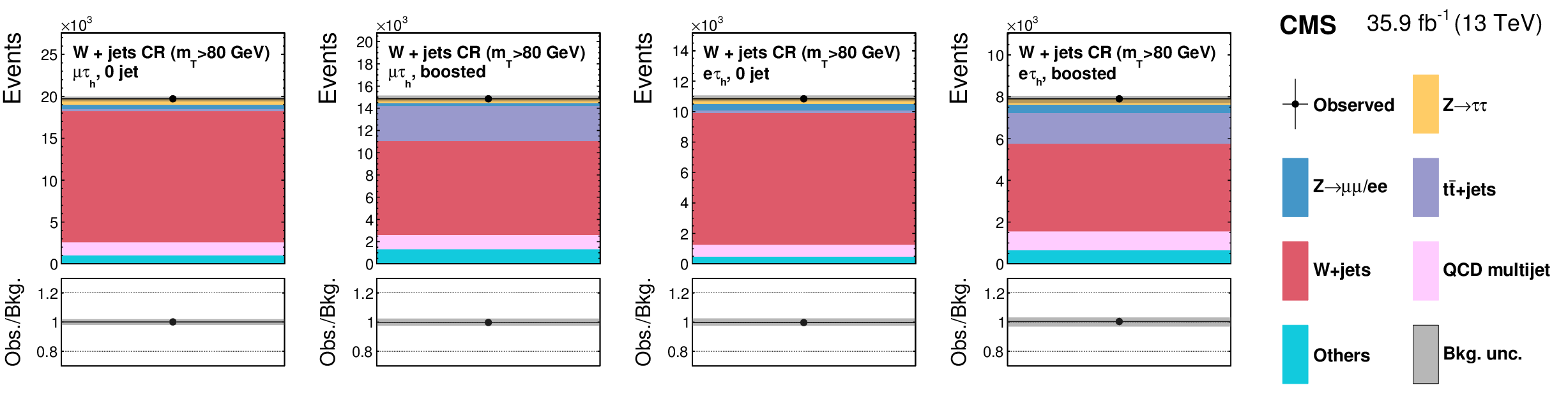
Figure 2:
Control regions enriched in the W+jets background used in the maximum likelihood fit, together with the signal regions, to extract the results. The normalization of the predicted background distributions corresponds to the result of the global fit. These regions, defined with $ {m_\mathrm {T}} > $ 80 GeV , control the yields of the W+jets background in the $\mu {\tau _\mathrm {h}} $ and $\mathrm{ e } {\tau _\mathrm {h}} $ channels. The constraints obtained in the boosted categories are propagated to the VBF categories of the corresponding channels. |
png pdf |
Figure 2-a:
Control region enriched in the W+jets background used in the maximum likelihood fit, together with the signal regions, to extract the results. This region, defined with $ {m_\mathrm {T}} > $ 80 GeV, controls the yield of the W+jets background for the $\mu {\tau _\mathrm {h}} $ channel in the 0-jet category. The normalization of the predicted background distribution corresponds to the result of the global fit. The legend is found on Fig.2-e. |
png pdf |
Figure 2-b:
Control region enriched in the W+jets background used in the maximum likelihood fit, together with the signal regions, to extract the results. This region, defined with $ {m_\mathrm {T}} > $ 80 GeV, controls the yield of the W+jets background for the $\mu {\tau _\mathrm {h}} $ channel in the boosted category. The normalization of the predicted background distribution corresponds to the result of the global fit. The legend is found on Fig.2-e. |

png pdf |
Figure 2-c:
Control region enriched in the W+jets background used in the maximum likelihood fit, together with the signal regions, to extract the results. This region, defined with $ {m_\mathrm {T}} > $ 80 GeV, controls the yield of the W+jets background for the $\mathrm{e} {\tau _\mathrm {h}} $ channel in the 0-jet category. The normalization of the predicted background distribution corresponds to the result of the global fit. The legend is found on Fig.2-e. |
png pdf |
Figure 2-d:
Control region enriched in the W+jets background used in the maximum likelihood fit, together with the signal regions, to extract the results. This region, defined with $ {m_\mathrm {T}} > $ 80 GeV, controls the yield of the W+jets background for the $\mathrm{e} {\tau _\mathrm {h}} $ channel in the boosted category. The normalization of the predicted background distribution corresponds to the result of the global fit. The legend is found on Fig.2-e. |

png pdf |
Figure 2-e:
Legend of Fig.2. |

png pdf |
Figure 3:
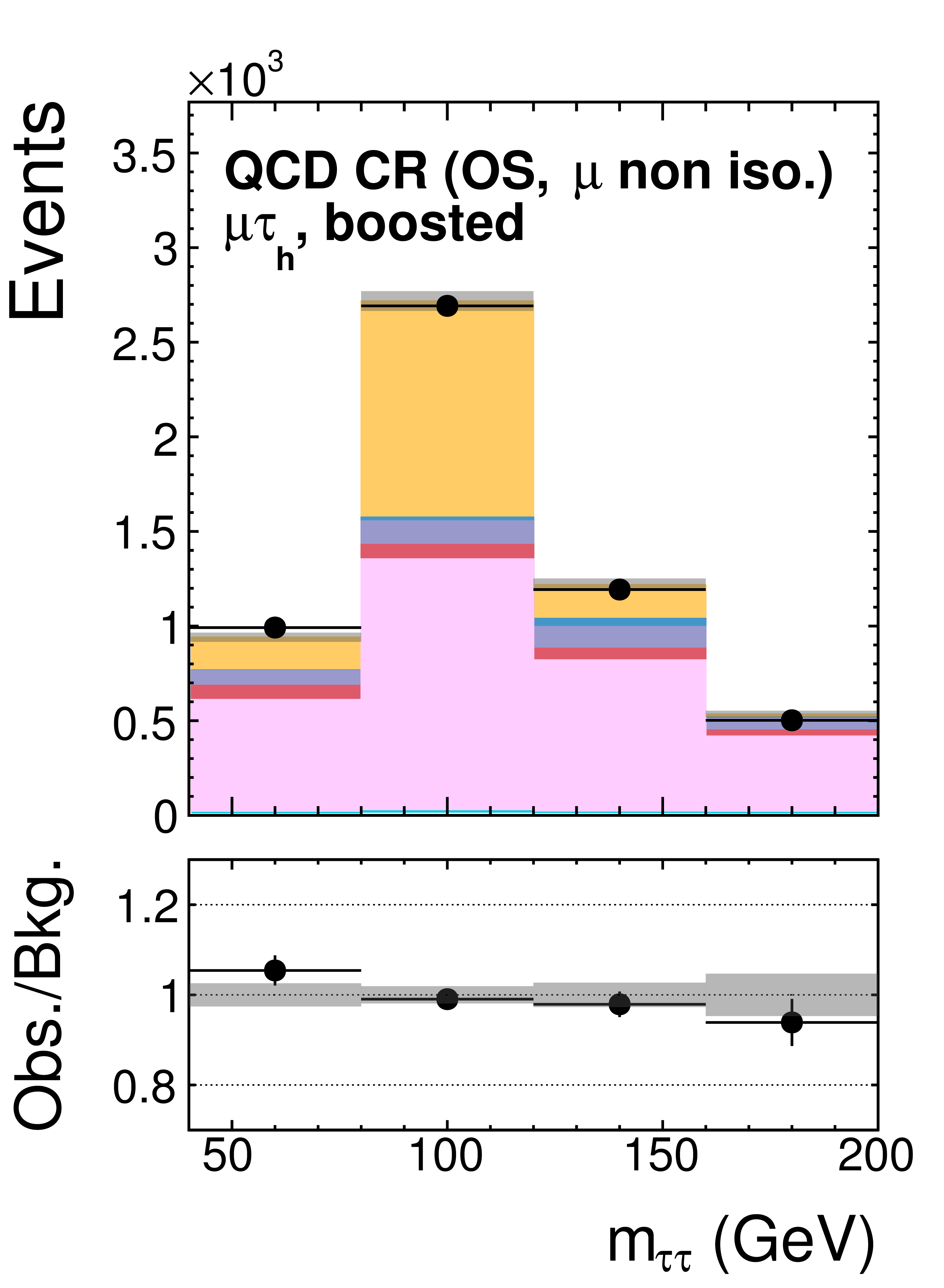
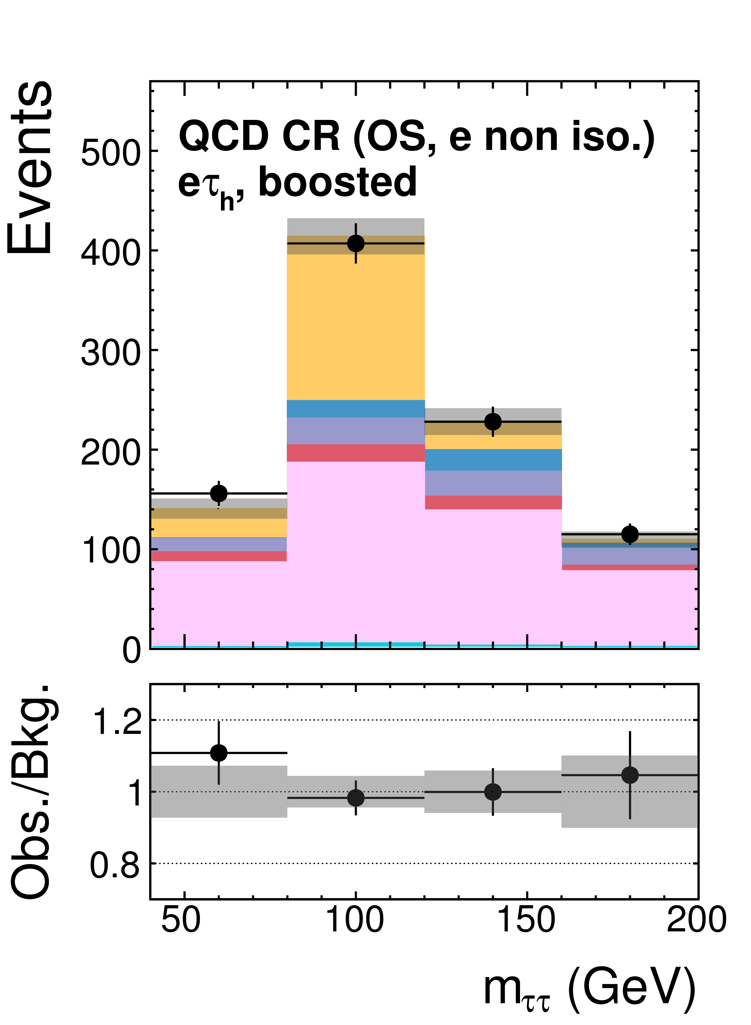
Control regions enriched in the QCD multijet background used in the maximum likelihood fit, together with the signal regions, to extract the results. The normalization of the predicted background distributions corresponds to the result of the global fit. These regions, defined by selecting events with opposite-sign $\ell $ and $ {\tau _\mathrm {h}} $ candidates with $\ell $ passing inverted isolation conditions, control the yields of the QCD multijet background in the $\mu {\tau _\mathrm {h}} $ and $\mathrm{ e } {\tau _\mathrm {h}} $ channels. The constraints obtained in the boosted categories are propagated to the VBF categories of the corresponding channels. |
png pdf |
Figure 3-a:
Control region enriched in the QCD multijet background used in the maximum likelihood fit, together with the signal regions, to extract the results. This region, defined by selecting events with opposite-sign $\ell $ and $ {\tau _\mathrm {h}} $ candidates with $\ell $ passing inverted isolation conditions, controls the yields of the QCD multijet background for the $\mu {\tau _\mathrm {h}} $ channel in the 0-jet category. The normalization of the predicted background distributions corresponds to the result of the global fit. The legend is found on Fig.3-c. |
png pdf |
Figure 3-b:
Control region enriched in the QCD multijet background used in the maximum likelihood fit, together with the signal regions, to extract the results. This region, defined by selecting events with opposite-sign $\ell $ and $ {\tau _\mathrm {h}} $ candidates with $\ell $ passing inverted isolation conditions, controls the yields of the QCD multijet background for the $\mu {\tau _\mathrm {h}} $ channel in the boosted category. The normalization of the predicted background distributions corresponds to the result of the global fit. The legend is found on Fig.3-c. |

png pdf |
Figure 3-c:
Legend of Fig.3. |

png pdf |
Figure 3-d:
Control region enriched in the QCD multijet background used in the maximum likelihood fit, together with the signal regions, to extract the results. This region, defined by selecting events with opposite-sign $\ell $ and $ {\tau _\mathrm {h}} $ candidates with $\ell $ passing inverted isolation conditions, controls the yields of the QCD multijet background for the $\mathrm{e} {\tau _\mathrm {h}} $ channel in the 0-jet category. The normalization of the predicted background distributions corresponds to the result of the global fit. The legend is found on Fig.3-c. |
png pdf |
Figure 3-e:
Control region enriched in the QCD multijet background used in the maximum likelihood fit, together with the signal regions, to extract the results. This region, defined by selecting events with opposite-sign $\ell $ and $ {\tau _\mathrm {h}} $ candidates with $\ell $ passing inverted isolation conditions, controls the yields of the QCD multijet background for the $\mathrm{e} {\tau _\mathrm {h}} $ channel in the boosted category. The normalization of the predicted background distributions corresponds to the result of the global fit. The legend is found on Fig.3-c. |
png pdf |
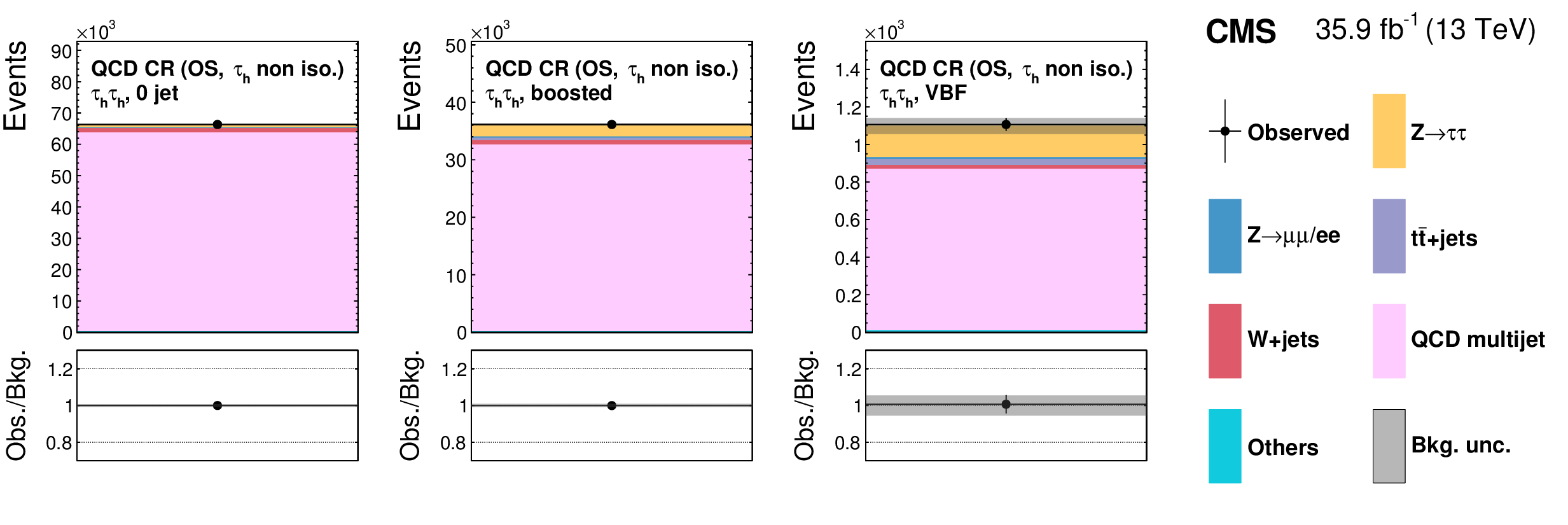
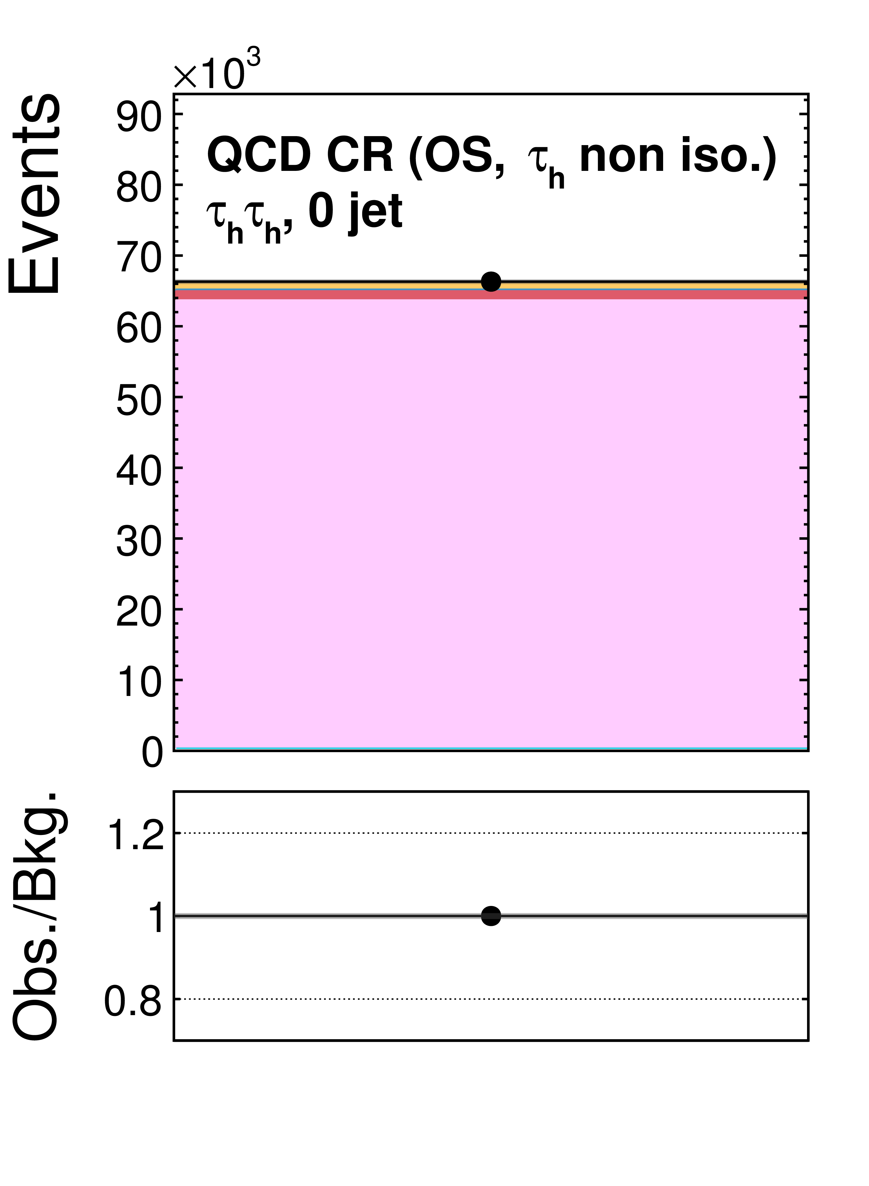
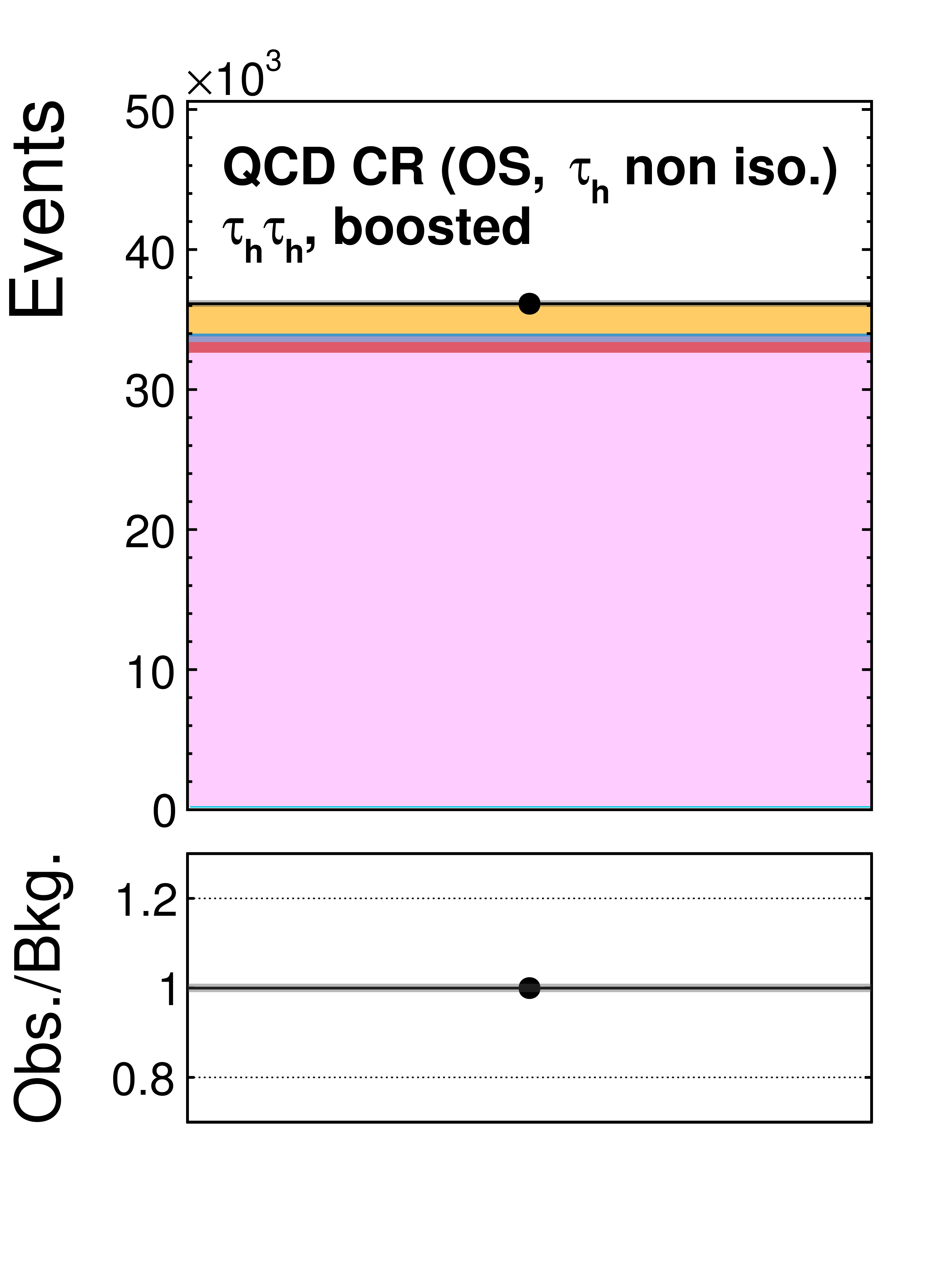
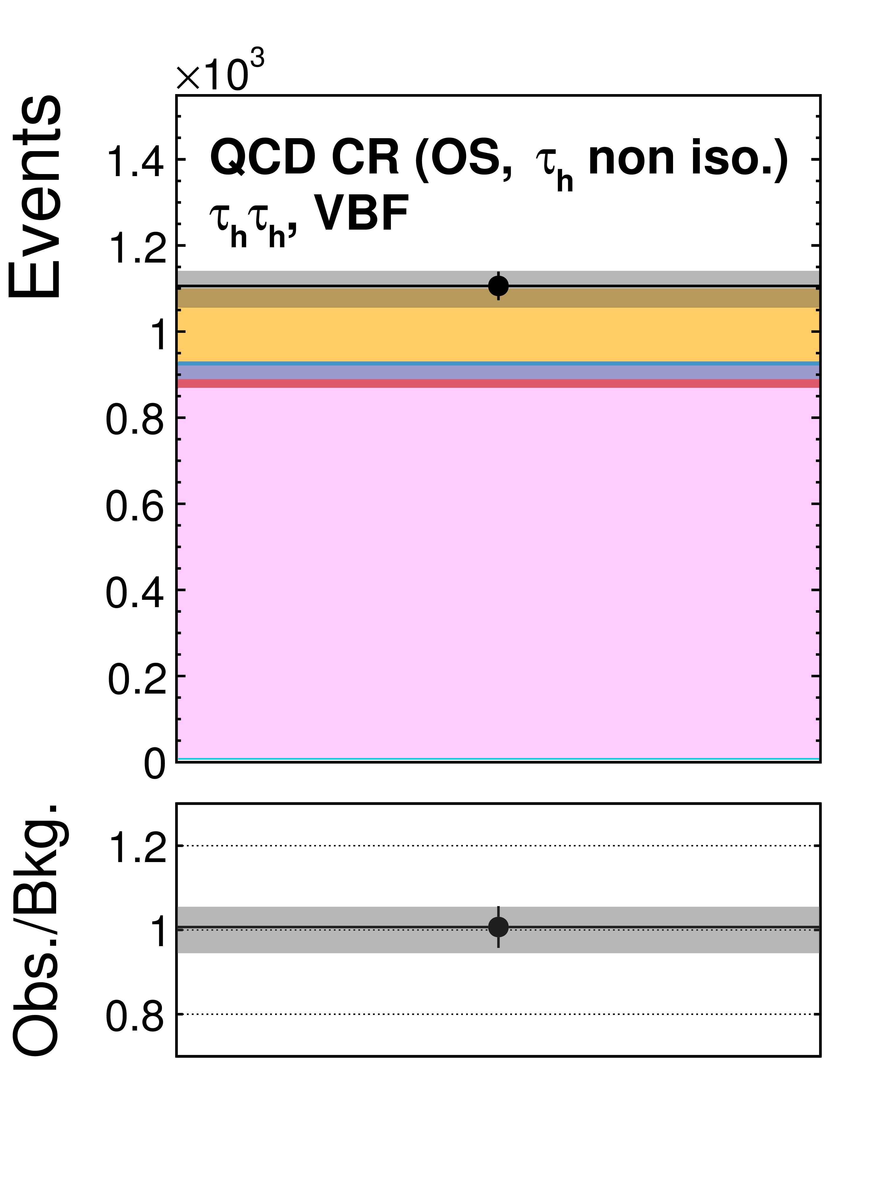
Figure 4:
Control regions enriched in the QCD multijet background used in the maximum likelihood fit, together with the signal regions, to extract the results. The normalization of the predicted background distributions corresponds to the result of the global fit. These regions, formed by selecting events with opposite-sign $ {\tau _\mathrm {h}} $ candidates passing relaxed isolation requirements, control the yields of the QCD multijet background in the $ {\tau _\mathrm {h}} {\tau _\mathrm {h}} $ channel. |
png pdf |
Figure 4-a:
Control region enriched in the QCD multijet background used in the maximum likelihood fit, together with the signal regions, to extract the results. This region, formed by selecting events with opposite-sign $ {\tau _\mathrm {h}} $ candidates passing relaxed isolation requirements, controls the yields of the QCD multijet background for the $ {\tau _\mathrm {h}} {\tau _\mathrm {h}} $ channel in the 0-jet category. The normalization of the predicted background distributions corresponds to the result of the global fit. The legend is found on Fig.4-d. |
png pdf |
Figure 4-b:
Control region enriched in the QCD multijet background used in the maximum likelihood fit, together with the signal regions, to extract the results. This region, formed by selecting events with opposite-sign $ {\tau _\mathrm {h}} $ candidates passing relaxed isolation requirements, controls the yields of the QCD multijet background for the $ {\tau _\mathrm {h}} {\tau _\mathrm {h}} $ channel in the boosted category. The normalization of the predicted background distributions corresponds to the result of the global fit. The legend is found on Fig.4-d. |
png pdf |
Figure 4-c:
Control region enriched in the QCD multijet background used in the maximum likelihood fit, together with the signal regions, to extract the results. This region, formed by selecting events with opposite-sign $ {\tau _\mathrm {h}} $ candidates passing relaxed isolation requirements, controls the yields of the QCD multijet background for the $ {\tau _\mathrm {h}} {\tau _\mathrm {h}} $ channel in the VBF category. The normalization of the predicted background distributions corresponds to the result of the global fit. The legend is found on Fig.4-d. |

png pdf |
Figure 4-d:
Legend of Fig.4. |

png pdf |
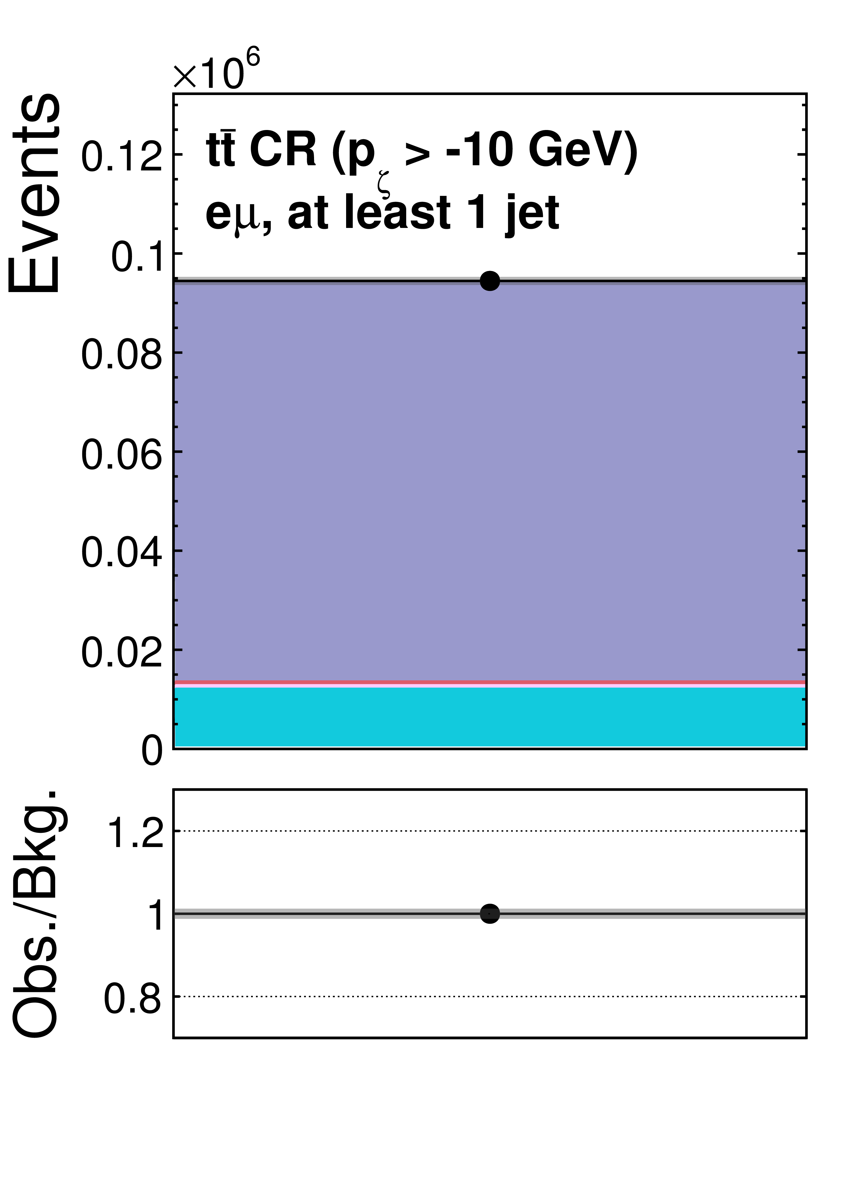
Figure 5:
Control region enriched in the ${\mathrm{ t } {}\mathrm{ \bar{t} } } $ background, used in the maximum likelihood fit, together with the signal regions, to extract the results. The normalization of the predicted background distributions corresponds to the result of the global fit. This region, defined by inverting the $p_\zeta $ requirement and rejecting events with no jet in the $\mathrm{ e } \mu $ final state, is used to estimate the yields of the ${\mathrm{ t } {}\mathrm{ \bar{t} } } $ background in all channels. |
png pdf |
Figure 5-a:
Control region enriched in the ${\mathrm{ t } {}\mathrm{ \bar{t} } } $ background, used in the maximum likelihood fit, together with the signal regions, to extract the results. The normalization of the predicted background distributions corresponds to the result of the global fit. This region, defined by inverting the $p_\zeta $ requirement and rejecting events with no jet in the $\mathrm{ e } \mu $ final state, is used to estimate the yields of the ${\mathrm{ t } {}\mathrm{ \bar{t} } } $ background in all channels. The legend is found on Fig.5-b. |
png pdf |
Figure 5-b:
Legend of Fig.5. |

png pdf |
Figure 6:
Observed and predicted 2D distributions in the VBF category of the $ {\tau _\mathrm {h}} {\tau _\mathrm {h}} $ decay channel. The normalization of the predicted background distributions corresponds to the result of the global fit. The signal distribution is normalized to its best fit signal strength. The background histograms are stacked. The "Others" background contribution includes events from diboson and single top quark production, as well as Higgs boson decays to a pair of W bosons. The background uncertainty band accounts for all sources of background uncertainty, systematic as well as statistical, after the global fit. The signal is shown both as a stacked filled histogram and an open overlaid histogram. |
png pdf |
Figure 7:
Observed and predicted 2D distributions in the VBF category of the $\mu {\tau _\mathrm {h}} $ decay channel. The description of the histograms is the same as in Fig. 6. |
png pdf |
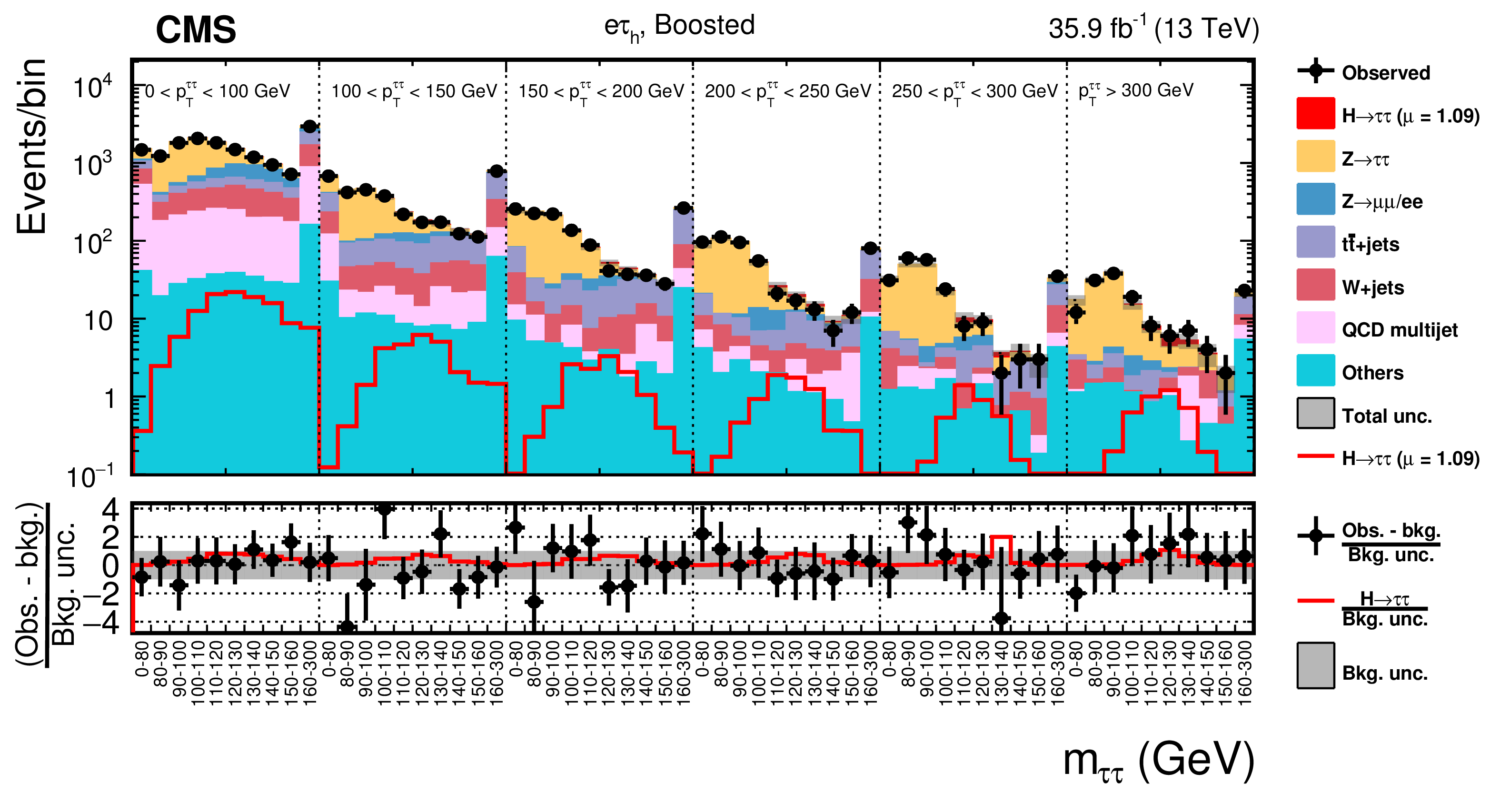
Figure 8:
Observed and predicted 2D distributions in the VBF category of the $\mathrm{ e } {\tau _\mathrm {h}} $ decay channel. The description of the histograms is the same as in Fig. 6. |
png pdf |
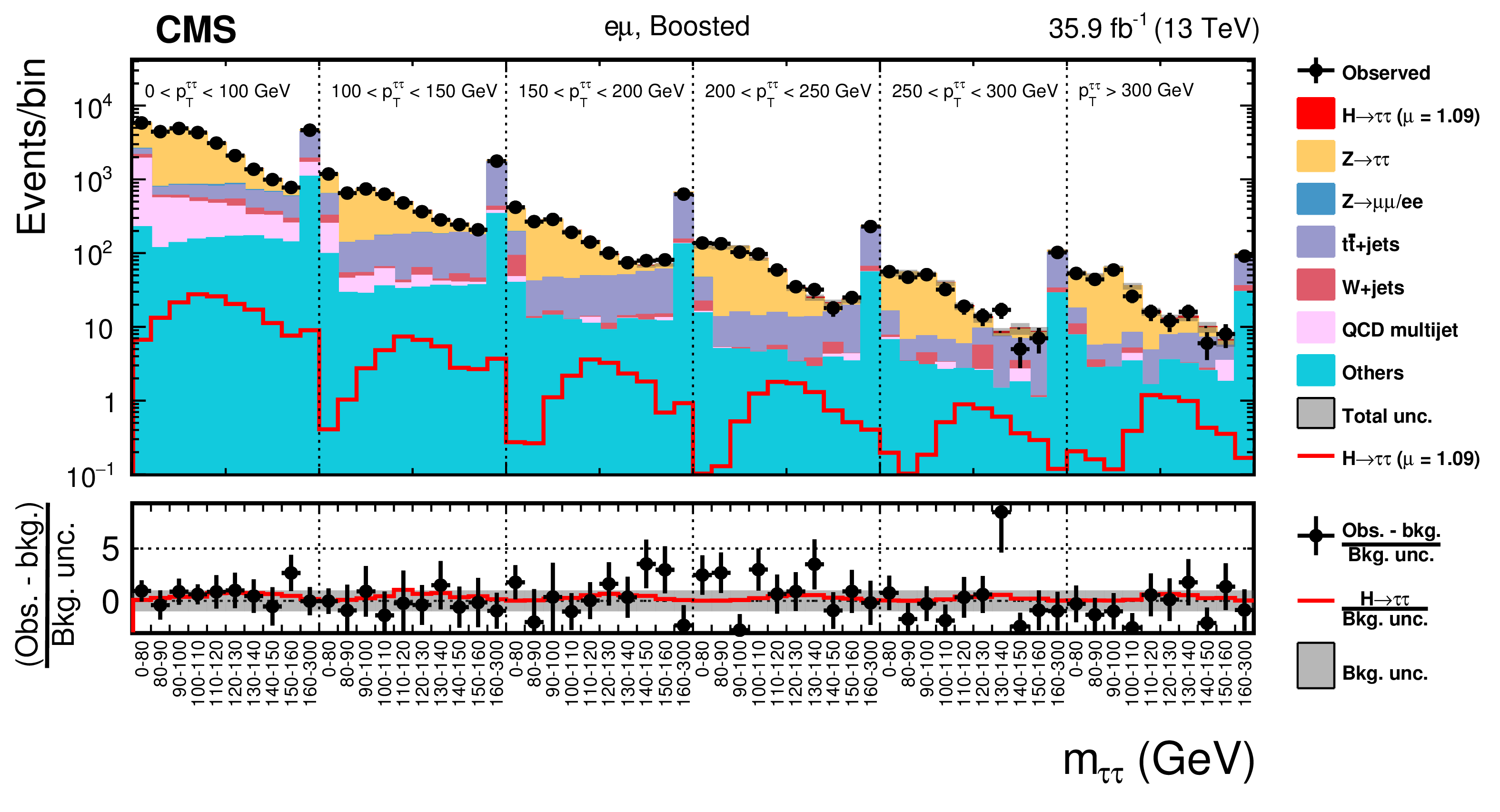
Figure 9:
Observed and predicted 2D distributions in the VBF category of the $\mathrm{ e } \mu $ decay channel. The description of the histograms is the same as in Fig. 6. |
png pdf |
Figure 10:
Observed and predicted 2D distributions in the boosted category of the $ {\tau _\mathrm {h}} {\tau _\mathrm {h}} $ decay channel. The description of the histograms is the same as in Fig. 6. |

png pdf |
Figure 11:
Observed and predicted 2D distributions in the boosted category of the $\mu {\tau _\mathrm {h}} $ decay channel. The description of the histograms is the same as in Fig. 6. |
png pdf |
Figure 12:
Observed and predicted 2D distributions in the boosted category of the $\mathrm{ e } {\tau _\mathrm {h}} $ decay channel. The description of the histograms is the same as in Fig. 6. |
png pdf |
Figure 13:
Observed and predicted 2D distributions in the boosted category of the $\mathrm{ e } \mu $ decay channel. The description of the histograms is the same as in Fig. 6. |
png pdf |
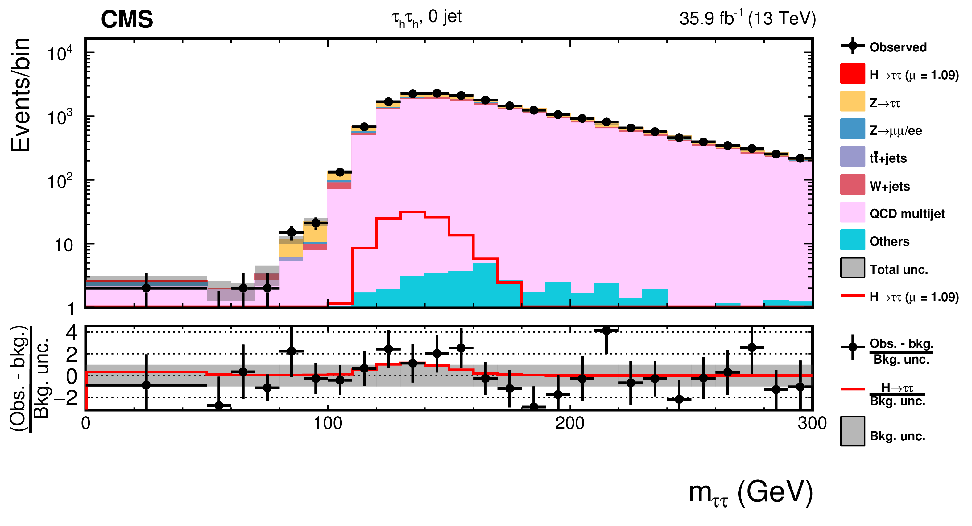
Figure 14:
Observed and predicted distributions in the 0-jet category of the $ {\tau _\mathrm {h}} {\tau _\mathrm {h}} $ decay channel. The description of the histograms is the same as in Fig. 6. |
png pdf |
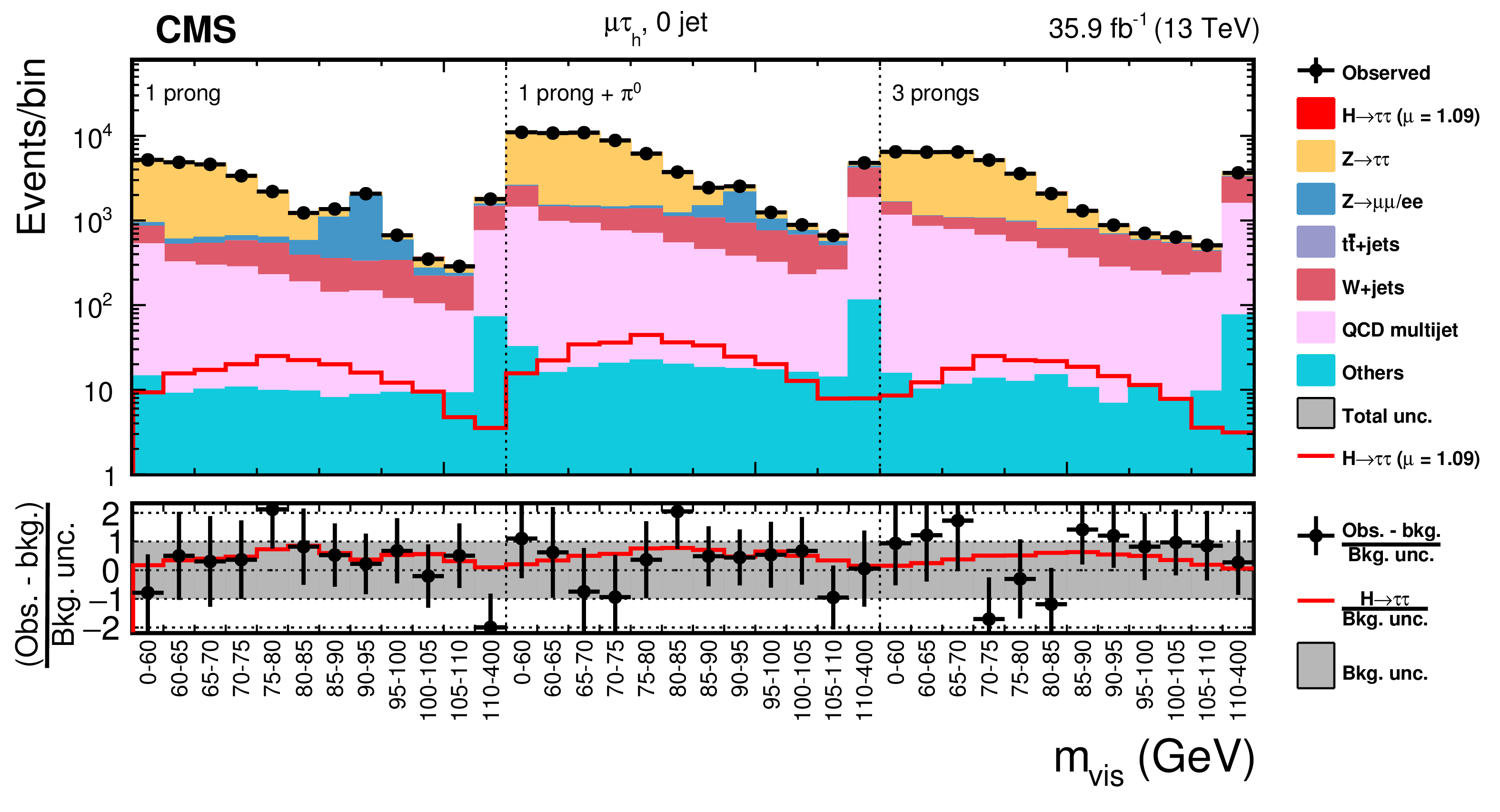
Figure 15:
Observed and predicted 2D distributions in the 0-jet category of the $\mu {\tau _\mathrm {h}} $ decay channel. The description of the histograms is the same as in Fig. 6. |
png pdf |
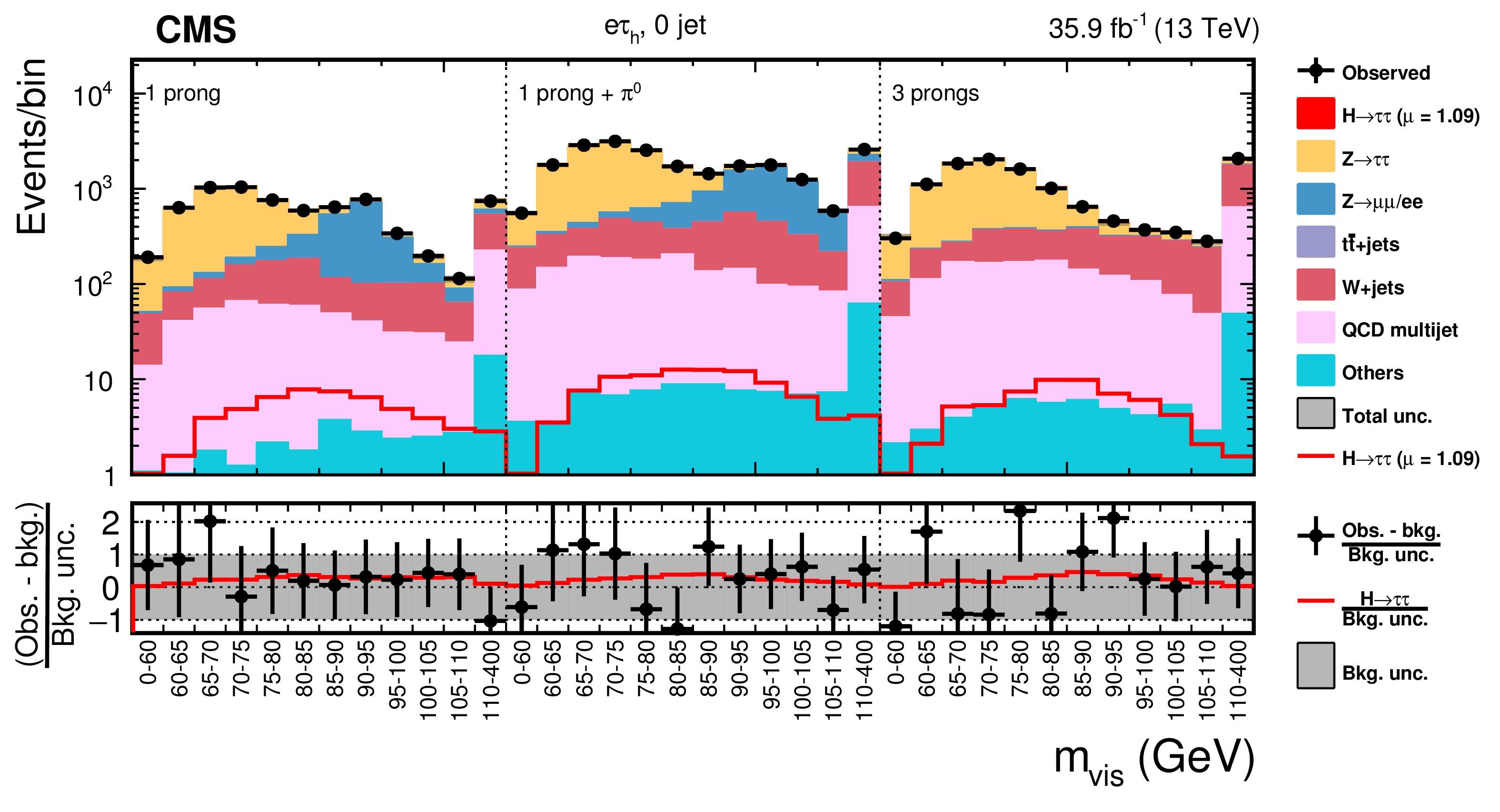
Figure 16:
Observed and predicted 2D distributions in the 0-jet category of the $\mathrm{ e } {\tau _\mathrm {h}} $ decay channel. The description of the histograms is the same as in Fig. 6. |
png pdf |
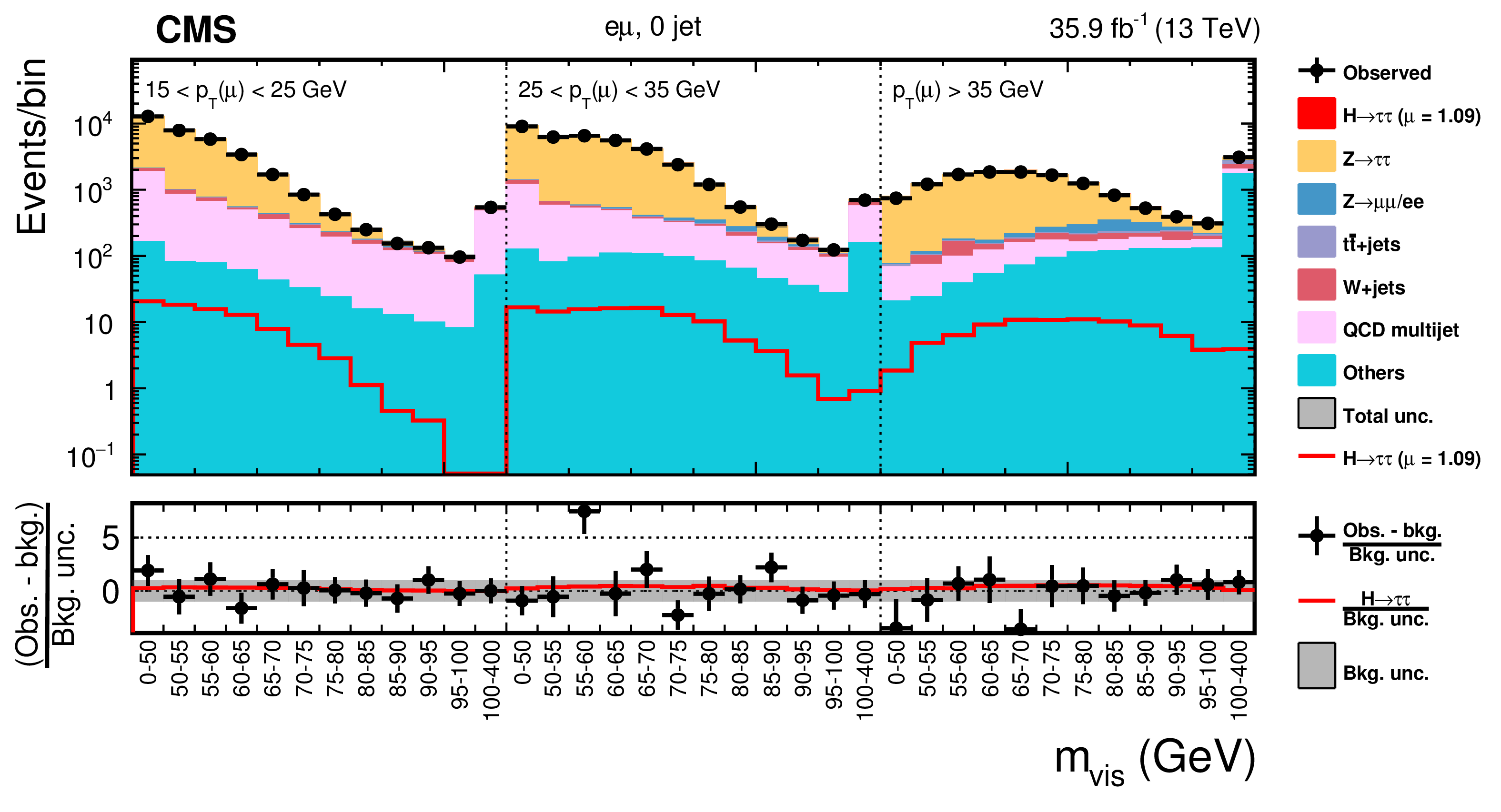
Figure 17:
Observed and predicted 2D distributions in the 0-jet category of the $\mathrm{ e } \mu $ decay channel. The description of the histograms is the same as in Fig. 6. |

png pdf |
Figure 18:
Distribution of the decimal logarithm of the ratio between the expected signal and the sum of expected signal and expected background in each bin of the mass distributions used to extract the results, in all signal regions. The background contributions are separated by decay channel. The inset shows the corresponding difference between the observed data and expected background distributions divided by the background expectation, as well as the signal expectation divided by the background expectation. |
png pdf |
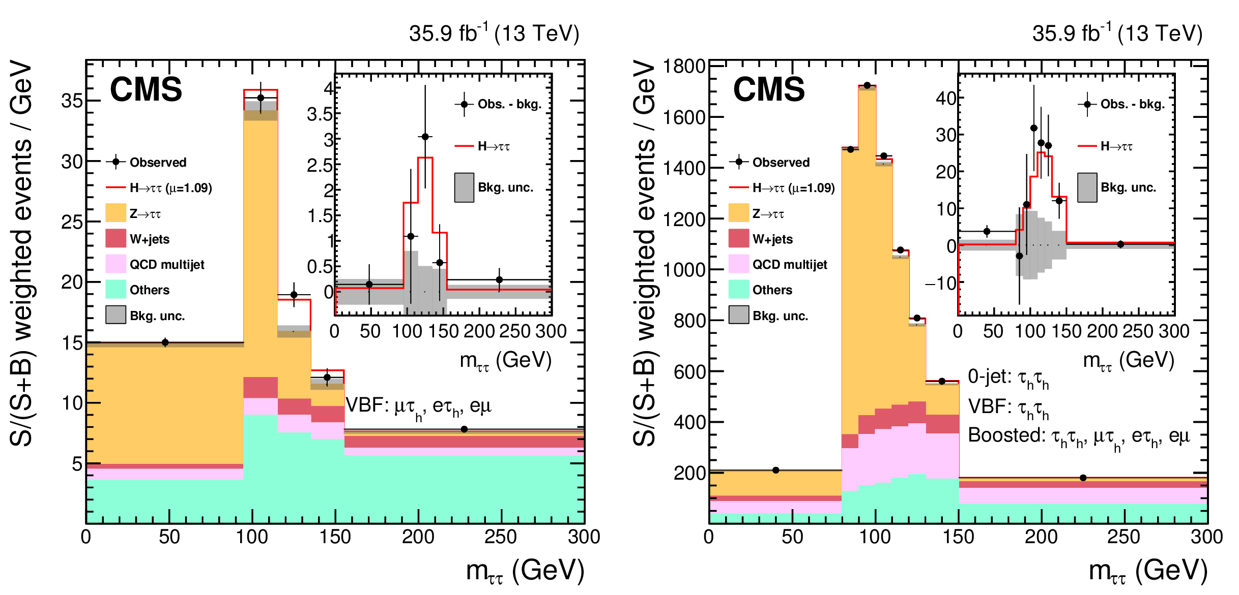
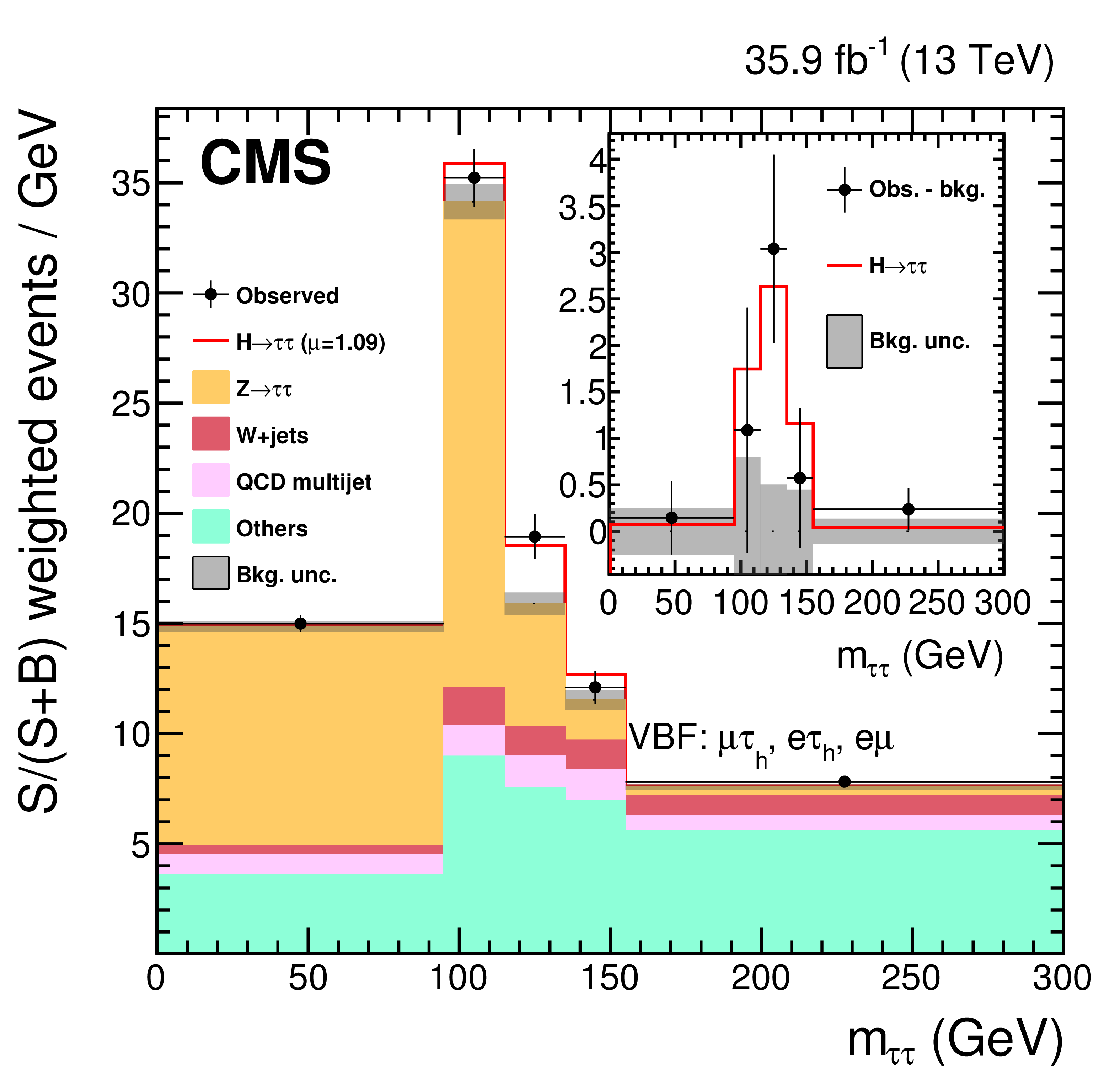
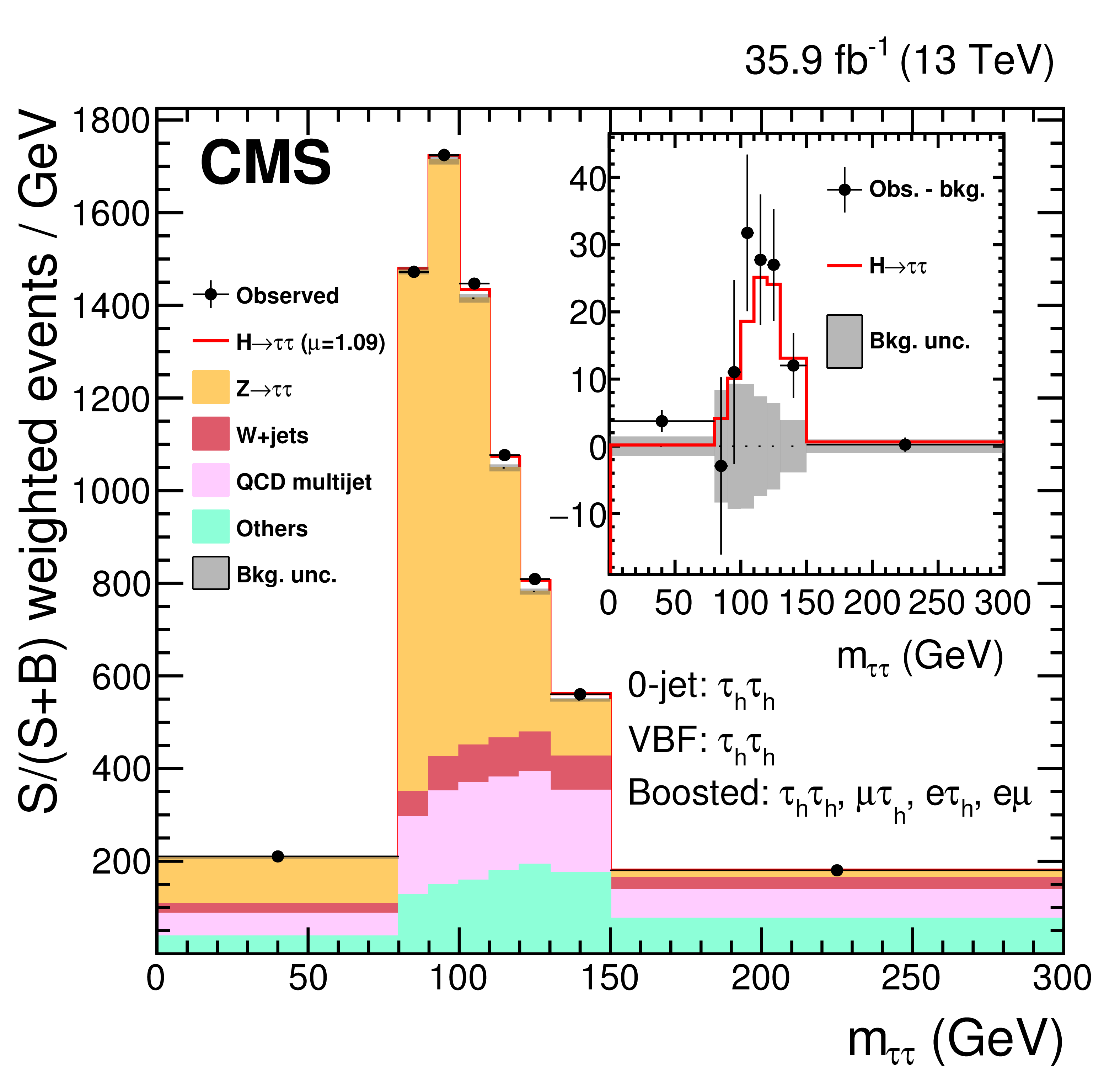
Figure 19:
Combined observed and predicted $ {m_{\tau \tau }} $ distributions. The leftpane includes the VBF category of the $\mu {\tau _\mathrm {h}} $, $\mathrm{ e } {\tau _\mathrm {h}} $ and $\mathrm{ e } \mu $ channels, and the rightpane includes all other channels that make use of $ {m_{\tau \tau }} $ instead of $ {m_\text {vis}} $ for the signal strength fit. The binning reflects the one used in the 2D distributions, and does not allow merging of the two figures. The normalization of the predicted background distributions corresponds to the result of the global fit, while the signal is normalized to its best fit signal strength. The mass distributions for a constant range of the second dimension of the signal distributions are weighted according to $S/(S+B)$, where $S$ and $B$ are computed, respectively, as the signal or background contribution in the mass distribution excluding the first and last bins. The "Others" background contribution includes events from diboson, ${\mathrm{ t } {}\mathrm{ \bar{t} } } $, and single top quark production, as well as Higgs boson decay to a pair of W bosons and $\mathrm{ Z } $ bosons decaying to a pair of light leptons. The background uncertainty band accounts for all sources of background uncertainty, systematic as well as statistical, after the global fit. The inset shows the corresponding difference between the observed data and expected background distributions, together with the signal expectation. The signal yield is not affected by the reweighting. |
png pdf |
Figure 19-a:
Combined observed and predicted $ {m_{\tau \tau }} $ distribution that includes the VBF category of the $\mu {\tau _\mathrm {h}} $, $\mathrm{ e } {\tau _\mathrm {h}} $ and $\mathrm{ e } \mu $ channels. The binning reflects the one used in the 2D distributions, and does not allow merging of the two figures. The normalization of the predicted background distributions corresponds to the result of the global fit, while the signal is normalized to its best fit signal strength. The mass distributions for a constant range of the second dimension of the signal distributions are weighted according to $S/(S+B)$, where $S$ and $B$ are computed, respectively, as the signal or background contribution in the mass distribution excluding the first and last bins. The "Others" background contribution includes events from diboson, ${\mathrm{ t } {}\mathrm{ \bar{t} } } $, and single top quark production, as well as Higgs boson decay to a pair of W bosons and $\mathrm{ Z } $ bosons decaying to a pair of light leptons. The background uncertainty band accounts for all sources of background uncertainty, systematic as well as statistical, after the global fit. The inset shows the corresponding difference between the observed data and expected background distributions, together with the signal expectation. The signal yield is not affected by the reweighting. |
png pdf |
Figure 19-b:
Combined observed and predicted $ {m_{\tau \tau }} $ distribution that includes all channels other than the VBF category of the $\mu {\tau _\mathrm {h}} $, $\mathrm{ e } {\tau _\mathrm {h}} $ and $\mathrm{ e } \mu $ channels that make use of $ {m_{\tau \tau }} $ instead of $ {m_\text {vis}} $ for the signal strength fit. The binning reflects the one used in the 2D distributions, and does not allow merging of the two figures. The normalization of the predicted background distributions corresponds to the result of the global fit, while the signal is normalized to its best fit signal strength. The mass distributions for a constant range of the second dimension of the signal distributions are weighted according to $S/(S+B)$, where $S$ and $B$ are computed, respectively, as the signal or background contribution in the mass distribution excluding the first and last bins. The "Others" background contribution includes events from diboson, ${\mathrm{ t } {}\mathrm{ \bar{t} } } $, and single top quark production, as well as Higgs boson decay to a pair of W bosons and $\mathrm{ Z } $ bosons decaying to a pair of light leptons. The background uncertainty band accounts for all sources of background uncertainty, systematic as well as statistical, after the global fit. The inset shows the corresponding difference between the observed data and expected background distributions, together with the signal expectation. The signal yield is not affected by the reweighting. |

png pdf |
Figure 20:
Local ${p}$-value and significance as a function of the SM Higgs boson mass hypothesis. The observation (red, solid) is compared to the expectation (blue, dashed) for a Higgs boson with a mass $ {m_{\mathrm{ H } }} = $ 125.09 GeV. The background includes Higgs boson decays to pairs of W bosons, with $ {m_{\mathrm{ H } }} = $ 125.09 GeV. |

png pdf |
Figure 21:
Best fit signal strength per category (left) and channel (right), for $ {m_{\mathrm{ H } }} = $ 125.09 GeV. The constraints from the global fit are used to extract each of the individual best fit signal strengths. The combined best fit signal strength is $\mu = $ 1.09$ ^{+0.27} _{-0.26}$. |

png pdf |
Figure 21-a:
Best fit signal strength per category, for $ {m_{\mathrm{ H } }} = $ 125.09 GeV. The constraints from the global fit are used to extract each of the individual best fit signal strengths. The combined best fit signal strength is $\mu = $ 1.09$ ^{+0.27} _{-0.26}$. |

png pdf |
Figure 21-b:
Best fit signal strength per channel, for $ {m_{\mathrm{ H } }} = $ 125.09 GeV. The constraints from the global fit are used to extract each of the individual best fit signal strengths. The combined best fit signal strength is $\mu = $ 1.09$ ^{+0.27} _{-0.26}$. |

png pdf |
Figure 22:
Scan of the negative log-likelihood difference as a function of $\kappa _V$ and $\kappa _f$, for $ {m_{\mathrm{ H } }} = $ 125.09 GeV. All nuisance parameters are profiled for each point. For this scan, the $\mathrm{ p } \mathrm{ p } \to \mathrm{ H } \to \mathrm{ W } \mathrm{ W } $ contribution is treated as a signal process. |
| Tables | |

png pdf |
Table 1:
Kinematic selection requirements for the four di-$\tau $ decay channels. The trigger requirement is defined by a combination of trigger candidates with $ {p_{\mathrm {T}}} $ over a given threshold (in GeV ), indicated inside parentheses. The pseudorapidity thresholds come from trigger and object reconstruction constraints. The $ {p_{\mathrm {T}}} $ thresholds for the lepton selection are driven by the trigger requirements, except for the leading $ {\tau _\mathrm {h}} $ candidate in the $ {\tau _\mathrm {h}} {\tau _\mathrm {h}} $ channel, the $ {\tau _\mathrm {h}} $ candidate in the $\mu {\tau _\mathrm {h}} $ and $\mathrm{ e } {\tau _\mathrm {h}} $ channels, and the muon in the $\mathrm{ e } \mu $ channel, where they have been optimized to increase the significance of the analysis. |

png pdf |
Table 2:
Category selection and observables used to build the 2D kinematic distributions. The events neither selected in the 0-jet nor in the VBF category are included in the boosted category, as denoted by "Others". |
png pdf |
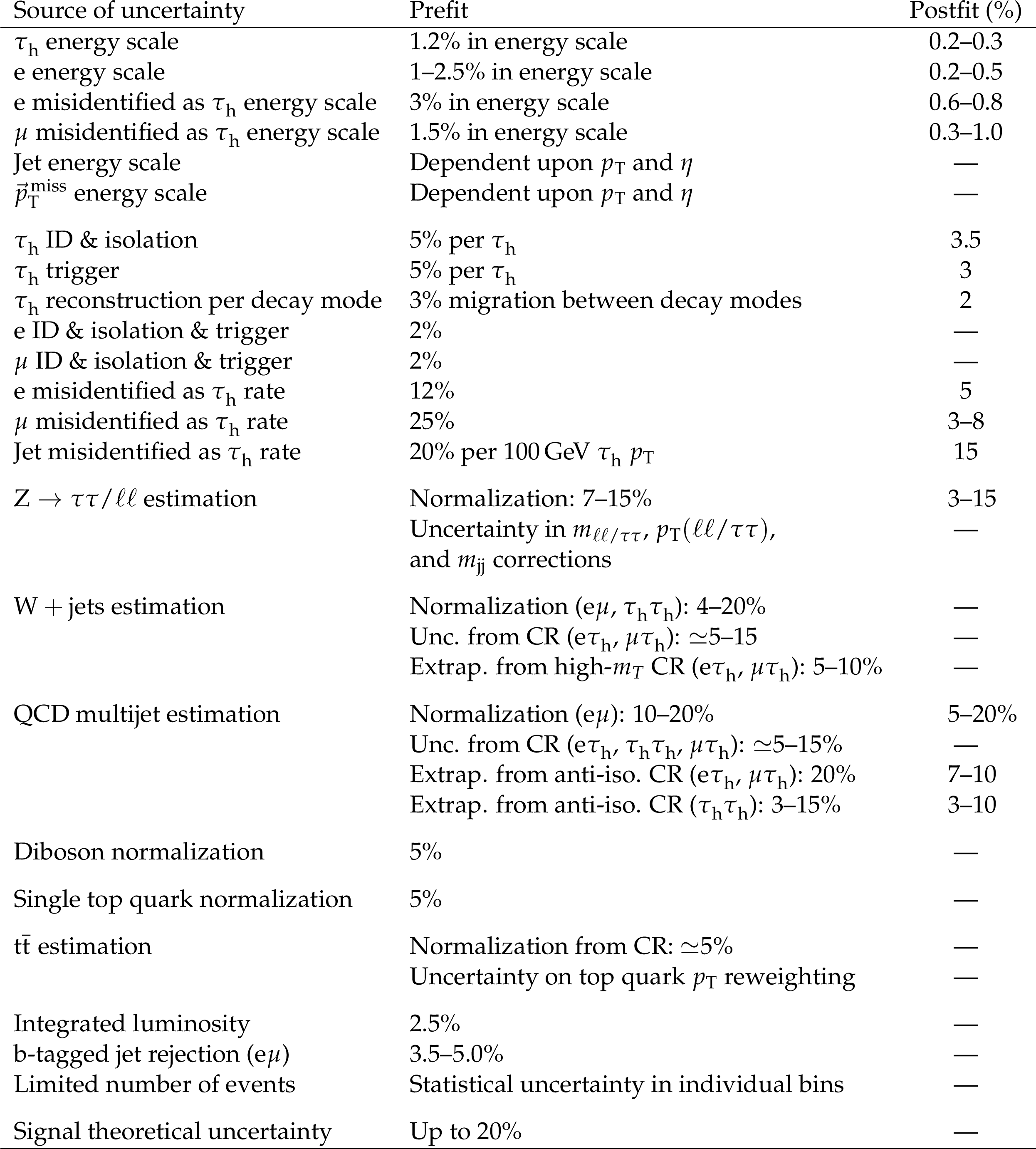
Table 3:
Sources of systematic uncertainty. If the global fit to the signal and control regions, described in the next section, significantly constrains these uncertainties, the values of the uncertainties after the global fit are indicated in the third column. The acronyms CR and ID stand for control region and identification, respectively. |

png pdf |
Table 4:
Background and signal expectations, together with the number of observed events, for bins in the signal region for which $\log_{10}(S/(S+B))>-0.9$, where $S$ and $B$ are, respectively, the number of expected signal events for a Higgs boson with a mass $ {m_{\mathrm{ H } }} = $ 125.09 GeV and of expected background events, in those bins. The background uncertainty accounts for all sources of background uncertainty, systematic as well as statistical, after the global fit. The contribution from "other backgrounds" includes events from diboson and single top quark production, as well as Higgs boson decays to a pair of W bosons. |
| Summary |
| A measurement of the coupling of the Higgs boson to $\tau$ leptons, based on data collected in pp collisions with the CMS detector in 2016 at a center-of-mass energy of 13 TeV, has been presented. Event categories are designed to separately target Higgs boson signal events produced by gluon or vector boson fusion. The results are extracted via maximum likelihood fits in two-dimensional planes, and give an observed significance for Higgs boson decays to $\tau$ lepton pairs of 4.9 standard deviations, to be compared with an expected significance of 4.7 standard deviations. The combination with the corresponding measurement performed at center-of-mass energies of 7 and 8 TeV with the CMS detector leads to the first observation by a single experiment of decays of the Higgs boson to pairs of $\tau$ leptons, with a significance of 5.9 standard deviations. |
| References | ||||
| 1 | S. L. Glashow | Partial-symmetries of weak interactions | NP 22 (1961) 579 | |
| 2 | S. Weinberg | A model of leptons | PRL 19 (1967) 1264 | |
| 3 | A. Salam | Weak and electromagnetic interactions | in Elementary particle physics: relativistic groups and analyticity, 1968, Proceedings of the eighth Nobel symposium | |
| 4 | F. Englert and R. Brout | Broken symmetry and the mass of gauge vector mesons | PRL 13 (1964) 321 | |
| 5 | P. W. Higgs | Broken symmetries, massless particles and gauge fields | PL12 (1964) 132 | |
| 6 | P. W. Higgs | Broken symmetries and the masses of gauge bosons | PRL 13 (1964) 508 | |
| 7 | G. S. Guralnik, C. R. Hagen, and T. W. B. Kibble | Global conservation laws and massless particles | PRL 13 (1964) 585 | |
| 8 | P. W. Higgs | Spontaneous symmetry breakdown without massless bosons | PR145 (1966) 1156 | |
| 9 | T. W. B. Kibble | Symmetry Breaking in Non-Abelian Gauge Theories | PR155 (1967) 1554 | |
| 10 | ATLAS Collaboration | Observation of a new particle in the search for the Standard Model Higgs boson with the ATLAS detector at the LHC | PLB 716 (2012) 1 | 1207.7214 |
| 11 | CMS Collaboration | Observation of a new boson at a mass of 125 GeV with the CMS experiment at the LHC | PLB 716 (2012) 30 | CMS-HIG-12-028 1207.7235 |
| 12 | CMS Collaboration | Observation of a new boson with mass near 125 GeV in pp collisions at $ \sqrt{s} = $ 7 and 8 TeV | JHEP 06 (2013) 081 | CMS-HIG-12-036 1303.4571 |
| 13 | ATLAS Collaboration | Measurements of the Higgs boson production and decay rates and coupling strengths using pp collision data at $ \sqrt{s}= $ 7 and 8 TeV in the ATLAS experiment | EPJC 76 (2016) 6 | 1507.04548 |
| 14 | CMS Collaboration | Precise determination of the mass of the Higgs boson and tests of compatibility of its couplings with the standard model predictions using proton collisions at 7 and 8 TeV | EPJC 75 (2015) 212 | CMS-HIG-14-009 1412.8662 |
| 15 | CMS Collaboration | Study of the mass and spin-parity of the Higgs boson candidate via its decays to Z boson pairs | PRL 110 (2013) 081803 | CMS-HIG-12-041 1212.6639 |
| 16 | ATLAS Collaboration | Evidence for the spin-0 nature of the Higgs boson using ATLAS data | PLB 726 (2013) 120 | 1307.1432 |
| 17 | CMS Collaboration | Constraints on the spin-parity and anomalous HVV couplings of the Higgs boson in proton collisions at 7 and 8 TeV | PRD 92 (2015) 012004 | CMS-HIG-14-018 1411.3441 |
| 18 | CMS Collaboration | Measurements of properties of the Higgs boson decaying into the four-lepton final state in pp collisions at $ \sqrt{s} = $ 13 TeV | Submitted to JHEP | CMS-HIG-16-041 1706.09936 |
| 19 | ATLAS and CMS Collaboration | Combined measurement of the Higgs boson mass in $ pp $ collisions at $ \sqrt{s}= $ 7 and 8 TeV with the ATLAS and CMS experiments | PRL 114 (2015) 191803 | 1503.07589 |
| 20 | ALEPH Collaboration | Observation of an excess in the search for the Standard Model Higgs boson at ALEPH | PLB 495 (2000) 1 | hep-ex/0011045 |
| 21 | DELPHI Collaboration | Final results from DELPHI on the searches for SM and MSSM neutral Higgs bosons | EPJC 32 (2004) 145 | hep-ex/0303013 |
| 22 | L3 Collaboration | Standard model Higgs boson with the L3 experiment at LEP | PLB 517 (2001) 319 | hep-ex/0107054 |
| 23 | OPAL Collaboration | Search for the Standard Model Higgs boson in e$ ^+ $e$ ^- $ collisions at $ \sqrt{s} = $ 192--209 GeV | PLB 499 (2001) 38 | hep-ex/0101014 |
| 24 | CDF Collaboration | Search for a low-mass standard model Higgs boson in the $ \tau \tau $ decay channel in $ {p}\bar{{p}} $ collisions at $ \sqrt{s} = $ 1.96 TeV | PRL 108 (2012) 181804 | 1201.4880 |
| 25 | D0 Collaboration | Search for the standard model Higgs boson in tau lepton final states | PLB 714 (2012) 237 | 1203.4443 |
| 26 | CMS Collaboration | Evidence for the 125 GeV Higgs boson decaying to a pair of $ \tau $ leptons | JHEP 05 (2014) 104 | CMS-HIG-13-004 1401.5041 |
| 27 | ATLAS Collaboration | Evidence for the Higgs-boson Yukawa coupling to tau leptons with the ATLAS detector | JHEP 04 (2015) 117 | 1501.04943 |
| 28 | ATLAS, CMS Collaboration | Measurements of the Higgs boson production and decay rates and constraints on its couplings from a combined ATLAS and CMS analysis of the LHC pp collision data at $ \sqrt{s}= $ 7 and 8 TeV | JHEP 08 (2016) 045 | 1606.02266 |
| 29 | CMS Collaboration | The CMS trigger system | JINST 12 (2017) P01020 | CMS-TRG-12-001 1609.02366 |
| 30 | CMS Collaboration | The CMS experiment at the CERN LHC | JINST 3 (2008) S08004 | CMS-00-001 |
| 31 | P. Nason | A new method for combining NLO QCD with shower Monte Carlo algorithms | JHEP 11 (2004) 040 | hep-ph/0409146 |
| 32 | S. Frixione, P. Nason, and C. Oleari | Matching NLO QCD computations with parton shower simulations: the POWHEG method | JHEP 11 (2007) 070 | 0709.2092 |
| 33 | S. Alioli, P. Nason, C. Oleari, and E. Re | A general framework for implementing NLO calculations in shower Monte Carlo programs: the POWHEG BOX | JHEP 06 (2010) 043 | 1002.2581 |
| 34 | S. Alioli et al. | Jet pair production in POWHEG | JHEP 04 (2011) 081 | 1012.3380 |
| 35 | S. Alioli, P. Nason, C. Oleari, and E. Re | NLO Higgs boson production via gluon fusion matched with shower in POWHEG | JHEP 04 (2009) 002 | 0812.0578 |
| 36 | G. Luisoni, P. Nason, C. Oleari, and F. Tramontano | $ HW^{\pm}/HZ + 0 $ and 1 jet at NLO with the POWHEG BOX interfaced to GoSam and their merging within MiNLO | JHEP 10 (2013) 083 | 1306.2542 |
| 37 | R. D. Ball et al. | Unbiased global determination of parton distributions and their uncertainties at NNLO and at LO | NPB 855 (2012) 153 | 1107.2652 |
| 38 | D. de Florian et al. | Handbook of LHC Higgs cross sections: 4. deciphering the nature of the Higgs sector | CERN-2017-002-M | 1610.07922 |
| 39 | A. Denner et al. | Standard model Higgs-boson branching ratios with uncertainties | EPJC 71 (2011) 1753 | 1107.5909 |
| 40 | NNPDF Collaboration | Impact of heavy quark masses on parton distributions and LHC phenomenology | NPB 849 (2011) 296 | 1101.1300 |
| 41 | J. Alwall et al. | The automated computation of tree-level and next-to-leading order differential cross sections, and their matching to parton shower simulations | JHEP 07 (2014) 079 | 1405.0301 |
| 42 | J. Alwall et al. | Comparative study of various algorithms for the merging of parton showers and matrix elements in hadronic collisions | EPJC 53 (2008) 473 | 0706.2569 |
| 43 | R. Frederix and S. Frixione | Merging meets matching in MC@NLO | JHEP 12 (2012) 061 | 1209.6215 |
| 44 | T. Sjostrand et al. | An introduction to PYTHIA 8.2 | CPC 191 (2015) 159 | 1410.3012 |
| 45 | CMS Collaboration | Event generator tunes obtained from underlying event and multiparton scattering measurements | EPJC 76 (2016) 155 | CMS-GEN-14-001 1512.00815 |
| 46 | GEANT4 Collaboration | GEANT4 --- a simulation toolkit | NIMA 506 (2003) 250 | |
| 47 | CMS Collaboration | Particle-flow reconstruction and global event description with the CMS detector | Submitted to J. Instrum | CMS-PRF-14-001 1706.04965 |
| 48 | M. Cacciari, G. P. Salam, and G. Soyez | The anti-$ k_t $ jet clustering algorithm | JHEP 04 (2008) 063 | 0802.1189 |
| 49 | M. Cacciari, G. P. Salam, and G. Soyez | FastJet user manual | EPJC 72 (2012) 1896 | 1111.6097 |
| 50 | CMS Collaboration | Performance of CMS muon reconstruction in pp collision events at $ \sqrt{s}= $ 7 TeV | JINST 7 (2012) P10002 | CMS-MUO-10-004 1206.4071 |
| 51 | CMS Collaboration | Performance of electron reconstruction and selection with the CMS detector in proton-proton collisions at $ \sqrt{s} = $ 8 TeV | JINST 10 (2015) P06005 | CMS-EGM-13-001 1502.02701 |
| 52 | M. Cacciari and G. P. Salam | Dispelling the $ N^{3} $ myth for the $ k_t $ jet-finder | PLB 641 (2006) 57 | hep-ph/0512210 |
| 53 | CMS Collaboration | Determination of jet energy calibration and transverse momentum resolution in CMS | JINST 6 (2011) 11002 | CMS-JME-10-011 1107.4277 |
| 54 | CMS Collaboration | Reconstruction and identification of $ \tau $ lepton decays to hadrons and $ \nu_\tau $ at CMS | JINST 11 (2016) P01019 | CMS-TAU-14-001 1510.07488 |
| 55 | CMS Collaboration | Performance of reconstruction and identification of tau leptons in their decays to hadrons and tau neutrino in LHC Run-2 | CMS-PAS-TAU-16-002 | CMS-PAS-TAU-16-002 |
| 56 | H. Voss, A. Hocker, J. Stelzer, and F. Tegenfeldt | TMVA, the toolkit for multivariate data analysis with ROOT | in XI Int. Workshop on Advanced Computing and Analysis Techniques in Physics Research, 2007 | physics/0703039 |
| 57 | CMS Collaboration | Measurement of the Inclusive $ W $ and $ Z $ Production Cross Sections in $ pp $ Collisions at $ \sqrt{s}= $ 7 TeV | JHEP 10 (2011) 132 | CMS-EWK-10-005 1107.4789 |
| 58 | CMS Collaboration | Performance of the CMS missing transverse momentum reconstruction in pp data at $ \sqrt{s} = $ 8 TeV | JINST 10 (2015) P02006 | CMS-JME-13-003 1411.0511 |
| 59 | L. Bianchini, J. Conway, E. K. Friis, and C. Veelken | Reconstruction of the Higgs mass in $ H \to \tau\tau $ Events by Dynamical Likelihood techniques | J. Phys. Conf. Ser. 513 (2014) 022035 | |
| 60 | CMS Collaboration | Performance of missing transverse momentum reconstruction algorithms in proton-proton collisions at $ \sqrt{s}= $ 8 TeV with the CMS detector | CMS-PAS-JME-12-002 | CMS-PAS-JME-12-002 |
| 61 | CMS Collaboration | Measurement of the WZ production cross section in pp collisions at $ \sqrt{s} = $ 13 TeV | PLB 766 (2017) 268 | CMS-SMP-16-002 1607.06943 |
| 62 | CMS Collaboration | Cross section measurement of $ t $-channel single top quark production in pp collisions at $ \sqrt{s} = $ 13 TeV | In proofs, PLB | CMS-TOP-16-003 1610.00678 |
| 63 | D. de Florian, G. Ferrera, M. Grazzini, and D. Tommasini | Higgs boson production at the LHC: transverse momentum resummation effects in the $ \mathrm{H}\rightarrow \gamma\gamma $, $ \mathrm{H}\rightarrow WW \rightarrow l\nu l\nu $ and $ \mathrm{H}\rightarrow ZZ\rightarrow 4\ell $ decay modes | JHEP 06 (2012) 132 | 1203.6321 |
| 64 | M. Grazzini and H. Sargsyan | Heavy-quark mass effects in Higgs boson production at the LHC | JHEP 09 (2013) 129 | 1306.4581 |
| 65 | J. Bellm et al. | Herwig++ 2.7 release note | 1310.6877 | |
| 66 | I. W. Stewart and F. J. Tackmann | Theory uncertainties for Higgs and other searches using jet bins | PRD 85 (2012) 034011 | 1107.2117 |
| 67 | CMS Collaboration | CMS luminosity measurements for the 2016 data taking period | CMS-PAS-LUM-17-001 | CMS-PAS-LUM-17-001 |
| 68 | J. S. Conway | Incorporating nuisance parameters in likelihoods for multisource spectra | in Proceedings of PHYSTAT 2011 Workshop on Statistical Issues Related to Discovery Claims in Search Experiments and Unfolding, CERN-2011-006 | |
| 69 | R. J. Barlow | Event classification using weighting methods | J. Comput. Phys. 72 (1987) 202 | |
| 70 | ATLAS, CMS Collaborations, LHC Higgs Combination Group | Procedure for the LHC Higgs boson search combination in Summer 2011 | Technical Report ATL-PHYS-PUB 2011-11, CMS NOTE 2011/005, CERN | |
| 71 | CMS Collaboration | Combined results of searches for the standard model Higgs boson in pp collisions at $ \sqrt{s}= $ 7 TeV | PLB 710 (2012) 26 | CMS-HIG-11-032 1202.1488 |
| 72 | T. Junk | Confidence level computation for combining searches with small statistics | NIMA 434 (1999) 435 | hep-ex/9902006 |
| 73 | A. L. Read | Presentation of search results: the $ CL_s $ technique | in Durham IPPP Workshop: Advanced Statistical Techniques in Particle Physics, Durham, 2002 [JPG 28 (2002) 2693] | |
|
|
Compact Muon Solenoid LHC, CERN |
|

|

|

|

|

|