Loading [MathJax]/jax/output/HTML-CSS/jax.js

Compact Muon Solenoid
LHC, CERN

Visit us: CMS Public Website, CMS Physics ; Contact us: CMS Publications Committee

CMS-HIG-14-018 ; CERN-PH-EP-2014-265

Constraints on the spin-parity and anomalous HVV couplings of the Higgs boson in proton collisions at 7 and 8 TeV

CMS Collaboration

13 November 2014

Phys. Rev. D 92 (2015) 012004

Abstract: The study of the spin-parity and tensor structure of the interactions of the recently discovered Higgs boson is performed using the H $\to$ ZZ, Z$\gamma^*$, $\gamma^* \gamma^*$ $\to$ 4$\ell$, H $\to$ WW $\to$ $\ell \nu \ell \nu$, and H $\to$ $\gamma \gamma$ decay modes. The full dataset recorded by the CMS experiment during the LHC Run 1 is used, corresponding to an integrated luminosity of up to 5.1 fb$^{-1}$ at a center-of-mass energy of 7 TeV and up to 19.7 fb$^{-1}$ at 8 TeV. A wide range of spin-two models is excluded at a 99% confidence level or higher, or at a 99.87% confidence level for the minimal gravity-like couplings, regardless of whether assumptions are made on the production mechanism. Any mixed-parity spin-one state is excluded in the ZZ and WW modes at a greater than 99.999% confidence level. Under the hypothesis that the resonance is a spin-zero boson, the tensor structure of the interactions of the Higgs boson with two vector bosons ZZ, Z$\gamma$, $\gamma \gamma$, and WW is investigated and limits on eleven anomalous contributions are set. Tighter constraints on anomalous HVV interactions are obtained by combining the HZZ and HWW measurements. All observations are consistent with the expectations for the standard model Higgs boson with the quantum numbers $J^{\mathrm{PC}}$ = $0^{++}$.

Links: e-print arXiv:1411.3441 [hep-ex] (PDF) ; CDS record ; inSPIRE record ; Public twiki page ; CADI line (restricted) ;

Figures
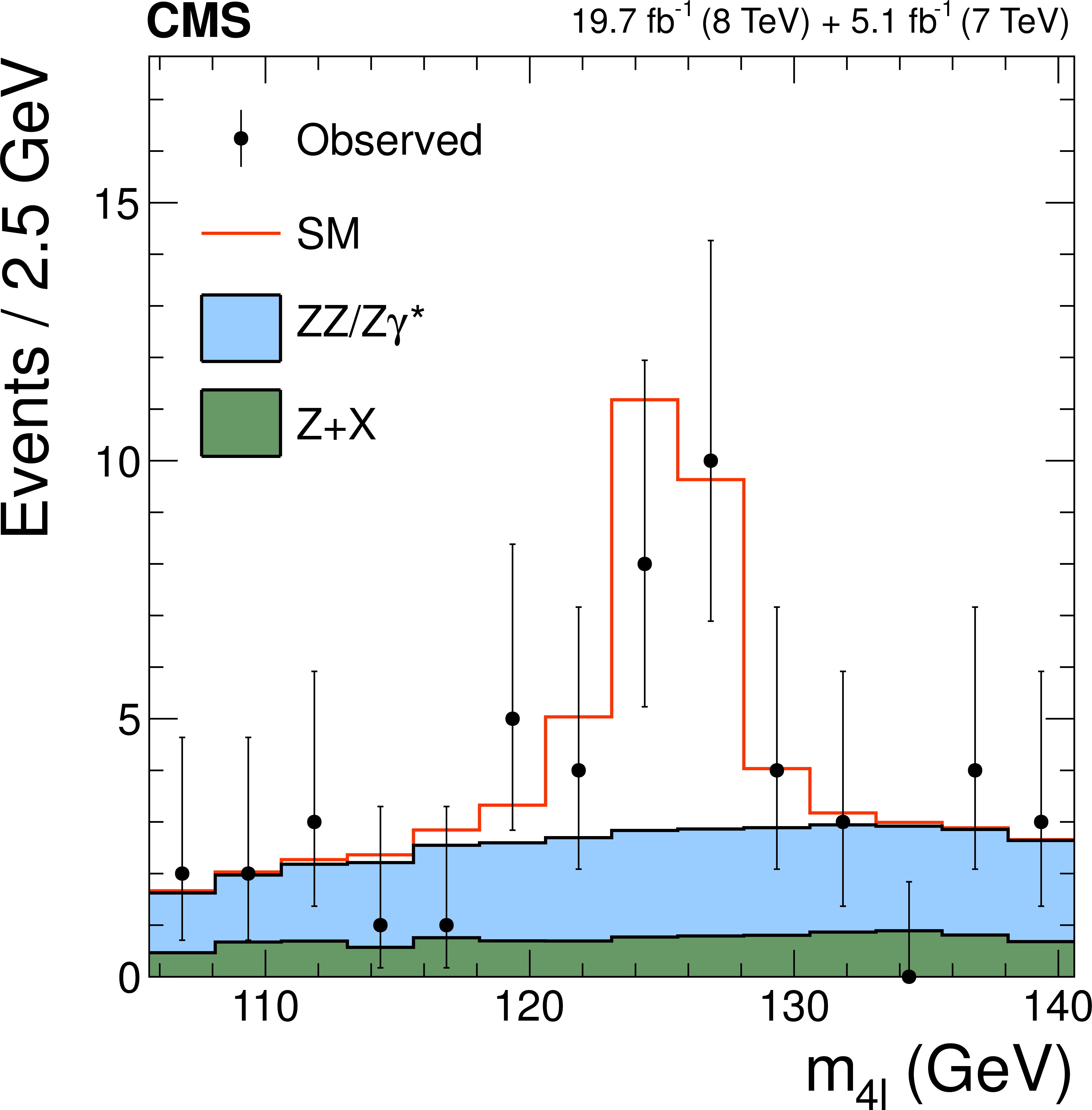
png pdf	Figure 1: Illustration of the production of a system ${\mathrm {X}}$ in a parton collision and its decay to two vector bosons ${\mathrm {g}} {\mathrm {g}}$ or ${ {\mathrm {q}} {\mathrm {\overline {q}}}} \to {\mathrm {X}} \to {\mathrm {Z}} {\mathrm {Z}}$, ${\mathrm {W}} {\mathrm {W}}$, ${\mathrm {Z}} \gamma ,$ and $\gamma \gamma$ either with or without sequential decay of each vector boson to a fermion-antifermion pair. The two production angles $\theta ^*$ and $\Phi _1$ are shown in the ${\mathrm {X}}$ rest frame and the three decay angles $\theta _1$, $\theta _2$, and $\Phi$ are shown in the ${\mathrm {V}}$ rest frames. Here ${\mathrm {X}}$ stands either for a Higgs boson, an exotic particle, or, in general, the genuine or misidentified ${\mathrm {V}} {\mathrm {V}}$ system, including background.
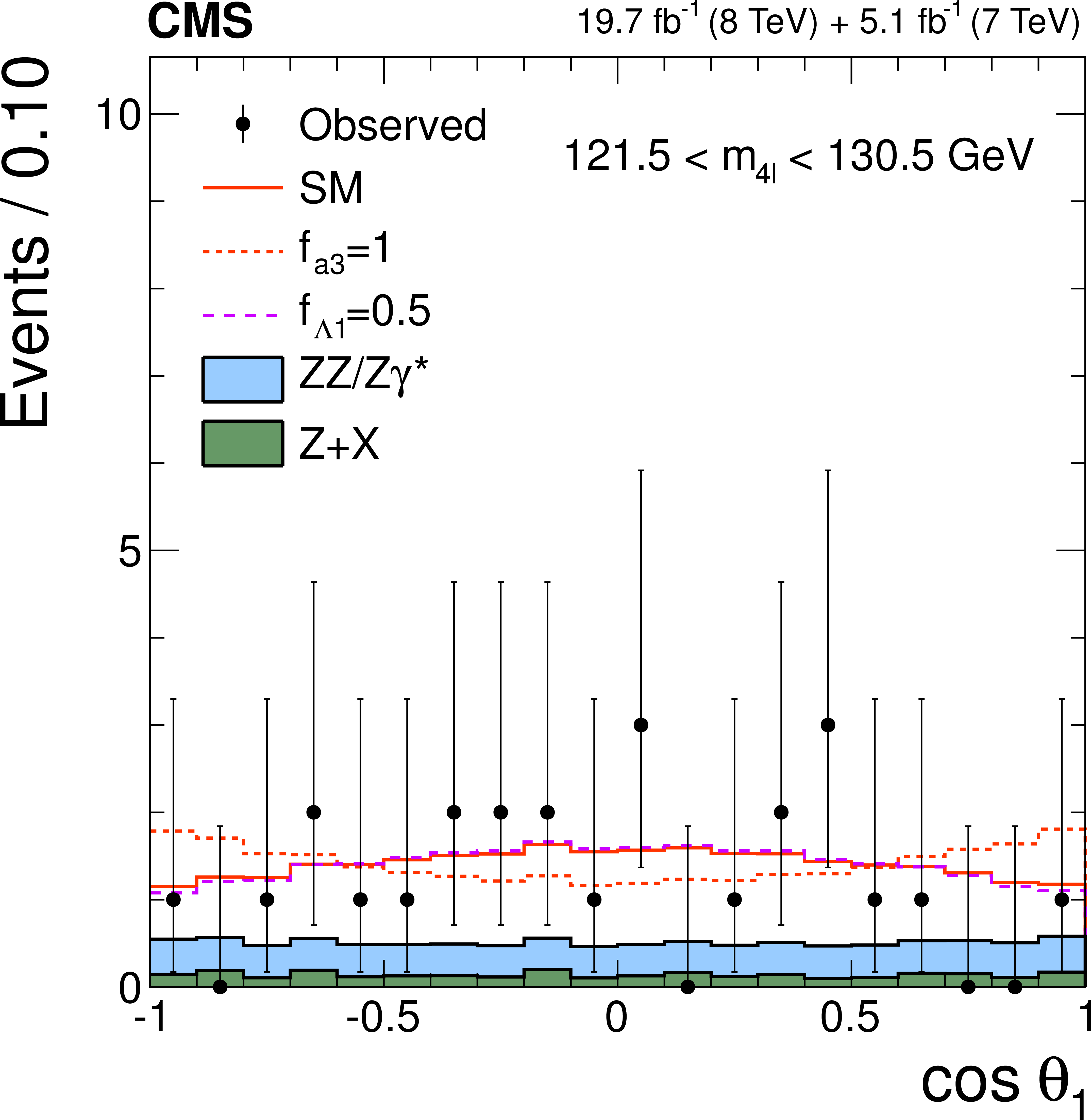
png pdf	Figure 2-a: Distributions of the eight kinematic observables used in the ${\mathrm {H}} \to {\mathrm {V}} {\mathrm {V}} \to 4\ell$ analysis: $m_{4\ell }$, $m_1$, $m_2$, $\cos\theta ^*$, $\cos\theta _{1}$, $\cos\theta _{2}$, $\Phi$, and $\Phi _{1}$. The observed data (points with error bars), the expectations for the SM background (shaded areas), the SM Higgs boson signal (open areas under the solid histogram), and the alternative spin-zero resonances (open areas under the dashed histograms) are shown, as indicated in the legend. The mass of the resonance is taken to be 125.6 GeV and the SM cross section is used. All distributions, with the exception of $m_{4\ell }$, are presented with the requirement 121.5 $< m_{4\ell } <$ 130.5 GeV .
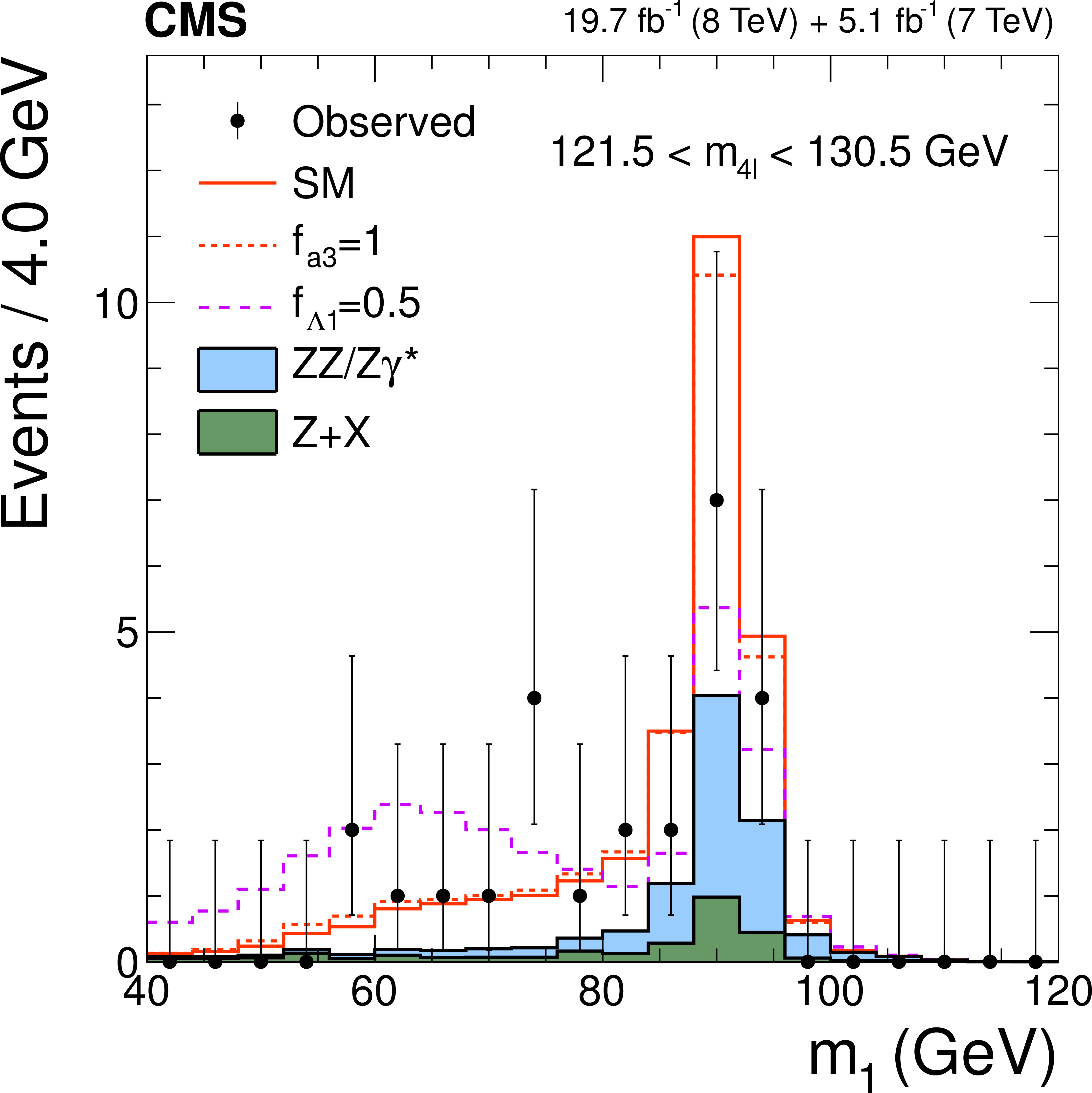
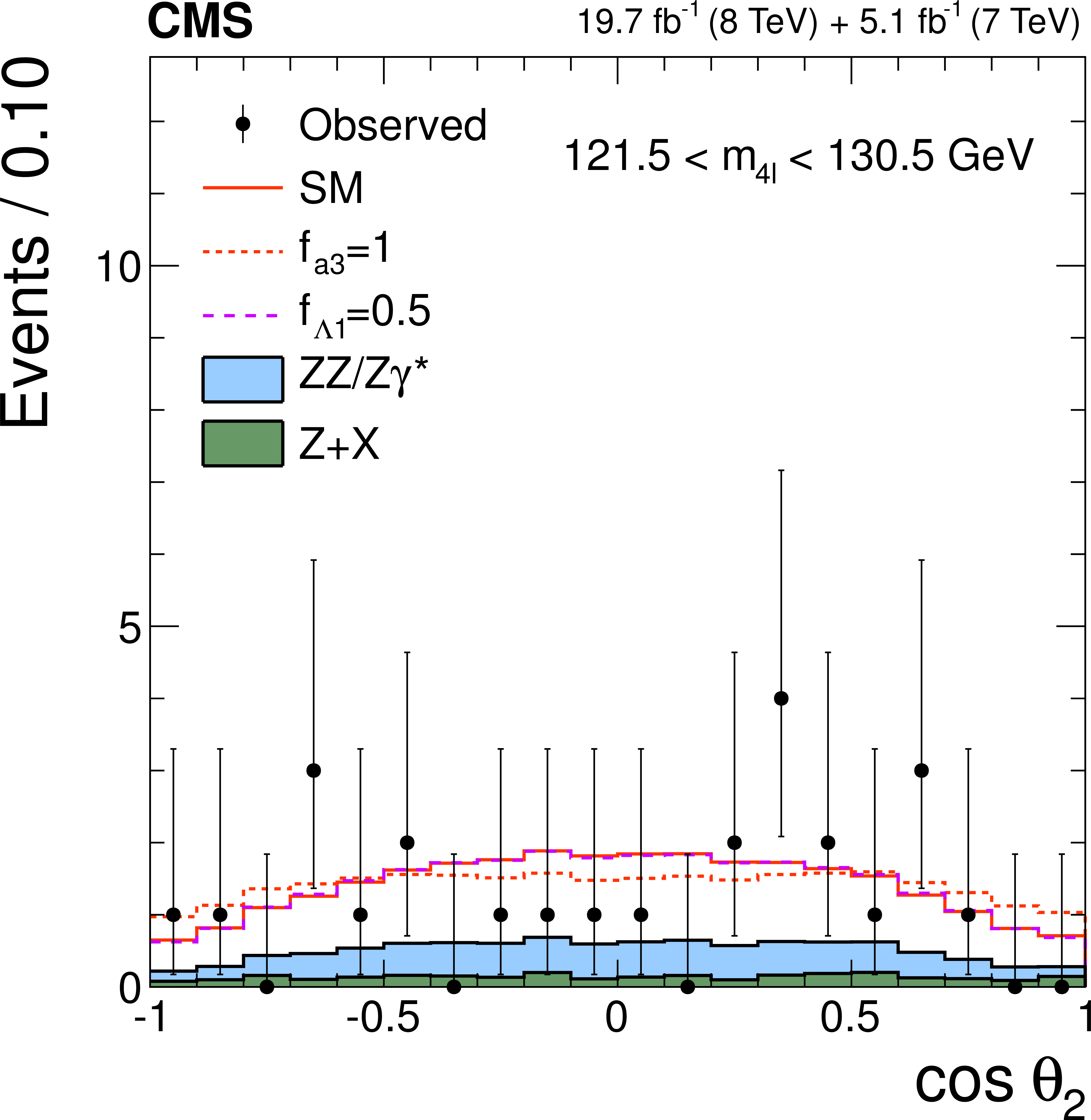
png pdf	Figure 2-b: Distributions of the eight kinematic observables used in the ${\mathrm {H}} \to {\mathrm {V}} {\mathrm {V}} \to 4\ell$ analysis: $m_{4\ell }$, $m_1$, $m_2$, $\cos\theta ^*$, $\cos\theta _{1}$, $\cos\theta _{2}$, $\Phi$, and $\Phi _{1}$. The observed data (points with error bars), the expectations for the SM background (shaded areas), the SM Higgs boson signal (open areas under the solid histogram), and the alternative spin-zero resonances (open areas under the dashed histograms) are shown, as indicated in the legend. The mass of the resonance is taken to be 125.6 GeV and the SM cross section is used. All distributions, with the exception of $m_{4\ell }$, are presented with the requirement 121.5 $< m_{4\ell } <$ 130.5 GeV .
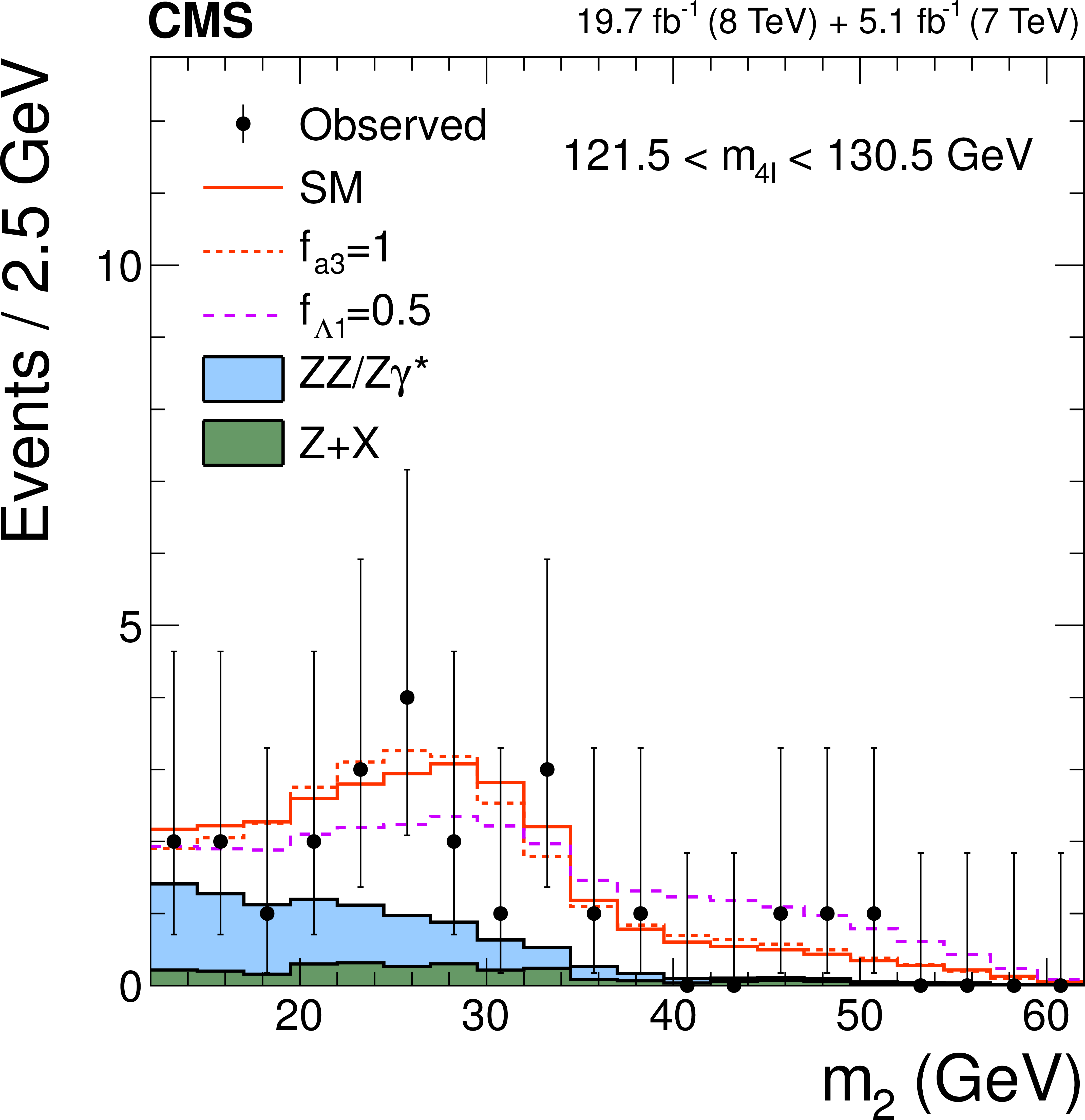
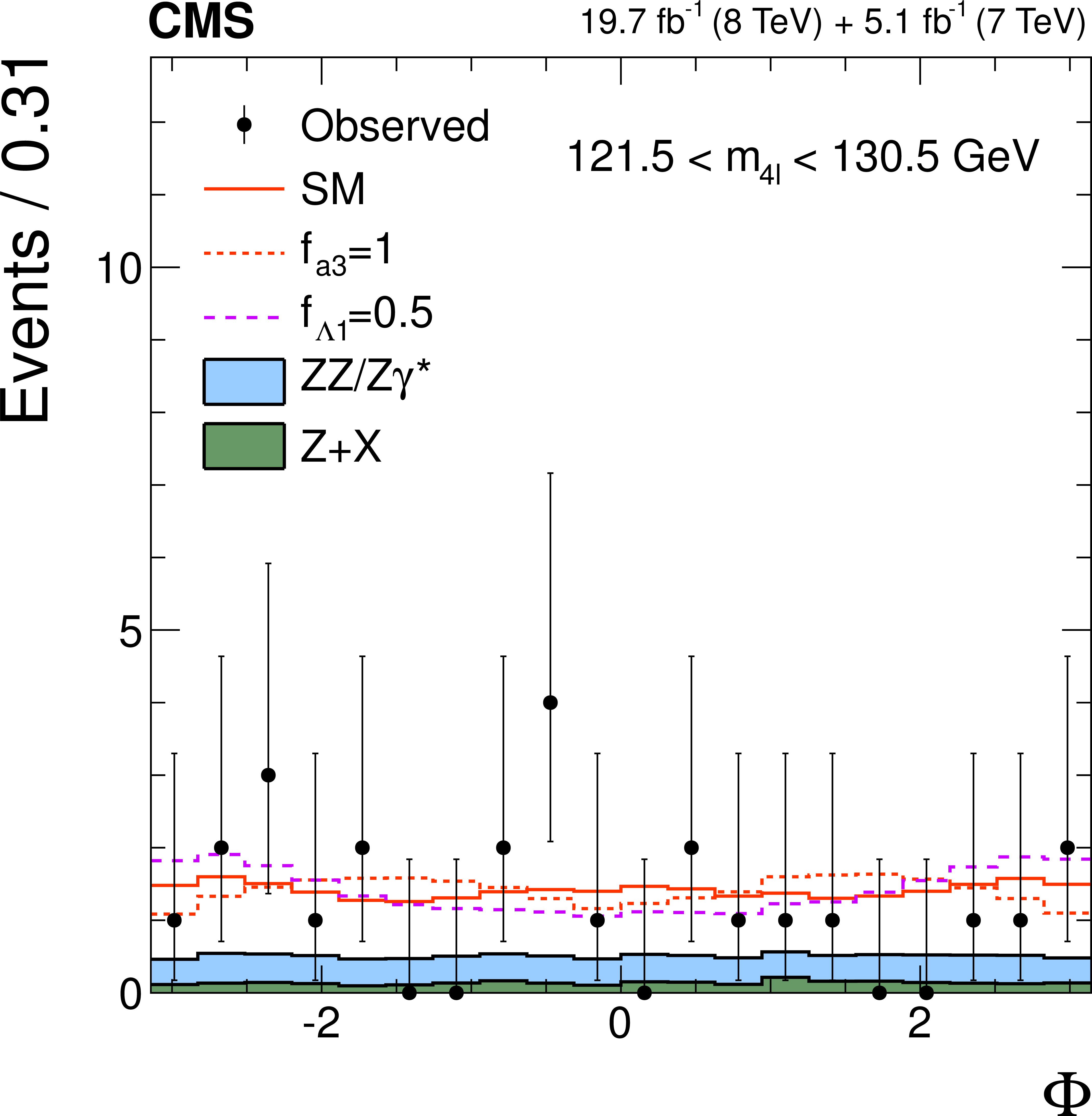
png pdf	Figure 2-c: Distributions of the eight kinematic observables used in the ${\mathrm {H}} \to {\mathrm {V}} {\mathrm {V}} \to 4\ell$ analysis: $m_{4\ell }$, $m_1$, $m_2$, $\cos\theta ^*$, $\cos\theta _{1}$, $\cos\theta _{2}$, $\Phi$, and $\Phi _{1}$. The observed data (points with error bars), the expectations for the SM background (shaded areas), the SM Higgs boson signal (open areas under the solid histogram), and the alternative spin-zero resonances (open areas under the dashed histograms) are shown, as indicated in the legend. The mass of the resonance is taken to be 125.6 GeV and the SM cross section is used. All distributions, with the exception of $m_{4\ell }$, are presented with the requirement 121.5 $< m_{4\ell } <$ 130.5 GeV .
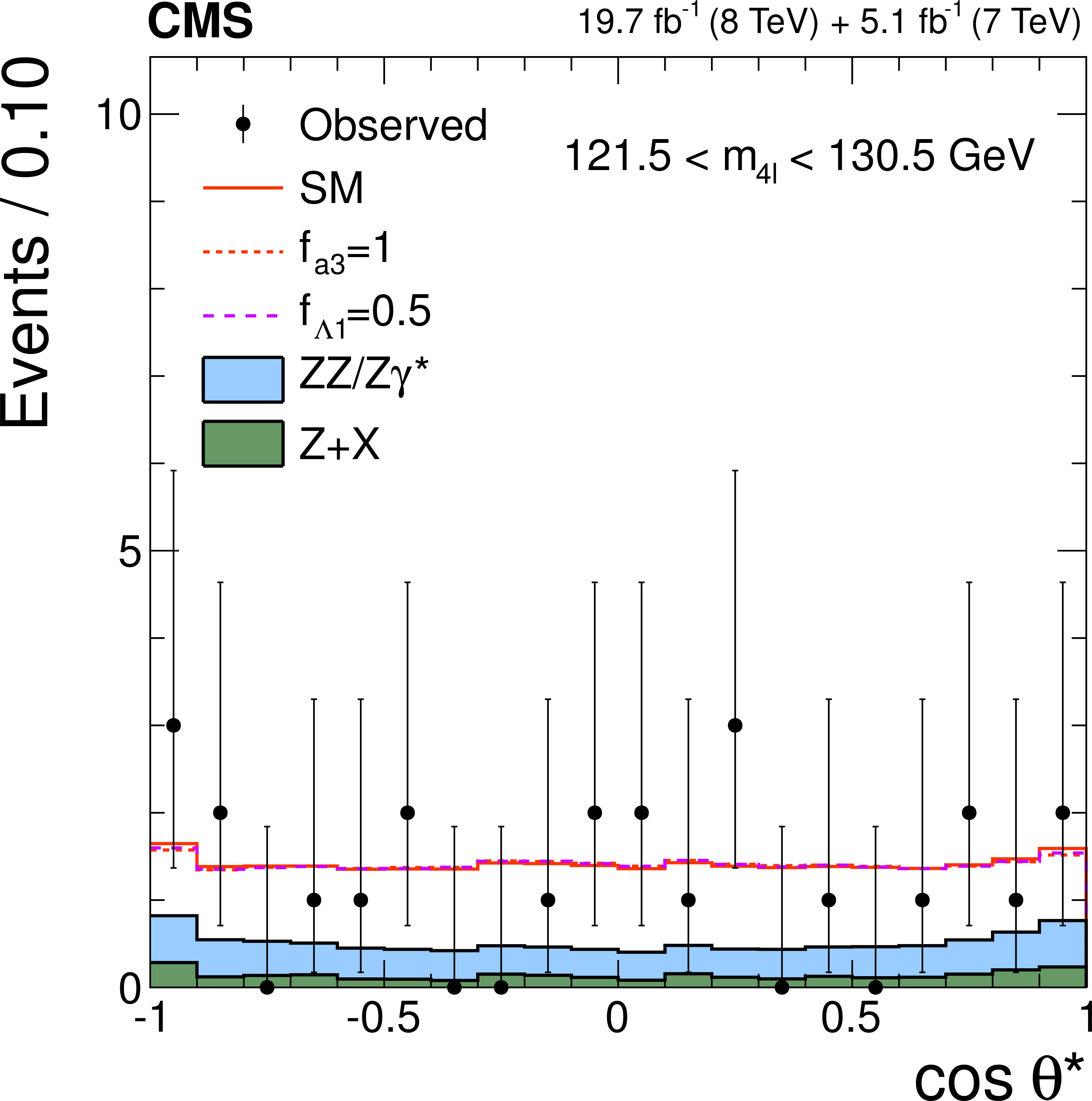
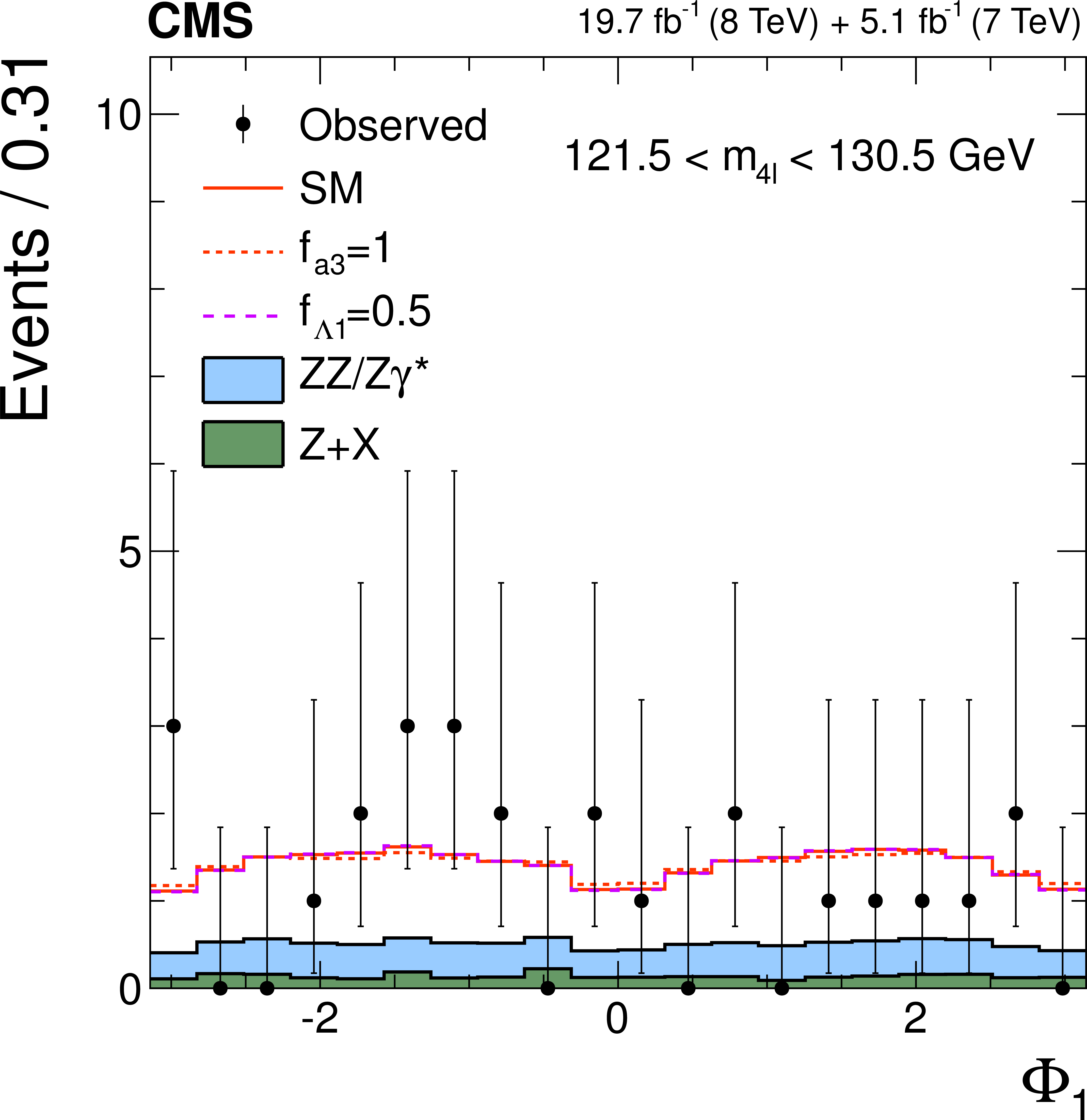
png pdf	Figure 2-d: Distributions of the eight kinematic observables used in the ${\mathrm {H}} \to {\mathrm {V}} {\mathrm {V}} \to 4\ell$ analysis: $m_{4\ell }$, $m_1$, $m_2$, $\cos\theta ^*$, $\cos\theta _{1}$, $\cos\theta _{2}$, $\Phi$, and $\Phi _{1}$. The observed data (points with error bars), the expectations for the SM background (shaded areas), the SM Higgs boson signal (open areas under the solid histogram), and the alternative spin-zero resonances (open areas under the dashed histograms) are shown, as indicated in the legend. The mass of the resonance is taken to be 125.6 GeV and the SM cross section is used. All distributions, with the exception of $m_{4\ell }$, are presented with the requirement 121.5 $< m_{4\ell } <$ 130.5 GeV .
png pdf	Figure 2-e: Distributions of the eight kinematic observables used in the ${\mathrm {H}} \to {\mathrm {V}} {\mathrm {V}} \to 4\ell$ analysis: $m_{4\ell }$, $m_1$, $m_2$, $\cos\theta ^*$, $\cos\theta _{1}$, $\cos\theta _{2}$, $\Phi$, and $\Phi _{1}$. The observed data (points with error bars), the expectations for the SM background (shaded areas), the SM Higgs boson signal (open areas under the solid histogram), and the alternative spin-zero resonances (open areas under the dashed histograms) are shown, as indicated in the legend. The mass of the resonance is taken to be 125.6 GeV and the SM cross section is used. All distributions, with the exception of $m_{4\ell }$, are presented with the requirement 121.5 $< m_{4\ell } <$ 130.5 GeV .
png pdf	Figure 2-f: Distributions of the eight kinematic observables used in the ${\mathrm {H}} \to {\mathrm {V}} {\mathrm {V}} \to 4\ell$ analysis: $m_{4\ell }$, $m_1$, $m_2$, $\cos\theta ^*$, $\cos\theta _{1}$, $\cos\theta _{2}$, $\Phi$, and $\Phi _{1}$. The observed data (points with error bars), the expectations for the SM background (shaded areas), the SM Higgs boson signal (open areas under the solid histogram), and the alternative spin-zero resonances (open areas under the dashed histograms) are shown, as indicated in the legend. The mass of the resonance is taken to be 125.6 GeV and the SM cross section is used. All distributions, with the exception of $m_{4\ell }$, are presented with the requirement 121.5 $< m_{4\ell } <$ 130.5 GeV .
png pdf	Figure 2-g: Distributions of the eight kinematic observables used in the ${\mathrm {H}} \to {\mathrm {V}} {\mathrm {V}} \to 4\ell$ analysis: $m_{4\ell }$, $m_1$, $m_2$, $\cos\theta ^*$, $\cos\theta _{1}$, $\cos\theta _{2}$, $\Phi$, and $\Phi _{1}$. The observed data (points with error bars), the expectations for the SM background (shaded areas), the SM Higgs boson signal (open areas under the solid histogram), and the alternative spin-zero resonances (open areas under the dashed histograms) are shown, as indicated in the legend. The mass of the resonance is taken to be 125.6 GeV and the SM cross section is used. All distributions, with the exception of $m_{4\ell }$, are presented with the requirement 121.5 $< m_{4\ell } <$ 130.5 GeV .
png pdf	Figure 2-h: Distributions of the eight kinematic observables used in the ${\mathrm {H}} \to {\mathrm {V}} {\mathrm {V}} \to 4\ell$ analysis: $m_{4\ell }$, $m_1$, $m_2$, $\cos\theta ^*$, $\cos\theta _{1}$, $\cos\theta _{2}$, $\Phi$, and $\Phi _{1}$. The observed data (points with error bars), the expectations for the SM background (shaded areas), the SM Higgs boson signal (open areas under the solid histogram), and the alternative spin-zero resonances (open areas under the dashed histograms) are shown, as indicated in the legend. The mass of the resonance is taken to be 125.6 GeV and the SM cross section is used. All distributions, with the exception of $m_{4\ell }$, are presented with the requirement 121.5 $< m_{4\ell } <$ 130.5 GeV .
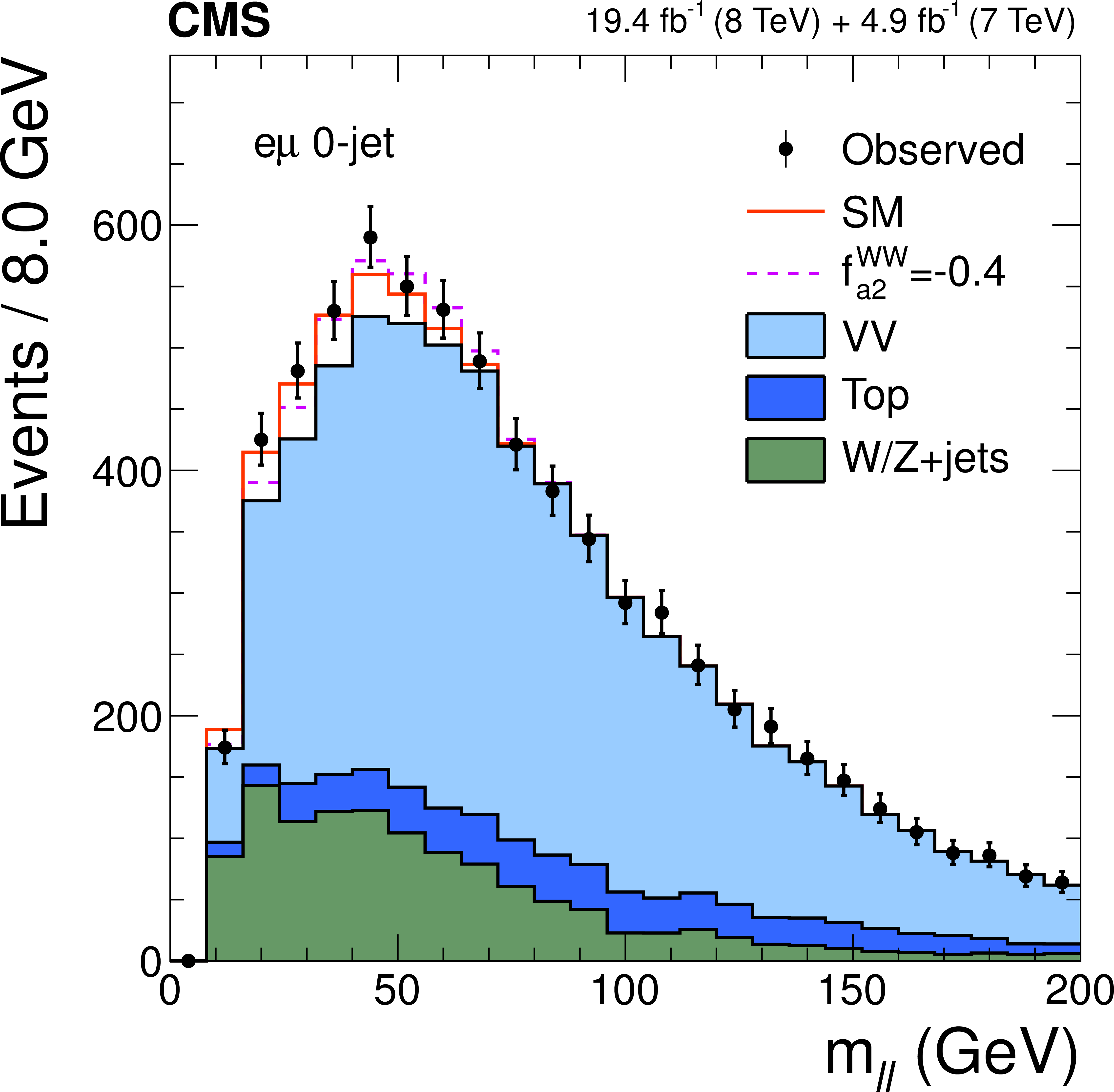
png pdf	Figure 3-a: Distributions of ${m_{\ell \ell }}$ (a, c) and ${m_\mathrm {T}}$ (b, d) for events with 0 jets (a, b) and 1 jet (c, d) in the ${\mathrm {H}} \to {\mathrm {W}} {\mathrm {W}}\to \ell \nu \ell \nu$ analysis. The observed data (points with error bars), the expectations for the SM background (shaded areas), the SM Higgs boson signal (open areas under the solid histogram), and the alternative spin-zero resonance (open areas under the dashed histograms) are shown, as indicated in the legend. The mass of the resonance is taken to be 125.6 GeV and the SM cross section is used.
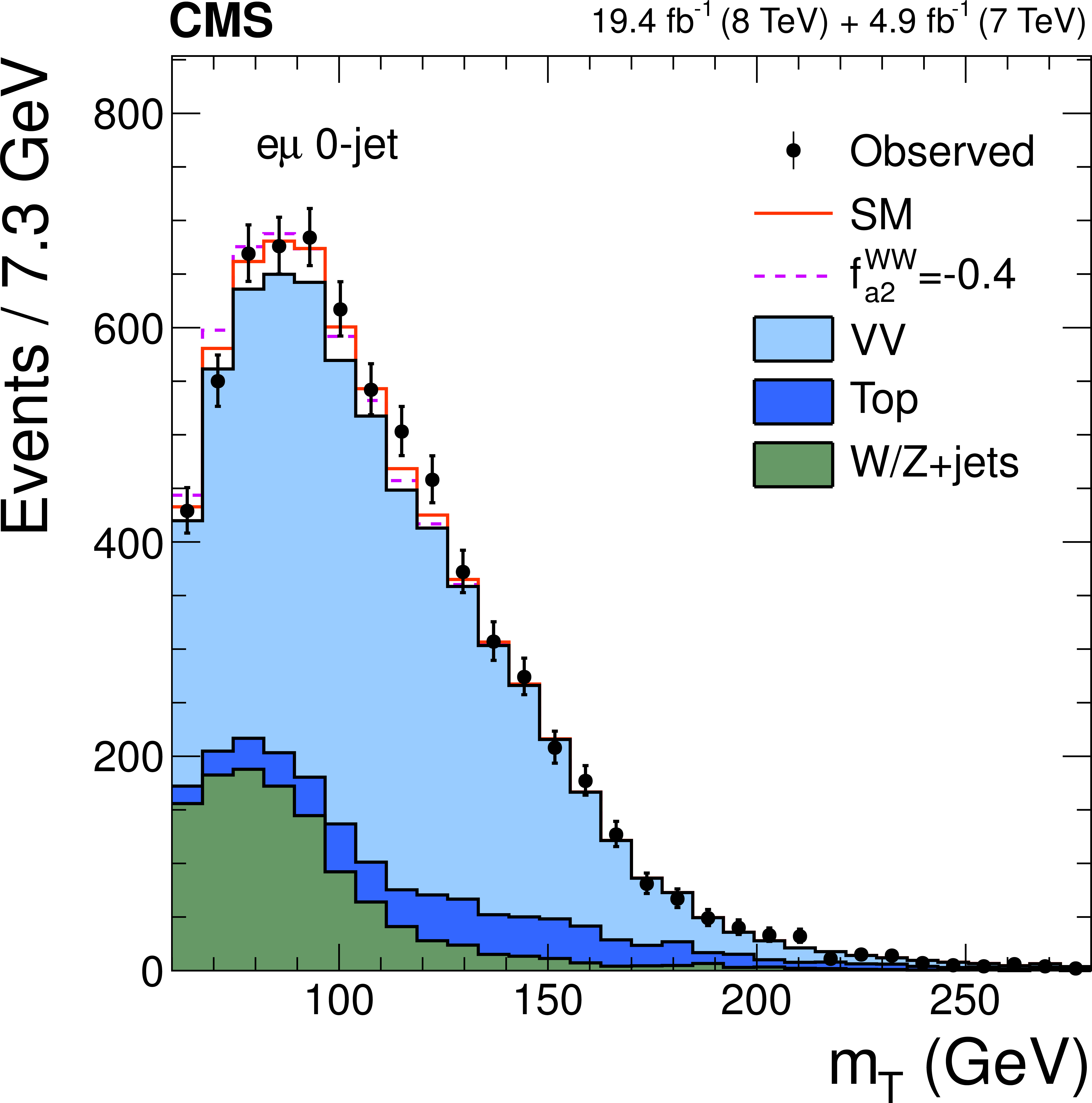
png pdf	Figure 3-b: Distributions of ${m_{\ell \ell }}$ (a, c) and ${m_\mathrm {T}}$ (b, d) for events with 0 jets (a, b) and 1 jet (c, d) in the ${\mathrm {H}} \to {\mathrm {W}} {\mathrm {W}}\to \ell \nu \ell \nu$ analysis. The observed data (points with error bars), the expectations for the SM background (shaded areas), the SM Higgs boson signal (open areas under the solid histogram), and the alternative spin-zero resonance (open areas under the dashed histograms) are shown, as indicated in the legend. The mass of the resonance is taken to be 125.6 GeV and the SM cross section is used.
png pdf	Figure 3-c: Distributions of ${m_{\ell \ell }}$ (a, c) and ${m_\mathrm {T}}$ (b, d) for events with 0 jets (a, b) and 1 jet (c, d) in the ${\mathrm {H}} \to {\mathrm {W}} {\mathrm {W}}\to \ell \nu \ell \nu$ analysis. The observed data (points with error bars), the expectations for the SM background (shaded areas), the SM Higgs boson signal (open areas under the solid histogram), and the alternative spin-zero resonance (open areas under the dashed histograms) are shown, as indicated in the legend. The mass of the resonance is taken to be 125.6 GeV and the SM cross section is used.
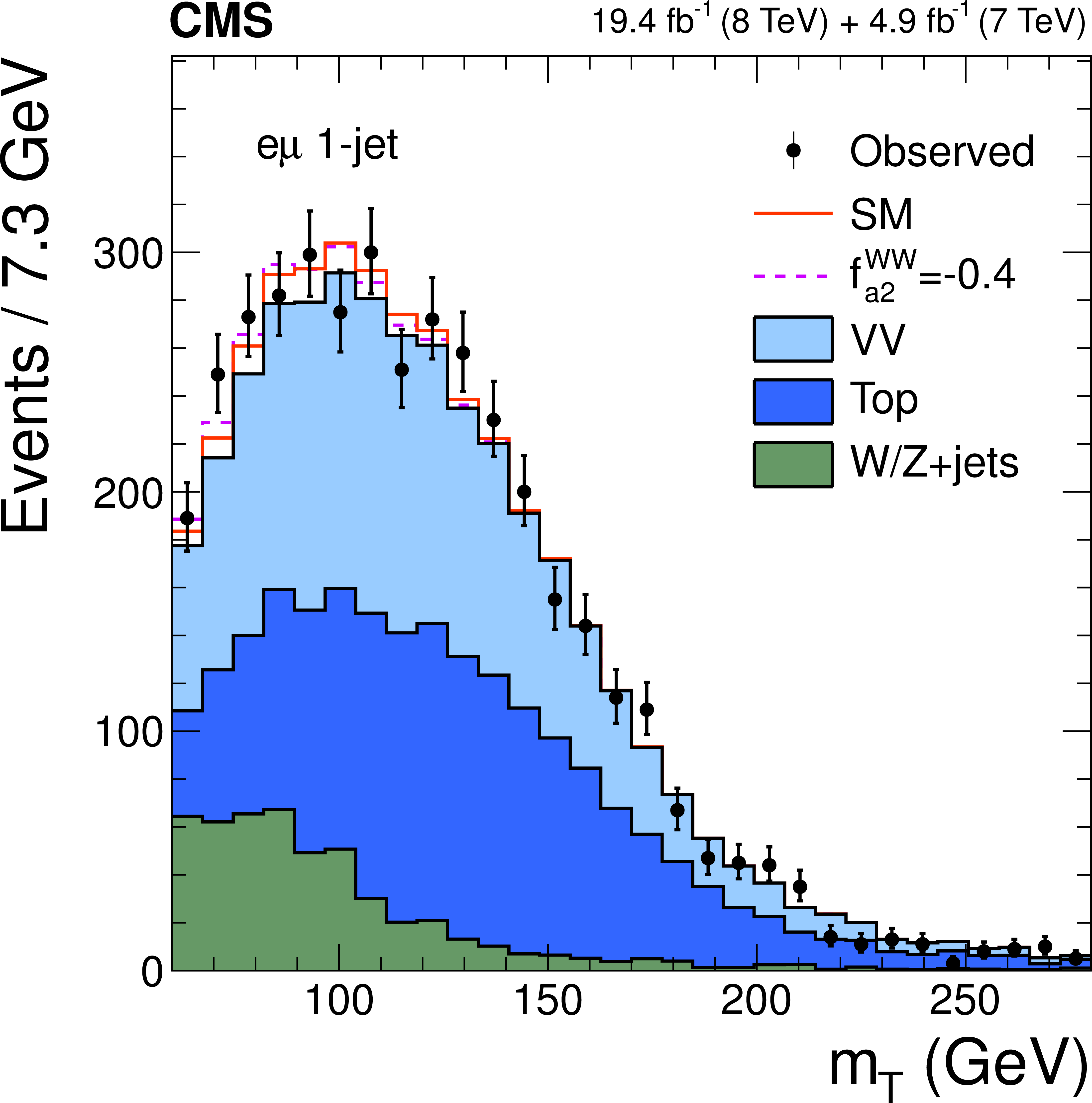
png pdf	Figure 3-d: Distributions of ${m_{\ell \ell }}$ (a, c) and ${m_\mathrm {T}}$ (b, d) for events with 0 jets (a, b) and 1 jet (c, d) in the ${\mathrm {H}} \to {\mathrm {W}} {\mathrm {W}}\to \ell \nu \ell \nu$ analysis. The observed data (points with error bars), the expectations for the SM background (shaded areas), the SM Higgs boson signal (open areas under the solid histogram), and the alternative spin-zero resonance (open areas under the dashed histograms) are shown, as indicated in the legend. The mass of the resonance is taken to be 125.6 GeV and the SM cross section is used.
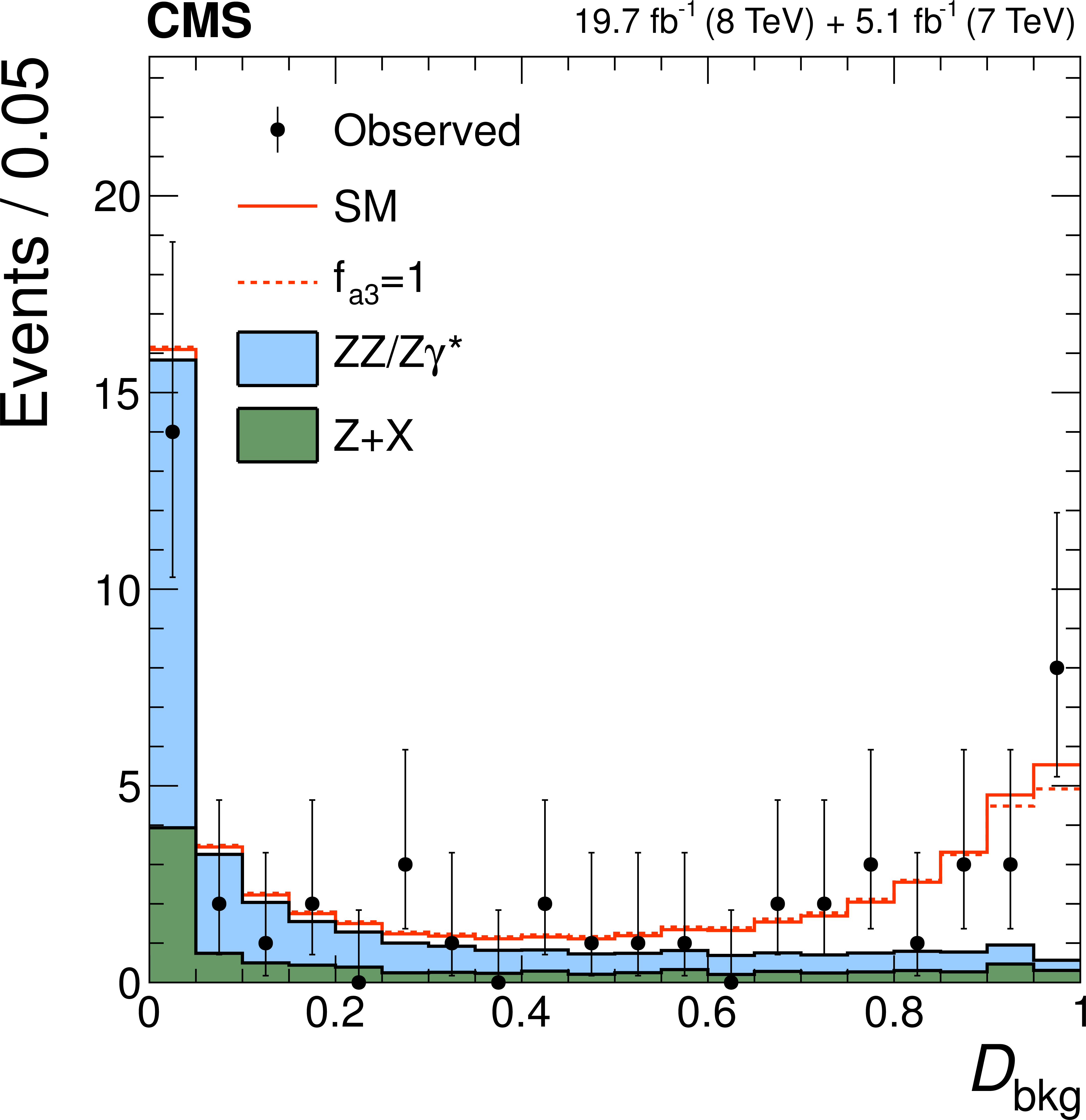
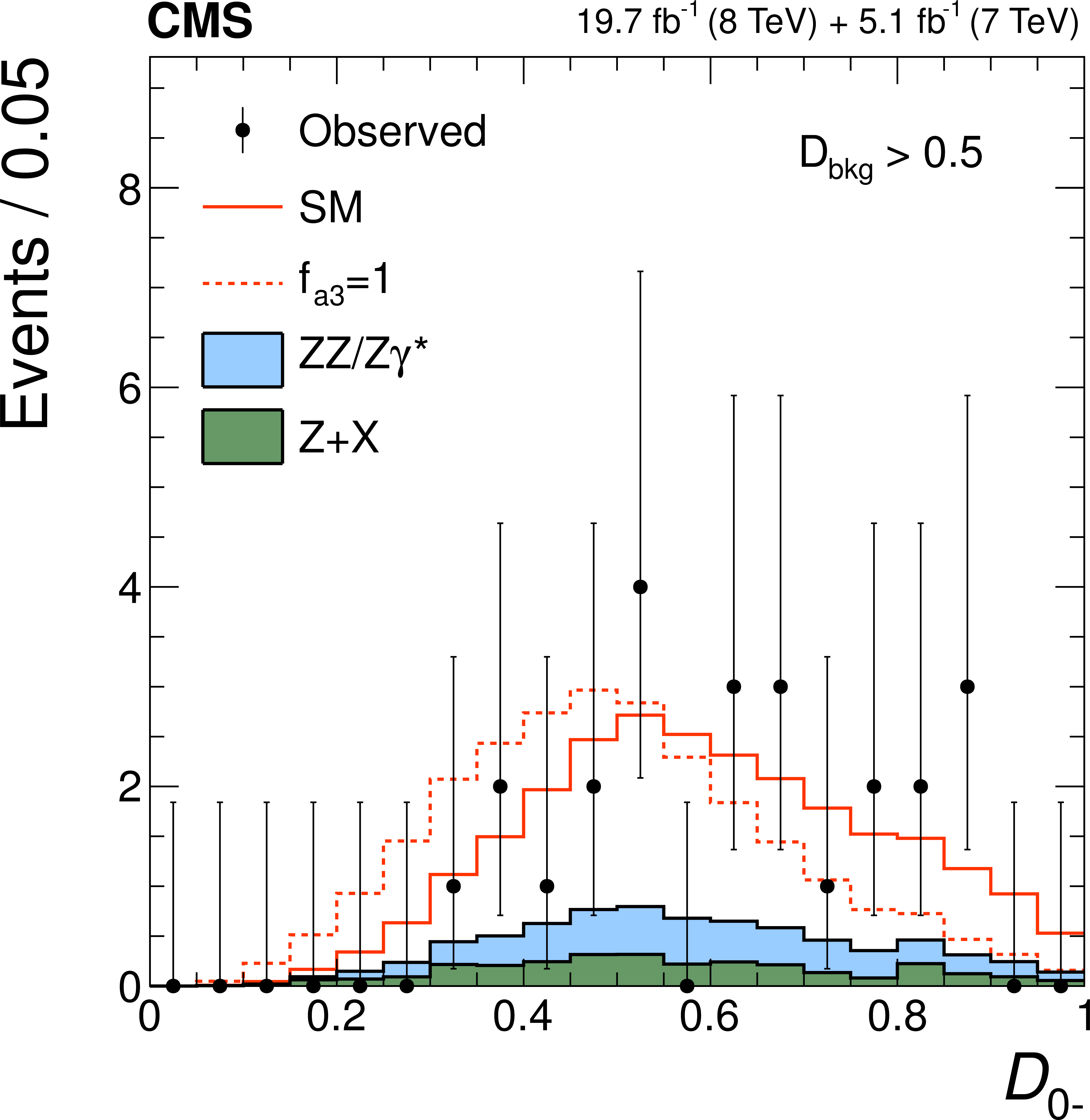
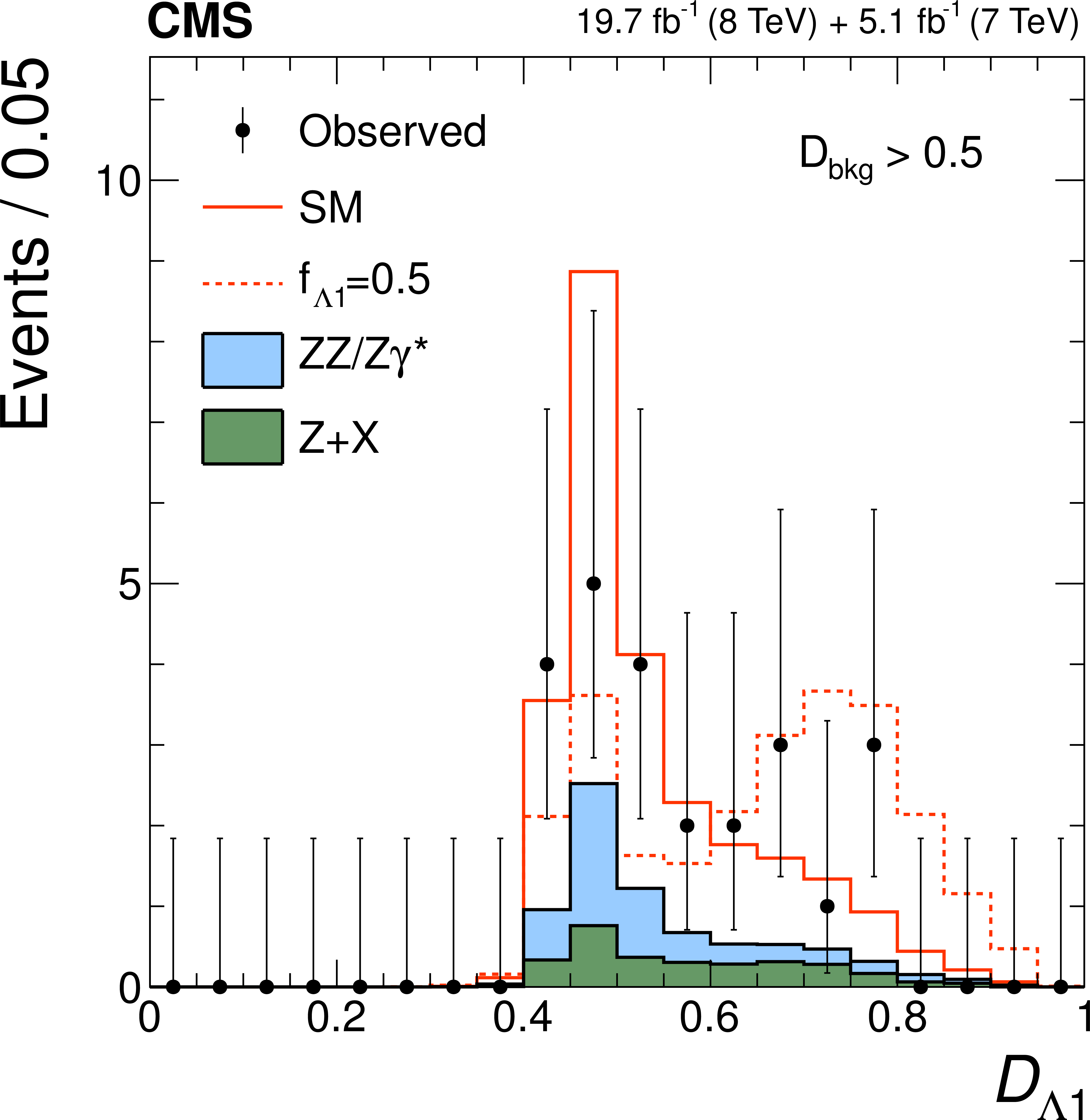
png pdf	Figure 4-a: Distributions of the kinematic discriminants for the observed data (points with error bars), the expectations for the SM background (shaded areas), the SM Higgs boson signal (open areas under the solid histogram), and the alternative spin-zero resonances (open areas under the dashed histograms) are shown, as indicated in the legend. The mass of the resonance is taken to be 125.6 GeV and the SM cross section is used. a, b, c: $\mathcal {D}_\text {bkg}$, $\mathcal {D}_{0-}$, $\mathcal {D}_{CP}$; d, e, f: $\mathcal {D}_{0h+}$, $\mathcal {D}_\text {int}$, $\mathcal {D}_{\Lambda 1}$. All distributions, with the exception of $\mathcal {D}_\text {bkg}$, are shown with the requirement $\mathcal {D}_\text {bkg}>$ 0.5 to enhance signal purity.
png pdf	Figure 4-b: Distributions of the kinematic discriminants for the observed data (points with error bars), the expectations for the SM background (shaded areas), the SM Higgs boson signal (open areas under the solid histogram), and the alternative spin-zero resonances (open areas under the dashed histograms) are shown, as indicated in the legend. The mass of the resonance is taken to be 125.6 GeV and the SM cross section is used. a, b, c: $\mathcal {D}_\text {bkg}$, $\mathcal {D}_{0-}$, $\mathcal {D}_{CP}$; d, e, f: $\mathcal {D}_{0h+}$, $\mathcal {D}_\text {int}$, $\mathcal {D}_{\Lambda 1}$. All distributions, with the exception of $\mathcal {D}_\text {bkg}$, are shown with the requirement $\mathcal {D}_\text {bkg}>$ 0.5 to enhance signal purity.
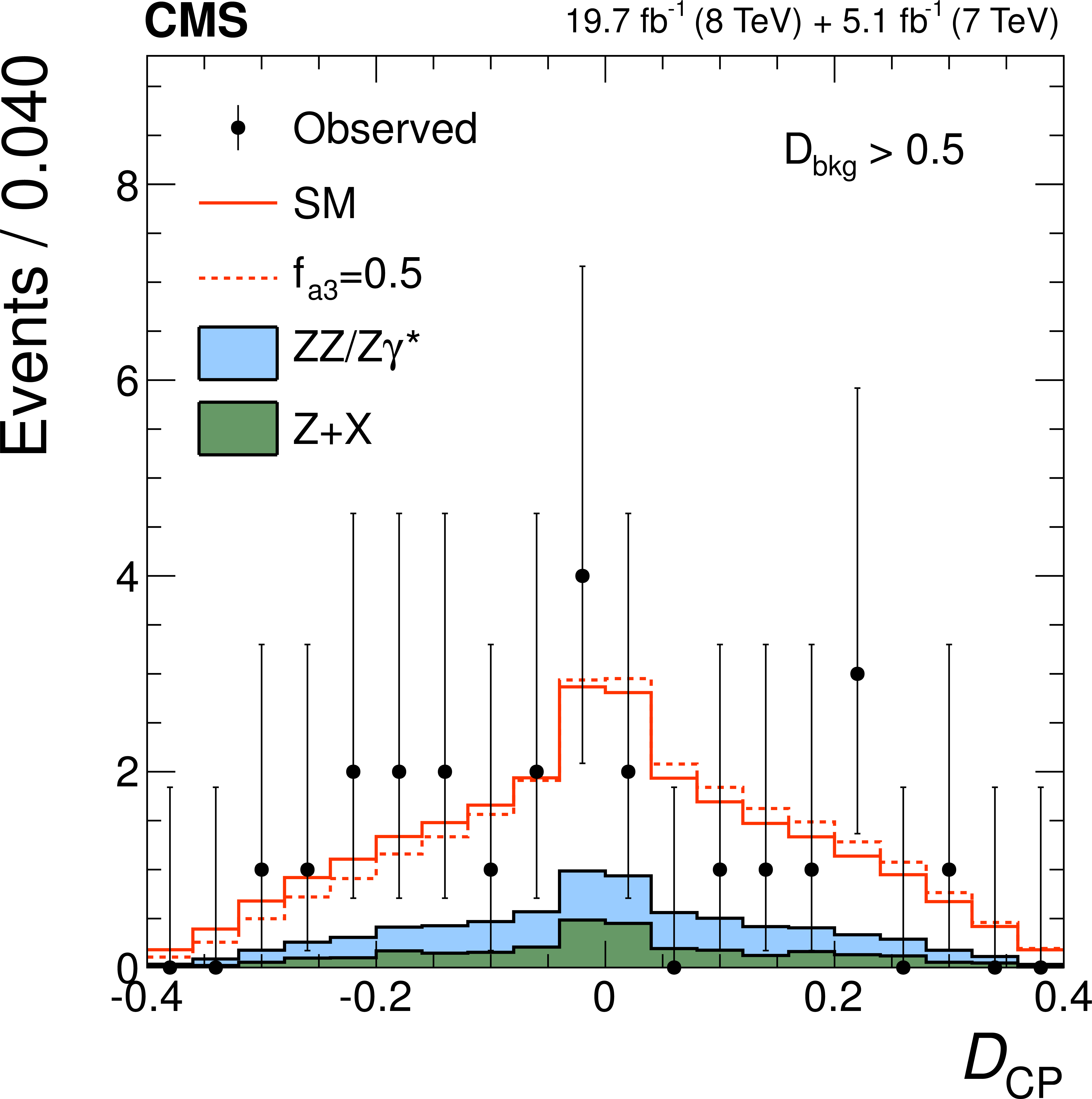
png pdf	Figure 4-c: Distributions of the kinematic discriminants for the observed data (points with error bars), the expectations for the SM background (shaded areas), the SM Higgs boson signal (open areas under the solid histogram), and the alternative spin-zero resonances (open areas under the dashed histograms) are shown, as indicated in the legend. The mass of the resonance is taken to be 125.6 GeV and the SM cross section is used. a, b, c: $\mathcal {D}_\text {bkg}$, $\mathcal {D}_{0-}$, $\mathcal {D}_{CP}$; d, e, f: $\mathcal {D}_{0h+}$, $\mathcal {D}_\text {int}$, $\mathcal {D}_{\Lambda 1}$. All distributions, with the exception of $\mathcal {D}_\text {bkg}$, are shown with the requirement $\mathcal {D}_\text {bkg}>$ 0.5 to enhance signal purity.
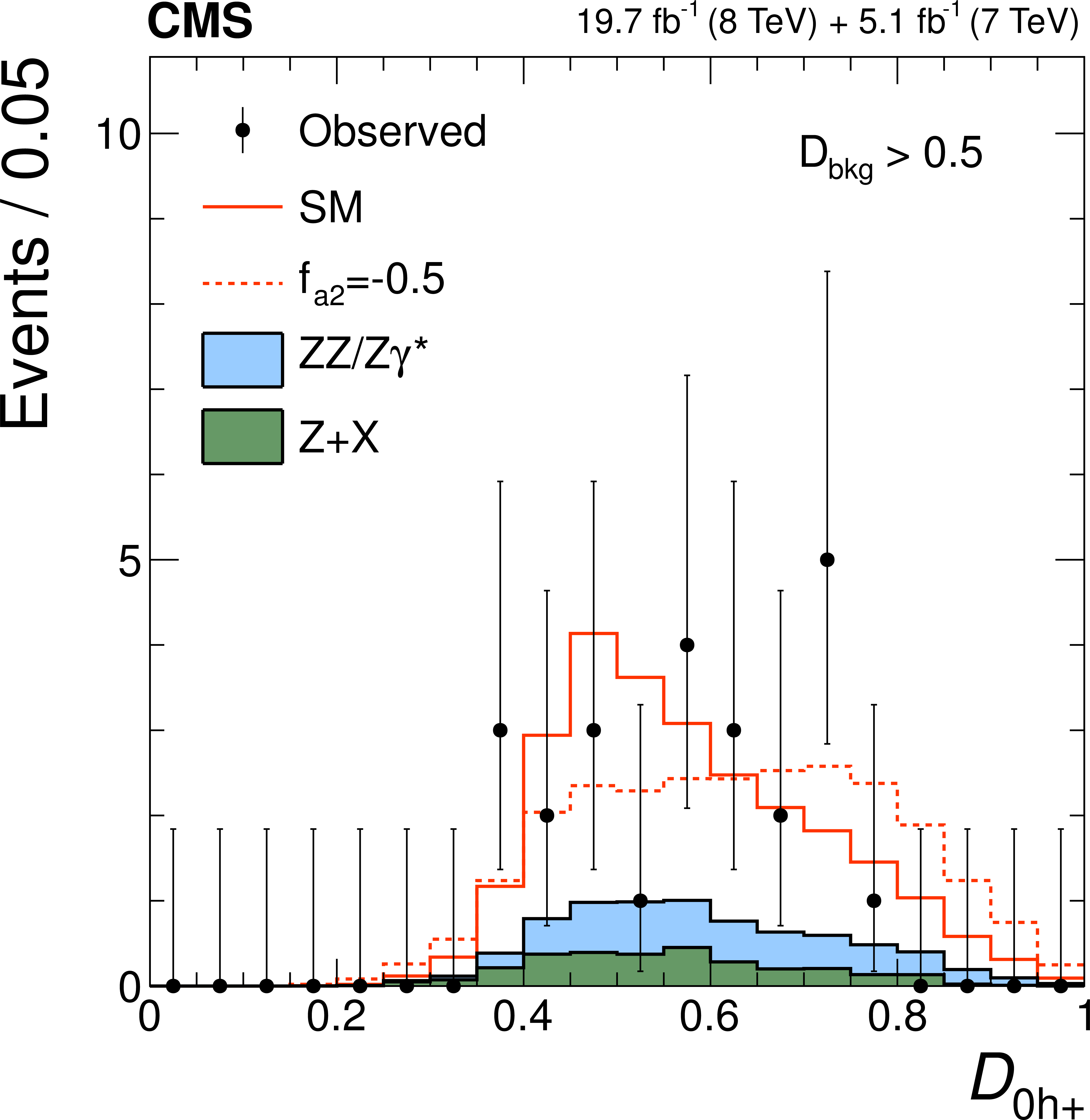
png pdf	Figure 4-d: Distributions of the kinematic discriminants for the observed data (points with error bars), the expectations for the SM background (shaded areas), the SM Higgs boson signal (open areas under the solid histogram), and the alternative spin-zero resonances (open areas under the dashed histograms) are shown, as indicated in the legend. The mass of the resonance is taken to be 125.6 GeV and the SM cross section is used. a, b, c: $\mathcal {D}_\text {bkg}$, $\mathcal {D}_{0-}$, $\mathcal {D}_{CP}$; d, e, f: $\mathcal {D}_{0h+}$, $\mathcal {D}_\text {int}$, $\mathcal {D}_{\Lambda 1}$. All distributions, with the exception of $\mathcal {D}_\text {bkg}$, are shown with the requirement $\mathcal {D}_\text {bkg}>$ 0.5 to enhance signal purity.
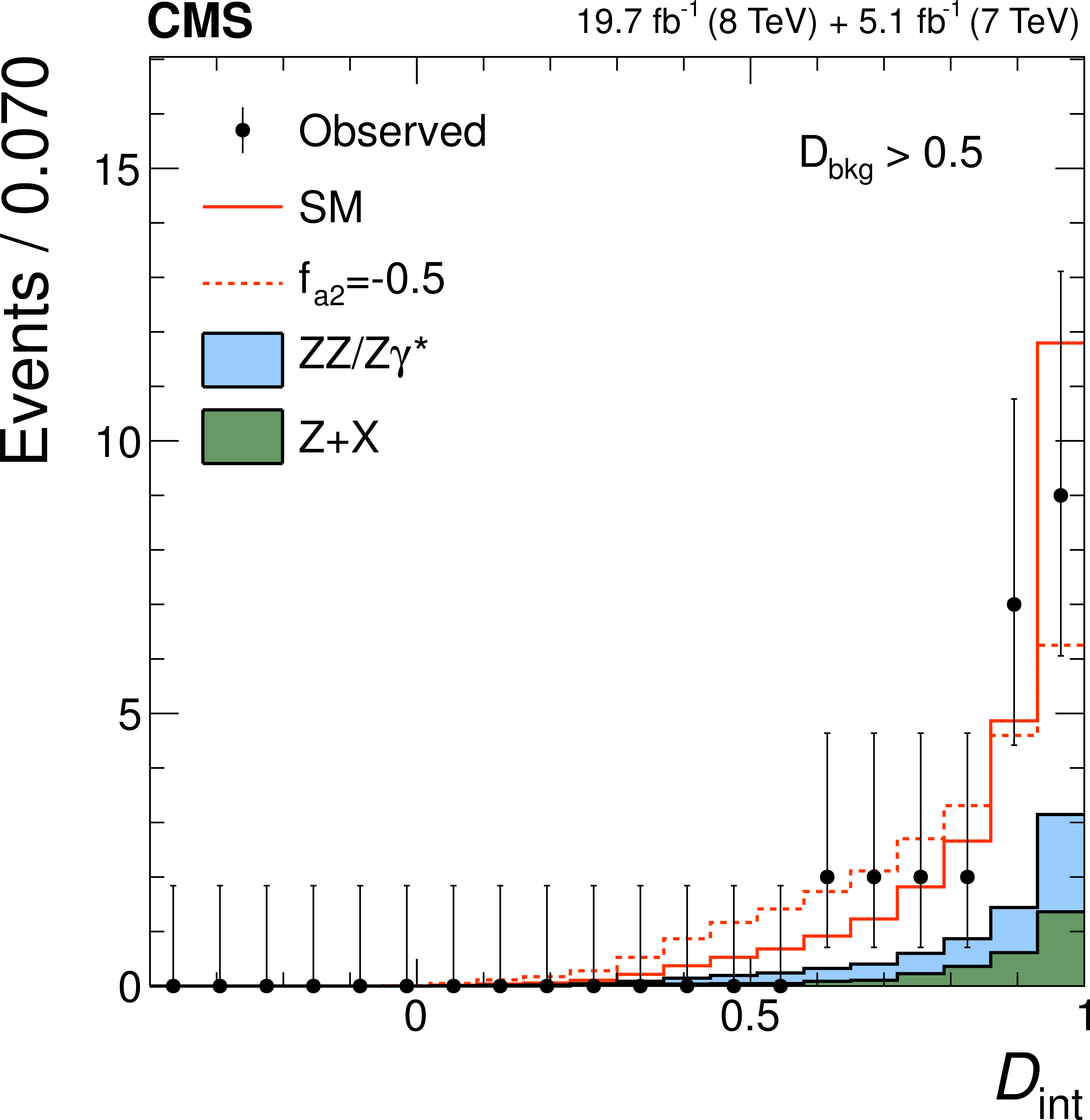
png pdf	Figure 4-e: Distributions of the kinematic discriminants for the observed data (points with error bars), the expectations for the SM background (shaded areas), the SM Higgs boson signal (open areas under the solid histogram), and the alternative spin-zero resonances (open areas under the dashed histograms) are shown, as indicated in the legend. The mass of the resonance is taken to be 125.6 GeV and the SM cross section is used. a, b, c: $\mathcal {D}_\text {bkg}$, $\mathcal {D}_{0-}$, $\mathcal {D}_{CP}$; d, e, f: $\mathcal {D}_{0h+}$, $\mathcal {D}_\text {int}$, $\mathcal {D}_{\Lambda 1}$. All distributions, with the exception of $\mathcal {D}_\text {bkg}$, are shown with the requirement $\mathcal {D}_\text {bkg}>$ 0.5 to enhance signal purity.
png pdf	Figure 4-f: Distributions of the kinematic discriminants for the observed data (points with error bars), the expectations for the SM background (shaded areas), the SM Higgs boson signal (open areas under the solid histogram), and the alternative spin-zero resonances (open areas under the dashed histograms) are shown, as indicated in the legend. The mass of the resonance is taken to be 125.6 GeV and the SM cross section is used. a, b, c: $\mathcal {D}_\text {bkg}$, $\mathcal {D}_{0-}$, $\mathcal {D}_{CP}$; d, e, f: $\mathcal {D}_{0h+}$, $\mathcal {D}_\text {int}$, $\mathcal {D}_{\Lambda 1}$. All distributions, with the exception of $\mathcal {D}_\text {bkg}$, are shown with the requirement $\mathcal {D}_\text {bkg}>$ 0.5 to enhance signal purity.
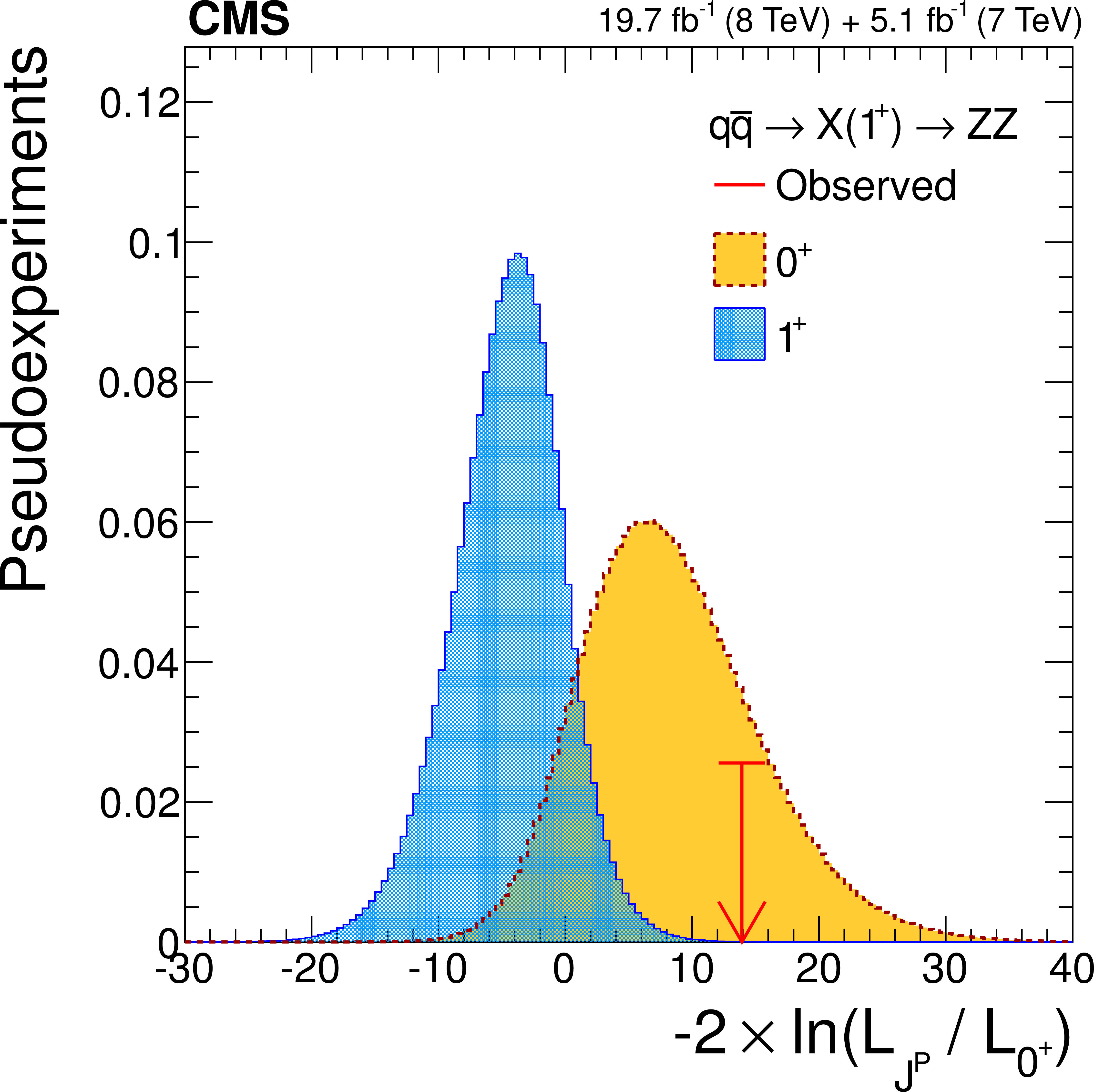
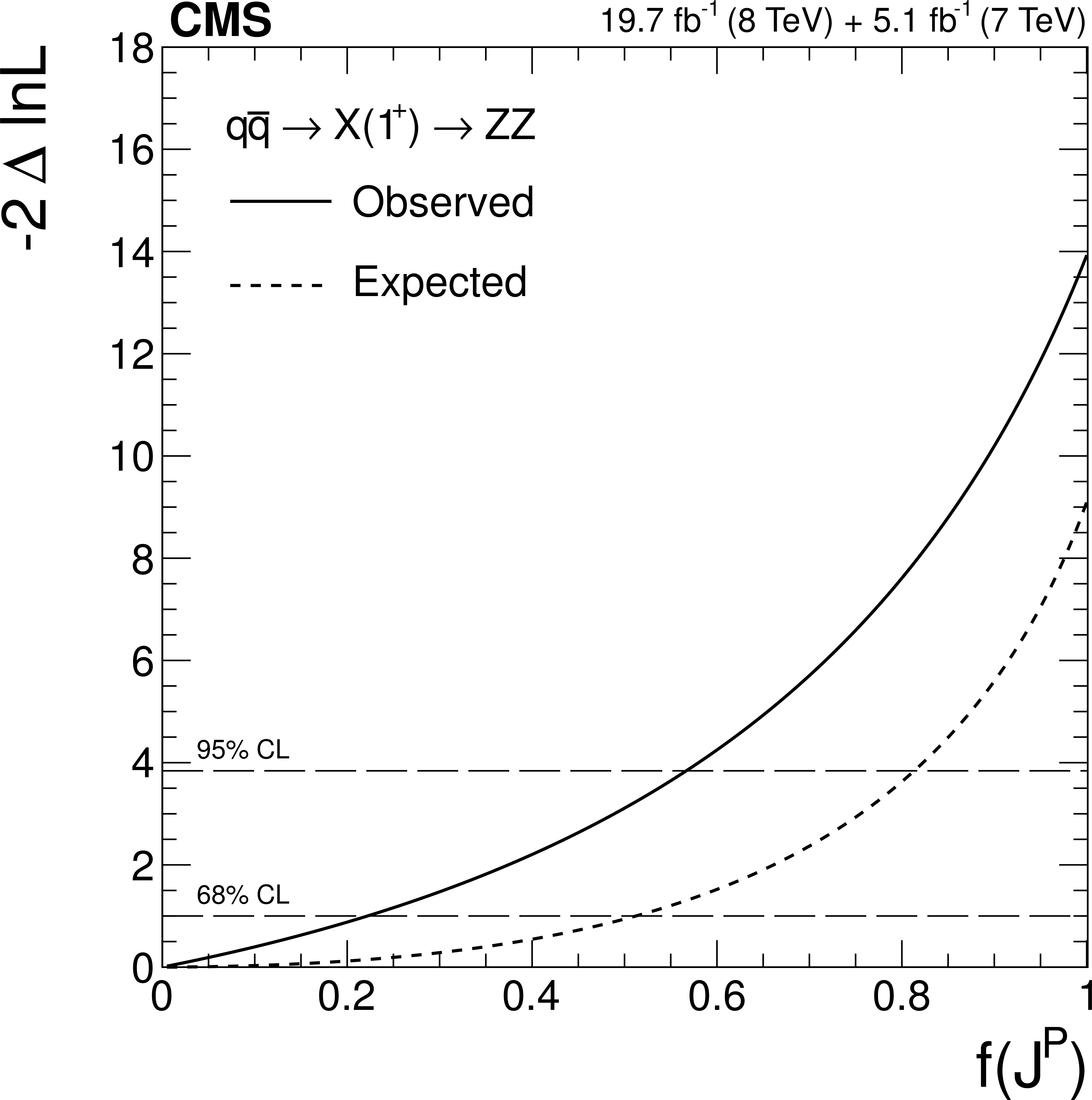
png pdf	Figure 5-a: (a) Distributions of the test statistic $q=-2\ln(\mathcal {L}_{J^P}/\mathcal {L}_{0^+})$ for the $J^P=1^+$ hypothesis of ${ {\mathrm {q}} {\mathrm {\overline {q}}}} \to {\mathrm {X}} (1^+)\to {\mathrm {Z}} {\mathrm {Z}}$ tested against the SM Higgs boson hypothesis ($0^+$). The expectation for the SM Higgs boson is represented by the yellow histogram on the right and the alternative $J^P$ hypothesis by the blue histogram on the left. The red arrow indicates the observed $q$ value. (b) Observed value of $-2\Delta \ln\mathcal {L}$ as a function of $f(J^P)$ and the expectation in the SM for the ${ {\mathrm {q}} {\mathrm {\overline {q}}}} \to {\mathrm {X}} (1^+)\to {\mathrm {Z}} {\mathrm {Z}}$ alternative $J^P$ model.
png pdf	Figure 5-b: (a) Distributions of the test statistic $q=-2\ln(\mathcal {L}_{J^P}/\mathcal {L}_{0^+})$ for the $J^P=1^+$ hypothesis of ${ {\mathrm {q}} {\mathrm {\overline {q}}}} \to {\mathrm {X}} (1^+)\to {\mathrm {Z}} {\mathrm {Z}}$ tested against the SM Higgs boson hypothesis ($0^+$). The expectation for the SM Higgs boson is represented by the yellow histogram on the right and the alternative $J^P$ hypothesis by the blue histogram on the left. The red arrow indicates the observed $q$ value. (b) Observed value of $-2\Delta \ln\mathcal {L}$ as a function of $f(J^P)$ and the expectation in the SM for the ${ {\mathrm {q}} {\mathrm {\overline {q}}}} \to {\mathrm {X}} (1^+)\to {\mathrm {Z}} {\mathrm {Z}}$ alternative $J^P$ model.
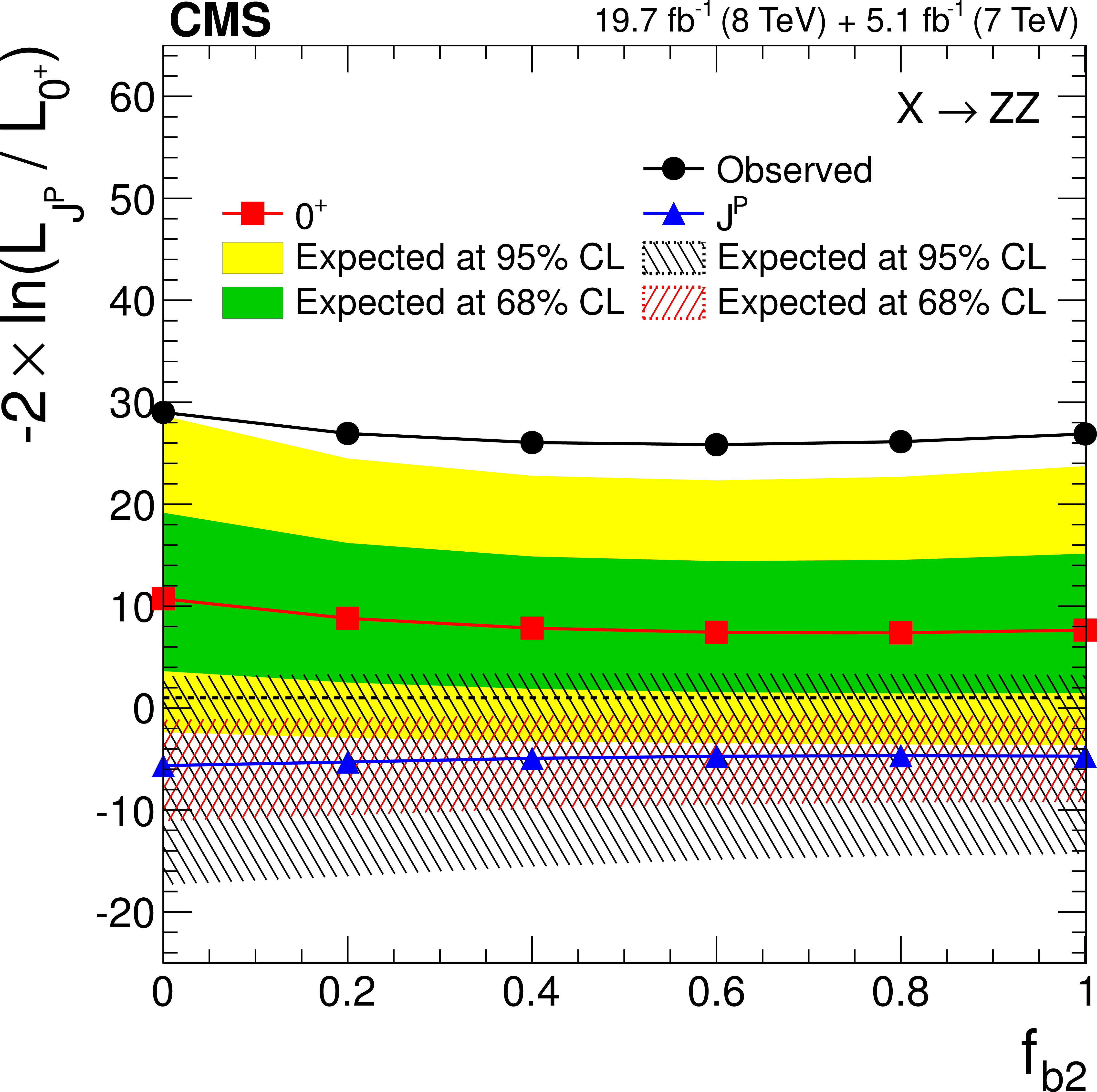
png pdf	Figure 6-a: Distributions of the test statistic $q=-2\ln(\mathcal {L}_{J^P}/\mathcal {L}_{0^+})$ as a function of $f_{b2}$ for the spin-one $J^{P}$ models tested against the SM Higgs boson hypothesis in the ${ {\mathrm {q}} {\mathrm {\overline {q}}}} \to {\mathrm {X}} \to {\mathrm {Z}} {\mathrm {Z}}$ (a) and decay-only ${\mathrm {X}} \to {\mathrm {Z}} {\mathrm {Z}}$ (b) analyses. The median expectation for the SM Higgs boson is represented by the red squares with the green (68% CL) and yellow (95% CL) solid color regions and for the alternative $J^P$ hypotheses by the blue triangles with the red (68% CL) and blue (95% CL) hatched regions. The observed values are indicated by the black dots.
png pdf	Figure 6-b: Distributions of the test statistic $q=-2\ln(\mathcal {L}_{J^P}/\mathcal {L}_{0^+})$ as a function of $f_{b2}$ for the spin-one $J^{P}$ models tested against the SM Higgs boson hypothesis in the ${ {\mathrm {q}} {\mathrm {\overline {q}}}} \to {\mathrm {X}} \to {\mathrm {Z}} {\mathrm {Z}}$ (a) and decay-only ${\mathrm {X}} \to {\mathrm {Z}} {\mathrm {Z}}$ (b) analyses. The median expectation for the SM Higgs boson is represented by the red squares with the green (68% CL) and yellow (95% CL) solid color regions and for the alternative $J^P$ hypotheses by the blue triangles with the red (68% CL) and blue (95% CL) hatched regions. The observed values are indicated by the black dots.
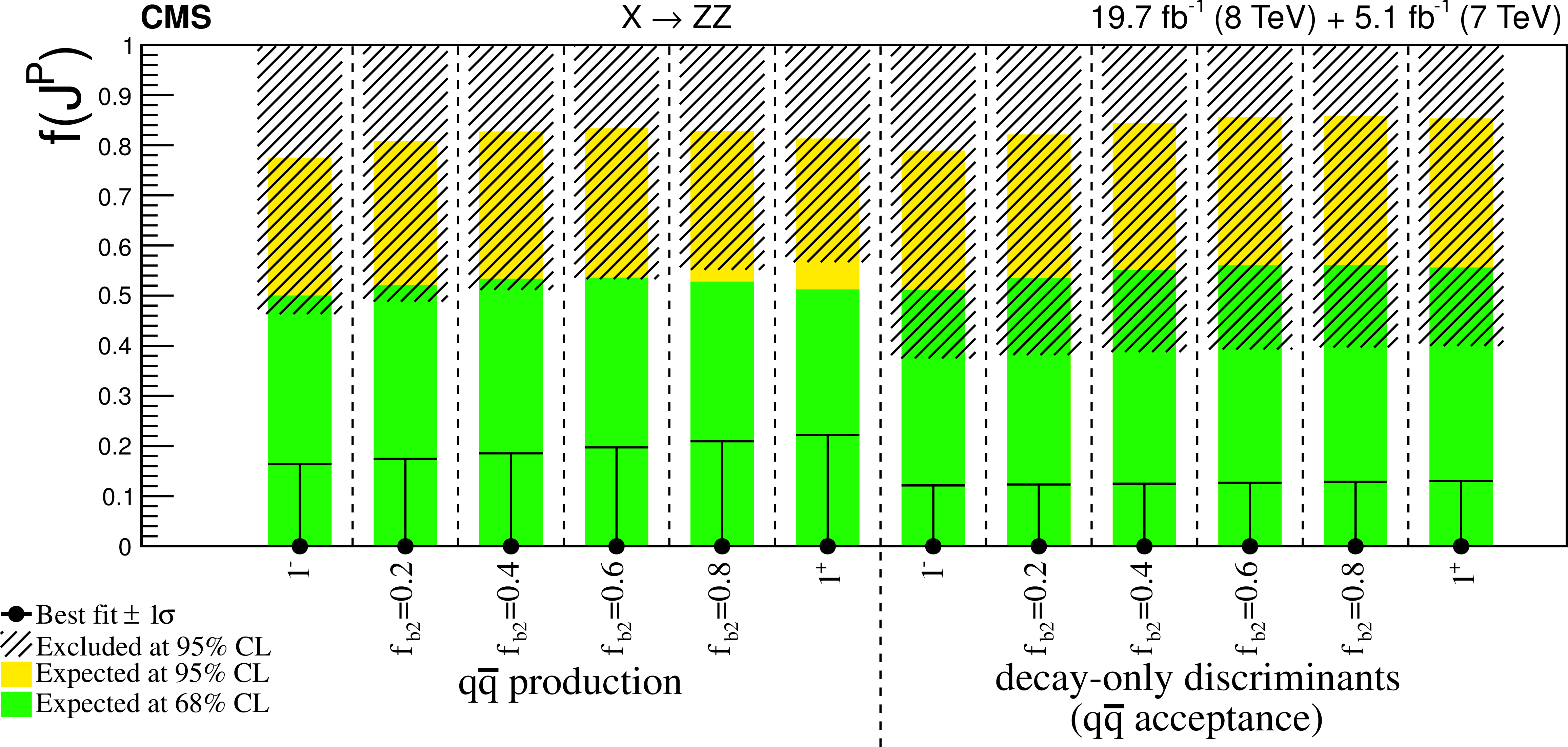
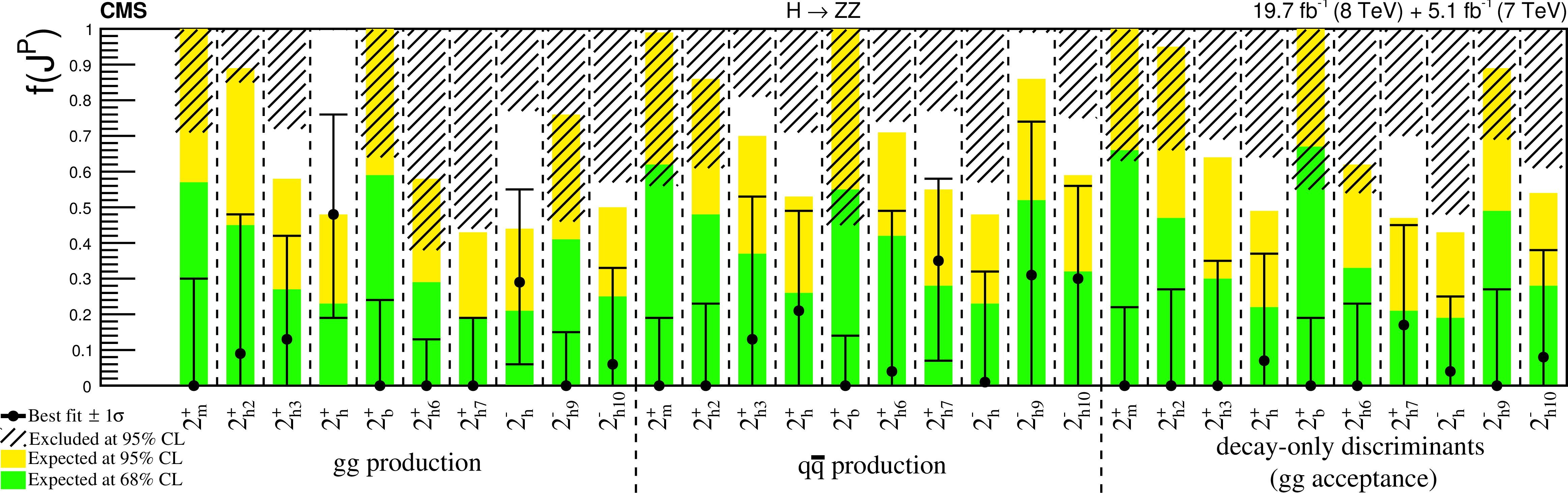
png pdf	Figure 7: Summary of the $f(J^P)$ constraints as a function of $f_{b2}$ from Table 6, where the decay-only measurements are performed using the efficiency of the ${ {\mathrm {q}} {\mathrm {\overline {q}}}} \to {\mathrm {X}} \to {\mathrm {Z}} {\mathrm {Z}}$ selection. The expected 68% and 95% CL regions are shown as green and yellow bands. The observed constraints at 68% and 95% CL are shown as the points with error bars and the excluded hatched regions.
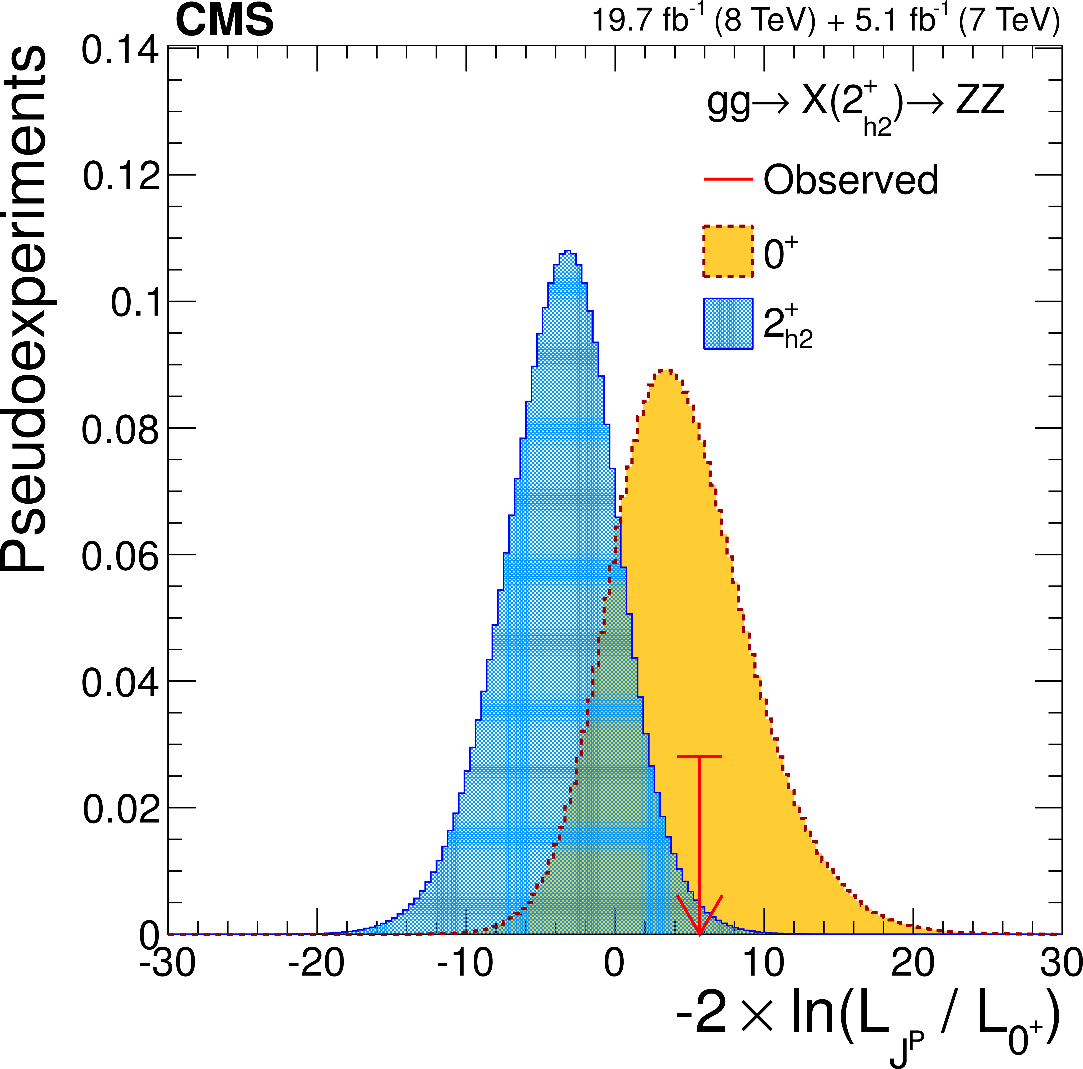
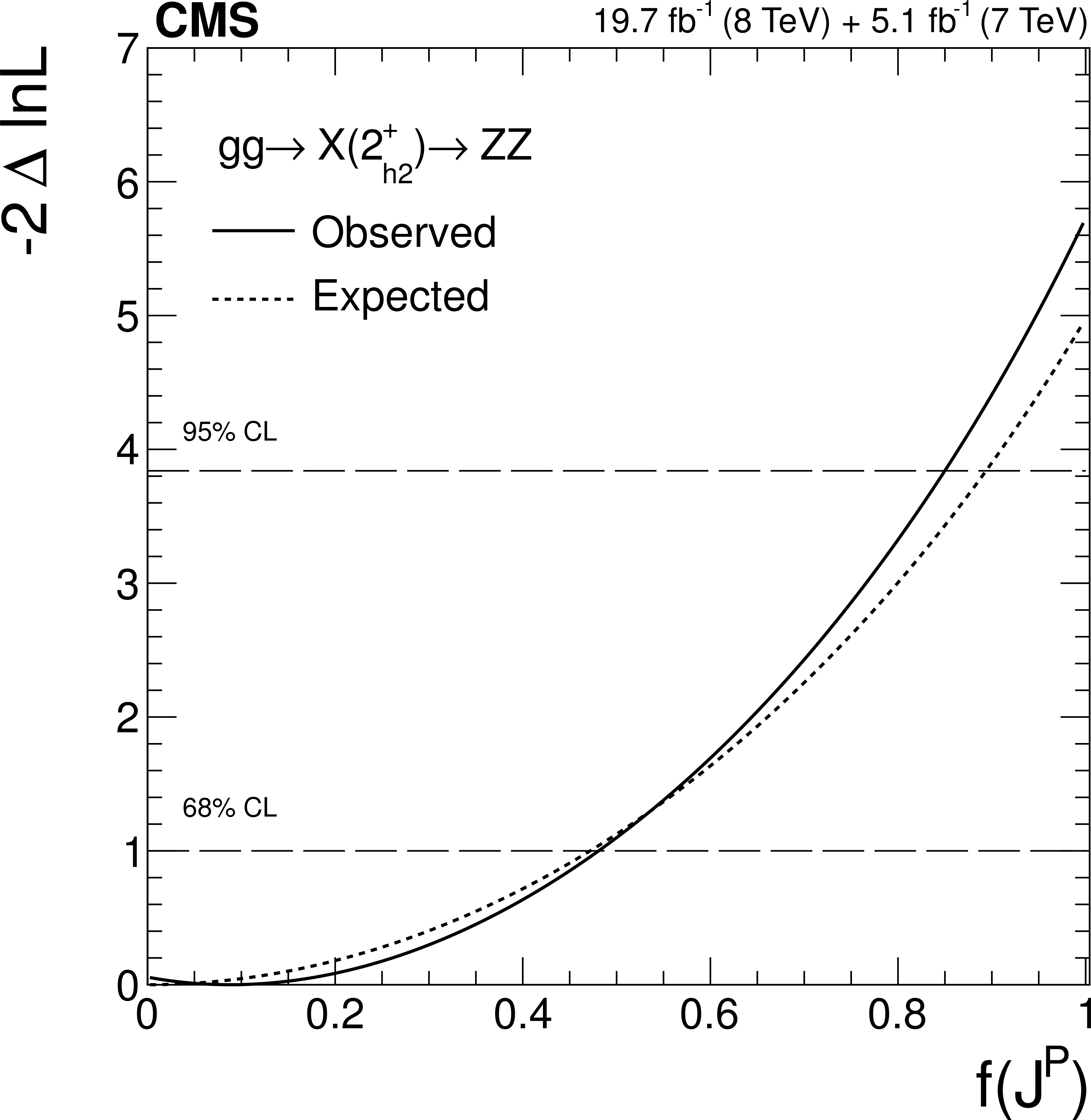
png pdf	Figure 8-a: (a) Distributions of the test statistic $q=-2\ln(\mathcal {L}_{J^P}/\mathcal {L}_{0^+})$ for the $J^P=2^+_{h2}$ hypothesis of ${\mathrm {g}} {\mathrm {g}} \to {\mathrm {X}} (2^+_{h2})\to {\mathrm {Z}} {\mathrm {Z}}$ tested against the SM Higgs boson hypothesis ($0^+$). The expectation for the SM Higgs boson is represented by the yellow histogram on the right and the alternative $J^P$ hypothesis by the blue histogram on the left. The red arrow indicates the observed $q$ value. (b) Observed value of $-2\Delta \ln\mathcal {L}$ as a function of $f(J^P)$ and the expectation in the SM for the ${\mathrm {g}} {\mathrm {g}} \to {\mathrm {X}} (2^+_{h2})\to {\mathrm {Z}} {\mathrm {Z}}$ alternative $J^P$ model.
png pdf	Figure 8-b: (a) Distributions of the test statistic $q=-2\ln(\mathcal {L}_{J^P}/\mathcal {L}_{0^+})$ for the $J^P=2^+_{h2}$ hypothesis of ${\mathrm {g}} {\mathrm {g}} \to {\mathrm {X}} (2^+_{h2})\to {\mathrm {Z}} {\mathrm {Z}}$ tested against the SM Higgs boson hypothesis ($0^+$). The expectation for the SM Higgs boson is represented by the yellow histogram on the right and the alternative $J^P$ hypothesis by the blue histogram on the left. The red arrow indicates the observed $q$ value. (b) Observed value of $-2\Delta \ln\mathcal {L}$ as a function of $f(J^P)$ and the expectation in the SM for the ${\mathrm {g}} {\mathrm {g}} \to {\mathrm {X}} (2^+_{h2})\to {\mathrm {Z}} {\mathrm {Z}}$ alternative $J^P$ model.
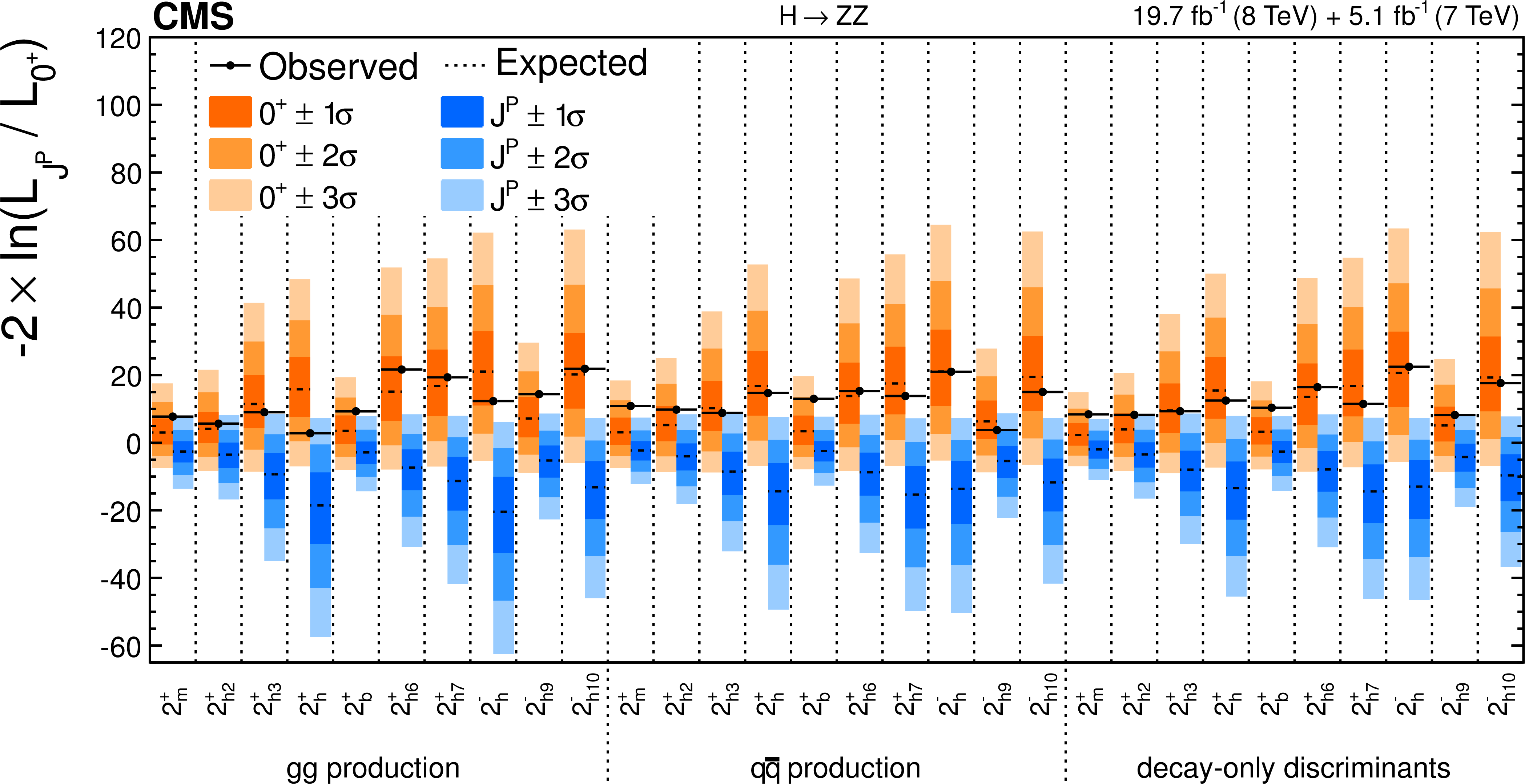
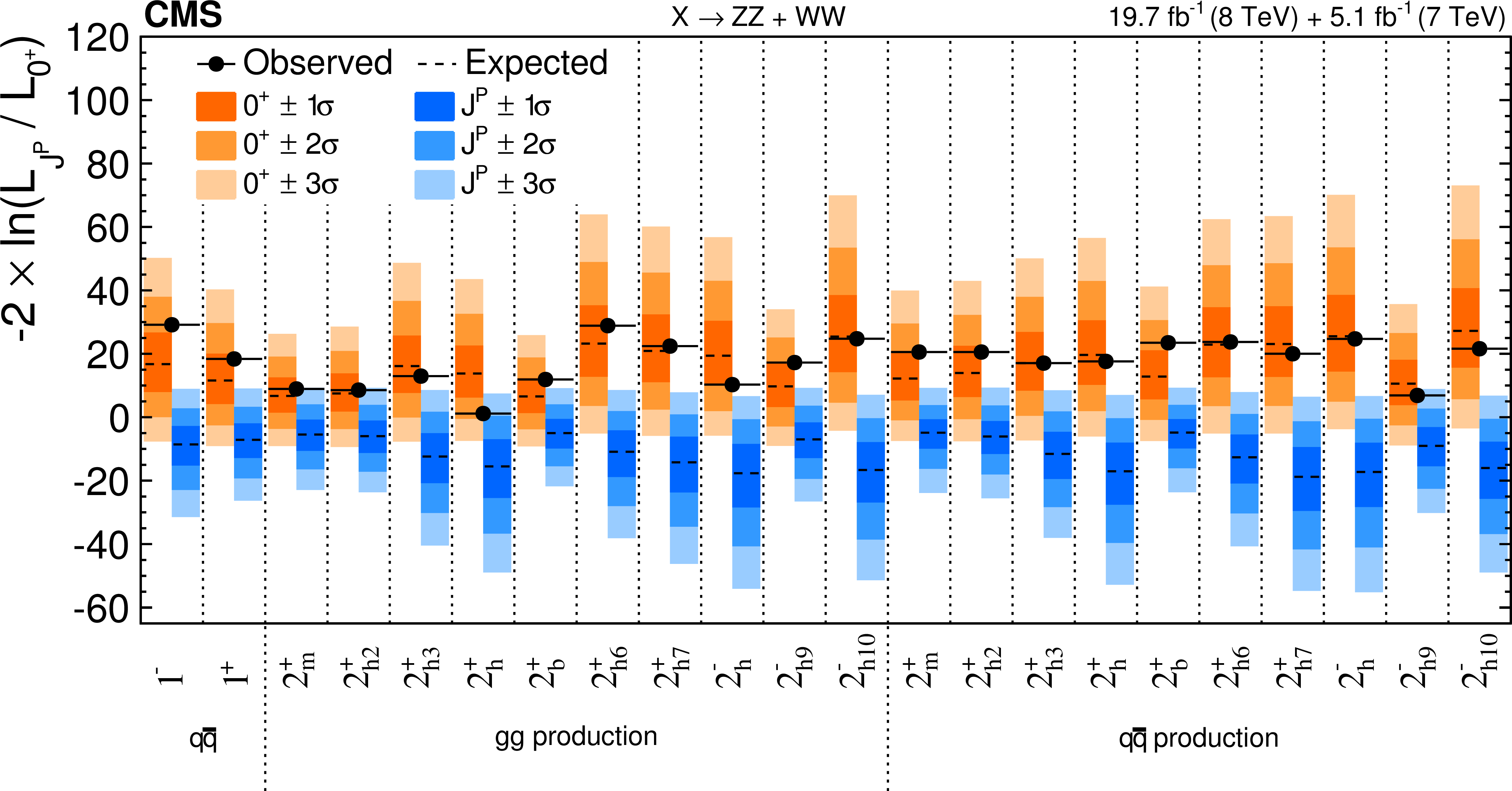
png pdf	Figure 9: Distributions of the test statistic $q=-2\ln(\mathcal {L}_{J^P}/\mathcal {L}_{0^+})$ for the spin-two $J^{P}$ models tested against the SM Higgs boson hypothesis in the ${\mathrm {X}} \to {\mathrm {Z}} {\mathrm {Z}}$ analyses. The expected median and the 68.3%, 95.4%, and 99.7% CL regions for the SM Higgs boson (orange, the left for each model) and for the alternative $J^P$ hypotheses (blue, right) are shown. The observed $q$ values are indicated by the black dots.
png pdf	Figure 10: Summary of the $f(J^P)$ constraints for the spin-two models from Table 7, where the decay-only measurements are performed using the efficiency of the ${\mathrm {g}} {\mathrm {g}} \to {\mathrm {X}} \to {\mathrm {Z}} {\mathrm {Z}}$ selection. The expected 68% and 95% CL regions are shown as the green and yellow bands. The observed constraints at 68% and 95% CL are shown as the points with error bars and the excluded hatched regions.
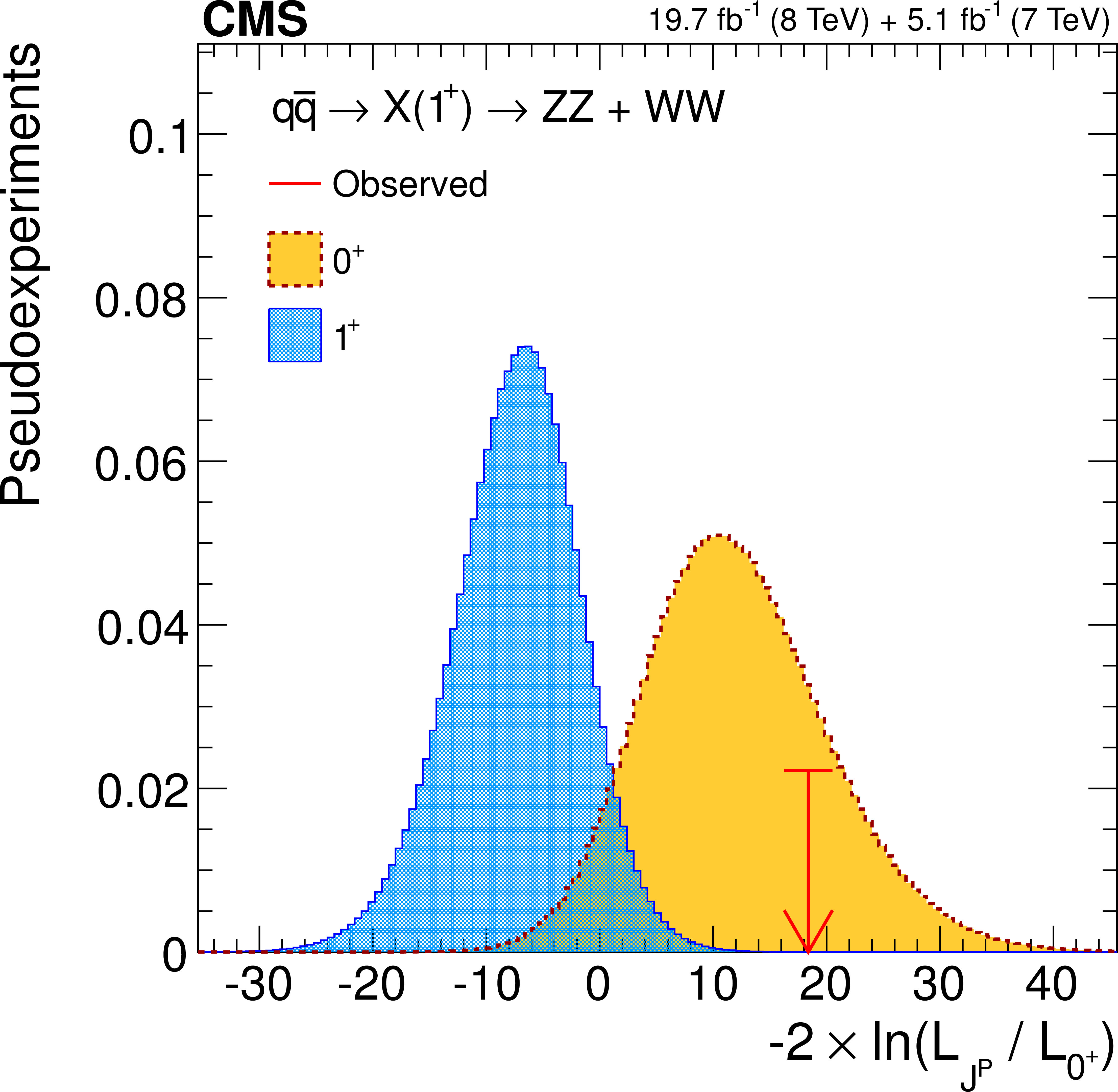
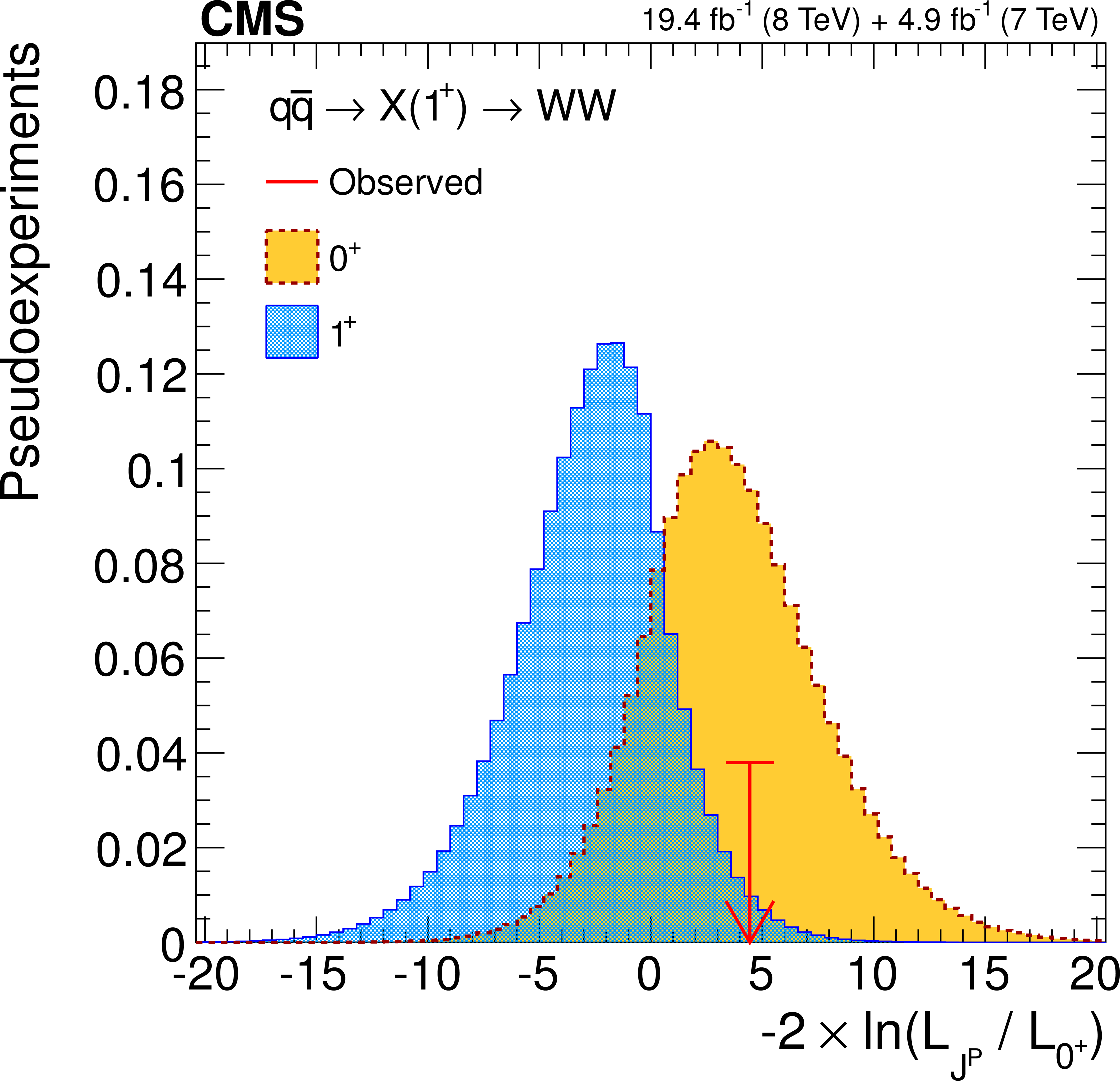
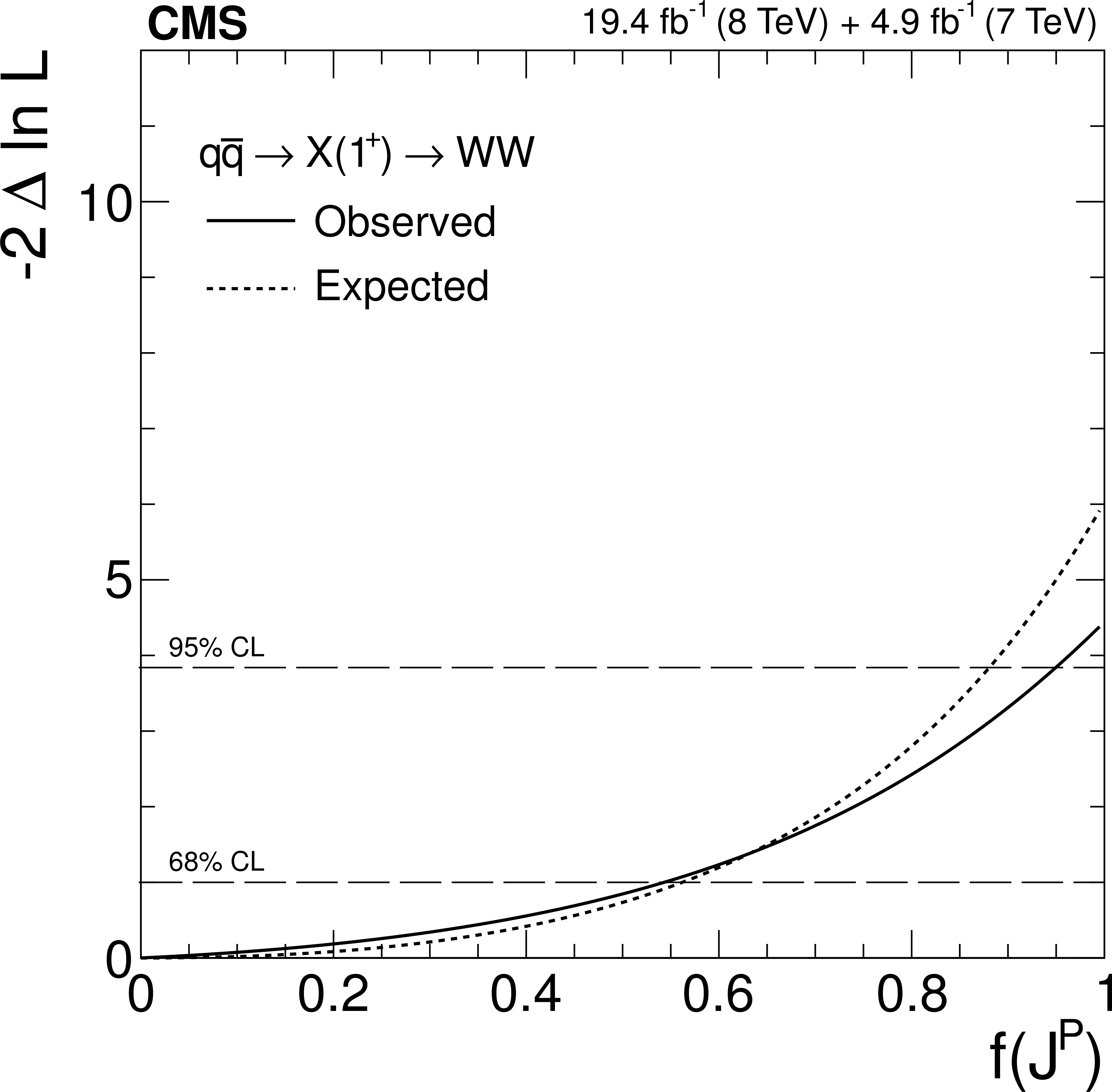
png pdf	Figure 11-a: (a) Distributions of the test statistic $q=-2\ln(\mathcal {L}_{J^P}/\mathcal {L}_{0^+})$ for the $J^P=1^+$ hypothesis of ${ {\mathrm {q}} {\mathrm {\overline {q}}}} \to {\mathrm {X}} (1^+)\to {\mathrm {W}} {\mathrm {W}}$ against the SM Higgs boson hypothesis ($0^+$). The expectation for the SM Higgs boson is represented by the yellow histogram on the right and the alternative $J^P$ hypothesis by the blue histogram on the left. The red arrow indicates the observed $q$ value. (b) Observed value of $-2\Delta \ln\mathcal {L}$ as a function of $f(J^P)$ and the expectation in the SM for the ${ {\mathrm {q}} {\mathrm {\overline {q}}}} \to {\mathrm {X}} (1^+)\to {\mathrm {W}} {\mathrm {W}}$ alternative $J^P$ model.
png pdf	Figure 11-b: (a) Distributions of the test statistic $q=-2\ln(\mathcal {L}_{J^P}/\mathcal {L}_{0^+})$ for the $J^P=1^+$ hypothesis of ${ {\mathrm {q}} {\mathrm {\overline {q}}}} \to {\mathrm {X}} (1^+)\to {\mathrm {W}} {\mathrm {W}}$ against the SM Higgs boson hypothesis ($0^+$). The expectation for the SM Higgs boson is represented by the yellow histogram on the right and the alternative $J^P$ hypothesis by the blue histogram on the left. The red arrow indicates the observed $q$ value. (b) Observed value of $-2\Delta \ln\mathcal {L}$ as a function of $f(J^P)$ and the expectation in the SM for the ${ {\mathrm {q}} {\mathrm {\overline {q}}}} \to {\mathrm {X}} (1^+)\to {\mathrm {W}} {\mathrm {W}}$ alternative $J^P$ model.
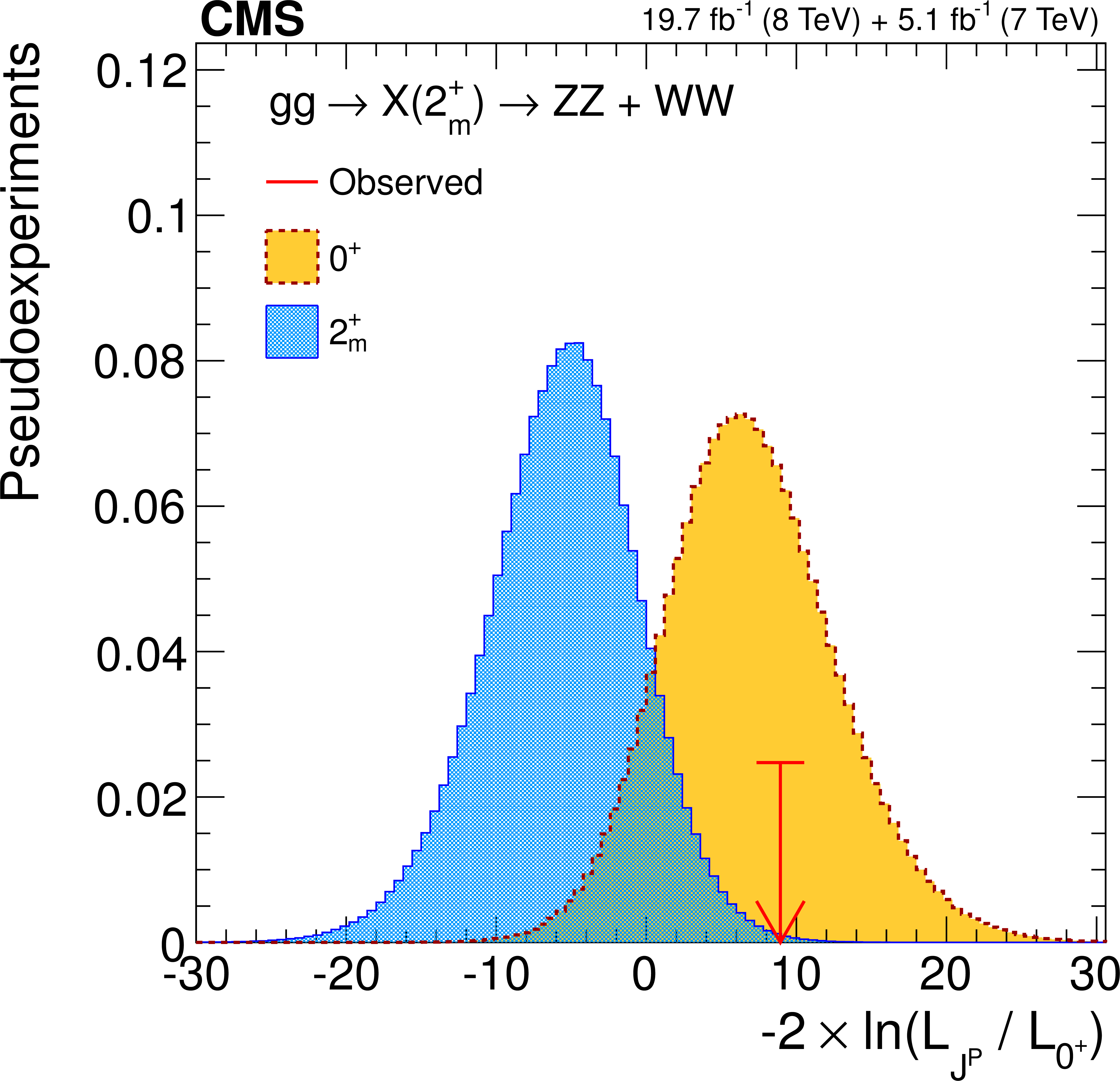
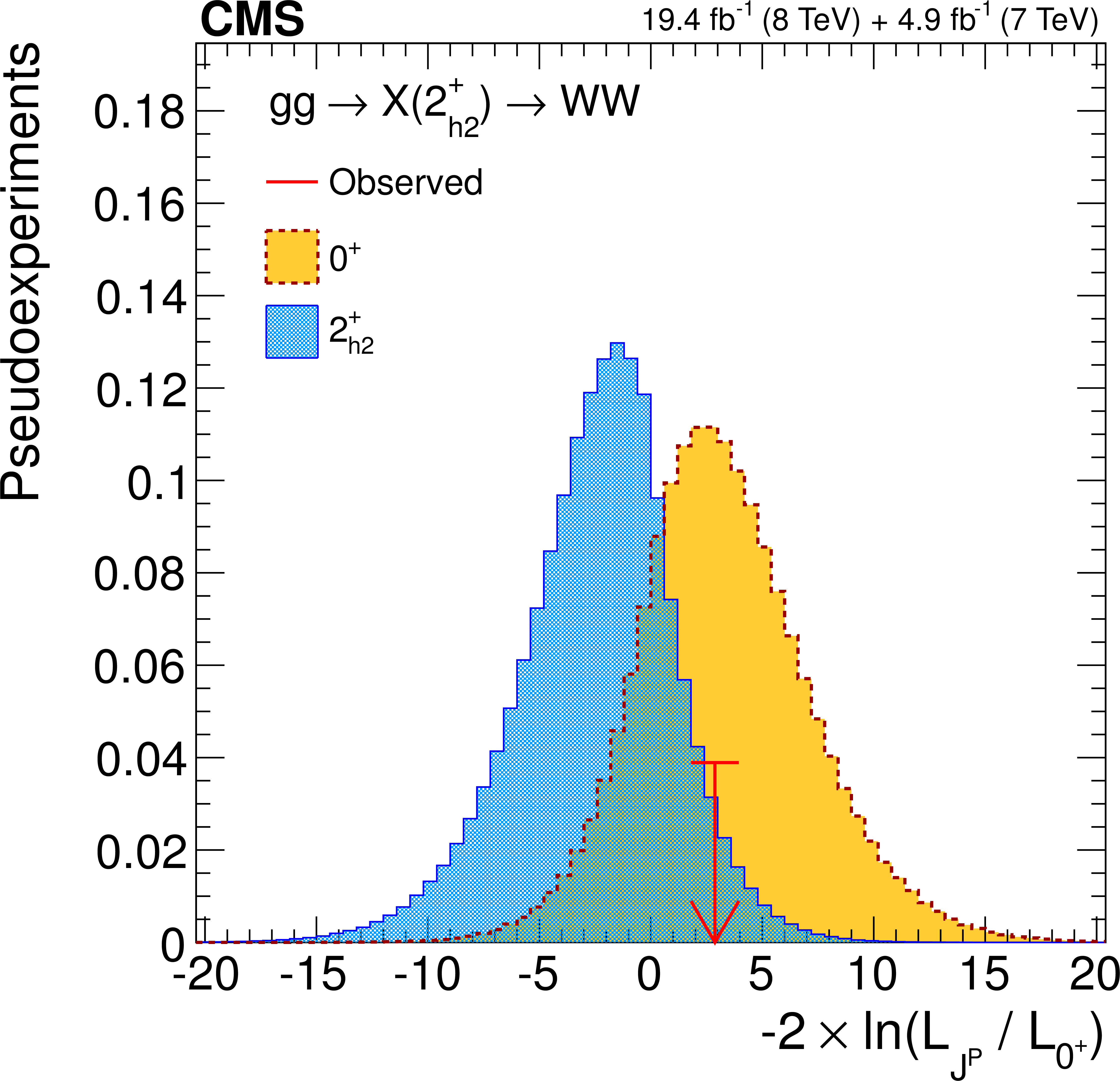
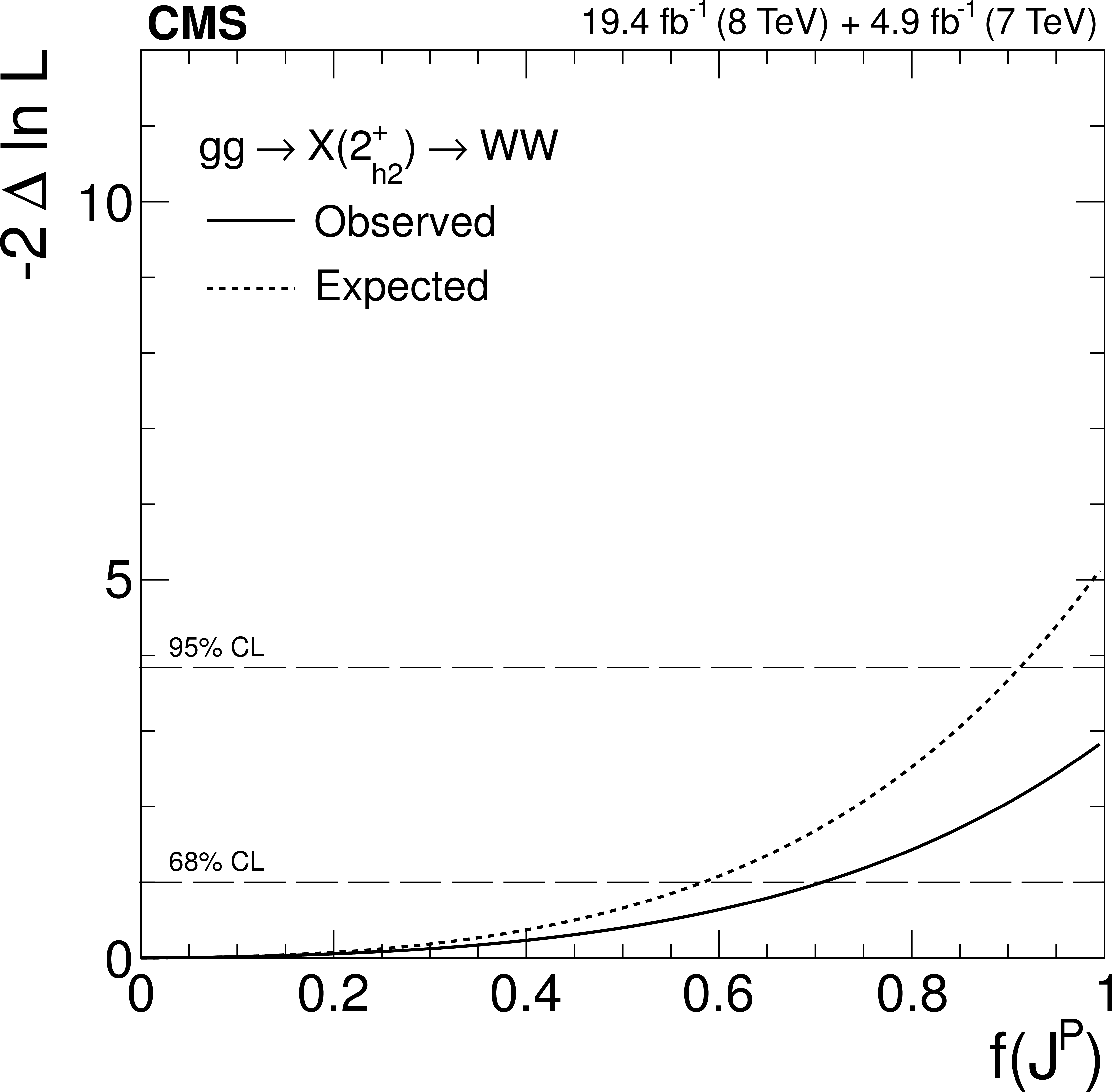
png pdf	Figure 12-a: (a) Distributions of the test statistic $q=-2\ln(\mathcal {L}_{J^P}/\mathcal {L}_{0^+})$ for the $J^P=2^+_{h2}$ hypothesis of ${\mathrm {g}} {\mathrm {g}} \to {\mathrm {X}} (2^+_{h2})\to {\mathrm {W}} {\mathrm {W}}$ against the SM Higgs boson hypothesis ($0^+$). The expectation for the SM Higgs boson is represented by the yellow histogram on the right and the alternative $J^P$ hypothesis by the blue histogram on the left. The red arrow indicates the observed $q$ value. (b) Observed value of $-2\Delta \ln\mathcal {L}$ as a function of $f(J^P)$ and the expectation in the SM for the ${\mathrm {g}} {\mathrm {g}} \to {\mathrm {X}} (2^+_{h2})\to {\mathrm {W}} {\mathrm {W}}$ alternative $J^P$ model.
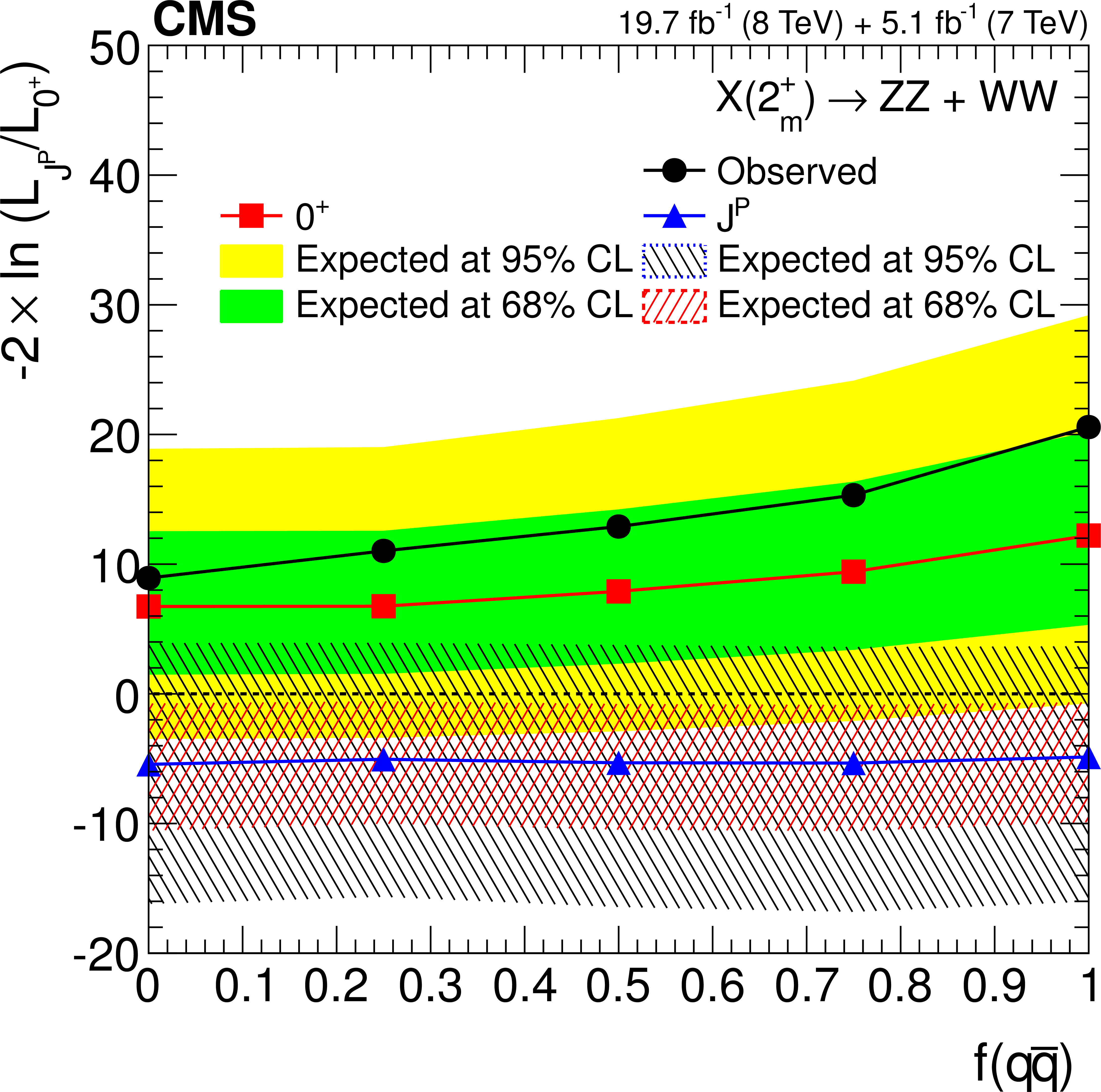
png pdf	Figure 12-b: (a) Distributions of the test statistic $q=-2\ln(\mathcal {L}_{J^P}/\mathcal {L}_{0^+})$ for the $J^P=2^+_{h2}$ hypothesis of ${\mathrm {g}} {\mathrm {g}} \to {\mathrm {X}} (2^+_{h2})\to {\mathrm {W}} {\mathrm {W}}$ against the SM Higgs boson hypothesis ($0^+$). The expectation for the SM Higgs boson is represented by the yellow histogram on the right and the alternative $J^P$ hypothesis by the blue histogram on the left. The red arrow indicates the observed $q$ value. (b) Observed value of $-2\Delta \ln\mathcal {L}$ as a function of $f(J^P)$ and the expectation in the SM for the ${\mathrm {g}} {\mathrm {g}} \to {\mathrm {X}} (2^+_{h2})\to {\mathrm {W}} {\mathrm {W}}$ alternative $J^P$ model.
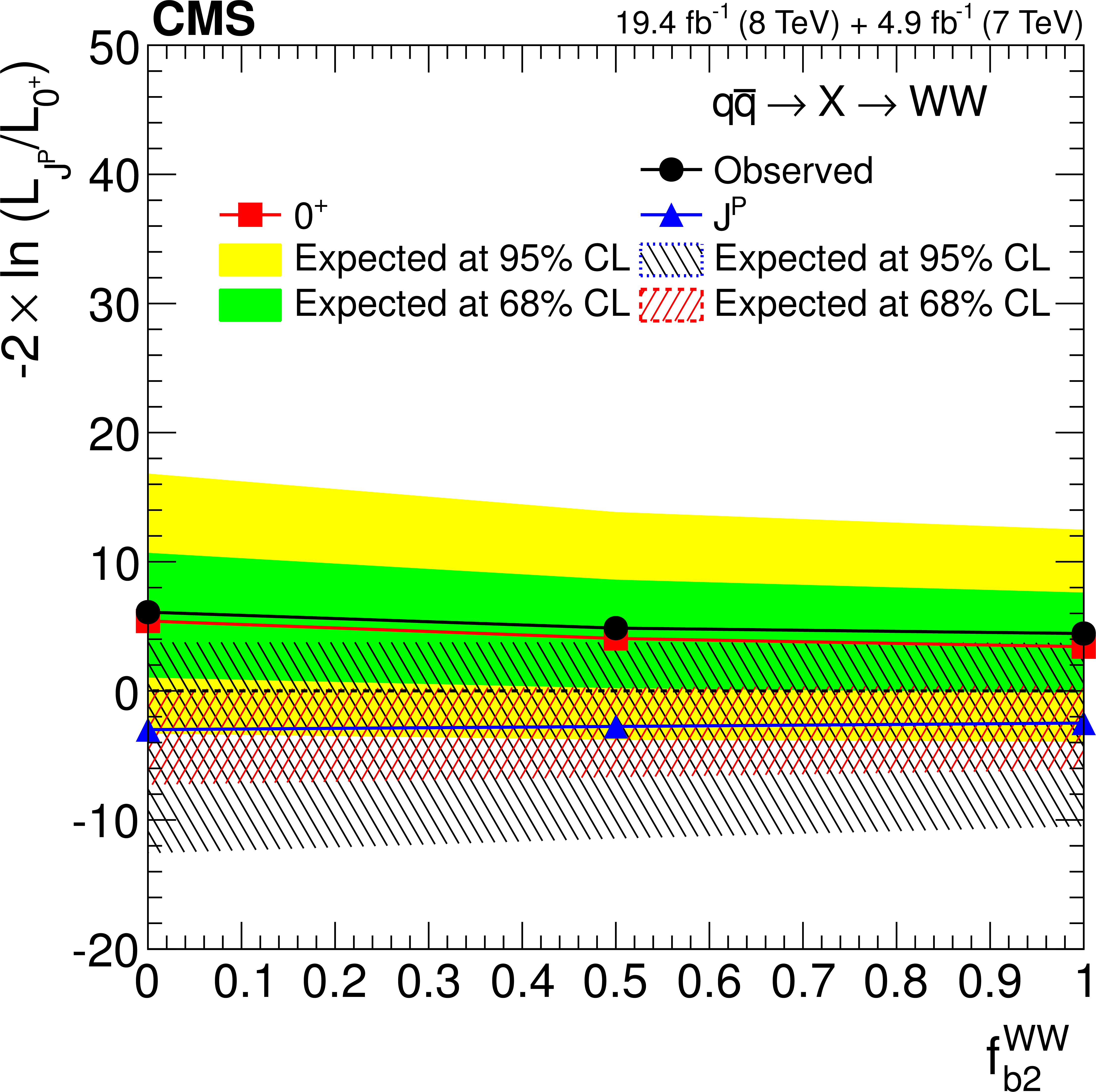
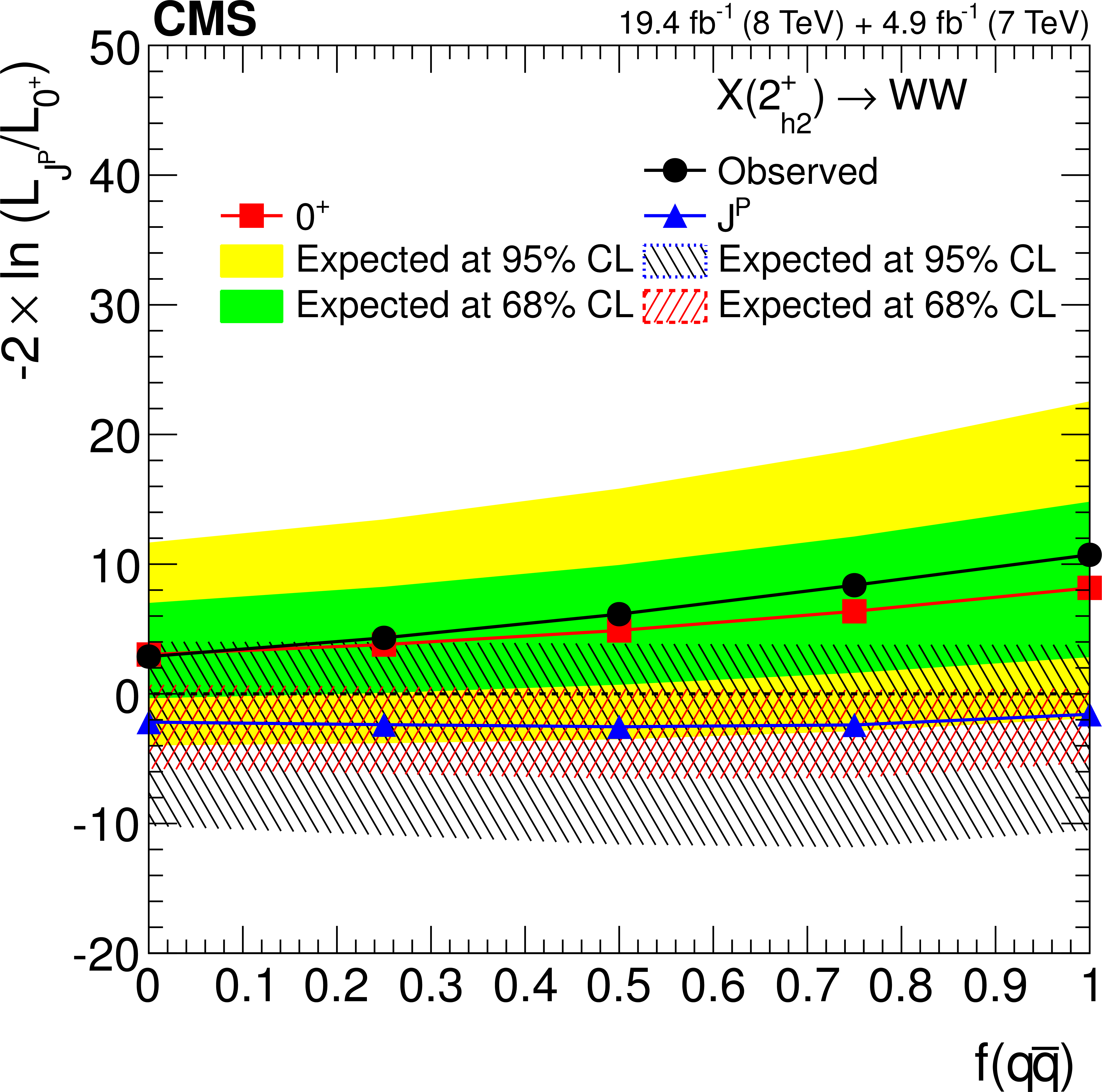
png pdf	Figure 13-a: (a) Distributions of the test statistic $q=-2\ln(\mathcal {L}_{J^P}/\mathcal {L}_{0^+})$ as a function of $f_{b2}^{ {\mathrm {W}} {\mathrm {W}}}$ for the hypothesis of the spin-one $J^{P}$ models against the SM Higgs boson hypothesis in the ${ {\mathrm {q}} {\mathrm {\overline {q}}}} \to {\mathrm {X}} \to {\mathrm {W}} {\mathrm {W}}$ analysis. (b) Distribution of the test statistic $q=-2\ln(\mathcal {L}_{J^P}/\mathcal {L}_{0^+})$ as a function of $f( { {\mathrm {q}} {\mathrm {\overline {q}}}} )$ for the $2^+_{h2}$ hypothesis against the SM Higgs boson hypothesis in the ${\mathrm {H}} \to {\mathrm {W}} {\mathrm {W}}$ analysis. The median expectation for the SM Higgs boson is represented by the red squares with the green (68% CL) and yellow (95% CL) solid color regions and for the alternative $J^P$ hypotheses by the blue triangles with the red (68% CL) and blue (95% CL) hatched regions. The observed values are indicated by the black dots.
png pdf	Figure 13-b: (a) Distributions of the test statistic $q=-2\ln(\mathcal {L}_{J^P}/\mathcal {L}_{0^+})$ as a function of $f_{b2}^{ {\mathrm {W}} {\mathrm {W}}}$ for the hypothesis of the spin-one $J^{P}$ models against the SM Higgs boson hypothesis in the ${ {\mathrm {q}} {\mathrm {\overline {q}}}} \to {\mathrm {X}} \to {\mathrm {W}} {\mathrm {W}}$ analysis. (b) Distribution of the test statistic $q=-2\ln(\mathcal {L}_{J^P}/\mathcal {L}_{0^+})$ as a function of $f( { {\mathrm {q}} {\mathrm {\overline {q}}}} )$ for the $2^+_{h2}$ hypothesis against the SM Higgs boson hypothesis in the ${\mathrm {H}} \to {\mathrm {W}} {\mathrm {W}}$ analysis. The median expectation for the SM Higgs boson is represented by the red squares with the green (68% CL) and yellow (95% CL) solid color regions and for the alternative $J^P$ hypotheses by the blue triangles with the red (68% CL) and blue (95% CL) hatched regions. The observed values are indicated by the black dots.
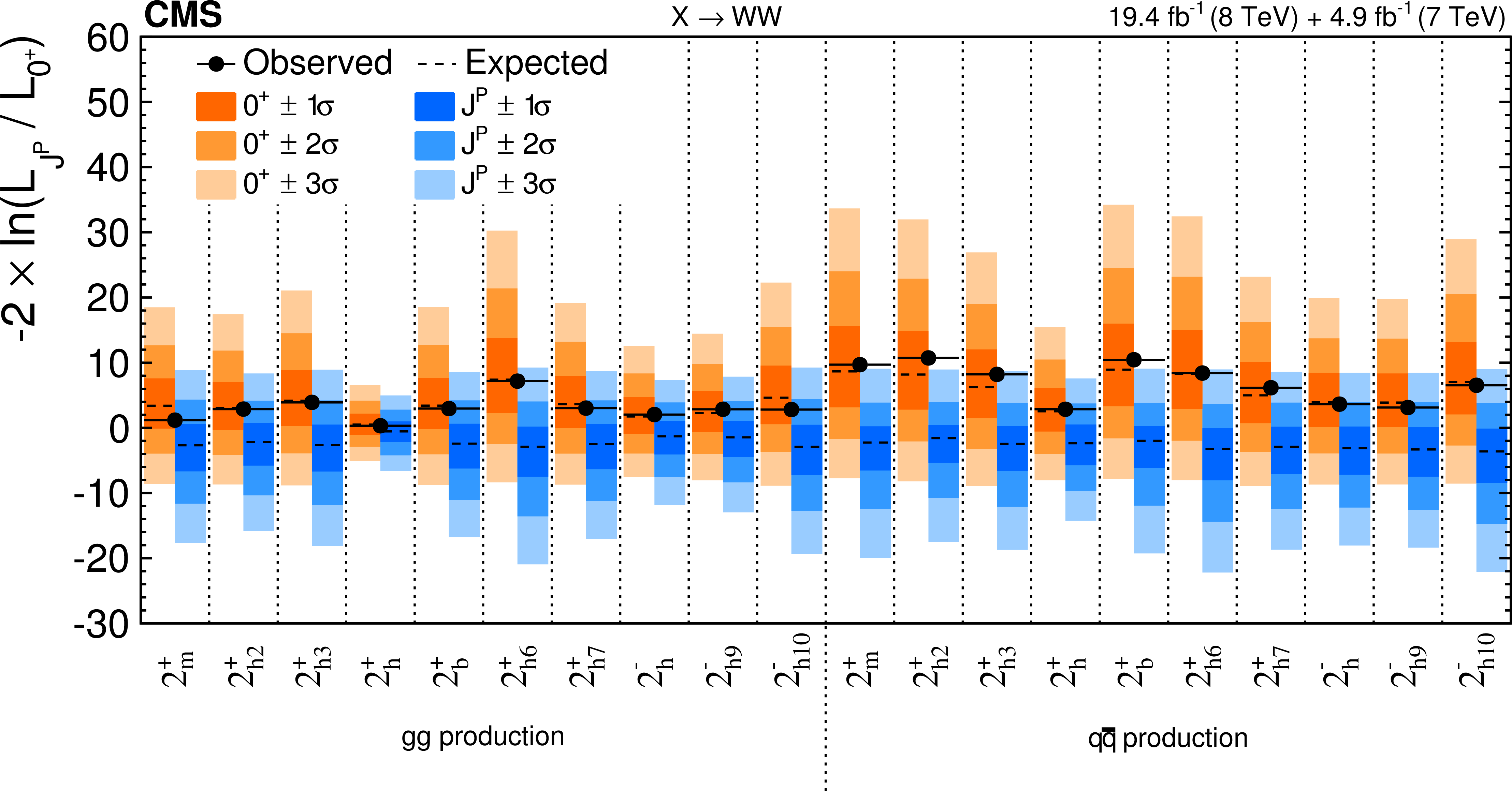
png pdf	Figure 14: Distribution of the test statistic $q=-2\ln(\mathcal {L}_{J^P}/\mathcal {L}_{0^+})$ for the spin-two $J^{P}$ models tested against the SM Higgs boson hypothesis in the ${\mathrm {X}} \to {\mathrm {W}} {\mathrm {W}}$ analyses. The expected median and the 68.3%, 95.4%, and 99.7% CL regions for the SM Higgs boson (orange, the left for each model) and for the alternative $J^P$ hypotheses (blue, right) are shown. The observed $q$ values are indicated by the black dots.
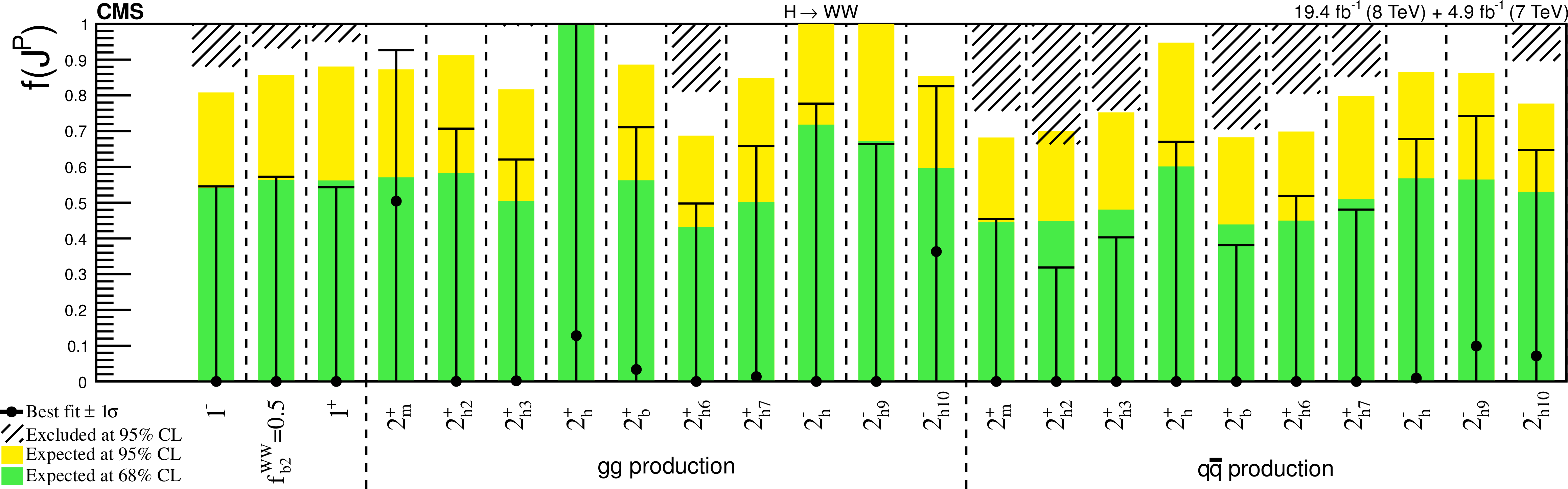
png pdf	Figure 15: Summary of the $f(J^P)$ constraints for the spin-one and spin-two models from Tables 8 and 9 in the ${\mathrm {X}} \to {\mathrm {W}} {\mathrm {W}}$ analyses. The expected 68% and 95% CL regions are shown as the green and yellow bands. The observed constraints at 68% and 95% CL are shown as the points with error bars and the excluded hatched regions.
png pdf	Figure 16-a: Distributions of the test statistic $q=-2\ln(\mathcal {L}_{J^P}/\mathcal {L}_{0^+})$ in the combination of the ${\mathrm {X}} \to {\mathrm {Z}} {\mathrm {Z}}$ and ${\mathrm {W}} {\mathrm {W}}$ channels for the hypotheses of ${ {\mathrm {q}} {\mathrm {\overline {q}}}} \to {\mathrm {X}} (1^+)$ (a) and ${\mathrm {g}} {\mathrm {g}} \to {\mathrm {X}} (2^+_{h2})$ (b) tested against the SM Higgs boson hypothesis. The expectation for the SM Higgs boson is represented by the yellow histogram on the right of each plot and the alternative $J^P$ hypothesis by the blue histogram on the left. The red arrow indicates the observed $q$ value.
png pdf	Figure 16-b: Distributions of the test statistic $q=-2\ln(\mathcal {L}_{J^P}/\mathcal {L}_{0^+})$ in the combination of the ${\mathrm {X}} \to {\mathrm {Z}} {\mathrm {Z}}$ and ${\mathrm {W}} {\mathrm {W}}$ channels for the hypotheses of ${ {\mathrm {q}} {\mathrm {\overline {q}}}} \to {\mathrm {X}} (1^+)$ (a) and ${\mathrm {g}} {\mathrm {g}} \to {\mathrm {X}} (2^+_{h2})$ (b) tested against the SM Higgs boson hypothesis. The expectation for the SM Higgs boson is represented by the yellow histogram on the right of each plot and the alternative $J^P$ hypothesis by the blue histogram on the left. The red arrow indicates the observed $q$ value.
png pdf	Figure 17-a: (a) Distributions of the test statistic $q=-2\ln(\mathcal {L}_{J^P}/\mathcal {L}_{0^+})$ in the combination of the ${\mathrm {X}} \to {\mathrm {Z}} {\mathrm {Z}}$ and ${\mathrm {W}} {\mathrm {W}}$ channels for the hypothesis of ${\mathrm {g}} {\mathrm {g}} \to {\mathrm {X}} (2^+_{m})$ tested against the SM Higgs boson hypothesis. The expectation for the SM Higgs boson is represented by the yellow histogram on the right and the alternative $J^P$ hypothesis by the blue histogram on the left. The red arrow indicates the observed $q$ value. (b) Distribution of $q$ as a function of $f( { {\mathrm {q}} {\mathrm {\overline {q}}}} )$ for the $2^+_{m}$ hypothesis against the SM Higgs boson hypothesis in the ${\mathrm {X}} \to {\mathrm {Z}} {\mathrm {Z}}$ and ${\mathrm {W}} {\mathrm {W}}$ channels. The median expectation for the SM Higgs boson is represented with the solid green (68% CL) and yellow (95% CL) regions. The alternative $2^+_{m}$ hypotheses are represented by the blue triangles with the red (68% CL) and blue (95% CL) hatched regions. The observed values are indicated by the black dots.
png pdf	Figure 17-b: (a) Distributions of the test statistic $q=-2\ln(\mathcal {L}_{J^P}/\mathcal {L}_{0^+})$ in the combination of the ${\mathrm {X}} \to {\mathrm {Z}} {\mathrm {Z}}$ and ${\mathrm {W}} {\mathrm {W}}$ channels for the hypothesis of ${\mathrm {g}} {\mathrm {g}} \to {\mathrm {X}} (2^+_{m})$ tested against the SM Higgs boson hypothesis. The expectation for the SM Higgs boson is represented by the yellow histogram on the right and the alternative $J^P$ hypothesis by the blue histogram on the left. The red arrow indicates the observed $q$ value. (b) Distribution of $q$ as a function of $f( { {\mathrm {q}} {\mathrm {\overline {q}}}} )$ for the $2^+_{m}$ hypothesis against the SM Higgs boson hypothesis in the ${\mathrm {X}} \to {\mathrm {Z}} {\mathrm {Z}}$ and ${\mathrm {W}} {\mathrm {W}}$ channels. The median expectation for the SM Higgs boson is represented with the solid green (68% CL) and yellow (95% CL) regions. The alternative $2^+_{m}$ hypotheses are represented by the blue triangles with the red (68% CL) and blue (95% CL) hatched regions. The observed values are indicated by the black dots.
png pdf	Figure 18: Distributions of the test statistic $q=-2\ln(\mathcal {L}_{J^P}/\mathcal {L}_{0^+})$ for the spin-one and spin-two $J^{P}$ models tested against the SM Higgs boson hypothesis in the combined ${\mathrm {X}} \to {\mathrm {Z}} {\mathrm {Z}}$ and ${\mathrm {W}} {\mathrm {W}}$ analyses. The expected median and the 68.3%, 95.4%, and 99.7% CL regions for the SM Higgs boson (orange, the left for each model) and for the alternative $J^P$ hypotheses (blue, right) are shown. The observed $q$ values are indicated by the black dots.
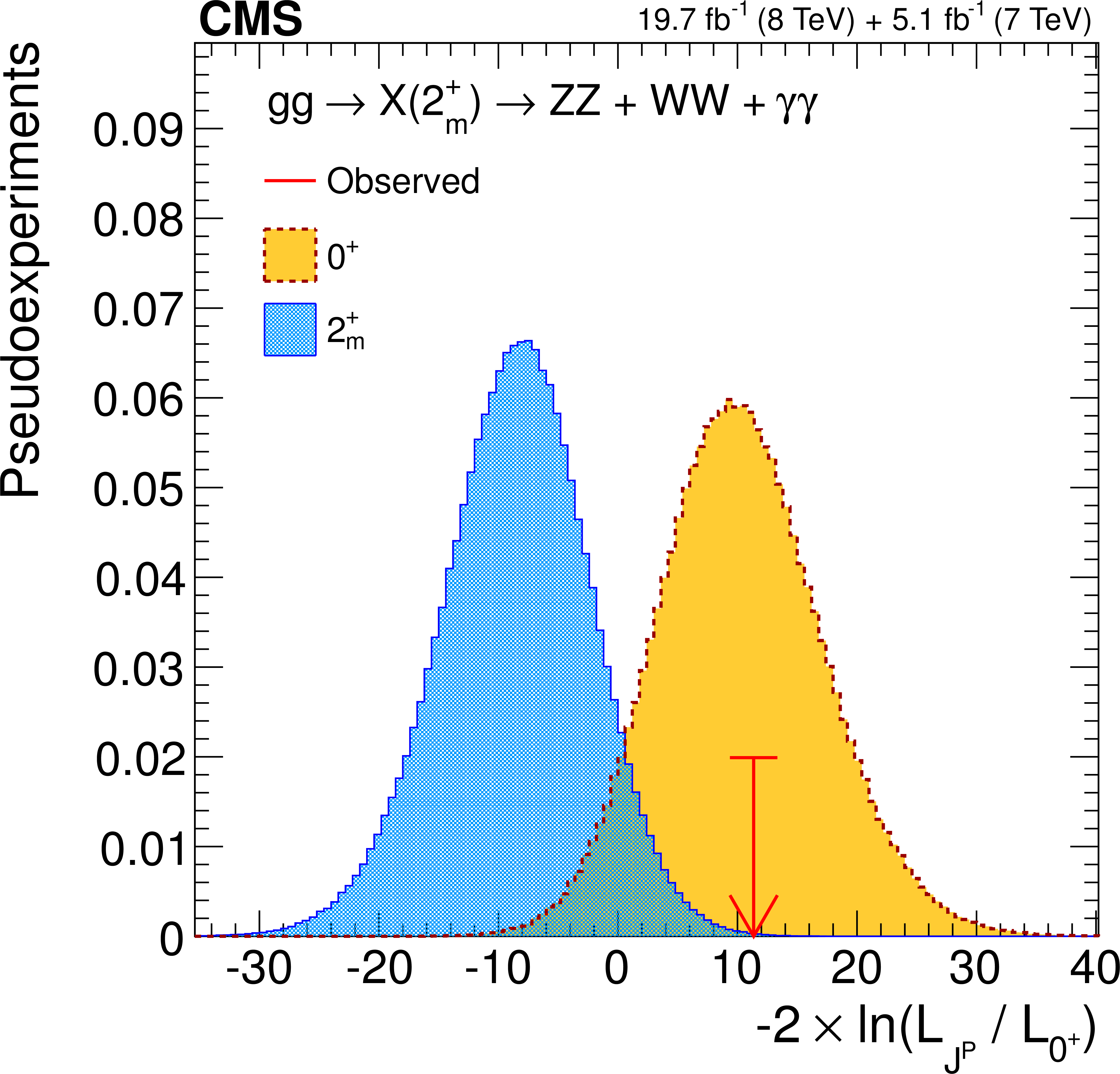
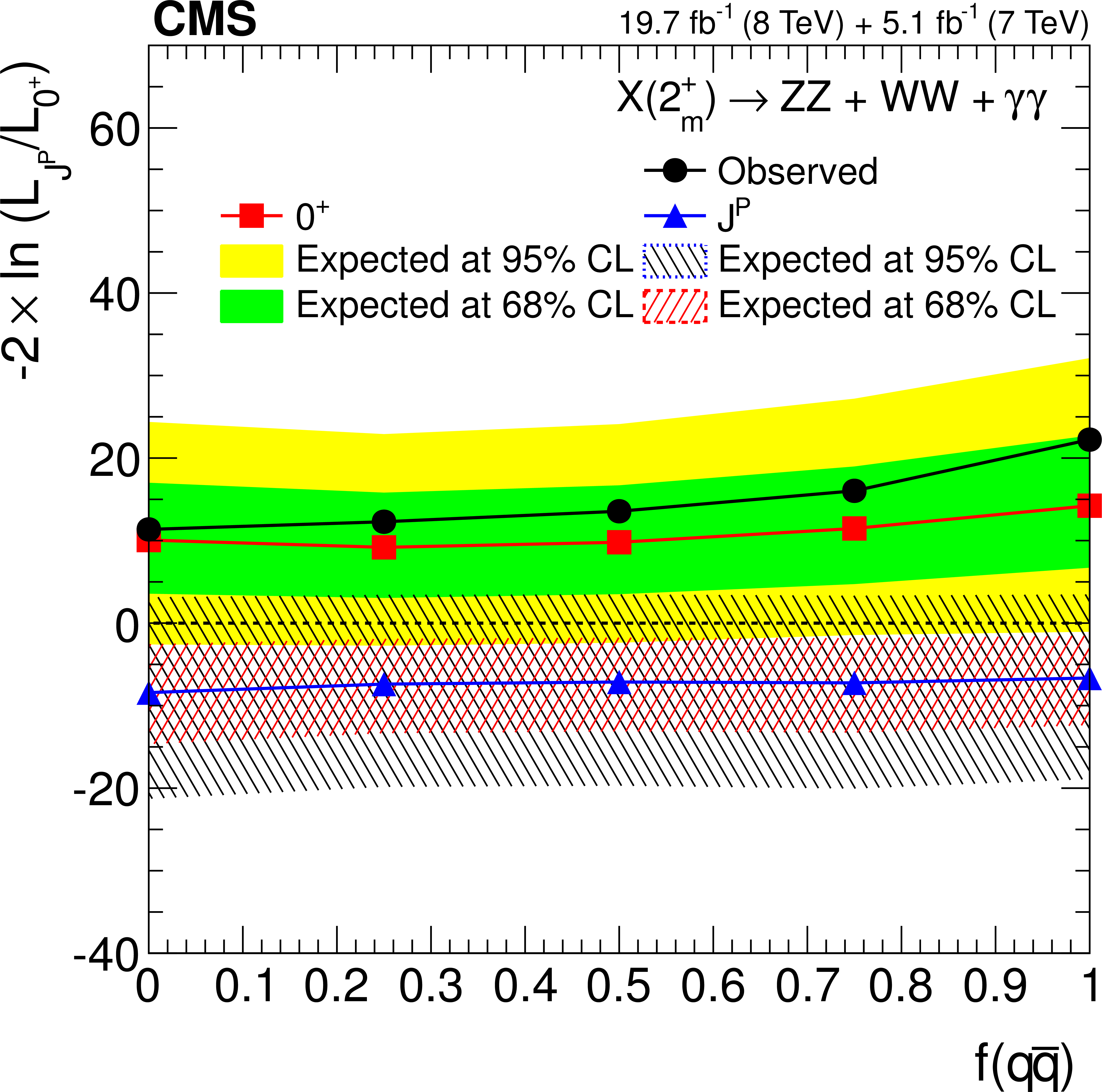
png pdf	Figure 19-a: (a) Distributions of the test statistic $q=-2\ln(\mathcal {L}_{J^P}/\mathcal {L}_{0^+})$ in the combination of the ${\mathrm {X}} \to {\mathrm {Z}} {\mathrm {Z}} , {\mathrm {W}} {\mathrm {W}},$ and $\gamma \gamma$ channels for the hypothesis of ${\mathrm {g}} {\mathrm {g}} \to X(2^+_{m})$ tested against the SM Higgs boson hypothesis ($0^+$). The expectation for the SM Higgs boson is represented by the yellow histogram on the right and the alternative $J^P$ hypothesis by the blue histogram on the left. The red arrow indicates the observed $q$ value. (b) Distributions of the test statistic $q=-2\ln(\mathcal {L}_{J^P}/\mathcal {L}_{0^+})$ as a function of $f( { {\mathrm {q}} {\mathrm {\overline {q}}}} )$ for the hypotheses of the $2^+_{m}$ model tested against the SM Higgs boson hypothesis in the ${\mathrm {X}} \to {\mathrm {Z}} {\mathrm {Z}} , {\mathrm {W}} {\mathrm {W}},$ and $\gamma \gamma$ channels. The median expectation for the SM Higgs boson is represented with the solid green (68% CL) and yellow (95% CL) regions. The alternative $2^+_{m}$ hypotheses are represented by the blue triangles with the red (68% CL) and blue (95% CL) hatched regions. The observed values are indicated by the black dots.
png pdf	Figure 19-b: (a) Distributions of the test statistic $q=-2\ln(\mathcal {L}_{J^P}/\mathcal {L}_{0^+})$ in the combination of the ${\mathrm {X}} \to {\mathrm {Z}} {\mathrm {Z}} , {\mathrm {W}} {\mathrm {W}},$ and $\gamma \gamma$ channels for the hypothesis of ${\mathrm {g}} {\mathrm {g}} \to X(2^+_{m})$ tested against the SM Higgs boson hypothesis ($0^+$). The expectation for the SM Higgs boson is represented by the yellow histogram on the right and the alternative $J^P$ hypothesis by the blue histogram on the left. The red arrow indicates the observed $q$ value. (b) Distributions of the test statistic $q=-2\ln(\mathcal {L}_{J^P}/\mathcal {L}_{0^+})$ as a function of $f( { {\mathrm {q}} {\mathrm {\overline {q}}}} )$ for the hypotheses of the $2^+_{m}$ model tested against the SM Higgs boson hypothesis in the ${\mathrm {X}} \to {\mathrm {Z}} {\mathrm {Z}} , {\mathrm {W}} {\mathrm {W}},$ and $\gamma \gamma$ channels. The median expectation for the SM Higgs boson is represented with the solid green (68% CL) and yellow (95% CL) regions. The alternative $2^+_{m}$ hypotheses are represented by the blue triangles with the red (68% CL) and blue (95% CL) hatched regions. The observed values are indicated by the black dots.
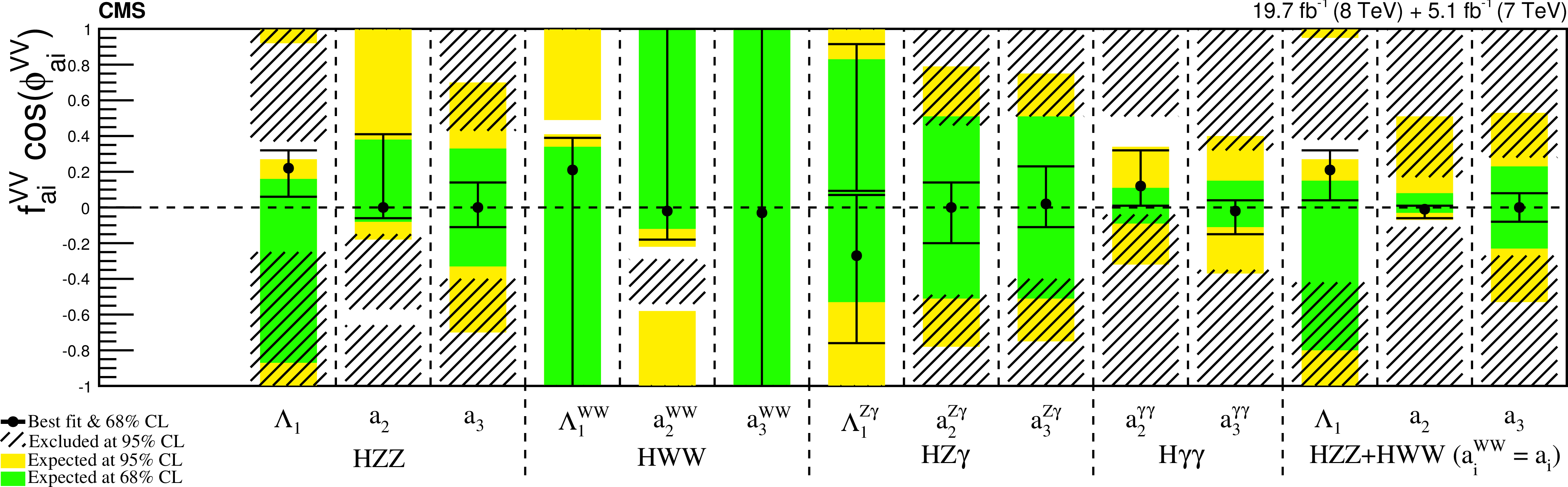
png pdf	Figure 20: Summary of allowed confidence level intervals on anomalous coupling parameters in ${\mathrm {H}} {\mathrm {V}} {\mathrm {V}}$ interactions under the assumption that all the coupling ratios are real ($\phi _{ai}^{ {\mathrm {V}} {\mathrm {V}} }=0$ or $\pi$). The expected 68% and 95% CL regions are shown as the green and yellow bands. The observed constraints at 68% and 95% CL are shown as the points with errors and the excluded hatched regions. In the case of the $f_{\Lambda 1}^{Z\gamma }$ measurement, there are two minima and two 68%CL intervals, while only one global minimum is indicated with a point. The combination of the ${\mathrm {H}} {\mathrm {Z}} {\mathrm {Z}}$ and ${\mathrm {H}} {\mathrm {W}} {\mathrm {W}}$ measurements is presented, assuming the symmetry $a_i = a_i^{ {\mathrm {W}} {\mathrm {W}}}$, including $R_{ai}$ = 0.5.
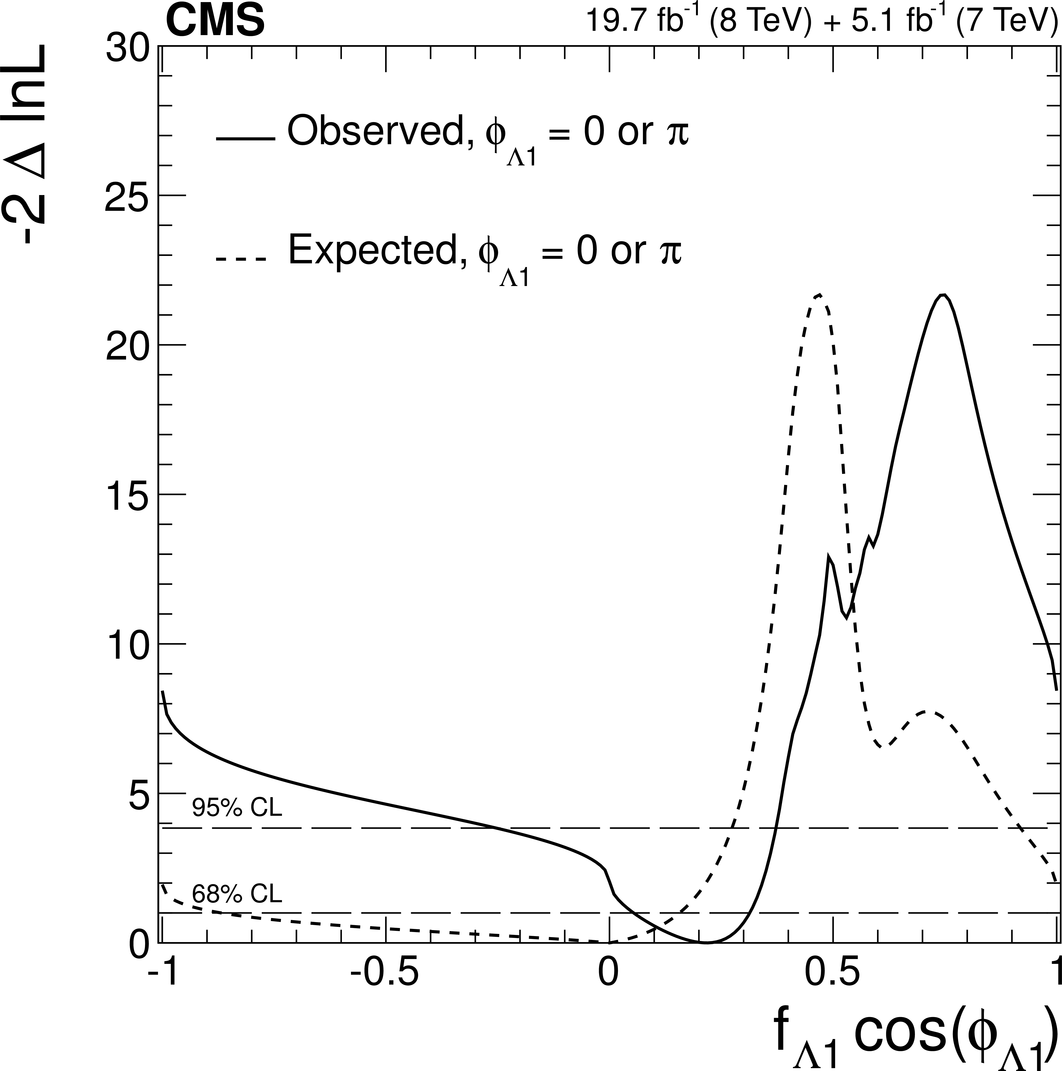
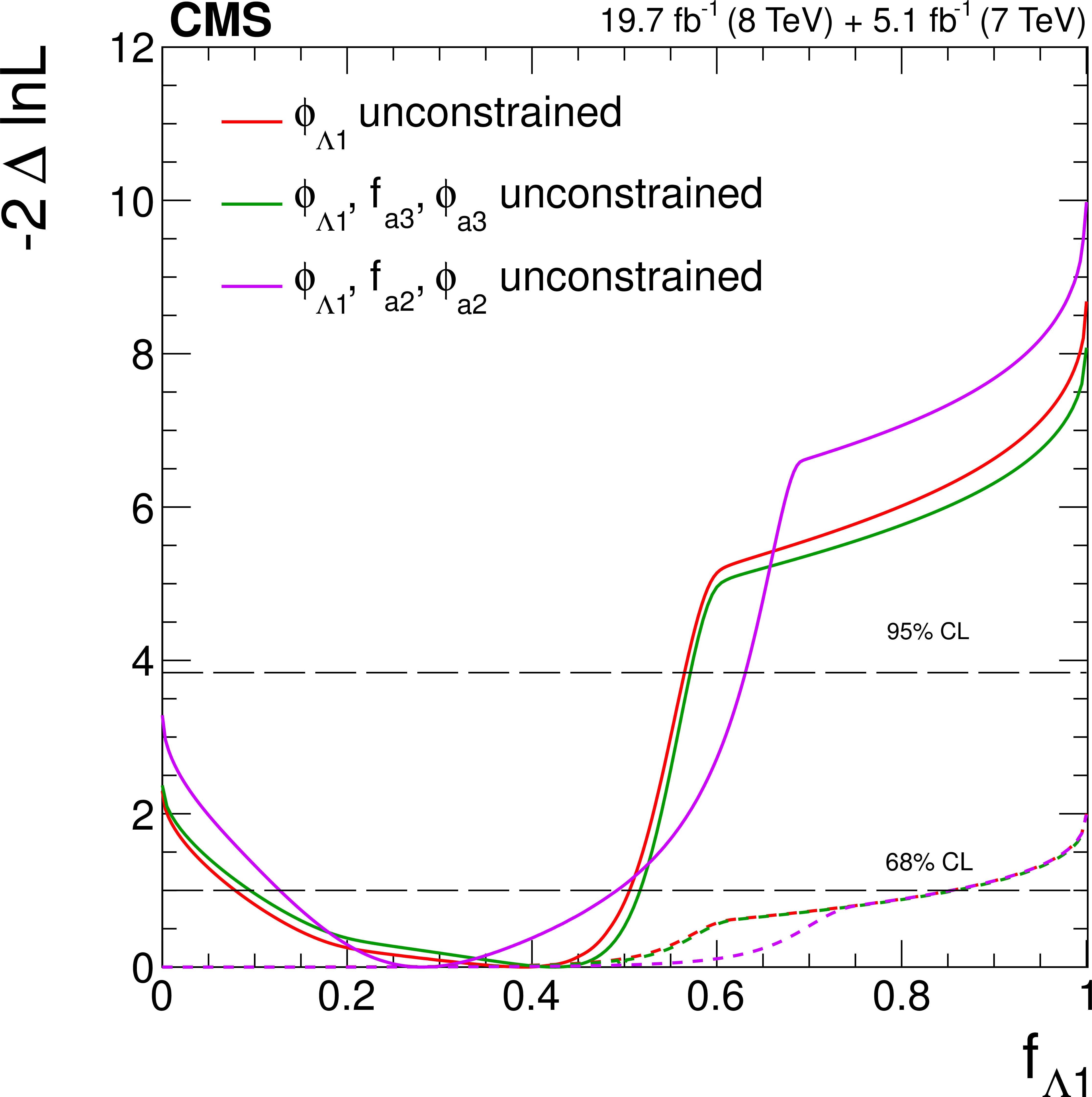
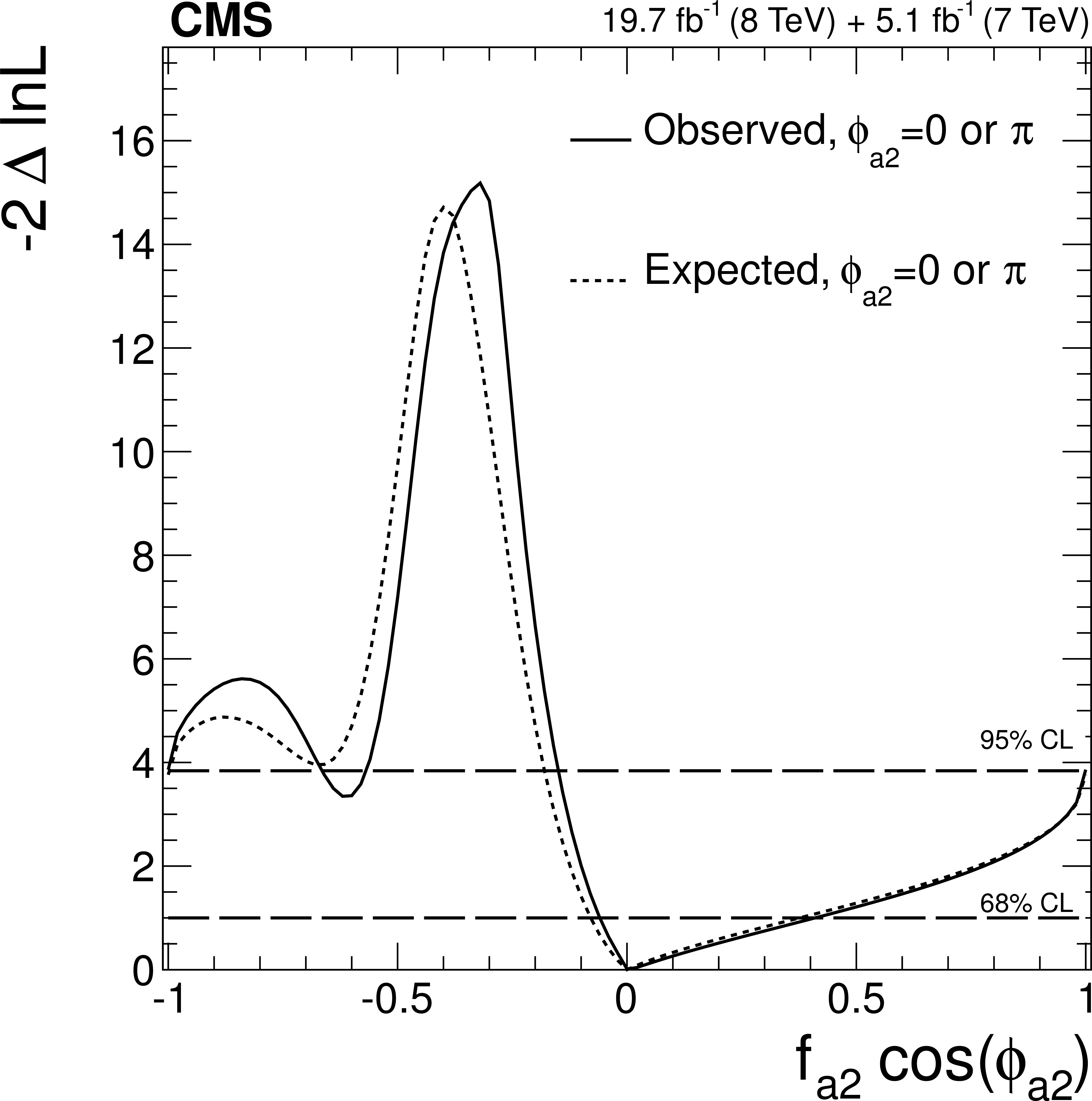
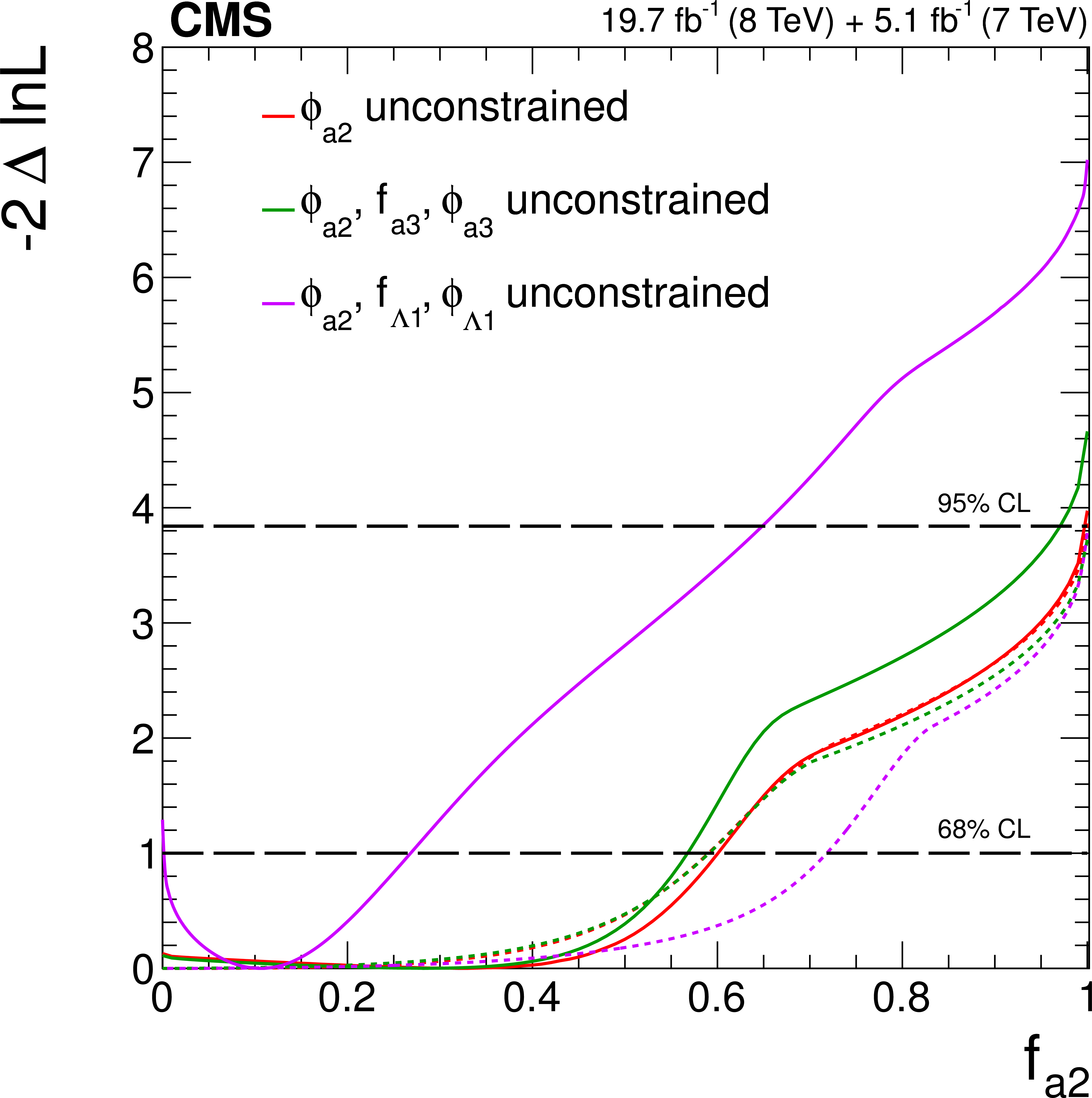
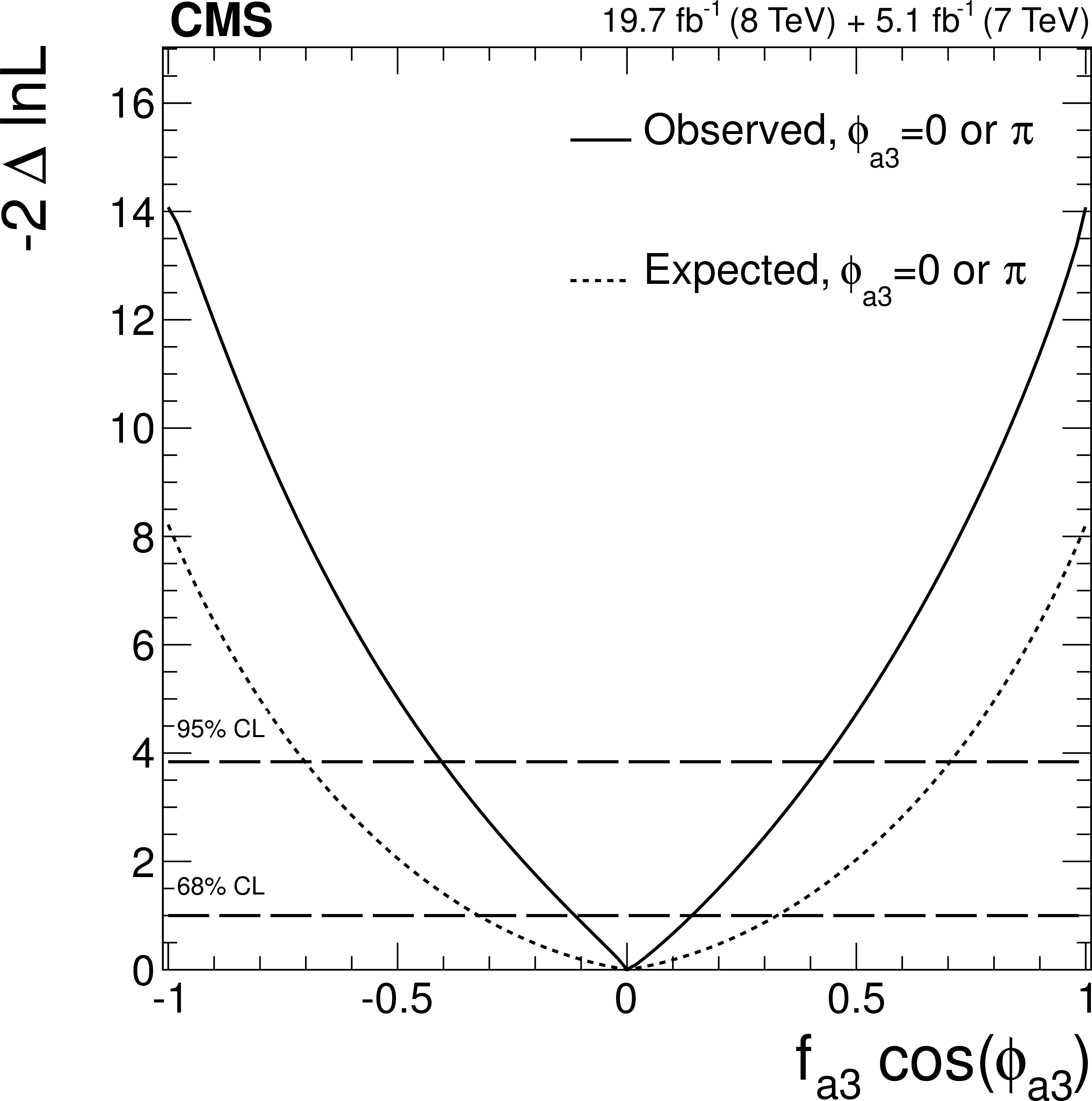
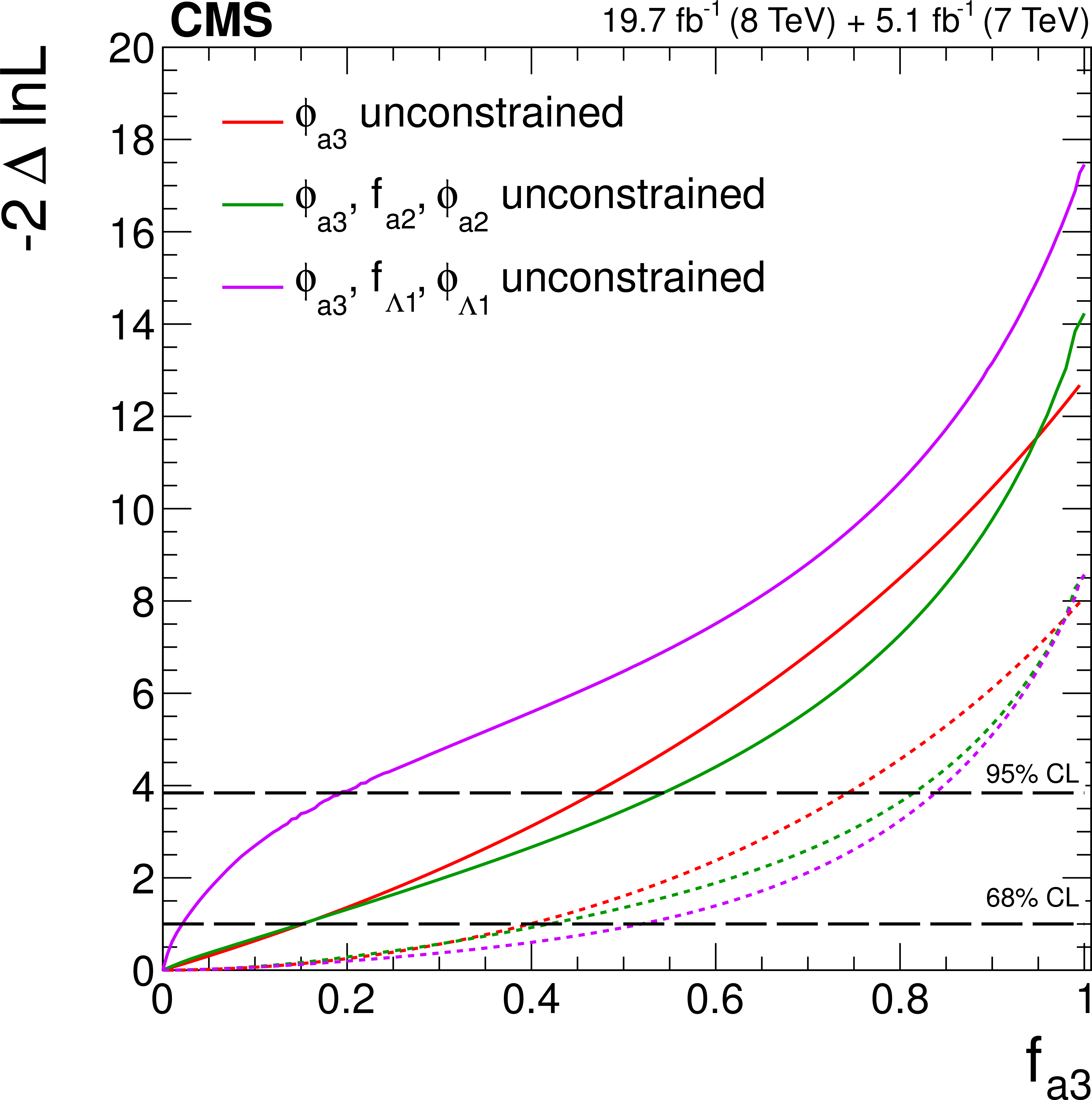
png pdf	Figure 21-a: Expected (dashed) and observed (solid) likelihood scans using the template method for the effective fractions $f_{\Lambda 1}$, $f_{a2}$, $f_{a3}$ (from top to bottom) describing ${\mathrm {H}} {\mathrm {Z}} {\mathrm {Z}}$ interactions. Plots on the left show the results when the couplings studied are constrained to be real and all other couplings are fixed to the SM predictions. The $\cos\phi _{ai}$ term allows a signed quantity where $\cos\phi _{ai}=-1$ or $+1$. Plots on the right show the results where the phases of the anomalous couplings and additional ${\mathrm {H}} {\mathrm {Z}} {\mathrm {Z}}$ couplings are left unconstrained, as indicated in the legend. The $f_{a3}$ result with $\phi _{a3}$ unconstrained (in the bottom-right plot) is from PRD 89 (2014) 092007.
png pdf	Figure 21-b: Expected (dashed) and observed (solid) likelihood scans using the template method for the effective fractions $f_{\Lambda 1}$, $f_{a2}$, $f_{a3}$ (from top to bottom) describing ${\mathrm {H}} {\mathrm {Z}} {\mathrm {Z}}$ interactions. Plots on the left show the results when the couplings studied are constrained to be real and all other couplings are fixed to the SM predictions. The $\cos\phi _{ai}$ term allows a signed quantity where $\cos\phi _{ai}=-1$ or $+1$. Plots on the right show the results where the phases of the anomalous couplings and additional ${\mathrm {H}} {\mathrm {Z}} {\mathrm {Z}}$ couplings are left unconstrained, as indicated in the legend. The $f_{a3}$ result with $\phi _{a3}$ unconstrained (in the bottom-right plot) is from PRD 89 (2014) 092007.
png pdf	Figure 21-c: Expected (dashed) and observed (solid) likelihood scans using the template method for the effective fractions $f_{\Lambda 1}$, $f_{a2}$, $f_{a3}$ (from top to bottom) describing ${\mathrm {H}} {\mathrm {Z}} {\mathrm {Z}}$ interactions. Plots on the left show the results when the couplings studied are constrained to be real and all other couplings are fixed to the SM predictions. The $\cos\phi _{ai}$ term allows a signed quantity where $\cos\phi _{ai}=-1$ or $+1$. Plots on the right show the results where the phases of the anomalous couplings and additional ${\mathrm {H}} {\mathrm {Z}} {\mathrm {Z}}$ couplings are left unconstrained, as indicated in the legend. The $f_{a3}$ result with $\phi _{a3}$ unconstrained (in the bottom-right plot) is from PRD 89 (2014) 092007.
png pdf	Figure 21-d: Expected (dashed) and observed (solid) likelihood scans using the template method for the effective fractions $f_{\Lambda 1}$, $f_{a2}$, $f_{a3}$ (from top to bottom) describing ${\mathrm {H}} {\mathrm {Z}} {\mathrm {Z}}$ interactions. Plots on the left show the results when the couplings studied are constrained to be real and all other couplings are fixed to the SM predictions. The $\cos\phi _{ai}$ term allows a signed quantity where $\cos\phi _{ai}=-1$ or $+1$. Plots on the right show the results where the phases of the anomalous couplings and additional ${\mathrm {H}} {\mathrm {Z}} {\mathrm {Z}}$ couplings are left unconstrained, as indicated in the legend. The $f_{a3}$ result with $\phi _{a3}$ unconstrained (in the bottom-right plot) is from PRD 89 (2014) 092007.
png pdf	Figure 21-e: Expected (dashed) and observed (solid) likelihood scans using the template method for the effective fractions $f_{\Lambda 1}$, $f_{a2}$, $f_{a3}$ (from top to bottom) describing ${\mathrm {H}} {\mathrm {Z}} {\mathrm {Z}}$ interactions. Plots on the left show the results when the couplings studied are constrained to be real and all other couplings are fixed to the SM predictions. The $\cos\phi _{ai}$ term allows a signed quantity where $\cos\phi _{ai}=-1$ or $+1$. Plots on the right show the results where the phases of the anomalous couplings and additional ${\mathrm {H}} {\mathrm {Z}} {\mathrm {Z}}$ couplings are left unconstrained, as indicated in the legend. The $f_{a3}$ result with $\phi _{a3}$ unconstrained (in the bottom-right plot) is from PRD 89 (2014) 092007.
png pdf	Figure 21-f: Expected (dashed) and observed (solid) likelihood scans using the template method for the effective fractions $f_{\Lambda 1}$, $f_{a2}$, $f_{a3}$ (from top to bottom) describing ${\mathrm {H}} {\mathrm {Z}} {\mathrm {Z}}$ interactions. Plots on the left show the results when the couplings studied are constrained to be real and all other couplings are fixed to the SM predictions. The $\cos\phi _{ai}$ term allows a signed quantity where $\cos\phi _{ai}=-1$ or $+1$. Plots on the right show the results where the phases of the anomalous couplings and additional ${\mathrm {H}} {\mathrm {Z}} {\mathrm {Z}}$ couplings are left unconstrained, as indicated in the legend. The $f_{a3}$ result with $\phi _{a3}$ unconstrained (in the bottom-right plot) is from PRD 89 (2014) 092007.
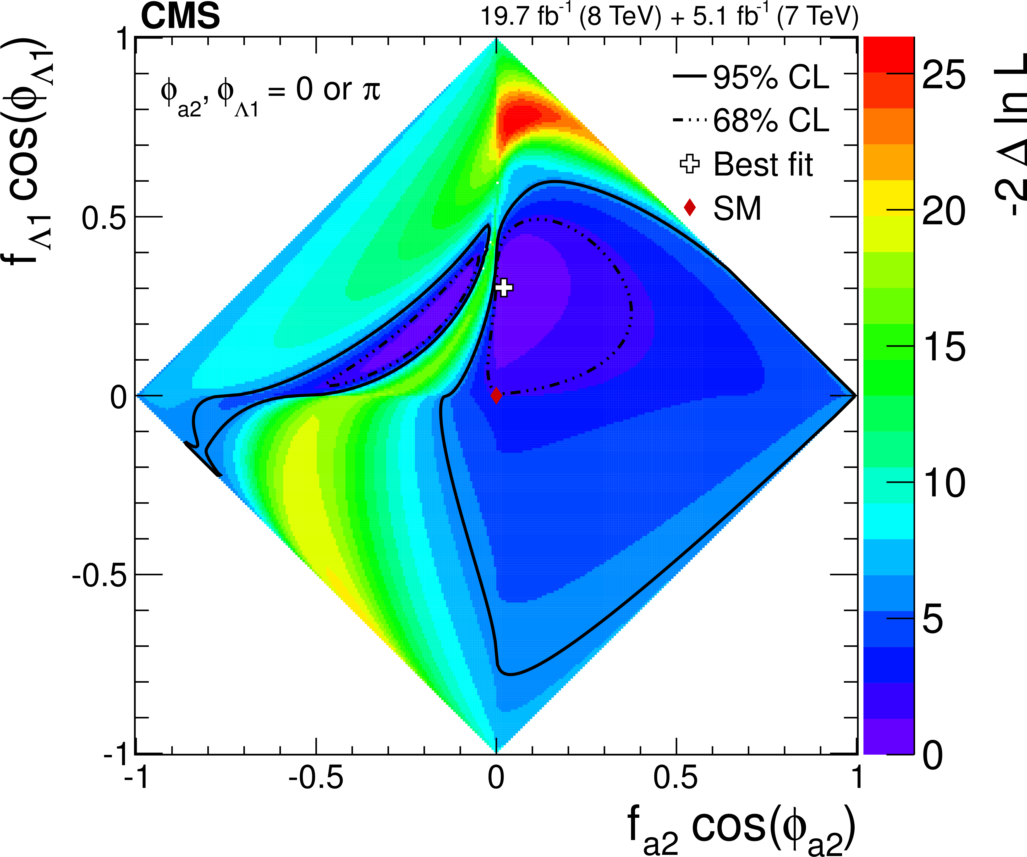
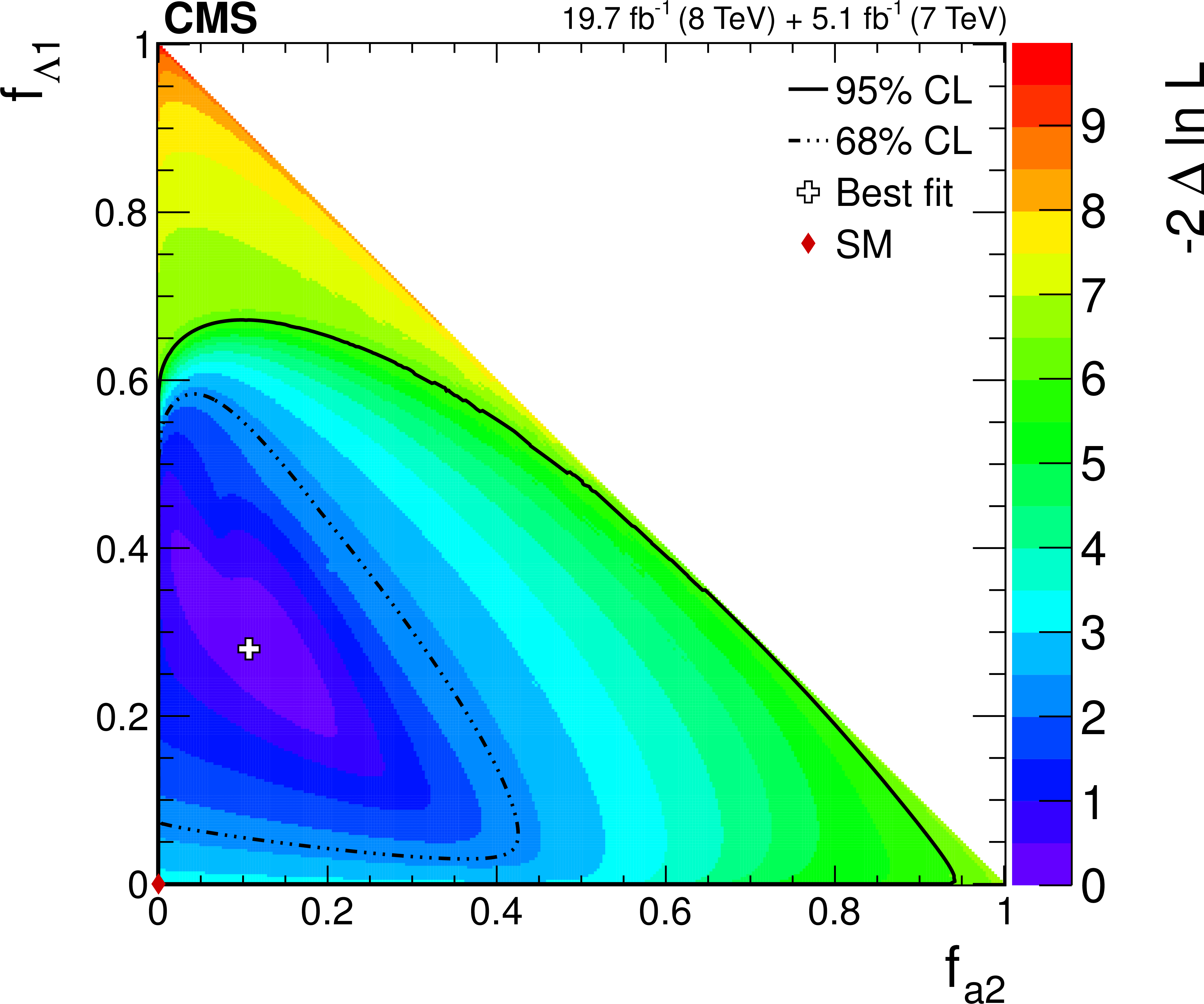
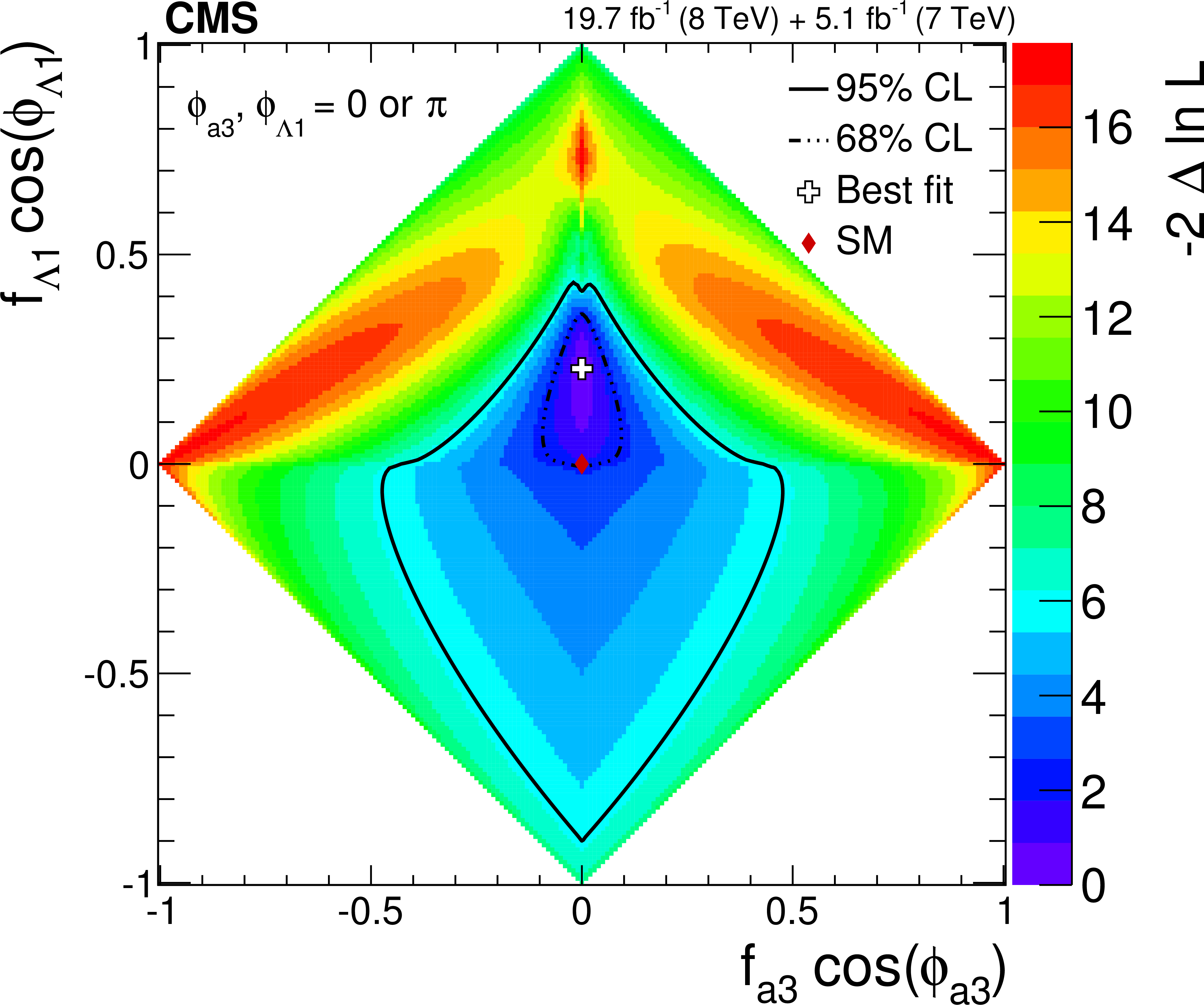
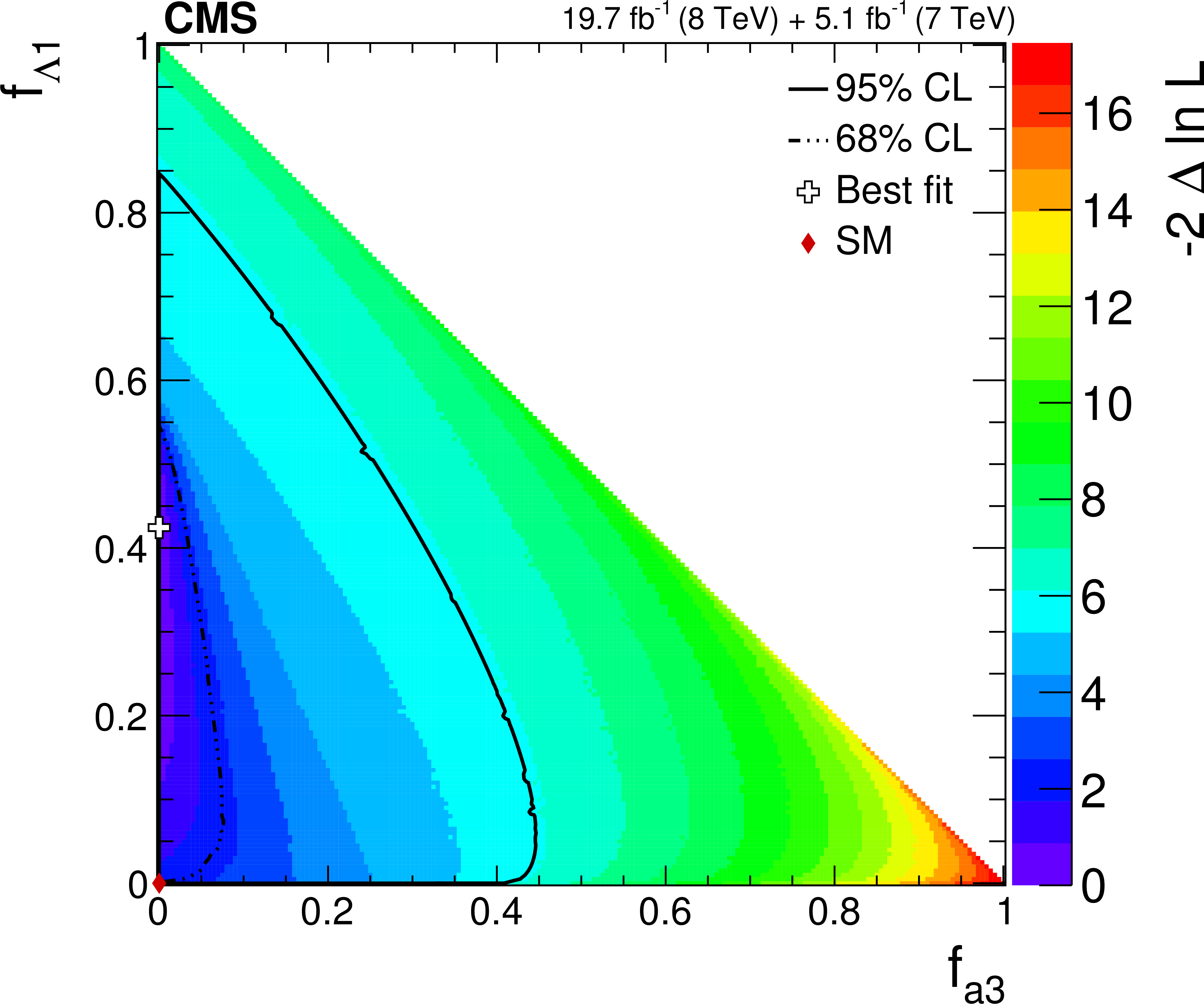
png pdf	Figure 22-a: Observed likelihood scans using the template method for pairs of effective fractions $f_{\Lambda 1}$ vs. $f_{a2}$, $f_{\Lambda 1}$ vs. $f_{a3}$, and $f_{a2}$ vs. $f_{a3}$ (from top to bottom) describing ${\mathrm {H}} {\mathrm {Z}} {\mathrm {Z}}$ interactions. Plots on the left show the results when the couplings studied are constrained to be real and all other couplings are fixed to the SM predictions. Plots on the right show the results when the phases of the anomalous couplings are left unconstrained. The SM expectations correspond to points (0,0) and the best fit values are shown with the crosses. The confidence level intervals are indicated by the corresponding $-2\Delta \ln\mathcal {L}$ contours.
png pdf	Figure 22-b: Observed likelihood scans using the template method for pairs of effective fractions $f_{\Lambda 1}$ vs. $f_{a2}$, $f_{\Lambda 1}$ vs. $f_{a3}$, and $f_{a2}$ vs. $f_{a3}$ (from top to bottom) describing ${\mathrm {H}} {\mathrm {Z}} {\mathrm {Z}}$ interactions. Plots on the left show the results when the couplings studied are constrained to be real and all other couplings are fixed to the SM predictions. Plots on the right show the results when the phases of the anomalous couplings are left unconstrained. The SM expectations correspond to points (0,0) and the best fit values are shown with the crosses. The confidence level intervals are indicated by the corresponding $-2\Delta \ln\mathcal {L}$ contours.
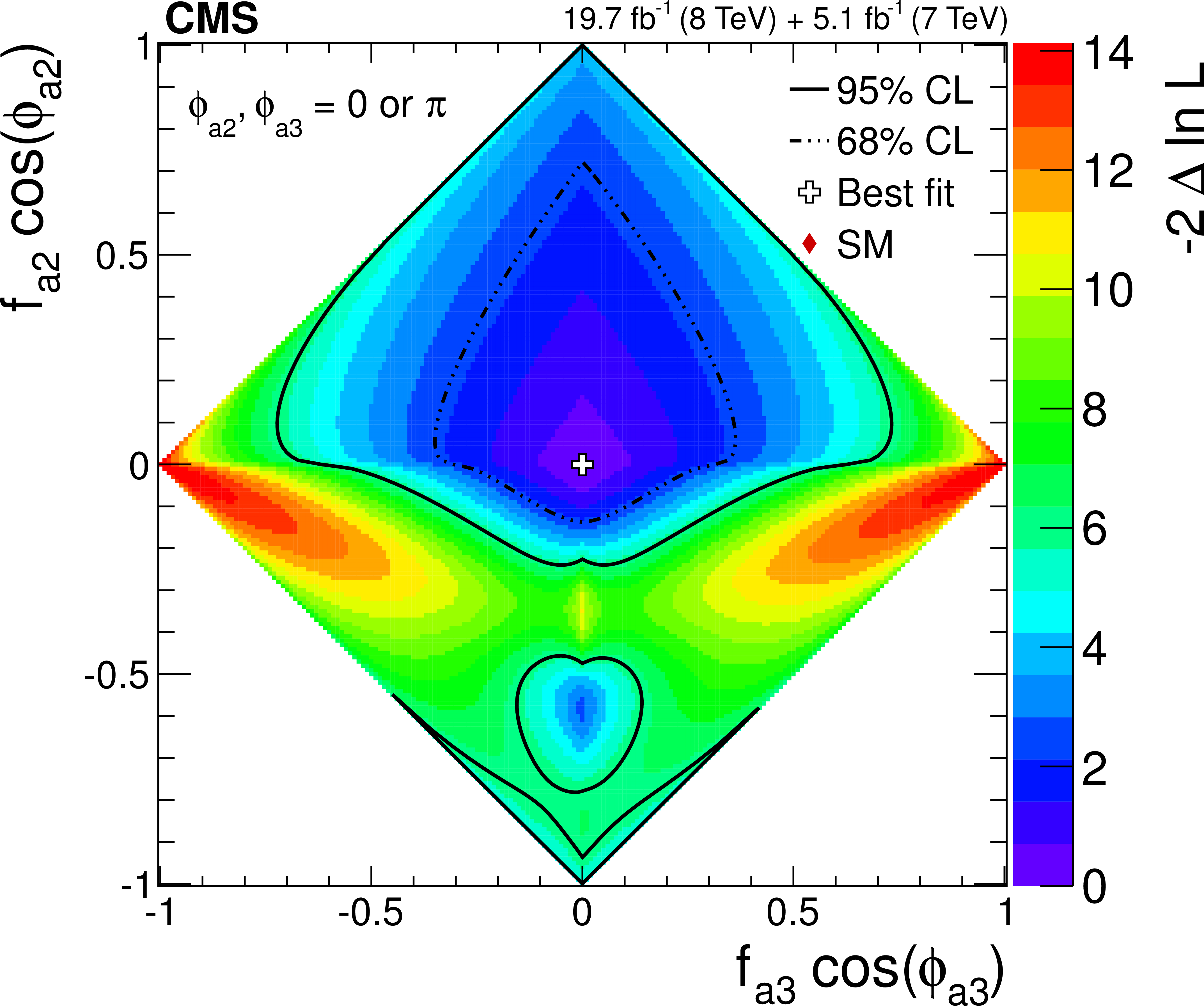
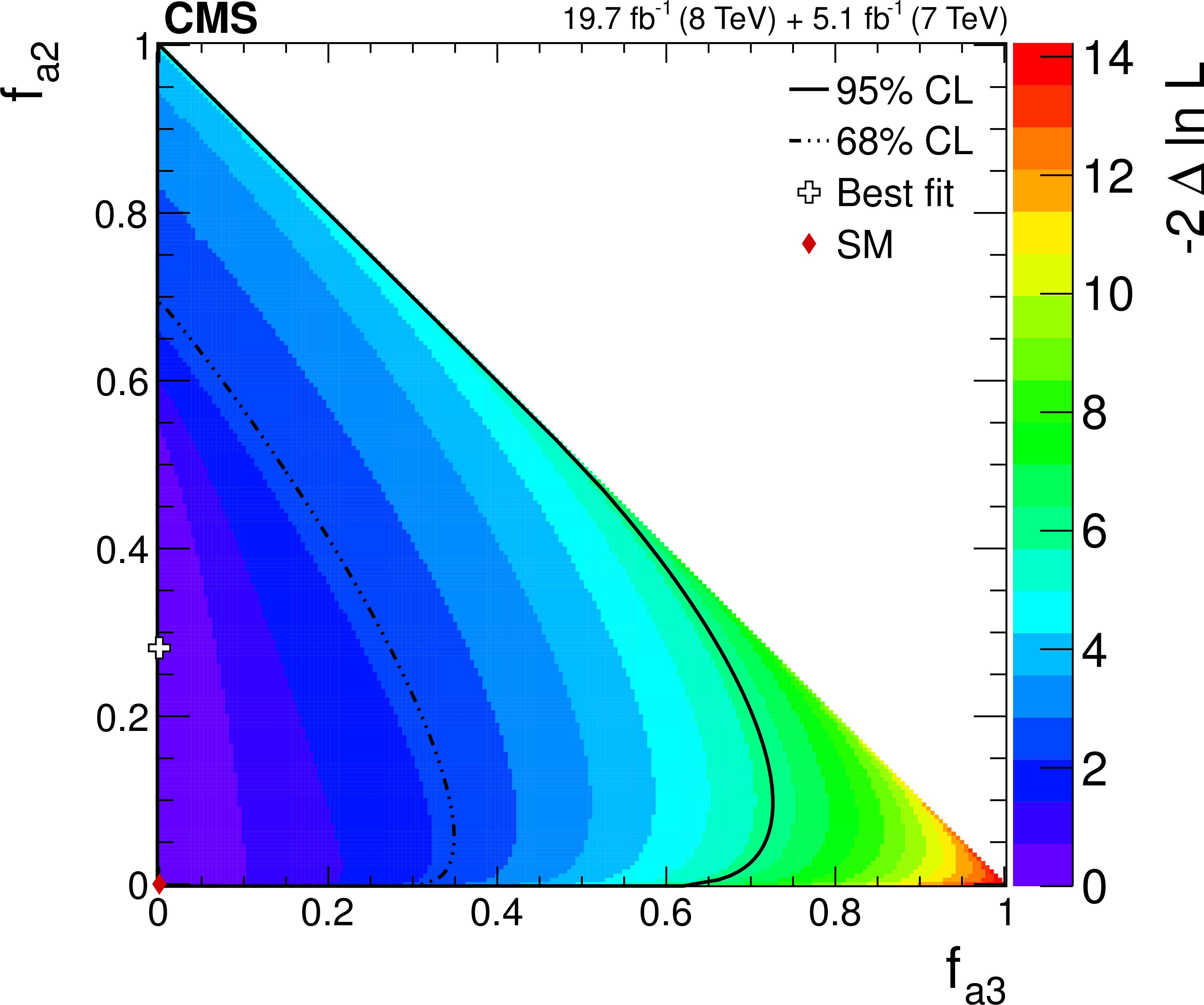
png pdf	Figure 22-c: Observed likelihood scans using the template method for pairs of effective fractions $f_{\Lambda 1}$ vs. $f_{a2}$, $f_{\Lambda 1}$ vs. $f_{a3}$, and $f_{a2}$ vs. $f_{a3}$ (from top to bottom) describing ${\mathrm {H}} {\mathrm {Z}} {\mathrm {Z}}$ interactions. Plots on the left show the results when the couplings studied are constrained to be real and all other couplings are fixed to the SM predictions. Plots on the right show the results when the phases of the anomalous couplings are left unconstrained. The SM expectations correspond to points (0,0) and the best fit values are shown with the crosses. The confidence level intervals are indicated by the corresponding $-2\Delta \ln\mathcal {L}$ contours.
png pdf	Figure 22-d: Observed likelihood scans using the template method for pairs of effective fractions $f_{\Lambda 1}$ vs. $f_{a2}$, $f_{\Lambda 1}$ vs. $f_{a3}$, and $f_{a2}$ vs. $f_{a3}$ (from top to bottom) describing ${\mathrm {H}} {\mathrm {Z}} {\mathrm {Z}}$ interactions. Plots on the left show the results when the couplings studied are constrained to be real and all other couplings are fixed to the SM predictions. Plots on the right show the results when the phases of the anomalous couplings are left unconstrained. The SM expectations correspond to points (0,0) and the best fit values are shown with the crosses. The confidence level intervals are indicated by the corresponding $-2\Delta \ln\mathcal {L}$ contours.
png pdf	Figure 22-e: Observed likelihood scans using the template method for pairs of effective fractions $f_{\Lambda 1}$ vs. $f_{a2}$, $f_{\Lambda 1}$ vs. $f_{a3}$, and $f_{a2}$ vs. $f_{a3}$ (from top to bottom) describing ${\mathrm {H}} {\mathrm {Z}} {\mathrm {Z}}$ interactions. Plots on the left show the results when the couplings studied are constrained to be real and all other couplings are fixed to the SM predictions. Plots on the right show the results when the phases of the anomalous couplings are left unconstrained. The SM expectations correspond to points (0,0) and the best fit values are shown with the crosses. The confidence level intervals are indicated by the corresponding $-2\Delta \ln\mathcal {L}$ contours.
png pdf	Figure 22-f: Observed likelihood scans using the template method for pairs of effective fractions $f_{\Lambda 1}$ vs. $f_{a2}$, $f_{\Lambda 1}$ vs. $f_{a3}$, and $f_{a2}$ vs. $f_{a3}$ (from top to bottom) describing ${\mathrm {H}} {\mathrm {Z}} {\mathrm {Z}}$ interactions. Plots on the left show the results when the couplings studied are constrained to be real and all other couplings are fixed to the SM predictions. Plots on the right show the results when the phases of the anomalous couplings are left unconstrained. The SM expectations correspond to points (0,0) and the best fit values are shown with the crosses. The confidence level intervals are indicated by the corresponding $-2\Delta \ln\mathcal {L}$ contours.
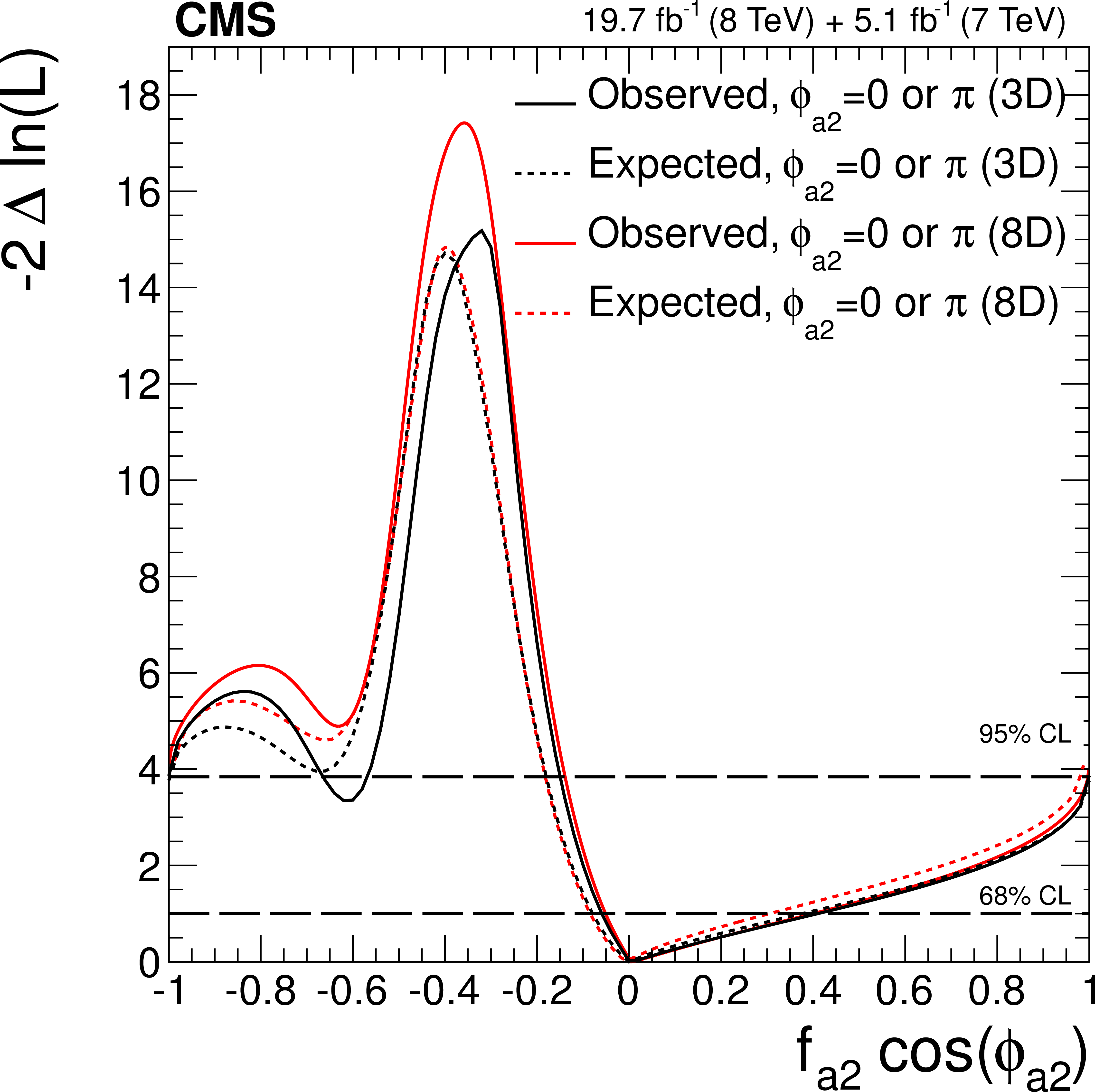
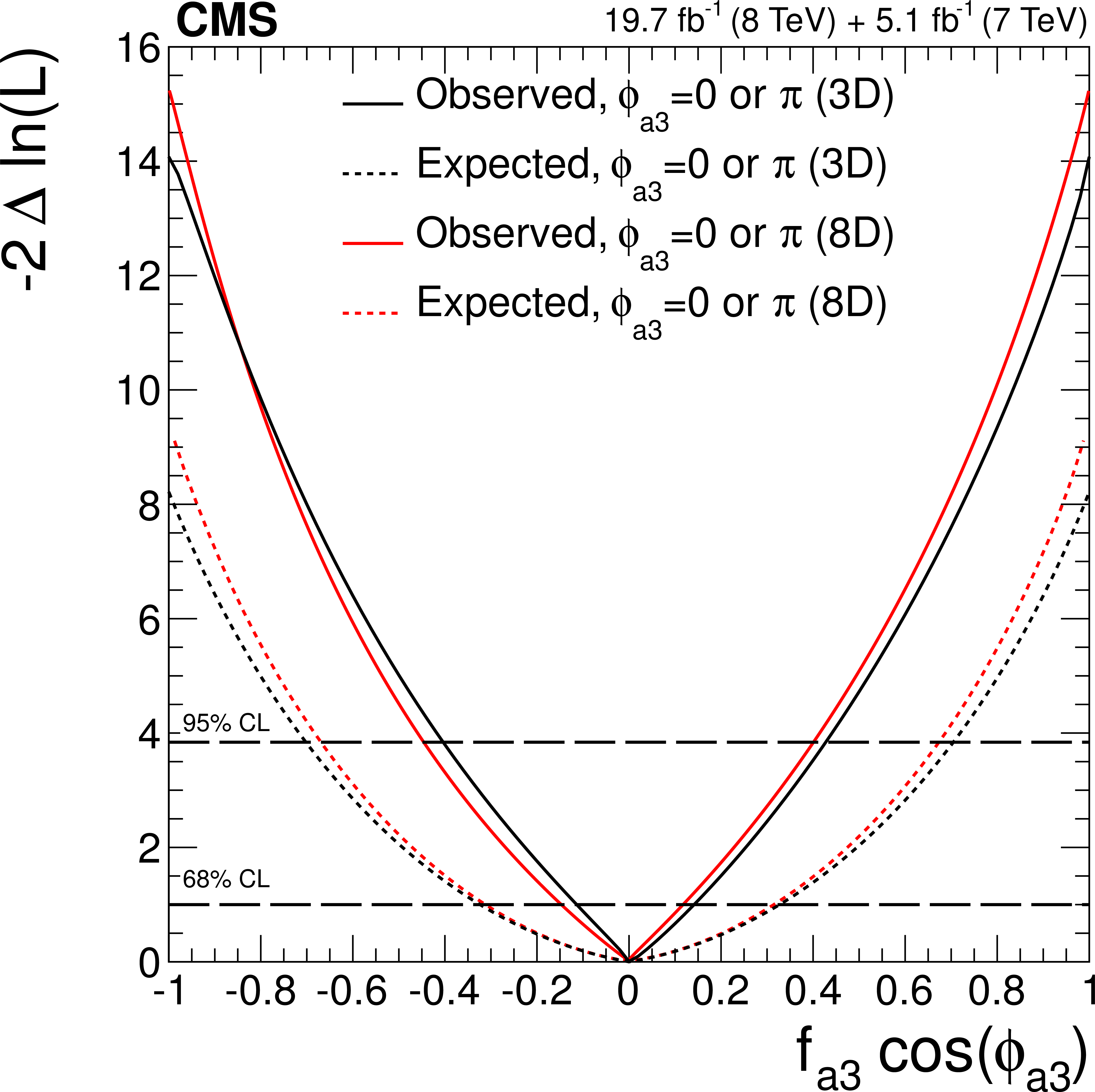
png pdf	Figure 23-a: Expected (dashed) and observed (solid) likelihood scans for $f_{a2}$ (a) and $f_{a3}$ (b), and observed likelihood scan for the $f_{a2}$ vs. $f_{a3}$ fractions (c), obtained using the template method (3D, black) and the multidimensional distribution method (8D, red) in the study of anomalous ${\mathrm {H}} {\mathrm {Z}} {\mathrm {Z}}$ interactions. The couplings are constrained to be real.
png pdf	Figure 23-b: Expected (dashed) and observed (solid) likelihood scans for $f_{a2}$ (a) and $f_{a3}$ (b), and observed likelihood scan for the $f_{a2}$ vs. $f_{a3}$ fractions (c), obtained using the template method (3D, black) and the multidimensional distribution method (8D, red) in the study of anomalous ${\mathrm {H}} {\mathrm {Z}} {\mathrm {Z}}$ interactions. The couplings are constrained to be real.
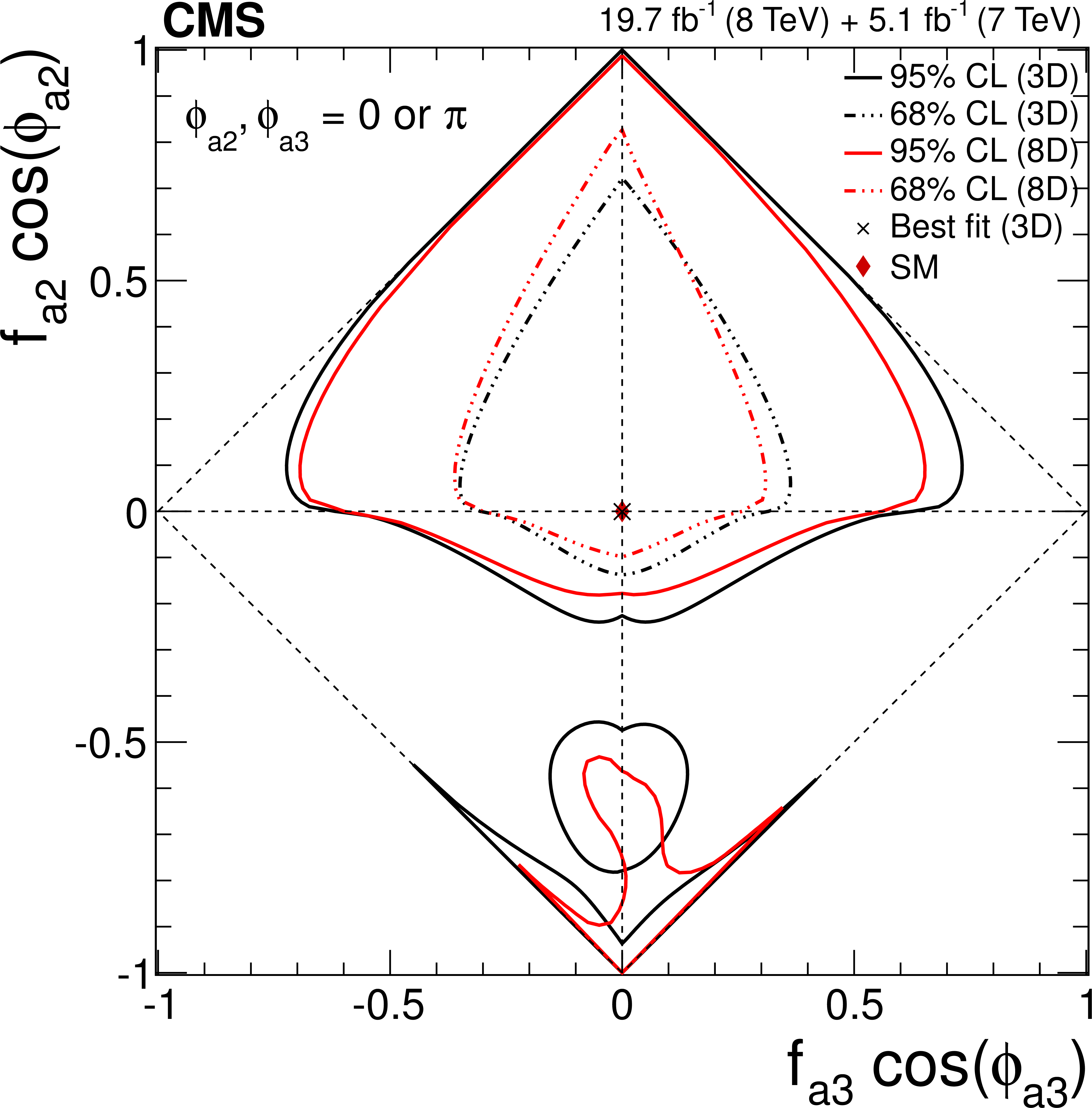
png pdf	Figure 23-c: Expected (dashed) and observed (solid) likelihood scans for $f_{a2}$ (a) and $f_{a3}$ (b), and observed likelihood scan for the $f_{a2}$ vs. $f_{a3}$ fractions (c), obtained using the template method (3D, black) and the multidimensional distribution method (8D, red) in the study of anomalous ${\mathrm {H}} {\mathrm {Z}} {\mathrm {Z}}$ interactions. The couplings are constrained to be real.
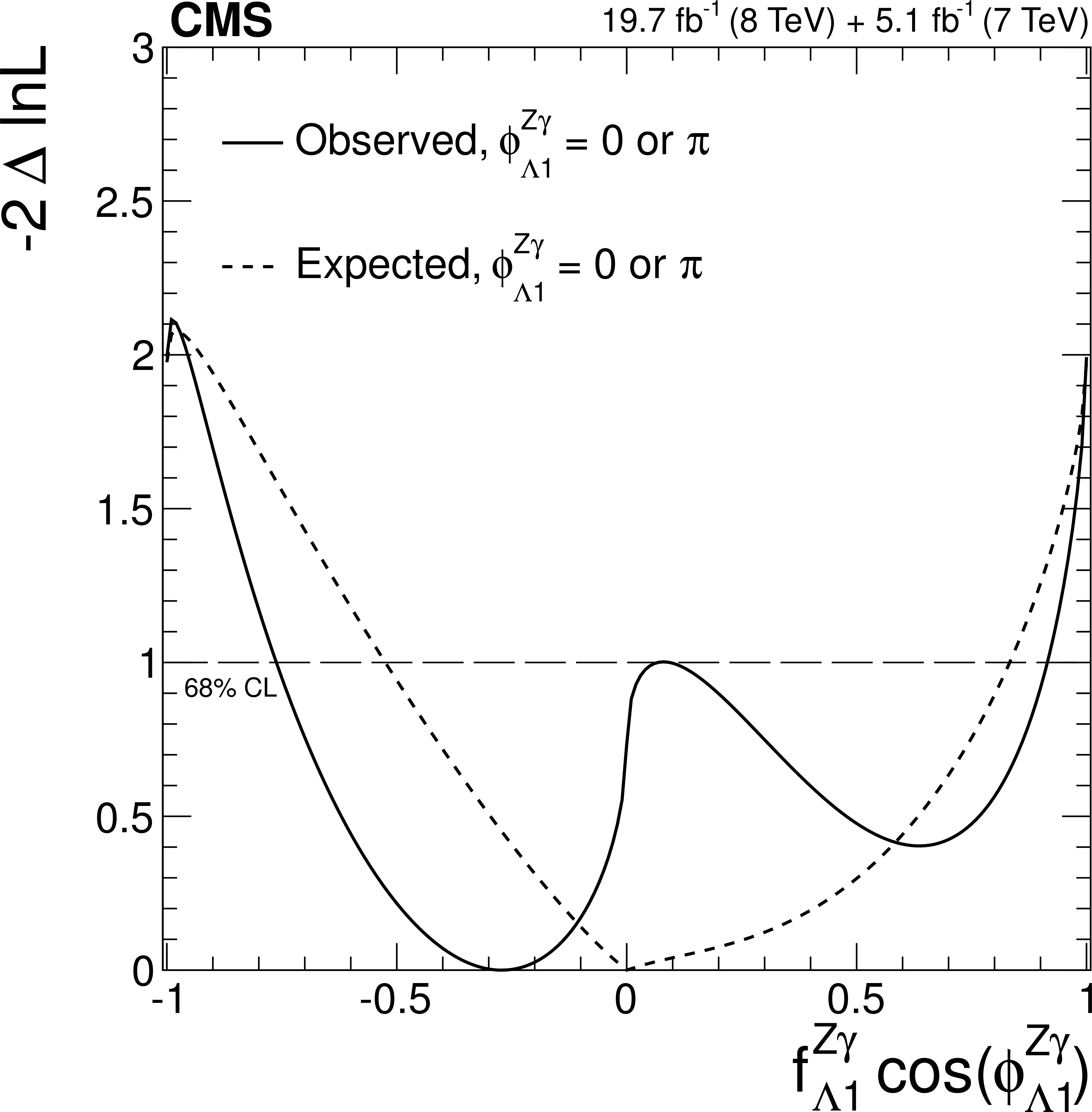
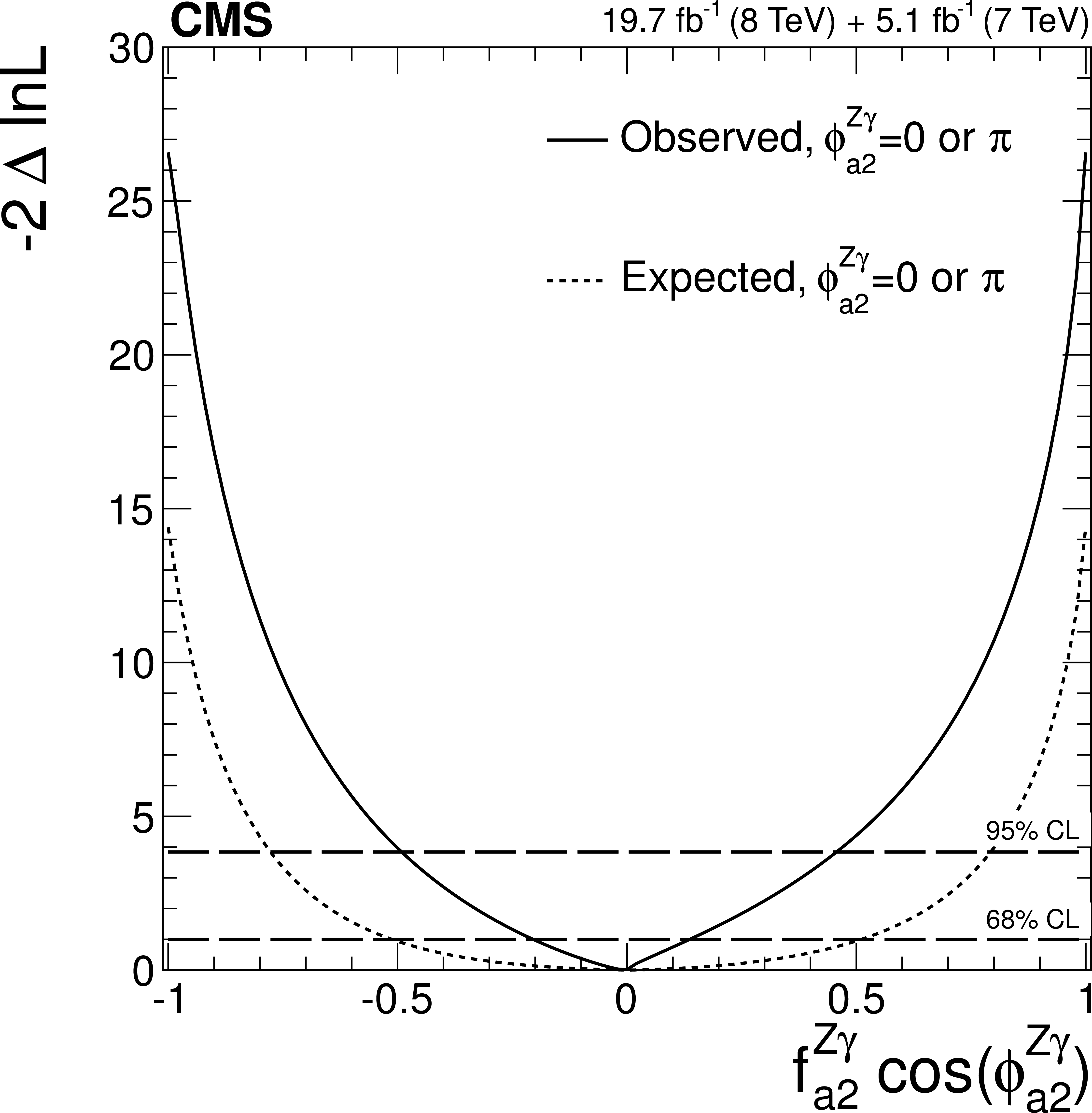
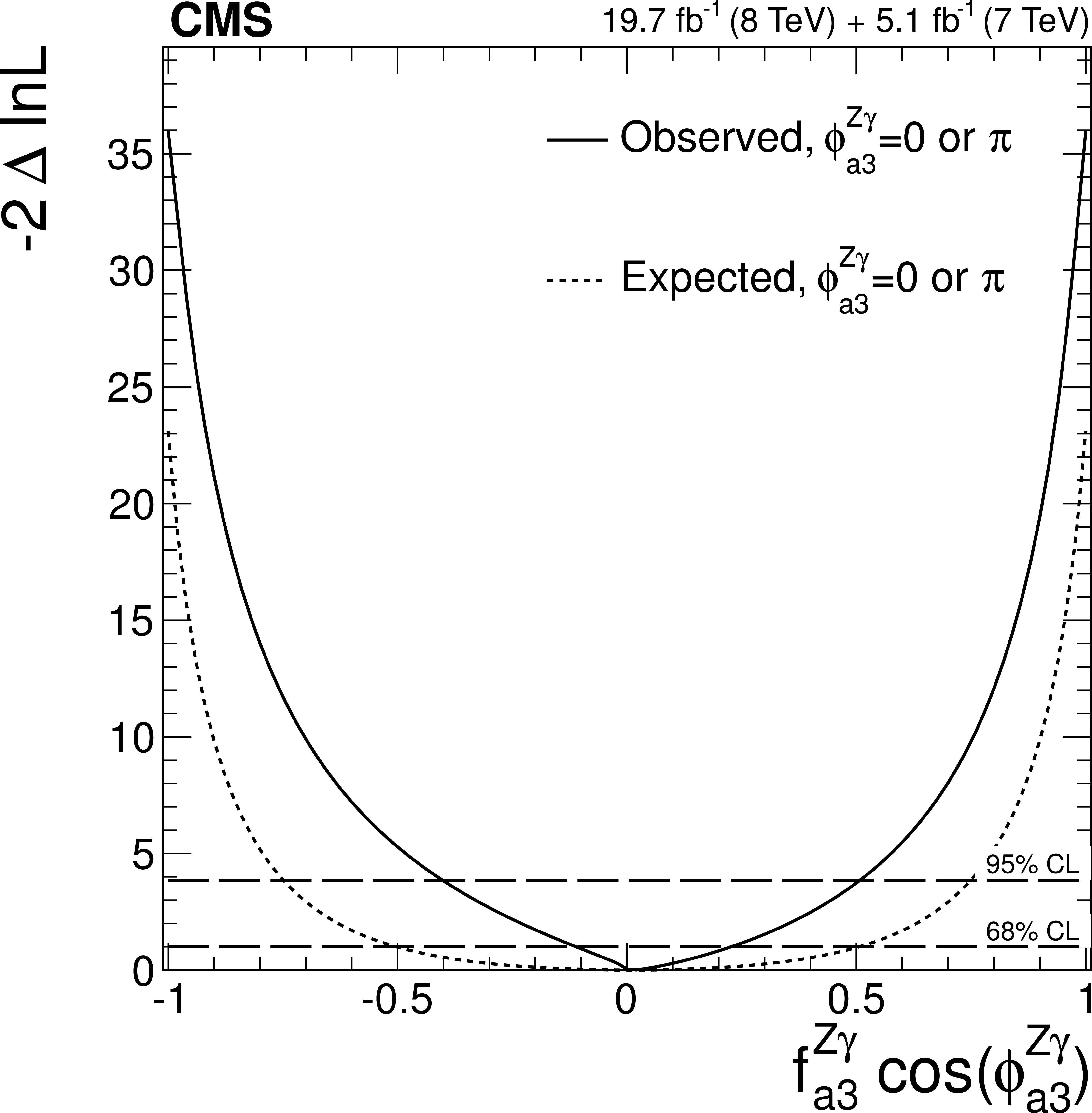
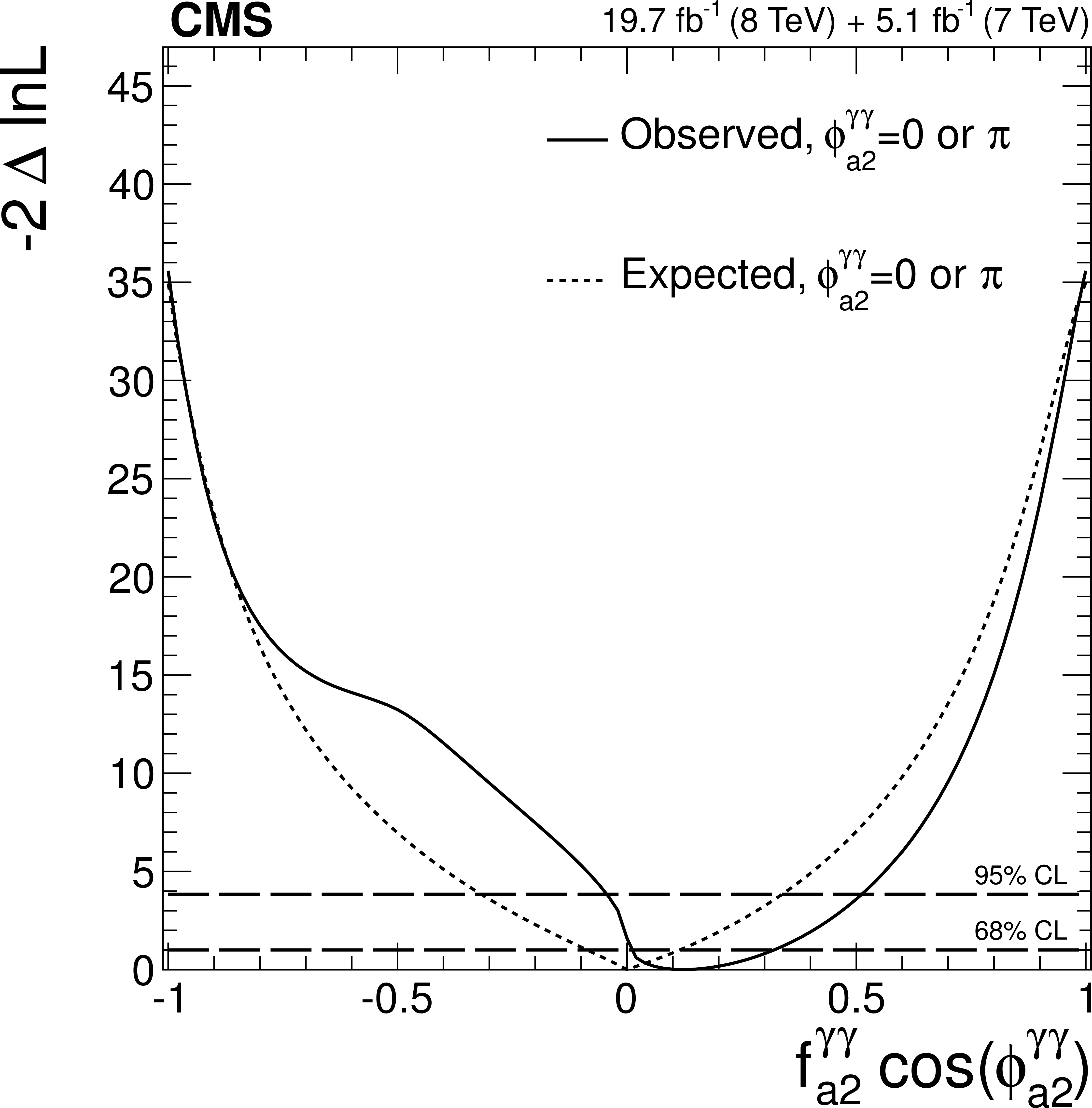
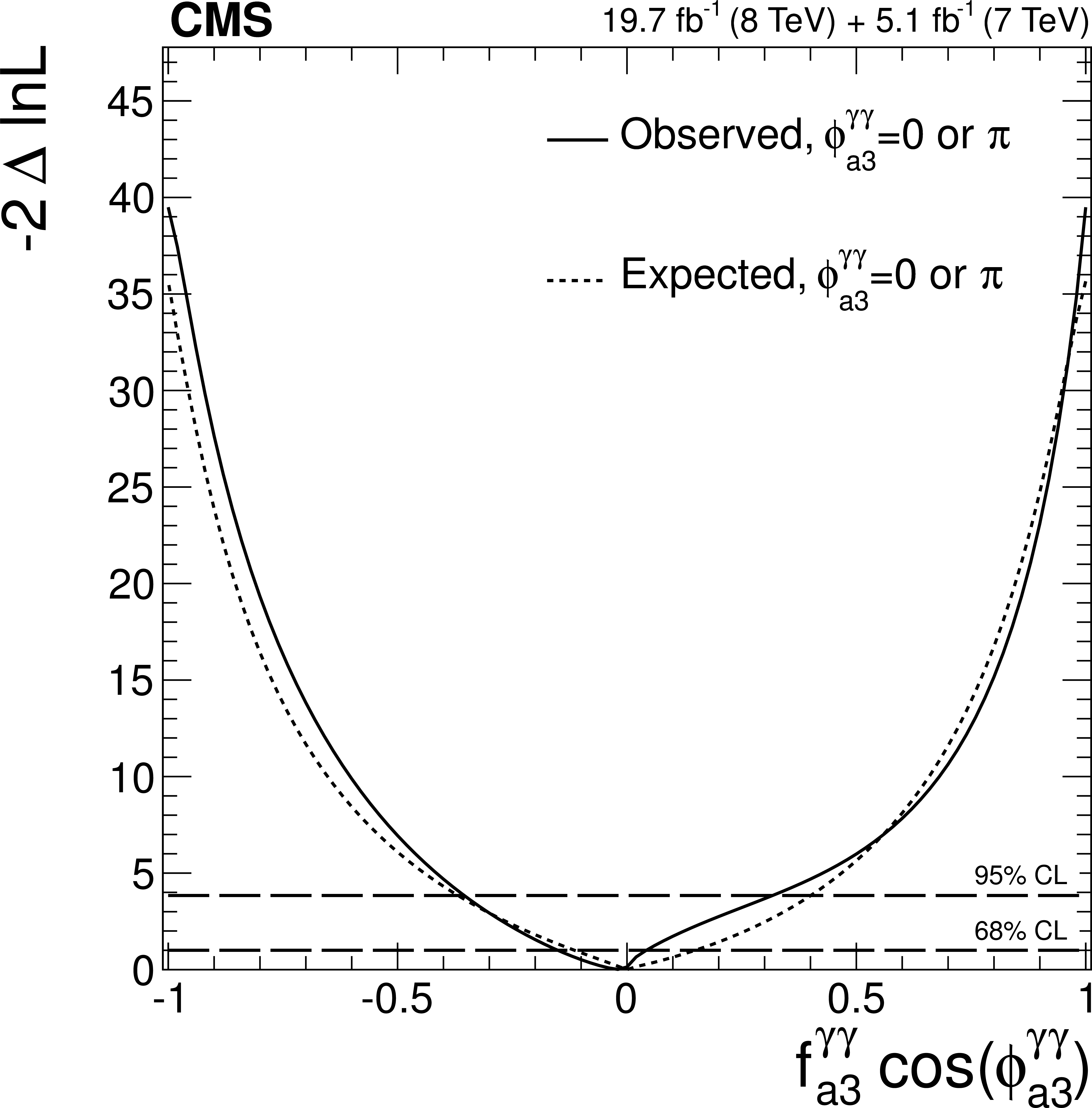
png pdf	Figure 24-a: Expected (dashed) and observed (solid) likelihood scans using the template method for the effective fractions $f_{\Lambda 1}^{Z\gamma }$ (a), $f_{a2}^{Z\gamma }$ (b), $f_{a3}^{Z\gamma }$ (c), $f_{a2}^{\gamma \gamma }$ (d), and $f_{a3}^{\gamma \gamma }$ (e). The couplings studied are constrained to be real and all other couplings are fixed to the SM predictions. The $\cos\phi _{ai}^{ {\mathrm {V}} {\mathrm {V}} }$ term allows a signed quantity where $\cos\phi _{ai}^{ {\mathrm {V}} {\mathrm {V}} }=-1$ or$+1$.
png pdf	Figure 24-b: Expected (dashed) and observed (solid) likelihood scans using the template method for the effective fractions $f_{\Lambda 1}^{Z\gamma }$ (a), $f_{a2}^{Z\gamma }$ (b), $f_{a3}^{Z\gamma }$ (c), $f_{a2}^{\gamma \gamma }$ (d), and $f_{a3}^{\gamma \gamma }$ (e). The couplings studied are constrained to be real and all other couplings are fixed to the SM predictions. The $\cos\phi _{ai}^{ {\mathrm {V}} {\mathrm {V}} }$ term allows a signed quantity where $\cos\phi _{ai}^{ {\mathrm {V}} {\mathrm {V}} }=-1$ or$+1$.
png pdf	Figure 24-c: Expected (dashed) and observed (solid) likelihood scans using the template method for the effective fractions $f_{\Lambda 1}^{Z\gamma }$ (a), $f_{a2}^{Z\gamma }$ (b), $f_{a3}^{Z\gamma }$ (c), $f_{a2}^{\gamma \gamma }$ (d), and $f_{a3}^{\gamma \gamma }$ (e). The couplings studied are constrained to be real and all other couplings are fixed to the SM predictions. The $\cos\phi _{ai}^{ {\mathrm {V}} {\mathrm {V}} }$ term allows a signed quantity where $\cos\phi _{ai}^{ {\mathrm {V}} {\mathrm {V}} }=-1$ or$+1$.
png pdf	Figure 24-d: Expected (dashed) and observed (solid) likelihood scans using the template method for the effective fractions $f_{\Lambda 1}^{Z\gamma }$ (a), $f_{a2}^{Z\gamma }$ (b), $f_{a3}^{Z\gamma }$ (c), $f_{a2}^{\gamma \gamma }$ (d), and $f_{a3}^{\gamma \gamma }$ (e). The couplings studied are constrained to be real and all other couplings are fixed to the SM predictions. The $\cos\phi _{ai}^{ {\mathrm {V}} {\mathrm {V}} }$ term allows a signed quantity where $\cos\phi _{ai}^{ {\mathrm {V}} {\mathrm {V}} }=-1$ or$+1$.
png pdf	Figure 24-e: Expected (dashed) and observed (solid) likelihood scans using the template method for the effective fractions $f_{\Lambda 1}^{Z\gamma }$ (a), $f_{a2}^{Z\gamma }$ (b), $f_{a3}^{Z\gamma }$ (c), $f_{a2}^{\gamma \gamma }$ (d), and $f_{a3}^{\gamma \gamma }$ (e). The couplings studied are constrained to be real and all other couplings are fixed to the SM predictions. The $\cos\phi _{ai}^{ {\mathrm {V}} {\mathrm {V}} }$ term allows a signed quantity where $\cos\phi _{ai}^{ {\mathrm {V}} {\mathrm {V}} }=-1$ or$+1$.
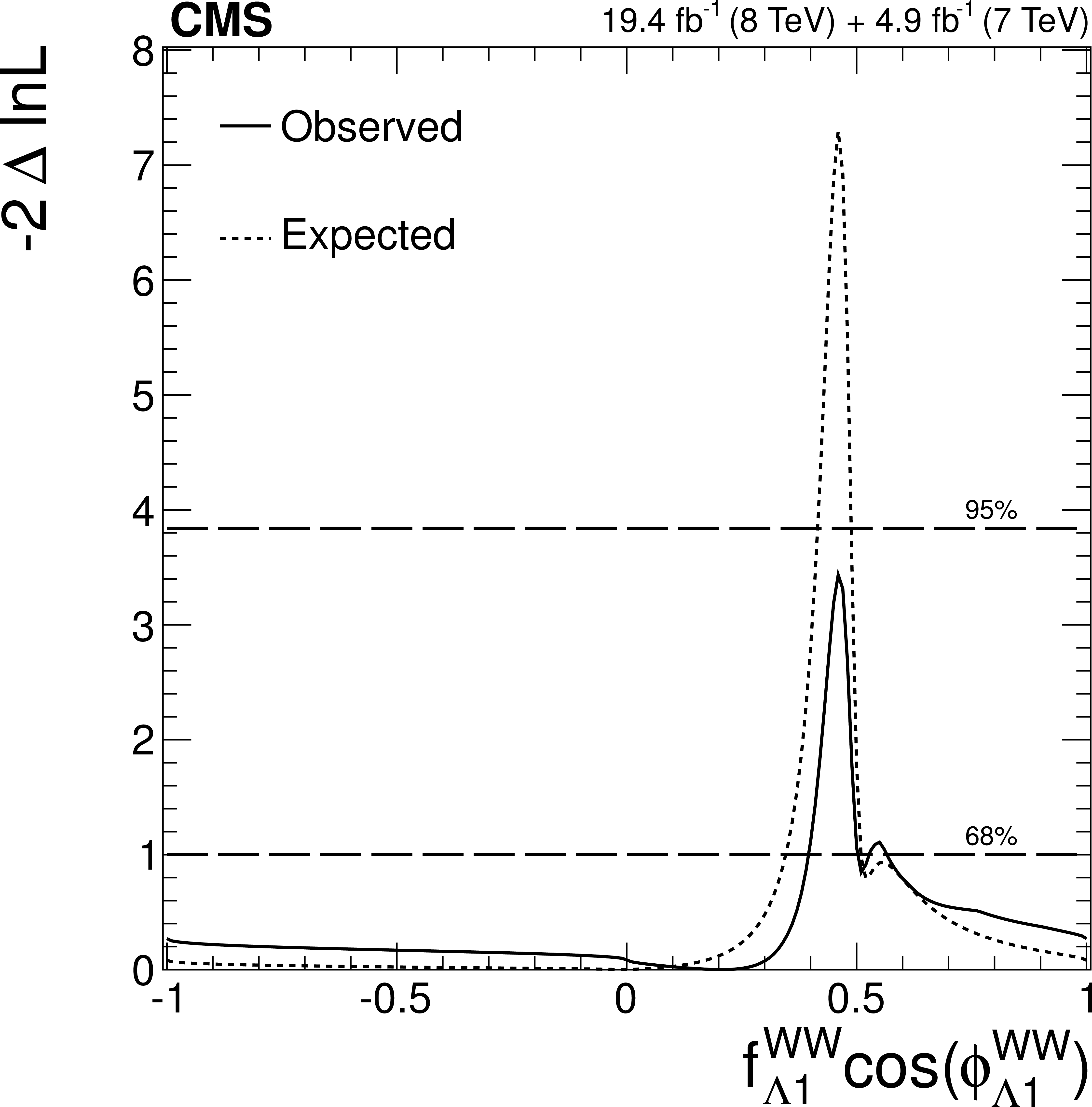
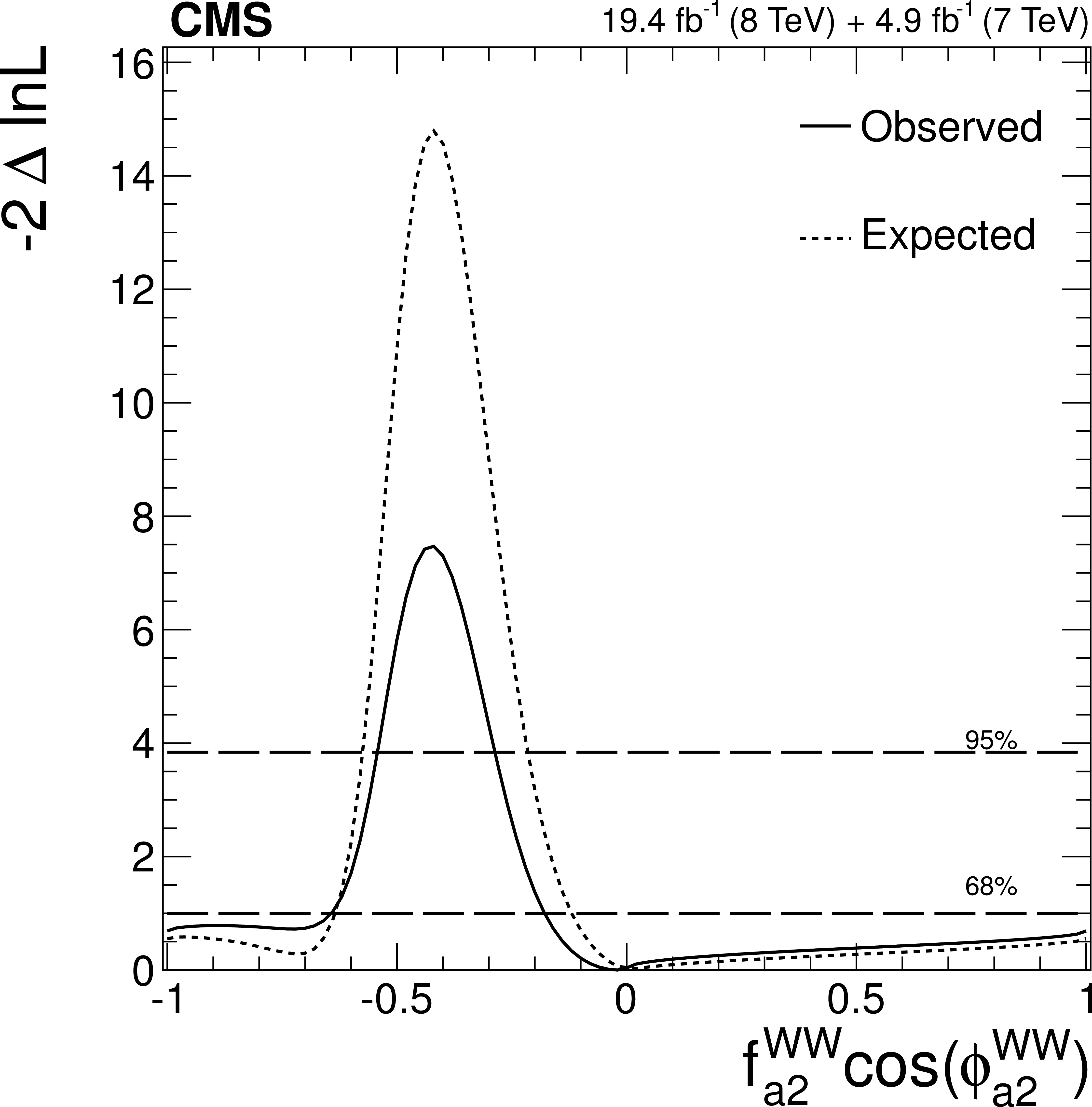
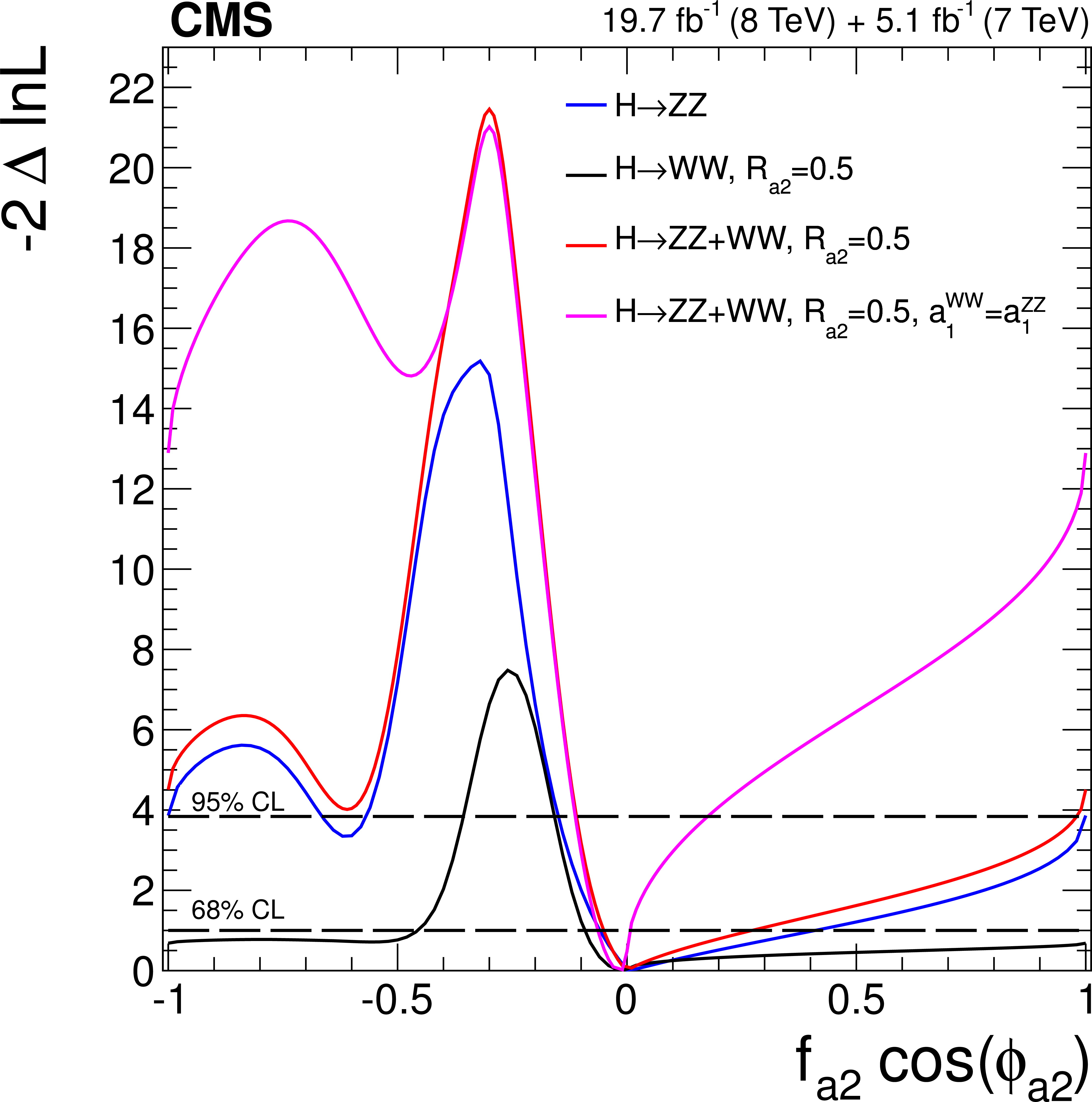
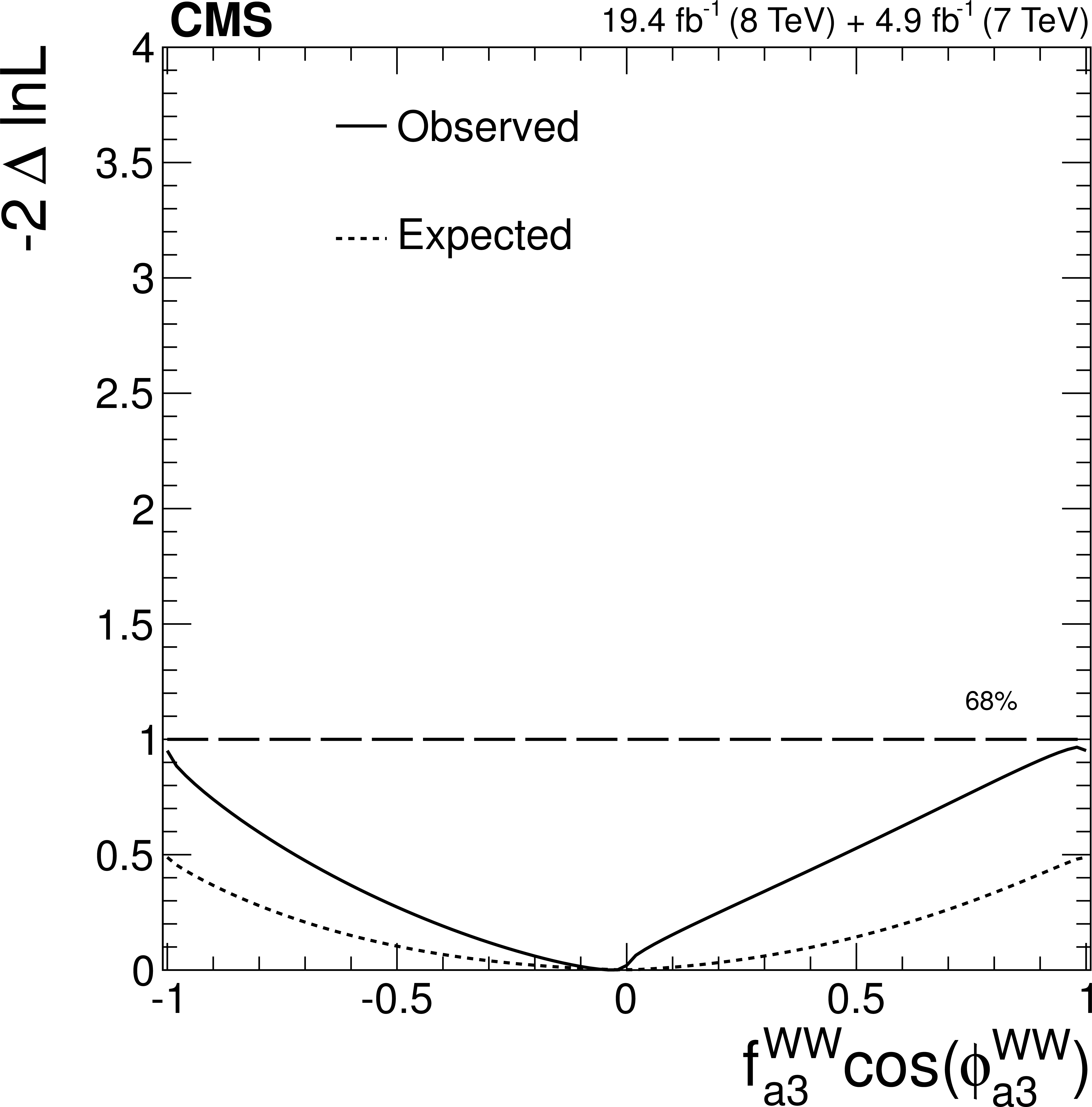
png pdf	Figure 25-a: Expected (dashed) and observed (solid) likelihood scans for effective fractions $f_{\Lambda 1}$ (a, b), $f_{a2}$ (c, d), $f_{a3}$ (e, f). The couplings studied are constrained to be real and all other anomalous couplings are fixed to the SM predictions. The $\cos\phi _{ai}$ term allows a signed quantity where $\cos\phi _{ai}=-1$ or $+1$. Plots a, c, and e show the results of the ${\mathrm {H}} \to {\mathrm {W}} {\mathrm {W}}\to \ell \nu \ell \nu$ analysis expressed in terms of the ${\mathrm {H}} {\mathrm {W}} {\mathrm {W}}$ couplings. Plots b, d, and f show the combined ${\mathrm {H}} \to {\mathrm {W}} {\mathrm {W}}$ and ${\mathrm {H}} \to {\mathrm {Z}} {\mathrm {Z}}$ result in terms of the ${\mathrm {H}} {\mathrm {Z}} {\mathrm {Z}}$ couplings for $R_{ai} = 0.5$. Measurements are shown for each channel separately and two types of combination are present: using $a_1^{ {\mathrm {W}} {\mathrm {W}}} = a_1$ (red) and without such a constraint (magenta).
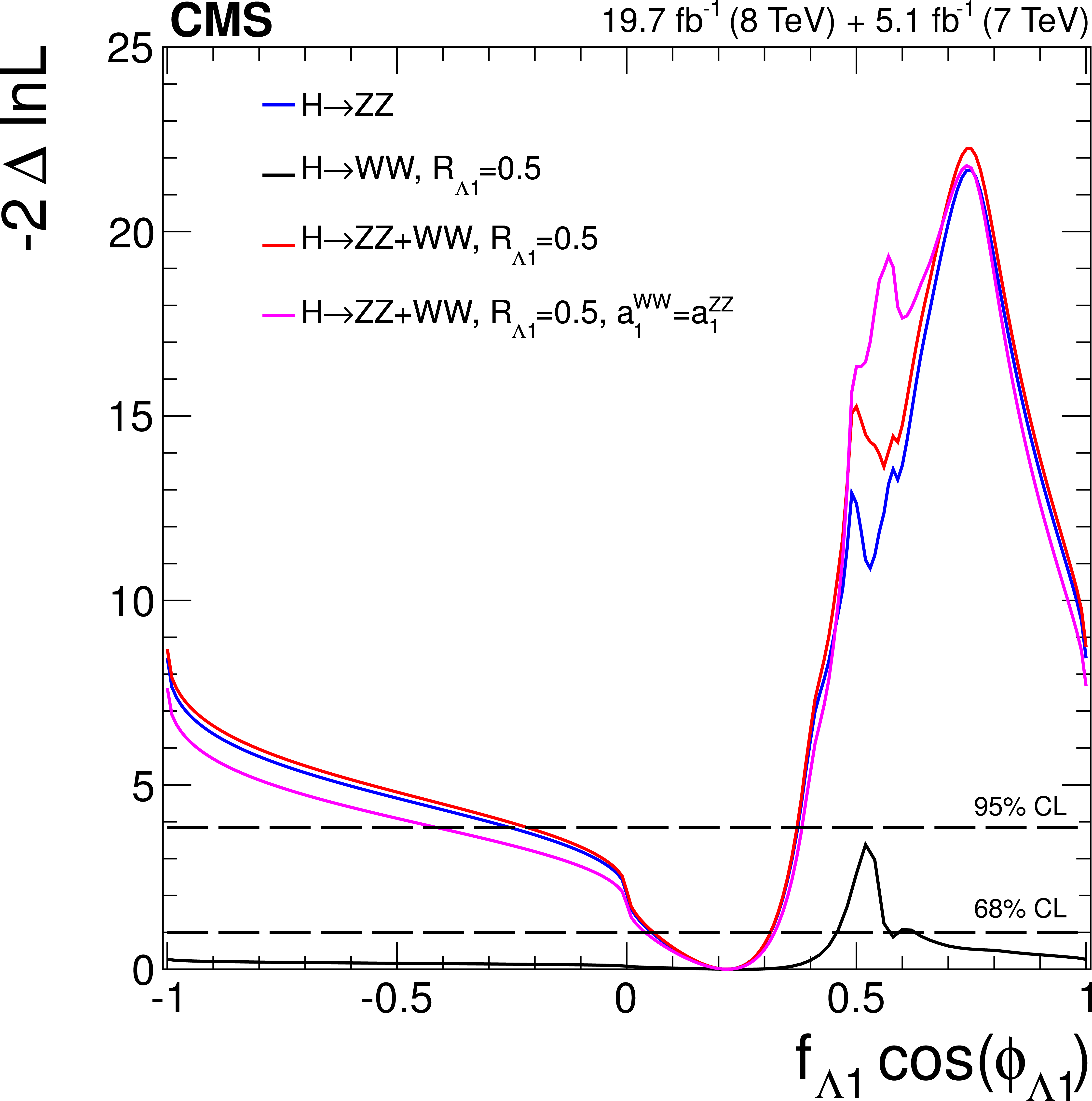
png pdf	Figure 25-b: Expected (dashed) and observed (solid) likelihood scans for effective fractions $f_{\Lambda 1}$ (a, b), $f_{a2}$ (c, d), $f_{a3}$ (e, f). The couplings studied are constrained to be real and all other anomalous couplings are fixed to the SM predictions. The $\cos\phi _{ai}$ term allows a signed quantity where $\cos\phi _{ai}=-1$ or $+1$. Plots a, c, and e show the results of the ${\mathrm {H}} \to {\mathrm {W}} {\mathrm {W}}\to \ell \nu \ell \nu$ analysis expressed in terms of the ${\mathrm {H}} {\mathrm {W}} {\mathrm {W}}$ couplings. Plots b, d, and f show the combined ${\mathrm {H}} \to {\mathrm {W}} {\mathrm {W}}$ and ${\mathrm {H}} \to {\mathrm {Z}} {\mathrm {Z}}$ result in terms of the ${\mathrm {H}} {\mathrm {Z}} {\mathrm {Z}}$ couplings for $R_{ai} = 0.5$. Measurements are shown for each channel separately and two types of combination are present: using $a_1^{ {\mathrm {W}} {\mathrm {W}}} = a_1$ (red) and without such a constraint (magenta).
png pdf	Figure 25-c: Expected (dashed) and observed (solid) likelihood scans for effective fractions $f_{\Lambda 1}$ (a, b), $f_{a2}$ (c, d), $f_{a3}$ (e, f). The couplings studied are constrained to be real and all other anomalous couplings are fixed to the SM predictions. The $\cos\phi _{ai}$ term allows a signed quantity where $\cos\phi _{ai}=-1$ or $+1$. Plots a, c, and e show the results of the ${\mathrm {H}} \to {\mathrm {W}} {\mathrm {W}}\to \ell \nu \ell \nu$ analysis expressed in terms of the ${\mathrm {H}} {\mathrm {W}} {\mathrm {W}}$ couplings. Plots b, d, and f show the combined ${\mathrm {H}} \to {\mathrm {W}} {\mathrm {W}}$ and ${\mathrm {H}} \to {\mathrm {Z}} {\mathrm {Z}}$ result in terms of the ${\mathrm {H}} {\mathrm {Z}} {\mathrm {Z}}$ couplings for $R_{ai} = 0.5$. Measurements are shown for each channel separately and two types of combination are present: using $a_1^{ {\mathrm {W}} {\mathrm {W}}} = a_1$ (red) and without such a constraint (magenta).
png pdf	Figure 25-d: Expected (dashed) and observed (solid) likelihood scans for effective fractions $f_{\Lambda 1}$ (a, b), $f_{a2}$ (c, d), $f_{a3}$ (e, f). The couplings studied are constrained to be real and all other anomalous couplings are fixed to the SM predictions. The $\cos\phi _{ai}$ term allows a signed quantity where $\cos\phi _{ai}=-1$ or $+1$. Plots a, c, and e show the results of the ${\mathrm {H}} \to {\mathrm {W}} {\mathrm {W}}\to \ell \nu \ell \nu$ analysis expressed in terms of the ${\mathrm {H}} {\mathrm {W}} {\mathrm {W}}$ couplings. Plots b, d, and f show the combined ${\mathrm {H}} \to {\mathrm {W}} {\mathrm {W}}$ and ${\mathrm {H}} \to {\mathrm {Z}} {\mathrm {Z}}$ result in terms of the ${\mathrm {H}} {\mathrm {Z}} {\mathrm {Z}}$ couplings for $R_{ai} = 0.5$. Measurements are shown for each channel separately and two types of combination are present: using $a_1^{ {\mathrm {W}} {\mathrm {W}}} = a_1$ (red) and without such a constraint (magenta).
png pdf	Figure 25-e: Expected (dashed) and observed (solid) likelihood scans for effective fractions $f_{\Lambda 1}$ (a, b), $f_{a2}$ (c, d), $f_{a3}$ (e, f). The couplings studied are constrained to be real and all other anomalous couplings are fixed to the SM predictions. The $\cos\phi _{ai}$ term allows a signed quantity where $\cos\phi _{ai}=-1$ or $+1$. Plots a, c, and e show the results of the ${\mathrm {H}} \to {\mathrm {W}} {\mathrm {W}}\to \ell \nu \ell \nu$ analysis expressed in terms of the ${\mathrm {H}} {\mathrm {W}} {\mathrm {W}}$ couplings. Plots b, d, and f show the combined ${\mathrm {H}} \to {\mathrm {W}} {\mathrm {W}}$ and ${\mathrm {H}} \to {\mathrm {Z}} {\mathrm {Z}}$ result in terms of the ${\mathrm {H}} {\mathrm {Z}} {\mathrm {Z}}$ couplings for $R_{ai} = 0.5$. Measurements are shown for each channel separately and two types of combination are present: using $a_1^{ {\mathrm {W}} {\mathrm {W}}} = a_1$ (red) and without such a constraint (magenta).
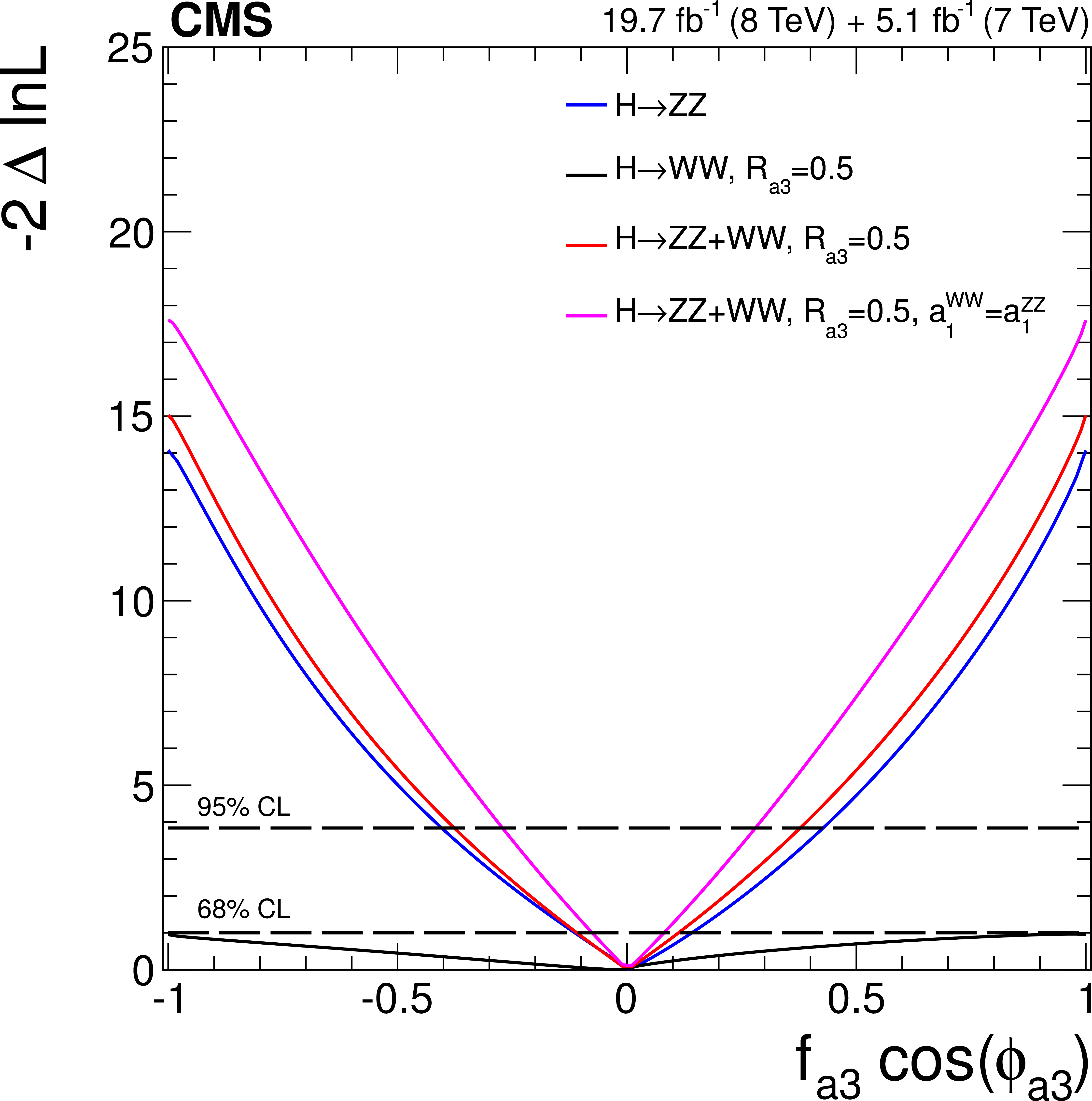
png pdf	Figure 25-f: Expected (dashed) and observed (solid) likelihood scans for effective fractions $f_{\Lambda 1}$ (a, b), $f_{a2}$ (c, d), $f_{a3}$ (e, f). The couplings studied are constrained to be real and all other anomalous couplings are fixed to the SM predictions. The $\cos\phi _{ai}$ term allows a signed quantity where $\cos\phi _{ai}=-1$ or $+1$. Plots a, c, and e show the results of the ${\mathrm {H}} \to {\mathrm {W}} {\mathrm {W}}\to \ell \nu \ell \nu$ analysis expressed in terms of the ${\mathrm {H}} {\mathrm {W}} {\mathrm {W}}$ couplings. Plots b, d, and f show the combined ${\mathrm {H}} \to {\mathrm {W}} {\mathrm {W}}$ and ${\mathrm {H}} \to {\mathrm {Z}} {\mathrm {Z}}$ result in terms of the ${\mathrm {H}} {\mathrm {Z}} {\mathrm {Z}}$ couplings for $R_{ai} = 0.5$. Measurements are shown for each channel separately and two types of combination are present: using $a_1^{ {\mathrm {W}} {\mathrm {W}}} = a_1$ (red) and without such a constraint (magenta).
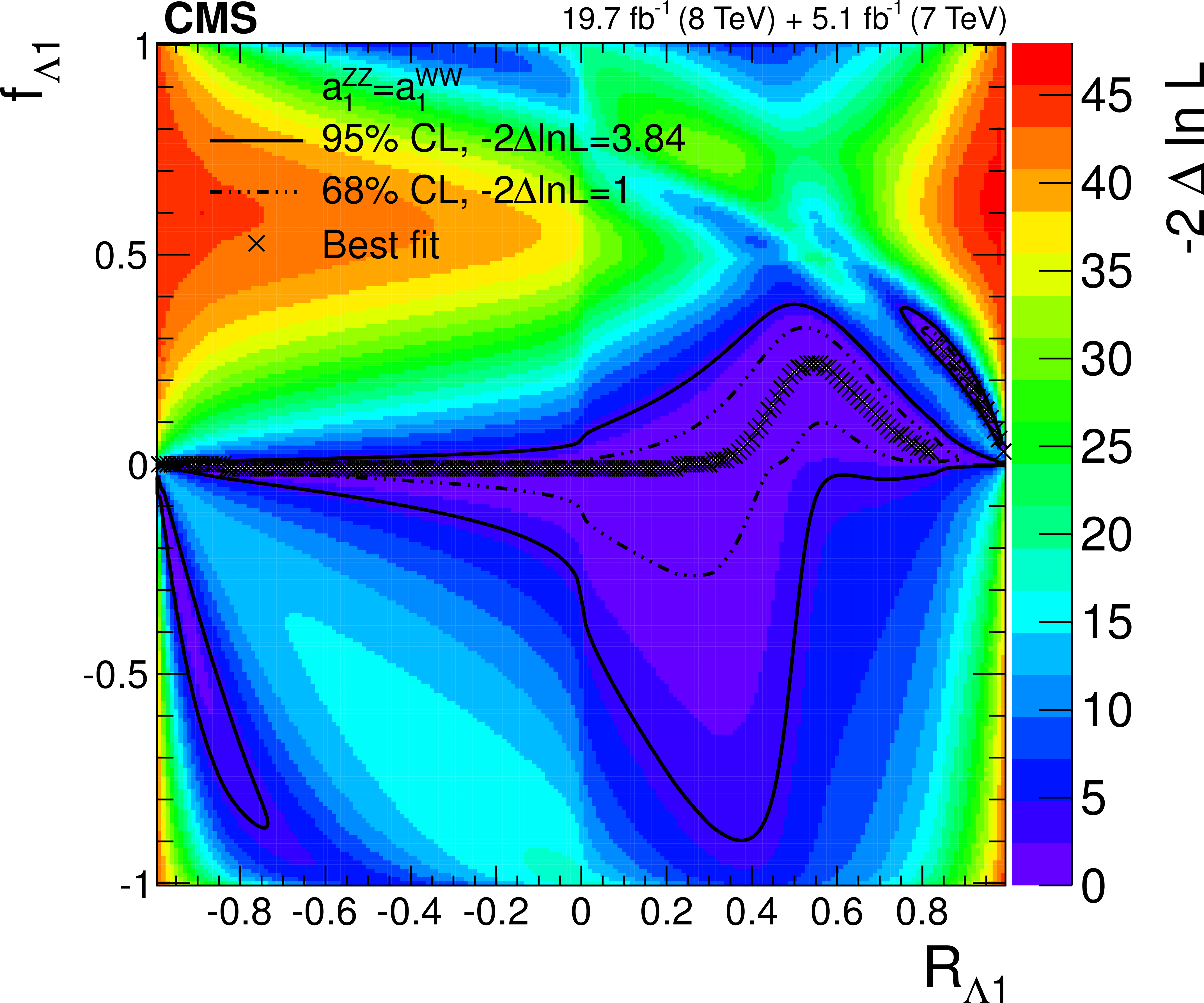
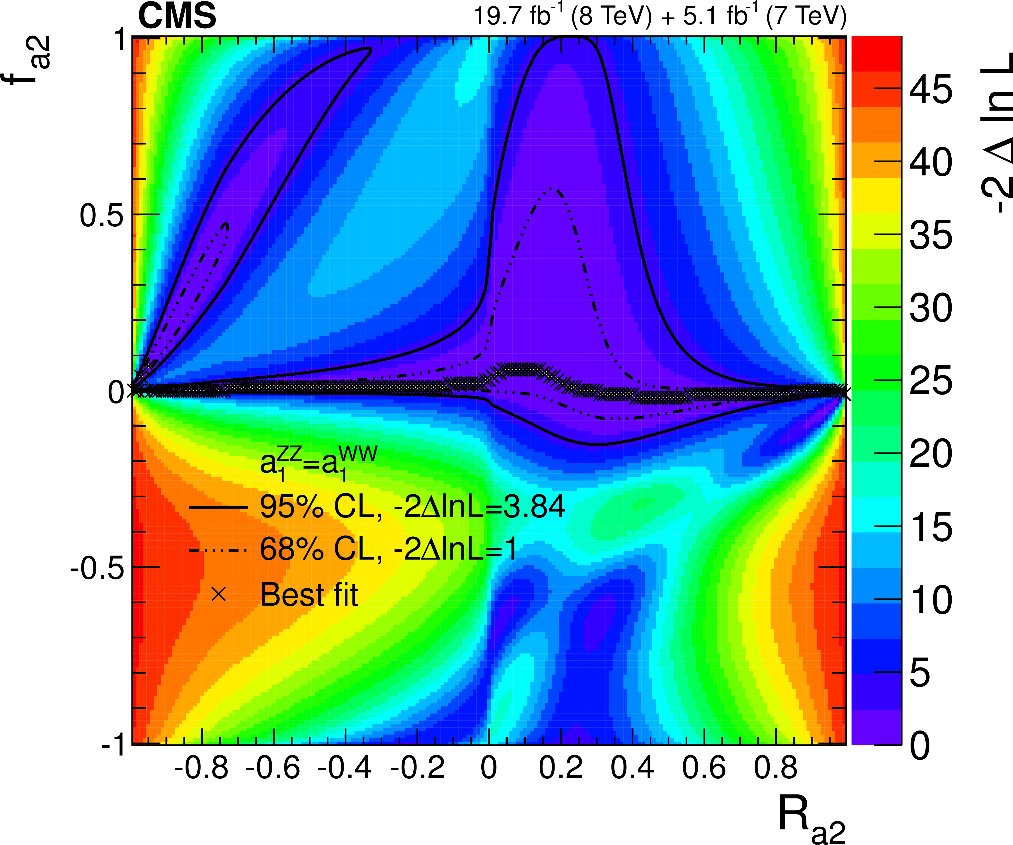
png pdf	Figure 26-a: Observed conditional likelihood scans of $f_{\Lambda 1}$ (a, b), $f_{a2}$ (c, d), $f_{a3}$ (e, f) for a given $R_{ai}$ value from the combined analysis of the ${\mathrm {H}} \to {\mathrm {W}} {\mathrm {W}}$ and ${\mathrm {H}} \to {\mathrm {Z}} {\mathrm {Z}}$ channels using the template method. The results are shown with custodial symmetry $a_1=a_1^{ {\mathrm {W}} {\mathrm {W}}}$ (a, c, e) and without such an assumption (b, d, f). Each cross indicates the minimum value of $-2 \Delta \ln\mathcal {L}$ and the contours indicate the one-parameter confidence intervals of $f_{ai}$ for a given value of $R_{ai}$.
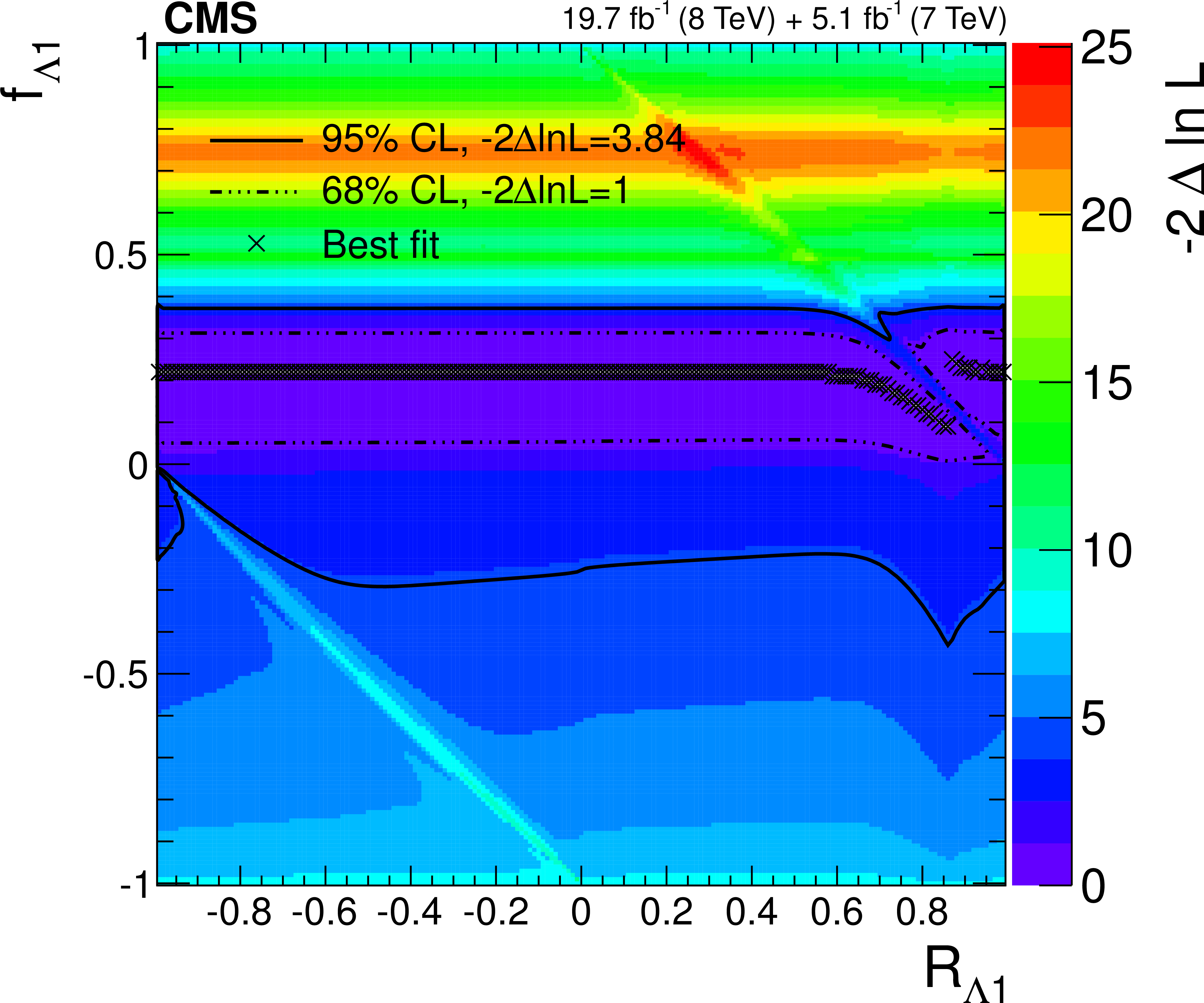
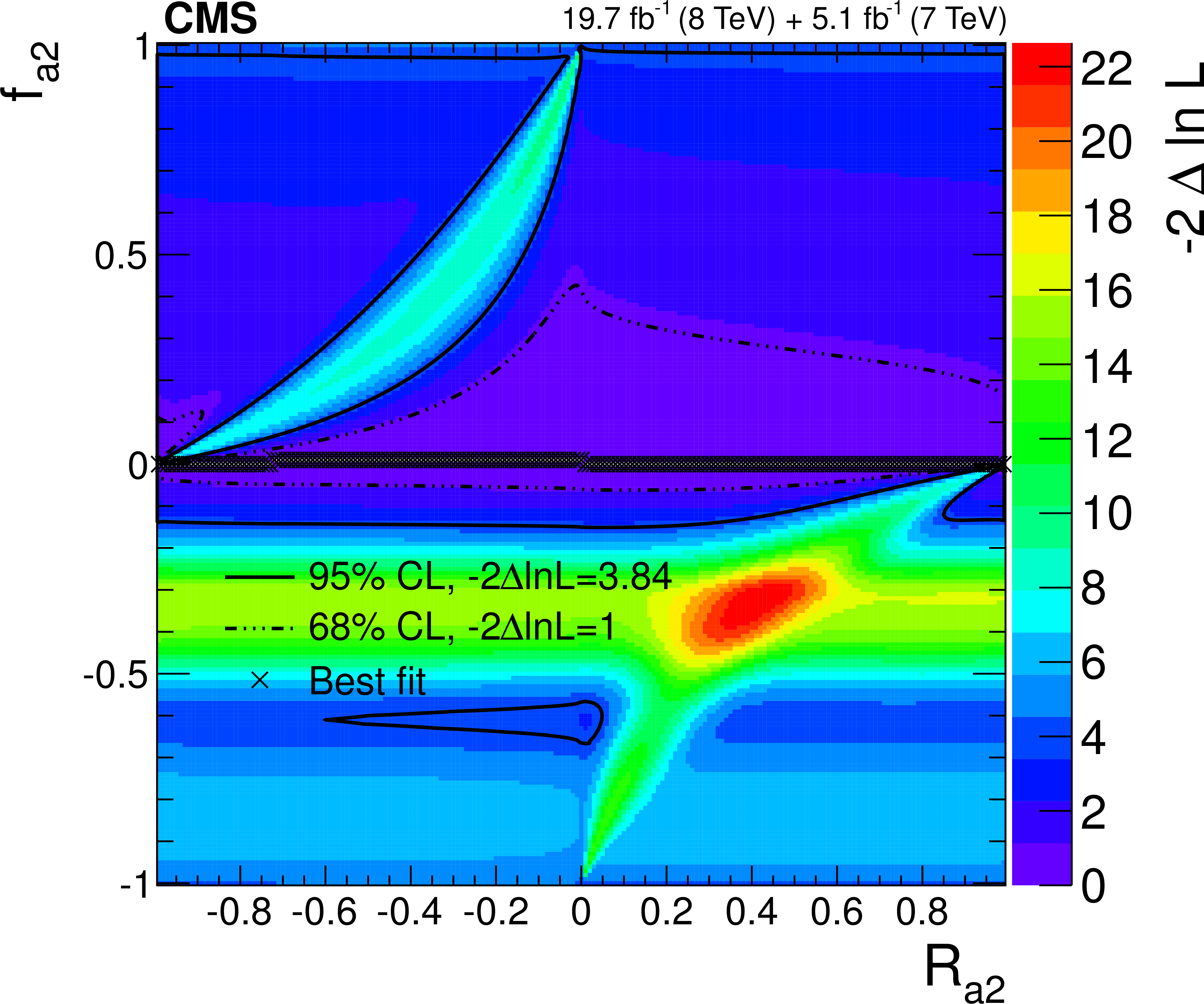
png pdf	Figure 26-b: Observed conditional likelihood scans of $f_{\Lambda 1}$ (a, b), $f_{a2}$ (c, d), $f_{a3}$ (e, f) for a given $R_{ai}$ value from the combined analysis of the ${\mathrm {H}} \to {\mathrm {W}} {\mathrm {W}}$ and ${\mathrm {H}} \to {\mathrm {Z}} {\mathrm {Z}}$ channels using the template method. The results are shown with custodial symmetry $a_1=a_1^{ {\mathrm {W}} {\mathrm {W}}}$ (a, c, e) and without such an assumption (b, d, f). Each cross indicates the minimum value of $-2 \Delta \ln\mathcal {L}$ and the contours indicate the one-parameter confidence intervals of $f_{ai}$ for a given value of $R_{ai}$.
png pdf	Figure 26-c: Observed conditional likelihood scans of $f_{\Lambda 1}$ (a, b), $f_{a2}$ (c, d), $f_{a3}$ (e, f) for a given $R_{ai}$ value from the combined analysis of the ${\mathrm {H}} \to {\mathrm {W}} {\mathrm {W}}$ and ${\mathrm {H}} \to {\mathrm {Z}} {\mathrm {Z}}$ channels using the template method. The results are shown with custodial symmetry $a_1=a_1^{ {\mathrm {W}} {\mathrm {W}}}$ (a, c, e) and without such an assumption (b, d, f). Each cross indicates the minimum value of $-2 \Delta \ln\mathcal {L}$ and the contours indicate the one-parameter confidence intervals of $f_{ai}$ for a given value of $R_{ai}$.
png pdf	Figure 26-d: Observed conditional likelihood scans of $f_{\Lambda 1}$ (a, b), $f_{a2}$ (c, d), $f_{a3}$ (e, f) for a given $R_{ai}$ value from the combined analysis of the ${\mathrm {H}} \to {\mathrm {W}} {\mathrm {W}}$ and ${\mathrm {H}} \to {\mathrm {Z}} {\mathrm {Z}}$ channels using the template method. The results are shown with custodial symmetry $a_1=a_1^{ {\mathrm {W}} {\mathrm {W}}}$ (a, c, e) and without such an assumption (b, d, f). Each cross indicates the minimum value of $-2 \Delta \ln\mathcal {L}$ and the contours indicate the one-parameter confidence intervals of $f_{ai}$ for a given value of $R_{ai}$.
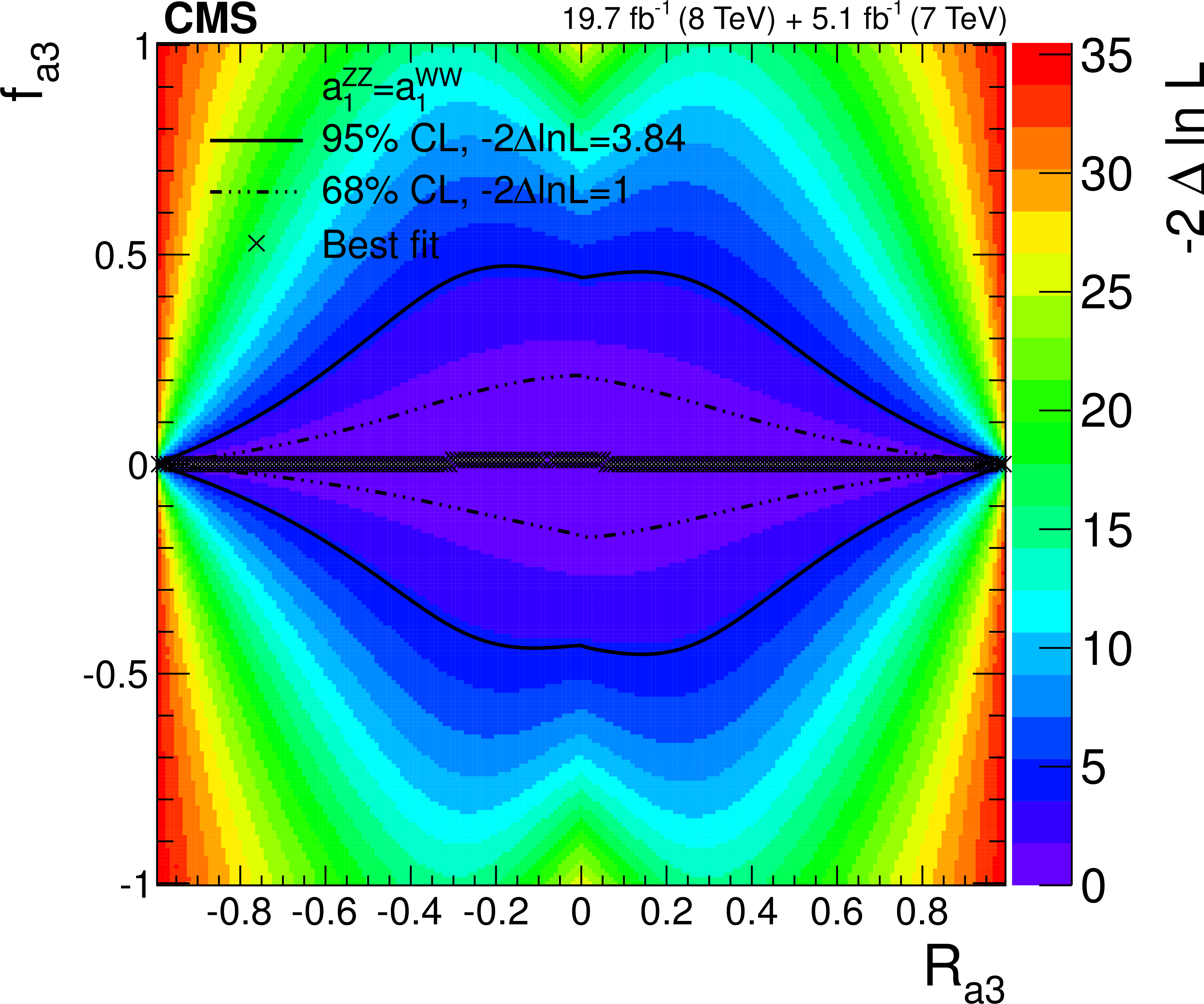
png pdf	Figure 26-e: Observed conditional likelihood scans of $f_{\Lambda 1}$ (a, b), $f_{a2}$ (c, d), $f_{a3}$ (e, f) for a given $R_{ai}$ value from the combined analysis of the ${\mathrm {H}} \to {\mathrm {W}} {\mathrm {W}}$ and ${\mathrm {H}} \to {\mathrm {Z}} {\mathrm {Z}}$ channels using the template method. The results are shown with custodial symmetry $a_1=a_1^{ {\mathrm {W}} {\mathrm {W}}}$ (a, c, e) and without such an assumption (b, d, f). Each cross indicates the minimum value of $-2 \Delta \ln\mathcal {L}$ and the contours indicate the one-parameter confidence intervals of $f_{ai}$ for a given value of $R_{ai}$.
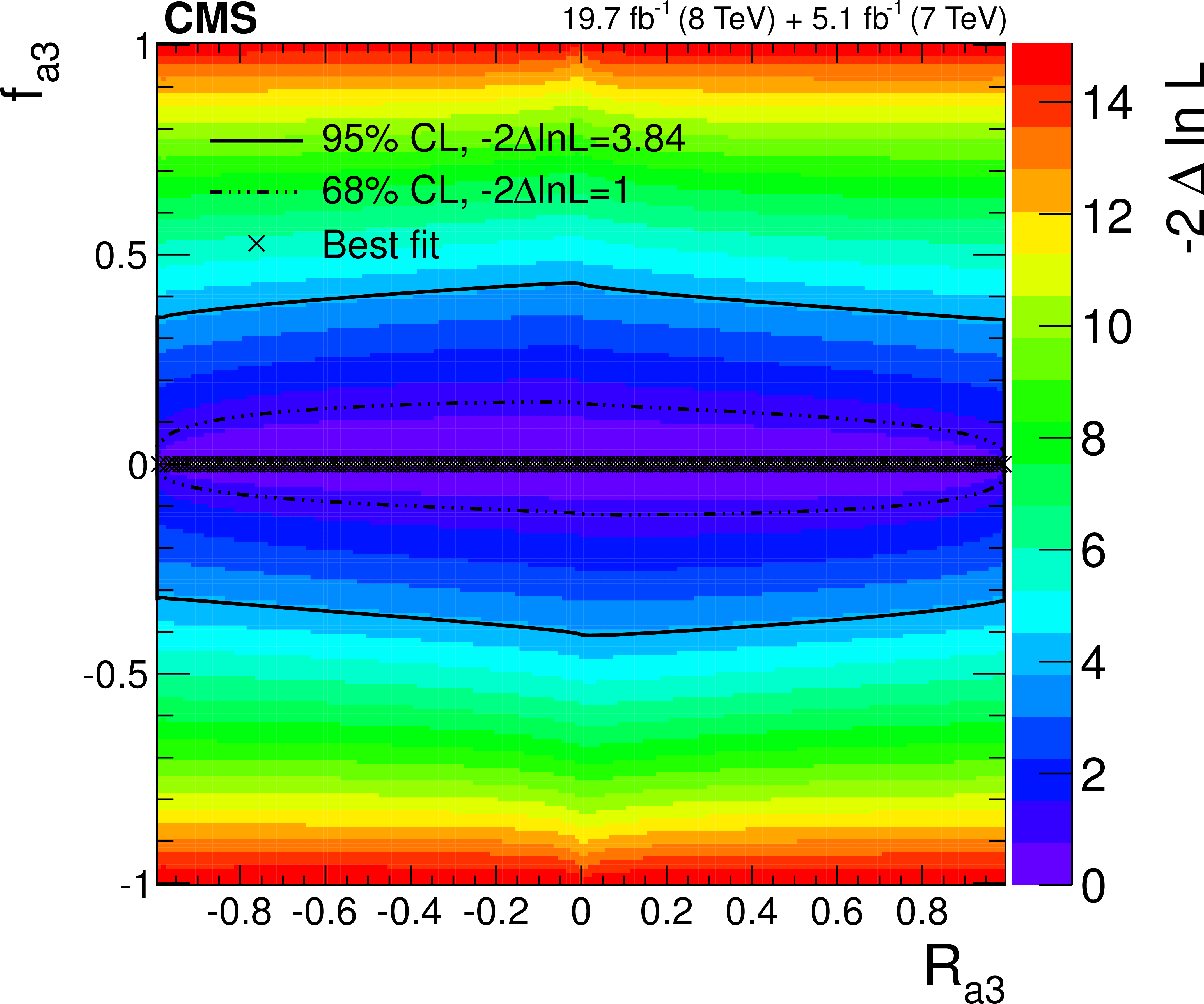
png pdf	Figure 26-f: Observed conditional likelihood scans of $f_{\Lambda 1}$ (a, b), $f_{a2}$ (c, d), $f_{a3}$ (e, f) for a given $R_{ai}$ value from the combined analysis of the ${\mathrm {H}} \to {\mathrm {W}} {\mathrm {W}}$ and ${\mathrm {H}} \to {\mathrm {Z}} {\mathrm {Z}}$ channels using the template method. The results are shown with custodial symmetry $a_1=a_1^{ {\mathrm {W}} {\mathrm {W}}}$ (a, c, e) and without such an assumption (b, d, f). Each cross indicates the minimum value of $-2 \Delta \ln\mathcal {L}$ and the contours indicate the one-parameter confidence intervals of $f_{ai}$ for a given value of $R_{ai}$.

Tables
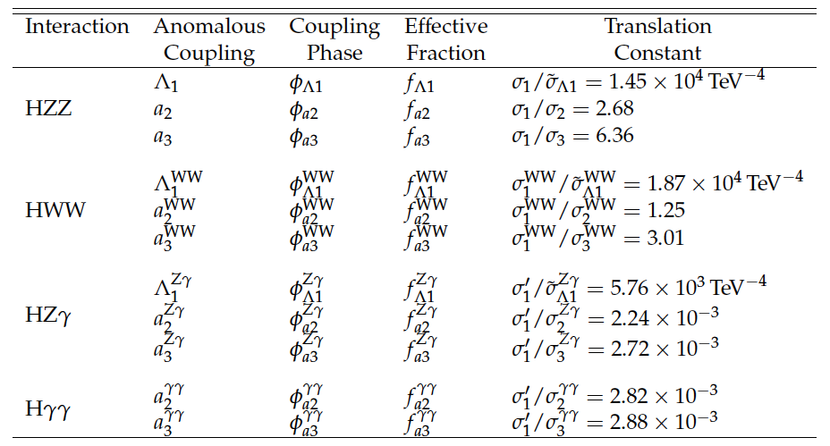
png pdf	Table 1: List of anomalous ${\mathrm {H}} {\mathrm {V}} {\mathrm {V}}$ couplings considered in the measurements assuming a spin-zero Higgs boson. The definition of the effective fractions is discussed in the text and the translation constant is given in each case. The effective cross sections correspond to the processes ${\mathrm {H}} \to {\mathrm {V}} {\mathrm {V}} \to 2 {\mathrm {e}}2\mu$ and ${\mathrm {H}} \to {\mathrm {W}} {\mathrm {W}}\to \ell \nu \ell \nu$ and the Higgs boson mass $m_{ {\mathrm {H}} }=125.6 GeV$ using the JHUGen calculation. The cross-section ratios for the ${\mathrm {H}} {\mathrm {Z}} \gamma$ and ${\mathrm {H}} \gamma \gamma$ couplings include the requirement $\sqrt {q^2_{ {\mathrm {V}} }} \ge 4 GeV$.
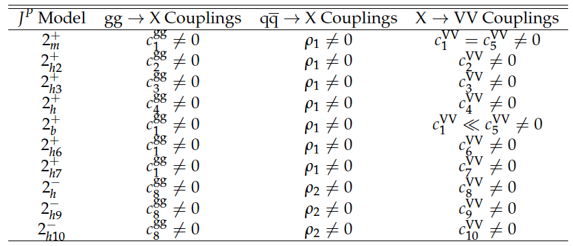
png pdf	Table 2: List of spin-two models with the production and decay couplings of an exotic ${\mathrm {X}}$ particle. The subscripts $m$ (minimal couplings), $h$ (couplings with higher-dimension operators), and $b$ (bulk) distinguish different scenarios.
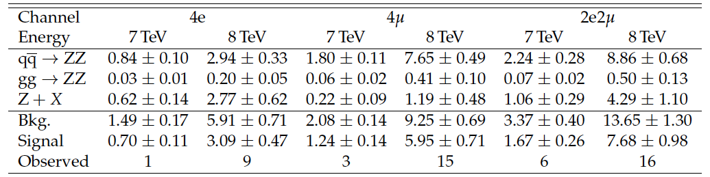
png pdf	Table 3: Number of background (Bkg.) and signal events expected in the SM, and number of observed candidates, for the ${\mathrm {H}} \to {\mathrm {V}} {\mathrm {V}} \to 4\ell$ analysis after the final selection in the mass region 105.6 $< m_{4\ell } <$ 140.6 GeV. The signal and ${\mathrm {Z}} {\mathrm {Z}}$ background are estimated from MC simulation, while the ${\mathrm {Z}} +X$ background is estimated from data. Only systematic uncertainties are quoted.
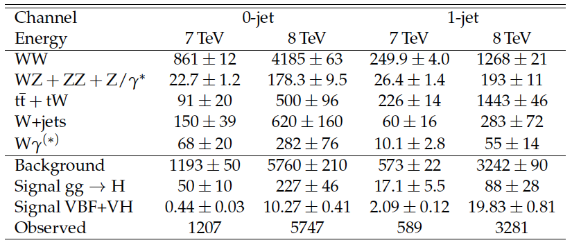
png pdf	Table 4: Number of background and signal events expected in the SM, and number of observed candidates, for the ${\mathrm {H}} \to {\mathrm {W}} {\mathrm {W}}$ analysis after final selection. The signal and background are estimated from MC simulation and from data control regions, as discussed in the text. Only systematic uncertainties are quoted.
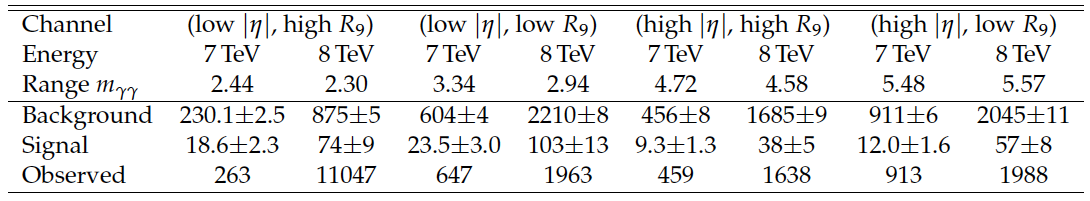
png pdf	Table 5: Number of background and signal events expected in the SM, and number of observed candidates, for the ${\mathrm {H}} \to \gamma \gamma$ analysis after final selection. The four categories are defined as follows: low ${| \eta | }$ indicates that both photons are in the barrel with ${| \eta | } < 1.5$ and high ${| \eta | }$ otherwise, high $R_9$ indicates that both photons have $R_9>0.94$ and low $R_9$ otherwise. The $m_{\gamma \gamma }$ range (GeV) centered at $m_ {\mathrm {H}} =$125 GeV corresponds to the full width at half maximum for the signal distribution in each category. Only systematic uncertainties are quoted, which include uncertainty from the background $m_{\gamma \gamma }$ parameterization in the background estimates.
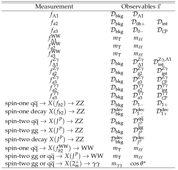
png pdf	Table 6: List of observables $\vec{x}$ used in the analysis of the ${\mathrm {H}} {\mathrm {V}} {\mathrm {V}}$ couplings. The $J^P$ notation for spin-two refers to the ten scenarios defined in Table {table-scenarios}. The ${\mathrm {H}} \to \gamma \gamma$ channel is illustrated with two main observables, where $\cos \theta ^*$ represents categories constructed from the angular and other observables, and more details are given in Section 3.5 and Ref.[15].
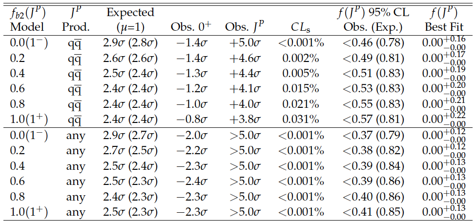
png pdf	Table 7: List of spin-one models tested in the ${\mathrm {X}} \to {\mathrm {Z}} {\mathrm {Z}}$ analysis. The expected separation is quoted for two scenarios, for the signal production cross section obtained from the fit to data for each hypothesis and using the SM expectation ($\mu =1$). The observed separation shows the consistency of the observation with the SM Higgs boson model or the alternative $J^{P}$ model, from which the $CL_\mathrm {s}$ value is derived. The $f(J^P)$ constraints are quoted, where the decay-only measurements are valid for any production (Prod.) mechanism and are performed using the efficiency of the ${ {\mathrm {q}} {\mathrm {\overline {q}}}} \to {\mathrm {X}} \to {\mathrm {Z}} {\mathrm {Z}}$ selection.
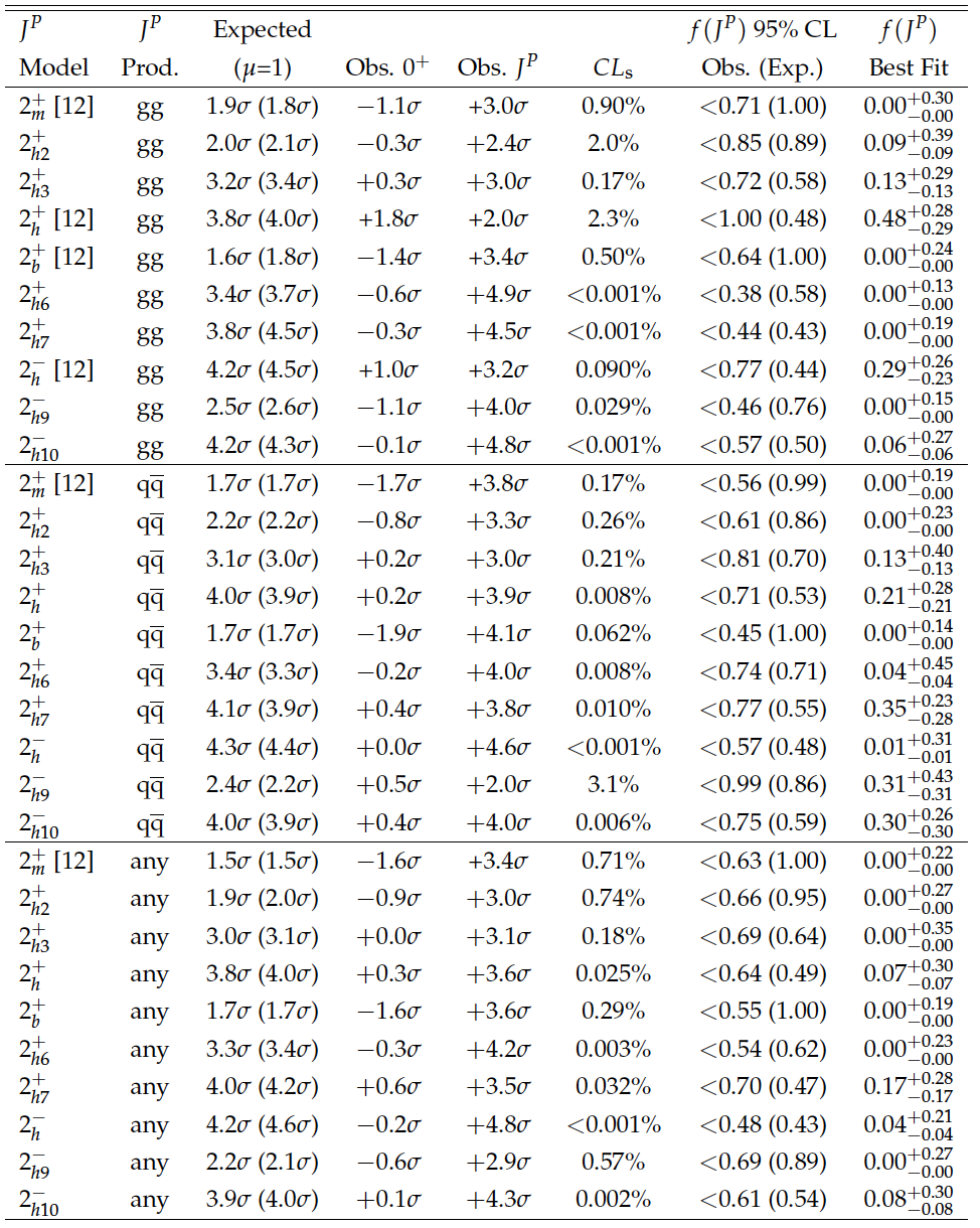
png pdf	Table 8: List of spin-two models tested in the ${\mathrm {X}} \to {\mathrm {Z}} {\mathrm {Z}}$ analysis. The expected separation is quoted for two scenarios, for the signal production cross section obtained from the fit to data for each hypothesis, and using the SM expectation ($\mu =1$). The observed separation shows the consistency of the observation with the SM Higgs boson or an alternative $J^{P}$ model, from which the ${CL_\mathrm {s}}$ value is derived. The $f(J^P)$ constraints are quoted, where the decay-only measurements are valid for any production (Prod.) mechanism and are performed using the efficiency of the ${\mathrm {g}} {\mathrm {g}} \to {\mathrm {X}} \to {\mathrm {Z}} {\mathrm {Z}}$ selection. Results from Ref.[12]are explicitly noted.
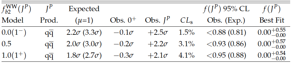
png pdf	Table 9: List of spin-one models tested in the ${\mathrm {X}} \to {\mathrm {W}} {\mathrm {W}}$ analysis. The expected separation is quoted for two scenarios, for the signal production cross section obtained from the fit to data for each hypothesis, and using the SM expectation ($\mu =1$). The observed separation shows the consistency of the observation with the SM Higgs boson model or the alternative $J^{P}$ model, from which a ${CL_\mathrm {s}}$ value is derived. The constraints on the non-interfering $J^{P}$ fraction are quoted in the last two columns.
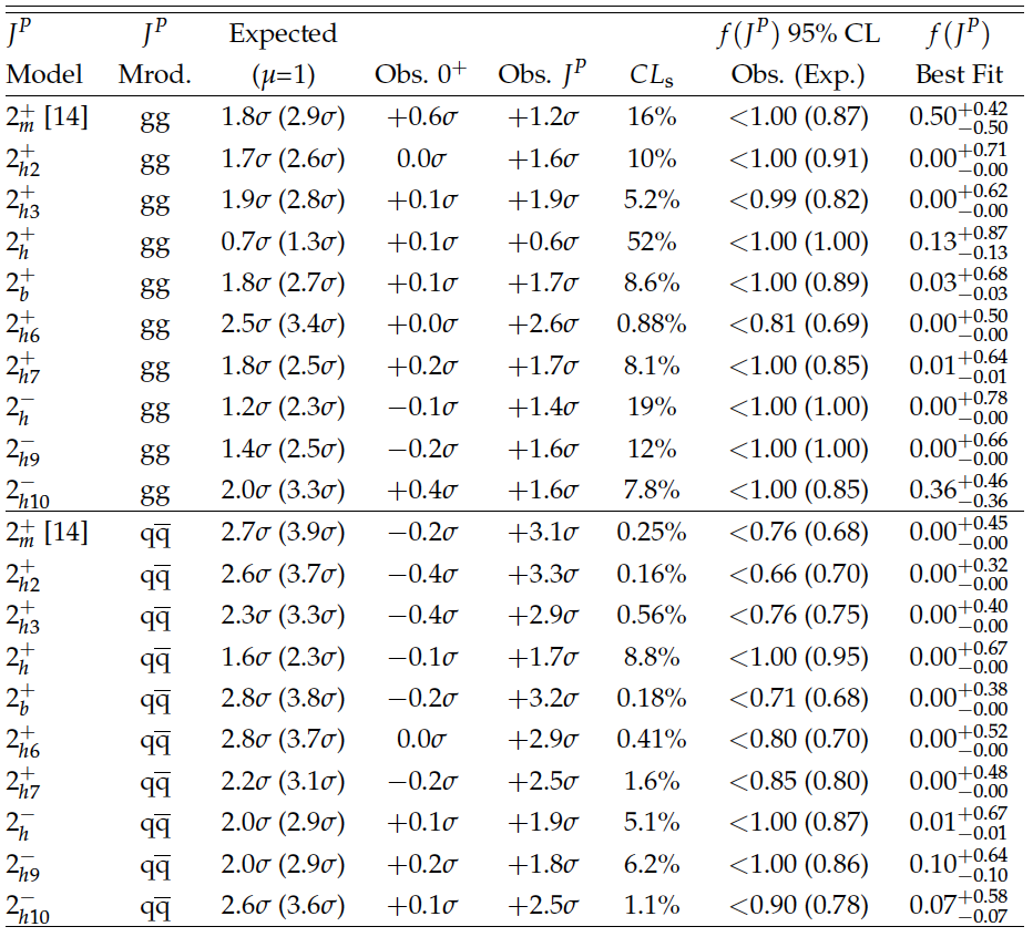
png pdf	Table 10: List of spin-two models tested in the ${\mathrm {X}} \to {\mathrm {W}} {\mathrm {W}}$ analysis. The expected separation is quoted for two scenarios, for the signal production cross section obtained from the fit to data for each hypothesis, and using the SM expectation ($\mu =1$). The observed separation shows the consistency of the observation with the SM Higgs boson or an alternative $J^{P}$ model, from which the ${CL_\mathrm {s}}$ value is derived. The constraints on the non-interfering $J^{P}$ fraction are quoted in the last two columns. Results from Ref.[14] are explicitly noted.
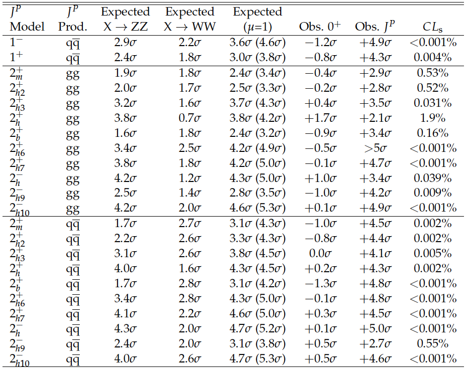
png pdf	Table 11: List of spin-one and spin-two models tested in the combination of the ${\mathrm {X}} \to {\mathrm {Z}} {\mathrm {Z}}$ and ${\mathrm {X}} \to {\mathrm {W}} {\mathrm {W}}$ channels. The combined expected separation is quoted for two scenarios, for the signal production cross section obtained from the fit to data for each hypothesis and using the SM expectation ($\mu =1$). For comparison, the former expectations are also quoted for the individual channels as in Tables 7-10. The observed separation shows the consistency of the observation with the SM Higgs boson model or an alternative $J^{P}$ model, from which the ${CL_\mathrm {s}}$ value is derived.
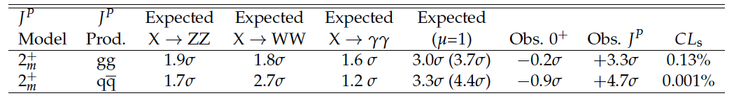
png pdf	Table 12: Results of the study of the $2^+_{m}$ model for the combination of the ${\mathrm {X}} \to {\mathrm {Z}} {\mathrm {Z}}$, ${\mathrm {W}} {\mathrm {W}}$, and $\gamma \gamma$ decay channels. The expected separation is quoted for the three channels separately and for the combination with the signal strength for each hypothesis determined from the fit to data independently in each channel. Also shown in parentheses is the expectation with the SM signal cross section ($\mu$=1). The observed separation shows the consistency of the observation with the SM $0^+$ model or $J^P$ model and corresponds to the scenario where the signal strength is floated in the fit to data.
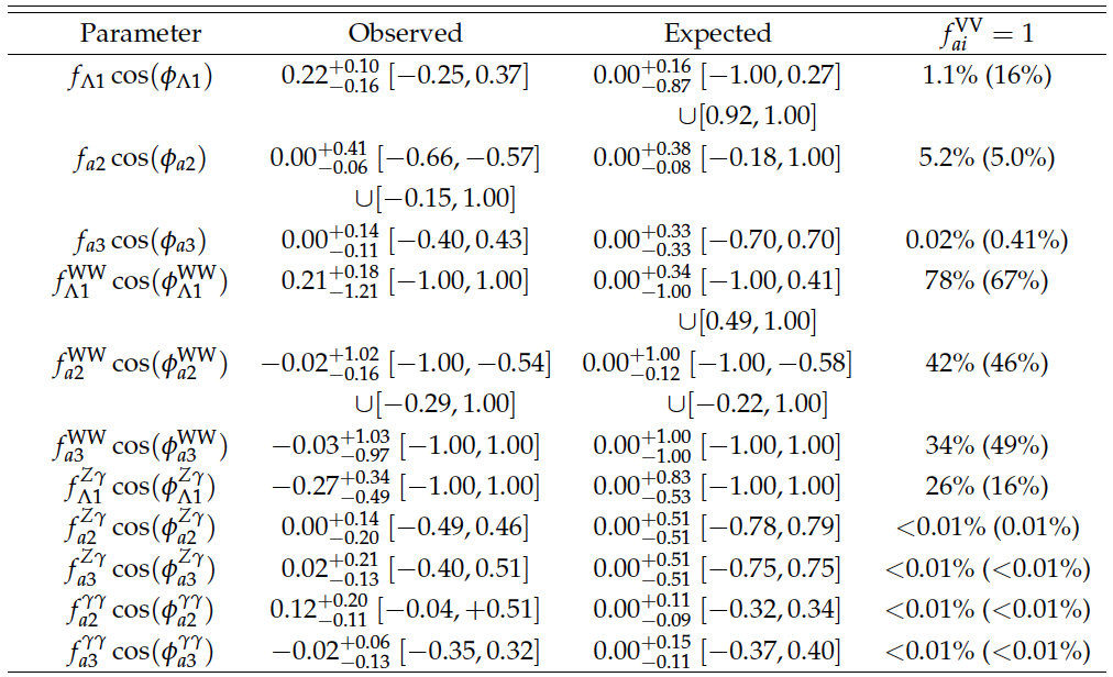
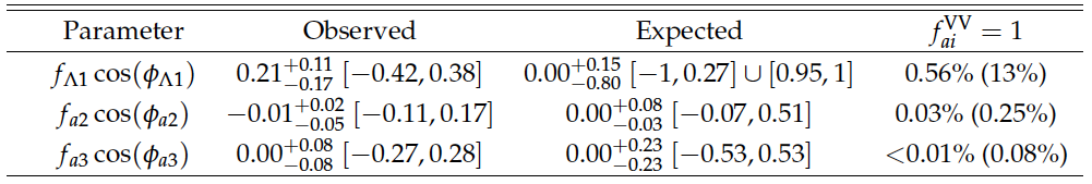
png pdf	Table 13: Summary of allowed 68%CL (central values with uncertainties) and 95%CL (ranges in square brackets) intervals on anomalous coupling parameters in ${\mathrm {H}} {\mathrm {V}} {\mathrm {V}}$ interactions under the assumption that all the coupling ratios are real ($\phi _{ai}^{ {\mathrm {V}} {\mathrm {V}} }=0$ or $\pi$). The ranges are truncated at the physical boundaries of $f_{ai}^{ {\mathrm {V}} {\mathrm {V}} }=1$. The last column indicates the observed (expected) confidence level of a pure anomalous coupling corresponding to $f_{ai}^{ {\mathrm {V}} {\mathrm {V}} }=1$ when compared to the SM expectation $f_{ai}^{ {\mathrm {V}} {\mathrm {V}} }=0$. The expected results are quoted for the SM signal production cross section ($\mu =1$). The results are obtained with the template method.
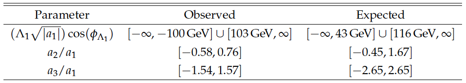
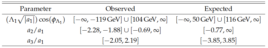
png pdf	Table 14: Summary of the allowed 95\%CL intervals on the anomalous couplings in ${\mathrm {H}} {\mathrm {Z}} {\mathrm {Z}}$ interactions using results in Table 13. The coupling ratios are assumed to be real (including $\cos(\phi _{\Lambda _{1}})=0$ or $\pi$).
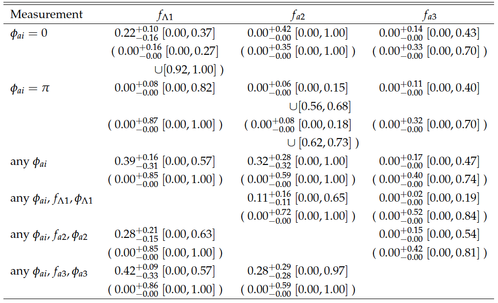
png pdf	Table 15: Summary of the allowed 68%CL (central values with uncertainties) and 95%CL (ranges in square brackets) intervals on anomalous coupling parameters in the ${\mathrm {H}} {\mathrm {Z}} {\mathrm {Z}}$ interactions under the condition of a given phase of the coupling (0 or $\pi$) or when the phase or other parameters are unconstrained (any value allowed). Results are presented with the template method and expectations are quoted in parentheses following the observed values. The results for $f_{a3}$ with $\phi _{a3}$ unconstrained are from Ref.[12].
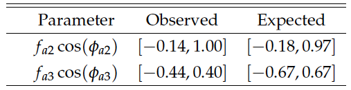
png pdf	Table 16: Summary of the allowed 95\%CL intervals on the anomalous coupling parameters in ${\mathrm {H}} {\mathrm {Z}} {\mathrm {Z}}$ interactions under the assumption that all the coupling ratios are real ($\phi _{ai}=0$ or $\pi$) using the multidimensional distribution method. These results cross-check those presented in Table 13.
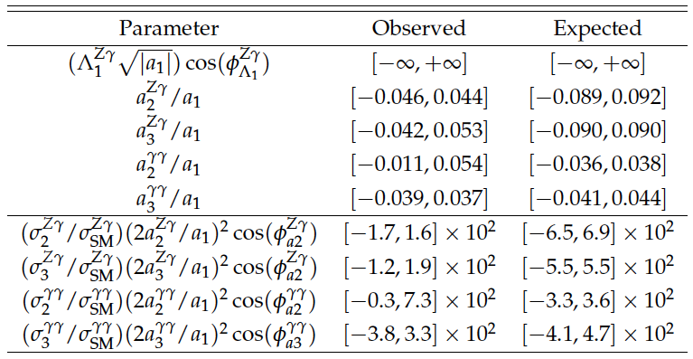
png pdf	Table 17: Summary of the allowed 95\%CL intervals on the anomalous couplings in ${\mathrm {H}} {\mathrm {Z}} \gamma$ and ${\mathrm {H}} \gamma \gamma$ interactions using results obtained with the template method in Table 13. The coupling ratios are assumed to be real ($\cos(\phi ^{ {\mathrm {V}} {\mathrm {V}} }_{ai})=0$ or $\pi$).
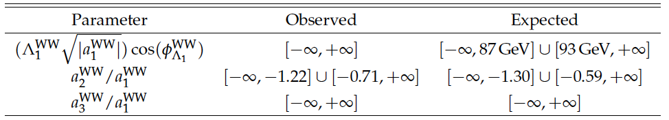
png pdf	Table 18: Summary of the allowed 95\%CL intervals on the anomalous couplings in ${\mathrm {H}} {\mathrm {W}} {\mathrm {W}}$ interactions using results obtained with the template method in Table 13. The coupling ratios are assumed to be real (including $\cos(\phi ^{ {\mathrm {W}} {\mathrm {W}}}_{\Lambda _{1}})=0$ or $\pi$).
png pdf	Table 19: Summary of allowed 68%CL (central values with uncertainties) and 95%CL (ranges in square brackets) intervals on anomalous coupling parameters in ${\mathrm {H}} {\mathrm {V}} {\mathrm {V}}$ interactions in combination of ${\mathrm {H}} {\mathrm {Z}} {\mathrm {Z}}$ and ${\mathrm {H}} {\mathrm {W}} {\mathrm {W}}$ measurements assuming the symmetry $a_i = a_i^{ {\mathrm {W}} {\mathrm {W}}}$, including $R_{ai}=0.5$, and real coupling ratios ($\phi _{ai}^{ {\mathrm {V}} {\mathrm {V}} }=0$ or $\pi$). The last column indicates the observed (expected) confidence level of a pure anomalous coupling corresponding to $f_{ai}^{ {\mathrm {V}} {\mathrm {V}} }=1$ when compared to the SM expectation $f_{ai}^{ {\mathrm {V}} {\mathrm {V}} }=0$. The results are obtained with the template method.
png pdf	Table 20: Summary of the allowed 95\%CL intervals on the anomalous couplings in ${\mathrm {H}} {\mathrm {V}} {\mathrm {V}}$ interactions in combination of ${\mathrm {H}} {\mathrm {Z}} {\mathrm {Z}}$ and ${\mathrm {H}} {\mathrm {W}} {\mathrm {W}}$ measurements in Table 19 assuming the symmetry $a_i = a_i^{ {\mathrm {W}} {\mathrm {W}}}$, including $R_{ai}=0.5$, and real coupling ratios ($\phi _{ai}^{ {\mathrm {V}} {\mathrm {V}} }=0$ or $\pi$).

Summary

In this paper, a comprehensive study of the spin-parity properties of the recently discovered H boson and of the tensor structure of its interactions with electroweak gauge bosons is presented using the $\mathrm{ H \to ZZ^*,\, Z\gamma^*,\, \gamma^* \gamma^* \to 4 \ell }$, $\mathrm{ H \to WW^* \to \ell \nu \ell \nu }$, and $\mathrm { H \to \gamma \gamma }$ decay modes. The results are based on the 2011 and 2012 data from pp collisions recorded with the CMS detector at the LHC, and correspond to an integrated luminosity of up to 5.1 fb$^{-1}$ at a center-of-mass energy of 7 TeV and up to 19.7 fb$^{-1}$ at 8 TeV. The phenomenological formulation for the interactions of a spin-zero, -one, or -two boson with the SM particles is based on a scattering amplitude or, equivalently, an effective field theory Lagrangian, with operators up to dimension five. The dedicated simulation and matrix element likelihood approach for the analysis of the kinematics of H boson production and decay in different topologies are based on this formulation. A maximum likelihood fit of the signal and background distributions provides constraints on the anomalous couplings of the H boson. The study focuses on testing for the presence of anomalous effects in HZZ and HWW interactions under spin-zero, -one, and -two hypotheses. The combination of the $\mathrm{ H \to ZZ^* }$ and $\mathrm{ H \to WW^* }$ measurements leads to tighter constraints on the H boson spin-parity and anomalous HVV interactions. The combination with the $\mathrm{ H \to \gamma \gamma }$ measurements also allows tighter constraints in the spin-two case. The $\mathrm{ HZ\gamma }$ and $\mathrm{ H\gamma\gamma }$ interactions are probed for the first time using the $4 \ell$ final state. The exotic-spin study covers the analysis of mixed-parity spin-one states and ten spin-two hypotheses under the assumption of production either via gluon fusion or quark-antiquark annihilation, or without such an assumption. The spin-one hypotheses are excluded at a greater than 99.999% CL in the ZZ and WW modes, while in the $\gamma \gamma$ mode they are excluded by the Landau-Yang theorem. The spin-two boson with gravity-like minimal couplings is excluded at a 99.87% CL, and the other spin-two hypotheses tested are excluded at a 99% CL or higher. Given the exclusion of the spin-one and spin-two scenarios, constraints are set on the contribution of eleven anomalous couplings to the $\mathrm{ HZZ }$, $\mathrm{ HZ\gamma }$, $\mathrm{ H\gamma\gamma }$, and $\mathrm{ HWW }$ interactions of a spin-zero H boson, as summarized in Table 13. Among these is the measurement of the $f_{a3}$ parameter, which is defined as the fractional pseudoscalar cross section in the $\mathrm{ H \to ZZ }$ channel. The constraint is $f_{a3} < 0.43 (0.40)$ at a 95% CL for the positive (negative) phase of the pseudoscalar coupling with respect to the dominant SM-like coupling and $f_{a3} = 1$ exclusion of a pure pseudoscalar hypothesis at a 99.98% CL. All observations are consistent with the expectations for a scalar SM-like Higgs boson. It is not presently established that the interactions of the observed state conserve $C$-parity or $CP$-parity. However, under the assumption that both quantities are conserved, our measurements require the quantum numbers of the new state to be $J^{PC} = 0^{++}$. The positive $P$-parity follows from the $f^{ \mathrm{VV}}_{a3}$ measurements in the $\mathrm{ H \to ZZ,\, Z\gamma^*,\, \gamma^* \gamma^* \to 4 \ell }$, and $\mathrm{ H \to WW^* \to \ell \nu \ell \nu }$ decays and the positive $C$-parity follows from observation of the $\mathrm { H \to \gamma \gamma }$ decay. Further measurements probing the tensor structure of the $\mathrm{ HVV }$ and $\mathrm{ Hf\bar{f} }$ interactions can test the assumption of $CP$ invariance.

Compact Muon Solenoid LHC, CERN

© Copyright CERN 2015 for the benefit of the CMS Collaboration