

Compact Muon Solenoid
LHC, CERN
| CMS-PAS-HIG-19-015 | ||
| Measurements of Higgs boson properties in the diphoton decay channel at $\sqrt{s} = $ 13 TeV | ||
| CMS Collaboration | ||
| July 2020 | ||
| Abstract: Measurements of Higgs boson properties in events where the Higgs boson decays into a pair of photons are reported. Events with two photons are selected from a sample of proton-proton collisions at $\sqrt{s} = $ 13 TeV collected by the CMS detector at the LHC from 2016 to 2018, corresponding to an integrated luminosity of 137 fb$^{-1}$. Analysis categories enriched in events produced via gluon fusion, vector boson fusion, vector boson associated production, and production associated with top quarks are constructed. The total Higgs boson signal strength, relative to the standard model prediction, is measured to be 1.03$^{+0.11}_{-0.09}$. Other properties of the Higgs boson are measured, including standard model signal strength modifiers, production cross sections, and its couplings to other particles. All results are found to be in agreement with the standard model expectations. | ||
|
Links:
CDS record (PDF) ;
CADI line (restricted) ;
These preliminary results are superseded in this paper, Accepted by JHEP. The superseded preliminary plots can be found here. |
||
| Figures & Tables | Summary | Additional Figures & Tables | References | CMS Publications |
|---|
| Figures | |
png pdf |
Figure 1:
Diagram showing the full set of STXS stage 1.2 bins, adapted from Ref. [13]. The solid lines define each stage 1.2 bin. The ggH region (blue) is split into bins using the Higgs boson transverse momentum (${{p_{\mathrm {T}}} ^\mathrm{H}}$), the number of jets, and additionally has a VBF-like region with high dijet mass (${m_{\text {jj}}}$). The VBF and hadronic VH modes are considered together as electroweak (EW) qqH production (orange). Here the bins are defined using the ${{p_{\mathrm {T}}} ^\mathrm{H}}$, number of jets, and ${m_{\text {jj}}}$ as with ggH, with additional divisions in the high dijet mass phase space using the transverse momentum of the Higgs boson plus dijet system (${{p_{\mathrm {T}}} ^{\mathrm{H} \text {jj}}}$). The leptonic VH bins (green) are defined by the number of jets and the transverse momentum of the vector boson (${{p_{\mathrm {T}}} ^{\text {V}}}$). The ${{\mathrm{t} {}\mathrm{\bar{t}}} \mathrm{H}}$ production mode (magenta) is split only by ${{p_{\mathrm {T}}} ^\mathrm{H}}$. Finally, the tH and ${\mathrm{b} {}\mathrm{\bar{b}} \mathrm{H}}$ processes (yellow) are not further divided at STXS stage 1.2. |
png pdf |
Figure 2:
Comparison of the dielectron invariant mass spectra in data and simulation, after applying energy scale corrections to data and energy smearing to the simulation, for ${\mathrm{Z} \rightarrow \mathrm{e} \mathrm{e}}$ events with electrons reconstructed as photons. The comparison is shown for events where both electrons are reconstructed in the ECAL barrel (left), and where both electrons are reconstructed in the ECAL endcaps (right). The full data set collected in the period 2016-2018 and the corresponding simulation are shown. |
png pdf |
Figure 2-a:
Comparison of the dielectron invariant mass spectra in data and simulation, after applying energy scale corrections to data and energy smearing to the simulation, for ${\mathrm{Z} \rightarrow \mathrm{e} \mathrm{e}}$ events with electrons reconstructed as photons. The comparison is shown for events where both electrons are reconstructed in the ECAL barrel. The full data set collected in the period 2016-2018 and the corresponding simulation are shown. |

png pdf |
Figure 2-b:
Comparison of the dielectron invariant mass spectra in data and simulation, after applying energy scale corrections to data and energy smearing to the simulation, for ${\mathrm{Z} \rightarrow \mathrm{e} \mathrm{e}}$ events with electrons reconstructed as photons. The comparison is shown for events where both electrons are reconstructed in the ECAL endcaps. The full data set collected in the period 2016-2018 and the corresponding simulation are shown. |

png pdf |
Figure 3:
The left plot shows the distribution of the photon identification BDT score of the lowest scoring photon in diphoton pairs with an invariant mass in the range 100 $ < {m_{\gamma \gamma}} < $ 180 GeV, for data events passing the preselection (black points), and for simulated background events (red band). Histograms are also shown for different components of the simulated background. The blue histogram corresponds to simulated Higgs boson signal events. The right plot shows the same distribution for ${\mathrm{Z} \rightarrow \mathrm{e} \mathrm{e}}$ events in data and simulation, where the electrons are reconstructed as photons. The statistical and systematic uncertainty in simulation is also shown (pink band). The regions shaded grey contain photon identification BDT scores below the threshold applied to each photon entering the analysis. The full data set collected in the period 2016-2018 and the corresponding simulation are shown. |

png pdf |
Figure 3-a:
The plot shows the distribution of the photon identification BDT score of the lowest scoring photon in diphoton pairs with an invariant mass in the range 100 $ < {m_{\gamma \gamma}} < $ 180 GeV, for data events passing the preselection (black points), and for simulated background events (red band). Histograms are also shown for different components of the simulated background. The blue histogram corresponds to simulated Higgs boson signal events. The region shaded grey contains photon identification BDT scores below the threshold applied to each photon entering the analysis. The full data set collected in the period 2016-2018 is shown. |

png pdf |
Figure 3-b:
The plot shows the distribution of the photon identification BDT score of the lowest scoring photon in diphoton pairs with an invariant mass in the range 100 $ < {m_{\gamma \gamma}} < $ 180 GeV, for ${\mathrm{Z} \rightarrow \mathrm{e} \mathrm{e}}$ events in data and simulation, where the electrons are reconstructed as photons. The statistical and systematic uncertainty in simulation is also shown (pink band). The region shaded grey contains photon identification BDT scores below the threshold applied to each photon entering the analysis. The full data set collected in the period 2016-2018 and the corresponding simulation are shown. |

png pdf |
Figure 4:
The left plot shows the validation of the ${\mathrm{H} \rightarrow \gamma \gamma}$ vertex identification algorithm on ${\mathrm{Z} \rightarrow \mu \mu}$ events, where the the muon tracks are omitted when performing the event reconstruction. This allows the fraction of events with the correctly assigned vertex estimated with simulation to be compared with data, as a function of the ${p_{\mathrm {T}}}$ of the dimuon system. Simulated events are weighted to match the distributions of pileup and distribution of vertices along the beam axis in data. The right plot demonstrates that the average vertex probability agrees with the true vertex efficiency in simulated events. The full data set collected in the period 2016-2018 and the corresponding simulation are shown. |

png pdf |
Figure 4-a:
The plot shows the validation of the ${\mathrm{H} \rightarrow \gamma \gamma}$ vertex identification algorithm on ${\mathrm{Z} \rightarrow \mu \mu}$ events, where the the muon tracks are omitted when performing the event reconstruction. This allows the fraction of events with the correctly assigned vertex estimated with simulation to be compared with data, as a function of the ${p_{\mathrm {T}}}$ of the dimuon system. Simulated events are weighted to match the distributions of pileup and distribution of vertices along the beam axis in data. The full data set collected in the period 2016-2018 and the corresponding simulation are shown. |
png pdf |
Figure 4-b:
The plot demonstrates that the average vertex probability agrees with the true vertex efficiency in simulated events. The full data set collected in the period 2016-2018 and the corresponding simulation are shown. |

png pdf |
Figure 5:
The most probable output class from the ggH BDT in ${\mathrm{Z} \rightarrow \mathrm{e} \mathrm{e}}$ events where the electrons are reconstructed as photons is shown. The points show the predicted class for data, whilst the histogram shows predicted score for simulated Drell-Yan events, including statistical and systematic uncertainties (pink band). The full data set collected in the period 2016-2018 and the corresponding simulation are shown. |

png pdf |
Figure 6:
The left plot shows the distribution of the diphoton BDT score in events with an invariant mass in the range 100 $ < {m_{\gamma \gamma}} < $ 180 GeV, for data events passing the preselection (black points), and for simulated background events (red band). Histograms are also shown for different components of the simulated background in red. The blue histogram corresponds to simulated Higgs boson signal events. The right plot shows the same distribution in ${\mathrm{Z} \rightarrow \mathrm{e} \mathrm{e}}$ events where the electrons are reconstructed as photons. The points show the score for data, the histogram shows the score for simulated Drell-Yan events, including statistical and systematic uncertainties (pink band). The regions shaded grey contain diphoton BDT scores below the lowest threshold used to define an analysis category. The full data set collected in the period 2016-2018 and the corresponding simulation are shown. |
png pdf |
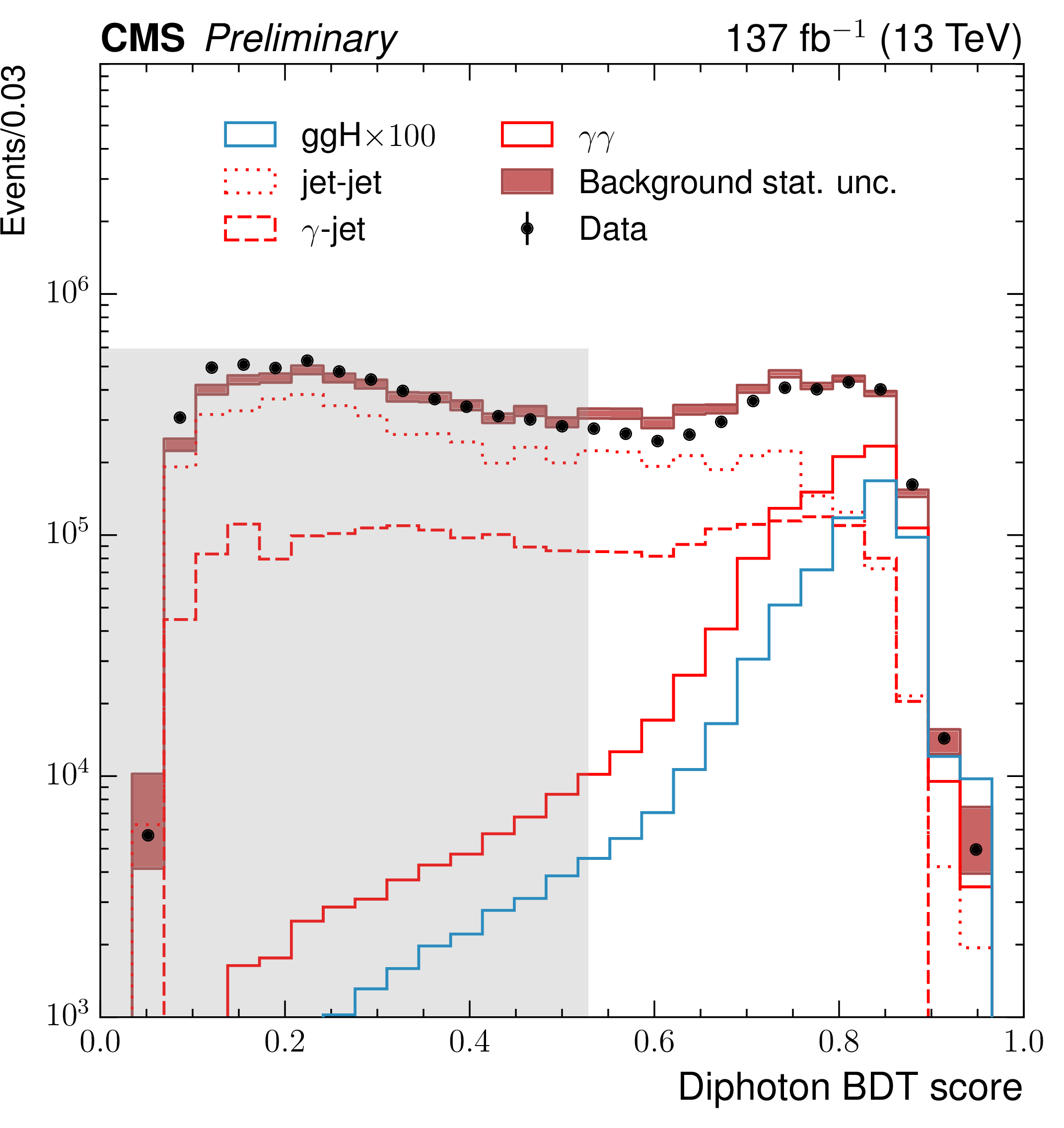
Figure 6-a:
The plot shows the distribution of the diphoton BDT score in events with an invariant mass in the range 100 $ < {m_{\gamma \gamma}} < $ 180 GeV, for data events passing the preselection (black points), and for simulated background events (red band). Histograms are also shown for different components of the simulated background in red. The blue histogram corresponds to simulated Higgs boson signal events. The region shaded grey contains diphoton BDT scores below the lowest threshold used to define an analysis category. The full data set collected in the period 2016-2018 is shown. |
png pdf |
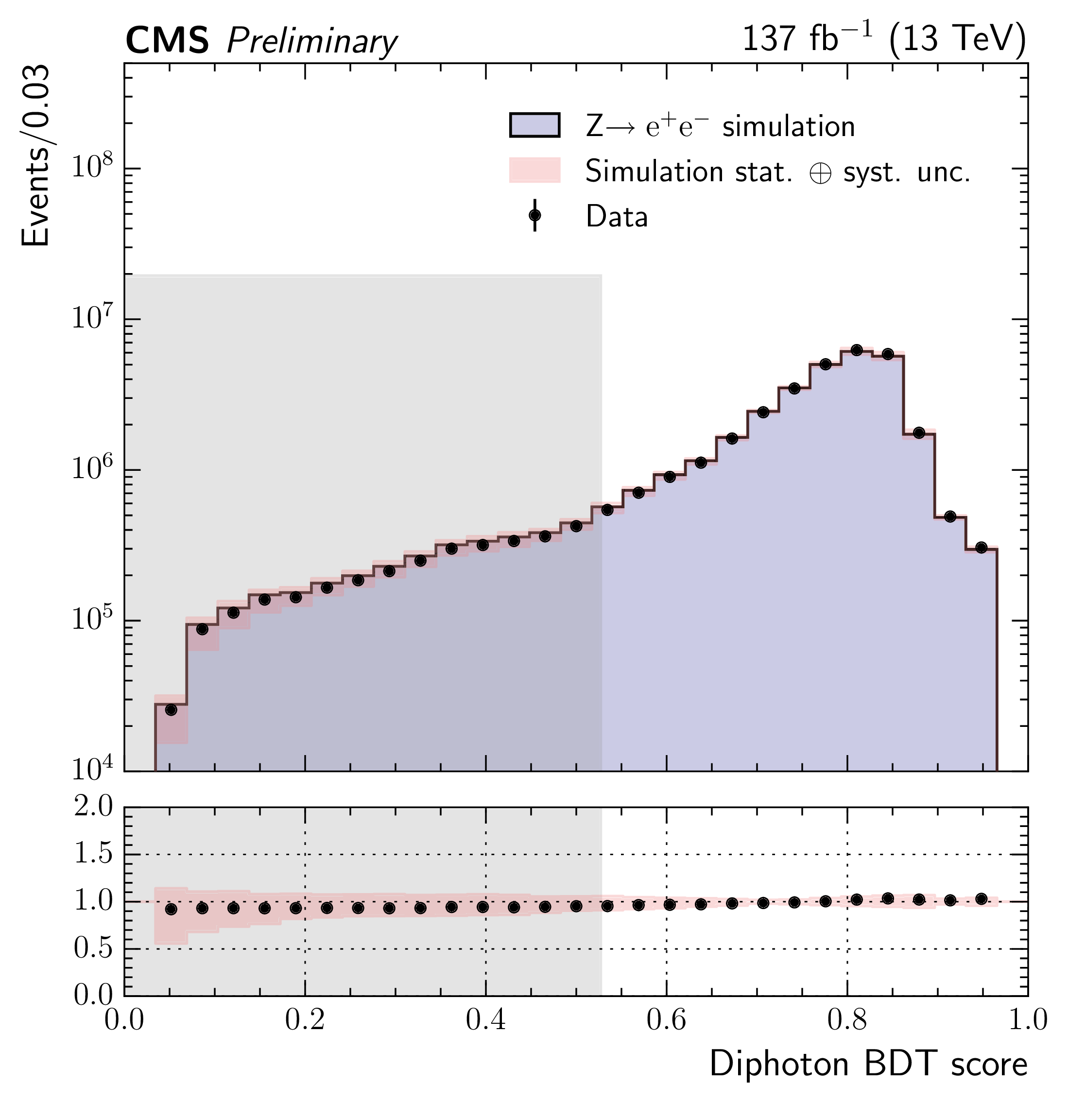
Figure 6-b:
The plot shows the distribution of the diphoton BDT score in events with an invariant mass in the range 100 $ < {m_{\gamma \gamma}} < $ 180 GeV in ${\mathrm{Z} \rightarrow \mathrm{e} \mathrm{e}}$ events where the electrons are reconstructed as photons. The points show the score for data, the histogram shows the score for simulated Drell-Yan events, including statistical and systematic uncertainties (pink band). The region shaded grey contains diphoton BDT scores below the lowest threshold used to define an analysis category. The full data set collected in the period 2016-2018 and the corresponding simulation are shown. |
png pdf |
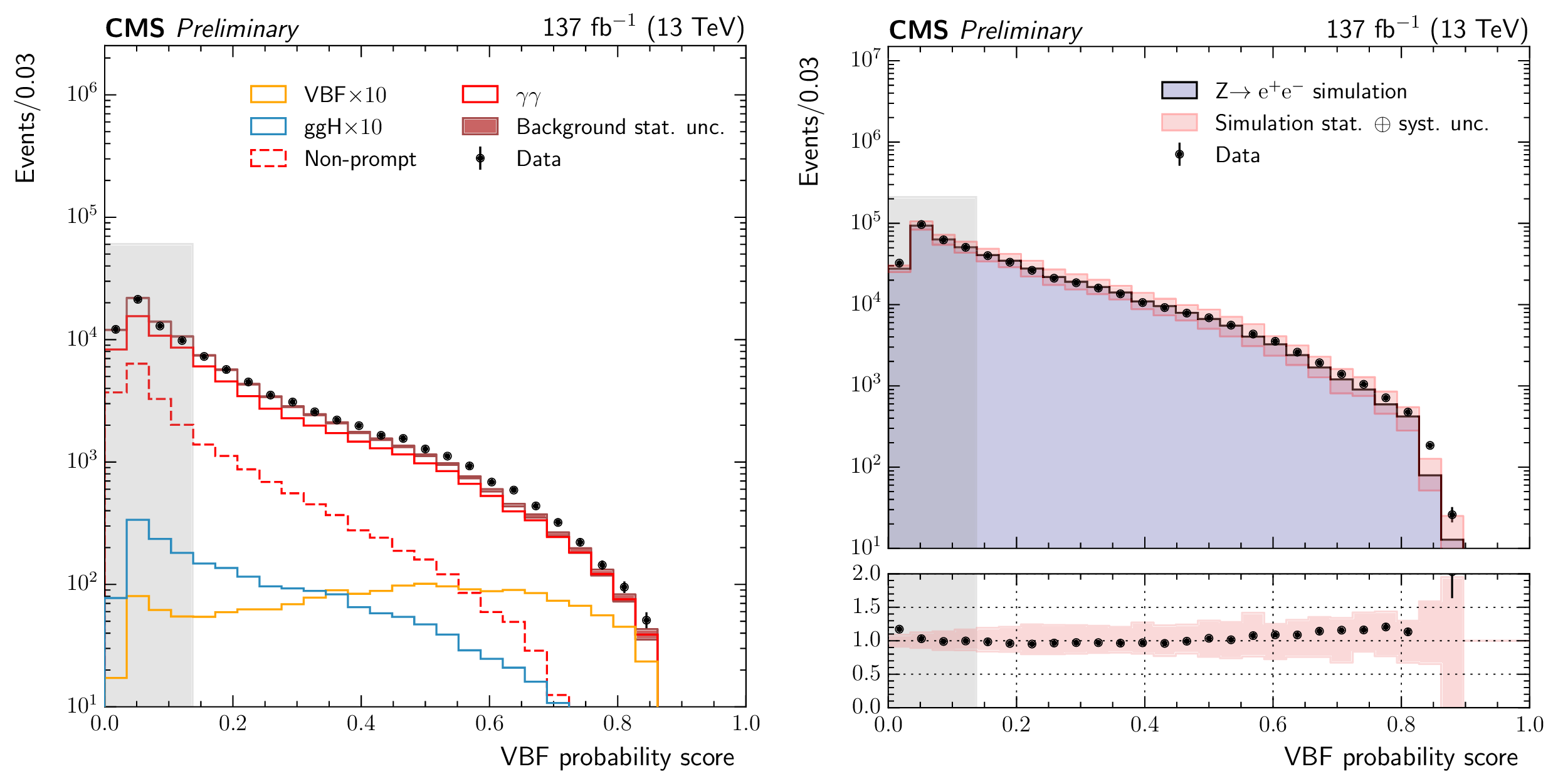
Figure 7:
The left plot shows the distribution of the dijet BDT output VBF probability in events with an invariant mass in the range 100 $ < {m_{\gamma \gamma}} < $ 180 GeV, for data events passing the preselection (black points), and for simulated background events (red band). Histograms are also shown for different components of the simulated background in red. The orange histogram corresponds to simulated VBF signal events, with the ggH events shown in blue. The right plot shows the same distribution in ${\mathrm{Z} \rightarrow \mathrm{e} \mathrm{e}}$ events where the electrons are reconstructed as photons. The points show the score for data, the histogram shows the score for simulated Drell-Yan events, including statistical and systematic uncertainties (pink band). The regions shaded grey contain VBF probability values below the lowest threshold used to define an analysis category. The full data set collected in the period 2016-2018 and the corresponding simulation are shown. |
png pdf |
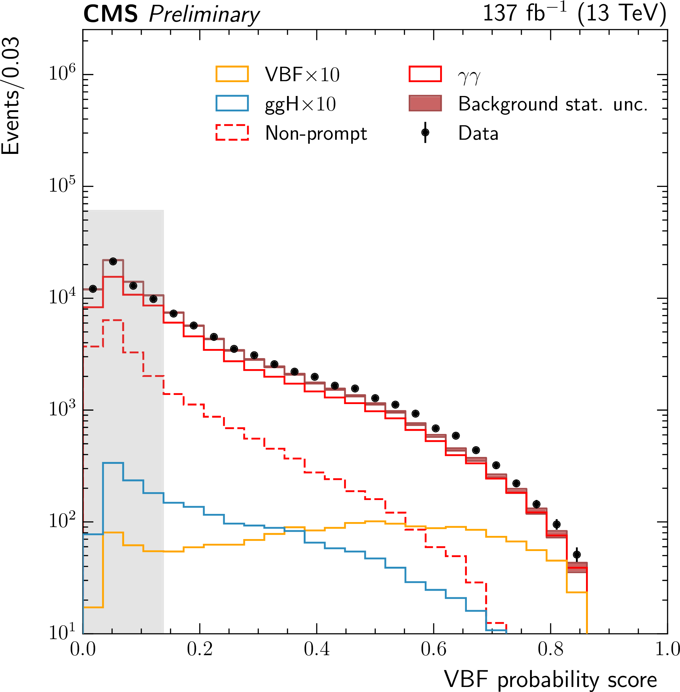
Figure 7-a:
The plot shows the distribution of the dijet BDT output VBF probability in events with an invariant mass in the range 100 $ < {m_{\gamma \gamma}} < $ 180 GeV, for data events passing the preselection (black points), and for simulated background events (red band). Histograms are also shown for different components of the simulated background in red. The orange histogram corresponds to simulated VBF signal events, with the ggH events shown in blue. The region shaded grey contains VBF probability values below the lowest threshold used to define an analysis category. The full data set collected in the period 2016-2018 is shown. |

png pdf |
Figure 7-b:
The plot shows the same distribution in ${\mathrm{Z} \rightarrow \mathrm{e} \mathrm{e}}$ events where the electrons are reconstructed as photons. The points show the score for data, the histogram shows the score for simulated Drell-Yan events, including statistical and systematic uncertainties (pink band). The region shaded grey contains VBF probability values below the lowest threshold used to define an analysis category. The full data set collected in the period 2016-2018 and the corresponding simulation are shown. |
png pdf |
Figure 8:
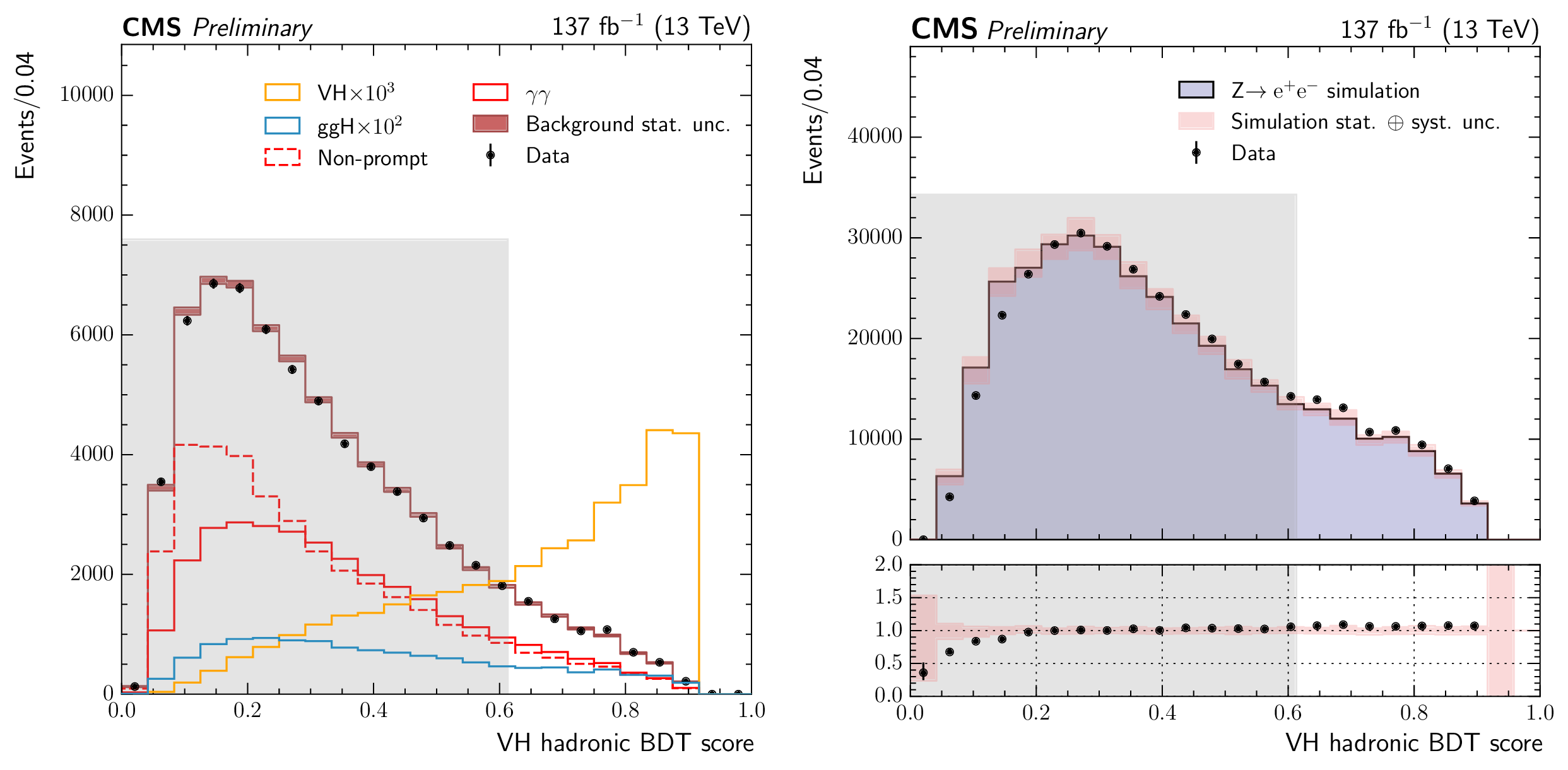
The left plot shows the distribution of the VH hadronic BDT output score in events with an invariant mass in the range 100 $ < {m_{\gamma \gamma}} < $ 180 GeV, for data events passing the preselection (black points), and for simulated background events (red band). Histograms are also shown for different components of the simulated background in red. The sum of all background distributions is scaled to the data. The orange histogram corresponds to simulated VH hadronic signal events. The right plot shows the same distribution in ${\mathrm{Z} \rightarrow \mathrm{e} \mathrm{e}}$ events where the electrons are reconstructed as photons. The points show the score for data, the histogram shows the score for simulated Drell-Yan events, including statistical and systematic uncertainties (pink band). The regions shaded grey contain VH hadronic BDT scores below the lowest threshold used to define an analysis category. The full data set collected in the period 2016-2018 and the corresponding simulation are shown. |

png pdf |
Figure 8-a:
The plot shows the distribution of the VH hadronic BDT output score in events with an invariant mass in the range 100 $ < {m_{\gamma \gamma}} < $ 180 GeV, for data events passing the preselection (black points), and for simulated background events (red band). Histograms are also shown for different components of the simulated background in red. The sum of all background distributions is scaled to the data. The orange histogram corresponds to simulated VH hadronic signal events. The region shaded grey contains VH hadronic BDT scores below the lowest threshold used to define an analysis category. The full data set collected in the period 2016-2018 is shown. |
png pdf |
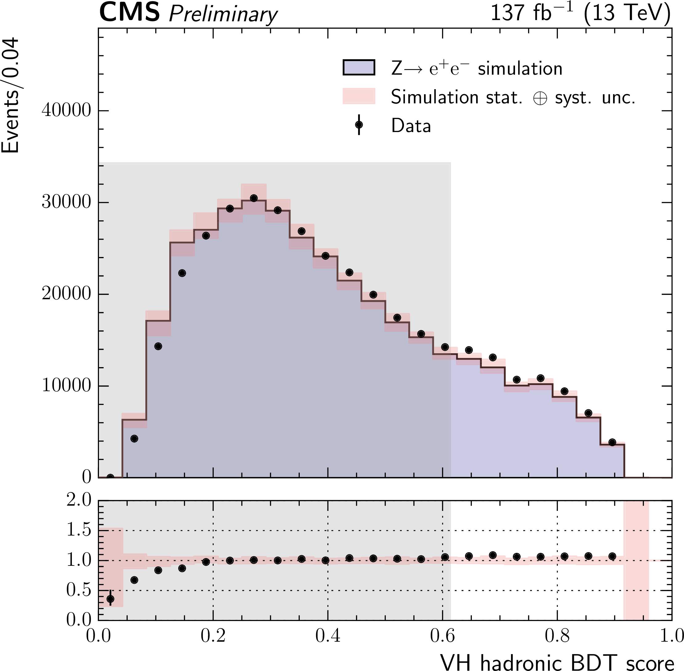
Figure 8-b:
The plot shows the same distribution in ${\mathrm{Z} \rightarrow \mathrm{e} \mathrm{e}}$ events where the electrons are reconstructed as photons. The points show the score for data, the histogram shows the score for simulated Drell-Yan events, including statistical and systematic uncertainties (pink band). The region shaded grey contains VH hadronic BDT scores below the lowest threshold used to define an analysis category. The full data set collected in the period 2016-2018 and the corresponding simulation are shown. |

png pdf |
Figure 9:
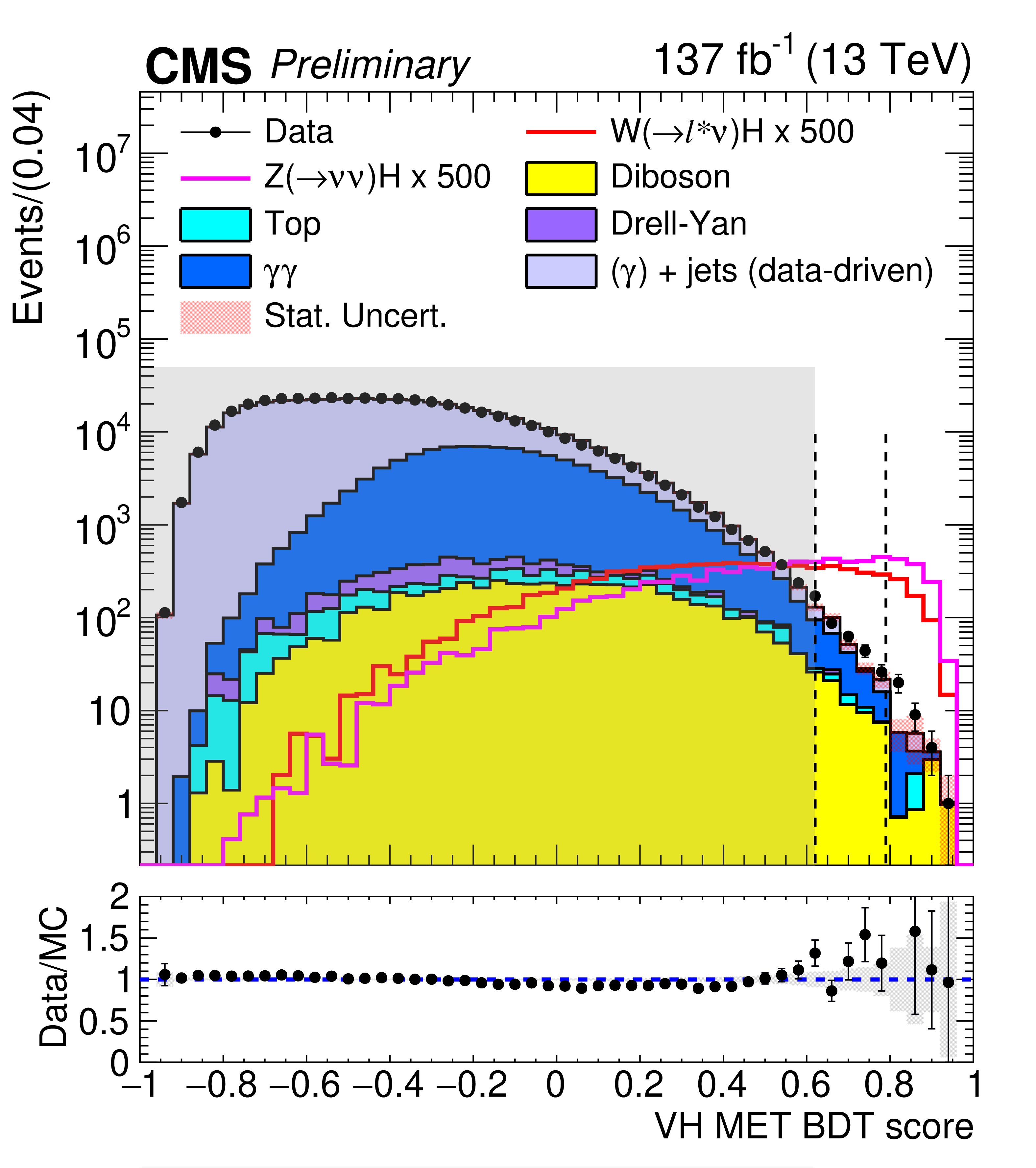
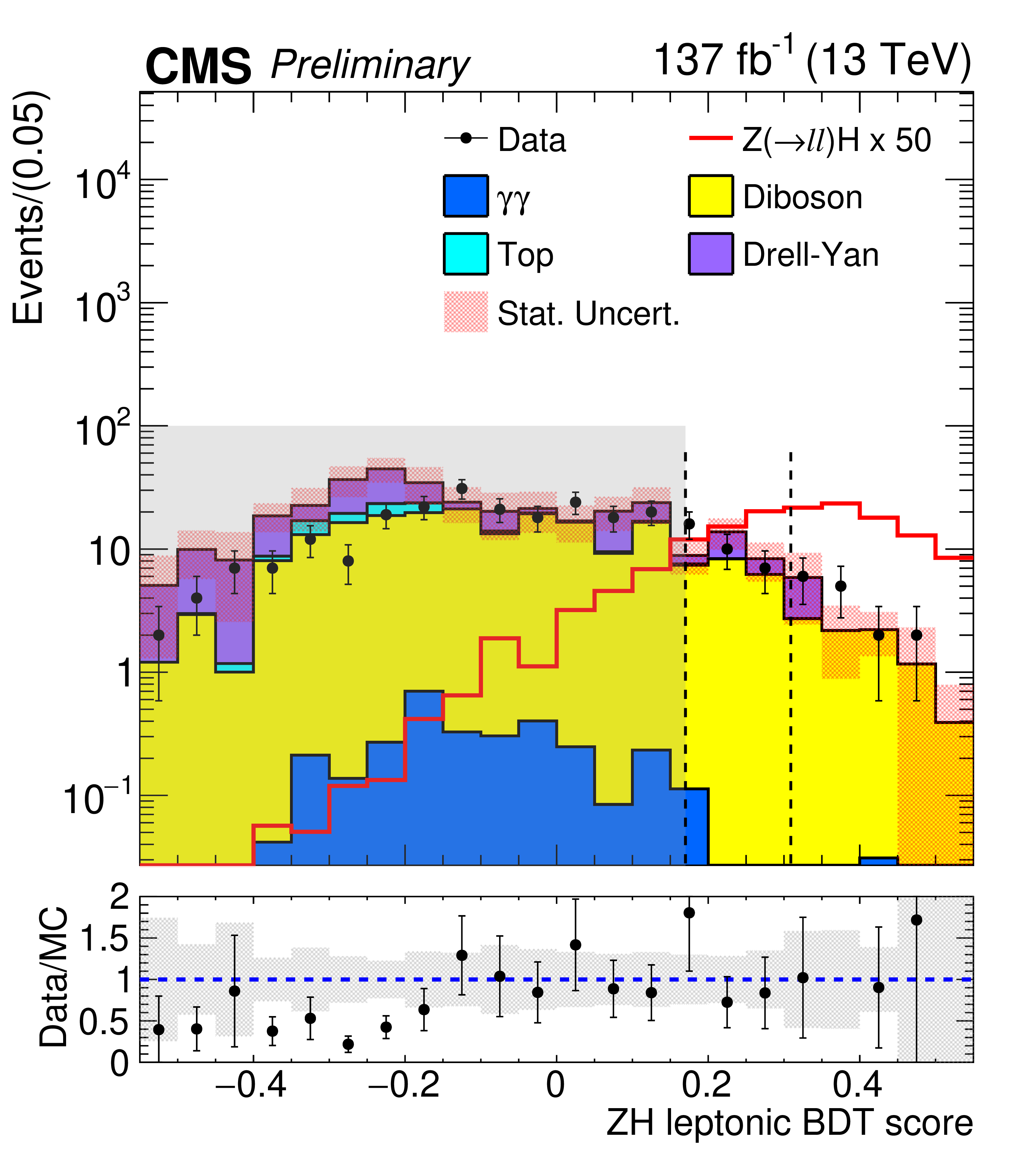
Output scores for the three VH leptonic BDTs. The VH MET BDT is shown in the top left, with the ZH leptonic BDT in the top right. Below, the WH leptonic BDT score with ${p_{\mathrm {T}}}$ of the diphoton system less than 75 GeV (left) and greater than 75 GeV (right) is shown. In each case, the signal and background simulation are shown as histograms with the data as black points. The statistical uncertainty in the data points is denoted as vertical bars and that on the background simulation by the pink band. The simulated signal and background distributions are normalised to the luminosity of the data. To increase its visibility, the signal is scaled by a factor of 500, 50, and 100 for the VH MET, ZH leptonic, and WH leptonic BDTs, respectively. The vertical dotted lines denote the BDT boundaries that define the final analysis categories. The regions shaded grey are not considered in the analysis. The full data set collected in the period 2016-2018 and the corresponding simulation are shown. |
png pdf |
Figure 9-a:
Output scores for the VH MET BDT. The signal and background simulation are shown as histograms with the data as black points. The statistical uncertainty in the data points is denoted as vertical bars and that on the background simulation by the pink band. The simulated signal and background distributions are normalised to the luminosity of the data. To increase its visibility, the signal is scaled by a factor of 500. The vertical dotted lines denote the BDT boundaries that define the final analysis categories. The region shaded grey is not considered in the analysis. The full data set collected in the period 2016-2018 and the corresponding simulation are shown. |
png pdf |
Figure 9-b:
Output scores for the ZH leptonic BDT. The signal and background simulation are shown as histograms with the data as black points. The statistical uncertainty in the data points is denoted as vertical bars and that on the background simulation by the pink band. The simulated signal and background distributions are normalised to the luminosity of the data. To increase its visibility, the signal is scaled by a factor of 50. The vertical dotted lines denote the BDT boundaries that define the final analysis categories. The region shaded grey is not considered in the analysis. The full data set collected in the period 2016-2018 and the corresponding simulation are shown. |

png pdf |
Figure 9-c:
Output scores for the WH leptonic BDT score with ${p_{\mathrm {T}}}$ of the diphoton system less than 75 GeV. The signal and background simulation are shown as histograms with the data as black points. The statistical uncertainty in the data points is denoted as vertical bars and that on the background simulation by the pink band. The simulated signal and background distributions are normalised to the luminosity of the data. To increase its visibility, the signal is scaled by a factor of 100. The vertical dotted lines denote the BDT boundaries that define the final analysis categories. The region shaded grey is not considered in the analysis. The full data set collected in the period 2016-2018 and the corresponding simulation are shown. |

png pdf |
Figure 9-d:
Output scores for the WH leptonic BDT score with ${p_{\mathrm {T}}}$ of the diphoton system greater than 75 GeV. The signal and background simulation are shown as histograms with the data as black points. The statistical uncertainty in the data points is denoted as vertical bars and that on the background simulation by the pink band. The simulated signal and background distributions are normalised to the luminosity of the data. To increase its visibility, the signal is scaled by a factor of 100. The vertical dotted lines denote the BDT boundaries that define the final analysis categories. The region shaded grey is not considered in the analysis. The full data set collected in the period 2016-2018 and the corresponding simulation are shown. |

png pdf |
Figure 10:
Distributions of tHq BDT-bkg score (left) and the top DNN (right), which are used together to define the tHq leptonic category. Events are taken from the $ {m_{\gamma \gamma}} $ sidebands, satisfying either 100 $ < {m_{\gamma \gamma}} < $ 120 GeV or 130 $ < {m_{\gamma \gamma}} < $ 180 GeV. The statistical uncertainty in the background background estimation is represented by the red band. The regions shaded grey contain BDT-bkg and top DNN scores below and above the respective thresholds for the tHq category. The full data set collected in the period 2016-2018 and the corresponding simulation are shown. |
png pdf |
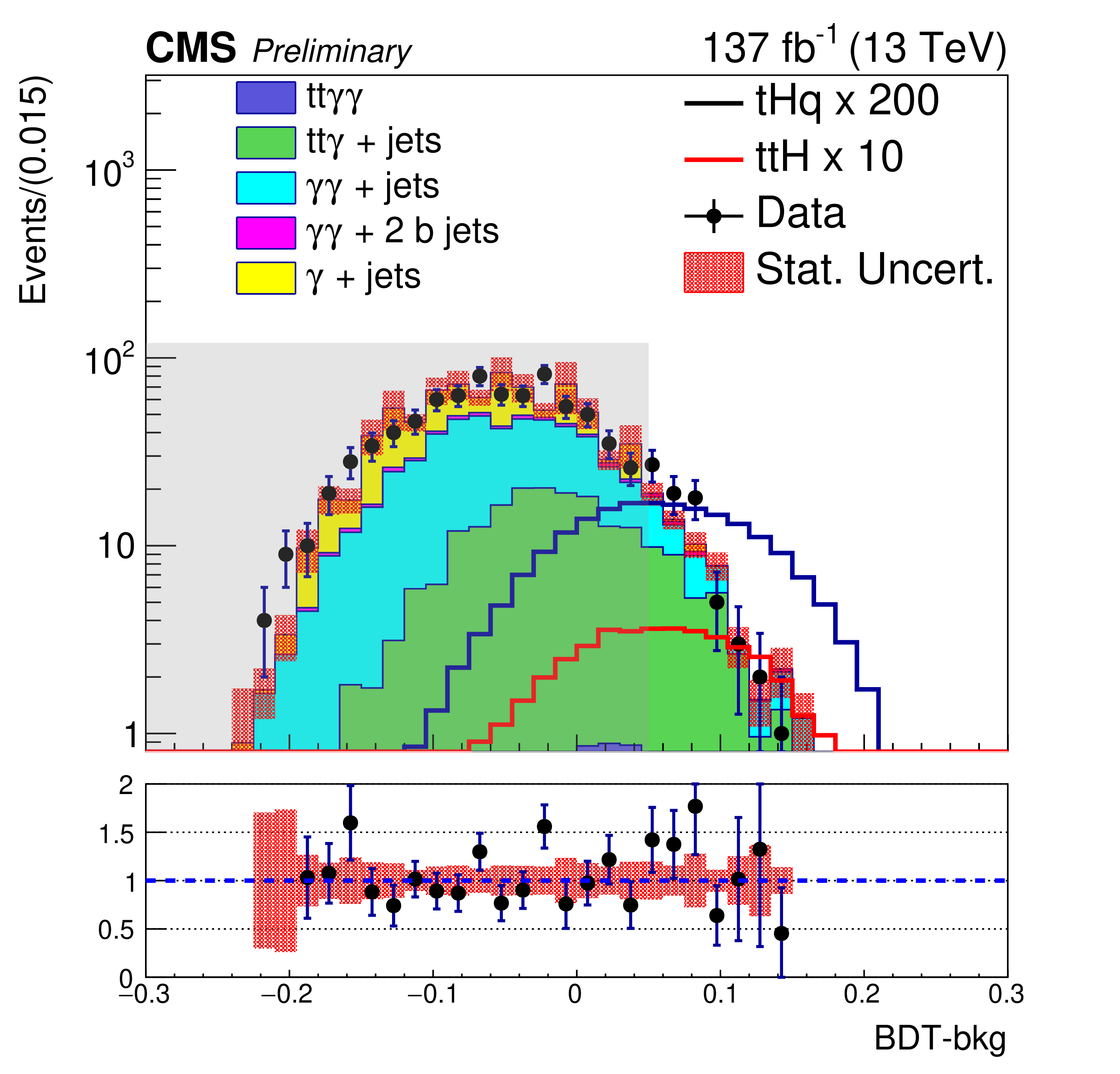
Figure 10-a:
Distribution of the tHq BDT-bkg score, which is used to define the tHq leptonic category. Events are taken from the $ {m_{\gamma \gamma}} $ sidebands, satisfying either 100 $ < {m_{\gamma \gamma}} < $ 120 GeV or 130 $ < {m_{\gamma \gamma}} < $ 180 GeV. The statistical uncertainty in the background background estimation is represented by the red band. The region shaded grey contains scores below the threshold for the tHq category. The full data set collected in the period 2016-2018 and the corresponding simulation are shown. |

png pdf |
Figure 10-b:
Distribution of the top DNN, which is used to define the tHq leptonic category. Events are taken from the $ {m_{\gamma \gamma}} $ sidebands, satisfying either 100 $ < {m_{\gamma \gamma}} < $ 120 GeV or 130 $ < {m_{\gamma \gamma}} < $ 180 GeV. The statistical uncertainty in the background background estimation is represented by the red band. The region shaded grey contains scores above the threshold for the tHq category. The full data set collected in the period 2016-2018 and the corresponding simulation are shown. |
png pdf |
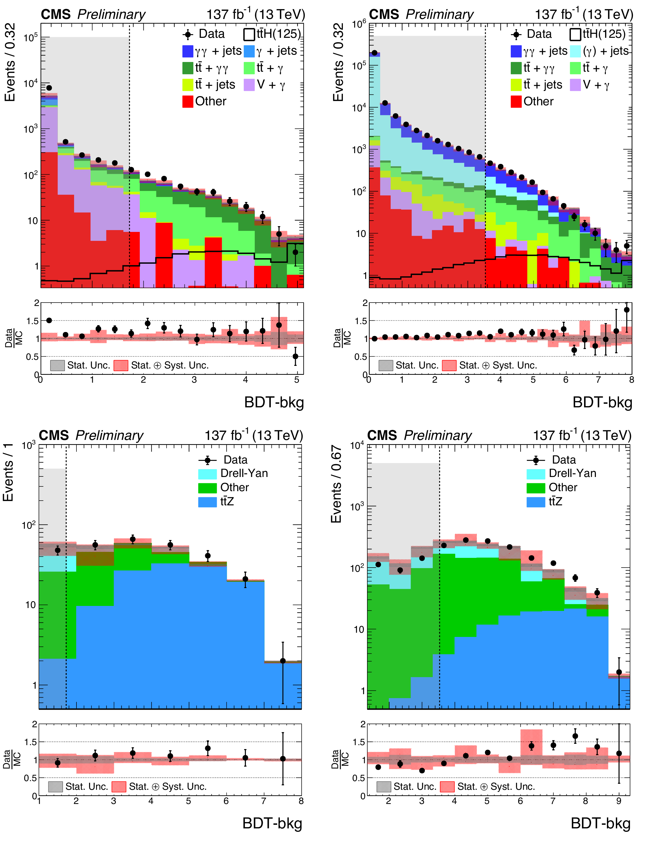
Figure 11:
Distributions of BDT-bkg output used for event categorisation, for the leptonic (left) and the hadronic (right) channels. The upper two plots show events taken from the $ {m_{\gamma \gamma}} $ sidebands, satisfying either 100 $ < {m_{\gamma \gamma}} < $ 120 GeV or 130 $ < {m_{\gamma \gamma}} < $ 180 GeV. The lower two contain events from the $ {{\mathrm{t} {}\mathrm{\bar{t}}} \mathrm{Z}} $ control regions, described in the text. The grey region contains BDT-bkg scores below the lowest threshold for the $ {{\mathrm{t} {}\mathrm{\bar{t}}} \mathrm{H}} $ categories. Statistical (statistical $\oplus $ systematic) background uncertainties are represented by the black (red) shaded bands. |

png pdf |
Figure 11-a:
Distribution of the BDT-bkg output used for event categorisation, for the leptonic channel. The plot shows events taken from the $ {m_{\gamma \gamma}} $ sidebands, satisfying either 100 $ < {m_{\gamma \gamma}} < $ 120 GeV or 130 $ < {m_{\gamma \gamma}} < $ 180 GeV. The grey region contains BDT-bkg scores below the lowest threshold for the $ {{\mathrm{t} {}\mathrm{\bar{t}}} \mathrm{H}} $ categories. Statistical (statistical $\oplus $ systematic) background uncertainties are represented by the black (red) shaded bands. |

png pdf |
Figure 11-b:
Distribution of the BDT-bkg output used for event categorisation, for the hadronic channel. The plot shows events taken from the $ {m_{\gamma \gamma}} $ sidebands, satisfying either 100 $ < {m_{\gamma \gamma}} < $ 120 GeV or 130 $ < {m_{\gamma \gamma}} < $ 180 GeV. The grey region contains BDT-bkg scores below the lowest threshold for the $ {{\mathrm{t} {}\mathrm{\bar{t}}} \mathrm{H}} $ categories. Statistical (statistical $\oplus $ systematic) background uncertainties are represented by the black (red) shaded bands. |
png pdf |
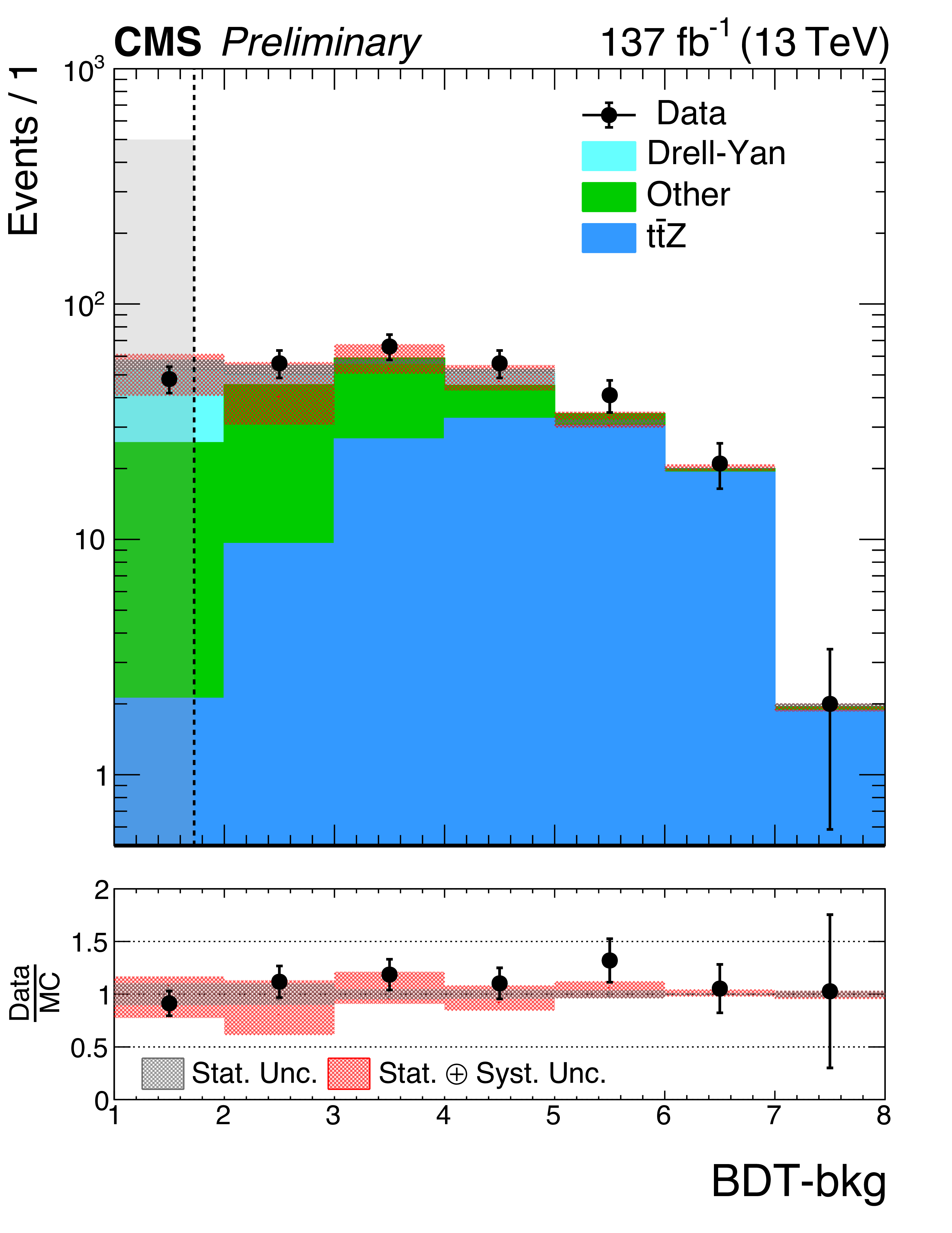
Figure 11-c:
Distribution of the BDT-bkg output used for event categorisation, for the leptonic channel. The plot contains events from the $ {{\mathrm{t} {}\mathrm{\bar{t}}} \mathrm{Z}} $ control regions, described in the text. The grey region contains BDT-bkg scores below the lowest threshold for the $ {{\mathrm{t} {}\mathrm{\bar{t}}} \mathrm{H}} $ categories. Statistical (statistical $\oplus $ systematic) background uncertainties are represented by the black (red) shaded bands. |

png pdf |
Figure 11-d:
Distribution of the BDT-bkg output used for event categorisation, for the hadronic channel. The plot contains events from the $ {{\mathrm{t} {}\mathrm{\bar{t}}} \mathrm{Z}} $ control regions, described in the text. The grey region contains BDT-bkg scores below the lowest threshold for the $ {{\mathrm{t} {}\mathrm{\bar{t}}} \mathrm{H}} $ categories. Statistical (statistical $\oplus $ systematic) background uncertainties are represented by the black (red) shaded bands. |
png pdf |
Figure 12:
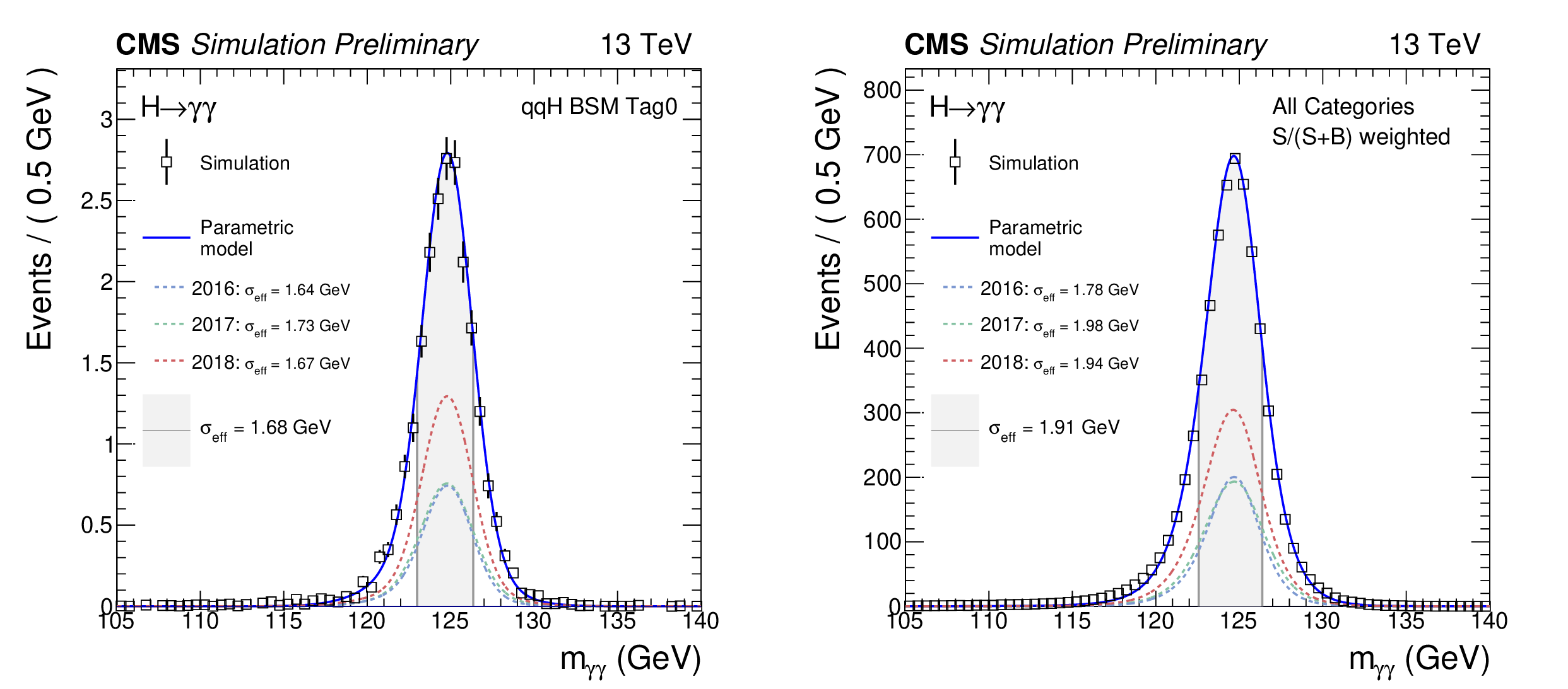
The shape of the parametric signal model for each year of simulated data, and for the sum of all years together, is shown. The open squares represent weighted simulation events and the blue line the corresponding model. Also shown is the ${\sigma _{\text {eff}}}$ value (half the width of the narrowest interval containing 68.3% of the invariant mass distribution) in the grey shaded area. The contribution of the signal model from each year of data-taking is illustrated with the dotted lines. The models are shown for an analysis category targeting high ${{p_{\mathrm {T}}} ^\mathrm{H}}$ VBF production (left), and for the weighted sum of all categories (right). Here each category is weighted by S/(S + B), where S and B are the numbers of expected signal and background events, respectively, in a $ \pm $1$ {\sigma _{\text {eff}}} $ mass window centred on ${m_\mathrm{H}}$. |

png pdf |
Figure 12-a:
The shape of the parametric signal model for each year of simulated data, and for the sum of all years together, is shown. The open squares represent weighted simulation events and the blue line the corresponding model. Also shown is the ${\sigma _{\text {eff}}}$ value (half the width of the narrowest interval containing 68.3% of the invariant mass distribution) in the grey shaded area. The contribution of the signal model from each year of data-taking is illustrated with the dotted lines. The model is shown for an analysis category targeting high ${{p_{\mathrm {T}}} ^\mathrm{H}}$ VBF production. |

png pdf |
Figure 12-b:
The shape of the parametric signal model for each year of simulated data, and for the sum of all years together, is shown. The open squares represent weighted simulation events and the blue line the corresponding model. Also shown is the ${\sigma _{\text {eff}}}$ value (half the width of the narrowest interval containing 68.3% of the invariant mass distribution) in the grey shaded area. The contribution of the signal model from each year of data-taking is illustrated with the dotted lines. The model is shown for the weighted sum of all categories. Here each category is weighted by S/(S + B), where S and B are the numbers of expected signal and background events, respectively, in a $ \pm $1$ {\sigma _{\text {eff}}} $ mass window centred on ${m_\mathrm{H}}$. |

png pdf |
Figure 13:
The composition of each analysis category in terms of a reduced set of STXS bins is shown. The colour scale corresponds to the fractional yield in each category (rows) accounted for by each STXS process (columns). Each row therefore sums to 100%. Entries with values less than 0.5% are not shown. Simulated events for each year in the period 2016-2018 are combined with appropriate weights corresponding to their relative integrated luminosity in data. The column labelled as qqH rest includes contributions from the qqH 0J, qqH 1J, qqH $ {m_{\text {jj}}} < 60$ GeV and qqH 120 $ < {m_{\gamma \gamma}} < 350$ GeV STXS bins. |

png pdf |
Figure 14:
Data points (black) and signal-plus-background model fit for the sum of all categories is shown. Each category is weighted by $S/(S + B)$, where S and B are the numbers of expected signal and background events, respectively, in a $ \pm $1$ {\sigma _{\text {eff}}} $ mass window centred on ${m_\mathrm{H}}$. The one standard deviation (green) and two standard deviation (yellow) bands show the uncertainties in the background component of the fit. The solid red line shows the total signal-plus-background contribution, whereas the dashed red line shows the background component only. The bottom panel shows the residuals after subtraction of this background component. |

png pdf |
Figure 15:
The best fit signal-plus-background model with data points (black) in the fit to four production mode signal strength modifiers. The model is shown separately for group of categories targeting the ggH (top left), VBF (top right), VH (bottom left) and top (bottom right) production modes. Here, the categories in each group are summed after weighting by $S/(S + B)$, where S and B are the numbers of expected signal and background events in a $ \pm $1$ {\sigma _{\text {eff}}} $ mass window centred on ${m_\mathrm{H}}$. The one standard deviation (green) and two standard deviation (yellow) bands show the uncertainties in the background component of the fit. The solid red line shows the total signal-plus-background contribution, whereas the dashed red line represents the background component only. The bottom panel in each plot shows the residuals after subtraction of this background component. |

png pdf |
Figure 15-a:
The best fit signal-plus-background model with data points (black) in the fit to four production mode signal strength modifiers. The model is shown separately for group of categories targeting the ggH production mode. Here, the categories in each group are summed after weighting by $S/(S + B)$, where S and B are the numbers of expected signal and background events in a $ \pm $1$ {\sigma _{\text {eff}}} $ mass window centred on ${m_\mathrm{H}}$. The one standard deviation (green) and two standard deviation (yellow) bands show the uncertainties in the background component of the fit. The solid red line shows the total signal-plus-background contribution, whereas the dashed red line represents the background component only. The bottom panel shows the residuals after subtraction of this background component. |
png pdf |
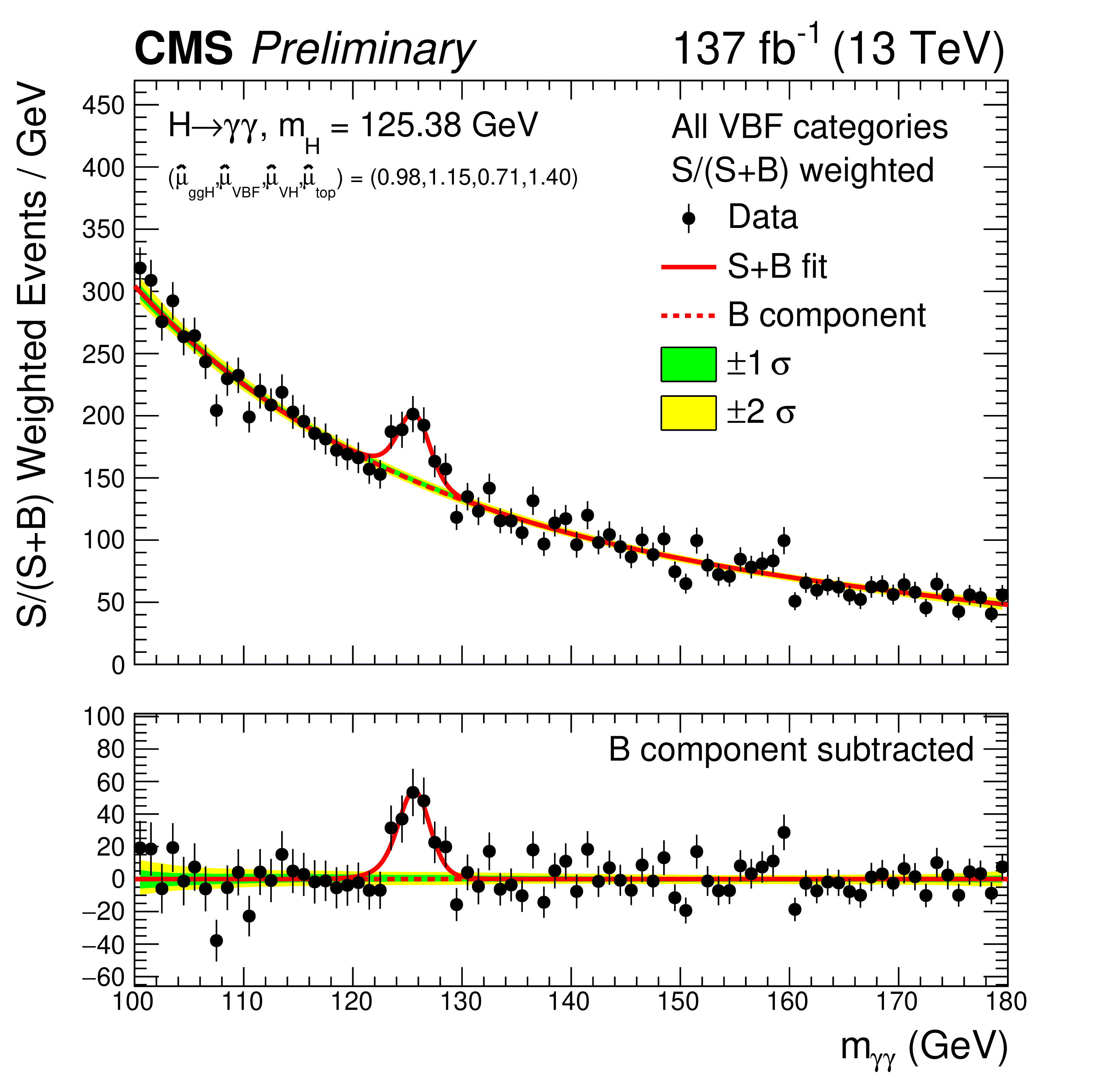
Figure 15-b:
The best fit signal-plus-background model with data points (black) in the fit to four production mode signal strength modifiers. The model is shown separately for group of categories targeting the VBF production mode. Here, the categories in each group are summed after weighting by $S/(S + B)$, where S and B are the numbers of expected signal and background events in a $ \pm $1$ {\sigma _{\text {eff}}} $ mass window centred on ${m_\mathrm{H}}$. The one standard deviation (green) and two standard deviation (yellow) bands show the uncertainties in the background component of the fit. The solid red line shows the total signal-plus-background contribution, whereas the dashed red line represents the background component only. The bottom panel shows the residuals after subtraction of this background component. |
png pdf |
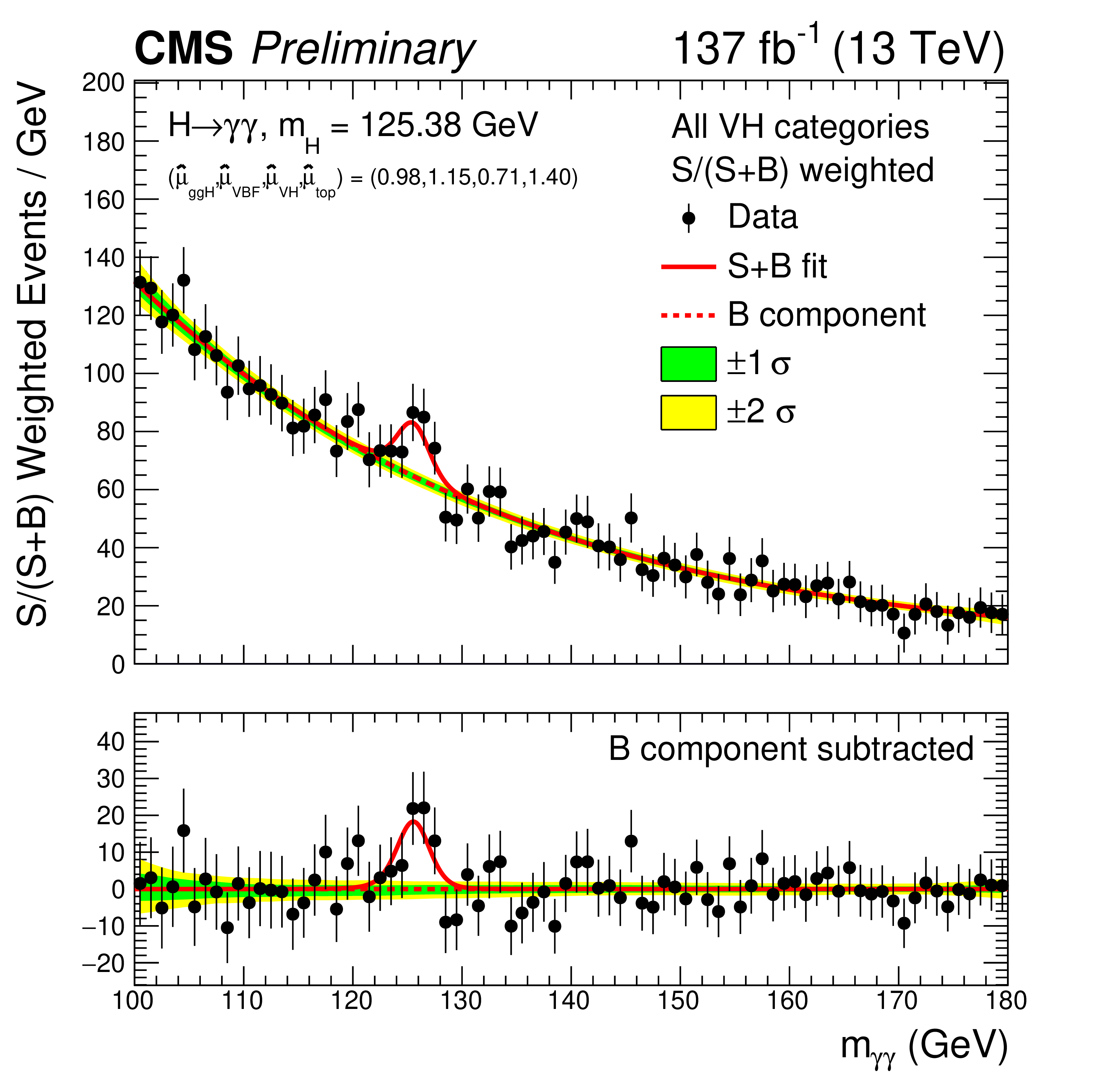
Figure 15-c:
The best fit signal-plus-background model with data points (black) in the fit to four production mode signal strength modifiers. The model is shown separately for group of categories targeting the VH top production mode. Here, the categories in each group are summed after weighting by $S/(S + B)$, where S and B are the numbers of expected signal and background events in a $ \pm $1$ {\sigma _{\text {eff}}} $ mass window centred on ${m_\mathrm{H}}$. The one standard deviation (green) and two standard deviation (yellow) bands show the uncertainties in the background component of the fit. The solid red line shows the total signal-plus-background contribution, whereas the dashed red line represents the background component only. The bottom panel shows the residuals after subtraction of this background component. |
png pdf |
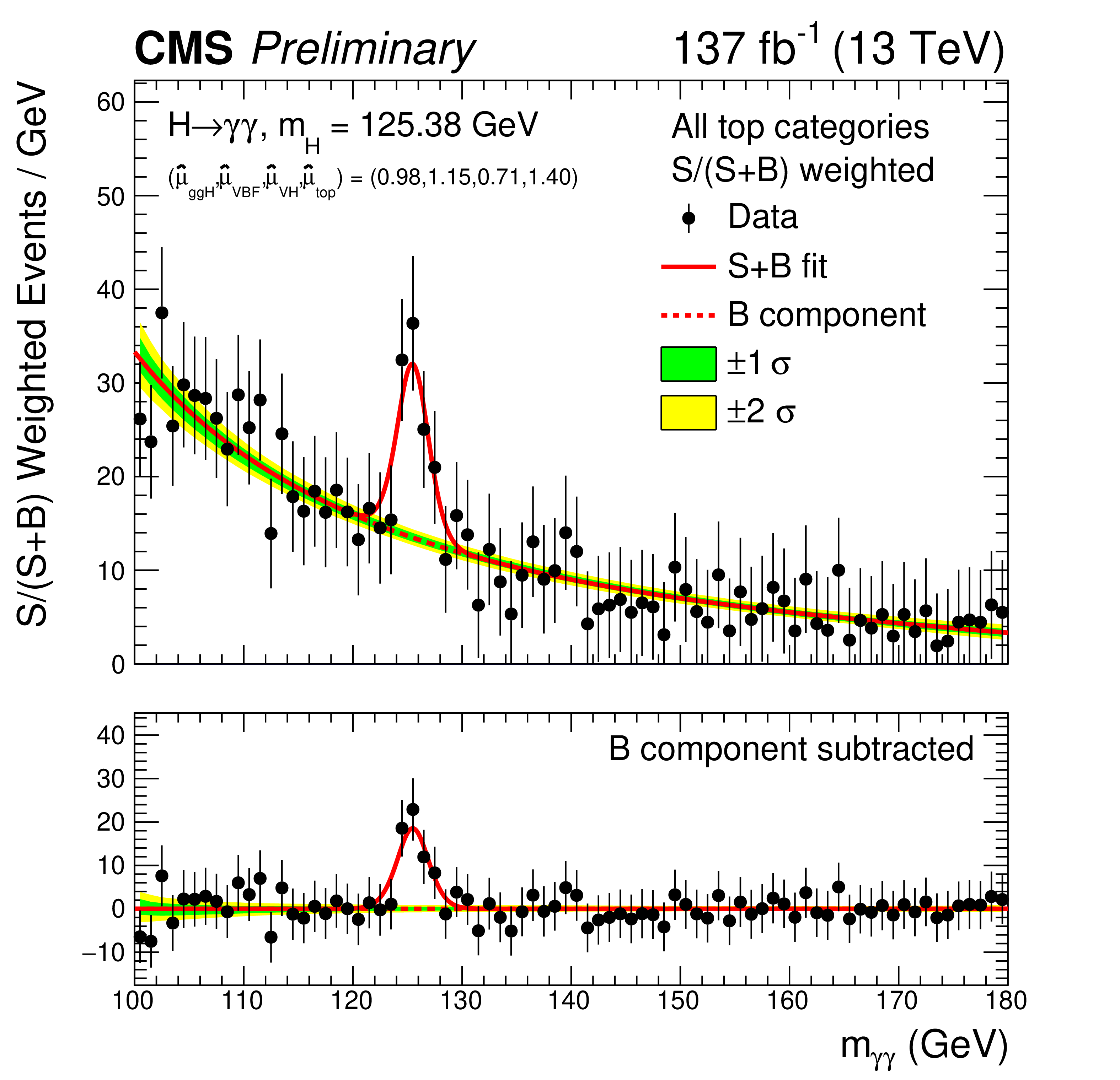
Figure 15-d:
The best fit signal-plus-background model with data points (black) in the fit to four production mode signal strength modifiers. The model is shown separately for group of categories targeting the top production mode. Here, the categories in each group are summed after weighting by $S/(S + B)$, where S and B are the numbers of expected signal and background events in a $ \pm $1$ {\sigma _{\text {eff}}} $ mass window centred on ${m_\mathrm{H}}$. The one standard deviation (green) and two standard deviation (yellow) bands show the uncertainties in the background component of the fit. The solid red line shows the total signal-plus-background contribution, whereas the dashed red line represents the background component only. The bottom panel shows the residuals after subtraction of this background component. |

png pdf |
Figure 16:
Observed results of the fit to four production mode signal strength modifiers. The contributions to the total uncertainty in each parameter from the theoretical systematic, experimental systematic and statistical components are shown. Also shown in black is the result of the fit to the inclusive signal strength modifier. The compatibility of this fit with respect to the SM prediction, expressed as a $p$-value, is approximately 53%. |

png pdf |
Figure 17:
A summary of the impact of the main sources of systematic uncertainty in the fit to four production mode signal strength modifiers. The observed (expected) impacts are shown by the solid (empty) bars. |
png pdf |
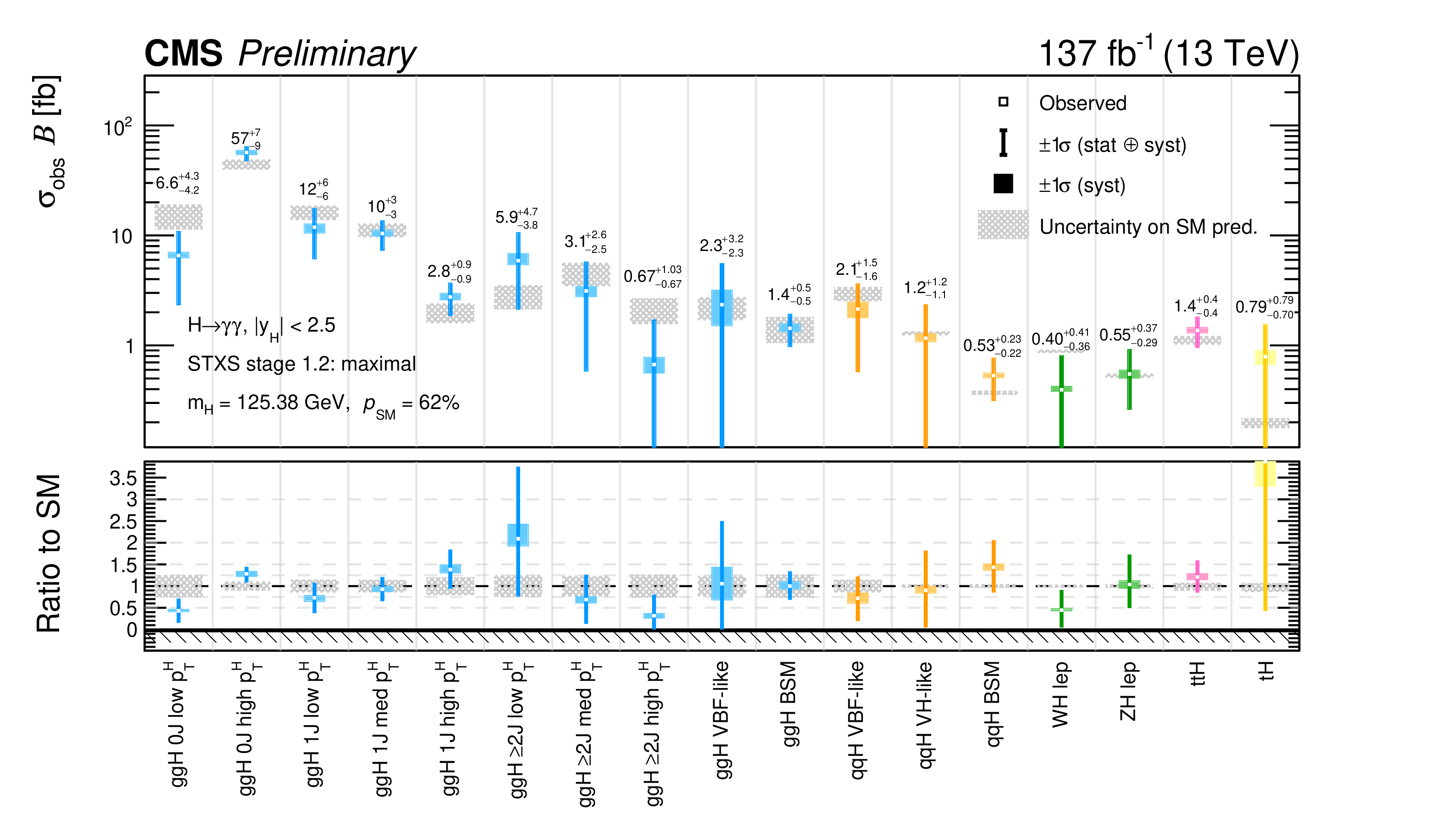
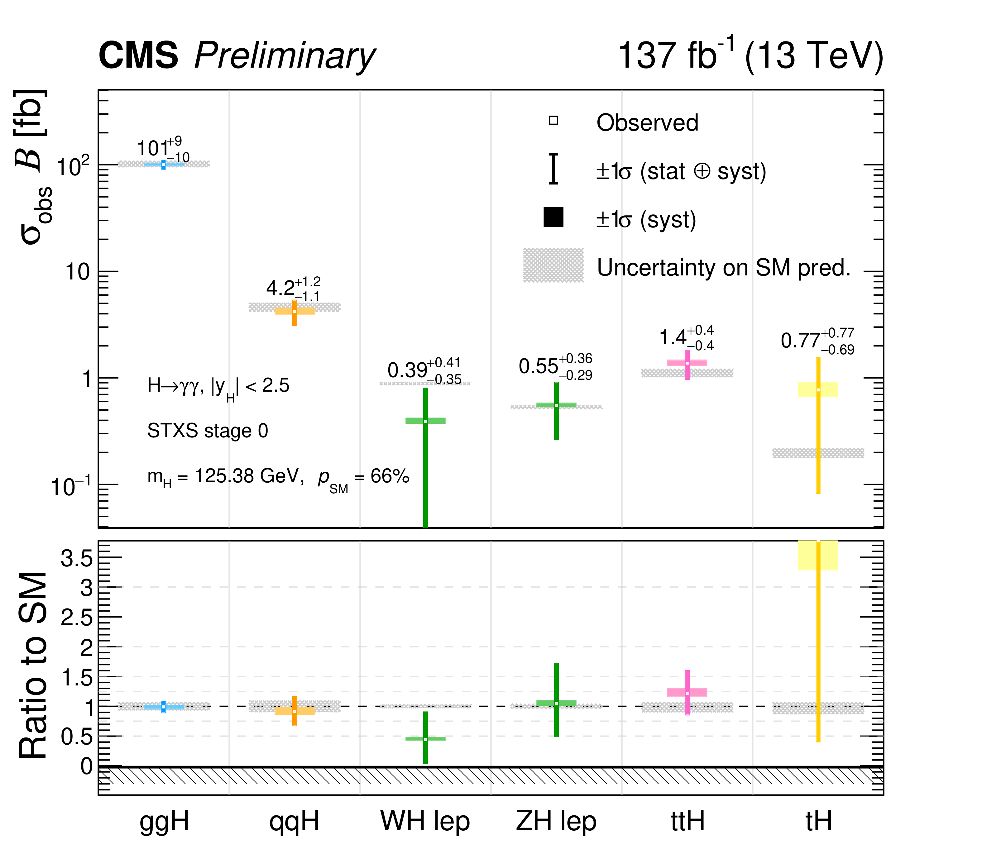
Figure 18:
Observed results of the maximal merging scheme STXS fit. The best fit cross sections are plotted along with the respective 68% confidence level intervals. The systematic components of the uncertainty in each parameter are shown by the coloured boxes. The hatched grey boxes demonstrate the theoretical uncertainties in the SM predictions. The bottom panel shows the ratio of the fitted values to the SM predictions. The colour scheme is chosen to match the diagram presented in Fig. 1. The compatibility of this fit with respect to the SM prediction, expressed as a $p$-value, is approximately 62%. |
png pdf |
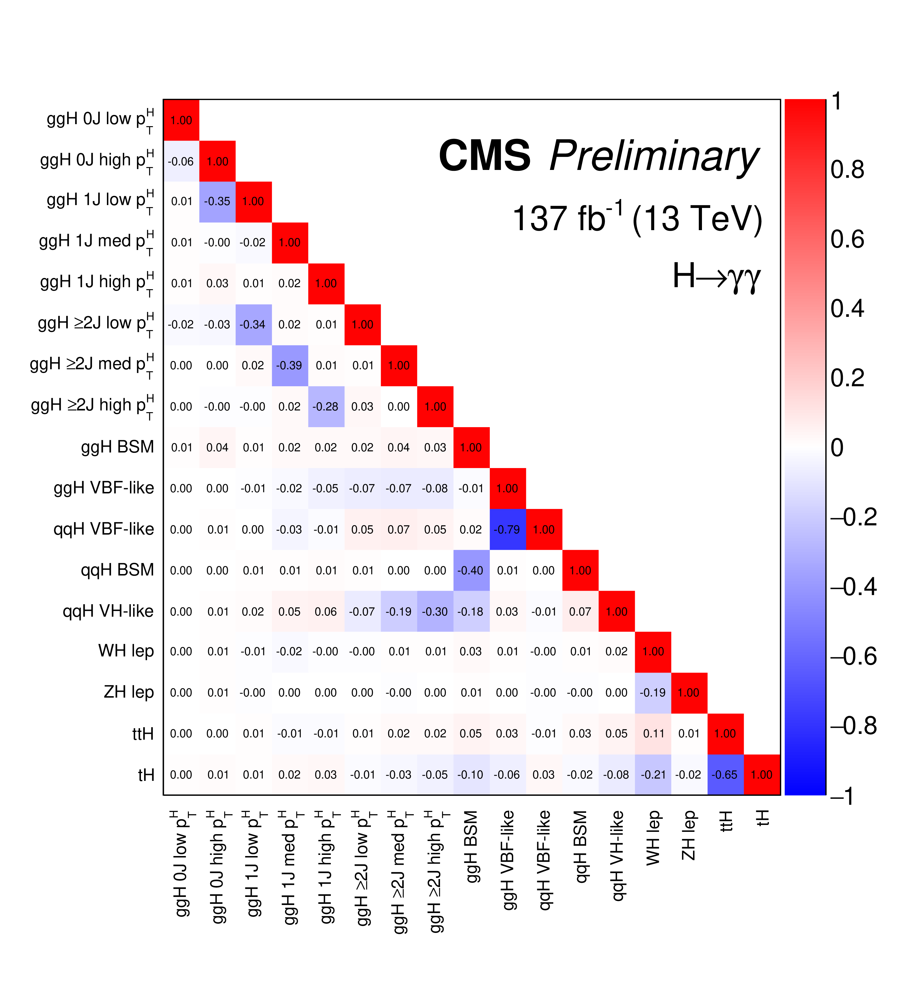
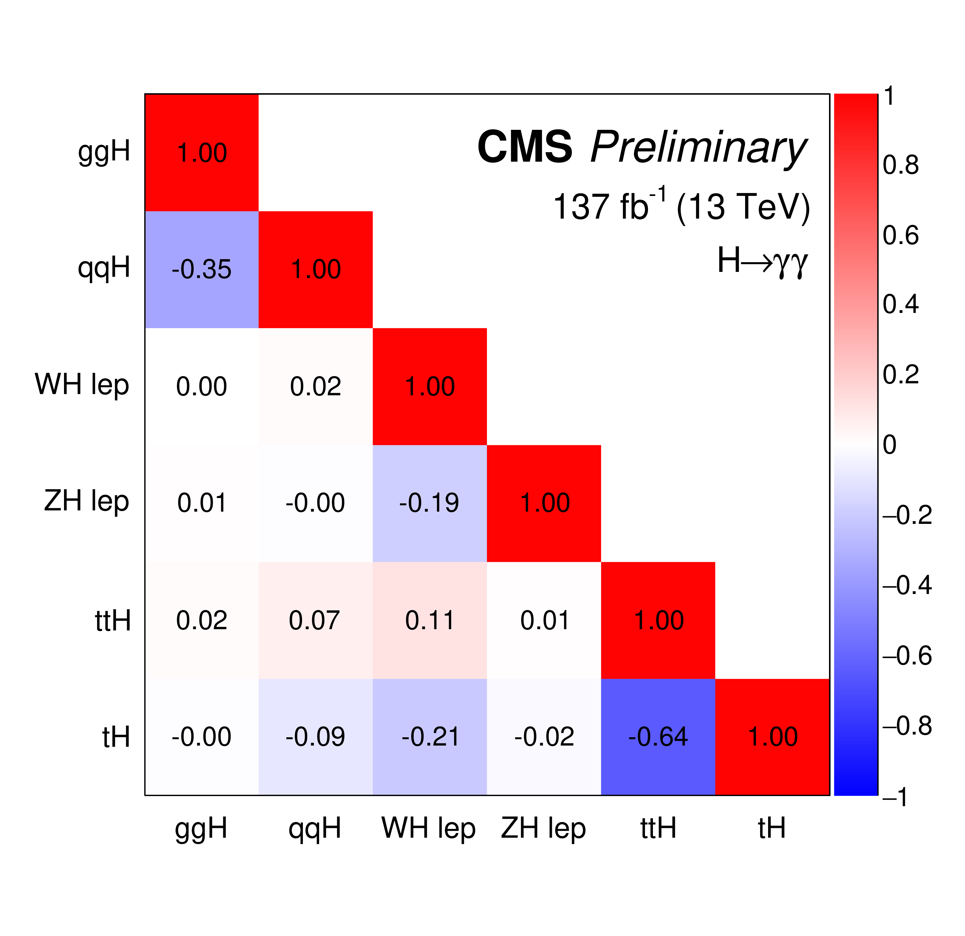
Figure 19:
Observed correlations between the 17 parameters considered in the maximal merging fit. The size of the correlations is indicated by the colour scale. |

png pdf |
Figure 20:
Observed results of the minimal merging scheme STXS fit. The best fit cross sections are plotted along with the respective 68% confidence level intervals. The systematic components of the uncertainty in each parameter are shown by the coloured boxes. The hatched grey boxes demonstrate the theoretical uncertainties in the SM predictions. The bottom panel shows the ratio of the fitted values to the SM predictions. The colour scheme is chosen to match the diagram presented in Fig. 1. The orange and blue dashed lines for the VBF-like parameters represents contributions from both ggH and qqH STXS bins. The compatibility of this fit with respect to the SM prediction, expressed as a $p$-value, is approximately 85%. |

png pdf |
Figure 21:
Observed correlations between the 24 parameters considered in the minimal merging fit. The size of the correlations is indicated by the colour scale. |

png pdf |
Figure 22:
Observed two dimensional likelihood scans performed in the $\kappa $-framework: $ {\kappa _\text {V}} $-vs-$ {\kappa _\text {f}} $ in the resolved $\kappa $ model (top) and $ {\kappa _{\gamma}} $-vs-$ {\kappa _{\mathrm{g}}} $ in the unresolved $\kappa $ model (bottom). The 68% and 95% confidence level regions are given by the solid and dashed contours, respectively. The best fit and SM points are shown by the black cross and red diamond, respectively. The colour scale indicates the value of the test statistic. |

png pdf |
Figure 22-a:
Observed two dimensional likelihood scans performed in the $\kappa $-framework: $ {\kappa _\text {V}} $-vs-$ {\kappa _\text {f}} $ in the resolved $\kappa $ model. The 68% and 95% confidence level regions are given by the solid and dashed contours, respectively. The best fit and SM points are shown by the black cross and red diamond, respectively. The colour scale indicates the value of the test statistic. |
png pdf |
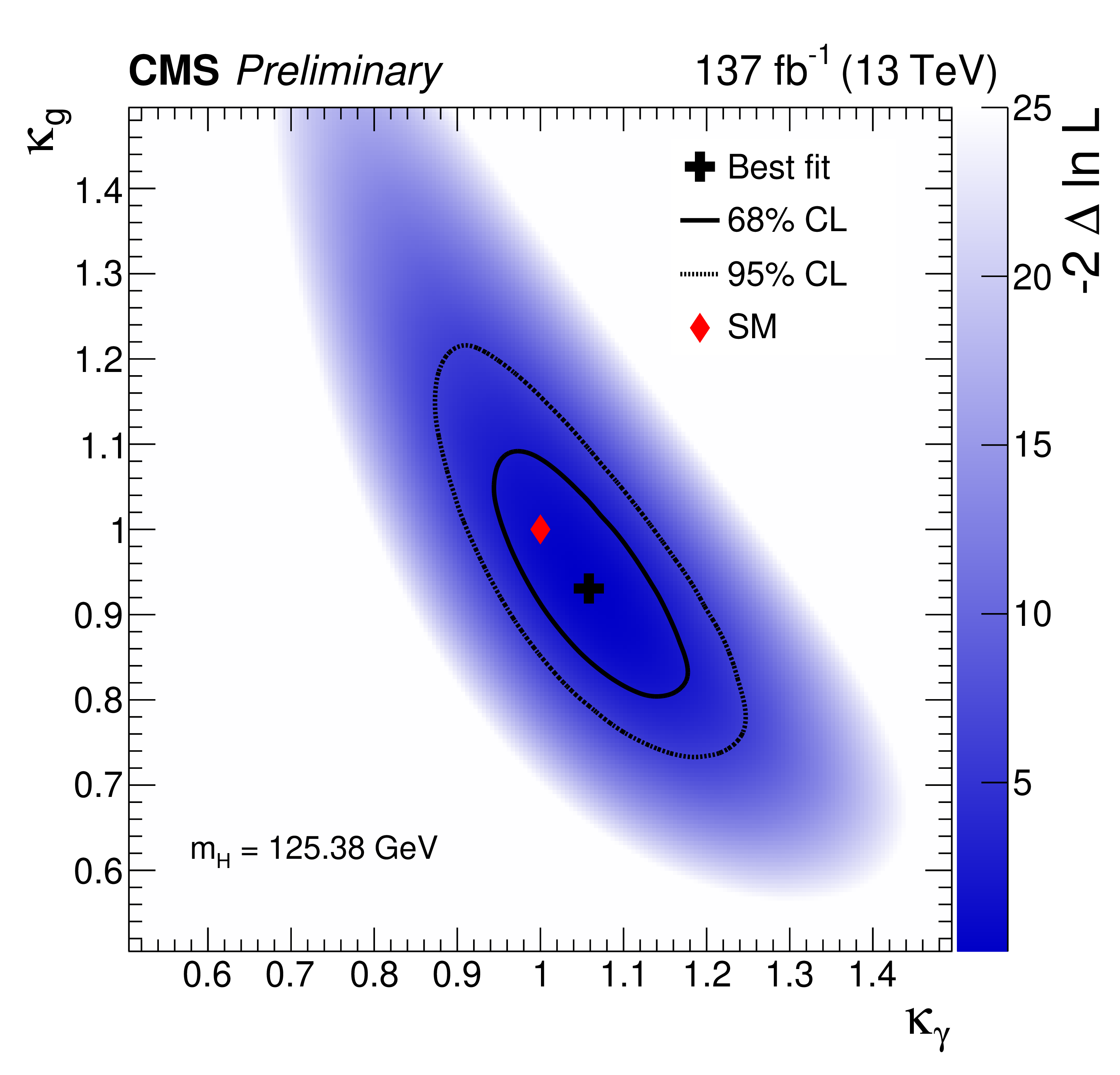
Figure 22-b:
Observed two dimensional likelihood scans performed in the $\kappa $-framework: $ {\kappa _{\gamma}} $-vs-$ {\kappa _{\mathrm{g}}} $ in the unresolved $\kappa $ model. The 68% and 95% confidence level regions are given by the solid and dashed contours, respectively. The best fit and SM points are shown by the black cross and red diamond, respectively. The colour scale indicates the value of the test statistic. |
| Tables | |
png pdf |
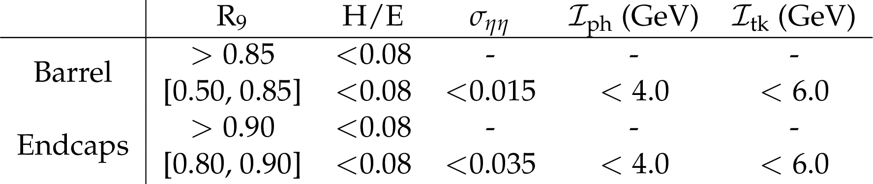
Table 1:
Schema of the photon preselection requirements. |

png pdf |
Table 2:
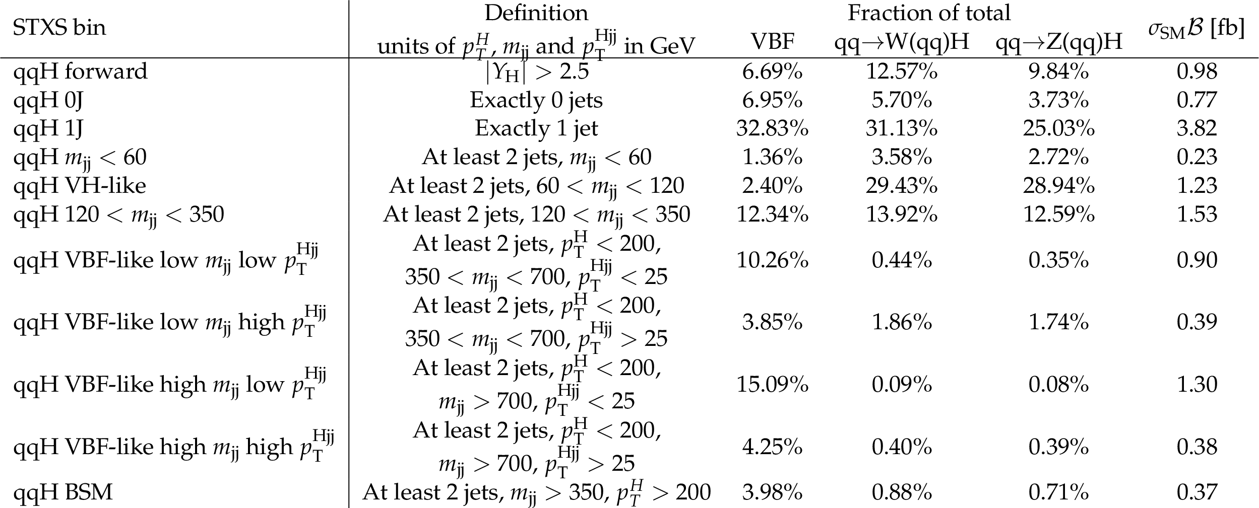
The product of the cross section and branching fraction for the ggH STXS bins, evaluated at $\sqrt {s}=$ 13 TeV and $ {m_\mathrm{H}} = $ 125 GeV. The relative contribution of each STXS bin is also shown. |
png pdf |
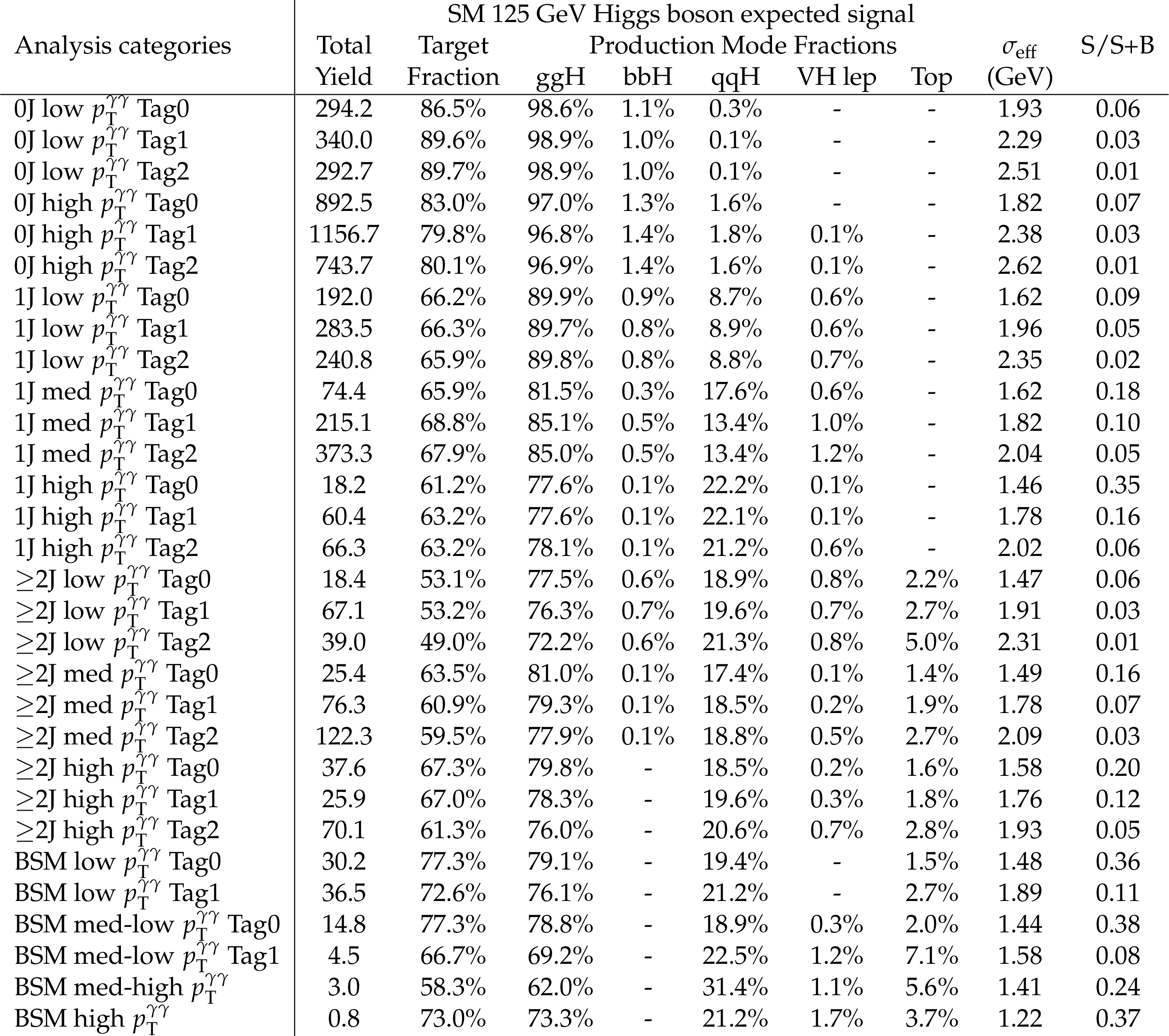
Table 3:
The expected number of signal events for $ {m_\mathrm{H}} = $ 125 GeV in categories targeting ggH production, excluding those targeting the VBF-like phase space. The relative yield of each production mode in each category is shown, as is the fraction of events originating from the targeted STXS bins. Here qqH includes contributions from both VBF and hadronic VH production. The $ {\sigma _{\text {eff}}} $, defined as the smallest interval containing 68.3% of the ${m_{\gamma \gamma}}$ distribution, is listed for each category. The final column shows the expected ratio of signal to signal-plus-background, S/(S+B), where S and B are the numbers of expected signal and background events in a $ \pm $1$ {\sigma _{\text {eff}}} $ window centred on $ {m_\mathrm{H}} $. |
png pdf |
Table 4:
The product of the cross section and branching fraction for the qqH STXS bins, evaluated at $\sqrt {s}=$ 13 TeV and $ {m_\mathrm{H}} = $ 125 GeV. The relative contribution of each STXS bin is also shown. |
png pdf |
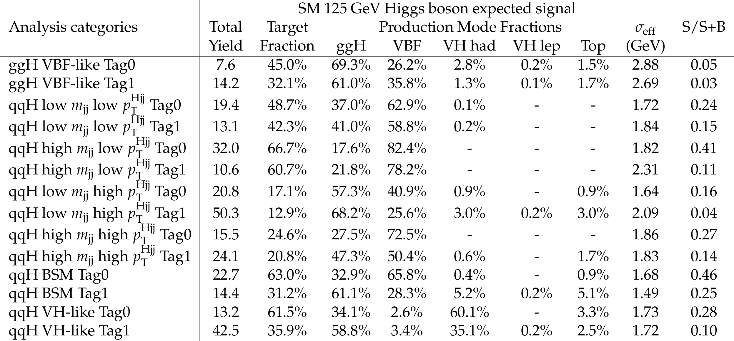
Table 5:
The expected number of signal events for $ {m_\mathrm{H}} = $ 125 GeV in categories targeting VBF-like phase space and VH production in which the vector boson decays hadronically. The relative yield of each production mode in each category is shown, as is the fraction of events originating from the targeted STXS bins. Here ggH also includes contributions from the subdominant ${\mathrm{b} {}\mathrm{\bar{b}} \mathrm{H}}$ production mode. The $ {\sigma _{\text {eff}}} $, defined as the smallest interval containing 68.3% of the ${m_{\gamma \gamma}}$ distribution, is listed for each category. The final column shows the expected ratio of signal to signal-plus-background, S/(S+B), where S and B are the numbers of expected signal and background events in a $ \pm $1$ {\sigma _{\text {eff}}} $ window centred on $ {m_\mathrm{H}} $. |

png pdf |
Table 6:
The product of the cross section and branching fraction for the VH leptonic STXS bins, evaluated at $\sqrt {s}=$ 13 TeV and $ {m_\mathrm{H}} = $ 125 GeV. The relative contribution of each STXS bin is also shown. |

png pdf |
Table 7:
The expected number of signal events for $ {m_\mathrm{H}} = $ 125 GeV in categories targeting Higgs boson production in association with a leptonically decaying W or Z boson. The relative yield of each production mode in each category is shown, as is the fraction of events originating from the targeted STXS bins. Here ggH also includes contributions from the subdominant ${\mathrm{b} {}\mathrm{\bar{b}} \mathrm{H}}$ production mode, whilst qqH incorporates both VBF and hadronic VH production. The $ {\sigma _{\text {eff}}} $, defined as the smallest interval containing 68.3% of the ${m_{\gamma \gamma}}$ distribution, is listed for each category. The final column shows the expected ratio of signal to signal-plus-background, S/(S+B), where S and B are the numbers of expected signal and background events in a $ \pm $1$ {\sigma _{\text {eff}}} $ window centred on $ {m_\mathrm{H}} $. |

png pdf |
Table 8:
The product of the cross section and branching fraction for the ${{\mathrm{t} {}\mathrm{\bar{t}}} \mathrm{H}}$, tH, and ${\mathrm{b} {}\mathrm{\bar{b}} \mathrm{H}}$ STXS bins, evaluated at $\sqrt {s}=$ 13 TeV and $ {m_\mathrm{H}} = $ 125 GeV. The relative contribution of each STXS bin is also shown. |
png pdf |
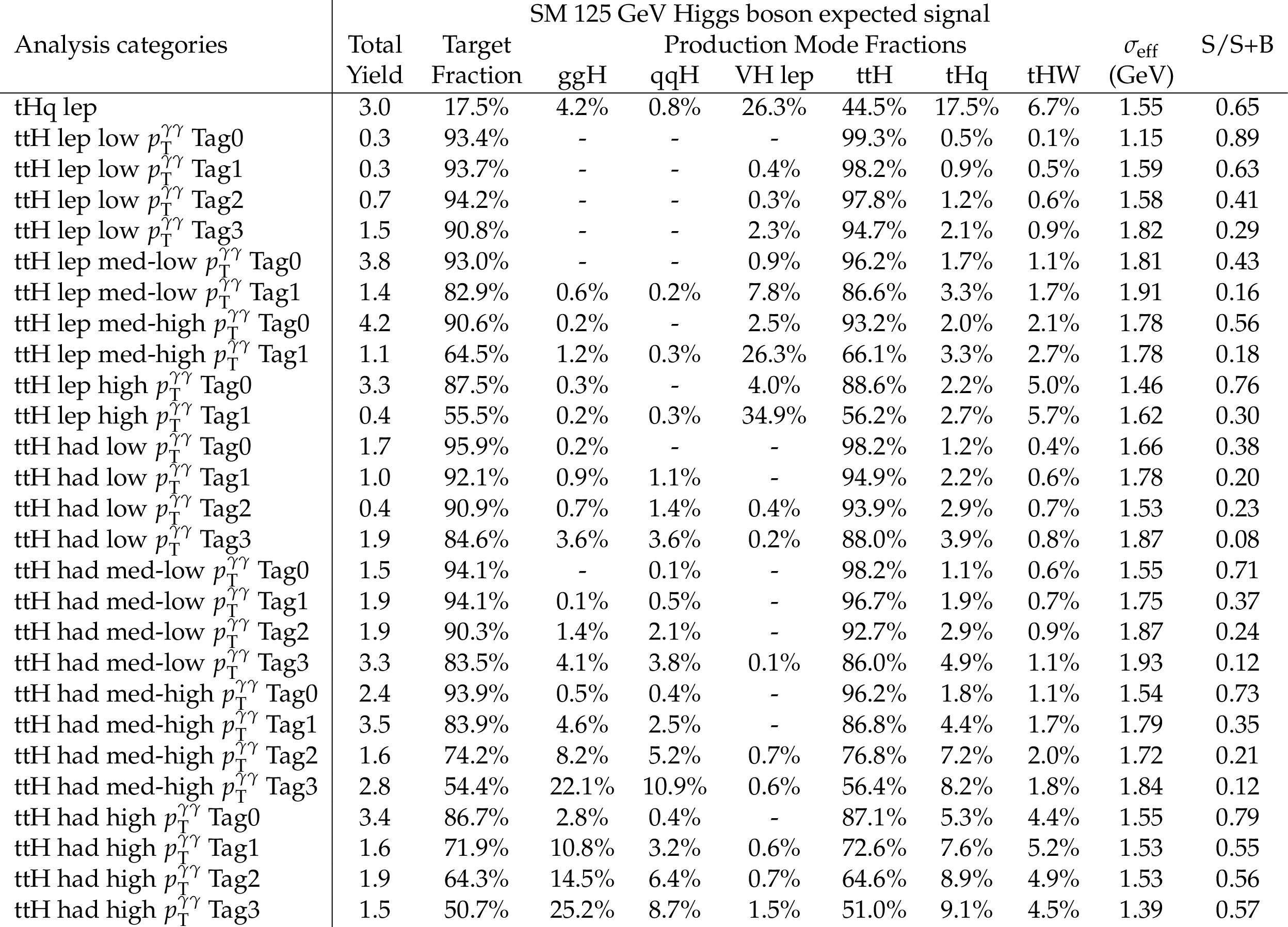
Table 9:
The expected number of signal events for $ {m_\mathrm{H}} = $ 125 GeV in categories targeting Higgs boson production in association with top quarks. The relative yield of each production mode in each category is shown, as is the fraction of events originating from the targeted STXS bins. Here ggH also includes contributions from the subdominant ${\mathrm{b} {}\mathrm{\bar{b}} \mathrm{H}}$ production mode, whilst qqH incorporates both VBF and hadronic VH production. The $ {\sigma _{\text {eff}}} $, defined as the smallest interval containing 68.3% of the ${m_{\gamma \gamma}}$ distribution, is listed for each category. The final column shows the expected ratio of signal to signal-plus-background, S/(S+B), where S and B are the numbers of expected signal and background events in a $ \pm $1$ {\sigma _{\text {eff}}} $ window centred on $ {m_\mathrm{H}} $. |
png pdf |
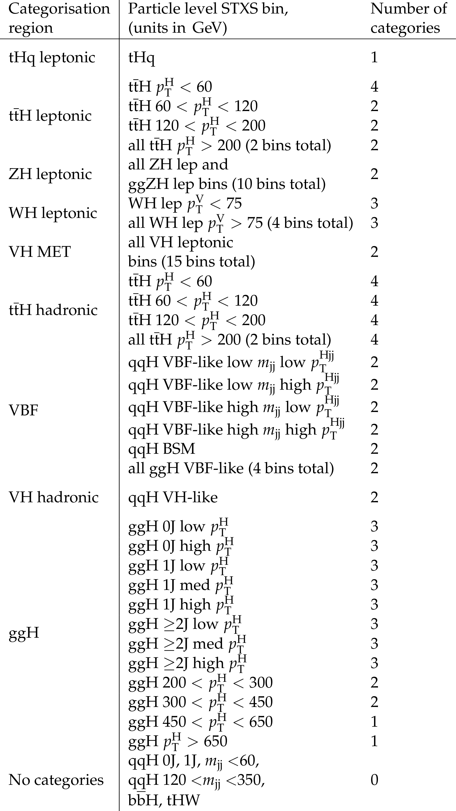
Table 10:
Description of the different categorisation regions, listed in descending order of priority in the first column. The second column shows each targeted STXS bin, or merged group of bins, together with the number of associated analysis categories. The last row contains the bins for which no analysis categories are constructed. |
png pdf |
Table 11:
A summary of the maximal and minimal parameter merging scenarios. The STXS bins that contribute to each parameter are listed. Furthermore, the bins that are constrained to their respective SM predictions in the fits are listed at the bottom. |
| Summary |
| Measurements of Higgs boson properties with the Higgs boson decaying into a pair of photons are reported. Events with two photons are selected from a sample of proton-proton collisions at a centre-of-mass energy $\sqrt{s} = $ 13 TeV collected by the CMS detector at the LHC from 2016 to 2018, corresponding to an integrated luminosity of 137 fb$^{-1}$. Analysis categories enriched in events produced via gluon fusion, vector boson fusion, vector boson associated production, production associated with two top quarks, and production associated with one top quark are constructed.The total Higgs boson signal strength, relative to the standard model prediction, is measured to be 1.03$^{+0.11}_{-0.09}$. Various other properties of the Higgs boson are measured, including standard model signal strength modifiers, production cross sections, and its couplings to other particles. These include the first measurements of cross sections at stage 1.2 of the simplified template cross section framework. Examples of the cross sections include those of Higgs boson production in associated with a top quark antiquark pair in four bins of the Higgs boson transverse momentum. The most precise measurement of Higgs boson production in association with a single top quark is also presented. The observed (expected) limit at 95% CL is found to be 12 (9) times the standard model prediction. All other results are also in agreement with the standard model expectations. |
| Additional Figures | |
png pdf |
Additional Figure 1:
Schematic to show the maximal parameter merging scenario. The parameters of interest are defined by the solid black boxes, which span over multiple bins for the cases in which bins are merged. The hatched boxes demonstrate the regions of phase space which are fixed to the SM prediction in the fit. |
png pdf |
Additional Figure 2:
Schematic to show the minimal parameter merging scenario. The parameters of interest are defined by the solid black boxes, which span over multiple bins for the cases in which bins are merged. The hatched boxes demonstrate the regions of phase space which are fixed to the SM prediction in the fit. |
png pdf |
Additional Figure 3:
Observed correlations between the parameters in the per-production-mode signal strengths fit. The size of the correlations is indicated by the colour scale. |
png pdf |
Additional Figure 4:
Observed results of the stage 0 STXS fit. The best fit cross sections are plotted along with the respective 68% confidence intervals. The systematic components of the uncertainty in each parameter are shown by the coloured boxes. The hatched grey boxes demonstrate the theoretical uncertainties in the SM predictions. The bottom panel shows the ratio of the fitted values to the SM predictions. The orange and blue dashed lines for the VBF-like parameters represents contributions from both ggH and qqH STXS bins. The compatibility of this fit with respect to the SM prediction, expressed as a $p$-value, is approximately 53%. |
png pdf |
Additional Figure 5:
Observed correlations between the parameters in the STXS stage 0 cross sections fit. The size of the correlations is indicated by the colour scale. |

png pdf |
Additional Figure 6:
Two dimensional likelihood profiles for pairs of parameters in the maximal merging scheme with the largest correlations: ggH VBF-like vs qqH VBF-like (left) and tH vs ttH (right). The best fit value along with the 68% and 95% confidence interval contours are shown by the black cross, solid line and dashed line respectively. The parameters are plotted as a ratio with respect to their SM prediction. |

png pdf |
Additional Figure 6-a:
Two dimensional likelihood profile for ggH VBF-like vs qqH VBF-like in the maximal merging scheme with the largest correlations. The best fit value along with the 68% and 95% confidence interval contours are shown by the black cross, solid line and dashed line respectively. The parameters are plotted as a ratio with respect to their SM prediction. |

png pdf |
Additional Figure 6-b:
Two dimensional likelihood profile for tH vs ttH in the maximal merging scheme with the largest correlations. The best fit value along with the 68% and 95% confidence interval contours are shown by the black cross, solid line and dashed line respectively. The parameters are plotted as a ratio with respect to their SM prediction. |
png pdf |
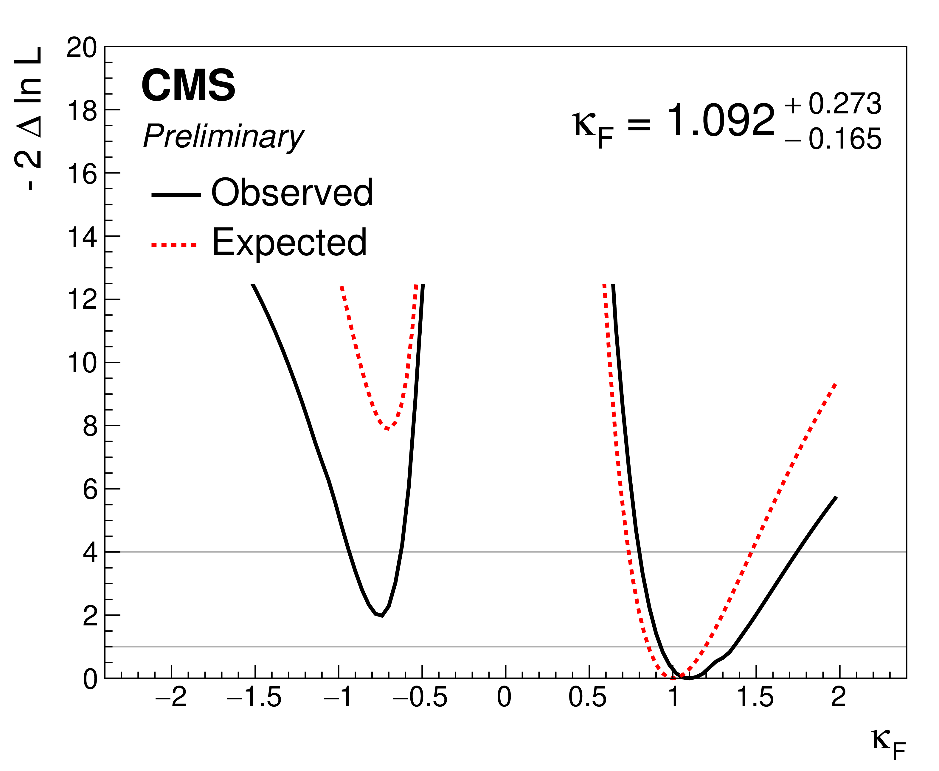
Additional Figure 7:
One dimensional likelihood scans in $ {\kappa _\text {f}} $, using the resolved $\kappa $ model and where $ {\kappa _\text {V}} $ is profiled. The expected (red) and observed (black) scans are shown overlaid. |
png pdf |
Additional Figure 8:
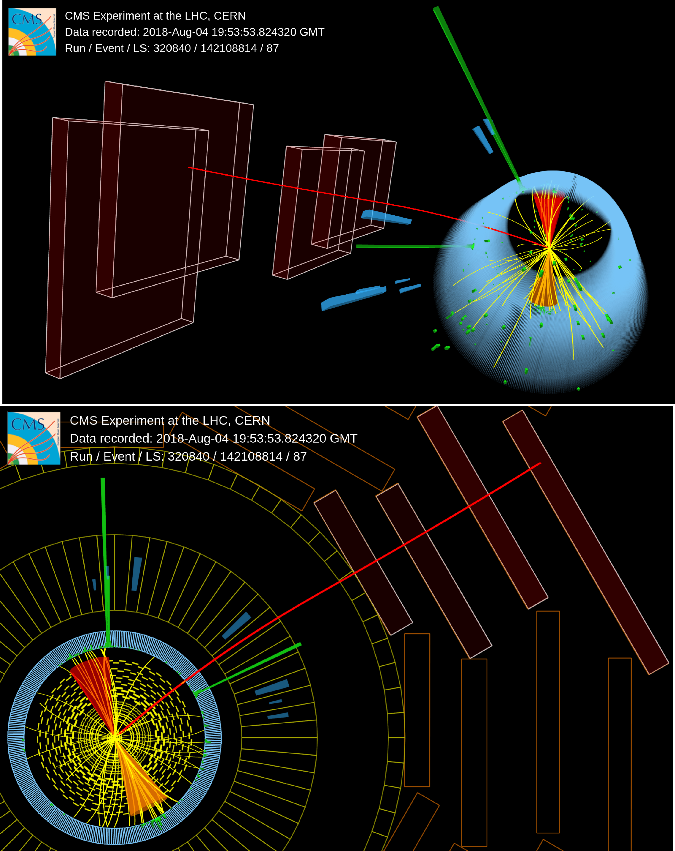
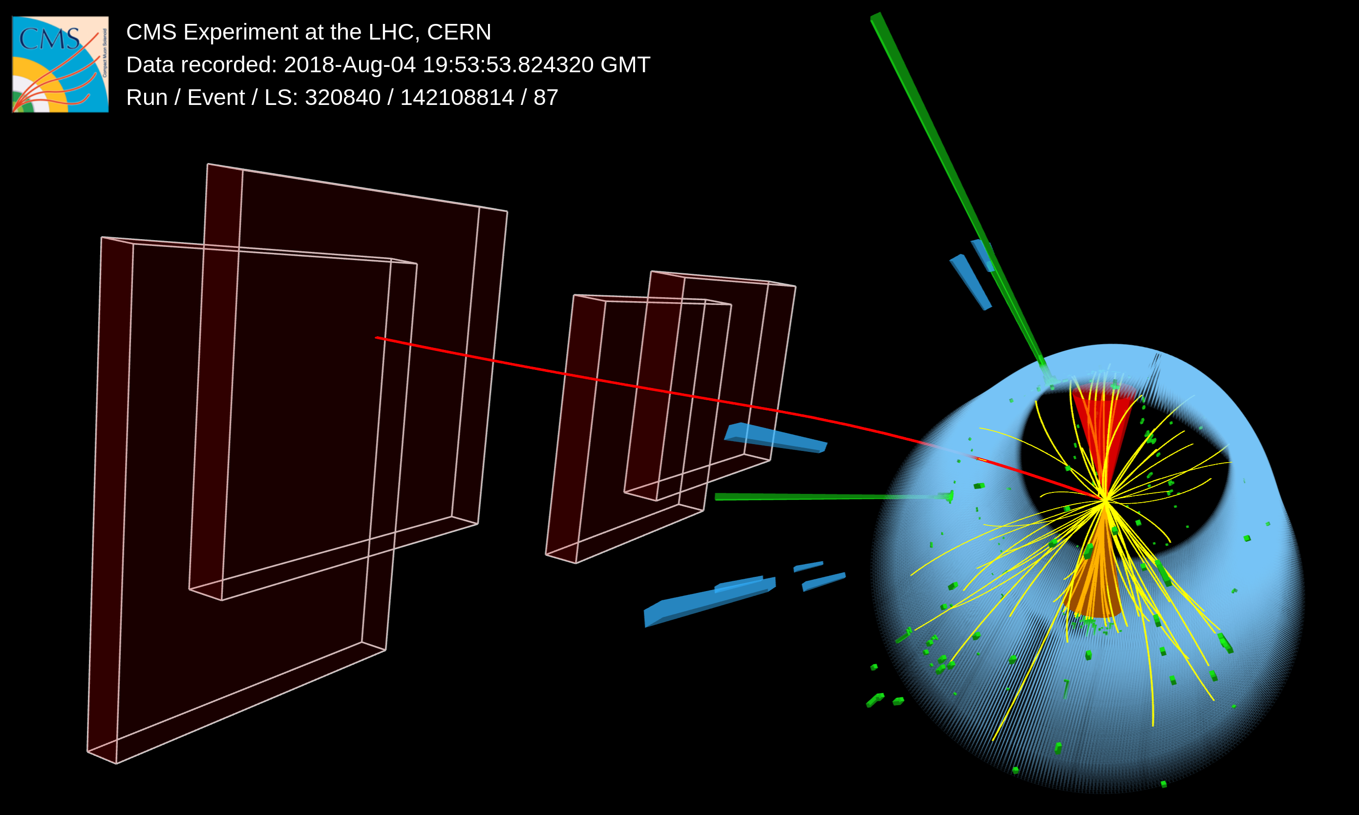
Visualisations of a candidate single top-associated production event in data. The event is selected in the tHq leptonic analysis category and is characterised by two photon candidates with a diphoton invariant mass of 125.52 GeV, shown by the green rectangles. The top quark decays into a W boson and a b quark. The long red line depicts the muon from the decay of the W boson and the red cone depicts the b-tagged jet originating from the b quark. The jet produced from the additional quark is shown as the orange cone. |
png |
Additional Figure 8-a:
Visualisation of a candidate single top-associated production event in data. The event is selected in the tHq leptonic analysis category and is characterised by two photon candidates with a diphoton invariant mass of 125.52 GeV, shown by the green rectangles. The top quark decays into a W boson and a b quark. The long red line depicts the muon from the decay of the W boson and the red cone depicts the b-tagged jet originating from the b quark. The jet produced from the additional quark is shown as the orange cone. |

png |
Additional Figure 8-b:
Visualisation of a candidate single top-associated production event in data. The event is selected in the tHq leptonic analysis category and is characterised by two photon candidates with a diphoton invariant mass of 125.52 GeV, shown by the green rectangles. The top quark decays into a W boson and a b quark. The long red line depicts the muon from the decay of the W boson and the red cone depicts the b-tagged jet originating from the b quark. The jet produced from the additional quark is shown as the orange cone. |
| Additional Tables | |
png pdf |
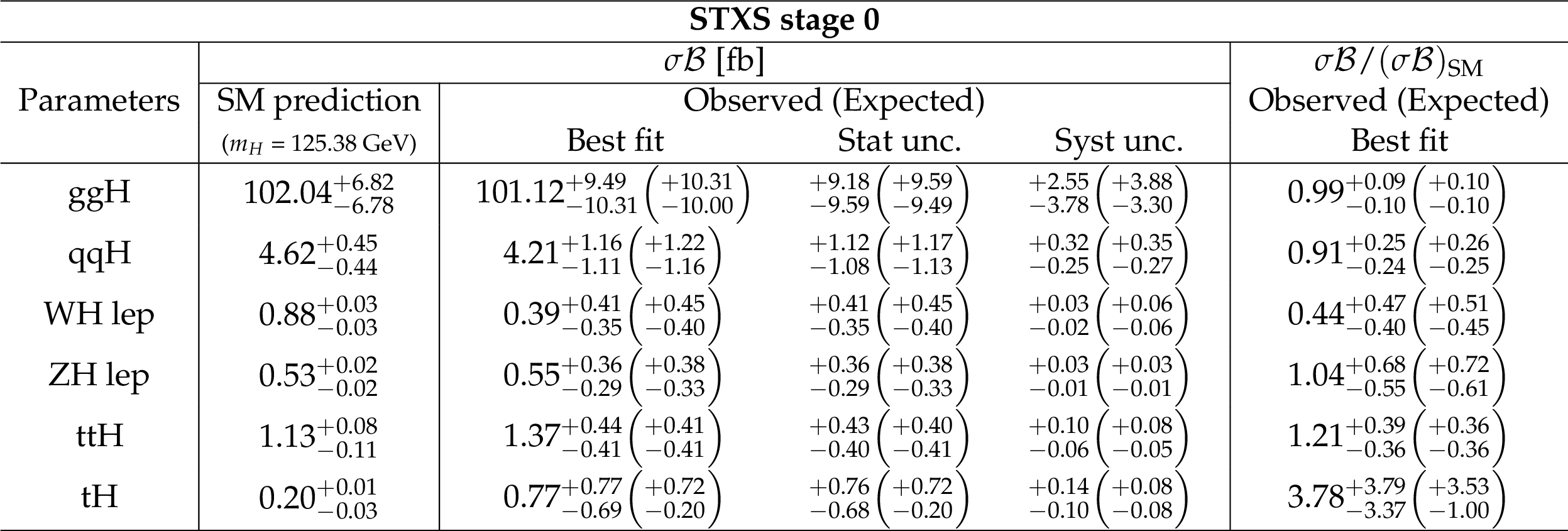
Additional Table 1:
The best-fit cross sections with 68% confidence intervals for the STXS stage 0 fit. The uncertainty is decomposed into the systematic and statistical components. The expected uncertainties on the fitted parameters are given in brackets. Also listed are the SM predictions for the cross sections and the theoretical uncertainty in these predictions. |
png pdf |
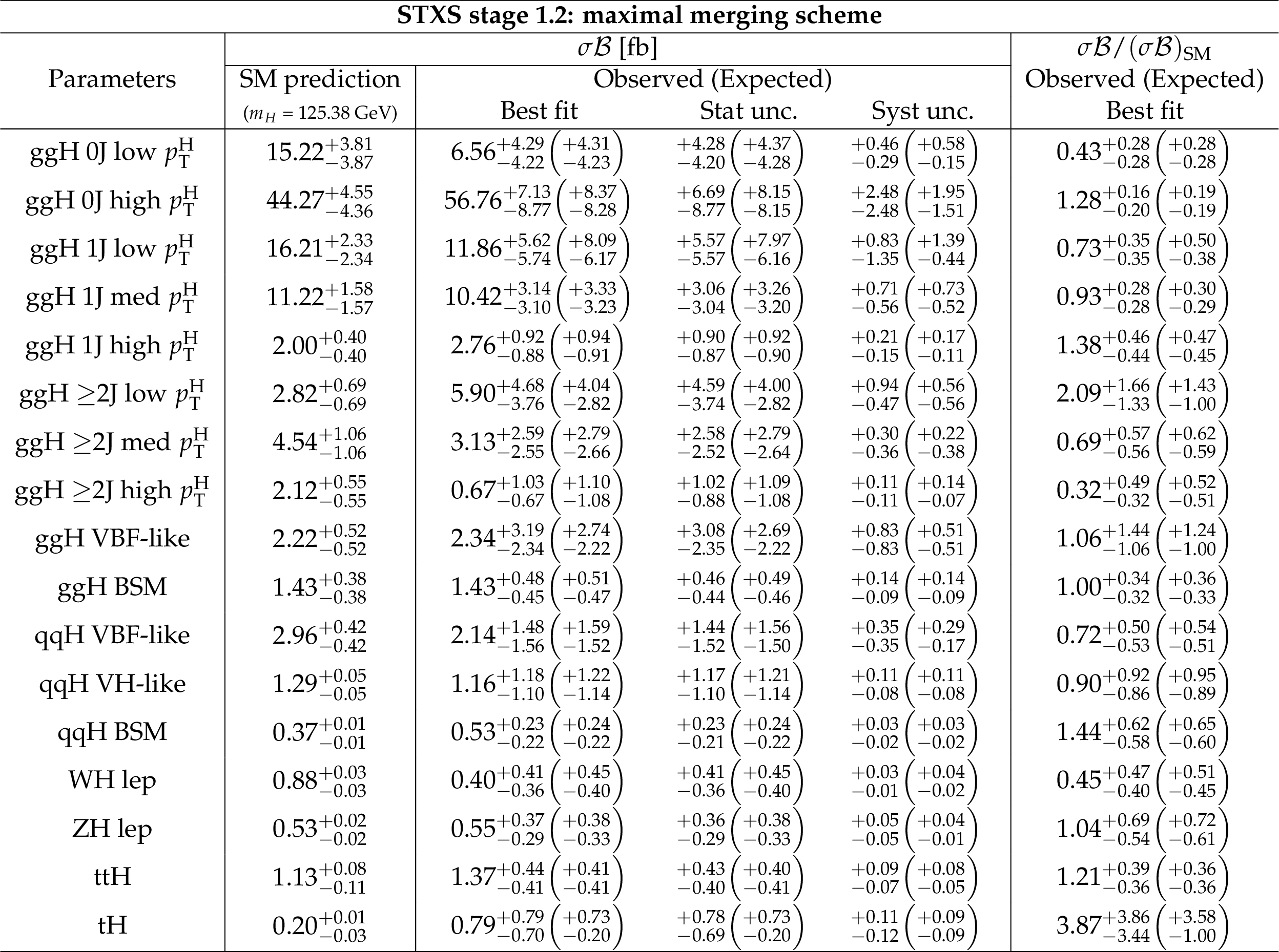
Additional Table 2:
The best-fit cross sections with 68% confidence intervals for the maximal merging scenario. The uncertainty is decomposed into the systematic and statistical components. The expected uncertainties on the fitted parameters are given in brackets. Also listed are the SM predictions for the cross sections and the theoretical uncertainty in these predictions. |
png pdf |
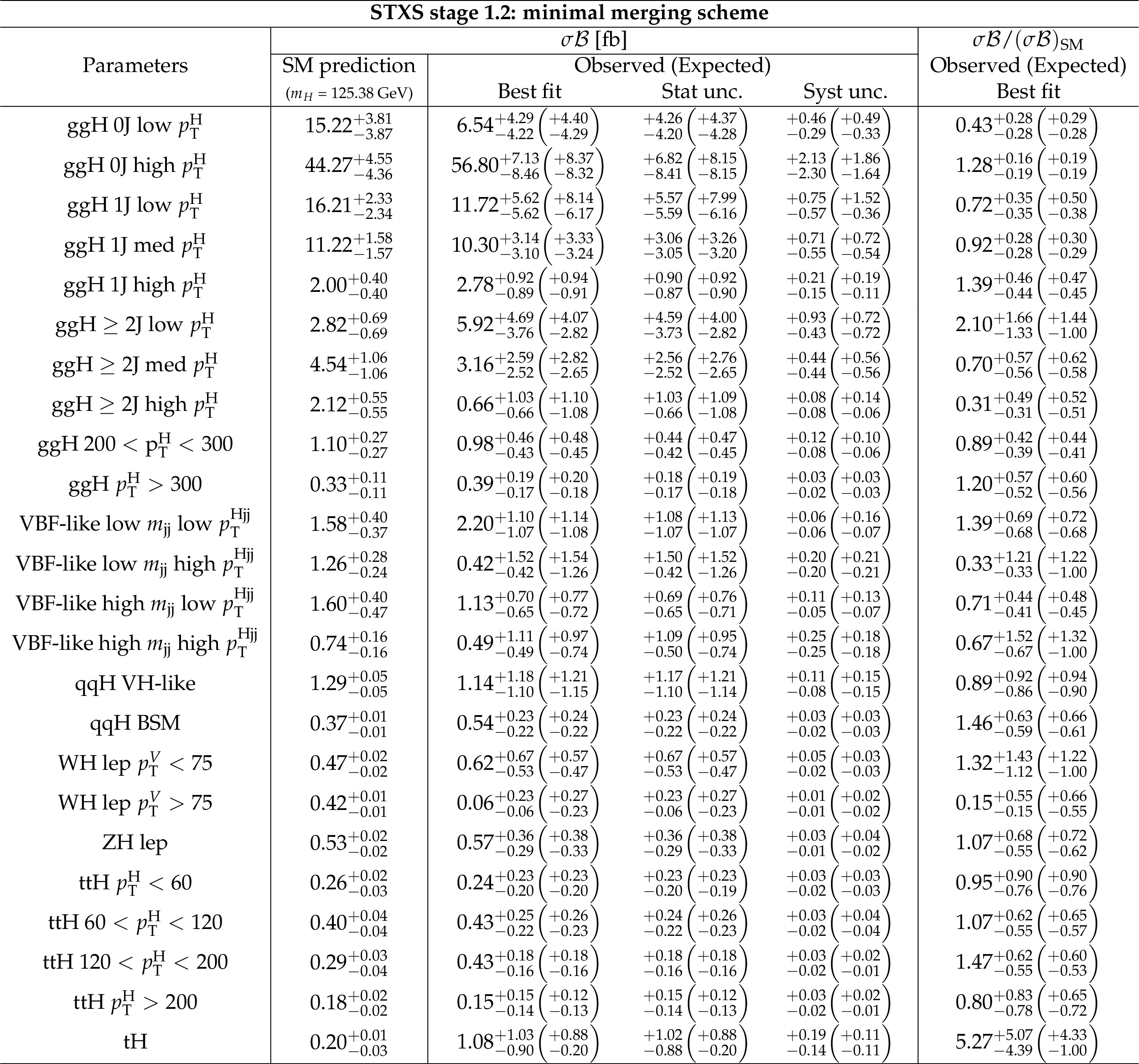
Additional Table 3:
The best-fit cross sections with 68% confidence intervals for the minimal merging scenario. The uncertainty is decomposed into the systematic and statistical components. The expected uncertainties on the fitted parameters are given in brackets. Also listed are the SM predictions for the cross sections and the theoretical uncertainty in these predictions. |
| References | ||||
| 1 | ATLAS Collaboration | Observation of a new particle in the search for the standard model Higgs boson with the detector at the LHC | PLB 716 (2012) 1 | 1207.7214 |
| 2 | CMS Collaboration | Observation of a new boson at a mass of 125 GeV with the CMS experiment at the LHC | PLB 716 (2012) 30 | CMS-HIG-12-028 1207.7235 |
| 3 | CMS Collaboration | Observation of a new boson with mass near 125 GeV in pp collisions at $ \sqrt{s} = $ 7 and 8 TeV | JHEP 06 (2013) 081 | CMS-HIG-12-036 1303.4571 |
| 4 | CMS Collaboration | Observation of $ \mathrm{t\bar{t}}\mathrm{H} $ production | PRL 120 (2018) 231801 | CMS-HIG-17-035 1804.02610 |
| 5 | ATLAS Collaboration | Observation of Higgs boson production in association with a top quark pair at the LHC with the ATLAS detector | PLB 784 (2018) 173 | 1806.00425 |
| 6 | CMS Collaboration | Observation of Higgs boson decay to bottom quarks | PRL 121 (2018) 121801 | CMS-HIG-18-016 1808.08242 |
| 7 | ATLAS Collaboration | Observation of $ \mathrm{H} \rightarrow \mathrm{b\bar{b}} $ decays and V$ \mathrm{H} $ production with the ATLAS detector | PLB 786 (2018) 59 | 1808.08238 |
| 8 | CMS Collaboration | Combined measurements of Higgs boson couplings in proton--proton collisions at $ \sqrt{s}=$ 13 TeV | EPJC 79 (2019) 421 | CMS-HIG-17-031 1809.10733 |
| 9 | ATLAS Collaboration | Combined measurements of Higgs boson production and decay using up to 80 fb$ ^{-1} $ of proton-proton collision data at $ \sqrt{s}= $ 13 TeV collected with the ATLAS experiment | PRD 101 (2020) 012002 | 1909.02845 |
| 10 | CMS Collaboration | Combined Higgs boson production and decay measurements with up to 137 fb$ ^{-1} $ of proton-proton collision data at $ \sqrt{s} = $ 13 TeV | CMS-PAS-HIG-19-005 | CMS-PAS-HIG-19-005 |
| 11 | CMS Collaboration | Measurements of Higgs boson properties in the diphoton decay channel in proton-proton collisions at $ \sqrt{s} = $ 13 TeV | JHEP 11 (2018) 185 | CMS-HIG-16-040 1804.02716 |
| 12 | CMS Collaboration | Measurements of Higgs boson production via gluon fusion and vector boson fusion in the diphoton decay channel at $ \sqrt{s} = $ 13 TeV | CMS-PAS-HIG-18-029 | CMS-PAS-HIG-18-029 |
| 13 | LHC Higgs Cross Section Working Group | Handbook of LHC Higgs cross sections: 4. deciphering the nature of the Higgs sector | CERN (2016) | 1610.07922 |
| 14 | CMS Collaboration | Measurements of $ \mathrm{t\bar{t}} $H production and the CP structure of the Yukawa interaction between the Higgs boson and top quark in the diphoton decay channel | Accepted by PRLett | CMS-HIG-19-013 2003.10866 |
| 15 | ATLAS Collaboration | Measurements of Higgs boson properties in the diphoton decay channel with 36 fb$ ^{-1} $ of pp collision data at $ \sqrt{s} = $ 13 TeV with the ATLAS detector | PRD 98 (2018) 052005 | 1802.04146 |
| 16 | ATLAS Collaboration | Measurements of Higgs boson properties in the diphoton decay channel using 80 fb$ ^{-1} $ of pp collision data at $ \sqrt s = $ 13 TeV with the ATLAS detector | ATLAS Conference note ATLAS-CONF-2018-028 | |
| 17 | ATLAS Collaboration | Higgs boson production cross-section measurements and their EFT interpretation in the $ 4\ell $ decay channel at $ \sqrt{s} = $ 13 TeV with the ATLAS detector | Submitted to EPJC | 2004.03447 |
| 18 | ATLAS Collaboration | Measurements of gluon-gluon fusion and vector-boson fusion Higgs boson production cross-sections in the $ \mathrm{H} \to \mathrm{W}\mathrm{W}^{\ast} \to \mathrm{e}\nu\mu\nu $ decay channel in pp collisions at $ \sqrt{s}= $ 13 TeV with the ATLAS detector | PLB 789 (2019) 508 | 1808.09054 |
| 19 | ATLAS Collaboration | Cross-section measurements of the Higgs boson decaying into a pair of $ \tau $-leptons in proton-proton collisions at $ \sqrt{s}= $ 13 TeV with the ATLAS detector | PRD 99 (2019) 072001 | 1811.08856 |
| 20 | CMS Collaboration | Measurements of properties of the Higgs boson decaying into the four-lepton final state in pp collisions at $ \sqrt{s}= $ 13 TeV | JHEP 11 (2017) 047 | CMS-HIG-16-041 1706.09936 |
| 21 | CMS Collaboration | Measurements of properties of the Higgs boson in the four-lepton final state at $ \sqrt{s}= $ 13 TeV | CMS-PAS-HIG-18-001 | CMS-PAS-HIG-18-001 |
| 22 | CMS Collaboration | Measurements of properties of the Higgs boson decaying to a W boson pair in pp collisions at $ \sqrt{s}= $ 13 TeV | PLB 791 (2019) 96 | CMS-HIG-16-042 1806.05246 |
| 23 | CMS Collaboration | Observation of the Higgs boson decay to a pair of $ \tau $ leptons with the CMS detector | PLB 779 (2018) 283 | CMS-HIG-16-043 1708.00373 |
| 24 | CMS Collaboration | The CMS trigger system | JINST 12 (2017) P01020 | CMS-TRG-12-001 1609.02366 |
| 25 | CMS Trigger, Data Acquisition Group Collaboration | The CMS high level trigger | EPJC 46 (2006) 605 | hep-ex/0512077 |
| 26 | CMS Collaboration | Particle-flow reconstruction and global event description with the cms detector | JINST 12 (2017) P10003 | CMS-PRF-14-001 1706.04965 |
| 27 | M. Cacciari, G. P. Salam, and G. Soyez | The anti-$ {k_{\mathrm{T}}} $ jet clustering algorithm | JHEP 04 (2008) 063 | 0802.1189 |
| 28 | M. Cacciari, G. P. Salam, and G. Soyez | FastJet user manual | EPJC 72 (2012) 1896 | 1111.6097 |
| 29 | CMS Collaboration | Performance of missing transverse momentum reconstruction in proton-proton collisions at $ \sqrt{s} = $ 13 TeV using the CMS detector | JINST 14 (2019) P07004 | CMS-JME-17-001 1903.06078 |
| 30 | CMS Collaboration | The CMS experiment at the CERN LHC | JINST 3 (2008) S08004 | CMS-00-001 |
| 31 | CMS Collaboration | CMS luminosity measurements for the 2016 data taking period | CMS-PAS-LUM-17-001 | CMS-PAS-LUM-17-001 |
| 32 | CMS Collaboration | CMS luminosity measurement for the 2017 data-taking period at $ \sqrt{s} = $ 13 TeV | CMS-PAS-LUM-17-004 | CMS-PAS-LUM-17-004 |
| 33 | CMS Collaboration | CMS luminosity measurement for the 2018 data-taking period at $ \sqrt{s} = $ 13 TeV | CMS-PAS-LUM-18-002 | CMS-PAS-LUM-18-002 |
| 34 | CMS Collaboration | Measurement of the inclusive $ \mathrm{W} $ and $ \mathrm{Z} $ production cross sections in pp collisions at $ \sqrt{s}= $ 7 TeV | JHEP 10 (2011) 132 | CMS-EWK-10-005 1107.4789 |
| 35 | J. Alwall et al. | The automated computation of tree-level and next-to-leading order differential cross sections, and their matching to parton shower simulations | JHEP 07 (2014) 079 | 1405.0301 |
| 36 | K. Hamilton, P. Nason, E. Re, and G. Zanderighi | NNLOPS simulation of Higgs boson production | JHEP 10 (2013) 222 | 1309.0017 |
| 37 | T. Sjostrand et al. | An introduction to PYTHIA 8.2 | CPC 191 (2015) 159 | 1410.3012 |
| 38 | CMS Collaboration | Event generator tunes obtained from underlying event and multiparton scattering measurements | EPJC 76 (2016) 155 | CMS-GEN-14-001 1512.00815 |
| 39 | CMS Collaboration | Extraction and validation of a new set of CMS PYTHIA8 tunes from underlying-event measurements | EPJC 80 (2020) 4 | CMS-GEN-17-001 1903.12179 |
| 40 | NNPDF Collaboration | Parton distributions for the LHC Run II | JHEP 04 (2015) 040 | 1410.8849 |
| 41 | NNPDF Collaboration | Parton distributions from high-precision collider data | EPJC 77 (2017) 663 | 1706.00428 |
| 42 | P. Nason | A new method for combining NLO QCD with shower Monte Carlo algorithms | JHEP 11 (2004) 040 | hep-ph/0409146 |
| 43 | S. Frixione, P. Nason, and C. Oleari | Matching NLO QCD computations with parton shower simulations: the POWHEG method | JHEP 11 (2007) 070 | 0709.2092 |
| 44 | S. Alioli, P. Nason, C. Oleari, and E. Re | NLO Higgs boson production via gluon fusion matched with shower in POWHEG | JHEP 04 (2009) 002 | 0812.0578 |
| 45 | P. Nason and C. Oleari | NLO Higgs boson production via vector-boson fusion matched with shower in POWHEG | JHEP 02 (2010) 037 | 0911.5299 |
| 46 | S. Alioli, P. Nason, C. Oleari, and E. Re | A general framework for implementing NLO calculations in shower Monte Carlo programs: the POWHEG BOX | JHEP 06 (2010) 043 | 1002.2581 |
| 47 | H. B. Hartanto, B. Jager, L. Reina, and D. Wackeroth | Higgs boson production in association with top quarks in the POWHEG BOX | PRD 91 (2015) 094003 | 1501.04498 |
| 48 | T. Gleisberg et al. | Event generation with SHERPA 1.1 | JHEP 02 (2009) 007 | 0811.4622 |
| 49 | GEANT4 Collaboration | GEANT4--a simulation toolkit | NIMA 506 (2003) 250 | |
| 50 | CMS Collaboration | Energy calibration and resolution of the CMS electromagnetic calorimeter in pp collisions at $ \sqrt{s} = $ 7 TeV | JINST 8 (2013) P09009 | CMS-EGM-11-001 1306.2016 |
| 51 | CMS Collaboration | Performance of photon reconstruction and identification with the CMS detector in proton-proton collisions at sqrt(s) = 8 TeV | JINST 10 (2015) P08010 | CMS-EGM-14-001 1502.02702 |
| 52 | CMS Collaboration | A measurement of the Higgs boson mass in the diphoton decay channel | PLB 805 (2020) 135425 | CMS-HIG-19-004 2002.06398 |
| 53 | CMS Collaboration | Pileup mitigation at CMS in 13 TeV data | Submitted to JINST | CMS-JME-18-001 2003.00503 |
| 54 | CMS Collaboration | Identification of heavy-flavour jets with the CMS detector in pp collisions at 13 TeV | JINST 13 (2018) P05011 | CMS-BTV-16-002 1712.07158 |
| 55 | CMS Collaboration | Performance of the CMS muon detector and muon reconstruction with proton-proton collisions at $ \sqrt{s}= $ 13 TeV | JINST 13 (2018) P06015 | CMS-MUO-16-001 1804.04528 |
| 56 | T. Chen and C. Guestrin | XGBoost: A scalable tree boosting system | in Proceedings of the 22nd ACM SIGKDD International Conference on Knowledge Discovery and Data Mining, 2016 | |
| 57 | Y.-Y. Li, R. Nicolaidou, and S. Paganis | Exclusion of heavy, broad resonances from precise measurements of WZ and VH final states at the LHC | EPJC 79 (2019) 348 | 1904.03995 |
| 58 | H. Voss, A. Hocker, J. Stelzer, and F. Tegenfeldt | TMVA, the toolkit for multivariate data analysis with ROOT | in XIth International Workshop on Advanced Computing and Analysis Techniques in Physics Research (ACAT), 2007 | physics/0703039 |
| 59 | ATLAS Collaboration | Study of the CP properties of the interaction of the Higgs boson with top quarks using top quark associated production of the Higgs boson and its decay into two photons with the ATLAS detector at the LHC | Submitted to PRL | 2004.04545 |
| 60 | CMS Collaboration | Search for direct production of supersymmetric partners of the top quark in the all-jets final state in proton-proton collisions at $ \sqrt{s}= $ 13 TeV | JHEP 10 (2017) 005 | CMS-SUS-16-049 1707.03316 |
| 61 | CMS Collaboration | Precise determination of the mass of the Higgs boson and tests of compatibility of its couplings with the standard model predictions using proton collisions at 7 and 8 TeV | EPJC 75 (2015) 212 | CMS-HIG-14-009 1412.8662 |
| 62 | G. Cowan, K. Cranmer, E. Gross, and O. Vitells | Asymptotic formulae for likelihood-based tests of new physics | EPJC 71 (2011) 1554 | 1007.1727 |
| 63 | P. D. Dauncey, M. Kenzie, N. Wardle, and G. J. Davies | Handling uncertainties in background shapes: the discrete profiling method | JINST 10 (2015) P04015 | 1408.6865 |
| 64 | CMS Collaboration | Observation of the diphoton decay of the Higgs boson and measurement of its properties | EPJC 74 (2014) 3076 | CMS-HIG-13-001 1407.0558 |
| 65 | R. A. Fisher | On the interpretation of $ \chi^2 $ from contingency tables, and the calculation of p | Journal of the Royal Statistical Society 85 (1922) 87 | |
| 66 | CMS Collaboration | Measurements of $ \mathrm{t\overline{t}} $ differential cross sections in proton-proton collisions at $ \sqrt{s}= $ 13 TeV using events containing two leptons | JHEP 02 (2019) 149 | CMS-TOP-17-014 1811.06625 |
| 67 | CMS Collaboration | Measurement of the cross section ratio $ \mathrm{t\bar{t}}+\mathrm{b\bar{b}}/\mathrm{t\bar{t}} $ + jj using dilepton final states in pp collisions at 13 TeV | CMS-PAS-TOP-16-010 | CMS-PAS-TOP-16-010 |
| 68 | J. Butterworth et al. | PDF4LHC recommendations for LHC Run II | JPG 43 (2016) 023001 | 1510.03865 |
| 69 | S. Dulat et al. | New parton distribution functions from a global analysis of quantum chromodynamics | PRD 93 (2016) 033006 | 1506.07443 |
| 70 | L. A. Harland-Lang et al. | Parton distributions in the LHC era: MMHT 2014 PDFs | EPJC 75 (2015) 204 | 1412.3989 |
| 71 | S. Carrazza et al. | An unbiased Hessian representation for Monte Carlo PDFs | EPJC 75 (2015) 369 | 1505.06736 |
| 72 | J. Gao and P. Nadolsky | A meta-analysis of parton distribution functions | JHEP 07 (2014) 035 | 1401.0013 |
| 73 | CMS Collaboration | Jet algorithms performance in 13 TeV data | CMS-PAS-JME-16-003 | CMS-PAS-JME-16-003 |
| 74 | The ATLAS Collaboration, The CMS Collaboration, The LHC Higgs Combination Group | Procedure for the LHC Higgs boson search combination in Summer 2011 | CMS-NOTE-2011-005 | |
| 75 | LHC Higgs Cross Section Working Group | Handbook of LHC Higgs cross sections: 3. Higgs properties | CERN (2013) | 1307.1347 |
|
|
Compact Muon Solenoid LHC, CERN |
|

|

|

|

|

|