

Compact Muon Solenoid
LHC, CERN
| CMS-HIG-13-001 ; CERN-PH-EP-2014-117 | ||
| Observation of the diphoton decay of the Higgs boson and measurement of its properties | ||
| CMS Collaboration | ||
| 2 July 2014 | ||
| Eur. Phys. J. C 74 (2014) 3076 | ||
| Abstract: Observation of the diphoton decay mode of the recently discovered Higgs boson and measurement of some of its properties are reported. The analysis uses the entire dataset collected by the CMS experiment in proton-proton collisions during the 2011 and 2012 LHC running periods. The data samples correspond to integrated luminosities of 5.1 fb$ ^{-1} $ at $ \sqrt{s} $ = 7 TeV and 19.7 fb$ ^{-1} $ at 8 TeV. A clear signal is observed in the diphoton channel at a mass close to 125 GeV with a local significance of 5.7$ \sigma $, where a significance of 5.2$ \sigma $ is expected for the standard model Higgs boson. The mass is measured to be 124.70 $\pm$ 0.34 GeV = 124.70 $\pm$ 0.31 (stat) $\pm$ 0.15 (syst) GeV, and the best-fit signal strength relative to the standard model prediction is 1.14 $ ^{+0.26}_{-0.23} $ =1.14 $\pm$ 0.21 (stat) $ ^{+0.09}_{-0.05}$ (syst) $ ^{+0.13}_{-0.09} $ (theo). Additional measurements include the signal strength modifiers associated with different production mechanisms, and hypothesis tests between spin-0 and spin-2 models. | ||
| Links: e-print arXiv:1407.0558 [hep-ex] (PDF) ; CDS record ; inSPIRE record ; Public twiki page ; CADI line (restricted) ; | ||
| Cover | |
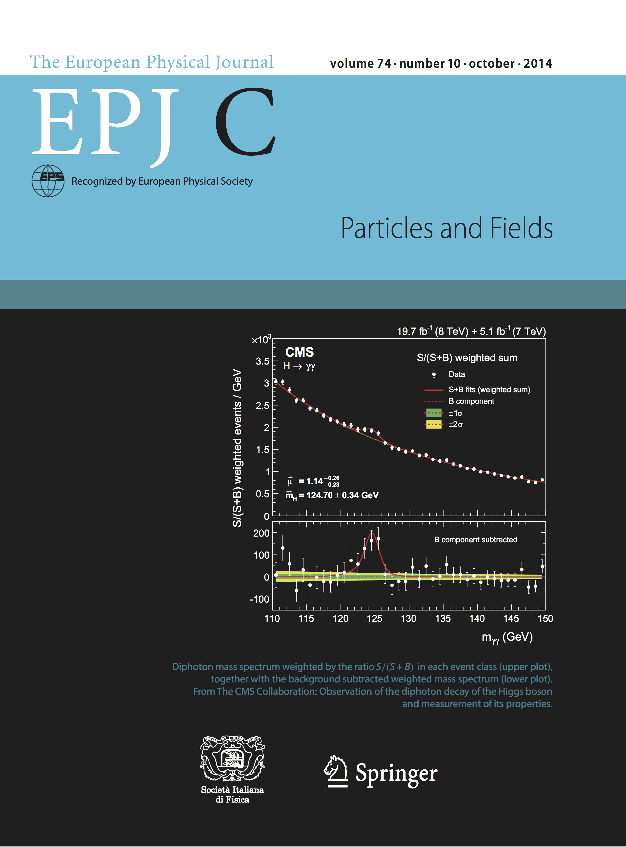
png ; pdf |
Cover of the European Journal or Physics C, Volume 14, Number 10, published October 2014. |
| Figures | |

png pdf |
Figure 1:
Invariant mass of $\mathrm{ e }^- \mathrm{ e }^+ $ pairs in $ {\mathrm{ Z } \to \mathrm{ e }^- \mathrm{ e }^+ } $ events in the 8 TeV data (points), and in simulated events (histogram), in which the electron showers are reconstructed as photons, and the full set of photon corrections and smearings are applied. The comparison is shown for (left) events with both showers in the barrel, and (right) the remaining events. For each bin, the ratio of the number of events in data to the number of simulated events is shown in the lower main plot. |

png pdf |
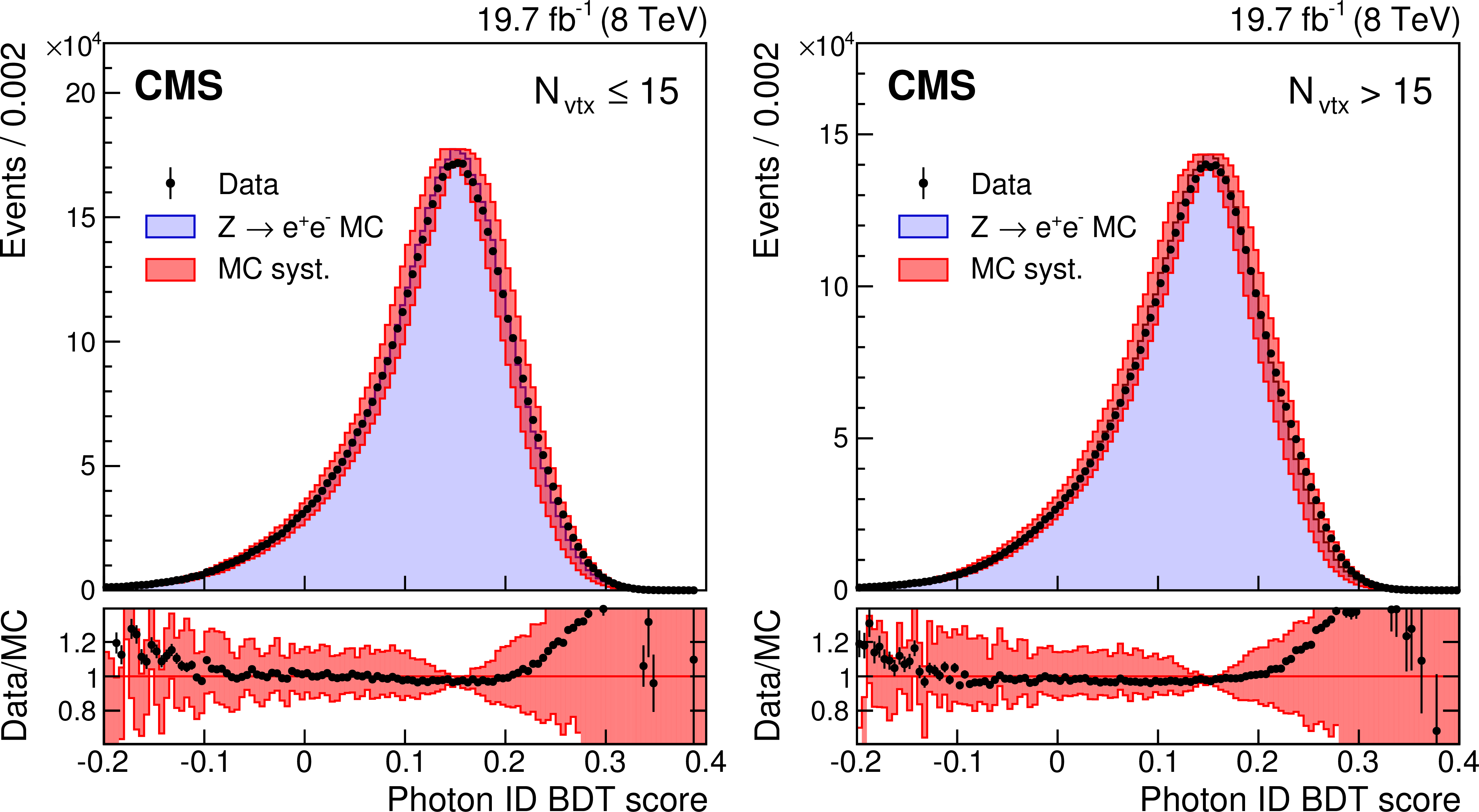
Figure 2:
Photon identification BDT score of the lower-scoring photon of diphoton pairs with an invariant mass in the range 100 $ < {m_{\gamma \gamma }} < $ 180 GeV, for events passing the preselection in the 8 TeV dataset (points), and for simulated background events (histogram with shaded error bands showing the statistical uncertainty). Histograms are also shown for different components of the simulated background, in which there are either two, one, or zero prompt signal-like photons. The tall histogram on the right (righthand vertical axis) corresponds to simulated Higgs boson signal events. |
png pdf |
Figure 3:
Comparison of the photon identification BDT score for electron showers in the barrel in $ { {\mathrm {Z}}\to {\mathrm {e}^+} {\mathrm {e}^-}} $ events in the 8 TeV dataset and MC simulated events, for events passing the preselection, but with the electron veto condition inverted. The systematic uncertainty assigned to the photon identification BDT score is shown as a band. The comparison is shown for two sets of events with different numbers of primary vertices, $ {N_\mathrm {vtx}} $. For each bin, the ratio of the number of events in data to the number of simulated events is shown in the lower plot. |
png pdf |
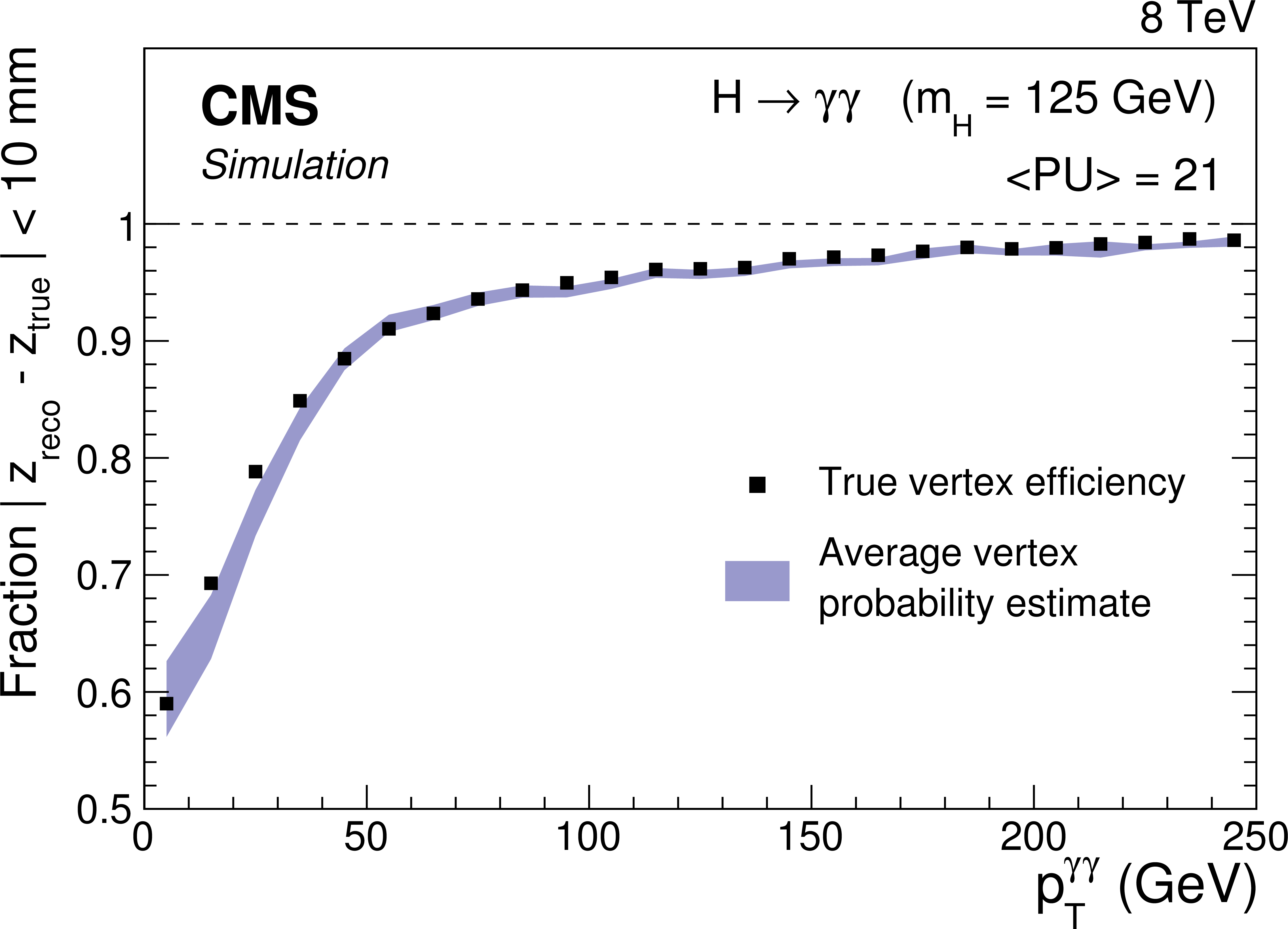
Figure 4:
Fraction of diphoton vertices (solid points) assigned, by the vertex assignment BDT, to a reconstructed vertex within 10 mm of their true location in simulated Higgs boson events, $ {m_ {\mathrm {H}} }$ = 125 GeV , $\sqrt {s}$ = 8 TeV , as a function of $ {p_{\mathrm {T}}^{\gamma \gamma }} $. Also shown is a band, the centre of which is the mean prediction, from the vertex probability BDT, of the probability of correctly locating the vertex. The mean is calculated in ${p_{\mathrm {T}}^{\gamma \gamma }} $ bins, and the width of the band represents the event-to-event uncertainty in the estimates. |

png pdf |
Figure 5:
Distribution of the vertex probability estimate in $ { {\mathrm {Z}}\to {{\mu ^+}} {{\mu ^-}}} $ events. The vertex probability estimates in 8 TeV data (points), are compared to the estimates in MC simulation (histograms). The comparison is made separately for events in which the vertex is assigned to the same (open circles and filled histogram), or to a different vertex (filled circles and outlined histogram), as that identified by the muons. |
png pdf |
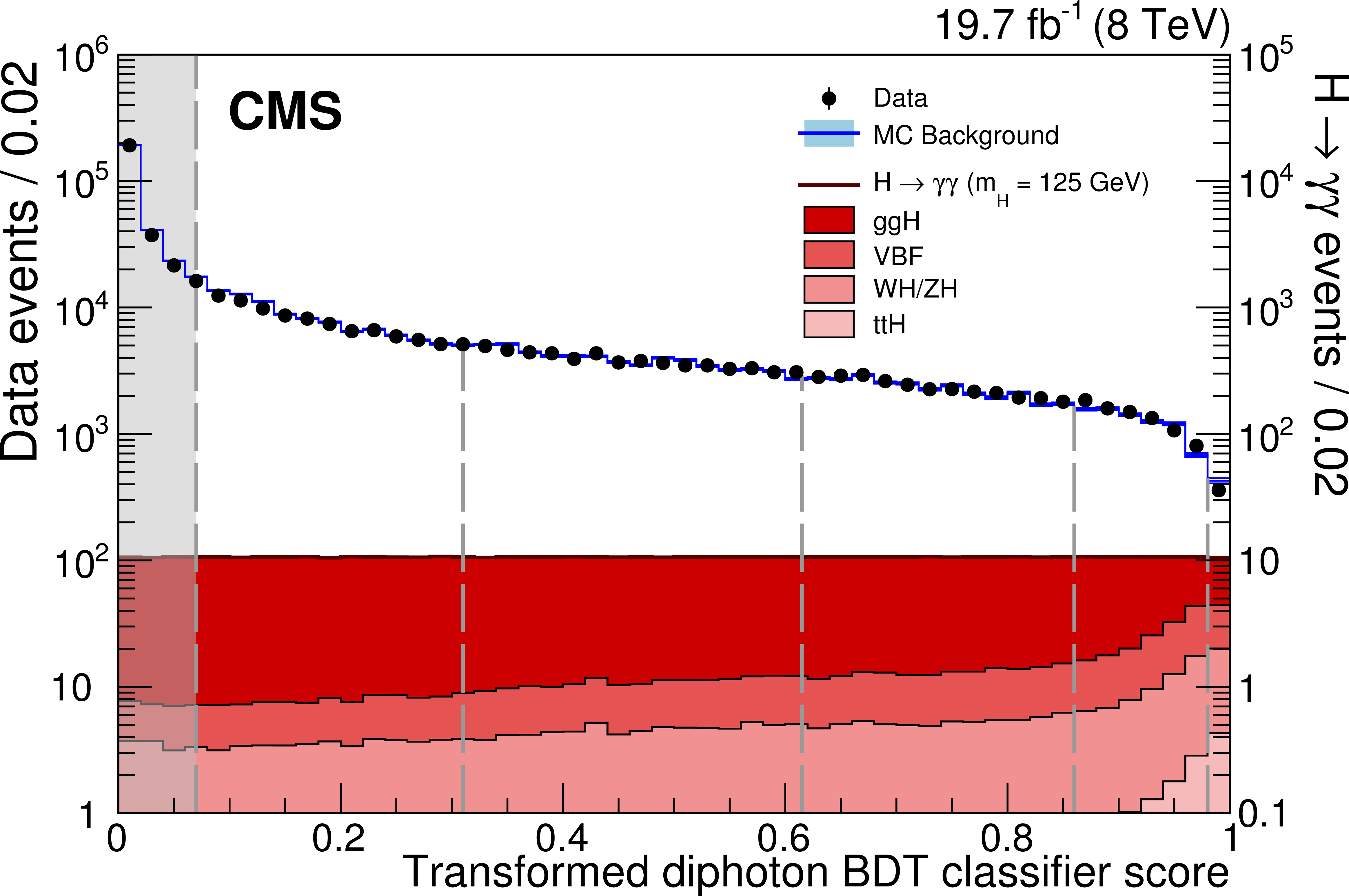
Figure 6:
Transformed diphoton BDT classifier score for events satisfying the full diphoton preselection in the 8 TeV data (points with error bars, left axis), and for simulated signal events from the four production processes (solid filled histograms, right axis). The outlined histogram, following the data points, is for simulated background events. The vertical dashed lines show the boundaries of the untagged event classes, with the leftmost dashed line representing the score below which events are discarded and not used in the final analysis. |
png pdf |
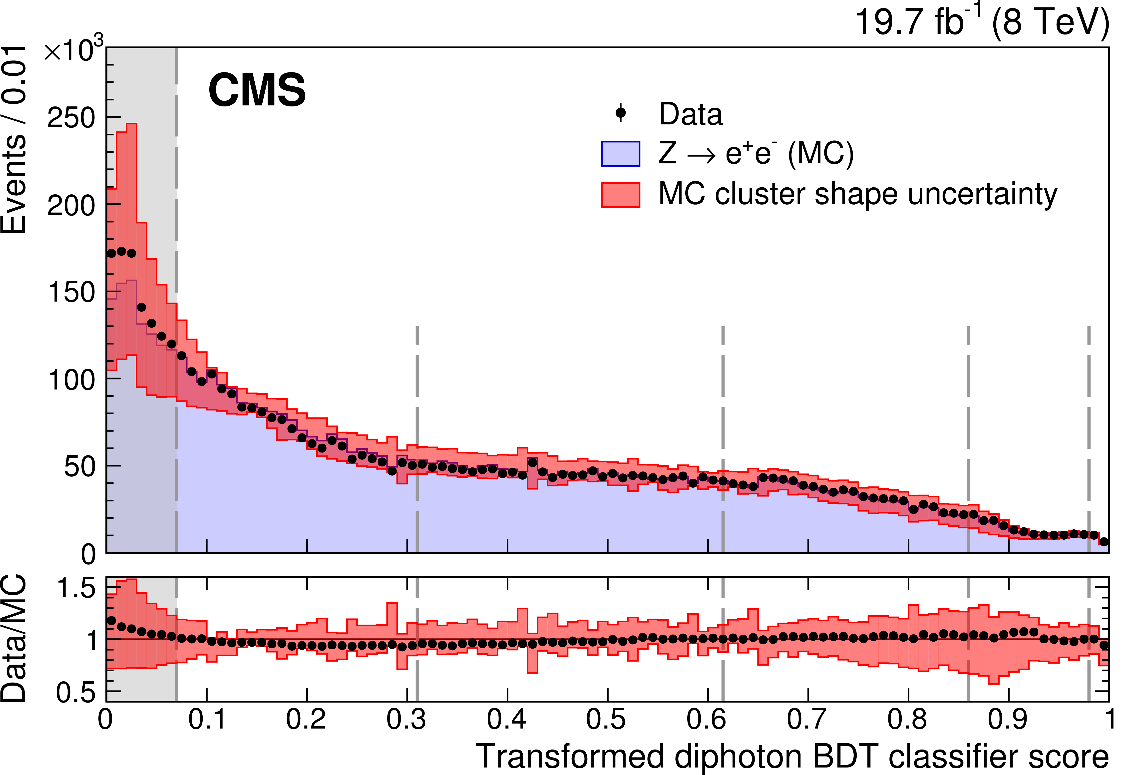
Figure 7:
Transformed diphoton BDT classifier score for $ { {\mathrm {Z}}\to {\mathrm {e}^+} {\mathrm {e}^-}} $ events in 8 TeV data, and in MC simulation, in which the electrons are reconstructed as photons. The distribution of simulated events is represented by a histogram, and the data by points with error bars. For each bin, the ratio of the number of events in data to the number of simulated events is shown in the lower plot. The bands in the two plots indicate the systematic uncertainty related to the MC cluster shape uncertainty (see text). The vertical dashed lines show the boundaries of the untagged event classes, with the leftmost dashed line representing the score below which events are discarded and not used in the final analysis. |
png pdf |
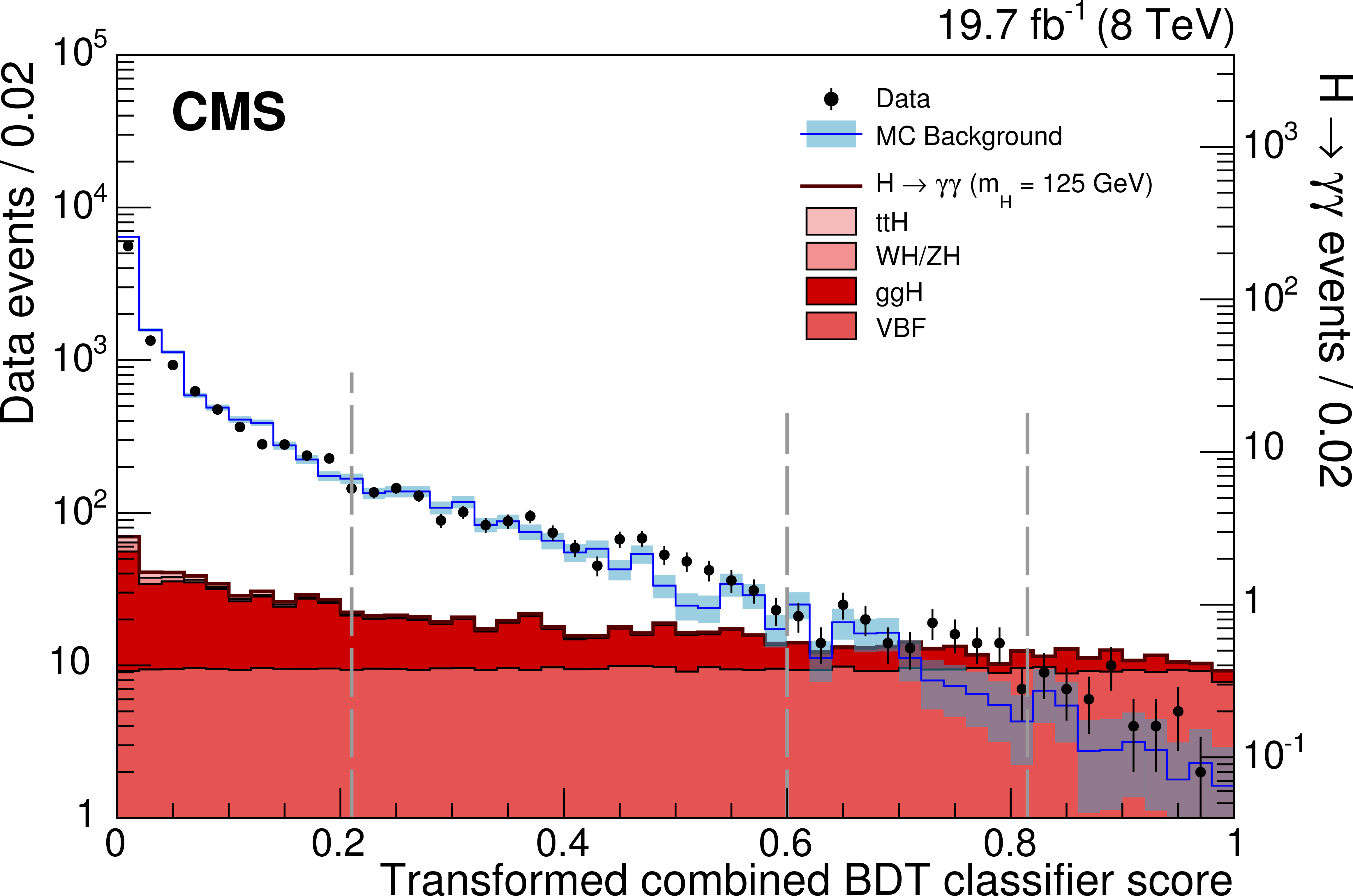
Figure 8:
Score of the combined dijet-diphoton BDT for events satisfying the dijet preselection in 8 TeV data (points with error bars, left axis) and for simulated signal events from the four production processes (histograms, right axis). The outlined histogram is for simulated background events; the shaded error bands on the histogram show the statistical uncertainty in the simulation. The vertical dashed lines show the boundaries of the event classes, with the leftmost dashed line representing the score below which events are not included in the VBF dijet-tagged classes, but remain candidates for inclusion in other classes. The classifier score is transformed such that signal events produced by the VBF process have a uniform, flat, distribution. |
png pdf |
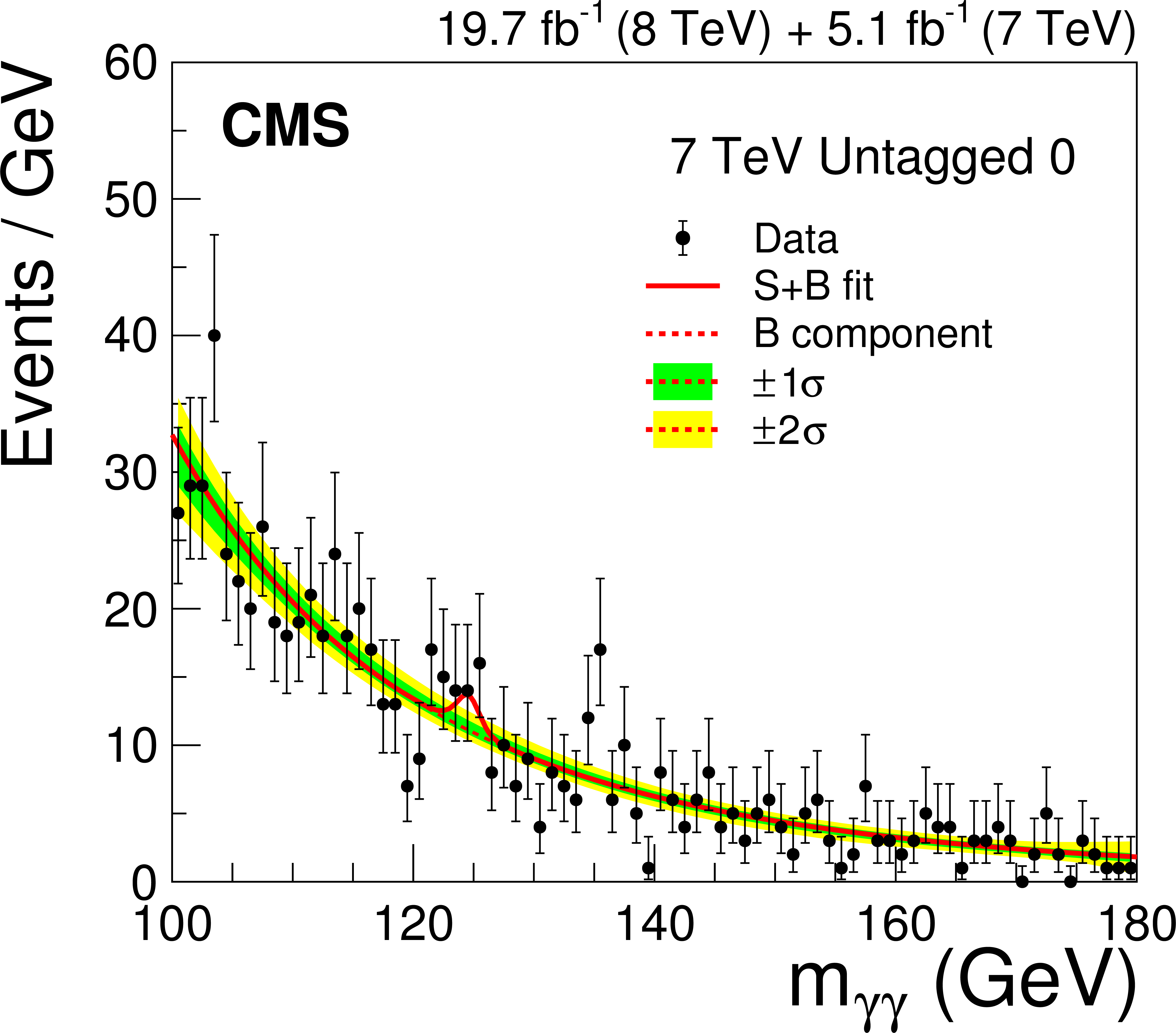
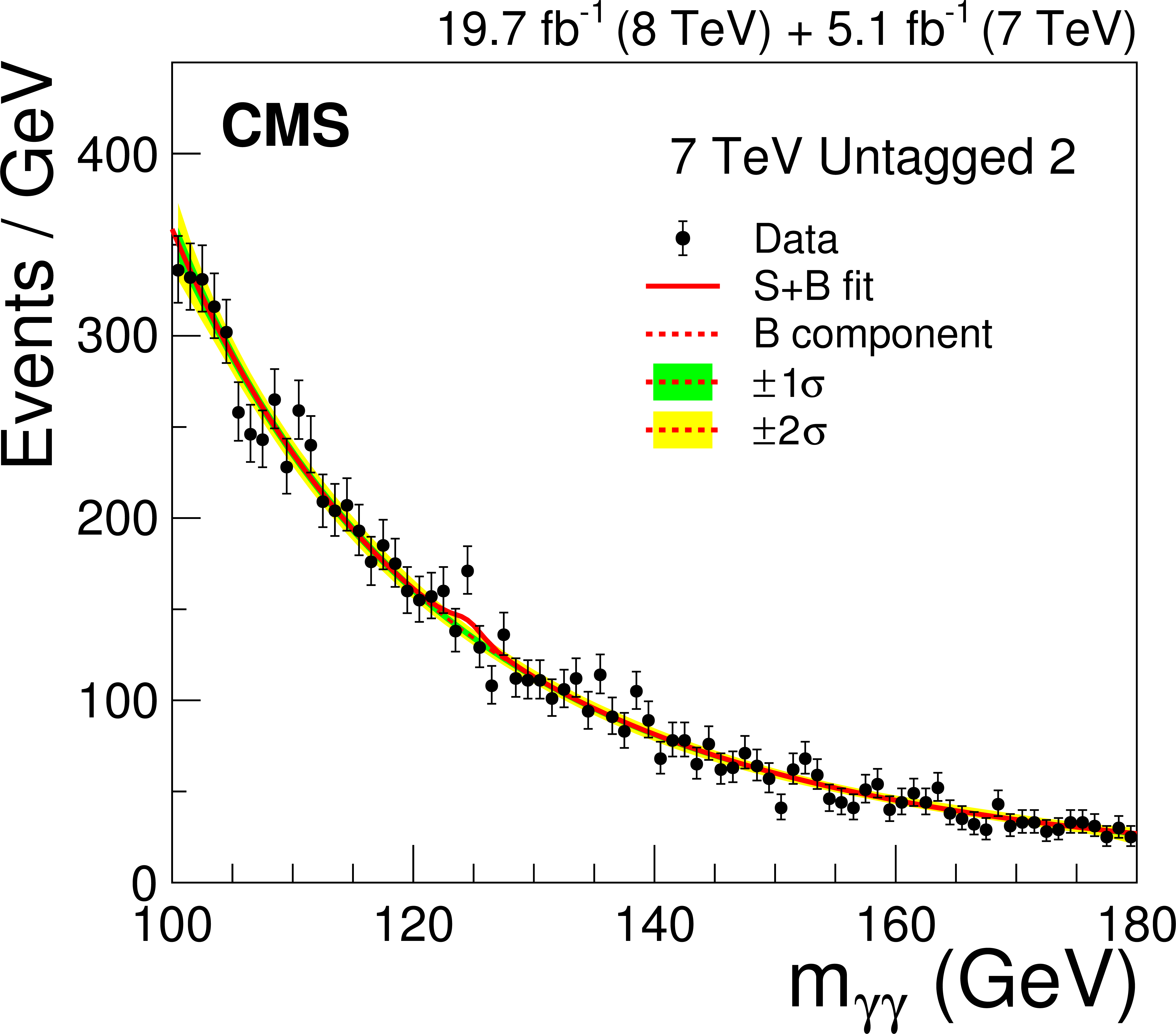
Figure 9-a:
Events in the four untagged classes of the 7 TeV dataset, binned as a function of $ {m_{\gamma \gamma }} $, together with the result of a fit of the signal-plus-background model. The $1\sigma $ and $2\sigma $ uncertainty bands shown for the background component of the fit include the uncertainty due to the choice of function and the uncertainty in the fitted parameters. These bands do not contain the Poisson uncertainty that must be included when the full uncertainty in the number of background events in any given mass range is estimated. |

png pdf |
Figure 9-b:
Events in the four untagged classes of the 7 TeV dataset, binned as a function of $ {m_{\gamma \gamma }} $, together with the result of a fit of the signal-plus-background model. The $1\sigma $ and $2\sigma $ uncertainty bands shown for the background component of the fit include the uncertainty due to the choice of function and the uncertainty in the fitted parameters. These bands do not contain the Poisson uncertainty that must be included when the full uncertainty in the number of background events in any given mass range is estimated. |
png pdf |
Figure 9-c:
Events in the four untagged classes of the 7 TeV dataset, binned as a function of $ {m_{\gamma \gamma }} $, together with the result of a fit of the signal-plus-background model. The $1\sigma $ and $2\sigma $ uncertainty bands shown for the background component of the fit include the uncertainty due to the choice of function and the uncertainty in the fitted parameters. These bands do not contain the Poisson uncertainty that must be included when the full uncertainty in the number of background events in any given mass range is estimated. |

png pdf |
Figure 9-d:
Events in the four untagged classes of the 7 TeV dataset, binned as a function of $ {m_{\gamma \gamma }} $, together with the result of a fit of the signal-plus-background model. The $1\sigma $ and $2\sigma $ uncertainty bands shown for the background component of the fit include the uncertainty due to the choice of function and the uncertainty in the fitted parameters. These bands do not contain the Poisson uncertainty that must be included when the full uncertainty in the number of background events in any given mass range is estimated. |
png pdf |
Figure 10-a:
Events in the five untagged classes of the 8 TeV dataset, binned as a function of $ {m_{\gamma \gamma }} $, together with the result of a fit of the signal-plus-background model. The $1\sigma $ and $2\sigma $ uncertainty bands shown for the background component of the fit include the uncertainty due to the choice of function and the uncertainty in the fitted parameters. These bands do not contain the Poisson uncertainty that must be included when the full uncertainty in the number of background events in any given mass range is estimated. |
png pdf |
Figure 10-b:
Events in the five untagged classes of the 8 TeV dataset, binned as a function of $ {m_{\gamma \gamma }} $, together with the result of a fit of the signal-plus-background model. The $1\sigma $ and $2\sigma $ uncertainty bands shown for the background component of the fit include the uncertainty due to the choice of function and the uncertainty in the fitted parameters. These bands do not contain the Poisson uncertainty that must be included when the full uncertainty in the number of background events in any given mass range is estimated. |
png pdf |
Figure 10-c:
Events in the five untagged classes of the 8 TeV dataset, binned as a function of $ {m_{\gamma \gamma }} $, together with the result of a fit of the signal-plus-background model. The $1\sigma $ and $2\sigma $ uncertainty bands shown for the background component of the fit include the uncertainty due to the choice of function and the uncertainty in the fitted parameters. These bands do not contain the Poisson uncertainty that must be included when the full uncertainty in the number of background events in any given mass range is estimated. |

png pdf |
Figure 10-d:
Events in the five untagged classes of the 8 TeV dataset, binned as a function of $ {m_{\gamma \gamma }} $, together with the result of a fit of the signal-plus-background model. The $1\sigma $ and $2\sigma $ uncertainty bands shown for the background component of the fit include the uncertainty due to the choice of function and the uncertainty in the fitted parameters. These bands do not contain the Poisson uncertainty that must be included when the full uncertainty in the number of background events in any given mass range is estimated. |
png pdf |
Figure 10-e:
Events in the five untagged classes of the 8 TeV dataset, binned as a function of $ {m_{\gamma \gamma }} $, together with the result of a fit of the signal-plus-background model. The $1\sigma $ and $2\sigma $ uncertainty bands shown for the background component of the fit include the uncertainty due to the choice of function and the uncertainty in the fitted parameters. These bands do not contain the Poisson uncertainty that must be included when the full uncertainty in the number of background events in any given mass range is estimated. |
png pdf |
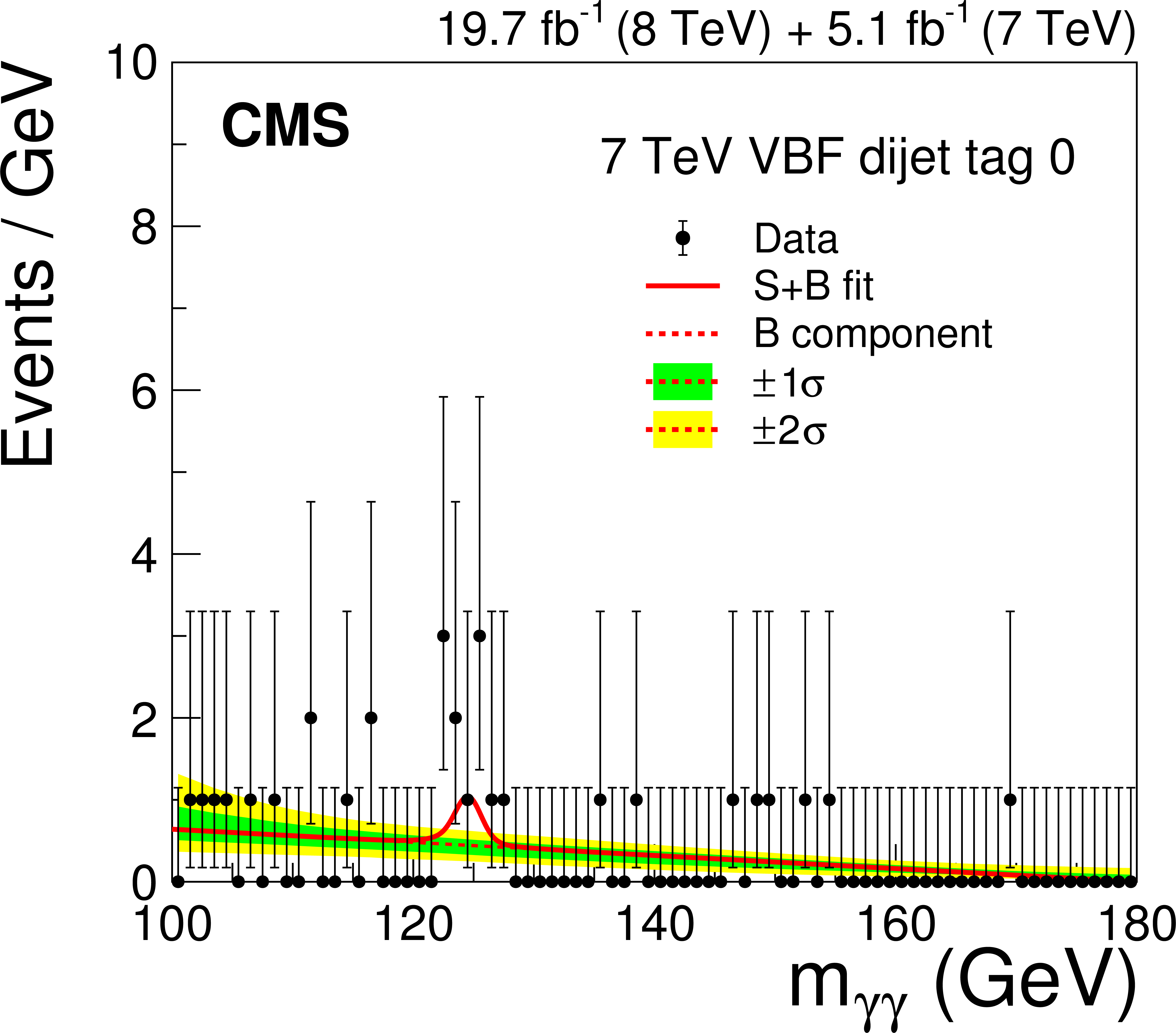
Figure 11-a:
Events in the two VBF dijet-tagged classes of the 7 TeV dataset, binned as a function of $ {m_{\gamma \gamma }} $, together with the result of a fit of the signal-plus-background model. The $1\sigma $ and $2\sigma $ uncertainty bands shown for the background component of the fit include the uncertainty due to the choice of function and the uncertainty in the fitted parameters. These bands do not contain the Poisson uncertainty that must be included when the full uncertainty in the number of background events in any given mass range is estimated. |

png pdf |
Figure 11-b:
Events in the two VBF dijet-tagged classes of the 7 TeV dataset, binned as a function of $ {m_{\gamma \gamma }} $, together with the result of a fit of the signal-plus-background model. The $1\sigma $ and $2\sigma $ uncertainty bands shown for the background component of the fit include the uncertainty due to the choice of function and the uncertainty in the fitted parameters. These bands do not contain the Poisson uncertainty that must be included when the full uncertainty in the number of background events in any given mass range is estimated. |
png pdf |
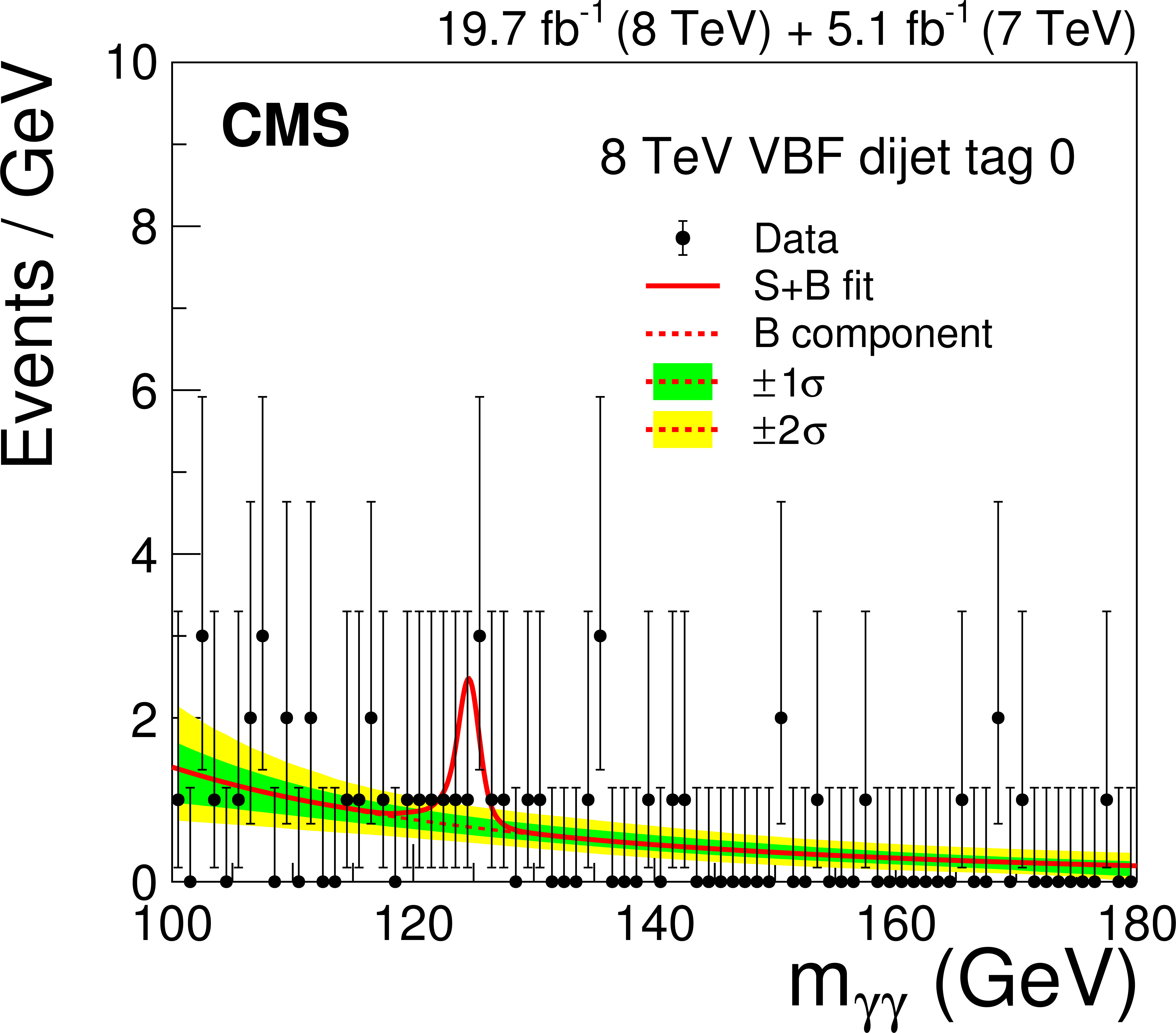
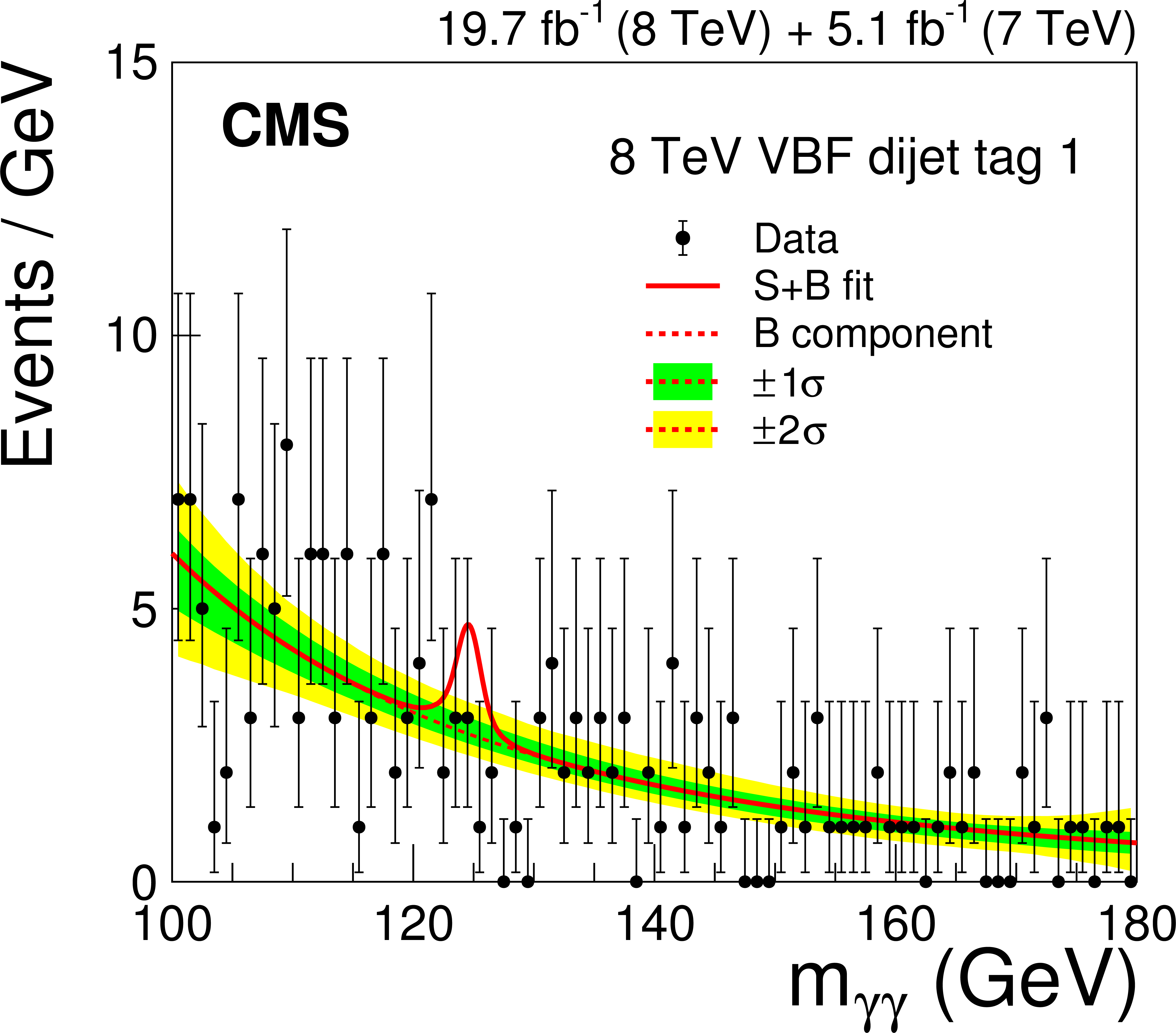
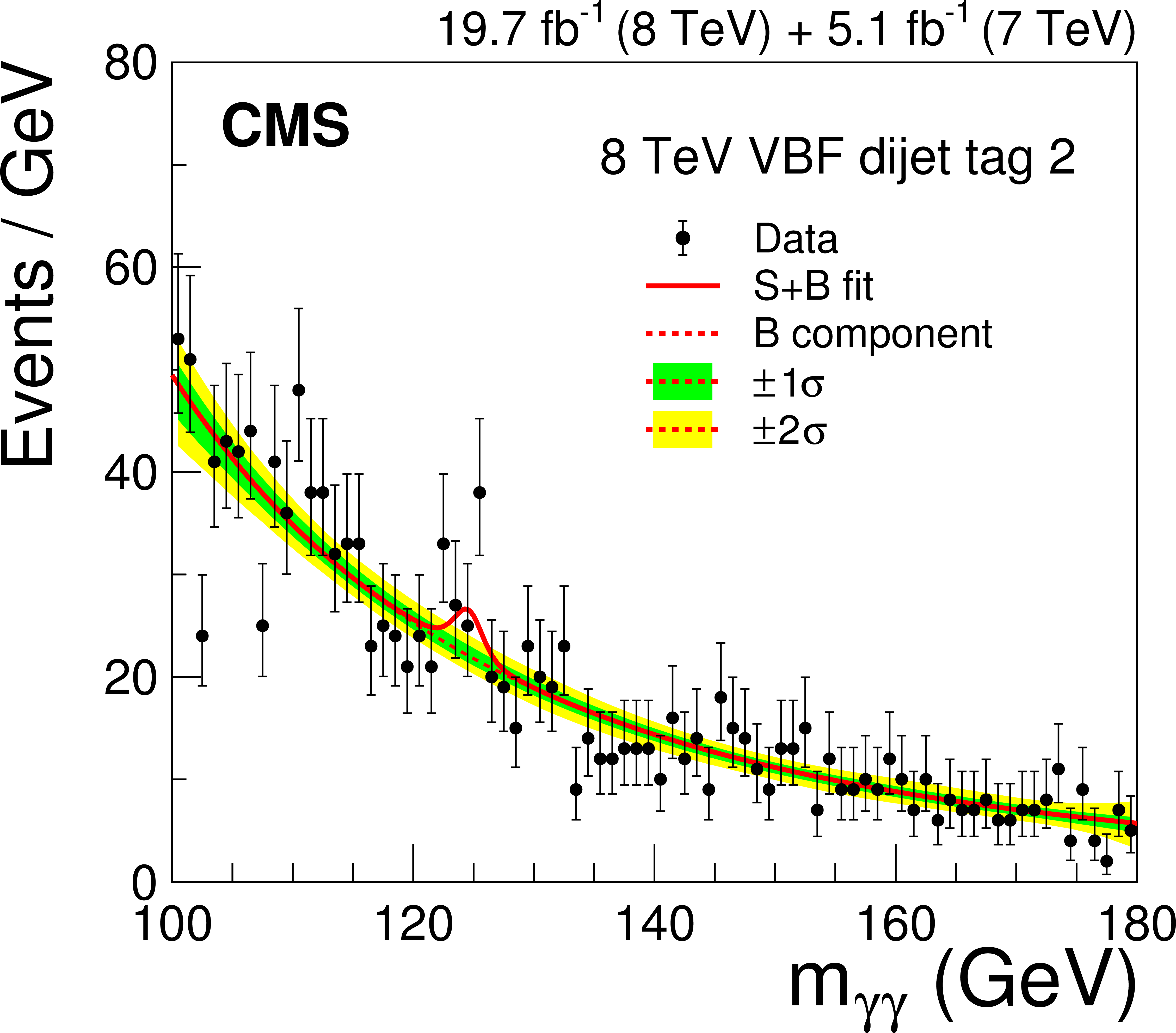
Figure 12-a:
Events in the three VBF dijet-tagged classes of the 8 TeV dataset, binned as a function of $ {m_{\gamma \gamma }} $, together with the result of a fit of the signal-plus-background model. The $1\sigma $ and $2\sigma $ uncertainty bands shown for the background component of the fit include the uncertainty due to the choice of function and the uncertainty in the fitted parameters. These bands do not contain the Poisson uncertainty that must be included when the full uncertainty in the number of background events in any given mass range is estimated. |
png pdf |
Figure 12-b:
Events in the three VBF dijet-tagged classes of the 8 TeV dataset, binned as a function of $ {m_{\gamma \gamma }} $, together with the result of a fit of the signal-plus-background model. The $1\sigma $ and $2\sigma $ uncertainty bands shown for the background component of the fit include the uncertainty due to the choice of function and the uncertainty in the fitted parameters. These bands do not contain the Poisson uncertainty that must be included when the full uncertainty in the number of background events in any given mass range is estimated. |
png pdf |
Figure 12-c:
Events in the three VBF dijet-tagged classes of the 8 TeV dataset, binned as a function of $ {m_{\gamma \gamma }} $, together with the result of a fit of the signal-plus-background model. The $1\sigma $ and $2\sigma $ uncertainty bands shown for the background component of the fit include the uncertainty due to the choice of function and the uncertainty in the fitted parameters. These bands do not contain the Poisson uncertainty that must be included when the full uncertainty in the number of background events in any given mass range is estimated. |

png pdf |
Figure 13-a:
Events in the VH-tagged classes of the 7 TeV dataset, binned as a function of $ {m_{\gamma \gamma }} $, together with the result of a fit of the signal-plus-background model. The $1\sigma $ and $2\sigma $ uncertainty bands shown for the background component of the fit include the uncertainty due to the choice of function and the uncertainty in the fitted parameters. These bands do not contain the Poisson uncertainty that must be included when the full uncertainty in the number of background events in any given mass range is estimated. |
png pdf |
Figure 13-b:
Events in the VH-tagged classes of the 7 TeV dataset, binned as a function of $ {m_{\gamma \gamma }} $, together with the result of a fit of the signal-plus-background model. The $1\sigma $ and $2\sigma $ uncertainty bands shown for the background component of the fit include the uncertainty due to the choice of function and the uncertainty in the fitted parameters. These bands do not contain the Poisson uncertainty that must be included when the full uncertainty in the number of background events in any given mass range is estimated. |
png pdf |
Figure 13-c:
Events in the VH-tagged classes of the 7 TeV dataset, binned as a function of $ {m_{\gamma \gamma }} $, together with the result of a fit of the signal-plus-background model. The $1\sigma $ and $2\sigma $ uncertainty bands shown for the background component of the fit include the uncertainty due to the choice of function and the uncertainty in the fitted parameters. These bands do not contain the Poisson uncertainty that must be included when the full uncertainty in the number of background events in any given mass range is estimated. |
png pdf |
Figure 13-d:
Events in the VH-tagged classes of the 7 TeV dataset, binned as a function of $ {m_{\gamma \gamma }} $, together with the result of a fit of the signal-plus-background model. The $1\sigma $ and $2\sigma $ uncertainty bands shown for the background component of the fit include the uncertainty due to the choice of function and the uncertainty in the fitted parameters. These bands do not contain the Poisson uncertainty that must be included when the full uncertainty in the number of background events in any given mass range is estimated. |
png pdf |
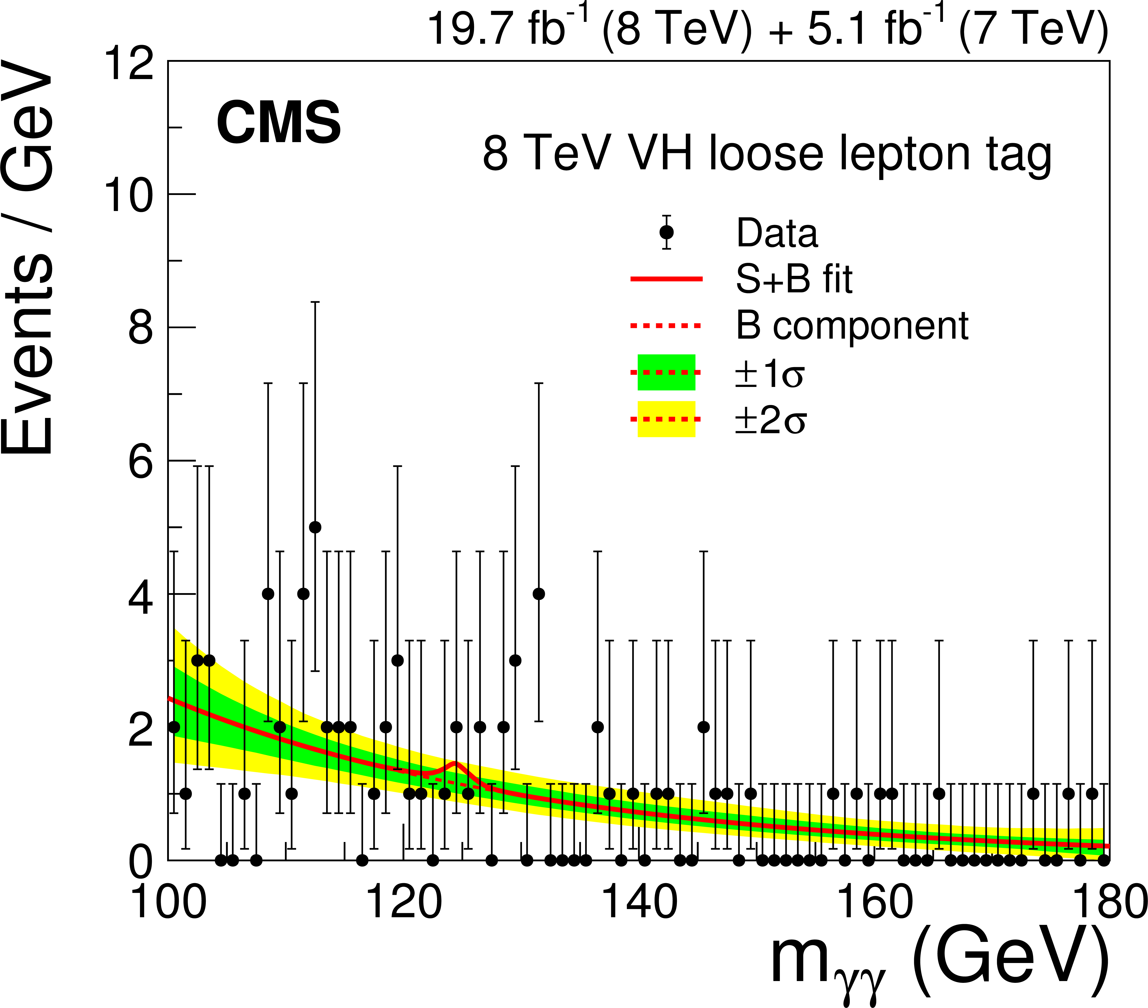
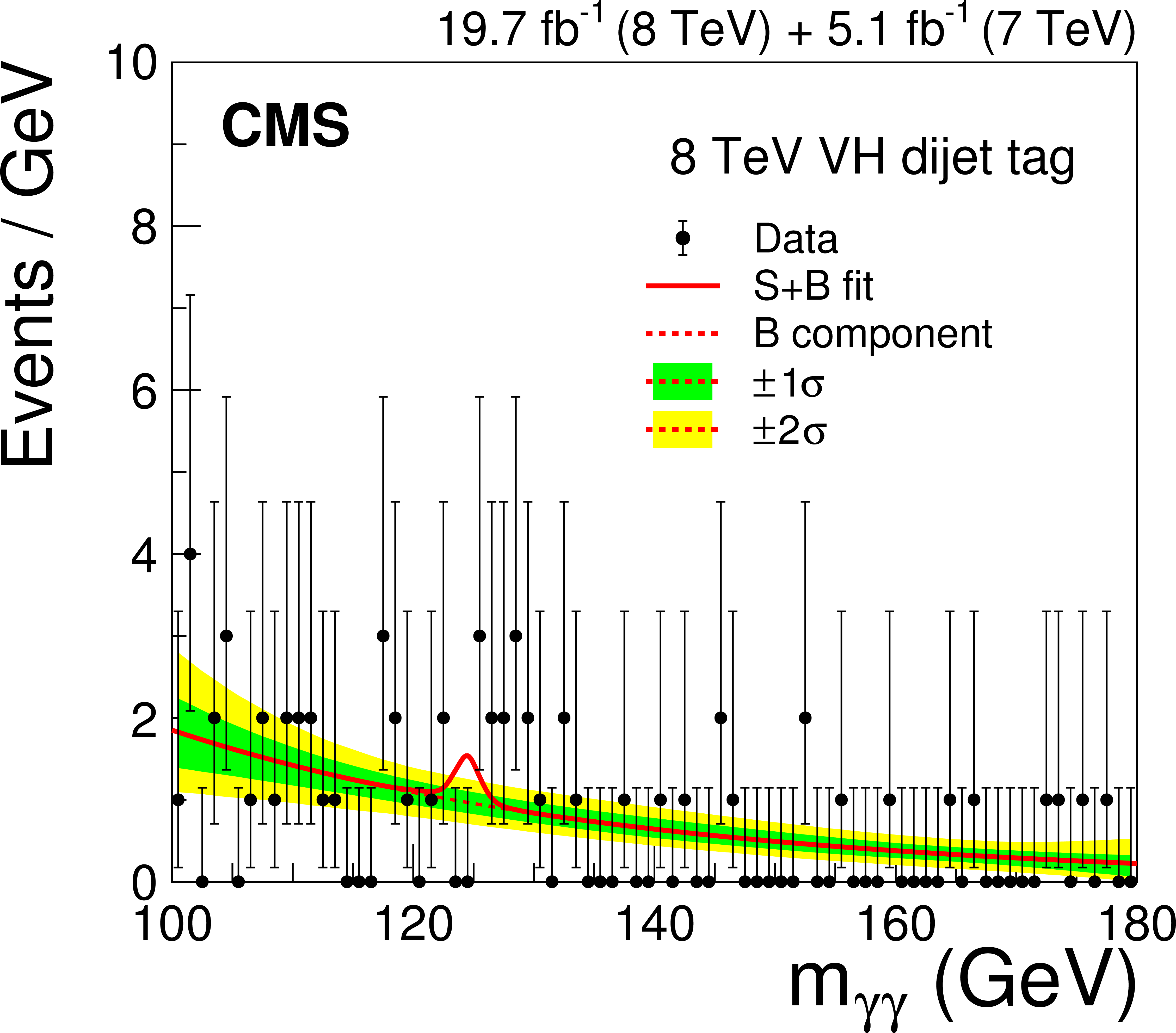
Figure 14-a:
Events in the VH-tagged classes of the 8 TeV dataset, binned as a function of $ {m_{\gamma \gamma }} $, together with the result of a fit of the signal-plus-background model. The $1\sigma $ and $2\sigma $ uncertainty bands shown for the background component of the fit are computed from the fit uncertainty in the background yield in bins corresponding to those used to display the data. These bands do not contain the Poisson uncertainty that must be included when the full uncertainty in the number of background events in any given mass range is estimated. |
png pdf |
Figure 14-b:
Events in the VH-tagged classes of the 8 TeV dataset, binned as a function of $ {m_{\gamma \gamma }} $, together with the result of a fit of the signal-plus-background model. The $1\sigma $ and $2\sigma $ uncertainty bands shown for the background component of the fit are computed from the fit uncertainty in the background yield in bins corresponding to those used to display the data. These bands do not contain the Poisson uncertainty that must be included when the full uncertainty in the number of background events in any given mass range is estimated. |

png pdf |
Figure 14-c:
Events in the VH-tagged classes of the 8 TeV dataset, binned as a function of $ {m_{\gamma \gamma }} $, together with the result of a fit of the signal-plus-background model. The $1\sigma $ and $2\sigma $ uncertainty bands shown for the background component of the fit are computed from the fit uncertainty in the background yield in bins corresponding to those used to display the data. These bands do not contain the Poisson uncertainty that must be included when the full uncertainty in the number of background events in any given mass range is estimated. |
png pdf |
Figure 14-d:
Events in the VH-tagged classes of the 8 TeV dataset, binned as a function of $ {m_{\gamma \gamma }} $, together with the result of a fit of the signal-plus-background model. The $1\sigma $ and $2\sigma $ uncertainty bands shown for the background component of the fit are computed from the fit uncertainty in the background yield in bins corresponding to those used to display the data. These bands do not contain the Poisson uncertainty that must be included when the full uncertainty in the number of background events in any given mass range is estimated. |
png pdf |
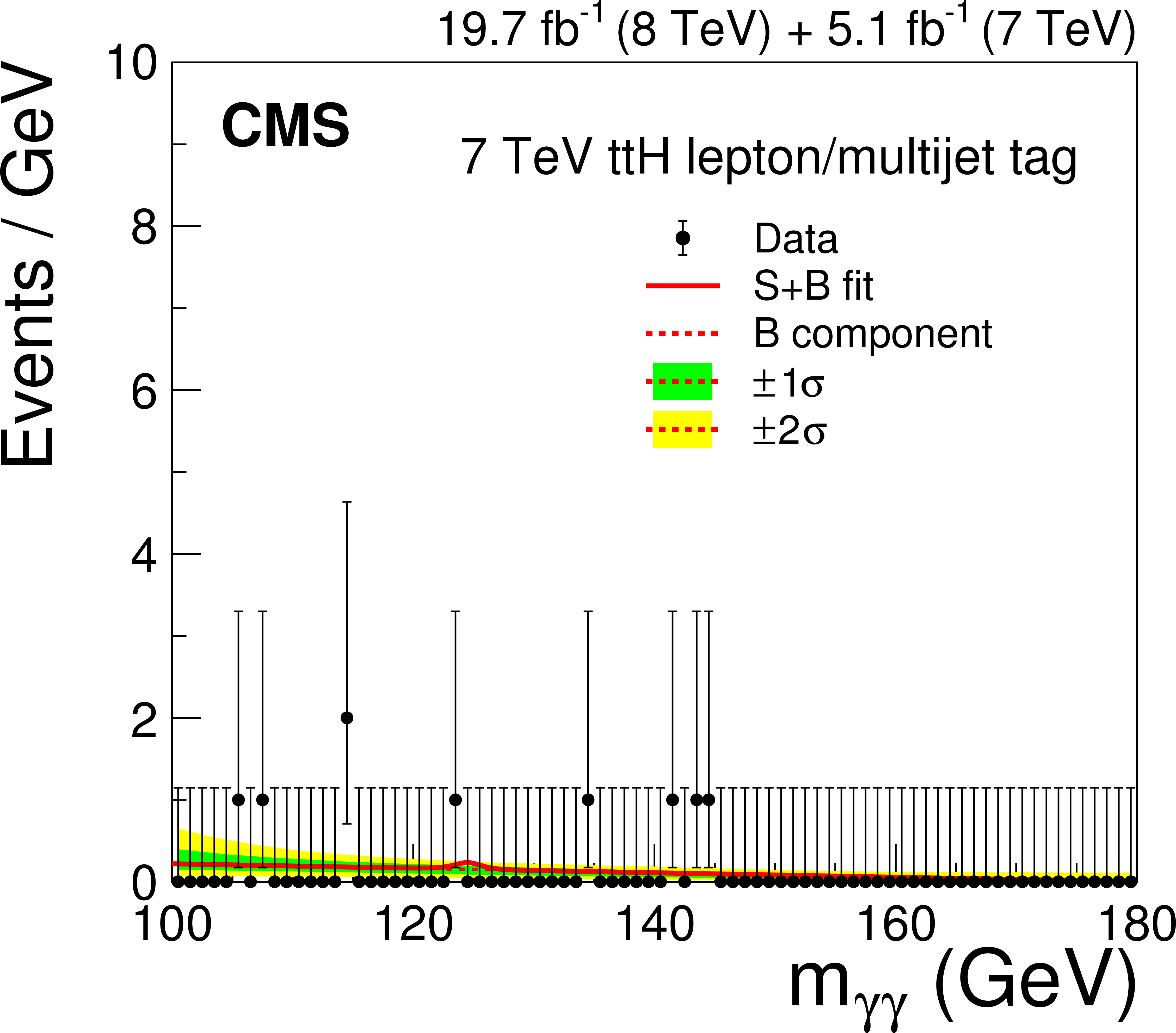
Figure 15:
Events in the $ { {\mathrm {t}} {\overline {\mathrm {t}}} {\mathrm {H}} } $-tagged class of the 7 TeV dataset, binned as a function of $ {m_{\gamma \gamma }} $, together with the result of a fit of the signal-plus-background model for $ {m_ {\mathrm {H}} }$ = 124.7 GeV. The $1\sigma $ and $2\sigma $ uncertainty bands shown for the background component of the fit include the uncertainty due to the choice of function and the uncertainty in the fitted parameters. These bands do not contain the Poisson uncertainty that must be included when the full uncertainty in the number of background events in any given mass range is estimated. |
png pdf |
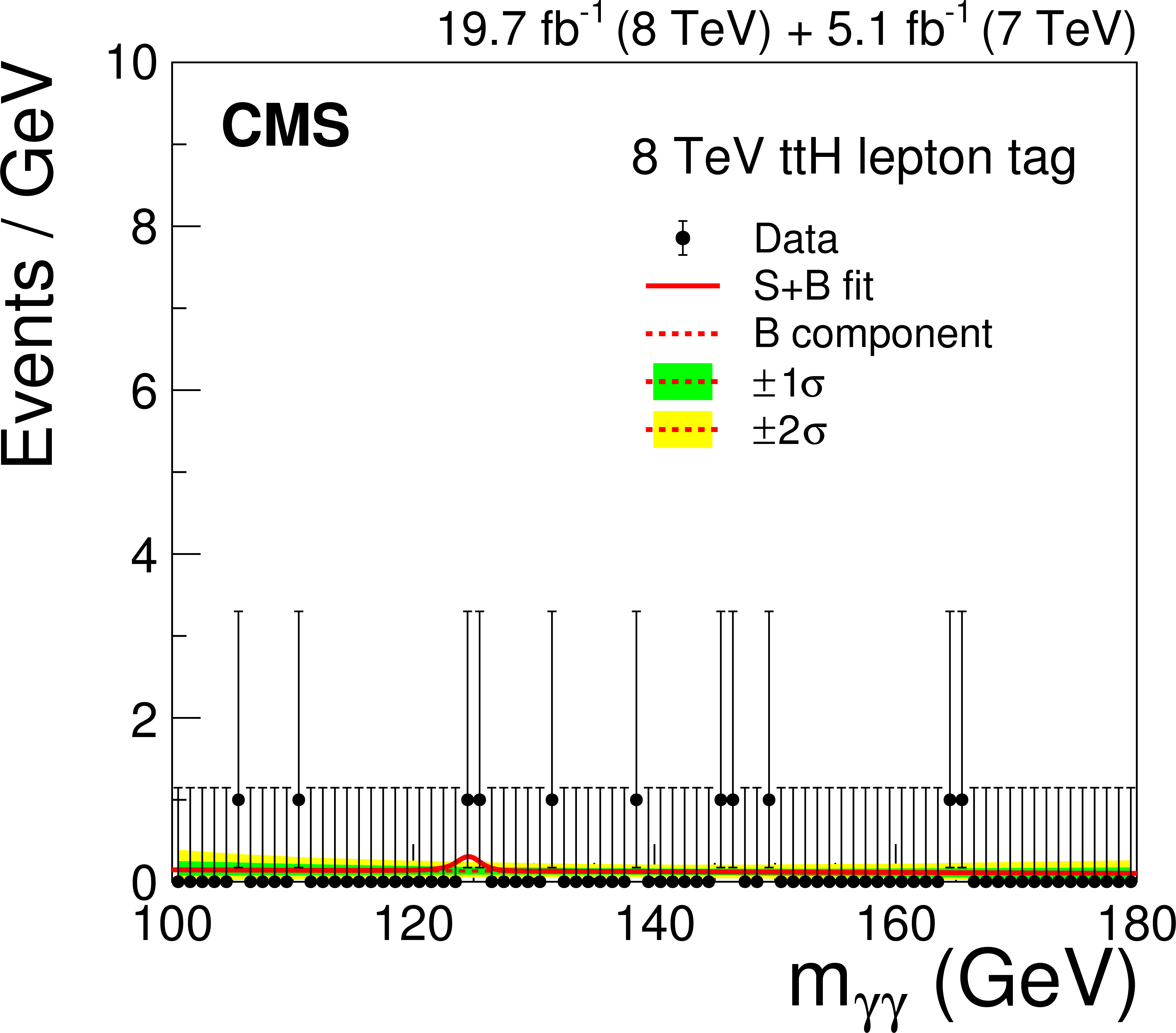
Figure 16-a:
Events in the two $ { {\mathrm {t}} {\overline {\mathrm {t}}} {\mathrm {H}} } $-tagged classes of the 8 TeV dataset, binned as a function of $ {m_{\gamma \gamma }} $, together with the result of a fit of the signal-plus-background model. The $1\sigma $ and $2\sigma $ uncertainty bands shown for the background component of the fit are computed from the fit uncertainty in the background yield in bins corresponding to those used to display the data. These bands do not contain the Poisson uncertainty that must be included when the full uncertainty in the number of background events in any given mass range is estimated. |
png pdf |
Figure 16-b:
Events in the two $ { {\mathrm {t}} {\overline {\mathrm {t}}} {\mathrm {H}} } $-tagged classes of the 8 TeV dataset, binned as a function of $ {m_{\gamma \gamma }} $, together with the result of a fit of the signal-plus-background model. The $1\sigma $ and $2\sigma $ uncertainty bands shown for the background component of the fit are computed from the fit uncertainty in the background yield in bins corresponding to those used to display the data. These bands do not contain the Poisson uncertainty that must be included when the full uncertainty in the number of background events in any given mass range is estimated. |
png pdf |
Figure 17:
Sum of the 25 signal-plus-background model fits to the event classes in both the 7 and 8 TeV datasets, together with the data binned as a function of ${m_{\gamma \gamma }}$ . The $1\sigma $ and $2\sigma $ uncertainty bands shown for the background component of the fit are computed from the fit uncertainty in the background yield in bins corresponding to those used to display the data. These bands do not contain the Poisson uncertainty that must be included when the full uncertainty in the number of background events in any given mass range is estimated. The lower plot shows the residual data after subtracting the fitted background component. |
png pdf |
Figure 18:
Local $p$-values as a function of $ {m_ {\mathrm {H}} }$ for the 7 TeV, 8 TeV, and the combined dataset. The values of the expected significance, calculated using the background expectation obtained from the signal-plus-background fit, are shown as dashed lines. |
png pdf |
Figure 19:
Diphoton mass spectrum weighted by the ratio $S/(S+B)$ in each event class, together with the background subtracted weighted mass spectrum. |
png pdf |
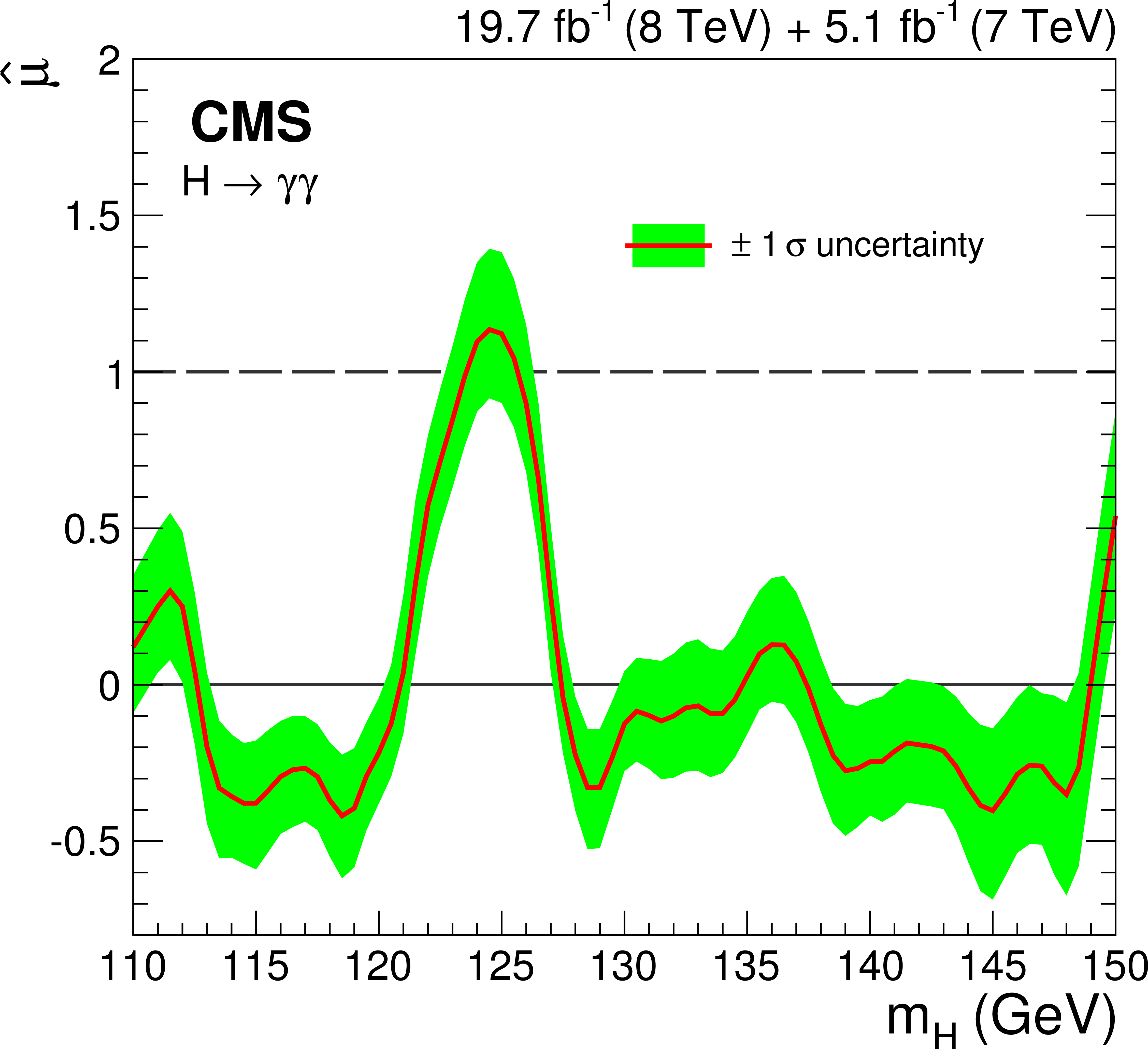
Figure 20-a:
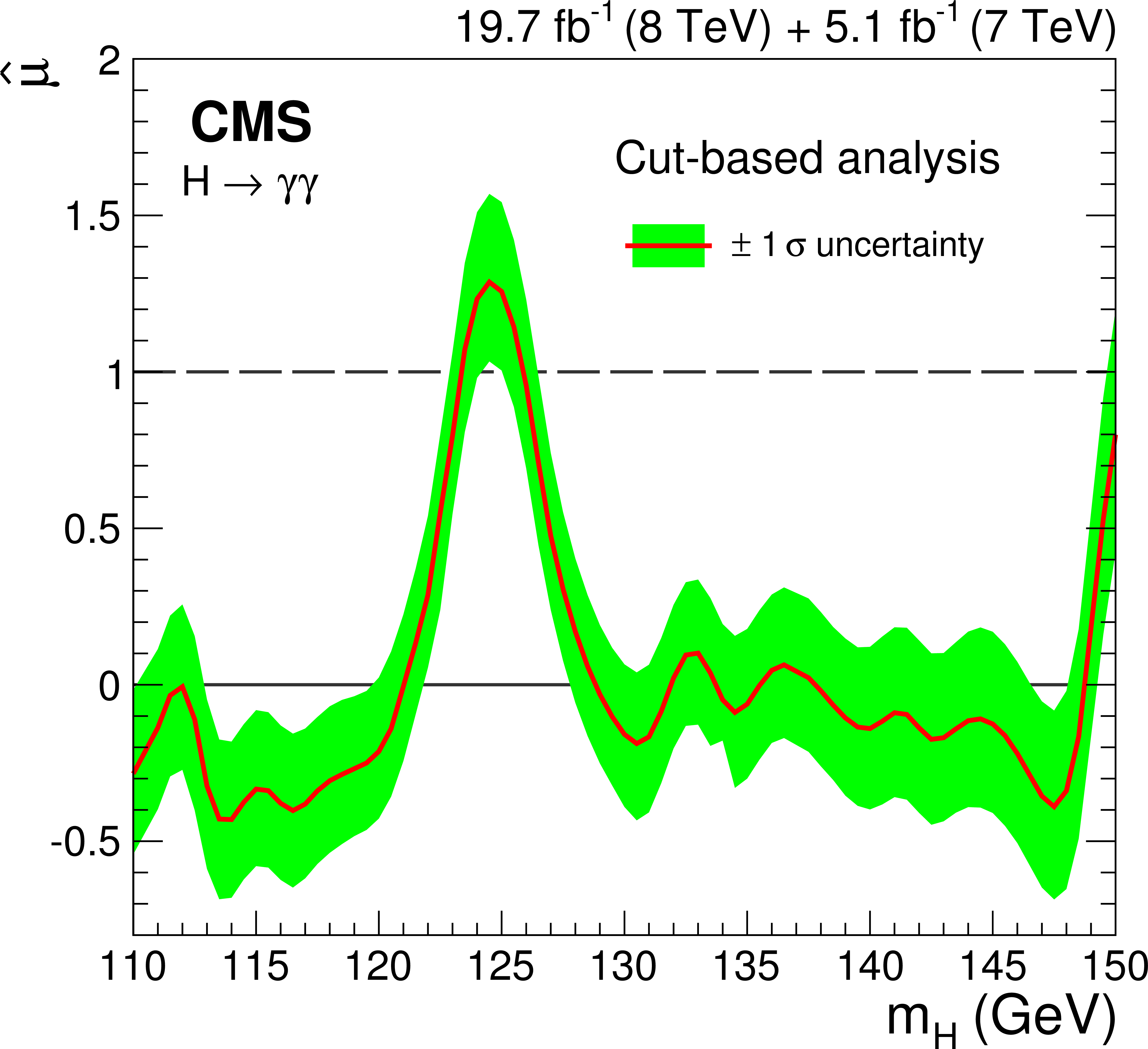
Best-fit signal strength, $ \hat{\mu } $, shown as a function of the mass hypothesis, ${m_ {\mathrm {H}} }$. The results are shown for the standard analysis (a), and for the cut-based cross-check analysis (b). |
png pdf |
Figure 20-b:
Best-fit signal strength, $ \hat{\mu } $, shown as a function of the mass hypothesis, ${m_ {\mathrm {H}} }$. The results are shown for the standard analysis (a), and for the cut-based cross-check analysis (b). |
png pdf |
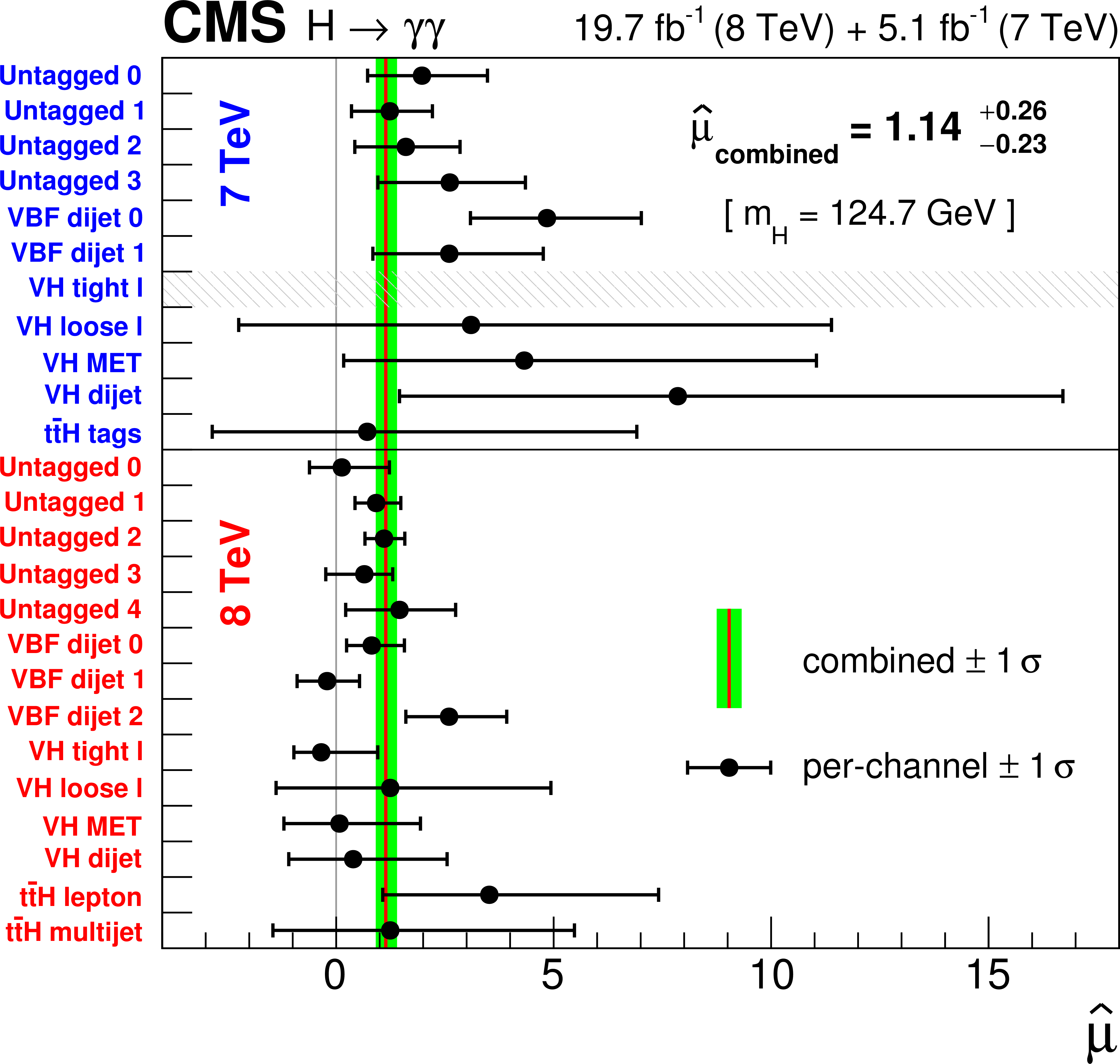
Figure 21:
Values of $ \hat{\mu} $ measured individually for all event classes in the 7 and 8 TeV datasets, fixing $ {m_ {\mathrm {H}} }$ =124.7 GeV. The horizontal bars indicate ${\pm }1\sigma $ uncertainties in the values, and the vertical line and band indicate the best-fit signal strength in the combined fit to the data and its uncertainty. |
png pdf |
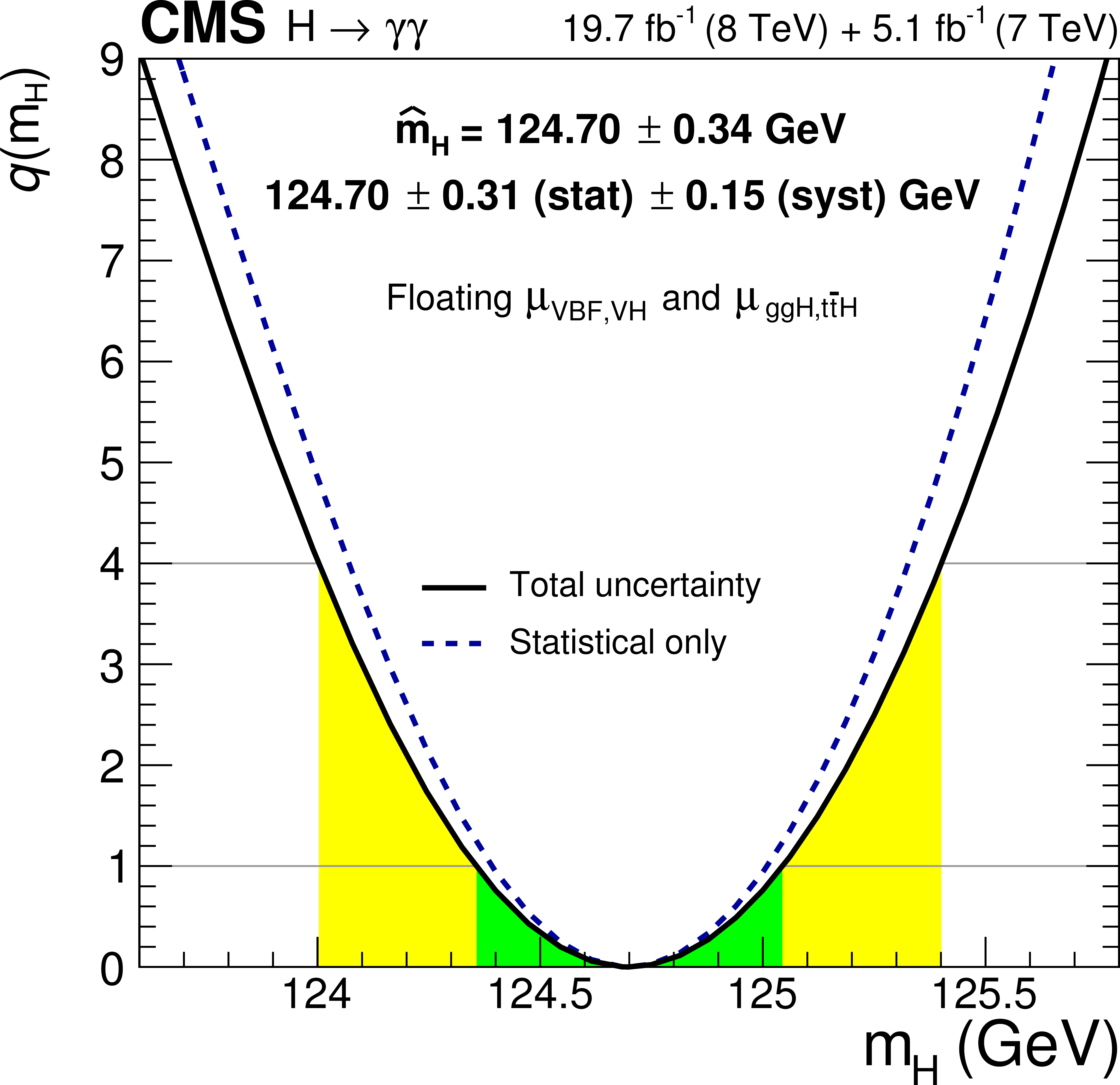
Figure 22-a:
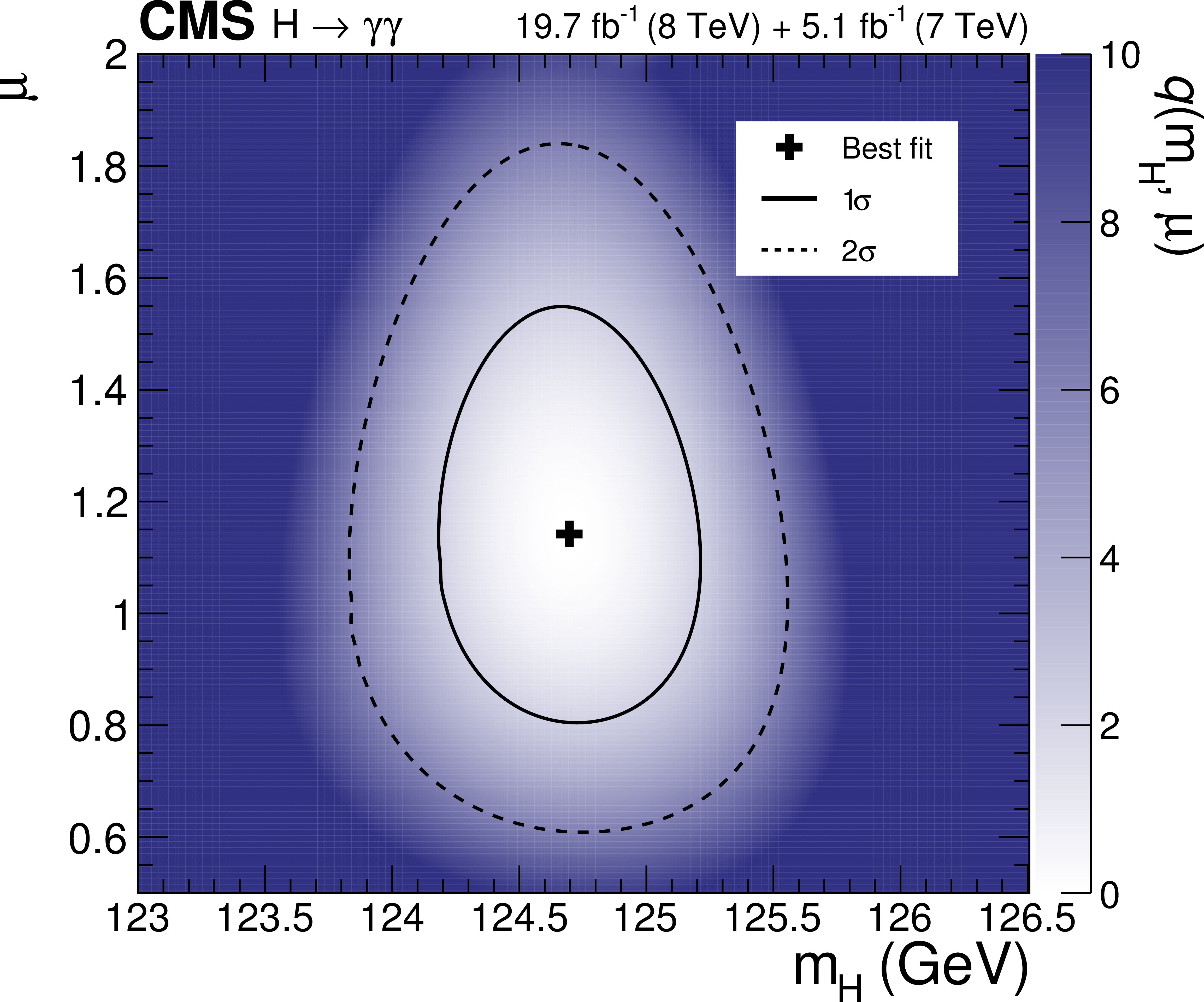
(a) Scan of the likelihood ratio, $q$, as a function of the hypothesised mass when $\mu _{ {\mathrm {g}} {\mathrm {g}} {\mathrm {H}} , { {\mathrm {t}} {\overline {\mathrm {t}}} {\mathrm {H}} } }$ and $\mu _\text {VBF, VH}$ are allowed to vary independently. (b) Map of $q( {m_ {\mathrm {H}} },\mu )$ showing the $1\sigma $ and $2\sigma $ regions, and the best-fit point $( \hat{m}_{\mathrm{H}} , \hat{\mu} )$ = (124.70 GeV ,1.14). |
png pdf |
Figure 22-b:
(a) Scan of the likelihood ratio, $q$, as a function of the hypothesised mass when $\mu _{ {\mathrm {g}} {\mathrm {g}} {\mathrm {H}} , { {\mathrm {t}} {\overline {\mathrm {t}}} {\mathrm {H}} } }$ and $\mu _\text {VBF, VH}$ are allowed to vary independently. (b) Map of $q( {m_ {\mathrm {H}} },\mu )$ showing the $1\sigma $ and $2\sigma $ regions, and the best-fit point $( \hat{m}_{\mathrm{H}} , \hat{\mu} )$ = (124.70 GeV ,1.14). |
png pdf |
Figure 23:
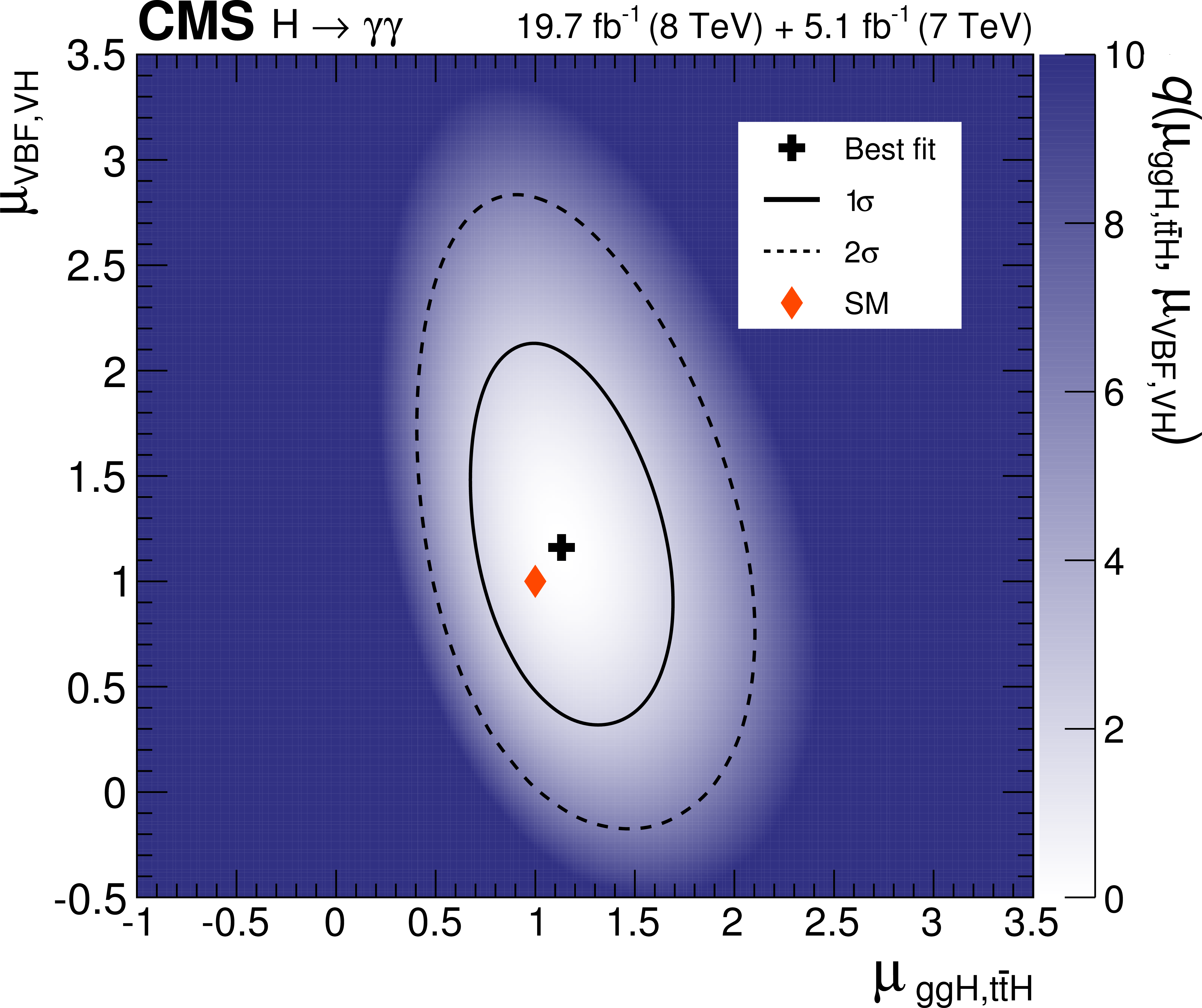
Map of the likelihood ratio $q(\mu _{ {\mathrm {g}} {\mathrm {g}} {\mathrm {H}} , { {\mathrm {t}} {\overline {\mathrm {t}}} {\mathrm {H}} } },\mu _\text {VBF, VH})$ with ${m_ {\mathrm {H}} }$ treated as an unconstrained parameter. The $1\sigma $ and $2\sigma $ uncertainty contours are shown. The cross indicates the best-fit values, ($ \hat{\mu} _{ {\mathrm {g}} {\mathrm {g}} {\mathrm {H}} , { {\mathrm {t}} {\overline {\mathrm {t}}} {\mathrm {H}} } }, \hat{\mu} _\text {VBF, VH})=(1.13, 1.16)$, and the diamond represents the SM expectation. |
png pdf |
Figure 24:
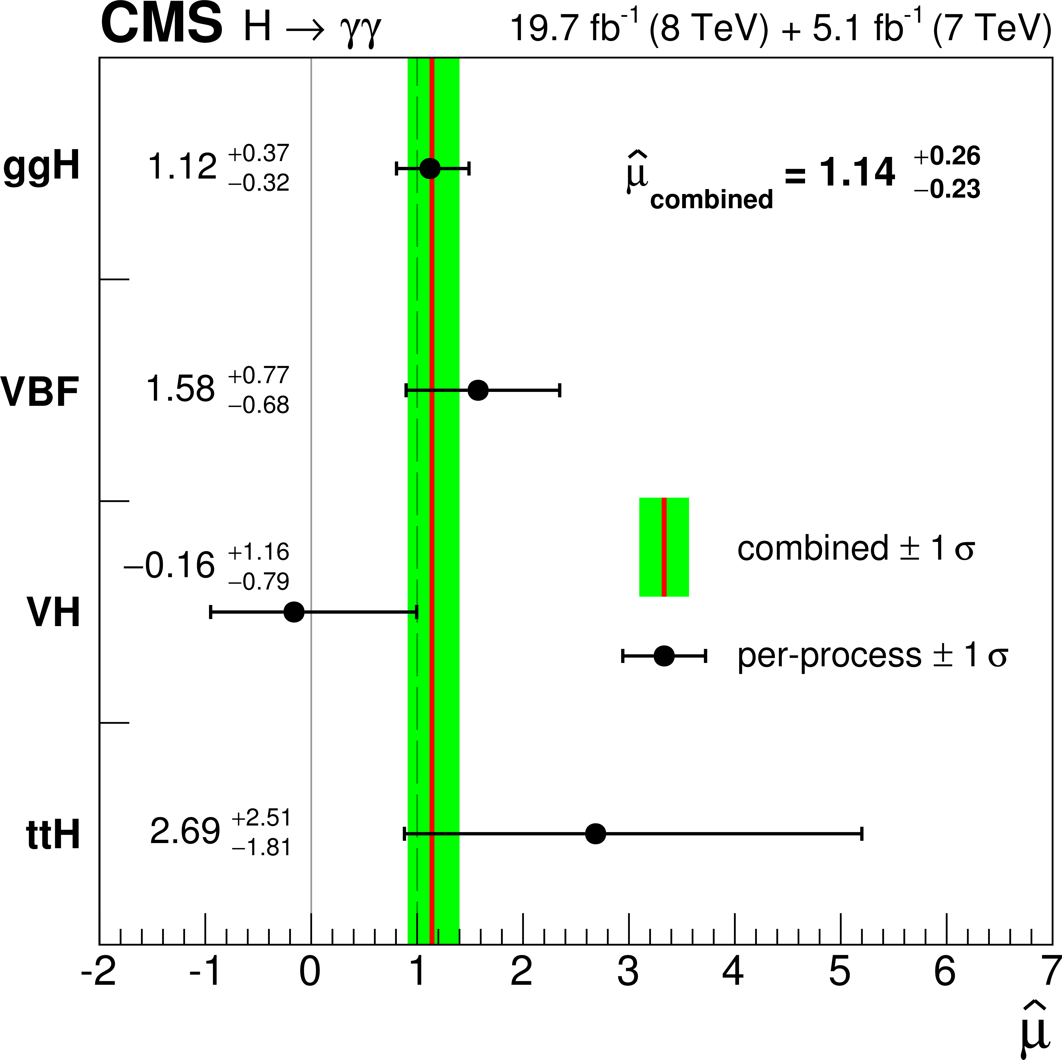
Best-fit signal strength, $ \hat{\mu} $, measured for each of the production processes in a combined fit where the signal strengths of all four processes have been allowed to vary independently in the fit. The signal mass, common to all four processes, is treated as an unconstrained parameter in the fit. The horizontal bars indicate ${\pm }1\sigma $ uncertainties in the values for the individual processes. The band corresponds to ${\pm }1\sigma $ uncertainties in the value obtained from the combined fit with a single signal strength. |

png pdf |
Figure 25-a:
Maps of the likelihood ratio $q( {\kappa _\mathrm {V}} , {\kappa _\mathrm {f}} )$ (a), and $q( {\kappa _{\gamma }} , {\kappa _\mathrm {g}} )$ (b), showing the $1\sigma $ and $2\sigma $ uncertainty contours. The crosses indicate the best-fit values, and the diamonds indicate the SM expectation. |

png pdf |
Figure 25-b:
Maps of the likelihood ratio $q( {\kappa _\mathrm {V}} , {\kappa _\mathrm {f}} )$ (a), and $q( {\kappa _{\gamma }} , {\kappa _\mathrm {g}} )$ (b), showing the $1\sigma $ and $2\sigma $ uncertainty contours. The crosses indicate the best-fit values, and the diamonds indicate the SM expectation. |
png pdf |
Figure 26:
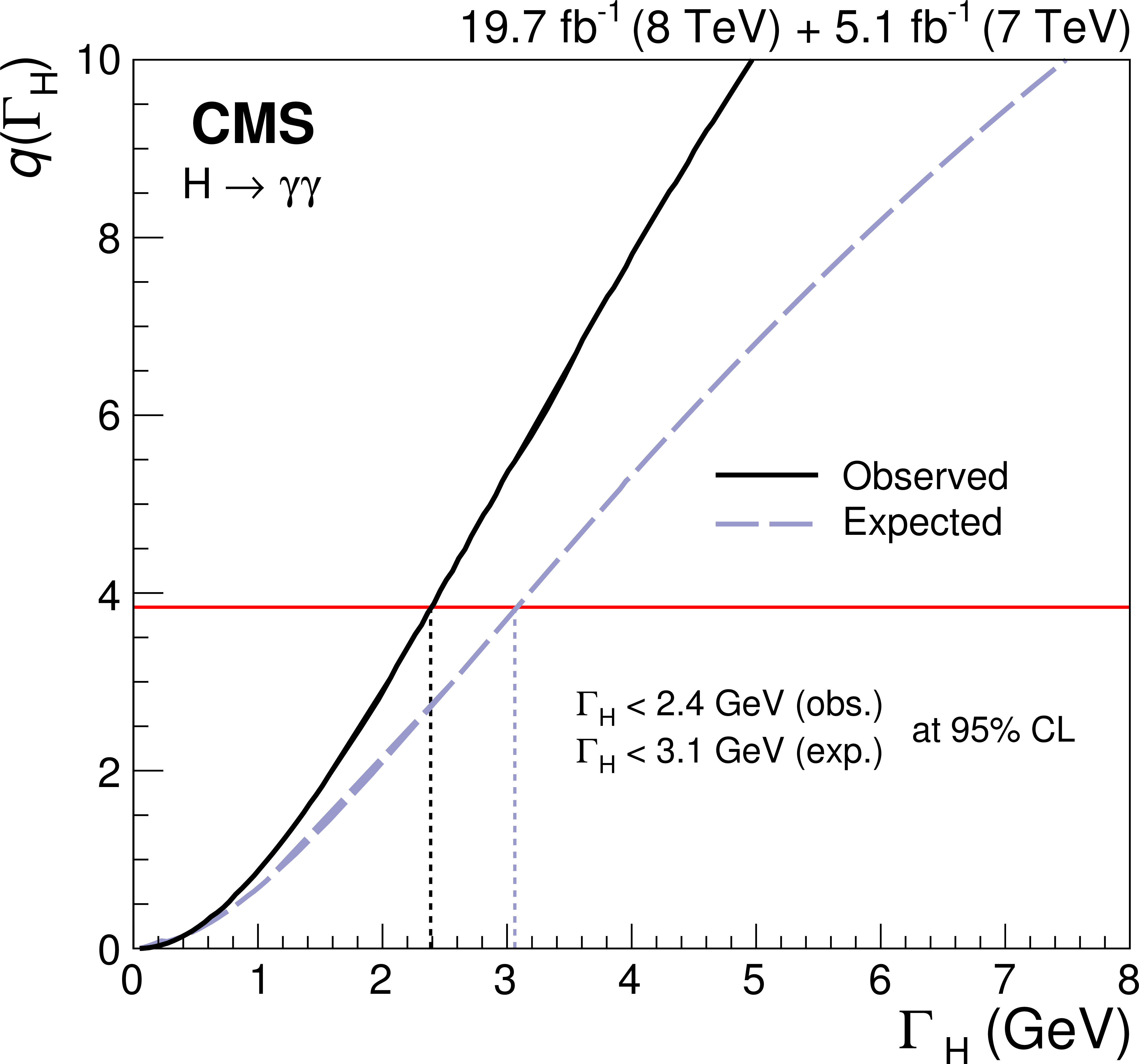
Scan of the negative-log-likelihood ratio as a function of the Higgs boson decay width. The observed (expected) upper limit on the width is found to be 2.4 (3.1) GeV at a 95% CL. |
png pdf |
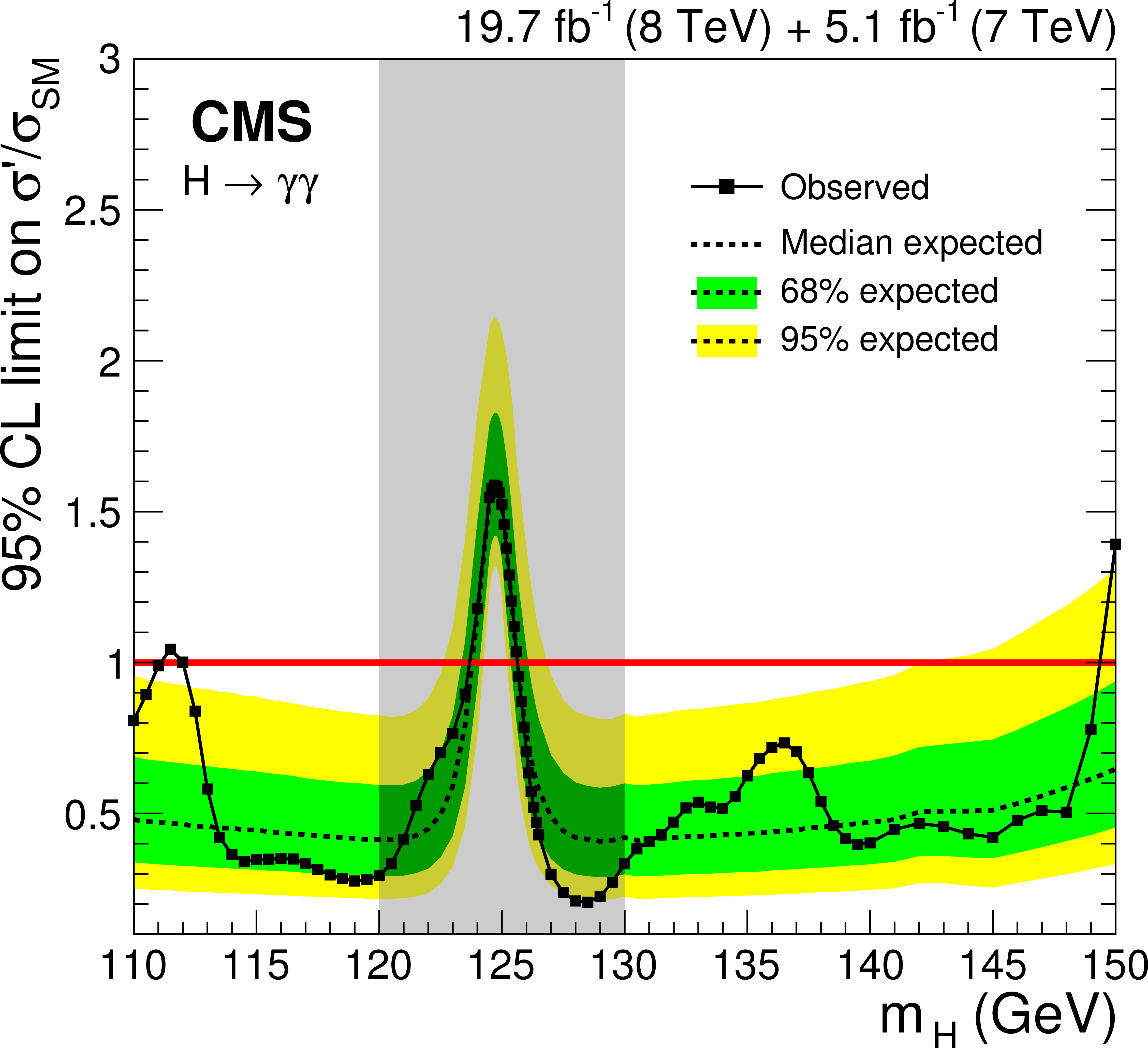
Figure 27:
Exclusion limit on the signal strength, $ {\sigma \mathrm {'}/\sigma _\mathrm {SM}} $, for a second Higgs-boson-like state with SM couplings taking the observed state at 125 GeV as part of the background. The shading indicates a window with a width of 10 GeV , centred at the best-fit mass, where the expected sensitivity to a second Higgs boson is severely degraded due to the presence of the already observed state. |
png pdf |
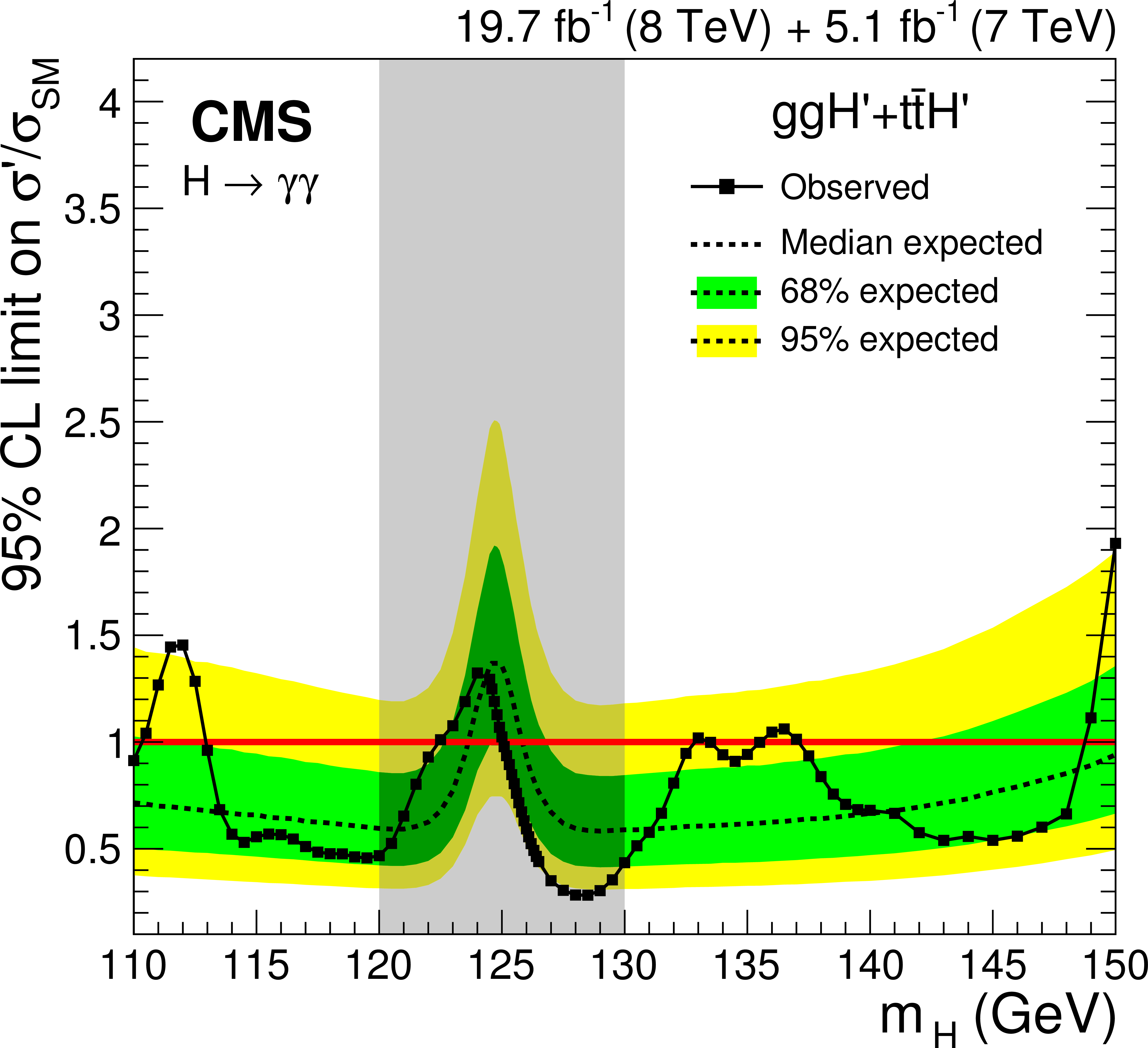
Figure 28-a:
Exclusion limits on $ {\sigma \mathrm {'}/\sigma _\mathrm {SM}} $ for a second Higgs-boson-like state produced with gluon-gluon fusion only (left) or VBF and VH only (right) taking the observed state at 125 GeV as part of the background. The shading indicates a window with a width of 10 GeV, centred at the best-fit mass, where the expected sensitivity to a second Higgs boson is severely degraded due to the presence of the already observed state. |
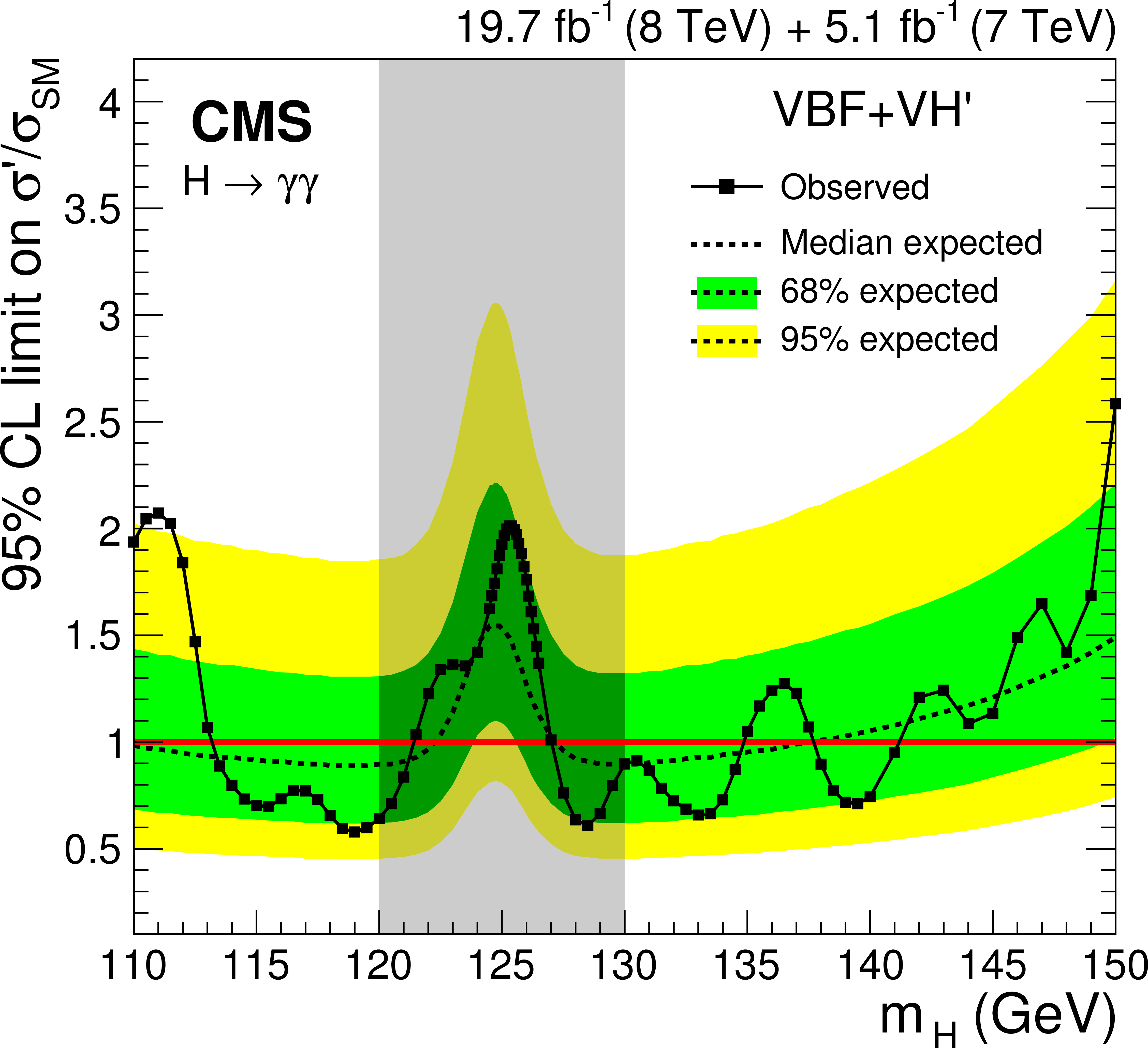
png pdf |
Figure 28-b:
Exclusion limits on $ {\sigma \mathrm {'}/\sigma _\mathrm {SM}} $ for a second Higgs-boson-like state produced with gluon-gluon fusion only (left) or VBF and VH only (right) taking the observed state at 125 GeV as part of the background. The shading indicates a window with a width of 10 GeV, centred at the best-fit mass, where the expected sensitivity to a second Higgs boson is severely degraded due to the presence of the already observed state. |
png pdf |
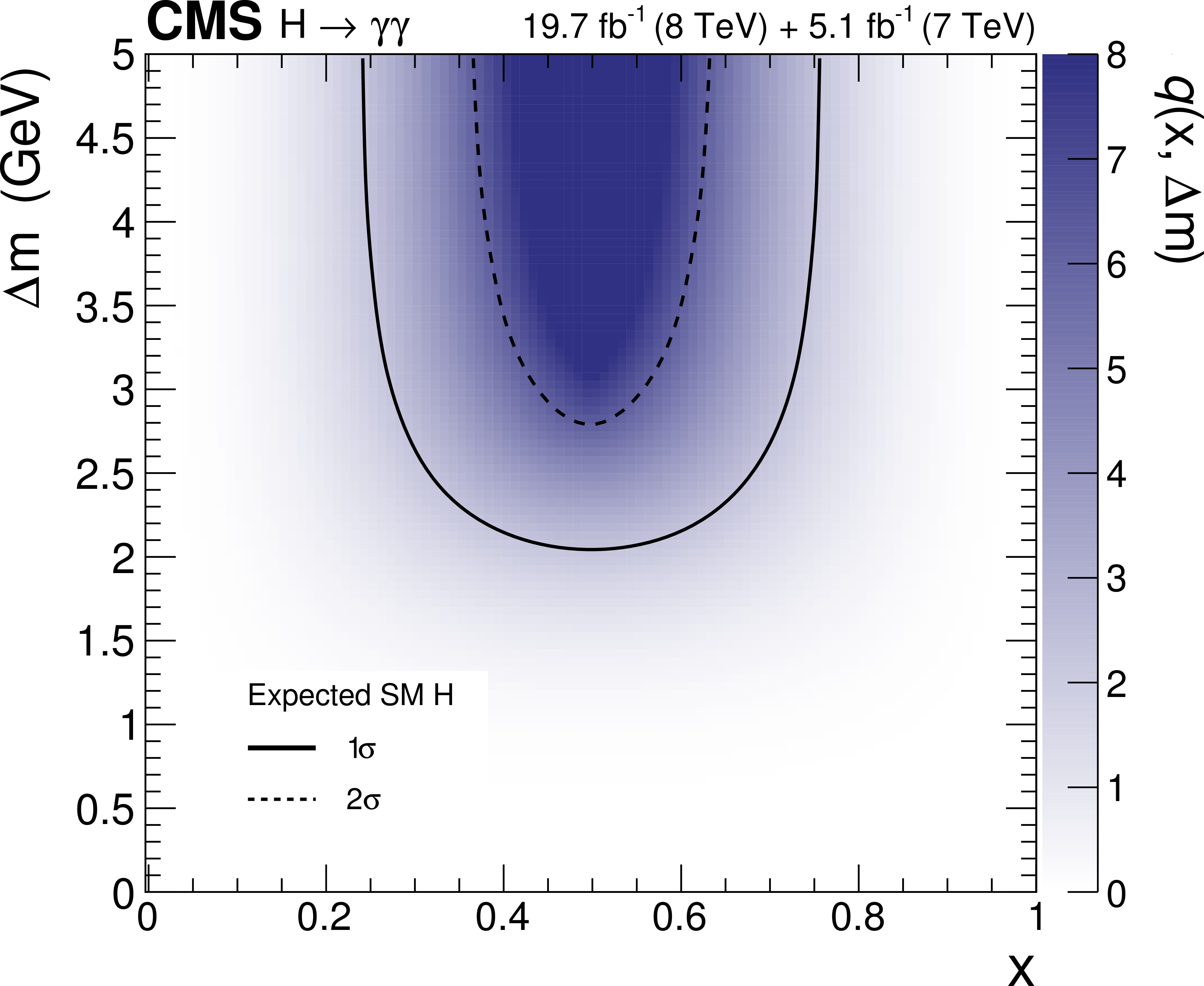
Figure 29-a:
Map of the values of the likelihood ratio $q(x,\Delta m)$ for two near mass-degenerate states parameterized by $x$ (the fraction of signal in the lower mass state) and $\Delta m$ (the mass difference between the states). The black cross shows the best-fit value, and the lines correspond to the $1\sigma $ and $2\sigma $ uncertainty contours for the SM (single state) expectation (upper plot) and the observation (lower plot). |
png pdf |
Figure 29-b:
Map of the values of the likelihood ratio $q(x,\Delta m)$ for two near mass-degenerate states parameterized by $x$ (the fraction of signal in the lower mass state) and $\Delta m$ (the mass difference between the states). The black cross shows the best-fit value, and the lines correspond to the $1\sigma $ and $2\sigma $ uncertainty contours for the SM (single state) expectation (upper plot) and the observation (lower plot). |

png pdf |
Figure 30:
Product of acceptance and efficiency $A\times \epsilon $ for ${0^{+}}$ (all SM production modes), ${2^{+}_{m}}$ (gluon-fusion) and $ {2^{+}_{m}} $ ($ {\mathrm {q}} {\overline {\mathrm {q}}}$ production) as a function of $ | \cos{ \theta^*}_{\mathrm{SC} } | $, as calculated for the 8 TeV dataset. The value of $A\times \epsilon $ for the ${2^{+}_{m}}$ models divided by $A\times \epsilon $ for SM is shown below, where the bands indicate the spread of values among the four diphoton classes. The $ | \cos{ \theta^*}_{\mathrm{SC} }| $ bin boundaries are shown by vertical dashed lines. |
png pdf |
Figure 31:
Histograms showing signal strength in five bins of $ | \cos{ \theta^*}_{\mathrm{SC} }| $ expected for SM, for $ {2^{+}_{m}} $ produced by $ {\mathrm {g}} {\mathrm {g}}$, and for ${2^{+}_{m}}$ produced by $ {\mathrm {q}} {\overline {\mathrm {q}}}$. The signal strength observed in the data is shown by the black points. |

png pdf |
Figure 32:
Test statistic for pseudo-experiments generated under the SM, $ {0^{+}} $, hypothesis (open squares) and the graviton-like, ${2^{+}_{m}} $, hypothesis (open diamonds), as a function of the fraction, $ {f_{ {\mathrm {q}} {\overline {\mathrm {q}}}}} $, of $ {\mathrm {q}} {\overline {\mathrm {q}}}$ production. The observed distribution in the data is shown by the black points. |
| Tables | |
png pdf |
Table 1:
Photon preselection efficiencies for both the 7 and 8 TeV datasets measured for $ {\mathrm{ Z } \to \mathrm{ e }^- \mathrm{ e }^+ } $ events, where the electrons are reconstructed as photons, in four photon categories. The statistical uncertainties in the efficiencies found in simulated events are negligible, and the uncertainties measured in data are discussed in the text. |

png pdf |
Table 2:
Event classes for the 7 and 8 TeV datasets and some of their main selection requirements. Events are tested against the selection requirements of the classes in the order they are listed here. |
png pdf |
Table 3:
Expected number of SM Higgs boson events ($ {m_\mathrm{ H } }= $ 125 GeV) and estimated background (``Bkg.'') at $ {m_{\gamma \gamma }} = $ 125 GeV for all event classes of the 7 and 8 TeV datasets. The composition of the SM Higgs boson signal in terms of the production processes and its mass resolution is also given. The number corresponding to the production process making the largest contribution to each event class is highlighted in boldface. Numbers are omitted for production processes representing less than 0.05% of the total signal. The variables used to characterize the resolution, $\sigma _\text {eff}$ and $\sigma _\mathrm {HM}$, are defined in the text. |
png pdf |
Table 4:
Selection requirements for the VBF dijet tag in the cut-based and dijet 2D analyses. The variables are defined in the text. |
png pdf |
Table 5:
Values of the best-fit signal strength, $ {\hat{\mu }} $, when ${m_\mathrm{ H } }$ is treated as an unconstrained parameter, for the 7 TeV , 8 TeV , and combined datasets. The corresponding best-fit value of $ {m_\mathrm{ H } }$, $ { \hat{m}_\mathrm{ H } } $, is also given. |
png pdf |
Table 6:
Expected and observed best-fit values of the signal strength for a SM Higgs boson signal in the alternative analyses, together with their uncertainties, indicating the expected uncertainty in the measurement at the best-fit values of $ {m_\mathrm{ H } }$, and the best-fit values obtained from the data. The corresponding values for the main analysis are shown for comparison. |

png pdf |
Table 7:
Magnitude of the uncertainty in the best fit signal strength, $ {\hat{\mu }} $, induced by the systematic uncertainties in the signal model. To obtain the values, the quadratic subtraction, needed to remove the statistical uncertainty, is made for the positive and negative uncertainties separately. The values quoted are the average magnitudes of the positive and negative uncertainties. The statistical uncertainty includes all uncertainties in the background modelling. |

png pdf |
Table 8:
Magnitude of the uncertainty in the best fit mass induced by the systematic uncertainties in the signal model. These numbers have been obtained by quadratic subtraction of the statistical uncertainty. The statistical uncertainty includes all uncertainties in the background modelling. |
png pdf |
Table 9:
Expected and observed best-fit values of the signal strength modifiers $\mu _{ \mathrm{ggH } , \mathrm{ ttH } }$ and $\mu _{\text {VBF, VH}}$ for a SM Higgs boson signal together with their uncertainties, indicating the expected uncertainty in the measurement and the best-fit values obtained from the data. |
png pdf |
Table 10:
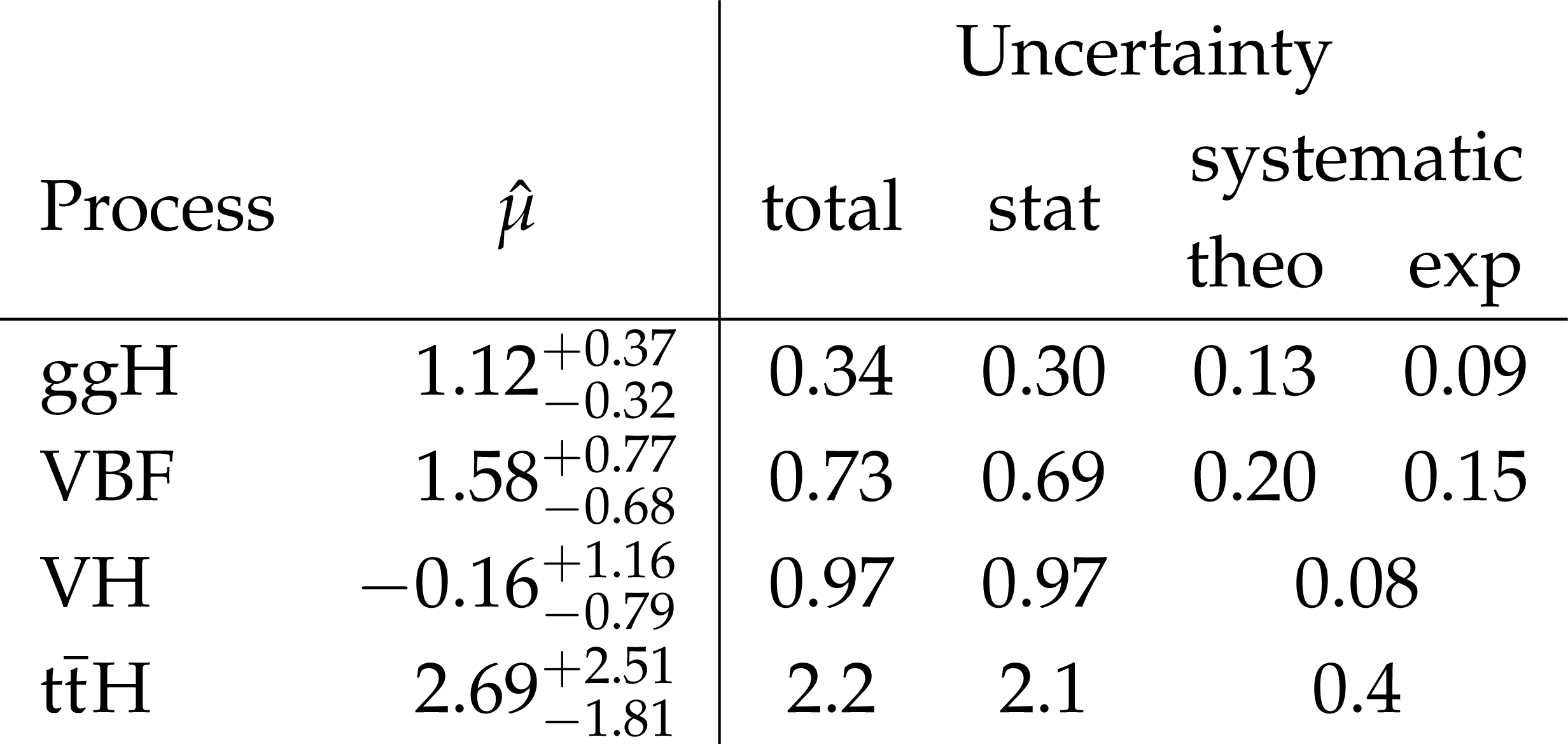
Best-fit signal strength modifiers for the four production processes. The total uncertainty for each process is separated into statistical (stat) and systematic contributions. The systematic uncertainty has been separated, where feasible, into the contributions from theoretical (theo), and experimental (exp) uncertainties. To obtain the values, the quadratic subtraction, needed to remove the statistical uncertainty, is made for the positive and negative uncertainties separately. The values quoted are the average magnitudes of the positive and negative uncertainties. |

png pdf |
Table 11:
Expected and observed values of $1- {\mathrm {CL}_\mathrm {s}} $ for the ${2^{+}_{m}}$ signal hypothesis with respect to the ${0^{+}}$ hypothesis, for different mixtures of $\mathrm{gg} $ and $\mathrm{ q } \mathrm{ \bar{q} } $ production. |
| References | ||||
| 1 | ATLAS Collaboration | Observation of a new particle in the search for the Standard Model Higgs boson with the ATLAS detector at the LHC | PLB 716 (2012) 1 | 1207.7214 |
| 2 | CMS Collaboration | Observation of a new boson at a mass of 125 GeV with the CMS experiment at the LHC | PLB 716 (2012) 30 | CMS-HIG-12-028 1207.7235 |
| 3 | S. L. Glashow | Partial-symmetries of weak interactions | Nucl. Phys. 22 (1961) 579 | |
| 4 | S. Weinberg | A Model of Leptons | PRL 19 (1967) 1264 | |
| 5 | A. Salam | Weak and electromagnetic interactions | in Elementary particle physics: relativistic groups and analyticity, N. Svartholm, ed., p. 367 Almqvist \& Wiskell, 1968 Proceedings of the eighth Nobel symposium | |
| 6 | F. Englert and R. Brout | Broken symmetry and the mass of gauge vector mesons | PRL 13 (1964) 321 | |
| 7 | P. W. Higgs | Broken symmetries, massless particles and gauge fields | PL12 (1964) 132 | |
| 8 | P. W. Higgs | Broken symmetries and the masses of gauge bosons | PRL 13 (1964) 508 | |
| 9 | G. S. Guralnik, C. R. Hagen, and T. W. B. Kibble | Global conservation laws and massless particles | PRL 13 (1964) 585 | |
| 10 | P. W. Higgs | Spontaneous symmetry breakdown without massless bosons | PR145 (1966) 1156 | |
| 11 | T. W. B. Kibble | Symmetry breaking in non-Abelian gauge theories | PR155 (1967) 1554 | |
| 12 | CMS Collaboration | Search for the standard model Higgs boson produced in association with a W or a Z boson and decaying to bottom quarks | PRD 89 (2014) 012003 | CMS-HIG-13-012 1310.3687 |
| 13 | CMS Collaboration | Measurement of Higgs boson production and properties in the WW decay channel with leptonic final states | JHEP 01 (2014) 096 | CMS-HIG-13-023 1312.1129 |
| 14 | CMS Collaboration | Measurement of the properties of a Higgs boson in the four-lepton final state | PRD 89 (2014) 092007 | CMS-HIG-13-002 1312.5353 |
| 15 | CMS Collaboration | Evidence for the 125 GeV Higgs boson decaying to a pair of $ \tau $ leptons | JHEP 05 (2014) 104 | CMS-HIG-13-004 1401.5041 |
| 16 | CMS Collaboration | Search for the standard model Higgs boson produced in association with a top-quark pair in pp collisions at the LHC | JHEP 05 (2013) 145 | CMS-HIG-12-035 1303.0763 |
| 17 | CMS Collaboration | Study of the mass and spin-parity of the Higgs boson candidate via its decays to Z boson pairs | PRL 110 (2013) 081803 | CMS-HIG-12-041 1212.6639 |
| 18 | CMS Collaboration | Search for a Higgs boson decaying into a Z and a photon in pp collisions at $ \sqrt{s} =$ 7 and 8 TeV | PLB 726 (2013) 587 | CMS-HIG-13-006 1307.5515 |
| 19 | CMS Collaboration | Search for invisible decays of Higgs bosons in the vector boson fusion and associated ZH production modes | Submitted to EPJC | CMS-HIG-13-030 1404.1344 |
| 20 | ATLAS Collaboration | Measurements of Higgs boson production and couplings in diboson final states with the ATLAS detector at the LHC | PLB 726 (2013) 88 | 1307.1427 |
| 21 | ATLAS Collaboration | Evidence for the spin-0 nature of the Higgs boson using ATLAS data | PLB 726 (2013) 120 | 1307.1432 |
| 22 | ATLAS Collaboration | Measurement of the Higgs boson mass from the $ H\rightarrow \gamma\gamma $ and $ H \rightarrow ZZ^{*} \rightarrow 4\ell $ channels with the ATLAS detector using 25 fb$ ^{-1} $ of pp collision data | Submitted to PRD | 1406.3827 |
| 23 | ATLAS Collaboration | Search for Higgs boson decays to a photon and a Z boson in pp collisions at $ \sqrt{s}=$ 7 and 8 TeV with the ATLAS detector | PLB 732 (2014) 8 | 1402.3051 |
| 24 | ATLAS Collaboration | Search for Invisible Decays of a Higgs Boson Produced in Association with a Z Boson in ATLAS | PRL 112 (2014) 201802 | 1402.3244 |
| 25 | ATLAS Collaboration | Measurement of Higgs boson production in the diphoton decay channel in pp collisions at center-of-mass energies of 7 and 8 TeV with the ATLAS detector | Submitted to PRD | 1408.7084 |
| 26 | S. Actis, G. Passarino, C. Sturm, and S. Uccirati | NNLO computational techniques: the cases $ H \to \gamma \gamma $ and $ H \to g g $ | Nucl. Phys. B 811 (2009) 182 | 0809.3667 |
| 27 | CMS Collaboration | Search for the standard model Higgs boson decaying into two photons in pp collisions at $ \sqrt{s}=$ 7 TeV | PLB 710 (2012) 403 | CMS-HIG-11-033 1202.1487 |
| 28 | CMS Collaboration | Observation of a new boson with mass near 125 GeV in pp collisions at $ \sqrt{s} $ = 7 and 8$ \,TeV $ | JHEP 06 (2013) 081 | CMS-HIG-12-036 1303.4571 |
| 29 | H. M. Georgi, S. L. Glashow, M. E. Machacek, and D. V. Nanopoulos | Higgs Bosons from Two-Gluon Annihilation in Proton-Proton Collisions | PRL 40 (1978) 692 | |
| 30 | R. N. Cahn, S. D. Ellis, R. Kleiss, and W. J. Stirling | Transverse momentum signatures for heavy Higgs bosons | PRD 35 (1987) 1626 | |
| 31 | S. L. Glashow, D. V. Nanopoulos, and A. Yildiz | Associated production of Higgs bosons and Z particles | PRD 18 (1978) 1724 | |
| 32 | R. Raitio and W. W. Wada | Higgs-boson production at large transverse momentum in quantum chromodynamics | PRD 19 (1979) 941 | |
| 33 | Z. Kunszt | Associated production of heavy Higgs boson with top quarks | Nucl. Phys. B 247 (1984) 339 | |
| 34 | CMS Collaboration | Energy calibration and resolution of the CMS electromagnetic calorimeter in pp collisions at $ \sqrt{s} $ = 7 TeV | JINST 8 (2013) P09009 | CMS-EGM-11-001 1306.2016 |
| 35 | CMS Collaboration | The CMS experiment at the CERN LHC | JINST 3 (2008) S08004 | CMS-00-001 |
| 36 | CMS Collaboration | Particle-Flow Event Reconstruction in CMS and Performance for Jets, Taus, and MET | CDS | |
| 37 | CMS Collaboration | Commissioning of the Particle-flow Event Reconstruction with the first LHC collisions recorded in the CMS detector | CDS | |
| 38 | M. Cacciari, G. P. Salam, and G. Soyez | The anti-$ k_t $ jet clustering algorithm | JHEP 04 (2008) 063 | 0802.1189 |
| 39 | CMS Collaboration | Determination of Jet Energy Calibration and Transverse Momentum Resolution in CMS | JINST 6 (2011) P11002 | |
| 40 | CMS Collaboration | Identification of b-quark jets with the CMS experiment | JINST 8 (2013) P04013 | CMS-BTV-12-001 1211.4462 |
| 41 | GEANT4 Collaboration | GEANT4 - a simulation toolkit | NIMA 506 (2003) 250 | |
| 42 | T. Sjostrand, S. Mrenna, and P. Z. Skands | PYTHIA 6.4 physics and manual | JHEP 05 (2006) 026 | hep-ph/0603175 |
| 43 | CMS Collaboration | Measurement of the Underlying Event Activity at the LHC with $ \sqrt{s}= 7 $ TeV and Comparison with $ \sqrt{s} = 0.9 $ TeV | JHEP 09 (2011) 109 | CMS-QCD-10-010 1107.0330 |
| 44 | P. Nason | A new method for combining NLO QCD with shower Monte Carlo algorithms | JHEP 11 (2004) 040 | hep-ph/0409146 |
| 45 | S. Frixione, P. Nason, and C. Oleari | Matching NLO QCD computations with parton shower simulations: the POWHEG method | JHEP 11 (2007) 070 | 0709.2092 |
| 46 | S. Alioli, P. Nason, C. Oleari, and E. Re | A general framework for implementing NLO calculations in shower Monte Carlo programs: the POWHEG BOX | JHEP 06 (2010) 043 | 1002.2581 |
| 47 | S. Alioli, P. Nason, C. Oleari, and E. Re | NLO Higgs boson production via gluon fusion matched with shower in POWHEG | JHEP 04 (2009) 002 | 0812.0578 |
| 48 | P. Nason and C. Oleari | NLO Higgs boson production via vector-boson fusion matched with shower in POWHEG | JHEP 02 (2010) 037 | 0911.5299 |
| 49 | G. Bozzi, S. Catani, D. de Florian, and M. Grazzini | The $ \text{q}_\text{T} $ spectrum of the Higgs boson at the LHC in QCD perturbation theory | PLB 564 (2003) 65 | hep-ph/0302104 |
| 50 | G. Bozzi, S. Catani, D. de Florian, and M. Grazzini | Transverse-momentum resummation and the spectrum of the Higgs boson at the LHC | Nucl. Phys. B 737 (2006) 73 | hep-ph/0508068 |
| 51 | D. de Florian, G. Ferrera, M. Grazzini, and D. Tommasini | Transverse-momentum resummation: Higgs boson production at the Tevatron and the LHC | JHEP 11 (2011) 064 | 1109.2109 |
| 52 | LHC Higgs Cross Section Working Group | Handbook of LHC Higgs cross sections: 2. Differential Distributions | CERN Report CERN-2012-002 | 1201.3084 |
| 53 | L. J. Dixon and M. S. Siu | Resonance-Continuum Interference in the Diphoton Higgs Signal at the LHC | PRL 90 (2003) 252001 | hep-ph/0302233 |
| 54 | LHC Higgs Cross Section Working Group | Handbook of LHC Higgs cross sections: 3. Higgs Properties | CERN Report CERN-2013-004 | 1307.1347 |
| 55 | Y. Gao et al. | Spin determination of single-produced resonances at hadron colliders | PRD 81 (2010) 075022 | 1001.3396 |
| 56 | S. Bolognesi et al. | On the spin and parity of a single-produced resonance at the LHC | PRD 86 (2012) 095031 | 1208.4018 |
| 57 | E. Re | NLO corrections merged with parton showers for Z+2 jets production using the POWHEG method | JHEP 10 (2012) 031 | 1204.5433 |
| 58 | J. Alwall et al. | MadGraph 5 : going beyond | JHEP 06 (2011) 128 | 1106.0522 |
| 59 | T. Gleisberg et al. | Event generation with SHERPA 1.1 | JHEP 02 (2009) 007 | 0811.4622 |
| 60 | CMS Collaboration | Measurement of the Production Cross Section for Pairs of Isolated Photons in pp collisions at $ \sqrt{s}=7 $ TeV | JHEP 01 (2012) 133 | CMS-QCD-10-035 1110.6461 |
| 61 | CMS Collaboration | Measurement of the differential dijet production cross section in proton-proton collisions at $ \sqrt {s} = 7 $ TeV | PLB 700 (2011) 187 | CMS-QCD-10-025 1104.1693 |
| 62 | M. J. Oreglia | A study of the reactions $\psi' \to \gamma\gamma \psi$ | PhD thesis, Stanford University, 1980 SLAC Report SLAC-R-236, see Appendix D | |
| 63 | M. Cacciari and G. P. Salam | Pileup subtraction using jet areas | PLB 659 (2008) 119 | 0707.1378 |
| 64 | CMS Collaboration | Measurement of the inclusive W and Z production cross sections in pp collisions at $ \sqrt {s} = 7 $ TeV with the CMS experiment | JHEP 10 (2011) 132 | CMS-EWK-10-005 1107.4789 |
| 65 | H. Voss, A. Hocker, J. Stelzer, and F. Tegenfeldt | TMVA: Toolkit for Multivariate Data Analysis with ROOT | in XIth International Workshop on Advanced Computing and Analysis Techniques in Physics Research (ACAT), p. 40 2007 | physics/0703039 |
| 66 | R. N. Cahn and S. Dawson | Production of very massive Higgs bosons | PLB 136 (1984) 196 | |
| 67 | G. Altarelli, B. Mele, and F. Pitolli | Heavy Higgs production at future colliders | Nucl. Phys. B 287 (1987) 205 | |
| 68 | M. Cacciari, G. P. Salam, and G. Soyez | The catchment area of jets | JHEP 04 (2008) 005 | 0802.1188 |
| 69 | M. Cacciari, G. P. Salam, and G. Soyez | FastJet user manual | 1111.6097 | |
| 70 | CMS Collaboration | Pileup Jet Identification | CMS-PAS-JME-13-005 | CMS-PAS-JME-13-005 |
| 71 | D. L. Rainwater, R. Szalapski, and D. Zeppenfeld | Probing color singlet exchange in Z + two jet events at the CERN LHC | PRD 54 (1996) 6680 | hep-ph/9605444 |
| 72 | I. W. Stewart and F. J. Tackmann | Theory uncertainties for Higgs mass and other searches using jet bins | PRD 85 (2012) 034011 | 1107.2117 |
| 73 | CMS Collaboration | Studies of Tracker Material | CDS | |
| 74 | W. Verkerke and D. P. Kirkby | The RooFit toolkit for data modeling | in Proceedings, 13th International Conference on Computing in High-Enery and Nuclear Physics (CHEP 2003) SLAC-R-636 | physics/0306116 |
| 75 | ATLAS and CMS Collaborations, LHC Higgs Combination Group | Procedure for the LHC Higgs boson search combination in Summer 2011 | Technical Report ATL-PHYS-PUB 2011-11, CMS NOTE 2011/005, CERN | |
| 76 | CMS Collaboration | Combined results of searches for the standard model Higgs boson in pp collisions at $ \sqrt{s} =$ 7 $ TeV | PLB 710 (2012) 26 | CMS-HIG-11-032 1202.1488 |
| 77 | G. Cowan, K. Cranmer, E. Gross, and O. Vitells | Asymptotic formulae for likelihood-based tests of new physics | EPJC 71 (2011) 1 | 1007.1727 |
| 78 | L. Moneta et al. | The RooStats project | in 13$^\textth$ International Workshop on Advanced Computing and Analysis Techniques in Physics Research (ACAT2010) SISSA | 1009.1003 |
| 79 | P. D. Dauncey, M. Kenzie, N. Wardle, and G. J. Davies | Handling uncertainties in background shapes: the discrete profiling method | To be submitted to JINST | 1408.6865 |
| 80 | H. Akaike | A new look at the statistical model identification | IEEE Transactions on Automatic Control 19 (1974) 716 | |
| 81 | E. W. Weisstein | F-Distribution | From MathWorld -- A Wolfram Web Resource | |
| 82 | F. Garwood | Fiducial Limits for the Poisson Distribution | Biometrika 28 (1936) 437 | |
| 83 | LHC Higgs Cross Section Working Group | Handbook of LHC Higgs cross sections: 1. Inclusive observables | CERN Report CERN-2011-002 | 1101.0593 |
| 84 | CMS Collaboration | Absolute Calibration of the Luminosity Measurement at CMS: Winter 2012 Update | CDS | |
| 85 | CMS Collaboration | CMS Luminosity Based on Pixel Cluster Counting - Summer 2013 Update | CMS-PAS-LUM-13-001 | CMS-PAS-LUM-13-001 |
| 86 | R. Paramatti and CMS ECAL group | Crystal properties in the electromagnetic calorimeter of CMS | AIP Conf. Proc. 867 (2006) 245 | |
| 87 | E. Auffray | Overview of the 63000 PWO barrel crystals for CMS ECAL production | IEEE Trans. Nucl. Sci. 55 (2008) 1314 | |
| 88 | S. M. Seltzer and M. J. Berger | Transmission and reflection of electrons by foils | NIM119 (1974) 157 | |
| 89 | E. Gross and O. Vitells | Trial factors for the look elsewhere effect in high energy physics | EPJC 70 (2010) 525 | 1005.1891 |
| 90 | B. Efron | Bootstrap methods: another look at the jackknife | ||
| 91 | S. M. S. Lee and G. A. Young | Parametric bootstrapping with nuisance parameters | Statist. Probab. Lett. 71 (2005) 143 | |
| 92 | R. Barlow | Event classification using weighting methods | J. Comp. Phys. 72 (1987) 202 | |
| 93 | S. P. Martin | Shift in the LHC Higgs diphoton mass peak from interference with background | PRD 86 (2012) 073016 | 1208.1533 |
| 94 | L. J. Dixon and Y. Li | Bounding the Higgs Boson Width through Interferometry | PRL 111 (2013) 111802 | 1305.3854 |
| 95 | T. Junk | Confidence level computation for combining searches with small statistics | NIMA 434 (1999) 435 | hep-ex/9902006 |
| 96 | A. L. Read | Presentation of search results: The CLs technique | JPG 28 (2002) 2693 | |
| 97 | G. C. Branco et al. | Theory and phenomenology of two-Higgs-doublet models | PR 516 (2012) 1 | 1106.0034 |
| 98 | L. D. Landau | On the angular momentum of a two-photon system | Dokl. Akad. Nauk Ser. Fiz. 60 (1948) 207 | |
| 99 | C. N. Yang | Selection Rules for the Dematerialization of a Particle Into Two Photons | PR77 (1950) 242 | |
| 100 | J. C. Collins and D. E. Soper | Angular distribution of dileptons in high-energy hadron collisions | PRD 16 (1977) 2219 | |
|
|
Compact Muon Solenoid LHC, CERN |
|

|

|

|

|

|