CMS-HIG-13-023

CMS-HIG-13-023 ; CERN-PH-EP-2013-221
Measurement of Higgs boson production and properties in the WW decay channel with leptonic final states
CMS Collaboration
4 December 2013
J. High Energy Phys. 01 (2014) 096
Abstract: A search for the standard model Higgs boson decaying to a W-boson pair at the LHC is reported. The event sample corresponds to an integrated luminosity of 4.9 and 19.4 fb $^{-1}$ collected with the CMS detector in pp collisions at $\sqrt{s}$ = 7 and 8 TeV, respectively. The Higgs boson candidates are selected in events with two or three charged leptons. An excess of events above background is observed, consistent with the expectation from the standard model Higgs boson with a mass of around 125 GeV. The probability to observe an excess equal or larger than the one seen, under the background-only hypothesis, corresponds to a significance of 4.3 standard deviations for $m_{\mathrm{H}}$ = 125.6 GeV. The observed signal cross section times the branching fraction to WW for $m_{\mathrm{H}}$ = 125.6 GeV is 0.72 $^{+0.20}_{-0.18}$ times the standard model expectation. The spin-parity $\mathrm{ J^P} = 0^+$ hypothesis is favored against a narrow resonance with $\mathrm{ J^P} = 2^+$ or $\mathrm{ J^P} = 0^-$ that decays to a W-boson pair. This result provides strong evidence for a Higgs-like boson decaying to a W-boson pair.
Links: e-print arXiv:1312.1129 [hep-ex] (PDF) ; CDS record ; inSPIRE record ; Public twiki page ; CADI line (restricted) ;

Figures	CMS Publications

Figures
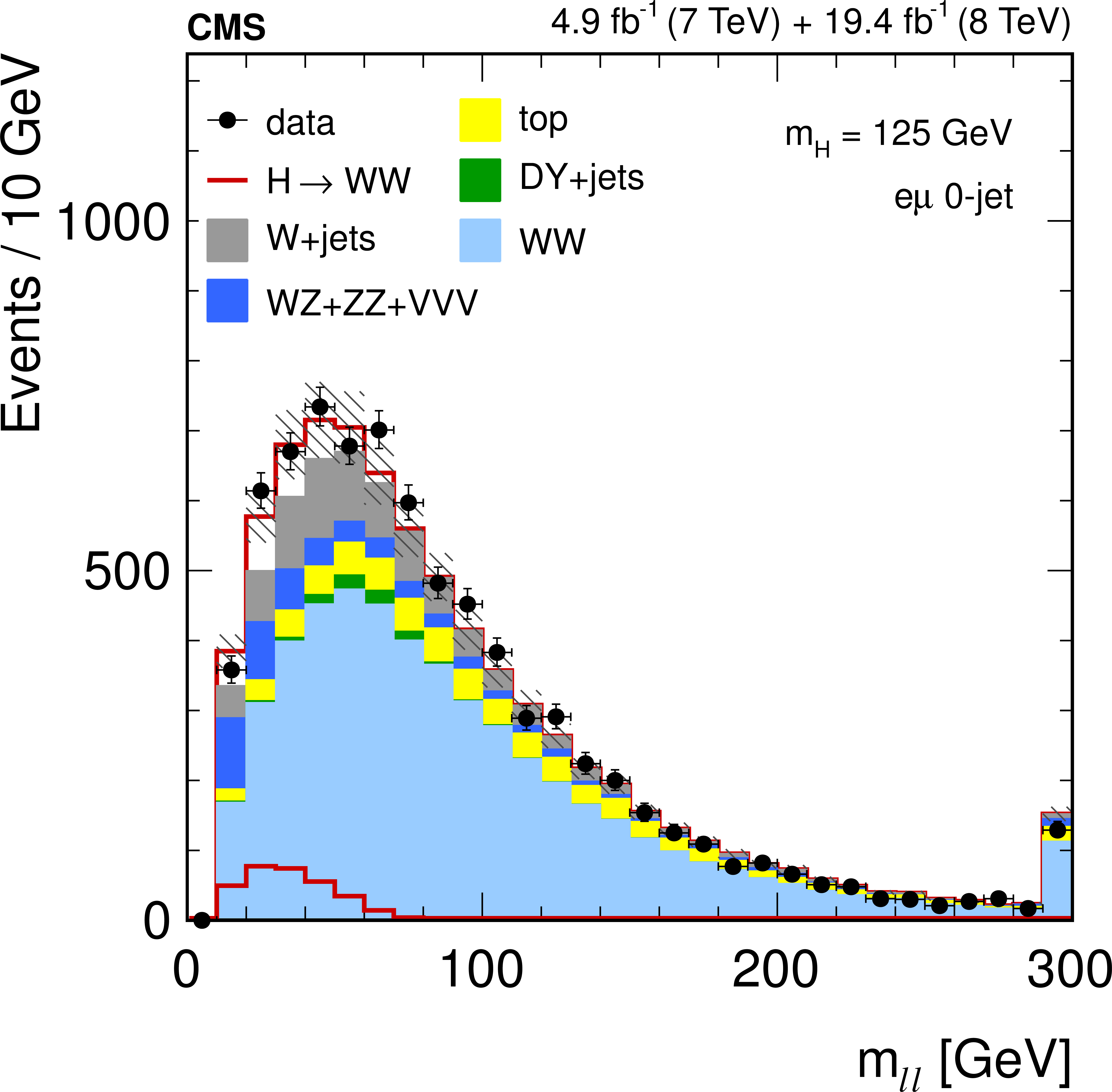
png pdf	Figure 1-a: Distributions of the dilepton invariant mass in the 0-jet category (a), and in the 1-jet category (b), in the ${\mathrm {e}}\mu$ final state for the main backgrounds (stacked histograms), and for a SM Higgs boson signal with ${m_{ {\mathrm {H}} }}$ = 125 (superimposed and stacked open histogram) at the ${\mathrm {W}} {\mathrm {W}}$ selection level. The last bin of the histograms includes overflows.
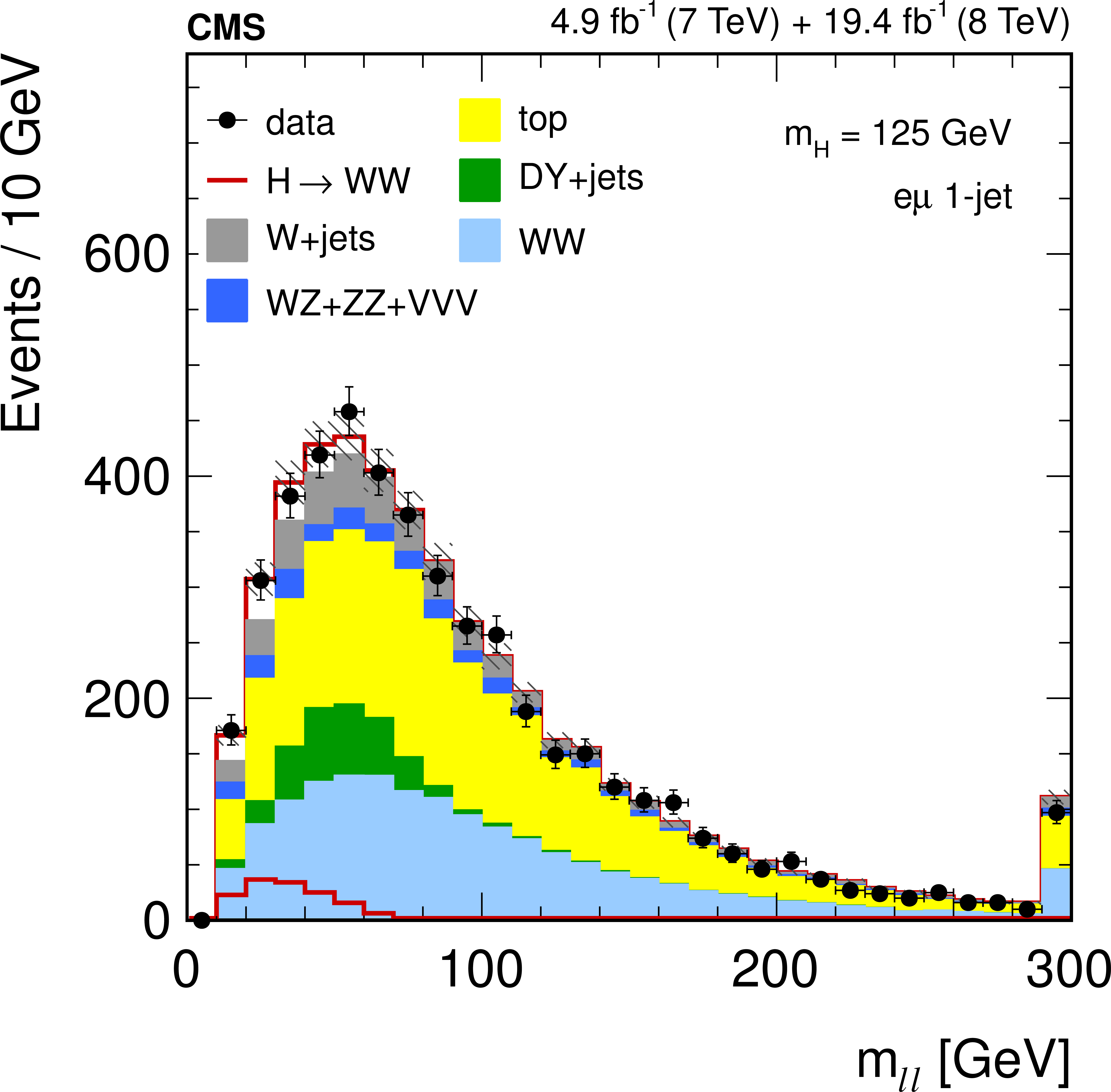
png pdf	Figure 1-b: Distributions of the dilepton invariant mass in the 0-jet category (a), and in the 1-jet category (b), in the ${\mathrm {e}}\mu$ final state for the main backgrounds (stacked histograms), and for a SM Higgs boson signal with ${m_{ {\mathrm {H}} }}$ = 125 (superimposed and stacked open histogram) at the ${\mathrm {W}} {\mathrm {W}}$ selection level. The last bin of the histograms includes overflows.
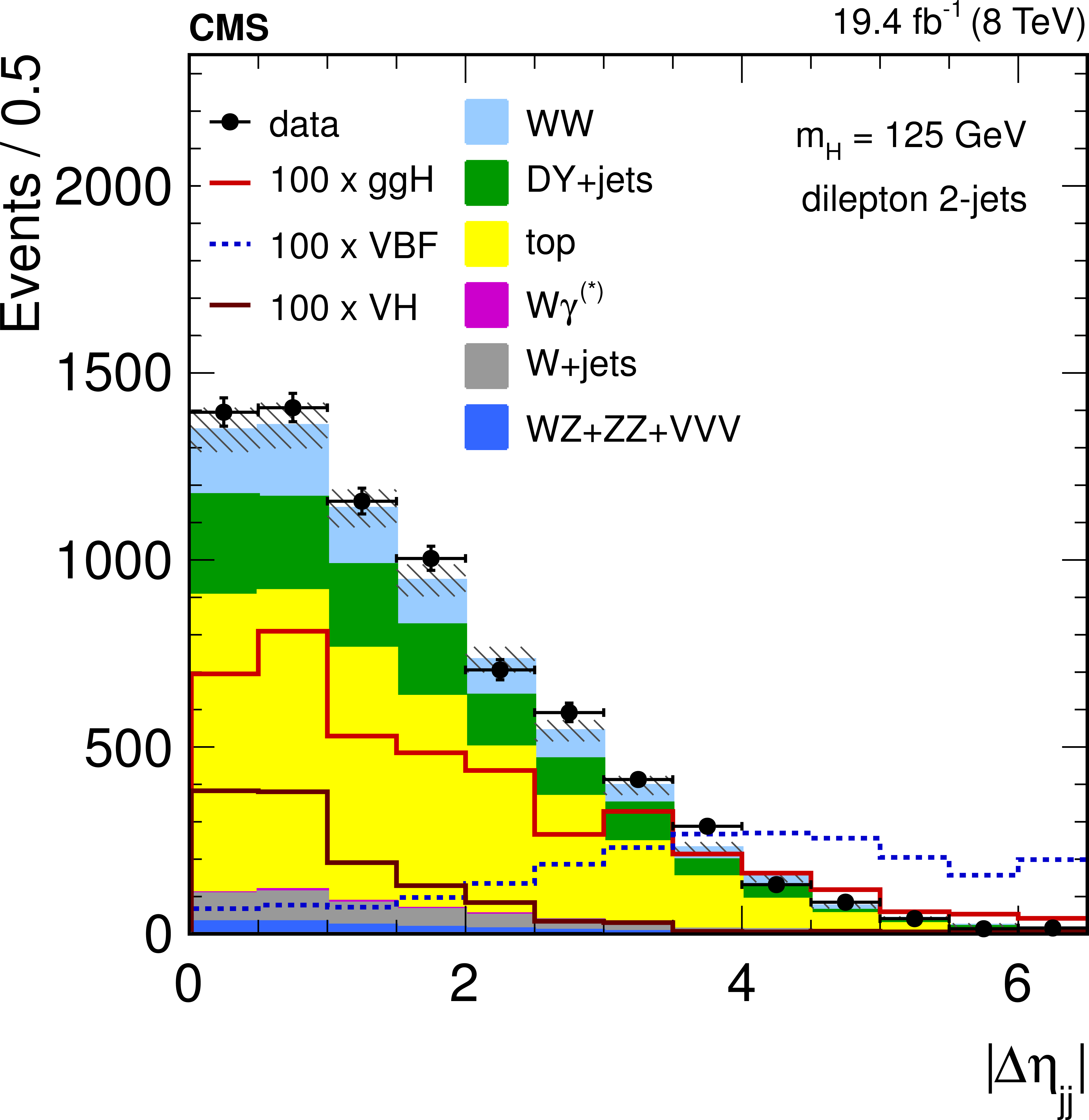
png pdf	Figure 2-a: Distributions of the pseudorapidity separation between two highest ${p_{\mathrm {T}}}$ jets (a) and the dijet invariant mass (b) in the 2-jet category for the main backgrounds (stacked histograms), and for a SM Higgs boson signal with ${m_{ {\mathrm {H}} }}$ = 125 GeV (superimposed histogram) at the ${\mathrm {W}} {\mathrm {W}}$ selection level. The signal contributions are multiplied by 100. All three final states, ${\mathrm {e}} {\mathrm {e}}$ , $\mu \mu$ , and ${\mathrm {e}}\mu$ , are included. The last bin of the histograms includes overflows.
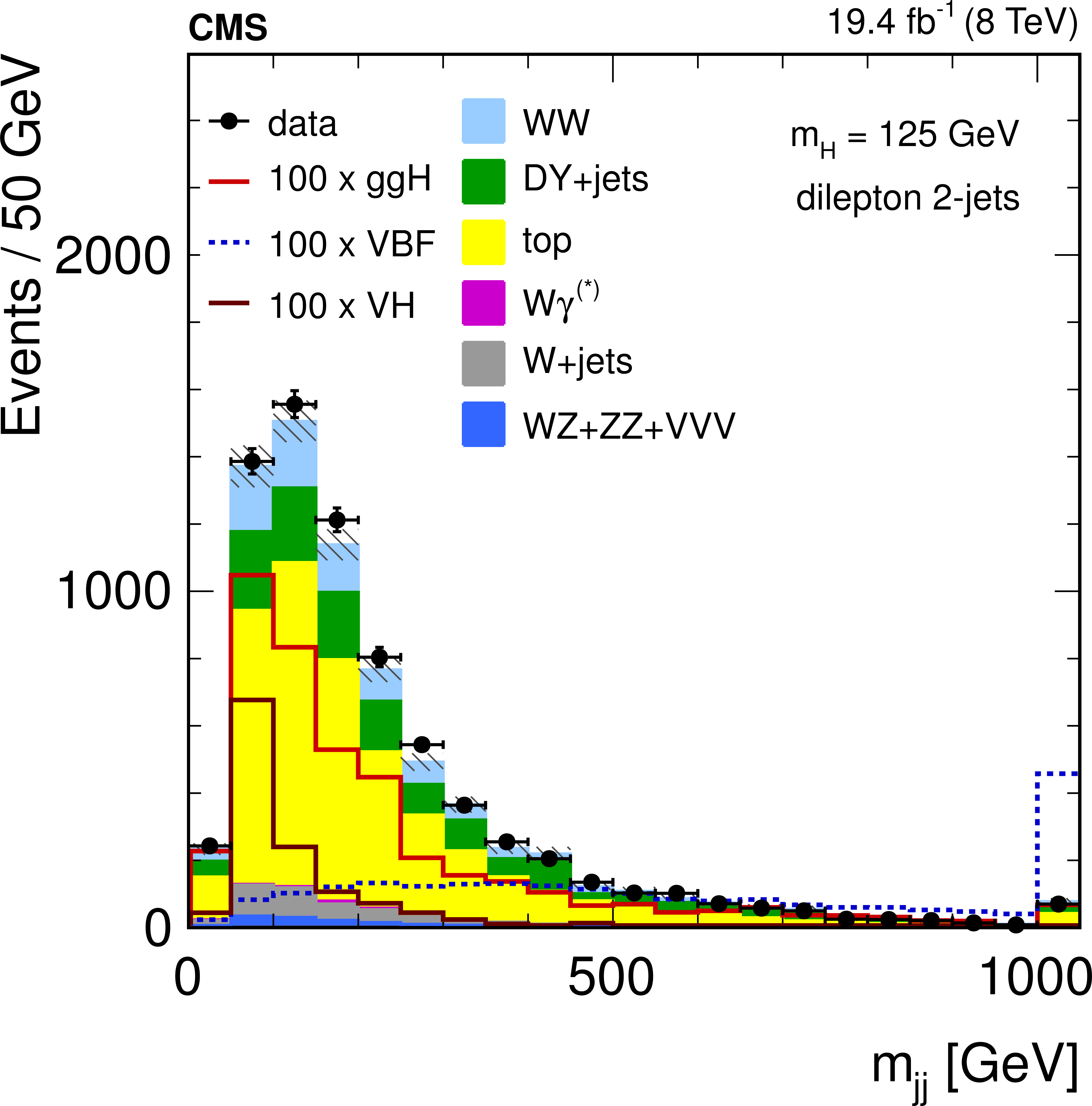
png pdf	Figure 2-b: Distributions of the pseudorapidity separation between two highest ${p_{\mathrm {T}}}$ jets (a) and the dijet invariant mass (b) in the 2-jet category for the main backgrounds (stacked histograms), and for a SM Higgs boson signal with ${m_{ {\mathrm {H}} }}$ = 125 GeV (superimposed histogram) at the ${\mathrm {W}} {\mathrm {W}}$ selection level. The signal contributions are multiplied by 100. All three final states, ${\mathrm {e}} {\mathrm {e}}$ , $\mu \mu$ , and ${\mathrm {e}}\mu$ , are included. The last bin of the histograms includes overflows.
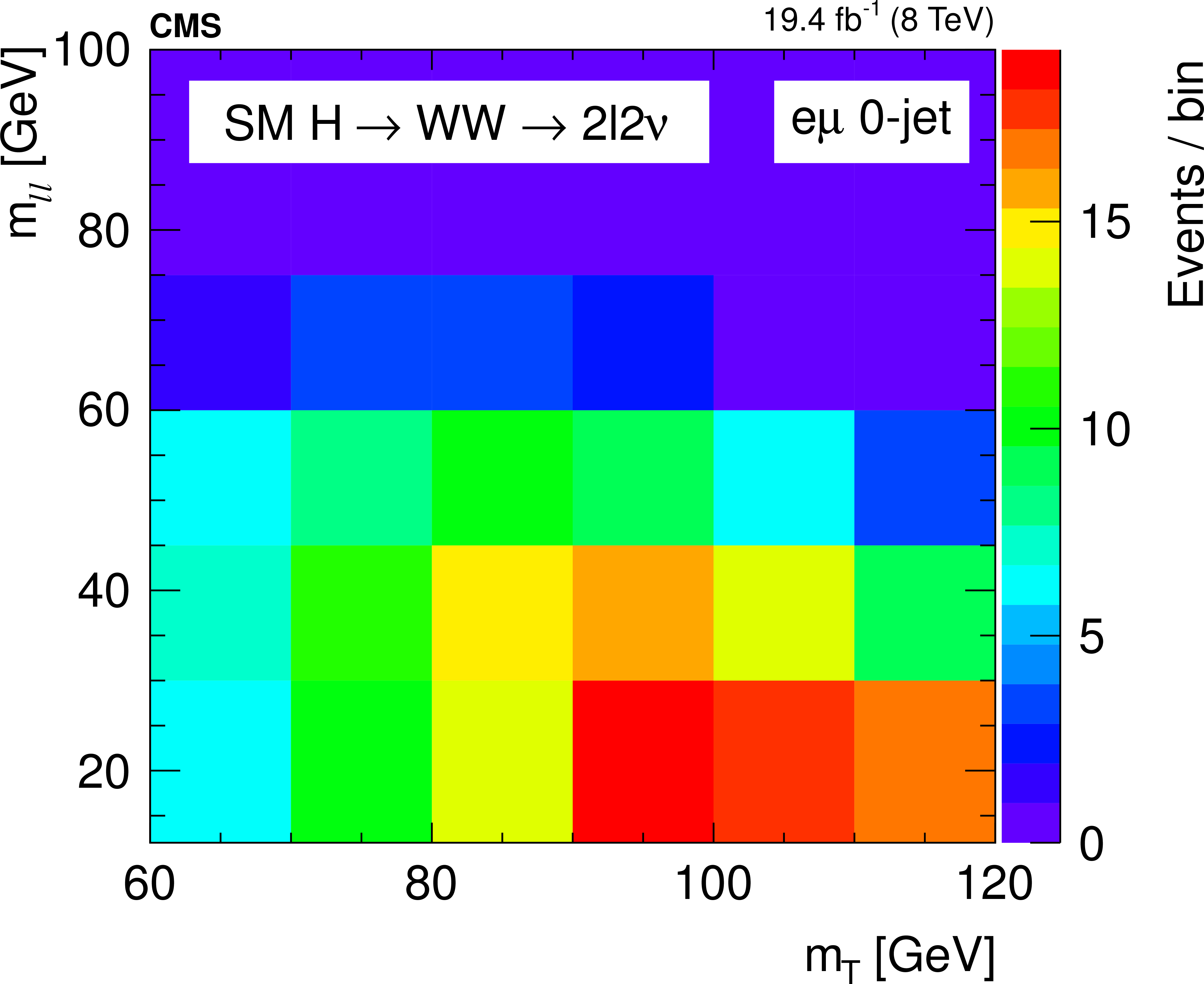
png pdf	Figure 3-a: Two-dimensional ( ${m_{\mathrm {T}}}$ , ${m_{ {\ell } {\ell }}}$ ) distributions for 8 TeV data in the 0-jet category for the ${m_{ {\mathrm {H}} }}$ = 125 GeV SM Higgs boson signal hypothesis (a), the ${2^+_\text {min}}$ hypothesis (b), the background processes (c), and the data (d). The distributions are restricted to the signal region expected for a low mass Higgs boson, that is: ${m_{ {\ell } {\ell }}}$ [12--100] GeV and ${m_{\mathrm {T}}}$ [60--120] GeV .
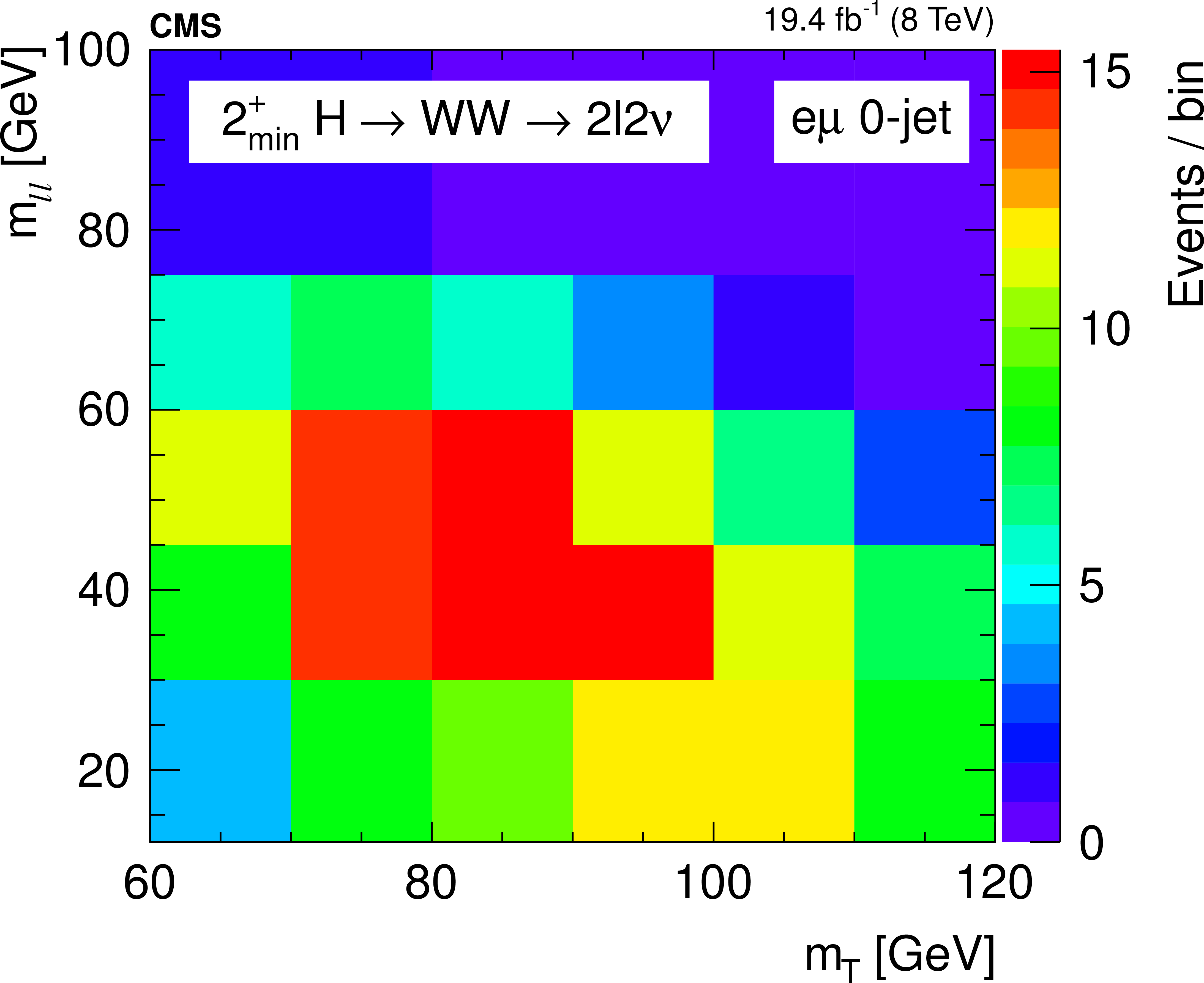
png pdf	Figure 3-b: Two-dimensional ( ${m_{\mathrm {T}}}$ , ${m_{ {\ell } {\ell }}}$ ) distributions for 8 TeV data in the 0-jet category for the ${m_{ {\mathrm {H}} }}$ = 125 GeV SM Higgs boson signal hypothesis (a), the ${2^+_\text {min}}$ hypothesis (b), the background processes (c), and the data (d). The distributions are restricted to the signal region expected for a low mass Higgs boson, that is: ${m_{ {\ell } {\ell }}}$ [12--100] GeV and ${m_{\mathrm {T}}}$ [60--120] GeV .
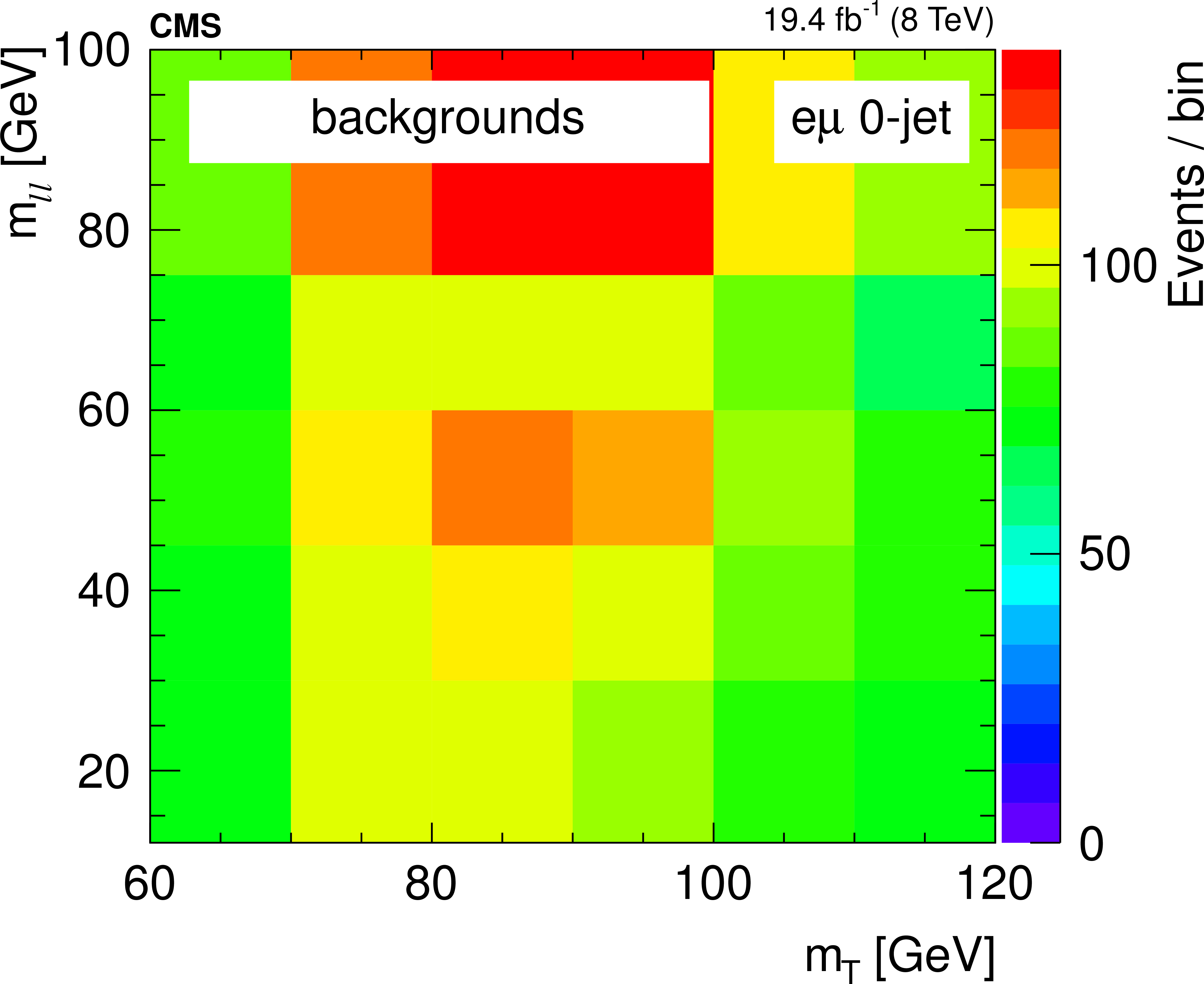
png pdf	Figure 3-c: Two-dimensional ( ${m_{\mathrm {T}}}$ , ${m_{ {\ell } {\ell }}}$ ) distributions for 8 TeV data in the 0-jet category for the ${m_{ {\mathrm {H}} }}$ = 125 GeV SM Higgs boson signal hypothesis (a), the ${2^+_\text {min}}$ hypothesis (b), the background processes (c), and the data (d). The distributions are restricted to the signal region expected for a low mass Higgs boson, that is: ${m_{ {\ell } {\ell }}}$ [12--100] GeV and ${m_{\mathrm {T}}}$ [60--120] GeV .
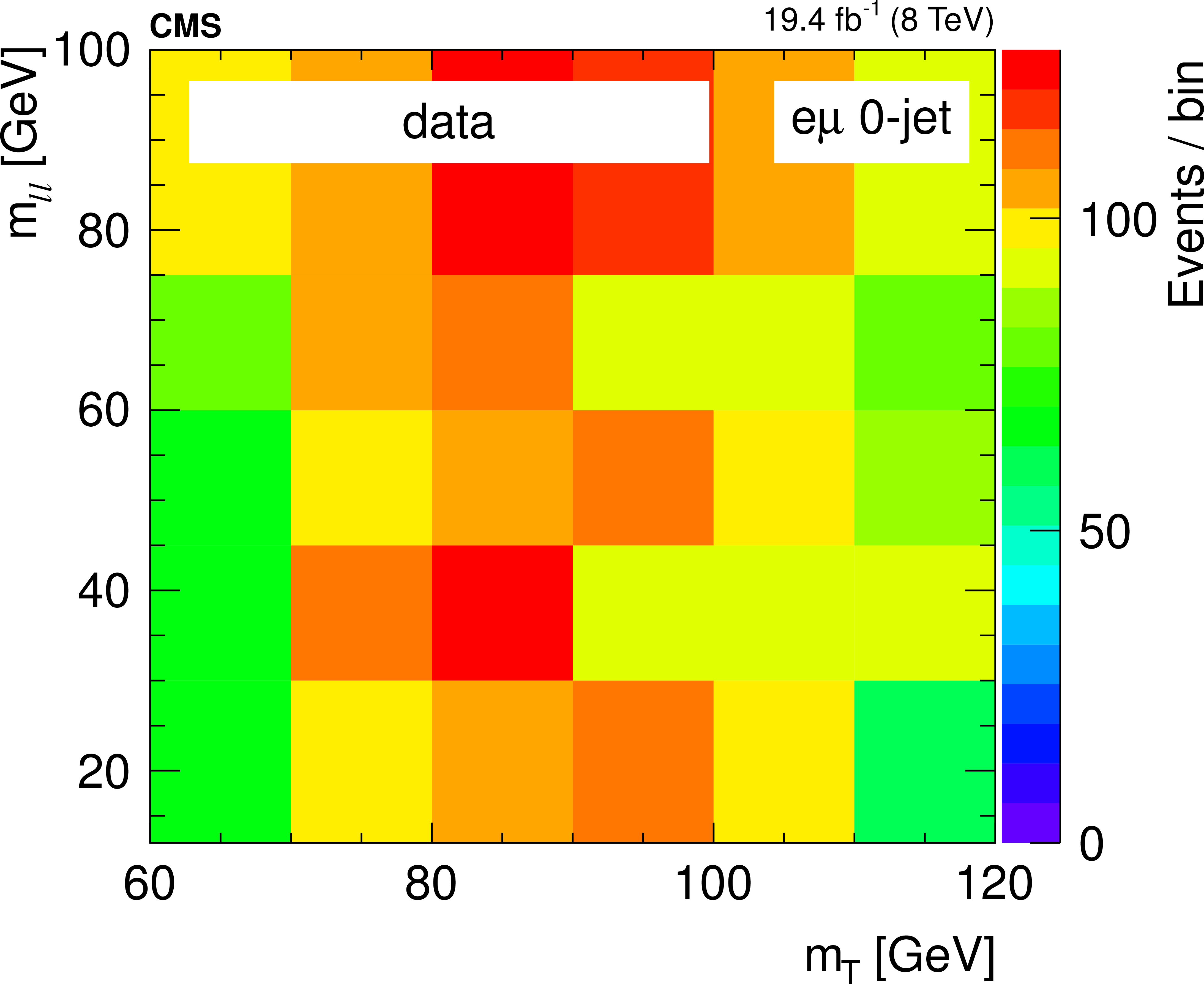
png pdf	Figure 3-d: Two-dimensional ( ${m_{\mathrm {T}}}$ , ${m_{ {\ell } {\ell }}}$ ) distributions for 8 TeV data in the 0-jet category for the ${m_{ {\mathrm {H}} }}$ = 125 GeV SM Higgs boson signal hypothesis (a), the ${2^+_\text {min}}$ hypothesis (b), the background processes (c), and the data (d). The distributions are restricted to the signal region expected for a low mass Higgs boson, that is: ${m_{ {\ell } {\ell }}}$ [12--100] GeV and ${m_{\mathrm {T}}}$ [60--120] GeV .
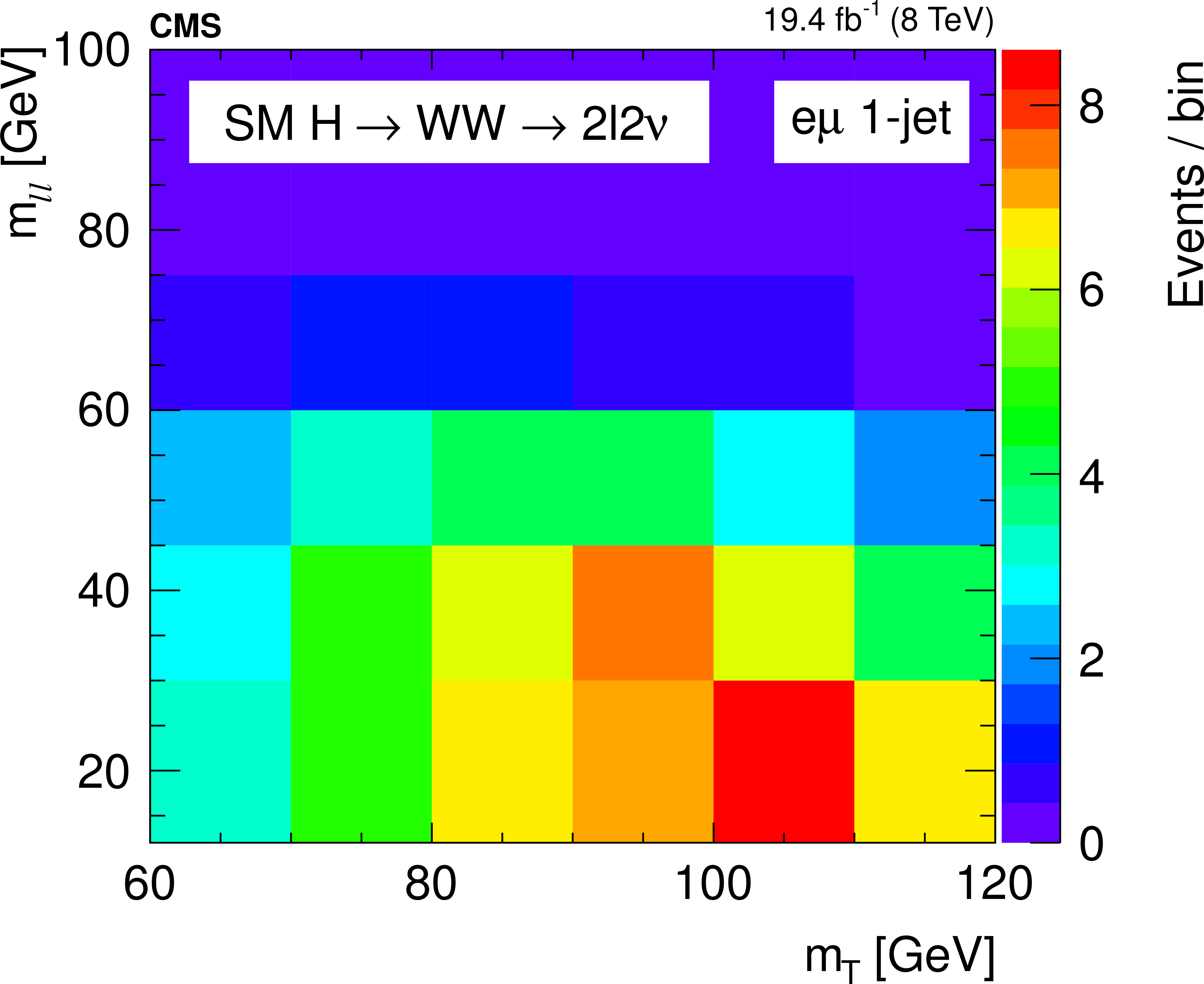
png pdf	Figure 4-a: Two-dimensional ( ${m_{\mathrm {T}}}$ , ${m_{ {\ell } {\ell }}}$ ) distributions in the 1-jet category for the ${m_{ {\mathrm {H}} }}$ = 125 GeV SM Higgs boson signal hypothesis (a), the ${2^+_\text {min}}$ hypothesis (b), the background processes (c), and the data (d). The distributions are restricted to the signal region expected for a low mass Higgs boson, that is: ${m_{ {\ell } {\ell }}}$ [12--100] GeV and ${m_{\mathrm {T}}}$ [60--120] GeV .
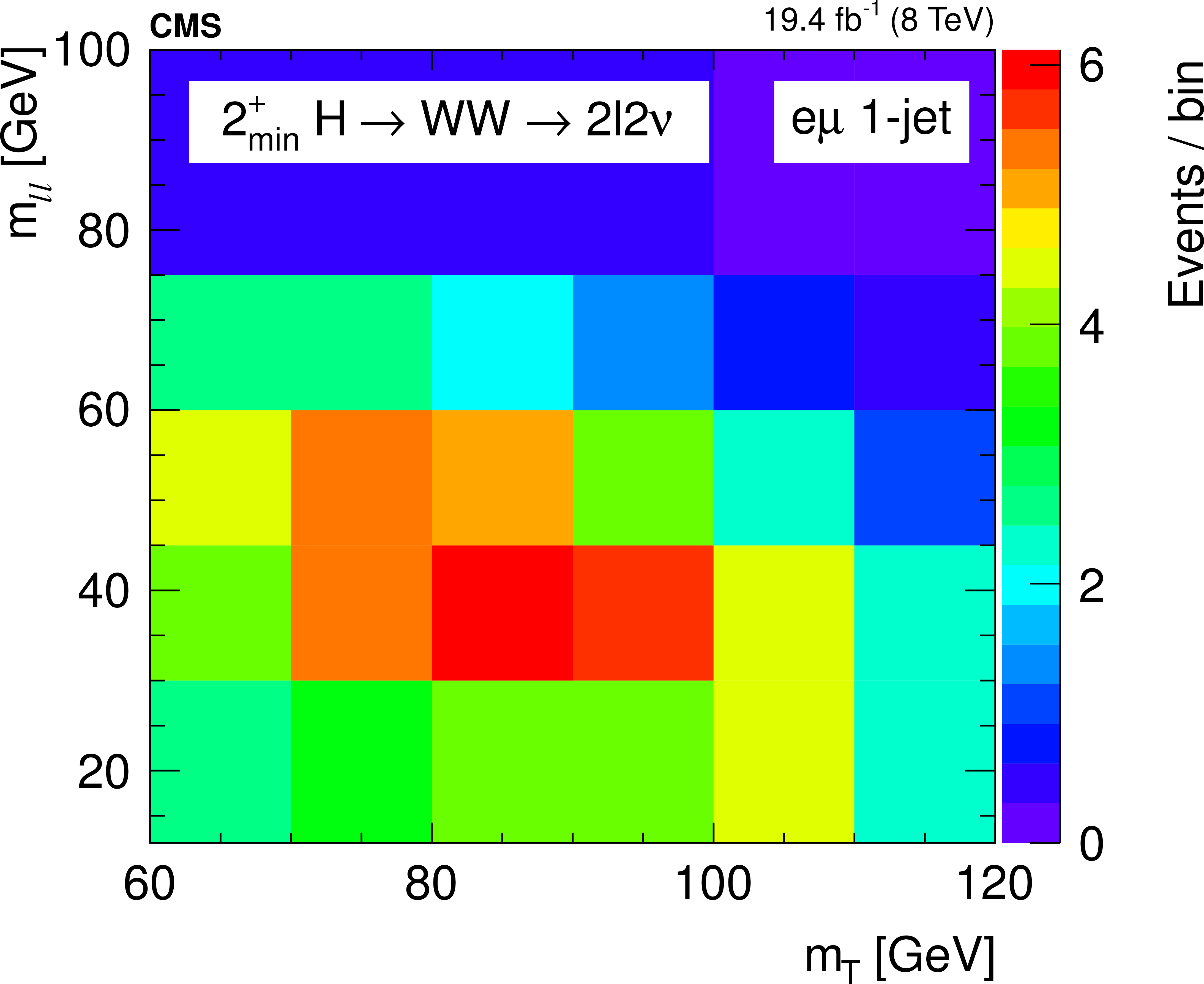
png pdf	Figure 4-b: Two-dimensional ( ${m_{\mathrm {T}}}$ , ${m_{ {\ell } {\ell }}}$ ) distributions in the 1-jet category for the ${m_{ {\mathrm {H}} }}$ = 125 GeV SM Higgs boson signal hypothesis (a), the ${2^+_\text {min}}$ hypothesis (b), the background processes (c), and the data (d). The distributions are restricted to the signal region expected for a low mass Higgs boson, that is: ${m_{ {\ell } {\ell }}}$ [12--100] GeV and ${m_{\mathrm {T}}}$ [60--120] GeV .
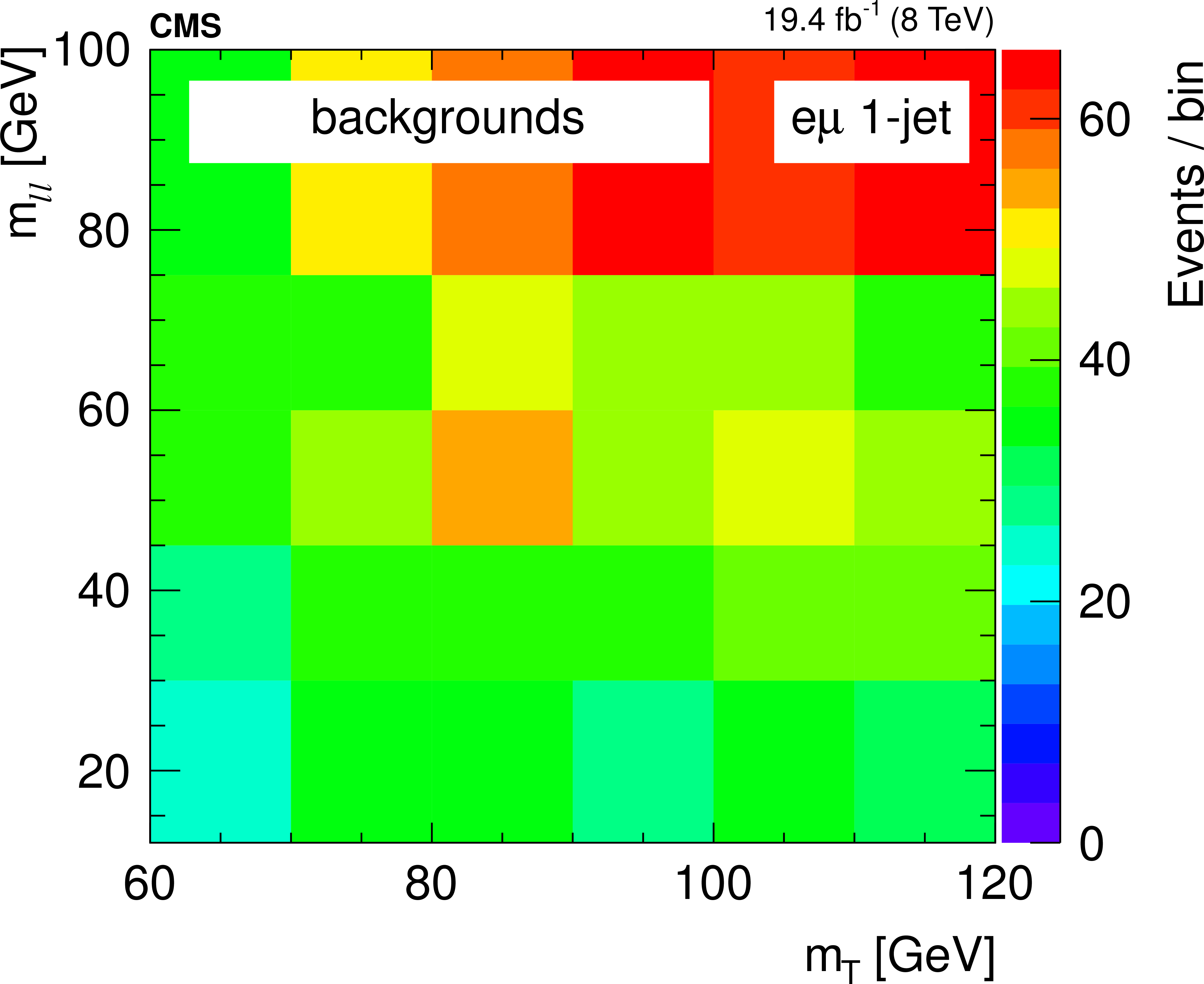
png pdf	Figure 4-c: Two-dimensional ( ${m_{\mathrm {T}}}$ , ${m_{ {\ell } {\ell }}}$ ) distributions in the 1-jet category for the ${m_{ {\mathrm {H}} }}$ = 125 GeV SM Higgs boson signal hypothesis (a), the ${2^+_\text {min}}$ hypothesis (b), the background processes (c), and the data (d). The distributions are restricted to the signal region expected for a low mass Higgs boson, that is: ${m_{ {\ell } {\ell }}}$ [12--100] GeV and ${m_{\mathrm {T}}}$ [60--120] GeV .
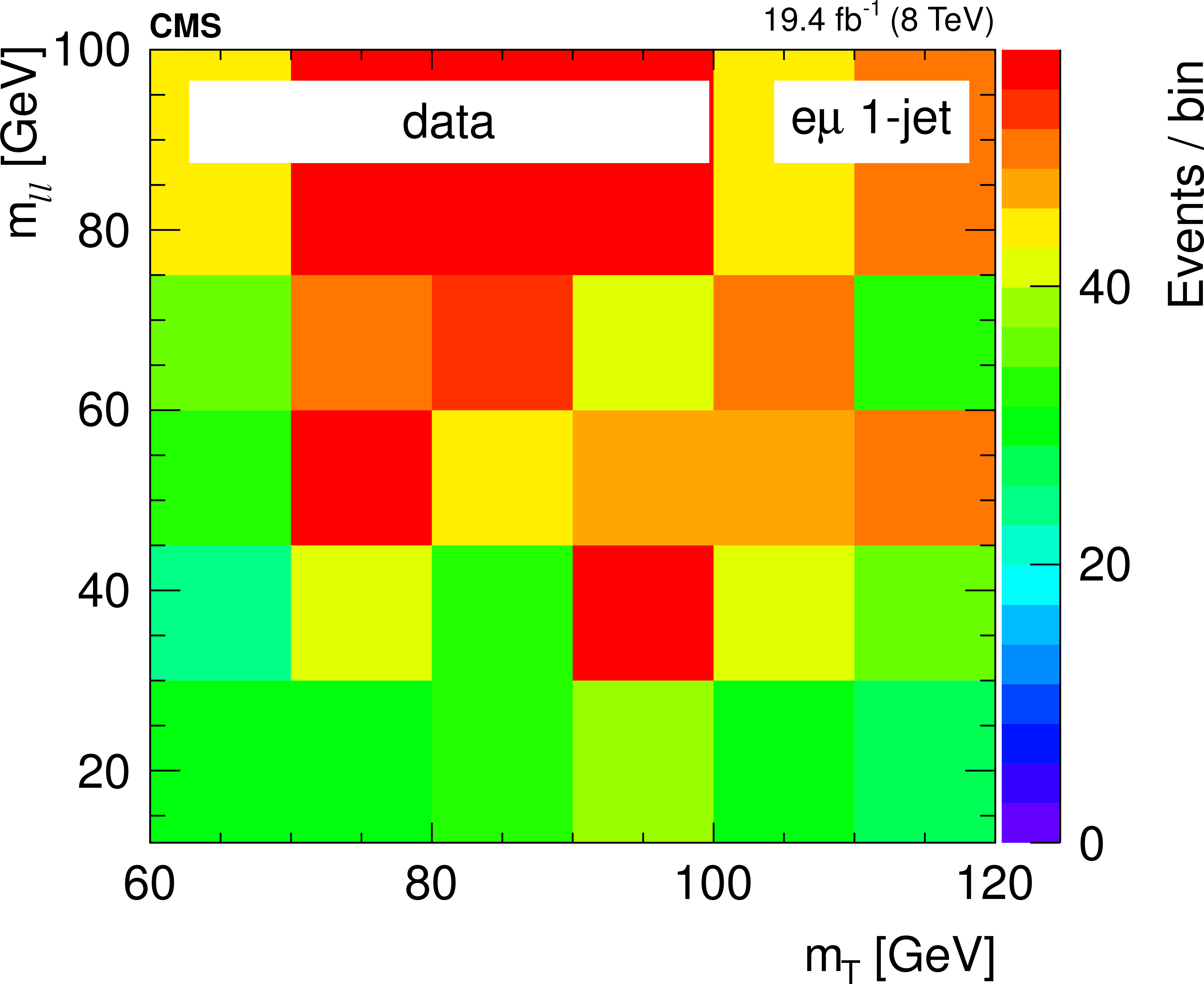
png pdf	Figure 4-d: Two-dimensional ( ${m_{\mathrm {T}}}$ , ${m_{ {\ell } {\ell }}}$ ) distributions in the 1-jet category for the ${m_{ {\mathrm {H}} }}$ = 125 GeV SM Higgs boson signal hypothesis (a), the ${2^+_\text {min}}$ hypothesis (b), the background processes (c), and the data (d). The distributions are restricted to the signal region expected for a low mass Higgs boson, that is: ${m_{ {\ell } {\ell }}}$ [12--100] GeV and ${m_{\mathrm {T}}}$ [60--120] GeV .
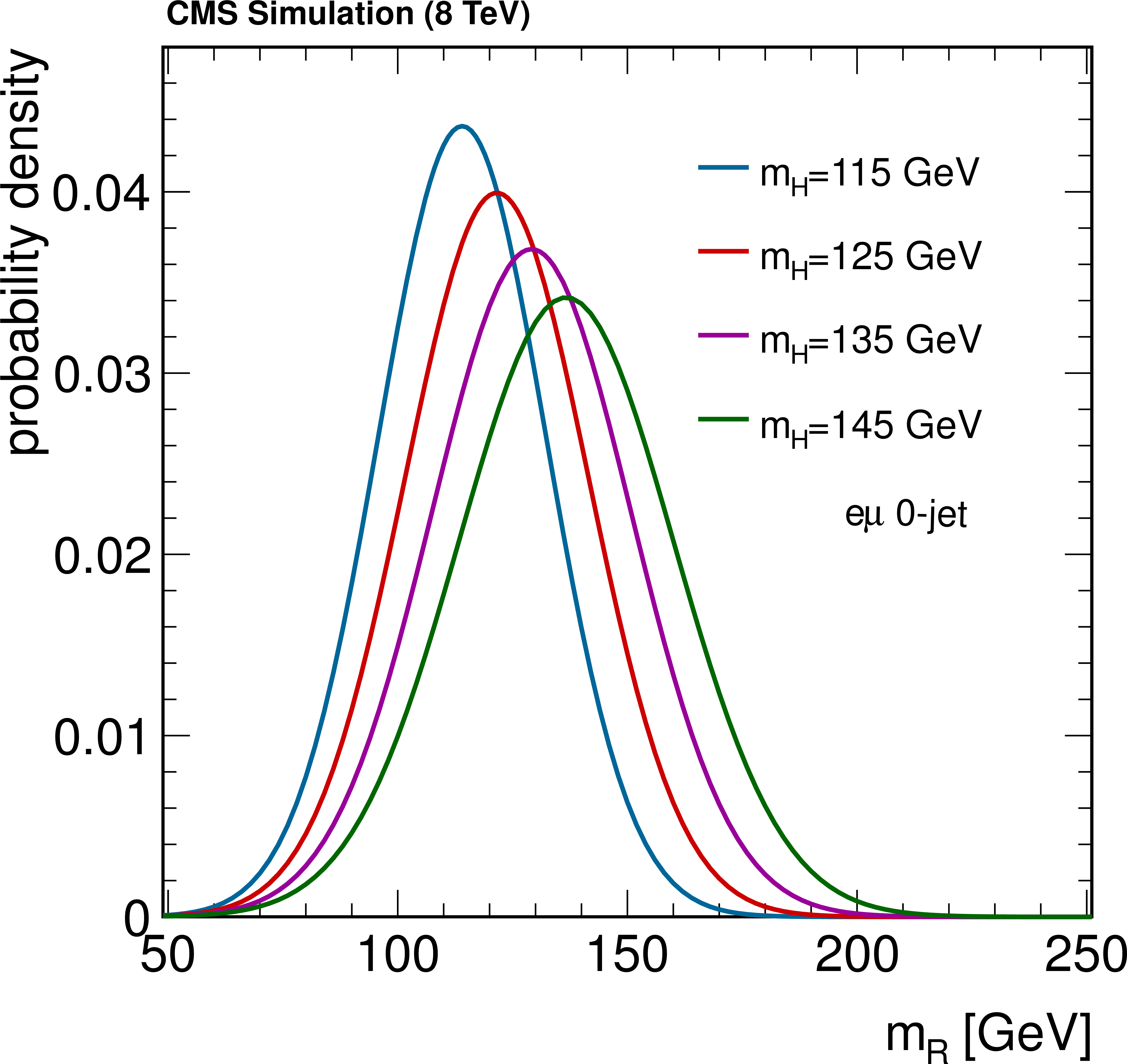
png pdf	Figure 5-a: Evolution of ${m_{\mathrm {R}}}$ distribution with Higgs boson mass hypotheses (a), and distribution of ${m_{\mathrm {R}}}$ for signal and different backgrounds (b), all normalized to unity, for the 0-jet category in the ${\mathrm {e}}\mu$ final state.
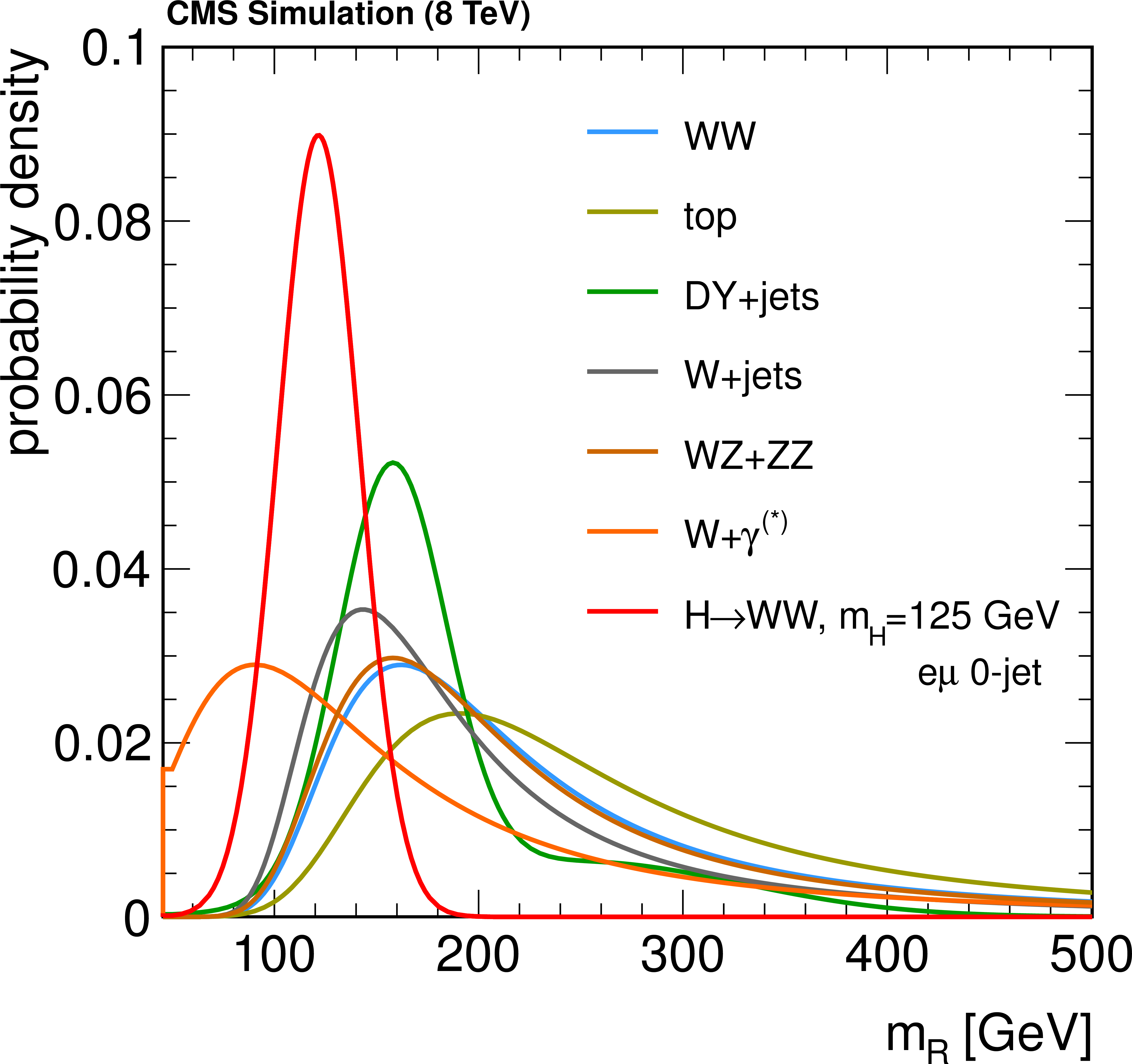
png pdf	Figure 5-b: Evolution of ${m_{\mathrm {R}}}$ distribution with Higgs boson mass hypotheses (a), and distribution of ${m_{\mathrm {R}}}$ for signal and different backgrounds (b), all normalized to unity, for the 0-jet category in the ${\mathrm {e}}\mu$ final state.
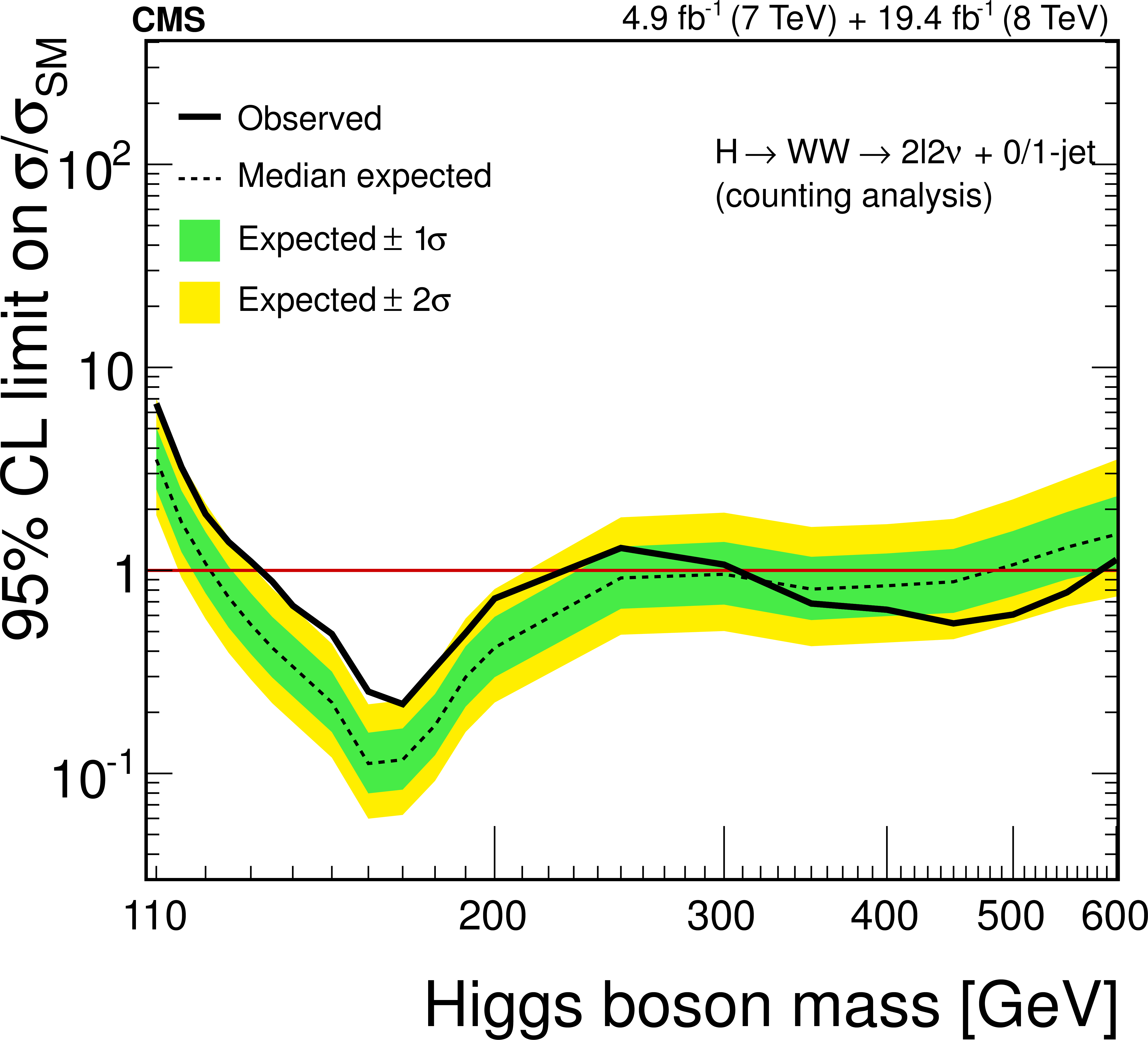
png pdf	Figure 6-a: Expected and observed 95% CL upper limits on the ${\mathrm {H}} \to {\mathrm {W}} {\mathrm {W}}$ production cross section relative to the SM Higgs boson expectation using the counting analysis (a) and the shape-based template fit approach (b) in the 0-jet and 1-jet categories. The shape-based analysis results use a binned template fit to ( ${m_{\mathrm {T}}}$ , ${m_{ {\ell } {\ell }}}$ ) for the ${\mathrm {e}}\mu$ final state, combined with the counting analysis results for the ${\mathrm {e}} {\mathrm {e}}/\mu \mu$ final states.
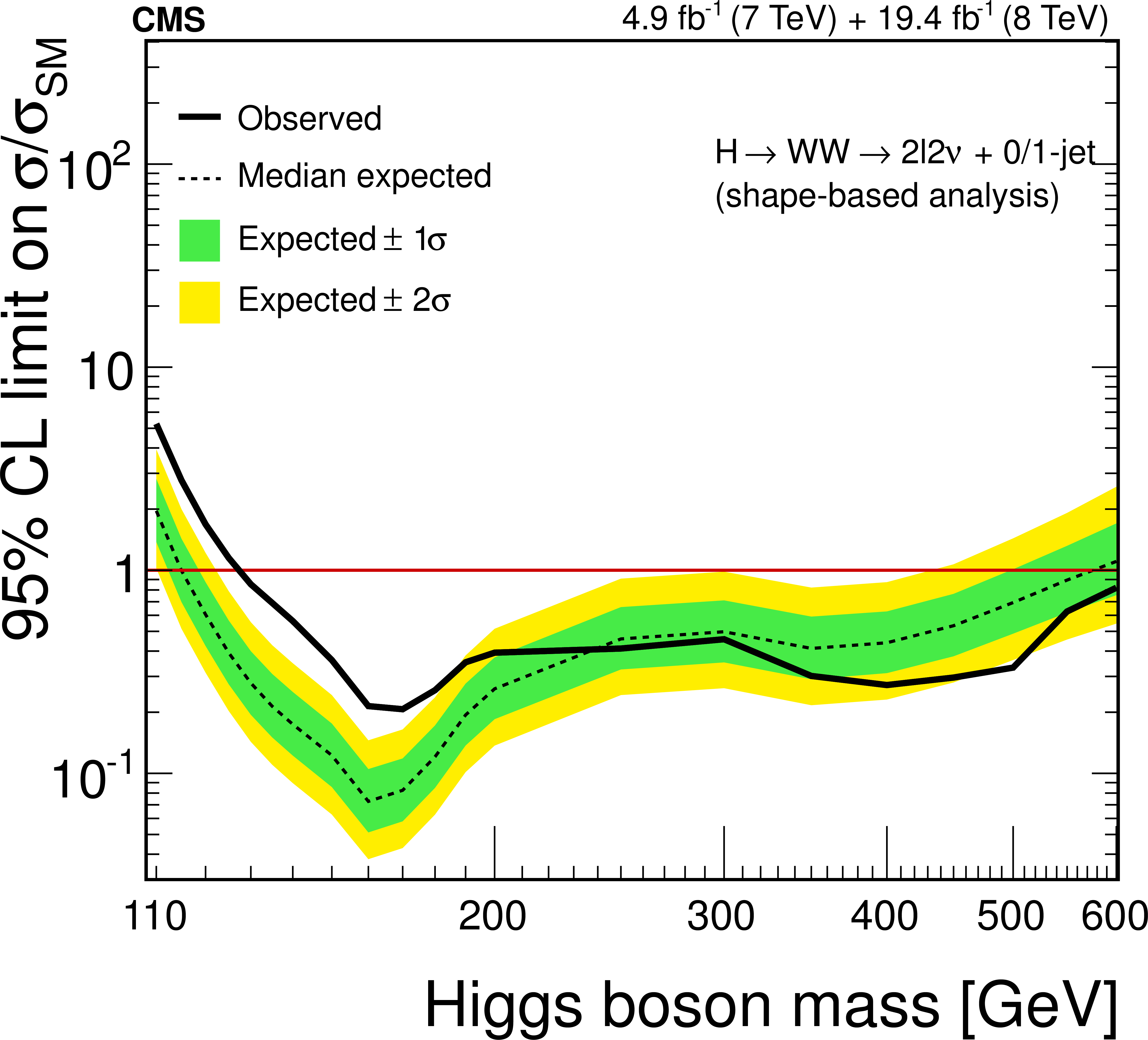
png pdf	Figure 6-b: Expected and observed 95% CL upper limits on the ${\mathrm {H}} \to {\mathrm {W}} {\mathrm {W}}$ production cross section relative to the SM Higgs boson expectation using the counting analysis (a) and the shape-based template fit approach (b) in the 0-jet and 1-jet categories. The shape-based analysis results use a binned template fit to ( ${m_{\mathrm {T}}}$ , ${m_{ {\ell } {\ell }}}$ ) for the ${\mathrm {e}}\mu$ final state, combined with the counting analysis results for the ${\mathrm {e}} {\mathrm {e}}/\mu \mu$ final states.
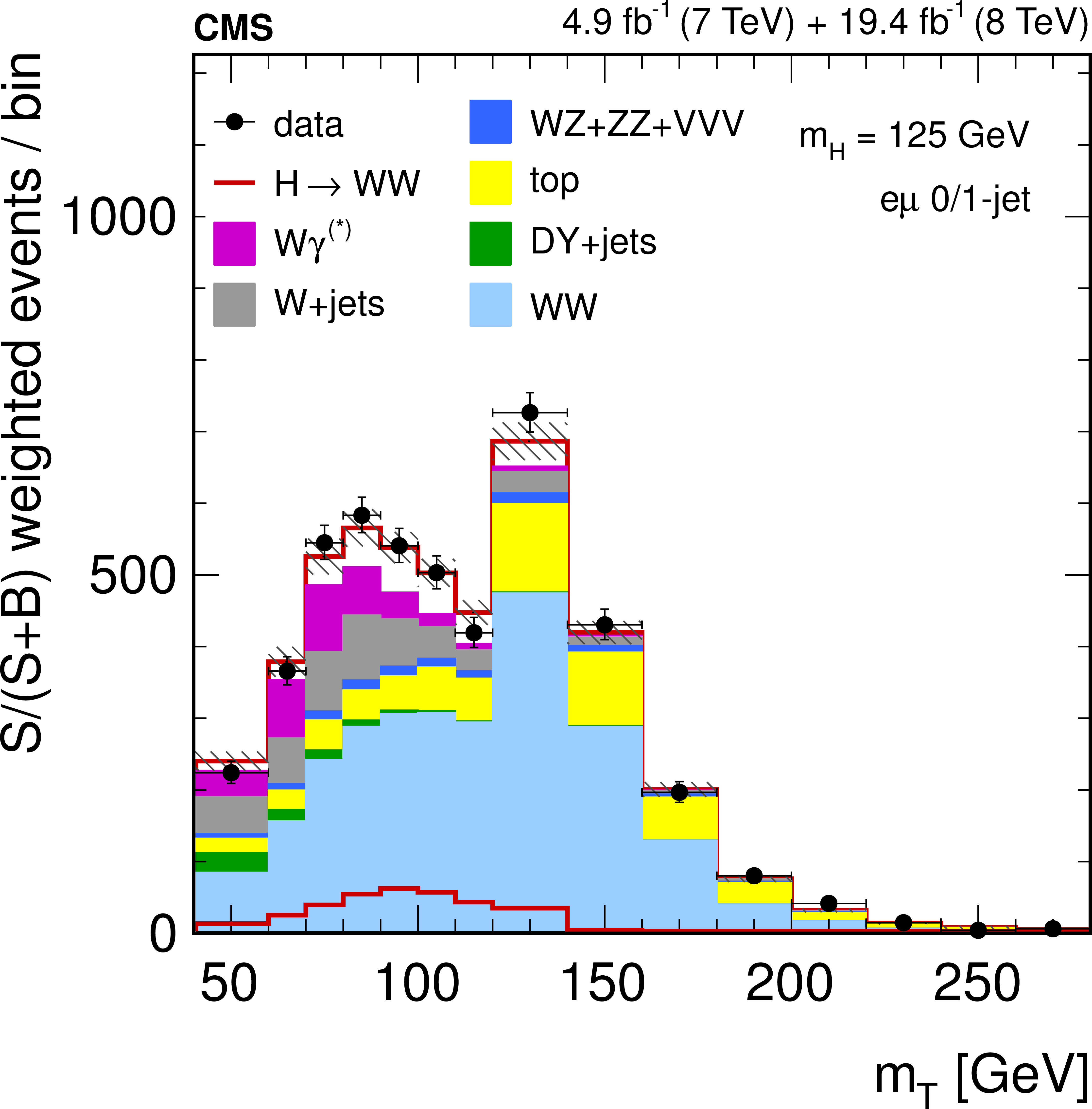
png pdf	Figure 7-a: The ${m_{\mathrm {T}}}$ distribution in the ${\mathrm {e}}\mu$ final state for the 0-jet and 1-jet categories combined for observed data superimposed on signal + background events and separately for the signal events alone (a) and background-subtracted data with best-fit signal component (b). The signal and background processes are normalized to the result of the template fit to the ( ${m_{\mathrm {T}}}$ , ${m_{ {\ell } {\ell }}}$ ) distribution and weighted according to the observed S/(S+B) ratio in each bin of the ${m_{ {\ell } {\ell }}}$ distribution integrating over the ${m_{\mathrm {T}}}$ variable. To better visualize a peak structure, an extended ${m_{\mathrm {T}}}$ range including ${m_{\mathrm {T}}}$ =[40,60] GeV is shown, with the normalization of signal and background events extrapolated from the fit result.
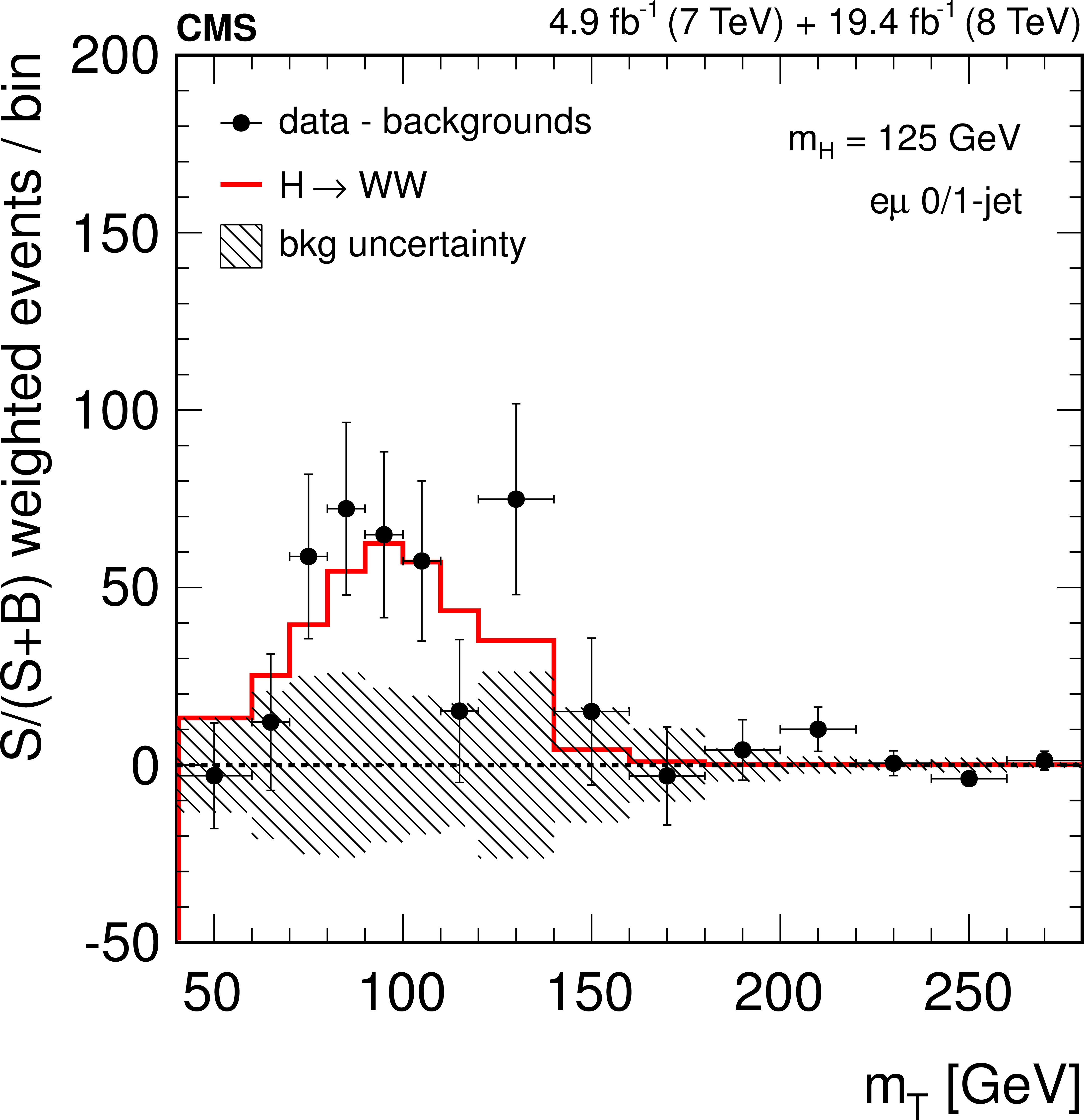
png pdf	Figure 7-b: The ${m_{\mathrm {T}}}$ distribution in the ${\mathrm {e}}\mu$ final state for the 0-jet and 1-jet categories combined for observed data superimposed on signal + background events and separately for the signal events alone (a) and background-subtracted data with best-fit signal component (b). The signal and background processes are normalized to the result of the template fit to the ( ${m_{\mathrm {T}}}$ , ${m_{ {\ell } {\ell }}}$ ) distribution and weighted according to the observed S/(S+B) ratio in each bin of the ${m_{ {\ell } {\ell }}}$ distribution integrating over the ${m_{\mathrm {T}}}$ variable. To better visualize a peak structure, an extended ${m_{\mathrm {T}}}$ range including ${m_{\mathrm {T}}}$ =[40,60] GeV is shown, with the normalization of signal and background events extrapolated from the fit result.
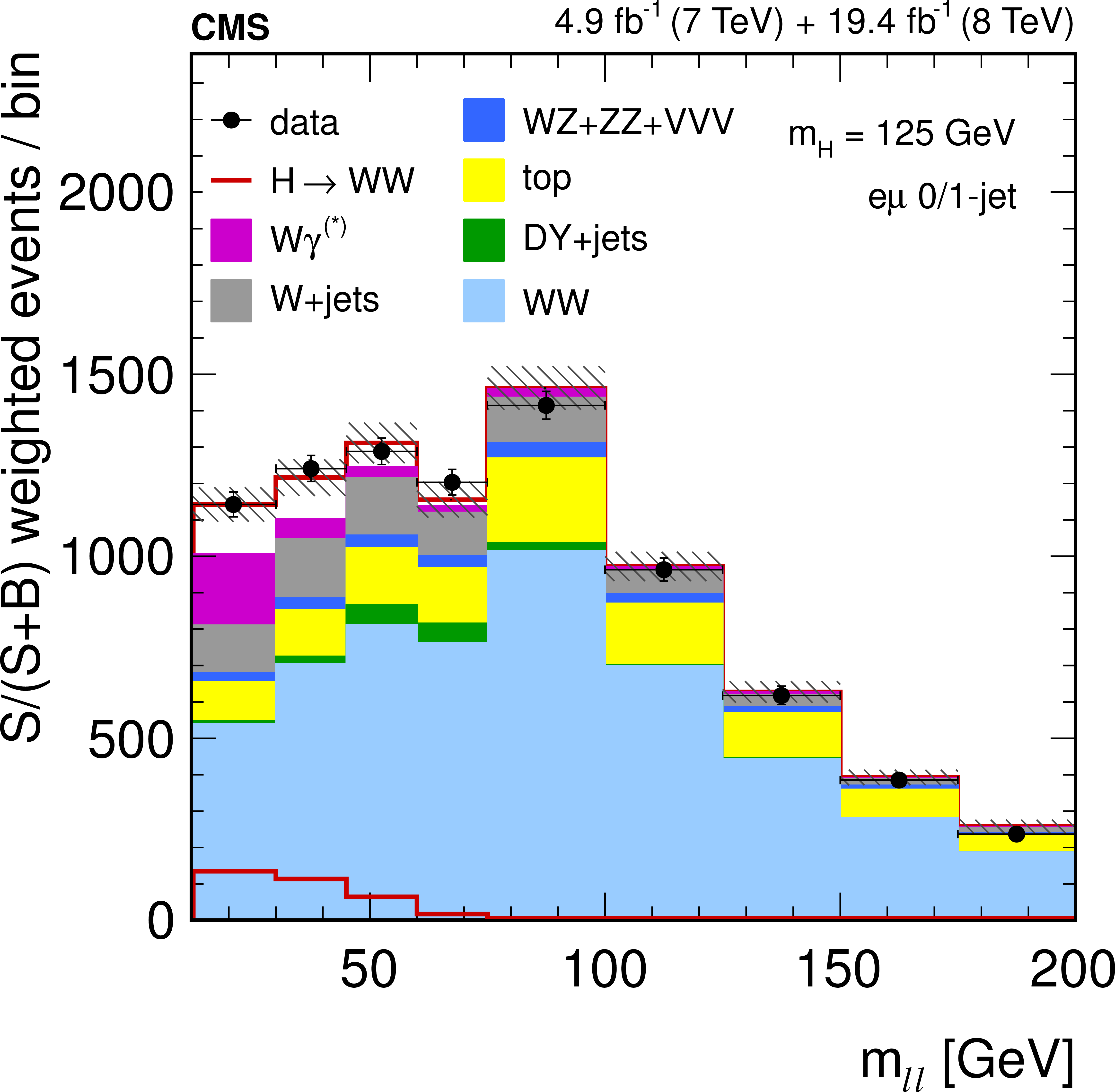
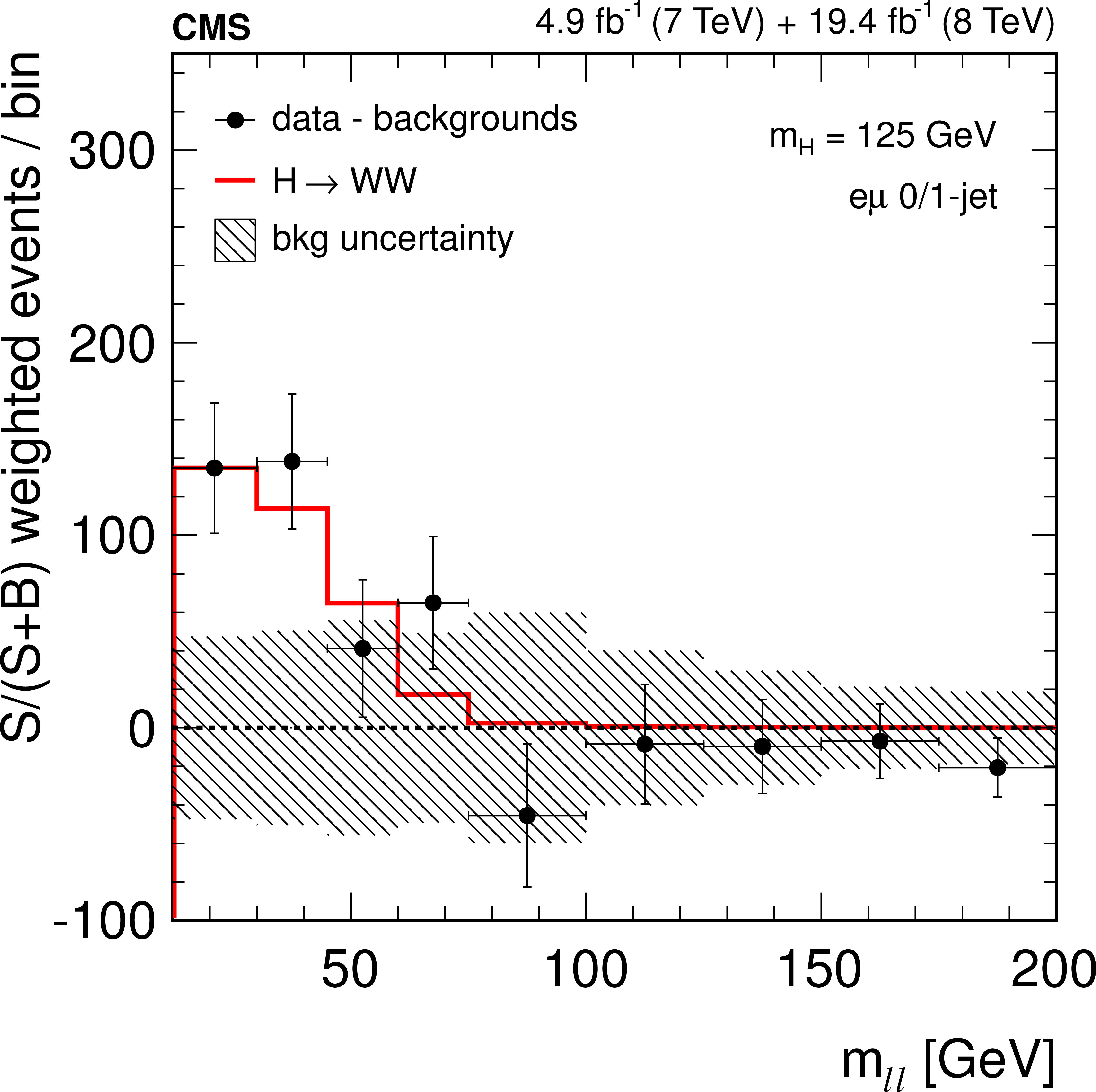
png pdf	Figure 8-a: The ${m_{ {\ell } {\ell }}}$ distribution in the ${\mathrm {e}}\mu$ final state for the 0-jet and 1-jet categories combined for observed data superimposed on signal + background events, and separately for the signal events alone (a) and background-subtracted data with best-fit signal component (b). The signal and background processes are normalized to the result of the template fit to the ( ${m_{\mathrm {T}}}$ , ${m_{ {\ell } {\ell }}}$ ) distribution and weighted according to the observed S/(S+B) ratio in each bin of the ${m_{\mathrm {T}}}$ distribution integrating over the ${m_{ {\ell } {\ell }}}$ variable.
png pdf	Figure 8-b: The ${m_{ {\ell } {\ell }}}$ distribution in the ${\mathrm {e}}\mu$ final state for the 0-jet and 1-jet categories combined for observed data superimposed on signal + background events, and separately for the signal events alone (a) and background-subtracted data with best-fit signal component (b). The signal and background processes are normalized to the result of the template fit to the ( ${m_{\mathrm {T}}}$ , ${m_{ {\ell } {\ell }}}$ ) distribution and weighted according to the observed S/(S+B) ratio in each bin of the ${m_{\mathrm {T}}}$ distribution integrating over the ${m_{ {\ell } {\ell }}}$ variable.
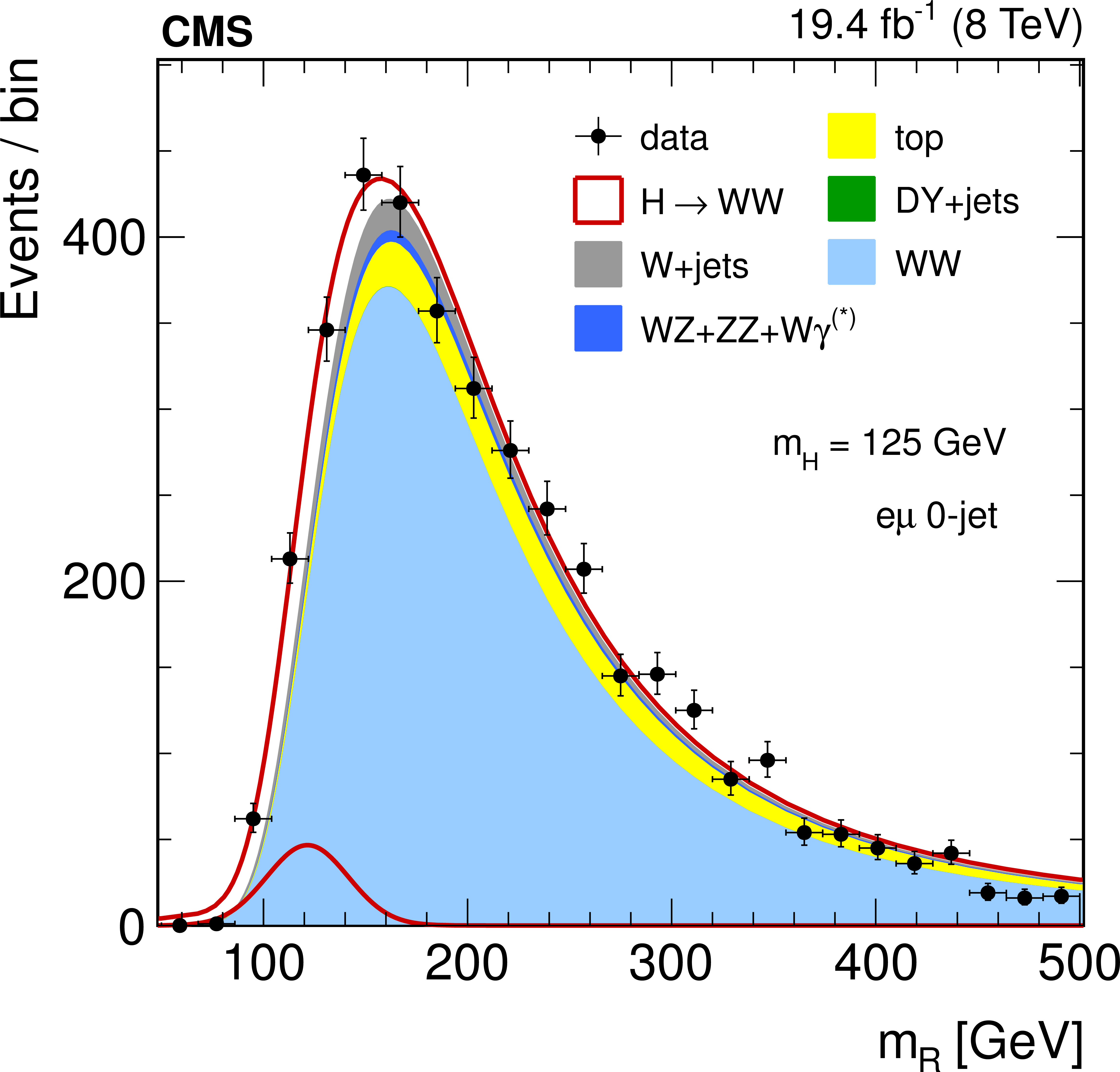
png pdf	Figure 9-a: Distributions of ${m_{\mathrm {R}}}$ showing the composition of signal and backgrounds, superimposed on the signal events alone, in the ${\mathrm {e}}\mu$ final state for the 0-jet (a) and 1-jet (b) categories for $\sqrt {s}$ = 8 TeV. The signal and background processes are normalized to the result of the parametric fit to the ( ${m_{\mathrm {R}}}$ , ${\Delta \phi _{\mathrm {R}}}$ ) distribution.
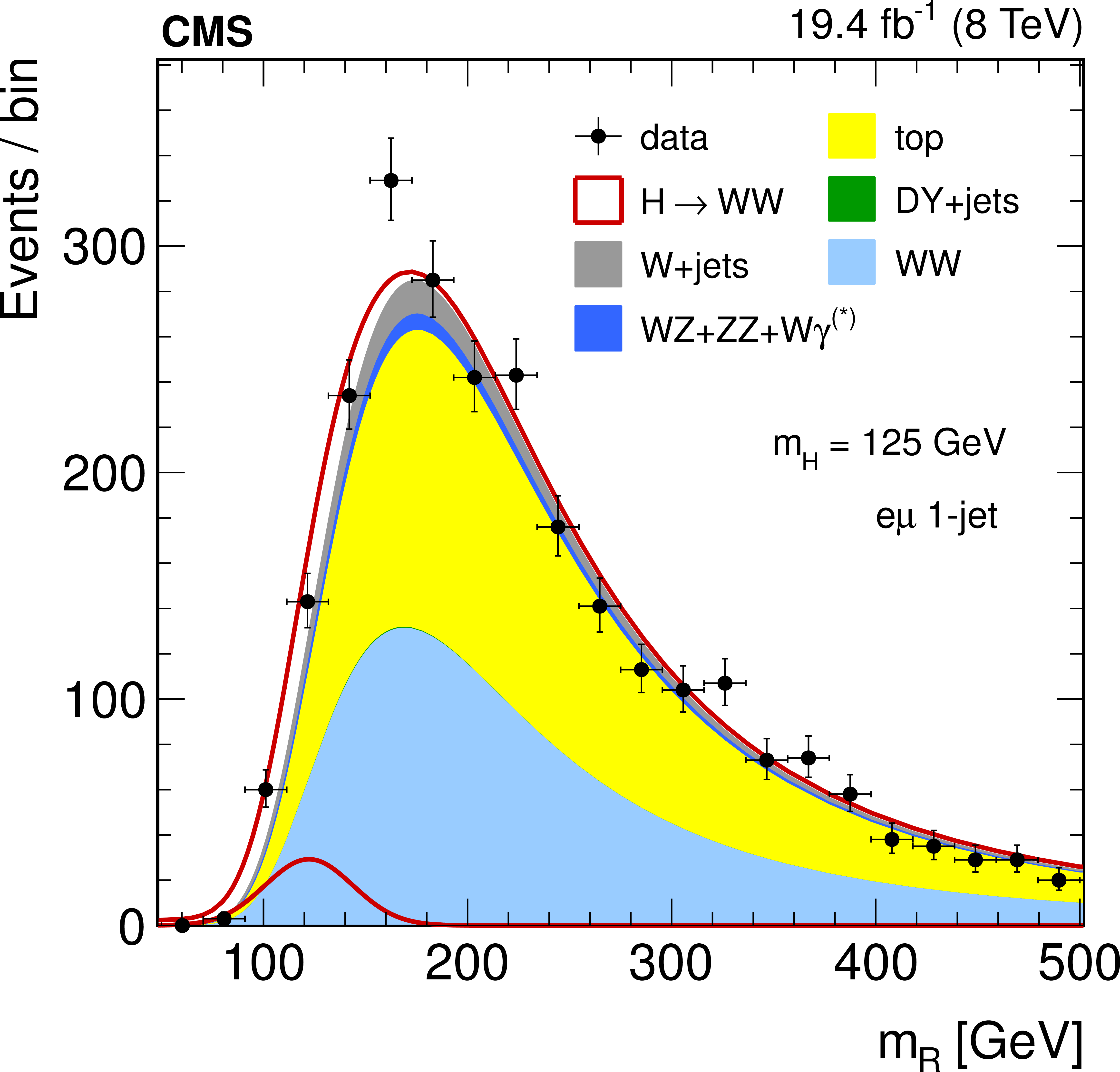
png pdf	Figure 9-b: Distributions of ${m_{\mathrm {R}}}$ showing the composition of signal and backgrounds, superimposed on the signal events alone, in the ${\mathrm {e}}\mu$ final state for the 0-jet (a) and 1-jet (b) categories for $\sqrt {s}$ = 8 TeV. The signal and background processes are normalized to the result of the parametric fit to the ( ${m_{\mathrm {R}}}$ , ${\Delta \phi _{\mathrm {R}}}$ ) distribution.
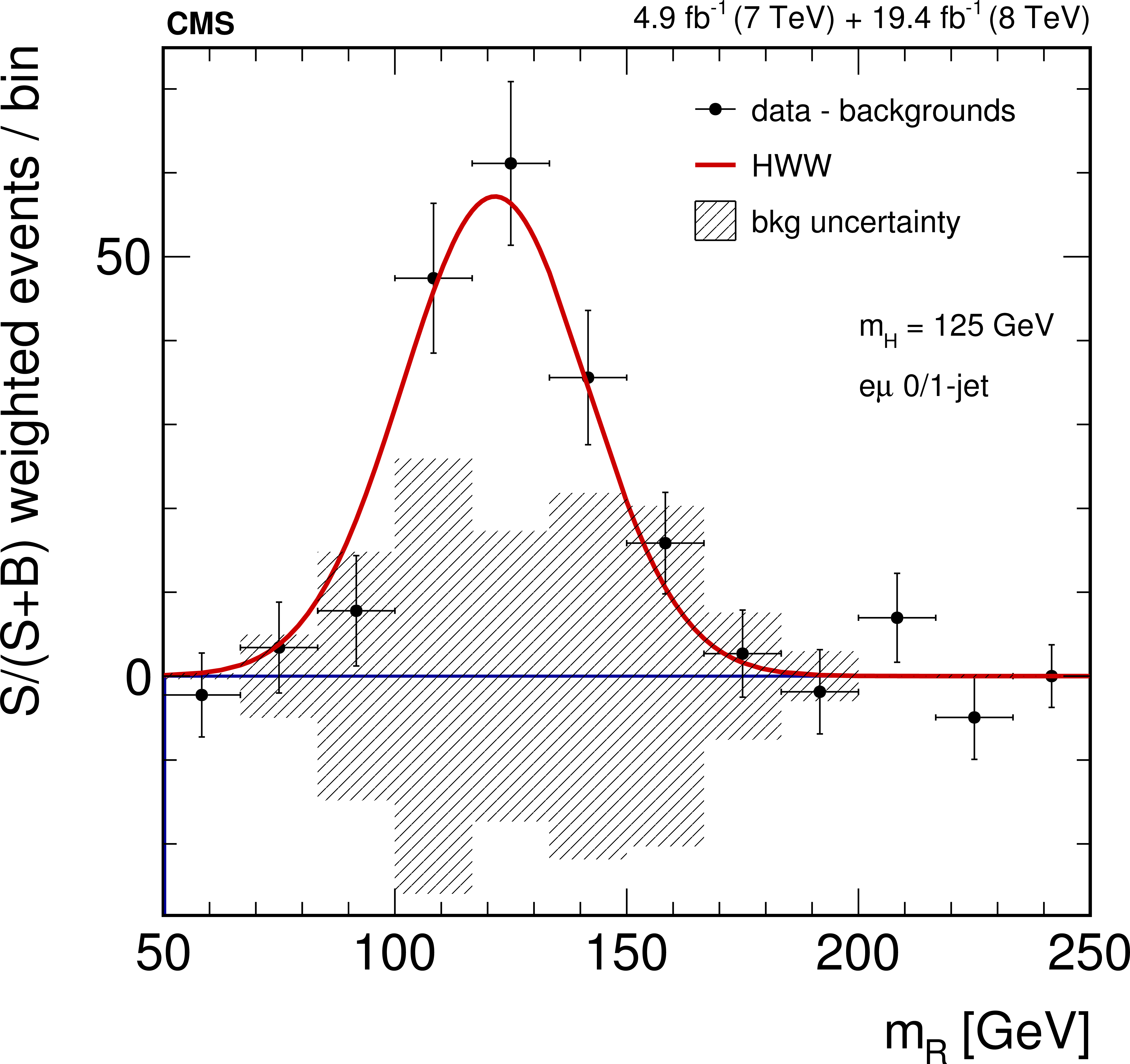
png pdf	Figure 10-a: The background-subtracted data distribution for ${m_{\mathrm {R}}}$ (a) and $\Delta \phi _R$ (b) with the best-fit superimposed for the 0-jet and 1-jet categories combined for $\sqrt {s}$ = 7 and 8 TeV. The signal and background processes are normalized to the result of the parametric fit to the ( ${m_{\mathrm {R}}}$ , ${\Delta \phi _{\mathrm {R}}}$ ) distribution. The events are weighted according to the observed S/(S+B) ratio of the second variable.
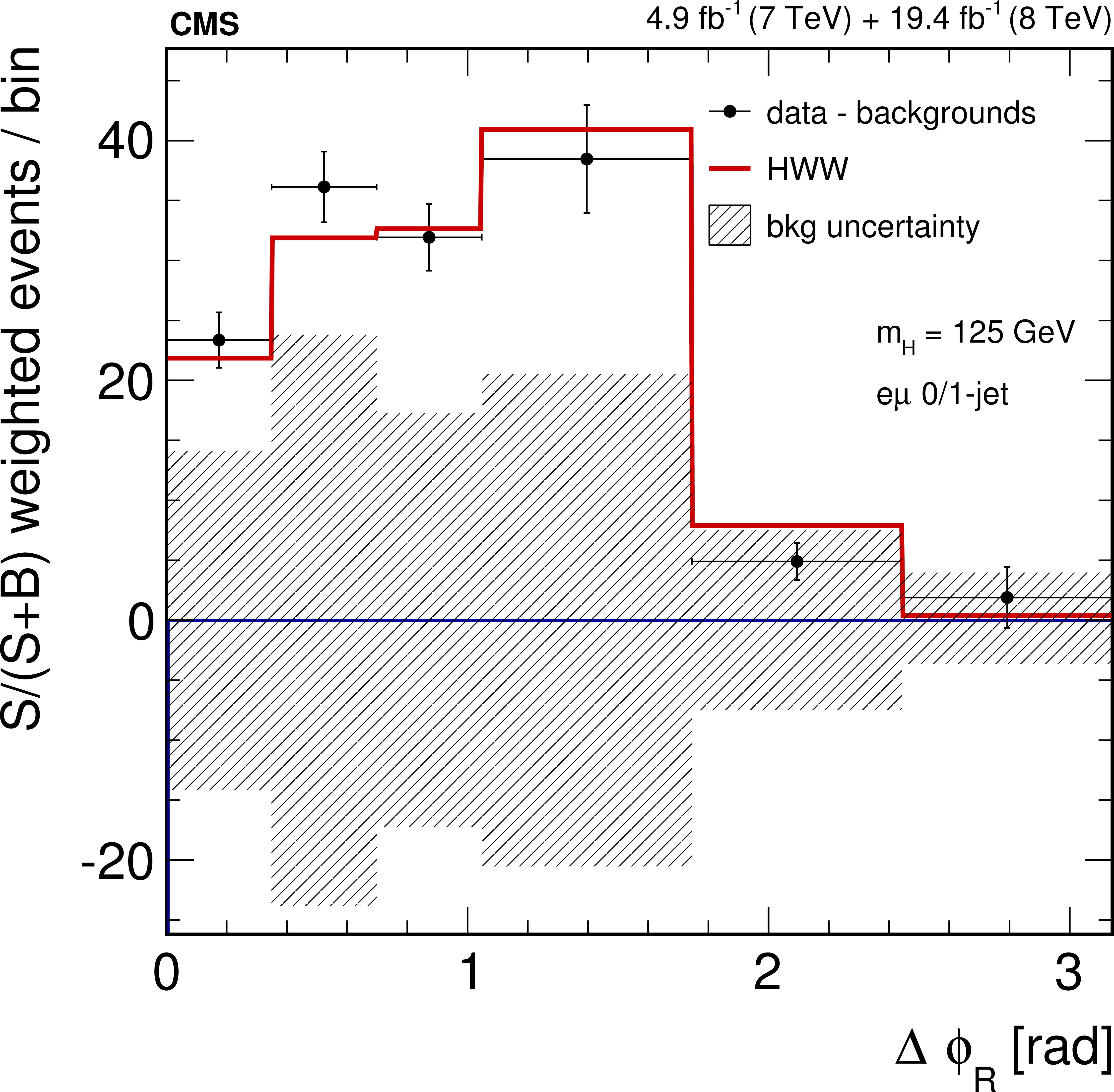
png pdf	Figure 10-b: The background-subtracted data distribution for ${m_{\mathrm {R}}}$ (a) and $\Delta \phi _R$ (b) with the best-fit superimposed for the 0-jet and 1-jet categories combined for $\sqrt {s}$ = 7 and 8 TeV. The signal and background processes are normalized to the result of the parametric fit to the ( ${m_{\mathrm {R}}}$ , ${\Delta \phi _{\mathrm {R}}}$ ) distribution. The events are weighted according to the observed S/(S+B) ratio of the second variable.
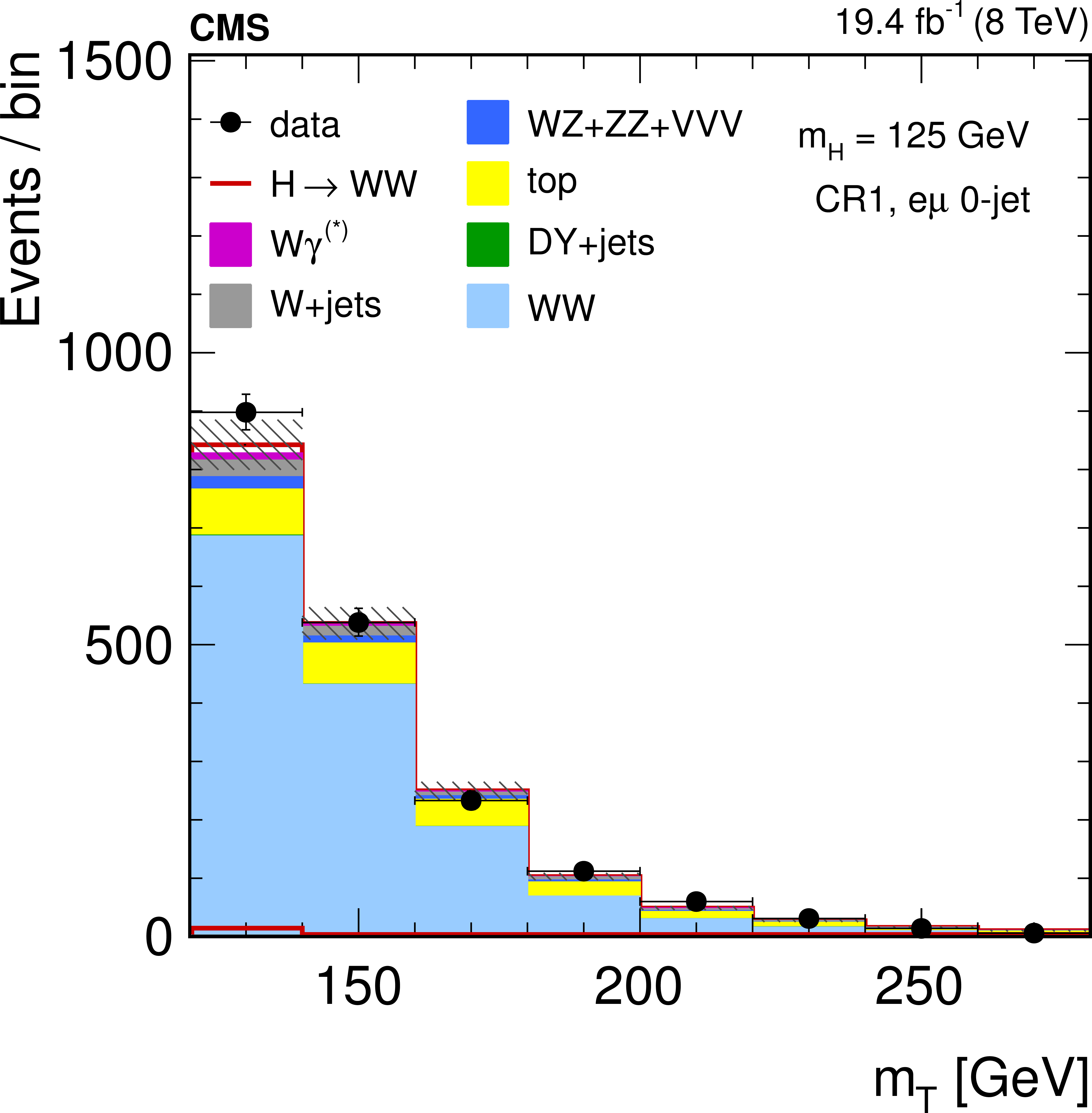
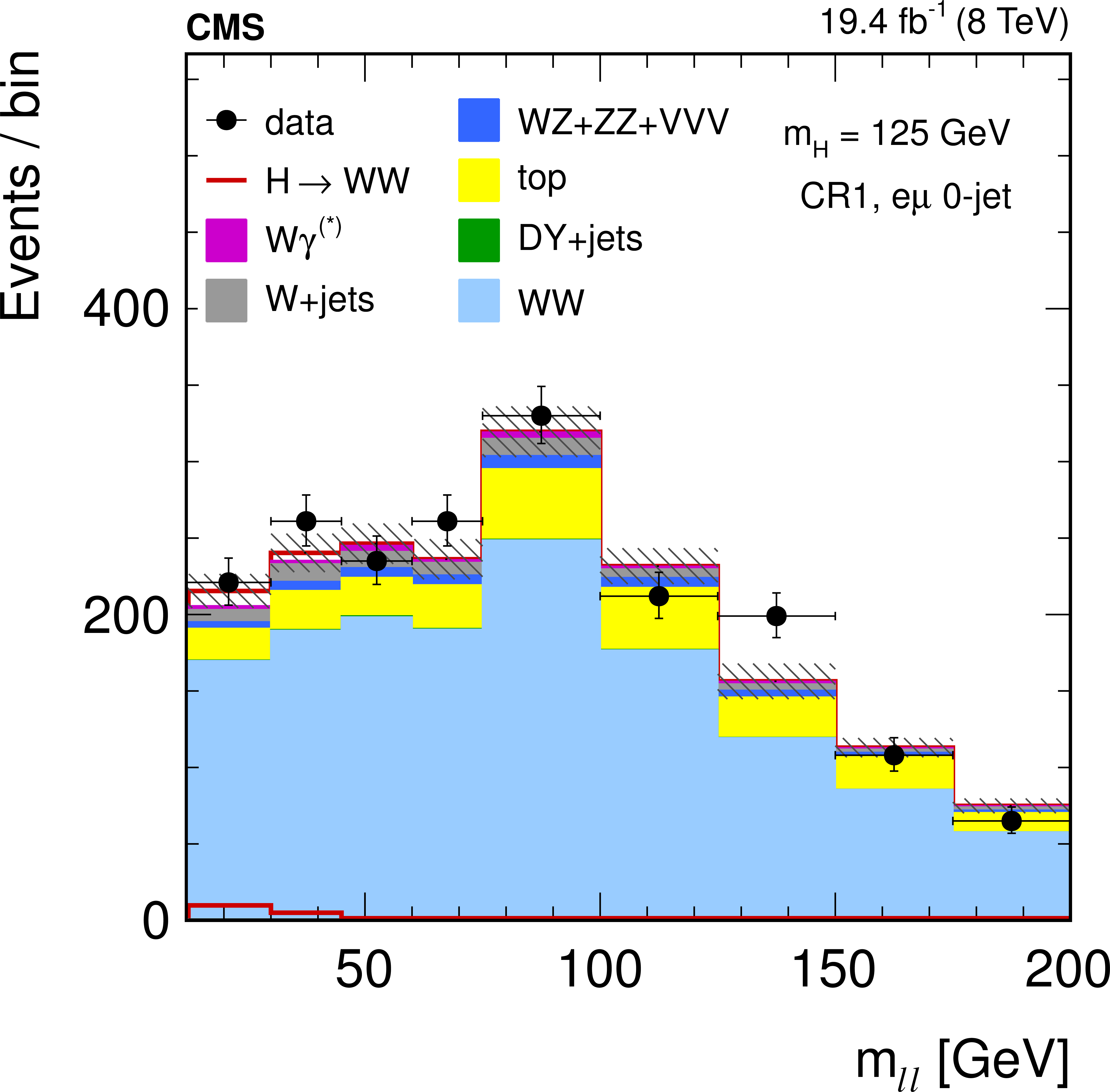
png pdf	Figure 11-a: Distributions of ${m_{\mathrm {T}}}$ (a, c) and ${m_{ {\ell } {\ell }}}$ (b, d) extrapolated to the control regions CR1 (a, b) and CR2 (c, d) in the 0-jet bin category, after fitting the other control region.
png pdf	Figure 11-b: Distributions of ${m_{\mathrm {T}}}$ (a, c) and ${m_{ {\ell } {\ell }}}$ (b, d) extrapolated to the control regions CR1 (a, b) and CR2 (c, d) in the 0-jet bin category, after fitting the other control region.
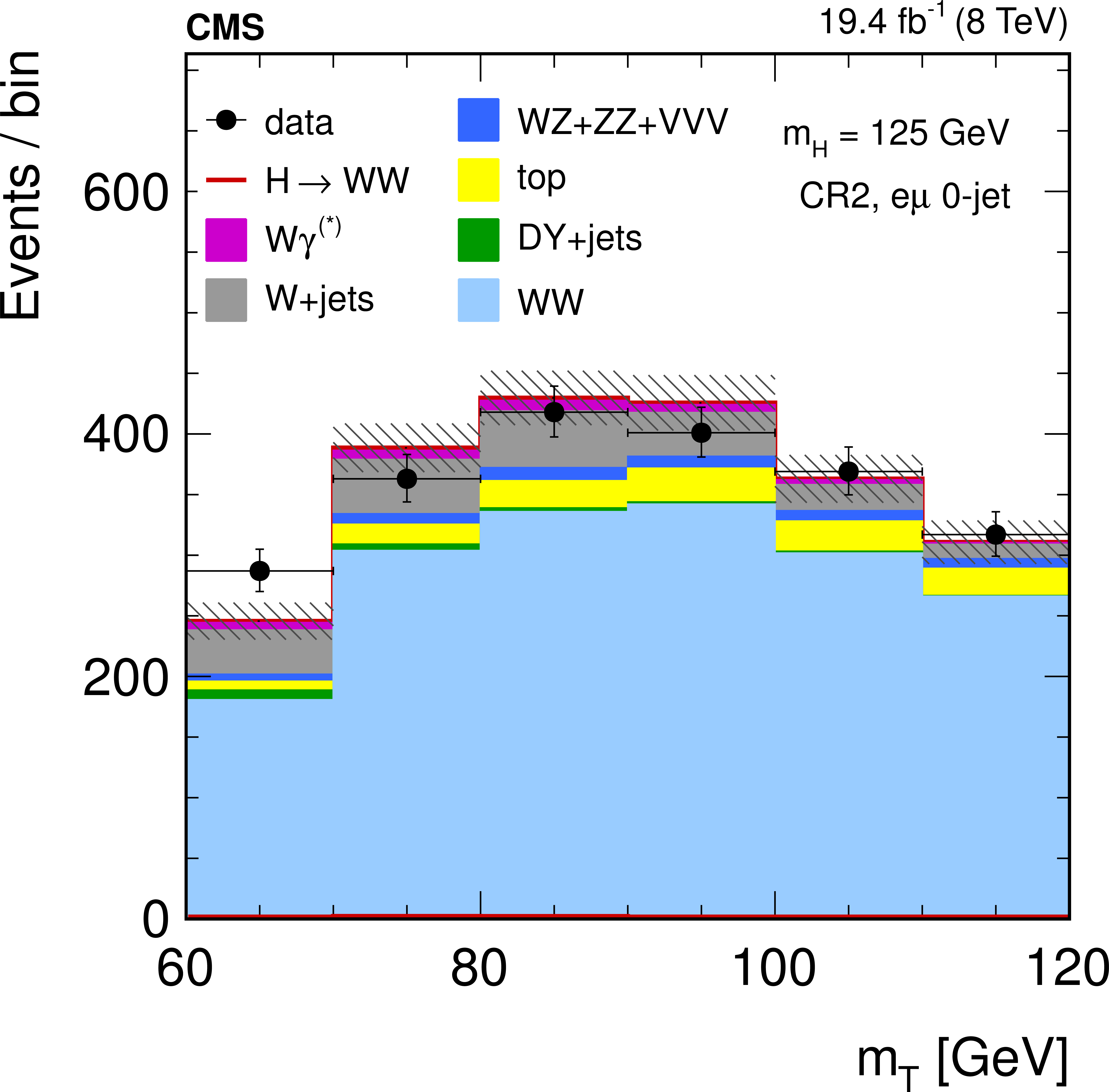
png pdf	Figure 11-c: Distributions of ${m_{\mathrm {T}}}$ (a, c) and ${m_{ {\ell } {\ell }}}$ (b, d) extrapolated to the control regions CR1 (a, b) and CR2 (c, d) in the 0-jet bin category, after fitting the other control region.
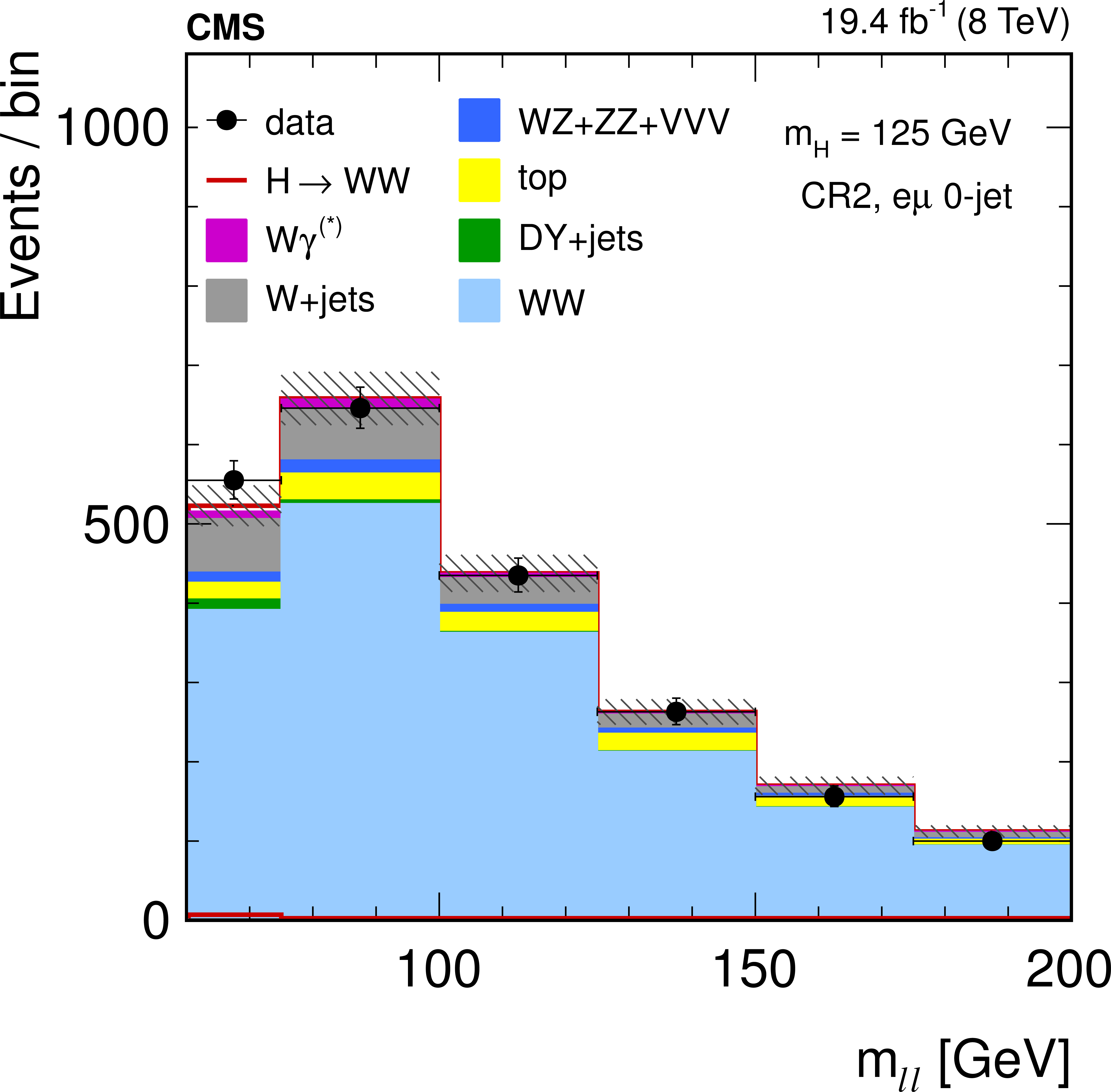
png pdf	Figure 11-d: Distributions of ${m_{\mathrm {T}}}$ (a, c) and ${m_{ {\ell } {\ell }}}$ (b, d) extrapolated to the control regions CR1 (a, b) and CR2 (c, d) in the 0-jet bin category, after fitting the other control region.
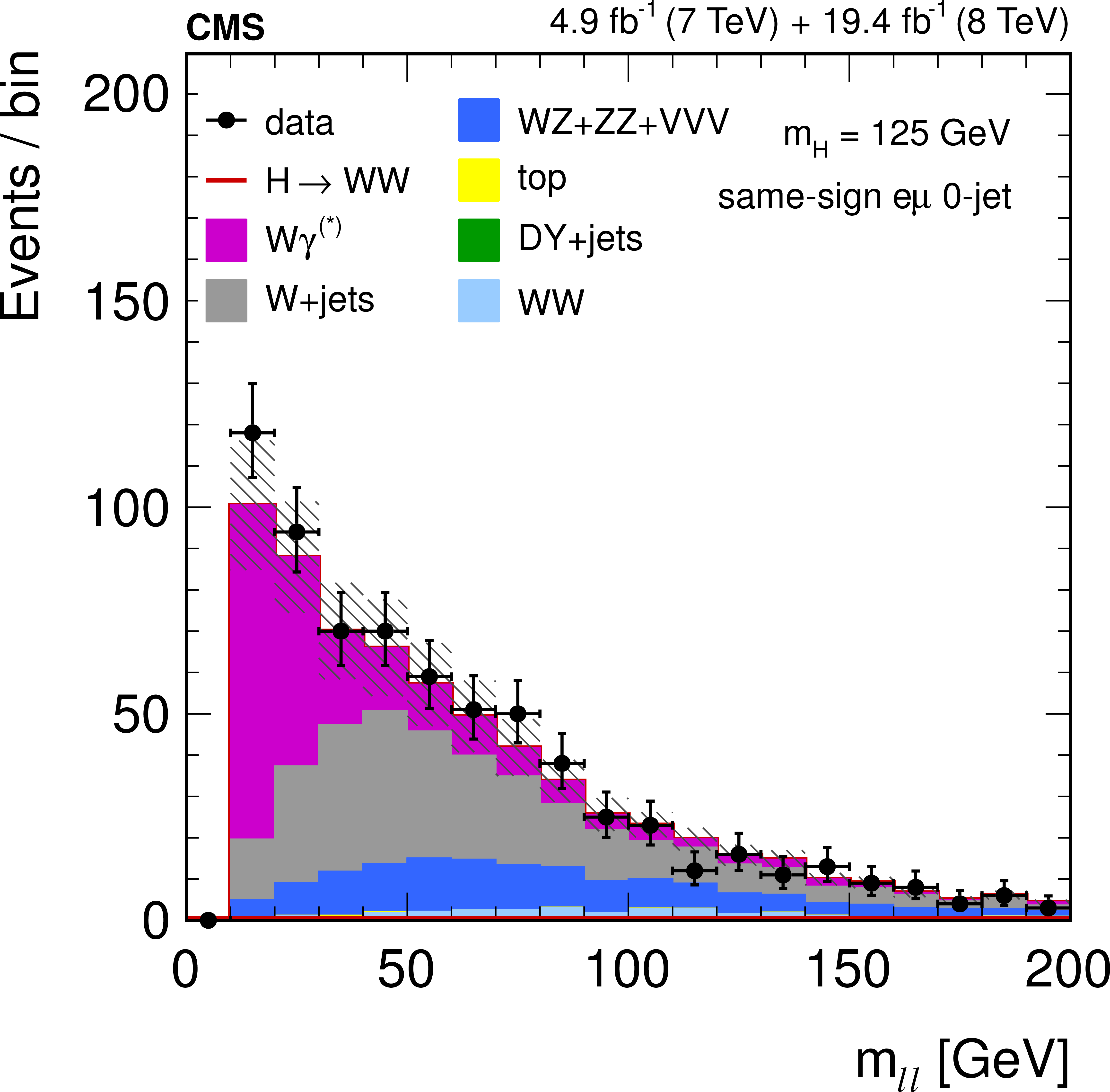
png pdf	Figure 12-a: Distributions of the dilepton mass (a) in the same-charge dilepton control region in the 0-jet category and the transverse mass (b) in the top-tagged control region in the 1-jet category of the ${\mathrm {e}}\mu$ final state.
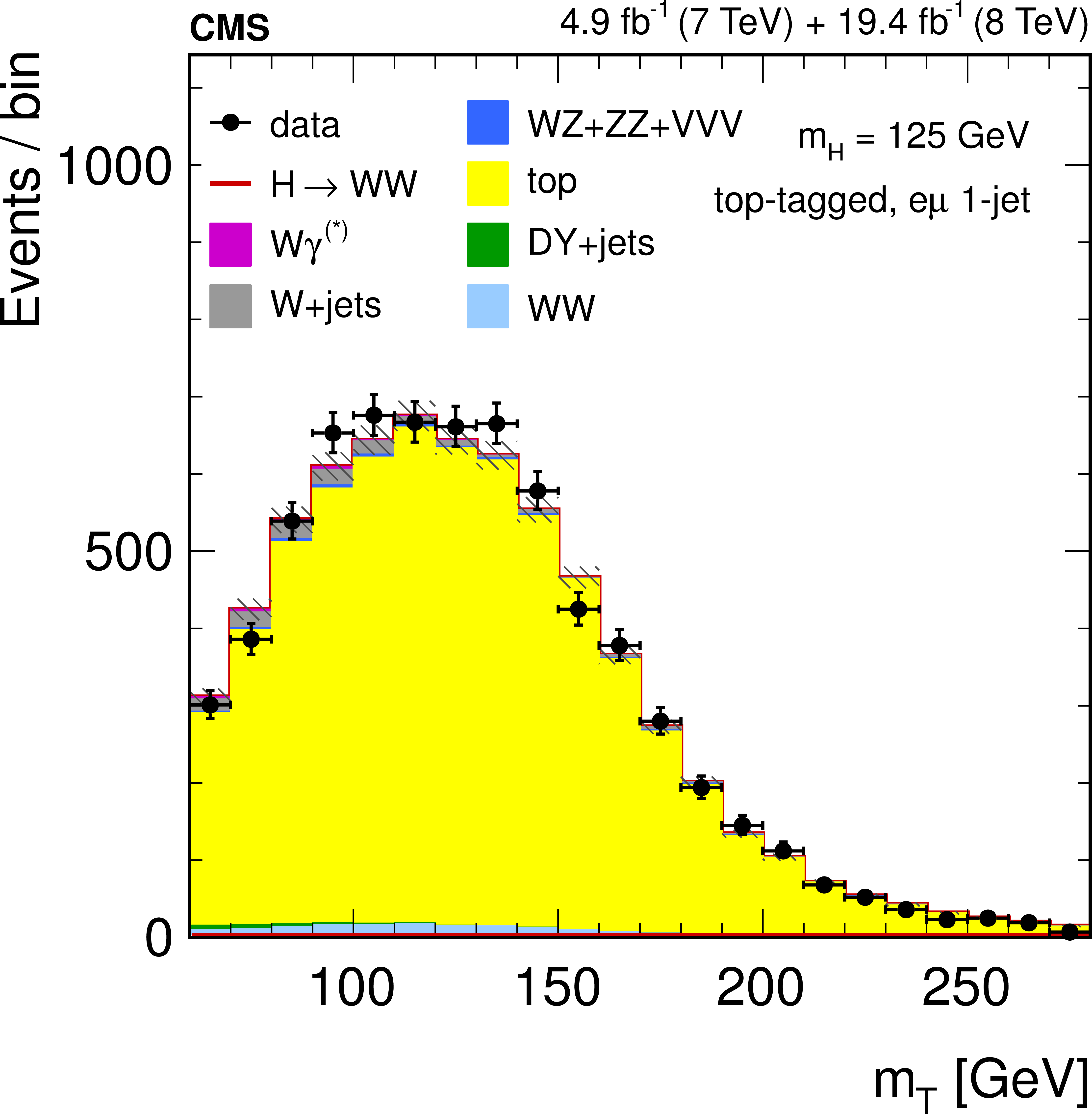
png pdf	Figure 12-b: Distributions of the dilepton mass (a) in the same-charge dilepton control region in the 0-jet category and the transverse mass (b) in the top-tagged control region in the 1-jet category of the ${\mathrm {e}}\mu$ final state.
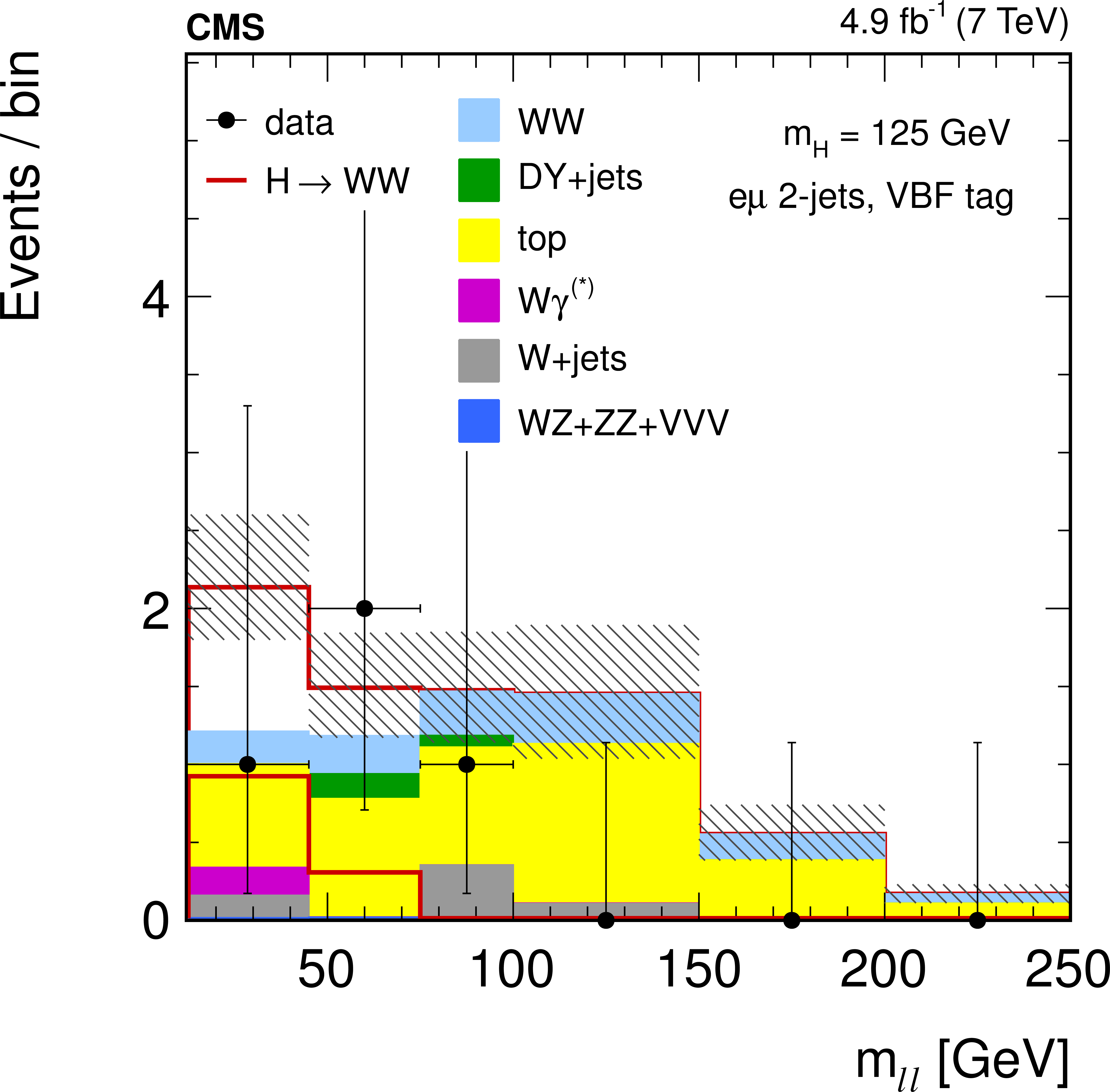
png pdf	Figure 13-a: The ${m_{ {\ell } {\ell }}}$ distributions for the data and background predictions for 7 TeV (a) and 8 TeV (b) analyses in the different-flavor final state for the 2-jet category with VBF tag. Selection criteria correspond to a Higgs boson mass of 125 GeV for the shape-based analysis. The uncertainty bands correspond to the sum of the statistical and systematic uncertainties in the background processes. The expected contribution for a Higgs boson signal with ${m_{ {\mathrm {H}} }}$ = 125 GeV (red open histogram) is also shown, both separately and stacked with the background histograms. For illustration purposes the region between 250 and 600 GeV is not shown in the figures, but is used in the measurement.
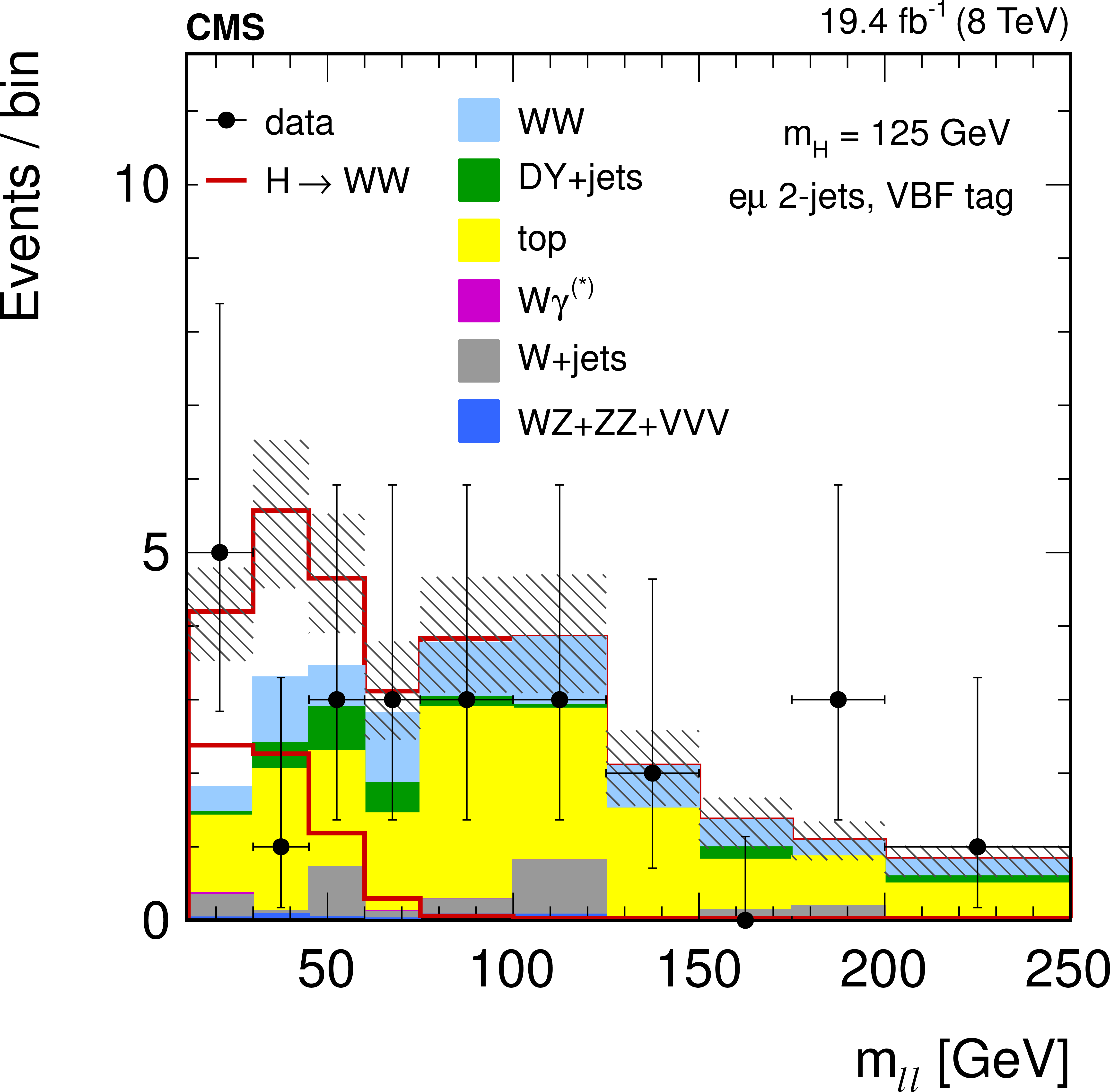
png pdf	Figure 13-b: The ${m_{ {\ell } {\ell }}}$ distributions for the data and background predictions for 7 TeV (a) and 8 TeV (b) analyses in the different-flavor final state for the 2-jet category with VBF tag. Selection criteria correspond to a Higgs boson mass of 125 GeV for the shape-based analysis. The uncertainty bands correspond to the sum of the statistical and systematic uncertainties in the background processes. The expected contribution for a Higgs boson signal with ${m_{ {\mathrm {H}} }}$ = 125 GeV (red open histogram) is also shown, both separately and stacked with the background histograms. For illustration purposes the region between 250 and 600 GeV is not shown in the figures, but is used in the measurement.
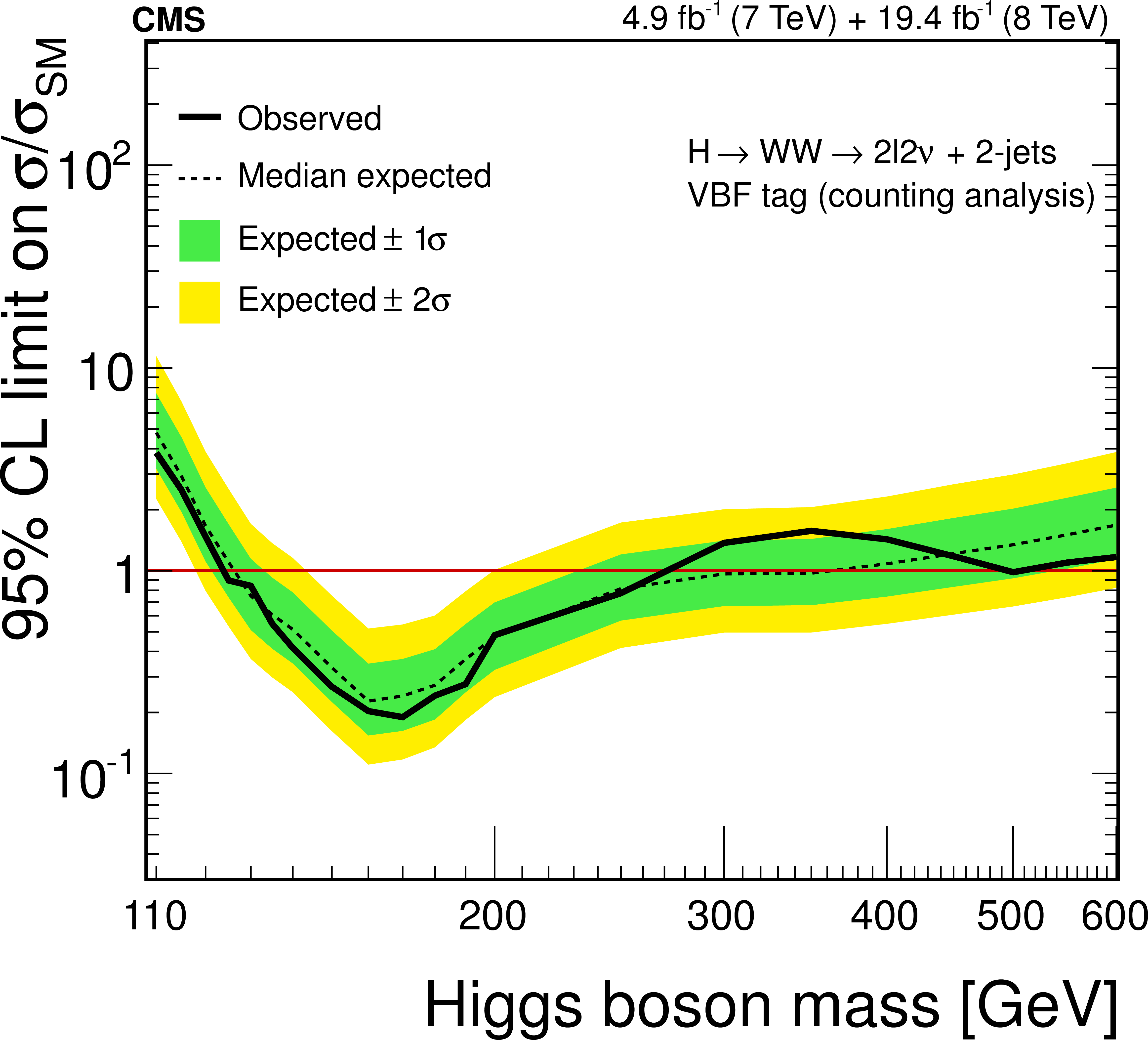
png pdf	Figure 14-a: Expected and observed 95% CL upper limits on the ${\mathrm {H}} \to {\mathrm {W}} {\mathrm {W}}$ production cross section relative to the SM Higgs boson expectation using the counting analysis (a), and shape-based template fit approach (b) in the 2-jet category with VBF tag. The shape-based analysis results use the one-dimensional binned template fit to ${m_{ {\ell } {\ell }}}$ distribution for the ${\mathrm {e}}\mu$ final state, combined with counting analysis inputs for the ${\mathrm {e}} {\mathrm {e}}/\mu \mu$ final states.
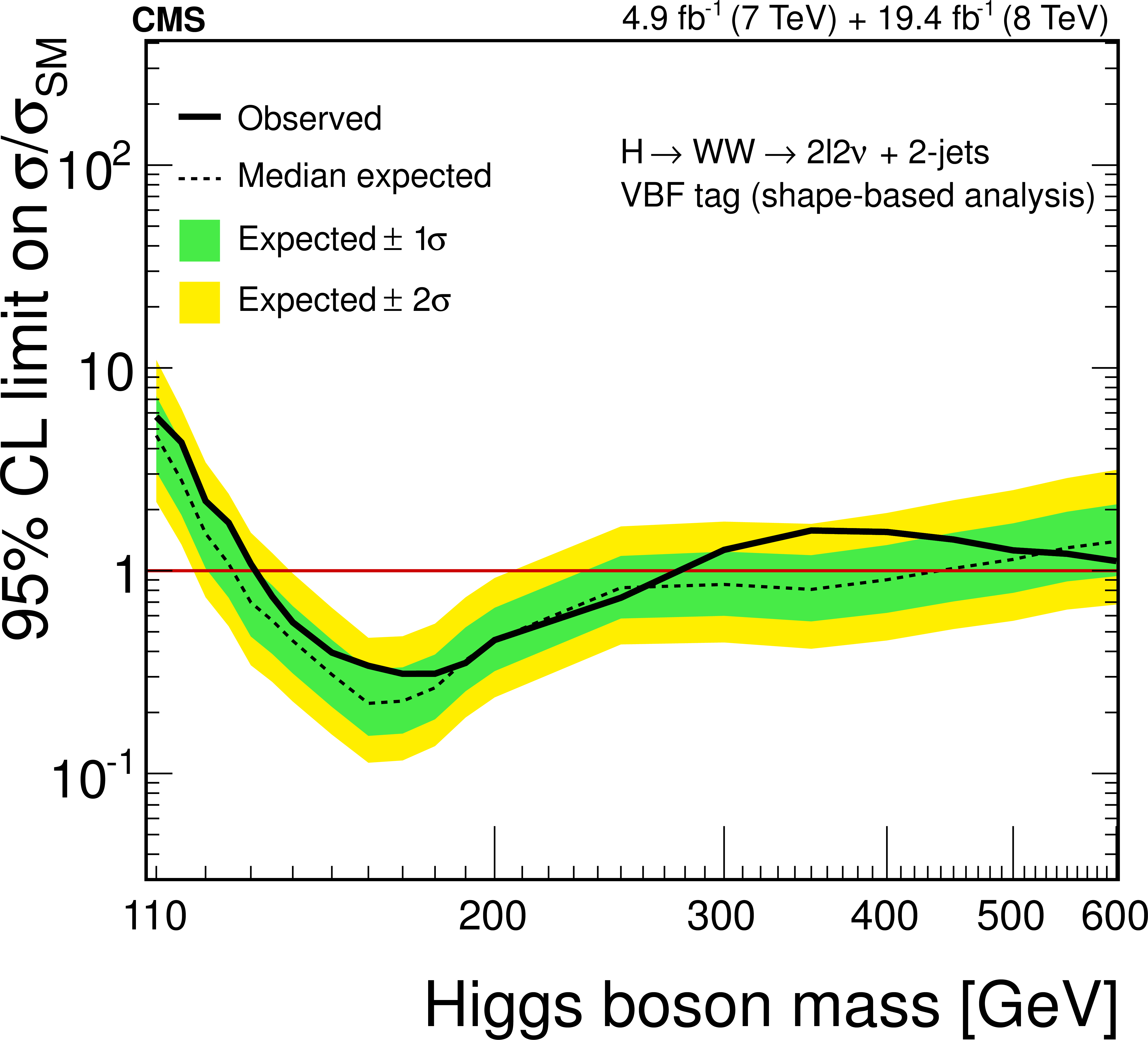
png pdf	Figure 14-b: Expected and observed 95% CL upper limits on the ${\mathrm {H}} \to {\mathrm {W}} {\mathrm {W}}$ production cross section relative to the SM Higgs boson expectation using the counting analysis (a), and shape-based template fit approach (b) in the 2-jet category with VBF tag. The shape-based analysis results use the one-dimensional binned template fit to ${m_{ {\ell } {\ell }}}$ distribution for the ${\mathrm {e}}\mu$ final state, combined with counting analysis inputs for the ${\mathrm {e}} {\mathrm {e}}/\mu \mu$ final states.
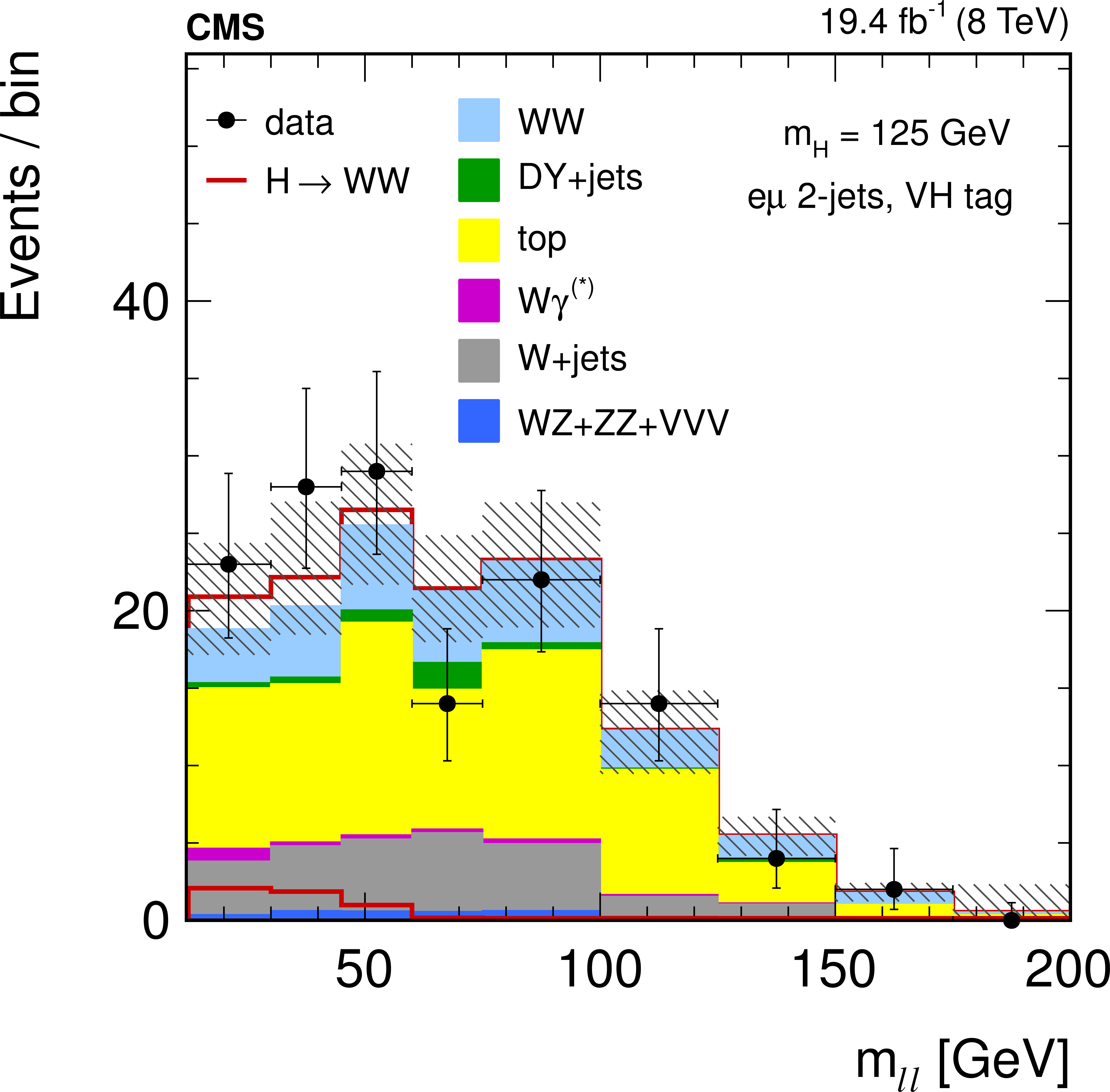
png pdf	Figure 15: The ${m_{ {\ell } {\ell }}}$ distribution for ${m_{ {\mathrm {H}} }}$ = 125 GeV used as input to the template fit in the ${\mathrm {e}}\mu$ final state for the ${\mathrm {V}} {\mathrm {H}}$ analysis after the corresponding selection at $\sqrt {s}= 8 TeV$ .
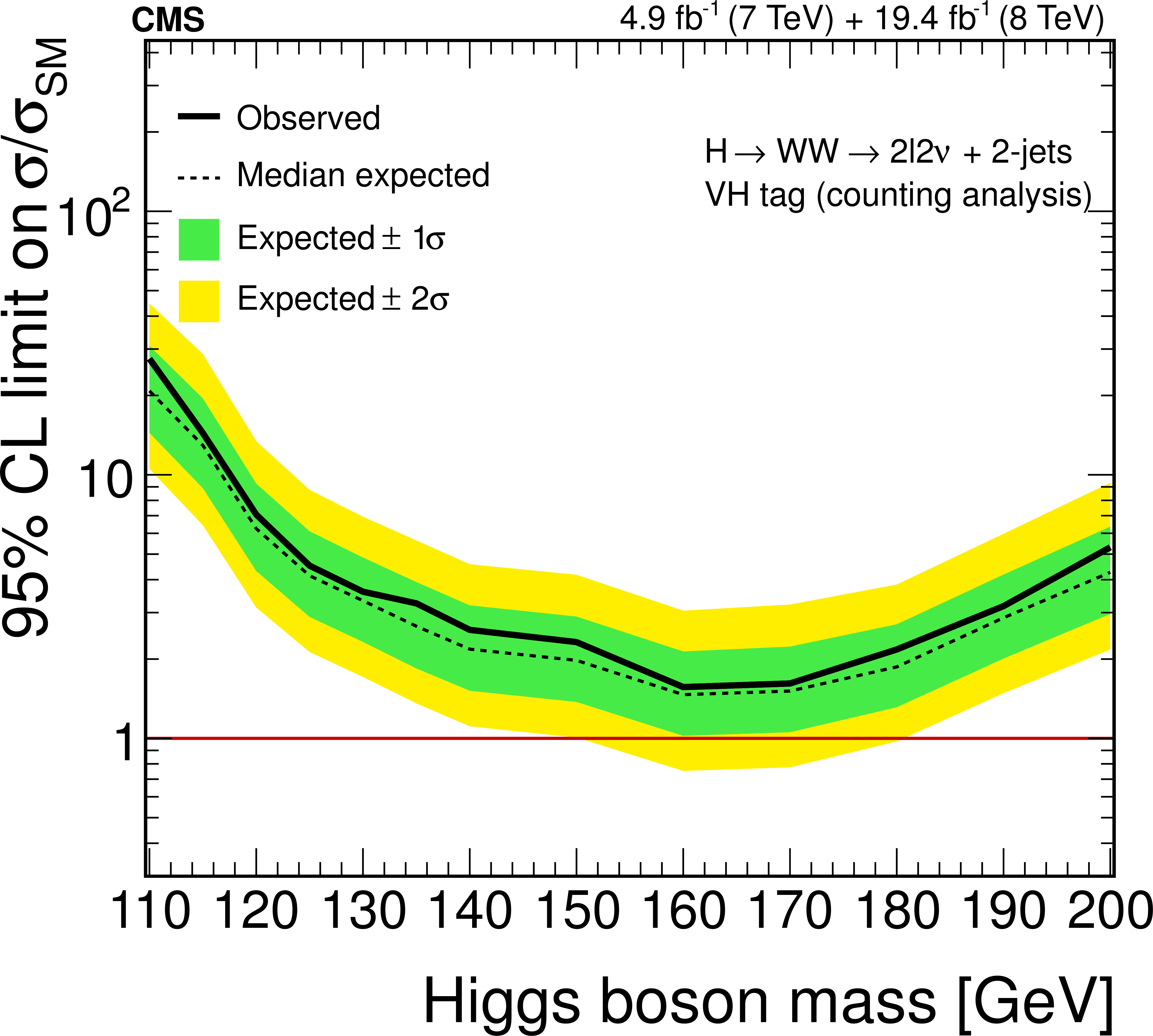
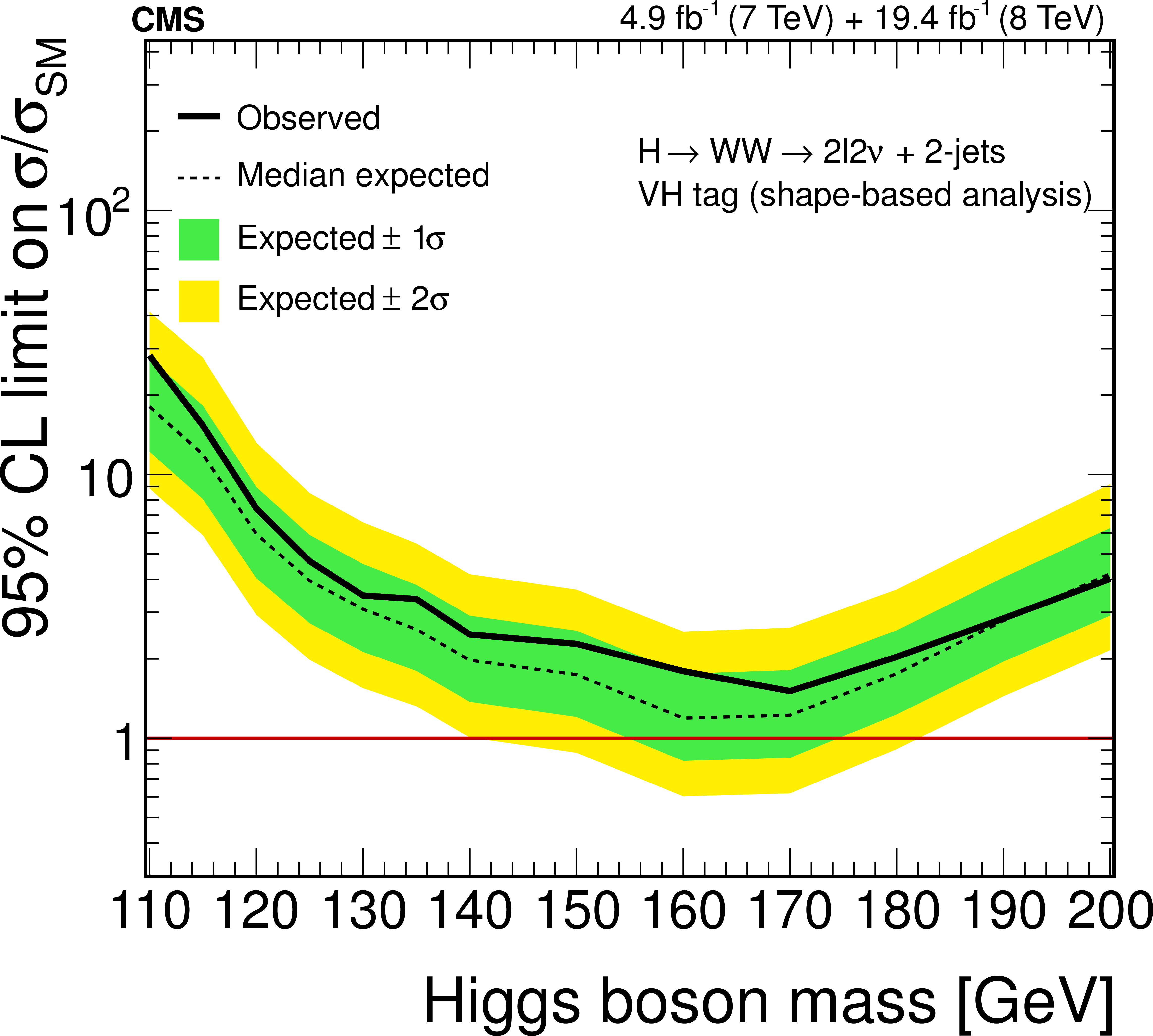
png pdf	Figure 16-a: Expected and observed 95% CL upper limits on the ${\mathrm {H}} \to {\mathrm {W}} {\mathrm {W}}$ production cross section relative to the SM Higgs boson expectation using the counting analysis (a), and the shape-based template fit approach (b) in the ${\mathrm {V}} {\mathrm {H}}$ category. The shape-based analysis results use the one-dimensional binned template fit to the ${m_{ {\ell } {\ell }}}$ distribution for the ${\mathrm {e}}\mu$ final state, combined with counting analysis results for the ${\mathrm {e}} {\mathrm {e}}/\mu \mu$ final states.
png pdf	Figure 16-b: Expected and observed 95% CL upper limits on the ${\mathrm {H}} \to {\mathrm {W}} {\mathrm {W}}$ production cross section relative to the SM Higgs boson expectation using the counting analysis (a), and the shape-based template fit approach (b) in the ${\mathrm {V}} {\mathrm {H}}$ category. The shape-based analysis results use the one-dimensional binned template fit to the ${m_{ {\ell } {\ell }}}$ distribution for the ${\mathrm {e}}\mu$ final state, combined with counting analysis results for the ${\mathrm {e}} {\mathrm {e}}/\mu \mu$ final states.
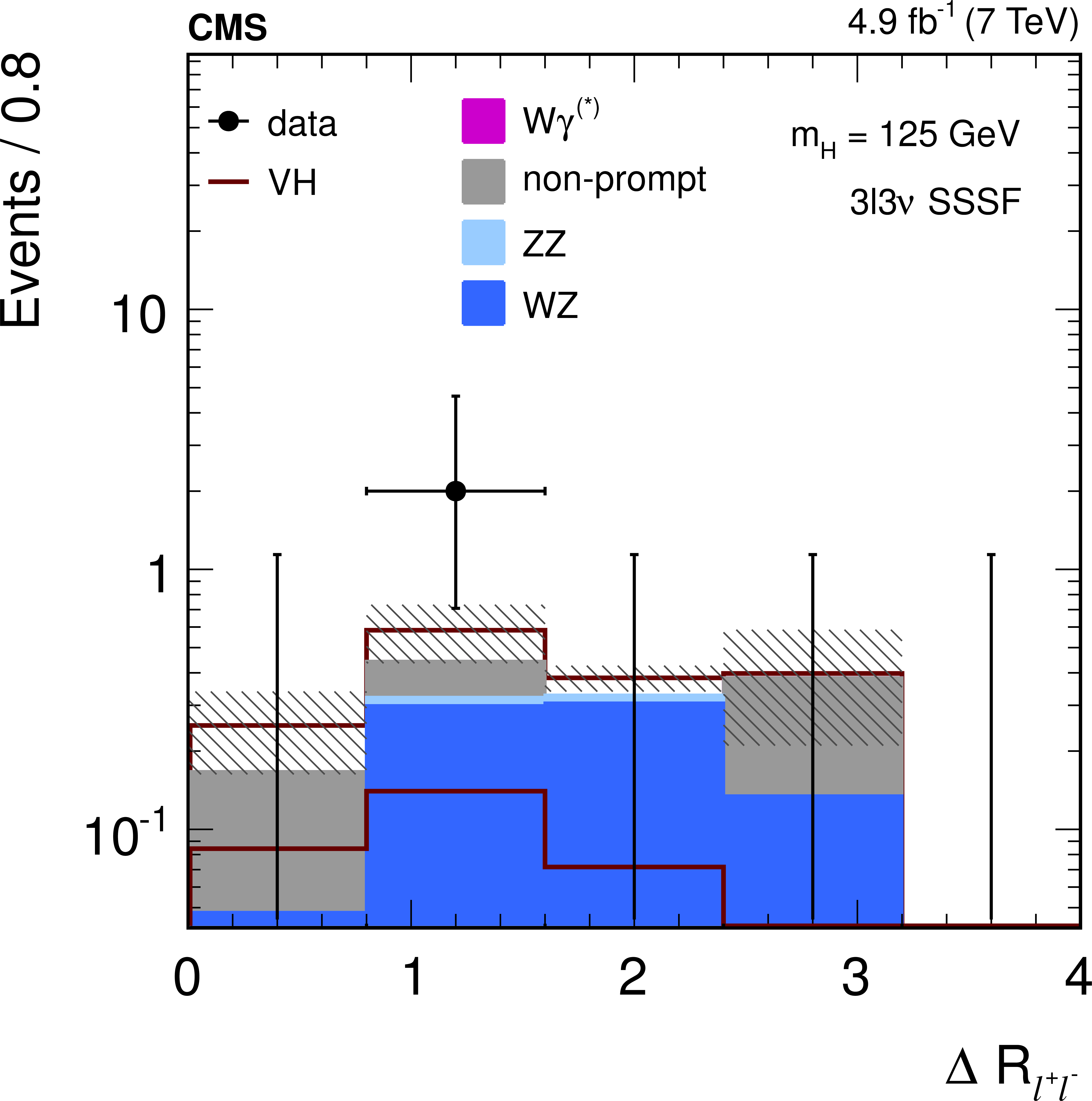
png pdf	Figure 17-a: The $\Delta R_{\ell ^+\ell ^-}$ distribution, after applying all other requirements for the ${\mathrm {W}} {\mathrm {H}} \to 3\ell 3\nu$ analysis, in the SSSF final state at 7 TeV (a), the OSSF final state at 7 TeV (b), the SSSF final state at 8 TeV (c), and the OSSF final state at 8 TeV (d). The legend entry labeled as ``non-prompt" is the combination of the backgrounds from ${\mathrm {Z+jets}}$ and top-quark decays.
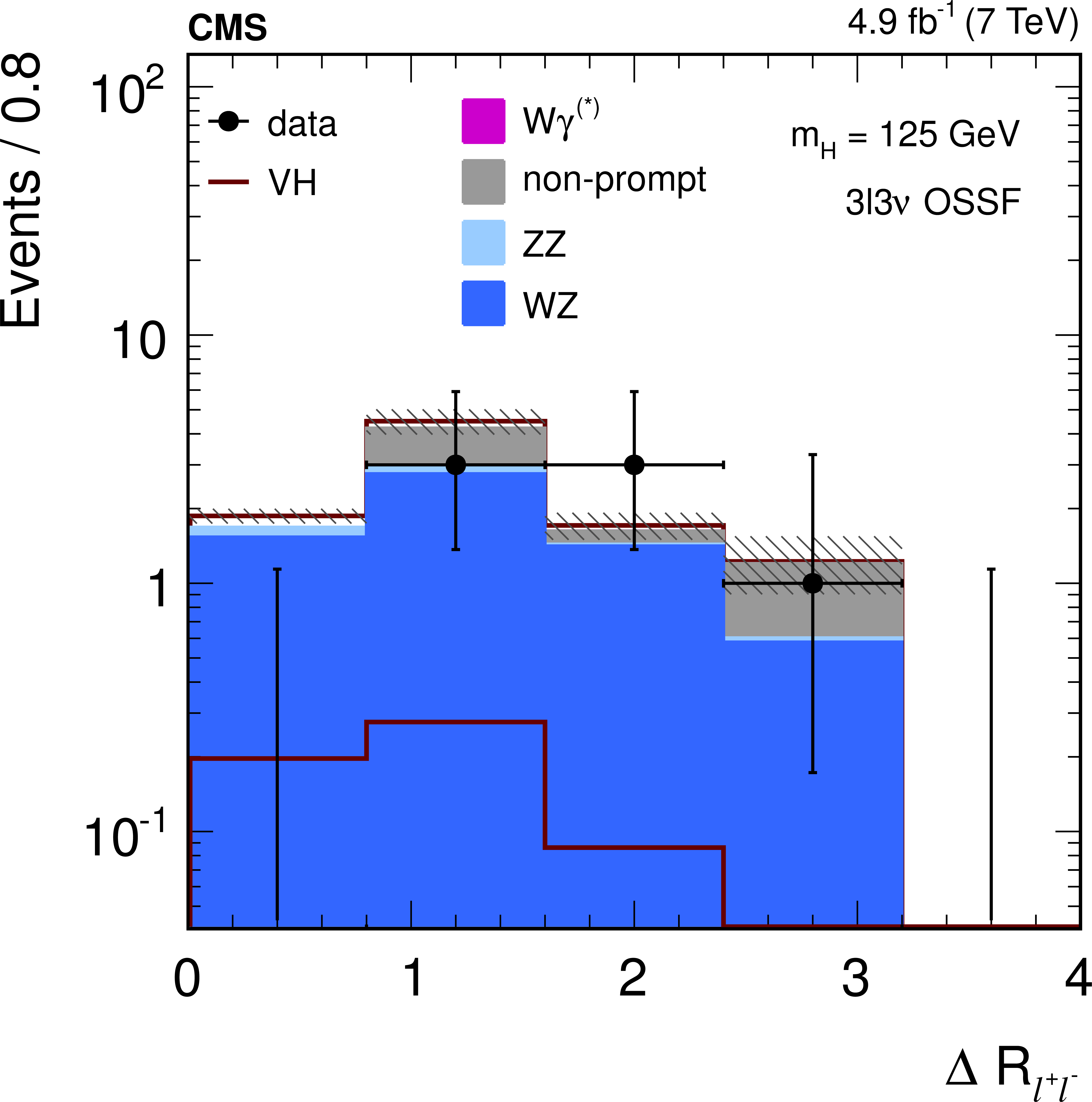
png pdf	Figure 17-b: The $\Delta R_{\ell ^+\ell ^-}$ distribution, after applying all other requirements for the ${\mathrm {W}} {\mathrm {H}} \to 3\ell 3\nu$ analysis, in the SSSF final state at 7 TeV (a), the OSSF final state at 7 TeV (b), the SSSF final state at 8 TeV (c), and the OSSF final state at 8 TeV (d). The legend entry labeled as ``non-prompt" is the combination of the backgrounds from ${\mathrm {Z+jets}}$ and top-quark decays.
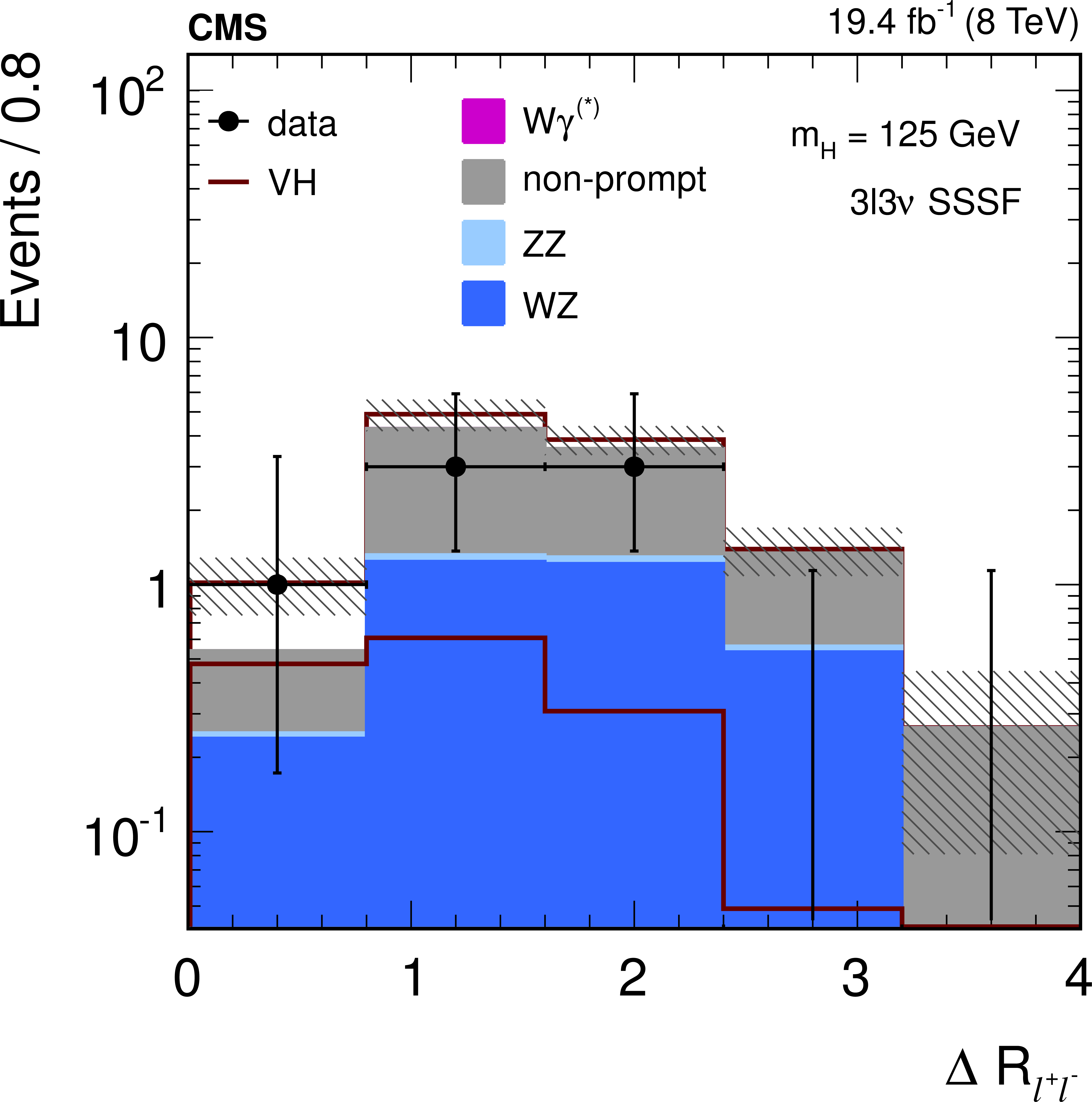
png pdf	Figure 17-c: The $\Delta R_{\ell ^+\ell ^-}$ distribution, after applying all other requirements for the ${\mathrm {W}} {\mathrm {H}} \to 3\ell 3\nu$ analysis, in the SSSF final state at 7 TeV (a), the OSSF final state at 7 TeV (b), the SSSF final state at 8 TeV (c), and the OSSF final state at 8 TeV (d). The legend entry labeled as ``non-prompt" is the combination of the backgrounds from ${\mathrm {Z+jets}}$ and top-quark decays.
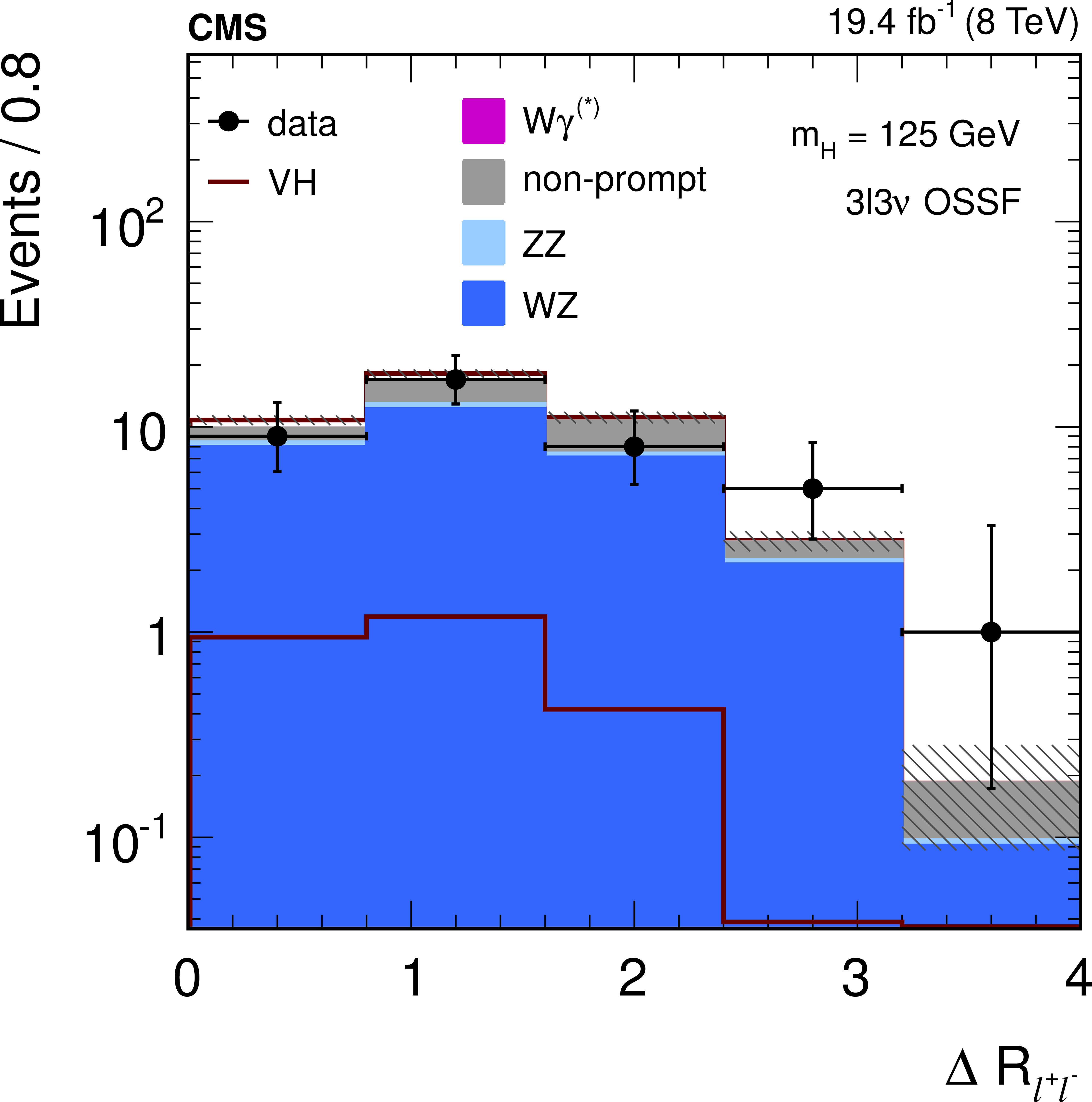
png pdf	Figure 17-d: The $\Delta R_{\ell ^+\ell ^-}$ distribution, after applying all other requirements for the ${\mathrm {W}} {\mathrm {H}} \to 3\ell 3\nu$ analysis, in the SSSF final state at 7 TeV (a), the OSSF final state at 7 TeV (b), the SSSF final state at 8 TeV (c), and the OSSF final state at 8 TeV (d). The legend entry labeled as ``non-prompt" is the combination of the backgrounds from ${\mathrm {Z+jets}}$ and top-quark decays.
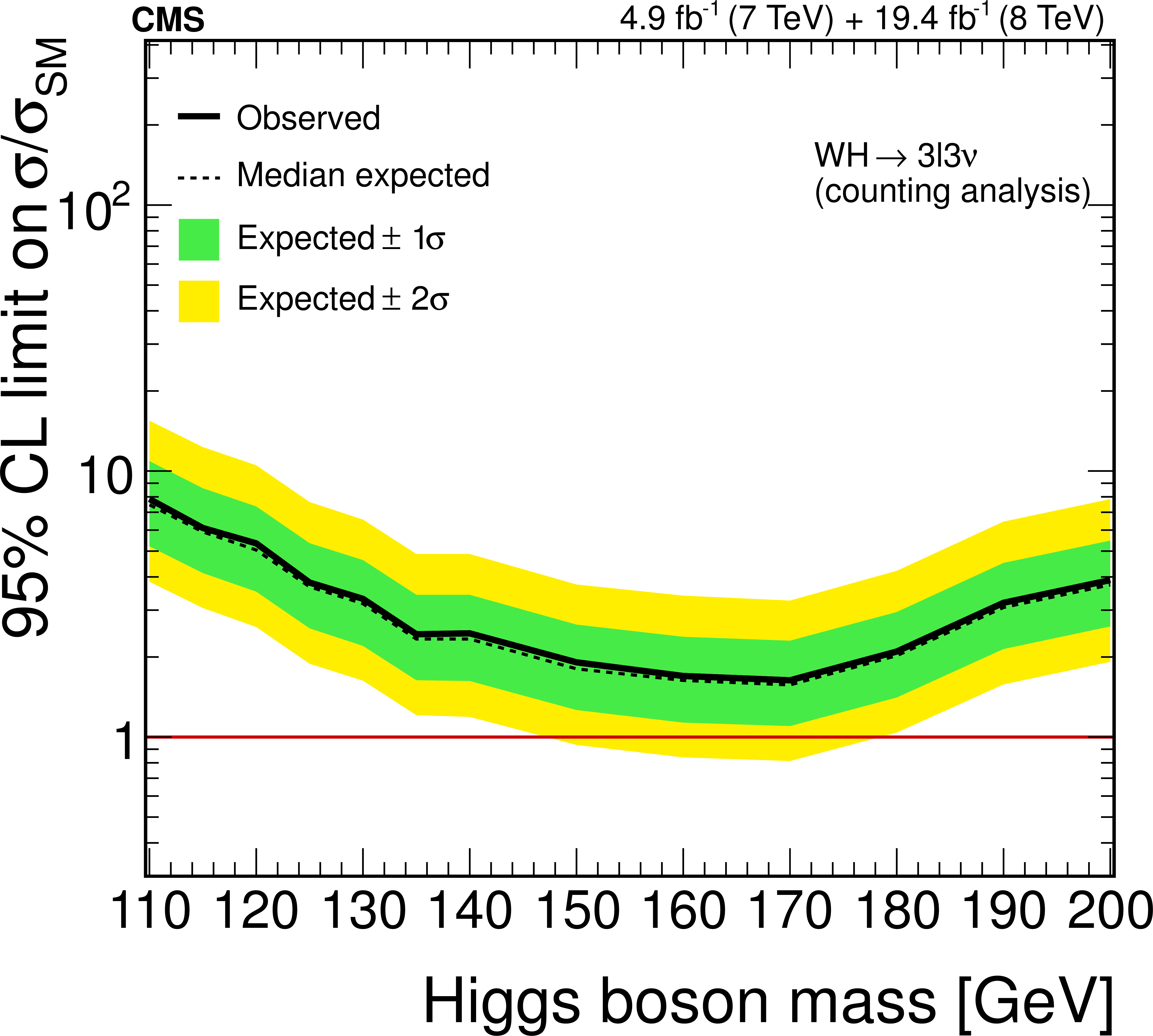
png pdf	Figure 18-a: Expected and observed 95% CL upper limits on the signal production cross section relative to the SM Higgs boson expectation using the counting analysis (left) and the shape-based template fit approach (right) in the ${\mathrm {W}} {\mathrm {H}} \to 3\ell 3\nu$ category.
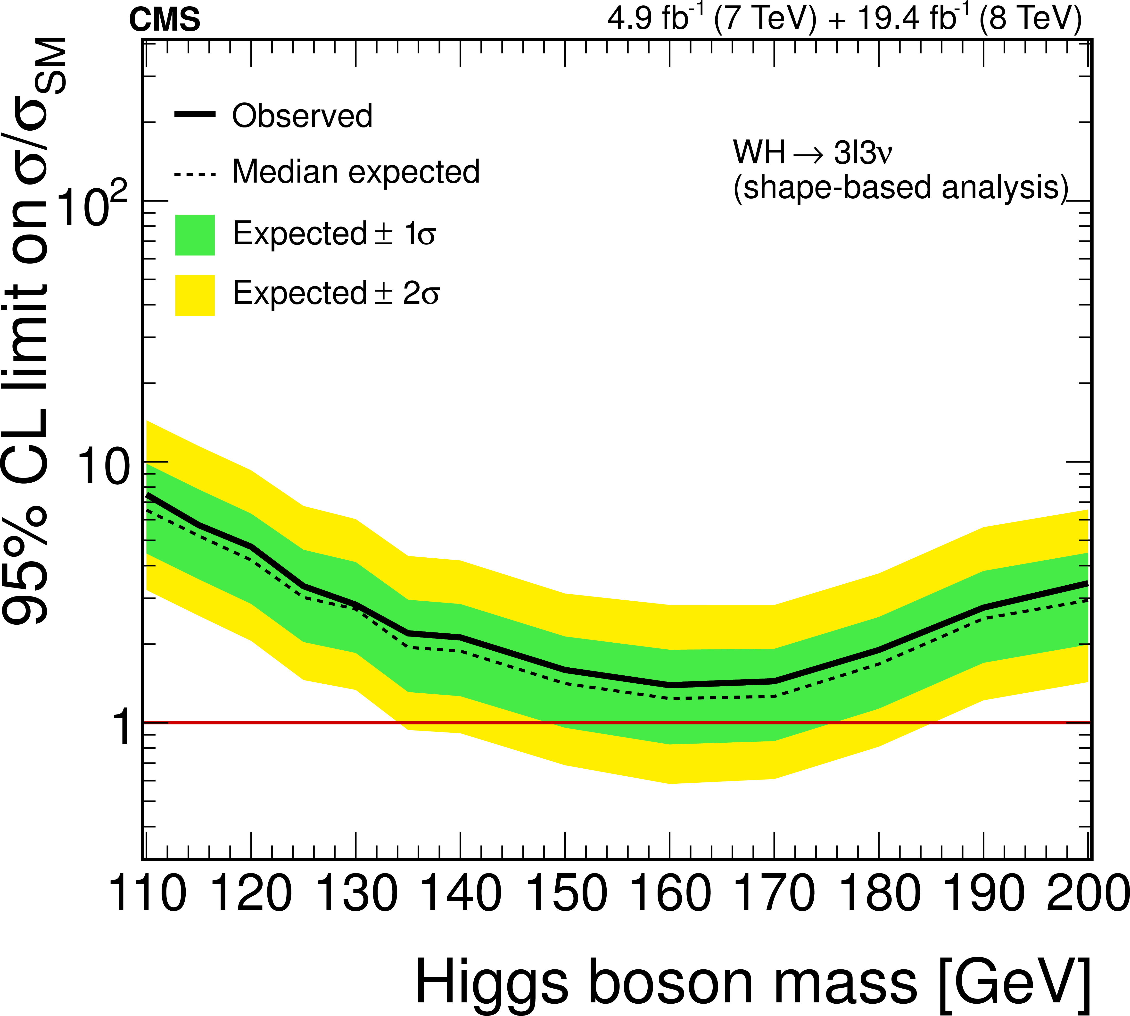
png pdf	Figure 18-b: Expected and observed 95% CL upper limits on the signal production cross section relative to the SM Higgs boson expectation using the counting analysis (left) and the shape-based template fit approach (right) in the ${\mathrm {W}} {\mathrm {H}} \to 3\ell 3\nu$ category.
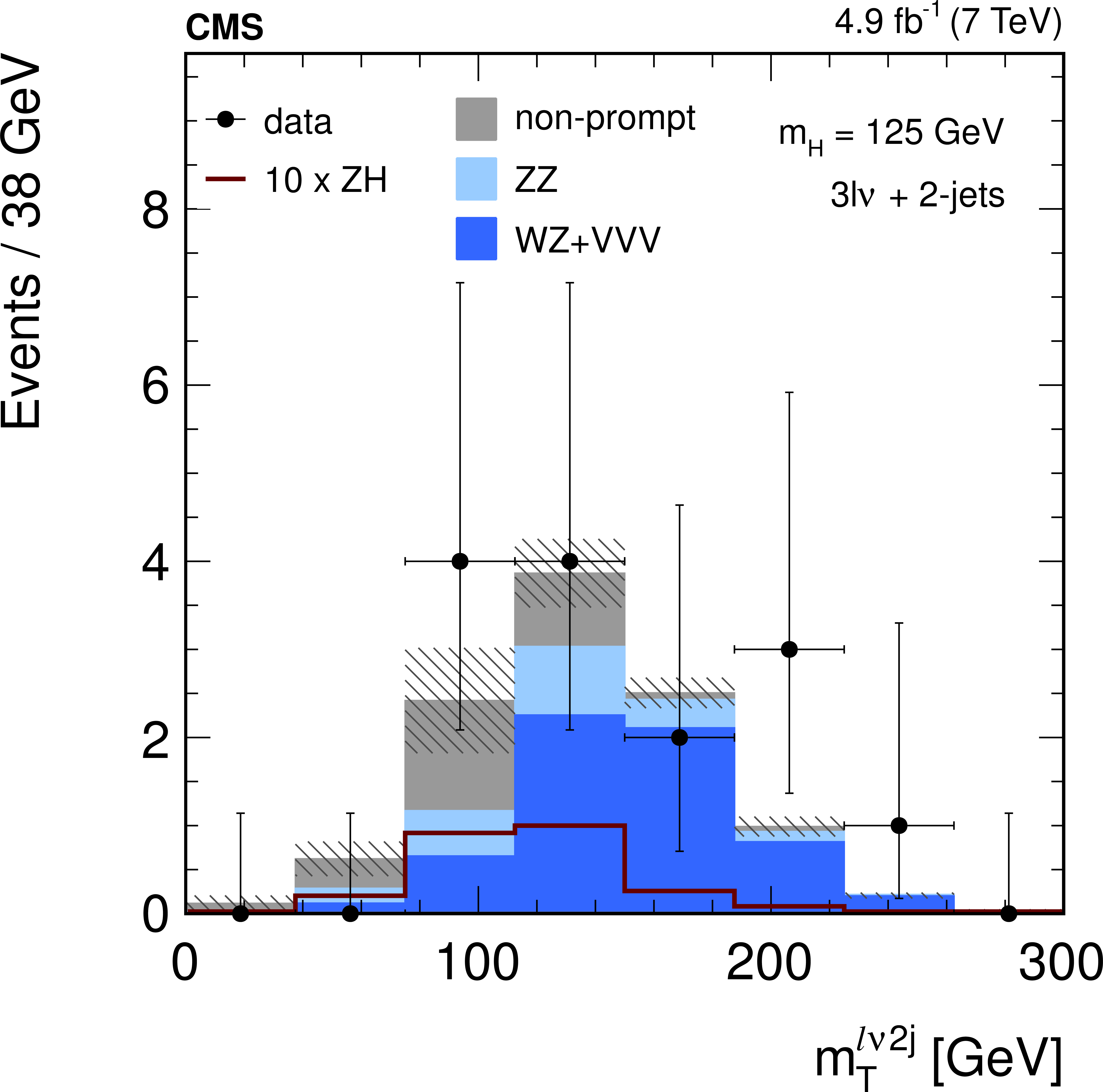
png pdf	Figure 19-a: The ${m_{\mathrm {T}}^{\ell \nu 2j}}$ distribution after all other requirements for the ${\mathrm {Z}} {\mathrm {H}} \to 3\ell \nu \text {+ 2 jets}$ analysis at 7 TeV (a), and at 8 TeV (b). The signal yield (red open histogram) is multiplied by 10 with respect to the SM expectation. The legend entry labeled as ``non-prompt'' is the combination of the backgrounds from ${\mathrm {Z+jets}}$ and top-quark decays.
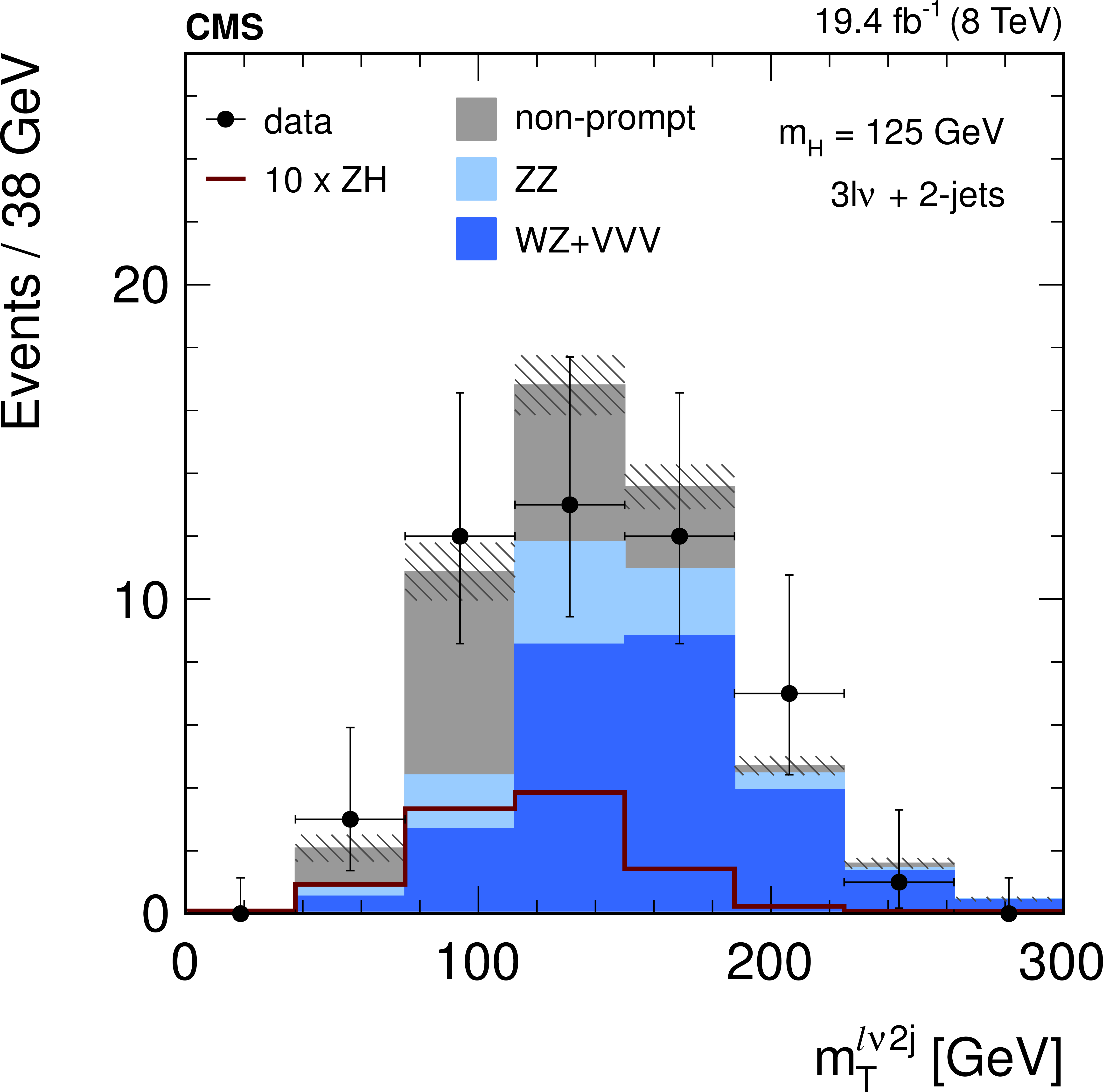
png pdf	Figure 19-b: The ${m_{\mathrm {T}}^{\ell \nu 2j}}$ distribution after all other requirements for the ${\mathrm {Z}} {\mathrm {H}} \to 3\ell \nu \text {+ 2 jets}$ analysis at 7 TeV (a), and at 8 TeV (b). The signal yield (red open histogram) is multiplied by 10 with respect to the SM expectation. The legend entry labeled as ``non-prompt'' is the combination of the backgrounds from ${\mathrm {Z+jets}}$ and top-quark decays.
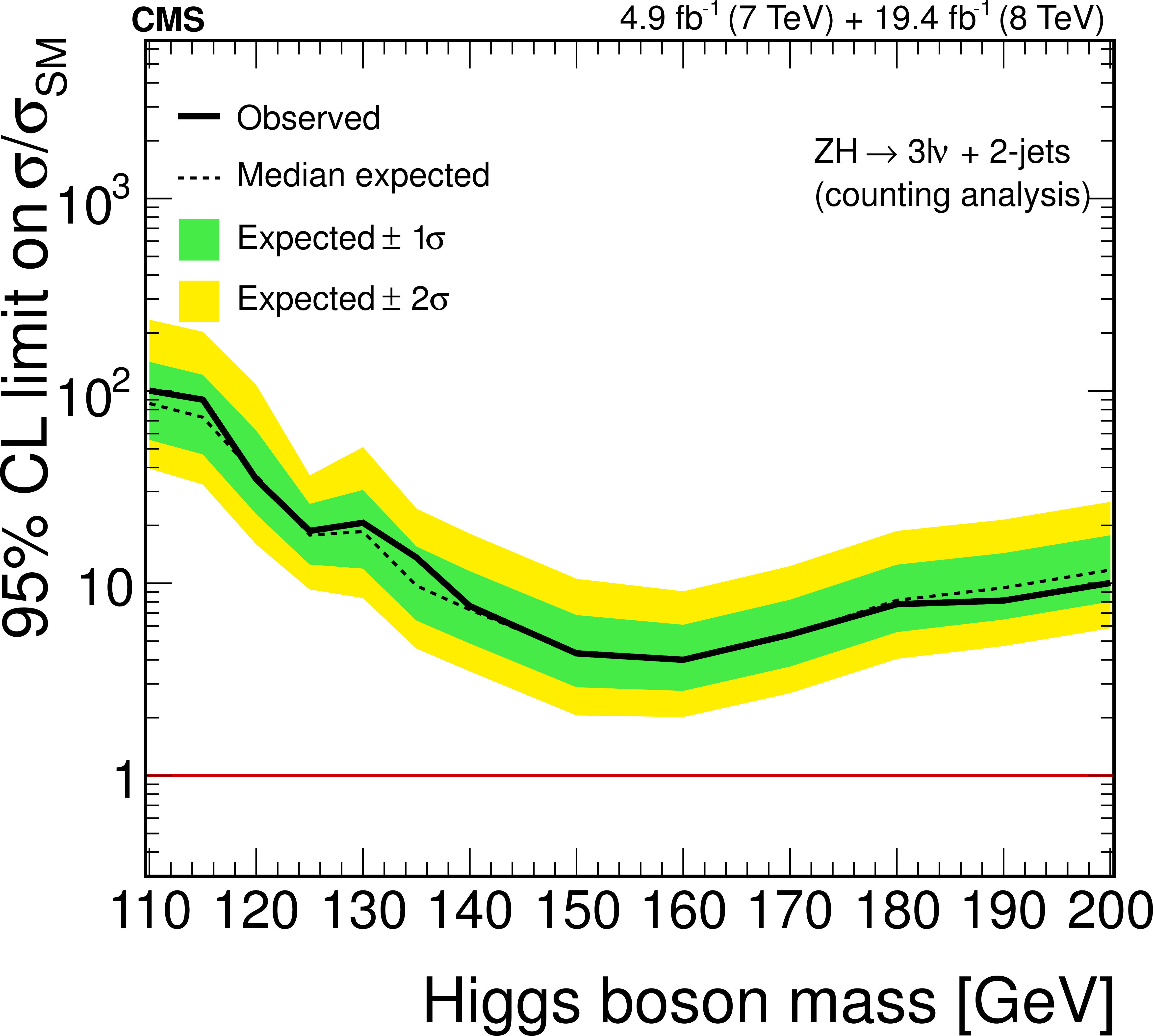
png pdf	Figure 20-a: Expected and observed 95% CL upper limits on the signal production cross section relative to the SM Higgs boson expectation using the counting analysis (left) and the shape-based template fit approach (right) in the ${\mathrm {Z}} {\mathrm {H}} \to 3\ell \nu \text {+ 2 jets}$ category.
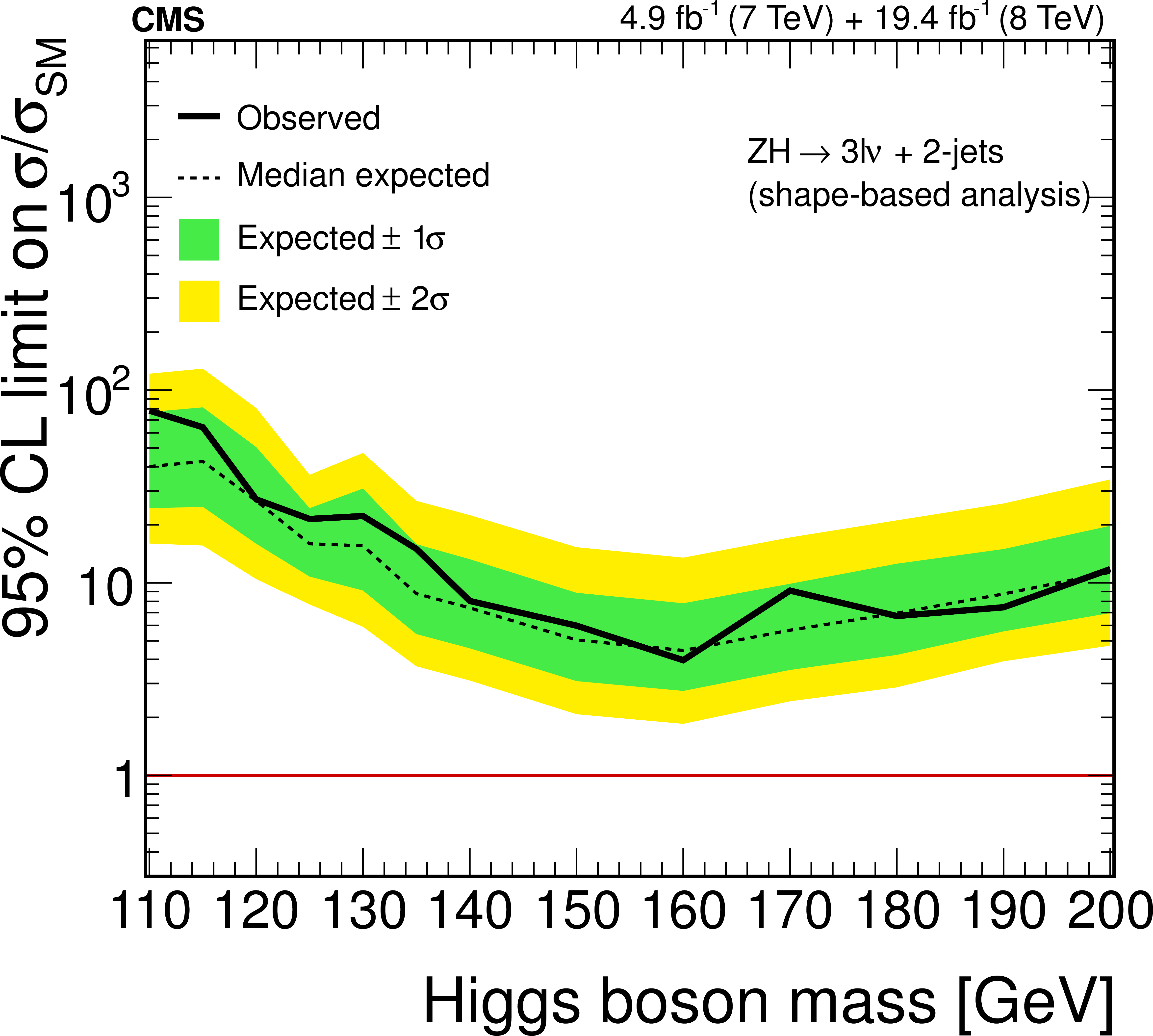
png pdf	Figure 20-b: Expected and observed 95% CL upper limits on the signal production cross section relative to the SM Higgs boson expectation using the counting analysis (left) and the shape-based template fit approach (right) in the ${\mathrm {Z}} {\mathrm {H}} \to 3\ell \nu \text {+ 2 jets}$ category.
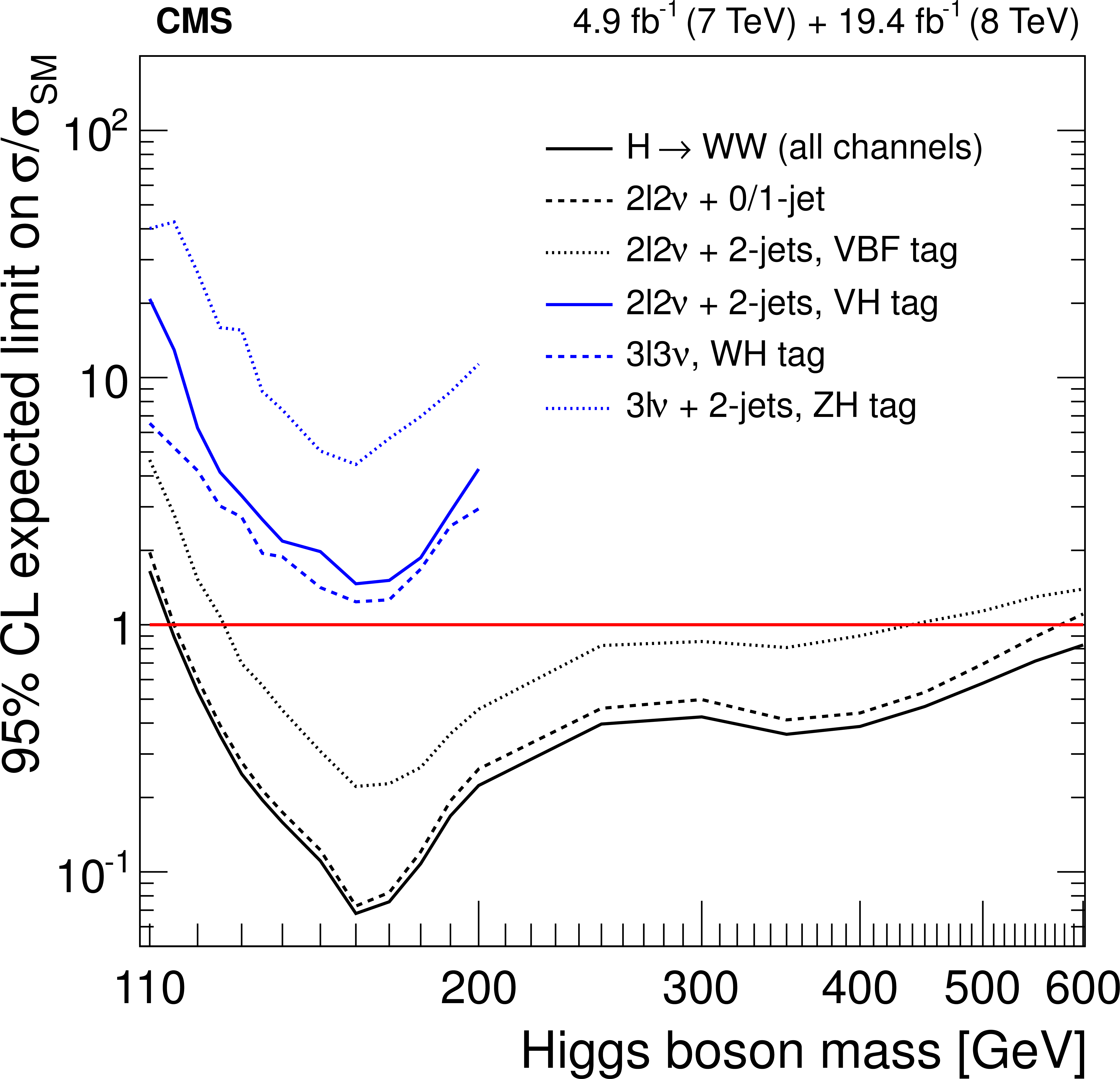
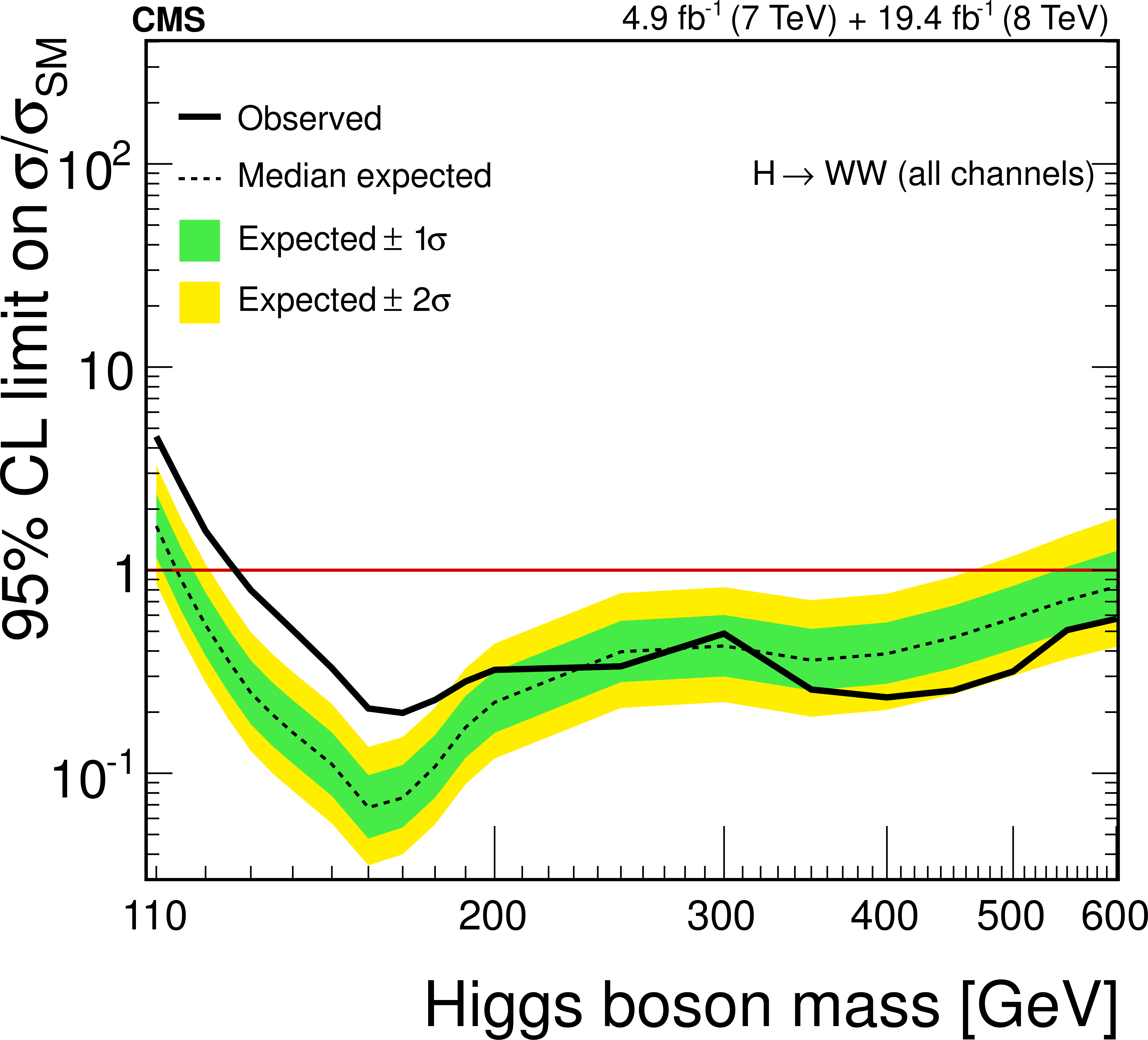
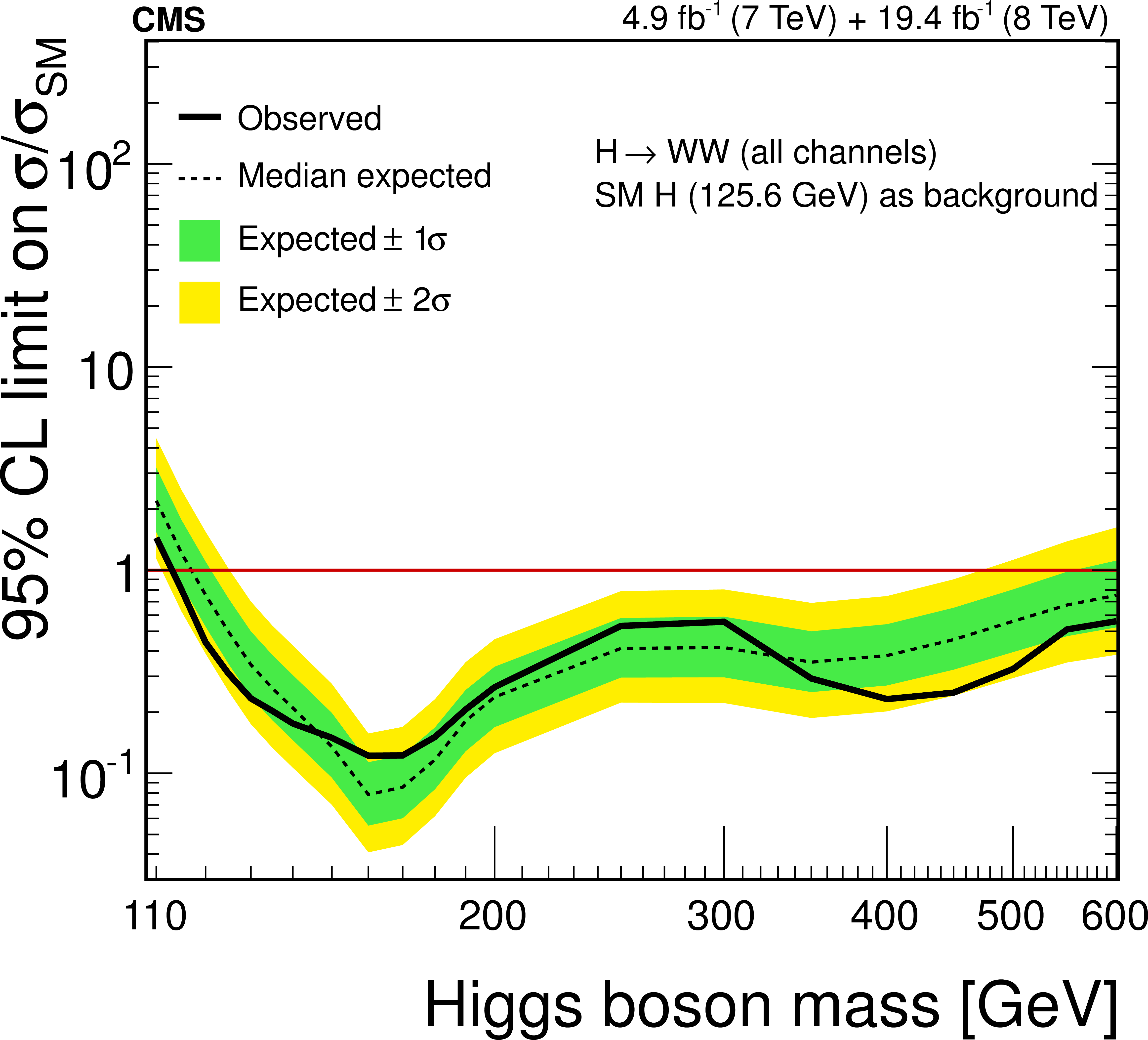
png pdf	Figure 21-a: Expected 95% CL upper limits on the ${\mathrm {H}} \to {\mathrm {W}} {\mathrm {W}}$ production cross section relative to the SM expectation, shown as a function of the SM Higgs boson mass hypothesis, individually for each search category considered in the combination, and the combined result from all categories (top). Expected and observed results are shown with no assumptions on the presence of a Higgs boson (bottom left) and considering the SM Higgs boson with ${m_{ {\mathrm {H}} }}$ = 125.6 GeV as part of the background processes (bottom right). As expected, the excess observed on the bottom left distribution is reduced on the bottom right by considering the SM Higgs boson with ${m_{ {\mathrm {H}} }}$ = 125.6 GeV as part of the background processes.
png pdf	Figure 21-b: Expected 95% CL upper limits on the ${\mathrm {H}} \to {\mathrm {W}} {\mathrm {W}}$ production cross section relative to the SM expectation, shown as a function of the SM Higgs boson mass hypothesis, individually for each search category considered in the combination, and the combined result from all categories (top). Expected and observed results are shown with no assumptions on the presence of a Higgs boson (bottom left) and considering the SM Higgs boson with ${m_{ {\mathrm {H}} }}$ = 125.6 GeV as part of the background processes (bottom right). As expected, the excess observed on the bottom left distribution is reduced on the bottom right by considering the SM Higgs boson with ${m_{ {\mathrm {H}} }}$ = 125.6 GeV as part of the background processes.
png pdf	Figure 21-c: Expected 95% CL upper limits on the ${\mathrm {H}} \to {\mathrm {W}} {\mathrm {W}}$ production cross section relative to the SM expectation, shown as a function of the SM Higgs boson mass hypothesis, individually for each search category considered in the combination, and the combined result from all categories (top). Expected and observed results are shown with no assumptions on the presence of a Higgs boson (bottom left) and considering the SM Higgs boson with ${m_{ {\mathrm {H}} }}$ = 125.6 GeV as part of the background processes (bottom right). As expected, the excess observed on the bottom left distribution is reduced on the bottom right by considering the SM Higgs boson with ${m_{ {\mathrm {H}} }}$ = 125.6 GeV as part of the background processes.
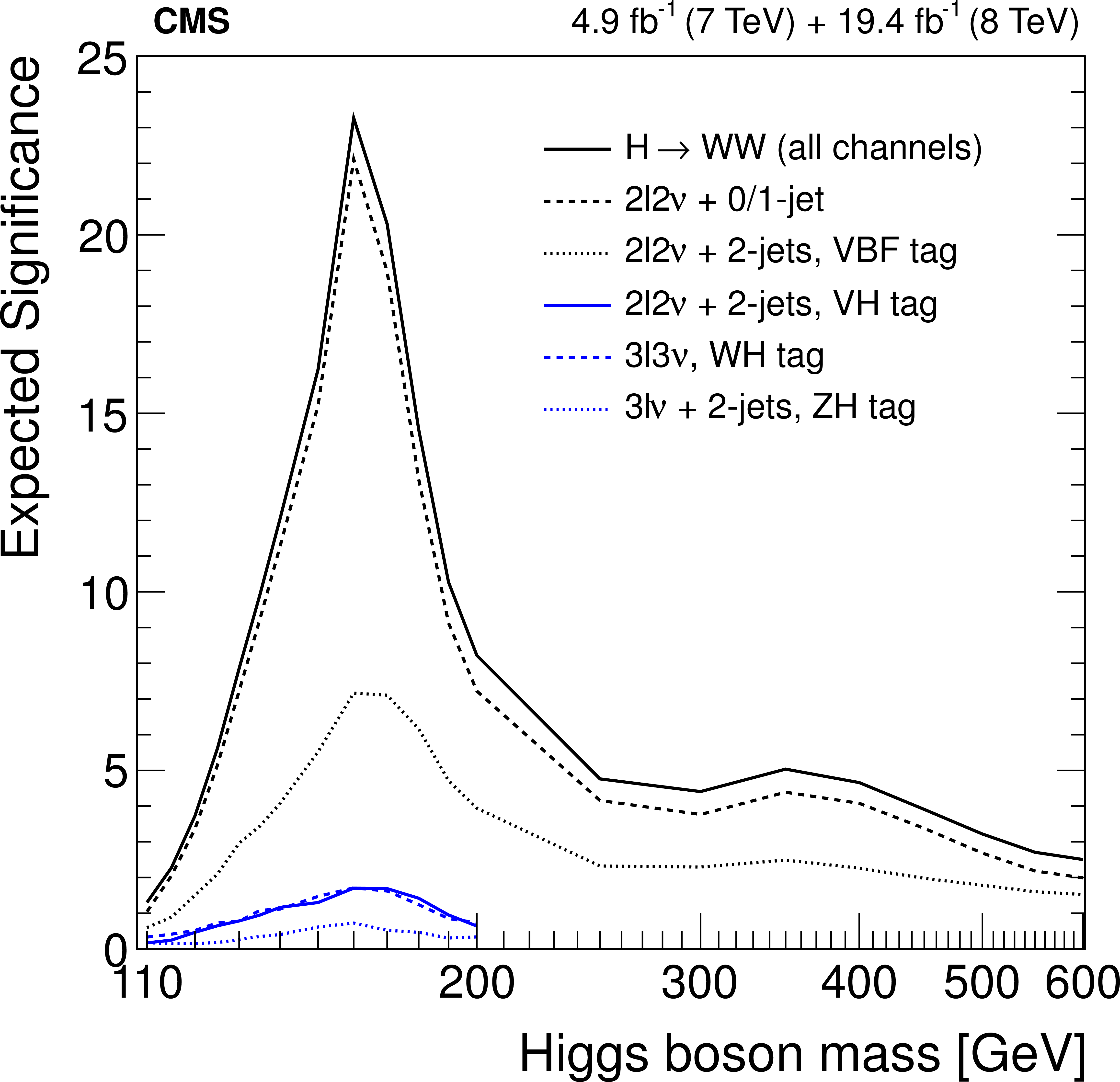
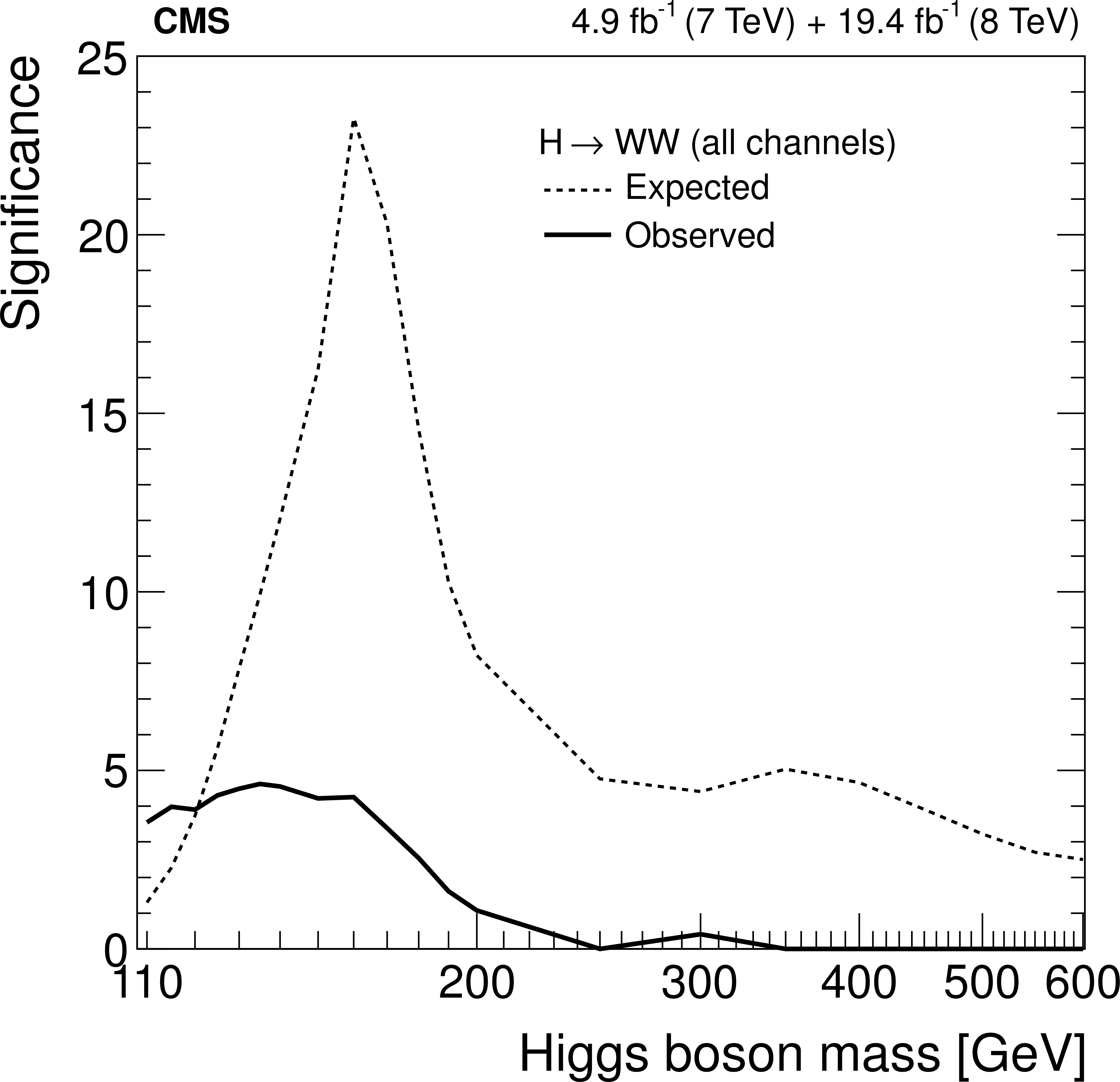
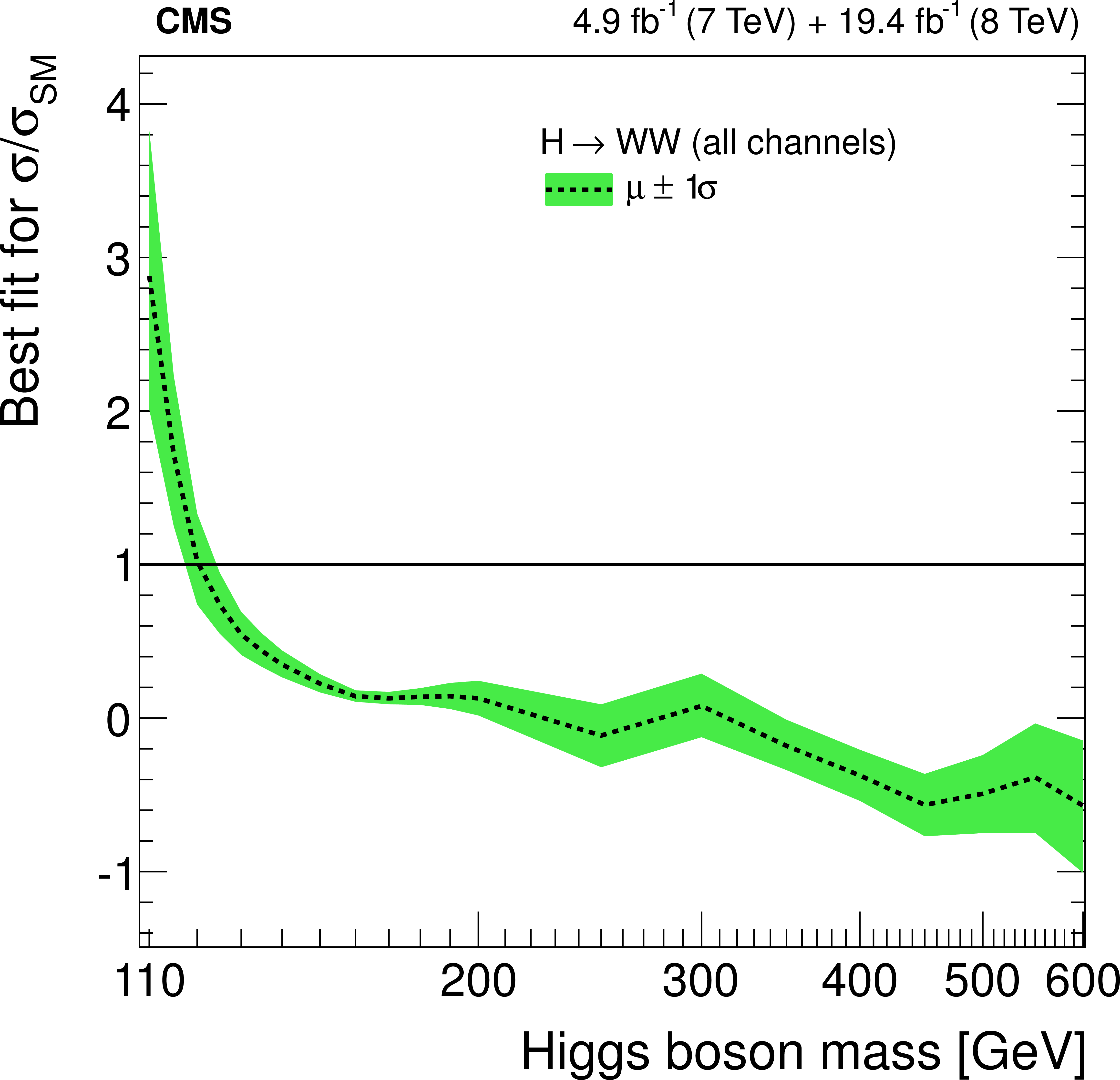
png pdf	Figure 22-a: Expected significance as a function of the SM Higgs boson mass, individually for each search category considered in the combination, and the combined result from all categories (a). Expected and observed significance (b), and observed $\sigma /\sigma _\mathrm {SM}$ (c) as a function of the SM Higgs boson mass for the combination of all ${\mathrm {H}} \to {\mathrm {W}} {\mathrm {W}}$ categories. The very large expected significance at ${m_{ {\mathrm {H}} }} \sim$ 160 GeV is due to the branching fraction to ${\mathrm {W}} {\mathrm {W}}$ close to unity for those masses.
png pdf	Figure 22-b: Expected significance as a function of the SM Higgs boson mass, individually for each search category considered in the combination, and the combined result from all categories (a). Expected and observed significance (b), and observed $\sigma /\sigma _\mathrm {SM}$ (c) as a function of the SM Higgs boson mass for the combination of all ${\mathrm {H}} \to {\mathrm {W}} {\mathrm {W}}$ categories. The very large expected significance at ${m_{ {\mathrm {H}} }} \sim$ 160 GeV is due to the branching fraction to ${\mathrm {W}} {\mathrm {W}}$ close to unity for those masses.
png pdf	Figure 22-c: Expected significance as a function of the SM Higgs boson mass, individually for each search category considered in the combination, and the combined result from all categories (a). Expected and observed significance (b), and observed $\sigma /\sigma _\mathrm {SM}$ (c) as a function of the SM Higgs boson mass for the combination of all ${\mathrm {H}} \to {\mathrm {W}} {\mathrm {W}}$ categories. The very large expected significance at ${m_{ {\mathrm {H}} }} \sim$ 160 GeV is due to the branching fraction to ${\mathrm {W}} {\mathrm {W}}$ close to unity for those masses.
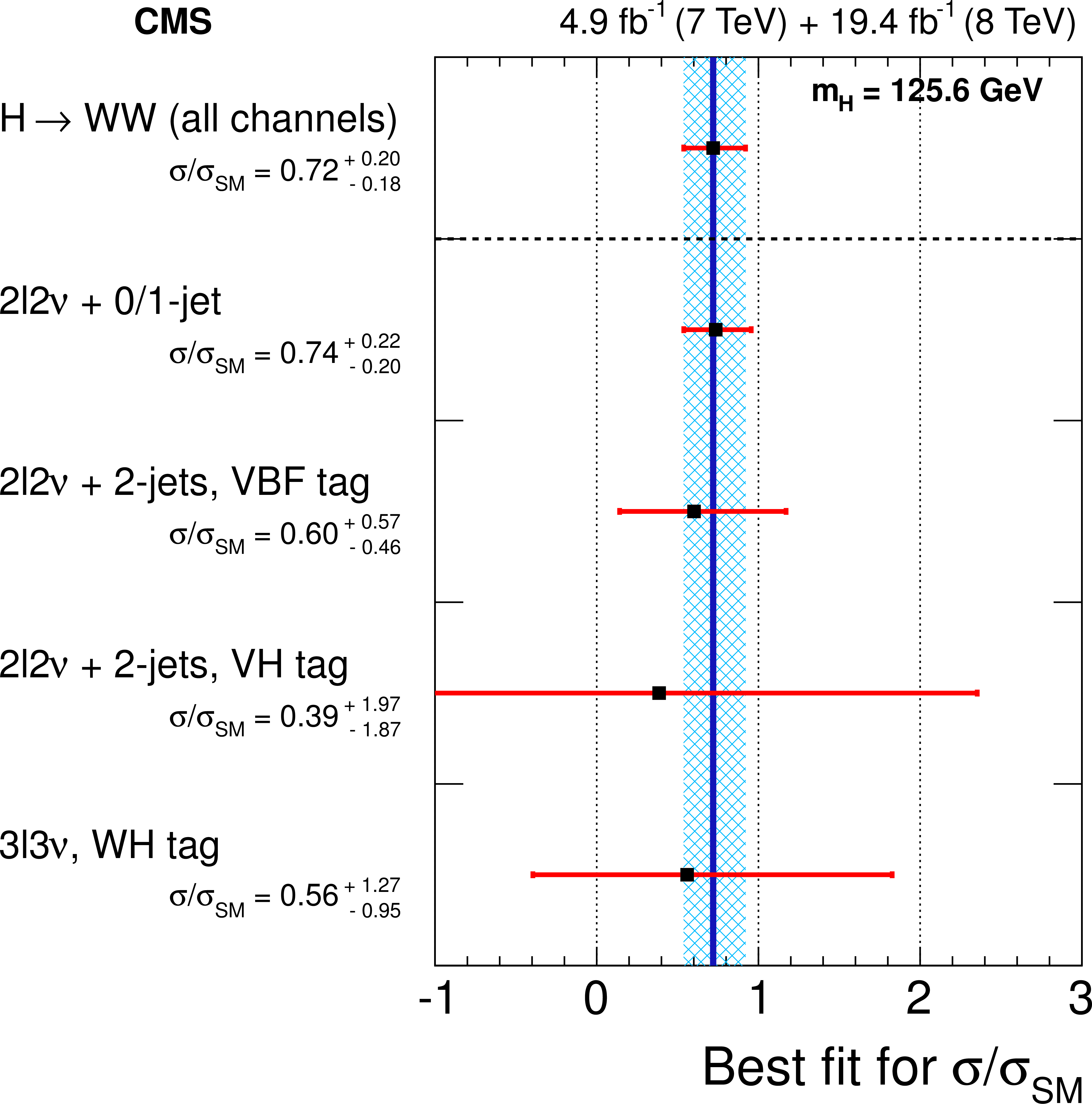
png pdf	Figure 23: Observed $\sigma /\sigma _\mathrm {SM}$ for ${m_{ {\mathrm {H}} }}$ = 125.6 GeV for each category used in the combination. The observed $\sigma /\sigma _\mathrm {SM}$ value in the ${\mathrm {Z}} {\mathrm {H}} \to 3\ell \nu \text {2 jets}$ category is 6.41 $^{+7.43}_{-6.38}$ . Given its relatively large uncertainty with respect to the other categories it is not shown individually, but it is used in the combination.
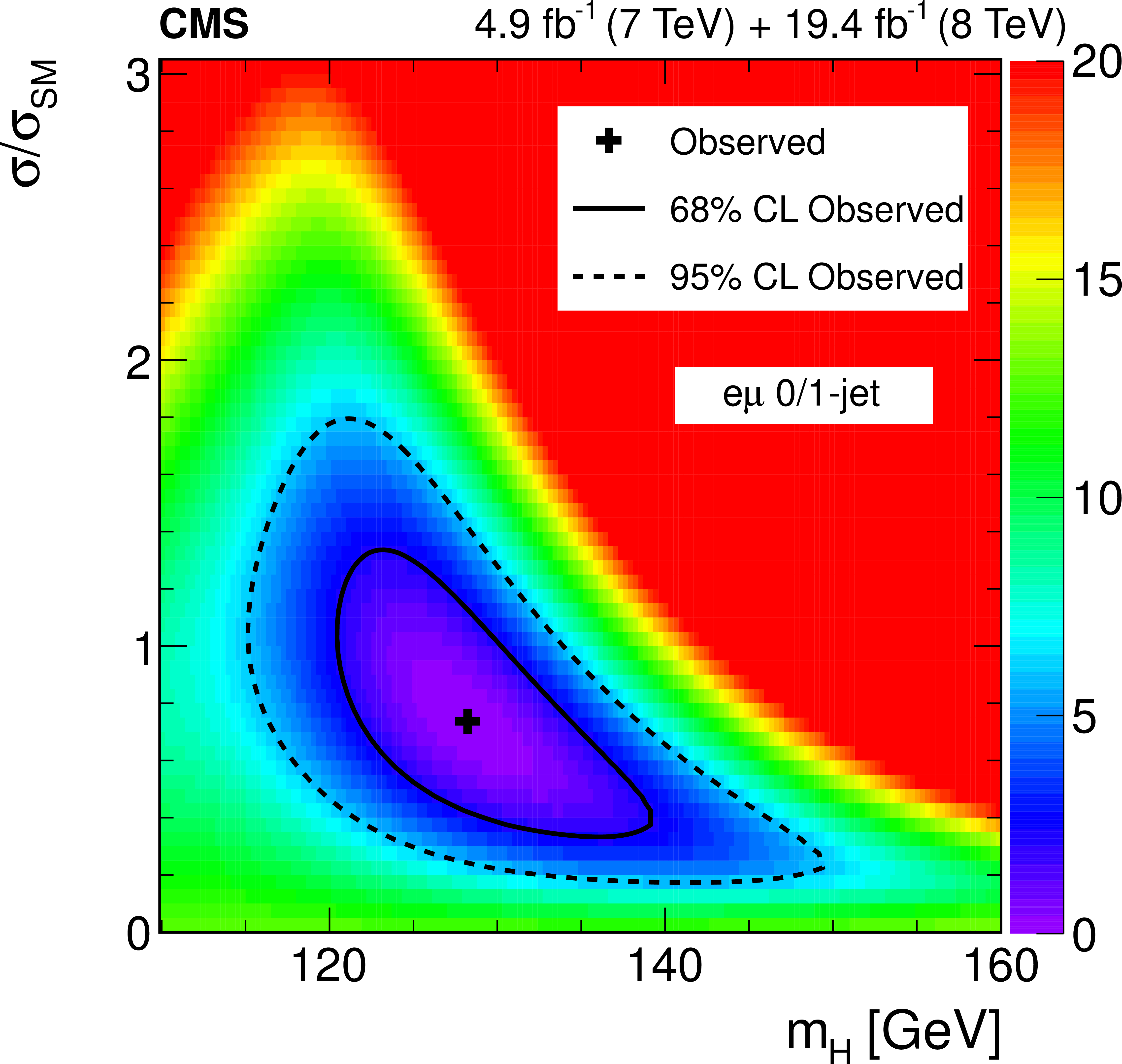
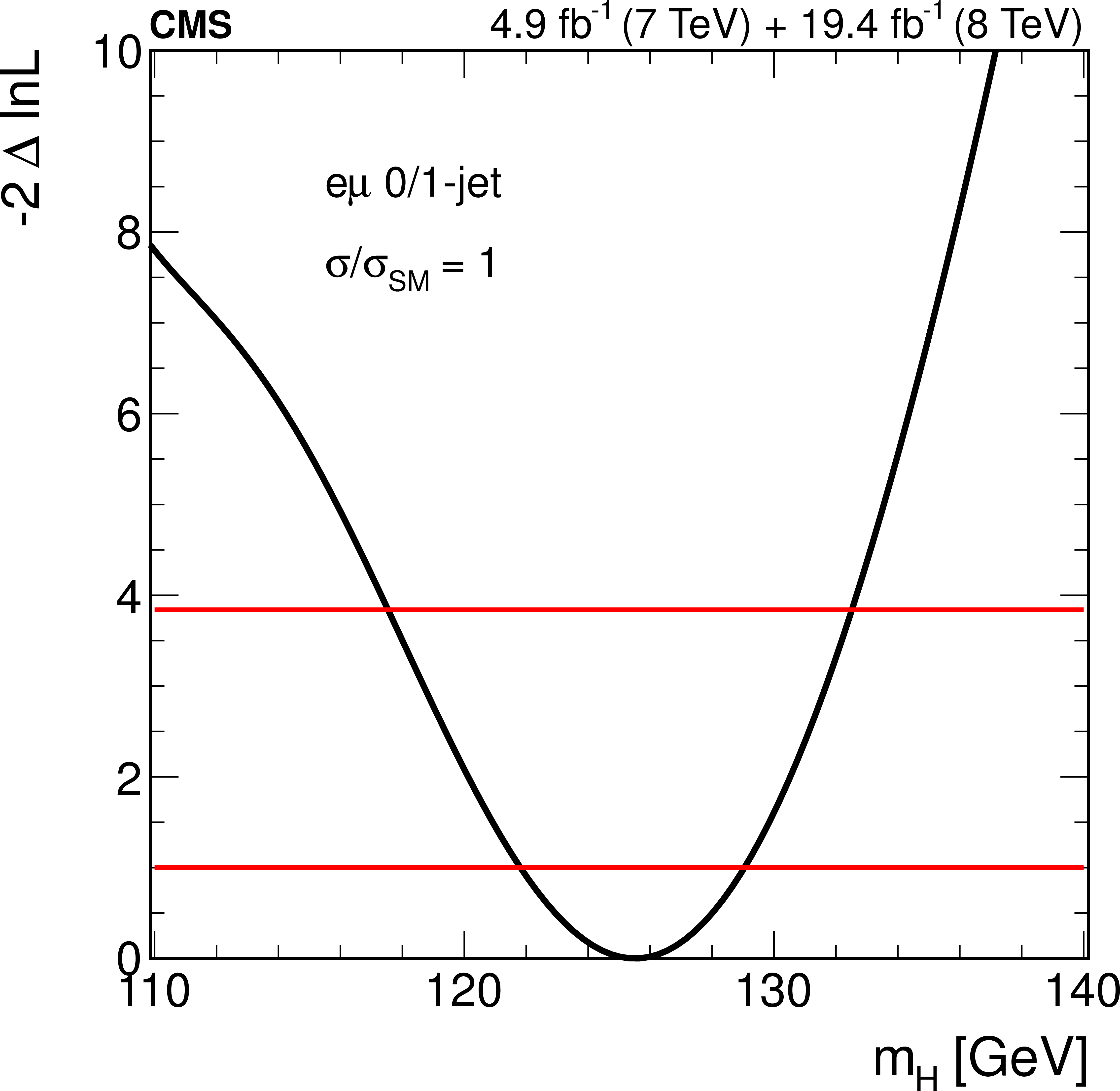
png pdf	Figure 24-a: Confidence intervals in the ( $\sigma /\sigma _\mathrm {SM}$ , ${m_{ {\mathrm {H}} }}$ ) plane using the parametric unbinned fit in ( ${m_{\mathrm {R}}}$ , ${\Delta \phi _{\mathrm {R}}}$ ) distribution (a) for the 0-jet and 1-jet categories in the ${\mathrm {e}}\mu$ final states. Solid and dashed lines indicate the 68% and 95% CL contours, respectively. On Fig.24-b, the one-dimensional likelihood profile for $\sigma /\sigma _\mathrm {SM}$ = 1 is shown. The crossings with the horizontal line at $-2\Delta \ln{L}$ = 1 (3.84) define the 68% (95%) CL interval. The SM Higgs boson production cross section uncertainties are considered.
png pdf	Figure 24-b: Confidence intervals in the ( $\sigma /\sigma _\mathrm {SM}$ , ${m_{ {\mathrm {H}} }}$ ) plane using the parametric unbinned fit in ( ${m_{\mathrm {R}}}$ , ${\Delta \phi _{\mathrm {R}}}$ ) distribution (a) for the 0-jet and 1-jet categories in the ${\mathrm {e}}\mu$ final states. Solid and dashed lines indicate the 68% and 95% CL contours, respectively. On Fig.24-b, the one-dimensional likelihood profile for $\sigma /\sigma _\mathrm {SM}$ = 1 is shown. The crossings with the horizontal line at $-2\Delta \ln{L}$ = 1 (3.84) define the 68% (95%) CL interval. The SM Higgs boson production cross section uncertainties are considered.
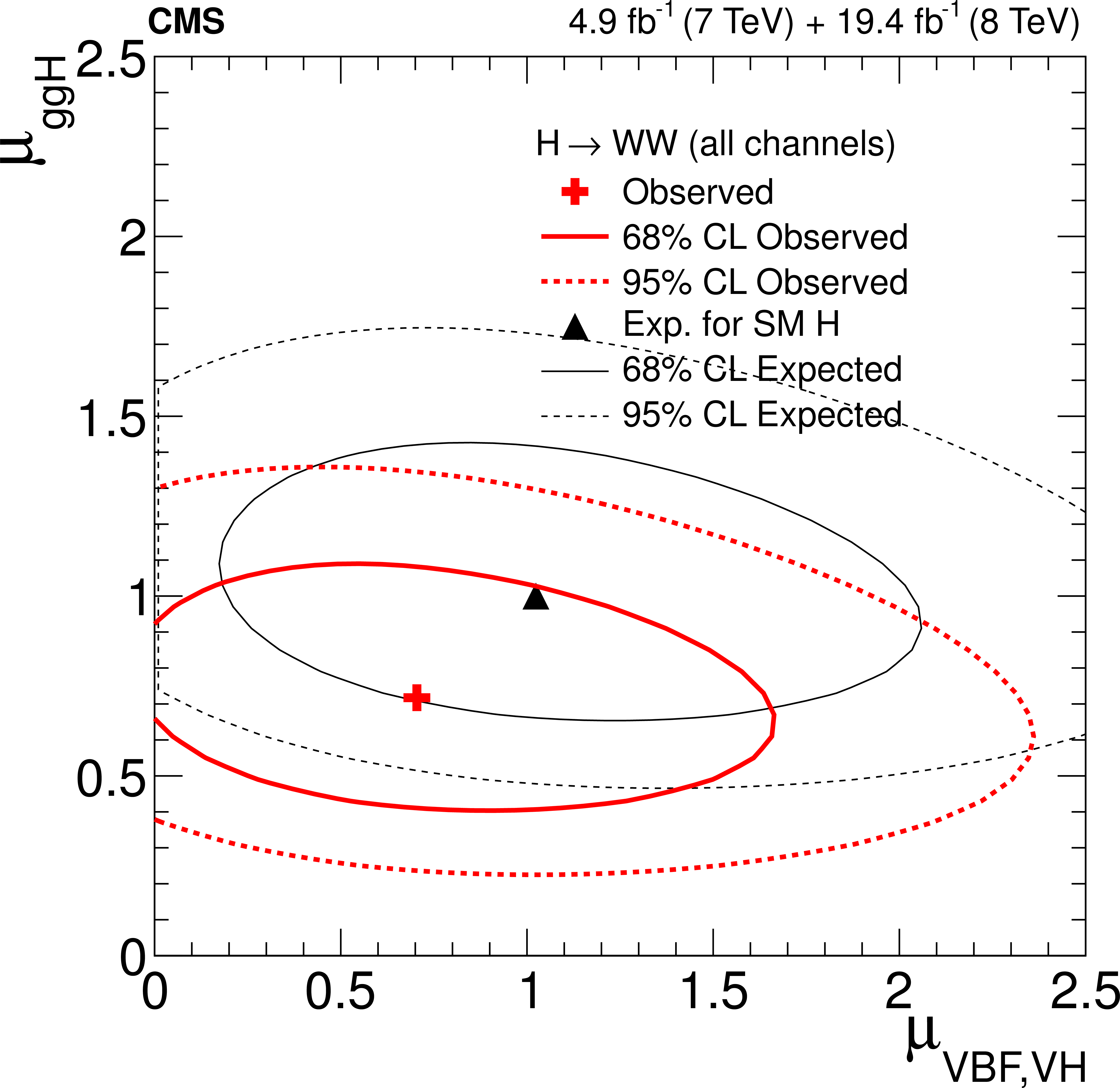
png pdf	Figure 25: Likelihood profiles on $\mu _{ {\mathrm {g}} {\mathrm {g}} {\mathrm {H}} }$ and $\mu _{\mathrm {VBF}, {\mathrm {V}} {\mathrm {H}} }$ at 68% (solid) and 95% CL (dotted). The expected (black) and observed (red) distributions for ${m_{ {\mathrm {H}} }}$ = 125.6 GeV are shown.
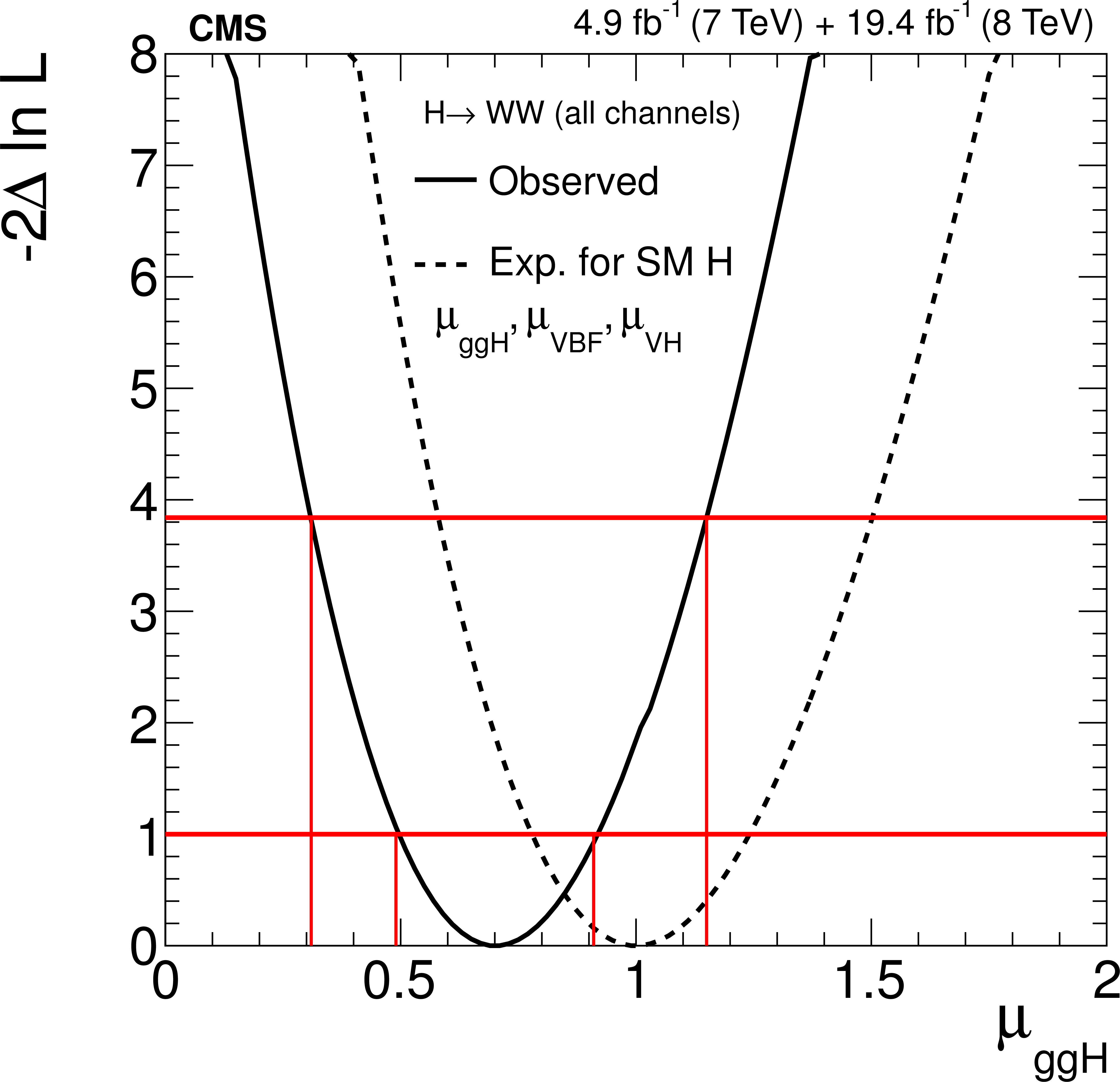
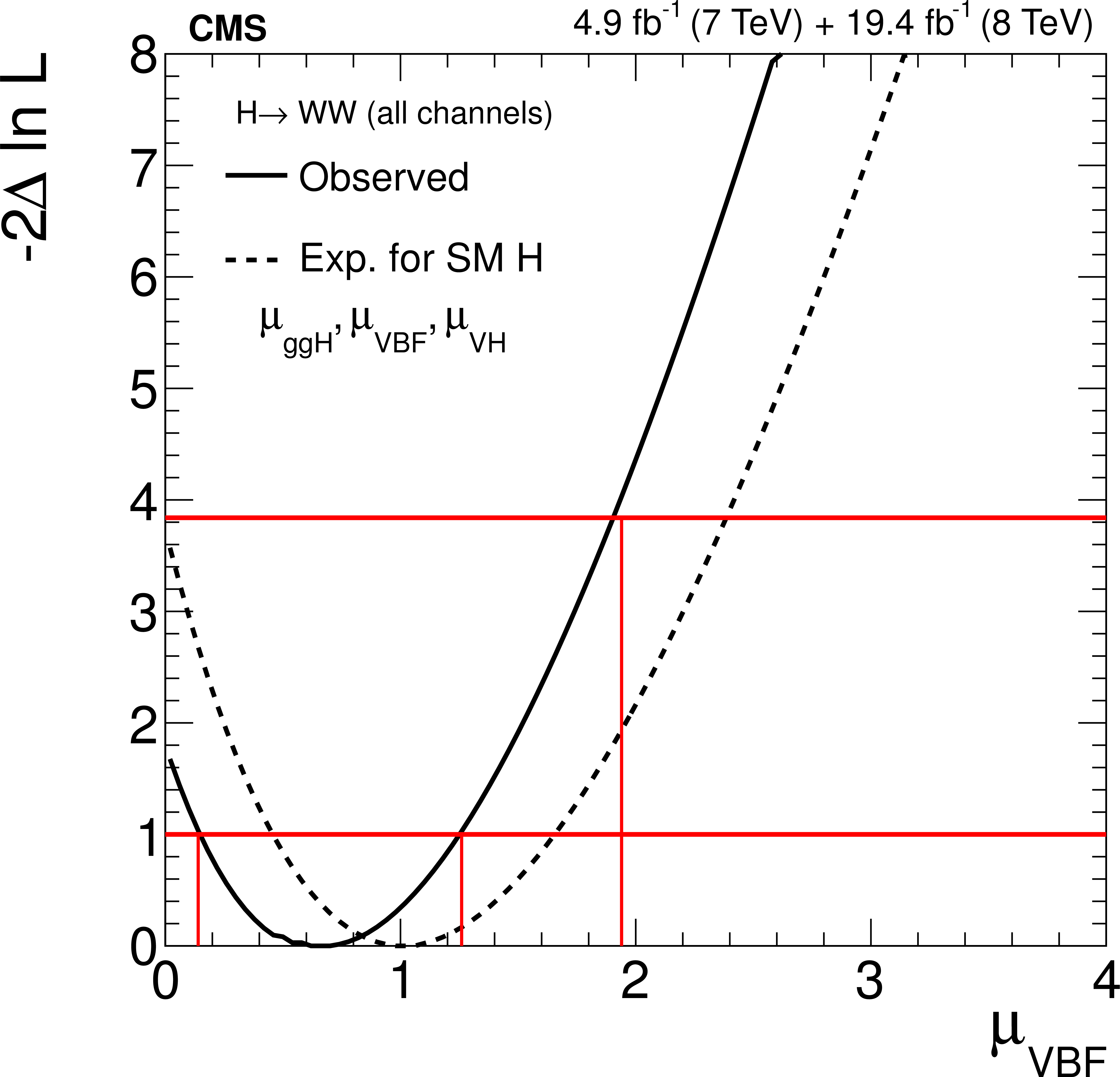
png pdf	Figure 26-a: Expected and observed likelihood profiles for ${m_{ {\mathrm {H}} }}$ = 125.6 GeV for the three production modes separately, ${\mathrm {g}} {\mathrm {g}} {\mathrm {H}}$ (a), VBF (b), and ${\mathrm {V}} {\mathrm {H}}$ (c). In each case, the modifiers for the other productions modes are profiled. The crossings with the horizontal line at $-2\Delta \ln{L}$ = 1 (3.84) define the 68% (95%) CL interval.
png pdf	Figure 26-b: Expected and observed likelihood profiles for ${m_{ {\mathrm {H}} }}$ = 125.6 GeV for the three production modes separately, ${\mathrm {g}} {\mathrm {g}} {\mathrm {H}}$ (a), VBF (b), and ${\mathrm {V}} {\mathrm {H}}$ (c). In each case, the modifiers for the other productions modes are profiled. The crossings with the horizontal line at $-2\Delta \ln{L}$ = 1 (3.84) define the 68% (95%) CL interval.
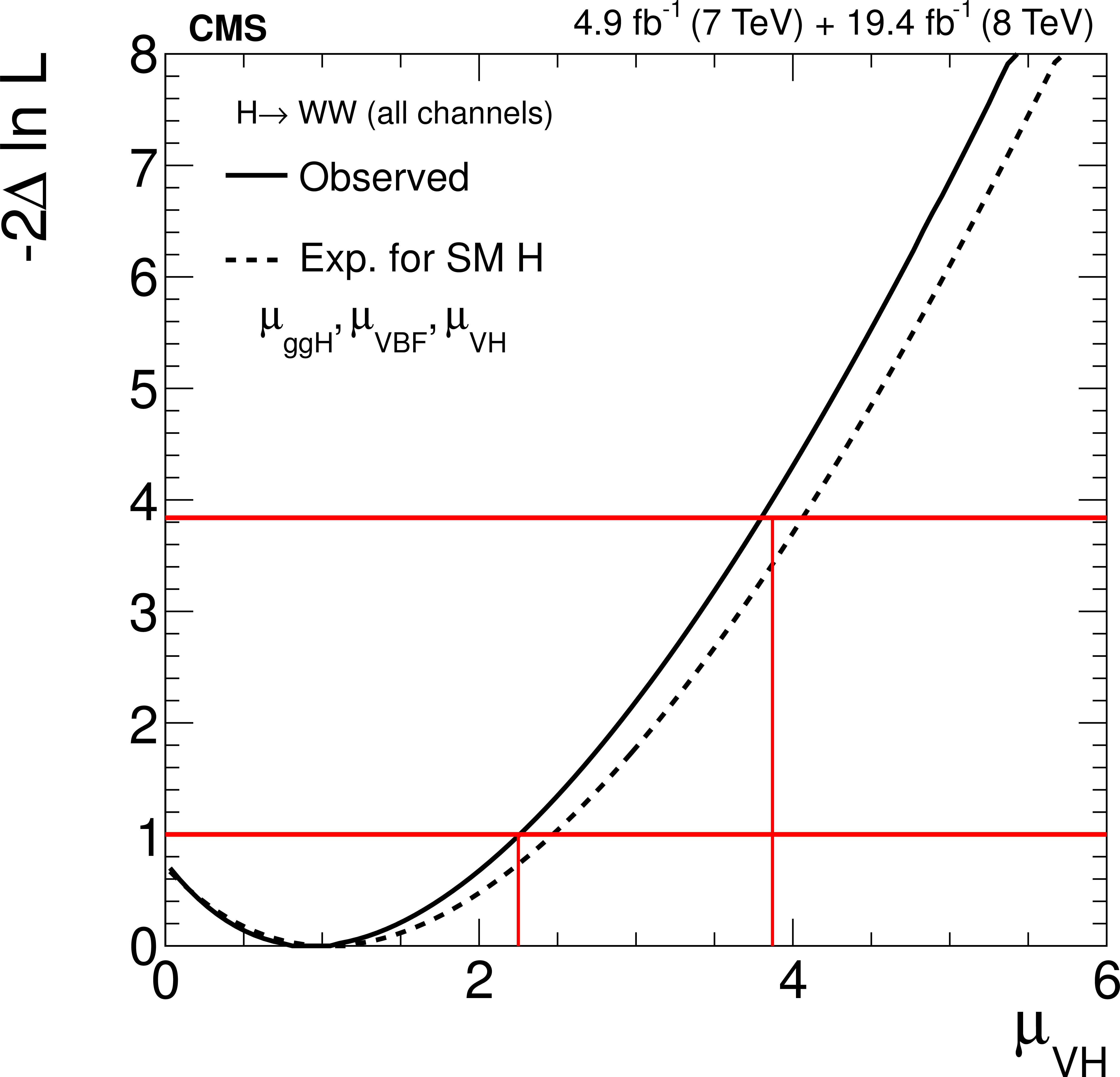
png pdf	Figure 26-c: Expected and observed likelihood profiles for ${m_{ {\mathrm {H}} }}$ = 125.6 GeV for the three production modes separately, ${\mathrm {g}} {\mathrm {g}} {\mathrm {H}}$ (a), VBF (b), and ${\mathrm {V}} {\mathrm {H}}$ (c). In each case, the modifiers for the other productions modes are profiled. The crossings with the horizontal line at $-2\Delta \ln{L}$ = 1 (3.84) define the 68% (95%) CL interval.
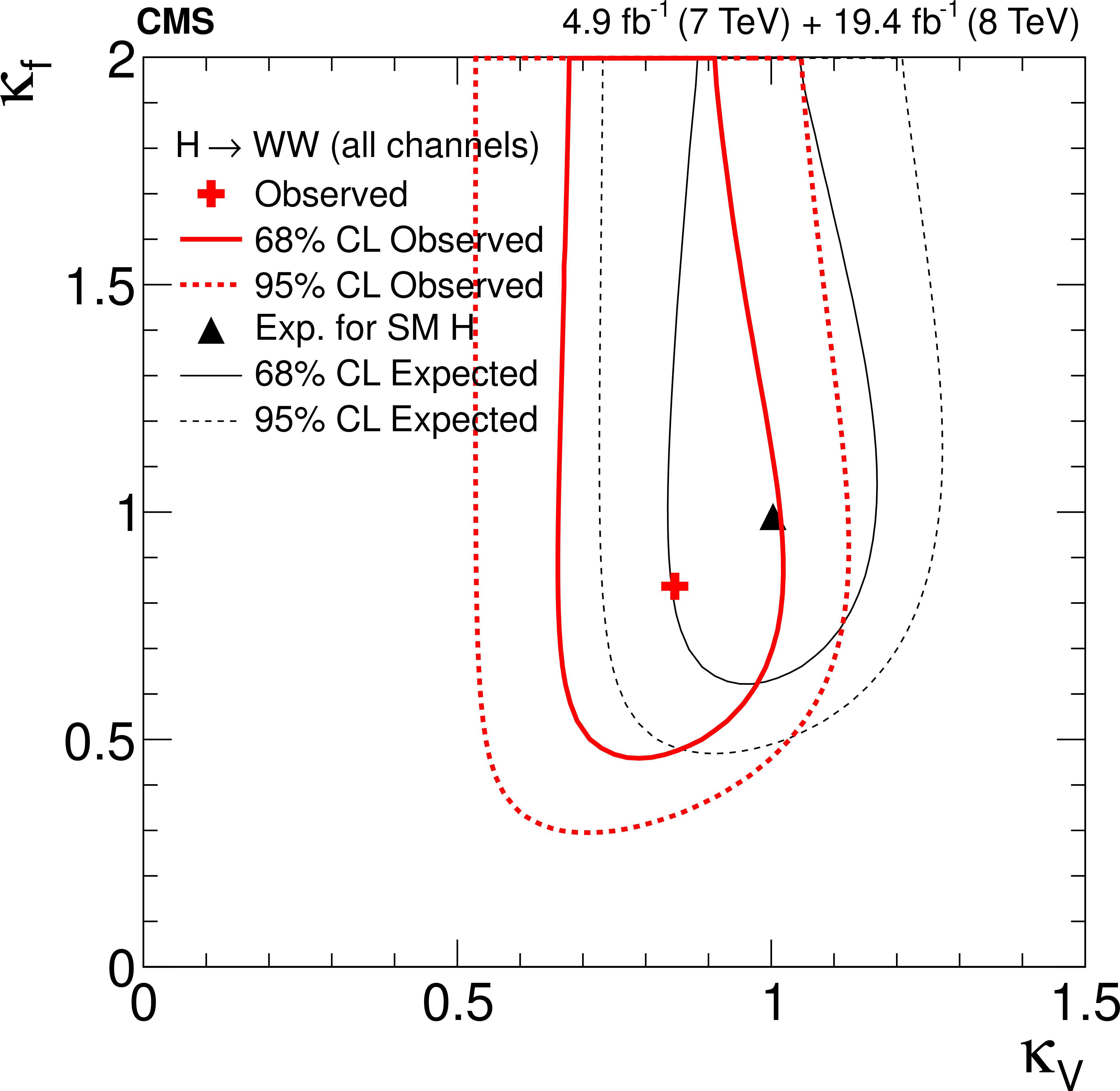
png pdf	Figure 27-a: The two-dimensional likelihood of the $\kappa _{\mathrm V}$ and $\kappa _{\mathrm f}$ parameters (a). The observed value (red) and the SM expectation (black) are shown, together with the 68% (solid) and 95% (dotted) CL contours. The likelihood scan versus $\mathrm {BR_{BSM}}$ (b) for the observed data (solid) and the expectation (dashed) in the presence of the SM Higgs boson with ${m_{ {\mathrm {H}} }}$ = 125.6 GeV are shown. The crossing with the horizontal line at $-2\Delta \ln{L}$ = 1 (3.84) defines the 68% (95%) CL. The parameters $\kappa _{\mathrm V}$ and $\kappa _{\mathrm f}$ are profiled in the scan of $\mathrm {BR_{BSM}}$ , with $\kappa _{\mathrm V} \leq 1$ .
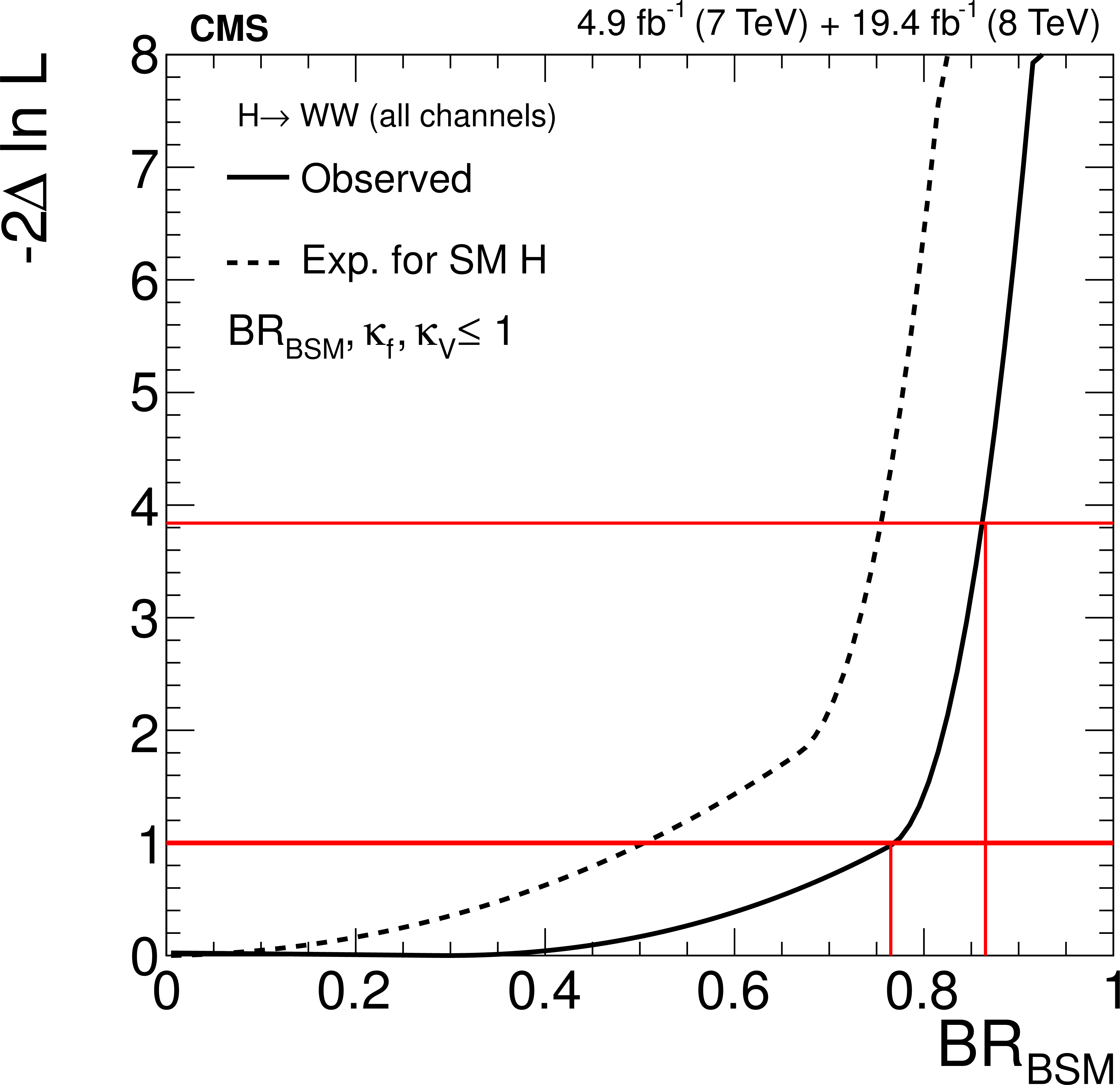
png pdf	Figure 27-b: The two-dimensional likelihood of the $\kappa _{\mathrm V}$ and $\kappa _{\mathrm f}$ parameters (a). The observed value (red) and the SM expectation (black) are shown, together with the 68% (solid) and 95% (dotted) CL contours. The likelihood scan versus $\mathrm {BR_{BSM}}$ (b) for the observed data (solid) and the expectation (dashed) in the presence of the SM Higgs boson with ${m_{ {\mathrm {H}} }}$ = 125.6 GeV are shown. The crossing with the horizontal line at $-2\Delta \ln{L}$ = 1 (3.84) defines the 68% (95%) CL. The parameters $\kappa _{\mathrm V}$ and $\kappa _{\mathrm f}$ are profiled in the scan of $\mathrm {BR_{BSM}}$ , with $\kappa _{\mathrm V} \leq 1$ .
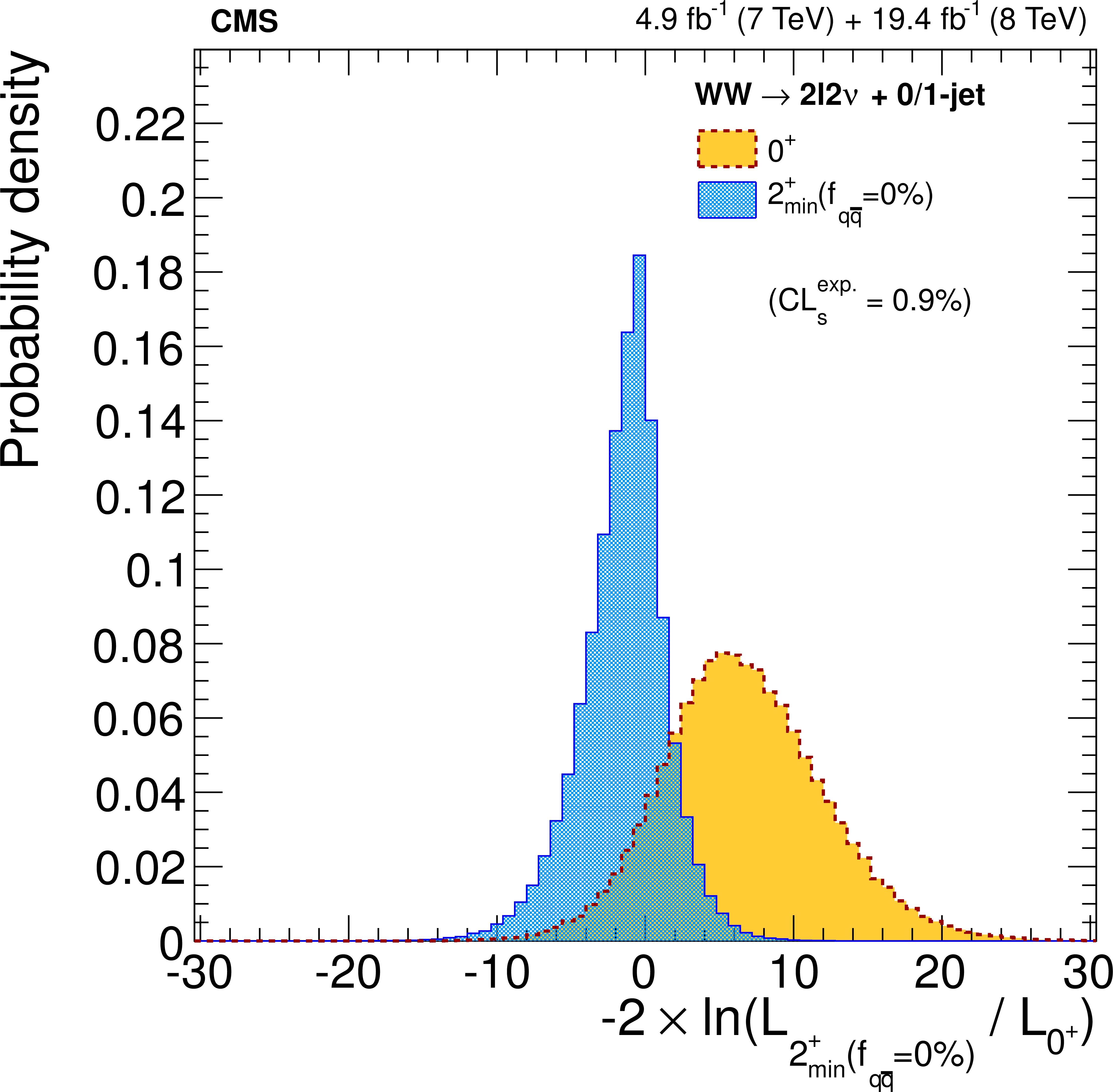
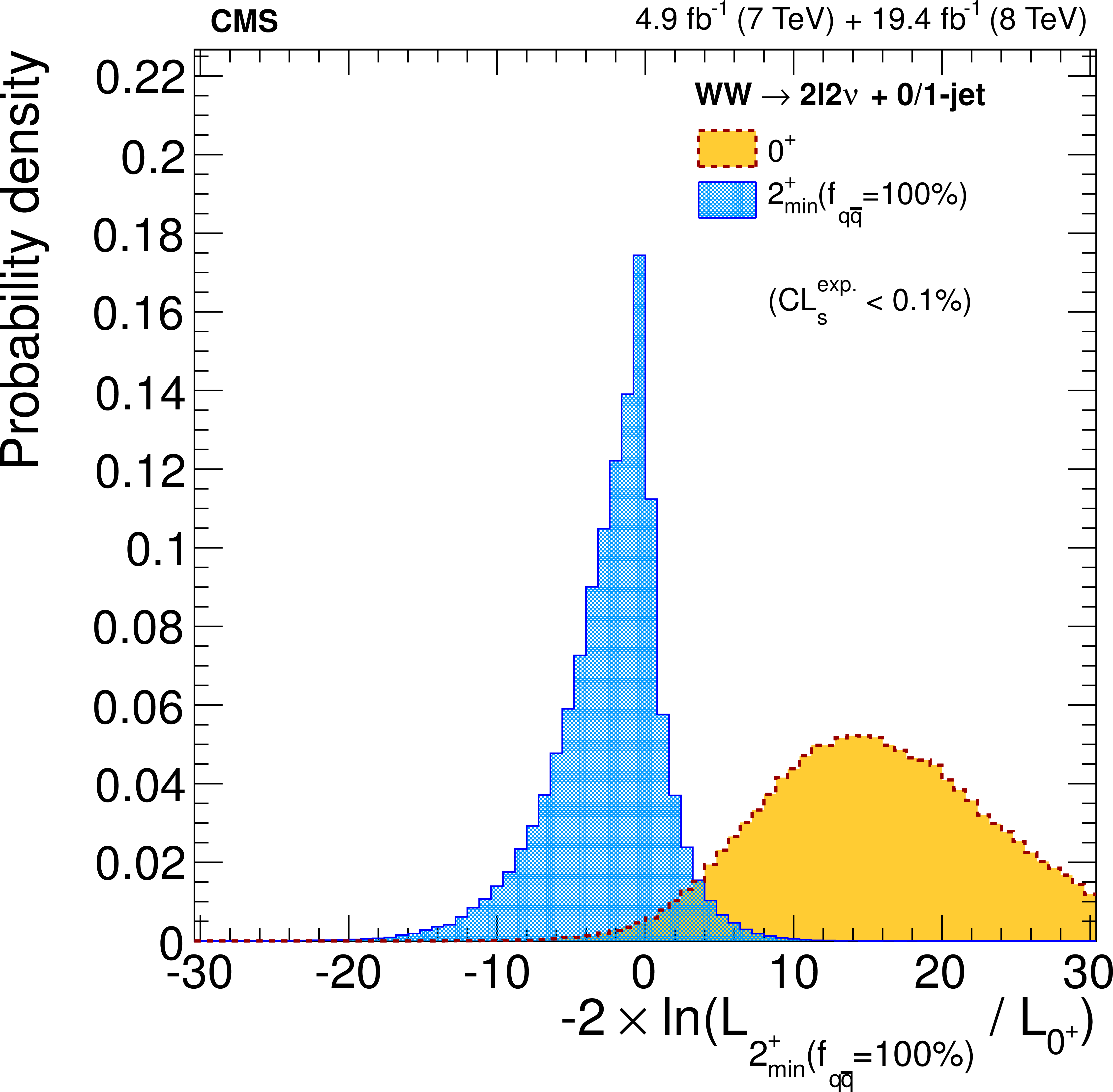
png pdf	Figure 28-a: Distributions of $-2 \ln{(L_{ {2^+}_\text {min}}} / L_{0^+})$ , combining the 0-jet and 1-jet categories in the ${\mathrm {e}}\mu$ final state, for the $0^+$ and ${2^+_\text {min}}$ hypotheses at ${m_{ {\mathrm {H}} }}$ = 125.6 GeV. The distributions are produced assuming $\sigma /\sigma _\mathrm {SM}$ =1 (a, c) and using the $\sigma /\sigma _\mathrm {SM}$ value determined from the fit to data (b, d). The distributions are shown for the case $f_{ {\mathrm {q}\overline {\mathrm {q}}}} =$ 0% (a, b) and $f_{ {\mathrm {q}\overline {\mathrm {q}}}} =$ 100% (c, d). The observed value is indicated by the red arrow.
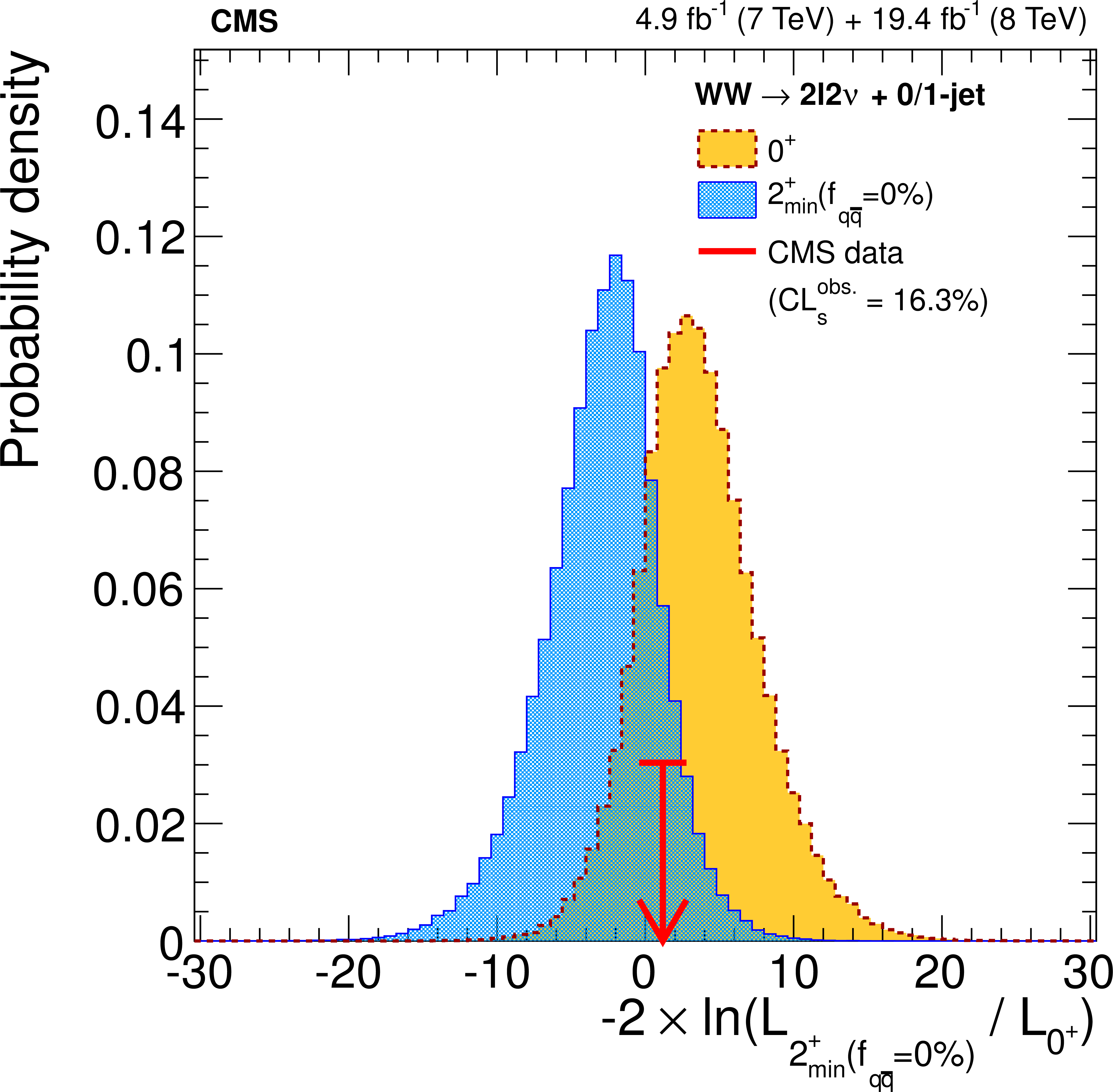
png pdf	Figure 28-b: Distributions of $-2 \ln{(L_{ {2^+}_\text {min}}} / L_{0^+})$ , combining the 0-jet and 1-jet categories in the ${\mathrm {e}}\mu$ final state, for the $0^+$ and ${2^+_\text {min}}$ hypotheses at ${m_{ {\mathrm {H}} }}$ = 125.6 GeV. The distributions are produced assuming $\sigma /\sigma _\mathrm {SM}$ =1 (a, c) and using the $\sigma /\sigma _\mathrm {SM}$ value determined from the fit to data (b, d). The distributions are shown for the case $f_{ {\mathrm {q}\overline {\mathrm {q}}}} =$ 0% (a, b) and $f_{ {\mathrm {q}\overline {\mathrm {q}}}} =$ 100% (c, d). The observed value is indicated by the red arrow.
png pdf	Figure 28-c: Distributions of $-2 \ln{(L_{ {2^+}_\text {min}}} / L_{0^+})$ , combining the 0-jet and 1-jet categories in the ${\mathrm {e}}\mu$ final state, for the $0^+$ and ${2^+_\text {min}}$ hypotheses at ${m_{ {\mathrm {H}} }}$ = 125.6 GeV. The distributions are produced assuming $\sigma /\sigma _\mathrm {SM}$ =1 (a, c) and using the $\sigma /\sigma _\mathrm {SM}$ value determined from the fit to data (b, d). The distributions are shown for the case $f_{ {\mathrm {q}\overline {\mathrm {q}}}} =$ 0% (a, b) and $f_{ {\mathrm {q}\overline {\mathrm {q}}}} =$ 100% (c, d). The observed value is indicated by the red arrow.
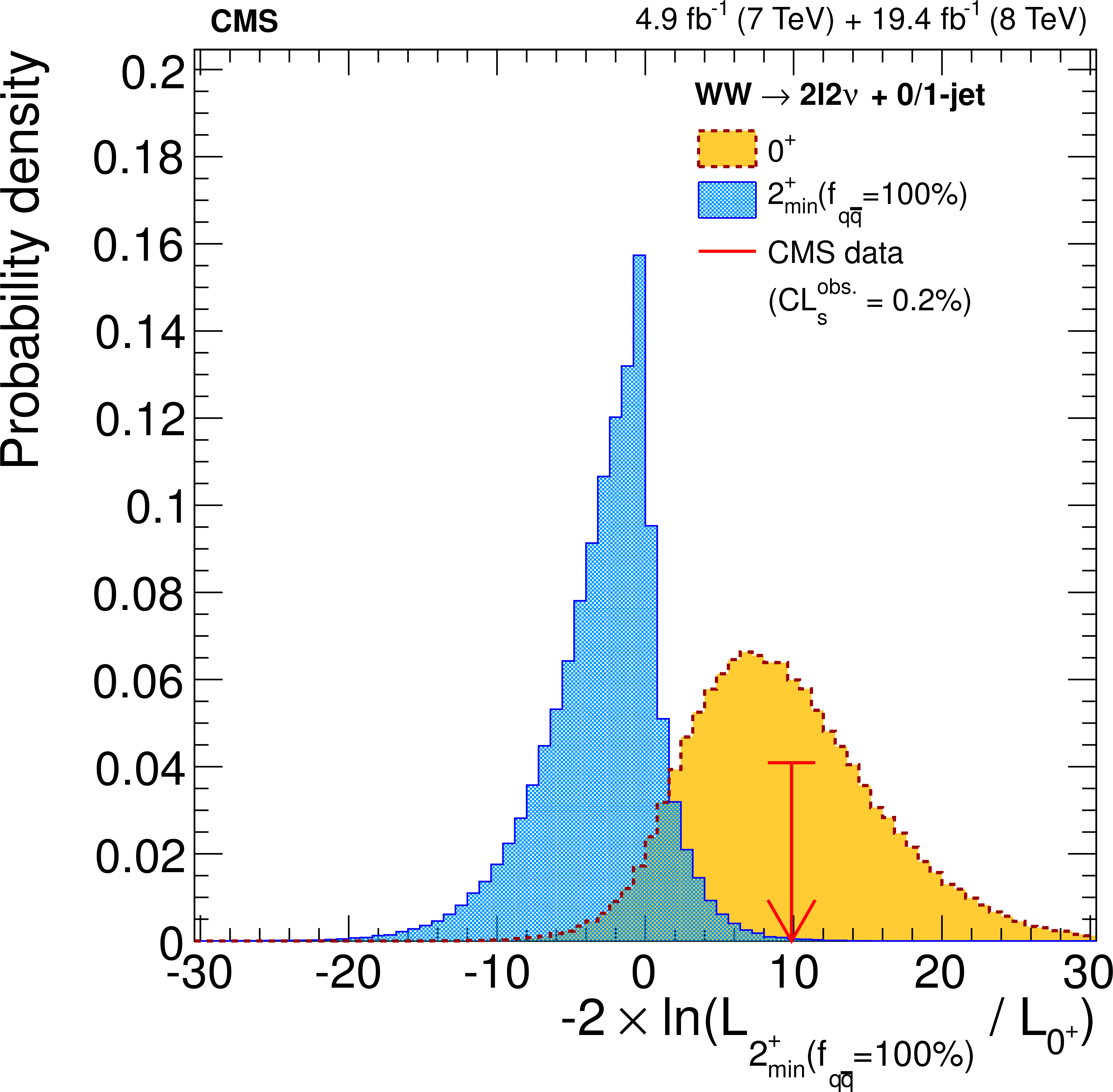
png pdf	Figure 28-d: Distributions of $-2 \ln{(L_{ {2^+}_\text {min}}} / L_{0^+})$ , combining the 0-jet and 1-jet categories in the ${\mathrm {e}}\mu$ final state, for the $0^+$ and ${2^+_\text {min}}$ hypotheses at ${m_{ {\mathrm {H}} }}$ = 125.6 GeV. The distributions are produced assuming $\sigma /\sigma _\mathrm {SM}$ =1 (a, c) and using the $\sigma /\sigma _\mathrm {SM}$ value determined from the fit to data (b, d). The distributions are shown for the case $f_{ {\mathrm {q}\overline {\mathrm {q}}}} =$ 0% (a, b) and $f_{ {\mathrm {q}\overline {\mathrm {q}}}} =$ 100% (c, d). The observed value is indicated by the red arrow.
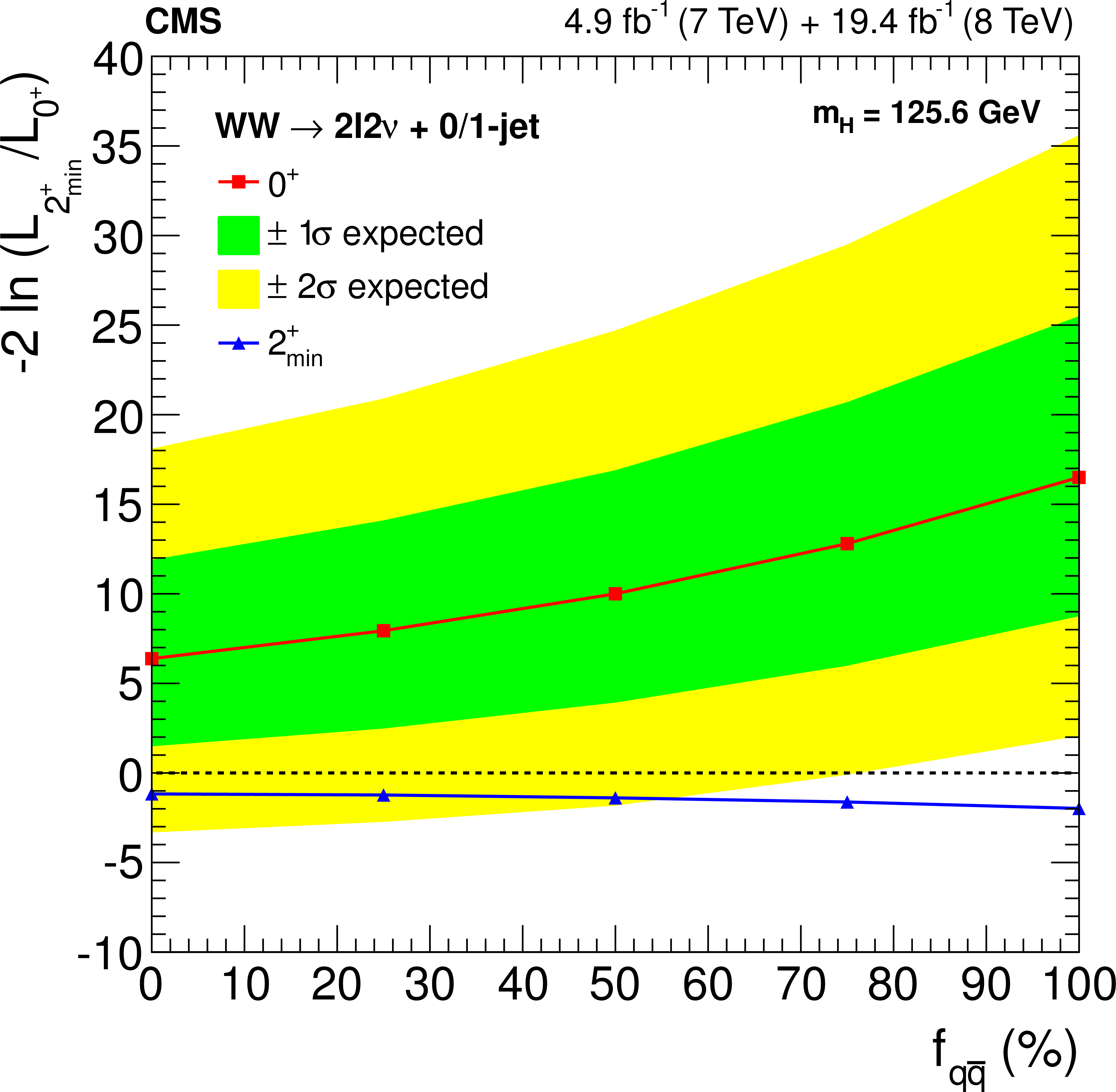
png pdf	Figure 29-a: Median test statistic for the $0^+$ and ${2^+_\text {min}}$ hypotheses, as a function of $f_{ {\mathrm {q}\overline {\mathrm {q}}}}$ of the ${2^+_\text {min}}$ particle, assuming $\sigma /\sigma _\mathrm {SM}=1$ (a) and using the $\sigma /\sigma _\mathrm {SM}$ value determined from the fit to data (b). The observed values are also reported in the second case.
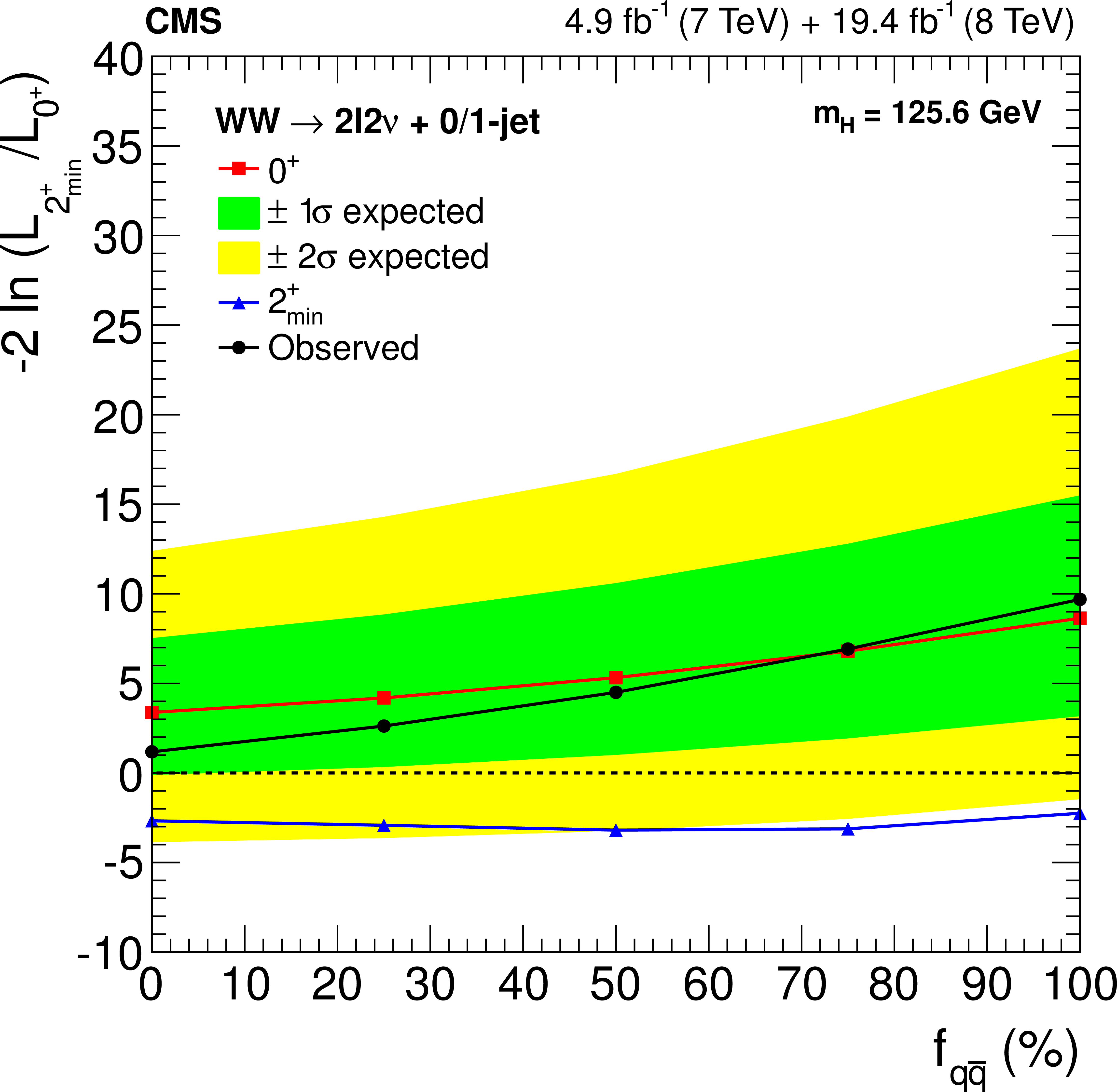
png pdf	Figure 29-b: Median test statistic for the $0^+$ and ${2^+_\text {min}}$ hypotheses, as a function of $f_{ {\mathrm {q}\overline {\mathrm {q}}}}$ of the ${2^+_\text {min}}$ particle, assuming $\sigma /\sigma _\mathrm {SM}=1$ (a) and using the $\sigma /\sigma _\mathrm {SM}$ value determined from the fit to data (b). The observed values are also reported in the second case.
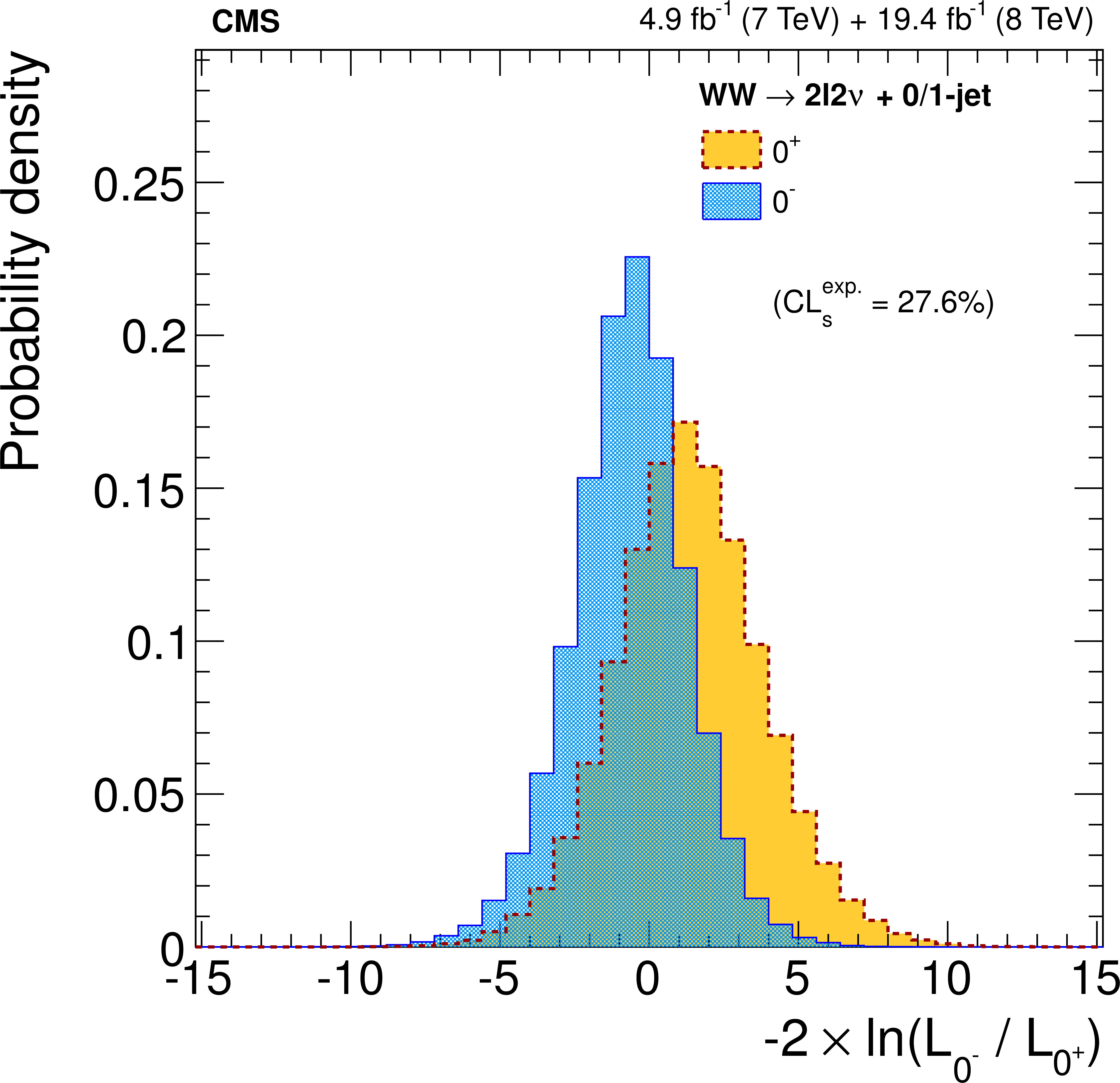
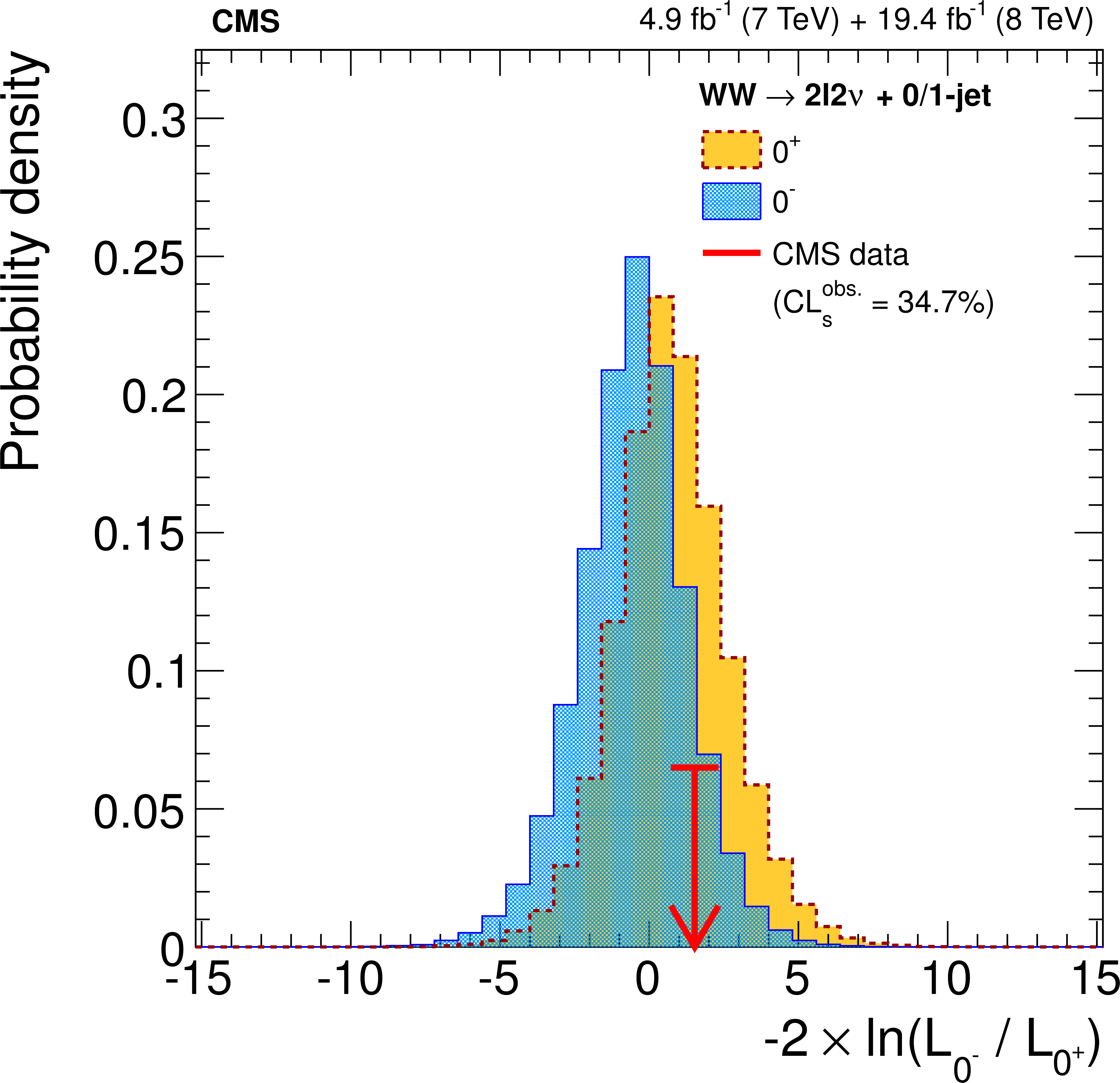
png pdf	Figure 30-a: Distributions of $-2 \ln{(L_{0^-}} / L_{0^+})$ , combining the 0-jet and 1-jet categories in the ${\mathrm {e}}\mu$ final state, for the $0^+$ and $0^-$ hypotheses at ${m_{ {\mathrm {H}} }}$ =125.6 GeV. The distributions are produced assuming $\sigma /\sigma _\mathrm {SM}$ = 1 (a) and using the signal strength determined from the fit to data (b). The observed value is indicated by the red arrow.
png pdf	Figure 30-b: Distributions of $-2 \ln{(L_{0^-}} / L_{0^+})$ , combining the 0-jet and 1-jet categories in the ${\mathrm {e}}\mu$ final state, for the $0^+$ and $0^-$ hypotheses at ${m_{ {\mathrm {H}} }}$ =125.6 GeV. The distributions are produced assuming $\sigma /\sigma _\mathrm {SM}$ = 1 (a) and using the signal strength determined from the fit to data (b). The observed value is indicated by the red arrow.
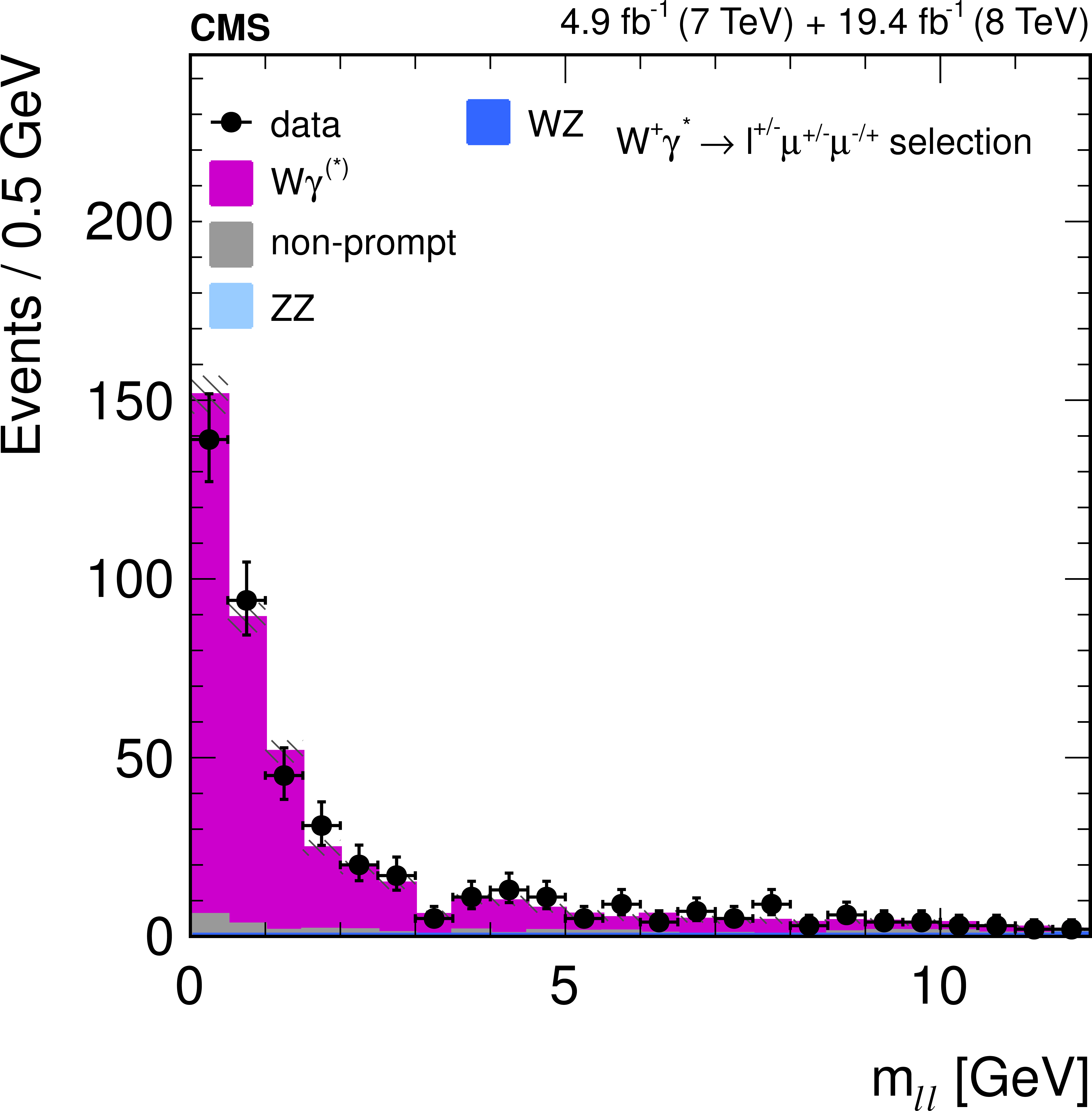
png pdf	Figure 31: The ${m_{ {\ell } {\ell }}}$ mass distribution for opposite-sign muons after the ${ {\mathrm {W}}\gamma }^{}$ selection. The ${ {\mathrm {W}}\gamma }^{}$ contribution is normalized to match the data.
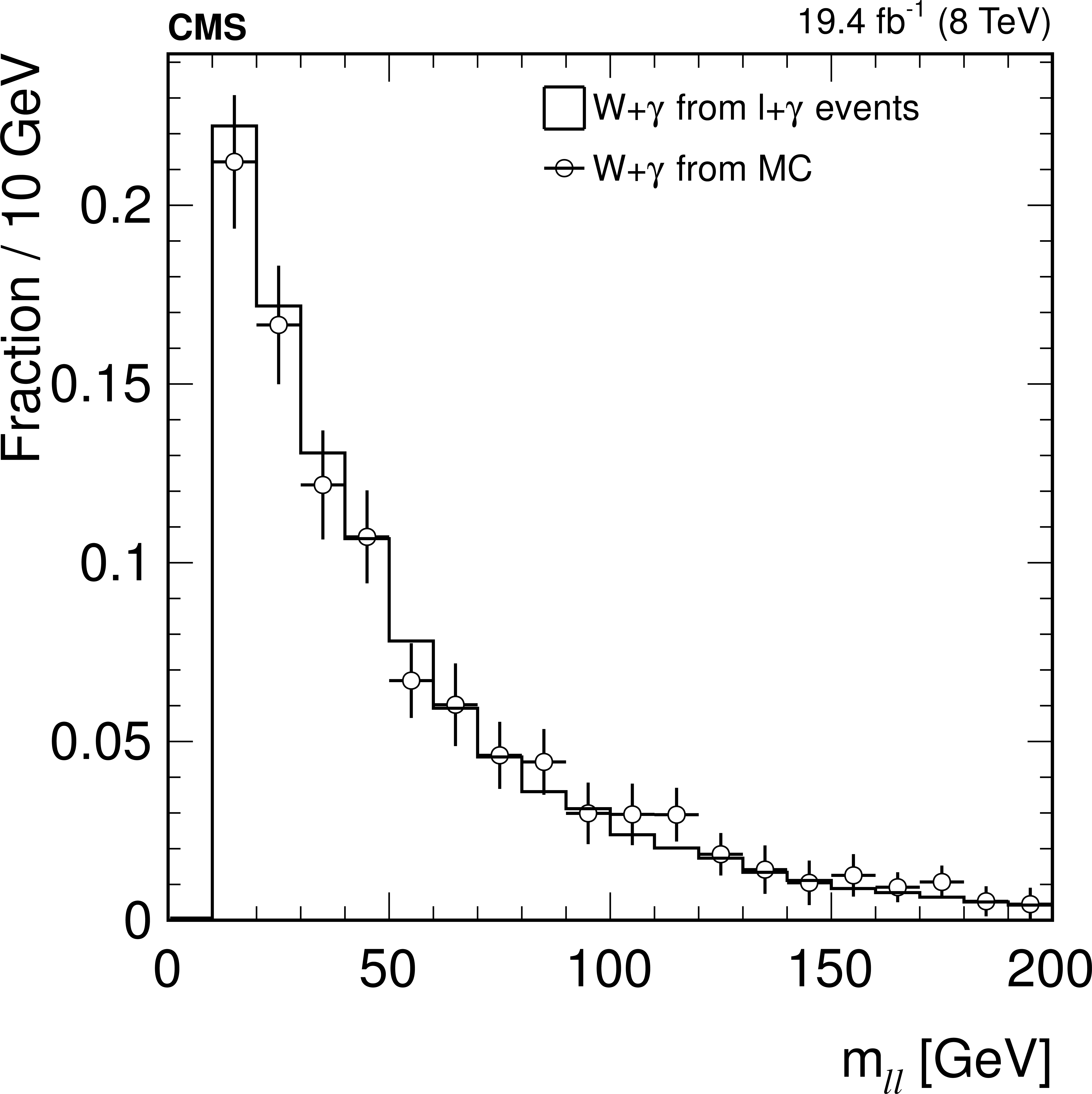
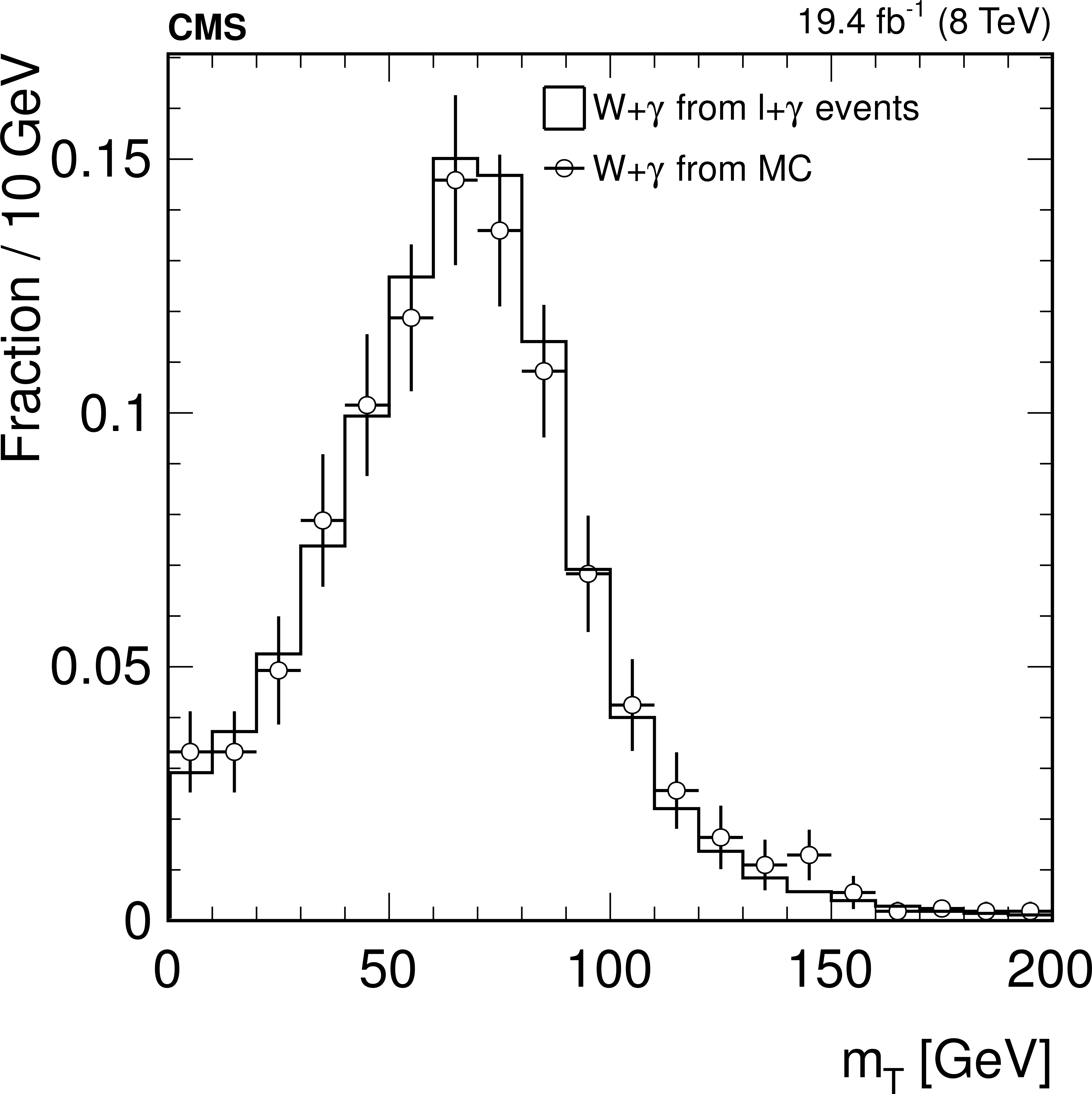
png pdf	Figure 32-a: The ${m_{ {\ell } {\ell }}}$ (a) and ${m_{\mathrm {T}}}$ (b) distributions for the ${\mathrm {W}}+\gamma$ process in events passing the dilepton selection. The dots show the distribution from simulated events, while the histogram shows the distribution from a data sample with a lepton and a photon, which has about 200 times more events.
png pdf	Figure 32-b: The ${m_{ {\ell } {\ell }}}$ (a) and ${m_{\mathrm {T}}}$ (b) distributions for the ${\mathrm {W}}+\gamma$ process in events passing the dilepton selection. The dots show the distribution from simulated events, while the histogram shows the distribution from a data sample with a lepton and a photon, which has about 200 times more events.
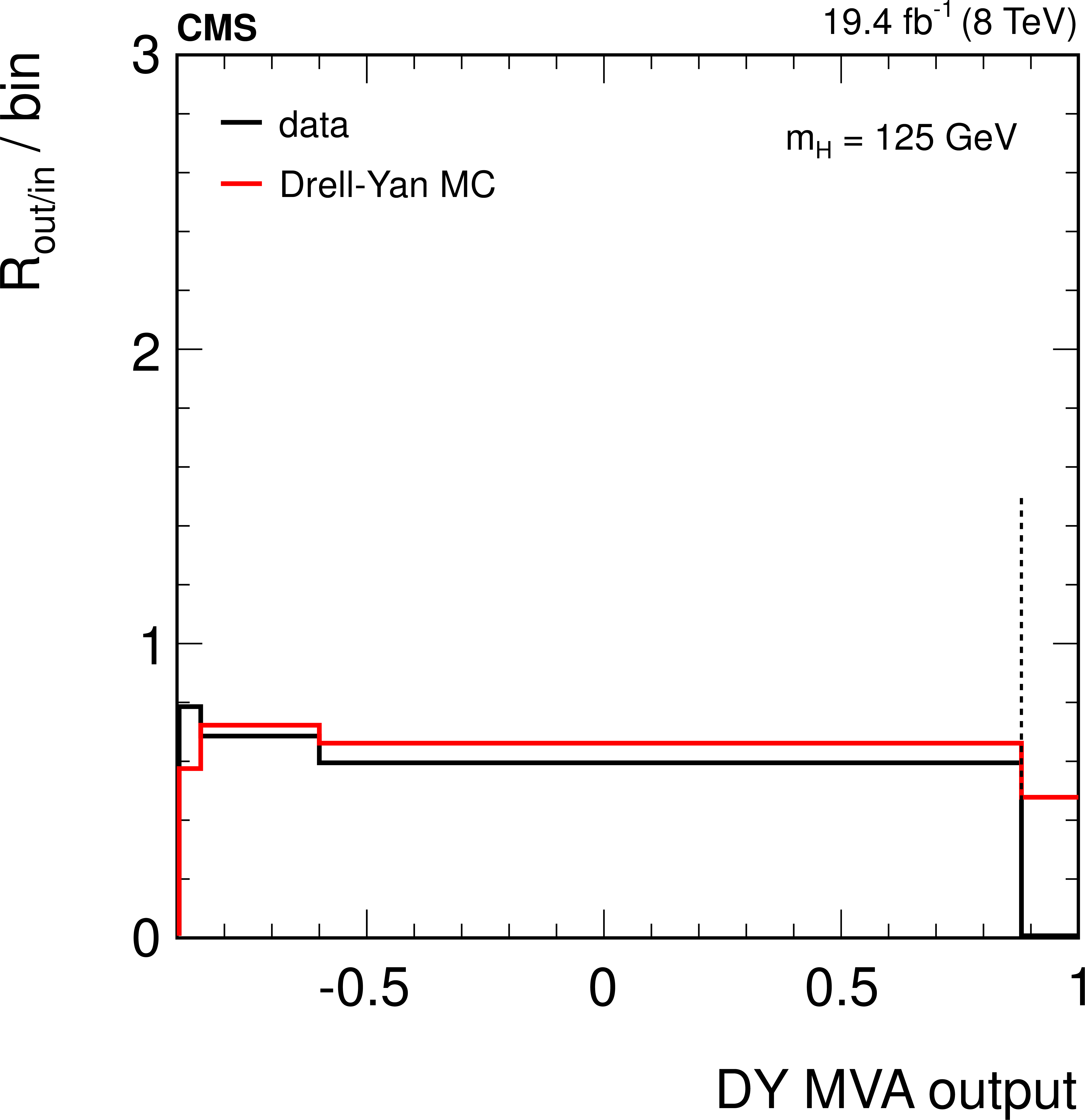
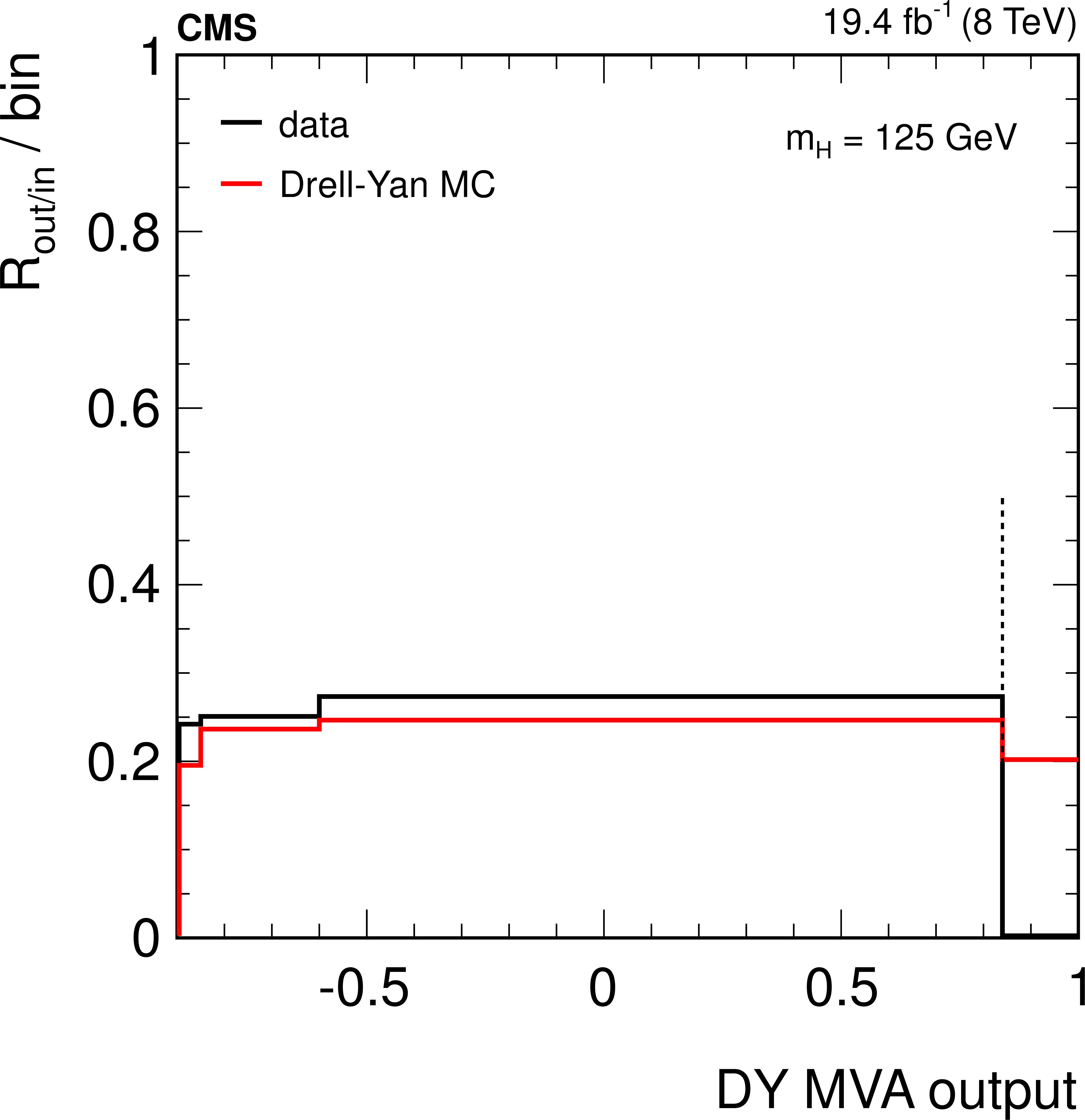
png pdf	Figure 33-a: The $R_{\text {out}/\text {in}}$ values as a function of the multivariate Drell-Yan output variable in the 0-jet (a) and 1-jet (b) categories for the ${m_{ {\mathrm {H}} }}$ = 125 GeV counting analysis at $\sqrt {s}$ = 8 TeV. High output values are signal-like events, while low output values are more likely to be Drell-Yan events. The vertical dashed line indicates the minimum threshold on the discriminant value used to select events for the analysis, which is 0.88 for the 0-jet and 0.84 for the 1-jet category. The dependence of the $R_{\text {out}/\text {in}}$ ratio on the Drell--Yan discriminant value and the agreement between the data and the simulation are studied in the regions below this threshold.
png pdf	Figure 33-b: The $R_{\text {out}/\text {in}}$ values as a function of the multivariate Drell-Yan output variable in the 0-jet (a) and 1-jet (b) categories for the ${m_{ {\mathrm {H}} }}$ = 125 GeV counting analysis at $\sqrt {s}$ = 8 TeV. High output values are signal-like events, while low output values are more likely to be Drell-Yan events. The vertical dashed line indicates the minimum threshold on the discriminant value used to select events for the analysis, which is 0.88 for the 0-jet and 0.84 for the 1-jet category. The dependence of the $R_{\text {out}/\text {in}}$ ratio on the Drell--Yan discriminant value and the agreement between the data and the simulation are studied in the regions below this threshold.
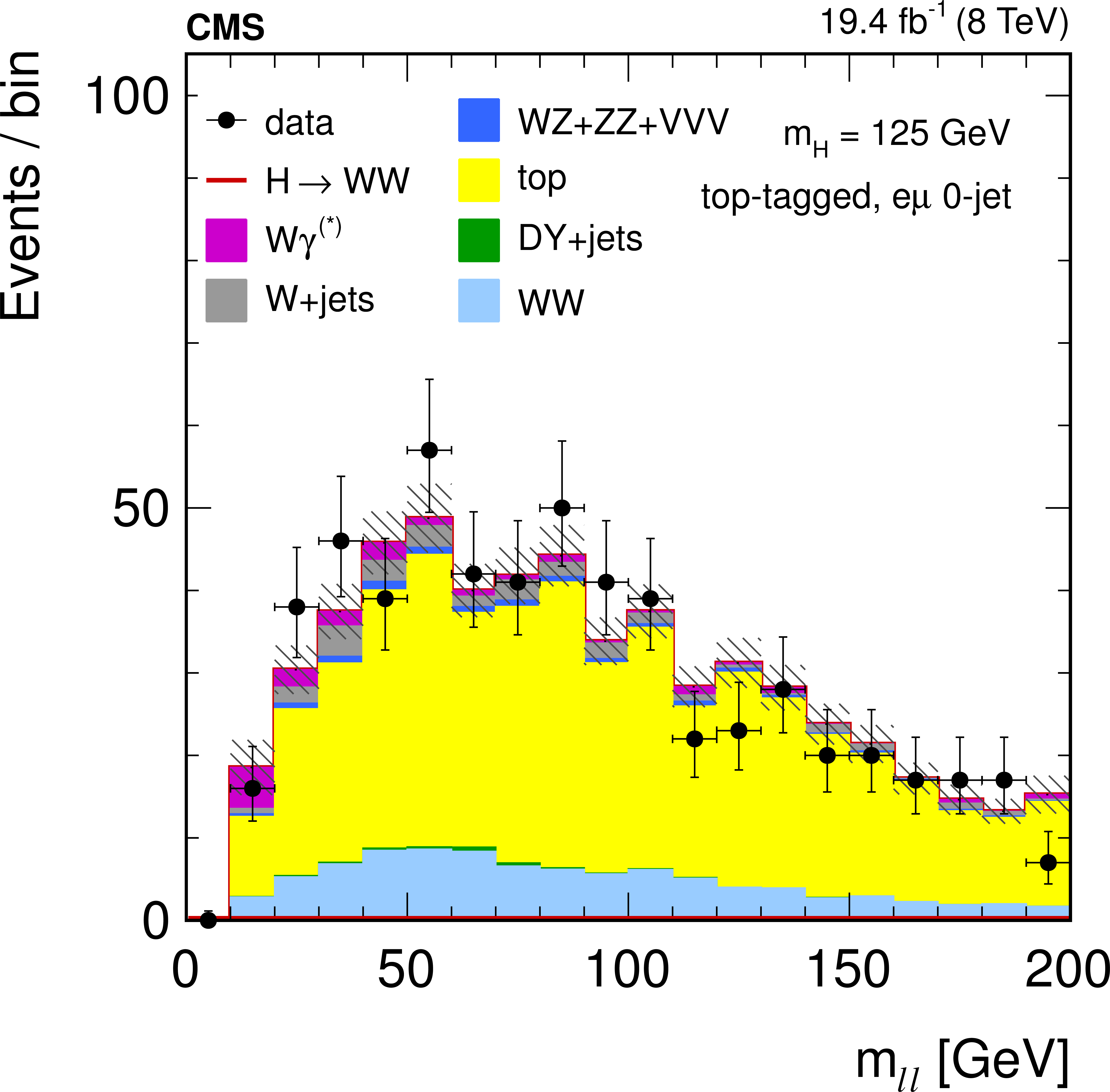
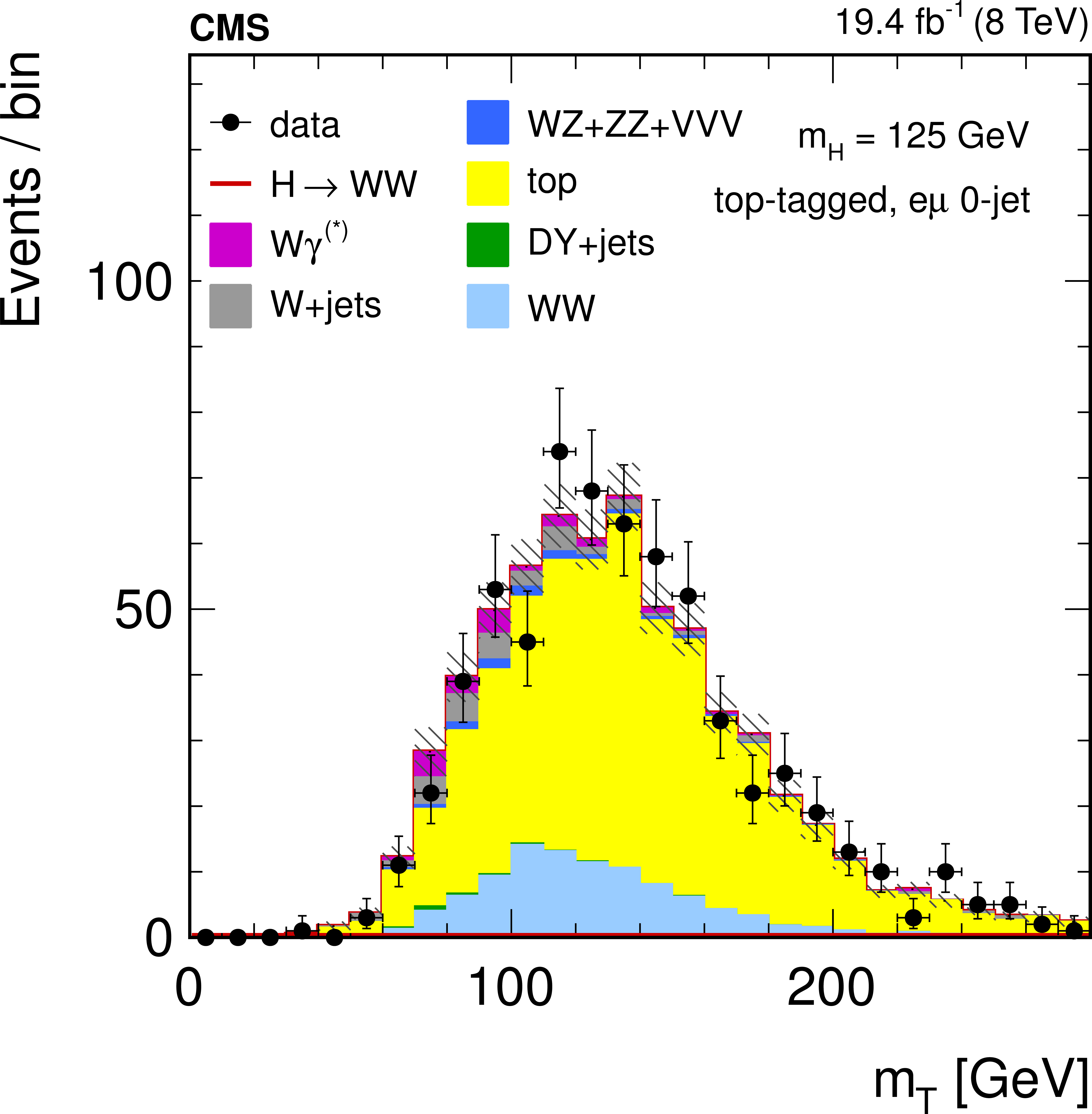
png pdf	Figure 34-a: The ${m_{ {\ell } {\ell }}}$ (a) and ${m_{\mathrm {T}}}$ (b) distributions in the 0-jet category for top-tagged events in the different-flavor final state at the ${\mathrm {W}} {\mathrm {W}}$ selection level for $\sqrt {s} = 8 TeV$ data sample. The uncertainty band includes the statistical and systematic uncertainty of all background processes.
png pdf	Figure 34-b: The ${m_{ {\ell } {\ell }}}$ (a) and ${m_{\mathrm {T}}}$ (b) distributions in the 0-jet category for top-tagged events in the different-flavor final state at the ${\mathrm {W}} {\mathrm {W}}$ selection level for $\sqrt {s} = 8 TeV$ data sample. The uncertainty band includes the statistical and systematic uncertainty of all background processes.
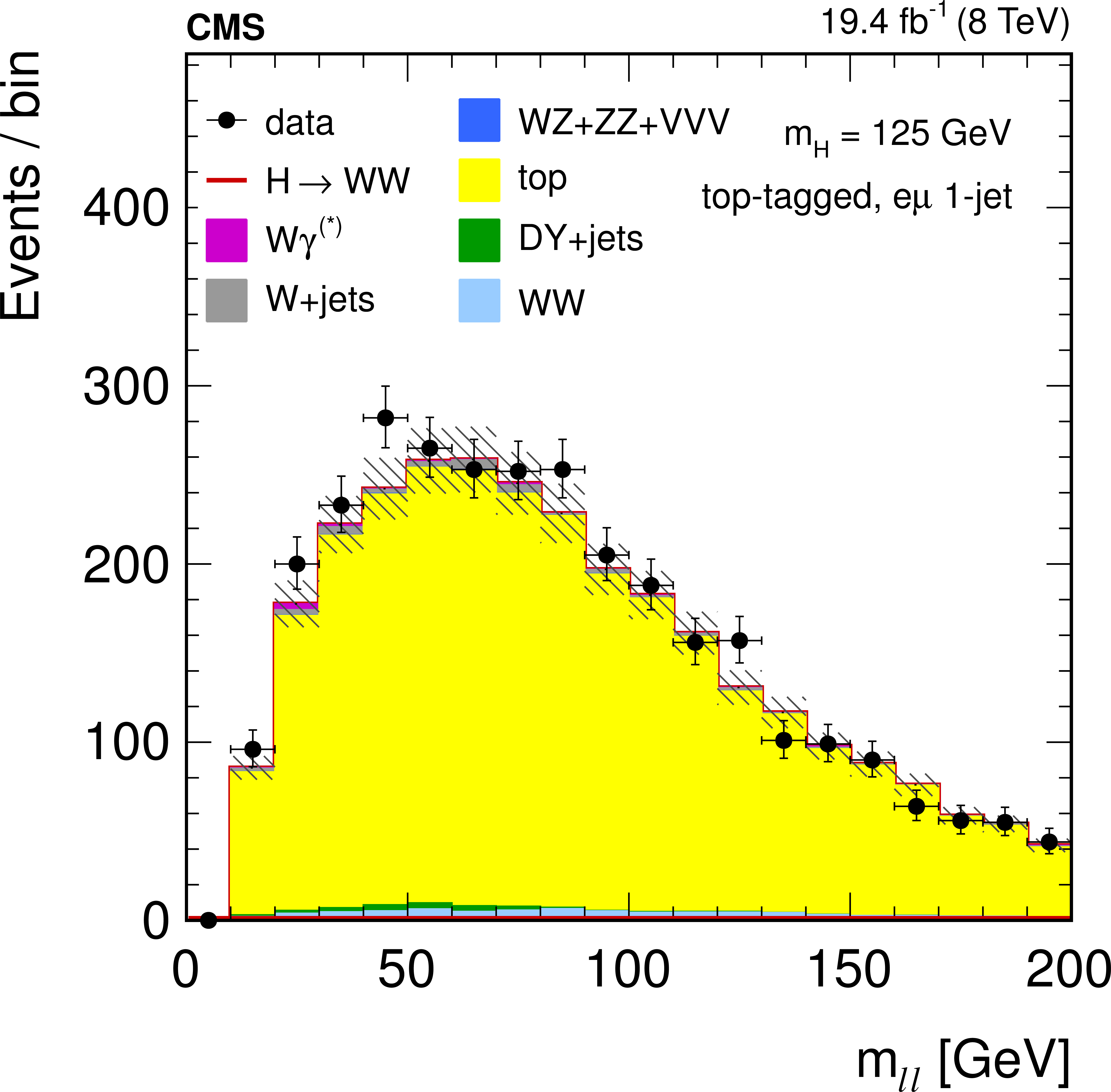
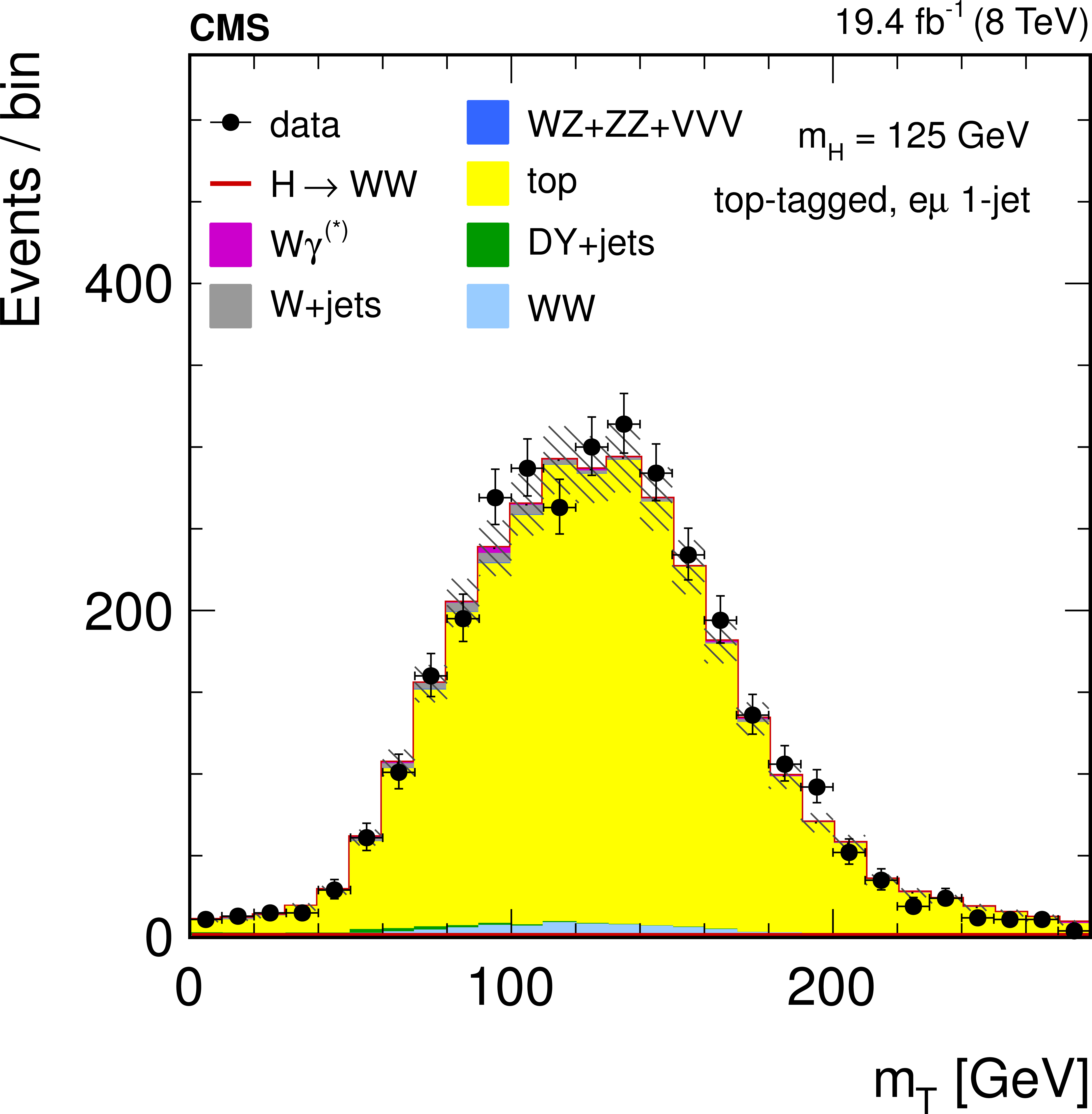
png pdf	Figure 35-a: The ${m_{ {\ell } {\ell }}}$ (a) and ${m_{\mathrm {T}}}$ (b) distributions in the 1-jet category for top-tagged events in the different-flavor final state at the ${\mathrm {W}} {\mathrm {W}}$ selection level for the $\sqrt {s}$ = 8 TeV data sample. The uncertainty band includes the statistical and systematic uncertainty of all background processes.
png pdf	Figure 35-b: The ${m_{ {\ell } {\ell }}}$ (a) and ${m_{\mathrm {T}}}$ (b) distributions in the 1-jet category for top-tagged events in the different-flavor final state at the ${\mathrm {W}} {\mathrm {W}}$ selection level for the $\sqrt {s}$ = 8 TeV data sample. The uncertainty band includes the statistical and systematic uncertainty of all background processes.
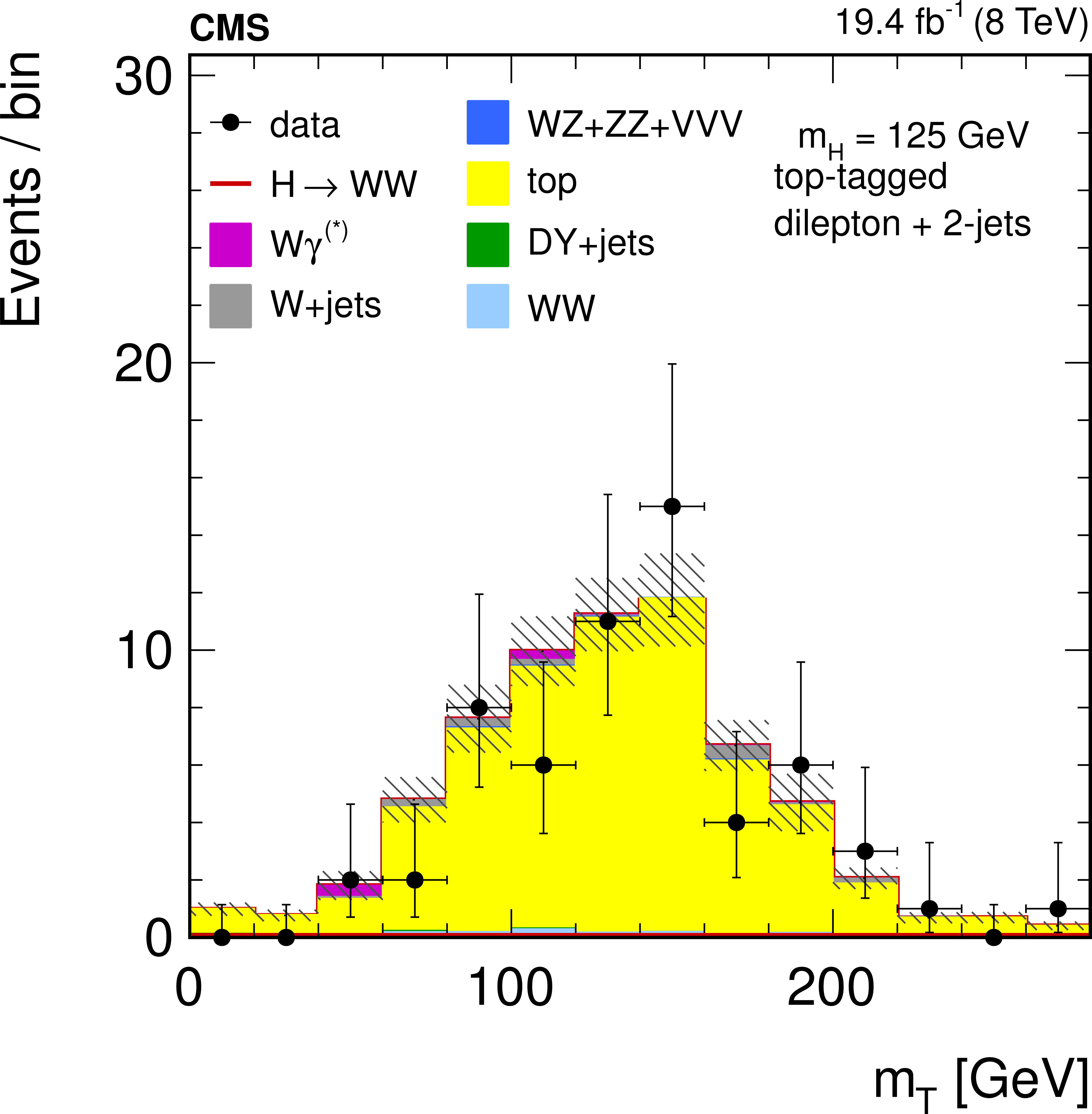
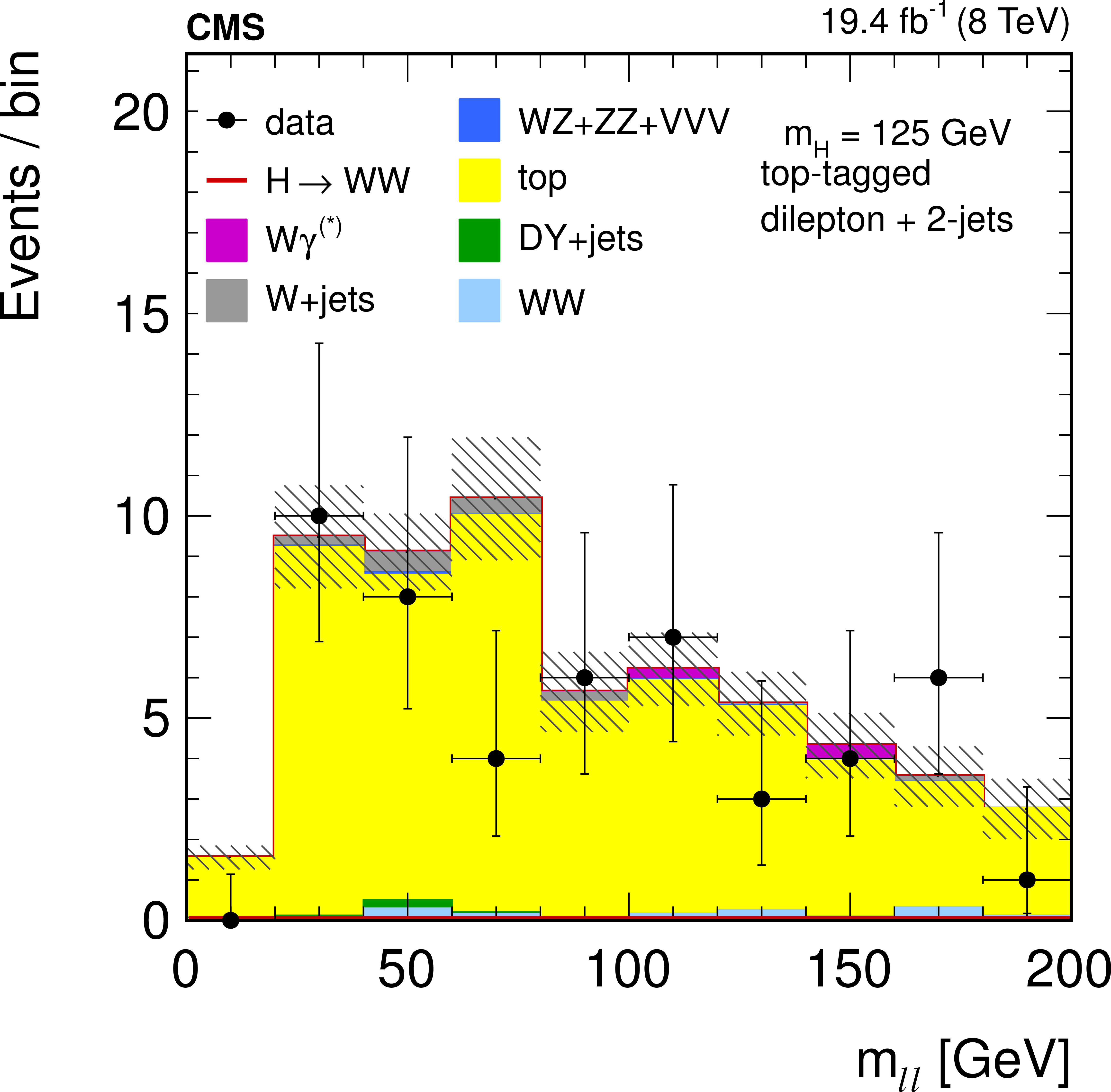
png pdf	Figure 36-a: The ${m_{ {\ell } {\ell }}}$ (a) and ${m_{\mathrm {T}}}$ (b) distributions in the 2-jet category for top-tagged events after applying the ${\mathrm {W}} {\mathrm {W}}$ and VBF-tag selections for the $\sqrt {s}$ = 8 TeV data sample. The uncertainty band includes the statistical and systematic uncertainty for all background processes.
png pdf	Figure 36-b: The ${m_{ {\ell } {\ell }}}$ (a) and ${m_{\mathrm {T}}}$ (b) distributions in the 2-jet category for top-tagged events after applying the ${\mathrm {W}} {\mathrm {W}}$ and VBF-tag selections for the $\sqrt {s}$ = 8 TeV data sample. The uncertainty band includes the statistical and systematic uncertainty for all background processes.