
Compact Muon Solenoid
LHC, CERN
 Visit us: CMS Public Website, CMS Physics ;
Contact us: CMS Publications Committee
Visit us: CMS Public Website, CMS Physics ;
Contact us: CMS Publications Committee
| CMS-TOP-24-008 ; CERN-EP-2026-140 | ||
| Search for physics beyond the standard model in four and three top quark production events using proton-proton collisions at $ \sqrt{s}= $ 13 TeV | ||
| CMS Collaboration | ||
| 29 June 2026 | ||
| Submitted to the Journal of High Energy Physics | ||
| Abstract: A search for physics beyond the standard model using four and three top quark production events is reported. The analyzed proton-proton collision data were recorded at 13 TeV with the CMS detector at the CERN LHC in 2016--2018 and correspond to an integrated luminosity of 138 fb$ ^{-1} $. Events with two same-sign, three, or four leptons (electrons and/or muons) are selected. Constraints on six Wilson coefficients that modify interactions between four third-generation quarks or between top quarks and the Higgs boson in the standard model effective field theory framework are derived. The data are further used to exclude narrow topphilic heavy resonances in the mass ranges between 400 GeV and 1.6 TeV depending on their spin and color states. Finally, the top quark Yukawa coupling is extracted, considering both $ CP $-even and $ CP $-odd contributions. | ||
| Links: e-print arXiv:2606.30862 [hep-ex] (PDF) ; CDS record ; inSPIRE record ; HepData record ; CADI line (restricted) ; | ||
| Figures | Summary | Additional Figures & Tables | References | CMS Publications |
|---|
| Figures | |
png pdf |
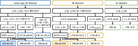
Figure 1:
Schematic representation of the event selection and categorization. |
png pdf |
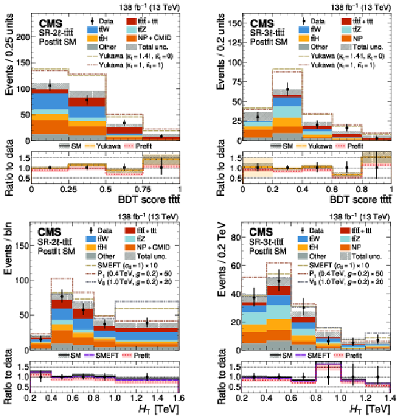
Figure 2:
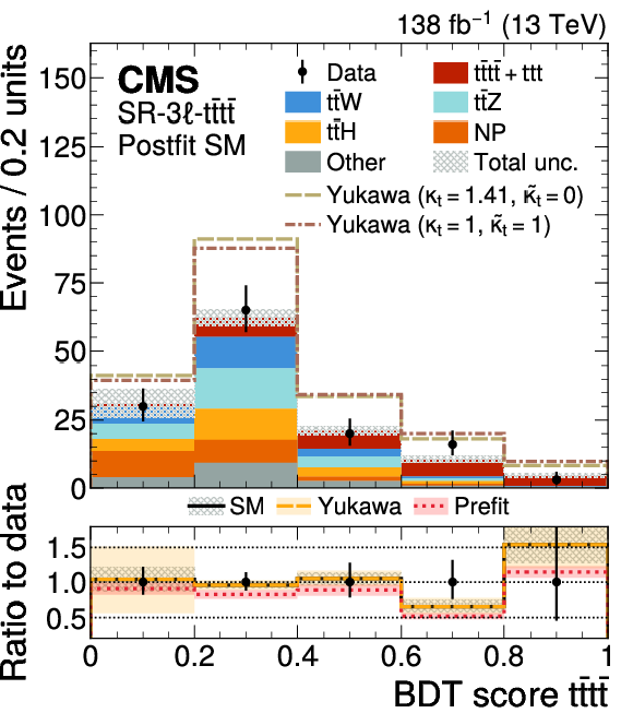
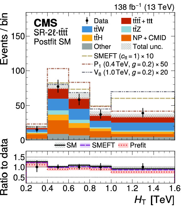
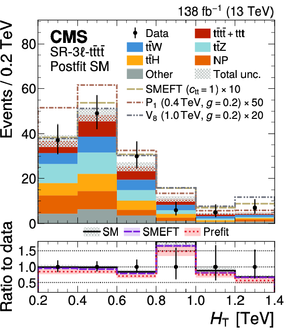
Comparison of the number of observed (points) and predicted (colored histograms) events in the BDT score $ {\mathrm{t}\overline{\mathrm{t}}} {\mathrm{t}\overline{\mathrm{t}}} $ (upper row) or $ H_{\mathrm{T}} $ (lower row) distribution, shown for the $ \text{SR-}2\ell\text{-}{\mathrm{t}\overline{\mathrm{t}}} {\mathrm{t}\overline{\mathrm{t}}} $ (left, merged across all lepton flavor categories) and the $ \text{SR-}3\ell\text{-}{\mathrm{t}\overline{\mathrm{t}}} {\mathrm{t}\overline{\mathrm{t}}} $ (right). The last bins of the $ H_{\mathrm{T}} $ distributions include the overflow contribution. The vertical bars on the points represent the statistical uncertainties in the data, and the hatched bands the total uncertainty in the predictions. The SM yields are shown with their best fit normalizations from the simultaneous fit to the data (``postfit'') for the SM fit. The dashed/dotted lines show the enhancement of $ {\mathrm{t}\overline{\mathrm{t}}} {\mathrm{t}\overline{\mathrm{t}}} \text{+}\mathrm{t}\mathrm{t}\mathrm{t} $ production in different new-physics scenarios. The lower panels show the ratio of the total prediction to data for three postfit scenarios---SM, Yukawa coupling extraction, and SMEFT---and also using the SM yields before any fit to the data (``prefit''). |
png pdf |
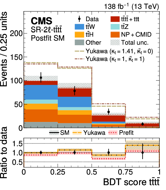
Figure 2-a:
Comparison of the number of observed (points) and predicted (colored histograms) events in the BDT score $ {\mathrm{t}\overline{\mathrm{t}}} {\mathrm{t}\overline{\mathrm{t}}} $ (upper row) or $ H_{\mathrm{T}} $ (lower row) distribution, shown for the $ \text{SR-}2\ell\text{-}{\mathrm{t}\overline{\mathrm{t}}} {\mathrm{t}\overline{\mathrm{t}}} $ (left, merged across all lepton flavor categories) and the $ \text{SR-}3\ell\text{-}{\mathrm{t}\overline{\mathrm{t}}} {\mathrm{t}\overline{\mathrm{t}}} $ (right). The last bins of the $ H_{\mathrm{T}} $ distributions include the overflow contribution. The vertical bars on the points represent the statistical uncertainties in the data, and the hatched bands the total uncertainty in the predictions. The SM yields are shown with their best fit normalizations from the simultaneous fit to the data (``postfit'') for the SM fit. The dashed/dotted lines show the enhancement of $ {\mathrm{t}\overline{\mathrm{t}}} {\mathrm{t}\overline{\mathrm{t}}} \text{+}\mathrm{t}\mathrm{t}\mathrm{t} $ production in different new-physics scenarios. The lower panels show the ratio of the total prediction to data for three postfit scenarios---SM, Yukawa coupling extraction, and SMEFT---and also using the SM yields before any fit to the data (``prefit''). |
png pdf |
Figure 2-b:
Comparison of the number of observed (points) and predicted (colored histograms) events in the BDT score $ {\mathrm{t}\overline{\mathrm{t}}} {\mathrm{t}\overline{\mathrm{t}}} $ (upper row) or $ H_{\mathrm{T}} $ (lower row) distribution, shown for the $ \text{SR-}2\ell\text{-}{\mathrm{t}\overline{\mathrm{t}}} {\mathrm{t}\overline{\mathrm{t}}} $ (left, merged across all lepton flavor categories) and the $ \text{SR-}3\ell\text{-}{\mathrm{t}\overline{\mathrm{t}}} {\mathrm{t}\overline{\mathrm{t}}} $ (right). The last bins of the $ H_{\mathrm{T}} $ distributions include the overflow contribution. The vertical bars on the points represent the statistical uncertainties in the data, and the hatched bands the total uncertainty in the predictions. The SM yields are shown with their best fit normalizations from the simultaneous fit to the data (``postfit'') for the SM fit. The dashed/dotted lines show the enhancement of $ {\mathrm{t}\overline{\mathrm{t}}} {\mathrm{t}\overline{\mathrm{t}}} \text{+}\mathrm{t}\mathrm{t}\mathrm{t} $ production in different new-physics scenarios. The lower panels show the ratio of the total prediction to data for three postfit scenarios---SM, Yukawa coupling extraction, and SMEFT---and also using the SM yields before any fit to the data (``prefit''). |
png pdf |
Figure 2-c:
Comparison of the number of observed (points) and predicted (colored histograms) events in the BDT score $ {\mathrm{t}\overline{\mathrm{t}}} {\mathrm{t}\overline{\mathrm{t}}} $ (upper row) or $ H_{\mathrm{T}} $ (lower row) distribution, shown for the $ \text{SR-}2\ell\text{-}{\mathrm{t}\overline{\mathrm{t}}} {\mathrm{t}\overline{\mathrm{t}}} $ (left, merged across all lepton flavor categories) and the $ \text{SR-}3\ell\text{-}{\mathrm{t}\overline{\mathrm{t}}} {\mathrm{t}\overline{\mathrm{t}}} $ (right). The last bins of the $ H_{\mathrm{T}} $ distributions include the overflow contribution. The vertical bars on the points represent the statistical uncertainties in the data, and the hatched bands the total uncertainty in the predictions. The SM yields are shown with their best fit normalizations from the simultaneous fit to the data (``postfit'') for the SM fit. The dashed/dotted lines show the enhancement of $ {\mathrm{t}\overline{\mathrm{t}}} {\mathrm{t}\overline{\mathrm{t}}} \text{+}\mathrm{t}\mathrm{t}\mathrm{t} $ production in different new-physics scenarios. The lower panels show the ratio of the total prediction to data for three postfit scenarios---SM, Yukawa coupling extraction, and SMEFT---and also using the SM yields before any fit to the data (``prefit''). |
png pdf |
Figure 2-d:
Comparison of the number of observed (points) and predicted (colored histograms) events in the BDT score $ {\mathrm{t}\overline{\mathrm{t}}} {\mathrm{t}\overline{\mathrm{t}}} $ (upper row) or $ H_{\mathrm{T}} $ (lower row) distribution, shown for the $ \text{SR-}2\ell\text{-}{\mathrm{t}\overline{\mathrm{t}}} {\mathrm{t}\overline{\mathrm{t}}} $ (left, merged across all lepton flavor categories) and the $ \text{SR-}3\ell\text{-}{\mathrm{t}\overline{\mathrm{t}}} {\mathrm{t}\overline{\mathrm{t}}} $ (right). The last bins of the $ H_{\mathrm{T}} $ distributions include the overflow contribution. The vertical bars on the points represent the statistical uncertainties in the data, and the hatched bands the total uncertainty in the predictions. The SM yields are shown with their best fit normalizations from the simultaneous fit to the data (``postfit'') for the SM fit. The dashed/dotted lines show the enhancement of $ {\mathrm{t}\overline{\mathrm{t}}} {\mathrm{t}\overline{\mathrm{t}}} \text{+}\mathrm{t}\mathrm{t}\mathrm{t} $ production in different new-physics scenarios. The lower panels show the ratio of the total prediction to data for three postfit scenarios---SM, Yukawa coupling extraction, and SMEFT---and also using the SM yields before any fit to the data (``prefit''). |
png pdf |
Figure 3:
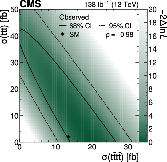
Two-dimensional scan of the $ {\mathrm{t}\overline{\mathrm{t}}} {\mathrm{t}\overline{\mathrm{t}}} $ and $ \mathrm{t}\mathrm{t}\mathrm{t} $ cross sections. The color scale shows the negative log-likelihood difference with respect to the best fit point, and the contour lines show the 68% (solid) and 95% (dashed) CL intervals. The SM prediction is indicated with a black cross. The correlation $ \rho $ between the two measured cross sections is-0.98. |
png pdf |
Figure 4:
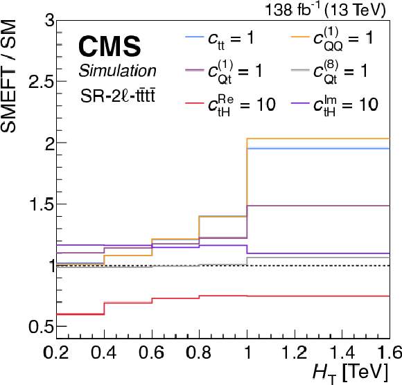
Comparison of the $ H_{\mathrm{T}} $ distribution in the $ \text{SR-}2\ell\text{-}{\mathrm{t}\overline{\mathrm{t}}} {\mathrm{t}\overline{\mathrm{t}}} $ for different SMEFT scenarios relative to the SM prediction. Each line shows the ratio of the SMEFT prediction for $ {\mathrm{t}\overline{\mathrm{t}}} {\mathrm{t}\overline{\mathrm{t}}} $, $ \mathrm{t}\mathrm{t}\mathrm{t} $, and $ {\mathrm{t}\overline{\mathrm{t}}} \mathrm{H} $ production combined with exactly one WC at a nonzero value to the SM prediction for the same processes. The last bin includes the overflow contribution. |
png pdf |
Figure 5:
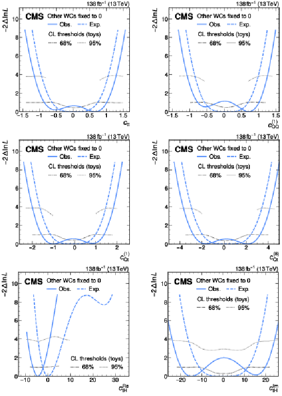
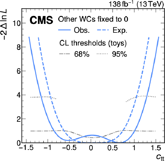
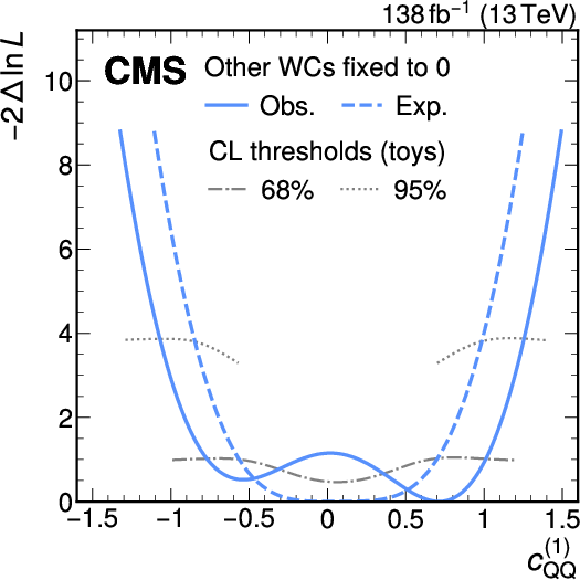
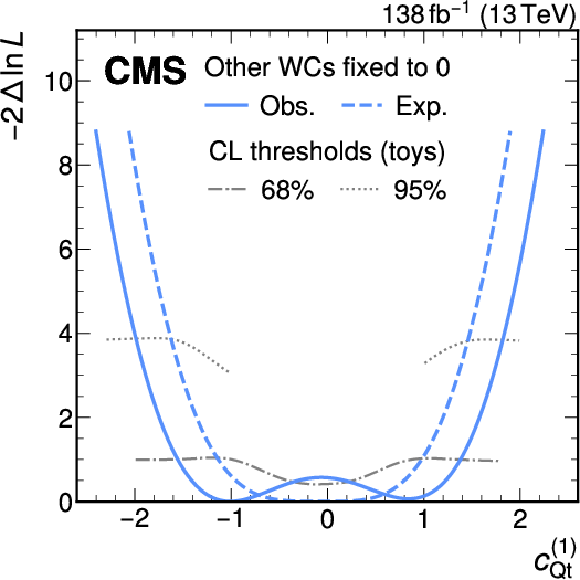
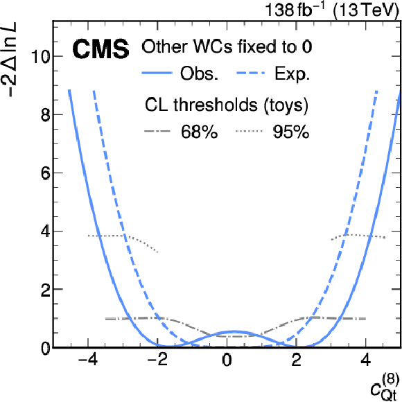
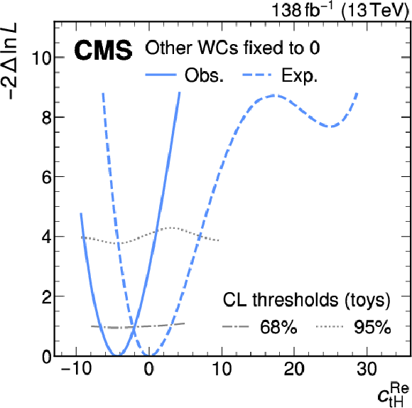
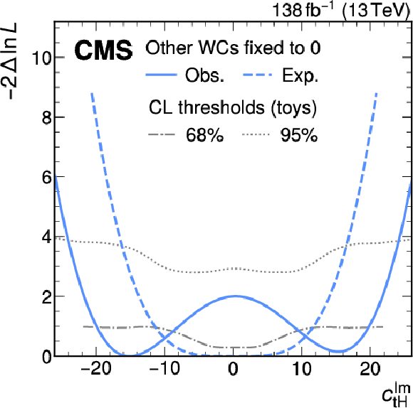
Negative log-likelihood difference from the best fit value for the one-dimensional scans of the WCs $ c_{\mathrm{t}\mathrm{t}} $ (upper left), $ c_{QQ}^{(1)} $ (upper right), $ c_{Q\mathrm{t}}^{(1)} $ (middle left), $ c_{Q\mathrm{t}}^{(8)} $ (middle right), $ c_{\mathrm{t}\mathrm{H}}^{\mathrm{Re}} $ (lower left), and $ c_{\mathrm{t}\mathrm{H}}^{\mathrm{Im}} $ (lower right), where the other WCs are fixed to zero. Shown are the expected (blue dashed line) and observed (blue solid line) results, as well as the threshold values for 68% (gray dash-dotted line) and 95% (gray dotted lines) CL intervals as evaluated with toys. |
png pdf |
Figure 5-a:
Negative log-likelihood difference from the best fit value for the one-dimensional scans of the WCs $ c_{\mathrm{t}\mathrm{t}} $ (upper left), $ c_{QQ}^{(1)} $ (upper right), $ c_{Q\mathrm{t}}^{(1)} $ (middle left), $ c_{Q\mathrm{t}}^{(8)} $ (middle right), $ c_{\mathrm{t}\mathrm{H}}^{\mathrm{Re}} $ (lower left), and $ c_{\mathrm{t}\mathrm{H}}^{\mathrm{Im}} $ (lower right), where the other WCs are fixed to zero. Shown are the expected (blue dashed line) and observed (blue solid line) results, as well as the threshold values for 68% (gray dash-dotted line) and 95% (gray dotted lines) CL intervals as evaluated with toys. |
png pdf |
Figure 5-b:
Negative log-likelihood difference from the best fit value for the one-dimensional scans of the WCs $ c_{\mathrm{t}\mathrm{t}} $ (upper left), $ c_{QQ}^{(1)} $ (upper right), $ c_{Q\mathrm{t}}^{(1)} $ (middle left), $ c_{Q\mathrm{t}}^{(8)} $ (middle right), $ c_{\mathrm{t}\mathrm{H}}^{\mathrm{Re}} $ (lower left), and $ c_{\mathrm{t}\mathrm{H}}^{\mathrm{Im}} $ (lower right), where the other WCs are fixed to zero. Shown are the expected (blue dashed line) and observed (blue solid line) results, as well as the threshold values for 68% (gray dash-dotted line) and 95% (gray dotted lines) CL intervals as evaluated with toys. |
png pdf |
Figure 5-c:
Negative log-likelihood difference from the best fit value for the one-dimensional scans of the WCs $ c_{\mathrm{t}\mathrm{t}} $ (upper left), $ c_{QQ}^{(1)} $ (upper right), $ c_{Q\mathrm{t}}^{(1)} $ (middle left), $ c_{Q\mathrm{t}}^{(8)} $ (middle right), $ c_{\mathrm{t}\mathrm{H}}^{\mathrm{Re}} $ (lower left), and $ c_{\mathrm{t}\mathrm{H}}^{\mathrm{Im}} $ (lower right), where the other WCs are fixed to zero. Shown are the expected (blue dashed line) and observed (blue solid line) results, as well as the threshold values for 68% (gray dash-dotted line) and 95% (gray dotted lines) CL intervals as evaluated with toys. |
png pdf |
Figure 5-d:
Negative log-likelihood difference from the best fit value for the one-dimensional scans of the WCs $ c_{\mathrm{t}\mathrm{t}} $ (upper left), $ c_{QQ}^{(1)} $ (upper right), $ c_{Q\mathrm{t}}^{(1)} $ (middle left), $ c_{Q\mathrm{t}}^{(8)} $ (middle right), $ c_{\mathrm{t}\mathrm{H}}^{\mathrm{Re}} $ (lower left), and $ c_{\mathrm{t}\mathrm{H}}^{\mathrm{Im}} $ (lower right), where the other WCs are fixed to zero. Shown are the expected (blue dashed line) and observed (blue solid line) results, as well as the threshold values for 68% (gray dash-dotted line) and 95% (gray dotted lines) CL intervals as evaluated with toys. |
png pdf |
Figure 5-e:
Negative log-likelihood difference from the best fit value for the one-dimensional scans of the WCs $ c_{\mathrm{t}\mathrm{t}} $ (upper left), $ c_{QQ}^{(1)} $ (upper right), $ c_{Q\mathrm{t}}^{(1)} $ (middle left), $ c_{Q\mathrm{t}}^{(8)} $ (middle right), $ c_{\mathrm{t}\mathrm{H}}^{\mathrm{Re}} $ (lower left), and $ c_{\mathrm{t}\mathrm{H}}^{\mathrm{Im}} $ (lower right), where the other WCs are fixed to zero. Shown are the expected (blue dashed line) and observed (blue solid line) results, as well as the threshold values for 68% (gray dash-dotted line) and 95% (gray dotted lines) CL intervals as evaluated with toys. |
png pdf |
Figure 5-f:
Negative log-likelihood difference from the best fit value for the one-dimensional scans of the WCs $ c_{\mathrm{t}\mathrm{t}} $ (upper left), $ c_{QQ}^{(1)} $ (upper right), $ c_{Q\mathrm{t}}^{(1)} $ (middle left), $ c_{Q\mathrm{t}}^{(8)} $ (middle right), $ c_{\mathrm{t}\mathrm{H}}^{\mathrm{Re}} $ (lower left), and $ c_{\mathrm{t}\mathrm{H}}^{\mathrm{Im}} $ (lower right), where the other WCs are fixed to zero. Shown are the expected (blue dashed line) and observed (blue solid line) results, as well as the threshold values for 68% (gray dash-dotted line) and 95% (gray dotted lines) CL intervals as evaluated with toys. |
png pdf |
Figure 6:
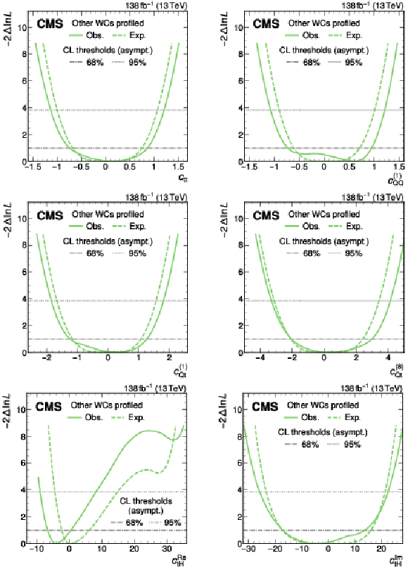
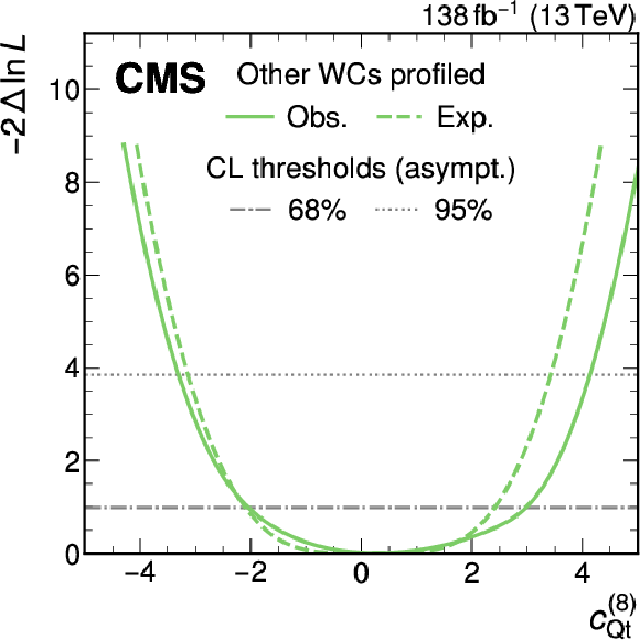
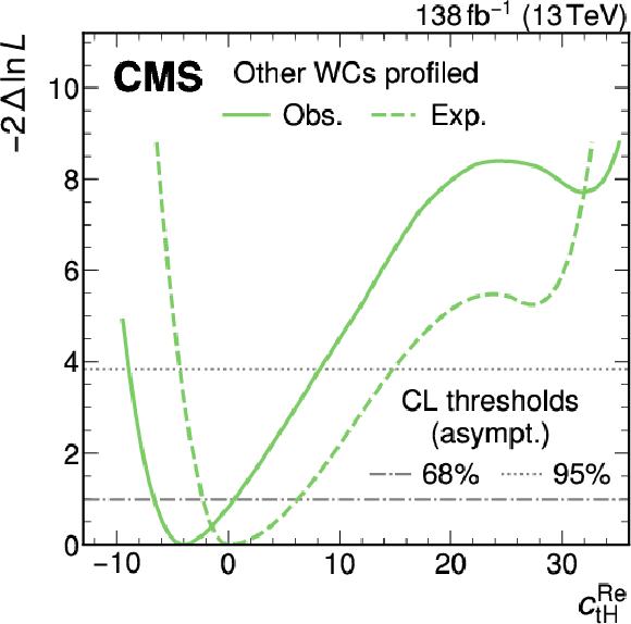
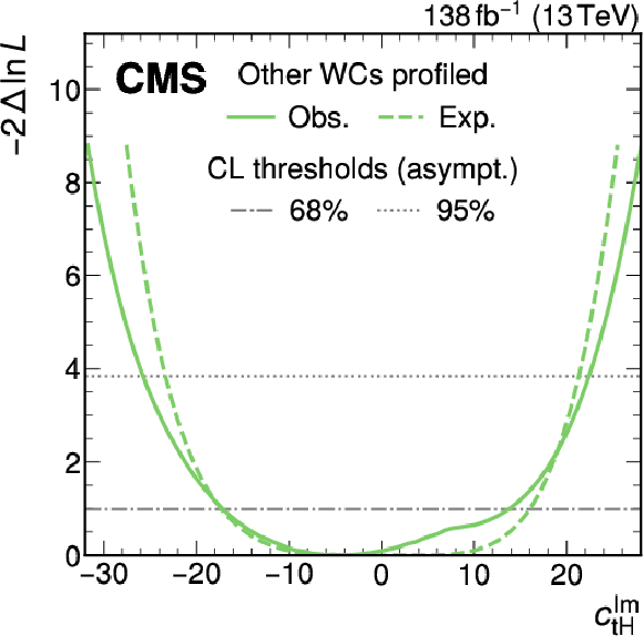
Negative log-likelihood difference from the best fit value for the one-dimensional scans of the WCs $ c_{\mathrm{t}\mathrm{t}} $ (upper left), $ c_{QQ}^{(1)} $ (upper right), $ c_{Q\mathrm{t}}^{(1)} $ (middle left), $ c_{Q\mathrm{t}}^{(8)} $ (middle right), $ c_{\mathrm{t}\mathrm{H}}^{\mathrm{Re}} $ (lower left), and $ c_{\mathrm{t}\mathrm{H}}^{\mathrm{Im}} $ (lower right), where the other WCs are profiled. Shown are the expected (green dashed line) and observed (green solid line) results, as well as the threshold values that would apply for 68% (gray dash-dotted line) and 95% (gray dotted line) CL intervals if the asymptotic approximation was valid. |
png pdf |
Figure 6-a:
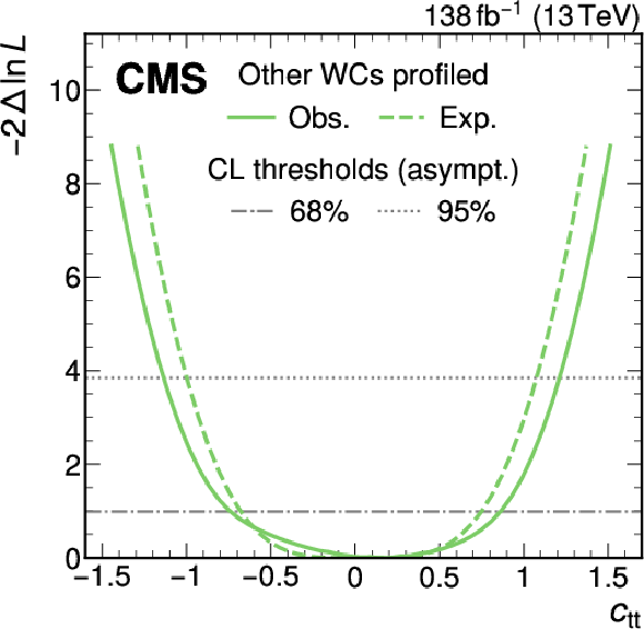
Negative log-likelihood difference from the best fit value for the one-dimensional scans of the WCs $ c_{\mathrm{t}\mathrm{t}} $ (upper left), $ c_{QQ}^{(1)} $ (upper right), $ c_{Q\mathrm{t}}^{(1)} $ (middle left), $ c_{Q\mathrm{t}}^{(8)} $ (middle right), $ c_{\mathrm{t}\mathrm{H}}^{\mathrm{Re}} $ (lower left), and $ c_{\mathrm{t}\mathrm{H}}^{\mathrm{Im}} $ (lower right), where the other WCs are profiled. Shown are the expected (green dashed line) and observed (green solid line) results, as well as the threshold values that would apply for 68% (gray dash-dotted line) and 95% (gray dotted line) CL intervals if the asymptotic approximation was valid. |
png pdf |
Figure 6-b:
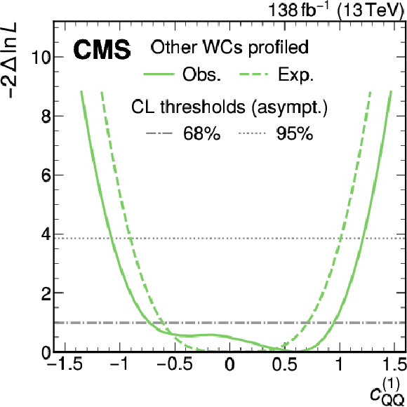
Negative log-likelihood difference from the best fit value for the one-dimensional scans of the WCs $ c_{\mathrm{t}\mathrm{t}} $ (upper left), $ c_{QQ}^{(1)} $ (upper right), $ c_{Q\mathrm{t}}^{(1)} $ (middle left), $ c_{Q\mathrm{t}}^{(8)} $ (middle right), $ c_{\mathrm{t}\mathrm{H}}^{\mathrm{Re}} $ (lower left), and $ c_{\mathrm{t}\mathrm{H}}^{\mathrm{Im}} $ (lower right), where the other WCs are profiled. Shown are the expected (green dashed line) and observed (green solid line) results, as well as the threshold values that would apply for 68% (gray dash-dotted line) and 95% (gray dotted line) CL intervals if the asymptotic approximation was valid. |
png pdf |
Figure 6-c:
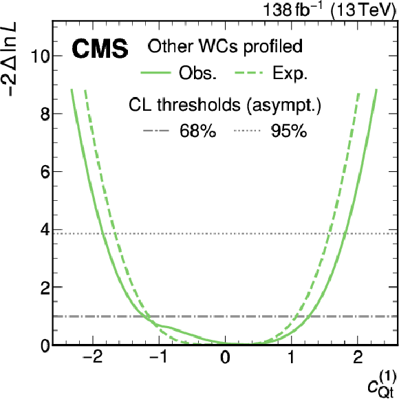
Negative log-likelihood difference from the best fit value for the one-dimensional scans of the WCs $ c_{\mathrm{t}\mathrm{t}} $ (upper left), $ c_{QQ}^{(1)} $ (upper right), $ c_{Q\mathrm{t}}^{(1)} $ (middle left), $ c_{Q\mathrm{t}}^{(8)} $ (middle right), $ c_{\mathrm{t}\mathrm{H}}^{\mathrm{Re}} $ (lower left), and $ c_{\mathrm{t}\mathrm{H}}^{\mathrm{Im}} $ (lower right), where the other WCs are profiled. Shown are the expected (green dashed line) and observed (green solid line) results, as well as the threshold values that would apply for 68% (gray dash-dotted line) and 95% (gray dotted line) CL intervals if the asymptotic approximation was valid. |
png pdf |
Figure 6-d:
Negative log-likelihood difference from the best fit value for the one-dimensional scans of the WCs $ c_{\mathrm{t}\mathrm{t}} $ (upper left), $ c_{QQ}^{(1)} $ (upper right), $ c_{Q\mathrm{t}}^{(1)} $ (middle left), $ c_{Q\mathrm{t}}^{(8)} $ (middle right), $ c_{\mathrm{t}\mathrm{H}}^{\mathrm{Re}} $ (lower left), and $ c_{\mathrm{t}\mathrm{H}}^{\mathrm{Im}} $ (lower right), where the other WCs are profiled. Shown are the expected (green dashed line) and observed (green solid line) results, as well as the threshold values that would apply for 68% (gray dash-dotted line) and 95% (gray dotted line) CL intervals if the asymptotic approximation was valid. |
png pdf |
Figure 6-e:
Negative log-likelihood difference from the best fit value for the one-dimensional scans of the WCs $ c_{\mathrm{t}\mathrm{t}} $ (upper left), $ c_{QQ}^{(1)} $ (upper right), $ c_{Q\mathrm{t}}^{(1)} $ (middle left), $ c_{Q\mathrm{t}}^{(8)} $ (middle right), $ c_{\mathrm{t}\mathrm{H}}^{\mathrm{Re}} $ (lower left), and $ c_{\mathrm{t}\mathrm{H}}^{\mathrm{Im}} $ (lower right), where the other WCs are profiled. Shown are the expected (green dashed line) and observed (green solid line) results, as well as the threshold values that would apply for 68% (gray dash-dotted line) and 95% (gray dotted line) CL intervals if the asymptotic approximation was valid. |
png pdf |
Figure 6-f:
Negative log-likelihood difference from the best fit value for the one-dimensional scans of the WCs $ c_{\mathrm{t}\mathrm{t}} $ (upper left), $ c_{QQ}^{(1)} $ (upper right), $ c_{Q\mathrm{t}}^{(1)} $ (middle left), $ c_{Q\mathrm{t}}^{(8)} $ (middle right), $ c_{\mathrm{t}\mathrm{H}}^{\mathrm{Re}} $ (lower left), and $ c_{\mathrm{t}\mathrm{H}}^{\mathrm{Im}} $ (lower right), where the other WCs are profiled. Shown are the expected (green dashed line) and observed (green solid line) results, as well as the threshold values that would apply for 68% (gray dash-dotted line) and 95% (gray dotted line) CL intervals if the asymptotic approximation was valid. |
png pdf |
Figure 7:
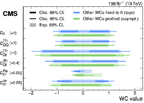
Constraints on the individual WCs, obtained by either fixing the other WCs to zero (blue) or profiling them (green). The lines and shaded areas indicate the observed and expected CL intervals, respectively. For the case where the other WCs are fixed to zero, the 68 and 95% CL intervals are evaluated with toys. For the case where the other WCs are profiled, the intervals are instead evaluated by applying the asymptotic approximation. The constraints are scaled to ensure that all six WCs can be visualized on the same axis range. |
png pdf |
Figure 8:
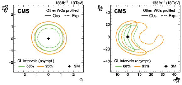
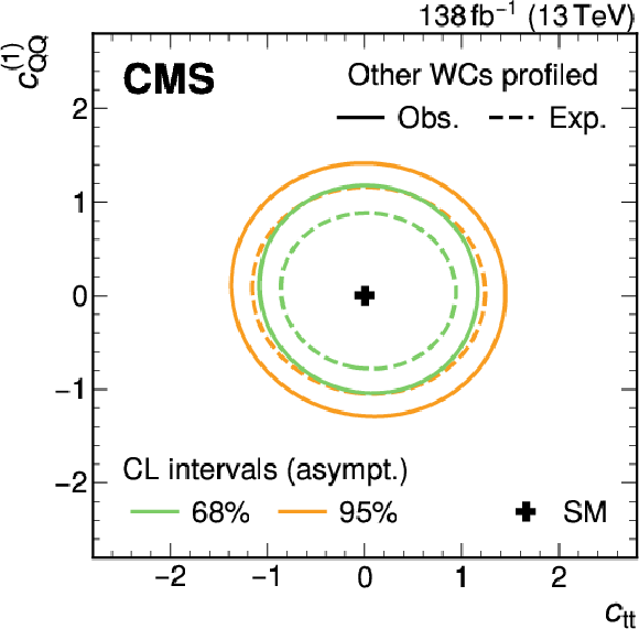
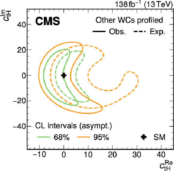
Expected (dashed lines) and observed (solid lines) exclusion contours for the two-dimensional scans of the WCs $ c_{\mathrm{t}\mathrm{t}} $ and $ c_{QQ}^{(1)} $ (left) and $ c_{\mathrm{t}\mathrm{H}}^{\mathrm{Re}} $ and $ c_{\mathrm{t}\mathrm{H}}^{\mathrm{Im}} $ (right), with the other WCs profiled in both cases. Shown are the CL intervals where the test statistic falls below 2.3 (green lines) and 6.2 (orange lines), i.e.,, corresponding to the 68 and 95% CL intervals if the asymptotic approximation was valid. |
png pdf |
Figure 8-a:
Expected (dashed lines) and observed (solid lines) exclusion contours for the two-dimensional scans of the WCs $ c_{\mathrm{t}\mathrm{t}} $ and $ c_{QQ}^{(1)} $ (left) and $ c_{\mathrm{t}\mathrm{H}}^{\mathrm{Re}} $ and $ c_{\mathrm{t}\mathrm{H}}^{\mathrm{Im}} $ (right), with the other WCs profiled in both cases. Shown are the CL intervals where the test statistic falls below 2.3 (green lines) and 6.2 (orange lines), i.e.,, corresponding to the 68 and 95% CL intervals if the asymptotic approximation was valid. |
png pdf |
Figure 8-b:
Expected (dashed lines) and observed (solid lines) exclusion contours for the two-dimensional scans of the WCs $ c_{\mathrm{t}\mathrm{t}} $ and $ c_{QQ}^{(1)} $ (left) and $ c_{\mathrm{t}\mathrm{H}}^{\mathrm{Re}} $ and $ c_{\mathrm{t}\mathrm{H}}^{\mathrm{Im}} $ (right), with the other WCs profiled in both cases. Shown are the CL intervals where the test statistic falls below 2.3 (green lines) and 6.2 (orange lines), i.e.,, corresponding to the 68 and 95% CL intervals if the asymptotic approximation was valid. |
png pdf |
Figure 9:
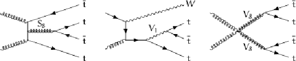
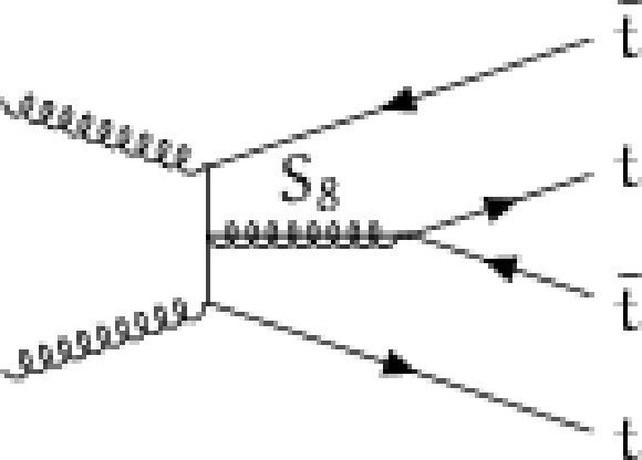
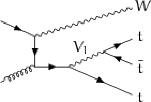
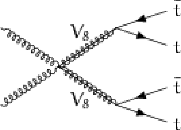
Example LO Feynman diagrams for $ {\mathrm{t}\overline{\mathrm{t}}} {\mathrm{t}\overline{\mathrm{t}}} $ production with resonant $ {{S}{8}} \to{\mathrm{t}\overline{\mathrm{t}}} $ decay (left), $ \mathrm{t}\mathrm{t}\mathrm{t}\mathrm{W} $ production with resonant $ {{V}{1}} \to{\mathrm{t}\overline{\mathrm{t}}} $ decay (center), and doubly resonant $ {\mathrm{t}\overline{\mathrm{t}}} {\mathrm{t}\overline{\mathrm{t}}} $ production as {V8} pair production with subsequent $ {{V}{8}} \to{\mathrm{t}\overline{\mathrm{t}}} $ decays (right). |
png pdf |
Figure 9-a:
Example LO Feynman diagrams for $ {\mathrm{t}\overline{\mathrm{t}}} {\mathrm{t}\overline{\mathrm{t}}} $ production with resonant $ {{S}{8}} \to{\mathrm{t}\overline{\mathrm{t}}} $ decay (left), $ \mathrm{t}\mathrm{t}\mathrm{t}\mathrm{W} $ production with resonant $ {{V}{1}} \to{\mathrm{t}\overline{\mathrm{t}}} $ decay (center), and doubly resonant $ {\mathrm{t}\overline{\mathrm{t}}} {\mathrm{t}\overline{\mathrm{t}}} $ production as {V8} pair production with subsequent $ {{V}{8}} \to{\mathrm{t}\overline{\mathrm{t}}} $ decays (right). |
png pdf |
Figure 9-b:
Example LO Feynman diagrams for $ {\mathrm{t}\overline{\mathrm{t}}} {\mathrm{t}\overline{\mathrm{t}}} $ production with resonant $ {{S}{8}} \to{\mathrm{t}\overline{\mathrm{t}}} $ decay (left), $ \mathrm{t}\mathrm{t}\mathrm{t}\mathrm{W} $ production with resonant $ {{V}{1}} \to{\mathrm{t}\overline{\mathrm{t}}} $ decay (center), and doubly resonant $ {\mathrm{t}\overline{\mathrm{t}}} {\mathrm{t}\overline{\mathrm{t}}} $ production as {V8} pair production with subsequent $ {{V}{8}} \to{\mathrm{t}\overline{\mathrm{t}}} $ decays (right). |
png pdf |
Figure 9-c:
Example LO Feynman diagrams for $ {\mathrm{t}\overline{\mathrm{t}}} {\mathrm{t}\overline{\mathrm{t}}} $ production with resonant $ {{S}{8}} \to{\mathrm{t}\overline{\mathrm{t}}} $ decay (left), $ \mathrm{t}\mathrm{t}\mathrm{t}\mathrm{W} $ production with resonant $ {{V}{1}} \to{\mathrm{t}\overline{\mathrm{t}}} $ decay (center), and doubly resonant $ {\mathrm{t}\overline{\mathrm{t}}} {\mathrm{t}\overline{\mathrm{t}}} $ production as {V8} pair production with subsequent $ {{V}{8}} \to{\mathrm{t}\overline{\mathrm{t}}} $ decays (right). |
png pdf |
Figure 10:
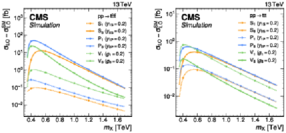
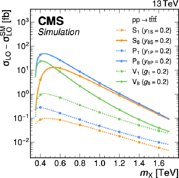
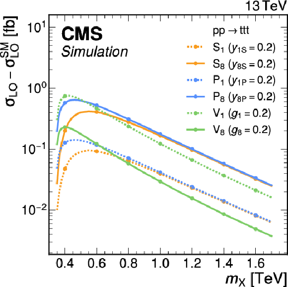
Enhancement of the $ {\mathrm{t}\overline{\mathrm{t}}} {\mathrm{t}\overline{\mathrm{t}}} $ (left) and $ \mathrm{t}\mathrm{t}\mathrm{t} $ (right) production cross section in the different scenarios for a narrow topphilic heavy resonance with $ \Gamma_{\mathrm{X}}= $ 10 GeV as a function of $ m_{\mathrm{X}} $, evaluated at LO as the difference between the cross section calculated with all SM, BSM, and interference contributions and the SM-only cross section. The coupling strength is fixed to a value of 0.2 in all scenarios. The points indicate the mass values at which we evaluate exclusion limits. |
png pdf |
Figure 10-a:
Enhancement of the $ {\mathrm{t}\overline{\mathrm{t}}} {\mathrm{t}\overline{\mathrm{t}}} $ (left) and $ \mathrm{t}\mathrm{t}\mathrm{t} $ (right) production cross section in the different scenarios for a narrow topphilic heavy resonance with $ \Gamma_{\mathrm{X}}= $ 10 GeV as a function of $ m_{\mathrm{X}} $, evaluated at LO as the difference between the cross section calculated with all SM, BSM, and interference contributions and the SM-only cross section. The coupling strength is fixed to a value of 0.2 in all scenarios. The points indicate the mass values at which we evaluate exclusion limits. |
png pdf |
Figure 10-b:
Enhancement of the $ {\mathrm{t}\overline{\mathrm{t}}} {\mathrm{t}\overline{\mathrm{t}}} $ (left) and $ \mathrm{t}\mathrm{t}\mathrm{t} $ (right) production cross section in the different scenarios for a narrow topphilic heavy resonance with $ \Gamma_{\mathrm{X}}= $ 10 GeV as a function of $ m_{\mathrm{X}} $, evaluated at LO as the difference between the cross section calculated with all SM, BSM, and interference contributions and the SM-only cross section. The coupling strength is fixed to a value of 0.2 in all scenarios. The points indicate the mass values at which we evaluate exclusion limits. |
png pdf |
Figure 11:
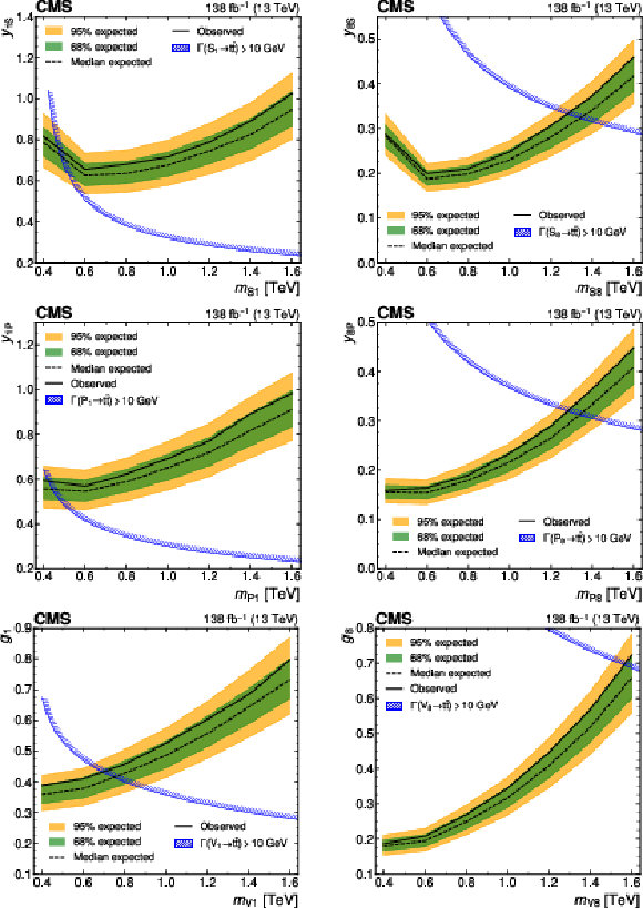
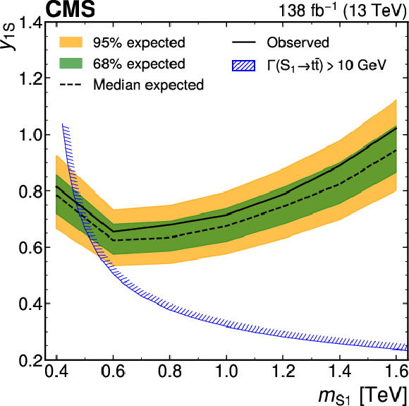
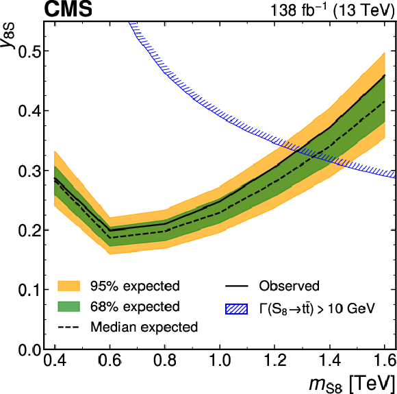
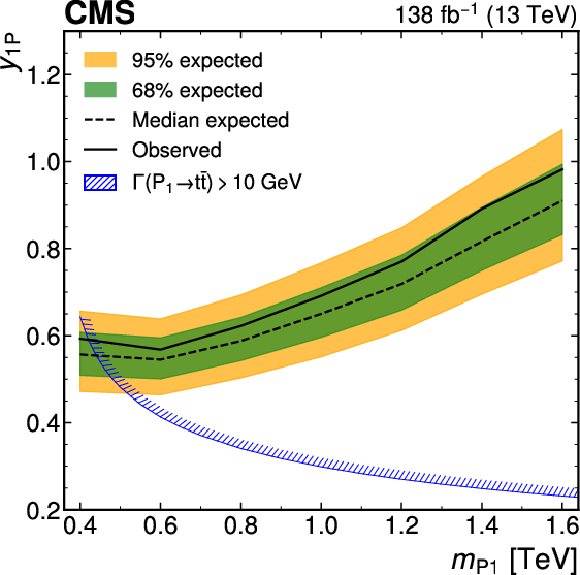
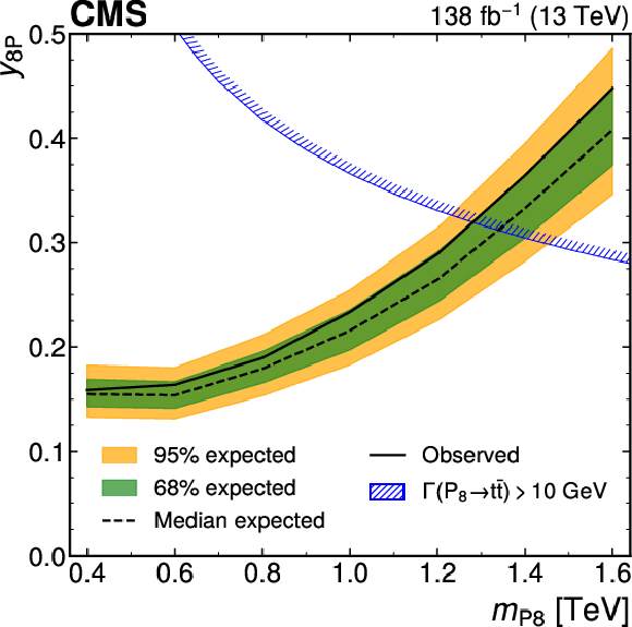
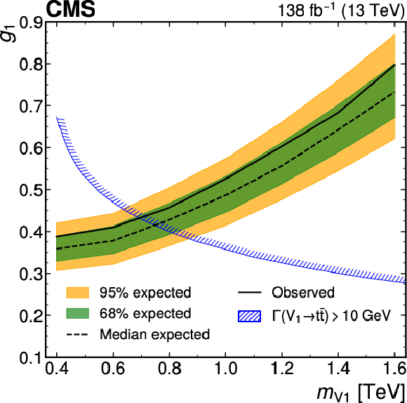
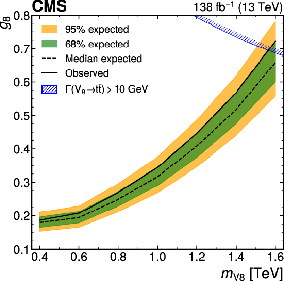
The 95% CL exclusion limits on $ y_{1{S}} $ as a function of $ m_{{S}1} $ (upper left), on $ y_{8{S}} $ as a function of $ m_{{S}8} $ (upper right), on $ y_{1{P}} $ as a function of $ m_{{P}1} $ (center left), on $ y_{8{P}} $ as a function of $ m_{{P}8} $ (center right), on $ g_1 $ as a function of $ m_{{V}1} $ (lower left), and on $ g_8 $ as a function of $ m_{{V}8} $ (lower right). The area above the solid (dashed) black line indicates the observed (expected) exclusion region. The total decay width is fixed to 10 GeV in all scenarios. The area above the hatched blue line indicates the nonphysical region of phase space in which the partial width $ \Gamma(\mathrm{X}\to{\mathrm{t}\overline{\mathrm{t}}} ) $ becomes larger than 10 GeV. |
png pdf |
Figure 11-a:
The 95% CL exclusion limits on $ y_{1{S}} $ as a function of $ m_{{S}1} $ (upper left), on $ y_{8{S}} $ as a function of $ m_{{S}8} $ (upper right), on $ y_{1{P}} $ as a function of $ m_{{P}1} $ (center left), on $ y_{8{P}} $ as a function of $ m_{{P}8} $ (center right), on $ g_1 $ as a function of $ m_{{V}1} $ (lower left), and on $ g_8 $ as a function of $ m_{{V}8} $ (lower right). The area above the solid (dashed) black line indicates the observed (expected) exclusion region. The total decay width is fixed to 10 GeV in all scenarios. The area above the hatched blue line indicates the nonphysical region of phase space in which the partial width $ \Gamma(\mathrm{X}\to{\mathrm{t}\overline{\mathrm{t}}} ) $ becomes larger than 10 GeV. |
png pdf |
Figure 11-b:
The 95% CL exclusion limits on $ y_{1{S}} $ as a function of $ m_{{S}1} $ (upper left), on $ y_{8{S}} $ as a function of $ m_{{S}8} $ (upper right), on $ y_{1{P}} $ as a function of $ m_{{P}1} $ (center left), on $ y_{8{P}} $ as a function of $ m_{{P}8} $ (center right), on $ g_1 $ as a function of $ m_{{V}1} $ (lower left), and on $ g_8 $ as a function of $ m_{{V}8} $ (lower right). The area above the solid (dashed) black line indicates the observed (expected) exclusion region. The total decay width is fixed to 10 GeV in all scenarios. The area above the hatched blue line indicates the nonphysical region of phase space in which the partial width $ \Gamma(\mathrm{X}\to{\mathrm{t}\overline{\mathrm{t}}} ) $ becomes larger than 10 GeV. |
png pdf |
Figure 11-c:
The 95% CL exclusion limits on $ y_{1{S}} $ as a function of $ m_{{S}1} $ (upper left), on $ y_{8{S}} $ as a function of $ m_{{S}8} $ (upper right), on $ y_{1{P}} $ as a function of $ m_{{P}1} $ (center left), on $ y_{8{P}} $ as a function of $ m_{{P}8} $ (center right), on $ g_1 $ as a function of $ m_{{V}1} $ (lower left), and on $ g_8 $ as a function of $ m_{{V}8} $ (lower right). The area above the solid (dashed) black line indicates the observed (expected) exclusion region. The total decay width is fixed to 10 GeV in all scenarios. The area above the hatched blue line indicates the nonphysical region of phase space in which the partial width $ \Gamma(\mathrm{X}\to{\mathrm{t}\overline{\mathrm{t}}} ) $ becomes larger than 10 GeV. |
png pdf |
Figure 11-d:
The 95% CL exclusion limits on $ y_{1{S}} $ as a function of $ m_{{S}1} $ (upper left), on $ y_{8{S}} $ as a function of $ m_{{S}8} $ (upper right), on $ y_{1{P}} $ as a function of $ m_{{P}1} $ (center left), on $ y_{8{P}} $ as a function of $ m_{{P}8} $ (center right), on $ g_1 $ as a function of $ m_{{V}1} $ (lower left), and on $ g_8 $ as a function of $ m_{{V}8} $ (lower right). The area above the solid (dashed) black line indicates the observed (expected) exclusion region. The total decay width is fixed to 10 GeV in all scenarios. The area above the hatched blue line indicates the nonphysical region of phase space in which the partial width $ \Gamma(\mathrm{X}\to{\mathrm{t}\overline{\mathrm{t}}} ) $ becomes larger than 10 GeV. |
png pdf |
Figure 11-e:
The 95% CL exclusion limits on $ y_{1{S}} $ as a function of $ m_{{S}1} $ (upper left), on $ y_{8{S}} $ as a function of $ m_{{S}8} $ (upper right), on $ y_{1{P}} $ as a function of $ m_{{P}1} $ (center left), on $ y_{8{P}} $ as a function of $ m_{{P}8} $ (center right), on $ g_1 $ as a function of $ m_{{V}1} $ (lower left), and on $ g_8 $ as a function of $ m_{{V}8} $ (lower right). The area above the solid (dashed) black line indicates the observed (expected) exclusion region. The total decay width is fixed to 10 GeV in all scenarios. The area above the hatched blue line indicates the nonphysical region of phase space in which the partial width $ \Gamma(\mathrm{X}\to{\mathrm{t}\overline{\mathrm{t}}} ) $ becomes larger than 10 GeV. |
png pdf |
Figure 11-f:
The 95% CL exclusion limits on $ y_{1{S}} $ as a function of $ m_{{S}1} $ (upper left), on $ y_{8{S}} $ as a function of $ m_{{S}8} $ (upper right), on $ y_{1{P}} $ as a function of $ m_{{P}1} $ (center left), on $ y_{8{P}} $ as a function of $ m_{{P}8} $ (center right), on $ g_1 $ as a function of $ m_{{V}1} $ (lower left), and on $ g_8 $ as a function of $ m_{{V}8} $ (lower right). The area above the solid (dashed) black line indicates the observed (expected) exclusion region. The total decay width is fixed to 10 GeV in all scenarios. The area above the hatched blue line indicates the nonphysical region of phase space in which the partial width $ \Gamma(\mathrm{X}\to{\mathrm{t}\overline{\mathrm{t}}} ) $ becomes larger than 10 GeV. |
png pdf |
Figure 12:
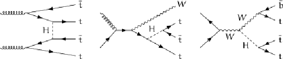
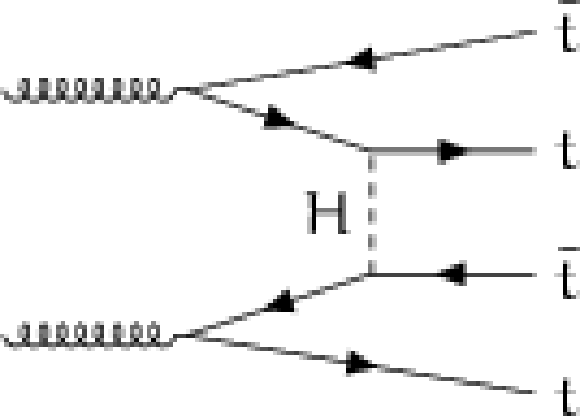
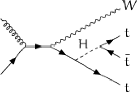
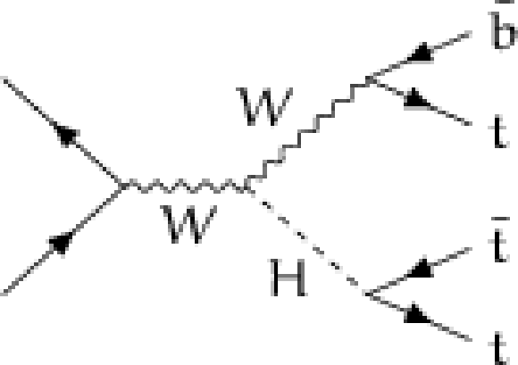
Example LO Feynman diagrams for $ {\mathrm{t}\overline{\mathrm{t}}} {\mathrm{t}\overline{\mathrm{t}}} $ (left), $ \mathrm{t}\mathrm{t}\mathrm{t}\mathrm{W} $ (center), and $ \mathrm{t}\mathrm{t}\mathrm{t}\mathrm{q} $ (right) production that contain the top quark Yukawa coupling. |
png pdf |
Figure 12-a:
Example LO Feynman diagrams for $ {\mathrm{t}\overline{\mathrm{t}}} {\mathrm{t}\overline{\mathrm{t}}} $ (left), $ \mathrm{t}\mathrm{t}\mathrm{t}\mathrm{W} $ (center), and $ \mathrm{t}\mathrm{t}\mathrm{t}\mathrm{q} $ (right) production that contain the top quark Yukawa coupling. |
png pdf |
Figure 12-b:
Example LO Feynman diagrams for $ {\mathrm{t}\overline{\mathrm{t}}} {\mathrm{t}\overline{\mathrm{t}}} $ (left), $ \mathrm{t}\mathrm{t}\mathrm{t}\mathrm{W} $ (center), and $ \mathrm{t}\mathrm{t}\mathrm{t}\mathrm{q} $ (right) production that contain the top quark Yukawa coupling. |
png pdf |
Figure 12-c:
Example LO Feynman diagrams for $ {\mathrm{t}\overline{\mathrm{t}}} {\mathrm{t}\overline{\mathrm{t}}} $ (left), $ \mathrm{t}\mathrm{t}\mathrm{t}\mathrm{W} $ (center), and $ \mathrm{t}\mathrm{t}\mathrm{t}\mathrm{q} $ (right) production that contain the top quark Yukawa coupling. |
png pdf |
Figure 13:
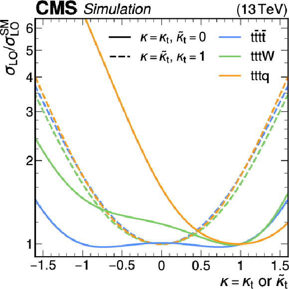
Ratio of the $ {\mathrm{t}\overline{\mathrm{t}}} {\mathrm{t}\overline{\mathrm{t}}} $, $ \mathrm{t}\mathrm{t}\mathrm{t}\mathrm{W} $, and $ \mathrm{t}\mathrm{t}\mathrm{t}\mathrm{q} $ cross sections with modified top quark Yukawa couplings to the SM values, evaluated at LO. The solid lines show modifications of $ \kappa_{\mathrm{t}} $ for a fixed value of $ \tilde{\kappa}_{\mathrm{t}}= $ 0, and dashed lines modifications of $ \tilde{\kappa}_{\mathrm{t}} $ for fixed $ \kappa_{\mathrm{t}}= $ 1. |
png pdf |
Figure 14:
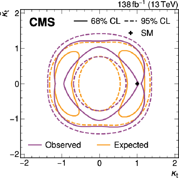
Expected (orange lines) and observed (purple lines) exclusion contours on the Yukawa coupling modifiers $ \kappa_{\mathrm{t}} $ and $ \tilde{\kappa}_{\mathrm{t}} $ corresponding to the 68% (solid lines) and 95% (dashed lines) CL intervals as evaluated with toys. The SM prediction is shown with a black cross. |
png pdf |
Figure 15:
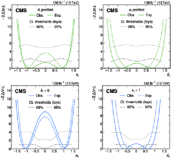
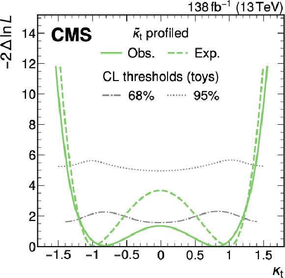
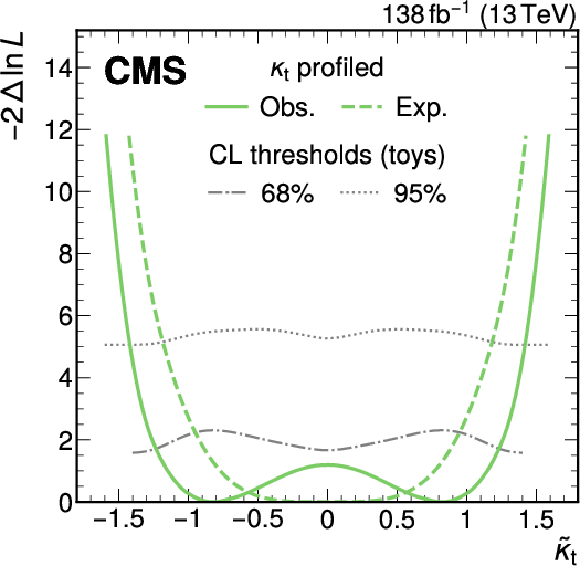
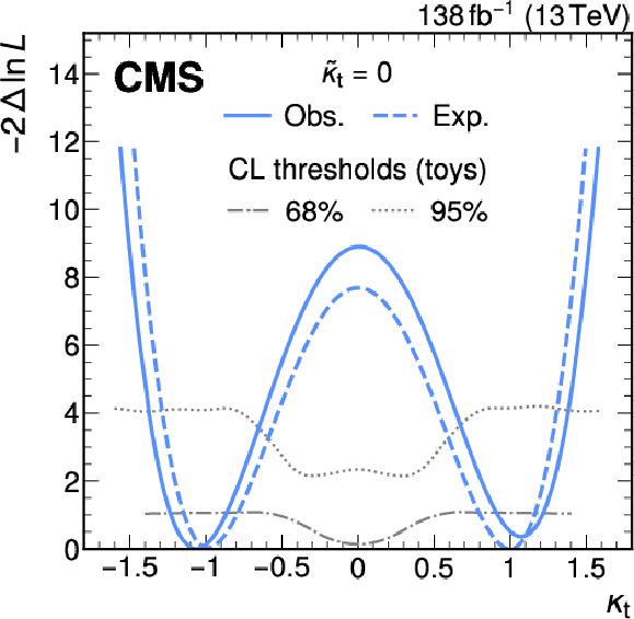
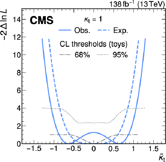
Negative log-likelihood difference from the best fit value for the one-dimensional scans of the Yukawa coupling modifiers $ \kappa_{\mathrm{t}} $ (left) and $ \tilde{\kappa}_{\mathrm{t}} $ (right), where the other modifier is profiled (upper) or fixed to its SM prediction (lower). Shown are the expected (colored dashed line) and observed (colored solid line) results, as well as the threshold values for 68% (gray dash-dotted line) and 95% (gray dotted lines) CL intervals as evaluated with toys. |
png pdf |
Figure 15-a:
Negative log-likelihood difference from the best fit value for the one-dimensional scans of the Yukawa coupling modifiers $ \kappa_{\mathrm{t}} $ (left) and $ \tilde{\kappa}_{\mathrm{t}} $ (right), where the other modifier is profiled (upper) or fixed to its SM prediction (lower). Shown are the expected (colored dashed line) and observed (colored solid line) results, as well as the threshold values for 68% (gray dash-dotted line) and 95% (gray dotted lines) CL intervals as evaluated with toys. |
png pdf |
Figure 15-b:
Negative log-likelihood difference from the best fit value for the one-dimensional scans of the Yukawa coupling modifiers $ \kappa_{\mathrm{t}} $ (left) and $ \tilde{\kappa}_{\mathrm{t}} $ (right), where the other modifier is profiled (upper) or fixed to its SM prediction (lower). Shown are the expected (colored dashed line) and observed (colored solid line) results, as well as the threshold values for 68% (gray dash-dotted line) and 95% (gray dotted lines) CL intervals as evaluated with toys. |
png pdf |
Figure 15-c:
Negative log-likelihood difference from the best fit value for the one-dimensional scans of the Yukawa coupling modifiers $ \kappa_{\mathrm{t}} $ (left) and $ \tilde{\kappa}_{\mathrm{t}} $ (right), where the other modifier is profiled (upper) or fixed to its SM prediction (lower). Shown are the expected (colored dashed line) and observed (colored solid line) results, as well as the threshold values for 68% (gray dash-dotted line) and 95% (gray dotted lines) CL intervals as evaluated with toys. |
png pdf |
Figure 15-d:
Negative log-likelihood difference from the best fit value for the one-dimensional scans of the Yukawa coupling modifiers $ \kappa_{\mathrm{t}} $ (left) and $ \tilde{\kappa}_{\mathrm{t}} $ (right), where the other modifier is profiled (upper) or fixed to its SM prediction (lower). Shown are the expected (colored dashed line) and observed (colored solid line) results, as well as the threshold values for 68% (gray dash-dotted line) and 95% (gray dotted lines) CL intervals as evaluated with toys. |
| Summary |
| A search for physics beyond the standard model (beyond the SM, BSM) using four and three top quark ($ {\mathrm{t}\overline{\mathrm{t}}} {\mathrm{t}\overline{\mathrm{t}}} $ and $ \mathrm{t}\mathrm{t}\mathrm{t} $) production events has been reported. The analyzed proton-proton collision data were recorded at 13 TeV with the CMS detector at the CERN LHC in 2016--2018 and correspond to an integrated luminosity of 138 fb$ ^{-1} $. Following the experimental analysis of Ref. [54], events with two same-sign, three, or four leptons (electrons and/or muons) are selected and categorized in signal and control regions. The signal regions in the two same-sign and three lepton channels are further split following a machine-learning discriminant trained to distinguish between $ {\mathrm{t}\overline{\mathrm{t}}} {\mathrm{t}\overline{\mathrm{t}}} $ production and the main background processes. Assuming no BSM contributions, a mild excess of events in data in the selection enriched with $ {\mathrm{t}\overline{\mathrm{t}}} {\mathrm{t}\overline{\mathrm{t}}} $ and $ \mathrm{t}\mathrm{t}\mathrm{t} $ production events is observed at the level of one standard deviation, consistent with the result from Ref. [54]. To interpret this observation in different models of BSM physics, three interpretations are performed using either the machine-learning discriminant or the scalar sum of the jet transverse momenta, optimized for the considered scenario. Throughout, $ \mathrm{t}\mathrm{t}\mathrm{t} $ production is treated as signal process alongside $ {\mathrm{t}\overline{\mathrm{t}}} {\mathrm{t}\overline{\mathrm{t}}} $ production, accounting for the observation that the existing experimental analysis is not able to distinguish between $ {\mathrm{t}\overline{\mathrm{t}}} {\mathrm{t}\overline{\mathrm{t}}} $ and $ \mathrm{t}\mathrm{t}\mathrm{t} $ contributions in the most sensitive signal regions. Using the SM effective field theory framework, constraints are derived on six Wilson coefficients that modify interactions between four third-generation quarks or between top quarks and the Higgs boson. This is the first SM effective field theory interpretation that considers these operators simultaneously. Exclusion limits are set on topphilic heavy resonances of different spin and color states, covering masses between 400 GeV and 1.6 TeV. The top quark Yukawa coupling is extracted, considering both $ CP $-even and $ CP $-odd contributions. All interpretations provide a good description of the data and are statistically compatible with the SM expectation. |
| Additional Figures | |
png pdf |
Additional Figure 1:
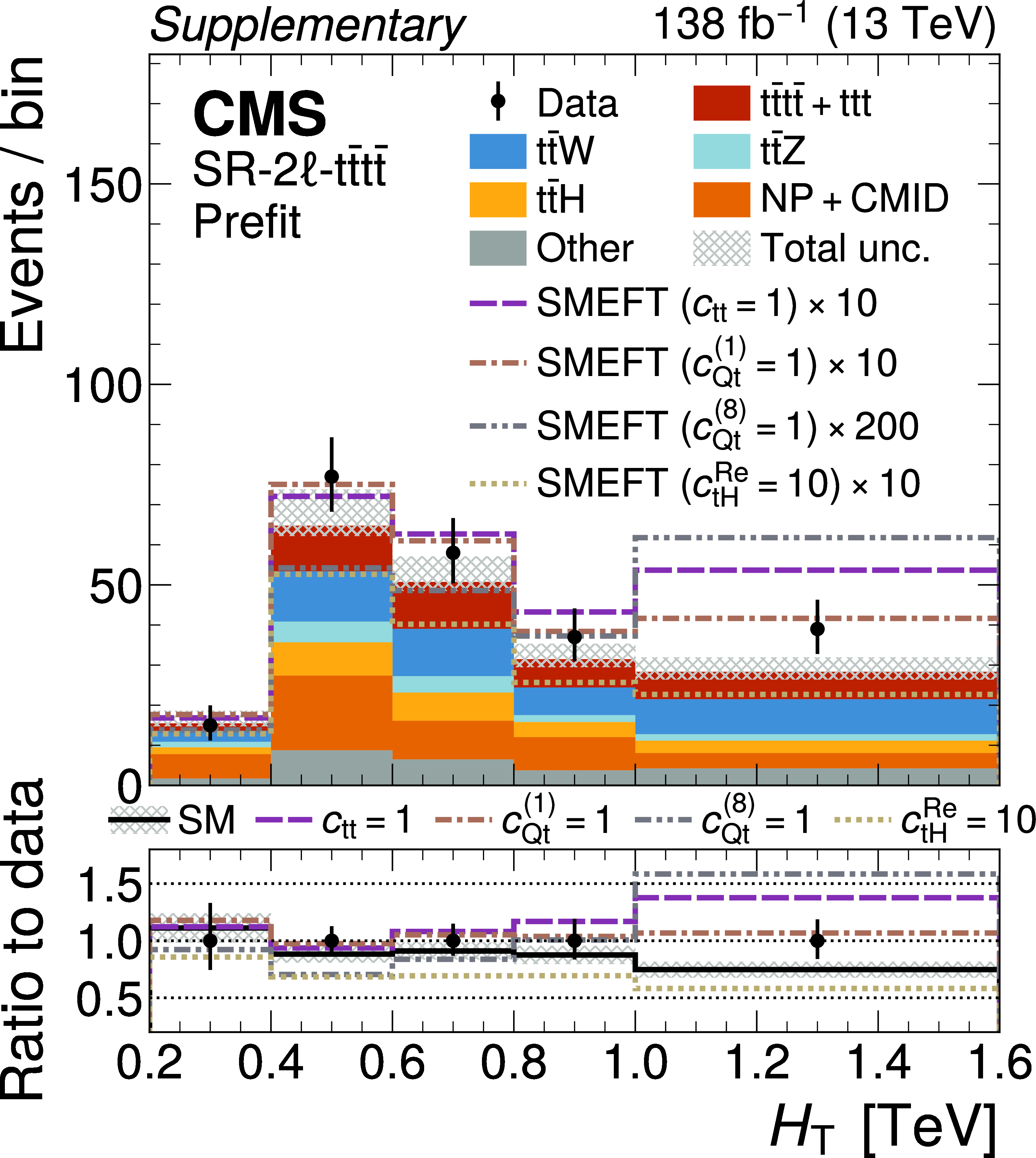
Comparison of the number of observed (points) and predicted (colored histograms) events in the $H_{\mathrm{T}}$ distribution, shown for the SR-2$\ell$-$\mathrm{t\bar{t}t\bar{t}}$ merged across all lepton flavor categories. The last bin includes the overflow contribution. The vertical bars on the points represent the statistical uncertainties in the data, and the hatched bands the total uncertainty in the predictions. The signal and background yields are shown before the fit to the data (``prefit''). The dashed/dotted lines show the enhancement of $\mathrm{t\bar{t}t\bar{t}}$+$\mathrm{ttt}$+$\mathrm{t\bar{t}H}$ production through one of four SMEFT operators. The lower panels shows the ratio of the total SM prediction to data, and also of the sum of the total SM prediction and the SMEFT contribution to data for the same configurations as in the upper panel. |
png pdf |
Additional Figure 2:
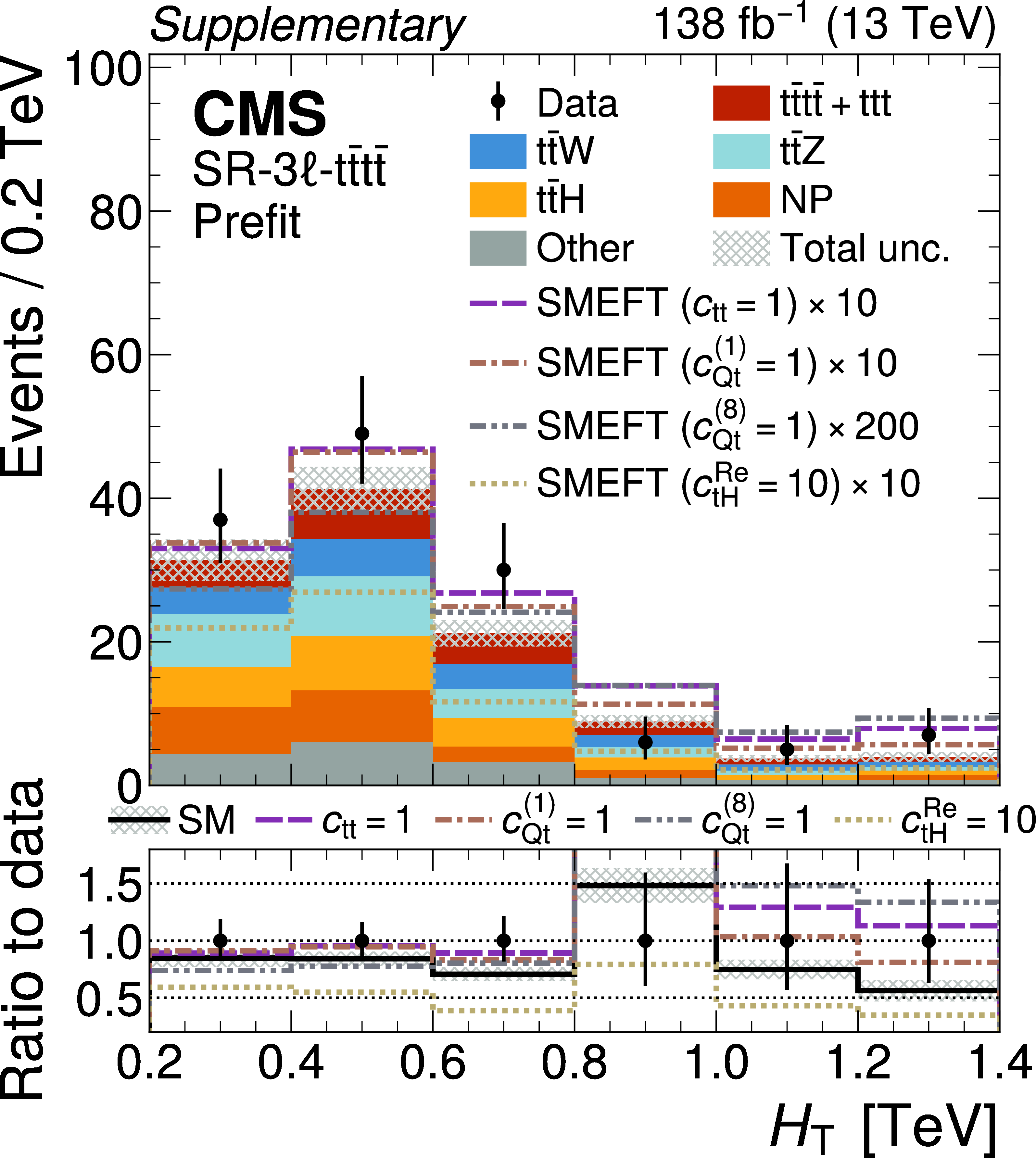
Comparison of the number of observed (points) and predicted (colored histograms) events in the $H_{\mathrm{T}}$ distribution, shown for the SR-3$\ell$-$\mathrm{t\bar{t}t\bar{t}}$. The last bin includes the overflow contribution. The vertical bars on the points represent the statistical uncertainties in the data, and the hatched bands the total uncertainty in the predictions. The signal and background yields are shown before the fit to the data (``prefit''). The dashed/dotted lines show the enhancement of $\mathrm{t\bar{t}t\bar{t}}$+$\mathrm{ttt}$+$\mathrm{t\bar{t}H}$ production through one of four SMEFT operators. The lower panels shows the ratio of the total SM prediction to data, and also of the sum of the total SM prediction and the SMEFT contribution to data for the same configurations as in the upper panel. |
png pdf |
Additional Figure 3:
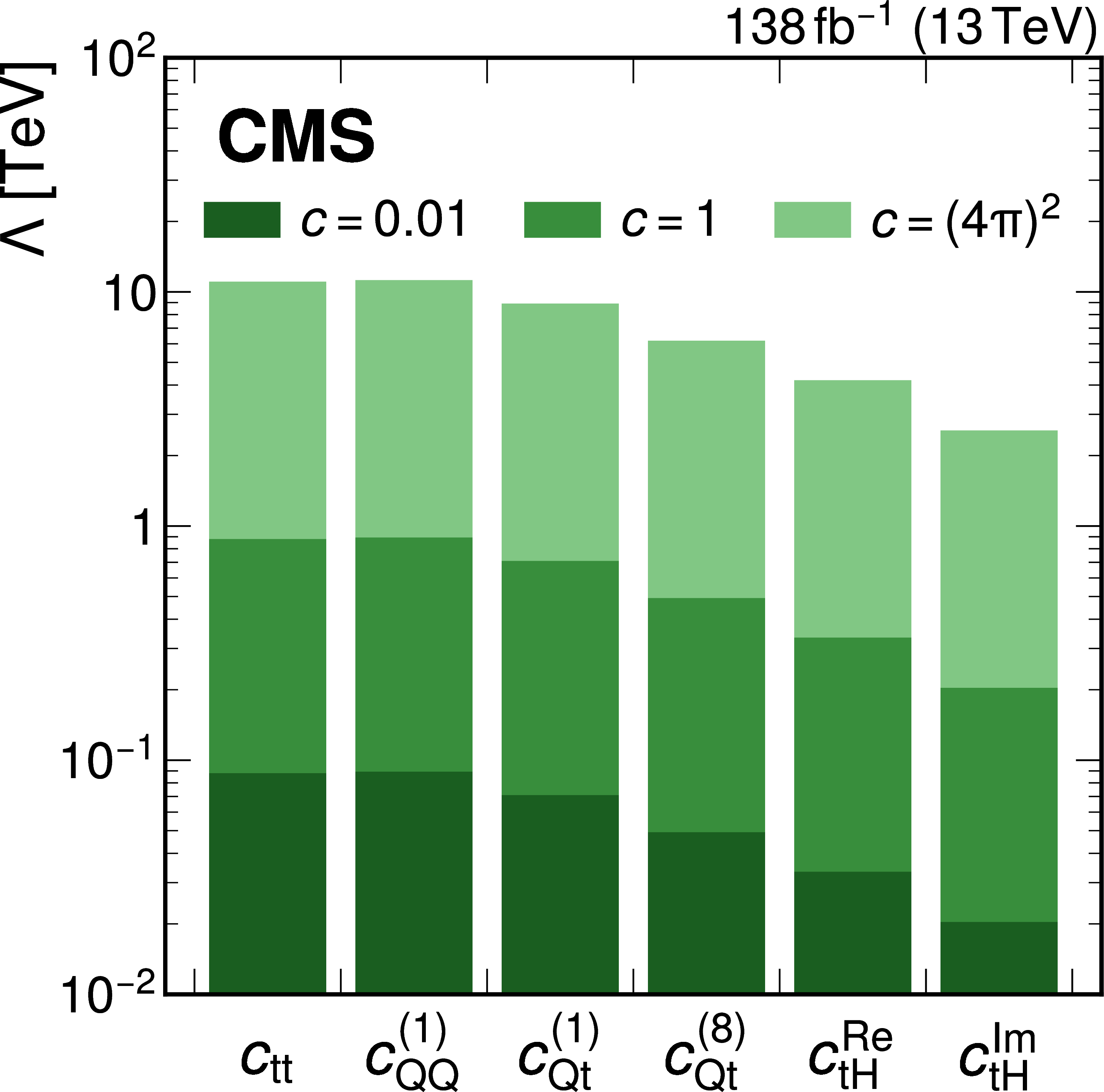
Lower limits on the BSM energy scale $\Lambda$ obtained from the 95% CL intervals when fixing one the WCs to the indicated value and all other WCs to the SM expectation of zero. |
png pdf |
Additional Figure 4:
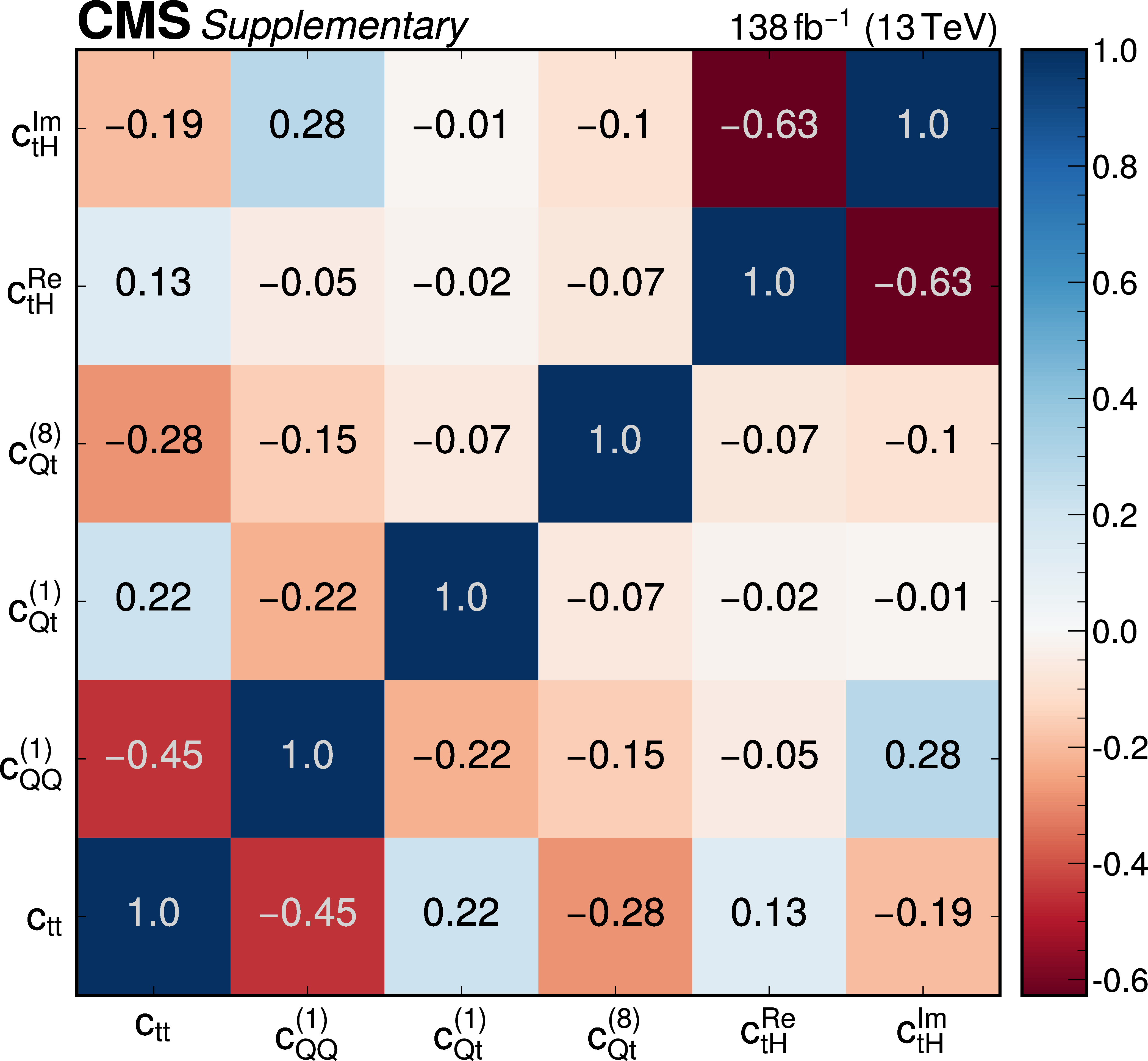
Correlation matrix of the fit with all six EFT operators fitted simultaneously. |
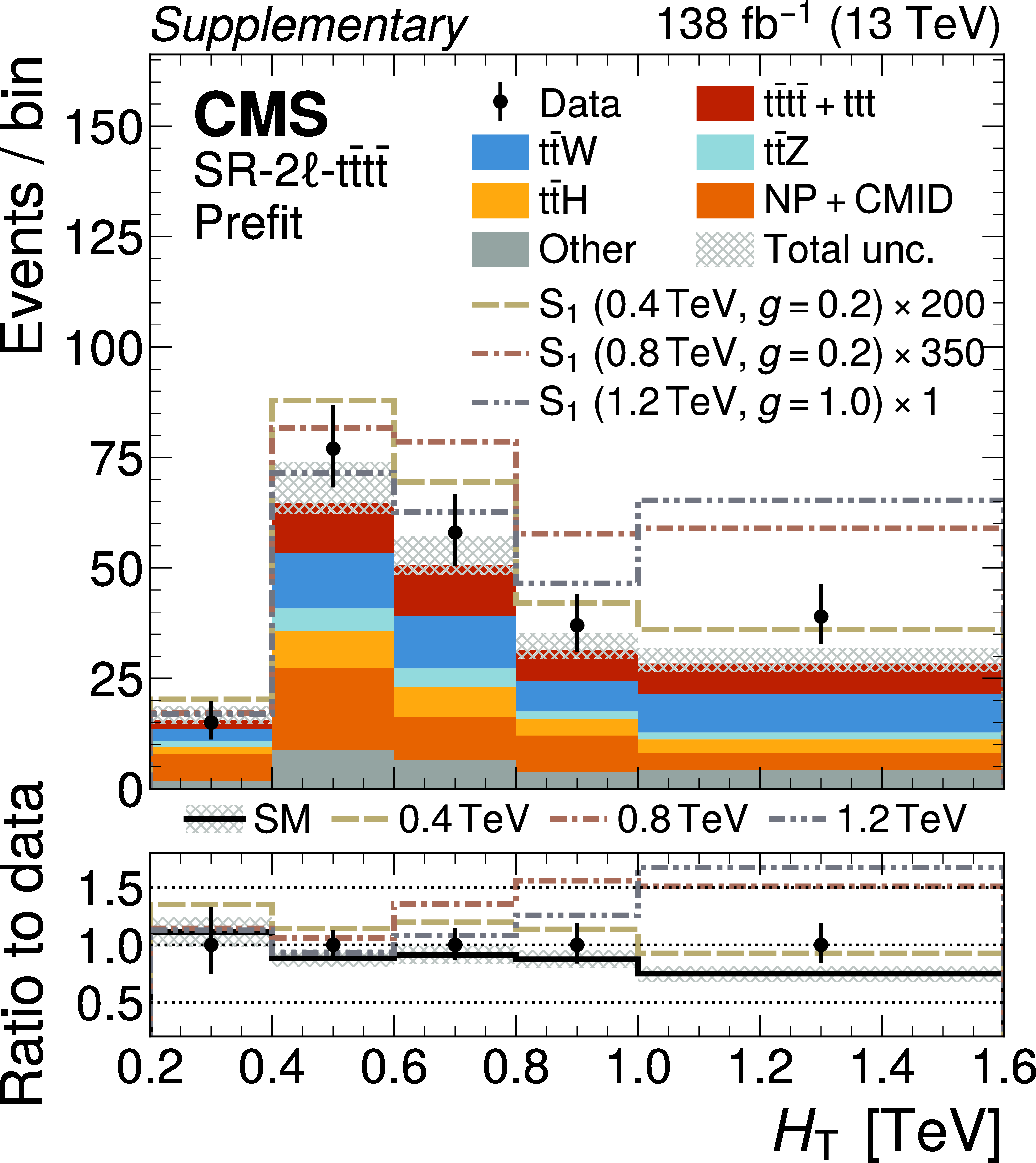
png pdf |
Additional Figure 5:
Comparison of the number of observed (points) and predicted (colored histograms) events in the $H_{\mathrm{T}}$ distribution, shown for the SR-2$\ell$-$\mathrm{t\bar{t}t\bar{t}}$ merged across all lepton flavor categories. The last bin includes the overflow contribution. The vertical bars on the points represent the statistical uncertainties in the data, and the hatched bands the total uncertainty in the predictions. The signal and background yields are shown before the fit to the data (``prefit''). The dashed/dotted lines show the enhancement of $\mathrm{t\bar{t}t\bar{t}}$+$\mathrm{ttt}$ production through an $\mathrm{S}_1$ resonance in three different scenarios. The lower panel shows the ratio of the total SM prediction to data, and also of the sum of the total SM prediction and the $\mathrm{S}_1$ contribution to data for the same configurations as in the upper panel. |
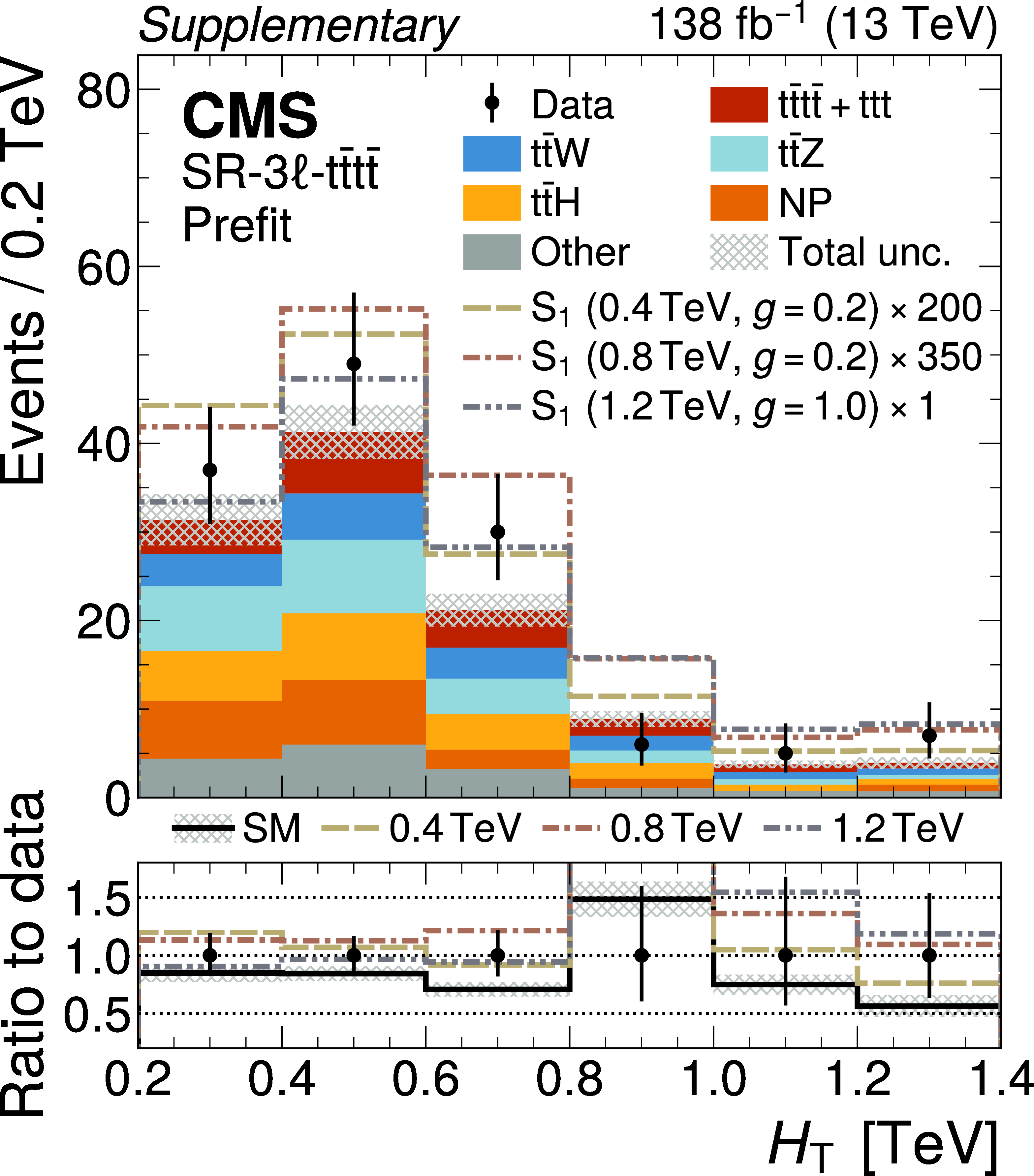
png pdf |
Additional Figure 6:
Comparison of the number of observed (points) and predicted (colored histograms) events in the $H_{\mathrm{T}}$ distribution, shown for the SR-3$\ell$-$\mathrm{t\bar{t}t\bar{t}}$. The last bin includes the overflow contribution. The vertical bars on the points represent the statistical uncertainties in the data, and the hatched bands the total uncertainty in the predictions. The signal and background yields are shown before the fit to the data (``prefit''). The dashed/dotted lines show the enhancement of $\mathrm{t\bar{t}t\bar{t}}$+$\mathrm{ttt}$ production through an $\mathrm{S}_1$ resonance in three different scenarios. The lower panel shows the ratio of the total SM prediction to data, and also of the sum of the total SM prediction and the $\mathrm{S}_1$ contribution to data for the same configurations as in the upper panel. |
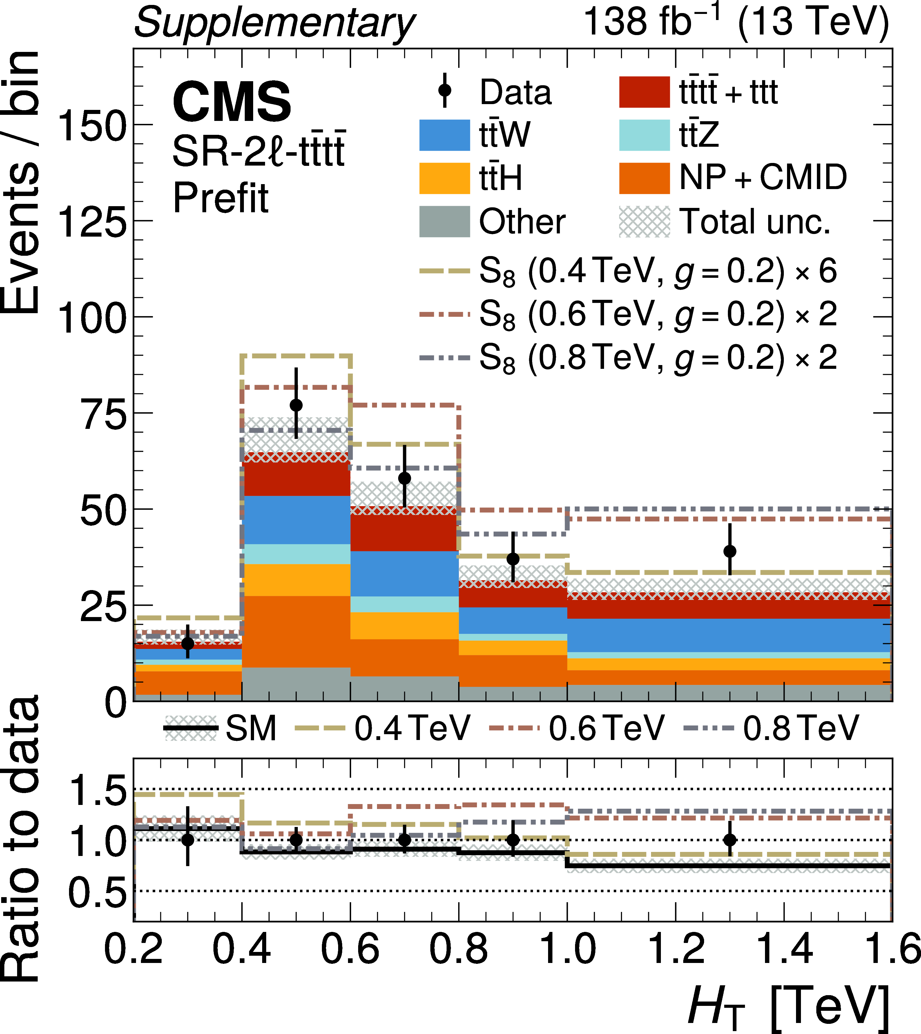
png pdf |
Additional Figure 7:
Comparison of the number of observed (points) and predicted (colored histograms) events in the $H_{\mathrm{T}}$ distribution, shown for the SR-2$\ell$-$\mathrm{t\bar{t}t\bar{t}}$ merged across all lepton flavor categories. The last bin includes the overflow contribution. The vertical bars on the points represent the statistical uncertainties in the data, and the hatched bands the total uncertainty in the predictions. The signal and background yields are shown before the fit to the data (``prefit''). The dashed/dotted lines show the enhancement of $\mathrm{t\bar{t}t\bar{t}}$+$\mathrm{ttt}$ production through an $\mathrm{S}_8$ resonance in three different scenarios. The lower panel shows the ratio of the total SM prediction to data, and also of the sum of the total SM prediction and the $\mathrm{S}_8$ contribution to data for the same configurations as in the upper panel. |
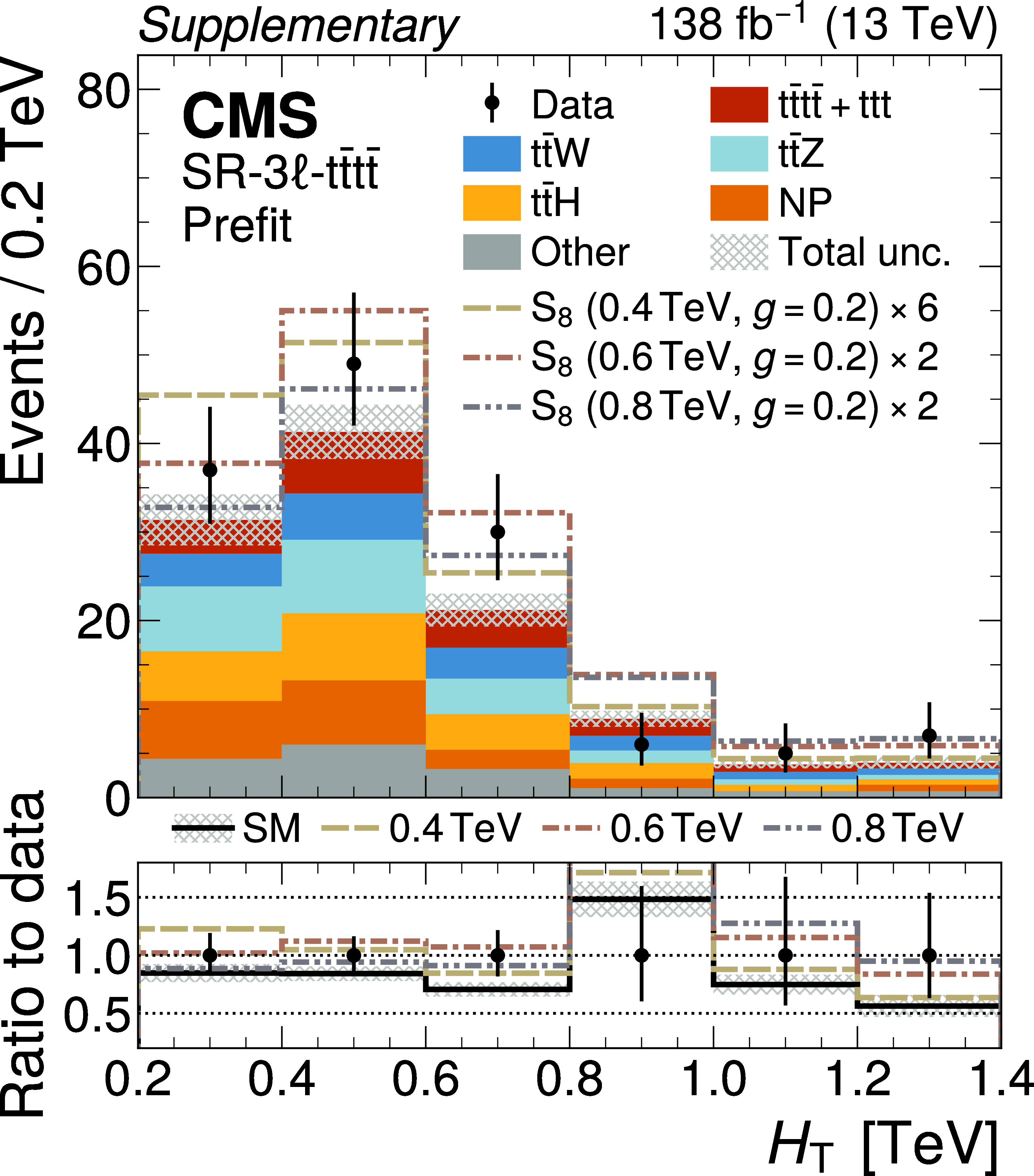
png pdf |
Additional Figure 8:
Comparison of the number of observed (points) and predicted (colored histograms) events in the $H_{\mathrm{T}}$ distribution, shown for the SR-3$\ell$-$\mathrm{t\bar{t}t\bar{t}}$. The last bin includes the overflow contribution. The vertical bars on the points represent the statistical uncertainties in the data, and the hatched bands the total uncertainty in the predictions. The signal and background yields are shown before the fit to the data (``prefit''). The dashed/dotted lines show the enhancement of $\mathrm{t\bar{t}t\bar{t}}$+$\mathrm{ttt}$ production through an $\mathrm{S}_8$ resonance in three different scenarios. The lower panel shows the ratio of the total SM prediction to data, and also of the sum of the total SM prediction and the $\mathrm{S}_8$ contribution to data for the same configurations as in the upper panel. |
png pdf |
Additional Figure 9:
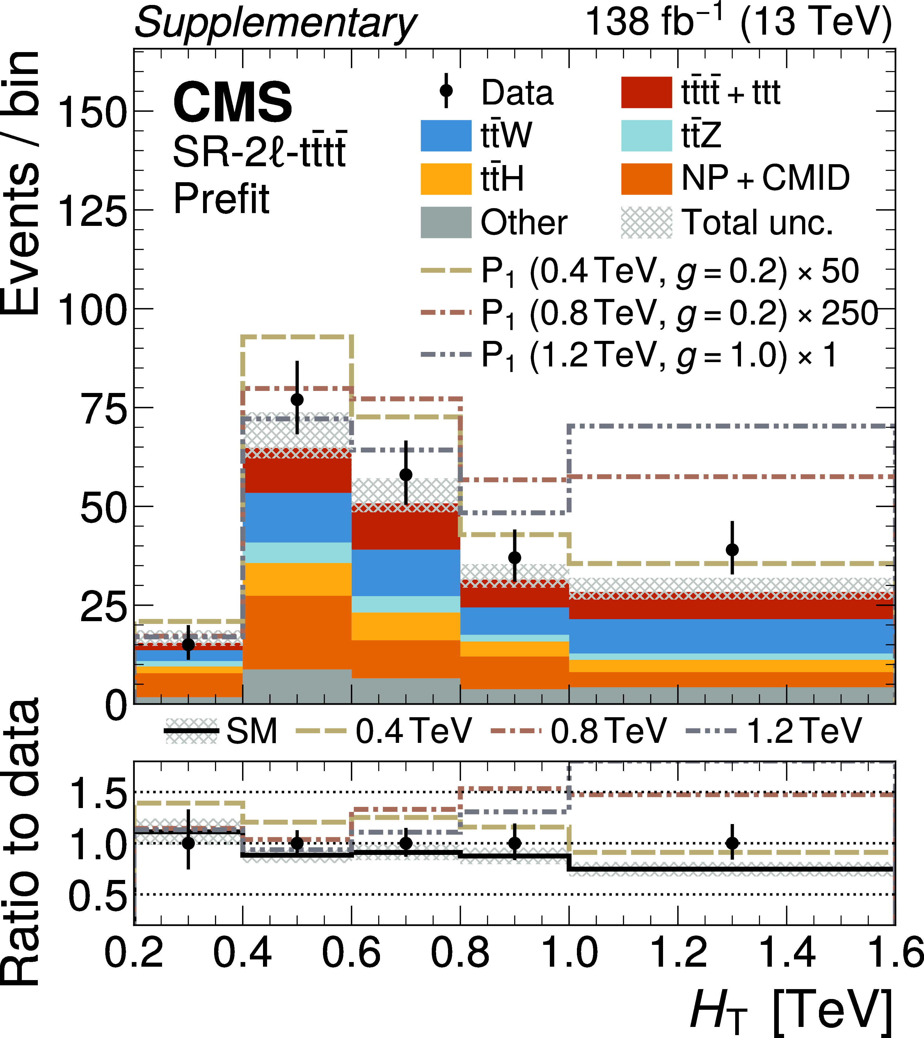
Comparison of the number of observed (points) and predicted (colored histograms) events in the $H_{\mathrm{T}}$ distribution, shown for the SR-2$\ell$-$\mathrm{t\bar{t}t\bar{t}}$ merged across all lepton flavor categories. The last bin includes the overflow contribution. The vertical bars on the points represent the statistical uncertainties in the data, and the hatched bands the total uncertainty in the predictions. The signal and background yields are shown before the fit to the data (``prefit''). The dashed/dotted lines show the enhancement of $\mathrm{t\bar{t}t\bar{t}}$+$\mathrm{ttt}$ production through an $\mathrm{P}_1$ resonance in three different scenarios. The lower panel shows the ratio of the total SM prediction to data, and also of the sum of the total SM prediction and the $\mathrm{P}_1$ contribution to data for the same configurations as in the upper panel. |
png pdf |
Additional Figure 10:
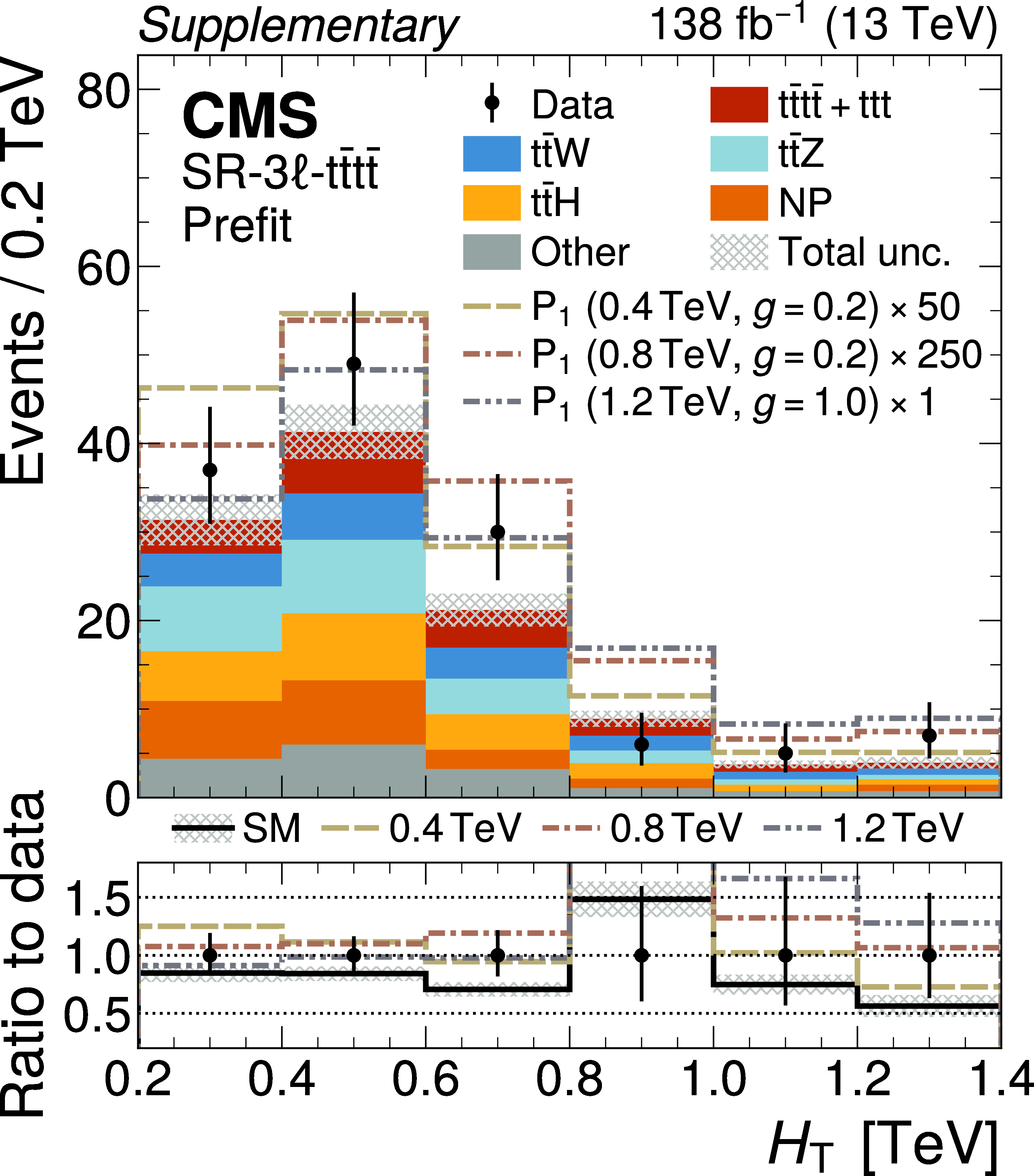
Comparison of the number of observed (points) and predicted (colored histograms) events in the $H_{\mathrm{T}}$ distribution, shown for the SR-3$\ell$-$\mathrm{t\bar{t}t\bar{t}}$. The last bin includes the overflow contribution. The vertical bars on the points represent the statistical uncertainties in the data, and the hatched bands the total uncertainty in the predictions. The signal and background yields are shown before the fit to the data (``prefit''). The dashed/dotted lines show the enhancement of $\mathrm{t\bar{t}t\bar{t}}$+$\mathrm{ttt}$ production through an $\mathrm{P}_1$ resonance in three different scenarios. The lower panel shows the ratio of the total SM prediction to data, and also of the sum of the total SM prediction and the $\mathrm{P}_1$ contribution to data for the same configurations as in the upper panel. |
png pdf |
Additional Figure 11:
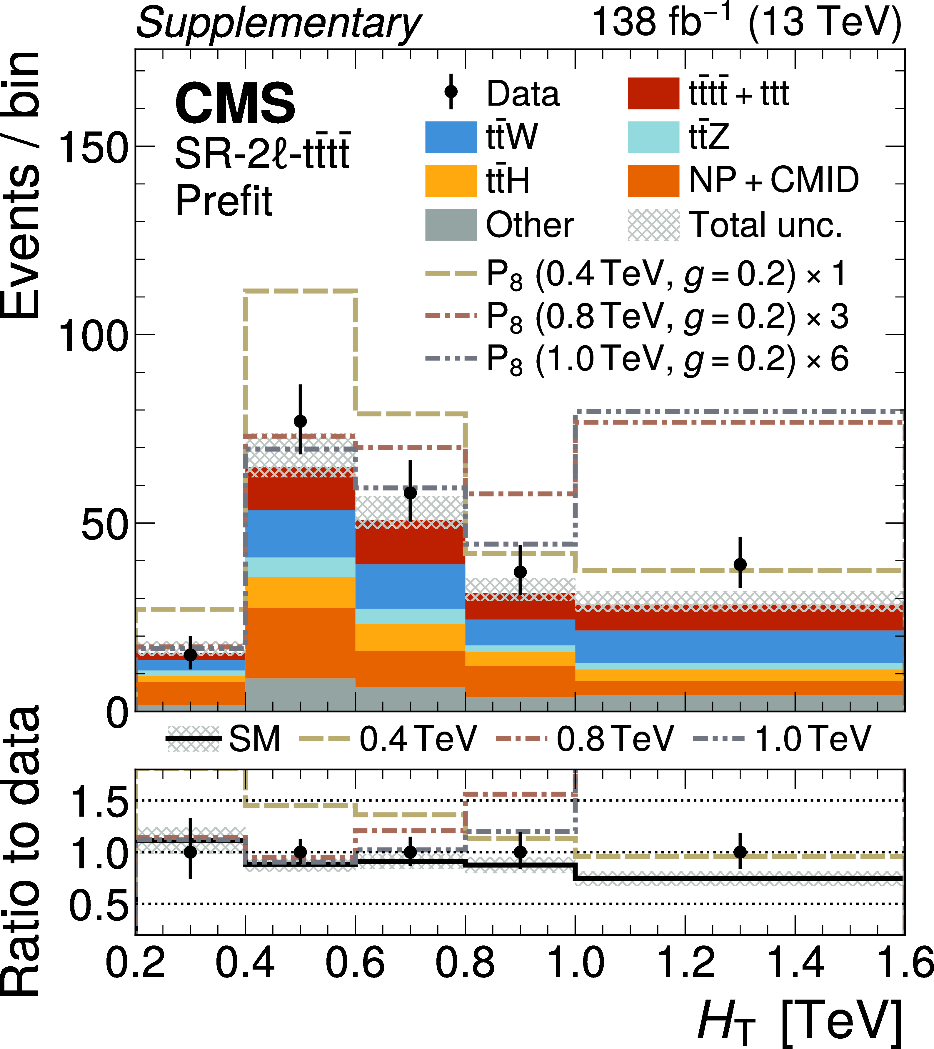
Comparison of the number of observed (points) and predicted (colored histograms) events in the $H_{\mathrm{T}}$ distribution, shown for the SR-2$\ell$-$\mathrm{t\bar{t}t\bar{t}}$ merged across all lepton flavor categories. The last bin includes the overflow contribution. The vertical bars on the points represent the statistical uncertainties in the data, and the hatched bands the total uncertainty in the predictions. The signal and background yields are shown before the fit to the data (``prefit''). The dashed/dotted lines show the enhancement of $\mathrm{t\bar{t}t\bar{t}}$+$\mathrm{ttt}$ production through an $\mathrm{P}_8$ resonance in three different scenarios. The lower panel shows the ratio of the total SM prediction to data, and also of the sum of the total SM prediction and the $\mathrm{P}_8$ contribution to data for the same configurations as in the upper panel. |
png pdf |
Additional Figure 12:
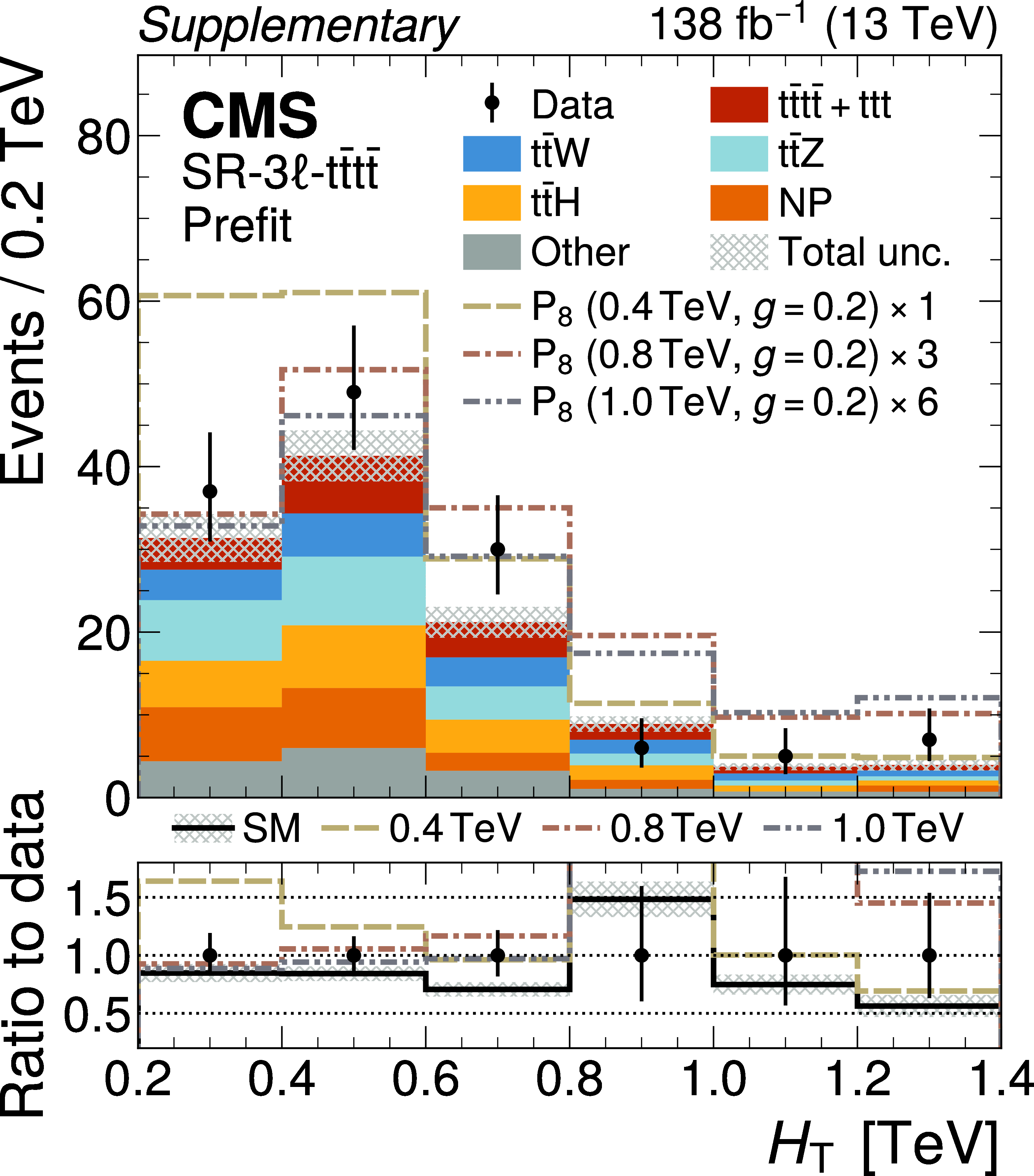
Comparison of the number of observed (points) and predicted (colored histograms) events in the $H_{\mathrm{T}}$ distribution, shown for the SR-3$\ell$-$\mathrm{t\bar{t}t\bar{t}}$. The last bin includes the overflow contribution. The vertical bars on the points represent the statistical uncertainties in the data, and the hatched bands the total uncertainty in the predictions. The signal and background yields are shown before the fit to the data (``prefit''). The dashed/dotted lines show the enhancement of $\mathrm{t\bar{t}t\bar{t}}$+$\mathrm{ttt}$ production through an $\mathrm{P}_8$ resonance in three different scenarios. The lower panel shows the ratio of the total SM prediction to data, and also of the sum of the total SM prediction and the $\mathrm{P}_8$ contribution to data for the same configurations as in the upper panel. |
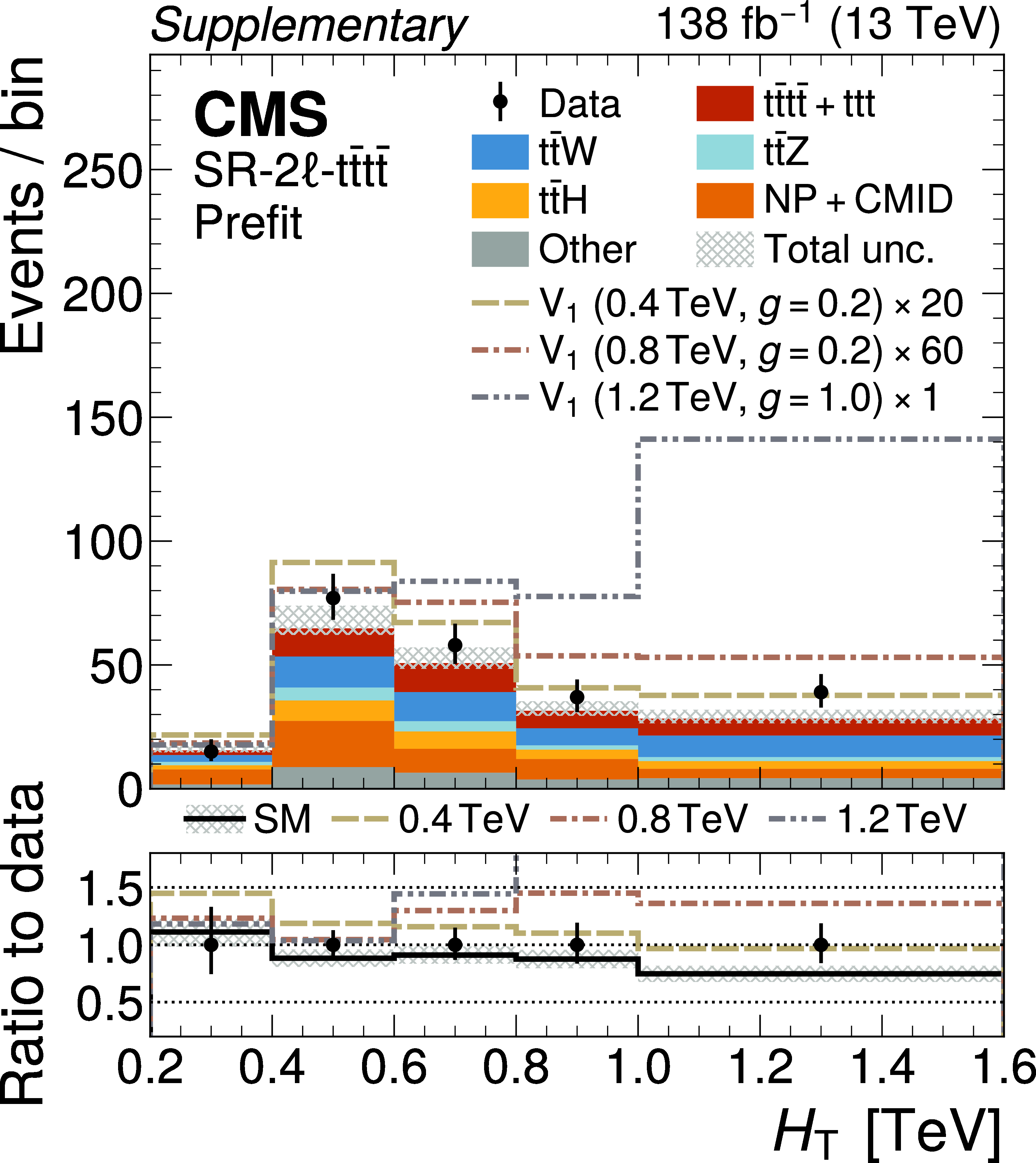
png pdf |
Additional Figure 13:
Comparison of the number of observed (points) and predicted (colored histograms) events in the $H_{\mathrm{T}}$ distribution, shown for the SR-2$\ell$-$\mathrm{t\bar{t}t\bar{t}}$ merged across all lepton flavor categories. The last bin includes the overflow contribution. The vertical bars on the points represent the statistical uncertainties in the data, and the hatched bands the total uncertainty in the predictions. The signal and background yields are shown before the fit to the data (``prefit''). The dashed/dotted lines show the enhancement of $\mathrm{t\bar{t}t\bar{t}}$+$\mathrm{ttt}$ production through an $\mathrm{V}_1$ resonance in three different scenarios. The lower panel shows the ratio of the total SM prediction to data, and also of the sum of the total SM prediction and the $\mathrm{V}_1$ contribution to data for the same configurations as in the upper panel. |
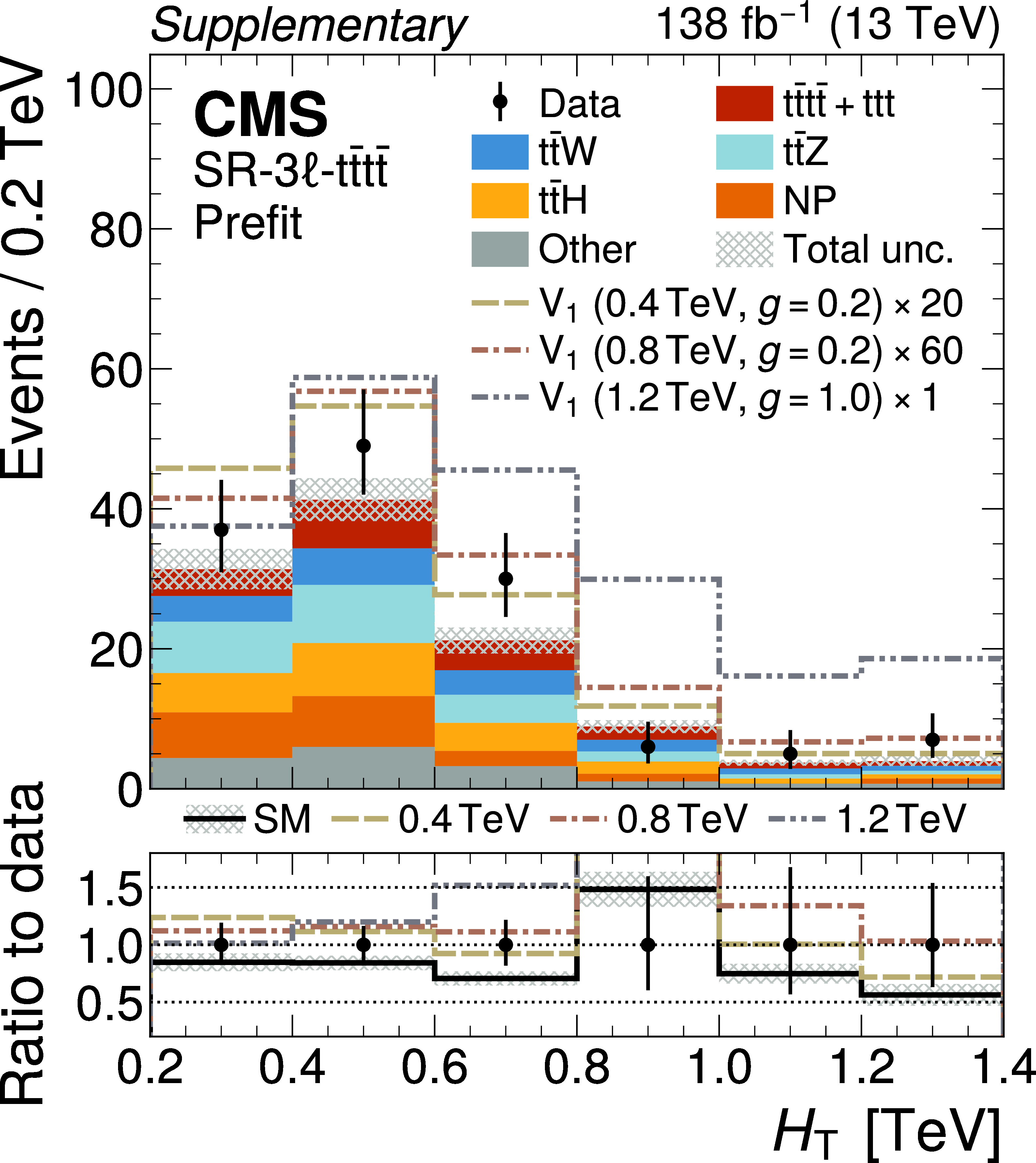
png pdf |
Additional Figure 14:
Comparison of the number of observed (points) and predicted (colored histograms) events in the $H_{\mathrm{T}}$ distribution, shown for the SR-3$\ell$-$\mathrm{t\bar{t}t\bar{t}}$. The last bin includes the overflow contribution. The vertical bars on the points represent the statistical uncertainties in the data, and the hatched bands the total uncertainty in the predictions. The signal and background yields are shown before the fit to the data (``prefit''). The dashed/dotted lines show the enhancement of $\mathrm{t\bar{t}t\bar{t}}$+$\mathrm{ttt}$ production through an $\mathrm{V}_1$ resonance in three different scenarios. The lower panel shows the ratio of the total SM prediction to data, and also of the sum of the total SM prediction and the $\mathrm{V}_1$ contribution to data for the same configurations as in the upper panel. |
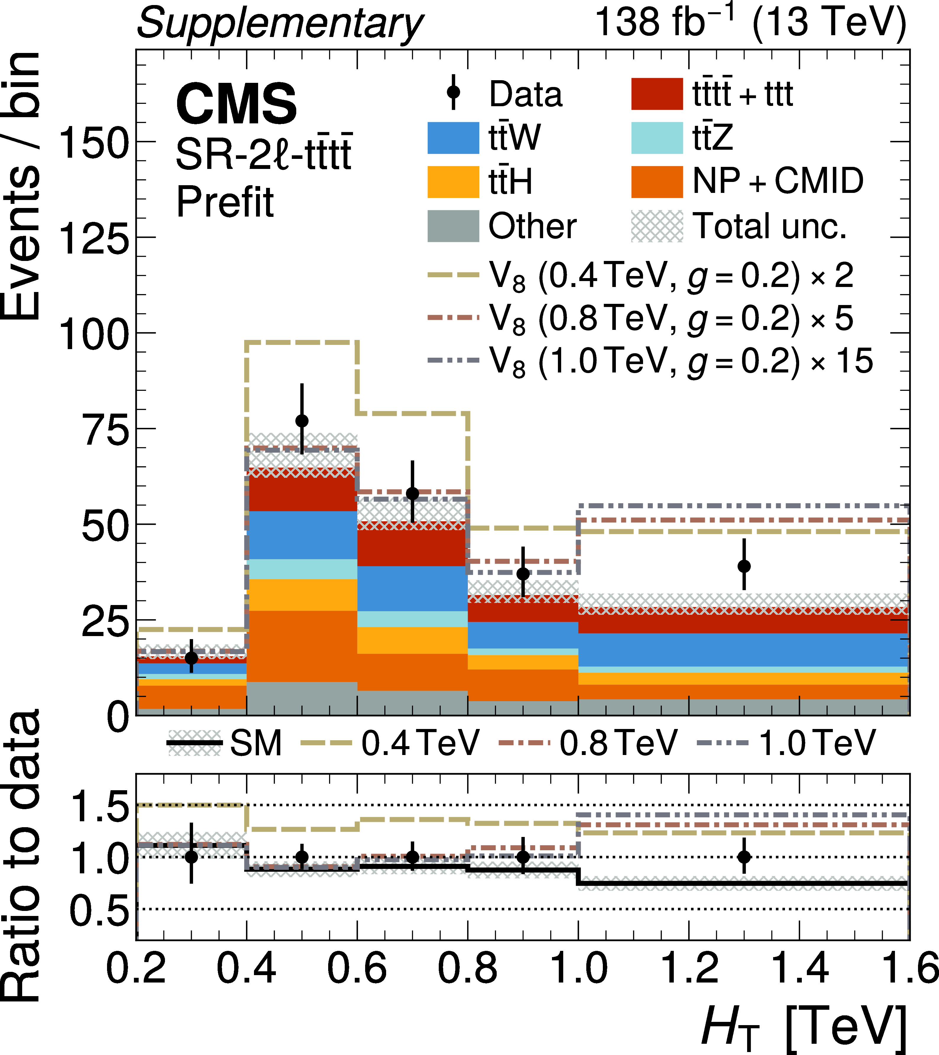
png pdf |
Additional Figure 15:
Comparison of the number of observed (points) and predicted (colored histograms) events in the $H_{\mathrm{T}}$ distribution, shown for the SR-2$\ell$-$\mathrm{t\bar{t}t\bar{t}}$ merged across all lepton flavor categories. The last bin includes the overflow contribution. The vertical bars on the points represent the statistical uncertainties in the data, and the hatched bands the total uncertainty in the predictions. The signal and background yields are shown before the fit to the data (``prefit''). The dashed/dotted lines show the enhancement of $\mathrm{t\bar{t}t\bar{t}}$+$\mathrm{ttt}$ production through an $\mathrm{V}_8$ resonance in three different scenarios. The lower panel shows the ratio of the total SM prediction to data, and also of the sum of the total SM prediction and the $\mathrm{V}_8$ contribution to data for the same configurations as in the upper panel. |
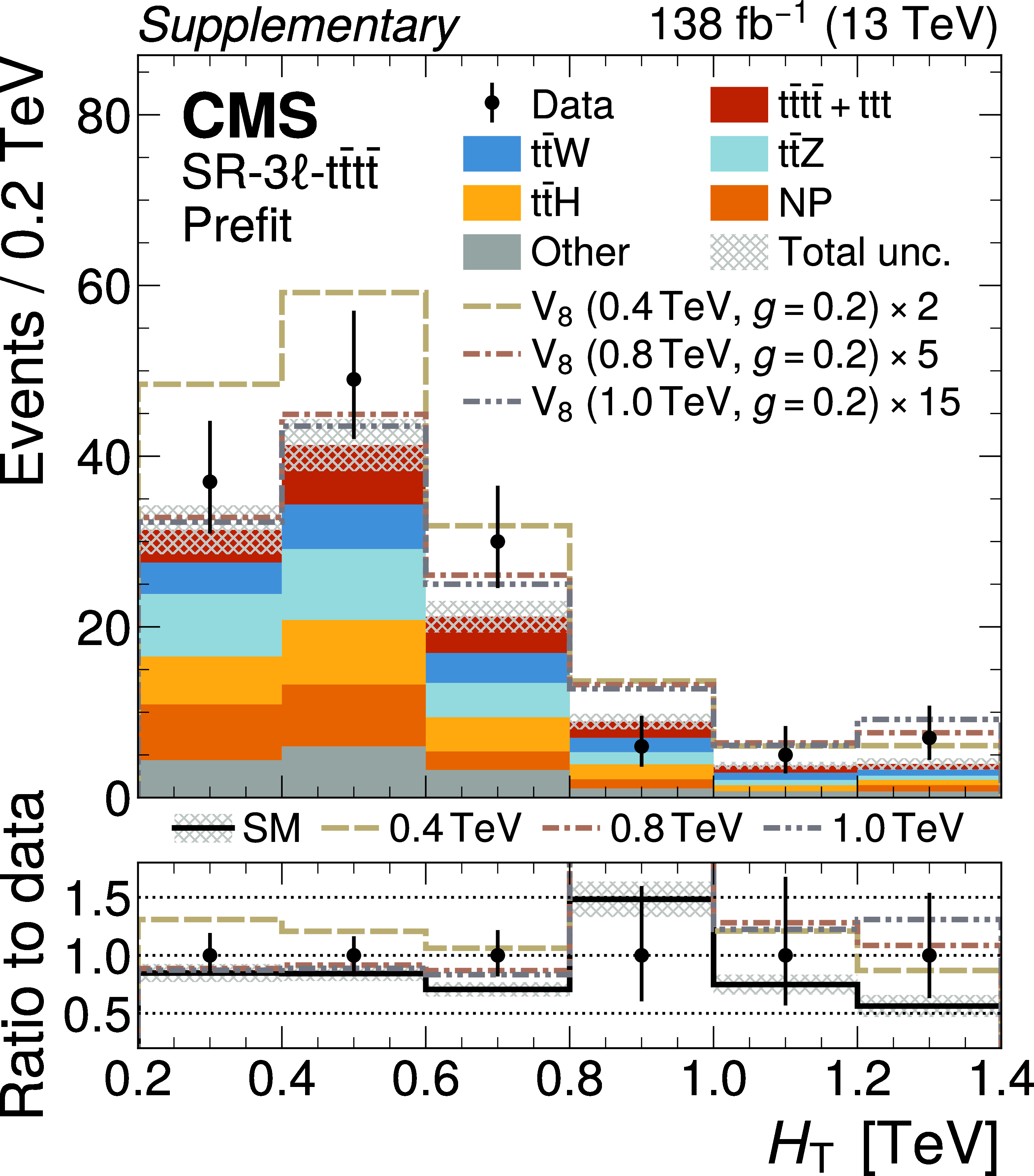
png pdf |
Additional Figure 16:
Comparison of the number of observed (points) and predicted (colored histograms) events in the $H_{\mathrm{T}}$ distribution, shown for the SR-3$\ell$-$\mathrm{t\bar{t}t\bar{t}}$. The last bin includes the overflow contribution. The vertical bars on the points represent the statistical uncertainties in the data, and the hatched bands the total uncertainty in the predictions. The signal and background yields are shown before the fit to the data (``prefit''). The dashed/dotted lines show the enhancement of $\mathrm{t\bar{t}t\bar{t}}$+$\mathrm{ttt}$ production through an $\mathrm{V}_8$ resonance in three different scenarios. The lower panel shows the ratio of the total SM prediction to data, and also of the sum of the total SM prediction and the $\mathrm{V}_8$ contribution to data for the same configurations as in the upper panel. |
png pdf |
Additional Figure 17:
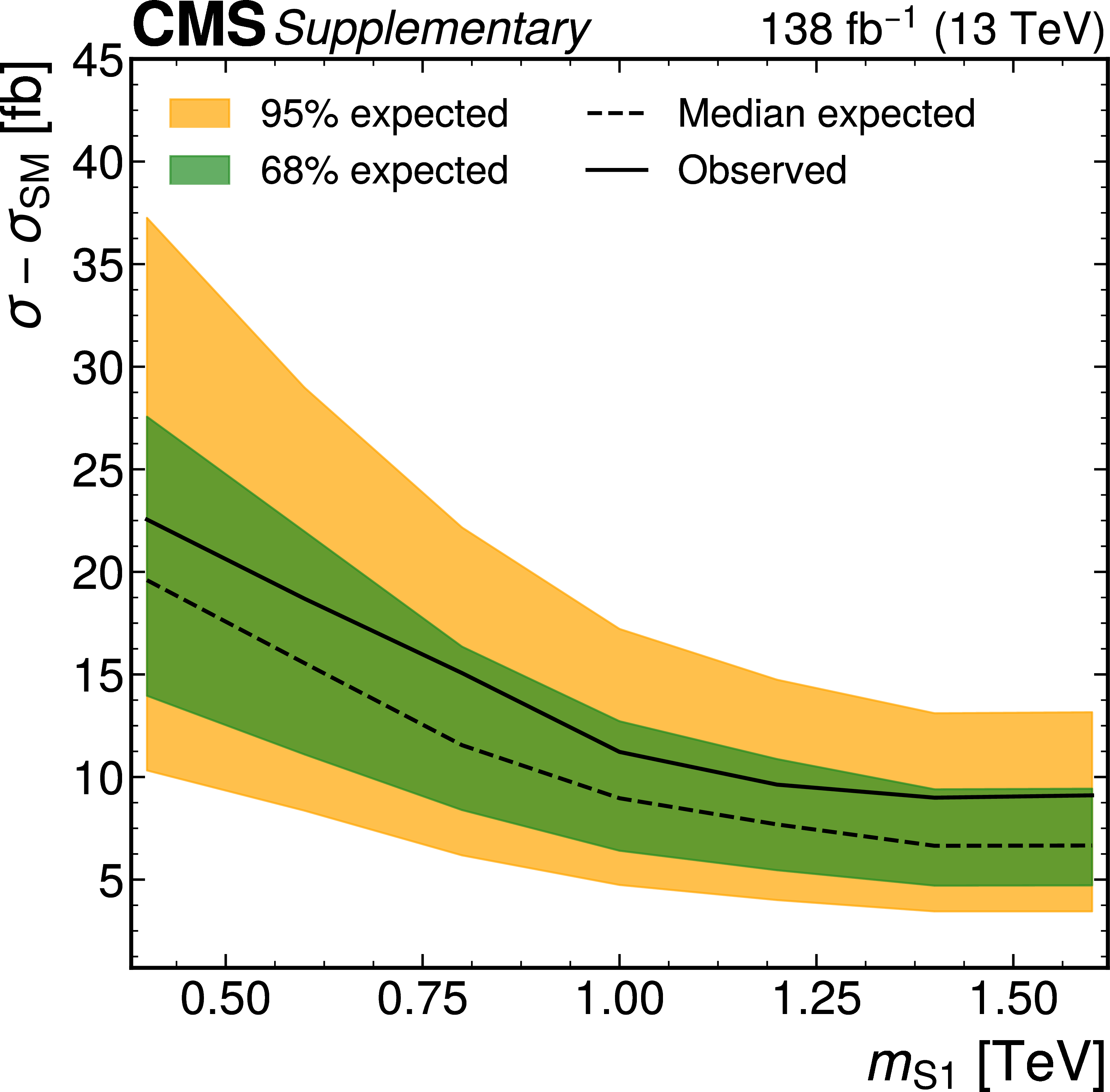
The enhancement of the $\mathrm{t\bar{t}t\bar{t}}$+$\mathrm{ttt}$ production cross section corresponding to the $95%$ CL exclusion limits on $y_{1\mathrm{S}}$ as a function of $m_{\mathrm{S}1}$. The area above the solid (dashed) black line indicates the observed (expected) exclusion region. |
png pdf |
Additional Figure 18:
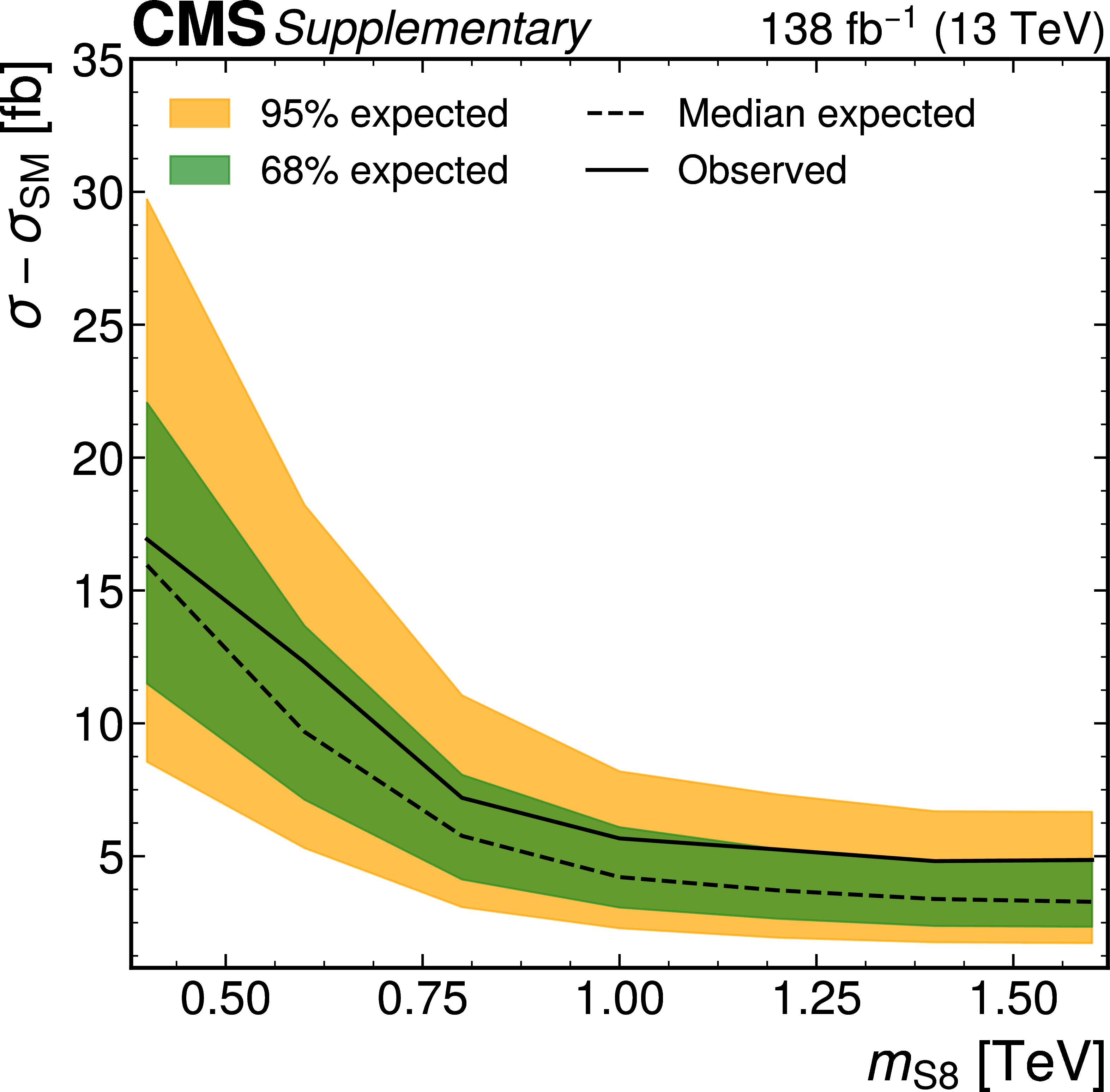
The enhancement of the $\mathrm{t\bar{t}t\bar{t}}$+$\mathrm{ttt}$ production cross section corresponding to the $95%$ CL exclusion limits on $y_{8\mathrm{S}}$ as a function of $m_{\mathrm{S}8}$. The area above the solid (dashed) black line indicates the observed (expected) exclusion region. |
png pdf |
Additional Figure 19:
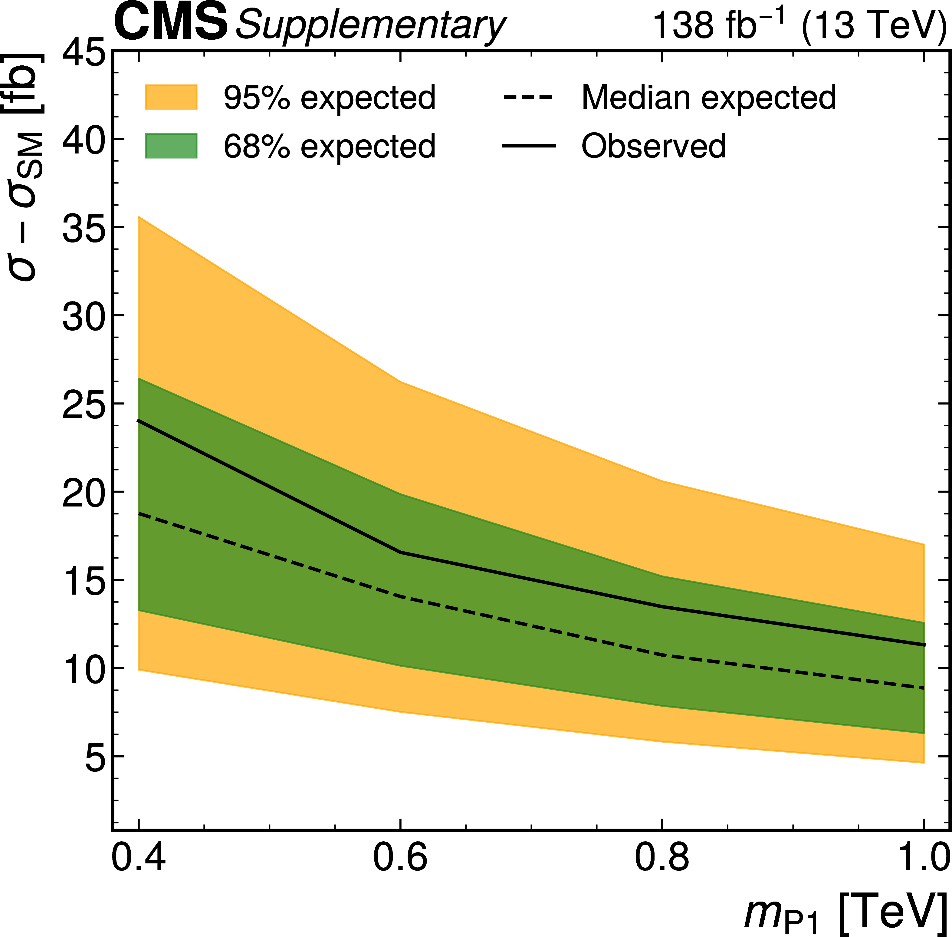
The enhancement of the $\mathrm{t\bar{t}t\bar{t}}$+$\mathrm{ttt}$ production cross section corresponding to the $95%$ CL exclusion limits on $y_{1\mathrm{P}}$ as a function of $m_{\mathrm{P}1}$. The area above the solid (dashed) black line indicates the observed (expected) exclusion region. |
png pdf |
Additional Figure 20:
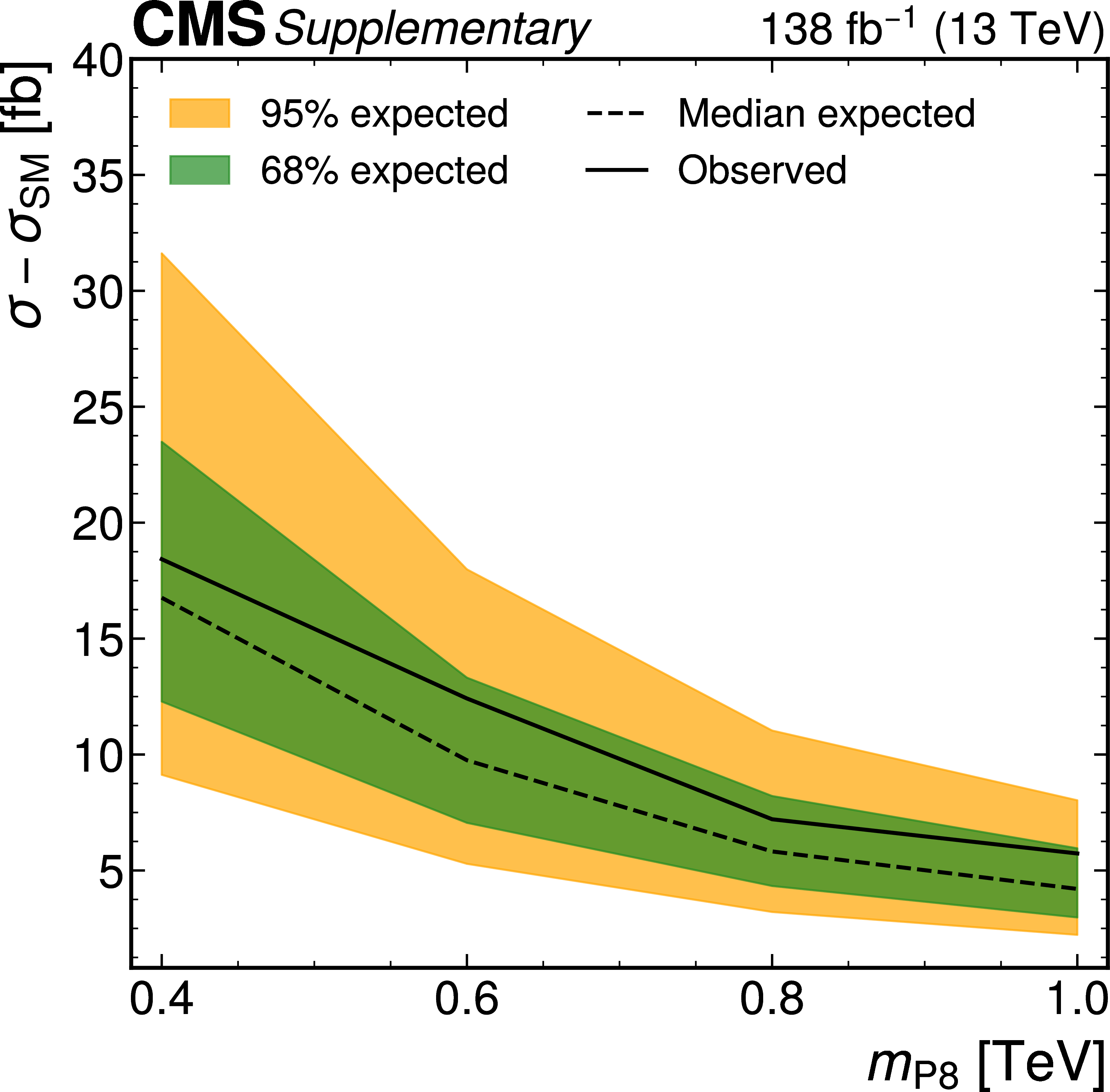
The enhancement of the $\mathrm{t\bar{t}t\bar{t}}$+$\mathrm{ttt}$ production cross section corresponding to the $95%$ CL exclusion limits on $y_{8\mathrm{P}}$ as a function of $m_{\mathrm{P}8}$. The area above the solid (dashed) black line indicates the observed (expected) exclusion region. |
png pdf |
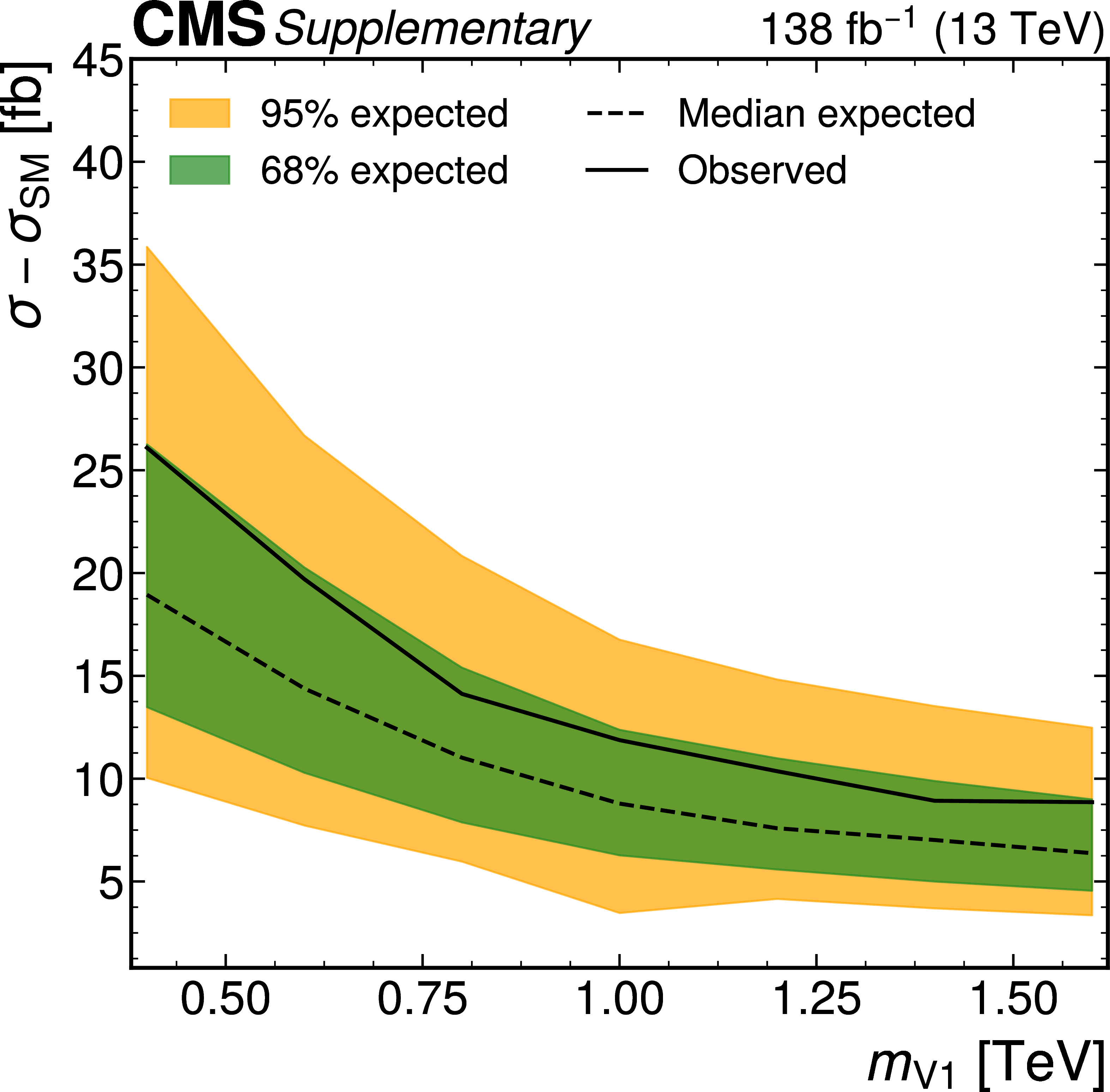
Additional Figure 21:
The enhancement of the $\mathrm{t\bar{t}t\bar{t}}$+$\mathrm{ttt}$ production cross section corresponding to the $95%$ CL exclusion limits on $g_{1}$ as a function of $m_{\mathrm{V}1}$. The area above the solid (dashed) black line indicates the observed (expected) exclusion region. |
png pdf |
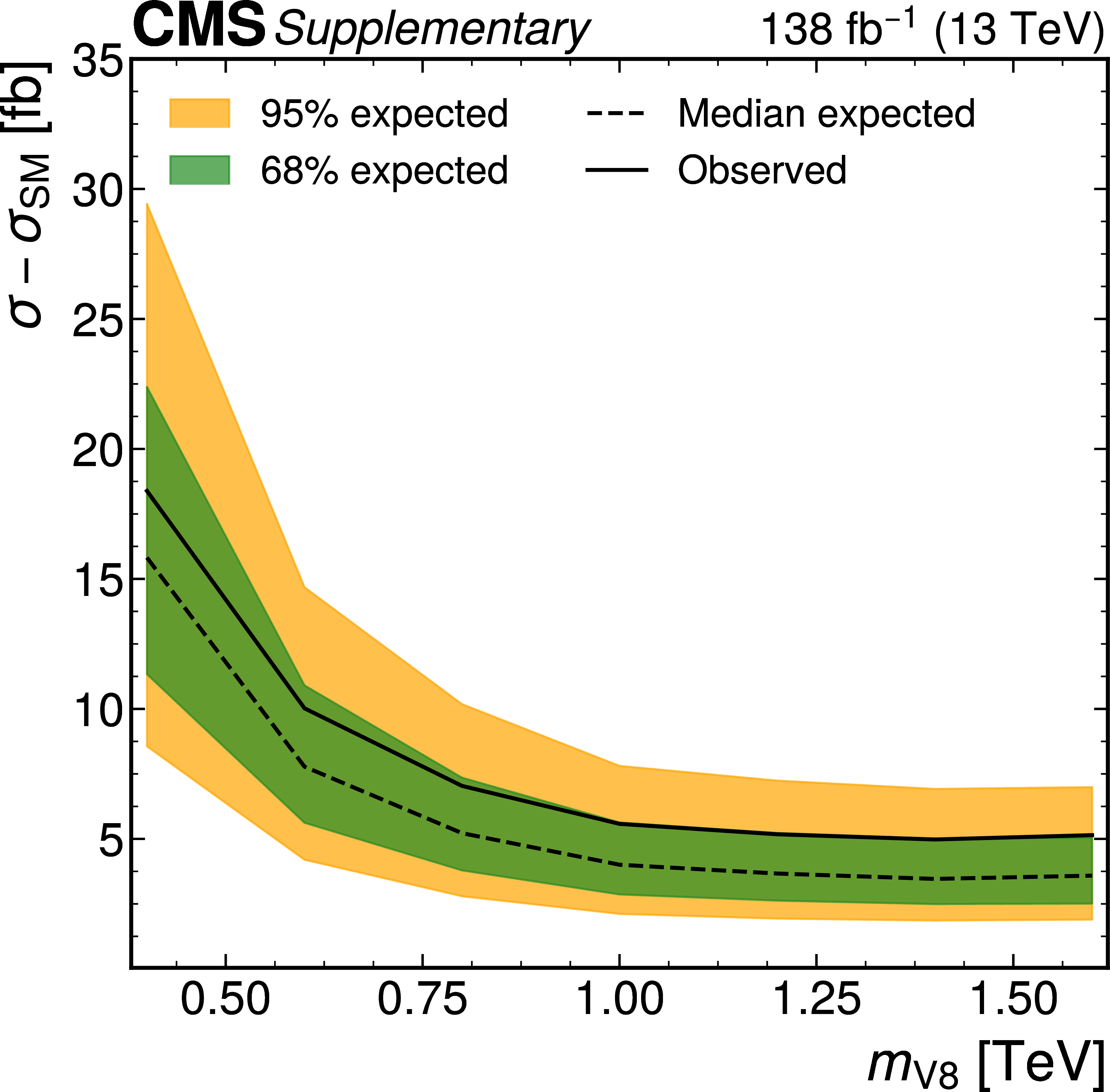
Additional Figure 22:
The enhancement of the $\mathrm{t\bar{t}t\bar{t}}$+$\mathrm{ttt}$ production cross section corresponding to the $95%$ CL exclusion limits on $g_{8}$ as a function of $m_{\mathrm{V}8}$. The area above the solid (dashed) black line indicates the observed (expected) exclusion region. |
png pdf |
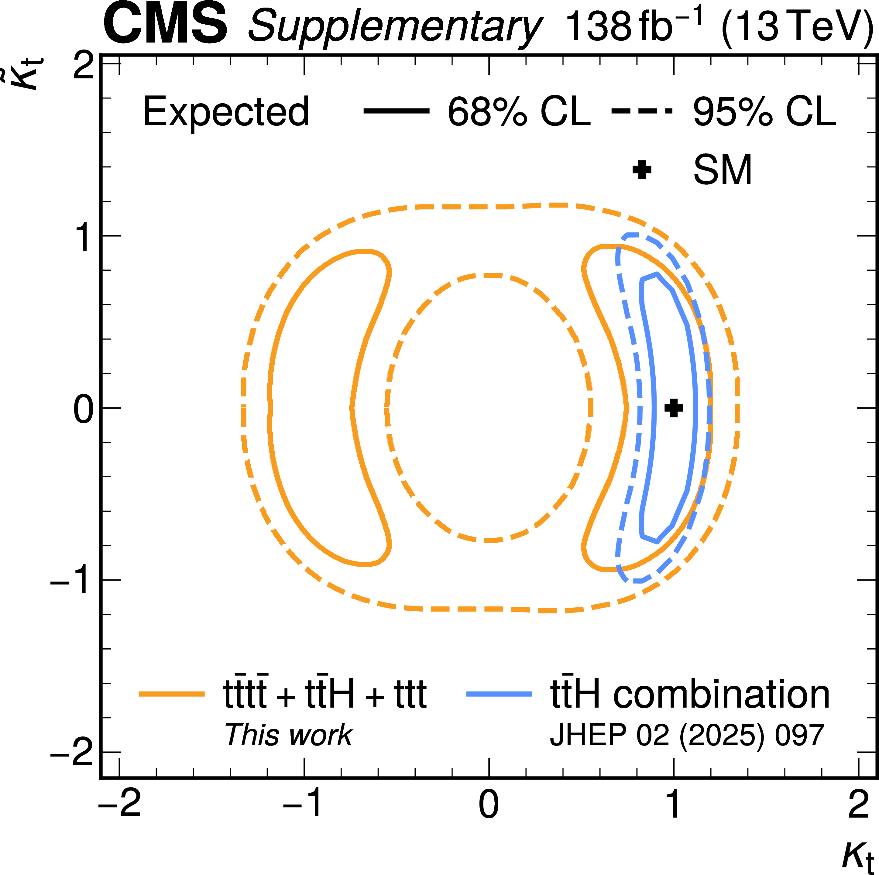
Additional Figure 23:
Expected exclusion contours on the Yukawa coupling modifiers $\kappa_{\mathrm{t}}$ and $\tilde{\kappa}_{\mathrm{t}}$ corresponding to the $68%$ (solid) and $95%$ (dashed) CL intervals as evaluated with toys, from this work (orange) or from a combination of $\mathrm{t\bar{t}H}$ production measurements (blue). The SM prediction is shown with a black cross. |
png pdf |
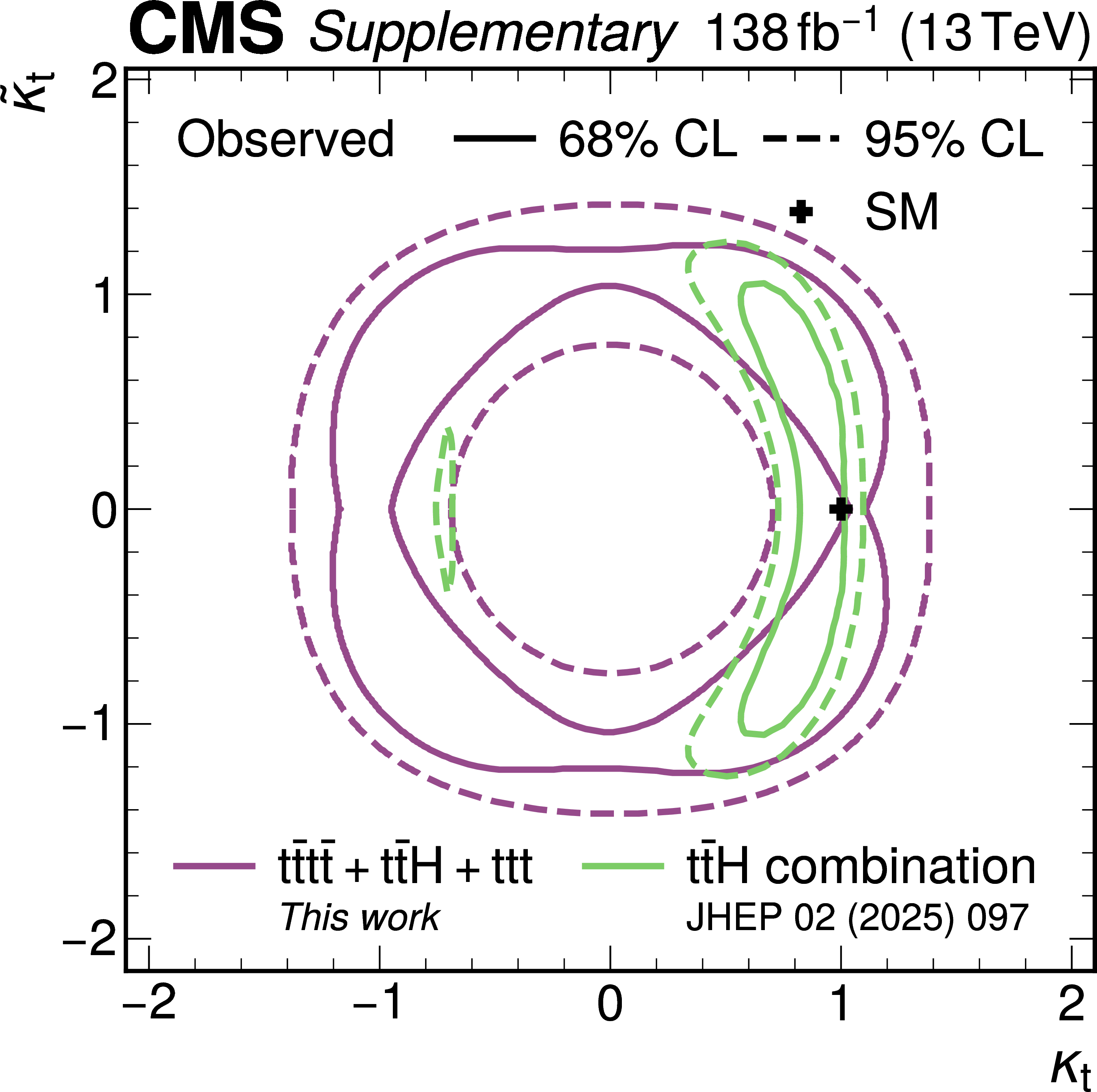
Additional Figure 24:
Observed exclusion contours on the Yukawa coupling modifiers $\kappa_{\mathrm{t}}$ and $\tilde{\kappa}_{\mathrm{t}}$ corresponding to the $68%$ (solid) and $95%$ (dashed) CL intervals as evaluated with toys, from this work (orange) or from a combination of $\mathrm{t\bar{t}H}$ production measurements (blue). The SM prediction is shown with a black cross. |
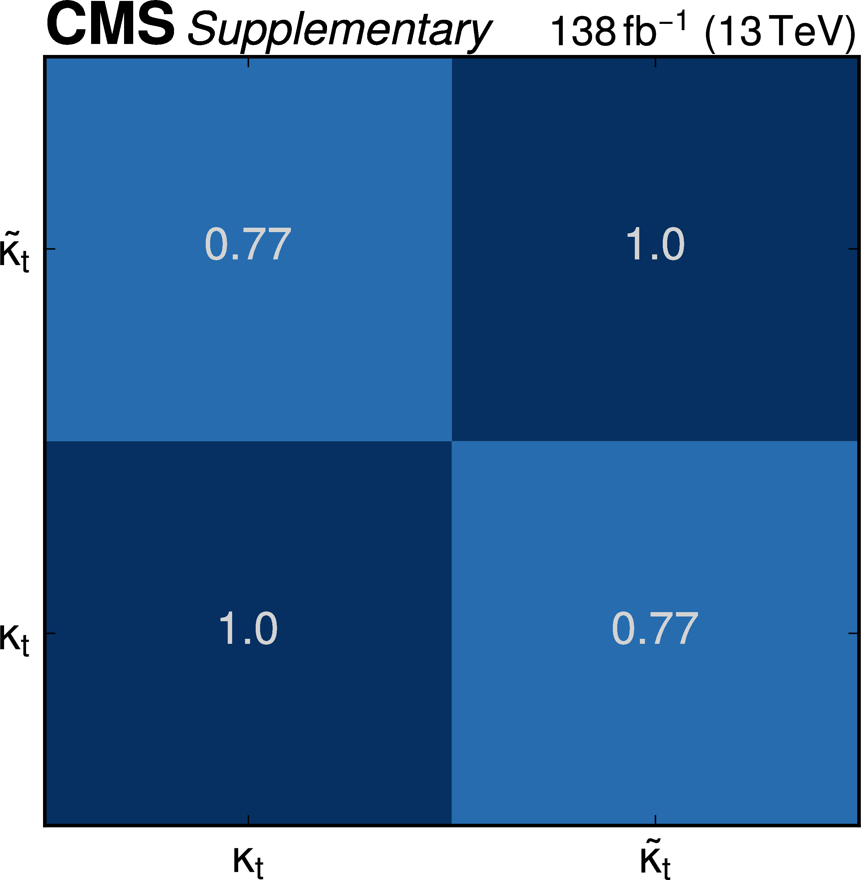
png pdf |
Additional Figure 25:
Correlation matrix of the fit with the Yukawa coupling modifiers $\kappa_{\mathrm{t}}$ and $\tilde{\kappa}_{\mathrm{t}}$ fitted simultaneously. |
| Additional Tables | |
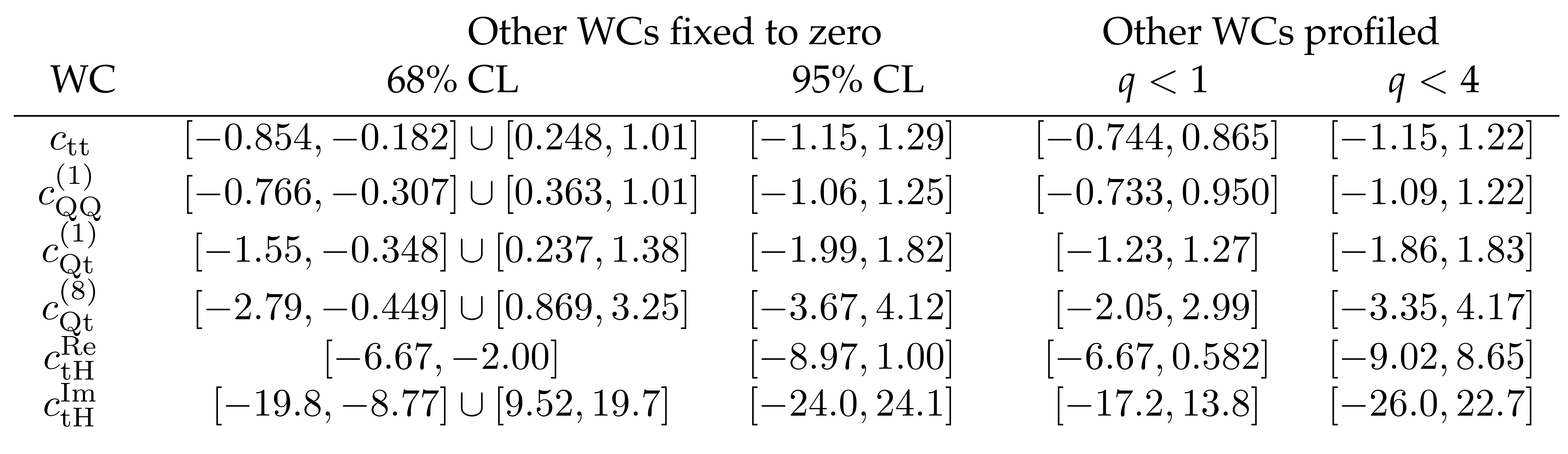
png pdf |
Additional Table 1:
Summary of the observed constraints on the individual WCs. For the case where the other WCs are fixed to zero, the 68 and $95%$ CL intervals are evaluated with toys. For the case where the other WCs are profiled, the intervals are instead evaluated by applying the asymptotic approximation. |
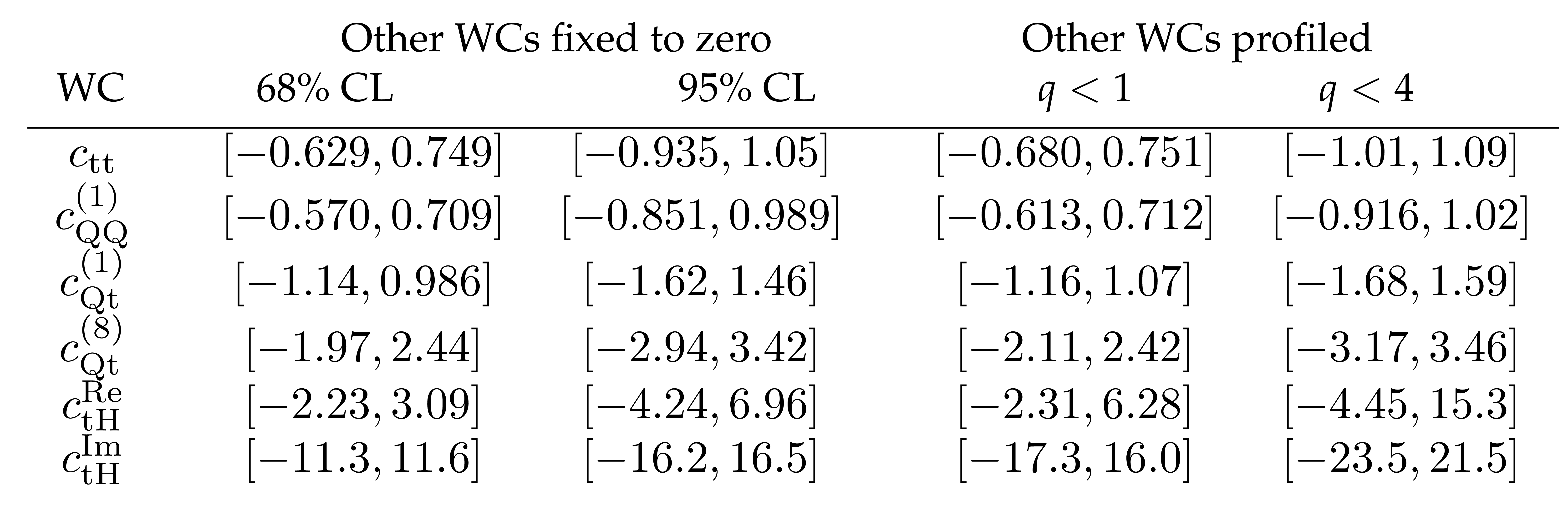
png pdf |
Additional Table 2:
Summary of the expected constraints on the individual WCs. For the case where the other WCs are fixed to zero, the 68 and $95%$ CL intervals are evaluated with toys. For the case where the other WCs are profiled, the intervals are instead evaluated by applying the asymptotic approximation. |
| References | ||||
| 1 | H. Nilles | Supersymmetry, supergravity and particle physics | Phys. Rept. 110 (1984) 1 | |
| 2 | G. Farrar and P. Fayet | Phenomenology of the production, decay, and detection of new hadronic states associated with supersymmetry | PLB 76 (1978) 575 | |
| 3 | M. Toharia and J. Wells | Gluino decays with heavier scalar superpartners | JHEP 02 (2006) 015 | hep-ph/0503175 |
| 4 | T. Plehn and T. Tait | Seeking sgluons | JPG 36 (2009) 075001 | 0810.3919 |
| 5 | S. Calvet, B. Fuks, P. Gris, and L. Valery | Searching for sgluons in multitop events at a center-of-mass energy of 8 TeV | JHEP 04 (2013) 043 | 1212.3360 |
| 6 | L. Beck et al. | Probing top-philic sgluons with LHC \mboxRun 1 data | PLB 746 (2015) 48 | 1501.07580 |
| 7 | L. Darm é , B. Fuks, and M. Goodsell | Cornering sgluons with four-top-quark events | PLB 784 (2018) 223 | 1805.10835 |
| 8 | B. Lillie, J. Shu, and T. M. P. Tait | Top compositeness at the Tevatron and LHC | JHEP 04 (2008) 087 | 0712.3057 |
| 9 | A. Pomarol and J. Serra | Top quark compositeness: Feasibility and implications | PRD 78 (2008) 074026 | 0806.3247 |
| 10 | K. Kumar, T. M. P. Tait, and R. Vega-Morales | Manifestations of top compositeness at colliders | JHEP 05 (2009) 022 | 0901.3808 |
| 11 | G. Cacciapaglia et al. | Composite scalars at the LHC: the Higgs, the sextet and the octet | JHEP 11 (2015) 201 | 1507.02283 |
| 12 | G. Cacciapaglia et al. | Four tops on the real projective plane at LHC | JHEP 10 (2011) 042 | 1107.4616 |
| 13 | P. S. Bhupal Dev and A. Pilaftsis | Maximally symmetric two Higgs doublet model with natural standard model alignment | JHEP 12 (2014) 024 | 1408.3405 |
| 14 | D. Dicus, A. Stange, and S. Willenbrock | Higgs decay to top quarks at hadron colliders | PLB 333 (1994) 126 | hep-ph/9404359 |
| 15 | N. Craig et al. | The hunt for the rest of the Higgs bosons | JHEP 06 (2015) 137 | 1504.04630 |
| 16 | N. Craig et al. | Heavy Higgs bosons at low $ \tan\beta $: from the LHC to 100 TeV | JHEP 01 (2017) 018 | 1605.08744 |
| 17 | Anisha et al. | BSM reach of four-top production at the LHC | PRD 108 (2023) 035001 | 2302.08281 |
| 18 | O. Ducu, L. Heurtier, and J. Maurer | LHC signatures of a $ \mathrm{Z}^{'} $ mediator between dark matter and the SU(3) sector | JHEP 03 (2016) 006 | 1509.05615 |
| 19 | S. Blasi et al. | Top-philic ALP phenomenology at the LHC: the elusive mass-window | JHEP 06 (2024) 077 | 2311.16048 |
| 20 | M. Kohda, T. Modak, and W.-S. Hou | Searching for new scalar bosons via triple-top signature in $ \mathrm{c}\mathrm{g}\to\mathrm{t}{S}{0}\to\mathrm{t}{\mathrm{t}\overline{\mathrm{t}}} $ | PLB 776 (2018) 379 | 1710.07260 |
| 21 | Q.-H. Cao, S.-L. Chen, Y. Liu, and X.-P. Wang | What can we learn from triple top-quark production? | PRD 100 (2019) 055035 | 1901.04643 |
| 22 | H. Khanpour | Probing top quark FCNC couplings in the triple-top signal at the high energy LHC and future circular collider | NPB 958 (2020) 115141 | 1909.03998 |
| 23 | S. Iguro and K. Tobe | $ {R({\mathrm{D}}{(\ast)})} $ in a general two Higgs doublet model | NPB 925 (2017) 560 | 1708.06176 |
| 24 | S. Cho et al. | Top FCNC induced by a $ \mathrm{Z}^{'} $ boson | PRD 101 (2020) 055015 | 1910.05925 |
| 25 | E. Abasov et al. | Search for dark matter mediator in the production of three and four top quarks | Phys. Part. Nucl. 56 (2025) 440 | 2407.08308 |
| 26 | C. Degrande et al. | Non-resonant new physics in top pair production at hadron colliders | JHEP 03 (2011) 125 | 1010.6304 |
| 27 | C. Zhang | Constraining $ {\mathrm{q}\mathrm{q}\mathrm{t}\mathrm{t}} $ operators from four-top production: a case for enhanced EFT sensitivity | Chin. Phys. C 42 (2018) 023104 | 1708.05928 |
| 28 | C. Englert, G. F. Giudice, A. Greljo, and M. McCullough | The $ \widehat{\mathrm{H}} $-parameter: an oblique Higgs view | JHEP 09 (2019) 041 | 1903.07725 |
| 29 | G. Banelli et al. | The present and future of four top operators | JHEP 02 (2021) 043 | 2010.05915 |
| 30 | L. Darm é , B. Fuks, and F. Maltoni | Top-philic heavy resonances in four-top final states and their EFT interpretation | JHEP 09 (2021) 143 | 2104.09512 |
| 31 | R. Aoude, H. El Faham, F. Maltoni, and E. Vryonidou | Complete SMEFT predictions for four top quark production at hadron colliders | JHEP 10 (2022) 163 | 2208.04962 |
| 32 | A. Aleshko, E. Boos, V. Bunichev, and L. Dudko | Prospects for establishing limits on the SMEFT operators from the production processes of three and four top quarks in hadron collisions | Int. J. Mod. Phys. A 39 (2024) 2450119 | 2309.12514 |
| 33 | A. M. Aleshko, E. E. Boos, V. E. Bunichev, and L. V. Dudko | Sensitivity of the three top quark production process to the contribution of top-related SMEFT operators | Phys. Part. Nucl. 56 (2025) 374 | |
| 34 | S. Di Noi et al. | Constraining four-heavy-quark operators with top-quark, Higgs, and electroweak precision data | JHEP 01 (2026) 025 | 2507.01137 |
| 35 | J. H. Kim, K. Kong, S. J. Lee, and G. Mohlabeng | Probing TeVns scale top-philic resonances with boosted top-tagging at the high luminosity LHC | PRD 94 (2016) 035023 | 1604.07421 |
| 36 | L. Darm é et al. | Searching for top-philic heavy resonances in boosted four-top final states | JHEP 11 (2025) 091 | 2507.05334 |
| 37 | Q.-H. Cao, S.-L. Chen, and Y. Liu | Probing Higgs width and top quark Yukawa coupling from $ {{\mathrm{t}\overline{\mathrm{t}}} \mathrm{H}} $ and $ {\mathrm{t}\overline{\mathrm{t}}} {\mathrm{t}\overline{\mathrm{t}}} $ productions | PRD 95 (2017) 053004 | 1602.01934 |
| 38 | Q.-H. Cao et al. | Limiting top quark-Higgs boson interaction and Higgs-boson width from multitop productions | PRD 99 (2019) 113003 | 1901.04567 |
| 39 | ATLAS Collaboration | The ATLAS experiment at the CERN Large Hadron Collider | JINST 3 (2008) S08003 | |
| 40 | ATLAS Collaboration | The ATLAS experiment at the CERN Large Hadron Collider: a description of the detector configuration for \mboxRun 3 | JINST 19 (2024) P05063 | 2305.16623 |
| 41 | CMS Collaboration | The CMS experiment at the CERN LHC | JINST 3 (2008) S08004 | |
| 42 | CMS Collaboration | Development of the CMS detector for the CERN LHC \mboxRun 3 | JINST 19 (2024) P05064 | CMS-PRF-21-001 2309.05466 |
| 43 | CMS Collaboration | Search for physics beyond the standard model in events with two leptons of same sign, missing transverse momentum, and jets in proton-proton collisions at $ \sqrt{s}= $ 13 TeV | EPJC 77 (2017) 578 | CMS-SUS-16-035 1704.07323 |
| 44 | CMS Collaboration | Search for standard model production of four top quarks with same-sign and multilepton final states in proton-proton collisions at $ \sqrt{s}= $ 13 TeV | EPJC 78 (2018) 140 | CMS-TOP-17-009 1710.10614 |
| 45 | ATLAS Collaboration | Search for new phenomena in events with same-charge leptons and b jets in $ {\mathrm{p}\mathrm{p}} $ collisions at $ \sqrt{s}= $ 13 TeV with the ATLAS detector | JHEP 12 (2018) 039 | 1807.11883 |
| 46 | ATLAS Collaboration | Search for four-top-quark production in the single-lepton and opposite-sign dilepton final states in $ {\mathrm{p}\mathrm{p}} $ collisions at $ \sqrt{s}= $ 13 TeV with the ATLAS detector | PRD 99 (2019) 052009 | 1811.02305 |
| 47 | CMS Collaboration | Search for the production of four top quarks in the single-lepton and opposite-sign dilepton final states in proton-proton collisions at $ \sqrt{s}= $ 13 TeV | JHEP 11 (2019) 082 | CMS-TOP-17-019 1906.02805 |
| 48 | CMS Collaboration | Search for production of four top quarks in final states with same-sign or multiple leptons in proton-proton collisions at $ \sqrt{s}= $ 13 TeV | EPJC 80 (2020) 75 | CMS-TOP-18-003 1908.06463 |
| 49 | ATLAS Collaboration | Evidence for $ {\mathrm{t}\overline{\mathrm{t}}} {\mathrm{t}\overline{\mathrm{t}}} $ production in the multilepton final state in proton-proton collisions at $ \sqrt{s}= $ 13 TeV with the ATLAS detector | EPJC 80 (2020) 1085 | 2007.14858 |
| 50 | ATLAS Collaboration | Measurement of the $ {\mathrm{t}\overline{\mathrm{t}}} {\mathrm{t}\overline{\mathrm{t}}} $ production cross section in $ {\mathrm{p}\mathrm{p}} $ collisions at $ \sqrt{s}= $ 13 TeV with the ATLAS detector | JHEP 11 (2021) 118 | 2106.11683 |
| 51 | CMS Collaboration | Evidence for four-top quark production in proton-proton collisions at $ \sqrt{s}= $ 13 TeV | PLB 844 (2023) 138076 | CMS-TOP-21-005 2303.03864 |
| 52 | F. Blekman, F. D é liot, V. Dutta, and E. Usai | Four-top quark physics at the LHC | Universe 8 (2022) 638 | 2208.04085 |
| 53 | ATLAS Collaboration | Observation of four-top-quark production in the multilepton final state with the ATLAS detector | EPJC 83 (2023) 496 | 2303.15061 |
| 54 | CMS Collaboration | Observation of four top quark production in proton-proton collisions at $ \sqrt{s}= $ 13 TeV | PLB 847 (2023) 138290 | CMS-TOP-22-013 2305.13439 |
| 55 | ATLAS Collaboration | Search for pair production of up-type vector-like quarks and for four-top-quark events in final states with multiple b-jets with the ATLAS detector | JHEP 07 (2018) 089 | 1803.09678 |
| 56 | CMS Collaboration | Search for new physics using effective field theory in 13 TeV $ {\mathrm{p}\mathrm{p}} $ collision events that contain a top quark pair and a boosted Z or Higgs boson | PRD 108 (2023) 032008 | CMS-TOP-21-003 2208.12837 |
| 57 | ATLAS Collaboration | Interpretations of the ATLAS measurements of Higgs boson production and decay rates and differential cross-sections in $ {\mathrm{p}\mathrm{p}} $ collisions at $ \sqrt{s}= $ 13 TeV | JHEP 11 (2024) 097 | 2402.05742 |
| 58 | CMS Collaboration | Search for physics beyond the standard model in top quark production with additional leptons in the context of effective field theory | JHEP 12 (2023) 068 | CMS-TOP-22-006 2307.15761 |
| 59 | CMS Collaboration | Combined effective field theory interpretation of Higgs boson, electroweak vector boson, top quark, and multijet measurements | EPJC 86 (2026) 331 | CMS-SMP-24-003 2504.02958 |
| 60 | N. Hartland et al. | A Monte Carlo global analysis of the standard model effective field theory: the top quark sector | JHEP 04 (2019) 100 | 1901.05965 |
| 61 | SMEFiT Collaboration | Combined SMEFT interpretation of Higgs, diboson, and top quark data from the LHC | JHEP 11 (2021) 089 | 2105.00006 |
| 62 | E. Celada et al. | Mapping the SMEFT at high-energy colliders: from LEP and the (HL-)LHC to the FCC-$ {\mathrm{e}\mathrm{e}} $ | JHEP 09 (2024) 091 | 2404.12809 |
| 63 | J. de Blas et al. | Constraining new physics effective interactions via a global fit of electroweak, Drell--Yan, Higgs, top, and flavour observables | JHEP 03 (2026) 013 | 2507.06191 |
| 64 | J. Ellis et al. | Top, Higgs, diboson and electroweak fit to the standard model effective field theory | JHEP 04 (2021) 279 | 2012.02779 |
| 65 | V. Miralles et al. | The top quark electro-weak couplings after LHC \mboxRun 2 | JHEP 02 (2022) 032 | 2107.13917 |
| 66 | ATLAS Collaboration | Search for $ {{\mathrm{t}\overline{\mathrm{t}}} \mathrm{H}/\mathrm{A}\to{\mathrm{t}\overline{\mathrm{t}}} {\mathrm{t}\overline{\mathrm{t}}} } $ production in the multilepton final state in proton-proton collisions at $ \sqrt{s}= $ 13 TeV with the ATLAS detector | JHEP 07 (2023) 203 | 2211.01136 |
| 67 | ATLAS Collaboration | Search for top-philic heavy resonances in $ {\mathrm{p}\mathrm{p}} $ collisions at $ \sqrt{s}= $ 13 TeV with the ATLAS detector | EPJC 84 (2024) 157 | 2304.01678 |
| 68 | CMS Collaboration | Search for $ \mathrm{t} \overline{\mathrm{t}} $ resonances in highly-boosted lepton+jets and fully hadronic final states in proton-proton collisions at $ \sqrt{s}= $ 13 TeV | JHEP 07 (2017) 001 | 1704.03366 |
| 69 | ATLAS Collaboration | Search for heavy particles decaying into top-quark pairs using lepton-plus-jets events in proton-proton collisions at $ \sqrt{s}= $ 13 TeV with the ATLAS detector | EPJC 78 (2018) 565 | 1804.10823 |
| 70 | CMS Collaboration | Search for resonant $ \mathrm{t} \overline{\mathrm{t}} $ production in proton-proton collisions at $ \sqrt{s}= $ 13 TeV | JHEP 04 (2019) 031 | 1810.05905 |
| 71 | ATLAS Collaboration | Search for heavy particles decaying into a top-quark pair in the fully hadronic final state in $ {\mathrm{p}\mathrm{p}} $ collisions at $ \sqrt{s}= $ 13 TeV with the ATLAS detector | PRD 99 (2019) 092004 | 1902.10077 |
| 72 | CMS Collaboration | Search for heavy Higgs bosons decaying to a top quark pair in proton-proton collisions at $ \sqrt{s}= $ 13 TeV | JHEP 04 (2020) 171 | CMS-HIG-17-027 1908.01115 |
| 73 | ATLAS Collaboration | Search for $ \mathrm{t} \overline{\mathrm{t}} $ resonances in fully hadronic final states in $ {\mathrm{p}\mathrm{p}} $ collisions at $ \sqrt{s}= $ 13 TeV with the ATLAS detector | JHEP 10 (2020) 061 | 2005.05138 |
| 74 | ATLAS Collaboration | Search for heavy neutral Higgs bosons decaying into a top quark pair in 140 fb$ ^{-1} $ of proton-proton collision data at $ \sqrt{s}= $ 13 TeV with the ATLAS detector | JHEP 08 (2024) 013 | 2404.18986 |
| 75 | CMS Collaboration | Observation of a pseudoscalar excess at the top quark pair production threshold | Rep. Prog. Phys. 88 (2025) 087801 | CMS-TOP-24-007 2503.22382 |
| 76 | CMS Collaboration | Search for heavy pseudoscalar and scalar bosons decaying to a top quark pair in proton-proton collisions at $ \sqrt{s}= $ 13 TeV | Rep. Prog. Phys. 88 (2025) 127801 | CMS-HIG-22-013 2507.05119 |
| 77 | ATLAS Collaboration | Search for $ \mathrm{t} \overline{\mathrm{t}} $ resonances in final states with exactly one or two leptons using 140 fb$ ^{-1} $ of $ {\mathrm{p}\mathrm{p}} $ collision data at $ \sqrt{s}= $ 13 TeV with the ATLAS experiment | Submitted to JHEP, 2025 | 2512.17856 |
| 78 | ATLAS Collaboration | Observation of a cross-section enhancement near the $ \mathrm{t} \overline{\mathrm{t}} $ production threshold in $ \sqrt{s}= $ 13 TeV $ {\mathrm{p}\mathrm{p}} $ collisions with the ATLAS detector | Submitted to Rep. Prog. Phys, 2026 | 2601.11780 |
| 79 | CMS Collaboration | Search for new particles decaying into top quark-antiquark pairs in proton-proton collisions at $ \sqrt{s}= $ 13 TeV | Submitted to JHEP, 2026 | 2603.23454 |
| 80 | ATLAS Collaboration | Search for a $ {CP} $-odd Higgs boson decaying into a heavy $ {CP} $-even Higgs boson and a Z boson in the $ {\ell^+\ell^-{\mathrm{t}\overline{\mathrm{t}}} } $ and $ {\nu\overline{\nu}\mathrm{b}\overline{\mathrm{b}}} $ final states using 140 fb$ ^{-1} $ of data collected with the ATLAS detector | JHEP 02 (2024) 197 | 2311.04033 |
| 81 | CMS Collaboration | Search for heavy neutral Higgs bosons $ \mathrm{A} $ and H in the $ {{\mathrm{t}\overline{\mathrm{t}}} \mathrm{Z}} $ channel in proton-proton collisions at 13 TeV | PLB 866 (2025) 139568 | 2412.00570 |
| 82 | CMS Collaboration | Measurements of $ {{\mathrm{t}\overline{\mathrm{t}}} \mathrm{H}} $ production and the CP structure of the Yukawa interaction between the Higgs boson and top quark in the diphoton decay channel | PRL 125 (2020) 061801 | CMS-HIG-19-013 2003.10866 |
| 83 | ATLAS Collaboration | $ {CP} $ properties of Higgs boson interactions with top quarks in the $ {{\mathrm{t}\overline{\mathrm{t}}} \mathrm{H}} $ and $ {\mathrm{t}\mathrm{H}} $ processes using $ {\mathrm{H}\to\gamma\gamma} $ with the ATLAS detector | PRL 125 (2020) 061802 | 2004.04545 |
| 84 | CMS Collaboration | Measurement of the Higgs boson production rate in association with top quarks in final states with electrons, muons, and hadronically decaying tau leptons at $ \sqrt{s}= $ 13 TeV | EPJC 81 (2021) 378 | CMS-HIG-19-008 2011.03652 |
| 85 | CMS Collaboration | Search for CP violation in $ {{\mathrm{t}\overline{\mathrm{t}}} \mathrm{H}} $ and $ {\mathrm{t}\mathrm{H}} $ production in multilepton channels in proton-proton collisions at $ \sqrt{s}= $ 13 TeV | JHEP 07 (2023) 092 | CMS-HIG-21-006 2208.02686 |
| 86 | ATLAS Collaboration | Probing the $ {CP} $ nature of the top--Higgs Yukawa coupling in $ {{\mathrm{t}\overline{\mathrm{t}}} \mathrm{H}} $ and $ {\mathrm{t}\mathrm{H}} $ events with $ {\mathrm{H}\to\mathrm{b}\overline{\mathrm{b}}} $ decays using the ATLAS detector at the LHC | PLB 849 (2024) 138469 | 2303.05974 |
| 87 | CMS Collaboration | Measurement of the $ {{\mathrm{t}\overline{\mathrm{t}}} \mathrm{H}} $ and $ {\mathrm{t}\mathrm{H}} $ production rates in the $ {\mathrm{H}\to\mathrm{b}\overline{\mathrm{b}}} $ decay channel using proton-proton collision data at $ \sqrt{s}= $ 13 TeV | JHEP 02 (2025) 097 | CMS-HIG-19-011 2407.10896 |
| 88 | CMS Collaboration | Constraints on anomalous Higgs boson couplings to vector bosons and fermions in its production and decay using the four-lepton final state | PRD 104 (2021) 052004 | CMS-HIG-19-009 2104.12152 |
| 89 | CMS Collaboration | A portrait of the Higgs boson by the CMS experiment ten years after the discovery | [Author correction: \DOI10./s41586-023-06164-8], 2022 Nature 607 (2022) 60 |
CMS-HIG-22-001 2207.00043 |
| 90 | ATLAS Collaboration | A detailed map of Higgs boson interactions by the ATLAS experiment ten years after the discovery | [Publisher correction: \DOI10./s41586-022-05581-5, author correction: \DOI10./s41586-023-06248-5], 2022 Nature 607 (2022) 52 |
2207.00092 |
| 91 | ATLAS Collaboration | Measurement of the properties of Higgs boson production at $ \sqrt{s}= $ 13 TeV in the $ {\mathrm{H}\to\gamma\gamma} $ channel using 139 fb$ ^{-1} $ of $ {\mathrm{p}\mathrm{p}} $ collision data with the ATLAS experiment | JHEP 07 (2023) 088 | 2207.00348 |
| 92 | CMS Collaboration | Measurement of the top quark Yukawa coupling from $ \mathrm{t} \overline{\mathrm{t}} $ kinematic distributions in the lepton+jets final state in proton-proton collisions at $ \sqrt{s}= $ 13 TeV | PRD 100 (2019) 072007 | CMS-TOP-17-004 1907.01590 |
| 93 | CMS Collaboration | Measurement of the top quark Yukawa coupling from $ \mathrm{t} \overline{\mathrm{t}} $ kinematic distributions in the dilepton final state in proton-proton collisions at $ \sqrt{s}= $ 13 TeV | PRD 102 (2020) 092013 | CMS-TOP-19-008 2009.07123 |
| 94 | ATLAS Collaboration | Measurement of the top-quark Yukawa coupling from $ \mathrm{t} \overline{\mathrm{t}} $ production in the lepton+jets final state using $ {\mathrm{p}\mathrm{p}} $ collisions at $ \sqrt{s}= $ 13 TeV with the ATLAS detector | JHEP 01 (2026) 117 | 2509.16039 |
| 95 | ATLAS Collaboration | Constraint on the total width of the Higgs boson from Higgs boson and four-top-quark measurements in $ {\mathrm{p}\mathrm{p}} $ collisions at $ \sqrt{s}= $ 13 TeV with the ATLAS detector | PLB 861 (2025) 139277 | 2407.10631 |
| 96 | CMS Collaboration | Combined measurements and interpretations of Higgs boson production and decay in proton-proton collisions at $ \sqrt{s}= $ 13 TeV | Accepted by Rep. Prog. Phys, 2026 | CMS-HIG-21-018 2602.18611 |
| 97 | CMS Collaboration | HEPData record for this analysis | link | |
| 98 | CMS Collaboration | Performance of the CMS Level-1 trigger in proton-proton collisions at $ \sqrt{s}= $ 13 TeV | JINST 15 (2020) P10017 | CMS-TRG-17-001 2006.10165 |
| 99 | CMS Collaboration | The CMS trigger system | JINST 12 (2017) P01020 | CMS-TRG-12-001 1609.02366 |
| 100 | CMS Collaboration | Performance of the CMS high-level trigger during LHC \mboxRun 2 | JINST 19 (2024) P11021 | CMS-TRG-19-001 2410.17038 |
| 101 | CMS Collaboration | Electron and photon reconstruction and identification with the CMS experiment at the CERN LHC | JINST 16 (2021) P05014 | CMS-EGM-17-001 2012.06888 |
| 102 | CMS Collaboration | Performance of the CMS muon detector and muon reconstruction with proton-proton collisions at $ \sqrt{s}= $ 13 TeV | JINST 13 (2018) P06015 | CMS-MUO-16-001 1804.04528 |
| 103 | CMS Collaboration | Description and performance of track and primary-vertex reconstruction with the CMS tracker | JINST 9 (2014) P10009 | CMS-TRK-11-001 1405.6569 |
| 104 | CMS Collaboration | Particle-flow reconstruction and global event description with the CMS detector | JINST 12 (2017) P10003 | CMS-PRF-14-001 1706.04965 |
| 105 | CMS Collaboration | Performance of reconstruction and identification of $ \tau $ leptons decaying to hadrons and $ \nu_{\!\tau} $ in $ {\mathrm{p}\mathrm{p}} $ collisions at $ \sqrt{s}= $ 13 TeV | JINST 13 (2018) P10005 | CMS-TAU-16-003 1809.02816 |
| 106 | CMS Collaboration | Jet energy scale and resolution in the CMS experiment in $ {\mathrm{p}\mathrm{p}} $ collisions at 8 TeV | JINST 12 (2017) P02014 | CMS-JME-13-004 1607.03663 |
| 107 | CMS Collaboration | Performance of missing transverse momentum reconstruction in proton-proton collisions at $ \sqrt{s}= $ 13 TeV using the CMS detector | JINST 14 (2019) P07004 | CMS-JME-17-001 1903.06078 |
| 108 | CMS Collaboration | Pileup mitigation at CMS in 13 TeV data | JINST 15 (2020) P09018 | CMS-JME-18-001 2003.00503 |
| 109 | M. Cacciari, G. P. Salam, and G. Soyez | The anti-$ k_{\mathrm{T}} $ jet clustering algorithm | JHEP 04 (2008) 063 | 0802.1189 |
| 110 | M. Cacciari, G. P. Salam, and G. Soyez | FASTJET user manual | EPJC 72 (2012) 1896 | 1111.6097 |
| 111 | CMS Collaboration | Jet energy scale and resolution measurements with legacy \mboxRun 2 data collected by CMS at 13 TeV | CMS Detector Performance Note CMS-DP-2021-033, 2021 CDS |
|
| 112 | CMS Collaboration | Identification of heavy-flavour jets with the CMS detector in $ {\mathrm{p}\mathrm{p}} $ collisions at 13 TeV | JINST 13 (2018) P05011 | CMS-BTV-16-002 1712.07158 |
| 113 | E. Bols et al. | Jet flavour classification using DeepJet | JINST 15 (2020) P12012 | 2008.10519 |
| 114 | CMS Collaboration | Performance summary of AK4 jet b tagging with data from proton-proton collisions at 13 TeV with the CMS detector | CMS Detector Performance Note CMS-DP-2023-005, 2023 CDS |
|
| 115 | CMS Collaboration | ECAL 2016 refined calibration and \mboxRun 2 summary plots | CMS Detector Performance Note CMS-DP-2020-021, 2020 CDS |
|
| 116 | CMS Collaboration | Performance of electron reconstruction and selection with the CMS detector in proton-proton collisions at $ \sqrt{s}= $ 8 TeV | JINST 10 (2015) P06005 | CMS-EGM-13-001 1502.02701 |
| 117 | CMS Collaboration | Performance of CMS muon reconstruction in cosmic-ray events | JINST 5 (2010) T03022 | CMS-CFT-09-014 0911.4994 |
| 118 | CMS Collaboration | Performance of the reconstruction and identification of high-momentum muons in proton-proton collisions at $ \sqrt{s}= $ 13 TeV | JINST 15 (2020) P02027 | CMS-MUO-17-001 1912.03516 |
| 119 | CMS Collaboration | Evidence for associated production of a Higgs boson with a top quark pair in final states with electrons, muons, and hadronically decaying $ \tau $ leptons at $ \sqrt{s}= $ 13 TeV | JHEP 08 (2018) 066 | CMS-HIG-17-018 1803.05485 |
| 120 | CMS Collaboration | Observation of single top quark production in association with a Z boson in proton-proton collisions at $ \sqrt{s}= $ 13 TeV | PRL 122 (2019) 132003 | CMS-TOP-18-008 1812.05900 |
| 121 | CMS Collaboration | Search for electroweak production of charginos and neutralinos in proton-proton collisions at $ \sqrt{s}= $ 13 TeV | JHEP 04 (2022) 147 | CMS-SUS-19-012 2106.14246 |
| 122 | CMS Collaboration | Measurements of the electroweak diboson production cross sections in proton-proton collisions at $ \sqrt{s}= $ 5.02 TeV using leptonic decays | PRL 127 (2021) 191801 | CMS-SMP-20-012 2107.01137 |
| 123 | CMS Collaboration | Inclusive and differential cross section measurements of single top quark production in association with a Z boson in proton-proton collisions at $ \sqrt{s}= $ 13 TeV | JHEP 02 (2022) 107 | CMS-TOP-20-010 2111.02860 |
| 124 | CMS Collaboration | Muon identification using multivariate techniques in the CMS experiment in proton-proton collisions at $ \sqrt{s}= $ 13 TeV | JINST 19 (2024) P02031 | CMS-MUO-22-001 2310.03844 |
| 125 | CMS Collaboration | Precision luminosity measurement in proton-proton collisions at $ \sqrt{s}= $ 13 TeV in 2015 and 2016 at CMS | EPJC 81 (2021) 800 | CMS-LUM-17-003 2104.01927 |
| 126 | CMS Collaboration | CMS luminosity measurement for the 2017 data-taking period at $ \sqrt{s}= $ 13 TeV | CMS Physics Analysis Summary, 2018 CMS-PAS-LUM-17-004 |
CMS-PAS-LUM-17-004 |
| 127 | CMS Collaboration | CMS luminosity measurement for the 2018 data-taking period at $ \sqrt{s}= $ 13 TeV | CMS Physics Analysis Summary, 2019 CMS-PAS-LUM-18-002 |
CMS-PAS-LUM-18-002 |
| 128 | NNPDF Collaboration | Parton distributions from high-precision collider data | EPJC 77 (2017) 663 | 1706.00428 |
| 129 | T. Sjöstrand et al. | An introduction to PYTHIA8.2 | Comput. Phys. Commun. 191 (2015) 159 | 1410.3012 |
| 130 | CMS Collaboration | Extraction and validation of a new set of CMS PYTHIA8 tunes from underlying-event measurements | EPJC 80 (2020) 4 | CMS-GEN-17-001 1903.12179 |
| 131 | GEANT4 Collaboration | GEANT 4---a simulation toolkit | NIM A 506 (2003) 250 | |
| 132 | CMS Collaboration | Simulation of the silicon strip tracker pre-amplifier in early 2016 data | CMS Detector Performance Note CMS-DP-2020-045, 2020 CDS |
|
| 133 | J. Alwall et al. | The automated computation of tree-level and next-to-leading order differential cross sections, and their matching to parton shower simulations | JHEP 07 (2014) 079 | 1405.0301 |
| 134 | P. Artoisenet, R. Frederix, O. Mattelaer, and R. Rietkerk | Automatic spin-entangled decays of heavy resonances in Monte Carlo simulations | JHEP 03 (2013) 015 | 1212.3460 |
| 135 | G. Bevilacqua and M. Worek | Constraining BSM physics at the LHC: Four top final states with NLO accuracy in perturbative QCD | JHEP 07 (2012) 111 | 1206.3064 |
| 136 | F. Maltoni, D. Pagani, and I. Tsinikos | Associated production of a top-quark pair with vector bosons at NLO in QCD: impact on $ {{\mathrm{t}\overline{\mathrm{t}}} \mathrm{H}} $ searches at the LHC | JHEP 02 (2016) 113 | 1507.05640 |
| 137 | R. Frederix, D. Pagani, and M. Zaro | Large NLO corrections in $ {{\mathrm{t}\overline{\mathrm{t}}} \mathrm{W}^{\pm}} $ and $ {\mathrm{t}\overline{\mathrm{t}}} {\mathrm{t}\overline{\mathrm{t}}} $ hadroproduction from supposedly subleading EW contributions | JHEP 02 (2018) 031 | 1711.02116 |
| 138 | T. Je \v z o and M. Kraus | Hadroproduction of four top quarks in the POWHEG box | PRD 105 (2022) 114024 | 2110.15159 |
| 139 | N. Dimitrakopoulos and M. Worek | Four top final states with NLO accuracy in perturbative QCD: 4 lepton channel | JHEP 06 (2024) 129 | 2401.10678 |
| 140 | M. van Beekveld, A. Kulesza, and L. Moreno Valero | Threshold resummation for the production of four top quarks at the LHC | PRL 131 (2023) 211901 | 2212.03259 |
| 141 | M. van Beekveld, A. Kulesza, M. Lupattelli, and T. Saracco | Invariant-mass threshold resummation for the production of four top quarks at the LHC | JHEP 10 (2025) 209 | 2505.10381 |
| 142 | S. Frixione et al. | Single-top hadroproduction in association with a W boson | JHEP 07 (2008) 029 | 0805.3067 |
| 143 | F. Demartin et al. | $ {\mathrm{t}\mathrm{W}\mathrm{H}} $ associated production at the LHC | EPJC 77 (2017) 34 | 1607.05862 |
| 144 | G. Durieux | Triple top-quark production at NLO in QCD | Zenodo, 2023 link |
|
| 145 | V. Barger, W.-Y. Keung, and B. Yencho | Triple-top signal of new physics at the LHC | PLB 687 (2010) 70 | 1001.0221 |
| 146 | C.-R. Chen | Searching for new physics with triple-top signal at the LHC | PLB 736 (2014) 321 | |
| 147 | M. Malekhosseini, M. Ghominejad, H. Khanpour, and M. Mohammadi Najafabadi | Constraining top quark flavor violation and dipole moments through three and four top quark productions at the LHC | PRD 98 (2018) 095001 | 1804.05598 |
| 148 | E. Boos and L. Dudko | Triple top quark production in standard model | Int. J. Mod. Phys. A 37 (2022) 2250023 | 2107.07629 |
| 149 | CMS Collaboration | Measurement of the cross section of top quark-antiquark pair production in association with a W boson in proton-proton collisions at $ \sqrt{s}= $ 13 TeV | JHEP 07 (2023) 219 | CMS-TOP-21-011 2208.06485 |
| 150 | H. Voss, A. Höcker, J. Stelzer, and F. Tegenfeldt | tmva, the toolkit for multivariate data analysis with root | in the International Workshop on Advanced Computing and Analysis Techniques in Physics Research (ACAT ): Amsterdam, The Netherlands, April 23--27,.. [PoS (ACAT) 040], 2017 Proc. 1 (2017) 1 |
physics/0703039 |
| 151 | CMS Collaboration | Search for new physics in same-sign dilepton events in proton-proton collisions at $ \sqrt{s}= $ 13 TeV | EPJC 76 (2016) 439 | CMS-SUS-15-008 1605.03171 |
| 152 | J. Butterworth et al. | PDF4LHC recommendations for LHC \mboxRun 2 | JPG 43 (2016) 023001 | 1510.03865 |
| 153 | CMS Collaboration | Measurement of the cross section for $ \mathrm{t} \overline{\mathrm{t}} $ production with additional jets and b jets in $ {\mathrm{p}\mathrm{p}} $ collisions at $ \sqrt{s}= $ 13 TeV | JHEP 07 (2020) 125 | CMS-TOP-18-002 2003.06467 |
| 154 | CMS Collaboration | Inclusive and differential cross section measurements of $ {\mathrm{t}\overline{\mathrm{t}}} \mathrm{b}\overline{\mathrm{b}} $ production in the lepton+jets channel at $ \sqrt{s}= $ 13 TeV | JHEP 05 (2024) 042 | CMS-TOP-22-009 2309.14442 |
| 155 | R. Frederix and I. Tsinikos | On improving NLO merging for $ {{\mathrm{t}\overline{\mathrm{t}}} \mathrm{W}} $ production | JHEP 11 (2021) 029 | 2108.07826 |
| 156 | ATLAS and CMS Collaborations, and LHC Higgs Combination Group | Procedure for the LHC Higgs boson search combination in Summer 2011 | Technical Report CMS-NOTE-2011-005, ATL-PHYS-PUB-2011-11, 2011 | |
| 157 | R. Barlow and C. Beeston | Fitting using finite Monte Carlo samples | Comput. Phys. Commun. 77 (1993) 219 | |
| 158 | J. S. Conway | Incorporating nuisance parameters in likelihoods for multisource spectra | in Workshop on Statistical Issues Related to Discovery Claims in Search Experiments and Unfolding (PHYSTAT ): Geneva, Switzerland, January 17--20,, 2011 Proc. 2011 (2011) W |
1103.0354 |
| 159 | CMS Collaboration | The CMS statistical analysis and combination tool: combine | Comput. Softw. Big Sci. 8 (2024) 19 | CMS-CAT-23-001 2404.06614 |
| 160 | W. Verkerke and D. Kirkby | The RooFit toolkit for data modeling | in the International Conference on Computing in High Energy and Nuclear Physics (CHEP ): La Jolla CA, United States, March 24--28,.. [eConf C0303241 MOLT007], 2003 Proc. 1 (2003) 3 |
physics/0306116 |
| 161 | L. Moneta et al. | The RooStats project | in the International Workshop on Advanced Computing and Analysis Techniques in Physics Research (ACAT ): Jaipur, India, February 22--27,.. [PoS (ACAT) 057], 2010 Proc. 1 (2010) 3 |
1009.1003 |
| 162 | G. Cowan, K. Cranmer, E. Gross, and O. Vitells | Asymptotic formulae for likelihood-based tests of new physics | EPJC 71 (2011) 1554 | 1007.1727 |
| 163 | S. S. Wilks | The large-sample distribution of the likelihood ratio for testing composite hypotheses | Annals Math. Statist. 9 (1938) 60 | |
| 164 | F. U. Bernlochner, D. C. Fry, S. B. Menary, and E. Persson | Cover your bases: asymptotic distributions of the profile likelihood ratio when constraining effective field theories in high-energy physics | SciPost Phys. Core 6 (2023) 013 | 2207.01350 |
| 165 | C. Degrande et al. | Effective field theory: A modern approach to anomalous couplings | Annals Phys. 335 (2013) 21 | 1205.4231 |
| 166 | I. Brivio, Y. Jiang, and M. Trott | The SMEFTsim package, theory and tools | JHEP 12 (2017) 070 | 1709.06492 |
| 167 | I. Brivio | SMEFTsim 3.0---a practical guide | JHEP 04 (2021) 073 | 2012.11343 |
| 168 | O. Mattelaer | On the maximal use of Monte Carlo samples: re-weighting events at NLO accuracy | EPJC 76 (2016) 674 | 1607.00763 |
| 169 | CMS Collaboration | Search for new physics in top quark production with additional leptons in proton-proton collisions at $ \sqrt{s}= $ 13 TeV using effective field theory | JHEP 03 (2021) 095 | CMS-TOP-19-001 2012.04120 |
| 170 | A. V. Gritsan, R. Röntsch, M. Schulze, and M. Xiao | Constraining anomalous Higgs boson couplings to the heavy-flavor fermions using matrix element techniques | PRD 94 (2016) 055023 | 1606.03107 |
| 171 | P. Artoisenet et al. | A framework for Higgs characterisation | JHEP 11 (2013) 043 | 1306.6464 |
| 172 | F. Demartin et al. | Higgs characterisation at NLO in QCD: $ {CP} $ properties of the top-quark Yukawa interaction | EPJC 74 (2014) 3065 | 1407.5089 |
| 173 | J. Brod, J. M. Cornell, D. Skodras, and E. Stamou | Global constraints on Yukawa operators in the standard model effective theory | JHEP 08 (2022) 294 | 2203.03736 |
| 174 | CMS Collaboration | Combined measurements of Higgs boson couplings in proton-proton collisions at $ \sqrt{s}= $ 13 TeV | EPJC 79 (2019) 421 | CMS-HIG-17-031 1809.10733 |
|
|
Compact Muon Solenoid LHC, CERN |

|
|
|
|
|
|