Compact Muon Solenoid
LHC, CERN
 Visit us: CMS Public Website, CMS Physics ;
Contact us: CMS Publications Committee
Visit us: CMS Public Website, CMS Physics ;
Contact us: CMS Publications Committee
| CMS-SMP-24-003 ; CERN-EP-2025-035 | ||
| Combined effective field theory interpretation of Higgs boson, electroweak vector boson, top quark, and multijet measurements | ||
| CMS Collaboration | ||
| 3 April 2025 | ||
| EPJC 86 (2026) 331 | ||
| Abstract: Constraints on Wilson coefficients (WCs) corresponding to dimension-6 operators of the standard model effective field theory (SMEFT) are determined from a simultaneous fit to seven sets of CMS measurements probing Higgs boson, electroweak vector boson, top quark, and multijet production. Measurements of electroweak precision observables are also included and provide complementary constraints to those from the CMS experiment. The CMS measurements, using LHC proton-proton collision data at $ \sqrt{s}= $ 13 TeV, corresponding to integrated luminosities of 36.3 or 138 fb$ ^{-1} $, are chosen to provide sensitivity to a broad set of operators, for which consistent SMEFT predictions can be derived. These are primarily measurements of differential cross sections which are parameterized as functions of the WCs. In measurements targeting $ \mathrm{t}(\overline{\mathrm{t}})\mathrm{X} $ production, SMEFT effects are modelled at the detector level. Individual constraints on 64 WCs, and constraints on 43 linear combinations of WCs, are obtained. | ||
| Links: e-print arXiv:2504.02958 [hep-ex] (PDF) ; CDS record ; inSPIRE record ; CADI line (restricted) ; | ||
| Figures & Tables | Summary | Additional Figures & Tables | References | CMS Publications |
|---|
| Figures | |
png pdf |
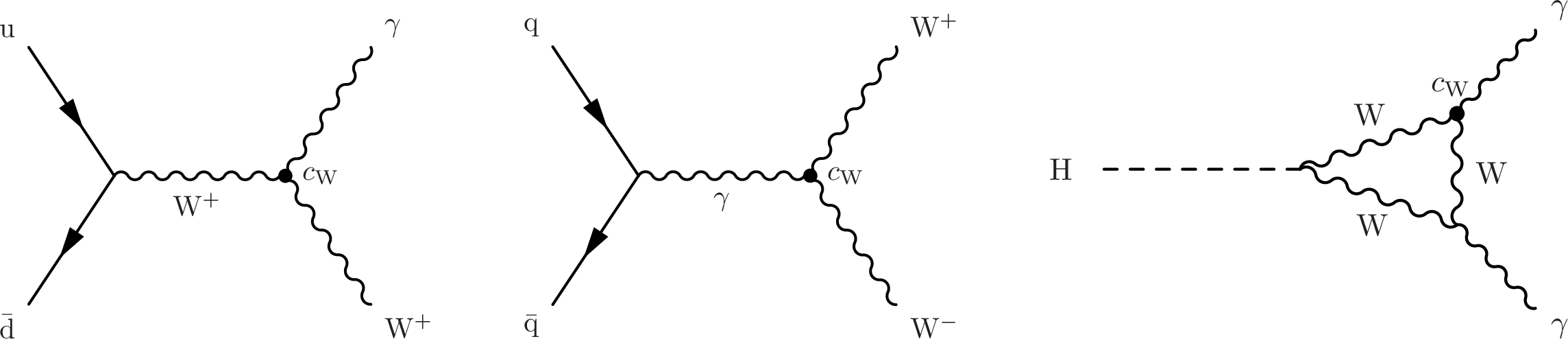
Figure 1:
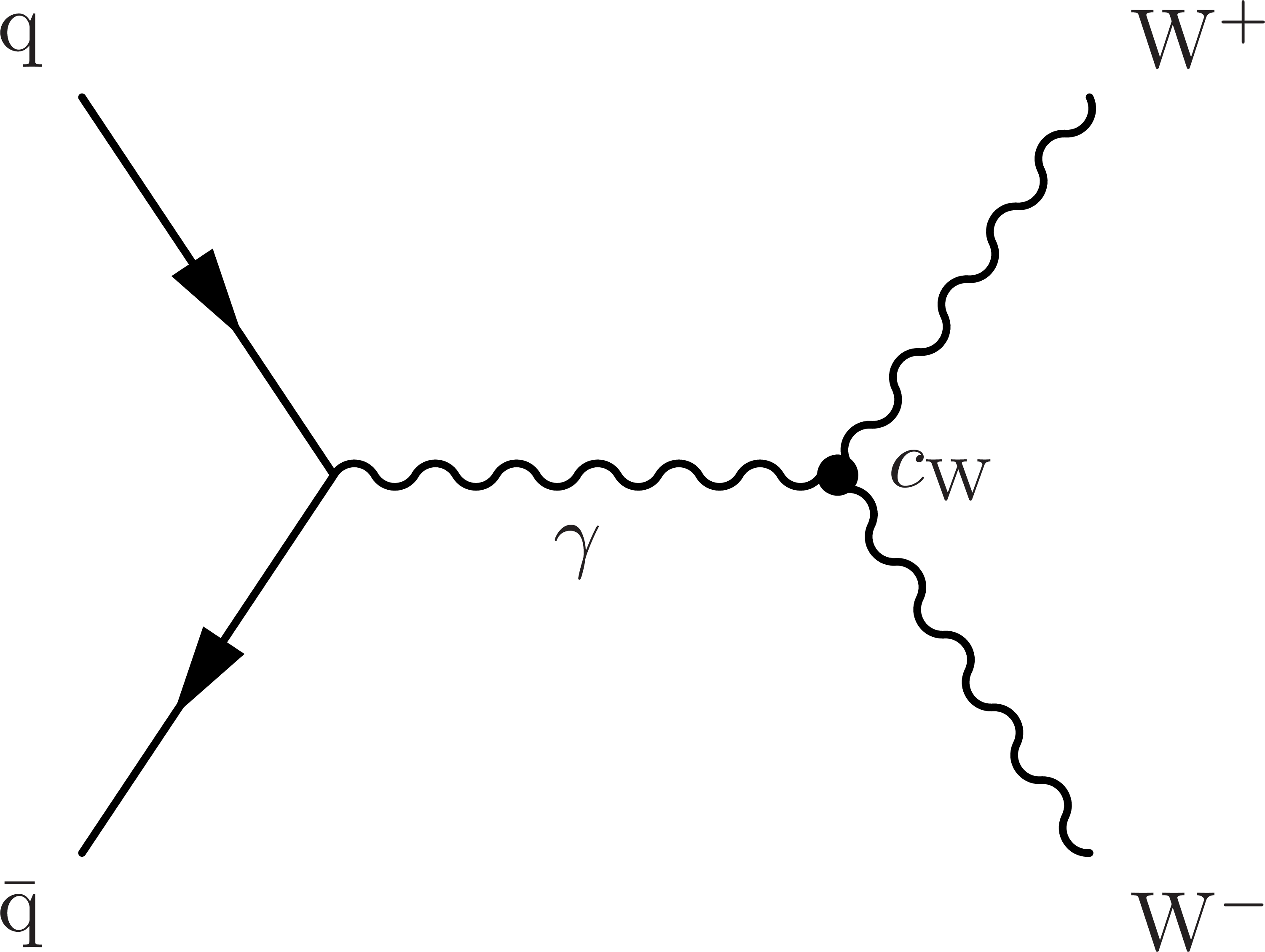
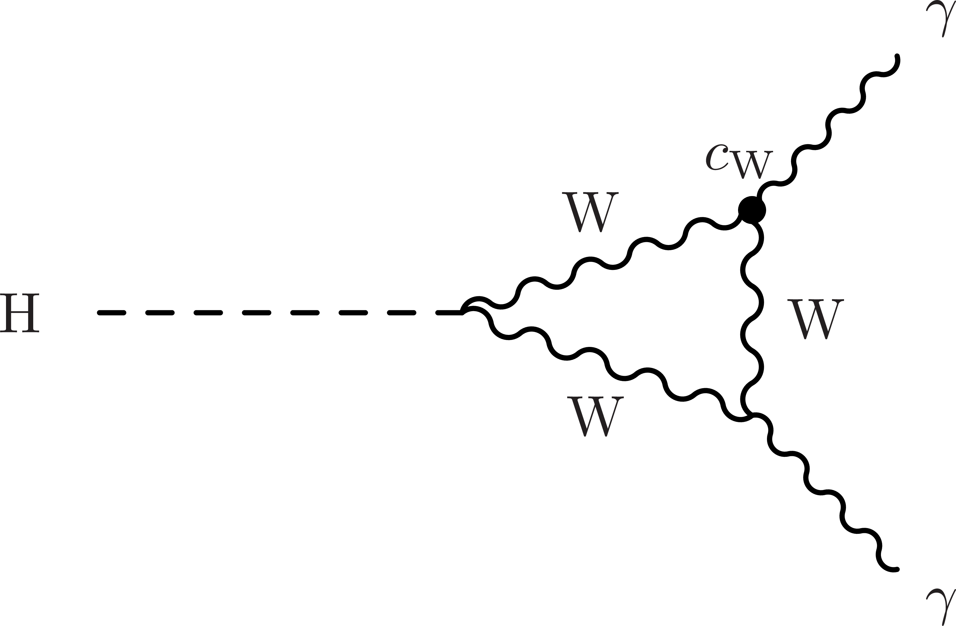
Example Feynman diagrams of modifications of SM processes by the SMEFT operator $ \mathcal{Q}_{\mathrm{W}} $: $ \mathrm{W}\gamma $ production (left), WW production (centre), $ \mathrm{H}\to\gamma\gamma $ decay (right). The WC $ c_{\mathrm{W}} $ controls the strength of the interaction. |
png pdf |
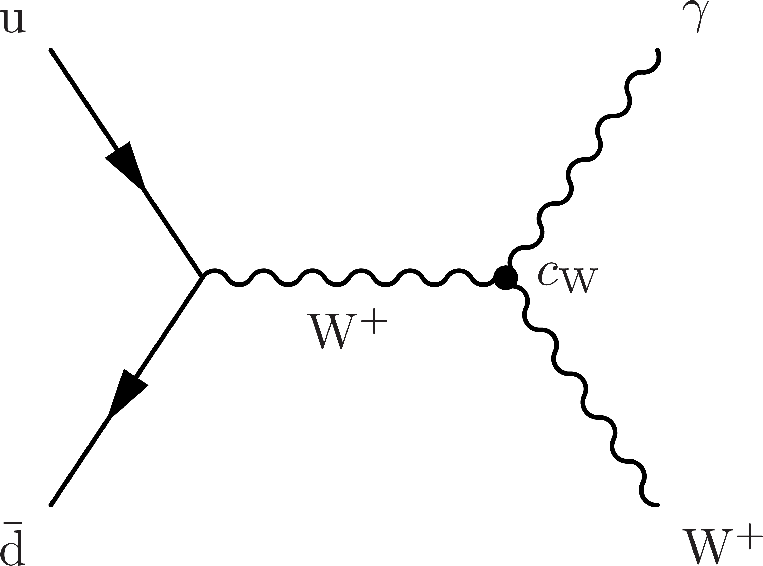
Figure 1-a:
Example Feynman diagrams of modifications of SM processes by the SMEFT operator $ \mathcal{Q}_{\mathrm{W}} $: $ \mathrm{W}\gamma $ production (left), WW production (centre), $ \mathrm{H}\to\gamma\gamma $ decay (right). The WC $ c_{\mathrm{W}} $ controls the strength of the interaction. |
png pdf |
Figure 1-b:
Example Feynman diagrams of modifications of SM processes by the SMEFT operator $ \mathcal{Q}_{\mathrm{W}} $: $ \mathrm{W}\gamma $ production (left), WW production (centre), $ \mathrm{H}\to\gamma\gamma $ decay (right). The WC $ c_{\mathrm{W}} $ controls the strength of the interaction. |
png pdf |
Figure 1-c:
Example Feynman diagrams of modifications of SM processes by the SMEFT operator $ \mathcal{Q}_{\mathrm{W}} $: $ \mathrm{W}\gamma $ production (left), WW production (centre), $ \mathrm{H}\to\gamma\gamma $ decay (right). The WC $ c_{\mathrm{W}} $ controls the strength of the interaction. |
png pdf |
Figure 2:
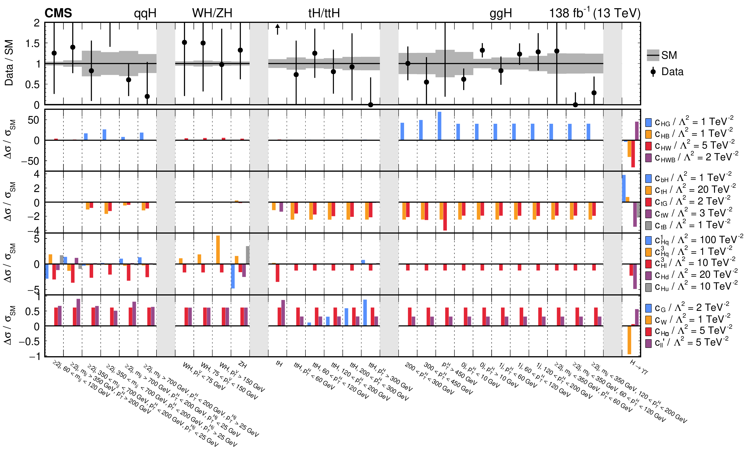
Relative effect of the linear SMEFT terms for the WCs that affect the Higgs STXS cross sections and the $ \mathrm{H}\to\gamma\gamma $ branching fraction. The parameters $ c_j/\Lambda^2 $ are set to different values to ensure the effect of all WCs can be visualized on the same $ y $ axis scale. The upper panel shows the measured values and their uncertainties relative to the predictions in the SM. As these are measurements of the cross sections times branching fraction, no measurement is displayed in the rightmost bin (labelled ``$ \mathrm{H}\to\gamma\gamma $''). |
png pdf |
Figure 3:
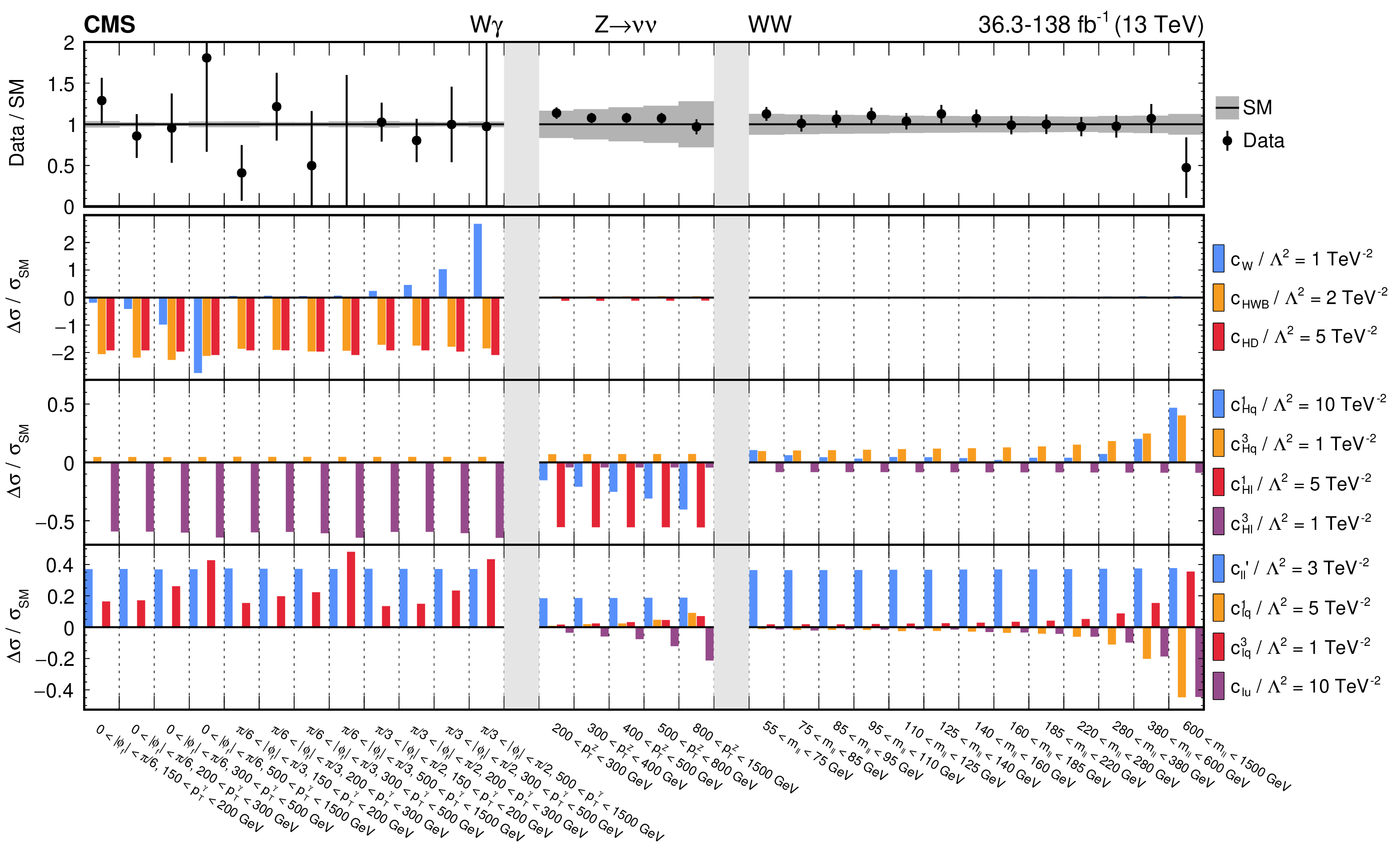
Relative effect of the linear SMEFT terms for the WCs that affect the $ \mathrm{W}\gamma $, $ \mathrm{Z}\to\nu\nu $, and WW differential cross sections. The parameters $ c_j/\Lambda^2 $ are set to different values to ensure the effect of all WCs can be visualized on the same $ y $ axis scale. The upper panel shows the measured values and their uncertainties relative to the predictions in the SM. |
png pdf |
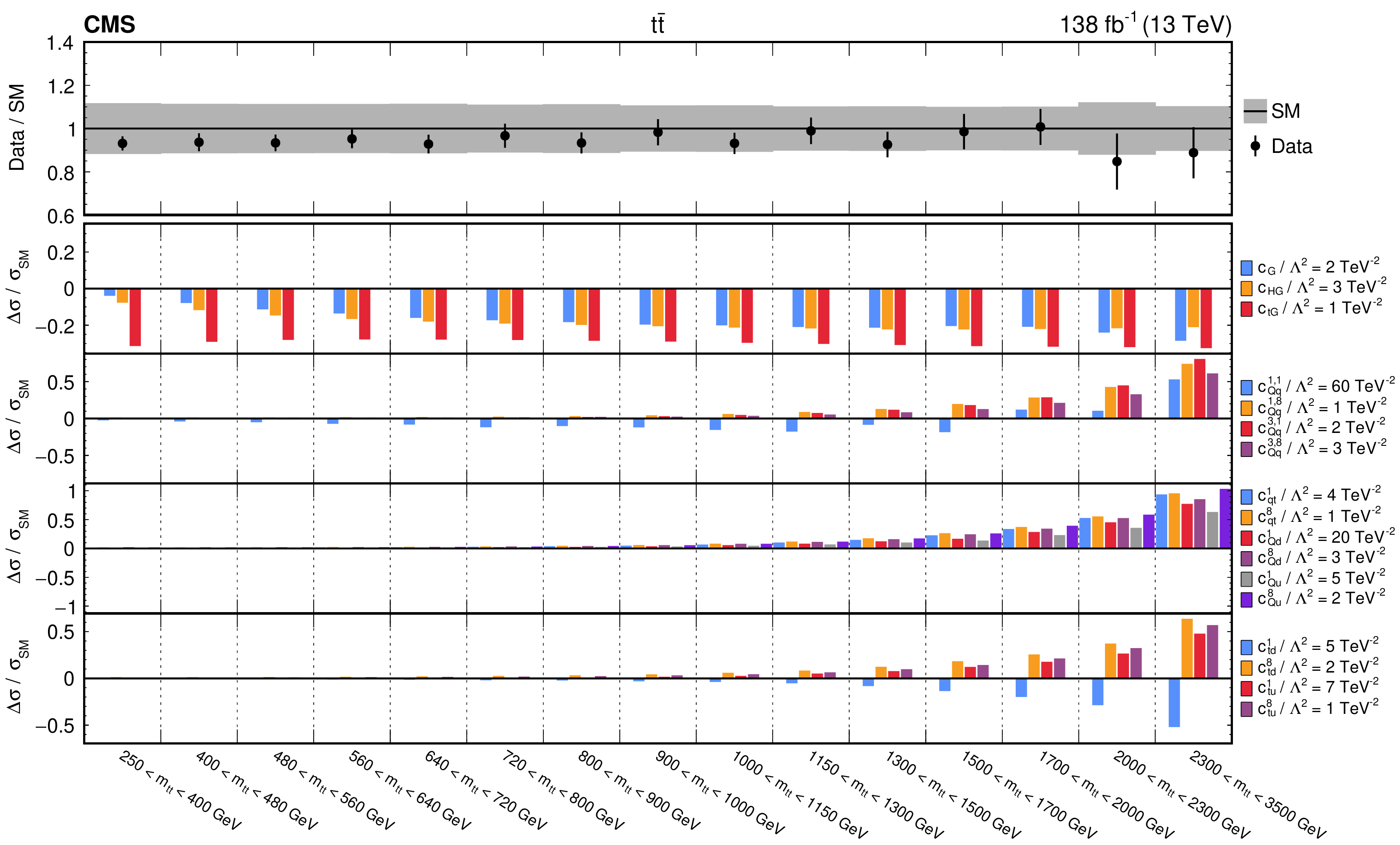
Figure 4:
Relative effect of the linear SMEFT terms for the WCs that affect the $ \mathrm{t} \overline{\mathrm{t}} $ differential cross sections. The parameters $ c_j/\Lambda^2 $ are set to different values to ensure the effect of all WCs can be visualized on the same $ y $ axis scale. The upper panel shows the measured values and their uncertainties relative to the predictions in the SM. |
png pdf |
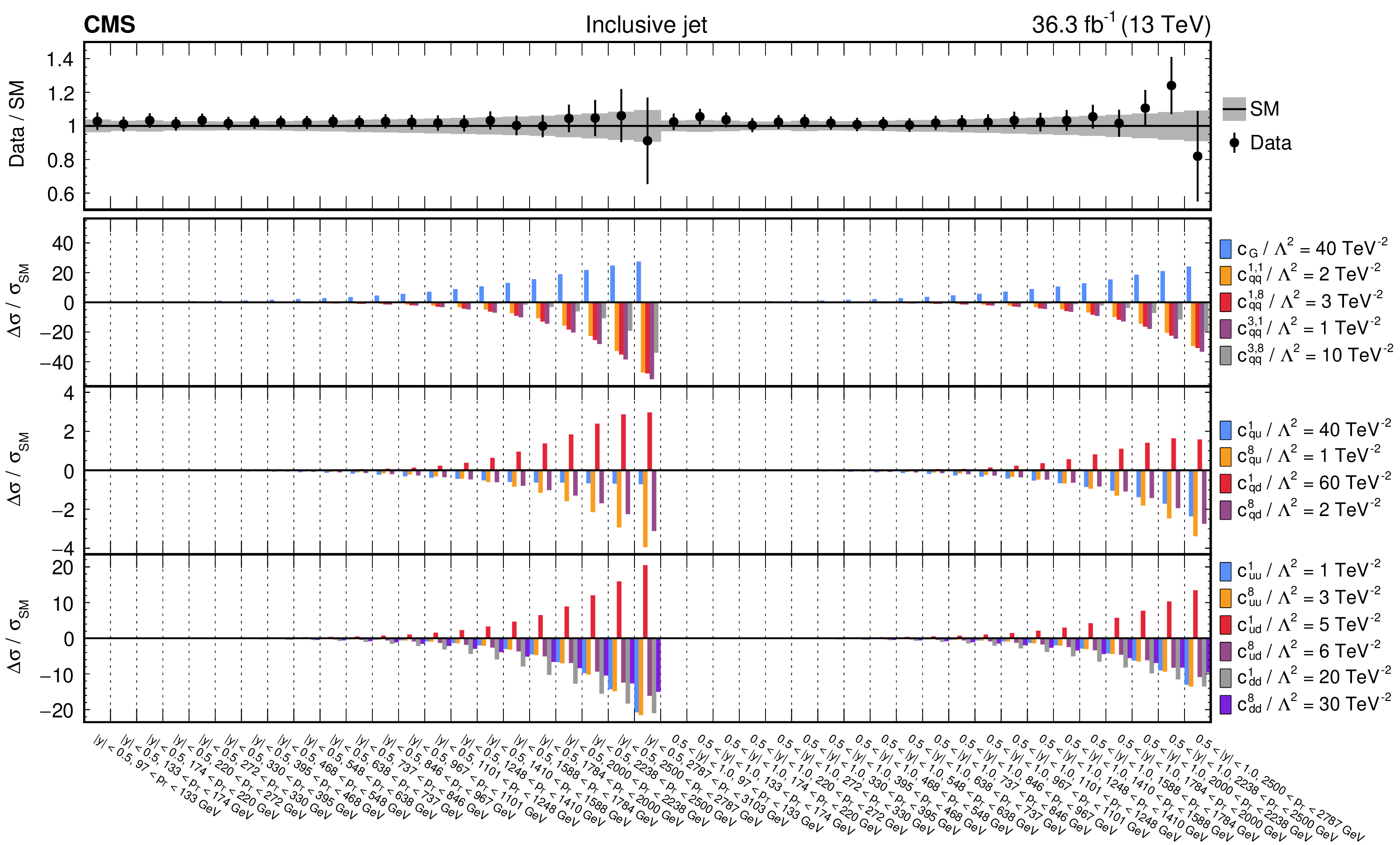
Figure 5:
Relative effect of the linear SMEFT terms for the WCs that affect the inclusive jet differential cross sections in the rapidity bins $ (0, 0.5) $ and $ (0.5, 1) $. The parameters $ c_j/\Lambda^2 $ are set to different values to ensure the effect of all WCs can be visualized on the same $ y $ axis scale. The upper panel shows the measured values and their uncertainties relative to the predictions in the SM. |
png pdf |
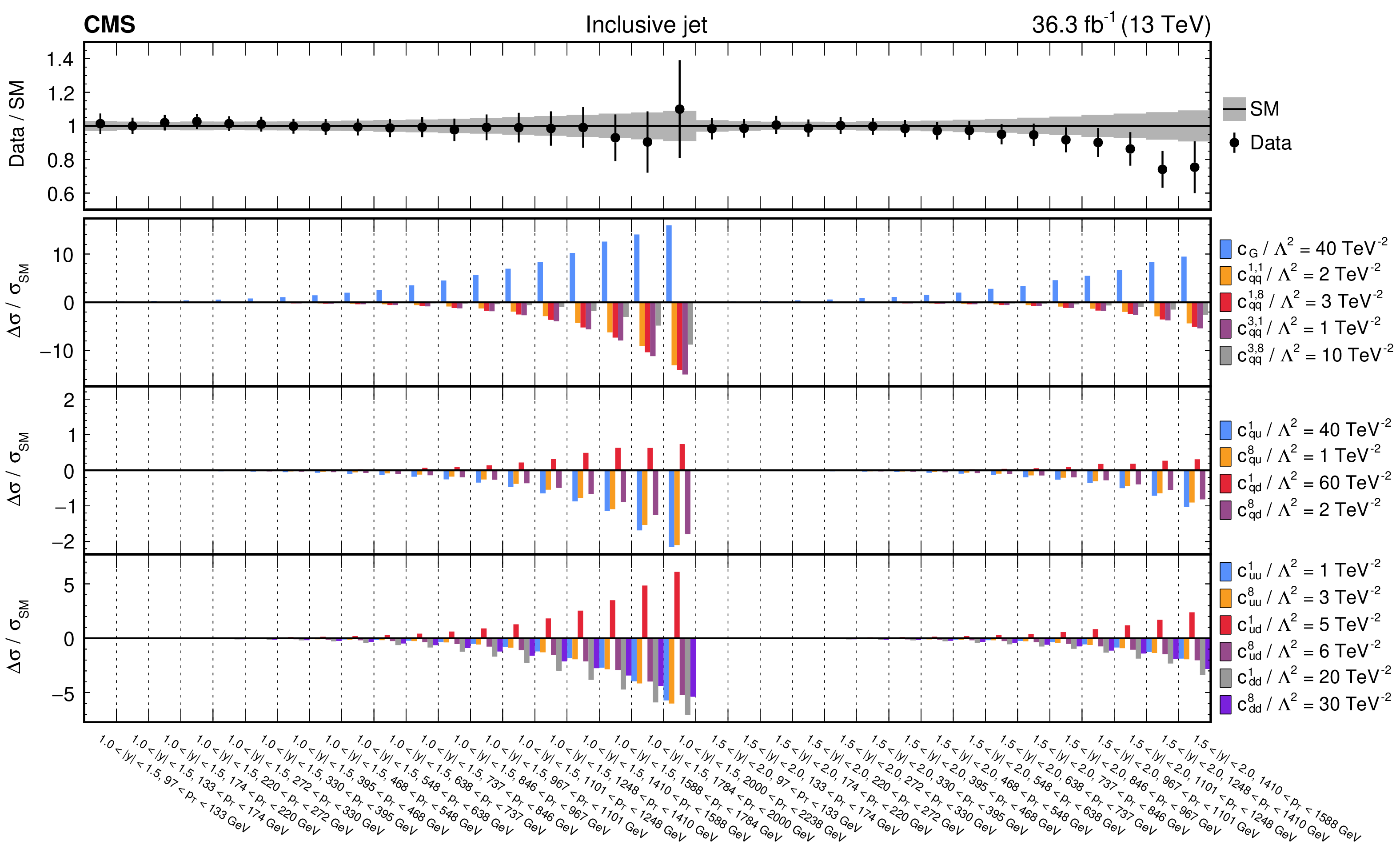
Figure 6:
Relative effect of the linear SMEFT terms for the WCs that affect the inclusive jet differential cross sections in the rapidity bins $ (1, 1.5) $ and $ (1.5, 2) $. The parameters $ c_j/\Lambda^2 $ are set to different values to ensure the effect of all WCs can be visualized on the same $ y $ axis scale. The upper panel shows the measured values and their uncertainties relative to the predictions in the SM. |
png pdf |
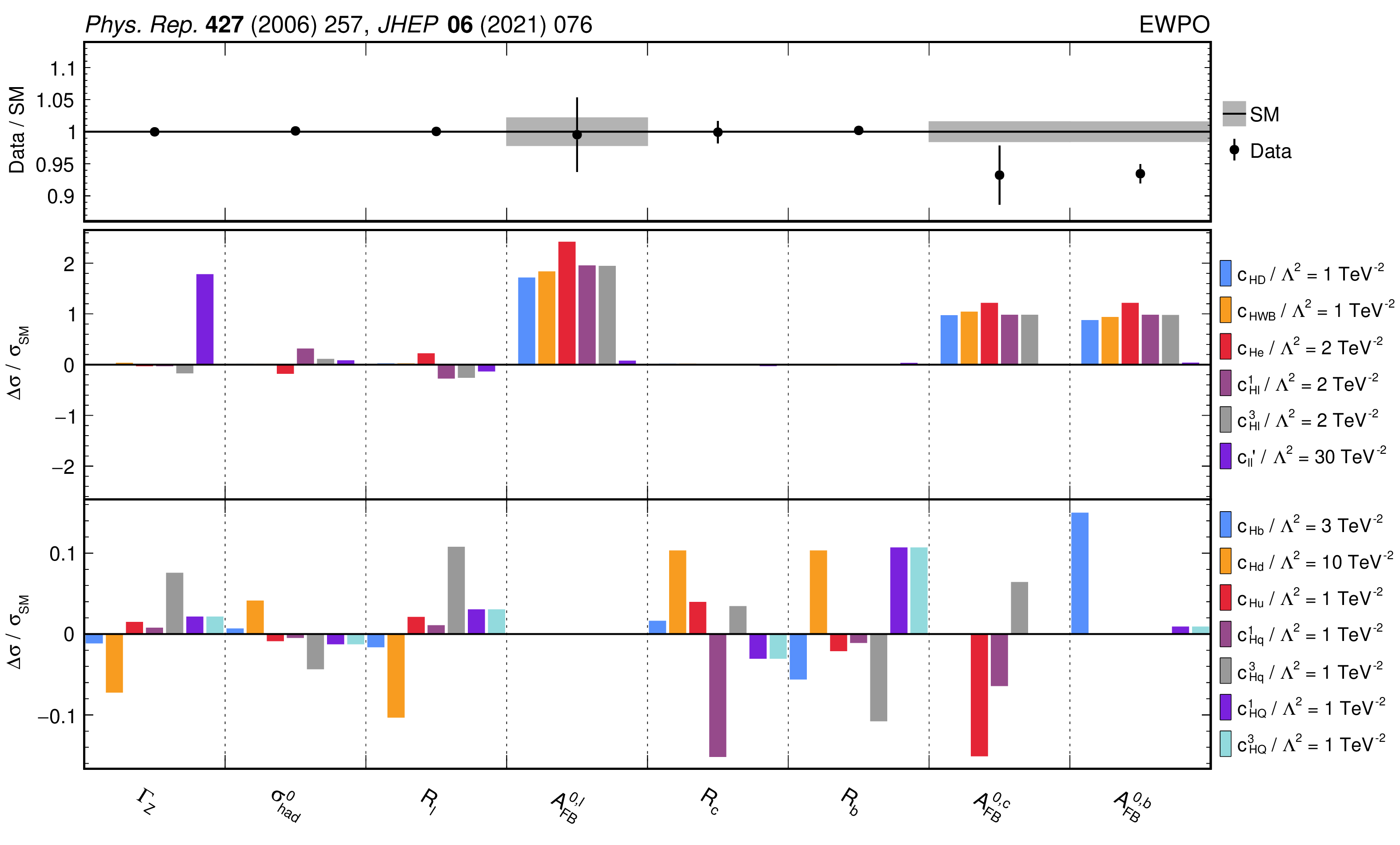
Figure 7:
Relative effect of the linear SMEFT terms for the WCs that affect the EWPO [37,38,39]. The parameters $ c_j/\Lambda^2 $ are set to different values to ensure the effect of all WCs can be visualized on the same $ y $ axis scale. The upper panel shows the measured values and their uncertainties relative to the predictions in the SM. |
png pdf |
Figure 8:
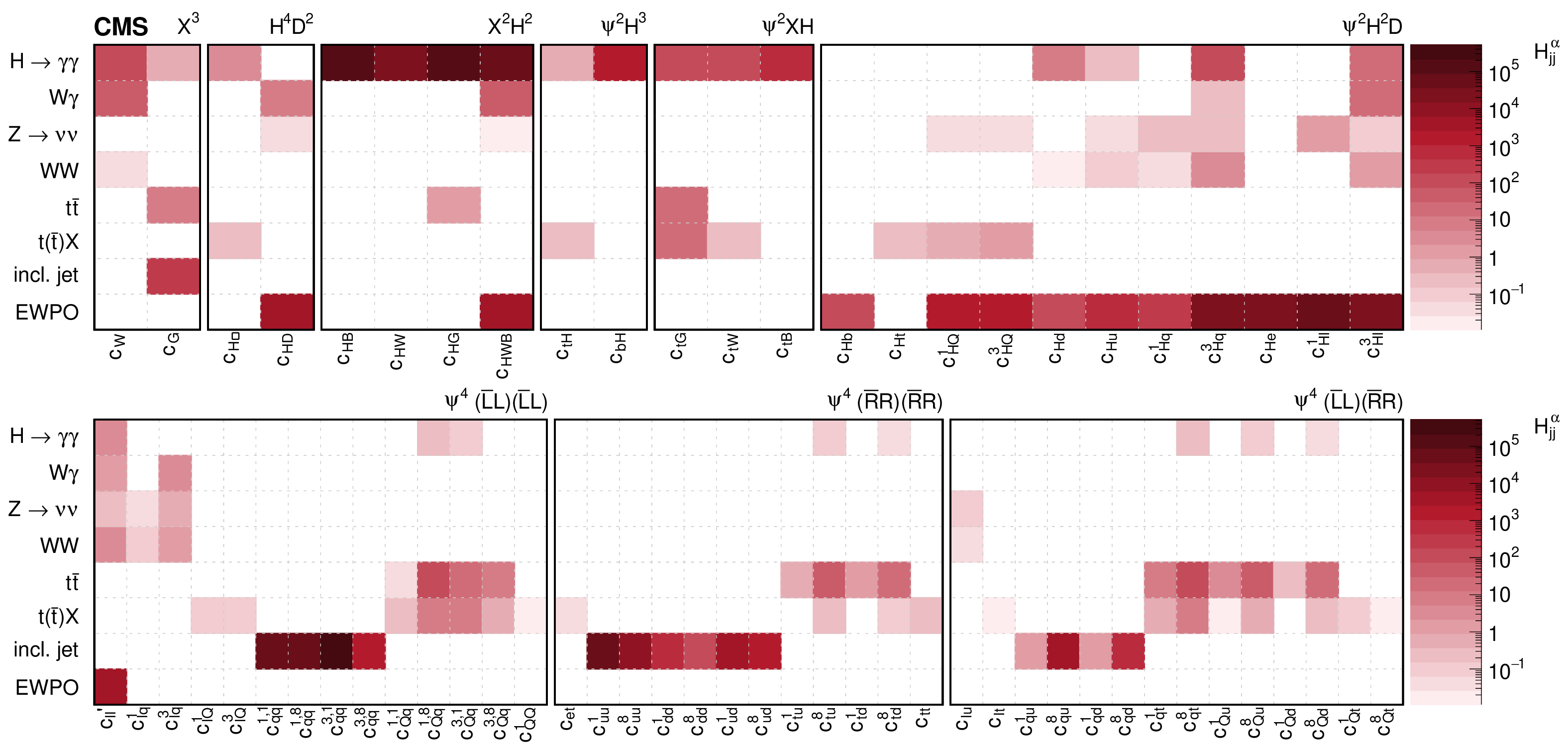
Diagonal entries $ H_{jj}^{\alpha} $ of the Hessian matrix evaluated for each input channel. These indicate which of the input channels are expected to be the most sensitive to any given operator. Larger values of $ H_{jj}^{\alpha} $ correspond to higher sensitivity. |
png pdf |
Figure 9:
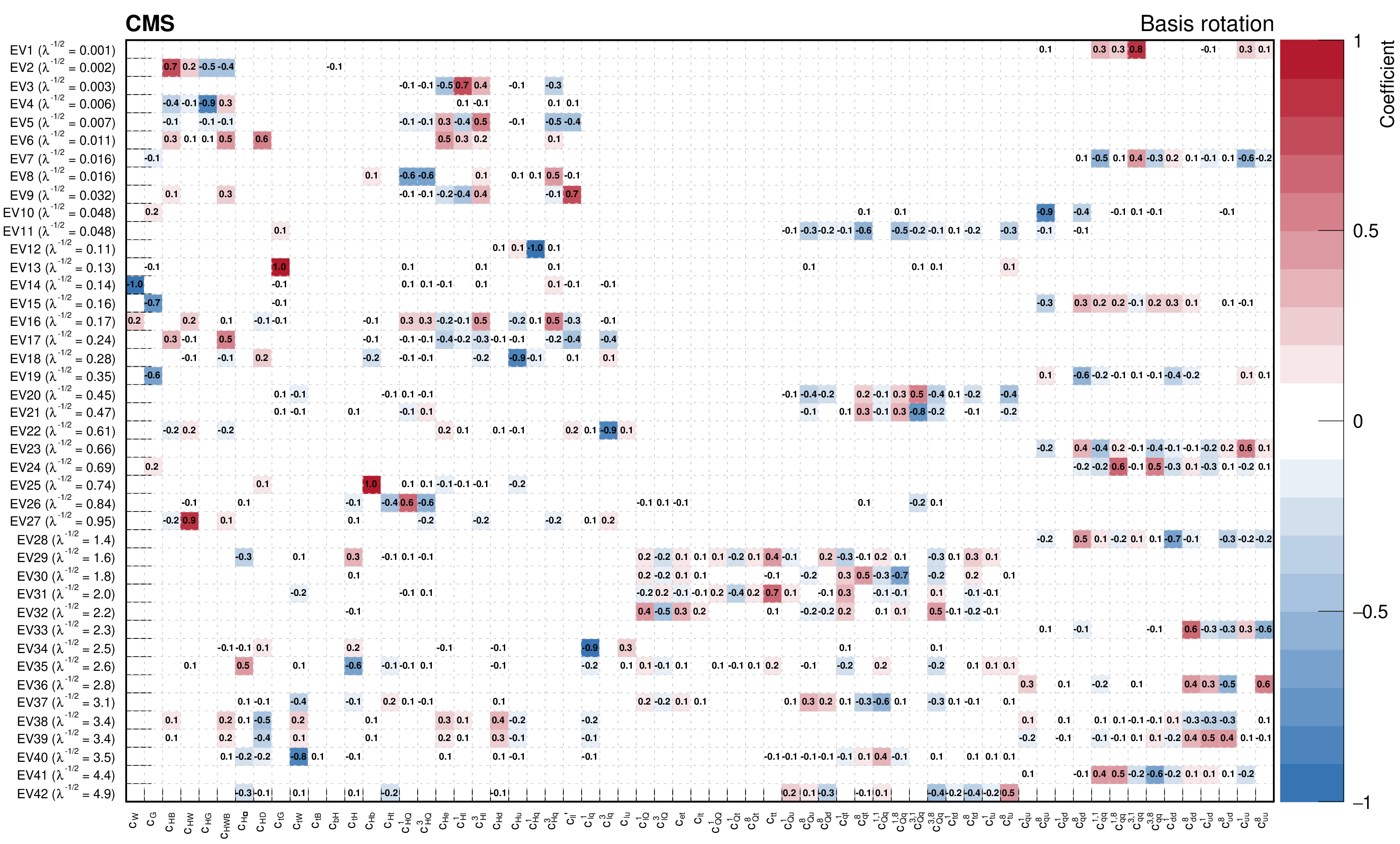
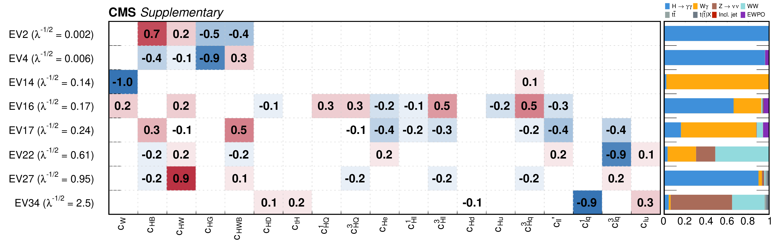
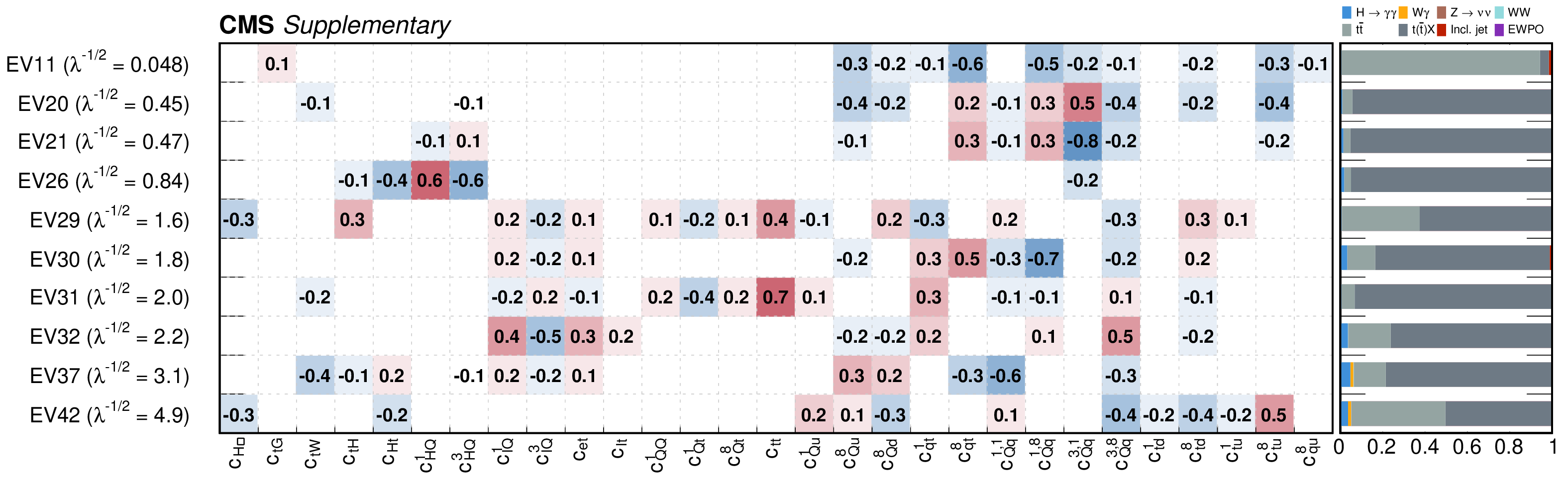
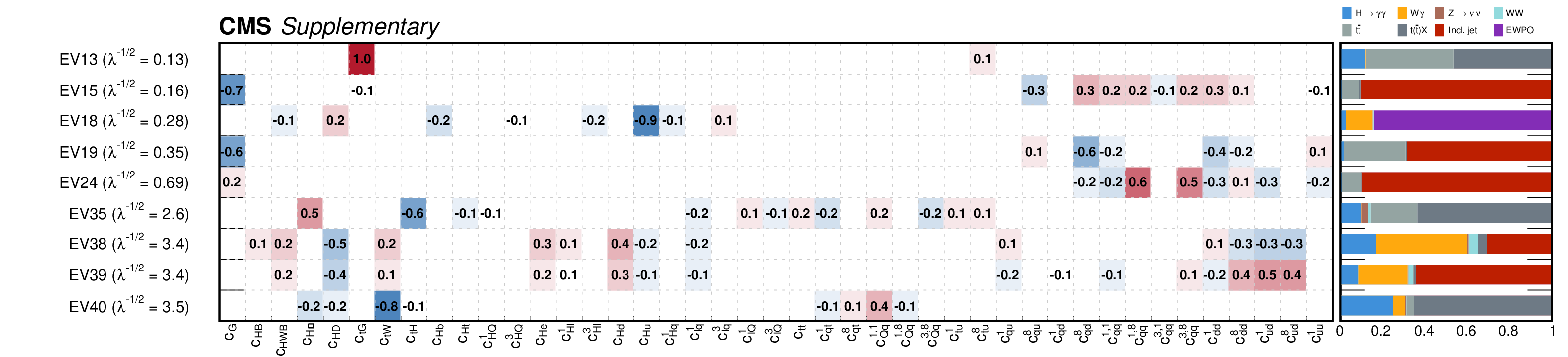
Rotation matrix obtained by performing the PCA on the Hessian matrix of the full set of measurements. Only matrix coefficients with absolute value $ {\geq} $ 0.05 are displayed. |
png pdf |
Figure 10:
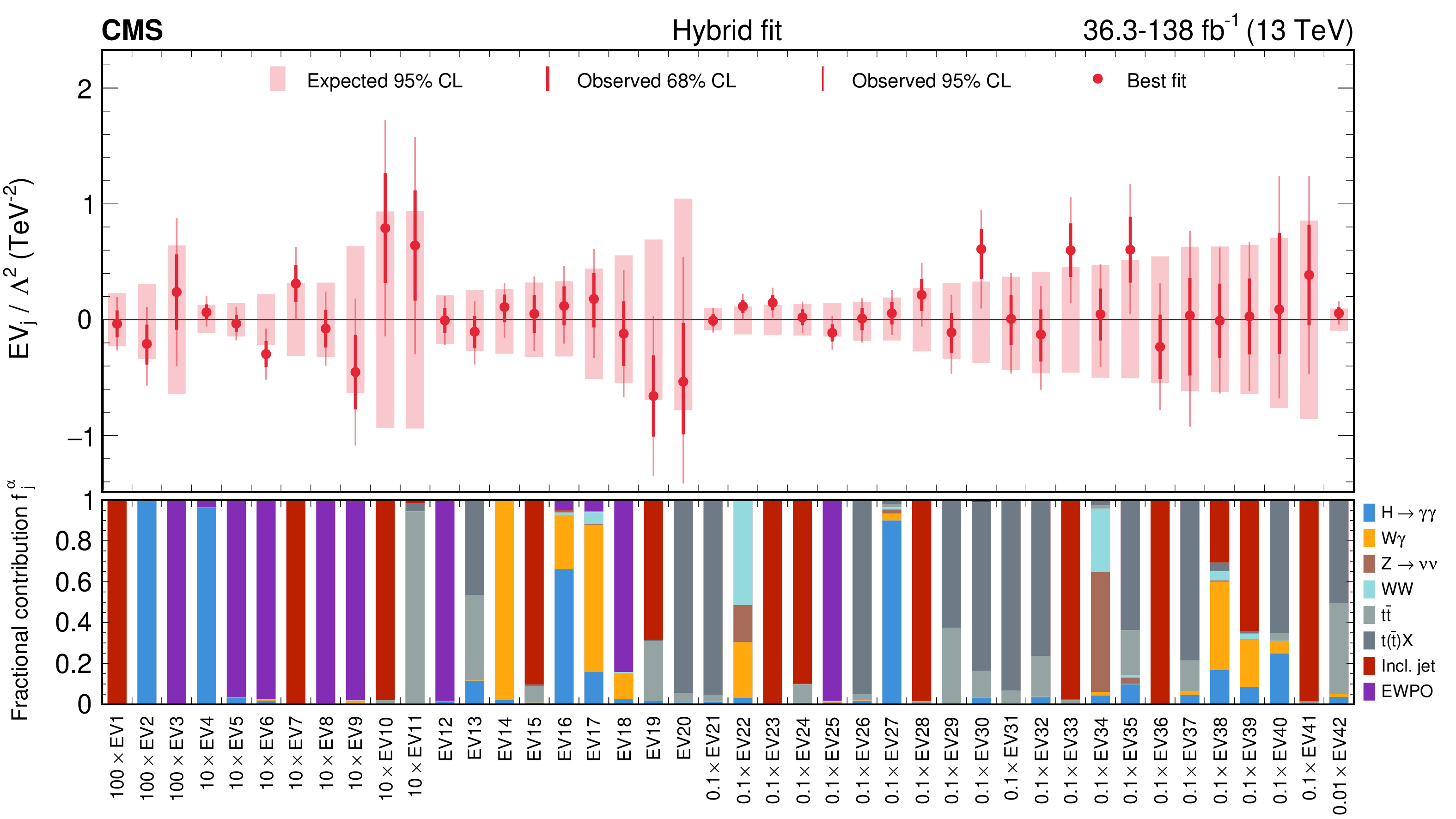
Constraints on linear combinations of WCs, for the hybrid fit including the full set of measurements. The shaded areas correspond to the expected 95% confidence intervals, the thick and thin bars to the observed 68% and 95% confidence intervals, respectively. The lower panel shows the contribution of different input measurements to the total constraints. The constraints are scaled by powers of 10 to ensure the constraints on all 43 eigenvectors can be visualized on the same $ y $ axis scale. |
png pdf |
Figure 11:
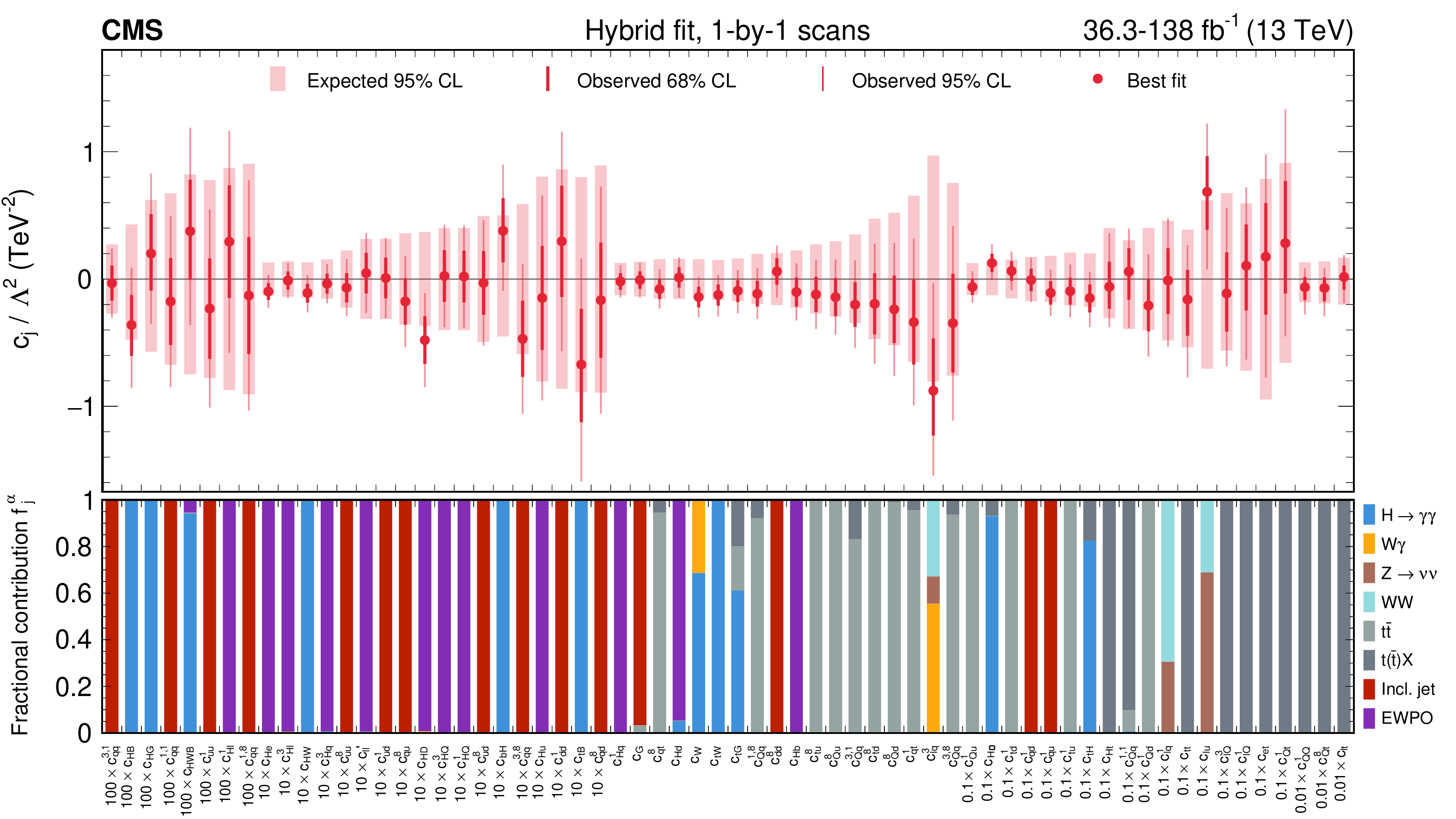
Constraints on individual WCs, for the hybrid fit including the full set of measurements. The constraints for each WC are obtained keeping the other coefficients fixed to 0. The shaded areas correspond to the expected 95% confidence intervals, the thick and thin bars to the observed 68% and 95% confidence intervals, respectively. The lower panel shows the contribution of different input measurements to the total constraints. The constraints are scaled by powers of 10 to ensure the constraints on all 64 WCs can be visualized on the same $ y $ axis scale. |
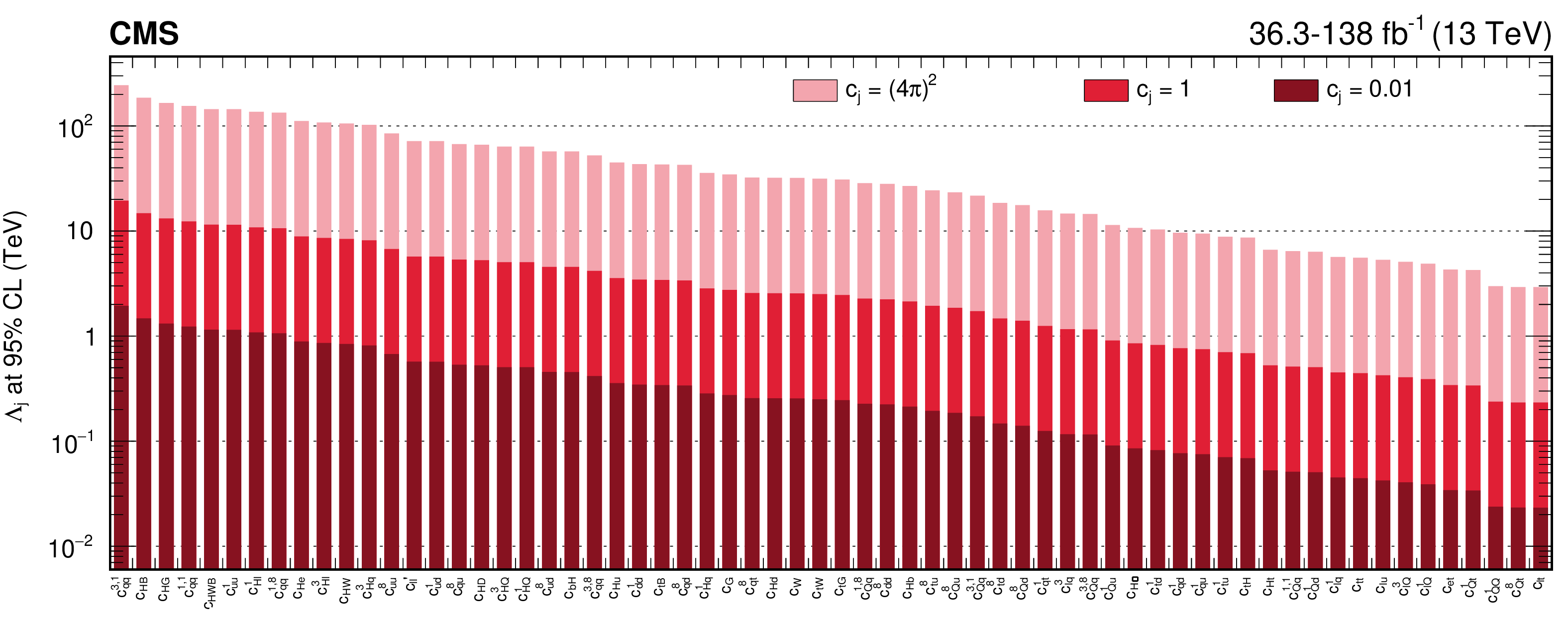
png pdf |
Figure 12:
The 95% CL lower limits on the scales $ \Lambda_j $ for the indicated values of the WCs $ c_j $. |
png pdf |
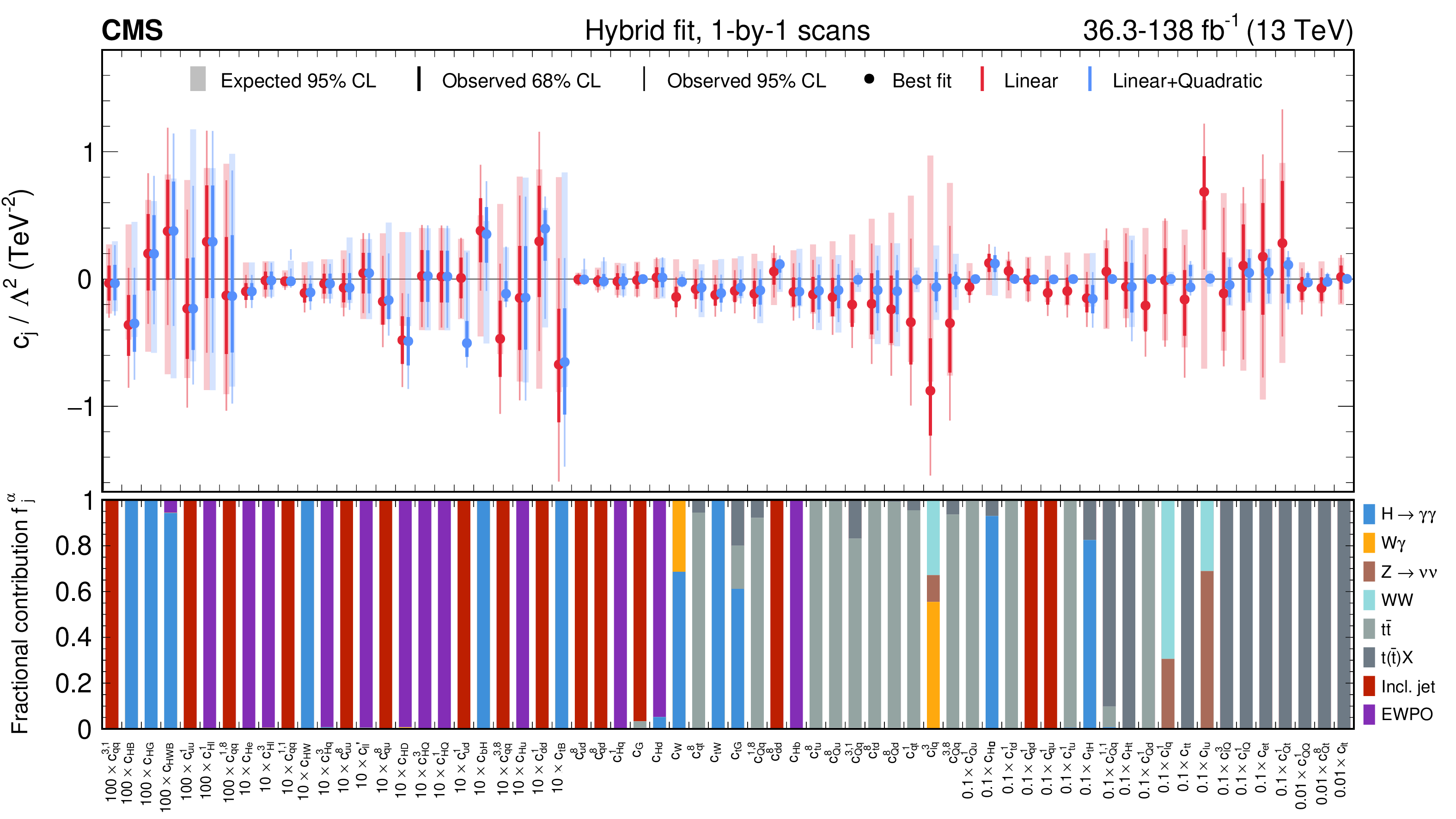
Figure 13:
Constraints on individual WCs, showing both the constraints considering only linear terms in the SMEFT parameterization and those considering both linear and quadratic terms. The constraints for each WC are obtained keeping the other coefficients fixed to 0. The shaded areas correspond to the expected 95% confidence intervals, the thick and thin bars to the observed 68% and 95% confidence intervals, respectively. The constraints are scaled by powers of 10 to ensure the constraints on all 64 WCs can be visualized on the same $ y $ axis scale. |
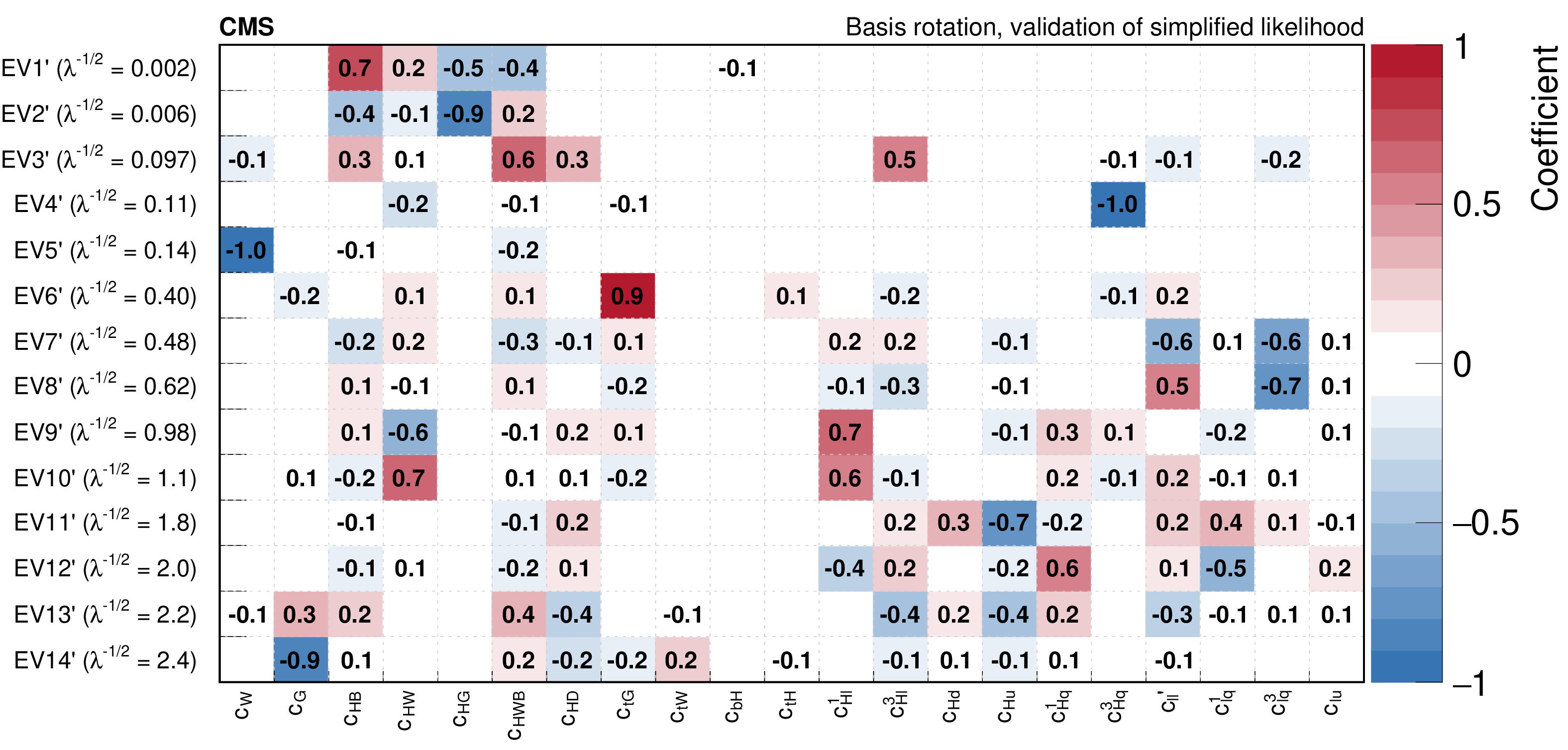
png pdf |
Figure A1:
Rotation matrix obtained by performing the PCA on the Hessian matrix of a reduced set of input measurements, $ \mathrm{H}\to\gamma\gamma $, $ \mathrm{W}\gamma $, $ \mathrm{Z}\to\nu\nu $, and WW. Only matrix coefficients with absolute value $ \geq $0.05 are displayed. |
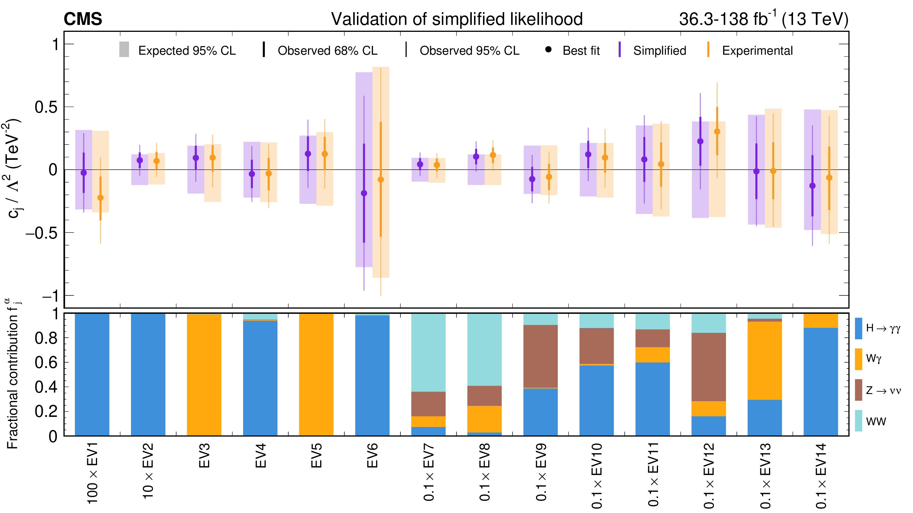
png pdf |
Figure A2:
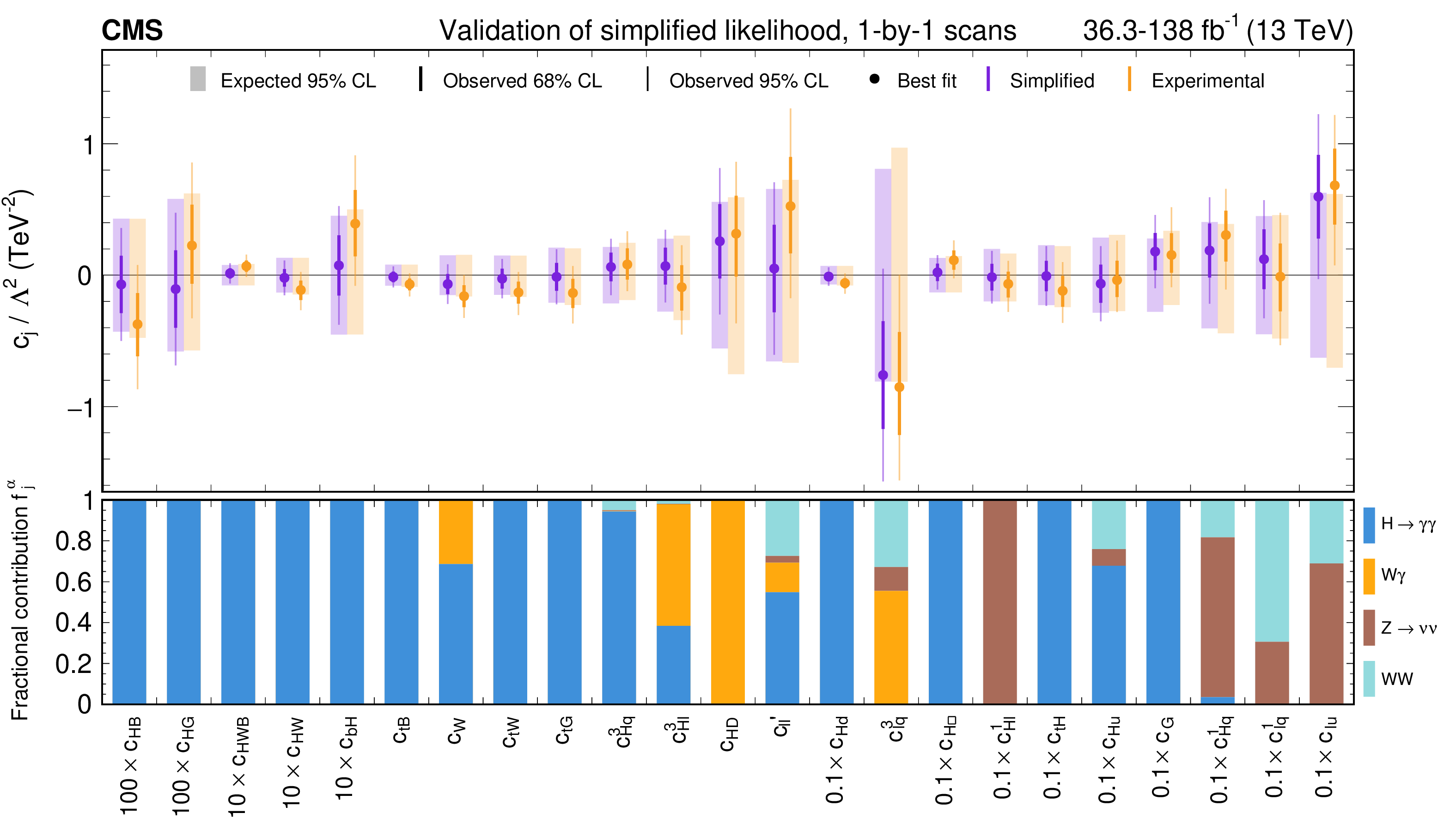
Constraints on linear combinations of WCs, using a reduced set of input measurements, $ \mathrm{H}\to\gamma\gamma $, $ \mathrm{W}\gamma $, $ \mathrm{Z}\to\nu\nu $, and WW. The shaded areas correspond to the expected 95% confidence intervals, the thick and thin bars to the observed 68% and 95% confidence intervals, respectively. The lower panel shows the contribution of different input measurements to the total constraints. The constraints are scaled by powers of 10 to ensure the constraints on all eigenvectors can be visualized on the same $ y $ axis scale. |
png pdf |
Figure A3:
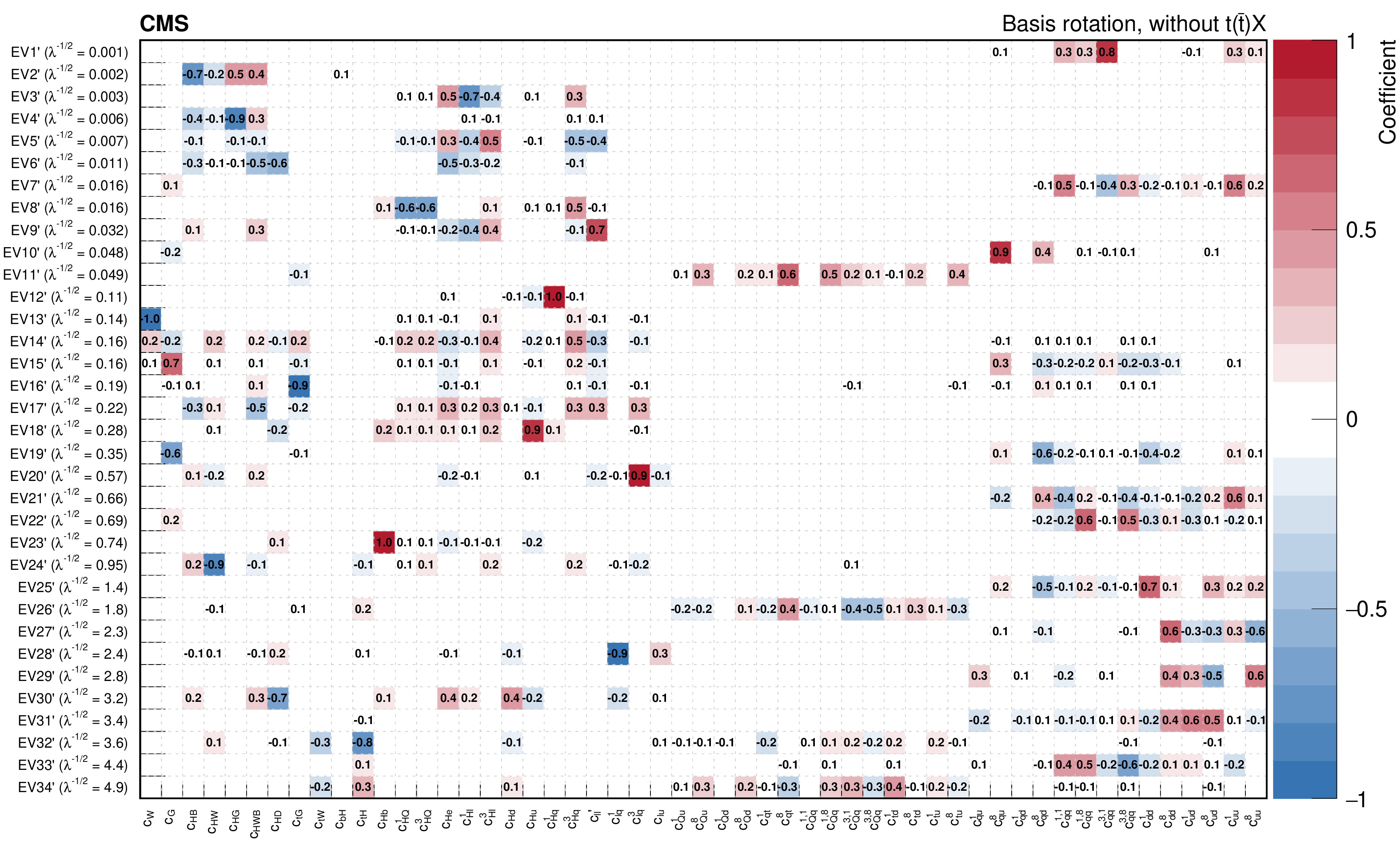
Constraints on individual WCs, using a reduced set of input measurements, $ \mathrm{H}\to\gamma\gamma $, $ \mathrm{W}\gamma $, $ \mathrm{Z}\to\nu\nu $, and WW. The constraints for each WC are obtained keeping the other coefficients fixed to 0. The shaded areas correspond to the expected 95% confidence intervals, the thick and thin bars to the observed 68% and 95% confidence intervals, respectively. The lower panel shows the contribution of different input measurements to the total constraints. The constraints are scaled by powers of 10 to ensure the constraints on all WCs can be visualized on the same $ y $ axis scale. |
png pdf |
Figure B1:
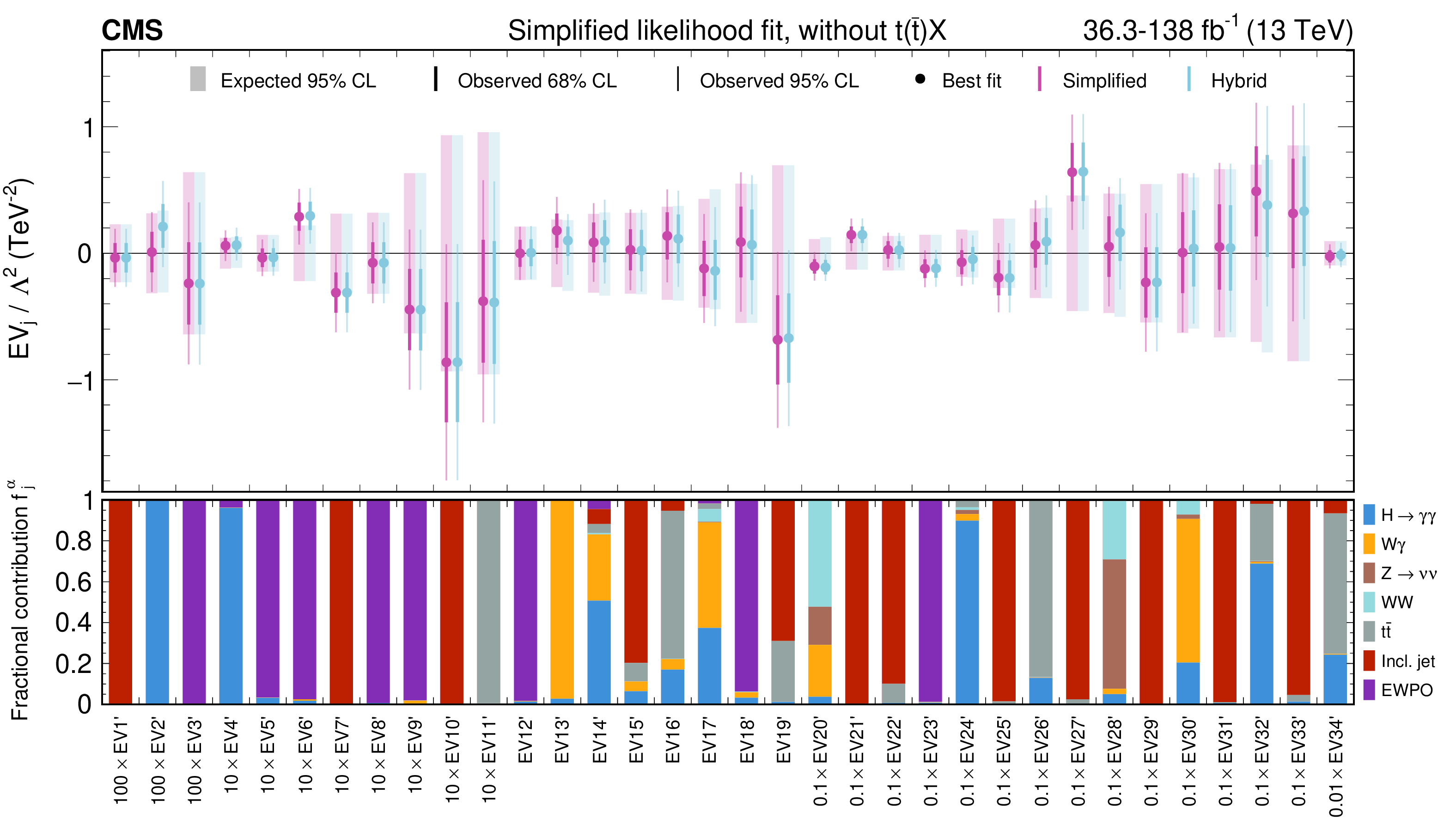
Rotation matrix obtained by performing the PCA on the Hessian matrix of a reduced set of measurements, excluding the $ \mathrm{t}(\overline{\mathrm{t}})\mathrm{X} $ measurement. Only matrix coefficients with absolute value $ \geq $0.05 are displayed. |
png pdf |
Figure B2:
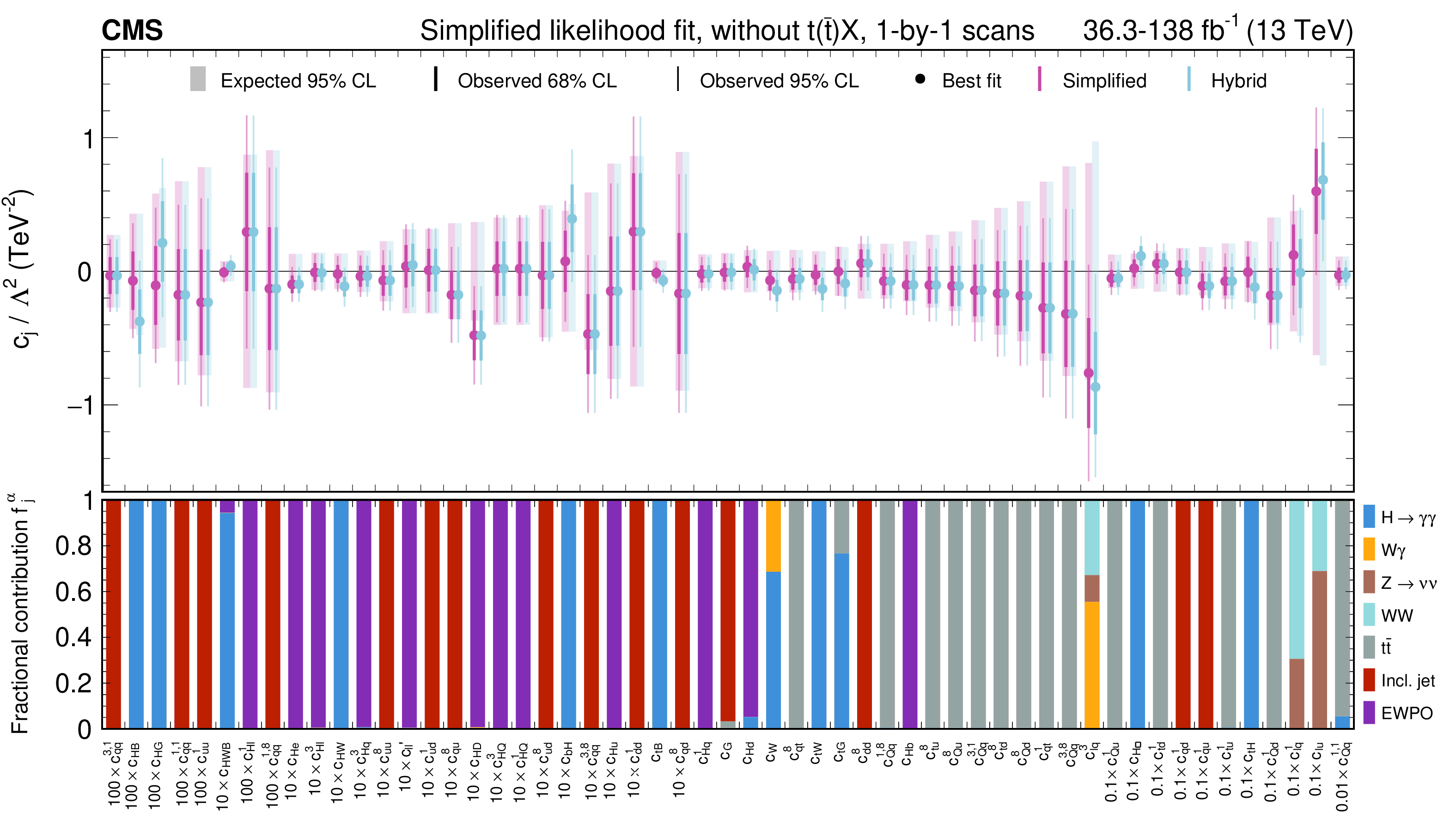
Constraints on linear combinations of WCs, from the simplified and hybrid likelihood fits, excluding the $ \mathrm{t}(\overline{\mathrm{t}})\mathrm{X} $ analysis. The shaded areas correspond to the expected 95% confidence intervals, the thick and thin bars to the observed 68% and 95% confidence intervals, respectively. The lower panel shows the contribution of different input measurements to the total constraints. The constraints are scaled by powers of 10 to ensure the constraints on all eigenvectors can be visualized on the same $ y $ axis scale. |
png pdf |
Figure B3:
Constraints on individual WCs, from the simplified and hybrid likelihood fits, excluding the $ \mathrm{t}(\overline{\mathrm{t}})\mathrm{X} $ analysis. The constraints for each WC are obtained keeping the other coefficients fixed to 0. The shaded areas correspond to the expected 95% confidence intervals, the thick and thin bars to the observed 68% and 95% confidence intervals, respectively. The lower panel shows the contribution of different input measurements to the total constraints. The constraints are scaled by powers of 10 to ensure the constraints on all WCs can be visualized on the same $ y $ axis scale. |
png pdf |
Figure C1:
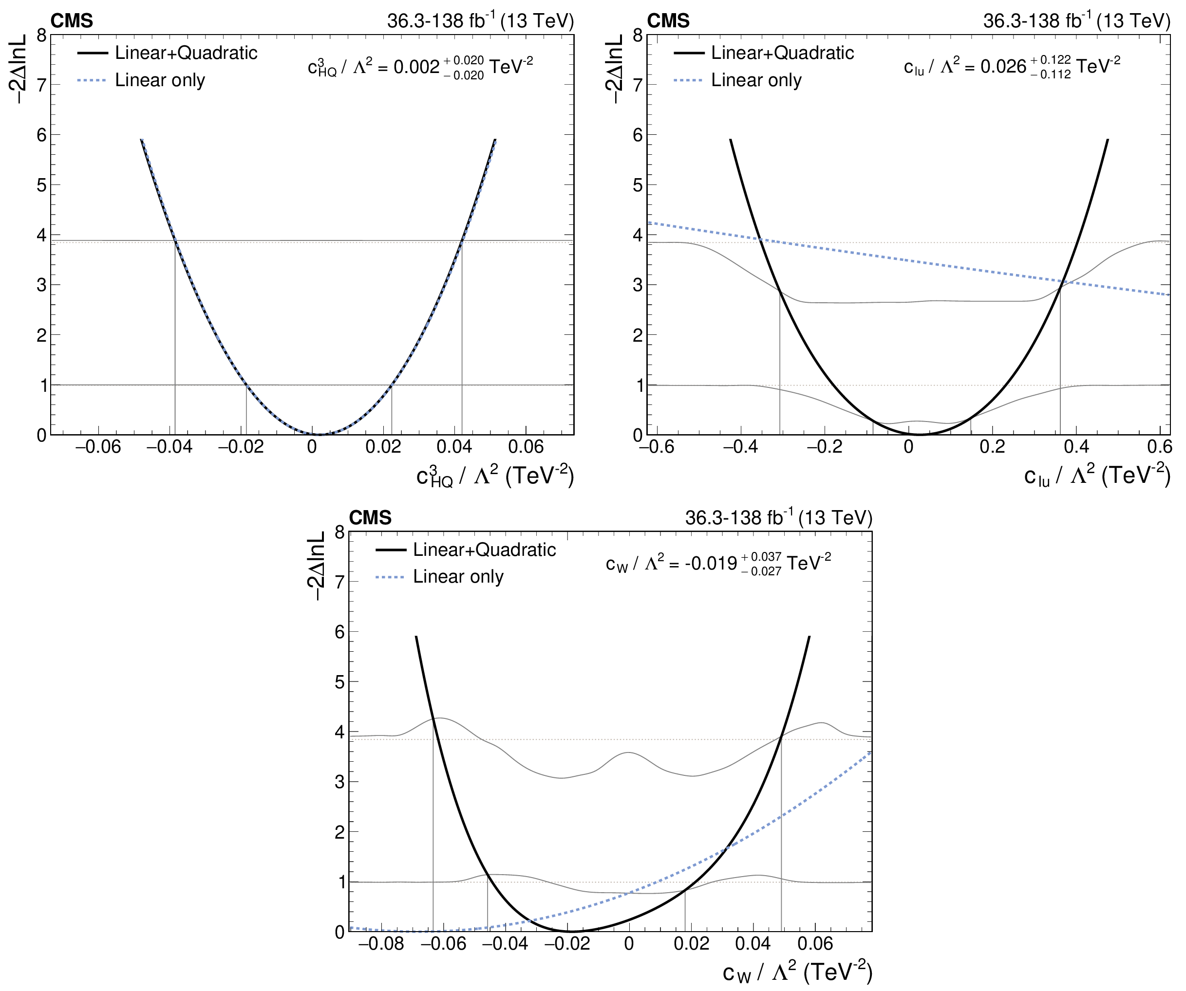
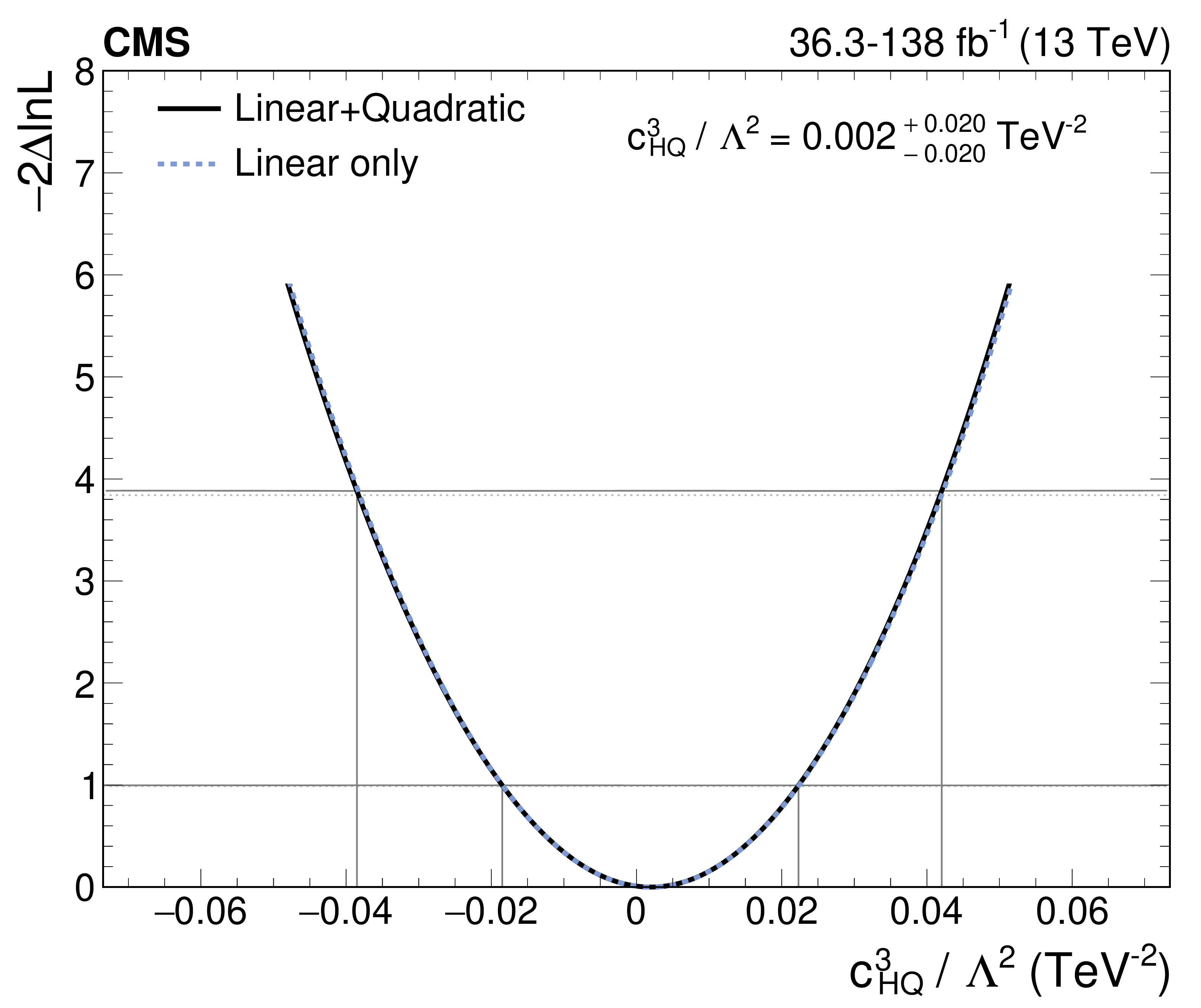
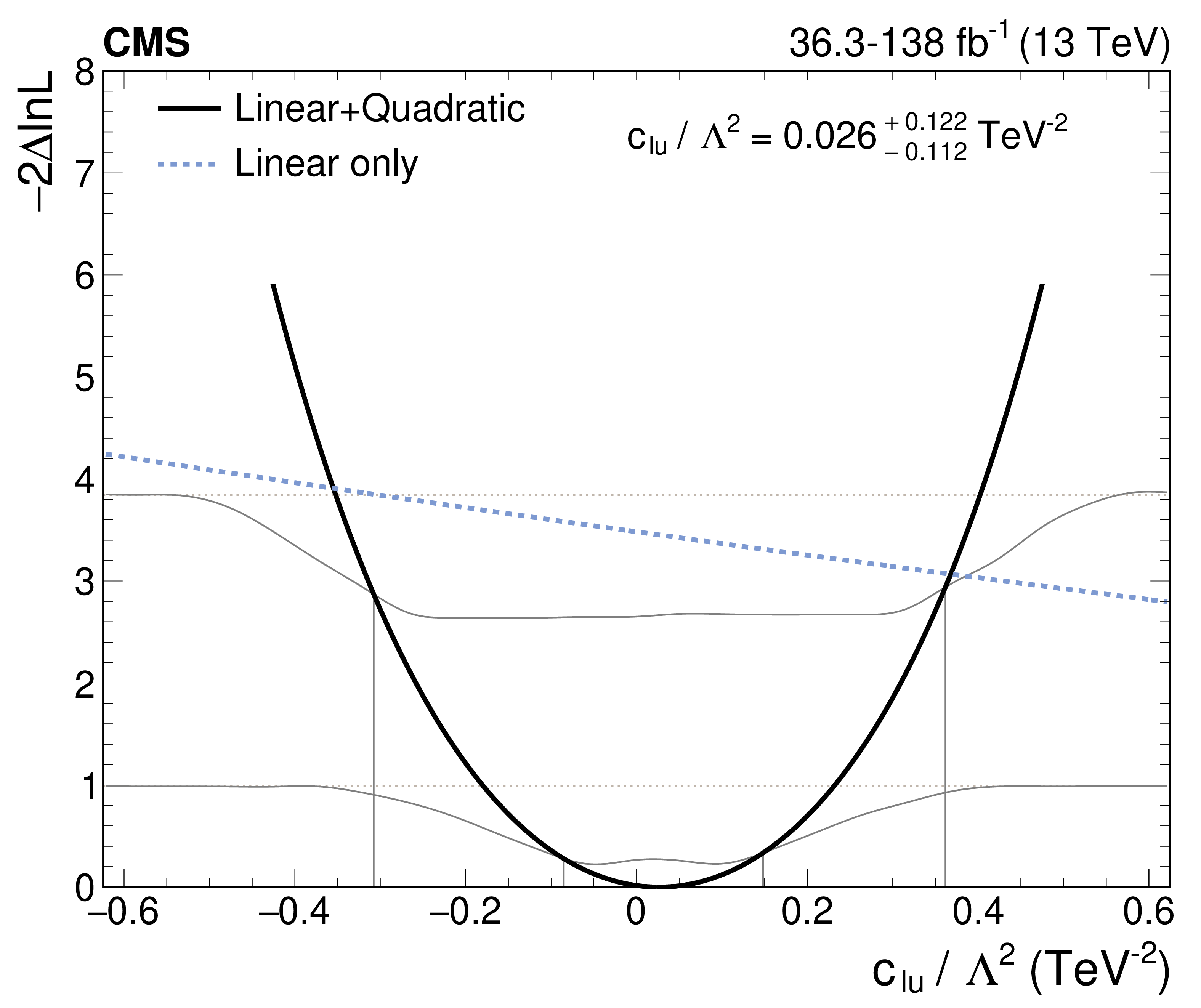
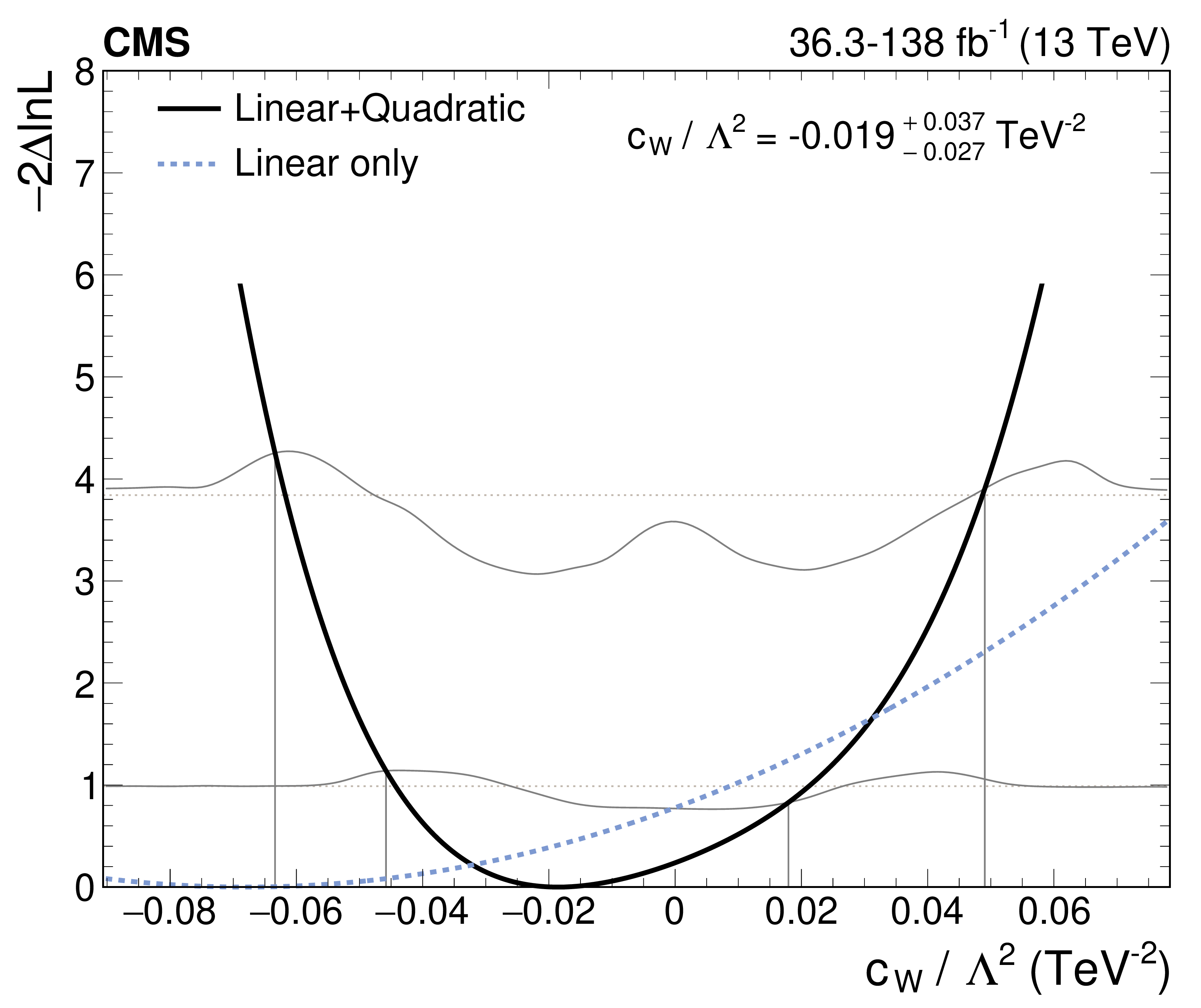
Observed likelihood scans for $ c_{\mathrm{H}\mathrm{b}} $, where linear terms dominate (upper left); $ c_{\mathrm{l}\mathrm{u}} $, where quadratic terms dominate (upper right); and $ c_{\mathrm{q}\mathrm{d}}^{(8)} $, where quadratic and linear terms both contribute (lower). The results with quadratic terms included in the parameterization (solid purple line) and with linear terms only (dashed black line) are shown. The solid grey lines indicate the sets of points $ q^{68\%} $ (lower line) and $ q^{95\%} $ (upper line), whereas the dashed grey lines denote the test statistic values used to determine the 68% and 95% confidence intervals in the asymptotic approximation. The confidence intervals shown on the figures are the 68% confidence intervals extracted from the intersection of the linear-plus-quadratic curve with the $ q ^{68\%} $ line. |
png pdf |
Figure C1-a:
Observed likelihood scans for $ c_{\mathrm{H}\mathrm{b}} $, where linear terms dominate (upper left); $ c_{\mathrm{l}\mathrm{u}} $, where quadratic terms dominate (upper right); and $ c_{\mathrm{q}\mathrm{d}}^{(8)} $, where quadratic and linear terms both contribute (lower). The results with quadratic terms included in the parameterization (solid purple line) and with linear terms only (dashed black line) are shown. The solid grey lines indicate the sets of points $ q^{68\%} $ (lower line) and $ q^{95\%} $ (upper line), whereas the dashed grey lines denote the test statistic values used to determine the 68% and 95% confidence intervals in the asymptotic approximation. The confidence intervals shown on the figures are the 68% confidence intervals extracted from the intersection of the linear-plus-quadratic curve with the $ q ^{68\%} $ line. |
png pdf |
Figure C1-b:
Observed likelihood scans for $ c_{\mathrm{H}\mathrm{b}} $, where linear terms dominate (upper left); $ c_{\mathrm{l}\mathrm{u}} $, where quadratic terms dominate (upper right); and $ c_{\mathrm{q}\mathrm{d}}^{(8)} $, where quadratic and linear terms both contribute (lower). The results with quadratic terms included in the parameterization (solid purple line) and with linear terms only (dashed black line) are shown. The solid grey lines indicate the sets of points $ q^{68\%} $ (lower line) and $ q^{95\%} $ (upper line), whereas the dashed grey lines denote the test statistic values used to determine the 68% and 95% confidence intervals in the asymptotic approximation. The confidence intervals shown on the figures are the 68% confidence intervals extracted from the intersection of the linear-plus-quadratic curve with the $ q ^{68\%} $ line. |
png pdf |
Figure C1-c:
Observed likelihood scans for $ c_{\mathrm{H}\mathrm{b}} $, where linear terms dominate (upper left); $ c_{\mathrm{l}\mathrm{u}} $, where quadratic terms dominate (upper right); and $ c_{\mathrm{q}\mathrm{d}}^{(8)} $, where quadratic and linear terms both contribute (lower). The results with quadratic terms included in the parameterization (solid purple line) and with linear terms only (dashed black line) are shown. The solid grey lines indicate the sets of points $ q^{68\%} $ (lower line) and $ q^{95\%} $ (upper line), whereas the dashed grey lines denote the test statistic values used to determine the 68% and 95% confidence intervals in the asymptotic approximation. The confidence intervals shown on the figures are the 68% confidence intervals extracted from the intersection of the linear-plus-quadratic curve with the $ q ^{68\%} $ line. |
png pdf |
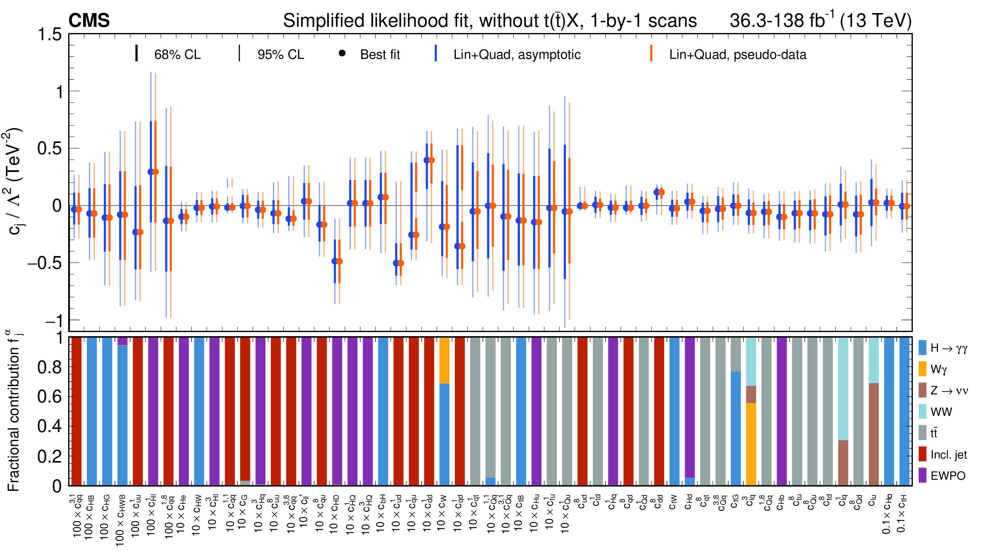
Figure C2:
Summary of best fit values and confidence intervals extracted with the asymptotic approximation (blue lines) and with the pseudo-experiment-based method described in this appendix (purple lines). The constraints are scaled by powers of 10 to ensure the constraints on all WCs can be visualized on the same $ y $ axis scale. The intervals are generally compatible with each other, with only some small differences visible. |
png pdf |
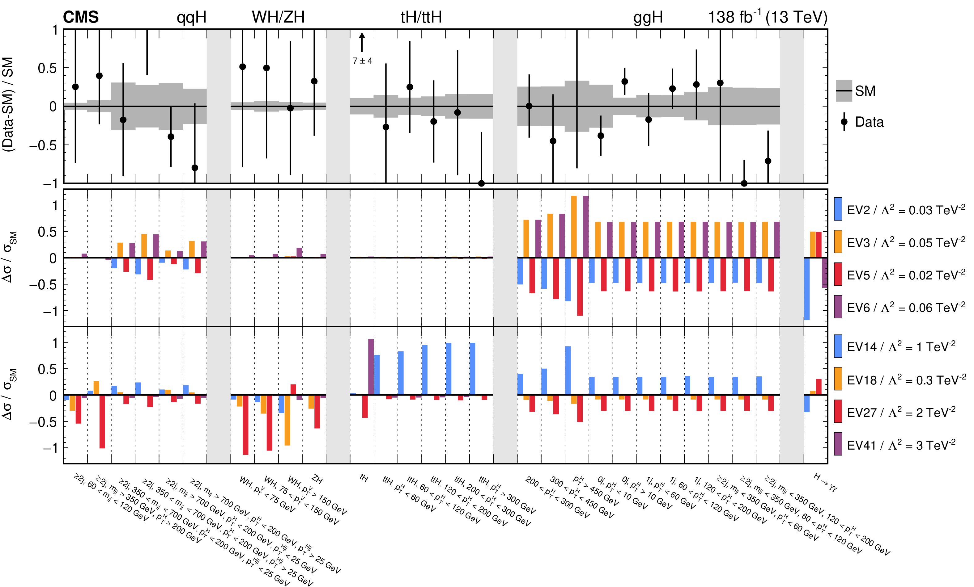
Figure D1:
Relative effect of the linear combinations of WCs that affect the Higgs STXS cross sections and the $ \mathrm{H}\to\gamma\gamma $ branching fraction. The parameters $ \mathrm{EV}_j/\Lambda^2 $ are set to different values to ensure the effect of all linear combinations can be visualized on the same $ y $ axis scale. The upper panel shows the measured values and their uncertainties relative to the predictions in the SM. As these are measurements of the cross sections times branching fraction, no measurement is displayed in the rightmost bin (labelled ``$ \mathrm{H}\to\gamma\gamma $''). |
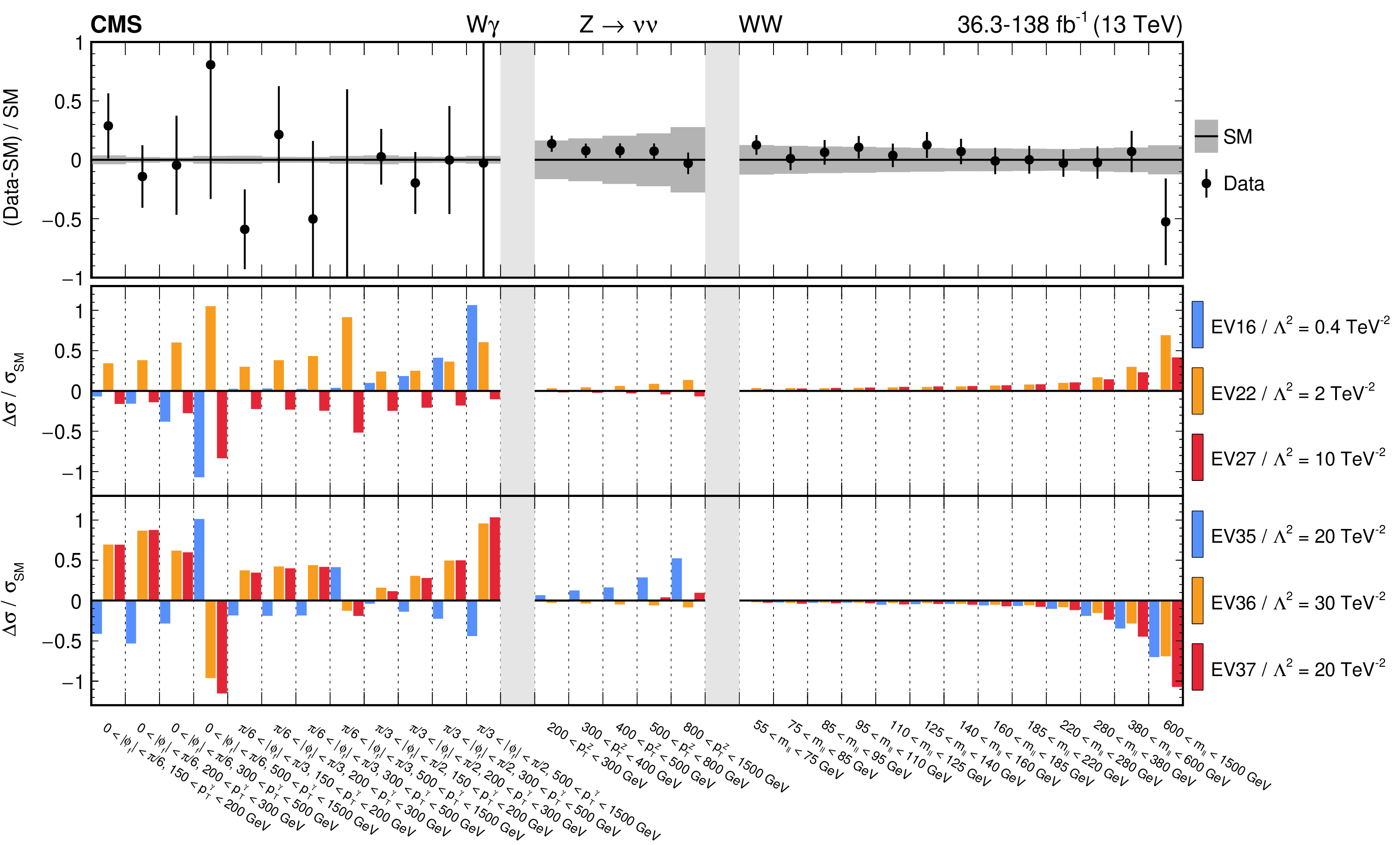
png pdf |
Figure D2:
Relative effect of the linear combinations of WCs that affect the $ \mathrm{W}\gamma $, $ \mathrm{Z}\to\nu\nu $, and WW differential cross sections. The parameters $ \mathrm{EV}_j/\Lambda^2 $ are set to different values to ensure the effect of all linear combinations can be visualized on the same $ y $ axis scale. The upper panel shows the measured values and their uncertainties relative to the predictions in the SM. |
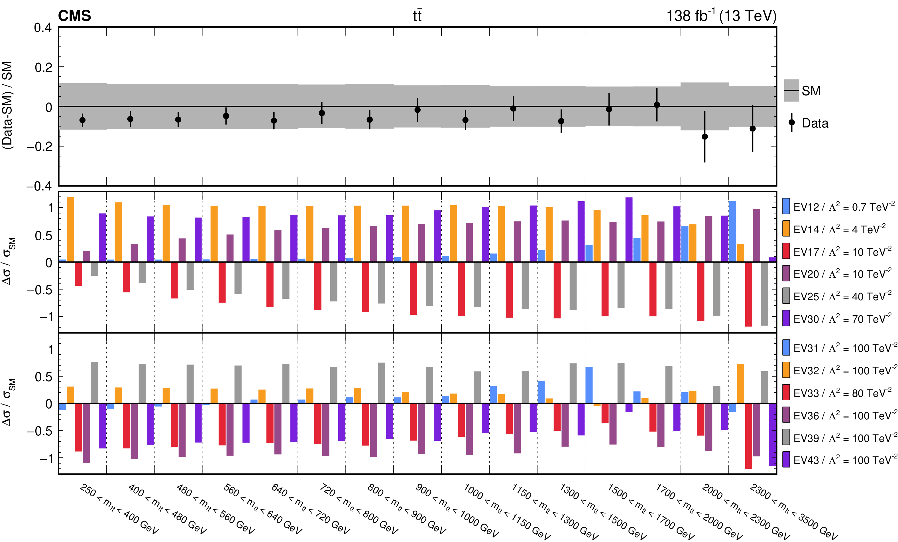
png pdf |
Figure D3:
Relative effect of the linear combinations of WCs that affect the $ \mathrm{t} \overline{\mathrm{t}} $ differential cross sections. The parameters $ \mathrm{EV}_j/\Lambda^2 $ are set to different values to ensure the effect of all linear combinations can be visualized on the same $ y $ axis scale. The upper panel shows the measured values and their uncertainties relative to the predictions in the SM. |
png pdf |
Figure D4:
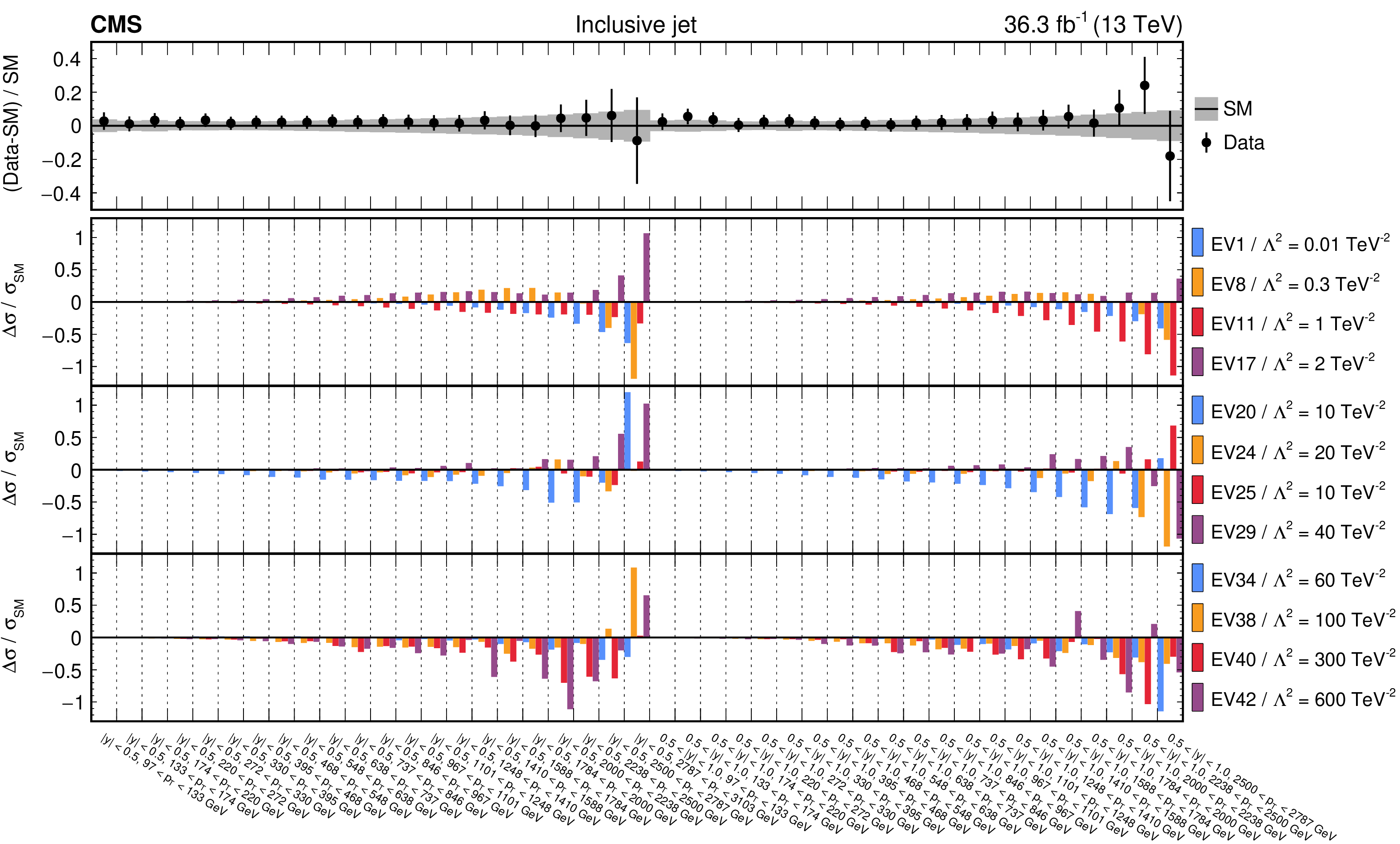
Relative effect of the linear combinations of WCs that affect the inclusive jet differential cross sections in the rapidity bins $ (0, 0.5) $ and $ (0.5, 1) $. The parameters $ \mathrm{EV}_j/\Lambda^2 $ are set to different values to ensure the effect of all linear combinations can be visualized on the same $ y $ axis scale. The upper panel shows the measured values and their uncertainties relative to the predictions in the SM. |
png pdf |
Figure D5:
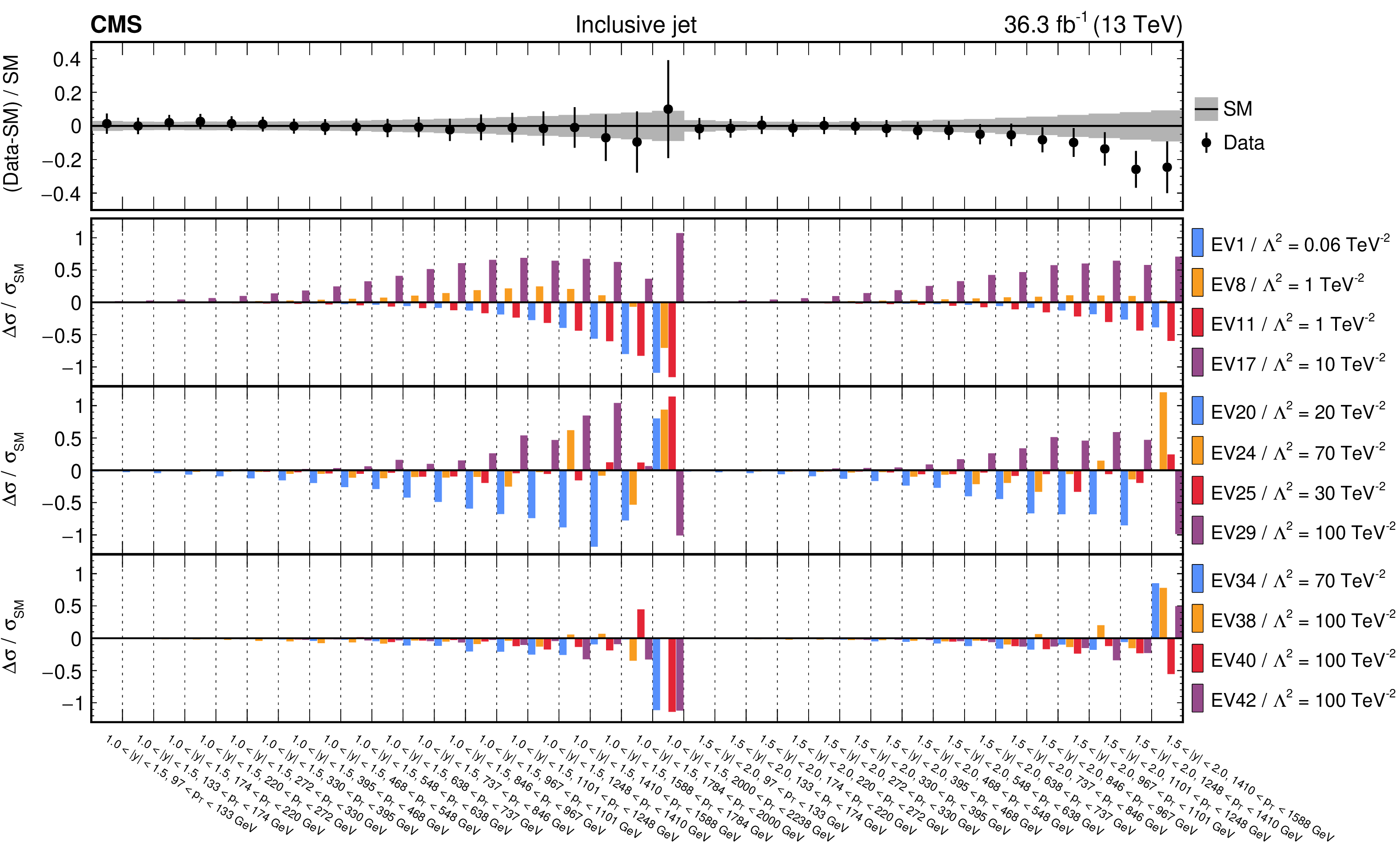
Relative effect of the linear combinations of WCs that affect the inclusive jet differential cross sections in the rapidity bins $ (1, 1.5) $ and $ (1.5, 2) $. The parameters $ \mathrm{EV}_j/\Lambda^2 $ are set to different values to ensure the effect of all linear combinations can be visualized on the same $ y $ axis scale. The upper panel shows the measured values and their uncertainties relative to the predictions in the SM. |
png pdf |
Figure D6:
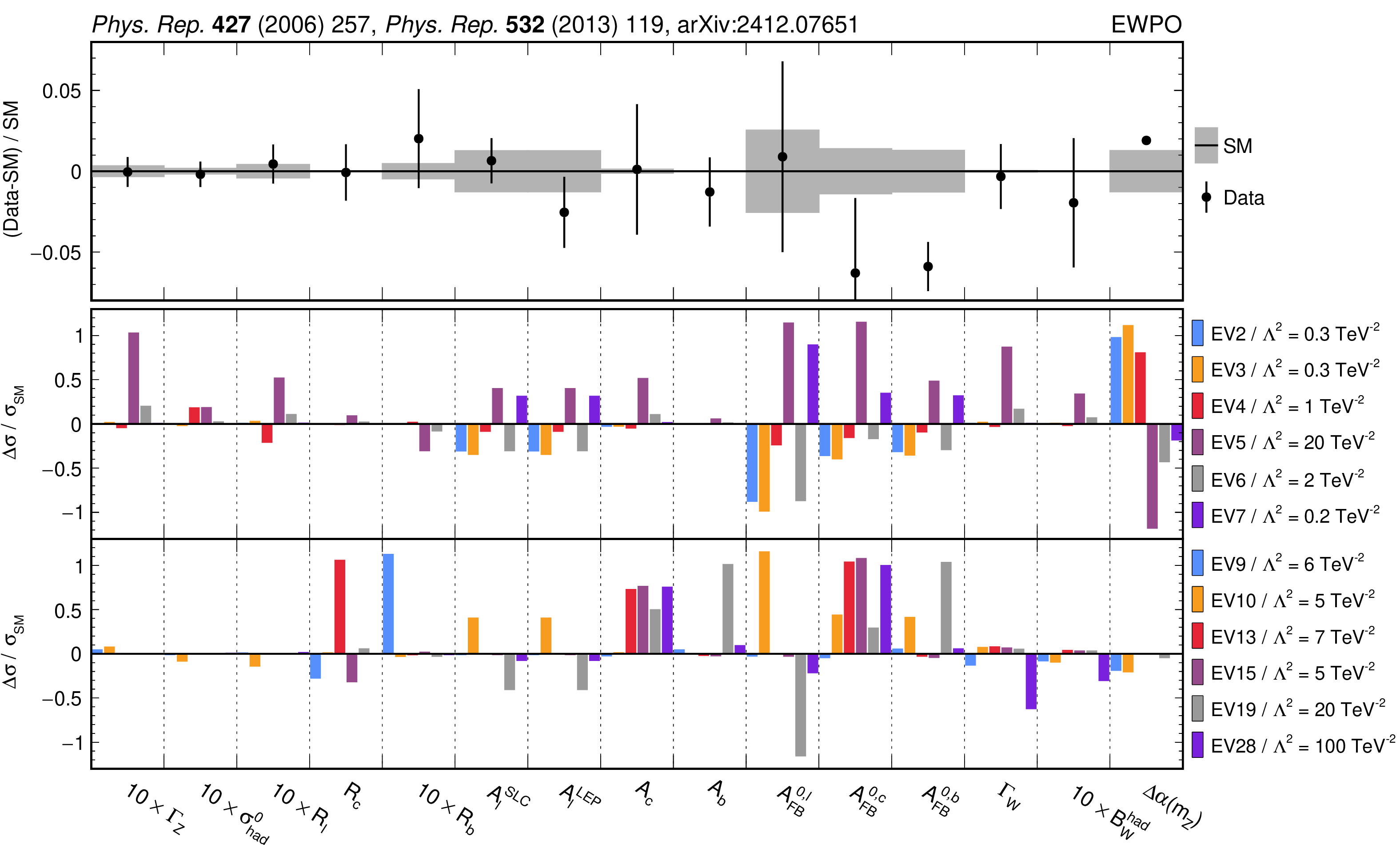
Relative effect of the linear combinations of WCs that affect the EWPO [37,38,39]. The parameters $ \mathrm{EV}_j/\Lambda^2 $ are set to different values to ensure the effect of all linear combinations can be visualized on the same $ y $ axis scale. The upper panel shows the measured values and their uncertainties relative to the predictions in the SM. |
| Tables | |
png pdf |
Table 1:
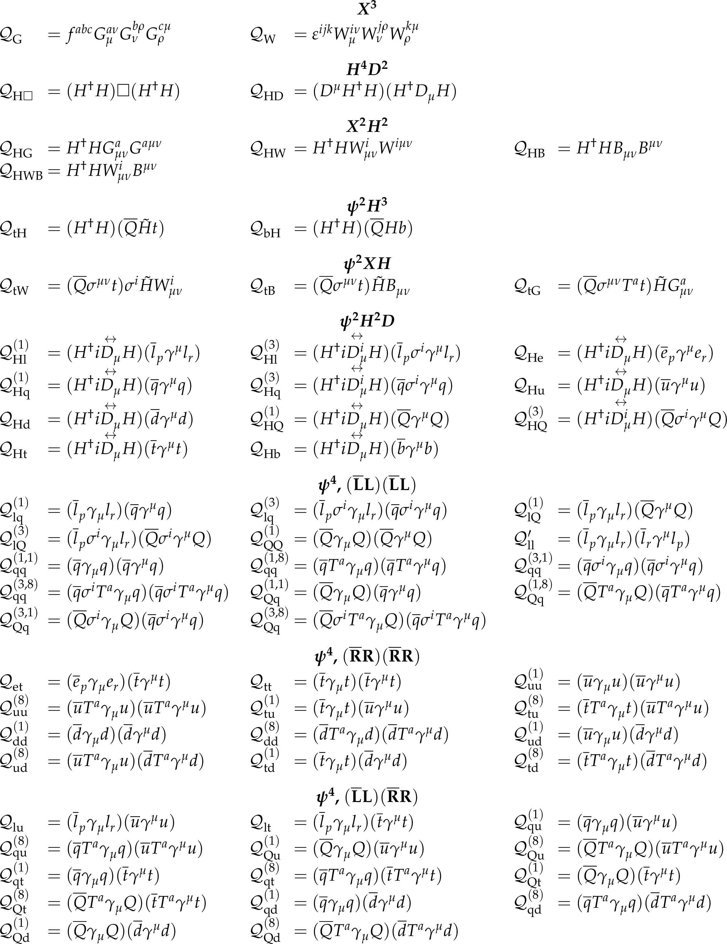
The SMEFT operators studied in this analysis, following the definitions of Ref. [9,10], where $ (q,u,d) $ denote quark fields of the first two generations, $ (Q,t,b) $ quark fields of the third generation, and $ (l,e,\nu) $ lepton fields of all three generations. The Higgs doublet field is indicated by $ H $; $ D $ represents a covariant derivative; $ \Box $ is the d'Alembert operator; $ X = G, W, B $ denotes a vector boson field strength tensor; $ p,r $ are flavour indices. Fermion fields are represented by $ \psi $, with $ L $ and $ R $ indicating left- and right-handed fermion fields. |
png pdf |
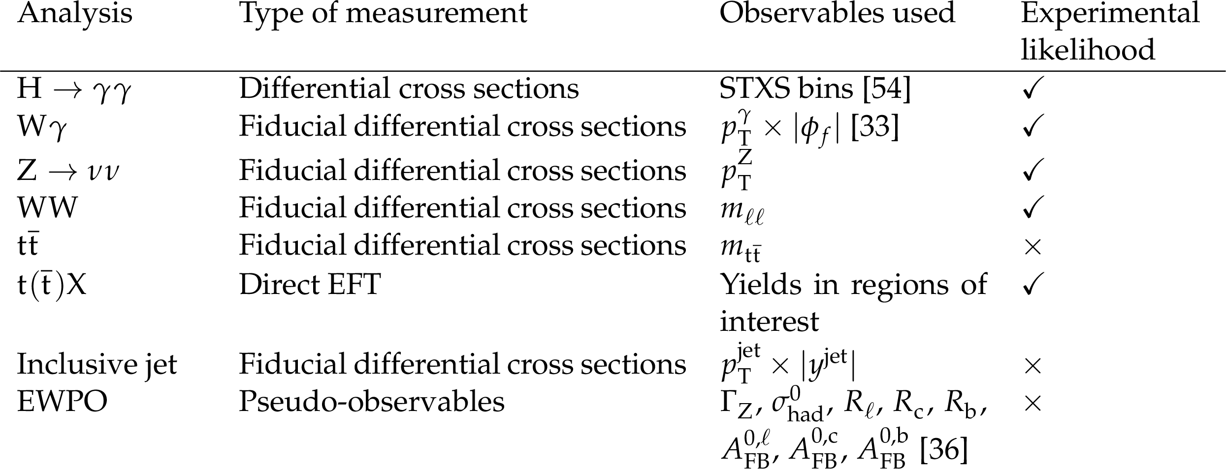
Table 2:
Summary of input analysis characteristics. The observables are defined in the following sections and the experimental likelihood is defined in Section 6. |
png pdf |
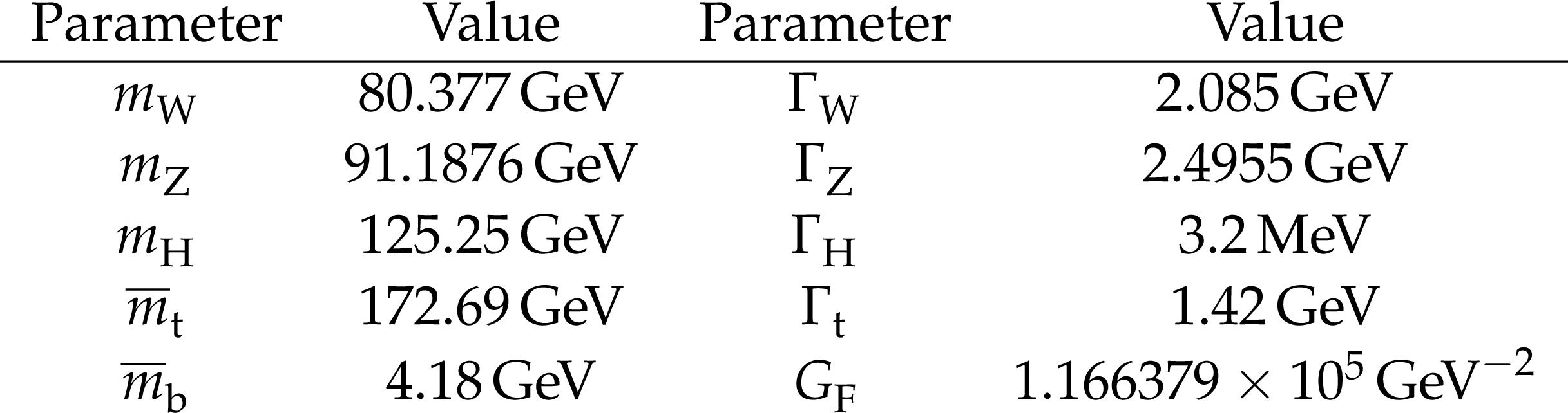
Table 3:
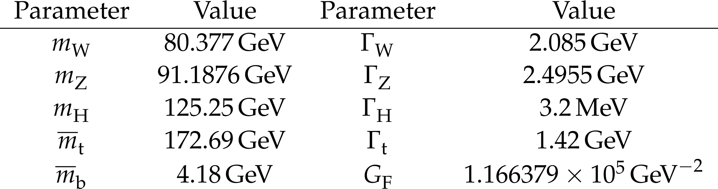
Input parameters used to calculate SM predictions for the electroweak precision observables. The values of $ m_{\mathrm{W}} $, $ m_{\mathrm{Z}} $, $ m_{\mathrm{H}} $, $ m_{\mathrm{t}} $, and $ G_\text{F} $ are set to the PDG averages [86], with an additional uncertainty of 0.5 GeV on $ m_{\mathrm{t}} $ to account for ambiguities in the definition of the top quark mass [87]. The strong coupling $ \alpha_s $ is set to the average of the Flavour Lattice Averaging Group (FLAG) [88], as it is more robust against SMEFT effects than the PDG value [89]. |
png pdf |
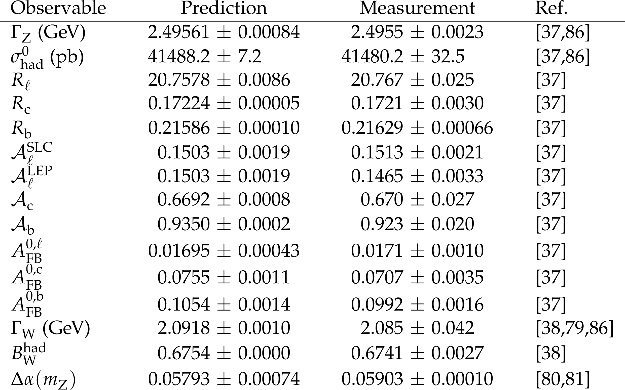
Table 4:
Predicted and measured values of the 15 electroweak precision observables included in the fit. $ \Delta\alpha(m_\mathrm{Z}) $ is the sum of $ \Delta\alpha_\mathrm{had}(m_\mathrm{Z})= $ 0.02753 $ \pm $ 0.00010 [80] and $ \Delta\alpha_\mathrm{lep}(m_\mathrm{Z})= $ 0.0314979 $ \pm $ 0.0000002 [81]. The measurements of $ \Gamma_\mathrm{Z} $ and $ \sigma_\mathrm{had}^0 $ include corrections to Ref. [37], accounting for an underestimation of the integrated luminosity and using an updated Bhabha scattering cross section, as recommended by the PDG [86]. The SM predictions are calculated in the $ \{m_\mathrm{W}, m_\mathrm{Z}, G_\text{F}\} $ input parameter scheme with the input parameters of Table 3, using EWPD4LHC [39]. |
png pdf |
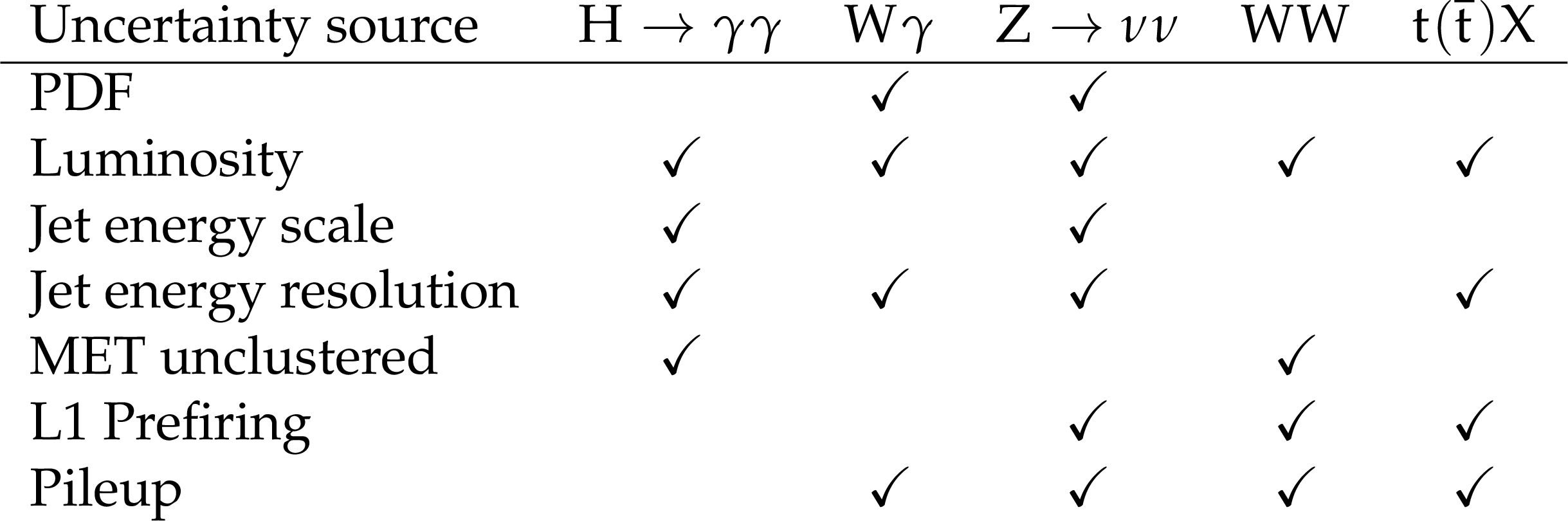
Table 5:
Correlation scheme of the systematic uncertainties. |
png pdf |
Table 6:
The SM parameters used in the event generation to derive the SMEFT parameterizations [86]. |
png pdf |
Table E1:
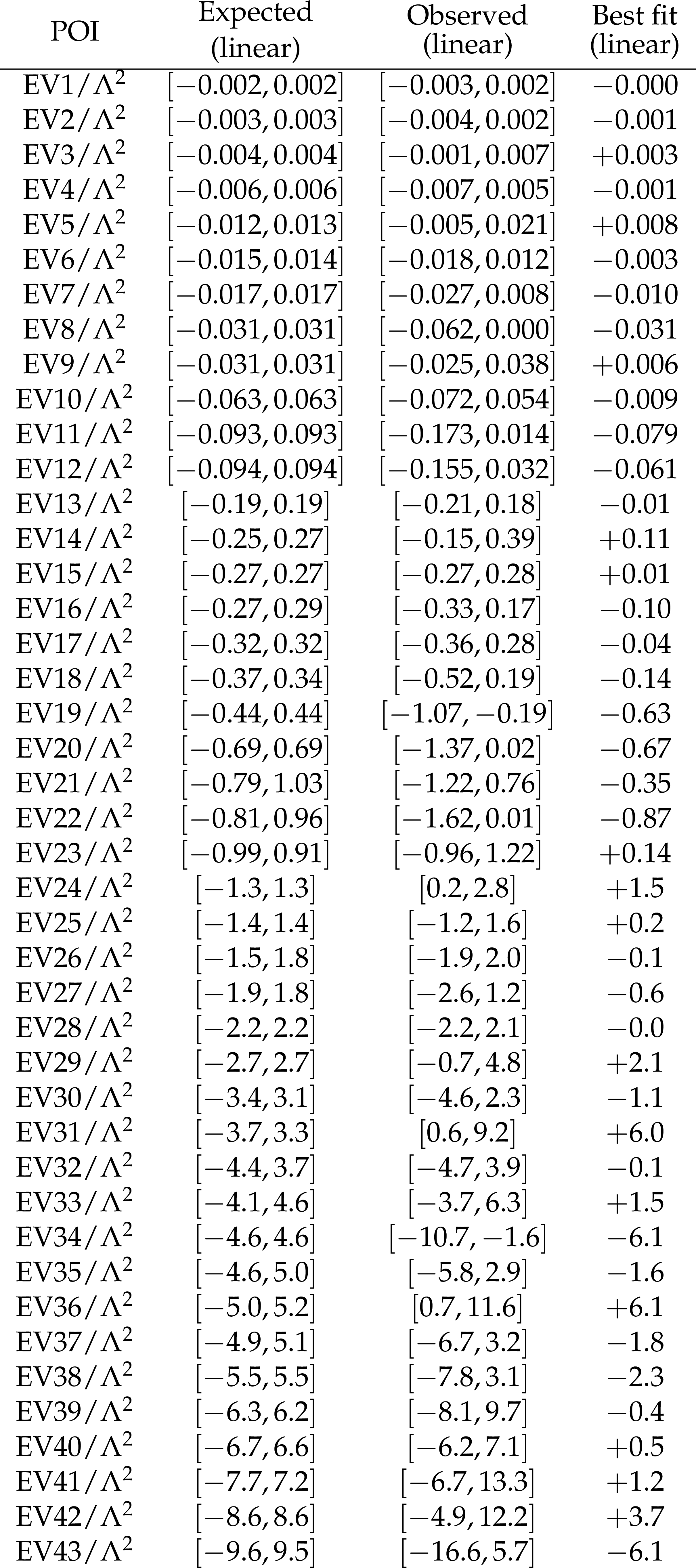
Expected and observed 95% CL limits on linear combinations of WCs from the hybrid fit with the full set of input measurements, in units of $ \text{TeV}^{-2} $. |
png pdf |
Table E2:
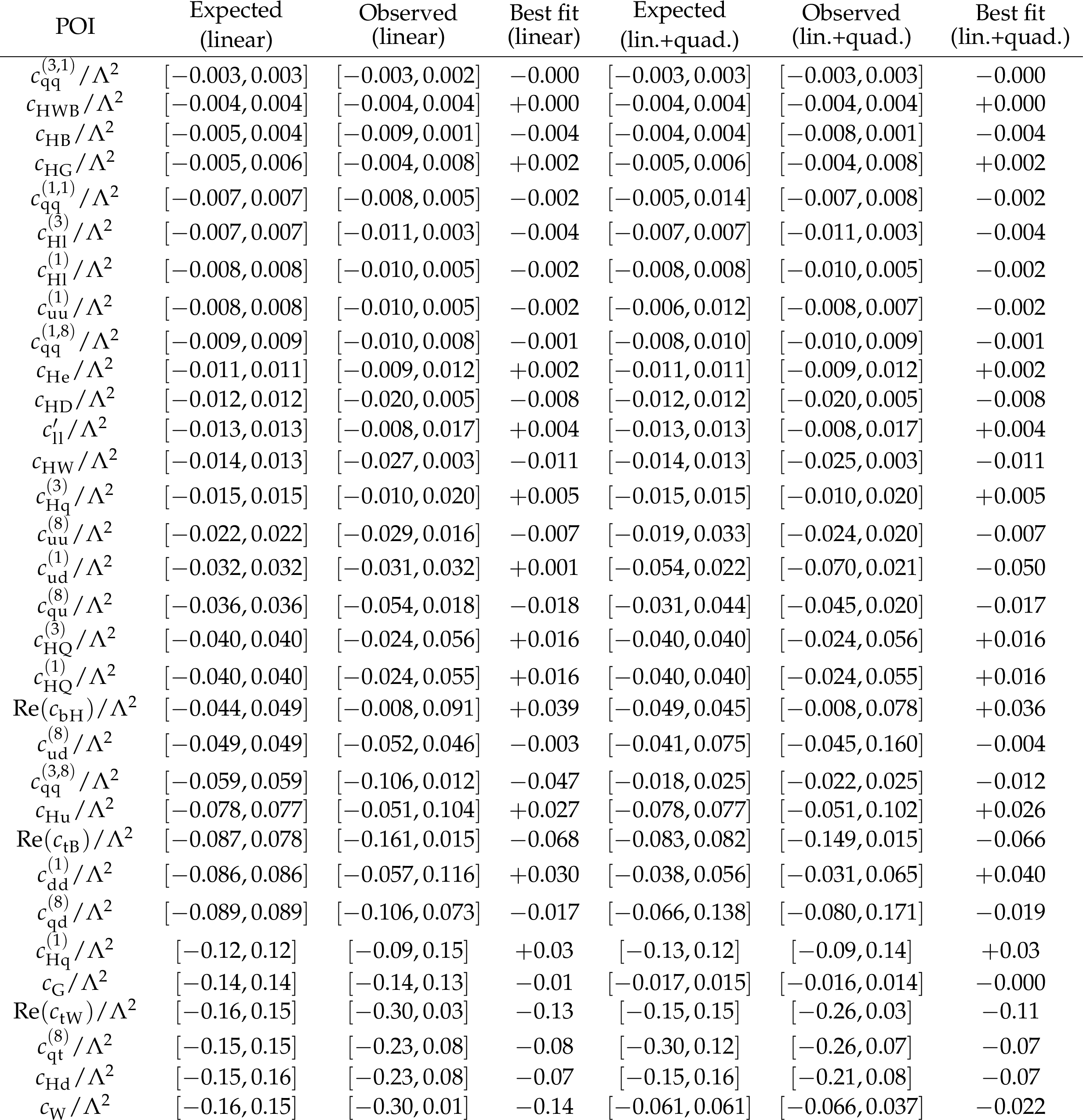
Expected and observed individual 95% CL limits on WCs from the hybrid fit with the full set of input measurements, in units of $ \text{TeV}^{-2} $. This table shows the 32 WCs with the strongest expected constraints, when considering the fit with linear terms only. |
png pdf |
Table E3:
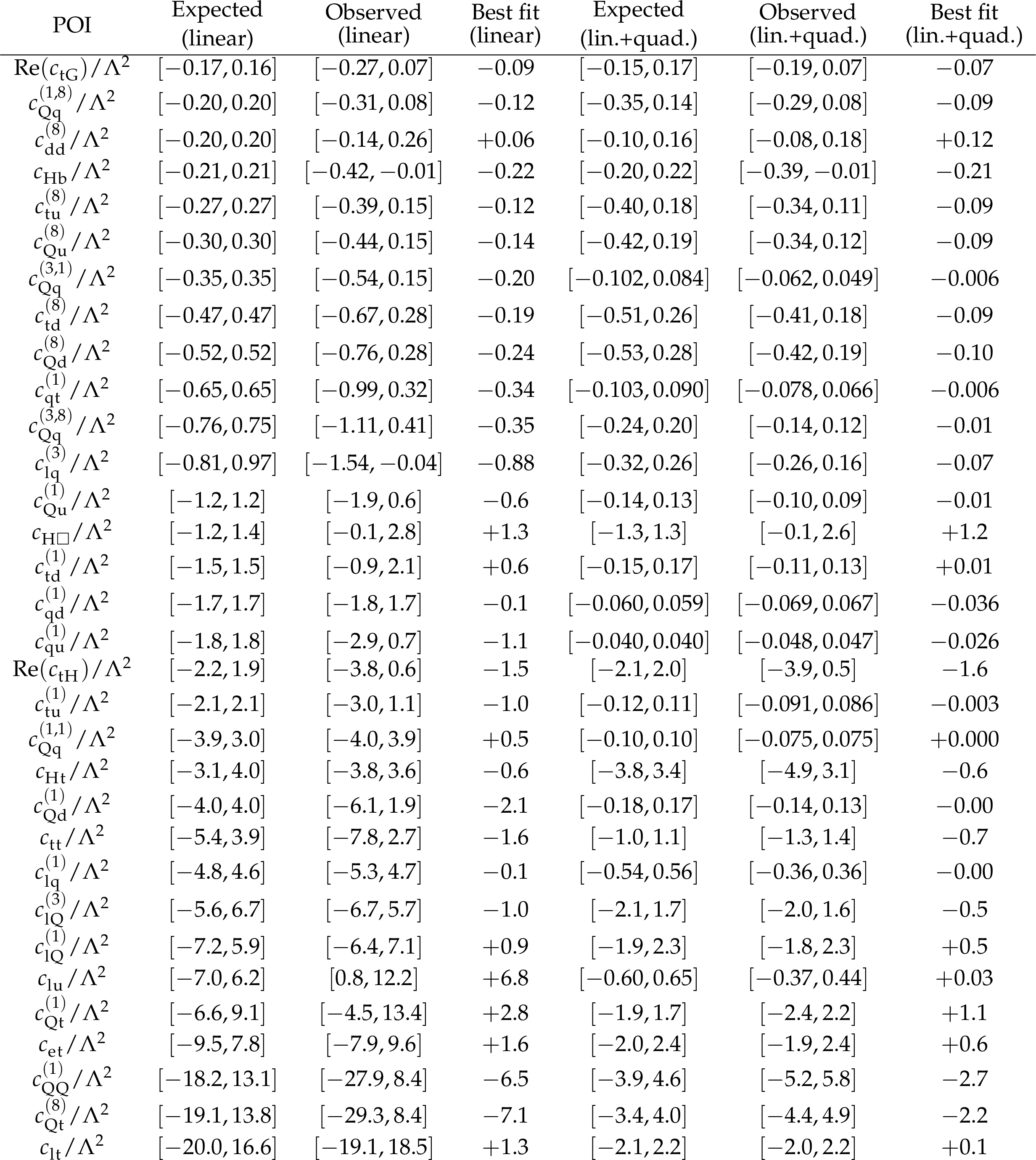
Expected and observed individual 95% CL limits on WCs from the hybrid fit with the full set of input measurements, in units of $ \text{TeV}^{-2} $. This table shows the 32 WCs with the weakest expected constraints, when considering the fit with linear terms only. |
| Summary |
| A standard model effective field theory (SMEFT) interpretation of data collected by the CMS experiment has been presented. This combined interpretation is based on a simultaneous fit of seven sets of CMS measurements that probe Higgs boson, electroweak vector boson, top quark, and multijet production, and also incorporates measurements of electroweak precision observables. These input measurements were chosen to obtain sensitivity to a broad set of SMEFT operators. Out of 129 operators in the SMEFT basis considered in this paper, the combined interpretation constrains 64 Wilson coefficients (WCs) individually. The constraints are provided for both linear-only and linear-plus-quadratic parameterizations. Simultaneous constraints are set on 43 linear combinations of WCs. In the fit that constrains the linear combinations of WCs, the $ p $-value for the compatibility with the standard model is 2.5%. When excluding the inclusive jet measurement from the combination, the $ p $-value is 27%. The 95% confidence intervals range from around $ \pm $ 0.002 to $ \pm10 \text{TeV}^{-2} $ for the constraints on the linear combinations of WCs, whereas for the individual WCs the constraints range from $ \pm $ 0.003 to $ \pm 20 \text{TeV}^{-2} $. These constraints are also translated into lower limits on the probed energy scale of new physics $ \Lambda $, for given values of the WCs. This combined interpretation yields improved constraints with respect to single-analysis results from CMS. |
| Additional Figures | |

png pdf |
Additional Figure 1:
Eigenvectors constrained mostly by the inclusive jet measurement. Part of the rotation matrix obtained by performing the PCA on the Hessian matrix of the full set of measurements, including the $ \mathrm{t}(\overline{\mathrm{t}})\mathrm{X} $ analysis. |
png pdf |
Additional Figure 2:
Eigenvectors constrained mostly by the $ \mathrm{H}\to\gamma\gamma $, $ \mathrm{W}\gamma $, WW, and $ \mathrm{Z}\to\nu\nu $ measurements. Part of the rotation matrix obtained by performing the PCA on the Hessian matrix of the full set of measurements, including the $ \mathrm{t}(\overline{\mathrm{t}})\mathrm{X} $ analysis. |

png pdf |
Additional Figure 3:
Eigenvectors constrained mostly by the EWPO. Part of the rotation matrix obtained by performing the PCA on the Hessian matrix of the full set of measurements, including the $ \mathrm{t}(\overline{\mathrm{t}})\mathrm{X} $ analysis. |
png pdf |
Additional Figure 4:
Eigenvectors constrained mostly by the $ {\mathrm{t}\overline{\mathrm{t}}} $ and $ \mathrm{t}(\overline{\mathrm{t}})\mathrm{X} $ measurements. Part of the rotation matrix obtained by performing the PCA on the Hessian matrix of the full set of measurements, including the $ \mathrm{t}(\overline{\mathrm{t}})\mathrm{X} $ analysis. |
png pdf |
Additional Figure 5:
Eigenvectors constrained by a mixture of measurements. Part of the rotation matrix obtained by performing the PCA on the Hessian matrix of the full set of measurements, including the $ \mathrm{t}(\overline{\mathrm{t}})\mathrm{X} $ analysis. |

png pdf |
Additional Figure 6:
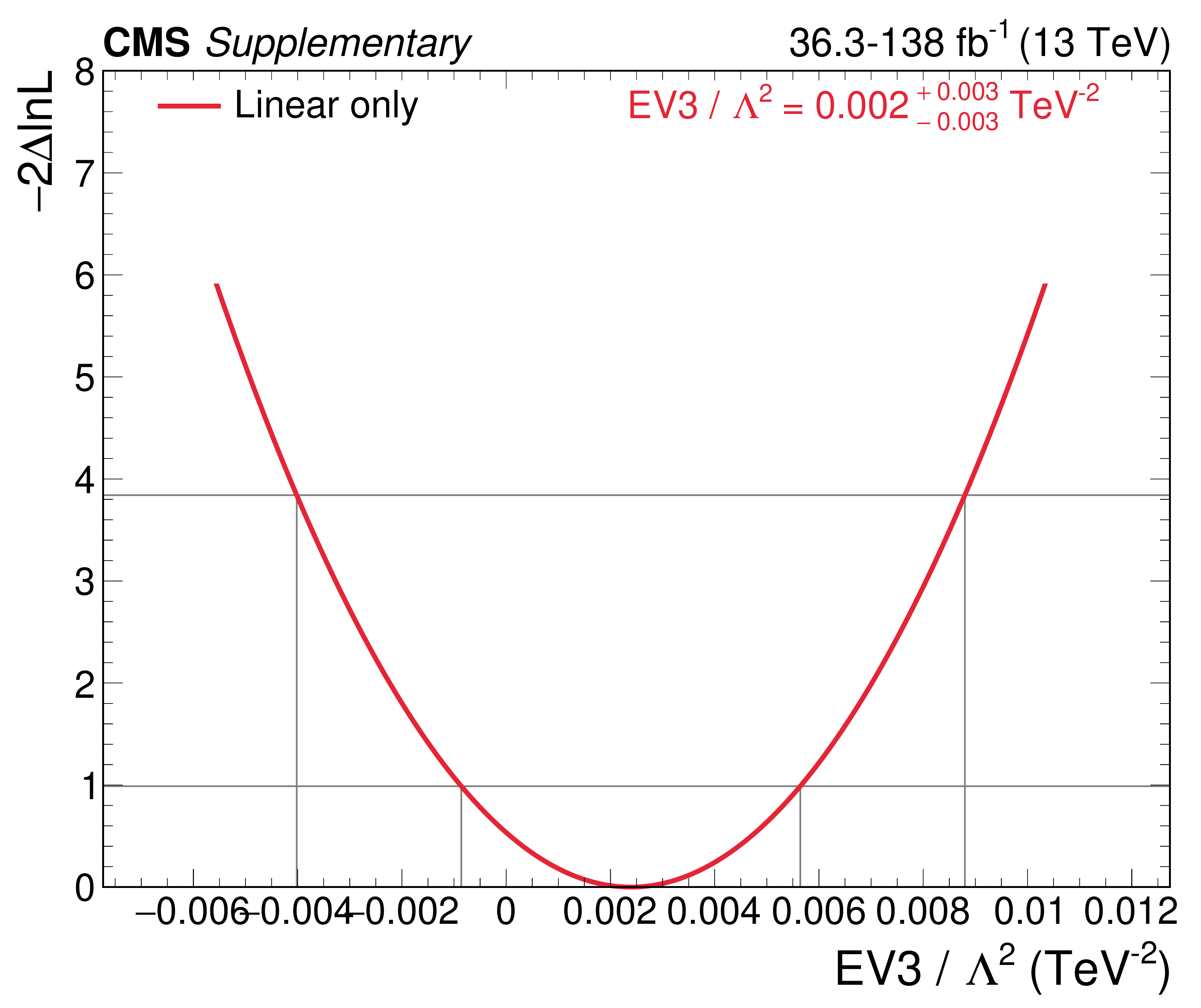
NLL scans of linear combinations of WCs, for the hybrid fit including the $ \mathrm{t}(\overline{\mathrm{t}})\mathrm{X} $ analysis. |

png pdf |
Additional Figure 6-a:
NLL scans of linear combinations of WCs, for the hybrid fit including the $ \mathrm{t}(\overline{\mathrm{t}})\mathrm{X} $ analysis. |

png pdf |
Additional Figure 6-b:
NLL scans of linear combinations of WCs, for the hybrid fit including the $ \mathrm{t}(\overline{\mathrm{t}})\mathrm{X} $ analysis. |
png pdf |
Additional Figure 6-c:
NLL scans of linear combinations of WCs, for the hybrid fit including the $ \mathrm{t}(\overline{\mathrm{t}})\mathrm{X} $ analysis. |
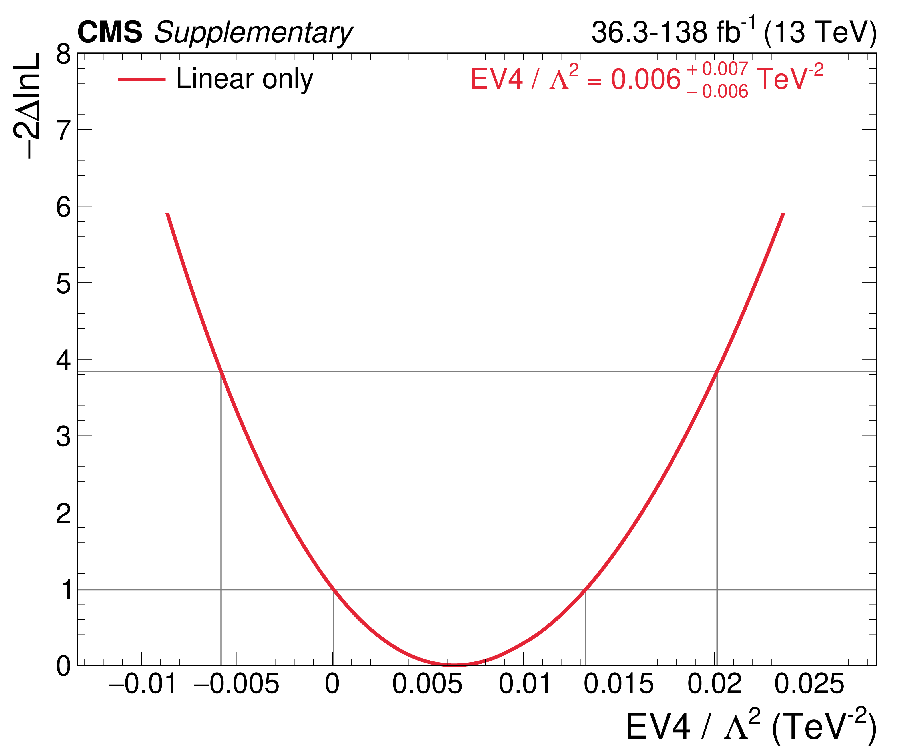
png pdf |
Additional Figure 6-d:
NLL scans of linear combinations of WCs, for the hybrid fit including the $ \mathrm{t}(\overline{\mathrm{t}})\mathrm{X} $ analysis. |
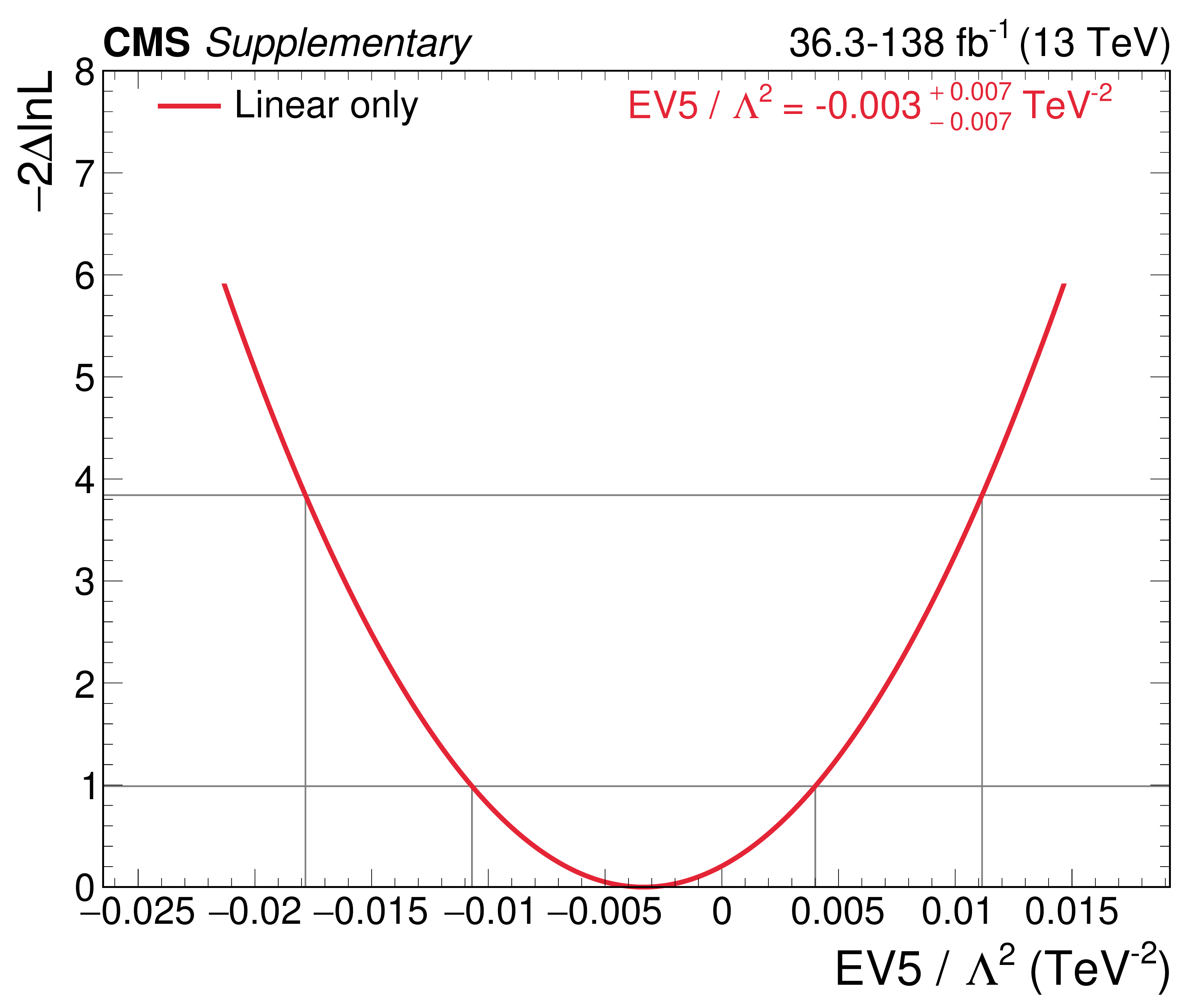
png pdf |
Additional Figure 6-e:
NLL scans of linear combinations of WCs, for the hybrid fit including the $ \mathrm{t}(\overline{\mathrm{t}})\mathrm{X} $ analysis. |
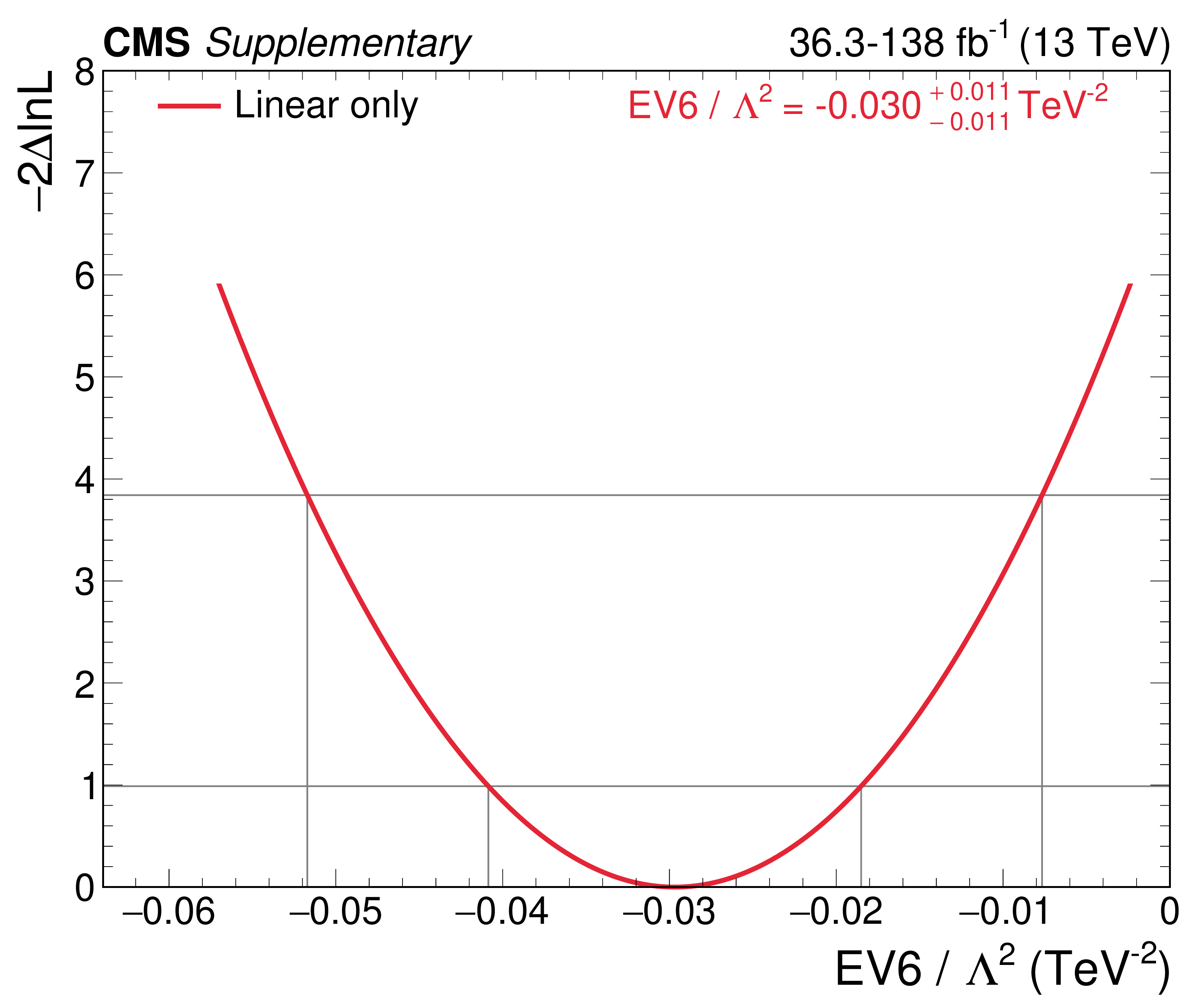
png pdf |
Additional Figure 6-f:
NLL scans of linear combinations of WCs, for the hybrid fit including the $ \mathrm{t}(\overline{\mathrm{t}})\mathrm{X} $ analysis. |
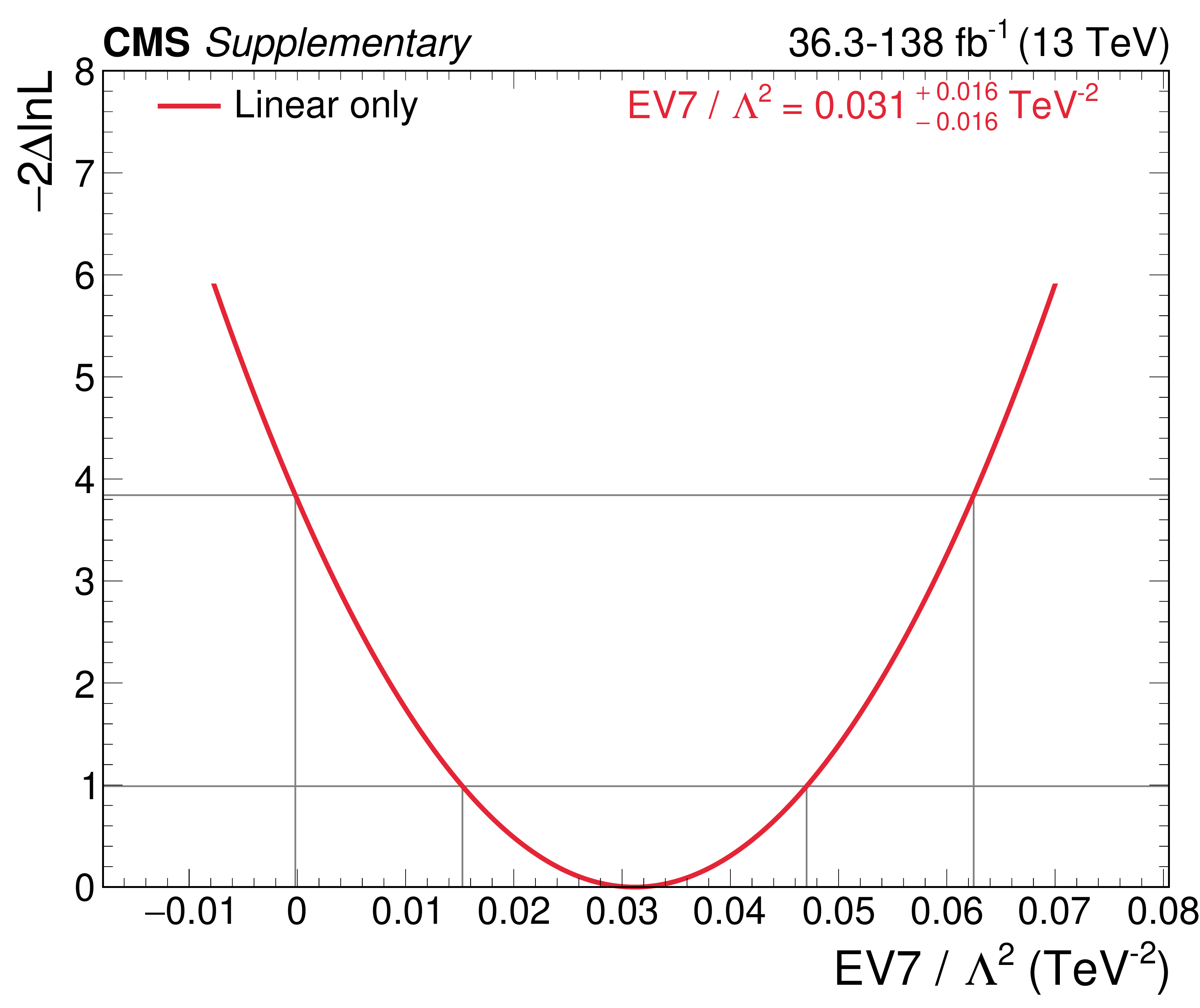
png pdf |
Additional Figure 6-g:
NLL scans of linear combinations of WCs, for the hybrid fit including the $ \mathrm{t}(\overline{\mathrm{t}})\mathrm{X} $ analysis. |
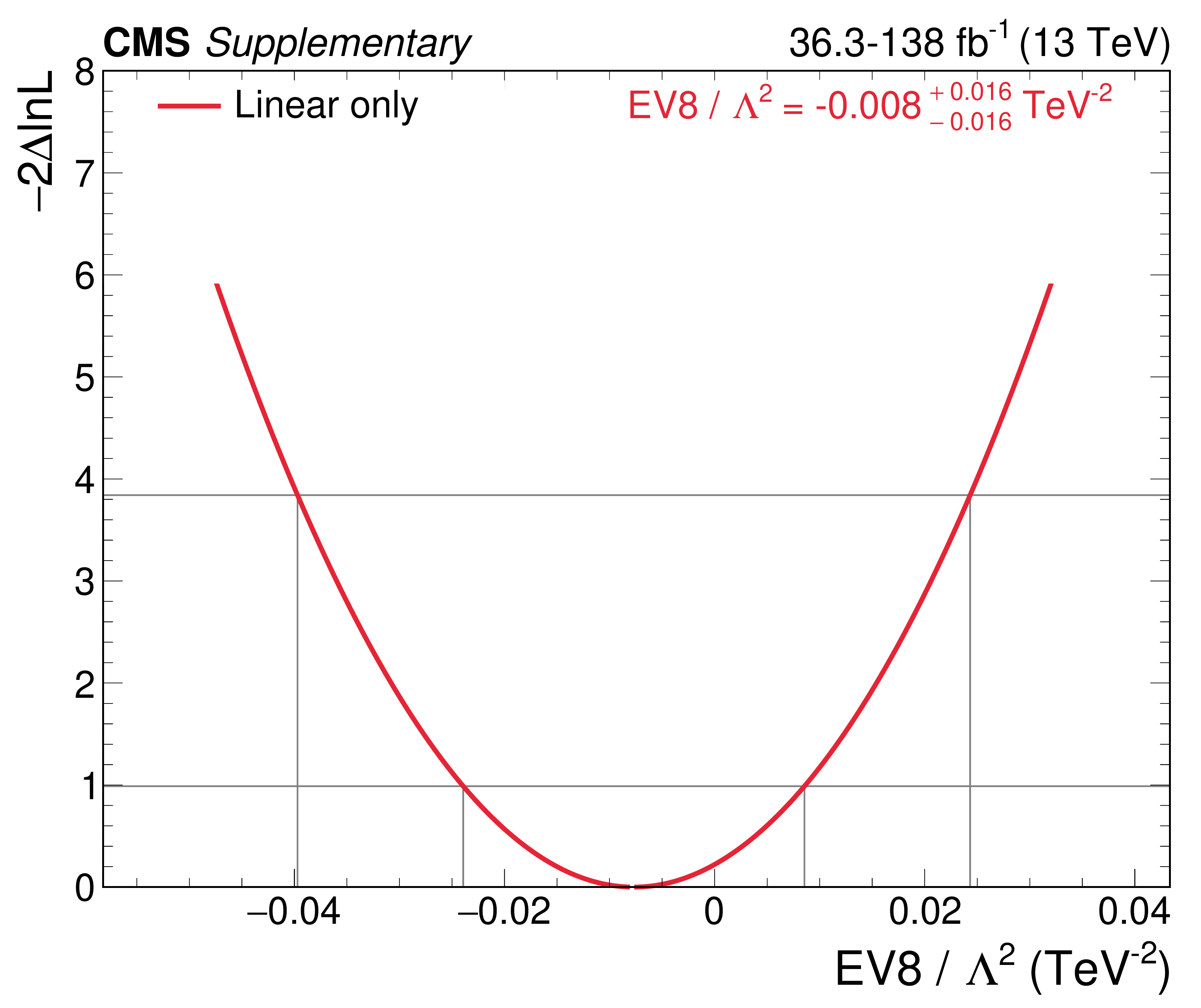
png pdf |
Additional Figure 6-h:
NLL scans of linear combinations of WCs, for the hybrid fit including the $ \mathrm{t}(\overline{\mathrm{t}})\mathrm{X} $ analysis. |

png pdf |
Additional Figure 6-i:
NLL scans of linear combinations of WCs, for the hybrid fit including the $ \mathrm{t}(\overline{\mathrm{t}})\mathrm{X} $ analysis. |
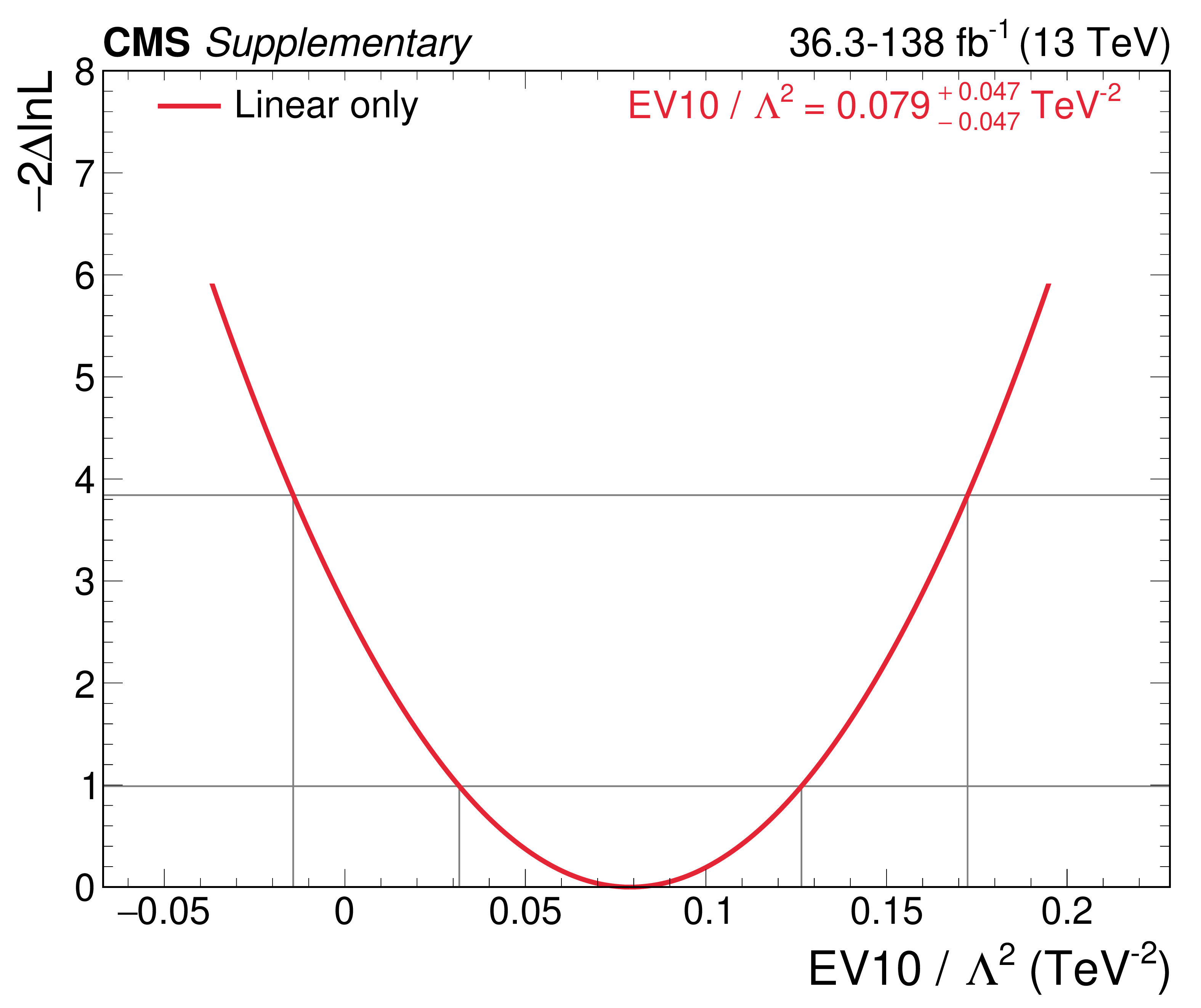
png pdf |
Additional Figure 6-j:
NLL scans of linear combinations of WCs, for the hybrid fit including the $ \mathrm{t}(\overline{\mathrm{t}})\mathrm{X} $ analysis. |
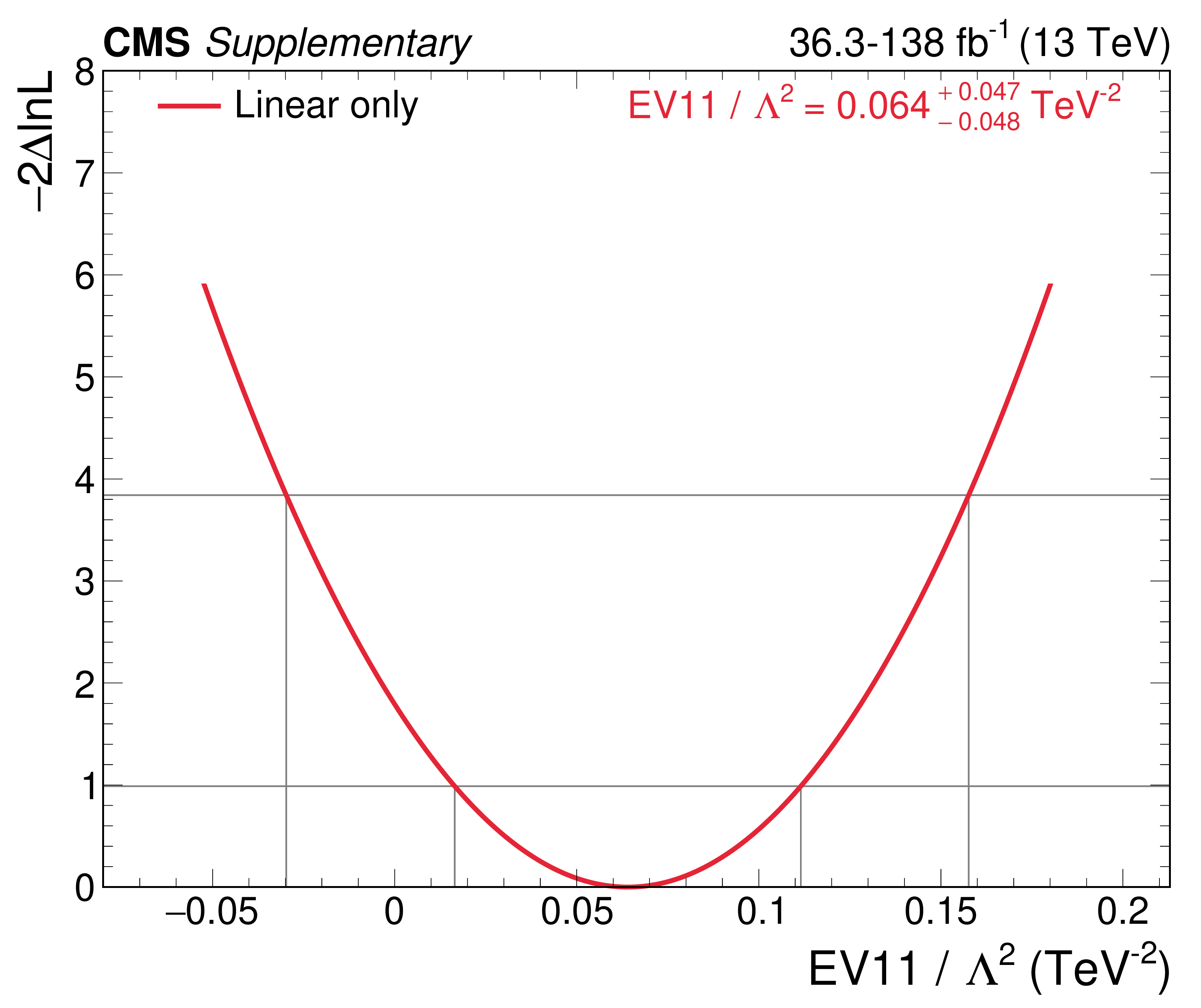
png pdf |
Additional Figure 6-k:
NLL scans of linear combinations of WCs, for the hybrid fit including the $ \mathrm{t}(\overline{\mathrm{t}})\mathrm{X} $ analysis. |

png pdf |
Additional Figure 6-l:
NLL scans of linear combinations of WCs, for the hybrid fit including the $ \mathrm{t}(\overline{\mathrm{t}})\mathrm{X} $ analysis. |

png pdf |
Additional Figure 6-m:
NLL scans of linear combinations of WCs, for the hybrid fit including the $ \mathrm{t}(\overline{\mathrm{t}})\mathrm{X} $ analysis. |
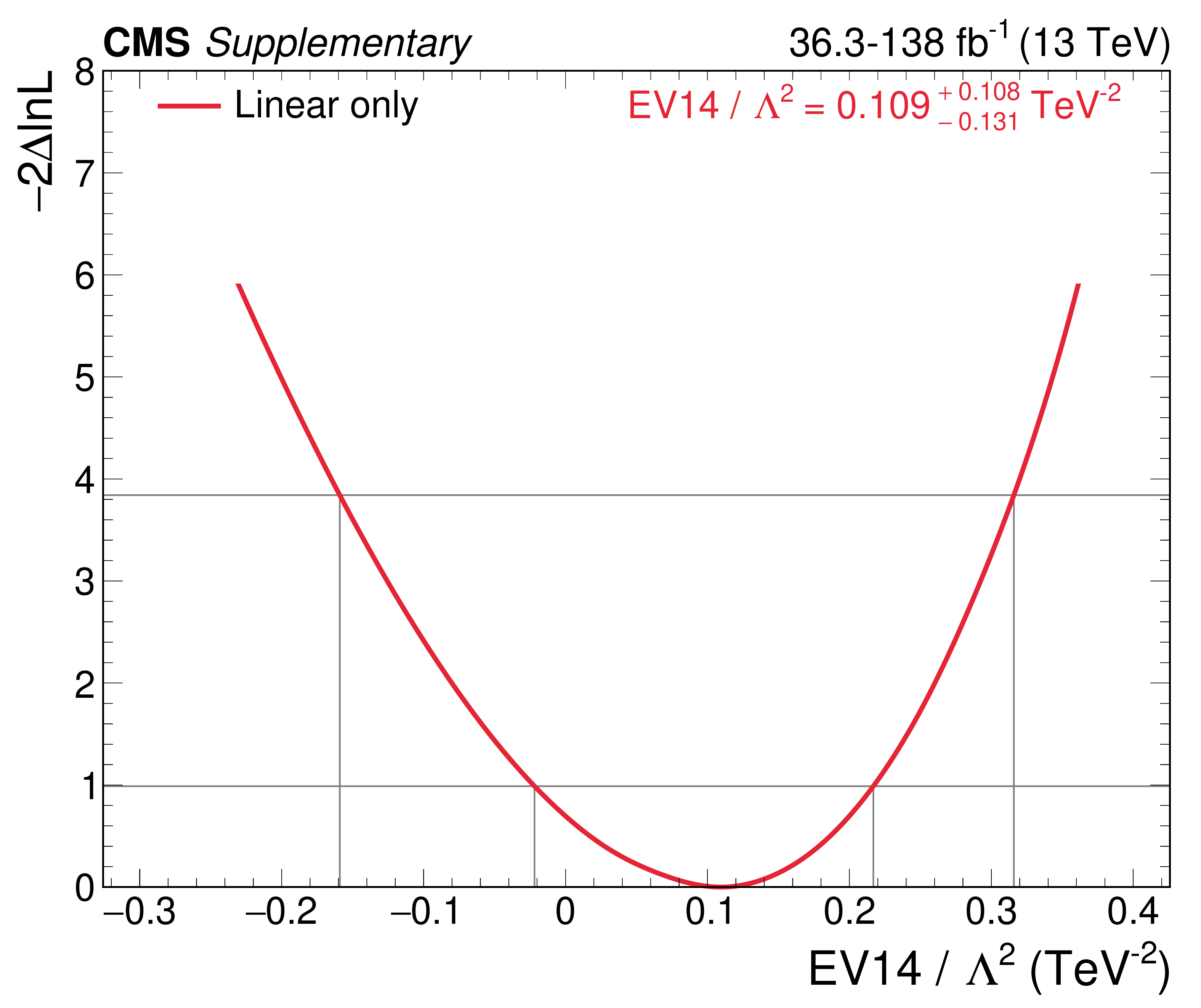
png pdf |
Additional Figure 6-n:
NLL scans of linear combinations of WCs, for the hybrid fit including the $ \mathrm{t}(\overline{\mathrm{t}})\mathrm{X} $ analysis. |

png pdf |
Additional Figure 6-o:
NLL scans of linear combinations of WCs, for the hybrid fit including the $ \mathrm{t}(\overline{\mathrm{t}})\mathrm{X} $ analysis. |
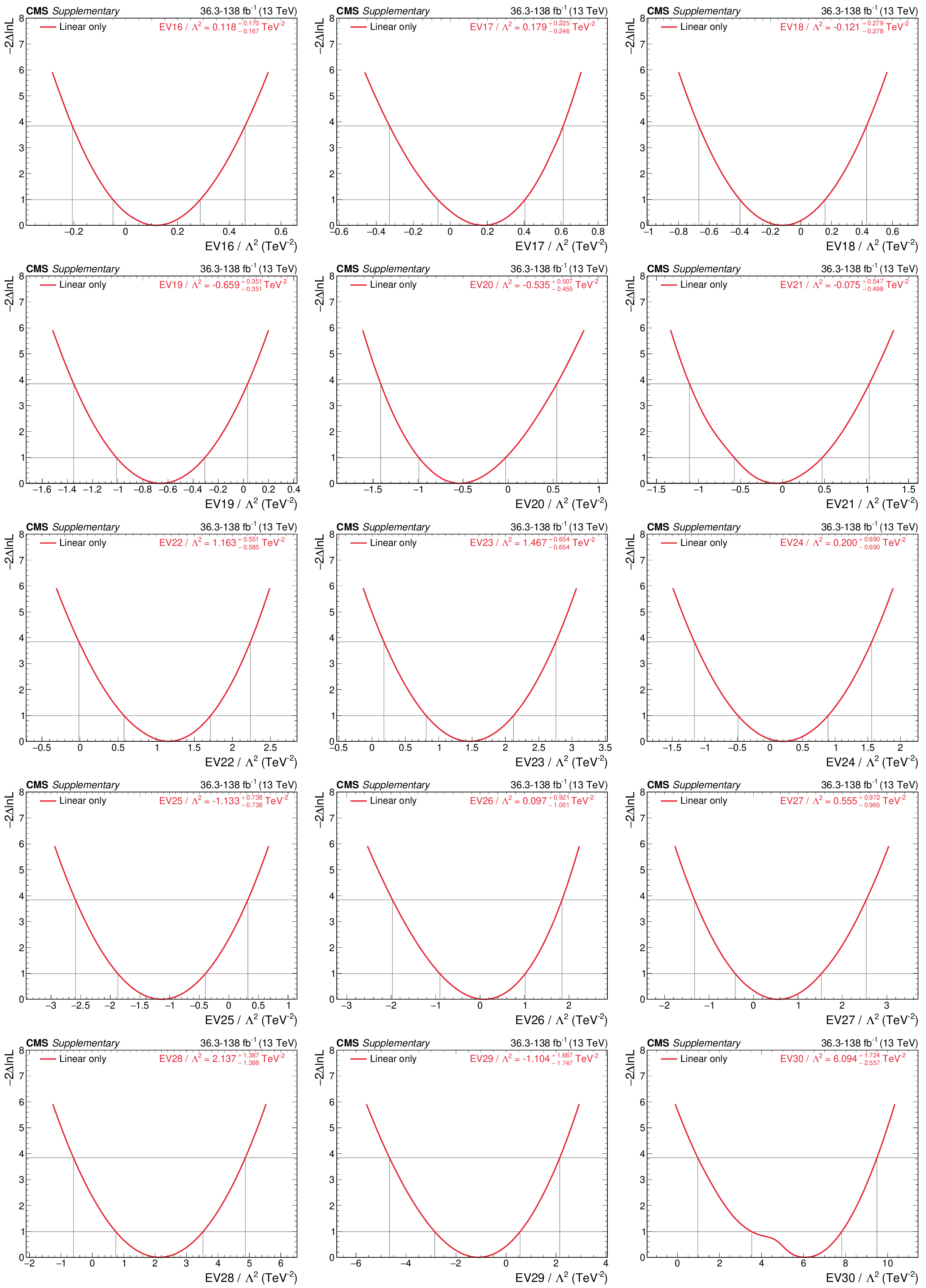
png pdf |
Additional Figure 7:
NLL scans of linear combinations of WCs, for the hybrid fit including the $ \mathrm{t}(\overline{\mathrm{t}})\mathrm{X} $ analysis. |
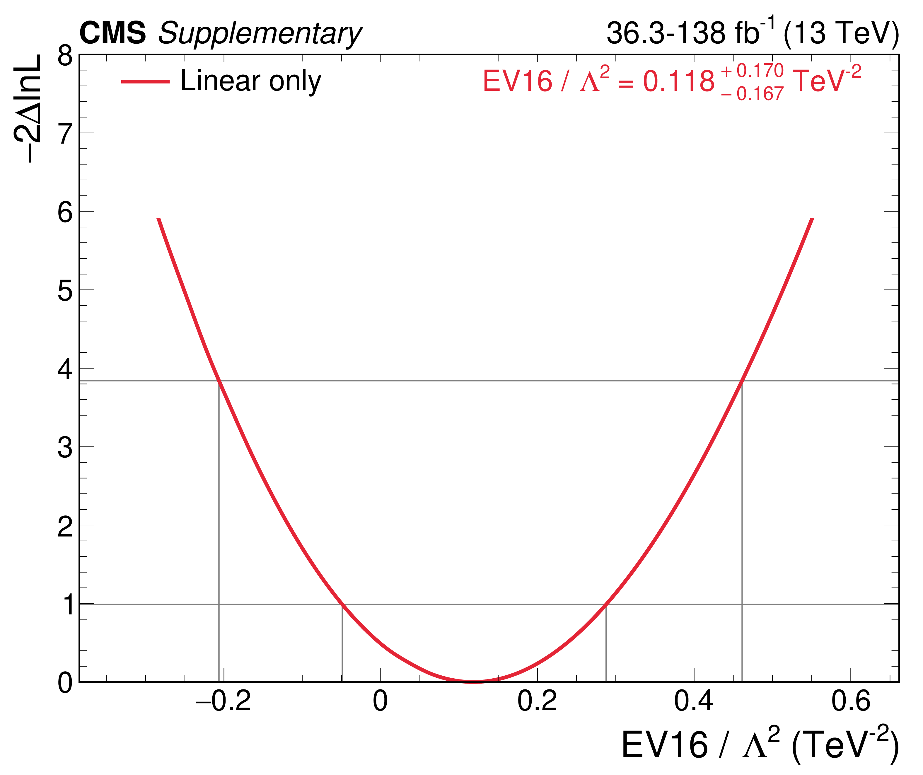
png pdf |
Additional Figure 7-a:
NLL scans of linear combinations of WCs, for the hybrid fit including the $ \mathrm{t}(\overline{\mathrm{t}})\mathrm{X} $ analysis. |

png pdf |
Additional Figure 7-b:
NLL scans of linear combinations of WCs, for the hybrid fit including the $ \mathrm{t}(\overline{\mathrm{t}})\mathrm{X} $ analysis. |

png pdf |
Additional Figure 7-c:
NLL scans of linear combinations of WCs, for the hybrid fit including the $ \mathrm{t}(\overline{\mathrm{t}})\mathrm{X} $ analysis. |
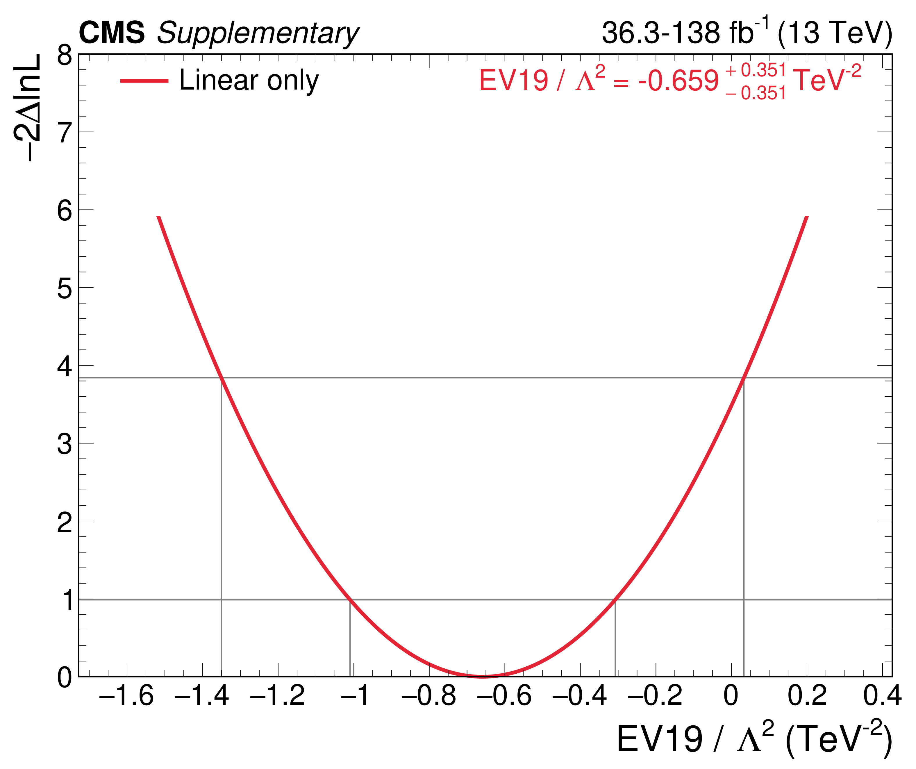
png pdf |
Additional Figure 7-d:
NLL scans of linear combinations of WCs, for the hybrid fit including the $ \mathrm{t}(\overline{\mathrm{t}})\mathrm{X} $ analysis. |

png pdf |
Additional Figure 7-e:
NLL scans of linear combinations of WCs, for the hybrid fit including the $ \mathrm{t}(\overline{\mathrm{t}})\mathrm{X} $ analysis. |
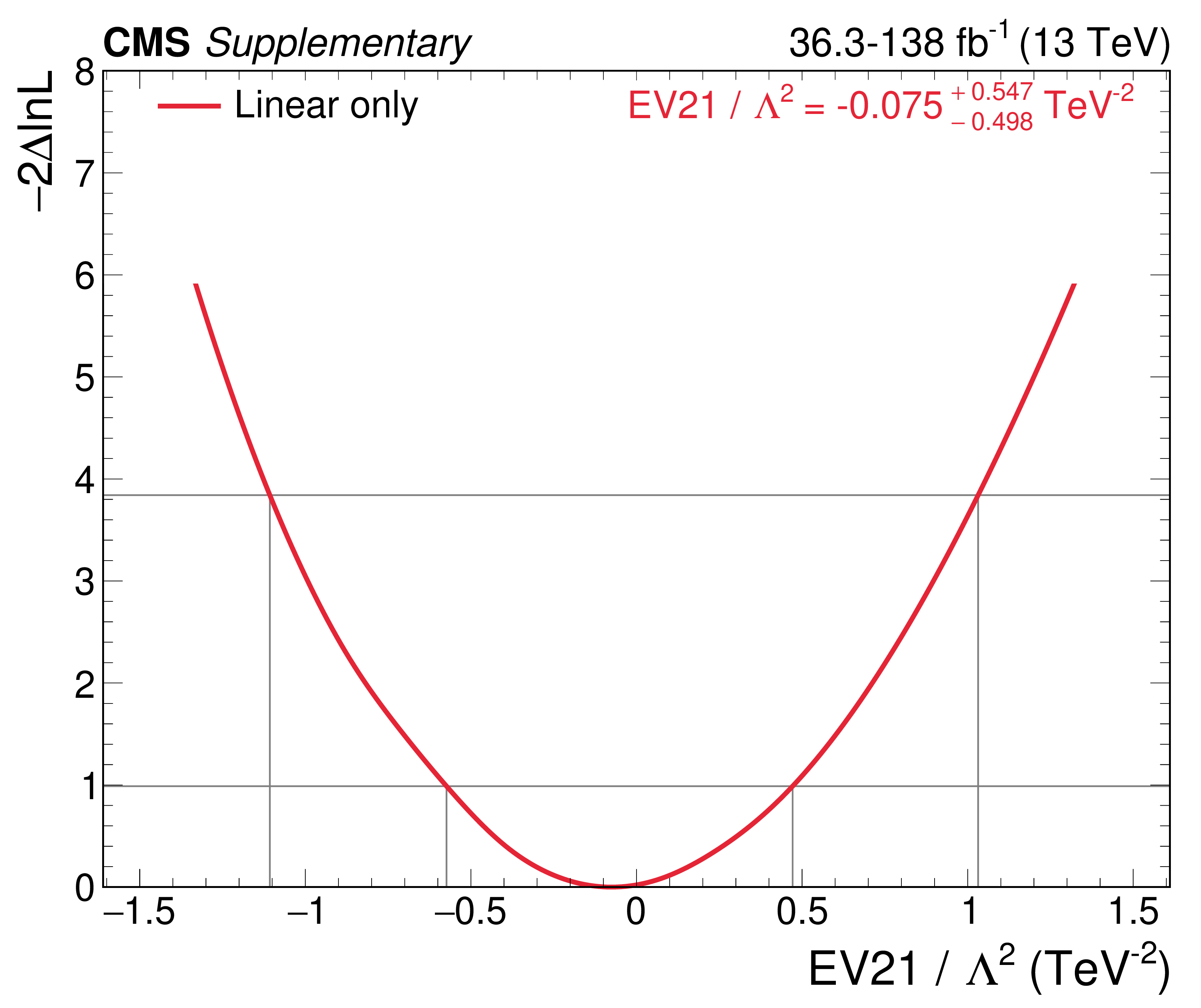
png pdf |
Additional Figure 7-f:
NLL scans of linear combinations of WCs, for the hybrid fit including the $ \mathrm{t}(\overline{\mathrm{t}})\mathrm{X} $ analysis. |
png pdf |
Additional Figure 7-g:
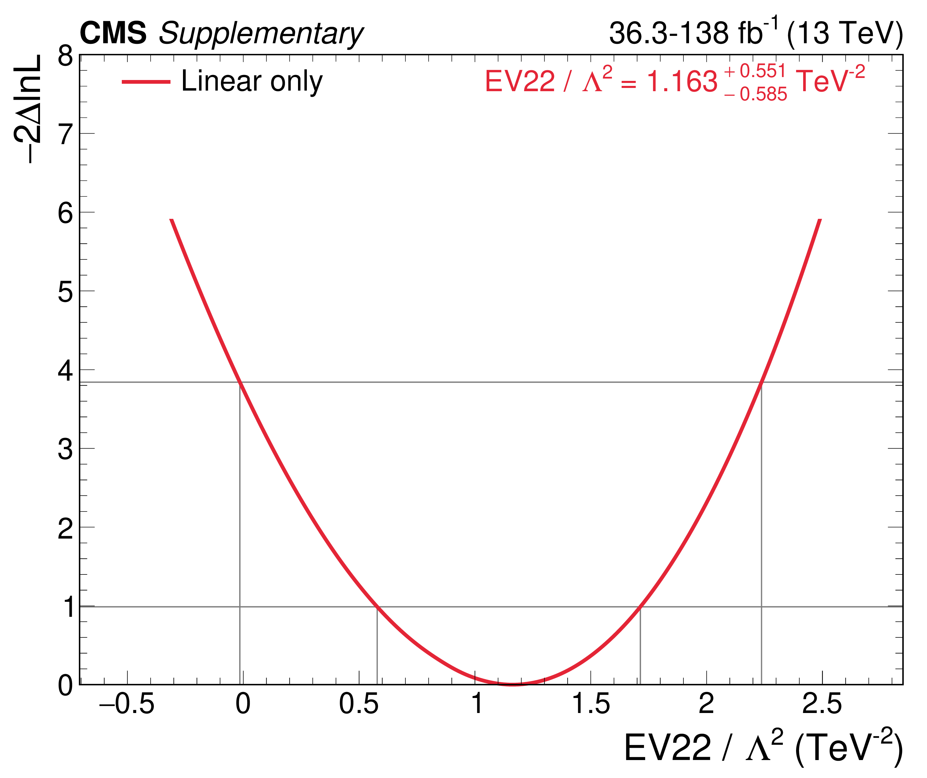
NLL scans of linear combinations of WCs, for the hybrid fit including the $ \mathrm{t}(\overline{\mathrm{t}})\mathrm{X} $ analysis. |
png pdf |
Additional Figure 7-h:
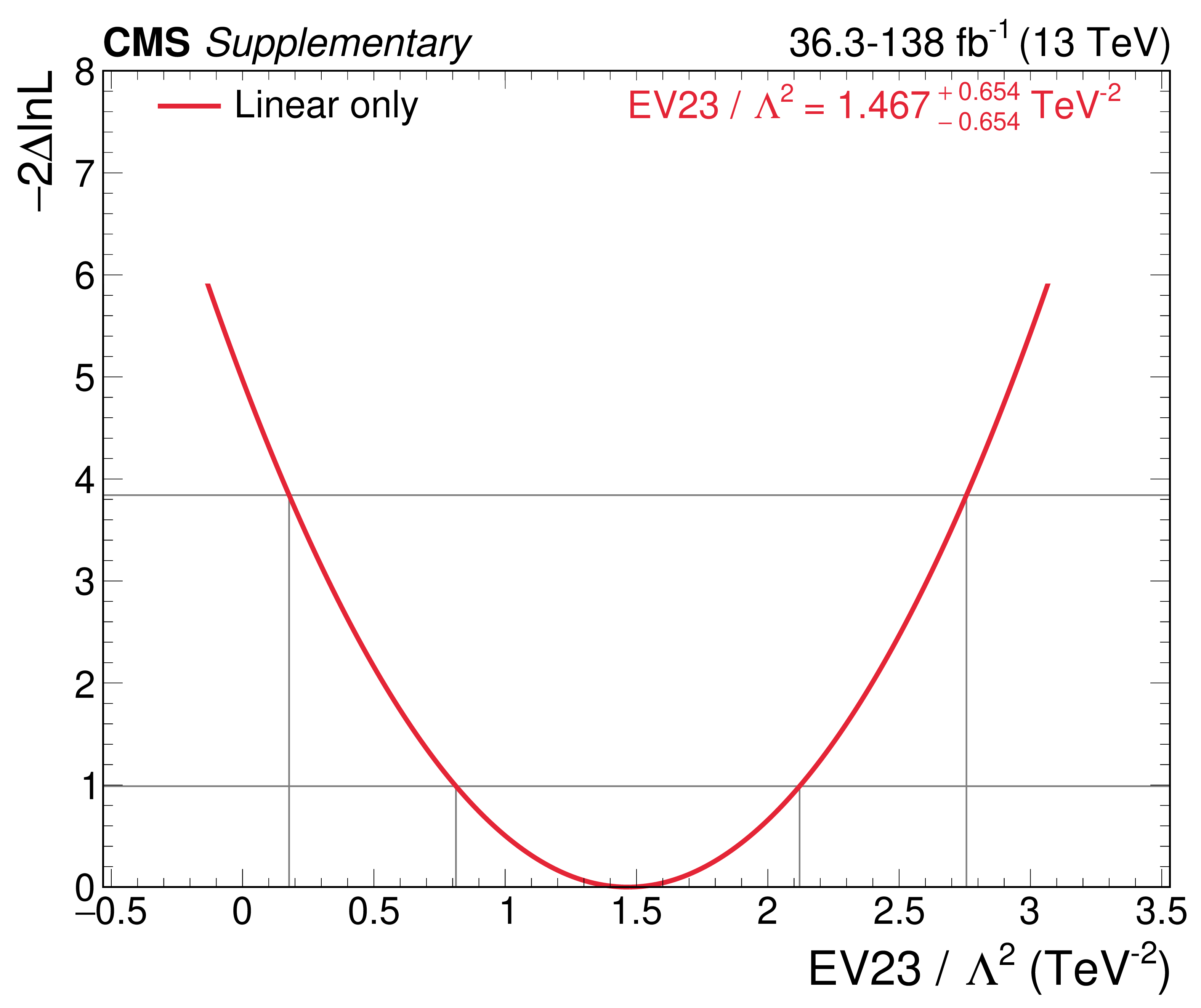
NLL scans of linear combinations of WCs, for the hybrid fit including the $ \mathrm{t}(\overline{\mathrm{t}})\mathrm{X} $ analysis. |
png pdf |
Additional Figure 7-i:
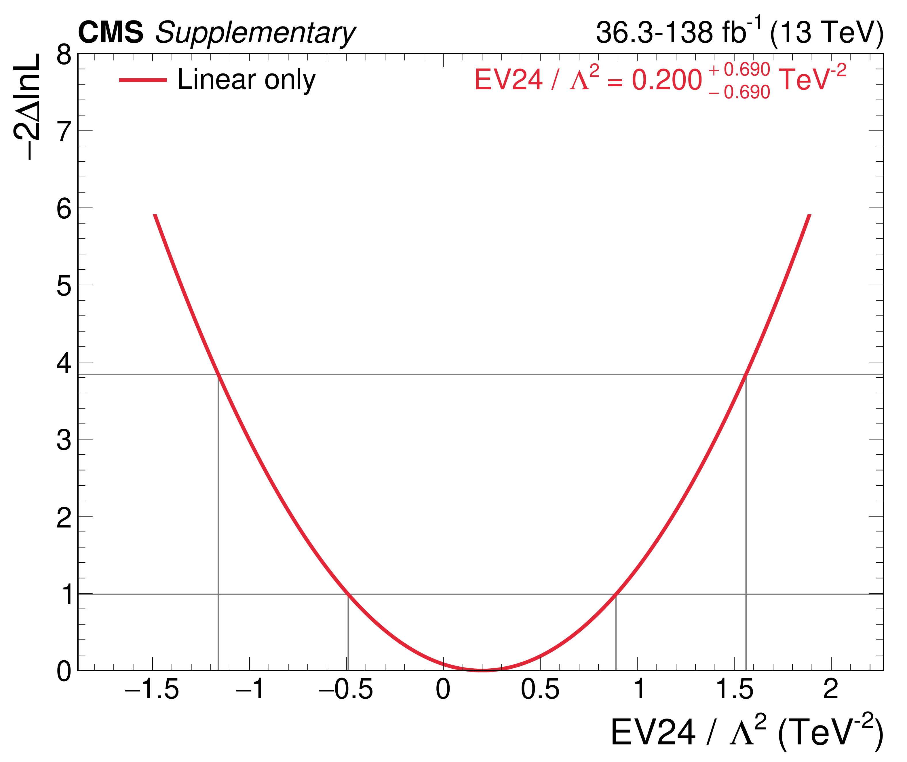
NLL scans of linear combinations of WCs, for the hybrid fit including the $ \mathrm{t}(\overline{\mathrm{t}})\mathrm{X} $ analysis. |
png pdf |
Additional Figure 7-j:
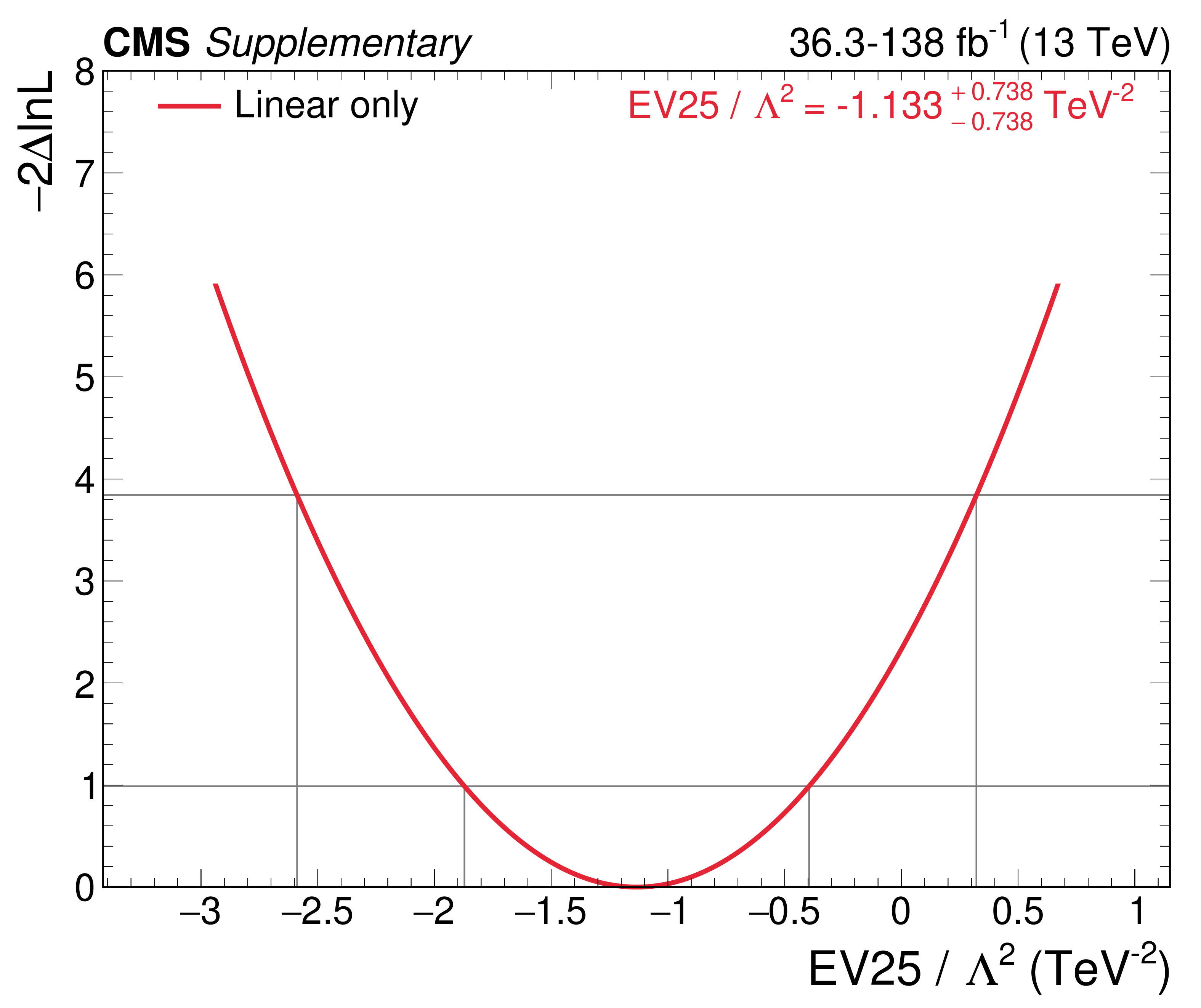
NLL scans of linear combinations of WCs, for the hybrid fit including the $ \mathrm{t}(\overline{\mathrm{t}})\mathrm{X} $ analysis. |

png pdf |
Additional Figure 7-k:
NLL scans of linear combinations of WCs, for the hybrid fit including the $ \mathrm{t}(\overline{\mathrm{t}})\mathrm{X} $ analysis. |
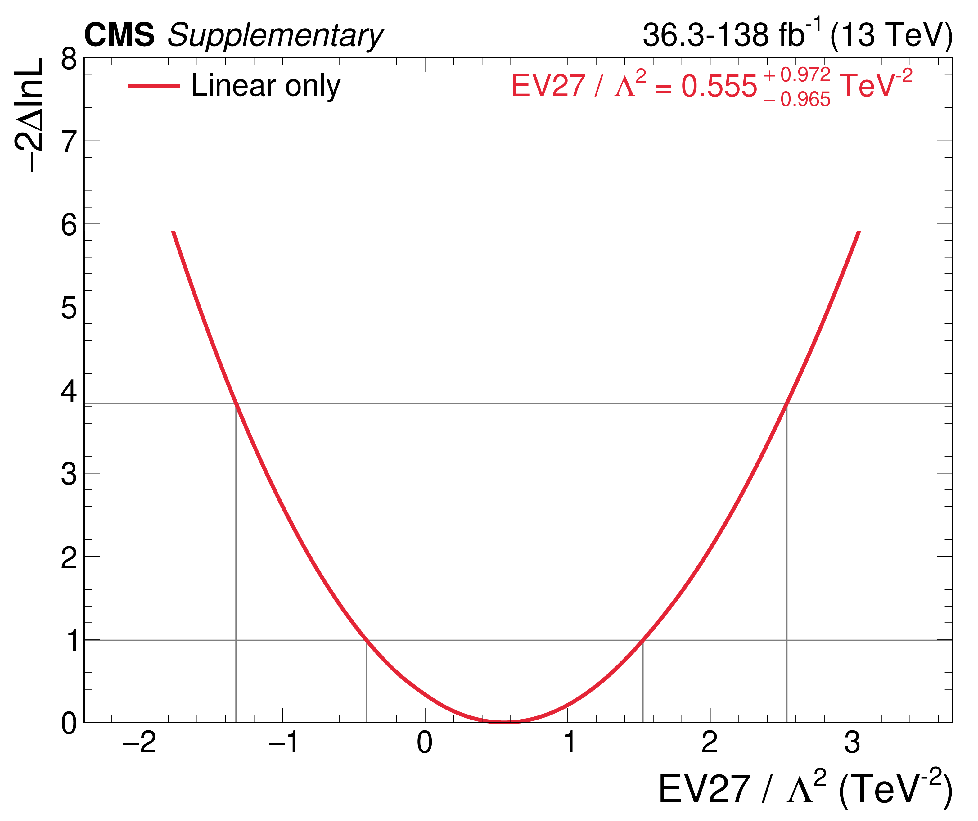
png pdf |
Additional Figure 7-l:
NLL scans of linear combinations of WCs, for the hybrid fit including the $ \mathrm{t}(\overline{\mathrm{t}})\mathrm{X} $ analysis. |

png pdf |
Additional Figure 7-m:
NLL scans of linear combinations of WCs, for the hybrid fit including the $ \mathrm{t}(\overline{\mathrm{t}})\mathrm{X} $ analysis. |
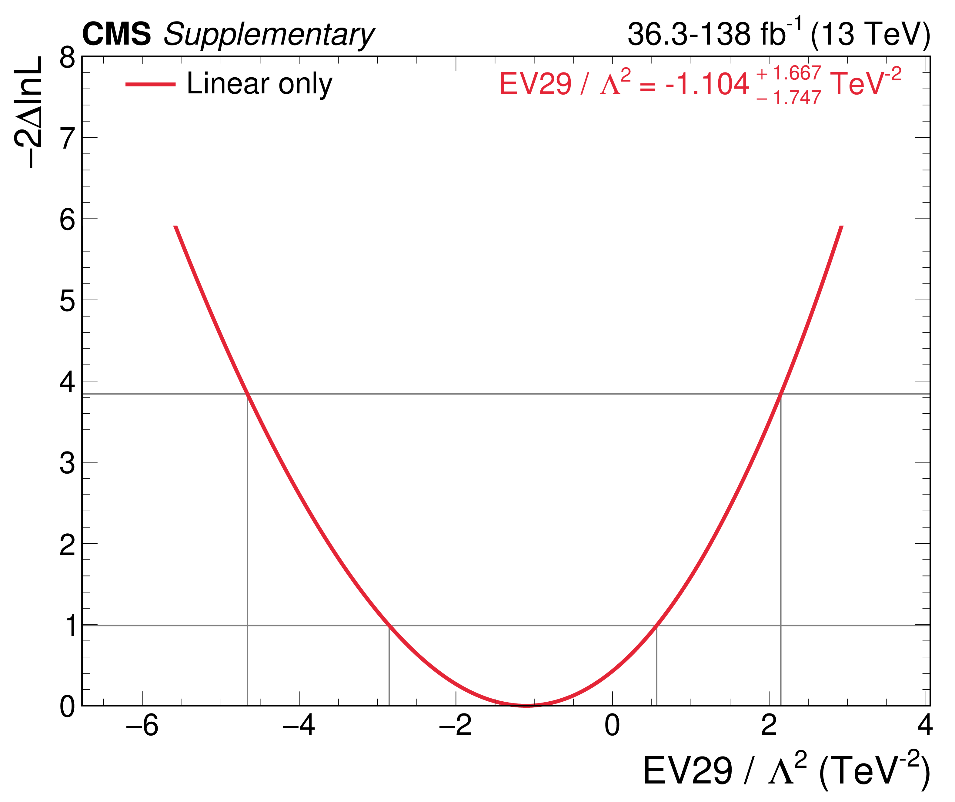
png pdf |
Additional Figure 7-n:
NLL scans of linear combinations of WCs, for the hybrid fit including the $ \mathrm{t}(\overline{\mathrm{t}})\mathrm{X} $ analysis. |
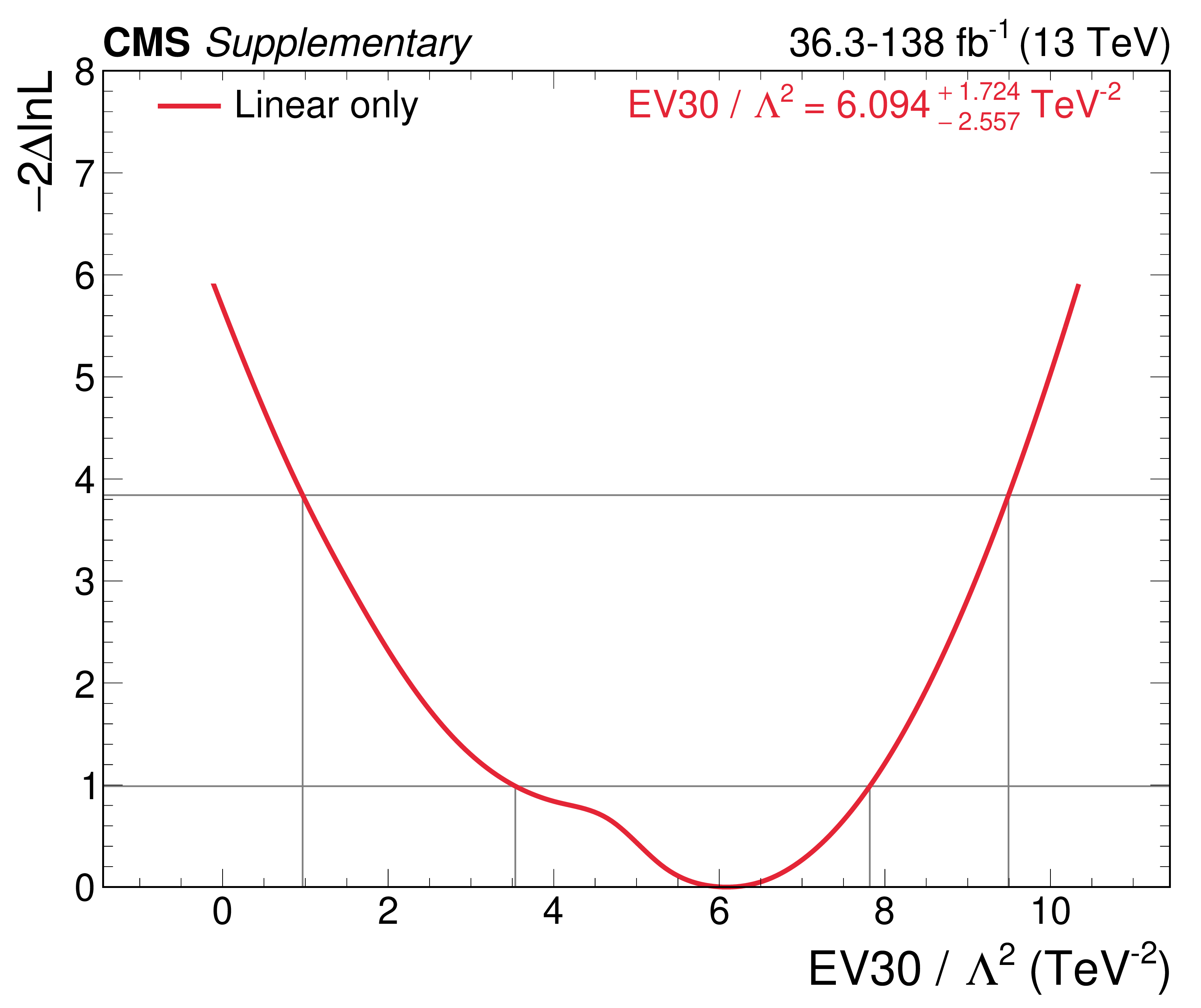
png pdf |
Additional Figure 7-o:
NLL scans of linear combinations of WCs, for the hybrid fit including the $ \mathrm{t}(\overline{\mathrm{t}})\mathrm{X} $ analysis. |

png pdf |
Additional Figure 8:
NLL scans of linear combinations of WCs, for the hybrid fit including the $ \mathrm{t}(\overline{\mathrm{t}})\mathrm{X} $ analysis. |

png pdf |
Additional Figure 8-a:
NLL scans of linear combinations of WCs, for the hybrid fit including the $ \mathrm{t}(\overline{\mathrm{t}})\mathrm{X} $ analysis. |

png pdf |
Additional Figure 8-b:
NLL scans of linear combinations of WCs, for the hybrid fit including the $ \mathrm{t}(\overline{\mathrm{t}})\mathrm{X} $ analysis. |
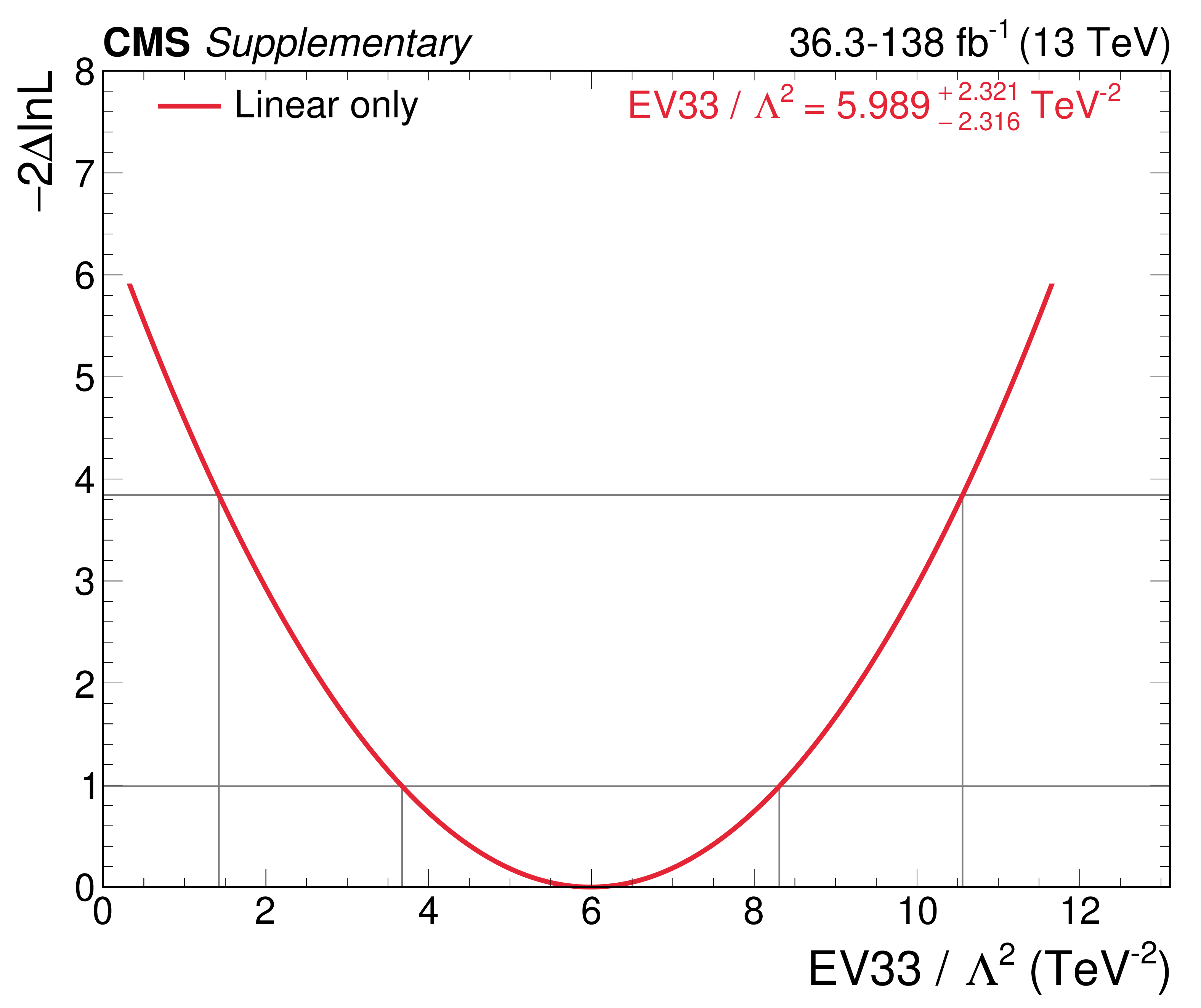
png pdf |
Additional Figure 8-c:
NLL scans of linear combinations of WCs, for the hybrid fit including the $ \mathrm{t}(\overline{\mathrm{t}})\mathrm{X} $ analysis. |
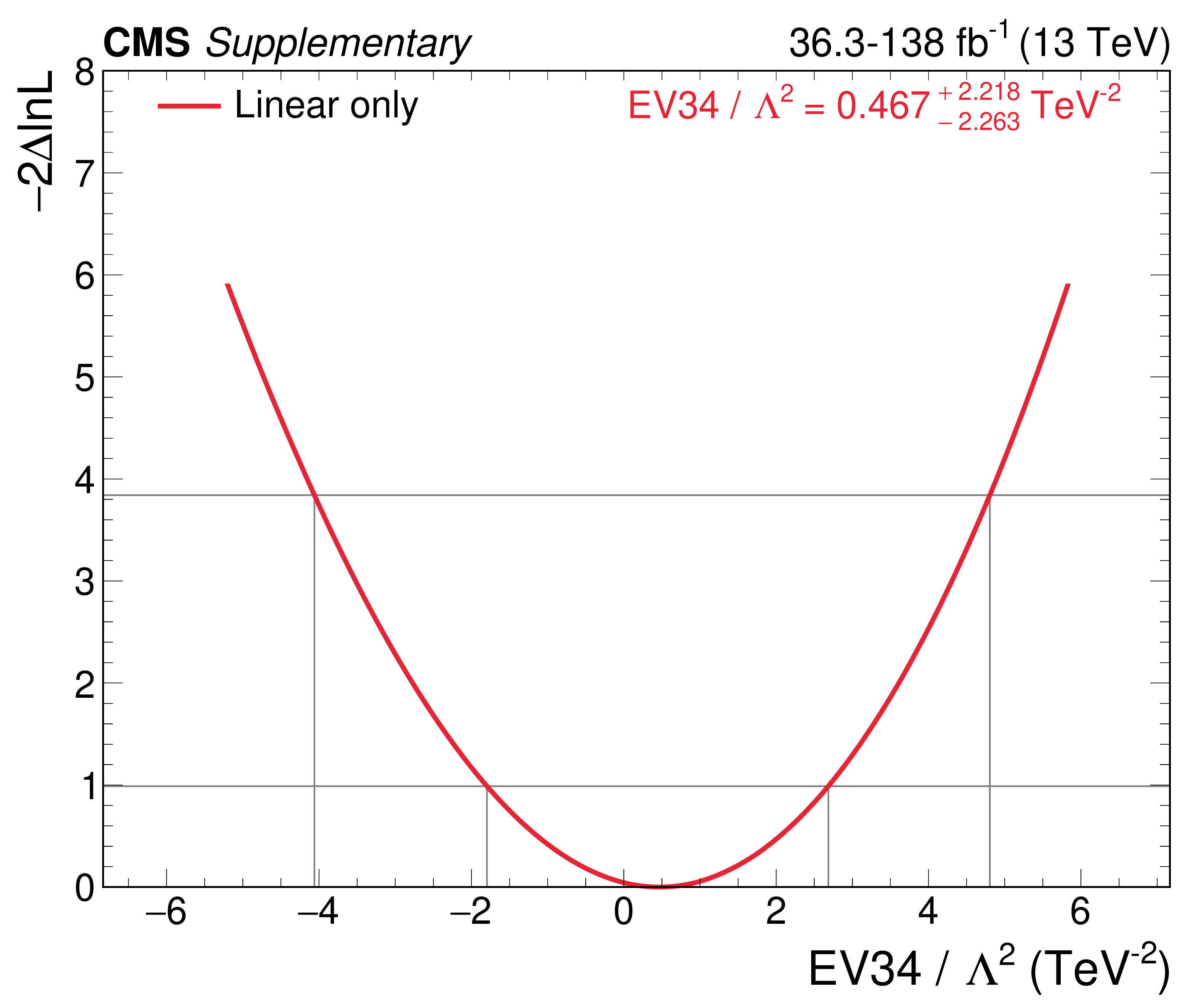
png pdf |
Additional Figure 8-d:
NLL scans of linear combinations of WCs, for the hybrid fit including the $ \mathrm{t}(\overline{\mathrm{t}})\mathrm{X} $ analysis. |
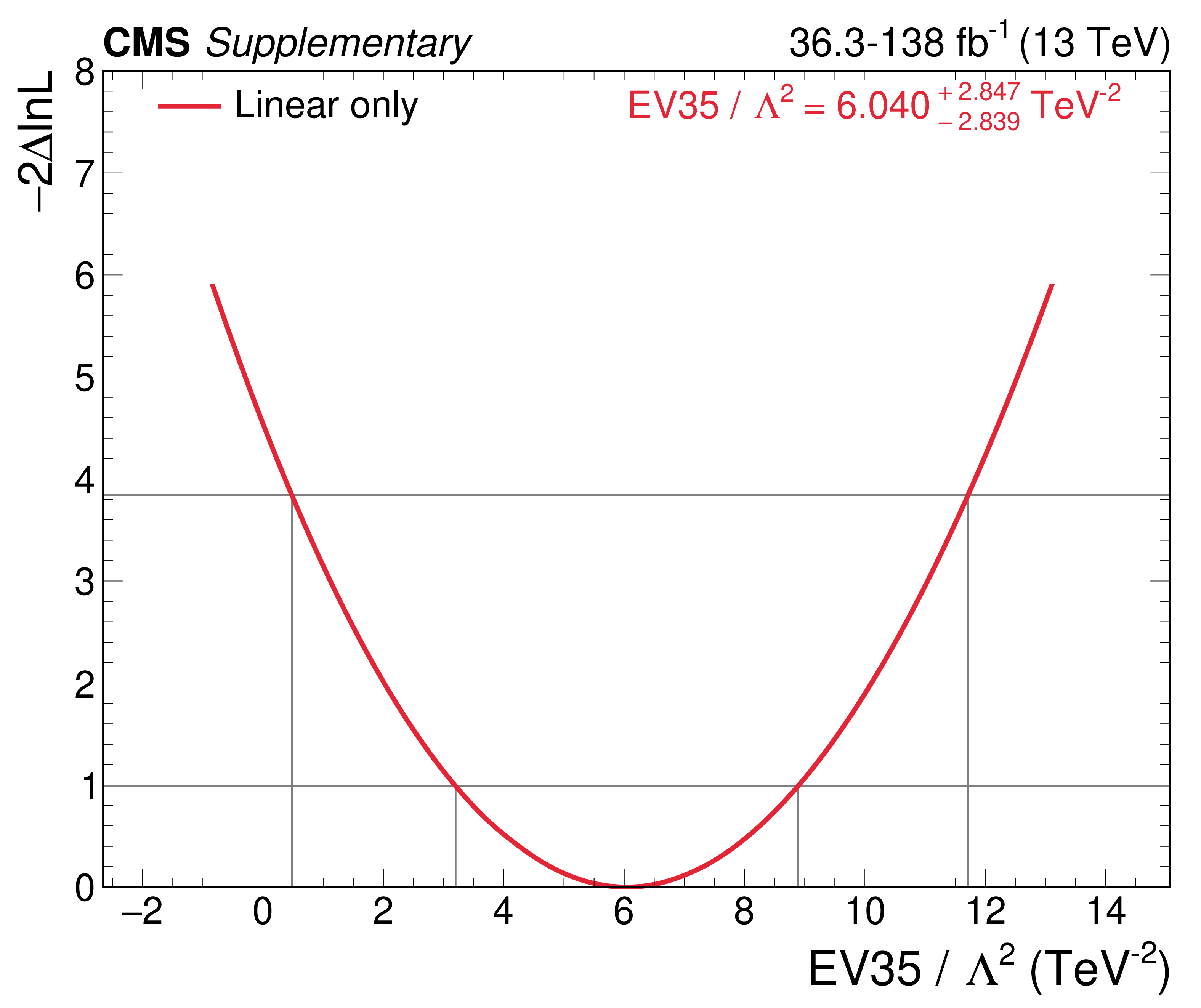
png pdf |
Additional Figure 8-e:
NLL scans of linear combinations of WCs, for the hybrid fit including the $ \mathrm{t}(\overline{\mathrm{t}})\mathrm{X} $ analysis. |
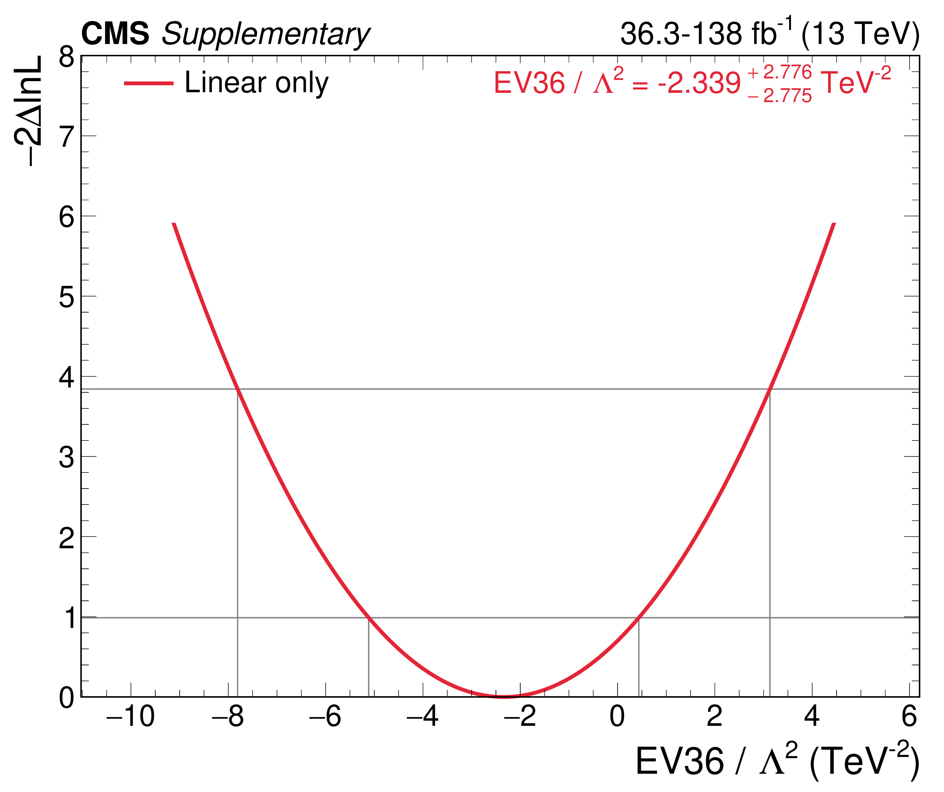
png pdf |
Additional Figure 8-f:
NLL scans of linear combinations of WCs, for the hybrid fit including the $ \mathrm{t}(\overline{\mathrm{t}})\mathrm{X} $ analysis. |
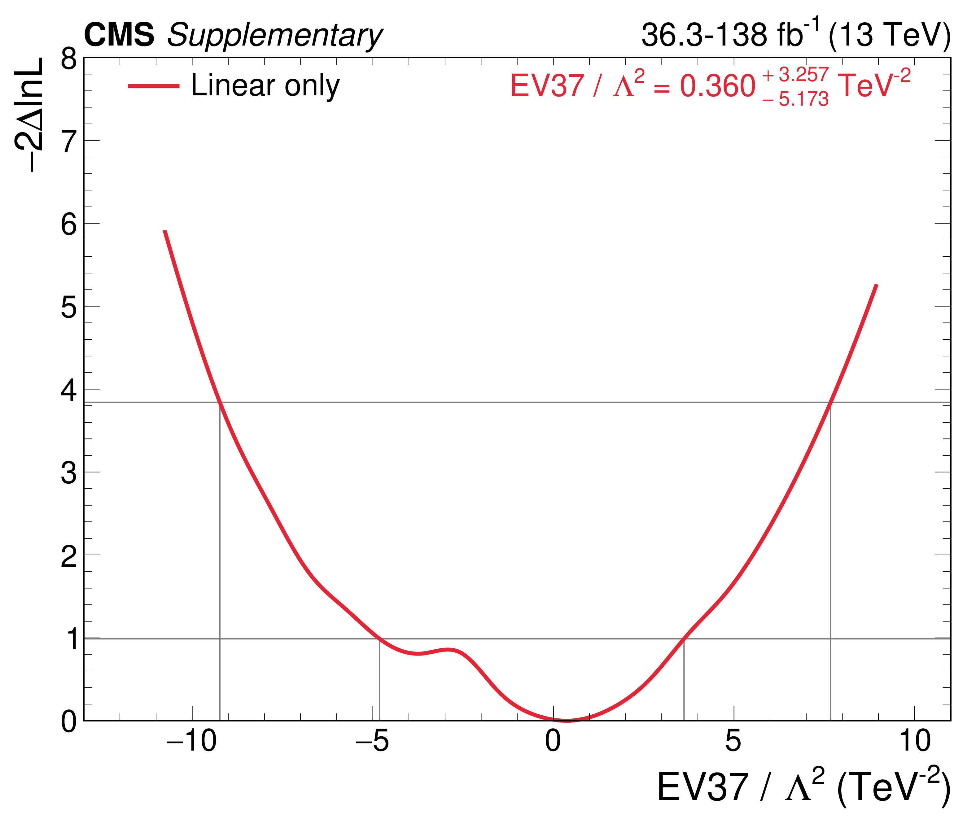
png pdf |
Additional Figure 8-g:
NLL scans of linear combinations of WCs, for the hybrid fit including the $ \mathrm{t}(\overline{\mathrm{t}})\mathrm{X} $ analysis. |
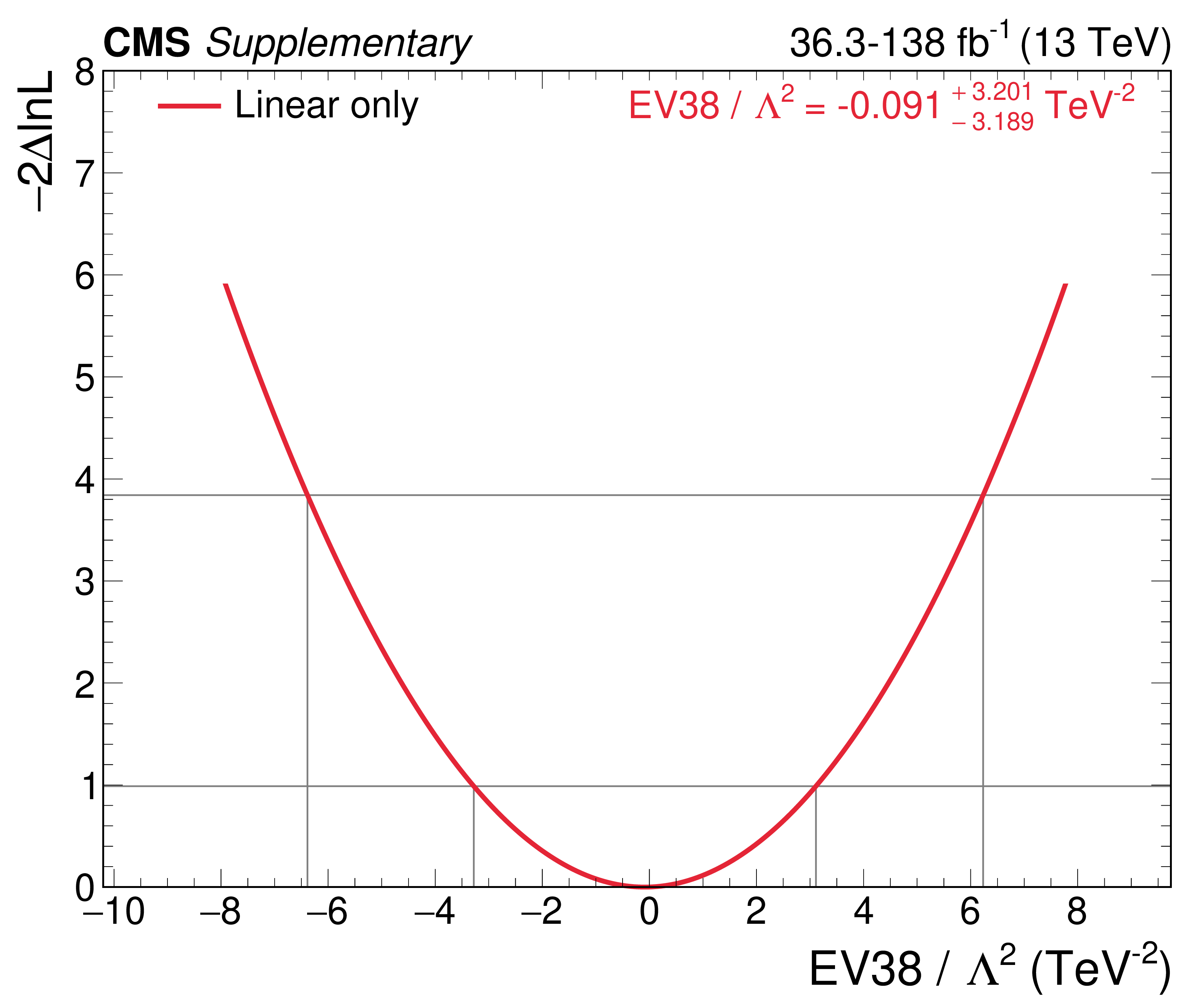
png pdf |
Additional Figure 8-h:
NLL scans of linear combinations of WCs, for the hybrid fit including the $ \mathrm{t}(\overline{\mathrm{t}})\mathrm{X} $ analysis. |

png pdf |
Additional Figure 8-i:
NLL scans of linear combinations of WCs, for the hybrid fit including the $ \mathrm{t}(\overline{\mathrm{t}})\mathrm{X} $ analysis. |
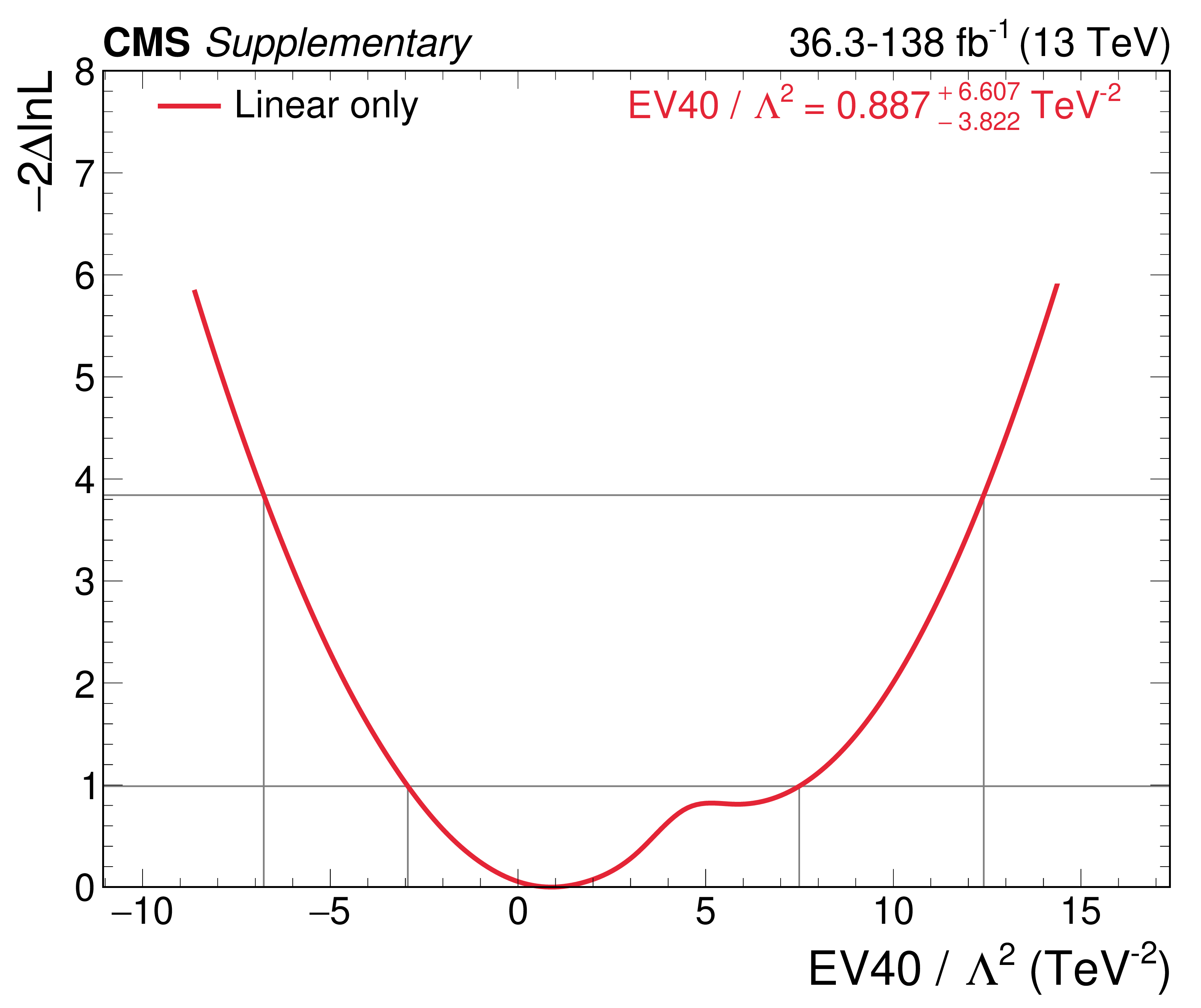
png pdf |
Additional Figure 8-j:
NLL scans of linear combinations of WCs, for the hybrid fit including the $ \mathrm{t}(\overline{\mathrm{t}})\mathrm{X} $ analysis. |
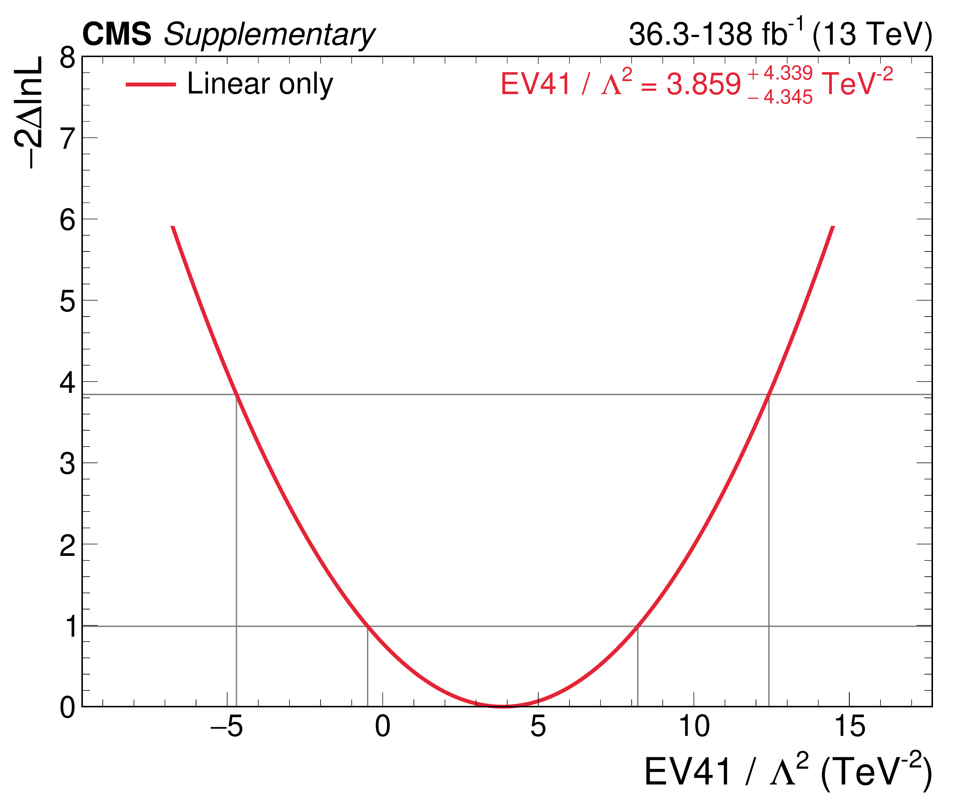
png pdf |
Additional Figure 8-k:
NLL scans of linear combinations of WCs, for the hybrid fit including the $ \mathrm{t}(\overline{\mathrm{t}})\mathrm{X} $ analysis. |

png pdf |
Additional Figure 8-l:
NLL scans of linear combinations of WCs, for the hybrid fit including the $ \mathrm{t}(\overline{\mathrm{t}})\mathrm{X} $ analysis. |
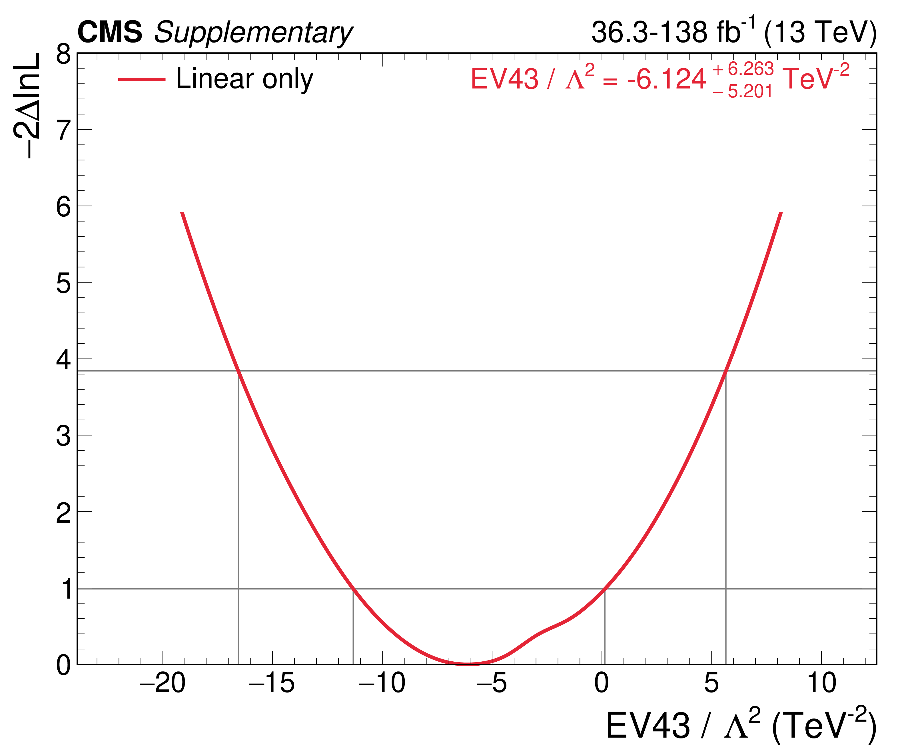
png pdf |
Additional Figure 8-m:
NLL scans of linear combinations of WCs, for the hybrid fit including the $ \mathrm{t}(\overline{\mathrm{t}})\mathrm{X} $ analysis. |
png pdf |
Additional Figure 9:
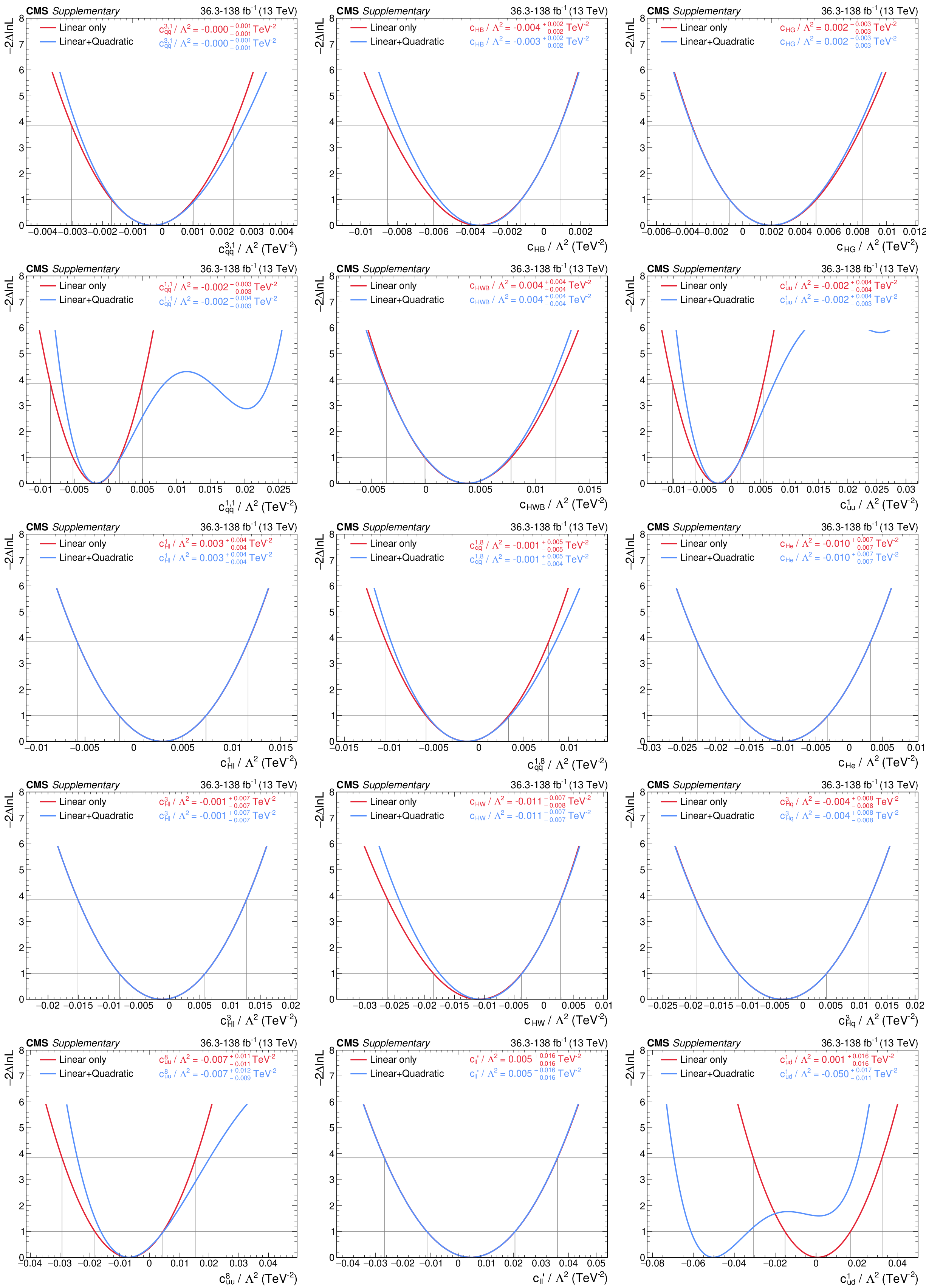
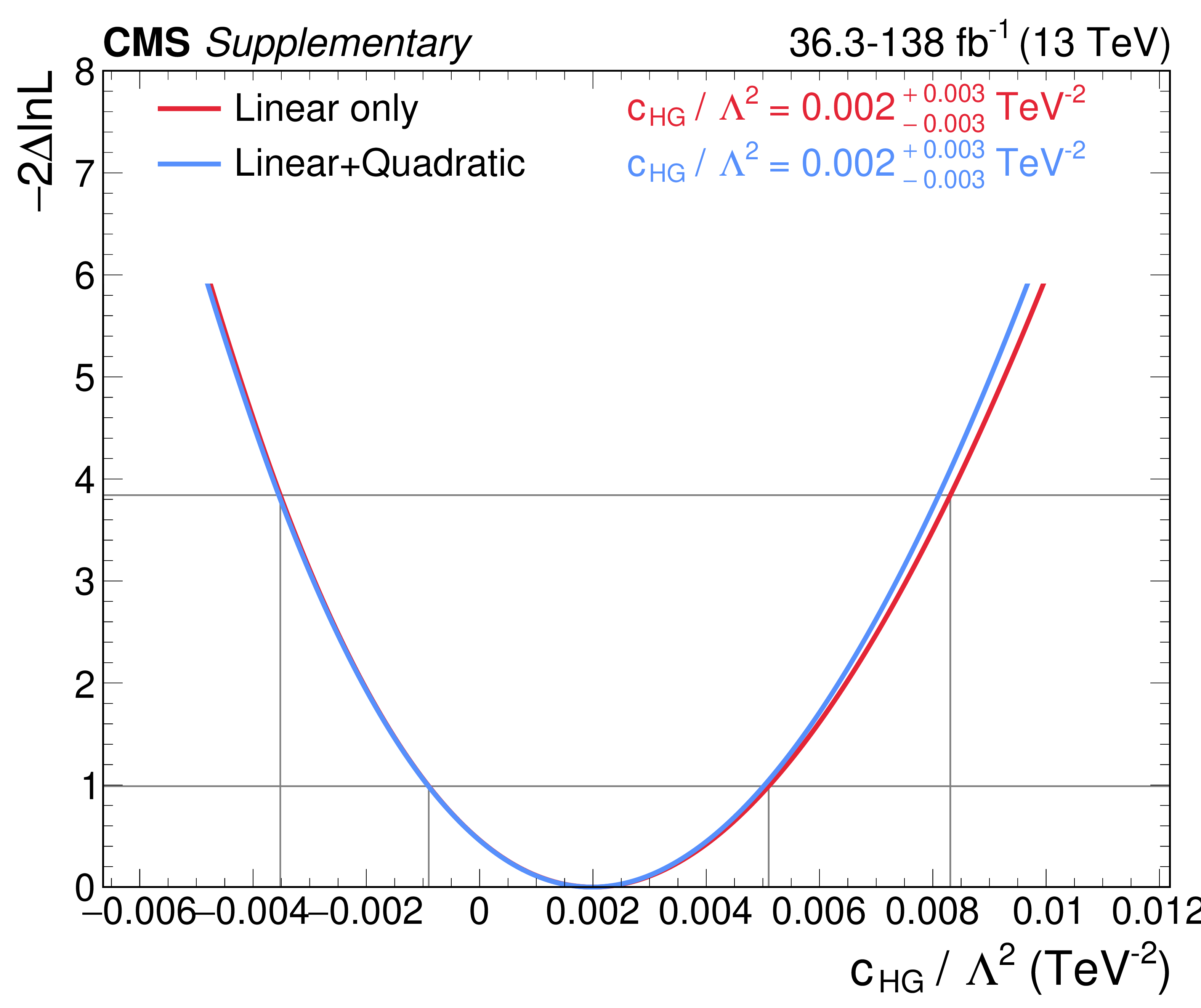
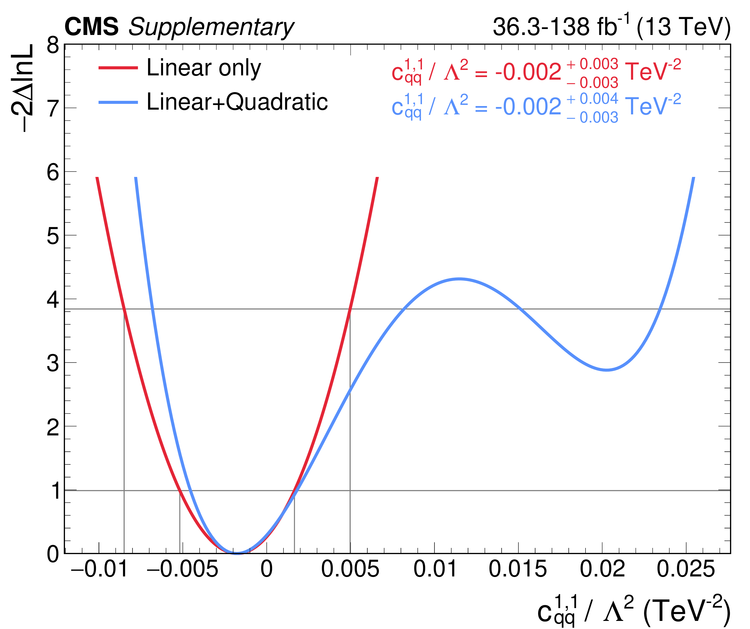
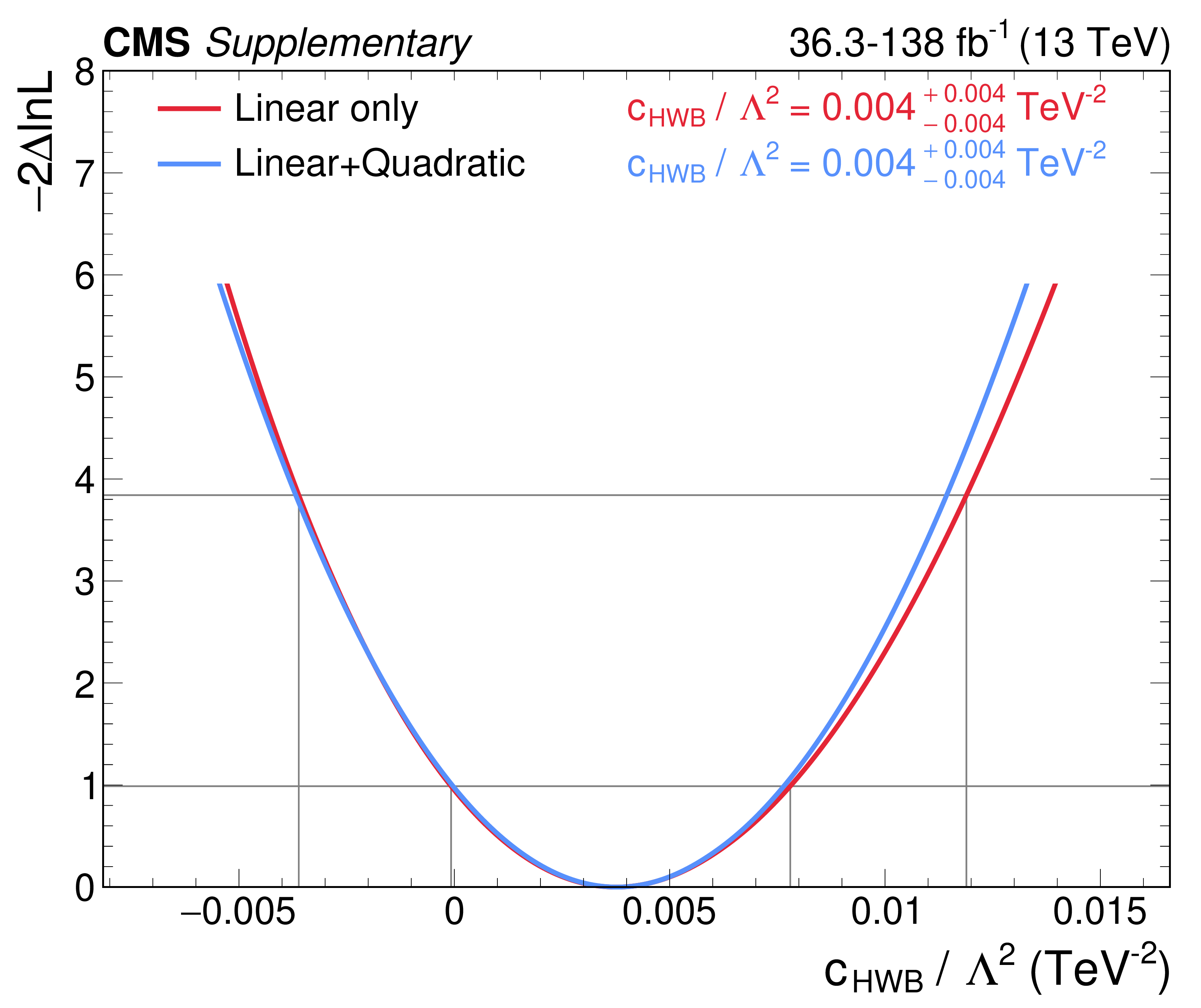
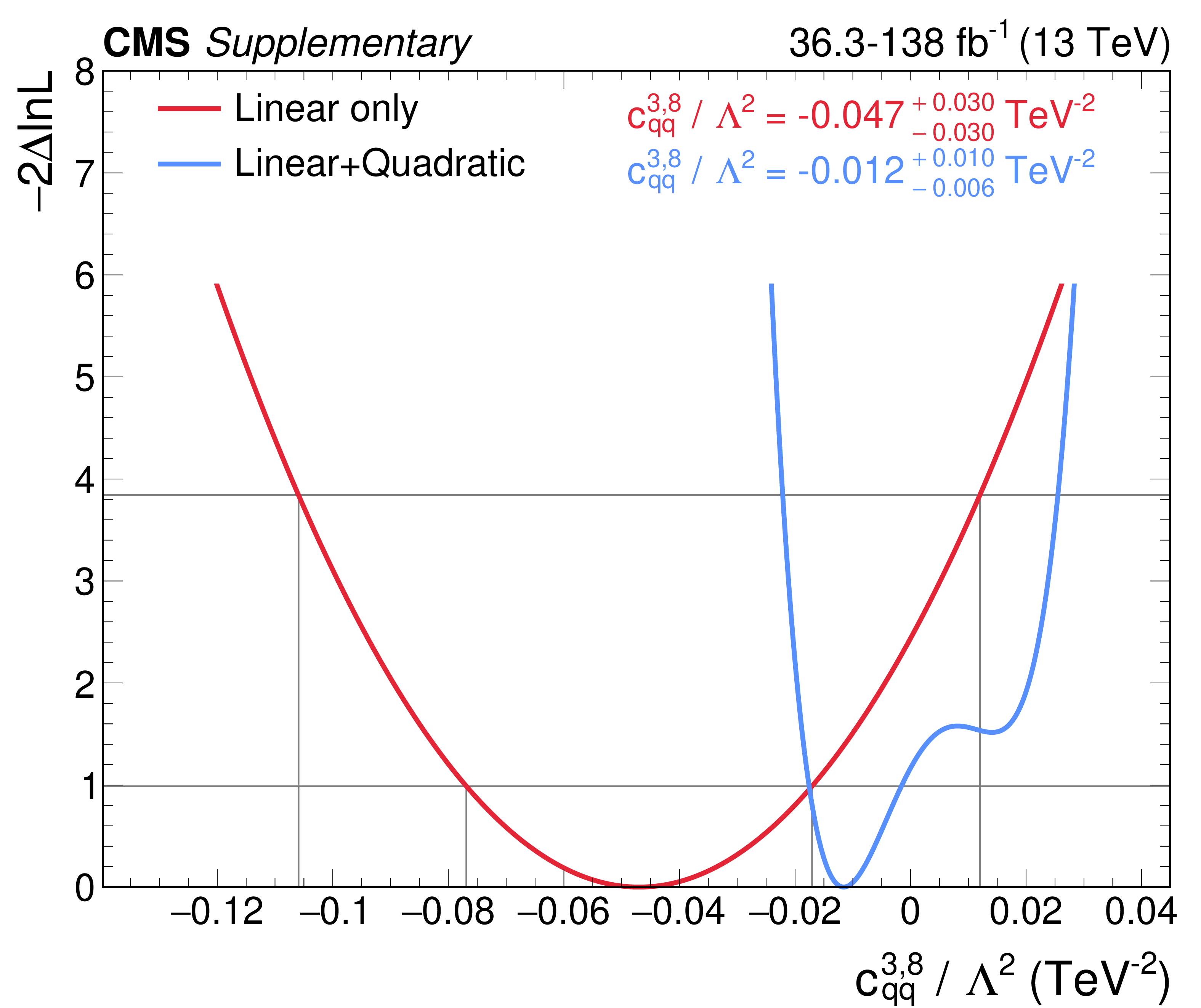
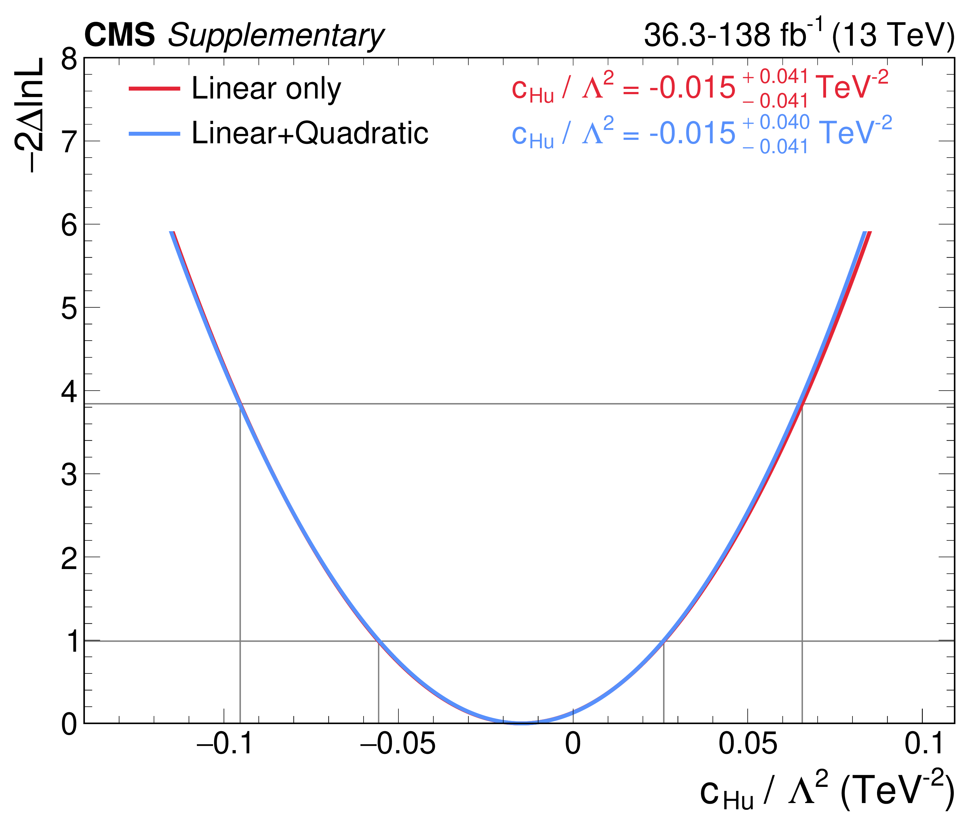
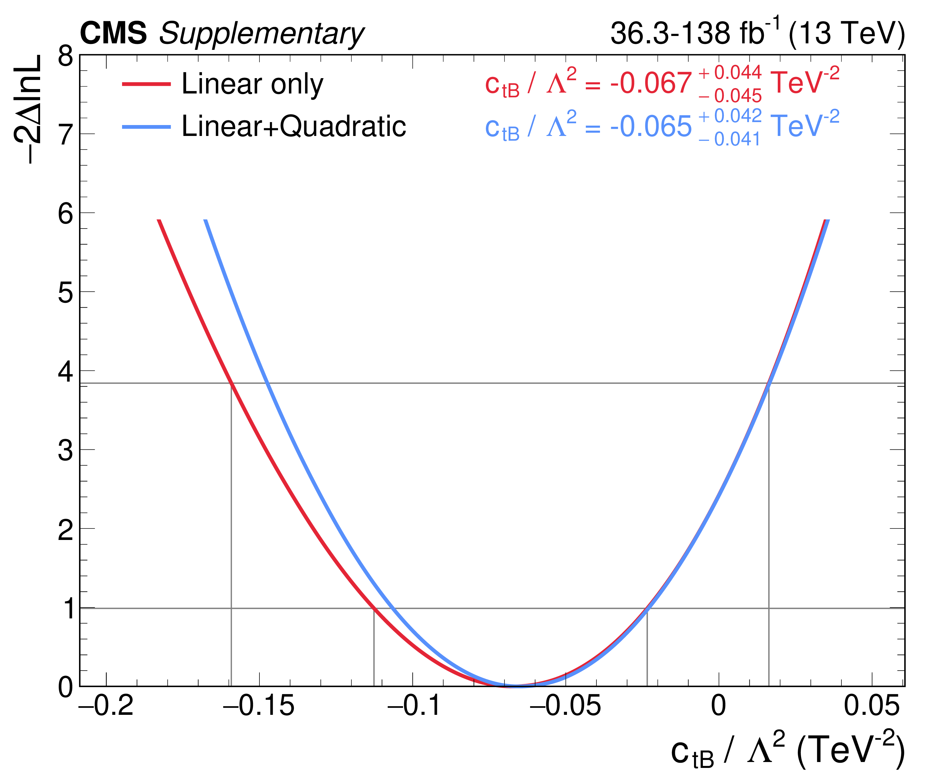
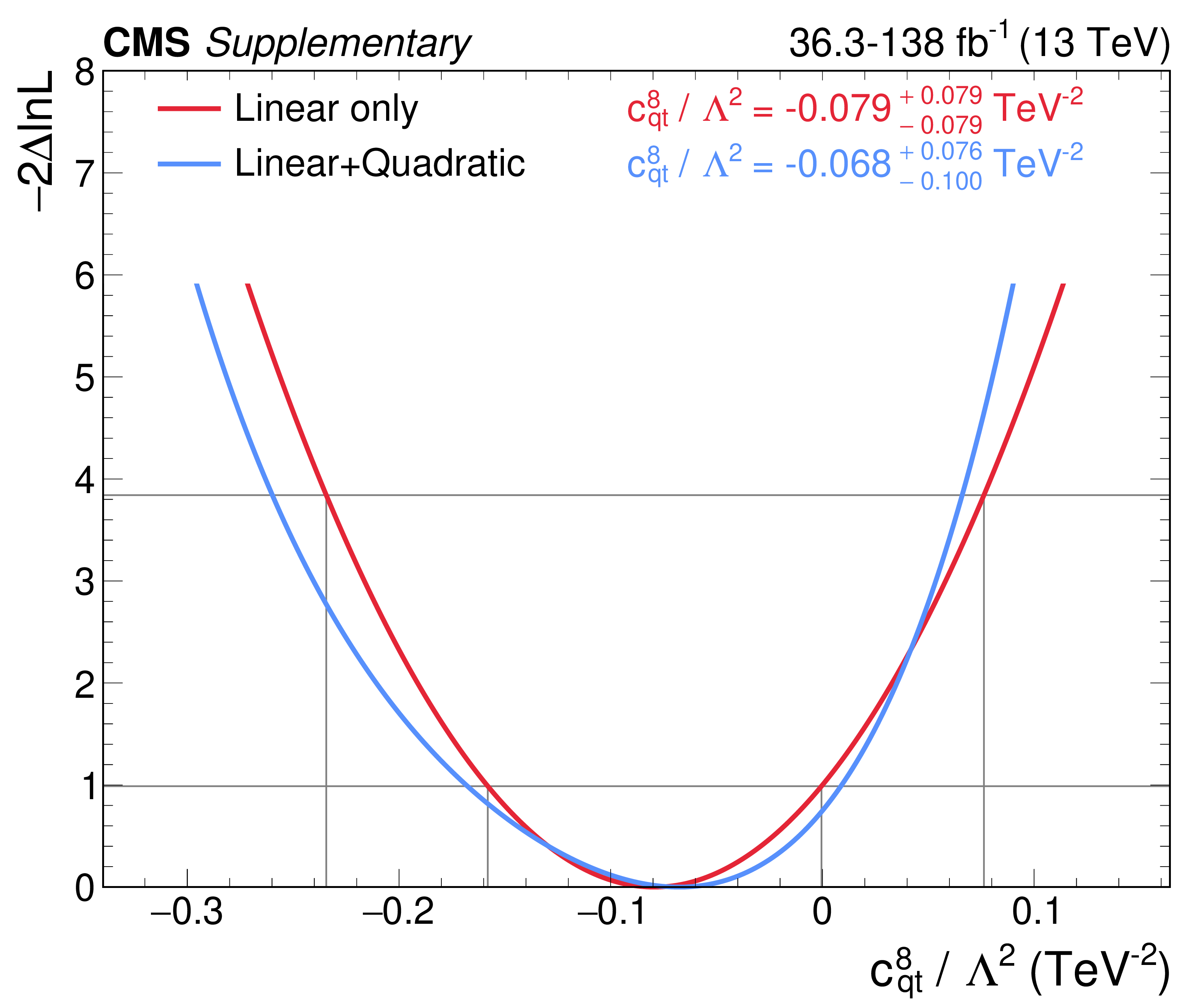
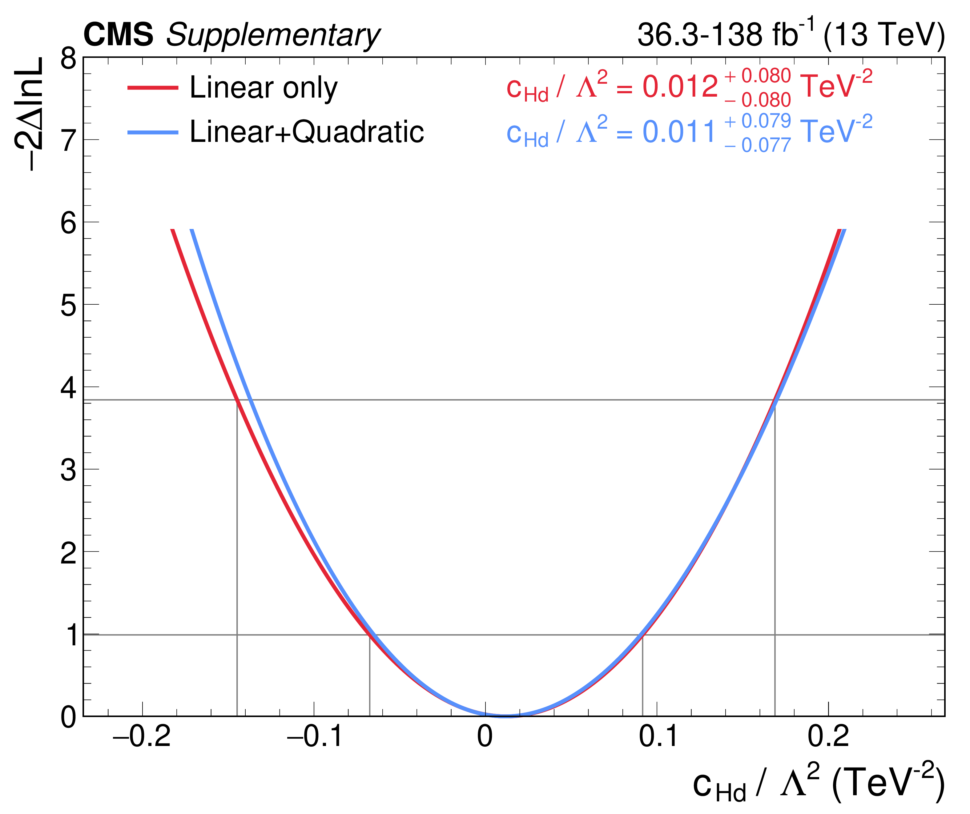
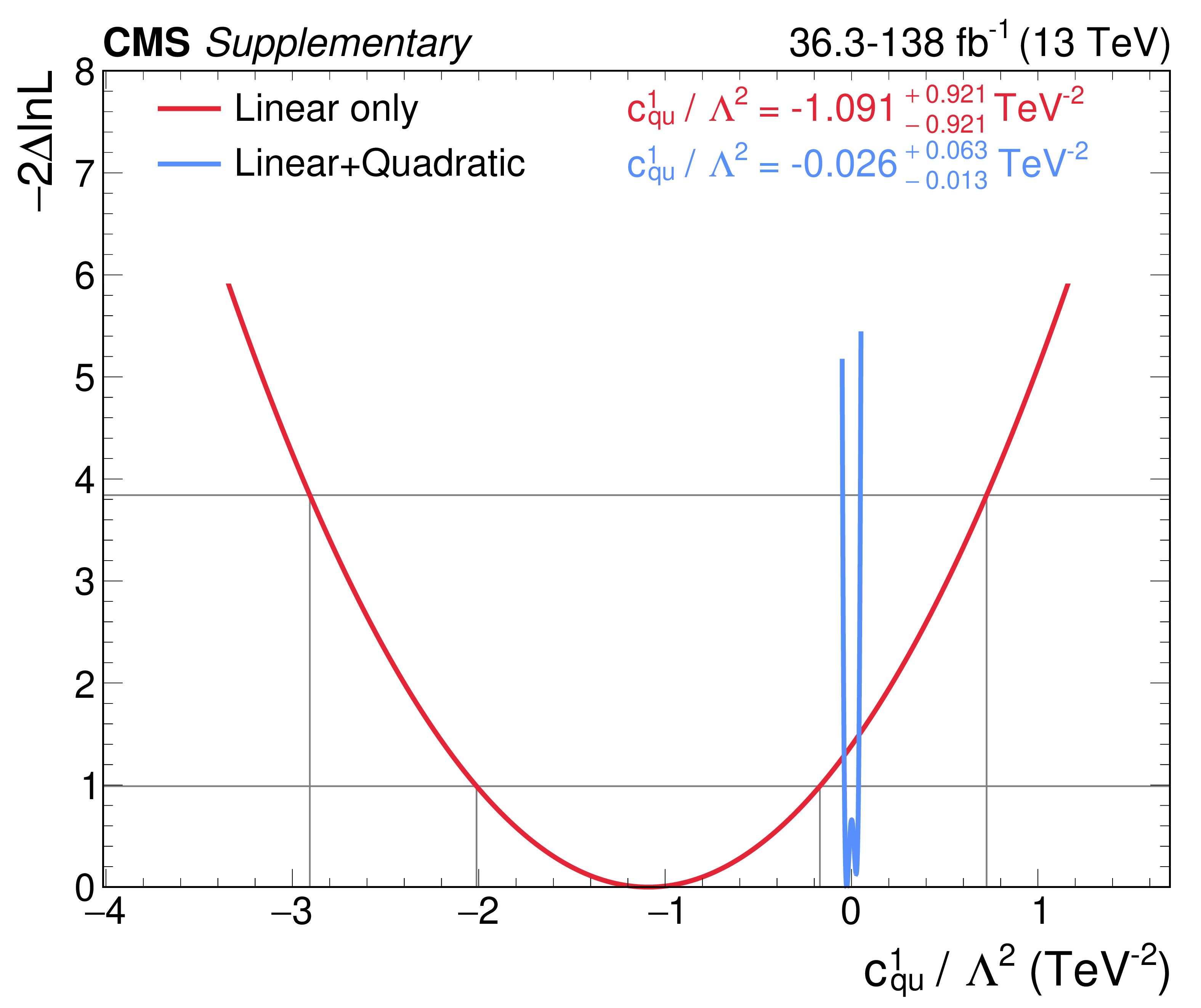
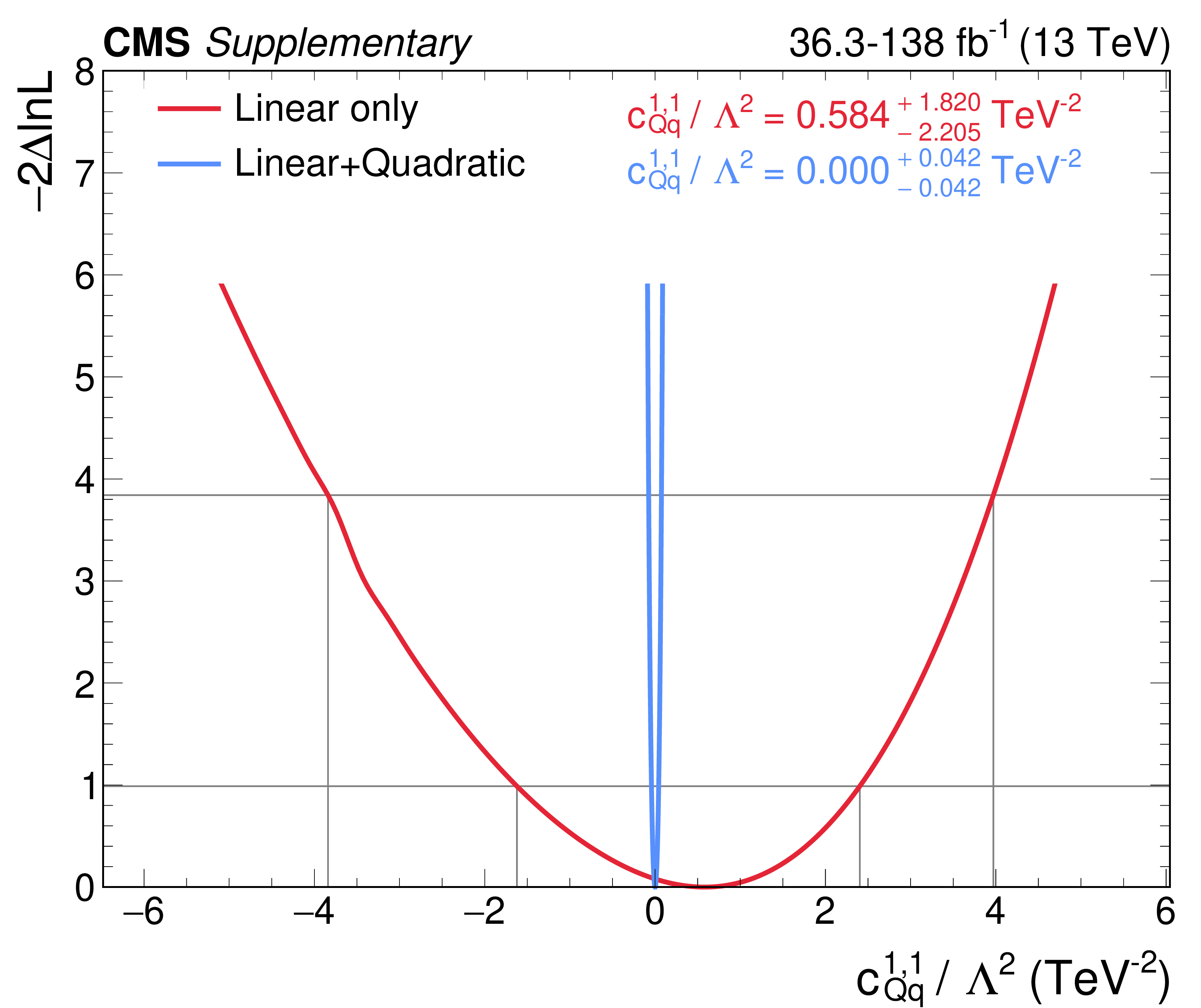
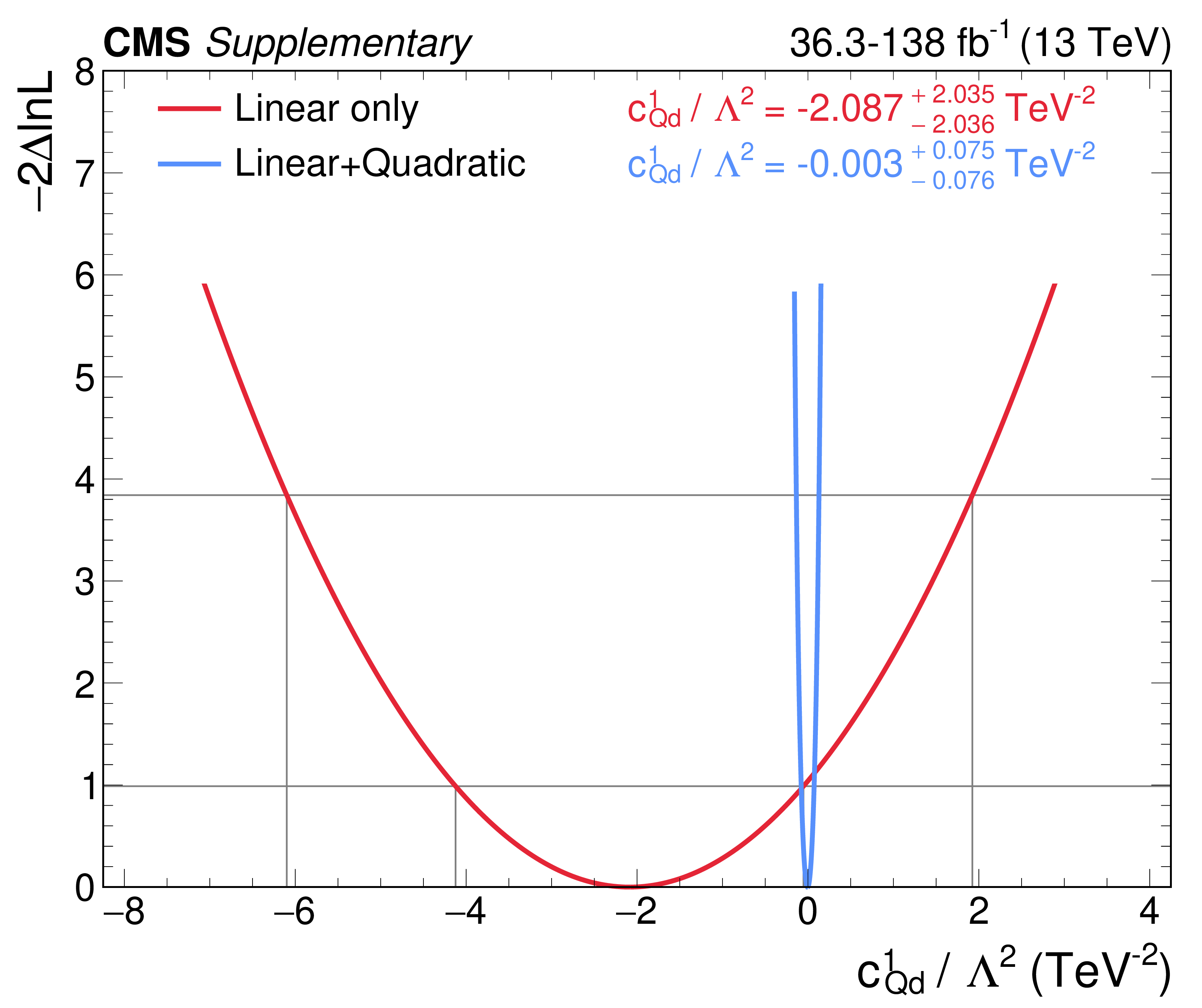
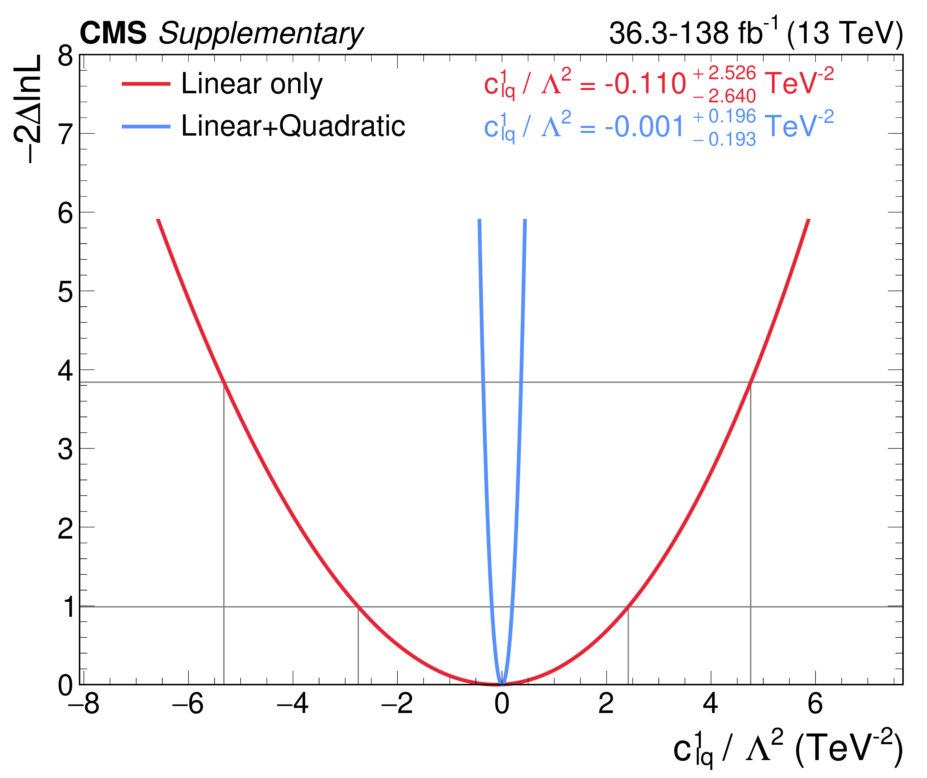
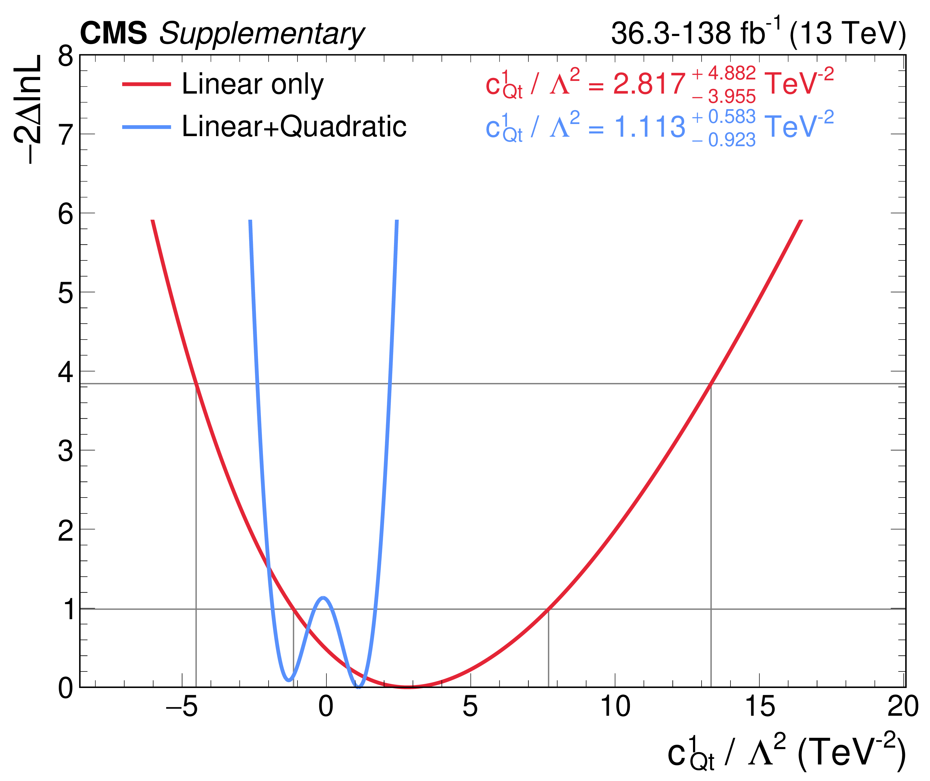
NLL scans of WCs, for the hybrid fit including the $ \mathrm{t}(\overline{\mathrm{t}})\mathrm{X} $ analysis, with and without the inclusion of quadratic terms. |

png pdf |
Additional Figure 9-a:
NLL scans of WCs, for the hybrid fit including the $ \mathrm{t}(\overline{\mathrm{t}})\mathrm{X} $ analysis, with and without the inclusion of quadratic terms. |

png pdf |
Additional Figure 9-b:
NLL scans of WCs, for the hybrid fit including the $ \mathrm{t}(\overline{\mathrm{t}})\mathrm{X} $ analysis, with and without the inclusion of quadratic terms. |
png pdf |
Additional Figure 9-c:
NLL scans of WCs, for the hybrid fit including the $ \mathrm{t}(\overline{\mathrm{t}})\mathrm{X} $ analysis, with and without the inclusion of quadratic terms. |
png pdf |
Additional Figure 9-d:
NLL scans of WCs, for the hybrid fit including the $ \mathrm{t}(\overline{\mathrm{t}})\mathrm{X} $ analysis, with and without the inclusion of quadratic terms. |
png pdf |
Additional Figure 9-e:
NLL scans of WCs, for the hybrid fit including the $ \mathrm{t}(\overline{\mathrm{t}})\mathrm{X} $ analysis, with and without the inclusion of quadratic terms. |
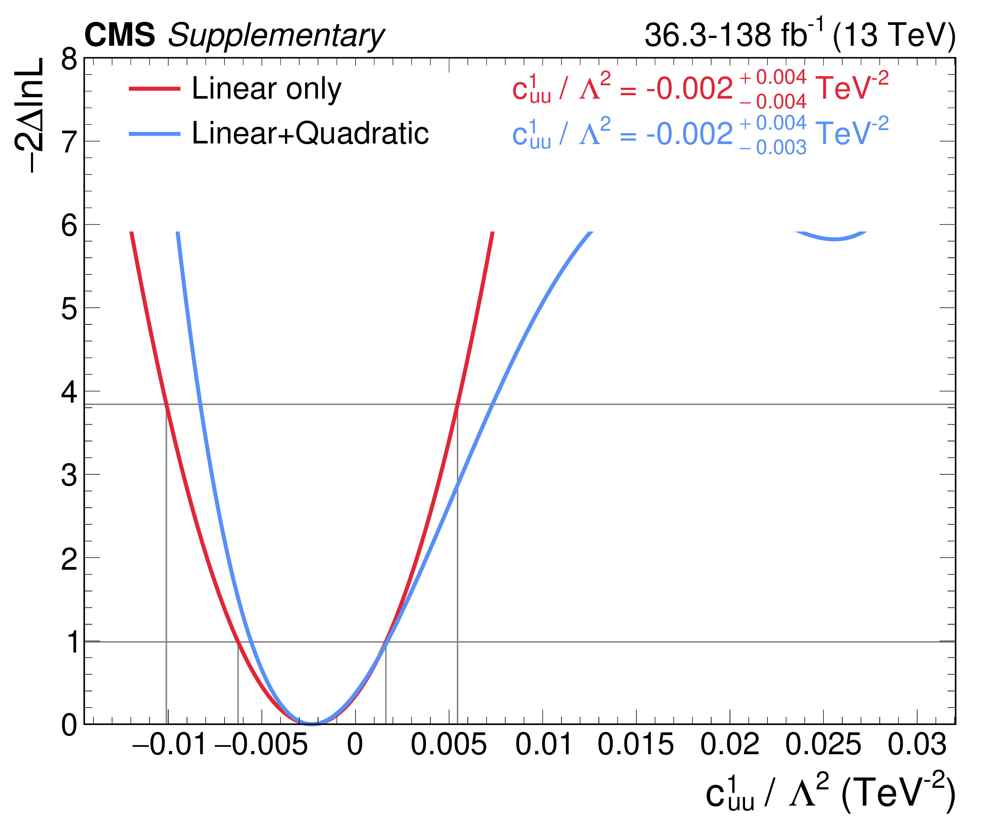
png pdf |
Additional Figure 9-f:
NLL scans of WCs, for the hybrid fit including the $ \mathrm{t}(\overline{\mathrm{t}})\mathrm{X} $ analysis, with and without the inclusion of quadratic terms. |
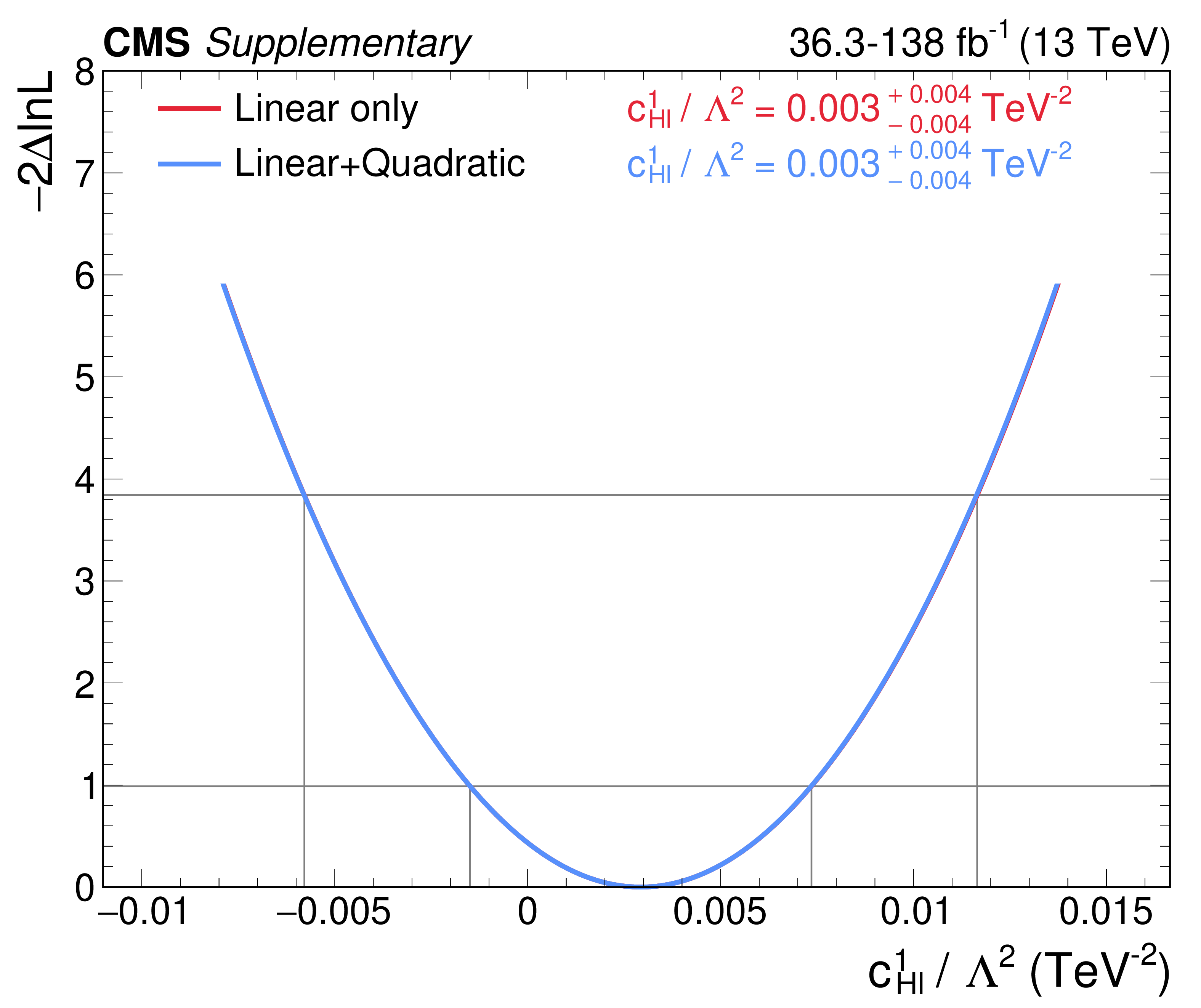
png pdf |
Additional Figure 9-g:
NLL scans of WCs, for the hybrid fit including the $ \mathrm{t}(\overline{\mathrm{t}})\mathrm{X} $ analysis, with and without the inclusion of quadratic terms. |
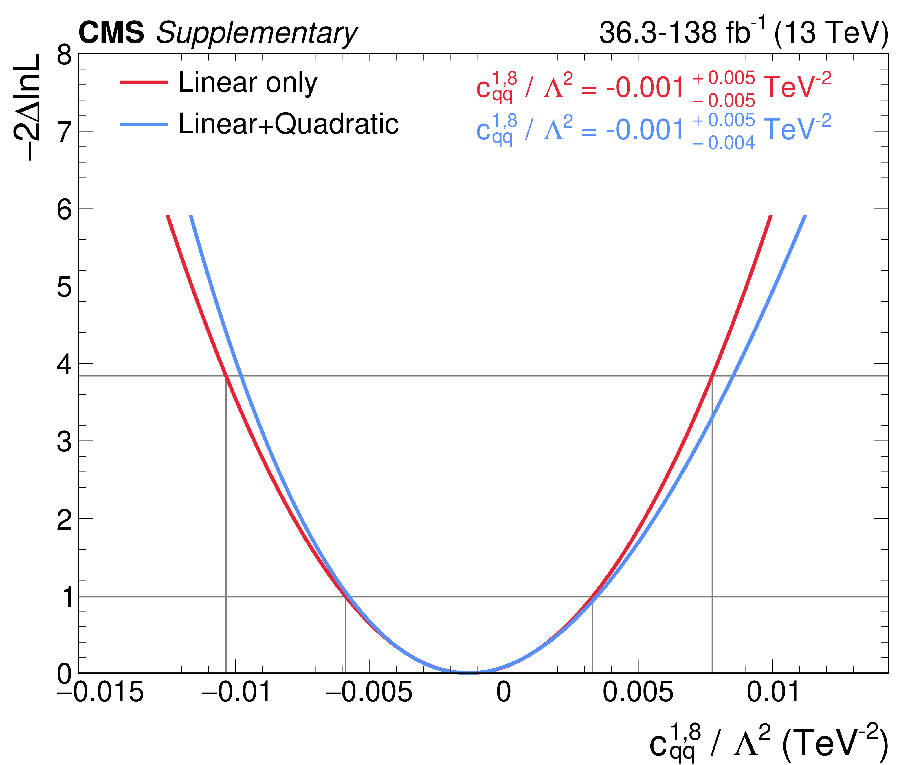
png pdf |
Additional Figure 9-h:
NLL scans of WCs, for the hybrid fit including the $ \mathrm{t}(\overline{\mathrm{t}})\mathrm{X} $ analysis, with and without the inclusion of quadratic terms. |

png pdf |
Additional Figure 9-i:
NLL scans of WCs, for the hybrid fit including the $ \mathrm{t}(\overline{\mathrm{t}})\mathrm{X} $ analysis, with and without the inclusion of quadratic terms. |
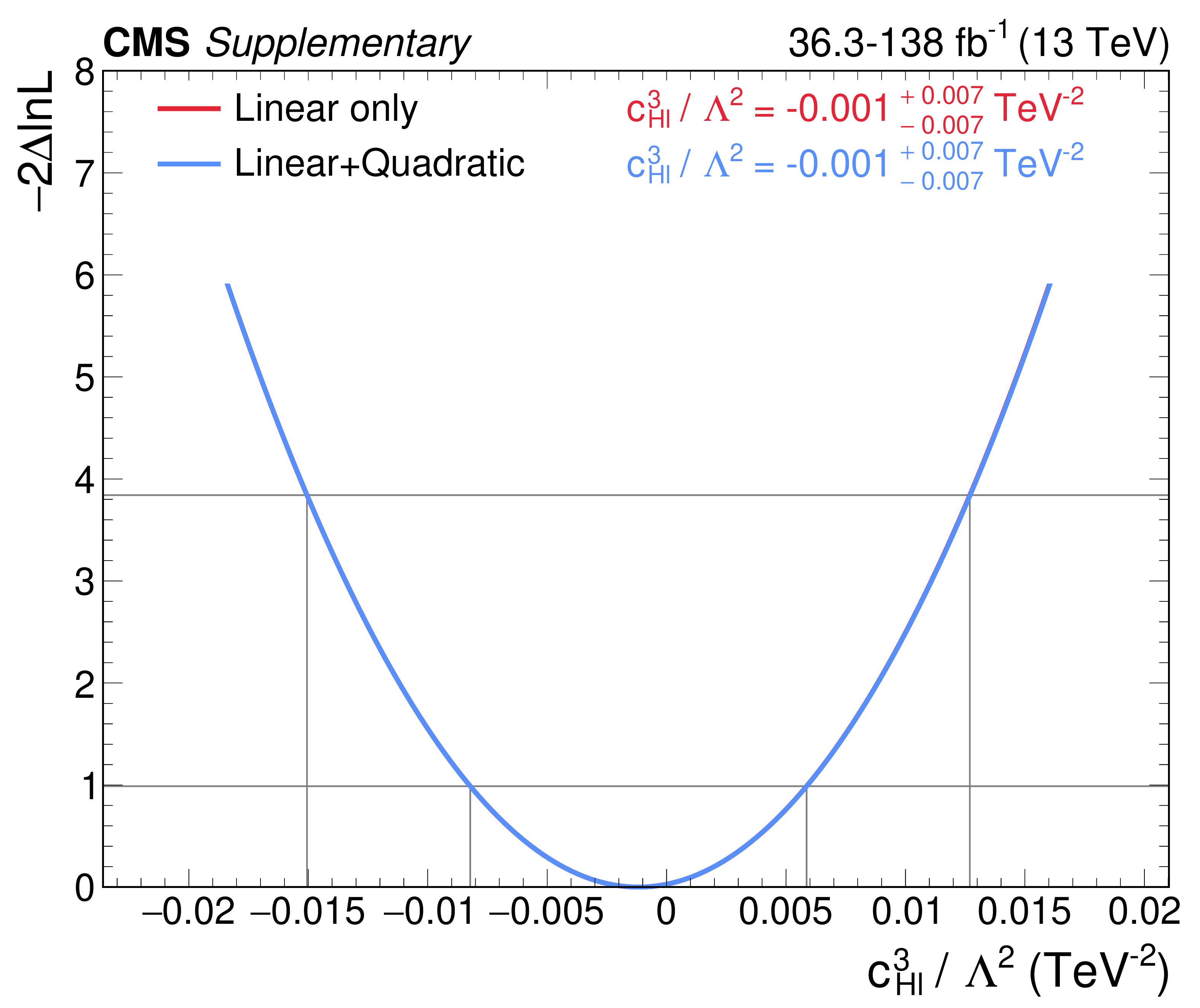
png pdf |
Additional Figure 9-j:
NLL scans of WCs, for the hybrid fit including the $ \mathrm{t}(\overline{\mathrm{t}})\mathrm{X} $ analysis, with and without the inclusion of quadratic terms. |

png pdf |
Additional Figure 9-k:
NLL scans of WCs, for the hybrid fit including the $ \mathrm{t}(\overline{\mathrm{t}})\mathrm{X} $ analysis, with and without the inclusion of quadratic terms. |

png pdf |
Additional Figure 9-l:
NLL scans of WCs, for the hybrid fit including the $ \mathrm{t}(\overline{\mathrm{t}})\mathrm{X} $ analysis, with and without the inclusion of quadratic terms. |

png pdf |
Additional Figure 9-m:
NLL scans of WCs, for the hybrid fit including the $ \mathrm{t}(\overline{\mathrm{t}})\mathrm{X} $ analysis, with and without the inclusion of quadratic terms. |
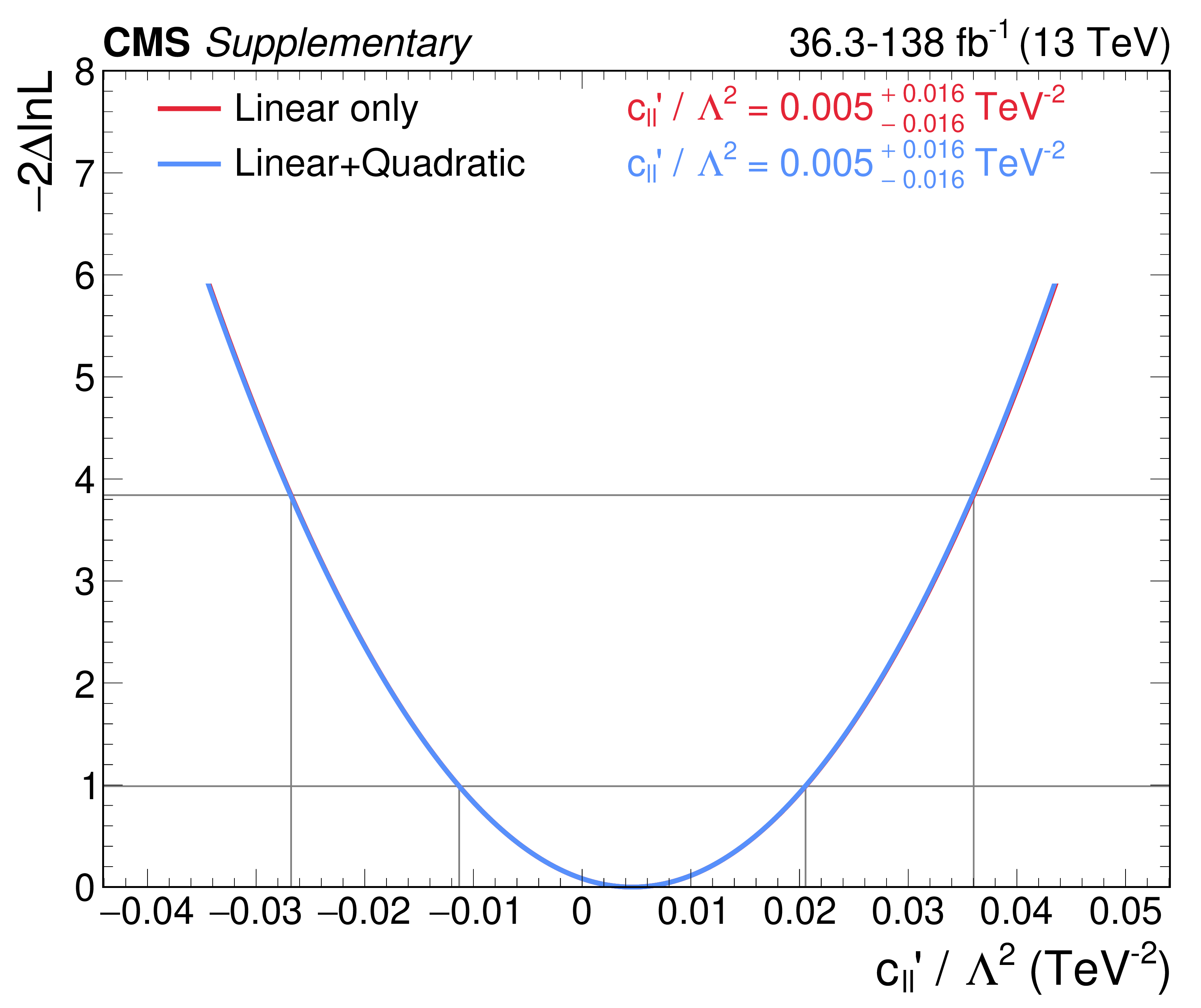
png pdf |
Additional Figure 9-n:
NLL scans of WCs, for the hybrid fit including the $ \mathrm{t}(\overline{\mathrm{t}})\mathrm{X} $ analysis, with and without the inclusion of quadratic terms. |
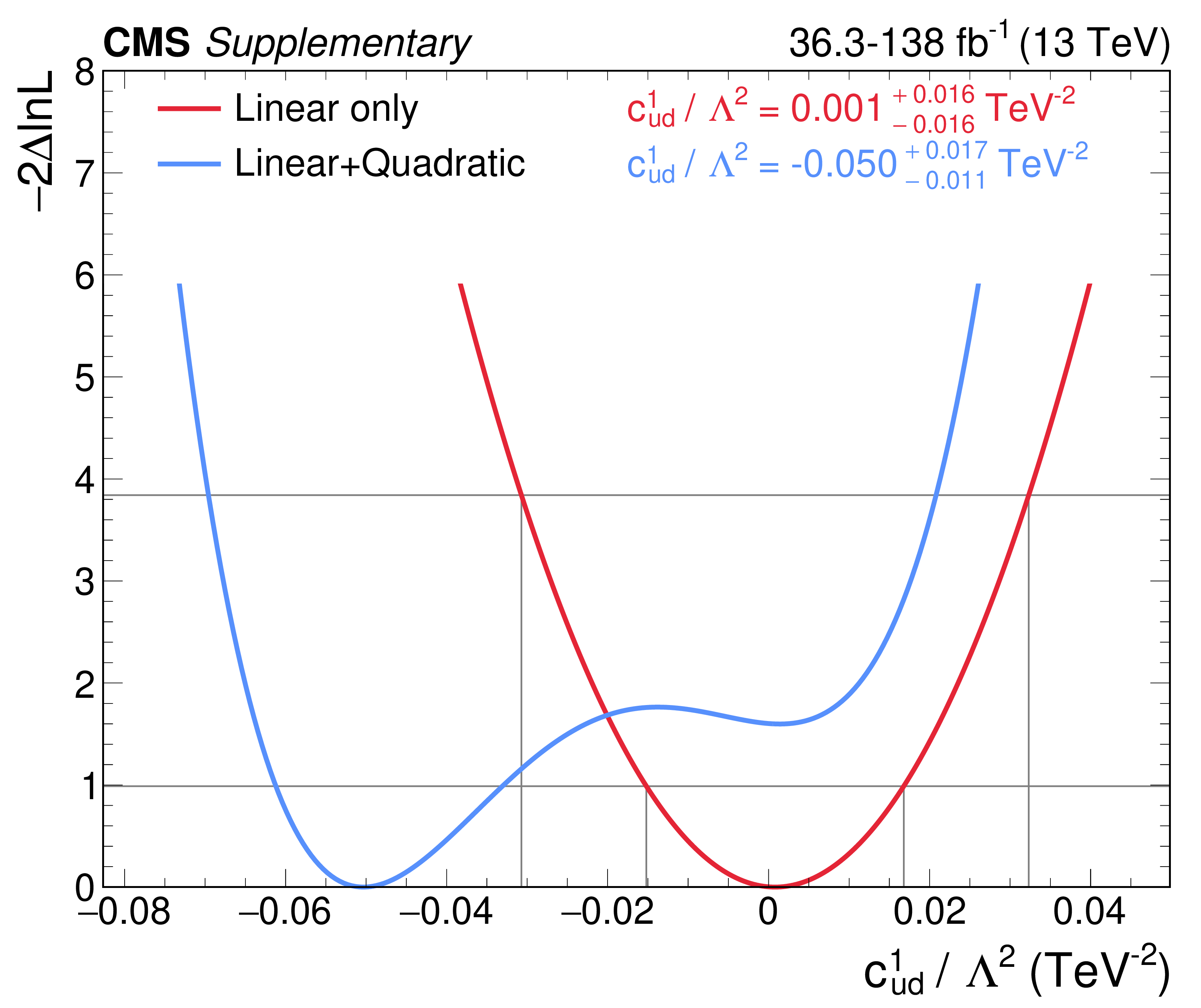
png pdf |
Additional Figure 9-o:
NLL scans of WCs, for the hybrid fit including the $ \mathrm{t}(\overline{\mathrm{t}})\mathrm{X} $ analysis, with and without the inclusion of quadratic terms. |
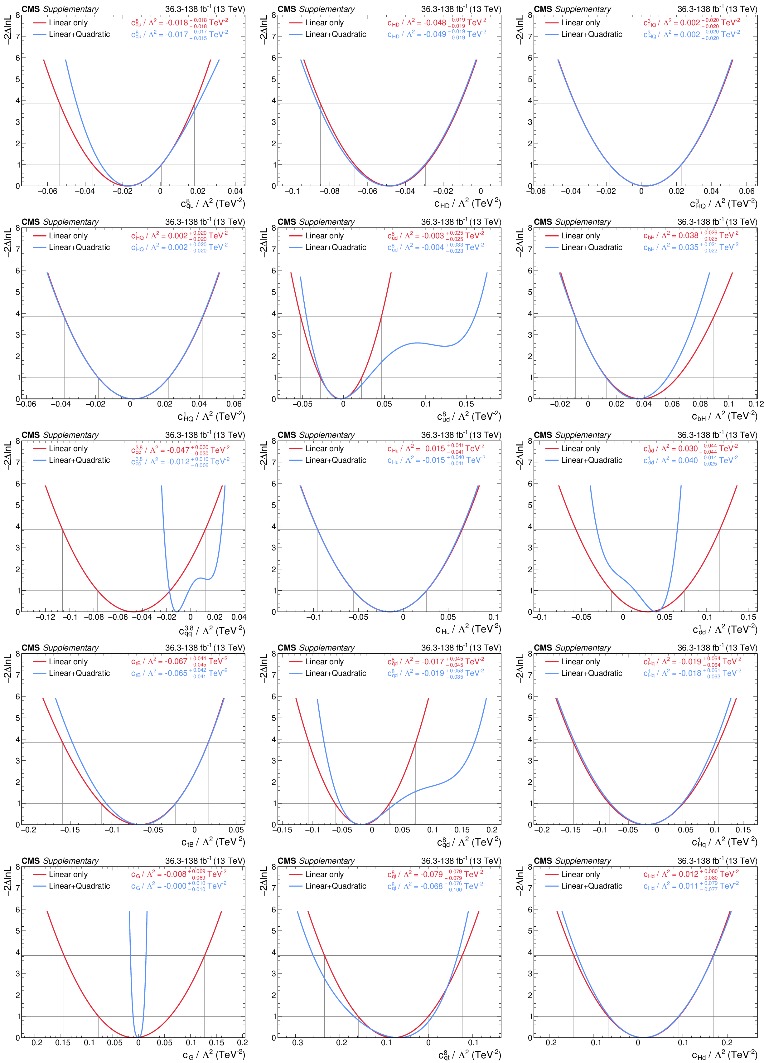
png pdf |
Additional Figure 10:
NLL scans of WCs, for the hybrid fit including the $ \mathrm{t}(\overline{\mathrm{t}})\mathrm{X} $ analysis, with and without the inclusion of quadratic terms. |
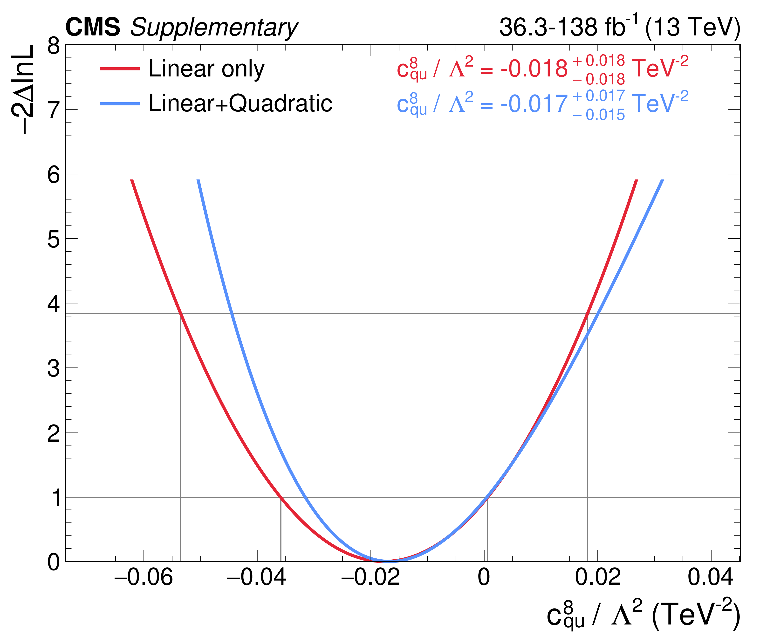
png pdf |
Additional Figure 10-a:
NLL scans of WCs, for the hybrid fit including the $ \mathrm{t}(\overline{\mathrm{t}})\mathrm{X} $ analysis, with and without the inclusion of quadratic terms. |

png pdf |
Additional Figure 10-b:
NLL scans of WCs, for the hybrid fit including the $ \mathrm{t}(\overline{\mathrm{t}})\mathrm{X} $ analysis, with and without the inclusion of quadratic terms. |
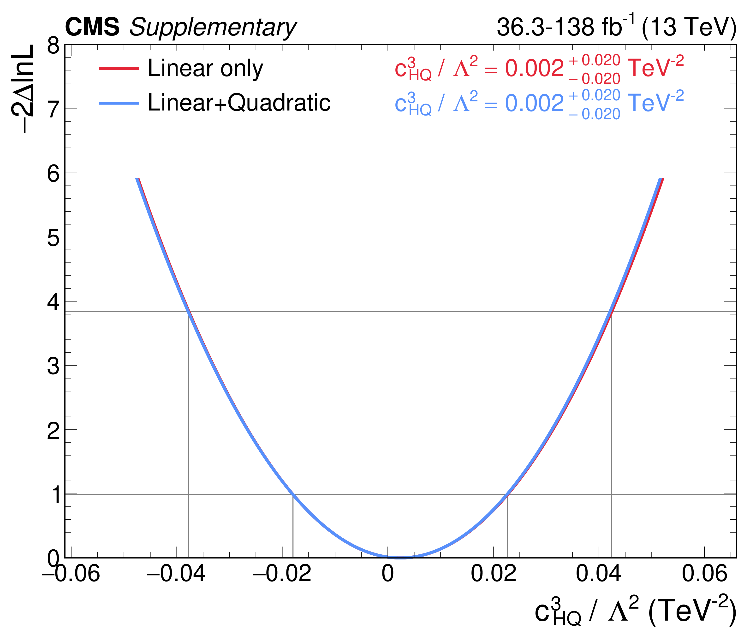
png pdf |
Additional Figure 10-c:
NLL scans of WCs, for the hybrid fit including the $ \mathrm{t}(\overline{\mathrm{t}})\mathrm{X} $ analysis, with and without the inclusion of quadratic terms. |
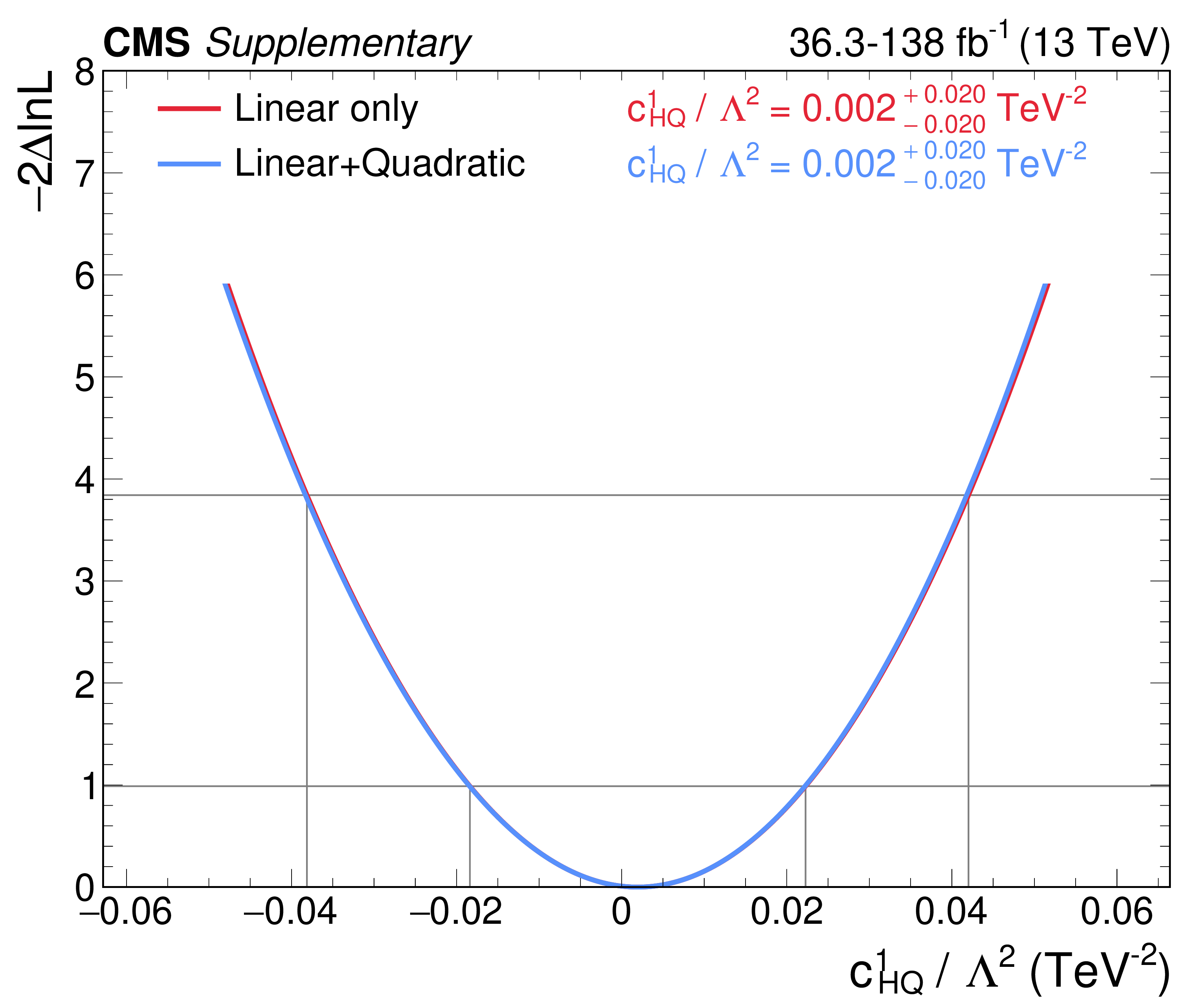
png pdf |
Additional Figure 10-d:
NLL scans of WCs, for the hybrid fit including the $ \mathrm{t}(\overline{\mathrm{t}})\mathrm{X} $ analysis, with and without the inclusion of quadratic terms. |
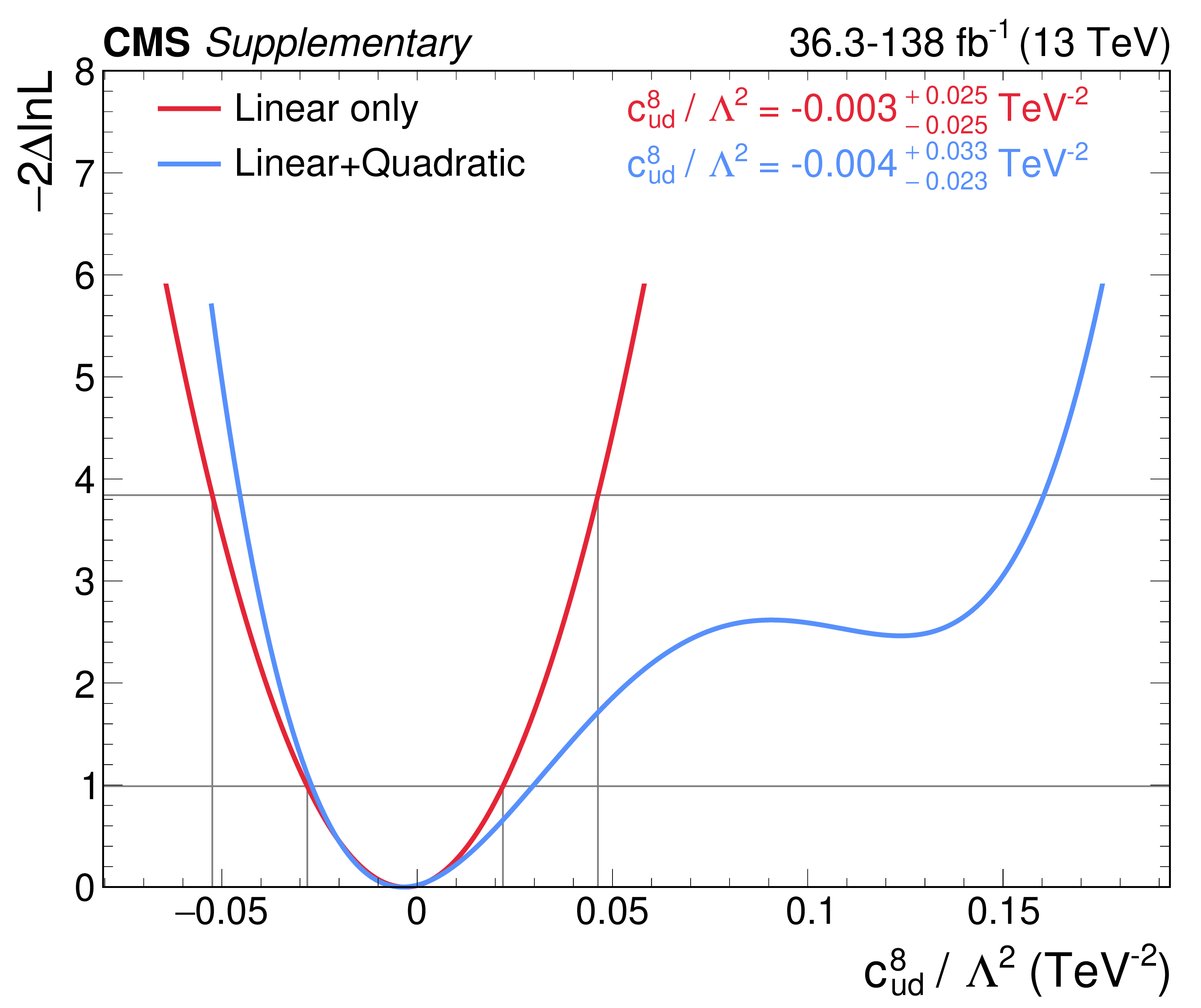
png pdf |
Additional Figure 10-e:
NLL scans of WCs, for the hybrid fit including the $ \mathrm{t}(\overline{\mathrm{t}})\mathrm{X} $ analysis, with and without the inclusion of quadratic terms. |
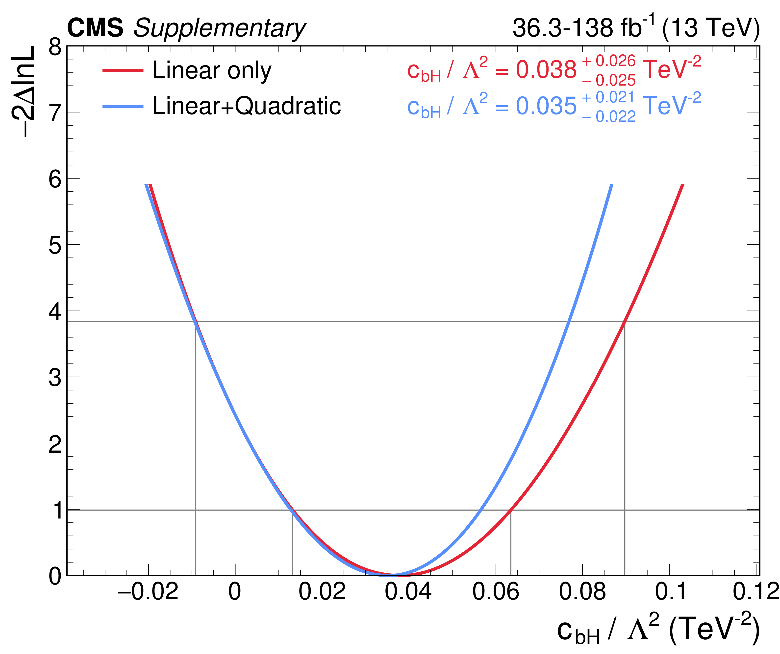
png pdf |
Additional Figure 10-f:
NLL scans of WCs, for the hybrid fit including the $ \mathrm{t}(\overline{\mathrm{t}})\mathrm{X} $ analysis, with and without the inclusion of quadratic terms. |
png pdf |
Additional Figure 10-g:
NLL scans of WCs, for the hybrid fit including the $ \mathrm{t}(\overline{\mathrm{t}})\mathrm{X} $ analysis, with and without the inclusion of quadratic terms. |
png pdf |
Additional Figure 10-h:
NLL scans of WCs, for the hybrid fit including the $ \mathrm{t}(\overline{\mathrm{t}})\mathrm{X} $ analysis, with and without the inclusion of quadratic terms. |

png pdf |
Additional Figure 10-i:
NLL scans of WCs, for the hybrid fit including the $ \mathrm{t}(\overline{\mathrm{t}})\mathrm{X} $ analysis, with and without the inclusion of quadratic terms. |
png pdf |
Additional Figure 10-j:
NLL scans of WCs, for the hybrid fit including the $ \mathrm{t}(\overline{\mathrm{t}})\mathrm{X} $ analysis, with and without the inclusion of quadratic terms. |

png pdf |
Additional Figure 10-k:
NLL scans of WCs, for the hybrid fit including the $ \mathrm{t}(\overline{\mathrm{t}})\mathrm{X} $ analysis, with and without the inclusion of quadratic terms. |

png pdf |
Additional Figure 10-l:
NLL scans of WCs, for the hybrid fit including the $ \mathrm{t}(\overline{\mathrm{t}})\mathrm{X} $ analysis, with and without the inclusion of quadratic terms. |

png pdf |
Additional Figure 10-m:
NLL scans of WCs, for the hybrid fit including the $ \mathrm{t}(\overline{\mathrm{t}})\mathrm{X} $ analysis, with and without the inclusion of quadratic terms. |
png pdf |
Additional Figure 10-n:
NLL scans of WCs, for the hybrid fit including the $ \mathrm{t}(\overline{\mathrm{t}})\mathrm{X} $ analysis, with and without the inclusion of quadratic terms. |
png pdf |
Additional Figure 10-o:
NLL scans of WCs, for the hybrid fit including the $ \mathrm{t}(\overline{\mathrm{t}})\mathrm{X} $ analysis, with and without the inclusion of quadratic terms. |
png pdf |
Additional Figure 11:
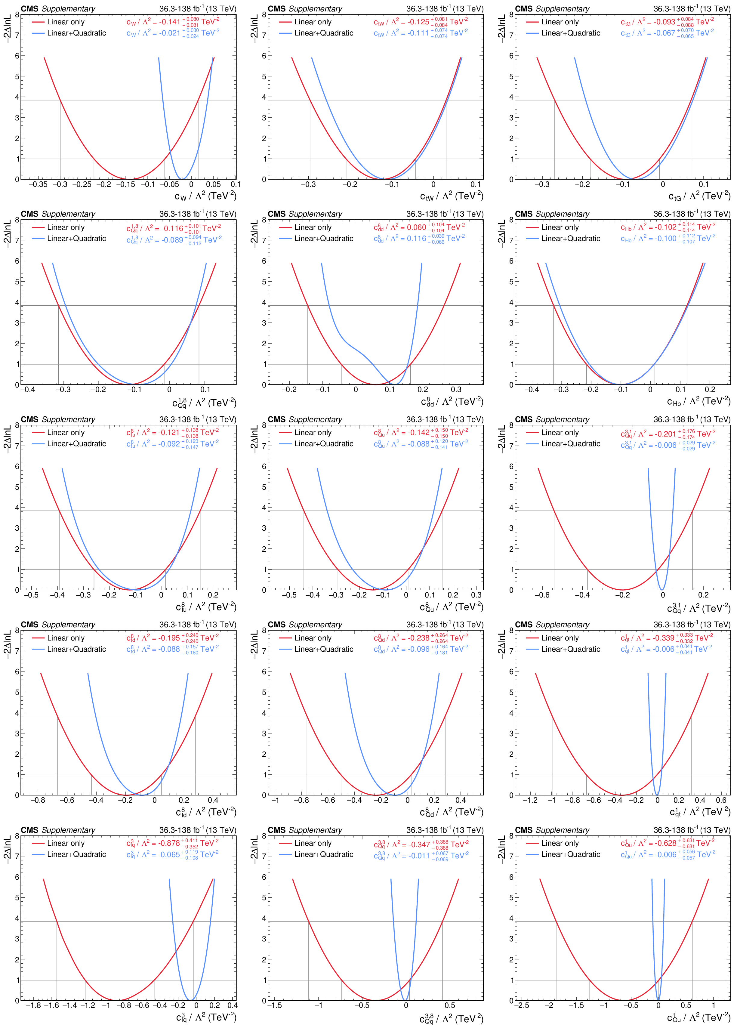
NLL scans of WCs, for the hybrid fit including the $ \mathrm{t}(\overline{\mathrm{t}})\mathrm{X} $ analysis, with and without the inclusion of quadratic terms. |
png pdf |
Additional Figure 11-a:
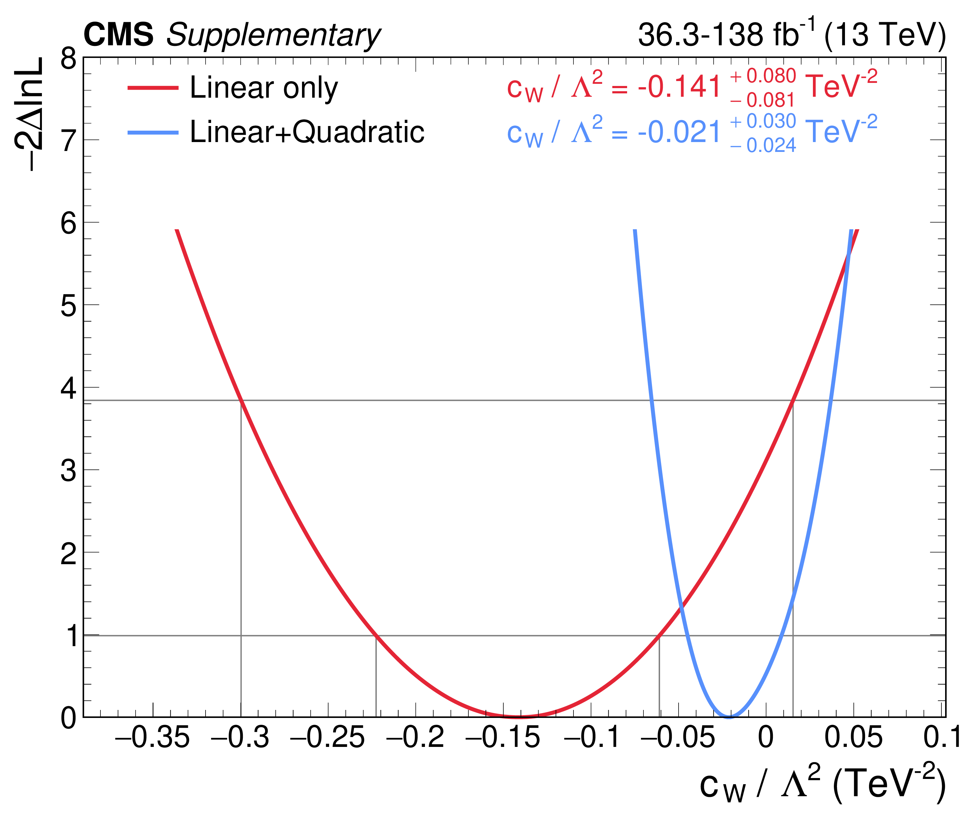
NLL scans of WCs, for the hybrid fit including the $ \mathrm{t}(\overline{\mathrm{t}})\mathrm{X} $ analysis, with and without the inclusion of quadratic terms. |

png pdf |
Additional Figure 11-b:
NLL scans of WCs, for the hybrid fit including the $ \mathrm{t}(\overline{\mathrm{t}})\mathrm{X} $ analysis, with and without the inclusion of quadratic terms. |
png pdf |
Additional Figure 11-c:
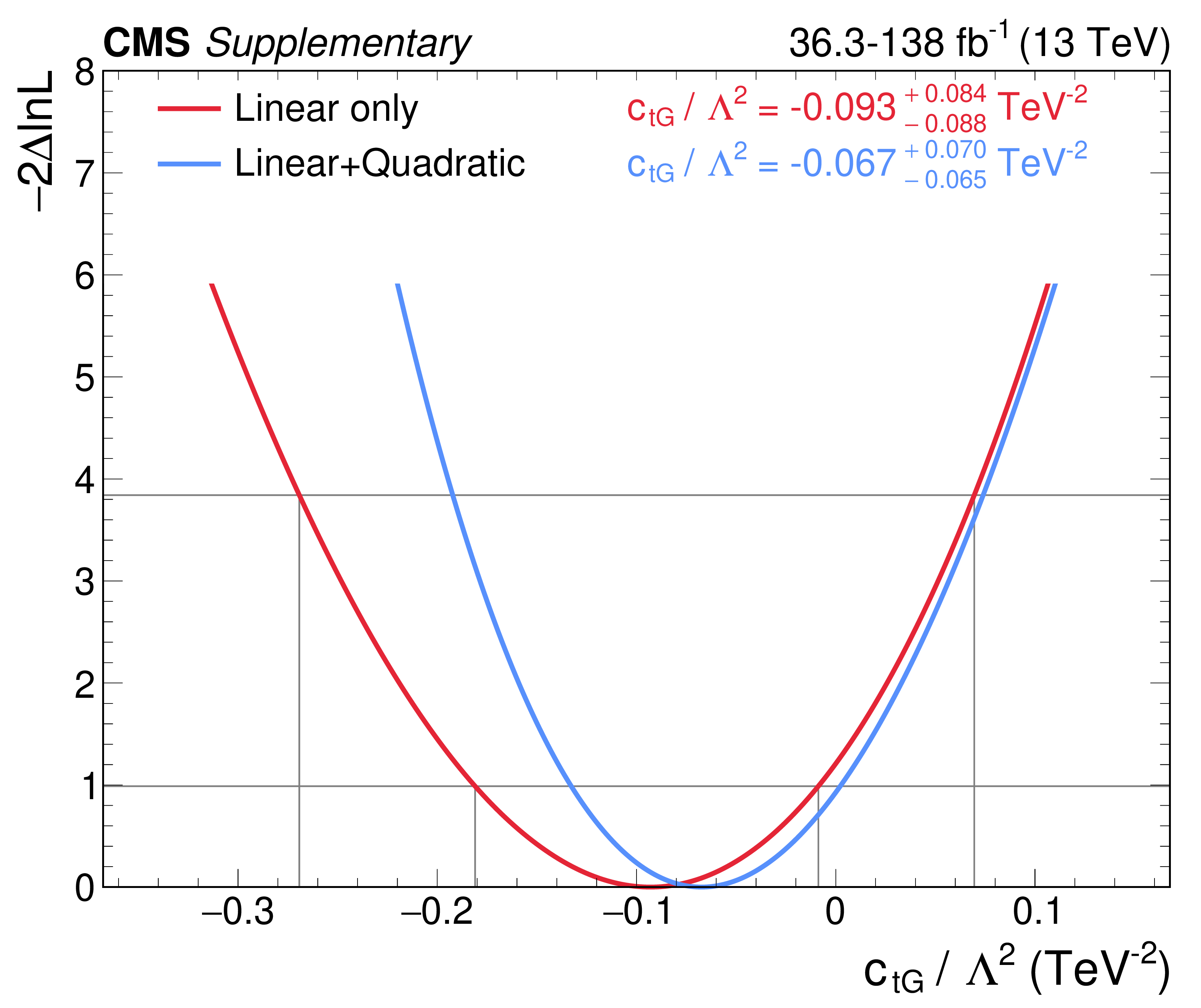
NLL scans of WCs, for the hybrid fit including the $ \mathrm{t}(\overline{\mathrm{t}})\mathrm{X} $ analysis, with and without the inclusion of quadratic terms. |
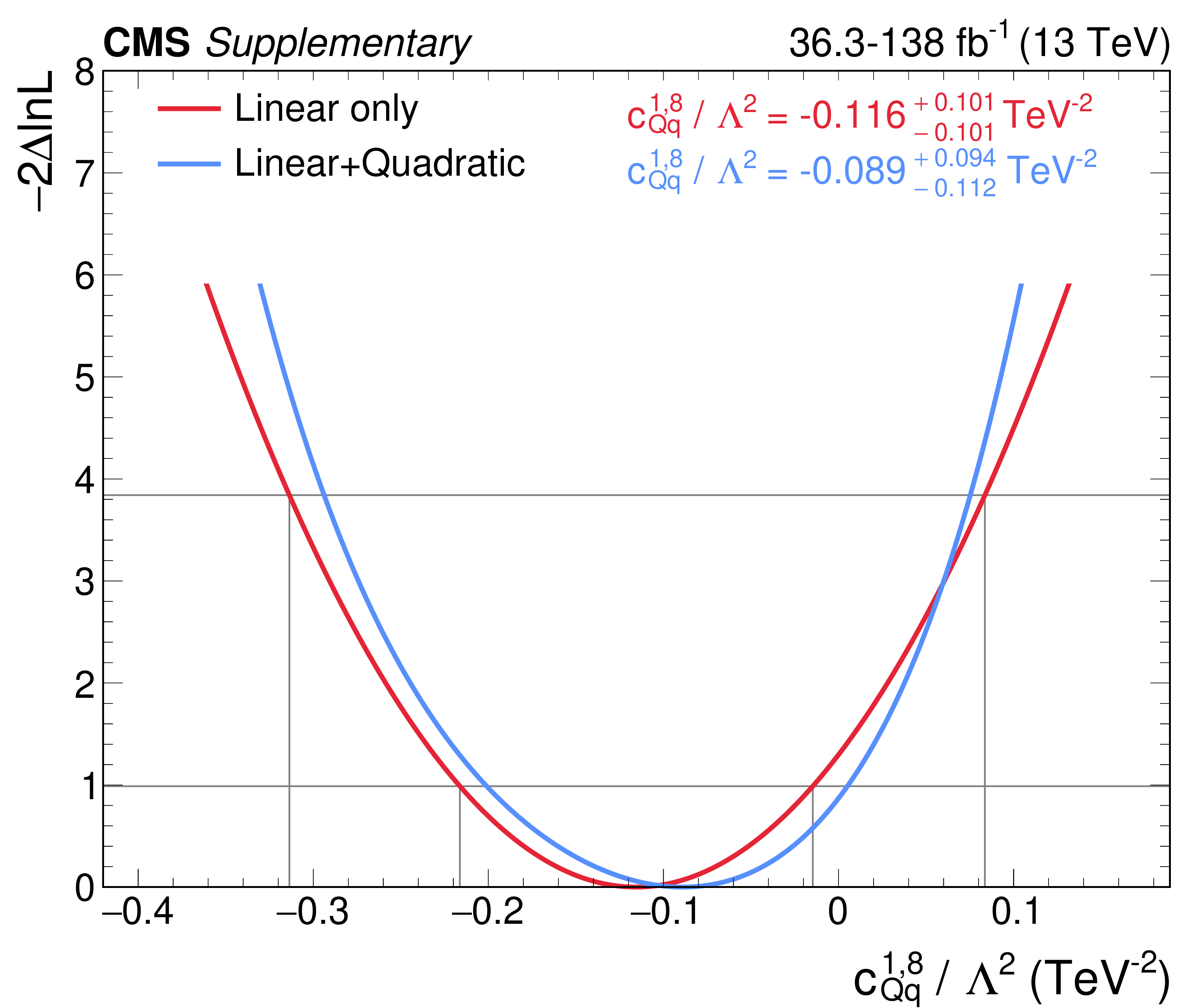
png pdf |
Additional Figure 11-d:
NLL scans of WCs, for the hybrid fit including the $ \mathrm{t}(\overline{\mathrm{t}})\mathrm{X} $ analysis, with and without the inclusion of quadratic terms. |

png pdf |
Additional Figure 11-e:
NLL scans of WCs, for the hybrid fit including the $ \mathrm{t}(\overline{\mathrm{t}})\mathrm{X} $ analysis, with and without the inclusion of quadratic terms. |

png pdf |
Additional Figure 11-f:
NLL scans of WCs, for the hybrid fit including the $ \mathrm{t}(\overline{\mathrm{t}})\mathrm{X} $ analysis, with and without the inclusion of quadratic terms. |

png pdf |
Additional Figure 11-g:
NLL scans of WCs, for the hybrid fit including the $ \mathrm{t}(\overline{\mathrm{t}})\mathrm{X} $ analysis, with and without the inclusion of quadratic terms. |

png pdf |
Additional Figure 11-h:
NLL scans of WCs, for the hybrid fit including the $ \mathrm{t}(\overline{\mathrm{t}})\mathrm{X} $ analysis, with and without the inclusion of quadratic terms. |
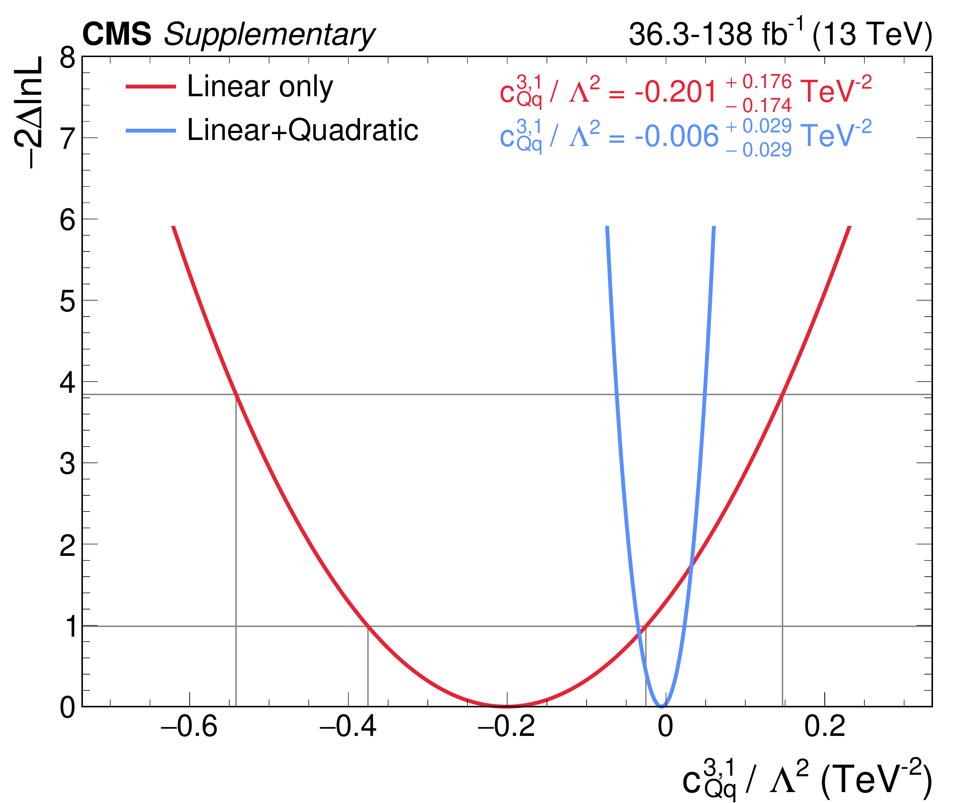
png pdf |
Additional Figure 11-i:
NLL scans of WCs, for the hybrid fit including the $ \mathrm{t}(\overline{\mathrm{t}})\mathrm{X} $ analysis, with and without the inclusion of quadratic terms. |
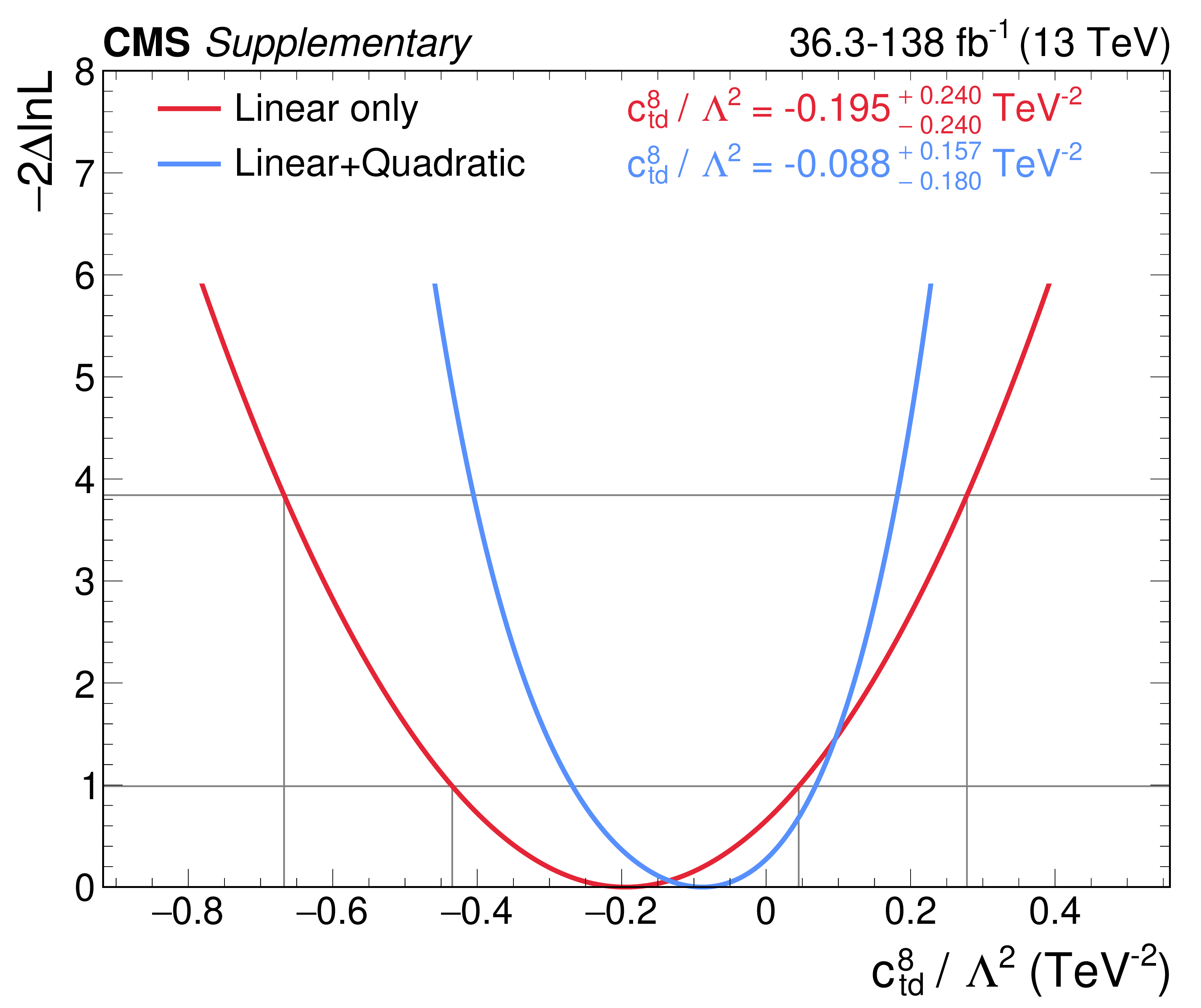
png pdf |
Additional Figure 11-j:
NLL scans of WCs, for the hybrid fit including the $ \mathrm{t}(\overline{\mathrm{t}})\mathrm{X} $ analysis, with and without the inclusion of quadratic terms. |

png pdf |
Additional Figure 11-k:
NLL scans of WCs, for the hybrid fit including the $ \mathrm{t}(\overline{\mathrm{t}})\mathrm{X} $ analysis, with and without the inclusion of quadratic terms. |
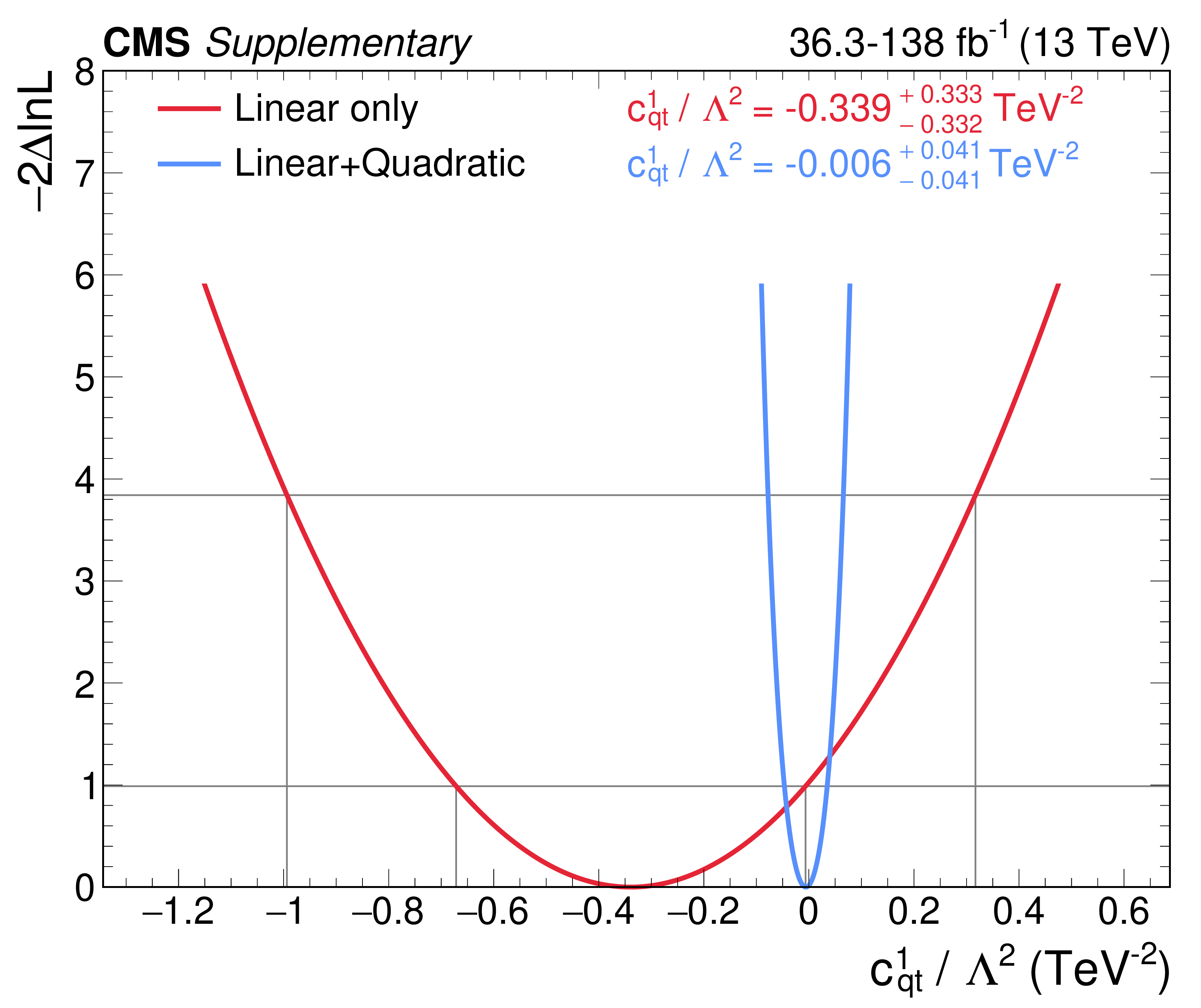
png pdf |
Additional Figure 11-l:
NLL scans of WCs, for the hybrid fit including the $ \mathrm{t}(\overline{\mathrm{t}})\mathrm{X} $ analysis, with and without the inclusion of quadratic terms. |

png pdf |
Additional Figure 11-m:
NLL scans of WCs, for the hybrid fit including the $ \mathrm{t}(\overline{\mathrm{t}})\mathrm{X} $ analysis, with and without the inclusion of quadratic terms. |
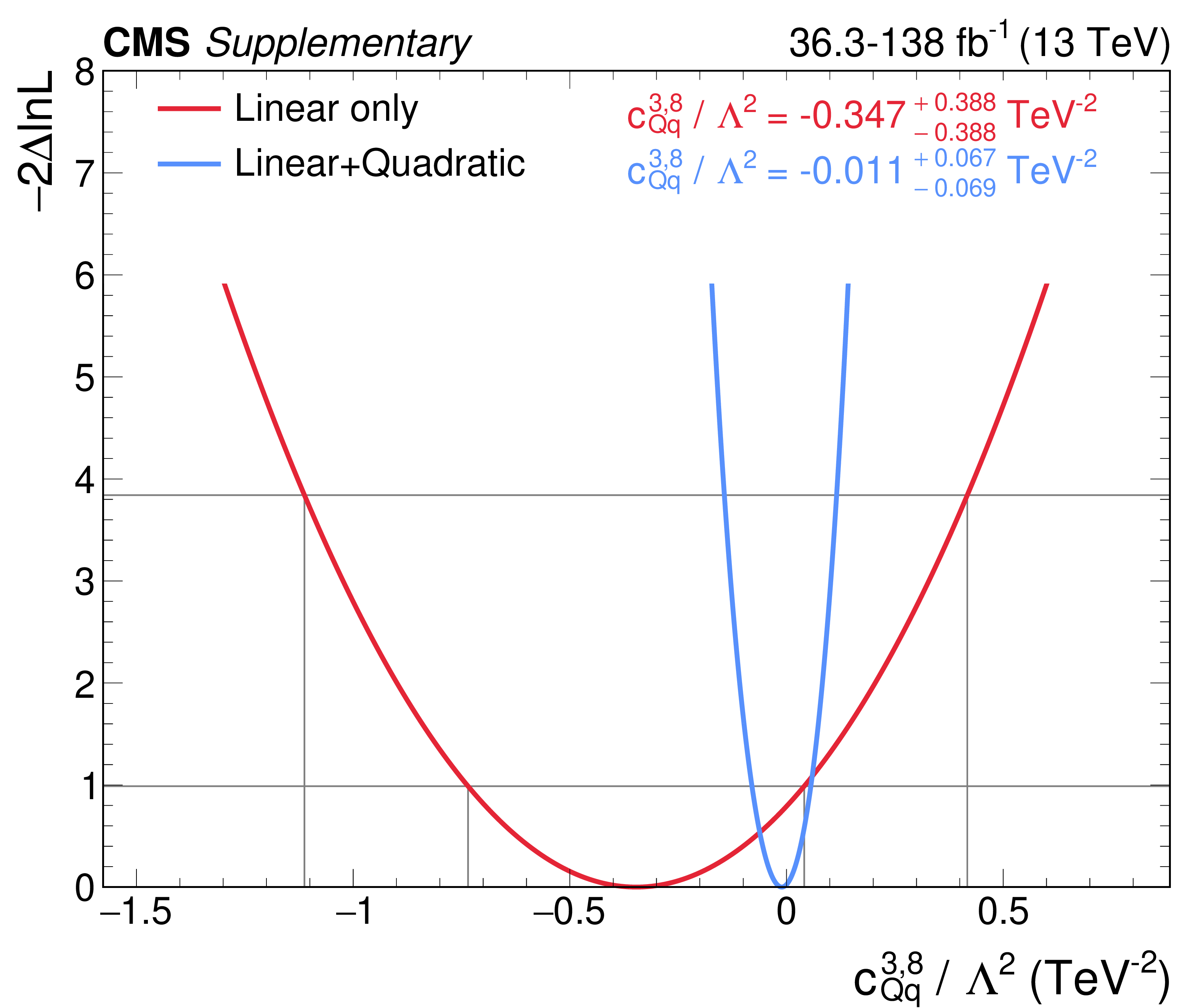
png pdf |
Additional Figure 11-n:
NLL scans of WCs, for the hybrid fit including the $ \mathrm{t}(\overline{\mathrm{t}})\mathrm{X} $ analysis, with and without the inclusion of quadratic terms. |
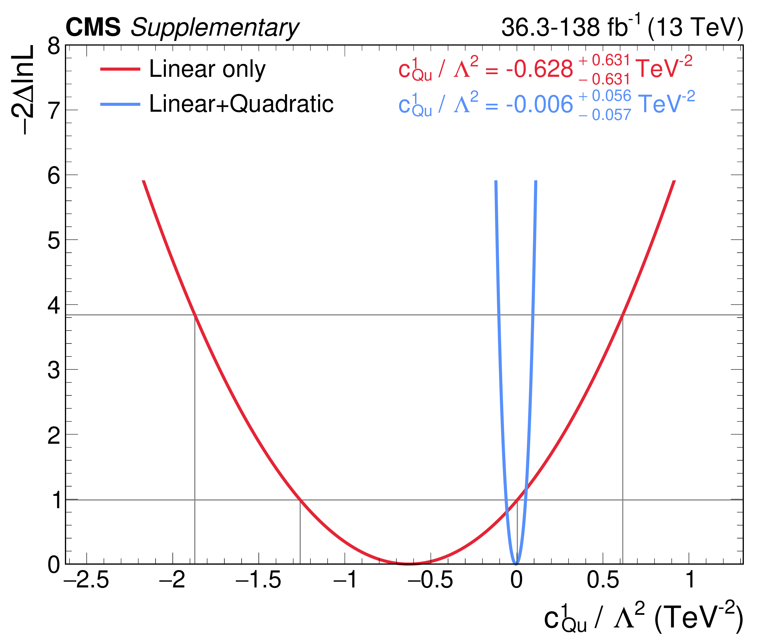
png pdf |
Additional Figure 11-o:
NLL scans of WCs, for the hybrid fit including the $ \mathrm{t}(\overline{\mathrm{t}})\mathrm{X} $ analysis, with and without the inclusion of quadratic terms. |

png pdf |
Additional Figure 12:
NLL scans of WCs, for the hybrid fit including the $ \mathrm{t}(\overline{\mathrm{t}})\mathrm{X} $ analysis, with and without the inclusion of quadratic terms. |
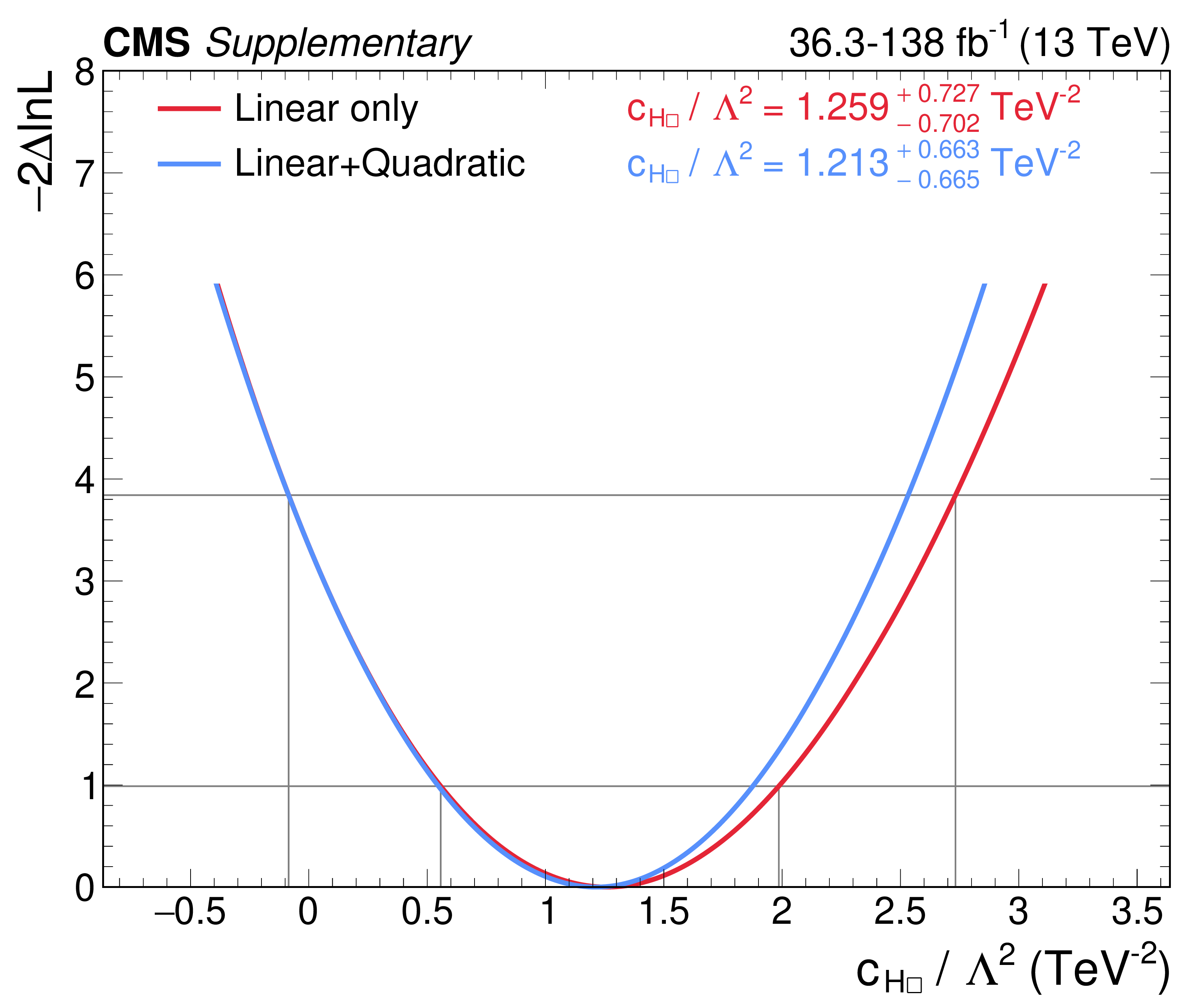
png pdf |
Additional Figure 12-a:
NLL scans of WCs, for the hybrid fit including the $ \mathrm{t}(\overline{\mathrm{t}})\mathrm{X} $ analysis, with and without the inclusion of quadratic terms. |

png pdf |
Additional Figure 12-b:
NLL scans of WCs, for the hybrid fit including the $ \mathrm{t}(\overline{\mathrm{t}})\mathrm{X} $ analysis, with and without the inclusion of quadratic terms. |
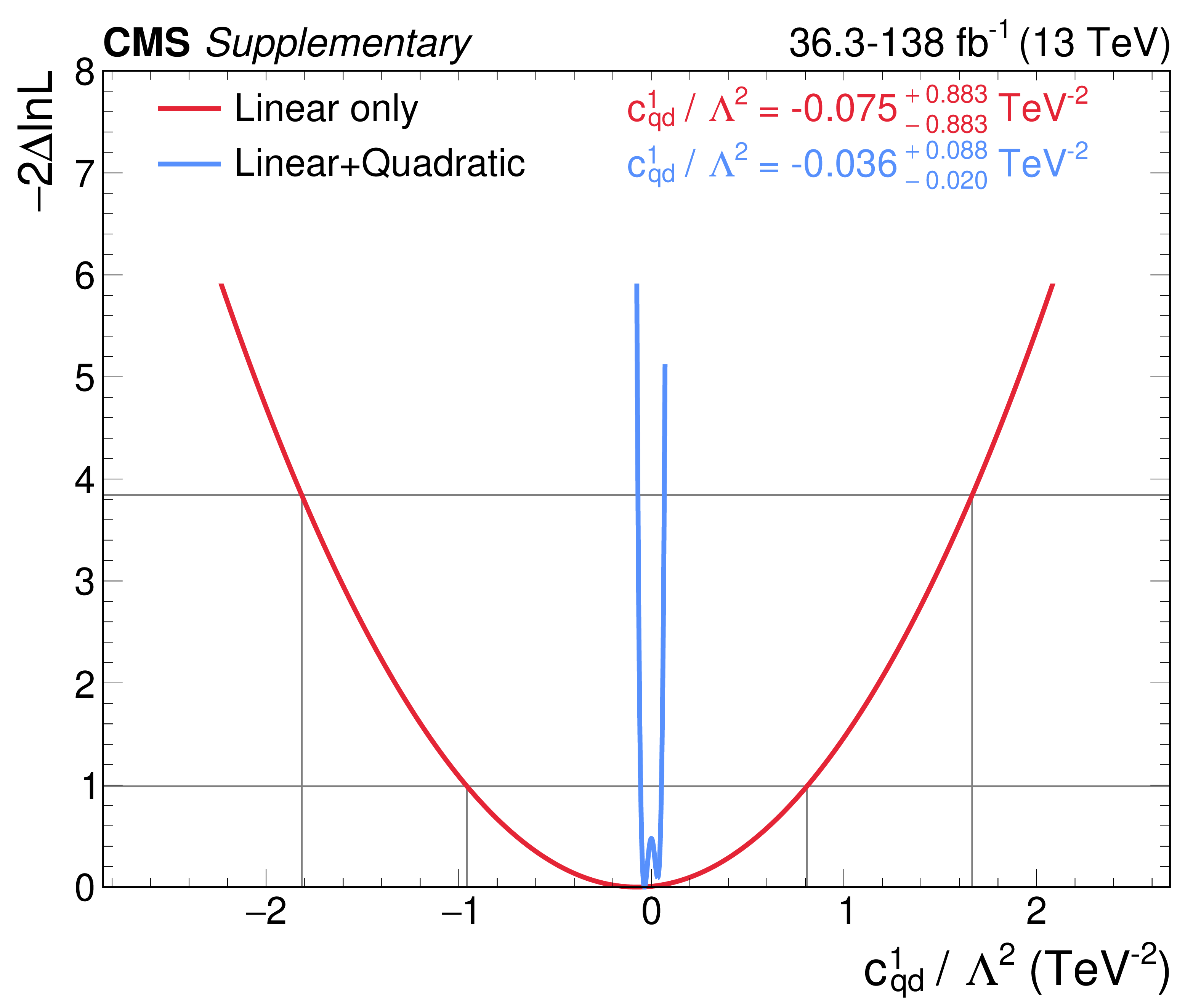
png pdf |
Additional Figure 12-c:
NLL scans of WCs, for the hybrid fit including the $ \mathrm{t}(\overline{\mathrm{t}})\mathrm{X} $ analysis, with and without the inclusion of quadratic terms. |
png pdf |
Additional Figure 12-d:
NLL scans of WCs, for the hybrid fit including the $ \mathrm{t}(\overline{\mathrm{t}})\mathrm{X} $ analysis, with and without the inclusion of quadratic terms. |

png pdf |
Additional Figure 12-e:
NLL scans of WCs, for the hybrid fit including the $ \mathrm{t}(\overline{\mathrm{t}})\mathrm{X} $ analysis, with and without the inclusion of quadratic terms. |

png pdf |
Additional Figure 12-f:
NLL scans of WCs, for the hybrid fit including the $ \mathrm{t}(\overline{\mathrm{t}})\mathrm{X} $ analysis, with and without the inclusion of quadratic terms. |

png pdf |
Additional Figure 12-g:
NLL scans of WCs, for the hybrid fit including the $ \mathrm{t}(\overline{\mathrm{t}})\mathrm{X} $ analysis, with and without the inclusion of quadratic terms. |
png pdf |
Additional Figure 12-h:
NLL scans of WCs, for the hybrid fit including the $ \mathrm{t}(\overline{\mathrm{t}})\mathrm{X} $ analysis, with and without the inclusion of quadratic terms. |
png pdf |
Additional Figure 12-i:
NLL scans of WCs, for the hybrid fit including the $ \mathrm{t}(\overline{\mathrm{t}})\mathrm{X} $ analysis, with and without the inclusion of quadratic terms. |
png pdf |
Additional Figure 12-j:
NLL scans of WCs, for the hybrid fit including the $ \mathrm{t}(\overline{\mathrm{t}})\mathrm{X} $ analysis, with and without the inclusion of quadratic terms. |

png pdf |
Additional Figure 12-k:
NLL scans of WCs, for the hybrid fit including the $ \mathrm{t}(\overline{\mathrm{t}})\mathrm{X} $ analysis, with and without the inclusion of quadratic terms. |
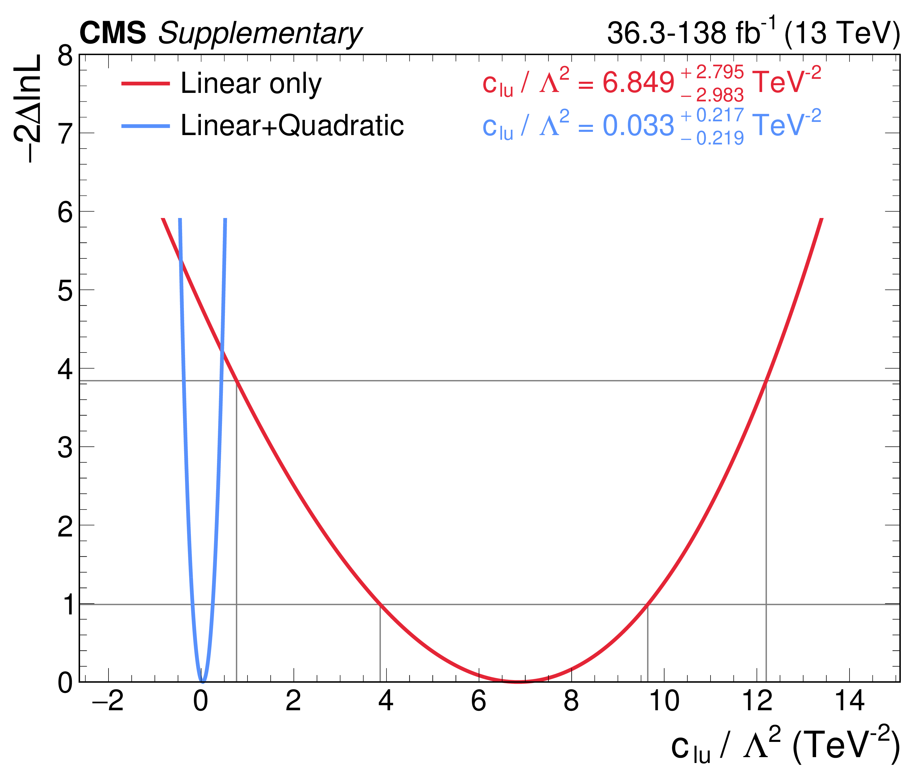
png pdf |
Additional Figure 12-l:
NLL scans of WCs, for the hybrid fit including the $ \mathrm{t}(\overline{\mathrm{t}})\mathrm{X} $ analysis, with and without the inclusion of quadratic terms. |

png pdf |
Additional Figure 12-m:
NLL scans of WCs, for the hybrid fit including the $ \mathrm{t}(\overline{\mathrm{t}})\mathrm{X} $ analysis, with and without the inclusion of quadratic terms. |
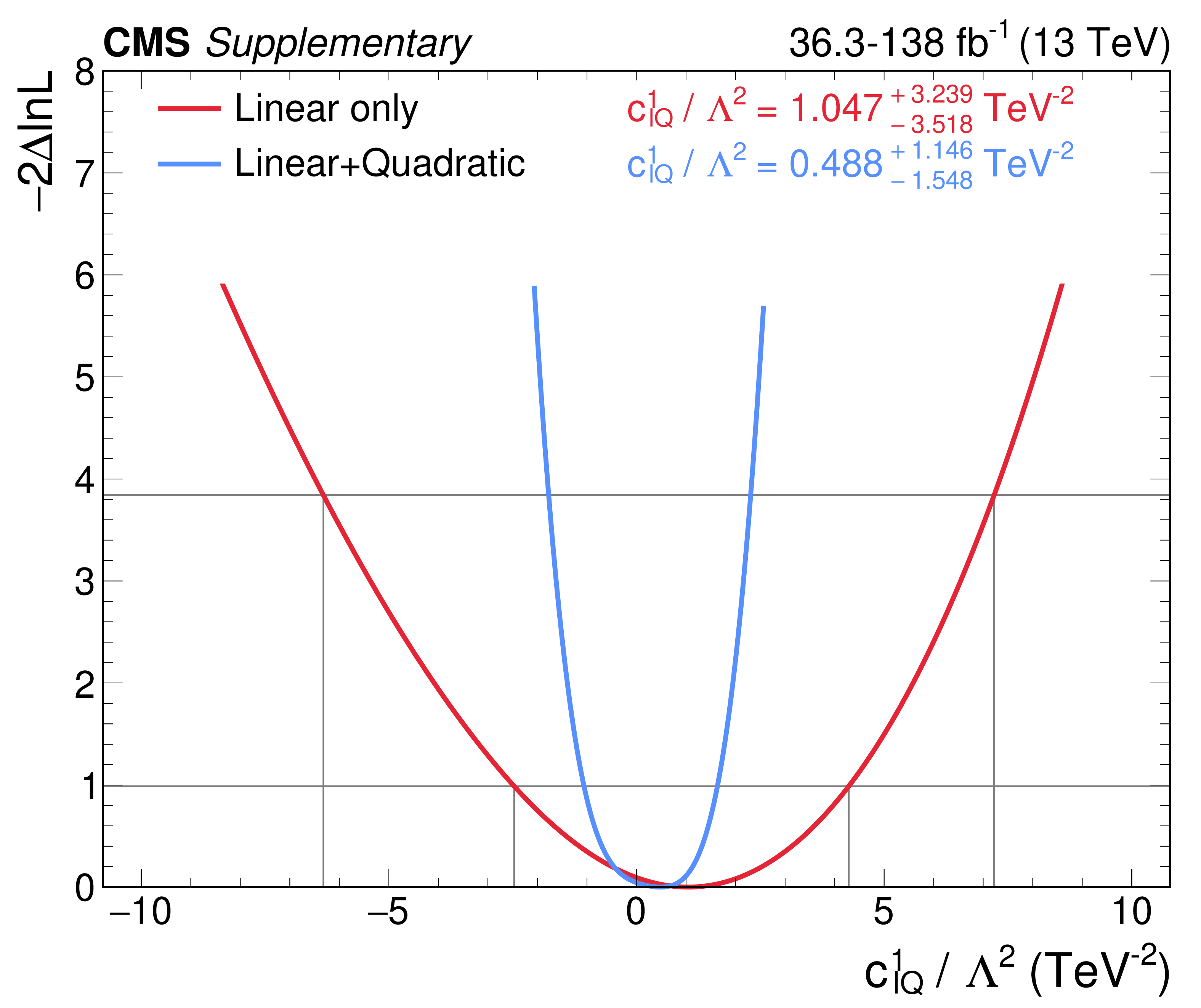
png pdf |
Additional Figure 12-n:
NLL scans of WCs, for the hybrid fit including the $ \mathrm{t}(\overline{\mathrm{t}})\mathrm{X} $ analysis, with and without the inclusion of quadratic terms. |
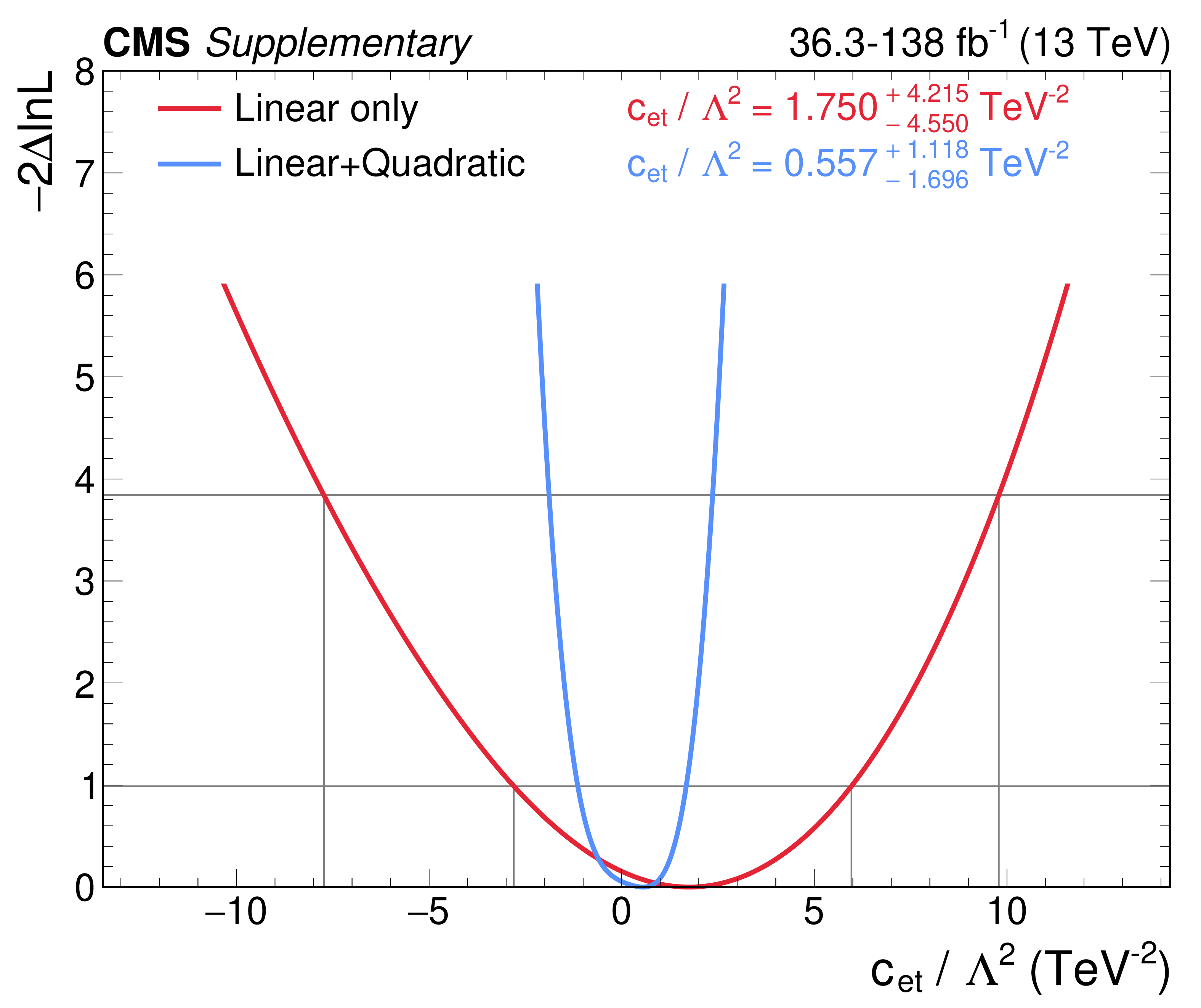
png pdf |
Additional Figure 12-o:
NLL scans of WCs, for the hybrid fit including the $ \mathrm{t}(\overline{\mathrm{t}})\mathrm{X} $ analysis, with and without the inclusion of quadratic terms. |
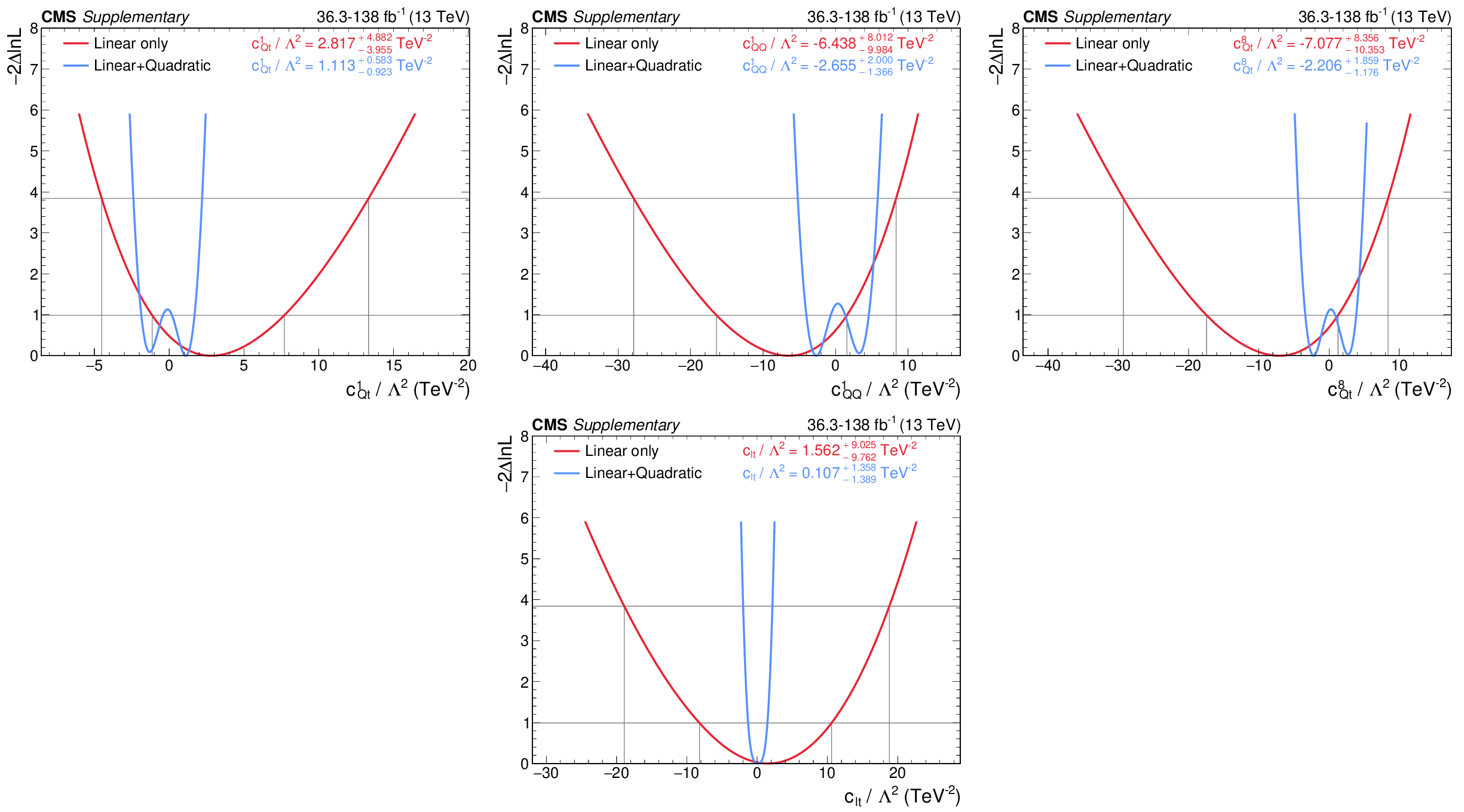
png pdf |
Additional Figure 13:
NLL scans of WCs, for the hybrid fit including the $ \mathrm{t}(\overline{\mathrm{t}})\mathrm{X} $ analysis, with and without the inclusion of quadratic terms. |
png pdf |
Additional Figure 13-a:
NLL scans of WCs, for the hybrid fit including the $ \mathrm{t}(\overline{\mathrm{t}})\mathrm{X} $ analysis, with and without the inclusion of quadratic terms. |

png pdf |
Additional Figure 13-b:
NLL scans of WCs, for the hybrid fit including the $ \mathrm{t}(\overline{\mathrm{t}})\mathrm{X} $ analysis, with and without the inclusion of quadratic terms. |

png pdf |
Additional Figure 13-c:
NLL scans of WCs, for the hybrid fit including the $ \mathrm{t}(\overline{\mathrm{t}})\mathrm{X} $ analysis, with and without the inclusion of quadratic terms. |
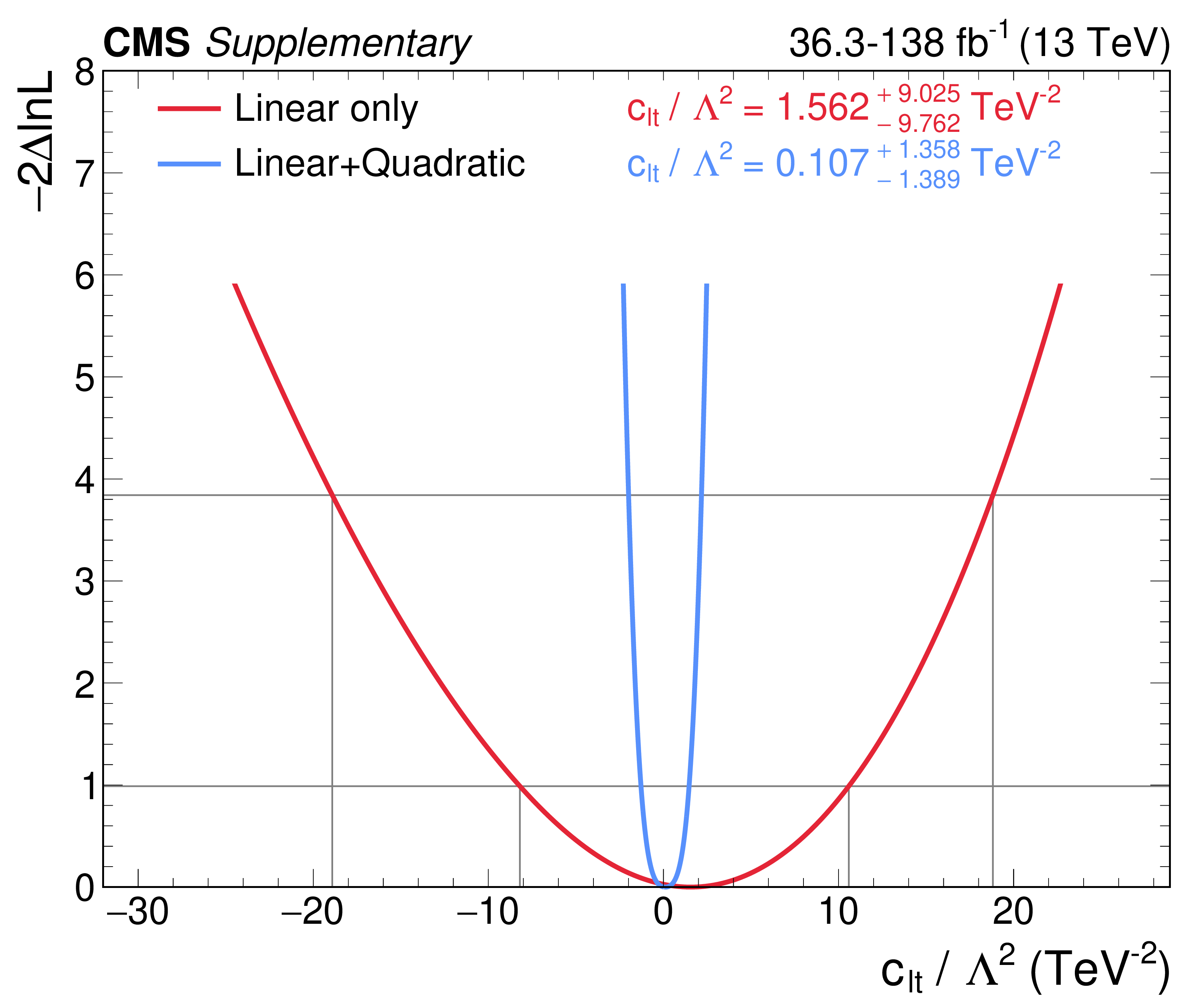
png pdf |
Additional Figure 13-d:
NLL scans of WCs, for the hybrid fit including the $ \mathrm{t}(\overline{\mathrm{t}})\mathrm{X} $ analysis, with and without the inclusion of quadratic terms. |

png pdf |
Additional Figure 14:
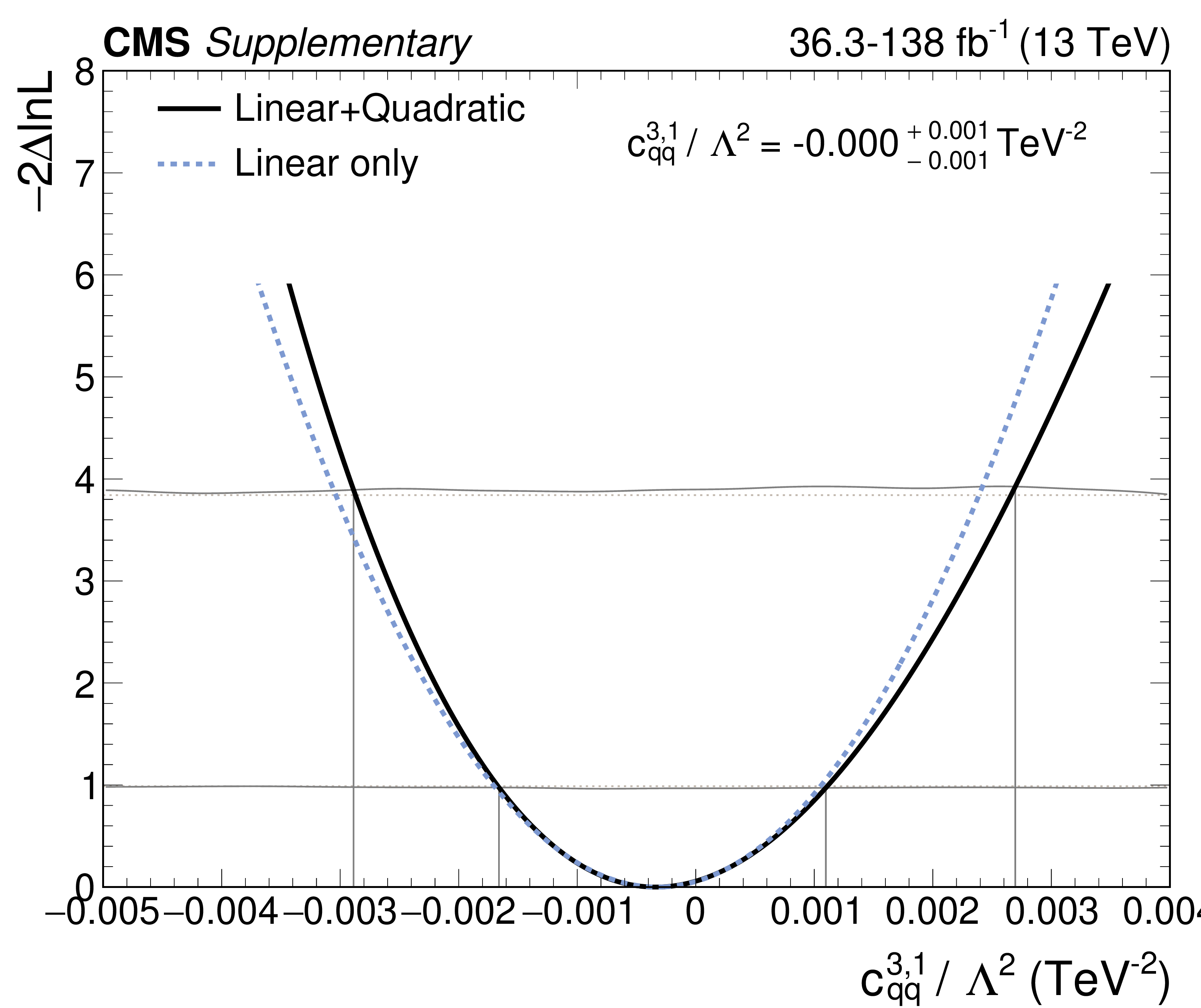
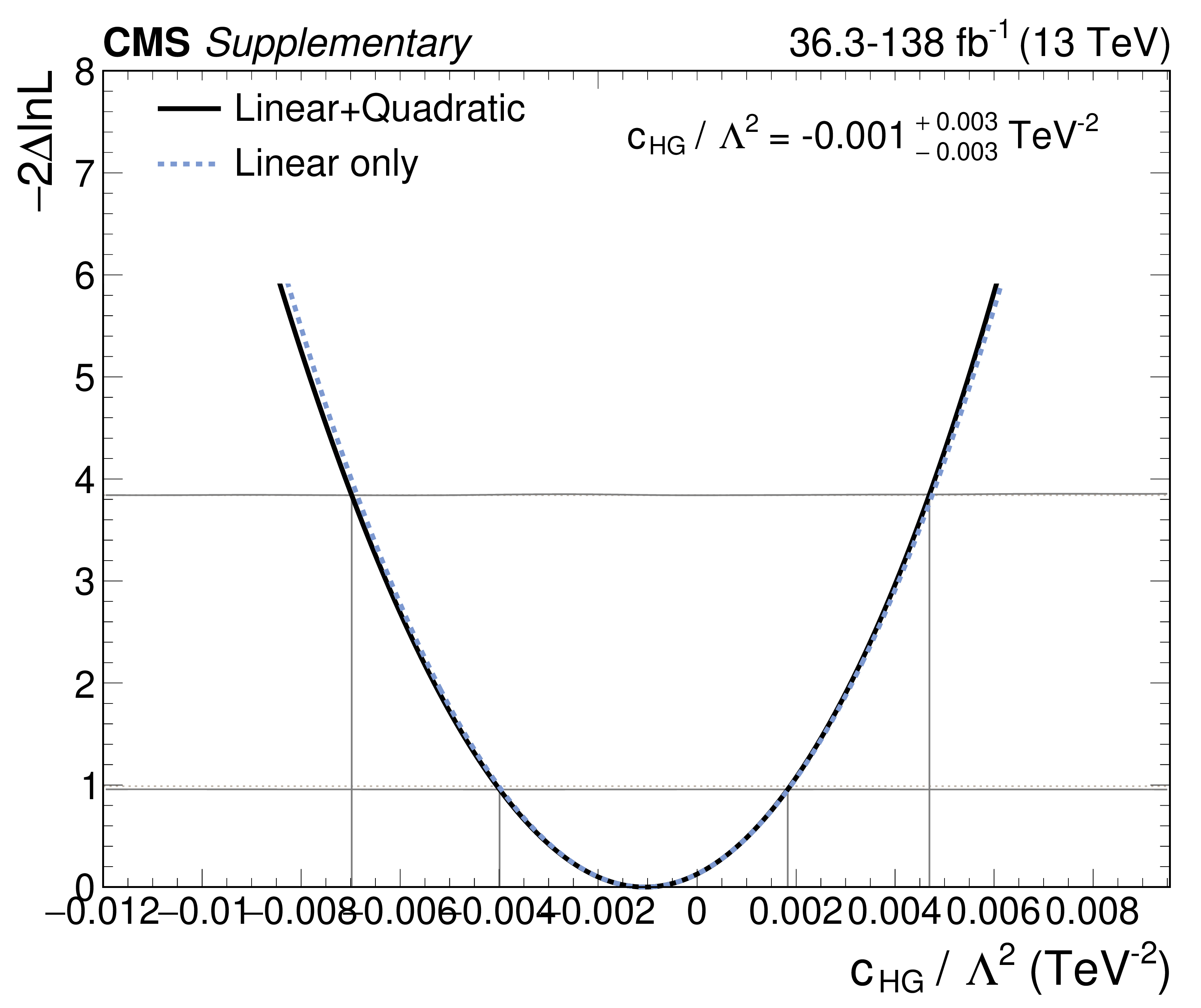
NLL scans of WCs, for the simplified fit without the $ \mathrm{t}(\overline{\mathrm{t}})\mathrm{X} $ analysis. The solid grey lines indicate the sets of points $ q^{68\%} $ (lower line) and $ q^{95\%} $ (upper line), while the dashed grey lines denote the test statistic values used to determine the 68% and 95% confidence intervals in the asymptotic approximation. |
png pdf |
Additional Figure 14-a:
NLL scans of WCs, for the simplified fit without the $ \mathrm{t}(\overline{\mathrm{t}})\mathrm{X} $ analysis. The solid grey lines indicate the sets of points $ q^{68\%} $ (lower line) and $ q^{95\%} $ (upper line), while the dashed grey lines denote the test statistic values used to determine the 68% and 95% confidence intervals in the asymptotic approximation. |

png pdf |
Additional Figure 14-b:
NLL scans of WCs, for the simplified fit without the $ \mathrm{t}(\overline{\mathrm{t}})\mathrm{X} $ analysis. The solid grey lines indicate the sets of points $ q^{68\%} $ (lower line) and $ q^{95\%} $ (upper line), while the dashed grey lines denote the test statistic values used to determine the 68% and 95% confidence intervals in the asymptotic approximation. |
png pdf |
Additional Figure 14-c:
NLL scans of WCs, for the simplified fit without the $ \mathrm{t}(\overline{\mathrm{t}})\mathrm{X} $ analysis. The solid grey lines indicate the sets of points $ q^{68\%} $ (lower line) and $ q^{95\%} $ (upper line), while the dashed grey lines denote the test statistic values used to determine the 68% and 95% confidence intervals in the asymptotic approximation. |
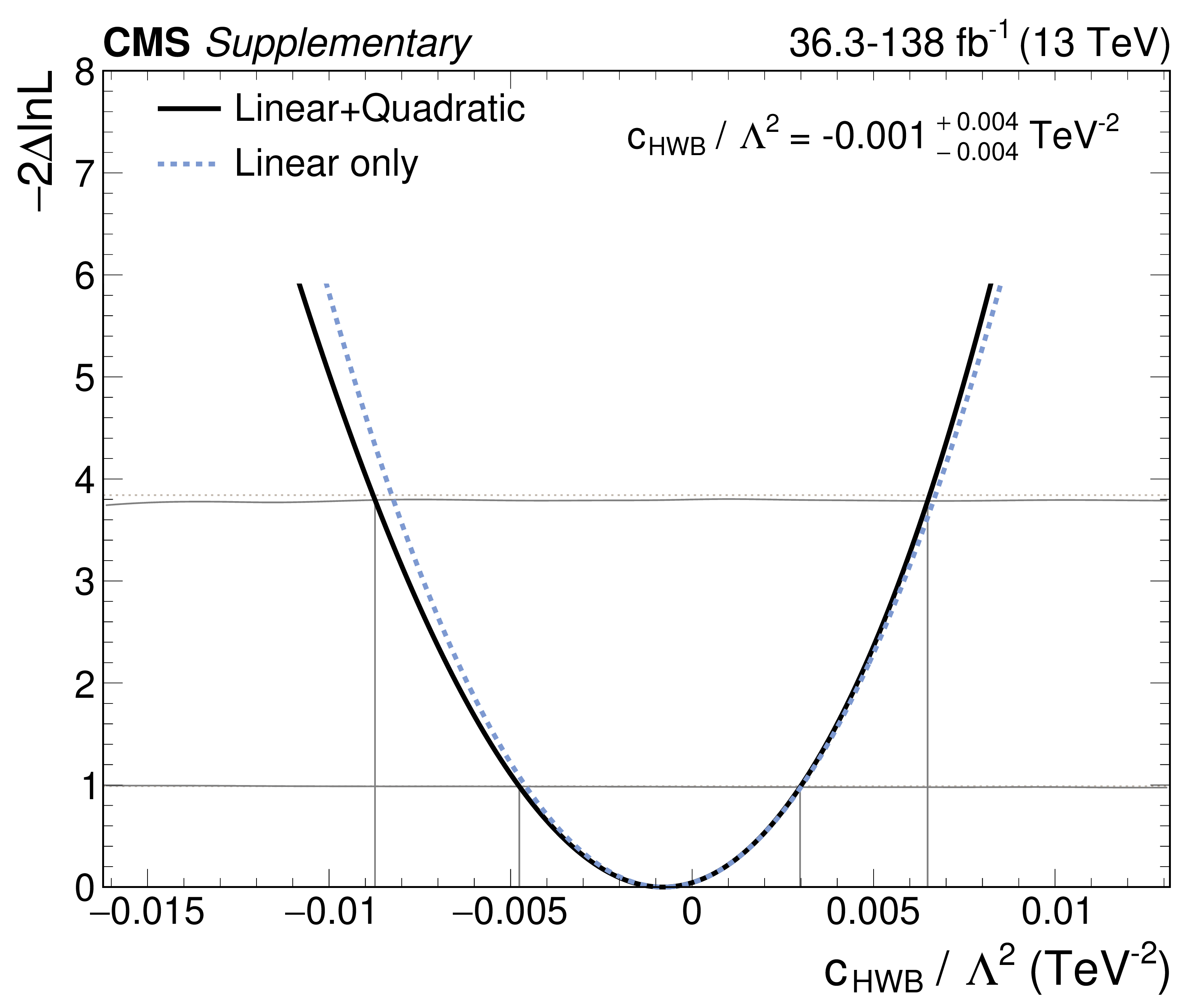
png pdf |
Additional Figure 14-d:
NLL scans of WCs, for the simplified fit without the $ \mathrm{t}(\overline{\mathrm{t}})\mathrm{X} $ analysis. The solid grey lines indicate the sets of points $ q^{68\%} $ (lower line) and $ q^{95\%} $ (upper line), while the dashed grey lines denote the test statistic values used to determine the 68% and 95% confidence intervals in the asymptotic approximation. |
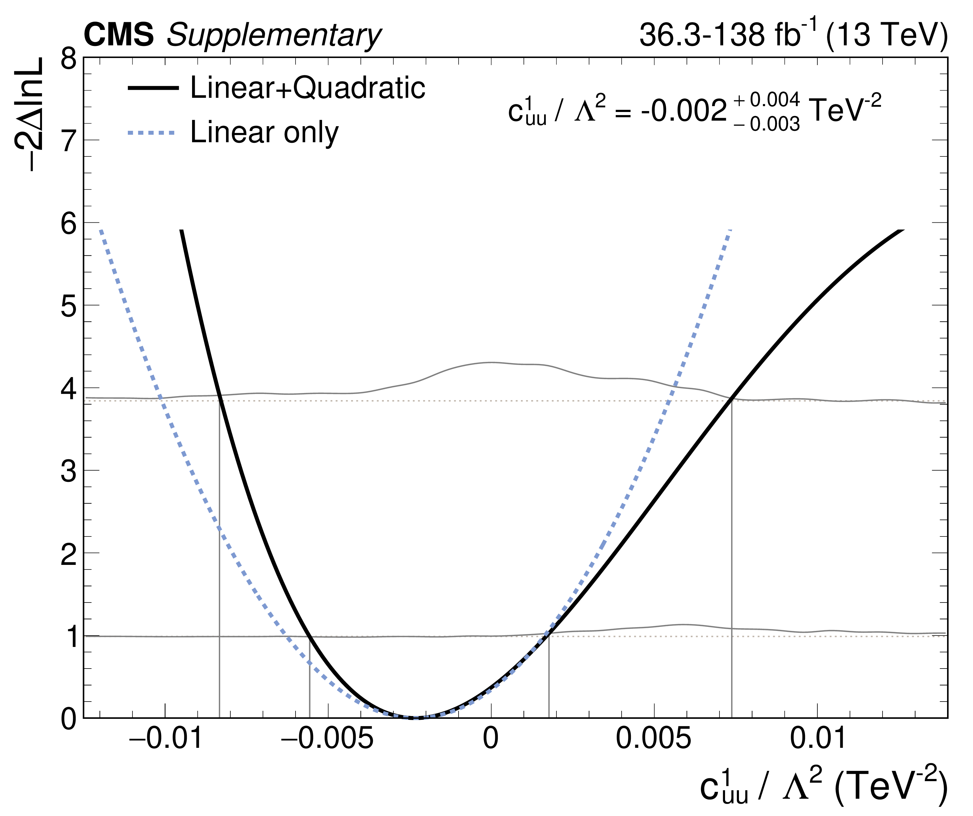
png pdf |
Additional Figure 14-e:
NLL scans of WCs, for the simplified fit without the $ \mathrm{t}(\overline{\mathrm{t}})\mathrm{X} $ analysis. The solid grey lines indicate the sets of points $ q^{68\%} $ (lower line) and $ q^{95\%} $ (upper line), while the dashed grey lines denote the test statistic values used to determine the 68% and 95% confidence intervals in the asymptotic approximation. |
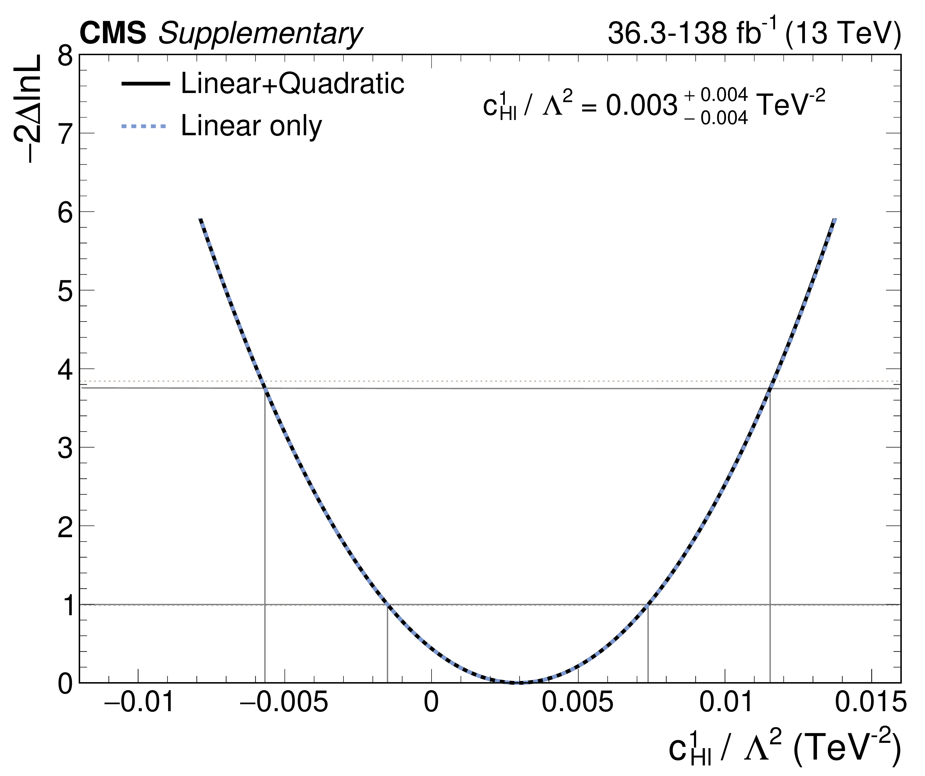
png pdf |
Additional Figure 14-f:
NLL scans of WCs, for the simplified fit without the $ \mathrm{t}(\overline{\mathrm{t}})\mathrm{X} $ analysis. The solid grey lines indicate the sets of points $ q^{68\%} $ (lower line) and $ q^{95\%} $ (upper line), while the dashed grey lines denote the test statistic values used to determine the 68% and 95% confidence intervals in the asymptotic approximation. |
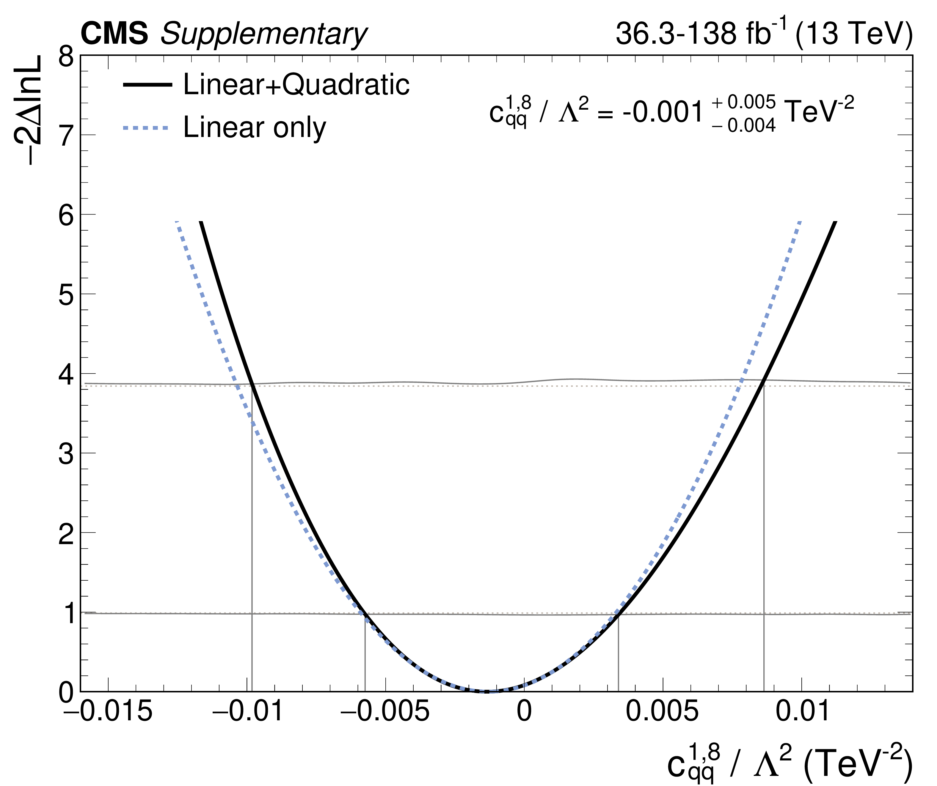
png pdf |
Additional Figure 14-g:
NLL scans of WCs, for the simplified fit without the $ \mathrm{t}(\overline{\mathrm{t}})\mathrm{X} $ analysis. The solid grey lines indicate the sets of points $ q^{68\%} $ (lower line) and $ q^{95\%} $ (upper line), while the dashed grey lines denote the test statistic values used to determine the 68% and 95% confidence intervals in the asymptotic approximation. |
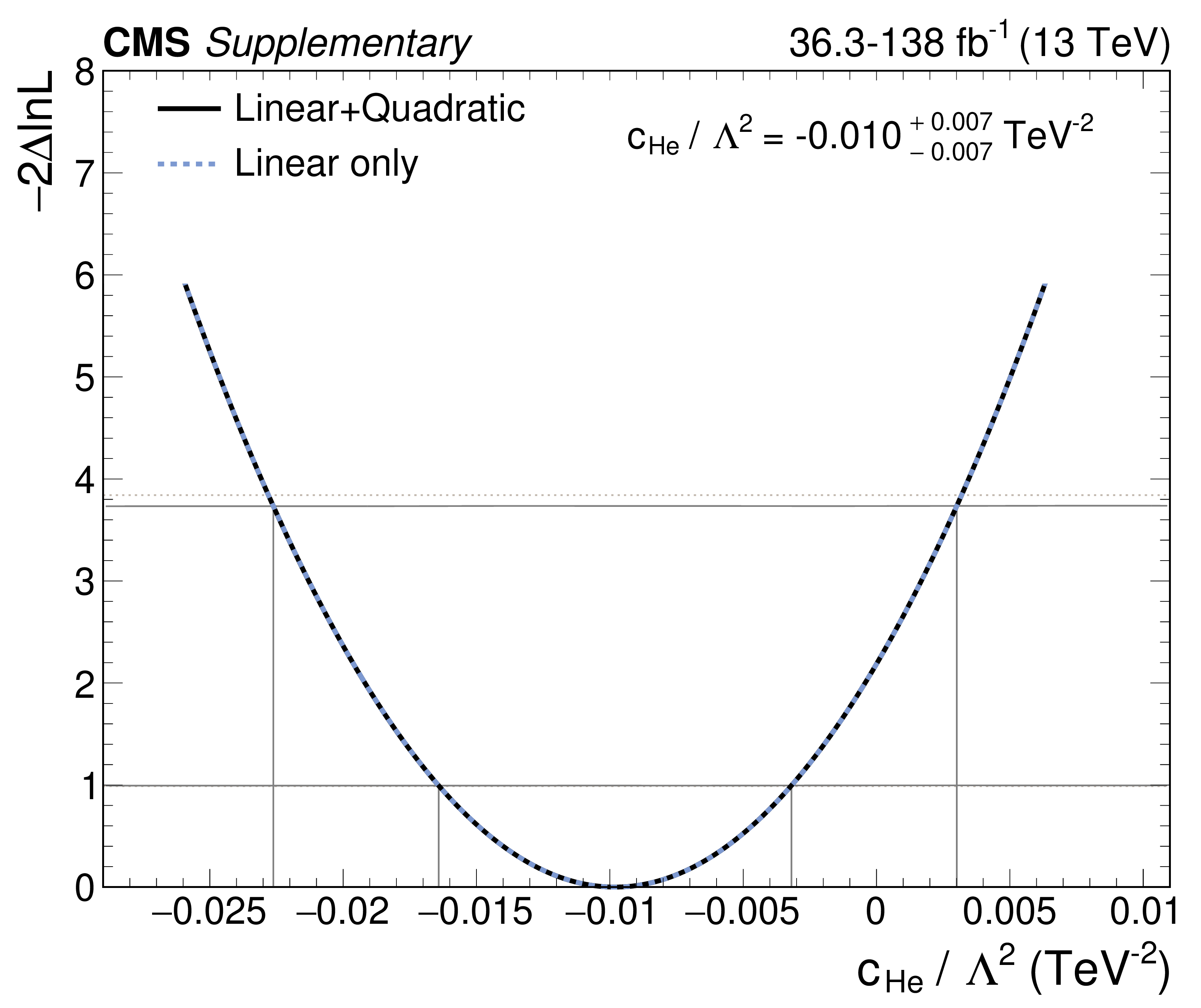
png pdf |
Additional Figure 14-h:
NLL scans of WCs, for the simplified fit without the $ \mathrm{t}(\overline{\mathrm{t}})\mathrm{X} $ analysis. The solid grey lines indicate the sets of points $ q^{68\%} $ (lower line) and $ q^{95\%} $ (upper line), while the dashed grey lines denote the test statistic values used to determine the 68% and 95% confidence intervals in the asymptotic approximation. |

png pdf |
Additional Figure 14-i:
NLL scans of WCs, for the simplified fit without the $ \mathrm{t}(\overline{\mathrm{t}})\mathrm{X} $ analysis. The solid grey lines indicate the sets of points $ q^{68\%} $ (lower line) and $ q^{95\%} $ (upper line), while the dashed grey lines denote the test statistic values used to determine the 68% and 95% confidence intervals in the asymptotic approximation. |
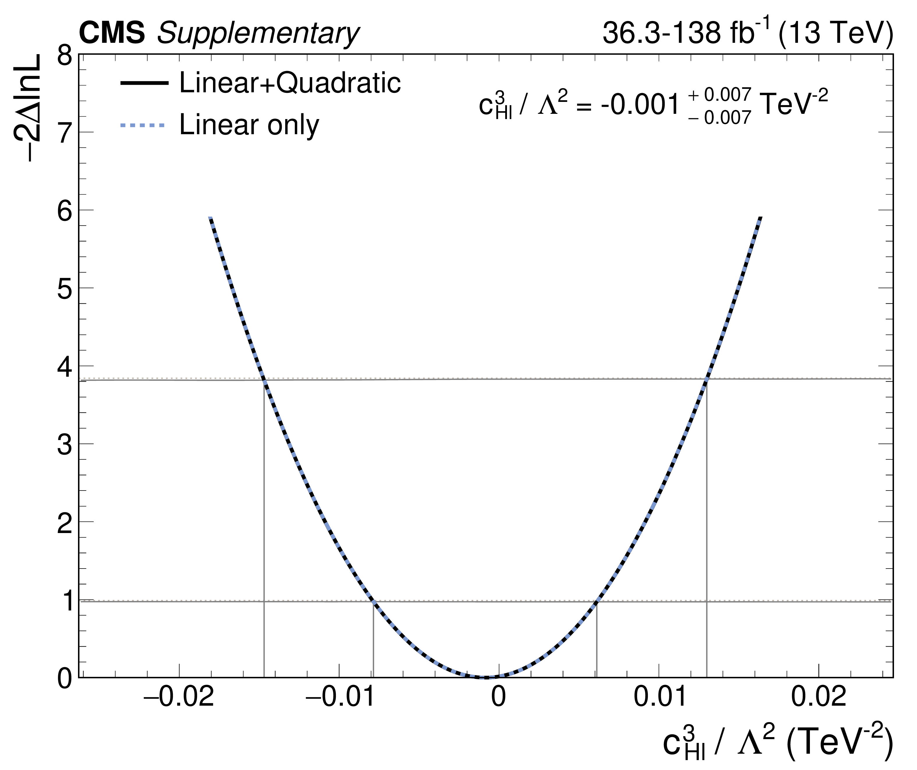
png pdf |
Additional Figure 14-j:
NLL scans of WCs, for the simplified fit without the $ \mathrm{t}(\overline{\mathrm{t}})\mathrm{X} $ analysis. The solid grey lines indicate the sets of points $ q^{68\%} $ (lower line) and $ q^{95\%} $ (upper line), while the dashed grey lines denote the test statistic values used to determine the 68% and 95% confidence intervals in the asymptotic approximation. |

png pdf |
Additional Figure 14-k:
NLL scans of WCs, for the simplified fit without the $ \mathrm{t}(\overline{\mathrm{t}})\mathrm{X} $ analysis. The solid grey lines indicate the sets of points $ q^{68\%} $ (lower line) and $ q^{95\%} $ (upper line), while the dashed grey lines denote the test statistic values used to determine the 68% and 95% confidence intervals in the asymptotic approximation. |
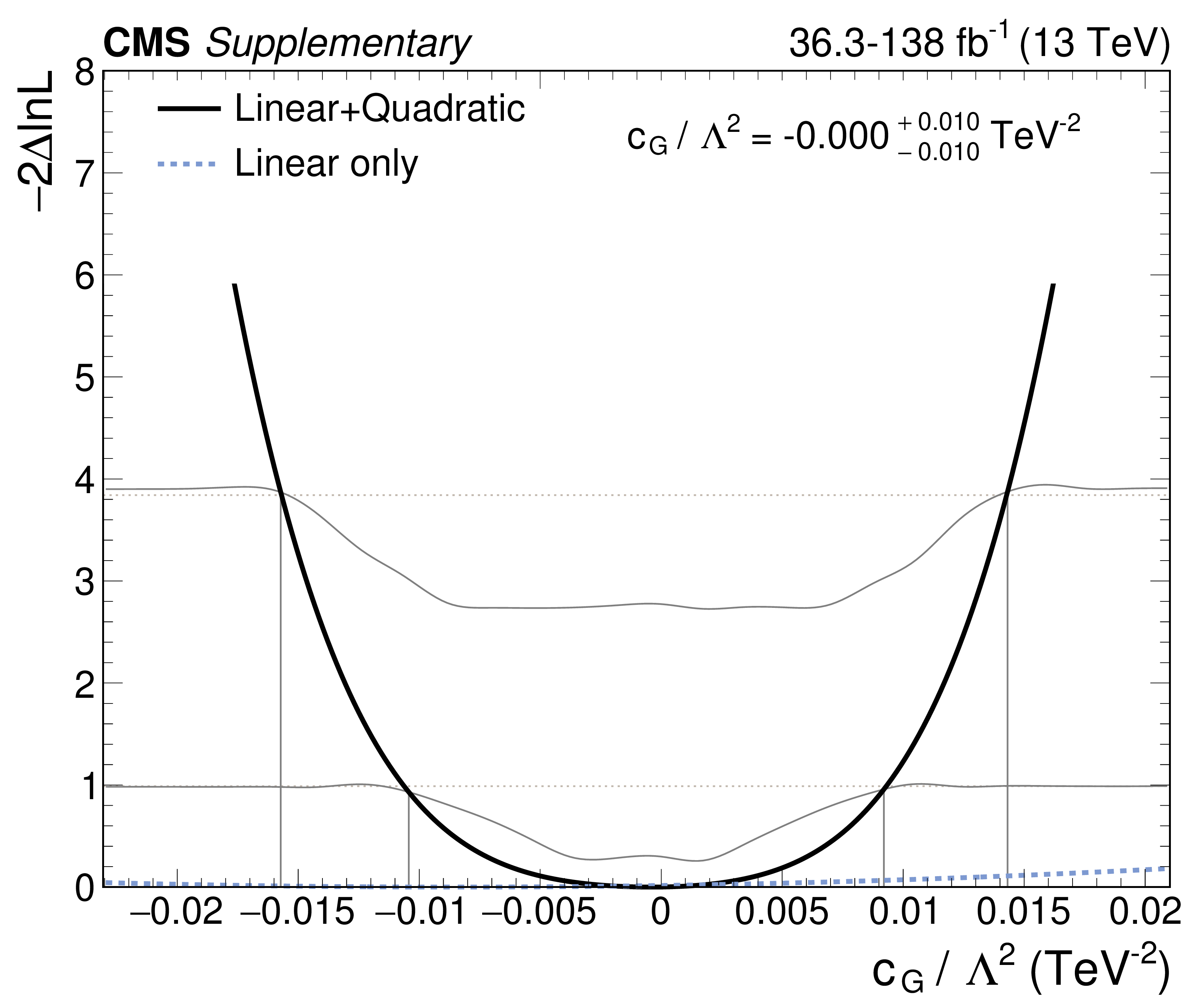
png pdf |
Additional Figure 14-l:
NLL scans of WCs, for the simplified fit without the $ \mathrm{t}(\overline{\mathrm{t}})\mathrm{X} $ analysis. The solid grey lines indicate the sets of points $ q^{68\%} $ (lower line) and $ q^{95\%} $ (upper line), while the dashed grey lines denote the test statistic values used to determine the 68% and 95% confidence intervals in the asymptotic approximation. |

png pdf |
Additional Figure 14-m:
NLL scans of WCs, for the simplified fit without the $ \mathrm{t}(\overline{\mathrm{t}})\mathrm{X} $ analysis. The solid grey lines indicate the sets of points $ q^{68\%} $ (lower line) and $ q^{95\%} $ (upper line), while the dashed grey lines denote the test statistic values used to determine the 68% and 95% confidence intervals in the asymptotic approximation. |
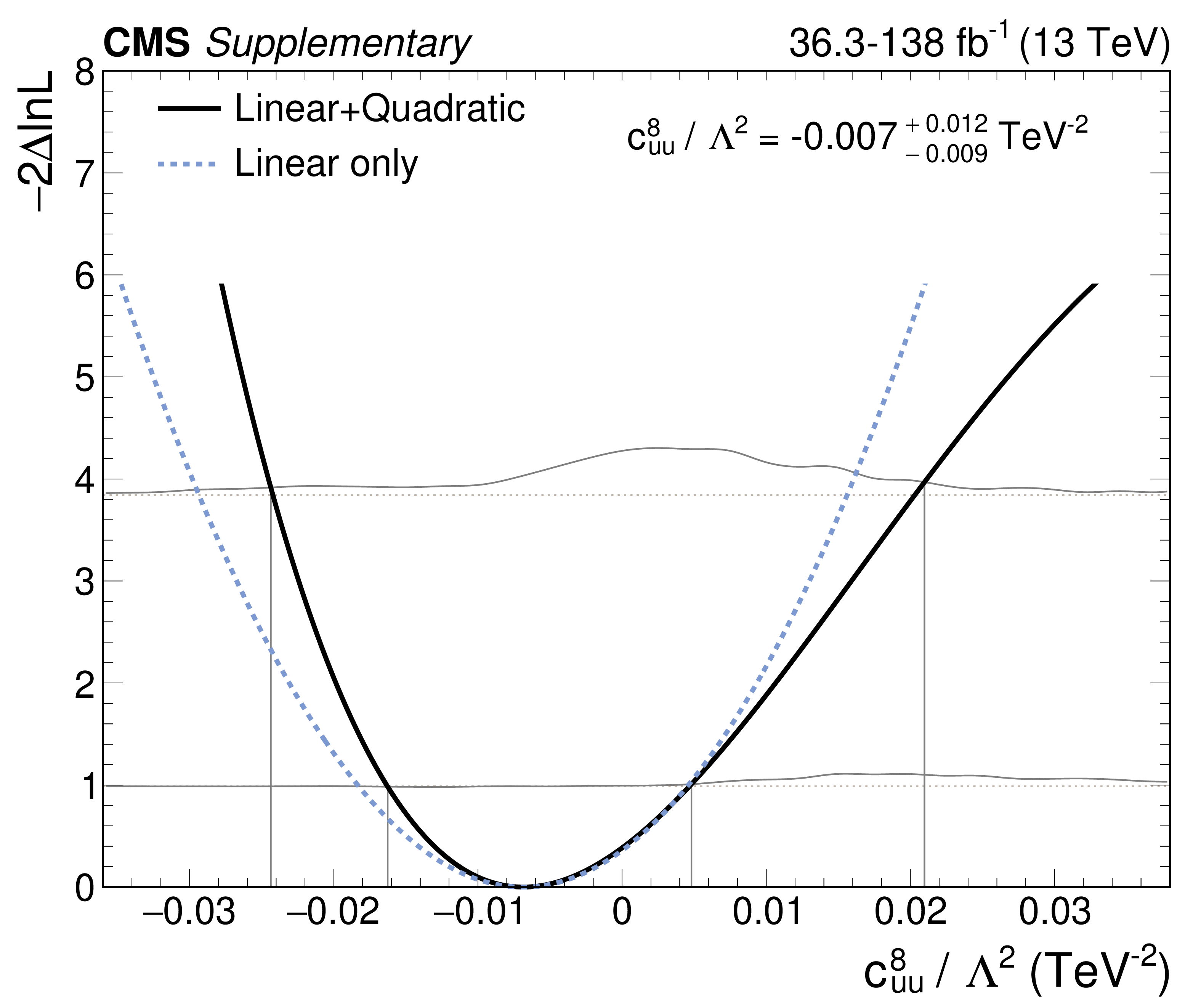
png pdf |
Additional Figure 14-n:
NLL scans of WCs, for the simplified fit without the $ \mathrm{t}(\overline{\mathrm{t}})\mathrm{X} $ analysis. The solid grey lines indicate the sets of points $ q^{68\%} $ (lower line) and $ q^{95\%} $ (upper line), while the dashed grey lines denote the test statistic values used to determine the 68% and 95% confidence intervals in the asymptotic approximation. |
png pdf |
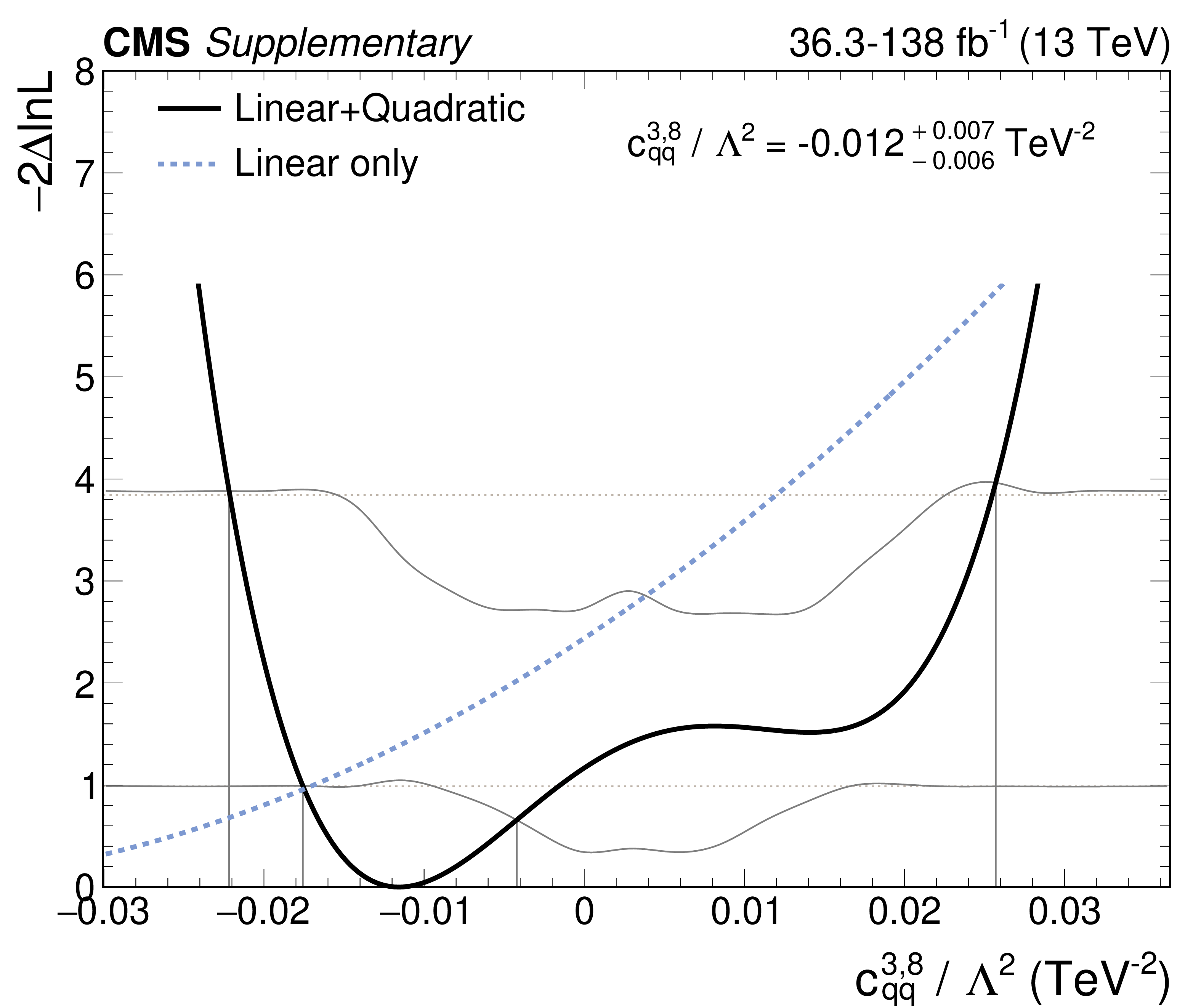
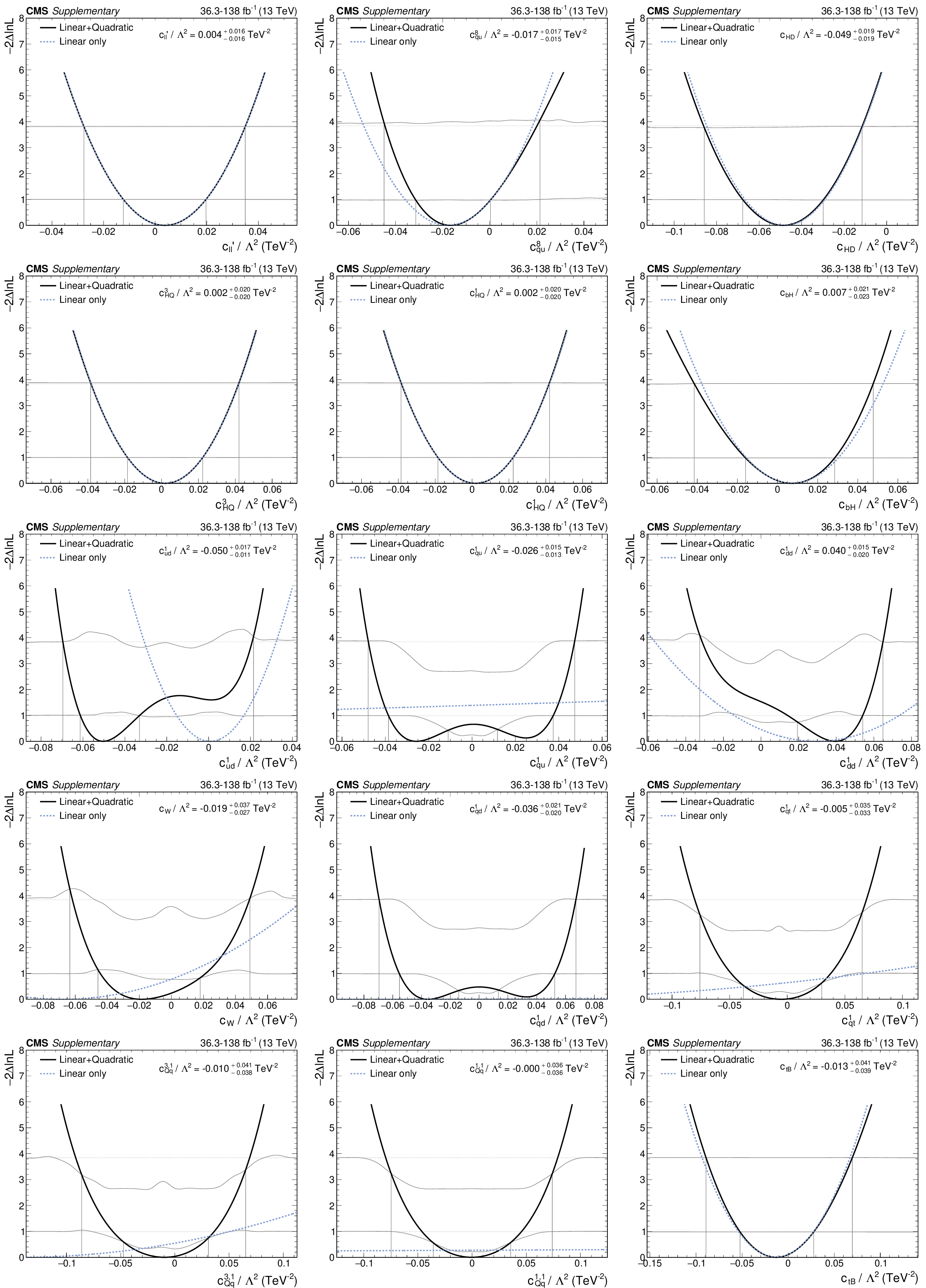
Additional Figure 14-o:
NLL scans of WCs, for the simplified fit without the $ \mathrm{t}(\overline{\mathrm{t}})\mathrm{X} $ analysis. The solid grey lines indicate the sets of points $ q^{68\%} $ (lower line) and $ q^{95\%} $ (upper line), while the dashed grey lines denote the test statistic values used to determine the 68% and 95% confidence intervals in the asymptotic approximation. |
png pdf |
Additional Figure 15:
NLL scans of WCs, for the simplified fit without the $ \mathrm{t}(\overline{\mathrm{t}})\mathrm{X} $ analysis. The solid grey lines indicate the sets of points $ q^{68\%} $ (lower line) and $ q^{95\%} $ (upper line), while the dashed grey lines denote the test statistic values used to determine the 68% and 95% confidence intervals in the asymptotic approximation. |

png pdf |
Additional Figure 15-a:
NLL scans of WCs, for the simplified fit without the $ \mathrm{t}(\overline{\mathrm{t}})\mathrm{X} $ analysis. The solid grey lines indicate the sets of points $ q^{68\%} $ (lower line) and $ q^{95\%} $ (upper line), while the dashed grey lines denote the test statistic values used to determine the 68% and 95% confidence intervals in the asymptotic approximation. |

png pdf |
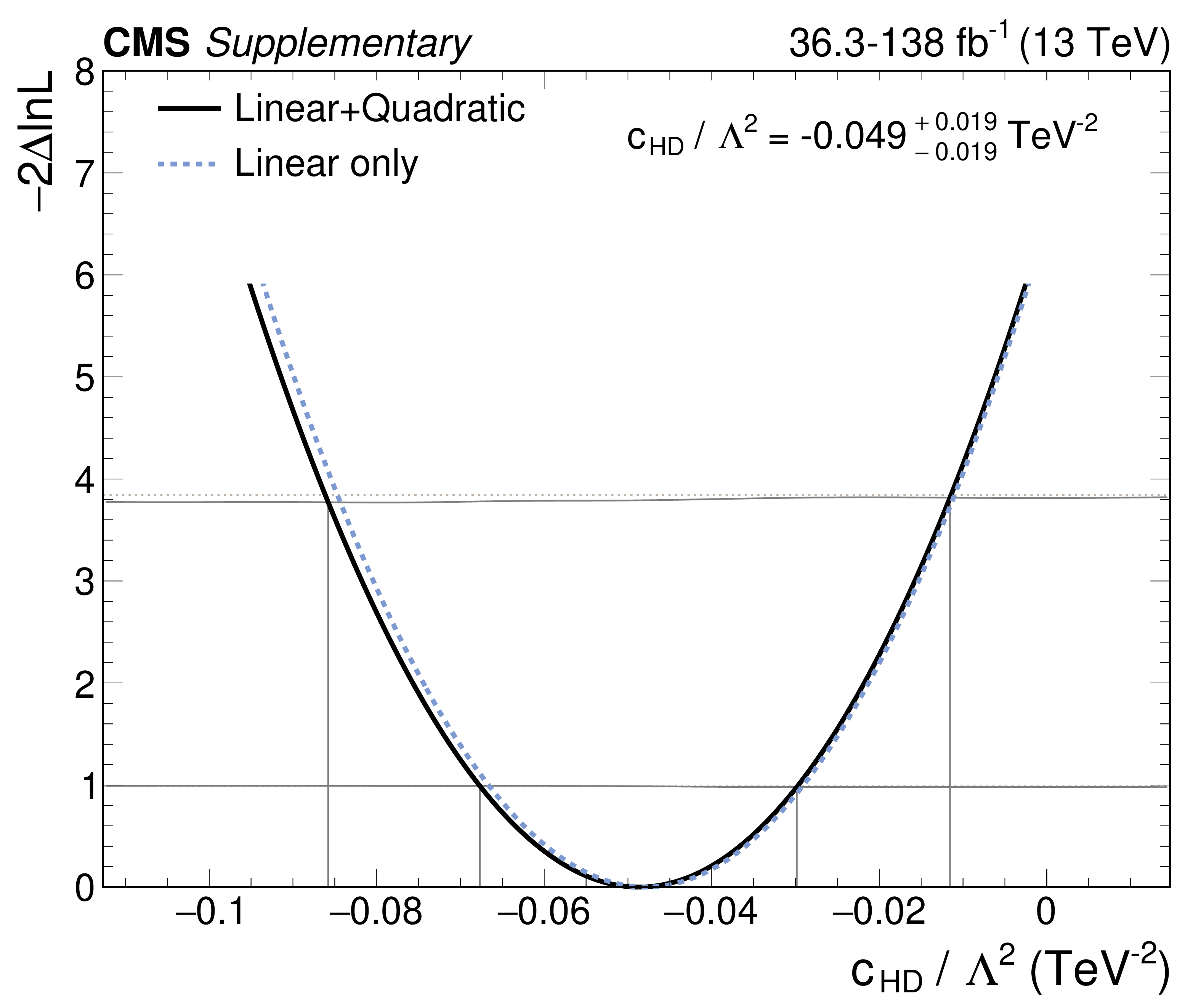
Additional Figure 15-b:
NLL scans of WCs, for the simplified fit without the $ \mathrm{t}(\overline{\mathrm{t}})\mathrm{X} $ analysis. The solid grey lines indicate the sets of points $ q^{68\%} $ (lower line) and $ q^{95\%} $ (upper line), while the dashed grey lines denote the test statistic values used to determine the 68% and 95% confidence intervals in the asymptotic approximation. |
png pdf |
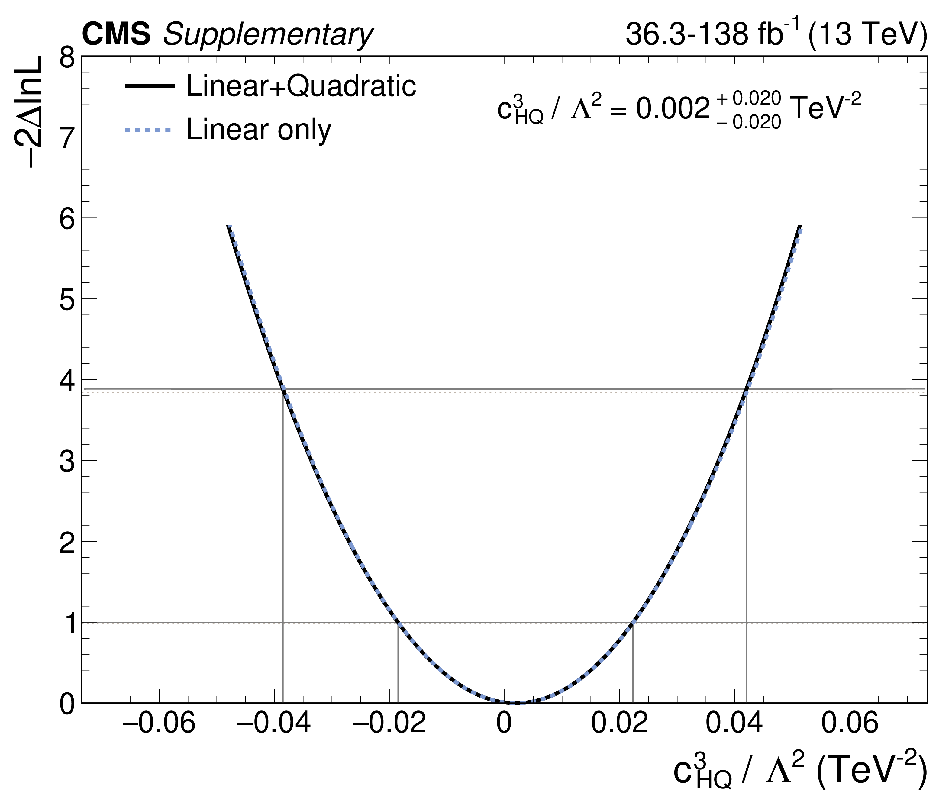
Additional Figure 15-c:
NLL scans of WCs, for the simplified fit without the $ \mathrm{t}(\overline{\mathrm{t}})\mathrm{X} $ analysis. The solid grey lines indicate the sets of points $ q^{68\%} $ (lower line) and $ q^{95\%} $ (upper line), while the dashed grey lines denote the test statistic values used to determine the 68% and 95% confidence intervals in the asymptotic approximation. |
png pdf |
Additional Figure 15-d:
NLL scans of WCs, for the simplified fit without the $ \mathrm{t}(\overline{\mathrm{t}})\mathrm{X} $ analysis. The solid grey lines indicate the sets of points $ q^{68\%} $ (lower line) and $ q^{95\%} $ (upper line), while the dashed grey lines denote the test statistic values used to determine the 68% and 95% confidence intervals in the asymptotic approximation. |
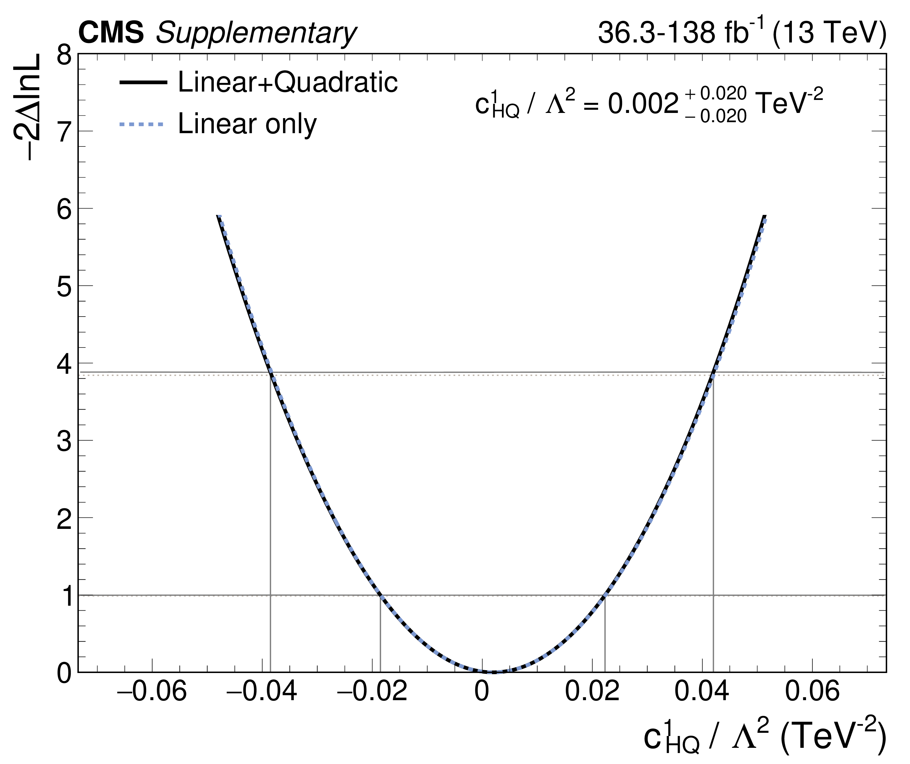
png pdf |
Additional Figure 15-e:
NLL scans of WCs, for the simplified fit without the $ \mathrm{t}(\overline{\mathrm{t}})\mathrm{X} $ analysis. The solid grey lines indicate the sets of points $ q^{68\%} $ (lower line) and $ q^{95\%} $ (upper line), while the dashed grey lines denote the test statistic values used to determine the 68% and 95% confidence intervals in the asymptotic approximation. |
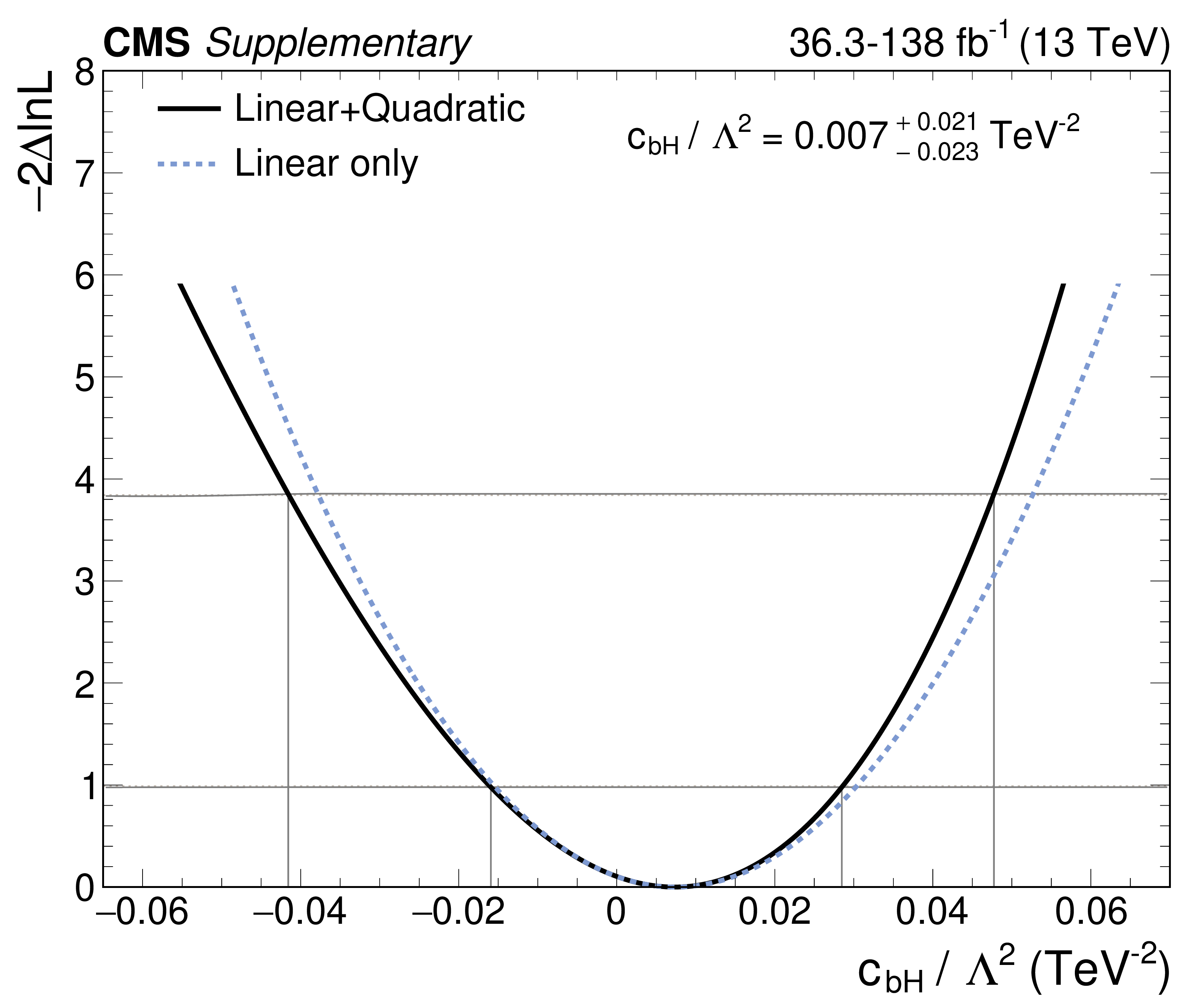
png pdf |
Additional Figure 15-f:
NLL scans of WCs, for the simplified fit without the $ \mathrm{t}(\overline{\mathrm{t}})\mathrm{X} $ analysis. The solid grey lines indicate the sets of points $ q^{68\%} $ (lower line) and $ q^{95\%} $ (upper line), while the dashed grey lines denote the test statistic values used to determine the 68% and 95% confidence intervals in the asymptotic approximation. |
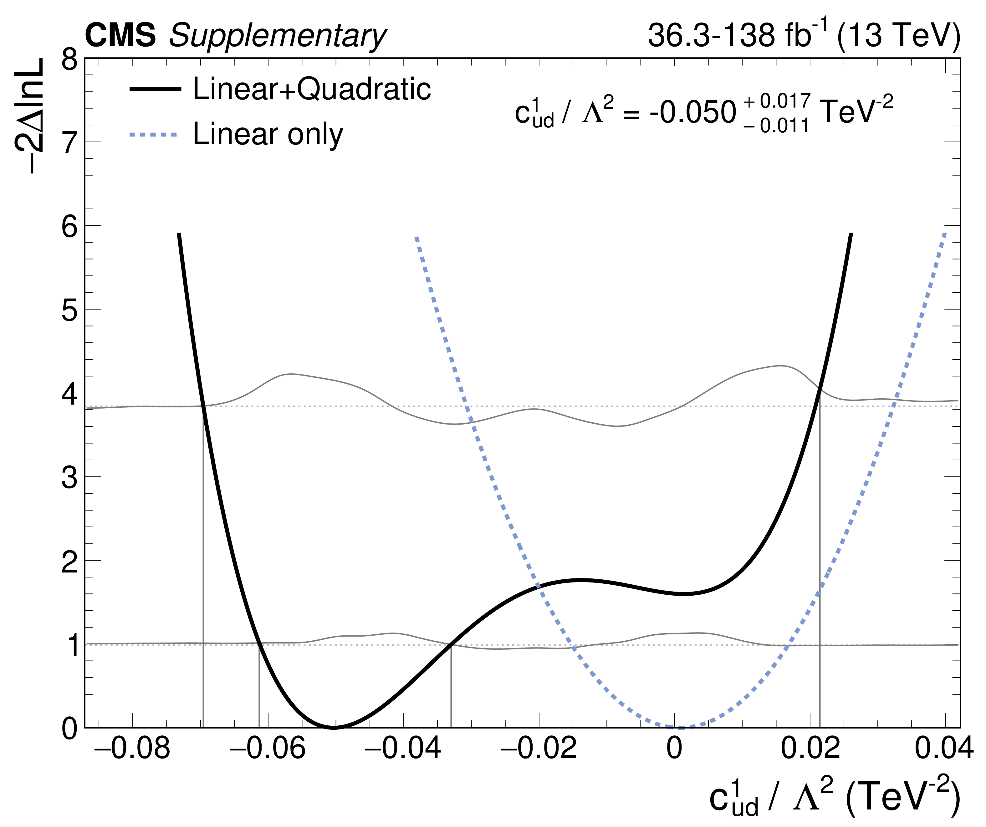
png pdf |
Additional Figure 15-g:
NLL scans of WCs, for the simplified fit without the $ \mathrm{t}(\overline{\mathrm{t}})\mathrm{X} $ analysis. The solid grey lines indicate the sets of points $ q^{68\%} $ (lower line) and $ q^{95\%} $ (upper line), while the dashed grey lines denote the test statistic values used to determine the 68% and 95% confidence intervals in the asymptotic approximation. |
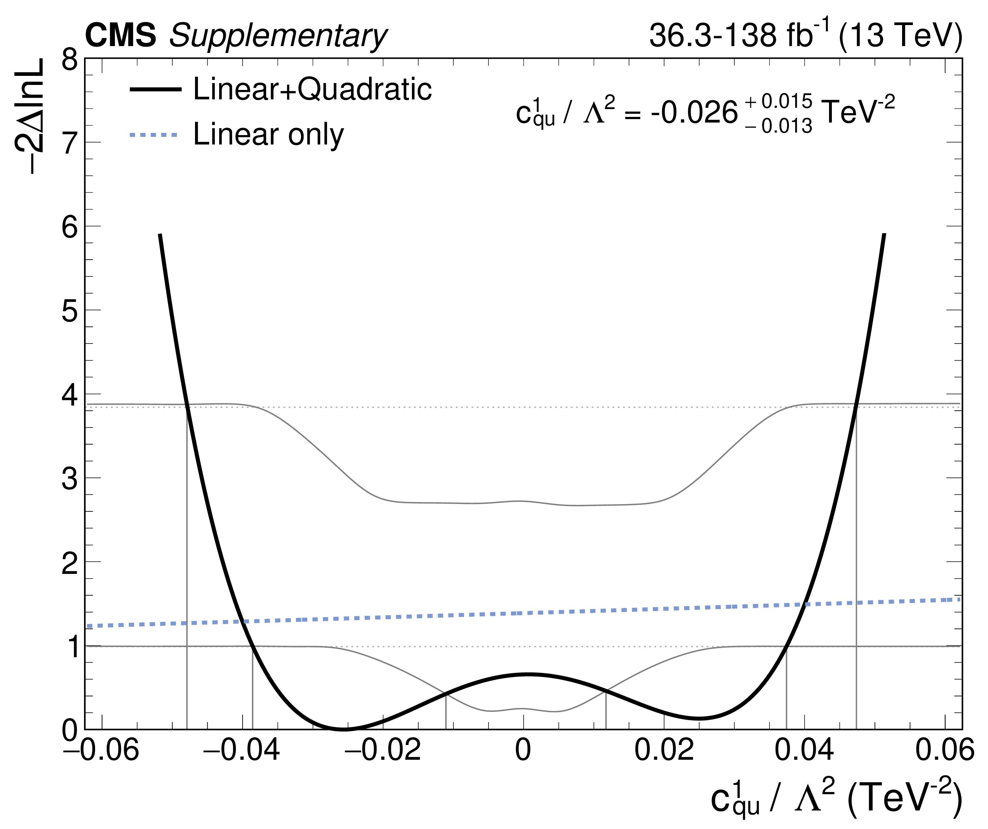
png pdf |
Additional Figure 15-h:
NLL scans of WCs, for the simplified fit without the $ \mathrm{t}(\overline{\mathrm{t}})\mathrm{X} $ analysis. The solid grey lines indicate the sets of points $ q^{68\%} $ (lower line) and $ q^{95\%} $ (upper line), while the dashed grey lines denote the test statistic values used to determine the 68% and 95% confidence intervals in the asymptotic approximation. |

png pdf |
Additional Figure 15-i:
NLL scans of WCs, for the simplified fit without the $ \mathrm{t}(\overline{\mathrm{t}})\mathrm{X} $ analysis. The solid grey lines indicate the sets of points $ q^{68\%} $ (lower line) and $ q^{95\%} $ (upper line), while the dashed grey lines denote the test statistic values used to determine the 68% and 95% confidence intervals in the asymptotic approximation. |
png pdf |
Additional Figure 15-j:
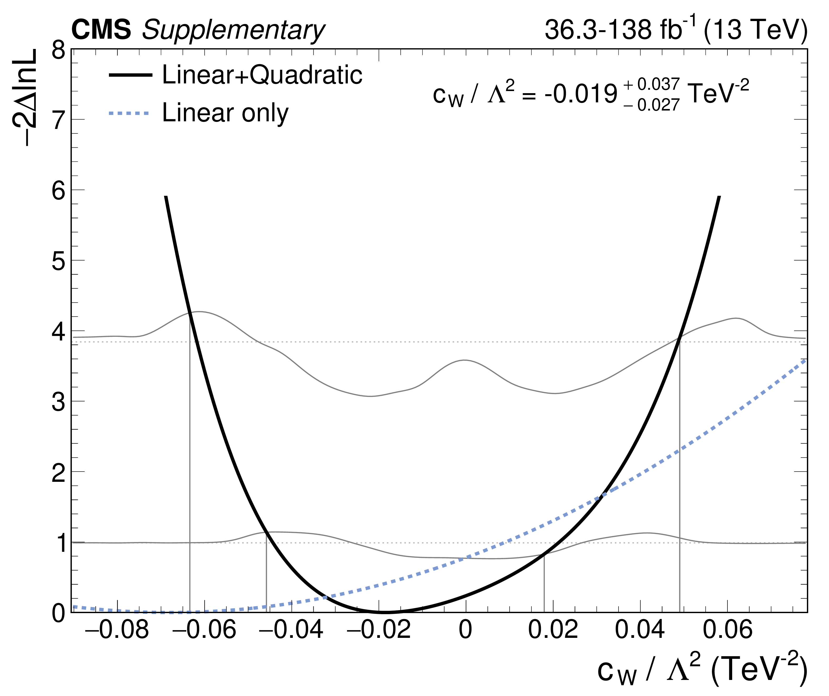
NLL scans of WCs, for the simplified fit without the $ \mathrm{t}(\overline{\mathrm{t}})\mathrm{X} $ analysis. The solid grey lines indicate the sets of points $ q^{68\%} $ (lower line) and $ q^{95\%} $ (upper line), while the dashed grey lines denote the test statistic values used to determine the 68% and 95% confidence intervals in the asymptotic approximation. |
png pdf |
Additional Figure 15-k:
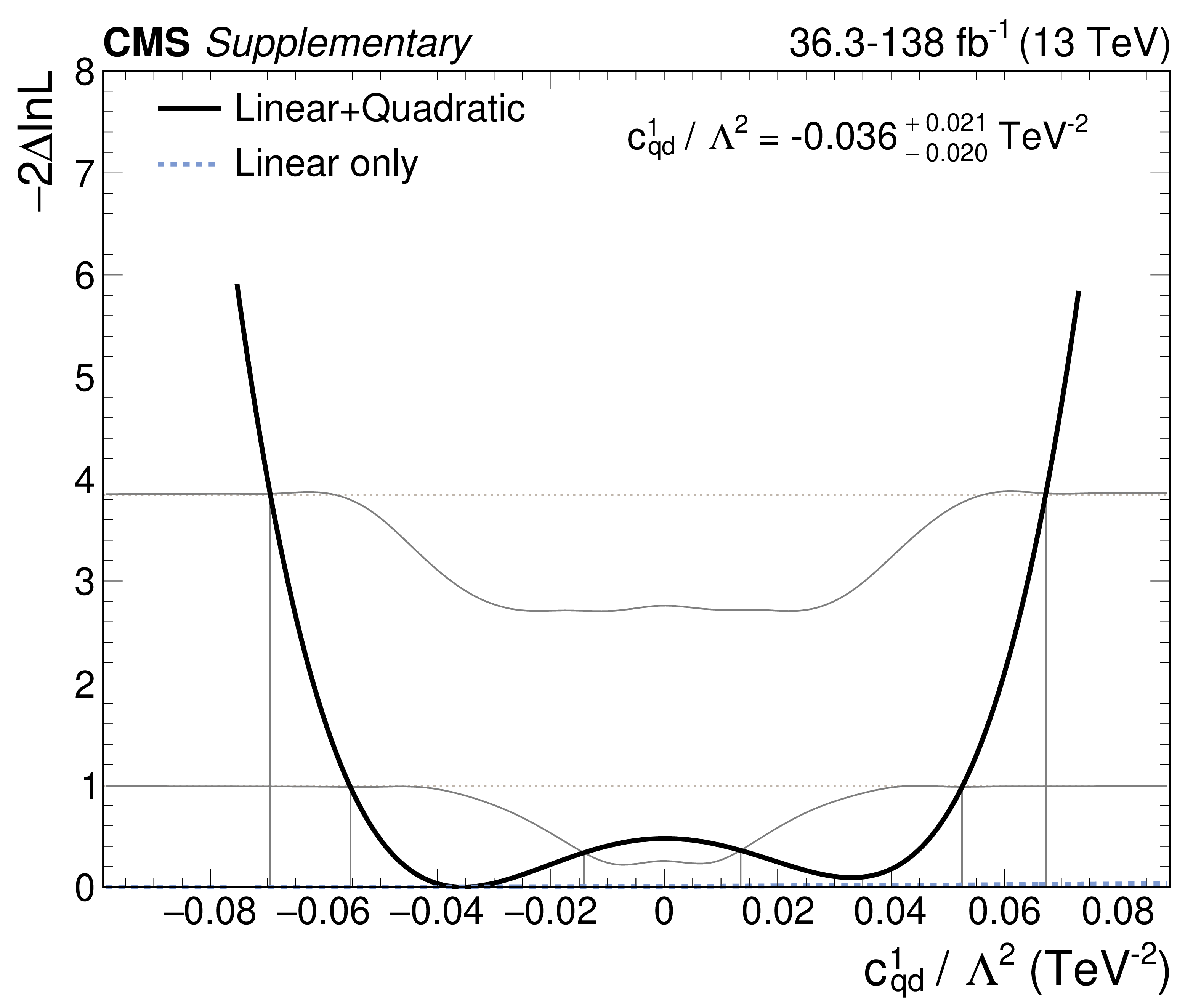
NLL scans of WCs, for the simplified fit without the $ \mathrm{t}(\overline{\mathrm{t}})\mathrm{X} $ analysis. The solid grey lines indicate the sets of points $ q^{68\%} $ (lower line) and $ q^{95\%} $ (upper line), while the dashed grey lines denote the test statistic values used to determine the 68% and 95% confidence intervals in the asymptotic approximation. |

png pdf |
Additional Figure 15-l:
NLL scans of WCs, for the simplified fit without the $ \mathrm{t}(\overline{\mathrm{t}})\mathrm{X} $ analysis. The solid grey lines indicate the sets of points $ q^{68\%} $ (lower line) and $ q^{95\%} $ (upper line), while the dashed grey lines denote the test statistic values used to determine the 68% and 95% confidence intervals in the asymptotic approximation. |

png pdf |
Additional Figure 15-m:
NLL scans of WCs, for the simplified fit without the $ \mathrm{t}(\overline{\mathrm{t}})\mathrm{X} $ analysis. The solid grey lines indicate the sets of points $ q^{68\%} $ (lower line) and $ q^{95\%} $ (upper line), while the dashed grey lines denote the test statistic values used to determine the 68% and 95% confidence intervals in the asymptotic approximation. |
png pdf |
Additional Figure 15-n:
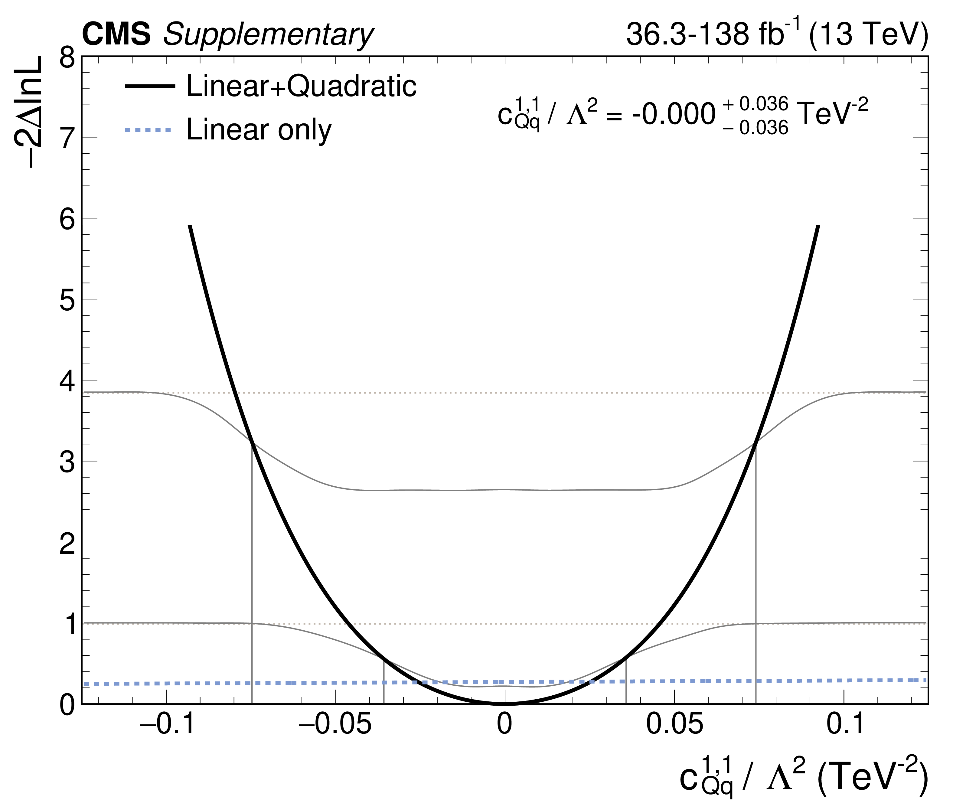
NLL scans of WCs, for the simplified fit without the $ \mathrm{t}(\overline{\mathrm{t}})\mathrm{X} $ analysis. The solid grey lines indicate the sets of points $ q^{68\%} $ (lower line) and $ q^{95\%} $ (upper line), while the dashed grey lines denote the test statistic values used to determine the 68% and 95% confidence intervals in the asymptotic approximation. |

png pdf |
Additional Figure 15-o:
NLL scans of WCs, for the simplified fit without the $ \mathrm{t}(\overline{\mathrm{t}})\mathrm{X} $ analysis. The solid grey lines indicate the sets of points $ q^{68\%} $ (lower line) and $ q^{95\%} $ (upper line), while the dashed grey lines denote the test statistic values used to determine the 68% and 95% confidence intervals in the asymptotic approximation. |

png pdf |
Additional Figure 16:
NLL scans of WCs, for the simplified fit without the $ \mathrm{t}(\overline{\mathrm{t}})\mathrm{X} $ analysis. The solid grey lines indicate the sets of points $ q^{68\%} $ (lower line) and $ q^{95\%} $ (upper line), while the dashed grey lines denote the test statistic values used to determine the 68% and 95% confidence intervals in the asymptotic approximation. |
png pdf |
Additional Figure 16-a:
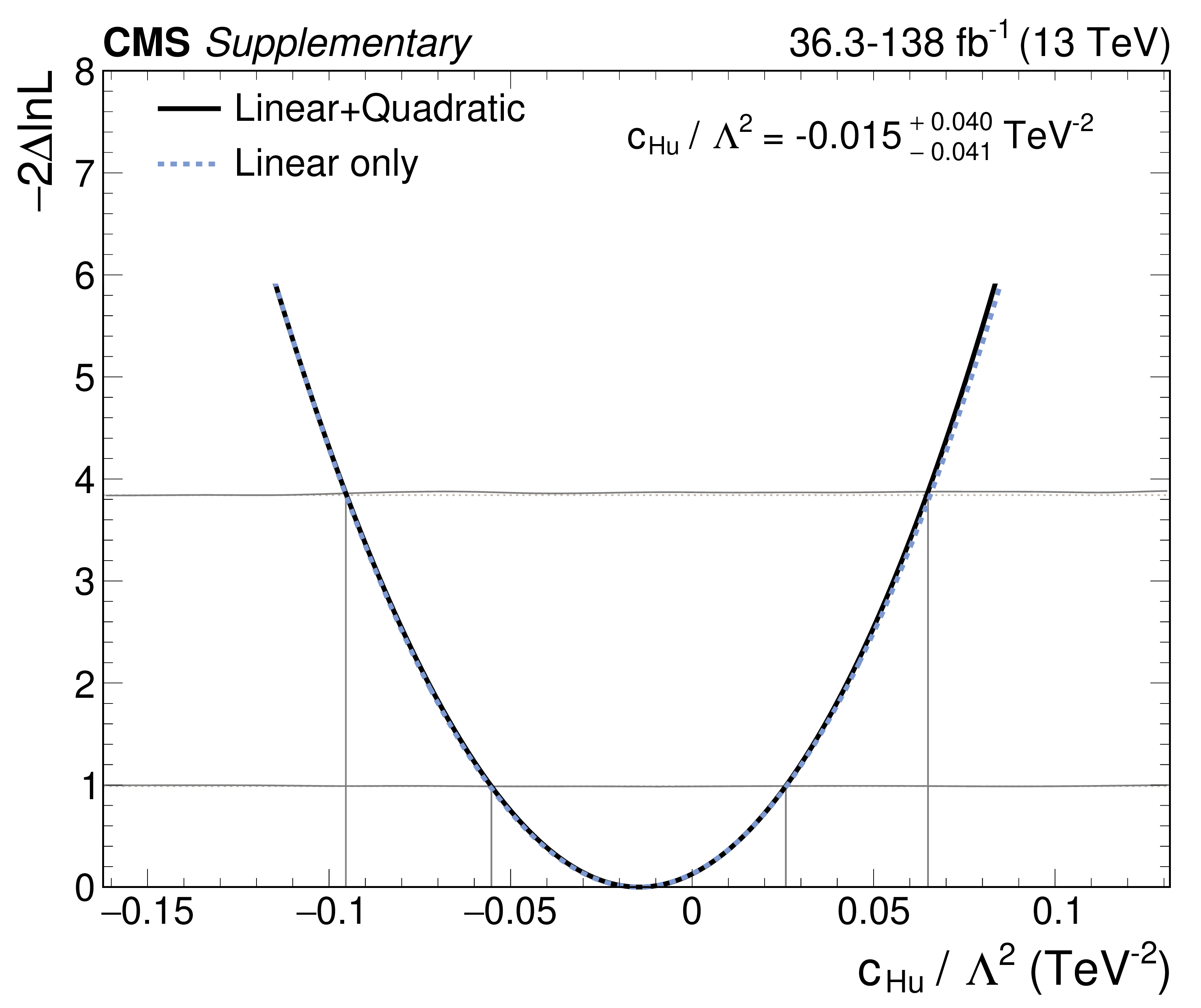
NLL scans of WCs, for the simplified fit without the $ \mathrm{t}(\overline{\mathrm{t}})\mathrm{X} $ analysis. The solid grey lines indicate the sets of points $ q^{68\%} $ (lower line) and $ q^{95\%} $ (upper line), while the dashed grey lines denote the test statistic values used to determine the 68% and 95% confidence intervals in the asymptotic approximation. |

png pdf |
Additional Figure 16-b:
NLL scans of WCs, for the simplified fit without the $ \mathrm{t}(\overline{\mathrm{t}})\mathrm{X} $ analysis. The solid grey lines indicate the sets of points $ q^{68\%} $ (lower line) and $ q^{95\%} $ (upper line), while the dashed grey lines denote the test statistic values used to determine the 68% and 95% confidence intervals in the asymptotic approximation. |
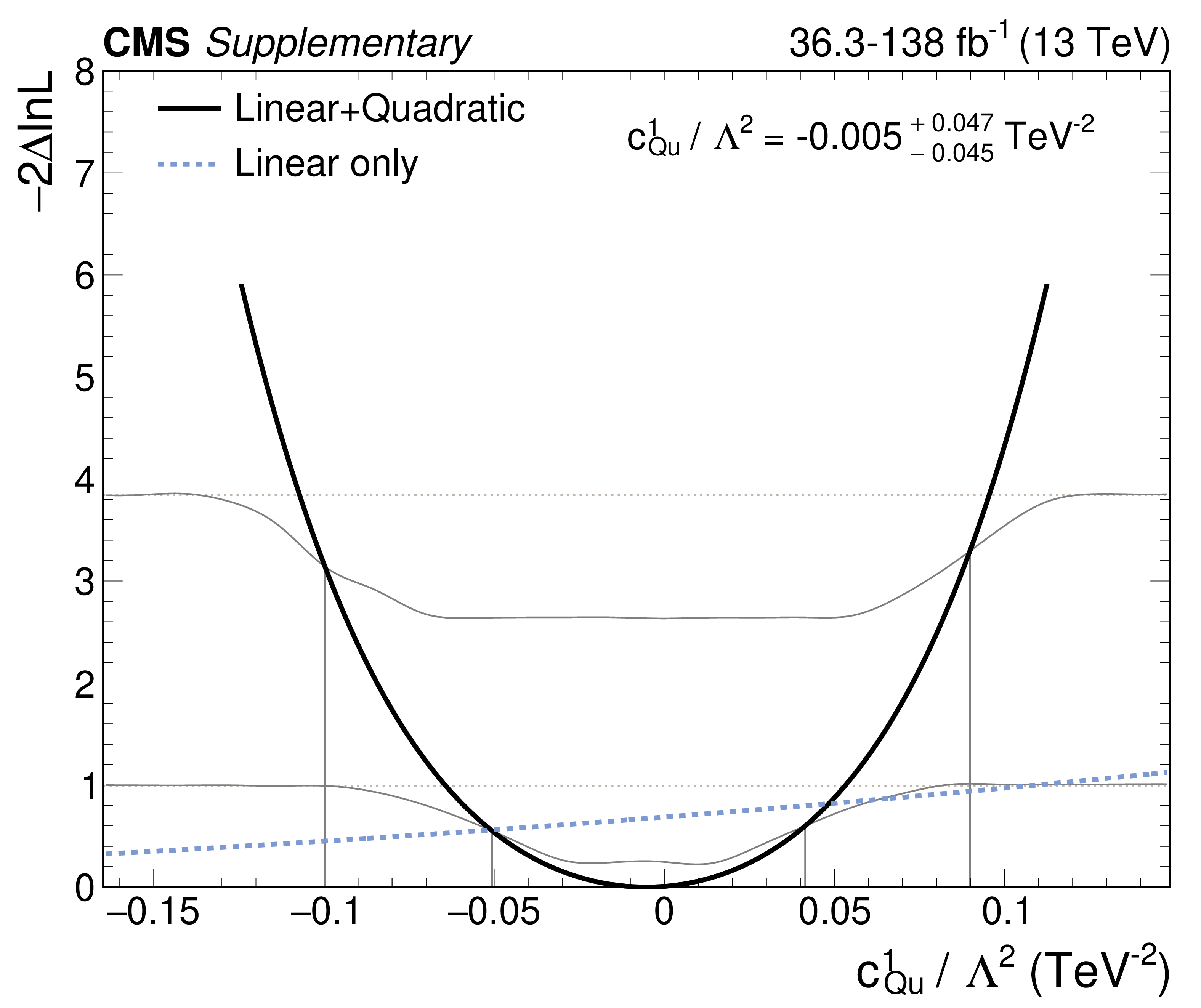
png pdf |
Additional Figure 16-c:
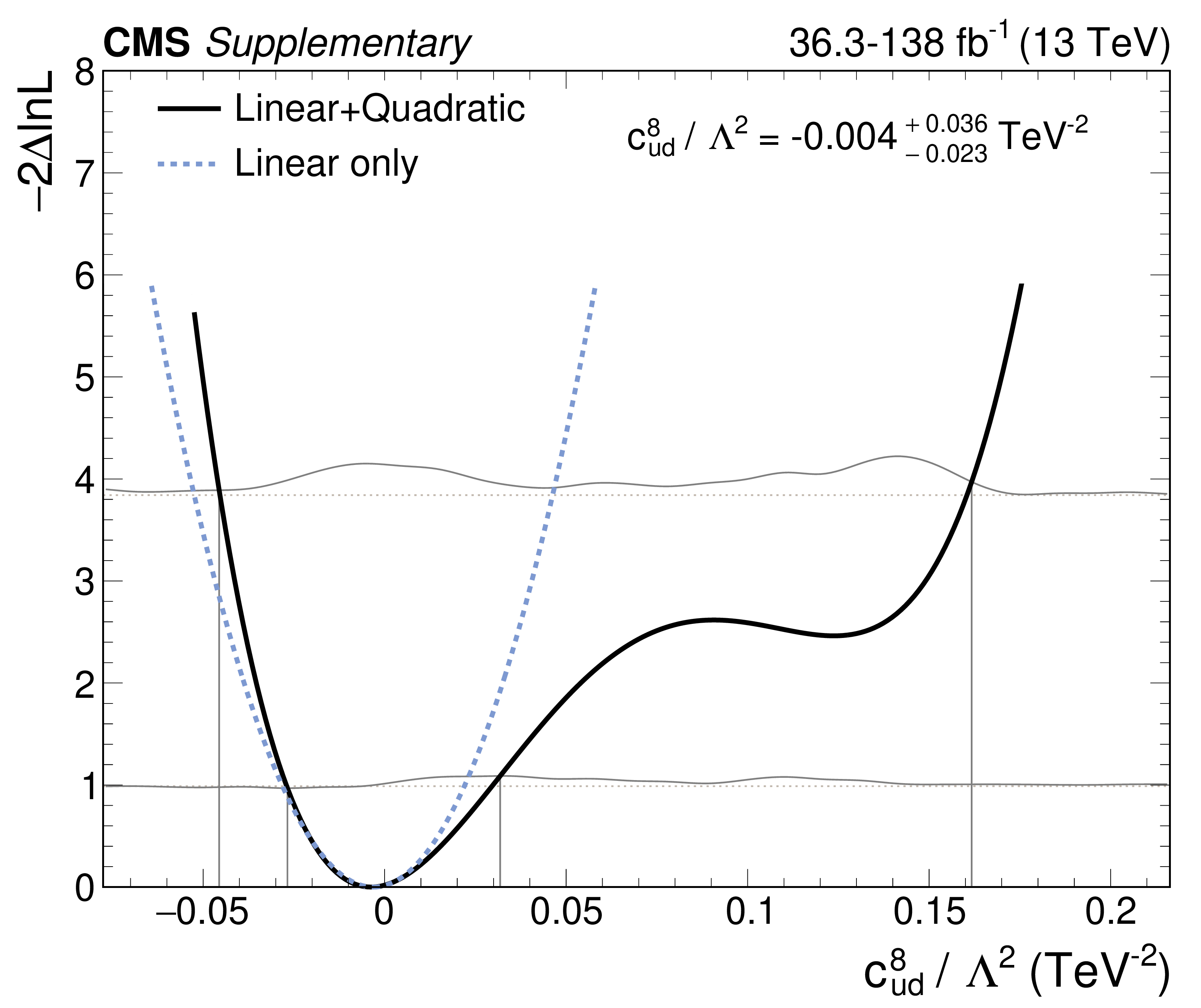
NLL scans of WCs, for the simplified fit without the $ \mathrm{t}(\overline{\mathrm{t}})\mathrm{X} $ analysis. The solid grey lines indicate the sets of points $ q^{68\%} $ (lower line) and $ q^{95\%} $ (upper line), while the dashed grey lines denote the test statistic values used to determine the 68% and 95% confidence intervals in the asymptotic approximation. |
png pdf |
Additional Figure 16-d:
NLL scans of WCs, for the simplified fit without the $ \mathrm{t}(\overline{\mathrm{t}})\mathrm{X} $ analysis. The solid grey lines indicate the sets of points $ q^{68\%} $ (lower line) and $ q^{95\%} $ (upper line), while the dashed grey lines denote the test statistic values used to determine the 68% and 95% confidence intervals in the asymptotic approximation. |

png pdf |
Additional Figure 16-e:
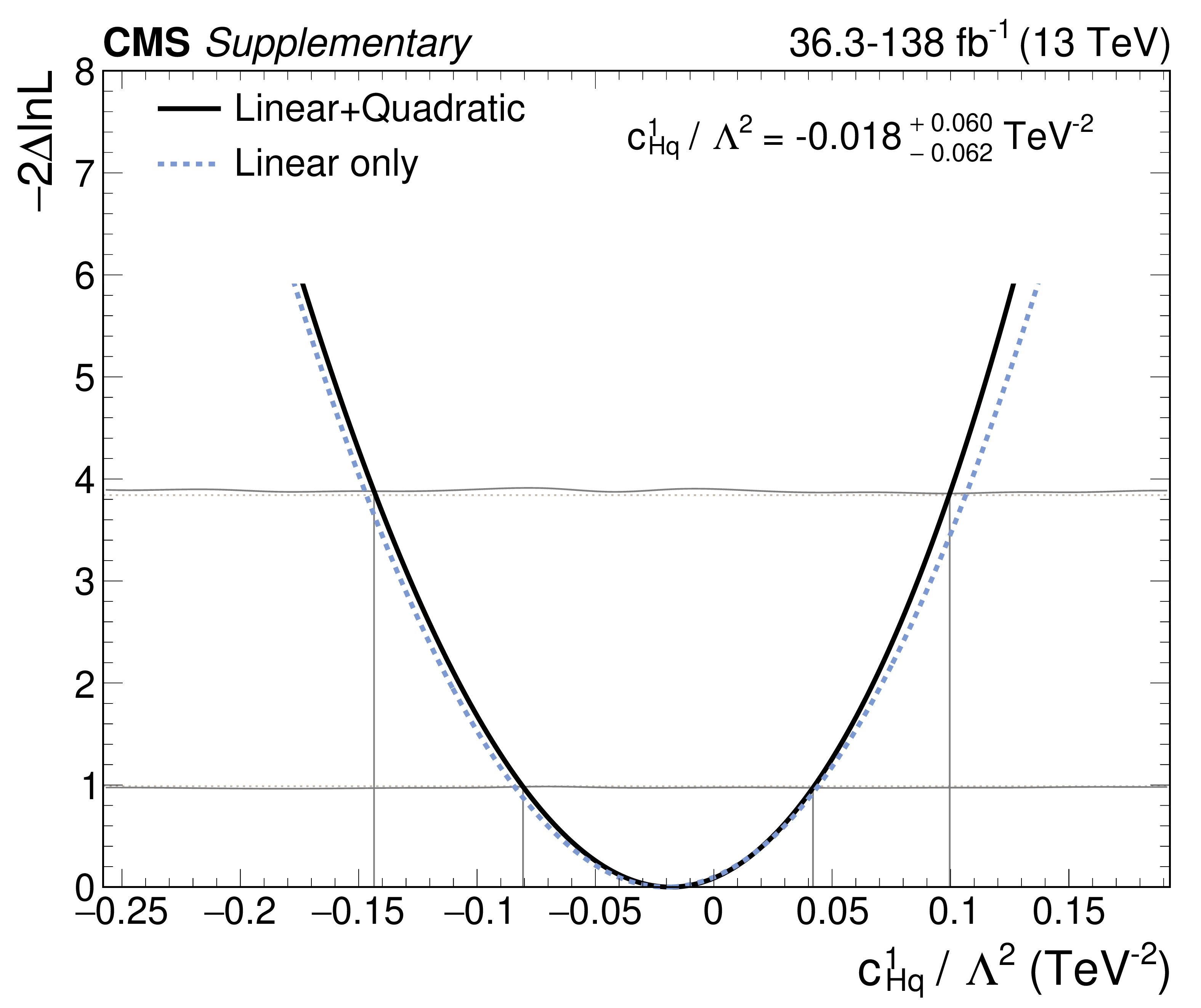
NLL scans of WCs, for the simplified fit without the $ \mathrm{t}(\overline{\mathrm{t}})\mathrm{X} $ analysis. The solid grey lines indicate the sets of points $ q^{68\%} $ (lower line) and $ q^{95\%} $ (upper line), while the dashed grey lines denote the test statistic values used to determine the 68% and 95% confidence intervals in the asymptotic approximation. |
png pdf |
Additional Figure 16-f:
NLL scans of WCs, for the simplified fit without the $ \mathrm{t}(\overline{\mathrm{t}})\mathrm{X} $ analysis. The solid grey lines indicate the sets of points $ q^{68\%} $ (lower line) and $ q^{95\%} $ (upper line), while the dashed grey lines denote the test statistic values used to determine the 68% and 95% confidence intervals in the asymptotic approximation. |

png pdf |
Additional Figure 16-g:
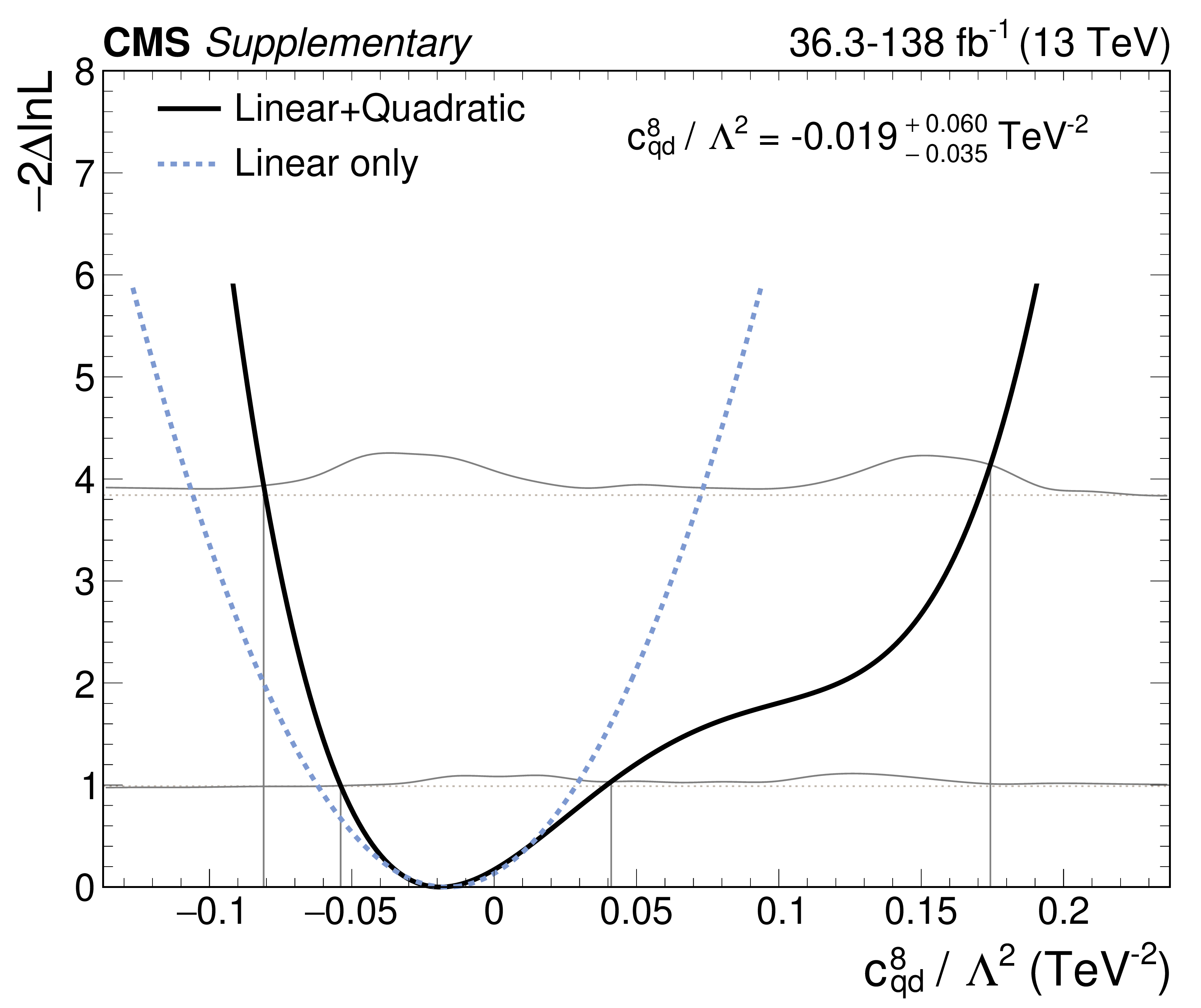
NLL scans of WCs, for the simplified fit without the $ \mathrm{t}(\overline{\mathrm{t}})\mathrm{X} $ analysis. The solid grey lines indicate the sets of points $ q^{68\%} $ (lower line) and $ q^{95\%} $ (upper line), while the dashed grey lines denote the test statistic values used to determine the 68% and 95% confidence intervals in the asymptotic approximation. |
png pdf |
Additional Figure 16-h:
NLL scans of WCs, for the simplified fit without the $ \mathrm{t}(\overline{\mathrm{t}})\mathrm{X} $ analysis. The solid grey lines indicate the sets of points $ q^{68\%} $ (lower line) and $ q^{95\%} $ (upper line), while the dashed grey lines denote the test statistic values used to determine the 68% and 95% confidence intervals in the asymptotic approximation. |
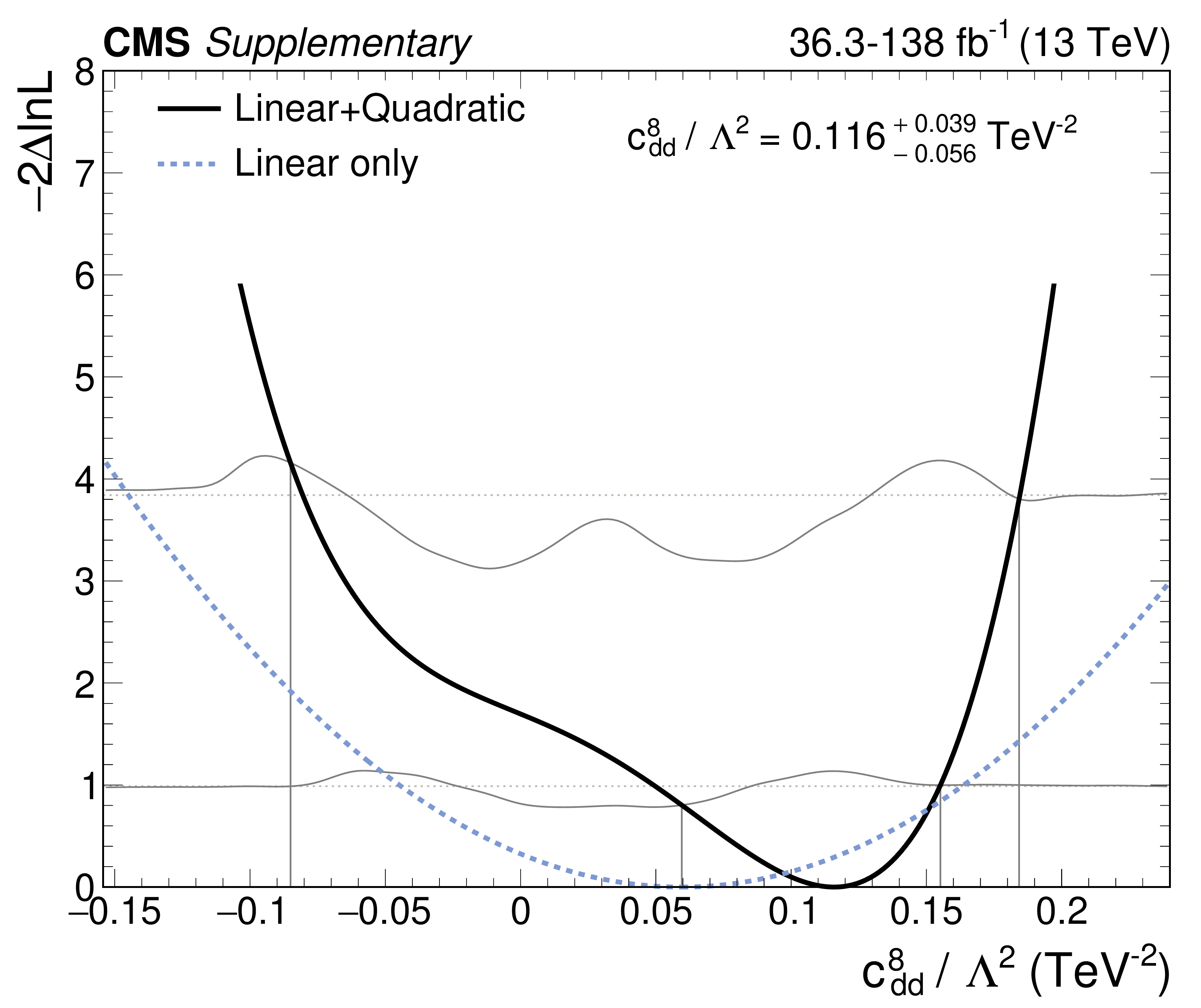
png pdf |
Additional Figure 16-i:
NLL scans of WCs, for the simplified fit without the $ \mathrm{t}(\overline{\mathrm{t}})\mathrm{X} $ analysis. The solid grey lines indicate the sets of points $ q^{68\%} $ (lower line) and $ q^{95\%} $ (upper line), while the dashed grey lines denote the test statistic values used to determine the 68% and 95% confidence intervals in the asymptotic approximation. |
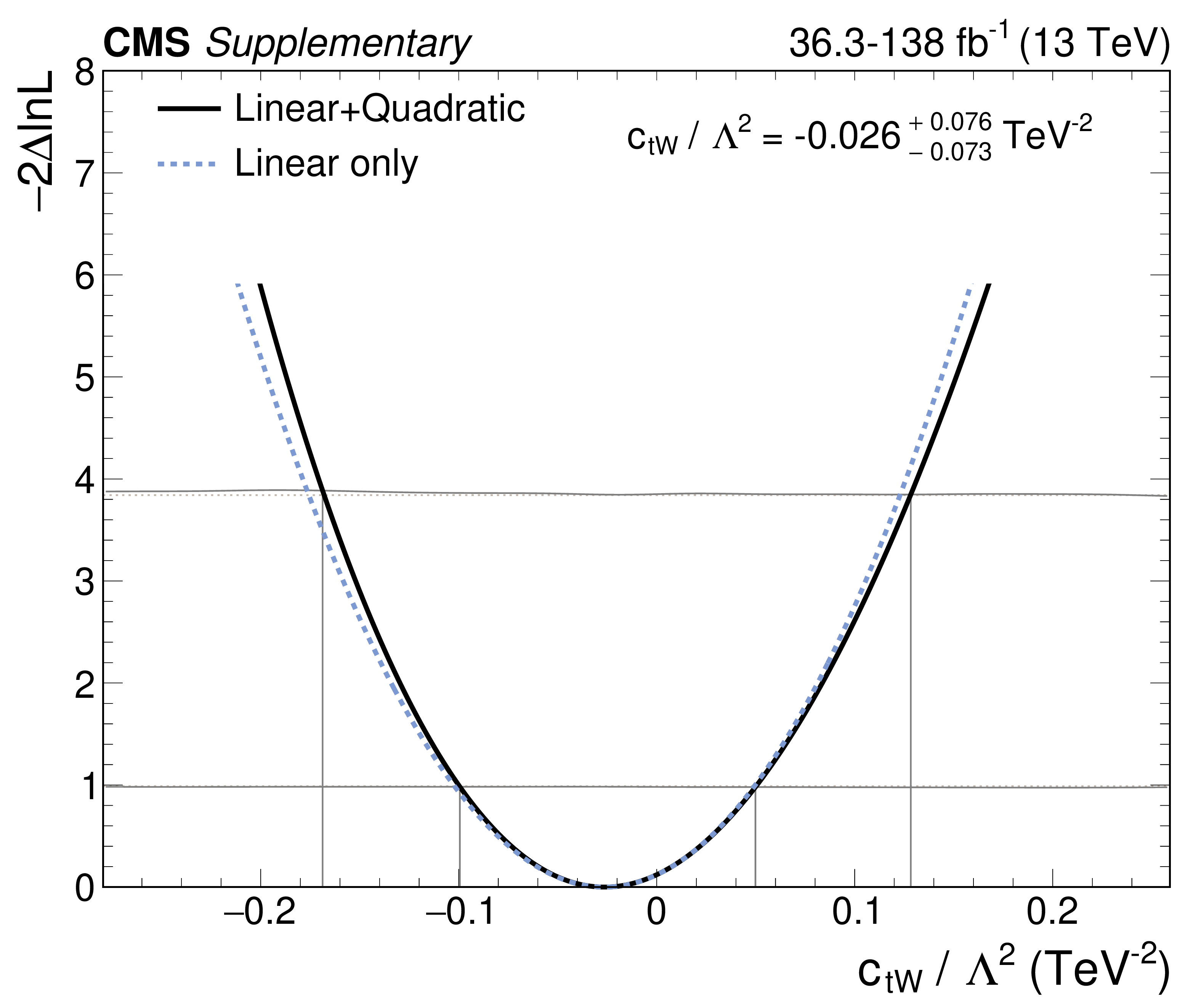
png pdf |
Additional Figure 16-j:
NLL scans of WCs, for the simplified fit without the $ \mathrm{t}(\overline{\mathrm{t}})\mathrm{X} $ analysis. The solid grey lines indicate the sets of points $ q^{68\%} $ (lower line) and $ q^{95\%} $ (upper line), while the dashed grey lines denote the test statistic values used to determine the 68% and 95% confidence intervals in the asymptotic approximation. |

png pdf |
Additional Figure 16-k:
NLL scans of WCs, for the simplified fit without the $ \mathrm{t}(\overline{\mathrm{t}})\mathrm{X} $ analysis. The solid grey lines indicate the sets of points $ q^{68\%} $ (lower line) and $ q^{95\%} $ (upper line), while the dashed grey lines denote the test statistic values used to determine the 68% and 95% confidence intervals in the asymptotic approximation. |
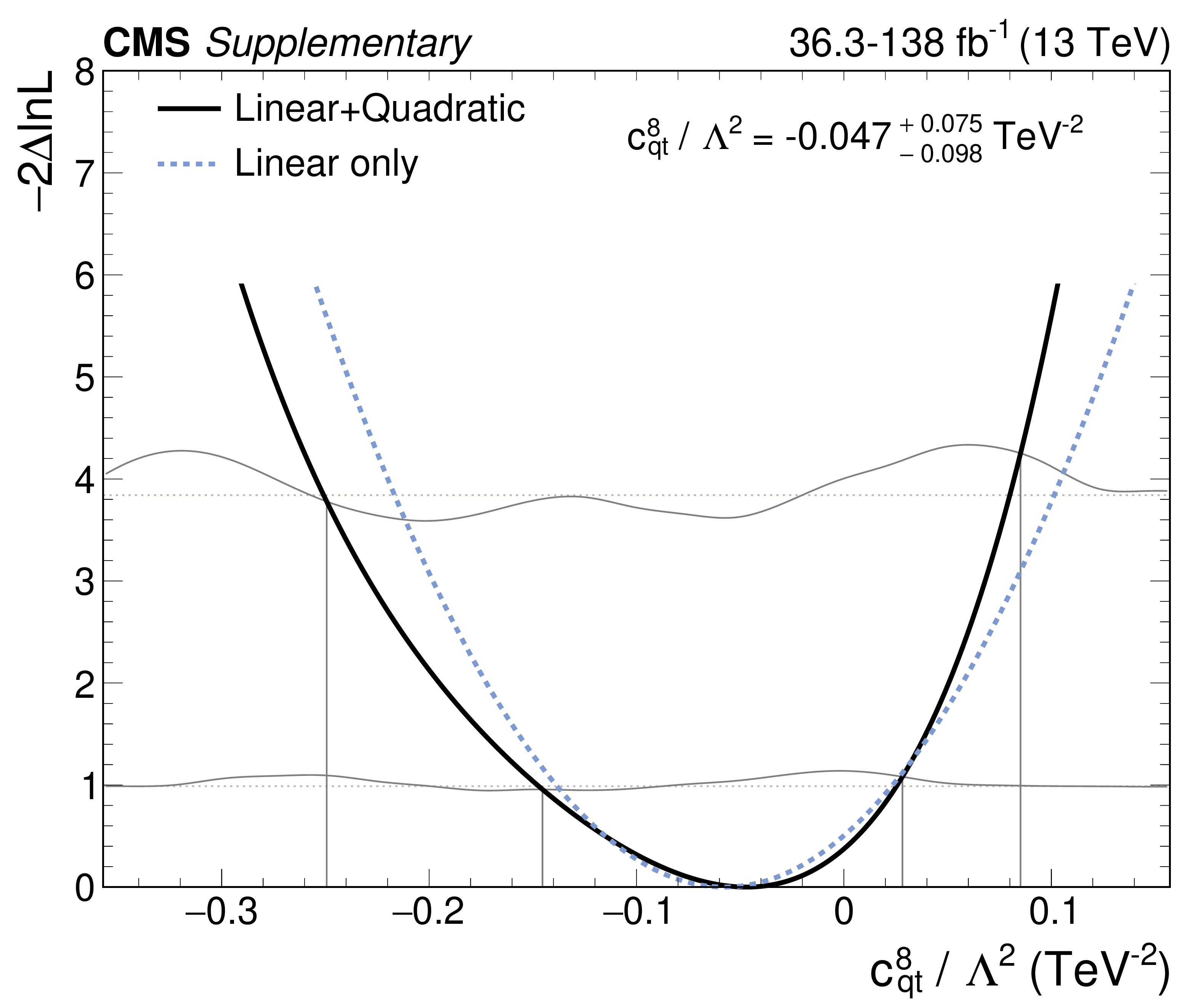
png pdf |
Additional Figure 16-l:
NLL scans of WCs, for the simplified fit without the $ \mathrm{t}(\overline{\mathrm{t}})\mathrm{X} $ analysis. The solid grey lines indicate the sets of points $ q^{68\%} $ (lower line) and $ q^{95\%} $ (upper line), while the dashed grey lines denote the test statistic values used to determine the 68% and 95% confidence intervals in the asymptotic approximation. |

png pdf |
Additional Figure 16-m:
NLL scans of WCs, for the simplified fit without the $ \mathrm{t}(\overline{\mathrm{t}})\mathrm{X} $ analysis. The solid grey lines indicate the sets of points $ q^{68\%} $ (lower line) and $ q^{95\%} $ (upper line), while the dashed grey lines denote the test statistic values used to determine the 68% and 95% confidence intervals in the asymptotic approximation. |
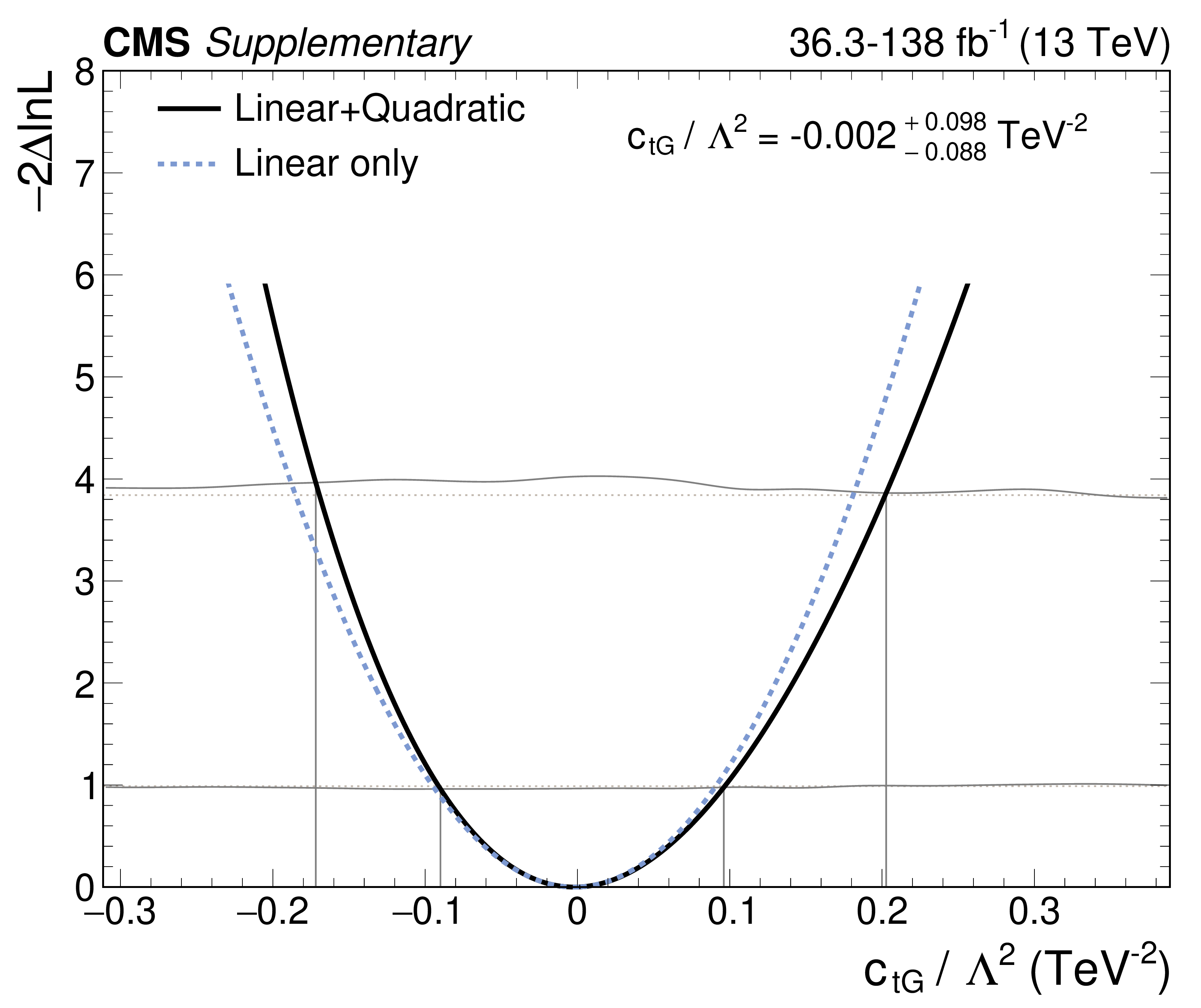
png pdf |
Additional Figure 16-n:
NLL scans of WCs, for the simplified fit without the $ \mathrm{t}(\overline{\mathrm{t}})\mathrm{X} $ analysis. The solid grey lines indicate the sets of points $ q^{68\%} $ (lower line) and $ q^{95\%} $ (upper line), while the dashed grey lines denote the test statistic values used to determine the 68% and 95% confidence intervals in the asymptotic approximation. |
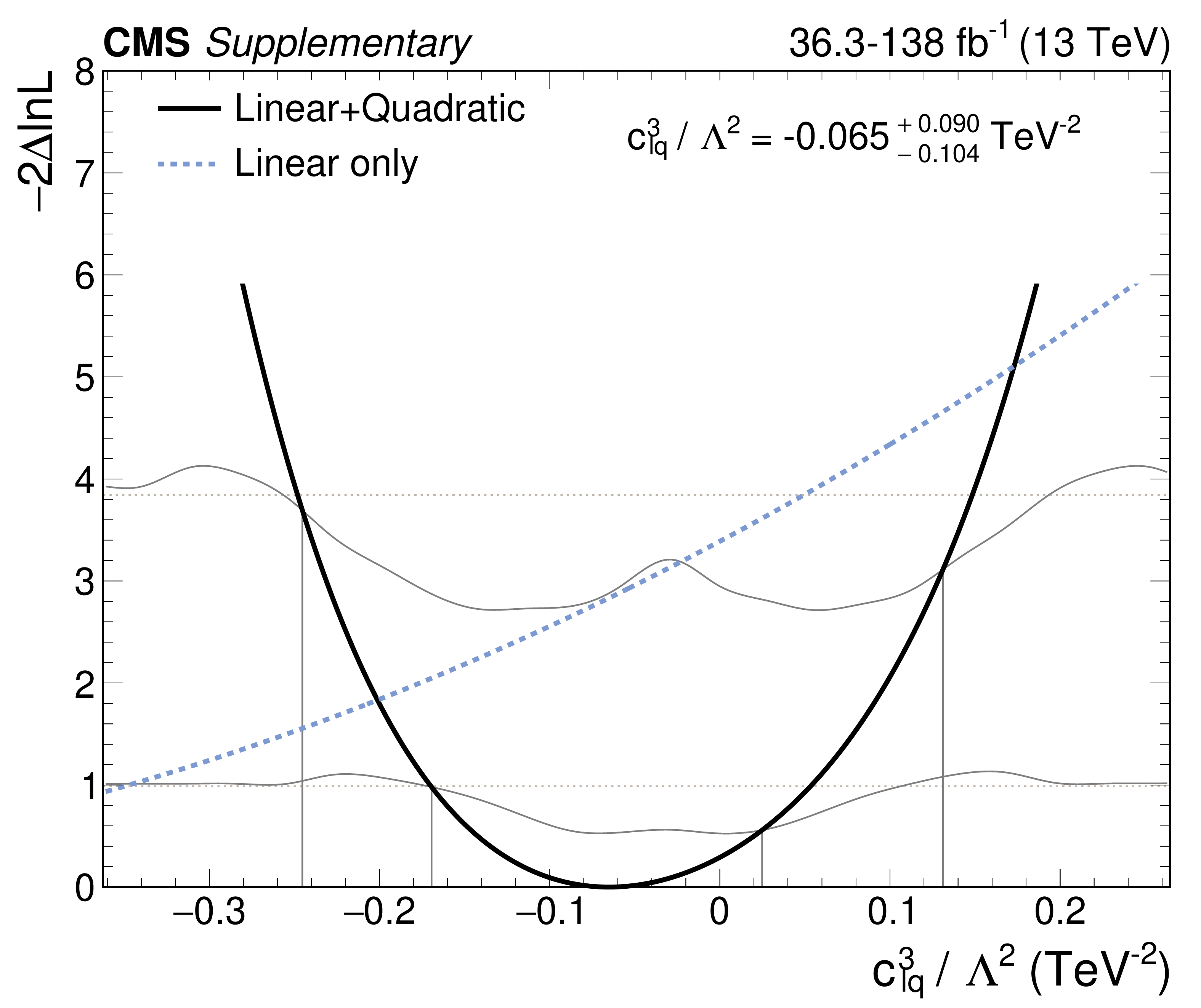
png pdf |
Additional Figure 16-o:
NLL scans of WCs, for the simplified fit without the $ \mathrm{t}(\overline{\mathrm{t}})\mathrm{X} $ analysis. The solid grey lines indicate the sets of points $ q^{68\%} $ (lower line) and $ q^{95\%} $ (upper line), while the dashed grey lines denote the test statistic values used to determine the 68% and 95% confidence intervals in the asymptotic approximation. |

png pdf |
Additional Figure 17:
NLL scans of WCs, for the simplified fit without the $ \mathrm{t}(\overline{\mathrm{t}})\mathrm{X} $ analysis. The solid grey lines indicate the sets of points $ q^{68\%} $ (lower line) and $ q^{95\%} $ (upper line), while the dashed grey lines denote the test statistic values used to determine the 68% and 95% confidence intervals in the asymptotic approximation. |
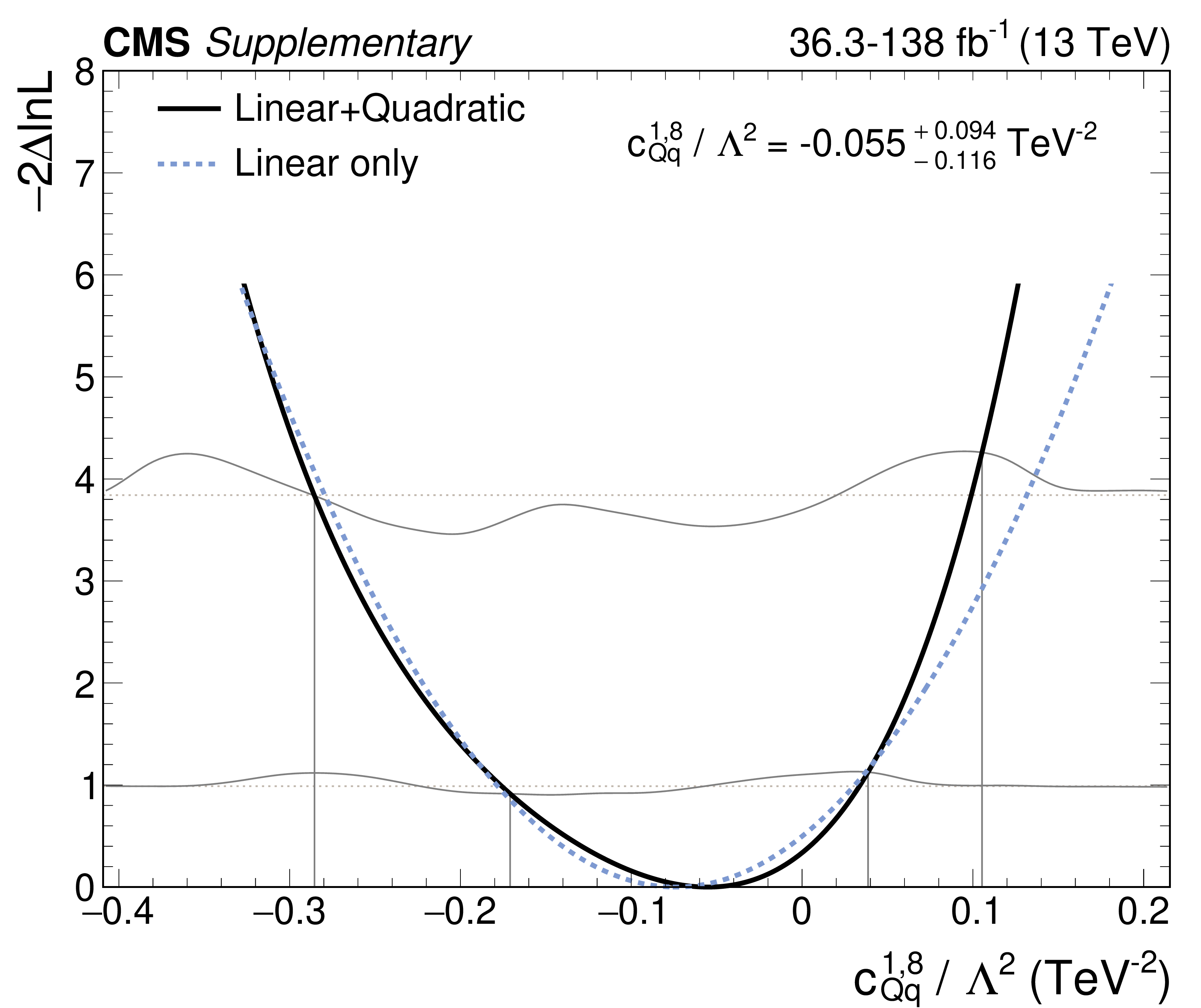
png pdf |
Additional Figure 17-a:
NLL scans of WCs, for the simplified fit without the $ \mathrm{t}(\overline{\mathrm{t}})\mathrm{X} $ analysis. The solid grey lines indicate the sets of points $ q^{68\%} $ (lower line) and $ q^{95\%} $ (upper line), while the dashed grey lines denote the test statistic values used to determine the 68% and 95% confidence intervals in the asymptotic approximation. |

png pdf |
Additional Figure 17-b:
NLL scans of WCs, for the simplified fit without the $ \mathrm{t}(\overline{\mathrm{t}})\mathrm{X} $ analysis. The solid grey lines indicate the sets of points $ q^{68\%} $ (lower line) and $ q^{95\%} $ (upper line), while the dashed grey lines denote the test statistic values used to determine the 68% and 95% confidence intervals in the asymptotic approximation. |

png pdf |
Additional Figure 17-c:
NLL scans of WCs, for the simplified fit without the $ \mathrm{t}(\overline{\mathrm{t}})\mathrm{X} $ analysis. The solid grey lines indicate the sets of points $ q^{68\%} $ (lower line) and $ q^{95\%} $ (upper line), while the dashed grey lines denote the test statistic values used to determine the 68% and 95% confidence intervals in the asymptotic approximation. |
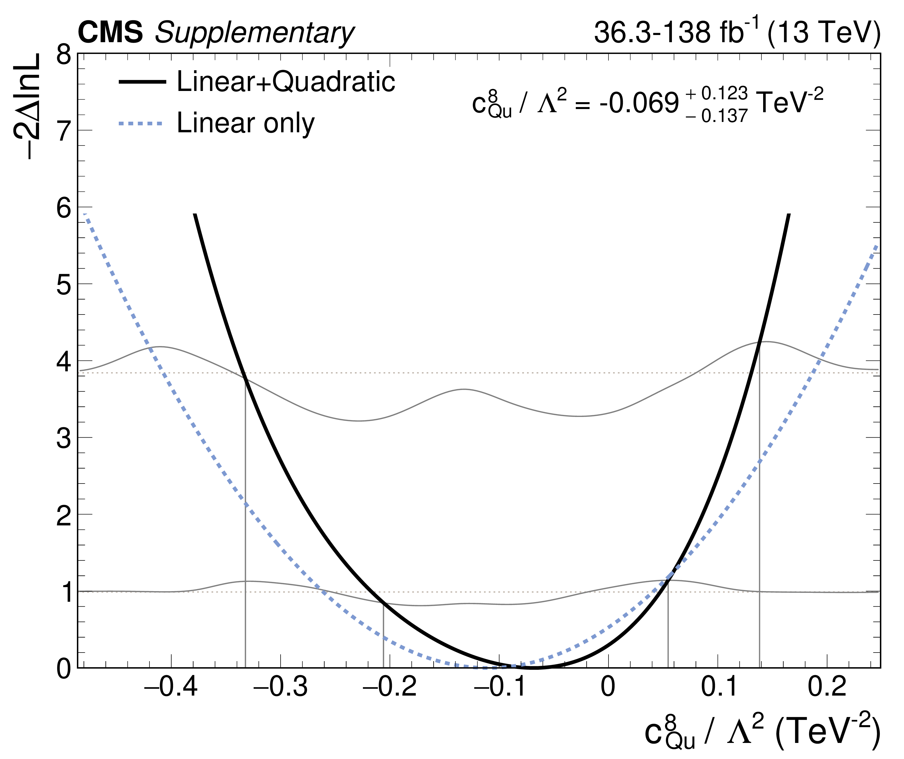
png pdf |
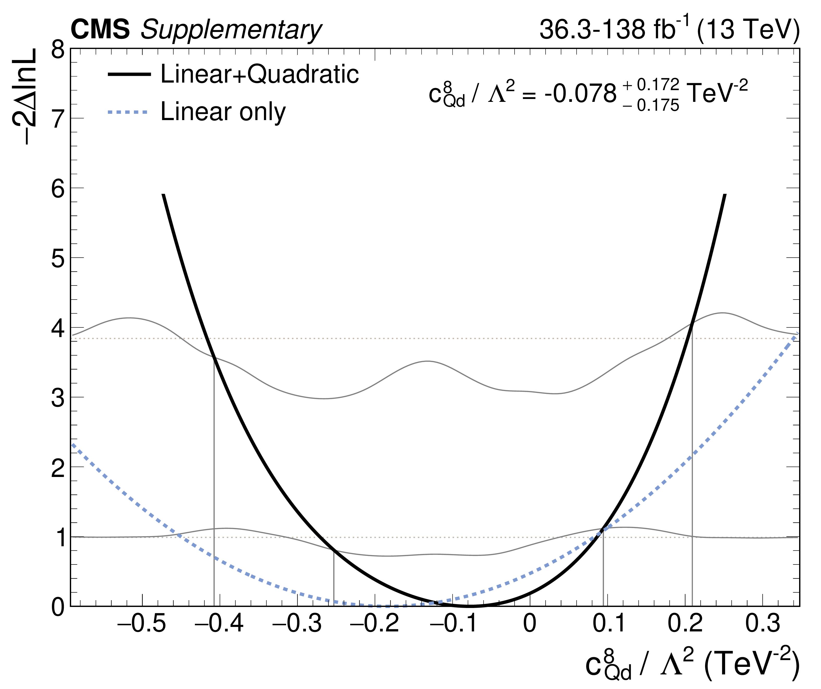
Additional Figure 17-d:
NLL scans of WCs, for the simplified fit without the $ \mathrm{t}(\overline{\mathrm{t}})\mathrm{X} $ analysis. The solid grey lines indicate the sets of points $ q^{68\%} $ (lower line) and $ q^{95\%} $ (upper line), while the dashed grey lines denote the test statistic values used to determine the 68% and 95% confidence intervals in the asymptotic approximation. |

png pdf |
Additional Figure 17-e:
NLL scans of WCs, for the simplified fit without the $ \mathrm{t}(\overline{\mathrm{t}})\mathrm{X} $ analysis. The solid grey lines indicate the sets of points $ q^{68\%} $ (lower line) and $ q^{95\%} $ (upper line), while the dashed grey lines denote the test statistic values used to determine the 68% and 95% confidence intervals in the asymptotic approximation. |
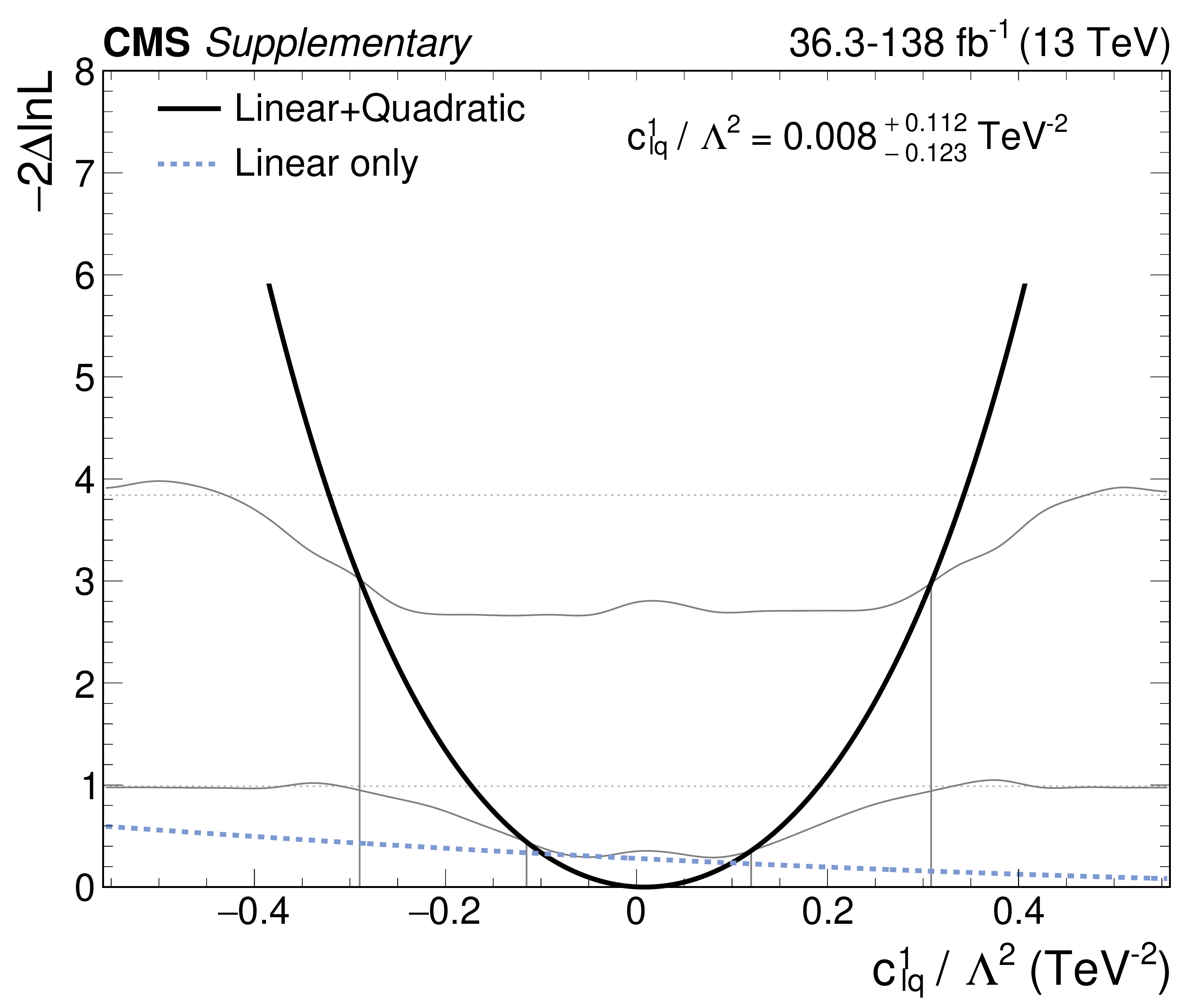
png pdf |
Additional Figure 17-f:
NLL scans of WCs, for the simplified fit without the $ \mathrm{t}(\overline{\mathrm{t}})\mathrm{X} $ analysis. The solid grey lines indicate the sets of points $ q^{68\%} $ (lower line) and $ q^{95\%} $ (upper line), while the dashed grey lines denote the test statistic values used to determine the 68% and 95% confidence intervals in the asymptotic approximation. |
png pdf |
Additional Figure 17-g:
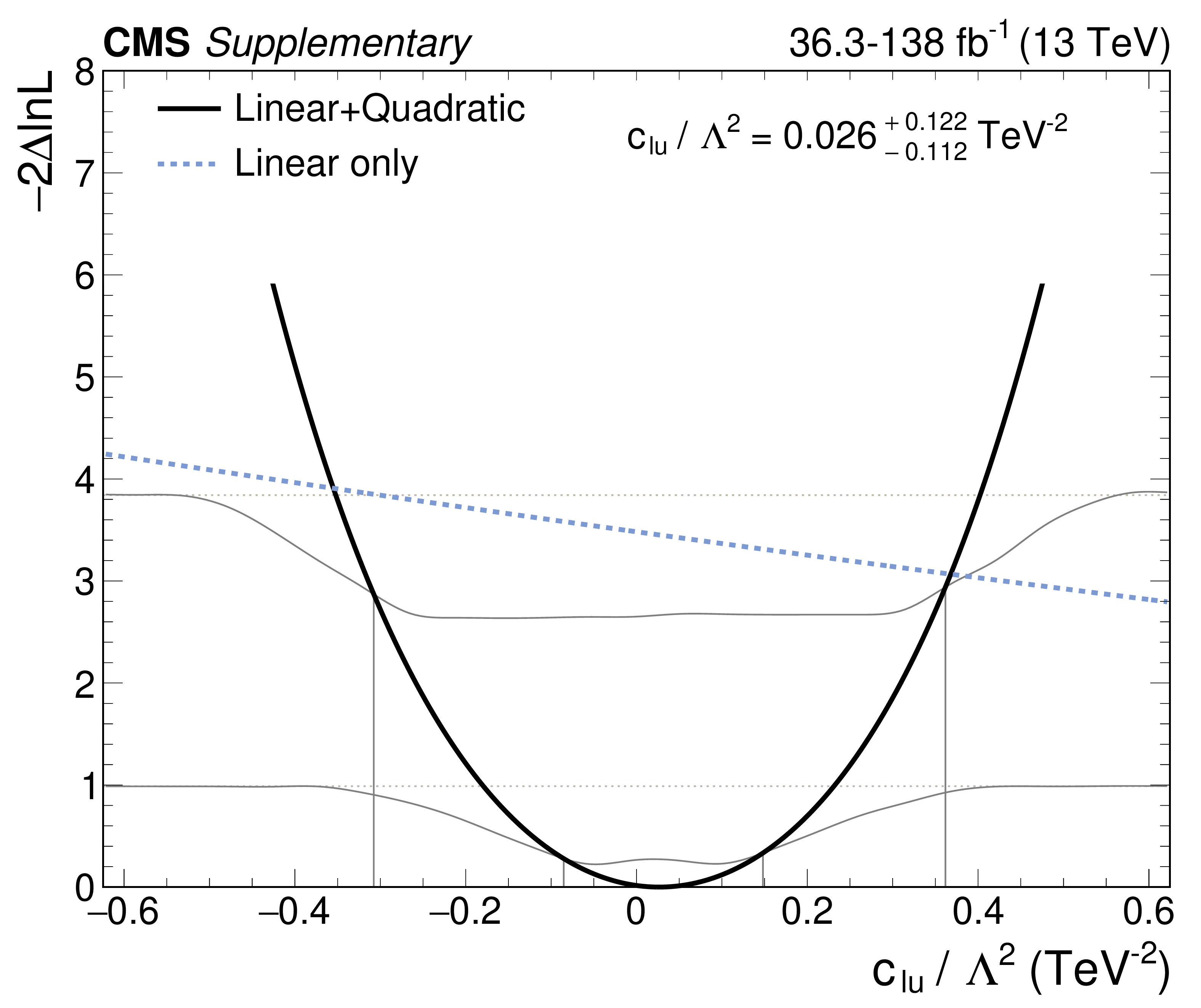
NLL scans of WCs, for the simplified fit without the $ \mathrm{t}(\overline{\mathrm{t}})\mathrm{X} $ analysis. The solid grey lines indicate the sets of points $ q^{68\%} $ (lower line) and $ q^{95\%} $ (upper line), while the dashed grey lines denote the test statistic values used to determine the 68% and 95% confidence intervals in the asymptotic approximation. |
png pdf |
Additional Figure 17-h:
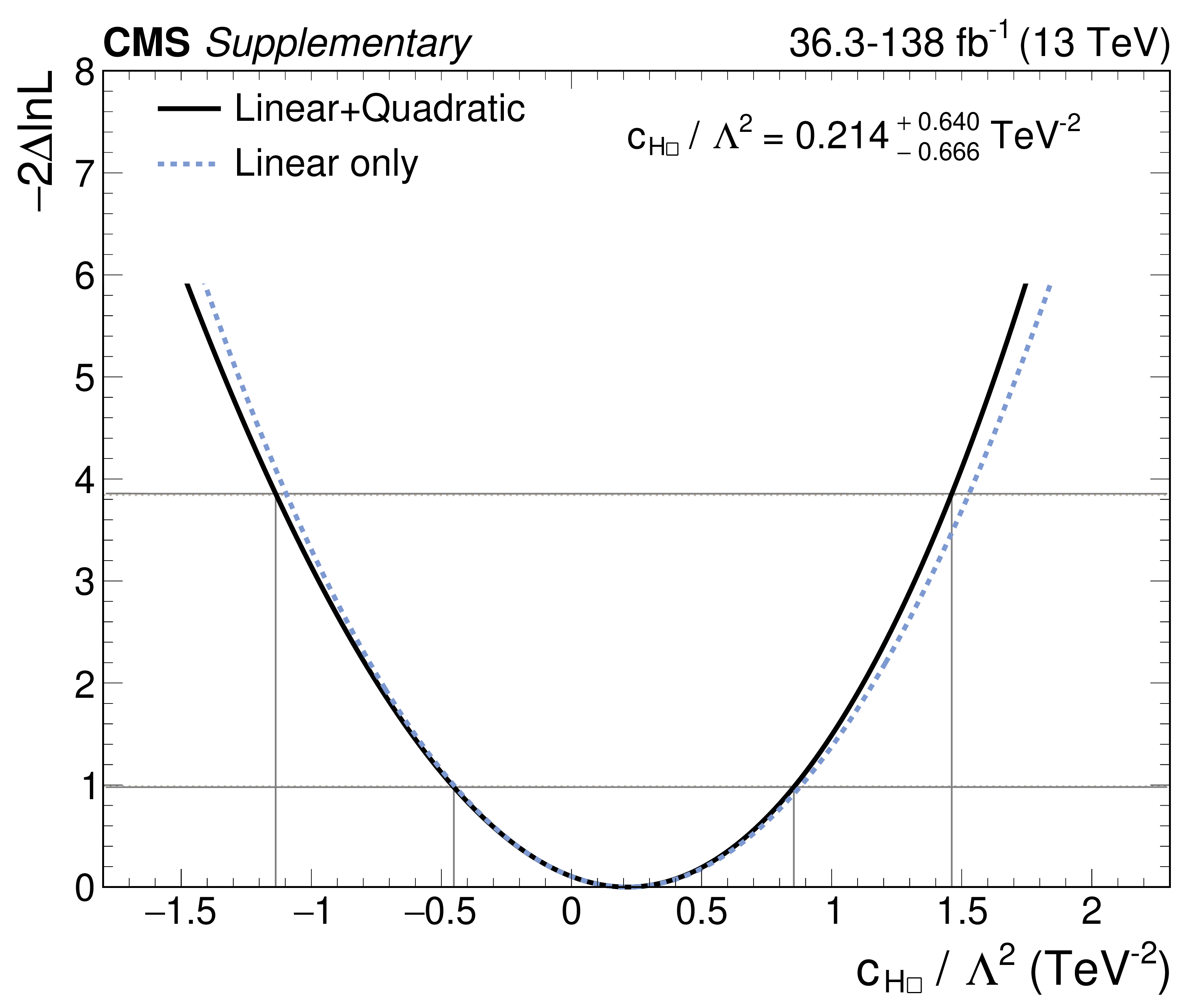
NLL scans of WCs, for the simplified fit without the $ \mathrm{t}(\overline{\mathrm{t}})\mathrm{X} $ analysis. The solid grey lines indicate the sets of points $ q^{68\%} $ (lower line) and $ q^{95\%} $ (upper line), while the dashed grey lines denote the test statistic values used to determine the 68% and 95% confidence intervals in the asymptotic approximation. |
png pdf |
Additional Figure 17-i:
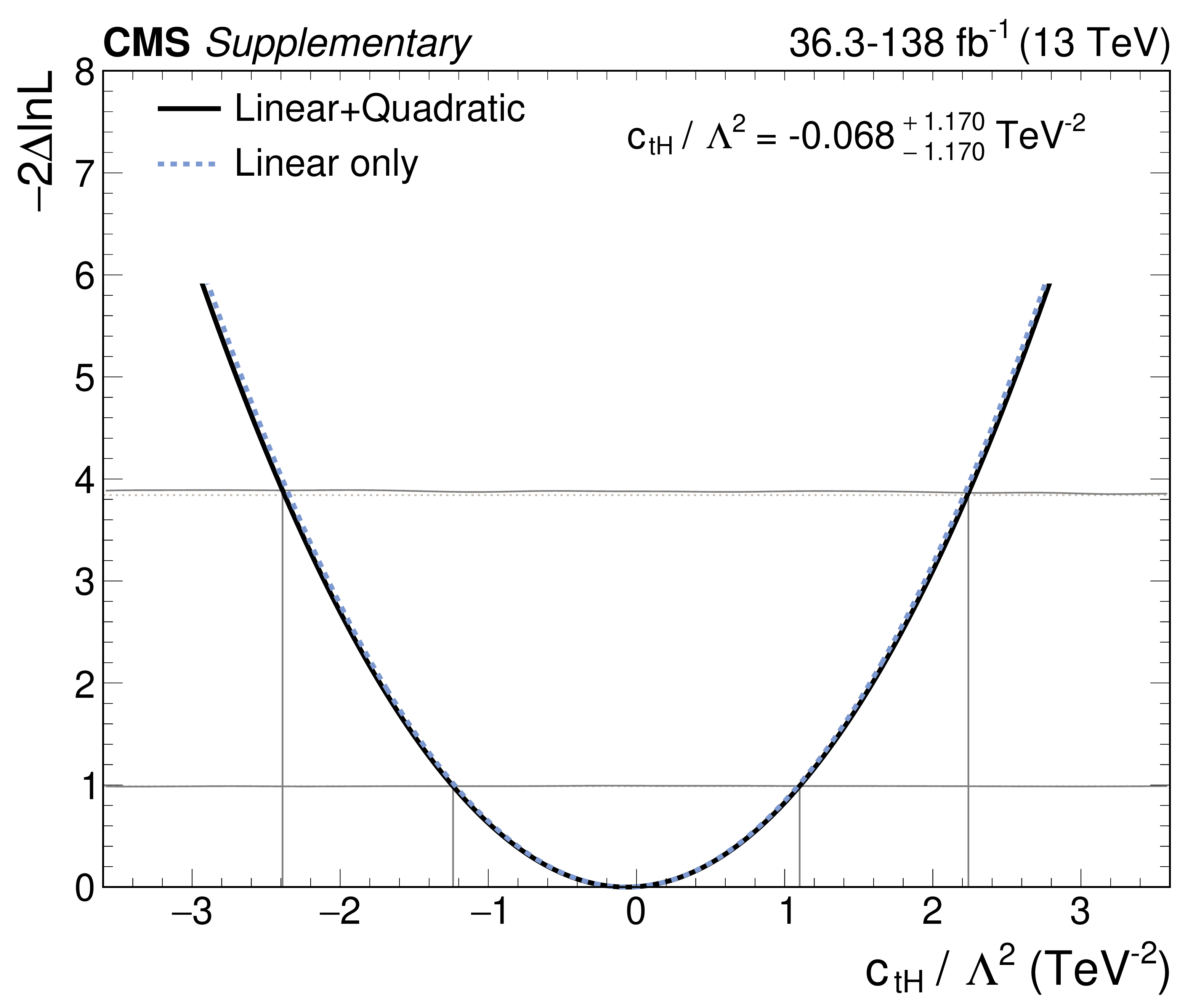
NLL scans of WCs, for the simplified fit without the $ \mathrm{t}(\overline{\mathrm{t}})\mathrm{X} $ analysis. The solid grey lines indicate the sets of points $ q^{68\%} $ (lower line) and $ q^{95\%} $ (upper line), while the dashed grey lines denote the test statistic values used to determine the 68% and 95% confidence intervals in the asymptotic approximation. |
png pdf |
Additional Figure 17-j:
NLL scans of WCs, for the simplified fit without the $ \mathrm{t}(\overline{\mathrm{t}})\mathrm{X} $ analysis. The solid grey lines indicate the sets of points $ q^{68\%} $ (lower line) and $ q^{95\%} $ (upper line), while the dashed grey lines denote the test statistic values used to determine the 68% and 95% confidence intervals in the asymptotic approximation. |
| Additional Tables | |
png pdf |
Additional Table 1:
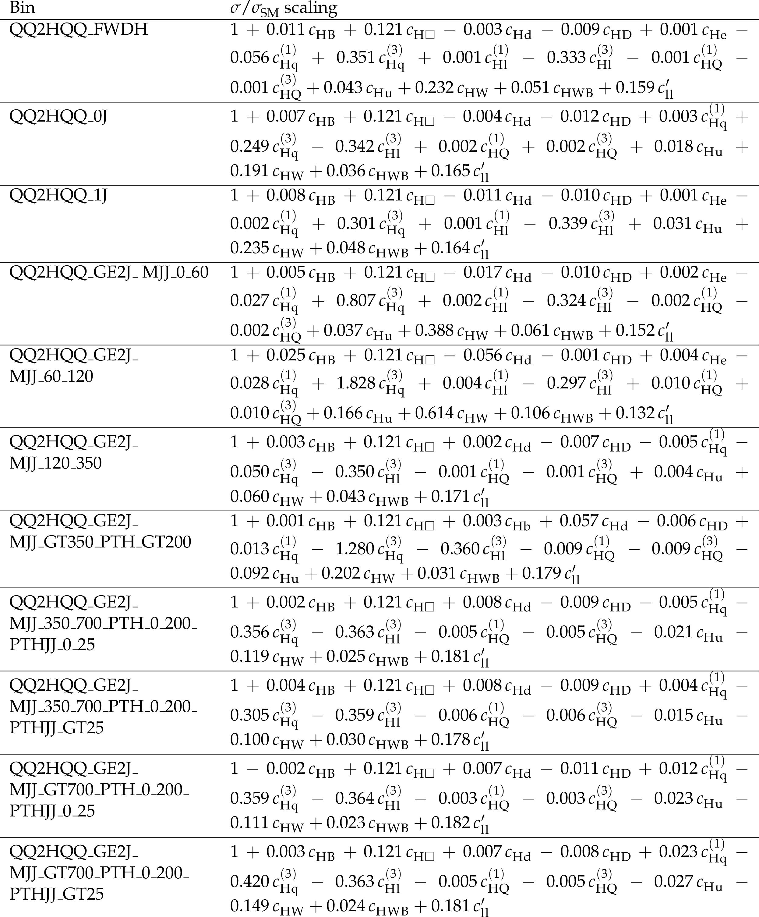
Linear parameterizations for the STXS $ \mathrm{q}\mathrm{q}\mathrm{H} $ bins. |

png pdf |
Additional Table 2:
Linear parameterizations for the STXS $ \mathrm{g}\mathrm{g}\mathrm{H} $ bins. |

png pdf |
Additional Table 3:
Linear parameterizations for the STXS VH leptonic bins (1 lepton). |

png pdf |
Additional Table 4:
Linear parameterizations for the STXS VH leptonic bins (2 leptons). |

png pdf |
Additional Table 5:
Linear parameterizations for the STXS $ \mathrm{t}\overline{\mathrm{t}}\mathrm{H} $ bins |
png pdf |
Additional Table 6:
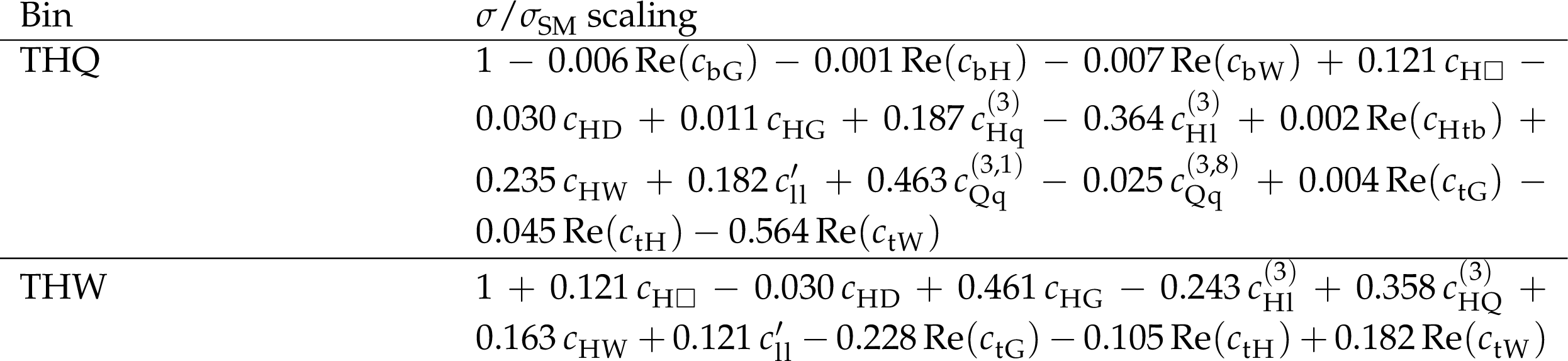
Linear parameterizations for the STXS $ \mathrm{t}\mathrm{H} $ bins |

png pdf |
Additional Table 7:
Linear parameterizations for the H decay modes. |
png pdf |
Additional Table 8:
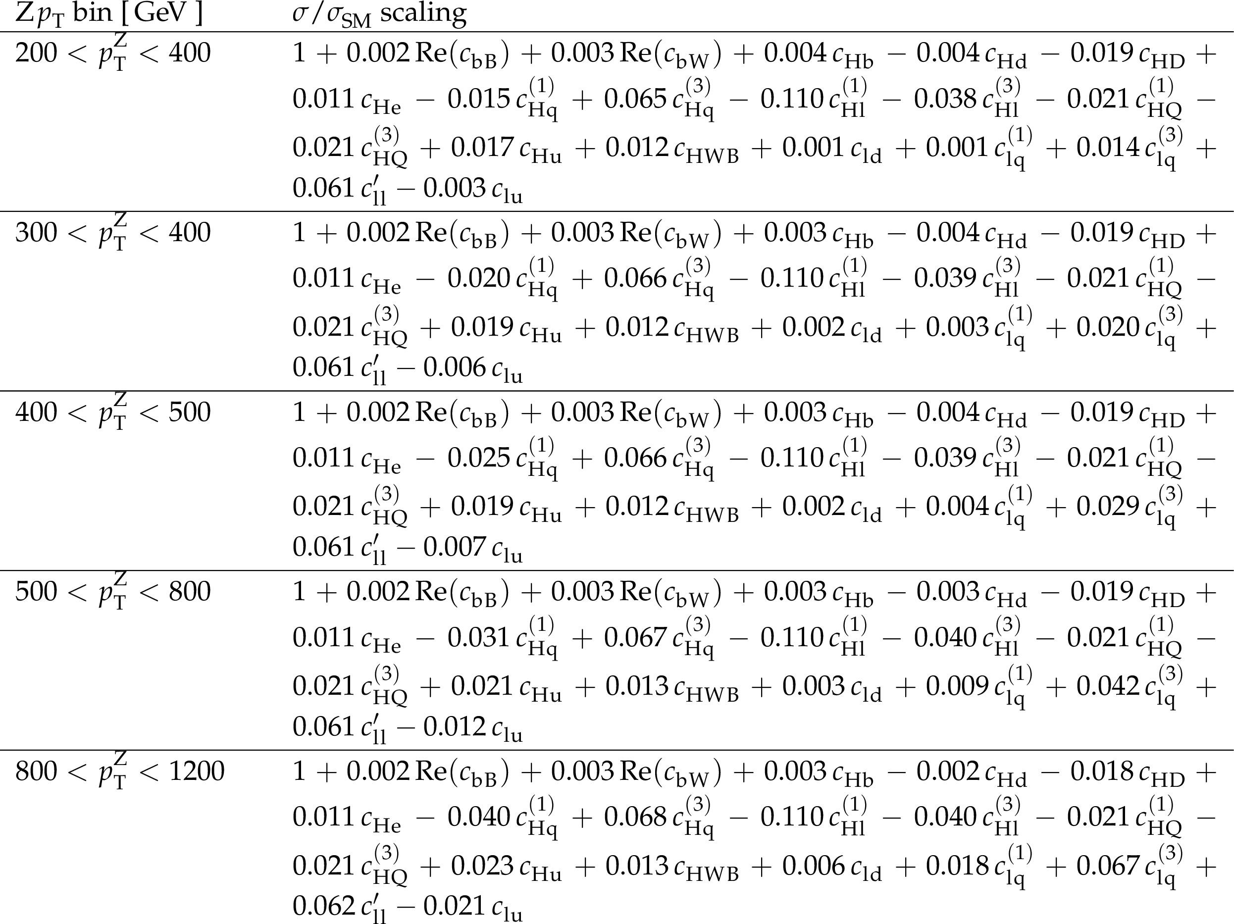
Linear parameterizations for the $ \mathrm{Z}\to\nu\nu $ analysis. |

png pdf |
Additional Table 9:
Linear parameterizations for the WW analysis. |
png pdf |
Additional Table 10:
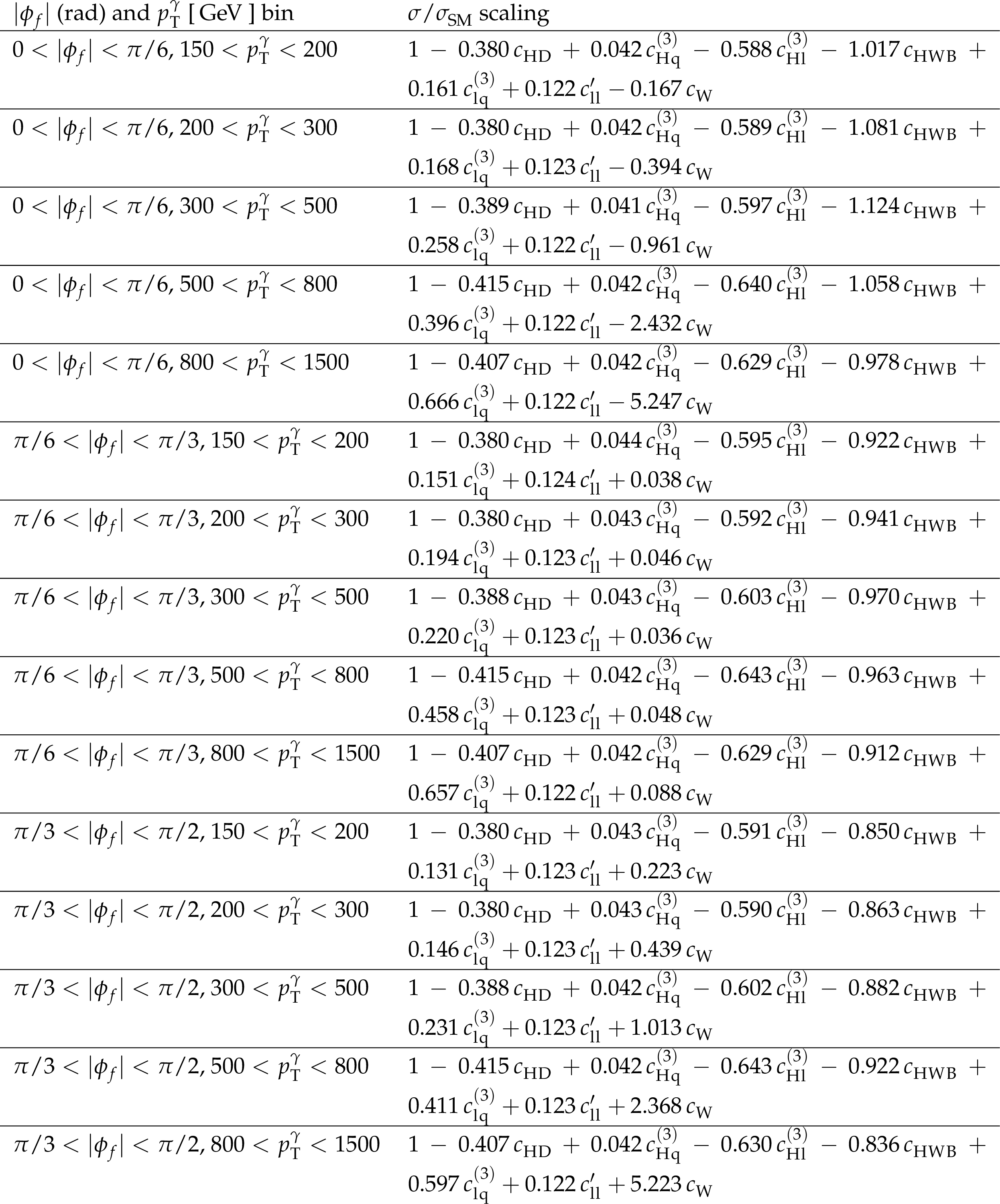
Linear parameterizations for the $ \mathrm{W}\gamma $ analysis. |
png pdf |
Additional Table 11:
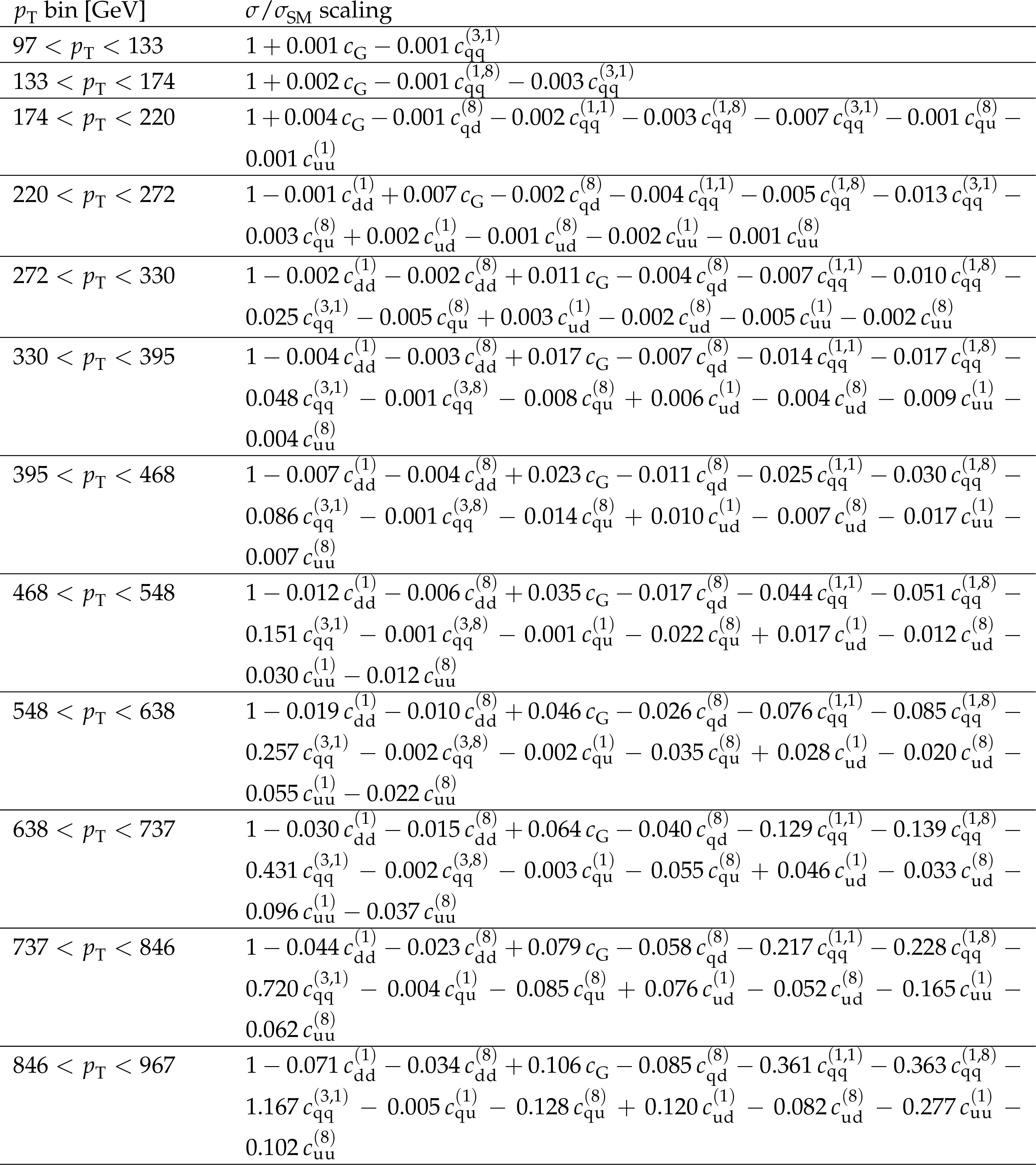
Linear parameterizations for the inclusive jet measurement, for the bins with $ |y| < $ 0.5 and $ p_{\mathrm{T}} < $ 967 GeV. |

png pdf |
Additional Table 12:
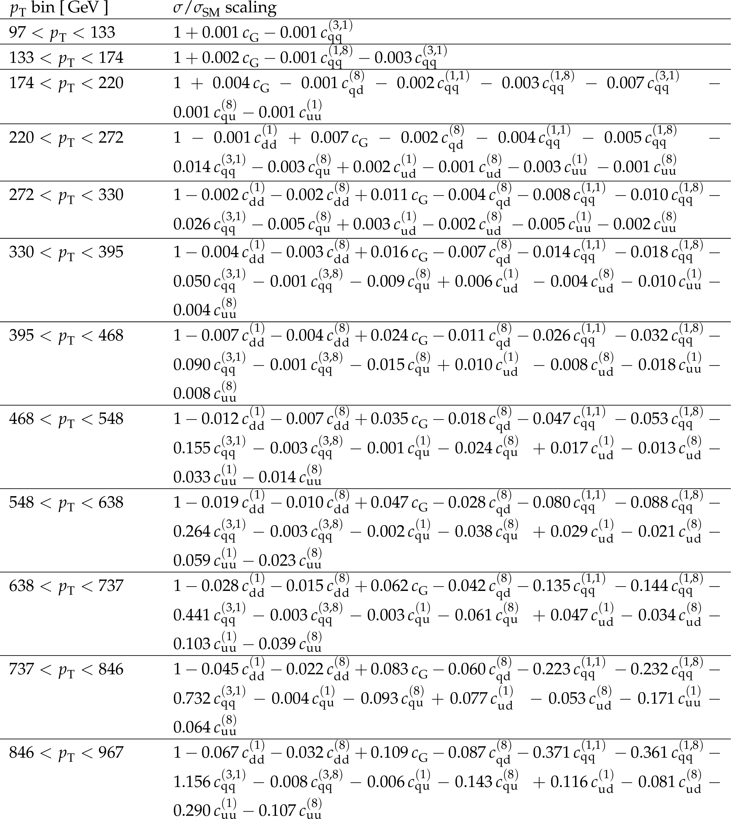
Linear parameterizations for the inclusive jet measurement, for the bins with $ |y| < $ 0.5 and $ p_{\mathrm{T}} > $ 967 GeV. |
png pdf |
Additional Table 13:
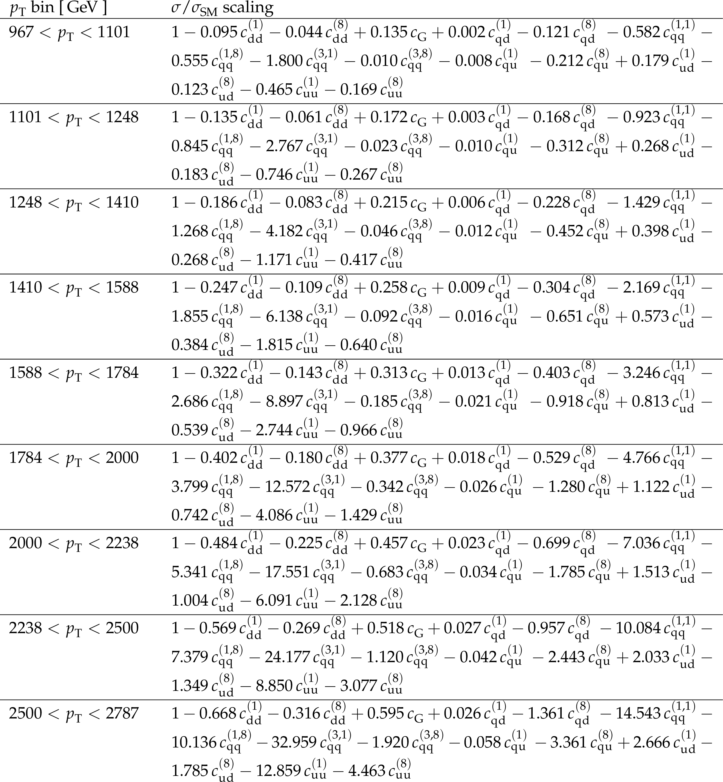
Linear parameterizations for the inclusive jet measurement, for the bins with $ < 0.5 < |y| < $ 1.0 and $ p_{\mathrm{T}} < $ 967 GeV. |
png pdf |
Additional Table 14:
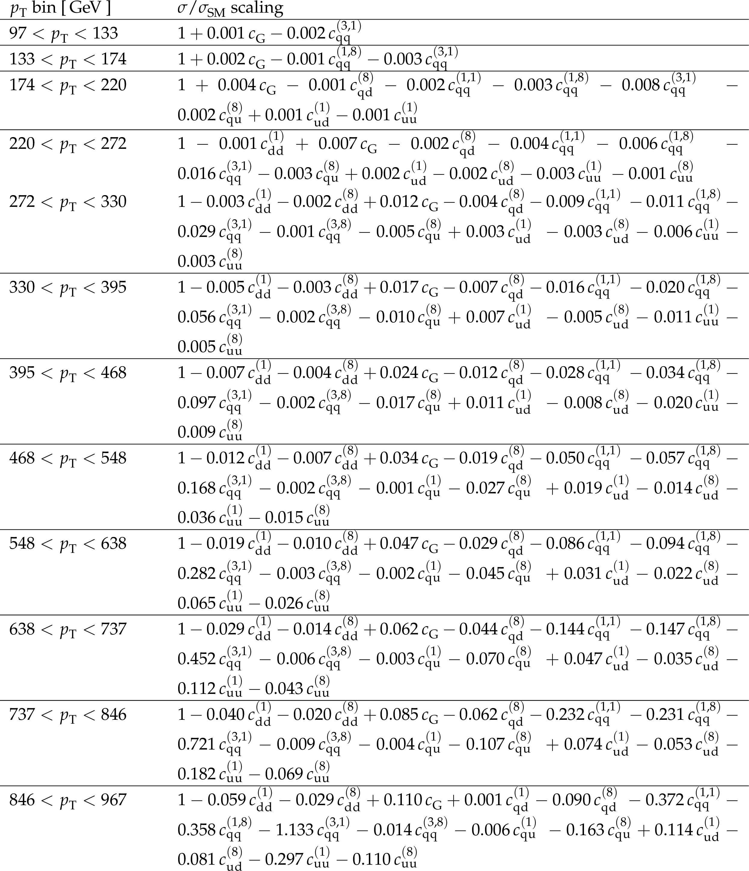
Linear parameterizations for the inclusive jet measurement, for the bins with $ < 0.5 < |y| < $ 1.0 and $ p_{\mathrm{T}} > $ 967 GeV. |
png pdf |
Additional Table 15:
Linear parameterizations for the inclusive jet measurement, for the bins with $ < 1.0 < |y| < $ 1.5 and $ p_{\mathrm{T}} < $ 967 GeV. |
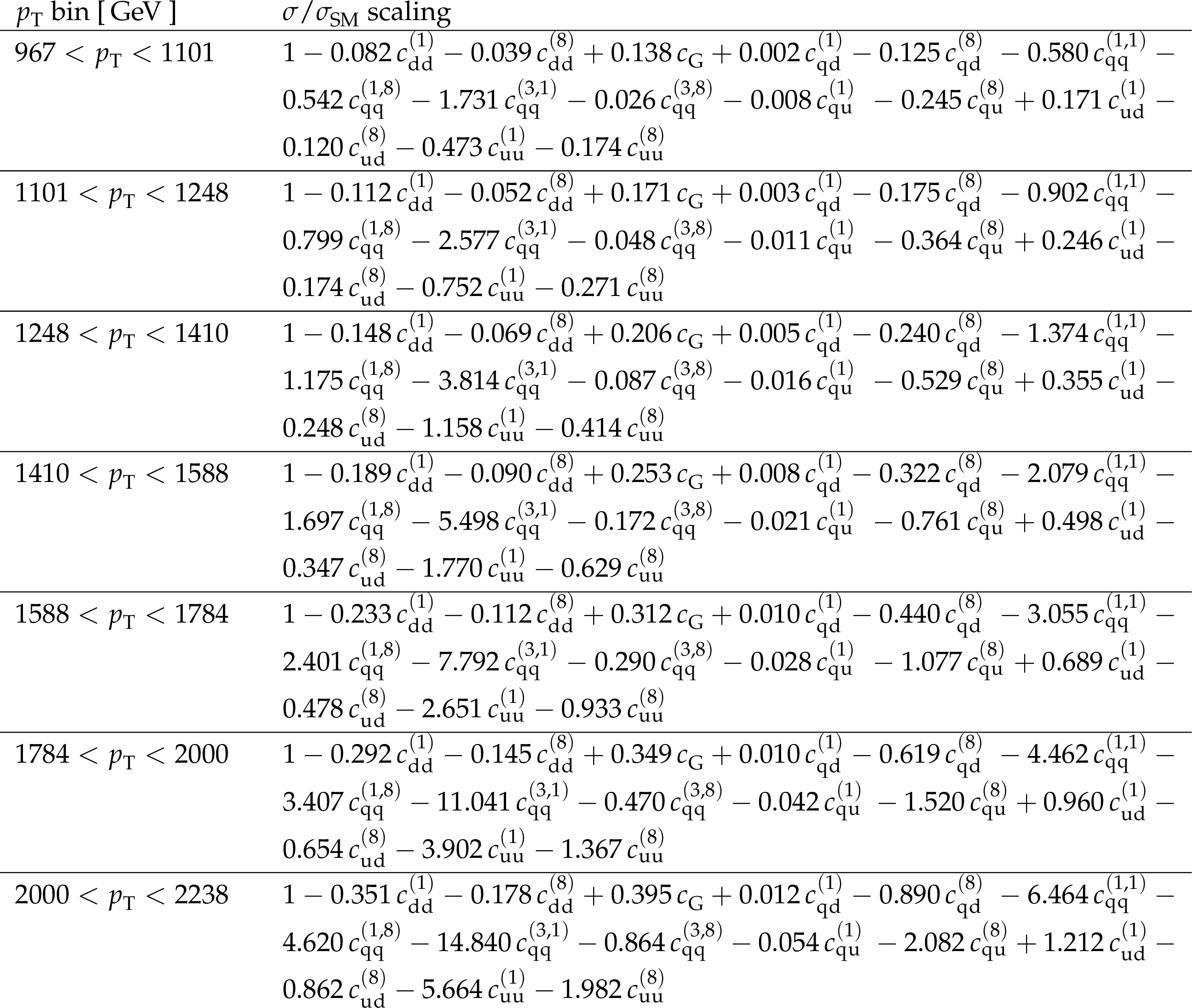
png pdf |
Additional Table 16:
Linear parameterizations for the inclusive jet measurement, for bins with $ < 1.0 < |y| < $ 1.5 and $ p_{\mathrm{T}} > $ 967 GeV. |

png pdf |
Additional Table 17:
Linear parameterizations for the inclusive jet measurement, for bins with $ < 1.5 < |y| < $ 2.0 and $ p_{\mathrm{T}} < $ 967 GeV. |
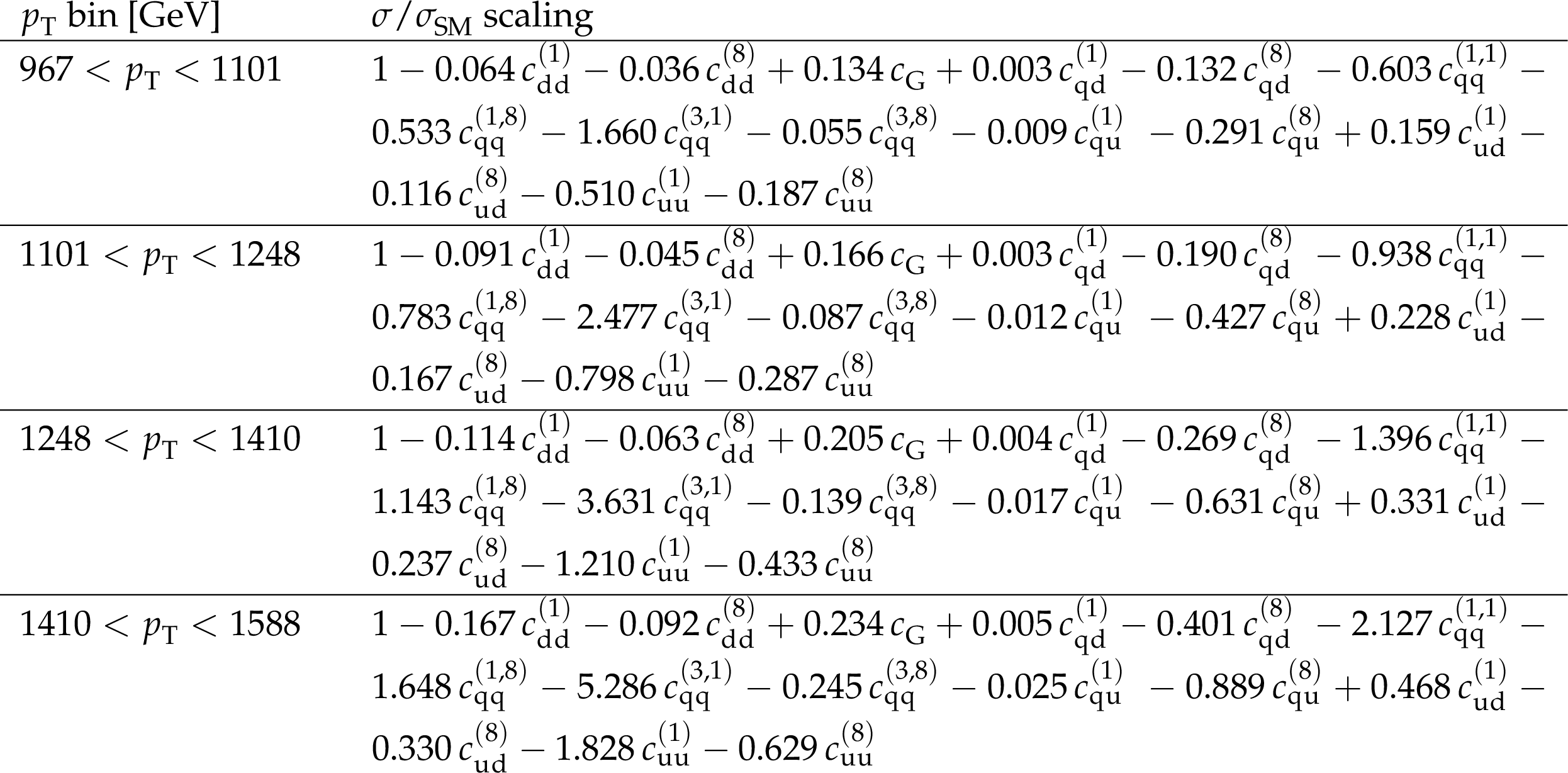
png pdf |
Additional Table 18:
Linear parameterizations for the inclusive jet measurement, for bins with $ < 1.5|y| < $ 2.0 and $ p_{\mathrm{T}} > $ 967 GeV. |
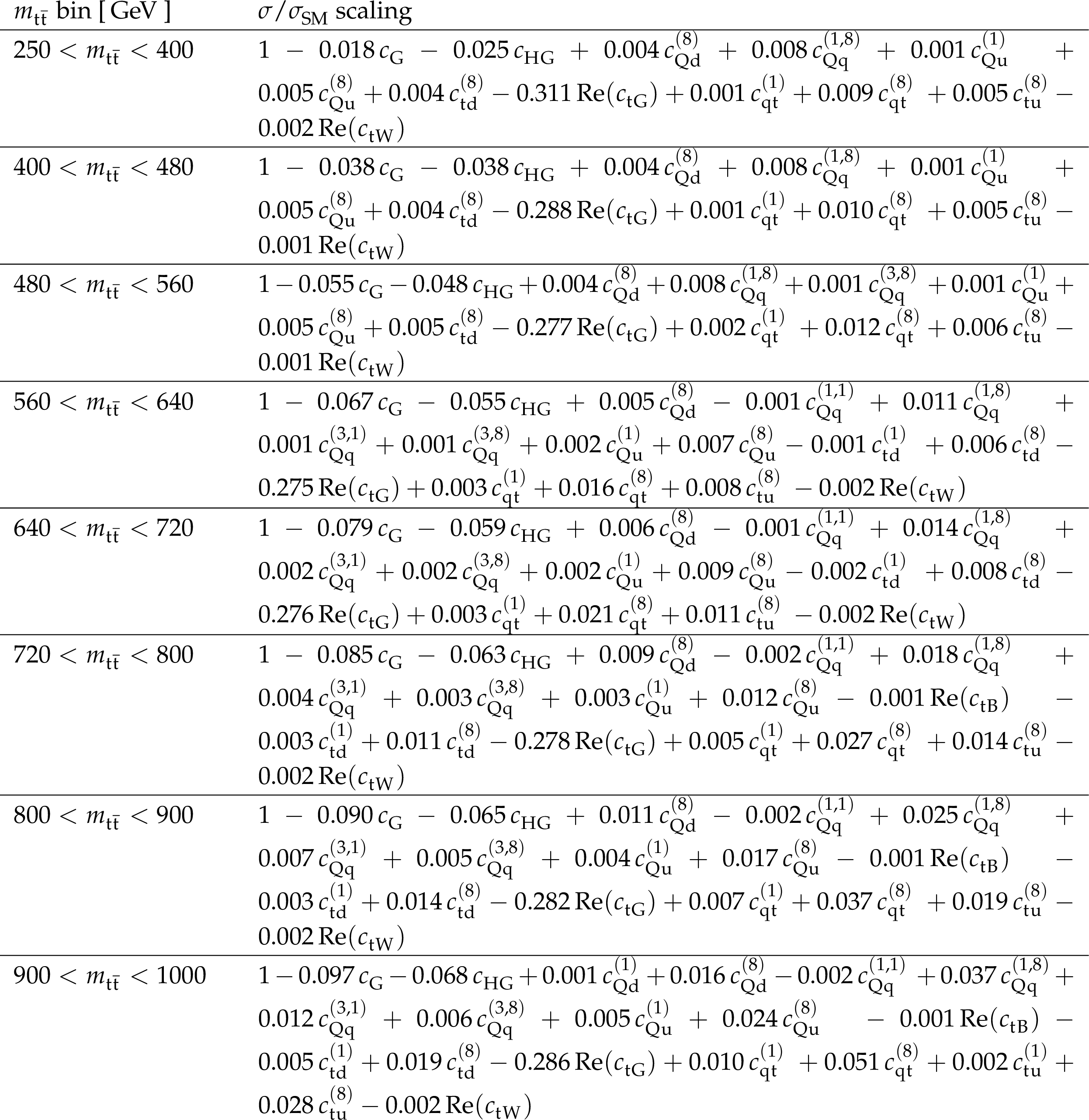
png pdf |
Additional Table 19:
Linear parameterizations for the $ \mathrm{t}\overline{\mathrm{t}} $ measurement, for bins with $ m_{\mathrm{t}\overline{\mathrm{t}}} < $ 1000 GeV. |
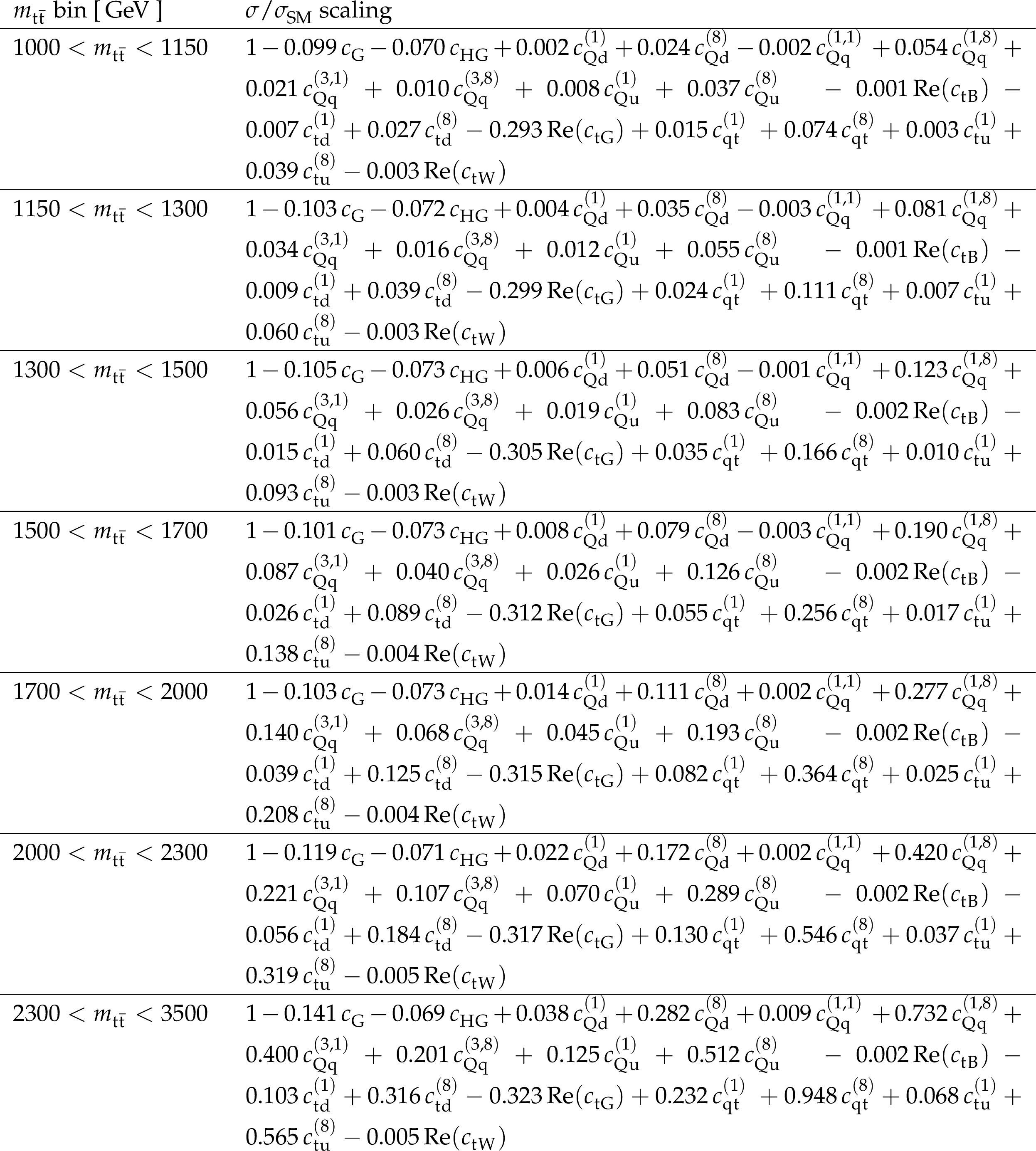
png pdf |
Additional Table 20:
Linear parameterizations for the $ \mathrm{t}\overline{\mathrm{t}} $ measurement, for bins with $ m_{\mathrm{t}\overline{\mathrm{t}}} > $ 1000 GeV. |
png pdf |
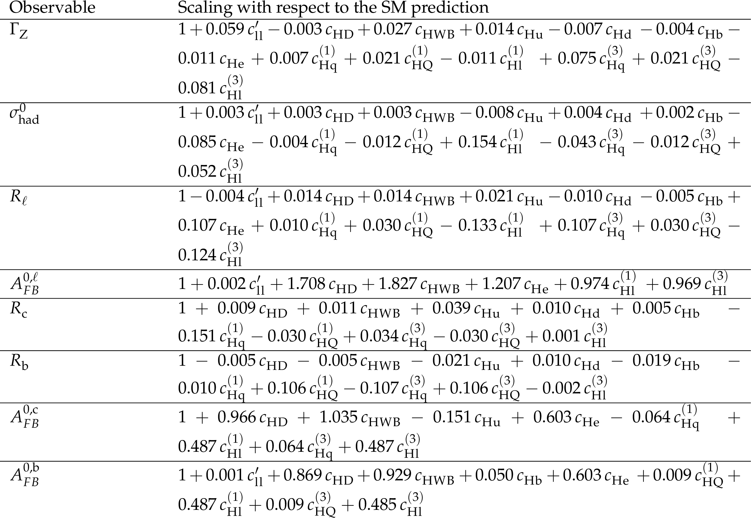
Additional Table 21:
Linear parameterizations for the electroweak precision observables. |
png pdf |
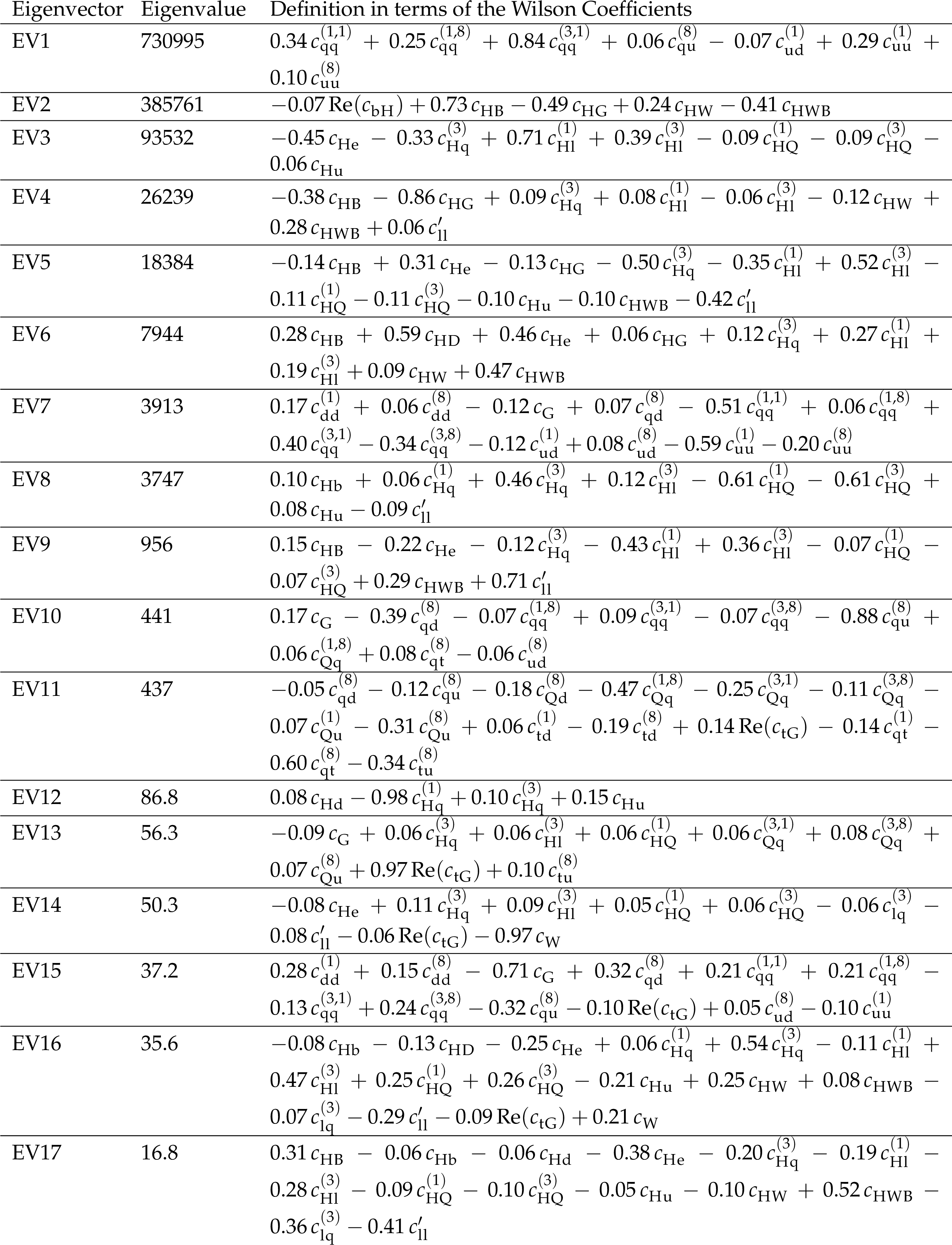
Additional Table 22:
Definitions of eigenvectors and their eigenvalues in the measurement including the $ \mathrm{t}(\overline{\mathrm{t}})\mathrm{X} $ analysis. Definitions of EV1-17. |

png pdf |
Additional Table 23:
Definitions of eigenvectors and their eigenvalues in the measurement including the $ \mathrm{t}(\overline{\mathrm{t}})\mathrm{X} $ analysis. Definitions of EV18-31. |

png pdf |
Additional Table 24:
Definitions of eigenvectors and their eigenvalues in the measurement including the $ \mathrm{t}(\overline{\mathrm{t}})\mathrm{X} $ analysis. Definitions of EV32-42. |
png pdf |
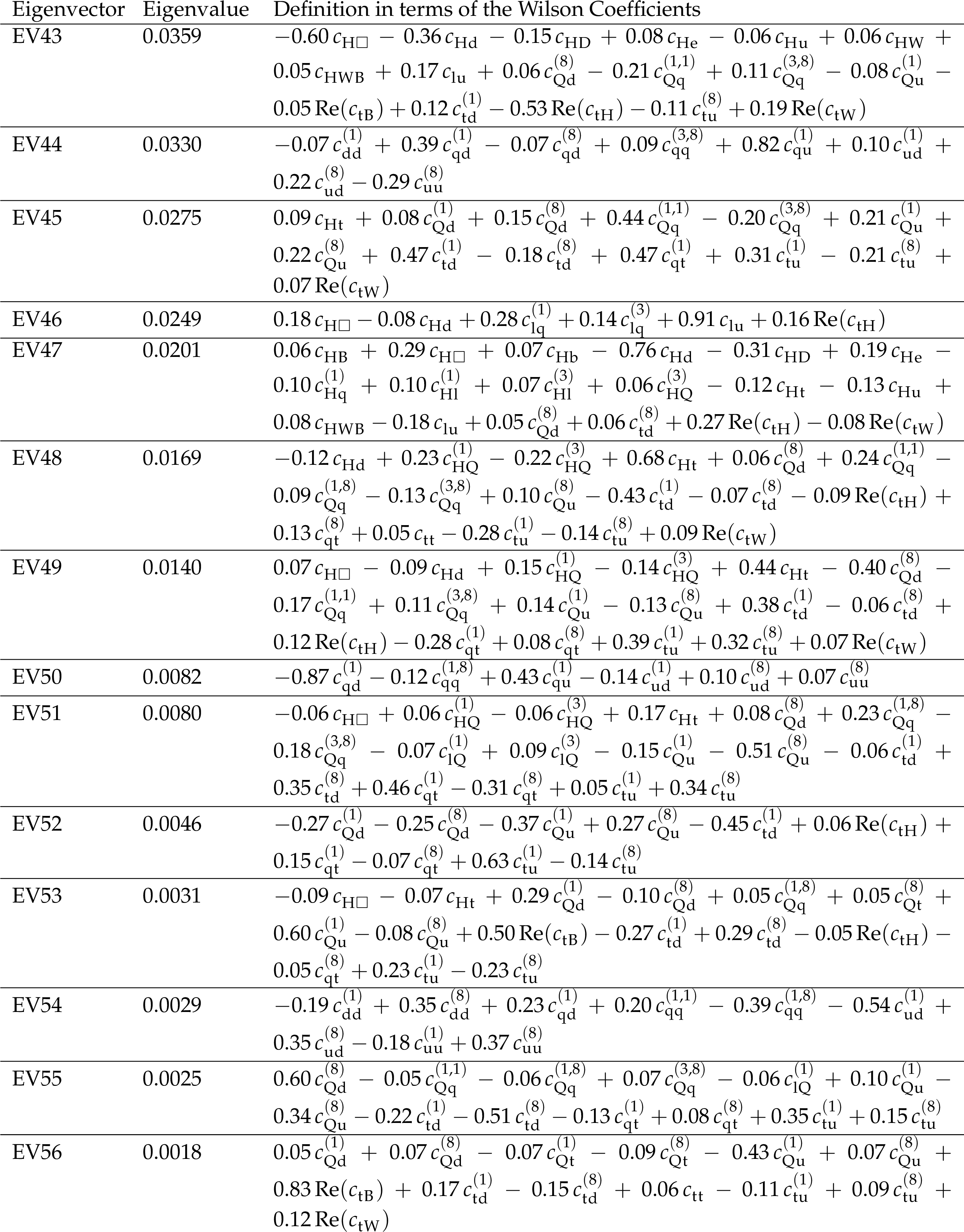
Additional Table 25:
Definitions of eigenvectors and their eigenvalues in the measurement including the $ \mathrm{t}(\overline{\mathrm{t}})\mathrm{X} $ analysis. Definitions of EV43-56. |
png pdf |
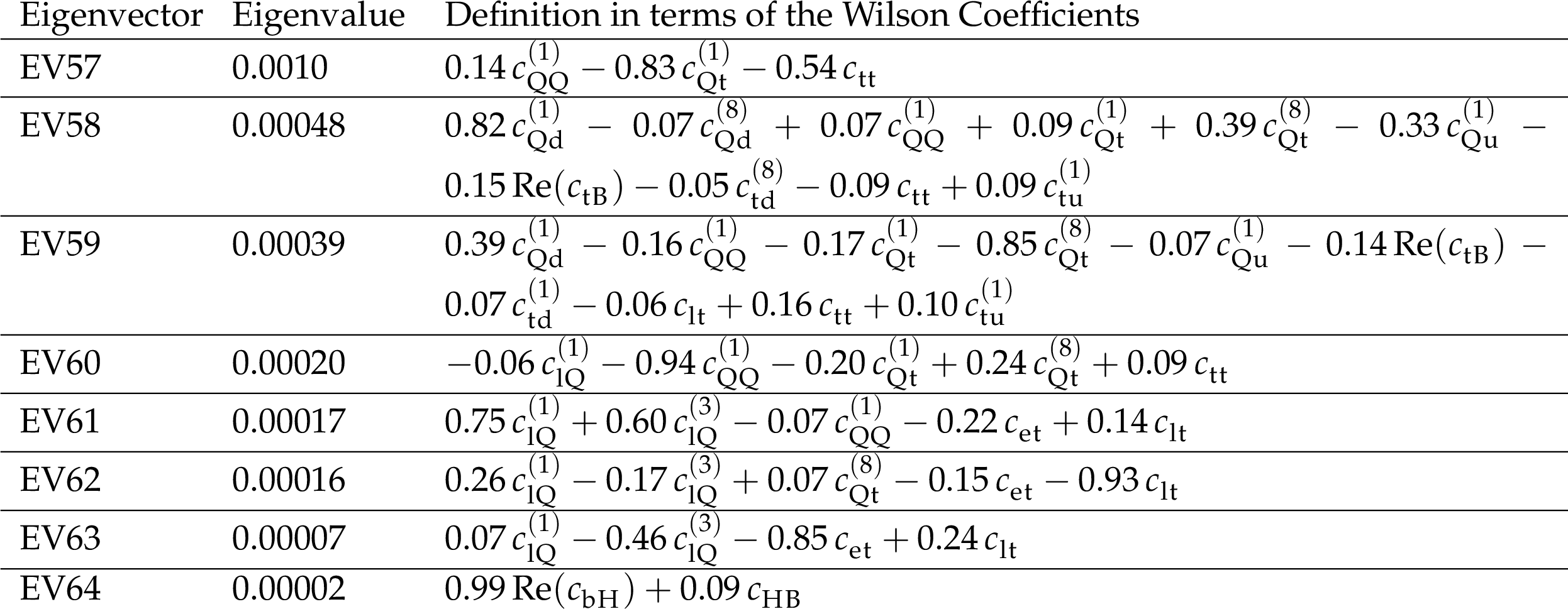
Additional Table 26:
Definitions of eigenvectors and their eigenvalues in the measurement including the $ \mathrm{t}(\overline{\mathrm{t}})\mathrm{X} $ analysis. Definitions of EV57-64. |
png pdf |
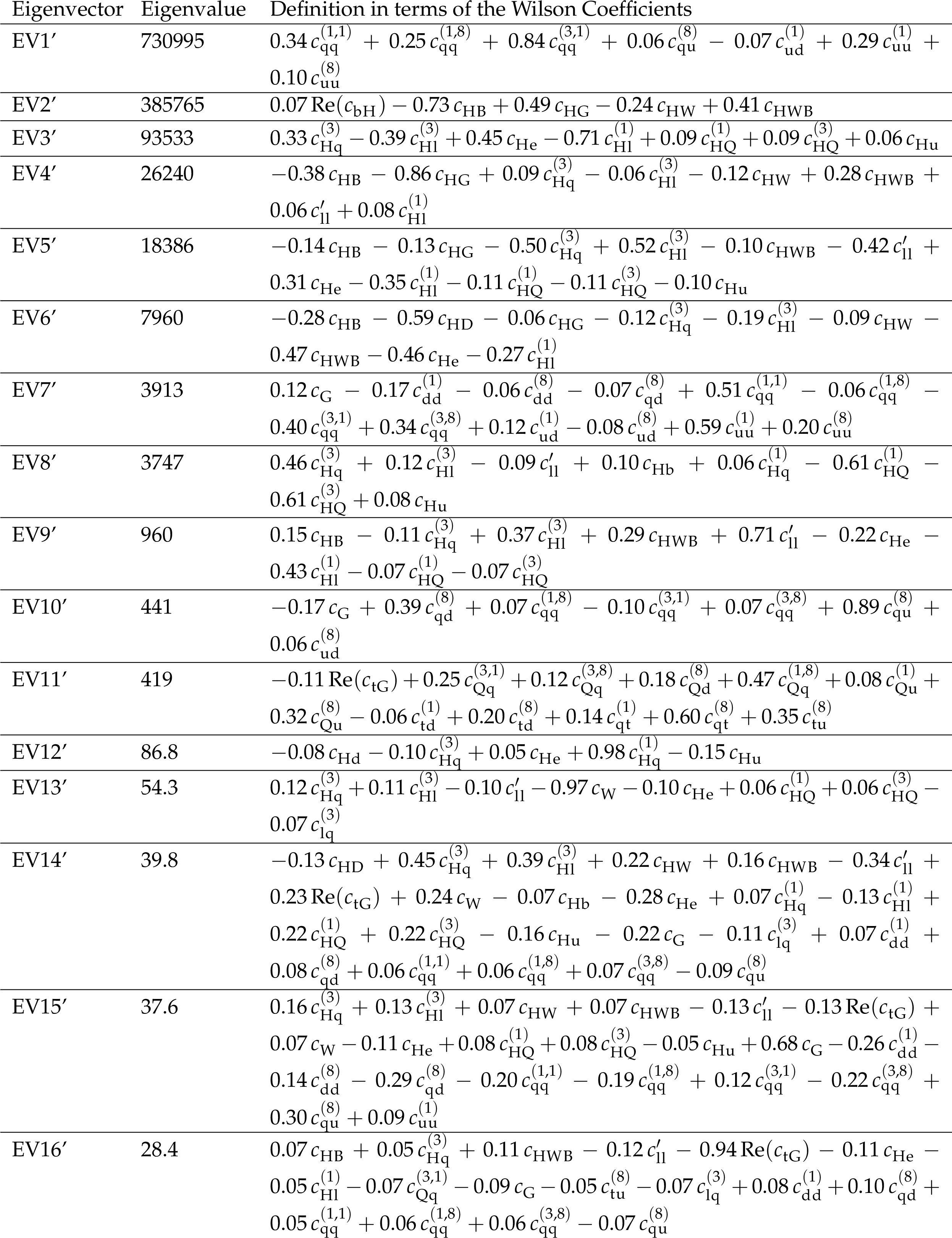
Additional Table 27:
Definitions of eigenvectors and their eigenvalues in the measurement with the $ \mathrm{t}(\overline{\mathrm{t}})\mathrm{X} $ analysis excluded. The eigenvectors are labelled $ \mathrm{EV}n' $ to distinguish them from the eigenvectors in the combination that does include the $ \mathrm{t}(\overline{\mathrm{t}})\mathrm{X} $ inputs. Definitions of EV1'-EV16'. |
png pdf |
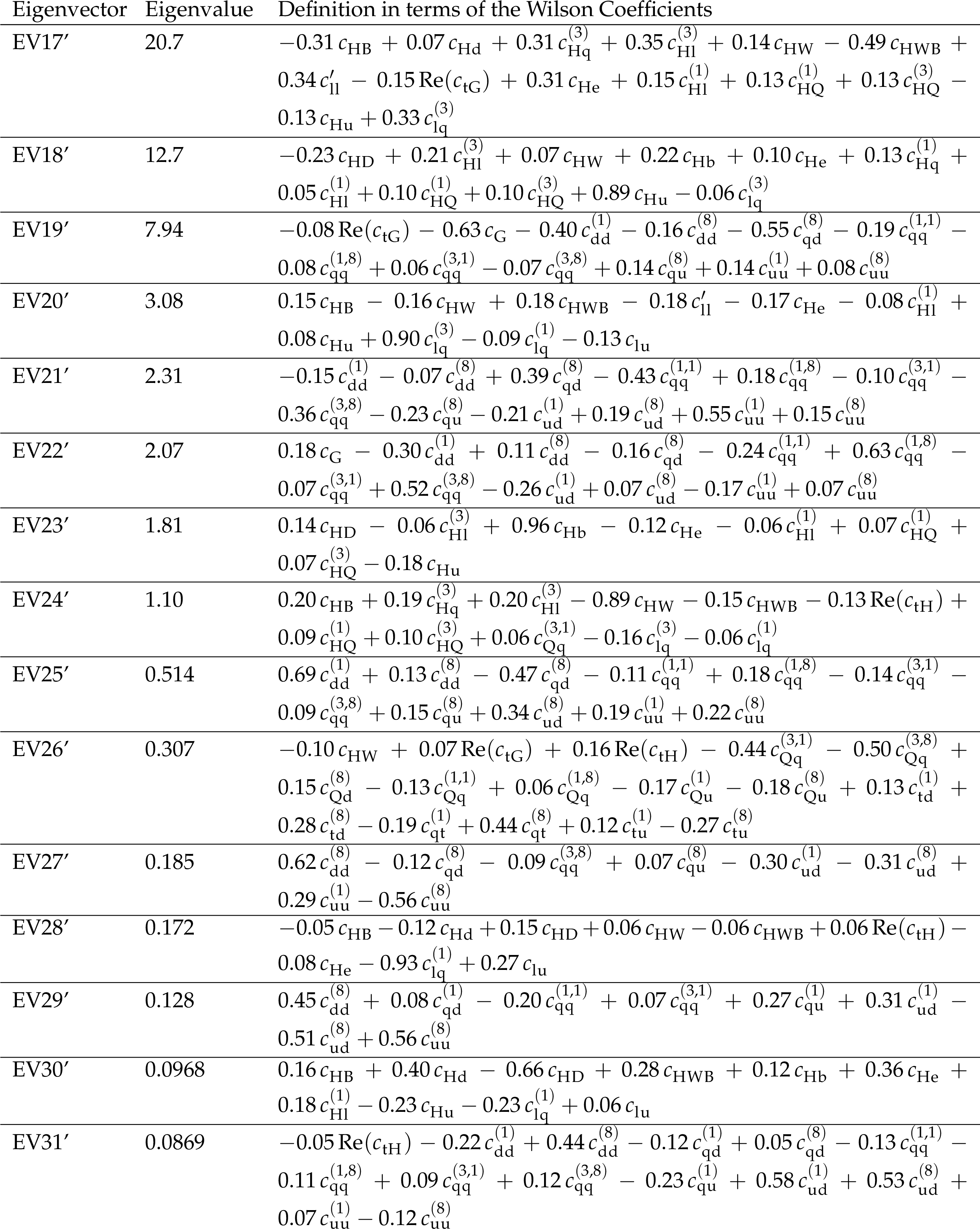
Additional Table 28:
Definitions of eigenvectors and their eigenvalues in the measurement with the $ \mathrm{t}(\overline{\mathrm{t}})\mathrm{X} $ analysis excluded. The eigenvectors are labelled $ \mathrm{EV}n' $ to distinguish them from the eigenvectors in the combination that does include the $ \mathrm{t}(\overline{\mathrm{t}})\mathrm{X} $ inputs. Definitions of EV17'-EV31'. |

png pdf |
Additional Table 29:
Definitions of eigenvectors and their eigenvalues in the measurement with the $ \mathrm{t}(\overline{\mathrm{t}})\mathrm{X} $ analysis excluded. The eigenvectors are labelled $ \mathrm{EV}n' $ to distinguish them from the eigenvectors in the combination that does include the $ \mathrm{t}(\overline{\mathrm{t}})\mathrm{X} $ inputs. Definitions of EV32'-EV42'. |
png pdf |
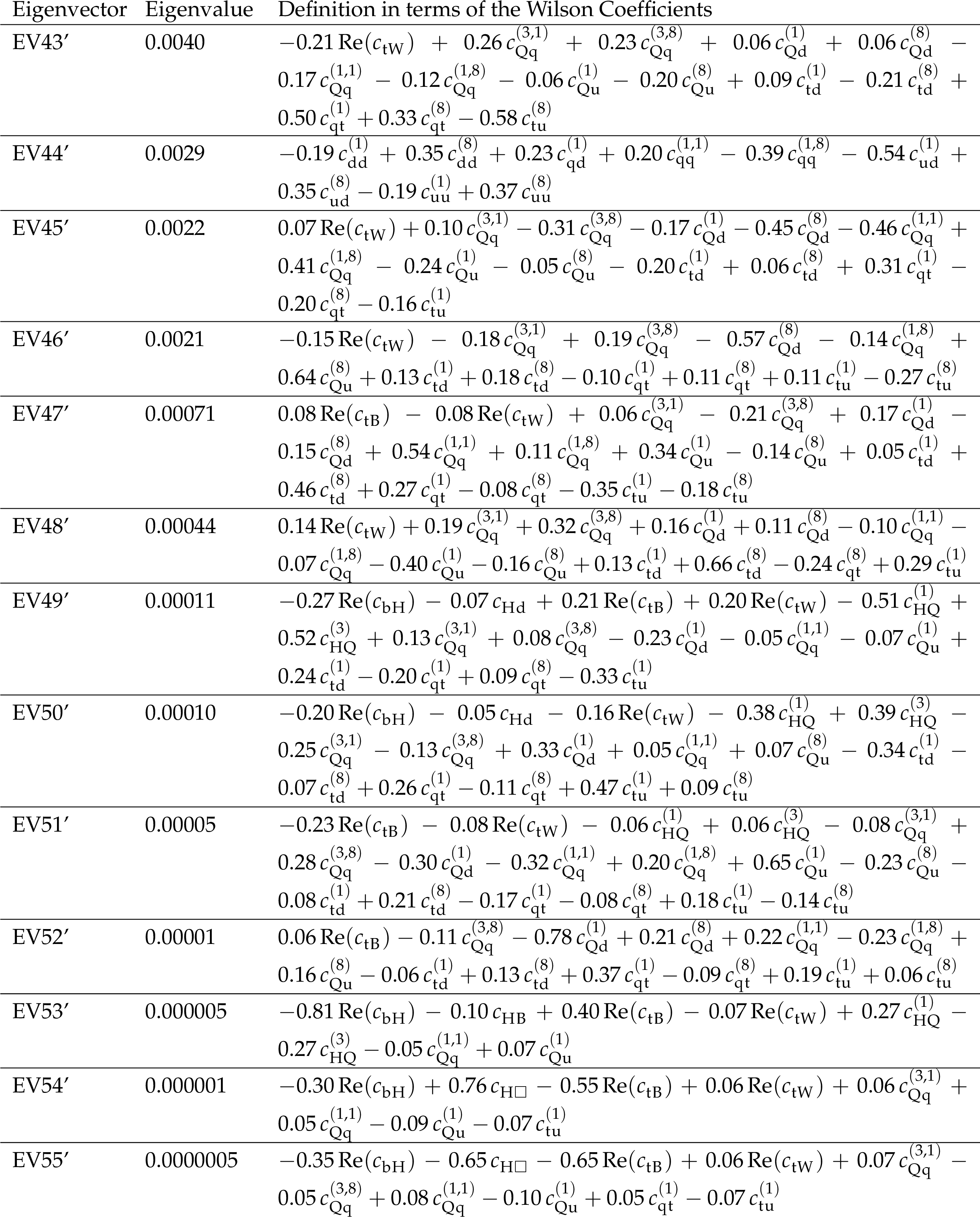
Additional Table 30:
Definitions of eigenvectors and their eigenvalues in the measurement with the $ \mathrm{t}(\overline{\mathrm{t}})\mathrm{X} $ analysis excluded. The eigenvectors are labelled $ \mathrm{EV}n' $ to distinguish them from the eigenvectors in the combination that does include the $ \mathrm{t}(\overline{\mathrm{t}})\mathrm{X} $ inputs. Definitions of EV43'-EV55'. |
| References | ||||
| 1 | ATLAS Collaboration | Observation of a new particle in the search for the standard model Higgs boson with the ATLAS detector at the LHC | PLB 716 (2012) 1 | 1207.7214 |
| 2 | CMS Collaboration | Observation of a new boson at a mass of 125 GeV with the CMS experiment at the LHC | PLB 716 (2012) 30 | CMS-HIG-12-028 1207.7235 |
| 3 | CMS Collaboration | Observation of a new boson with mass near 125 GeV in pp collisions at $ \sqrt{s} = $ 7 and 8 TeV | JHEP 06 (2013) 081 | CMS-HIG-12-036 1303.4571 |
| 4 | CMS Collaboration | Searches for Higgs boson production through decays of heavy resonances | Phys. Rep. 1115 (2025) 368 | 2403.16926 |
| 5 | ATLAS Collaboration | The quest to discover supersymmetry at the ATLAS experiment | Phys. Rep. 1116 (2025) 261 | 2403.02455 |
| 6 | ATLAS Collaboration | Exploration at the high-energy frontier: ATLAS Run 2 searches investigating the exotic jungle beyond the standard model | Phys. Rep. 1116 (2025) 301 | 2403.09292 |
| 7 | I. Brivio and M. Trott | The standard model as an effective field theory | Phys. Rep. 793 (2019) 1 | 1706.08945 |
| 8 | B. Grzadkowski, M. Iskrzy \'n ski, M. Misiak, and J. Rosiek | Dimension-six terms in the standard model Lagrangian | JHEP 10 (2010) 085 | 1008.4884 |
| 9 | I. Brivio, Y. Jiang, and M. Trott | The SMEFTsim package, theory and tools | JHEP 12 (2017) 070 | 1709.06492 |
| 10 | I. Brivio | SMEFTsim 3.0 \textemdash a practical guide | JHEP 04 (2021) 073 | 2012.11343 |
| 11 | CMS Collaboration | Constraints on anomalous Higgs boson couplings to vector bosons and fermions from the production of Higgs bosons using the $ \tau\tau $ final state | PRD 108 (2023) 032013 | CMS-HIG-20-007 2205.05120 |
| 12 | ATLAS Collaboration | Measurements of WH and ZH production in the $ \mathrm{H} \rightarrow \mathrm{b}\overline{\mathrm{b}} $ decay channel in pp collisions at 13 TeV with the ATLAS detector | EPJC 81 (2021) 178 | 2007.02873 |
| 13 | ATLAS Collaboration | Higgs boson production cross-section measurements and their EFT interpretation in the 4 $ \ell $ decay channel at $ \sqrt{s}= $13 TeV with the ATLAS detector | [Errata: \DOI10.1140/epjc/s2-021-09116-6; doi:10.1140/epjc/s2-020-08644-x] EPJC 80 (2020) 957 |
2004.03447 |
| 14 | CMS Collaboration | Measurement of the inclusive and differential $ {\mathrm{t}\overline{\mathrm{t}}} \gamma $ cross sections in the single-lepton channel and EFT interpretation at $ \sqrt{s} = $ 13 TeV | JHEP 12 (2021) 180 | CMS-TOP-18-010 2107.01508 |
| 15 | CMS Collaboration | Search for new physics using effective field theory in 13 TeV pp collision events that contain a top quark pair and a boosted Z or Higgs boson | PRD 108 (2023) 032008 | CMS-TOP-21-003 2208.12837 |
| 16 | CMS Collaboration | Probing effective field theory operators in the associated production of top quarks with a Z boson in multilepton final states at $ \sqrt{s} = $ 13 TeV | JHEP 12 (2021) 083 | CMS-TOP-21-001 2107.13896 |
| 17 | ATLAS Collaboration | Measurements of inclusive and differential cross-sections of $ {\mathrm{t}\overline{\mathrm{t}}} \gamma $ production in pp collisions at $ \sqrt{s}= $ 13 TeV with the ATLAS detector | JHEP 10 (2024) 191 | 2403.09452 |
| 18 | ATLAS Collaboration | Evidence for the charge asymmetry in $ \mathrm{p}\mathrm{p}\rightarrow\mathrm{t}\overline{\mathrm{t}} $ production at $ \sqrt{s} = $ 13 TeV with the ATLAS detector | JHEP 08 (2023) 077 | 2208.12095 |
| 19 | CMS Collaboration | Measurements of $ \mathrm{p}\mathrm{p}\rightarrow\mathrm{Z}\mathrm{Z} $ production cross sections and constraints on anomalous triple gauge couplings at $ \sqrt{s} = $ 13 TeV | EPJC 81 (2021) 200 | CMS-SMP-19-001 2009.01186 |
| 20 | CMS Collaboration | Measurement of the inclusive and differential WZ production cross sections, polarization angles, and triple gauge couplings in pp collisions at $ \sqrt{s}= $ 13 TeV | JHEP 07 (2022) 032 | CMS-SMP-20-014 2110.11231 |
| 21 | ATLAS Collaboration | Measurement and interpretation of same-sign W boson pair production in association with two jets in pp collisions at $ \sqrt{s} = $ 13 TeV with the ATLAS detector | JHEP 04 (2024) 026 | 2312.00420 |
| 22 | ATLAS Collaboration | Differential cross-section measurements of the production of four charged leptons in association with two jets using the ATLAS detector | JHEP 01 (2024) 004 | 2308.12324 |
| 23 | CMS Collaboration | Constraints on standard model effective field theory for a Higgs boson produced in association with W or Z bosons in the $ \mathrm{H}\to\mathrm{b}\overline{\mathrm{b}} $ decay channel in proton-proton collisions at $ \sqrt{s} = $ 13 TeV | JHEP 03 (2025) 114 | CMS-HIG-23-016 2411.16907 |
| 24 | N. Castro et al. | Experimental measurements and observables | LHC EFT WG Note CERN-LHCEFTWG-2022-001, CERN-LPCC-2022-05, 2022 | 2211.08353 |
| 25 | J. Ellis et al. | Top, Higgs, diboson and electroweak fit to the standard model effective field theory | JHEP 04 (2021) 279 | 2012.02779 |
| 26 | R. Bartocci, A. Biekötter, and T. Hurth | A global analysis of the SMEFT under the minimal MFV assumption | JHEP 05 (2024) 074 | 2311.04963 |
| 27 | I. Brivio et al. | From models to SMEFT and back? | SciPost Phys. 12 (2022) 036 | 2108.01094 |
| 28 | E. Celada et al. | Mapping the SMEFT at high-energy colliders: From LEP and the (HL-)LHC to the FCC-ee | JHEP 09 (2024) 091 | 2404.12809 |
| 29 | CMS Collaboration | Search for physics beyond the standard model in top quark production with additional leptons in the context of effective field theory | JHEP 12 (2023) 068 | CMS-TOP-22-006 2307.15761 |
| 30 | ATLAS Collaboration | Interpretations of the ATLAS measurements of Higgs boson production and decay rates and differential cross-sections in pp collisions at $ \sqrt{s}= $ 13 TeV | JHEP 11 (2024) 097 | 2402.05742 |
| 31 | CMS Collaboration | Measurements of Higgs boson production cross sections and couplings in the diphoton decay channel at $ \sqrt{s} = $ 13 TeV | JHEP 07 (2021) 027 | CMS-HIG-19-015 2103.06956 |
| 32 | CMS Collaboration | Measurement of differential $ \mathrm{t} \overline{\mathrm{t}} $ production cross sections in the full kinematic range using lepton+jets events from proton-proton collisions at $ \sqrt{s} = $ 13 TeV | PRD 104 (2021) 092013 | CMS-TOP-20-001 2108.02803 |
| 33 | CMS Collaboration | $ \mathrm{W^+}\mathrm{W^-} $ boson pair production in proton-proton collisions at $ \sqrt{s} = $ 13 TeV | PRD 102 (2020) 092001 | CMS-SMP-18-004 2009.00119 |
| 34 | CMS Collaboration | Measurement of $ \mathrm{W}^{\pm}\gamma $ differential cross sections in proton-proton collisions at $ \sqrt{s} = $ 13 TeV and effective field theory constraints | PRD 105 (2022) 052003 | CMS-SMP-20-005 2111.13948 |
| 35 | CMS Collaboration | Measurement of the Z boson differential production cross section using its invisible decay mode ($ \mathrm{Z}\to\nu\bar{\nu} $) in proton-proton collisions at $ \sqrt{s}= $ 13 TeV | JHEP 05 (2021) 205 | CMS-SMP-18-003 2012.09254 |
| 36 | CMS Collaboration | Measurement and QCD analysis of double-differential inclusive jet cross sections in proton-proton collisions at $ \sqrt{s} = $ 13 TeV | [Addendum: doi:10./JHEP12()035] JHEP 02 (2022) 142 |
CMS-SMP-20-011 2111.10431 |
| 37 | ALEPH, DELPHI, L3, OPAL, SLD, LEP Electroweak Working Group, SLD electroweak group, SLD heavy flavour group | Precision electroweak measurements on the Z resonance | Phys. Rep. 427 (2006) 257 | hep-ex/0509008 |
| 38 | ALEPH, DELPHI, L3, OPAL, LEP Electroweak Working Group | Electroweak measurements in electron-positron collisions at W-boson-pair energies at LEP | Phys. Rep. 532 (2013) 119 | 1302.3415 |
| 39 | H. Mildner | An EWPD SMEFT likelihood for the LHC -- and how to improve it with measurements of W and Z boson properties | JHEP 07 (2025) 089 | 2412.07651 |
| 40 | CMS Collaboration | HEPData record for this analysis | link | |
| 41 | CMS Collaboration | The CMS experiment at the CERN LHC | JINST 3 (2008) S08004 | |
| 42 | CMS Collaboration | Development of the CMS detector for the CERN LHC Run 3 | JINST 19 (2024) P05064 | CMS-PRF-21-001 2309.05466 |
| 43 | CMS Collaboration | Performance of the CMS Level-1 trigger in proton-proton collisions at $ \sqrt{s} = $ 13 TeV | JINST 15 (2020) P10017 | CMS-TRG-17-001 2006.10165 |
| 44 | CMS Collaboration | The CMS trigger system | JINST 12 (2017) P01020 | CMS-TRG-12-001 1609.02366 |
| 45 | CMS Collaboration | Performance of the CMS high-level trigger during LHC Run 2 | JINST 19 (2024) P11021 | CMS-TRG-19-001 2410.17038 |
| 46 | CMS Collaboration | Electron and photon reconstruction and identification with the CMS experiment at the CERN LHC | JINST 16 (2021) P05014 | CMS-EGM-17-001 2012.06888 |
| 47 | CMS Collaboration | Performance of the CMS muon detector and muon reconstruction with proton-proton collisions at $ \sqrt{s}= $ 13 TeV | JINST 13 (2018) P06015 | CMS-MUO-16-001 1804.04528 |
| 48 | CMS Collaboration | Description and performance of track and primary-vertex reconstruction with the CMS tracker | JINST 9 (2014) P10009 | CMS-TRK-11-001 1405.6569 |
| 49 | CMS Collaboration | Particle-flow reconstruction and global event description with the CMS detector | JINST 12 (2017) P10003 | CMS-PRF-14-001 1706.04965 |
| 50 | M. Cacciari, G. P. Salam, and G. Soyez | The anti-$ k_\text{T} $ jet clustering algorithm | JHEP 04 (2008) 063 | 0802.1189 |
| 51 | M. Cacciari, G. P. Salam, and G. Soyez | FastJet user manual | EPJC 72 (2012) 1896 | 1111.6097 |
| 52 | CMS Collaboration | Identification of heavy-flavour jets with the CMS detector in pp collisions at 13 TeV | JINST 13 (2018) P05011 | CMS-BTV-16-002 1712.07158 |
| 53 | E. Bols et al. | Jet flavour classification using DeepJet | JINST 15 (2020) P12012 | 2008.10519 |
| 54 | CMS Collaboration | Performance of the DeepJet b tagging algorithm using 41.9/fb of data from proton-proton collisions at 13 TeV with Phase 1 CMS detector | CMS Detector Performance Note CMS-DP-2018-058, 2018 CDS |
|
| 55 | CMS Collaboration | Performance of missing transverse momentum reconstruction in proton-proton collisions at $ \sqrt{s} = $ 13 TeV using the CMS detector | JINST 14 (2019) P07004 | CMS-JME-17-001 1903.06078 |
| 56 | N. Berger et al. | Simplified template cross sections - stage 1.1 | LHCHXSWG note LHCHXSWG-2019-003, DESY-19-070, 2019 link |
1906.02754 |
| 57 | J. Alwall et al. | The automated computation of tree-level and next-to-leading order differential cross sections, and their matching to parton shower simulations | JHEP 07 (2014) 079 | 1405.0301 |
| 58 | K. Hamilton, P. Nason, E. Re, and G. Zanderighi | NNLOPS simulation of Higgs boson production | JHEP 10 (2013) 222 | 1309.0017 |
| 59 | NNPDF Collaboration | Parton distributions for the LHC Run II | JHEP 04 (2015) 040 | 1410.8849 |
| 60 | NNPDF Collaboration | Parton distributions from high-precision collider data | EPJC 77 (2017) 663 | 1706.00428 |
| 61 | T. Sjöstrand et al. | An introduction to PYTHIA 8.2 | Comp. Phys. Comm. 191 (2015) 159 | 1410.3012 |
| 62 | LHC Higgs Cross Section Working Group | Handbook of LHC Higgs cross sections: 4. deciphering the nature of the Higgs sector | link | 1610.07922 |
| 63 | G. Panico, F. Riva, and A. Wulzer | Diboson interference resurrection | PLB 776 (2018) 473 | 1708.07823 |
| 64 | A. Azatov, J. Elias-Mir \'o , Y. Reyimuaji, and E. Venturini | Novel measurements of anomalous triple gauge couplings for the LHC | JHEP 10 (2017) 027 | 1707.08060 |
| 65 | P. Nason | A new method for combining NLO QCD with shower Monte Carlo algorithms | JHEP 11 (2004) 040 | hep-ph/0409146 |
| 66 | S. Frixione, P. Nason, and C. Oleari | Matching NLO QCD computations with parton shower simulations: the POWHEG method | JHEP 11 (2007) 070 | 0709.2092 |
| 67 | S. Alioli, P. Nason, C. Oleari, and E. Re | A general framework for implementing NLO calculations in shower Monte Carlo programs: the POWHEG BOX | JHEP 06 (2010) 043 | 1002.2581 |
| 68 | T. Melia, P. Nason, R. Rontsch, and G. Zanderighi | W+W-, WZ and ZZ production in the POWHEG BOX | JHEP 11 (2011) 078 | 1107.5051 |
| 69 | P. Nason and G. Zanderighi | $ W^+ W^- $, $ W Z $ and $ Z Z $ production in the POWHEG-BOX-V2 | EPJC 74 (2014) 2702 | 1311.1365 |
| 70 | J. M. Campbell and R. K. Ellis | MCFM for the Tevatron and the LHC | Nucl. Phys. Proc. Suppl. 205 (2010) 10 | 1007.3492 |
| 71 | T. Gehrmann et al. | $ \mathrm{W^+}\mathrm{W^-} $ production at hadron colliders in NNLO QCD | PRL 113 (2014) 212001 | 1408.5243 |
| 72 | NNPDF Collaboration | Parton distributions with LHC data | NPB 867 (2013) 244 | 1207.1303 |
| 73 | S. Frixione, P. Nason, and G. Ridolfi | A positive-weight next-to-leading-order Monte Carlo for heavy flavour hadroproduction | JHEP 09 (2007) 126 | 0707.3088 |
| 74 | M. Czakon and A. Mitov | Top++: A program for the calculation of the top-pair cross-section at hadron colliders | Comp. Phys. Comm. 185 (2014) 2930 | 1112.5675 |
| 75 | S. Catani et al. | Top-quark pair production at the LHC: Fully differential QCD predictions at NNLO | JHEP 07 (2019) 100 | 1906.06535 |
| 76 | CMS Collaboration | Search for new physics in top quark production with additional leptons in proton-proton collisions at $ \sqrt{s} = $ 13 TeV using effective field theory | JHEP 03 (2021) 095 | CMS-TOP-19-001 2012.04120 |
| 77 | R. Frederix and I. Tsinikos | On improving NLO merging for $ {\mathrm{t}\overline{\mathrm{t}}} \mathrm{W} $ production | JHEP 11 (2021) 029 | 2108.07826 |
| 78 | M. van Beekveld, A. Kulesza, and L. Moreno Valero | Threshold resummation for the production of four top quarks at the LHC | link | 2212.03259 |
| 79 | Tevatron Electroweak Working Group | Combination of CDF and D0 results on the width of the W boson | technical report, 2010 link |
1003.2826 |
| 80 | M. Davier, A. Hoecker, B. Malaescu, and Z. Zhang | A new evaluation of the hadronic vacuum polarisation contributions to the muon anomalous magnetic moment and to $ \alpha(m_{\mathrm{Z}}^{2}) $ | EPJC 80 (2020) 241 | 1908.00921 |
| 81 | C. Sturm | Leptonic contributions to the effective electromagnetic coupling at four-loop order in QED | NPB 874 (2013) 698 | 1305.0581 |
| 82 | I. Dubovyk et al. | Electroweak pseudo-observables and Z-boson form factors at two-loop accuracy | JHEP 08 (2019) 113 | 1906.08815 |
| 83 | M. Awramik, M. Czakon, and A. Freitas | Electroweak two-loop corrections to the effective weak mixing angle | JHEP 11 (2006) 048 | hep-ph/0608099 |
| 84 | M. Awramik, M. Czakon, A. Freitas, and G. Weiglein | Precise prediction for the W-boson mass in the standard model | PRD 69 (2004) 053006 | hep-ph/0311148 |
| 85 | G.-C. Cho, K. Hagiwara, Y. Matsumoto, and D. Nomura | The MSSM confronts the precision electroweak data and the muon $ g- $ 2 | JHEP 11 (2011) 068 | 1104.1769 |
| 86 | Particle Data Group , R. L. Workman et al. | Review of particle physics | Prog. Theor. Exp. Phys. 2022 (2022) 083C01 | |
| 87 | A. H. Hoang | What is the top quark mass? | Ann. Rev. Nucl. Part. Sci. 70 (2020) 225 | 2004.12915 |
| 88 | Y. Aoki et al. | FLAG review 2024 | link | 2411.04268 |
| 89 | M. Trott | $ \alpha_s $ as an input parameter in the SMEFT | link | 2306.14784 |
| 90 | J. Butterworth et al. | PDF4LHC recommendations for LHC Run II | J. Phys. G: Nucl. Part. Phys. 43 (2016) 023001 | 1510.03865 |
| 91 | D. Britzger, K. Rabbertz, F. Stober, and M. Wobisch | New features in version 2 of the fastNLO project | fastNLO Collaboration, in the Int. Workshop on Deep-Inelastic Scattering and Related Subjects, 2012 Proc. 2 (2012) 217 |
1208.3641 |
| 92 | fastNLO Collaboration | Theory-data comparisons for jet measurements in hadron-induced processes | Report DESY-11-150, FERMILAB-PUB-11-418-PPD, 2011 link |
1109.1310 |
| 93 | D. Britzger et al. | NNLO interpolation grids for jet production at the LHC | EPJC 82 (2022) 930 | 2207.13735 |
| 94 | J. Currie, E. W. N. Glover, and J. Pires | Next-to-next-to leading order QCD predictions for single jet inclusive production at the LHC | PRL 118 (2017) 072002 | 1611.01460 |
| 95 | J. Currie et al. | Infrared sensitivity of single jet inclusive production at hadron colliders | JHEP 10 (2018) 155 | 1807.03692 |
| 96 | T. Gehrmann et al. | Jet cross sections and transverse momentum distributions with NNLOJET | PoS RADCOR 074, 2018 link |
1801.06415 |
| 97 | T.-J. Hou et al. | New CTEQ global analysis of quantum chromodynamics with high-precision data from the LHC | PRD 103 (2021) 014013 | 1912.10053 |
| 98 | S. Dulat et al. | New parton distribution functions from a global analysis of quantum chromodynamics | PRD 93 (2016) 033006 | 1506.07443 |
| 99 | C. Bierlich et al. | Robust independent validation of experiment and theory: Rivet version 3 | SciPost Phys. 8 026, 2020 link |
1912.05451 |
| 100 | CMS Collaboration | Extraction and validation of a new set of CMS PYTHIA8 tunes from underlying-event measurements | EPJC 80 (2020) 4 | CMS-GEN-17-001 1903.12179 |
| 101 | R. Frederix and S. Frixione | Merging meets matching in MC@NLO | JHEP 12 (2012) 061 | 1209.6215 |
| 102 | J. A. Aguilar-Saavedra et al. | Interpreting top-quark LHC measurements in the standard-model effective field theory | LHC TOP WG note CERN-LPCC-2018-01, 2018 | 1802.07237 |
| 103 | A. Belvedere et al. | LHC EFT WG note: SMEFT predictions, event reweighting, and simulation | SciPost Phys. Comm. Rep. 4, 2024 link |
2406.14620 |
| 104 | CMS Collaboration | Precision luminosity measurement in proton-proton collisions at $ \sqrt{s} = $ 13 TeV in 2015 and 2016 at CMS | EPJC 81 (2021) 800 | CMS-LUM-17-003 2104.01927 |
| 105 | CMS Collaboration | CMS luminosity measurement for the 2017 data-taking period at $ \sqrt{s} = $ 13 TeV | CMS Physics Analysis Summary, 2018 link |
CMS-PAS-LUM-17-004 |
| 106 | CMS Collaboration | CMS luminosity measurement for the 2018 data-taking period at $ \sqrt{s} = $ 13 TeV | CMS Physics Analysis Summary, 2019 link |
CMS-PAS-LUM-18-002 |
| 107 | C. Bierlich et al. | A comprehensive guide to the physics and usage of PYTHIA 8.3 | SciPost Phys. Codebases 8, 2022 link |
2203.11601 |
| 108 | J. Alwall et al. | Comparative study of various algorithms for the merging of parton showers and matrix elements in hadronic collisions | EPJC 53 (2008) 473 | 0706.2569 |
| 109 | C. Degrande et al. | Automated one-loop computations in the standard model effective field theory | PRD 103 (2021) 096024 | 2008.11743 |
| 110 | S. Dawson and P. P. Giardino | Electroweak corrections to Higgs boson decays to $ \gamma\gamma $ and $ \mathrm{W^+}\mathrm{W^-} $ in standard model EFT | PRD 98 (2018) 095005 | 1807.11504 |
| 111 | I. Brivio et al. | Electroweak input parameters | LHC EFT WG Note CERN-LPCC-2021-002, CERN-LHCEFTWG-2021-001, 2021 | 2111.12515 |
| 112 | ATLAS Collaboration, CMS Collaboration, LHC Higgs Combination Group | Procedure for the LHC Higgs boson search combination in Summer 2011 | Technical Report CMS-NOTE-2011-005, ATL-PHYS-PUB-2011-11, 2011 | |
| 113 | CMS Collaboration | The CMS statistical analysis and combination tool: Combine | Comput. Softw. Big Sci. 8 (2024) 19 | CMS-CAT-23-001 2404.06614 |
| 114 | W. Verkerke and D. P. Kirkby | The RooFit toolkit for data modeling | in the Int. Conf. for Computing in High-Energy and Nuclear Physics (CHEP03)... [eConf C0303241, MOLT007], 2003 Proc. 1 (2003) 3 |
physics/0306116 |
| 115 | I. Brivio et al. | Truncation, validity, uncertainties | LHC EFT WG Note CERN-LHCEFTWG-2021-002, CERN-LPCC-2022-01, 2022 | 2201.04974 |
| 116 | A. Greljo et al. | Parton distributions in the SMEFT from high-energy Drell-Yan tails | JHEP 07 (2021) 122 | 2104.02723 |
| 117 | Z. Kassabov et al. | The top quark legacy of the LHC Run II for PDF and SMEFT analyses | JHEP 05 (2023) 205 | 2303.06159 |
| 118 | ATLAS Collaboration | Differential $ {\mathrm{t}\overline{\mathrm{t}}} $ cross-section measurements using boosted top quarks in the all-hadronic final state with 139 fb$^{-1}$ of ATLAS data | JHEP 04 (2023) 080 | 2205.02817 |
| 119 | C. Degrande et al. | Effective field theory: A modern approach to anomalous couplings | Annals Phys. 335 (2013) 21 | 1205.4231 |
| 120 | J. de Blas, J. C. Criado, M. P é rez-Victoria, and J. Santiago | Effective description of general extensions of the standard model: the complete tree-level dictionary | JHEP 03 (2018) 109 | 1711.10391 |
| 121 | F. U. Bernlochner, D. C. Fry, S. B. Menary, and E. Persson | Cover your bases: Asymptotic distributions of the profile likelihood ratio when constraining effective field theories in high-energy physics | SciPost Phys. Core 6 (2023) 013 | 2207.01350 |
|
|
Compact Muon Solenoid LHC, CERN |

|
|
|
|
|
|