

Compact Muon Solenoid
LHC, CERN
| CMS-HIG-23-016 ; CERN-EP-2024-294 | ||
| Constraints on standard model effective field theory for a Higgs boson produced in association with W or Z bosons in the H $ \to \mathrm{b}\overline{\mathrm{b}} $ decay channel in proton-proton collisions at $ \sqrt{s} = $ 13 TeV | ||
| CMS Collaboration | ||
| 25 November 2024 | ||
| JHEP 03 (2025) 114 | ||
| Abstract: A standard model effective field theory (SMEFT) analysis with dimension-six operators probing nonresonant new physics effects is performed in the Higgs-strahlung process, where the Higgs boson is produced in association with a W or Z boson, in proton-proton collisions at a center-of-mass energy of 13 TeV. The final states in which the W or Z boson decays leptonically and the Higgs boson decays to a pair of bottom quarks are considered. The analyzed data were collected by the CMS experiment between 2016 and 2018 and correspond to an integrated luminosity of 138 fb$ ^{-1} $. An approach designed to simultaneously optimize the sensitivity to Wilson coefficients of multiple SMEFT operators is employed. Likelihood scans as functions of the Wilson coefficients that carry SMEFT sensitivity in this final state are performed for different expansions in SMEFT. The results are consistent with the predictions of the standard model. | ||
| Links: e-print arXiv:2411.16907 [hep-ex] (PDF) ; CDS record ; inSPIRE record ; HepData record ; CADI line (restricted) ; | ||
| Figures | |

png pdf |
Figure 1:
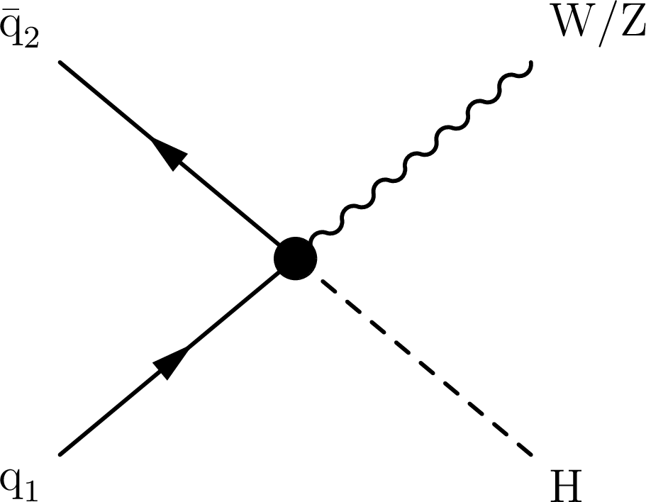
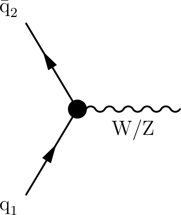
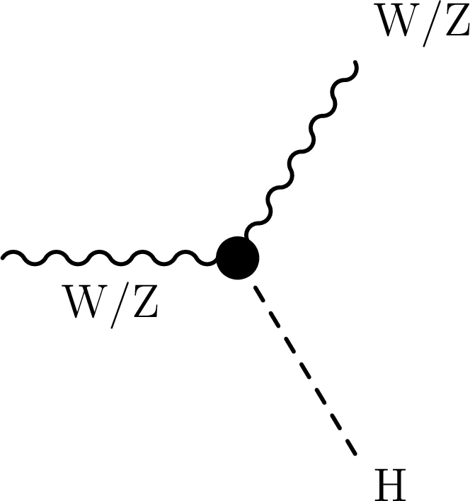
Representative Feynman diagrams for VH production sensitive to different dimension-six operators. The EFT effects contribute in vertices highlighted with a black dot. The diagram on the left shows effects due to $ {\cal O}^{(1)}_{\mathrm{H}\mathrm{q}} $, $ {\cal O}^{(3)}_{\mathrm{H}\mathrm{q}} $, $ {\cal O}_{\mathrm{H}\mathrm{u}} $, and $ {\cal O}_{\mathrm{H}\mathrm{d}} $. The diagram at the center also includes contributions due to $ {\cal O}_{\mathrm{H}\textrm{D}} $ and $ {\cal O}_{\mathrm{H}\mathrm{W}\textrm{B}} $. The diagram on the right displays effects from $ \mathcal{O}_{\mathrm{H}\mathrm{W}} $, $ \mathcal{O}_{\mathrm{H}\mathrm{W}\textrm{B}} $, $ \mathcal{O}_{\mathrm{H}\textrm{B}} $, and their CP conjugates. |
png pdf |
Figure 1-a:
Representative Feynman diagrams for VH production sensitive to different dimension-six operators. The EFT effects contribute in vertices highlighted with a black dot. The diagram on the left shows effects due to $ {\cal O}^{(1)}_{\mathrm{H}\mathrm{q}} $, $ {\cal O}^{(3)}_{\mathrm{H}\mathrm{q}} $, $ {\cal O}_{\mathrm{H}\mathrm{u}} $, and $ {\cal O}_{\mathrm{H}\mathrm{d}} $. The diagram at the center also includes contributions due to $ {\cal O}_{\mathrm{H}\textrm{D}} $ and $ {\cal O}_{\mathrm{H}\mathrm{W}\textrm{B}} $. The diagram on the right displays effects from $ \mathcal{O}_{\mathrm{H}\mathrm{W}} $, $ \mathcal{O}_{\mathrm{H}\mathrm{W}\textrm{B}} $, $ \mathcal{O}_{\mathrm{H}\textrm{B}} $, and their CP conjugates. |
png pdf |
Figure 1-b:
Representative Feynman diagrams for VH production sensitive to different dimension-six operators. The EFT effects contribute in vertices highlighted with a black dot. The diagram on the left shows effects due to $ {\cal O}^{(1)}_{\mathrm{H}\mathrm{q}} $, $ {\cal O}^{(3)}_{\mathrm{H}\mathrm{q}} $, $ {\cal O}_{\mathrm{H}\mathrm{u}} $, and $ {\cal O}_{\mathrm{H}\mathrm{d}} $. The diagram at the center also includes contributions due to $ {\cal O}_{\mathrm{H}\textrm{D}} $ and $ {\cal O}_{\mathrm{H}\mathrm{W}\textrm{B}} $. The diagram on the right displays effects from $ \mathcal{O}_{\mathrm{H}\mathrm{W}} $, $ \mathcal{O}_{\mathrm{H}\mathrm{W}\textrm{B}} $, $ \mathcal{O}_{\mathrm{H}\textrm{B}} $, and their CP conjugates. |
png pdf |
Figure 1-c:
Representative Feynman diagrams for VH production sensitive to different dimension-six operators. The EFT effects contribute in vertices highlighted with a black dot. The diagram on the left shows effects due to $ {\cal O}^{(1)}_{\mathrm{H}\mathrm{q}} $, $ {\cal O}^{(3)}_{\mathrm{H}\mathrm{q}} $, $ {\cal O}_{\mathrm{H}\mathrm{u}} $, and $ {\cal O}_{\mathrm{H}\mathrm{d}} $. The diagram at the center also includes contributions due to $ {\cal O}_{\mathrm{H}\textrm{D}} $ and $ {\cal O}_{\mathrm{H}\mathrm{W}\textrm{B}} $. The diagram on the right displays effects from $ \mathcal{O}_{\mathrm{H}\mathrm{W}} $, $ \mathcal{O}_{\mathrm{H}\mathrm{W}\textrm{B}} $, $ \mathcal{O}_{\mathrm{H}\textrm{B}} $, and their CP conjugates. |
png pdf |
Figure 2:
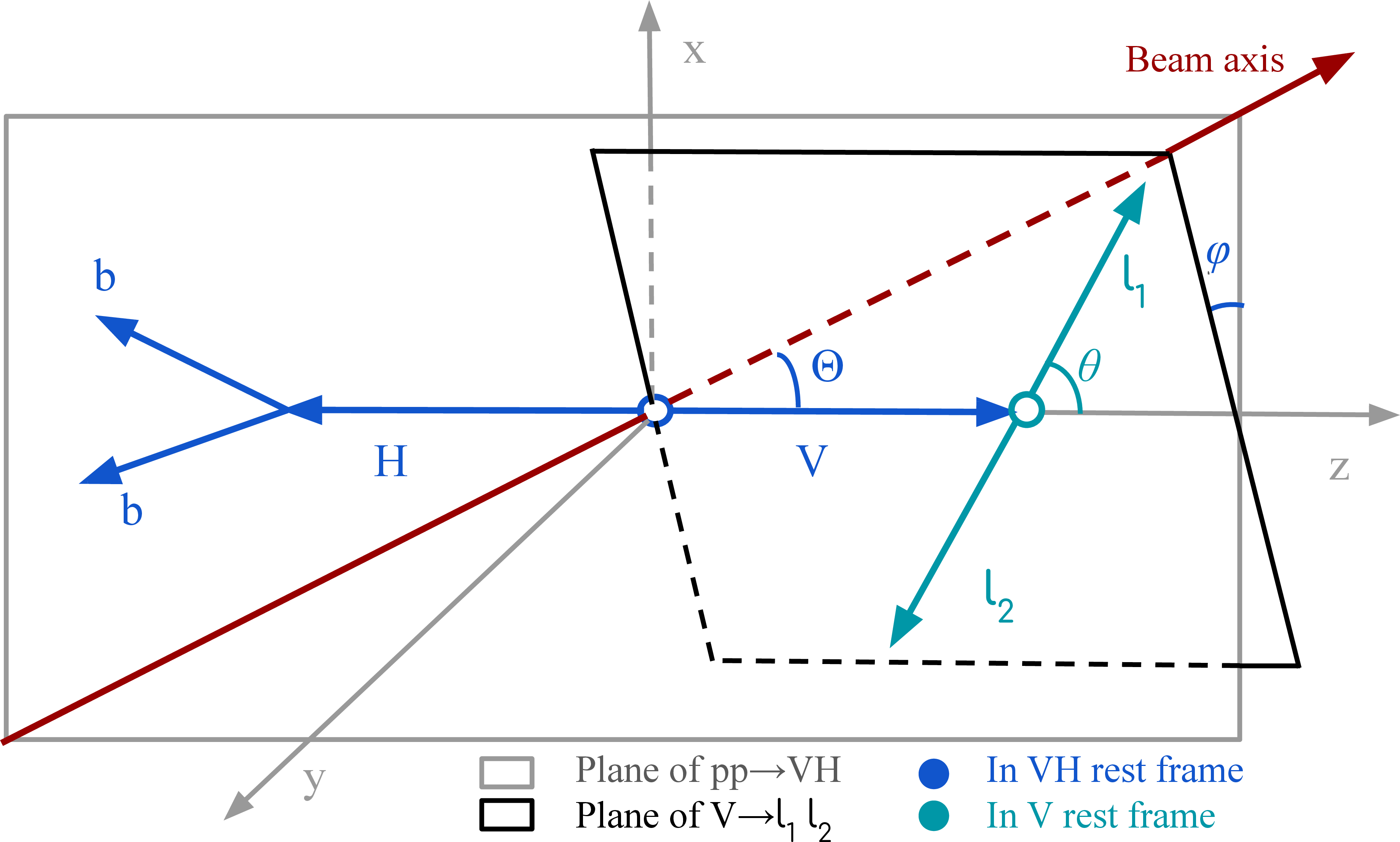
Decay planes and angles in the $ \mathrm{V}(\to \ell_1 \ell_2){\mathrm{H}}(\to \mathrm{b} \overline{\mathrm{b}}) $ production. The $ \Theta $ angle is defined in the VH rest frame, while $ \theta $ is defined in the V rest frame. Figure modified from Ref. [38]. The coordinate system used in the sketch of the decay plane is independent of the general CMS coordinate system that is used for the analysis. |
png pdf |
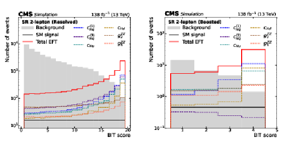
Figure 3:
Selected template shapes after the optimization process described in Section 7.3 in the resolved (left) and boosted (right) categories of the 2-lepton channel. The template shapes of the EFT signal components are shown for arbitrary values of the Wilson coefficients: ($ {c}^{(1)}_{\mathrm{H}\mathrm{q}} $, $ {c}^{(3)}_{\mathrm{H}\mathrm{q}} $, $ {c}_{\mathrm{H}\mathrm{u}} $, $ {c}_{\mathrm{H}\mathrm{d}} $, $ {g}^{\mathrm{Z}\mathrm{Z}}_{2} $, $ {g}^{\mathrm{Z}\mathrm{Z}}_{4} $) = (1, 0.8, 1, 1, 2, 2) and (0.2, $-$0.03, 0.2, 0.2, 1, 1) in the resolved and boosted categories, respectively. The SM VH signal is flat by construction. The background is shown as the grey histogram. |
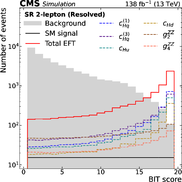
png pdf |
Figure 3-a:
Selected template shapes after the optimization process described in Section 7.3 in the resolved (left) and boosted (right) categories of the 2-lepton channel. The template shapes of the EFT signal components are shown for arbitrary values of the Wilson coefficients: ($ {c}^{(1)}_{\mathrm{H}\mathrm{q}} $, $ {c}^{(3)}_{\mathrm{H}\mathrm{q}} $, $ {c}_{\mathrm{H}\mathrm{u}} $, $ {c}_{\mathrm{H}\mathrm{d}} $, $ {g}^{\mathrm{Z}\mathrm{Z}}_{2} $, $ {g}^{\mathrm{Z}\mathrm{Z}}_{4} $) = (1, 0.8, 1, 1, 2, 2) and (0.2, $-$0.03, 0.2, 0.2, 1, 1) in the resolved and boosted categories, respectively. The SM VH signal is flat by construction. The background is shown as the grey histogram. |

png pdf |
Figure 3-b:
Selected template shapes after the optimization process described in Section 7.3 in the resolved (left) and boosted (right) categories of the 2-lepton channel. The template shapes of the EFT signal components are shown for arbitrary values of the Wilson coefficients: ($ {c}^{(1)}_{\mathrm{H}\mathrm{q}} $, $ {c}^{(3)}_{\mathrm{H}\mathrm{q}} $, $ {c}_{\mathrm{H}\mathrm{u}} $, $ {c}_{\mathrm{H}\mathrm{d}} $, $ {g}^{\mathrm{Z}\mathrm{Z}}_{2} $, $ {g}^{\mathrm{Z}\mathrm{Z}}_{4} $) = (1, 0.8, 1, 1, 2, 2) and (0.2, $-$0.03, 0.2, 0.2, 1, 1) in the resolved and boosted categories, respectively. The SM VH signal is flat by construction. The background is shown as the grey histogram. |

png pdf |
Figure 4:
The BIT templates obtained using a background-only fit to data in the 2-muon (left) and 2-electron (right) final states in the SR for resolved (upper row) and boosted (lower row) categories considering the 2017 data set. The SM VH signal has been scaled by 20 and 5 for the resolved and boosted BIT templates in the upper and lower row, respectively, for better visualization. The lower panels show the ratio of the data to the background expectation after the background-only fit to the data. |
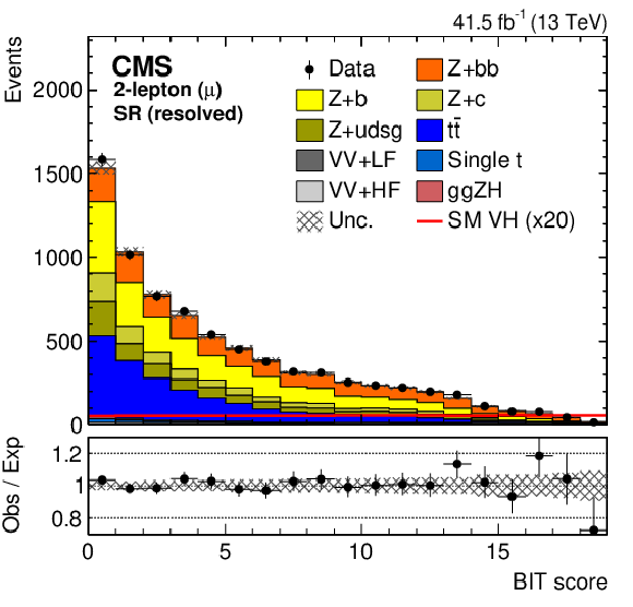
png pdf |
Figure 4-a:
The BIT templates obtained using a background-only fit to data in the 2-muon (left) and 2-electron (right) final states in the SR for resolved (upper row) and boosted (lower row) categories considering the 2017 data set. The SM VH signal has been scaled by 20 and 5 for the resolved and boosted BIT templates in the upper and lower row, respectively, for better visualization. The lower panels show the ratio of the data to the background expectation after the background-only fit to the data. |
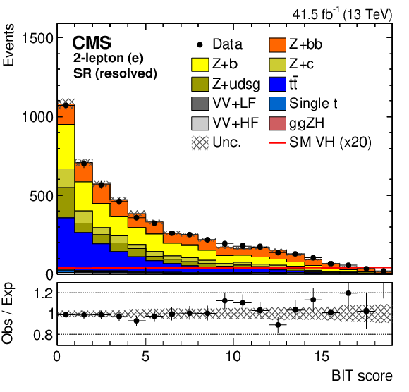
png pdf |
Figure 4-b:
The BIT templates obtained using a background-only fit to data in the 2-muon (left) and 2-electron (right) final states in the SR for resolved (upper row) and boosted (lower row) categories considering the 2017 data set. The SM VH signal has been scaled by 20 and 5 for the resolved and boosted BIT templates in the upper and lower row, respectively, for better visualization. The lower panels show the ratio of the data to the background expectation after the background-only fit to the data. |
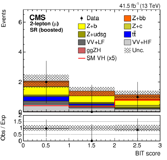
png pdf |
Figure 4-c:
The BIT templates obtained using a background-only fit to data in the 2-muon (left) and 2-electron (right) final states in the SR for resolved (upper row) and boosted (lower row) categories considering the 2017 data set. The SM VH signal has been scaled by 20 and 5 for the resolved and boosted BIT templates in the upper and lower row, respectively, for better visualization. The lower panels show the ratio of the data to the background expectation after the background-only fit to the data. |
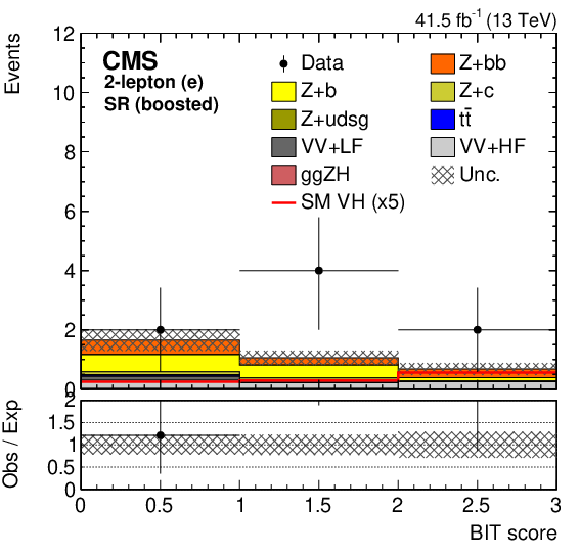
png pdf |
Figure 4-d:
The BIT templates obtained using a background-only fit to data in the 2-muon (left) and 2-electron (right) final states in the SR for resolved (upper row) and boosted (lower row) categories considering the 2017 data set. The SM VH signal has been scaled by 20 and 5 for the resolved and boosted BIT templates in the upper and lower row, respectively, for better visualization. The lower panels show the ratio of the data to the background expectation after the background-only fit to the data. |
png pdf |
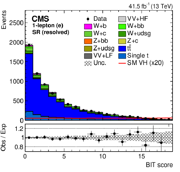
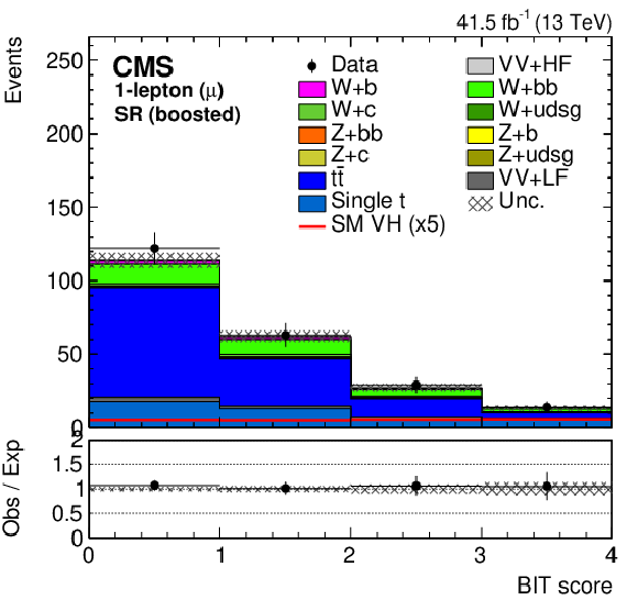
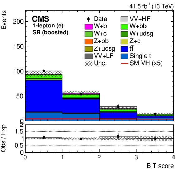
Figure 5:
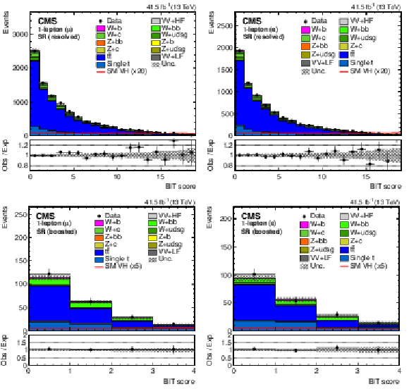
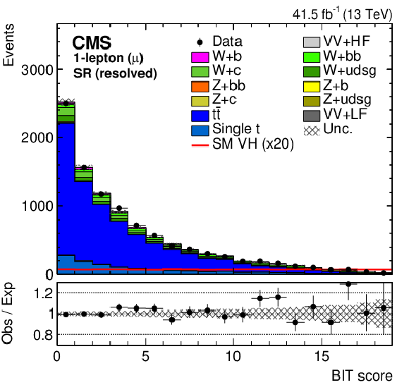
The BIT templates obtained using a background-only fit to data in the 1-muon (left) and 1-electron (right) final states in the SR for resolved (upper row) and boosted (lower row) categories considering the 2017 data set. The SM VH signal has been scaled by 20 and 5 for the resolved and boosted BIT templates in the upper and lower row, respectively, for better visualization. The lower panels show the ratio of the data to the background expectation after the background-only fit to the data. |
png pdf |
Figure 5-a:
The BIT templates obtained using a background-only fit to data in the 1-muon (left) and 1-electron (right) final states in the SR for resolved (upper row) and boosted (lower row) categories considering the 2017 data set. The SM VH signal has been scaled by 20 and 5 for the resolved and boosted BIT templates in the upper and lower row, respectively, for better visualization. The lower panels show the ratio of the data to the background expectation after the background-only fit to the data. |
png pdf |
Figure 5-b:
The BIT templates obtained using a background-only fit to data in the 1-muon (left) and 1-electron (right) final states in the SR for resolved (upper row) and boosted (lower row) categories considering the 2017 data set. The SM VH signal has been scaled by 20 and 5 for the resolved and boosted BIT templates in the upper and lower row, respectively, for better visualization. The lower panels show the ratio of the data to the background expectation after the background-only fit to the data. |
png pdf |
Figure 5-c:
The BIT templates obtained using a background-only fit to data in the 1-muon (left) and 1-electron (right) final states in the SR for resolved (upper row) and boosted (lower row) categories considering the 2017 data set. The SM VH signal has been scaled by 20 and 5 for the resolved and boosted BIT templates in the upper and lower row, respectively, for better visualization. The lower panels show the ratio of the data to the background expectation after the background-only fit to the data. |
png pdf |
Figure 5-d:
The BIT templates obtained using a background-only fit to data in the 1-muon (left) and 1-electron (right) final states in the SR for resolved (upper row) and boosted (lower row) categories considering the 2017 data set. The SM VH signal has been scaled by 20 and 5 for the resolved and boosted BIT templates in the upper and lower row, respectively, for better visualization. The lower panels show the ratio of the data to the background expectation after the background-only fit to the data. |
png pdf |
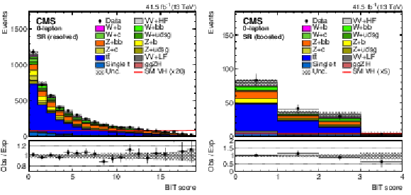
Figure 6:
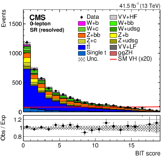
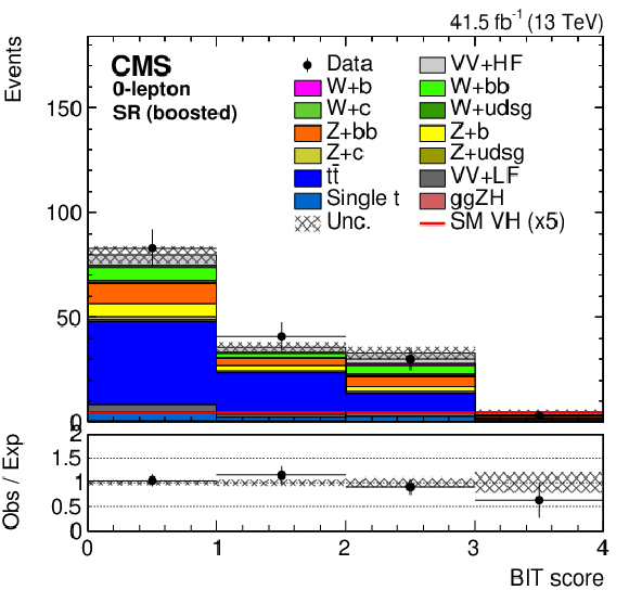
The BIT templates obtained using a background-only fit to data in the 0-lepton final state in the SR for resolved (left) and boosted (right) categories considering the 2017 data set. The SM VH signal has been scaled by 20 and 5 for the resolved and boosted BIT templates in the upper and lower row, respectively, for better visualization. The lower panels show the ratio of the data to the background expectation after the background-only fit to the data. |
png pdf |
Figure 6-a:
The BIT templates obtained using a background-only fit to data in the 0-lepton final state in the SR for resolved (left) and boosted (right) categories considering the 2017 data set. The SM VH signal has been scaled by 20 and 5 for the resolved and boosted BIT templates in the upper and lower row, respectively, for better visualization. The lower panels show the ratio of the data to the background expectation after the background-only fit to the data. |
png pdf |
Figure 6-b:
The BIT templates obtained using a background-only fit to data in the 0-lepton final state in the SR for resolved (left) and boosted (right) categories considering the 2017 data set. The SM VH signal has been scaled by 20 and 5 for the resolved and boosted BIT templates in the upper and lower row, respectively, for better visualization. The lower panels show the ratio of the data to the background expectation after the background-only fit to the data. |
png pdf |
Figure 7:
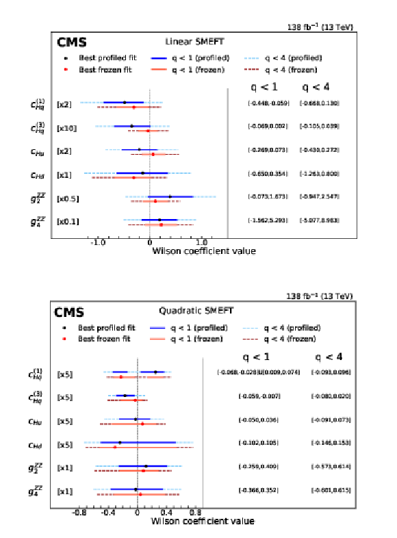
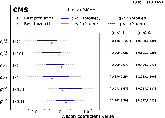
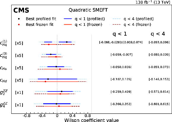
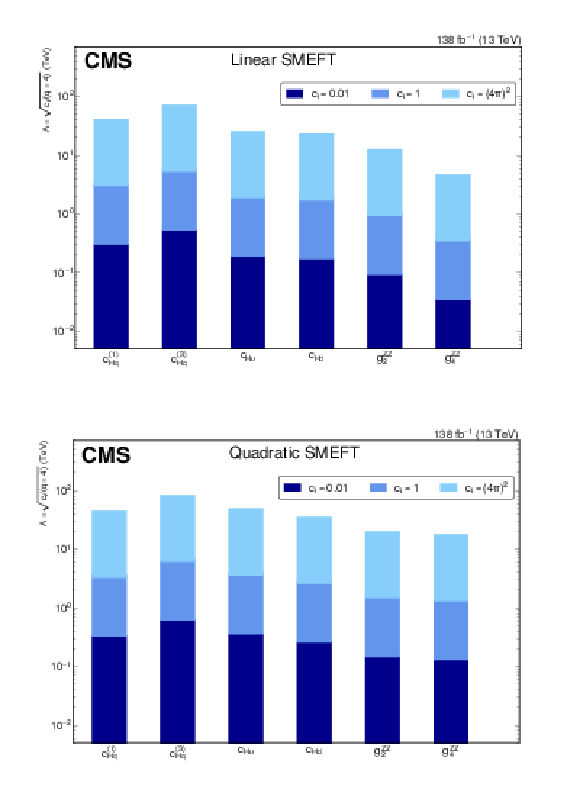
Summary of results in terms of best fit value of the Wilson coefficients and the intervals where the test statistic is below 1 and 4, with up to the linear (upper row) and quadratic (lower row) terms in the SMEFT parameterization. These results are obtained either by allowing all Wilson coefficients to float freely at every point of the scan (profiled fit), or by keeping all other Wilson coefficients to their SM values, i.e.,, 0, except for the one that is being considered in the scan (frozen fit). The multiplication factor applies to the sizes of intervals satisfying $ \textit{q} < $ 1 and $ \textit{q} < $ 4 but not to the values of the CIs on the right-hand side of the figure, which correspond to the profiled constraints in all cases. |
png pdf |
Figure 7-a:
Summary of results in terms of best fit value of the Wilson coefficients and the intervals where the test statistic is below 1 and 4, with up to the linear (upper row) and quadratic (lower row) terms in the SMEFT parameterization. These results are obtained either by allowing all Wilson coefficients to float freely at every point of the scan (profiled fit), or by keeping all other Wilson coefficients to their SM values, i.e.,, 0, except for the one that is being considered in the scan (frozen fit). The multiplication factor applies to the sizes of intervals satisfying $ \textit{q} < $ 1 and $ \textit{q} < $ 4 but not to the values of the CIs on the right-hand side of the figure, which correspond to the profiled constraints in all cases. |
png pdf |
Figure 7-b:
Summary of results in terms of best fit value of the Wilson coefficients and the intervals where the test statistic is below 1 and 4, with up to the linear (upper row) and quadratic (lower row) terms in the SMEFT parameterization. These results are obtained either by allowing all Wilson coefficients to float freely at every point of the scan (profiled fit), or by keeping all other Wilson coefficients to their SM values, i.e.,, 0, except for the one that is being considered in the scan (frozen fit). The multiplication factor applies to the sizes of intervals satisfying $ \textit{q} < $ 1 and $ \textit{q} < $ 4 but not to the values of the CIs on the right-hand side of the figure, which correspond to the profiled constraints in all cases. |
png pdf |
Figure 8:
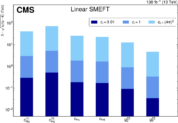
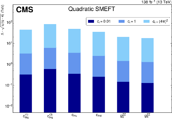
Profiled limits on the energy scale $ \Lambda $ for three different assumptions for each Wilson coefficient while fixing the other Wilson coefficients to their SM values with up to the linear (upper row) and quadratic (lower row) terms in SMEFT parameterization. The upper limits on the Wilson coefficients corresponding to $ \textit{q}= $ 4 is used for translating the constraints to $ \Lambda $. |
png pdf |
Figure 8-a:
Profiled limits on the energy scale $ \Lambda $ for three different assumptions for each Wilson coefficient while fixing the other Wilson coefficients to their SM values with up to the linear (upper row) and quadratic (lower row) terms in SMEFT parameterization. The upper limits on the Wilson coefficients corresponding to $ \textit{q}= $ 4 is used for translating the constraints to $ \Lambda $. |
png pdf |
Figure 8-b:
Profiled limits on the energy scale $ \Lambda $ for three different assumptions for each Wilson coefficient while fixing the other Wilson coefficients to their SM values with up to the linear (upper row) and quadratic (lower row) terms in SMEFT parameterization. The upper limits on the Wilson coefficients corresponding to $ \textit{q}= $ 4 is used for translating the constraints to $ \Lambda $. |
png pdf |
Figure 9:
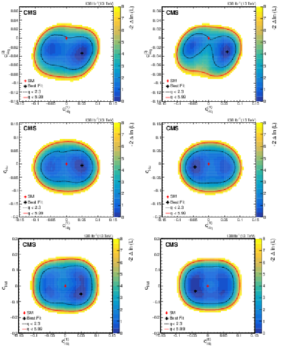
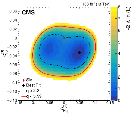
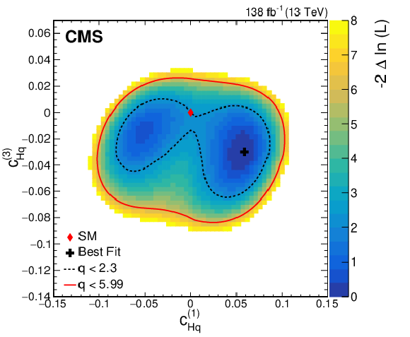
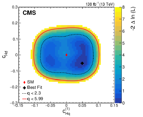
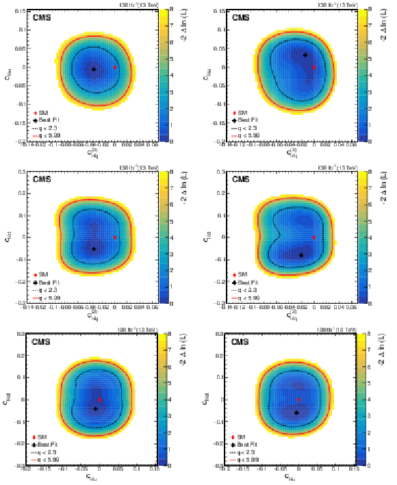
Observed two-dimensional likelihood scans for different pairs of Wilson coefficients: $ {c}^{(1)}_{\mathrm{H}\mathrm{q}} $ vs. $ {c}^{(3)}_{\mathrm{H}\mathrm{q}} $ (upper row), $ {c}^{(1)}_{\mathrm{H}\mathrm{q}} $ vs. $ {c}_{\mathrm{H}\mathrm{u}} $ (middle row), $ {c}^{(1)}_{\mathrm{H}\mathrm{q}} $ vs. $ {c}_{\mathrm{H}\mathrm{d}} $ (lower row) while allowing the other coefficients to float freely at each point of the scan (left) or fixed at their SM values (right) after combining results from all data-taking years and final states. |
png pdf |
Figure 9-a:
Observed two-dimensional likelihood scans for different pairs of Wilson coefficients: $ {c}^{(1)}_{\mathrm{H}\mathrm{q}} $ vs. $ {c}^{(3)}_{\mathrm{H}\mathrm{q}} $ (upper row), $ {c}^{(1)}_{\mathrm{H}\mathrm{q}} $ vs. $ {c}_{\mathrm{H}\mathrm{u}} $ (middle row), $ {c}^{(1)}_{\mathrm{H}\mathrm{q}} $ vs. $ {c}_{\mathrm{H}\mathrm{d}} $ (lower row) while allowing the other coefficients to float freely at each point of the scan (left) or fixed at their SM values (right) after combining results from all data-taking years and final states. |
png pdf |
Figure 9-b:
Observed two-dimensional likelihood scans for different pairs of Wilson coefficients: $ {c}^{(1)}_{\mathrm{H}\mathrm{q}} $ vs. $ {c}^{(3)}_{\mathrm{H}\mathrm{q}} $ (upper row), $ {c}^{(1)}_{\mathrm{H}\mathrm{q}} $ vs. $ {c}_{\mathrm{H}\mathrm{u}} $ (middle row), $ {c}^{(1)}_{\mathrm{H}\mathrm{q}} $ vs. $ {c}_{\mathrm{H}\mathrm{d}} $ (lower row) while allowing the other coefficients to float freely at each point of the scan (left) or fixed at their SM values (right) after combining results from all data-taking years and final states. |

png pdf |
Figure 9-c:
Observed two-dimensional likelihood scans for different pairs of Wilson coefficients: $ {c}^{(1)}_{\mathrm{H}\mathrm{q}} $ vs. $ {c}^{(3)}_{\mathrm{H}\mathrm{q}} $ (upper row), $ {c}^{(1)}_{\mathrm{H}\mathrm{q}} $ vs. $ {c}_{\mathrm{H}\mathrm{u}} $ (middle row), $ {c}^{(1)}_{\mathrm{H}\mathrm{q}} $ vs. $ {c}_{\mathrm{H}\mathrm{d}} $ (lower row) while allowing the other coefficients to float freely at each point of the scan (left) or fixed at their SM values (right) after combining results from all data-taking years and final states. |
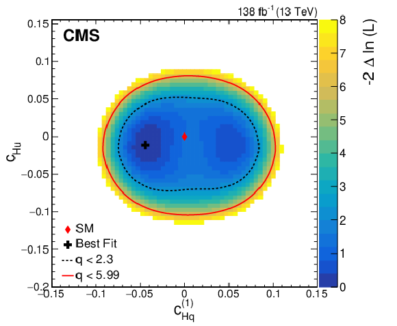
png pdf |
Figure 9-d:
Observed two-dimensional likelihood scans for different pairs of Wilson coefficients: $ {c}^{(1)}_{\mathrm{H}\mathrm{q}} $ vs. $ {c}^{(3)}_{\mathrm{H}\mathrm{q}} $ (upper row), $ {c}^{(1)}_{\mathrm{H}\mathrm{q}} $ vs. $ {c}_{\mathrm{H}\mathrm{u}} $ (middle row), $ {c}^{(1)}_{\mathrm{H}\mathrm{q}} $ vs. $ {c}_{\mathrm{H}\mathrm{d}} $ (lower row) while allowing the other coefficients to float freely at each point of the scan (left) or fixed at their SM values (right) after combining results from all data-taking years and final states. |
png pdf |
Figure 9-e:
Observed two-dimensional likelihood scans for different pairs of Wilson coefficients: $ {c}^{(1)}_{\mathrm{H}\mathrm{q}} $ vs. $ {c}^{(3)}_{\mathrm{H}\mathrm{q}} $ (upper row), $ {c}^{(1)}_{\mathrm{H}\mathrm{q}} $ vs. $ {c}_{\mathrm{H}\mathrm{u}} $ (middle row), $ {c}^{(1)}_{\mathrm{H}\mathrm{q}} $ vs. $ {c}_{\mathrm{H}\mathrm{d}} $ (lower row) while allowing the other coefficients to float freely at each point of the scan (left) or fixed at their SM values (right) after combining results from all data-taking years and final states. |

png pdf |
Figure 9-f:
Observed two-dimensional likelihood scans for different pairs of Wilson coefficients: $ {c}^{(1)}_{\mathrm{H}\mathrm{q}} $ vs. $ {c}^{(3)}_{\mathrm{H}\mathrm{q}} $ (upper row), $ {c}^{(1)}_{\mathrm{H}\mathrm{q}} $ vs. $ {c}_{\mathrm{H}\mathrm{u}} $ (middle row), $ {c}^{(1)}_{\mathrm{H}\mathrm{q}} $ vs. $ {c}_{\mathrm{H}\mathrm{d}} $ (lower row) while allowing the other coefficients to float freely at each point of the scan (left) or fixed at their SM values (right) after combining results from all data-taking years and final states. |
png pdf |
Figure 10:
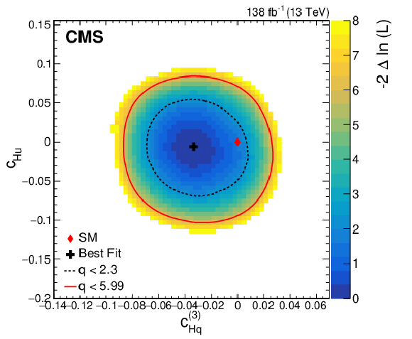
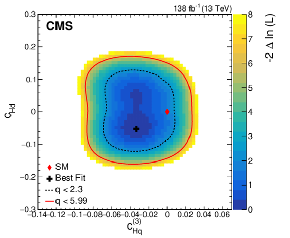
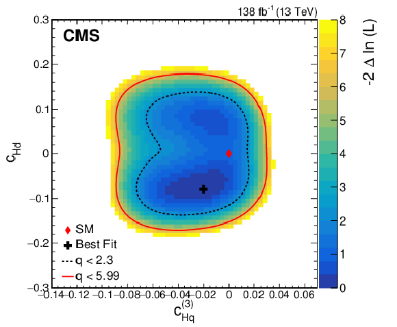
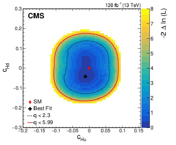
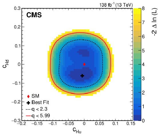
Observed two-dimensional likelihood scans for different pairs of Wilson coefficients: $ {c}^{(3)}_{\mathrm{H}\mathrm{q}} $ vs. $ {c}_{\mathrm{H}\mathrm{u}} $ (upper row), $ {c}^{(3)}_{\mathrm{H}\mathrm{q}} $ vs. $ {c}_{\mathrm{H}\mathrm{d}} $ (middle row), $ {c}_{\mathrm{H}\mathrm{u}} $ vs. $ {c}_{\mathrm{H}\mathrm{d}} $ (lower row) while allowing the other coefficients to float freely at each point of the scan (left) or fixed at their SM values (right) after combining results from all data-taking years and final states. |
png pdf |
Figure 10-a:
Observed two-dimensional likelihood scans for different pairs of Wilson coefficients: $ {c}^{(3)}_{\mathrm{H}\mathrm{q}} $ vs. $ {c}_{\mathrm{H}\mathrm{u}} $ (upper row), $ {c}^{(3)}_{\mathrm{H}\mathrm{q}} $ vs. $ {c}_{\mathrm{H}\mathrm{d}} $ (middle row), $ {c}_{\mathrm{H}\mathrm{u}} $ vs. $ {c}_{\mathrm{H}\mathrm{d}} $ (lower row) while allowing the other coefficients to float freely at each point of the scan (left) or fixed at their SM values (right) after combining results from all data-taking years and final states. |

png pdf |
Figure 10-b:
Observed two-dimensional likelihood scans for different pairs of Wilson coefficients: $ {c}^{(3)}_{\mathrm{H}\mathrm{q}} $ vs. $ {c}_{\mathrm{H}\mathrm{u}} $ (upper row), $ {c}^{(3)}_{\mathrm{H}\mathrm{q}} $ vs. $ {c}_{\mathrm{H}\mathrm{d}} $ (middle row), $ {c}_{\mathrm{H}\mathrm{u}} $ vs. $ {c}_{\mathrm{H}\mathrm{d}} $ (lower row) while allowing the other coefficients to float freely at each point of the scan (left) or fixed at their SM values (right) after combining results from all data-taking years and final states. |
png pdf |
Figure 10-c:
Observed two-dimensional likelihood scans for different pairs of Wilson coefficients: $ {c}^{(3)}_{\mathrm{H}\mathrm{q}} $ vs. $ {c}_{\mathrm{H}\mathrm{u}} $ (upper row), $ {c}^{(3)}_{\mathrm{H}\mathrm{q}} $ vs. $ {c}_{\mathrm{H}\mathrm{d}} $ (middle row), $ {c}_{\mathrm{H}\mathrm{u}} $ vs. $ {c}_{\mathrm{H}\mathrm{d}} $ (lower row) while allowing the other coefficients to float freely at each point of the scan (left) or fixed at their SM values (right) after combining results from all data-taking years and final states. |
png pdf |
Figure 10-d:
Observed two-dimensional likelihood scans for different pairs of Wilson coefficients: $ {c}^{(3)}_{\mathrm{H}\mathrm{q}} $ vs. $ {c}_{\mathrm{H}\mathrm{u}} $ (upper row), $ {c}^{(3)}_{\mathrm{H}\mathrm{q}} $ vs. $ {c}_{\mathrm{H}\mathrm{d}} $ (middle row), $ {c}_{\mathrm{H}\mathrm{u}} $ vs. $ {c}_{\mathrm{H}\mathrm{d}} $ (lower row) while allowing the other coefficients to float freely at each point of the scan (left) or fixed at their SM values (right) after combining results from all data-taking years and final states. |
png pdf |
Figure 10-e:
Observed two-dimensional likelihood scans for different pairs of Wilson coefficients: $ {c}^{(3)}_{\mathrm{H}\mathrm{q}} $ vs. $ {c}_{\mathrm{H}\mathrm{u}} $ (upper row), $ {c}^{(3)}_{\mathrm{H}\mathrm{q}} $ vs. $ {c}_{\mathrm{H}\mathrm{d}} $ (middle row), $ {c}_{\mathrm{H}\mathrm{u}} $ vs. $ {c}_{\mathrm{H}\mathrm{d}} $ (lower row) while allowing the other coefficients to float freely at each point of the scan (left) or fixed at their SM values (right) after combining results from all data-taking years and final states. |
png pdf |
Figure 10-f:
Observed two-dimensional likelihood scans for different pairs of Wilson coefficients: $ {c}^{(3)}_{\mathrm{H}\mathrm{q}} $ vs. $ {c}_{\mathrm{H}\mathrm{u}} $ (upper row), $ {c}^{(3)}_{\mathrm{H}\mathrm{q}} $ vs. $ {c}_{\mathrm{H}\mathrm{d}} $ (middle row), $ {c}_{\mathrm{H}\mathrm{u}} $ vs. $ {c}_{\mathrm{H}\mathrm{d}} $ (lower row) while allowing the other coefficients to float freely at each point of the scan (left) or fixed at their SM values (right) after combining results from all data-taking years and final states. |
png pdf |
Figure 11:
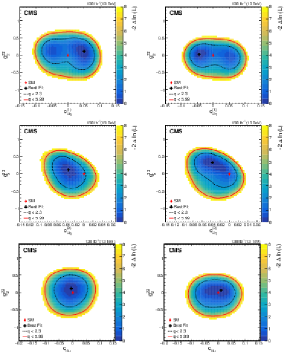
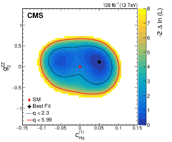
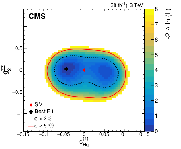
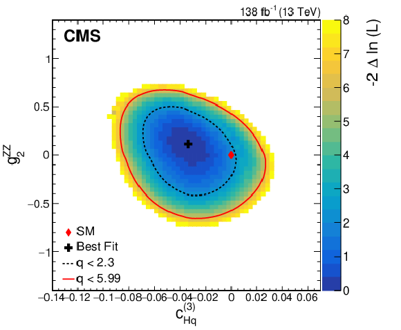
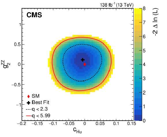
Observed two-dimensional likelihood scans for different pairs of Wilson coefficients: $ {c}^{(1)}_{\mathrm{H}\mathrm{q}} $ vs. $ {g}^{\mathrm{Z}\mathrm{Z}}_{2} $ (upper row), $ {c}^{(3)}_{\mathrm{H}\mathrm{q}} $ vs. $ {g}^{\mathrm{Z}\mathrm{Z}}_{2} $ (middle row), $ {c}_{\mathrm{H}\mathrm{u}} $ vs. $ {g}^{\mathrm{Z}\mathrm{Z}}_{2} $ (lower row) while allowing the other coefficients to float freely at each point of the scan (left) or fixed at their SM values (right) after combining results from all data-taking years and final states. |
png pdf |
Figure 11-a:
Observed two-dimensional likelihood scans for different pairs of Wilson coefficients: $ {c}^{(1)}_{\mathrm{H}\mathrm{q}} $ vs. $ {g}^{\mathrm{Z}\mathrm{Z}}_{2} $ (upper row), $ {c}^{(3)}_{\mathrm{H}\mathrm{q}} $ vs. $ {g}^{\mathrm{Z}\mathrm{Z}}_{2} $ (middle row), $ {c}_{\mathrm{H}\mathrm{u}} $ vs. $ {g}^{\mathrm{Z}\mathrm{Z}}_{2} $ (lower row) while allowing the other coefficients to float freely at each point of the scan (left) or fixed at their SM values (right) after combining results from all data-taking years and final states. |
png pdf |
Figure 11-b:
Observed two-dimensional likelihood scans for different pairs of Wilson coefficients: $ {c}^{(1)}_{\mathrm{H}\mathrm{q}} $ vs. $ {g}^{\mathrm{Z}\mathrm{Z}}_{2} $ (upper row), $ {c}^{(3)}_{\mathrm{H}\mathrm{q}} $ vs. $ {g}^{\mathrm{Z}\mathrm{Z}}_{2} $ (middle row), $ {c}_{\mathrm{H}\mathrm{u}} $ vs. $ {g}^{\mathrm{Z}\mathrm{Z}}_{2} $ (lower row) while allowing the other coefficients to float freely at each point of the scan (left) or fixed at their SM values (right) after combining results from all data-taking years and final states. |
png pdf |
Figure 11-c:
Observed two-dimensional likelihood scans for different pairs of Wilson coefficients: $ {c}^{(1)}_{\mathrm{H}\mathrm{q}} $ vs. $ {g}^{\mathrm{Z}\mathrm{Z}}_{2} $ (upper row), $ {c}^{(3)}_{\mathrm{H}\mathrm{q}} $ vs. $ {g}^{\mathrm{Z}\mathrm{Z}}_{2} $ (middle row), $ {c}_{\mathrm{H}\mathrm{u}} $ vs. $ {g}^{\mathrm{Z}\mathrm{Z}}_{2} $ (lower row) while allowing the other coefficients to float freely at each point of the scan (left) or fixed at their SM values (right) after combining results from all data-taking years and final states. |

png pdf |
Figure 11-d:
Observed two-dimensional likelihood scans for different pairs of Wilson coefficients: $ {c}^{(1)}_{\mathrm{H}\mathrm{q}} $ vs. $ {g}^{\mathrm{Z}\mathrm{Z}}_{2} $ (upper row), $ {c}^{(3)}_{\mathrm{H}\mathrm{q}} $ vs. $ {g}^{\mathrm{Z}\mathrm{Z}}_{2} $ (middle row), $ {c}_{\mathrm{H}\mathrm{u}} $ vs. $ {g}^{\mathrm{Z}\mathrm{Z}}_{2} $ (lower row) while allowing the other coefficients to float freely at each point of the scan (left) or fixed at their SM values (right) after combining results from all data-taking years and final states. |
png pdf |
Figure 11-e:
Observed two-dimensional likelihood scans for different pairs of Wilson coefficients: $ {c}^{(1)}_{\mathrm{H}\mathrm{q}} $ vs. $ {g}^{\mathrm{Z}\mathrm{Z}}_{2} $ (upper row), $ {c}^{(3)}_{\mathrm{H}\mathrm{q}} $ vs. $ {g}^{\mathrm{Z}\mathrm{Z}}_{2} $ (middle row), $ {c}_{\mathrm{H}\mathrm{u}} $ vs. $ {g}^{\mathrm{Z}\mathrm{Z}}_{2} $ (lower row) while allowing the other coefficients to float freely at each point of the scan (left) or fixed at their SM values (right) after combining results from all data-taking years and final states. |
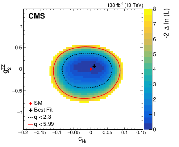
png pdf |
Figure 11-f:
Observed two-dimensional likelihood scans for different pairs of Wilson coefficients: $ {c}^{(1)}_{\mathrm{H}\mathrm{q}} $ vs. $ {g}^{\mathrm{Z}\mathrm{Z}}_{2} $ (upper row), $ {c}^{(3)}_{\mathrm{H}\mathrm{q}} $ vs. $ {g}^{\mathrm{Z}\mathrm{Z}}_{2} $ (middle row), $ {c}_{\mathrm{H}\mathrm{u}} $ vs. $ {g}^{\mathrm{Z}\mathrm{Z}}_{2} $ (lower row) while allowing the other coefficients to float freely at each point of the scan (left) or fixed at their SM values (right) after combining results from all data-taking years and final states. |
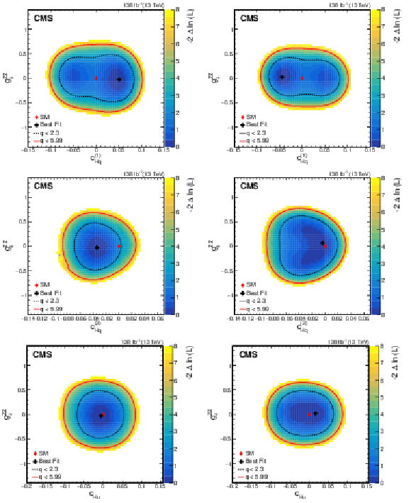
png pdf |
Figure 12:
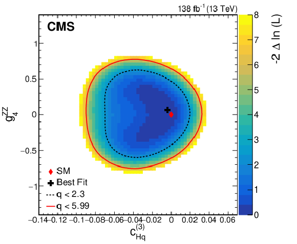
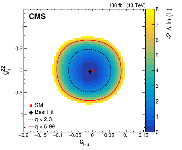
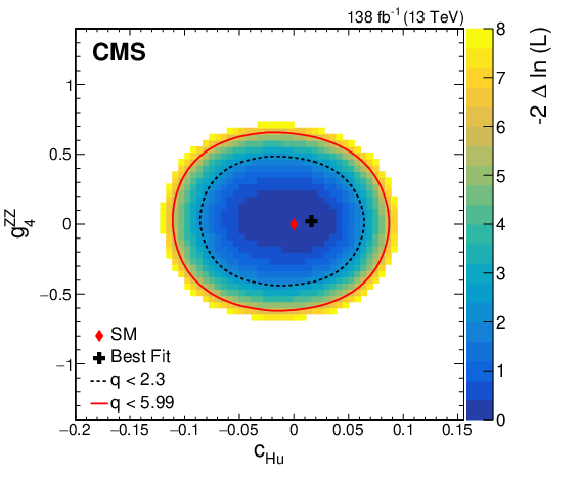
Observed two-dimensional likelihood scans for different pairs of Wilson coefficients: $ {c}^{(1)}_{\mathrm{H}\mathrm{q}} $ vs. $ {g}^{\mathrm{Z}\mathrm{Z}}_{4} $ (upper row), $ {c}^{(3)}_{\mathrm{H}\mathrm{q}} $ vs. $ {g}^{\mathrm{Z}\mathrm{Z}}_{4} $ (middle row), $ {c}_{\mathrm{H}\mathrm{u}} $ vs. $ {g}^{\mathrm{Z}\mathrm{Z}}_{4} $ (lower row) while allowing the other coefficients to float freely at each point of the scan (left) or fixed at their SM values (right) after combining results from all data-taking years and final states. |

png pdf |
Figure 12-a:
Observed two-dimensional likelihood scans for different pairs of Wilson coefficients: $ {c}^{(1)}_{\mathrm{H}\mathrm{q}} $ vs. $ {g}^{\mathrm{Z}\mathrm{Z}}_{4} $ (upper row), $ {c}^{(3)}_{\mathrm{H}\mathrm{q}} $ vs. $ {g}^{\mathrm{Z}\mathrm{Z}}_{4} $ (middle row), $ {c}_{\mathrm{H}\mathrm{u}} $ vs. $ {g}^{\mathrm{Z}\mathrm{Z}}_{4} $ (lower row) while allowing the other coefficients to float freely at each point of the scan (left) or fixed at their SM values (right) after combining results from all data-taking years and final states. |
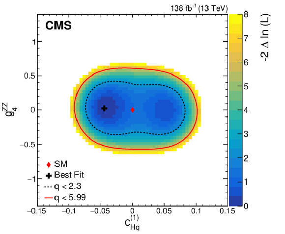
png pdf |
Figure 12-b:
Observed two-dimensional likelihood scans for different pairs of Wilson coefficients: $ {c}^{(1)}_{\mathrm{H}\mathrm{q}} $ vs. $ {g}^{\mathrm{Z}\mathrm{Z}}_{4} $ (upper row), $ {c}^{(3)}_{\mathrm{H}\mathrm{q}} $ vs. $ {g}^{\mathrm{Z}\mathrm{Z}}_{4} $ (middle row), $ {c}_{\mathrm{H}\mathrm{u}} $ vs. $ {g}^{\mathrm{Z}\mathrm{Z}}_{4} $ (lower row) while allowing the other coefficients to float freely at each point of the scan (left) or fixed at their SM values (right) after combining results from all data-taking years and final states. |
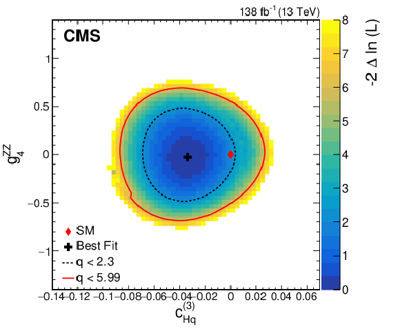
png pdf |
Figure 12-c:
Observed two-dimensional likelihood scans for different pairs of Wilson coefficients: $ {c}^{(1)}_{\mathrm{H}\mathrm{q}} $ vs. $ {g}^{\mathrm{Z}\mathrm{Z}}_{4} $ (upper row), $ {c}^{(3)}_{\mathrm{H}\mathrm{q}} $ vs. $ {g}^{\mathrm{Z}\mathrm{Z}}_{4} $ (middle row), $ {c}_{\mathrm{H}\mathrm{u}} $ vs. $ {g}^{\mathrm{Z}\mathrm{Z}}_{4} $ (lower row) while allowing the other coefficients to float freely at each point of the scan (left) or fixed at their SM values (right) after combining results from all data-taking years and final states. |
png pdf |
Figure 12-d:
Observed two-dimensional likelihood scans for different pairs of Wilson coefficients: $ {c}^{(1)}_{\mathrm{H}\mathrm{q}} $ vs. $ {g}^{\mathrm{Z}\mathrm{Z}}_{4} $ (upper row), $ {c}^{(3)}_{\mathrm{H}\mathrm{q}} $ vs. $ {g}^{\mathrm{Z}\mathrm{Z}}_{4} $ (middle row), $ {c}_{\mathrm{H}\mathrm{u}} $ vs. $ {g}^{\mathrm{Z}\mathrm{Z}}_{4} $ (lower row) while allowing the other coefficients to float freely at each point of the scan (left) or fixed at their SM values (right) after combining results from all data-taking years and final states. |
png pdf |
Figure 12-e:
Observed two-dimensional likelihood scans for different pairs of Wilson coefficients: $ {c}^{(1)}_{\mathrm{H}\mathrm{q}} $ vs. $ {g}^{\mathrm{Z}\mathrm{Z}}_{4} $ (upper row), $ {c}^{(3)}_{\mathrm{H}\mathrm{q}} $ vs. $ {g}^{\mathrm{Z}\mathrm{Z}}_{4} $ (middle row), $ {c}_{\mathrm{H}\mathrm{u}} $ vs. $ {g}^{\mathrm{Z}\mathrm{Z}}_{4} $ (lower row) while allowing the other coefficients to float freely at each point of the scan (left) or fixed at their SM values (right) after combining results from all data-taking years and final states. |
png pdf |
Figure 12-f:
Observed two-dimensional likelihood scans for different pairs of Wilson coefficients: $ {c}^{(1)}_{\mathrm{H}\mathrm{q}} $ vs. $ {g}^{\mathrm{Z}\mathrm{Z}}_{4} $ (upper row), $ {c}^{(3)}_{\mathrm{H}\mathrm{q}} $ vs. $ {g}^{\mathrm{Z}\mathrm{Z}}_{4} $ (middle row), $ {c}_{\mathrm{H}\mathrm{u}} $ vs. $ {g}^{\mathrm{Z}\mathrm{Z}}_{4} $ (lower row) while allowing the other coefficients to float freely at each point of the scan (left) or fixed at their SM values (right) after combining results from all data-taking years and final states. |
png pdf |
Figure 13:
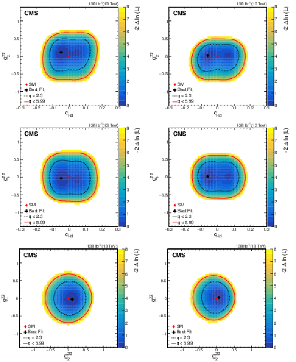
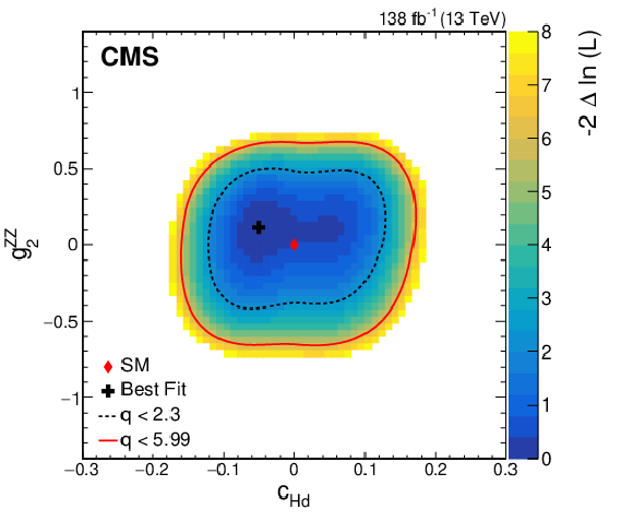
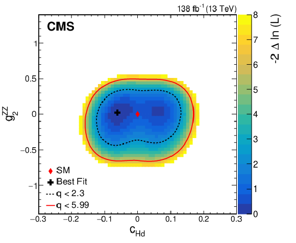
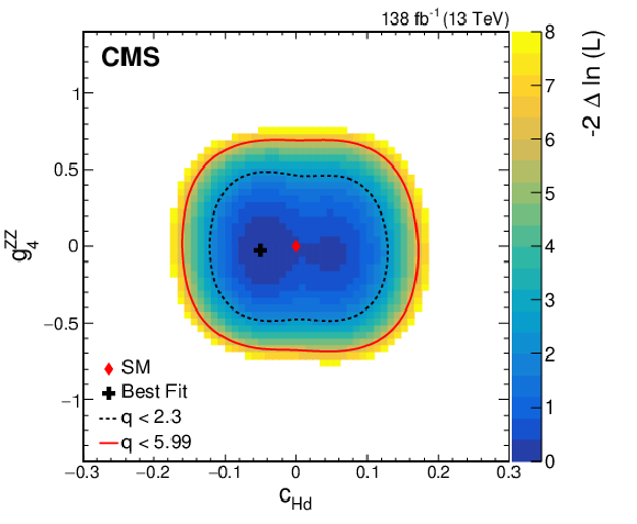
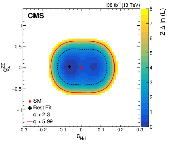
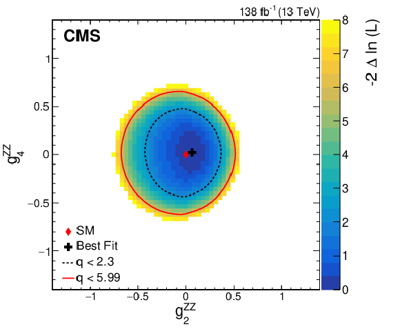
Observed two-dimensional likelihood scans for different pairs of Wilson coefficients: $ {c}_{\mathrm{H}\mathrm{d}} $ vs. $ {g}^{\mathrm{Z}\mathrm{Z}}_{2} $ (upper row), $ {c}_{\mathrm{H}\mathrm{d}} $ vs. $ {g}^{\mathrm{Z}\mathrm{Z}}_{4} $ (middle row), $ {g}^{\mathrm{Z}\mathrm{Z}}_{2} $ vs. $ {g}^{\mathrm{Z}\mathrm{Z}}_{4} $ (lower row) while allowing the other coefficients to float freely at each point of the scan (left) or fixed at their SM values (right) after combining results from all data-taking years and final states. |
png pdf |
Figure 13-a:
Observed two-dimensional likelihood scans for different pairs of Wilson coefficients: $ {c}_{\mathrm{H}\mathrm{d}} $ vs. $ {g}^{\mathrm{Z}\mathrm{Z}}_{2} $ (upper row), $ {c}_{\mathrm{H}\mathrm{d}} $ vs. $ {g}^{\mathrm{Z}\mathrm{Z}}_{4} $ (middle row), $ {g}^{\mathrm{Z}\mathrm{Z}}_{2} $ vs. $ {g}^{\mathrm{Z}\mathrm{Z}}_{4} $ (lower row) while allowing the other coefficients to float freely at each point of the scan (left) or fixed at their SM values (right) after combining results from all data-taking years and final states. |
png pdf |
Figure 13-b:
Observed two-dimensional likelihood scans for different pairs of Wilson coefficients: $ {c}_{\mathrm{H}\mathrm{d}} $ vs. $ {g}^{\mathrm{Z}\mathrm{Z}}_{2} $ (upper row), $ {c}_{\mathrm{H}\mathrm{d}} $ vs. $ {g}^{\mathrm{Z}\mathrm{Z}}_{4} $ (middle row), $ {g}^{\mathrm{Z}\mathrm{Z}}_{2} $ vs. $ {g}^{\mathrm{Z}\mathrm{Z}}_{4} $ (lower row) while allowing the other coefficients to float freely at each point of the scan (left) or fixed at their SM values (right) after combining results from all data-taking years and final states. |
png pdf |
Figure 13-c:
Observed two-dimensional likelihood scans for different pairs of Wilson coefficients: $ {c}_{\mathrm{H}\mathrm{d}} $ vs. $ {g}^{\mathrm{Z}\mathrm{Z}}_{2} $ (upper row), $ {c}_{\mathrm{H}\mathrm{d}} $ vs. $ {g}^{\mathrm{Z}\mathrm{Z}}_{4} $ (middle row), $ {g}^{\mathrm{Z}\mathrm{Z}}_{2} $ vs. $ {g}^{\mathrm{Z}\mathrm{Z}}_{4} $ (lower row) while allowing the other coefficients to float freely at each point of the scan (left) or fixed at their SM values (right) after combining results from all data-taking years and final states. |
png pdf |
Figure 13-d:
Observed two-dimensional likelihood scans for different pairs of Wilson coefficients: $ {c}_{\mathrm{H}\mathrm{d}} $ vs. $ {g}^{\mathrm{Z}\mathrm{Z}}_{2} $ (upper row), $ {c}_{\mathrm{H}\mathrm{d}} $ vs. $ {g}^{\mathrm{Z}\mathrm{Z}}_{4} $ (middle row), $ {g}^{\mathrm{Z}\mathrm{Z}}_{2} $ vs. $ {g}^{\mathrm{Z}\mathrm{Z}}_{4} $ (lower row) while allowing the other coefficients to float freely at each point of the scan (left) or fixed at their SM values (right) after combining results from all data-taking years and final states. |

png pdf |
Figure 13-e:
Observed two-dimensional likelihood scans for different pairs of Wilson coefficients: $ {c}_{\mathrm{H}\mathrm{d}} $ vs. $ {g}^{\mathrm{Z}\mathrm{Z}}_{2} $ (upper row), $ {c}_{\mathrm{H}\mathrm{d}} $ vs. $ {g}^{\mathrm{Z}\mathrm{Z}}_{4} $ (middle row), $ {g}^{\mathrm{Z}\mathrm{Z}}_{2} $ vs. $ {g}^{\mathrm{Z}\mathrm{Z}}_{4} $ (lower row) while allowing the other coefficients to float freely at each point of the scan (left) or fixed at their SM values (right) after combining results from all data-taking years and final states. |
png pdf |
Figure 13-f:
Observed two-dimensional likelihood scans for different pairs of Wilson coefficients: $ {c}_{\mathrm{H}\mathrm{d}} $ vs. $ {g}^{\mathrm{Z}\mathrm{Z}}_{2} $ (upper row), $ {c}_{\mathrm{H}\mathrm{d}} $ vs. $ {g}^{\mathrm{Z}\mathrm{Z}}_{4} $ (middle row), $ {g}^{\mathrm{Z}\mathrm{Z}}_{2} $ vs. $ {g}^{\mathrm{Z}\mathrm{Z}}_{4} $ (lower row) while allowing the other coefficients to float freely at each point of the scan (left) or fixed at their SM values (right) after combining results from all data-taking years and final states. |
| Tables | |
png pdf |
Table 1:
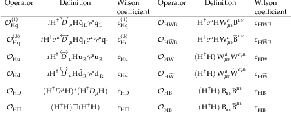
The dimension-six operators in the Warsaw basis affecting VH production at leading order. Here $ {{\mathrm{q}}_{\textrm{L}}} $ refers to a left-handed quark field and is a representation of an SU(2) quark doublets. $ {\mathrm{u}}_{\textrm{R}} $ refers to a right-handed up quark singlet, and $ {\mathrm{d}}_{\textrm{R}} $ a right-handed down quark singlet. |

png pdf |
Table 2:
Selection criteria for the resolved category in the 0-lepton final state. Momenta and masses have units of GeV. |

png pdf |
Table 3:
Selection criteria for the boosted category in the 0-lepton final state. Momenta and masses have units of GeV. |

png pdf |
Table 4:
Selection conditions for the resolved category in the 1-lepton final state. Momenta and masses have units of GeV. |

png pdf |
Table 5:
Selection conditions for the boosted category in the 1-lepton final state. Momenta and masses have units of GeV. |

png pdf |
Table 6:
Selection conditions for the resolved category in the 2-lepton final state. Momenta and masses have units of GeV. |

png pdf |
Table 7:
Selection conditions for the boosted category in the 2-lepton final state. Momenta and masses have units of GeV. |
| Summary |
| A standard model effective field theory (SMEFT) analysis is performed in the Higgs-strahlung process, where the Higgs boson is produced in association with a vector boson (V = W, Z), probing nonresonant new physics effects. Final states with the Higgs boson decaying to a pair of bottom quarks are targeted. Proton-proton collision data collected by the CMS experiment during 2016--2018 at a center-of-mass energy of 13 TeV are used, corresponding to an integrated luminosity of 138 fb$ ^{-1} $. Leptonic decay modes of W and Z bosons ($ \mathrm{W}\to\ell\nu $, $ \mathrm{Z}\to\ell\ell $, and $ \mathrm{Z}\to\nu\nu $) are considered, and both resolved- as well as merged-jet topologies are exploited for the $ \mathrm{H}\to\mathrm{b}\overline{\mathrm{b}} $ decay. A multivariate analysis strategy based on likelihood-free inference methods is adopted for the first time in the CMS experiment to probe the effects of multiple SMEFT operators including those giving rise to CP violation. The strategy employing boosted decision trees makes use of the angular information which is sensitive to the CP structure of SMEFT operators in this final state. Results are consistent with the standard model expectation. Constraints on the Wilson coefficients of six relevant SMEFT operators ($ {c}^{(1)}_{\mathrm{H}\mathrm{q}} $, $ {c}^{(3)}_{\mathrm{H}\mathrm{q}} $, $ {c}_{\mathrm{H}\mathrm{u}} $, $ {c}_{\mathrm{H}\mathrm{d}} $, $ {g}^{\mathrm{Z}\mathrm{Z}}_{2} $, and $ {g}^{\mathrm{Z}\mathrm{Z}}_{4} $) are obtained by performing a simultaneous fit to the data. Constraints on the vector-coupling operators are slightly more stringent than those on the gauge-coupling operators. Lower limits on the energy scales associated with various SMEFT operators are also presented, offering further constraints on different classes of new physics models. Additionally, constraints on two-dimensional planes of Wilson coefficients for all possible pairs are presented to explore correlations between pairs of Wilson coefficients. This constitutes the most comprehensive SMEFT analysis in this channel to date. |
| References | ||||
| 1 | F. Englert and R. Brout | Broken symmetry and the mass of gauge vector mesons | PRL 13 (1964) 321 | |
| 2 | P. W. Higgs | Broken symmetries, massless particles and gauge fields | PL 12 (1964) 132 | |
| 3 | P. W. Higgs | Broken symmetries and the masses of gauge bosons | PRL 13 (1964) 508 | |
| 4 | G. S. Guralnik, C. R. Hagen, and T. W. B. Kibble | Global conservation laws and massless particles | PRL 13 (1964) 585 | |
| 5 | ATLAS Collaboration | Observation of a new particle in the search for the Standard Model Higgs boson with the ATLAS detector at the LHC | PLB 716 (2012) 1 | 1207.7214 |
| 6 | CMS Collaboration | Observation of a new boson at a mass of 125 GeV with the CMS experiment at the LHC | PLB 716 (2012) 30 | CMS-HIG-12-028 1207.7235 |
| 7 | CMS Collaboration | Observation of a new boson with mass near 125 GeV in pp collisions at $ \sqrt{s} = $ 7 and 8 TeV | JHEP 06 (2013) 081 | CMS-HIG-12-036 1303.4571 |
| 8 | ATLAS Collaboration | Observation of $ \rm{H} \rightarrow \mathrm{b}\overline{\mathrm{b}} $ decays and VH production with the ATLAS detector | PLB 786 (2018) 59 | 1808.08238 |
| 9 | CMS Collaboration | Observation of Higgs boson decay to bottom quarks | PRL 121 (2018) 121801 | CMS-HIG-18-016 1808.08242 |
| 10 | ATLAS Collaboration | Measurements of WH and ZH production with Higgs boson decays into bottom quarks and direct constraints on the charm Yukawa coupling in 13 TeV pp collisions with the ATLAS detector | submitted to JHEP, 2024 | 2410.19611 |
| 11 | CMS Collaboration | Measurement of simplified template cross sections of the Higgs boson produced in association with W or Z bosons in the H $ \to \mathrm{b\bar{b}} $ decay channel in proton-proton collisions at $ \sqrt{s} = $ 13 TeV | PRD 109 (2024) 092011 | CMS-HIG-20-001 2312.07562 |
| 12 | W. Buchmuller and D. Wyler | Effective Lagrangian analysis of new interactions and flavor conservation | NPB 268 (1986) 621 | |
| 13 | B. Grinstein and M. B. Wise | Operator analysis for precision electroweak physics | PLB 265 (1991) 326 | |
| 14 | J.-y. Chiu, F. Golf, R. Kelley, and A. V. Manohar | Electroweak corrections in high energy processes using effective field theory | PRD 77 (2008) 053004 | 0712.0396 |
| 15 | C. Degrande et al. | Effective field theory: A modern approach to anomalous couplings | Annals Phys. 335 (2013) 21 | 1205.4231 |
| 16 | E. E. Jenkins, A. V. Manohar, and M. Trott | Renormalization group evolution of the standard model dimension six operators I: formalism and lambda dependence | JHEP 10 (2013) 087 | 1308.2627 |
| 17 | R. Alonso, E. E. Jenkins, A. V. Manohar, and M. Trott | Renormalization group evolution of the standard model dimension six operators III: gauge coupling dependence and phenomenology | JHEP 04 (2014) 159 | 1312.2014 |
| 18 | E. E. Jenkins, A. V. Manohar, and M. Trott | Renormalization group evolution of the standard model dimension six operators II: Yukawa dependence | JHEP 01 (2014) 035 | 1310.4838 |
| 19 | C. Englert and M. Spannowsky | Effective theories and measurements at colliders | PLB 740 (2015) 8 | 1408.5147 |
| 20 | I. Brivio and M. Trott | The standard model as an effective field theory | Phys. Rept. 793 (2019) 1 | 1706.08945 |
| 21 | G. Isidori, F. Wilsch, and D. Wyler | The standard model effective field theory at work | Rev. Mod. Phys. 96 (2024) 015006 | 2303.16922 |
| 22 | CMS Collaboration | Constraints on anomalous Higgs boson couplings to vector bosons and fermions in its production and decay using the four-lepton final state | PRD 104 (2021) 052004 | CMS-HIG-19-009 2104.12152 |
| 23 | CMS Collaboration | Constraints on anomalous Higgs boson couplings from its production and decay using the WW channel in proton-proton collisions at $ \sqrt{s} = $ 13 TeV | EPJC 84 (2024) 779 | CMS-HIG-22-008 2403.00657 |
| 24 | CMS Collaboration | Constraints on anomalous Higgs boson couplings to vector bosons and fermions from the production of Higgs bosons using the $ \tau\tau $ final state | PRD 108 (2023) 032013 | CMS-HIG-20-007 2205.05120 |
| 25 | Y. Gao et al. | Spin determination of single-produced resonances at hadron colliders | PRD 81 (2010) 075022 | 1001.3396 |
| 26 | S. Bolognesi et al. | On the spin and parity of a single-produced resonance at the LHC | PRD 86 (2012) 095031 | 1208.4018 |
| 27 | I. Anderson et al. | Constraining anomalous HVV interactions at proton and lepton colliders | PRD 89 (2014) 035007 | 1309.4819 |
| 28 | ATLAS Collaboration | Measurement of VH, $ \mathrm{H}\to \mathrm{b}\overline{\mathrm{b}} $ production as a function of the vector-boson transverse momentum in 13 TeV pp collisions with the ATLAS detector | JHEP 05 (2019) 141 | 1903.04618 |
| 29 | ATLAS Collaboration | Measurements of WH and ZH production in the $ \rm{H} \rightarrow \mathrm{b}\overline{\mathrm{b}} $ decay channel in pp collisions at 13 TeV with the ATLAS detector | EPJC 81 (2021) 178 | 2007.02873 |
| 30 | CMS Collaboration | Combined Higgs boson production and decay measurements with up to 137 fb$ ^{-1} $ of proton-proton collision data at $ \sqrt{s} = $ 13 TeV | CMS Physics Analysis Summary, 2020 CMS-PAS-HIG-19-005 |
CMS-PAS-HIG-19-005 |
| 31 | J. Ellis et al. | Top, higgs, diboson and electroweak fit to the standard model effective field theory | JHEP 04 (2021) 279 | 2012.02779 |
| 32 | SMEFiT Collaboration | Combined SMEFT interpretation of Higgs, diboson, and top quark data from the LHC | JHEP 11 (2021) 089 | 2105.00006 |
| 33 | CMS Collaboration | HEPData record for this analysis | link | |
| 34 | S. Weinberg | Baryon- and lepton-nonconserving processes | PRL 43 (1979) 1566 | |
| 35 | B. Grzadkowski, M. Iskrzynski, M. Misiak, and J. Rosiek | Dimension-six terms in the standard model Lagrangian | JHEP 10 (2010) 085 | 1008.4884 |
| 36 | A. Falkowski and F. Riva | Model-independent precision constraints on dimension-6 operators | JHEP 02 (2015) 039 | 1411.0669 |
| 37 | S. Banerjee, C. Englert, R. S. Gupta, and M. Spannowsky | Probing electroweak precision physics via boosted Higgs-strahlung at the LHC | PRD 98 (2018) 095012 | 1807.01796 |
| 38 | S. Banerjee et al. | Towards the ultimate differential SMEFT analysis | JHEP 09 (2020) 170 | 1912.07628 |
| 39 | J. Brehmer, K. Cranmer, G. Louppe, and J. Pavez | Constraining effective field theories with machine learning | PRL 121 (2018) 111801 | 1805.00013 |
| 40 | J. Brehmer, G. Louppe, J. Pavez, and K. Cranmer | Mining gold from implicit models to improve likelihood-free inference | Proc. Nat. Acad. Sci. 117 (2020) 5242 | 1805.12244 |
| 41 | S. Chen, A. Glioti, G. Panico, and A. Wulzer | Parametrized classifiers for optimal EFT sensitivity | JHEP 05 (2021) 247 | 2007.10356 |
| 42 | S. Chatterjee et al. | Tree boosting for learning EFT parameters | Comput. Phys. Commun. 277 (2022) 108385 | 2107.10859 |
| 43 | S. Chatterjee, S. Rohshap, R. Schöfbeck, and D. Schwarz | Learning the EFT likelihood with tree boosting | 2205.12976 | |
| 44 | R. Gomez Ambrosio et al. | Unbinned multivariate observables for global SMEFT analyses from machine learning | JHEP 03 (2023) 033 | 2211.02058 |
| 45 | LHC Higgs Cross Section Working Group | Handbook of LHC Higgs cross sections: 4. Deciphering the nature of the Higgs sector | CERN Report CERN-2017-002-M, 2016 link |
1610.07922 |
| 46 | J. Davis et al. | Constraining anomalous Higgs boson couplings to virtual photons | PRD 105 (2022) 096027 | 2109.13363 |
| 47 | A. Rossia, M. Thomas, and E. Vryonidou | Diboson production in the SMEFT from gluon fusion | JHEP 11 (2023) 132 | 2306.09963 |
| 48 | CMS Collaboration | The CMS experiment at the CERN LHC | JINST 3 (2008) S08004 | |
| 49 | CMS Collaboration | Development of the CMS detector for the CERN LHC Run 3 | JINST 19 (2024) P05064 | CMS-PRF-21-001 2309.05466 |
| 50 | CMS Collaboration | Description and performance of track and primary-vertex reconstruction with the CMS tracker | JINST 9 (2014) P10009 | CMS-TRK-11-001 1405.6569 |
| 51 | CMS Tracker Group | The CMS phase-1 pixel detector upgrade | JINST 16 (2021) P02027 | 2012.14304 |
| 52 | CMS Collaboration | Track impact parameter resolution for the full pseudo rapidity coverage in the 2017 dataset with the CMS phase-1 pixel detector | CMS Detector Performance Summary CMS-DP-2020-049, 2020 CDS |
|
| 53 | CMS Collaboration | Particle-flow reconstruction and global event description with the CMS detector | JINST 12 (2017) P10003 | CMS-PRF-14-001 1706.04965 |
| 54 | CMS Collaboration | Performance of the CMS Level-1 trigger in proton-proton collisions at $ \sqrt{s} = $ 13 TeV | JINST 15 (2020) P10017 | CMS-TRG-17-001 2006.10165 |
| 55 | CMS Collaboration | The CMS trigger system | JINST 12 (2017) P01020 | CMS-TRG-12-001 1609.02366 |
| 56 | CMS Collaboration | Performance of the CMS muon trigger system in proton-proton collisions at 13 TeV | JINST 16 (2021) P07001 | CMS-MUO-19-001 2102.04790 |
| 57 | P. Nason | A New method for combining NLO QCD with shower Monte Carlo algorithms | JHEP 11 (2004) 040 | hep-ph/0409146 |
| 58 | S. Frixione, P. Nason, and C. Oleari | Matching NLO QCD computations with parton shower simulations: the POWHEG method | JHEP 11 (2007) 070 | 0709.2092 |
| 59 | S. Alioli, P. Nason, C. Oleari, and E. Re | A general framework for implementing NLO calculations in shower Monte Carlo programs: the POWHEG BOX | JHEP 06 (2010) 043 | 1002.2581 |
| 60 | S. Frixione, P. Nason, and G. Ridolfi | A positive-weight next-to-leading-order Monte Carlo for heavy flavour hadroproduction | JHEP 09 (2007) 126 | 0707.3088 |
| 61 | M. Czakon and A. Mitov | Top++: a program for the calculation of the top-pair cross-section at hadron colliders | Comput. Phys. Commun. 185 (2014) 2930 | 1112.5675 |
| 62 | R. Frederix, E. Re, and P. Torrielli | Single-top $ t $-channel hadroproduction in the four-flavour scheme with POWHEG and aMC@NLO | JHEP 09 (2012) 130 | 1207.5391 |
| 63 | E. Re | Single-top $ \rm Wt $-channel production matched with parton showers using the POWHEG method | EPJC 71 (2011) 1547 | 1009.2450 |
| 64 | J. Alwall et al. | The automated computation of tree-level and next-to-leading order differential cross sections, and their matching to parton shower simulations | JHEP 07 (2014) 079 | 1405.0301 |
| 65 | P. Artoisenet, R. Frederix, O. Mattelaer, and R. Rietkerk | Automatic spin-entangled decays of heavy resonances in Monte Carlo simulations | JHEP 03 (2013) 015 | 1212.3460 |
| 66 | J. Alwall et al. | Comparative study of various algorithms for the merging of parton showers and matrix elements in hadronic collisions | EPJC 53 (2008) 473 | 0706.2569 |
| 67 | R. Frederix and S. Frixione | Merging meets matching in MC@NLO | JHEP 12 (2012) 061 | 1209.6215 |
| 68 | A. Belvedere et al. | LHC EFT WG Note: SMEFT predictions, event reweighting, and simulation | CERN Report CERN-LHCEFTWG-2024-001, 2024 link |
2406.14620 |
| 69 | K. Hamilton, P. Nason, and G. Zanderighi | MINLO: multi-scale improved NLO | JHEP 10 (2012) 155 | 1206.3572 |
| 70 | G. Luisoni, P. Nason, C. Oleari, and F. Tramontano | HW/HZ + 0 and 1 jet at NLO with the POWHEG BOX interfaced to GoSam and their merging within MiNLO | JHEP 10 (2013) 083 | 1306.2542 |
| 71 | I. Brivio, Y. Jiang, and M. Trott | The SMEFTsim package, theory and tools | JHEP 12 (2017) 070 | 1709.06492 |
| 72 | I. Brivio | SMEFTsim 3.0 -- a practical guide | JHEP 04 (2021) 073 | 2012.11343 |
| 73 | I. Brivio, T. Corbett, and M. Trott | The Higgs width in the SMEFT | JHEP 10 (2019) 056 | 1906.06949 |
| 74 | P. Artoisenet and O. Mattelaer | MadWeight: automatic event reweighting with matrix elements | in Proc. 2nd International Workshop on Prospects for Charged Higgs Discovery at Colliders, T. Ekelof and J. Rathsman, eds, 2008 CHARGED 200 (2008) 025 |
|
| 75 | NNPDF Collaboration | Parton distributions from high-precision collider data | EPJC 77 (2017) 663 | 1706.00428 |
| 76 | CMS Collaboration | Extraction and validation of a new set of CMS PYTHIA8 tunes from underlying-event measurements | EPJC 80 (2020) 4 | CMS-GEN-17-001 1903.12179 |
| 77 | CMS Collaboration | Measurement of the inelastic proton-proton cross section at $ \sqrt{s}= $ 13 TeV | JHEP 07 (2018) 161 | CMS-FSQ-15-005 1802.02613 |
| 78 | GEANT4 Collaboration | GEANT 4---a simulation toolkit | NIM A 506 (2003) 250 | |
| 79 | CMS Collaboration | Technical proposal for the Phase-II upgrade of the Compact Muon Solenoid | CMS Technical Proposal CERN-LHCC-2015-010, CMS-TDR-15-02, 2015 CDS |
|
| 80 | CMS Collaboration | Electron and photon reconstruction and identification with the CMS experiment at the CERN LHC | JINST 16 (2021) P05014 | CMS-EGM-17-001 2012.06888 |
| 81 | CMS Collaboration | ECAL 2016 refined calibration and Run2 summary plots | CMS Detector Performance Summary CMS-DP-2020-021, 2020 CDS |
|
| 82 | CMS Collaboration | Performance of the CMS muon detector and muon reconstruction with proton-proton collisions at $ \sqrt{s}= $ 13 TeV | JINST 13 (2018) P06015 | CMS-MUO-16-001 1804.04528 |
| 83 | M. Cacciari, G. P. Salam, and G. Soyez | The anti-$ k_{\mathrm{T}} $ jet clustering algorithm | JHEP 04 (2008) 063 | 0802.1189 |
| 84 | M. Cacciari, G. P. Salam, and G. Soyez | FastJet user manual | EPJC 72 (2012) 1896 | 1111.6097 |
| 85 | CMS Collaboration | Jet energy scale and resolution measurement with Run 2 legacy data collected by CMS at 13 TeV | CMS Detector Performance Summary CMS-DP-2021-033, 2021 CDS |
|
| 86 | M. Cacciari and G. P. Salam | Pileup subtraction using jet areas | PLB 659 (2008) 119 | 0707.1378 |
| 87 | CMS Collaboration | Jet energy scale and resolution in the CMS experiment in pp collisions at 8 TeV | JINST 12 (2017) P02014 | CMS-JME-13-004 1607.03663 |
| 88 | D. Bertolini, P. Harris, M. Low, and N. Tran | Pileup per particle identification | JHEP 10 (2014) 059 | 1407.6013 |
| 89 | CMS Collaboration | Pileup mitigation at CMS in 13 TeV data | JINST 15 (2020) P09018 | CMS-JME-18-001 2003.00503 |
| 90 | CMS Collaboration | Jet algorithms performance in 13 TeV data | CMS Physics Analysis Summary, 2017 CMS-PAS-JME-16-003 |
CMS-PAS-JME-16-003 |
| 91 | E. Bols et al. | Jet flavour classification using DeepJet | JINST 15 (2020) P12012 | 2008.10519 |
| 92 | CMS Collaboration | Performance summary of AK4 jet b tagging with data from proton-proton collisions at 13 TeV | CMS Detector Performance Report CMS-DP-2023-005, 2023 CDS |
|
| 93 | CMS Collaboration | A deep neural network for simultaneous estimation of b jet energy and resolution | Comput. Softw. Big Sci. 4 (2020) 10 | CMS-HIG-18-027 1912.06046 |
| 94 | H. Qu and L. Gouskos | Jet tagging via particle clouds | PRD 101 (2020) 056019 | 1902.08570 |
| 95 | J. M. Butterworth, A. R. Davison, M. Rubin, and G. P. Salam | Jet substructure as a new Higgs search channel at the LHC | PRL 100 (2008) 242001 | 0802.2470 |
| 96 | M. Dasgupta, A. Fregoso, S. Marzani, and G. P. Salam | Towards an understanding of jet substructure | JHEP 09 (2013) 029 | 1307.0007 |
| 97 | A. J. Larkoski, S. Marzani, G. Soyez, and J. Thaler | Soft Drop | JHEP 05 (2014) 146 | 1402.2657 |
| 98 | Y. L. Dokshitzer, G. D. Leder, S. Moretti, and B. R. Webber | Better jet clustering algorithms | JHEP 08 (1997) 001 | hep-ph/9707323 |
| 99 | M. Wobisch and T. Wengler | Hadronization corrections to jet cross-sections in deep inelastic scattering | in Workshop on Monte Carlo Generators for HERA Physics, Hamburg, Germany, 1998 link |
hep-ph/9907280 |
| 100 | CMS Collaboration | Identification of highly Lorentz-boosted heavy particles using graph neural networks and new mass decorrelation techniques | CMS Detector Performance Report CMS-DP-2020-002, 2020 CDS |
|
| 101 | CMS Collaboration | Calibration of the mass-decorrelated ParticleNet tagger for boosted $ \mathrm{b}\bar{\mathrm{b}} $ and $ \mathrm{c}\bar{\mathrm{c}} $ jets using LHC Run 2 data | CMS Detector Performance Report CMS-DP-2022-005, 2022 CDS |
|
| 102 | CMS Collaboration | Performance of heavy-flavour jet identification in boosted topologies in proton-proton collisions at $ \sqrt{s} = $ 13 TeV | CMS Physics Analysis Summary, 2023 CMS-PAS-BTV-22-001 |
CMS-PAS-BTV-22-001 |
| 103 | CMS Collaboration | Performance of missing transverse momentum reconstruction in proton-proton collisions at $ \sqrt{s} = $ 13 TeV using the CMS detector | JINST 14 (2019) P07004 | CMS-JME-17-001 1903.06078 |
| 104 | CMS Collaboration | Performance of Track-Corrected Missing Transverse Energy in CMS | CMS Physics Analysis Summary, 2009 CMS-PAS-JME-09-010 |
|
| 105 | Particle Data Group , R. L. Workman et al. | Review of particle physics | Prog. Theor. Exp. Phys. 2022 (2022) 083C01 | |
| 106 | J. Brehmer, K. Cranmer, G. Louppe, and J. Pavez | A guide to constraining effective field theories with machine learning | PRD 98 (2018) 052004 | 1805.00020 |
| 107 | G. Ke et al. | LightGBM: A highly efficient gradient boosting decision tree | in Advances in Neural Information Processing Systems 30 (NIPS 2017), I. Guyon et al. eds., Curran Associates, 2017 link |
|
| 108 | P. I. Frazier | A tutorial on Bayesian optimization | 1807.02811 | |
| 109 | J. Butterworth et al. | PDF4LHC recommendations for LHC run II | JPG 43 (2016) 040 | 1510.03865 |
| 110 | CMS Collaboration | Precision luminosity measurement in proton-proton collisions at $ \sqrt{s} = $ 13 TeV in 2015 and 2016 at CMS | EPJC 81 (2021) 800 | CMS-LUM-17-003 2104.01927 |
| 111 | CMS Collaboration | CMS luminosity measurement for the 2017 data-taking period at $ \sqrt{s} = $ 13 TeV | CMS Physics Analysis Summary, 2018 CMS-PAS-LUM-17-004 |
CMS-PAS-LUM-17-004 |
| 112 | CMS Collaboration | CMS luminosity measurement for the 2018 data-taking period at $ \sqrt{s} = $ 13 TeV | CMS Physics Analysis Summary, 2019 CMS-PAS-LUM-18-002 |
CMS-PAS-LUM-18-002 |
| 113 | R. Barlow and C. Beeston | Fitting using finite Monte Carlo samples | Comput. Phys. Commun. 77 (1993) 219 | |
| 114 | CMS Collaboration | The CMS statistical analysis and combination tool: COMBINE | Comput. Softw. Big Sci. 8 (2024) 19 | CMS-CAT-23-001 2404.06614 |
| 115 | W. Verkerke and D. P. Kirkby | The RooFit toolkit for data modeling | in Proc. Int. Conf. on Computing in High Energy and Nuclear Physics (CHEP03), L. Lyons and M. Karagoz, eds., 2003 | physics/0306116 |
| 116 | L. Moneta et al. | The RooStats project | in Proc. 13th Int. Workshop on Advanced Computing and Analysis Techniques in Physics Research, T. Speer et al., eds., volume ACAT, 2010 link |
1009.1003 |
| 117 | ATLAS and CMS Collaborations, and LHC Higgs Combination Group | Procedure for the LHC Higgs boson search combination in Summer 2011 | CMS Note CMS-NOTE-2011-005, ATL-PHYS-PUB-2011-11, 2011 | |
| 118 | T. Junk | Confidence level computation for combining searches with small statistics | NIM A 434 (1999) 435 | hep-ex/9902006 |
| 119 | A. L. Read | Presentation of search results: The CL$ _{\text{s}} $ technique | JPG 28 (2002) 2693 | |
| 120 | R. D. Cousins | Lectures on statistics in theory: Prelude to statistics in practice | 1807.05996 | |
| 121 | F. U. Bernlochner, D. C. Fry, S. B. Menary, and E. Persson | Cover your bases: asymptotic distributions of the profile likelihood ratio when constraining effective field theories in high-energy physics | SciPost Phys. Core 6 (2023) 013 | 2207.01350 |
| 122 | S. S. Wilks | The Large-Sample Distribution of the Likelihood Ratio for Testing Composite Hypotheses | The Ann. Math. Stat. 9 (1938) 60 | |

|
Compact Muon Solenoid LHC, CERN |

|

|

|

|

|

|