

Compact Muon Solenoid
LHC, CERN
| CMS-TRG-19-001 ; CERN-EP-2024-259 | ||
| Performance of the CMS high-level trigger during LHC Run 2 | ||
| CMS Collaboration | ||
| 22 October 2024 | ||
| JINST 19 (2024) P11021 | ||
| Abstract: The CERN LHC provided proton and heavy ion collisions during its Run 2 operation period from 2015 to 2018. Proton-proton collisions reached a peak instantaneous luminosity of 2.1 $ \times $ 10$^{34}$ cm$^{-2}$s$^{-1} $, twice the initial design value, at $ \sqrt{s}= $ 13 TeV. The CMS experiment records a subset of the collisions for further processing as part of its online selection of data for physics analyses, using a two-level trigger system: the Level-1 trigger, implemented in custom-designed electronics, and the high-level trigger, a streamlined version of the offline reconstruction software running on a large computer farm. This paper presents the performance of the CMS high-level trigger system during LHC Run 2 for physics objects, such as leptons, jets, and missing transverse momentum, which meet the broad needs of the CMS physics program and the challenge of the evolving LHC and detector conditions. Sophisticated algorithms that were originally used in offline reconstruction were deployed online. Highlights include a machine-learning b tagging algorithm and a reconstruction algorithm for tau leptons that decay hadronically. | ||
| Links: e-print arXiv:2410.17038 [hep-ex] (PDF) ; CDS record ; inSPIRE record ; CADI line (restricted) ; | ||
| Figures | |
png pdf |
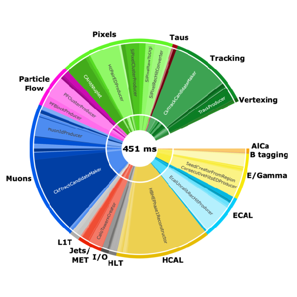
Figure 1:
Pie chart distribution of the CPU time per event spent by the HLT for different parts of the event reconstruction. Reconstruction modules and filters are grouped by detector and physics object (outermost ring and similarly colored groupings). The middle ring reports the names of specific C++ classes in CMSSW used in the HLT reconstruction, and the various slices in the innermost ring refer to different instances (modules) of that given C++ class in the HLT menu. The empty slice indicates the time spent outside of the individual algorithms. |
png pdf |
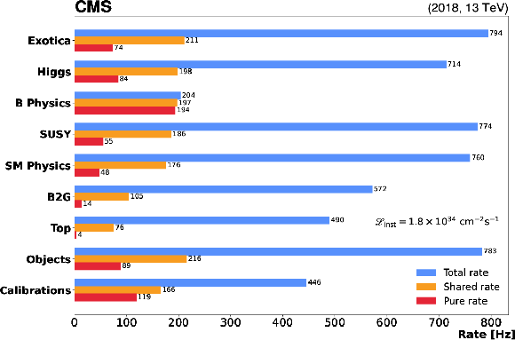
Figure 2:
The HLT rate consumption by physics group in the standard physics streams for a Run 2 menu deployed in September 2018. The ``Total Rate'' is the inclusive rate of all triggers owned by a group, and the ``Pure Rate'' is the exclusive rate of all triggers unique to that group. The ``Shared Rate'' is the rate calculated by dividing the rate of each trigger equally among all physics groups that use it, before summing the total group rate. It includes the Pure Rate of that physics group. The topic coverage of each group is discussed in the text. |
png pdf |
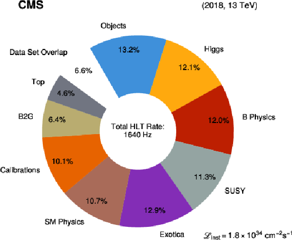
Figure 3:
Share of the total HLT rate that each physics group contributes. ``Data Set Overlap'' refers to the events that are duplicated and saved into separate data sets for analysis and offline processing convenience, but which must be reconstructed separately offline. |
png pdf |
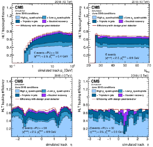
Figure 4:
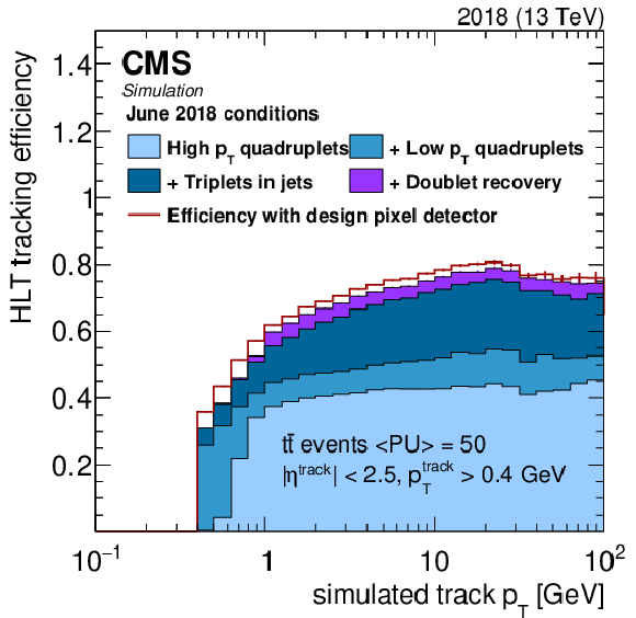
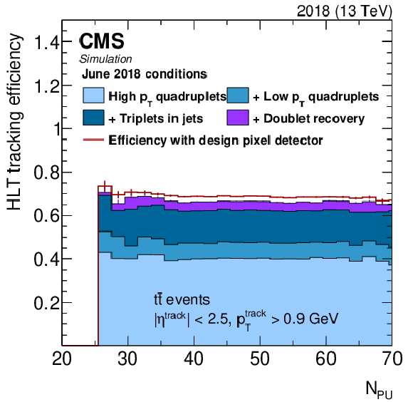
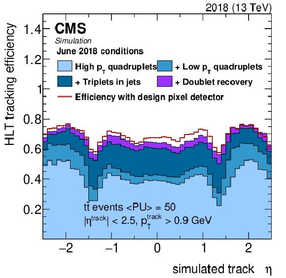
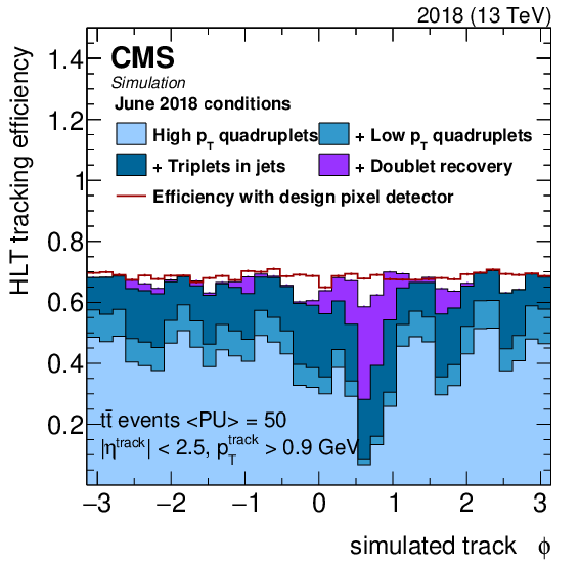
Tracking efficiency as a function of simulated track $ p_{\mathrm{T}} $ (upper left), $ N_{\text{PU}} $ (upper right), $ \eta $ (lower left), and $ \phi $ (lower right). The contributions to the total efficiency from the different tracking iterations are shown in different colors. The initial three iterations are shown in shades of blue, and the contribution of the doublet recovery iteration is shown in violet. The simulation includes a map of inactive modules representing the status of the real detector as of June 2018. The performance that would be achieved with no inactive pixel detector modules and no doublet recovery iteration (design pixel detector) is shown as a red line. Details of the observed features are discussed in the text. |
png pdf |
Figure 4-a:
Tracking efficiency as a function of simulated track $ p_{\mathrm{T}} $ (upper left), $ N_{\text{PU}} $ (upper right), $ \eta $ (lower left), and $ \phi $ (lower right). The contributions to the total efficiency from the different tracking iterations are shown in different colors. The initial three iterations are shown in shades of blue, and the contribution of the doublet recovery iteration is shown in violet. The simulation includes a map of inactive modules representing the status of the real detector as of June 2018. The performance that would be achieved with no inactive pixel detector modules and no doublet recovery iteration (design pixel detector) is shown as a red line. Details of the observed features are discussed in the text. |
png pdf |
Figure 4-b:
Tracking efficiency as a function of simulated track $ p_{\mathrm{T}} $ (upper left), $ N_{\text{PU}} $ (upper right), $ \eta $ (lower left), and $ \phi $ (lower right). The contributions to the total efficiency from the different tracking iterations are shown in different colors. The initial three iterations are shown in shades of blue, and the contribution of the doublet recovery iteration is shown in violet. The simulation includes a map of inactive modules representing the status of the real detector as of June 2018. The performance that would be achieved with no inactive pixel detector modules and no doublet recovery iteration (design pixel detector) is shown as a red line. Details of the observed features are discussed in the text. |
png pdf |
Figure 4-c:
Tracking efficiency as a function of simulated track $ p_{\mathrm{T}} $ (upper left), $ N_{\text{PU}} $ (upper right), $ \eta $ (lower left), and $ \phi $ (lower right). The contributions to the total efficiency from the different tracking iterations are shown in different colors. The initial three iterations are shown in shades of blue, and the contribution of the doublet recovery iteration is shown in violet. The simulation includes a map of inactive modules representing the status of the real detector as of June 2018. The performance that would be achieved with no inactive pixel detector modules and no doublet recovery iteration (design pixel detector) is shown as a red line. Details of the observed features are discussed in the text. |
png pdf |
Figure 4-d:
Tracking efficiency as a function of simulated track $ p_{\mathrm{T}} $ (upper left), $ N_{\text{PU}} $ (upper right), $ \eta $ (lower left), and $ \phi $ (lower right). The contributions to the total efficiency from the different tracking iterations are shown in different colors. The initial three iterations are shown in shades of blue, and the contribution of the doublet recovery iteration is shown in violet. The simulation includes a map of inactive modules representing the status of the real detector as of June 2018. The performance that would be achieved with no inactive pixel detector modules and no doublet recovery iteration (design pixel detector) is shown as a red line. Details of the observed features are discussed in the text. |
png pdf |
Figure 5:
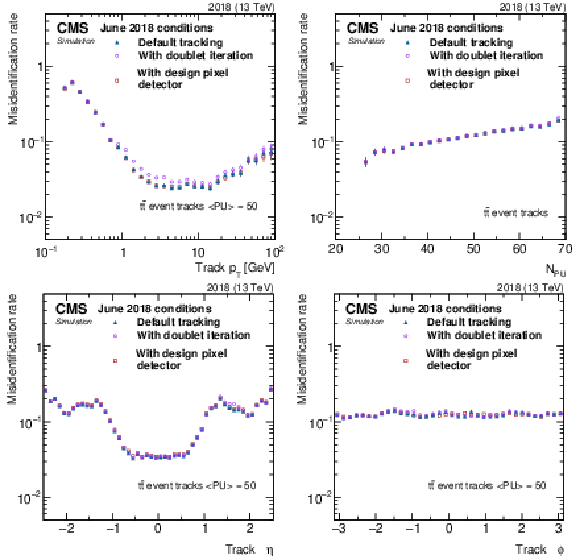
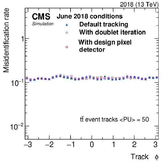
Tracking misidentification rate as a function of track $ p_{\mathrm{T}} $ (upper left), $ N_{\text{PU}} $ (upper right), $ \eta $ (lower left), and $ \phi $ (lower right). No selection on track kinematics is applied. The misidentification rate for the first three iterations (default tracking) is shown in dark blue triangles, whereas the misidentification rate after including the doublet recovery iteration is shown in violet circles. The simulation includes a map of inactive modules representing the status of the real detector as of June 2018. The misidentification rate that would be observed with no inactive pixel detector modules and no doublet recovery iteration (design pixel detector) is shown in dark red squares. |
png pdf |
Figure 5-a:
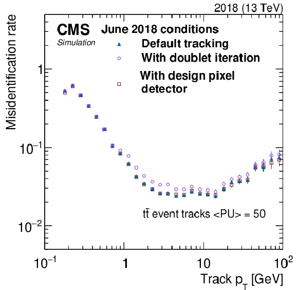
Tracking misidentification rate as a function of track $ p_{\mathrm{T}} $ (upper left), $ N_{\text{PU}} $ (upper right), $ \eta $ (lower left), and $ \phi $ (lower right). No selection on track kinematics is applied. The misidentification rate for the first three iterations (default tracking) is shown in dark blue triangles, whereas the misidentification rate after including the doublet recovery iteration is shown in violet circles. The simulation includes a map of inactive modules representing the status of the real detector as of June 2018. The misidentification rate that would be observed with no inactive pixel detector modules and no doublet recovery iteration (design pixel detector) is shown in dark red squares. |
png pdf |
Figure 5-b:
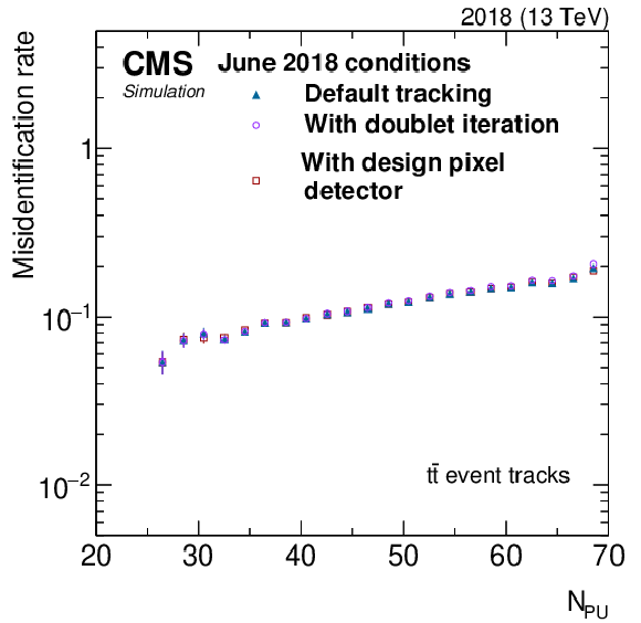
Tracking misidentification rate as a function of track $ p_{\mathrm{T}} $ (upper left), $ N_{\text{PU}} $ (upper right), $ \eta $ (lower left), and $ \phi $ (lower right). No selection on track kinematics is applied. The misidentification rate for the first three iterations (default tracking) is shown in dark blue triangles, whereas the misidentification rate after including the doublet recovery iteration is shown in violet circles. The simulation includes a map of inactive modules representing the status of the real detector as of June 2018. The misidentification rate that would be observed with no inactive pixel detector modules and no doublet recovery iteration (design pixel detector) is shown in dark red squares. |
png pdf |
Figure 5-c:
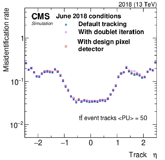
Tracking misidentification rate as a function of track $ p_{\mathrm{T}} $ (upper left), $ N_{\text{PU}} $ (upper right), $ \eta $ (lower left), and $ \phi $ (lower right). No selection on track kinematics is applied. The misidentification rate for the first three iterations (default tracking) is shown in dark blue triangles, whereas the misidentification rate after including the doublet recovery iteration is shown in violet circles. The simulation includes a map of inactive modules representing the status of the real detector as of June 2018. The misidentification rate that would be observed with no inactive pixel detector modules and no doublet recovery iteration (design pixel detector) is shown in dark red squares. |
png pdf |
Figure 5-d:
Tracking misidentification rate as a function of track $ p_{\mathrm{T}} $ (upper left), $ N_{\text{PU}} $ (upper right), $ \eta $ (lower left), and $ \phi $ (lower right). No selection on track kinematics is applied. The misidentification rate for the first three iterations (default tracking) is shown in dark blue triangles, whereas the misidentification rate after including the doublet recovery iteration is shown in violet circles. The simulation includes a map of inactive modules representing the status of the real detector as of June 2018. The misidentification rate that would be observed with no inactive pixel detector modules and no doublet recovery iteration (design pixel detector) is shown in dark red squares. |
png pdf |
Figure 6:
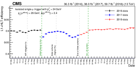
Evolution of the isolated single-muon trigger efficiency with $ p_{\mathrm{T}} > $ 24 GeV as a function of data-taking dates during the Run 2 period from 2016 to 2018. Each point is the efficiency measured using the data with an integrated luminosity of about 3 fb$ ^{-1} $. Dashed lines show the changes in the LHC or CMS conditions that could have an impact on the trigger performance, such as the fix for the degradation of the inner tracker as a result of heavily ionizing particles (``HIP mitigation fix'') or the change in the filling scheme for pp collisions at the LHC (``8b4e scheme'') that led to higher PU in CMS until the end of 2017. The change of the reconstruction algorithm for L3 muons are presented as green dotted lines, including the replacement of cascade or tracker muon algorithm to the iterative algorithm (``Change to iter. L3'') and the update of the iterative algorithm to overcome the limitations observed in 2017 (``Iter. L3 update''). |
png pdf |
Figure 7:
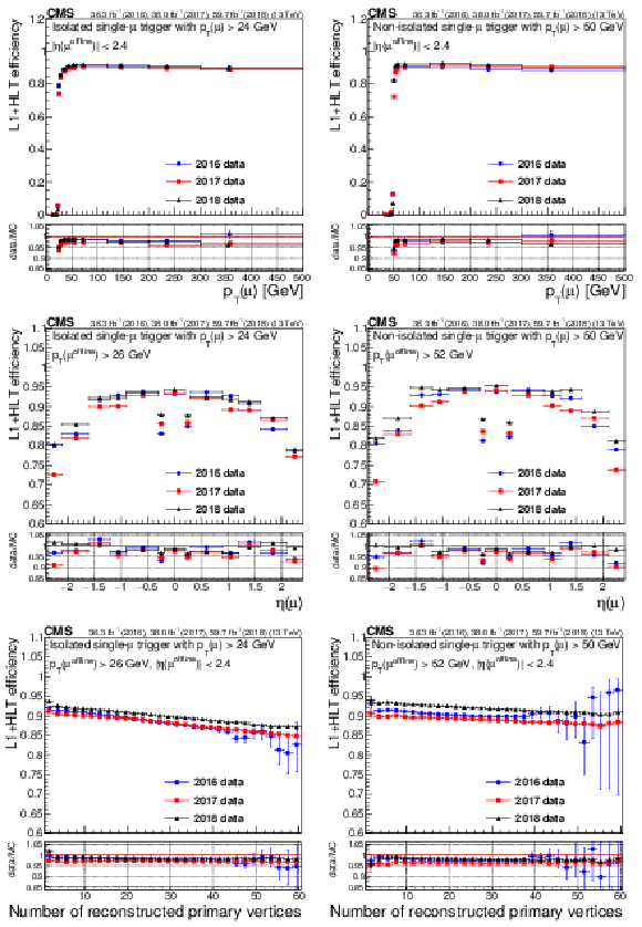
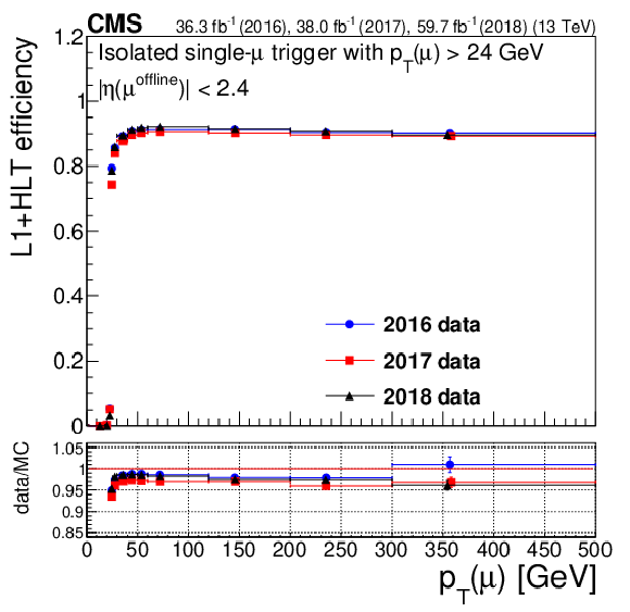
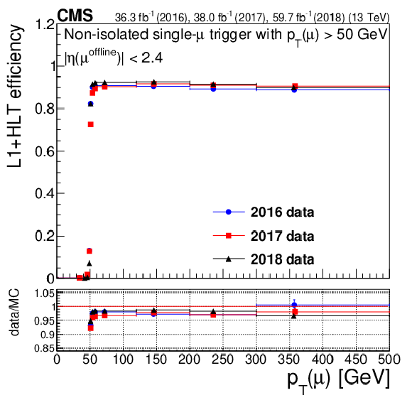
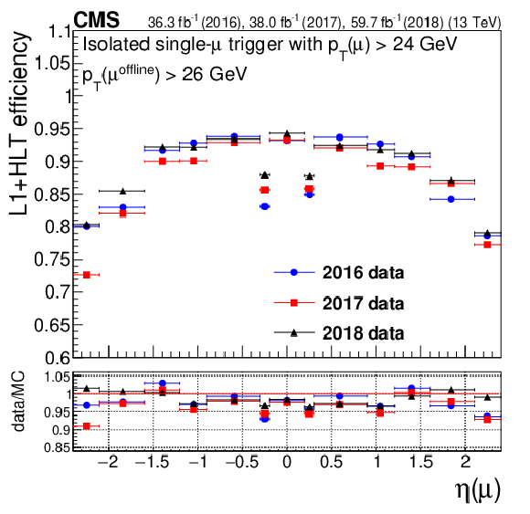
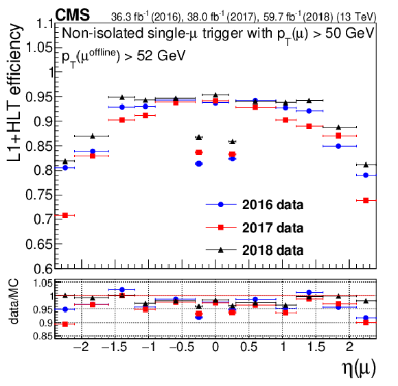
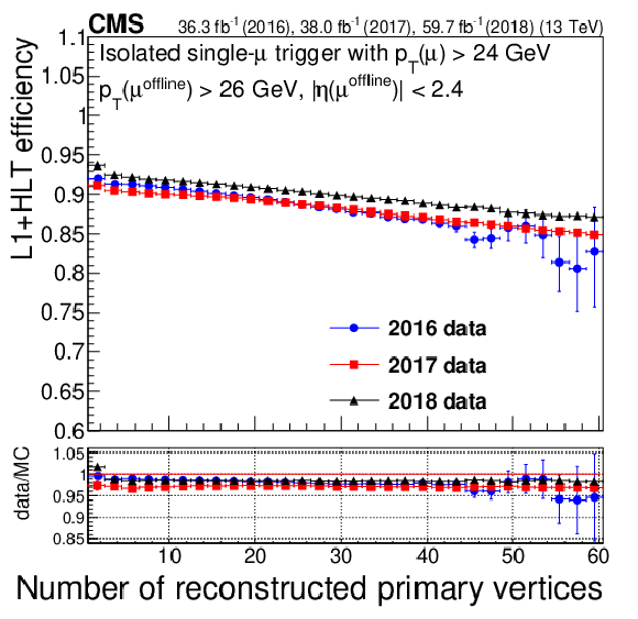
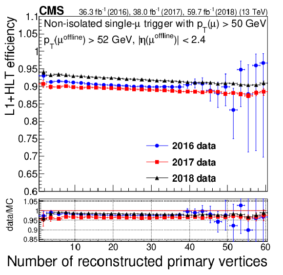
Trigger efficiencies for the isolated single-muon trigger with $ p_{\mathrm{T}} > $ 24 GeV (left column) and the nonisolated single-muon trigger with $ p_{\mathrm{T}} > $ 50 GeV (right column), as functions of muon $ p_{\mathrm{T}} $ (upper row), $ \eta $ (middle row), and $ N_{\text{vtx}} $ (lower row). The lower panel of each plot shows the ratio of data to MC simulation The vertical bars on the markers represent statistical uncertainties. |
png pdf |
Figure 7-a:
Trigger efficiencies for the isolated single-muon trigger with $ p_{\mathrm{T}} > $ 24 GeV (left column) and the nonisolated single-muon trigger with $ p_{\mathrm{T}} > $ 50 GeV (right column), as functions of muon $ p_{\mathrm{T}} $ (upper row), $ \eta $ (middle row), and $ N_{\text{vtx}} $ (lower row). The lower panel of each plot shows the ratio of data to MC simulation The vertical bars on the markers represent statistical uncertainties. |
png pdf |
Figure 7-b:
Trigger efficiencies for the isolated single-muon trigger with $ p_{\mathrm{T}} > $ 24 GeV (left column) and the nonisolated single-muon trigger with $ p_{\mathrm{T}} > $ 50 GeV (right column), as functions of muon $ p_{\mathrm{T}} $ (upper row), $ \eta $ (middle row), and $ N_{\text{vtx}} $ (lower row). The lower panel of each plot shows the ratio of data to MC simulation The vertical bars on the markers represent statistical uncertainties. |
png pdf |
Figure 7-c:
Trigger efficiencies for the isolated single-muon trigger with $ p_{\mathrm{T}} > $ 24 GeV (left column) and the nonisolated single-muon trigger with $ p_{\mathrm{T}} > $ 50 GeV (right column), as functions of muon $ p_{\mathrm{T}} $ (upper row), $ \eta $ (middle row), and $ N_{\text{vtx}} $ (lower row). The lower panel of each plot shows the ratio of data to MC simulation The vertical bars on the markers represent statistical uncertainties. |
png pdf |
Figure 7-d:
Trigger efficiencies for the isolated single-muon trigger with $ p_{\mathrm{T}} > $ 24 GeV (left column) and the nonisolated single-muon trigger with $ p_{\mathrm{T}} > $ 50 GeV (right column), as functions of muon $ p_{\mathrm{T}} $ (upper row), $ \eta $ (middle row), and $ N_{\text{vtx}} $ (lower row). The lower panel of each plot shows the ratio of data to MC simulation The vertical bars on the markers represent statistical uncertainties. |
png pdf |
Figure 7-e:
Trigger efficiencies for the isolated single-muon trigger with $ p_{\mathrm{T}} > $ 24 GeV (left column) and the nonisolated single-muon trigger with $ p_{\mathrm{T}} > $ 50 GeV (right column), as functions of muon $ p_{\mathrm{T}} $ (upper row), $ \eta $ (middle row), and $ N_{\text{vtx}} $ (lower row). The lower panel of each plot shows the ratio of data to MC simulation The vertical bars on the markers represent statistical uncertainties. |
png pdf |
Figure 7-f:
Trigger efficiencies for the isolated single-muon trigger with $ p_{\mathrm{T}} > $ 24 GeV (left column) and the nonisolated single-muon trigger with $ p_{\mathrm{T}} > $ 50 GeV (right column), as functions of muon $ p_{\mathrm{T}} $ (upper row), $ \eta $ (middle row), and $ N_{\text{vtx}} $ (lower row). The lower panel of each plot shows the ratio of data to MC simulation The vertical bars on the markers represent statistical uncertainties. |
png pdf |
Figure 8:
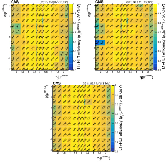
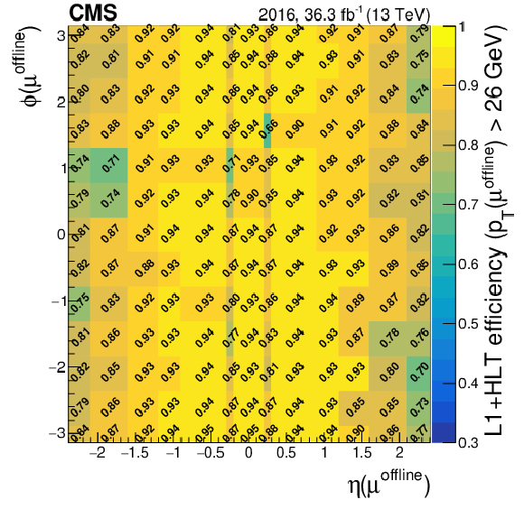
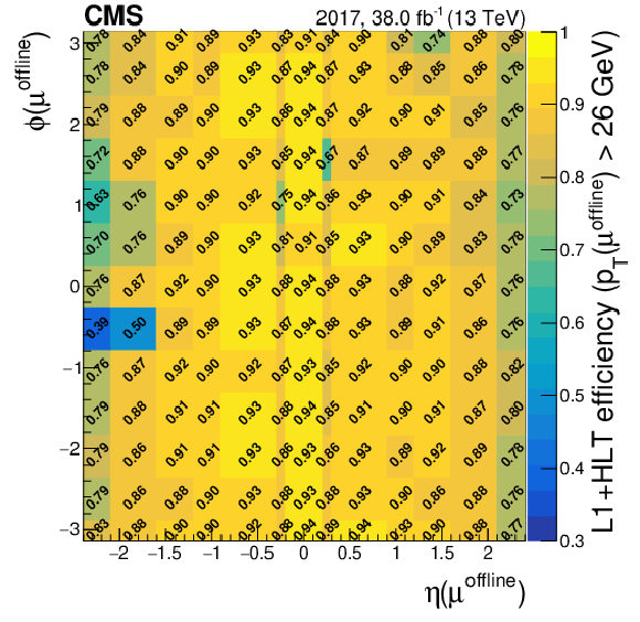
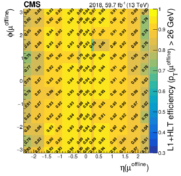
Efficiency of the isolated single-muon trigger with $ p_{\mathrm{T}} > $ 24 GeV as a function of the $ \eta $ and $ \phi $ of the muons in 2016 (upper left), 2017 (upper right), and 2018 (lower). |
png pdf |
Figure 8-a:
Efficiency of the isolated single-muon trigger with $ p_{\mathrm{T}} > $ 24 GeV as a function of the $ \eta $ and $ \phi $ of the muons in 2016 (upper left), 2017 (upper right), and 2018 (lower). |
png pdf |
Figure 8-b:
Efficiency of the isolated single-muon trigger with $ p_{\mathrm{T}} > $ 24 GeV as a function of the $ \eta $ and $ \phi $ of the muons in 2016 (upper left), 2017 (upper right), and 2018 (lower). |
png pdf |
Figure 8-c:
Efficiency of the isolated single-muon trigger with $ p_{\mathrm{T}} > $ 24 GeV as a function of the $ \eta $ and $ \phi $ of the muons in 2016 (upper left), 2017 (upper right), and 2018 (lower). |
png pdf |
Figure 9:
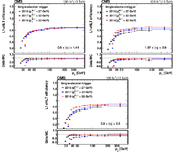
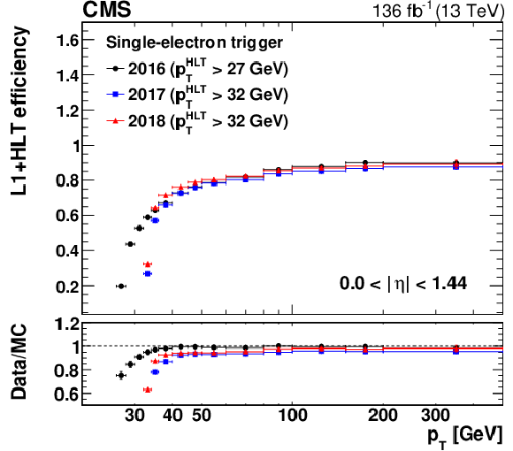
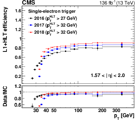
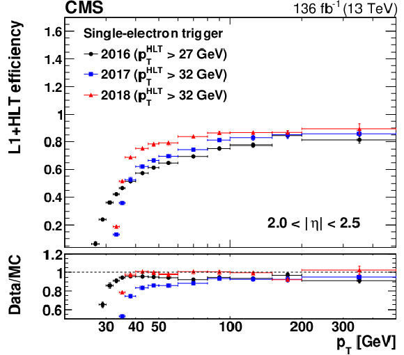
The L1+HLT efficiency of the single-electron HLT path with $ p_{\mathrm{T}} > $ 27 (32) GeV in 2016 (2017 and 2018) with respect to an offline-reconstructed electron as a function of the electron $ p_{\mathrm{T}} $, obtained for 0 $ < |\eta| < $ 1.44 (upper left), 1.57 $ < |\eta| < $ 2.0 (upper right), and 2.0 $ < |\eta| < $ 2.5 (lower). The lower panel of each plot shows the ratio of data to MC simulation. The vertical bars on the markers represent combined statistical and systematic uncertainties. |
png pdf |
Figure 9-a:
The L1+HLT efficiency of the single-electron HLT path with $ p_{\mathrm{T}} > $ 27 (32) GeV in 2016 (2017 and 2018) with respect to an offline-reconstructed electron as a function of the electron $ p_{\mathrm{T}} $, obtained for 0 $ < |\eta| < $ 1.44 (upper left), 1.57 $ < |\eta| < $ 2.0 (upper right), and 2.0 $ < |\eta| < $ 2.5 (lower). The lower panel of each plot shows the ratio of data to MC simulation. The vertical bars on the markers represent combined statistical and systematic uncertainties. |
png pdf |
Figure 9-b:
The L1+HLT efficiency of the single-electron HLT path with $ p_{\mathrm{T}} > $ 27 (32) GeV in 2016 (2017 and 2018) with respect to an offline-reconstructed electron as a function of the electron $ p_{\mathrm{T}} $, obtained for 0 $ < |\eta| < $ 1.44 (upper left), 1.57 $ < |\eta| < $ 2.0 (upper right), and 2.0 $ < |\eta| < $ 2.5 (lower). The lower panel of each plot shows the ratio of data to MC simulation. The vertical bars on the markers represent combined statistical and systematic uncertainties. |
png pdf |
Figure 9-c:
The L1+HLT efficiency of the single-electron HLT path with $ p_{\mathrm{T}} > $ 27 (32) GeV in 2016 (2017 and 2018) with respect to an offline-reconstructed electron as a function of the electron $ p_{\mathrm{T}} $, obtained for 0 $ < |\eta| < $ 1.44 (upper left), 1.57 $ < |\eta| < $ 2.0 (upper right), and 2.0 $ < |\eta| < $ 2.5 (lower). The lower panel of each plot shows the ratio of data to MC simulation. The vertical bars on the markers represent combined statistical and systematic uncertainties. |
png pdf |
Figure 10:
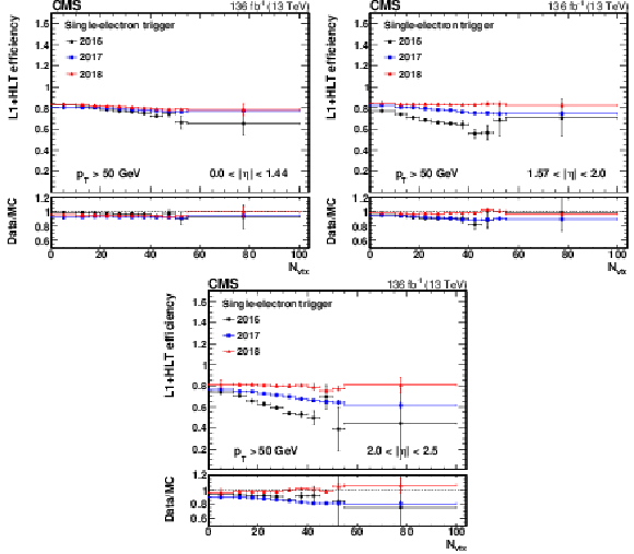
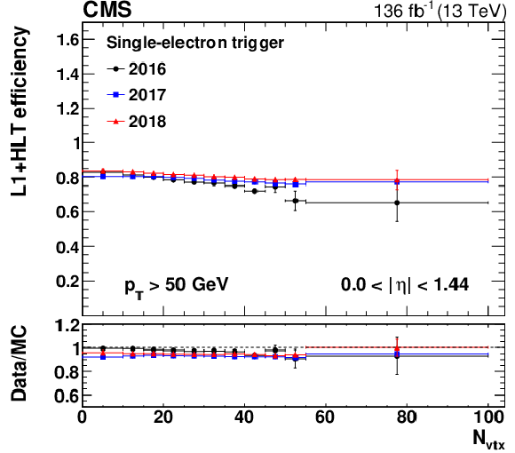
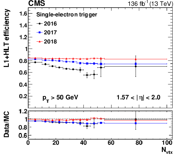
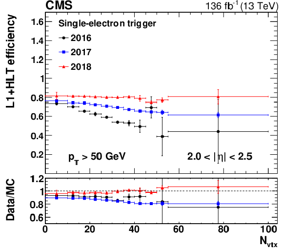
The L1+HLT efficiency of the single-electron HLT path with $ p_{\mathrm{T}} > $ 27 (32) GeV in 2016 (2017 and 2018) with respect to an offline-reconstructed electron as a function of $ N_{\text{vtx}} $, obtained for 0 $ < |\eta| < $ 1.44 (upper left), 1.57 $ < |\eta| < $ 2.0 (upper right), and 2.0 $ < |\eta| < $ 2.5 (lower). The electron $ p_{\mathrm{T}} $ is required to be above 50 GeV. The lower panel of each plot shows the ratio of data to MC simulation. The vertical bars on the markers represent combined statistical and systematic uncertainties. |
png pdf |
Figure 10-a:
The L1+HLT efficiency of the single-electron HLT path with $ p_{\mathrm{T}} > $ 27 (32) GeV in 2016 (2017 and 2018) with respect to an offline-reconstructed electron as a function of $ N_{\text{vtx}} $, obtained for 0 $ < |\eta| < $ 1.44 (upper left), 1.57 $ < |\eta| < $ 2.0 (upper right), and 2.0 $ < |\eta| < $ 2.5 (lower). The electron $ p_{\mathrm{T}} $ is required to be above 50 GeV. The lower panel of each plot shows the ratio of data to MC simulation. The vertical bars on the markers represent combined statistical and systematic uncertainties. |
png pdf |
Figure 10-b:
The L1+HLT efficiency of the single-electron HLT path with $ p_{\mathrm{T}} > $ 27 (32) GeV in 2016 (2017 and 2018) with respect to an offline-reconstructed electron as a function of $ N_{\text{vtx}} $, obtained for 0 $ < |\eta| < $ 1.44 (upper left), 1.57 $ < |\eta| < $ 2.0 (upper right), and 2.0 $ < |\eta| < $ 2.5 (lower). The electron $ p_{\mathrm{T}} $ is required to be above 50 GeV. The lower panel of each plot shows the ratio of data to MC simulation. The vertical bars on the markers represent combined statistical and systematic uncertainties. |
png pdf |
Figure 10-c:
The L1+HLT efficiency of the single-electron HLT path with $ p_{\mathrm{T}} > $ 27 (32) GeV in 2016 (2017 and 2018) with respect to an offline-reconstructed electron as a function of $ N_{\text{vtx}} $, obtained for 0 $ < |\eta| < $ 1.44 (upper left), 1.57 $ < |\eta| < $ 2.0 (upper right), and 2.0 $ < |\eta| < $ 2.5 (lower). The electron $ p_{\mathrm{T}} $ is required to be above 50 GeV. The lower panel of each plot shows the ratio of data to MC simulation. The vertical bars on the markers represent combined statistical and systematic uncertainties. |
png pdf |
Figure 11:
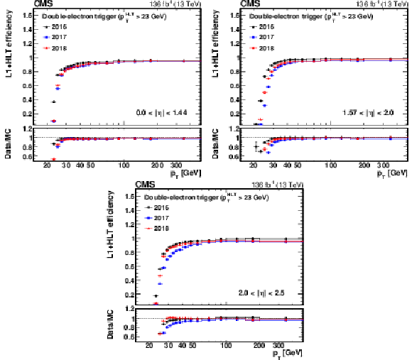
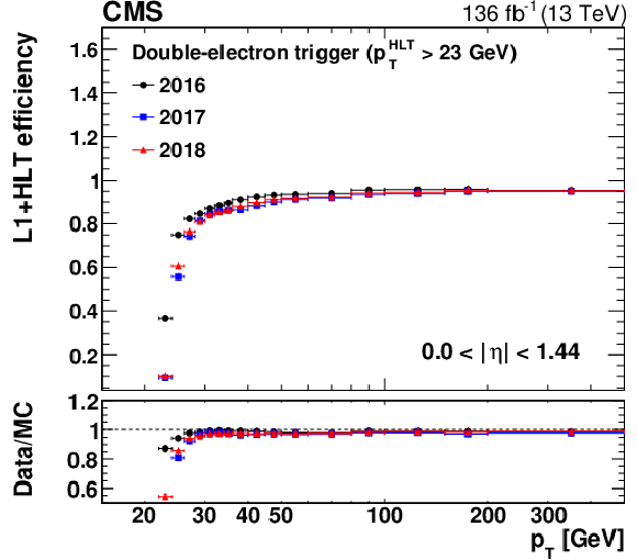
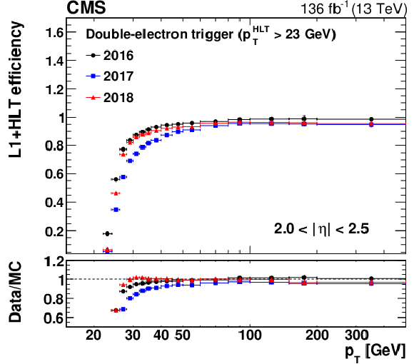
The L1+HLT efficiency of the $ p_{\mathrm{T}} > $ 23 GeV leg of the double-electron trigger with respect to an offline-reconstructed electron as a function of the electron $ p_{\mathrm{T}} $, obtained for 0 $ < |\eta| < $ 1.44 (upper left), 1.57 $ < |\eta| < $ 2.0 (upper right), and 2.0 $ < |\eta| < $ 2.5 (lower). The lower panel of each plot shows the ratio of data to MC simulation. The vertical bars on the markers represent combined statistical and systematic uncertainties. |
png pdf |
Figure 11-a:
The L1+HLT efficiency of the $ p_{\mathrm{T}} > $ 23 GeV leg of the double-electron trigger with respect to an offline-reconstructed electron as a function of the electron $ p_{\mathrm{T}} $, obtained for 0 $ < |\eta| < $ 1.44 (upper left), 1.57 $ < |\eta| < $ 2.0 (upper right), and 2.0 $ < |\eta| < $ 2.5 (lower). The lower panel of each plot shows the ratio of data to MC simulation. The vertical bars on the markers represent combined statistical and systematic uncertainties. |

png pdf |
Figure 11-b:
The L1+HLT efficiency of the $ p_{\mathrm{T}} > $ 23 GeV leg of the double-electron trigger with respect to an offline-reconstructed electron as a function of the electron $ p_{\mathrm{T}} $, obtained for 0 $ < |\eta| < $ 1.44 (upper left), 1.57 $ < |\eta| < $ 2.0 (upper right), and 2.0 $ < |\eta| < $ 2.5 (lower). The lower panel of each plot shows the ratio of data to MC simulation. The vertical bars on the markers represent combined statistical and systematic uncertainties. |
png pdf |
Figure 11-c:
The L1+HLT efficiency of the $ p_{\mathrm{T}} > $ 23 GeV leg of the double-electron trigger with respect to an offline-reconstructed electron as a function of the electron $ p_{\mathrm{T}} $, obtained for 0 $ < |\eta| < $ 1.44 (upper left), 1.57 $ < |\eta| < $ 2.0 (upper right), and 2.0 $ < |\eta| < $ 2.5 (lower). The lower panel of each plot shows the ratio of data to MC simulation. The vertical bars on the markers represent combined statistical and systematic uncertainties. |
png pdf |
Figure 12:
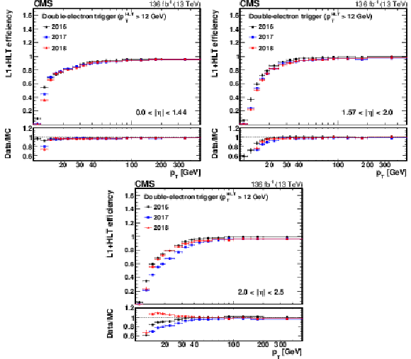
The L1+HLT efficiency of the $ p_{\mathrm{T}} > $ 12 GeV leg of the double-electron trigger with respect to an offline-reconstructed electron as a function of the electron $ p_{\mathrm{T}} $, obtained for 0 $ < |\eta| < $ 1.44 (upper left), 1.57 $ < |\eta| < $ 2.0 (upper right), and 2.0 $ < |\eta| < $ 2.5 (lower). The lower panel of each plot shows the ratio of data to MC simulation. The vertical bars on the markers represent combined statistical and systematic uncertainties. |
png pdf |
Figure 12-a:
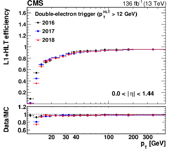
The L1+HLT efficiency of the $ p_{\mathrm{T}} > $ 12 GeV leg of the double-electron trigger with respect to an offline-reconstructed electron as a function of the electron $ p_{\mathrm{T}} $, obtained for 0 $ < |\eta| < $ 1.44 (upper left), 1.57 $ < |\eta| < $ 2.0 (upper right), and 2.0 $ < |\eta| < $ 2.5 (lower). The lower panel of each plot shows the ratio of data to MC simulation. The vertical bars on the markers represent combined statistical and systematic uncertainties. |
png pdf |
Figure 12-b:
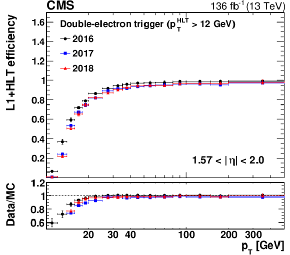
The L1+HLT efficiency of the $ p_{\mathrm{T}} > $ 12 GeV leg of the double-electron trigger with respect to an offline-reconstructed electron as a function of the electron $ p_{\mathrm{T}} $, obtained for 0 $ < |\eta| < $ 1.44 (upper left), 1.57 $ < |\eta| < $ 2.0 (upper right), and 2.0 $ < |\eta| < $ 2.5 (lower). The lower panel of each plot shows the ratio of data to MC simulation. The vertical bars on the markers represent combined statistical and systematic uncertainties. |
png pdf |
Figure 12-c:
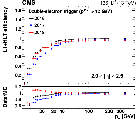
The L1+HLT efficiency of the $ p_{\mathrm{T}} > $ 12 GeV leg of the double-electron trigger with respect to an offline-reconstructed electron as a function of the electron $ p_{\mathrm{T}} $, obtained for 0 $ < |\eta| < $ 1.44 (upper left), 1.57 $ < |\eta| < $ 2.0 (upper right), and 2.0 $ < |\eta| < $ 2.5 (lower). The lower panel of each plot shows the ratio of data to MC simulation. The vertical bars on the markers represent combined statistical and systematic uncertainties. |
png pdf |
Figure 13:
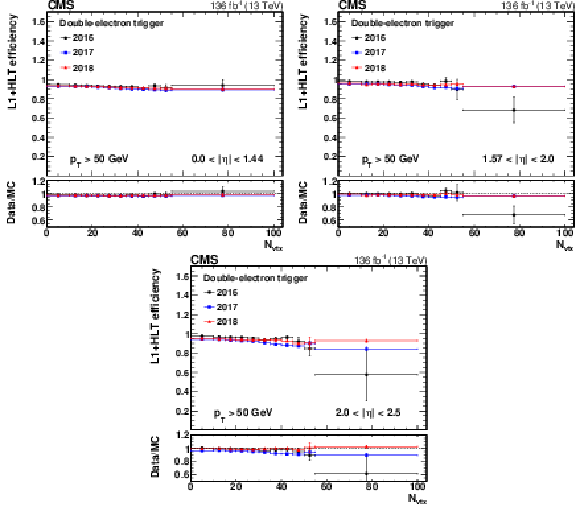
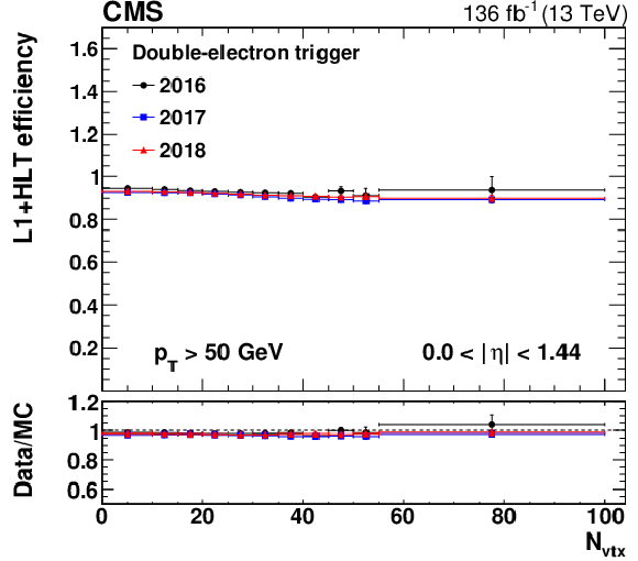
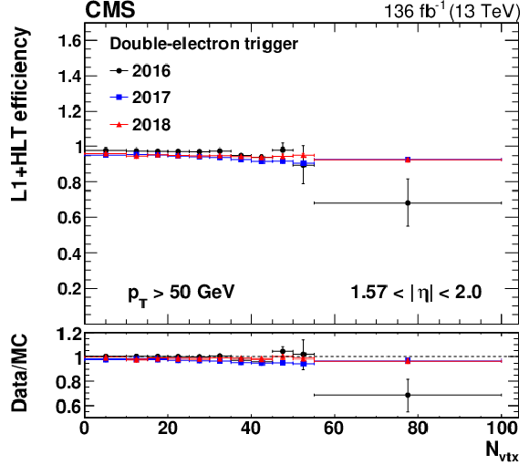
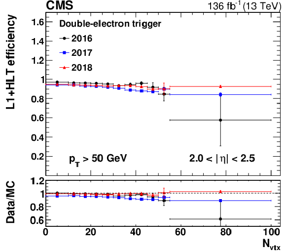
The L1+HLT efficiency of either leg of the double-electron trigger with respect to an offline-reconstructed electron as a function of $ N_{\text{vtx}} $, obtained for 0 $ < |\eta| < $ 1.44 (upper left), 1.57 $ < |\eta| < $ 2.0 (upper right), and 2.0 $ < |\eta| < $ 2.5 (lower). The electron $ p_{\mathrm{T}} $ is required to be above 50 GeV. The lower panel of each plot shows the ratio of data to MC simulation. The vertical bars on the markers represent combined statistical and systematic uncertainties. |
png pdf |
Figure 13-a:
The L1+HLT efficiency of either leg of the double-electron trigger with respect to an offline-reconstructed electron as a function of $ N_{\text{vtx}} $, obtained for 0 $ < |\eta| < $ 1.44 (upper left), 1.57 $ < |\eta| < $ 2.0 (upper right), and 2.0 $ < |\eta| < $ 2.5 (lower). The electron $ p_{\mathrm{T}} $ is required to be above 50 GeV. The lower panel of each plot shows the ratio of data to MC simulation. The vertical bars on the markers represent combined statistical and systematic uncertainties. |
png pdf |
Figure 13-b:
The L1+HLT efficiency of either leg of the double-electron trigger with respect to an offline-reconstructed electron as a function of $ N_{\text{vtx}} $, obtained for 0 $ < |\eta| < $ 1.44 (upper left), 1.57 $ < |\eta| < $ 2.0 (upper right), and 2.0 $ < |\eta| < $ 2.5 (lower). The electron $ p_{\mathrm{T}} $ is required to be above 50 GeV. The lower panel of each plot shows the ratio of data to MC simulation. The vertical bars on the markers represent combined statistical and systematic uncertainties. |
png pdf |
Figure 13-c:
The L1+HLT efficiency of either leg of the double-electron trigger with respect to an offline-reconstructed electron as a function of $ N_{\text{vtx}} $, obtained for 0 $ < |\eta| < $ 1.44 (upper left), 1.57 $ < |\eta| < $ 2.0 (upper right), and 2.0 $ < |\eta| < $ 2.5 (lower). The electron $ p_{\mathrm{T}} $ is required to be above 50 GeV. The lower panel of each plot shows the ratio of data to MC simulation. The vertical bars on the markers represent combined statistical and systematic uncertainties. |
png pdf |
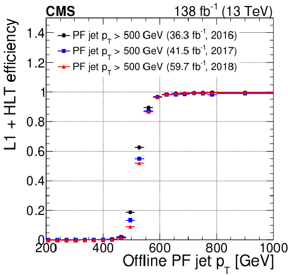
Figure 14:
The L1+HLT efficiency of the unprescaled single PF jet trigger having an online $ p_{\mathrm{T}} $ threshold of 500 GeV, measured with respect to the offline reconstructed PF jet $ p_{\mathrm{T}} $, for the data collected using an unbiased single-muon trigger during 2016, 2017, and 2018. The slight variation in turn-on curve is caused by differences in offline jet energy scale calibrations. The vertical bars on the markers represent statistical uncertainties. |
png pdf |
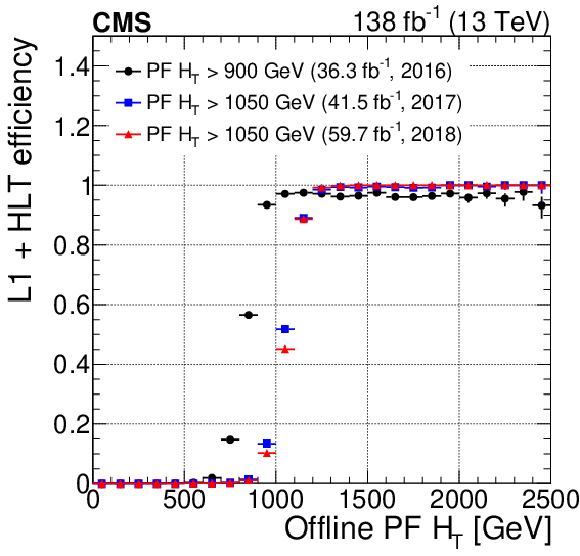
Figure 15:
The L1+HLT efficiency of the unprescaled $ H_{\mathrm{T}} $ triggers with the lowest thresholds, measured with respect to the offline-reconstructed $ H_{\mathrm{T}} $, for the data collected during 2016, 2017, and 2018. The inefficiency for 2016 is caused by an effect in the L1 trigger seed firmware implementation. The vertical bars on the markers represent statistical uncertainties. |
png pdf |
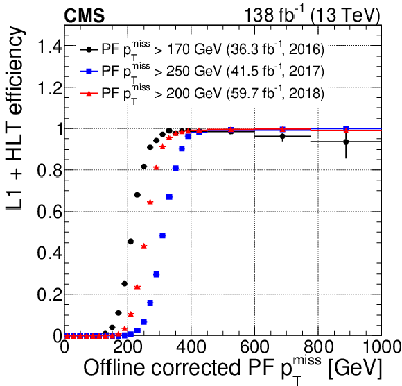
Figure 16:
The L1+HLT efficiencies of the unprescaled $ p_{\mathrm{T}}^\text{miss} $ triggers with the lowest thresholds, measured with respect to the offline-reconstructed corrected $ p_{\mathrm{T}}^\text{miss} $, for the data collected during 2016, 2017, and 2018. The vertical bars on the markers represent statistical uncertainties. |
png pdf |
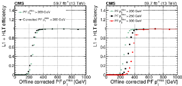
Figure 17:
Left: comparison of the L1+HLT efficiencies of the corrected vs. nominal $ p_{\mathrm{T}}^\text{miss} $ triggers of the same threshold, for the data collected during 2018. Right: nominal $ p_{\mathrm{T}}^\text{miss} $ trigger L1+HLT efficiencies using different thresholds. |
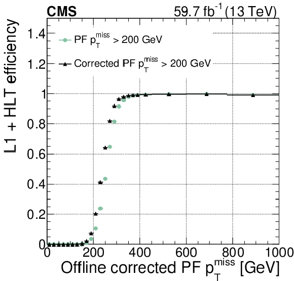
png pdf |
Figure 17-a:
Left: comparison of the L1+HLT efficiencies of the corrected vs. nominal $ p_{\mathrm{T}}^\text{miss} $ triggers of the same threshold, for the data collected during 2018. Right: nominal $ p_{\mathrm{T}}^\text{miss} $ trigger L1+HLT efficiencies using different thresholds. |
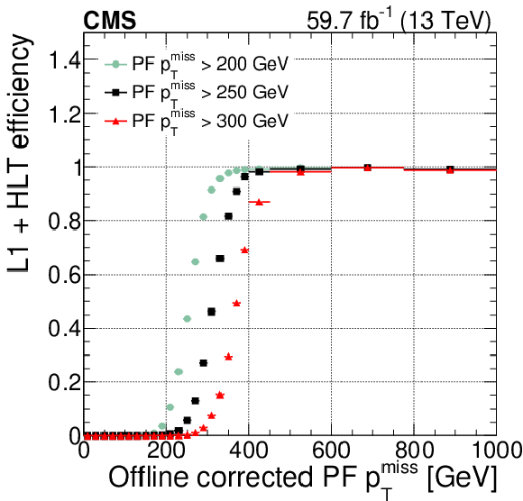
png pdf |
Figure 17-b:
Left: comparison of the L1+HLT efficiencies of the corrected vs. nominal $ p_{\mathrm{T}}^\text{miss} $ triggers of the same threshold, for the data collected during 2018. Right: nominal $ p_{\mathrm{T}}^\text{miss} $ trigger L1+HLT efficiencies using different thresholds. |
png pdf |
Figure 18:
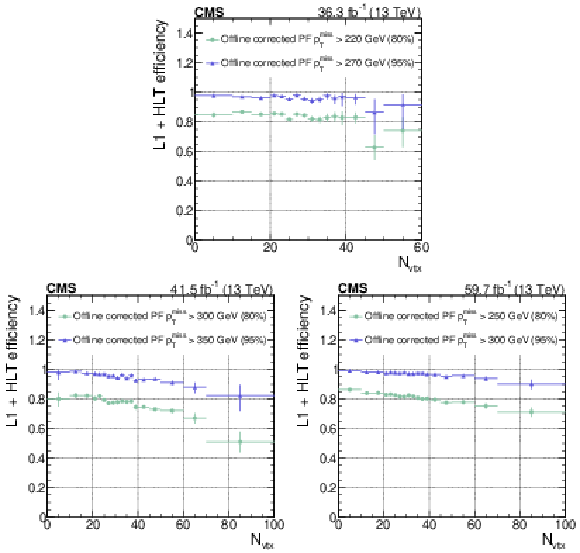
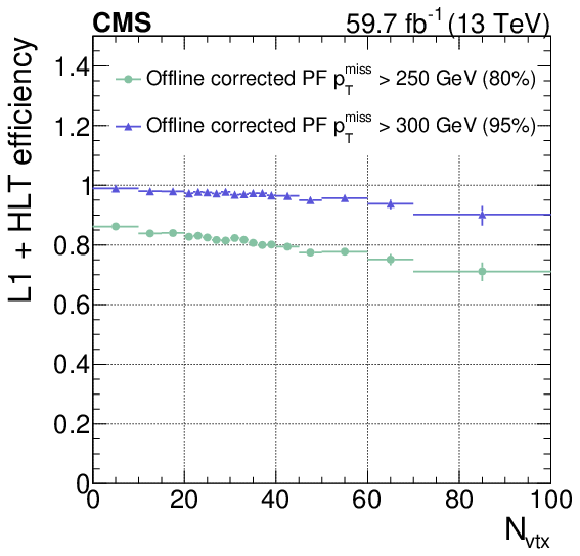
Event selection efficiencies as a function of $ N_{\text{vtx}} $ for fixed L1+HLT efficiency values of 80 and 95% of the unprescaled $ p_{\mathrm{T}}^\text{miss} $ triggers with the lowest $ p_{\mathrm{T}}^\text{miss} $ thresholds in 2016 (upper), 2017 (lower left), and 2018 (lower right). The PU is considerably lower in 2016, which allowed to lower thresholds for all triggers involving jets and $ p_{\mathrm{T}}^\text{miss} $. The vertical bars on the markers represent statistical uncertainties. |

png pdf |
Figure 18-a:
Event selection efficiencies as a function of $ N_{\text{vtx}} $ for fixed L1+HLT efficiency values of 80 and 95% of the unprescaled $ p_{\mathrm{T}}^\text{miss} $ triggers with the lowest $ p_{\mathrm{T}}^\text{miss} $ thresholds in 2016 (upper), 2017 (lower left), and 2018 (lower right). The PU is considerably lower in 2016, which allowed to lower thresholds for all triggers involving jets and $ p_{\mathrm{T}}^\text{miss} $. The vertical bars on the markers represent statistical uncertainties. |
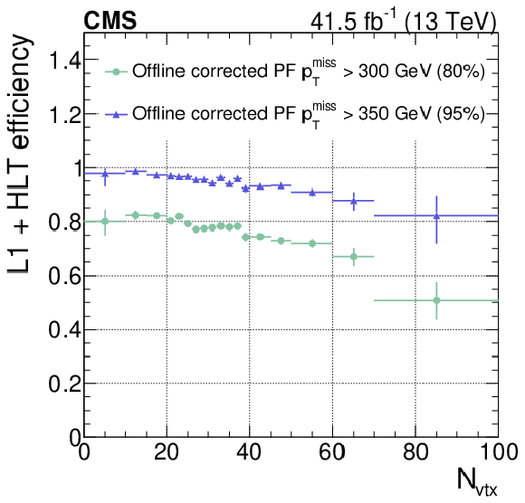
png pdf |
Figure 18-b:
Event selection efficiencies as a function of $ N_{\text{vtx}} $ for fixed L1+HLT efficiency values of 80 and 95% of the unprescaled $ p_{\mathrm{T}}^\text{miss} $ triggers with the lowest $ p_{\mathrm{T}}^\text{miss} $ thresholds in 2016 (upper), 2017 (lower left), and 2018 (lower right). The PU is considerably lower in 2016, which allowed to lower thresholds for all triggers involving jets and $ p_{\mathrm{T}}^\text{miss} $. The vertical bars on the markers represent statistical uncertainties. |
png pdf |
Figure 18-c:
Event selection efficiencies as a function of $ N_{\text{vtx}} $ for fixed L1+HLT efficiency values of 80 and 95% of the unprescaled $ p_{\mathrm{T}}^\text{miss} $ triggers with the lowest $ p_{\mathrm{T}}^\text{miss} $ thresholds in 2016 (upper), 2017 (lower left), and 2018 (lower right). The PU is considerably lower in 2016, which allowed to lower thresholds for all triggers involving jets and $ p_{\mathrm{T}}^\text{miss} $. The vertical bars on the markers represent statistical uncertainties. |
png pdf |
Figure 19:
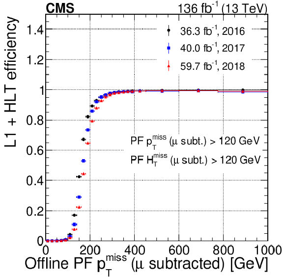
The L1+HLT efficiency of the $ \mu $-subtracted $ p_{\mathrm{T}}^\text{miss} $ trigger with a threshold of 120 GeV on both $ p_{\mathrm{T}}^\text{miss} $ and missing $ H_{\mathrm{T}} $ measured with respect to the offline reconstructed $ \mu $-subtracted $ p_{\mathrm{T}}^\text{miss} $, shown separately for data collected during 2016, 2017, and 2018. The vertical bars on the markers represent statistical uncertainties. |
png pdf |
Figure 20:
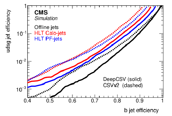
Performance of the online (red and blue) and offline (black) b quark jet identification algorithms demonstrated as the probability for a light jet to be misidentified as a b quark jet as a function of the efficiency to correctly identify a b quark jet. The performance of the CSVV2 (dashed) and DeepCSV (solid) algorithms are shown. The curves are obtained for online and offline jets with $ p_{\mathrm{T}} > $ 30 GeV and $ |\eta| < $ 2.4 in simulated $ \mathrm{t} \overline{\mathrm{t}} $ events. The plot is obtained using the 2017 detector conditions. |
png pdf |
Figure 21:
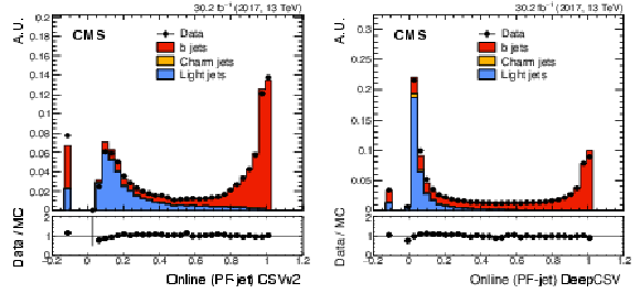
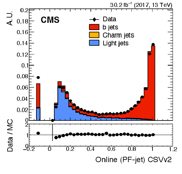
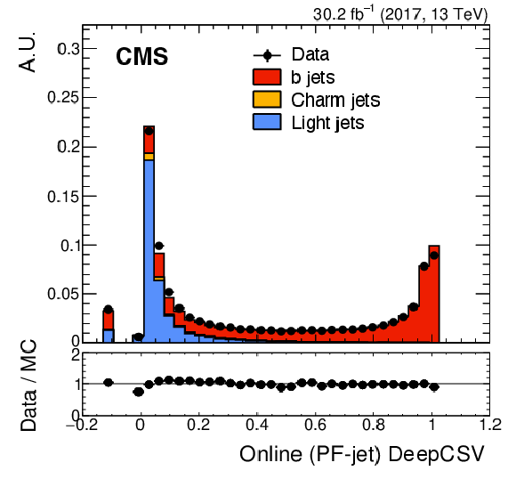
Left: Online (PF-Jets) CSVV2 discriminator distribution, normalized to unity for both data and the summed simulation. Different colors show the contributions from simulation of different jet flavors. The plot is obtained using the 2017 detector conditions. A negative value indicates that the tracking preselection has failed and the discriminator is not evaluated. Right: Same, but for the DeepCSV discriminator. The plot is obtained using 2017 data and MC simulation using the DeepCSV algorithm as it was run in 2018. The lower panel of each plot shows the ratio of data to MC simulation. The vertical bars on the markers represent statistical uncertainties. |
png pdf |
Figure 21-a:
Left: Online (PF-Jets) CSVV2 discriminator distribution, normalized to unity for both data and the summed simulation. Different colors show the contributions from simulation of different jet flavors. The plot is obtained using the 2017 detector conditions. A negative value indicates that the tracking preselection has failed and the discriminator is not evaluated. Right: Same, but for the DeepCSV discriminator. The plot is obtained using 2017 data and MC simulation using the DeepCSV algorithm as it was run in 2018. The lower panel of each plot shows the ratio of data to MC simulation. The vertical bars on the markers represent statistical uncertainties. |
png pdf |
Figure 21-b:
Left: Online (PF-Jets) CSVV2 discriminator distribution, normalized to unity for both data and the summed simulation. Different colors show the contributions from simulation of different jet flavors. The plot is obtained using the 2017 detector conditions. A negative value indicates that the tracking preselection has failed and the discriminator is not evaluated. Right: Same, but for the DeepCSV discriminator. The plot is obtained using 2017 data and MC simulation using the DeepCSV algorithm as it was run in 2018. The lower panel of each plot shows the ratio of data to MC simulation. The vertical bars on the markers represent statistical uncertainties. |
png pdf |
Figure 22:
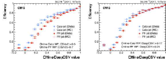
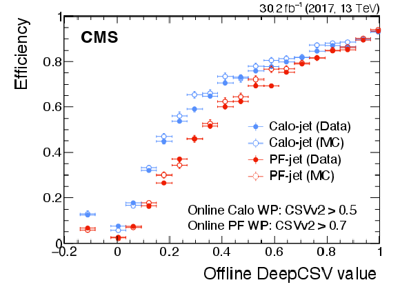
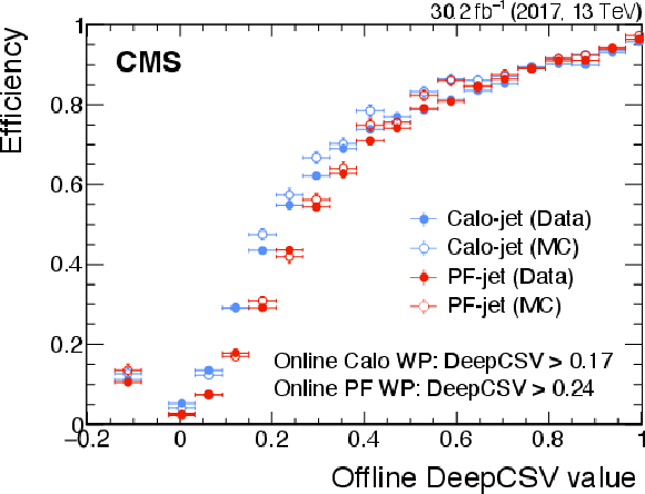
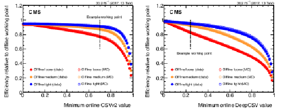
Efficiency to pass the online CSVV2 (left) and DeepCSV (right) working points as a function of the corresponding offline DeepCSV value. Data collected in 2017 are shown in closed circles; the result of the simulation is shown in open circles. The turn-on with respect to the online Calo-jets is shown in blue. The turn-on with respect to the online PF-jets is shown in red. The right plot is obtained using 2017 data and MC simulation using the DeepCSV algorithm as it was run in 2018. A negative value indicates that the tracking preselection has failed and the discriminator is not evaluated. The vertical bars on the markers represent statistical uncertainties. |
png pdf |
Figure 22-a:
Efficiency to pass the online CSVV2 (left) and DeepCSV (right) working points as a function of the corresponding offline DeepCSV value. Data collected in 2017 are shown in closed circles; the result of the simulation is shown in open circles. The turn-on with respect to the online Calo-jets is shown in blue. The turn-on with respect to the online PF-jets is shown in red. The right plot is obtained using 2017 data and MC simulation using the DeepCSV algorithm as it was run in 2018. A negative value indicates that the tracking preselection has failed and the discriminator is not evaluated. The vertical bars on the markers represent statistical uncertainties. |
png pdf |
Figure 22-b:
Efficiency to pass the online CSVV2 (left) and DeepCSV (right) working points as a function of the corresponding offline DeepCSV value. Data collected in 2017 are shown in closed circles; the result of the simulation is shown in open circles. The turn-on with respect to the online Calo-jets is shown in blue. The turn-on with respect to the online PF-jets is shown in red. The right plot is obtained using 2017 data and MC simulation using the DeepCSV algorithm as it was run in 2018. A negative value indicates that the tracking preselection has failed and the discriminator is not evaluated. The vertical bars on the markers represent statistical uncertainties. |
png pdf |
Figure 23:
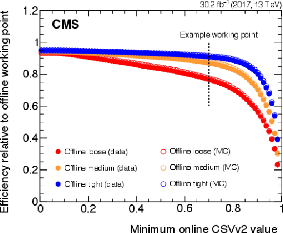
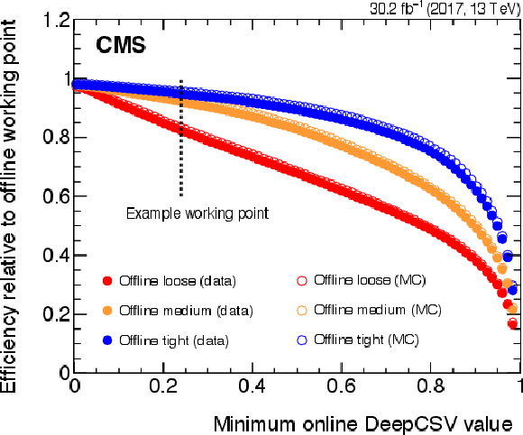
Efficiency of jets b tagged offline to pass the online CSVV2 (left) and DeepCSV (right) b tagging requirement, as a function of the online requirement. Three offline selections are shown: Loose (red), Medium (orange), and Tight (blue). Data are shown in closed circles; the result of the simulation is shown in open circles. The right plot is obtained using 2017 data and MC simulation but using the DeepCSV algorithm as it was run in 2018. |
png pdf |
Figure 23-a:
Efficiency of jets b tagged offline to pass the online CSVV2 (left) and DeepCSV (right) b tagging requirement, as a function of the online requirement. Three offline selections are shown: Loose (red), Medium (orange), and Tight (blue). Data are shown in closed circles; the result of the simulation is shown in open circles. The right plot is obtained using 2017 data and MC simulation but using the DeepCSV algorithm as it was run in 2018. |
png pdf |
Figure 23-b:
Efficiency of jets b tagged offline to pass the online CSVV2 (left) and DeepCSV (right) b tagging requirement, as a function of the online requirement. Three offline selections are shown: Loose (red), Medium (orange), and Tight (blue). Data are shown in closed circles; the result of the simulation is shown in open circles. The right plot is obtained using 2017 data and MC simulation but using the DeepCSV algorithm as it was run in 2018. |

png pdf |
Figure 24:
Flow chart for $ \tau_\mathrm{h} $-candidate reconstruction at the HLT. |
png pdf |
Figure 25:
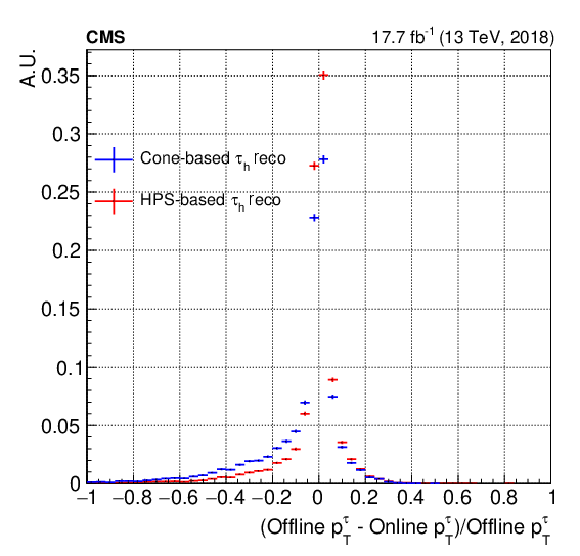
The $ p_{\mathrm{T}} $ resolution for the $ \mu \tau_\mathrm{h} $ trigger for cone-based and HPS-based $ \tau_\mathrm{h} $ reconstruction, calculated by using the first 17.7 fb$ ^{-1} $ of 2018 data taken with the cone-based tau reconstruction, where the trigger paths with HPS-based algorithm were included for the purpose of testing. The vertical bars on the markers represent statistical uncertainties. |
png pdf |
Figure 26:
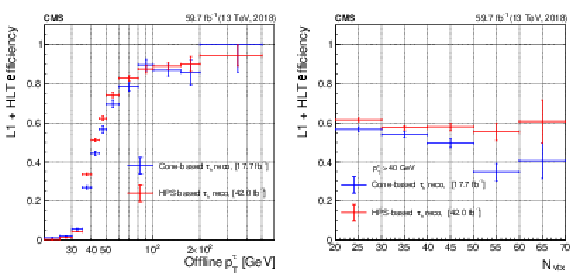
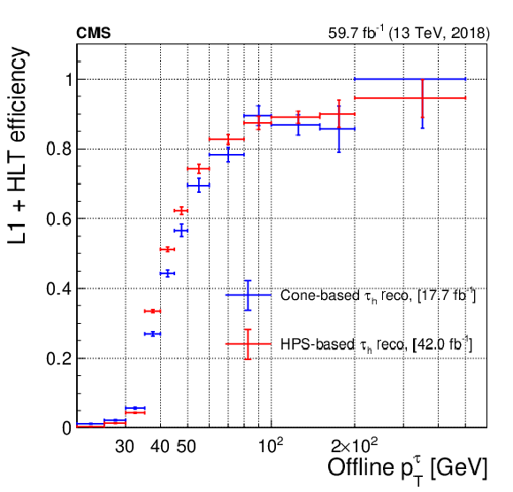
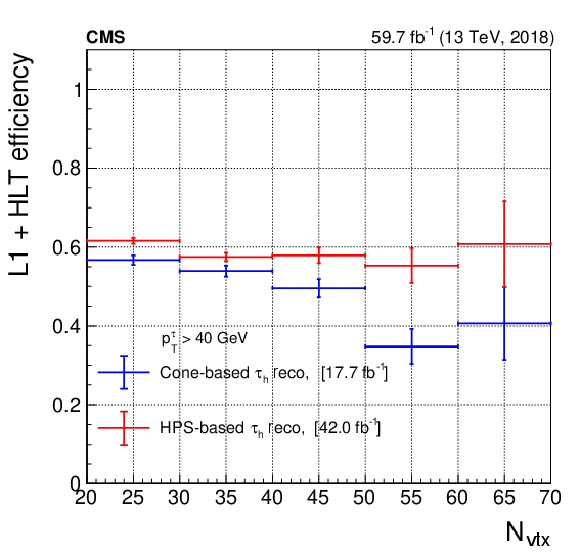
Combined L1 and HLT efficiency per leg of the $ \tau_\mathrm{h}\tau_\mathrm{h} $ triggers with cone-based and HPS-based $ \tau_\mathrm{h} $ reconstruction, using the first 17.7 fb$ ^{-1} $ and the next 42.0 fb$ ^{-1} $ of data in 2018. The figure shows the efficiency as a function of offline $ p_{\mathrm{T}}^{\tau} $ (left) and $ N_{\text{vtx}} $ (right). The vertical bars on the markers represent statistical uncertainties. |
png pdf |
Figure 26-a:
Combined L1 and HLT efficiency per leg of the $ \tau_\mathrm{h}\tau_\mathrm{h} $ triggers with cone-based and HPS-based $ \tau_\mathrm{h} $ reconstruction, using the first 17.7 fb$ ^{-1} $ and the next 42.0 fb$ ^{-1} $ of data in 2018. The figure shows the efficiency as a function of offline $ p_{\mathrm{T}}^{\tau} $ (left) and $ N_{\text{vtx}} $ (right). The vertical bars on the markers represent statistical uncertainties. |
png pdf |
Figure 26-b:
Combined L1 and HLT efficiency per leg of the $ \tau_\mathrm{h}\tau_\mathrm{h} $ triggers with cone-based and HPS-based $ \tau_\mathrm{h} $ reconstruction, using the first 17.7 fb$ ^{-1} $ and the next 42.0 fb$ ^{-1} $ of data in 2018. The figure shows the efficiency as a function of offline $ p_{\mathrm{T}}^{\tau} $ (left) and $ N_{\text{vtx}} $ (right). The vertical bars on the markers represent statistical uncertainties. |
png pdf |
Figure 27:
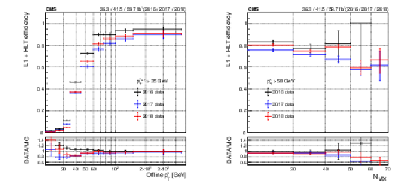
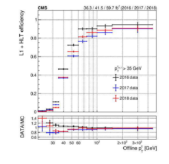
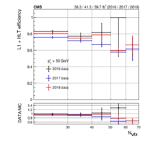
Combined L1 and HLT efficiency per leg of the $ \tau_\mathrm{h}\tau_\mathrm{h} $ triggers for 2016, 2017, and 2018 data taking. The figure shows the trigger efficiency as a function of the offline $ p_{\mathrm{T}}^{\tau} $ for a 35 GeV threshold (left) and as a function of $ N_{\text{vtx}} $ (right), for which an offline requirement of $ p_{\mathrm{T}}^{\tau} > $ 50 GeV is applied. The lower panels show the ratio of data to MC simulation for each year. The vertical bars on the markers represent statistical uncertainties. |
png pdf |
Figure 27-a:
Combined L1 and HLT efficiency per leg of the $ \tau_\mathrm{h}\tau_\mathrm{h} $ triggers for 2016, 2017, and 2018 data taking. The figure shows the trigger efficiency as a function of the offline $ p_{\mathrm{T}}^{\tau} $ for a 35 GeV threshold (left) and as a function of $ N_{\text{vtx}} $ (right), for which an offline requirement of $ p_{\mathrm{T}}^{\tau} > $ 50 GeV is applied. The lower panels show the ratio of data to MC simulation for each year. The vertical bars on the markers represent statistical uncertainties. |
png pdf |
Figure 27-b:
Combined L1 and HLT efficiency per leg of the $ \tau_\mathrm{h}\tau_\mathrm{h} $ triggers for 2016, 2017, and 2018 data taking. The figure shows the trigger efficiency as a function of the offline $ p_{\mathrm{T}}^{\tau} $ for a 35 GeV threshold (left) and as a function of $ N_{\text{vtx}} $ (right), for which an offline requirement of $ p_{\mathrm{T}}^{\tau} > $ 50 GeV is applied. The lower panels show the ratio of data to MC simulation for each year. The vertical bars on the markers represent statistical uncertainties. |
| Tables | |
png pdf |
Table 1:
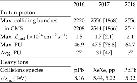
The LHC operations parameters during Run 2. The maximum PU is for standard physics fills with more than 600 bunches, and the average PU is calculated assuming an inelastic cross section of 80 mb. The 8b4e bunch-filling configuration values are given in brackets, and they refer to an LHC configuration used in 2017 to mitigate beam losses. The $ \sqrt{\smash[b]{s_{_{\mathrm{NN}}}}} $ is the center-of-mass energy per nucleon. |
png pdf |
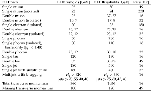
Table 2:
Representative set of HLT paths based on the basic HLT physics objects used during data taking in 2018, the associated thresholds at the L1 and HLT, and the corresponding HLT output rates. The total menu rate at $ \mathcal{L}_{\text{inst}}= $ 1.8 $\times $ 10$^{34}$ cm$^{-2}$s$^{-1} $, representative near the start of an LHC fill, is 1.6 kHz. |

png pdf |
Table 3:
ll} \hline |
png pdf |
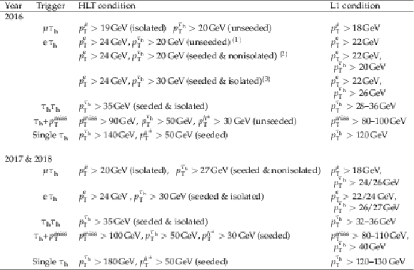
Table 4:
List of $ \tau_\mathrm{h} $ triggers used in 2016, 2017, and 2018 data-taking periods including both the L1 and HLT conditions. The $ \mathrm{e}\tau_\mathrm{h} $ triggers evolved in 2016 data taking, with the labels (1), (2), and (3) indicating use for the first 7.4 fb$ ^{-1} $, the next 10.2 fb$ ^{-1} $, and the last 18.3 fb$ ^{-1} $ of data, respectively. |
| Summary |
| The performance of the high-level trigger of CMS has been presented as it evolved over the course of LHC Run 2 in 2016--2018. The algorithms of the high-level trigger were adapted to meet the challenges of the increase of the LHC luminosity and pileup to twice their initial design values as well as two to three times the previous Run 1 values. Imperfect detector effects that arose also were mitigated to minimize inefficiencies. The trigger menu continuously evolved to meet the needs of the experiment across a wide range of physics areas under these conditions and within the CPU capacity of the online computer farm. The overall single isolated lepton trigger efficiency was maintained at the level of 90% for muons and 80% for electrons with $ p_{\mathrm{T}} $ thresholds of 24 and 32 GeV, respectively. Triggers based on jets and on energy sums such as $ p_{\mathrm{T}}^\text{miss} $ also were available. Jets also could be tagged as arising from a b quark jet with a performance of the identification algorithm approaching that achieved offline and using machine learning for the best discrimination. Hadronically decaying tau leptons were also reconstructed in the trigger and were typically used in combination with other leptons, with minimum $ p_{\mathrm{T}} $ thresholds from 20 to 35 GeV on the hadronic tau decay depending on the flavor of the other lepton and the data-taking year. |
| References | ||||
| 1 | CMS Collaboration | Enriching the physics program of the CMS experiment via data scouting and data parking | Accepted by Phys. Rept., 2024 | CMS-EXO-23-007 2403.16134 |
| 2 | CMS Collaboration | The CMS trigger system | JINST 12 (2017) P01020 | CMS-TRG-12-001 1609.02366 |
| 3 | CMS Collaboration | CMS technical design report for the Level-1 trigger upgrade | Technical Report CERN-LHCC-2013-011, CMS-TDR-12, 2013 CDS |
|
| 4 | CMS Collaboration | Performance of the CMS Level-1 trigger in proton-proton collisions at $ \sqrt{s} = $ 13 TeV | JINST 15 (2020) P10017 | CMS-TRG-17-001 2006.10165 |
| 5 | CMS Collaboration | Technical proposal for the upgrade of the CMS detector through 2020 | Technical Report CERN-LHCC-2011-006. LHCC-P-004, 2011 CDS |
|
| 6 | CMS Collaboration | Development of the CMS detector for the CERN LHC Run 3 | JINST 19 (2024) P05064 | CMS-PRF-21-001 2309.05466 |
| 7 | CMS Collaboration | The CMS experiment at the CERN LHC | JINST 3 (2008) S08004 | |
| 8 | CMS Collaboration | Description and performance of track and primary-vertex reconstruction with the CMS tracker | JINST 9 (2014) P10009 | CMS-TRK-11-001 1405.6569 |
| 9 | Tracker Group of the CMS Collaboration | The CMS Phase-1 pixel detector upgrade | JINST 16 (2021) P02027 | 2012.14304 |
| 10 | CMS Collaboration | Track impact parameter resolution for the full pseudorapidity coverage in the 2017 dataset with the CMS phase-1 pixel detector | CMS Detector Performance Summary CMS-DP-2020-049, 2020 CDS |
|
| 11 | CMS Collaboration | 2017 tracking performance plots | CMS Detector Performance Summary CMS-DP-2017-015, 2017 CDS |
|
| 12 | P. Grafström and W. Kozanecki | Luminosity determination at proton colliders | Prog. Part. Nucl. Phys. 81 (2015) 97 | |
| 13 | R. Bruce et al. | Review of LHC Run 2 machine configurations | in Proc. 9th LHC Operations Evian Workshop, 2019 | |
| 14 | J. Wenninger | Operation and configuration of the LHC in Run 2 | ||
| 15 | D. Mirarchi et al. | Special losses during LHC Run 2 | in Proc. 9th LHC Operations Evian Workshop, 2019 | |
| 16 | HEPiX Benchmarking Working Group | HEPiX | [Online], 2021 link |
|
| 17 | C. D. Jones et al. | Using the CMS threaded framework in a production environment | J. Phys. Conf. Ser. 664 (2015) 072026 | |
| 18 | CMS Collaboration | Particle-flow reconstruction and global event description with the CMS detector | JINST 12 (2017) P10003 | CMS-PRF-14-001 1706.04965 |
| 19 | CMS Collaboration | Measurement of the inclusive W and Z production cross sections in pp collisions at $ \sqrt{s}= $ 7 TeV | JHEP 10 (2011) 132 | CMS-EWK-10-005 1107.4789 |
| 20 | R. Frühwirth | Application of Kalman filtering to track and vertex fitting | NIM A 262 (1987) 444 | |
| 21 | F. Pantaleo | New track seeding techniques for the CMS experiment | PhD thesis, CERN, CMS-TS-2017-028, CERN-THESIS-2017-242, 2017 link |
|
| 22 | K. Rose | Deterministic annealing for clustering, compression, classification, regression, and related optimization problems | IEEE Proc. 86 (1998) 2210 | |
| 23 | R. Frühwirth, W. Waltenberger, and P. Vanlaer | Adaptive vertex fitting | JPG 34 (2007) N343 | |
| 24 | CMS Collaboration | Performance of the CMS muon trigger system in proton-proton collisions at $ \sqrt{s} = $ 13 TeV | JINST 16 (2021) P07001 | CMS-MUO-19-001 2102.04790 |
| 25 | CMS Collaboration | Performance of electron reconstruction and selection with the CMS detector in proton-proton collisions at $ \sqrt{s} = $ 8 TeV | JINST 10 (2015) P06005 | CMS-EGM-13-001 1502.02701 |
| 26 | W. Adam, R. Frühwirth, A. Strandlie, and T. Todorov | Reconstruction of electrons with the Gaussian-sum filter in the CMS tracker at LHC | Journal of Physics G: Nuclear and Particle Physics 31 (2005) N9 | physics/0306087 |
| 27 | CMS Collaboration | Precision luminosity measurement in proton-proton collisions at $ \sqrt{s} = $ 13 TeV in 2015 and 2016 at CMS | EPJC 81 (2021) 800 | CMS-LUM-17-003 2104.01927 |
| 28 | CMS Collaboration | CMS luminosity measurement for the 2017 data-taking period at $ \sqrt{s} = $ 13 TeV | CMS Physics Analysis Summary, 2018 link |
CMS-PAS-LUM-17-004 |
| 29 | CMS Collaboration | CMS luminosity measurement for the 2018 data-taking period at $ \sqrt{s} = $ 13 TeV | CMS Physics Analysis Summary, 2019 link |
CMS-PAS-LUM-18-002 |
| 30 | CMS Collaboration | Measurements of inclusive W and Z cross sections in pp collisions at $ \sqrt{s} = $ 7 TeV | JHEP 01 (2011) 080 | CMS-EWK-10-002 1012.2466 |
| 31 | CMS Collaboration | Electron and photon reconstruction and identification with the CMS experiment at the CERN LHC | JINST 16 (2021) P05014 | CMS-EGM-17-001 2012.06888 |
| 32 | M. Cacciari, G. P. Salam, and G. Soyez | The anti-$ k_{\mathrm{T}} $ jet clustering algorithm | JHEP 04 (2008) 063 | 0802.1189 |
| 33 | CMS Collaboration | Measurement of $ {\mathrm{B}}\overline{\mathrm{B}} $ angular correlations based on secondary vertex reconstruction at $ \sqrt{s}= $ 7 TeV | JHEP 03 (2011) 136 | CMS-BPH-10-010 1102.3194 |
| 34 | CMS Collaboration | Identification of heavy-flavour jets with the CMS detector in pp collisions at 13 TeV | JINST 13 (2018) P05011 | CMS-BTV-16-002 1712.07158 |
| 35 | CMS Collaboration | Performance of reconstruction and identification of $ \tau $ leptons decaying to hadrons and $ \nu_\tau $ in pp collisions at $ \sqrt{s}= $ 13 TeV | JINST 13 (2018) P10005 | CMS-TAU-16-003 1809.02816 |

|
Compact Muon Solenoid LHC, CERN |

|

|

|

|

|

|