

Compact Muon Solenoid
LHC, CERN
| CMS-HIG-22-013 ; CERN-EP-2025-124 | ||
| Search for heavy pseudoscalar and scalar bosons decaying to a top quark pair in proton-proton collisions at $ \sqrt{s}= $ 13 TeV | ||
| CMS Collaboration | ||
| 8 July 2025 | ||
| Rep. Prog. Phys. 88 (2025) 127801 | ||
| Abstract: A search for pseudoscalar or scalar bosons decaying to a top quark pair ($ \mathrm{t} \overline{\mathrm{t}} $) in final states with one or two charged leptons is presented. The analyzed proton-proton collision data was recorded at $ \sqrt{s}= $ 13 TeV by the CMS experiment at the CERN LHC and corresponds to an integrated luminosity of 138 fb$ ^{-1} $. The invariant mass $ m_{{\mathrm{t}\overline{\mathrm{t}}} } $ of the reconstructed $ \mathrm{t} \overline{\mathrm{t}} $ system and variables sensitive to its spin and parity are used to discriminate against the standard model $ \mathrm{t} \overline{\mathrm{t}} $ background. Interference between pseudoscalar or scalar boson production and the standard model $ \mathrm{t} \overline{\mathrm{t}} $ continuum is included, leading to peak-dip structures in the $ m_{{\mathrm{t}\overline{\mathrm{t}}} } $ distribution. An excess of the data above the background prediction, based on perturbative quantum chromodynamics (QCD) calculations, is observed near the kinematic $ \mathrm{t} \overline{\mathrm{t}} $ production threshold, while good agreement is found for high $ m_{{\mathrm{t}\overline{\mathrm{t}}} } $. The data are consistent with the background prediction if the contribution from a simplified model of a color-singlet $ ^1\mathrm{S}_0^{[1]} $\ $ \mathrm{t} \overline{\mathrm{t}} $ quasi-bound state $ \eta_{\mathrm{t}} $, inspired by nonrelativistic QCD, is added. Upper limits at 95% confidence level are set on the coupling between the pseudoscalar or scalar bosons and the top quark for boson masses in the range 365-1000 GeV, relative widths between 0.5 and 25%, and two background scenarios with or without $ \eta_{\mathrm{t}} $ contribution. | ||
| Links: e-print arXiv:2507.05119 [hep-ex] (PDF) ; CDS record ; inSPIRE record ; HepData record ; CADI line (restricted) ; | ||
| Figures & Tables | Summary | Additional Figures | References | CMS Publications |
|---|
| Figures | |
png pdf |
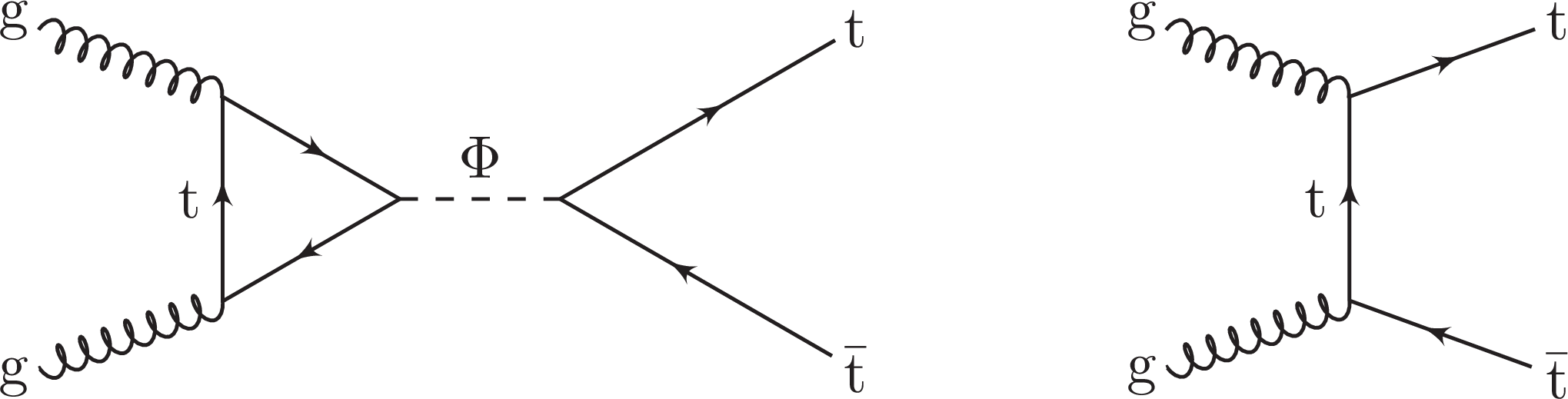
Figure 1:
Example Feynman diagrams for the signal process (left) and for SM $ \mathrm{t} \overline{\mathrm{t}} $ production (right). |
png pdf |
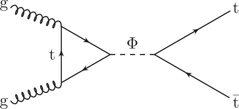
Figure 1-a:
Example Feynman diagrams for the signal process (left) and for SM $ \mathrm{t} \overline{\mathrm{t}} $ production (right). |
png pdf |
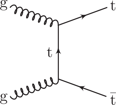
Figure 1-b:
Example Feynman diagrams for the signal process (left) and for SM $ \mathrm{t} \overline{\mathrm{t}} $ production (right). |
png pdf |
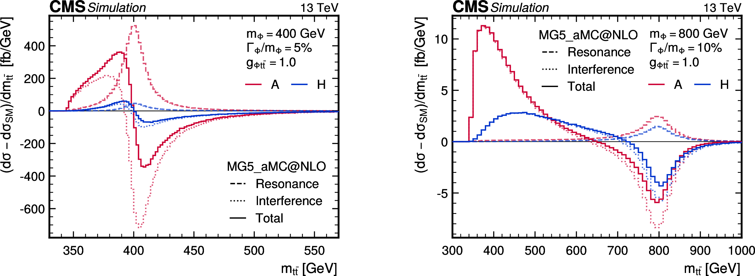
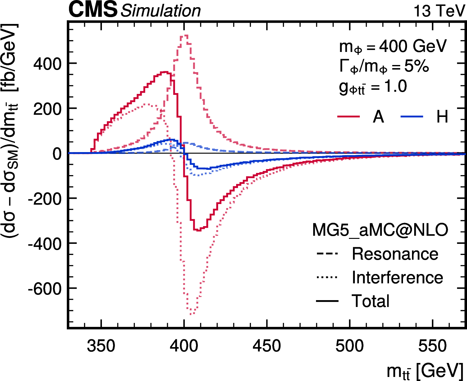
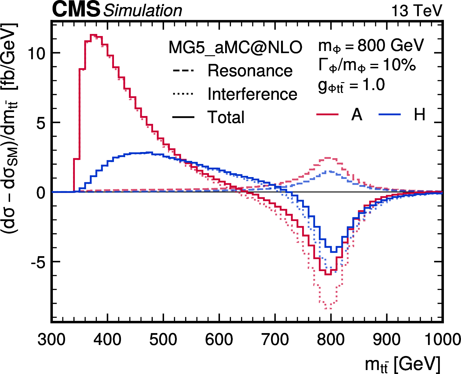
Figure 2:
Differential cross section of $ \mathrm{t} \overline{\mathrm{t}} $ production at parton level as a function of $ m_{{\mathrm{t}\overline{\mathrm{t}}} } $, shown as difference between various BSM scenarios and the SM prediction. Shown are the cases of a single A (red) or H (blue) boson for two example configurations: $ m_{\Phi}= $ 400 GeV and $ \Gamma_{\Phi}/m_{\Phi}= $ 5% (left), or $ m_{\Phi}= $ 800 GeV and $ \Gamma_{\Phi}/m_{\Phi}= $ 10% (right), with $ g_{\Phi\mathrm{tt}}= $ 1 in both cases. Separately shown are the cases where only the resonant $ \Phi\to{\mathrm{t}\overline{\mathrm{t}}} $ contribution is added to the SM prediction (dashed), where only the interference between SM and $ \Phi $ boson contributions is added (dotted), and where both contributions are added (solid). The distributions have been calculated using MadGraph-5_aMC@NLO as described in Section 3. |
png pdf |
Figure 2-a:
Differential cross section of $ \mathrm{t} \overline{\mathrm{t}} $ production at parton level as a function of $ m_{{\mathrm{t}\overline{\mathrm{t}}} } $, shown as difference between various BSM scenarios and the SM prediction. Shown are the cases of a single A (red) or H (blue) boson for two example configurations: $ m_{\Phi}= $ 400 GeV and $ \Gamma_{\Phi}/m_{\Phi}= $ 5% (left), or $ m_{\Phi}= $ 800 GeV and $ \Gamma_{\Phi}/m_{\Phi}= $ 10% (right), with $ g_{\Phi\mathrm{tt}}= $ 1 in both cases. Separately shown are the cases where only the resonant $ \Phi\to{\mathrm{t}\overline{\mathrm{t}}} $ contribution is added to the SM prediction (dashed), where only the interference between SM and $ \Phi $ boson contributions is added (dotted), and where both contributions are added (solid). The distributions have been calculated using MadGraph-5_aMC@NLO as described in Section 3. |
png pdf |
Figure 2-b:
Differential cross section of $ \mathrm{t} \overline{\mathrm{t}} $ production at parton level as a function of $ m_{{\mathrm{t}\overline{\mathrm{t}}} } $, shown as difference between various BSM scenarios and the SM prediction. Shown are the cases of a single A (red) or H (blue) boson for two example configurations: $ m_{\Phi}= $ 400 GeV and $ \Gamma_{\Phi}/m_{\Phi}= $ 5% (left), or $ m_{\Phi}= $ 800 GeV and $ \Gamma_{\Phi}/m_{\Phi}= $ 10% (right), with $ g_{\Phi\mathrm{tt}}= $ 1 in both cases. Separately shown are the cases where only the resonant $ \Phi\to{\mathrm{t}\overline{\mathrm{t}}} $ contribution is added to the SM prediction (dashed), where only the interference between SM and $ \Phi $ boson contributions is added (dotted), and where both contributions are added (solid). The distributions have been calculated using MadGraph-5_aMC@NLO as described in Section 3. |
png pdf |
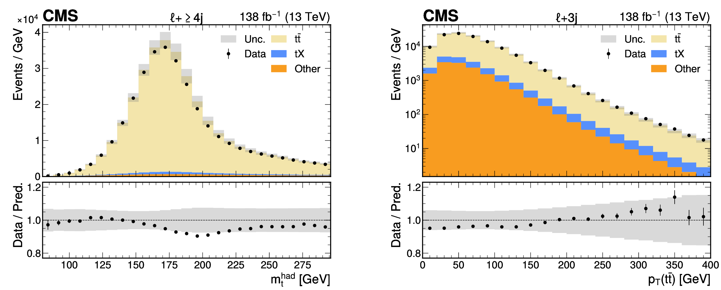
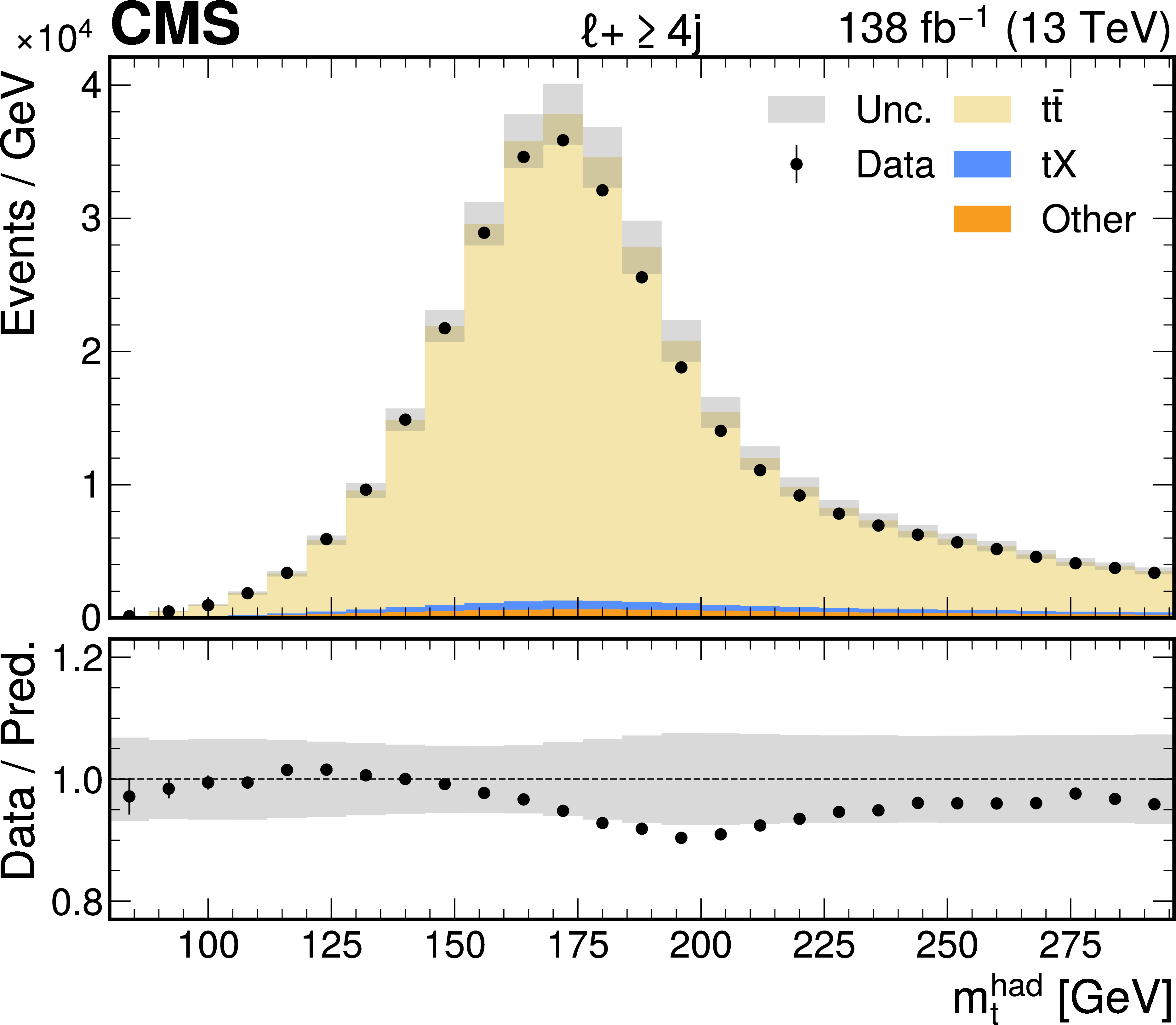
Figure 3:
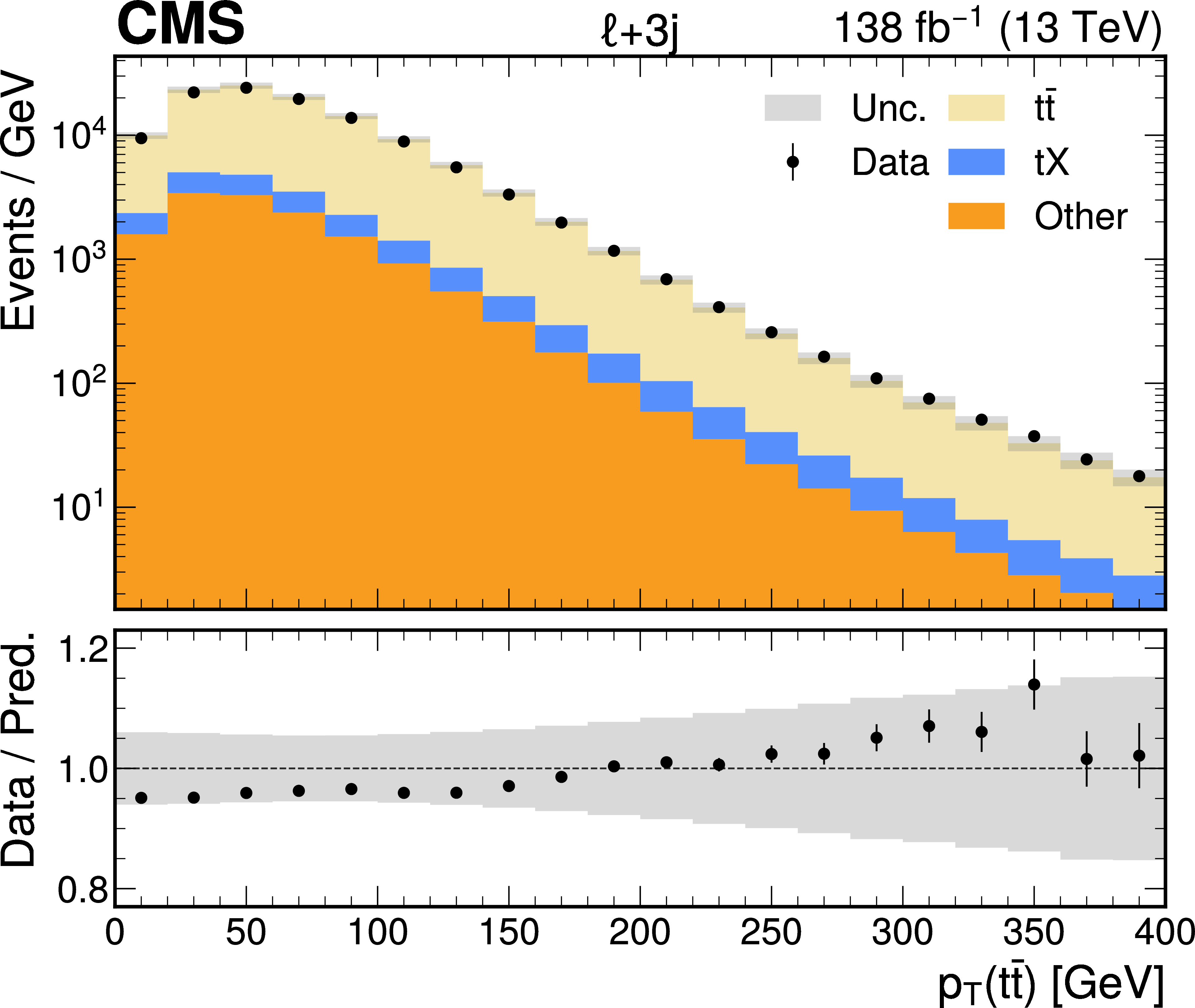
Comparison of the number of observed (points) and expected (colored histograms) events in the $ \ell{\mathrm{j}} $ channel after the kinematic reconstruction and background estimation for the distributions of the reconstructed hadronic top quark mass $ m_{\mathrm{t}}^{\text{had}} $ in the region with four or more jets (left) and the $ p_{\mathrm{T}} $ of the $ \mathrm{t} \overline{\mathrm{t}} $ system in the region with exactly three jets (right). The ratio to the total prediction is shown in the lower panel, and the total systematic uncertainty is shown as the gray band. |
png pdf |
Figure 3-a:
Comparison of the number of observed (points) and expected (colored histograms) events in the $ \ell{\mathrm{j}} $ channel after the kinematic reconstruction and background estimation for the distributions of the reconstructed hadronic top quark mass $ m_{\mathrm{t}}^{\text{had}} $ in the region with four or more jets (left) and the $ p_{\mathrm{T}} $ of the $ \mathrm{t} \overline{\mathrm{t}} $ system in the region with exactly three jets (right). The ratio to the total prediction is shown in the lower panel, and the total systematic uncertainty is shown as the gray band. |
png pdf |
Figure 3-b:
Comparison of the number of observed (points) and expected (colored histograms) events in the $ \ell{\mathrm{j}} $ channel after the kinematic reconstruction and background estimation for the distributions of the reconstructed hadronic top quark mass $ m_{\mathrm{t}}^{\text{had}} $ in the region with four or more jets (left) and the $ p_{\mathrm{T}} $ of the $ \mathrm{t} \overline{\mathrm{t}} $ system in the region with exactly three jets (right). The ratio to the total prediction is shown in the lower panel, and the total systematic uncertainty is shown as the gray band. |
png pdf |
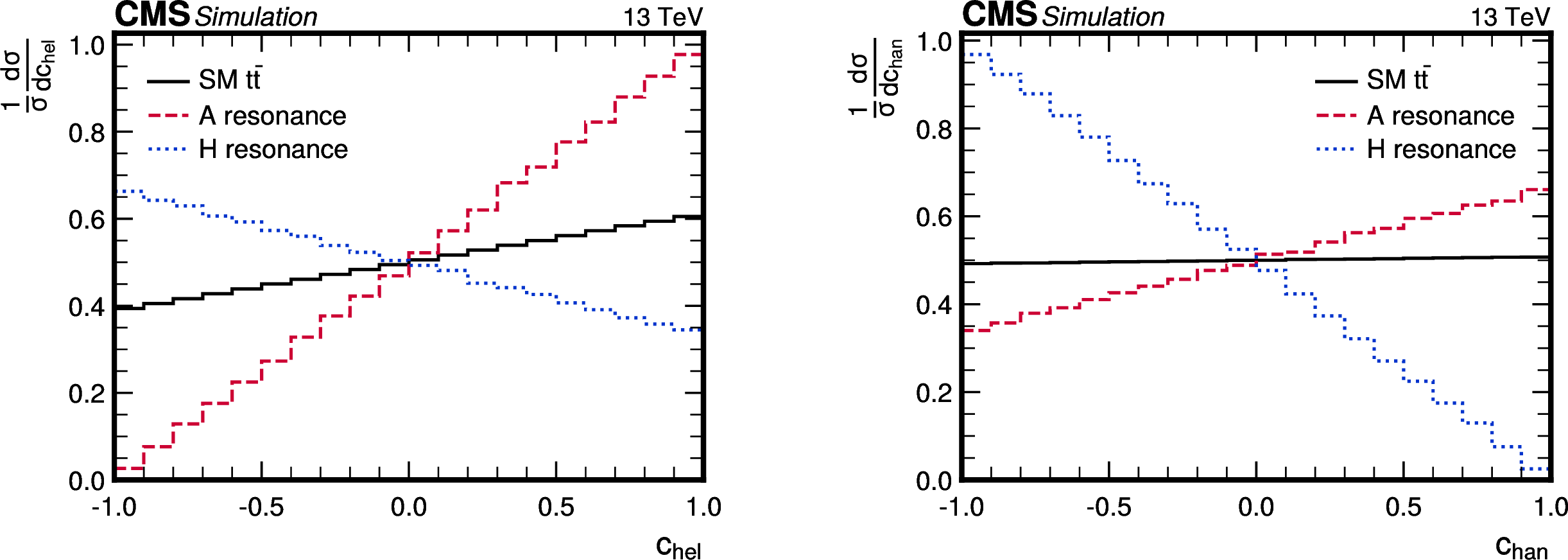
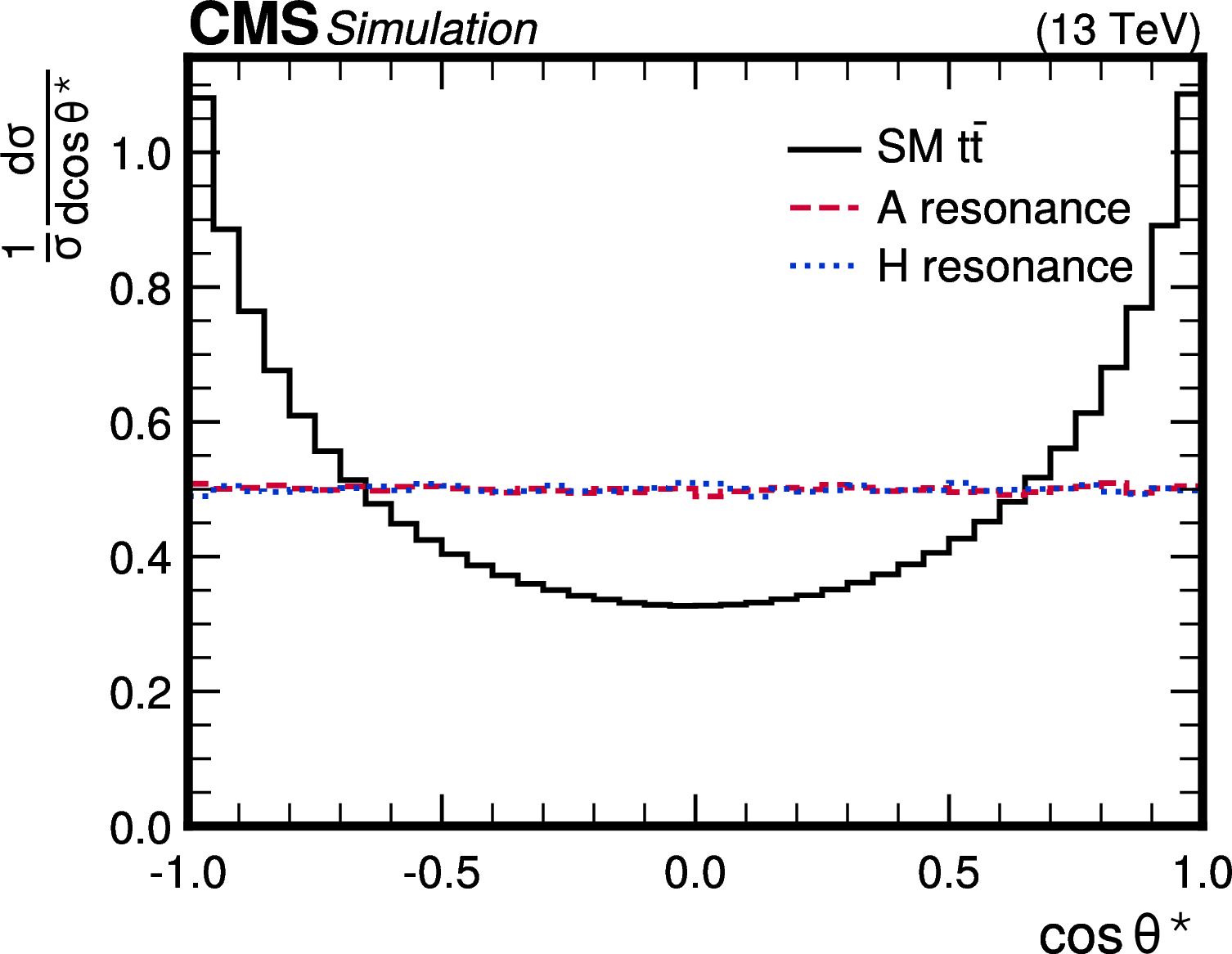
Figure 4:
Normalized differential cross sections in the spin correlation observables $ c_{\text{hel}} $ (left) and $ c_{\text{han}} $ (right) at the parton level in the $ \ell\ell $ channel, with no requirements on acceptance, for SM $ \mathrm{t} \overline{\mathrm{t}} $ production (black solid), resonant A boson production (red dashed), and resonant H boson production (blue dotted). The corresponding distributions for $ \eta_{\mathrm{t}} $ are identical to those of a A boson. |
png pdf |
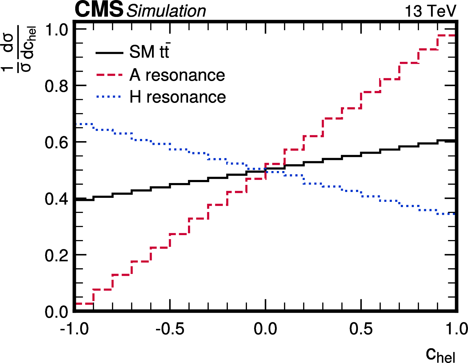
Figure 4-a:
Normalized differential cross sections in the spin correlation observables $ c_{\text{hel}} $ (left) and $ c_{\text{han}} $ (right) at the parton level in the $ \ell\ell $ channel, with no requirements on acceptance, for SM $ \mathrm{t} \overline{\mathrm{t}} $ production (black solid), resonant A boson production (red dashed), and resonant H boson production (blue dotted). The corresponding distributions for $ \eta_{\mathrm{t}} $ are identical to those of a A boson. |
png pdf |
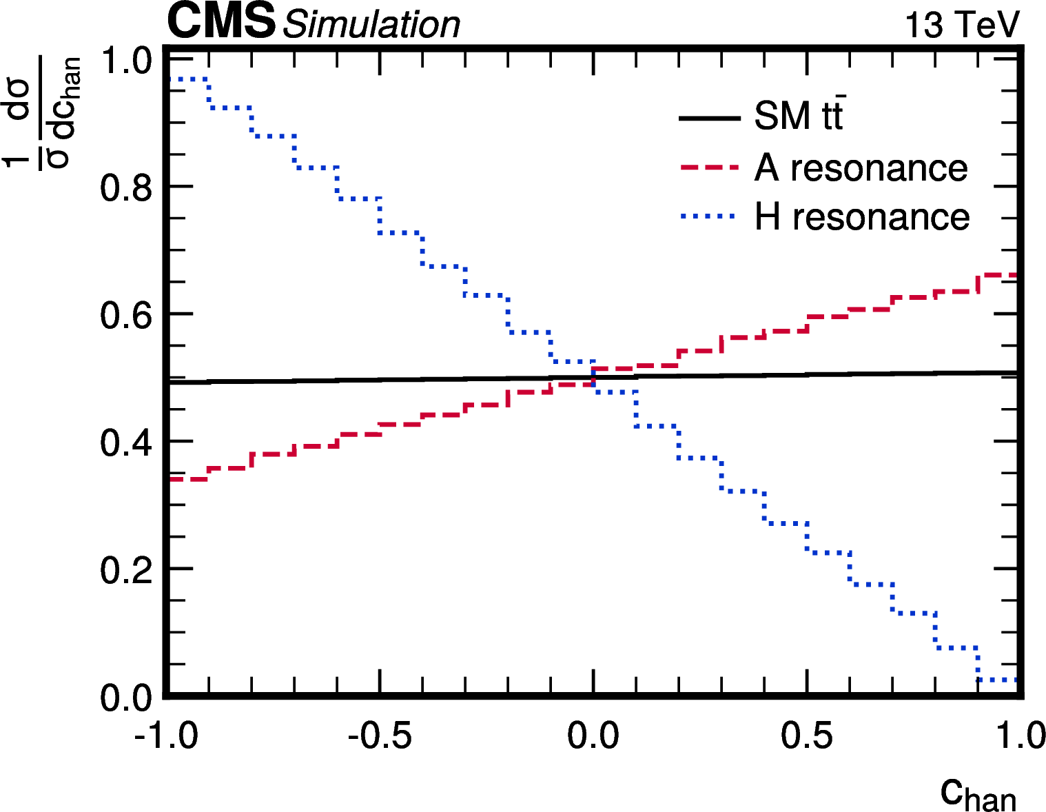
Figure 4-b:
Normalized differential cross sections in the spin correlation observables $ c_{\text{hel}} $ (left) and $ c_{\text{han}} $ (right) at the parton level in the $ \ell\ell $ channel, with no requirements on acceptance, for SM $ \mathrm{t} \overline{\mathrm{t}} $ production (black solid), resonant A boson production (red dashed), and resonant H boson production (blue dotted). The corresponding distributions for $ \eta_{\mathrm{t}} $ are identical to those of a A boson. |

png pdf |
Figure 5:
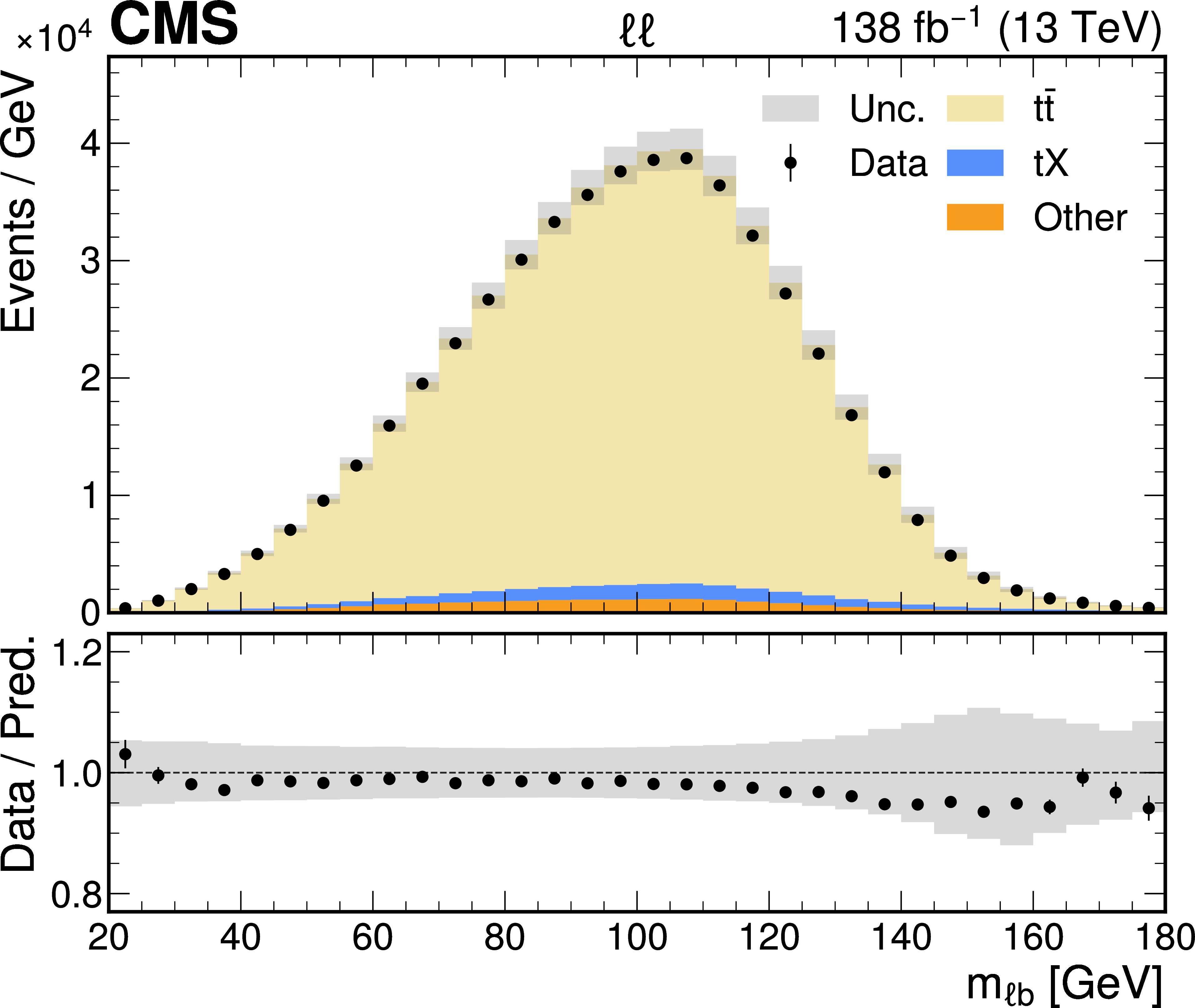
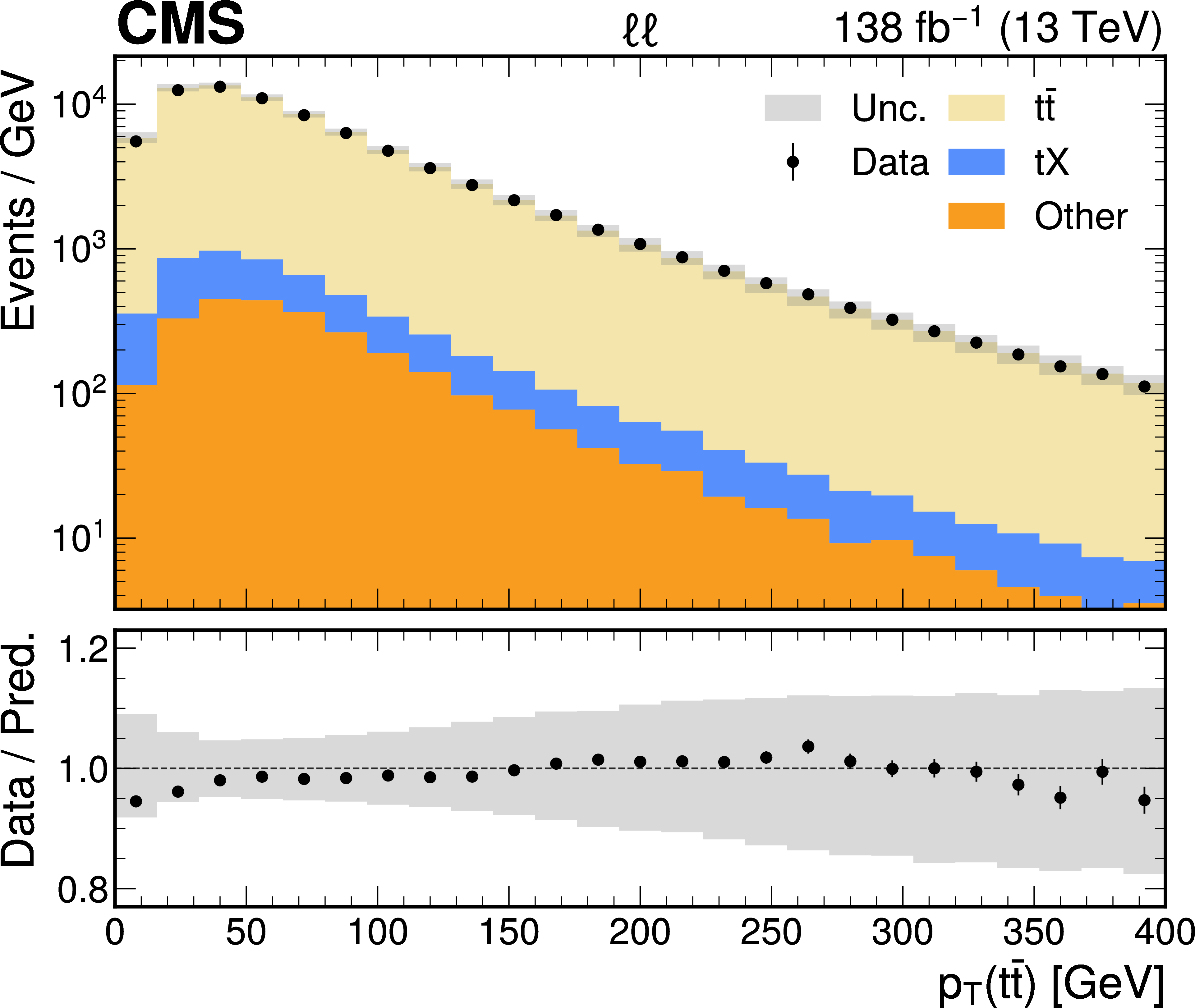
Comparison of the number of observed (points) and expected (colored histograms) events in the $ \ell\ell $ channel after the kinematic reconstruction and background estimation for the distributions of the invariant lepton-b jet mass $ m_{\ell\mathrm{b}} $ (left) and the $ p_{\mathrm{T}} $ of the $ \mathrm{t} \overline{\mathrm{t}} $ system (right). The ratio to the total prediction is shown in the lower panel, and the total systematic uncertainty is shown as the gray band. |
png pdf |
Figure 5-a:
Comparison of the number of observed (points) and expected (colored histograms) events in the $ \ell\ell $ channel after the kinematic reconstruction and background estimation for the distributions of the invariant lepton-b jet mass $ m_{\ell\mathrm{b}} $ (left) and the $ p_{\mathrm{T}} $ of the $ \mathrm{t} \overline{\mathrm{t}} $ system (right). The ratio to the total prediction is shown in the lower panel, and the total systematic uncertainty is shown as the gray band. |
png pdf |
Figure 5-b:
Comparison of the number of observed (points) and expected (colored histograms) events in the $ \ell\ell $ channel after the kinematic reconstruction and background estimation for the distributions of the invariant lepton-b jet mass $ m_{\ell\mathrm{b}} $ (left) and the $ p_{\mathrm{T}} $ of the $ \mathrm{t} \overline{\mathrm{t}} $ system (right). The ratio to the total prediction is shown in the lower panel, and the total systematic uncertainty is shown as the gray band. |
png pdf |
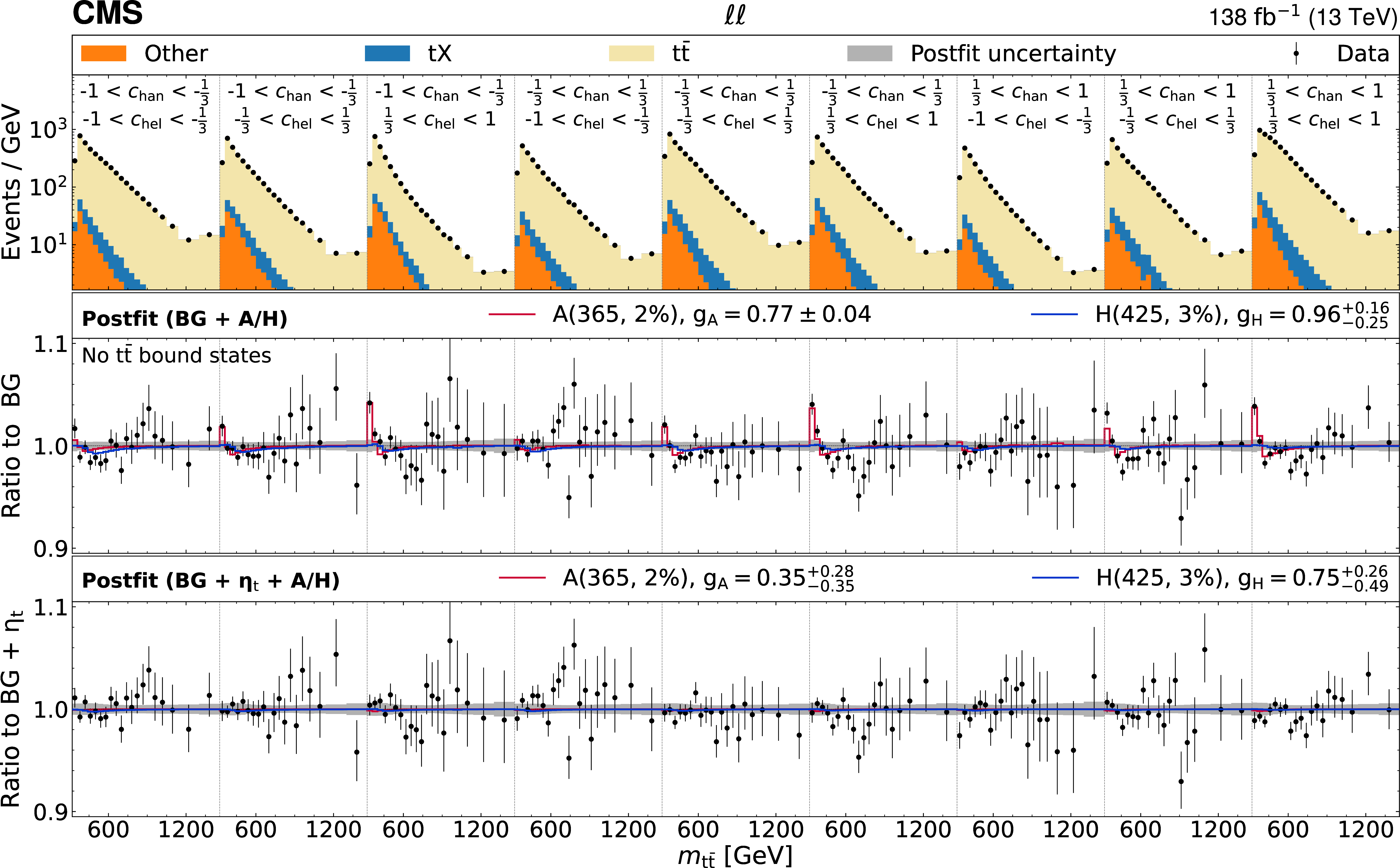
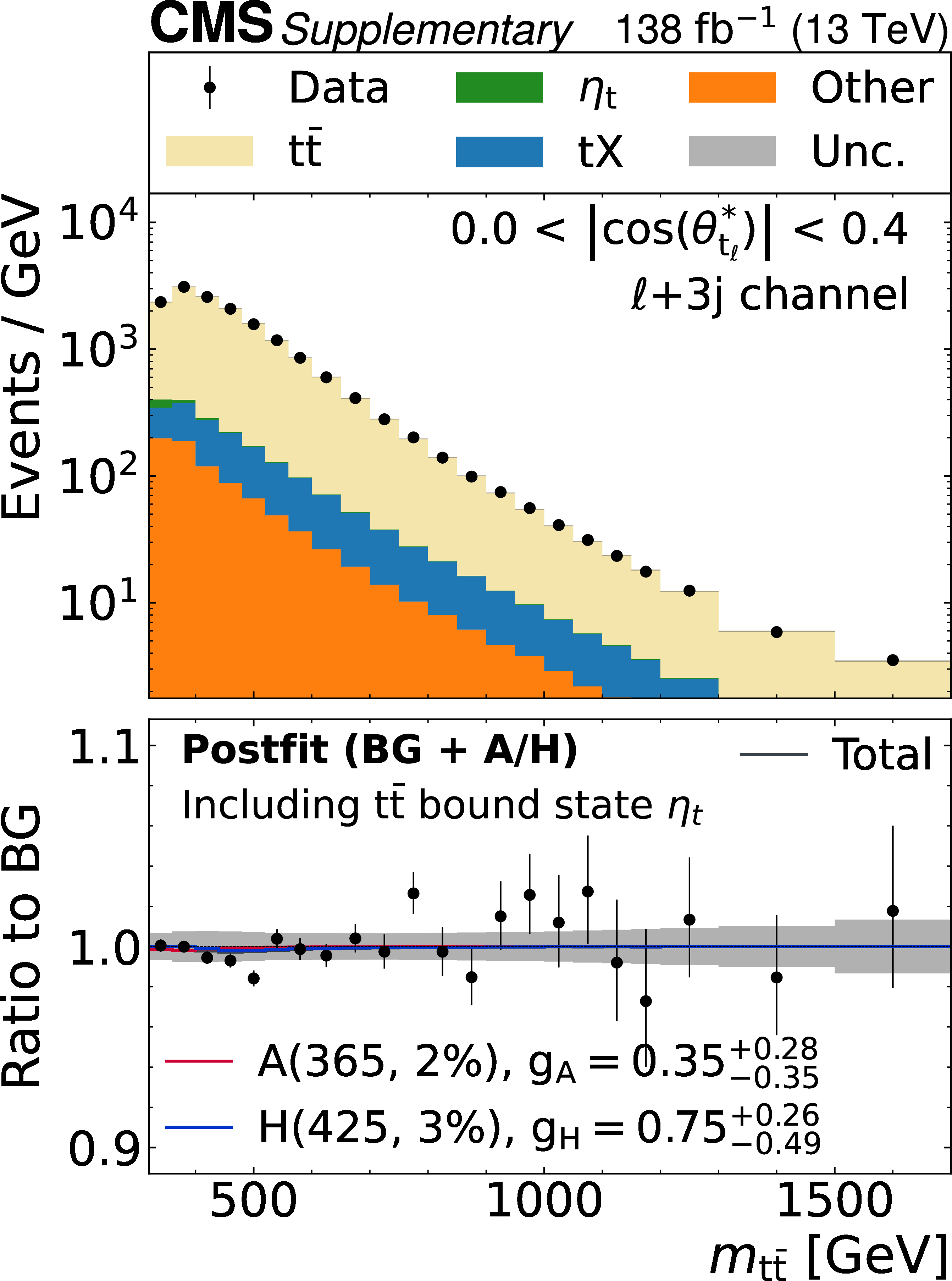
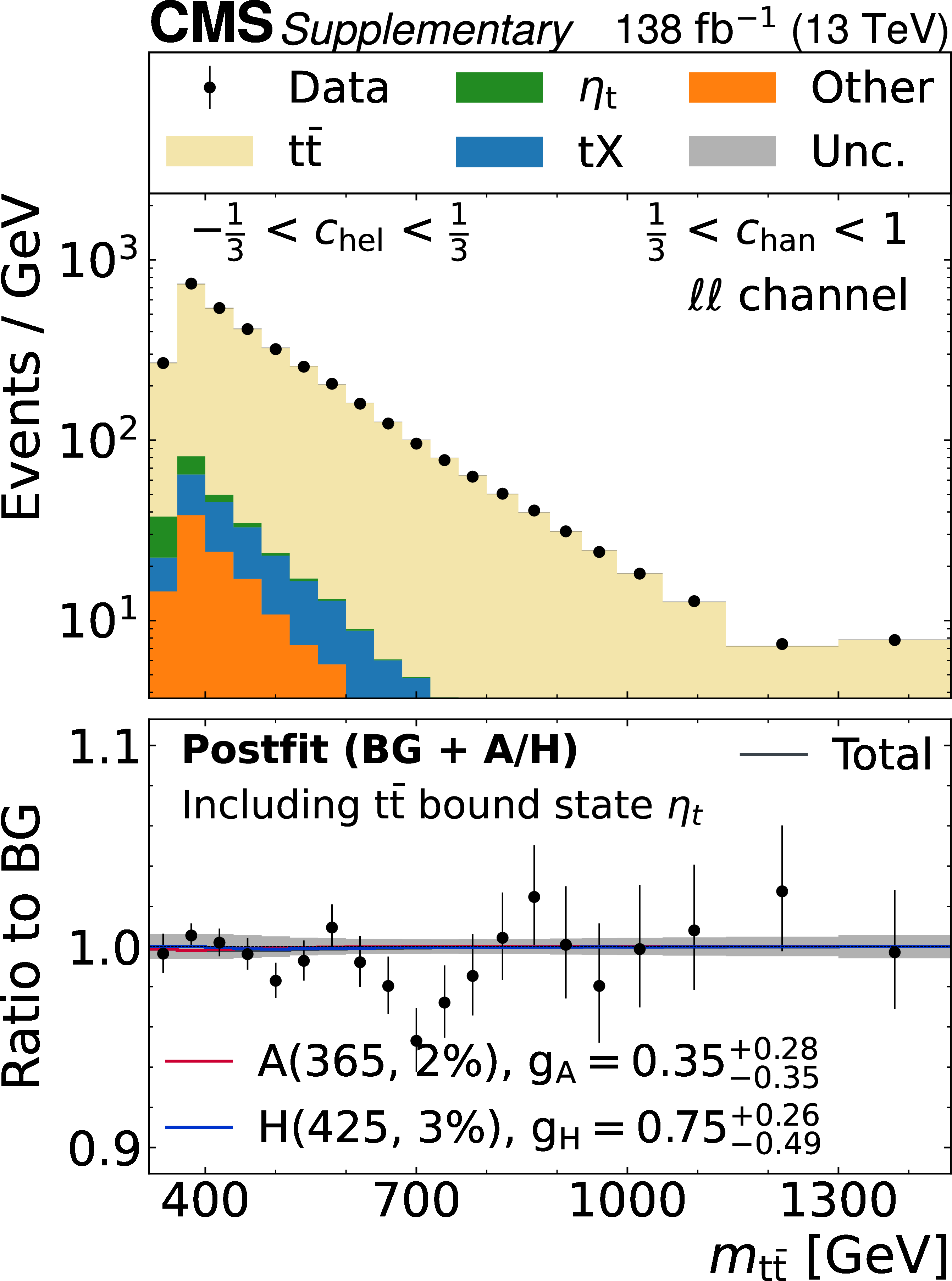
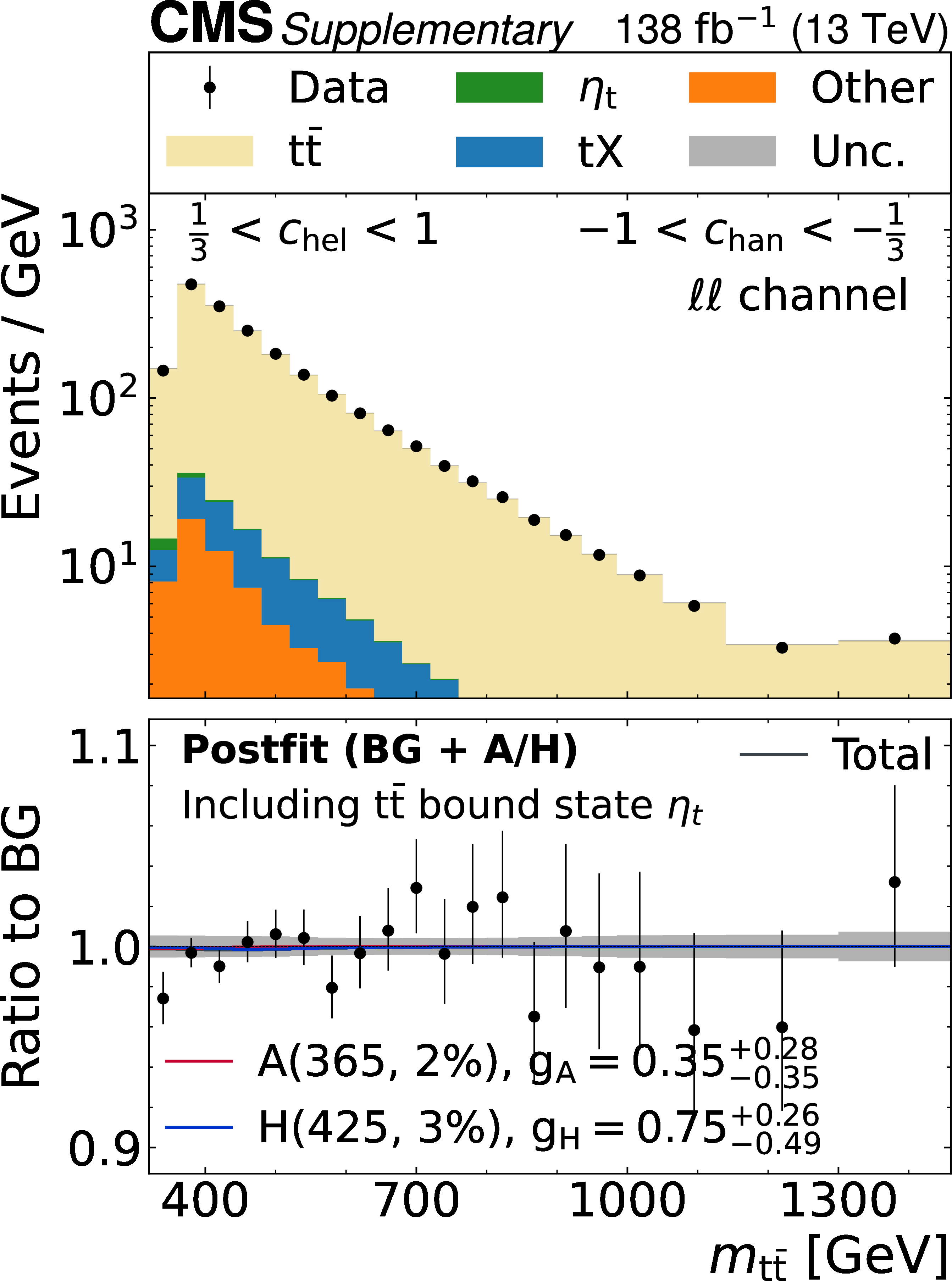
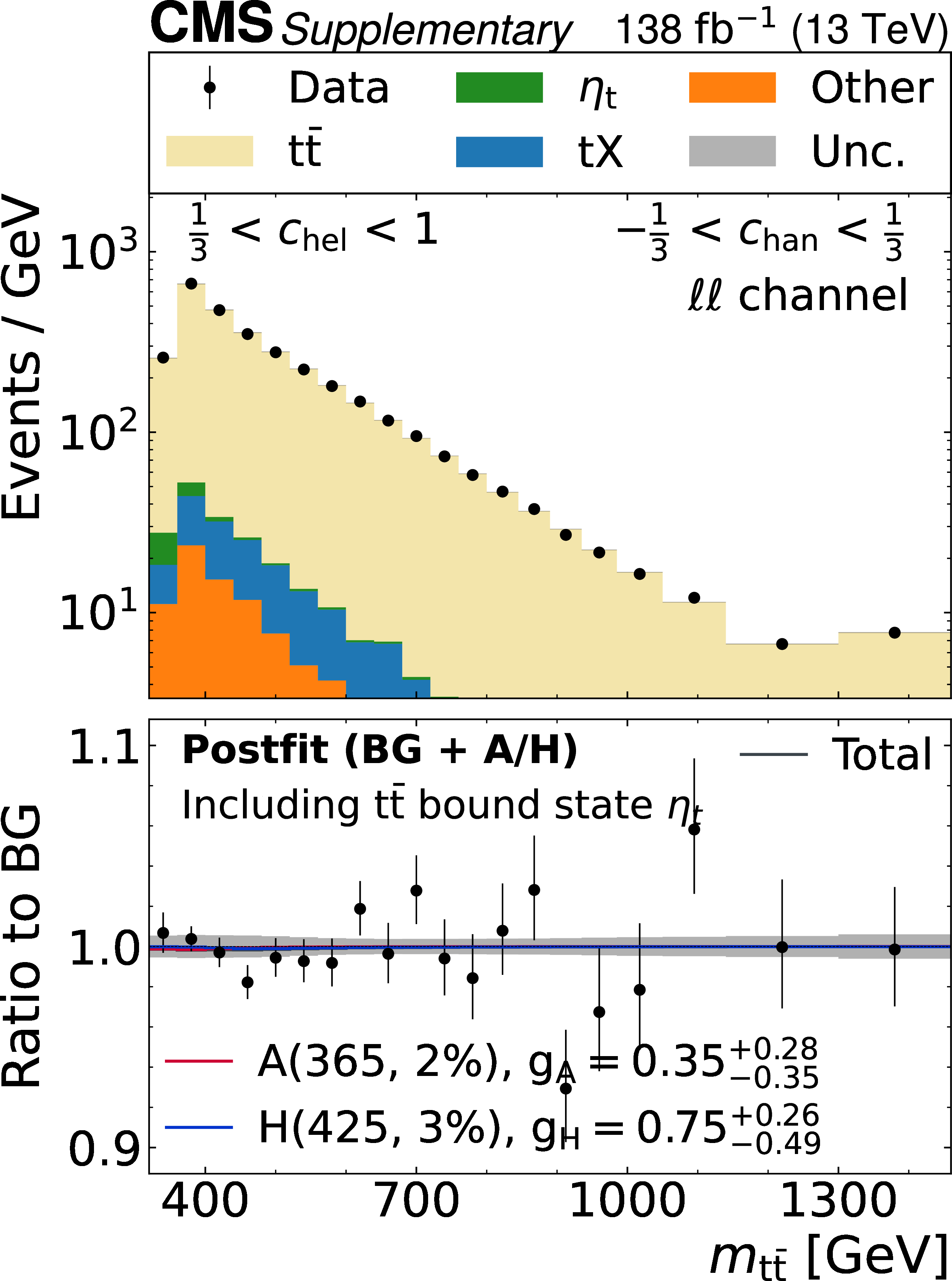
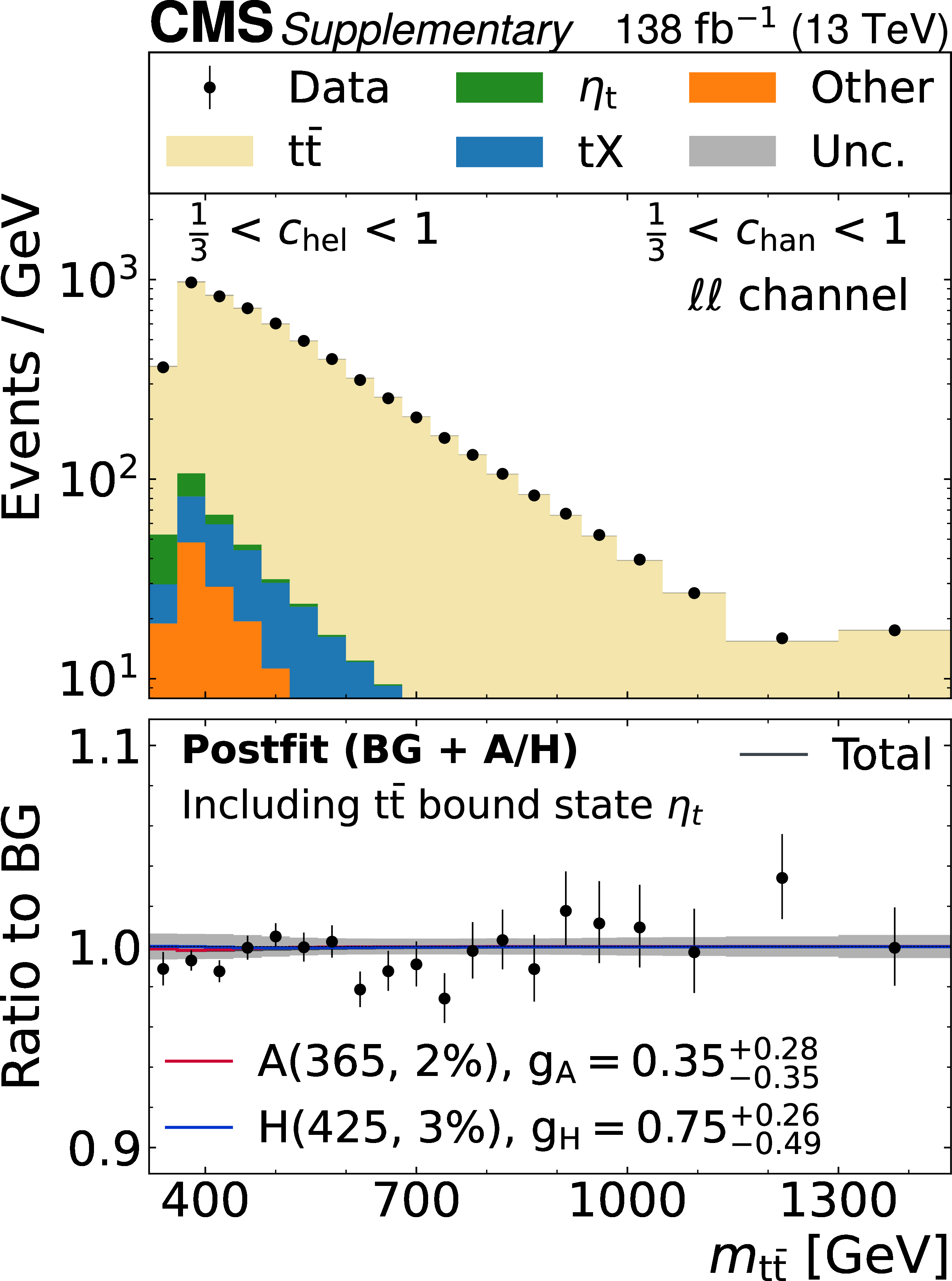
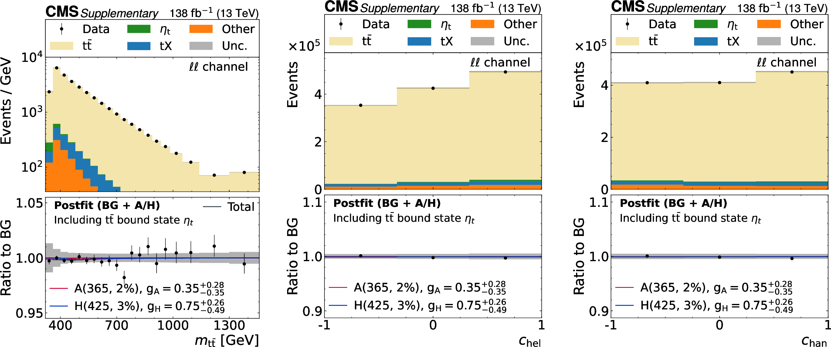
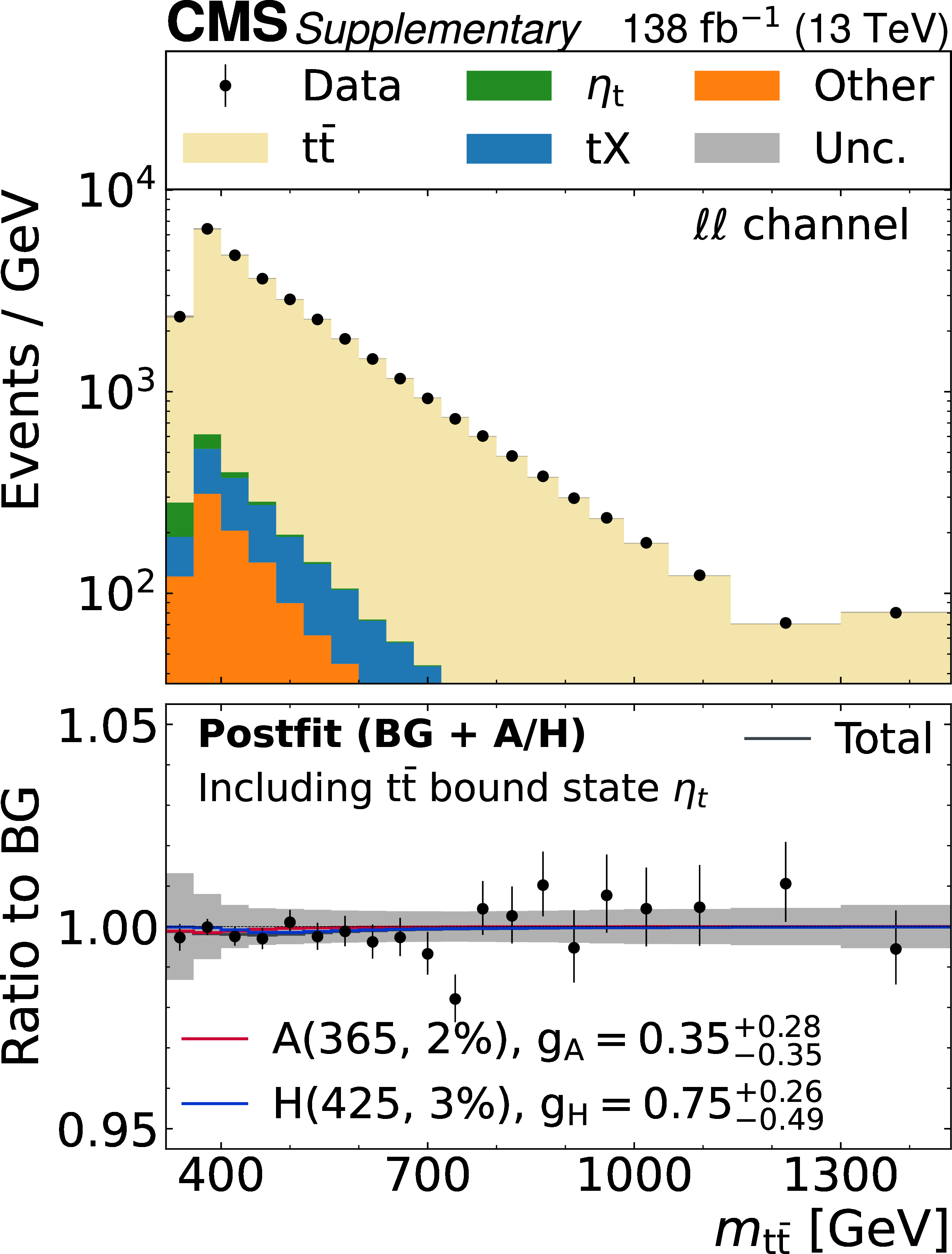
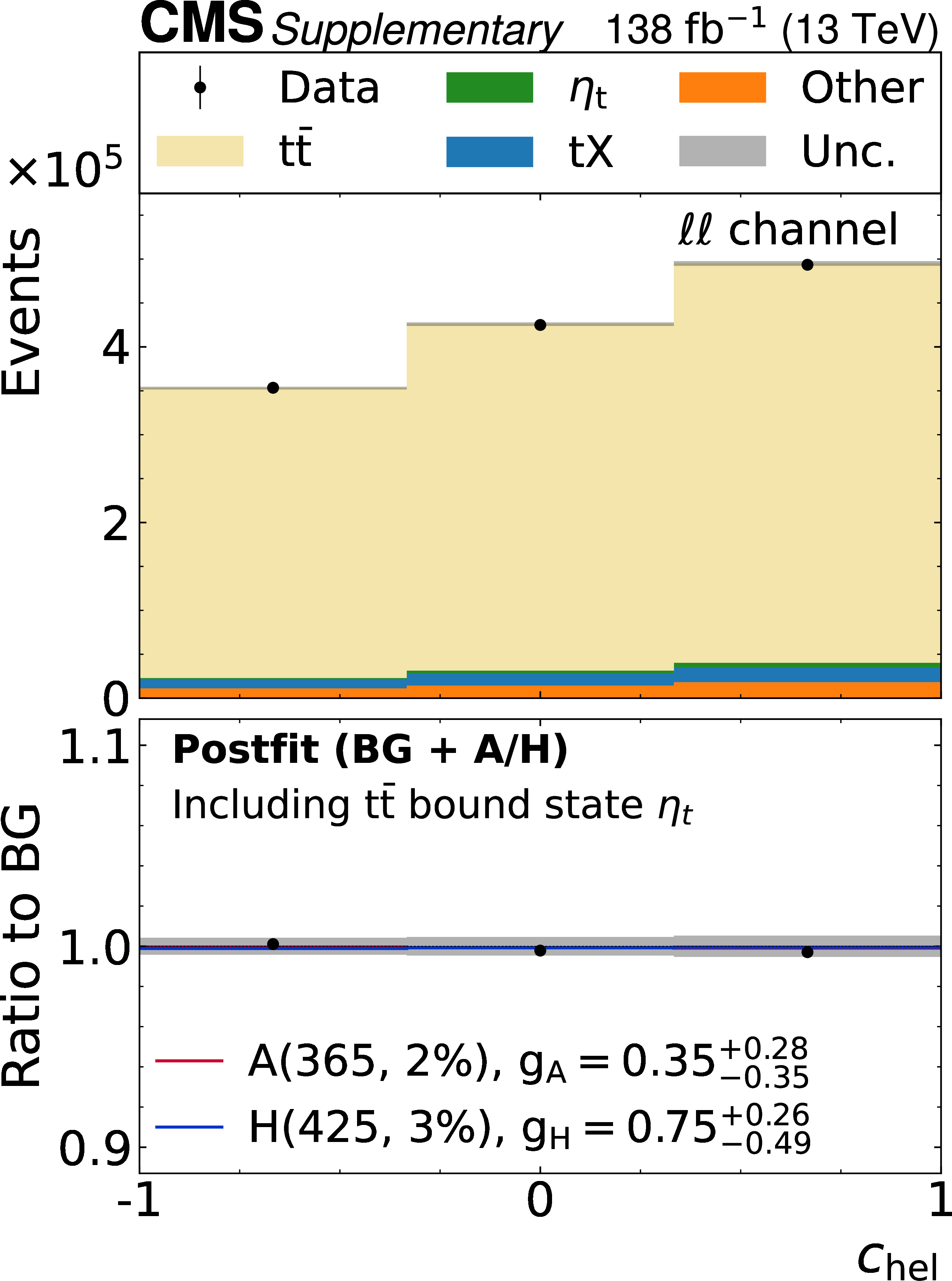
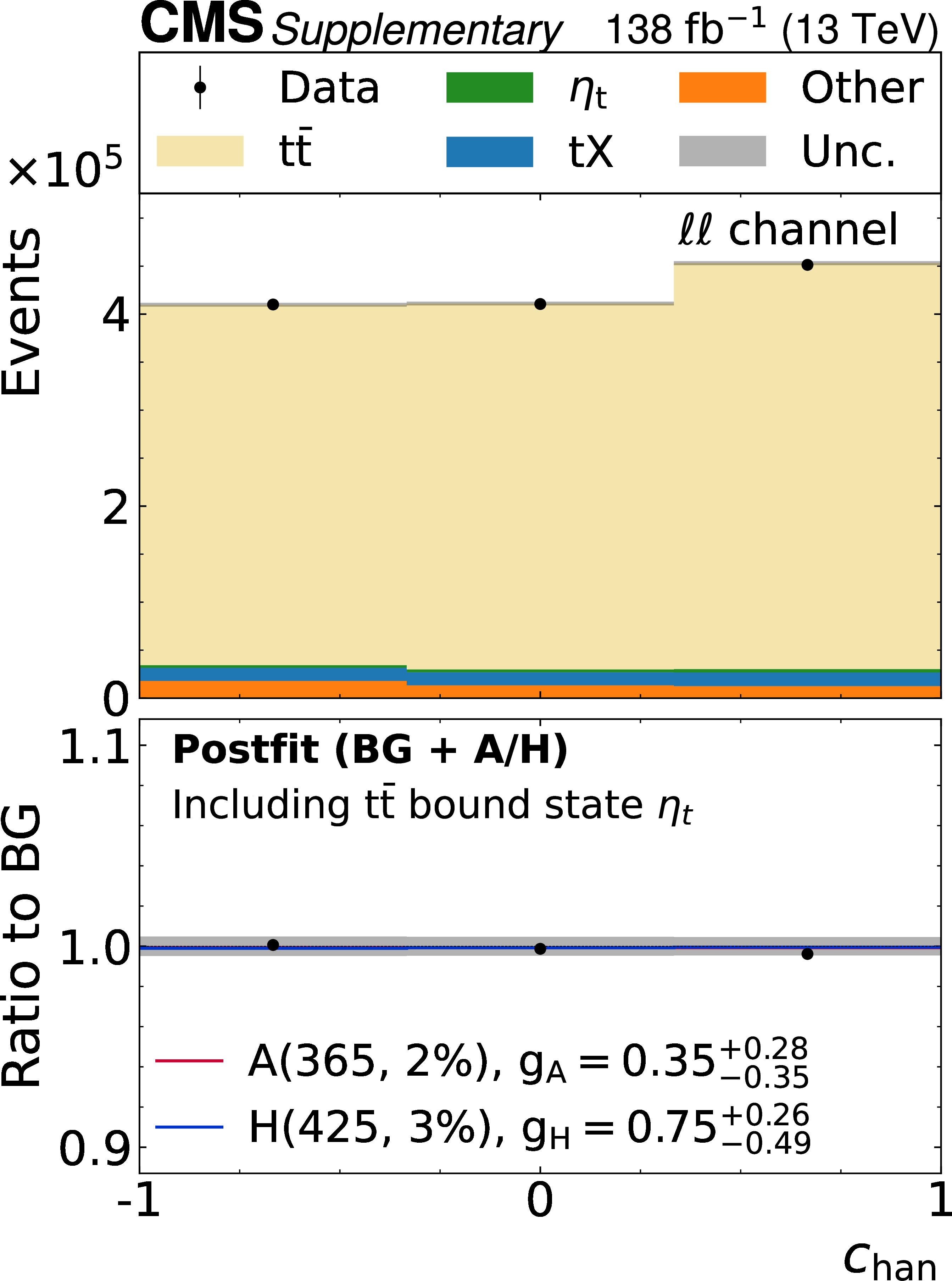
Figure 6:
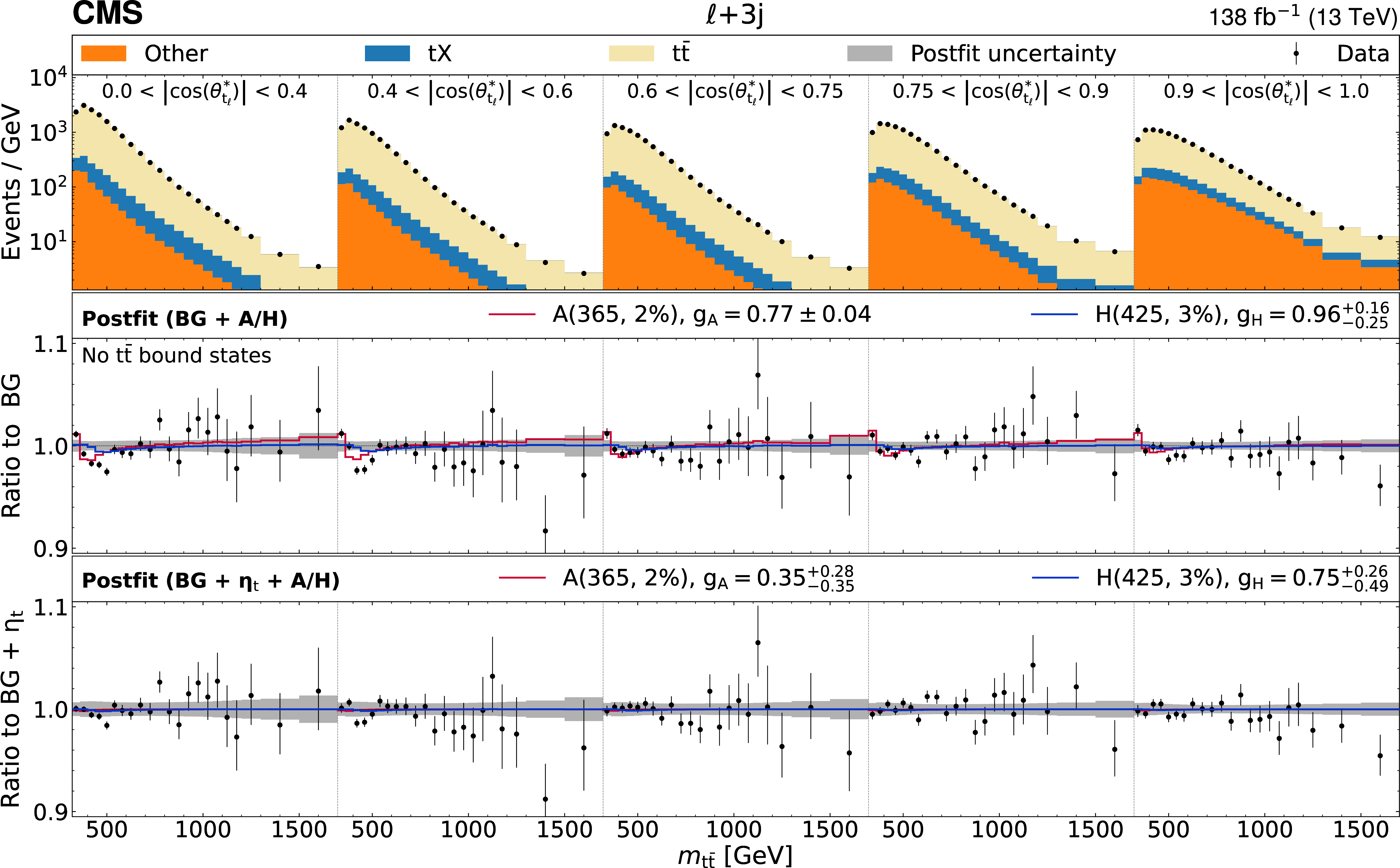
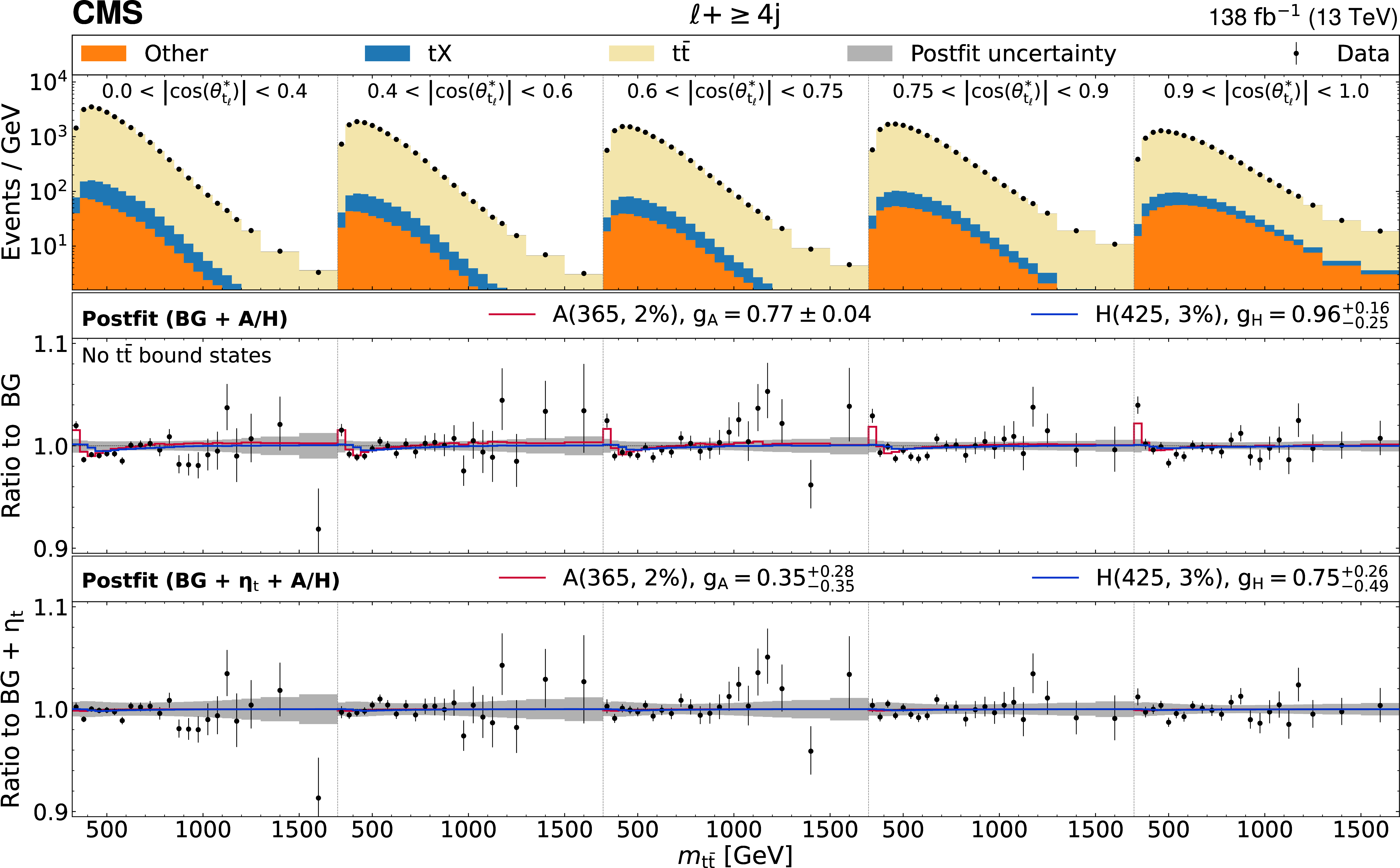
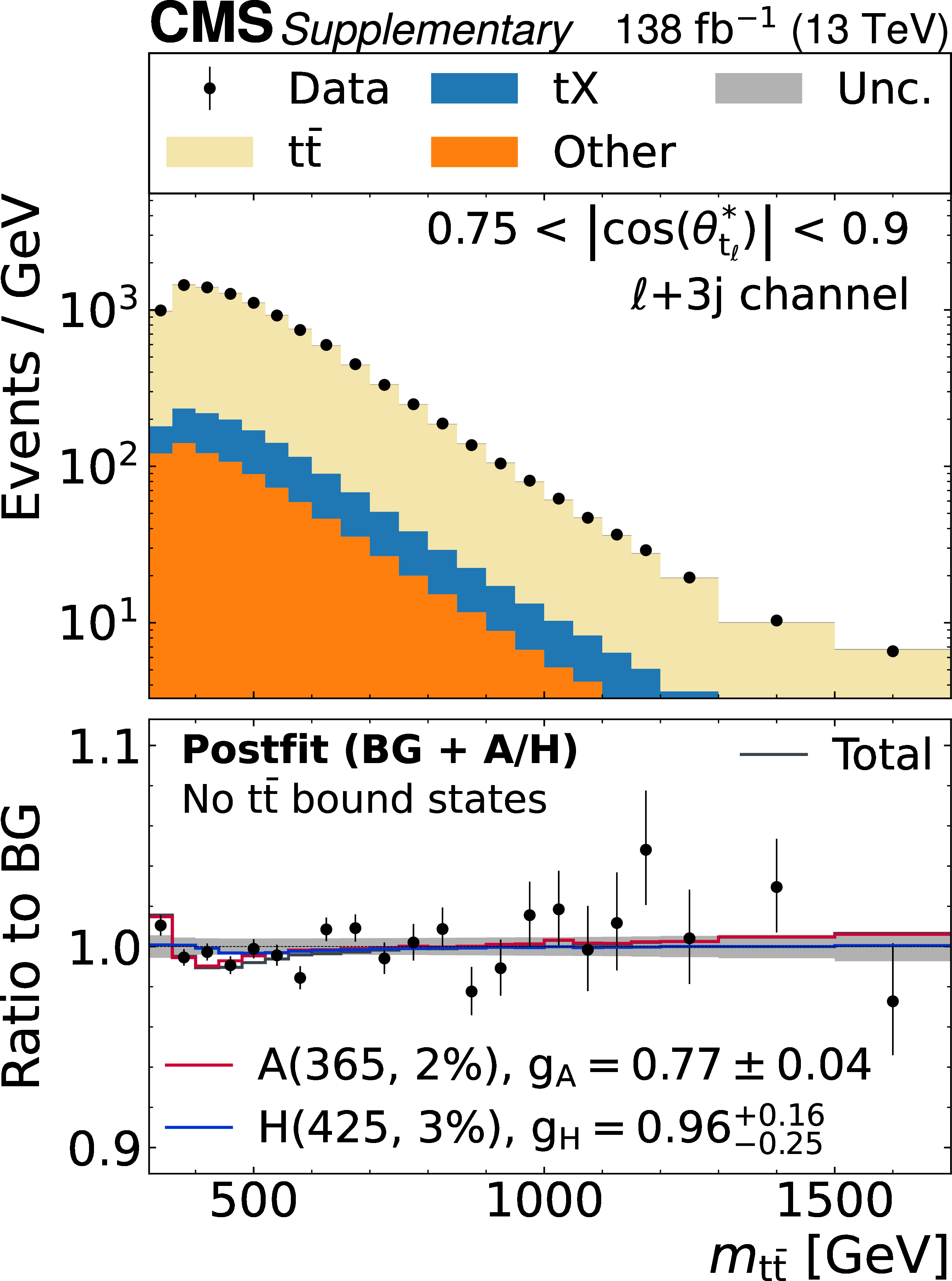
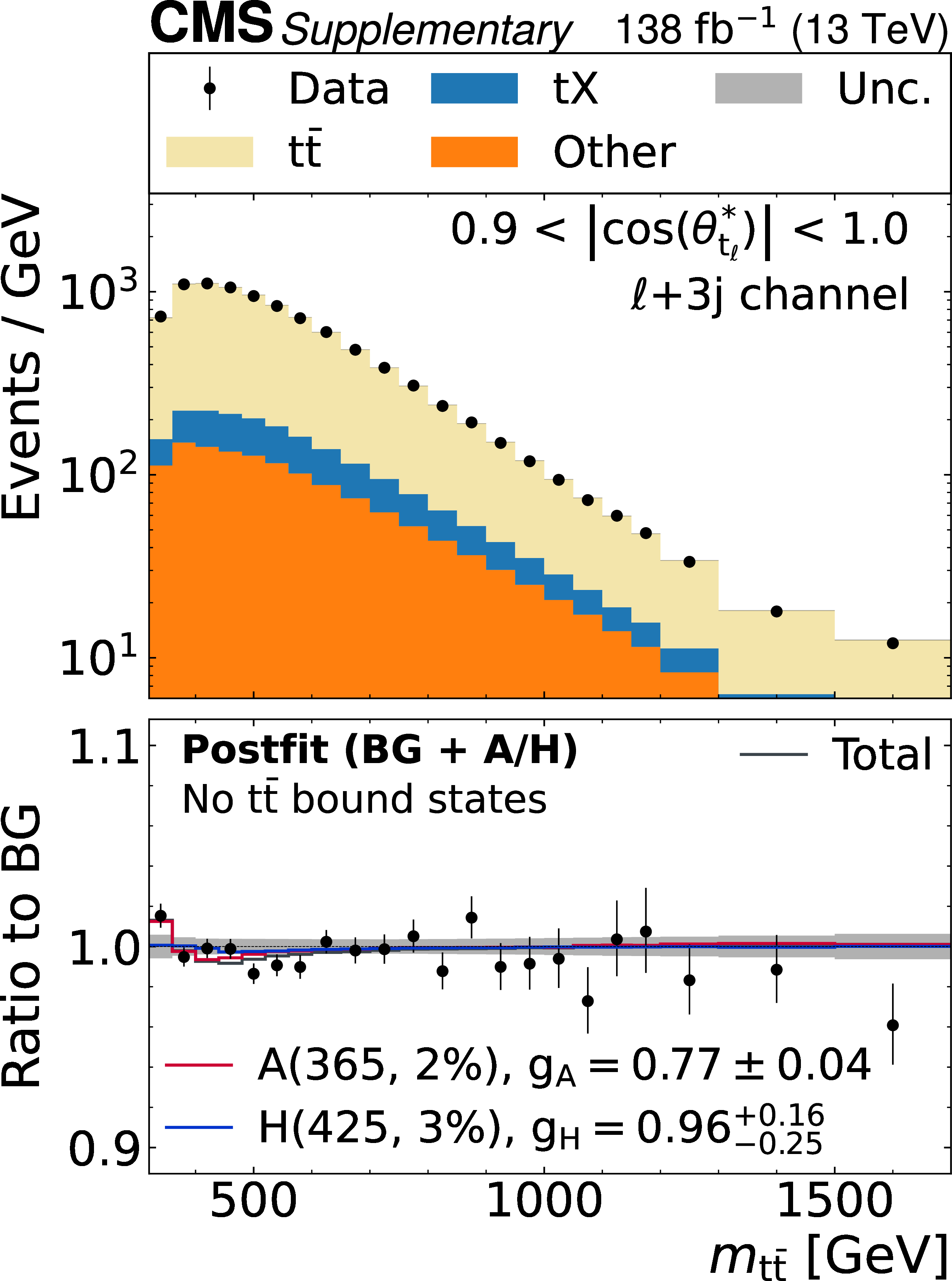
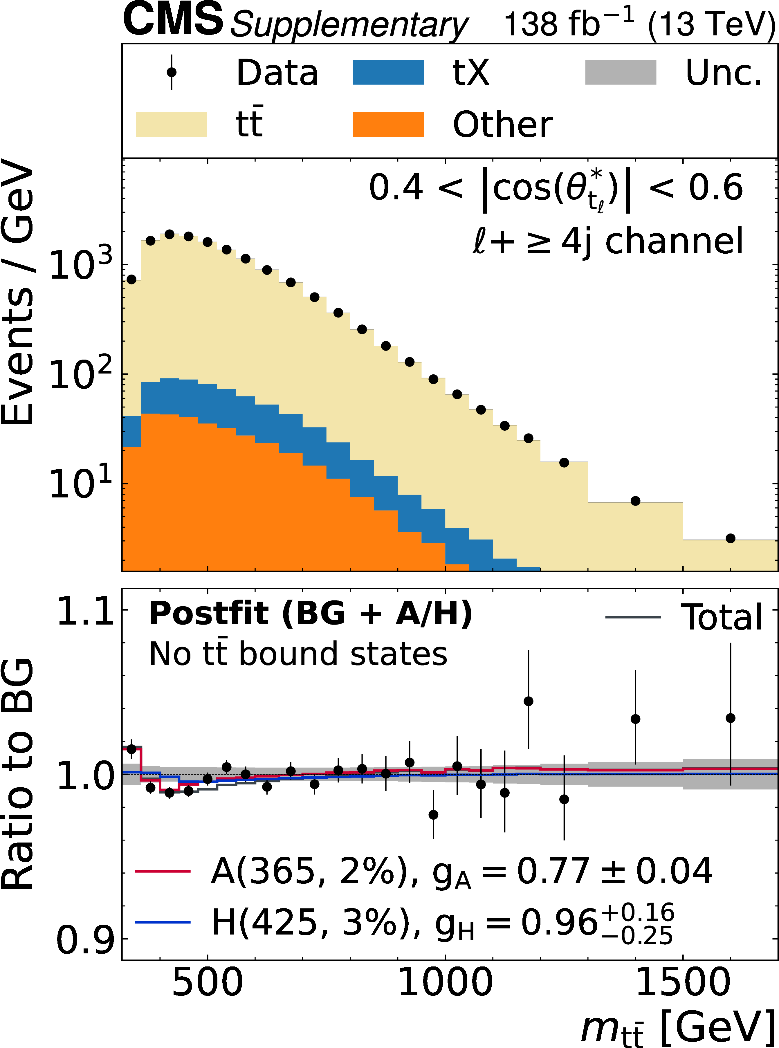
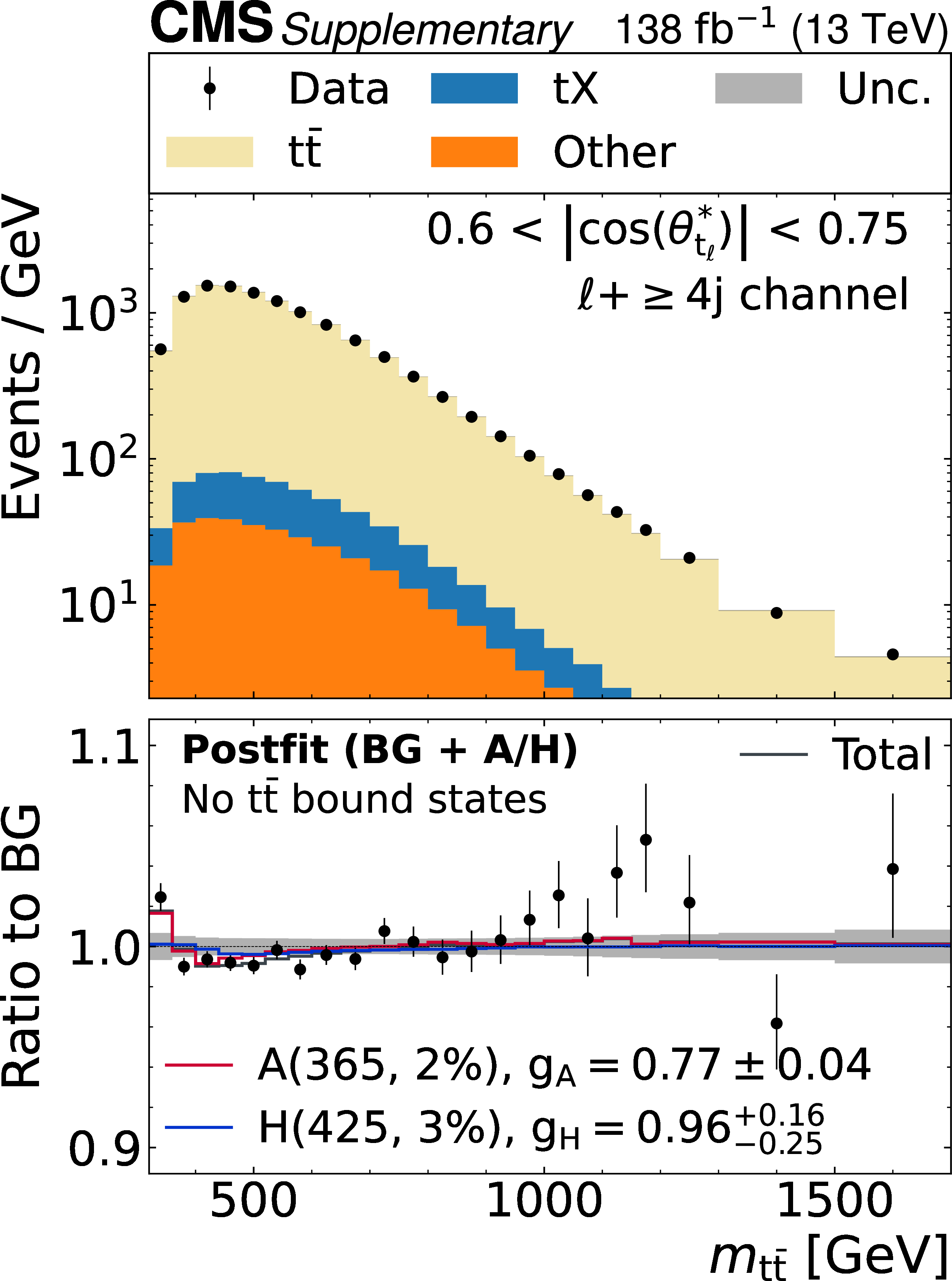
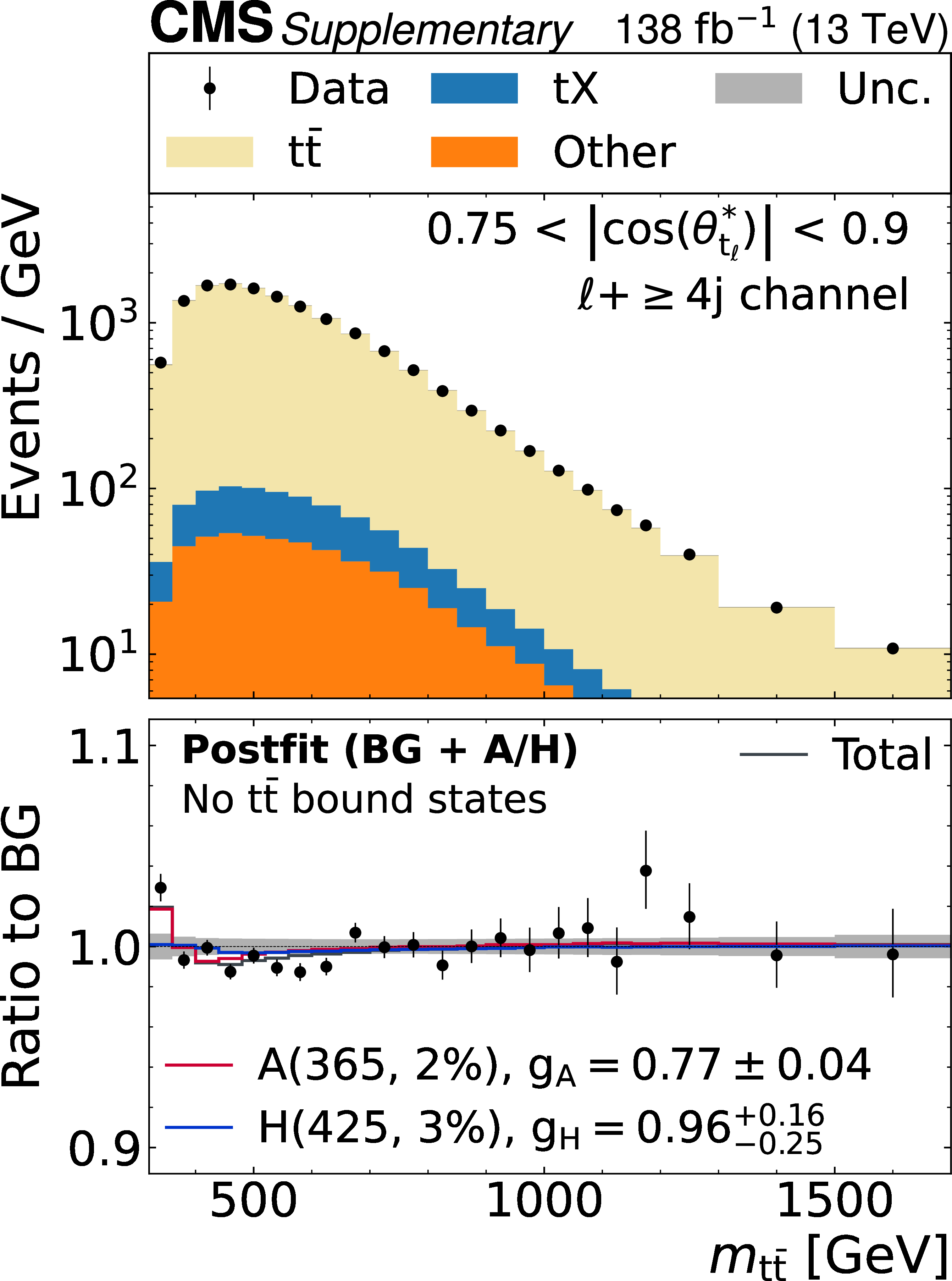
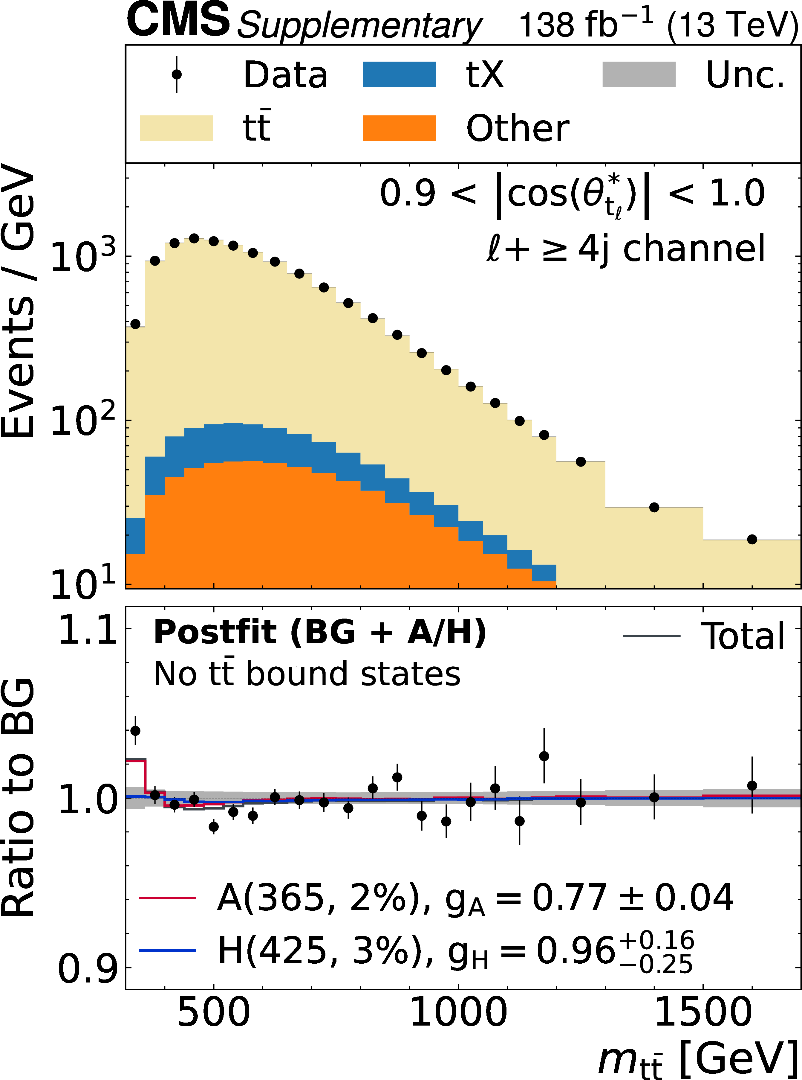
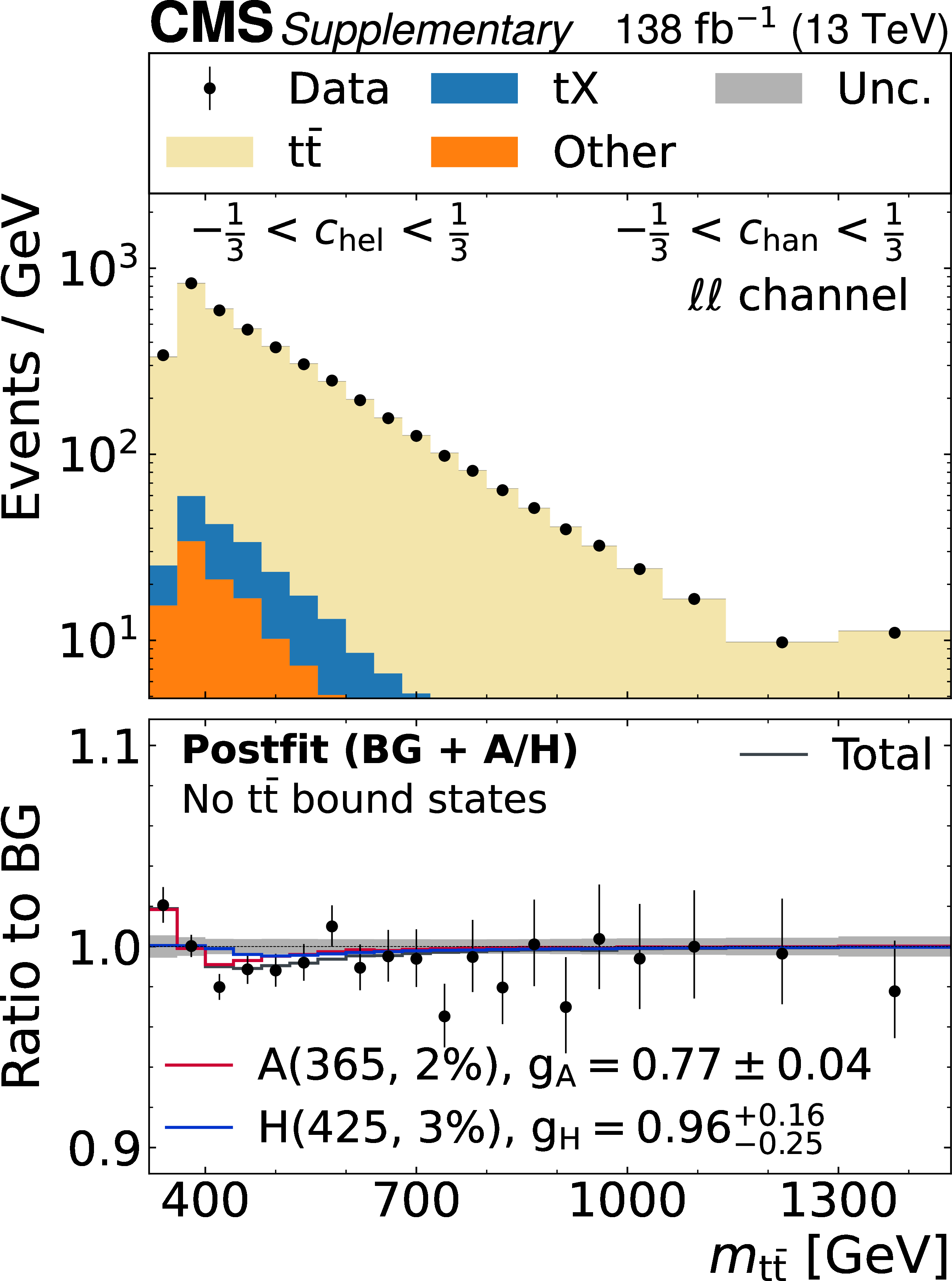
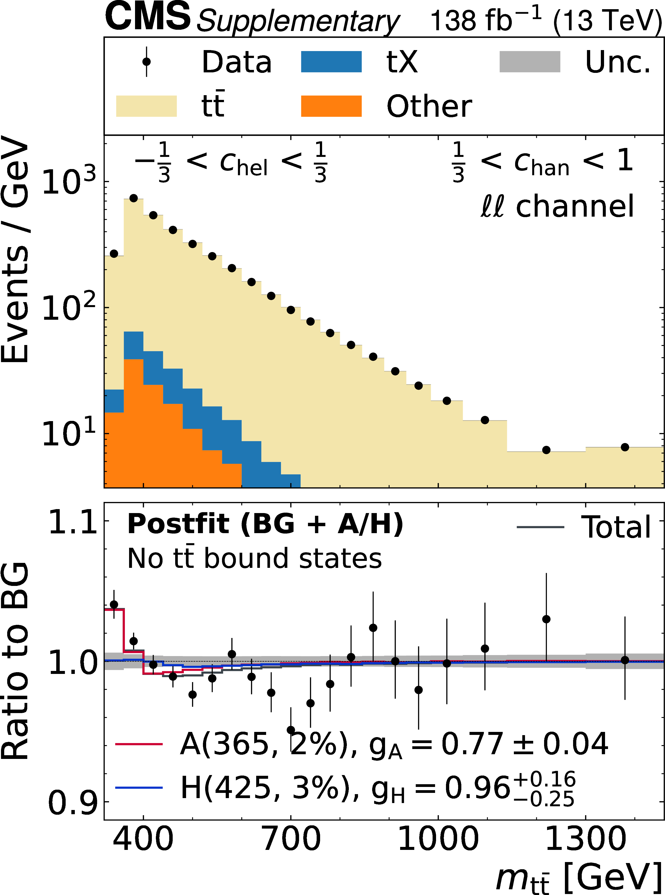
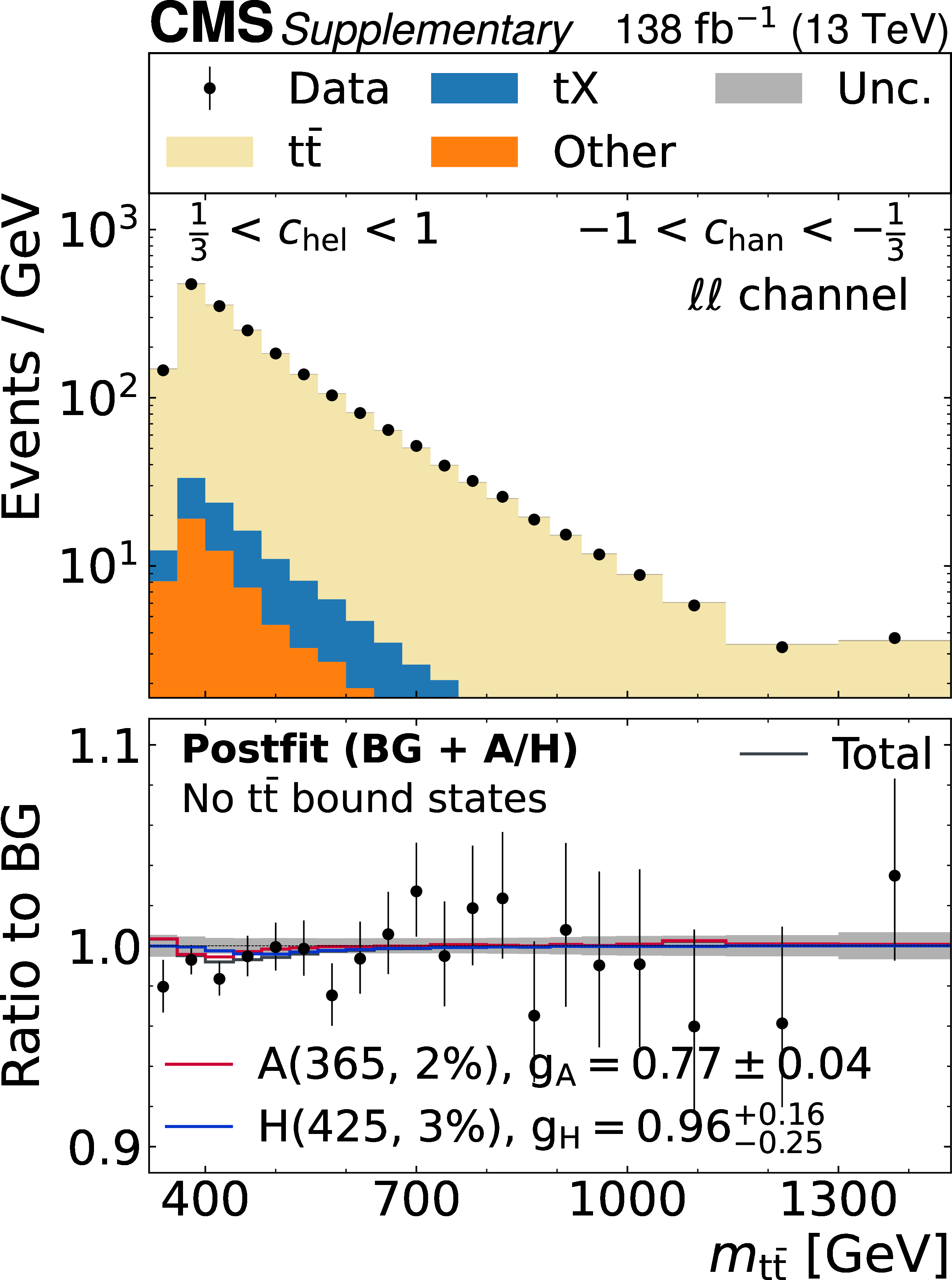
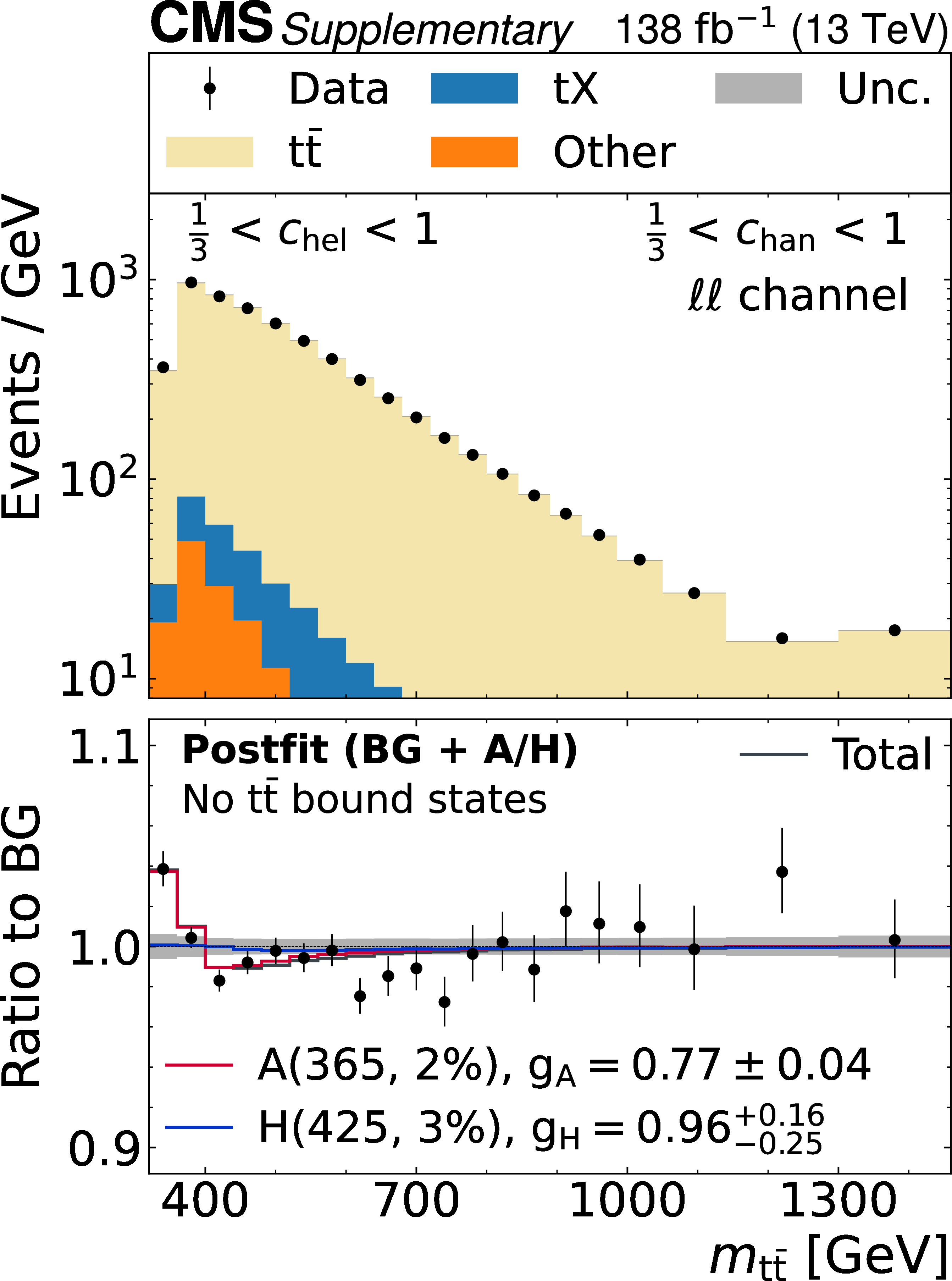
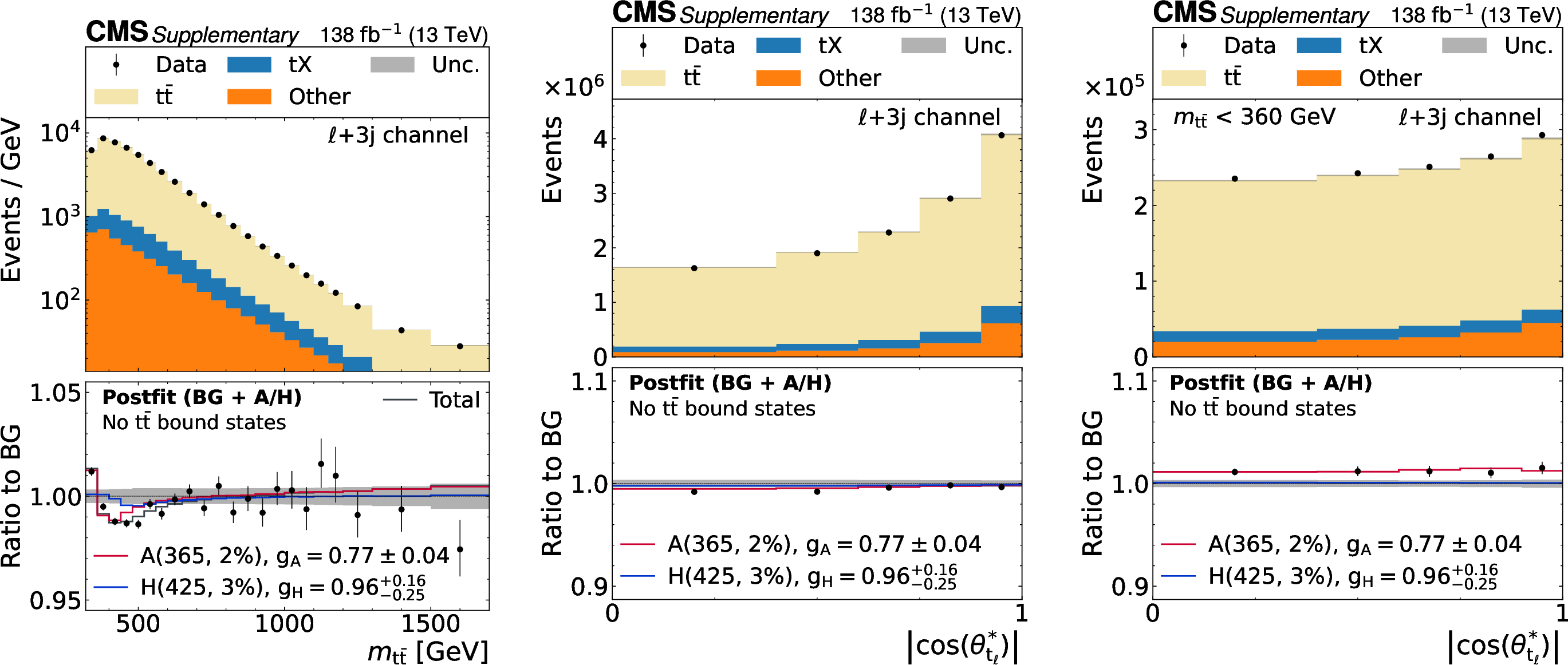
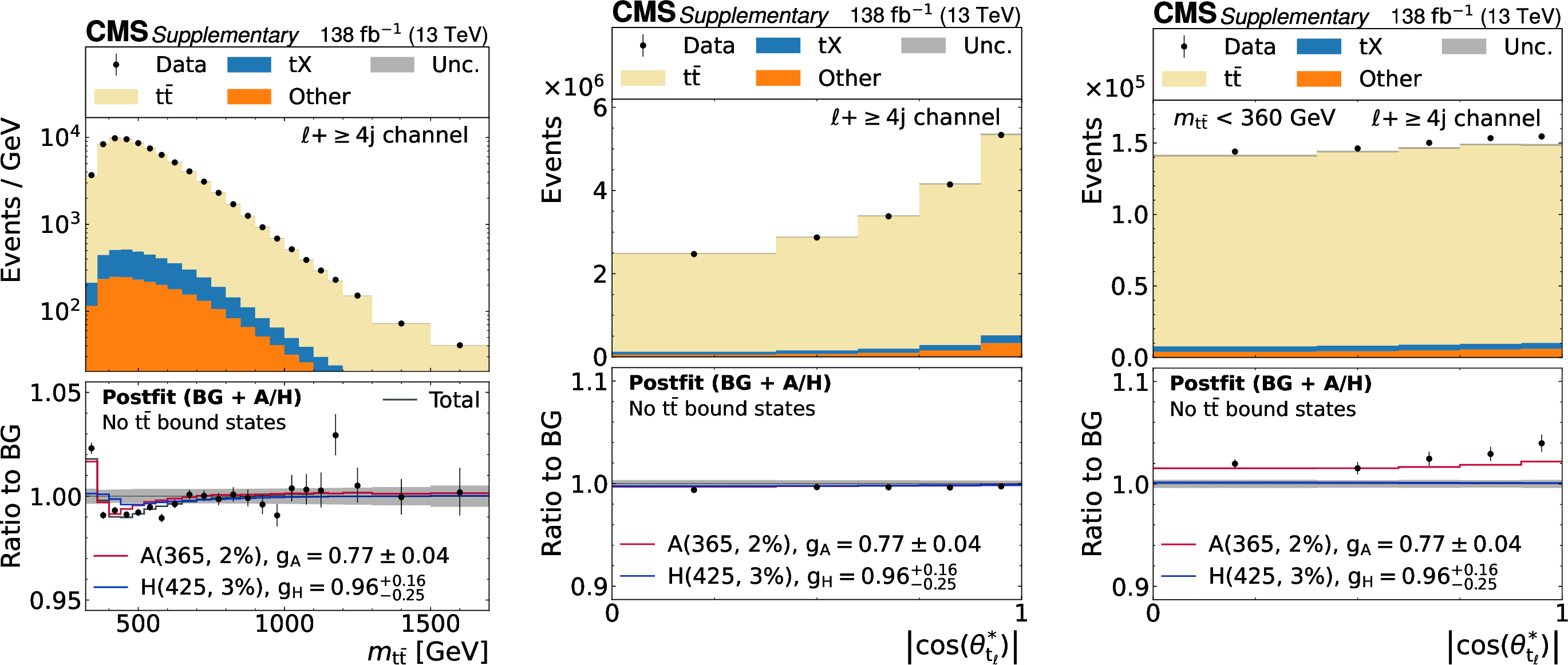
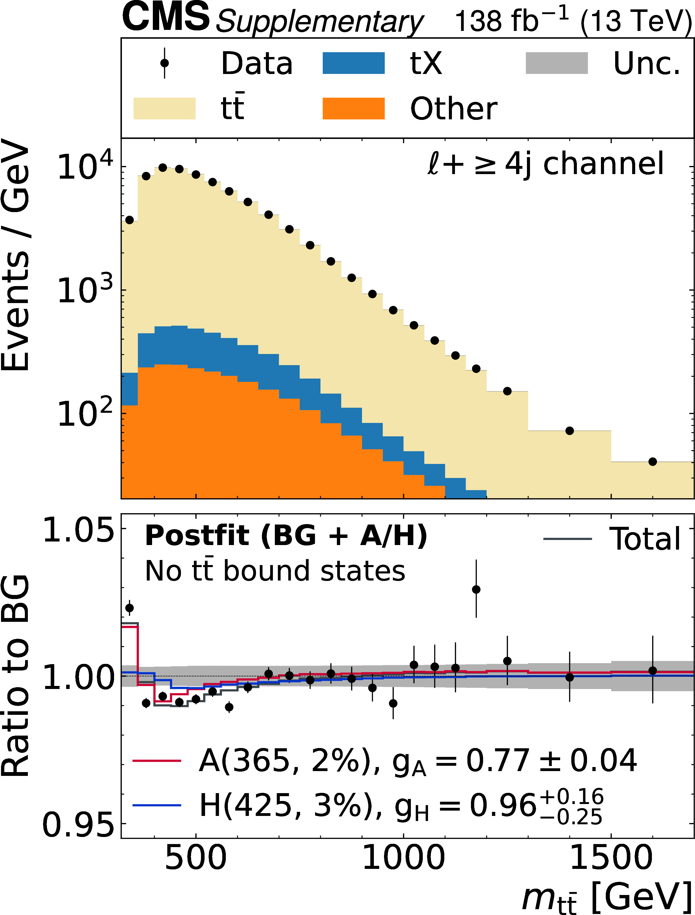
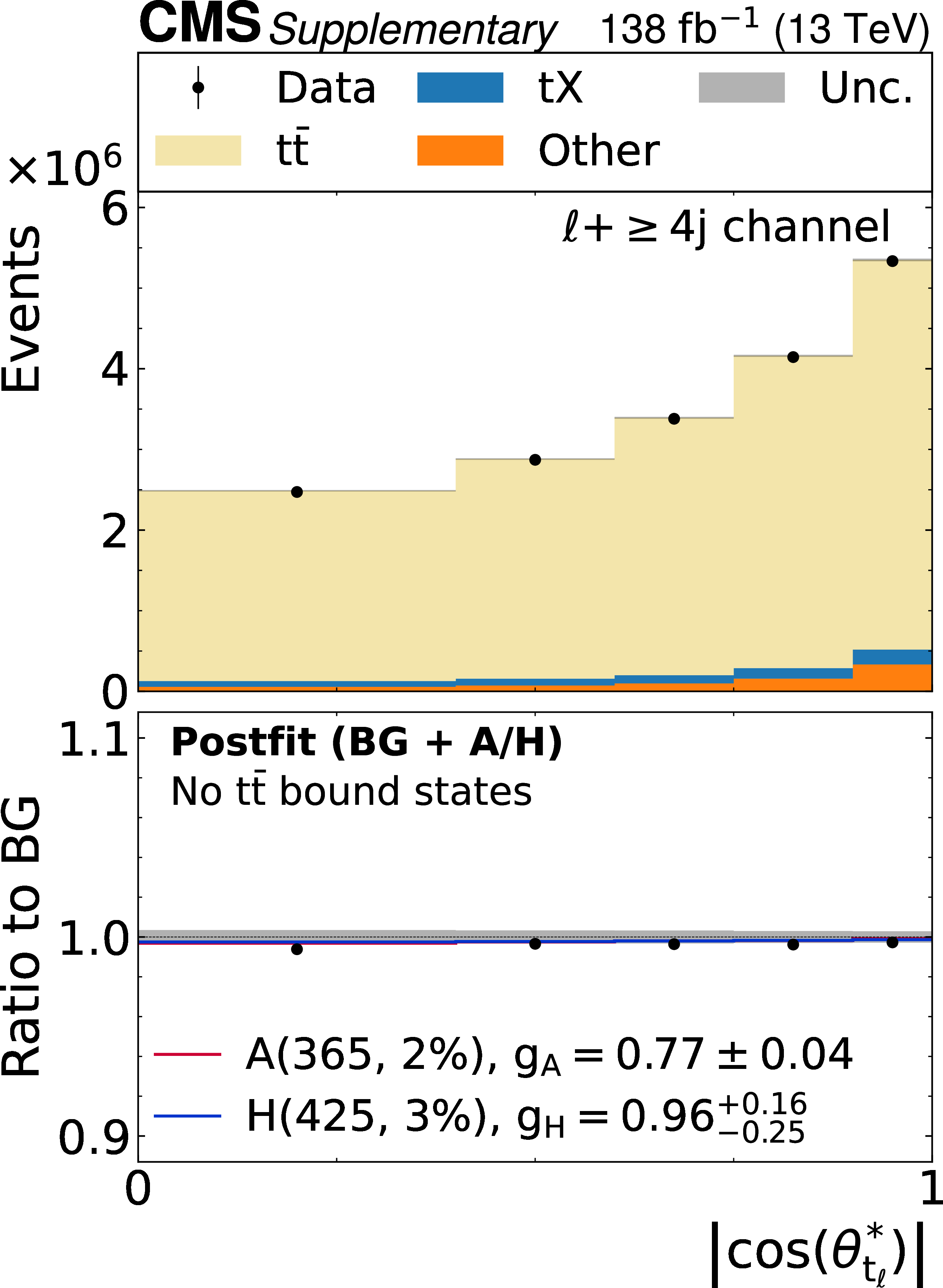
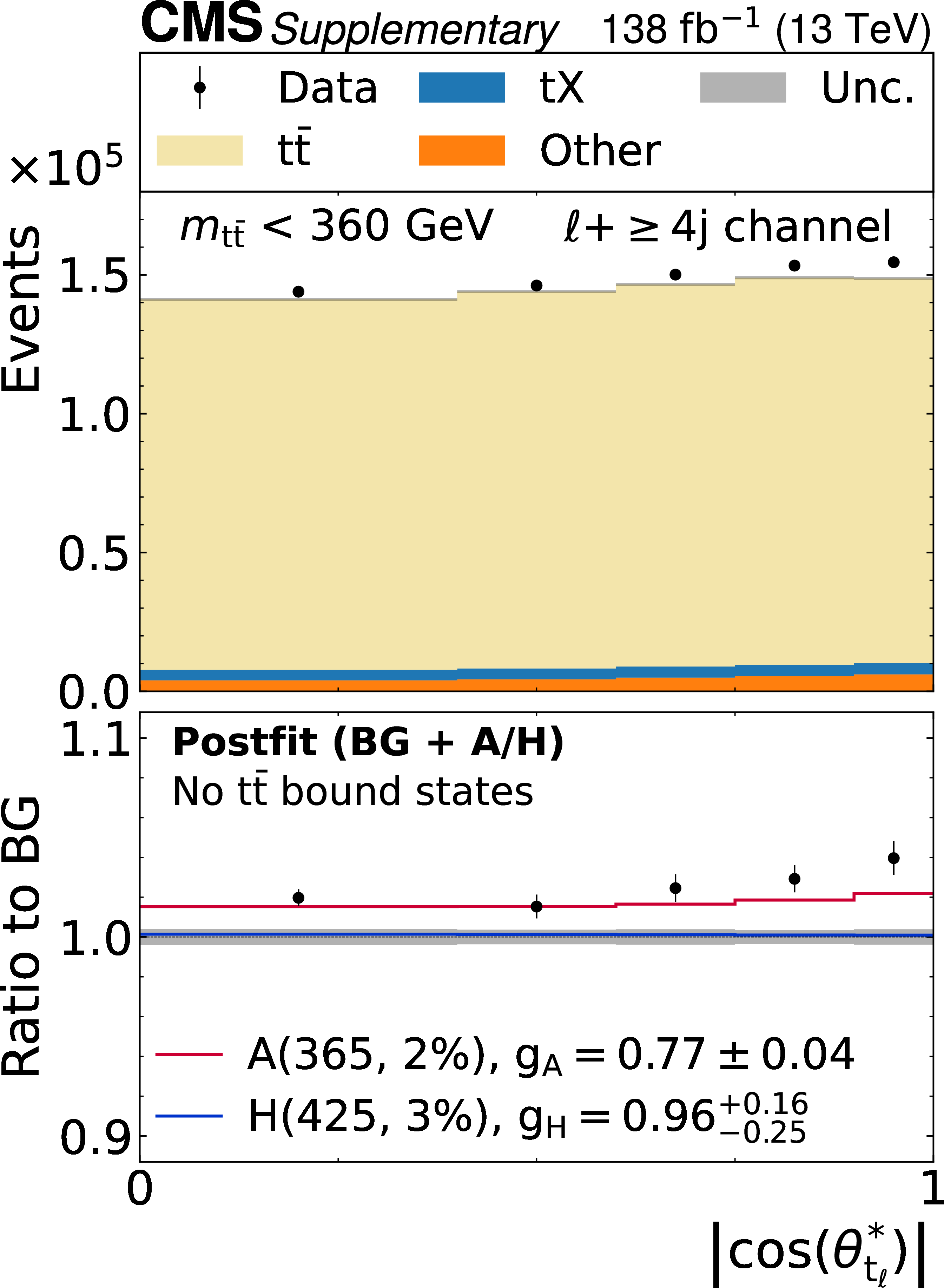
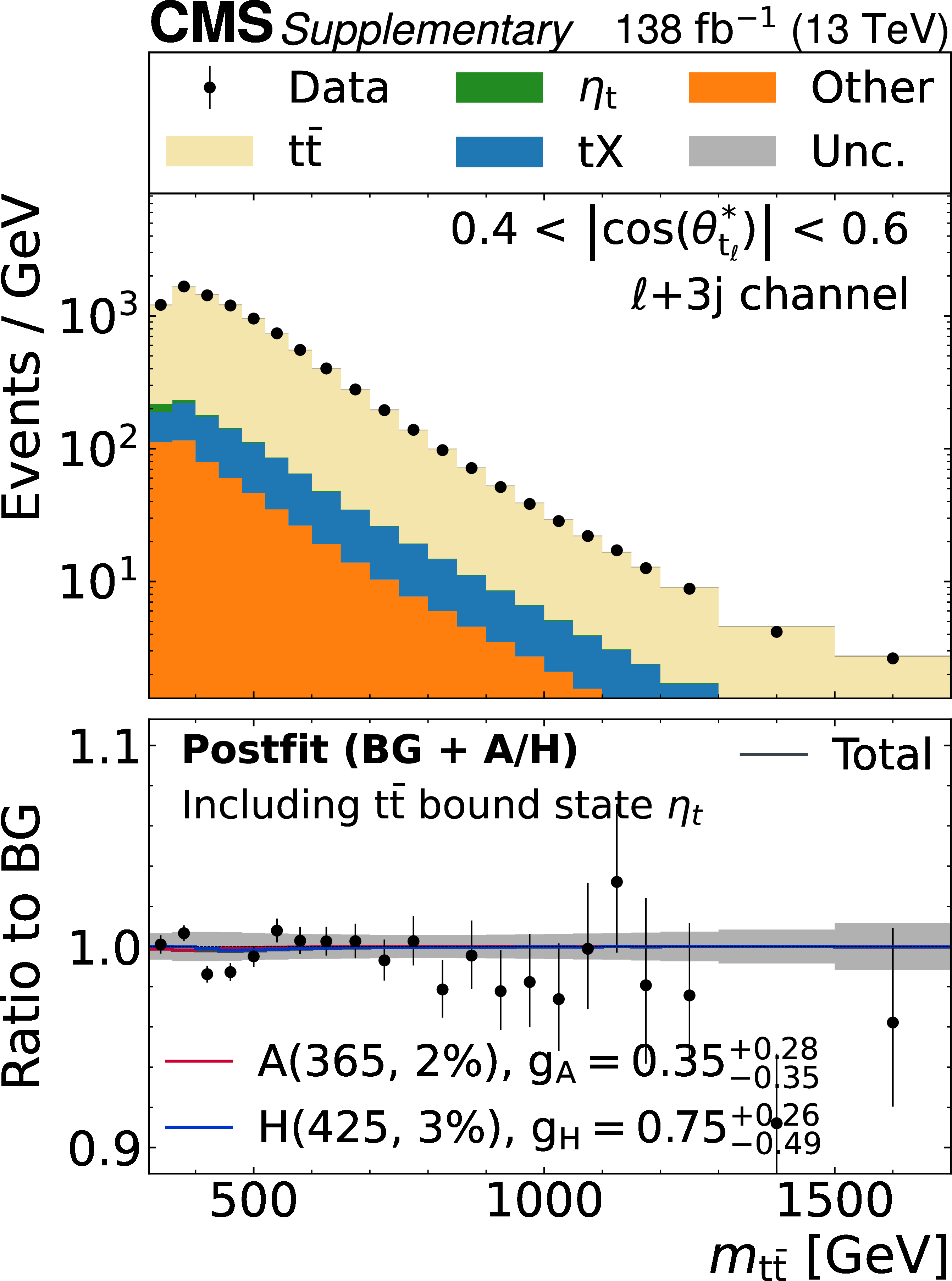
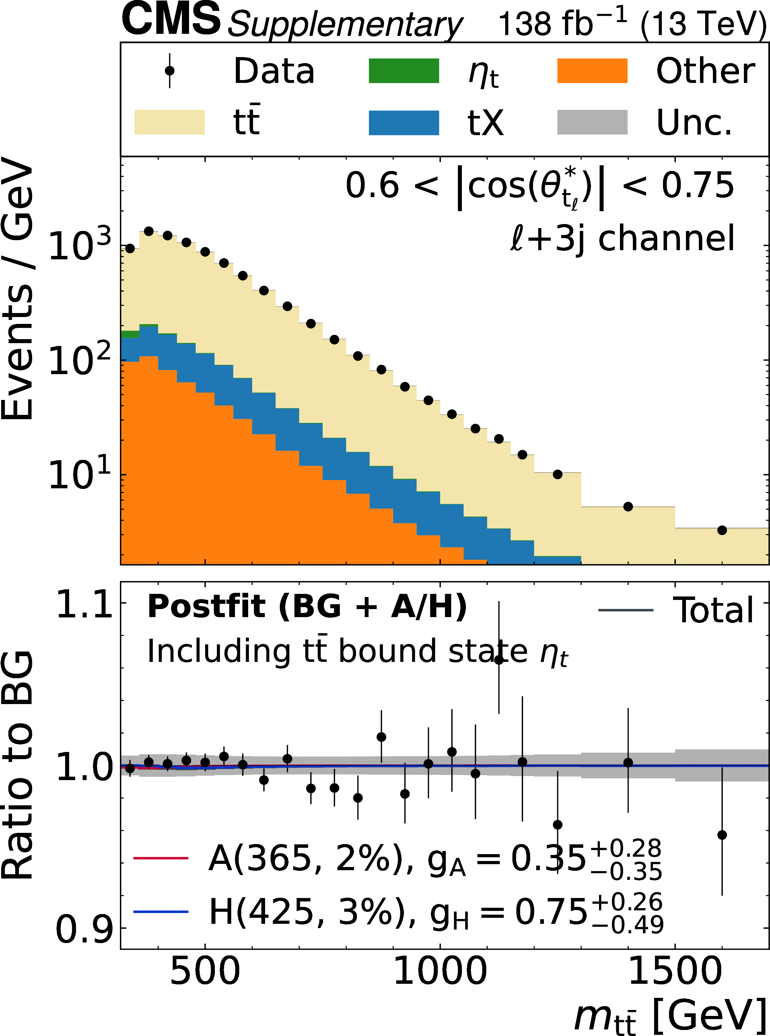
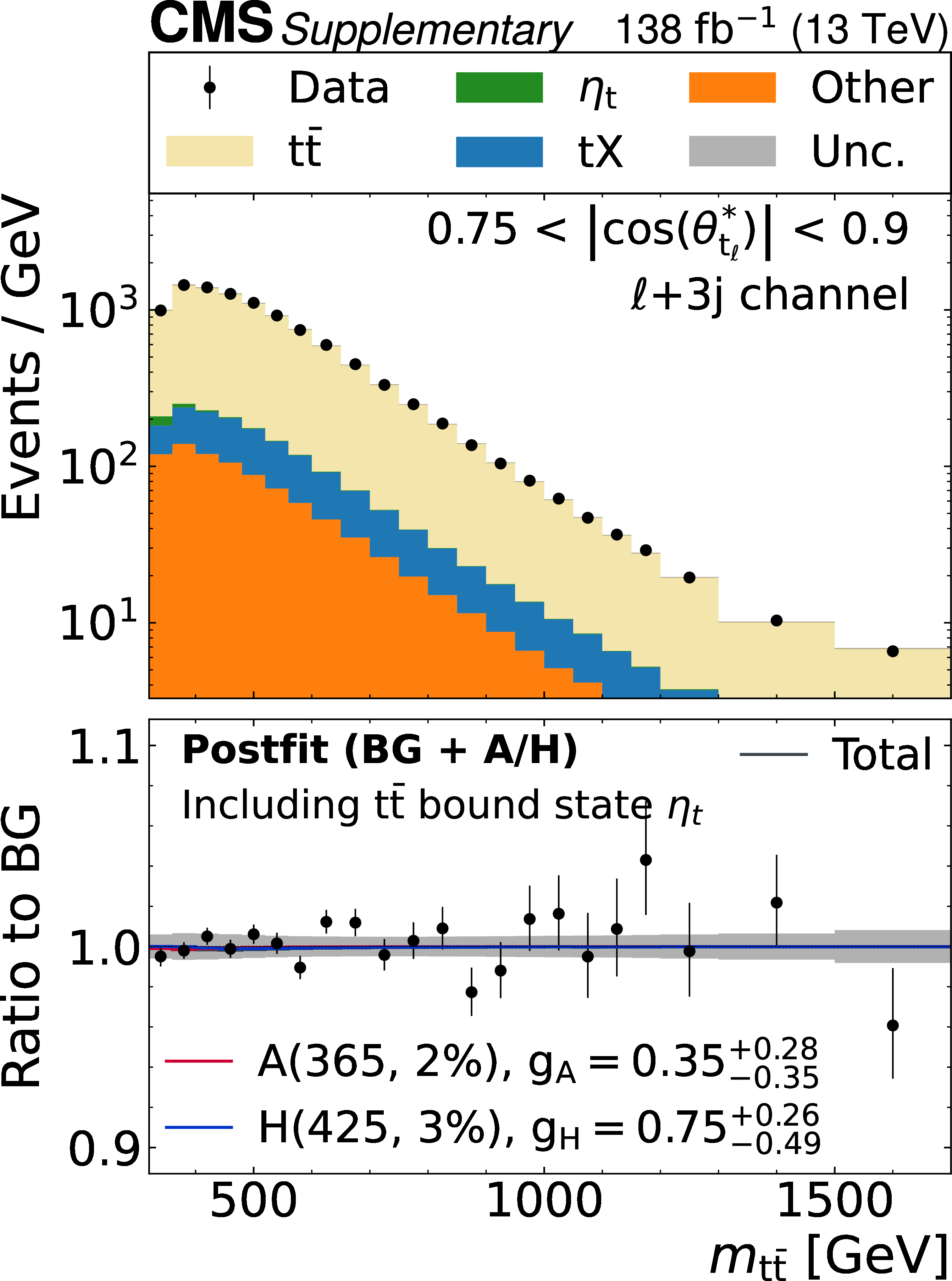
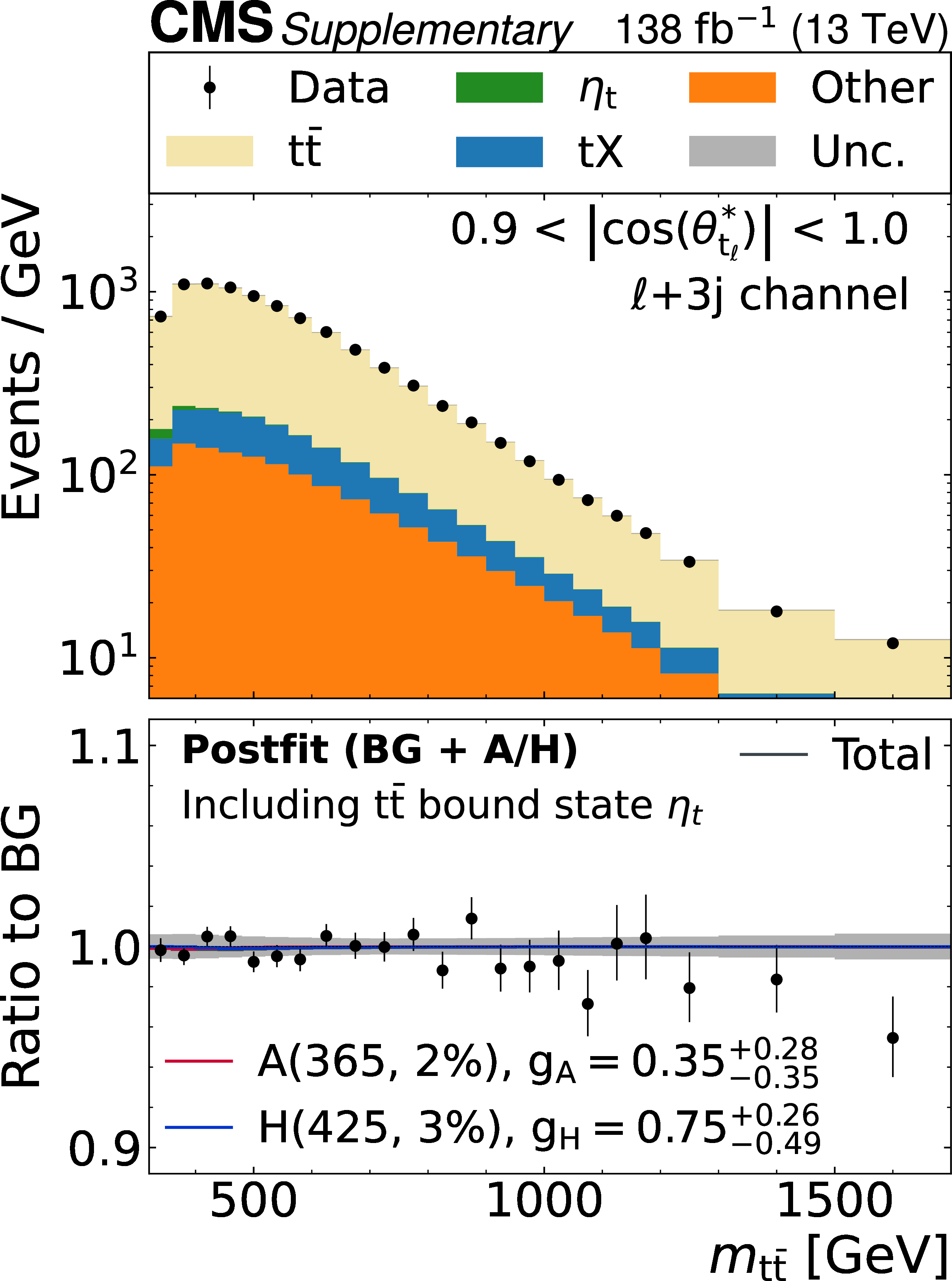
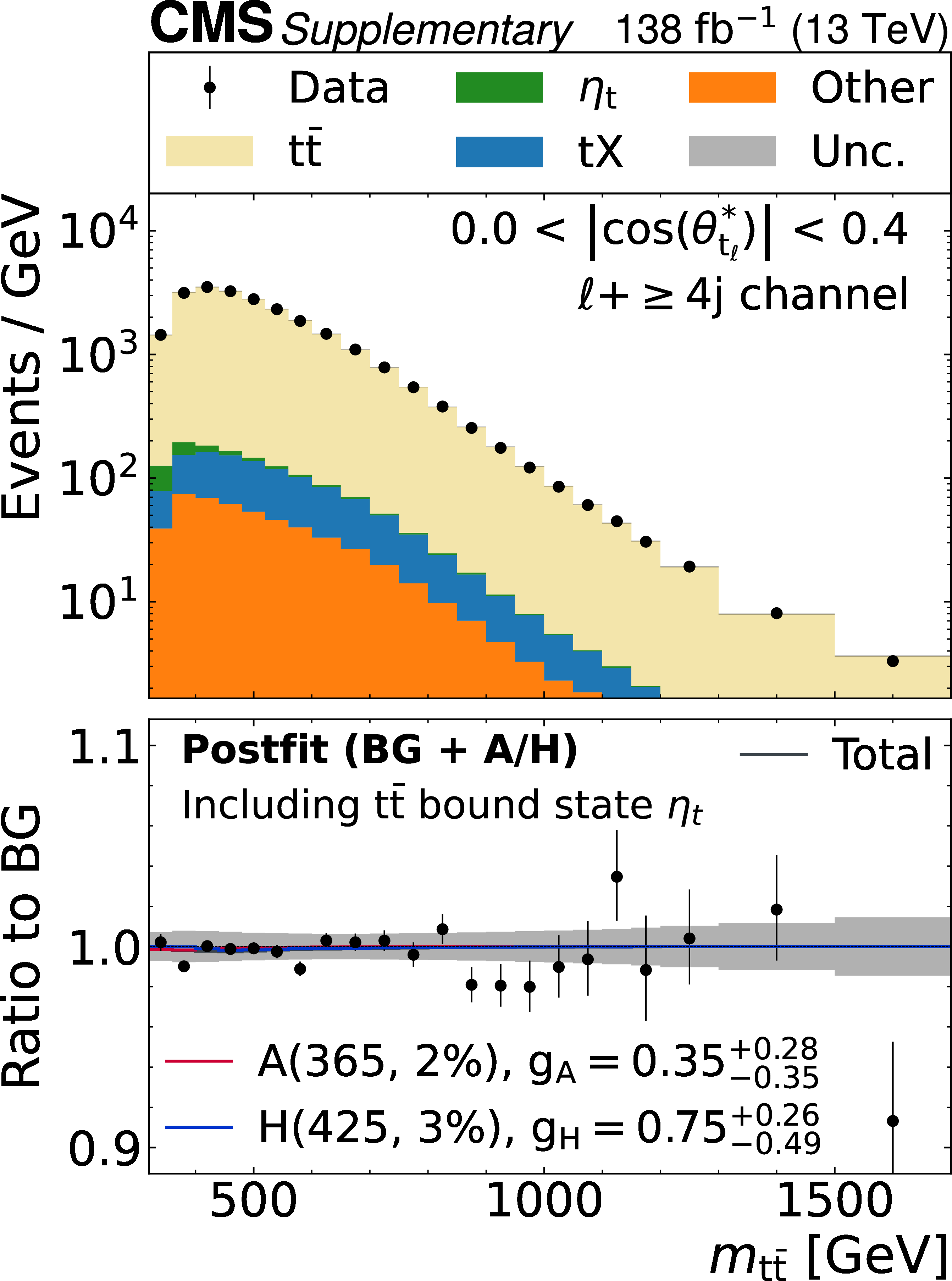
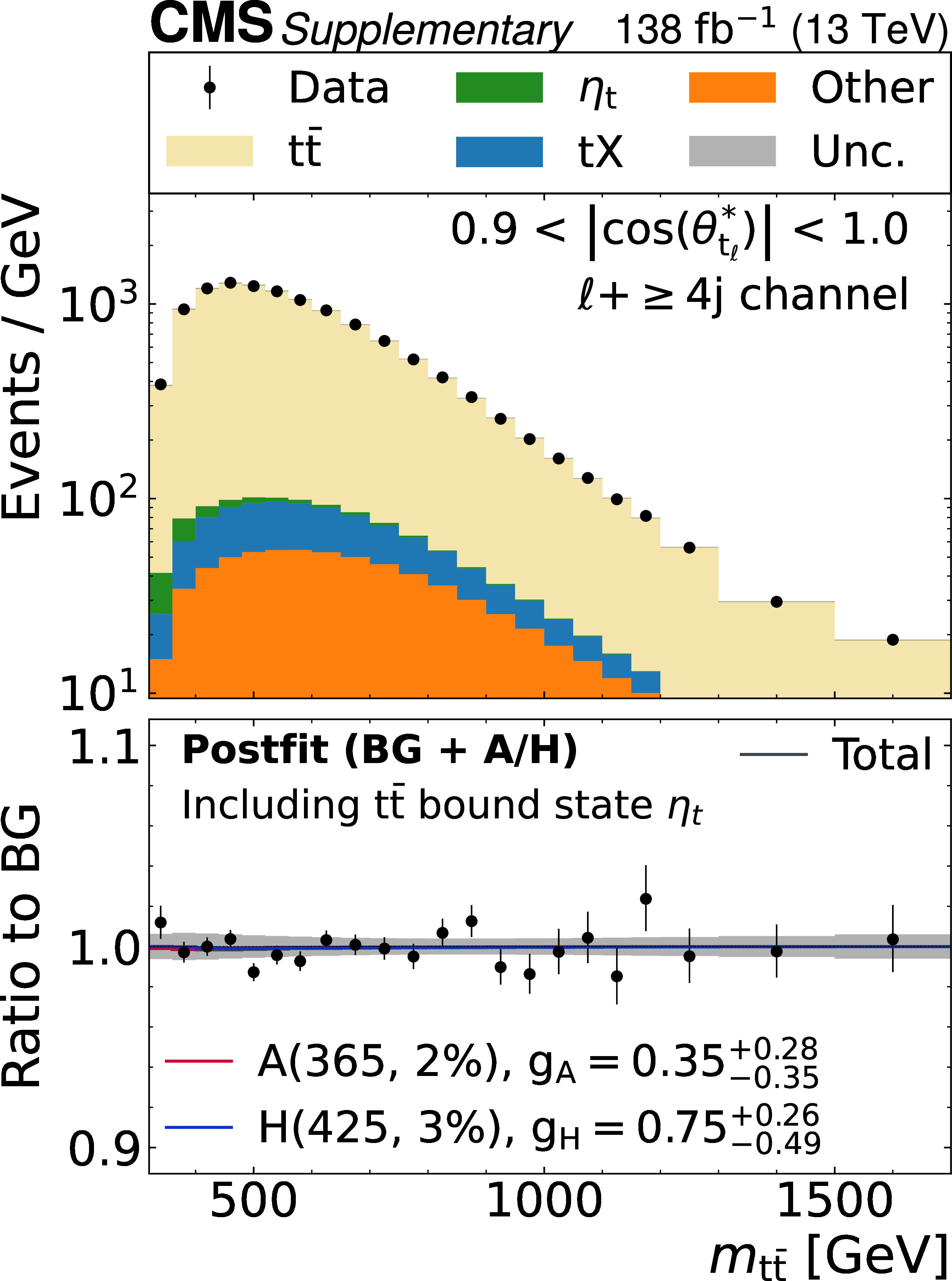
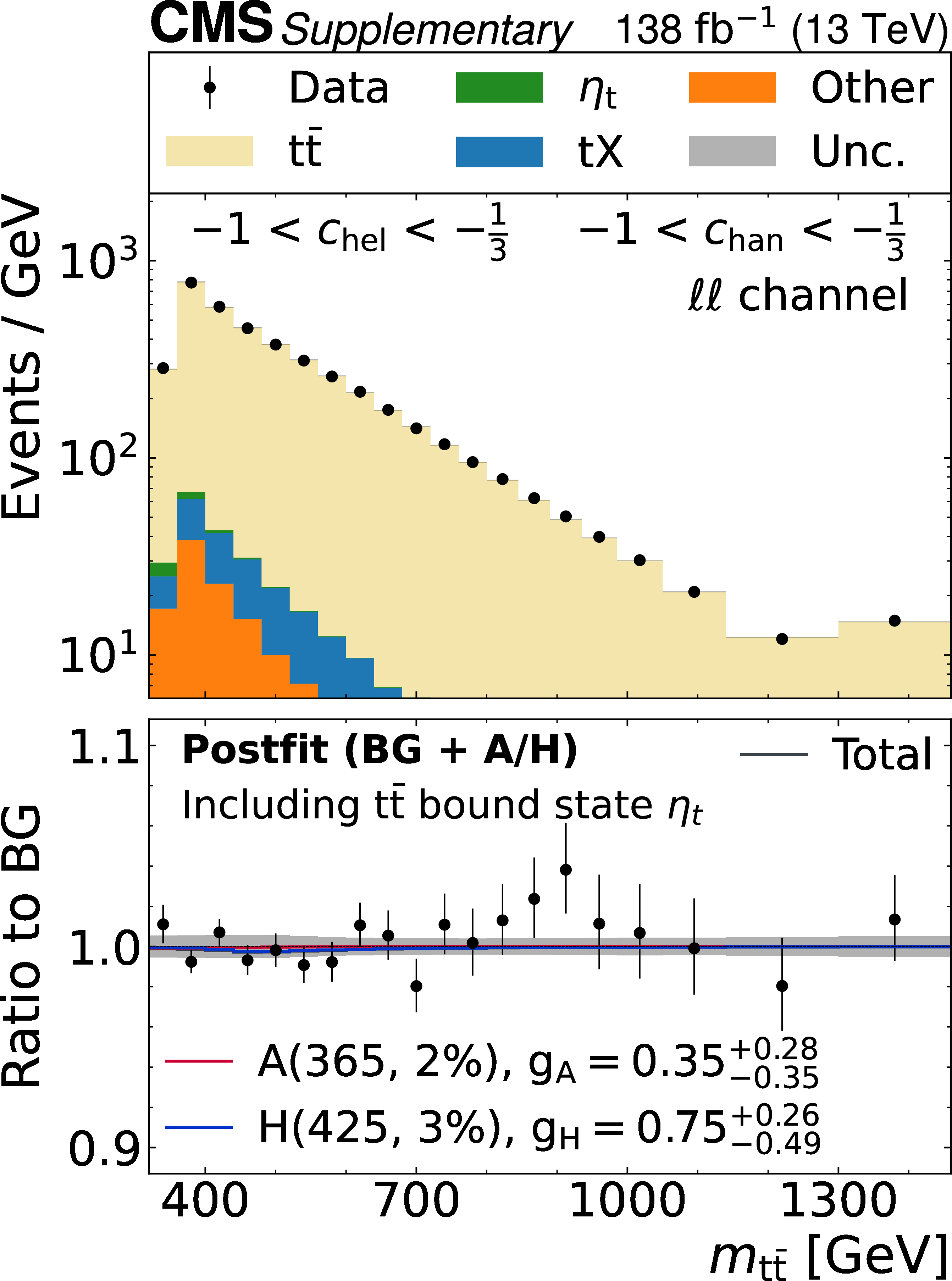
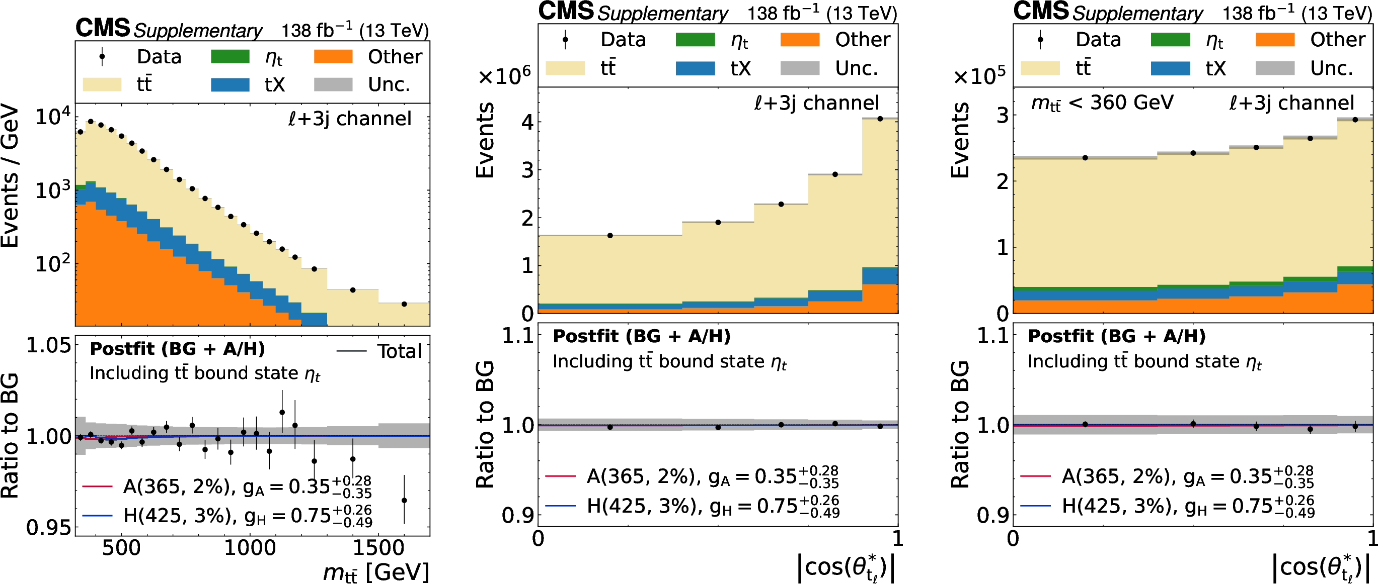
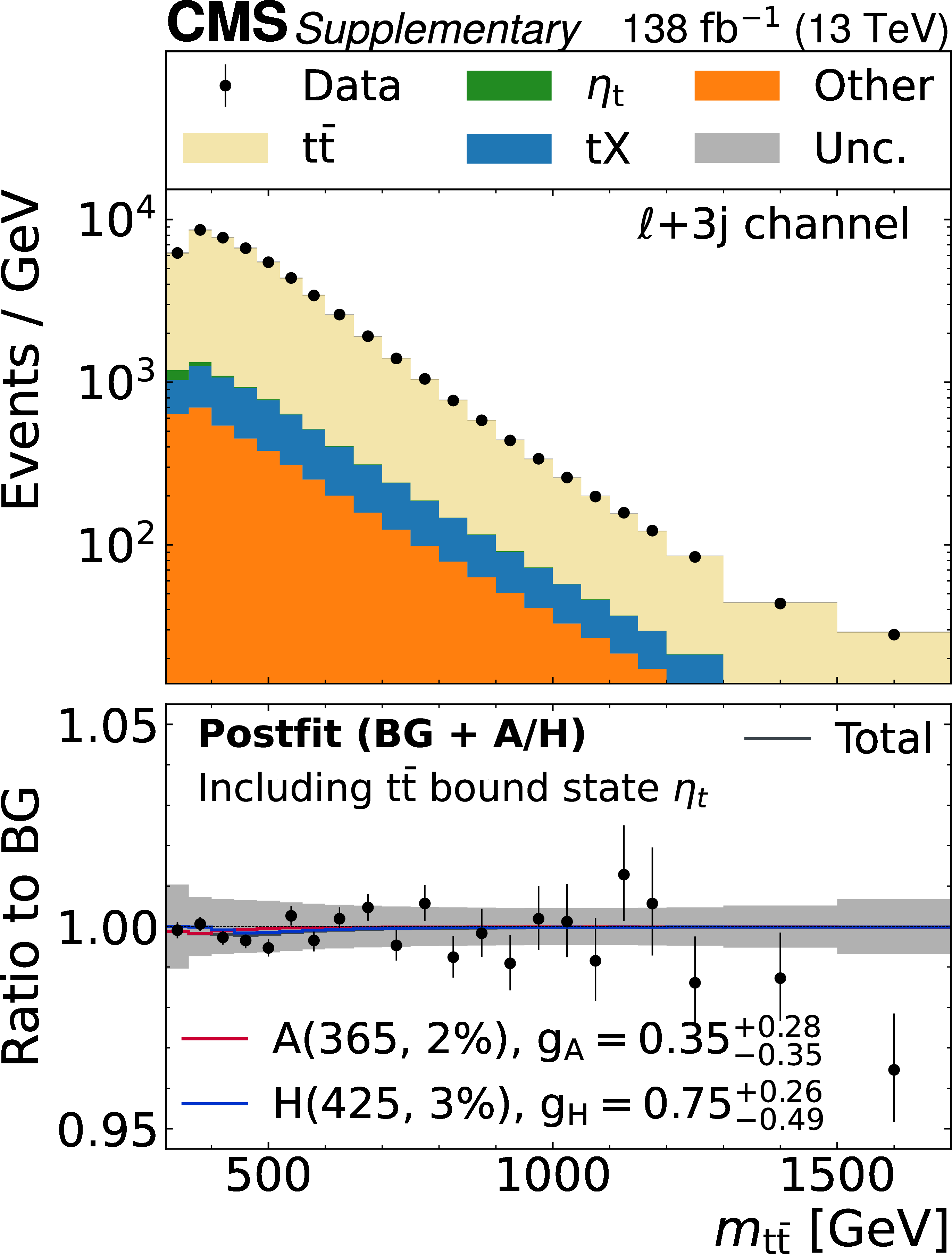
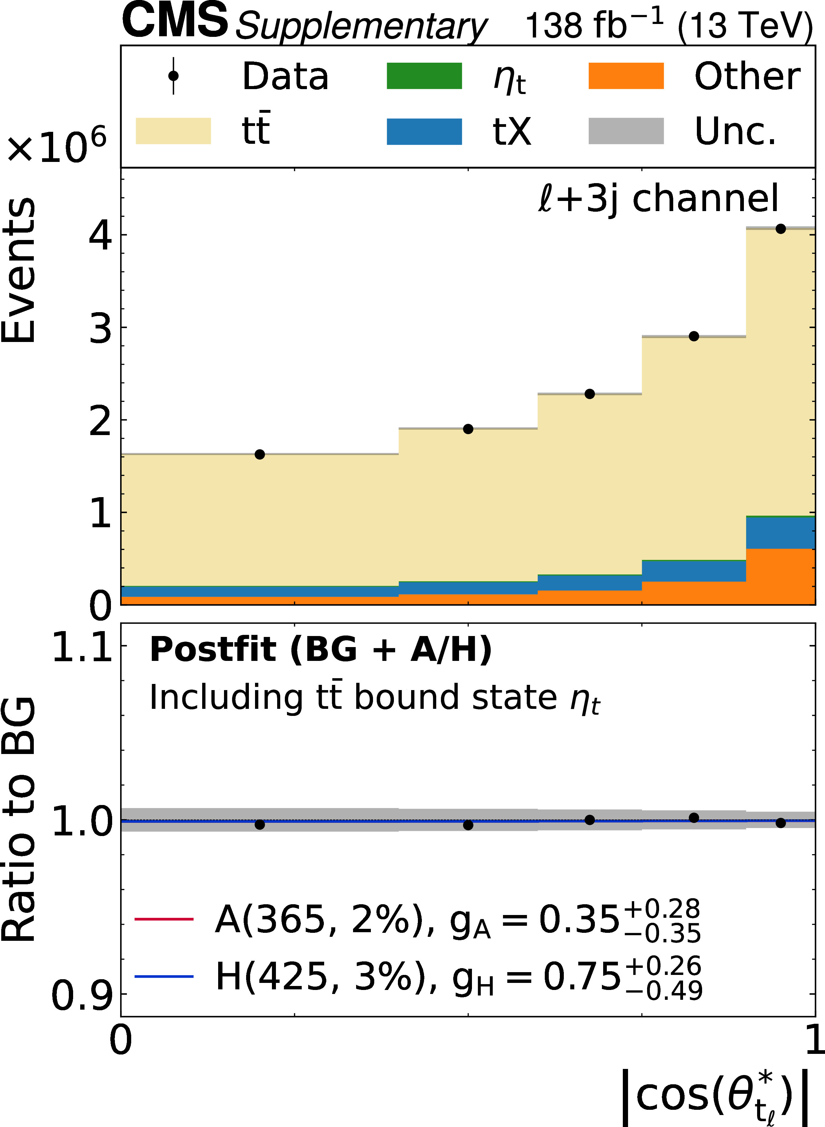
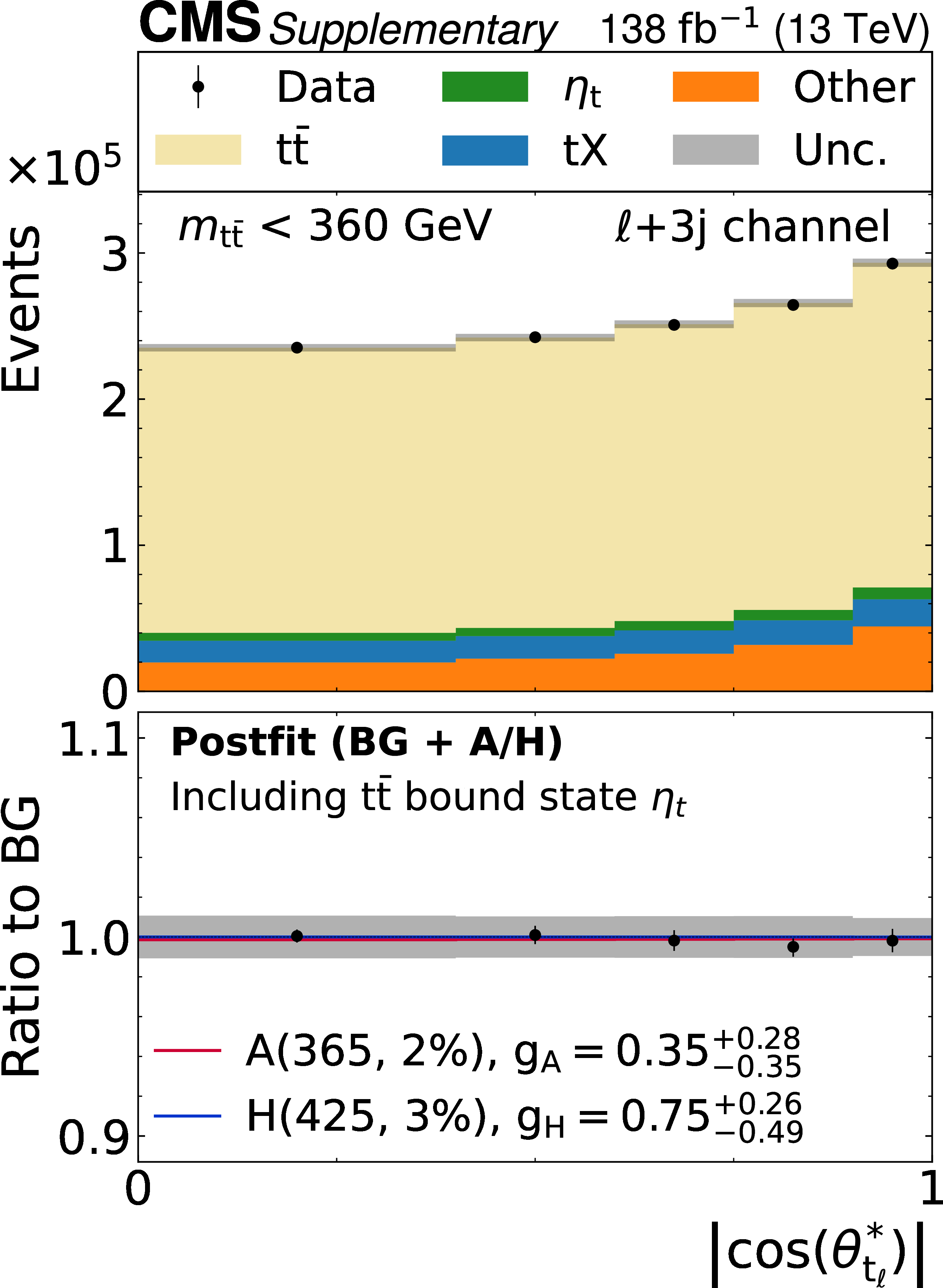
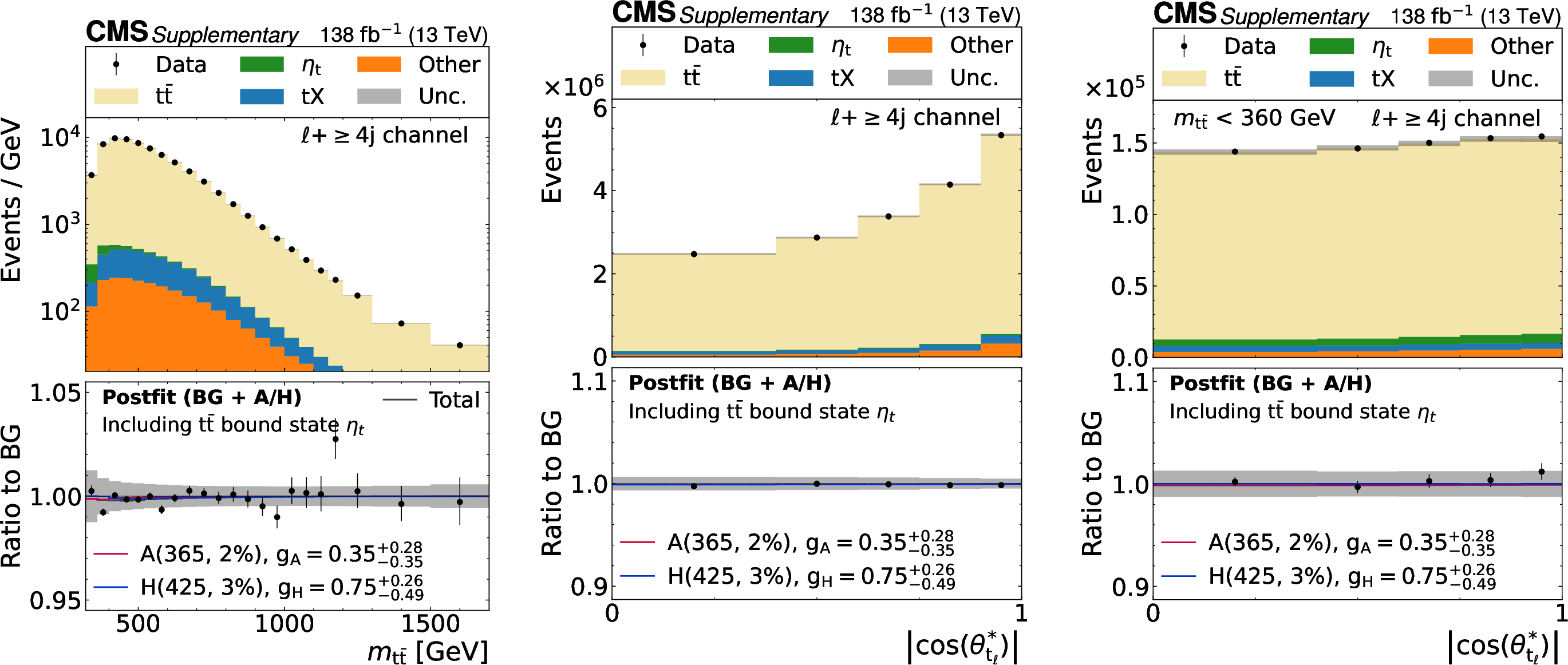
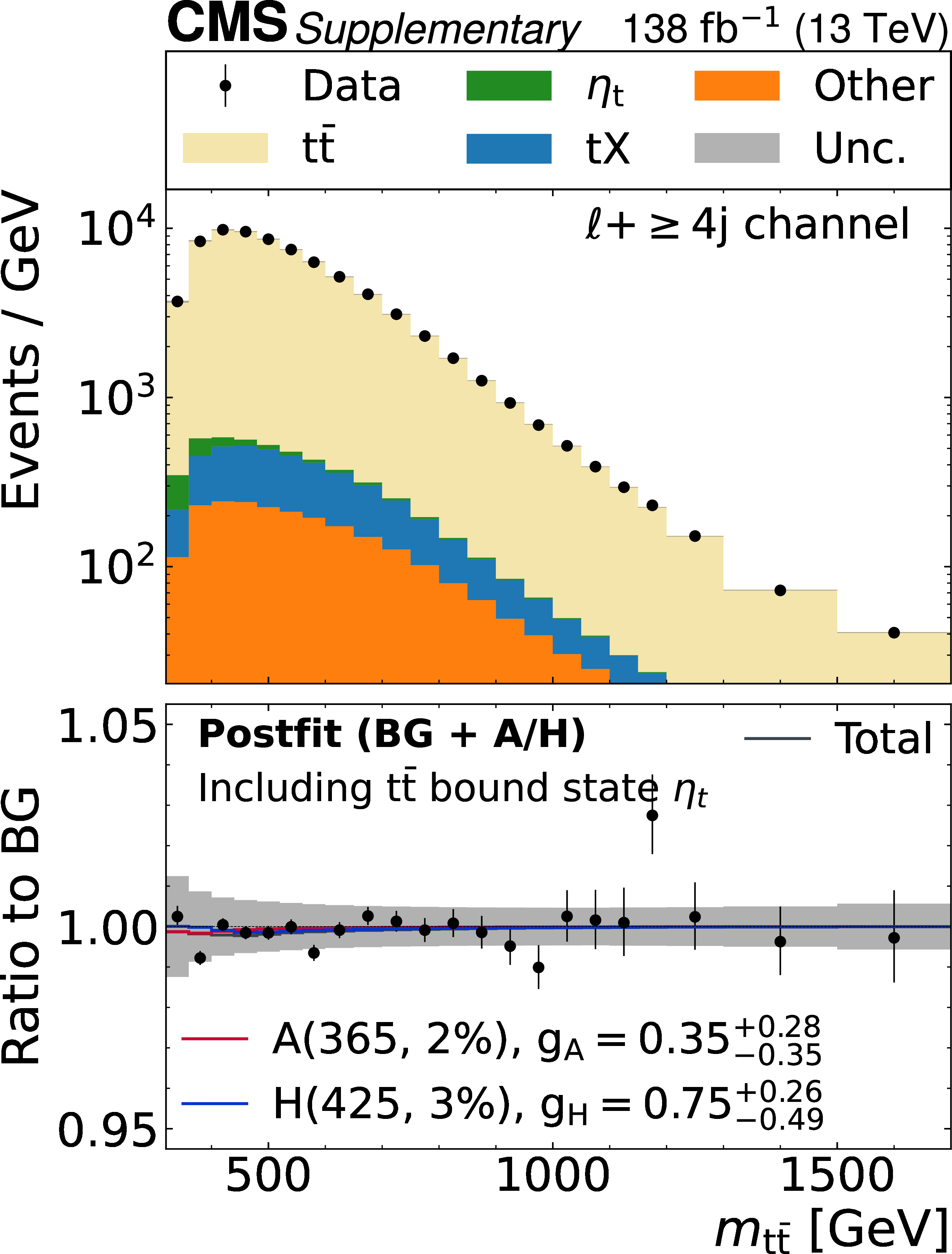
Observed and expected $ m_{{\mathrm{t}\overline{\mathrm{t}}} } $ distribution in bins of $ \lvert\cos\theta^\ast_{\mathrm{t}_{\ell}}\rvert $, shown for the $ \ell+3{\mathrm{j}} $ channel summed over lepton flavors and eras. In the upper panel, the data (points with statistical error bars) are compared to $ \mathrm{t} \overline{\mathrm{t}} $ production in FO pQCD and other sources of background (colored histograms) after the fit to the data in the A$+$H interpretation. The ratio of data to the prediction is shown in the middle panel, where the two signals A$(365,\,2\%)$ and H$(425,\,3\%)$, corresponding to the best fit point, are overlaid. The lower panel shows the equivalent ratio for the fit where $ \eta_{\mathrm{t}} $ is considered as an additional background, for the same signal points. In both cases, the gray band shows the postfit uncertainty, and the respective signals are overlaid with their best fit model parameters. |
png pdf |
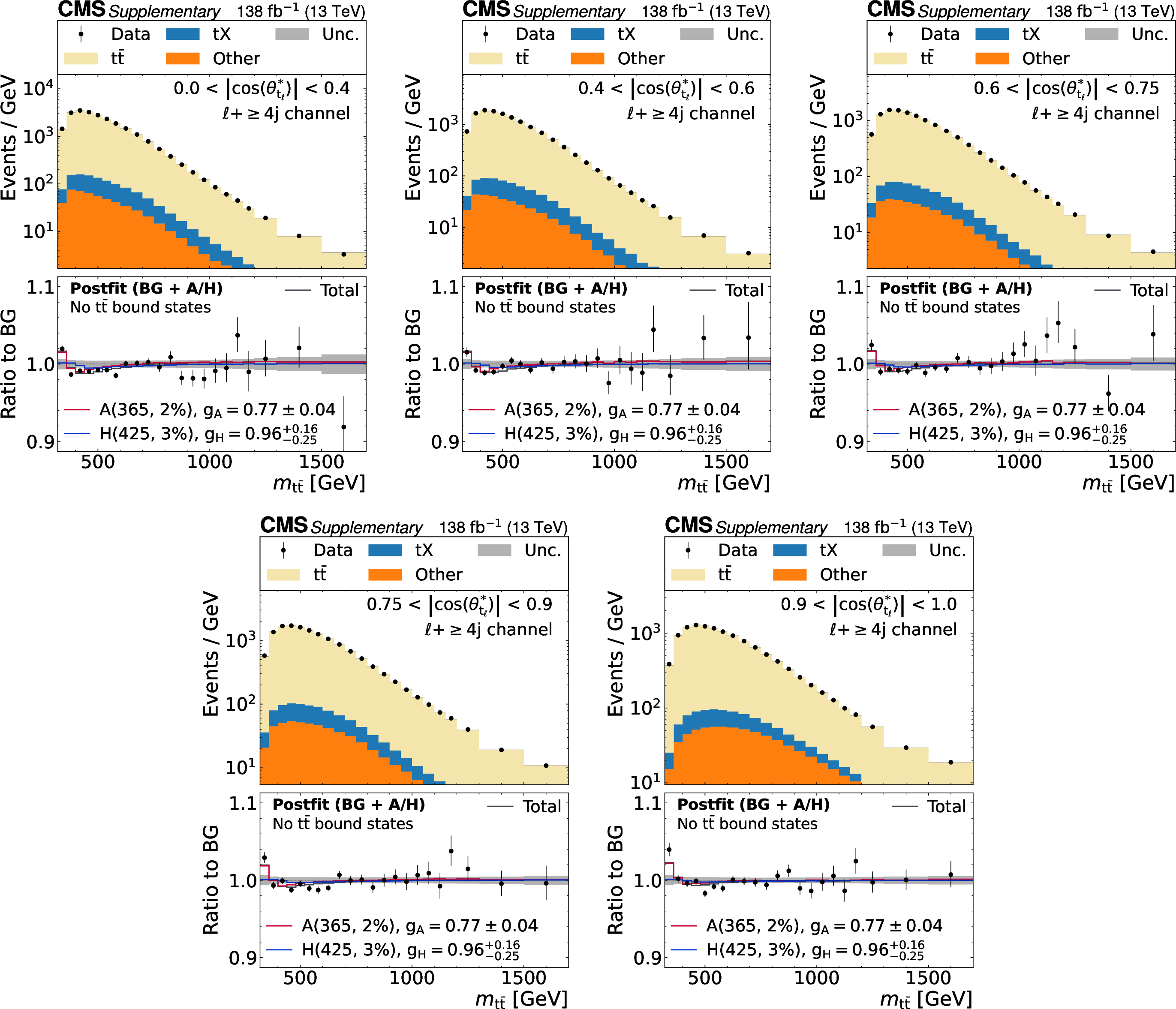
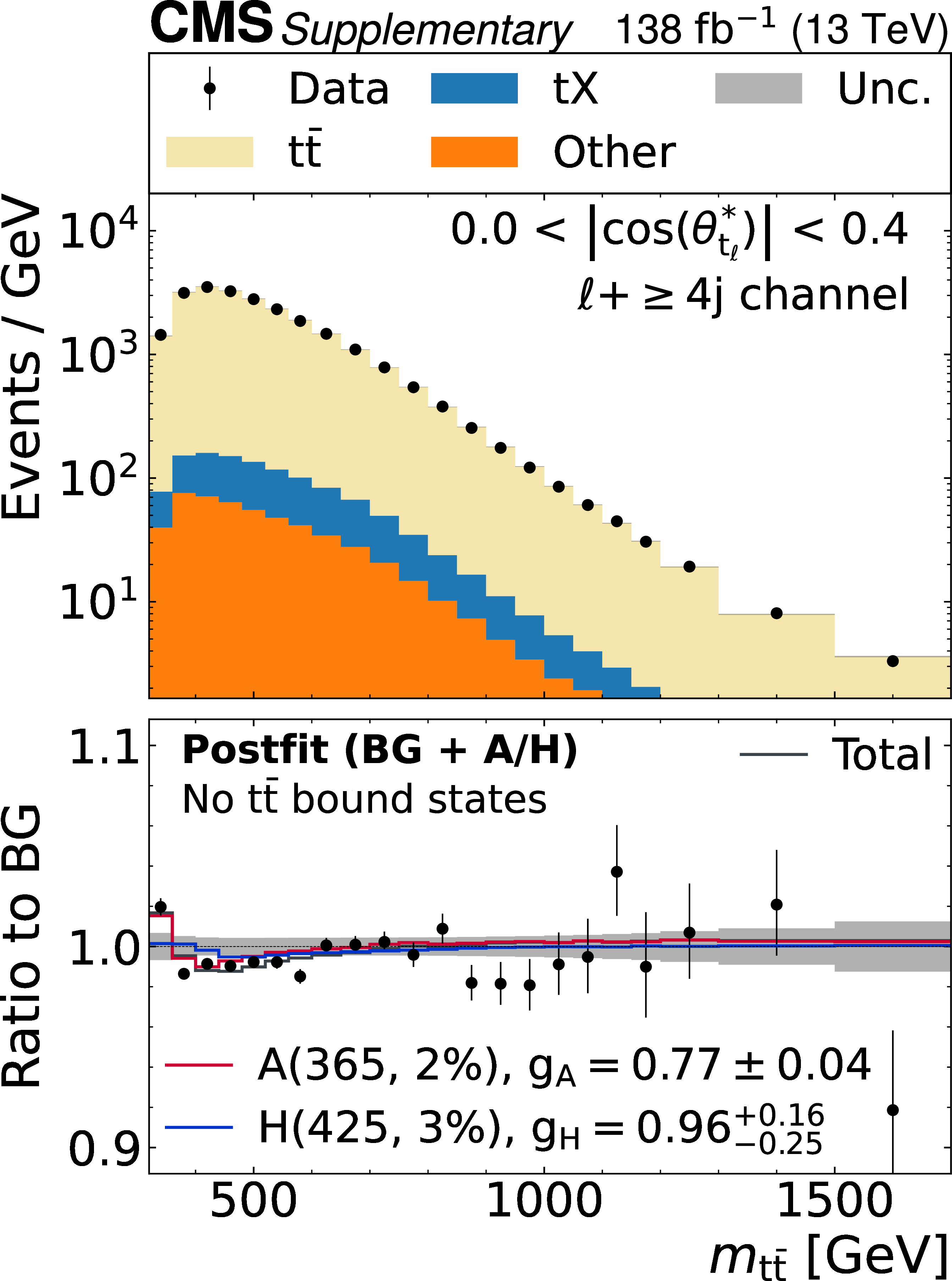
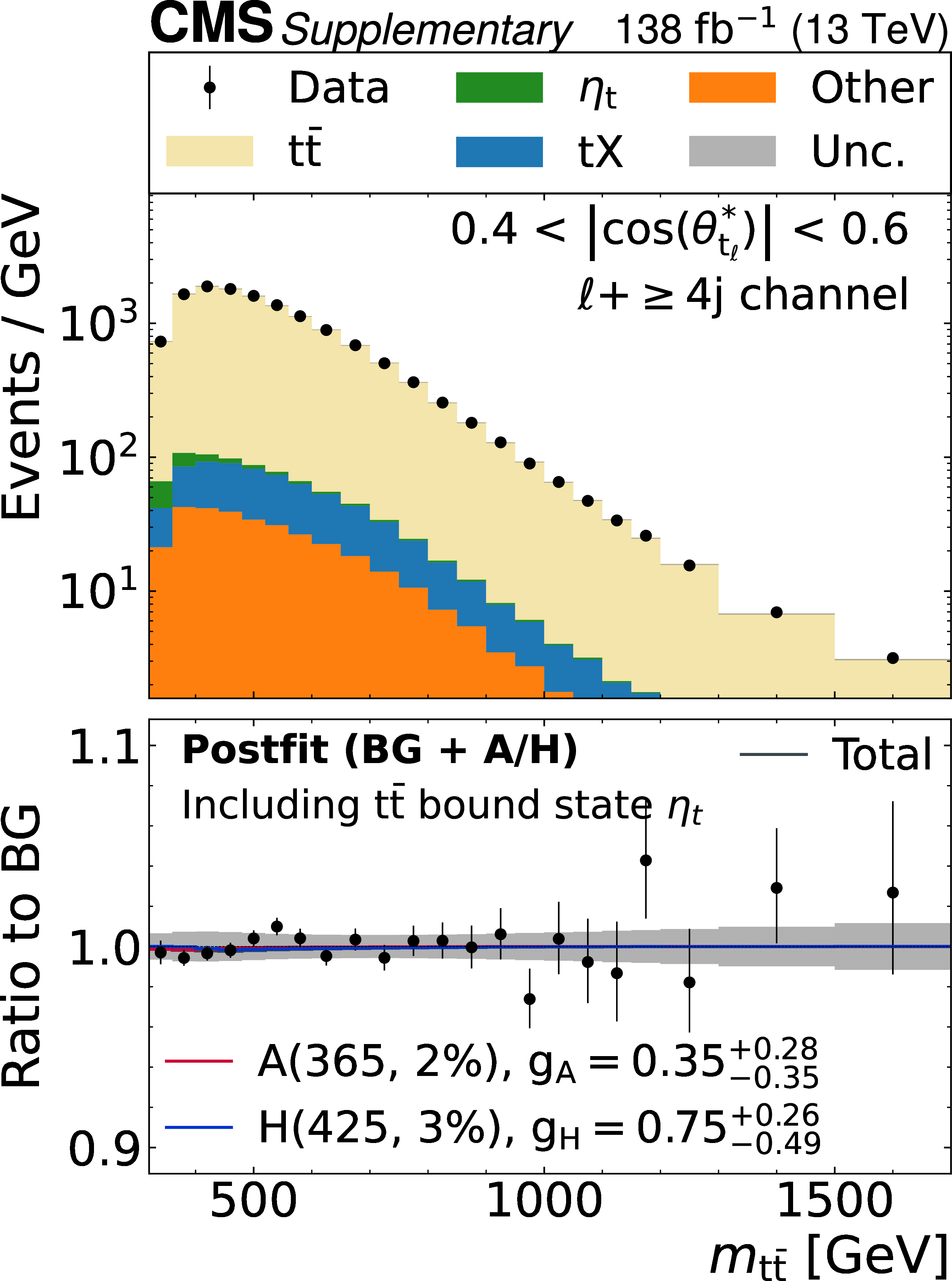
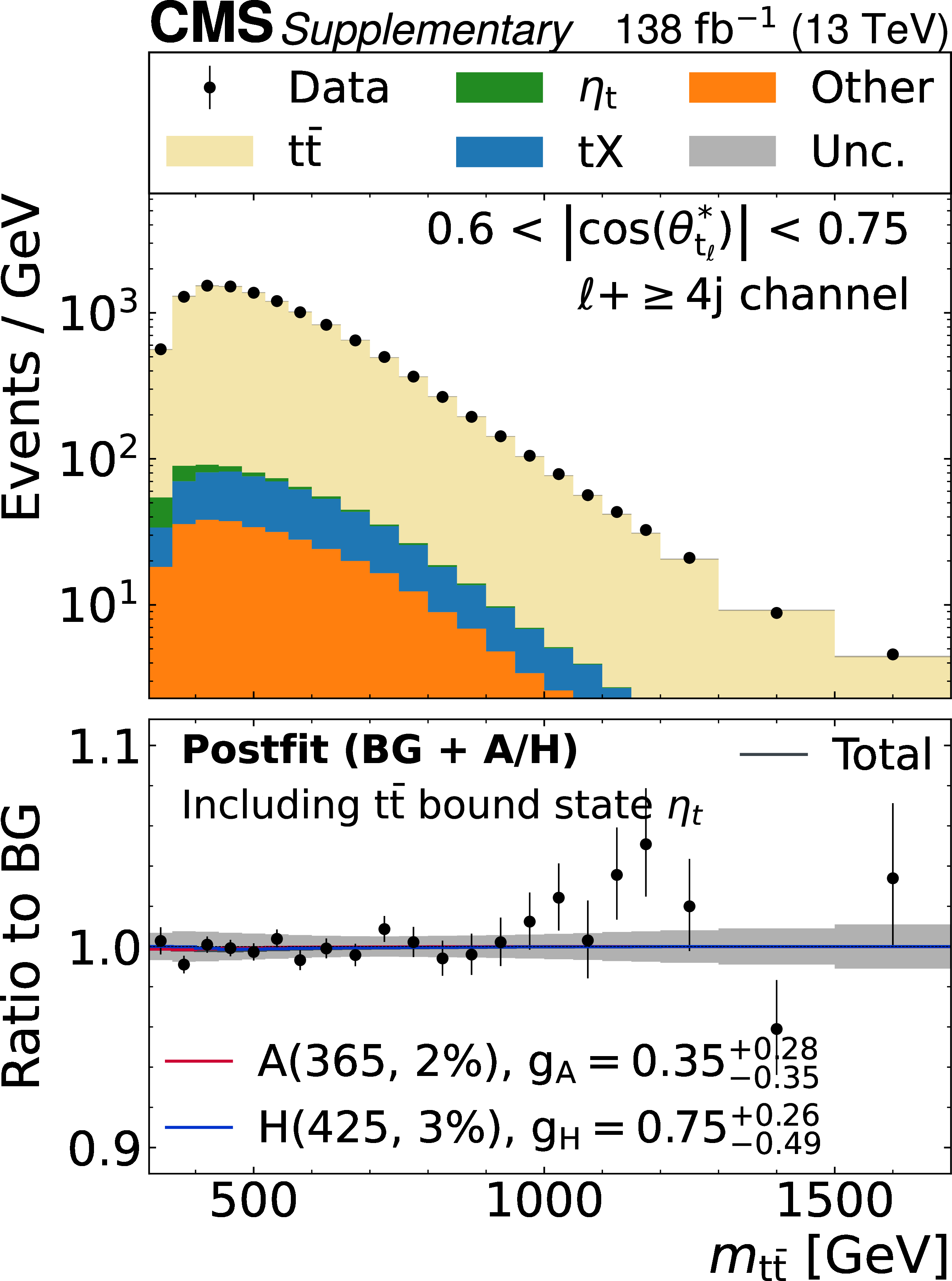
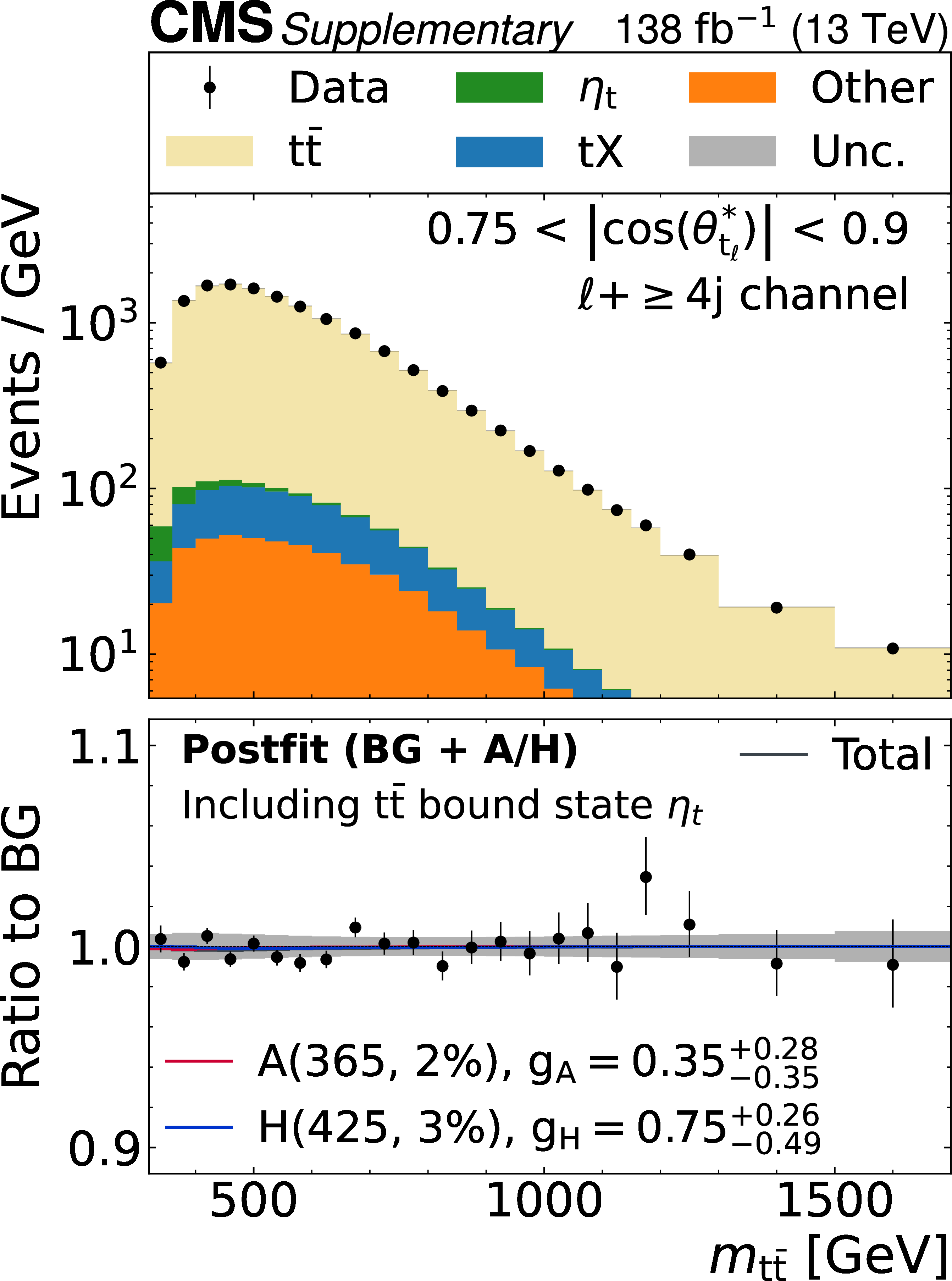
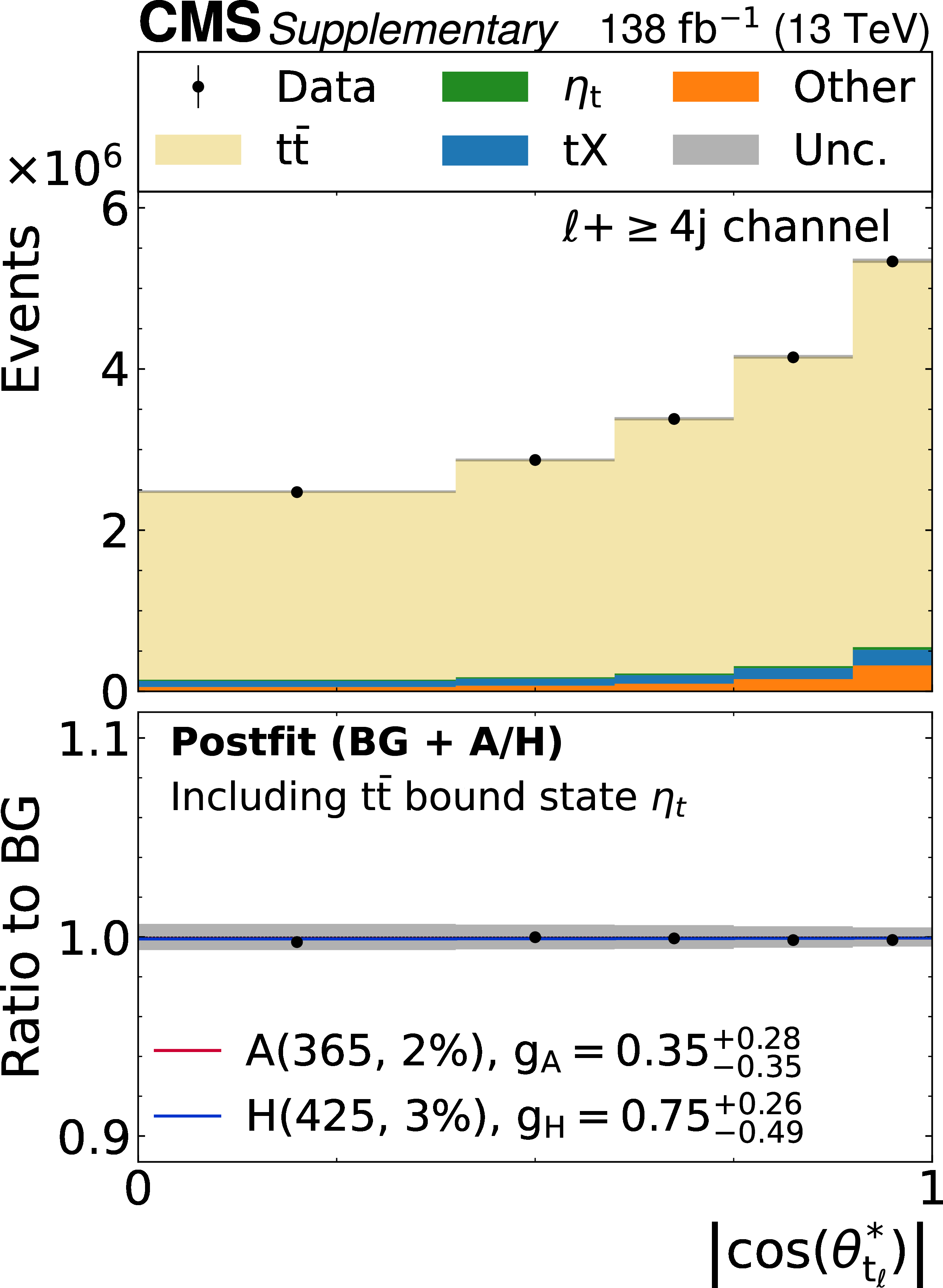
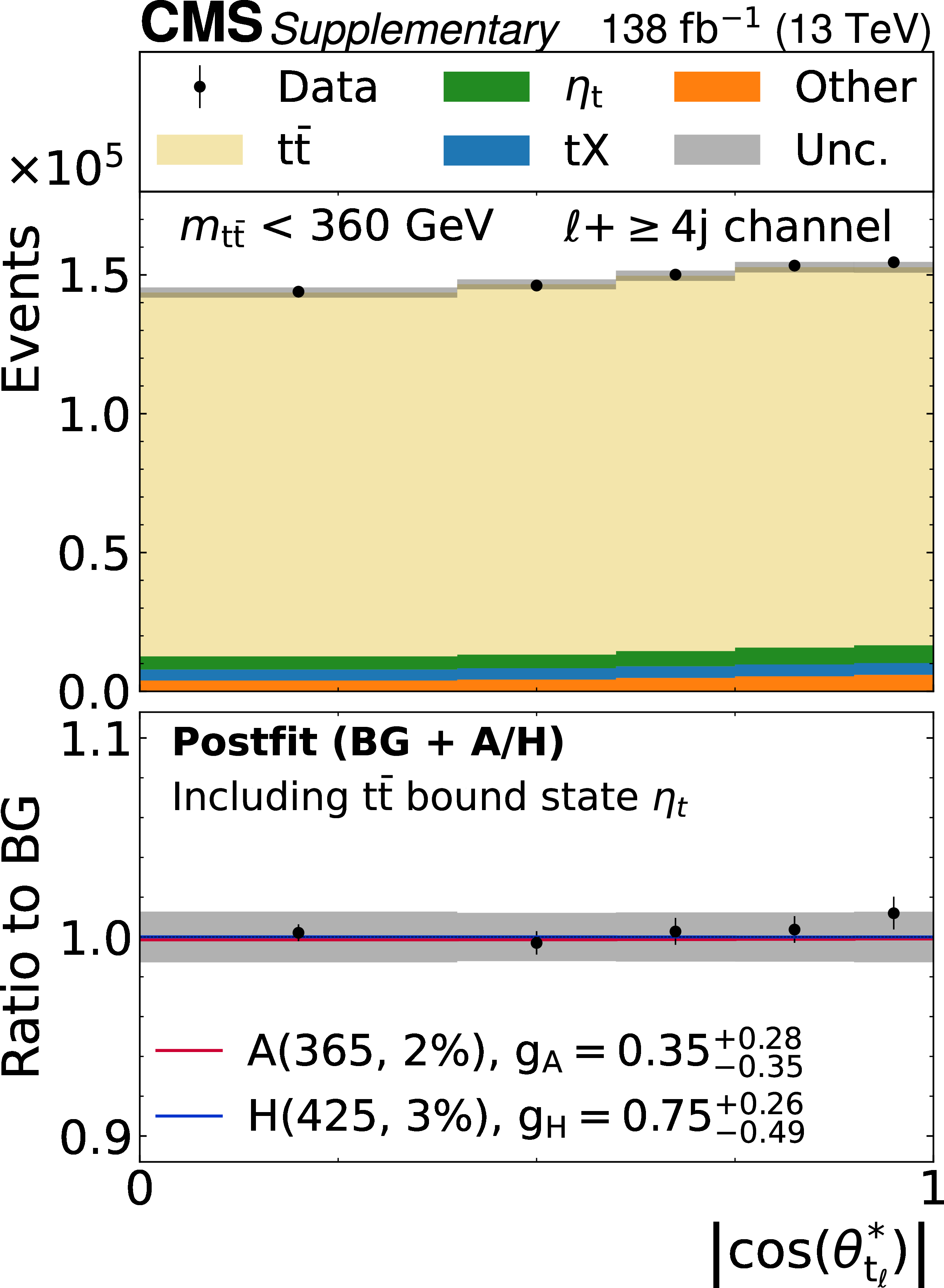
Figure 7:
Observed and expected $ m_{{\mathrm{t}\overline{\mathrm{t}}} } $ distribution in $ \lvert\cos\theta^\ast_{\mathrm{t}_{\ell}}\rvert $ bins, shown for the $ \ell+{\geq}4{\mathrm{j}} $ channel summed over lepton flavors and eras. Notations as in Fig. 6. |
png pdf |
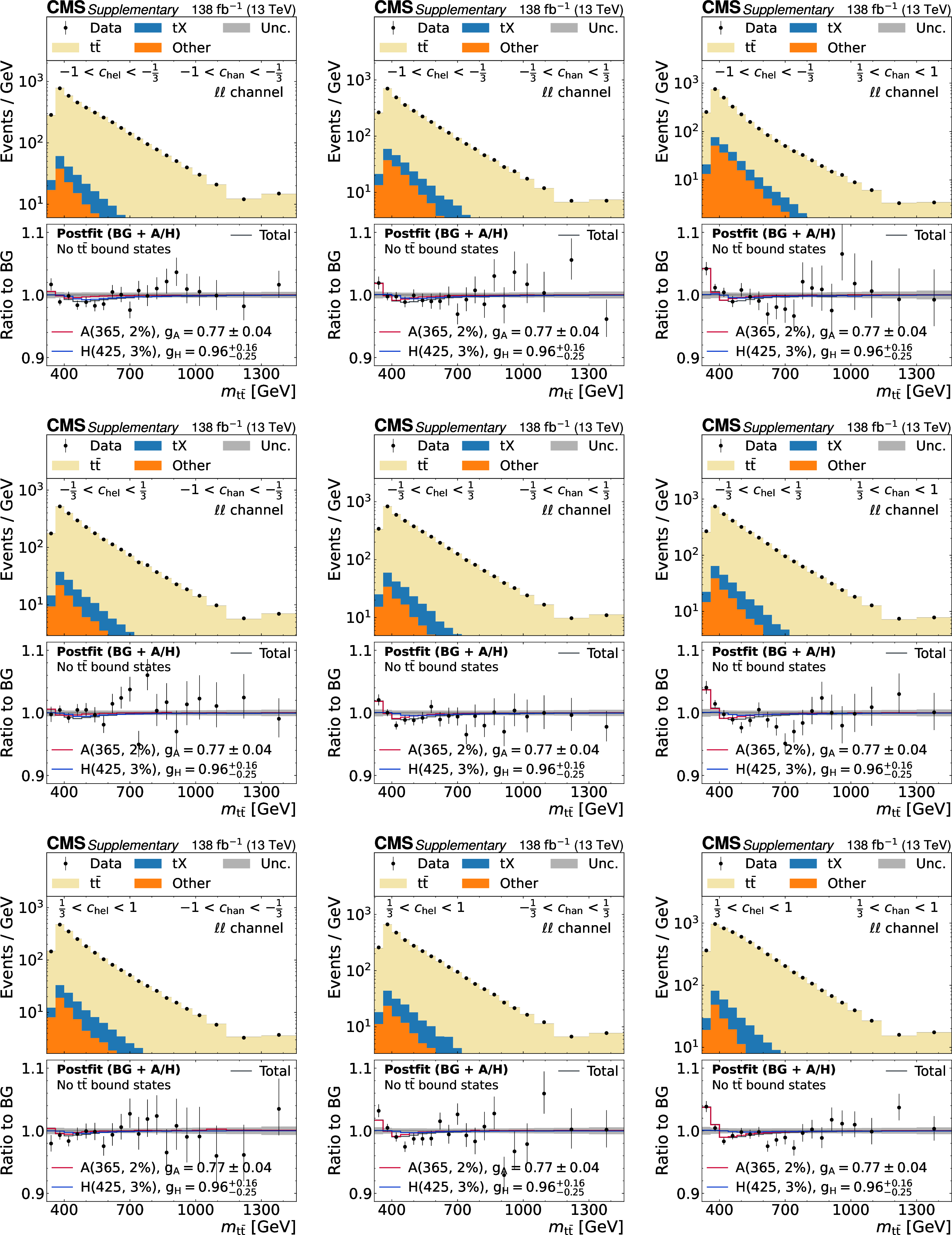
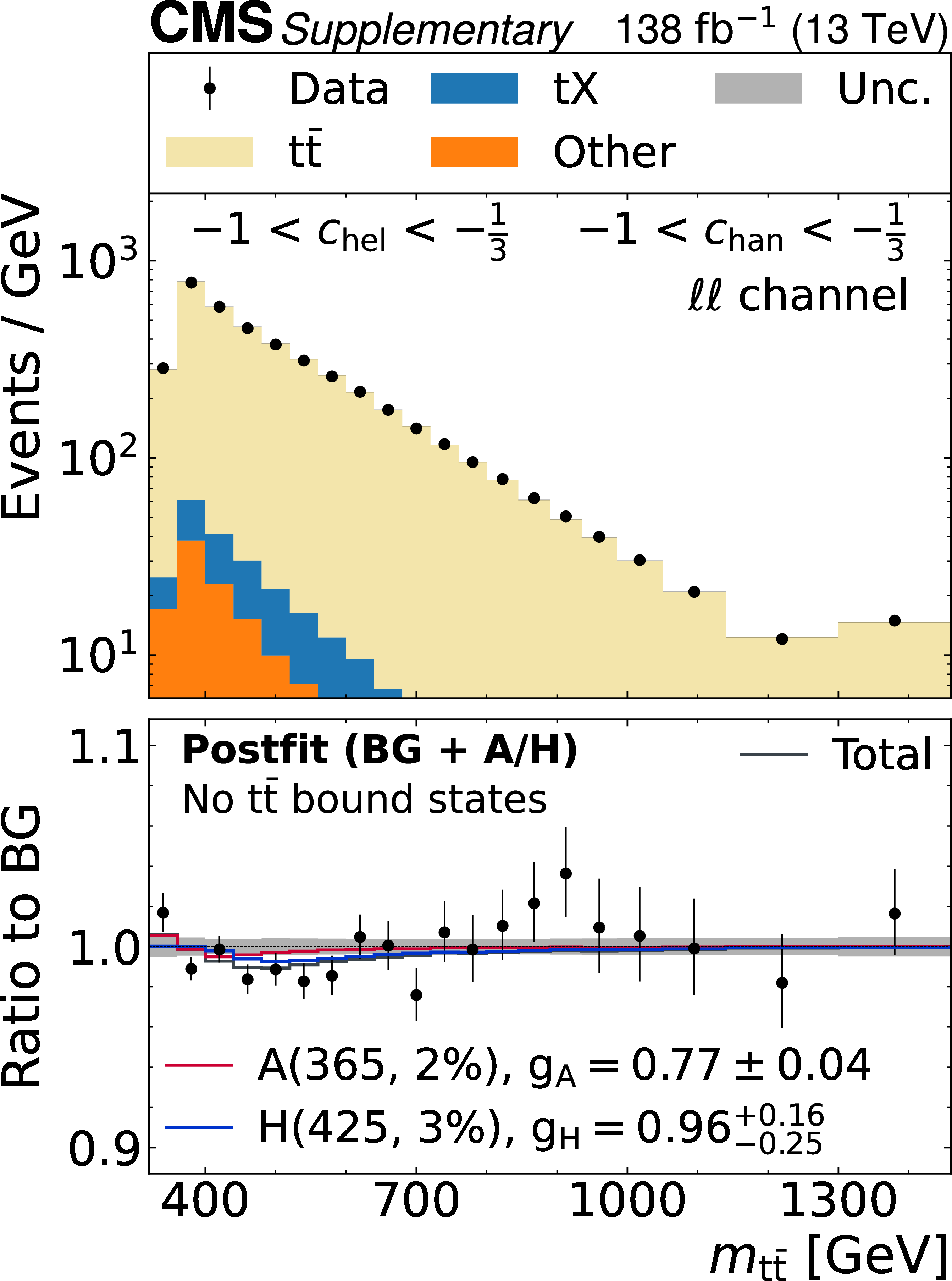
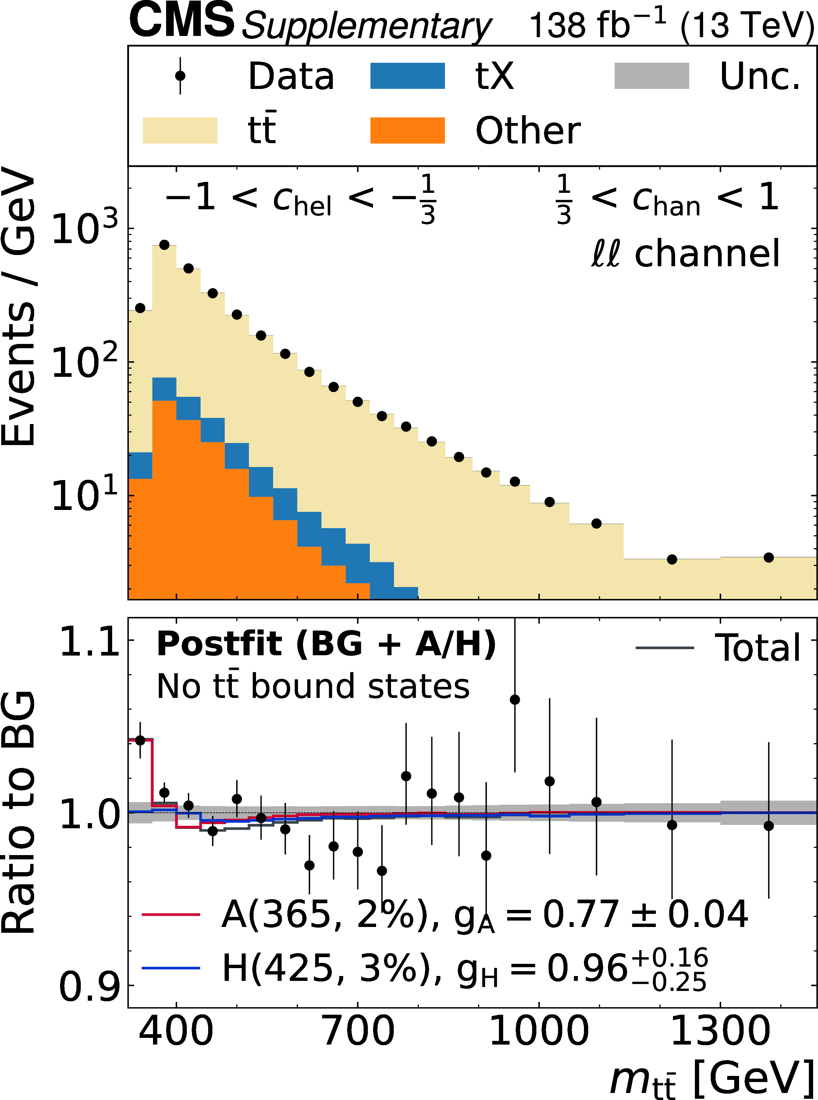
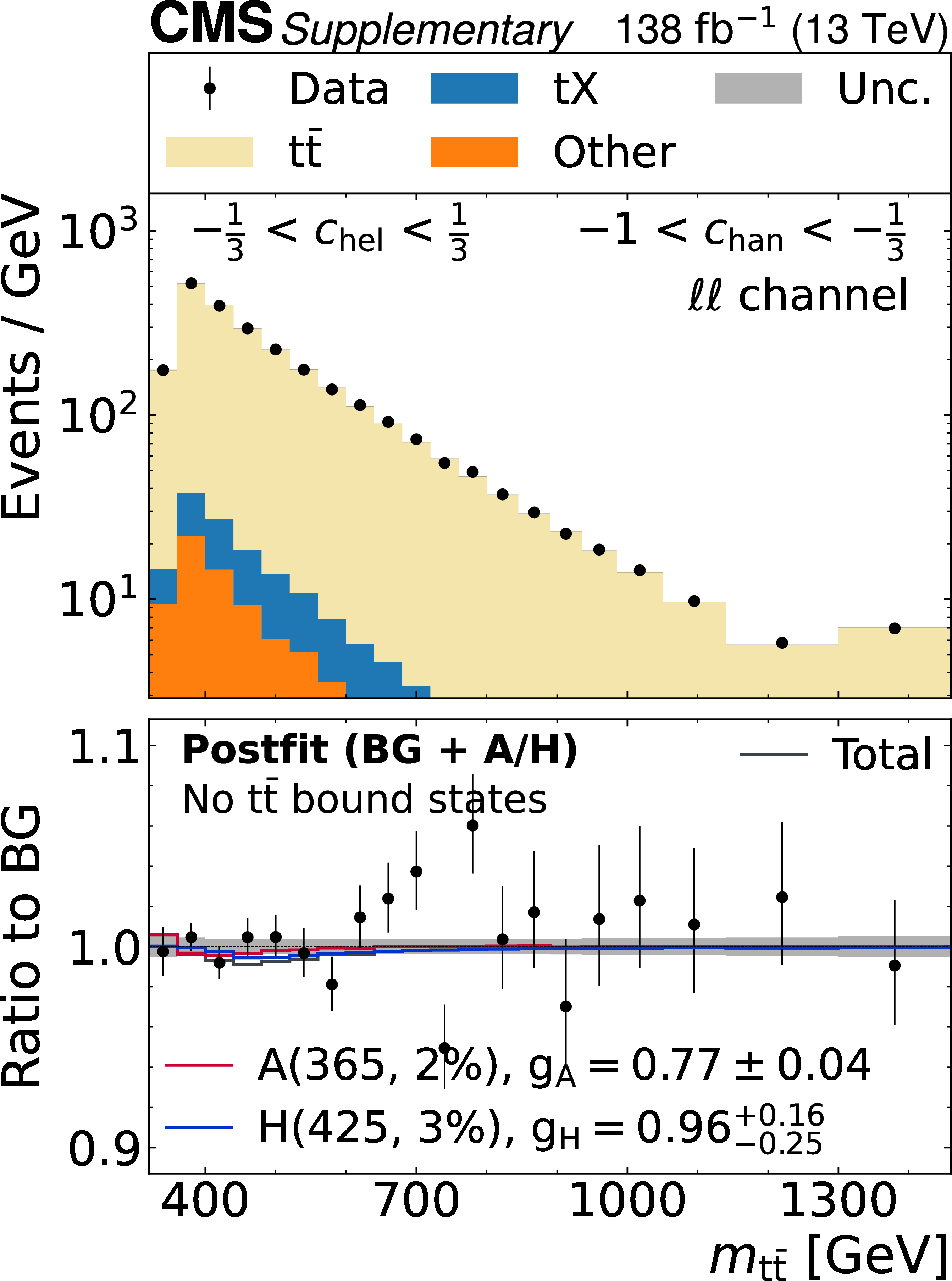
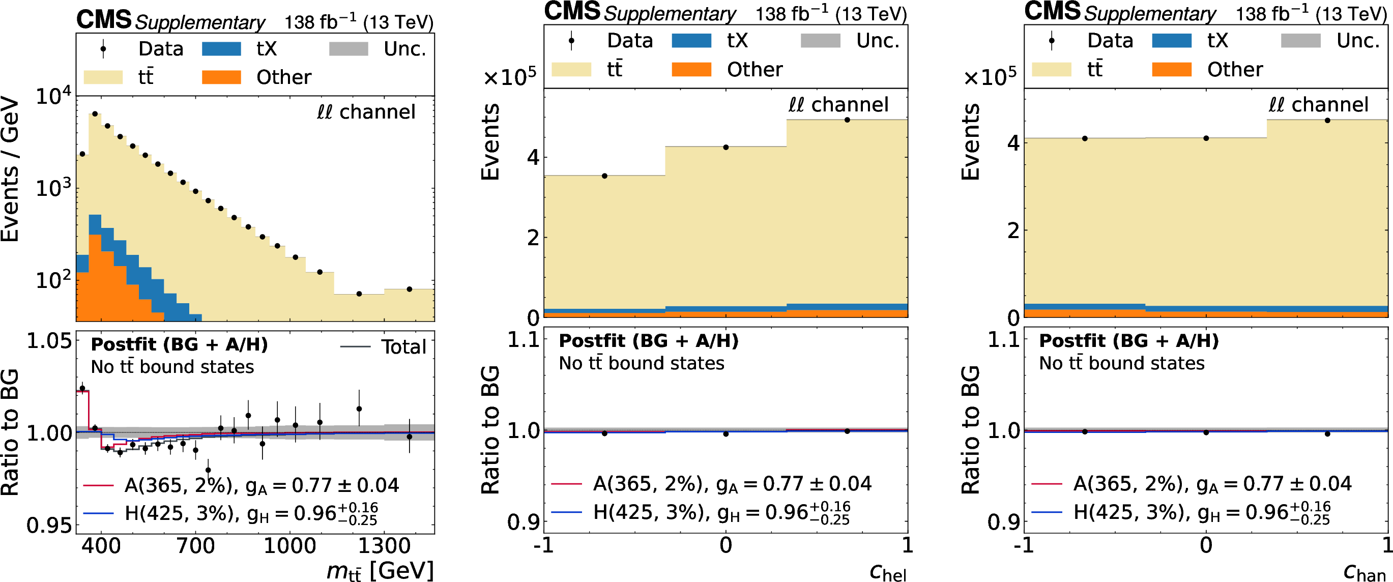
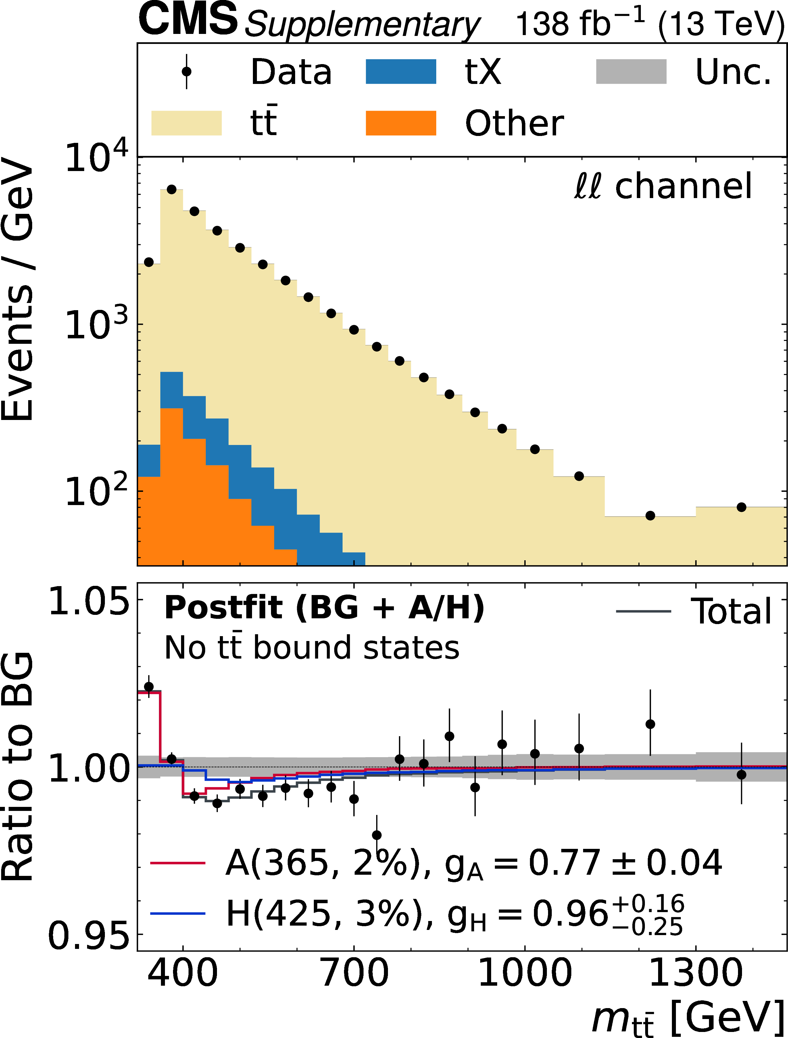
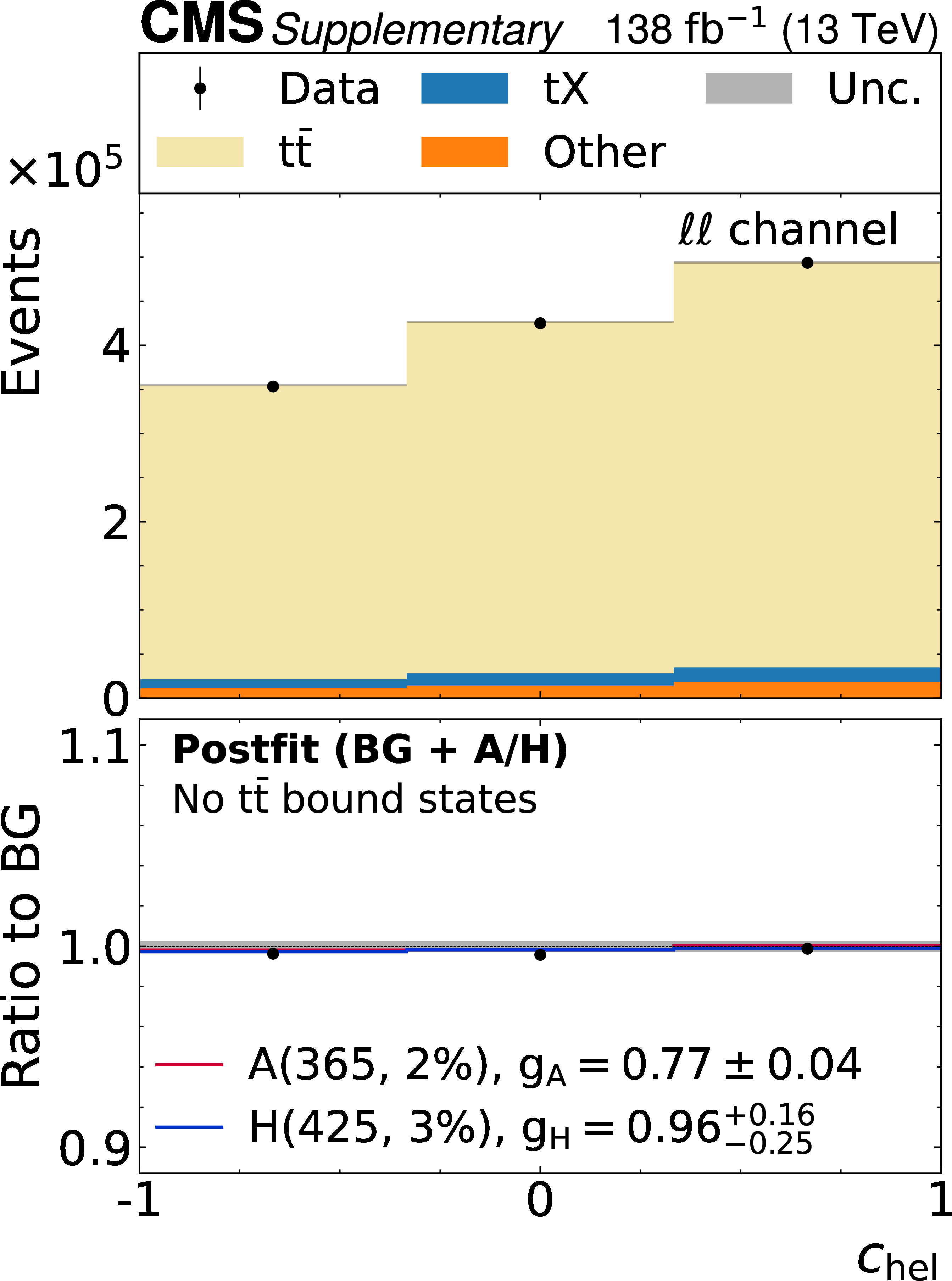
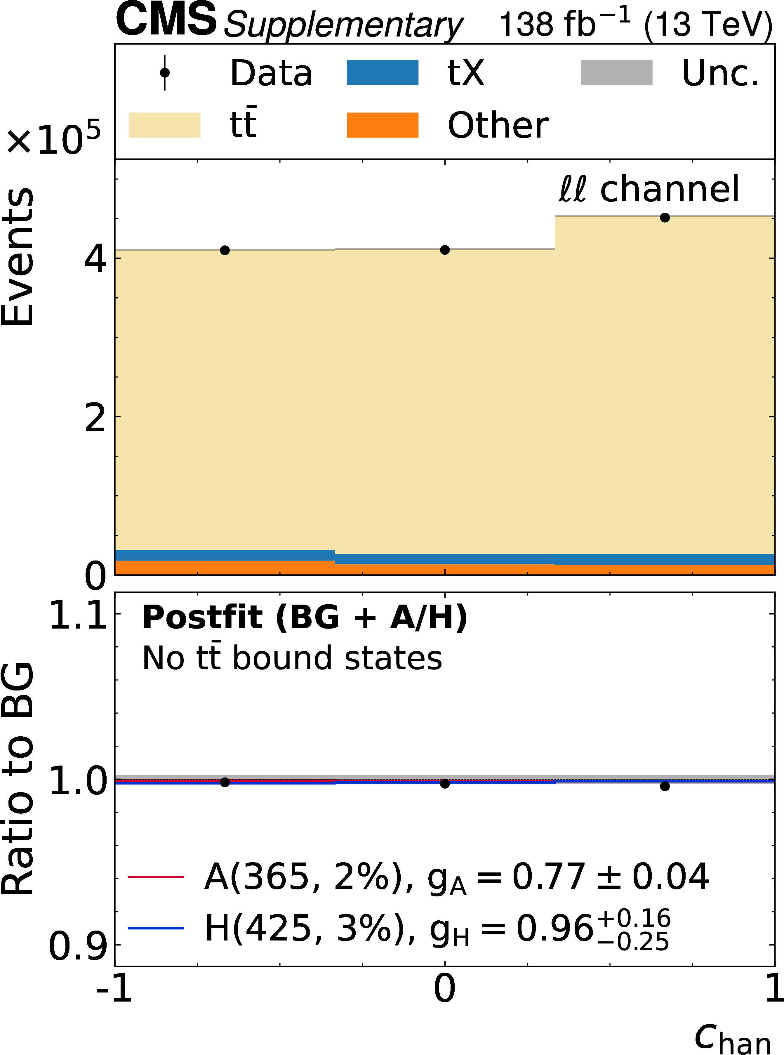
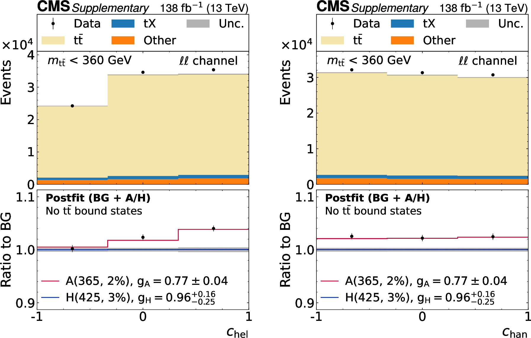
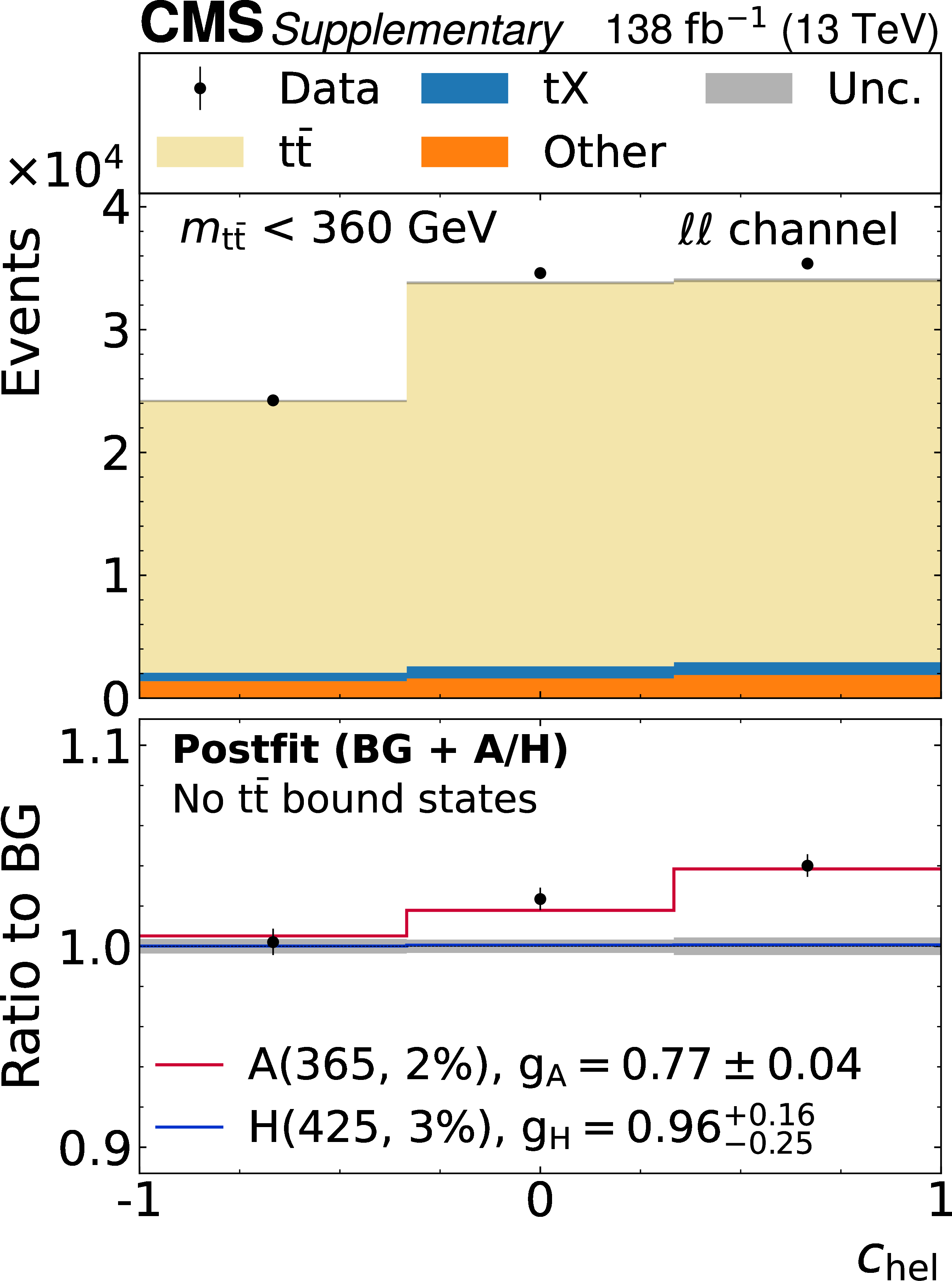
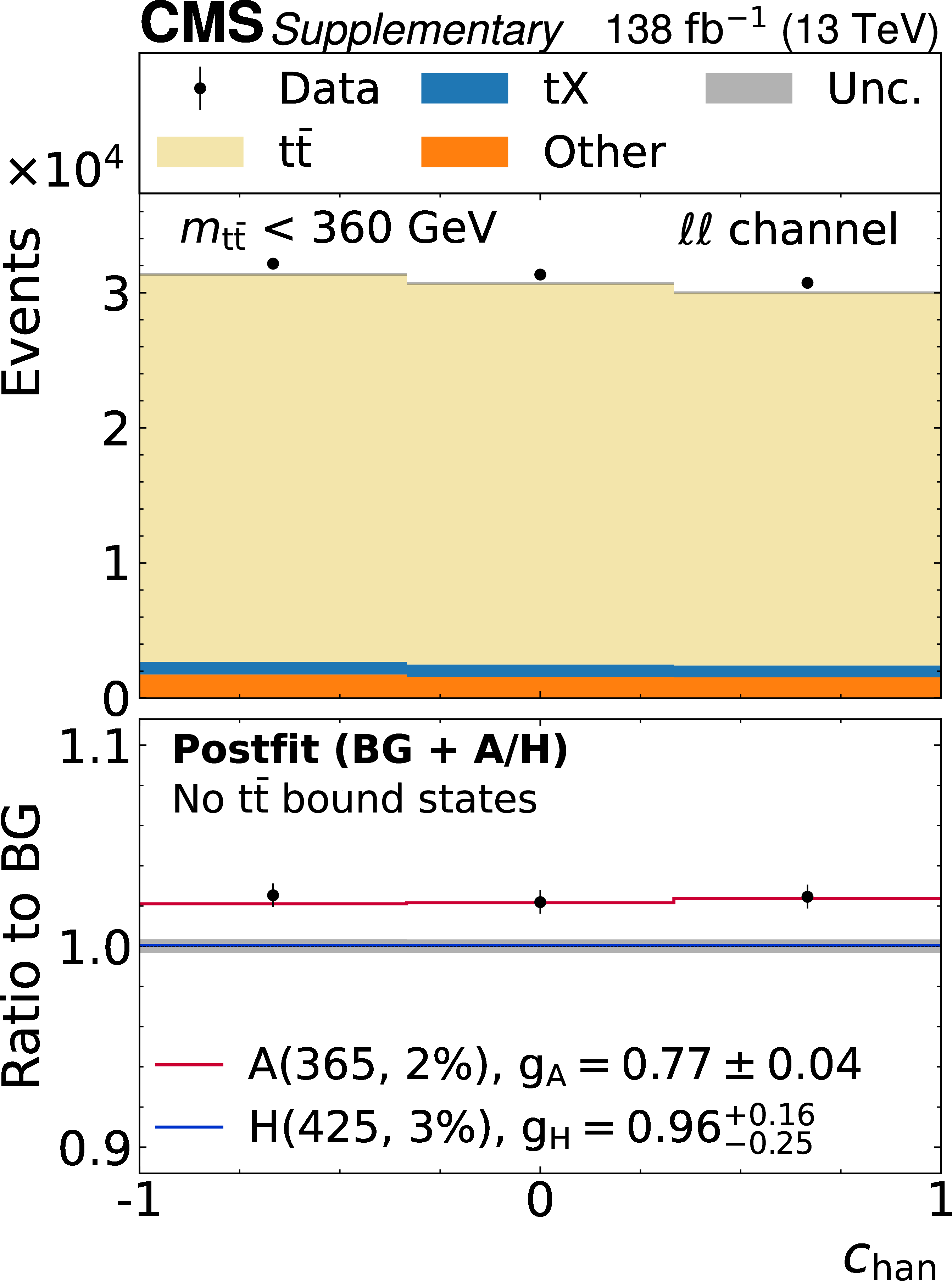
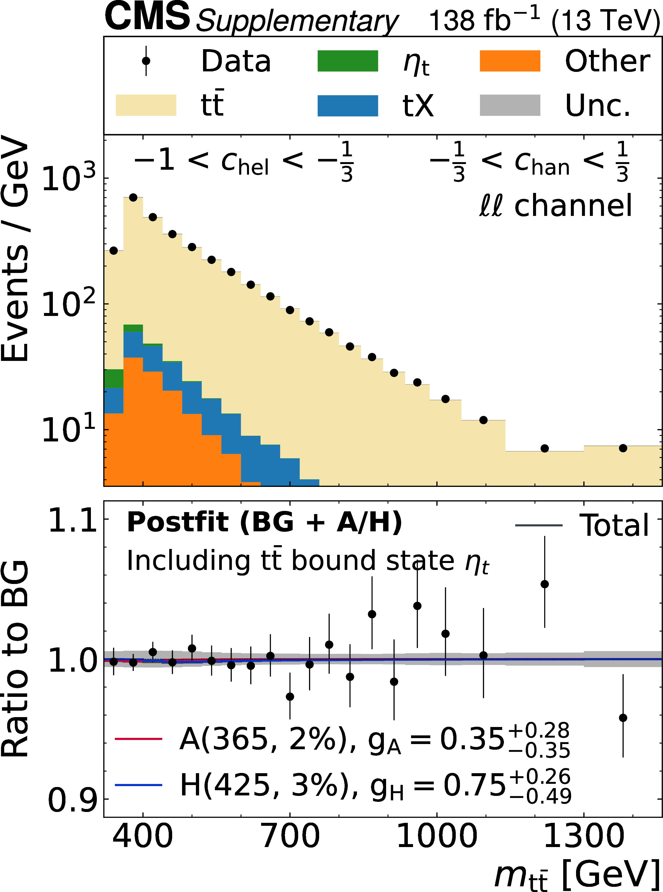
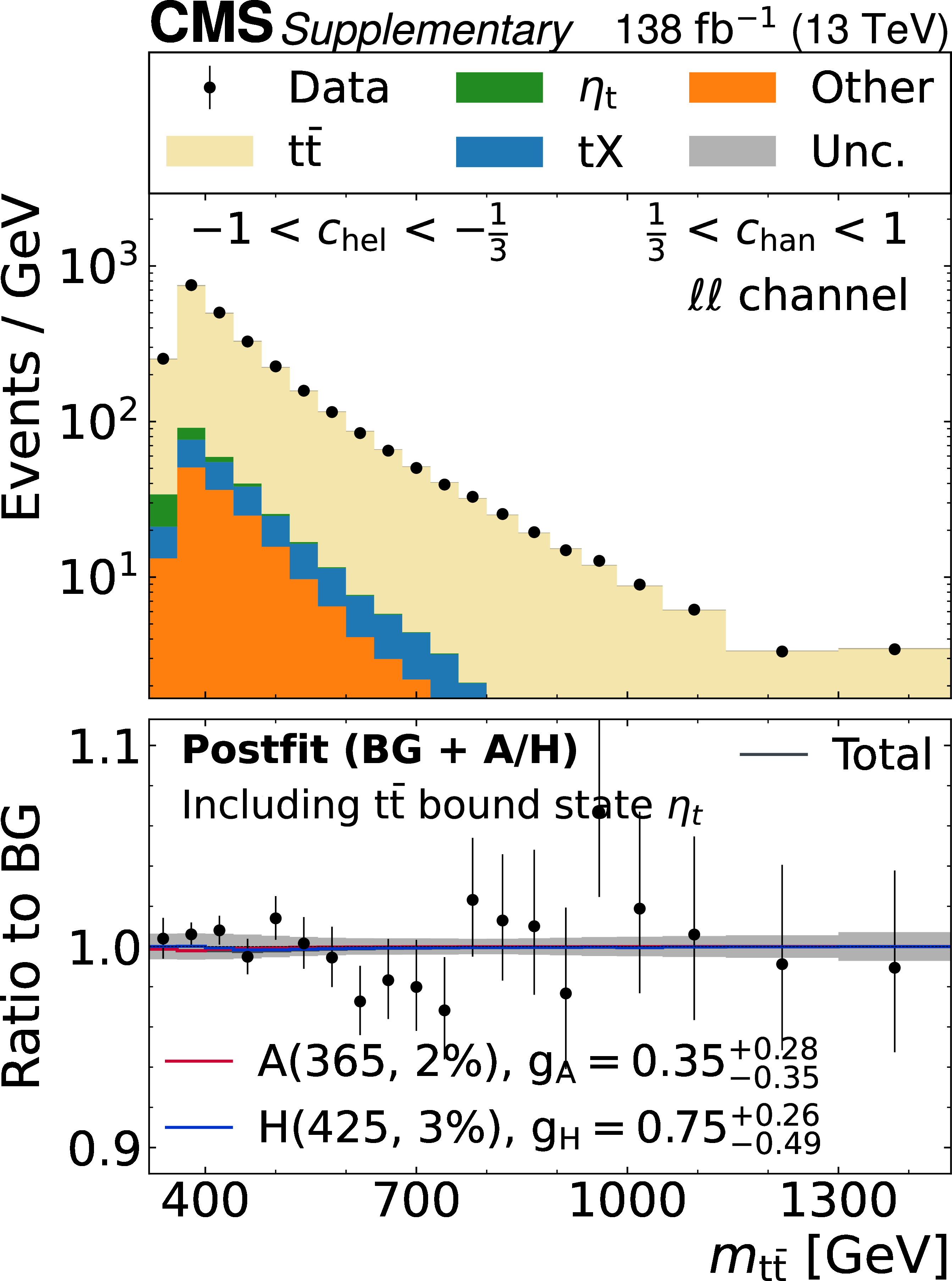
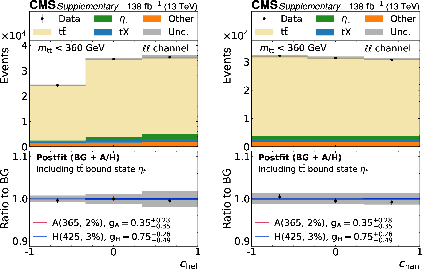
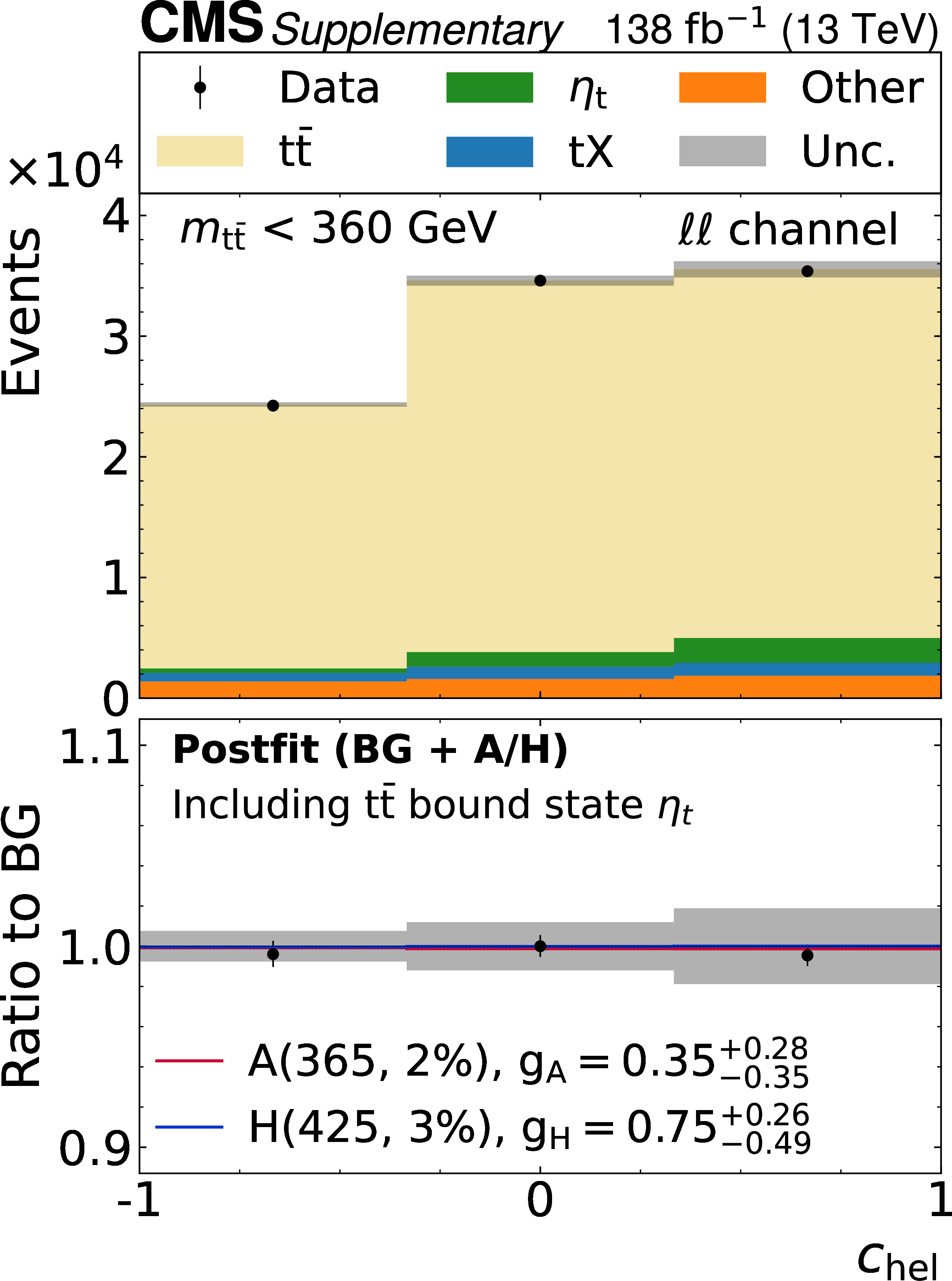
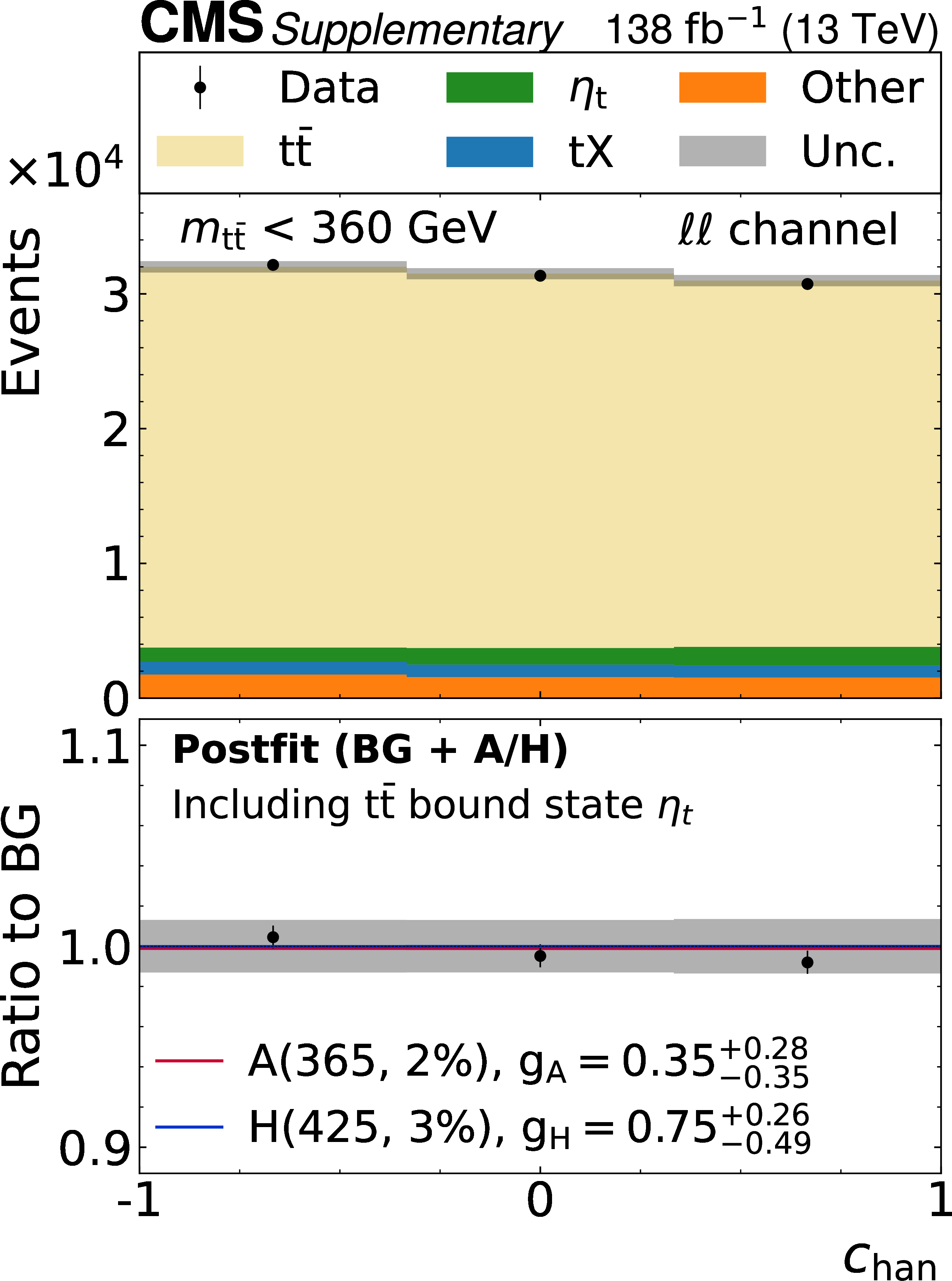
Figure 8:
Observed and expected $ m_{{\mathrm{t}\overline{\mathrm{t}}} } $ distribution in $ c_{\text{hel}} $ and $ c_{\text{han}} $ bins, shown for the $ \ell\ell $ channel summed over lepton flavors and eras. Notations as in Fig. 6. |
png pdf |
Figure 9:
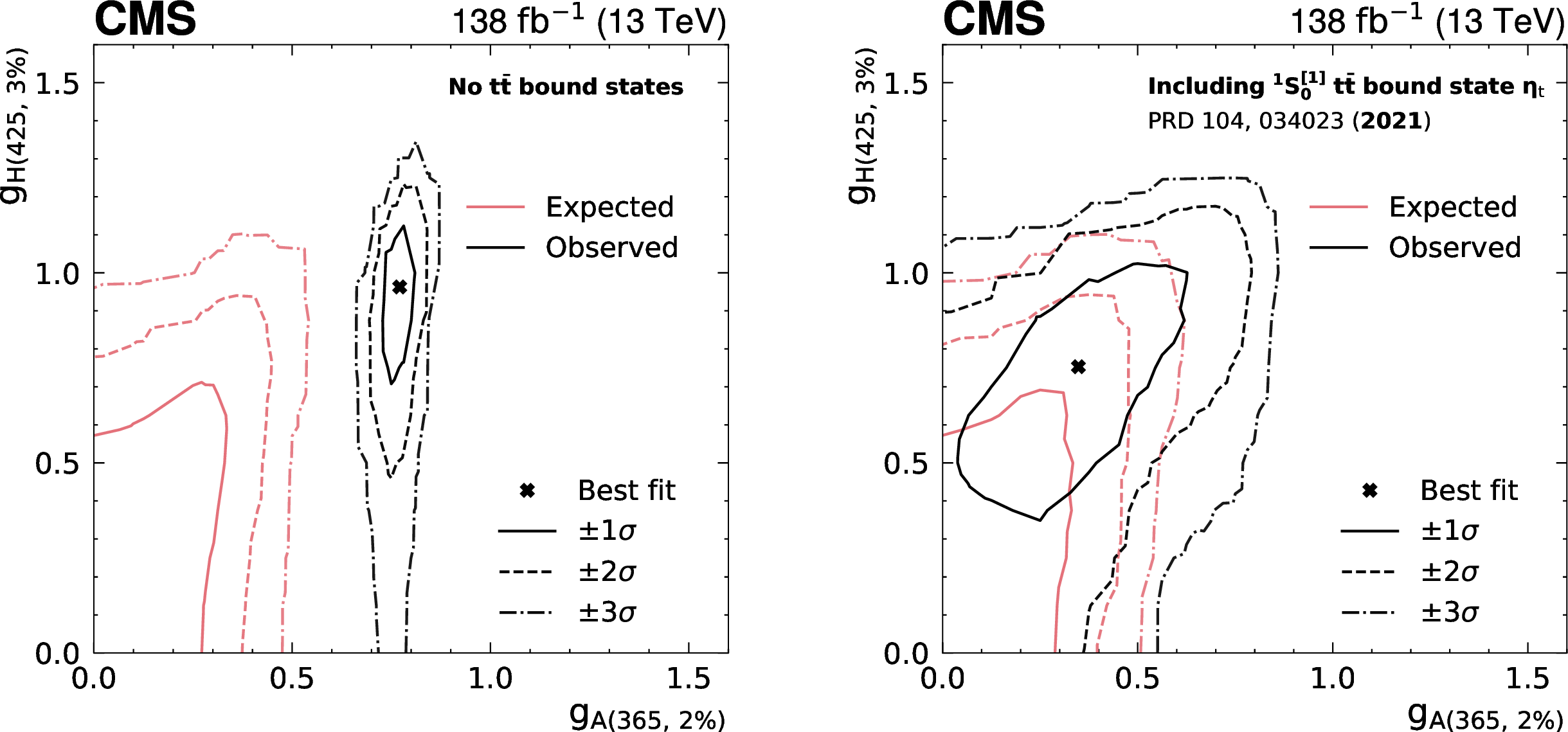
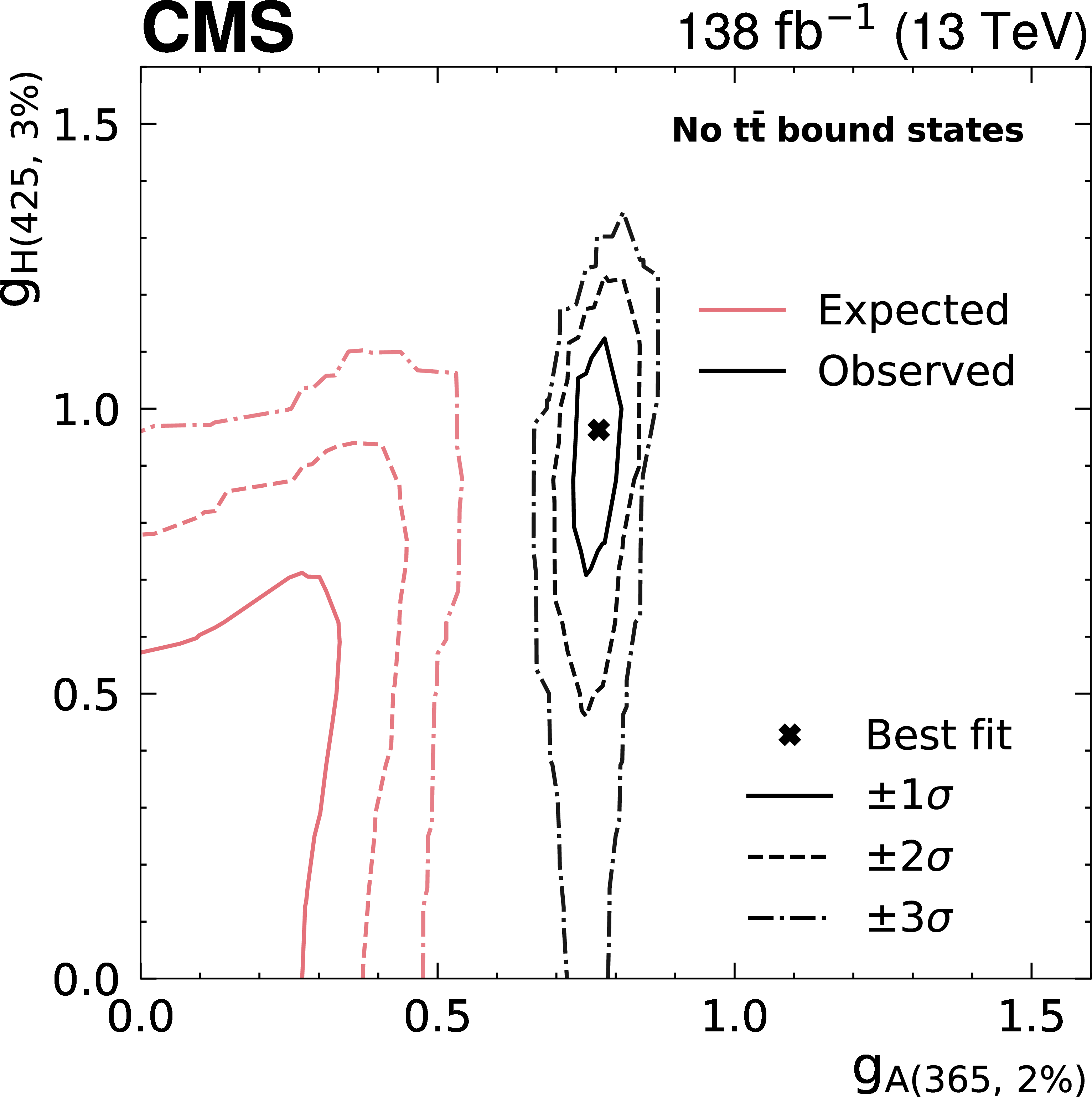
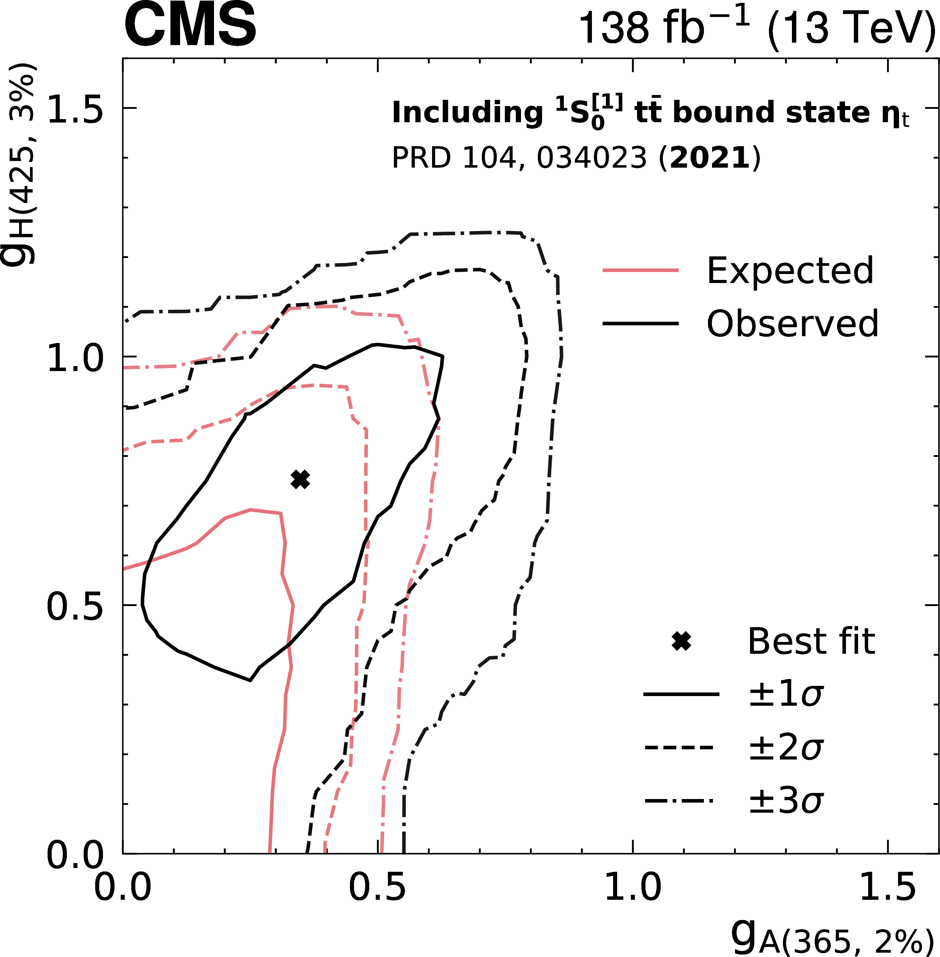
Frequentist 2D exclusion contours for $g_{\mathrm{At\bar{t}}}$ and $g_{\mathrm{Ht\bar{t}}}$ for the A$(365,\,2\%)$+H$(425,\,3\%)$ signal point, in the background scenario excluding (left) and including (right) $ \eta_{\mathrm{t}} $ production. The expected and observed contours, evaluated with the Feldman-Cousins prescription [128,129], are shown in black and pink, respectively, with different line styles denoting progressively higher $ \text{CL}_\text{s} $. The regions outside of the contours are considered excluded. |
png pdf |
Figure 9-a:
Frequentist 2D exclusion contours for $g_{\mathrm{At\bar{t}}}$ and $g_{\mathrm{Ht\bar{t}}}$ for the A$(365,\,2\%)$+H$(425,\,3\%)$ signal point, in the background scenario excluding (left) and including (right) $ \eta_{\mathrm{t}} $ production. The expected and observed contours, evaluated with the Feldman-Cousins prescription [128,129], are shown in black and pink, respectively, with different line styles denoting progressively higher $ \text{CL}_\text{s} $. The regions outside of the contours are considered excluded. |
png pdf |
Figure 9-b:
Frequentist 2D exclusion contours for $g_{\mathrm{At\bar{t}}}$ and $g_{\mathrm{Ht\bar{t}}}$ for the A$(365,\,2\%)$+H$(425,\,3\%)$ signal point, in the background scenario excluding (left) and including (right) $ \eta_{\mathrm{t}} $ production. The expected and observed contours, evaluated with the Feldman-Cousins prescription [128,129], are shown in black and pink, respectively, with different line styles denoting progressively higher $ \text{CL}_\text{s} $. The regions outside of the contours are considered excluded. |

png pdf |
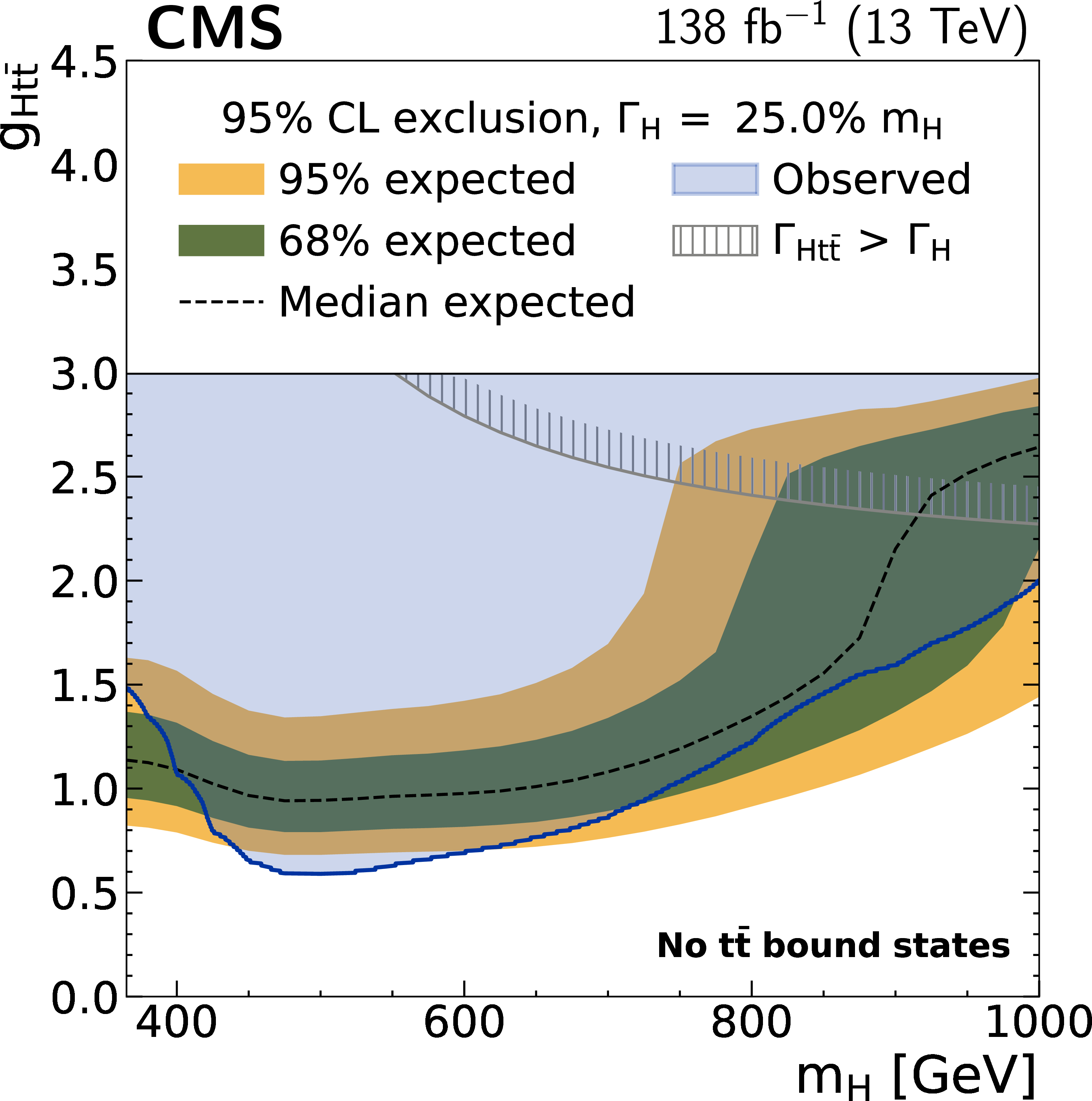
Figure 10:
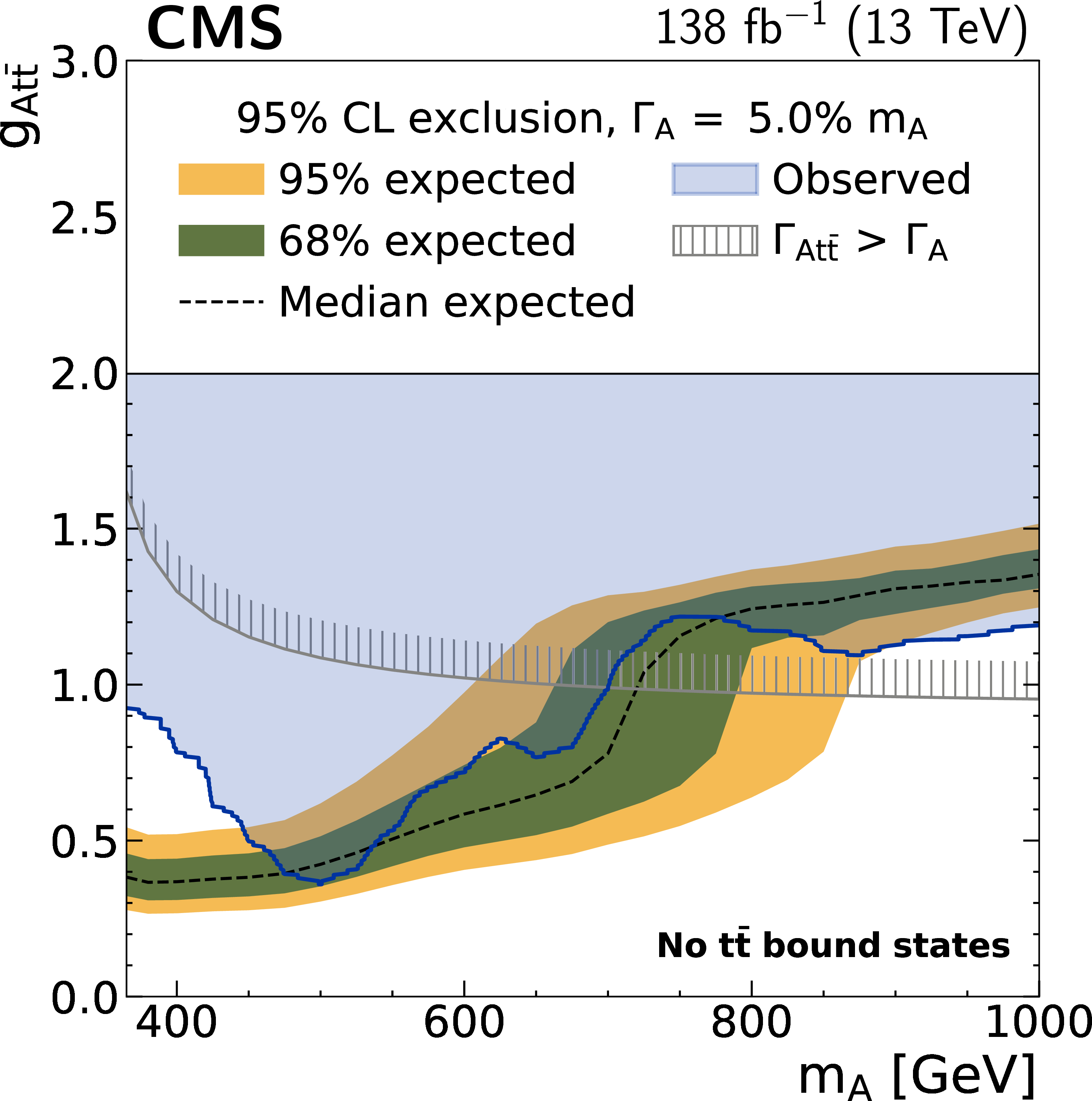
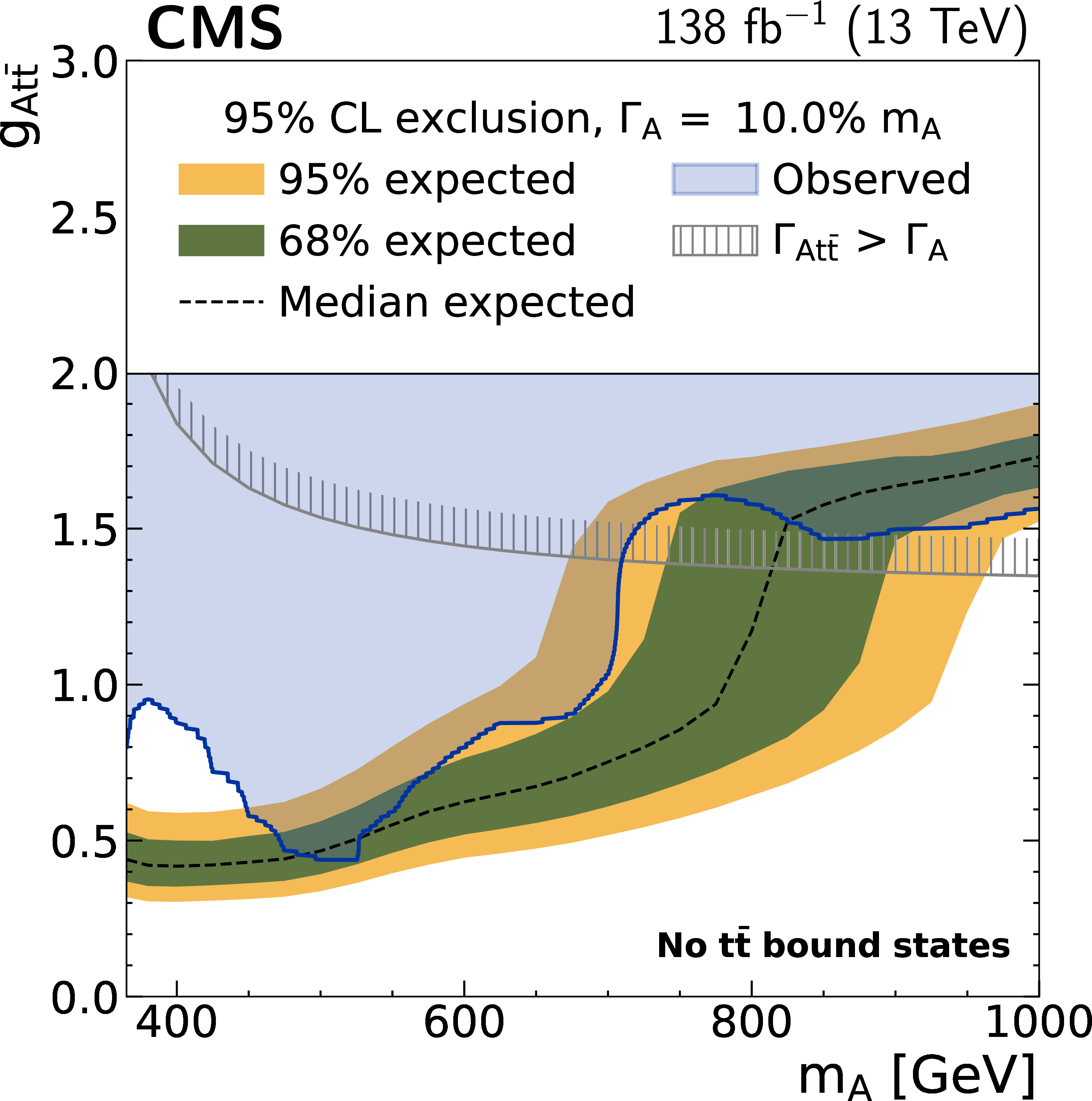
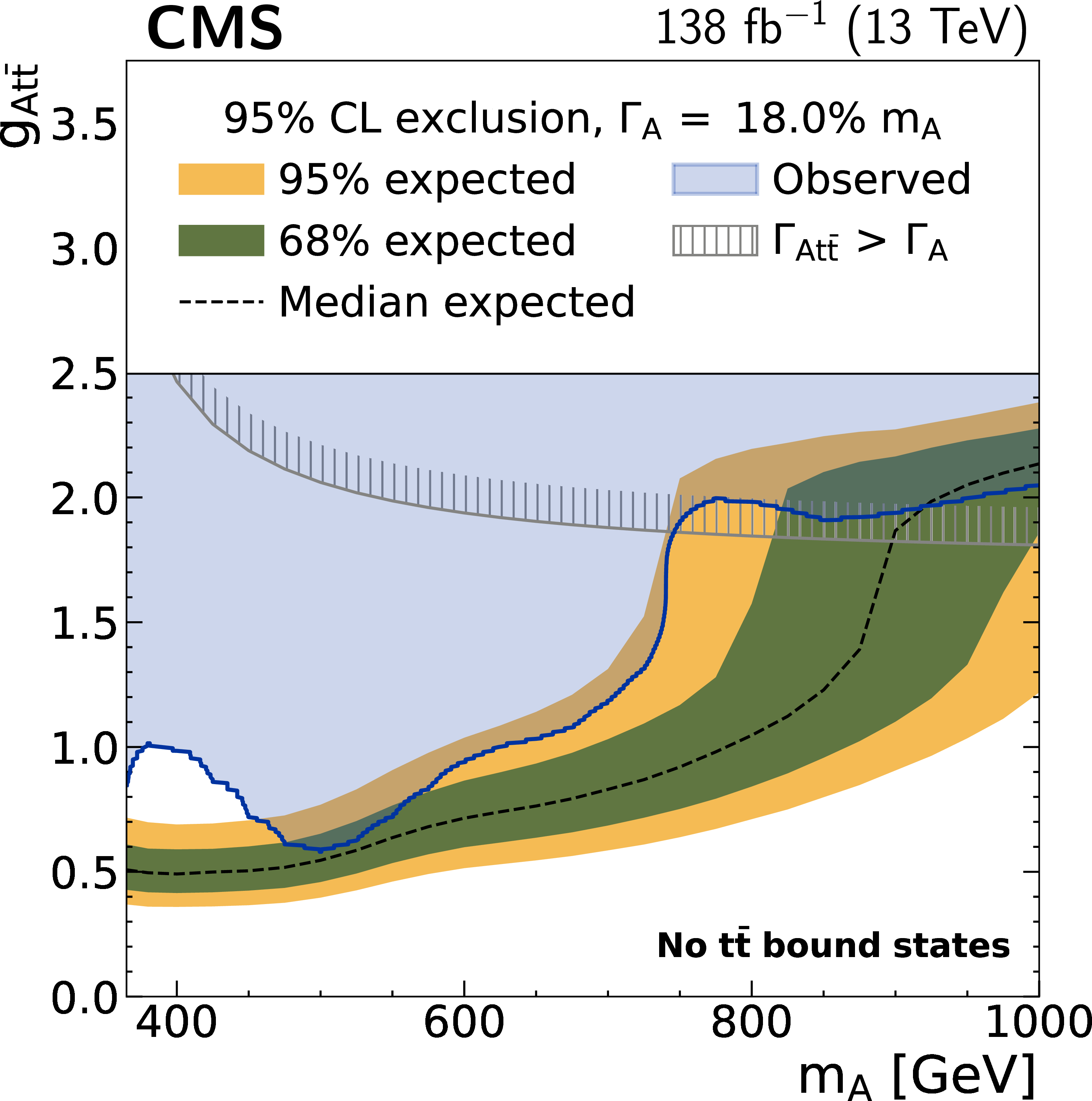
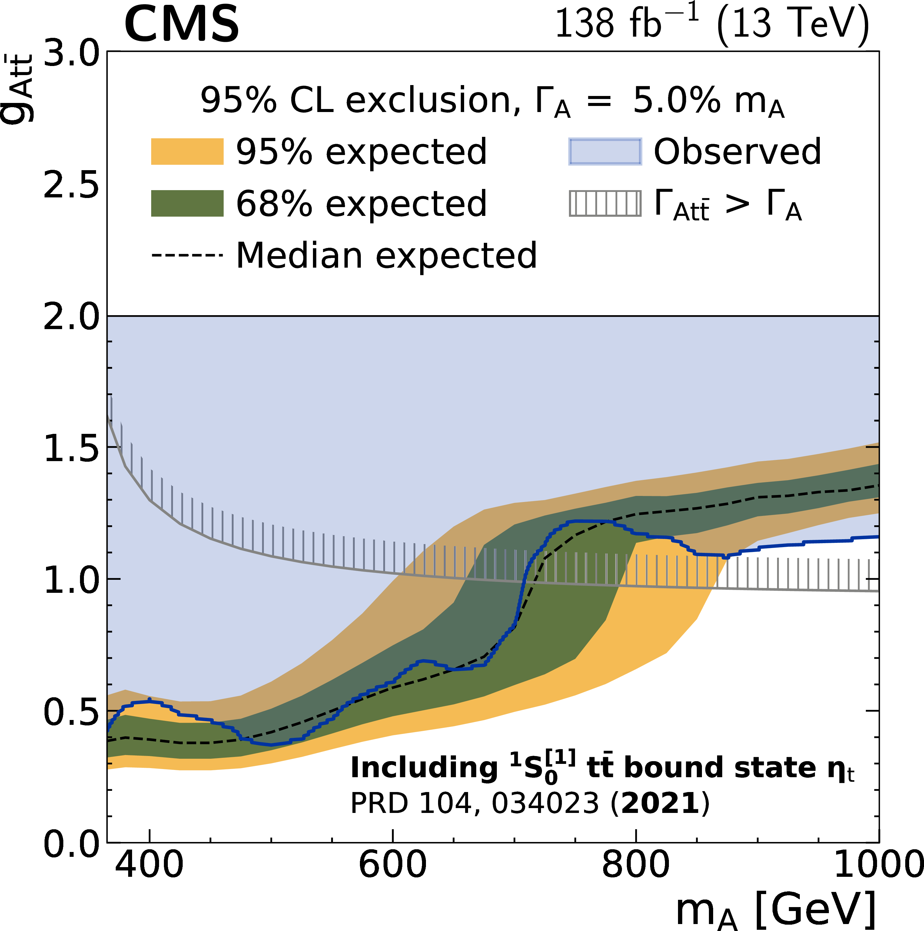
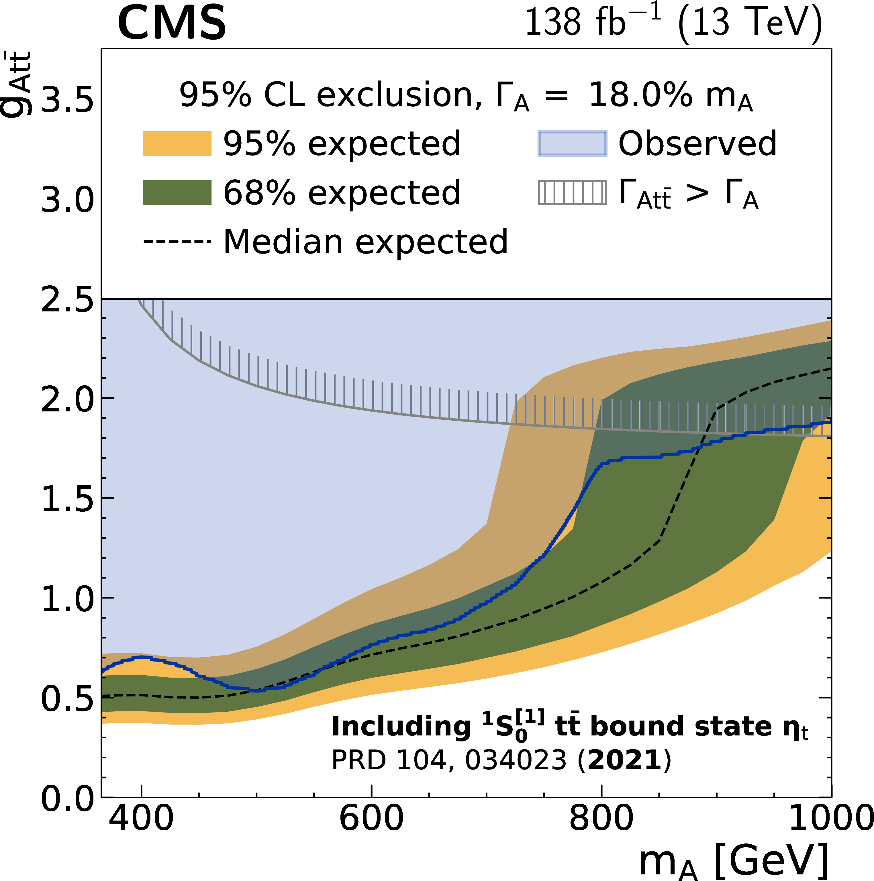
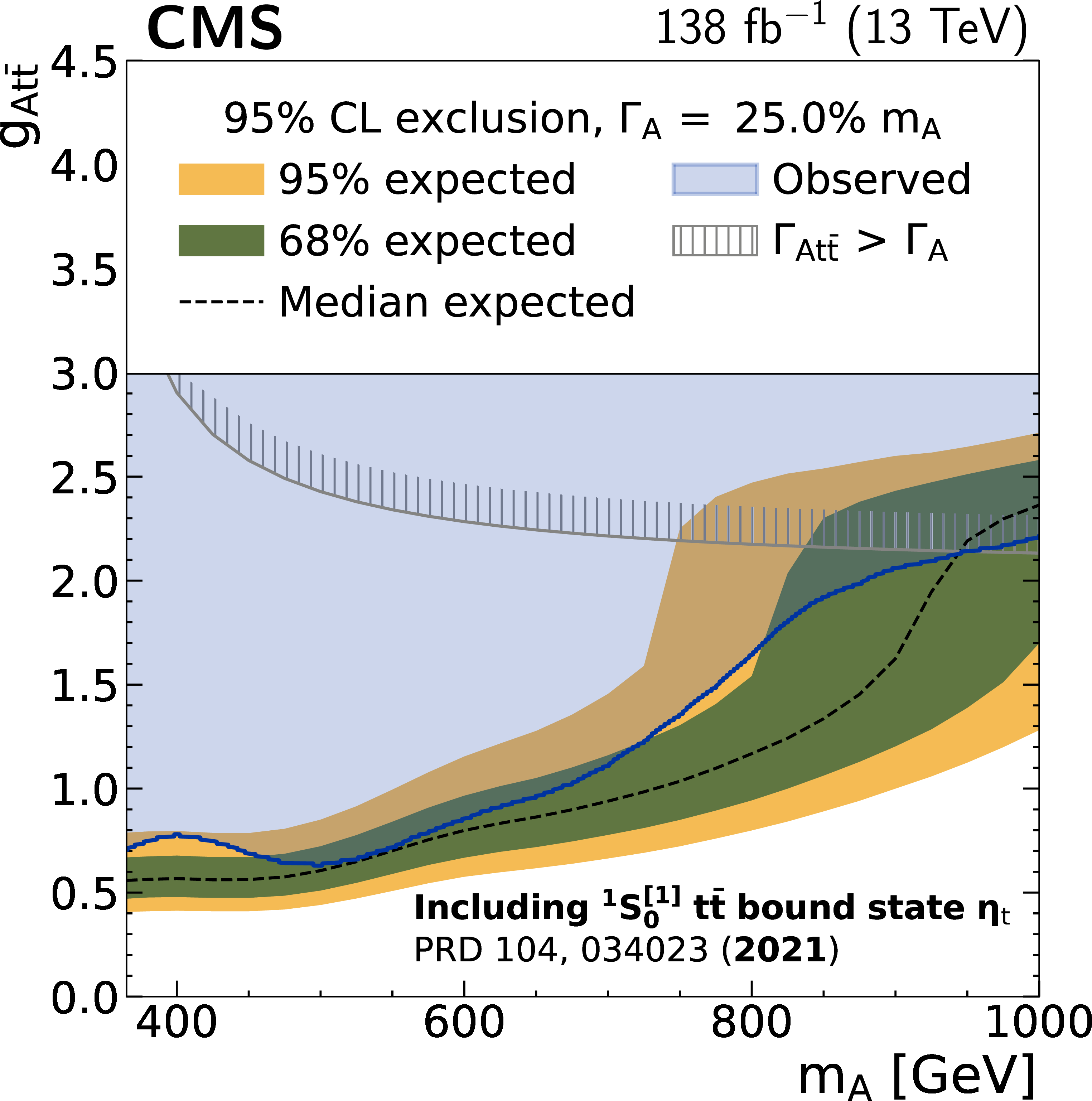
Model-independent constraints on $g_{\mathrm{At\bar{t}}}$ as functions of the A boson mass in the background scenario without $ \eta_{\mathrm{t}} $ contribution, for $ \Gamma_{\Phi}/m_{\Phi} $ of 1, 2, 5, 10, 18, and 25% (from upper left to lower right). The observed constraints are indicated by the shaded blue area, bounded by the solid blue curve. The inner green and outer yellow bands indicate the regions containing 68 and 95%, respectively, of the distribution of constraints expected under the background-only hypothesis. The unphysical region of phase space in which the partial width $ \Gamma_{\mathrm{A}\to{\mathrm{t}\overline{\mathrm{t}}} } $ becomes larger than the total width of the A boson is indicated by the hatched line. |
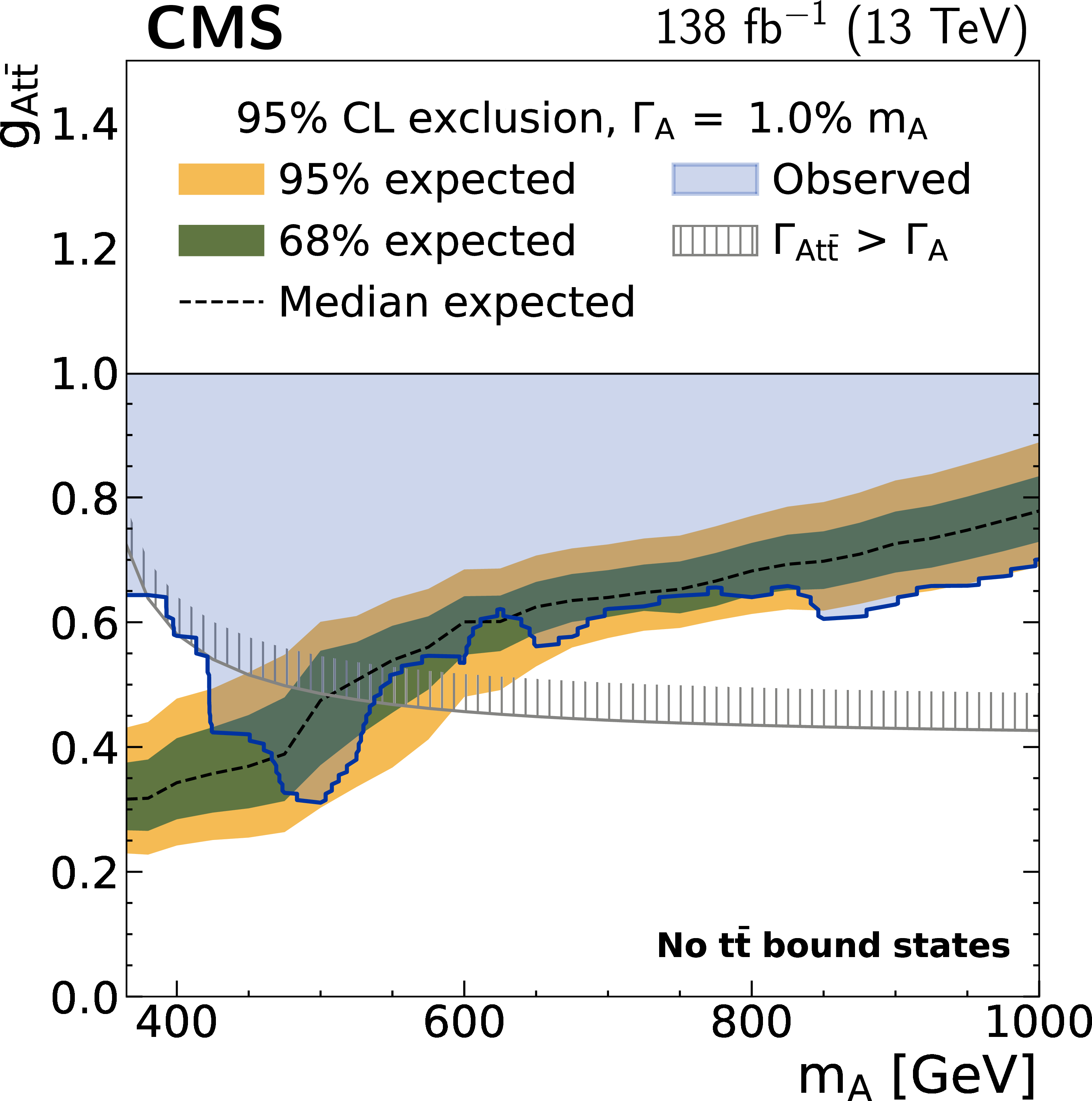
png pdf |
Figure 10-a:
Model-independent constraints on $g_{\mathrm{At\bar{t}}}$ as functions of the A boson mass in the background scenario without $ \eta_{\mathrm{t}} $ contribution, for $ \Gamma_{\Phi}/m_{\Phi} $ of 1, 2, 5, 10, 18, and 25% (from upper left to lower right). The observed constraints are indicated by the shaded blue area, bounded by the solid blue curve. The inner green and outer yellow bands indicate the regions containing 68 and 95%, respectively, of the distribution of constraints expected under the background-only hypothesis. The unphysical region of phase space in which the partial width $ \Gamma_{\mathrm{A}\to{\mathrm{t}\overline{\mathrm{t}}} } $ becomes larger than the total width of the A boson is indicated by the hatched line. |
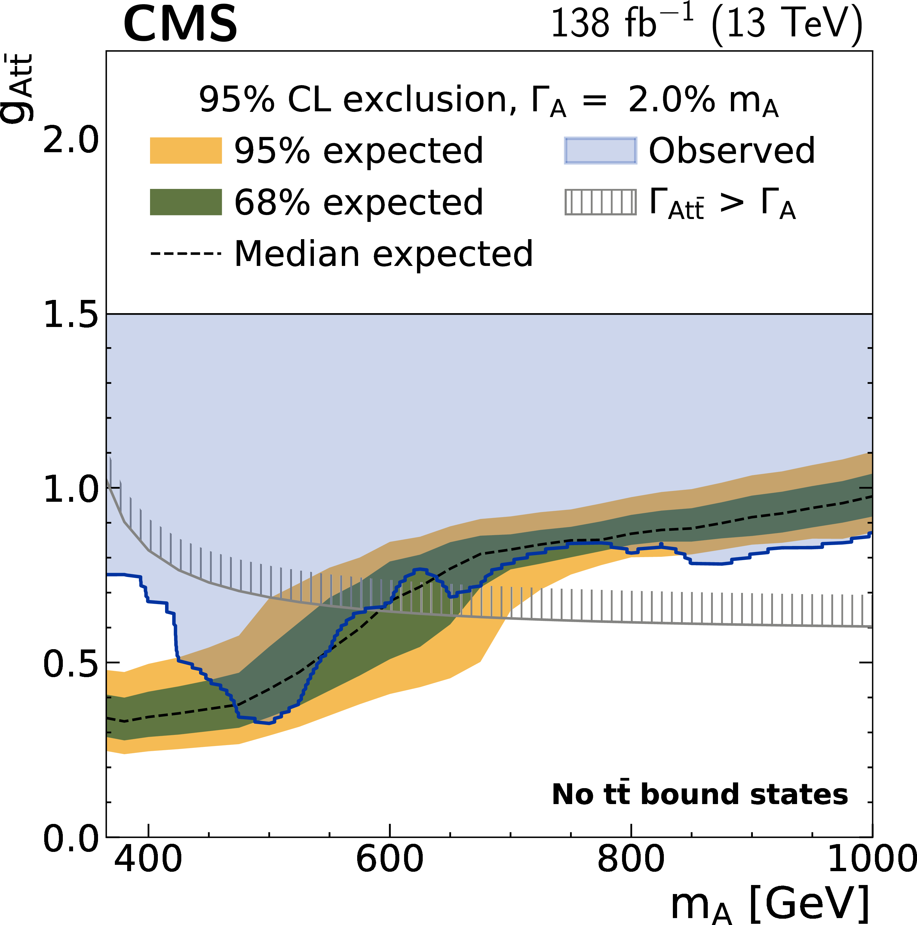
png pdf |
Figure 10-b:
Model-independent constraints on $g_{\mathrm{At\bar{t}}}$ as functions of the A boson mass in the background scenario without $ \eta_{\mathrm{t}} $ contribution, for $ \Gamma_{\Phi}/m_{\Phi} $ of 1, 2, 5, 10, 18, and 25% (from upper left to lower right). The observed constraints are indicated by the shaded blue area, bounded by the solid blue curve. The inner green and outer yellow bands indicate the regions containing 68 and 95%, respectively, of the distribution of constraints expected under the background-only hypothesis. The unphysical region of phase space in which the partial width $ \Gamma_{\mathrm{A}\to{\mathrm{t}\overline{\mathrm{t}}} } $ becomes larger than the total width of the A boson is indicated by the hatched line. |
png pdf |
Figure 10-c:
Model-independent constraints on $g_{\mathrm{At\bar{t}}}$ as functions of the A boson mass in the background scenario without $ \eta_{\mathrm{t}} $ contribution, for $ \Gamma_{\Phi}/m_{\Phi} $ of 1, 2, 5, 10, 18, and 25% (from upper left to lower right). The observed constraints are indicated by the shaded blue area, bounded by the solid blue curve. The inner green and outer yellow bands indicate the regions containing 68 and 95%, respectively, of the distribution of constraints expected under the background-only hypothesis. The unphysical region of phase space in which the partial width $ \Gamma_{\mathrm{A}\to{\mathrm{t}\overline{\mathrm{t}}} } $ becomes larger than the total width of the A boson is indicated by the hatched line. |
png pdf |
Figure 10-d:
Model-independent constraints on $g_{\mathrm{At\bar{t}}}$ as functions of the A boson mass in the background scenario without $ \eta_{\mathrm{t}} $ contribution, for $ \Gamma_{\Phi}/m_{\Phi} $ of 1, 2, 5, 10, 18, and 25% (from upper left to lower right). The observed constraints are indicated by the shaded blue area, bounded by the solid blue curve. The inner green and outer yellow bands indicate the regions containing 68 and 95%, respectively, of the distribution of constraints expected under the background-only hypothesis. The unphysical region of phase space in which the partial width $ \Gamma_{\mathrm{A}\to{\mathrm{t}\overline{\mathrm{t}}} } $ becomes larger than the total width of the A boson is indicated by the hatched line. |
png pdf |
Figure 10-e:
Model-independent constraints on $g_{\mathrm{At\bar{t}}}$ as functions of the A boson mass in the background scenario without $ \eta_{\mathrm{t}} $ contribution, for $ \Gamma_{\Phi}/m_{\Phi} $ of 1, 2, 5, 10, 18, and 25% (from upper left to lower right). The observed constraints are indicated by the shaded blue area, bounded by the solid blue curve. The inner green and outer yellow bands indicate the regions containing 68 and 95%, respectively, of the distribution of constraints expected under the background-only hypothesis. The unphysical region of phase space in which the partial width $ \Gamma_{\mathrm{A}\to{\mathrm{t}\overline{\mathrm{t}}} } $ becomes larger than the total width of the A boson is indicated by the hatched line. |
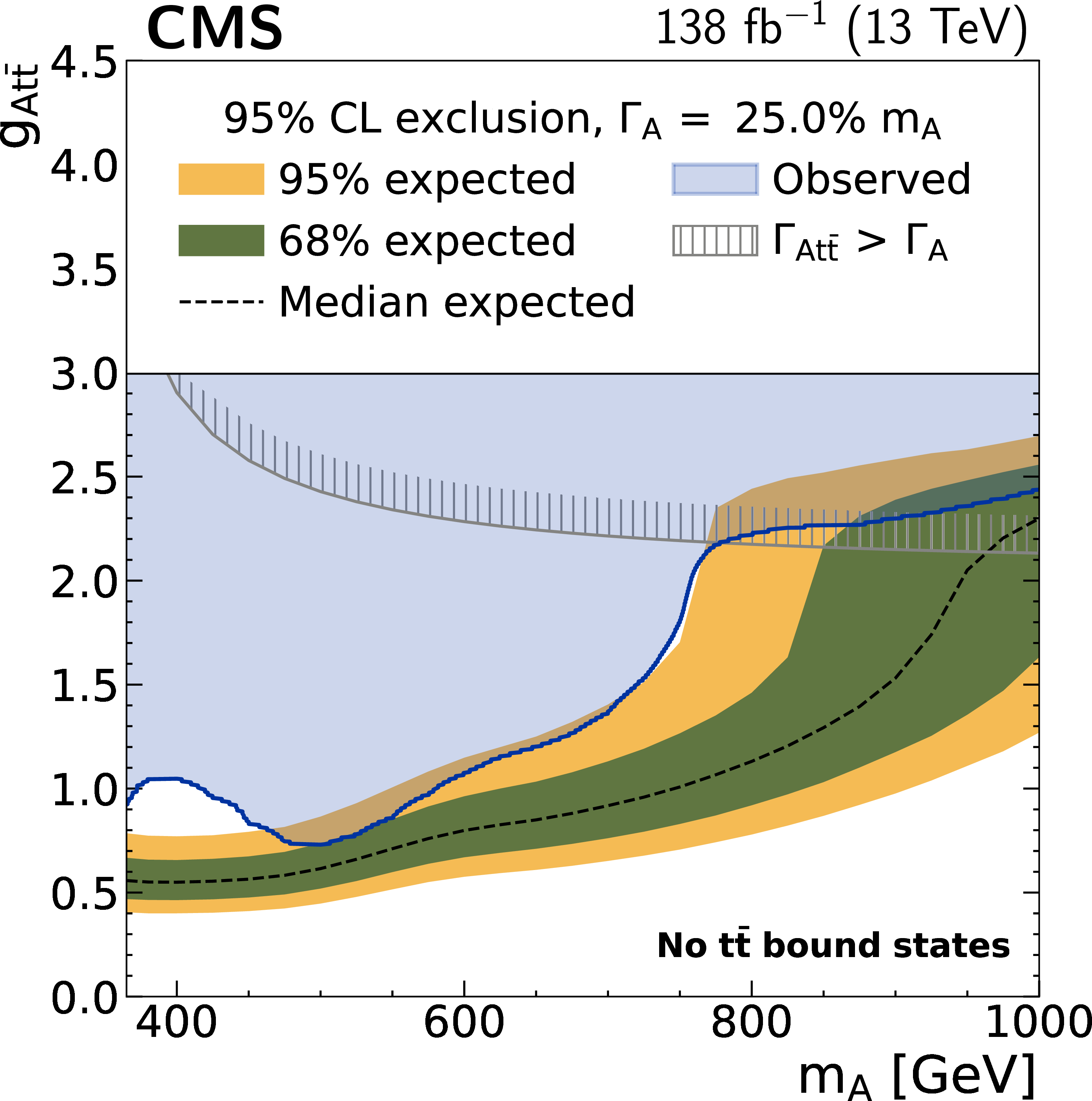
png pdf |
Figure 10-f:
Model-independent constraints on $g_{\mathrm{At\bar{t}}}$ as functions of the A boson mass in the background scenario without $ \eta_{\mathrm{t}} $ contribution, for $ \Gamma_{\Phi}/m_{\Phi} $ of 1, 2, 5, 10, 18, and 25% (from upper left to lower right). The observed constraints are indicated by the shaded blue area, bounded by the solid blue curve. The inner green and outer yellow bands indicate the regions containing 68 and 95%, respectively, of the distribution of constraints expected under the background-only hypothesis. The unphysical region of phase space in which the partial width $ \Gamma_{\mathrm{A}\to{\mathrm{t}\overline{\mathrm{t}}} } $ becomes larger than the total width of the A boson is indicated by the hatched line. |
png pdf |
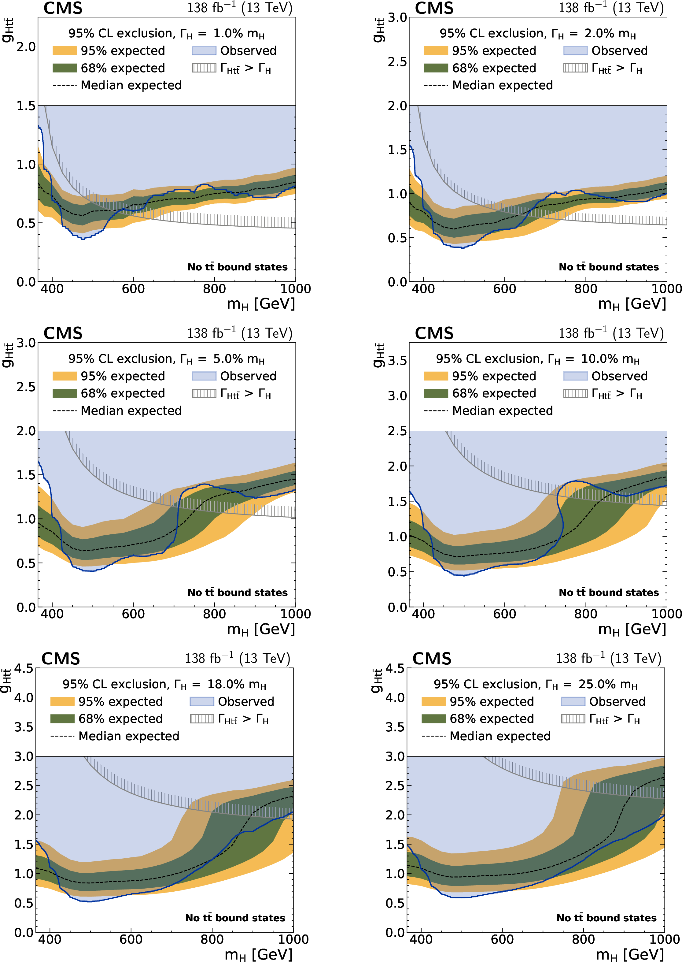
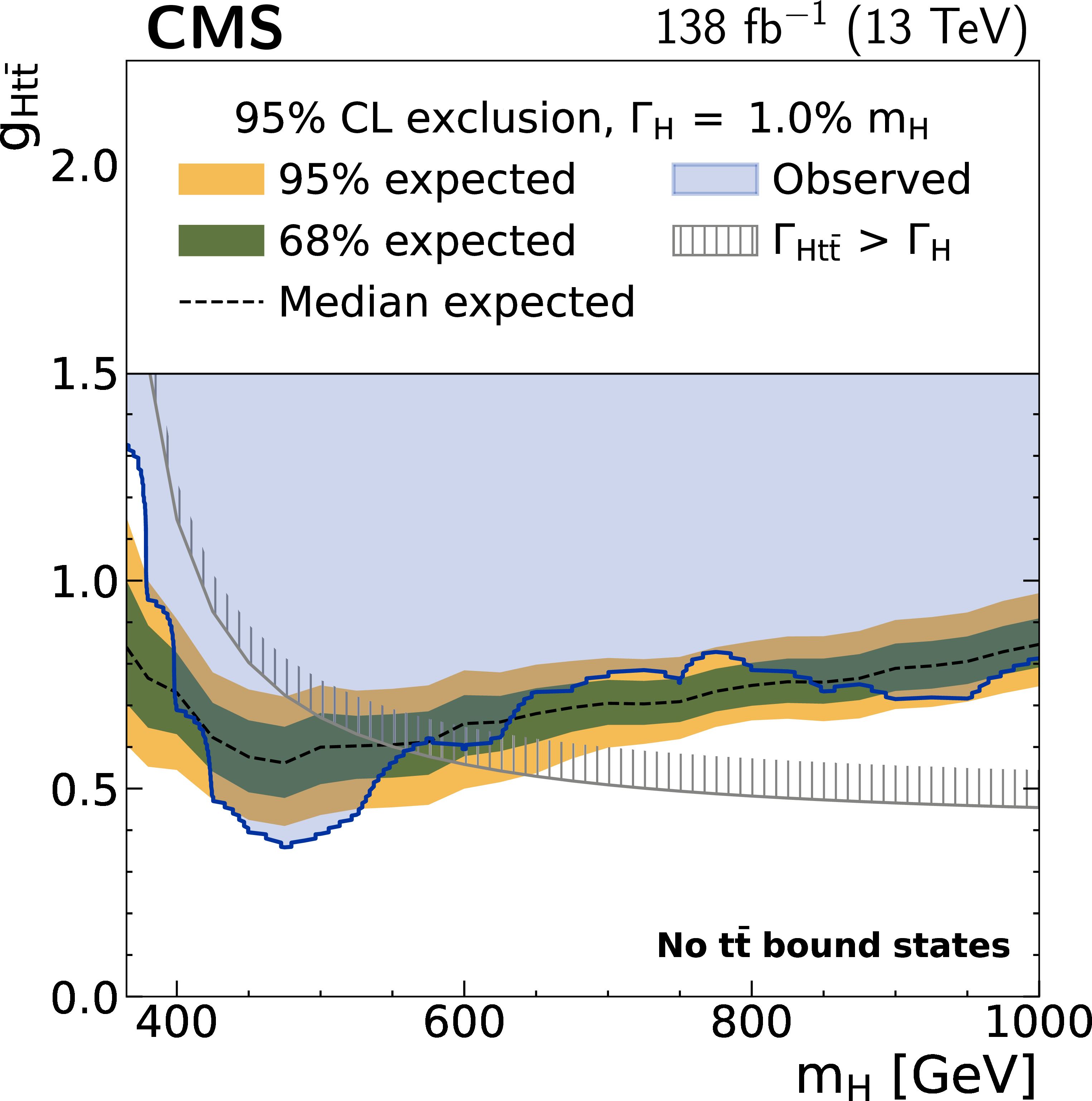
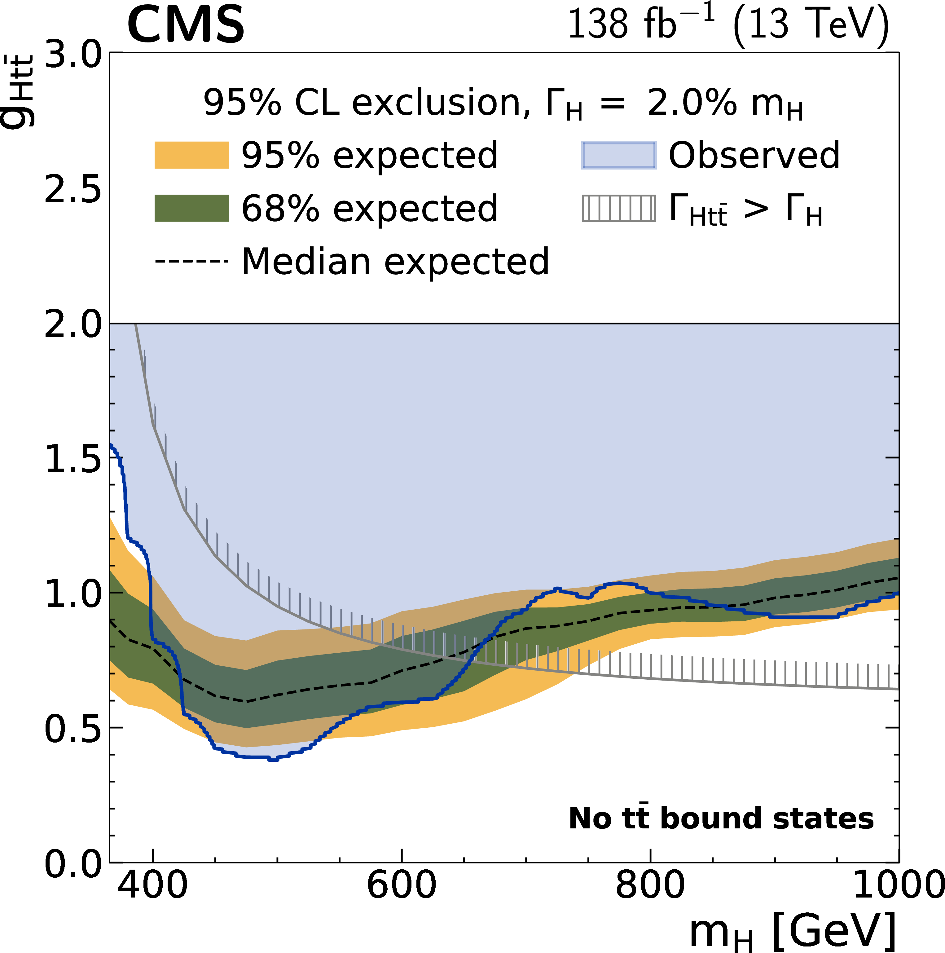
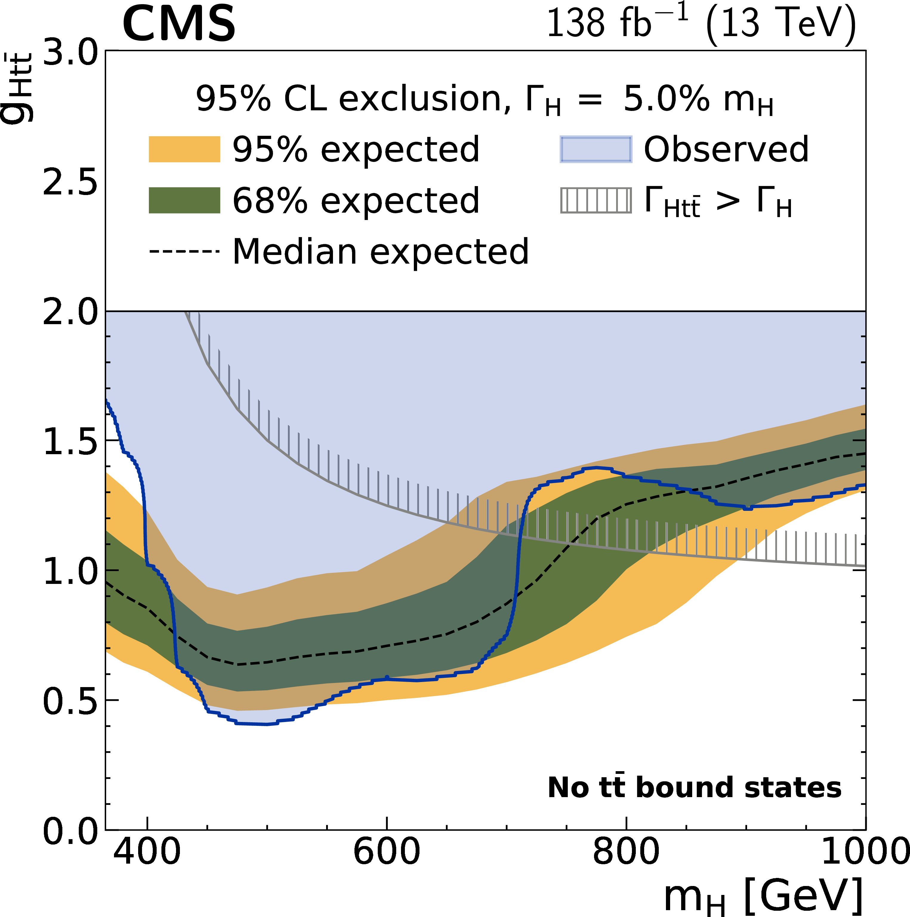
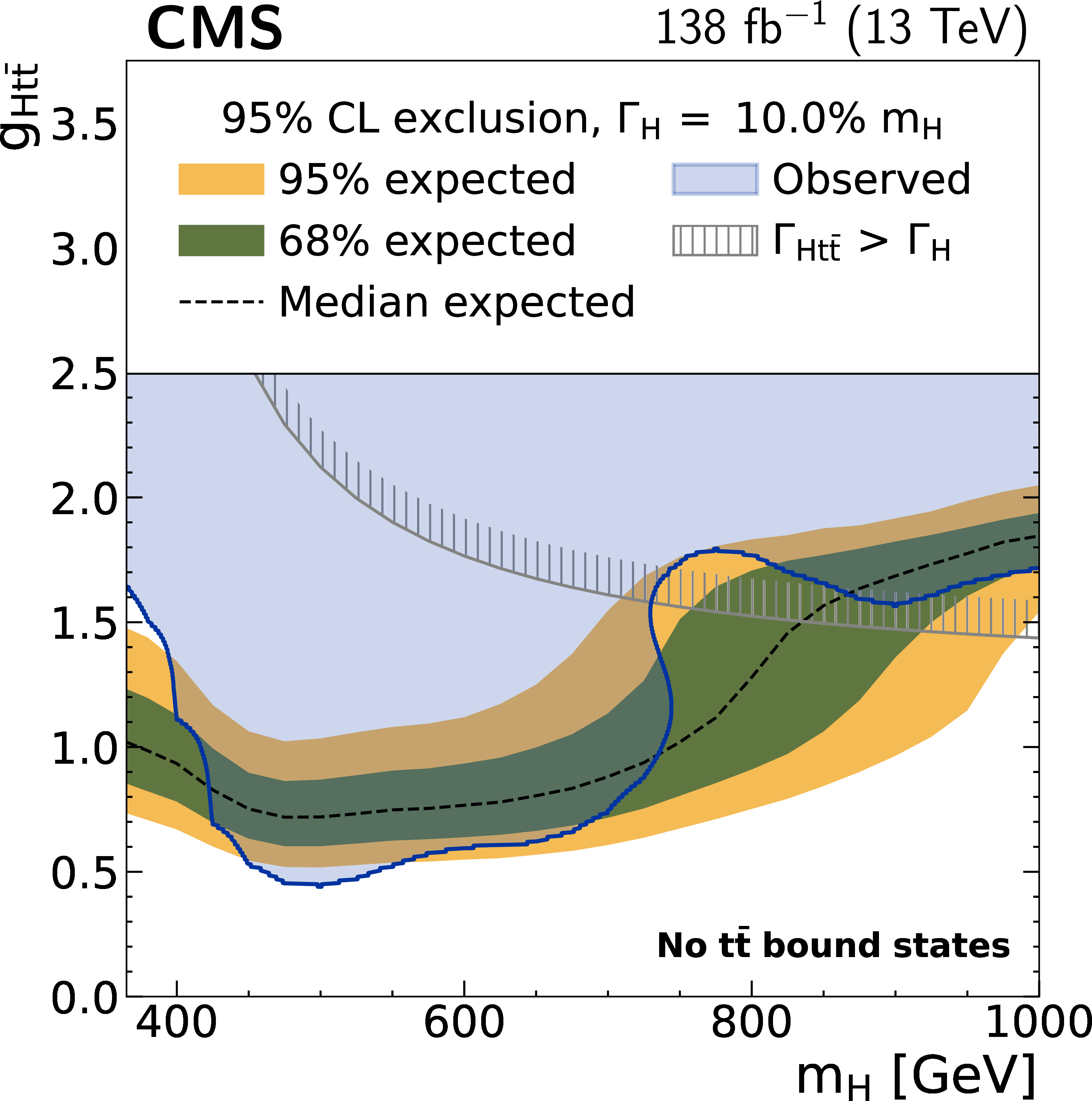
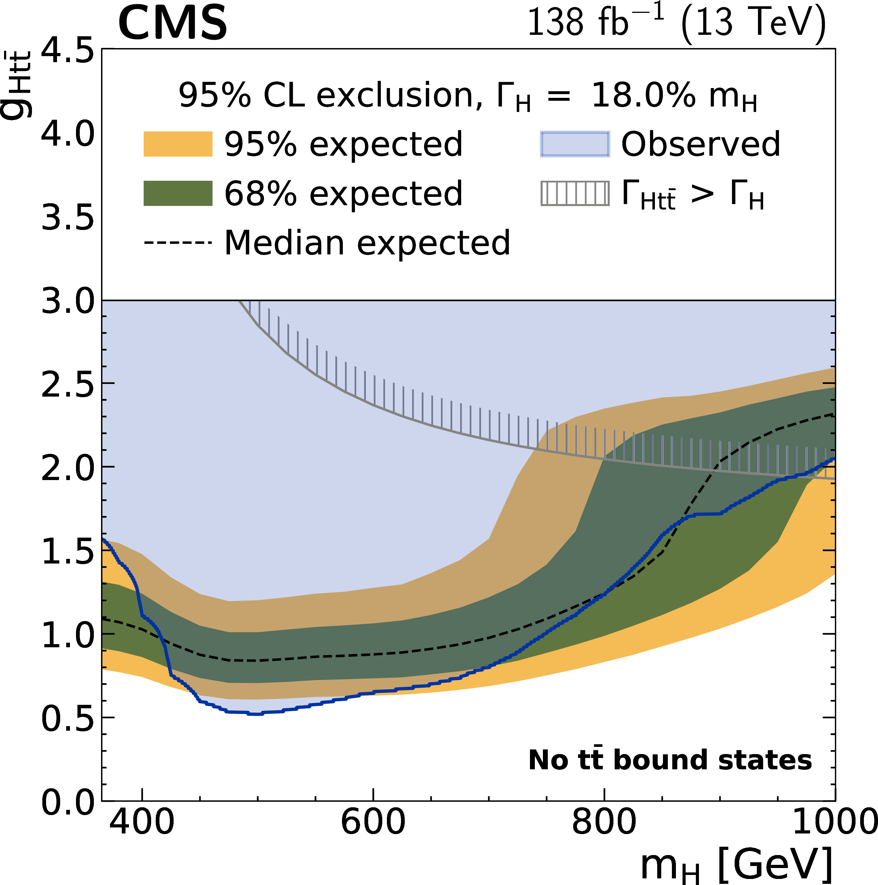
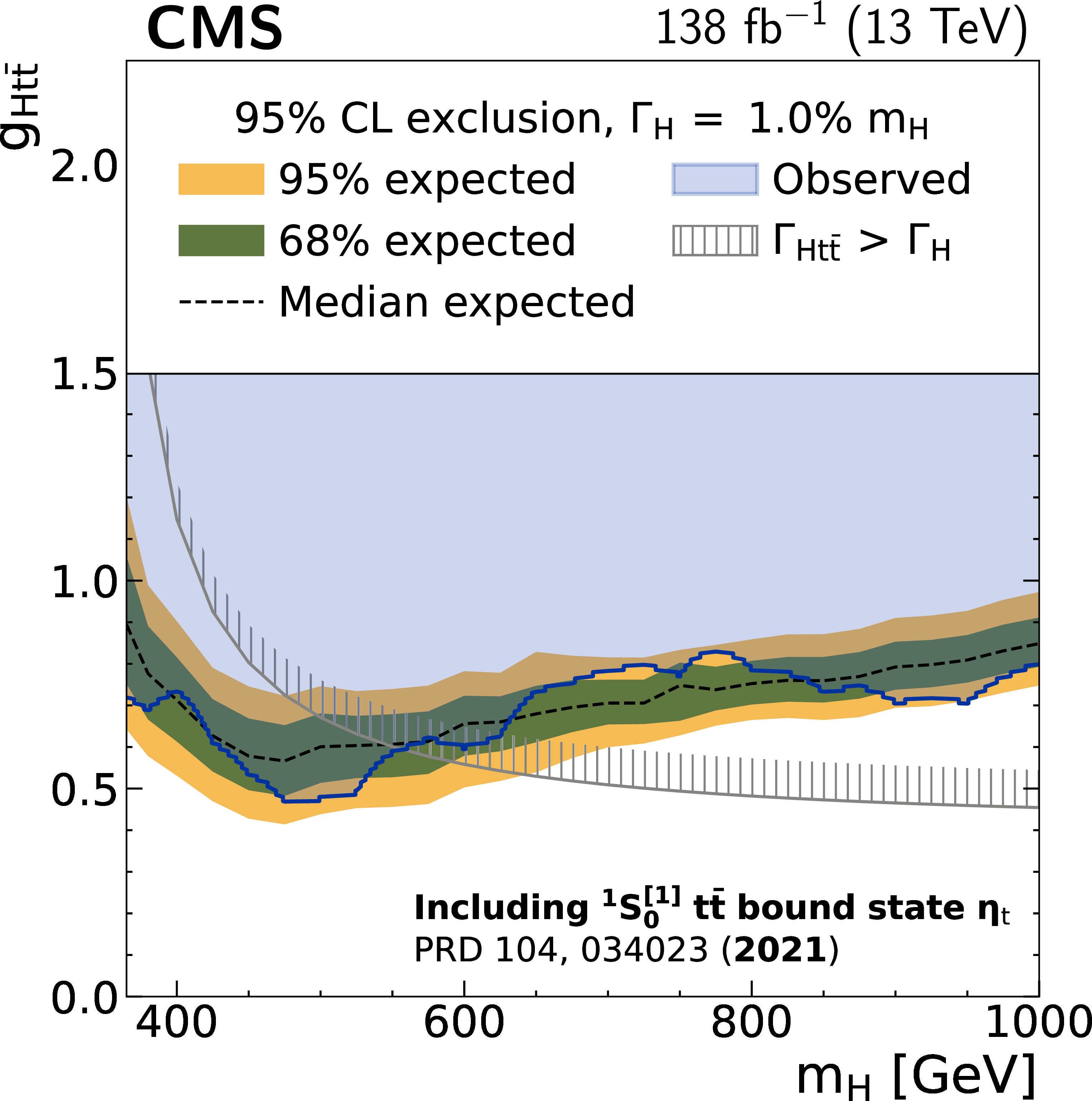
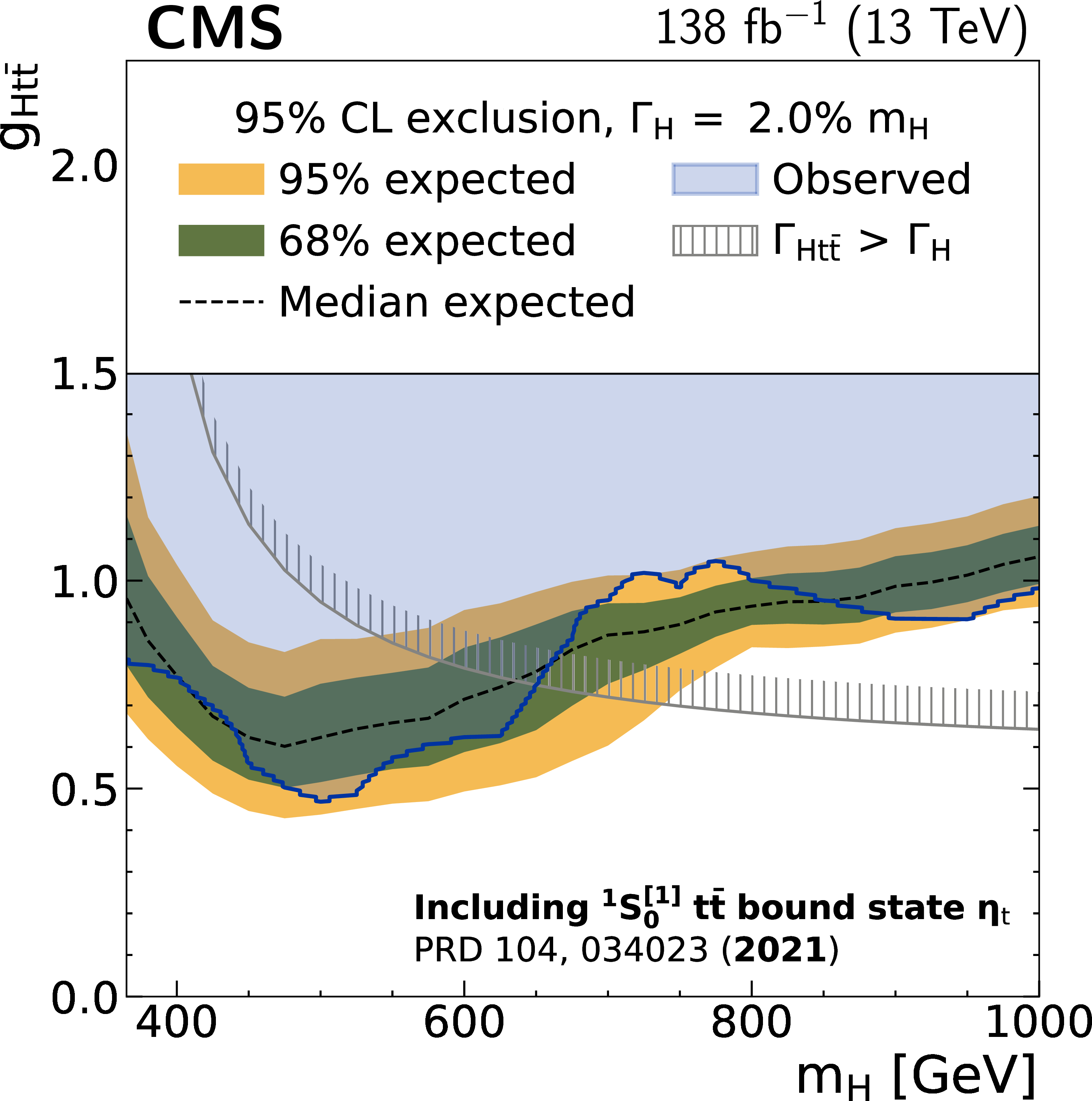
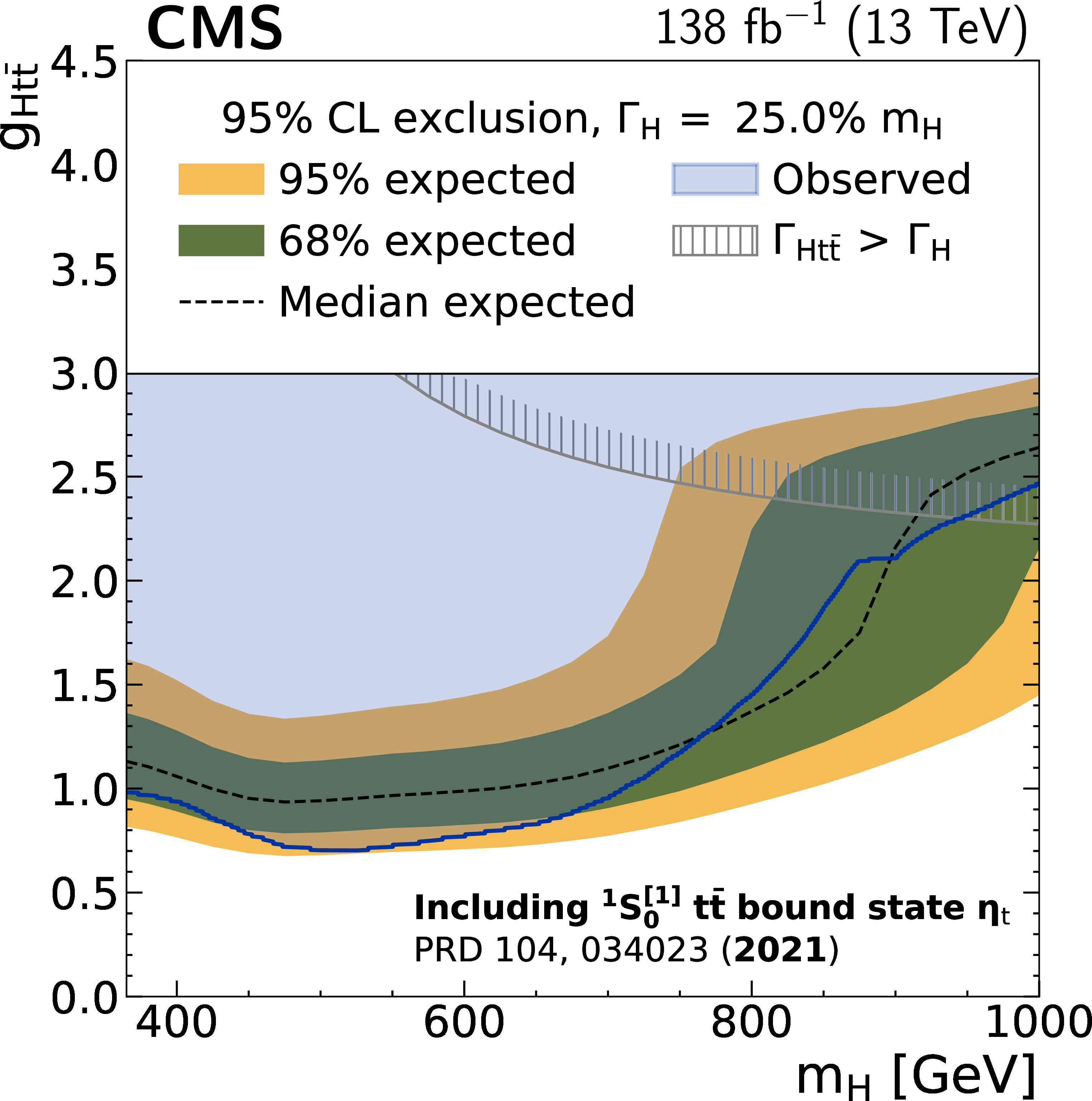
Figure 11:
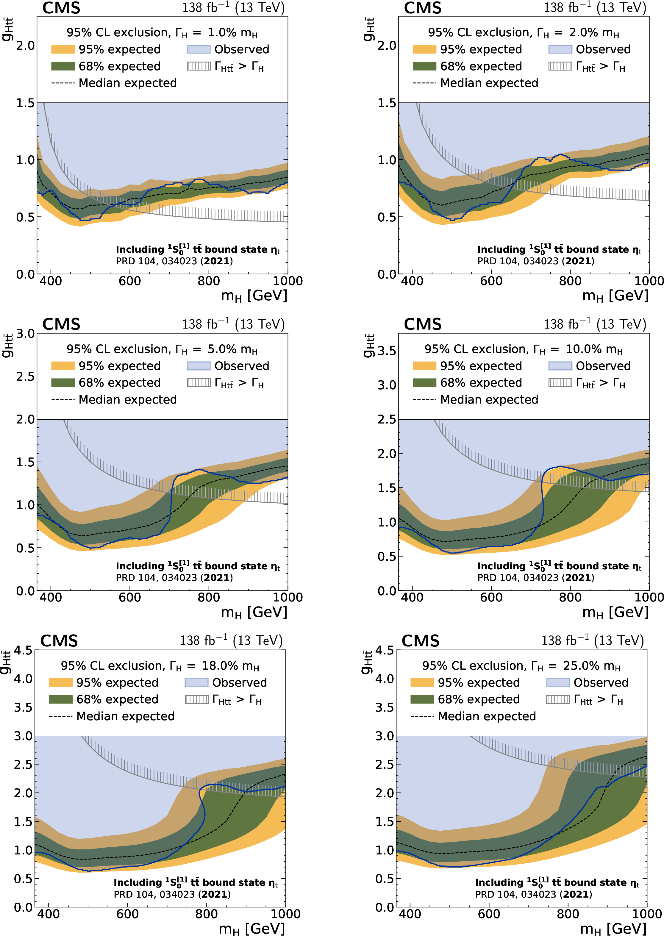
Model-independent constraints on $g_{\mathrm{Ht\bar{t}}}$ as functions of the H boson mass in the background scenario without $ \eta_{\mathrm{t}} $ contribution, shown in the same fashion as in Fig. 10. |
png pdf |
Figure 11-a:
Model-independent constraints on $g_{\mathrm{Ht\bar{t}}}$ as functions of the H boson mass in the background scenario without $ \eta_{\mathrm{t}} $ contribution, shown in the same fashion as in Fig. 10. |
png pdf |
Figure 11-b:
Model-independent constraints on $g_{\mathrm{Ht\bar{t}}}$ as functions of the H boson mass in the background scenario without $ \eta_{\mathrm{t}} $ contribution, shown in the same fashion as in Fig. 10. |
png pdf |
Figure 11-c:
Model-independent constraints on $g_{\mathrm{Ht\bar{t}}}$ as functions of the H boson mass in the background scenario without $ \eta_{\mathrm{t}} $ contribution, shown in the same fashion as in Fig. 10. |
png pdf |
Figure 11-d:
Model-independent constraints on $g_{\mathrm{Ht\bar{t}}}$ as functions of the H boson mass in the background scenario without $ \eta_{\mathrm{t}} $ contribution, shown in the same fashion as in Fig. 10. |
png pdf |
Figure 11-e:
Model-independent constraints on $g_{\mathrm{Ht\bar{t}}}$ as functions of the H boson mass in the background scenario without $ \eta_{\mathrm{t}} $ contribution, shown in the same fashion as in Fig. 10. |
png pdf |
Figure 11-f:
Model-independent constraints on $g_{\mathrm{Ht\bar{t}}}$ as functions of the H boson mass in the background scenario without $ \eta_{\mathrm{t}} $ contribution, shown in the same fashion as in Fig. 10. |
png pdf |
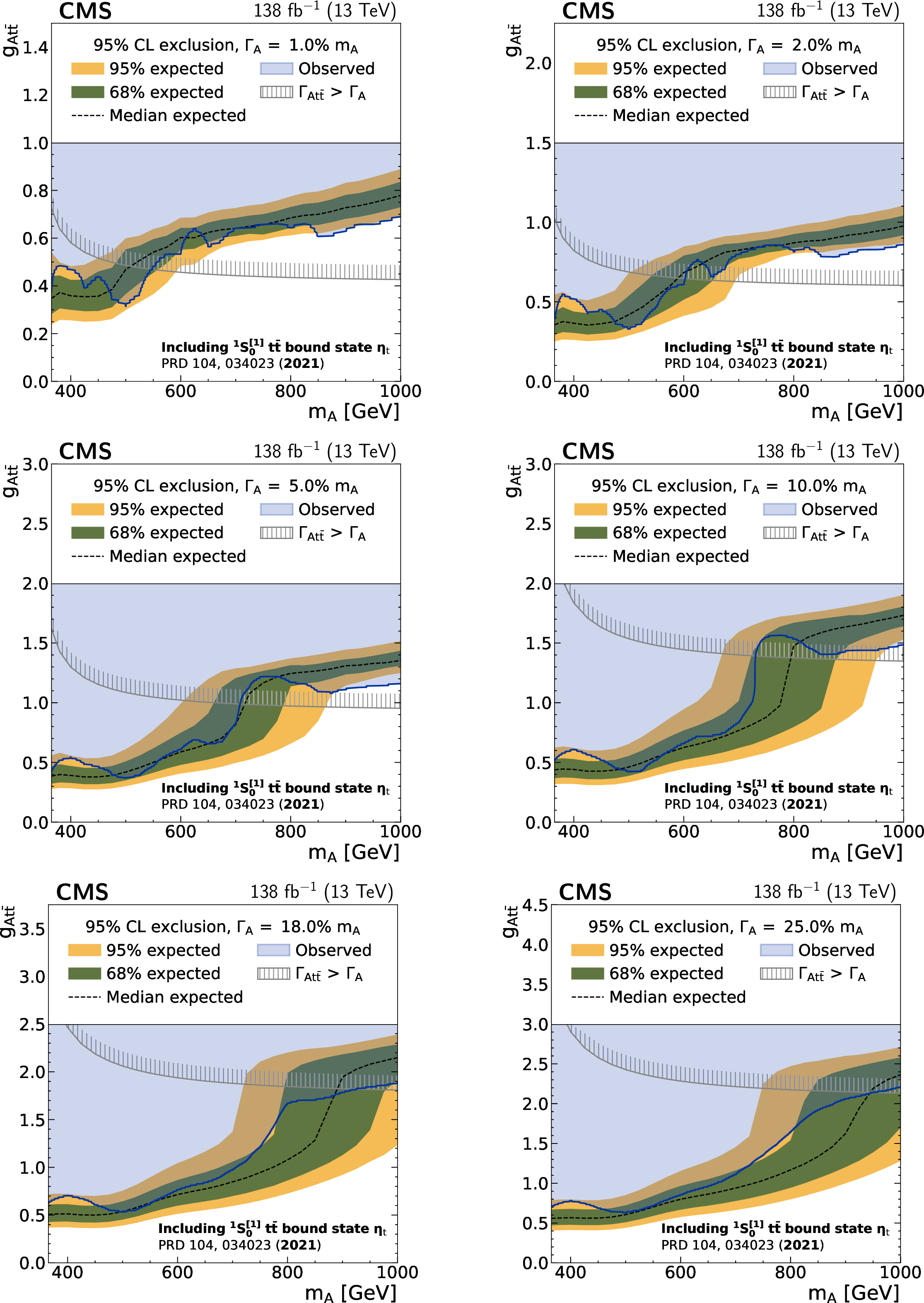
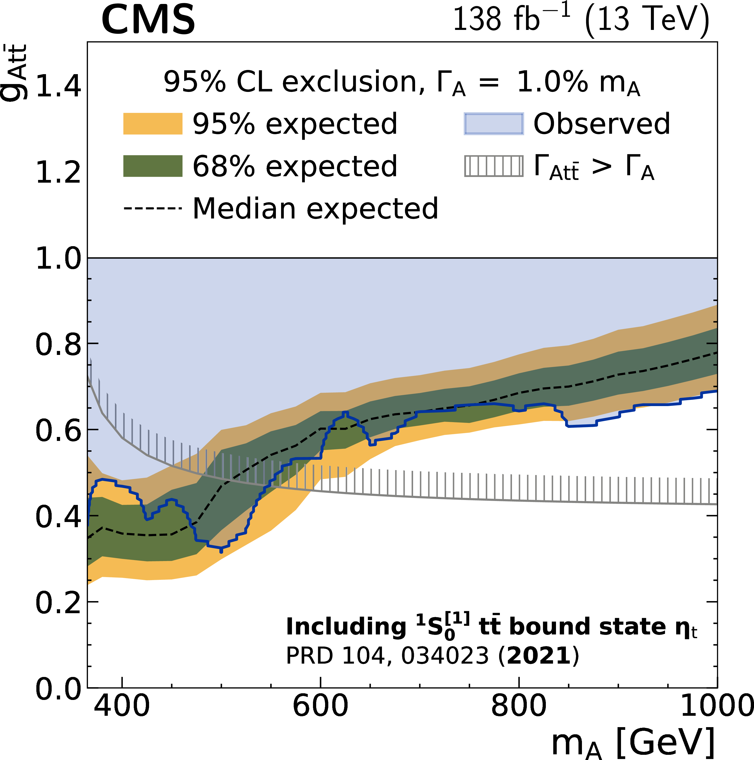
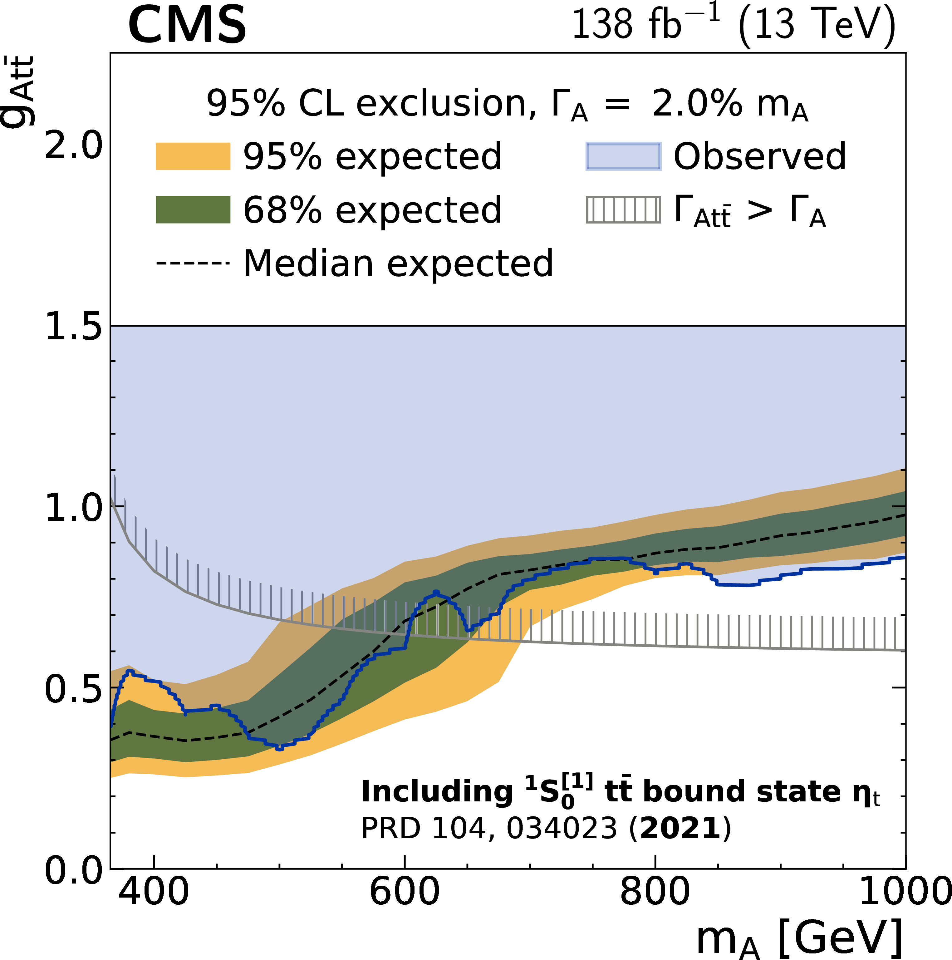
Figure 12:
Model-independent constraints on $g_{\mathrm{At\bar{t}}}$ as functions of the A boson mass in the background scenario with $ \eta_{\mathrm{t}} $ contribution, shown in the same fashion as in Fig. 10. |
png pdf |
Figure 12-a:
Model-independent constraints on $g_{\mathrm{At\bar{t}}}$ as functions of the A boson mass in the background scenario with $ \eta_{\mathrm{t}} $ contribution, shown in the same fashion as in Fig. 10. |
png pdf |
Figure 12-b:
Model-independent constraints on $g_{\mathrm{At\bar{t}}}$ as functions of the A boson mass in the background scenario with $ \eta_{\mathrm{t}} $ contribution, shown in the same fashion as in Fig. 10. |
png pdf |
Figure 12-c:
Model-independent constraints on $g_{\mathrm{At\bar{t}}}$ as functions of the A boson mass in the background scenario with $ \eta_{\mathrm{t}} $ contribution, shown in the same fashion as in Fig. 10. |

png pdf |
Figure 12-d:
Model-independent constraints on $g_{\mathrm{At\bar{t}}}$ as functions of the A boson mass in the background scenario with $ \eta_{\mathrm{t}} $ contribution, shown in the same fashion as in Fig. 10. |
png pdf |
Figure 12-e:
Model-independent constraints on $g_{\mathrm{At\bar{t}}}$ as functions of the A boson mass in the background scenario with $ \eta_{\mathrm{t}} $ contribution, shown in the same fashion as in Fig. 10. |
png pdf |
Figure 12-f:
Model-independent constraints on $g_{\mathrm{At\bar{t}}}$ as functions of the A boson mass in the background scenario with $ \eta_{\mathrm{t}} $ contribution, shown in the same fashion as in Fig. 10. |
png pdf |
Figure 13:
Model-independent constraints on $g_{\mathrm{Ht\bar{t}}}$ as functions of the H boson mass in the background scenario with $ \eta_{\mathrm{t}} $ contribution, shown in the same fashion as in Fig. 10. |
png pdf |
Figure 13-a:
Model-independent constraints on $g_{\mathrm{Ht\bar{t}}}$ as functions of the H boson mass in the background scenario with $ \eta_{\mathrm{t}} $ contribution, shown in the same fashion as in Fig. 10. |
png pdf |
Figure 13-b:
Model-independent constraints on $g_{\mathrm{Ht\bar{t}}}$ as functions of the H boson mass in the background scenario with $ \eta_{\mathrm{t}} $ contribution, shown in the same fashion as in Fig. 10. |

png pdf |
Figure 13-c:
Model-independent constraints on $g_{\mathrm{Ht\bar{t}}}$ as functions of the H boson mass in the background scenario with $ \eta_{\mathrm{t}} $ contribution, shown in the same fashion as in Fig. 10. |

png pdf |
Figure 13-d:
Model-independent constraints on $g_{\mathrm{Ht\bar{t}}}$ as functions of the H boson mass in the background scenario with $ \eta_{\mathrm{t}} $ contribution, shown in the same fashion as in Fig. 10. |

png pdf |
Figure 13-e:
Model-independent constraints on $g_{\mathrm{Ht\bar{t}}}$ as functions of the H boson mass in the background scenario with $ \eta_{\mathrm{t}} $ contribution, shown in the same fashion as in Fig. 10. |
png pdf |
Figure 13-f:
Model-independent constraints on $g_{\mathrm{Ht\bar{t}}}$ as functions of the H boson mass in the background scenario with $ \eta_{\mathrm{t}} $ contribution, shown in the same fashion as in Fig. 10. |
png pdf |
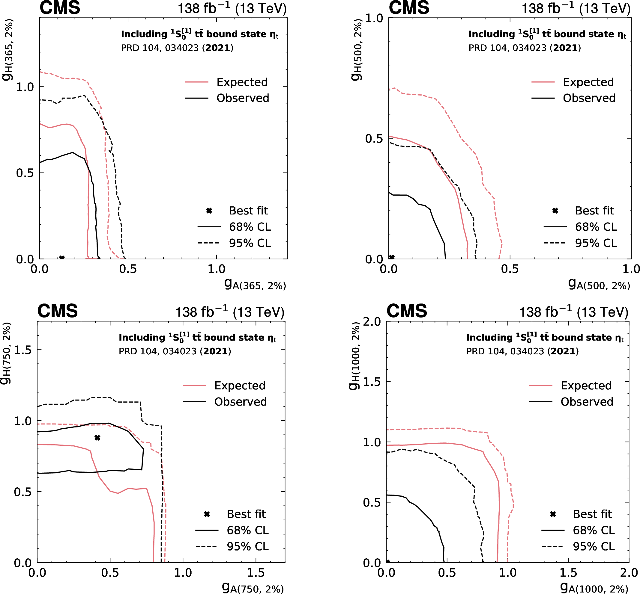
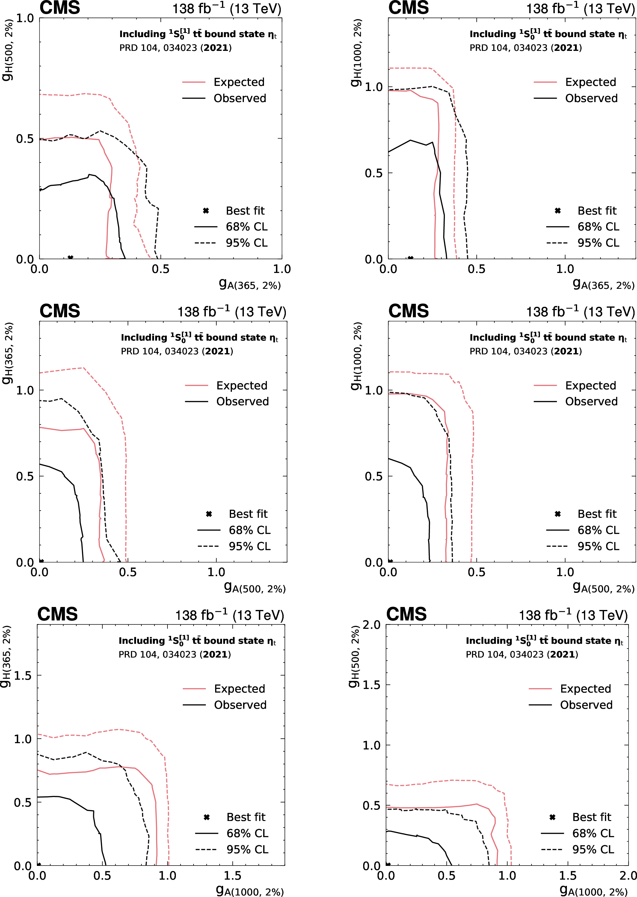
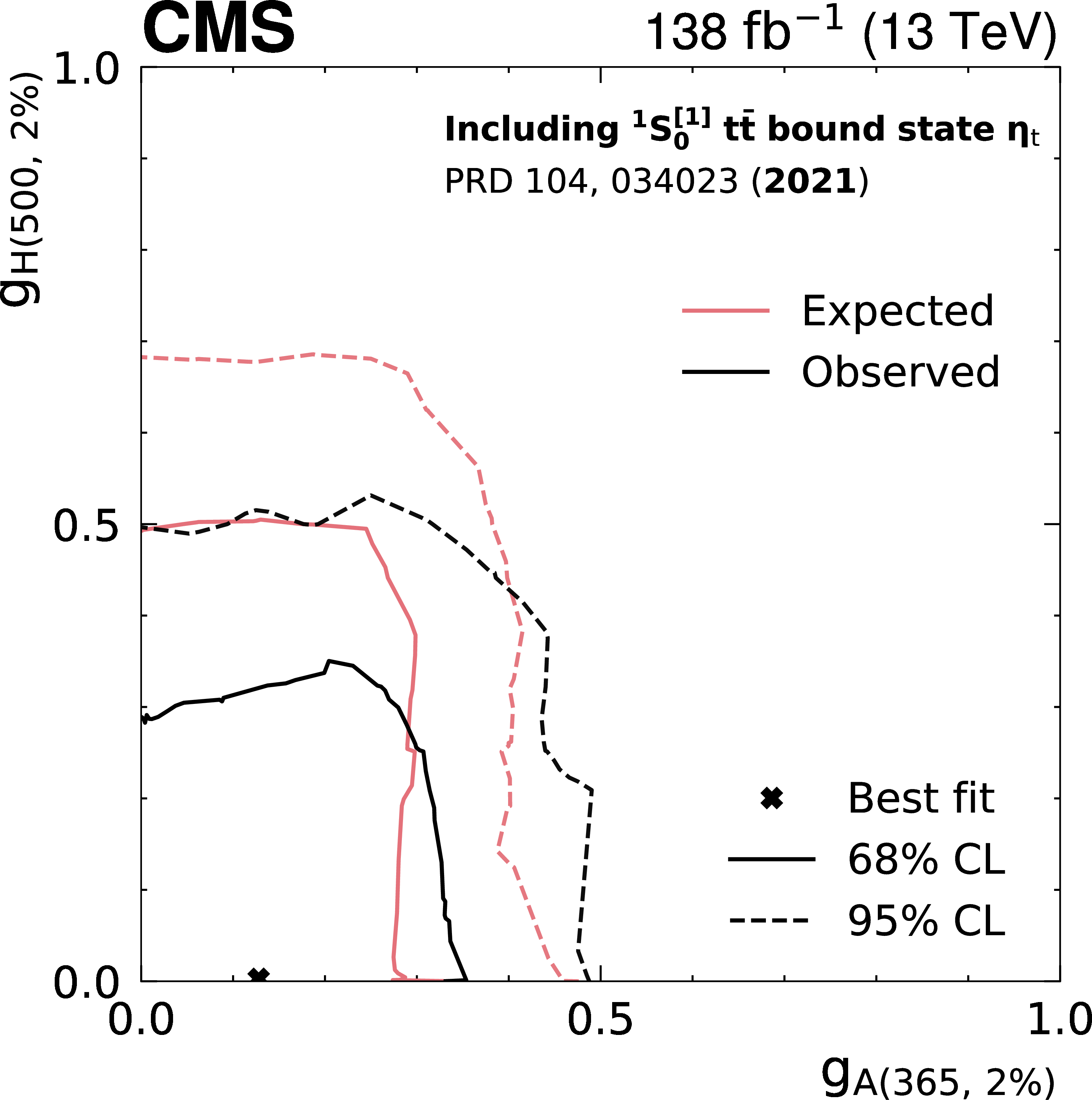
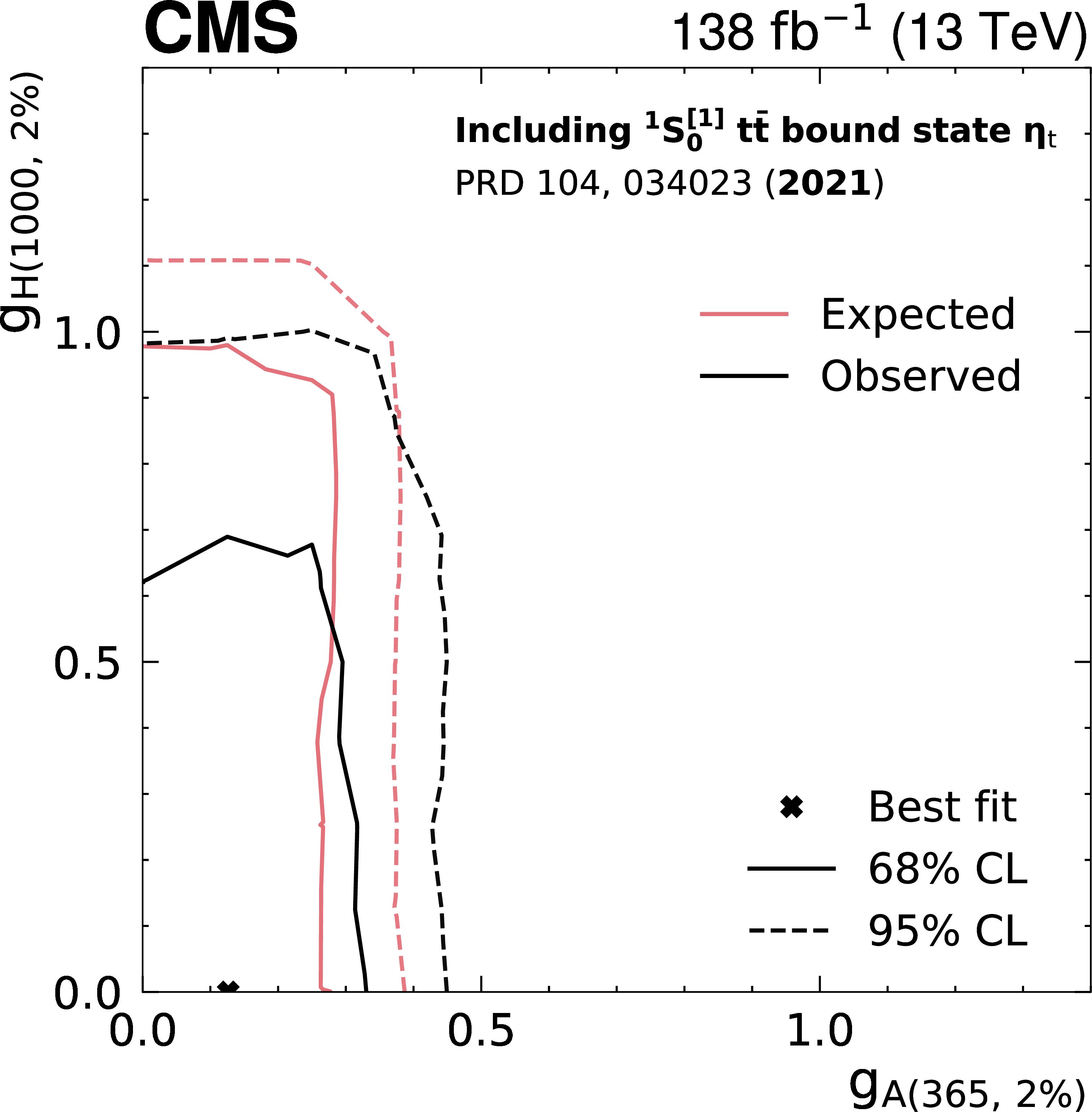
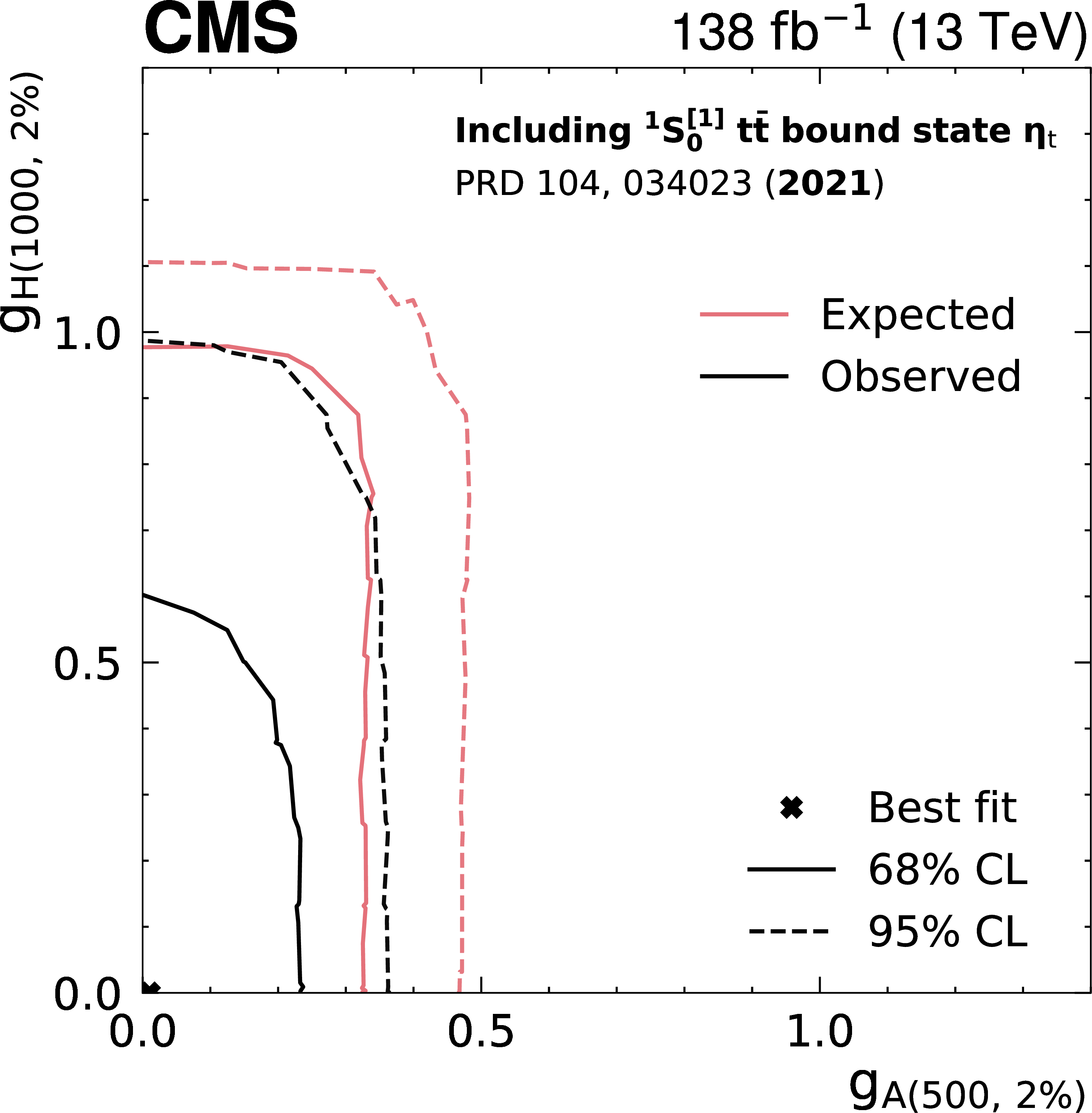
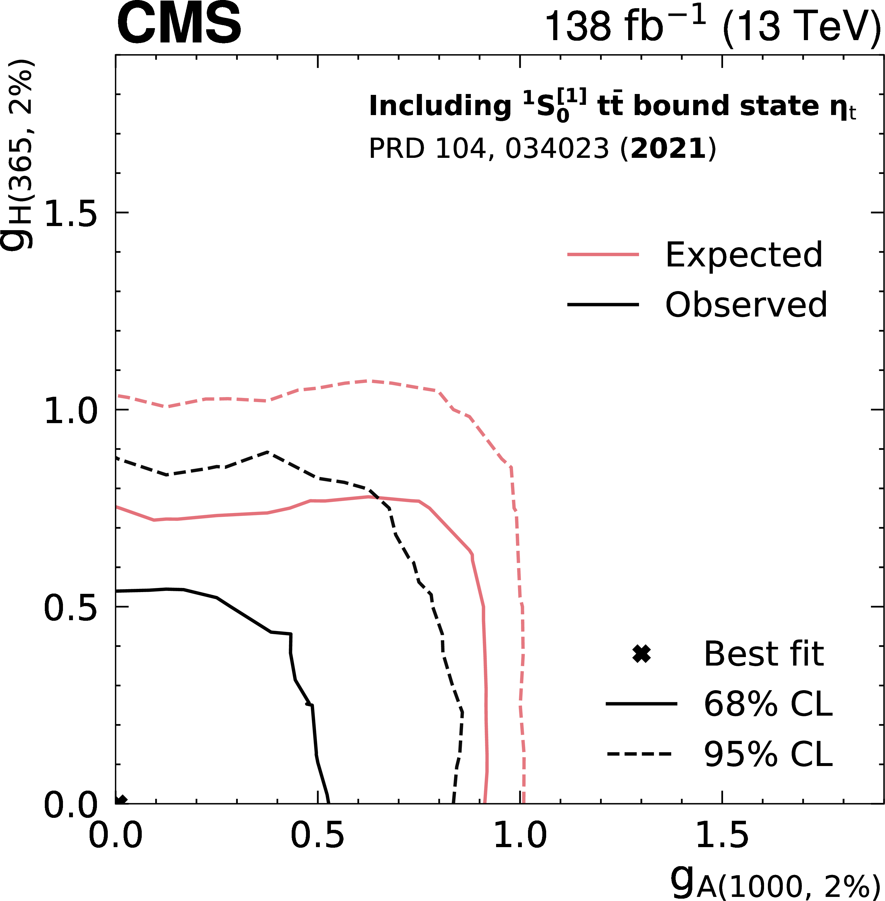
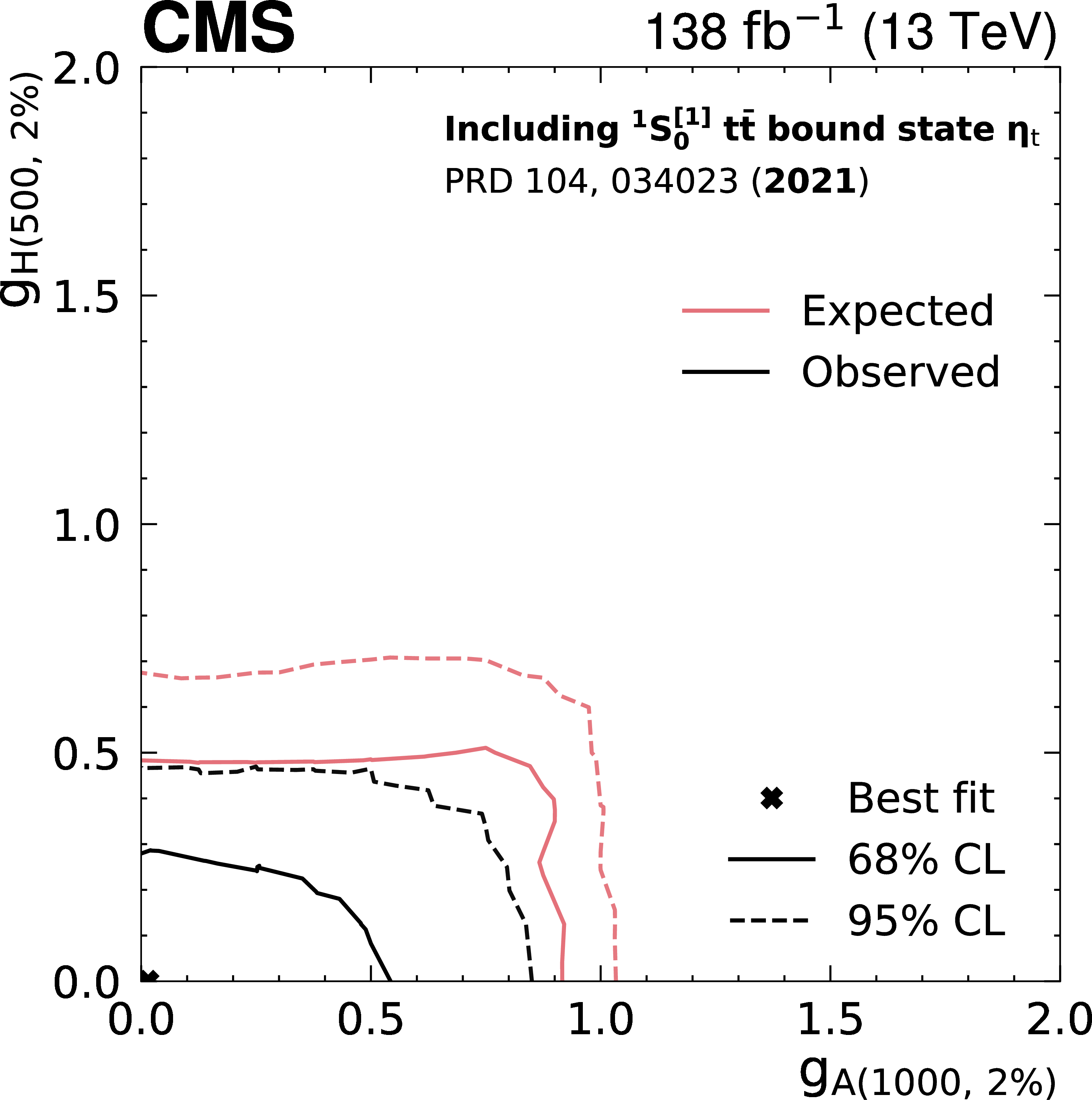
Figure 14:
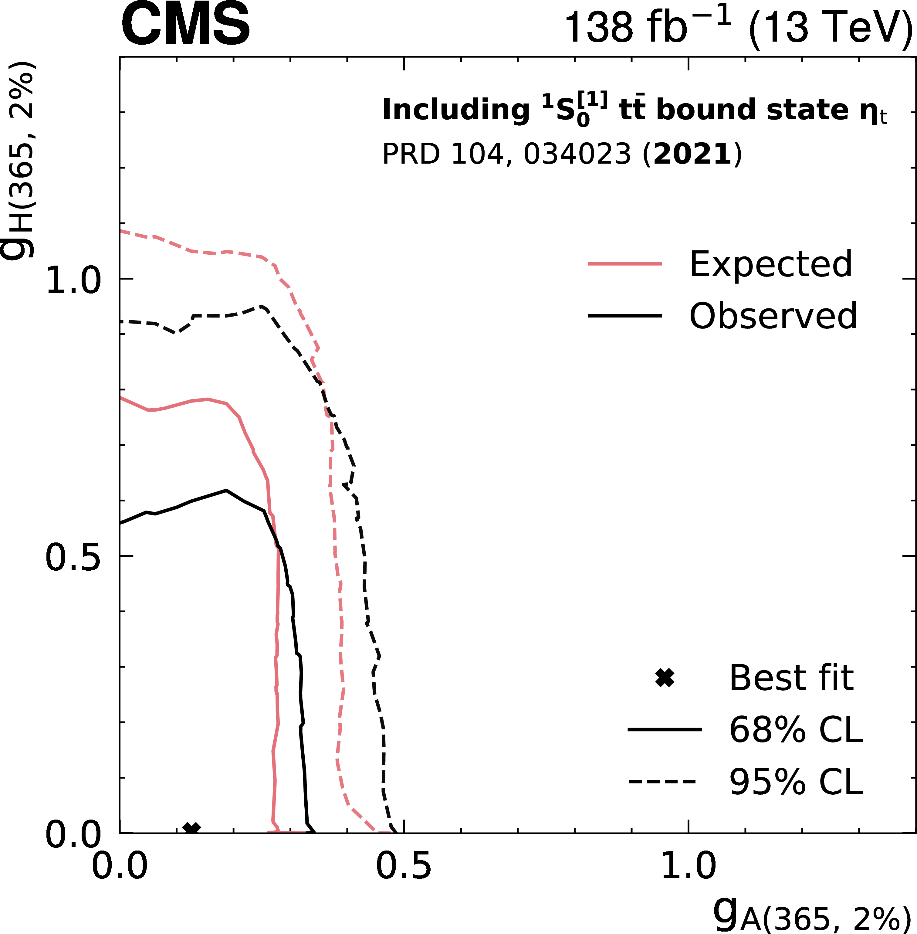
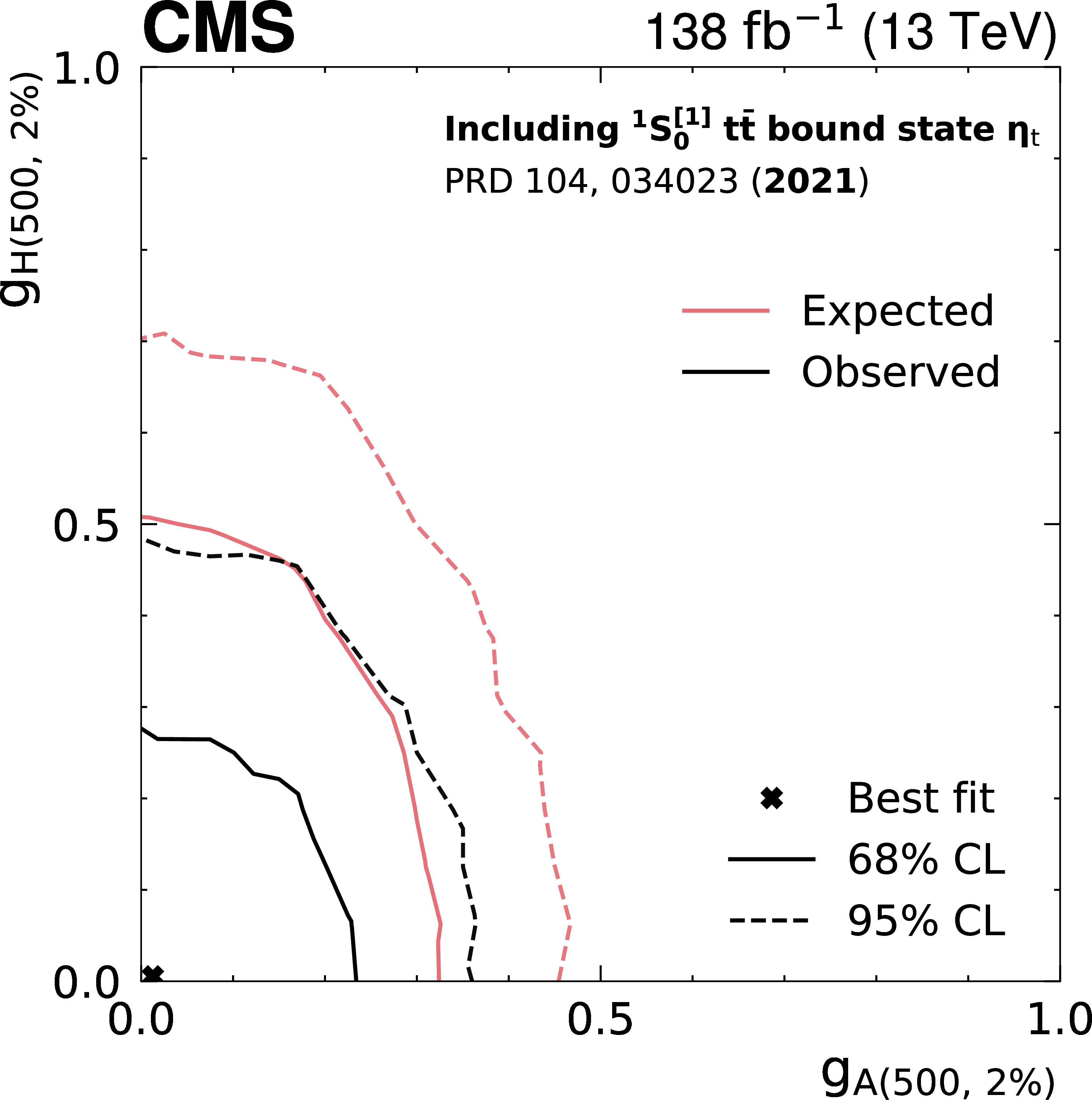
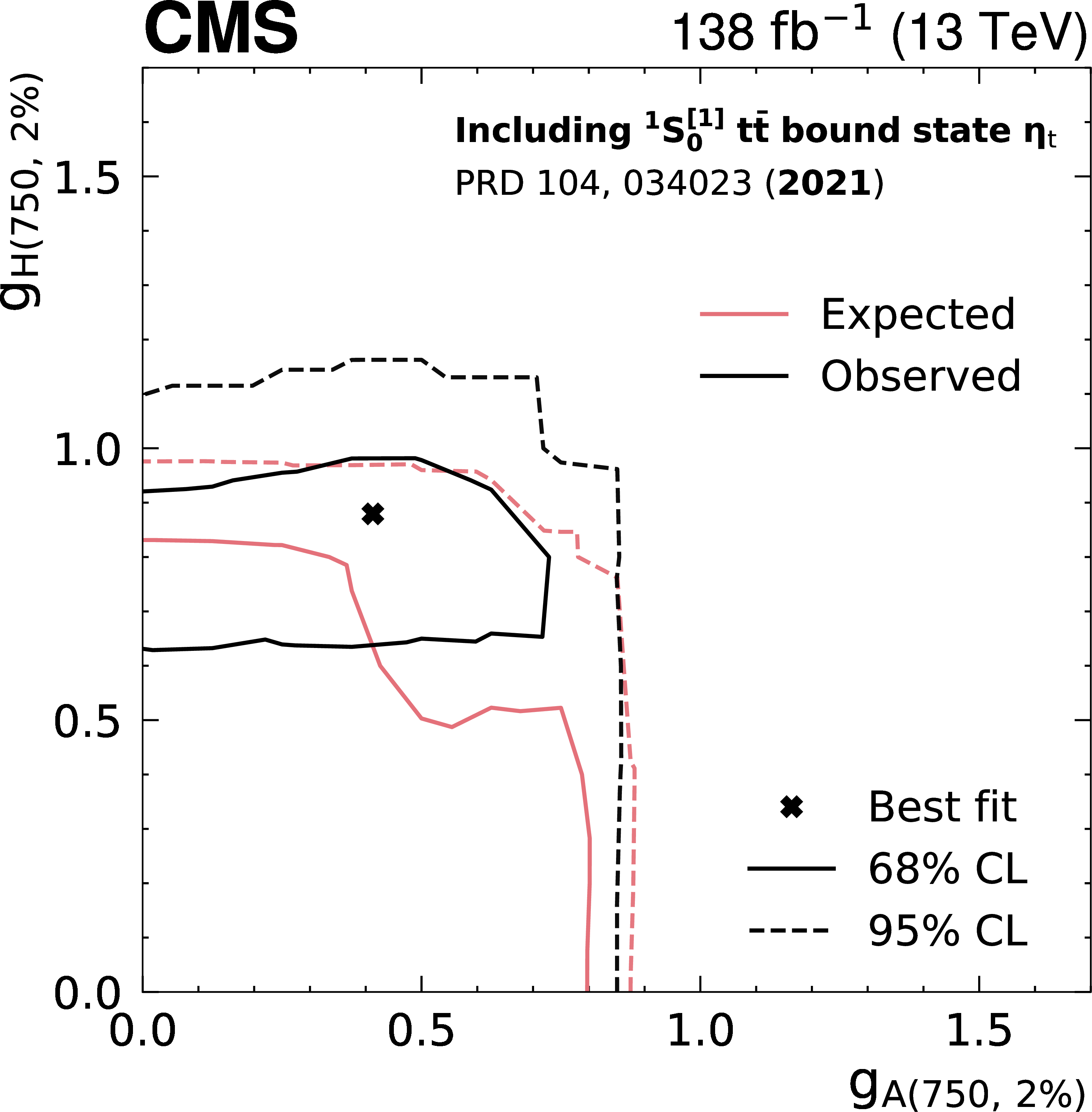
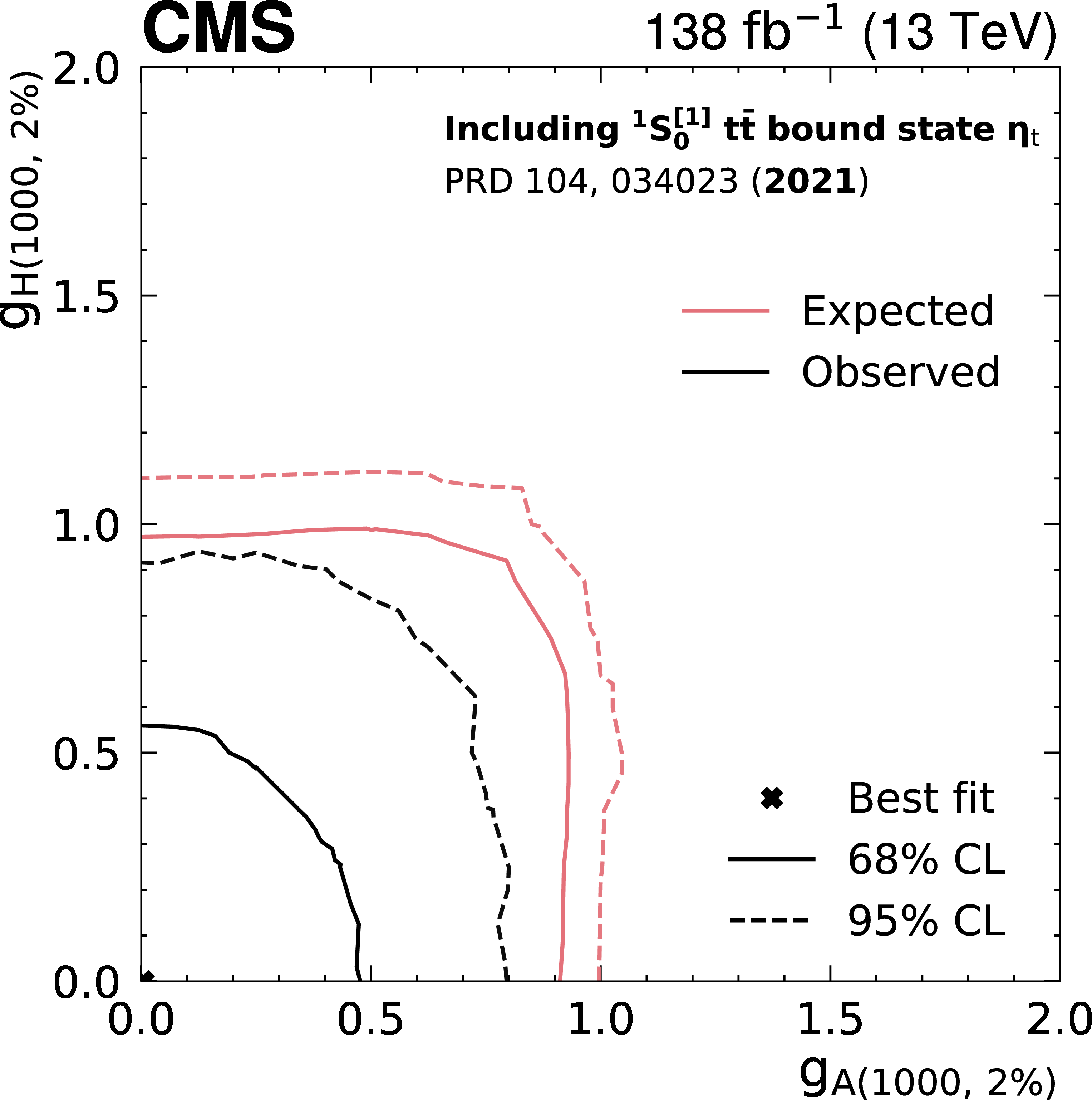
Frequentist 2D exclusion contours for $g_{\mathrm{At\bar{t}}}$ and $g_{\mathrm{Ht\bar{t}}}$ in the A$+$H boson interpretation for four different signal hypotheses with identical A and H boson masses of 365 GeV (upper left), 500 GeV (upper right), 750 GeV (lower left), and 1000 GeV (lower right), all assuming a relative width of 2%. The expected and observed contours, evaluated with the Feldman-Cousins prescription [128,129], are shown in pink and black, respectively, with the solid and dashed lines corresponding to exclusions at 68 and 95% CL. The regions outside of the contours are considered excluded. In all cases, $ \eta_{\mathrm{t}} $ production is included in the background model. |
png pdf |
Figure 14-a:
Frequentist 2D exclusion contours for $g_{\mathrm{At\bar{t}}}$ and $g_{\mathrm{Ht\bar{t}}}$ in the A$+$H boson interpretation for four different signal hypotheses with identical A and H boson masses of 365 GeV (upper left), 500 GeV (upper right), 750 GeV (lower left), and 1000 GeV (lower right), all assuming a relative width of 2%. The expected and observed contours, evaluated with the Feldman-Cousins prescription [128,129], are shown in pink and black, respectively, with the solid and dashed lines corresponding to exclusions at 68 and 95% CL. The regions outside of the contours are considered excluded. In all cases, $ \eta_{\mathrm{t}} $ production is included in the background model. |
png pdf |
Figure 14-b:
Frequentist 2D exclusion contours for $g_{\mathrm{At\bar{t}}}$ and $g_{\mathrm{Ht\bar{t}}}$ in the A$+$H boson interpretation for four different signal hypotheses with identical A and H boson masses of 365 GeV (upper left), 500 GeV (upper right), 750 GeV (lower left), and 1000 GeV (lower right), all assuming a relative width of 2%. The expected and observed contours, evaluated with the Feldman-Cousins prescription [128,129], are shown in pink and black, respectively, with the solid and dashed lines corresponding to exclusions at 68 and 95% CL. The regions outside of the contours are considered excluded. In all cases, $ \eta_{\mathrm{t}} $ production is included in the background model. |
png pdf |
Figure 14-c:
Frequentist 2D exclusion contours for $g_{\mathrm{At\bar{t}}}$ and $g_{\mathrm{Ht\bar{t}}}$ in the A$+$H boson interpretation for four different signal hypotheses with identical A and H boson masses of 365 GeV (upper left), 500 GeV (upper right), 750 GeV (lower left), and 1000 GeV (lower right), all assuming a relative width of 2%. The expected and observed contours, evaluated with the Feldman-Cousins prescription [128,129], are shown in pink and black, respectively, with the solid and dashed lines corresponding to exclusions at 68 and 95% CL. The regions outside of the contours are considered excluded. In all cases, $ \eta_{\mathrm{t}} $ production is included in the background model. |
png pdf |
Figure 14-d:
Frequentist 2D exclusion contours for $g_{\mathrm{At\bar{t}}}$ and $g_{\mathrm{Ht\bar{t}}}$ in the A$+$H boson interpretation for four different signal hypotheses with identical A and H boson masses of 365 GeV (upper left), 500 GeV (upper right), 750 GeV (lower left), and 1000 GeV (lower right), all assuming a relative width of 2%. The expected and observed contours, evaluated with the Feldman-Cousins prescription [128,129], are shown in pink and black, respectively, with the solid and dashed lines corresponding to exclusions at 68 and 95% CL. The regions outside of the contours are considered excluded. In all cases, $ \eta_{\mathrm{t}} $ production is included in the background model. |
png pdf |
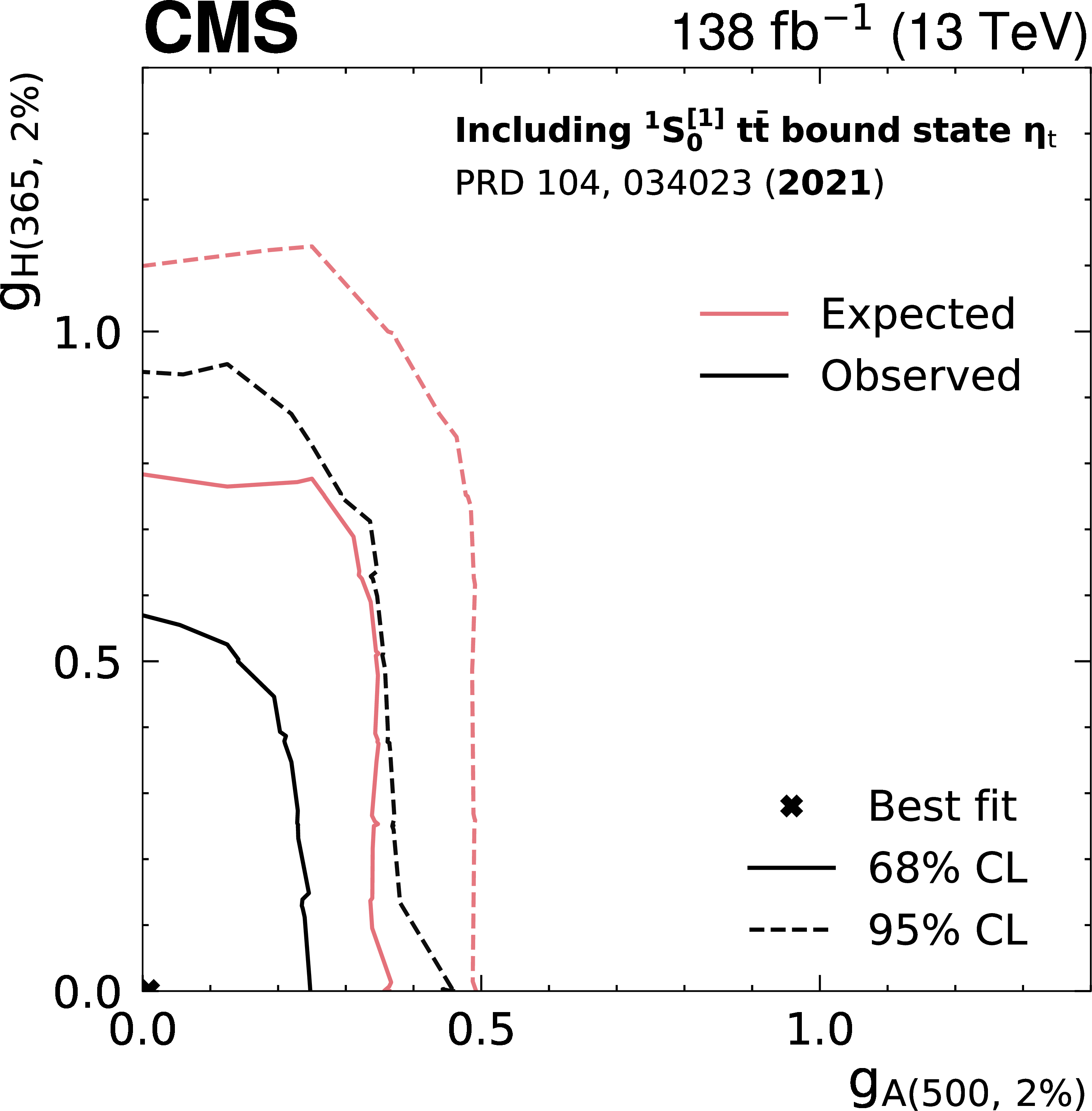
Figure 15:
Frequentist 2D exclusion contours for $g_{\mathrm{At\bar{t}}}$ and $g_{\mathrm{Ht\bar{t}}}$ in the A$+$H boson interpretation for six different signal hypotheses with unequal A and H boson masses, corresponding to combinations of 365, 500, and 1000 GeV, all assuming a relative width of 2%. The expected and observed contours, evaluated with the Feldman-Cousins prescription [128,129], are shown in pink and black, respectively, with the solid and dashed lines corresponding to exclusions at 68 and 95% CL. The regions outside of the contours are considered excluded. In all cases, $ \eta_{\mathrm{t}} $ production is included in the background model. |
png pdf |
Figure 15-a:
Frequentist 2D exclusion contours for $g_{\mathrm{At\bar{t}}}$ and $g_{\mathrm{Ht\bar{t}}}$ in the A$+$H boson interpretation for six different signal hypotheses with unequal A and H boson masses, corresponding to combinations of 365, 500, and 1000 GeV, all assuming a relative width of 2%. The expected and observed contours, evaluated with the Feldman-Cousins prescription [128,129], are shown in pink and black, respectively, with the solid and dashed lines corresponding to exclusions at 68 and 95% CL. The regions outside of the contours are considered excluded. In all cases, $ \eta_{\mathrm{t}} $ production is included in the background model. |
png pdf |
Figure 15-b:
Frequentist 2D exclusion contours for $g_{\mathrm{At\bar{t}}}$ and $g_{\mathrm{Ht\bar{t}}}$ in the A$+$H boson interpretation for six different signal hypotheses with unequal A and H boson masses, corresponding to combinations of 365, 500, and 1000 GeV, all assuming a relative width of 2%. The expected and observed contours, evaluated with the Feldman-Cousins prescription [128,129], are shown in pink and black, respectively, with the solid and dashed lines corresponding to exclusions at 68 and 95% CL. The regions outside of the contours are considered excluded. In all cases, $ \eta_{\mathrm{t}} $ production is included in the background model. |
png pdf |
Figure 15-c:
Frequentist 2D exclusion contours for $g_{\mathrm{At\bar{t}}}$ and $g_{\mathrm{Ht\bar{t}}}$ in the A$+$H boson interpretation for six different signal hypotheses with unequal A and H boson masses, corresponding to combinations of 365, 500, and 1000 GeV, all assuming a relative width of 2%. The expected and observed contours, evaluated with the Feldman-Cousins prescription [128,129], are shown in pink and black, respectively, with the solid and dashed lines corresponding to exclusions at 68 and 95% CL. The regions outside of the contours are considered excluded. In all cases, $ \eta_{\mathrm{t}} $ production is included in the background model. |
png pdf |
Figure 15-d:
Frequentist 2D exclusion contours for $g_{\mathrm{At\bar{t}}}$ and $g_{\mathrm{Ht\bar{t}}}$ in the A$+$H boson interpretation for six different signal hypotheses with unequal A and H boson masses, corresponding to combinations of 365, 500, and 1000 GeV, all assuming a relative width of 2%. The expected and observed contours, evaluated with the Feldman-Cousins prescription [128,129], are shown in pink and black, respectively, with the solid and dashed lines corresponding to exclusions at 68 and 95% CL. The regions outside of the contours are considered excluded. In all cases, $ \eta_{\mathrm{t}} $ production is included in the background model. |
png pdf |
Figure 15-e:
Frequentist 2D exclusion contours for $g_{\mathrm{At\bar{t}}}$ and $g_{\mathrm{Ht\bar{t}}}$ in the A$+$H boson interpretation for six different signal hypotheses with unequal A and H boson masses, corresponding to combinations of 365, 500, and 1000 GeV, all assuming a relative width of 2%. The expected and observed contours, evaluated with the Feldman-Cousins prescription [128,129], are shown in pink and black, respectively, with the solid and dashed lines corresponding to exclusions at 68 and 95% CL. The regions outside of the contours are considered excluded. In all cases, $ \eta_{\mathrm{t}} $ production is included in the background model. |
png pdf |
Figure 15-f:
Frequentist 2D exclusion contours for $g_{\mathrm{At\bar{t}}}$ and $g_{\mathrm{Ht\bar{t}}}$ in the A$+$H boson interpretation for six different signal hypotheses with unequal A and H boson masses, corresponding to combinations of 365, 500, and 1000 GeV, all assuming a relative width of 2%. The expected and observed contours, evaluated with the Feldman-Cousins prescription [128,129], are shown in pink and black, respectively, with the solid and dashed lines corresponding to exclusions at 68 and 95% CL. The regions outside of the contours are considered excluded. In all cases, $ \eta_{\mathrm{t}} $ production is included in the background model. |
| Tables | |
png pdf |
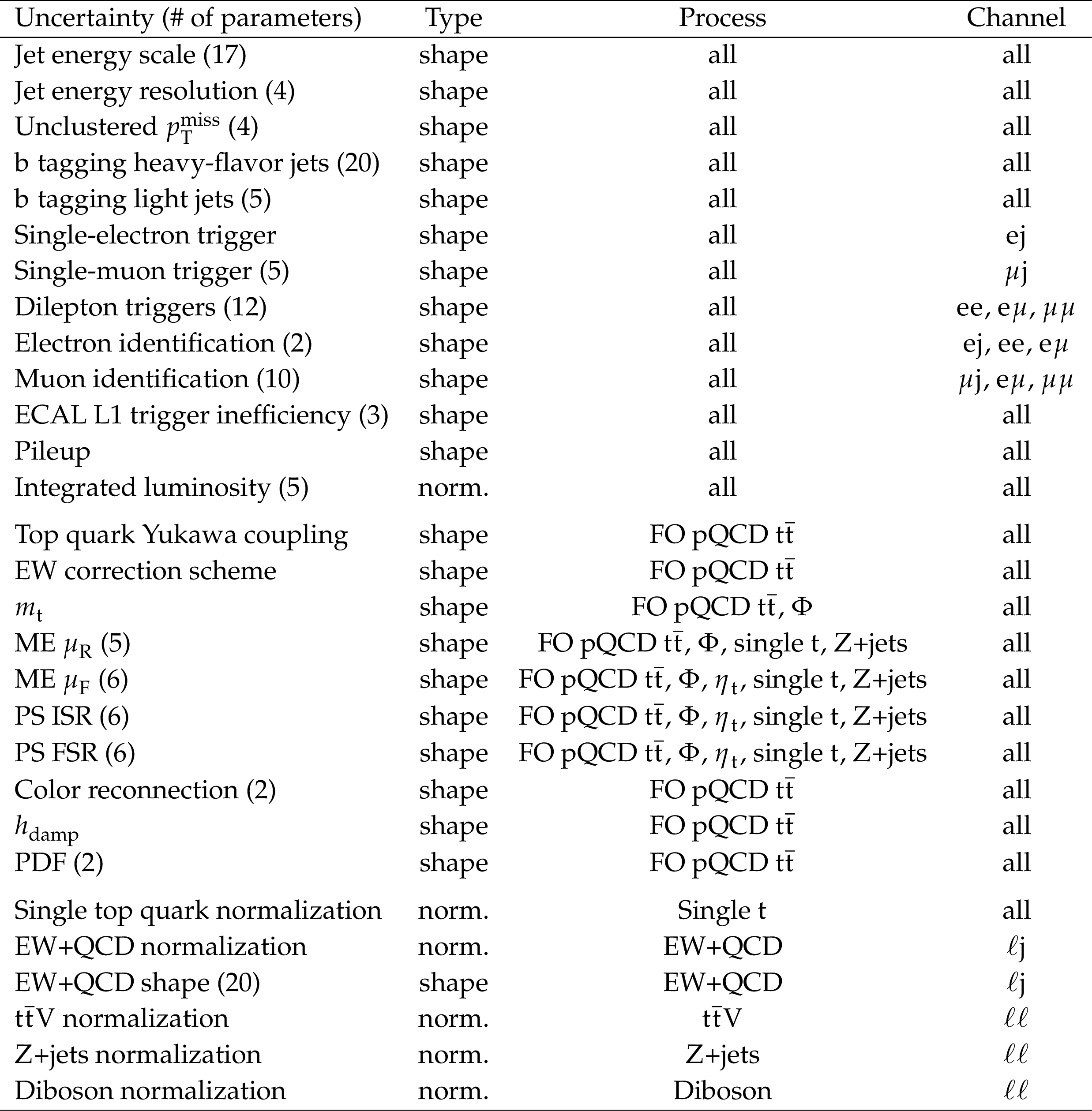
Table 1:
The systematic uncertainties considered in the analysis, indicating in parenthesis the number of corresponding nuisance parameters in the statistical model (if more than one), the type (affecting only normalization or also the shape of the search templates), and the affected physics processes and analysis channels they are applicable to. |
| Summary |
| A search has been presented for the production of pseudoscalar or scalar bosons in proton-proton collisions at $ \sqrt{s}= $ 13 TeV, decaying into a top quark pair ($ \mathrm{t} \overline{\mathrm{t}} $) in final states with one or two charged leptons. The analysis uses data collected with the CMS detector at the LHC, corresponding to an integrated luminosity of 138 fb$ ^{-1} $. To discriminate the signal from the standard model $ \mathrm{t} \overline{\mathrm{t}} $ background, the search utilizes the invariant mass of the reconstructed $ \mathrm{t} \overline{\mathrm{t}} $ system along with angular observables sensitive to its spin and parity. The signal model accounts for both the resonant production of the new boson and its interference with the perturbative quantum chromodynamics (pQCD) $ \mathrm{t} \overline{\mathrm{t}} $ background. A deviation from the background prediction, modeled using fixed-order (FO) pQCD, is observed near the $ \mathrm{t} \overline{\mathrm{t}} $ production threshold. This deviation is similar to the moderate excess previously reported by CMS using data corresponding to an integrated luminosity of 35.9 fb$ ^{-1} $ [30]. The local significance of the excess exceeds five standard deviations, with a strong preference for the pseudoscalar signal hypothesis over the scalar one. Incorporating the production of a color-singlet $ ^1\mathrm{S}_0^{[1]} $\ $ \mathrm{t} \overline{\mathrm{t}} $ quasi-bound state, $ \eta_{\mathrm{t}} $, within a simplified nonrelativistic QCD model, with an unconstrained normalization to the background, yields agreement with the observed data, eliminating the need for additional exotic pseudoscalar or scalar boson production. However, the precision of the measurement is insufficient to clearly favor either the $ \eta_{\mathrm{t}} $ production model, or a new A boson down to a mass of 365 GeV, or any potential mixture of the two. A detailed analysis of the excess using the $ \mathrm{t} \overline{\mathrm{t}} $ quasi-bound-state interpretation is provided in Ref. [29]. Exclusion limits at the 95% confidence level are set on the coupling strength between top quarks and new bosons, covering mass ranges of 365-1000 GeV and relative widths of 0.5-25%. When the background model includes both FO pQCD $ \mathrm{t} \overline{\mathrm{t}} $ production and $ \eta_{\mathrm{t}} $ production, stringent constraints are obtained for three scenarios: a new pseudoscalar boson, a new scalar boson, and the simultaneous presence of both. Coupling values as low as 0.4 (0.6) are excluded for the pseudoscalar (scalar) case. These limits are similar to the ATLAS results [32] in case of pseudoscalar production, and represent the most stringent limits on scalar resonances decaying into $ \mathrm{t} \overline{\mathrm{t}} $ over a wide range of mass and width values. |
| Additional Figures | |
png pdf |
Additional Figure 1:
Normalized differential cross sections in the cosine of the top quark scattering angle $\cos\theta^\ast_{t} $ at the parton level in the $\ell j$ channel, with no requirements on acceptance, for SM $\mathrm{t} \overline{\mathrm{t}}$ (black), resonant A (red), and resonant H (blue) production. |
png pdf |
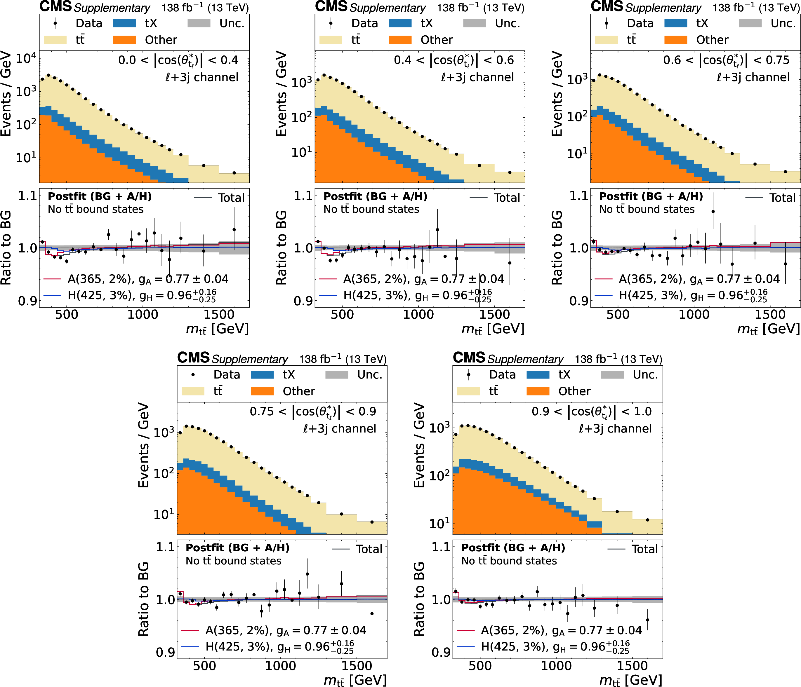
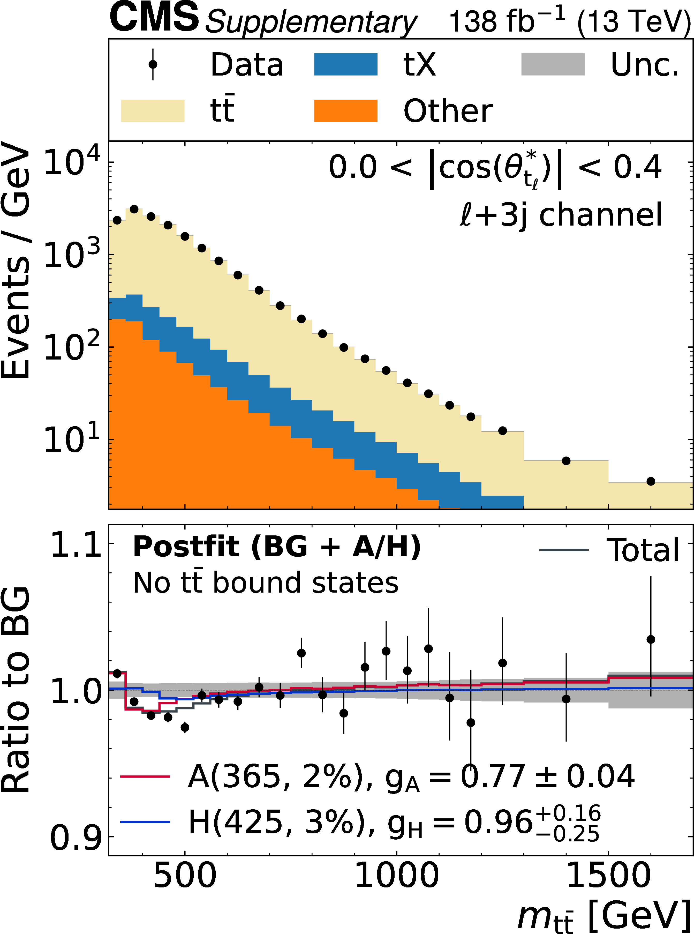
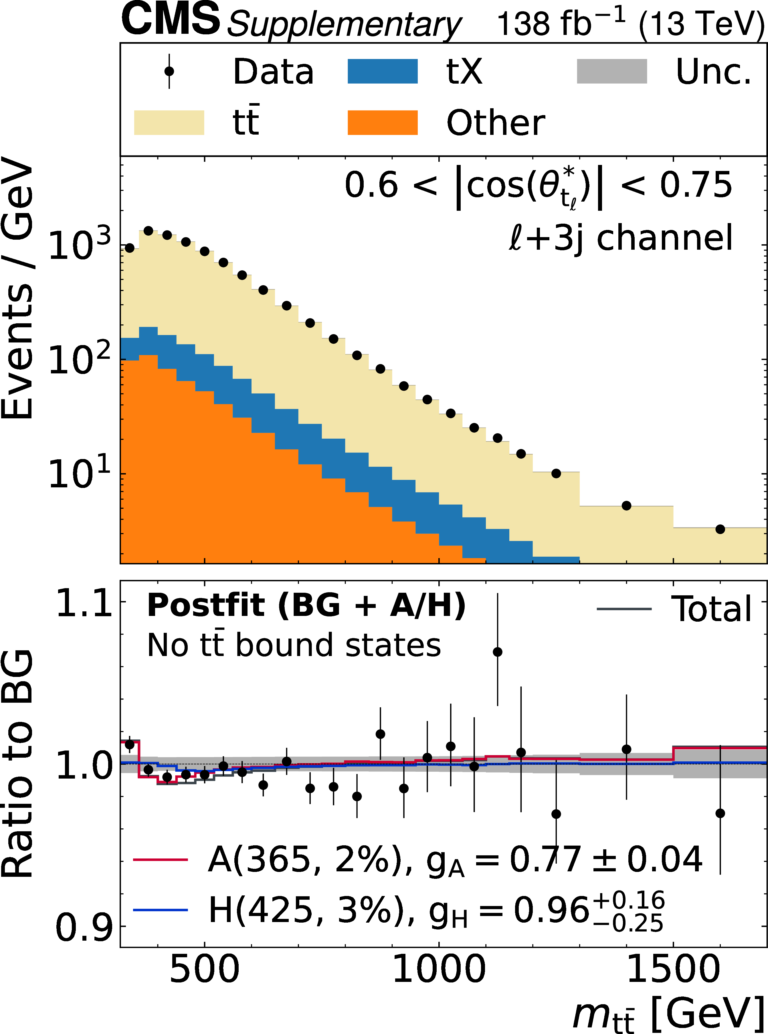
Additional Figure 2:
Observed and expected $m_{ \mathrm{t} \overline{\mathrm{t}}}$ distribution in the $\ell+3j $ channel in five bins of $\lvert{\cos{\theta^\ast_{t_{\ell}}} } \rvert$, in the fit without $\eta_t$ contribution, corresponding to the middle panel of Fig. 6 in the main text. In the upper panel, the data (points with statistical error bars) are compared to $\mathrm{t} \overline{\mathrm{t}}$ production in FO pQCD and other sources of background (colored histograms) after the fit to the data in the ${A}\text{+}{H}$ interpretation. The ratio of data to the prediction is shown in the lower panel, where the two signals A(365, 2%) and H(425, 3%), corresponding to the best fit point, are overlaid. |
png pdf |
Additional Figure 2-a:
Observed and expected $m_{ \mathrm{t} \overline{\mathrm{t}}}$ distribution in the $\ell+3j $ channel in five bins of $\lvert{\cos{\theta^\ast_{t_{\ell}}} } \rvert$, in the fit without $\eta_t$ contribution, corresponding to the middle panel of Fig. 6 in the main text. In the upper panel, the data (points with statistical error bars) are compared to $\mathrm{t} \overline{\mathrm{t}}$ production in FO pQCD and other sources of background (colored histograms) after the fit to the data in the ${A}\text{+}{H}$ interpretation. The ratio of data to the prediction is shown in the lower panel, where the two signals A(365, 2%) and H(425, 3%), corresponding to the best fit point, are overlaid. |

png pdf |
Additional Figure 2-b:
Observed and expected $m_{ \mathrm{t} \overline{\mathrm{t}}}$ distribution in the $\ell+3j $ channel in five bins of $\lvert{\cos{\theta^\ast_{t_{\ell}}} } \rvert$, in the fit without $\eta_t$ contribution, corresponding to the middle panel of Fig. 6 in the main text. In the upper panel, the data (points with statistical error bars) are compared to $\mathrm{t} \overline{\mathrm{t}}$ production in FO pQCD and other sources of background (colored histograms) after the fit to the data in the ${A}\text{+}{H}$ interpretation. The ratio of data to the prediction is shown in the lower panel, where the two signals A(365, 2%) and H(425, 3%), corresponding to the best fit point, are overlaid. |
png pdf |
Additional Figure 2-c:
Observed and expected $m_{ \mathrm{t} \overline{\mathrm{t}}}$ distribution in the $\ell+3j $ channel in five bins of $\lvert{\cos{\theta^\ast_{t_{\ell}}} } \rvert$, in the fit without $\eta_t$ contribution, corresponding to the middle panel of Fig. 6 in the main text. In the upper panel, the data (points with statistical error bars) are compared to $\mathrm{t} \overline{\mathrm{t}}$ production in FO pQCD and other sources of background (colored histograms) after the fit to the data in the ${A}\text{+}{H}$ interpretation. The ratio of data to the prediction is shown in the lower panel, where the two signals A(365, 2%) and H(425, 3%), corresponding to the best fit point, are overlaid. |
png pdf |
Additional Figure 2-d:
Observed and expected $m_{ \mathrm{t} \overline{\mathrm{t}}}$ distribution in the $\ell+3j $ channel in five bins of $\lvert{\cos{\theta^\ast_{t_{\ell}}} } \rvert$, in the fit without $\eta_t$ contribution, corresponding to the middle panel of Fig. 6 in the main text. In the upper panel, the data (points with statistical error bars) are compared to $\mathrm{t} \overline{\mathrm{t}}$ production in FO pQCD and other sources of background (colored histograms) after the fit to the data in the ${A}\text{+}{H}$ interpretation. The ratio of data to the prediction is shown in the lower panel, where the two signals A(365, 2%) and H(425, 3%), corresponding to the best fit point, are overlaid. |
png pdf |
Additional Figure 2-e:
Observed and expected $m_{ \mathrm{t} \overline{\mathrm{t}}}$ distribution in the $\ell+3j $ channel in five bins of $\lvert{\cos{\theta^\ast_{t_{\ell}}} } \rvert$, in the fit without $\eta_t$ contribution, corresponding to the middle panel of Fig. 6 in the main text. In the upper panel, the data (points with statistical error bars) are compared to $\mathrm{t} \overline{\mathrm{t}}$ production in FO pQCD and other sources of background (colored histograms) after the fit to the data in the ${A}\text{+}{H}$ interpretation. The ratio of data to the prediction is shown in the lower panel, where the two signals A(365, 2%) and H(425, 3%), corresponding to the best fit point, are overlaid. |
png pdf |
Additional Figure 3:
Observed and expected $m_{ \mathrm{t} \overline{\mathrm{t}}}$ distribution in the $\ell+{\geq}4j $ channel in five bins of $\lvert{\cos{\theta^\ast_{t_{\ell}}} } \rvert$, in the fit without $\eta_t$ contribution, corresponding to the middle panel of Fig. 7 in the main text. Notations are as in Supplemental Figure 2. |
png pdf |
Additional Figure 3-a:
Observed and expected $m_{ \mathrm{t} \overline{\mathrm{t}}}$ distribution in the $\ell+{\geq}4j $ channel in five bins of $\lvert{\cos{\theta^\ast_{t_{\ell}}} } \rvert$, in the fit without $\eta_t$ contribution, corresponding to the middle panel of Fig. 7 in the main text. Notations are as in Supplemental Figure 2. |
png pdf |
Additional Figure 3-b:
Observed and expected $m_{ \mathrm{t} \overline{\mathrm{t}}}$ distribution in the $\ell+{\geq}4j $ channel in five bins of $\lvert{\cos{\theta^\ast_{t_{\ell}}} } \rvert$, in the fit without $\eta_t$ contribution, corresponding to the middle panel of Fig. 7 in the main text. Notations are as in Supplemental Figure 2. |
png pdf |
Additional Figure 3-c:
Observed and expected $m_{ \mathrm{t} \overline{\mathrm{t}}}$ distribution in the $\ell+{\geq}4j $ channel in five bins of $\lvert{\cos{\theta^\ast_{t_{\ell}}} } \rvert$, in the fit without $\eta_t$ contribution, corresponding to the middle panel of Fig. 7 in the main text. Notations are as in Supplemental Figure 2. |
png pdf |
Additional Figure 3-d:
Observed and expected $m_{ \mathrm{t} \overline{\mathrm{t}}}$ distribution in the $\ell+{\geq}4j $ channel in five bins of $\lvert{\cos{\theta^\ast_{t_{\ell}}} } \rvert$, in the fit without $\eta_t$ contribution, corresponding to the middle panel of Fig. 7 in the main text. Notations are as in Supplemental Figure 2. |
png pdf |
Additional Figure 3-e:
Observed and expected $m_{ \mathrm{t} \overline{\mathrm{t}}}$ distribution in the $\ell+{\geq}4j $ channel in five bins of $\lvert{\cos{\theta^\ast_{t_{\ell}}} } \rvert$, in the fit without $\eta_t$ contribution, corresponding to the middle panel of Fig. 7 in the main text. Notations are as in Supplemental Figure 2. |
png pdf |
Additional Figure 4:
Observed and expected $m_{ \mathrm{t} \overline{\mathrm{t}}}$ distribution in the $\ell\ell$ channel in nine bins of $c_{\text{hel}}$ and $c_{\text{han}}$, in the fit without $\eta_t$ contribution, corresponding to the middle panel of Fig. 8 in the main text. Notations are as in Supplemental Figure 2. |
png pdf |
Additional Figure 4-a:
Observed and expected $m_{ \mathrm{t} \overline{\mathrm{t}}}$ distribution in the $\ell\ell$ channel in nine bins of $c_{\text{hel}}$ and $c_{\text{han}}$, in the fit without $\eta_t$ contribution, corresponding to the middle panel of Fig. 8 in the main text. Notations are as in Supplemental Figure 2. |

png pdf |
Additional Figure 4-b:
Observed and expected $m_{ \mathrm{t} \overline{\mathrm{t}}}$ distribution in the $\ell\ell$ channel in nine bins of $c_{\text{hel}}$ and $c_{\text{han}}$, in the fit without $\eta_t$ contribution, corresponding to the middle panel of Fig. 8 in the main text. Notations are as in Supplemental Figure 2. |
png pdf |
Additional Figure 4-c:
Observed and expected $m_{ \mathrm{t} \overline{\mathrm{t}}}$ distribution in the $\ell\ell$ channel in nine bins of $c_{\text{hel}}$ and $c_{\text{han}}$, in the fit without $\eta_t$ contribution, corresponding to the middle panel of Fig. 8 in the main text. Notations are as in Supplemental Figure 2. |
png pdf |
Additional Figure 4-d:
Observed and expected $m_{ \mathrm{t} \overline{\mathrm{t}}}$ distribution in the $\ell\ell$ channel in nine bins of $c_{\text{hel}}$ and $c_{\text{han}}$, in the fit without $\eta_t$ contribution, corresponding to the middle panel of Fig. 8 in the main text. Notations are as in Supplemental Figure 2. |
png pdf |
Additional Figure 4-e:
Observed and expected $m_{ \mathrm{t} \overline{\mathrm{t}}}$ distribution in the $\ell\ell$ channel in nine bins of $c_{\text{hel}}$ and $c_{\text{han}}$, in the fit without $\eta_t$ contribution, corresponding to the middle panel of Fig. 8 in the main text. Notations are as in Supplemental Figure 2. |
png pdf |
Additional Figure 4-f:
Observed and expected $m_{ \mathrm{t} \overline{\mathrm{t}}}$ distribution in the $\ell\ell$ channel in nine bins of $c_{\text{hel}}$ and $c_{\text{han}}$, in the fit without $\eta_t$ contribution, corresponding to the middle panel of Fig. 8 in the main text. Notations are as in Supplemental Figure 2. |
png pdf |
Additional Figure 4-g:
Observed and expected $m_{ \mathrm{t} \overline{\mathrm{t}}}$ distribution in the $\ell\ell$ channel in nine bins of $c_{\text{hel}}$ and $c_{\text{han}}$, in the fit without $\eta_t$ contribution, corresponding to the middle panel of Fig. 8 in the main text. Notations are as in Supplemental Figure 2. |

png pdf |
Additional Figure 4-h:
Observed and expected $m_{ \mathrm{t} \overline{\mathrm{t}}}$ distribution in the $\ell\ell$ channel in nine bins of $c_{\text{hel}}$ and $c_{\text{han}}$, in the fit without $\eta_t$ contribution, corresponding to the middle panel of Fig. 8 in the main text. Notations are as in Supplemental Figure 2. |
png pdf |
Additional Figure 4-i:
Observed and expected $m_{ \mathrm{t} \overline{\mathrm{t}}}$ distribution in the $\ell\ell$ channel in nine bins of $c_{\text{hel}}$ and $c_{\text{han}}$, in the fit without $\eta_t$ contribution, corresponding to the middle panel of Fig. 8 in the main text. Notations are as in Supplemental Figure 2. |
png pdf |
Additional Figure 5:
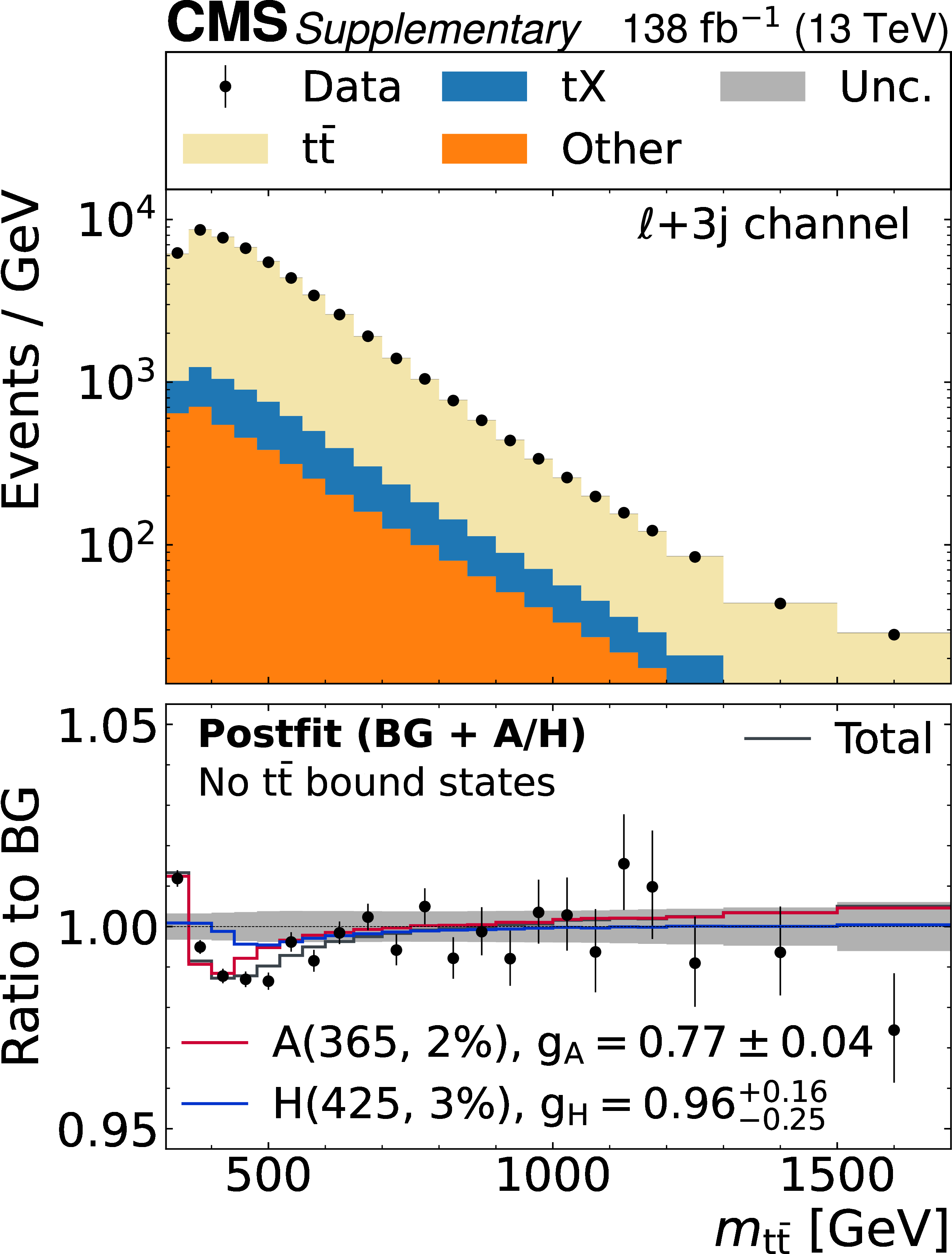
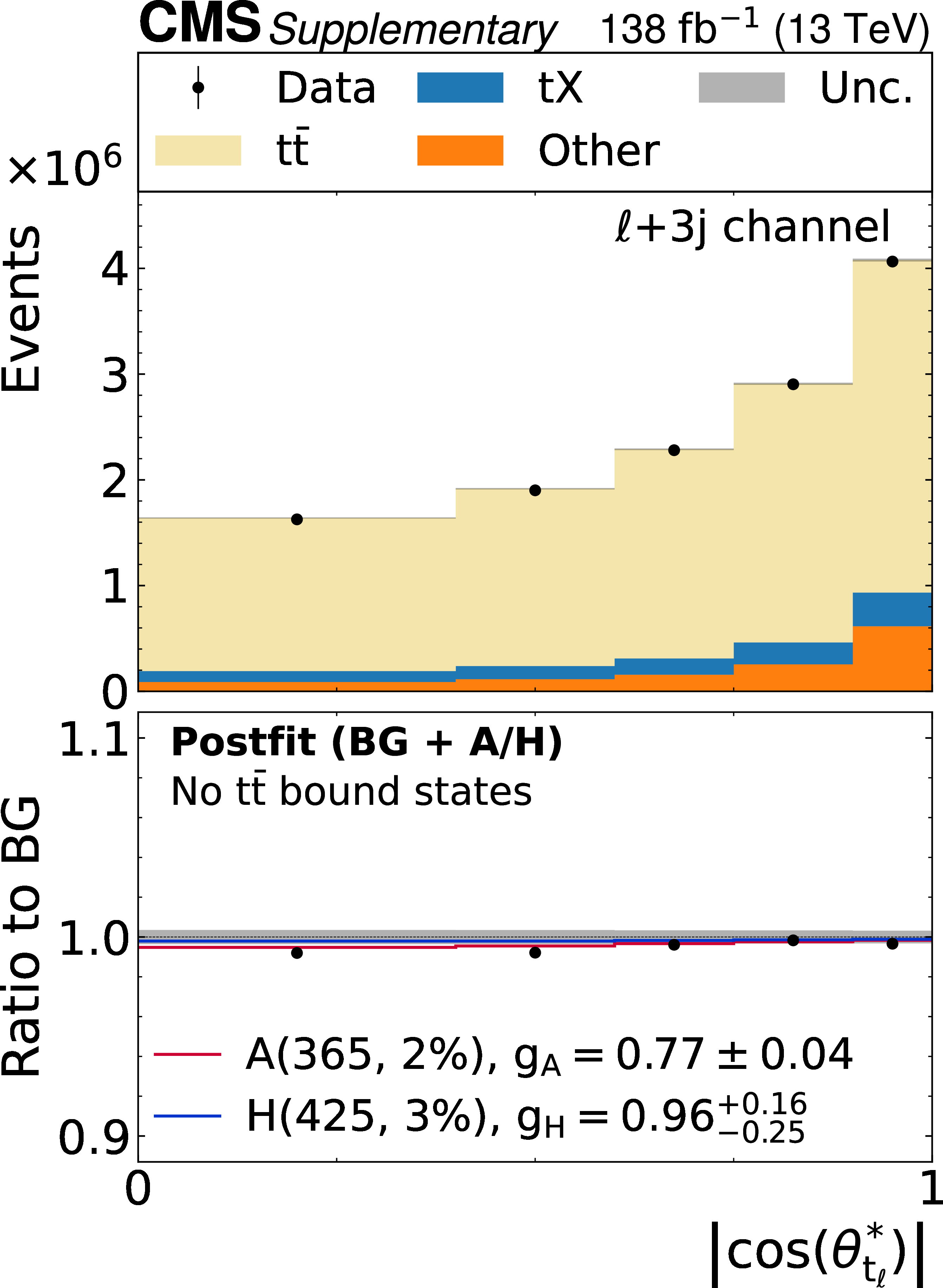
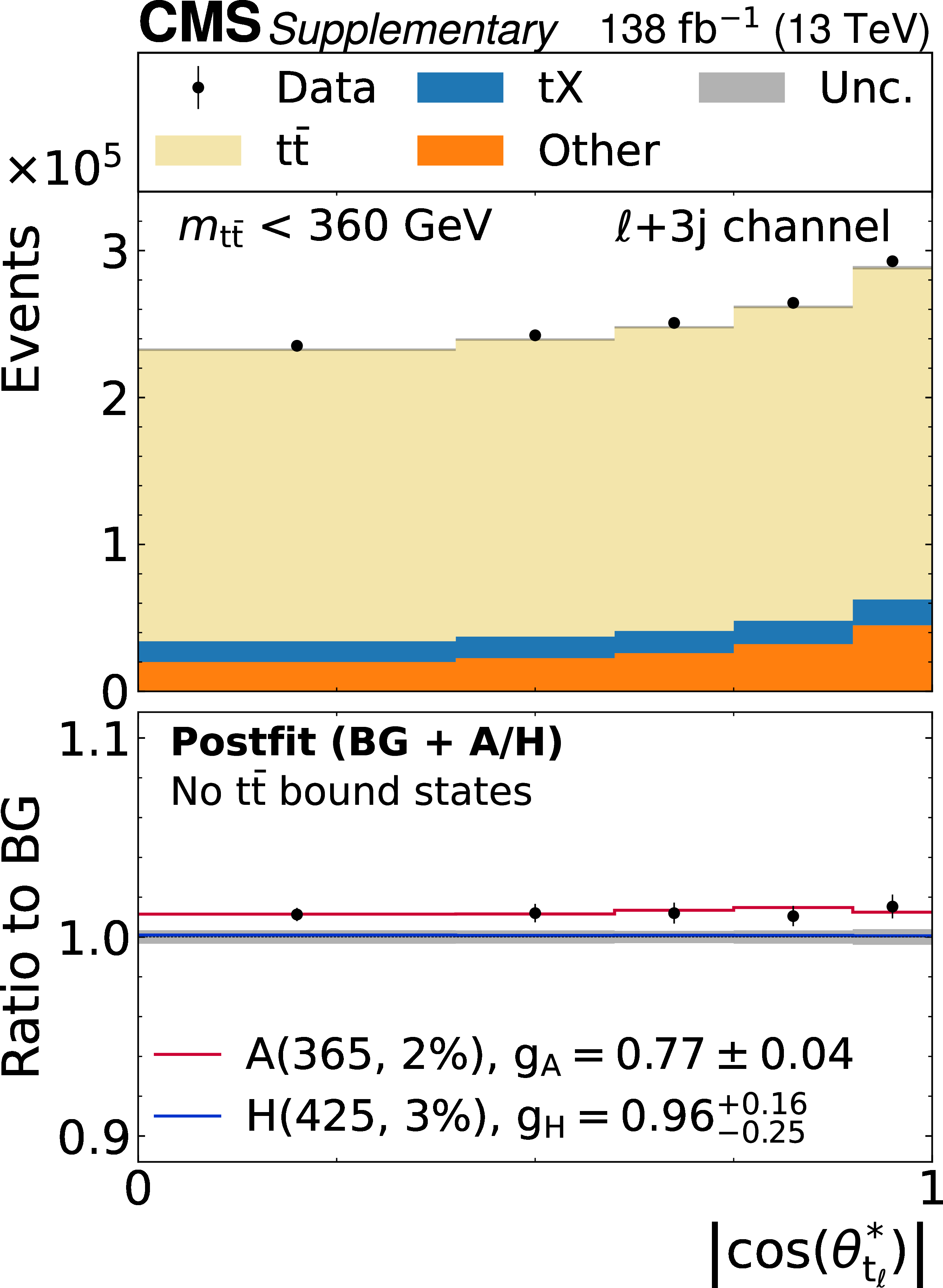
Observed and expected $m_{ \mathrm{t} \overline{\mathrm{t}}}$ distribution, integrated over $\lvert{\cos{\theta^\ast_{t_{\ell}}} } \rvert$ (left), $\lvert{\cos{\theta^\ast_{t_{\ell}}} } \rvert$ distribution, integrated over $m_{ \mathrm{t} \overline{\mathrm{t}}}$ (center), and $\lvert{\cos{\theta^\ast_{t_{\ell}}} } \rvert$ distribution for $m_{ \mathrm{t} \overline{\mathrm{t}}} < 360 $ GeV (right) in the $\ell+3j $ channel and in the fit without $\eta_t$ contribution, projected from Fig. 6 in the main text. Notations are as in Supplemental Figure 2. |
png pdf |
Additional Figure 5-a:
Observed and expected $m_{ \mathrm{t} \overline{\mathrm{t}}}$ distribution, integrated over $\lvert{\cos{\theta^\ast_{t_{\ell}}} } \rvert$ (left), $\lvert{\cos{\theta^\ast_{t_{\ell}}} } \rvert$ distribution, integrated over $m_{ \mathrm{t} \overline{\mathrm{t}}}$ (center), and $\lvert{\cos{\theta^\ast_{t_{\ell}}} } \rvert$ distribution for $m_{ \mathrm{t} \overline{\mathrm{t}}} < 360 $ GeV (right) in the $\ell+3j $ channel and in the fit without $\eta_t$ contribution, projected from Fig. 6 in the main text. Notations are as in Supplemental Figure 2. |
png pdf |
Additional Figure 5-b:
Observed and expected $m_{ \mathrm{t} \overline{\mathrm{t}}}$ distribution, integrated over $\lvert{\cos{\theta^\ast_{t_{\ell}}} } \rvert$ (left), $\lvert{\cos{\theta^\ast_{t_{\ell}}} } \rvert$ distribution, integrated over $m_{ \mathrm{t} \overline{\mathrm{t}}}$ (center), and $\lvert{\cos{\theta^\ast_{t_{\ell}}} } \rvert$ distribution for $m_{ \mathrm{t} \overline{\mathrm{t}}} < 360 $ GeV (right) in the $\ell+3j $ channel and in the fit without $\eta_t$ contribution, projected from Fig. 6 in the main text. Notations are as in Supplemental Figure 2. |
png pdf |
Additional Figure 5-c:
Observed and expected $m_{ \mathrm{t} \overline{\mathrm{t}}}$ distribution, integrated over $\lvert{\cos{\theta^\ast_{t_{\ell}}} } \rvert$ (left), $\lvert{\cos{\theta^\ast_{t_{\ell}}} } \rvert$ distribution, integrated over $m_{ \mathrm{t} \overline{\mathrm{t}}}$ (center), and $\lvert{\cos{\theta^\ast_{t_{\ell}}} } \rvert$ distribution for $m_{ \mathrm{t} \overline{\mathrm{t}}} < 360 $ GeV (right) in the $\ell+3j $ channel and in the fit without $\eta_t$ contribution, projected from Fig. 6 in the main text. Notations are as in Supplemental Figure 2. |
png pdf |
Additional Figure 6:
Observed and expected $m_{ \mathrm{t} \overline{\mathrm{t}}}$ distribution, integrated over $\lvert{\cos{\theta^\ast_{t_{\ell}}} } \rvert$ (left), $\lvert{\cos{\theta^\ast_{t_{\ell}}} } \rvert$ distribution, integrated over $m_{ \mathrm{t} \overline{\mathrm{t}}}$ (center), and $\lvert{\cos{\theta^\ast_{t_{\ell}}} } \rvert$ distribution for $m_{ \mathrm{t} \overline{\mathrm{t}}} < 360 $ GeV (right) in the $\ell+{\geq}4j $ channel and in the fit without $\eta_t$ contribution, projected from Fig. 7 in the main text. Notations are as in Supplemental Figure 2. |
png pdf |
Additional Figure 6-a:
Observed and expected $m_{ \mathrm{t} \overline{\mathrm{t}}}$ distribution, integrated over $\lvert{\cos{\theta^\ast_{t_{\ell}}} } \rvert$ (left), $\lvert{\cos{\theta^\ast_{t_{\ell}}} } \rvert$ distribution, integrated over $m_{ \mathrm{t} \overline{\mathrm{t}}}$ (center), and $\lvert{\cos{\theta^\ast_{t_{\ell}}} } \rvert$ distribution for $m_{ \mathrm{t} \overline{\mathrm{t}}} < 360 $ GeV (right) in the $\ell+{\geq}4j $ channel and in the fit without $\eta_t$ contribution, projected from Fig. 7 in the main text. Notations are as in Supplemental Figure 2. |
png pdf |
Additional Figure 6-b:
Observed and expected $m_{ \mathrm{t} \overline{\mathrm{t}}}$ distribution, integrated over $\lvert{\cos{\theta^\ast_{t_{\ell}}} } \rvert$ (left), $\lvert{\cos{\theta^\ast_{t_{\ell}}} } \rvert$ distribution, integrated over $m_{ \mathrm{t} \overline{\mathrm{t}}}$ (center), and $\lvert{\cos{\theta^\ast_{t_{\ell}}} } \rvert$ distribution for $m_{ \mathrm{t} \overline{\mathrm{t}}} < 360 $ GeV (right) in the $\ell+{\geq}4j $ channel and in the fit without $\eta_t$ contribution, projected from Fig. 7 in the main text. Notations are as in Supplemental Figure 2. |
png pdf |
Additional Figure 6-c:
Observed and expected $m_{ \mathrm{t} \overline{\mathrm{t}}}$ distribution, integrated over $\lvert{\cos{\theta^\ast_{t_{\ell}}} } \rvert$ (left), $\lvert{\cos{\theta^\ast_{t_{\ell}}} } \rvert$ distribution, integrated over $m_{ \mathrm{t} \overline{\mathrm{t}}}$ (center), and $\lvert{\cos{\theta^\ast_{t_{\ell}}} } \rvert$ distribution for $m_{ \mathrm{t} \overline{\mathrm{t}}} < 360 $ GeV (right) in the $\ell+{\geq}4j $ channel and in the fit without $\eta_t$ contribution, projected from Fig. 7 in the main text. Notations are as in Supplemental Figure 2. |
png pdf |
Additional Figure 7:
Observed and expected distributions of $m_{ \mathrm{t} \overline{\mathrm{t}}}$ (left), $c_{\text{hel}}$ (center), and $c_{\text{han}}$ (right) integrated over other observables, in the $\ell\ell$ channel and in the fit without $\eta_t$ contribution, projected from Fig. 8 in the main text. Notations are as in Supplemental Figure 2. |
png pdf |
Additional Figure 7-a:
Observed and expected distributions of $m_{ \mathrm{t} \overline{\mathrm{t}}}$ (left), $c_{\text{hel}}$ (center), and $c_{\text{han}}$ (right) integrated over other observables, in the $\ell\ell$ channel and in the fit without $\eta_t$ contribution, projected from Fig. 8 in the main text. Notations are as in Supplemental Figure 2. |
png pdf |
Additional Figure 7-b:
Observed and expected distributions of $m_{ \mathrm{t} \overline{\mathrm{t}}}$ (left), $c_{\text{hel}}$ (center), and $c_{\text{han}}$ (right) integrated over other observables, in the $\ell\ell$ channel and in the fit without $\eta_t$ contribution, projected from Fig. 8 in the main text. Notations are as in Supplemental Figure 2. |
png pdf |
Additional Figure 7-c:
Observed and expected distributions of $m_{ \mathrm{t} \overline{\mathrm{t}}}$ (left), $c_{\text{hel}}$ (center), and $c_{\text{han}}$ (right) integrated over other observables, in the $\ell\ell$ channel and in the fit without $\eta_t$ contribution, projected from Fig. 8 in the main text. Notations are as in Supplemental Figure 2. |
png pdf |
Additional Figure 8:
Observed and expected distributions of $c_{\text{hel}}$ (left) and $c_{\text{han}}$ (right) for $m_{ \mathrm{t} \overline{\mathrm{t}}} < 360 $ GeV, in the $\ell\ell$ channel and in the fit without $\eta_t$ contribution, projected from Fig. 8 in the main text. Notations are as in Supplemental Figure 2. |
png pdf |
Additional Figure 8-a:
Observed and expected distributions of $c_{\text{hel}}$ (left) and $c_{\text{han}}$ (right) for $m_{ \mathrm{t} \overline{\mathrm{t}}} < 360 $ GeV, in the $\ell\ell$ channel and in the fit without $\eta_t$ contribution, projected from Fig. 8 in the main text. Notations are as in Supplemental Figure 2. |
png pdf |
Additional Figure 8-b:
Observed and expected distributions of $c_{\text{hel}}$ (left) and $c_{\text{han}}$ (right) for $m_{ \mathrm{t} \overline{\mathrm{t}}} < 360 $ GeV, in the $\ell\ell$ channel and in the fit without $\eta_t$ contribution, projected from Fig. 8 in the main text. Notations are as in Supplemental Figure 2. |

png pdf |
Additional Figure 9:
Observed and expected $m_{ \mathrm{t} \overline{\mathrm{t}}}$ distribution in the $\ell+3j $ channel in five bins of $\lvert{\cos{\theta^\ast_{t_{\ell}}} } \rvert$, in the fit including an $\eta_t$ contribution, corresponding to the lower panel of Fig. 6 in the main text. In the upper panel, the data (points with statistical error bars) are compared to $\mathrm{t} \overline{\mathrm{t}}$ production in FO pQCD and other sources of background (colored histograms) after the fit to the data in the ${A}\text{+}{H}$ interpretation. The ratio of data to the prediction is shown in the lower panel, where the two signals A(365, 2%) and H(425,3%), corresponding to the best fit point, are overlaid. |
png pdf |
Additional Figure 9-a:
Observed and expected $m_{ \mathrm{t} \overline{\mathrm{t}}}$ distribution in the $\ell+3j $ channel in five bins of $\lvert{\cos{\theta^\ast_{t_{\ell}}} } \rvert$, in the fit including an $\eta_t$ contribution, corresponding to the lower panel of Fig. 6 in the main text. In the upper panel, the data (points with statistical error bars) are compared to $\mathrm{t} \overline{\mathrm{t}}$ production in FO pQCD and other sources of background (colored histograms) after the fit to the data in the ${A}\text{+}{H}$ interpretation. The ratio of data to the prediction is shown in the lower panel, where the two signals A(365, 2%) and H(425,3%), corresponding to the best fit point, are overlaid. |
png pdf |
Additional Figure 9-b:
Observed and expected $m_{ \mathrm{t} \overline{\mathrm{t}}}$ distribution in the $\ell+3j $ channel in five bins of $\lvert{\cos{\theta^\ast_{t_{\ell}}} } \rvert$, in the fit including an $\eta_t$ contribution, corresponding to the lower panel of Fig. 6 in the main text. In the upper panel, the data (points with statistical error bars) are compared to $\mathrm{t} \overline{\mathrm{t}}$ production in FO pQCD and other sources of background (colored histograms) after the fit to the data in the ${A}\text{+}{H}$ interpretation. The ratio of data to the prediction is shown in the lower panel, where the two signals A(365, 2%) and H(425,3%), corresponding to the best fit point, are overlaid. |
png pdf |
Additional Figure 9-c:
Observed and expected $m_{ \mathrm{t} \overline{\mathrm{t}}}$ distribution in the $\ell+3j $ channel in five bins of $\lvert{\cos{\theta^\ast_{t_{\ell}}} } \rvert$, in the fit including an $\eta_t$ contribution, corresponding to the lower panel of Fig. 6 in the main text. In the upper panel, the data (points with statistical error bars) are compared to $\mathrm{t} \overline{\mathrm{t}}$ production in FO pQCD and other sources of background (colored histograms) after the fit to the data in the ${A}\text{+}{H}$ interpretation. The ratio of data to the prediction is shown in the lower panel, where the two signals A(365, 2%) and H(425,3%), corresponding to the best fit point, are overlaid. |
png pdf |
Additional Figure 9-d:
Observed and expected $m_{ \mathrm{t} \overline{\mathrm{t}}}$ distribution in the $\ell+3j $ channel in five bins of $\lvert{\cos{\theta^\ast_{t_{\ell}}} } \rvert$, in the fit including an $\eta_t$ contribution, corresponding to the lower panel of Fig. 6 in the main text. In the upper panel, the data (points with statistical error bars) are compared to $\mathrm{t} \overline{\mathrm{t}}$ production in FO pQCD and other sources of background (colored histograms) after the fit to the data in the ${A}\text{+}{H}$ interpretation. The ratio of data to the prediction is shown in the lower panel, where the two signals A(365, 2%) and H(425,3%), corresponding to the best fit point, are overlaid. |
png pdf |
Additional Figure 9-e:
Observed and expected $m_{ \mathrm{t} \overline{\mathrm{t}}}$ distribution in the $\ell+3j $ channel in five bins of $\lvert{\cos{\theta^\ast_{t_{\ell}}} } \rvert$, in the fit including an $\eta_t$ contribution, corresponding to the lower panel of Fig. 6 in the main text. In the upper panel, the data (points with statistical error bars) are compared to $\mathrm{t} \overline{\mathrm{t}}$ production in FO pQCD and other sources of background (colored histograms) after the fit to the data in the ${A}\text{+}{H}$ interpretation. The ratio of data to the prediction is shown in the lower panel, where the two signals A(365, 2%) and H(425,3%), corresponding to the best fit point, are overlaid. |

png pdf |
Additional Figure 10:
Observed and expected $m_{ \mathrm{t} \overline{\mathrm{t}}}$ distribution in the $\ell+{\geq}4j $ channel in five bins of $\lvert{\cos{\theta^\ast_{t_{\ell}}} } \rvert$, in the fit including an $\eta_t$ contribution, corresponding to the lower panel of Fig. 7 in the main text. Notations are as in Supplemental Figure 9. |
png pdf |
Additional Figure 10-a:
Observed and expected $m_{ \mathrm{t} \overline{\mathrm{t}}}$ distribution in the $\ell+{\geq}4j $ channel in five bins of $\lvert{\cos{\theta^\ast_{t_{\ell}}} } \rvert$, in the fit including an $\eta_t$ contribution, corresponding to the lower panel of Fig. 7 in the main text. Notations are as in Supplemental Figure 9. |
png pdf |
Additional Figure 10-b:
Observed and expected $m_{ \mathrm{t} \overline{\mathrm{t}}}$ distribution in the $\ell+{\geq}4j $ channel in five bins of $\lvert{\cos{\theta^\ast_{t_{\ell}}} } \rvert$, in the fit including an $\eta_t$ contribution, corresponding to the lower panel of Fig. 7 in the main text. Notations are as in Supplemental Figure 9. |
png pdf |
Additional Figure 10-c:
Observed and expected $m_{ \mathrm{t} \overline{\mathrm{t}}}$ distribution in the $\ell+{\geq}4j $ channel in five bins of $\lvert{\cos{\theta^\ast_{t_{\ell}}} } \rvert$, in the fit including an $\eta_t$ contribution, corresponding to the lower panel of Fig. 7 in the main text. Notations are as in Supplemental Figure 9. |
png pdf |
Additional Figure 10-d:
Observed and expected $m_{ \mathrm{t} \overline{\mathrm{t}}}$ distribution in the $\ell+{\geq}4j $ channel in five bins of $\lvert{\cos{\theta^\ast_{t_{\ell}}} } \rvert$, in the fit including an $\eta_t$ contribution, corresponding to the lower panel of Fig. 7 in the main text. Notations are as in Supplemental Figure 9. |
png pdf |
Additional Figure 10-e:
Observed and expected $m_{ \mathrm{t} \overline{\mathrm{t}}}$ distribution in the $\ell+{\geq}4j $ channel in five bins of $\lvert{\cos{\theta^\ast_{t_{\ell}}} } \rvert$, in the fit including an $\eta_t$ contribution, corresponding to the lower panel of Fig. 7 in the main text. Notations are as in Supplemental Figure 9. |

png pdf |
Additional Figure 11:
Observed and expected $m_{ \mathrm{t} \overline{\mathrm{t}}}$ distribution in the $\ell\ell$ channel in nine bins of $c_{\text{hel}}$ and $c_{\text{han}}$, in the fit including an $\eta_t$ contribution, corresponding to the lower panel of Fig. 8 in the main text. Notations are as in Supplemental Figure 9. |
png pdf |
Additional Figure 11-a:
Observed and expected $m_{ \mathrm{t} \overline{\mathrm{t}}}$ distribution in the $\ell\ell$ channel in nine bins of $c_{\text{hel}}$ and $c_{\text{han}}$, in the fit including an $\eta_t$ contribution, corresponding to the lower panel of Fig. 8 in the main text. Notations are as in Supplemental Figure 9. |
png pdf |
Additional Figure 11-b:
Observed and expected $m_{ \mathrm{t} \overline{\mathrm{t}}}$ distribution in the $\ell\ell$ channel in nine bins of $c_{\text{hel}}$ and $c_{\text{han}}$, in the fit including an $\eta_t$ contribution, corresponding to the lower panel of Fig. 8 in the main text. Notations are as in Supplemental Figure 9. |
png pdf |
Additional Figure 11-c:
Observed and expected $m_{ \mathrm{t} \overline{\mathrm{t}}}$ distribution in the $\ell\ell$ channel in nine bins of $c_{\text{hel}}$ and $c_{\text{han}}$, in the fit including an $\eta_t$ contribution, corresponding to the lower panel of Fig. 8 in the main text. Notations are as in Supplemental Figure 9. |

png pdf |
Additional Figure 11-d:
Observed and expected $m_{ \mathrm{t} \overline{\mathrm{t}}}$ distribution in the $\ell\ell$ channel in nine bins of $c_{\text{hel}}$ and $c_{\text{han}}$, in the fit including an $\eta_t$ contribution, corresponding to the lower panel of Fig. 8 in the main text. Notations are as in Supplemental Figure 9. |

png pdf |
Additional Figure 11-e:
Observed and expected $m_{ \mathrm{t} \overline{\mathrm{t}}}$ distribution in the $\ell\ell$ channel in nine bins of $c_{\text{hel}}$ and $c_{\text{han}}$, in the fit including an $\eta_t$ contribution, corresponding to the lower panel of Fig. 8 in the main text. Notations are as in Supplemental Figure 9. |
png pdf |
Additional Figure 11-f:
Observed and expected $m_{ \mathrm{t} \overline{\mathrm{t}}}$ distribution in the $\ell\ell$ channel in nine bins of $c_{\text{hel}}$ and $c_{\text{han}}$, in the fit including an $\eta_t$ contribution, corresponding to the lower panel of Fig. 8 in the main text. Notations are as in Supplemental Figure 9. |
png pdf |
Additional Figure 11-g:
Observed and expected $m_{ \mathrm{t} \overline{\mathrm{t}}}$ distribution in the $\ell\ell$ channel in nine bins of $c_{\text{hel}}$ and $c_{\text{han}}$, in the fit including an $\eta_t$ contribution, corresponding to the lower panel of Fig. 8 in the main text. Notations are as in Supplemental Figure 9. |
png pdf |
Additional Figure 11-h:
Observed and expected $m_{ \mathrm{t} \overline{\mathrm{t}}}$ distribution in the $\ell\ell$ channel in nine bins of $c_{\text{hel}}$ and $c_{\text{han}}$, in the fit including an $\eta_t$ contribution, corresponding to the lower panel of Fig. 8 in the main text. Notations are as in Supplemental Figure 9. |
png pdf |
Additional Figure 11-i:
Observed and expected $m_{ \mathrm{t} \overline{\mathrm{t}}}$ distribution in the $\ell\ell$ channel in nine bins of $c_{\text{hel}}$ and $c_{\text{han}}$, in the fit including an $\eta_t$ contribution, corresponding to the lower panel of Fig. 8 in the main text. Notations are as in Supplemental Figure 9. |
png pdf |
Additional Figure 12:
Observed and expected $m_{ \mathrm{t} \overline{\mathrm{t}}}$ distribution, integrated over $\lvert{\cos{\theta^\ast_{t_{\ell}}} } \rvert$ (left), $\lvert{\cos{\theta^\ast_{t_{\ell}}} } \rvert$ distribution, integrated over $m_{ \mathrm{t} \overline{\mathrm{t}}}$ (center), and $\lvert{\cos{\theta^\ast_{t_{\ell}}} } \rvert$ distribution for $m_{ \mathrm{t} \overline{\mathrm{t}}} < 360 $ GeV (right) in the $\ell+3j $ channel and in the fit including an $\eta_t$ contribution, projected from Fig. 6 in the main text. Notations are as in Supplemental Figure 9. |
png pdf |
Additional Figure 12-a:
Observed and expected $m_{ \mathrm{t} \overline{\mathrm{t}}}$ distribution, integrated over $\lvert{\cos{\theta^\ast_{t_{\ell}}} } \rvert$ (left), $\lvert{\cos{\theta^\ast_{t_{\ell}}} } \rvert$ distribution, integrated over $m_{ \mathrm{t} \overline{\mathrm{t}}}$ (center), and $\lvert{\cos{\theta^\ast_{t_{\ell}}} } \rvert$ distribution for $m_{ \mathrm{t} \overline{\mathrm{t}}} < 360 $ GeV (right) in the $\ell+3j $ channel and in the fit including an $\eta_t$ contribution, projected from Fig. 6 in the main text. Notations are as in Supplemental Figure 9. |
png pdf |
Additional Figure 12-b:
Observed and expected $m_{ \mathrm{t} \overline{\mathrm{t}}}$ distribution, integrated over $\lvert{\cos{\theta^\ast_{t_{\ell}}} } \rvert$ (left), $\lvert{\cos{\theta^\ast_{t_{\ell}}} } \rvert$ distribution, integrated over $m_{ \mathrm{t} \overline{\mathrm{t}}}$ (center), and $\lvert{\cos{\theta^\ast_{t_{\ell}}} } \rvert$ distribution for $m_{ \mathrm{t} \overline{\mathrm{t}}} < 360 $ GeV (right) in the $\ell+3j $ channel and in the fit including an $\eta_t$ contribution, projected from Fig. 6 in the main text. Notations are as in Supplemental Figure 9. |
png pdf |
Additional Figure 12-c:
Observed and expected $m_{ \mathrm{t} \overline{\mathrm{t}}}$ distribution, integrated over $\lvert{\cos{\theta^\ast_{t_{\ell}}} } \rvert$ (left), $\lvert{\cos{\theta^\ast_{t_{\ell}}} } \rvert$ distribution, integrated over $m_{ \mathrm{t} \overline{\mathrm{t}}}$ (center), and $\lvert{\cos{\theta^\ast_{t_{\ell}}} } \rvert$ distribution for $m_{ \mathrm{t} \overline{\mathrm{t}}} < 360 $ GeV (right) in the $\ell+3j $ channel and in the fit including an $\eta_t$ contribution, projected from Fig. 6 in the main text. Notations are as in Supplemental Figure 9. |
png pdf |
Additional Figure 13:
Observed and expected $m_{ \mathrm{t} \overline{\mathrm{t}}}$ distribution, integrated over $\lvert{\cos{\theta^\ast_{t_{\ell}}} } \rvert$ (left), $\lvert{\cos{\theta^\ast_{t_{\ell}}} } \rvert$ distribution, integrated over $m_{ \mathrm{t} \overline{\mathrm{t}}}$ (center), and $\lvert{\cos{\theta^\ast_{t_{\ell}}} } \rvert$ distribution for $m_{ \mathrm{t} \overline{\mathrm{t}}} < 360 $ GeV (right) in the $\ell+{\geq}4j $ channel and in the fit including an $\eta_t$ contribution, projected from Fig. 7 in the main text. Notations are as in Supplemental Figure 9. |
png pdf |
Additional Figure 13-a:
Observed and expected $m_{ \mathrm{t} \overline{\mathrm{t}}}$ distribution, integrated over $\lvert{\cos{\theta^\ast_{t_{\ell}}} } \rvert$ (left), $\lvert{\cos{\theta^\ast_{t_{\ell}}} } \rvert$ distribution, integrated over $m_{ \mathrm{t} \overline{\mathrm{t}}}$ (center), and $\lvert{\cos{\theta^\ast_{t_{\ell}}} } \rvert$ distribution for $m_{ \mathrm{t} \overline{\mathrm{t}}} < 360 $ GeV (right) in the $\ell+{\geq}4j $ channel and in the fit including an $\eta_t$ contribution, projected from Fig. 7 in the main text. Notations are as in Supplemental Figure 9. |
png pdf |
Additional Figure 13-b:
Observed and expected $m_{ \mathrm{t} \overline{\mathrm{t}}}$ distribution, integrated over $\lvert{\cos{\theta^\ast_{t_{\ell}}} } \rvert$ (left), $\lvert{\cos{\theta^\ast_{t_{\ell}}} } \rvert$ distribution, integrated over $m_{ \mathrm{t} \overline{\mathrm{t}}}$ (center), and $\lvert{\cos{\theta^\ast_{t_{\ell}}} } \rvert$ distribution for $m_{ \mathrm{t} \overline{\mathrm{t}}} < 360 $ GeV (right) in the $\ell+{\geq}4j $ channel and in the fit including an $\eta_t$ contribution, projected from Fig. 7 in the main text. Notations are as in Supplemental Figure 9. |
png pdf |
Additional Figure 13-c:
Observed and expected $m_{ \mathrm{t} \overline{\mathrm{t}}}$ distribution, integrated over $\lvert{\cos{\theta^\ast_{t_{\ell}}} } \rvert$ (left), $\lvert{\cos{\theta^\ast_{t_{\ell}}} } \rvert$ distribution, integrated over $m_{ \mathrm{t} \overline{\mathrm{t}}}$ (center), and $\lvert{\cos{\theta^\ast_{t_{\ell}}} } \rvert$ distribution for $m_{ \mathrm{t} \overline{\mathrm{t}}} < 360 $ GeV (right) in the $\ell+{\geq}4j $ channel and in the fit including an $\eta_t$ contribution, projected from Fig. 7 in the main text. Notations are as in Supplemental Figure 9. |
png pdf |
Additional Figure 14:
Observed and expected distributions of $m_{ \mathrm{t} \overline{\mathrm{t}}}$ (left), $c_{\text{hel}}$ (center), and $c_{\text{han}}$ (right) integrated over other observables, in the $\ell\ell$ channel and in the fit including an $\eta_t$ contribution, projected from Fig. 8 in the main text. Notations are as in Supplemental Figure 9. |
png pdf |
Additional Figure 14-a:
Observed and expected distributions of $m_{ \mathrm{t} \overline{\mathrm{t}}}$ (left), $c_{\text{hel}}$ (center), and $c_{\text{han}}$ (right) integrated over other observables, in the $\ell\ell$ channel and in the fit including an $\eta_t$ contribution, projected from Fig. 8 in the main text. Notations are as in Supplemental Figure 9. |
png pdf |
Additional Figure 14-b:
Observed and expected distributions of $m_{ \mathrm{t} \overline{\mathrm{t}}}$ (left), $c_{\text{hel}}$ (center), and $c_{\text{han}}$ (right) integrated over other observables, in the $\ell\ell$ channel and in the fit including an $\eta_t$ contribution, projected from Fig. 8 in the main text. Notations are as in Supplemental Figure 9. |
png pdf |
Additional Figure 14-c:
Observed and expected distributions of $m_{ \mathrm{t} \overline{\mathrm{t}}}$ (left), $c_{\text{hel}}$ (center), and $c_{\text{han}}$ (right) integrated over other observables, in the $\ell\ell$ channel and in the fit including an $\eta_t$ contribution, projected from Fig. 8 in the main text. Notations are as in Supplemental Figure 9. |
png pdf |
Additional Figure 15:
Observed and expected distributions of $c_{\text{hel}}$ (left) and $c_{\text{han}}$ (right) for $m_{ \mathrm{t} \overline{\mathrm{t}}} < 360 $ GeV, in the $\ell\ell$ channel and in the fit including an $\eta_t$ contribution, projected from Fig. 8 in the main text. Notations are as in Supplemental Figure 9. |
png pdf |
Additional Figure 15-a:
Observed and expected distributions of $c_{\text{hel}}$ (left) and $c_{\text{han}}$ (right) for $m_{ \mathrm{t} \overline{\mathrm{t}}} < 360 $ GeV, in the $\ell\ell$ channel and in the fit including an $\eta_t$ contribution, projected from Fig. 8 in the main text. Notations are as in Supplemental Figure 9. |
png pdf |
Additional Figure 15-b:
Observed and expected distributions of $c_{\text{hel}}$ (left) and $c_{\text{han}}$ (right) for $m_{ \mathrm{t} \overline{\mathrm{t}}} < 360 $ GeV, in the $\ell\ell$ channel and in the fit including an $\eta_t$ contribution, projected from Fig. 8 in the main text. Notations are as in Supplemental Figure 9. |
| References | ||||
| 1 | ATLAS Collaboration | Observation of a new particle in the search for the standard model Higgs boson with the ATLAS detector at the LHC | PLB 716 (2012) 1 | 1207.7214 |
| 2 | CMS Collaboration | Observation of a new boson at a mass of 125 GeV with the CMS experiment at the LHC | PLB 716 (2012) 30 | CMS-HIG-12-028 1207.7235 |
| 3 | CMS Collaboration | Observation of a new boson with mass near 125 GeV in $ {\mathrm{p}\mathrm{p}} $ collisions at $ \sqrt{s}= $ 7 and 8 TeV | JHEP 06 (2013) 081 | CMS-HIG-12-036 1303.4571 |
| 4 | G. C. Branco et al. | Theory and phenomenology of two-Higgs-doublet models | Phys. Rept. 516 (2012) 1 | 1106.0034 |
| 5 | K. Huitu et al. | Probing pseudo-Goldstone dark matter at the LHC | PRD 100 (2019) 015009 | 1812.05952 |
| 6 | M. Muhlleitner, M. O. P. Sampaio, R. Santos, and J. Wittbrodt | Phenomenological comparison of models with extended Higgs sectors | JHEP 08 (2017) 132 | 1703.07750 |
| 7 | J. Abdallah et al. | Simplified models for dark matter searches at the LHC | Phys. Dark Univ. 9--10 8, 2015 link |
1506.03116 |
| 8 | C. Arina et al. | A comprehensive approach to dark matter studies: exploration of simplified top-philic models | JHEP 11 (2016) 111 | 1605.09242 |
| 9 | N. Craig, J. Galloway, and S. Thomas | Searching for signs of the second Higgs doublet | 1305.2424 | |
| 10 | M. Carena and Z. Liu | Challenges and opportunities for heavy scalar searches in the $ \mathrm{t} \overline{\mathrm{t}} $ channel at the LHC | JHEP 11 (2016) 159 | 1608.07282 |
| 11 | A. Djouadi, J. Ellis, A. Popov, and J. Quevillon | Interference effects in $ \mathrm{t} \overline{\mathrm{t}} $ production at the LHC as a window on new physics | JHEP 03 (2019) 119 | 1901.03417 |
| 12 | K. J. F. Gaemers and F. Hoogeveen | Higgs production and decay into heavy flavours with the gluon fusion mechanism | PLB 146 (1984) 347 | |
| 13 | D. Dicus, A. Stange, and S. Willenbrock | Higgs decay to top quarks at hadron colliders | PLB 333 (1994) 126 | hep-ph/9404359 |
| 14 | W. Bernreuther, M. Flesch, and P. Haberl | Signatures of Higgs bosons in the top quark decay channel at hadron colliders | PRD 58 (1998) 114031 | hep-ph/9709284 |
| 15 | W. Bernreuther et al. | Production of heavy Higgs bosons and decay into top quarks at the LHC | PRD 93 (2016) 034032 | 1511.05584 |
| 16 | W. Bernreuther, P. Galler, Z.-G. Si, and P. Uwer | Production of heavy Higgs bosons and decay into top quarks at the LHC. II. Top-quark polarization and spin correlation effects | PRD 95 (2017) 095012 | 1702.06063 |
| 17 | W. Bernreuther, A. Brandenburg, Z. G. Si, and P. Uwer | Top quark pair production and decay at hadron colliders | NPB 690 (2004) 81 | hep-ph/0403035 |
| 18 | W. Bernreuther | Top-quark physics at the LHC | JPG 35 (2008) 083001 | 0805.1333 |
| 19 | G. Mahlon and S. J. Parke | Spin correlation effects in top quark pair production at the LHC | PRD 81 (2010) 074024 | 1001.3422 |
| 20 | V. S. Fadin and V. A. Khoze | Threshold behavior of the cross section for the production of t quarks in $ \mathrm{e}^+\mathrm{e}^- $ annihilation | JETP Lett. 46 (1987) 525 | |
| 21 | V. S. Fadin, V. A. Khoze, and T. Sjostrand | On the threshold behaviour of heavy top production | Z. Phys. C 48 (1990) 613 | |
| 22 | A. H. Hoang et al. | Top-antitop pair production close to threshold: Synopsis of recent NNLO results | in Proc. 4th Workshop of the 2nd ECFA/DESY Study on Physics and Detectors for a Linear Electron-Positron Collider: Oxford, UK, March 20--23, 2000 Eur. Phys. J. direct 2 (2000) 1 |
hep-ph/0001286 |
| 23 | Y. Kiyo et al. | Top-quark pair production near threshold at LHC | EPJC 60 (2009) 375 | 0812.0919 |
| 24 | W.-L. Ju et al. | Top quark pair production near threshold: single/double distributions and mass determination | JHEP 06 (2020) 158 | 2004.03088 |
| 25 | B. Fuks, K. Hagiwara, K. Ma, and Y.-J. Zheng | Signatures of toponium formation in LHC run 2 data | PRD 104 (2021) 034023 | 2102.11281 |
| 26 | CMS Collaboration | Precision luminosity measurement in proton-proton collisions at $ \sqrt{s}= $ 13 TeV in 2015 and 2016 at CMS | EPJC 81 (2021) 800 | CMS-LUM-17-003 2104.01927 |
| 27 | CMS Collaboration | CMS luminosity measurement for the 2017 data-taking period at $ \sqrt{s}= $ 13 TeV | CMS Physics Analysis Summary, 2018 CMS-PAS-LUM-17-004 |
CMS-PAS-LUM-17-004 |
| 28 | CMS Collaboration | CMS luminosity measurement for the 2018 data-taking period at $ \sqrt{s}= $ 13 TeV | CMS Physics Analysis Summary, 2019 CMS-PAS-LUM-18-002 |
CMS-PAS-LUM-18-002 |
| 29 | CMS Collaboration | Observation of a pseudoscalar excess at the top quark pair production threshold | Rep. Prog. Phys. 88 (2025) 087801 | CMS-TOP-24-007 2503.22382 |
| 30 | CMS Collaboration | Search for heavy Higgs bosons decaying to a top quark pair in proton-proton collisions at $ \sqrt{s}= $ 13 TeV | JHEP 04 (2020) 171 | CMS-HIG-17-027 1908.01115 |
| 31 | ATLAS Collaboration | Search for heavy Higgs bosons $ \mathrm{A} $/H decaying to a top quark pair in $ {\mathrm{p}\mathrm{p}} $ collisions at $ \sqrt{s}= $ 8 TeV with the ATLAS detector | PRL 119 (2017) 191803 | 1707.06025 |
| 32 | ATLAS Collaboration | Search for heavy neutral Higgs bosons decaying into a top quark pair in 140 fb$ ^{-1} $ of proton-proton collision data at $ \sqrt{s}= $ 13 TeV with the ATLAS detector | JHEP 08 (2024) 013 | 2404.18986 |
| 33 | CMS Collaboration | The CMS experiment at the CERN LHC | JINST 3 (2008) S08004 | |
| 34 | CMS Collaboration | Development of the CMS detector for the CERN LHC \mboxRun 3 | JINST 19 (2024) P05064 | CMS-PRF-21-001 2309.05466 |
| 35 | CMS Collaboration | Performance of the CMS Level-1 trigger in proton-proton collisions at $ \sqrt{s}= $ 13 TeV | JINST 15 (2020) P10017 | CMS-TRG-17-001 2006.10165 |
| 36 | CMS Collaboration | The CMS trigger system | JINST 12 (2017) P01020 | CMS-TRG-12-001 1609.02366 |
| 37 | CMS Collaboration | Performance of the CMS high-level trigger during LHC \mboxRun 2 | JINST 19 (2024) P11021 | CMS-TRG-19-001 2410.17038 |
| 38 | CMS Collaboration | Technical proposal for the Phase-II upgrade of the Compact Muon Solenoid | CMS Technical Proposal CERN-LHCC-2015-010, CMS-TDR-15-02, 2015 link |
|
| 39 | CMS Collaboration | Particle-flow reconstruction and global event description with the CMS detector | JINST 12 (2017) P10003 | CMS-PRF-14-001 1706.04965 |
| 40 | M. Cacciari, G. P. Salam, and G. Soyez | The anti-$ k_{\mathrm{T}} $ jet clustering algorithm | JHEP 04 (2008) 063 | 0802.1189 |
| 41 | M. Cacciari, G. P. Salam, and G. Soyez | FASTJET user manual | EPJC 72 (2012) 1896 | 1111.6097 |
| 42 | CMS Collaboration | Pileup mitigation at CMS in 13 TeV data | JINST 15 (2020) P09018 | CMS-JME-18-001 2003.00503 |
| 43 | CMS Collaboration | Jet energy scale and resolution in the CMS experiment in $ {\mathrm{p}\mathrm{p}} $ collisions at 8 TeV | JINST 12 (2017) P02014 | CMS-JME-13-004 1607.03663 |
| 44 | CMS Collaboration | Identification of heavy-flavour jets with the CMS detector in $ {\mathrm{p}\mathrm{p}} $ collisions at 13 TeV | JINST 13 (2018) P05011 | CMS-BTV-16-002 1712.07158 |
| 45 | E. Bols et al. | Jet flavour classification using DeepJet | JINST 15 (2020) P12012 | 2008.10519 |
| 46 | CMS Collaboration | Performance summary of AK4 jet b tagging with data from proton-proton collisions at 13 TeV with the CMS detector | CMS Detector Performance Note CMS-DP-2023-005, 2023 CDS |
|
| 47 | CMS Collaboration | Electron and photon reconstruction and identification with the CMS experiment at the CERN LHC | JINST 16 (2021) P05014 | CMS-EGM-17-001 2012.06888 |
| 48 | CMS Collaboration | ECAL 2016 refined calibration and \mboxRun 2 summary plots | CMS Detector Performance Note CMS-DP-2020-021, 2020 CDS |
|
| 49 | CMS Collaboration | Performance of the CMS muon detector and muon reconstruction with proton-proton collisions at $ \sqrt{s}= $ 13 TeV | JINST 13 (2018) P06015 | CMS-MUO-16-001 1804.04528 |
| 50 | CMS Collaboration | Performance of missing transverse momentum reconstruction in proton-proton collisions at $ \sqrt{s}= $ 13 TeV using the CMS detector | JINST 14 (2019) P07004 | CMS-JME-17-001 1903.06078 |
| 51 | CMS Collaboration | Simulation of the silicon strip tracker pre-amplifier in early 2016 data | CMS Detector Performance Note CMS-DP-2020-045, 2020 CDS |
|
| 52 | NNPDF Collaboration | Parton distributions for the LHC run II | JHEP 04 (2015) 040 | 1410.8849 |
| 53 | T. Sjostrand et al. | An introduction to PYTHIA8.2 | Comput. Phys. Commun. 191 (2015) 159 | 1410.3012 |
| 54 | P. Skands, S. Carrazza, and J. Rojo | Tuning PYTHIA8.1: the Monash 2013 tune | EPJC 74 (2014) 3024 | 1404.5630 |
| 55 | CMS Collaboration | Extraction and validation of a new set of CMS PYTHIA8 tunes from underlying-event measurements | EPJC 80 (2020) 4 | CMS-GEN-17-001 1903.12179 |
| 56 | GEANT4 Collaboration | GEANT 4---a simulation toolkit | NIM A 506 (2003) 250 | |
| 57 | J. Alwall et al. | The automated computation of tree-level and next-to-leading order differential cross sections, and their matching to parton shower simulations | JHEP 07 (2014) 079 | 1405.0301 |
| 58 | M. Spira, A. Djouadi, D. Graudenz, and P. M. Zerwas | Higgs boson production at the LHC | NPB 453 (1995) 17 | hep-ph/9504378 |
| 59 | B. Hespel, F. Maltoni, and E. Vryonidou | Signal background interference effects in heavy scalar production and decay to a top-anti-top pair | JHEP 10 (2016) 016 | 1606.04149 |
| 60 | R. V. Harlander, S. Liebler, and H. Mantler | SusHi: A program for the calculation of Higgs production in gluon fusion and bottom-quark annihilation in the standard model and the MSSM | Comput. Phys. Commun. 184 (2013) 1605 | 1212.3249 |
| 61 | R. V. Harlander, S. Liebler, and H. Mantler | SusHi bento: Beyond NNLO and the heavy-top limit | Comput. Phys. Commun. 212 (2017) 239 | 1605.03190 |
| 62 | D. Eriksson, J. Rathsman, and O. Staal | 2hdmc---two-Higgs-doublet model calculator | Comput. Phys. Commun. 181 (2010) 189 | 0902.0851 |
| 63 | A. Banfi et al. | Higgs interference effects in top-quark pair production in the 1HSM | JHEP 08 (2024) 112 | 2309.16759 |
| 64 | CMS Collaboration | HEPData record for this analysis | link | |
| 65 | B. Fuks, K. Hagiwara, K. Ma, and Y.-J. Zheng | Simulating toponium formation signals at the LHC | EPJC 85 (2025) 157 | 2411.18962 |
| 66 | Y. Sumino and H. Yokoya | Bound-state effects on kinematical distributions of top quarks at hadron colliders | JHEP 09 (2010) 034 | 1007.0075 |
| 67 | F. Maltoni, C. Severi, S. Tentori, and E. Vryonidou | Quantum detection of new physics in top-quark pair production at the LHC | JHEP 03 (2024) 099 | 2401.08751 |
| 68 | P. Nason | A new method for combining NLO QCD with shower Monte Carlo algorithms | JHEP 11 (2004) 040 | hep-ph/0409146 |
| 69 | S. Frixione, P. Nason, and C. Oleari | Matching NLO QCD computations with parton shower simulations: the POWHEG method | JHEP 11 (2007) 070 | 0709.2092 |
| 70 | S. Alioli, P. Nason, C. Oleari, and E. Re | A general framework for implementing NLO calculations in shower Monte Carlo programs: the POWHEG box | JHEP 06 (2010) 043 | 1002.2581 |
| 71 | J. M. Campbell, R. K. Ellis, P. Nason, and E. Re | Top-pair production and decay at NLO matched with parton showers | JHEP 04 (2015) 114 | 1412.1828 |
| 72 | M. A. Gigg and P. Richardson | Simulation of finite width effects in physics beyond the standard model | 0805.3037 | |
| 73 | M. Czakon and A. Mitov | top++: a program for the calculation of the top-pair cross-section at hadron colliders | Comput. Phys. Commun. 185 (2014) 2930 | 1112.5675 |
| 74 | M. Grazzini, S. Kallweit, and M. Wiesemann | Fully differential NNLO computations with matrix | EPJC 78 (2018) 537 | 1711.06631 |
| 75 | W. Bernreuther, M. Fucker, and Z. G. Si | Mixed QCD and weak corrections to top quark pair production at hadron colliders | PLB 633 (2006) 54 | hep-ph/0508091 |
| 76 | J. H. Kuhn, A. Scharf, and P. Uwer | Electroweak corrections to top-quark pair production in quark-antiquark annihilation | EPJC 45 (2006) 139 | hep-ph/0508092 |
| 77 | W. Bernreuther, M. Fucker, and Z.-G. Si | Weak interaction corrections to hadronic top quark pair production | PRD 74 (2006) 113005 | hep-ph/0610334 |
| 78 | J. H. Kuhn, A. Scharf, and P. Uwer | Electroweak effects in top-quark pair production at hadron colliders | EPJC 51 (2007) 37 | hep-ph/0610335 |
| 79 | M. Aliev et al. | hathor: Hadronic top and heavy quarks cross section calculator | Comput. Phys. Commun. 182 (2011) 1034 | 1007.1327 |
| 80 | J. H. Kuhn, A. Scharf, and P. Uwer | Weak interactions in top-quark pair production at hadron colliders: An update | PRD 91 (2015) 014020 | 1305.5773 |
| 81 | E. Re | Single-top $ {\mathrm{W}\mathrm{t}} $-channel production matched with parton showers using the POWHEG method | EPJC 71 (2011) 1547 | 1009.2450 |
| 82 | S. Alioli, P. Nason, C. Oleari, and E. Re | NLO single-top production matched with shower in POWHEG: $ s $- and $ t $-channel contributions | JHEP 09 (2009) 111 | 0907.4076 |
| 83 | P. Kant et al. | hathor for single top-quark production: Updated predictions and uncertainty estimates for single top-quark production in hadronic collisions | Comput. Phys. Commun. 191 (2015) 74 | 1406.4403 |
| 84 | N. Kidonakis and N. Yamanaka | Higher-order corrections for $ tW $ production at high-energy hadron colliders | JHEP 05 (2021) 278 | 2102.11300 |
| 85 | P. F. Monni et al. | MiNNLO\textsubscriptps: a new method to match NNLO QCD to parton showers | JHEP 05 (2020) 143 | 1908.06987 |
| 86 | P. F. Monni, E. Re, and M. Wiesemann | MiNNLO\textsubscriptps: optimizing 2 $ \to $ 1 hadronic processes | EPJC 80 (2020) 1075 | 2006.04133 |
| 87 | E. Barberio and Z. Was | photos---a universal Monte Carlo for QED radiative corrections: version 2.0 | Comput. Phys. Commun. 79 (1994) 291 | |
| 88 | P. Golonka and Z. Was | photos Monte Carlo: a precision tool for QED corrections in Z and W decays | EPJC 45 (2006) 97 | hep-ph/0506026 |
| 89 | J. Alwall et al. | Comparative study of various algorithms for the merging of parton showers and matrix elements in hadronic collisions | EPJC 53 (2008) 473 | 0706.2569 |
| 90 | K. Melnikov and F. Petriello | Electroweak gauge boson production at hadron colliders through $ \mathcal{O}({\alpha_\mathrm{S}^2}) $ | PRD 74 (2006) 114017 | hep-ph/0609070 |
| 91 | Y. Li and F. Petriello | Combining QCD and electroweak corrections to dilepton production in FEWZ | PRD 86 (2012) 094034 | 1208.5967 |
| 92 | T. Gehrmann et al. | $ {\mathrm{W^+}\mathrm{W^-}} $ production at hadron colliders in next to next to leading order QCD | PRL 113 (2014) 212001 | 1408.5243 |
| 93 | J. M. Campbell and R. K. Ellis | MCFM for the Tevatron and the LHC | in Proc. 10th DESY Workshop on Elementary Particle Theory: Loops and Legs in Quantum Field Theory (LL2010): Worlitz, Germany, April 25--30, 2010. 2010.. [Nucl. Phys. B Proc. Suppl. 205--206 (2010) 10] link |
1007.3492 |
| 94 | S. Frixione and B. R. Webber | Matching NLO QCD computations and parton shower simulations | JHEP 06 (2002) 029 | hep-ph/0204244 |
| 95 | R. Frederix and S. Frixione | Merging meets matching in MC@NLO | JHEP 12 (2012) 061 | 1209.6215 |
| 96 | B. A. Betchart, R. Demina, and A. Harel | Analytic solutions for neutrino momenta in decay of top quarks | NIM A 736 (2014) 169 | 1305.1878 |
| 97 | R. Demina, A. Harel, and D. Orbaker | Reconstructing $ \mathrm{t} \overline{\mathrm{t}} $ events with one lost jet | NIM A 788 (2015) 128 | 1310.3263 |
| 98 | CMS Collaboration | Measurement of the differential cross section for top quark pair production in $ {\mathrm{p}\mathrm{p}} $ collisions at $ \sqrt{s} = $ 8 TeV | EPJC 75 (2015) 542 | CMS-TOP-12-028 1505.04480 |
| 99 | L. Sonnenschein | Analytical solution of $ \mathrm{t} \overline{\mathrm{t}} $ dilepton equations | PRD 73 (2006) 054015 | hep-ph/0603011 |
| 100 | CMS Collaboration | Measurement of double-differential cross sections for top quark pair production in $ {\mathrm{p}\mathrm{p}} $ collisions at $ \sqrt{s}= $ 8 TeV and impact on parton distribution functions | EPJC 77 (2017) 459 | CMS-TOP-14-013 1703.01630 |
| 101 | I. Korol | Measurement of double differential $ \mathrm{t} \overline{\mathrm{t}} $ production cross sections with the CMS detector | PhD thesis, Universität Hamburg, CERN-THESIS-2016-060, DESY-THESIS-2016-011, 2016 link |
|
| 102 | W. Bernreuther and Z.-G. Si | Distributions and correlations for top quark pair production and decay at the Tevatron and LHC | NPB 837 (2010) 90 | 1003.3926 |
| 103 | W. Bernreuther, D. Heisler, and Z.-G. Si | A set of top quark spin correlation and polarization observables for the LHC: Standard model predictions and new physics contributions | JHEP 12 (2015) 026 | 1508.05271 |
| 104 | J. A. Aguilar-Saavedra and J. A. Casas | Improved tests of entanglement and Bell inequalities with LHC tops | EPJC 82 (2022) 666 | 2205.00542 |
| 105 | J. A. Aguilar-Saavedra | Toponium hunter's guide | PRD 110 (2024) 054032 | 2407.20330 |
| 106 | CMS Collaboration | Measurement of the $ \mathrm{t} \overline{\mathrm{t}} $ production cross section and the top quark mass in the dilepton channel in $ {\mathrm{p}\mathrm{p}} $ collisions at $ \sqrt{s}= $ 7 TeV | JHEP 07 (2011) 049 | CMS-TOP-11-002 1105.5661 |
| 107 | CMS Collaboration | The CMS statistical analysis and combination tool: combine | Comput. Softw. Big Sci. 8 (2024) 19 | CMS-CAT-23-001 2404.06614 |
| 108 | CMS Collaboration | Combined measurements of Higgs boson couplings in proton-proton collisions at $ \sqrt{s}= $ 13 TeV | EPJC 79 (2019) 421 | CMS-HIG-17-031 1809.10733 |
| 109 | CMS Collaboration | Measurement of the top quark mass using proton-proton data at $ \sqrt{s}= $ 7 and 8 TeV | PRD 93 (2016) 072004 | CMS-TOP-14-022 1509.04044 |
| 110 | J. Butterworth et al. | PDF4LHC recommendations for LHC \mboxRun 2 | JPG 43 (2016) 023001 | 1510.03865 |
| 111 | J. R. Christiansen and P. Z. Skands | String formation beyond leading colour | JHEP 08 (2015) 003 | 1505.01681 |
| 112 | CMS Collaboration | CMS PYTHIA8 colour reconnection tunes based on underlying-event data | EPJC 83 (2023) 587 | CMS-GEN-17-002 2205.02905 |
| 113 | CMS Collaboration | Investigations of the impact of the parton shower tuning in PYTHIA8 in the modelling of $ \mathrm{t} \overline{\mathrm{t}} $ at $ \sqrt{s}= $ 8 and 13 TeV | CMS Physics Analysis Summary, 2016 CMS-PAS-TOP-16-021 |
CMS-PAS-TOP-16-021 |
| 114 | ATLAS Collaboration | Measurement of the inclusive cross-sections of single top-quark and top-antiquark $ t $-channel production in $ {\mathrm{p}\mathrm{p}} $ collisions at $ \sqrt{s}= $ 13 TeV with the ATLAS detector | JHEP 04 (2017) 086 | 1609.03920 |
| 115 | CMS Collaboration | Measurement of the single top quark and antiquark production cross sections in the $ t $ channel and their ratio in proton-proton collisions at $ \sqrt{s}= $ 13 TeV | PLB 800 (2020) 135042 | CMS-TOP-17-011 1812.10514 |
| 116 | CMS Collaboration | Measurement of the production cross section for single top quarks in association with W bosons in proton-proton collisions at $ \sqrt{s}= $ 13 TeV | JHEP 10 (2018) 117 | CMS-TOP-17-018 1805.07399 |
| 117 | CMS Collaboration | Measurement of the cross section for top quark pair production in association with a W or Z boson in proton-proton collisions at $ \sqrt{s}= $ 13 TeV | JHEP 08 (2018) 011 | CMS-TOP-17-005 1711.02547 |
| 118 | ATLAS Collaboration | Measurement of the $ {{\mathrm{t}\overline{\mathrm{t}}} \mathrm{Z}} $ and $ {{\mathrm{t}\overline{\mathrm{t}}} \mathrm{W}} $ cross sections in proton-proton collisions at $ \sqrt{s}= $ 13 TeV with the ATLAS detector | PRD 99 (2019) 072009 | 1901.03584 |
| 119 | ATLAS Collaboration | Measurements of top-quark pair to Z-boson cross-section ratios at $ \sqrt{s}= $ 13, 8, 7 TeV with the ATLAS detector | JHEP 02 (2017) 117 | 1612.03636 |
| 120 | R. Barlow and C. Beeston | Fitting using finite Monte Carlo samples | Comput. Phys. Commun. 77 (1993) 219 | |
| 121 | W. S. Cleveland | Robust locally weighted regression and smoothing scatterplots | J. Am. Stat. Assoc. 74 (1979) 829 | |
| 122 | W. S. Cleveland and S. J. Devlin | Locally weighted regression: an approach to regression analysis by local fitting | J. Am. Stat. Assoc. 83 (1988) 596 | |
| 123 | A. Djouadi, J. Ellis, and J. Quevillon | Contrasting pseudoscalar Higgs and toponium states at the LHC and beyond | PLB 866 (2025) 139583 | 2412.15138 |
| 124 | G. Cowan, K. Cranmer, E. Gross, and O. Vitells | Asymptotic formulae for likelihood-based tests of new physics | EPJC 71 (2011) 1554 | 1007.1727 |
| 125 | ATLAS and CMS Collaborations, and LHC Higgs Combination Group | Procedure for the LHC Higgs boson search combination in Summer 2011 | Technical Report CMS-NOTE-2011-005, ATL-PHYS-PUB-2011-11, 2011 | |
| 126 | T. Junk | Confidence level computation for combining searches with small statistics | NIM A 434 (1999) 435 | hep-ex/9902006 |
| 127 | A. L. Read | Presentation of search results: The $ \text{CL}_\text{s} $ technique | JPG 28 (2002) 2693 | |
| 128 | G. J. Feldman and R. D. Cousins | Unified approach to the classical statistical analysis of small signals | PRD 57 (1998) 3873 | physics/9711021 |
| 129 | R. D. Cousins and V. L. Highland | Incorporating systematic uncertainties into an upper limit | NIM A 320 (1992) 331 | |
|
|
Compact Muon Solenoid LHC, CERN |
|

|

|

|

|

|