

Compact Muon Solenoid
LHC, CERN
| CMS-PAS-SUS-21-004 | ||
| Search for top squark pair production in a final state with one or two tau leptons in proton-proton collisions at $ \sqrt{s} = $ 13 TeV | ||
| CMS Collaboration | ||
| 22 September 2022 | ||
| Abstract: A search for pair production of the supersymmetric partner of the top quark, the top squark, in proton-proton collision events at $ \sqrt{s} = $ 13 TeV is presented in final states containing at least one hadronically decaying tau lepton and large missing transverse momentum. This final state is highly sensitive to high-$ \tan\beta $ or higgsino-like scenarios in which decays of electroweakinos to tau leptons are dominant. The search uses a data sample corresponding to an integrated luminosity of 138 fb$^{-1}$, which was recorded with the CMS detector during 2016-2018. No significant excess is observed with respect to the standard model backgrounds. Exclusion limits at 95% confidence level on top squark and lightest neutralino masses are presented under the assumptions of simplified models. The search excludes top squark masses up to 1150 GeV for a nearly massless neutralino. | ||
|
Links:
CDS record (PDF) ;
CADI line (restricted) ;
These preliminary results are superseded in this paper, JHEP 07 (2023) 110. The superseded preliminary plots can be found here. |
||
| Figures | |
png pdf |
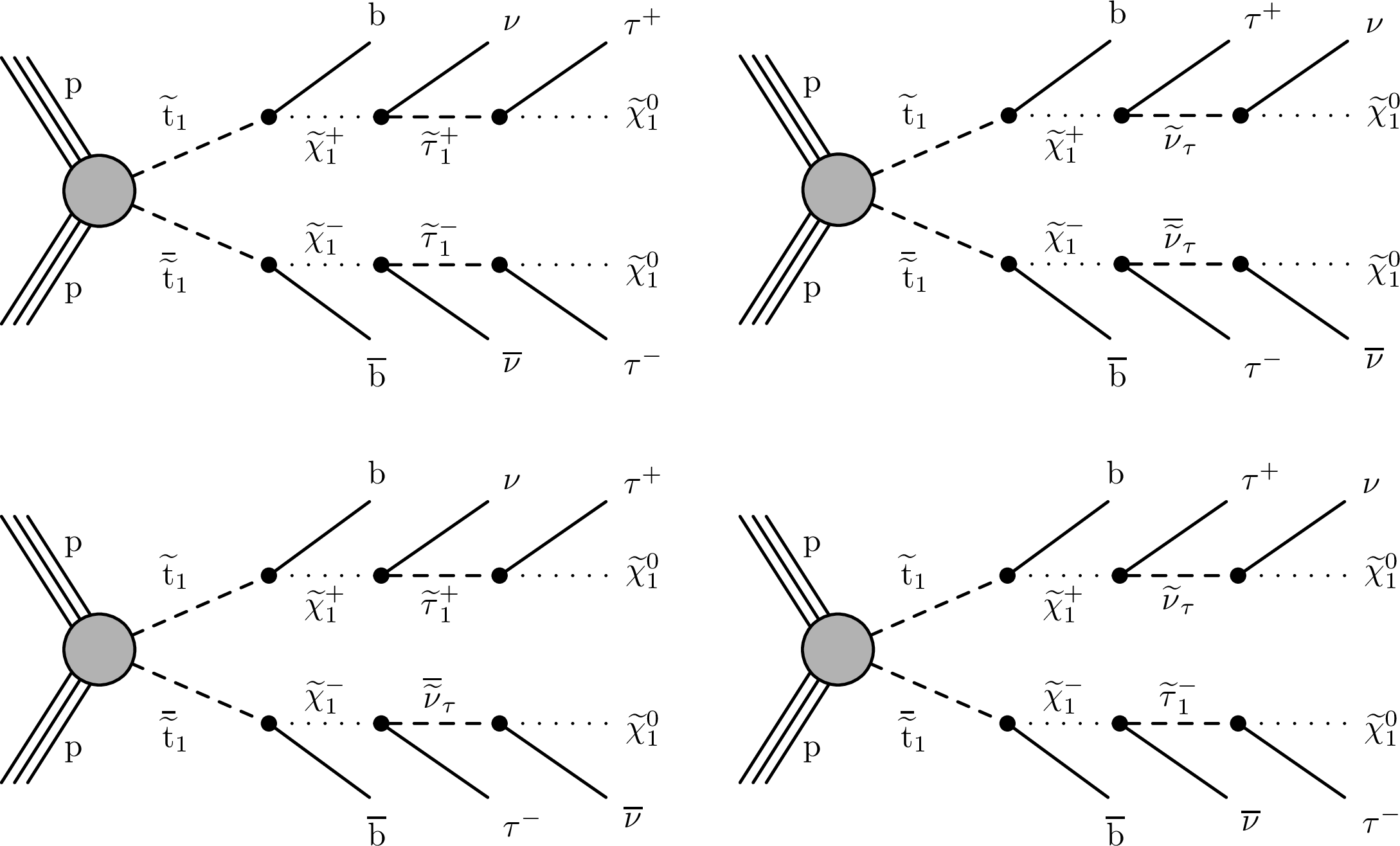
Figure 1:
Top squark pair production in proton-proton collisions at the LHC, producing pairs of b quarks and taus accompanied by neutrinos and LSPs in the final state. |
png pdf |
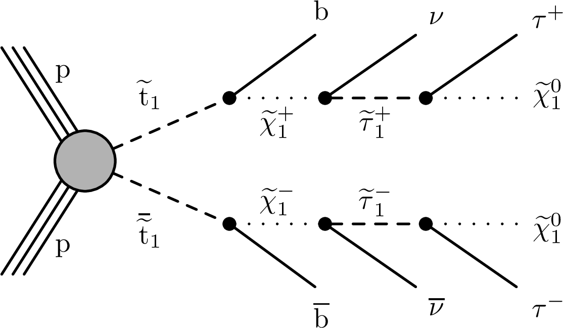
Figure 1-a:
Top squark pair production in proton-proton collisions at the LHC, producing pairs of b quarks and taus accompanied by neutrinos and LSPs in the final state. |
png pdf |
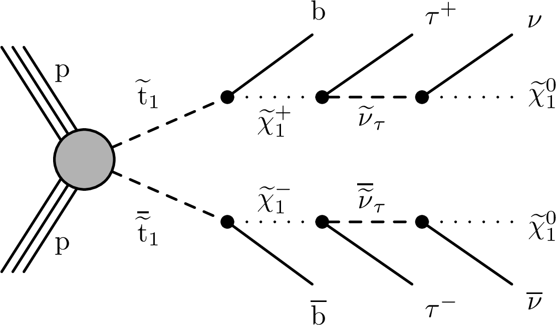
Figure 1-b:
Top squark pair production in proton-proton collisions at the LHC, producing pairs of b quarks and taus accompanied by neutrinos and LSPs in the final state. |
png pdf |
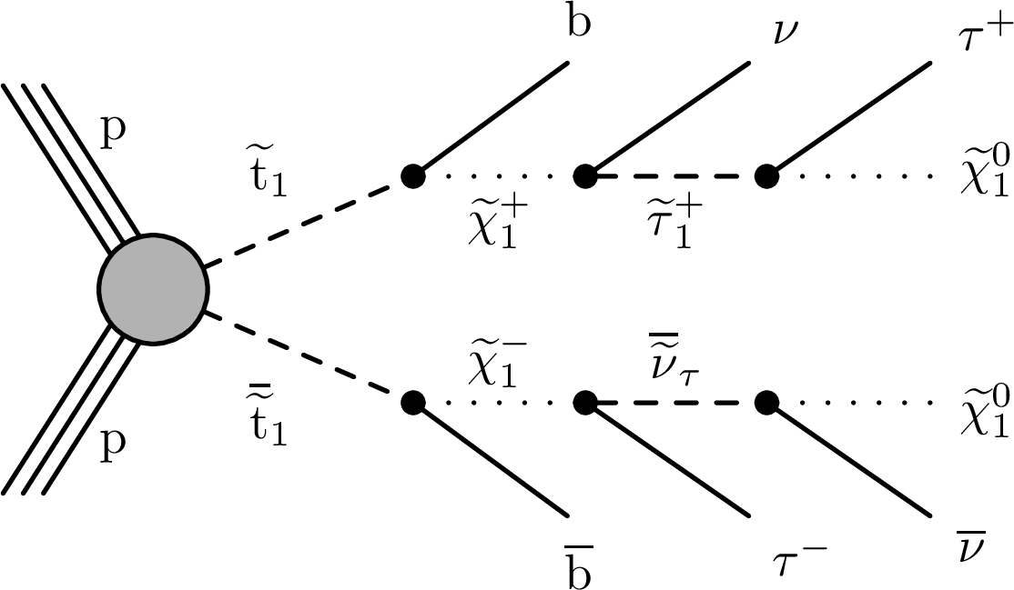
Figure 1-c:
Top squark pair production in proton-proton collisions at the LHC, producing pairs of b quarks and taus accompanied by neutrinos and LSPs in the final state. |

png pdf |
Figure 1-d:
Top squark pair production in proton-proton collisions at the LHC, producing pairs of b quarks and taus accompanied by neutrinos and LSPs in the final state. |
png pdf |
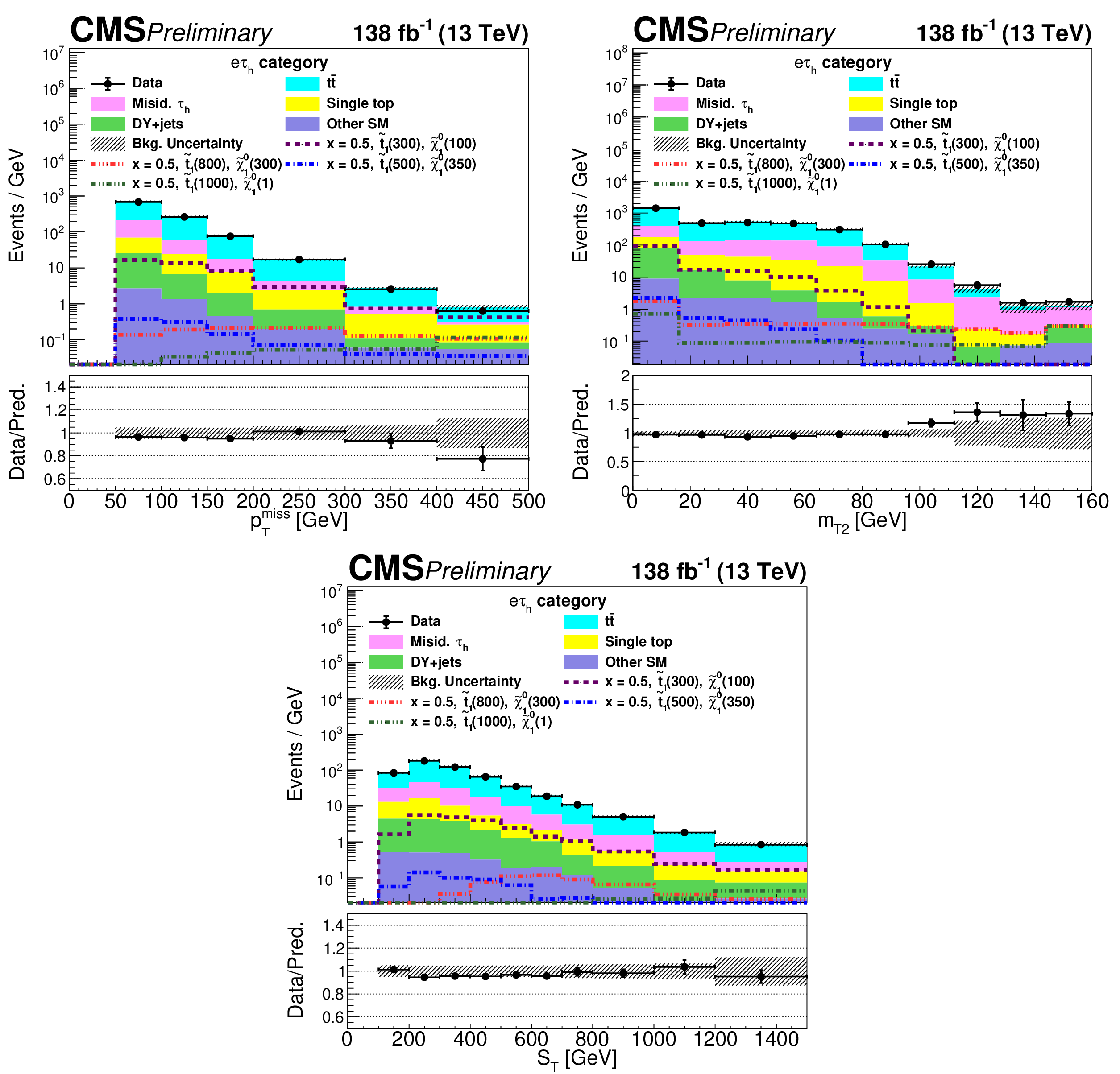
Figure 2:
Distributions of the search variables $ p_{\mathrm{T}}^\text{miss} $, $ m_{\mathrm{T2}} $, and $ S_{\mathrm{T}} $ after event selection, for data and the predicted background, corresponding to the e $ \tau_\mathrm{h} $ category. The histograms for the background processes are stacked, and the distributions for a few representative signal points corresponding to $ x = $ 0.5 and [$ m_{\tilde{\mathrm{t}}_{1}} $, $ m_{\tilde{\chi}_{1}^{0}} $] = [300, 100], [500, 350], [800, 300], and [1000, 1] GeV are overlaid. The lower panel indicates the ratio of the observed data to the background prediction. The shaded bands indicate the statistical and systematic uncertainties on the background, added in quadrature. |
png pdf |
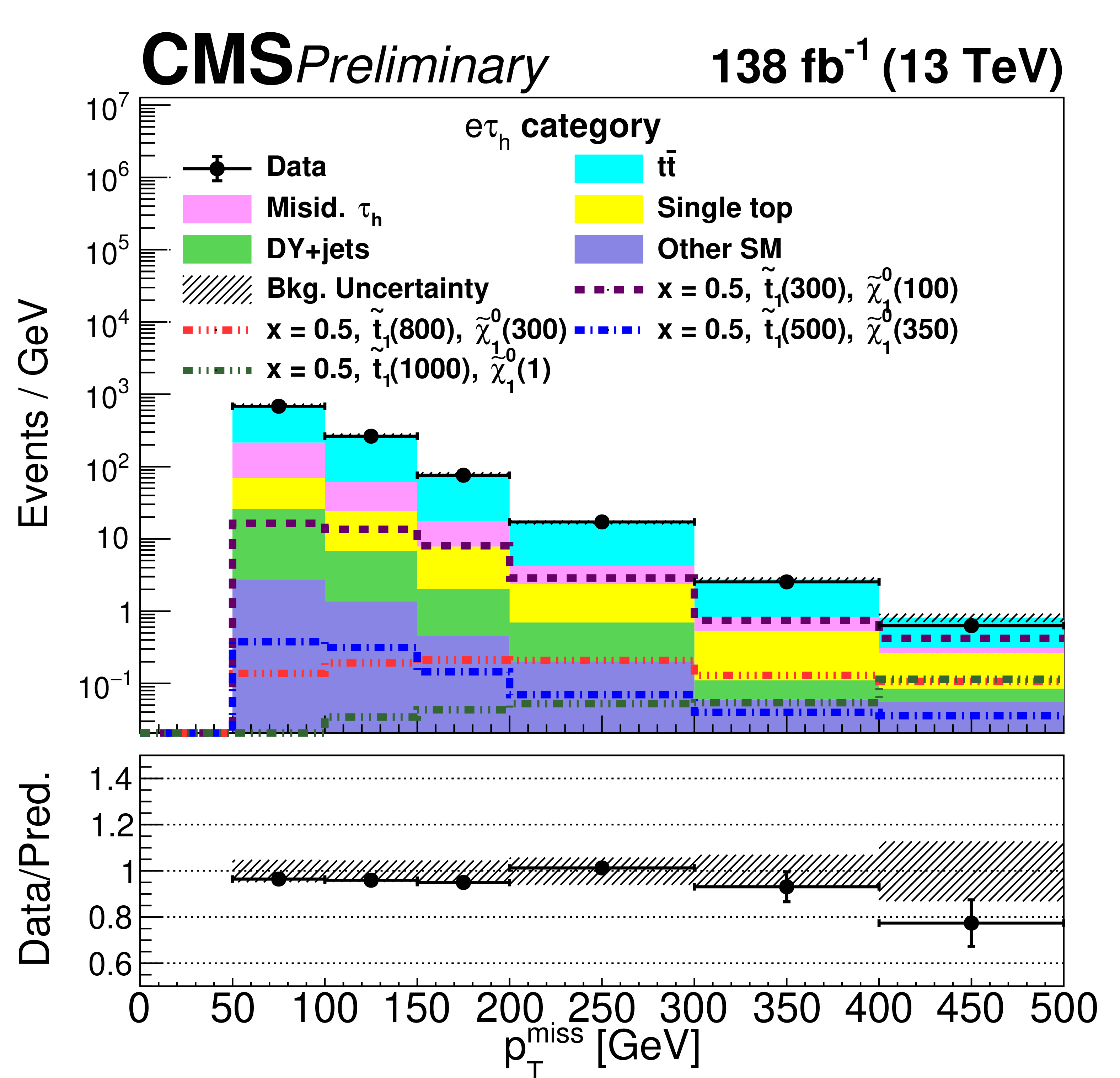
Figure 2-a:
Distributions of the search variables $ p_{\mathrm{T}}^\text{miss} $, $ m_{\mathrm{T2}} $, and $ S_{\mathrm{T}} $ after event selection, for data and the predicted background, corresponding to the e $ \tau_\mathrm{h} $ category. The histograms for the background processes are stacked, and the distributions for a few representative signal points corresponding to $ x = $ 0.5 and [$ m_{\tilde{\mathrm{t}}_{1}} $, $ m_{\tilde{\chi}_{1}^{0}} $] = [300, 100], [500, 350], [800, 300], and [1000, 1] GeV are overlaid. The lower panel indicates the ratio of the observed data to the background prediction. The shaded bands indicate the statistical and systematic uncertainties on the background, added in quadrature. |
png pdf |
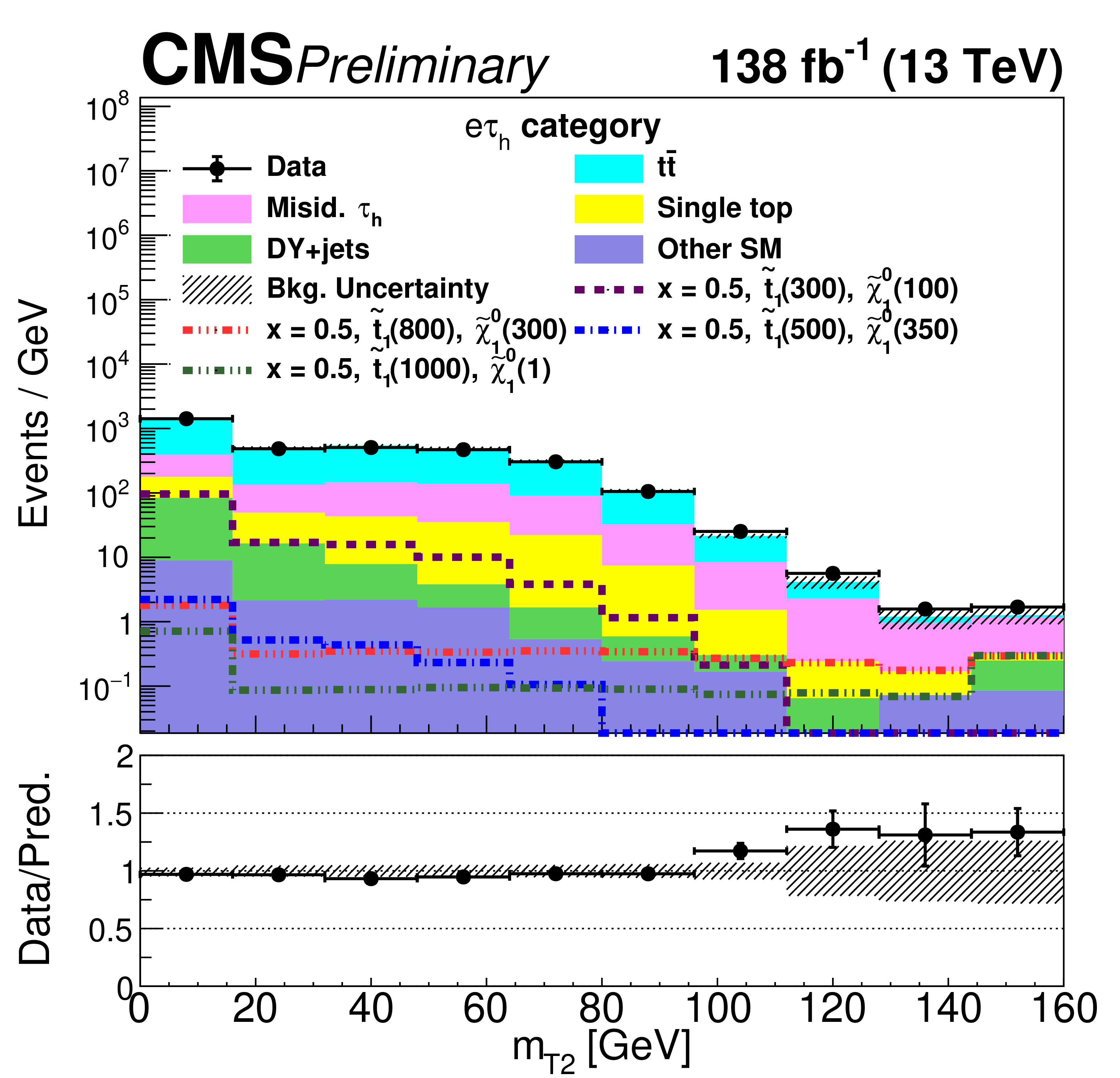
Figure 2-b:
Distributions of the search variables $ p_{\mathrm{T}}^\text{miss} $, $ m_{\mathrm{T2}} $, and $ S_{\mathrm{T}} $ after event selection, for data and the predicted background, corresponding to the e $ \tau_\mathrm{h} $ category. The histograms for the background processes are stacked, and the distributions for a few representative signal points corresponding to $ x = $ 0.5 and [$ m_{\tilde{\mathrm{t}}_{1}} $, $ m_{\tilde{\chi}_{1}^{0}} $] = [300, 100], [500, 350], [800, 300], and [1000, 1] GeV are overlaid. The lower panel indicates the ratio of the observed data to the background prediction. The shaded bands indicate the statistical and systematic uncertainties on the background, added in quadrature. |
png pdf |
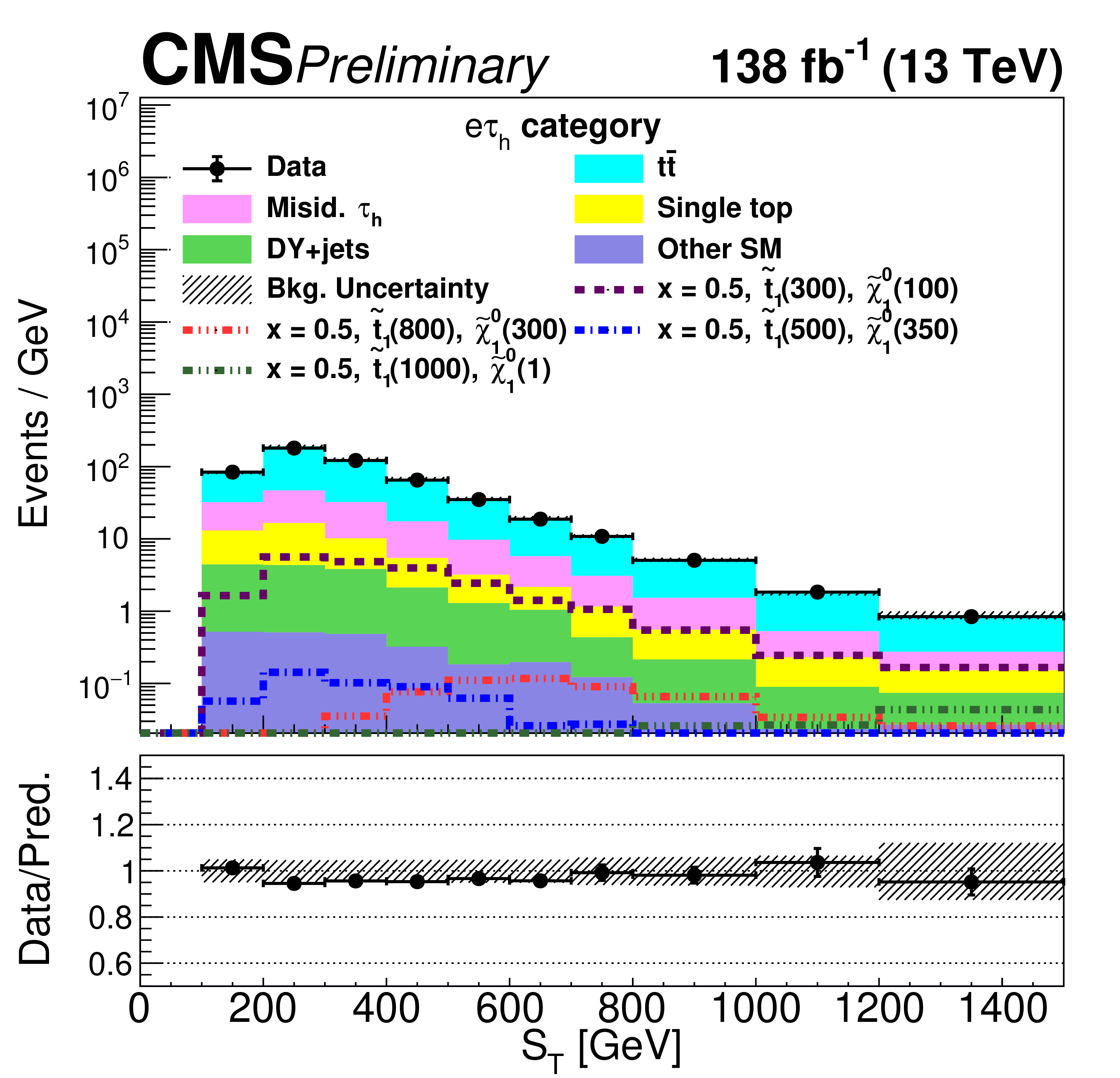
Figure 2-c:
Distributions of the search variables $ p_{\mathrm{T}}^\text{miss} $, $ m_{\mathrm{T2}} $, and $ S_{\mathrm{T}} $ after event selection, for data and the predicted background, corresponding to the e $ \tau_\mathrm{h} $ category. The histograms for the background processes are stacked, and the distributions for a few representative signal points corresponding to $ x = $ 0.5 and [$ m_{\tilde{\mathrm{t}}_{1}} $, $ m_{\tilde{\chi}_{1}^{0}} $] = [300, 100], [500, 350], [800, 300], and [1000, 1] GeV are overlaid. The lower panel indicates the ratio of the observed data to the background prediction. The shaded bands indicate the statistical and systematic uncertainties on the background, added in quadrature. |
png pdf |
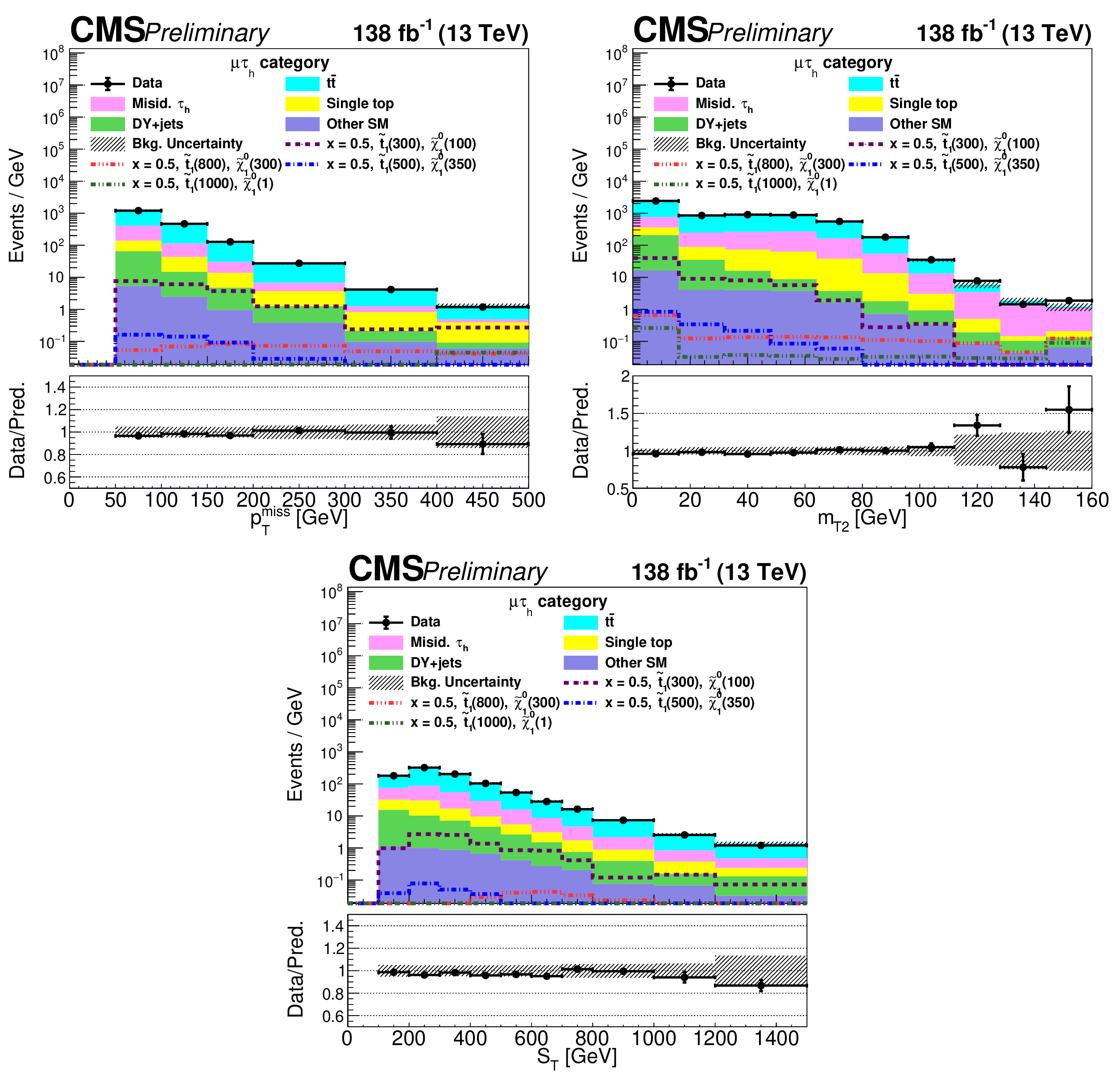
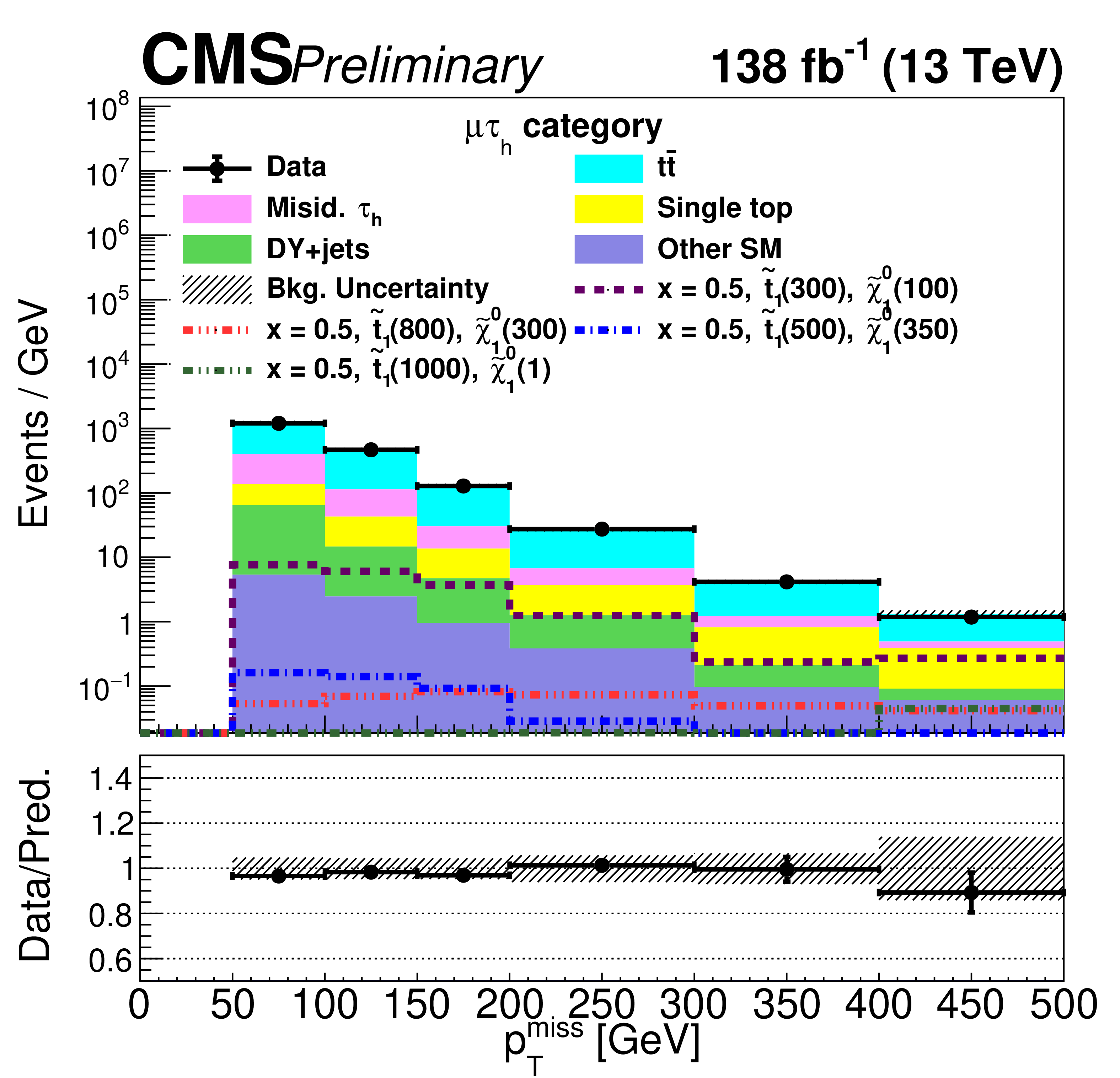
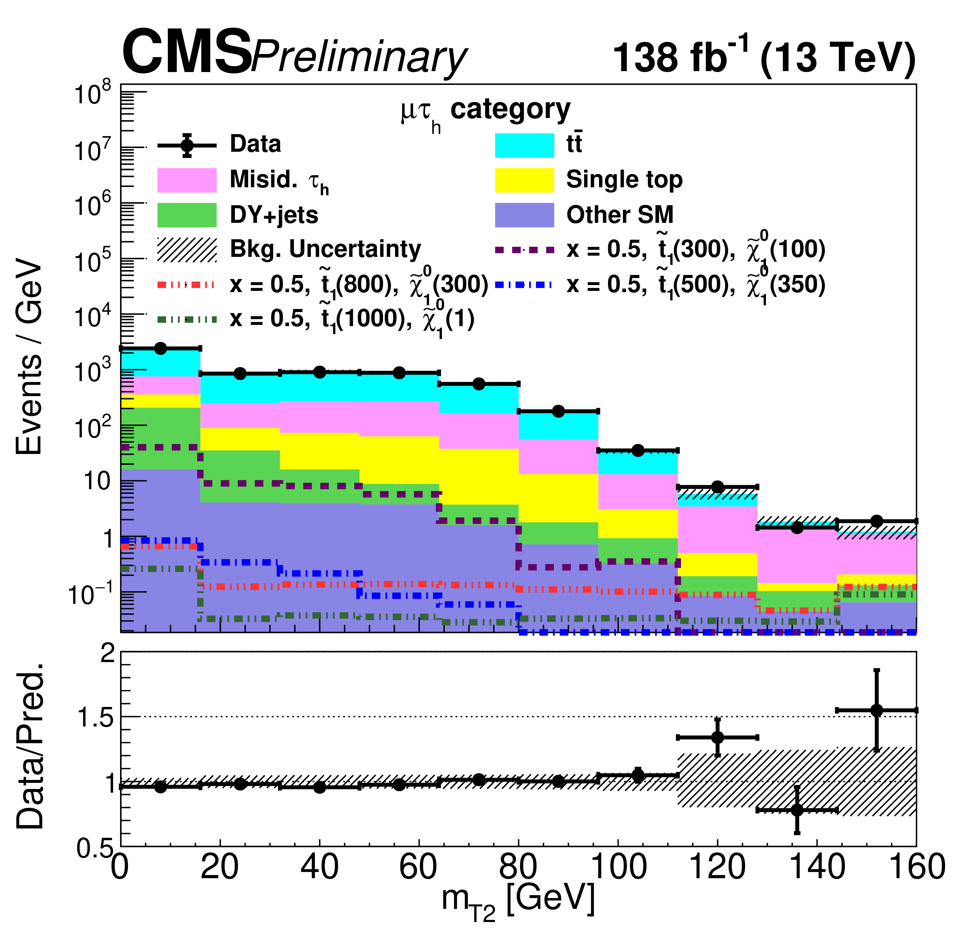
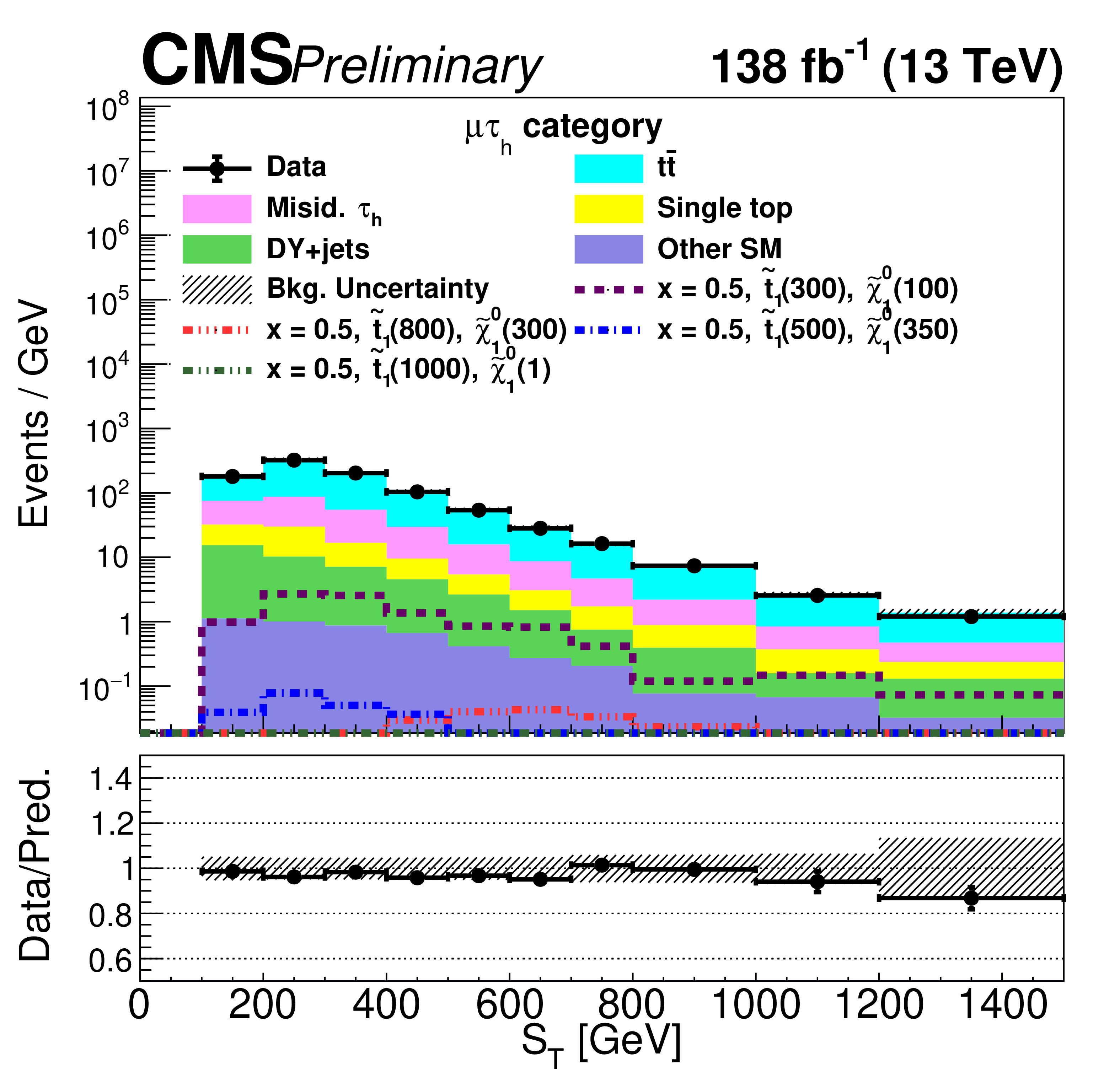
Figure 3:
Distributions of the search variables $ p_{\mathrm{T}}^\text{miss} $, $ m_{\mathrm{T2}} $, and $ S_{\mathrm{T}} $ after event selection, for data and the predicted background, corresponding to the $ \mu \tau_\mathrm{h} $ category. The histograms for the background processes are stacked, and the distributions for a few representative signal points corresponding to $ x = $ 0.5 and [$ m_{\tilde{\mathrm{t}}_{1}} $, $ m_{\tilde{\chi}_{1}^{0}} $] = [300, 100], [500, 350], [800, 300], and [1000, 1] GeV are overlaid. The lower panel indicates the ratio of the observed data to the background prediction. The shaded bands indicate the statistical and systematic uncertainties on the background, added in quadrature. |
png pdf |
Figure 3-a:
Distributions of the search variables $ p_{\mathrm{T}}^\text{miss} $, $ m_{\mathrm{T2}} $, and $ S_{\mathrm{T}} $ after event selection, for data and the predicted background, corresponding to the $ \mu \tau_\mathrm{h} $ category. The histograms for the background processes are stacked, and the distributions for a few representative signal points corresponding to $ x = $ 0.5 and [$ m_{\tilde{\mathrm{t}}_{1}} $, $ m_{\tilde{\chi}_{1}^{0}} $] = [300, 100], [500, 350], [800, 300], and [1000, 1] GeV are overlaid. The lower panel indicates the ratio of the observed data to the background prediction. The shaded bands indicate the statistical and systematic uncertainties on the background, added in quadrature. |
png pdf |
Figure 3-b:
Distributions of the search variables $ p_{\mathrm{T}}^\text{miss} $, $ m_{\mathrm{T2}} $, and $ S_{\mathrm{T}} $ after event selection, for data and the predicted background, corresponding to the $ \mu \tau_\mathrm{h} $ category. The histograms for the background processes are stacked, and the distributions for a few representative signal points corresponding to $ x = $ 0.5 and [$ m_{\tilde{\mathrm{t}}_{1}} $, $ m_{\tilde{\chi}_{1}^{0}} $] = [300, 100], [500, 350], [800, 300], and [1000, 1] GeV are overlaid. The lower panel indicates the ratio of the observed data to the background prediction. The shaded bands indicate the statistical and systematic uncertainties on the background, added in quadrature. |
png pdf |
Figure 3-c:
Distributions of the search variables $ p_{\mathrm{T}}^\text{miss} $, $ m_{\mathrm{T2}} $, and $ S_{\mathrm{T}} $ after event selection, for data and the predicted background, corresponding to the $ \mu \tau_\mathrm{h} $ category. The histograms for the background processes are stacked, and the distributions for a few representative signal points corresponding to $ x = $ 0.5 and [$ m_{\tilde{\mathrm{t}}_{1}} $, $ m_{\tilde{\chi}_{1}^{0}} $] = [300, 100], [500, 350], [800, 300], and [1000, 1] GeV are overlaid. The lower panel indicates the ratio of the observed data to the background prediction. The shaded bands indicate the statistical and systematic uncertainties on the background, added in quadrature. |
png pdf |
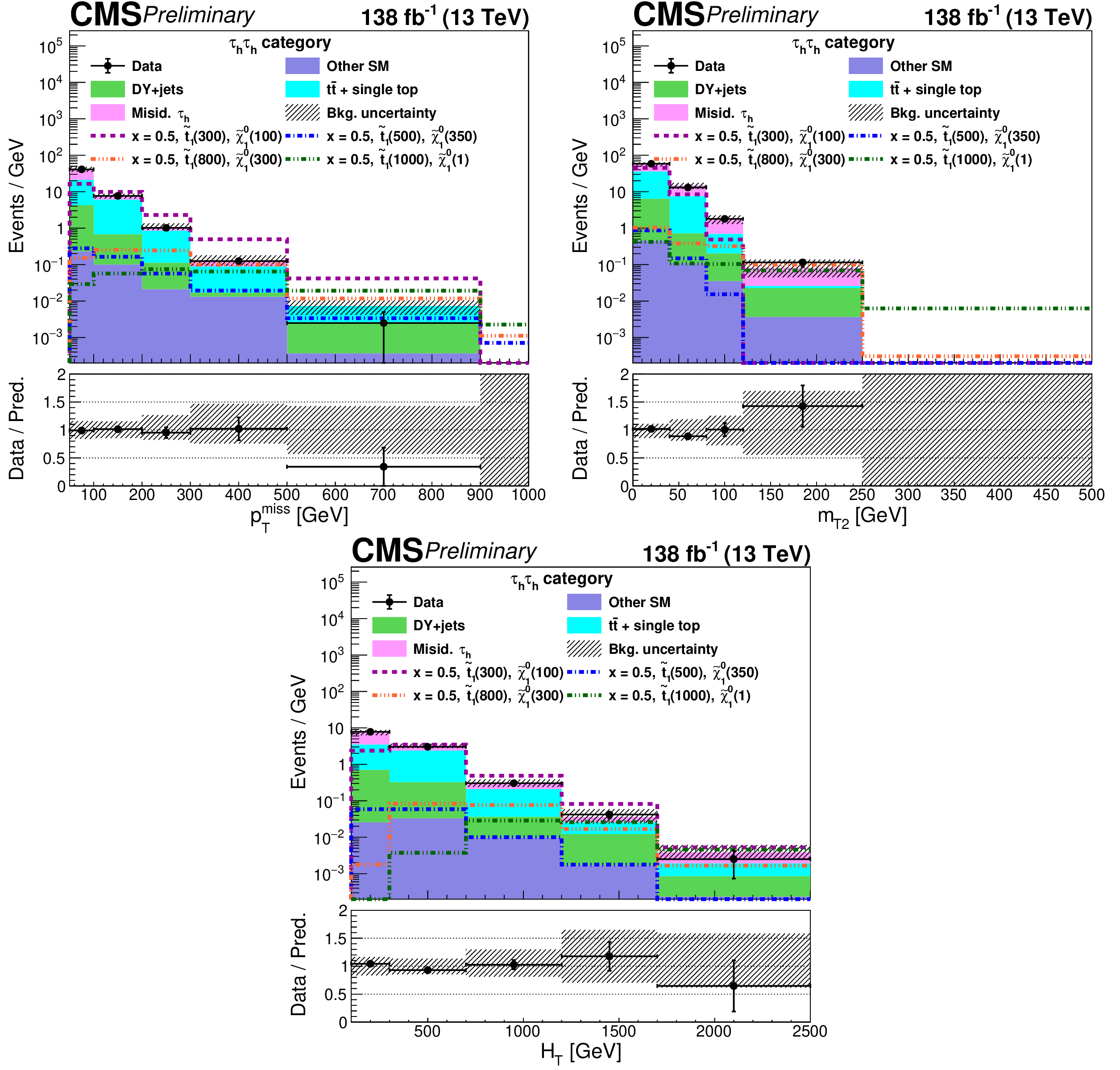
Figure 4:
Distributions of the search variables $ p_{\mathrm{T}}^\text{miss} $, $ m_{\mathrm{T2}} $, and $ H_{\mathrm{T}} $ after event selection, for data and the predicted background, corresponding to the $ \tau_\mathrm{h} \tau_\mathrm{h} $ category. The histograms for the background processes are stacked, and the distributions for a few representative signal points corresponding to $ x = $ 0.5 and [$ m_{\tilde{\mathrm{t}}_{1}} $, $ m_{\tilde{\chi}_{1}^{0}} $] = [300, 100], [500, 350], [800, 300], and [1000, 1] GeV are overlaid. The lower panel indicates the ratio of the observed data to the background prediction. The shaded bands indicate the statistical and systematic uncertainties on the background, added in quadrature. |
png pdf |
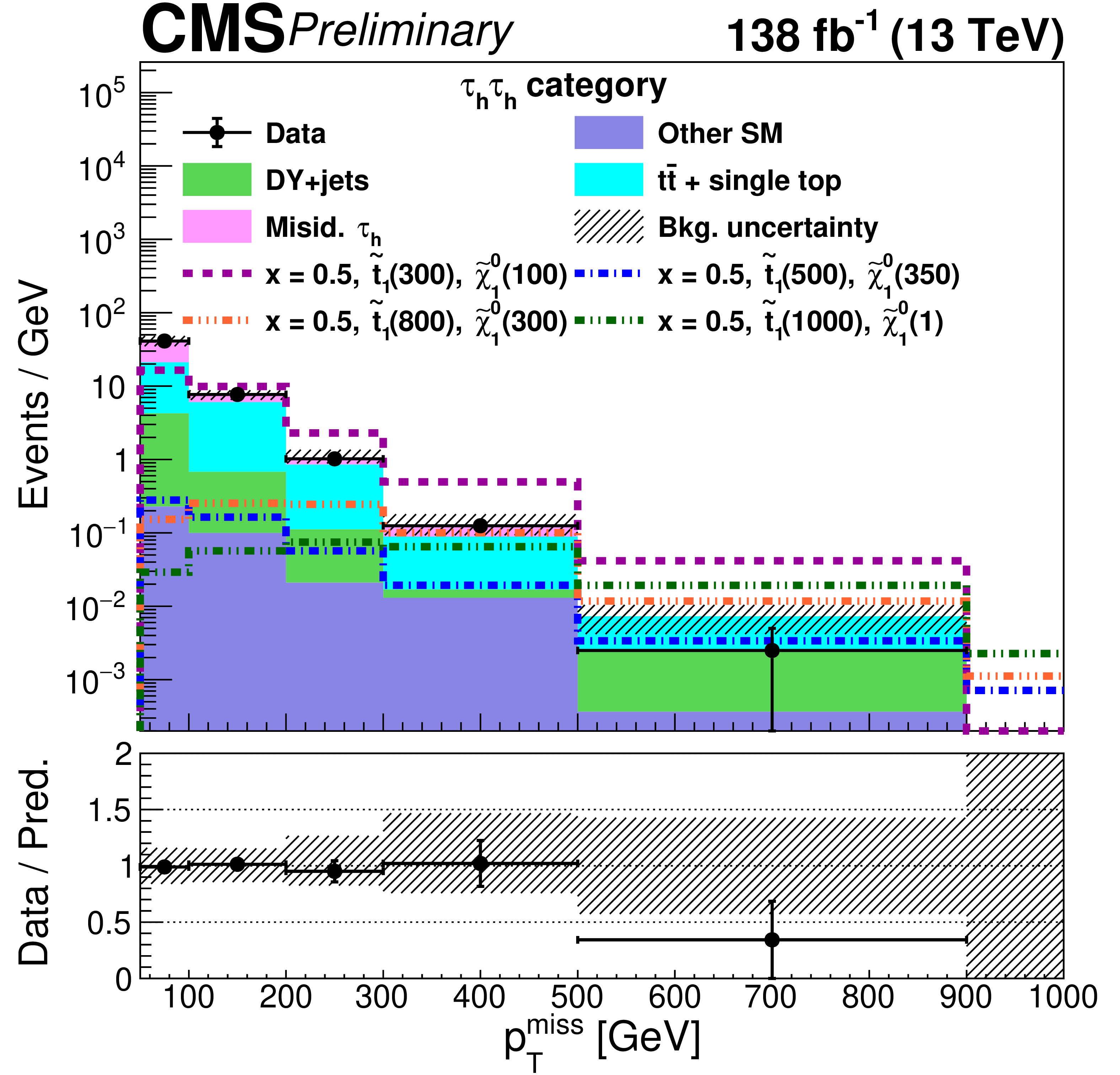
Figure 4-a:
Distributions of the search variables $ p_{\mathrm{T}}^\text{miss} $, $ m_{\mathrm{T2}} $, and $ H_{\mathrm{T}} $ after event selection, for data and the predicted background, corresponding to the $ \tau_\mathrm{h} \tau_\mathrm{h} $ category. The histograms for the background processes are stacked, and the distributions for a few representative signal points corresponding to $ x = $ 0.5 and [$ m_{\tilde{\mathrm{t}}_{1}} $, $ m_{\tilde{\chi}_{1}^{0}} $] = [300, 100], [500, 350], [800, 300], and [1000, 1] GeV are overlaid. The lower panel indicates the ratio of the observed data to the background prediction. The shaded bands indicate the statistical and systematic uncertainties on the background, added in quadrature. |
png pdf |
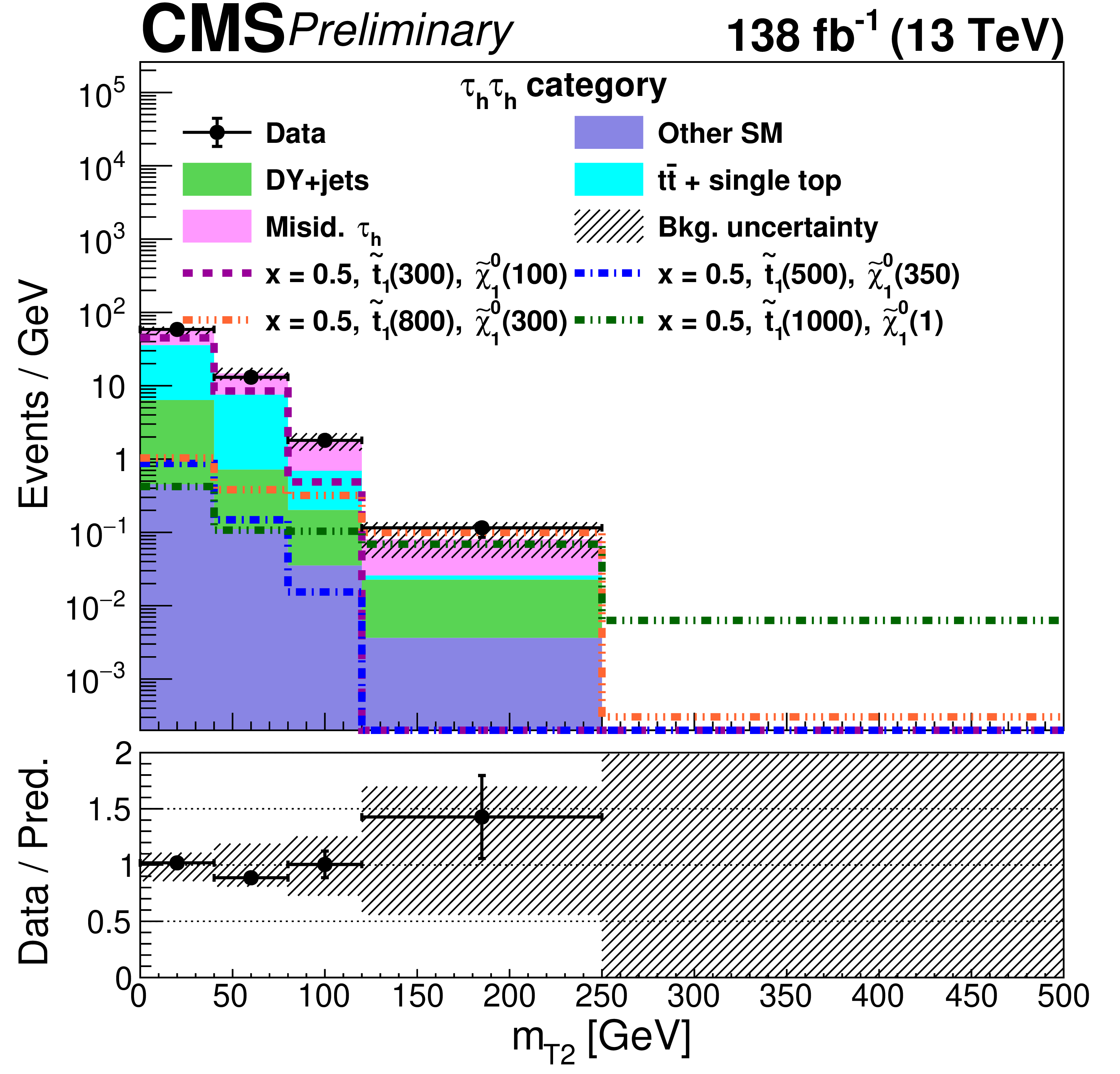
Figure 4-b:
Distributions of the search variables $ p_{\mathrm{T}}^\text{miss} $, $ m_{\mathrm{T2}} $, and $ H_{\mathrm{T}} $ after event selection, for data and the predicted background, corresponding to the $ \tau_\mathrm{h} \tau_\mathrm{h} $ category. The histograms for the background processes are stacked, and the distributions for a few representative signal points corresponding to $ x = $ 0.5 and [$ m_{\tilde{\mathrm{t}}_{1}} $, $ m_{\tilde{\chi}_{1}^{0}} $] = [300, 100], [500, 350], [800, 300], and [1000, 1] GeV are overlaid. The lower panel indicates the ratio of the observed data to the background prediction. The shaded bands indicate the statistical and systematic uncertainties on the background, added in quadrature. |
png pdf |
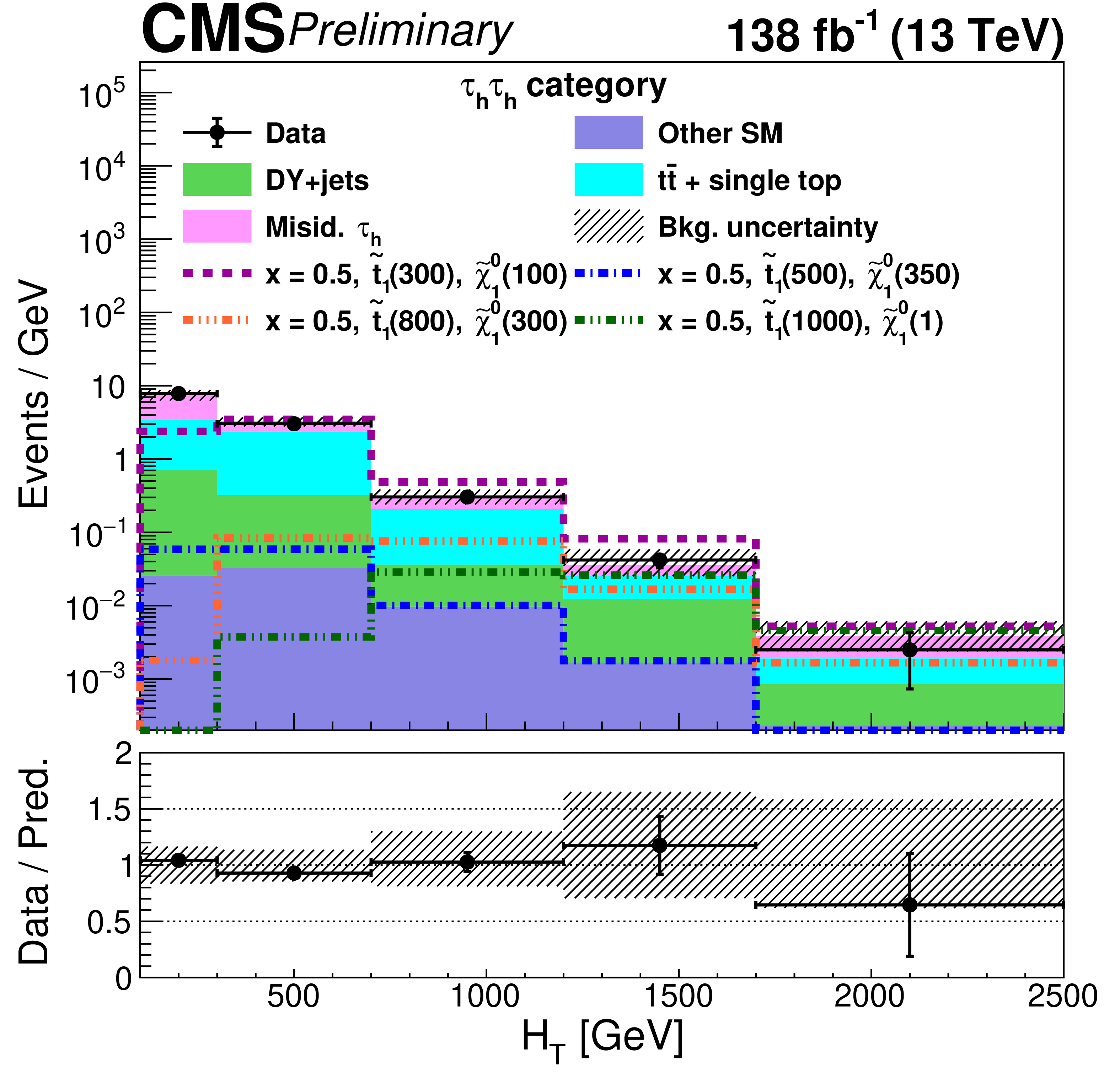
Figure 4-c:
Distributions of the search variables $ p_{\mathrm{T}}^\text{miss} $, $ m_{\mathrm{T2}} $, and $ H_{\mathrm{T}} $ after event selection, for data and the predicted background, corresponding to the $ \tau_\mathrm{h} \tau_\mathrm{h} $ category. The histograms for the background processes are stacked, and the distributions for a few representative signal points corresponding to $ x = $ 0.5 and [$ m_{\tilde{\mathrm{t}}_{1}} $, $ m_{\tilde{\chi}_{1}^{0}} $] = [300, 100], [500, 350], [800, 300], and [1000, 1] GeV are overlaid. The lower panel indicates the ratio of the observed data to the background prediction. The shaded bands indicate the statistical and systematic uncertainties on the background, added in quadrature. |
png pdf |
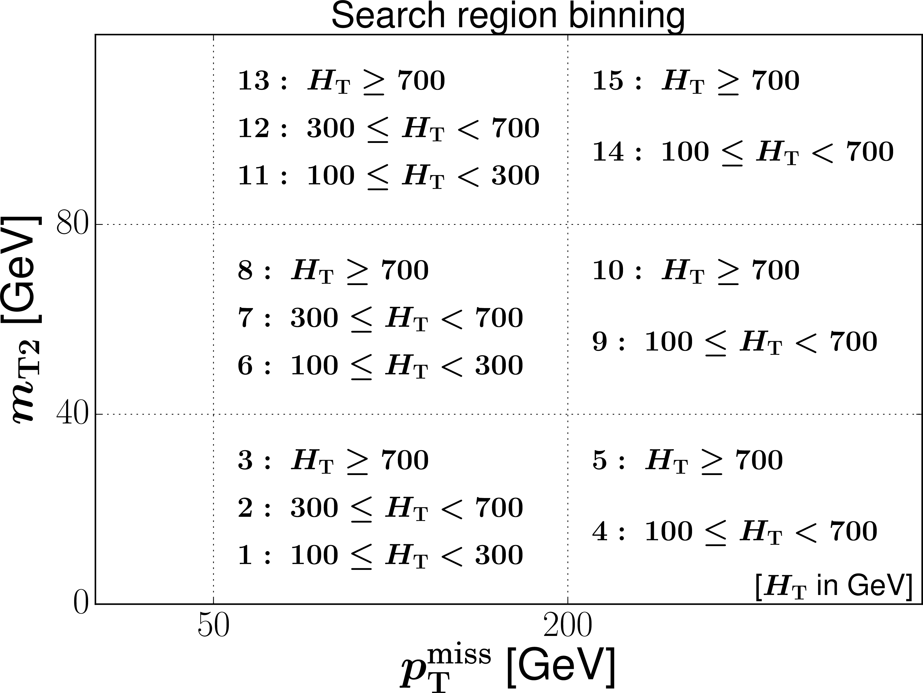
Figure 5:
The 15 search regions defined in bins of $ p_{\mathrm{T}}^\text{miss} $, $ m_{\mathrm{T2}} $, and $ H_{\mathrm{T}} $. The bin boundaries for $ S_{\mathrm{T}} $ are the same those for $ H_{\mathrm{T}} $. |
png pdf |
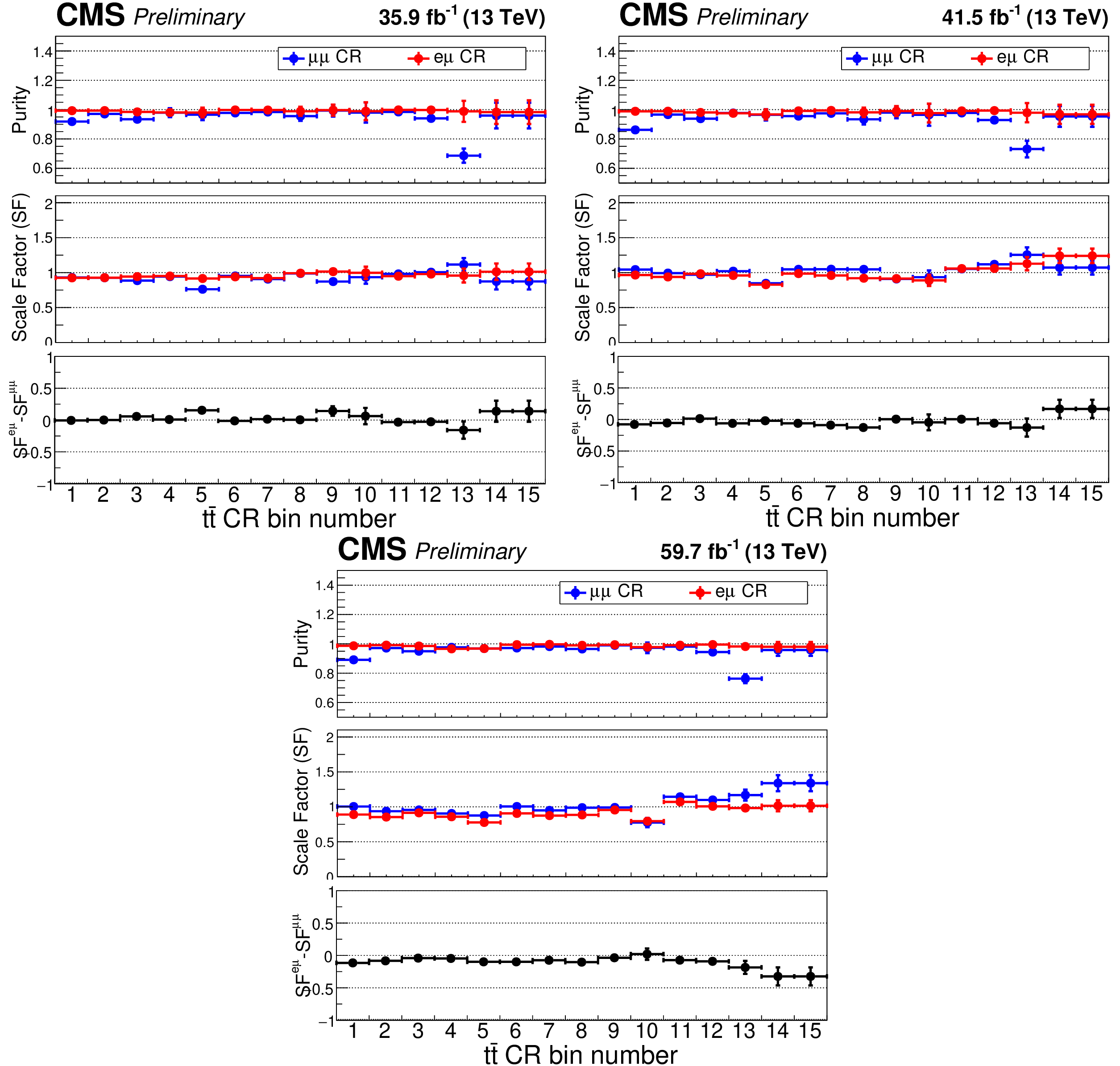
Figure 6:
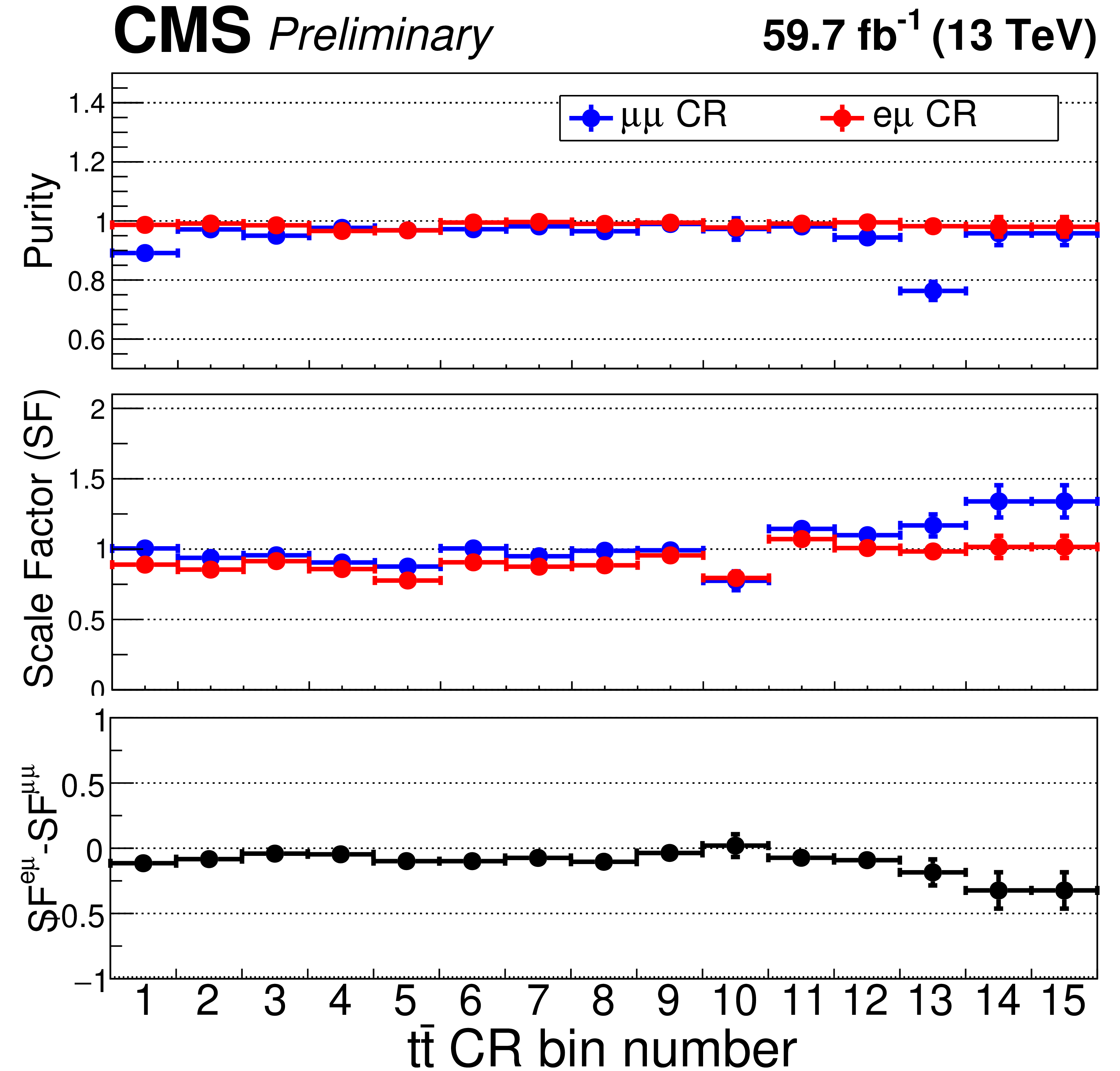
The top, middle and bottom panels of each sub-figure show the purities, scale factors, and $ \text{SF}^{\mathrm{e} \mu} - \text{SF}^{\mu \mu} $, respectively, in the different bins (as defined in Fig. 5) of the $ \mathrm{t}\overline{\mathrm{t}} $ CR. The upper left, upper right, and lower sub-figures correspond to 2016, 2017, and 2018 data, respectively. Note that in order to mitigate the effect of statistical fluctuations, bins 14 and 15 are merged to provide the same SF in both the bins for subsequent calculations. |
png pdf |
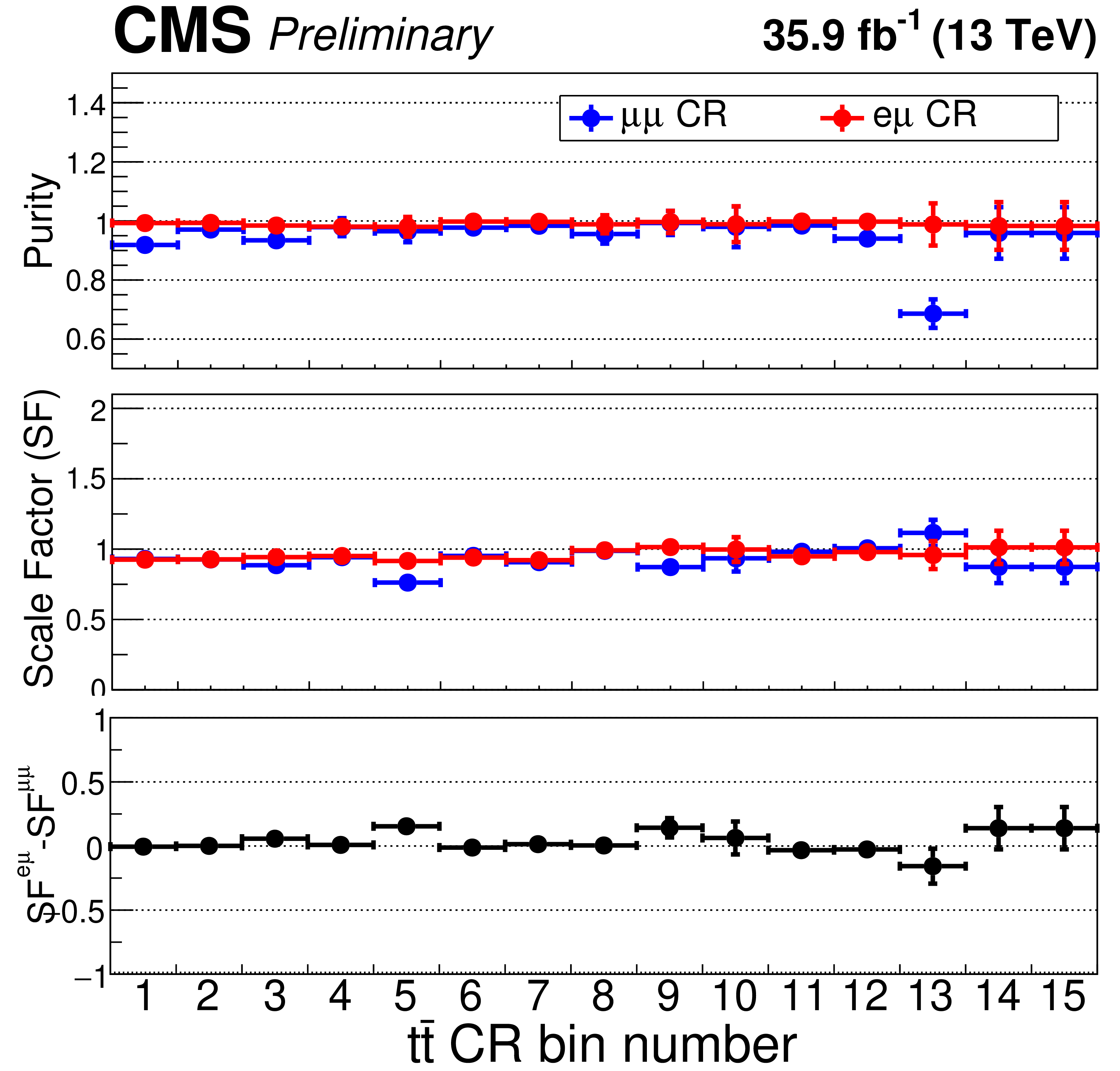
Figure 6-a:
The top, middle and bottom panels of each sub-figure show the purities, scale factors, and $ \text{SF}^{\mathrm{e} \mu} - \text{SF}^{\mu \mu} $, respectively, in the different bins (as defined in Fig. 5) of the $ \mathrm{t}\overline{\mathrm{t}} $ CR. The upper left, upper right, and lower sub-figures correspond to 2016, 2017, and 2018 data, respectively. Note that in order to mitigate the effect of statistical fluctuations, bins 14 and 15 are merged to provide the same SF in both the bins for subsequent calculations. |
png pdf |
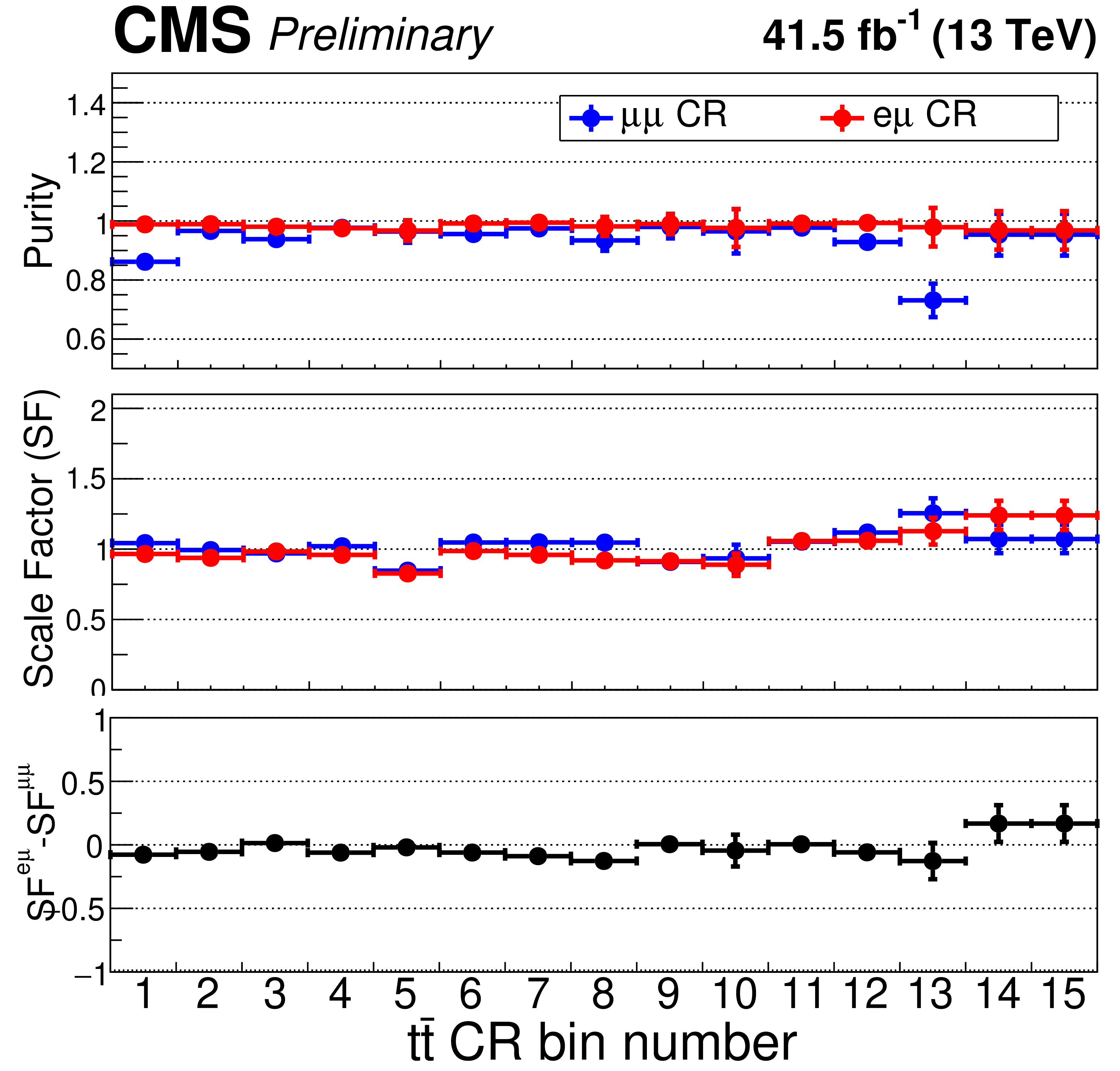
Figure 6-b:
The top, middle and bottom panels of each sub-figure show the purities, scale factors, and $ \text{SF}^{\mathrm{e} \mu} - \text{SF}^{\mu \mu} $, respectively, in the different bins (as defined in Fig. 5) of the $ \mathrm{t}\overline{\mathrm{t}} $ CR. The upper left, upper right, and lower sub-figures correspond to 2016, 2017, and 2018 data, respectively. Note that in order to mitigate the effect of statistical fluctuations, bins 14 and 15 are merged to provide the same SF in both the bins for subsequent calculations. |
png pdf |
Figure 6-c:
The top, middle and bottom panels of each sub-figure show the purities, scale factors, and $ \text{SF}^{\mathrm{e} \mu} - \text{SF}^{\mu \mu} $, respectively, in the different bins (as defined in Fig. 5) of the $ \mathrm{t}\overline{\mathrm{t}} $ CR. The upper left, upper right, and lower sub-figures correspond to 2016, 2017, and 2018 data, respectively. Note that in order to mitigate the effect of statistical fluctuations, bins 14 and 15 are merged to provide the same SF in both the bins for subsequent calculations. |
png pdf |
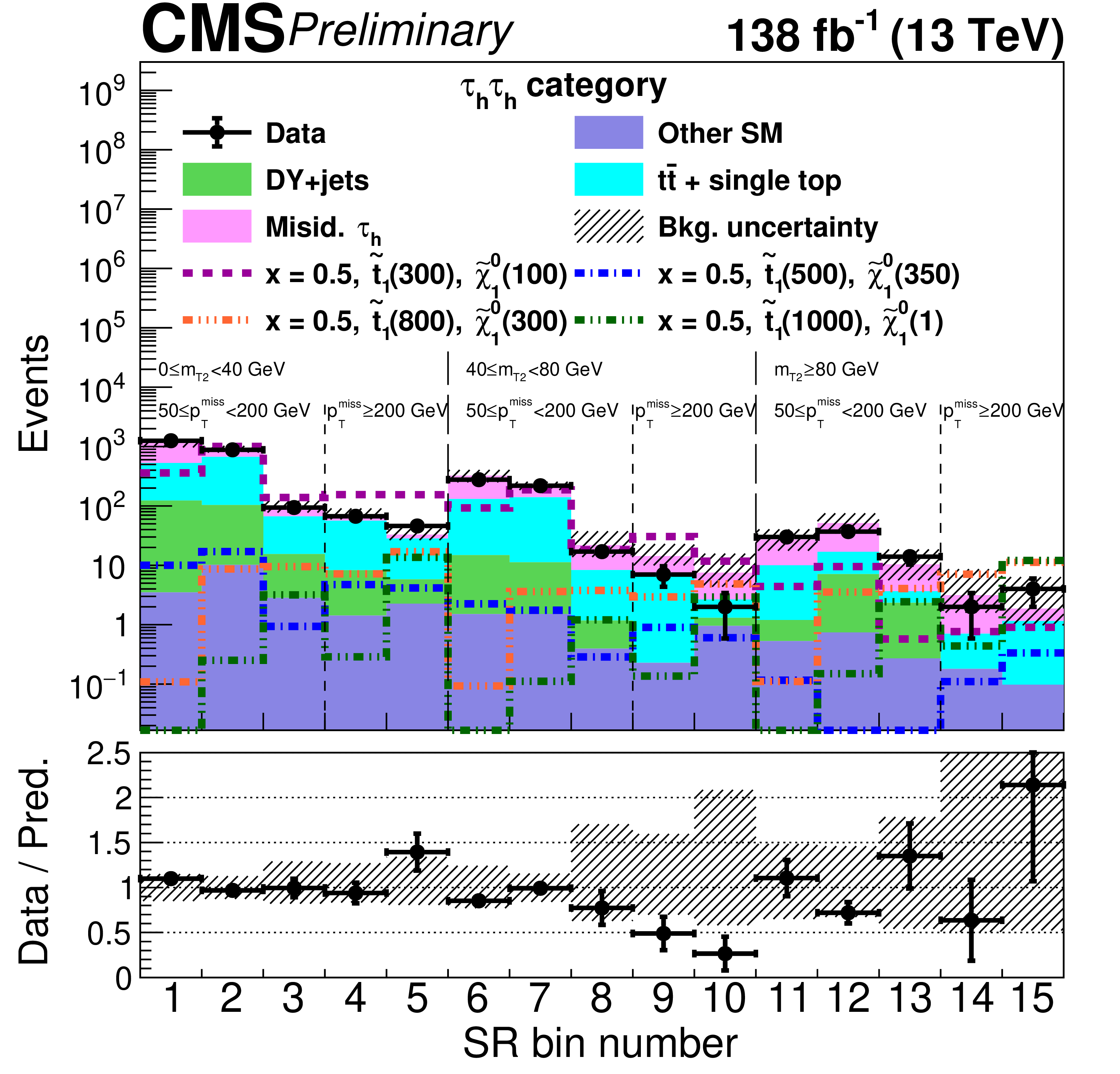
Figure 7:
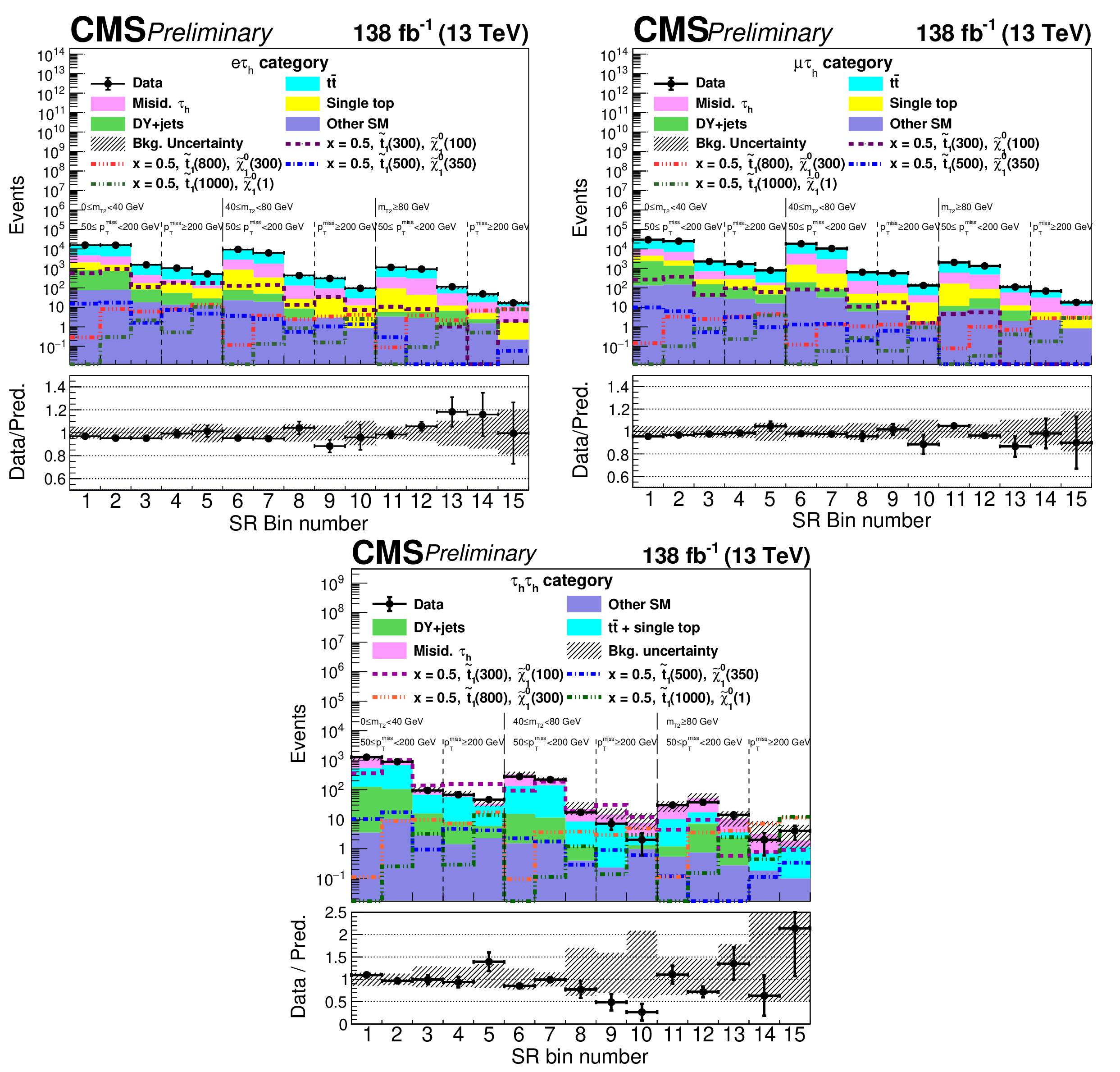
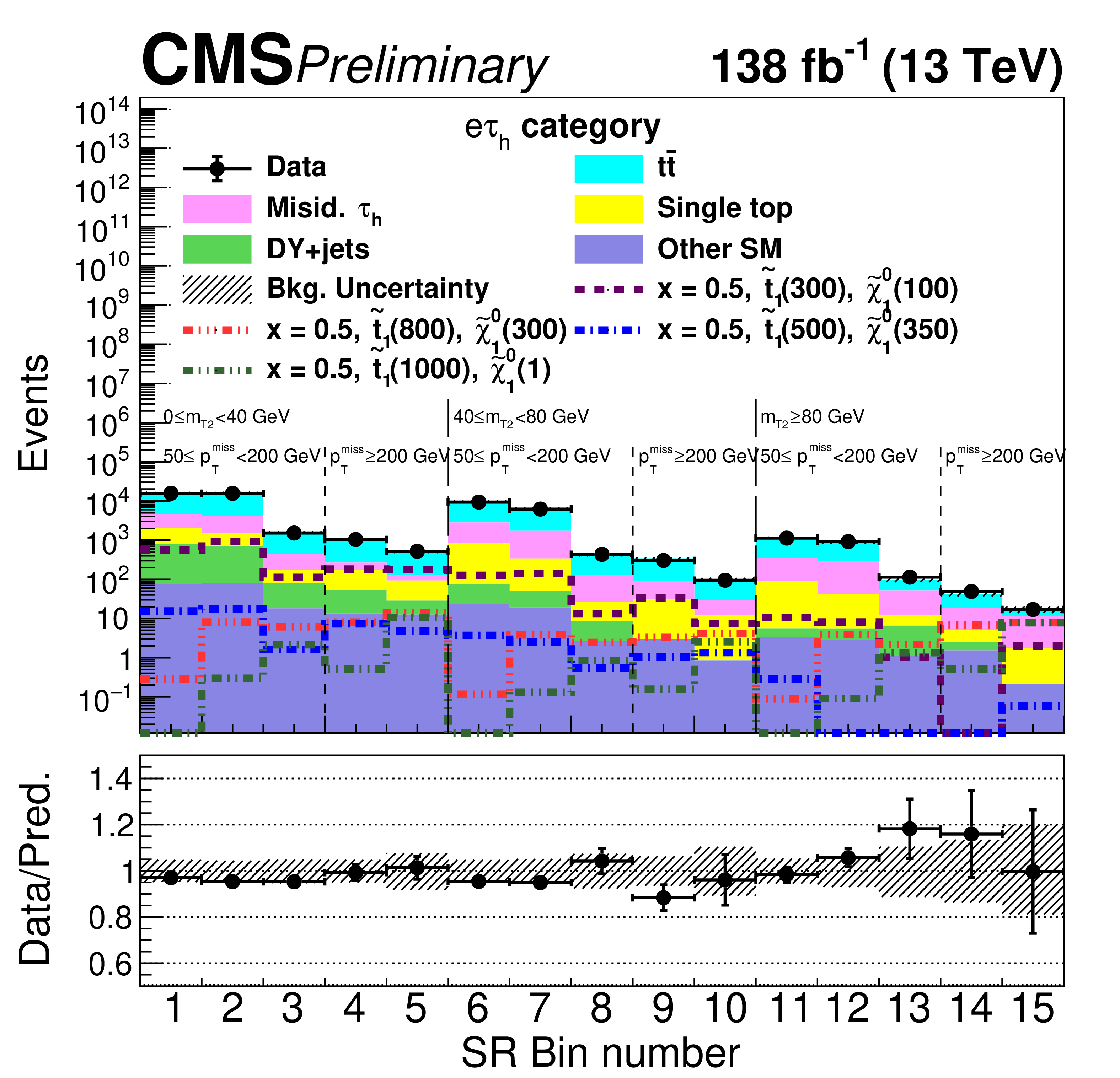
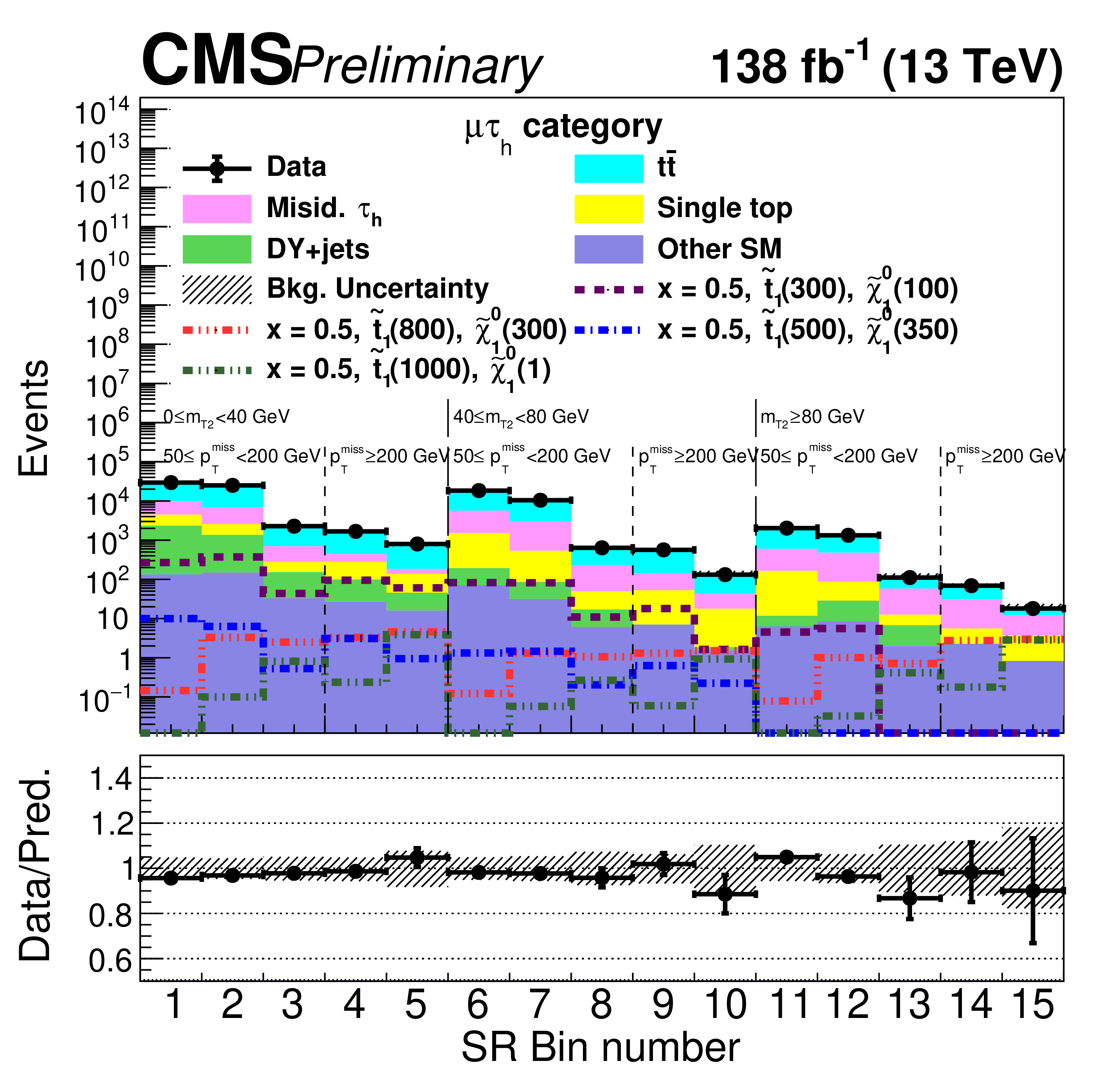
Event yields in the 15 search bins as defined in Fig. 5, for the $ \mathrm{e}\tau_\mathrm{h} $ (upper left), $ \mu\tau_\mathrm{h} $ (upper right), and $ \tau_\mathrm{h} \tau_\mathrm{h} $ (lower) categories. The yields for the background processes are stacked, and those for a few representative signal points corresponding to $ x = $ 0.5 and [$ m_{\tilde{\mathrm{t}}_{1}} $, $ m_{\tilde{\chi}_{1}^{0}} $] = [300, 100], [500, 350], [800, 300], and [1000, 1] GeV are overlaid. The lower panel indicates the ratio of the observed data to the background prediction in each bin. The shaded bands indicate the statistical and systematic uncertainties in the background, added in quadrature. |
png pdf |
Figure 7-a:
Event yields in the 15 search bins as defined in Fig. 5, for the $ \mathrm{e}\tau_\mathrm{h} $ (upper left), $ \mu\tau_\mathrm{h} $ (upper right), and $ \tau_\mathrm{h} \tau_\mathrm{h} $ (lower) categories. The yields for the background processes are stacked, and those for a few representative signal points corresponding to $ x = $ 0.5 and [$ m_{\tilde{\mathrm{t}}_{1}} $, $ m_{\tilde{\chi}_{1}^{0}} $] = [300, 100], [500, 350], [800, 300], and [1000, 1] GeV are overlaid. The lower panel indicates the ratio of the observed data to the background prediction in each bin. The shaded bands indicate the statistical and systematic uncertainties in the background, added in quadrature. |
png pdf |
Figure 7-b:
Event yields in the 15 search bins as defined in Fig. 5, for the $ \mathrm{e}\tau_\mathrm{h} $ (upper left), $ \mu\tau_\mathrm{h} $ (upper right), and $ \tau_\mathrm{h} \tau_\mathrm{h} $ (lower) categories. The yields for the background processes are stacked, and those for a few representative signal points corresponding to $ x = $ 0.5 and [$ m_{\tilde{\mathrm{t}}_{1}} $, $ m_{\tilde{\chi}_{1}^{0}} $] = [300, 100], [500, 350], [800, 300], and [1000, 1] GeV are overlaid. The lower panel indicates the ratio of the observed data to the background prediction in each bin. The shaded bands indicate the statistical and systematic uncertainties in the background, added in quadrature. |
png pdf |
Figure 7-c:
Event yields in the 15 search bins as defined in Fig. 5, for the $ \mathrm{e}\tau_\mathrm{h} $ (upper left), $ \mu\tau_\mathrm{h} $ (upper right), and $ \tau_\mathrm{h} \tau_\mathrm{h} $ (lower) categories. The yields for the background processes are stacked, and those for a few representative signal points corresponding to $ x = $ 0.5 and [$ m_{\tilde{\mathrm{t}}_{1}} $, $ m_{\tilde{\chi}_{1}^{0}} $] = [300, 100], [500, 350], [800, 300], and [1000, 1] GeV are overlaid. The lower panel indicates the ratio of the observed data to the background prediction in each bin. The shaded bands indicate the statistical and systematic uncertainties in the background, added in quadrature. |
png pdf |
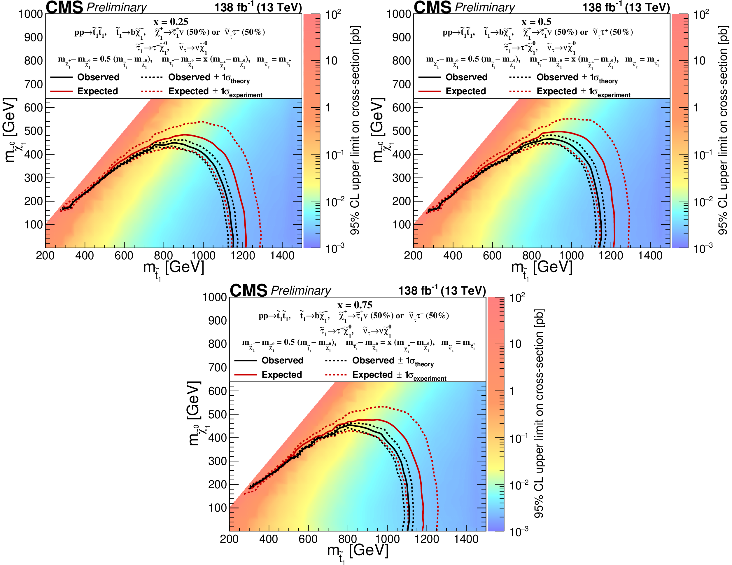
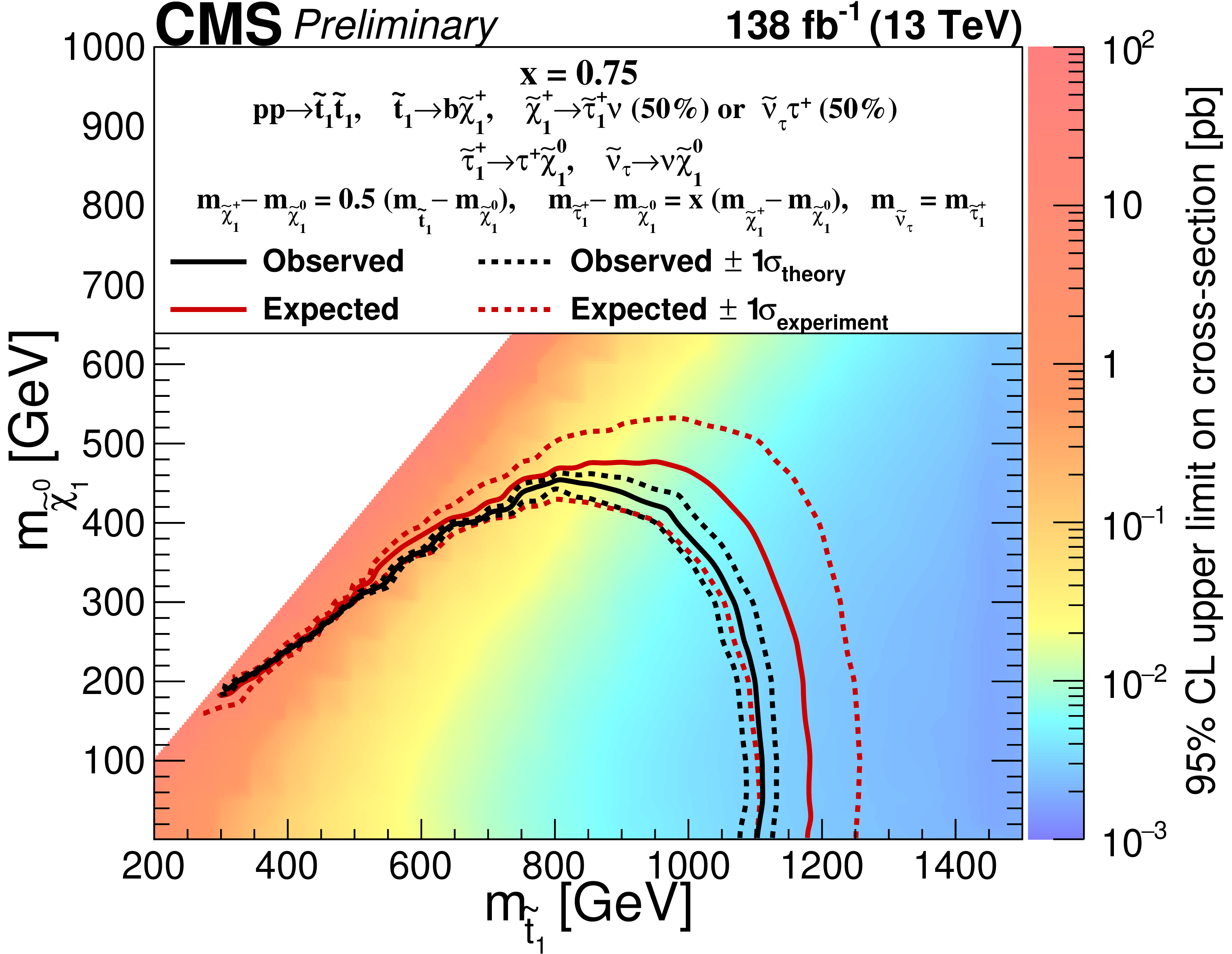
Figure 8:
Exclusion limits at 95% CL for the pair production of top squarks decaying to $ \tau_{\ell} \tau_\mathrm{h} $ or $ \tau_\mathrm{h} \tau_\mathrm{h} $ final states, displayed in the $ {m_{\tilde{\mathrm{t}}_{1}}}-m_{\tilde{\chi}_{1}^{0}} $ plane for $ x = $ 0.25 (upper left), 0.5 (upper right) and 0.75 (lower), as described in Eq. (1). The color axis represents the observed limit in the cross section, while the black (red) lines represent the observed (expected) mass limits. The signal cross sections are evaluated using NNLO plus next-to-leading logarithmic (NLL) calculations. The solid lines represent the central values. The dashed red lines indicate the region containing 68% of the distribution of limits expected under the background-only hypothesis. The dashed black lines show the change in the observed limit due to variation of the signal cross sections within their theoretical uncertainties. |
png pdf |
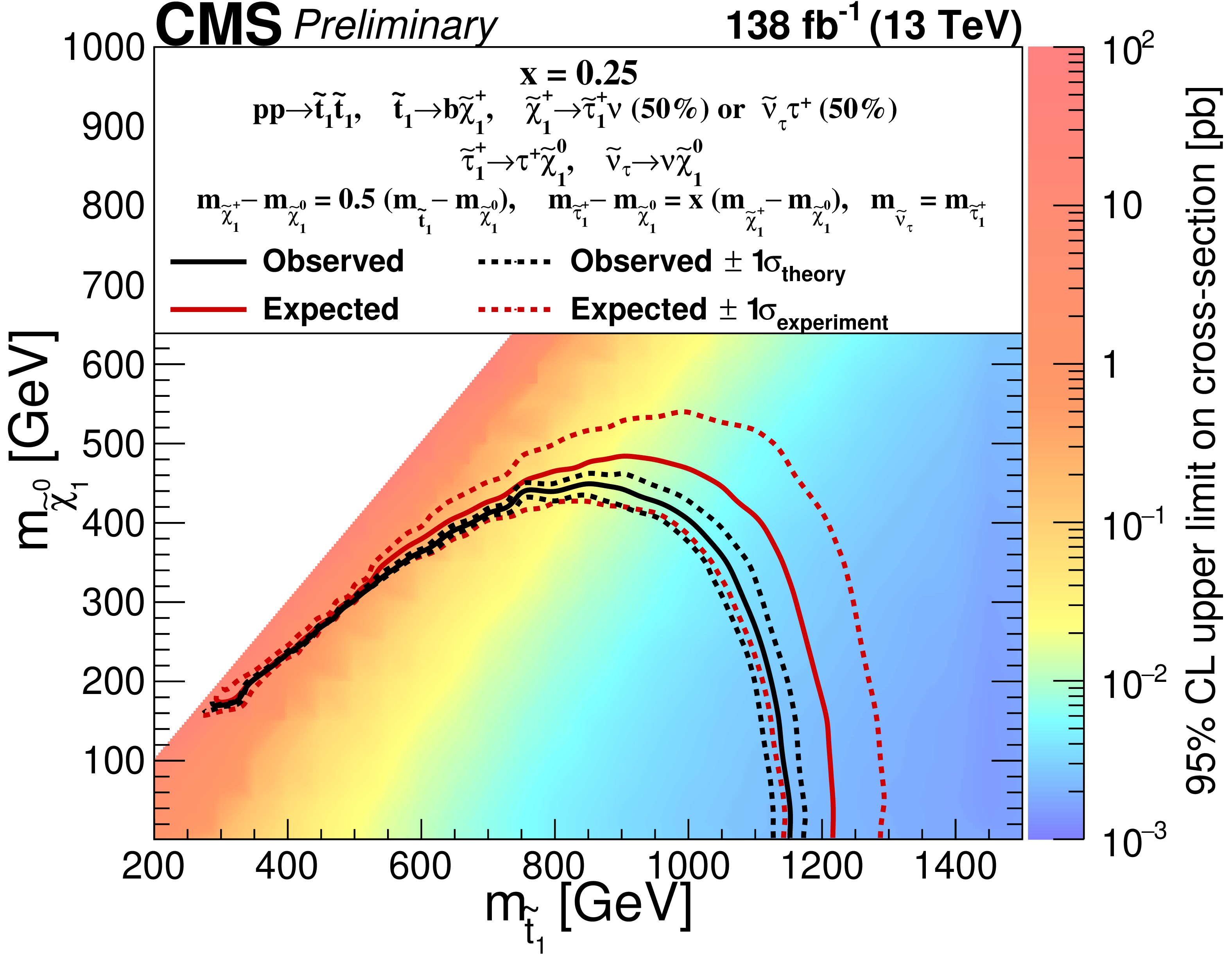
Figure 8-a:
Exclusion limits at 95% CL for the pair production of top squarks decaying to $ \tau_{\ell} \tau_\mathrm{h} $ or $ \tau_\mathrm{h} \tau_\mathrm{h} $ final states, displayed in the $ {m_{\tilde{\mathrm{t}}_{1}}}-m_{\tilde{\chi}_{1}^{0}} $ plane for $ x = $ 0.25 (upper left), 0.5 (upper right) and 0.75 (lower), as described in Eq. (1). The color axis represents the observed limit in the cross section, while the black (red) lines represent the observed (expected) mass limits. The signal cross sections are evaluated using NNLO plus next-to-leading logarithmic (NLL) calculations. The solid lines represent the central values. The dashed red lines indicate the region containing 68% of the distribution of limits expected under the background-only hypothesis. The dashed black lines show the change in the observed limit due to variation of the signal cross sections within their theoretical uncertainties. |
png pdf |
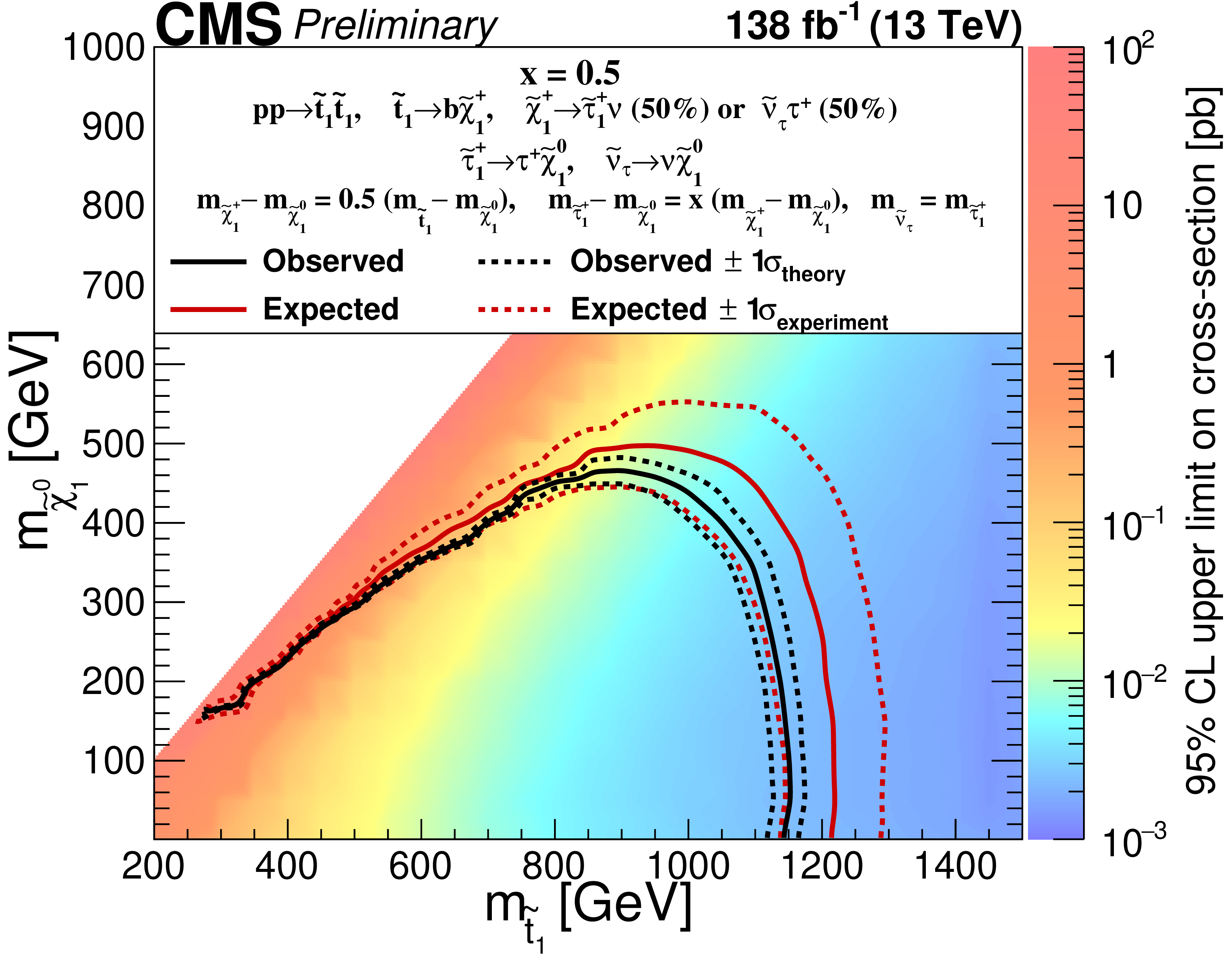
Figure 8-b:
Exclusion limits at 95% CL for the pair production of top squarks decaying to $ \tau_{\ell} \tau_\mathrm{h} $ or $ \tau_\mathrm{h} \tau_\mathrm{h} $ final states, displayed in the $ {m_{\tilde{\mathrm{t}}_{1}}}-m_{\tilde{\chi}_{1}^{0}} $ plane for $ x = $ 0.25 (upper left), 0.5 (upper right) and 0.75 (lower), as described in Eq. (1). The color axis represents the observed limit in the cross section, while the black (red) lines represent the observed (expected) mass limits. The signal cross sections are evaluated using NNLO plus next-to-leading logarithmic (NLL) calculations. The solid lines represent the central values. The dashed red lines indicate the region containing 68% of the distribution of limits expected under the background-only hypothesis. The dashed black lines show the change in the observed limit due to variation of the signal cross sections within their theoretical uncertainties. |
png pdf |
Figure 8-c:
Exclusion limits at 95% CL for the pair production of top squarks decaying to $ \tau_{\ell} \tau_\mathrm{h} $ or $ \tau_\mathrm{h} \tau_\mathrm{h} $ final states, displayed in the $ {m_{\tilde{\mathrm{t}}_{1}}}-m_{\tilde{\chi}_{1}^{0}} $ plane for $ x = $ 0.25 (upper left), 0.5 (upper right) and 0.75 (lower), as described in Eq. (1). The color axis represents the observed limit in the cross section, while the black (red) lines represent the observed (expected) mass limits. The signal cross sections are evaluated using NNLO plus next-to-leading logarithmic (NLL) calculations. The solid lines represent the central values. The dashed red lines indicate the region containing 68% of the distribution of limits expected under the background-only hypothesis. The dashed black lines show the change in the observed limit due to variation of the signal cross sections within their theoretical uncertainties. |
| Tables | |
png pdf |
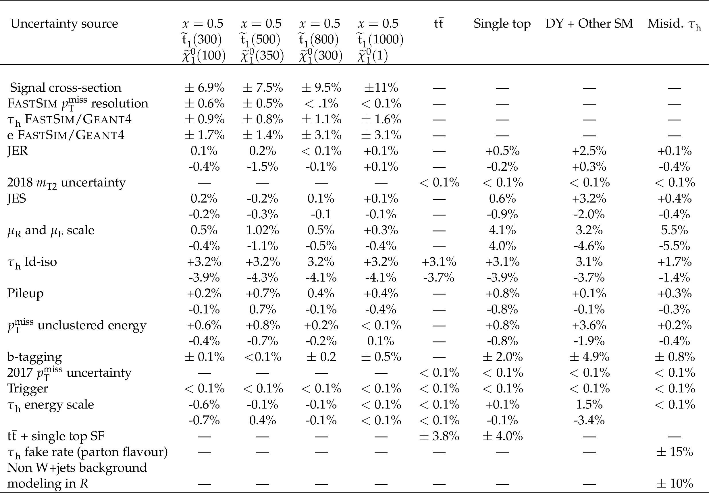
Table 1:
Relative systematic uncertainties from different sources in signal and background yields in the 2016, 2017 and 2018 analyses combined, for the $ \mathrm{e}\tau_\mathrm{h} $ category. These values are the weighted (by the yields in the respective bins) averages of the relative uncertainties in the different search regions. For the asymmetric uncertainties, the upper (lower) entry is the uncertainty due to the upward (downward) variation, which can be in the same direction as a result of taking the weighted average. In the heading, the top squark and LSP masses in GeV are indicated in parentheses. |
png pdf |
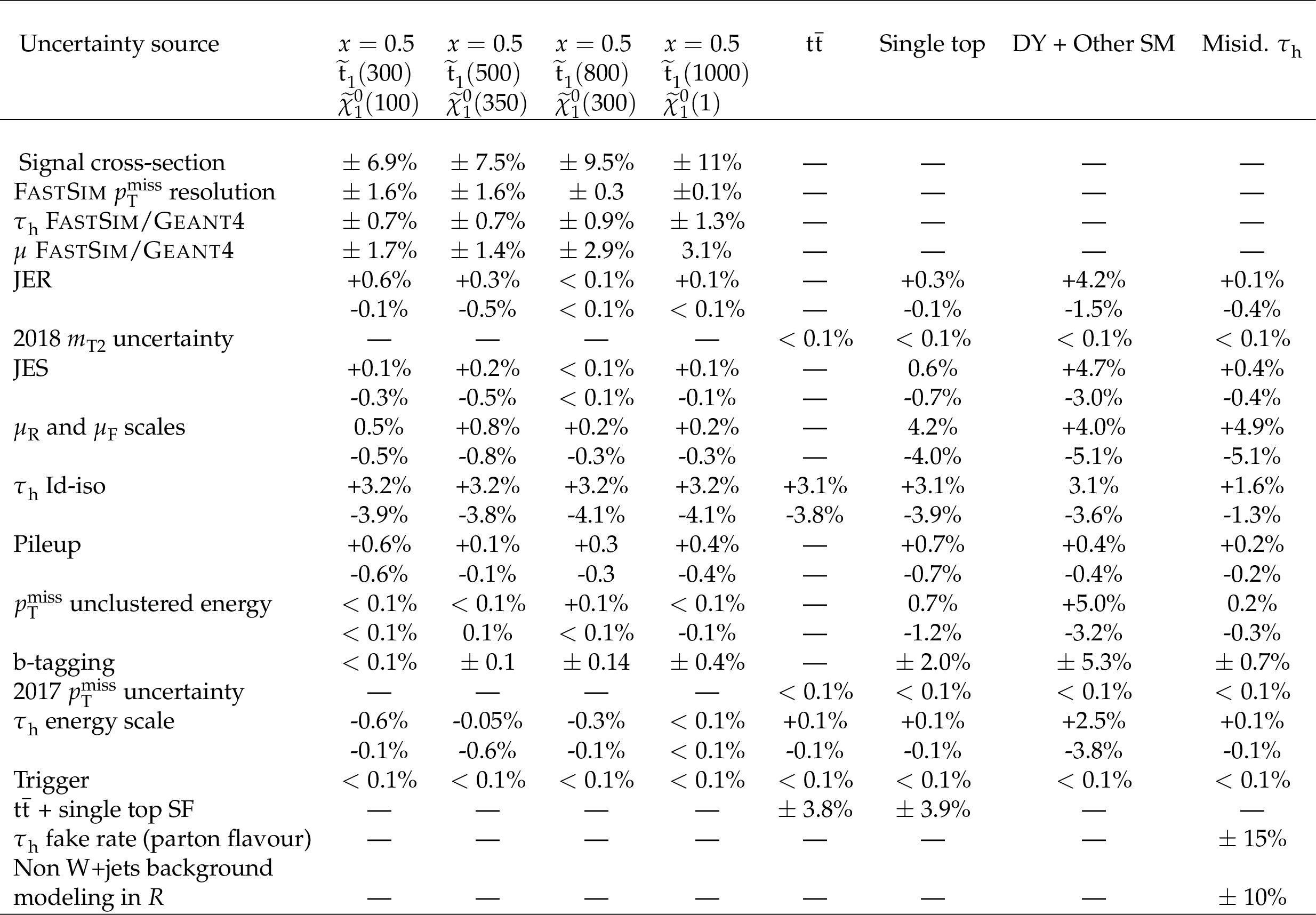
Table 2:
Relative systematic uncertainties from different sources in signal and background yields in the 2016, 2017 and 2018 analyses combined, for the $ \mu\tau_\mathrm{h} $ category. These values are the weighted (by the yields in the respective bins) averages of the relative uncertainties in the different search regions. For the asymmetric uncertainties, the upper (lower) entry is the uncertainty due to the upward (downward) variation, which can be in the same direction as a result of taking the weighted average. In the heading, the top squark and LSP masses in GeV are indicated in parentheses. |
png pdf |
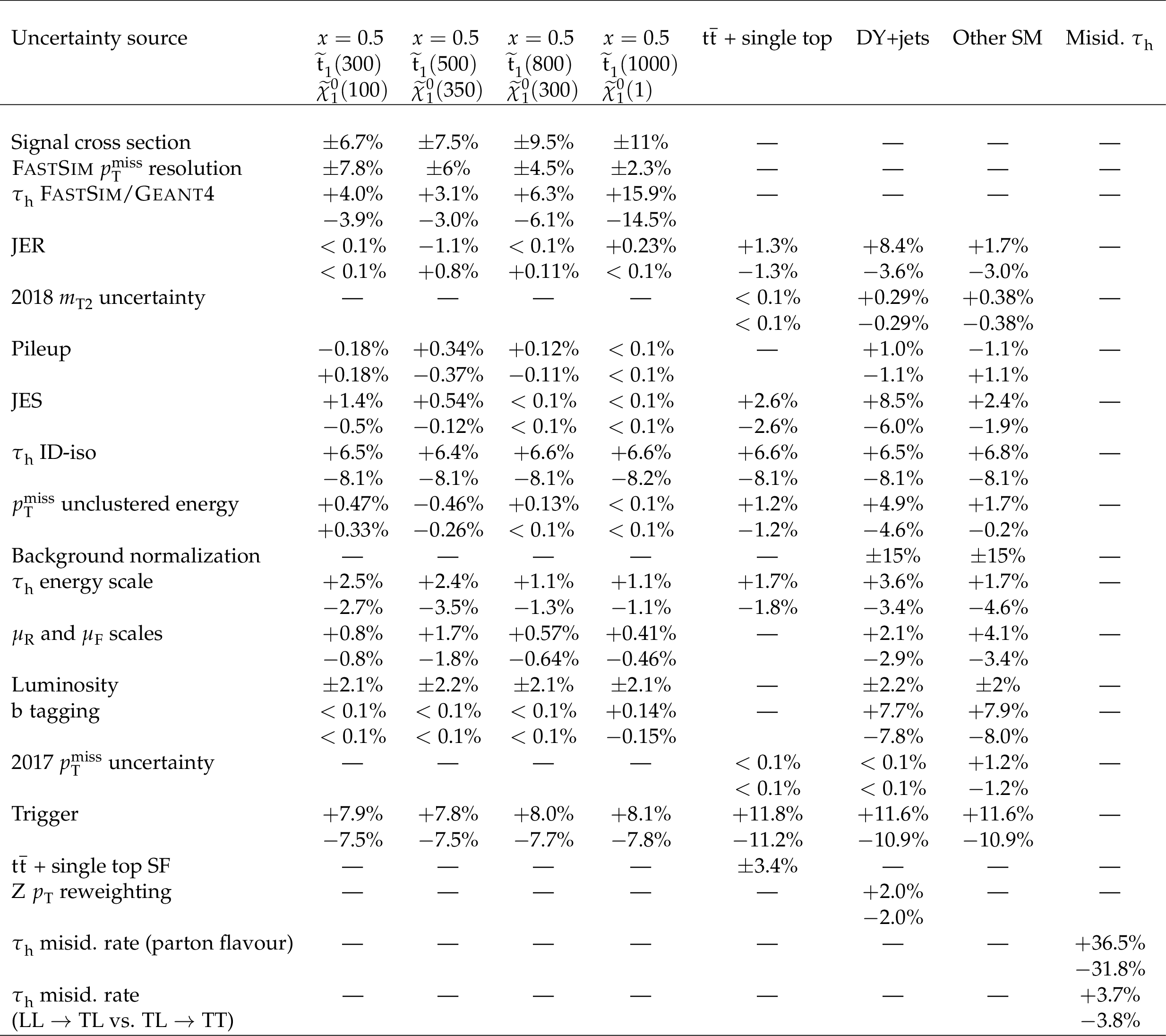
Table 3:
Relative systematic uncertainties from different sources in signal and background yields in the 2016, 2017 and 2018 analyses combined, for the $ \tau_\mathrm{h} \tau_\mathrm{h} $ category. These values are the weighted (by the yields in the respective bins) averages of the relative uncertainties in the different search regions. For the asymmetric uncertainties, the upper (lower) entry is the uncertainty due to the upward (downward) variation, which can be in the same direction as a result of taking the weighted average. In the heading, the top squark and LSP masses in GeV are indicated in parentheses. |
png pdf |
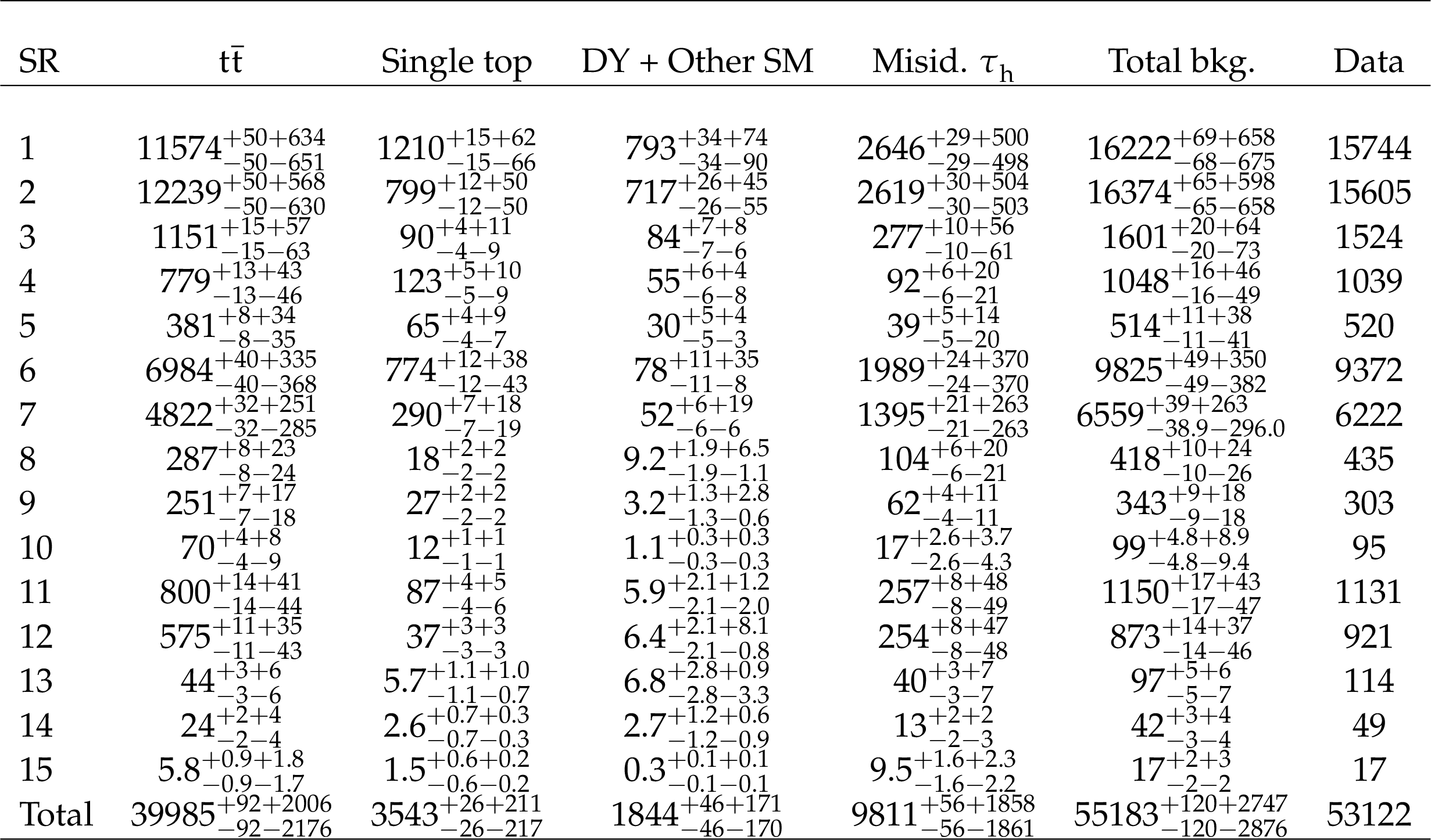
Table 4:
Event yields along with statistical and systematic uncertainties in the 2016, 2017 and 2018 analyses combined, for the $ \mathrm{e}\tau_\mathrm{h} $ category, for different background sources and the total background in the 15 search bins, as defined in Fig. 5. The uncertainties that are smaller than 0.05 are listed as 0.0. The number of events observed in data is also shown. The first uncertainty on yields is statistical whereas the second is systematic. |
png pdf |
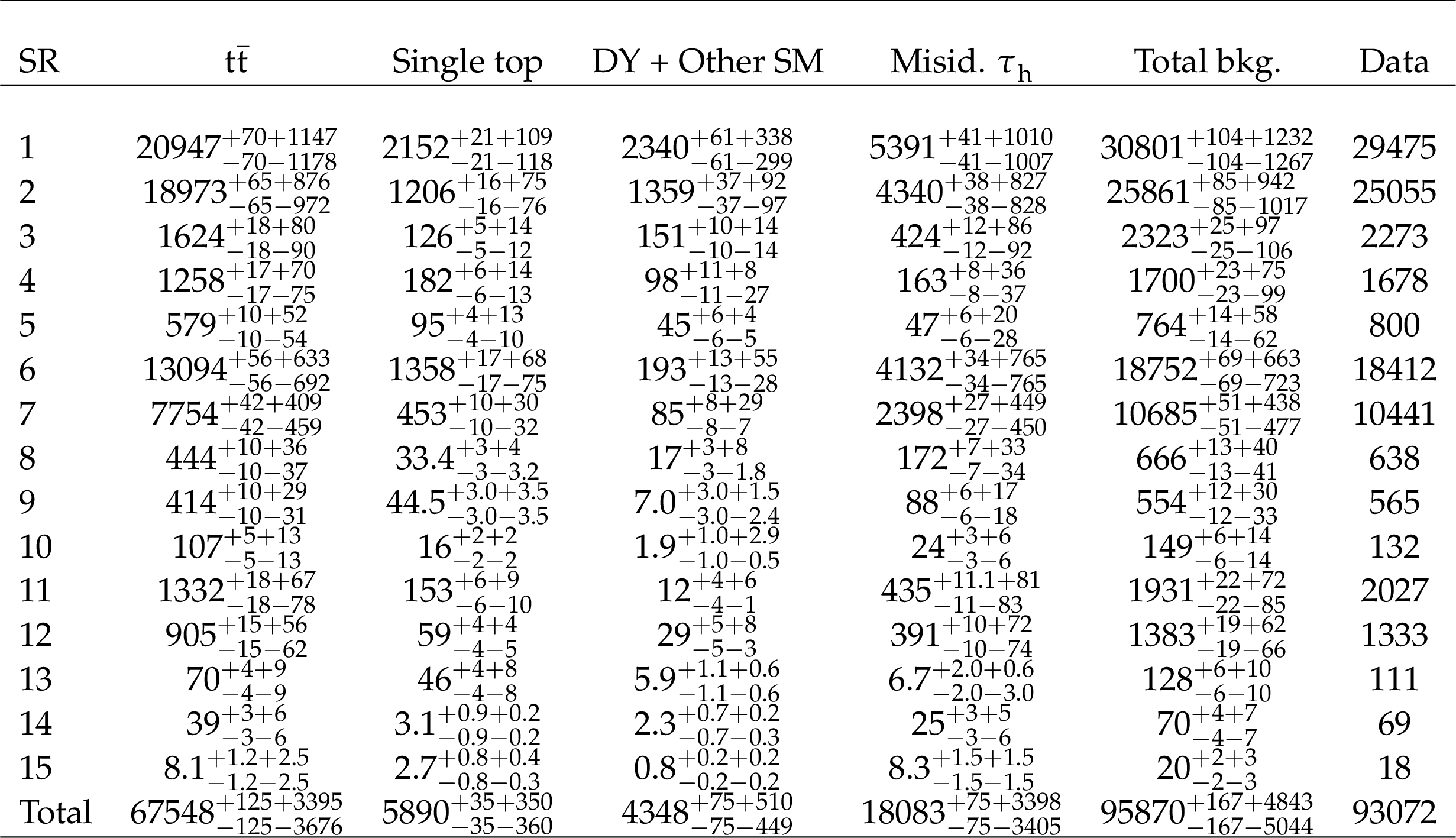
Table 5:
Event yields along with statistical and systematic uncertainties in the 2016, 2017 and 2018 analyses combined, for the $ \mu\tau_\mathrm{h} $ category, for different background sources and the total background in the 15 search bins, as defined in Fig. 5. The uncertainties that are smaller than 0.05 are listed as 0.0. The number of events observed in data is also shown. The first uncertainty on yields is statistical whereas the second is systematic. |
png pdf |
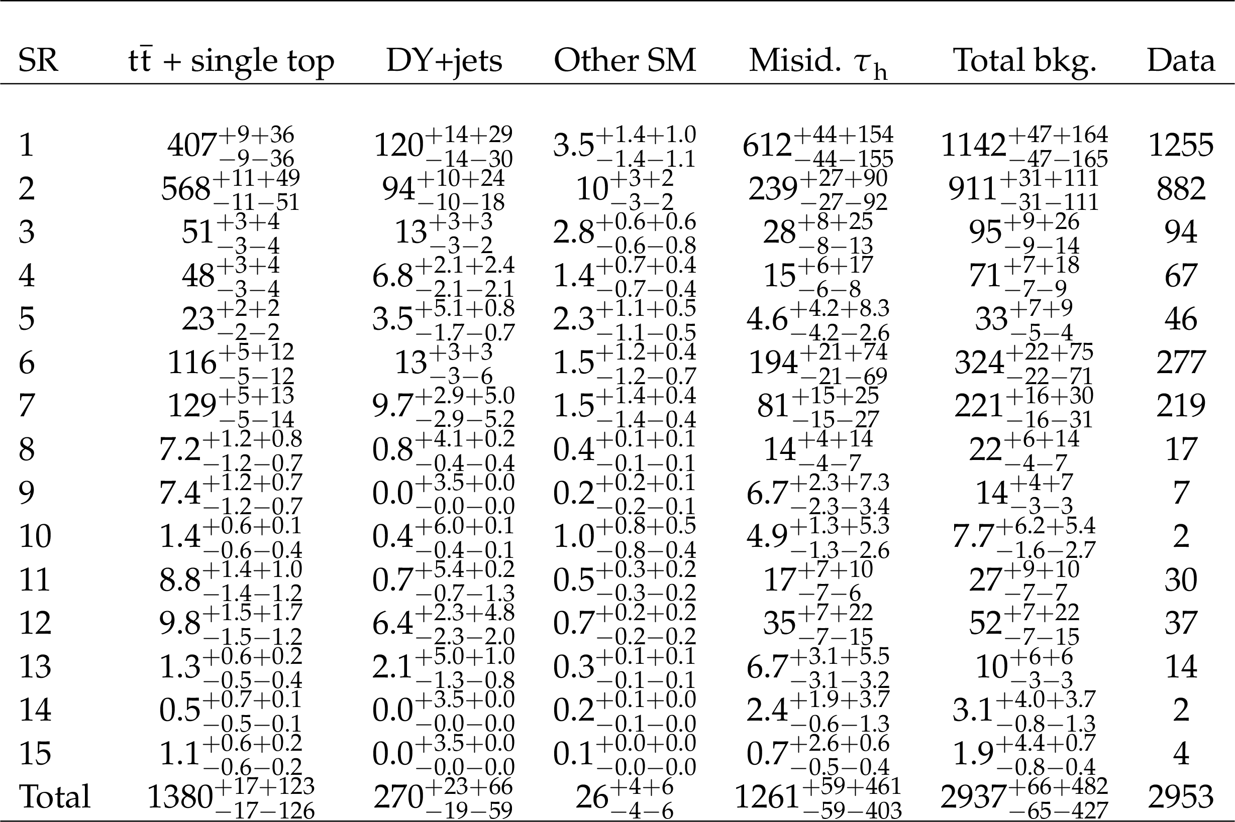
Table 6:
Event yields along with statistical and systematic uncertainties in the 2016, 2017 and 2018 analyses combined, for the $ \tau_\mathrm{h} \tau_\mathrm{h} $ category, for different background sources and the total background in the 15 search bins, as defined in Fig. 5. The uncertainties that are smaller than 0.05 are listed as 0.0. The number of events observed in data is also shown. The first uncertainty on yields is statistical whereas the second is systematic. |
| Summary |
| Top squark pair production in final states with two tau leptons has been explored in the data collected by the CMS detector during 2016, 2017 and 2018, corresponding to integrated luminosities of 35.9, 41.3, and 59.7 fb$ ^{-1} $, respectively. This search improves upon the previous iteration [36] by analyzing the entirety of the Run 2 data, adding the semileptonic final states (where one of two tau leptons decays to an electron or a muon), and utilizing improved $ \tau_\mathrm{h} $- and b-tagging algorithms. The dominant standard model backgrounds were found to originate from single top and top quark pair production and processes where jets were misidentified as hadronic tau lepton decays. Control regions in data were used to estimate these backgrounds, while other backgrounds were estimated using simulation. The simulated objects (leptons, jets, etc.) were corrected using scale factors to account for differences between their performances in simulation and collision data. No significant excess was observed, and exclusion limits on the top squark and lightest neutralino masses were set at 95% confidence level within the framework of simplified models where the top squark decays via a chargino to final states including tau leptons. This decay mode is motivated by high-$ \tan\beta $ and higgsino-like scenarios where decays to tau leptons are enhanced. In such models, top squark masses are excluded up to about 1150 GeV for an LSP of mass 1 GeV, and LSP masses up to 450 GeV are excluded for a top squark mass of 900 GeV. These are most stringent exclusion limits till date for the signal models considered in this study. |
| References | ||||
| 1 | P. Ramond | Dual theory for free fermions | PRD 3 (1971) 2415 | |
| 2 | Yu. A. Golfand and E. P. Likhtman | Extension of the algebra of Poincaré group generators and violation of p invariance | JETP Lett. 13 (1971) 323 | |
| 3 | A. Neveu and J. H. Schwarz | Factorizable dual model of pions | NPB 31 (1971) 86 | |
| 4 | J. Wess and B. Zumino | A Lagrangian model invariant under supergauge transformations | PLB 49 (1974) 52 | |
| 5 | P. Fayet | Supergauge invariant extension of the Higgs mechanism and a model for the electron and its neutrino | NPB 90 (1975) 104 | |
| 6 | G. 't Hooft | Naturalness, chiral symmetry, and spontaneous chiral symmetry breaking | NATO Sci. Ser. B 59 (1980) 135 | |
| 7 | R. K. Kaul and P. Majumdar | Cancellation of quadratically divergent mass corrections in globally supersymmetric spontaneously broken gauge theories | NPB 199 (1982) 36 | |
| 8 | H. P. Nilles | Supersymmetry, supergravity and particle physics | Phys. Rept. 110 (1984) 1 | |
| 9 | S. P. Martin | A supersymmetry primer | hep-ph/9709356 | |
| 10 | G. R. Farrar and P. Fayet | Phenomenology of the production, decay, and detection of new hadronic states associated with supersymmetry | PLB 76 (1978) 575 | |
| 11 | E. Witten | Dynamical Breaking of Supersymmetry | Nucl. Phys. B (1980) 188 | |
| 12 | S. Dimopoulos and H. Georgi | Softly Broken Supersymmetry and SU(5) | Nucl. Phys. B (1981) 193 | |
| 13 | N. Sakai | Naturalness in Supersymmetric Guts | Z. Phys. C 11 (1981) link |
|
| 14 | L. J. Hall, D. Pinner, and J. T. Ruderman | A Natural SUSY Higgs Near 126 GeV | JHEP 04 (2012) 131 | 1112.2703 |
| 15 | A. Arbey et al. | Implications of a 125 GeV Higgs for supersymmetric models | PLB 708 (2012) | 1112.3028 |
| 16 | H. Baer et al. | Collider phenomenology for supersymmetry with large $ \tan\beta $ | PRL 79 (1997) 986 | hep-ph/9704457 |
| 17 | M. Guchait and D. P. Roy | Using $ \tau $ polarization as a distinctive SUGRA signature at LHC | PLB 541 (2002) 356 | hep-ph/0205015 |
| 18 | J. Alwall, P. Schuster, and N. Toro | Simplified models for a first characterization of new physics at the LHC | PRD 79 (2009) 075020 | 0810.3921 |
| 19 | LHC New Physics Working Group Collaboration | Simplified models for LHC new physics searches | JPG 39 (2012) 105005 | 1105.2838 |
| 20 | Particle Data Group Collaboration | Review of Particle Physics | PTEP 8 (2020) 083C01 | |
| 21 | CMS Collaboration | Search for top squark pair production in pp collisions at $ \sqrt{s}= $ 13 TeV using single lepton events | JHEP 10 (2017) 019 | CMS-SUS-16-051 1706.04402 |
| 22 | CMS Collaboration | Search for top squarks and dark matter particles in opposite-charge dilepton final states at $ \sqrt{s}= $ 13 TeV | PRD 97 (2018) 032009 | CMS-SUS-17-001 1711.00752 |
| 23 | CMS Collaboration | Search for top-squark pair production in the single-lepton final state in pp collisions at $ \sqrt{s} $ = 8 TeV | EPJC 73 (2013) 2677 | CMS-SUS-13-011 1308.1586 |
| 24 | CMS Collaboration | Search for direct pair production of scalar top quarks in the single- and dilepton channels in proton-proton collisions at $ \sqrt{s}= $ 8 TeV | JHEP 07 (2016) 027 | CMS-SUS-14-015 1602.03169 |
| 25 | CMS Collaboration | Search for top squark pair production in compressed-mass-spectrum scenarios in proton-proton collisions at $ \sqrt{s} $ = 8 TeV using the $ \alpha_T $ variable | PLB 767 (2017) 403 | CMS-SUS-14-006 1605.08993 |
| 26 | CMS Collaboration | Searches for pair production of third-generation squarks in $ \sqrt{s}= $ 13 TeV pp collisions | EPJC 77 (2017) 327 | CMS-SUS-16-008 1612.03877 |
| 27 | CMS Collaboration | Search for direct production of supersymmetric partners of the top quark in the all-jets final state in proton-proton collisions at $ \sqrt{s}= $ 13 TeV | JHEP 10 (2017) 005 | CMS-SUS-16-049 1707.03316 |
| 28 | CMS Collaboration | Search for supersymmetry in proton-proton collisions at 13 TeV using identified top quarks | PRD 97 (2018) 012007 | CMS-SUS-16-050 1710.11188 |
| 29 | ATLAS Collaboration | Search for direct top squark pair production in final states with two leptons in $ \sqrt{s} = $ 13 TeV pp collisions with the ATLAS detector | EPJC 77 (2017) 898 | 1708.03247 |
| 30 | ATLAS Collaboration | ATLAS Run 1 searches for direct pair production of third-generation squarks at the Large Hadron Collider | EPJC 75 (2015) 510 | 1506.08616 |
| 31 | ATLAS Collaboration | Search for top squark pair production in final states with one isolated lepton, jets, and missing transverse momentum in $ \sqrt{s} = $ 8 TeV pp collisions with the ATLAS detector | JHEP 11 (2014) 118 | 1407.0583 |
| 32 | ATLAS Collaboration | Search for direct top-squark pair production in final states with two leptons in pp collisions at $ \sqrt{s} = $ 8 TeV with the ATLAS detector | JHEP 06 (2014) 124 | 1403.4853 |
| 33 | ATLAS Collaboration | Search for top squarks in final states with one isolated lepton, jets, and missing transverse momentum in $ \sqrt{s}= $ 13 TeV pp collisions with the ATLAS detector | PRD 94 (2016) 052009 | 1606.03903 |
| 34 | ATLAS Collaboration | Search for top squarks decaying to tau sleptons in pp collisions at $ \sqrt{s}= $ 13 TeV with the ATLAS detector | PRD 98 (2018) 032008 | 1803.10178 |
| 35 | ATLAS Collaboration | Search for new phenomena in pp collisions in final states with tau leptons, b-jets, and missing transverse momentum with the ATLAS detector | PRD 104 (2021) 112005 | 2108.07665 |
| 36 | CMS Collaboration | Search for top squark pair production in a final state with two tau leptons in proton-proton collisions at $ \sqrt{s} = $ 13 TeV | JHEP 02 (2020) 015 | CMS-SUS-19-003 1910.12932 |
| 37 | CMS Collaboration | The CMS experiment at the CERN LHC | JINST 3 (2008) S08004 | |
| 38 | CMS Collaboration | The CMS trigger system | JINST 12 (2017) P01020 | CMS-TRG-12-001 1609.02366 |
| 39 | CMS Collaboration | Performance of the CMS Level-1 trigger in proton-proton collisions at $ \sqrt{s} = $ 13 TeV | JINST 15 (2020) P10017 | CMS-TRG-17-001 2006.10165 |
| 40 | C. Oleari | The POWHEG-BOX | Nucl. Phys. B Proc. Suppl. (2010) 205-206 | 1007.3893 |
| 41 | P. Nason | A New method for combining NLO QCD with shower Monte Carlo algorithms | JHEP 11 (2004) 040 | hep-ph/0409146 |
| 42 | S. Frixione, P. Nason, and C. Oleari | Matching NLO QCD computations with Parton Shower simulations: the POWHEG method | JHEP 11 (2007) 070 | 0709.2092 |
| 43 | S. Alioli, P. Nason, C. Oleari, and E. Re | A general framework for implementing NLO calculations in shower Monte Carlo programs: the POWHEG BOX | JHEP 06 (2010) 043 | 1002.2581 |
| 44 | S. Frixione, P. Nason, and G. Ridolfi | A positive-weight next-to-leading-order Monte Carlo for heavy flavour hadroproduction | JHEP 09 (2007) 126 | 0707.3088 |
| 45 | S. Alioli, P. Nason, C. Oleari, and E. Re | NLO single-top production matched with shower in POWHEG:s- andt-channel contributions | JHEP 09 (2009) 111 | 0907.4076 |
| 46 | E. Re | Single-top Wt-channel production matched with parton showers using the POWHEG method | EPJC 71 (2011) 1547 | 1009.2450 |
| 47 | J. Alwall et al. | The automated computation of tree-level and next-to-leading order differential cross sections, and their matching to parton shower simulations | JHEP 07 (2014) 079 | 1405.0301 |
| 48 | Y. Li and F. Petriello | Combining QCD and electroweak corrections to dilepton production in FEWZ | PRD 86 (2012) 094034 | 1208.5967 |
| 49 | T. Sjöstrand et al. | An Introduction to PYTHIA 8.2 | Comput. Phys. Commun. 191 (2015) 159 | 1410.3012 |
| 50 | CMS Collaboration | Event generator tunes obtained from underlying event and multiparton scattering measurements | EPJC 76 3 (2016) 155 | CMS-GEN-14-001 1512.00815 |
| 51 | CMS Collaboration | Investigations of the impact of the parton shower tuning in Pythia 8 in the modelling of $ \mathrm{t\overline{t}} $ at $ \sqrt{s}= $ 8 and 13 TeV | CMS Physics Analysis Summary, 2016 CMS-PAS-TOP-16-021 |
CMS-PAS-TOP-16-021 |
| 52 | CMS Collaboration | Extraction and validation of a new set of CMS PYTHIA8 tunes from underlying-event measurements | EPJC 80 1 (2020) 4 | CMS-GEN-17-001 1903.12179 |
| 53 | GEANT4 Collaboration | GEANT4--a simulation toolkit | NIMA 506 (2003) | |
| 54 | W. Beenakker, R. Höpker, M. Spira, and P. M. Zerwas | Squark and gluino production at hadron colliders | NPB 492 (1997) 51 | hep-ph/9610490 |
| 55 | A. Kulesza and L. Motyka | Threshold resummation for squark-antisquark and gluino-pair production at the LHC | PRL 102 (2009) 111802 | 0807.2405 |
| 56 | A. Kulesza and L. Motyka | Soft gluon resummation for the production of gluino-gluino and squark-antisquark pairs at the LHC | PRD 80 (2009) 095004 | 0905.4749 |
| 57 | W. Beenakker et al. | Soft-gluon resummation for squark and gluino hadroproduction | JHEP 12 (2009) 041 | 0909.4418 |
| 58 | W. Beenakker et al. | Squark and gluino hadroproduction | Int. J. Mod. Phys. A 26 (2011) 2637 | 1105.1110 |
| 59 | A. Giammanco | The fast simulation of the CMS experiment | J. Phys. Conf. Ser. 513 (2014) 022012 | |
| 60 | CMS Collaboration | Particle-flow reconstruction and global event description with the CMS detector | JINST 12 (2017) P10003 | CMS-PRF-14-001 1706.04965 |
| 61 | M. Cacciari, G. P. Salam, and G. Soyez | The anti-$k_{\mathrm{T}}$ jet clustering algorithm | JHEP 04 (2008) 063 | 0802.1189 |
| 62 | CMS Collaboration | Jet energy scale and resolution in the CMS experiment in pp collisions at 8 TeV | JINST 12 (2017) P02014 | CMS-JME-13-004 1607.03663 |
| 63 | CMS Collaboration | Jet algorithms performance in 13 TeV data | CMS Physics Analysis Summary, 2017 CMS-PAS-JME-16-003 |
CMS-PAS-JME-16-003 |
| 64 | CMS Collaboration | Performance of the DeepJet b tagging algorithm using 41.9 fb$^{-1}$ of data from proton-proton collisions at 13 TeV with phase 1 CMS detector | CMS Detector Performance Note CMS-DP-2018-058, 2018 CDS |
|
| 65 | E. Bols et al. | Jet Flavour Classification Using DeepJet | JINST 15 (2020) P12012 | 2008.10519 |
| 66 | CMS Collaboration | Electron and photon reconstruction and identification with the CMS experiment at the CERN LHC | JINST 16 (2021) P05014 | CMS-EGM-17-001 2012.06888 |
| 67 | CMS Collaboration | Performance of electron reconstruction and selection with the CMS detector in proton-proton collisions at $ \sqrt{s} = $ 8 TeV | JINST 10 (2015) P06005 | CMS-EGM-13-001 1502.02701 |
| 68 | CMS Collaboration | Performance of the CMS muon detector and muon reconstruction with proton-proton collisions at $ \sqrt{s} = $ 13 TeV | JINST 13 (2018) P06015 | CMS-MUO-16-001 1804.04528 |
| 69 | CMS Collaboration | Performance of reconstruction and identification of $ \tau $ leptons decaying to hadrons and $ \nu_\tau $ in pp collisions at $ \sqrt{s}= $ 13 TeV | JINST 13 (2018) P10005 | CMS-TAU-16-003 1809.02816 |
| 70 | CMS Collaboration | Identification of hadronic tau lepton decays using a deep neural network | JINST 17 (2022) P07023 | CMS-TAU-20-001 2201.08458 |
| 71 | CMS Collaboration | Performance of missing transverse momentum reconstruction in proton-proton collisions at $ \sqrt{s} = $ 13 TeV using the CMS detector | JINST 14 (2019) P07004 | CMS-JME-17-001 1903.06078 |
| 72 | C. G. Lester and D. J. Summers | Measuring masses of semiinvisibly decaying particles pair produced at hadron colliders | PLB 463 (1999) 945 | hep-ph/9906349 |
| 73 | A. Barr, C. Lester, and P. Stephens | $m_{\mathrm{T2}}$: The truth behind the glamour | JPG 29 (2003) 2343 | hep-ph/0304226 |
| 74 | A. J. Barr and C. Gwenlan | The race for supersymmetry: Using $m_{\mathrm{T2}}$ for discovery | PRD 80 (2009) 074007 | 0907.2713 |
| 75 | CMS Collaboration | Search for heavy neutrinos and third-generation leptoquarks in hadronic states of two $ \tau $ leptons and two jets in proton-proton collisions at $ \sqrt{s} = $ 13 TeV | JHEP 03 (2019) 170 | CMS-EXO-17-016 1811.00806 |
| 76 | CMS Collaboration | Search for direct pair production of supersymmetric partners to the $ \tau $ lepton in proton-proton collisions at $ \sqrt{s}= $ 13 TeV | EPJC 80 (2020) 189 | CMS-SUS-18-006 1907.13179 |
| 77 | CMS Collaboration | Search for supersymmetry in events with a $ \tau $ lepton pair and missing transverse momentum in proton-proton collisions at $ \sqrt{s} = $ 13 TeV | JHEP 11 (2018) 151 | CMS-SUS-17-003 1807.02048 |
| 78 | CMS Collaboration | Search for direct pair production of supersymmetric partners to the $ \tau $ lepton in the all-hadronic final state at $ \sqrt{s}= $ 13 TeV | CMS Physics Analysis Summary, 2021 CMS-PAS-SUS-21-001 |
CMS-PAS-SUS-21-001 |
| 79 | CMS Collaboration | Measurement of the inelastic proton-proton cross section at $ \sqrt{s}= $ 13 TeV | JHEP 07 (2018) 161 | CMS-FSQ-15-005 1802.02613 |
| 80 | A. Kalogeropoulos and J. Alwall | The SysCalc code: A tool to derive theoretical systematic uncertainties | 1801.08401 | |
| 81 | CMS Collaboration | CMS luminosity measurement for the 2017 data-taking period at $ \sqrt{s} = $ 13 TeV | CMS Physics Analysis Summary, 2018 CMS-PAS-LUM-17-004 |
CMS-PAS-LUM-17-004 |
| 82 | CMS Collaboration | CMS luminosity measurements for the 2016 data taking period | CMS Physics Analysis Summary, 2017 CMS-PAS-LUM-17-001 |
CMS-PAS-LUM-17-001 |
| 83 | CMS Collaboration | Precision luminosity measurement in proton-proton collisions at $ \sqrt{s} = $ 13 TeV in 2015 and 2016 at CMS | EPJC 81 (2021) 800 | CMS-LUM-17-003 2104.01927 |
| 84 | CMS Collaboration | Cms luminosity measurement for the 2018 data-taking period at $ \sqrt{s} = $ 13 TeV | CMS Physics Analysis Summary, 2019 CMS-PAS-LUM-18-002 |
CMS-PAS-LUM-18-002 |
| 85 | CMS Collaboration | Measurement of the differential Drell-Yan cross section in proton-proton collisions at $ \sqrt{s} = $ 13 TeV | JHEP 12 (2019) 059 | CMS-SMP-17-001 1812.10529 |
| 86 | CMS Collaboration | Measurements of $ \mathrm{t\overline{t}} $ differential cross sections in proton-proton collisions at $ \sqrt{s}= $ 13 TeV using events containing two leptons | JHEP 02 (2019) 149 | CMS-TOP-17-014 1811.06625 |
| 87 | ATLAS Collaboration | Measurement of the $ W^+W^- $ production cross section in pp collisions at a centre-of-mass energy of $ \sqrt{s} $ = 13 TeV with the ATLAS experiment | PLB 773 (2017) 354 | 1702.04519 |
| 88 | CMS Collaboration | Measurement of top quark pair production in association with a Z boson in proton-proton collisions at $ \sqrt{s}= $ 13 TeV | JHEP 03 (2020) 056 | CMS-TOP-18-009 1907.11270 |
| 89 | CMS Collaboration | Measurements of the pp $ \to $ WZ inclusive and differential production cross section and constraints on charged anomalous triple gauge couplings at $ \sqrt{s} = $ 13 TeV | JHEP 04 (2019) 122 | CMS-SMP-18-002 1901.03428 |
| 90 | CMS Collaboration | Measurement of the differential cross sections for the associated production of a $ W $ boson and jets in proton-proton collisions at $ \sqrt{s}= $ 13 TeV | PRD 96 (2017) 072005 | CMS-SMP-16-005 1707.05979 |
| 91 | ATLAS and CMS Collaborations, and LHC Higgs Combination Group | Procedure for the LHC Higgs boson search combination in Summer 2011 | Technical Report CMS-NOTE-2011-005, ATL-PHYS-PUB-2011-11, 2011 | |
| 92 | T. Junk | Confidence level computation for combining searches with small statistics | Nucl. Instrum. Meth A 434 (1999) 435 | hep-ex/9902006 |
| 93 | A. L. Read | Presentation of search results: the CL$_\text{s}$ technique | JPG 28 (2002) 2693 | |
| 94 | G. Cowan, K. Cranmer, E. Gross, and O. Vitells | Asymptotic formulae for likelihood-based tests of new physics | EPJC 71 (2011) 1554 | 1007.1727 |
|
|
Compact Muon Solenoid LHC, CERN |
|

|

|

|

|

|