CMS-PAS-SUS-16-017

CMS-PAS-SUS-16-017
Inclusive search for supersymmetry using razor variables in pp collisions at $\sqrt{s}=$ 13 TeV
CMS Collaboration
September 2018

Abstract: An inclusive search for supersymmetry with the razor variables is performed using a data sample of proton-proton collisions corresponding to an integrated luminosity of 35.9 fb $^{-1}$ collected with the CMS experiment in 2016 at a center-of-mass energy of $\sqrt{s}=$ 13 TeV. The search covers final states with zero or one charged lepton and features event categories divided according to the presence of a high-transverse momentum hadronically decaying W boson or top quark, the number of jets, the number of b-tagged jets, and the values of the razor kinematic variables in order to separate signal from background for a wide variety of supersymmetric particle signatures. The combination of the zero-lepton, one-lepton, and boosted W boson and top quark event categories increases the sensitivity particularly to signal models with large mass splitting between the produced gluino or squark and the lightest supersymmetric particle. Limits on the gluino mass extend to 2.0 TeV while limits on top squark masses reach 1.14 TeV.
Links: CDS record (PDF) ; CADI line (restricted) ; These preliminary results are superseded in this paper, JHEP 03 (2019) 031. The superseded preliminary plots can be found here.

Figures & Tables	Summary	References	CMS Publications

Figures
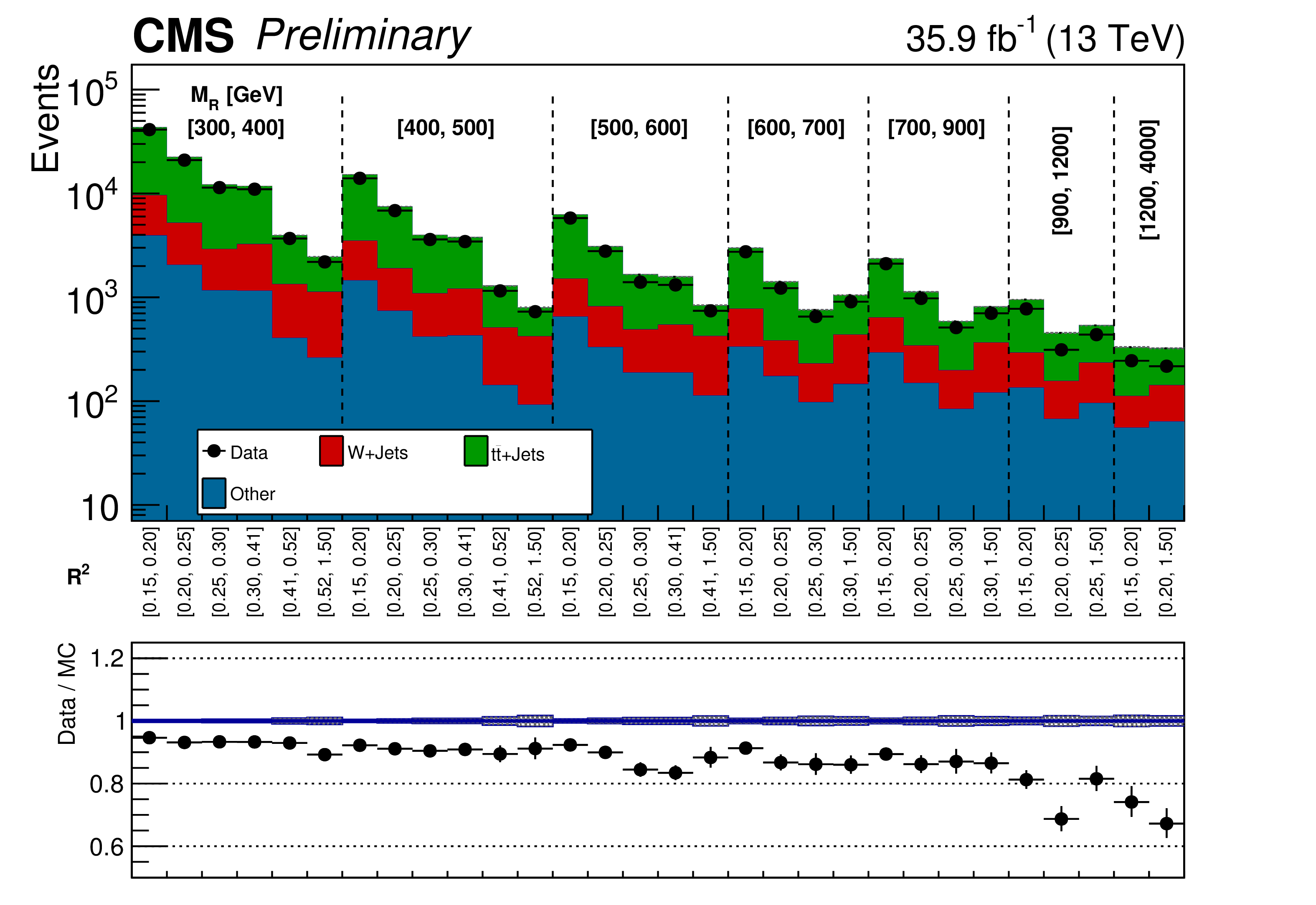
png pdf	Figure 1: The ${M_\mathrm {R}}$ - ${\mathrm {R}^2}$ distribution observed in data is shown along with the MC prediction in the ${{\mathrm {t}\overline {\mathrm {t}}}}$ one-lepton control region. The two-dimensional ${M_\mathrm {R}}$ - ${\mathrm {R}^2}$ distribution is shown in a one dimensional representation, with each ${M_\mathrm {R}}$ bin marked by the dashed lines and labeled near the top, and each ${\mathrm {R}^2}$ bin labeled below. The ratio of data to the MC simulation prediction is shown on the bottom inset, with the statistical uncertainty expressed through the data point error bars and the systematic uncertainty of the background prediction represented by the shaded region. The corrections derived from background control regions have not been applied yet.
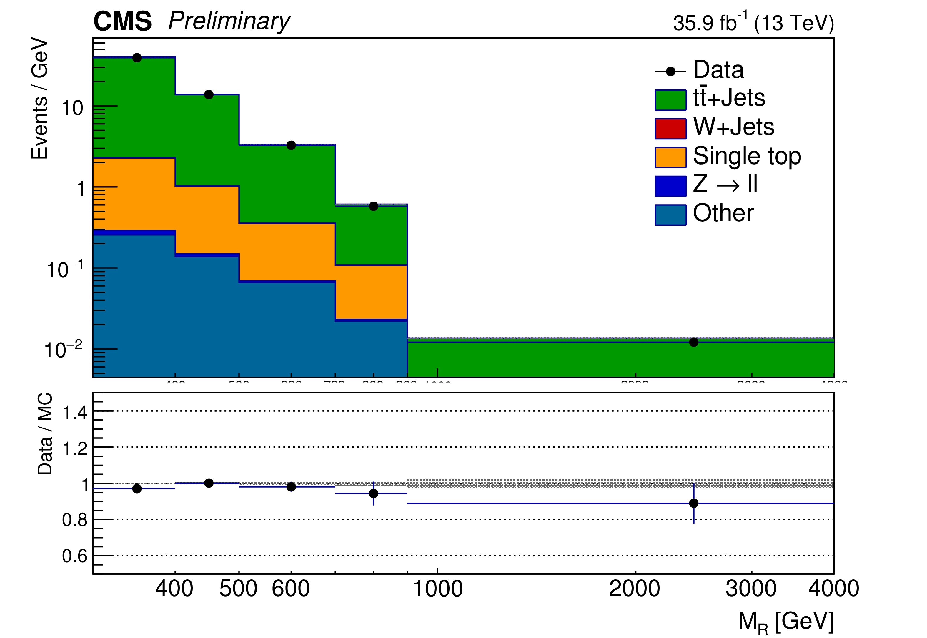
png pdf	Figure 2: The ${M_\mathrm {R}}$ distribution in the ${{\mathrm {t}\overline {\mathrm {t}}}}$ dilepton control region is displayed in the 2-3 and 4-6 jet categories along with the corresponding MC predictions. The corrections derived from the ${{\mathrm {t}\overline {\mathrm {t}}}}$ and ${\mathrm {W}}$ +jets control regions have been applied.
png pdf	Figure 2-a: The ${M_\mathrm {R}}$ distribution in the ${{\mathrm {t}\overline {\mathrm {t}}}}$ dilepton control region is displayed in the 2-3 and 4-6 jet categories along with the corresponding MC predictions. The corrections derived from the ${{\mathrm {t}\overline {\mathrm {t}}}}$ and ${\mathrm {W}}$ +jets control regions have been applied.
png pdf	Figure 2-b: The ${M_\mathrm {R}}$ distribution in the ${{\mathrm {t}\overline {\mathrm {t}}}}$ dilepton control region is displayed in the 2-3 and 4-6 jet categories along with the corresponding MC predictions. The corrections derived from the ${{\mathrm {t}\overline {\mathrm {t}}}}$ and ${\mathrm {W}}$ +jets control regions have been applied.
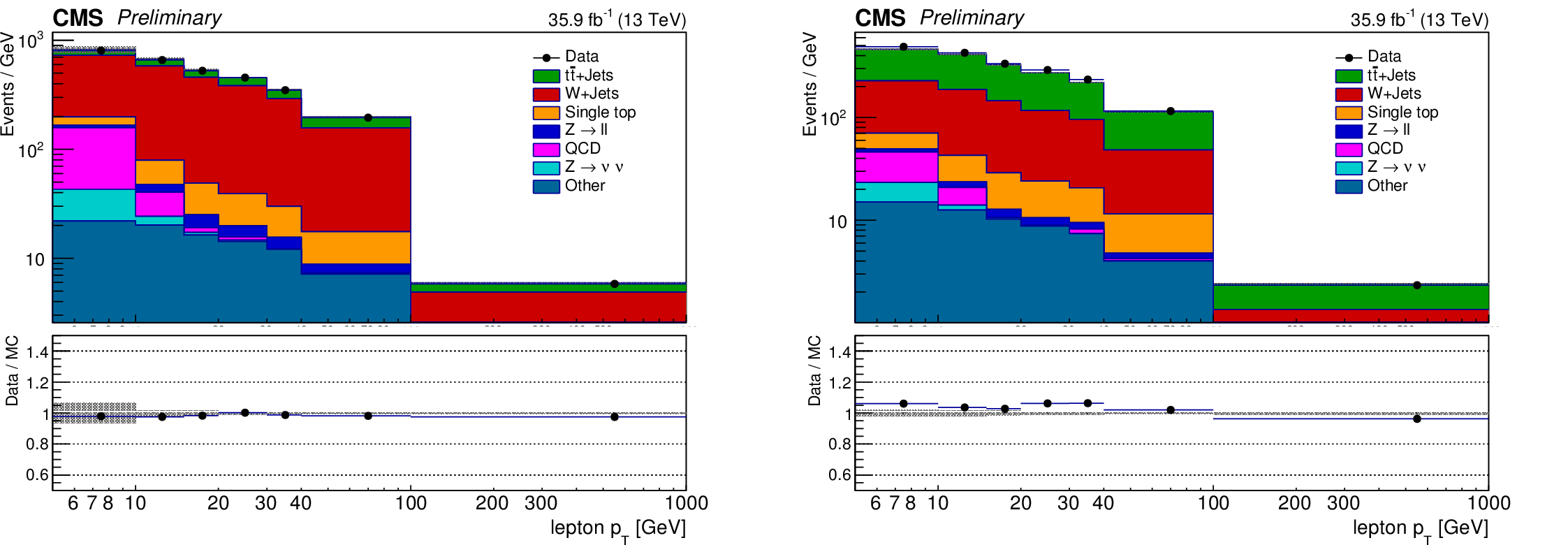
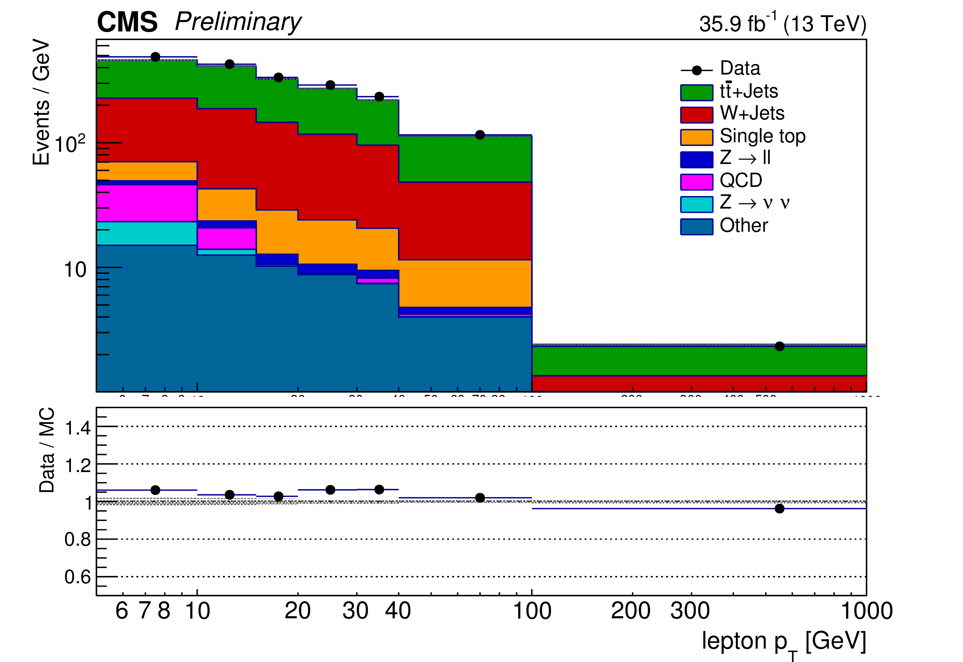
png pdf	Figure 3: The ${p_{\mathrm {T}}}$ distribution for leptons passing the veto identification criteria is displayed in the 2-3 and 4-6 jet categories along with the corresponding MC predictions. The corrections derived from the ${{\mathrm {t}\overline {\mathrm {t}}}}$ and ${\mathrm {W}}$ +jets control regions have been applied.
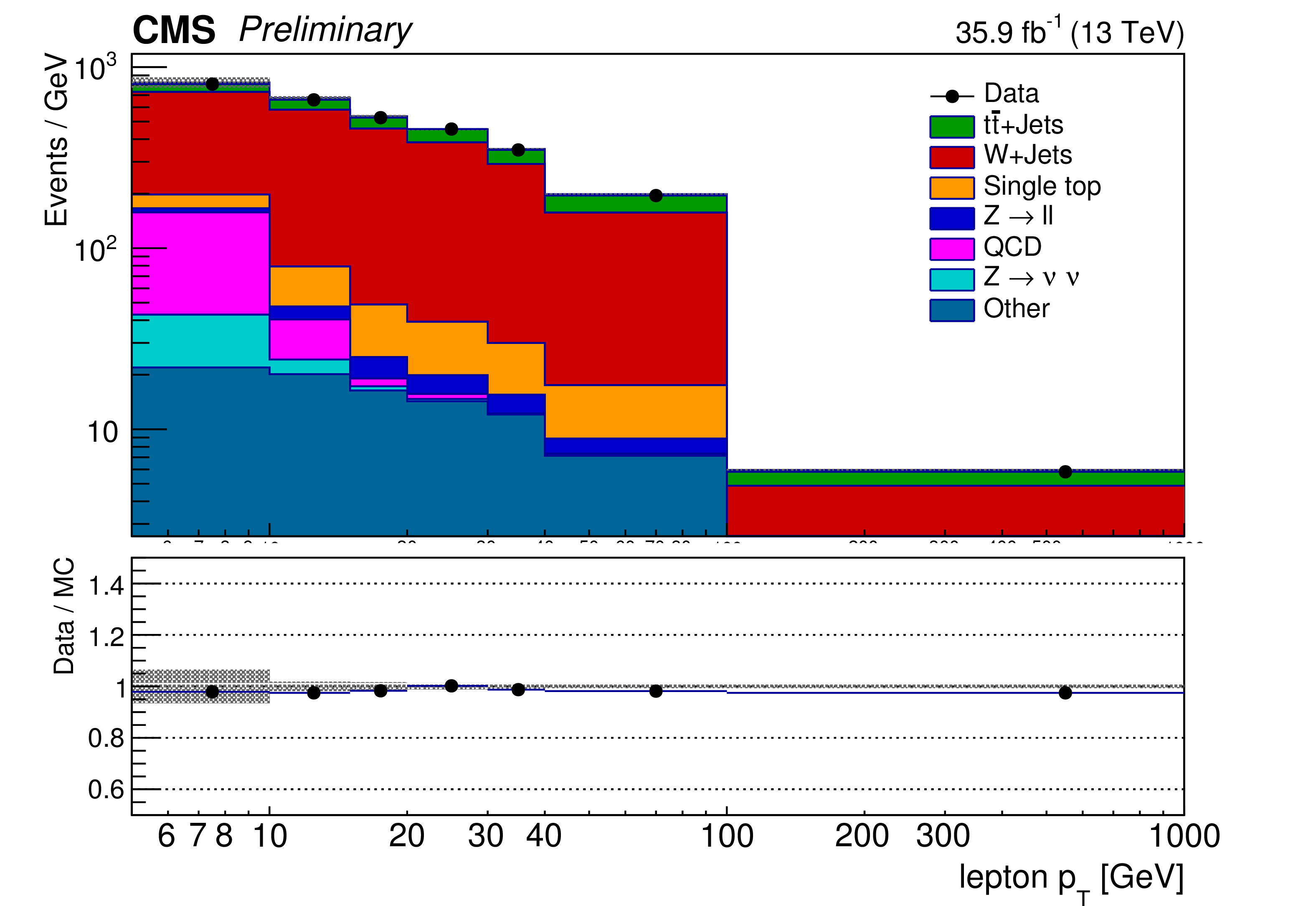
png pdf	Figure 3-a: The ${p_{\mathrm {T}}}$ distribution for leptons passing the veto identification criteria is displayed in the 2-3 and 4-6 jet categories along with the corresponding MC predictions. The corrections derived from the ${{\mathrm {t}\overline {\mathrm {t}}}}$ and ${\mathrm {W}}$ +jets control regions have been applied.
png pdf	Figure 3-b: The ${p_{\mathrm {T}}}$ distribution for leptons passing the veto identification criteria is displayed in the 2-3 and 4-6 jet categories along with the corresponding MC predictions. The corrections derived from the ${{\mathrm {t}\overline {\mathrm {t}}}}$ and ${\mathrm {W}}$ +jets control regions have been applied.
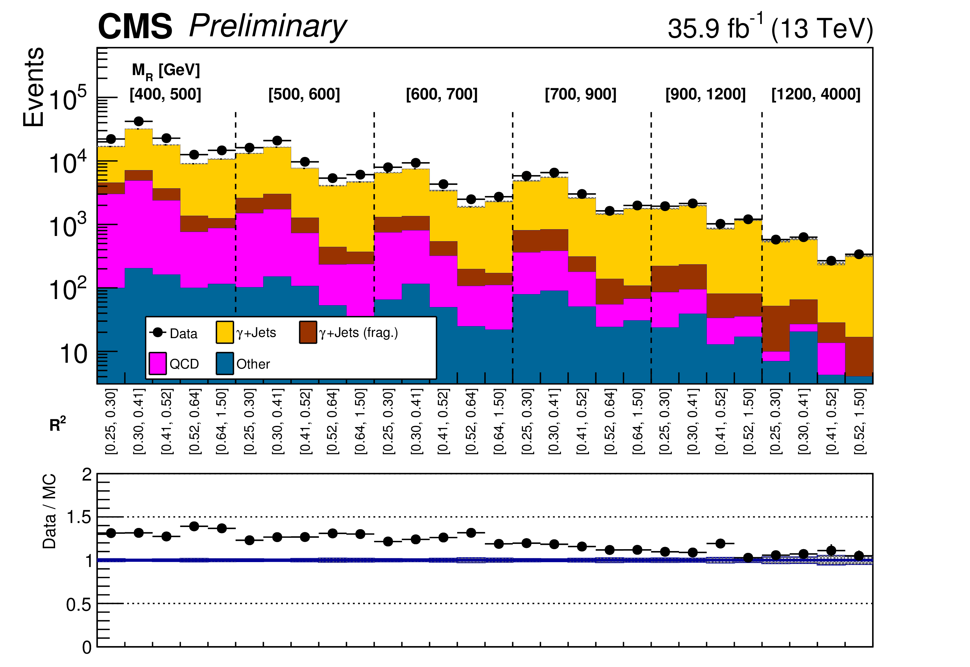
png pdf	Figure 4: The ${M_\mathrm {R}}$ - ${\mathrm {R}^2}$ distribution observed in data is shown along with the MC prediction in the photon+jets control region. The two-dimensional ${M_\mathrm {R}}$ - ${\mathrm {R}^2}$ distribution is shown in a one dimensional representation, with each ${M_\mathrm {R}}$ bin marked by the dashed lines and labeled near the top, and each ${\mathrm {R}^2}$ bin labeled below. The ratio of data to the background prediction is shown on the bottom inset, with the statistical uncertainty expressed through the data point error bars and the systematic uncertainty of the background prediction represented by the shaded region. The contribution from the ${\gamma}$ +jets process where the photon was produced from a jet fragmentation is labeled as " ${\gamma}$ +jets (frag.)''. The corrections derived from background control regions have not been applied yet in this figure.
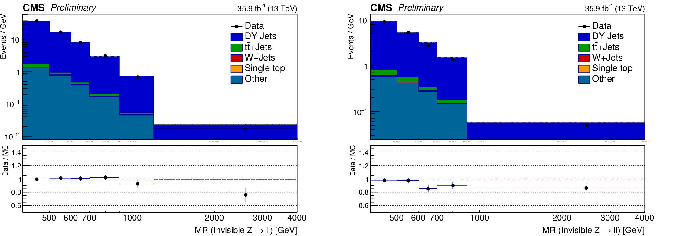
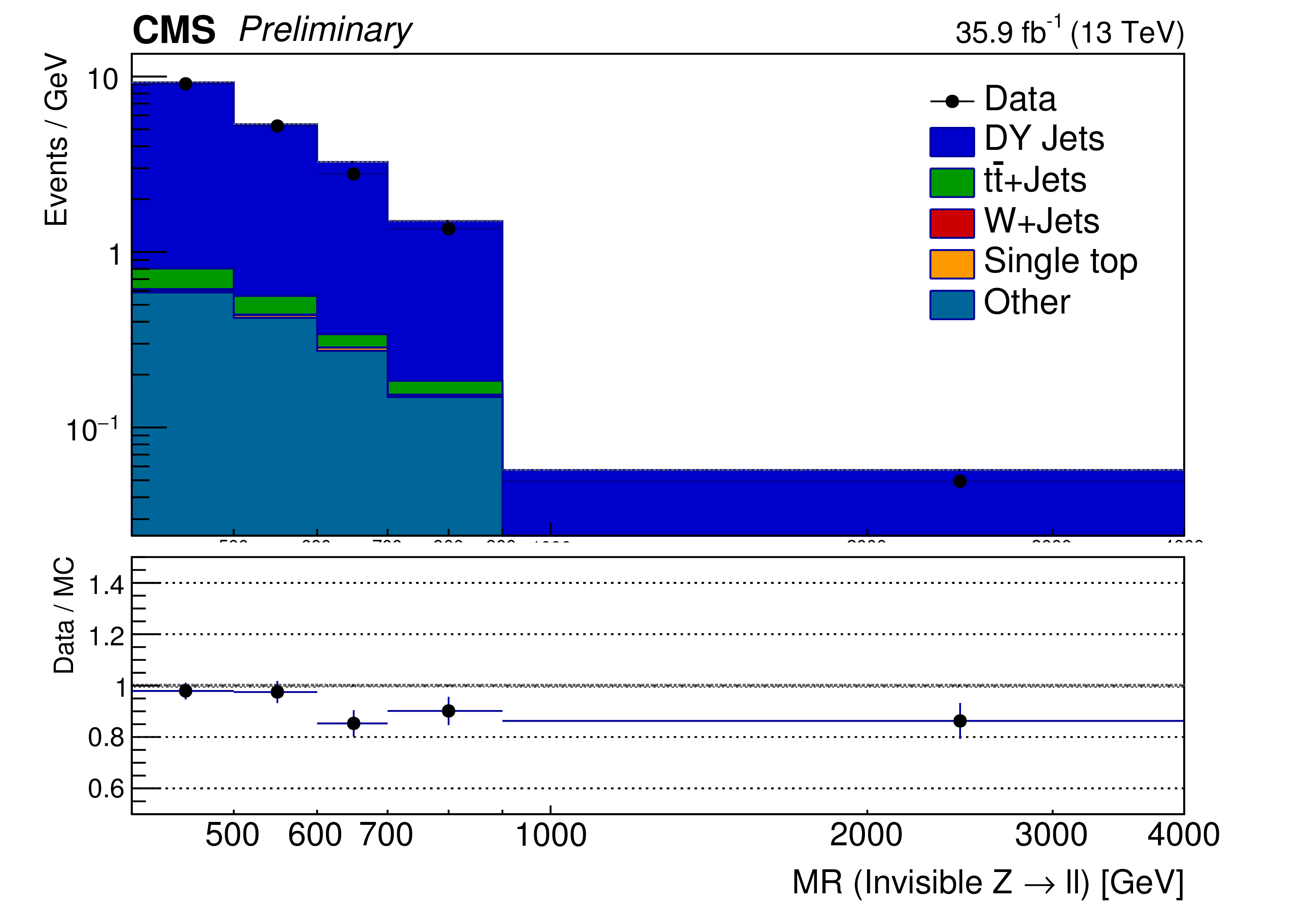
png pdf	Figure 5: The ${M_\mathrm {R}}$ distribution in the Drell-Yan(DY)+jets dilepton control region is displayed in the 2-3 and 4-6 jet categories along with the corresponding MC predictions. The corrections derived from the ${\gamma}$ +jets control region as well as the overall normalization correction have been applied in this figure.
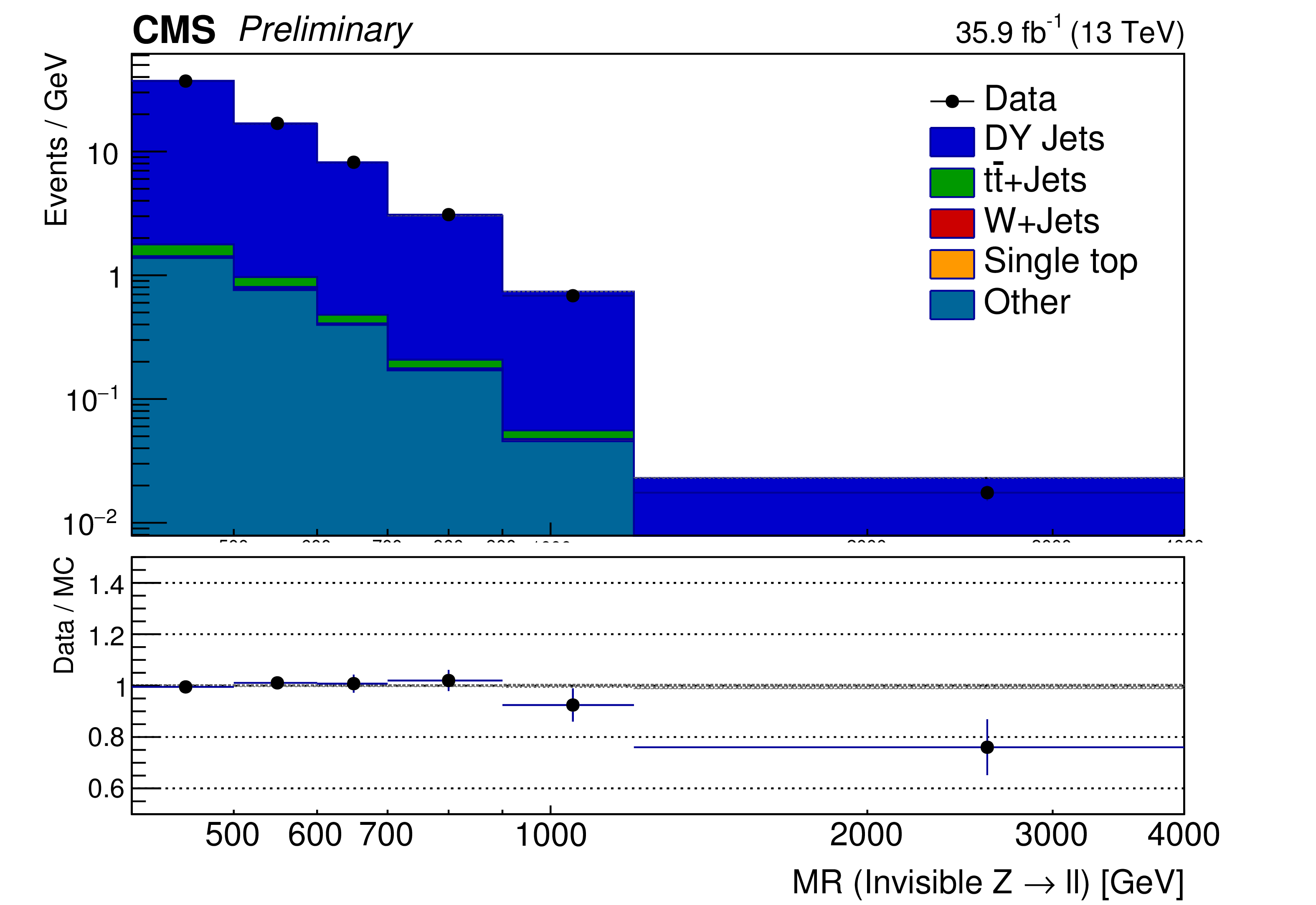
png pdf	Figure 5-a: The ${M_\mathrm {R}}$ distribution in the Drell-Yan(DY)+jets dilepton control region is displayed in the 2-3 and 4-6 jet categories along with the corresponding MC predictions. The corrections derived from the ${\gamma}$ +jets control region as well as the overall normalization correction have been applied in this figure.
png pdf	Figure 5-b: The ${M_\mathrm {R}}$ distribution in the Drell-Yan(DY)+jets dilepton control region is displayed in the 2-3 and 4-6 jet categories along with the corresponding MC predictions. The corrections derived from the ${\gamma}$ +jets control region as well as the overall normalization correction have been applied in this figure.
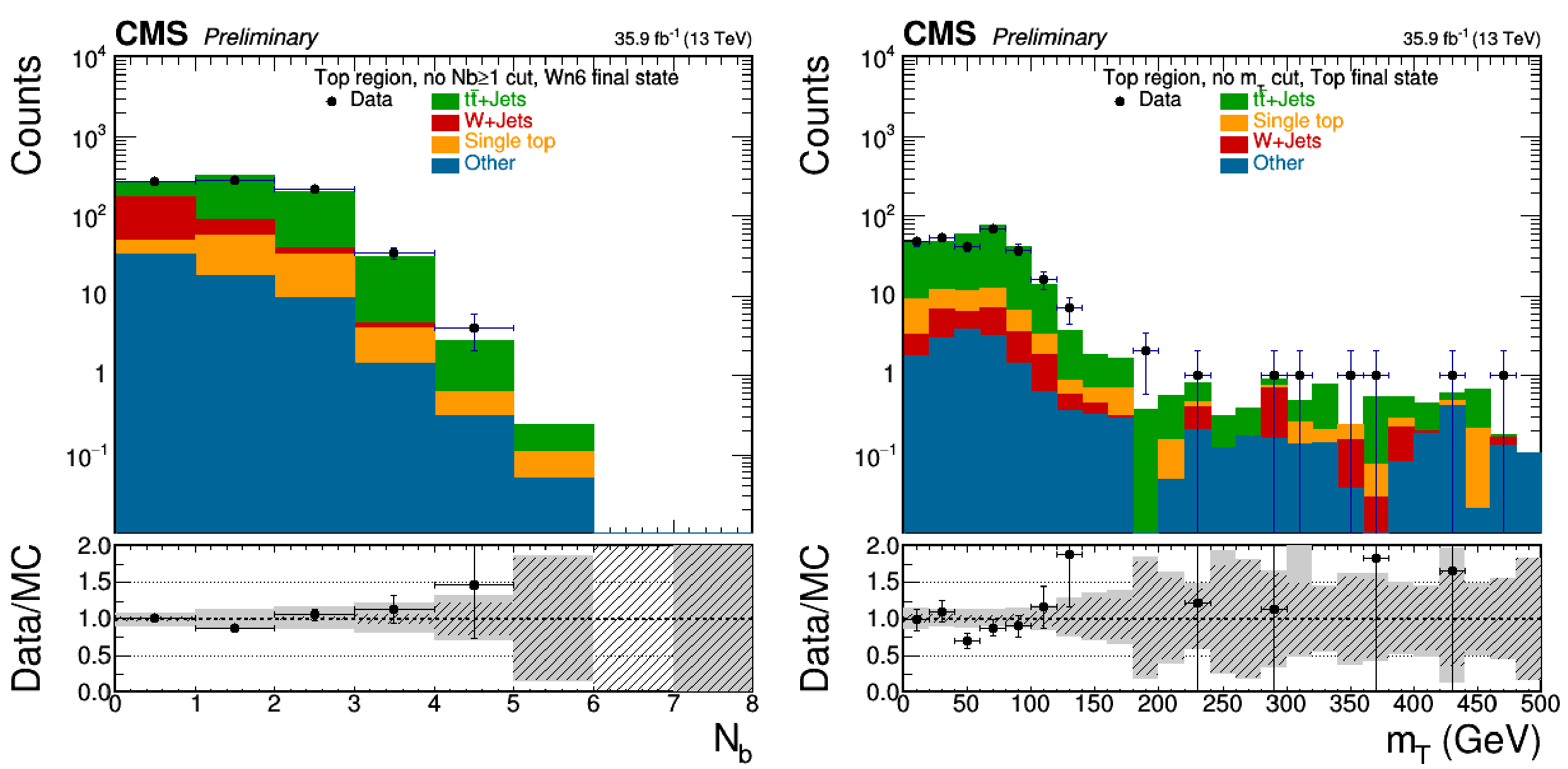
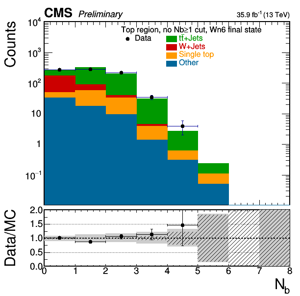
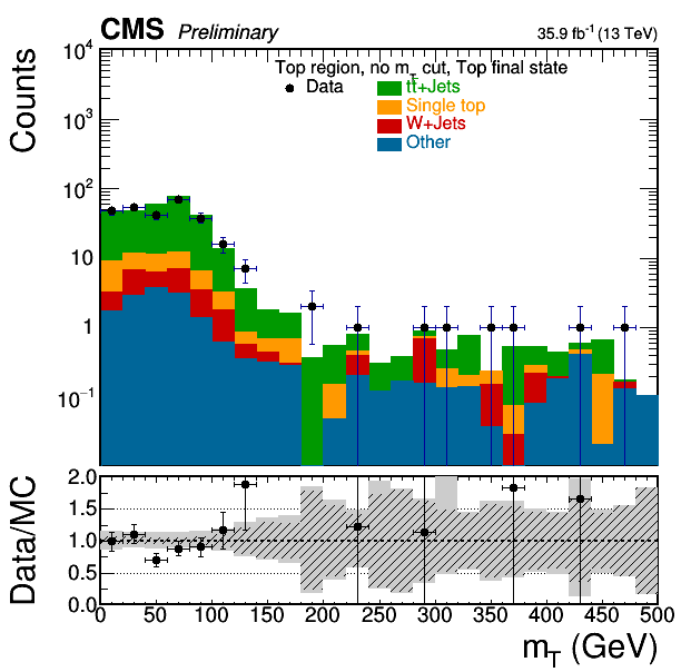
png pdf	Figure 6: Distributions of b-tagged jet multiplicity before applying the b-tagging selection requirement in the ${\mathrm {W}}$ +jets control region of the boosted Wnj6 category (left), and distributions in $M_{\mathrm {T}}$ before applying the $M_{\mathrm {T}}$ selection requirement in the top quark control region of the boosted Top category (right) are shown. The ratio of data over MC prediction is shown in the lower panels, where the gray band is the total uncertainty and the dashed band is the statistical uncertainty in the MC prediction.
png	Figure 6-a: Distributions of b-tagged jet multiplicity before applying the b-tagging selection requirement in the ${\mathrm {W}}$ +jets control region of the boosted Wnj6 category (left), and distributions in $M_{\mathrm {T}}$ before applying the $M_{\mathrm {T}}$ selection requirement in the top quark control region of the boosted Top category (right) are shown. The ratio of data over MC prediction is shown in the lower panels, where the gray band is the total uncertainty and the dashed band is the statistical uncertainty in the MC prediction.
png	Figure 6-b: Distributions of b-tagged jet multiplicity before applying the b-tagging selection requirement in the ${\mathrm {W}}$ +jets control region of the boosted Wnj6 category (left), and distributions in $M_{\mathrm {T}}$ before applying the $M_{\mathrm {T}}$ selection requirement in the top quark control region of the boosted Top category (right) are shown. The ratio of data over MC prediction is shown in the lower panels, where the gray band is the total uncertainty and the dashed band is the statistical uncertainty in the MC prediction.
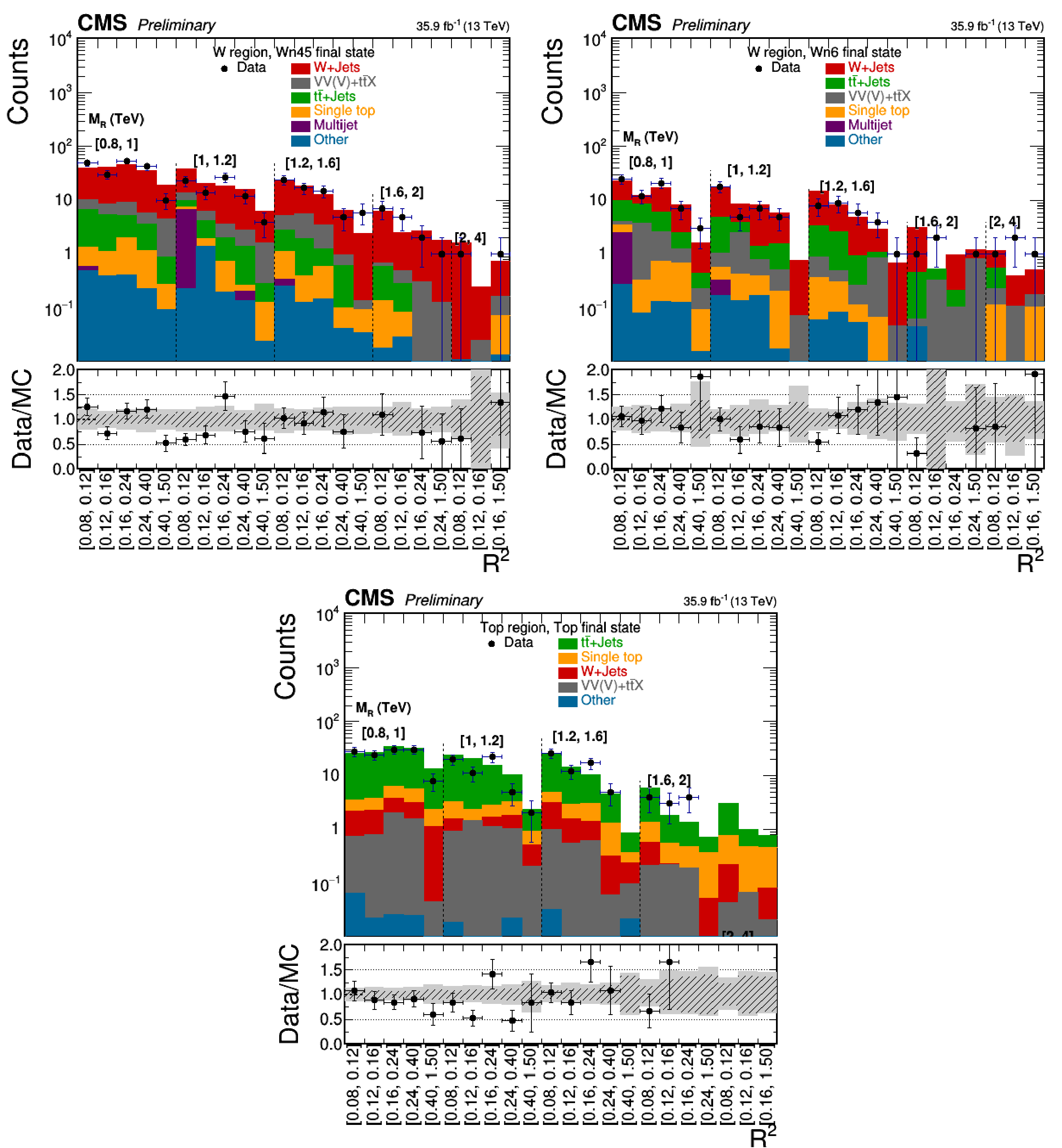
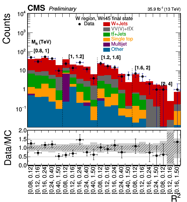
png pdf	Figure 7: ${M_\mathrm {R}}$ - ${\mathrm {R}^2}$ distributions in the ${\mathrm {W}}$ +jets control regions of the boosted Wnj45 and Wnj6 categories, and the top quark control region of the Top category. The ratio of data over MC prediction is shown in the lower panels, where the gray band is the total uncertainty and the dashed band is the statistical uncertainty in the MC prediction.
png	Figure 7-a: ${M_\mathrm {R}}$ - ${\mathrm {R}^2}$ distributions in the ${\mathrm {W}}$ +jets control regions of the boosted Wnj45 and Wnj6 categories, and the top quark control region of the Top category. The ratio of data over MC prediction is shown in the lower panels, where the gray band is the total uncertainty and the dashed band is the statistical uncertainty in the MC prediction.
png	Figure 7-b: ${M_\mathrm {R}}$ - ${\mathrm {R}^2}$ distributions in the ${\mathrm {W}}$ +jets control regions of the boosted Wnj45 and Wnj6 categories, and the top quark control region of the Top category. The ratio of data over MC prediction is shown in the lower panels, where the gray band is the total uncertainty and the dashed band is the statistical uncertainty in the MC prediction.
png	Figure 7-c: ${M_\mathrm {R}}$ - ${\mathrm {R}^2}$ distributions in the ${\mathrm {W}}$ +jets control regions of the boosted Wnj45 and Wnj6 categories, and the top quark control region of the Top category. The ratio of data over MC prediction is shown in the lower panels, where the gray band is the total uncertainty and the dashed band is the statistical uncertainty in the MC prediction.
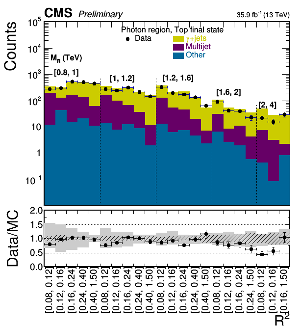
png pdf	Figure 8: Photon ${p_{\mathrm {T}}}$ and ${M_\mathrm {R}}$ - ${\mathrm {R}^2}$ distributions for the ${\gamma}$ +jets control regions of the boosted Top category. The ratio of data over MC prediction is shown in the lower panels, where the gray band is the total uncertainty and the dashed band is the statistical uncertainty in the MC prediction.
png	Figure 8-a: Photon ${p_{\mathrm {T}}}$ and ${M_\mathrm {R}}$ - ${\mathrm {R}^2}$ distributions for the ${\gamma}$ +jets control regions of the boosted Top category. The ratio of data over MC prediction is shown in the lower panels, where the gray band is the total uncertainty and the dashed band is the statistical uncertainty in the MC prediction.
png	Figure 8-b: Photon ${p_{\mathrm {T}}}$ and ${M_\mathrm {R}}$ - ${\mathrm {R}^2}$ distributions for the ${\gamma}$ +jets control regions of the boosted Top category. The ratio of data over MC prediction is shown in the lower panels, where the gray band is the total uncertainty and the dashed band is the statistical uncertainty in the MC prediction.
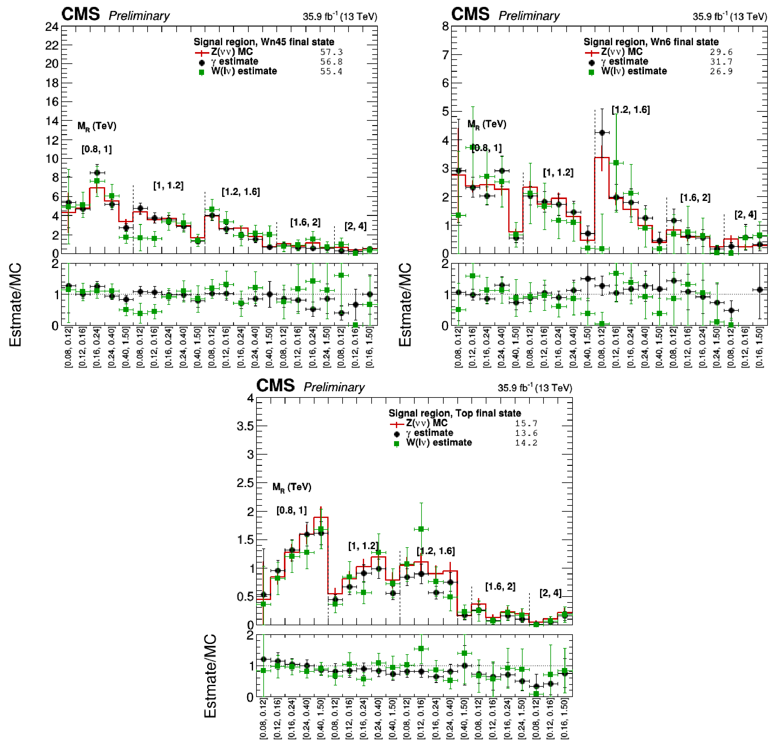
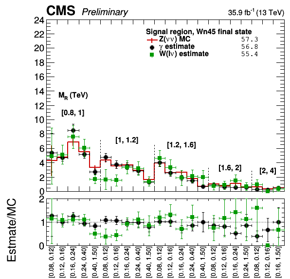
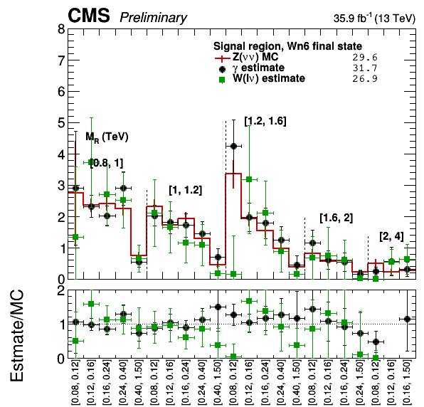
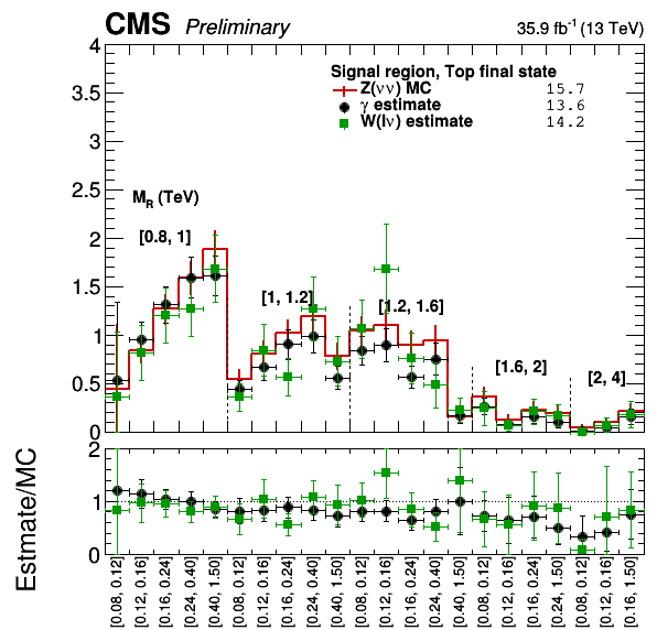
png pdf	Figure 9: Comparison of the estimation of the $\mathrm{Z}(\rightarrow \nu \nu)+$ jets background contribution in the search region extrapolated from the ${\gamma}$ +jets control region with the estimation extrapolated from the $\mathrm{W}(\rightarrow \ell \nu)$ +jets control region for the boosted Wnj45, Wnj6 and Top categories. The prediction from the uncorrected MC simulation is also shown.
png	Figure 9-a: Comparison of the estimation of the $\mathrm{Z}(\rightarrow \nu \nu)+$ jets background contribution in the search region extrapolated from the ${\gamma}$ +jets control region with the estimation extrapolated from the $\mathrm{W}(\rightarrow \ell \nu)$ +jets control region for the boosted Wnj45, Wnj6 and Top categories. The prediction from the uncorrected MC simulation is also shown.
png	Figure 9-b: Comparison of the estimation of the $\mathrm{Z}(\rightarrow \nu \nu)+$ jets background contribution in the search region extrapolated from the ${\gamma}$ +jets control region with the estimation extrapolated from the $\mathrm{W}(\rightarrow \ell \nu)$ +jets control region for the boosted Wnj45, Wnj6 and Top categories. The prediction from the uncorrected MC simulation is also shown.
png	Figure 9-c: Comparison of the estimation of the $\mathrm{Z}(\rightarrow \nu \nu)+$ jets background contribution in the search region extrapolated from the ${\gamma}$ +jets control region with the estimation extrapolated from the $\mathrm{W}(\rightarrow \ell \nu)$ +jets control region for the boosted Wnj45, Wnj6 and Top categories. The prediction from the uncorrected MC simulation is also shown.
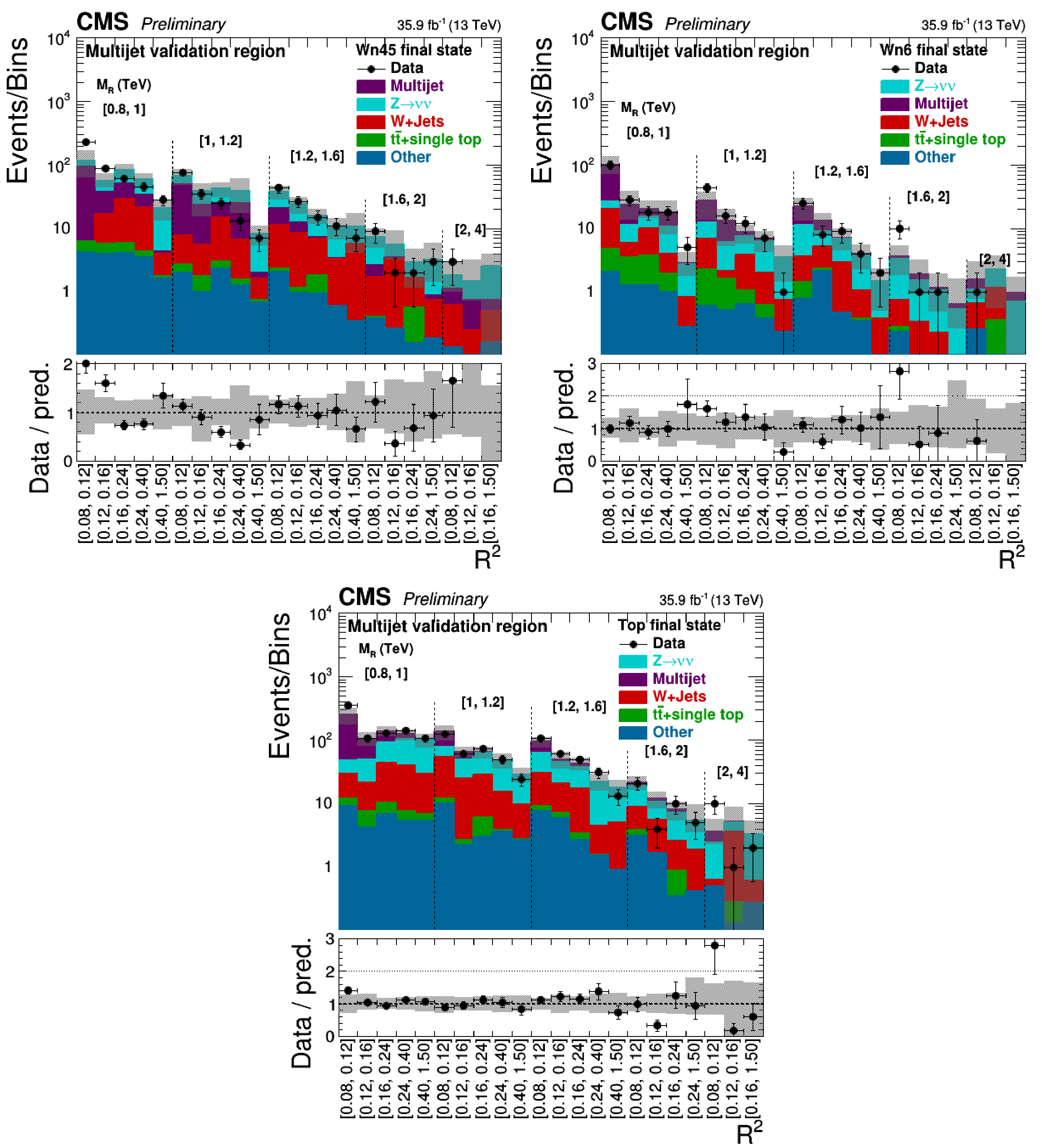
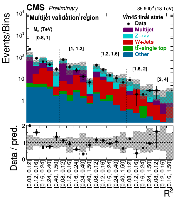
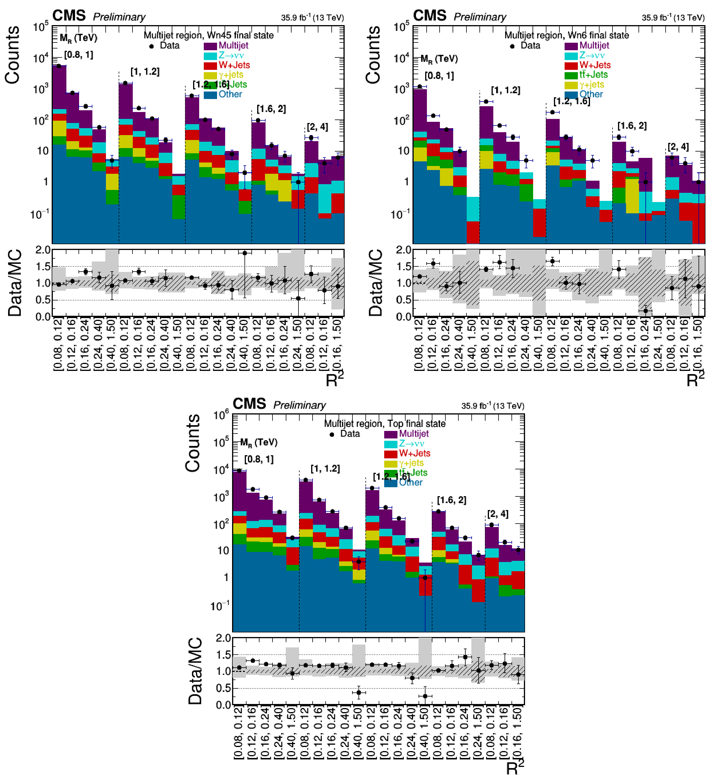
png pdf	Figure 10: ${M_\mathrm {R}}$ - ${\mathrm {R}^2}$ distributions in the QCD multijet control regions of the Wnj45 (upper left), Wnj6 (upper right) and Top (bottom) categories. The ratio of data over MC prediction is shown in the lower panels, where the gray band is the total uncertainty and the dashed band is the statistical uncertainty on the MC prediction.
png	Figure 10-a: ${M_\mathrm {R}}$ - ${\mathrm {R}^2}$ distributions in the QCD multijet control regions of the Wnj45 (upper left), Wnj6 (upper right) and Top (bottom) categories. The ratio of data over MC prediction is shown in the lower panels, where the gray band is the total uncertainty and the dashed band is the statistical uncertainty on the MC prediction.
png	Figure 10-b: ${M_\mathrm {R}}$ - ${\mathrm {R}^2}$ distributions in the QCD multijet control regions of the Wnj45 (upper left), Wnj6 (upper right) and Top (bottom) categories. The ratio of data over MC prediction is shown in the lower panels, where the gray band is the total uncertainty and the dashed band is the statistical uncertainty on the MC prediction.
png	Figure 10-c: ${M_\mathrm {R}}$ - ${\mathrm {R}^2}$ distributions in the QCD multijet control regions of the Wnj45 (upper left), Wnj6 (upper right) and Top (bottom) categories. The ratio of data over MC prediction is shown in the lower panels, where the gray band is the total uncertainty and the dashed band is the statistical uncertainty on the MC prediction.
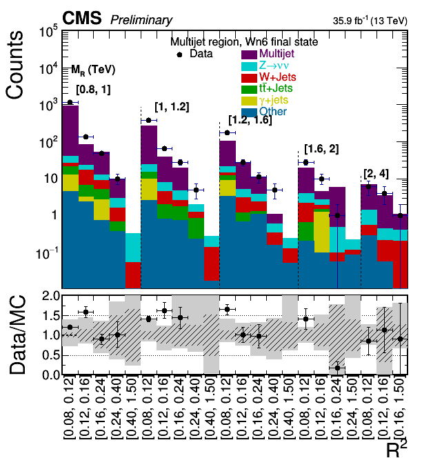
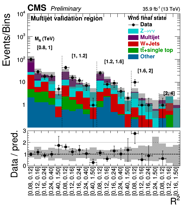
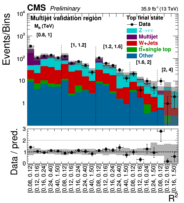
png pdf	Figure 11: Comparisons between data and the predicted background for the inverted ${\Delta \phi _\mathrm {R}}$ validation region for the boosted Wnj45 (upper left), Wnj6 (upper right) and Top (bottom) categories.
png	Figure 11-a: Comparisons between data and the predicted background for the inverted ${\Delta \phi _\mathrm {R}}$ validation region for the boosted Wnj45 (upper left), Wnj6 (upper right) and Top (bottom) categories.
png	Figure 11-b: Comparisons between data and the predicted background for the inverted ${\Delta \phi _\mathrm {R}}$ validation region for the boosted Wnj45 (upper left), Wnj6 (upper right) and Top (bottom) categories.
png	Figure 11-c: Comparisons between data and the predicted background for the inverted ${\Delta \phi _\mathrm {R}}$ validation region for the boosted Wnj45 (upper left), Wnj6 (upper right) and Top (bottom) categories.
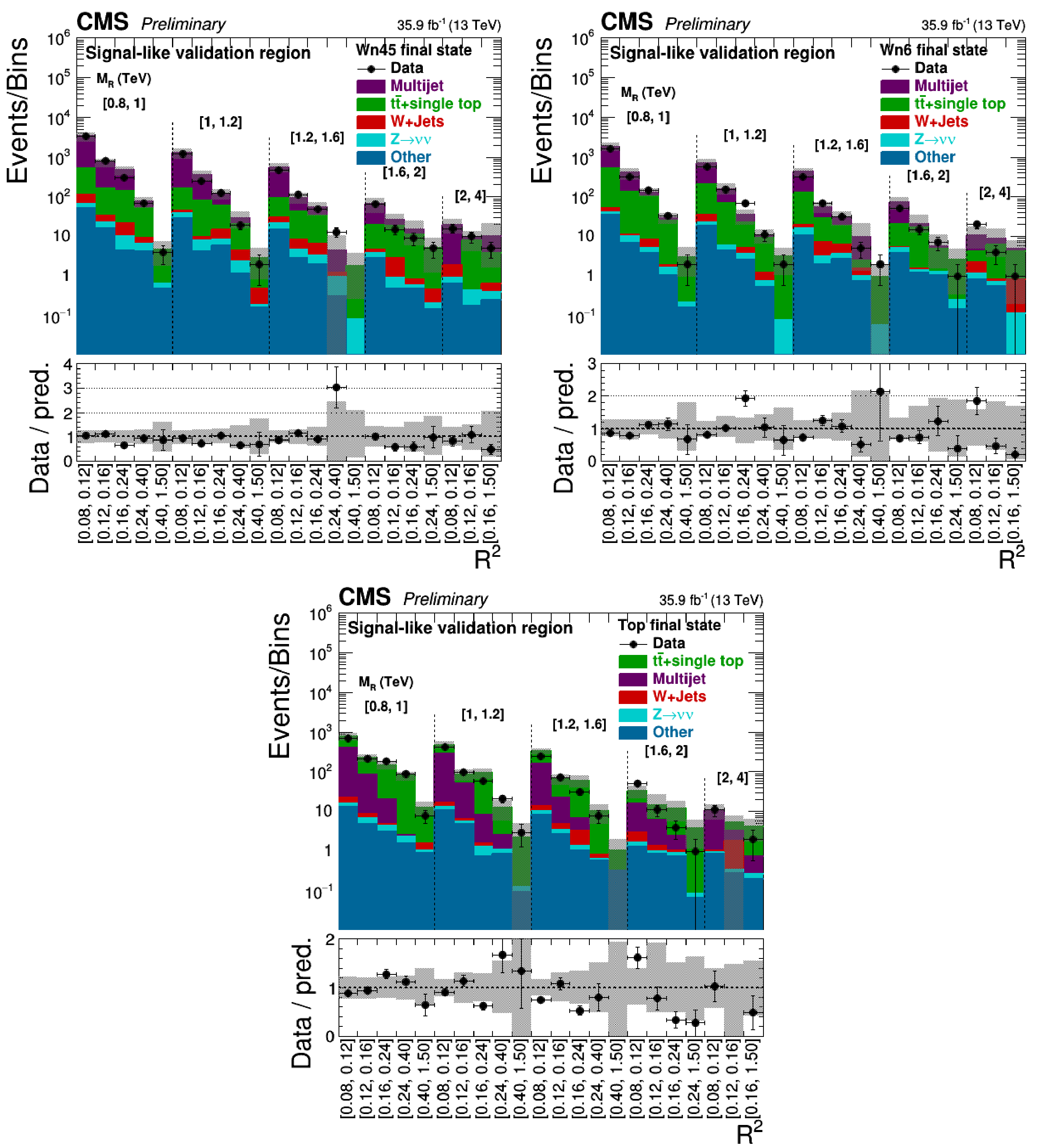
png pdf	Figure 12: Comparisons between data and the predicted background for the validation region with anti-tagged W boson or top quark candidates for the boosted Wnj45 (upper left), Wnj6 (upper right) and Top (bottom) categories.
png	Figure 12-a: Comparisons between data and the predicted background for the validation region with anti-tagged W boson or top quark candidates for the boosted Wnj45 (upper left), Wnj6 (upper right) and Top (bottom) categories.
png	Figure 12-b: Comparisons between data and the predicted background for the validation region with anti-tagged W boson or top quark candidates for the boosted Wnj45 (upper left), Wnj6 (upper right) and Top (bottom) categories.
png	Figure 12-c: Comparisons between data and the predicted background for the validation region with anti-tagged W boson or top quark candidates for the boosted Wnj45 (upper left), Wnj6 (upper right) and Top (bottom) categories.
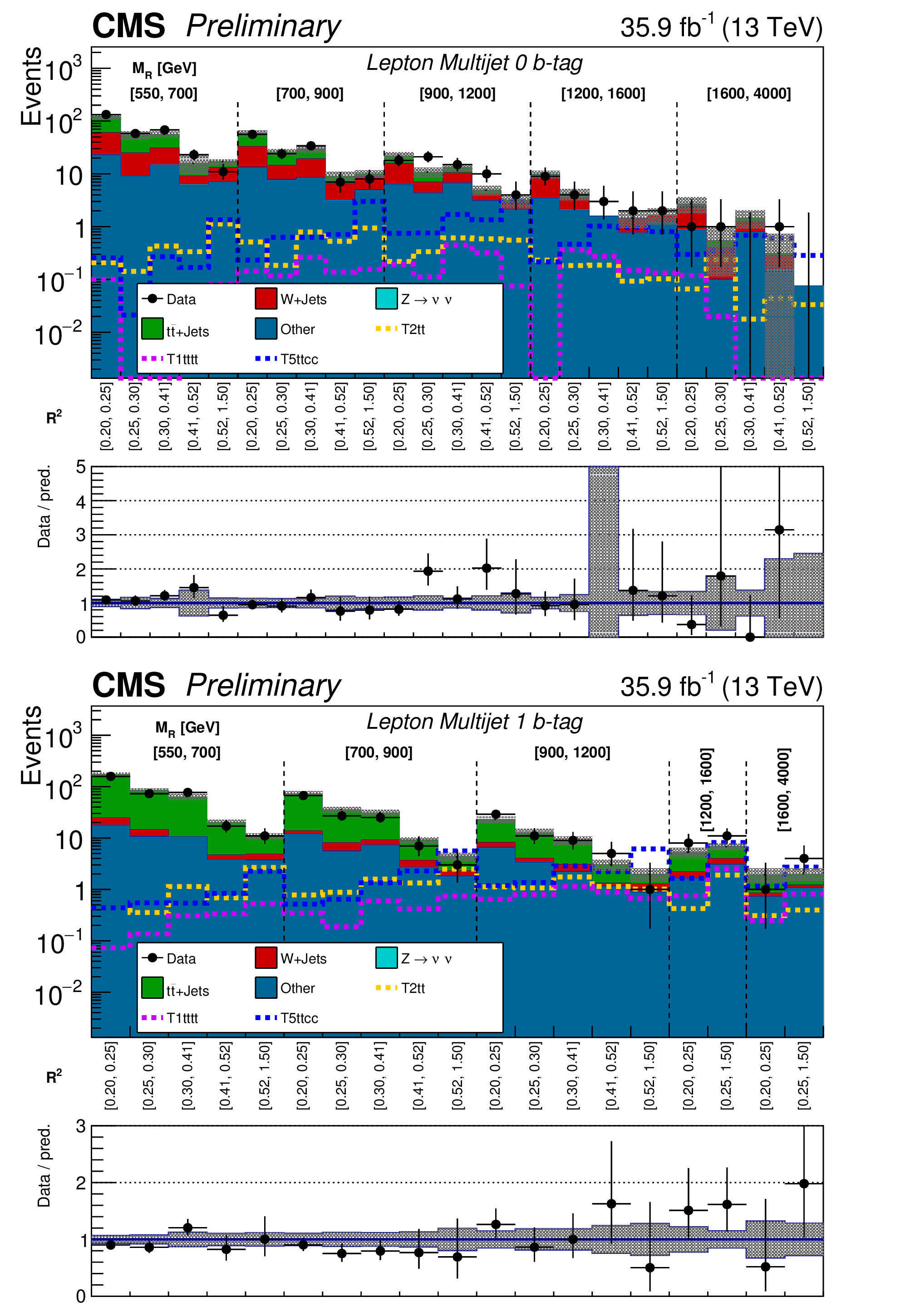
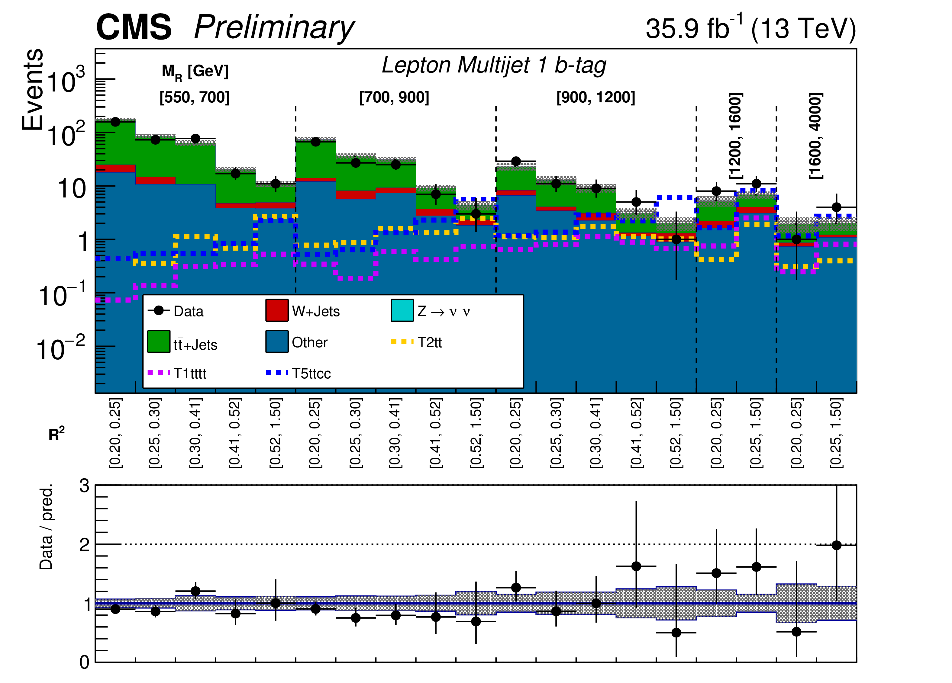
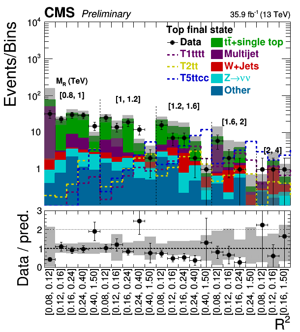
png pdf	Figure 13: The ${M_\mathrm {R}}$ - ${\mathrm {R}^2}$ distribution observed in data is shown along with the background prediction obtained for the Lepton Multijet event category in the 0 b-tag (top) and 1 b-tag (bottom) bins. The two-dimensional ${M_\mathrm {R}}$ - ${\mathrm {R}^2}$ distribution is shown in a one dimensional representation, with each ${M_\mathrm {R}}$ bin marked by the dashed lines and labeled near the top, and each ${\mathrm {R}^2}$ bin labeled below. The ratio of data to the background prediction is shown on the bottom inset, with the statistical uncertainty expressed through the data point error bars and the systematic uncertainty of the background prediction represented by the shaded region. Signal benchmarks shown are T5ttcc with $m_{\tilde{\mathrm{g}}} =$ 1.4 TeV, $m_{\tilde{\mathrm{t}}} =$ 320 GeV and $m_{\tilde{\chi}_1^0} =$ 300 GeV; T1tttt with $m_{\tilde{\mathrm{g}}} =$ 1.4 TeV and $m_{\tilde{\chi}_1^0} =$ 300 GeV; and T2tt with $m_{\tilde{\mathrm{t}}} =$ 850 GeV and $m_{\tilde{\chi}_1^0} =$ 100 GeV. The diagrams corresponding to these signal models are shown in Figure xxxxx.
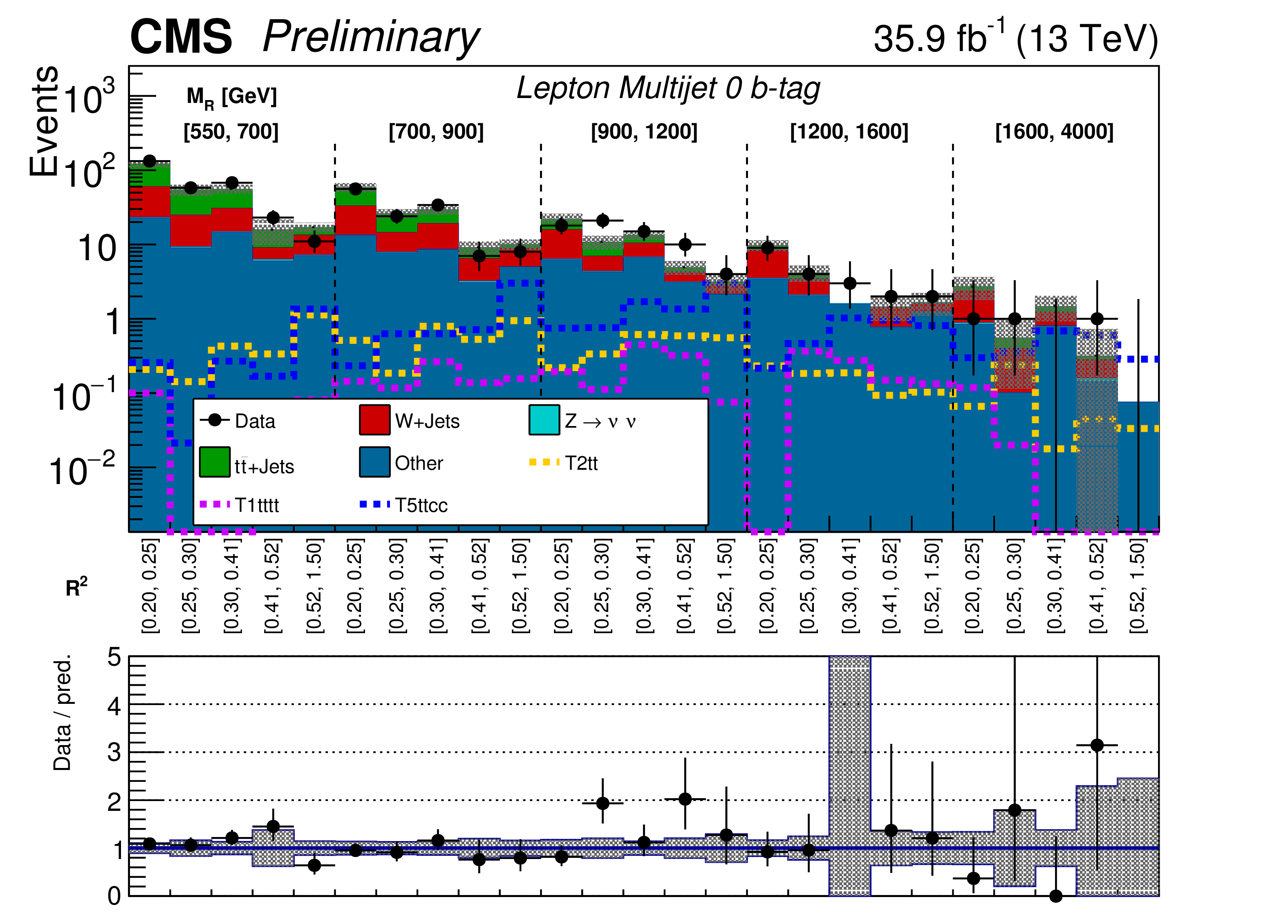
png pdf	Figure 13-a: The ${M_\mathrm {R}}$ - ${\mathrm {R}^2}$ distribution observed in data is shown along with the background prediction obtained for the Lepton Multijet event category in the 0 b-tag (top) and 1 b-tag (bottom) bins. The two-dimensional ${M_\mathrm {R}}$ - ${\mathrm {R}^2}$ distribution is shown in a one dimensional representation, with each ${M_\mathrm {R}}$ bin marked by the dashed lines and labeled near the top, and each ${\mathrm {R}^2}$ bin labeled below. The ratio of data to the background prediction is shown on the bottom inset, with the statistical uncertainty expressed through the data point error bars and the systematic uncertainty of the background prediction represented by the shaded region. Signal benchmarks shown are T5ttcc with $m_{\tilde{\mathrm{g}}} =$ 1.4 TeV, $m_{\tilde{\mathrm{t}}} =$ 320 GeV and $m_{\tilde{\chi}_1^0} =$ 300 GeV; T1tttt with $m_{\tilde{\mathrm{g}}} =$ 1.4 TeV and $m_{\tilde{\chi}_1^0} =$ 300 GeV; and T2tt with $m_{\tilde{\mathrm{t}}} =$ 850 GeV and $m_{\tilde{\chi}_1^0} =$ 100 GeV. The diagrams corresponding to these signal models are shown in Figure xxxxx.-a
png pdf	Figure 13-b: The ${M_\mathrm {R}}$ - ${\mathrm {R}^2}$ distribution observed in data is shown along with the background prediction obtained for the Lepton Multijet event category in the 0 b-tag (top) and 1 b-tag (bottom) bins. The two-dimensional ${M_\mathrm {R}}$ - ${\mathrm {R}^2}$ distribution is shown in a one dimensional representation, with each ${M_\mathrm {R}}$ bin marked by the dashed lines and labeled near the top, and each ${\mathrm {R}^2}$ bin labeled below. The ratio of data to the background prediction is shown on the bottom inset, with the statistical uncertainty expressed through the data point error bars and the systematic uncertainty of the background prediction represented by the shaded region. Signal benchmarks shown are T5ttcc with $m_{\tilde{\mathrm{g}}} =$ 1.4 TeV, $m_{\tilde{\mathrm{t}}} =$ 320 GeV and $m_{\tilde{\chi}_1^0} =$ 300 GeV; T1tttt with $m_{\tilde{\mathrm{g}}} =$ 1.4 TeV and $m_{\tilde{\chi}_1^0} =$ 300 GeV; and T2tt with $m_{\tilde{\mathrm{t}}} =$ 850 GeV and $m_{\tilde{\chi}_1^0} =$ 100 GeV. The diagrams corresponding to these signal models are shown in Figure xxxxx.-b
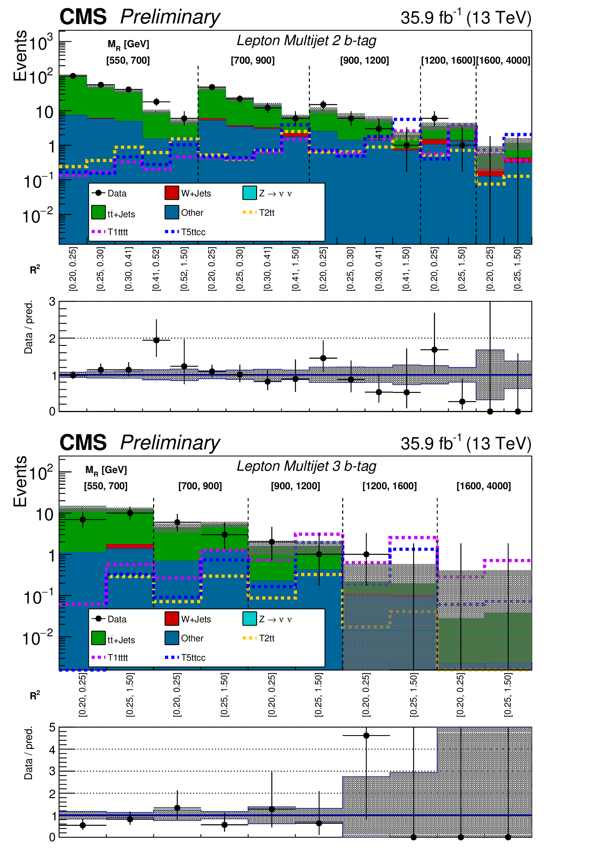
png pdf	Figure 14: The ${M_\mathrm {R}}$ - ${\mathrm {R}^2}$ distribution observed in data is shown along with the background prediction obtained for the Lepton Multijet event category in the 2 b-tag (top) and 3 b-tag (bottom) bins. The two-dimensional ${M_\mathrm {R}}$ - ${\mathrm {R}^2}$ distribution is shown in a one dimensional representation, with each ${M_\mathrm {R}}$ bin marked by the dashed lines and labeled near the top, and each ${\mathrm {R}^2}$ bin labeled below. The ratio of data to the background prediction is shown on the bottom inset, with the statistical uncertainty expressed through the data point error bars and the systematic uncertainty of the background prediction represented by the shaded region. Signal benchmarks shown are T5ttcc with $m_{\tilde{\mathrm{g}}} =$ 1.4 TeV, $m_{\tilde{\mathrm{t}}} =$ 320 GeV and $m_{\tilde{\chi}_1^0} =$ 300 GeV; T1tttt with $m_{\tilde{\mathrm{g}}} =$ 1.4 TeV and $m_{\tilde{\chi}_1^0} =$ 300 GeV; and T2tt with $m_{\tilde{\mathrm{t}}} =$ 850 GeV and $m_{\tilde{\chi}_1^0} =$ 100 GeV. The diagrams corresponding to these signal models are shown in Figure xxxxx.
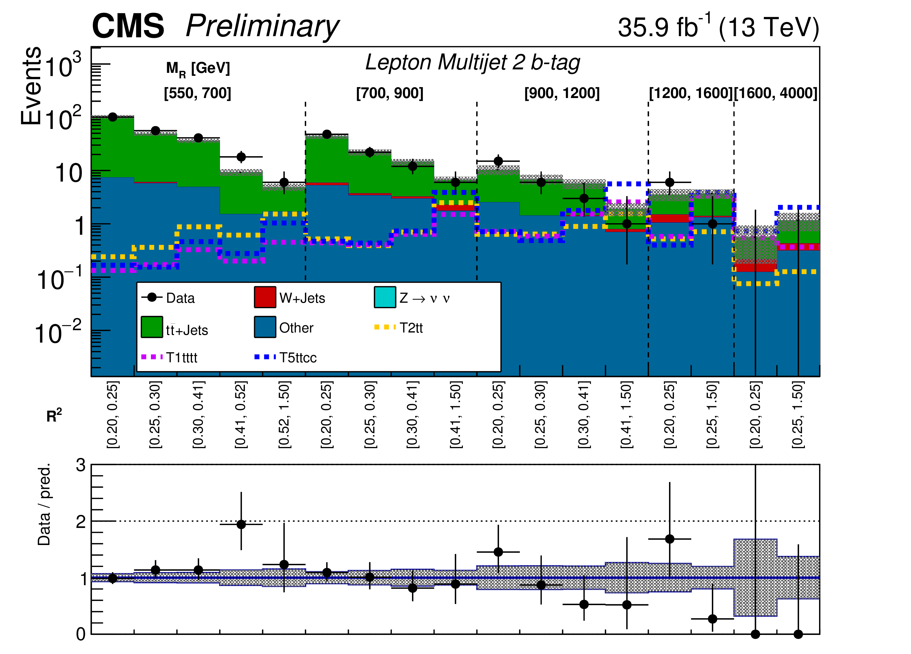
png pdf	Figure 14-a: The ${M_\mathrm {R}}$ - ${\mathrm {R}^2}$ distribution observed in data is shown along with the background prediction obtained for the Lepton Multijet event category in the 2 b-tag (top) and 3 b-tag (bottom) bins. The two-dimensional ${M_\mathrm {R}}$ - ${\mathrm {R}^2}$ distribution is shown in a one dimensional representation, with each ${M_\mathrm {R}}$ bin marked by the dashed lines and labeled near the top, and each ${\mathrm {R}^2}$ bin labeled below. The ratio of data to the background prediction is shown on the bottom inset, with the statistical uncertainty expressed through the data point error bars and the systematic uncertainty of the background prediction represented by the shaded region. Signal benchmarks shown are T5ttcc with $m_{\tilde{\mathrm{g}}} =$ 1.4 TeV, $m_{\tilde{\mathrm{t}}} =$ 320 GeV and $m_{\tilde{\chi}_1^0} =$ 300 GeV; T1tttt with $m_{\tilde{\mathrm{g}}} =$ 1.4 TeV and $m_{\tilde{\chi}_1^0} =$ 300 GeV; and T2tt with $m_{\tilde{\mathrm{t}}} =$ 850 GeV and $m_{\tilde{\chi}_1^0} =$ 100 GeV. The diagrams corresponding to these signal models are shown in Figure xxxxx.-a
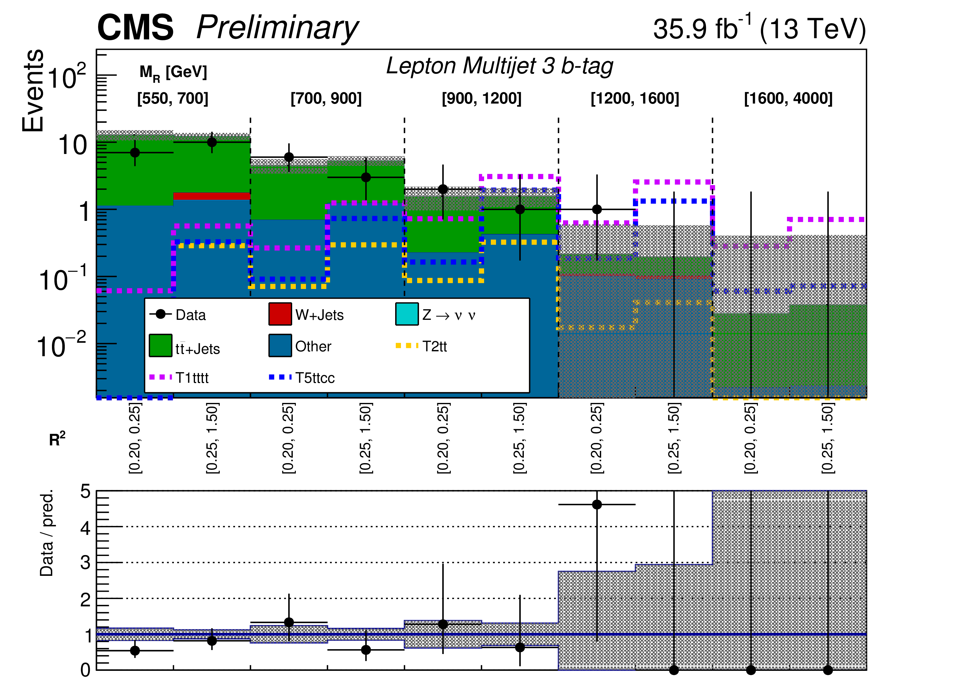
png pdf	Figure 14-b: The ${M_\mathrm {R}}$ - ${\mathrm {R}^2}$ distribution observed in data is shown along with the background prediction obtained for the Lepton Multijet event category in the 2 b-tag (top) and 3 b-tag (bottom) bins. The two-dimensional ${M_\mathrm {R}}$ - ${\mathrm {R}^2}$ distribution is shown in a one dimensional representation, with each ${M_\mathrm {R}}$ bin marked by the dashed lines and labeled near the top, and each ${\mathrm {R}^2}$ bin labeled below. The ratio of data to the background prediction is shown on the bottom inset, with the statistical uncertainty expressed through the data point error bars and the systematic uncertainty of the background prediction represented by the shaded region. Signal benchmarks shown are T5ttcc with $m_{\tilde{\mathrm{g}}} =$ 1.4 TeV, $m_{\tilde{\mathrm{t}}} =$ 320 GeV and $m_{\tilde{\chi}_1^0} =$ 300 GeV; T1tttt with $m_{\tilde{\mathrm{g}}} =$ 1.4 TeV and $m_{\tilde{\chi}_1^0} =$ 300 GeV; and T2tt with $m_{\tilde{\mathrm{t}}} =$ 850 GeV and $m_{\tilde{\chi}_1^0} =$ 100 GeV. The diagrams corresponding to these signal models are shown in Figure xxxxx.-b
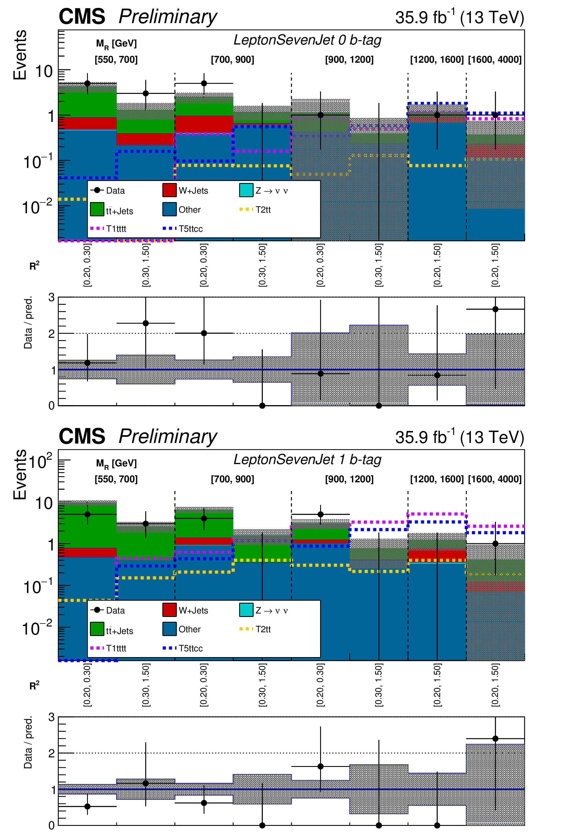
png pdf	Figure 15: The ${M_\mathrm {R}}$ - ${\mathrm {R}^2}$ distribution observed in data is shown along with the background prediction obtained for the Lepton Seven-jet event category in the 0 b-tag (top) and 1 b-tag (bottom) bins. The two-dimensional ${M_\mathrm {R}}$ - ${\mathrm {R}^2}$ distribution is shown in a one dimensional representation, with each ${M_\mathrm {R}}$ bin marked by the dashed lines and labeled near the top, and each ${\mathrm {R}^2}$ bin labeled below. The ratio of data to the background prediction is shown on the bottom inset, with the statistical uncertainty expressed through the data point error bars and the systematic uncertainty of the background prediction represented by the shaded region. Signal benchmarks shown are T5ttcc with $m_{\tilde{\mathrm{g}}} =$ 1.4 TeV, $m_{\tilde{\mathrm{t}}} =$ 320 GeV and $m_{\tilde{\chi}_1^0} =$ 300 GeV; T1tttt with $m_{\tilde{\mathrm{g}}} =$ 1.4 TeV and $m_{\tilde{\chi}_1^0} =$ 300 GeV; and T2tt with $m_{\tilde{\mathrm{t}}} =$ 850 GeV and $m_{\tilde{\chi}_1^0} =$ 100 GeV. The diagrams corresponding to these signal models are shown in Figure xxxxx.
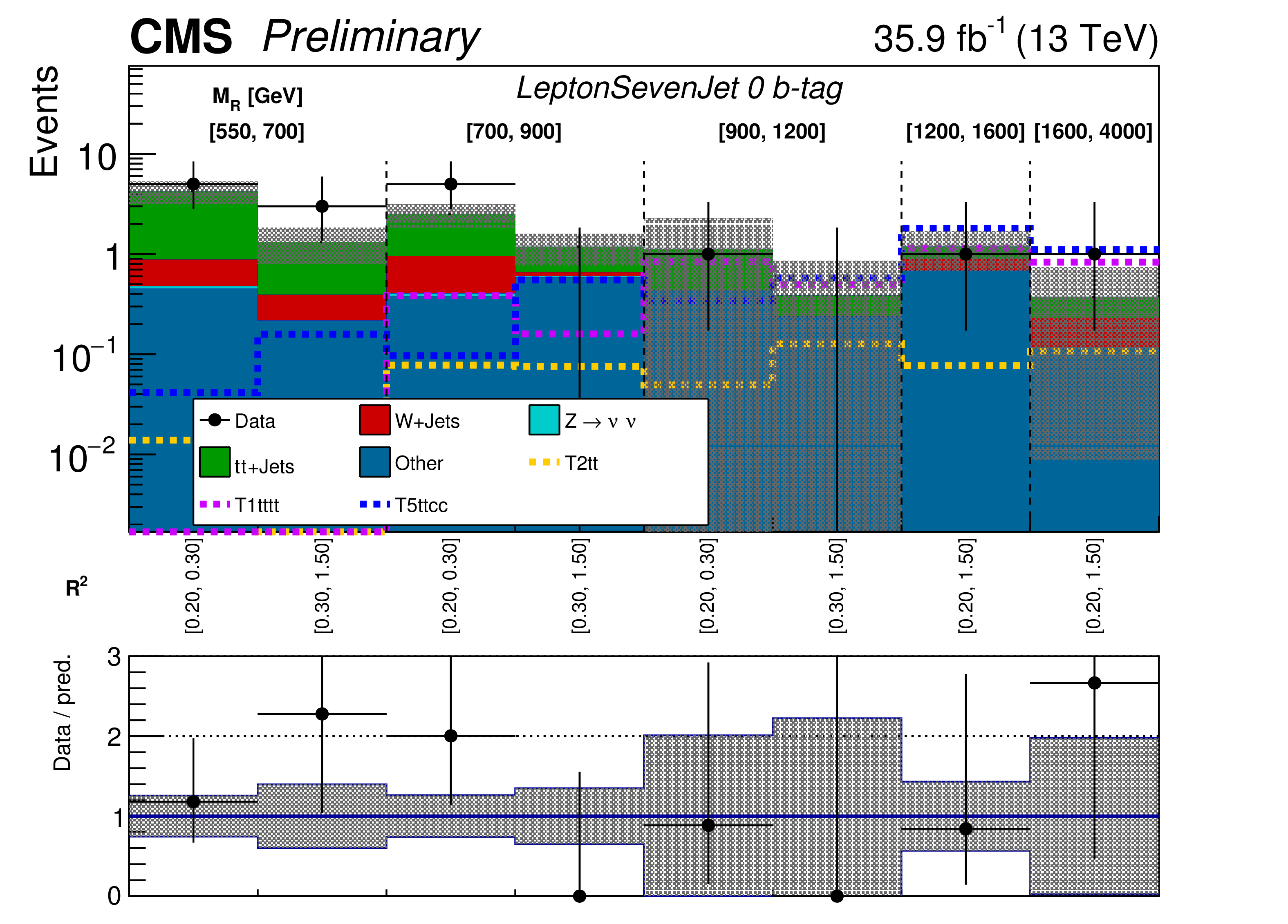
png pdf	Figure 15-a: The ${M_\mathrm {R}}$ - ${\mathrm {R}^2}$ distribution observed in data is shown along with the background prediction obtained for the Lepton Seven-jet event category in the 0 b-tag (top) and 1 b-tag (bottom) bins. The two-dimensional ${M_\mathrm {R}}$ - ${\mathrm {R}^2}$ distribution is shown in a one dimensional representation, with each ${M_\mathrm {R}}$ bin marked by the dashed lines and labeled near the top, and each ${\mathrm {R}^2}$ bin labeled below. The ratio of data to the background prediction is shown on the bottom inset, with the statistical uncertainty expressed through the data point error bars and the systematic uncertainty of the background prediction represented by the shaded region. Signal benchmarks shown are T5ttcc with $m_{\tilde{\mathrm{g}}} =$ 1.4 TeV, $m_{\tilde{\mathrm{t}}} =$ 320 GeV and $m_{\tilde{\chi}_1^0} =$ 300 GeV; T1tttt with $m_{\tilde{\mathrm{g}}} =$ 1.4 TeV and $m_{\tilde{\chi}_1^0} =$ 300 GeV; and T2tt with $m_{\tilde{\mathrm{t}}} =$ 850 GeV and $m_{\tilde{\chi}_1^0} =$ 100 GeV. The diagrams corresponding to these signal models are shown in Figure xxxxx.-a
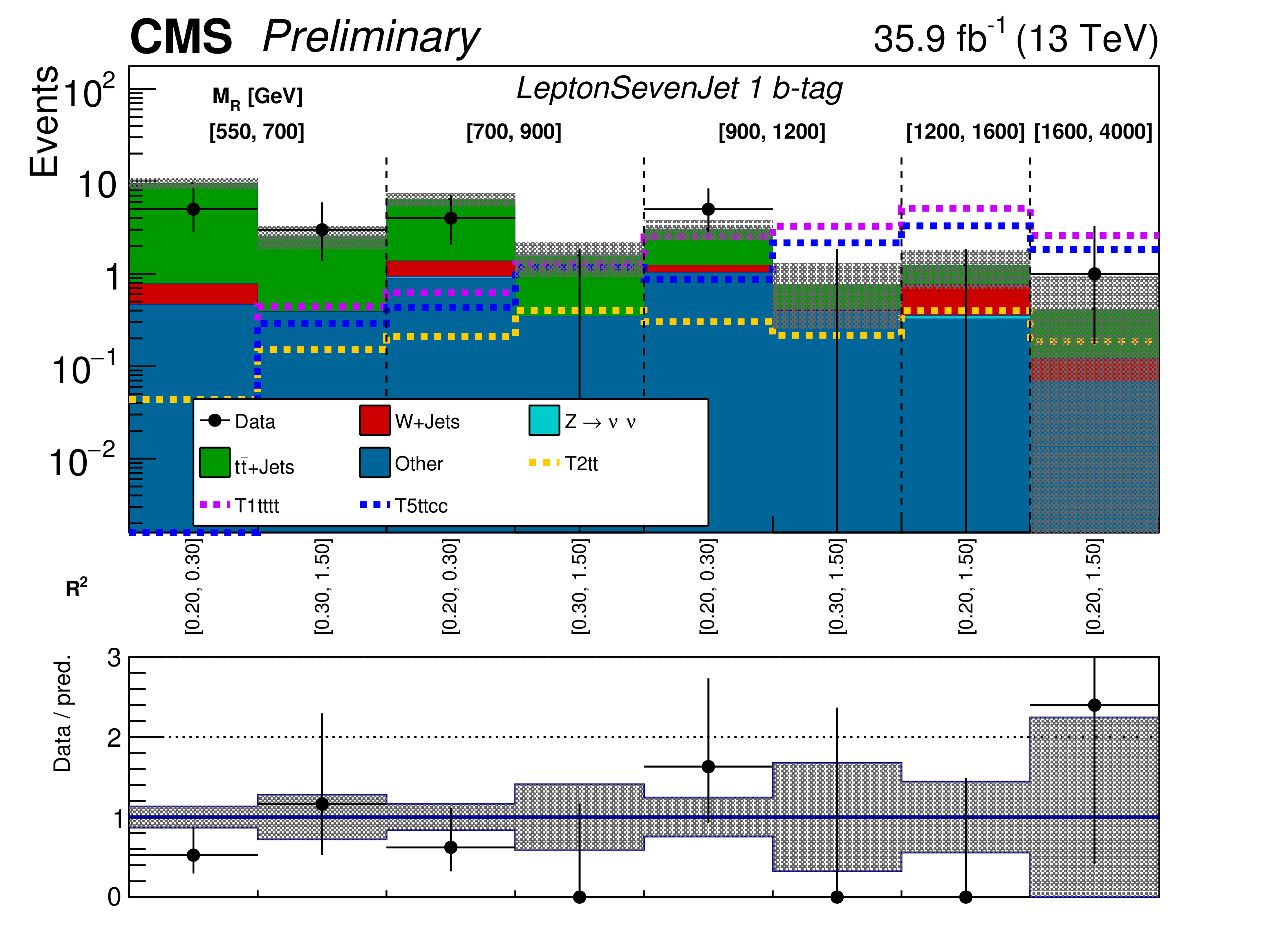
png pdf	Figure 15-b: The ${M_\mathrm {R}}$ - ${\mathrm {R}^2}$ distribution observed in data is shown along with the background prediction obtained for the Lepton Seven-jet event category in the 0 b-tag (top) and 1 b-tag (bottom) bins. The two-dimensional ${M_\mathrm {R}}$ - ${\mathrm {R}^2}$ distribution is shown in a one dimensional representation, with each ${M_\mathrm {R}}$ bin marked by the dashed lines and labeled near the top, and each ${\mathrm {R}^2}$ bin labeled below. The ratio of data to the background prediction is shown on the bottom inset, with the statistical uncertainty expressed through the data point error bars and the systematic uncertainty of the background prediction represented by the shaded region. Signal benchmarks shown are T5ttcc with $m_{\tilde{\mathrm{g}}} =$ 1.4 TeV, $m_{\tilde{\mathrm{t}}} =$ 320 GeV and $m_{\tilde{\chi}_1^0} =$ 300 GeV; T1tttt with $m_{\tilde{\mathrm{g}}} =$ 1.4 TeV and $m_{\tilde{\chi}_1^0} =$ 300 GeV; and T2tt with $m_{\tilde{\mathrm{t}}} =$ 850 GeV and $m_{\tilde{\chi}_1^0} =$ 100 GeV. The diagrams corresponding to these signal models are shown in Figure xxxxx.-b
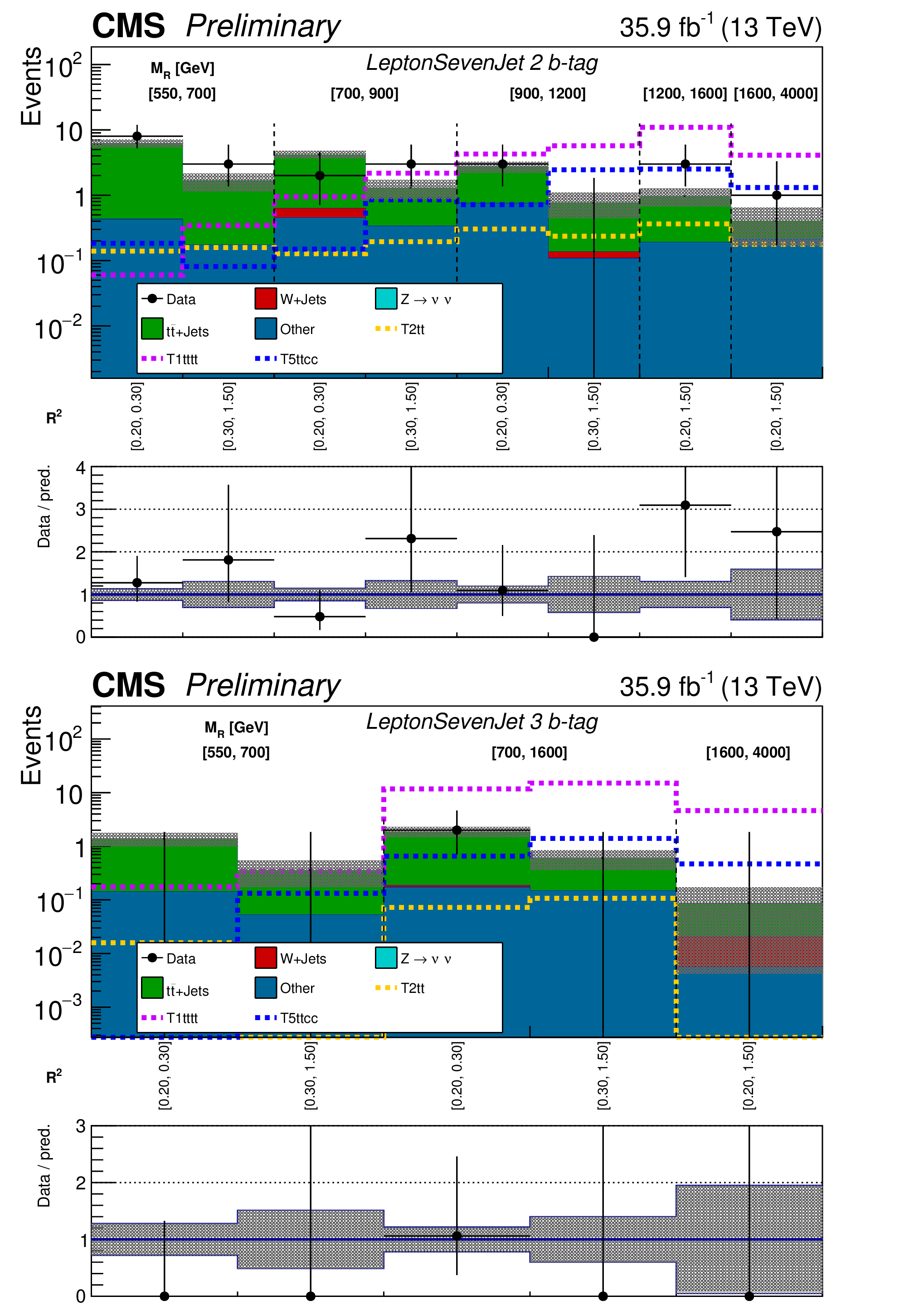
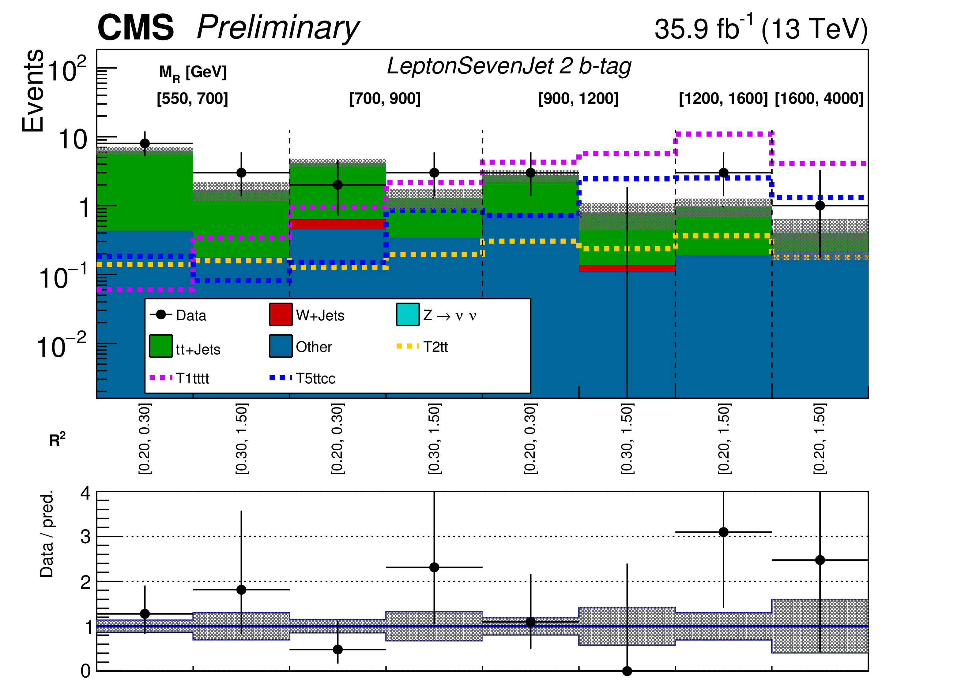
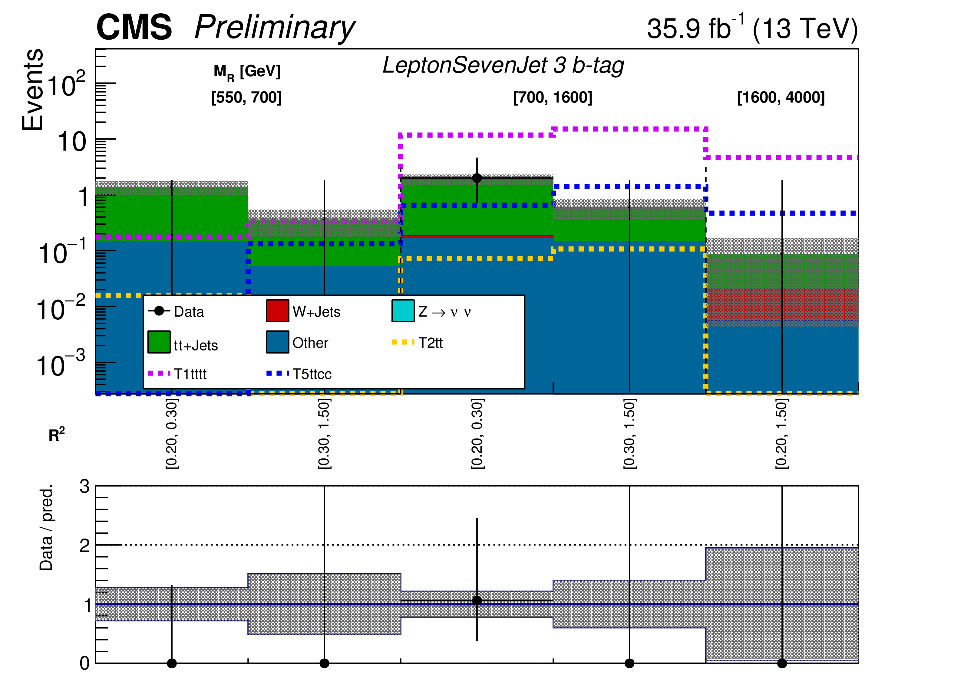
png pdf	Figure 16: The ${M_\mathrm {R}}$ - ${\mathrm {R}^2}$ distribution observed in data is shown along with the background prediction obtained for the Lepton Seven-jet event category in the 2 b-tag (top) and 3 b-tag (bottom) bins. The two-dimensional ${M_\mathrm {R}}$ - ${\mathrm {R}^2}$ distribution is shown in a one dimensional representation, with each ${M_\mathrm {R}}$ bin marked by the dashed lines and labeled near the top, and each ${\mathrm {R}^2}$ bin labeled below. The ratio of data to the background prediction is shown on the bottom inset, with the statistical uncertainty expressed through the data point error bars and the systematic uncertainty of the background prediction represented by the shaded region. Signal benchmarks shown are T5ttcc with $m_{\tilde{\mathrm{g}}} =$ 1.4 TeV, $m_{\tilde{\mathrm{t}}} =$ 320 GeV and $m_{\tilde{\chi}_1^0} =$ 300 GeV; T1tttt with $m_{\tilde{\mathrm{g}}} =$ 1.4 TeV and $m_{\tilde{\chi}_1^0} =$ 300 GeV; and T2tt with $m_{\tilde{\mathrm{t}}} =$ 850 GeV and $m_{\tilde{\chi}_1^0} =$ 100 GeV. The diagrams corresponding to these signal models are shown in Figure xxxxx.
png pdf	Figure 16-a: The ${M_\mathrm {R}}$ - ${\mathrm {R}^2}$ distribution observed in data is shown along with the background prediction obtained for the Lepton Seven-jet event category in the 2 b-tag (top) and 3 b-tag (bottom) bins. The two-dimensional ${M_\mathrm {R}}$ - ${\mathrm {R}^2}$ distribution is shown in a one dimensional representation, with each ${M_\mathrm {R}}$ bin marked by the dashed lines and labeled near the top, and each ${\mathrm {R}^2}$ bin labeled below. The ratio of data to the background prediction is shown on the bottom inset, with the statistical uncertainty expressed through the data point error bars and the systematic uncertainty of the background prediction represented by the shaded region. Signal benchmarks shown are T5ttcc with $m_{\tilde{\mathrm{g}}} =$ 1.4 TeV, $m_{\tilde{\mathrm{t}}} =$ 320 GeV and $m_{\tilde{\chi}_1^0} =$ 300 GeV; T1tttt with $m_{\tilde{\mathrm{g}}} =$ 1.4 TeV and $m_{\tilde{\chi}_1^0} =$ 300 GeV; and T2tt with $m_{\tilde{\mathrm{t}}} =$ 850 GeV and $m_{\tilde{\chi}_1^0} =$ 100 GeV. The diagrams corresponding to these signal models are shown in Figure xxxxx.-a
png pdf	Figure 16-b: The ${M_\mathrm {R}}$ - ${\mathrm {R}^2}$ distribution observed in data is shown along with the background prediction obtained for the Lepton Seven-jet event category in the 2 b-tag (top) and 3 b-tag (bottom) bins. The two-dimensional ${M_\mathrm {R}}$ - ${\mathrm {R}^2}$ distribution is shown in a one dimensional representation, with each ${M_\mathrm {R}}$ bin marked by the dashed lines and labeled near the top, and each ${\mathrm {R}^2}$ bin labeled below. The ratio of data to the background prediction is shown on the bottom inset, with the statistical uncertainty expressed through the data point error bars and the systematic uncertainty of the background prediction represented by the shaded region. Signal benchmarks shown are T5ttcc with $m_{\tilde{\mathrm{g}}} =$ 1.4 TeV, $m_{\tilde{\mathrm{t}}} =$ 320 GeV and $m_{\tilde{\chi}_1^0} =$ 300 GeV; T1tttt with $m_{\tilde{\mathrm{g}}} =$ 1.4 TeV and $m_{\tilde{\chi}_1^0} =$ 300 GeV; and T2tt with $m_{\tilde{\mathrm{t}}} =$ 850 GeV and $m_{\tilde{\chi}_1^0} =$ 100 GeV. The diagrams corresponding to these signal models are shown in Figure xxxxx.-b
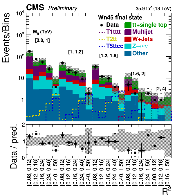
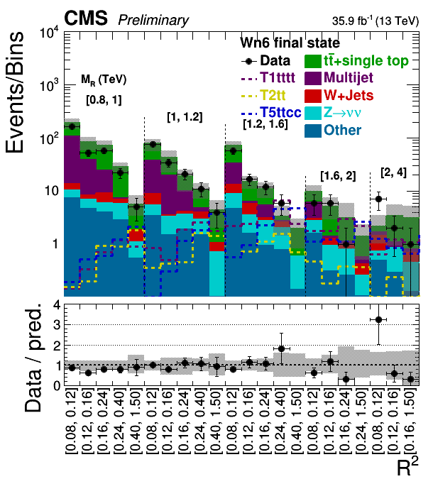
png pdf	Figure 17: The ${M_\mathrm {R}}$ - ${\mathrm {R}^2}$ distribution observed in data is shown along with the background prediction obtained for the boosted Wnj45 (upper left), Wnj6 (upper right), and Top (bottom) categories. The two-dimensional ${M_\mathrm {R}}$ - ${\mathrm {R}^2}$ distribution is shown in a one dimensional representation.The ratio of data to the background prediction is shown on the bottom inset, with the statistical uncertainty expressed through the data point error bars and the systematic uncertainty of the background prediction represented by the shaded region. Signal benchmarks shown are T5ttcc with $m_{\tilde{\mathrm{g}}} =$ 1.4 TeV, $m_{\tilde{\mathrm{t}}} =$ 320 GeV and $m_{\tilde{\chi}_1^0} =$ 300 GeV; T1tttt with $m_{\tilde{\mathrm{g}}} =$ 1.4 TeV and $m_{\tilde{\chi}_1^0} =$ 300 GeV; and T2tt with $m_{\tilde{\mathrm{t}}} =$ 850 GeV and $m_{\tilde{\chi}_1^0} =$ 100 GeV. The diagrams corresponding to these signal models are shown in Figure xxxxx.
png	Figure 17-a: The ${M_\mathrm {R}}$ - ${\mathrm {R}^2}$ distribution observed in data is shown along with the background prediction obtained for the boosted Wnj45 (upper left), Wnj6 (upper right), and Top (bottom) categories. The two-dimensional ${M_\mathrm {R}}$ - ${\mathrm {R}^2}$ distribution is shown in a one dimensional representation.The ratio of data to the background prediction is shown on the bottom inset, with the statistical uncertainty expressed through the data point error bars and the systematic uncertainty of the background prediction represented by the shaded region. Signal benchmarks shown are T5ttcc with $m_{\tilde{\mathrm{g}}} =$ 1.4 TeV, $m_{\tilde{\mathrm{t}}} =$ 320 GeV and $m_{\tilde{\chi}_1^0} =$ 300 GeV; T1tttt with $m_{\tilde{\mathrm{g}}} =$ 1.4 TeV and $m_{\tilde{\chi}_1^0} =$ 300 GeV; and T2tt with $m_{\tilde{\mathrm{t}}} =$ 850 GeV and $m_{\tilde{\chi}_1^0} =$ 100 GeV. The diagrams corresponding to these signal models are shown in Figure xxxxx.-a
png	Figure 17-b: The ${M_\mathrm {R}}$ - ${\mathrm {R}^2}$ distribution observed in data is shown along with the background prediction obtained for the boosted Wnj45 (upper left), Wnj6 (upper right), and Top (bottom) categories. The two-dimensional ${M_\mathrm {R}}$ - ${\mathrm {R}^2}$ distribution is shown in a one dimensional representation.The ratio of data to the background prediction is shown on the bottom inset, with the statistical uncertainty expressed through the data point error bars and the systematic uncertainty of the background prediction represented by the shaded region. Signal benchmarks shown are T5ttcc with $m_{\tilde{\mathrm{g}}} =$ 1.4 TeV, $m_{\tilde{\mathrm{t}}} =$ 320 GeV and $m_{\tilde{\chi}_1^0} =$ 300 GeV; T1tttt with $m_{\tilde{\mathrm{g}}} =$ 1.4 TeV and $m_{\tilde{\chi}_1^0} =$ 300 GeV; and T2tt with $m_{\tilde{\mathrm{t}}} =$ 850 GeV and $m_{\tilde{\chi}_1^0} =$ 100 GeV. The diagrams corresponding to these signal models are shown in Figure xxxxx.-b
png	Figure 17-c: The ${M_\mathrm {R}}$ - ${\mathrm {R}^2}$ distribution observed in data is shown along with the background prediction obtained for the boosted Wnj45 (upper left), Wnj6 (upper right), and Top (bottom) categories. The two-dimensional ${M_\mathrm {R}}$ - ${\mathrm {R}^2}$ distribution is shown in a one dimensional representation.The ratio of data to the background prediction is shown on the bottom inset, with the statistical uncertainty expressed through the data point error bars and the systematic uncertainty of the background prediction represented by the shaded region. Signal benchmarks shown are T5ttcc with $m_{\tilde{\mathrm{g}}} =$ 1.4 TeV, $m_{\tilde{\mathrm{t}}} =$ 320 GeV and $m_{\tilde{\chi}_1^0} =$ 300 GeV; T1tttt with $m_{\tilde{\mathrm{g}}} =$ 1.4 TeV and $m_{\tilde{\chi}_1^0} =$ 300 GeV; and T2tt with $m_{\tilde{\mathrm{t}}} =$ 850 GeV and $m_{\tilde{\chi}_1^0} =$ 100 GeV. The diagrams corresponding to these signal models are shown in Figure xxxxx.-c
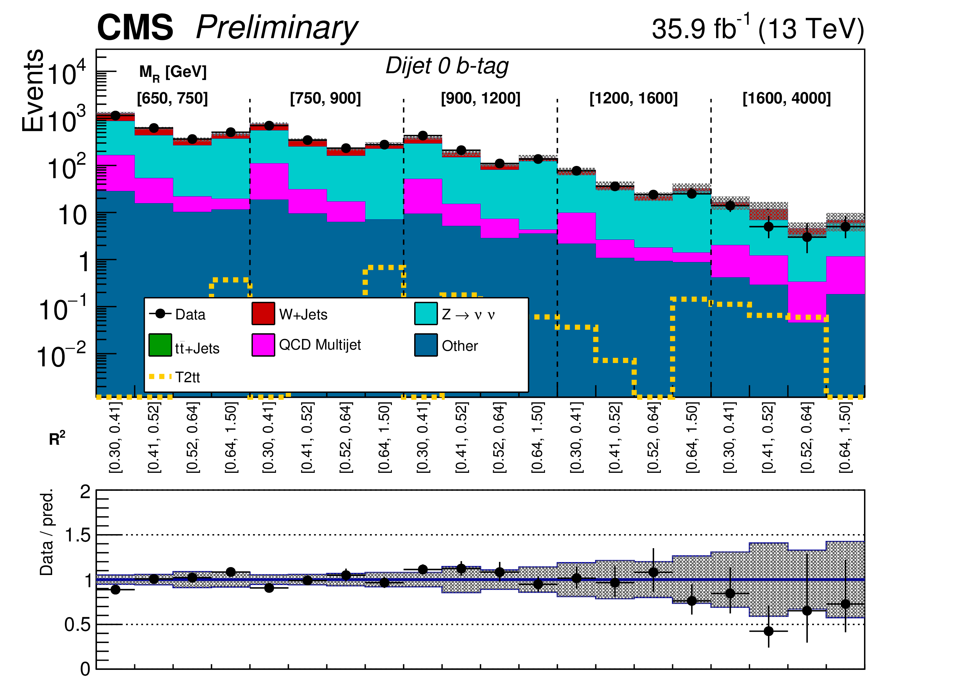
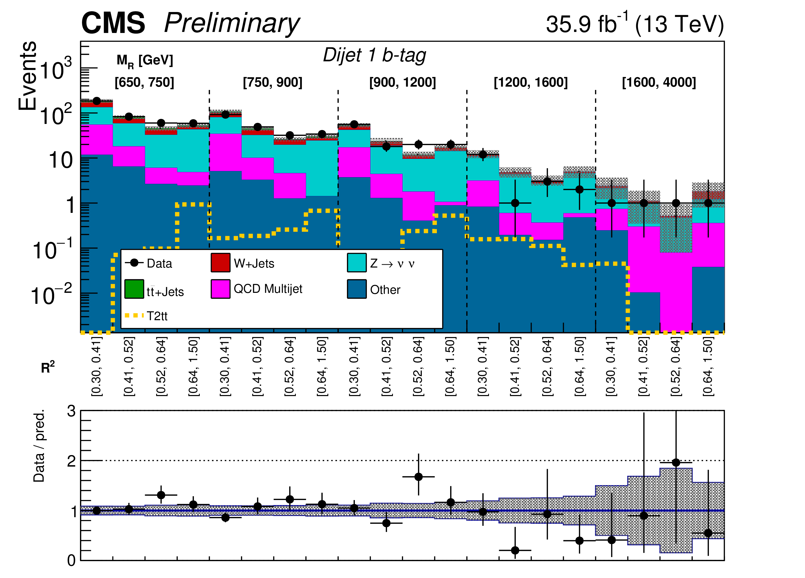
png pdf	Figure 18: The ${M_\mathrm {R}}$ - ${\mathrm {R}^2}$ distribution observed in data is shown along with the background prediction obtained for the Dijet event category in the 0 b-tag (top) and 1 b-tag (bottom) bins. The two-dimensional ${M_\mathrm {R}}$ - ${\mathrm {R}^2}$ distribution is shown in a one dimensional representation, with each ${M_\mathrm {R}}$ bin marked by the dashed lines and labeled near the top, and each ${\mathrm {R}^2}$ bin labeled below. The ratio of data to the background prediction is shown on the bottom inset, with the statistical uncertainty expressed through the data point error bars and the systematic uncertainty of the background prediction represented by the shaded region. Signal benchmarks shown are T5ttcc with $m_{\tilde{\mathrm{g}}} =$ 1.4 TeV, $m_{\tilde{\mathrm{t}}} =$ 320 GeV and $m_{\tilde{\chi}_1^0} =$ 300 GeV; T1tttt with $m_{\tilde{\mathrm{g}}} =$ 1.4 TeV and $m_{\tilde{\chi}_1^0} =$ 300 GeV; and T2tt with $m_{\tilde{\mathrm{t}}} =$ 850 GeV and $m_{\tilde{\chi}_1^0} =$ 100 GeV. The diagrams corresponding to these signal models are shown in Figure xxxxx.
png pdf	Figure 18-a: The ${M_\mathrm {R}}$ - ${\mathrm {R}^2}$ distribution observed in data is shown along with the background prediction obtained for the Dijet event category in the 0 b-tag (top) and 1 b-tag (bottom) bins. The two-dimensional ${M_\mathrm {R}}$ - ${\mathrm {R}^2}$ distribution is shown in a one dimensional representation, with each ${M_\mathrm {R}}$ bin marked by the dashed lines and labeled near the top, and each ${\mathrm {R}^2}$ bin labeled below. The ratio of data to the background prediction is shown on the bottom inset, with the statistical uncertainty expressed through the data point error bars and the systematic uncertainty of the background prediction represented by the shaded region. Signal benchmarks shown are T5ttcc with $m_{\tilde{\mathrm{g}}} =$ 1.4 TeV, $m_{\tilde{\mathrm{t}}} =$ 320 GeV and $m_{\tilde{\chi}_1^0} =$ 300 GeV; T1tttt with $m_{\tilde{\mathrm{g}}} =$ 1.4 TeV and $m_{\tilde{\chi}_1^0} =$ 300 GeV; and T2tt with $m_{\tilde{\mathrm{t}}} =$ 850 GeV and $m_{\tilde{\chi}_1^0} =$ 100 GeV. The diagrams corresponding to these signal models are shown in Figure xxxxx.-a
png pdf	Figure 18-b: The ${M_\mathrm {R}}$ - ${\mathrm {R}^2}$ distribution observed in data is shown along with the background prediction obtained for the Dijet event category in the 0 b-tag (top) and 1 b-tag (bottom) bins. The two-dimensional ${M_\mathrm {R}}$ - ${\mathrm {R}^2}$ distribution is shown in a one dimensional representation, with each ${M_\mathrm {R}}$ bin marked by the dashed lines and labeled near the top, and each ${\mathrm {R}^2}$ bin labeled below. The ratio of data to the background prediction is shown on the bottom inset, with the statistical uncertainty expressed through the data point error bars and the systematic uncertainty of the background prediction represented by the shaded region. Signal benchmarks shown are T5ttcc with $m_{\tilde{\mathrm{g}}} =$ 1.4 TeV, $m_{\tilde{\mathrm{t}}} =$ 320 GeV and $m_{\tilde{\chi}_1^0} =$ 300 GeV; T1tttt with $m_{\tilde{\mathrm{g}}} =$ 1.4 TeV and $m_{\tilde{\chi}_1^0} =$ 300 GeV; and T2tt with $m_{\tilde{\mathrm{t}}} =$ 850 GeV and $m_{\tilde{\chi}_1^0} =$ 100 GeV. The diagrams corresponding to these signal models are shown in Figure xxxxx.-b
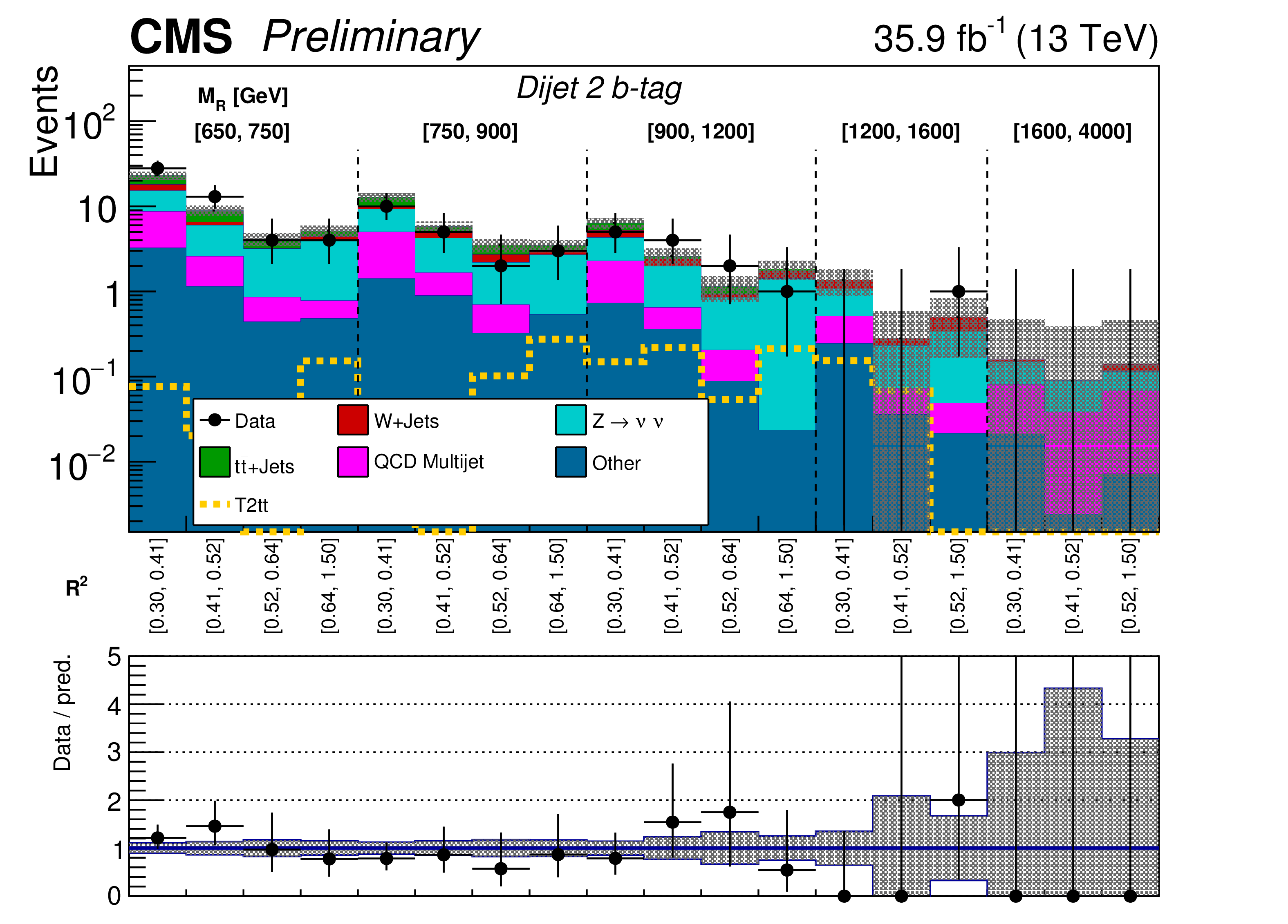
png pdf	Figure 19: The ${M_\mathrm {R}}$ - ${\mathrm {R}^2}$ distribution observed in data is shown along with the background prediction obtained for the Dijet event category in the 2 b-tag bin. The two-dimensional ${M_\mathrm {R}}$ - ${\mathrm {R}^2}$ distribution is shown in a one dimensional representation, with each ${M_\mathrm {R}}$ bin marked by the dashed lines and labeled near the top, and each ${\mathrm {R}^2}$ bin labeled below. The ratio of data to the background prediction is shown on the bottom inset, with the statistical uncertainty expressed through the data point error bars and the systematic uncertainty of the background prediction represented by the shaded region. Signal benchmarks shown are T5ttcc with $m_{\tilde{\mathrm{g}}} =$ 1.4 TeV, $m_{\tilde{\mathrm{t}}} =$ 320 GeV and $m_{\tilde{\chi}_1^0} =$ 300 GeV; T1tttt with $m_{\tilde{\mathrm{g}}} =$ 1.4 TeV and $m_{\tilde{\chi}_1^0} =$ 300 GeV; and T2tt with $m_{\tilde{\mathrm{t}}} =$ 850 GeV and $m_{\tilde{\chi}_1^0} =$ 100 GeV. The diagrams corresponding to these signal models are shown in Figure xxxxx.
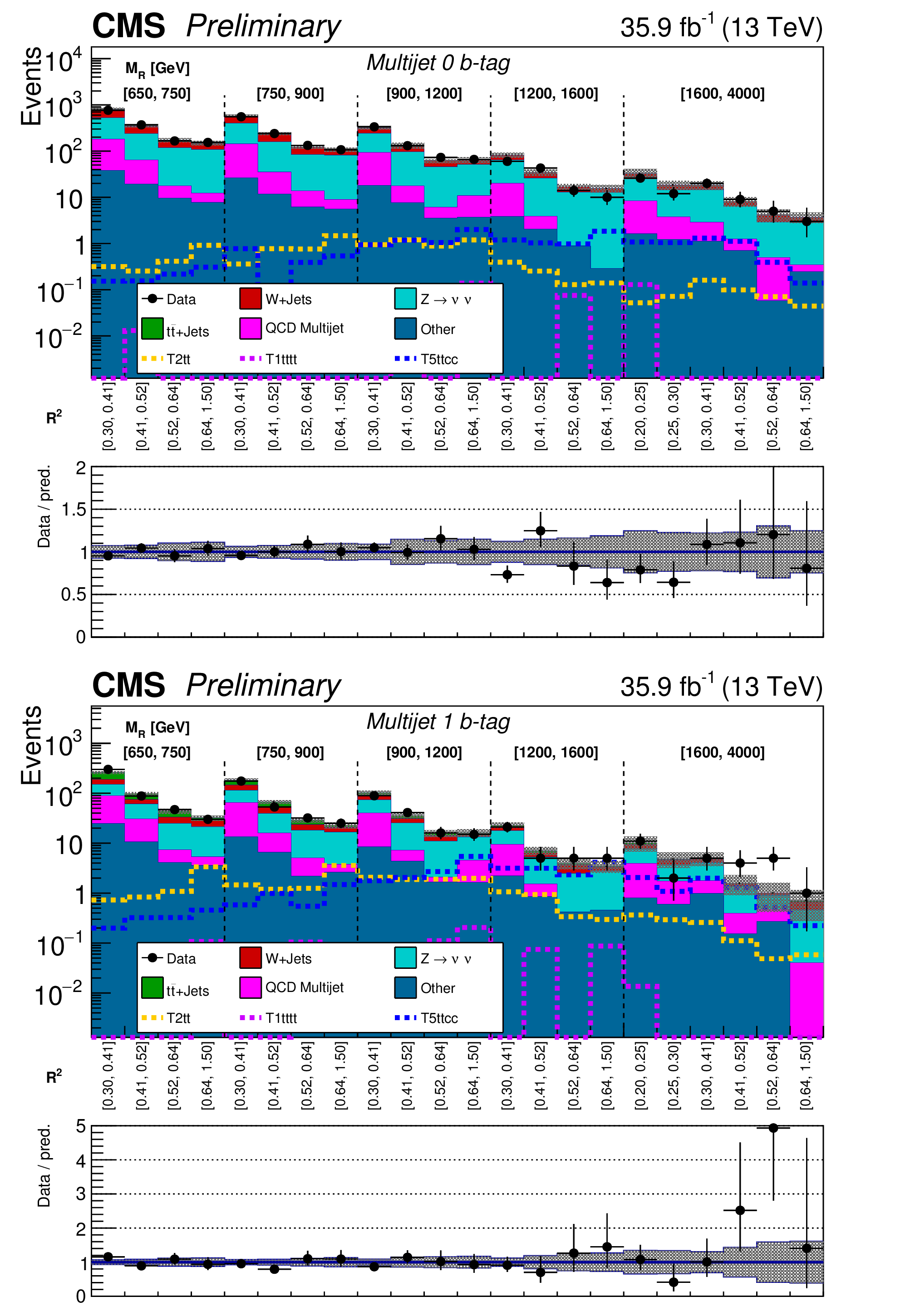
png pdf	Figure 20: The ${M_\mathrm {R}}$ - ${\mathrm {R}^2}$ distribution observed in data is shown along with the background prediction obtained for the Multijet event category in the 0 b-tag (top) and 1 b-tag (bottom) bins. The two-dimensional ${M_\mathrm {R}}$ - ${\mathrm {R}^2}$ distribution is shown in a one dimensional representation, with each ${M_\mathrm {R}}$ bin marked by the dashed lines and labeled near the top, and each ${\mathrm {R}^2}$ bin labeled below. The ratio of data to the background prediction is shown on the bottom inset, with the statistical uncertainty expressed through the data point error bars and the systematic uncertainty of the background prediction represented by the shaded region. Signal benchmarks shown are T5ttcc with $m_{\tilde{\mathrm{g}}} =$ 1.4 TeV, $m_{\tilde{\mathrm{t}}} =$ 320 GeV and $m_{\tilde{\chi}_1^0} =$ 300 GeV; T1tttt with $m_{\tilde{\mathrm{g}}} =$ 1.4 TeV and $m_{\tilde{\chi}_1^0} =$ 300 GeV; and T2tt with $m_{\tilde{\mathrm{t}}} =$ 850 GeV and $m_{\tilde{\chi}_1^0} =$ 100 GeV. The diagrams corresponding to these signal models are shown in Figure xxxxx.
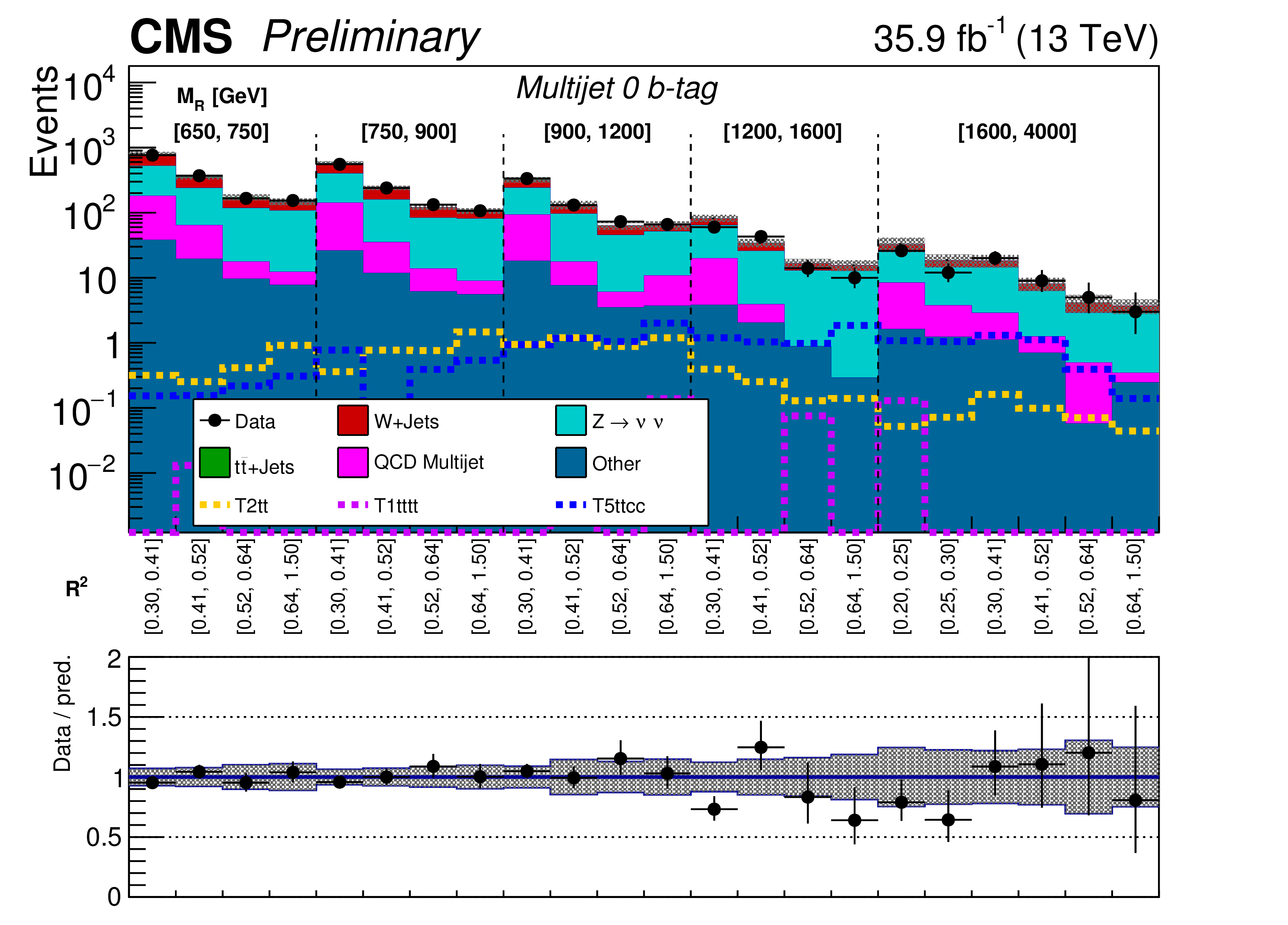
png pdf	Figure 20-a: The ${M_\mathrm {R}}$ - ${\mathrm {R}^2}$ distribution observed in data is shown along with the background prediction obtained for the Multijet event category in the 0 b-tag (top) and 1 b-tag (bottom) bins. The two-dimensional ${M_\mathrm {R}}$ - ${\mathrm {R}^2}$ distribution is shown in a one dimensional representation, with each ${M_\mathrm {R}}$ bin marked by the dashed lines and labeled near the top, and each ${\mathrm {R}^2}$ bin labeled below. The ratio of data to the background prediction is shown on the bottom inset, with the statistical uncertainty expressed through the data point error bars and the systematic uncertainty of the background prediction represented by the shaded region. Signal benchmarks shown are T5ttcc with $m_{\tilde{\mathrm{g}}} =$ 1.4 TeV, $m_{\tilde{\mathrm{t}}} =$ 320 GeV and $m_{\tilde{\chi}_1^0} =$ 300 GeV; T1tttt with $m_{\tilde{\mathrm{g}}} =$ 1.4 TeV and $m_{\tilde{\chi}_1^0} =$ 300 GeV; and T2tt with $m_{\tilde{\mathrm{t}}} =$ 850 GeV and $m_{\tilde{\chi}_1^0} =$ 100 GeV. The diagrams corresponding to these signal models are shown in Figure xxxxx.-a
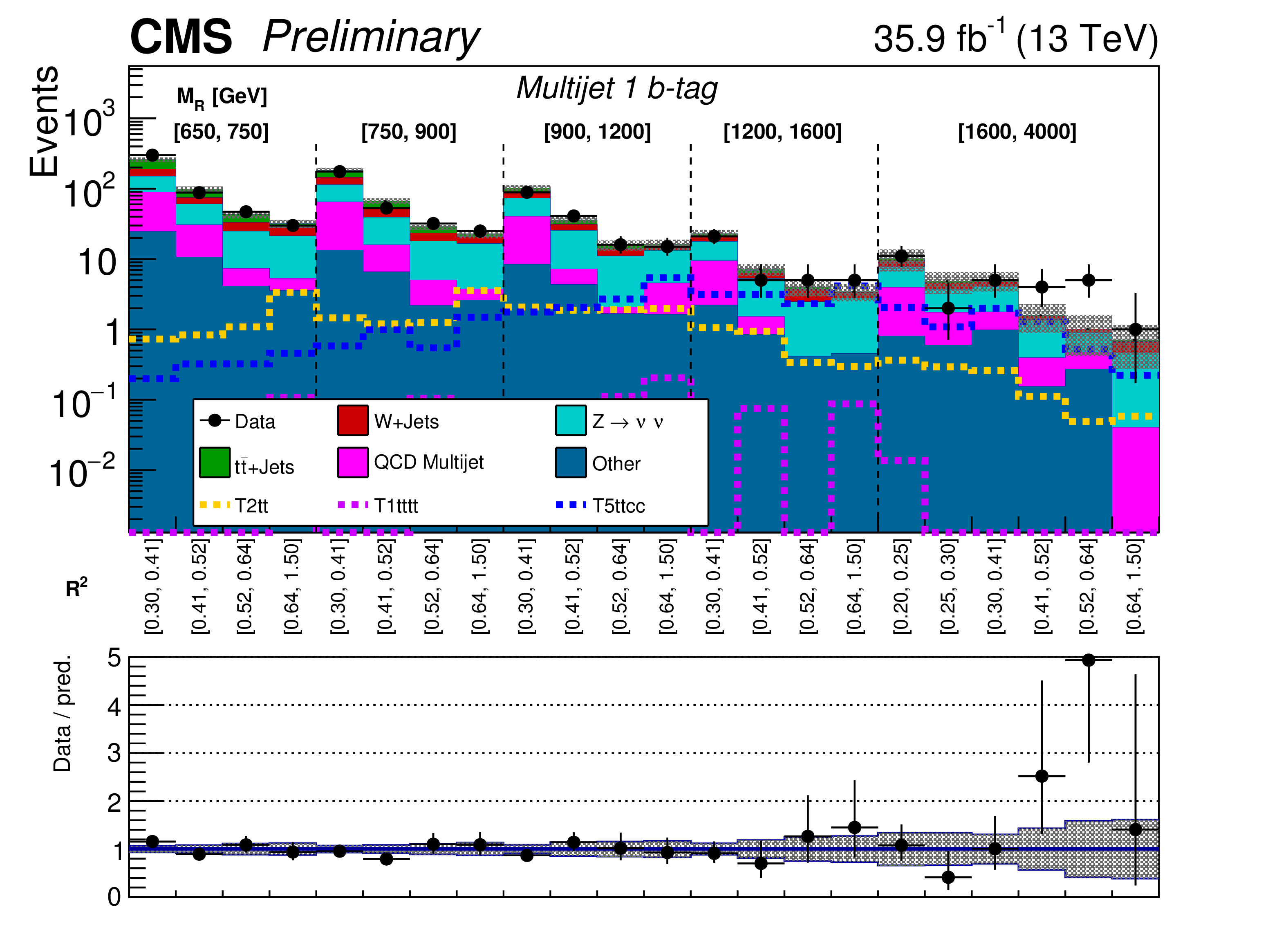
png pdf	Figure 20-b: The ${M_\mathrm {R}}$ - ${\mathrm {R}^2}$ distribution observed in data is shown along with the background prediction obtained for the Multijet event category in the 0 b-tag (top) and 1 b-tag (bottom) bins. The two-dimensional ${M_\mathrm {R}}$ - ${\mathrm {R}^2}$ distribution is shown in a one dimensional representation, with each ${M_\mathrm {R}}$ bin marked by the dashed lines and labeled near the top, and each ${\mathrm {R}^2}$ bin labeled below. The ratio of data to the background prediction is shown on the bottom inset, with the statistical uncertainty expressed through the data point error bars and the systematic uncertainty of the background prediction represented by the shaded region. Signal benchmarks shown are T5ttcc with $m_{\tilde{\mathrm{g}}} =$ 1.4 TeV, $m_{\tilde{\mathrm{t}}} =$ 320 GeV and $m_{\tilde{\chi}_1^0} =$ 300 GeV; T1tttt with $m_{\tilde{\mathrm{g}}} =$ 1.4 TeV and $m_{\tilde{\chi}_1^0} =$ 300 GeV; and T2tt with $m_{\tilde{\mathrm{t}}} =$ 850 GeV and $m_{\tilde{\chi}_1^0} =$ 100 GeV. The diagrams corresponding to these signal models are shown in Figure xxxxx.-b
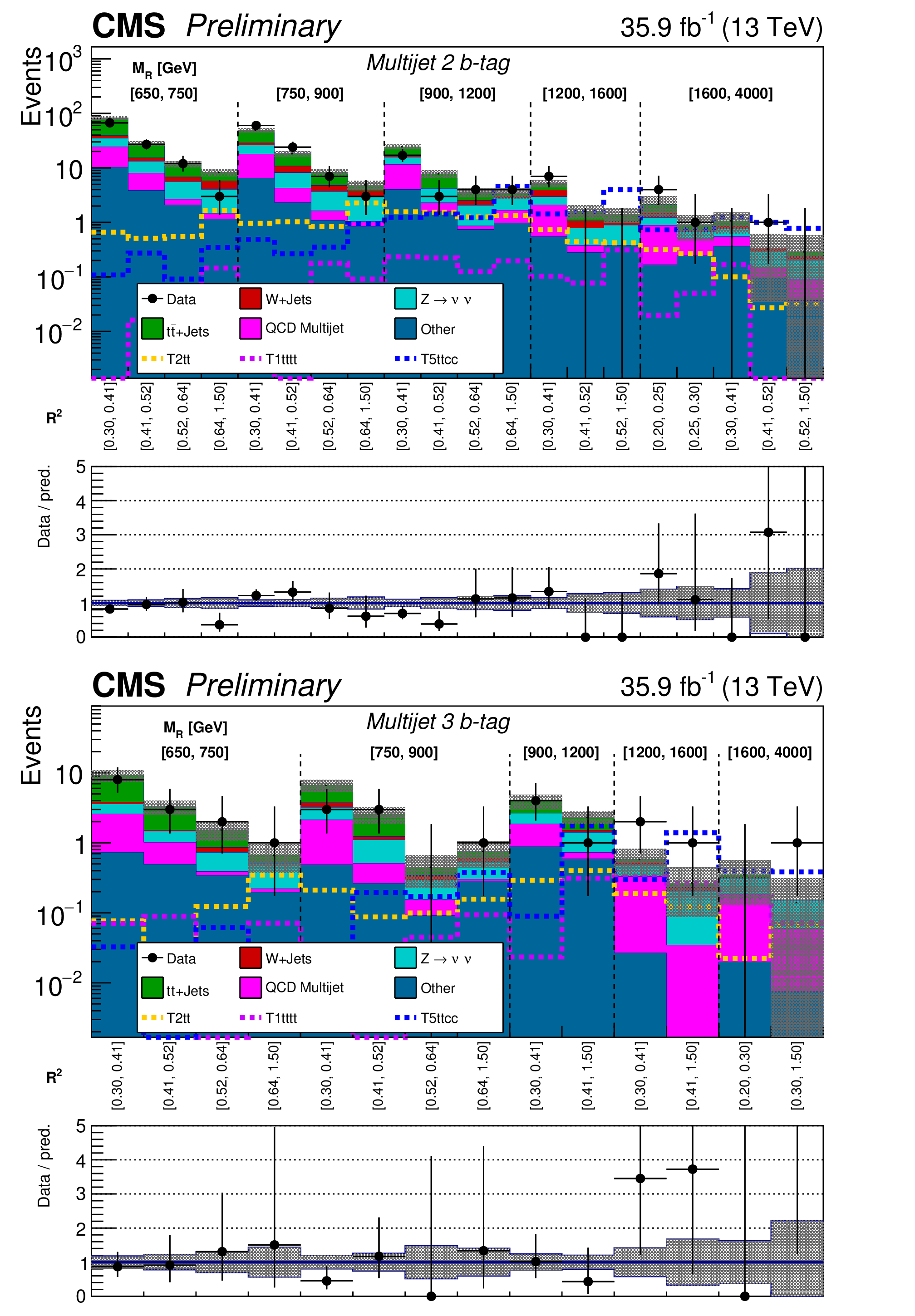
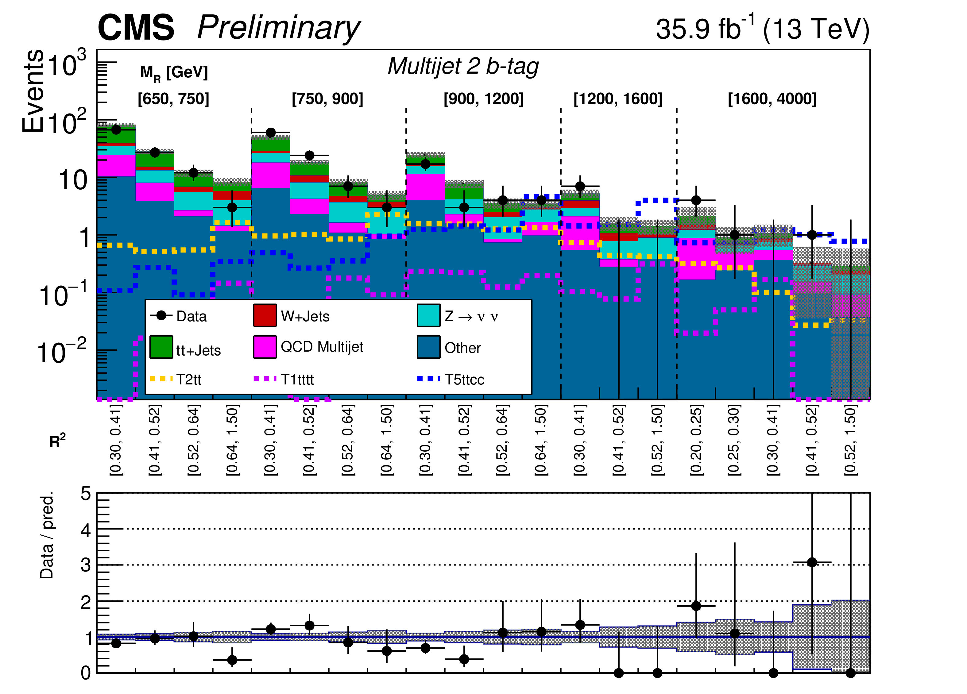
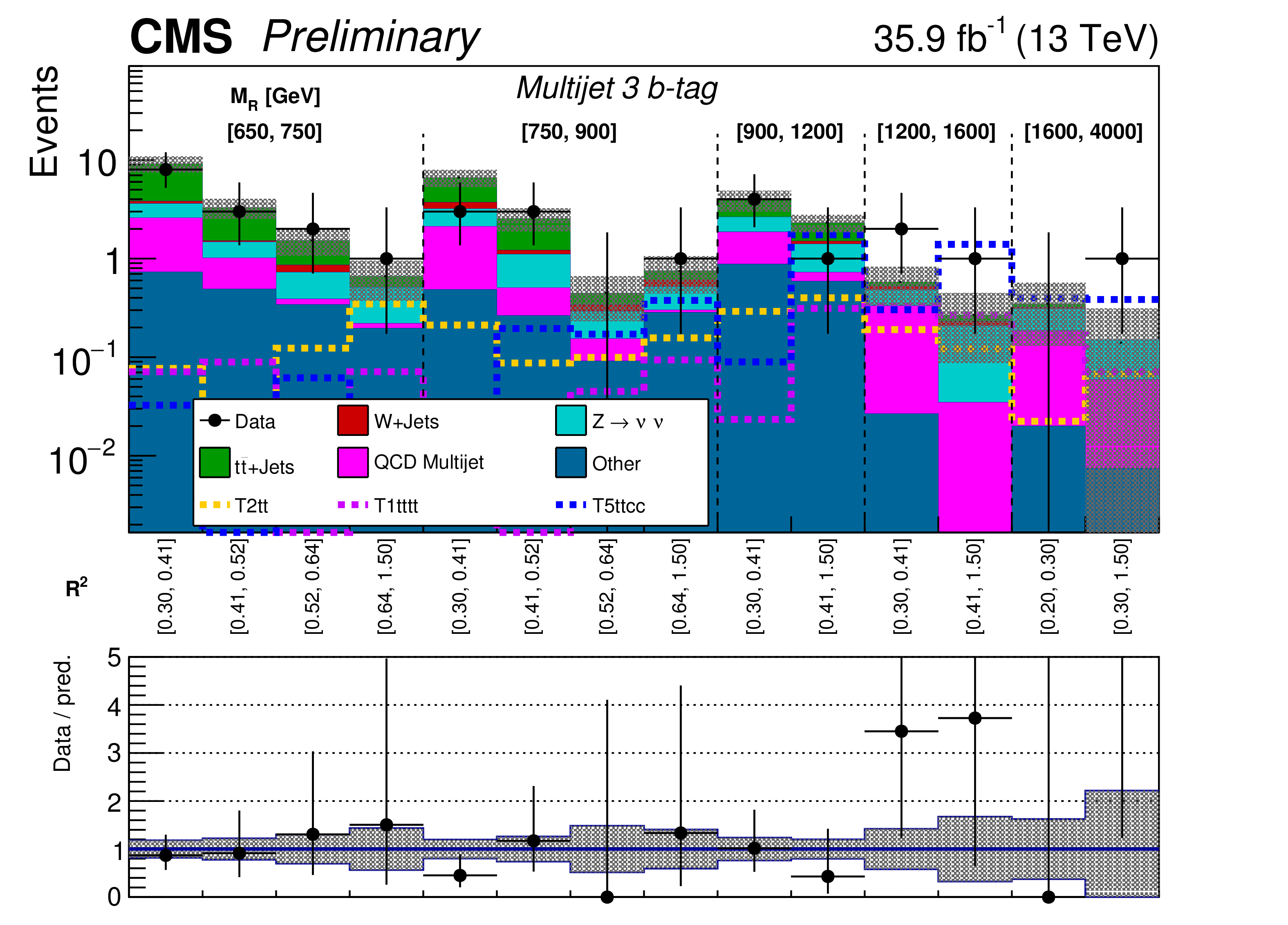
png pdf	Figure 21: The ${M_\mathrm {R}}$ - ${\mathrm {R}^2}$ distribution observed in data is shown along with the background prediction obtained for the Multijet event category in the 2 b-tag (top) and 3 b-tag (bottom) bins. The two-dimensional ${M_\mathrm {R}}$ - ${\mathrm {R}^2}$ distribution is shown in a one dimensional representation, with each ${M_\mathrm {R}}$ bin marked by the dashed lines and labeled near the top, and each ${\mathrm {R}^2}$ bin labeled below. The ratio of data to the background prediction is shown on the bottom inset, with the statistical uncertainty expressed through the data point error bars and the systematic uncertainty of the background prediction represented by the shaded region. Signal benchmarks shown are T5ttcc with $m_{\tilde{\mathrm{g}}} =$ 1.4 TeV, $m_{\tilde{\mathrm{t}}} =$ 320 GeV and $m_{\tilde{\chi}_1^0} =$ 300 GeV; T1tttt with $m_{\tilde{\mathrm{g}}} =$ 1.4 TeV and $m_{\tilde{\chi}_1^0} =$ 300 GeV; and T2tt with $m_{\tilde{\mathrm{t}}} =$ 850 GeV and $m_{\tilde{\chi}_1^0} =$ 100 GeV. The diagrams corresponding to these signal models are shown in Figure xxxxx.
png pdf	Figure 21-a: The ${M_\mathrm {R}}$ - ${\mathrm {R}^2}$ distribution observed in data is shown along with the background prediction obtained for the Multijet event category in the 2 b-tag (top) and 3 b-tag (bottom) bins. The two-dimensional ${M_\mathrm {R}}$ - ${\mathrm {R}^2}$ distribution is shown in a one dimensional representation, with each ${M_\mathrm {R}}$ bin marked by the dashed lines and labeled near the top, and each ${\mathrm {R}^2}$ bin labeled below. The ratio of data to the background prediction is shown on the bottom inset, with the statistical uncertainty expressed through the data point error bars and the systematic uncertainty of the background prediction represented by the shaded region. Signal benchmarks shown are T5ttcc with $m_{\tilde{\mathrm{g}}} =$ 1.4 TeV, $m_{\tilde{\mathrm{t}}} =$ 320 GeV and $m_{\tilde{\chi}_1^0} =$ 300 GeV; T1tttt with $m_{\tilde{\mathrm{g}}} =$ 1.4 TeV and $m_{\tilde{\chi}_1^0} =$ 300 GeV; and T2tt with $m_{\tilde{\mathrm{t}}} =$ 850 GeV and $m_{\tilde{\chi}_1^0} =$ 100 GeV. The diagrams corresponding to these signal models are shown in Figure xxxxx.-a
png pdf	Figure 21-b: The ${M_\mathrm {R}}$ - ${\mathrm {R}^2}$ distribution observed in data is shown along with the background prediction obtained for the Multijet event category in the 2 b-tag (top) and 3 b-tag (bottom) bins. The two-dimensional ${M_\mathrm {R}}$ - ${\mathrm {R}^2}$ distribution is shown in a one dimensional representation, with each ${M_\mathrm {R}}$ bin marked by the dashed lines and labeled near the top, and each ${\mathrm {R}^2}$ bin labeled below. The ratio of data to the background prediction is shown on the bottom inset, with the statistical uncertainty expressed through the data point error bars and the systematic uncertainty of the background prediction represented by the shaded region. Signal benchmarks shown are T5ttcc with $m_{\tilde{\mathrm{g}}} =$ 1.4 TeV, $m_{\tilde{\mathrm{t}}} =$ 320 GeV and $m_{\tilde{\chi}_1^0} =$ 300 GeV; T1tttt with $m_{\tilde{\mathrm{g}}} =$ 1.4 TeV and $m_{\tilde{\chi}_1^0} =$ 300 GeV; and T2tt with $m_{\tilde{\mathrm{t}}} =$ 850 GeV and $m_{\tilde{\chi}_1^0} =$ 100 GeV. The diagrams corresponding to these signal models are shown in Figure xxxxx.-b
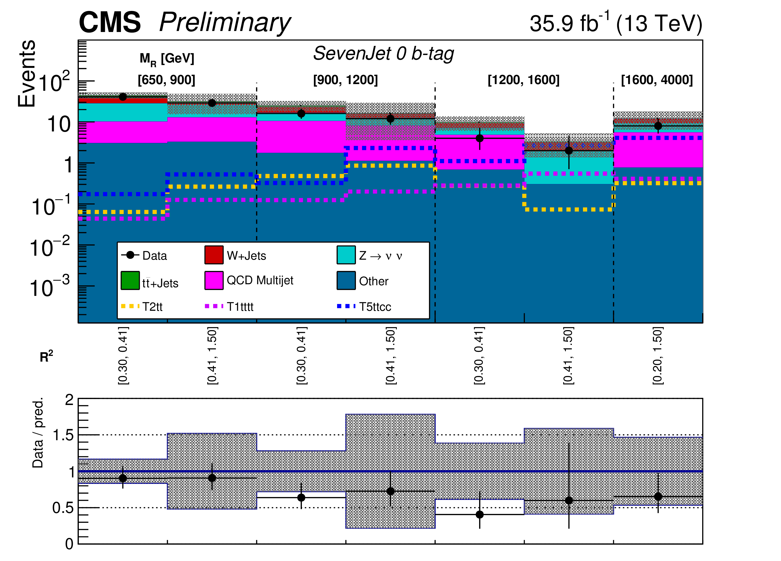
png pdf	Figure 22: The ${M_\mathrm {R}}$ - ${\mathrm {R}^2}$ distribution observed in data is shown along with the background prediction obtained for the Seven-jet event category in the 0 b-tag (top) and 1 b-tag (bottom) bins. The two-dimensional ${M_\mathrm {R}}$ - ${\mathrm {R}^2}$ distribution is shown in a one dimensional representation, with each ${M_\mathrm {R}}$ bin marked by the dashed lines and labeled near the top, and each ${\mathrm {R}^2}$ bin labeled below. The ratio of data to the background prediction is shown on the bottom inset, with the statistical uncertainty expressed through the data point error bars and the systematic uncertainty of the background prediction represented by the shaded region. Signal benchmarks shown are T5ttcc with $m_{\tilde{\mathrm{g}}} =$ 1.4 TeV, $m_{\tilde{\mathrm{t}}} =$ 320 GeV and $m_{\tilde{\chi}_1^0} =$ 300 GeV; T1tttt with $m_{\tilde{\mathrm{g}}} =$ 1.4 TeV and $m_{\tilde{\chi}_1^0} =$ 300 GeV; and T2tt with $m_{\tilde{\mathrm{t}}} =$ 850 GeV and $m_{\tilde{\chi}_1^0} =$ 100 GeV. The diagrams corresponding to these signal models are shown in Figure xxxxx.
png pdf	Figure 22-a: The ${M_\mathrm {R}}$ - ${\mathrm {R}^2}$ distribution observed in data is shown along with the background prediction obtained for the Seven-jet event category in the 0 b-tag (top) and 1 b-tag (bottom) bins. The two-dimensional ${M_\mathrm {R}}$ - ${\mathrm {R}^2}$ distribution is shown in a one dimensional representation, with each ${M_\mathrm {R}}$ bin marked by the dashed lines and labeled near the top, and each ${\mathrm {R}^2}$ bin labeled below. The ratio of data to the background prediction is shown on the bottom inset, with the statistical uncertainty expressed through the data point error bars and the systematic uncertainty of the background prediction represented by the shaded region. Signal benchmarks shown are T5ttcc with $m_{\tilde{\mathrm{g}}} =$ 1.4 TeV, $m_{\tilde{\mathrm{t}}} =$ 320 GeV and $m_{\tilde{\chi}_1^0} =$ 300 GeV; T1tttt with $m_{\tilde{\mathrm{g}}} =$ 1.4 TeV and $m_{\tilde{\chi}_1^0} =$ 300 GeV; and T2tt with $m_{\tilde{\mathrm{t}}} =$ 850 GeV and $m_{\tilde{\chi}_1^0} =$ 100 GeV. The diagrams corresponding to these signal models are shown in Figure xxxxx.-a
png pdf	Figure 22-b: The ${M_\mathrm {R}}$ - ${\mathrm {R}^2}$ distribution observed in data is shown along with the background prediction obtained for the Seven-jet event category in the 0 b-tag (top) and 1 b-tag (bottom) bins. The two-dimensional ${M_\mathrm {R}}$ - ${\mathrm {R}^2}$ distribution is shown in a one dimensional representation, with each ${M_\mathrm {R}}$ bin marked by the dashed lines and labeled near the top, and each ${\mathrm {R}^2}$ bin labeled below. The ratio of data to the background prediction is shown on the bottom inset, with the statistical uncertainty expressed through the data point error bars and the systematic uncertainty of the background prediction represented by the shaded region. Signal benchmarks shown are T5ttcc with $m_{\tilde{\mathrm{g}}} =$ 1.4 TeV, $m_{\tilde{\mathrm{t}}} =$ 320 GeV and $m_{\tilde{\chi}_1^0} =$ 300 GeV; T1tttt with $m_{\tilde{\mathrm{g}}} =$ 1.4 TeV and $m_{\tilde{\chi}_1^0} =$ 300 GeV; and T2tt with $m_{\tilde{\mathrm{t}}} =$ 850 GeV and $m_{\tilde{\chi}_1^0} =$ 100 GeV. The diagrams corresponding to these signal models are shown in Figure xxxxx.-b
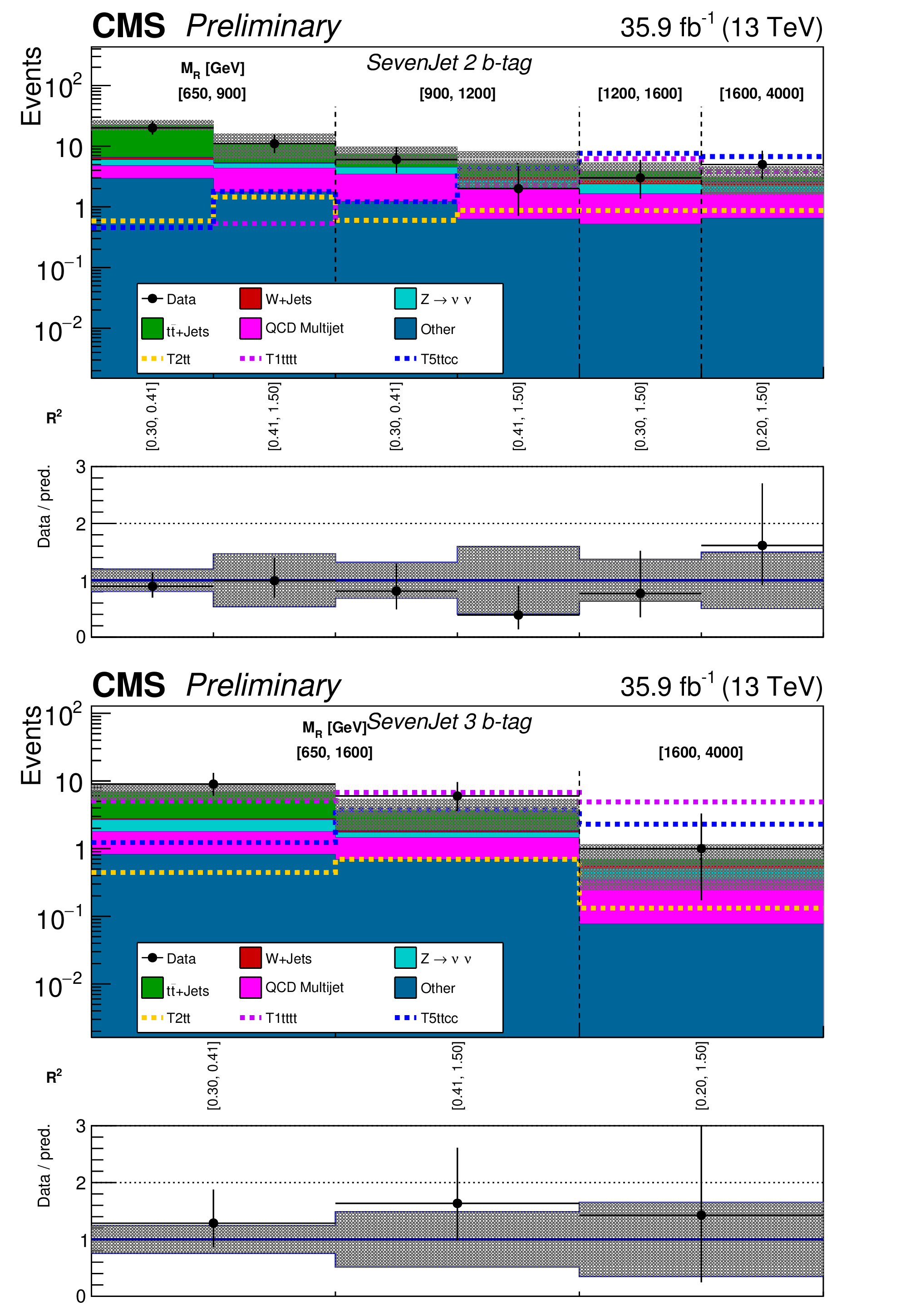
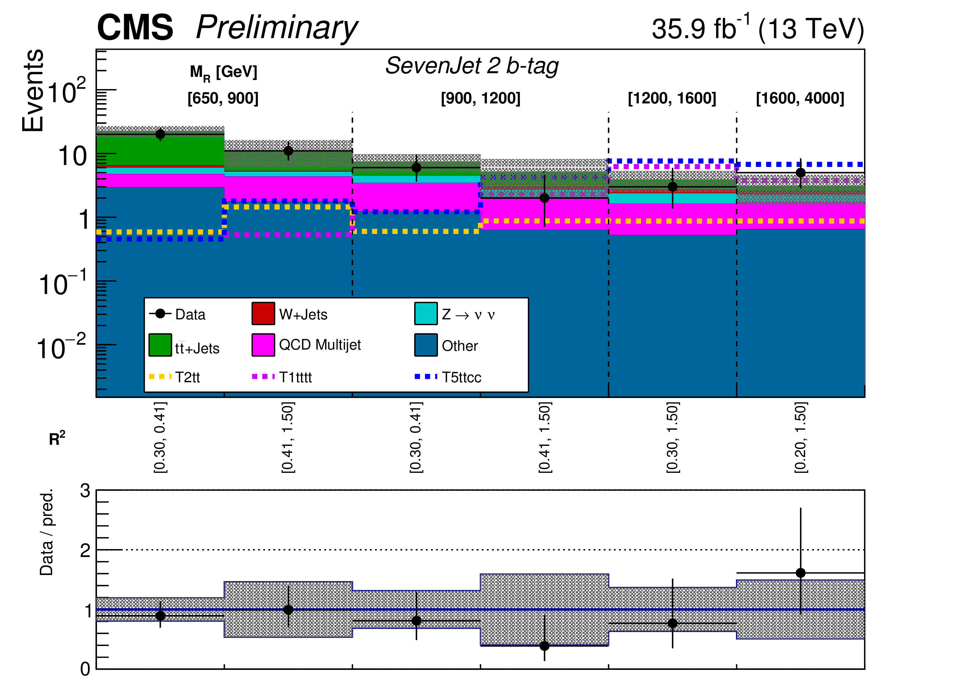
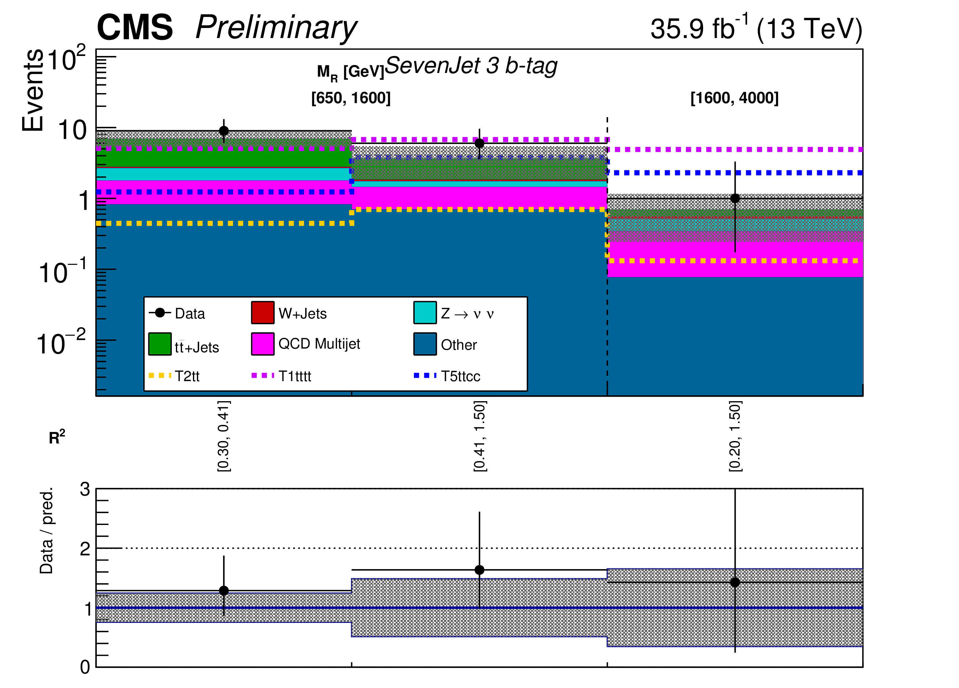
png pdf	Figure 23: The ${M_\mathrm {R}}$ - ${\mathrm {R}^2}$ distribution observed in data is shown along with the background prediction obtained for the Seven-jet event category in the 2 b-tag (top) and 3 b-tag (bottom) bins. The two-dimensional ${M_\mathrm {R}}$ - ${\mathrm {R}^2}$ distribution is shown in a one dimensional representation, with each ${M_\mathrm {R}}$ bin marked by the dashed lines and labeled near the top, and each ${\mathrm {R}^2}$ bin labeled below. The ratio of data to the background prediction is shown on the bottom inset, with the statistical uncertainty expressed through the data point error bars and the systematic uncertainty of the background prediction represented by the shaded region. Signal benchmarks shown are T5ttcc with $m_{\tilde{\mathrm{g}}} =$ 1.4 TeV, $m_{\tilde{\mathrm{t}}} =$ 320 GeV and $m_{\tilde{\chi}_1^0} =$ 300 GeV; T1tttt with $m_{\tilde{\mathrm{g}}} =$ 1.4 TeV and $m_{\tilde{\chi}_1^0} =$ 300 GeV; and T2tt with $m_{\tilde{\mathrm{t}}} =$ 850 GeV and $m_{\tilde{\chi}_1^0} =$ 100 GeV. The diagrams corresponding to these signal models are shown in Figure xxxxx.
png pdf	Figure 23-a: The ${M_\mathrm {R}}$ - ${\mathrm {R}^2}$ distribution observed in data is shown along with the background prediction obtained for the Seven-jet event category in the 2 b-tag (top) and 3 b-tag (bottom) bins. The two-dimensional ${M_\mathrm {R}}$ - ${\mathrm {R}^2}$ distribution is shown in a one dimensional representation, with each ${M_\mathrm {R}}$ bin marked by the dashed lines and labeled near the top, and each ${\mathrm {R}^2}$ bin labeled below. The ratio of data to the background prediction is shown on the bottom inset, with the statistical uncertainty expressed through the data point error bars and the systematic uncertainty of the background prediction represented by the shaded region. Signal benchmarks shown are T5ttcc with $m_{\tilde{\mathrm{g}}} =$ 1.4 TeV, $m_{\tilde{\mathrm{t}}} =$ 320 GeV and $m_{\tilde{\chi}_1^0} =$ 300 GeV; T1tttt with $m_{\tilde{\mathrm{g}}} =$ 1.4 TeV and $m_{\tilde{\chi}_1^0} =$ 300 GeV; and T2tt with $m_{\tilde{\mathrm{t}}} =$ 850 GeV and $m_{\tilde{\chi}_1^0} =$ 100 GeV. The diagrams corresponding to these signal models are shown in Figure xxxxx.-a
png pdf	Figure 23-b: The ${M_\mathrm {R}}$ - ${\mathrm {R}^2}$ distribution observed in data is shown along with the background prediction obtained for the Seven-jet event category in the 2 b-tag (top) and 3 b-tag (bottom) bins. The two-dimensional ${M_\mathrm {R}}$ - ${\mathrm {R}^2}$ distribution is shown in a one dimensional representation, with each ${M_\mathrm {R}}$ bin marked by the dashed lines and labeled near the top, and each ${\mathrm {R}^2}$ bin labeled below. The ratio of data to the background prediction is shown on the bottom inset, with the statistical uncertainty expressed through the data point error bars and the systematic uncertainty of the background prediction represented by the shaded region. Signal benchmarks shown are T5ttcc with $m_{\tilde{\mathrm{g}}} =$ 1.4 TeV, $m_{\tilde{\mathrm{t}}} =$ 320 GeV and $m_{\tilde{\chi}_1^0} =$ 300 GeV; T1tttt with $m_{\tilde{\mathrm{g}}} =$ 1.4 TeV and $m_{\tilde{\chi}_1^0} =$ 300 GeV; and T2tt with $m_{\tilde{\mathrm{t}}} =$ 850 GeV and $m_{\tilde{\chi}_1^0} =$ 100 GeV. The diagrams corresponding to these signal models are shown in Figure xxxxx.-b
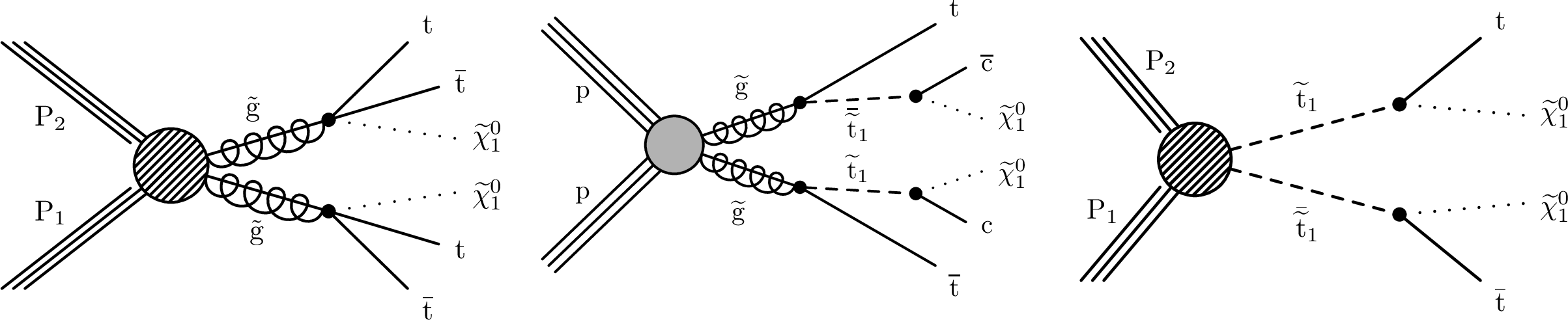
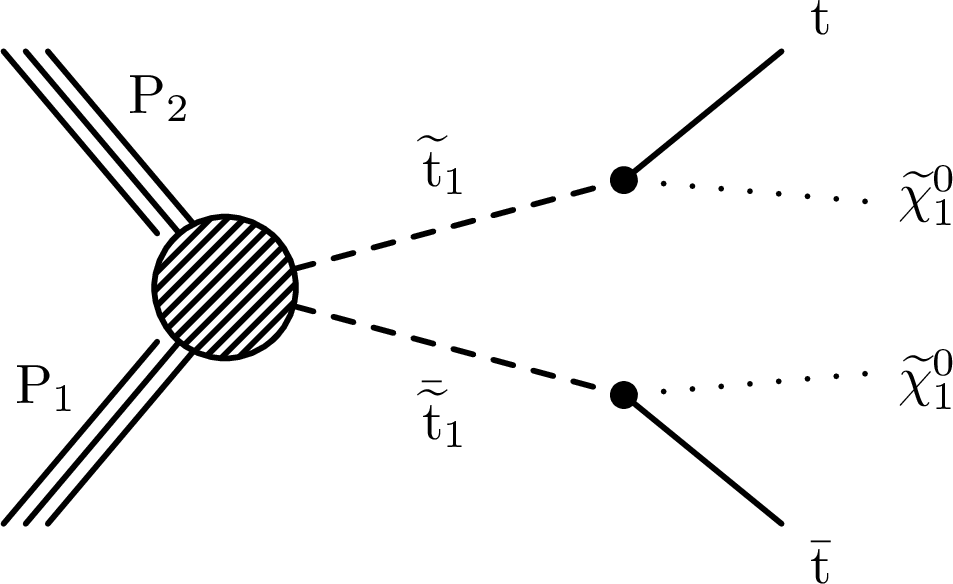
png pdf	Figure 24: Diagrams for the simplified models considered in this analysis: (left) Gluino pair production decaying to two top quarks and the LSP, denoted T1tttt; (middle) Gluino pair production decaying to a top quark and a low mass top squark, which subsequently decays to a charm quark and the LSP, denoted T5ttcc; (right) Top squark pair production decaying to a top quark and the LSP, denoted T2tt.
png pdf	Figure 24-a: Diagrams for the simplified models considered in this analysis: (left) Gluino pair production decaying to two top quarks and the LSP, denoted T1tttt; (middle) Gluino pair production decaying to a top quark and a low mass top squark, which subsequently decays to a charm quark and the LSP, denoted T5ttcc; (right) Top squark pair production decaying to a top quark and the LSP, denoted T2tt.
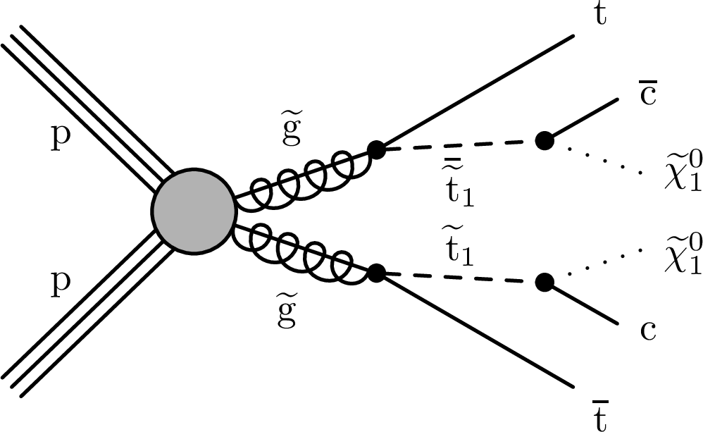
png pdf	Figure 24-b: Diagrams for the simplified models considered in this analysis: (left) Gluino pair production decaying to two top quarks and the LSP, denoted T1tttt; (middle) Gluino pair production decaying to a top quark and a low mass top squark, which subsequently decays to a charm quark and the LSP, denoted T5ttcc; (right) Top squark pair production decaying to a top quark and the LSP, denoted T2tt.
png pdf	Figure 24-c: Diagrams for the simplified models considered in this analysis: (left) Gluino pair production decaying to two top quarks and the LSP, denoted T1tttt; (middle) Gluino pair production decaying to a top quark and a low mass top squark, which subsequently decays to a charm quark and the LSP, denoted T5ttcc; (right) Top squark pair production decaying to a top quark and the LSP, denoted T2tt.
png pdf	Figure 25: Expected and observed 95% upper limits on the production cross section for pair-produced gluinos decaying to top quarks. The blue dotted contour represents the expected 95% upper limits using data in the nonboosted categories only.
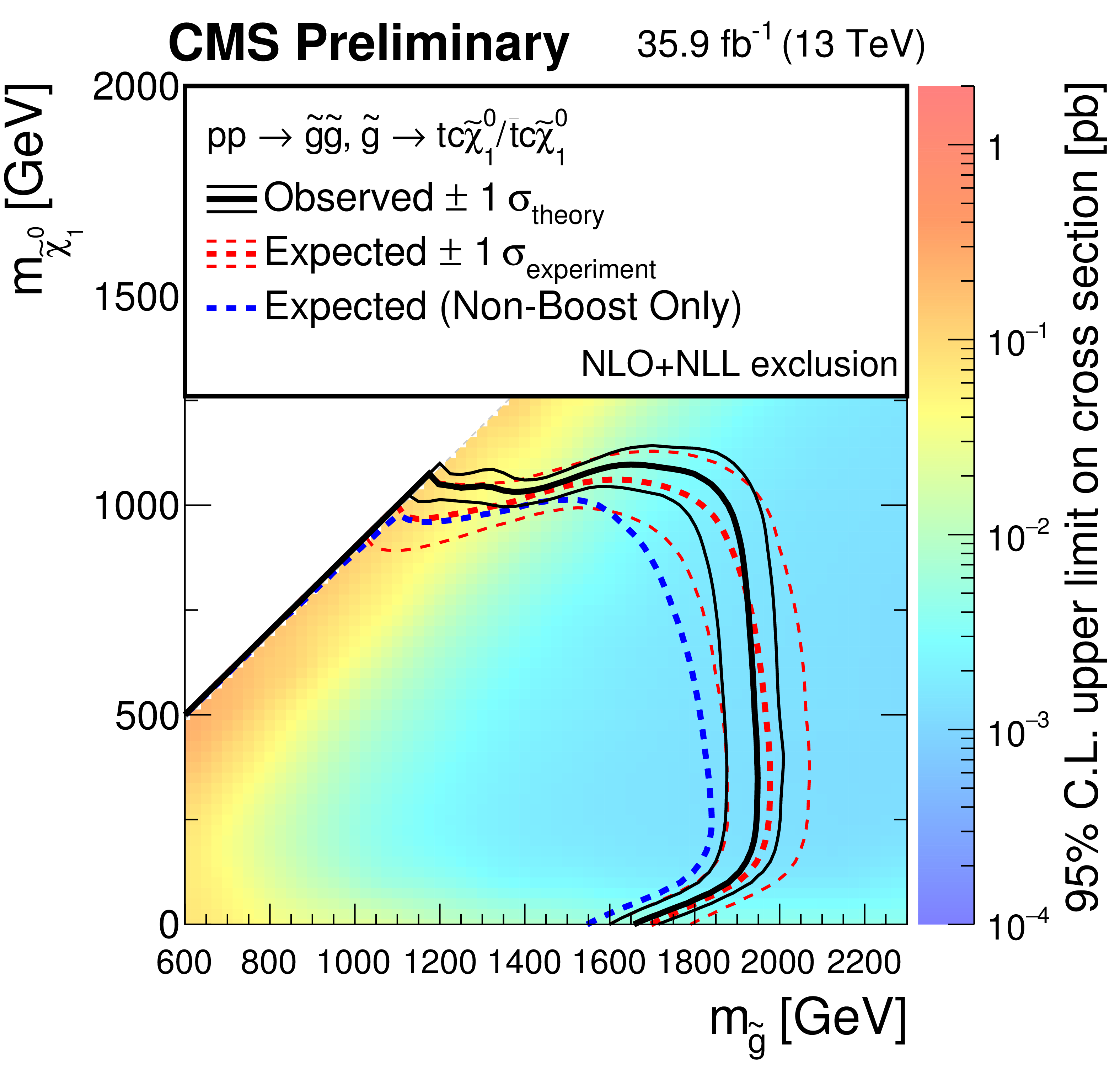
png pdf	Figure 26: Expected and observed 95% upper limit on the production cross section for pair-produced gluinos decaying to a top and a charm quark. The blue dotted contour represents the expected 95% upper limits using data in the nonboosted categories only.
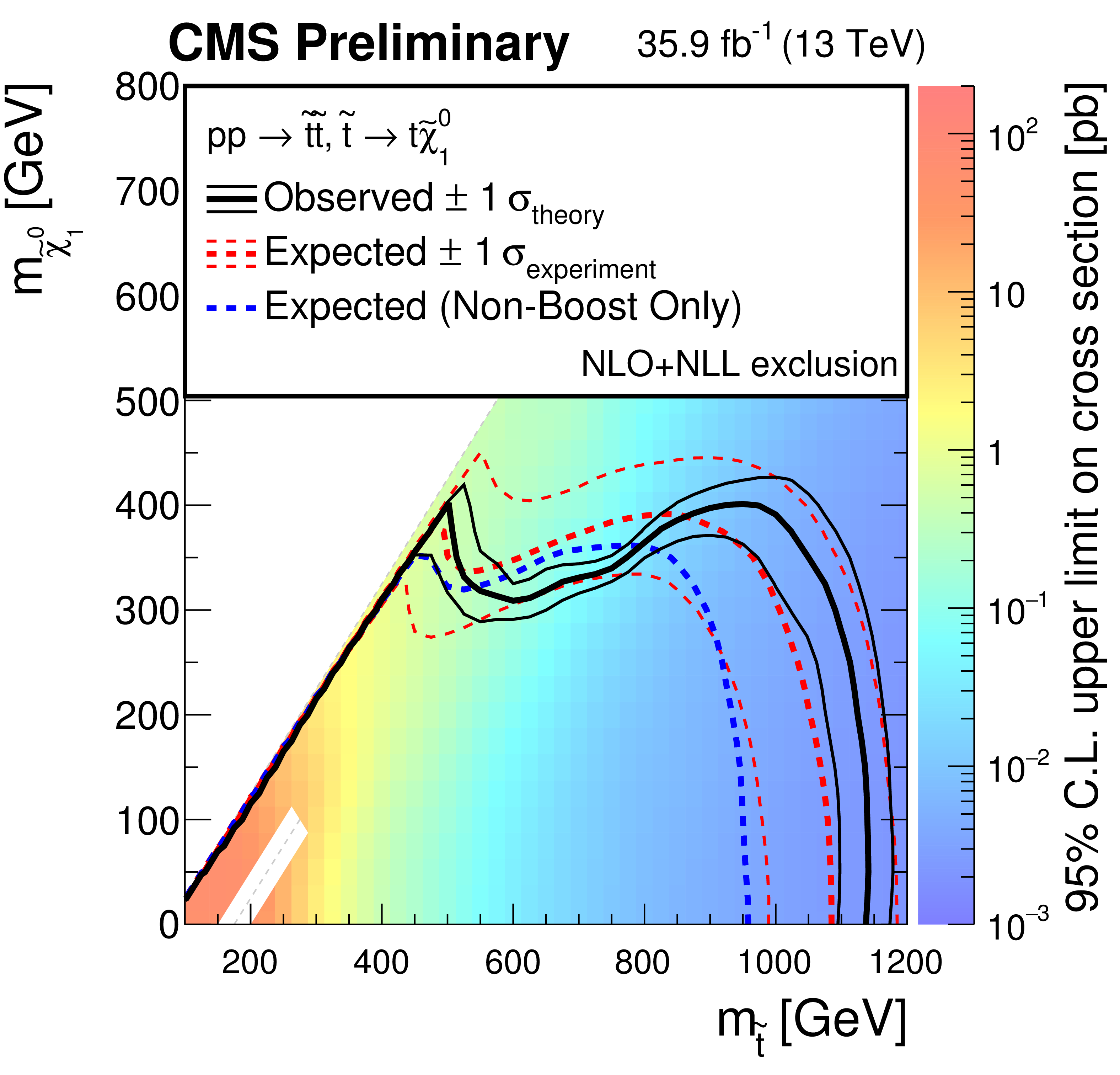
png pdf	Figure 27: Expected and observed 95% upper limits on the production cross section for pair-produced squarks decaying to top quarks. The blue dotted contour represents the expected 95% upper limits using data in the nonboosted categories only. The white diagonal band corresponds to the region $\| m_{\tilde{\mathrm{t}}}-m_{{\mathrm {t}}}-m_{\tilde{\chi}^{0} _1} \| <$ 25 GeV, where the signal efficiency is a strong function of $m_{\tilde{\mathrm{t}}}-m_{\tilde{\chi}^{0} _1}$ , and as a result the precise determination of the cross section upper limit is uncertain because of the finite granularity of the available MC samples in this region of the ( $m_{\tilde{\mathrm{t}}}$ , $m_{\tilde{\chi}^{0} _1}$ ) plane.

Tables
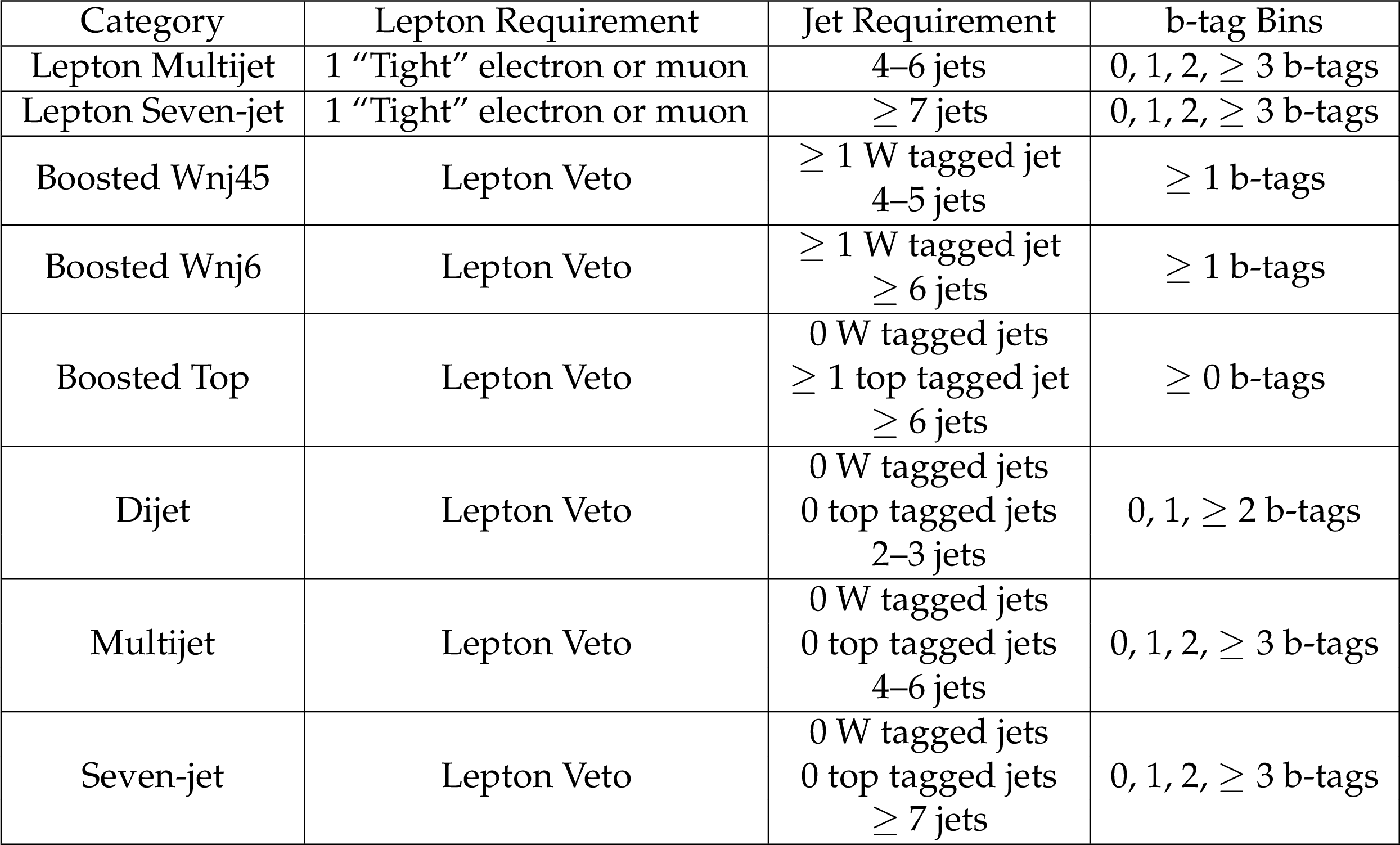
png pdf	Table 1: Summary of the search categories, their charged lepton and jet count requirements, and the b-tag bins that define the subcategories. Events passing the "Lepton Veto'' requirement must have no tight electron or muon, no veto electron or muon, and no hadronic taus.
png pdf	Table 2: The baseline requirements on the razor variables ${M_\mathrm {R}}$ and ${\mathrm {R}^2}$ , additional requirements on $M_{\mathrm {T}}$ and ${\Delta \phi _\mathrm {R}}$ , and the trigger requirements are shown for each event category.
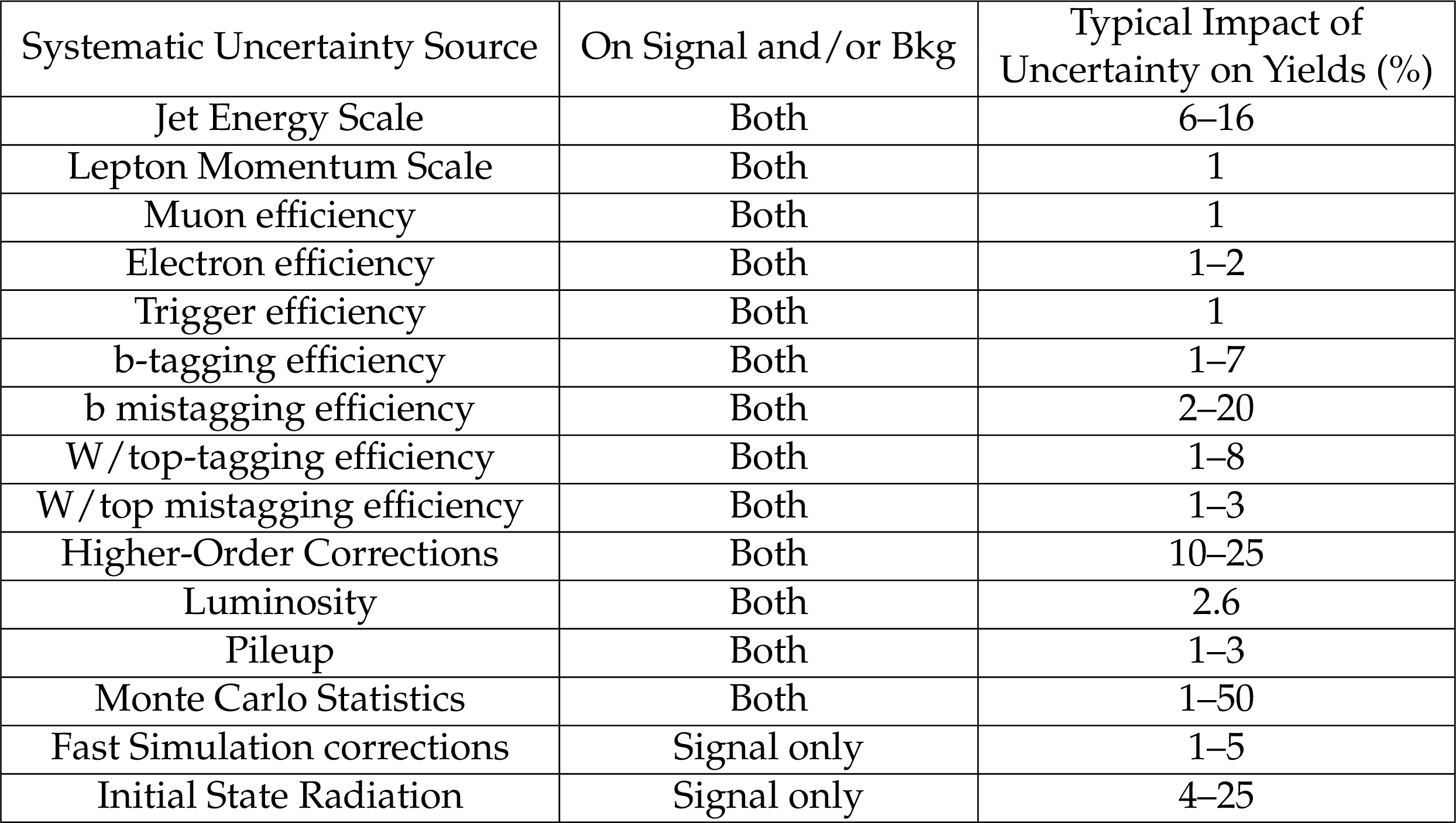
png pdf	Table 3: Summary of the main instrumental and theoretical systematic uncertainties.
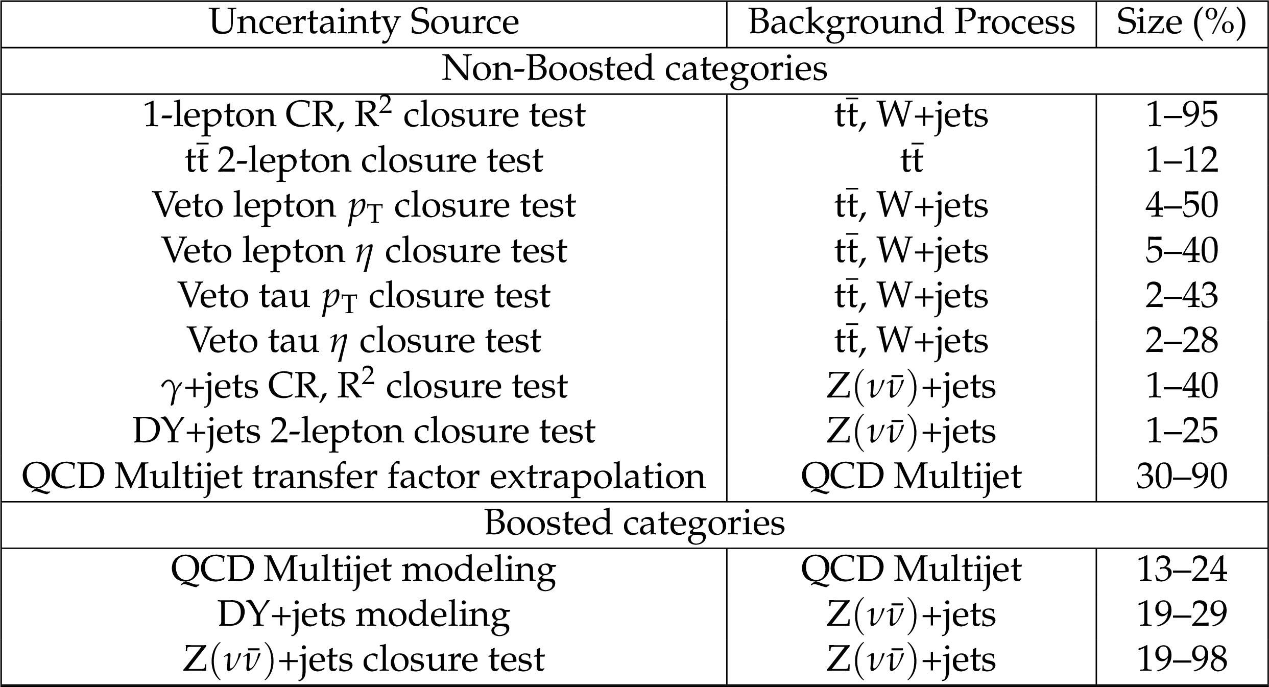
png pdf	Table 4: Summary of systematic uncertainties due to background estimation methodology expressed as relative or fractional uncertainties.

Summary

We have presented an inclusive search for supersymmetry in events with no more than one lepton, a large multiplicity of energetic jets, and evidence of invisible particles using the razor kinematic variables. To enhance sensitivity to a broad range of signal models, the events are categorized according to the number of leptons, the presence of jets consistent with hadronically decaying W bosons or top quarks, and the number of jets and b-tagged jets. This analysis is the first inclusive search for supersymmetry from the CMS experiment that explicitly incorporates event categories with boosted W boson or top quark jets. The analysis uses 35.9 fb

$^{-1}$ of

$\sqrt{s}=$ 13 TeV proton-proton collision data collected by the CMS experiment. Standard model backgrounds were estimated using control regions in data and Monte Carlo simulation yields in signal and control regions. Background estimation procedures were verified using validation regions with kinematics resembling that of the signal regions and closure tests. Data are observed to be consistent with the SM expectation.

The search is sensitive to a broad range of SUSY scenarios including pair production of gluinos and top squarks, and the event categorization in the number of leptons, the number of jets and b-tagged jets, and the presence or absence of boosted jets consistent with hadronic W or top decays, enhances the signal to background and search sensitivity simultaneously for a variety of different SUSY signal scenarios.

The results were interpreted in the context of simplified models of gluino pair production decaying to various quark flavors, or direct top squark pair production. Limits on the gluino mass extend to

$2.0$ TeV while limits on top squark masses reach

$1.14$ TeV. The advantage of combining a large variety of final states enabled this analysis to improve the sensitivity in various signal scenarios. The analysis extended the exclusion limit of the gluino mass from the CMS experiment by

$\sim$ 100 GeV in decays to a low mass top squark and a top quark, and the exclusion limit of the top squark mass by

$\sim$ 20 GeV in direct top squark production.

References
1	CMS Collaboration	Inclusive search for supersymmetry using razor variables in pp collisions at $\sqrt s=$ 13 TeV	PRD 95 (2017) 012003	CMS-SUS-15-004 1609.07658
2	CMS Collaboration	Search for supersymmetry in pp collisions at $\sqrt{s} =$ 8 TeV in final states with boosted W bosons and b jets using razor variables	PRD93 (2016) 092009	CMS-SUS-14-007 1602.02917
3	J. Wess and B. Zumino	Supergauge transformations in four dimensions	NPB 70 (1974) 39
4	Y. A. Gol'fand and E. P. Likhtman	Extension of the algebra of poincare group generators and violation of P invariance	JEPTL 13 (1971) 323
5	D. V. Volkov and V. P. Akulov	Possible universal neutrino interaction	JEPTL 16 (1972) 438
6	A. H. Chamseddine, R. L. Arnowitt, and P. Nath	Locally supersymmetric grand unification	PRL 49 (1982) 970
7	G. L. Kane, C. F. Kolda, L. Roszkowski, and J. D. Wells	Study of constrained minimal supersymmetry	PRD 49 (1994) 6173	hep-ph/9312272
8	P. Fayet	Supergauge invariant extension of the Higgs mechanism and a model for the electron and its neutrino	NPB 90 (1975) 104
9	R. Barbieri, S. Ferrara, and C. A. Savoy	Gauge models with spontaneously broken local supersymmetry	PLB 119 (1982) 343
10	L. J. Hall, J. D. Lykken, and S. Weinberg	Supergravity as the messenger of supersymmetry breaking	PRD 27 (1983) 2359
11	P. Ramond	Dual theory for free fermions	PRD 3 (1971) 2415
12	E. Witten	Dynamical Breaking of Supersymmetry	NPB188 (1981) 513
13	S. Dimopoulos and H. Georgi	Softly Broken Supersymmetry and SU(5)	NPB193 (1981) 150
14	M. Dine, W. Fischler, and M. Srednicki	Supersymmetric Technicolor	NPB189 (1981) 575--593
15	S. Dimopoulos and S. Raby	Supercolor	NPB192 (1981) 353
16	N. Sakai	Naturalness in Supersymmetric Guts	Z. Phys. C11 (1981) 153
17	R. K. Kaul and P. Majumdar	Cancellation of Quadratically Divergent Mass Corrections in Globally Supersymmetric Spontaneously Broken Gauge Theories	NPB199 (1982) 36
18	S. Dimopoulos, S. Raby, and F. Wilczek	Supersymmetry and the Scale of Unification	PRD24 (1981) 1681--1683
19	W. J. Marciano and G. Senjanovic	Predictions of Supersymmetric Grand Unified Theories	PRD25 (1982) 3092
20	M. B. Einhorn and D. R. T. Jones	The Weak Mixing Angle and Unification Mass in Supersymmetric SU(5)	NPB196 (1982) 475
21	L. E. Ibanez and G. G. Ross	Low-Energy Predictions in Supersymmetric Grand Unified Theories	PLB105 (1981) 439
22	U. Amaldi, W. de Boer, and H. Furstenau	Comparison of grand unified theories with electroweak and strong coupling constants measured at LEP	PLB260 (1991) 447--455
23	P. Langacker and N. Polonsky	The Strong coupling, unification, and recent data	PRD52 (1995) 3081--3086	hep-ph/9503214
24	J. R. Ellis et al.	Supersymmetric Relics from the Big Bang	NPB238 (1984) 453--476
25	G. Jungman, M. Kamionkowski, and K. Griest	Supersymmetric dark matter	PR 267 (1996) 195--373	hep-ph/9506380
26	CMS Collaboration	Search for natural and split supersymmetry in proton-proton collisions at $\sqrt{s}=$ 13 TeV in final states with jets and missing transverse momentum	JHEP 05 (2018) 025	CMS-SUS-16-038 1802.02110
27	CMS Collaboration	Search for top squark pair production in pp collisions at $\sqrt{s}=$ 13 TeV using single lepton events	JHEP 10 (2017) 019	CMS-SUS-16-051 1706.04402
28	CMS Collaboration	Search for new phenomena with the $M_{\mathrm {T2}}$ variable in the all-hadronic final state produced in proton-proton collisions at $\sqrt{s} =$ 13 TeV	EPJC77 (2017) 710	CMS-SUS-16-036 1705.04650
29	CMS Collaboration	Search for Supersymmetry in $pp$ Collisions at $\sqrt{s}=$ 13 TeV in the Single-Lepton Final State Using the Sum of Masses of Large-Radius Jets	PRL 119 (2017) 151802	CMS-SUS-16-037 1705.04673
30	CMS Collaboration	Search for supersymmetry in multijet events with missing transverse momentum in proton-proton collisions at 13 TeV	PRD96 (2017) 032003	CMS-SUS-16-033 1704.07781
31	CMS Collaboration	Search for physics beyond the standard model in events with two leptons of same sign, missing transverse momentum, and jets in proton-proton collisions at $\sqrt{s} =$ 13 TeV	EPJC77 (2017) 578	CMS-SUS-16-035 1704.07323
32	CMS Collaboration	Search for supersymmetry in the all-hadronic final state using top quark tagging in pp collisions at $\sqrt{s} =$ 13 TeV	PRD96 (2017) 012004	CMS-SUS-16-009 1701.01954
33	CMS Collaboration	Searches for pair production of third-generation squarks in $\sqrt{s}=$ 13 TeV pp collisions	EPJC77 (2017) 327	CMS-SUS-16-008 1612.03877
34	ATLAS Collaboration	Search for a scalar partner of the top quark in the jets plus missing transverse momentum final state at $\sqrt{s}=$ 13 TeV with the ATLAS detector	JHEP 12 (2017) 085	1709.04183
35	ATLAS Collaboration	Search for supersymmetry in events with $b$ -tagged jets and missing transverse momentum in $pp$ collisions at $\sqrt{s}=$ 13 TeV with the ATLAS detector	JHEP 11 (2017) 195	1708.09266
36	ATLAS Collaboration	Search for squarks and gluinos in events with an isolated lepton, jets, and missing transverse momentum at $\sqrt{s}=$ 13 TeV with the ATLAS detector	PRD96 (2017) 112010	1708.08232
37	ATLAS Collaboration	Search for direct top squark pair production in final states with two leptons in $\sqrt{s} = 13 TeV pp$ collisions with the ATLAS detector	EPJC77 (2017) 898	1708.03247
38	ATLAS Collaboration	Search for new phenomena with large jet multiplicities and missing transverse momentum using large-radius jets and flavour-tagging at ATLAS in 13 $TeV pp$ collisions	JHEP 12 (2017) 034	1708.02794
39	ATLAS Collaboration	Search for supersymmetry in final states with two same-sign or three leptons and jets using 36 fb $^{-1}$ of $\sqrt{s}=13 TeV pp$ collision data with the ATLAS detector	JHEP 09 (2017) 084	1706.03731
40	ATLAS Collaboration	Search for new phenomena in a lepton plus high jet multiplicity final state with the ATLAS experiment using $\sqrt{s}=$ 13 TeV proton-proton collision data	JHEP 09 (2017) 088	1704.08493
41	CMS Collaboration	The CMS experiment at the CERN LHC	JINST 3 (2008) S08004	CMS-00-001
42	CMS Collaboration	Particle-flow reconstruction and global event description with the CMS detector	JINST 12 (2017) P10003	CMS-PRF-14-001 1706.04965
43	M. Cacciari, G. P. Salam, and G. Soyez	The anti- $k_t$ jet clustering algorithm	JHEP 04 (2008) 063	0802.1189
44	M. Cacciari, G. P. Salam, and G. Soyez	FastJet user manual	EPJC 72 (2012) 1896	1111.6097
45	CMS Collaboration	Identification of heavy-flavour jets with the CMS detector in pp collisions at 13 TeV	JINST 13 (2018) P05011	CMS-BTV-16-002 1712.07158
46	J. Thaler and K. Van Tilburg	Identifying boosted objects with N-subjettiness	JHEP 03 (2011) 015	1011.2268
47	A. J. Larkoski, S. Marzani, G. Soyez, and J. Thaler	Soft Drop	JHEP 05 (2014) 146	1402.2657
48	CMS Collaboration	Performance of Electron Reconstruction and Selection with the CMS Detector in Proton-Proton Collisions at 8 TeV	JINST 10 (2015) P06005	CMS-EGM-13-001 1502.02701
49	CMS Collaboration	Performance of CMS muon reconstruction in $pp$ collision events at $\sqrt{s}=$ 7 TeV	JINST 7 (2012) P10002	CMS-MUO-10-004 1206.4071
50	CMS Collaboration	Reconstruction and identification of $\tau$ lepton decays to hadrons and $\nu_{\tau}$ at CMS	JINST 11 (2016) P01019	CMS-TAU-14-001 1510.07488
51	CMS Collaboration	Performance of photon reconstruction and identification with the CMS detector in proton-proton collisions at $\sqrt{s} =$ 8 TeV	JINST 10 (2015) P08010	CMS-EGM-14-001 1502.02702
52	J. Alwall et al.	MadGraph5: going beyond	JHEP 06 (2011) 128	1106.0522
53	T. Sjostrand, S. Mrenna, and P. Z. Skands	A Brief Introduction to PYTHIA 8.1	CPC 178 (2008) 852--867	0710.3820
54	T. Sjostrand et al.	An Introduction to PYTHIA 8.2	CPC 191 (2015) 159--177	1410.3012
55	S. Hoeche et al.	Matching parton showers and matrix elements	in HERA and the LHC: A Workshop on the implications of HERA for LHC physics: Proceedings Part A, pp. 288--289 2005	hep-ph/0602031
56	J. Alwall et al.	Comparative study of various algorithms for the merging of parton showers and matrix elements in hadronic collisions	EPJC53 (2008) 473--500	0706.2569
57	J. Alwall et al.	The automated computation of tree-level and next-to-leading order differential cross sections, and their matching to parton shower simulations	JHEP 07 (2014) 079	1405.0301
58	S. Frixione, P. Nason, and G. Ridolfi	A Positive-weight next-to-leading-order Monte Carlo for heavy flavour hadroproduction	JHEP 09 (2007) 126	0707.3088
59	S. Alioli, P. Nason, C. Oleari, and E. Re	NLO single-top production matched with shower in POWHEG: s- and t-channel contributions	JHEP 09 (2009) 111	0907.4076
60	E. Re	Single-top Wt-channel production matched with parton showers using the POWHEG method	EPJC71 (2011) 1547	1009.2450
61	S. Agostinelli et al.	Geant4 - a simulation toolkit	NIMA 506 (2003) 250 -- 303
62	CMS Collaboration	The fast simulation of the CMS detector at LHC	J. Phys.: Conf. Ser. 331 (2011) 032049
63	W. Beenakker, R. Hopker, M. Spira, and P. M. Zerwas	Squark and gluino production at hadron colliders	NPB 492 (1997) 51	hep-ph/9610490
64	A. Kulesza and L. Motyka	Threshold resummation for squark-antisquark and gluino-pair production at the LHC	PRL 102 (2009) 111802	0807.2405
65	A. Kulesza and L. Motyka	Soft gluon resummation for the production of gluino-gluino and squark-antisquark pairs at the LHC	PRD 80 (2009) 095004	0905.4749
66	W. Beenakker et al.	Soft-gluon resummation for squark and gluino hadroproduction	JHEP 12 (2009) 041	0909.4418
67	W. Beenakker et al.	Squark and gluino hadroproduction	Int. J. Mod. Phys. A 26 (2011) 2637	1105.1110
68	C. Borschensky et al.	Squark and gluino production cross sections in pp collisions at $\sqrt{s}=$ 13, 14, 33 and 100 TeV	EPJC74 (2014) 3174	1407.5066
69	M. Kramer et al.	Supersymmetry production cross sections in $pp$ collisions at $\sqrt{s}=$ 7 TeV		1206.2892
70	CMS Collaboration	Inclusive search for squarks and gluinos in pp collisions at $\sqrt{s} =$ 7 TeV	PRD 85 (2012) 012004	CMS-SUS-10-009 1107.1279
71	CMS Collaboration	Missing transverse energy performance of the CMS detector	JINST 6 (2011) P09001	CMS-JME-10-009 1106.5048
72	CMS Collaboration	Performance of the CMS missing transverse momentum reconstruction in pp data at $\sqrt{s} =$ 8 TeV	JINST 10 (2015) P02006	CMS-JME-13-003 1411.0511
73	ATLAS and CMS Collaborations	Procedure for the LHC Higgs boson search combination in summer 2011	CMS-NOTE-2011-005
74	CMS Collaboration	Search for supersymmetry in proton-proton collisions at 13 TeV using identified top quarks	PRD97 (2018) 012007	CMS-SUS-16-050 1710.11188