

Compact Muon Solenoid
LHC, CERN
| CMS-HIG-24-008 ; CERN-EP-2026-033 | ||
| Search for Higgs boson production at high transverse momentum in the WW decay channel in proton-proton collisions at $ \sqrt{s} = $ 13 TeV | ||
| CMS Collaboration | ||
| 23 March 2026 | ||
| Accepted for publication in the Journal of High Energy Physics | ||
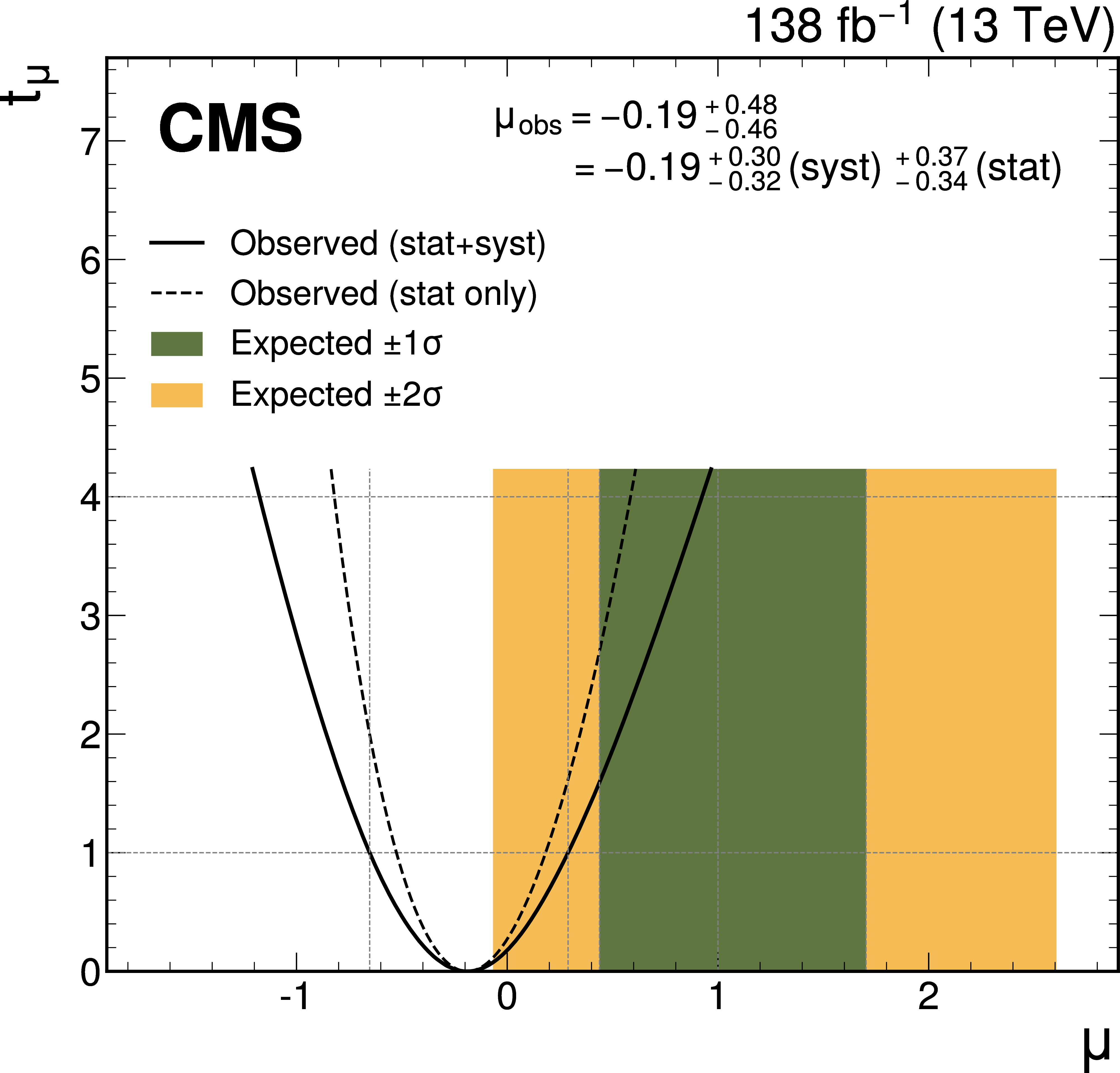
| Abstract: A search for Higgs boson (H) production at high transverse momentum ($ p_{\mathrm{T}} $) in the WW decay channel is presented. The analysis uses proton-proton collisions at $ \sqrt{s}= $ 13 TeV recorded by the CMS experiment in 2016--2018, corresponding to an integrated luminosity of 138 fb$ ^{-1} $. The visible decay products of the Higgs boson are reconstructed as a single large-radius jet with one isolated lepton or none (1 $ \ell $ and 0 $ \ell $, respectively; $ \ell=\mathrm{e},\mu $). The H-candidate jets are identified using an advanced transformer-based algorithm and are calibrated with the Lund jet plane reweighting technique. The 1 $ \ell $ channel is further split into gluon fusion, vector boson fusion, and associated production with hadronically decaying vector boson categories, while the 0 $ \ell $ channel considers all production processes inclusively. The measured cross section times the $ \mathrm{H} \to \mathrm{W} \mathrm{W} $ branching fraction relative to the standard model expectation is $ \mu = - $ 0.19 $ ^{+0.48}_{-0.46} $, indicating no evidence of a signal above the background. This measurement represents the first dedicated study of highly Lorentz-boosted $ \mathrm{H} \to \mathrm{W} \mathrm{W} $ decays, complementing earlier searches for high-$ p_{\mathrm{T}} $ Higgs boson in other decay channels. | ||
| Links: e-print arXiv:2603.22233 [hep-ex] (PDF) ; CDS record ; inSPIRE record ; HepData record ; CADI line (restricted) ; | ||
| Figures | |
png pdf |
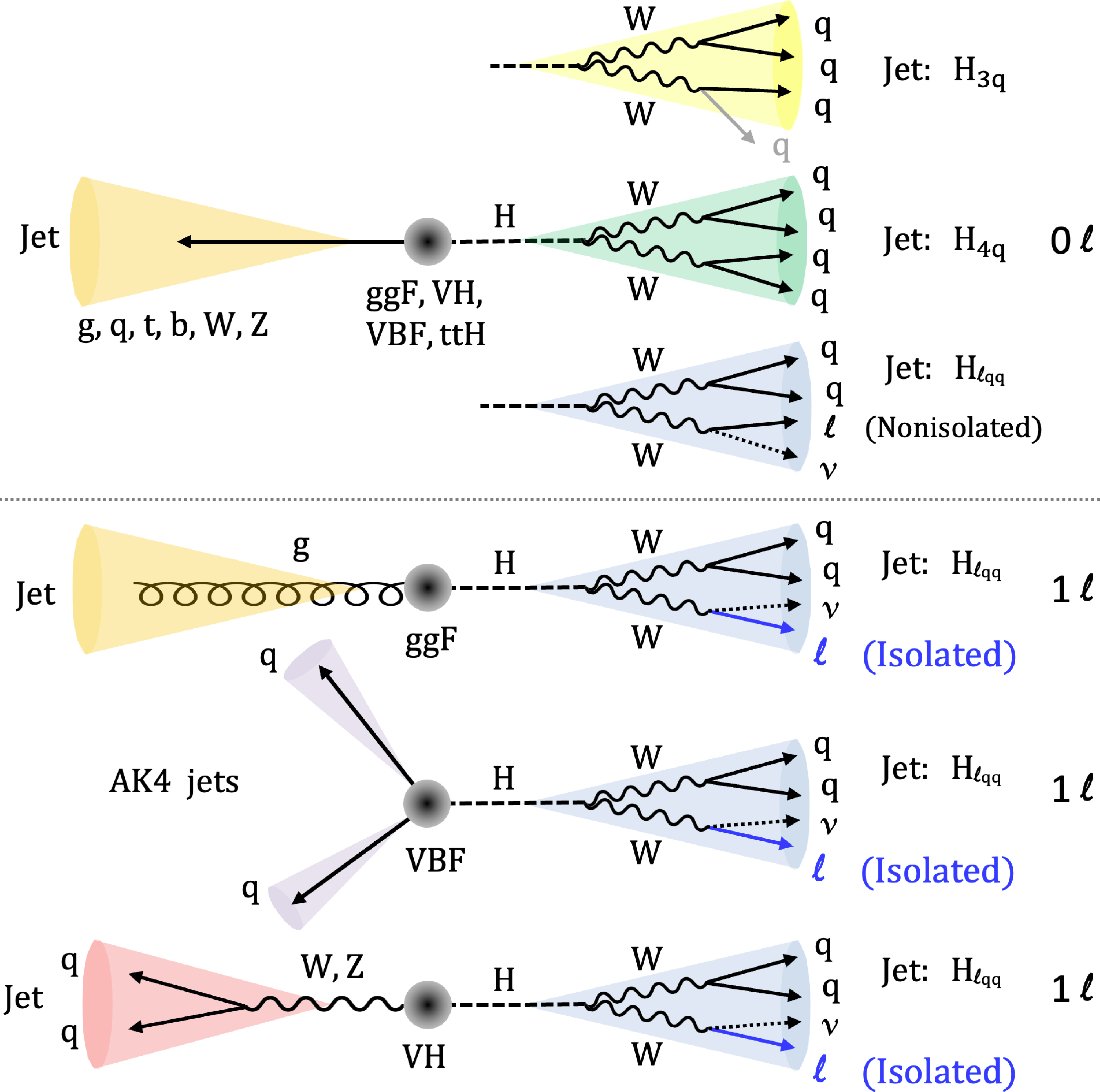
Figure 1:
Illustration of the event topologies analyzed. Right: boosted Higgs boson final states from the $ \mathrm{H}\to\mathrm{W}\mathrm{W}\to\ell\nu\mathrm{q}\mathrm{q}/\mathrm{q} \mathrm{q}\mathrm{q}\mathrm{q} $ decay. Left: associated jets corresponding to the different production processes. From upper to lower: 0 $ \ell $ inclusive (all production and decay modes), and the 1 $ \ell $ ggF, VBF, and VH production processes. |
png pdf |
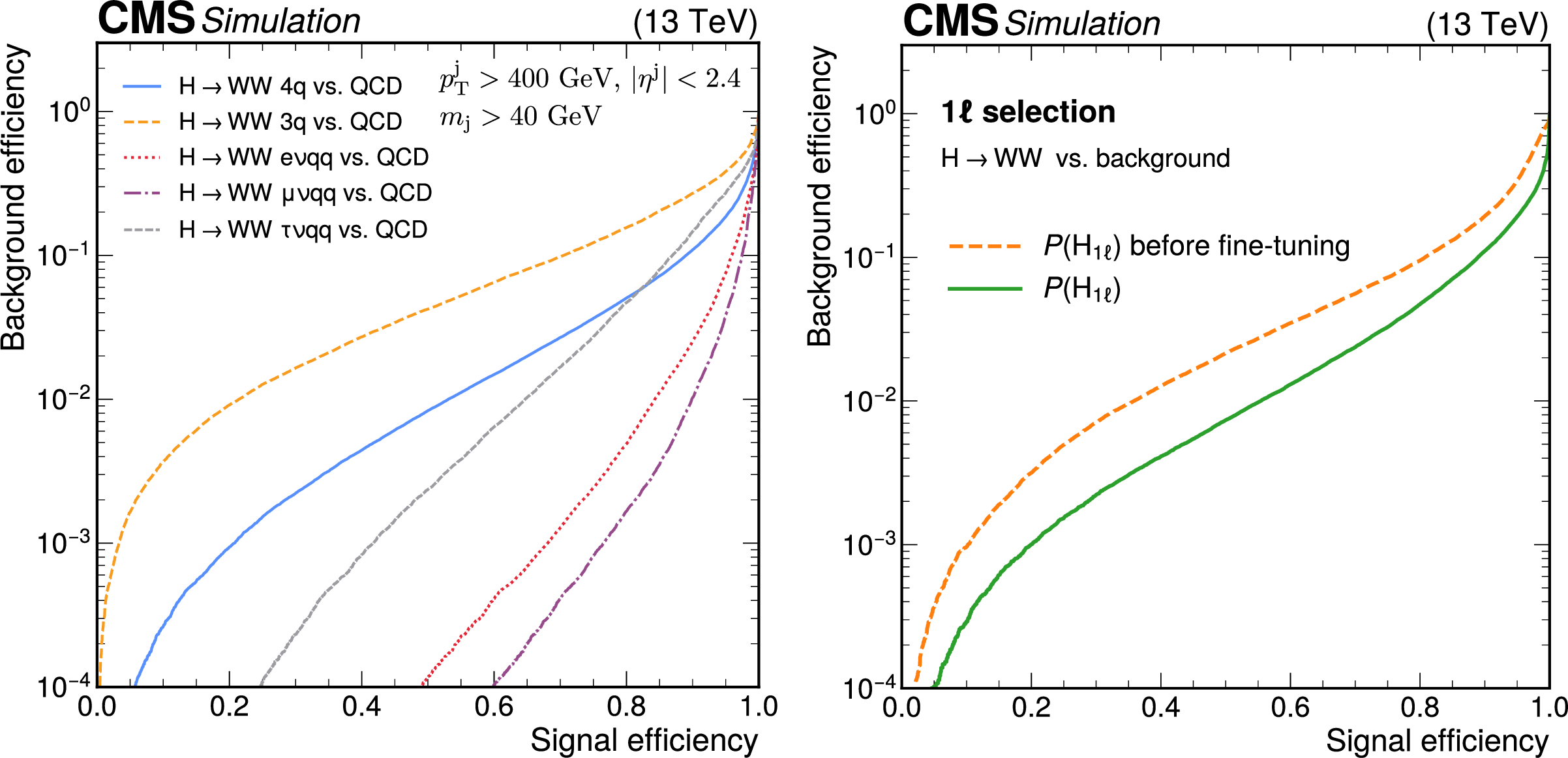
Figure 2:
Performance curves showing the identification probability of background jets versus $ \mathrm{H} \to \mathrm{W} \mathrm{W} $ signal jets for PART and PART-FINETUNED. Left: Discrimination performance of the PART model for various $ \mathrm{H} \to \mathrm{W} \mathrm{W} $ decays against the dominant QCD multijet background. Right: Comparison of $ P(\mathrm{H}_{1\ell}) $ before and after fine-tuning, following the event selection in the 1 $ \ell $ channel. The background includes jets originating from QCD multijet events, $ \mathrm{W}(\ell\nu) $+jets, and top quark processes. |
png pdf |
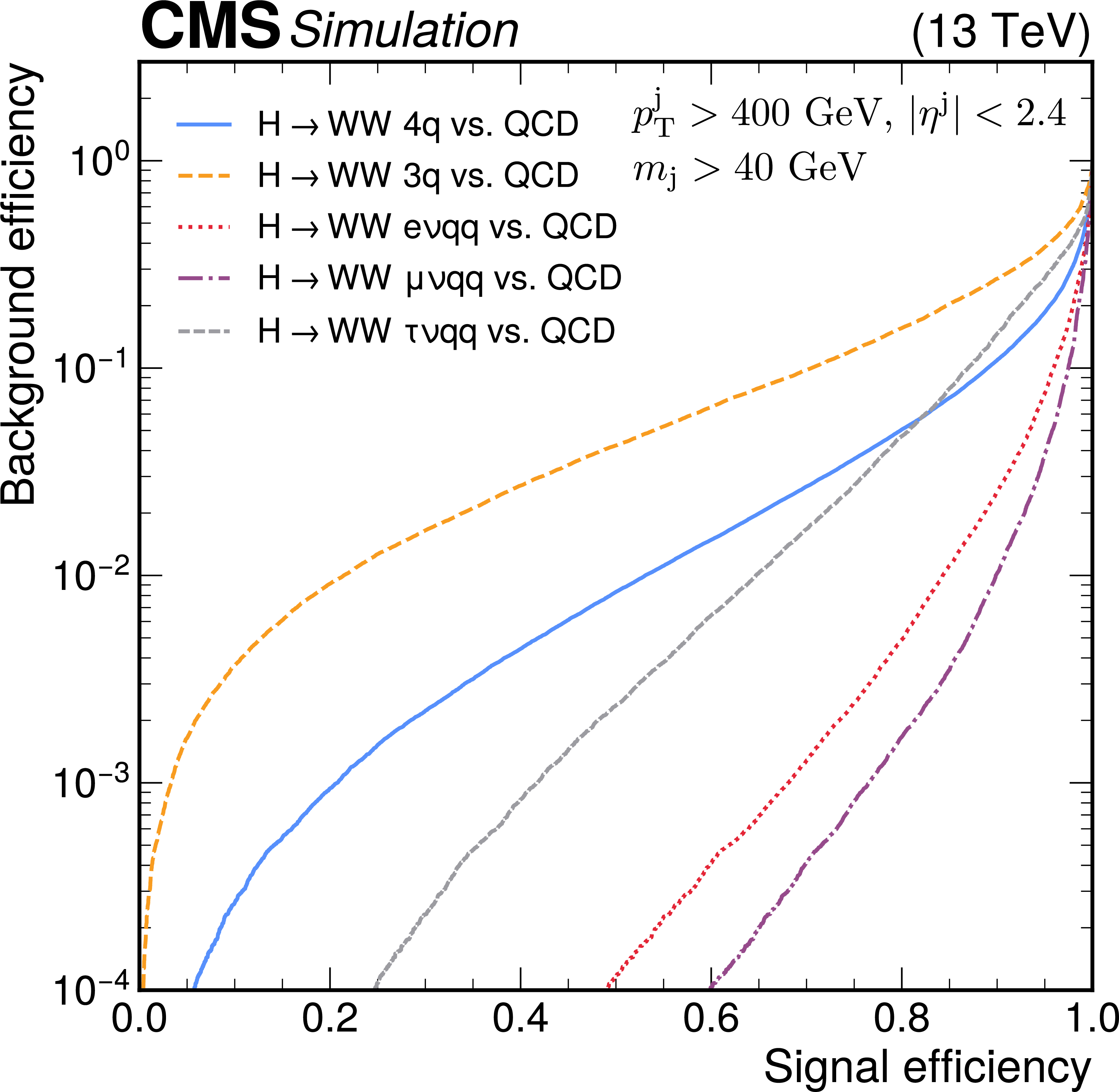
Figure 2-a:
Performance curves showing the identification probability of background jets versus $ \mathrm{H} \to \mathrm{W} \mathrm{W} $ signal jets for PART and PART-FINETUNED. Left: Discrimination performance of the PART model for various $ \mathrm{H} \to \mathrm{W} \mathrm{W} $ decays against the dominant QCD multijet background. Right: Comparison of $ P(\mathrm{H}_{1\ell}) $ before and after fine-tuning, following the event selection in the 1 $ \ell $ channel. The background includes jets originating from QCD multijet events, $ \mathrm{W}(\ell\nu) $+jets, and top quark processes. |
png pdf |
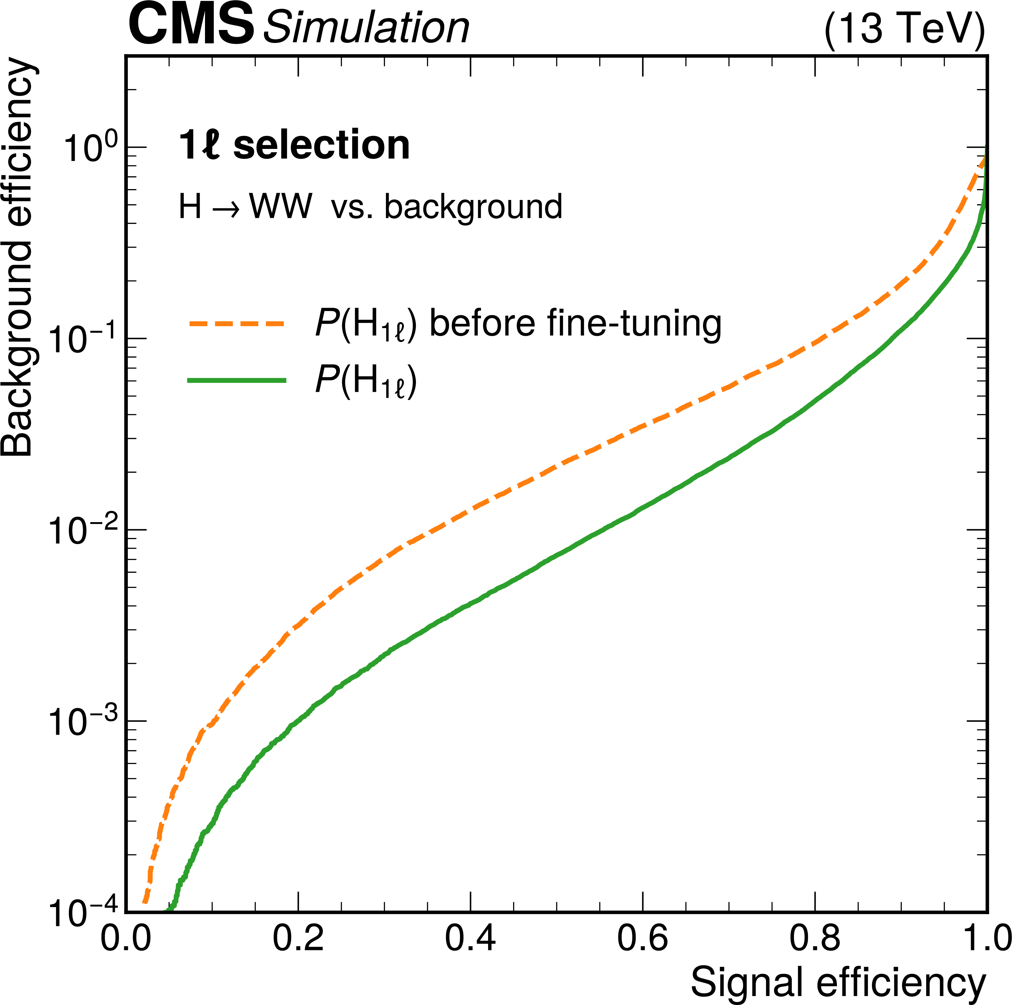
Figure 2-b:
Performance curves showing the identification probability of background jets versus $ \mathrm{H} \to \mathrm{W} \mathrm{W} $ signal jets for PART and PART-FINETUNED. Left: Discrimination performance of the PART model for various $ \mathrm{H} \to \mathrm{W} \mathrm{W} $ decays against the dominant QCD multijet background. Right: Comparison of $ P(\mathrm{H}_{1\ell}) $ before and after fine-tuning, following the event selection in the 1 $ \ell $ channel. The background includes jets originating from QCD multijet events, $ \mathrm{W}(\ell\nu) $+jets, and top quark processes. |
png pdf |
Figure 3:
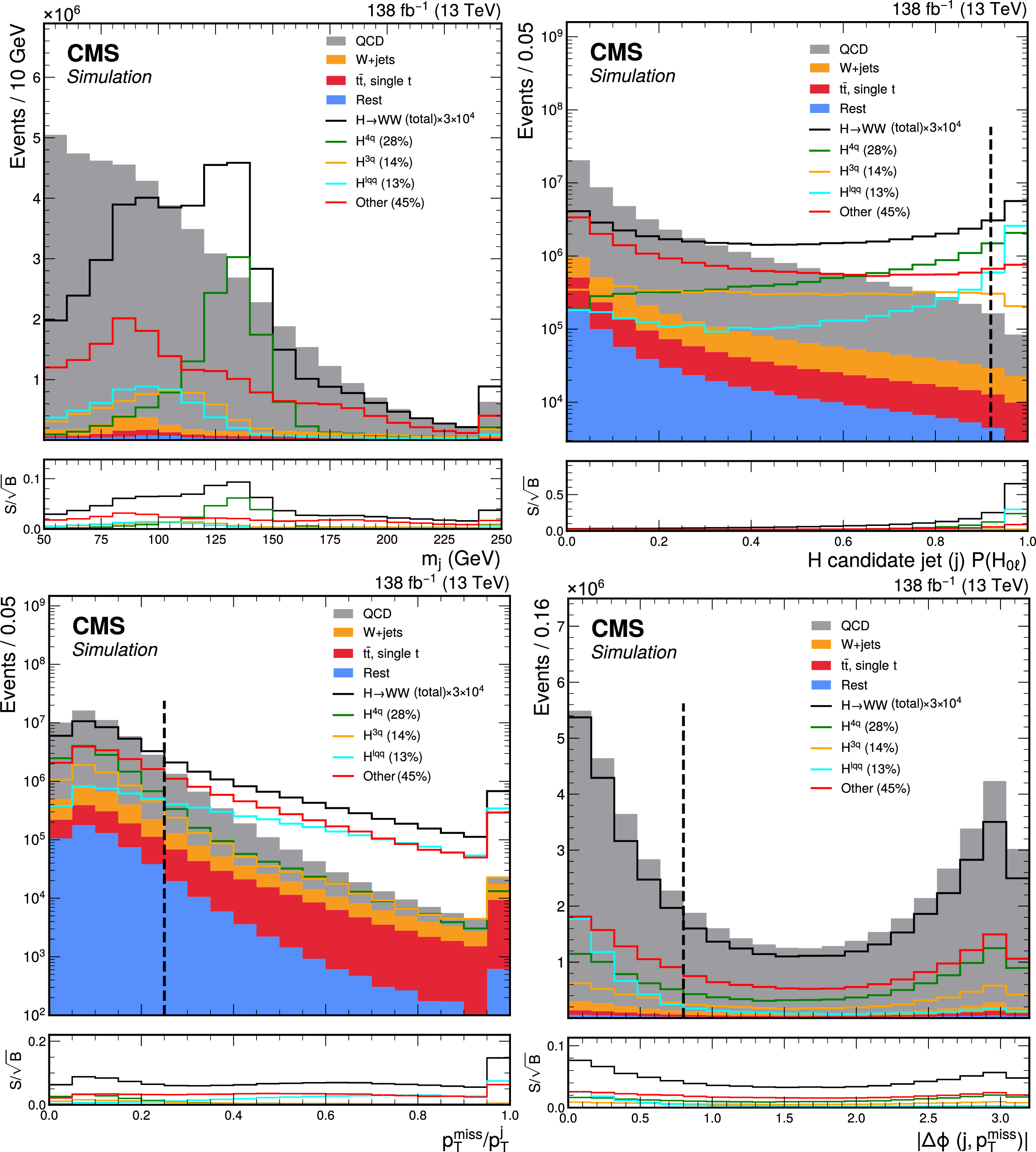
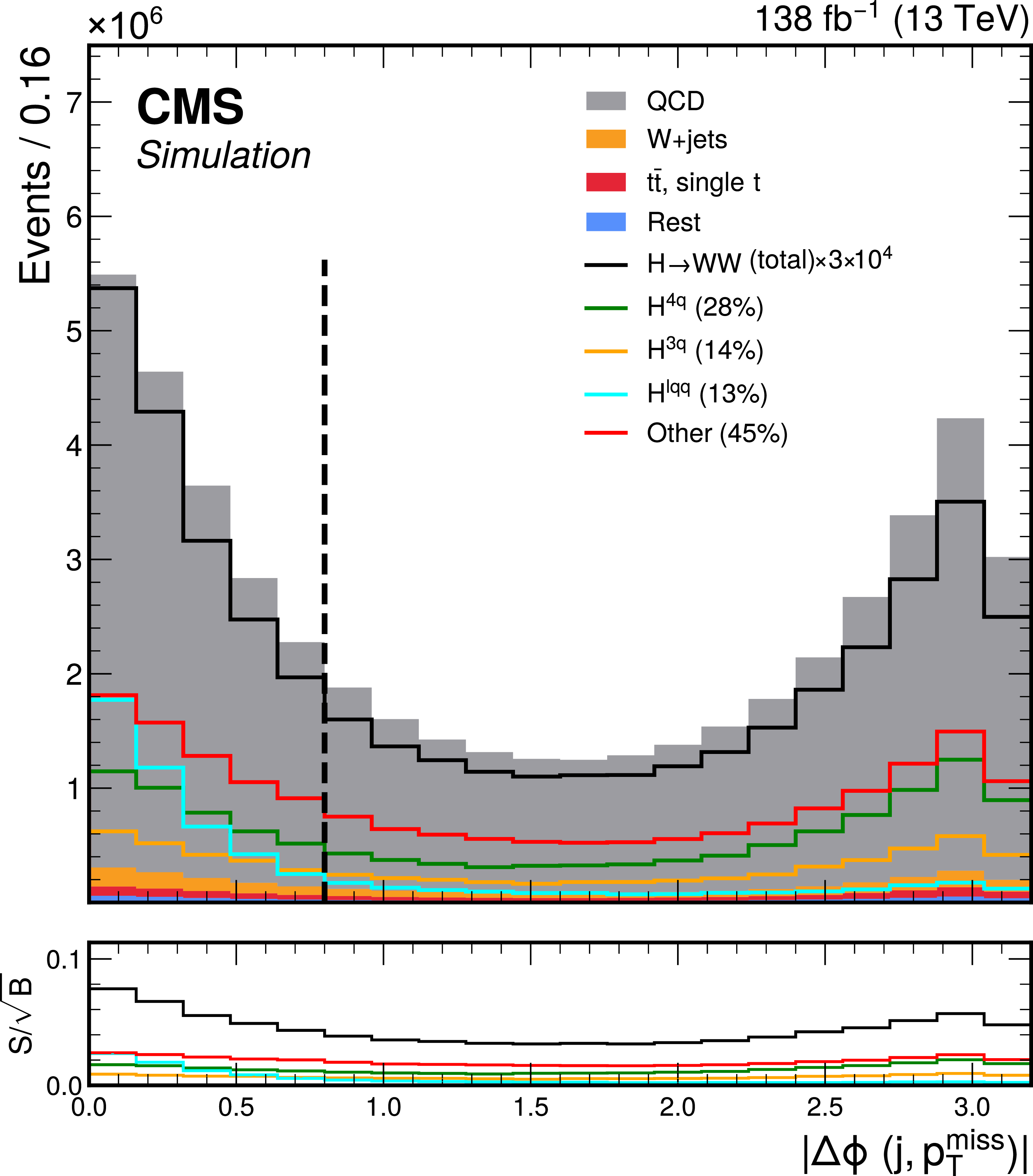
The distributions for the total simulated background and total signal (scaled by a factor of 3$ \times10^4 $ for visibility) passing event selection in the 0 $ \ell $ channel. The signal is split into classes as defined in the text. The upper left and upper right panels show the soft-drop mass and PART score distributions for the H-candidate jet (j) $ P(\mathrm{H}_{0\ell}) $, respectively. The lower left and lower right panels display the $ p_{\mathrm{T}}^\text{miss}/p_{\mathrm{T}}^{\text{j}} $ ratio and the angle $ |\Delta\phi (j|, {\vec p}_{\mathrm{T}}^{\mkern3mu\text{miss}) } $, respectively. Vertical lines indicate the selection conditions imposed to define the SRs. |
png pdf |
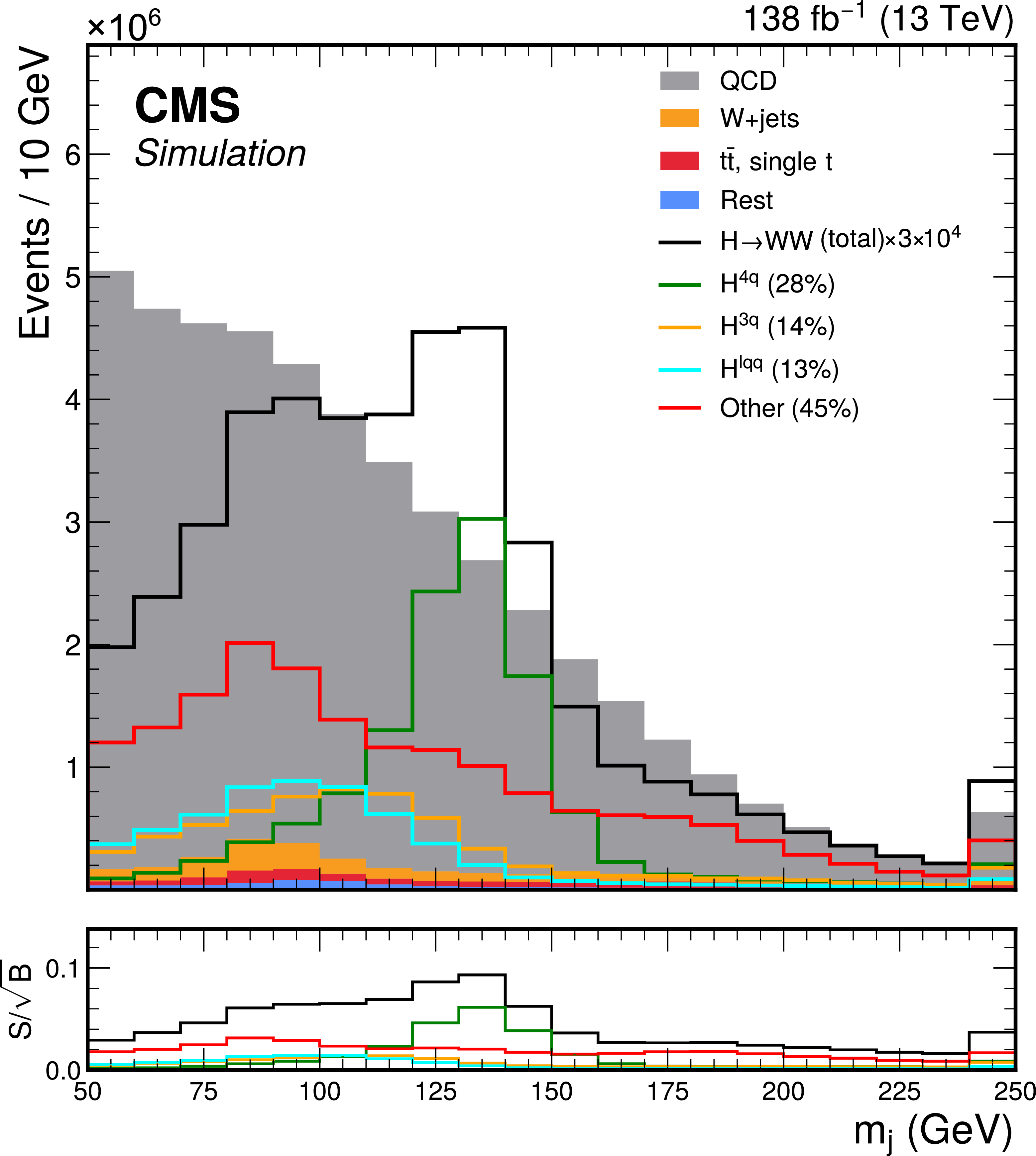
Figure 3-a:
The distributions for the total simulated background and total signal (scaled by a factor of 3$ \times10^4 $ for visibility) passing event selection in the 0 $ \ell $ channel. The signal is split into classes as defined in the text. The upper left and upper right panels show the soft-drop mass and PART score distributions for the H-candidate jet (j) $ P(\mathrm{H}_{0\ell}) $, respectively. The lower left and lower right panels display the $ p_{\mathrm{T}}^\text{miss}/p_{\mathrm{T}}^{\text{j}} $ ratio and the angle $ |\Delta\phi (j|, {\vec p}_{\mathrm{T}}^{\mkern3mu\text{miss}) } $, respectively. Vertical lines indicate the selection conditions imposed to define the SRs. |
png pdf |
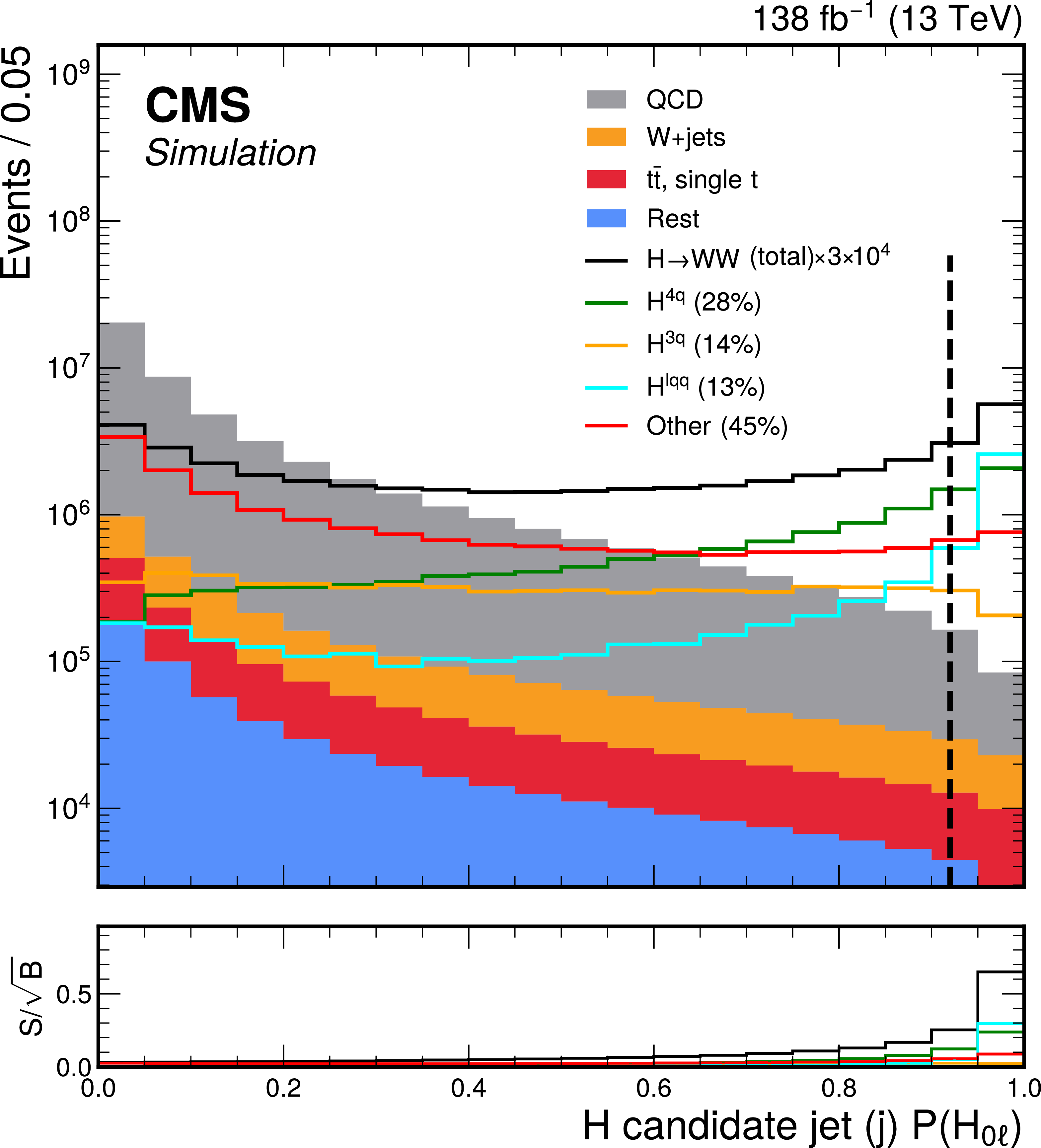
Figure 3-b:
The distributions for the total simulated background and total signal (scaled by a factor of 3$ \times10^4 $ for visibility) passing event selection in the 0 $ \ell $ channel. The signal is split into classes as defined in the text. The upper left and upper right panels show the soft-drop mass and PART score distributions for the H-candidate jet (j) $ P(\mathrm{H}_{0\ell}) $, respectively. The lower left and lower right panels display the $ p_{\mathrm{T}}^\text{miss}/p_{\mathrm{T}}^{\text{j}} $ ratio and the angle $ |\Delta\phi (j|, {\vec p}_{\mathrm{T}}^{\mkern3mu\text{miss}) } $, respectively. Vertical lines indicate the selection conditions imposed to define the SRs. |
png pdf |
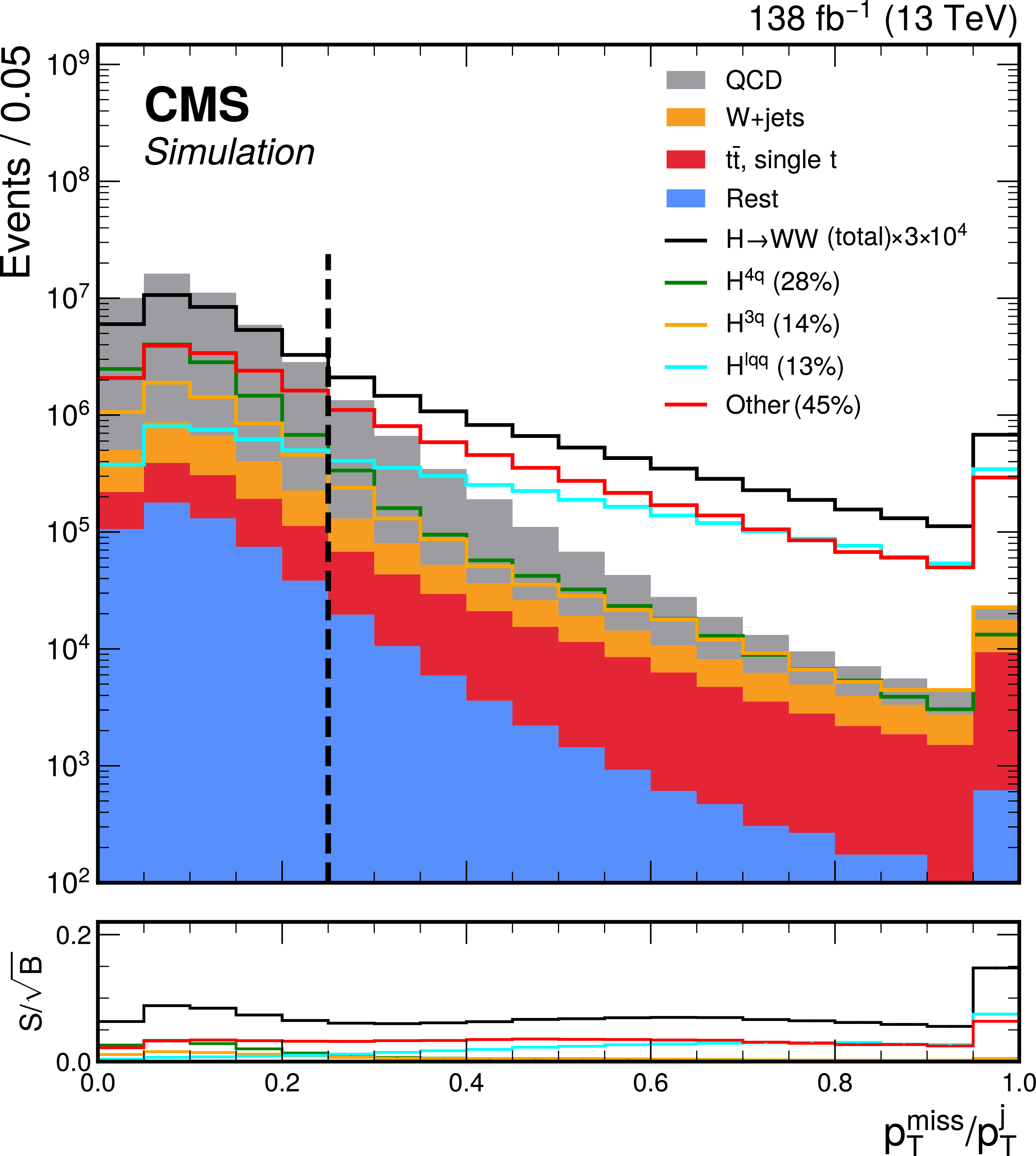
Figure 3-c:
The distributions for the total simulated background and total signal (scaled by a factor of 3$ \times10^4 $ for visibility) passing event selection in the 0 $ \ell $ channel. The signal is split into classes as defined in the text. The upper left and upper right panels show the soft-drop mass and PART score distributions for the H-candidate jet (j) $ P(\mathrm{H}_{0\ell}) $, respectively. The lower left and lower right panels display the $ p_{\mathrm{T}}^\text{miss}/p_{\mathrm{T}}^{\text{j}} $ ratio and the angle $ |\Delta\phi (j|, {\vec p}_{\mathrm{T}}^{\mkern3mu\text{miss}) } $, respectively. Vertical lines indicate the selection conditions imposed to define the SRs. |
png pdf |
Figure 3-d:
The distributions for the total simulated background and total signal (scaled by a factor of 3$ \times10^4 $ for visibility) passing event selection in the 0 $ \ell $ channel. The signal is split into classes as defined in the text. The upper left and upper right panels show the soft-drop mass and PART score distributions for the H-candidate jet (j) $ P(\mathrm{H}_{0\ell}) $, respectively. The lower left and lower right panels display the $ p_{\mathrm{T}}^\text{miss}/p_{\mathrm{T}}^{\text{j}} $ ratio and the angle $ |\Delta\phi (j|, {\vec p}_{\mathrm{T}}^{\mkern3mu\text{miss}) } $, respectively. Vertical lines indicate the selection conditions imposed to define the SRs. |
png pdf |
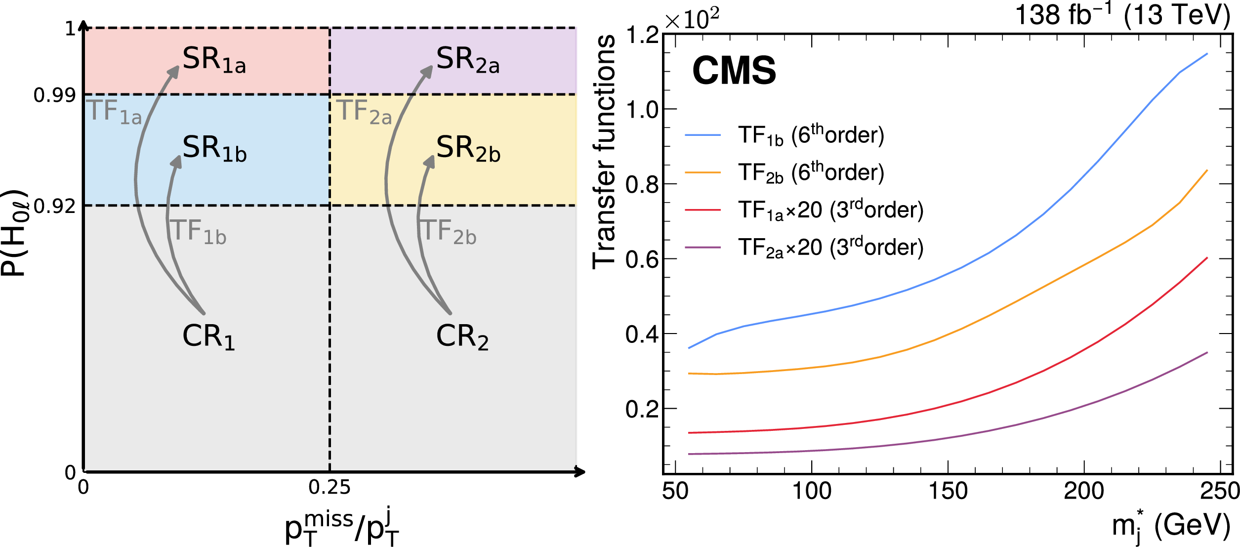
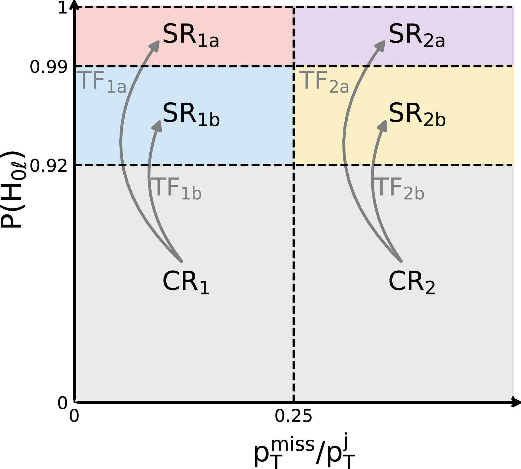
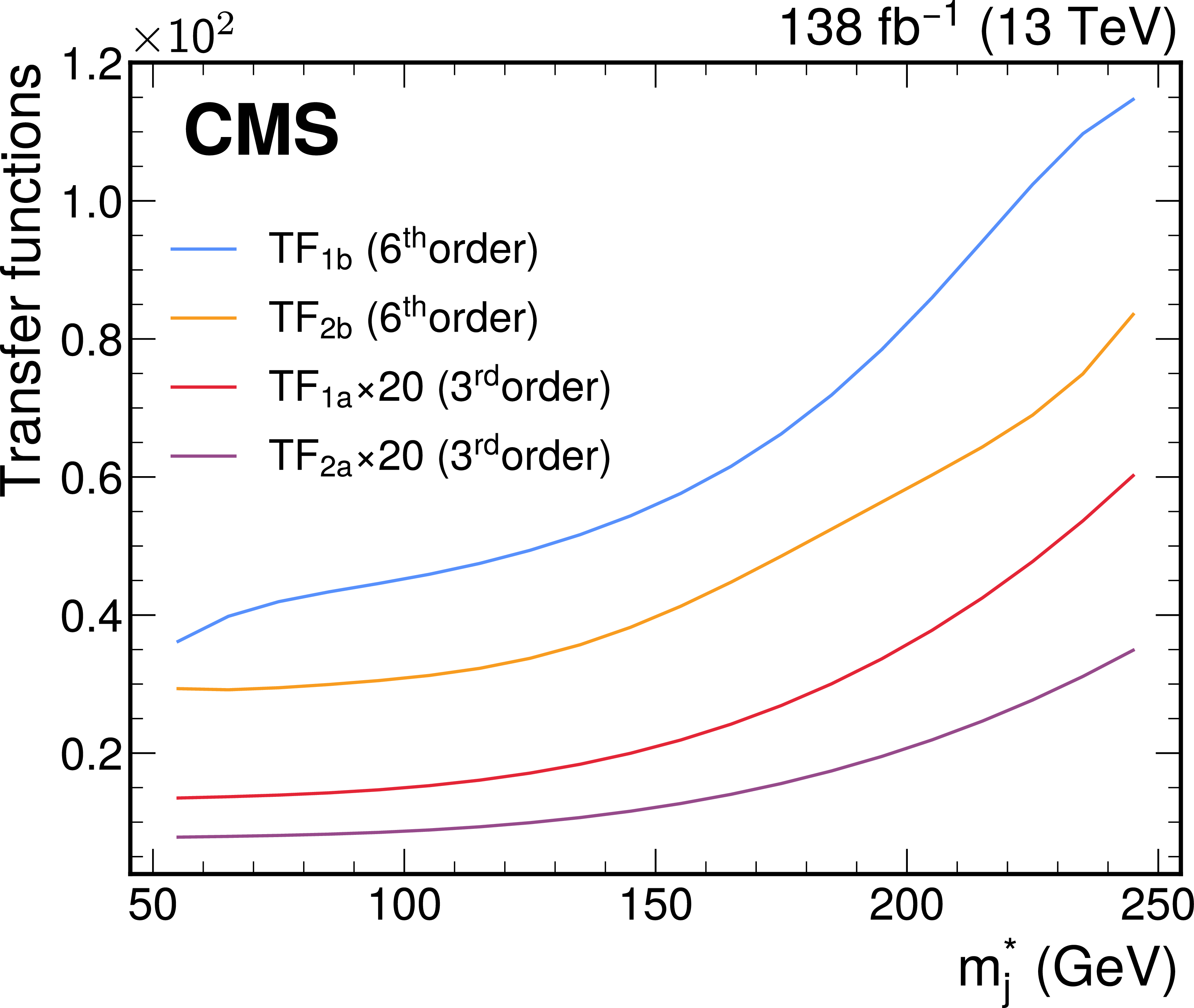
Figure 4:
Illustration of the SRs and CRs, and the TFs used to relate the QCD background in the different regions (left). The TFs used to predict the QCD process in the four SRs as a function of the $ m^*_{\text{j}} $ (right). |
png pdf |
Figure 4-a:
Illustration of the SRs and CRs, and the TFs used to relate the QCD background in the different regions (left). The TFs used to predict the QCD process in the four SRs as a function of the $ m^*_{\text{j}} $ (right). |
png pdf |
Figure 4-b:
Illustration of the SRs and CRs, and the TFs used to relate the QCD background in the different regions (left). The TFs used to predict the QCD process in the four SRs as a function of the $ m^*_{\text{j}} $ (right). |
png pdf |
Figure 5:
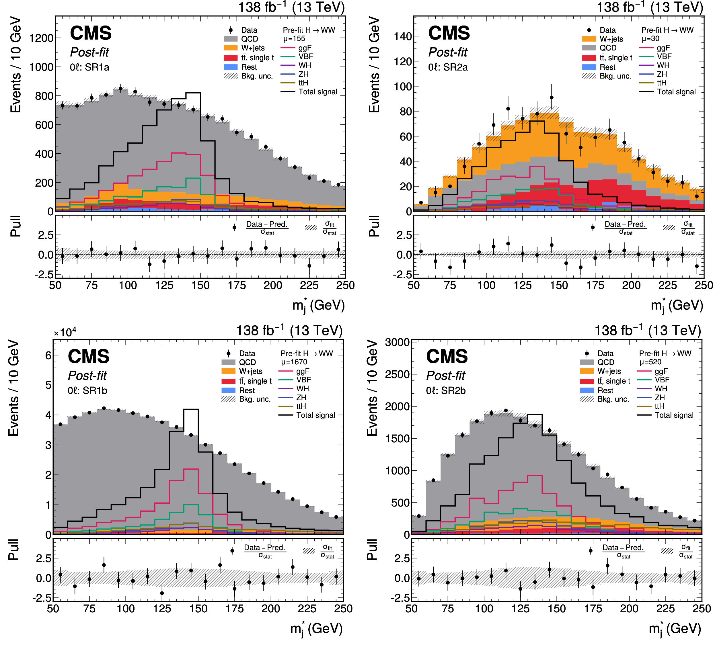
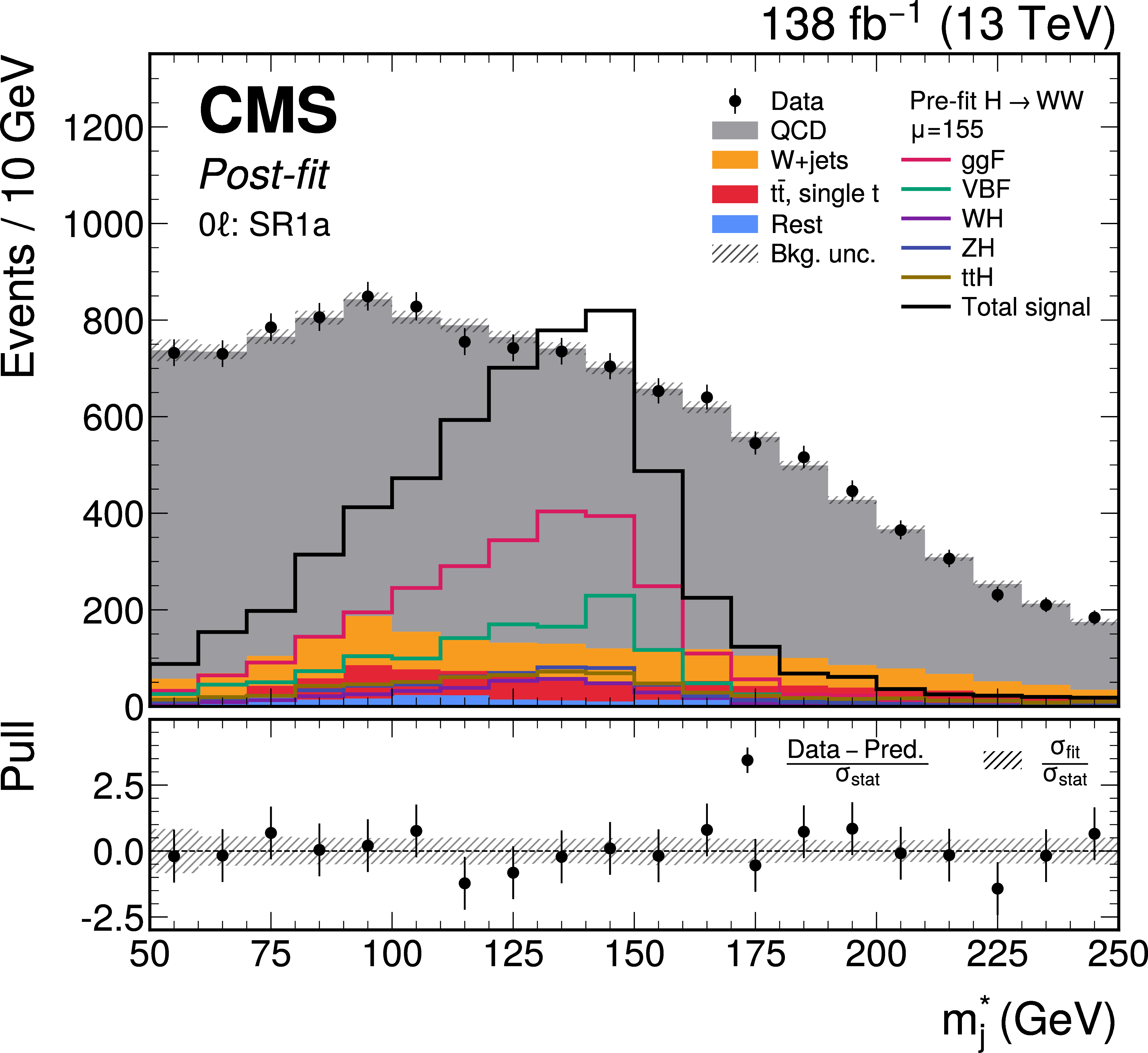
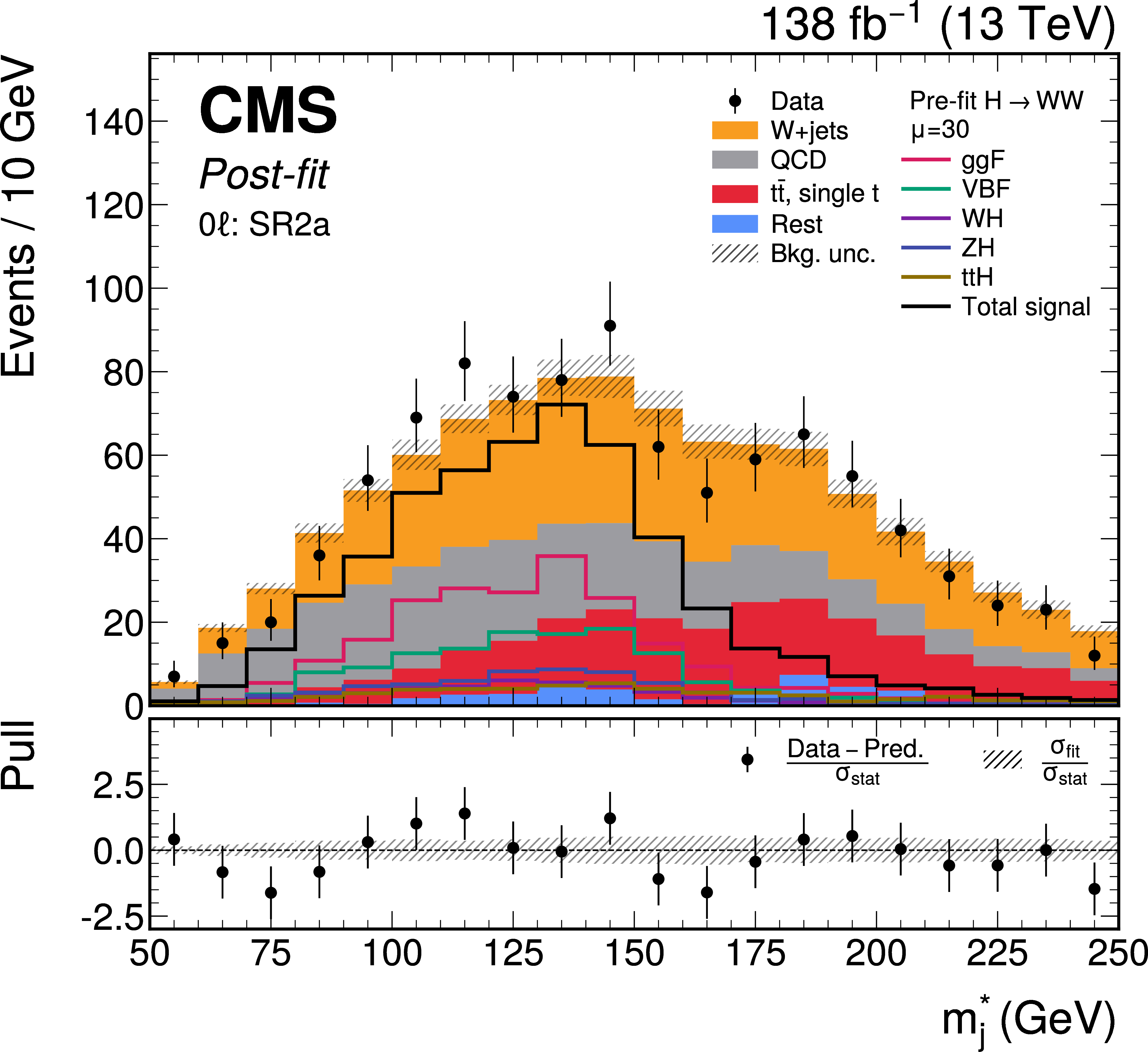
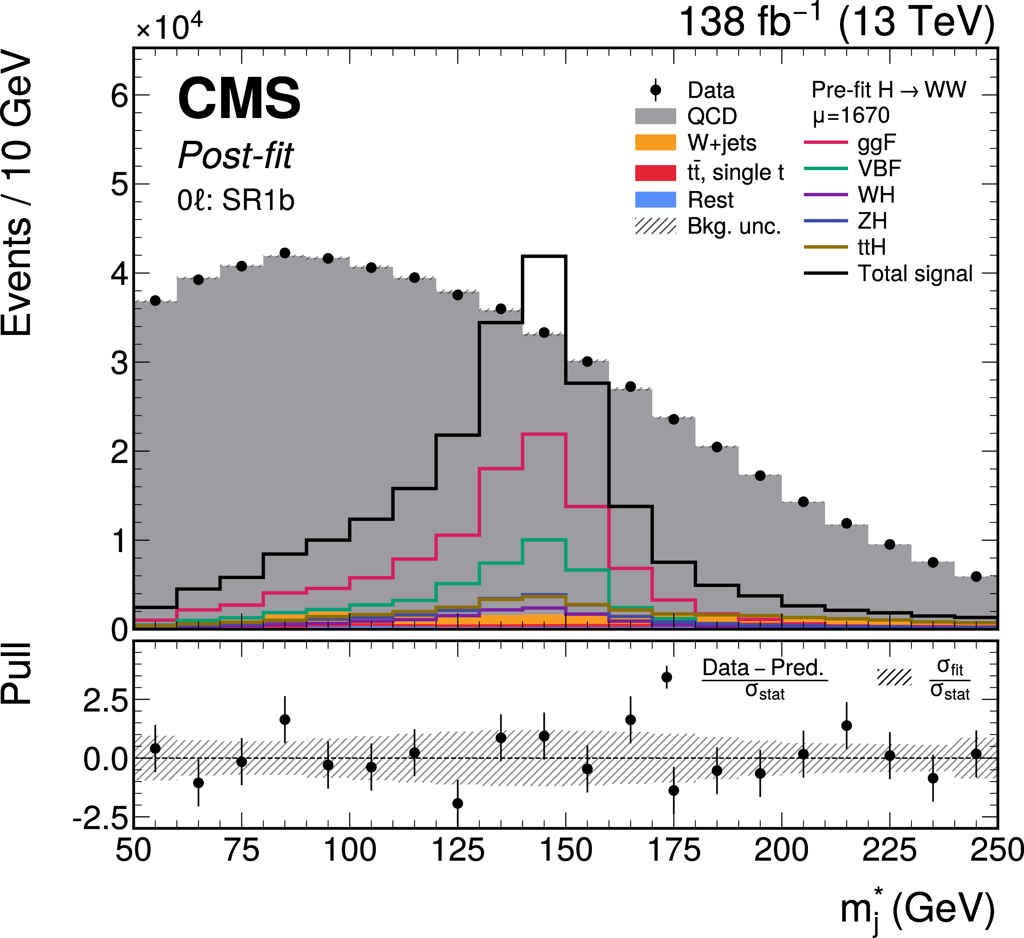
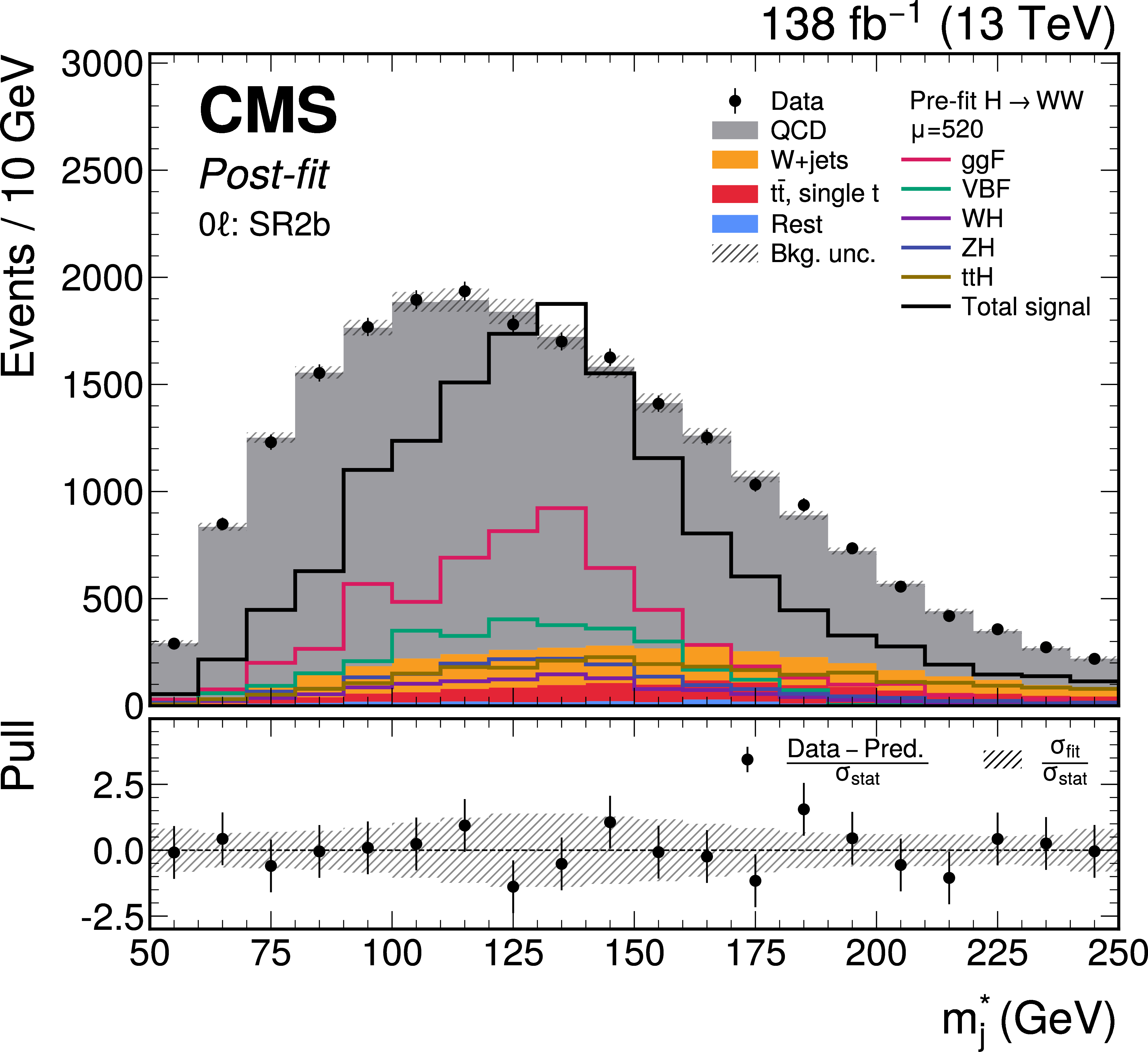
Post-fit $ m^*_{\text{j}} $ distributions in the 0 $ \ell $ channel, showing the predicted background with total uncertainty, observed data, and the expected pre-fit signal scaled by the labeled strength $ \mu $. From left to right, upper to lower, the plots correspond to $ \text{SR}_\text{1a} $, $ \text{SR}_\text{2a} $, $ \text{SR}_\text{1b} $, and $ \text{SR}_\text{2b} $. The lower panel of each plot presents the pull distribution, as well as the $ \sigma_\text{fit} $ normalized to the $ \sigma_\text{stat} $. |
png pdf |
Figure 5-a:
Post-fit $ m^*_{\text{j}} $ distributions in the 0 $ \ell $ channel, showing the predicted background with total uncertainty, observed data, and the expected pre-fit signal scaled by the labeled strength $ \mu $. From left to right, upper to lower, the plots correspond to $ \text{SR}_\text{1a} $, $ \text{SR}_\text{2a} $, $ \text{SR}_\text{1b} $, and $ \text{SR}_\text{2b} $. The lower panel of each plot presents the pull distribution, as well as the $ \sigma_\text{fit} $ normalized to the $ \sigma_\text{stat} $. |
png pdf |
Figure 5-b:
Post-fit $ m^*_{\text{j}} $ distributions in the 0 $ \ell $ channel, showing the predicted background with total uncertainty, observed data, and the expected pre-fit signal scaled by the labeled strength $ \mu $. From left to right, upper to lower, the plots correspond to $ \text{SR}_\text{1a} $, $ \text{SR}_\text{2a} $, $ \text{SR}_\text{1b} $, and $ \text{SR}_\text{2b} $. The lower panel of each plot presents the pull distribution, as well as the $ \sigma_\text{fit} $ normalized to the $ \sigma_\text{stat} $. |
png pdf |
Figure 5-c:
Post-fit $ m^*_{\text{j}} $ distributions in the 0 $ \ell $ channel, showing the predicted background with total uncertainty, observed data, and the expected pre-fit signal scaled by the labeled strength $ \mu $. From left to right, upper to lower, the plots correspond to $ \text{SR}_\text{1a} $, $ \text{SR}_\text{2a} $, $ \text{SR}_\text{1b} $, and $ \text{SR}_\text{2b} $. The lower panel of each plot presents the pull distribution, as well as the $ \sigma_\text{fit} $ normalized to the $ \sigma_\text{stat} $. |
png pdf |
Figure 5-d:
Post-fit $ m^*_{\text{j}} $ distributions in the 0 $ \ell $ channel, showing the predicted background with total uncertainty, observed data, and the expected pre-fit signal scaled by the labeled strength $ \mu $. From left to right, upper to lower, the plots correspond to $ \text{SR}_\text{1a} $, $ \text{SR}_\text{2a} $, $ \text{SR}_\text{1b} $, and $ \text{SR}_\text{2b} $. The lower panel of each plot presents the pull distribution, as well as the $ \sigma_\text{fit} $ normalized to the $ \sigma_\text{stat} $. |
png pdf |
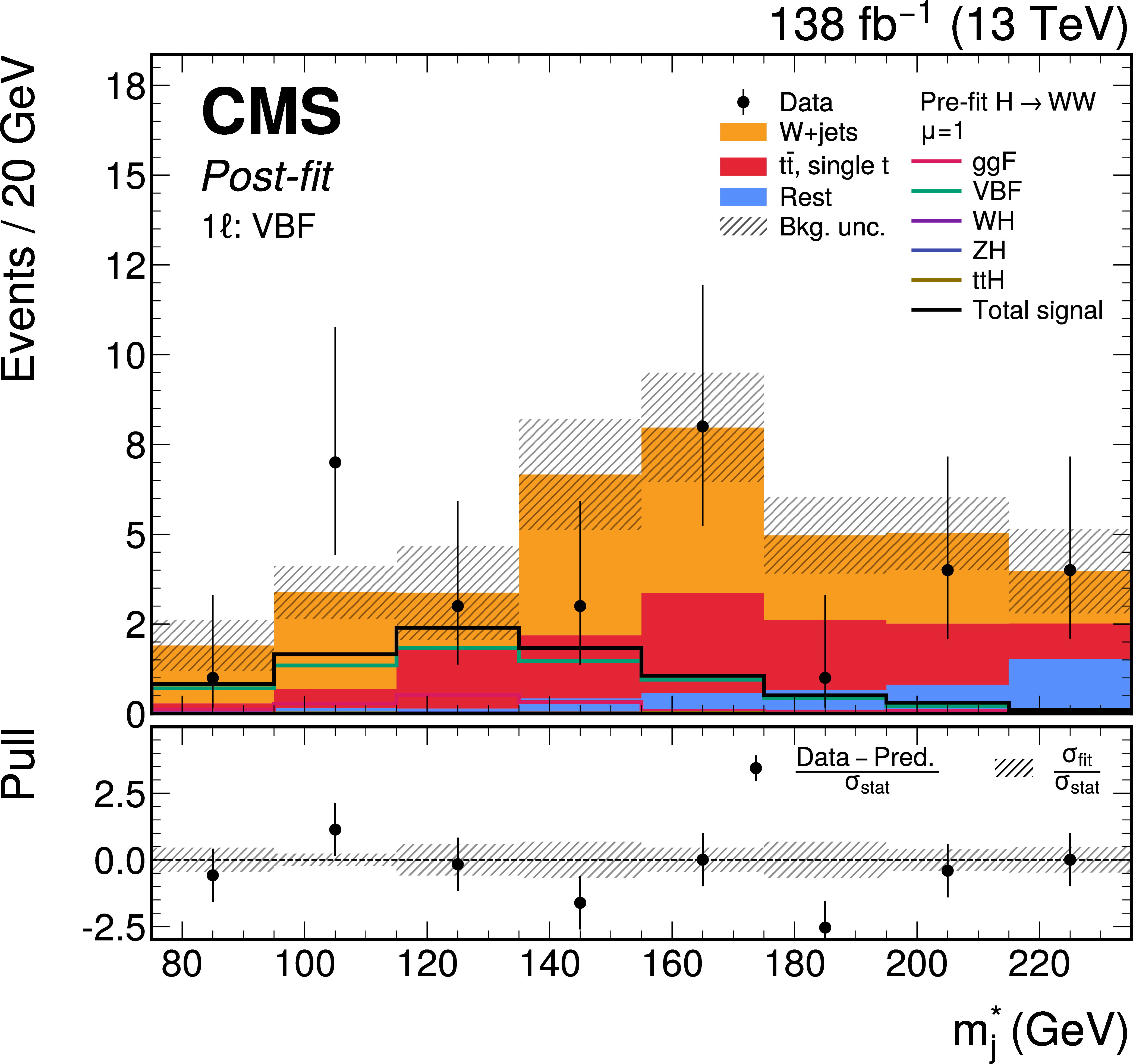
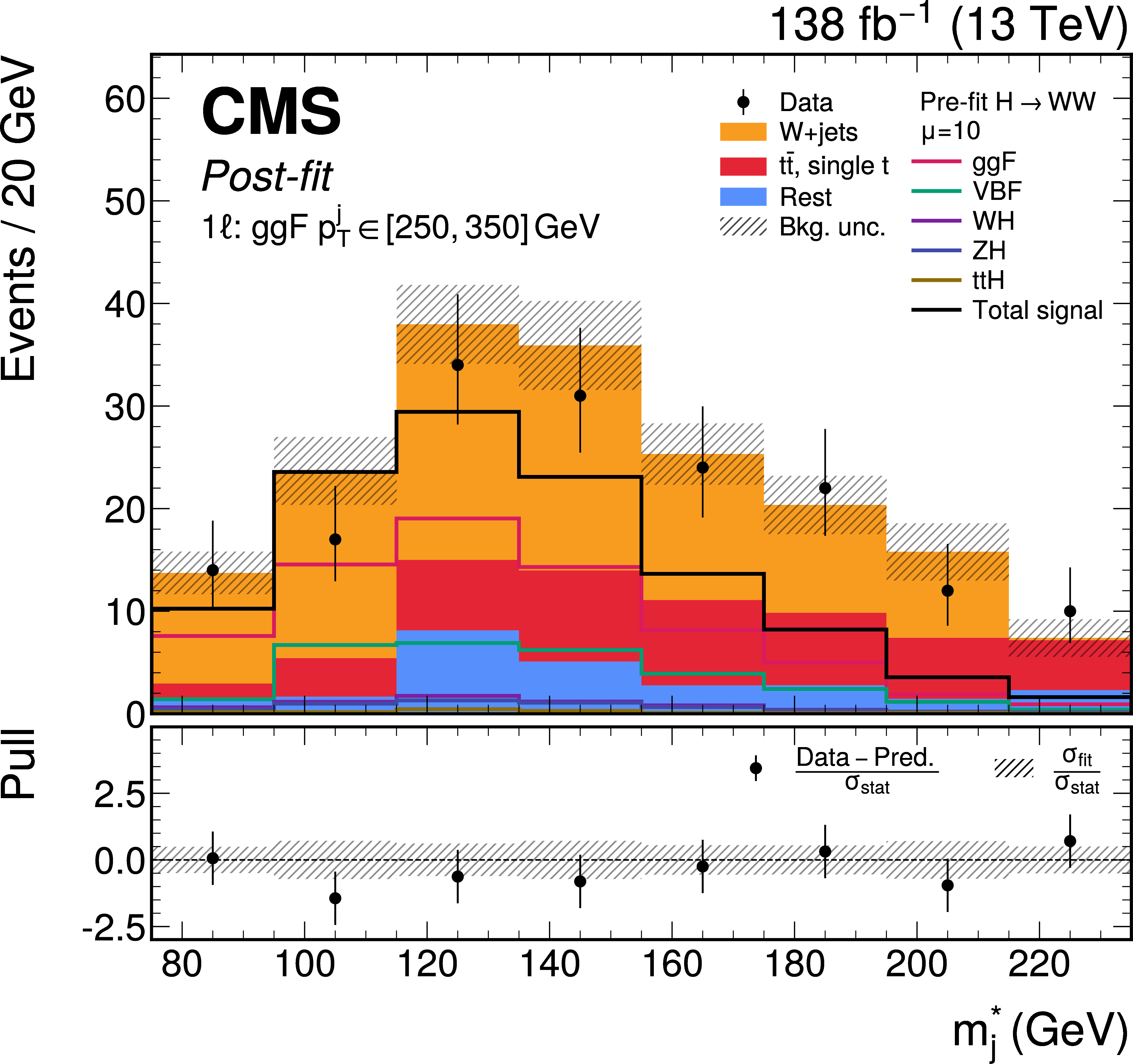
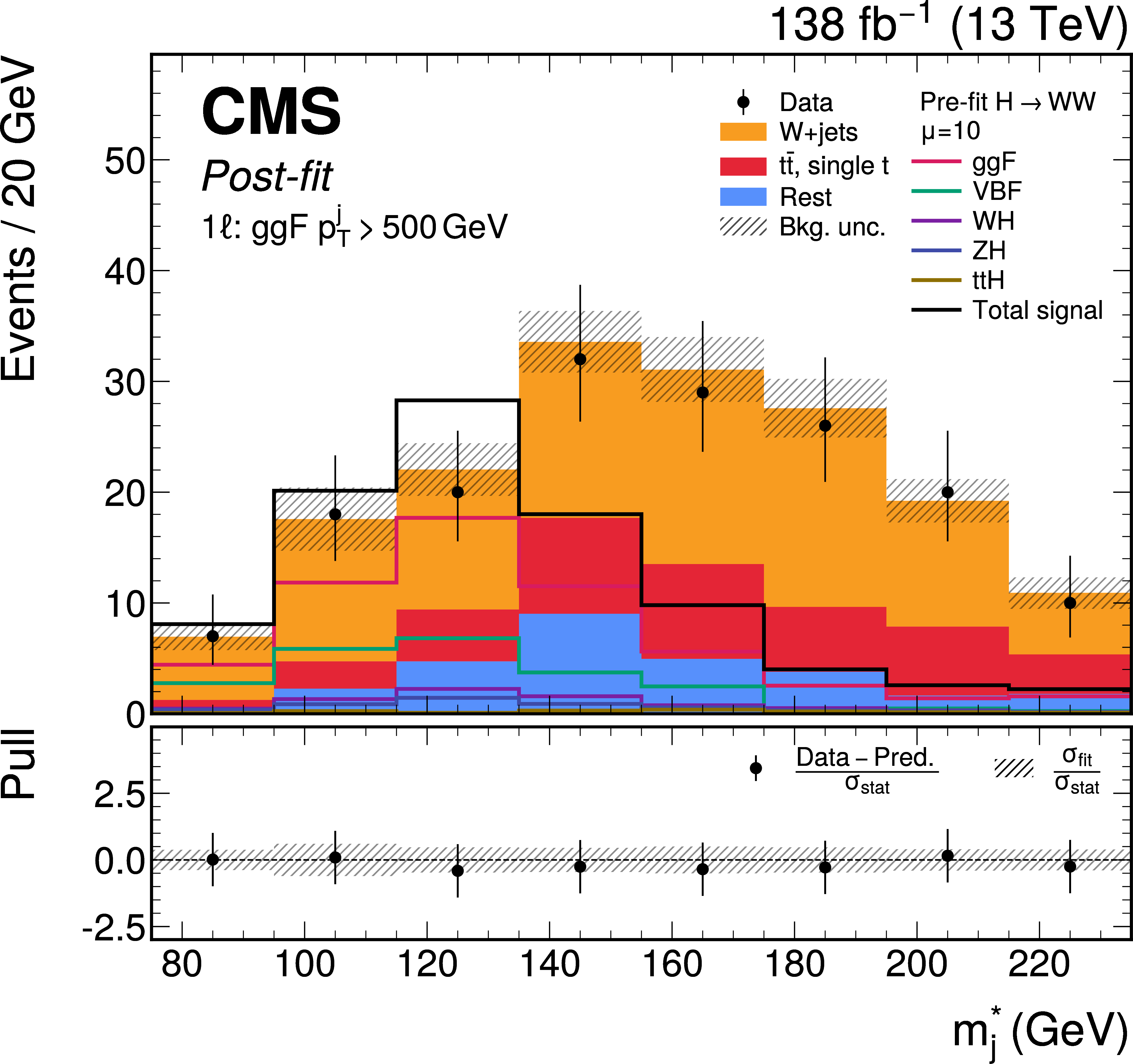
Figure 6:
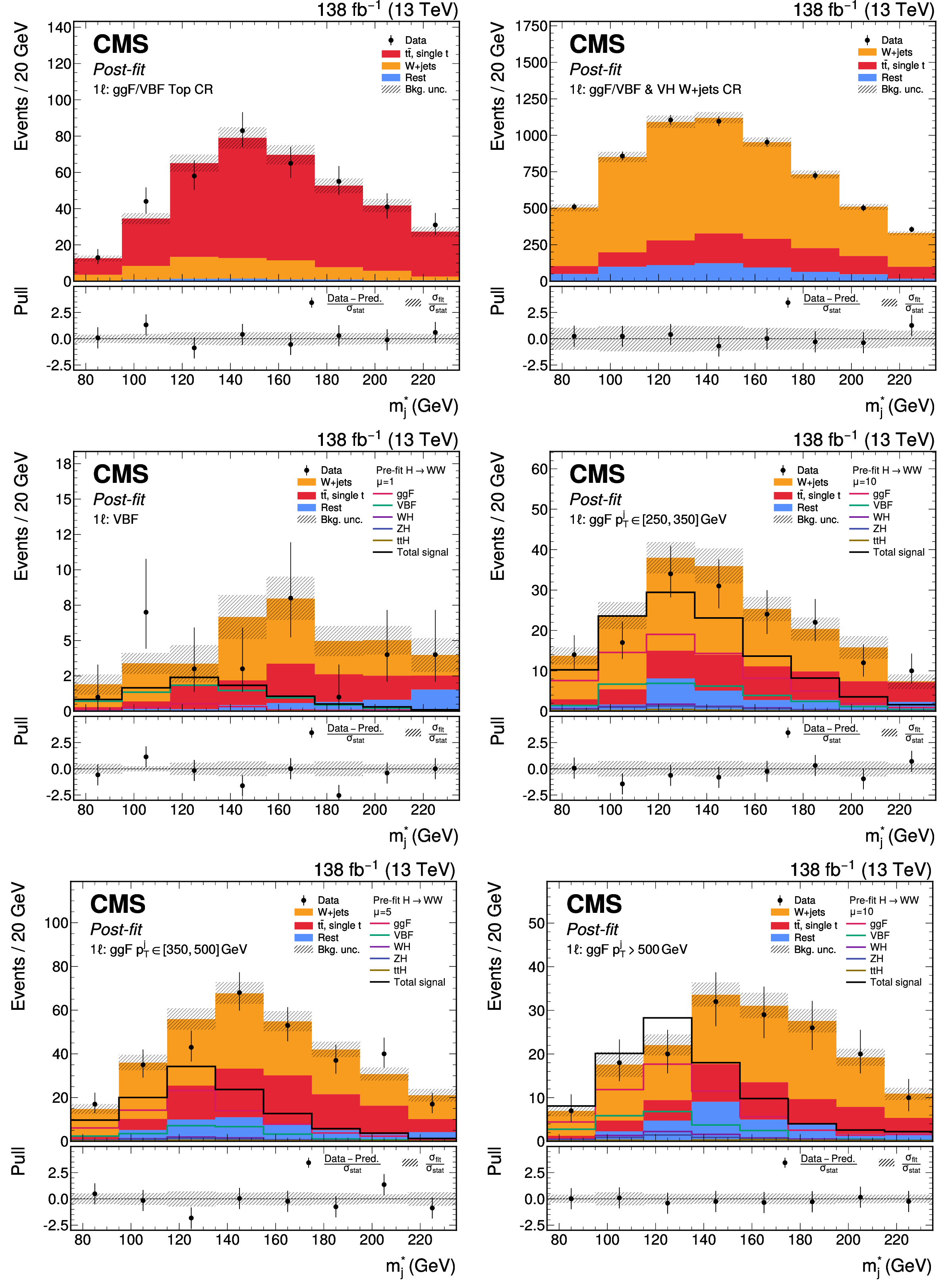
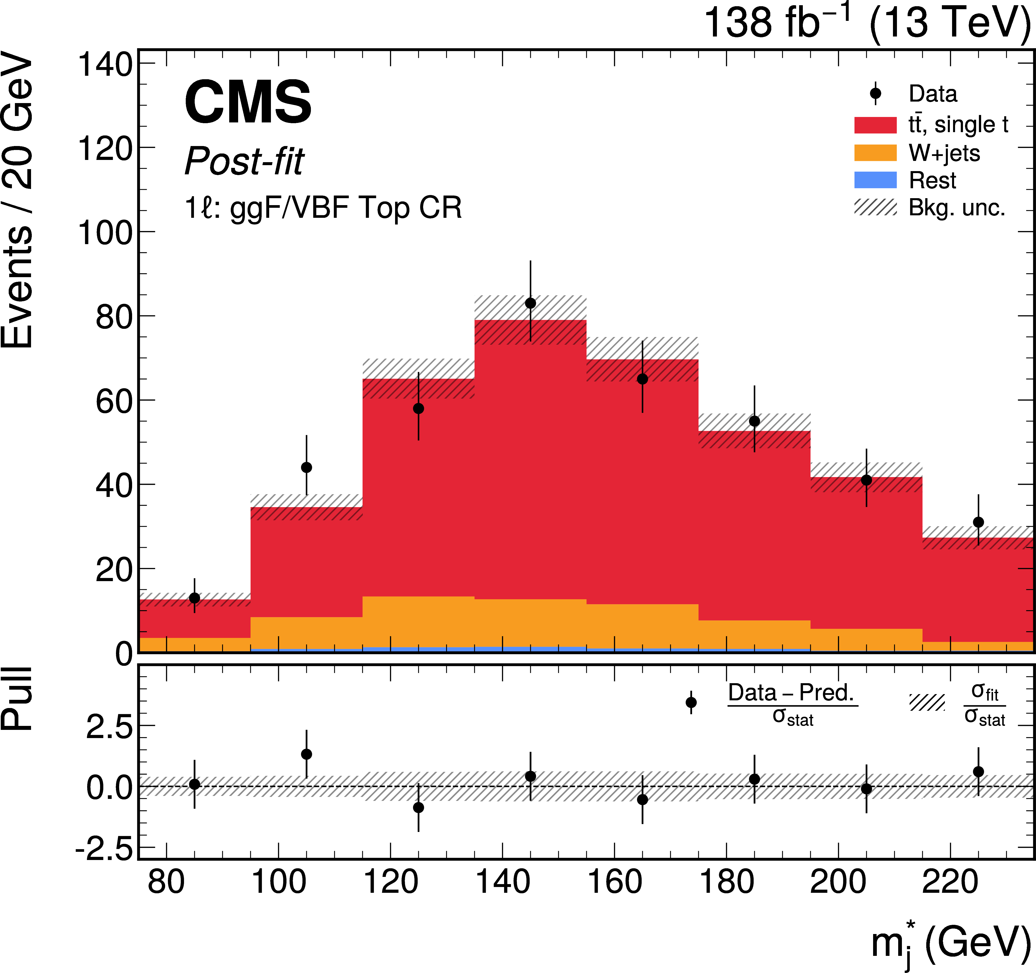
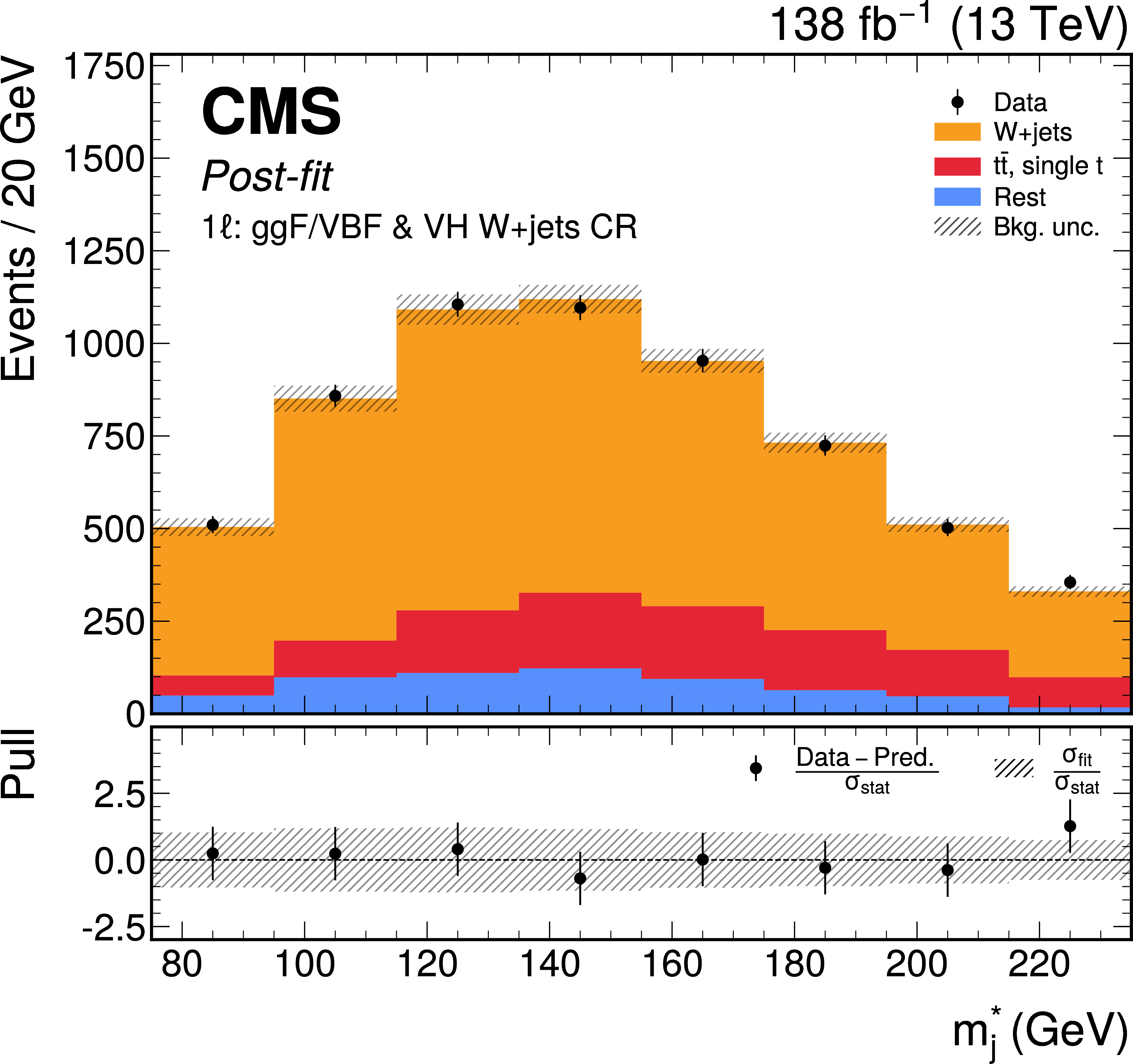
Post-fit $ m^*_{\text{j}} $ distributions in the 1 $ \ell $ channel, showing the predicted background with total uncertainty, observed data, and the expected pre-fit signal scaled by the labeled strength $ \mu $. Left to right and upper to lower: Top CR, W+jets CR, VBF SR, and the ggF SRs binned in $ p_{\mathrm{T}} $ as $ [250,350) $, $ [350,500) $, and $ [500,+\infty) \text{GeV} $, respectively. The lower panel of each plot presents the pull distribution, as well as $ \sigma_\text{fit} $ normalized to the $ \sigma_\text{stat} $. |
png pdf |
Figure 6-a:
Post-fit $ m^*_{\text{j}} $ distributions in the 1 $ \ell $ channel, showing the predicted background with total uncertainty, observed data, and the expected pre-fit signal scaled by the labeled strength $ \mu $. Left to right and upper to lower: Top CR, W+jets CR, VBF SR, and the ggF SRs binned in $ p_{\mathrm{T}} $ as $ [250,350) $, $ [350,500) $, and $ [500,+\infty) \text{GeV} $, respectively. The lower panel of each plot presents the pull distribution, as well as $ \sigma_\text{fit} $ normalized to the $ \sigma_\text{stat} $. |
png pdf |
Figure 6-b:
Post-fit $ m^*_{\text{j}} $ distributions in the 1 $ \ell $ channel, showing the predicted background with total uncertainty, observed data, and the expected pre-fit signal scaled by the labeled strength $ \mu $. Left to right and upper to lower: Top CR, W+jets CR, VBF SR, and the ggF SRs binned in $ p_{\mathrm{T}} $ as $ [250,350) $, $ [350,500) $, and $ [500,+\infty) \text{GeV} $, respectively. The lower panel of each plot presents the pull distribution, as well as $ \sigma_\text{fit} $ normalized to the $ \sigma_\text{stat} $. |
png pdf |
Figure 6-c:
Post-fit $ m^*_{\text{j}} $ distributions in the 1 $ \ell $ channel, showing the predicted background with total uncertainty, observed data, and the expected pre-fit signal scaled by the labeled strength $ \mu $. Left to right and upper to lower: Top CR, W+jets CR, VBF SR, and the ggF SRs binned in $ p_{\mathrm{T}} $ as $ [250,350) $, $ [350,500) $, and $ [500,+\infty) \text{GeV} $, respectively. The lower panel of each plot presents the pull distribution, as well as $ \sigma_\text{fit} $ normalized to the $ \sigma_\text{stat} $. |
png pdf |
Figure 6-d:
Post-fit $ m^*_{\text{j}} $ distributions in the 1 $ \ell $ channel, showing the predicted background with total uncertainty, observed data, and the expected pre-fit signal scaled by the labeled strength $ \mu $. Left to right and upper to lower: Top CR, W+jets CR, VBF SR, and the ggF SRs binned in $ p_{\mathrm{T}} $ as $ [250,350) $, $ [350,500) $, and $ [500,+\infty) \text{GeV} $, respectively. The lower panel of each plot presents the pull distribution, as well as $ \sigma_\text{fit} $ normalized to the $ \sigma_\text{stat} $. |

png pdf |
Figure 6-e:
Post-fit $ m^*_{\text{j}} $ distributions in the 1 $ \ell $ channel, showing the predicted background with total uncertainty, observed data, and the expected pre-fit signal scaled by the labeled strength $ \mu $. Left to right and upper to lower: Top CR, W+jets CR, VBF SR, and the ggF SRs binned in $ p_{\mathrm{T}} $ as $ [250,350) $, $ [350,500) $, and $ [500,+\infty) \text{GeV} $, respectively. The lower panel of each plot presents the pull distribution, as well as $ \sigma_\text{fit} $ normalized to the $ \sigma_\text{stat} $. |
png pdf |
Figure 6-f:
Post-fit $ m^*_{\text{j}} $ distributions in the 1 $ \ell $ channel, showing the predicted background with total uncertainty, observed data, and the expected pre-fit signal scaled by the labeled strength $ \mu $. Left to right and upper to lower: Top CR, W+jets CR, VBF SR, and the ggF SRs binned in $ p_{\mathrm{T}} $ as $ [250,350) $, $ [350,500) $, and $ [500,+\infty) \text{GeV} $, respectively. The lower panel of each plot presents the pull distribution, as well as $ \sigma_\text{fit} $ normalized to the $ \sigma_\text{stat} $. |
png pdf |
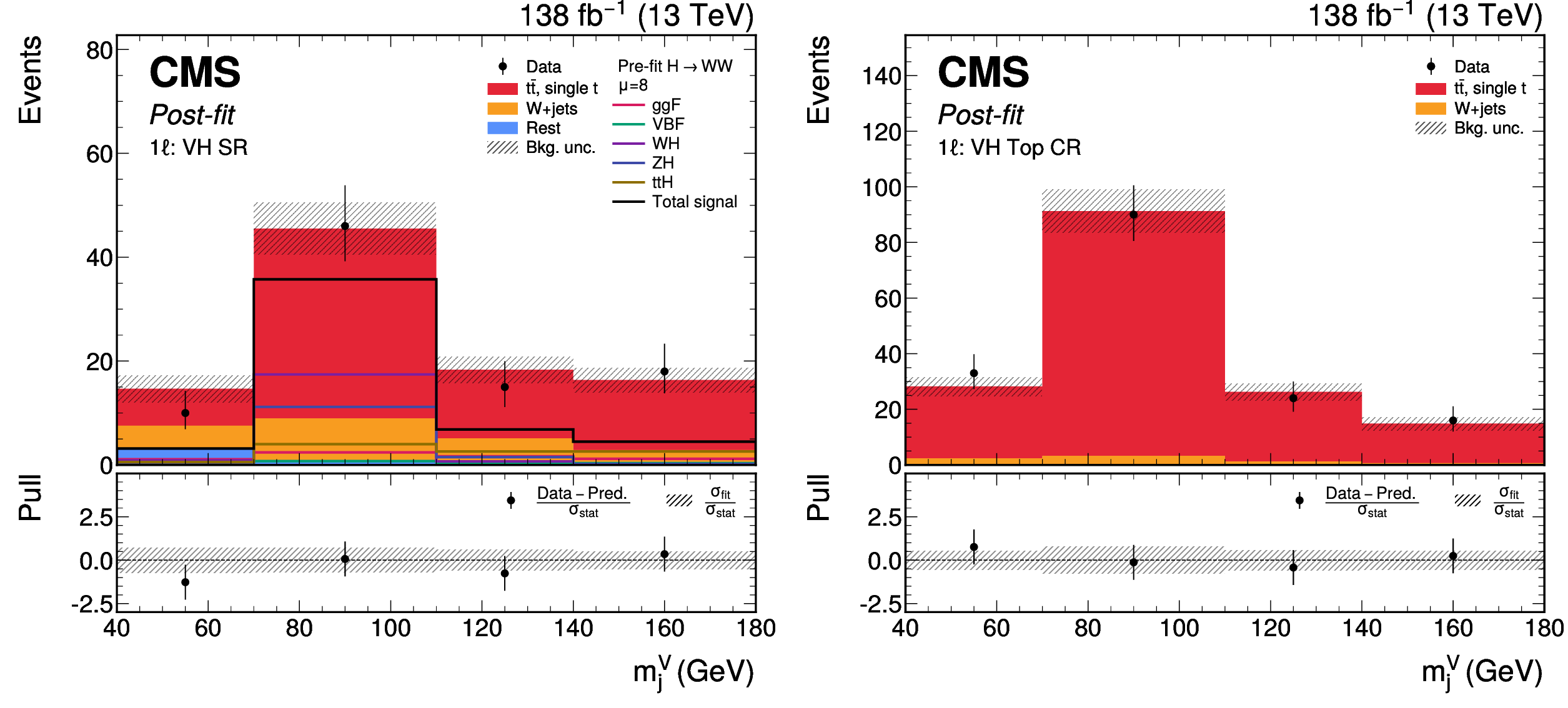
Figure 7:
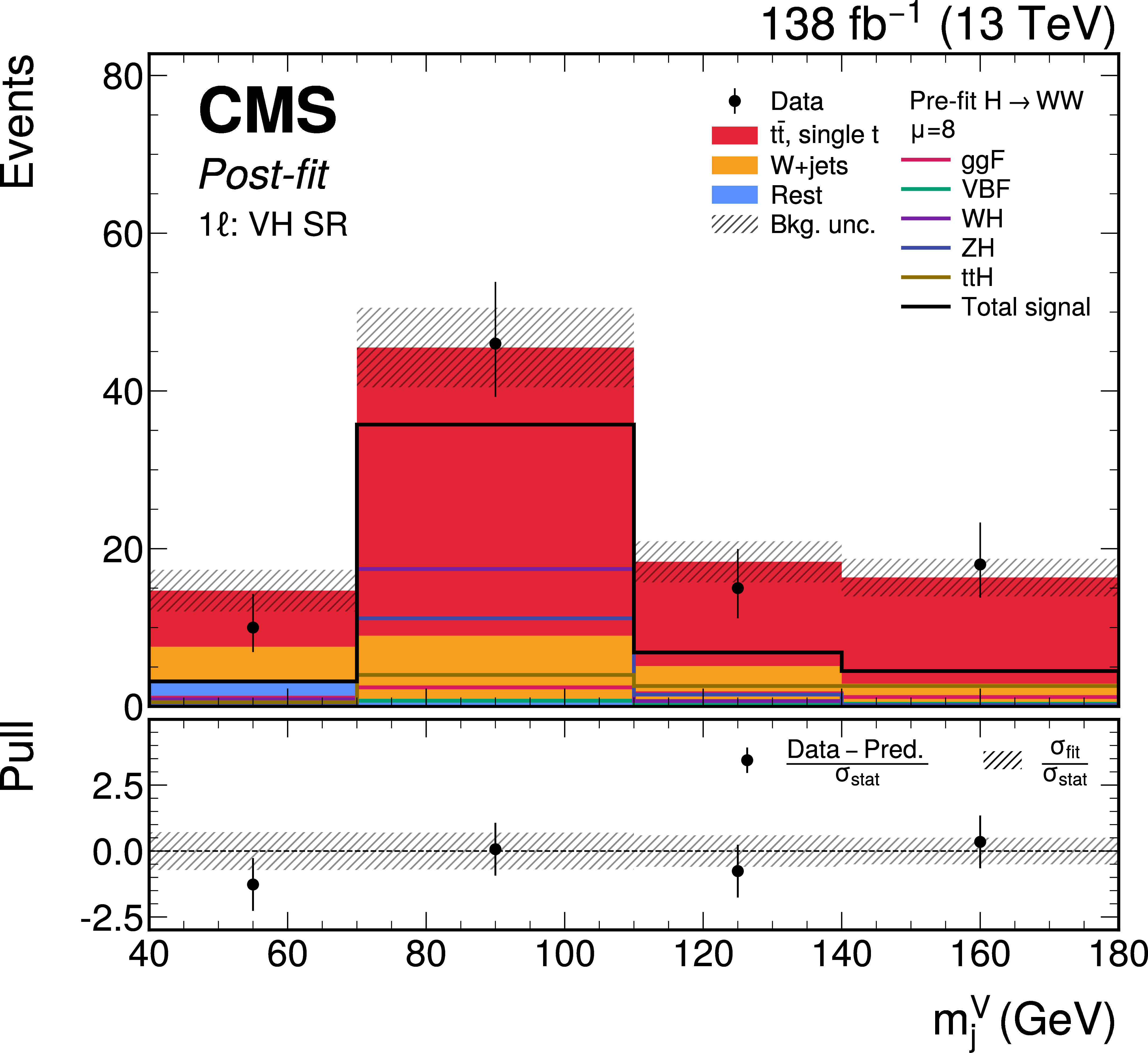
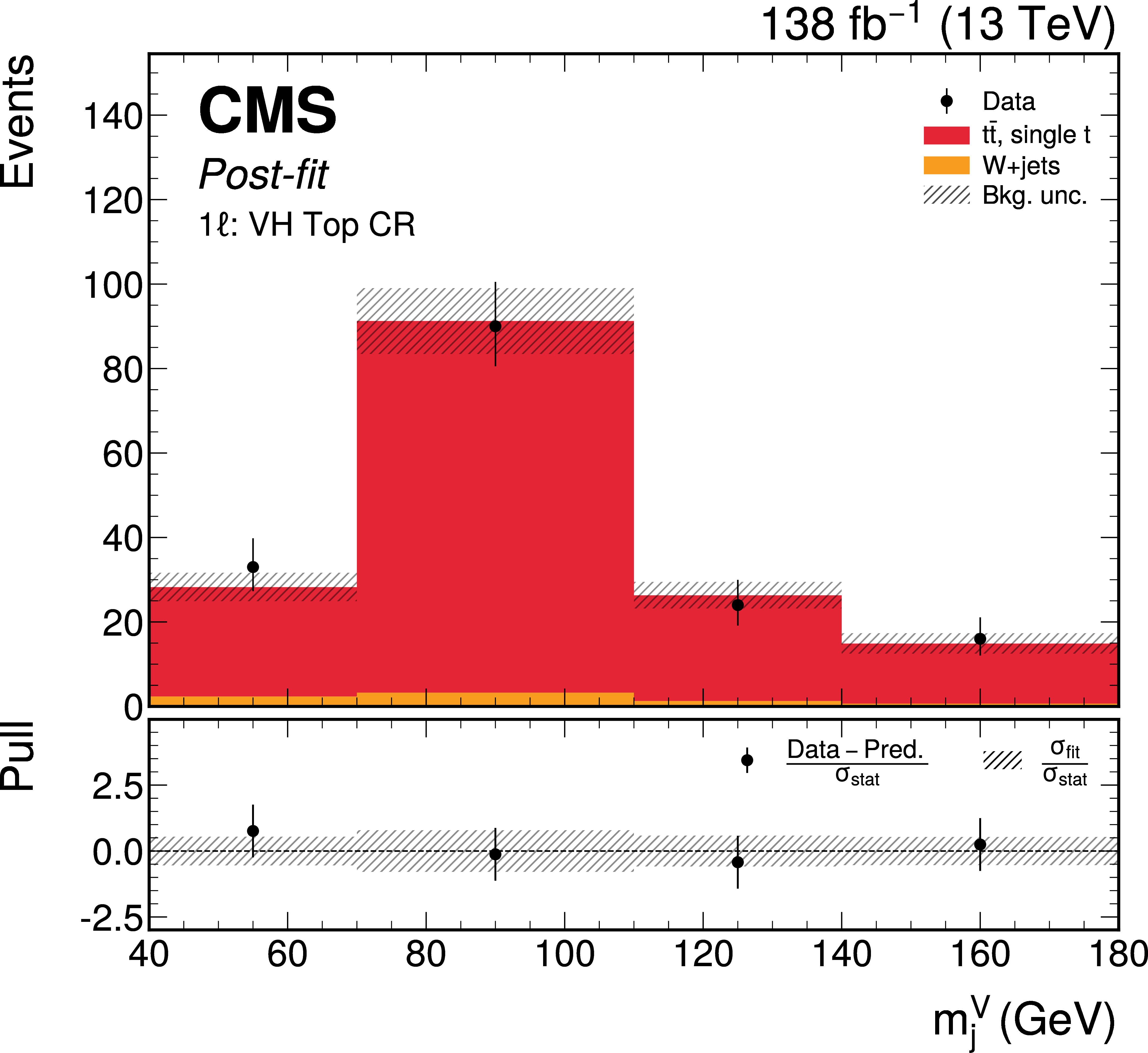
Post-fit $ m_\text{j}^\mathrm{V} $ distributions in the VH channel, showing the predicted background with total uncertainty, observed data, and expected signal, split by production process. Left to right: VH SR and VH Top CR. The lower panel of each plot presents the pull distribution, as well as $ \sigma_\text{fit} $ normalized to the $ \sigma_\text{stat} $. The predicted pre-fit signal is scaled for visibility. |
png pdf |
Figure 7-a:
Post-fit $ m_\text{j}^\mathrm{V} $ distributions in the VH channel, showing the predicted background with total uncertainty, observed data, and expected signal, split by production process. Left to right: VH SR and VH Top CR. The lower panel of each plot presents the pull distribution, as well as $ \sigma_\text{fit} $ normalized to the $ \sigma_\text{stat} $. The predicted pre-fit signal is scaled for visibility. |
png pdf |
Figure 7-b:
Post-fit $ m_\text{j}^\mathrm{V} $ distributions in the VH channel, showing the predicted background with total uncertainty, observed data, and expected signal, split by production process. Left to right: VH SR and VH Top CR. The lower panel of each plot presents the pull distribution, as well as $ \sigma_\text{fit} $ normalized to the $ \sigma_\text{stat} $. The predicted pre-fit signal is scaled for visibility. |
png pdf |
Figure 8:
Observed scan of the profile likelihood test statistic $ t_\mu $ as a function of the signal strength $ \mu $ for the combination of all the channels. The solid lines correspond to profiling all statistical and systematic uncertainties, while the dashed lines correspond to profiling only the statistical uncertainties. |
png pdf |
Figure 9:
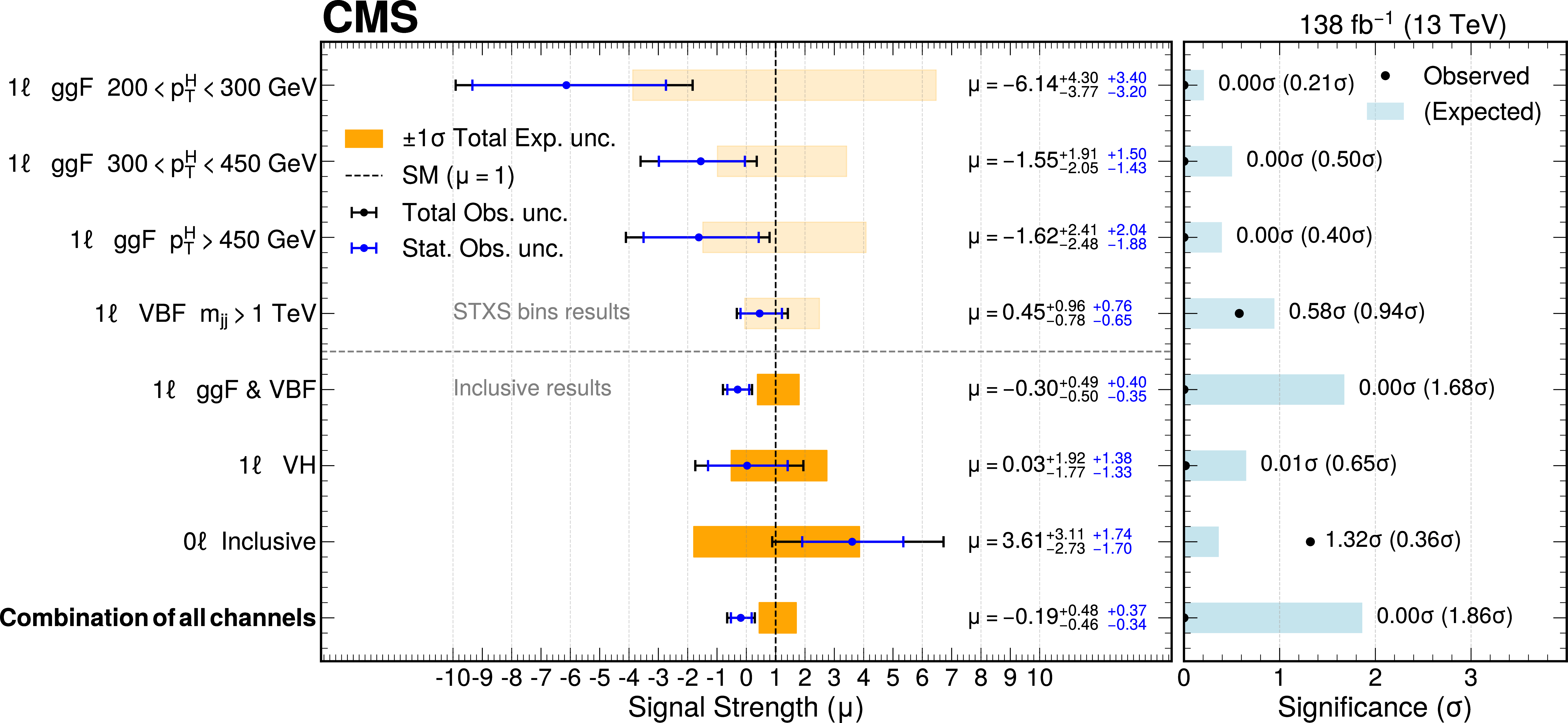
Observed and expected signal strength (left) and significance (right) for $ \mathrm{H} \to \mathrm{W} \mathrm{W} $ in all the channels using the full data set. Combined results are presented alongside individual contributions from each channel. Total expected uncertainties are indicated by yellow bands, while signal strength significances are shown with light blue bars. Blue and black lines represent statistical and total observed uncertainties, respectively. |
png pdf |
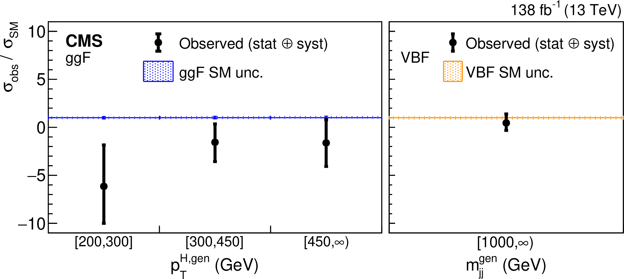
Figure 10:
Unfolded measurement of the STXS cross sections in generator-level bins for three bins of Higgs boson $ p_{\mathrm{T}} $ and one bin of $ m_\text{jj} $ in the 1 $ \ell $ channel. Measured cross sections are divided by standard-model expectations. Blue and orange uncertainty bands include theoretical uncertainties affecting the signal acceptance. |
| Tables | |
png pdf |
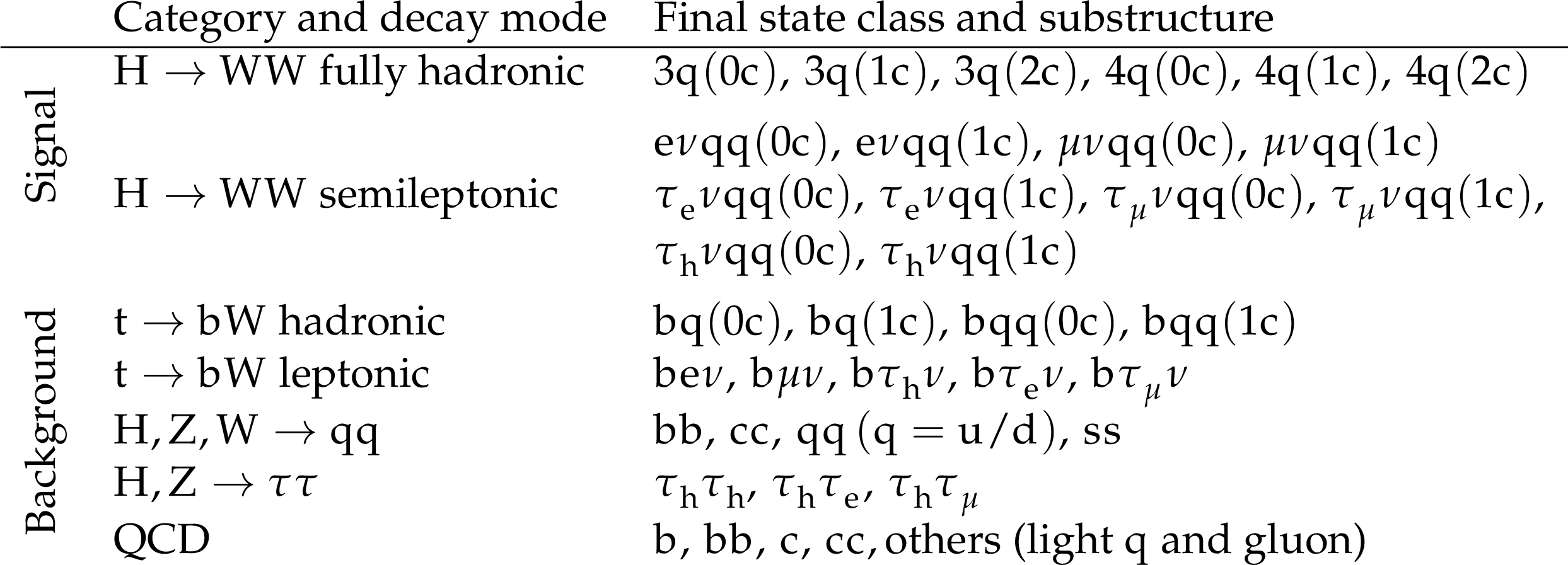
Table 1:
The 37 PART jet classification categories. The categories are based on the decay modes of H and V bosons, top quarks, and on QCD processes. All listed decay products are assumed to be contained within the jet cone, except for neutrinos. Numbers like 4 $ \mathrm{q} $ indicate the multiplicity of the adjacent quark, while those in parentheses indicate the number of c quarks in the preceding quark sequence. Classes such as 3 $ \mathrm{q} $ or $ \mathrm{b}\mathrm{q} $ imply that one quark escapes the jet cone in $ \mathrm{H}\to4\mathrm{q} $ or $ \mathrm{t}\to\mathrm{b}\mathrm{q}\mathrm{q} $ decays, respectively. Subscripts on $ \tau $ indicate hadronic (h) or leptonic (e, $ \mu $) decays. |
png pdf |
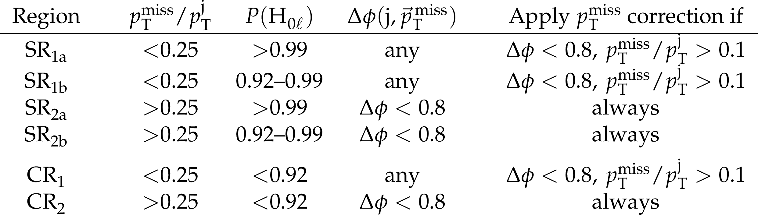
Table 2:
Kinematic requirements used to define the SRs and CRs in the 0 $ \ell $ channel. The rightmost columns list the conditions, combined with logical ``AND'', under which $ m_{\text{j}} $ is replaced by the corrected $ m^*_{\text{j}} $ mass. The $ \Delta\phi $ denotes the azimuthal angle difference between $ {\vec p}_{\mathrm{T}}^{\mkern3mu\text{miss}} $ and the Higgs boson candidate $ p_{\mathrm{T}} $ vector. |
png pdf |
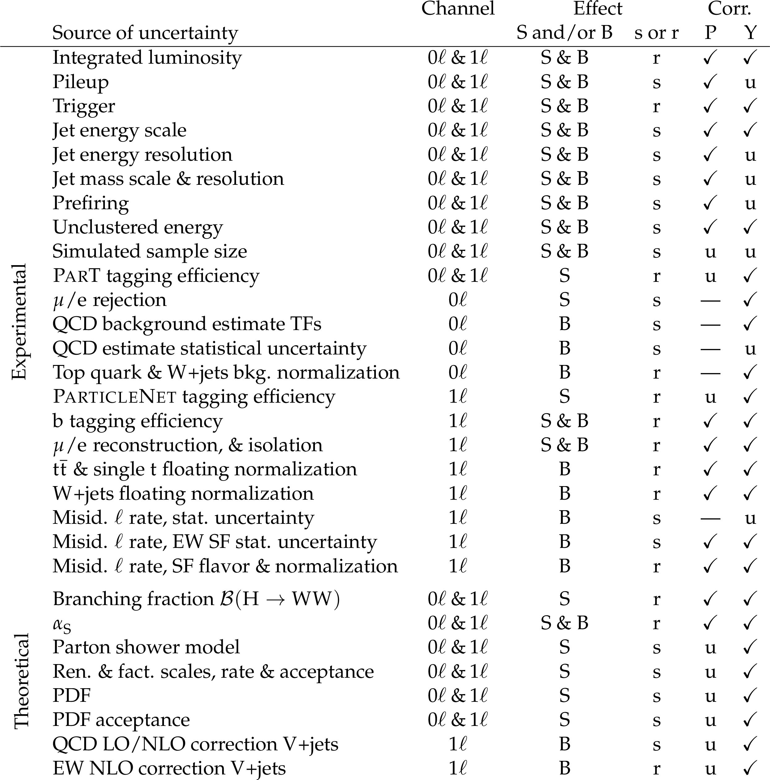
Table 3:
Systematic uncertainty sources considered in the analysis. Left to right columns: the sources, the channels, whether the uncertainty affects signal (S) or background (B), its influence on shape (s) or rate (r), and whether the nuisances are (un)correlated (u or $ \checkmark $) among different process models (P) or among the data-taking years (Y). |
png pdf |
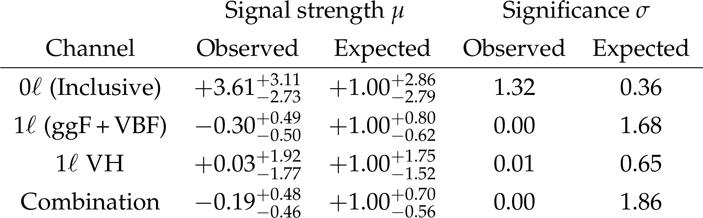
Table 4:
Observed and expected signal strength $ \mu $ (second column) and significance $ \sigma $ (third column) for $ \mathrm{H} \to \mathrm{W} \mathrm{W} $ in the 0 $ \ell $ and 1 $ \ell $ channels, followed by the combined results. |
| Summary |
| A search for Higgs boson (H) production at high transverse momentum is presented in the decay channel $ \mathrm{H} \to \mathrm{W} \mathrm{W} $. The analysis uses proton-proton collision data collected at $ \sqrt{s} = $ 13 TeV with the CMS experiment, corresponding to an integrated luminosity of 138 fb$ ^{-1} $, and focuses on WW decays with one or no isolated lepton (1 $ \ell $ and 0 $ \ell $, respectively; $ \ell=\mathrm{e},\mu $) in the final state. The final states are characterized by a single large-radius jet containing the hadronic decay products of the W bosons, utilizing the jet substructure resulting from the Lorentz-boosted topology of the Higgs boson decay. The 1 $ \ell $ channel categorizes events by the dominant Higgs boson production mechanisms: gluon fusion, vector boson fusion, and vector boson associated production, while the 0 $ \ell $ channel remains inclusive across all production processes. The particle transformer algorithm leverages advanced machine-learning techniques to identify H-candidate jets with intricate substructure, missing transverse momentum aligned with the jet, or leptons inside the jet. It is calibrated with the Lund jet plane reweighting method and fine-tuned to optimize the expected signal significance in the 1 $ \ell $ channel, achieving 60% higher signal efficiency than the baseline tagger. The invariant mass of the candidate jet H or vector boson is used for signal extraction. The expected signal significance is 1.86 standard deviations, while the observed signal strength relative to the standard model expectation is $ \mu = - $ 0.19 $ ^{+0.48}_{-0.46} $, indicating no evidence of a signal above the background. These measurements represent the first dedicated study of highly Lorentz-boosted $ \mathrm{H} \to \mathrm{W} \mathrm{W} $ decays, complementing earlier searches for high transverse momentum Higgs boson production in other decay channels and production processes. |
| References | ||||
| 1 | ATLAS Collaboration | Observation of a new particle in the search for the standard model Higgs boson with the ATLAS detector at the LHC | PLB 716 (2012) 1 | 1207.7214 |
| 2 | CMS Collaboration | Observation of a new boson at a mass of 125 GeV with the CMS experiment at the LHC | PLB 716 (2012) 30 | CMS-HIG-12-028 1207.7235 |
| 3 | CMS Collaboration | Observation of a new boson with mass near 125 GeV in pp collisions at $ \sqrt{s} = $ 7 and 8 TeV | JHEP 06 (2013) 081 | CMS-HIG-12-036 1303.4571 |
| 4 | G. Aad et al. | A detailed map of Higgs boson interactions by the ATLAS experiment ten years after the discovery | Nature 607 (2022) 52 | 2207.00092 |
| 5 | CMS Collaboration | A portrait of the Higgs boson by the CMS experiment ten years after the discovery | [Corrigendum: doi10./s41586-023-06164-8], 2022 Nature 607 (2022) 60 |
CMS-HIG-22-001 2207.00043 |
| 6 | K. Becker et al. | Precise predictions for boosted Higgs production | SciPost Phys. Core 7 (2024) 001 | 2005.07762 |
| 7 | C. Grojean, E. Salvioni, M. Schlaffer, and A. Weiler | Very boosted Higgs in gluon fusion | JHEP 05 (2014) 22 | 1312.3317 |
| 8 | M. Schlaffer et al. | Boosted Higgs shapes | EPJC 74 (2014) 3120 | 1405.4295 |
| 9 | S. Dawson, I. M. Lewis, and M. Zeng | Usefulness of effective field theory for boosted Higgs production | PRD 91 (2015) 074012 | 1501.04103 |
| 10 | M. Grazzini, A. Ilnicka, M. Spira, and M. Wiesemann | Modeling BSM effects on the Higgs transverse-momentum spectrum in an EFT approach | JHEP 03 (2017) 115 | 1612.00283 |
| 11 | F. Maltoni, K. Mawatari, and M. Zaro | Higgs characterisation via vector-boson fusion and associated production: NLO and parton-shower effects | EPJC 74 (2014) 2710 | 1311.1829 |
| 12 | C. Degrande et al. | Electroweak Higgs boson production in the standard model effective field theory beyond leading order in QCD | EPJC 77 (2017) 262 | 1609.04833 |
| 13 | CMS Collaboration | Measurement and interpretation of differential cross sections for Higgs boson production at $ \sqrt{s} = $ 13 TeV | PLB 792 (2019) 369 | CMS-HIG-17-028 1812.06504 |
| 14 | CMS Collaboration | Measurement of the Higgs boson inclusive and differential fiducial production cross sections in the diphoton decay channel with pp collisions at $ \sqrt{s} = $ 13 TeV | JHEP 07 (2023) 091 | CMS-HIG-19-016 2208.12279 |
| 15 | CMS Collaboration | Measurement of the inclusive and differential Higgs boson production cross sections in the leptonic WW decay mode at $ \sqrt{s} = $ 13 TeV | JHEP 03 (2021) 003 | CMS-HIG-19-002 2007.01984 |
| 16 | CMS Collaboration | Measurement of the inclusive and differential Higgs boson production cross sections in the decay mode to a pair of $ \tau $ leptons in pp collisions at $ \sqrt{s} = $ 13 TeV | PRL 128 (2022) 081805 | CMS-HIG-20-015 2107.11486 |
| 17 | CMS Collaboration | Measurements of inclusive and differential cross sections for the Higgs boson production and decay to four-leptons in proton-proton collisions at $ \sqrt{s} = $ 13 TeV | JHEP 08 (2023) 040 | CMS-HIG-21-009 2305.07532 |
| 18 | CMS Collaboration | Inclusive search for a highly boosted Higgs boson decaying to a bottom quark-antiquark pair | PRL 120 (2018) 071802 | CMS-HIG-17-010 1709.05543 |
| 19 | CMS Collaboration | Inclusive search for highly boosted Higgs bosons decaying to bottom quark-antiquark pairs in proton-proton collisions at $ \sqrt{s}= $ 13 TeV | JHEP 12 (2020) 085 | CMS-HIG-19-003 2006.13251 |
| 20 | CMS Collaboration | Search for a boosted Higgs boson decaying to bottom quark pairs in association with a W or Z boson in proton-proton collisions at $ \sqrt{s} = $ 13 TeV | Submitted to Phys. Lett. B | CMS-HIG-24-017 2601.05362 |
| 21 | ATLAS Collaboration | Constraints on Higgs boson production with large transverse momentum using $ \mathrm{H}\to\mathrm{b}\overline{\mathrm{b}} $ decays in the ATLAS detector | PRD 105 (2022) 092003 | 2111.08340 |
| 22 | ATLAS Collaboration | Study of high-transverse-momentum Higgs boson production in association with a vector boson in the $ \mathrm{q}\mathrm{q}\mathrm{b}\mathrm{b} $ final state with the ATLAS detector | PRL 132 (2024) 131802 | 2312.07605 |
| 23 | CMS Collaboration | Measurement of the production cross section of a Higgs boson with large transverse momentum in its decays to a pair of $ \tau $ leptons in proton-proton collisions at $ \sqrt{s}= $ 13 TeV | PLB 857 (2024) 138964 | CMS-HIG-21-017 2403.20201 |
| 24 | CMS Collaboration | Precision luminosity measurement in proton-proton collisions at $ \sqrt{s} = $ 13 TeV in 2015 and 2016 at CMS | EPJC 81 (2021) 800 | CMS-LUM-17-003 2104.01927 |
| 25 | CMS Collaboration | CMS luminosity measurement for the 2017 data-taking period at $ \sqrt{s} = $ 13 TeV | CMS Physics Analysis Summary, 2018 CMS-PAS-LUM-17-004 |
CMS-PAS-LUM-17-004 |
| 26 | CMS Collaboration | CMS luminosity measurement for the 2018 data-taking period at $ \sqrt{s} = $ 13 TeV | CMS Physics Analysis Summary, 2019 link |
CMS-PAS-LUM-18-002 |
| 27 | H. Qu, C. Li, and S. Qian | Particle transformer for jet tagging | in the Int. Conf. on Machine Learning, K. Chaudhuri et al., eds., volume 162, 2022 Proc. 3 (2022) 18281 |
2202.03772 |
| 28 | A. Vaswani et al. | Attention is all you need | in Advances in Neural Information Processing Systems, I. Guyon et al., eds., volume 30, 2017 link |
1706.03762 |
| 29 | CMS Collaboration | Particle transformers for identifying Lorentz-boosted Higgs bosons decaying to a pair of W bosons | CMS Physics Analysis Summary, 2025 CMS-PAS-JME-25-001 |
CMS-PAS-JME-25-001 |
| 30 | H. Qu and L. Gouskos | ParticleNet: Jet tagging via particle clouds | PRD 101 (2020) 056019 | 1902.08570 |
| 31 | CMS Collaboration | Identification of heavy, energetic, hadronically decaying particles using machine-learning techniques | JINST 15 (2020) P06005 | CMS-JME-18-002 2004.08262 |
| 32 | LHC Higgs Cross Section Working Group | Handbook of LHC Higgs Cross Sections: 4. Deciphering the nature of the Higgs sector | CERN Yellow Rep. Monogr. 2 (2017) | 1610.07922 |
| 33 | LHC Higgs Cross Section Working Group | Simplified template cross sections --- Stage 1.1 and 1.2 | Public Note LHCHWG-INT-2025-001, 2025 | |
| 34 | CMS Collaboration | HEPData record for this analysis | link | |
| 35 | CMS Collaboration | The CMS experiment at the CERN LHC | JINST 3 (2008) S08004 | |
| 36 | CMS Collaboration | Development of the CMS detector for the CERN LHC Run 3 | JINST 19 (2024) P05064 | CMS-PRF-21-001 2309.05466 |
| 37 | CMS Collaboration | Performance of the CMS Level-1 trigger in proton-proton collisions at $ \sqrt{s} = $ 13 TeV | JINST 15 (2020) P10017 | CMS-TRG-17-001 2006.10165 |
| 38 | CMS Collaboration | The CMS trigger system | JINST 12 (2017) P01020 | CMS-TRG-12-001 1609.02366 |
| 39 | CMS Collaboration | Performance of the CMS high-level trigger during LHC Run 2 | JINST 19 (2024) P11021 | CMS-TRG-19-001 2410.17038 |
| 40 | CMS Collaboration | Electron and photon reconstruction and identification with the CMS experiment at the CERN LHC | JINST 16 (2021) P05014 | CMS-EGM-17-001 2012.06888 |
| 41 | CMS Collaboration | Performance of the CMS muon detector and muon reconstruction with proton-proton collisions at $ {\sqrt{s}= $ 13 TeV | JINST 13 (2018) P06015 | CMS-MUO-16-001 1804.04528 |
| 42 | CMS Collaboration | Description and performance of track and primary-vertex reconstruction with the CMS tracker | JINST 9 (2014) P10009 | CMS-TRK-11-001 1405.6569 |
| 43 | K. Hamilton, P. Nason, C. Oleari, and G. Zanderighi | Merging H/W/Z + 0 and 1 jet at NLO with no merging scale: a path to parton shower + NNLO matching | JHEP 05 (2013) 082 | 1212.4504 |
| 44 | T. Neumann | NLO Higgs+jet production at large transverse momenta including top quark mass effects | J. Phys. Commun. 2 (2018) 095017 | 1802.02981 |
| 45 | P. Nason and C. Oleari | NLO Higgs boson production via vector-boson fusion matched with shower in POWHEG | JHEP 02 (2010) 037 | 0911.5299 |
| 46 | G. Luisoni, P. Nason, C. Oleari, and F. Tramontano | $ \mathrm{H}\mathrm{W}^{\pm} $/HZ + 0 and 1 jet at NLO with the POWHEG box interfaced to GoSam and their merging within MiNLO | JHEP 10 (2013) 083 | 1306.2542 |
| 47 | H. B. Hartanto, B. Jager, L. Reina, and D. Wackeroth | Higgs boson production in association with top quarks in the POWHEG box | PRD 91 (2015) 094003 | 1501.04498 |
| 48 | S. Alioli, P. Nason, C. Oleari, and E. Re | A general framework for implementing NLO calculations in shower Monte Carlo programs: the POWHEG box | JHEP 06 (2010) 043 | 1002.2581 |
| 49 | S. Bolognesi et al. | On the spin and parity of a single-produced resonance at the LHC | PRD 86 (2012) 095031 | 1208.4018 |
| 50 | T. Sjöstrand et al. | An introduction to PYTHIA 8.2 | Comput. Phys. Commun. 191 (2015) 159 | 1410.3012 |
| 51 | J. Alwall et al. | The automated computation of tree-level and next-to-leading order differential cross sections, and their matching to parton shower simulations | JHEP 07 (2014) 079 | 1405.0301 |
| 52 | T. Gleisberg et al. | Event generation with SHERPA 1.1 | JHEP 02 (2009) 007 | 0811.4622 |
| 53 | Sherpa Collaboration | Event Generation with SHERPA 2.2 | SciPost Phys. 7 (2019) 034 | 1905.09127 |
| 54 | T. Gleisberg and S. Hoeche | Comix, a new matrix element generator | JHEP 12 (2008) 039 | 0808.3674 |
| 55 | J. Alwall et al. | Comparative study of various algorithms for the merging of parton showers and matrix elements in hadronic collisions | EPJC 53 (2008) 473 | 0706.2569 |
| 56 | S. Hoeche, F. Krauss, M. Schonherr, and F. Siegert | QCD matrix elements + parton showers: The NLO case | JHEP 04 (2013) 027 | 1207.5030 |
| 57 | R. Frederix and S. Frixione | Merging meets matching in MC@NLO | JHEP 12 (2012) 061 | 1209.6215 |
| 58 | S. Kallweit et al. | NLO electroweak automation and precise predictions for W+multijet production at the LHC | JHEP 04 (2015) 012 | 1412.5157 |
| 59 | S. Kallweit et al. | NLO QCD+EW predictions for V+jets including off-shell vector-boson decays and multijet merging | JHEP 04 (2016) 021 | 1511.08692 |
| 60 | S. Kallweit et al. | NLO QCD+EW automation and precise predictions for V+multijet production | in the Int. Conf. Rencontres de Moriond on QCD and High Energy Interactions, 2015 Proc. 5 (2015) 121 |
1505.05704 |
| 61 | J. M. Lindert et al. | Precise predictions for V+jets dark matter backgrounds | EPJC 77 (2017) 829 | 1705.04664 |
| 62 | P. Nason | A new method for combining NLO QCD with shower Monte Carlo algorithms | JHEP 11 (2004) 040 | hep-ph/0409146 |
| 63 | S. Frixione, P. Nason, and C. Oleari | Matching NLO QCD computations with parton shower simulations: the POWHEG method | JHEP 11 (2007) 070 | 0709.2092 |
| 64 | S. Alioli, S.-O. Moch, and P. Uwer | Hadronic top-quark pair-production with one jet and parton showering | JHEP 01 (2012) 137 | 1110.5251 |
| 65 | S. Alioli, P. Nason, C. Oleari, and E. Re | NLO single-top production matched with shower in POWHEG: $ s $- and $ t $-channel contributions | JHEP 09 (2009) 111 | 0907.4076 |
| 66 | R. Frederix, E. Re, and P. Torrielli | Single-top $ t $-channel hadroproduction in the four-flavour scheme with POWHEG and aMC@NLO | JHEP 09 (2012) 130 | 1207.5391 |
| 67 | J. M. Campbell and R. K. Ellis | MCFM for the Tevatron and the LHC | Nucl. Phys. Proc. Suppl. 205 (2010) 10 | 1007.3492 |
| 68 | CMS Collaboration | Extraction and validation of a new set of CMS PYTHIA8 tunes from underlying-event measurements | EPJC 80 (2020) 4 | CMS-GEN-17-001 1903.12179 |
| 69 | NNPDF Collaboration | Parton distributions from high-precision collider data | EPJC 77 (2017) 663 | 1706.00428 |
| 70 | GEANT4 Collaboration | GEANT 4---a simulation toolkit | NIM A 506 (2003) 250 | |
| 71 | J. Allison et al. | GEANT 4 developments and applications | IEEE Trans. Nucl. Sci. 53 (2006) 270 | |
| 72 | CMS Collaboration | Particle-flow reconstruction and global event description with the CMS detector | JINST 12 (2017) P10003 | CMS-PRF-14-001 1706.04965 |
| 73 | CMS Collaboration | Technical proposal for the Phase-II upgrade of the Compact Muon Solenoid | CMS Technical Proposal CERN-LHCC-2015-010, CMS-TDR-15-02, 2015 CDS |
|
| 74 | M. Cacciari, G. P. Salam, and G. Soyez | The anti-$ k_{\mathrm{T}} $ jet clustering algorithm | JHEP 04 (2008) 063 | 0802.1189 |
| 75 | M. Cacciari, G. P. Salam, and G. Soyez | FastJet user manual | EPJC 72 (2012) 1896 | 1111.6097 |
| 76 | CMS Collaboration | Pileup mitigation at CMS in 13 TeV data | JINST 15 (2020) P09018 | CMS-JME-18-001 2003.00503 |
| 77 | D. Bertolini, P. Harris, M. Low, and N. Tran | Pileup per particle identification | JHEP 10 (2014) 059 | 1407.6013 |
| 78 | CMS Collaboration | Jet energy scale and resolution in the CMS experiment in pp collisions at 8 TeV | JINST 12 (2017) P02014 | CMS-JME-13-004 1607.03663 |
| 79 | CMS Collaboration | Jet algorithms performance in 13 TeV data | CMS Physics Analysis Summary, 2017 CMS-PAS-JME-16-003 |
CMS-PAS-JME-16-003 |
| 80 | CMS Collaboration | Performance of missing transverse momentum reconstruction in proton-proton collisions at $ \sqrt{s} = $ 13 TeV using the CMS detector | JINST 14 (2019) P07004 | CMS-JME-17-001 1903.06078 |
| 81 | A. J. Larkoski, S. Marzani, G. Soyez, and J. Thaler | Soft drop | JHEP 05 (2014) 146 | 1402.2657 |
| 82 | CMS Collaboration | Performance of heavy-flavour jet identification in Lorentz-boosted topologies in proton-proton collisions at $ \sqrt{s} = $ 13 TeV | JINST 20 (2025) P11006 | CMS-BTV-22-001 2510.10228 |
| 83 | E. Bols et al. | Jet flavour classification using DeepJet | JINST 15 (2020) P12012 | 2008.10519 |
| 84 | CMS Collaboration | Performance of the DeepJet b tagging algorithm using 41.9 fb$ ^{-1} $ of data from proton-proton collisions at 13 TeV with Phase 1 CMS detector | CMS Detector Performance Note CMS-DP-2018-058, 2018 CDS |
|
| 85 | CMS Collaboration | Performance of electron reconstruction and selection with the CMS detector in proton-proton collisions at $ \sqrt{s} = $ 8 TeV | JINST 10 (2015) P06005 | CMS-EGM-13-001 1502.02701 |
| 86 | K. Rehermann and B. Tweedie | Efficient identification of boosted semileptonic top quarks at the LHC | JHEP 03 (2011) 059 | 1007.2221 |
| 87 | C. Li et al. | Accelerating resonance searches via signature-oriented pre-training | 2405.12972 | |
| 88 | CMS Collaboration | The CMS statistical analysis and combination tool: Combine | Comput. Softw. Big Sci. 8 (2024) 19 | CMS-CAT-23-001 2404.06614 |
| 89 | CMS Collaboration | A method for correcting the substructure of multiprong jets using the Lund jet plane | JHEP 11 (2025) 038 | CMS-JME-23-001 2507.07775 |
| 90 | F. A. Dreyer, G. P. Salam, and G. Soyez | The Lund jet plane | JHEP 12 (2018) 064 | 1807.04758 |
| 91 | S. Catani, Y. L. Dokshitzer, M. H. Seymour, and B. R. Webber | Longitudinally invariant $ K_t $ clustering algorithms for hadron hadron collisions | NPB 406 (1993) 187 | |
| 92 | S. D. Ellis and D. E. Soper | Successive combination jet algorithm for hadron collisions | PRD 48 (1993) 3160 | hep-ph/9305266 |
| 93 | D. Krohn, J. Thaler, and L.-T. Wang | Jet trimming | JHEP 02 (2010) 084 | 0912.1342 |
| 94 | R. A. Fisher | On the interpretation of $ \chi^{2} $ from contingency tables, and the calculation of P | J. R. Stat. Soc. 85 (1922) 87 | |
| 95 | CMS Collaboration | Measurements of properties of the Higgs boson decaying to a W boson pair in pp collisions at $ \sqrt{s}= $ 13 TeV | PLB 791 (2019) 96 | CMS-HIG-16-042 1806.05246 |
| 96 | ATLAS and CMS Collaborations, and LHC Higgs Combination Group | Procedure for the LHC Higgs boson search combination in Summer 2011 | Technical Report CMS-NOTE-2011-005, ATL-PHYS-PUB-2011-11, 2011 | |
| 97 | CMS Collaboration | Measurement of the inelastic proton-proton cross section at $ \sqrt{s} = $ 13 TeV | JHEP 07 (2018) 161 | CMS-FSQ-15-005 1802.02613 |
| 98 | CMS Collaboration | Calibration of the top and W jet tagging efficiency in 13 TeV data collected by the CMS experiment in 2016--2018 | CMS Detector Performance Note CMS-DP-2025-010, 2025 CDS |
|
| 99 | R. J. Barlow and C. Beeston | Fitting using finite Monte Carlo samples | Comput. Phys. Commun. 77 (1993) 219 | |
| 100 | J. S. Conway | Incorporating nuisance parameters in likelihoods for multisource spectra | in, volume 1, 2011 PHYSTAT 201 (2011) 115 |
1103.0354 |
| 101 | W. Verkerke and D. P. Kirkby | The RooFit toolkit for data modeling | in the International Conference for Computing in High-Energy and Nuclear Physics (CHEP03), L. Lyons and M. Karagoz, eds, 2003 Proceedings of the 1 (2003) 3 |
physics/0306116 |
| 102 | L. Moneta et al. | The RooStats Project | in the International Workshop on Advanced Computing and Analysis Techniques in Physics Research Proceedings of 1 (2010) 057 |
1009.1003 |
| 103 | CMS Collaboration | Precise determination of the mass of the Higgs boson and tests of compatibility of its couplings with the standard model predictions using proton collisions at 7 and 8 TeV | EPJC 75 (2015) 212 | CMS-HIG-14-009 1412.8662 |
| 104 | G. Cowan, K. Cranmer, E. Gross, and O. Vitells | Asymptotic formulae for likelihood-based tests of new physics | EPJC 71 (2011) 1554 | 1007.1727 |
| 105 | CMS Collaboration | Measurement of boosted Higgs bosons produced via vector boson fusion or gluon fusion in the $ \mathrm{H}\to\mathrm{b}\overline{\mathrm{b}} $ decay mode using LHC proton-proton collision data at $ \sqrt{s} = $ 13 TeV | JHEP 12 (2024) 035 | CMS-HIG-21-020 2407.08012 |
|
|
Compact Muon Solenoid LHC, CERN |
|

|

|

|

|

|