

Compact Muon Solenoid
LHC, CERN
| CMS-BTV-22-001 ; CERN-EP-2025-161 | ||
| Performance of heavy-flavour jet identification in Lorentz-boosted topologies in proton-proton collisions at $ \sqrt{s} = $ 13 TeV | ||
| CMS Collaboration | ||
| 11 October 2025 | ||
| JINST 20 (2025) P11006 | ||
| Abstract: Measurements in the highly Lorentz-boosted regime provoke increased interest in probing the Higgs boson properties and in searching for particles beyond the standard model at the LHC. In the CMS Collaboration, various boosted-object tagging algorithms, designed to identify hadronic jets originating from a massive particle decaying to $ \mathrm{b}\overline{\mathrm{b}} $ or $ \mathrm{c}\overline{\mathrm{c}} $, have been developed and deployed across a range of physics analyses. This paper highlights their performance on simulated events, and summarizes novel calibration techniques using proton-proton collision data collected at $ \sqrt{s} = $ 13 TeV during the 2016-2018 LHC data-taking period. Three dedicated methods are used for the calibration in multijet events, leveraging either machine learning techniques, the presence of muons within energetic boosted jets, or the reconstruction of hadronically decaying high-energy Z bosons. The calibration results, obtained through a combination of these approaches, are presented and discussed. | ||
| Links: e-print arXiv:2510.10228 [hep-ex] (PDF) ; CDS record ; inSPIRE record ; CADI line (restricted) ; | ||
| Figures | |
png pdf |
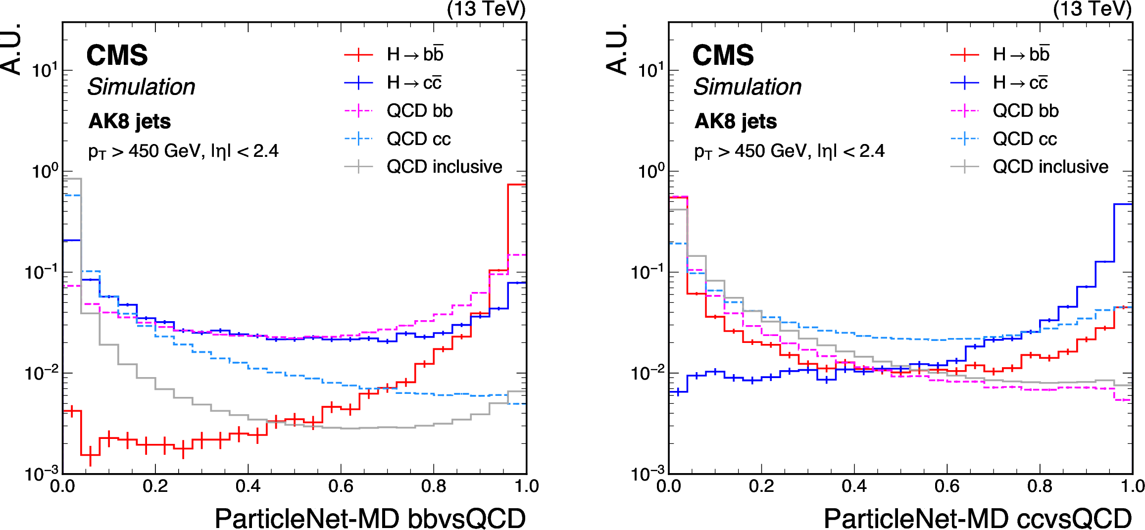
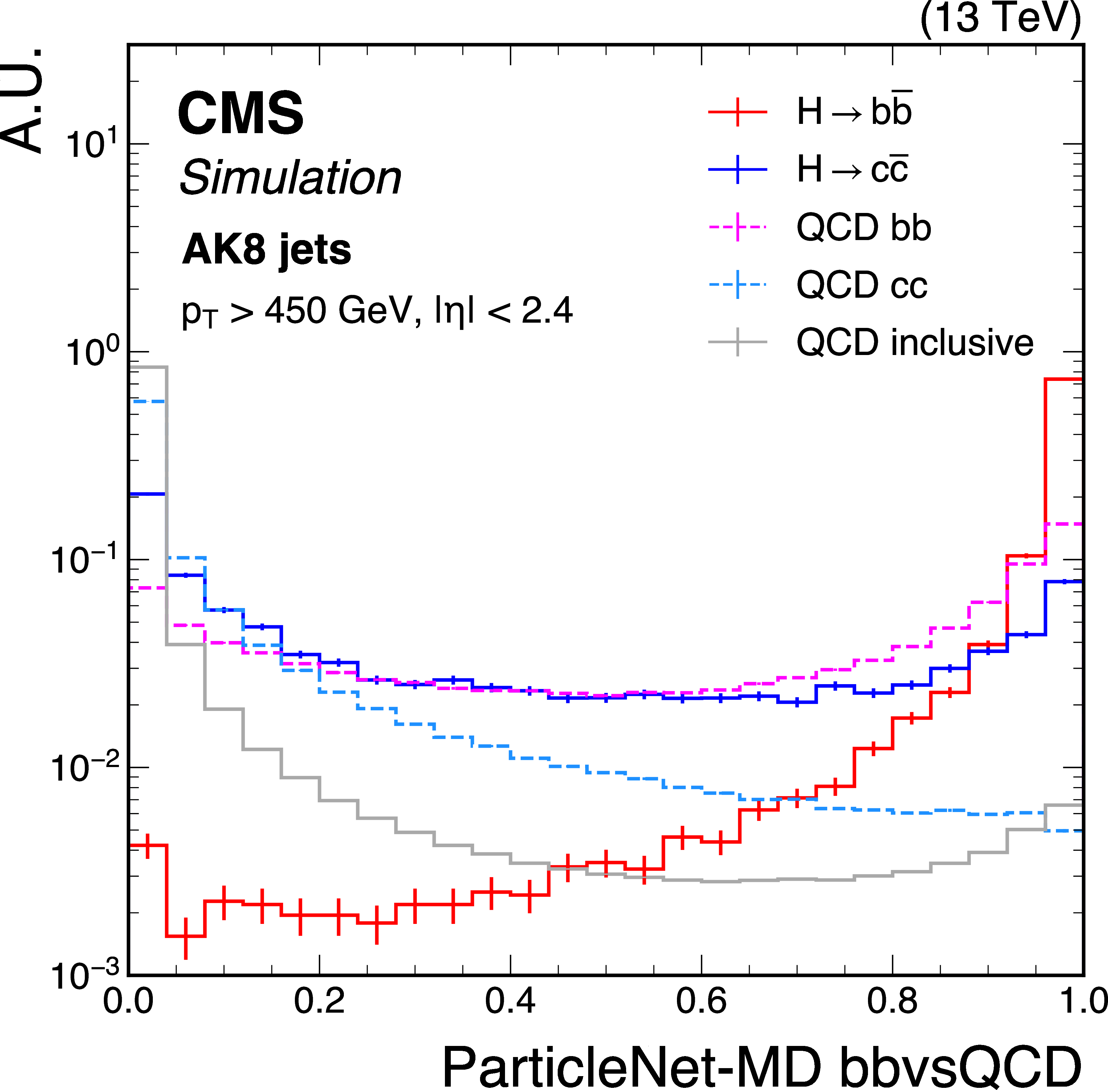
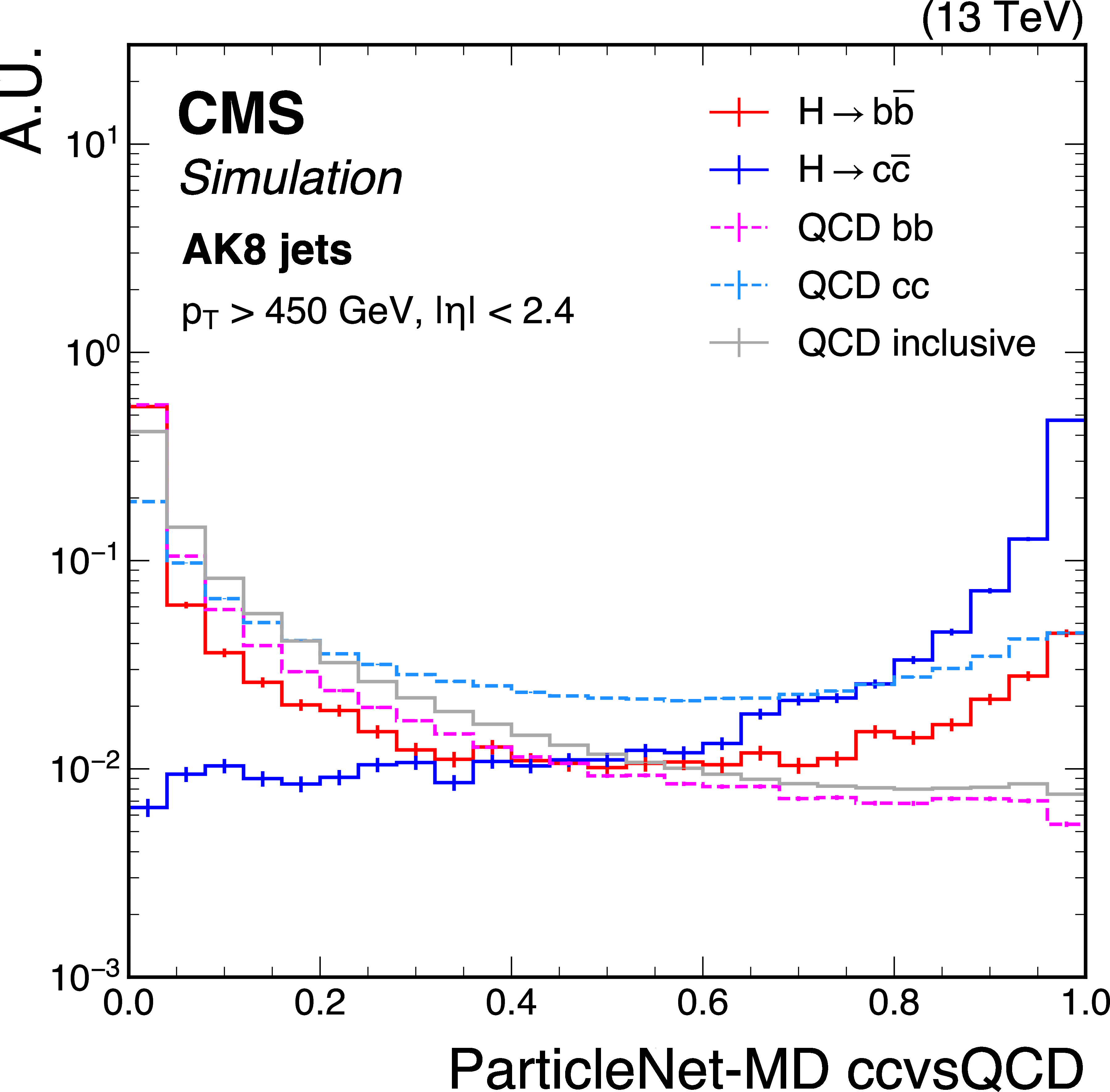
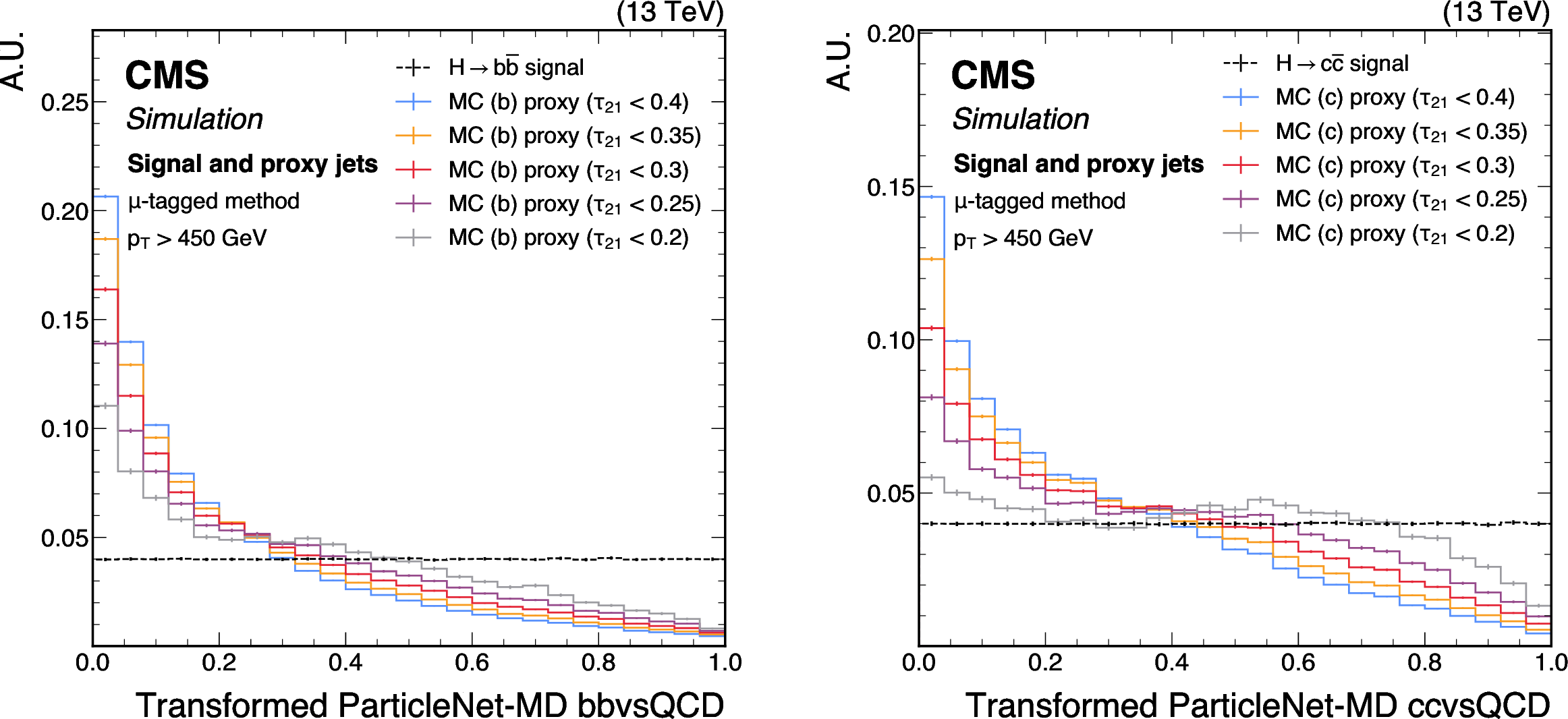
Figure 1:
Shape comparison of the ParticleNet-MD bbvsQCD (left) and ParticleNet-MD ccvsQCD (right) discriminants for the simulated standard model $ \mathrm{H} \to \mathrm{b} \overline{\mathrm{b}} $ and $ \mathrm{H} \to \mathrm{c} \overline{\mathrm{c}} $ jets, the bb and cc components of QCD multijet background jets, and inclusive QCD jets (without flavour-specific selection), using simulated events corresponding to the 2018 data-taking conditions for jets with $ p_{\mathrm{T}} > $ 450 GeV and $ |\eta| < $ 2.4. The error bars represent the statistical uncertainties due to the limited number of simulated events. |
png pdf |
Figure 1-a:
Shape comparison of the ParticleNet-MD bbvsQCD (left) and ParticleNet-MD ccvsQCD (right) discriminants for the simulated standard model $ \mathrm{H} \to \mathrm{b} \overline{\mathrm{b}} $ and $ \mathrm{H} \to \mathrm{c} \overline{\mathrm{c}} $ jets, the bb and cc components of QCD multijet background jets, and inclusive QCD jets (without flavour-specific selection), using simulated events corresponding to the 2018 data-taking conditions for jets with $ p_{\mathrm{T}} > $ 450 GeV and $ |\eta| < $ 2.4. The error bars represent the statistical uncertainties due to the limited number of simulated events. |
png pdf |
Figure 1-b:
Shape comparison of the ParticleNet-MD bbvsQCD (left) and ParticleNet-MD ccvsQCD (right) discriminants for the simulated standard model $ \mathrm{H} \to \mathrm{b} \overline{\mathrm{b}} $ and $ \mathrm{H} \to \mathrm{c} \overline{\mathrm{c}} $ jets, the bb and cc components of QCD multijet background jets, and inclusive QCD jets (without flavour-specific selection), using simulated events corresponding to the 2018 data-taking conditions for jets with $ p_{\mathrm{T}} > $ 450 GeV and $ |\eta| < $ 2.4. The error bars represent the statistical uncertainties due to the limited number of simulated events. |
png pdf |
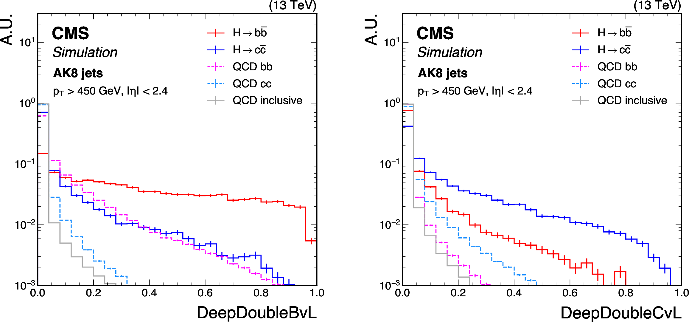
Figure 2:
Shape comparison of the DeepDoubleBvL (left) and DeepDoubleCvL (right) discriminants for the simulated standard model $ \mathrm{H} \to \mathrm{b} \overline{\mathrm{b}} $ and $ \mathrm{H} \to \mathrm{c} \overline{\mathrm{c}} $ jets, the bb and cc components of QCD multijet background jets, and inclusive QCD jets, using simulated events corresponding to the 2018 data-taking conditions for jets with $ p_{\mathrm{T}} > $ 450 GeV and $ |\eta| < $ 2.4. The error bars represent the statistical uncertainties due to the limited number of simulated events. |
png pdf |
Figure 2-a:
Shape comparison of the DeepDoubleBvL (left) and DeepDoubleCvL (right) discriminants for the simulated standard model $ \mathrm{H} \to \mathrm{b} \overline{\mathrm{b}} $ and $ \mathrm{H} \to \mathrm{c} \overline{\mathrm{c}} $ jets, the bb and cc components of QCD multijet background jets, and inclusive QCD jets, using simulated events corresponding to the 2018 data-taking conditions for jets with $ p_{\mathrm{T}} > $ 450 GeV and $ |\eta| < $ 2.4. The error bars represent the statistical uncertainties due to the limited number of simulated events. |
png pdf |
Figure 2-b:
Shape comparison of the DeepDoubleBvL (left) and DeepDoubleCvL (right) discriminants for the simulated standard model $ \mathrm{H} \to \mathrm{b} \overline{\mathrm{b}} $ and $ \mathrm{H} \to \mathrm{c} \overline{\mathrm{c}} $ jets, the bb and cc components of QCD multijet background jets, and inclusive QCD jets, using simulated events corresponding to the 2018 data-taking conditions for jets with $ p_{\mathrm{T}} > $ 450 GeV and $ |\eta| < $ 2.4. The error bars represent the statistical uncertainties due to the limited number of simulated events. |
png pdf |
Figure 3:
Shape comparison of the DeepAK8-MD bbvsQCD (left) and DeepAK8-MD ccvsQCD (right) discriminants for the simulated standard model $ \mathrm{H} \to \mathrm{b} \overline{\mathrm{b}} $ and $ \mathrm{H} \to \mathrm{c} \overline{\mathrm{c}} $ jets, the bb and cc components of QCD multijet background jets, and inclusive QCD jets, using simulated events corresponding to the 2018 data-taking conditions for jets with $ p_{\mathrm{T}} > $ 450 GeV and $ |\eta| < $ 2.4. The error bars represent the statistical uncertainties due to the limited number of simulated events. |
png pdf |
Figure 3-a:
Shape comparison of the DeepAK8-MD bbvsQCD (left) and DeepAK8-MD ccvsQCD (right) discriminants for the simulated standard model $ \mathrm{H} \to \mathrm{b} \overline{\mathrm{b}} $ and $ \mathrm{H} \to \mathrm{c} \overline{\mathrm{c}} $ jets, the bb and cc components of QCD multijet background jets, and inclusive QCD jets, using simulated events corresponding to the 2018 data-taking conditions for jets with $ p_{\mathrm{T}} > $ 450 GeV and $ |\eta| < $ 2.4. The error bars represent the statistical uncertainties due to the limited number of simulated events. |
png pdf |
Figure 3-b:
Shape comparison of the DeepAK8-MD bbvsQCD (left) and DeepAK8-MD ccvsQCD (right) discriminants for the simulated standard model $ \mathrm{H} \to \mathrm{b} \overline{\mathrm{b}} $ and $ \mathrm{H} \to \mathrm{c} \overline{\mathrm{c}} $ jets, the bb and cc components of QCD multijet background jets, and inclusive QCD jets, using simulated events corresponding to the 2018 data-taking conditions for jets with $ p_{\mathrm{T}} > $ 450 GeV and $ |\eta| < $ 2.4. The error bars represent the statistical uncertainties due to the limited number of simulated events. |
png pdf |
Figure 4:
Shape comparison of the double-b discriminant for the simulated standard model $ \mathrm{H} \to \mathrm{b} \overline{\mathrm{b}} $ and $ \mathrm{H} \to \mathrm{c} \overline{\mathrm{c}} $ jets, the bb and cc components of QCD multijet background jets, and inclusive QCD jets, using simulated events corresponding to the 2018 data-taking conditions for jets with $ p_{\mathrm{T}} > $ 450 GeV and $ |\eta| < $ 2.4. The error bars represent the statistical uncertainties due to the limited number of simulated events. |
png pdf |
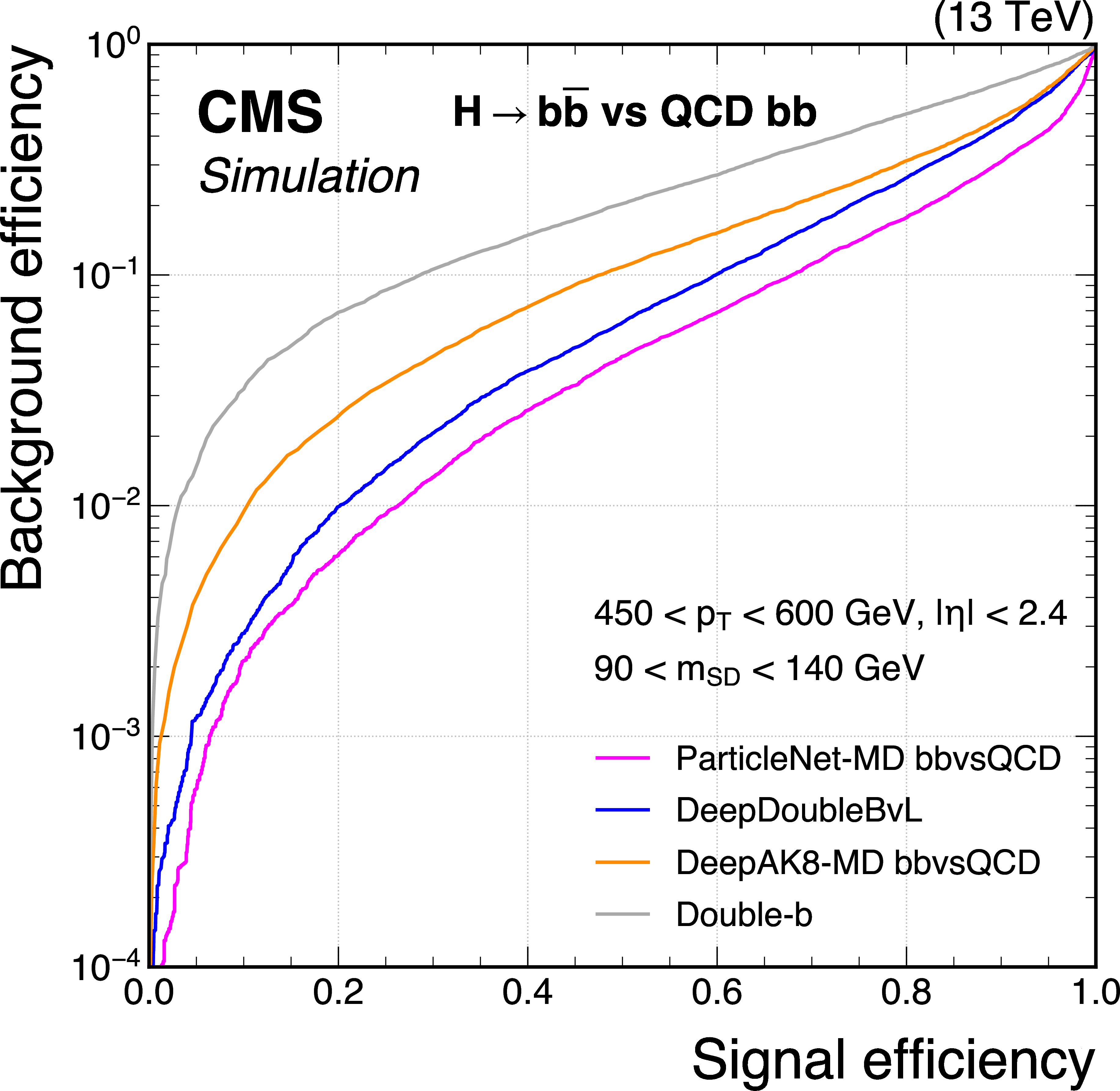
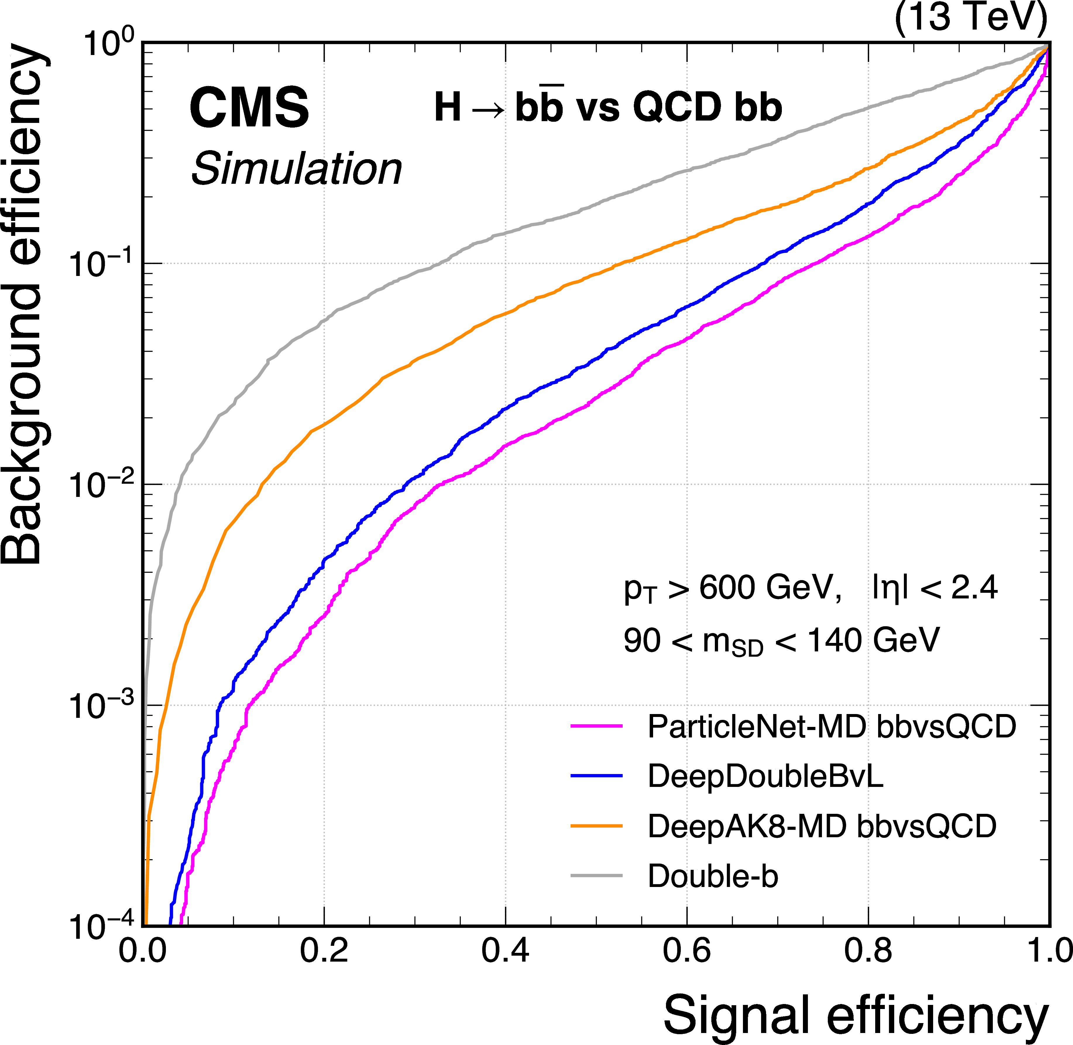
Figure 5:
Comparison of the performance of the $ \mathrm{X} \to \mathrm{b} \overline{\mathrm{b}} $ identification algorithms in terms of receiver operating characteristic (ROC) curves for $ \mathrm{H} \to \mathrm{b} \overline{\mathrm{b}} $ signal jets versus the inclusive QCD jets as background, using simulated events with the 2018 data-taking conditions. Performance is shown in the 450 $ < p_{\mathrm{T}} < $ 600 GeV (left) and $ p_{\mathrm{T}} > $ 600 GeV (right) regions. Additional selection criteria applied to the jets are displayed on the plots. |
png pdf |
Figure 5-a:
Comparison of the performance of the $ \mathrm{X} \to \mathrm{b} \overline{\mathrm{b}} $ identification algorithms in terms of receiver operating characteristic (ROC) curves for $ \mathrm{H} \to \mathrm{b} \overline{\mathrm{b}} $ signal jets versus the inclusive QCD jets as background, using simulated events with the 2018 data-taking conditions. Performance is shown in the 450 $ < p_{\mathrm{T}} < $ 600 GeV (left) and $ p_{\mathrm{T}} > $ 600 GeV (right) regions. Additional selection criteria applied to the jets are displayed on the plots. |
png pdf |
Figure 5-b:
Comparison of the performance of the $ \mathrm{X} \to \mathrm{b} \overline{\mathrm{b}} $ identification algorithms in terms of receiver operating characteristic (ROC) curves for $ \mathrm{H} \to \mathrm{b} \overline{\mathrm{b}} $ signal jets versus the inclusive QCD jets as background, using simulated events with the 2018 data-taking conditions. Performance is shown in the 450 $ < p_{\mathrm{T}} < $ 600 GeV (left) and $ p_{\mathrm{T}} > $ 600 GeV (right) regions. Additional selection criteria applied to the jets are displayed on the plots. |
png pdf |
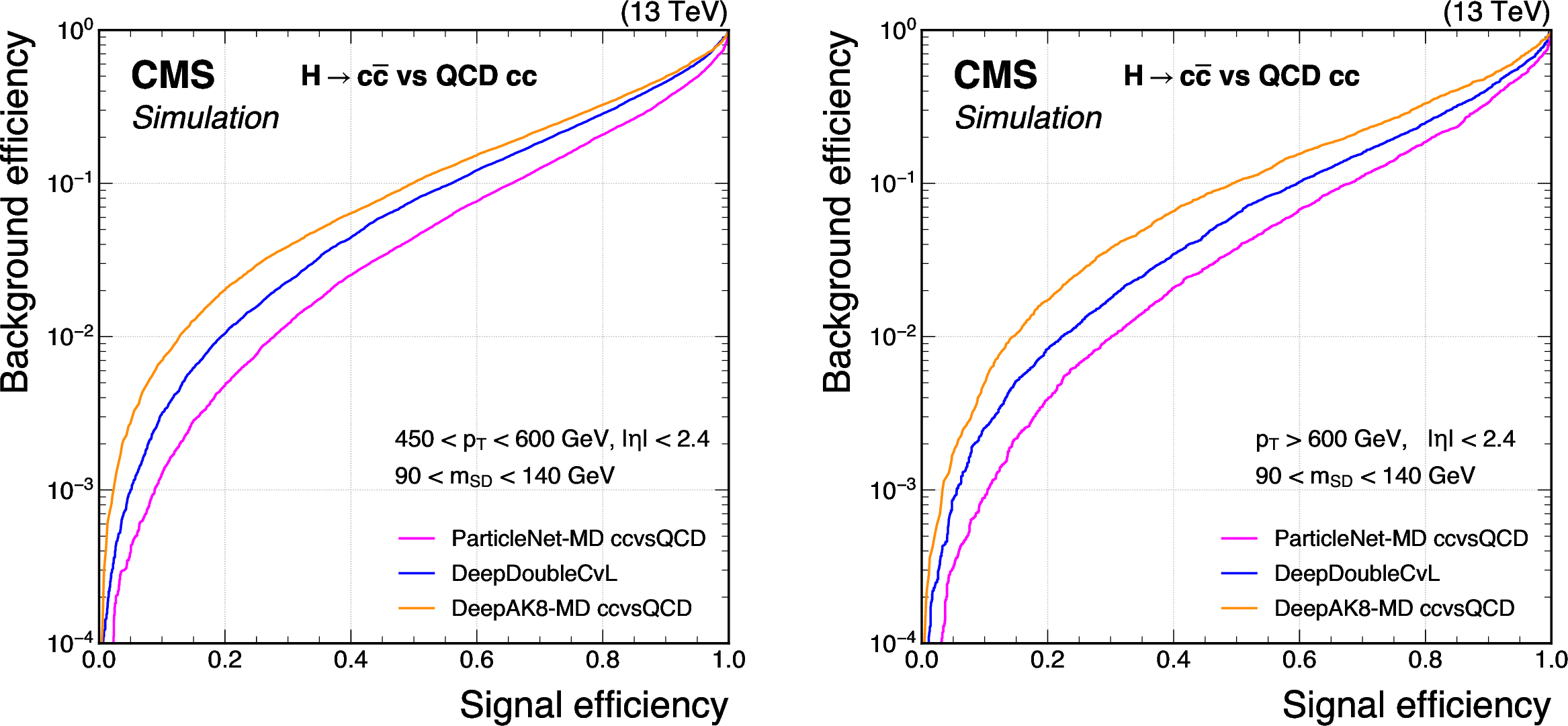
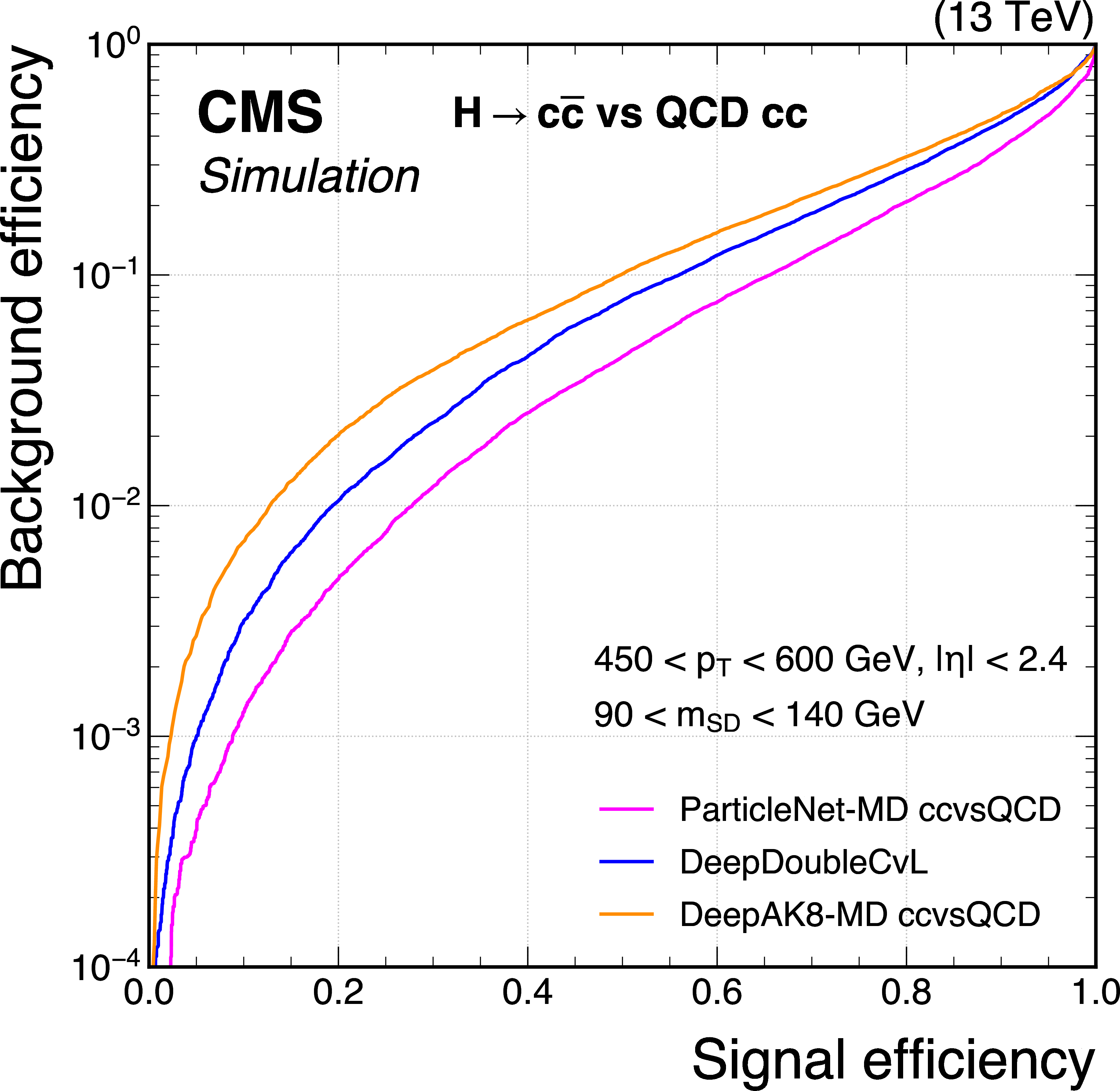
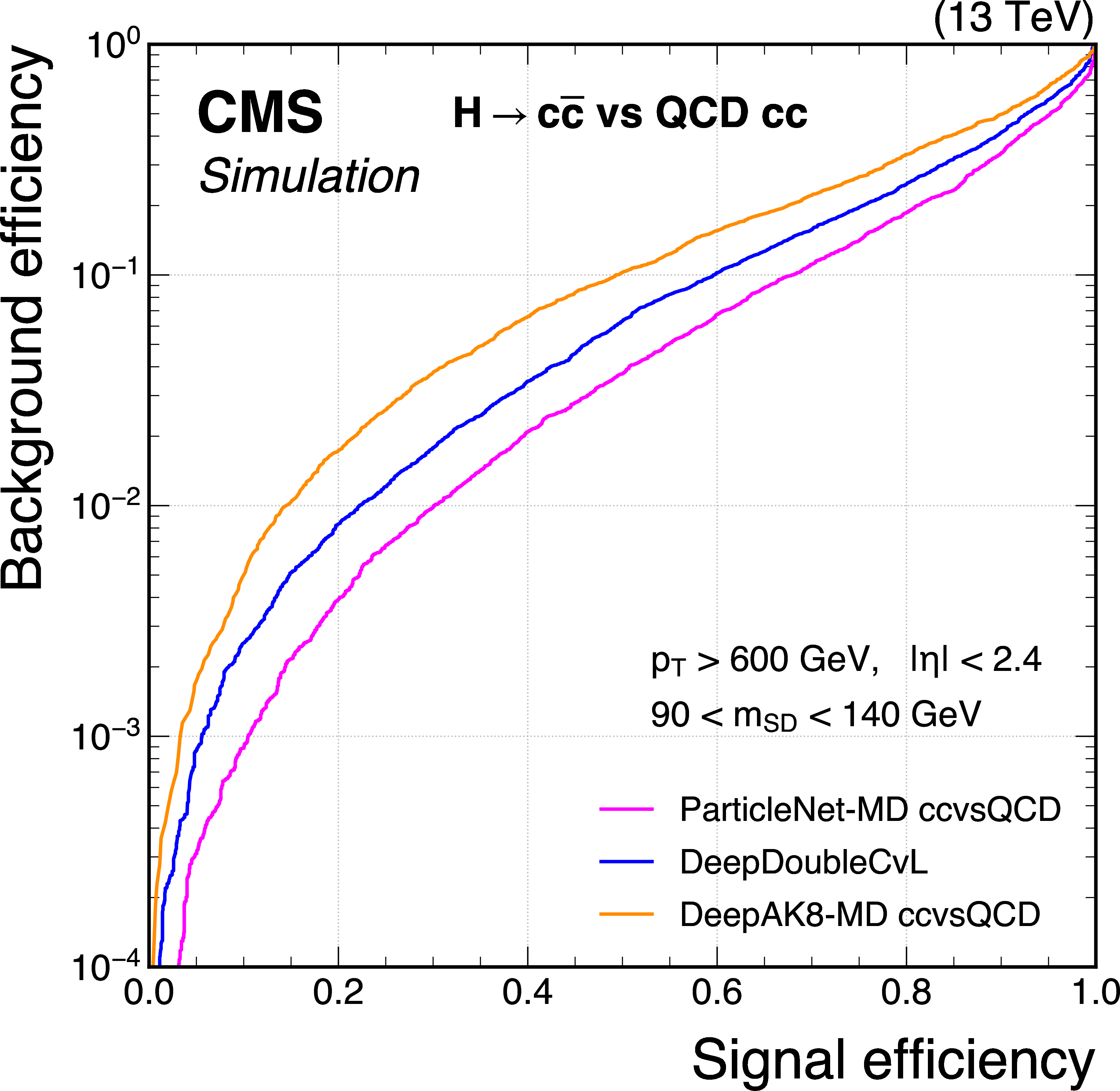
Figure 6:
Comparison of the performance of the $ \mathrm{X} \to \mathrm{c} \overline{\mathrm{c}} $ identification algorithms in terms of receiver operating characteristic (ROC) curves for $ \mathrm{H} \to \mathrm{c} \overline{\mathrm{c}} $ signal jets versus the inclusive QCD jets as background, using simulated events with the 2018 data-taking conditions. Performance is shown in the 450 $ < p_{\mathrm{T}} < $ 600 GeV (left) and $ p_{\mathrm{T}} > $ 600 GeV (right) regions. Additional selection criteria applied to the jets are displayed on the plots. |
png pdf |
Figure 6-a:
Comparison of the performance of the $ \mathrm{X} \to \mathrm{c} \overline{\mathrm{c}} $ identification algorithms in terms of receiver operating characteristic (ROC) curves for $ \mathrm{H} \to \mathrm{c} \overline{\mathrm{c}} $ signal jets versus the inclusive QCD jets as background, using simulated events with the 2018 data-taking conditions. Performance is shown in the 450 $ < p_{\mathrm{T}} < $ 600 GeV (left) and $ p_{\mathrm{T}} > $ 600 GeV (right) regions. Additional selection criteria applied to the jets are displayed on the plots. |

png pdf |
Figure 6-b:
Comparison of the performance of the $ \mathrm{X} \to \mathrm{c} \overline{\mathrm{c}} $ identification algorithms in terms of receiver operating characteristic (ROC) curves for $ \mathrm{H} \to \mathrm{c} \overline{\mathrm{c}} $ signal jets versus the inclusive QCD jets as background, using simulated events with the 2018 data-taking conditions. Performance is shown in the 450 $ < p_{\mathrm{T}} < $ 600 GeV (left) and $ p_{\mathrm{T}} > $ 600 GeV (right) regions. Additional selection criteria applied to the jets are displayed on the plots. |
png pdf |
Figure 7:
Comparison of the performance of the $ \mathrm{X} \to \mathrm{b} \overline{\mathrm{b}} $ identification algorithms in terms of receiver operating characteristic (ROC) curves for $ \mathrm{H} \to \mathrm{b} \overline{\mathrm{b}} $ signal jets versus the bb component of the QCD jets as background, using simulated events with the 2018 data-taking conditions. Performance is shown in the 450 $ < p_{\mathrm{T}} < $ 600 GeV (left) and $ p_{\mathrm{T}} > $ 600 GeV (right) regions. Additional selection criteria applied to the jets are displayed on the plots. |
png pdf |
Figure 7-a:
Comparison of the performance of the $ \mathrm{X} \to \mathrm{b} \overline{\mathrm{b}} $ identification algorithms in terms of receiver operating characteristic (ROC) curves for $ \mathrm{H} \to \mathrm{b} \overline{\mathrm{b}} $ signal jets versus the bb component of the QCD jets as background, using simulated events with the 2018 data-taking conditions. Performance is shown in the 450 $ < p_{\mathrm{T}} < $ 600 GeV (left) and $ p_{\mathrm{T}} > $ 600 GeV (right) regions. Additional selection criteria applied to the jets are displayed on the plots. |
png pdf |
Figure 7-b:
Comparison of the performance of the $ \mathrm{X} \to \mathrm{b} \overline{\mathrm{b}} $ identification algorithms in terms of receiver operating characteristic (ROC) curves for $ \mathrm{H} \to \mathrm{b} \overline{\mathrm{b}} $ signal jets versus the bb component of the QCD jets as background, using simulated events with the 2018 data-taking conditions. Performance is shown in the 450 $ < p_{\mathrm{T}} < $ 600 GeV (left) and $ p_{\mathrm{T}} > $ 600 GeV (right) regions. Additional selection criteria applied to the jets are displayed on the plots. |
png pdf |
Figure 8:
Comparison of the performance of the $ \mathrm{X} \to \mathrm{c} \overline{\mathrm{c}} $ identification algorithms in terms of receiver operating characteristic (ROC) curves for $ \mathrm{H} \to \mathrm{c} \overline{\mathrm{c}} $ signal jets versus the cc component of the QCD jets as background, using simulated events with the 2018 data-taking conditions. Performance is shown in the 450 $ < p_{\mathrm{T}} < $ 600 GeV (left) and $ p_{\mathrm{T}} > $ 600 GeV (right) regions. Additional selection criteria applied to the jets are displayed on the plots. |
png pdf |
Figure 8-a:
Comparison of the performance of the $ \mathrm{X} \to \mathrm{c} \overline{\mathrm{c}} $ identification algorithms in terms of receiver operating characteristic (ROC) curves for $ \mathrm{H} \to \mathrm{c} \overline{\mathrm{c}} $ signal jets versus the cc component of the QCD jets as background, using simulated events with the 2018 data-taking conditions. Performance is shown in the 450 $ < p_{\mathrm{T}} < $ 600 GeV (left) and $ p_{\mathrm{T}} > $ 600 GeV (right) regions. Additional selection criteria applied to the jets are displayed on the plots. |
png pdf |
Figure 8-b:
Comparison of the performance of the $ \mathrm{X} \to \mathrm{c} \overline{\mathrm{c}} $ identification algorithms in terms of receiver operating characteristic (ROC) curves for $ \mathrm{H} \to \mathrm{c} \overline{\mathrm{c}} $ signal jets versus the cc component of the QCD jets as background, using simulated events with the 2018 data-taking conditions. Performance is shown in the 450 $ < p_{\mathrm{T}} < $ 600 GeV (left) and $ p_{\mathrm{T}} > $ 600 GeV (right) regions. Additional selection criteria applied to the jets are displayed on the plots. |
png pdf |
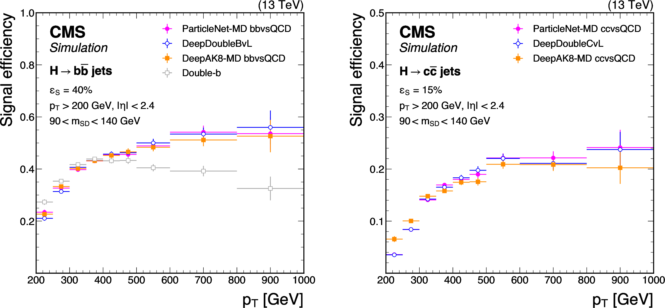
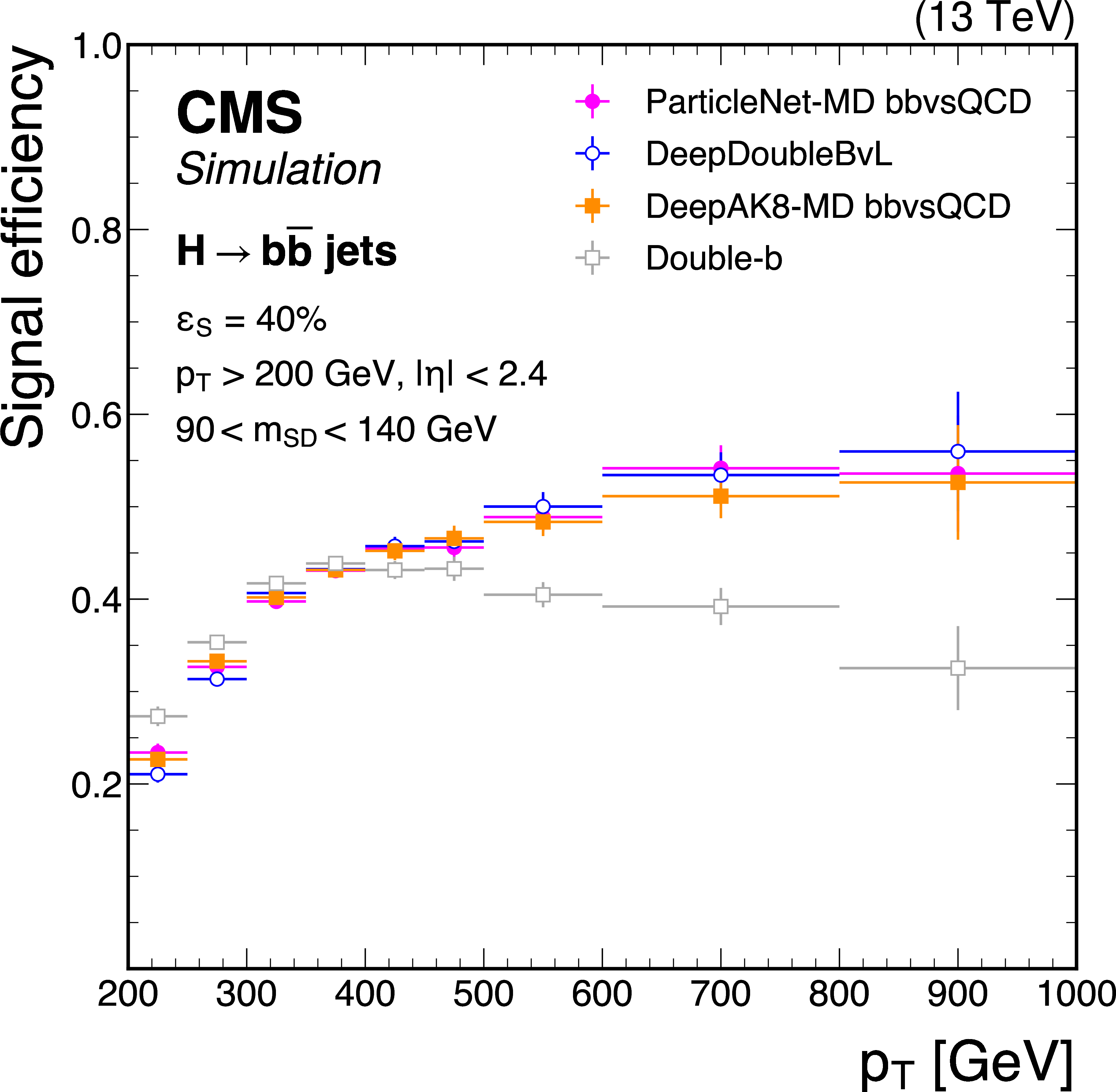
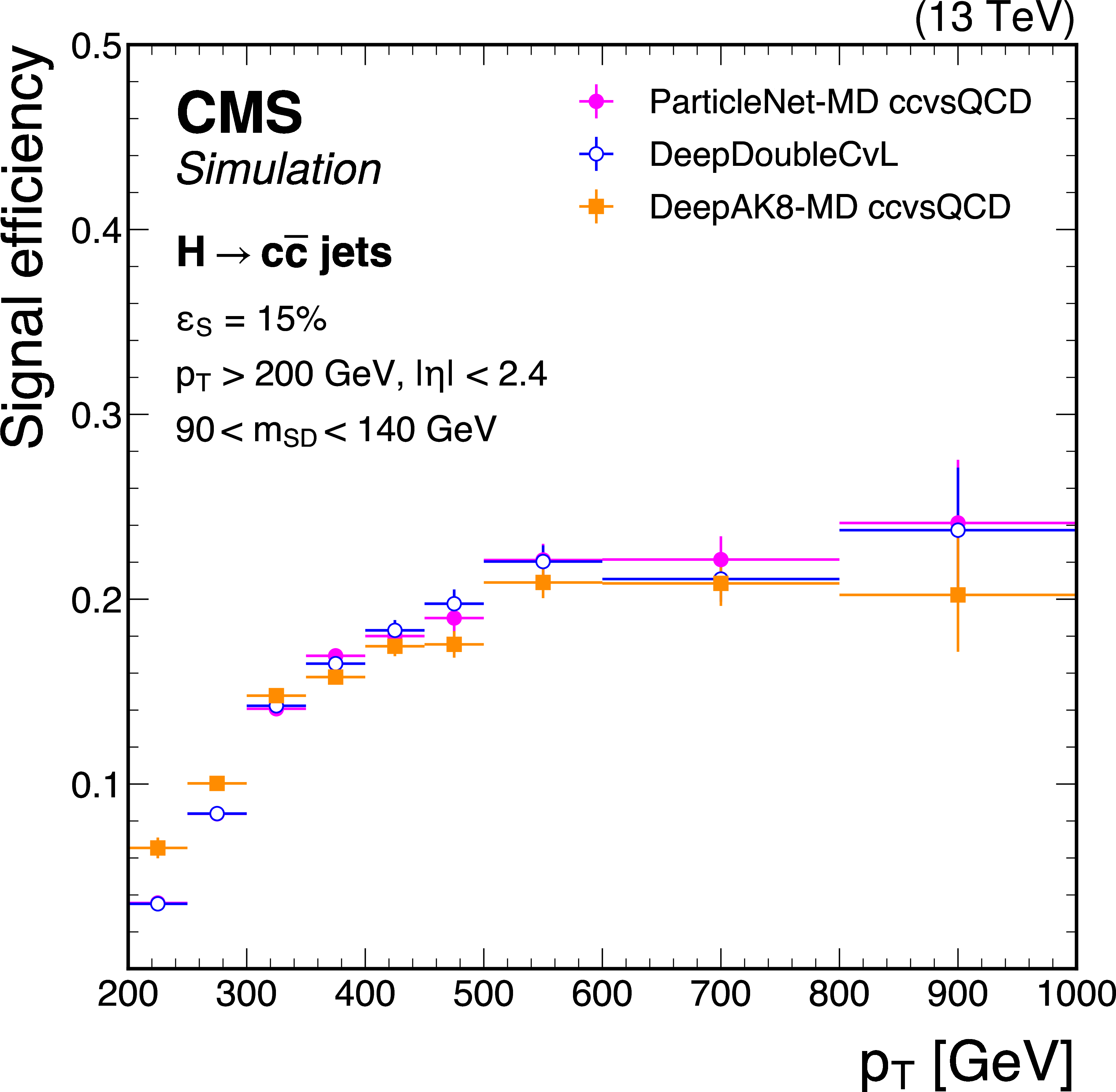
Figure 9:
Signal efficiency $ \epsilon_\mathrm{S} $ as a function of jet $ p_{\mathrm{T}} $ for a working point corresponding to overall selection efficiencies of 40% in $ \mathrm{H} \to \mathrm{b} \overline{\mathrm{b}} $ and 15% in $ \mathrm{H} \to \mathrm{c} \overline{\mathrm{c}} $ jets. The left and right plots compare the performance of various $ \mathrm{X} \to \mathrm{b} \overline{\mathrm{b}} $ and $ \mathrm{X} \to \mathrm{c} \overline{\mathrm{c}} $ tagging algorithms, respectively. The error bars represent the statistical uncertainties due to the limited number of simulated events. Additional selection criteria applied to the jets are displayed on the plots. |
png pdf |
Figure 9-a:
Signal efficiency $ \epsilon_\mathrm{S} $ as a function of jet $ p_{\mathrm{T}} $ for a working point corresponding to overall selection efficiencies of 40% in $ \mathrm{H} \to \mathrm{b} \overline{\mathrm{b}} $ and 15% in $ \mathrm{H} \to \mathrm{c} \overline{\mathrm{c}} $ jets. The left and right plots compare the performance of various $ \mathrm{X} \to \mathrm{b} \overline{\mathrm{b}} $ and $ \mathrm{X} \to \mathrm{c} \overline{\mathrm{c}} $ tagging algorithms, respectively. The error bars represent the statistical uncertainties due to the limited number of simulated events. Additional selection criteria applied to the jets are displayed on the plots. |
png pdf |
Figure 9-b:
Signal efficiency $ \epsilon_\mathrm{S} $ as a function of jet $ p_{\mathrm{T}} $ for a working point corresponding to overall selection efficiencies of 40% in $ \mathrm{H} \to \mathrm{b} \overline{\mathrm{b}} $ and 15% in $ \mathrm{H} \to \mathrm{c} \overline{\mathrm{c}} $ jets. The left and right plots compare the performance of various $ \mathrm{X} \to \mathrm{b} \overline{\mathrm{b}} $ and $ \mathrm{X} \to \mathrm{c} \overline{\mathrm{c}} $ tagging algorithms, respectively. The error bars represent the statistical uncertainties due to the limited number of simulated events. Additional selection criteria applied to the jets are displayed on the plots. |
png pdf |
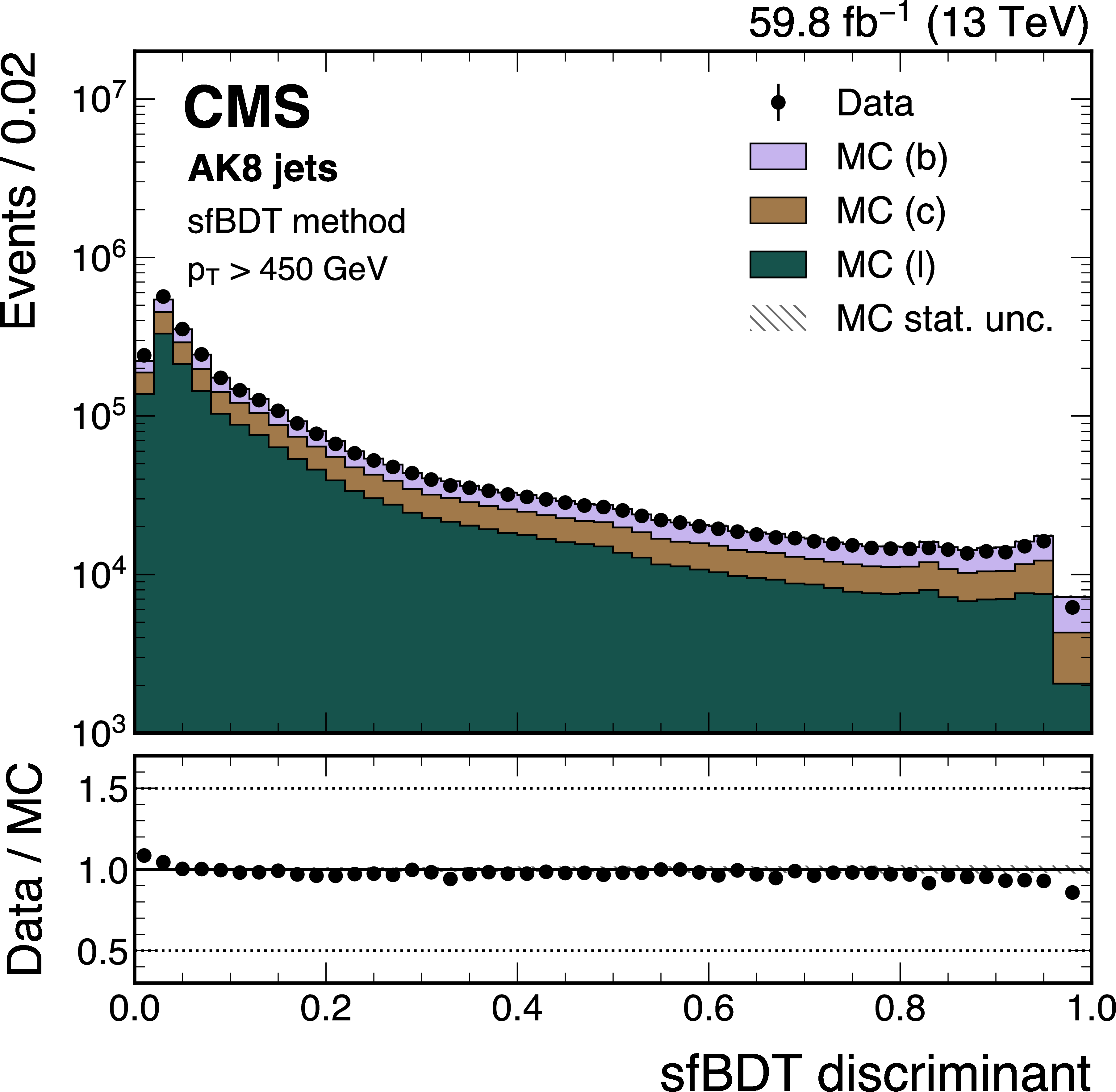
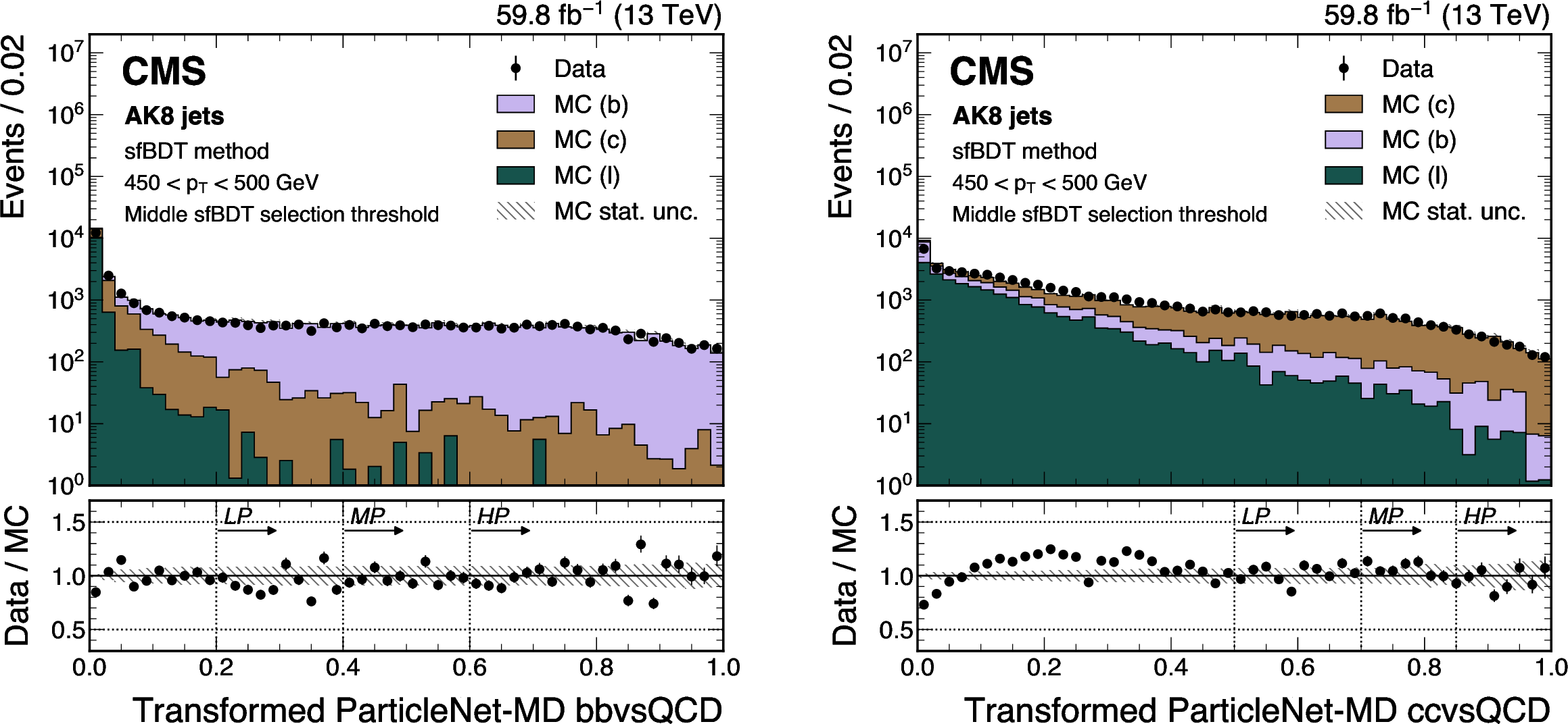
Figure 10:
Distributions of the sfBDT discriminant for data and simulation, illustrated using the 2018 data-taking conditions, for jets with $ p_{\mathrm{T}} > $ 450 GeV. The error bars indicate statistical uncertainties in observed data, which may be too small to be visible. |
png pdf |
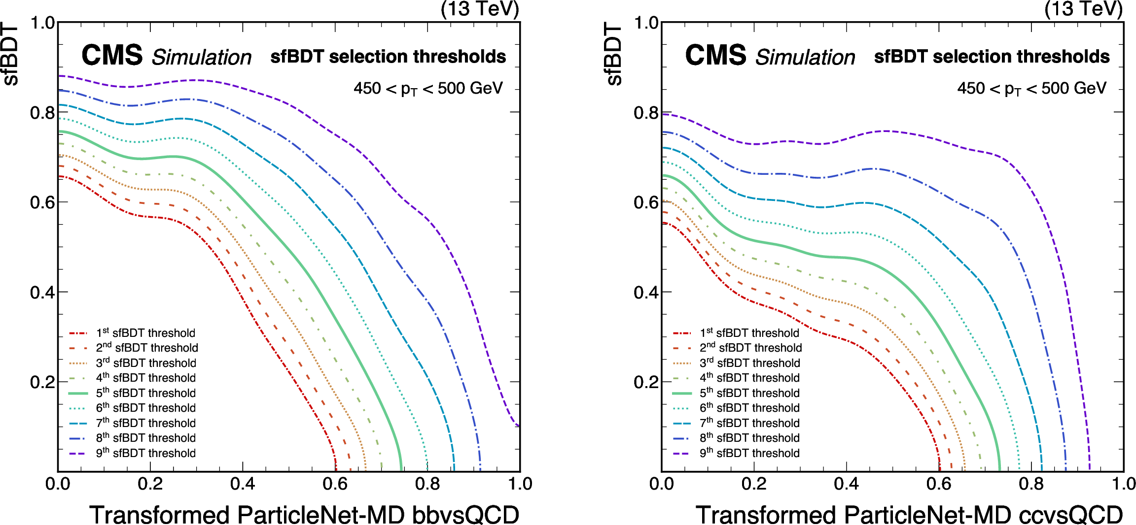
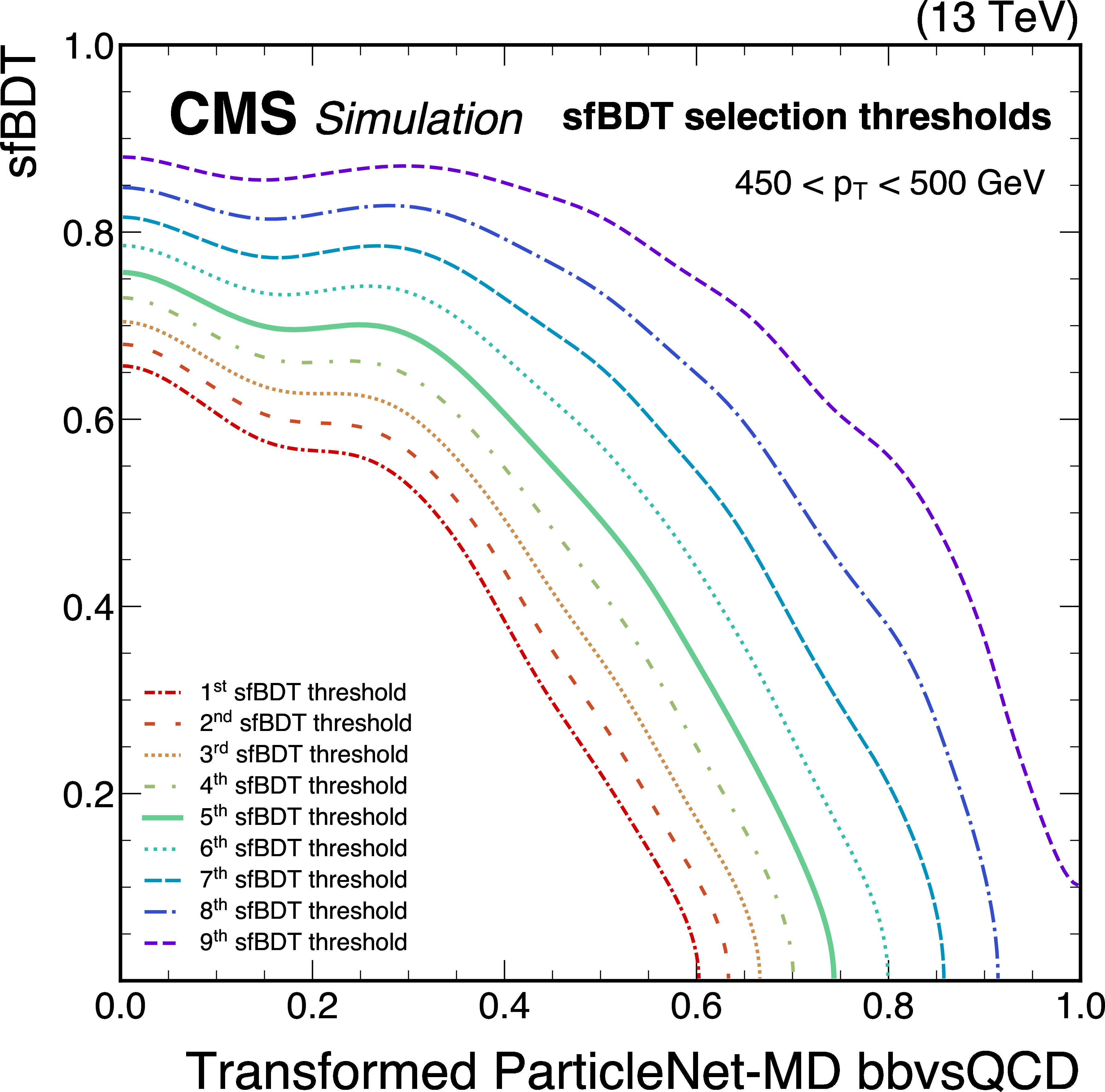
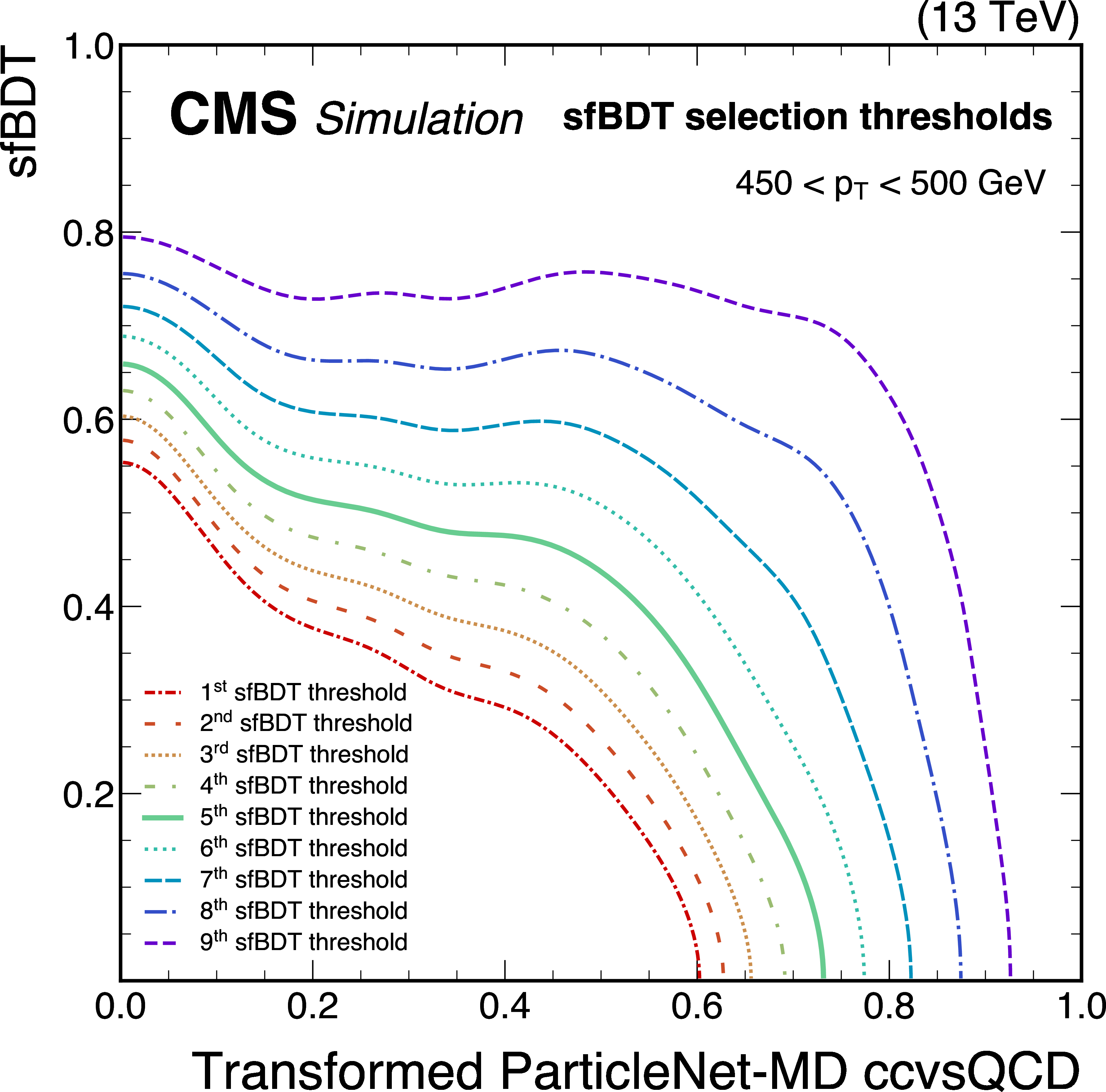
Figure 11:
Illustration of nine predefined ``reference selection thresholds'' visualized on the two-dimensional plane spanned by the sfBDT score and the transformed tagger discriminant scores. Selections based on these thresholds can be interpreted as sfBDT selections with thresholds as a function of the tagger discriminant score. Each selection aims to match the tagger discriminant distribution of the proxy jet to that of the signal. The examples shown correspond to the calibration of the ParticleNet-MD $ \mathrm{X} \to \mathrm{b} \overline{\mathrm{b}} $ (left) and ParticleNet-MD $ \mathrm{X} \to \mathrm{c} \overline{\mathrm{c}} $ (right) discriminants, using simulated events under 2018 data-taking conditions in the jet $ p_{\mathrm{T}} $ range of (450, 500) GeV. |
png pdf |
Figure 11-a:
Illustration of nine predefined ``reference selection thresholds'' visualized on the two-dimensional plane spanned by the sfBDT score and the transformed tagger discriminant scores. Selections based on these thresholds can be interpreted as sfBDT selections with thresholds as a function of the tagger discriminant score. Each selection aims to match the tagger discriminant distribution of the proxy jet to that of the signal. The examples shown correspond to the calibration of the ParticleNet-MD $ \mathrm{X} \to \mathrm{b} \overline{\mathrm{b}} $ (left) and ParticleNet-MD $ \mathrm{X} \to \mathrm{c} \overline{\mathrm{c}} $ (right) discriminants, using simulated events under 2018 data-taking conditions in the jet $ p_{\mathrm{T}} $ range of (450, 500) GeV. |
png pdf |
Figure 11-b:
Illustration of nine predefined ``reference selection thresholds'' visualized on the two-dimensional plane spanned by the sfBDT score and the transformed tagger discriminant scores. Selections based on these thresholds can be interpreted as sfBDT selections with thresholds as a function of the tagger discriminant score. Each selection aims to match the tagger discriminant distribution of the proxy jet to that of the signal. The examples shown correspond to the calibration of the ParticleNet-MD $ \mathrm{X} \to \mathrm{b} \overline{\mathrm{b}} $ (left) and ParticleNet-MD $ \mathrm{X} \to \mathrm{c} \overline{\mathrm{c}} $ (right) discriminants, using simulated events under 2018 data-taking conditions in the jet $ p_{\mathrm{T}} $ range of (450, 500) GeV. |
png pdf |
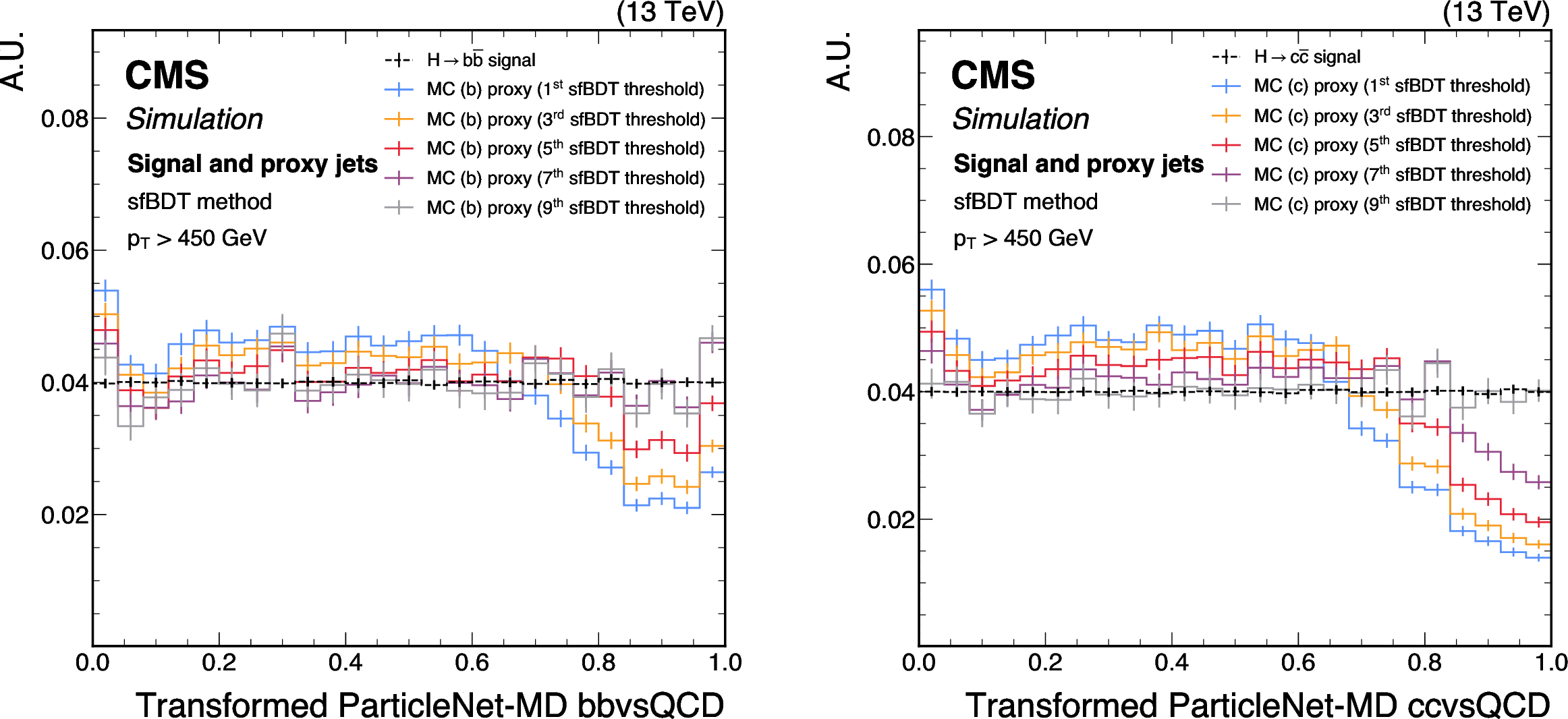
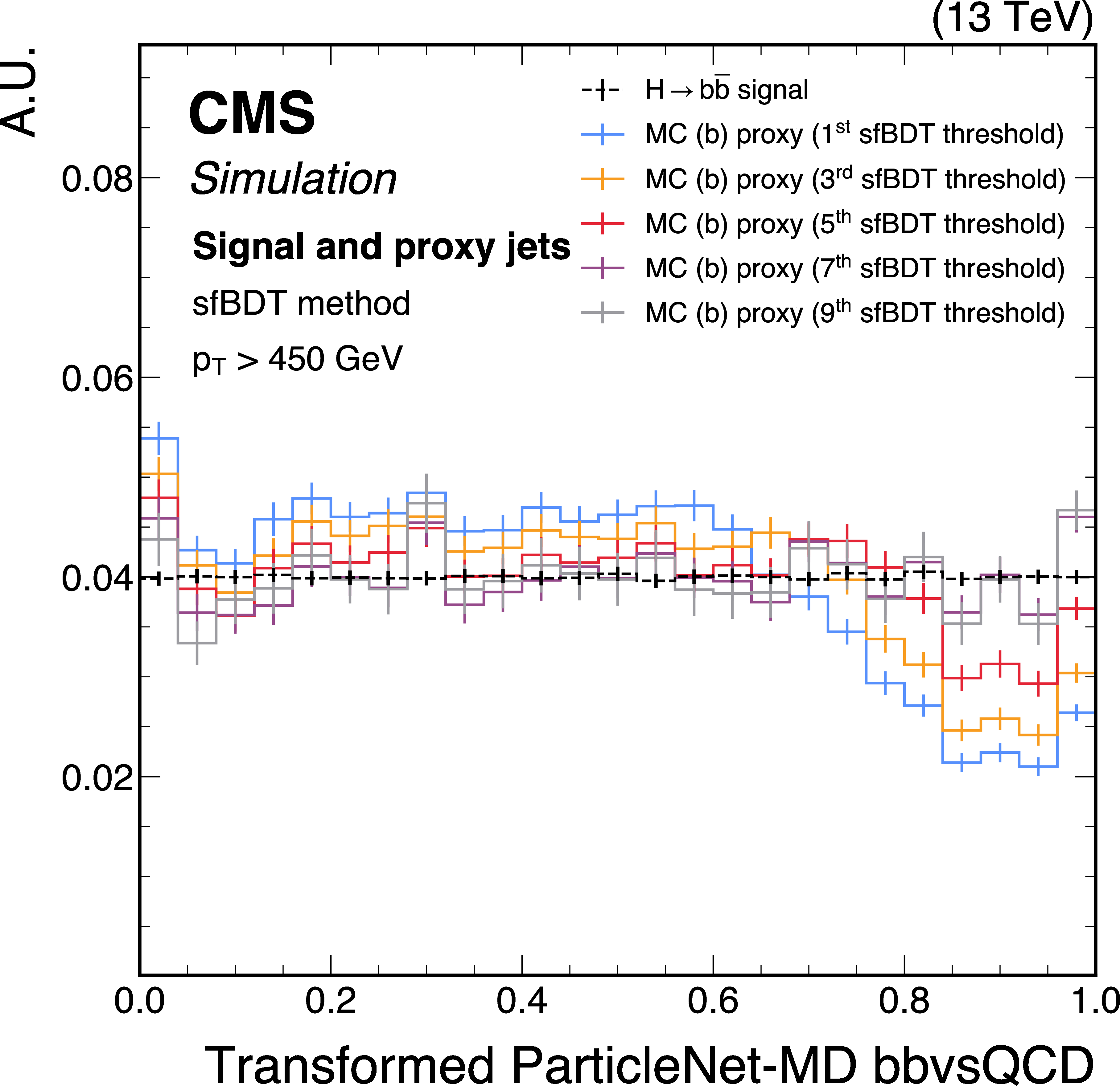
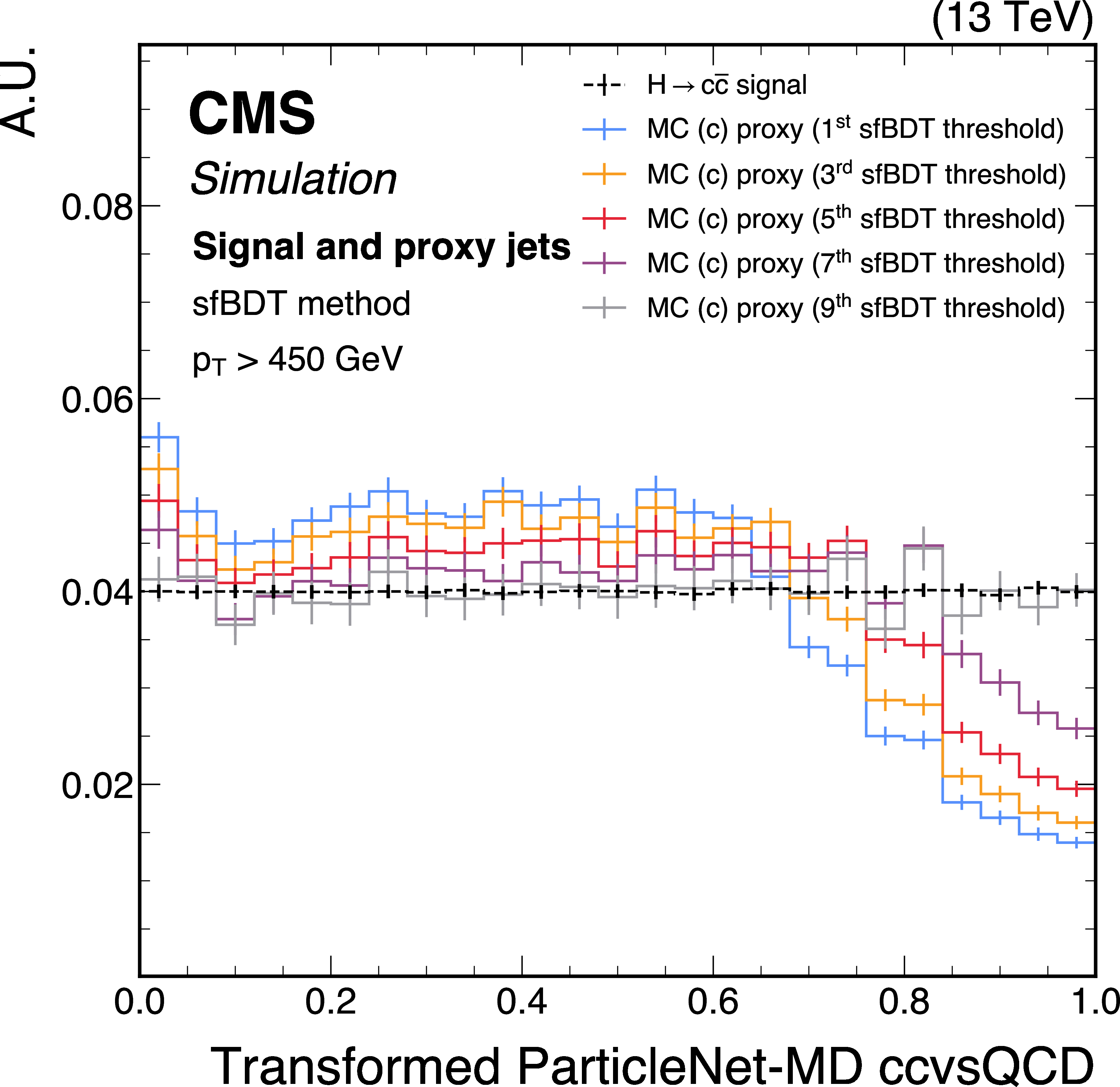
Figure 12:
Shapes of the transformed ParticleNet-MD $ \mathrm{X} \to \mathrm{b} \overline{\mathrm{b}} $ (left) and $ \mathrm{X} \to \mathrm{c} \overline{\mathrm{c}} $ (right) discriminants for SM $ \mathrm{H} \to \mathrm{b} \overline{\mathrm{b}} $ ($ \mathrm{c} \overline{\mathrm{c}} $) signal jets and proxy jets selected with different sfBDT selection thresholds. The examples correspond to the calibration of the ParticleNet-MD $ \mathrm{X} \to \mathrm{b} \overline{\mathrm{b}} $ and $ \mathrm{X} \to \mathrm{c} \overline{\mathrm{c}} $ discriminants with the sfBDT method, using simulated events under 2018 data-taking conditions for jets with $ p_{\mathrm{T}} > $ 450 GeV. The error bars represent the statistical uncertainties due to the limited number of simulated events. |
png pdf |
Figure 12-a:
Shapes of the transformed ParticleNet-MD $ \mathrm{X} \to \mathrm{b} \overline{\mathrm{b}} $ (left) and $ \mathrm{X} \to \mathrm{c} \overline{\mathrm{c}} $ (right) discriminants for SM $ \mathrm{H} \to \mathrm{b} \overline{\mathrm{b}} $ ($ \mathrm{c} \overline{\mathrm{c}} $) signal jets and proxy jets selected with different sfBDT selection thresholds. The examples correspond to the calibration of the ParticleNet-MD $ \mathrm{X} \to \mathrm{b} \overline{\mathrm{b}} $ and $ \mathrm{X} \to \mathrm{c} \overline{\mathrm{c}} $ discriminants with the sfBDT method, using simulated events under 2018 data-taking conditions for jets with $ p_{\mathrm{T}} > $ 450 GeV. The error bars represent the statistical uncertainties due to the limited number of simulated events. |
png pdf |
Figure 12-b:
Shapes of the transformed ParticleNet-MD $ \mathrm{X} \to \mathrm{b} \overline{\mathrm{b}} $ (left) and $ \mathrm{X} \to \mathrm{c} \overline{\mathrm{c}} $ (right) discriminants for SM $ \mathrm{H} \to \mathrm{b} \overline{\mathrm{b}} $ ($ \mathrm{c} \overline{\mathrm{c}} $) signal jets and proxy jets selected with different sfBDT selection thresholds. The examples correspond to the calibration of the ParticleNet-MD $ \mathrm{X} \to \mathrm{b} \overline{\mathrm{b}} $ and $ \mathrm{X} \to \mathrm{c} \overline{\mathrm{c}} $ discriminants with the sfBDT method, using simulated events under 2018 data-taking conditions for jets with $ p_{\mathrm{T}} > $ 450 GeV. The error bars represent the statistical uncertainties due to the limited number of simulated events. |
png pdf |
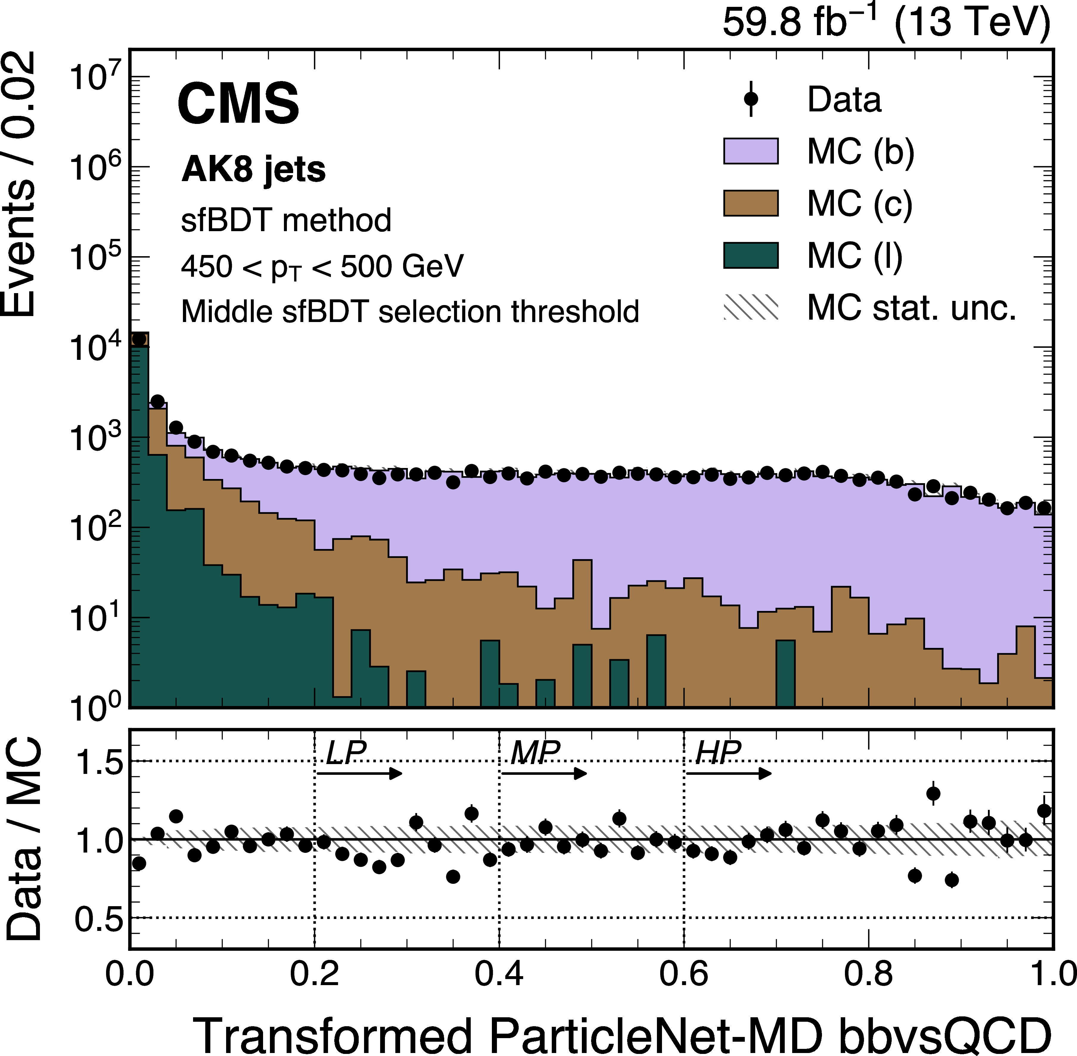
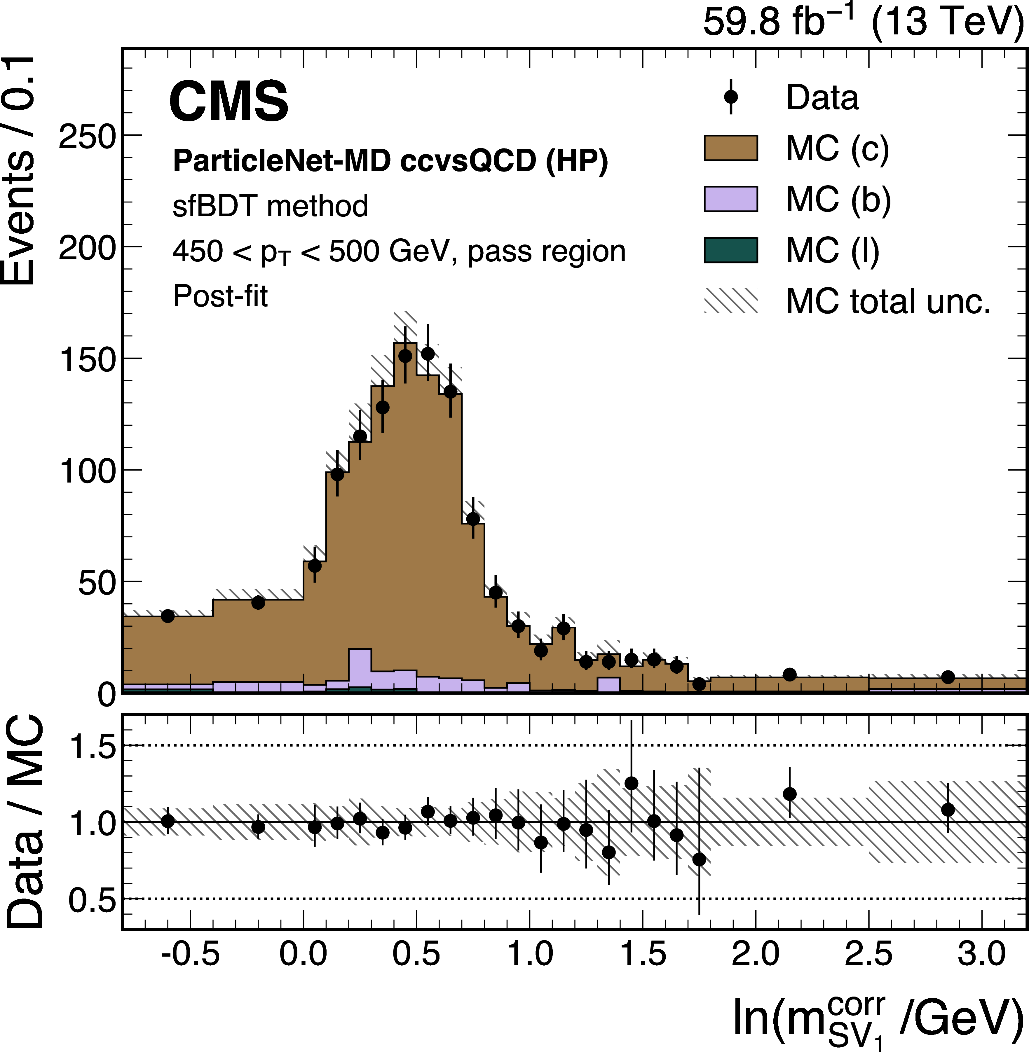
Figure 13:
An example of the transformed ParticleNet-MD $ \mathrm{X} \to \mathrm{b} \overline{\mathrm{b}} $ (left) and $ \mathrm{X} \to \mathrm{c} \overline{\mathrm{c}} $ (right) distribution in data and simulated events, after applying the preselection and the middle sfBDT selection threshold in the sfBDT method. The high-purity (HP), medium-purity (MP), and low-purity (LP) working points for the left (right) plot correspond to selections of $ X > 0.6, 0.4, 0.2 (0.85, 0.7, 0.5) $ on the transformed tagger discriminant. The error bars represent the statistical uncertainties in observed data. The lower panels display the ratio of data to simulation, with the hatched bands representing the normalized statistical uncertainty of simulated events for each bin. The distributions are based on data and simulated events with the 2018 data-taking conditions, in the jet $ p_{\mathrm{T}} $ range of (450, 500) GeV. |
png pdf |
Figure 13-a:
An example of the transformed ParticleNet-MD $ \mathrm{X} \to \mathrm{b} \overline{\mathrm{b}} $ (left) and $ \mathrm{X} \to \mathrm{c} \overline{\mathrm{c}} $ (right) distribution in data and simulated events, after applying the preselection and the middle sfBDT selection threshold in the sfBDT method. The high-purity (HP), medium-purity (MP), and low-purity (LP) working points for the left (right) plot correspond to selections of $ X > 0.6, 0.4, 0.2 (0.85, 0.7, 0.5) $ on the transformed tagger discriminant. The error bars represent the statistical uncertainties in observed data. The lower panels display the ratio of data to simulation, with the hatched bands representing the normalized statistical uncertainty of simulated events for each bin. The distributions are based on data and simulated events with the 2018 data-taking conditions, in the jet $ p_{\mathrm{T}} $ range of (450, 500) GeV. |
png pdf |
Figure 13-b:
An example of the transformed ParticleNet-MD $ \mathrm{X} \to \mathrm{b} \overline{\mathrm{b}} $ (left) and $ \mathrm{X} \to \mathrm{c} \overline{\mathrm{c}} $ (right) distribution in data and simulated events, after applying the preselection and the middle sfBDT selection threshold in the sfBDT method. The high-purity (HP), medium-purity (MP), and low-purity (LP) working points for the left (right) plot correspond to selections of $ X > 0.6, 0.4, 0.2 (0.85, 0.7, 0.5) $ on the transformed tagger discriminant. The error bars represent the statistical uncertainties in observed data. The lower panels display the ratio of data to simulation, with the hatched bands representing the normalized statistical uncertainty of simulated events for each bin. The distributions are based on data and simulated events with the 2018 data-taking conditions, in the jet $ p_{\mathrm{T}} $ range of (450, 500) GeV. |
png pdf |
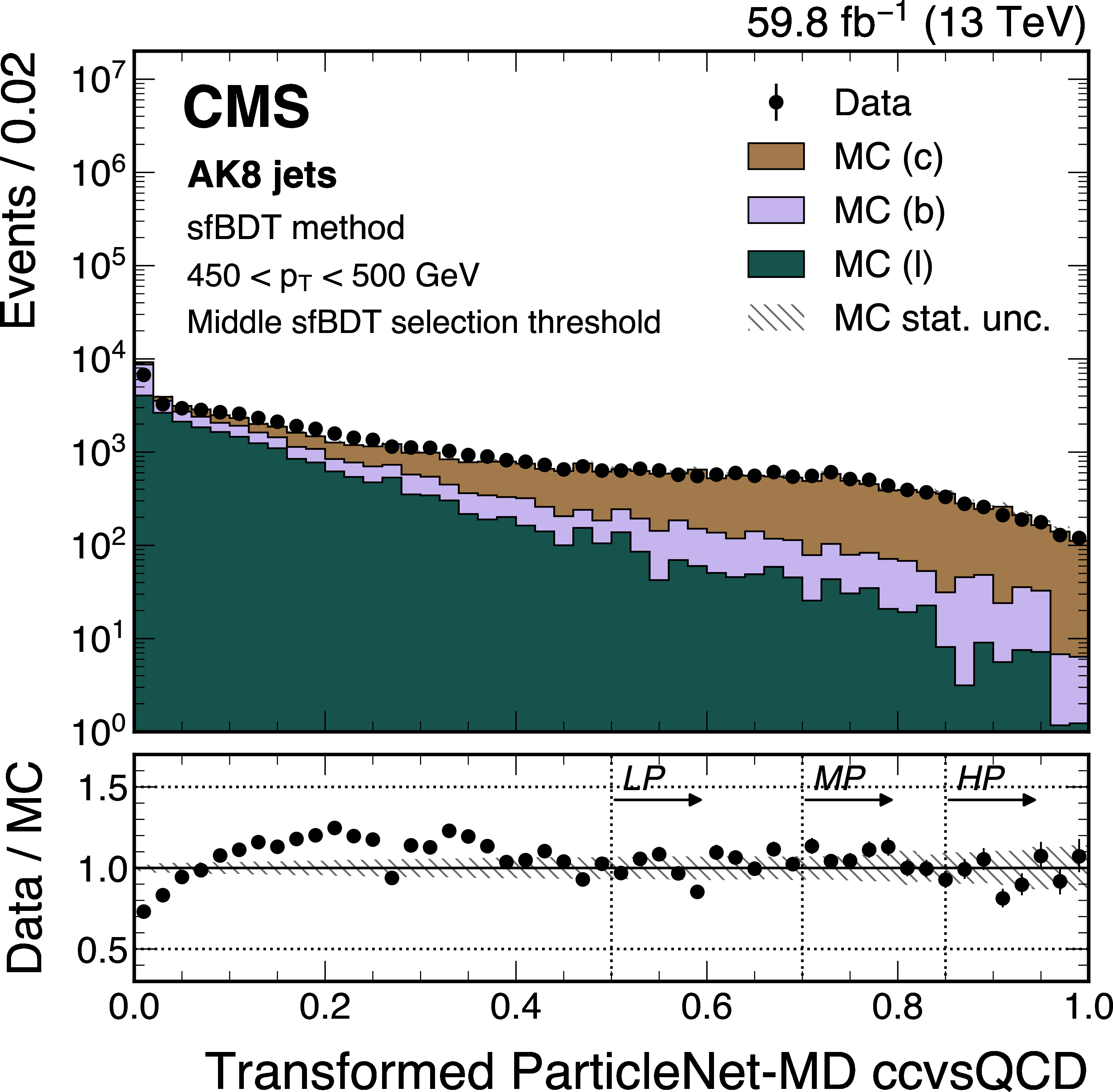
Figure 14:
An example of the transformed DeepDoubleX $ \mathrm{X} \to \mathrm{b} \overline{\mathrm{b}} $ (left) and $ \mathrm{X} \to \mathrm{c} \overline{\mathrm{c}} $ (right) distribution in data and simulated events, after applying the preselection and the middle sfBDT selection threshold in the sfBDT method. The high-purity (HP), medium-purity (MP), and low-purity (LP) working points for the left (right) plot correspond to selections of $ X > 0.6, 0.4, 0.2 (0.85, 0.7, 0.5) $ on the transformed tagger discriminant. The error bars represent the statistical uncertainties in observed data. The lower panels display the ratio of data to simulation, with the hatched bands representing the normalized statistical uncertainty of simulated events for each bin. The distributions are based on data and simulated events with the 2018 data-taking conditions, in the jet $ p_{\mathrm{T}} $ range of (450, 500) GeV. |
png pdf |
Figure 14-a:
An example of the transformed DeepDoubleX $ \mathrm{X} \to \mathrm{b} \overline{\mathrm{b}} $ (left) and $ \mathrm{X} \to \mathrm{c} \overline{\mathrm{c}} $ (right) distribution in data and simulated events, after applying the preselection and the middle sfBDT selection threshold in the sfBDT method. The high-purity (HP), medium-purity (MP), and low-purity (LP) working points for the left (right) plot correspond to selections of $ X > 0.6, 0.4, 0.2 (0.85, 0.7, 0.5) $ on the transformed tagger discriminant. The error bars represent the statistical uncertainties in observed data. The lower panels display the ratio of data to simulation, with the hatched bands representing the normalized statistical uncertainty of simulated events for each bin. The distributions are based on data and simulated events with the 2018 data-taking conditions, in the jet $ p_{\mathrm{T}} $ range of (450, 500) GeV. |
png pdf |
Figure 14-b:
An example of the transformed DeepDoubleX $ \mathrm{X} \to \mathrm{b} \overline{\mathrm{b}} $ (left) and $ \mathrm{X} \to \mathrm{c} \overline{\mathrm{c}} $ (right) distribution in data and simulated events, after applying the preselection and the middle sfBDT selection threshold in the sfBDT method. The high-purity (HP), medium-purity (MP), and low-purity (LP) working points for the left (right) plot correspond to selections of $ X > 0.6, 0.4, 0.2 (0.85, 0.7, 0.5) $ on the transformed tagger discriminant. The error bars represent the statistical uncertainties in observed data. The lower panels display the ratio of data to simulation, with the hatched bands representing the normalized statistical uncertainty of simulated events for each bin. The distributions are based on data and simulated events with the 2018 data-taking conditions, in the jet $ p_{\mathrm{T}} $ range of (450, 500) GeV. |
png pdf |
Figure 15:
An example of the transformed DeepAK8-MD $ \mathrm{X} \to \mathrm{b} \overline{\mathrm{b}} $ (left) and $ \mathrm{X} \to \mathrm{c} \overline{\mathrm{c}} $ (right) distribution in data and simulated events, after applying the preselection and the middle sfBDT selection threshold in the sfBDT method. The high-purity (HP), medium-purity (MP), and low-purity (LP) working points for the left (right) plot correspond to selections of $ X > 0.6, 0.4, 0.2 (0.85, 0.7, 0.5) $ on the transformed tagger discriminant. The error bars represent the statistical uncertainties in observed data, which may be too small to be visible. The lower panels display the ratio of data to simulation, with the hatched bands representing the normalized statistical uncertainty of simulated events for each bin. The distributions are based on data and simulated events with the 2018 data-taking conditions, in the jet $ p_{\mathrm{T}} $ range of (450, 500) GeV. |
png pdf |
Figure 15-a:
An example of the transformed DeepAK8-MD $ \mathrm{X} \to \mathrm{b} \overline{\mathrm{b}} $ (left) and $ \mathrm{X} \to \mathrm{c} \overline{\mathrm{c}} $ (right) distribution in data and simulated events, after applying the preselection and the middle sfBDT selection threshold in the sfBDT method. The high-purity (HP), medium-purity (MP), and low-purity (LP) working points for the left (right) plot correspond to selections of $ X > 0.6, 0.4, 0.2 (0.85, 0.7, 0.5) $ on the transformed tagger discriminant. The error bars represent the statistical uncertainties in observed data, which may be too small to be visible. The lower panels display the ratio of data to simulation, with the hatched bands representing the normalized statistical uncertainty of simulated events for each bin. The distributions are based on data and simulated events with the 2018 data-taking conditions, in the jet $ p_{\mathrm{T}} $ range of (450, 500) GeV. |
png pdf |
Figure 15-b:
An example of the transformed DeepAK8-MD $ \mathrm{X} \to \mathrm{b} \overline{\mathrm{b}} $ (left) and $ \mathrm{X} \to \mathrm{c} \overline{\mathrm{c}} $ (right) distribution in data and simulated events, after applying the preselection and the middle sfBDT selection threshold in the sfBDT method. The high-purity (HP), medium-purity (MP), and low-purity (LP) working points for the left (right) plot correspond to selections of $ X > 0.6, 0.4, 0.2 (0.85, 0.7, 0.5) $ on the transformed tagger discriminant. The error bars represent the statistical uncertainties in observed data, which may be too small to be visible. The lower panels display the ratio of data to simulation, with the hatched bands representing the normalized statistical uncertainty of simulated events for each bin. The distributions are based on data and simulated events with the 2018 data-taking conditions, in the jet $ p_{\mathrm{T}} $ range of (450, 500) GeV. |
png pdf |
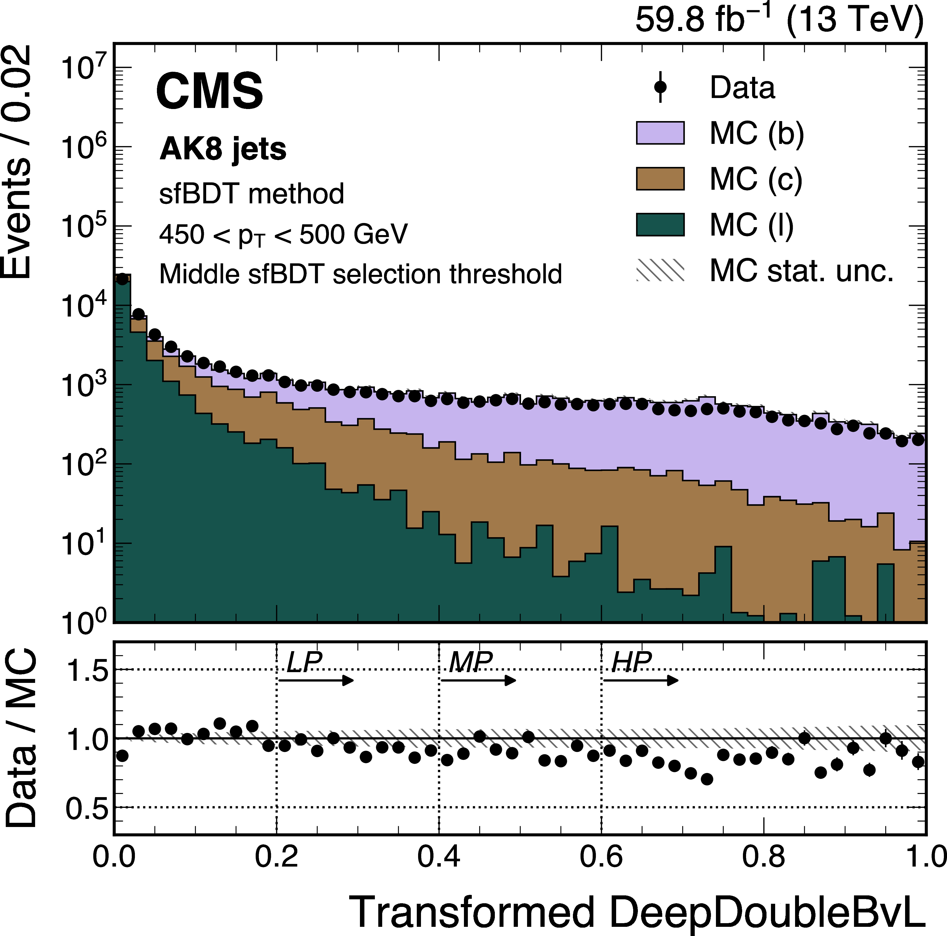
Figure 16:
An example of the transformed double-b distribution in data and simulated events, after applying the preselection and the middle sfBDT selection threshold in the sfBDT method. The high-purity (HP), medium-purity (MP), and low-purity (LP) working points correspond to selections of $ X > 0.6, 0.4, $ 0.2 on the transformed tagger discriminant. The error bars represent the statistical uncertainties in observed data, which may be too small to be visible. The lower panel displays the ratio of data to simulation, with the hatched bands representing the normalized statistical uncertainty of simulated events for each bin. The distribution is based on data and simulated events with the 2018 data-taking conditions, in the jet $ p_{\mathrm{T}} $ range of (450, 500) GeV. |
png pdf |
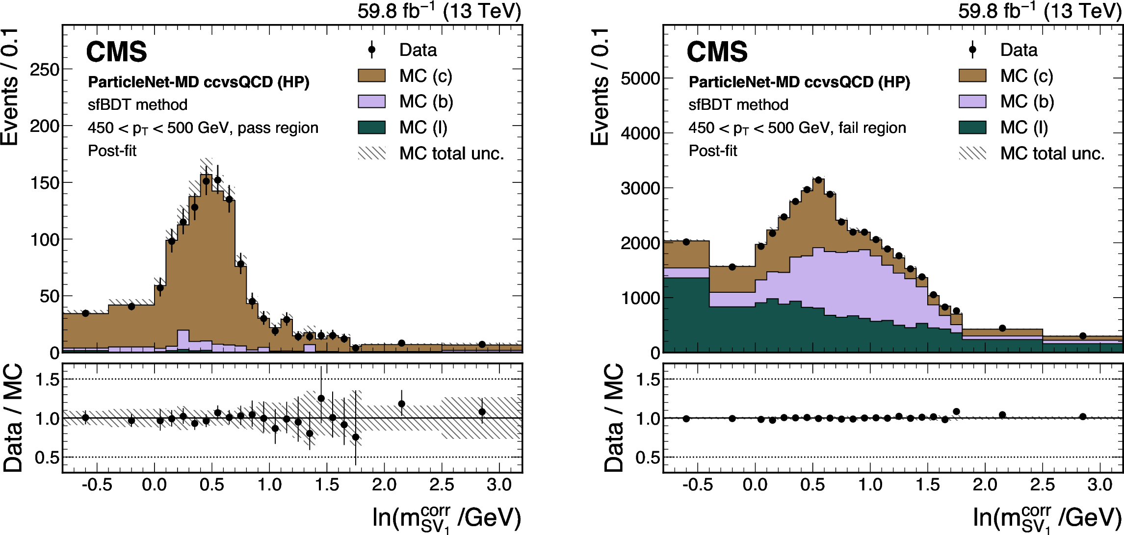
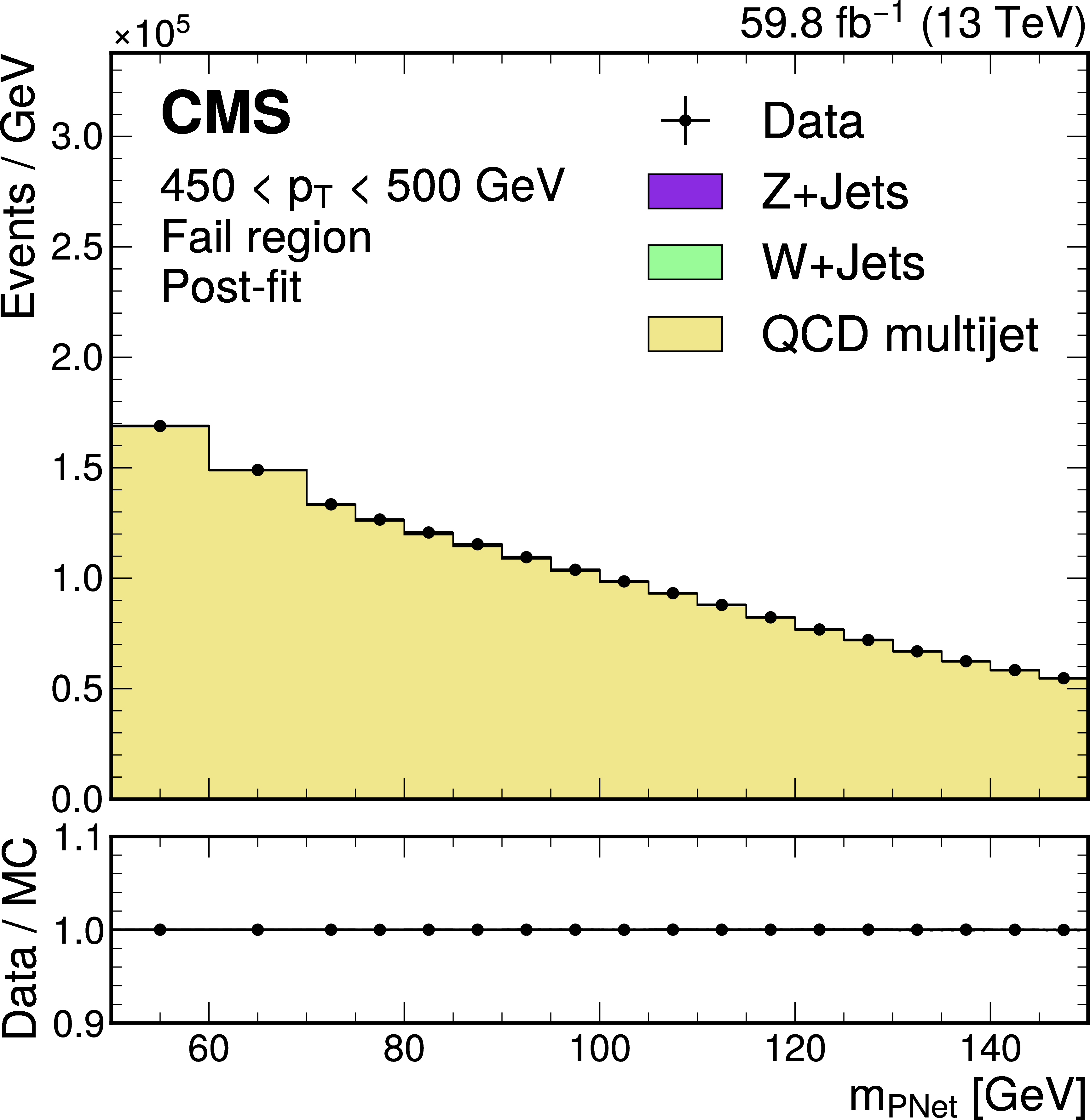
Figure 17:
Post-fit distributions from the sfBDT method for events passing (left) and failing (right) the tagger selection, used in the derivation of the scale factor for the ParticleNet-MD $ \mathrm{X} \to \mathrm{b} \overline{\mathrm{b}} $ discriminant at the high-purity working point. Error bars represent statistical uncertainties in data, whereas hatched bands denote the total uncertainties in the simulation. The example corresponds to data and simulated events from the 2018 data-taking conditions, in the jet $ p_{\mathrm{T}} $ range of (450, 500) GeV. |
png pdf |
Figure 17-a:
Post-fit distributions from the sfBDT method for events passing (left) and failing (right) the tagger selection, used in the derivation of the scale factor for the ParticleNet-MD $ \mathrm{X} \to \mathrm{b} \overline{\mathrm{b}} $ discriminant at the high-purity working point. Error bars represent statistical uncertainties in data, whereas hatched bands denote the total uncertainties in the simulation. The example corresponds to data and simulated events from the 2018 data-taking conditions, in the jet $ p_{\mathrm{T}} $ range of (450, 500) GeV. |
png pdf |
Figure 17-b:
Post-fit distributions from the sfBDT method for events passing (left) and failing (right) the tagger selection, used in the derivation of the scale factor for the ParticleNet-MD $ \mathrm{X} \to \mathrm{b} \overline{\mathrm{b}} $ discriminant at the high-purity working point. Error bars represent statistical uncertainties in data, whereas hatched bands denote the total uncertainties in the simulation. The example corresponds to data and simulated events from the 2018 data-taking conditions, in the jet $ p_{\mathrm{T}} $ range of (450, 500) GeV. |
png pdf |
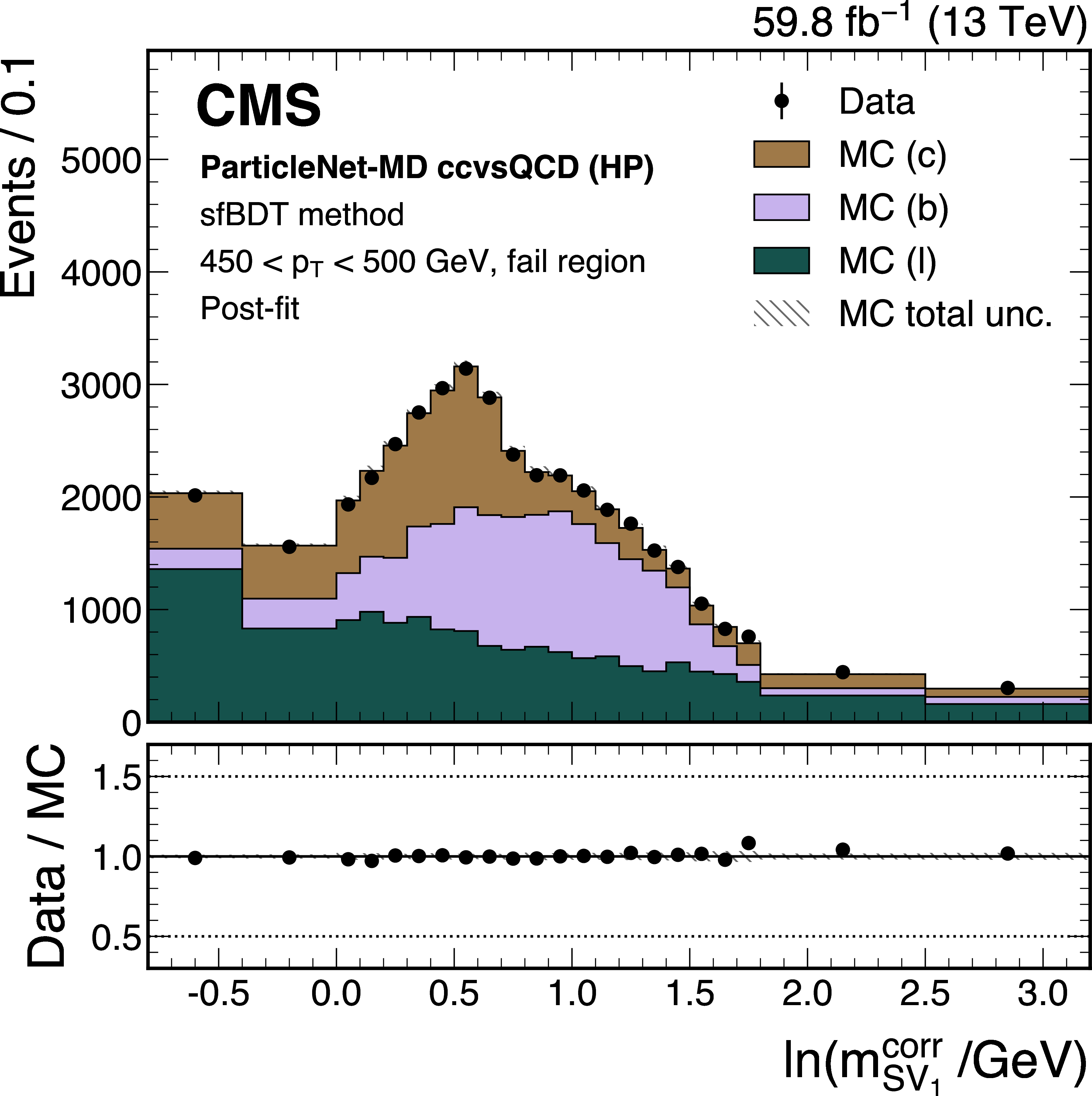
Figure 18:
Post-fit distributions from the sfBDT method for events passing (left) and failing (right) the tagger selection, used in the derivation of the scale factor for the ParticleNet-MD $ \mathrm{X} \to \mathrm{c} \overline{\mathrm{c}} $ discriminant at the high-purity working point. Error bars represent statistical uncertainties in data, whereas hatched bands denote the total uncertainties in the simulation. The example corresponds to data and simulated events from the 2018 data-taking conditions, in the jet $ p_{\mathrm{T}} $ range of (450, 500) GeV. |
png pdf |
Figure 18-a:
Post-fit distributions from the sfBDT method for events passing (left) and failing (right) the tagger selection, used in the derivation of the scale factor for the ParticleNet-MD $ \mathrm{X} \to \mathrm{c} \overline{\mathrm{c}} $ discriminant at the high-purity working point. Error bars represent statistical uncertainties in data, whereas hatched bands denote the total uncertainties in the simulation. The example corresponds to data and simulated events from the 2018 data-taking conditions, in the jet $ p_{\mathrm{T}} $ range of (450, 500) GeV. |
png pdf |
Figure 18-b:
Post-fit distributions from the sfBDT method for events passing (left) and failing (right) the tagger selection, used in the derivation of the scale factor for the ParticleNet-MD $ \mathrm{X} \to \mathrm{c} \overline{\mathrm{c}} $ discriminant at the high-purity working point. Error bars represent statistical uncertainties in data, whereas hatched bands denote the total uncertainties in the simulation. The example corresponds to data and simulated events from the 2018 data-taking conditions, in the jet $ p_{\mathrm{T}} $ range of (450, 500) GeV. |
png pdf |
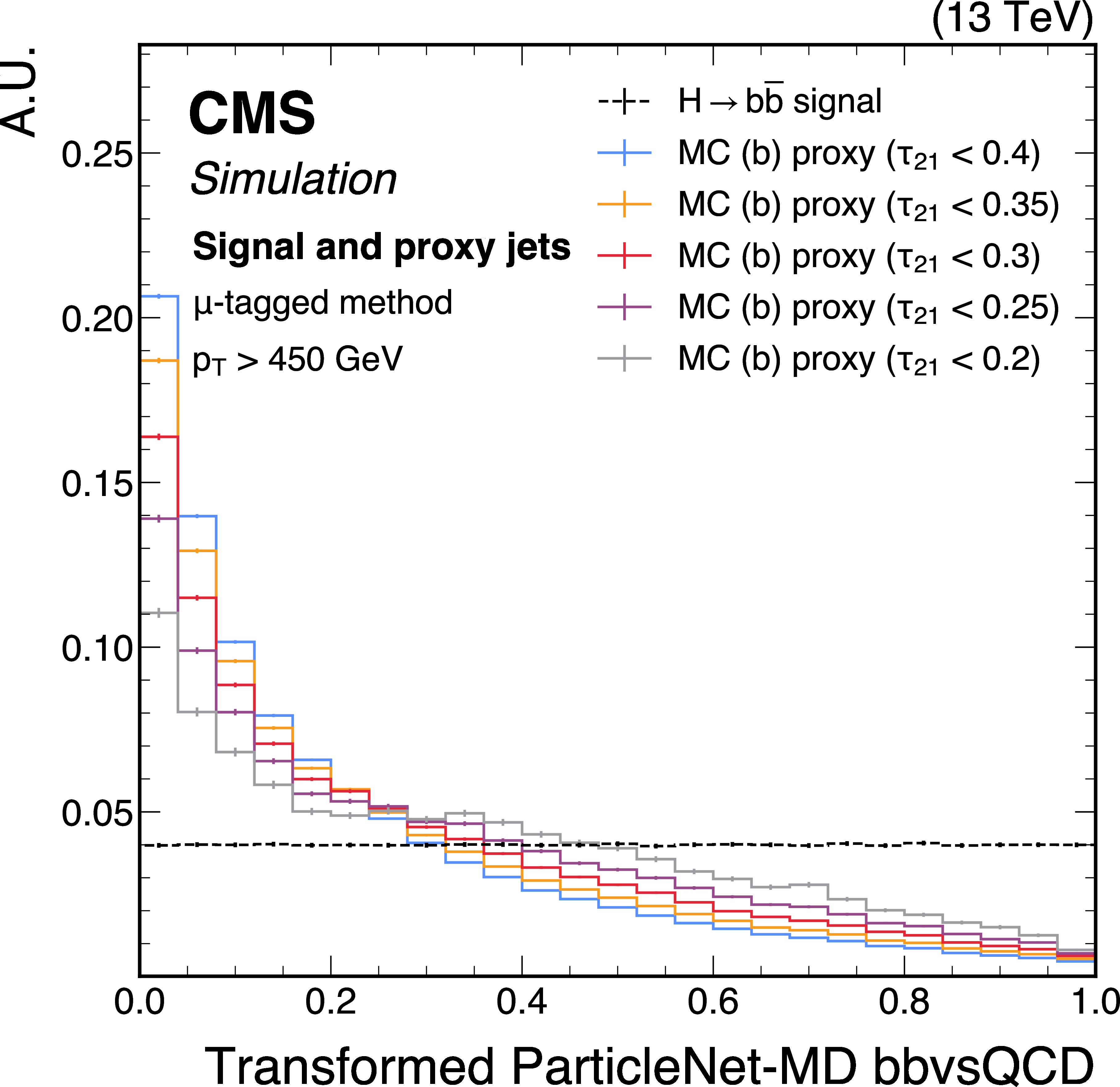
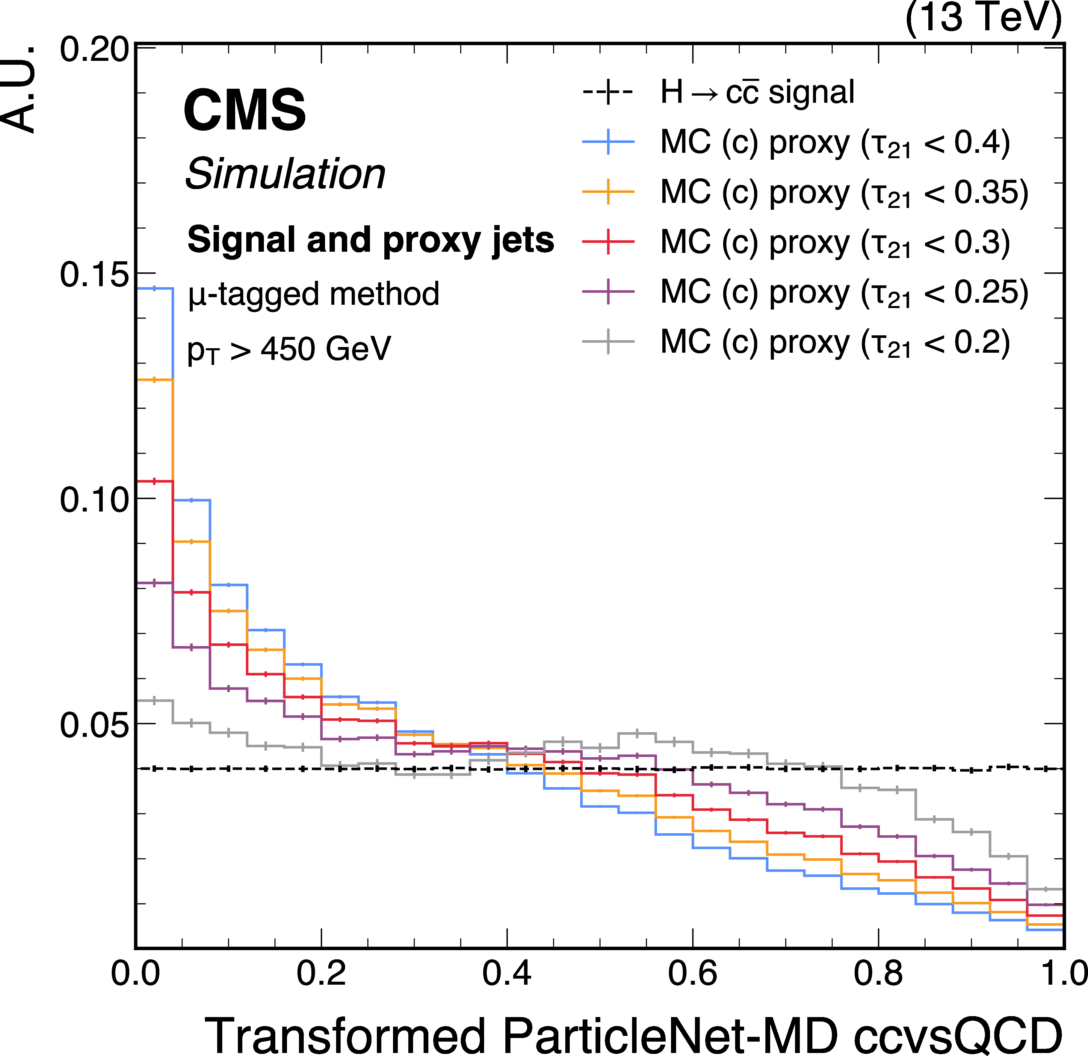
Figure 19:
Shapes of the transformed ParticleNet-MD $ \mathrm{X} \to \mathrm{b} \overline{\mathrm{b}} $ (left) and $ \mathrm{X} \to \mathrm{c} \overline{\mathrm{c}} $ (right) discriminants for SM $ \mathrm{H} \to \mathrm{b} \overline{\mathrm{b}} $ ($ \mathrm{c} \overline{\mathrm{c}} $) signal jets and proxy jets selected with different $ \tau_{21} $ selection thresholds. The examples correspond to the calibration of the ParticleNet-MD $ \mathrm{X} \to \mathrm{b} \overline{\mathrm{b}} $ and $ \mathrm{X} \to \mathrm{c} \overline{\mathrm{c}} $ discriminants with the $ \mu $-tagged method, using simulated events under 2018 data-taking conditions for jets with $ p_{\mathrm{T}} > $ 450 GeV. The error bars represent the statistical uncertainties due to the limited number of simulated events. |
png pdf |
Figure 19-a:
Shapes of the transformed ParticleNet-MD $ \mathrm{X} \to \mathrm{b} \overline{\mathrm{b}} $ (left) and $ \mathrm{X} \to \mathrm{c} \overline{\mathrm{c}} $ (right) discriminants for SM $ \mathrm{H} \to \mathrm{b} \overline{\mathrm{b}} $ ($ \mathrm{c} \overline{\mathrm{c}} $) signal jets and proxy jets selected with different $ \tau_{21} $ selection thresholds. The examples correspond to the calibration of the ParticleNet-MD $ \mathrm{X} \to \mathrm{b} \overline{\mathrm{b}} $ and $ \mathrm{X} \to \mathrm{c} \overline{\mathrm{c}} $ discriminants with the $ \mu $-tagged method, using simulated events under 2018 data-taking conditions for jets with $ p_{\mathrm{T}} > $ 450 GeV. The error bars represent the statistical uncertainties due to the limited number of simulated events. |
png pdf |
Figure 19-b:
Shapes of the transformed ParticleNet-MD $ \mathrm{X} \to \mathrm{b} \overline{\mathrm{b}} $ (left) and $ \mathrm{X} \to \mathrm{c} \overline{\mathrm{c}} $ (right) discriminants for SM $ \mathrm{H} \to \mathrm{b} \overline{\mathrm{b}} $ ($ \mathrm{c} \overline{\mathrm{c}} $) signal jets and proxy jets selected with different $ \tau_{21} $ selection thresholds. The examples correspond to the calibration of the ParticleNet-MD $ \mathrm{X} \to \mathrm{b} \overline{\mathrm{b}} $ and $ \mathrm{X} \to \mathrm{c} \overline{\mathrm{c}} $ discriminants with the $ \mu $-tagged method, using simulated events under 2018 data-taking conditions for jets with $ p_{\mathrm{T}} > $ 450 GeV. The error bars represent the statistical uncertainties due to the limited number of simulated events. |
png pdf |
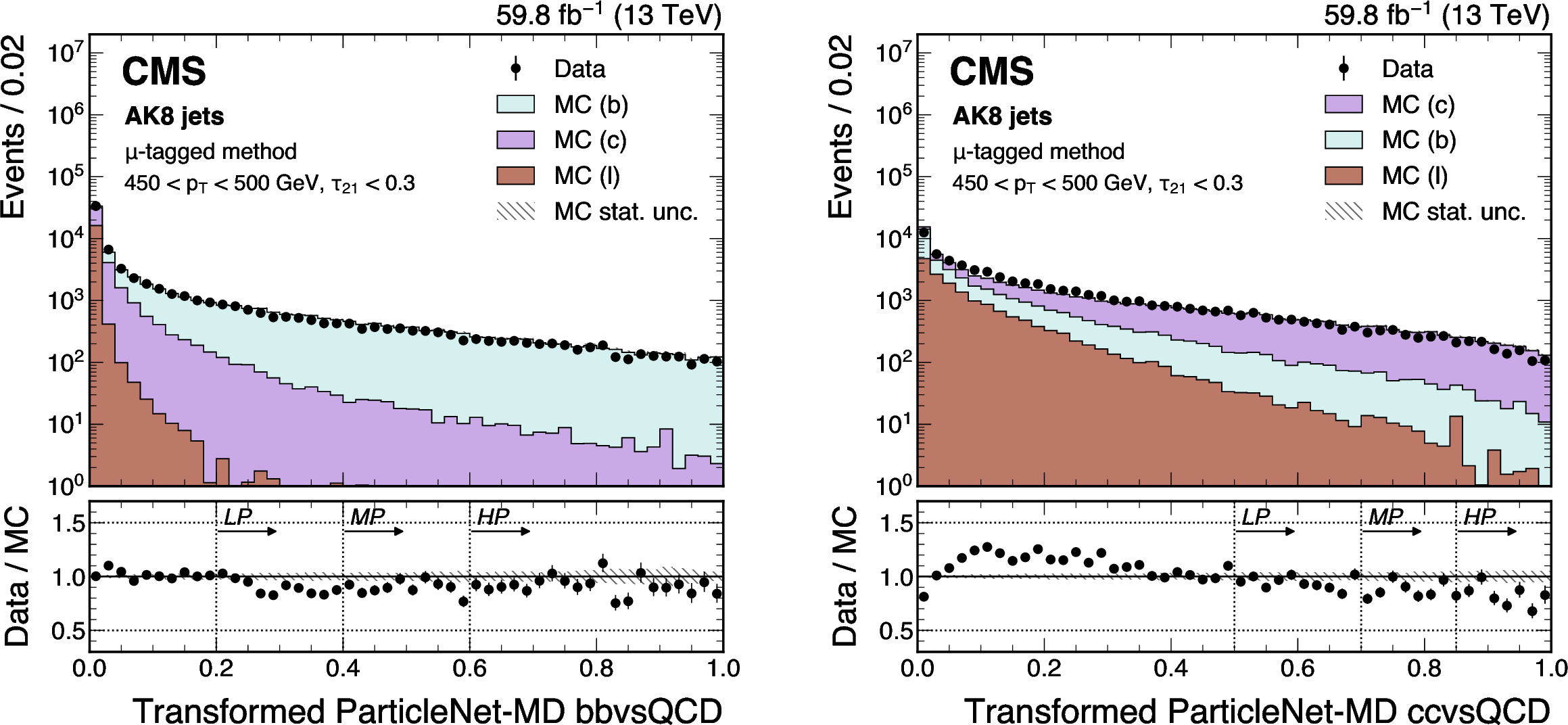
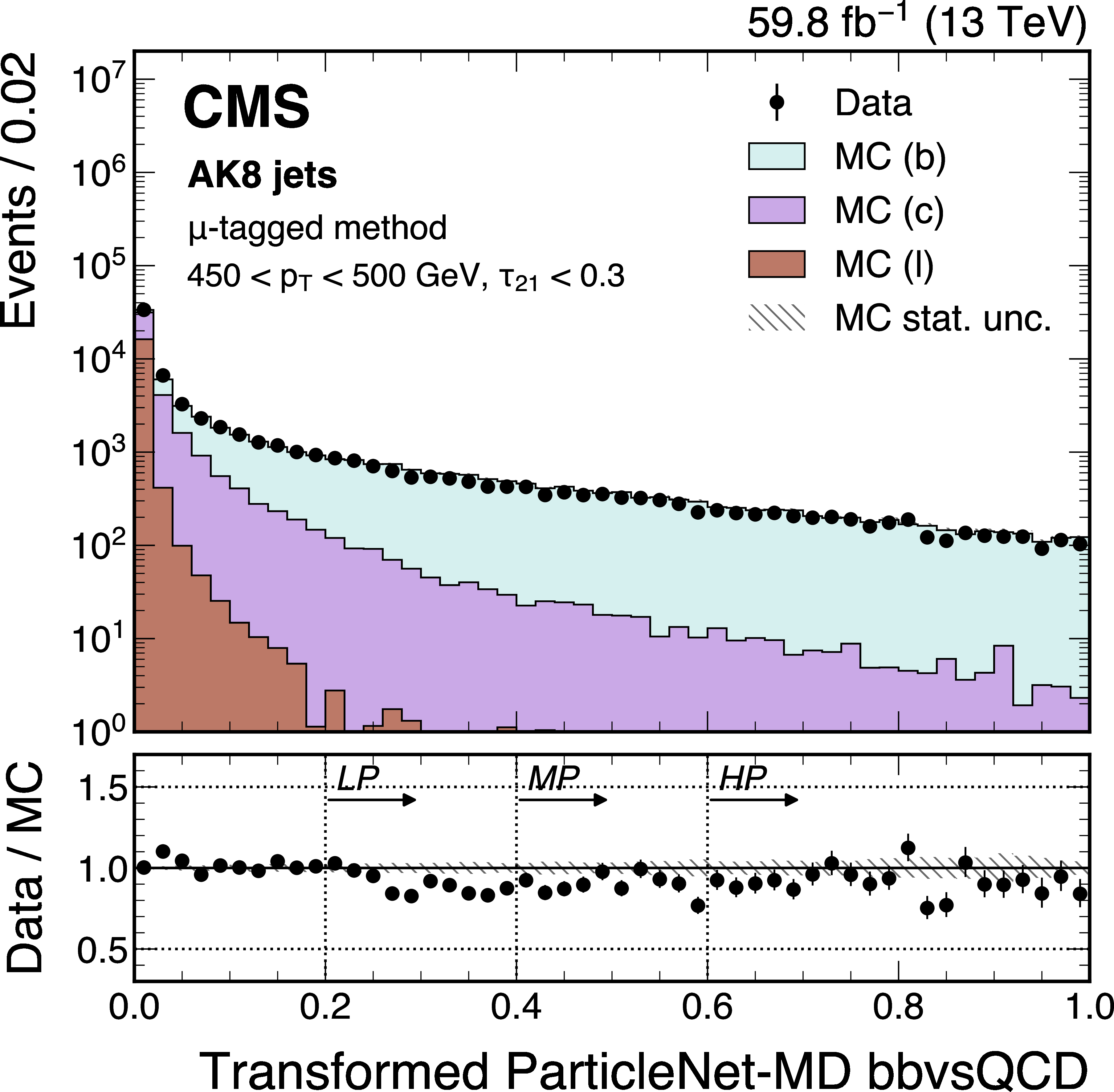
Figure 20:
An example of the transformed ParticleNet-MD $ \mathrm{X} \to \mathrm{b} \overline{\mathrm{b}} $ (left) and $ \mathrm{X} \to \mathrm{c} \overline{\mathrm{c}} $ (right) distribution in data and simulated events, passing the preselection of the $ \mu $-tagged method. The high-purity (HP), medium-purity (MP), and low-purity (LP) working points for the left (right) plot correspond to selections of $ X > 0.6, 0.4, 0.2 (0.85, 0.7, 0.5) $ on the transformed tagger discriminant. The error bars represent the statistical uncertainties in observed data. The lower panels display the ratio of data to simulation, with the hatched bands representing the normalized statistical uncertainty of simulated events for each bin. The distributions are based on data and simulated events with the 2018 data-taking conditions, in the jet $ p_{\mathrm{T}} $ range of (450, 500) GeV. |
png pdf |
Figure 20-a:
An example of the transformed ParticleNet-MD $ \mathrm{X} \to \mathrm{b} \overline{\mathrm{b}} $ (left) and $ \mathrm{X} \to \mathrm{c} \overline{\mathrm{c}} $ (right) distribution in data and simulated events, passing the preselection of the $ \mu $-tagged method. The high-purity (HP), medium-purity (MP), and low-purity (LP) working points for the left (right) plot correspond to selections of $ X > 0.6, 0.4, 0.2 (0.85, 0.7, 0.5) $ on the transformed tagger discriminant. The error bars represent the statistical uncertainties in observed data. The lower panels display the ratio of data to simulation, with the hatched bands representing the normalized statistical uncertainty of simulated events for each bin. The distributions are based on data and simulated events with the 2018 data-taking conditions, in the jet $ p_{\mathrm{T}} $ range of (450, 500) GeV. |
png pdf |
Figure 20-b:
An example of the transformed ParticleNet-MD $ \mathrm{X} \to \mathrm{b} \overline{\mathrm{b}} $ (left) and $ \mathrm{X} \to \mathrm{c} \overline{\mathrm{c}} $ (right) distribution in data and simulated events, passing the preselection of the $ \mu $-tagged method. The high-purity (HP), medium-purity (MP), and low-purity (LP) working points for the left (right) plot correspond to selections of $ X > 0.6, 0.4, 0.2 (0.85, 0.7, 0.5) $ on the transformed tagger discriminant. The error bars represent the statistical uncertainties in observed data. The lower panels display the ratio of data to simulation, with the hatched bands representing the normalized statistical uncertainty of simulated events for each bin. The distributions are based on data and simulated events with the 2018 data-taking conditions, in the jet $ p_{\mathrm{T}} $ range of (450, 500) GeV. |
png pdf |
Figure 21:
An example of the transformed DeepDoubleX $ \mathrm{X} \to \mathrm{b} \overline{\mathrm{b}} $ (left) and $ \mathrm{X} \to \mathrm{c} \overline{\mathrm{c}} $ (right) distribution in data and simulated events, passing the preselection of the $ \mu $-tagged method. The high-purity (HP), medium-purity (MP), and low-purity (LP) working points for the left (right) plot correspond to selections of $ X > 0.6, 0.4, 0.2 (0.85, 0.7, 0.5) $ on the transformed tagger discriminant. The error bars represent the statistical uncertainties in observed data. The lower panels display the ratio of data to simulation, with the hatched bands representing the normalized statistical uncertainty of simulated events for each bin. The distributions are based on data and simulated events with the 2018 data-taking conditions, in the jet $ p_{\mathrm{T}} $ range of (450, 500) GeV. |
png pdf |
Figure 21-a:
An example of the transformed DeepDoubleX $ \mathrm{X} \to \mathrm{b} \overline{\mathrm{b}} $ (left) and $ \mathrm{X} \to \mathrm{c} \overline{\mathrm{c}} $ (right) distribution in data and simulated events, passing the preselection of the $ \mu $-tagged method. The high-purity (HP), medium-purity (MP), and low-purity (LP) working points for the left (right) plot correspond to selections of $ X > 0.6, 0.4, 0.2 (0.85, 0.7, 0.5) $ on the transformed tagger discriminant. The error bars represent the statistical uncertainties in observed data. The lower panels display the ratio of data to simulation, with the hatched bands representing the normalized statistical uncertainty of simulated events for each bin. The distributions are based on data and simulated events with the 2018 data-taking conditions, in the jet $ p_{\mathrm{T}} $ range of (450, 500) GeV. |
png pdf |
Figure 21-b:
An example of the transformed DeepDoubleX $ \mathrm{X} \to \mathrm{b} \overline{\mathrm{b}} $ (left) and $ \mathrm{X} \to \mathrm{c} \overline{\mathrm{c}} $ (right) distribution in data and simulated events, passing the preselection of the $ \mu $-tagged method. The high-purity (HP), medium-purity (MP), and low-purity (LP) working points for the left (right) plot correspond to selections of $ X > 0.6, 0.4, 0.2 (0.85, 0.7, 0.5) $ on the transformed tagger discriminant. The error bars represent the statistical uncertainties in observed data. The lower panels display the ratio of data to simulation, with the hatched bands representing the normalized statistical uncertainty of simulated events for each bin. The distributions are based on data and simulated events with the 2018 data-taking conditions, in the jet $ p_{\mathrm{T}} $ range of (450, 500) GeV. |
png pdf |
Figure 22:
An example of the transformed DeepAK8-MD $ \mathrm{X} \to \mathrm{b} \overline{\mathrm{b}} $ (left) and $ \mathrm{X} \to \mathrm{c} \overline{\mathrm{c}} $ (right) distribution in data and simulated events, passing the preselection of the $ \mu $-tagged method. The high-purity (HP), medium-purity (MP), and low-purity (LP) working points for the left (right) plot correspond to selections of $ X > 0.6, 0.4, 0.2 (0.85, 0.7, 0.5) $ on the transformed tagger discriminant. The error bars represent the statistical uncertainties in observed data. The lower panels display the ratio of data to simulation, with the hatched bands representing the normalized statistical uncertainty of simulated events for each bin. The distributions are based on data and simulated events with the 2018 data-taking conditions, in the jet $ p_{\mathrm{T}} $ range of (450, 500) GeV. |
png pdf |
Figure 22-a:
An example of the transformed DeepAK8-MD $ \mathrm{X} \to \mathrm{b} \overline{\mathrm{b}} $ (left) and $ \mathrm{X} \to \mathrm{c} \overline{\mathrm{c}} $ (right) distribution in data and simulated events, passing the preselection of the $ \mu $-tagged method. The high-purity (HP), medium-purity (MP), and low-purity (LP) working points for the left (right) plot correspond to selections of $ X > 0.6, 0.4, 0.2 (0.85, 0.7, 0.5) $ on the transformed tagger discriminant. The error bars represent the statistical uncertainties in observed data. The lower panels display the ratio of data to simulation, with the hatched bands representing the normalized statistical uncertainty of simulated events for each bin. The distributions are based on data and simulated events with the 2018 data-taking conditions, in the jet $ p_{\mathrm{T}} $ range of (450, 500) GeV. |
png pdf |
Figure 22-b:
An example of the transformed DeepAK8-MD $ \mathrm{X} \to \mathrm{b} \overline{\mathrm{b}} $ (left) and $ \mathrm{X} \to \mathrm{c} \overline{\mathrm{c}} $ (right) distribution in data and simulated events, passing the preselection of the $ \mu $-tagged method. The high-purity (HP), medium-purity (MP), and low-purity (LP) working points for the left (right) plot correspond to selections of $ X > 0.6, 0.4, 0.2 (0.85, 0.7, 0.5) $ on the transformed tagger discriminant. The error bars represent the statistical uncertainties in observed data. The lower panels display the ratio of data to simulation, with the hatched bands representing the normalized statistical uncertainty of simulated events for each bin. The distributions are based on data and simulated events with the 2018 data-taking conditions, in the jet $ p_{\mathrm{T}} $ range of (450, 500) GeV. |
png pdf |
Figure 23:
An example of the transformed double-b distribution in data and simulated events, passing the preselection of the $ \mu $-tagged method. The high-purity (HP), medium-purity (MP), and low-purity (LP) working points correspond to selections of $ X > 0.6, 0.4, $ 0.2 on the transformed tagger discriminant. The error bars represent the statistical uncertainties in observed data. The lower panel displays the ratio of data to simulation, with the hatched bands representing the normalized statistical uncertainty of simulated events for each bin. The distribution is based on data and simulated events with the 2018 data-taking conditions, in the jet $ p_{\mathrm{T}} $ range of (450, 500) GeV. |
png pdf |
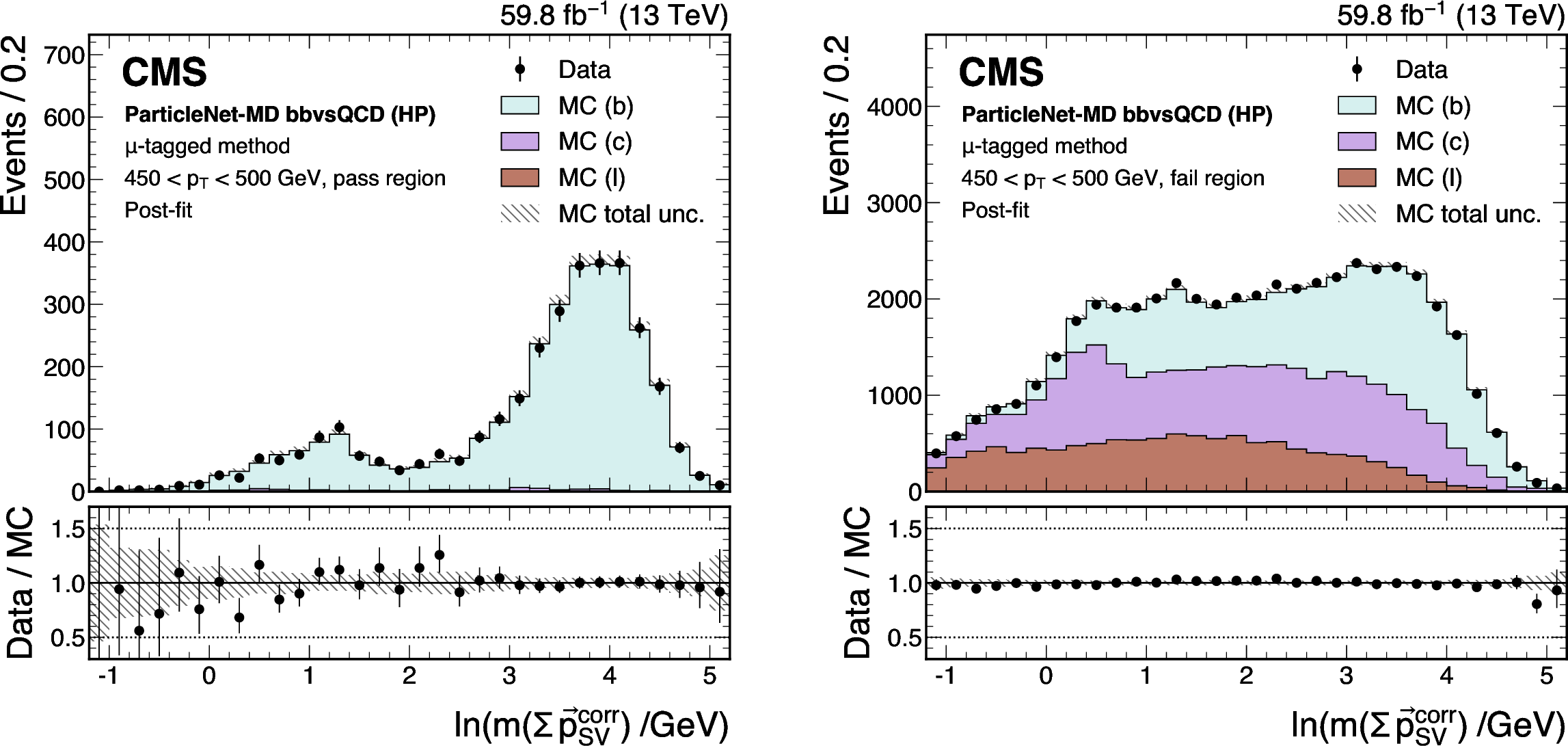
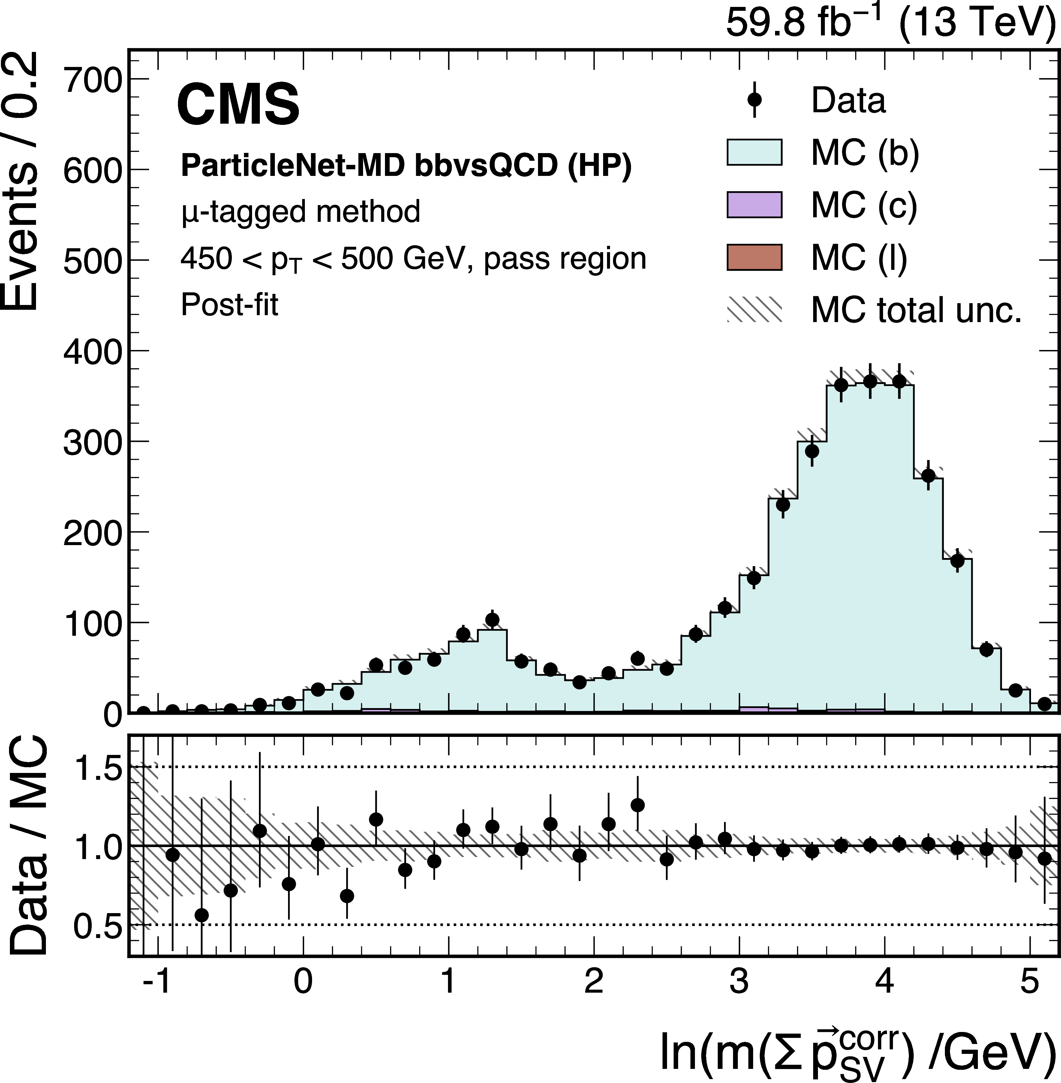
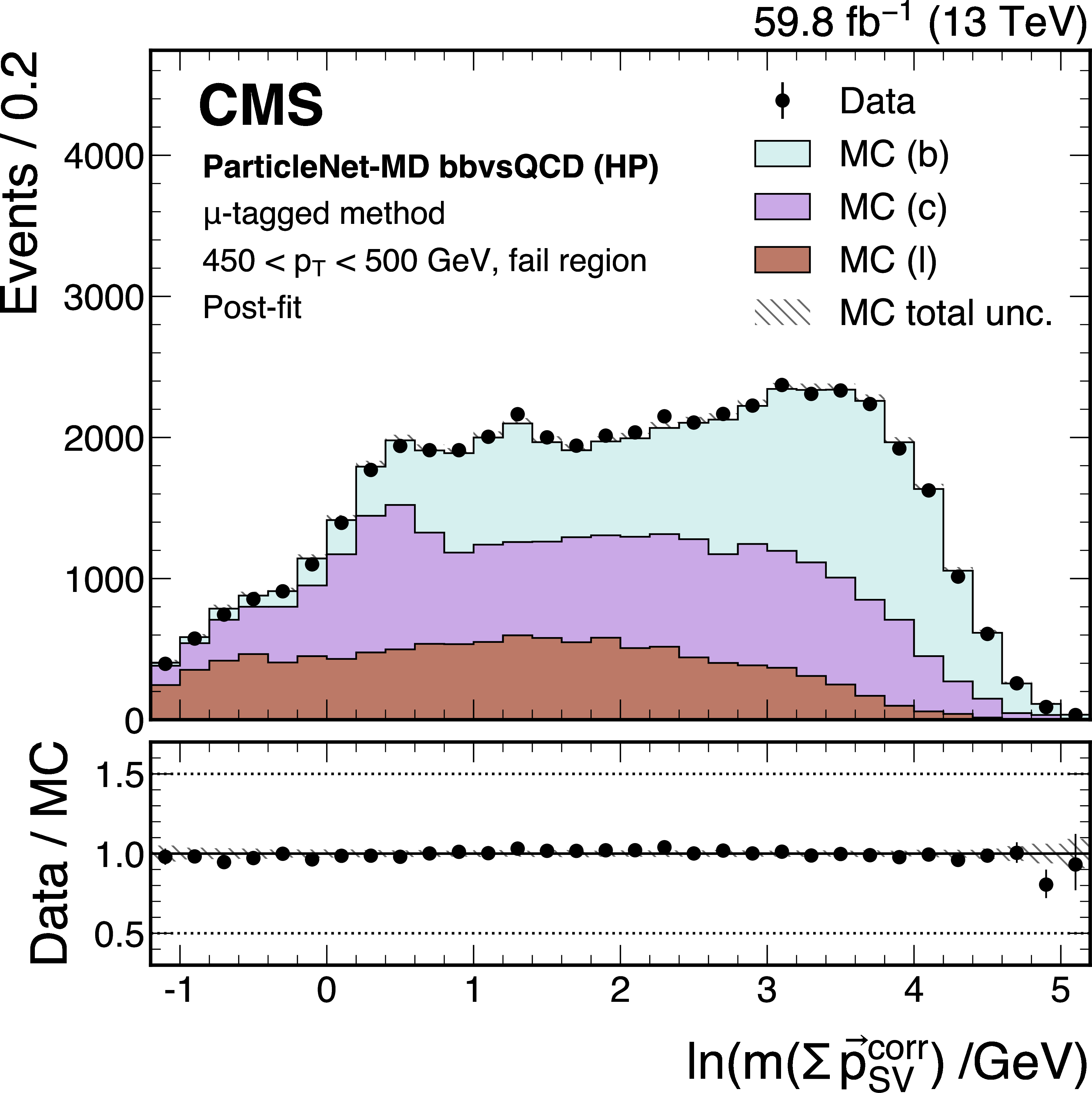
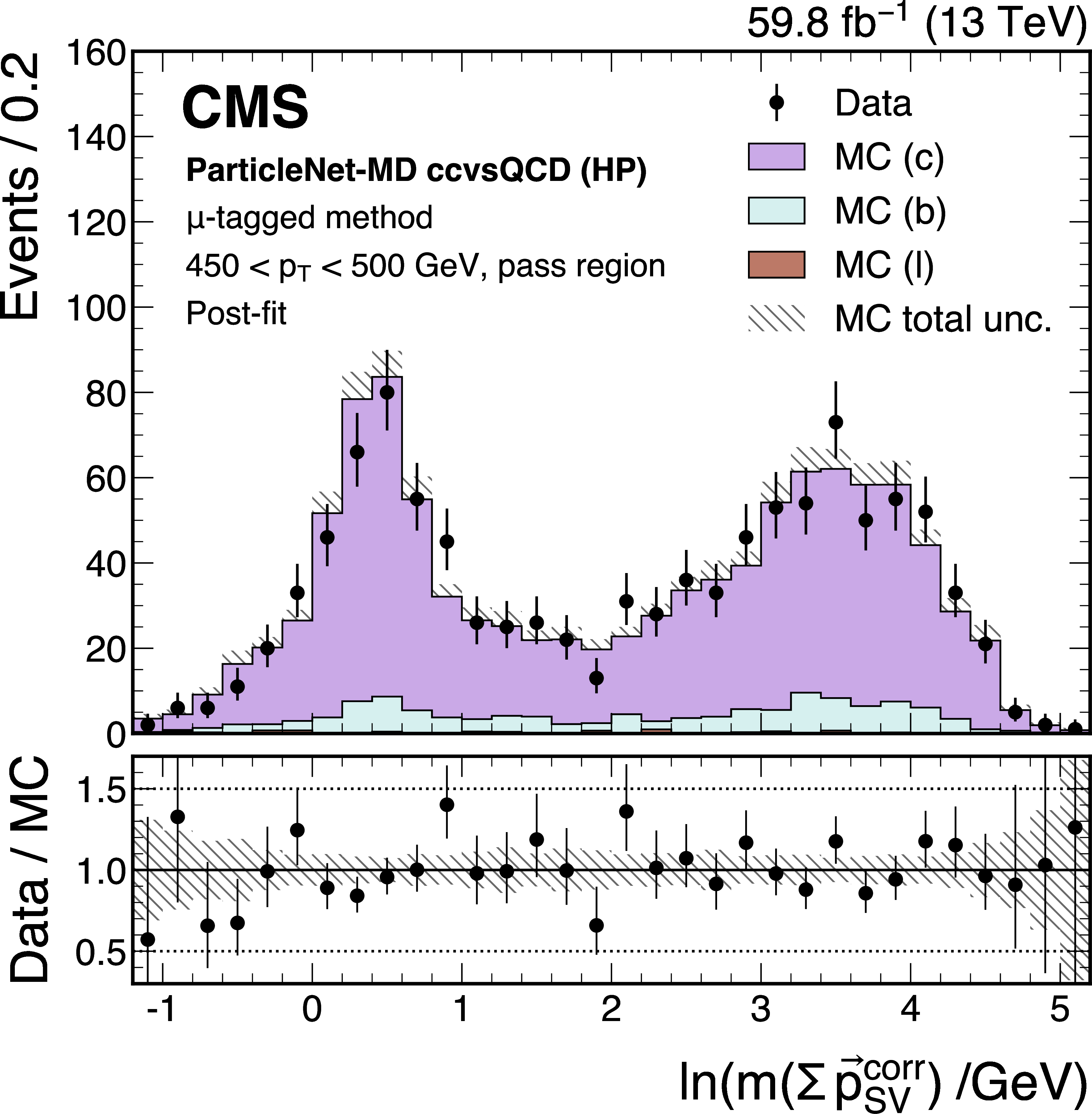
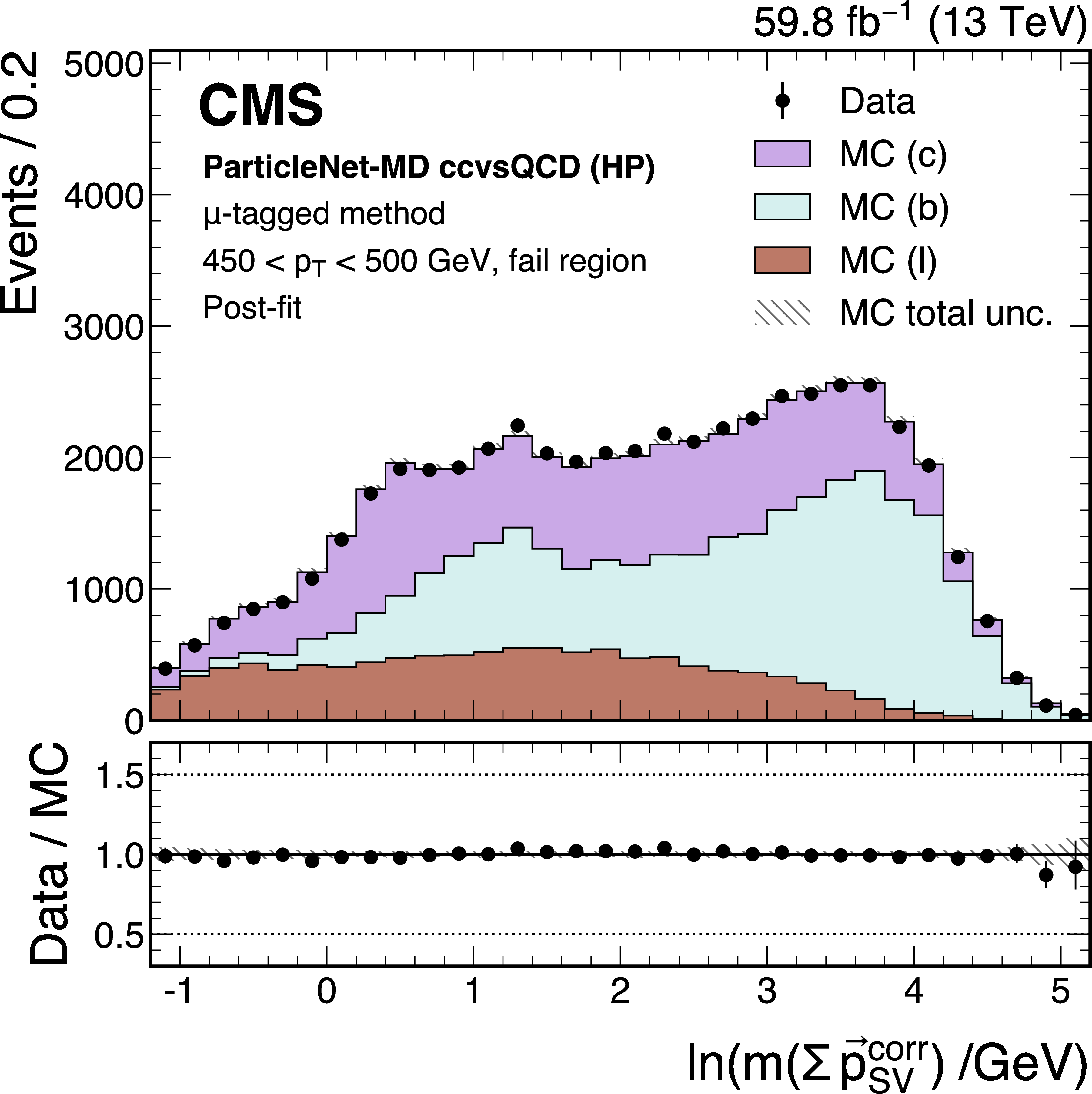
Figure 24:
Post-fit distributions from the $ \mu $-tagged method for events passing (left) and failing (right) the tagger selection, used in the derivation of the scale factor for the ParticleNet-MD $ \mathrm{X} \to \mathrm{b} \overline{\mathrm{b}} $ discriminant at the high-purity working point. Error bars represent statistical uncertainties in data, where hatched bands denote the total uncertainties in the simulation. The example corresponds to data and simulated events from the 2018 data-taking conditions, in the jet $ p_{\mathrm{T}} $ range of (450, 500) GeV. |
png pdf |
Figure 24-a:
Post-fit distributions from the $ \mu $-tagged method for events passing (left) and failing (right) the tagger selection, used in the derivation of the scale factor for the ParticleNet-MD $ \mathrm{X} \to \mathrm{b} \overline{\mathrm{b}} $ discriminant at the high-purity working point. Error bars represent statistical uncertainties in data, where hatched bands denote the total uncertainties in the simulation. The example corresponds to data and simulated events from the 2018 data-taking conditions, in the jet $ p_{\mathrm{T}} $ range of (450, 500) GeV. |
png pdf |
Figure 24-b:
Post-fit distributions from the $ \mu $-tagged method for events passing (left) and failing (right) the tagger selection, used in the derivation of the scale factor for the ParticleNet-MD $ \mathrm{X} \to \mathrm{b} \overline{\mathrm{b}} $ discriminant at the high-purity working point. Error bars represent statistical uncertainties in data, where hatched bands denote the total uncertainties in the simulation. The example corresponds to data and simulated events from the 2018 data-taking conditions, in the jet $ p_{\mathrm{T}} $ range of (450, 500) GeV. |
png pdf |
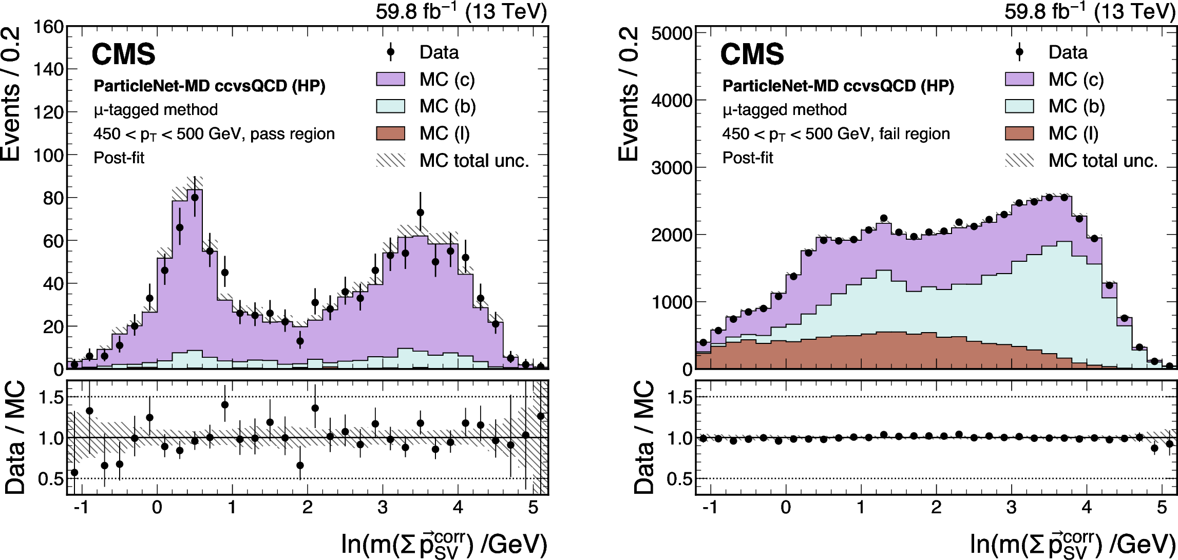
Figure 25:
Post-fit distributions from the $ \mu $-tagged method for events passing (left) and failing (right) the tagger selection, used in the derivation of the scale factor for the ParticleNet-MD $ \mathrm{X} \to \mathrm{c} \overline{\mathrm{c}} $ discriminant at the high-purity working point. Error bars represent statistical uncertainties in data, whereas hatched bands denote the total uncertainties in the simulation. The example corresponds to data and simulated events from the 2018 data-taking conditions, in the jet $ p_{\mathrm{T}} $ range of (450, 500) GeV. |
png pdf |
Figure 25-a:
Post-fit distributions from the $ \mu $-tagged method for events passing (left) and failing (right) the tagger selection, used in the derivation of the scale factor for the ParticleNet-MD $ \mathrm{X} \to \mathrm{c} \overline{\mathrm{c}} $ discriminant at the high-purity working point. Error bars represent statistical uncertainties in data, whereas hatched bands denote the total uncertainties in the simulation. The example corresponds to data and simulated events from the 2018 data-taking conditions, in the jet $ p_{\mathrm{T}} $ range of (450, 500) GeV. |
png pdf |
Figure 25-b:
Post-fit distributions from the $ \mu $-tagged method for events passing (left) and failing (right) the tagger selection, used in the derivation of the scale factor for the ParticleNet-MD $ \mathrm{X} \to \mathrm{c} \overline{\mathrm{c}} $ discriminant at the high-purity working point. Error bars represent statistical uncertainties in data, whereas hatched bands denote the total uncertainties in the simulation. The example corresponds to data and simulated events from the 2018 data-taking conditions, in the jet $ p_{\mathrm{T}} $ range of (450, 500) GeV. |
png pdf |
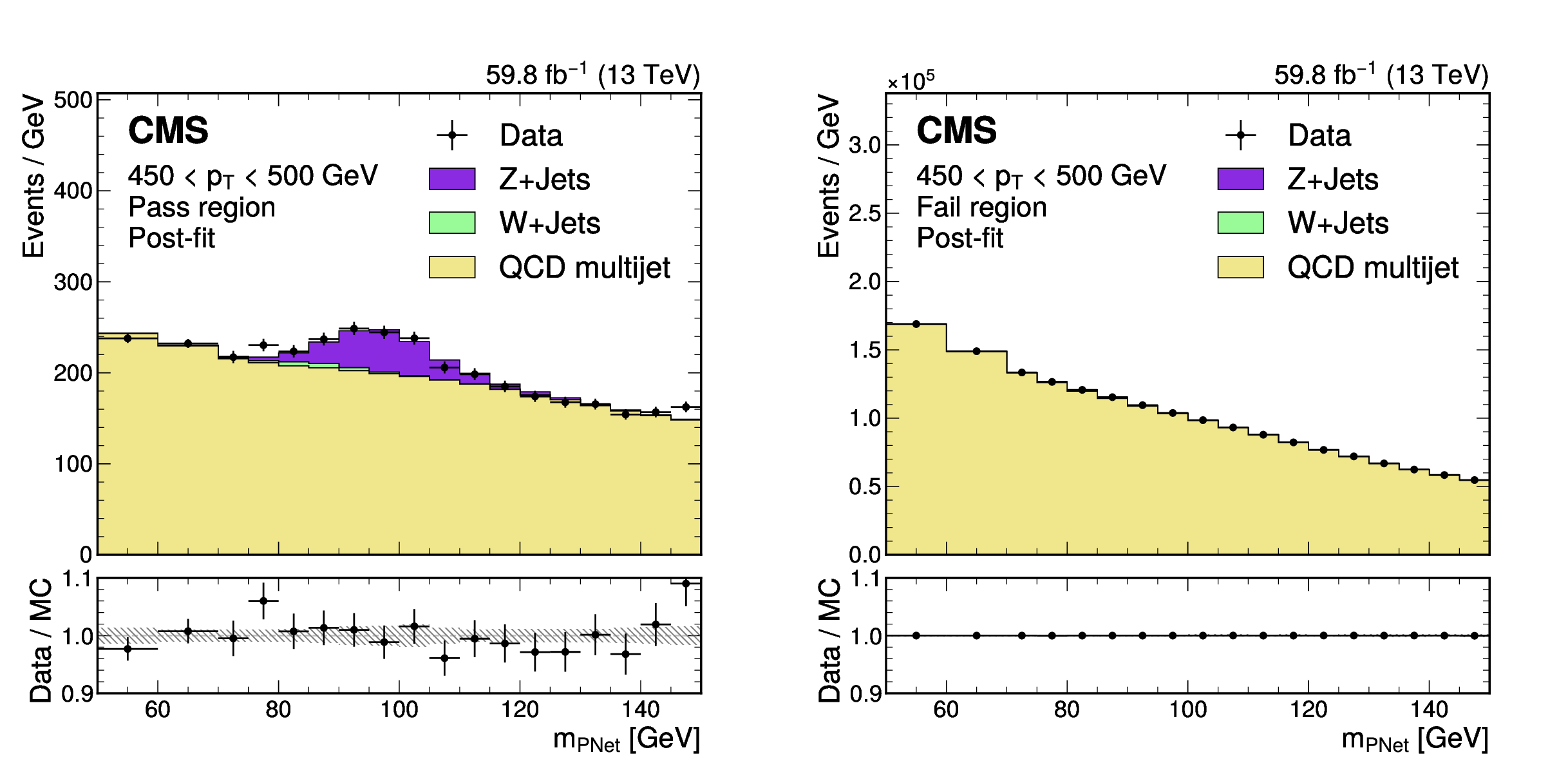
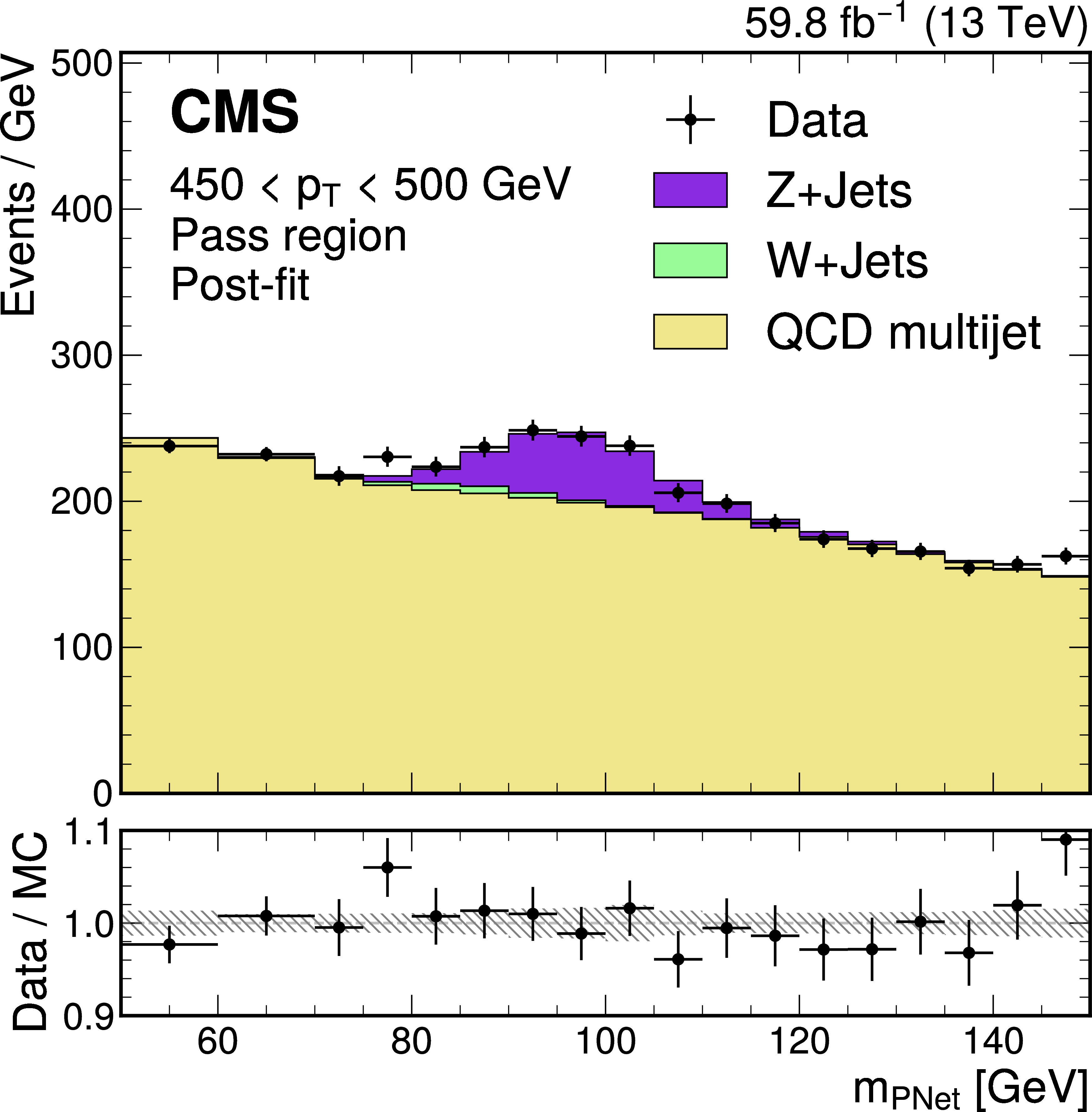
Figure 26:
Post-fit distributions from the boosted Z boson method for events passing (left) and failing (right) the tagger selection, used in the derivation of the scale factor for the ParticleNet-MD $ \mathrm{X} \to \mathrm{b} \overline{\mathrm{b}} $ discriminant at the high-purity working point. The error bars represent the statistical uncertainties in observed data. The lower panels show the pulls defined as (observed events} - \text{expected events) $ /\sqrt{\smash[b]{\sigma_{\text{obs}}^{2} + \sigma_{\text{exp}}^{2}}} $, where $ \sigma_{\text{obs}} $ and $ \sigma_{\text{exp}} $ are the total uncertainties in the observation and the background estimation, respectively. The example corresponds to data and simulated events from the 2018 data-taking conditions, in the jet $ p_{\mathrm{T}} $ range of (450, 500) GeV. |
png pdf |
Figure 26-a:
Post-fit distributions from the boosted Z boson method for events passing (left) and failing (right) the tagger selection, used in the derivation of the scale factor for the ParticleNet-MD $ \mathrm{X} \to \mathrm{b} \overline{\mathrm{b}} $ discriminant at the high-purity working point. The error bars represent the statistical uncertainties in observed data. The lower panels show the pulls defined as (observed events} - \text{expected events) $ /\sqrt{\smash[b]{\sigma_{\text{obs}}^{2} + \sigma_{\text{exp}}^{2}}} $, where $ \sigma_{\text{obs}} $ and $ \sigma_{\text{exp}} $ are the total uncertainties in the observation and the background estimation, respectively. The example corresponds to data and simulated events from the 2018 data-taking conditions, in the jet $ p_{\mathrm{T}} $ range of (450, 500) GeV. |
png pdf |
Figure 26-b:
Post-fit distributions from the boosted Z boson method for events passing (left) and failing (right) the tagger selection, used in the derivation of the scale factor for the ParticleNet-MD $ \mathrm{X} \to \mathrm{b} \overline{\mathrm{b}} $ discriminant at the high-purity working point. The error bars represent the statistical uncertainties in observed data. The lower panels show the pulls defined as (observed events} - \text{expected events) $ /\sqrt{\smash[b]{\sigma_{\text{obs}}^{2} + \sigma_{\text{exp}}^{2}}} $, where $ \sigma_{\text{obs}} $ and $ \sigma_{\text{exp}} $ are the total uncertainties in the observation and the background estimation, respectively. The example corresponds to data and simulated events from the 2018 data-taking conditions, in the jet $ p_{\mathrm{T}} $ range of (450, 500) GeV. |
png pdf |
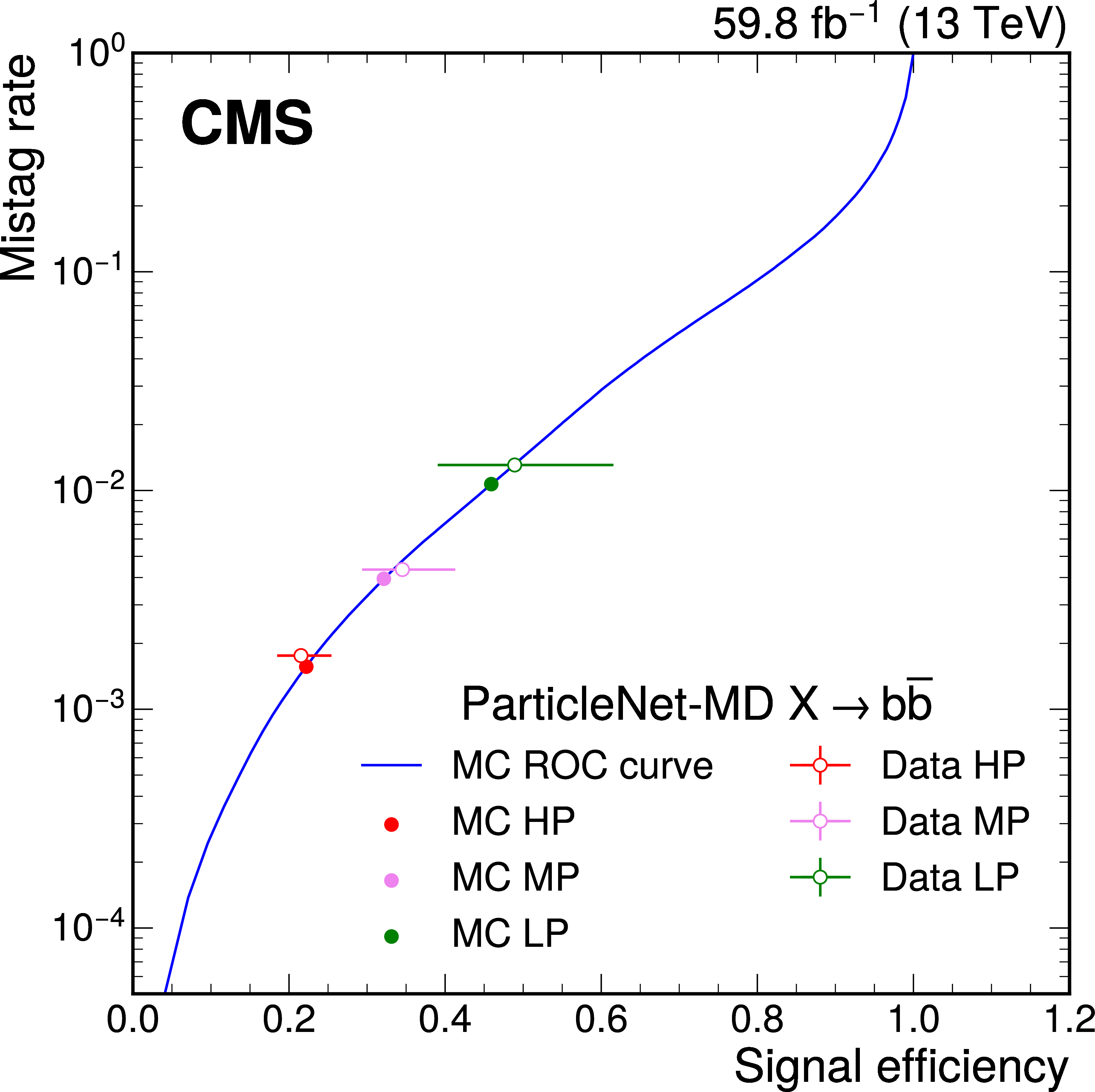
Figure 27:
Receiver operating characteristic (ROC) curve of the ParticleNet-MD $ \mathrm{X} \to \mathrm{b} \overline{\mathrm{b}} $ discriminant obtained from simulation (blue), under 2018 data-taking conditions with $ p_{\mathrm{T}} > $ 450 GeV. The high-purity (HP), medium-purity (MP), and low-purity (LP) working points are indicated by filled circles for simulation and hollow circles for data. The error bars represent the statistical uncertainties in observed data. |
png pdf |
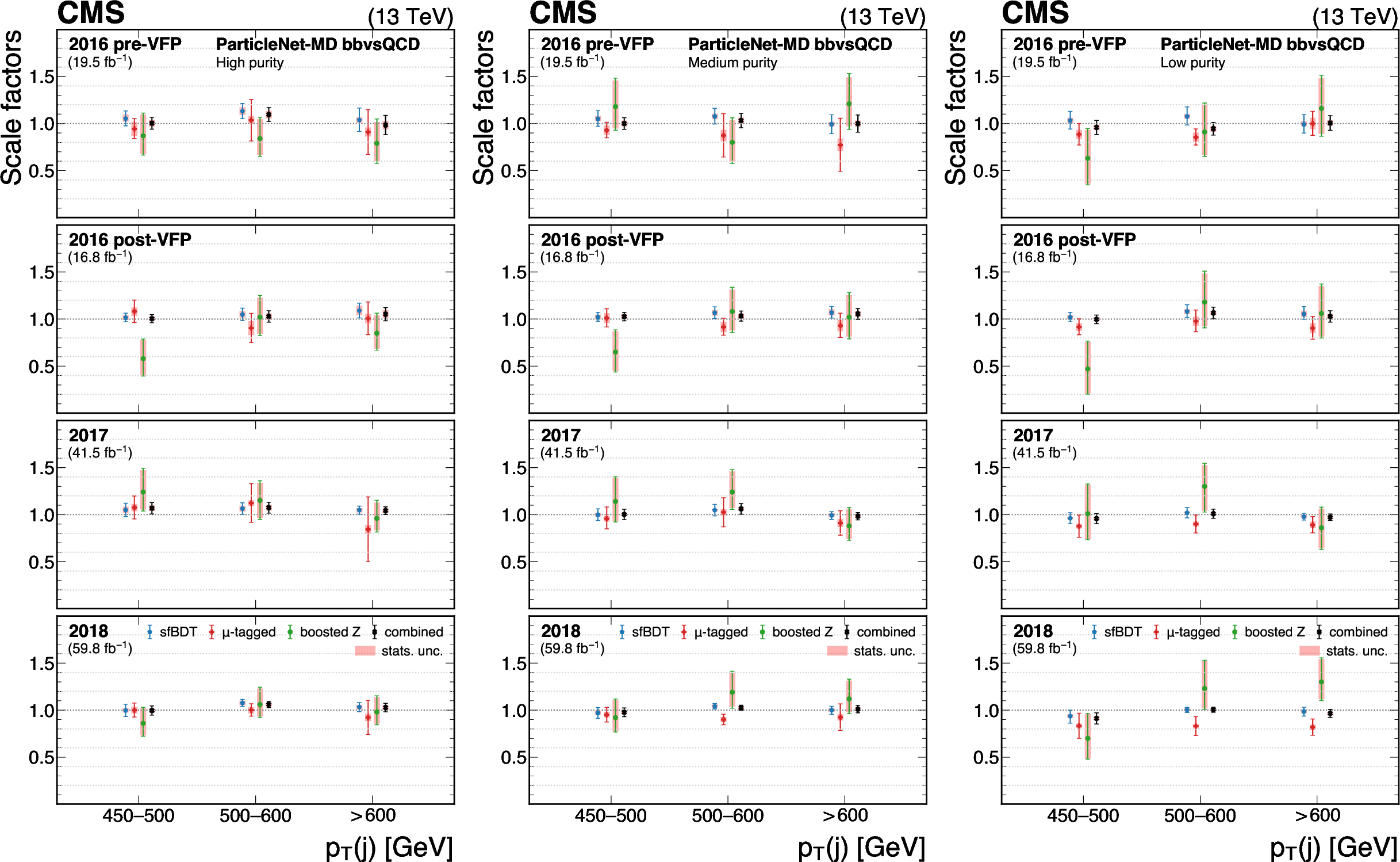
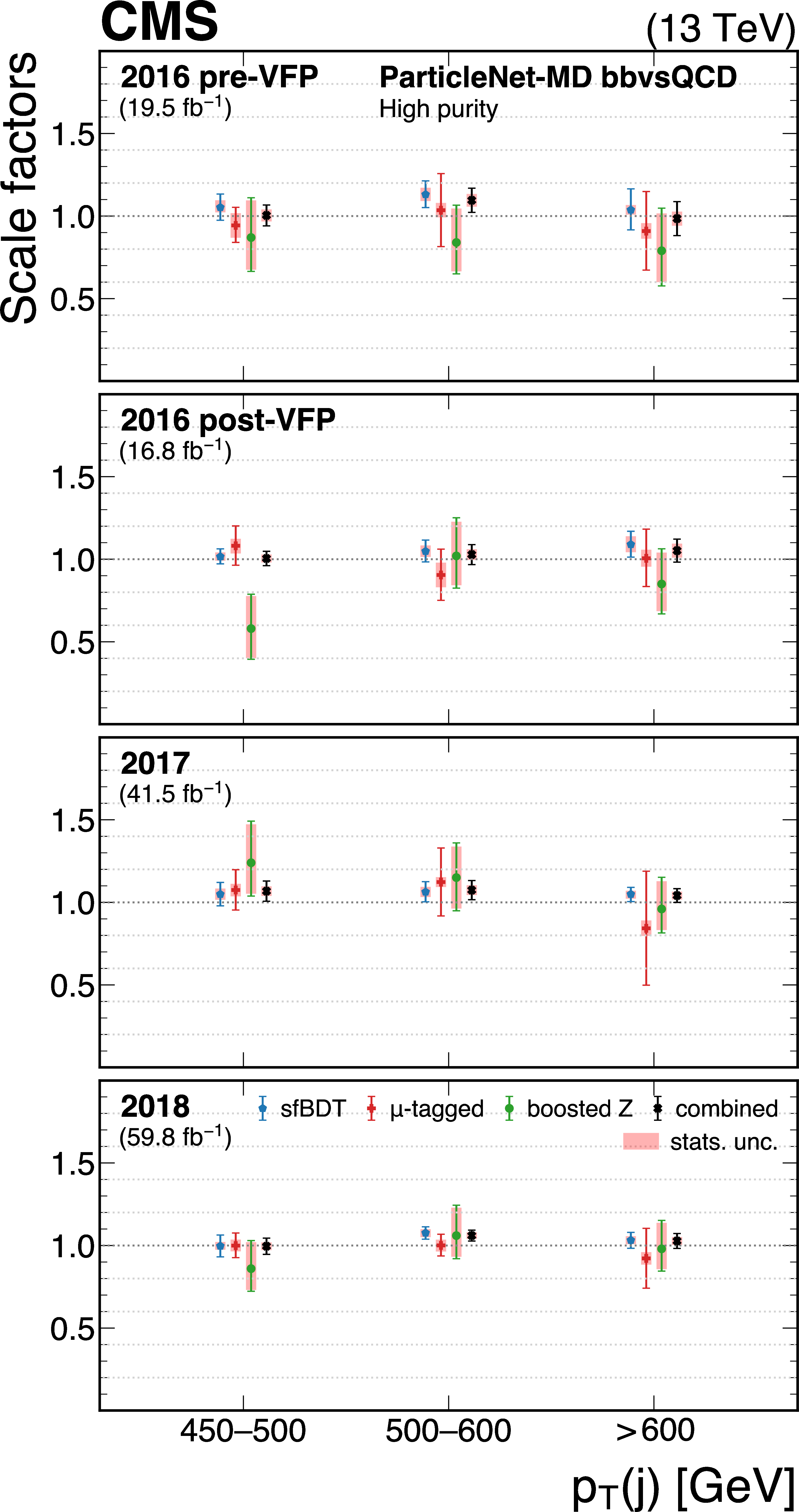
Figure 28:
The measured scale factors of the ParticleNet-MD $ \mathrm{X} \to \mathrm{b} \overline{\mathrm{b}} $ discriminant in the high-purity (left), medium-purity (middle), and low-purity (right) working points. Three methods are presented in the measurements: the sfBDT method, the $ \mu $-tagged method, and the boosted Z boson method. The combined measurements from available methods are also shown. |
png pdf |
Figure 28-a:
The measured scale factors of the ParticleNet-MD $ \mathrm{X} \to \mathrm{b} \overline{\mathrm{b}} $ discriminant in the high-purity (left), medium-purity (middle), and low-purity (right) working points. Three methods are presented in the measurements: the sfBDT method, the $ \mu $-tagged method, and the boosted Z boson method. The combined measurements from available methods are also shown. |
png pdf |
Figure 28-b:
The measured scale factors of the ParticleNet-MD $ \mathrm{X} \to \mathrm{b} \overline{\mathrm{b}} $ discriminant in the high-purity (left), medium-purity (middle), and low-purity (right) working points. Three methods are presented in the measurements: the sfBDT method, the $ \mu $-tagged method, and the boosted Z boson method. The combined measurements from available methods are also shown. |
png pdf |
Figure 28-c:
The measured scale factors of the ParticleNet-MD $ \mathrm{X} \to \mathrm{b} \overline{\mathrm{b}} $ discriminant in the high-purity (left), medium-purity (middle), and low-purity (right) working points. Three methods are presented in the measurements: the sfBDT method, the $ \mu $-tagged method, and the boosted Z boson method. The combined measurements from available methods are also shown. |
png pdf |
Figure 29:
The measured scale factors of the DeepDoubleX $ \mathrm{X} \to \mathrm{b} \overline{\mathrm{b}} $ discriminant in the high-purity (left), medium-purity (middle), and low-purity (right) working points. Three methods are presented in the measurements: the sfBDT method, the $ \mu $-tagged method, and the boosted Z boson method. The combined measurements from available methods are also shown. |
png pdf |
Figure 29-a:
The measured scale factors of the DeepDoubleX $ \mathrm{X} \to \mathrm{b} \overline{\mathrm{b}} $ discriminant in the high-purity (left), medium-purity (middle), and low-purity (right) working points. Three methods are presented in the measurements: the sfBDT method, the $ \mu $-tagged method, and the boosted Z boson method. The combined measurements from available methods are also shown. |
png pdf |
Figure 29-b:
The measured scale factors of the DeepDoubleX $ \mathrm{X} \to \mathrm{b} \overline{\mathrm{b}} $ discriminant in the high-purity (left), medium-purity (middle), and low-purity (right) working points. Three methods are presented in the measurements: the sfBDT method, the $ \mu $-tagged method, and the boosted Z boson method. The combined measurements from available methods are also shown. |
png pdf |
Figure 29-c:
The measured scale factors of the DeepDoubleX $ \mathrm{X} \to \mathrm{b} \overline{\mathrm{b}} $ discriminant in the high-purity (left), medium-purity (middle), and low-purity (right) working points. Three methods are presented in the measurements: the sfBDT method, the $ \mu $-tagged method, and the boosted Z boson method. The combined measurements from available methods are also shown. |
png pdf |
Figure 30:
The measured scale factors of the DeepAK8-MD $ \mathrm{X} \to \mathrm{b} \overline{\mathrm{b}} $ discriminant in the high-purity (left), medium-purity (middle), and low-purity (right) working points. Two methods are presented in the measurements: the sfBDT method and the $ \mu $-tagged method. The combined measurements from available methods are also shown. |
png pdf |
Figure 30-a:
The measured scale factors of the DeepAK8-MD $ \mathrm{X} \to \mathrm{b} \overline{\mathrm{b}} $ discriminant in the high-purity (left), medium-purity (middle), and low-purity (right) working points. Two methods are presented in the measurements: the sfBDT method and the $ \mu $-tagged method. The combined measurements from available methods are also shown. |
png pdf |
Figure 30-b:
The measured scale factors of the DeepAK8-MD $ \mathrm{X} \to \mathrm{b} \overline{\mathrm{b}} $ discriminant in the high-purity (left), medium-purity (middle), and low-purity (right) working points. Two methods are presented in the measurements: the sfBDT method and the $ \mu $-tagged method. The combined measurements from available methods are also shown. |
png pdf |
Figure 30-c:
The measured scale factors of the DeepAK8-MD $ \mathrm{X} \to \mathrm{b} \overline{\mathrm{b}} $ discriminant in the high-purity (left), medium-purity (middle), and low-purity (right) working points. Two methods are presented in the measurements: the sfBDT method and the $ \mu $-tagged method. The combined measurements from available methods are also shown. |
png pdf |
Figure 31:
The measured scale factors of the double-b $ \mathrm{X} \to \mathrm{b} \overline{\mathrm{b}} $ discriminant in the high-purity (left), medium-purity (middle), and low-purity (right) working points. Three methods are presented in the measurements: the sfBDT method, the $ \mu $-tagged method, and the boosted Z boson method. The combined measurements from available methods are also shown. |
png pdf |
Figure 31-a:
The measured scale factors of the double-b $ \mathrm{X} \to \mathrm{b} \overline{\mathrm{b}} $ discriminant in the high-purity (left), medium-purity (middle), and low-purity (right) working points. Three methods are presented in the measurements: the sfBDT method, the $ \mu $-tagged method, and the boosted Z boson method. The combined measurements from available methods are also shown. |
png pdf |
Figure 31-b:
The measured scale factors of the double-b $ \mathrm{X} \to \mathrm{b} \overline{\mathrm{b}} $ discriminant in the high-purity (left), medium-purity (middle), and low-purity (right) working points. Three methods are presented in the measurements: the sfBDT method, the $ \mu $-tagged method, and the boosted Z boson method. The combined measurements from available methods are also shown. |
png pdf |
Figure 31-c:
The measured scale factors of the double-b $ \mathrm{X} \to \mathrm{b} \overline{\mathrm{b}} $ discriminant in the high-purity (left), medium-purity (middle), and low-purity (right) working points. Three methods are presented in the measurements: the sfBDT method, the $ \mu $-tagged method, and the boosted Z boson method. The combined measurements from available methods are also shown. |
png pdf |
Figure 32:
The measured scale factors of the ParticleNet-MD $ \mathrm{X} \to \mathrm{c} \overline{\mathrm{c}} $ discriminant in the high-purity (left), medium-purity (middle), and low-purity (right) working points. Two methods are presented in the measurements: the sfBDT method and the $ \mu $-tagged method. The combined measurements from available methods are also shown. |
png pdf |
Figure 32-a:
The measured scale factors of the ParticleNet-MD $ \mathrm{X} \to \mathrm{c} \overline{\mathrm{c}} $ discriminant in the high-purity (left), medium-purity (middle), and low-purity (right) working points. Two methods are presented in the measurements: the sfBDT method and the $ \mu $-tagged method. The combined measurements from available methods are also shown. |
png pdf |
Figure 32-b:
The measured scale factors of the ParticleNet-MD $ \mathrm{X} \to \mathrm{c} \overline{\mathrm{c}} $ discriminant in the high-purity (left), medium-purity (middle), and low-purity (right) working points. Two methods are presented in the measurements: the sfBDT method and the $ \mu $-tagged method. The combined measurements from available methods are also shown. |
png pdf |
Figure 32-c:
The measured scale factors of the ParticleNet-MD $ \mathrm{X} \to \mathrm{c} \overline{\mathrm{c}} $ discriminant in the high-purity (left), medium-purity (middle), and low-purity (right) working points. Two methods are presented in the measurements: the sfBDT method and the $ \mu $-tagged method. The combined measurements from available methods are also shown. |
png pdf |
Figure 33:
The measured scale factors of the DeepDoubleX $ \mathrm{X} \to \mathrm{c} \overline{\mathrm{c}} $ discriminant in the high-purity (left), medium-purity (middle), and low-purity (right) working points. Two methods are presented in the measurements: the sfBDT method and the $ \mu $-tagged method. The combined measurements from available methods are also shown. |
png pdf |
Figure 33-a:
The measured scale factors of the DeepDoubleX $ \mathrm{X} \to \mathrm{c} \overline{\mathrm{c}} $ discriminant in the high-purity (left), medium-purity (middle), and low-purity (right) working points. Two methods are presented in the measurements: the sfBDT method and the $ \mu $-tagged method. The combined measurements from available methods are also shown. |
png pdf |
Figure 33-b:
The measured scale factors of the DeepDoubleX $ \mathrm{X} \to \mathrm{c} \overline{\mathrm{c}} $ discriminant in the high-purity (left), medium-purity (middle), and low-purity (right) working points. Two methods are presented in the measurements: the sfBDT method and the $ \mu $-tagged method. The combined measurements from available methods are also shown. |
png pdf |
Figure 33-c:
The measured scale factors of the DeepDoubleX $ \mathrm{X} \to \mathrm{c} \overline{\mathrm{c}} $ discriminant in the high-purity (left), medium-purity (middle), and low-purity (right) working points. Two methods are presented in the measurements: the sfBDT method and the $ \mu $-tagged method. The combined measurements from available methods are also shown. |
png pdf |
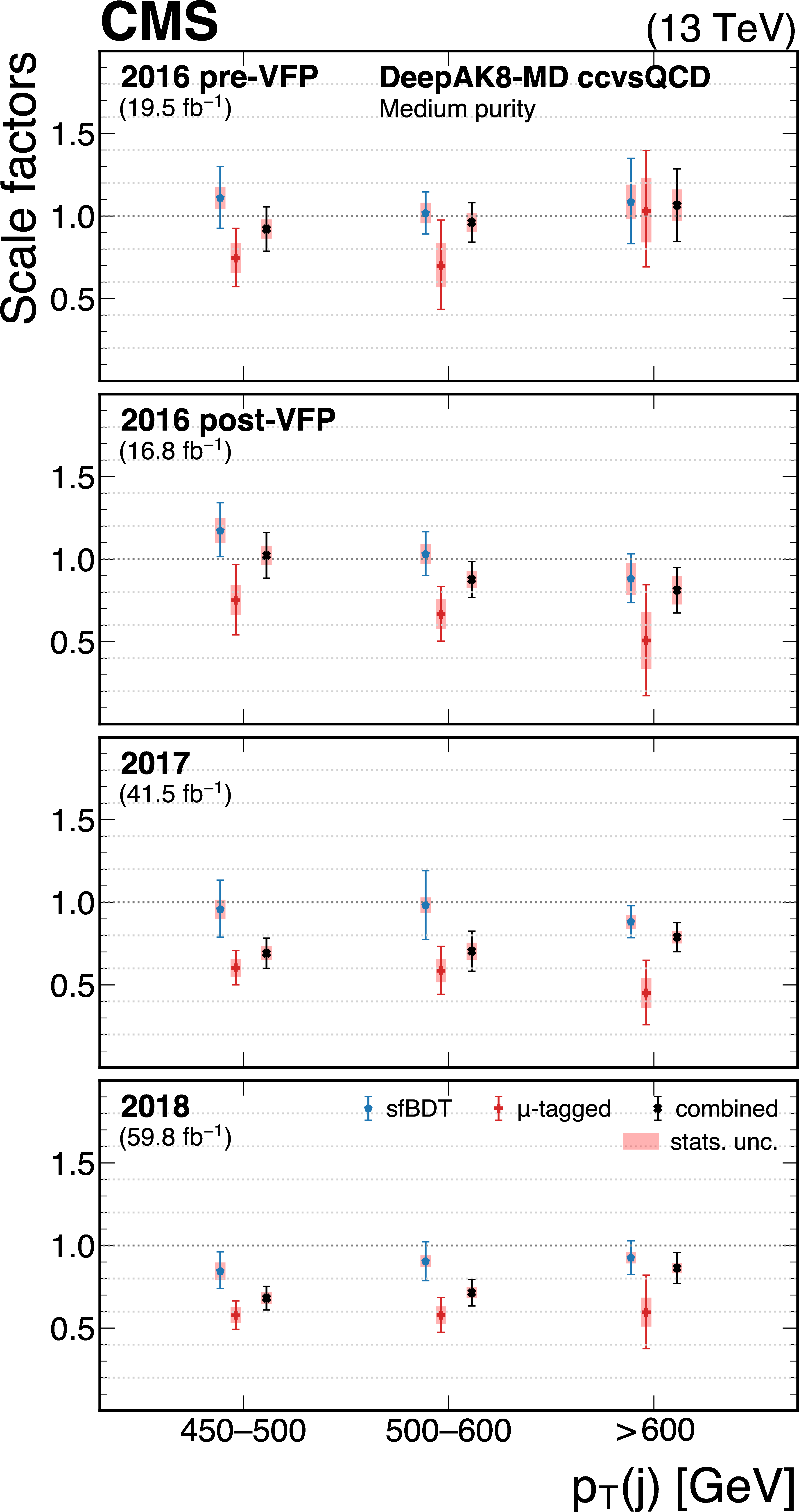
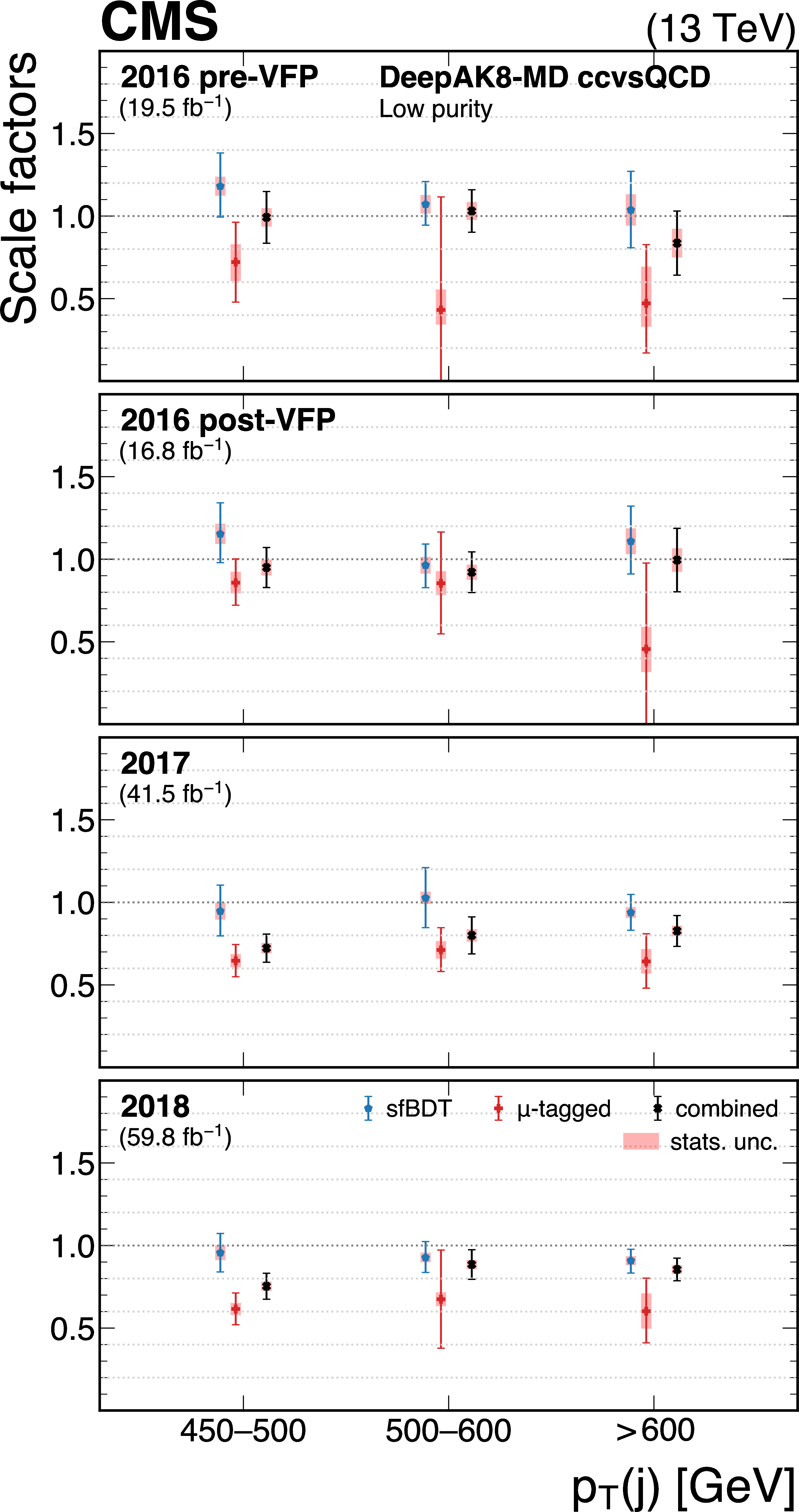
Figure 34:
The measured scale factors of the DeepAK8-MD $ \mathrm{X} \to \mathrm{c} \overline{\mathrm{c}} $ discriminant in the high-purity (left), medium-purity (middle), and low-purity (right) working points. Two methods are presented in the measurements: the sfBDT method and the $ \mu $-tagged method. The combined measurements from available methods are also shown. |
png pdf |
Figure 34-a:
The measured scale factors of the DeepAK8-MD $ \mathrm{X} \to \mathrm{c} \overline{\mathrm{c}} $ discriminant in the high-purity (left), medium-purity (middle), and low-purity (right) working points. Two methods are presented in the measurements: the sfBDT method and the $ \mu $-tagged method. The combined measurements from available methods are also shown. |
png pdf |
Figure 34-b:
The measured scale factors of the DeepAK8-MD $ \mathrm{X} \to \mathrm{c} \overline{\mathrm{c}} $ discriminant in the high-purity (left), medium-purity (middle), and low-purity (right) working points. Two methods are presented in the measurements: the sfBDT method and the $ \mu $-tagged method. The combined measurements from available methods are also shown. |
png pdf |
Figure 34-c:
The measured scale factors of the DeepAK8-MD $ \mathrm{X} \to \mathrm{c} \overline{\mathrm{c}} $ discriminant in the high-purity (left), medium-purity (middle), and low-purity (right) working points. Two methods are presented in the measurements: the sfBDT method and the $ \mu $-tagged method. The combined measurements from available methods are also shown. |
| Tables | |
png pdf |
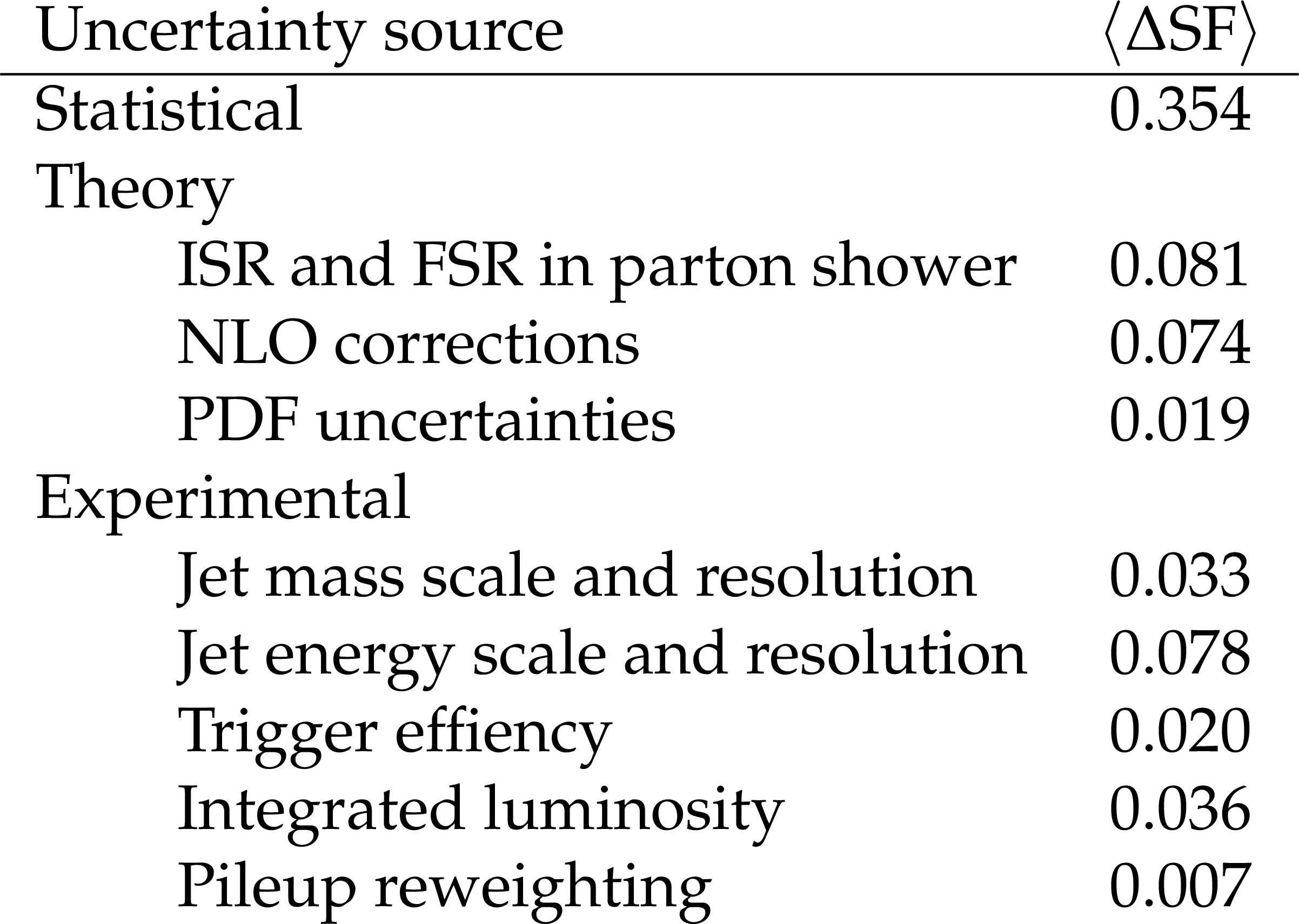
Table 1:
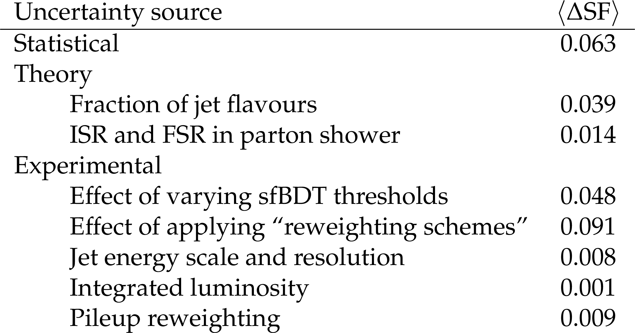
Breakdown of the contributions to the total uncertainty in the fitted scale factor (SF) of the ParticleNet-MD $ \mathrm{X} \to \mathrm{b} \overline{\mathrm{b}} $ discriminant at the high-purity working point, using the sfBDT method. The numbers are averaged over multiple SF derivation points, including all relevant $ p_{\mathrm{T}} $ bins and data-taking eras. |
png pdf |
Table 2:
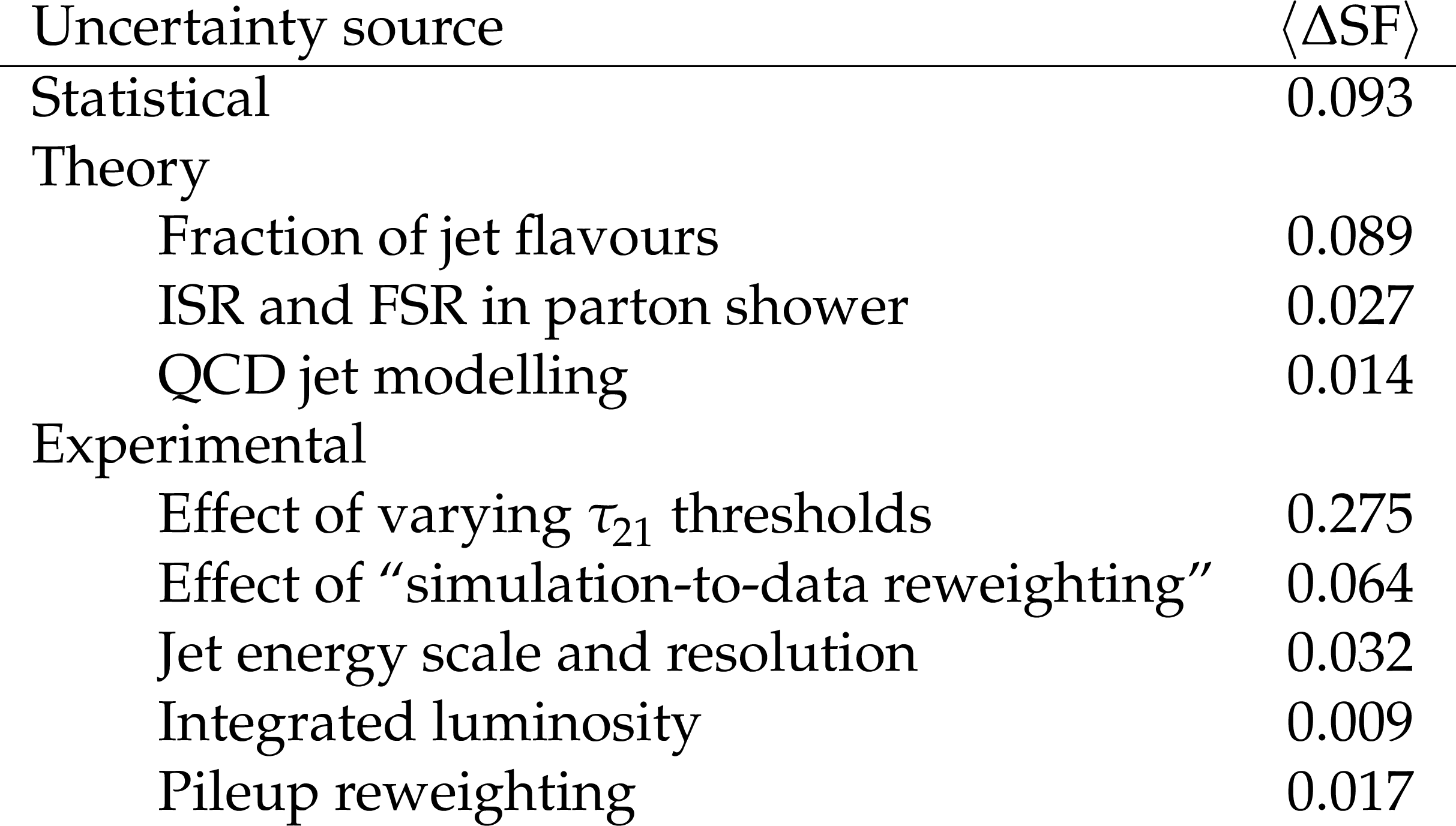
Breakdown of the contributions to the total uncertainty in the fitted scale factor (SF) of the ParticleNet-MD $ \mathrm{X} \to \mathrm{b} \overline{\mathrm{b}} $ discriminant at the high-purity working point, using the $ \mu $-tagged method. The numbers are averaged over multiple SF derivation points, including all relevant $ p_{\mathrm{T}} $ bins and data-taking eras. |
png pdf |
Table 3:
Breakdown of the contributions to the total uncertainty in the fitted scale factor (SF) of the ParticleNet-MD $ \mathrm{X} \to \mathrm{b} \overline{\mathrm{b}} $ discriminant at the high-purity working point, using the boosted Z boson method. The numbers are averaged over multiple SF derivation points, including all relevant $ p_{\mathrm{T}} $ bins and data-taking eras. |
| Summary |
| This paper presents the performance of heavy-flavour $ \mathrm{X} \to \mathrm{b} \overline{\mathrm{b}} $ and $ \mathrm{X} \to \mathrm{c} \overline{\mathrm{c}} $ jet tagging algorithms in the boosted topology, with a focus on the performance of various taggers in simulation and the calibration of tagging efficiencies using data collected by the CMS detector during the 2016-2018 data-taking period (LHC Run 2). With the boosted topology gaining increasing relevance in physics searches during Run 2, the development of dedicated jet-tagging techniques and robust calibration methods for taggers on data has become increasingly important. In this paper, we first provide a complete review and a comparison of $ \mathrm{X} \to \mathrm{b} \overline{\mathrm{b}} $ and $ \mathrm{X} \to \mathrm{c} \overline{\mathrm{c}} $ tagging algorithms, which were developed by the CMS Collaboration for analyzing Run 2 data and have been used for various physics measurements. These algorithms include the ParticleNet-MD, DeepDoubleX, DeepAK8-MD, and the double-b tagging algorithms. Three methods for evaluating the performance of the algorithms on data, in terms of deriving the scale factors to correct the selection efficiency of simulated $ \mathrm{X} \to \mathrm{b} \overline{\mathrm{b}} $ and $ \mathrm{X} \to \mathrm{c} \overline{\mathrm{c}} $ jets, are presented in detail. The three methods define the proxy jets based on (1) a novel phase space selected from gluon-splitting $ \mathrm{b} \overline{\mathrm{b}} $ and $ \mathrm{c} \overline{\mathrm{c}} $ jets via a dedicated boosted decision tree discriminant; (2) gluon-splitting $ \mathrm{b} \overline{\mathrm{b}} $ and $ \mathrm{c} \overline{\mathrm{c}} $ jets containing a soft muon, with an auxiliary selection on the $ N $-subjettiness variable; and (3) boosted $ \mathrm{Z} \to \mathrm{b} \overline{\mathrm{b}} $ jets for representing the $ \mathrm{X} \to \mathrm{b} \overline{\mathrm{b}} $ signal jet. The phase space of the selected proxy jets is largely orthogonal across the methods, which enables a meaningful comparison of their calibration results. Scale factors and their uncertainties are derived for all working points of the seven tagging discriminants developed for $ \mathrm{X} \to \mathrm{b} \overline{\mathrm{b}} $ and $ \mathrm{X} \to \mathrm{c} \overline{\mathrm{c}} $ tagging. These scale factors are presented both individually and in a combined form, obtained using the best linear unbiased estimator method. A reasonable agreement is found when comparing the results with previous CMS studies, which calibrated some of the discriminants studied in this work, either partially or under full Run 2 conditions. Additionally, the scale factors presented by the three methods remain consistent within the uncertainty range. Their combination provides the highest measurement precision for the scale factor while also reducing the systematic biases inherent to each individual method. The tagging algorithms and calibration approaches documented in this paper serve as a comprehensive summary and are considered as benchmarks for the techniques adopted by the CMS Collaboration during Run 2. These outcomes will facilitate further in-depth studies and wider experimental explorations of the boosted phase space with heavy-flavour tagging in the future. |
| References | ||||
| 1 | CMS Collaboration | Identification of heavy-flavour jets with the CMS detector in pp collisions at 13 TeV | JINST 13 (2018) P05011 | CMS-BTV-16-002 1712.07158 |
| 2 | ATLAS Collaboration | Identification of boosted Higgs bosons decaying into $ b $-quark pairs with the ATLAS detector at 13 TeV | EPJC 79 (2019) 836 | 1906.11005 |
| 3 | ATLAS Collaboration | Identification of boosted Higgs bosons decaying into $ b\overline{b} $ with neural networks and variable radius subjets in ATLAS | ATLAS PUB Note ATL-PHYS-PUB-2020-019, 2020 | |
| 4 | CMS Collaboration | Identification of heavy, energetic, hadronically decaying particles using machine-learning techniques | JINST 15 (2020) P06005 | CMS-JME-18-002 2004.08262 |
| 5 | ATLAS Collaboration | Identification of hadronically-decaying top quarks using UFO jets with ATLAS in Run 2 | ATLAS PUB Note ATL-PHYS-PUB-2021-028, 2021 | |
| 6 | ATLAS Collaboration | Performance of $ W $/$ Z $ taggers using UFO jets in ATLAS | ATLAS PUB Note ATL-PHYS-PUB-2021-029, 2021 | |
| 7 | CMS Collaboration | Identification of highly Lorentz-boosted heavy particles using graph neural networks and new mass decorrelation techniques | CMS Detector Performance Note CMS-DP-2020-002, 2020 CDS |
|
| 8 | CMS Collaboration | Performance of the mass-decorrelated DeepDoubleX classifier for double-b and double-c large-radius jets with the CMS detector | CMS Detector Performance Note CMS-DP-2022-041, 2022 CDS |
|
| 9 | CMS Collaboration | Inclusive search for a highly boosted Higgs boson decaying to a bottom quark-antiquark pair | PRL 120 (2018) 071802 | CMS-HIG-17-010 1709.05543 |
| 10 | CMS Collaboration | Inclusive search for highly boosted Higgs bosons decaying to bottom quark-antiquark pairs in proton-proton collisions at $ \sqrt{s} = $ 13 TeV | JHEP 12 (2020) 085 | CMS-HIG-19-003 2006.13251 |
| 11 | CMS Collaboration | Search for nonresonant pair production of highly energetic Higgs bosons decaying to bottom quarks | PRL 131 (2023) 041803 | 2205.06667 |
| 12 | CMS Collaboration | A search for the standard model Higgs boson decaying to charm quarks | JHEP 03 (2020) 131 | CMS-HIG-18-031 1912.01662 |
| 13 | CMS Collaboration | Search for Higgs boson decay to a charm quark-antiquark pair in proton-proton collisions at $ \sqrt{s} = $ 13 TeV | PRL 131 (2023) 061801 | CMS-HIG-21-008 2205.05550 |
| 14 | CMS Collaboration | Search for Higgs boson and observation of Z boson through their decay into a charm quark-antiquark pair in boosted topologies in proton-proton collisions at $ \sqrt{s} = $ 13 TeV | PRL 131 (2023) 041801 | CMS-HIG-21-012 2211.14181 |
| 15 | CMS Collaboration | Search for a massive scalar resonance decaying to a light scalar and a Higgs boson in the four b quarks final state with boosted topology | PLB 842 (2023) 137392 | 2204.12413 |
| 16 | CMS Collaboration | The CMS experiment at the CERN LHC | JINST 3 (2008) S08004 | |
| 17 | CMS Collaboration | Development of the CMS detector for the CERN LHC Run 3 | JINST 19 (2024) P05064 | |
| 18 | CMS Collaboration | The CMS trigger system | JINST 12 (2017) P01020 | CMS-TRG-12-001 1609.02366 |
| 19 | CMS Collaboration | Performance of the CMS Level-1 trigger in proton-proton collisions at $ \sqrt{s} = $ 13 TeV | JINST 15 (2020) P10017 | CMS-TRG-17-001 2006.10165 |
| 20 | J. Alwall et al. | The automated computation of tree-level and next-to-leading order differential cross sections, and their matching to parton shower simulations | JHEP 07 (2014) 079 | 1405.0301 |
| 21 | P. Nason | A new method for combining NLO QCD with shower Monte Carlo algorithms | JHEP 11 (2004) 040 | hep-ph/0409146 |
| 22 | S. Frixione, P. Nason, and C. Oleari | Matching NLO QCD computations with parton shower simulations: the POWHEG method | JHEP 11 (2007) 070 | 0709.2092 |
| 23 | S. Alioli, P. Nason, C. Oleari, and E. Re | A general framework for implementing NLO calculations in shower Monte Carlo programs: the POWHEG BOX | JHEP 06 (2010) 043 | 1002.2581 |
| 24 | J. M. Campbell, R. K. Ellis, P. Nason, and E. Re | Top-pair production and decay at NLO matched with parton showers | JHEP 04 (2015) 114 | 1412.1828 |
| 25 | M. Czakon and A. Mitov | Top++: A program for the calculation of the top-pair cross-section at hadron colliders | Comput. Phys. Commun. 185 (2014) 2930 | 1112.5675 |
| 26 | S. Frixione et al. | Single-top hadroproduction in association with a W boson | JHEP 07 (2008) 029 | 0805.3067 |
| 27 | S. Alioli, P. Nason, C. Oleari, and E. Re | NLO single-top production matched with shower in POWHEG: $ s $- and $ t $-channel contributions | JHEP 09 (2009) 111 | 0907.4076 |
| 28 | E. Re | Single-top Wt-channel production matched with parton showers using the POWHEG method | EPJC 71 (2011) 1547 | 1009.2450 |
| 29 | R. Frederix, E. Re, and P. Torrielli | Single-top $ t $-channel hadroproduction in the four-flavour scheme with POWHEG and aMC@NLO | JHEP 09 (2012) 130 | 1207.5391 |
| 30 | N. Kidonakis | NNLL threshold resummation for top-pair and single-top production | Phys. Part. Nucl. 45 (2014) 714 | 1210.7813 |
| 31 | T. Sjostrand et al. | An introduction to PYTHIA 8.2 | Comput. Phys. Commun. 191 (2015) 159 | 1410.3012 |
| 32 | CMS Collaboration | Extraction and validation of a new set of CMS PYTHIA8 tunes from underlying-event measurements | EPJC 80 (2020) 4 | CMS-GEN-17-001 1903.12179 |
| 33 | NNPDF Collaboration | Parton distributions from high-precision collider data | EPJC 77 (2017) 663 | 1706.00428 |
| 34 | J. Alwall et al. | Comparative study of various algorithms for the merging of parton showers and matrix elements in hadronic collisions | EPJC 53 (2008) 473 | 0706.2569 |
| 35 | R. Frederix and S. Frixione | Merging meets matching in MC@NLO | JHEP 12 (2012) 061 | 1209.6215 |
| 36 | J. M. Lindert et al. | Precise predictions for V+jets dark matter backgrounds | EPJC 77 (2017) 829 | 1705.04664 |
| 37 | K. Hamilton, P. Nason, C. Oleari, and G. Zanderighi | Merging H/W/Z + 0 and 1 jet at NLO with no merging scale: a path to parton shower + NNLO matching | JHEP 05 (2013) 082 | 1212.4504 |
| 38 | G. Luisoni, P. Nason, C. Oleari, and F. Tramontano | $ \mathrm{H}\mathrm{W}^{\pm} $/$\mathrm{HZ}$+0 and 1 jet at NLO with the POWHEG box interfaced to GoSam and their merging within MINLO | JHEP 10 (2013) 083 | 1306.2542 |
| 39 | GEANT4 Collaboration | GEANT4---a simulation toolkit | NIM A 506 (2003) 250 | |
| 40 | CMS Collaboration | Simulation of the Silicon Strip Tracker pre-amplifier in early 2016 data | CMS Detector Performance Note CMS-DP-2020-045, 2020 CDS |
|
| 41 | CMS Collaboration | Particle-flow reconstruction and global event description with the CMS detector | JINST 12 (2017) P10003 | CMS-PRF-14-001 1706.04965 |
| 42 | CMS Collaboration | Technical proposal for the Phase-II upgrade of the Compact Muon Solenoid | CMS Technical Proposal CERN-LHCC-2015-010, CMS-TDR-15-02, 2015 CDS |
|
| 43 | CMS Collaboration | Measurement of $ {\text{B}}\overline{\text{B}} $ angular correlations based on secondary vertex reconstruction at $ \sqrt{s}= $ 7 TeV | JHEP 03 (2011) 136 | CMS-BPH-10-010 1102.3194 |
| 44 | CMS Collaboration | Electron and photon reconstruction and identification with the CMS experiment at the CERN LHC | JINST 16 (2021) P05014 | CMS-EGM-17-001 2012.06888 |
| 45 | CMS Collaboration | Performance of the CMS muon detector and muon reconstruction with proton-proton collisions at $ \sqrt{s}= $ 13 TeV | JINST 13 (2018) P06015 | CMS-MUO-16-001 1804.04528 |
| 46 | M. Cacciari, G. P. Salam, and G. Soyez | The anti-$ k_{\mathrm{T}} $ jet clustering algorithm | JHEP 04 (2008) 063 | 0802.1189 |
| 47 | CMS Collaboration | Jet energy scale and resolution in the CMS experiment in pp collisions at 8 TeV | JINST 12 (2017) P02014 | CMS-JME-13-004 1607.03663 |
| 48 | D. Bertolini, P. Harris, M. Low, and N. Tran | Pileup per particle identification | JHEP 10 (2014) 059 | 1407.6013 |
| 49 | CMS Collaboration | Pileup mitigation at CMS in 13 TeV data | JINST 15 (2020) P09018 | CMS-JME-18-001 2003.00503 |
| 50 | J. Thaler and K. Van Tilburg | Identifying boosted objects with $ N $-subjettiness | JHEP 03 (2011) 015 | 1011.2268 |
| 51 | A. J. Larkoski, S. Marzani, G. Soyez, and J. Thaler | Soft drop | JHEP 05 (2014) 146 | 1402.2657 |
| 52 | CMS Collaboration | Mass regression of highly-boosted jets using graph neural networks | CMS Detector Performance Note CMS-DP-2021-017, 2021 CDS |
|
| 53 | H. Qu and L. Gouskos | Jet tagging via particle clouds | PRD 101 (2020) 056019 | 1902.08570 |
| 54 | M. Cacciari and G. P. Salam | Pileup subtraction using jet areas | PLB 659 (2008) 119 | 0707.1378 |
| 55 | CMS Collaboration | Performance of deep tagging algorithms for boosted double quark jet topology in proton-proton collisions at 13 TeV with the Phase-0 CMS detector | CMS Detector Performance Note CMS-DP-2018-046, 2018 CDS |
|
| 56 | E. Bols et al. | Jet flavour classification using DeepJet | JINST 15 (2020) P12012 | 2008.10519 |
| 57 | K. He, X. Zhang, S. Ren, and J. Sun | Deep residual learning for image recognition | in Proc. IEEE Conf. on Computer Vision and Pattern Recognition, p. 770. 2016 link |
|
| 58 | CMS Collaboration | Calibration of the mass-decorrelated ParticleNet tagger for boosted $ \mathrm{b} \overline{\mathrm{b}} $ and $ \mathrm{c} \overline{\mathrm{c}} $ jets using LHC Run 2 data | CMS Detector Performance Note CMS-DP-2022-005, 2022 CDS |
|
| 59 | S. Catani, Y. L. Dokshitzer, M. H. Seymour, and B. R. Webber | Longitudinally-invariant $ k_\perp $-clustering algorithms for hadron-hadron collisions | NPB 406 (1993) 187 | |
| 60 | S. D. Ellis and D. E. Soper | Successive combination jet algorithm for hadron collisions | PRD 48 (1993) 3160 | hep-ph/9305266 |
| 61 | CMS Collaboration | Performance of missing transverse momentum reconstruction in proton-proton collisions at $ \sqrt{s} = $ 13 TeV using the CMS detector | JINST 14 (2019) P07004 | CMS-JME-17-001 1903.06078 |
| 62 | CMS Collaboration | Precision luminosity measurement in proton-proton collisions at $ \sqrt{s} = $ 13 TeV in 2015 and 2016 at CMS | EPJC 81 (2021) 800 | CMS-LUM-17-003 2104.01927 |
| 63 | CMS Collaboration | CMS luminosity measurement for the 2017 data-taking period at $ \sqrt{s} = $ 13 TeV | CMS Physics Analysis Summary, 2018 link |
CMS-PAS-LUM-17-004 |
| 64 | CMS Collaboration | CMS luminosity measurement for the 2018 data-taking period at $ \sqrt{s} = $ 13 TeV | CMS Physics Analysis Summary, 2019 link |
CMS-PAS-LUM-18-002 |
| 65 | CMS Collaboration | Measurement of the inelastic proton-proton cross section at $ \sqrt{s} = $ 13 TeV | JHEP 07 (2018) 161 | CMS-FSQ-15-005 1802.02613 |
| 66 | Particle Data Group | Review of particle physics | PRD 110 (2024) 030001 | |
| 67 | CMS Collaboration | A new calibration method for charm jet identification validated with proton-proton collision events at $ \sqrt{s} = $ 13 TeV | JINST 17 (2022) P03014 | CMS-BTV-20-001 2111.03027 |
| 68 | D. Krohn, J. Thaler, and L.-T. Wang | Jet trimming | JHEP 02 (2010) 084 | 0912.1342 |
| 69 | R. A. Fisher | On the interpretation of $ \chi^{2} $ from contingency tables, and the calculation of P | J. R. Stat. Soc. 85 (1922) 87 | |
| 70 | J. Butterworth et al. | PDF4LHC recommendations for LHC Run II | JPG 43 (2016) 023001 | 1510.03865 |
| 71 | L. Lyons, D. Gibaut, and P. Clifford | How to combine correlated estimates of a single physical quantity | NIM A 270 (1988) 110 | |
| 72 | A. Valassi | Combining correlated measurements of several different physical quantities | NIM A 500 (2003) 391 | |
|
|
Compact Muon Solenoid LHC, CERN |
|

|

|

|

|

|