

Compact Muon Solenoid
LHC, CERN
| CMS-JME-23-001 ; CERN-EP-2025-128 | ||
| A method for correcting the substructure of multiprong jets using the Lund jet plane | ||
| CMS Collaboration | ||
| 10 July 2025 | ||
| JHEP 11 (2025) 038 | ||
| Abstract: Many analyses at the CERN LHC exploit the substructure of jets to identify heavy resonances produced with high momenta that decay into multiple quarks and/or gluons. This paper presents a new technique for correcting the substructure of simulated large-radius jets from multiprong decays. The technique is based on reclustering the jet constituents into several subjets such that each subjet represents a single prong, and separately correcting the radiation pattern in the Lund jet plane of each subjet using a correction derived from data. The data presented here correspond to an integrated luminosity of 138 fb$ ^{-1} $ collected by the CMS experiment between 2016-2018 at a center-of-mass energy of 13 TeV. The correction procedure improves the agreement between data and simulation for several different substructure observables of multiprong jets. This technique establishes, for the first time, a robust calibration for the substructure of jets with four or more prongs, enabling future measurements and searches for new phenomena containing these signatures. | ||
| Links: e-print arXiv:2507.07775 [hep-ex] (PDF) ; CDS record ; inSPIRE record ; CADI line (restricted) ; | ||
| Figures | |
png pdf |
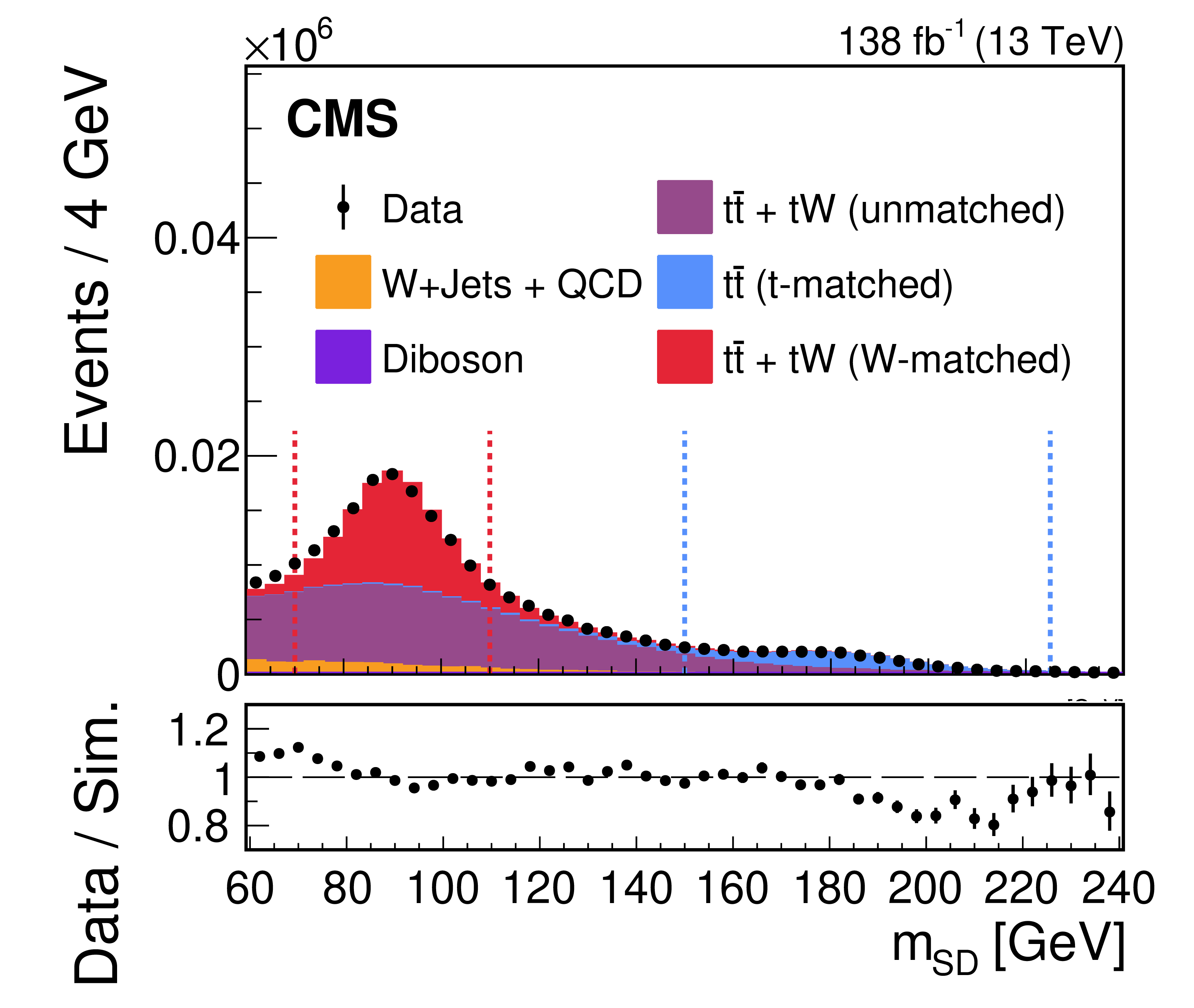
Figure 1:
The distribution of the soft-drop mass for AK8 jets in the lepton+jets $ \mathrm{t} \overline{\mathrm{t}} $ region prior to the LJP density correction. The number of simulated events has been scaled to match the observed number of data events. The lower panel shows the ratio between the observed data and the simulated estimates. Only statistical uncertainties are shown as vertical bars on the data points. The red (blue) dashed vertical lines denote the mass range of 70-110 GeV (150-225 GeV), which defines the W (t) region used in the analysis. |
png pdf |
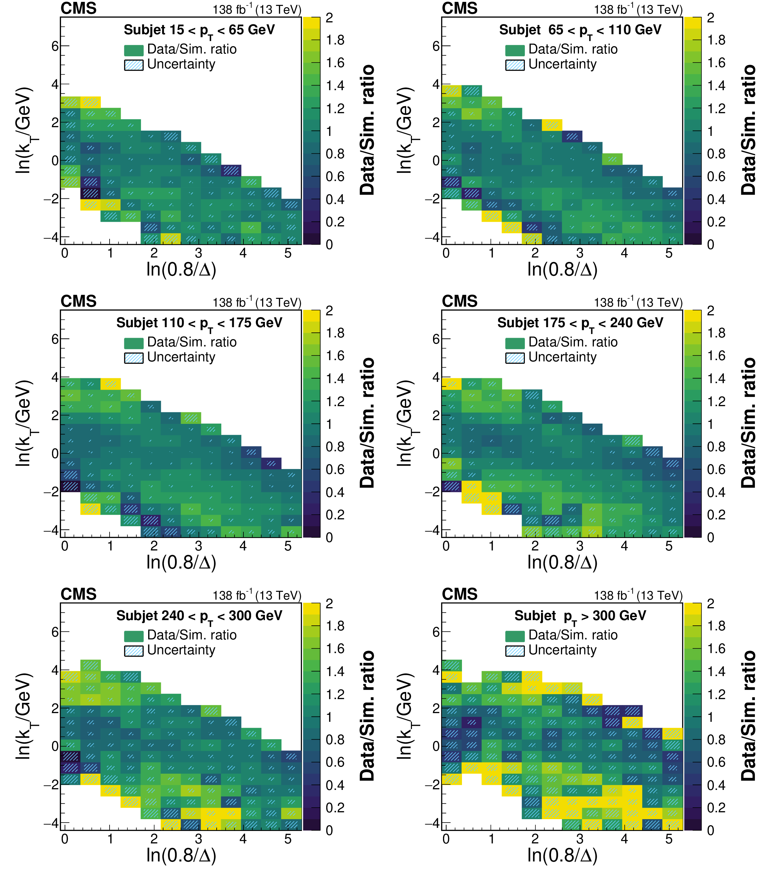
Figure 2:
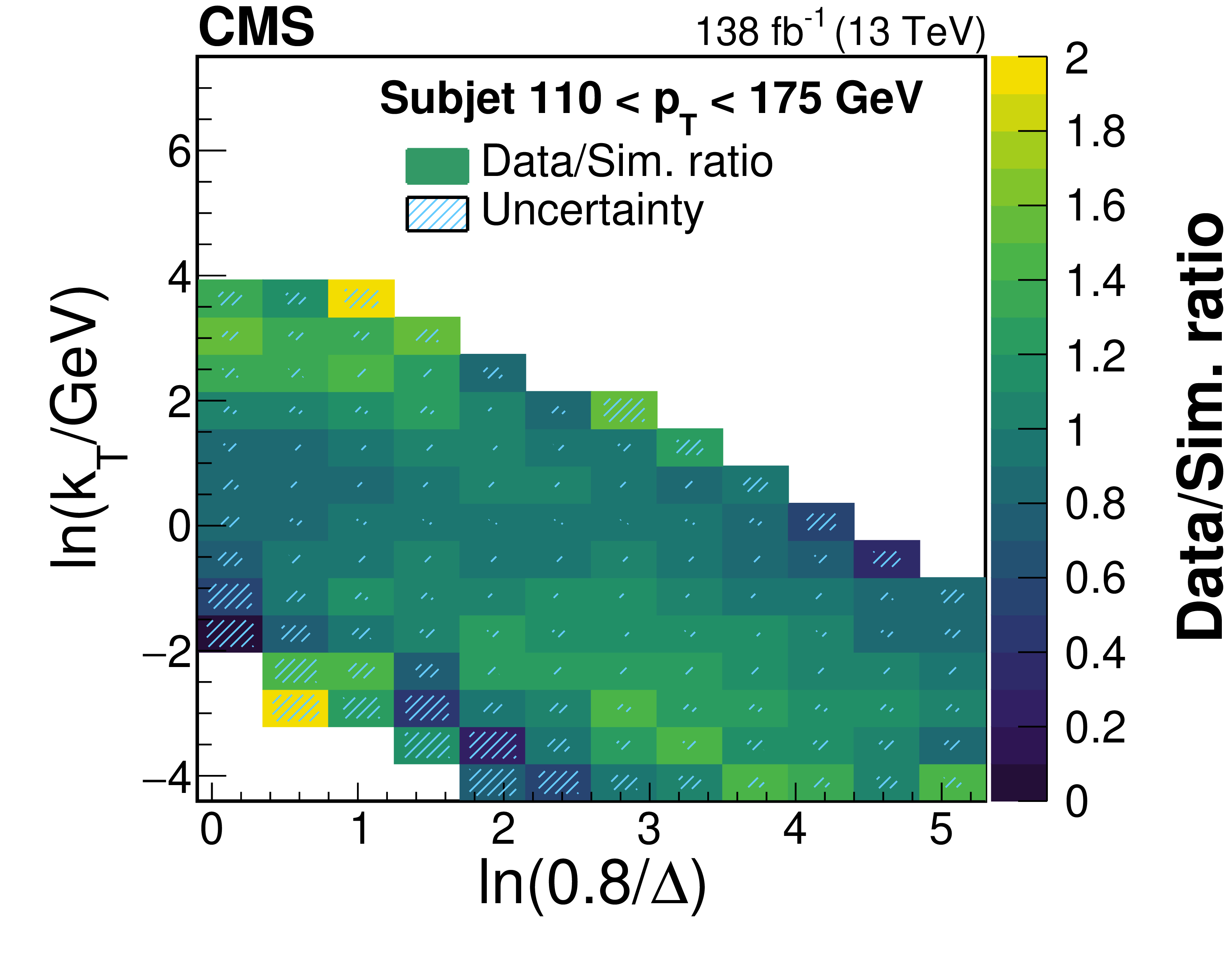
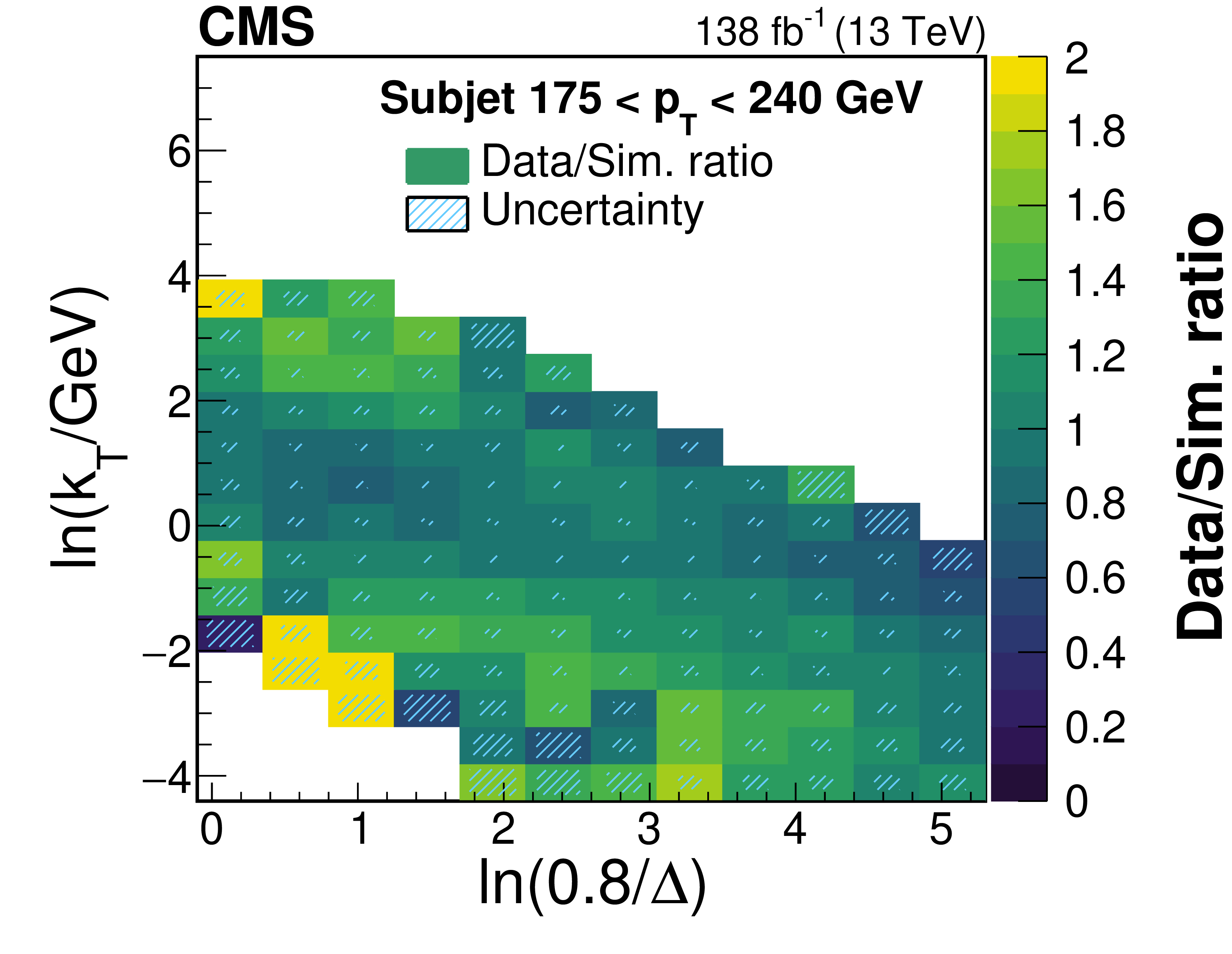
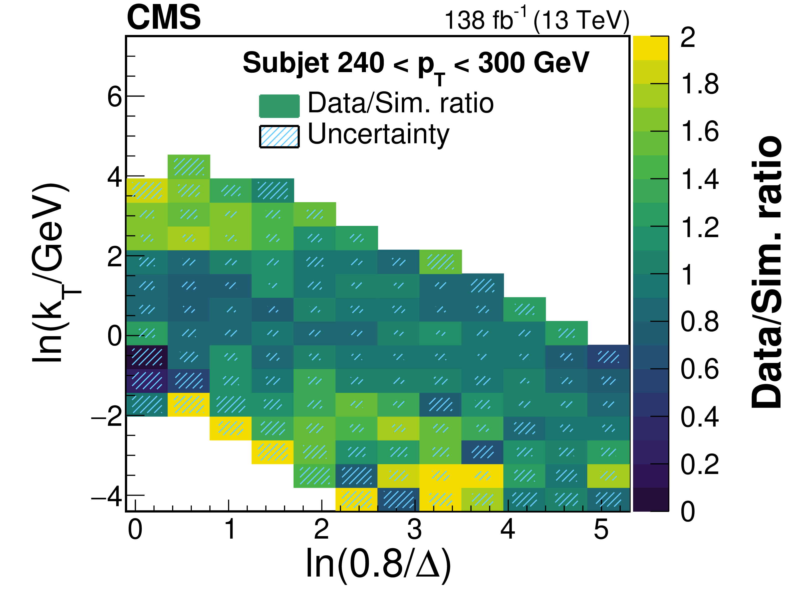
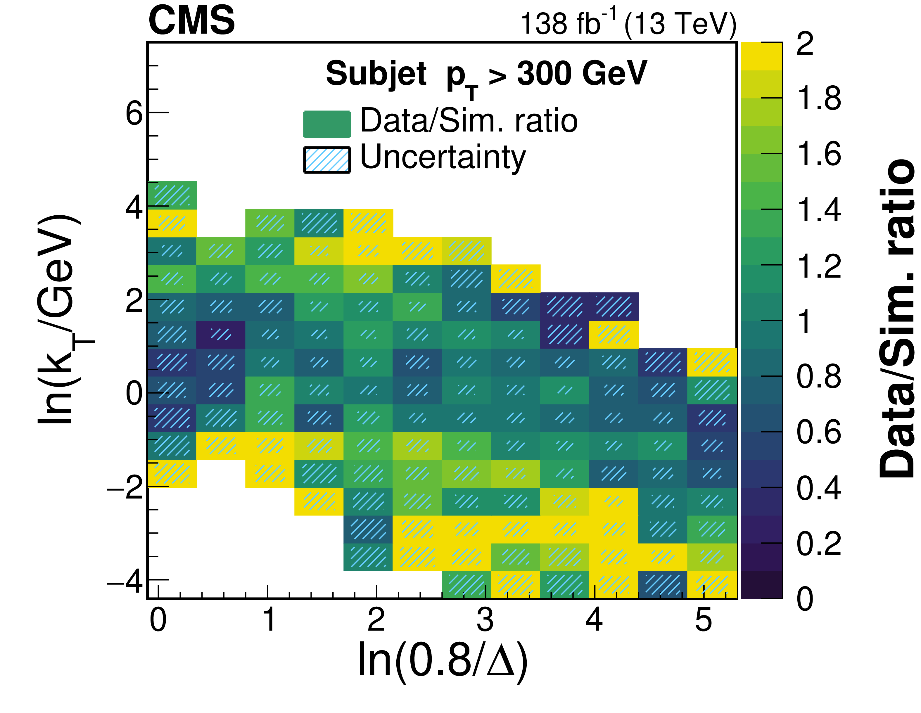
Ratios of the LJP densities between data and simulation in the six subjet $ p_{\mathrm{T}} $ bins. Bins with no data or simulation events are shown as white; in the application of the correction, they are assigned a ratio value of unity and an uncertainty of 100%. The ratio values have been restricted to an upper limit of 2 for visualization purposes. The combined statistical and systematic uncertainty in the ratio is represented by the area of the hatched region in each bin. The fractional size of the hatched region in each bin represents the uncertainty in the measured ratio value in that bin, e.g., for bins in which the hatched region covers half of the area, the fractional uncertainty in the measured ratio is 50%. A description of the considered systematic uncertainties is given in Section 8. The ratios are used to build the corrections to the substructure of a subjet. |
png pdf |
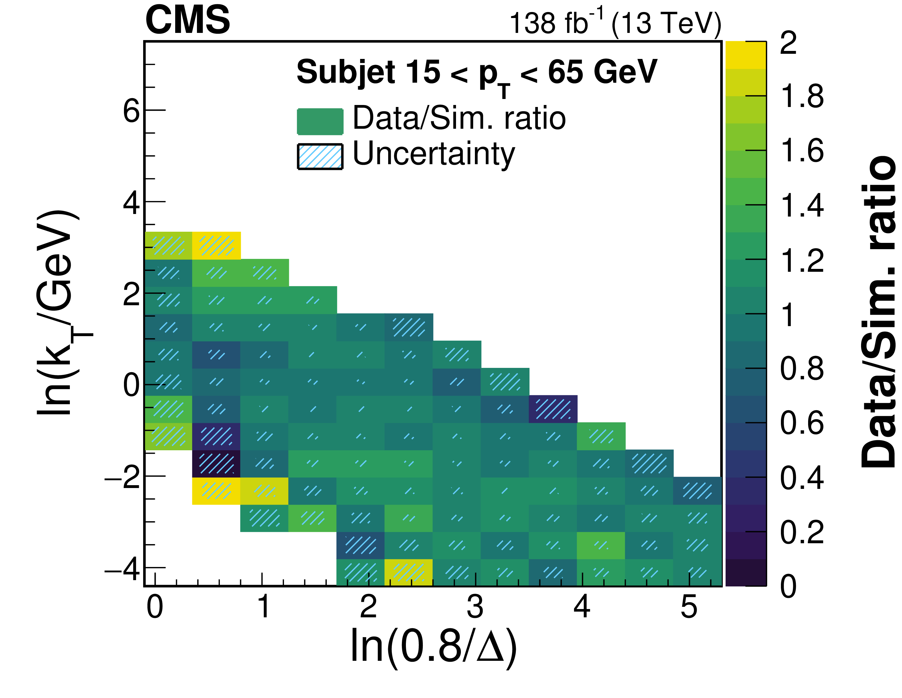
Figure 2-a:
Ratios of the LJP densities between data and simulation in the six subjet $ p_{\mathrm{T}} $ bins. Bins with no data or simulation events are shown as white; in the application of the correction, they are assigned a ratio value of unity and an uncertainty of 100%. The ratio values have been restricted to an upper limit of 2 for visualization purposes. The combined statistical and systematic uncertainty in the ratio is represented by the area of the hatched region in each bin. The fractional size of the hatched region in each bin represents the uncertainty in the measured ratio value in that bin, e.g., for bins in which the hatched region covers half of the area, the fractional uncertainty in the measured ratio is 50%. A description of the considered systematic uncertainties is given in Section 8. The ratios are used to build the corrections to the substructure of a subjet. |
png pdf |
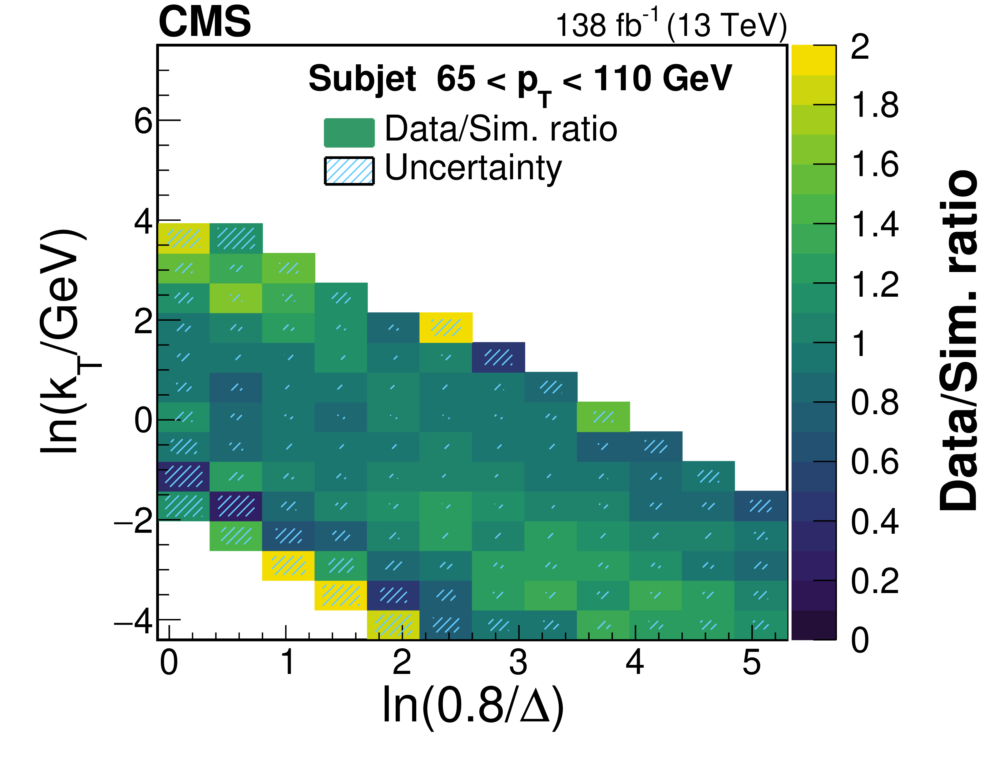
Figure 2-b:
Ratios of the LJP densities between data and simulation in the six subjet $ p_{\mathrm{T}} $ bins. Bins with no data or simulation events are shown as white; in the application of the correction, they are assigned a ratio value of unity and an uncertainty of 100%. The ratio values have been restricted to an upper limit of 2 for visualization purposes. The combined statistical and systematic uncertainty in the ratio is represented by the area of the hatched region in each bin. The fractional size of the hatched region in each bin represents the uncertainty in the measured ratio value in that bin, e.g., for bins in which the hatched region covers half of the area, the fractional uncertainty in the measured ratio is 50%. A description of the considered systematic uncertainties is given in Section 8. The ratios are used to build the corrections to the substructure of a subjet. |
png pdf |
Figure 2-c:
Ratios of the LJP densities between data and simulation in the six subjet $ p_{\mathrm{T}} $ bins. Bins with no data or simulation events are shown as white; in the application of the correction, they are assigned a ratio value of unity and an uncertainty of 100%. The ratio values have been restricted to an upper limit of 2 for visualization purposes. The combined statistical and systematic uncertainty in the ratio is represented by the area of the hatched region in each bin. The fractional size of the hatched region in each bin represents the uncertainty in the measured ratio value in that bin, e.g., for bins in which the hatched region covers half of the area, the fractional uncertainty in the measured ratio is 50%. A description of the considered systematic uncertainties is given in Section 8. The ratios are used to build the corrections to the substructure of a subjet. |
png pdf |
Figure 2-d:
Ratios of the LJP densities between data and simulation in the six subjet $ p_{\mathrm{T}} $ bins. Bins with no data or simulation events are shown as white; in the application of the correction, they are assigned a ratio value of unity and an uncertainty of 100%. The ratio values have been restricted to an upper limit of 2 for visualization purposes. The combined statistical and systematic uncertainty in the ratio is represented by the area of the hatched region in each bin. The fractional size of the hatched region in each bin represents the uncertainty in the measured ratio value in that bin, e.g., for bins in which the hatched region covers half of the area, the fractional uncertainty in the measured ratio is 50%. A description of the considered systematic uncertainties is given in Section 8. The ratios are used to build the corrections to the substructure of a subjet. |
png pdf |
Figure 2-e:
Ratios of the LJP densities between data and simulation in the six subjet $ p_{\mathrm{T}} $ bins. Bins with no data or simulation events are shown as white; in the application of the correction, they are assigned a ratio value of unity and an uncertainty of 100%. The ratio values have been restricted to an upper limit of 2 for visualization purposes. The combined statistical and systematic uncertainty in the ratio is represented by the area of the hatched region in each bin. The fractional size of the hatched region in each bin represents the uncertainty in the measured ratio value in that bin, e.g., for bins in which the hatched region covers half of the area, the fractional uncertainty in the measured ratio is 50%. A description of the considered systematic uncertainties is given in Section 8. The ratios are used to build the corrections to the substructure of a subjet. |
png pdf |
Figure 2-f:
Ratios of the LJP densities between data and simulation in the six subjet $ p_{\mathrm{T}} $ bins. Bins with no data or simulation events are shown as white; in the application of the correction, they are assigned a ratio value of unity and an uncertainty of 100%. The ratio values have been restricted to an upper limit of 2 for visualization purposes. The combined statistical and systematic uncertainty in the ratio is represented by the area of the hatched region in each bin. The fractional size of the hatched region in each bin represents the uncertainty in the measured ratio value in that bin, e.g., for bins in which the hatched region covers half of the area, the fractional uncertainty in the measured ratio is 50%. A description of the considered systematic uncertainties is given in Section 8. The ratios are used to build the corrections to the substructure of a subjet. |
png pdf |
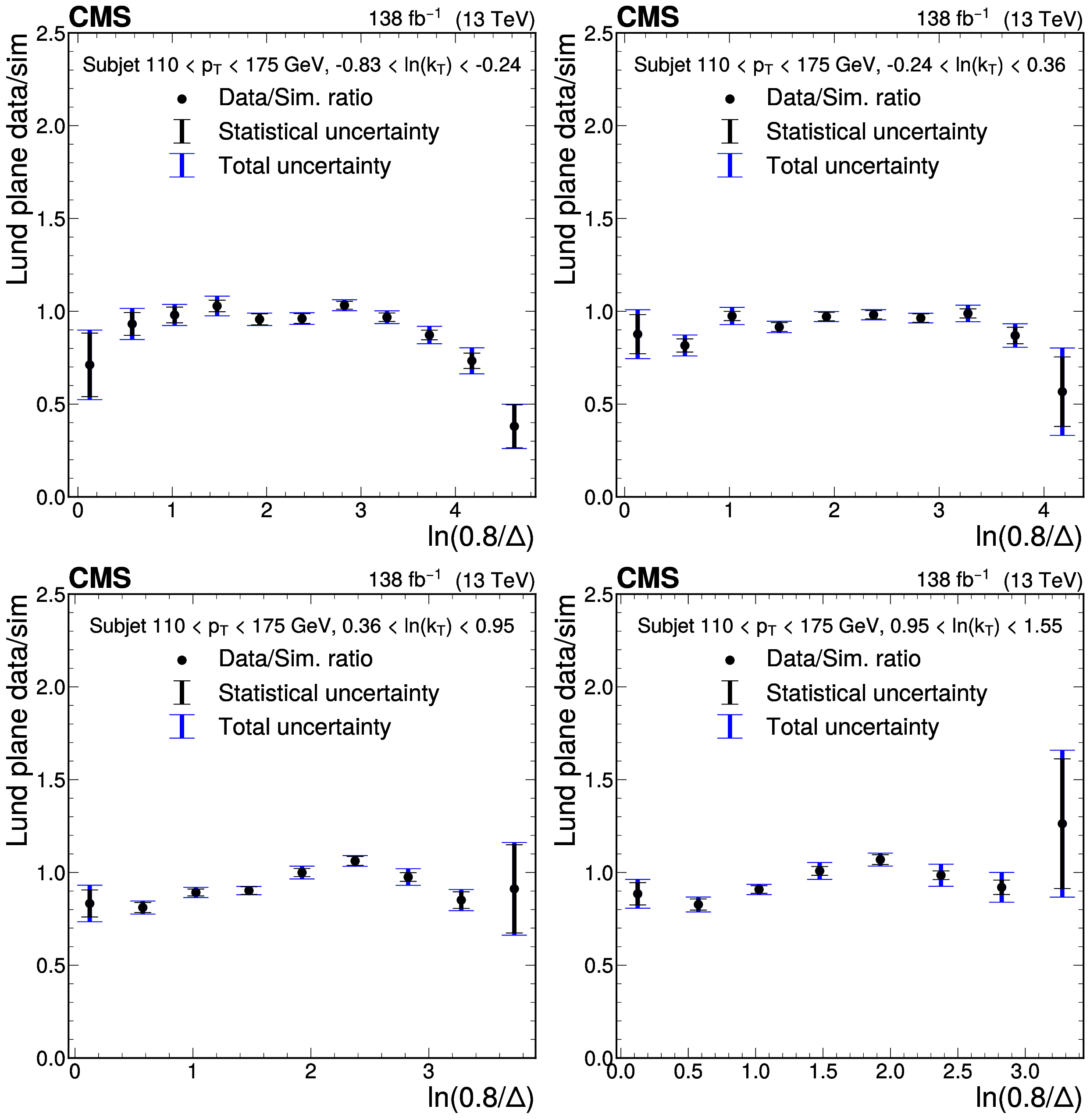
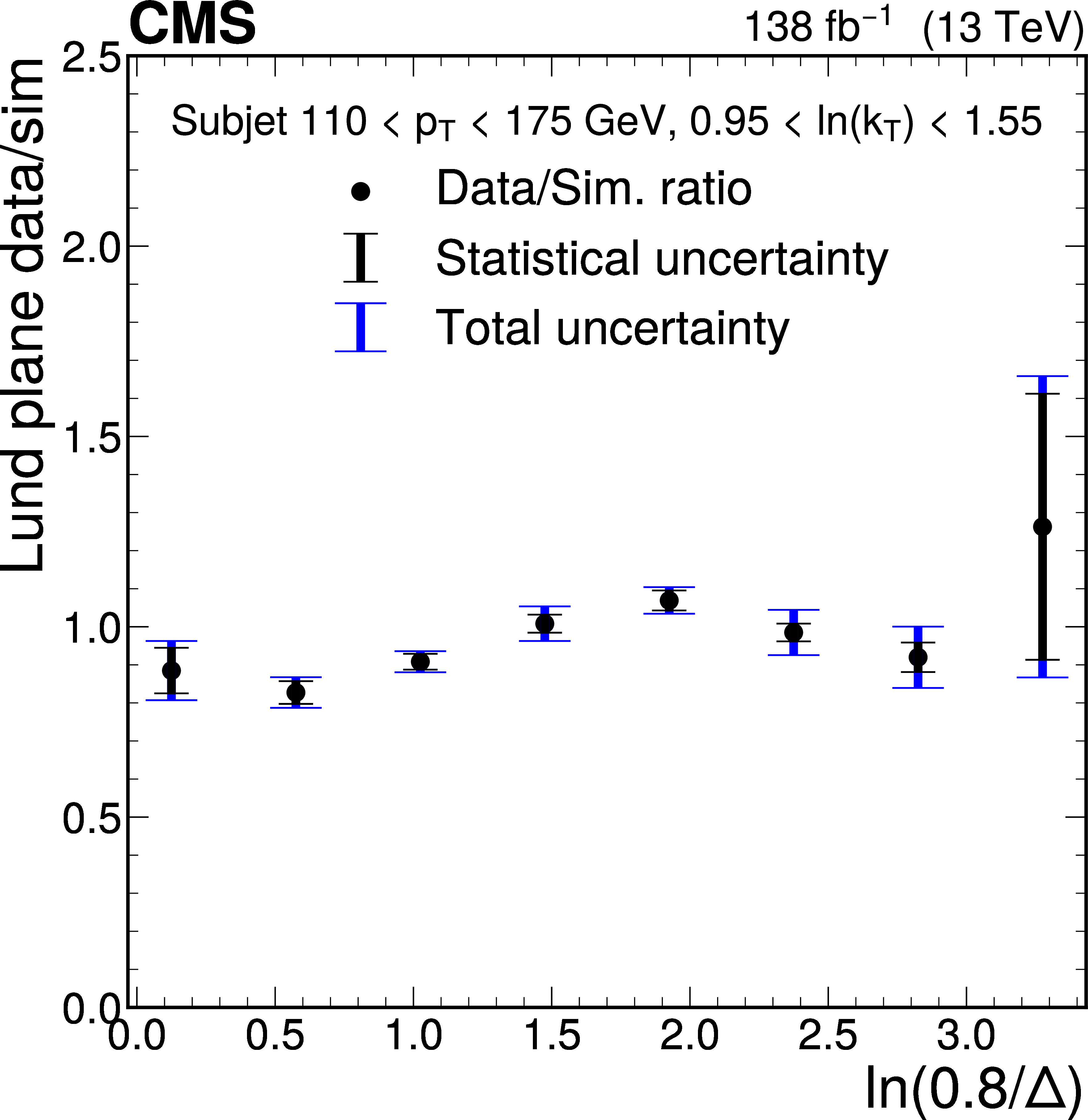
Figure 3:
Ratios of the LJP densities between data and simulation projected into one dimension. The ratio is shown as a function of $ \ln(0.8/\Delta) $ for several $ k_{\mathrm{T}} $ bins for the subjet $ p_{\mathrm{T}} $ bin 110-175 GeV. Statistical uncertainties are shown as the black error bars, and the combined statistical and systematic uncertainties are shown as the blue error bars. The statistical uncertainties dominate the uncertainty in most bins. |
png pdf |
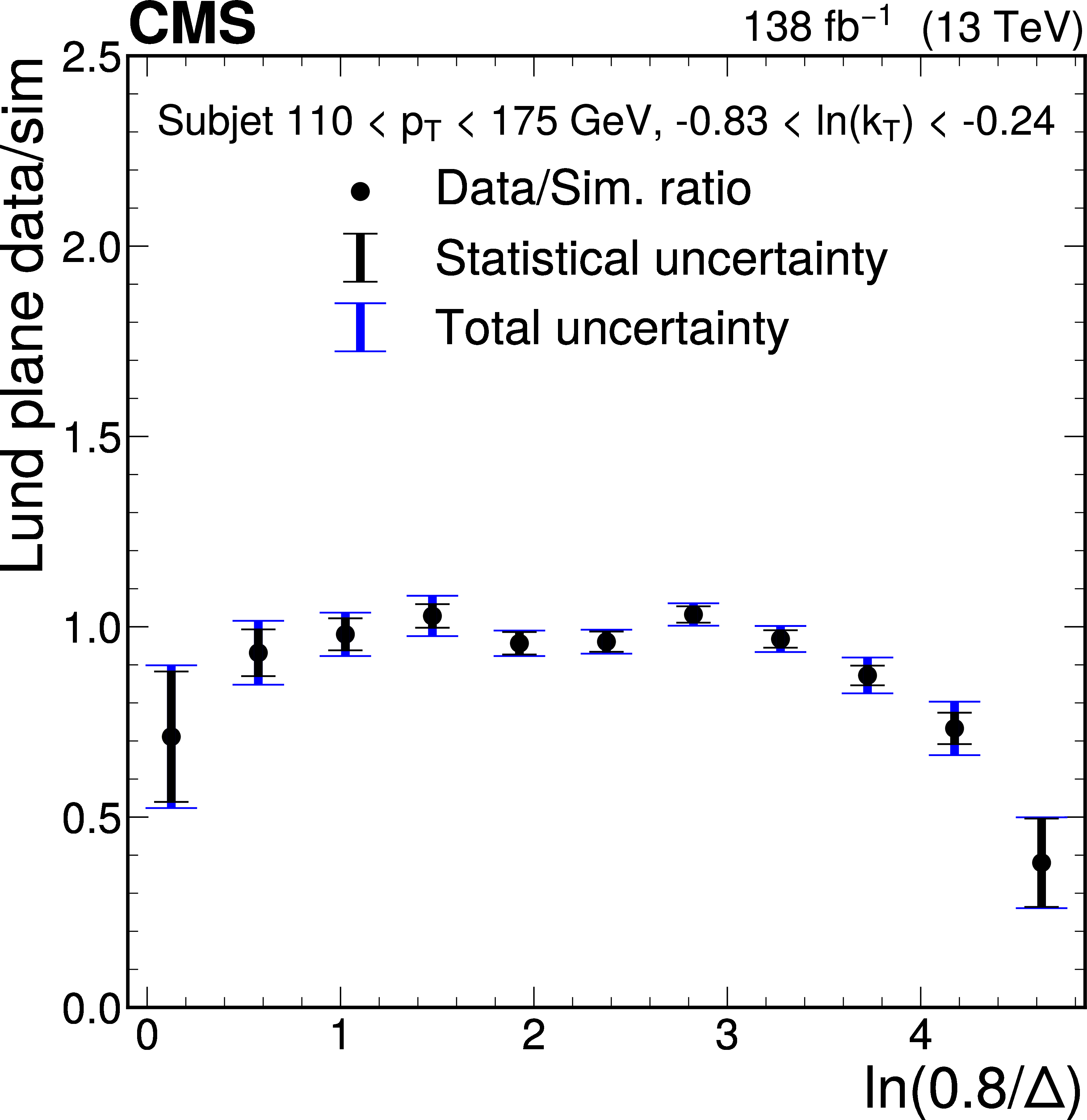
Figure 3-a:
Ratios of the LJP densities between data and simulation projected into one dimension. The ratio is shown as a function of $ \ln(0.8/\Delta) $ for several $ k_{\mathrm{T}} $ bins for the subjet $ p_{\mathrm{T}} $ bin 110-175 GeV. Statistical uncertainties are shown as the black error bars, and the combined statistical and systematic uncertainties are shown as the blue error bars. The statistical uncertainties dominate the uncertainty in most bins. |
png pdf |
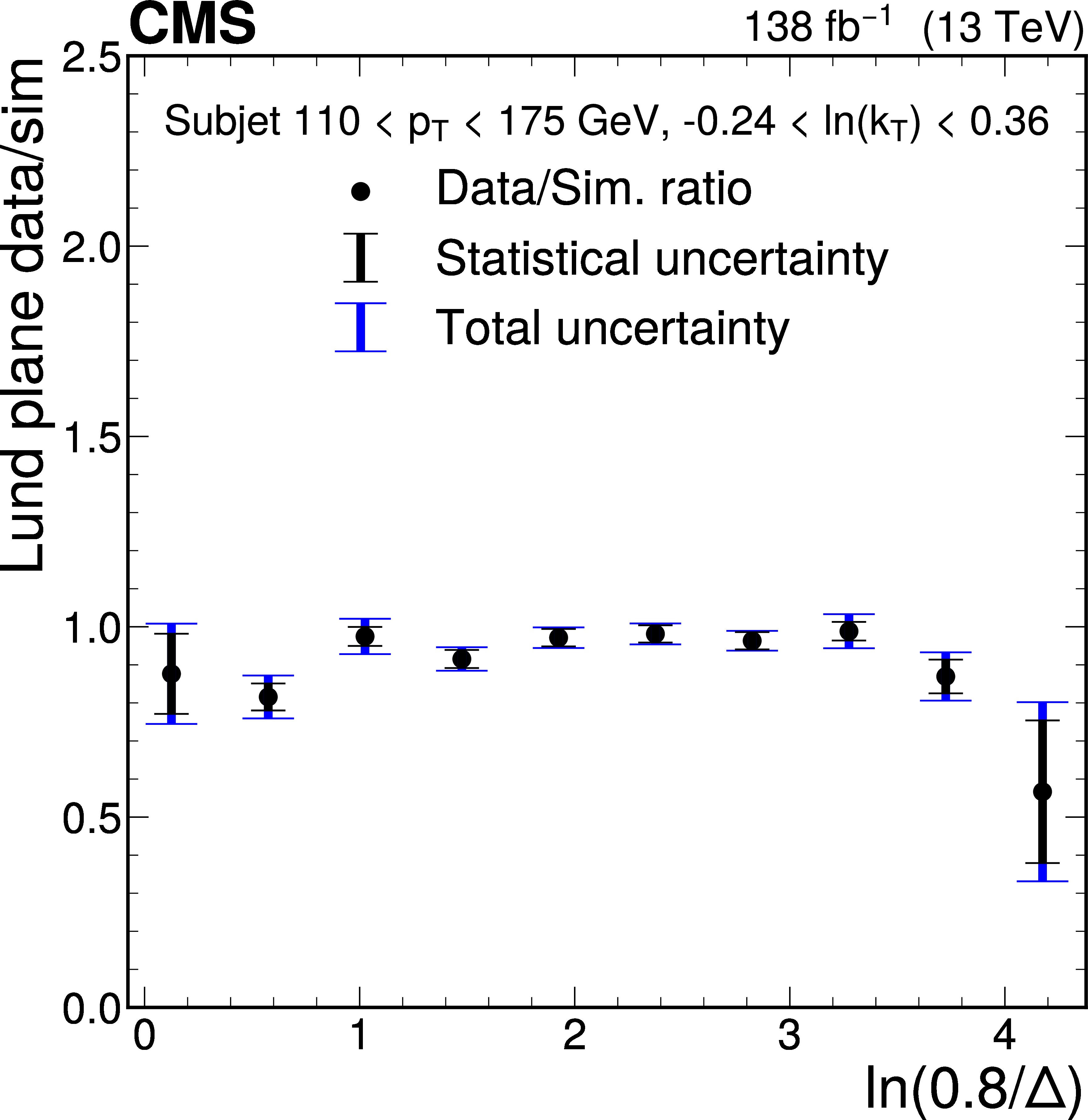
Figure 3-b:
Ratios of the LJP densities between data and simulation projected into one dimension. The ratio is shown as a function of $ \ln(0.8/\Delta) $ for several $ k_{\mathrm{T}} $ bins for the subjet $ p_{\mathrm{T}} $ bin 110-175 GeV. Statistical uncertainties are shown as the black error bars, and the combined statistical and systematic uncertainties are shown as the blue error bars. The statistical uncertainties dominate the uncertainty in most bins. |
png pdf |
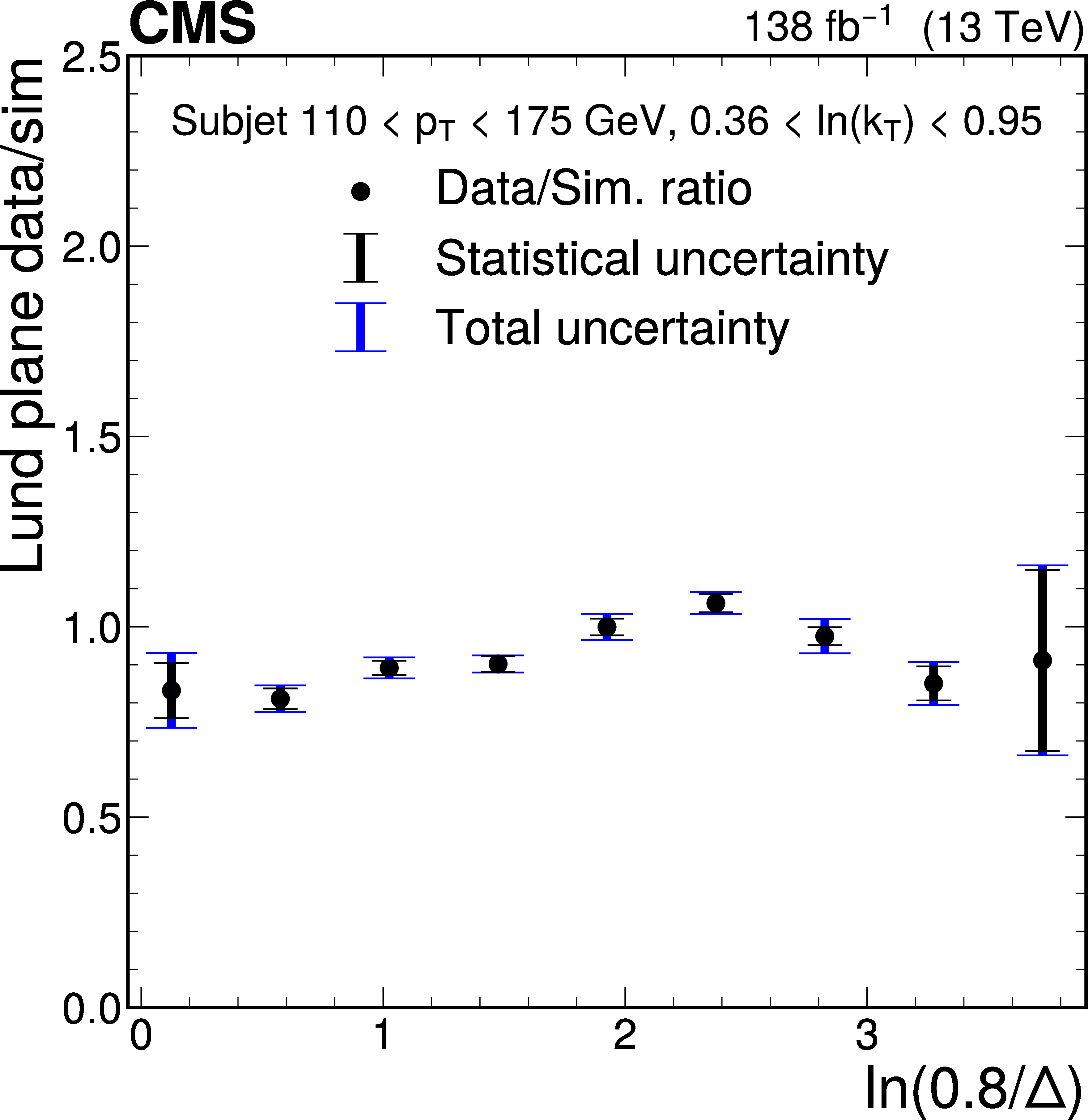
Figure 3-c:
Ratios of the LJP densities between data and simulation projected into one dimension. The ratio is shown as a function of $ \ln(0.8/\Delta) $ for several $ k_{\mathrm{T}} $ bins for the subjet $ p_{\mathrm{T}} $ bin 110-175 GeV. Statistical uncertainties are shown as the black error bars, and the combined statistical and systematic uncertainties are shown as the blue error bars. The statistical uncertainties dominate the uncertainty in most bins. |
png pdf |
Figure 3-d:
Ratios of the LJP densities between data and simulation projected into one dimension. The ratio is shown as a function of $ \ln(0.8/\Delta) $ for several $ k_{\mathrm{T}} $ bins for the subjet $ p_{\mathrm{T}} $ bin 110-175 GeV. Statistical uncertainties are shown as the black error bars, and the combined statistical and systematic uncertainties are shown as the blue error bars. The statistical uncertainties dominate the uncertainty in most bins. |
png pdf |
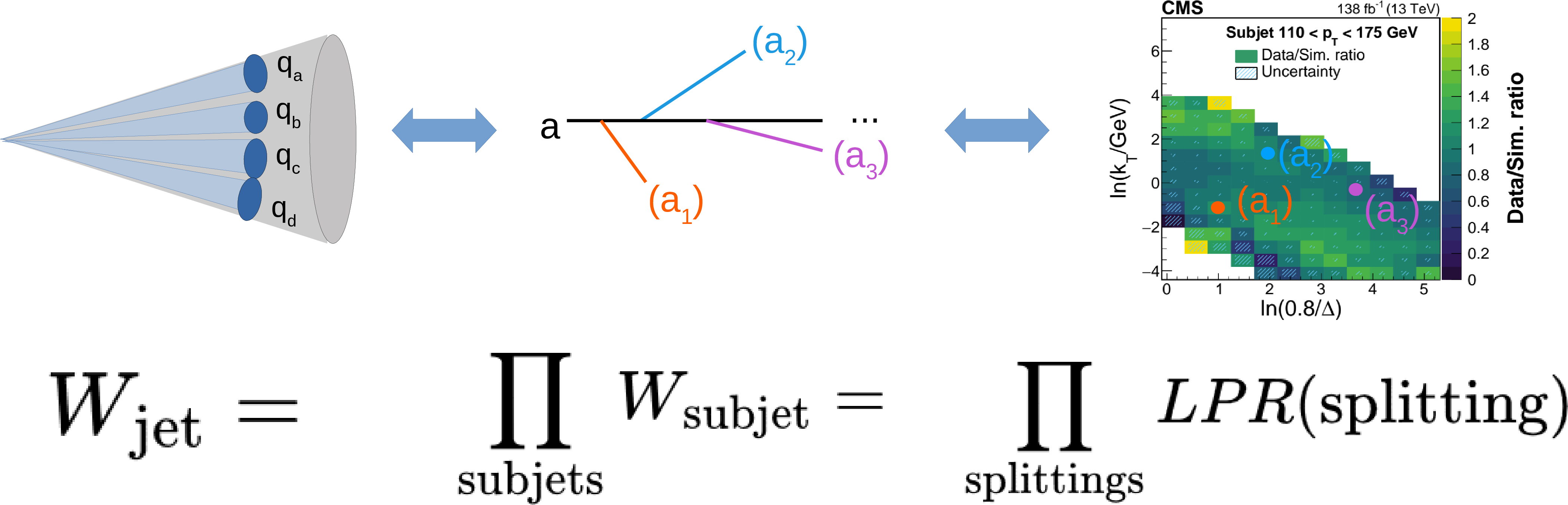
Figure 4:
A graphical illustration of the correction procedure. First, the large-$ R $ jet is reclustered into its subjets. Then, the clustering history for each subjet is used to obtain an list of splittings from the primary LJP. For each splitting, the LJP density ratio is used as a correction factor. |
png pdf |
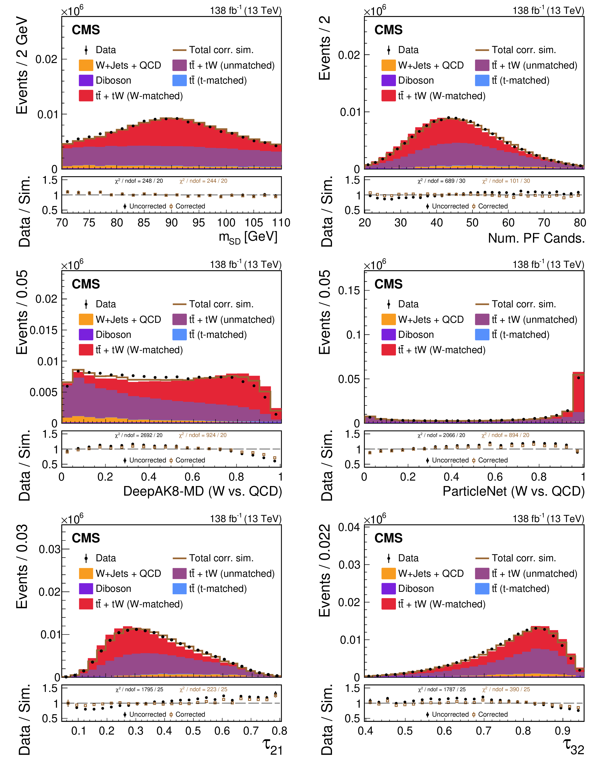
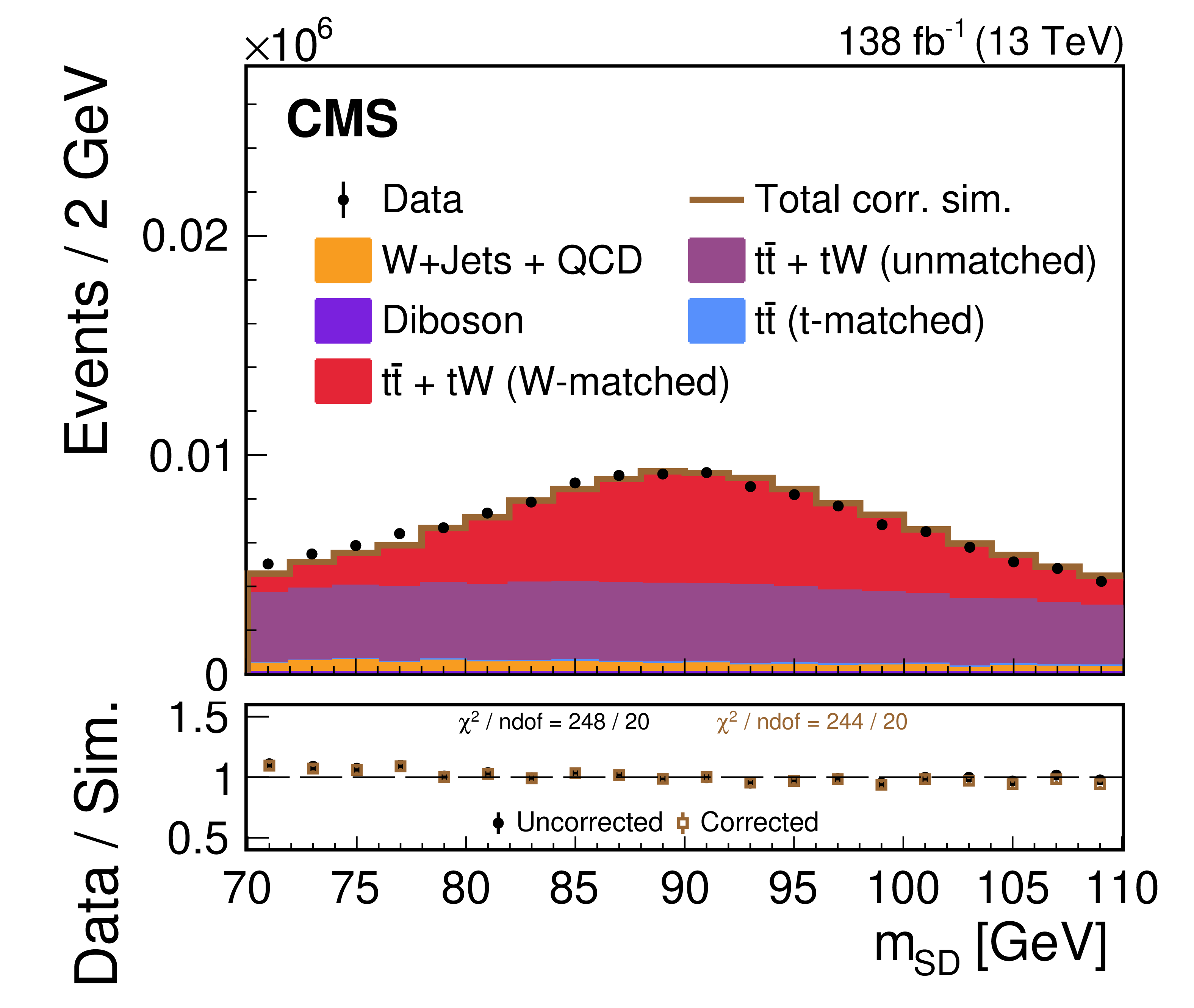
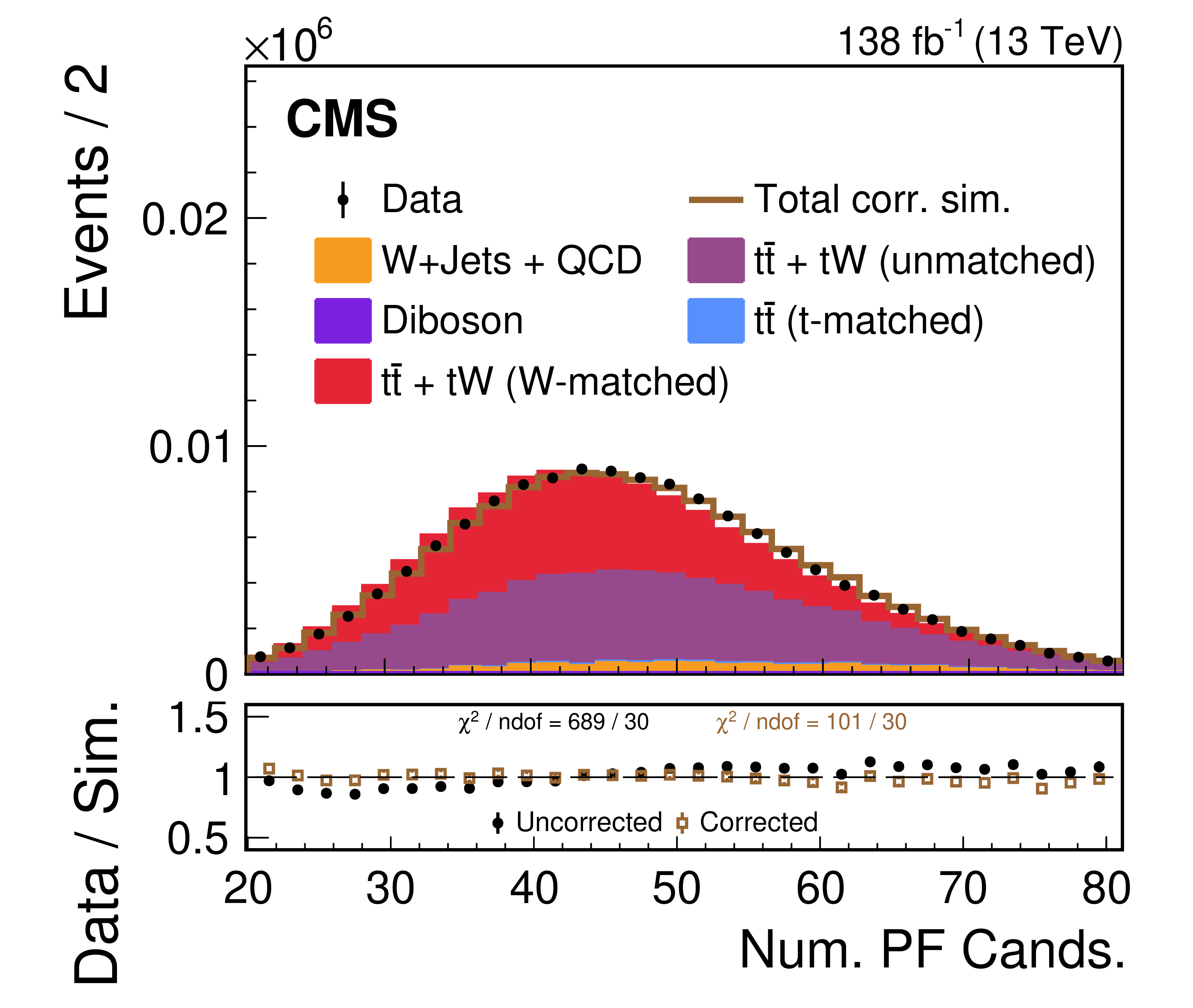
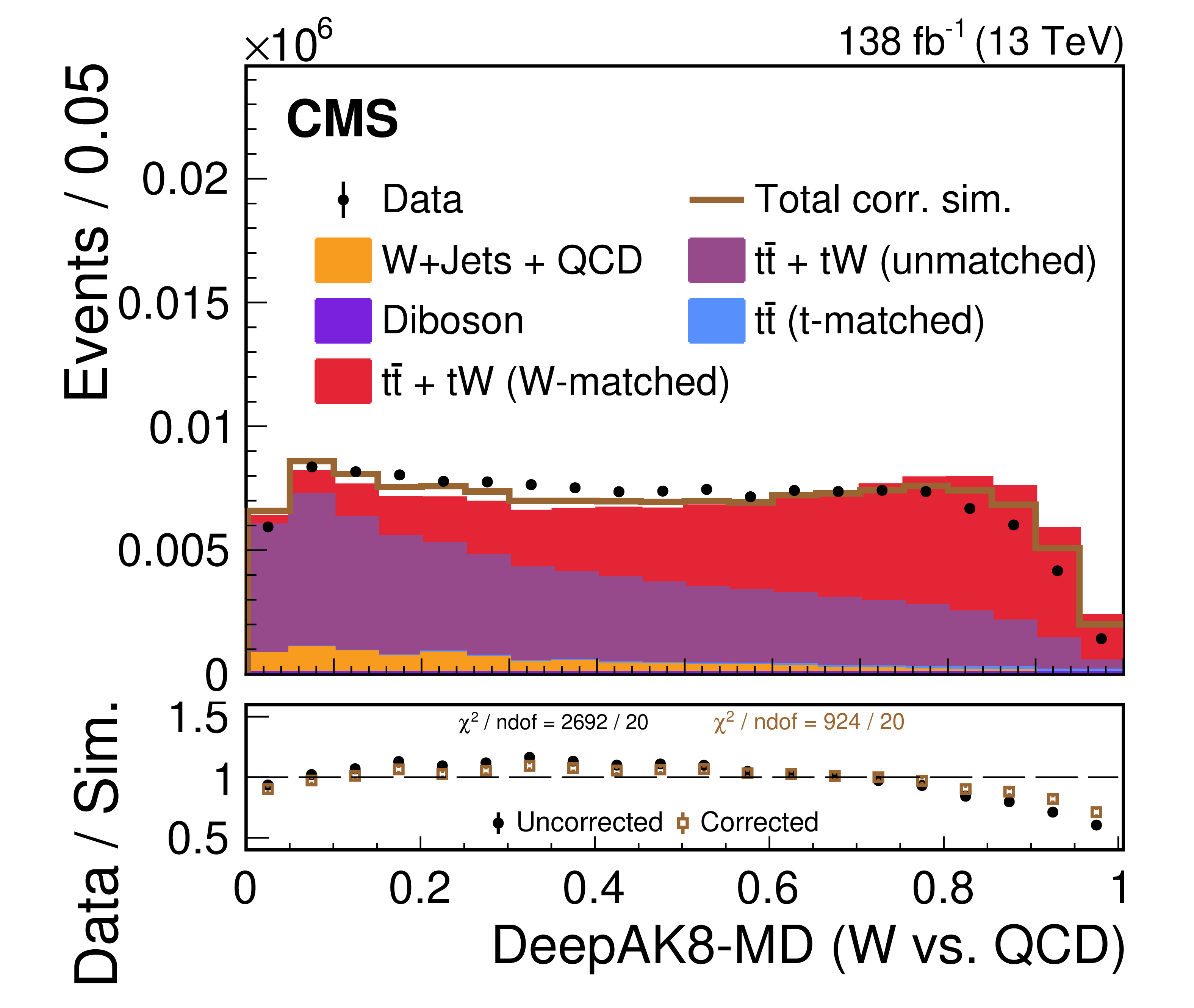
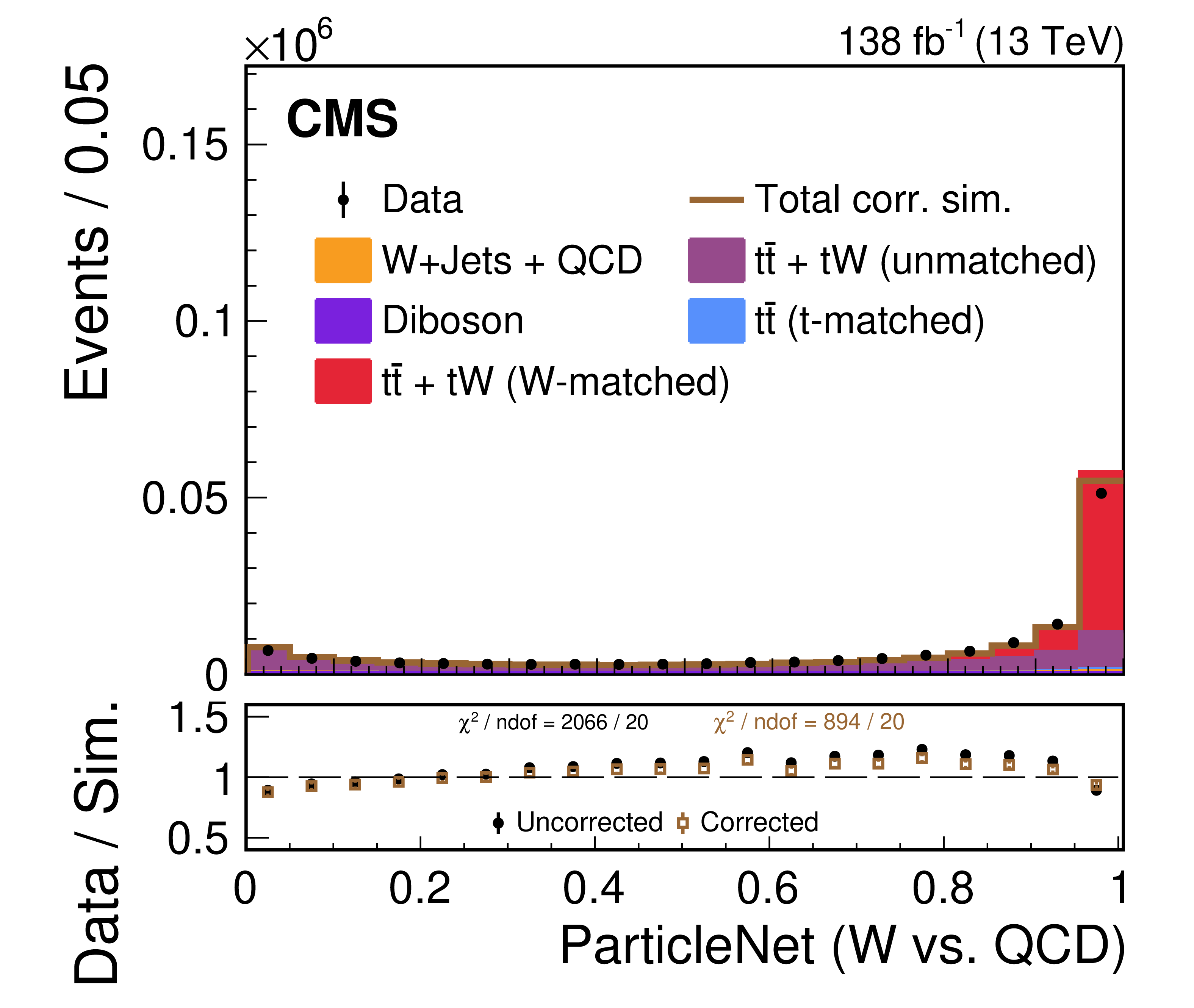
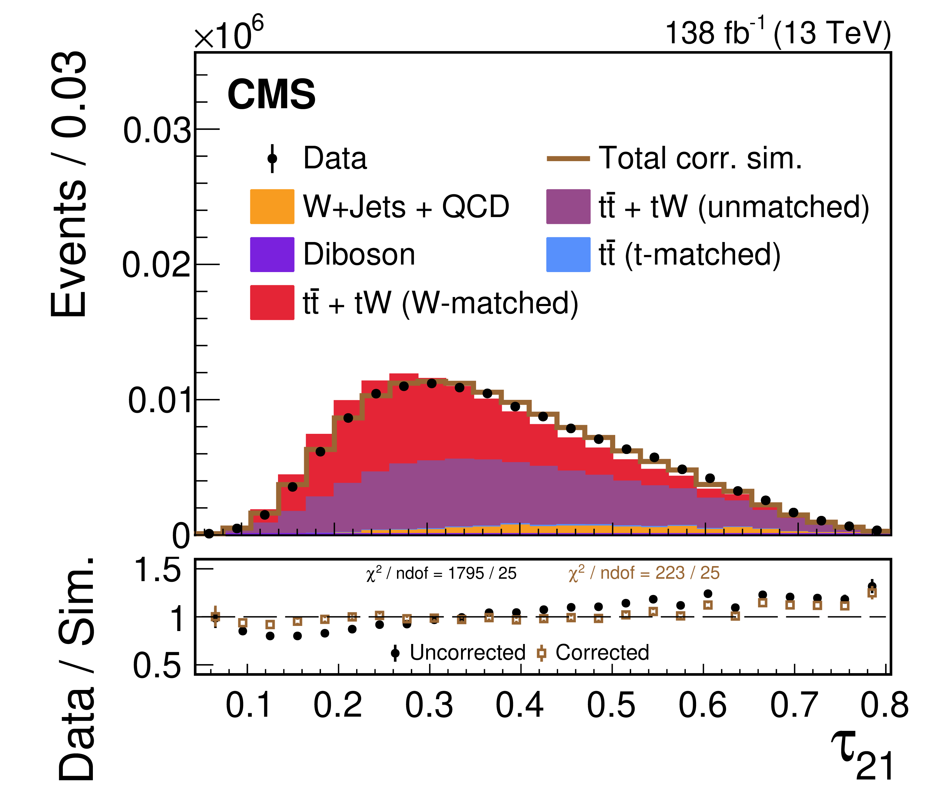
Figure 5:
A comparison of the data-simulation agreement of various substructure observables in the W region. The distribution of various simulated processes, without the LJP correction applied, are shown in the colored histograms and observed data points are shown in black. The brown line shows the total simulated distribution after the LJP correction has been applied to the W-matched $ \mathrm{t} \overline{\mathrm{t}} $ and $ \mathrm{t}\mathrm{W} $ simulations; the other background processes are not corrected. Only statistical uncertainties are shown as vertical bars on the data points, and the computed $ \chi^2 $ is based only on statistical uncertainties. The black solid points (brown open boxes) in the lower panel show the ratio between the data and the total uncorrected (corrected) estimate from simulation. The data-simulation agreement of the various substructure distributions generally improves after applying the correction. |
png pdf |
Figure 5-a:
A comparison of the data-simulation agreement of various substructure observables in the W region. The distribution of various simulated processes, without the LJP correction applied, are shown in the colored histograms and observed data points are shown in black. The brown line shows the total simulated distribution after the LJP correction has been applied to the W-matched $ \mathrm{t} \overline{\mathrm{t}} $ and $ \mathrm{t}\mathrm{W} $ simulations; the other background processes are not corrected. Only statistical uncertainties are shown as vertical bars on the data points, and the computed $ \chi^2 $ is based only on statistical uncertainties. The black solid points (brown open boxes) in the lower panel show the ratio between the data and the total uncorrected (corrected) estimate from simulation. The data-simulation agreement of the various substructure distributions generally improves after applying the correction. |
png pdf |
Figure 5-b:
A comparison of the data-simulation agreement of various substructure observables in the W region. The distribution of various simulated processes, without the LJP correction applied, are shown in the colored histograms and observed data points are shown in black. The brown line shows the total simulated distribution after the LJP correction has been applied to the W-matched $ \mathrm{t} \overline{\mathrm{t}} $ and $ \mathrm{t}\mathrm{W} $ simulations; the other background processes are not corrected. Only statistical uncertainties are shown as vertical bars on the data points, and the computed $ \chi^2 $ is based only on statistical uncertainties. The black solid points (brown open boxes) in the lower panel show the ratio between the data and the total uncorrected (corrected) estimate from simulation. The data-simulation agreement of the various substructure distributions generally improves after applying the correction. |
png pdf |
Figure 5-c:
A comparison of the data-simulation agreement of various substructure observables in the W region. The distribution of various simulated processes, without the LJP correction applied, are shown in the colored histograms and observed data points are shown in black. The brown line shows the total simulated distribution after the LJP correction has been applied to the W-matched $ \mathrm{t} \overline{\mathrm{t}} $ and $ \mathrm{t}\mathrm{W} $ simulations; the other background processes are not corrected. Only statistical uncertainties are shown as vertical bars on the data points, and the computed $ \chi^2 $ is based only on statistical uncertainties. The black solid points (brown open boxes) in the lower panel show the ratio between the data and the total uncorrected (corrected) estimate from simulation. The data-simulation agreement of the various substructure distributions generally improves after applying the correction. |
png pdf |
Figure 5-d:
A comparison of the data-simulation agreement of various substructure observables in the W region. The distribution of various simulated processes, without the LJP correction applied, are shown in the colored histograms and observed data points are shown in black. The brown line shows the total simulated distribution after the LJP correction has been applied to the W-matched $ \mathrm{t} \overline{\mathrm{t}} $ and $ \mathrm{t}\mathrm{W} $ simulations; the other background processes are not corrected. Only statistical uncertainties are shown as vertical bars on the data points, and the computed $ \chi^2 $ is based only on statistical uncertainties. The black solid points (brown open boxes) in the lower panel show the ratio between the data and the total uncorrected (corrected) estimate from simulation. The data-simulation agreement of the various substructure distributions generally improves after applying the correction. |
png pdf |
Figure 5-e:
A comparison of the data-simulation agreement of various substructure observables in the W region. The distribution of various simulated processes, without the LJP correction applied, are shown in the colored histograms and observed data points are shown in black. The brown line shows the total simulated distribution after the LJP correction has been applied to the W-matched $ \mathrm{t} \overline{\mathrm{t}} $ and $ \mathrm{t}\mathrm{W} $ simulations; the other background processes are not corrected. Only statistical uncertainties are shown as vertical bars on the data points, and the computed $ \chi^2 $ is based only on statistical uncertainties. The black solid points (brown open boxes) in the lower panel show the ratio between the data and the total uncorrected (corrected) estimate from simulation. The data-simulation agreement of the various substructure distributions generally improves after applying the correction. |
png pdf |
Figure 5-f:
A comparison of the data-simulation agreement of various substructure observables in the W region. The distribution of various simulated processes, without the LJP correction applied, are shown in the colored histograms and observed data points are shown in black. The brown line shows the total simulated distribution after the LJP correction has been applied to the W-matched $ \mathrm{t} \overline{\mathrm{t}} $ and $ \mathrm{t}\mathrm{W} $ simulations; the other background processes are not corrected. Only statistical uncertainties are shown as vertical bars on the data points, and the computed $ \chi^2 $ is based only on statistical uncertainties. The black solid points (brown open boxes) in the lower panel show the ratio between the data and the total uncorrected (corrected) estimate from simulation. The data-simulation agreement of the various substructure distributions generally improves after applying the correction. |
png pdf |
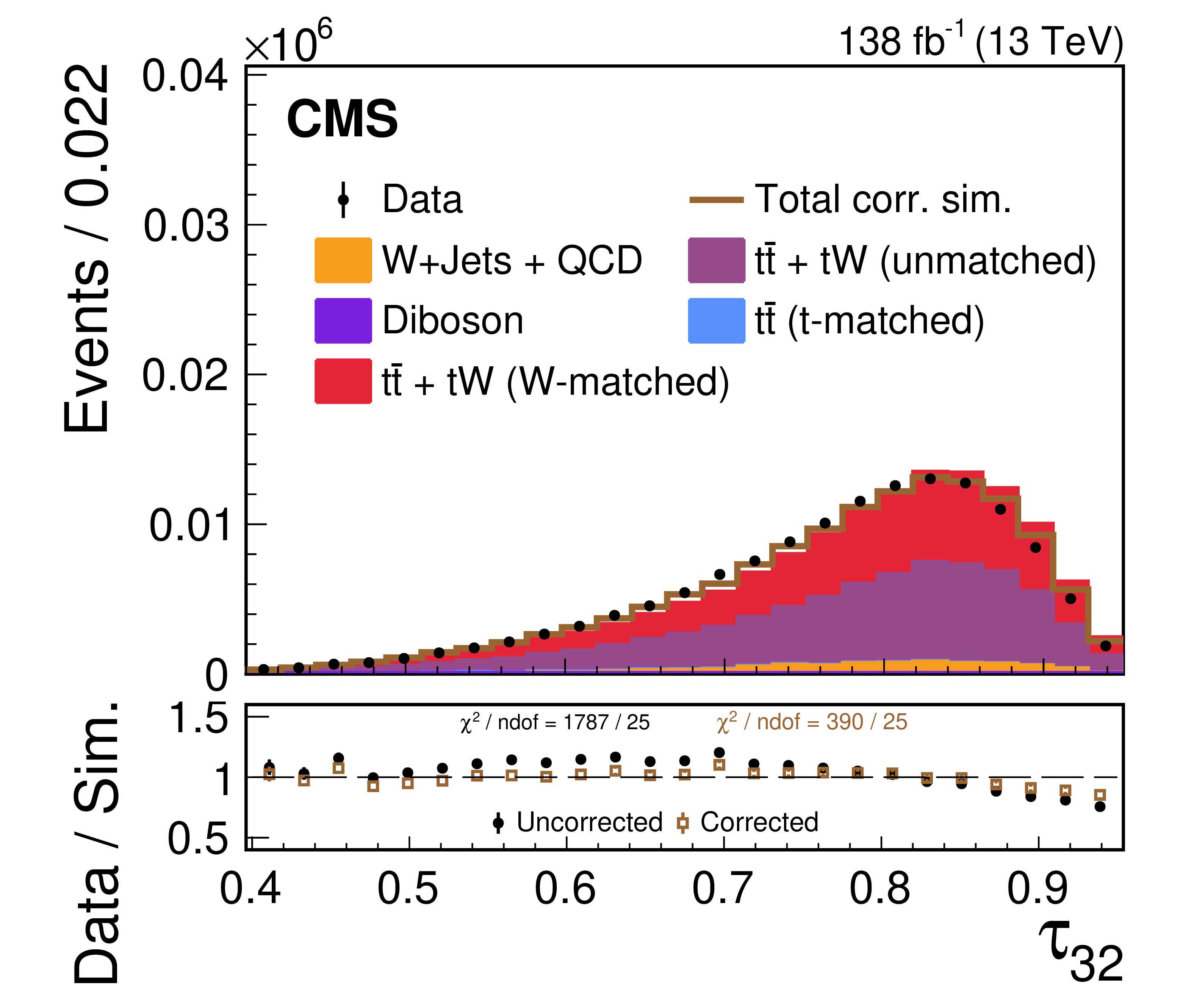
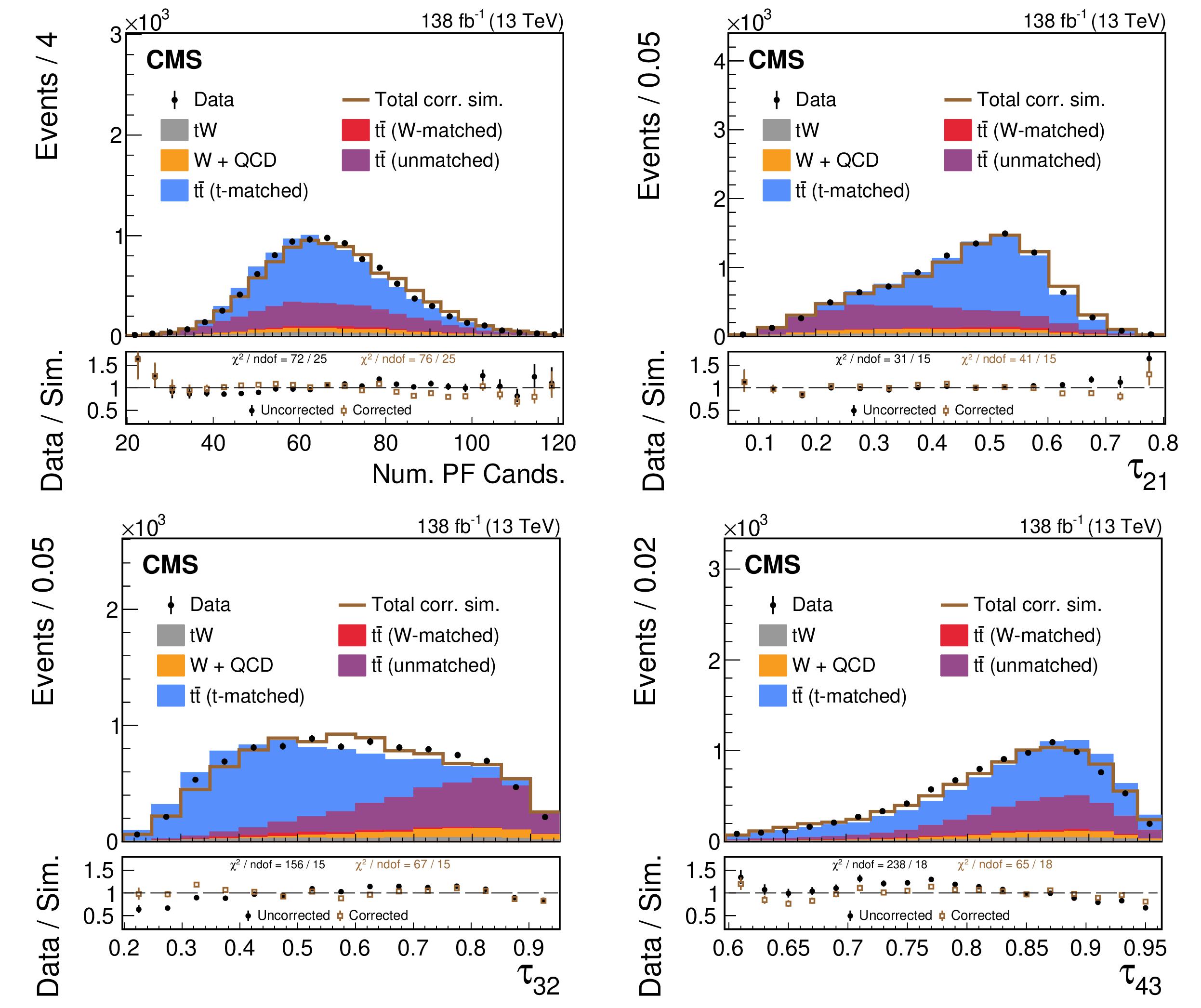
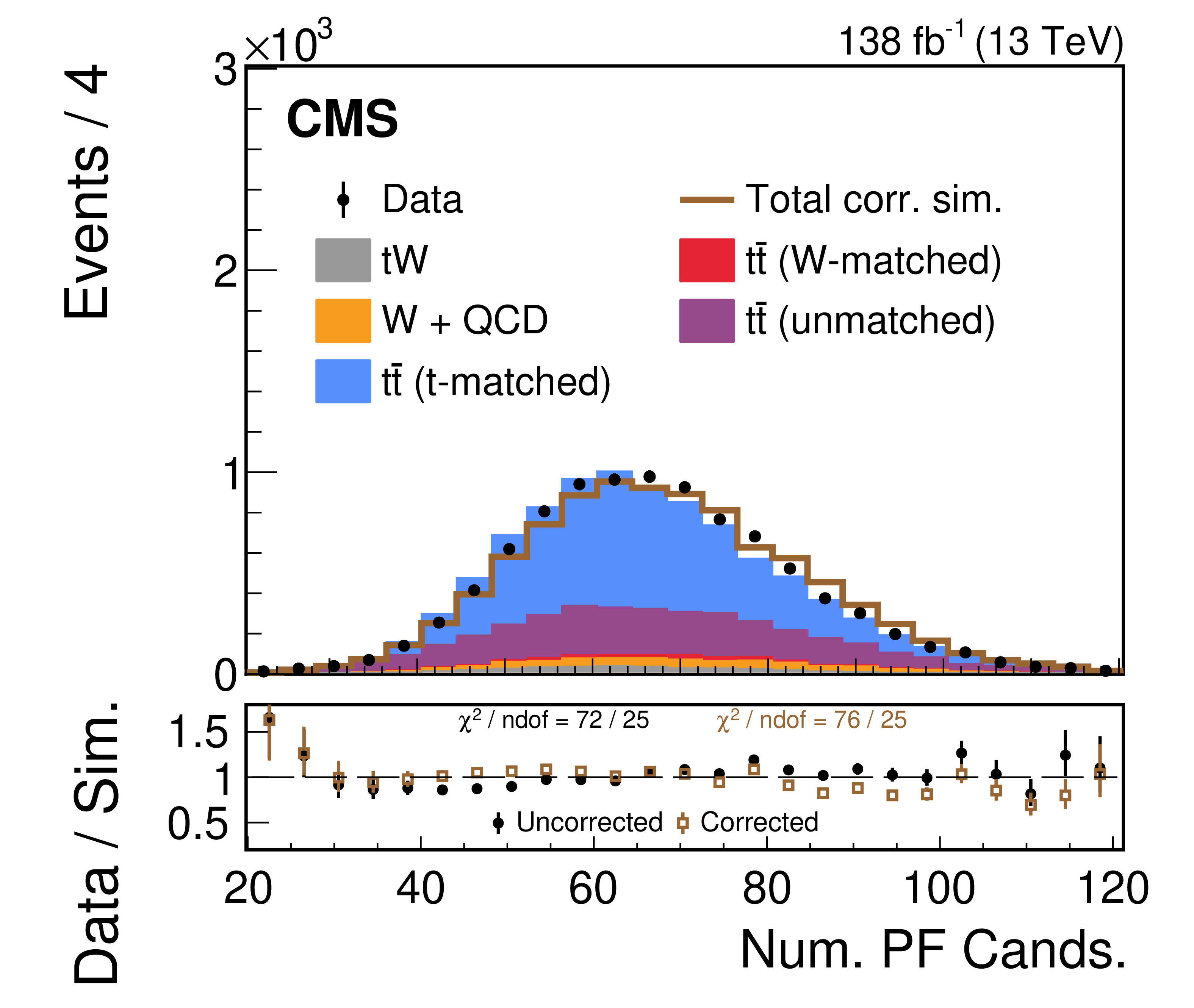
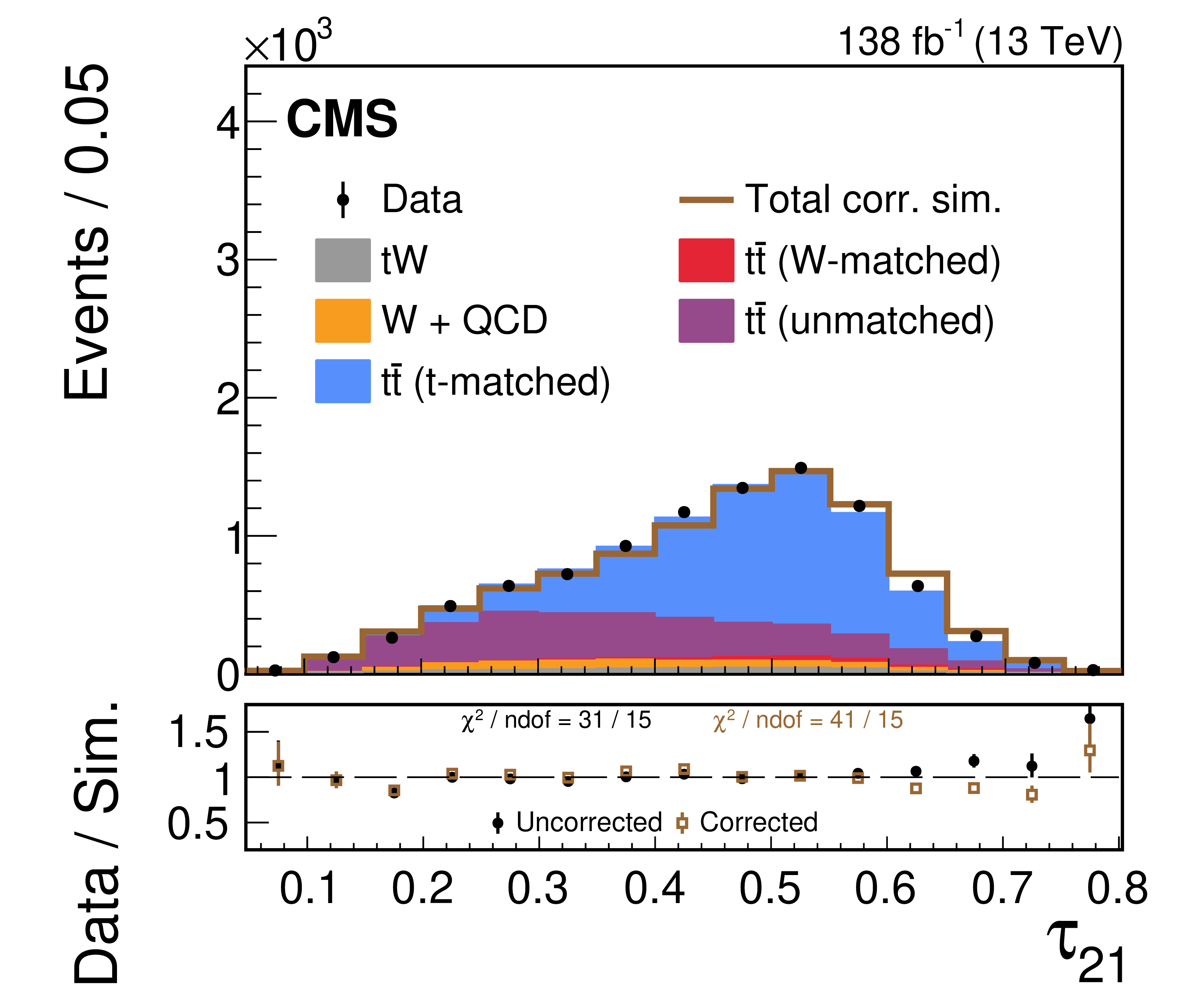
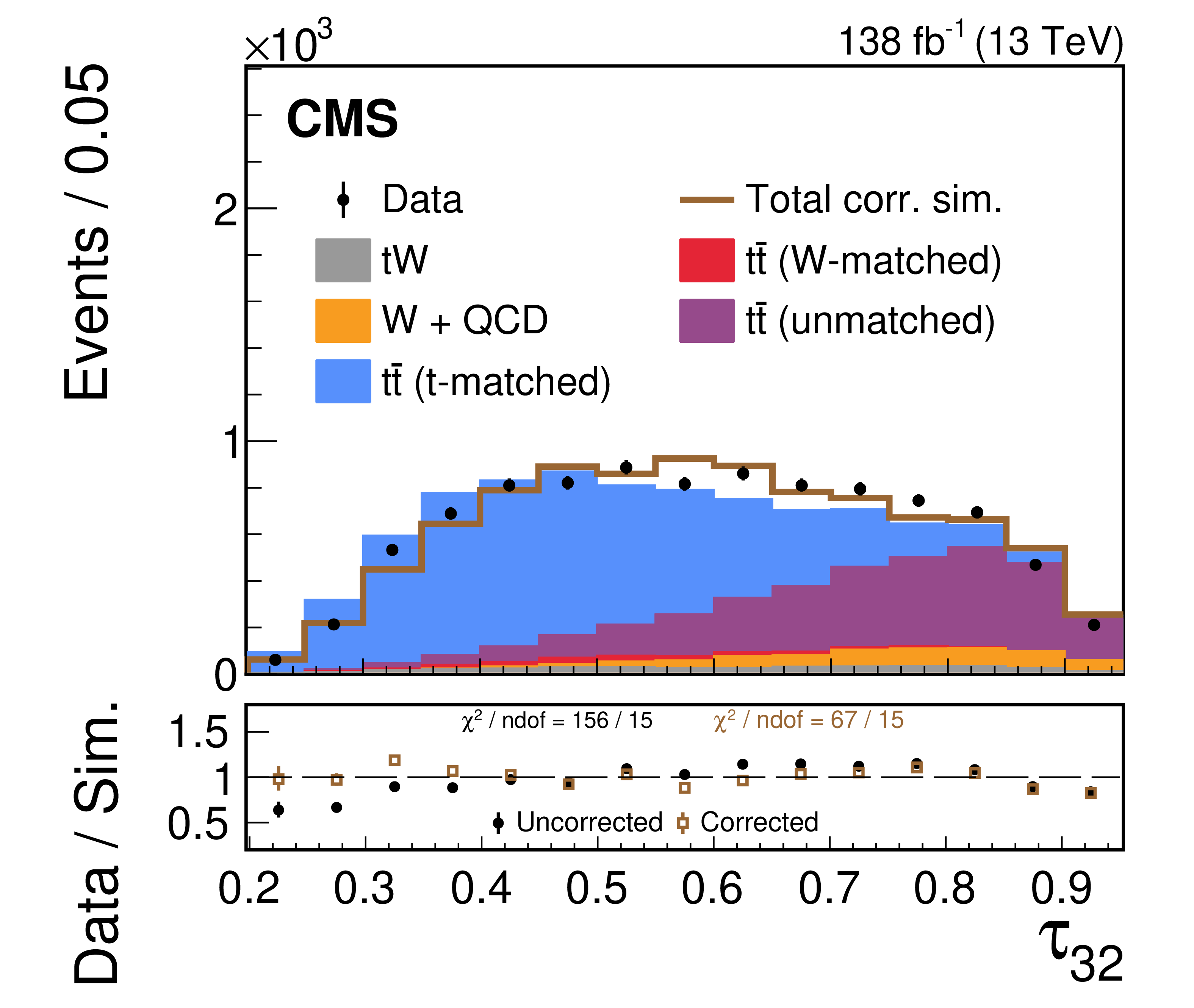
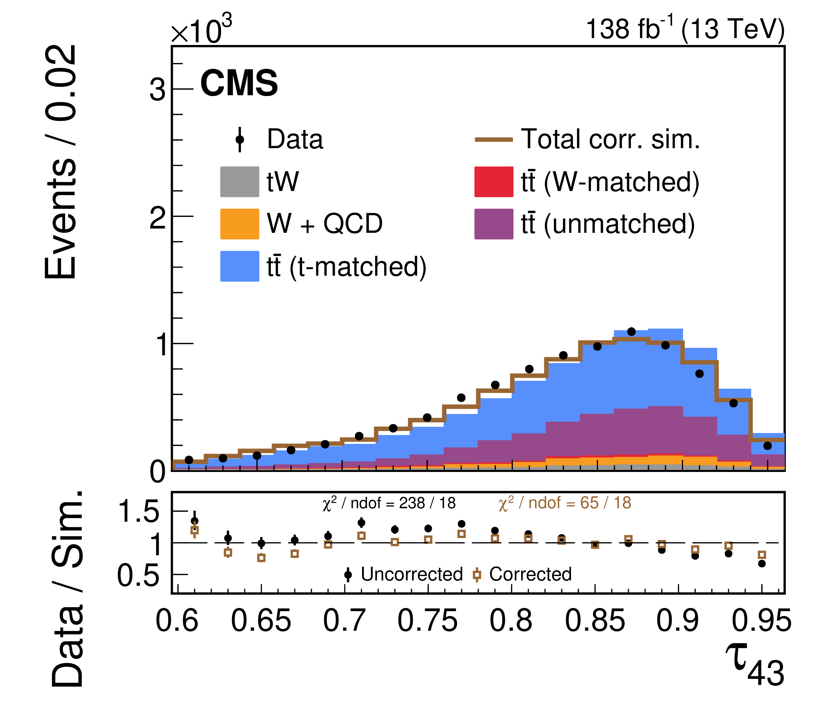
Figure 6:
A comparison of the data-simulation agreement of various substructure observables in the t region. The distribution of various simulated processes, without the LJP correction applied, are shown in the colored histograms and observed data points are shown in black. The brown line shows the total simulated distribution after the LJP correction has been applied to the t-matched $ \mathrm{t} \overline{\mathrm{t}} $ simulation; the other background processes are not corrected. Only statistical uncertainties are shown as vertical bars on the data points, and the computed $ \chi^2 $ is based only on statistical uncertainties. The black solid points (brown open boxes) in the lower panel show the ratio between the data and the total uncorrected (corrected) estimate from simulation. The data-simulation agreement of the worst modeled substructure observables, $ \tau_{32} $ and $ \tau_{43} $, improves after applying the correction. |
png pdf |
Figure 6-a:
A comparison of the data-simulation agreement of various substructure observables in the t region. The distribution of various simulated processes, without the LJP correction applied, are shown in the colored histograms and observed data points are shown in black. The brown line shows the total simulated distribution after the LJP correction has been applied to the t-matched $ \mathrm{t} \overline{\mathrm{t}} $ simulation; the other background processes are not corrected. Only statistical uncertainties are shown as vertical bars on the data points, and the computed $ \chi^2 $ is based only on statistical uncertainties. The black solid points (brown open boxes) in the lower panel show the ratio between the data and the total uncorrected (corrected) estimate from simulation. The data-simulation agreement of the worst modeled substructure observables, $ \tau_{32} $ and $ \tau_{43} $, improves after applying the correction. |
png pdf |
Figure 6-b:
A comparison of the data-simulation agreement of various substructure observables in the t region. The distribution of various simulated processes, without the LJP correction applied, are shown in the colored histograms and observed data points are shown in black. The brown line shows the total simulated distribution after the LJP correction has been applied to the t-matched $ \mathrm{t} \overline{\mathrm{t}} $ simulation; the other background processes are not corrected. Only statistical uncertainties are shown as vertical bars on the data points, and the computed $ \chi^2 $ is based only on statistical uncertainties. The black solid points (brown open boxes) in the lower panel show the ratio between the data and the total uncorrected (corrected) estimate from simulation. The data-simulation agreement of the worst modeled substructure observables, $ \tau_{32} $ and $ \tau_{43} $, improves after applying the correction. |
png pdf |
Figure 6-c:
A comparison of the data-simulation agreement of various substructure observables in the t region. The distribution of various simulated processes, without the LJP correction applied, are shown in the colored histograms and observed data points are shown in black. The brown line shows the total simulated distribution after the LJP correction has been applied to the t-matched $ \mathrm{t} \overline{\mathrm{t}} $ simulation; the other background processes are not corrected. Only statistical uncertainties are shown as vertical bars on the data points, and the computed $ \chi^2 $ is based only on statistical uncertainties. The black solid points (brown open boxes) in the lower panel show the ratio between the data and the total uncorrected (corrected) estimate from simulation. The data-simulation agreement of the worst modeled substructure observables, $ \tau_{32} $ and $ \tau_{43} $, improves after applying the correction. |
png pdf |
Figure 6-d:
A comparison of the data-simulation agreement of various substructure observables in the t region. The distribution of various simulated processes, without the LJP correction applied, are shown in the colored histograms and observed data points are shown in black. The brown line shows the total simulated distribution after the LJP correction has been applied to the t-matched $ \mathrm{t} \overline{\mathrm{t}} $ simulation; the other background processes are not corrected. Only statistical uncertainties are shown as vertical bars on the data points, and the computed $ \chi^2 $ is based only on statistical uncertainties. The black solid points (brown open boxes) in the lower panel show the ratio between the data and the total uncorrected (corrected) estimate from simulation. The data-simulation agreement of the worst modeled substructure observables, $ \tau_{32} $ and $ \tau_{43} $, improves after applying the correction. |
png pdf |
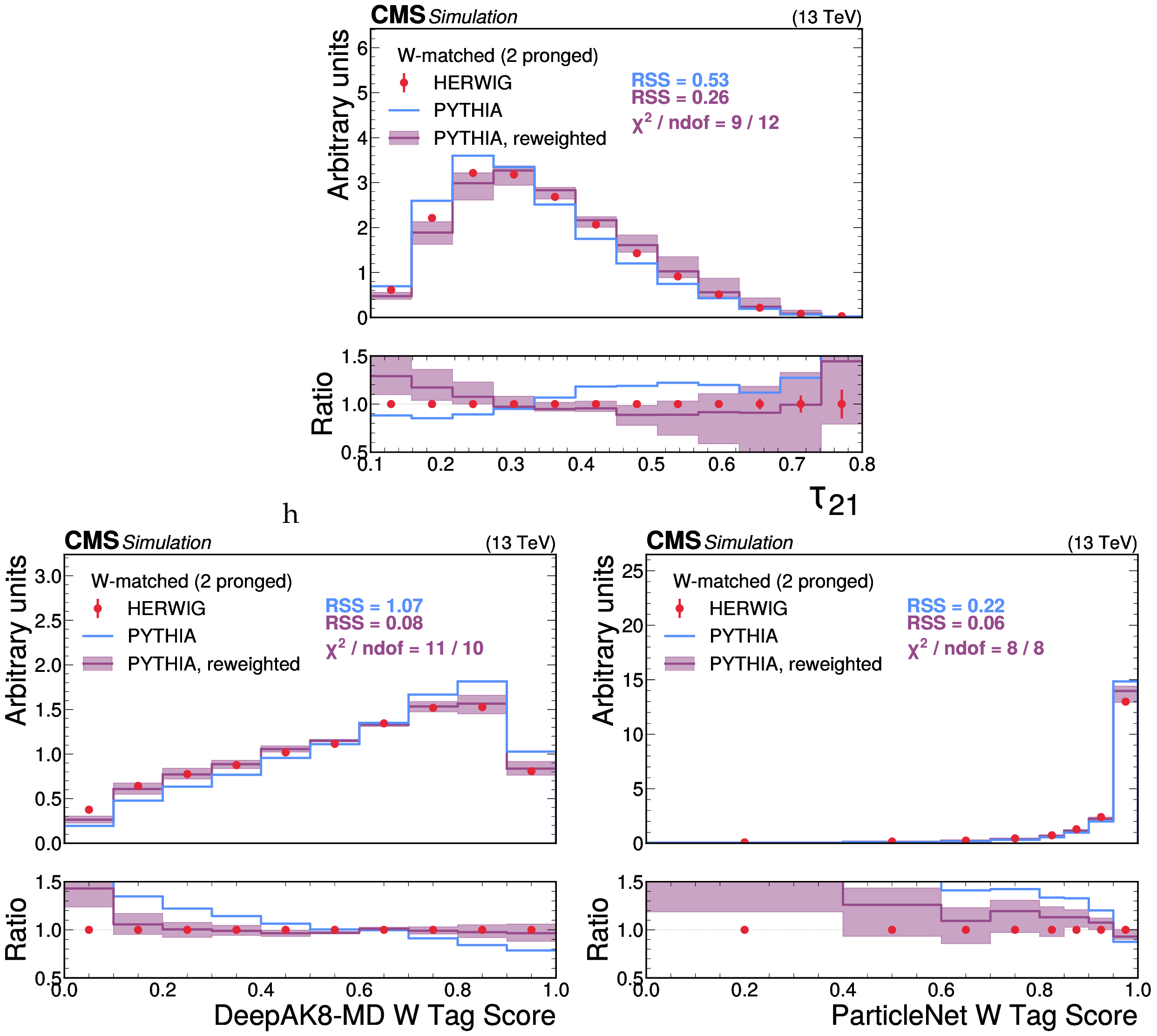
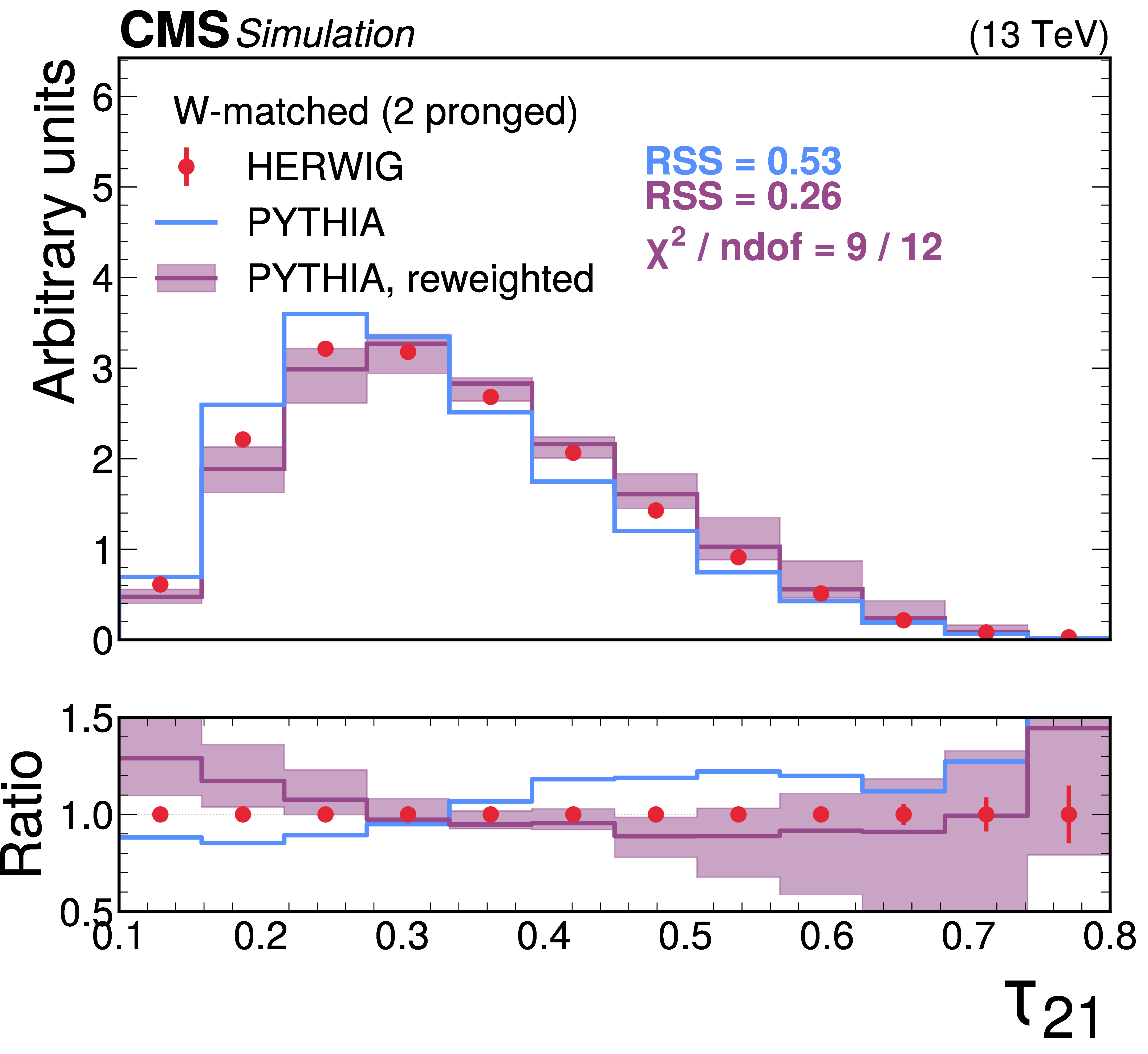
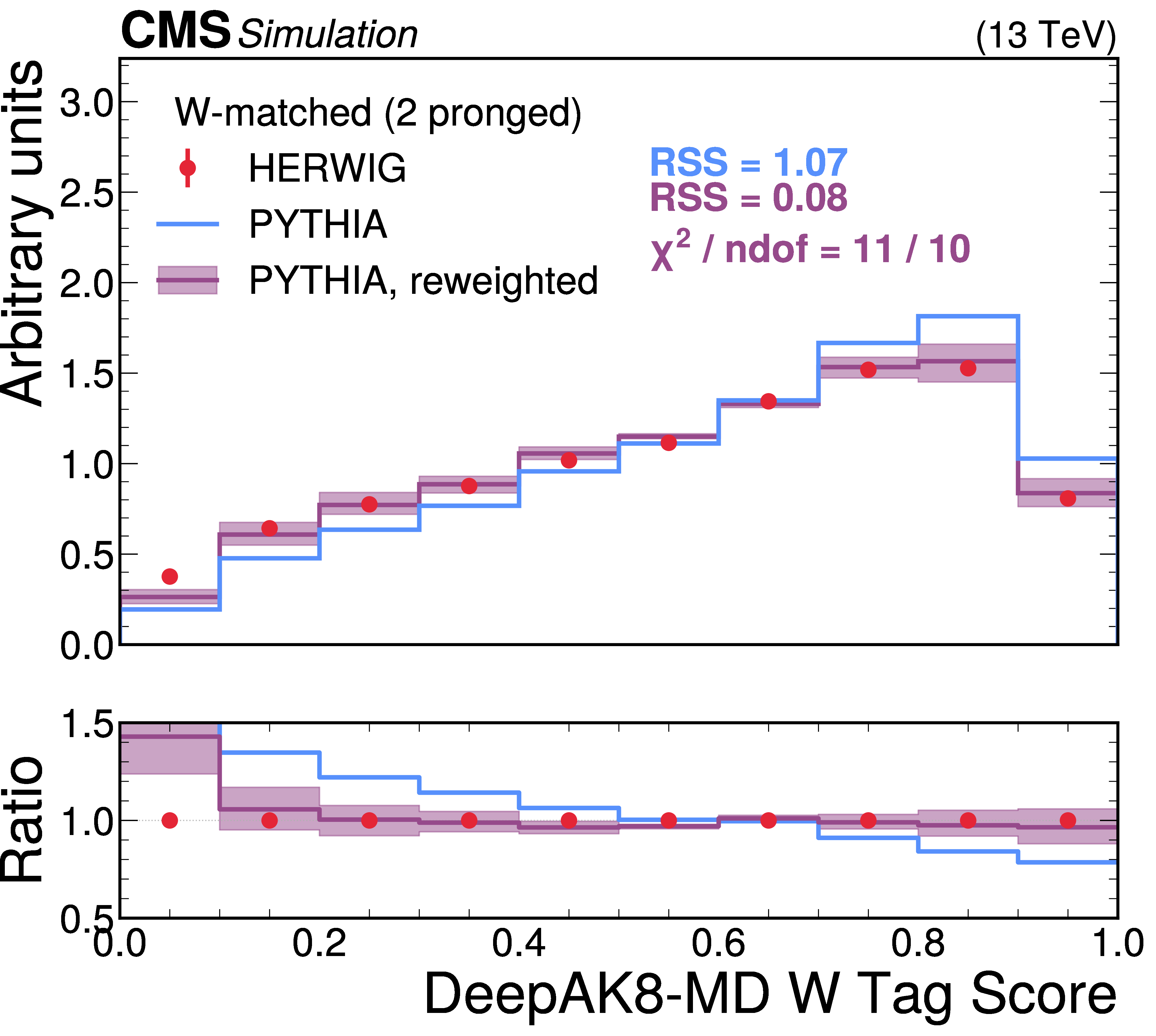
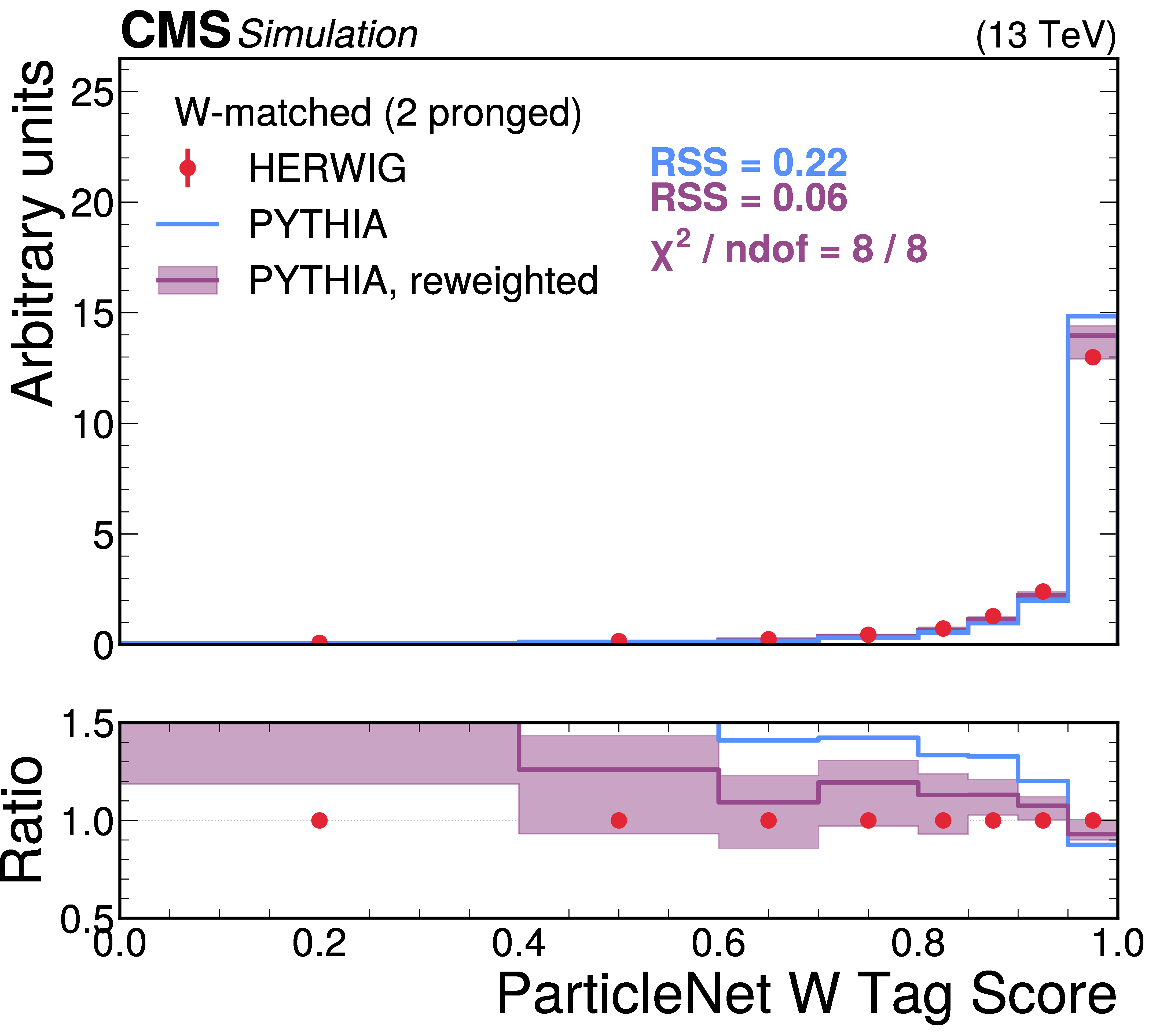
Figure 7:
A comparison of the HERWIG (red circles), PYTHIA (blue lines) and reweighted PYTHIA (purple lines) samples for W jets. The systematic uncertainty in the reweighted PYTHIA samples is shown in the light purple shading. The statistical uncertainty from the limited size of the simulated sample is shown as vertical red bars on the HERWIG points. The lower panel shows the ratio of the two PYTHIA distributions with respect to HERWIG. The RSS between the PYTHIA and HERWIG samples is computed based on the squared difference in normalized bin yields. The $ \chi^2 $ value is computed using both the statistical uncertainties of the simulated samples and the systematic uncertainties in the correction procedure, and therefore assesses the full closure of the correction procedure. It is computed only for the reweighted PYTHIA samples because the original sample does not have appropriate systematic uncertainties. |
png pdf |
Figure 7-a:
A comparison of the HERWIG (red circles), PYTHIA (blue lines) and reweighted PYTHIA (purple lines) samples for W jets. The systematic uncertainty in the reweighted PYTHIA samples is shown in the light purple shading. The statistical uncertainty from the limited size of the simulated sample is shown as vertical red bars on the HERWIG points. The lower panel shows the ratio of the two PYTHIA distributions with respect to HERWIG. The RSS between the PYTHIA and HERWIG samples is computed based on the squared difference in normalized bin yields. The $ \chi^2 $ value is computed using both the statistical uncertainties of the simulated samples and the systematic uncertainties in the correction procedure, and therefore assesses the full closure of the correction procedure. It is computed only for the reweighted PYTHIA samples because the original sample does not have appropriate systematic uncertainties. |
png pdf |
Figure 7-b:
A comparison of the HERWIG (red circles), PYTHIA (blue lines) and reweighted PYTHIA (purple lines) samples for W jets. The systematic uncertainty in the reweighted PYTHIA samples is shown in the light purple shading. The statistical uncertainty from the limited size of the simulated sample is shown as vertical red bars on the HERWIG points. The lower panel shows the ratio of the two PYTHIA distributions with respect to HERWIG. The RSS between the PYTHIA and HERWIG samples is computed based on the squared difference in normalized bin yields. The $ \chi^2 $ value is computed using both the statistical uncertainties of the simulated samples and the systematic uncertainties in the correction procedure, and therefore assesses the full closure of the correction procedure. It is computed only for the reweighted PYTHIA samples because the original sample does not have appropriate systematic uncertainties. |
png pdf |
Figure 7-c:
A comparison of the HERWIG (red circles), PYTHIA (blue lines) and reweighted PYTHIA (purple lines) samples for W jets. The systematic uncertainty in the reweighted PYTHIA samples is shown in the light purple shading. The statistical uncertainty from the limited size of the simulated sample is shown as vertical red bars on the HERWIG points. The lower panel shows the ratio of the two PYTHIA distributions with respect to HERWIG. The RSS between the PYTHIA and HERWIG samples is computed based on the squared difference in normalized bin yields. The $ \chi^2 $ value is computed using both the statistical uncertainties of the simulated samples and the systematic uncertainties in the correction procedure, and therefore assesses the full closure of the correction procedure. It is computed only for the reweighted PYTHIA samples because the original sample does not have appropriate systematic uncertainties. |
png pdf |
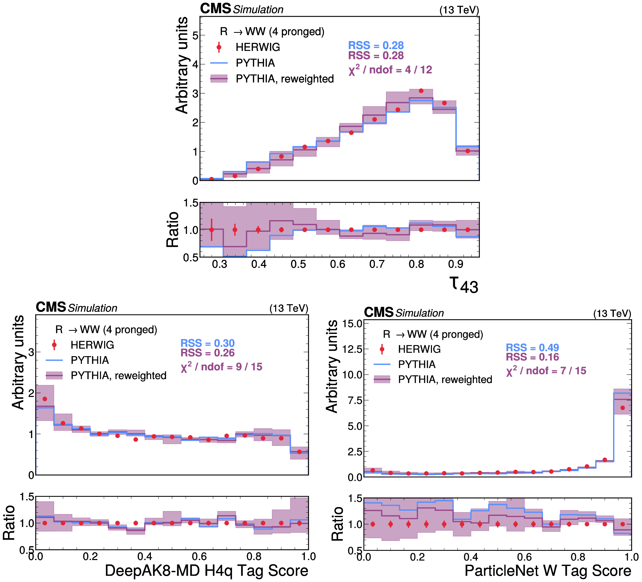
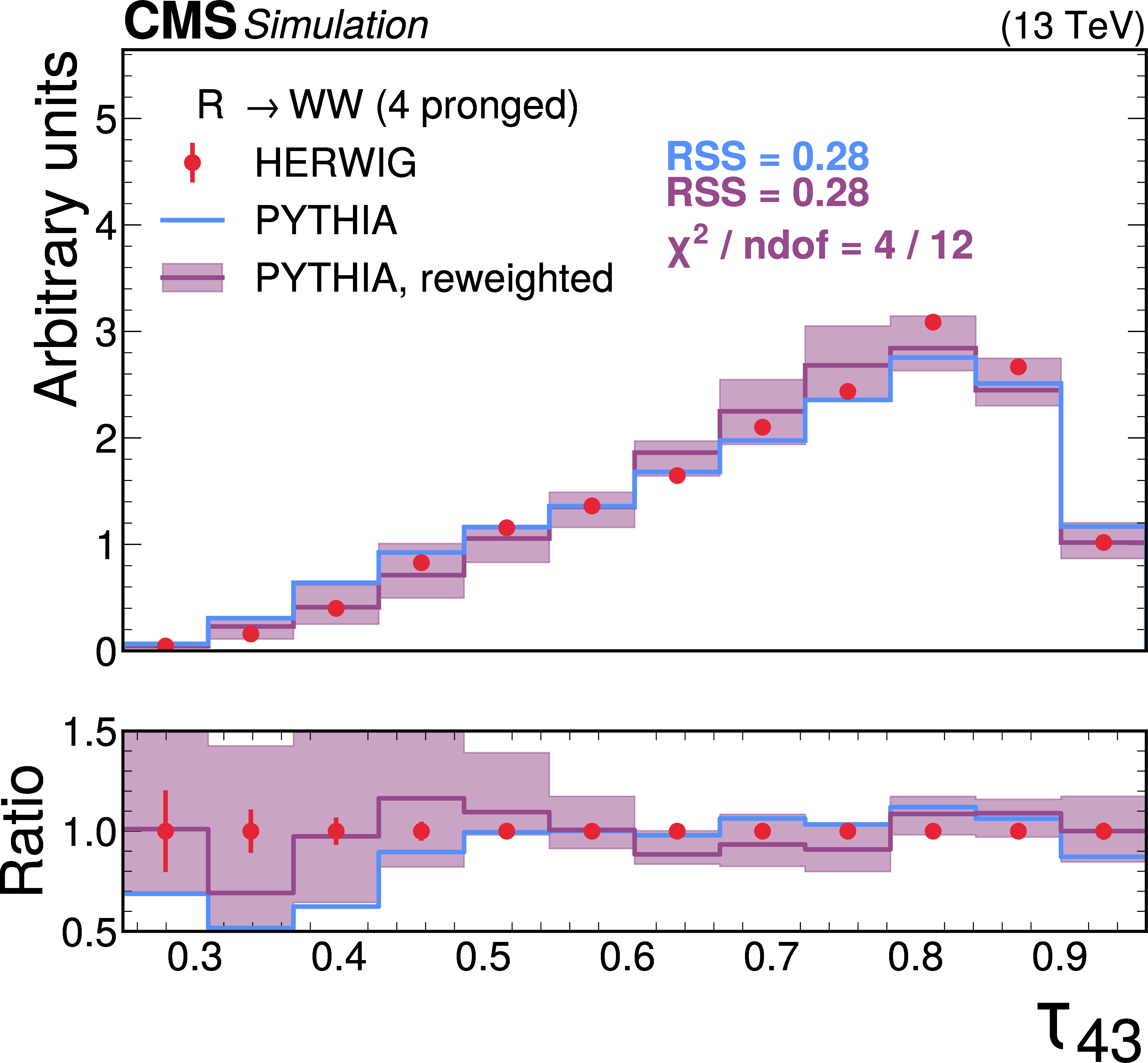
Figure 8:
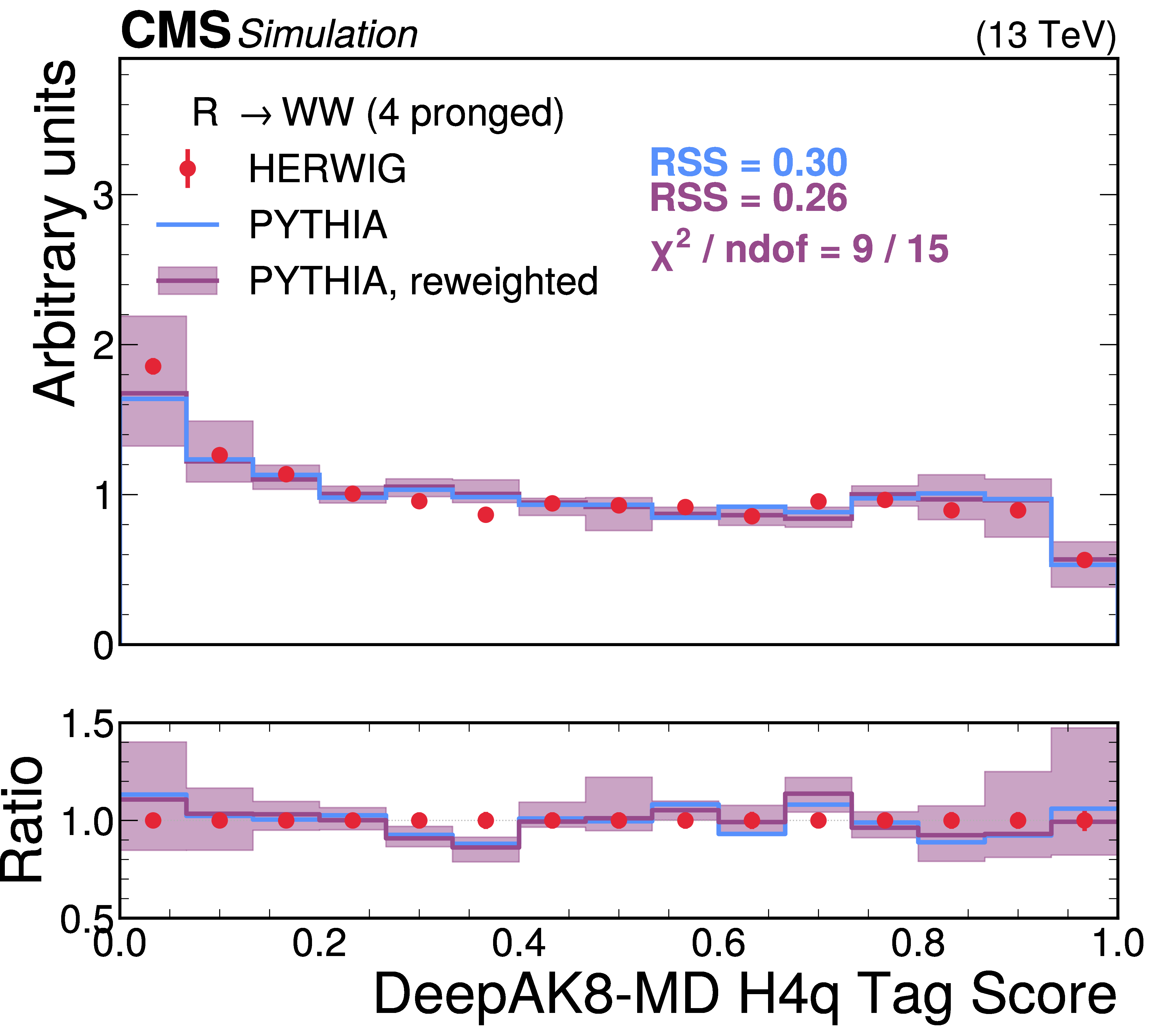
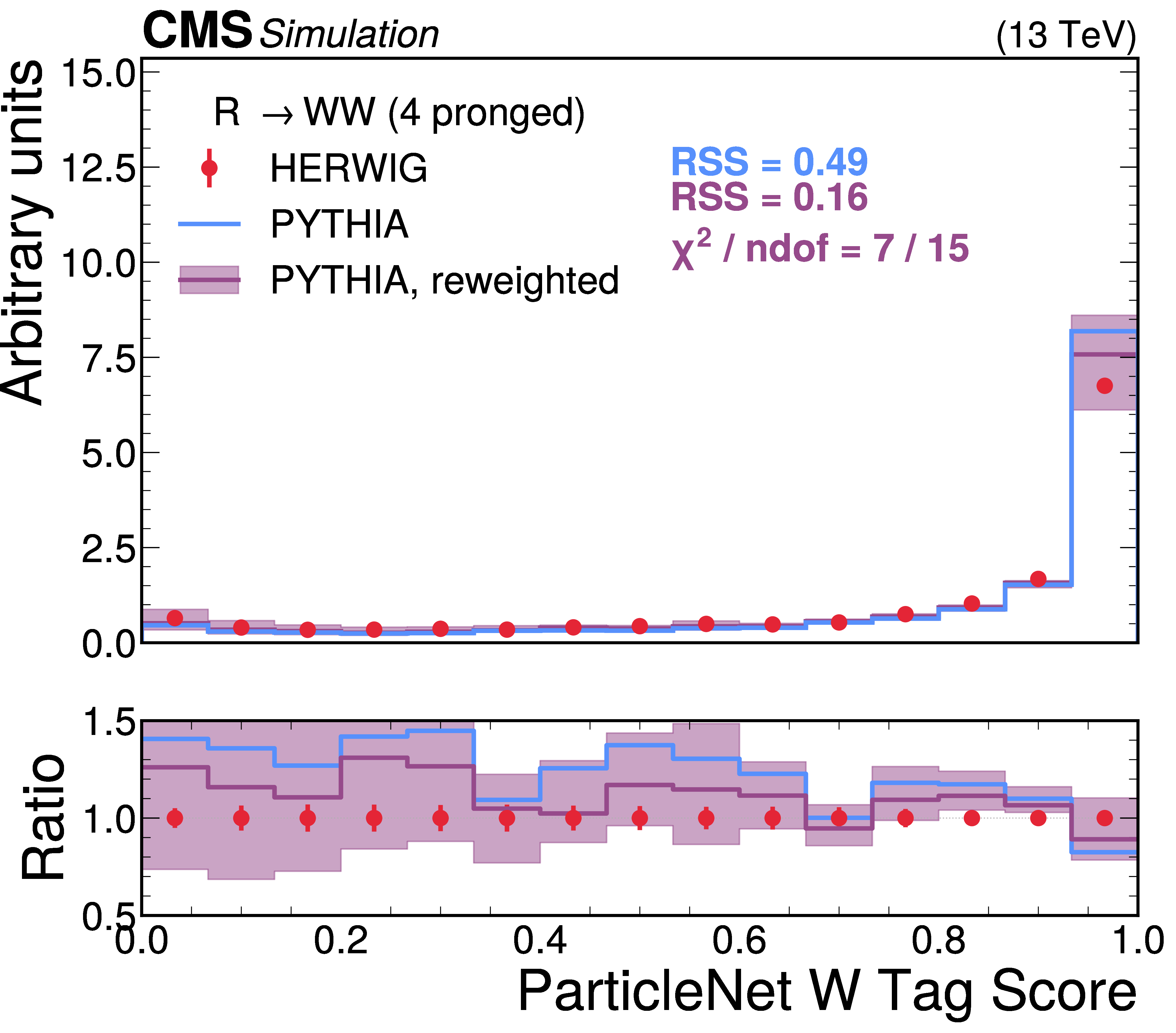
A comparison of the HERWIG (red circles), PYTHIA (blue lines) and reweighted PYTHIA (purple lines) samples for $ {\mathrm{R}} \to \mathrm{W}\mathrm{W} \to 4\mathrm{q} $ jets. The systematic uncertainty in the reweighted PYTHIA samples is shown in the light purple shading. The statistical uncertainty from the limited size of the simulated sample is shown as vertical red bars on the HERWIG points. The lower panel shows the ratio of the two PYTHIA distributions with respect to HERWIG. The RSS between the PYTHIA and HERWIG samples is computed based on the squared difference in normalized bin yields. The $ \chi^2 $ value is computed using both the statistical uncertainties of the simulated samples and the systematic uncertainties in the correction procedure, and therefore assesses the full closure of the correction procedure. It is computed only for the reweighted PYTHIA samples because the original sample does not have appropriate systematic uncertainties. |
png pdf |
Figure 8-a:
A comparison of the HERWIG (red circles), PYTHIA (blue lines) and reweighted PYTHIA (purple lines) samples for $ {\mathrm{R}} \to \mathrm{W}\mathrm{W} \to 4\mathrm{q} $ jets. The systematic uncertainty in the reweighted PYTHIA samples is shown in the light purple shading. The statistical uncertainty from the limited size of the simulated sample is shown as vertical red bars on the HERWIG points. The lower panel shows the ratio of the two PYTHIA distributions with respect to HERWIG. The RSS between the PYTHIA and HERWIG samples is computed based on the squared difference in normalized bin yields. The $ \chi^2 $ value is computed using both the statistical uncertainties of the simulated samples and the systematic uncertainties in the correction procedure, and therefore assesses the full closure of the correction procedure. It is computed only for the reweighted PYTHIA samples because the original sample does not have appropriate systematic uncertainties. |
png pdf |
Figure 8-b:
A comparison of the HERWIG (red circles), PYTHIA (blue lines) and reweighted PYTHIA (purple lines) samples for $ {\mathrm{R}} \to \mathrm{W}\mathrm{W} \to 4\mathrm{q} $ jets. The systematic uncertainty in the reweighted PYTHIA samples is shown in the light purple shading. The statistical uncertainty from the limited size of the simulated sample is shown as vertical red bars on the HERWIG points. The lower panel shows the ratio of the two PYTHIA distributions with respect to HERWIG. The RSS between the PYTHIA and HERWIG samples is computed based on the squared difference in normalized bin yields. The $ \chi^2 $ value is computed using both the statistical uncertainties of the simulated samples and the systematic uncertainties in the correction procedure, and therefore assesses the full closure of the correction procedure. It is computed only for the reweighted PYTHIA samples because the original sample does not have appropriate systematic uncertainties. |
png pdf |
Figure 8-c:
A comparison of the HERWIG (red circles), PYTHIA (blue lines) and reweighted PYTHIA (purple lines) samples for $ {\mathrm{R}} \to \mathrm{W}\mathrm{W} \to 4\mathrm{q} $ jets. The systematic uncertainty in the reweighted PYTHIA samples is shown in the light purple shading. The statistical uncertainty from the limited size of the simulated sample is shown as vertical red bars on the HERWIG points. The lower panel shows the ratio of the two PYTHIA distributions with respect to HERWIG. The RSS between the PYTHIA and HERWIG samples is computed based on the squared difference in normalized bin yields. The $ \chi^2 $ value is computed using both the statistical uncertainties of the simulated samples and the systematic uncertainties in the correction procedure, and therefore assesses the full closure of the correction procedure. It is computed only for the reweighted PYTHIA samples because the original sample does not have appropriate systematic uncertainties. |
png pdf |
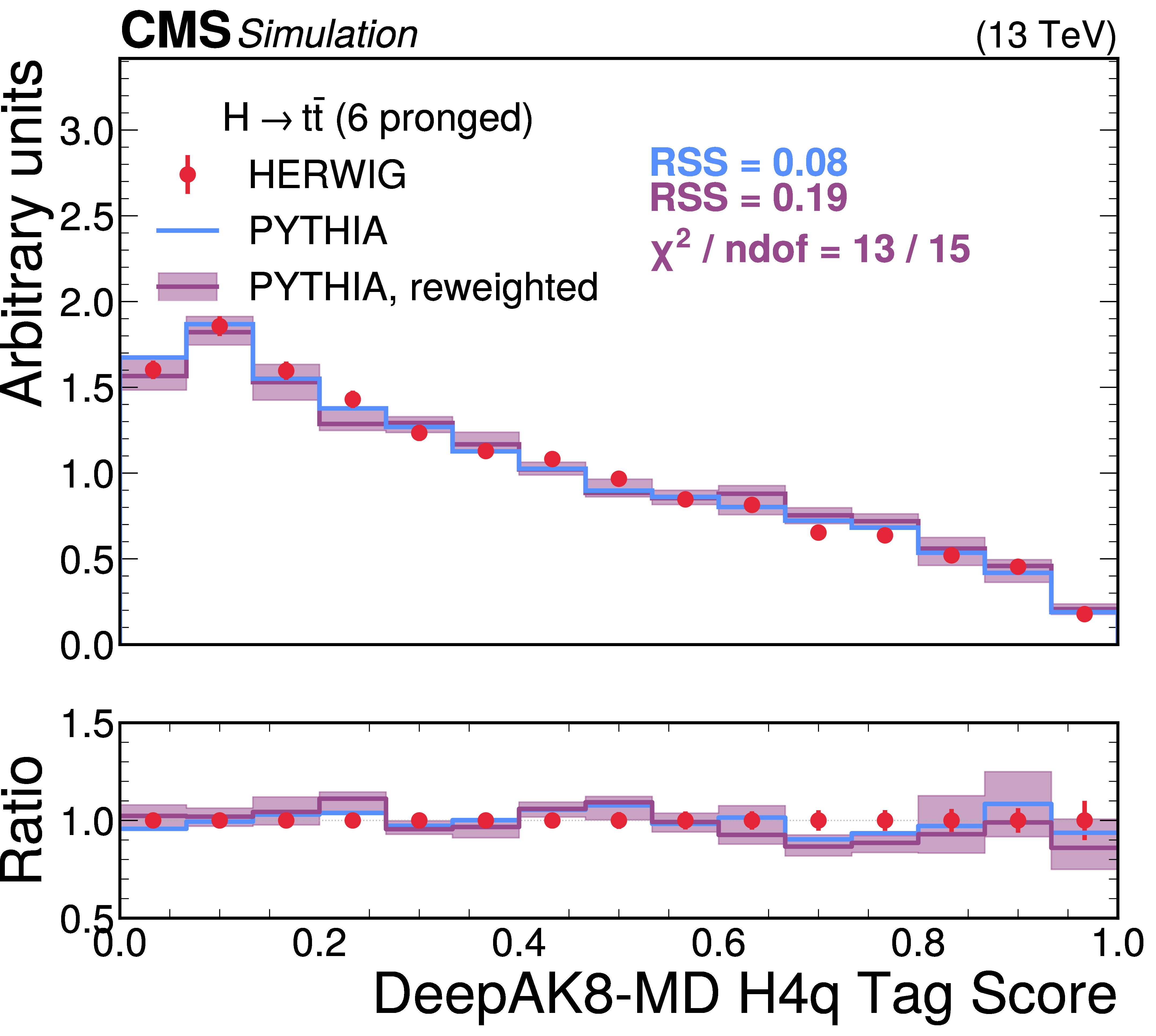
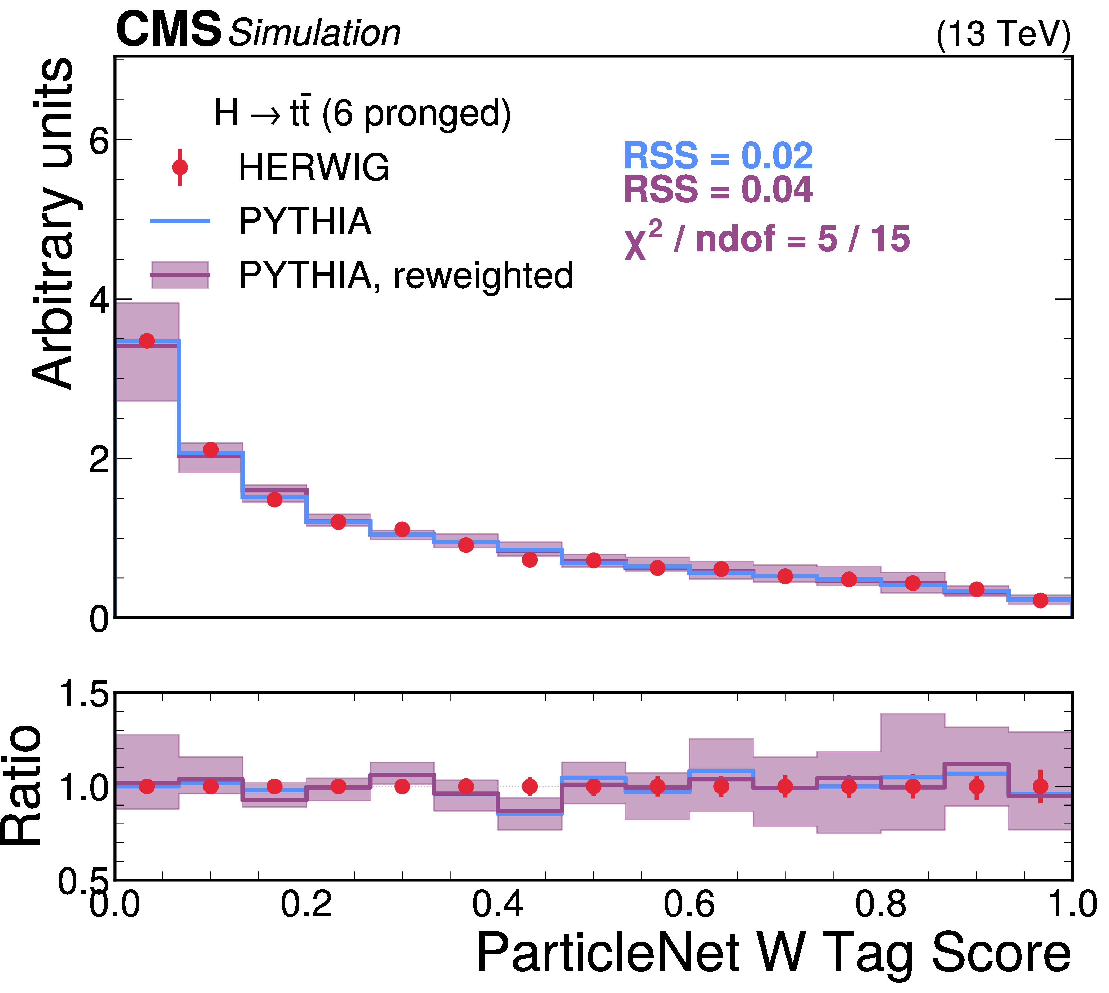
Figure 9:
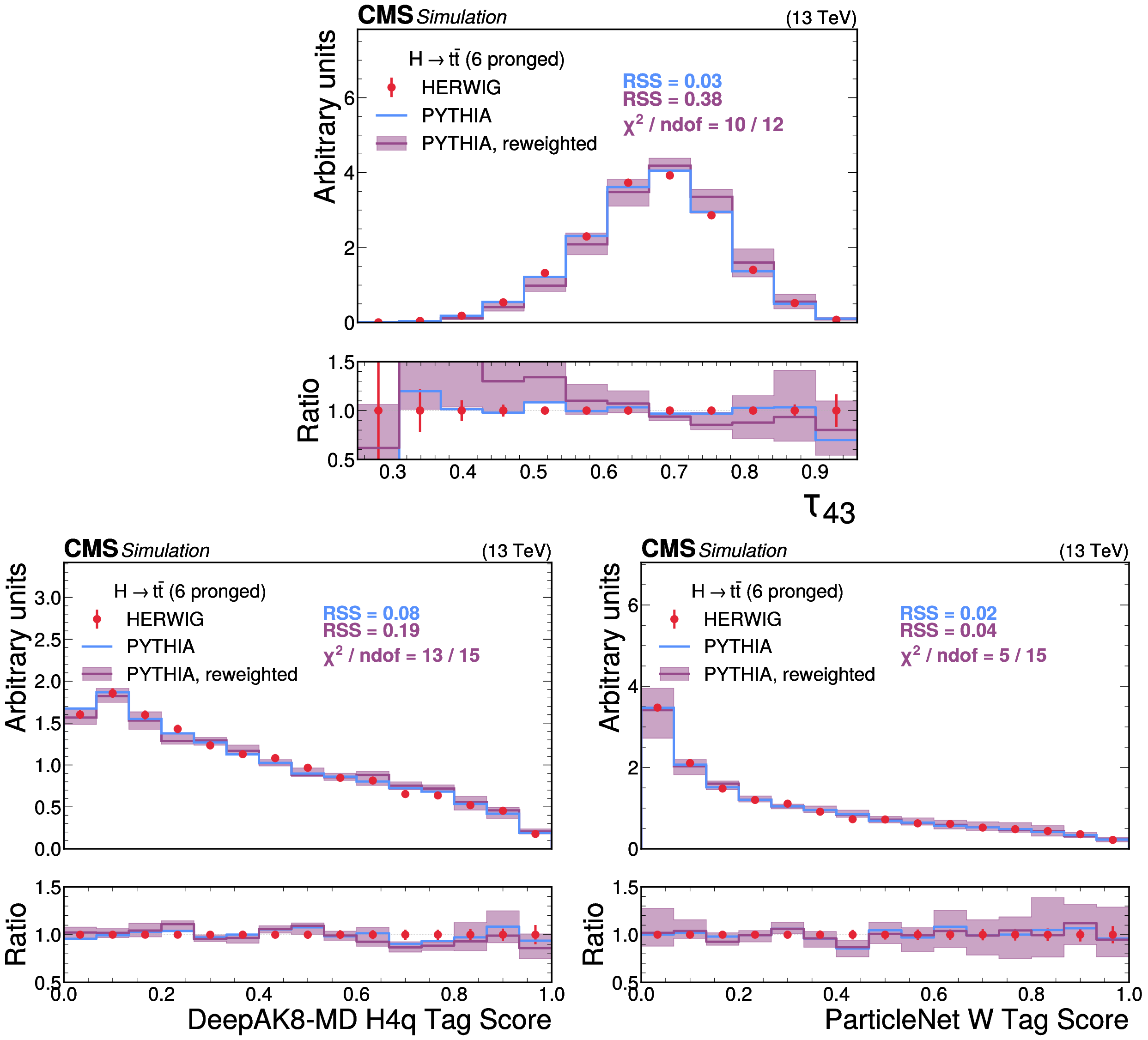
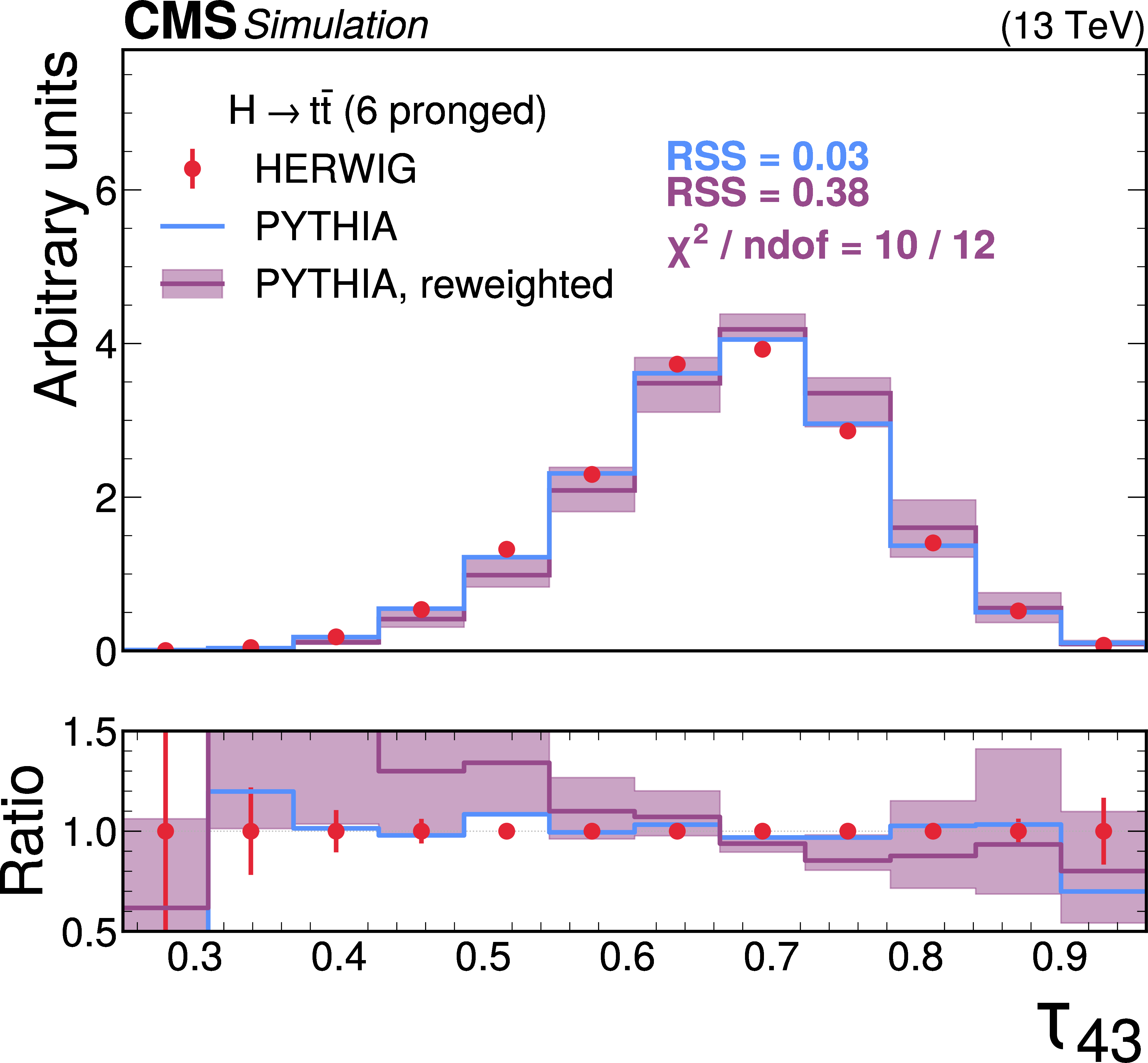
A comparison of the HERWIG (red circles), PYTHIA (blue lines) and reweighted PYTHIA (purple lines) samples for $ \mathrm{H} \to {\mathrm{t}\overline{\mathrm{t}}} \to 6\mathrm{q} $ jets. The systematic uncertainty in the reweighted PYTHIA samples is shown in the light purple shading. The statistical uncertainty from the limited size of the simulated sample is shown as vertical red bars on the HERWIG points. The lower panel shows the ratio of the two PYTHIA distributions with respect to HERWIG. The RSS between the PYTHIA and HERWIG samples is computed based on the squared difference in normalized bin yields. The $ \chi^2 $ value is computed using both the statistical uncertainties of the simulated samples and the systematic uncertainties in the correction procedure, and therefore assesses the full closure of the correction procedure. It is computed only for the reweighted PYTHIA samples because the original sample does not have appropriate systematic uncertainties. |
png pdf |
Figure 9-a:
A comparison of the HERWIG (red circles), PYTHIA (blue lines) and reweighted PYTHIA (purple lines) samples for $ \mathrm{H} \to {\mathrm{t}\overline{\mathrm{t}}} \to 6\mathrm{q} $ jets. The systematic uncertainty in the reweighted PYTHIA samples is shown in the light purple shading. The statistical uncertainty from the limited size of the simulated sample is shown as vertical red bars on the HERWIG points. The lower panel shows the ratio of the two PYTHIA distributions with respect to HERWIG. The RSS between the PYTHIA and HERWIG samples is computed based on the squared difference in normalized bin yields. The $ \chi^2 $ value is computed using both the statistical uncertainties of the simulated samples and the systematic uncertainties in the correction procedure, and therefore assesses the full closure of the correction procedure. It is computed only for the reweighted PYTHIA samples because the original sample does not have appropriate systematic uncertainties. |
png pdf |
Figure 9-b:
A comparison of the HERWIG (red circles), PYTHIA (blue lines) and reweighted PYTHIA (purple lines) samples for $ \mathrm{H} \to {\mathrm{t}\overline{\mathrm{t}}} \to 6\mathrm{q} $ jets. The systematic uncertainty in the reweighted PYTHIA samples is shown in the light purple shading. The statistical uncertainty from the limited size of the simulated sample is shown as vertical red bars on the HERWIG points. The lower panel shows the ratio of the two PYTHIA distributions with respect to HERWIG. The RSS between the PYTHIA and HERWIG samples is computed based on the squared difference in normalized bin yields. The $ \chi^2 $ value is computed using both the statistical uncertainties of the simulated samples and the systematic uncertainties in the correction procedure, and therefore assesses the full closure of the correction procedure. It is computed only for the reweighted PYTHIA samples because the original sample does not have appropriate systematic uncertainties. |
png pdf |
Figure 9-c:
A comparison of the HERWIG (red circles), PYTHIA (blue lines) and reweighted PYTHIA (purple lines) samples for $ \mathrm{H} \to {\mathrm{t}\overline{\mathrm{t}}} \to 6\mathrm{q} $ jets. The systematic uncertainty in the reweighted PYTHIA samples is shown in the light purple shading. The statistical uncertainty from the limited size of the simulated sample is shown as vertical red bars on the HERWIG points. The lower panel shows the ratio of the two PYTHIA distributions with respect to HERWIG. The RSS between the PYTHIA and HERWIG samples is computed based on the squared difference in normalized bin yields. The $ \chi^2 $ value is computed using both the statistical uncertainties of the simulated samples and the systematic uncertainties in the correction procedure, and therefore assesses the full closure of the correction procedure. It is computed only for the reweighted PYTHIA samples because the original sample does not have appropriate systematic uncertainties. |
png pdf |
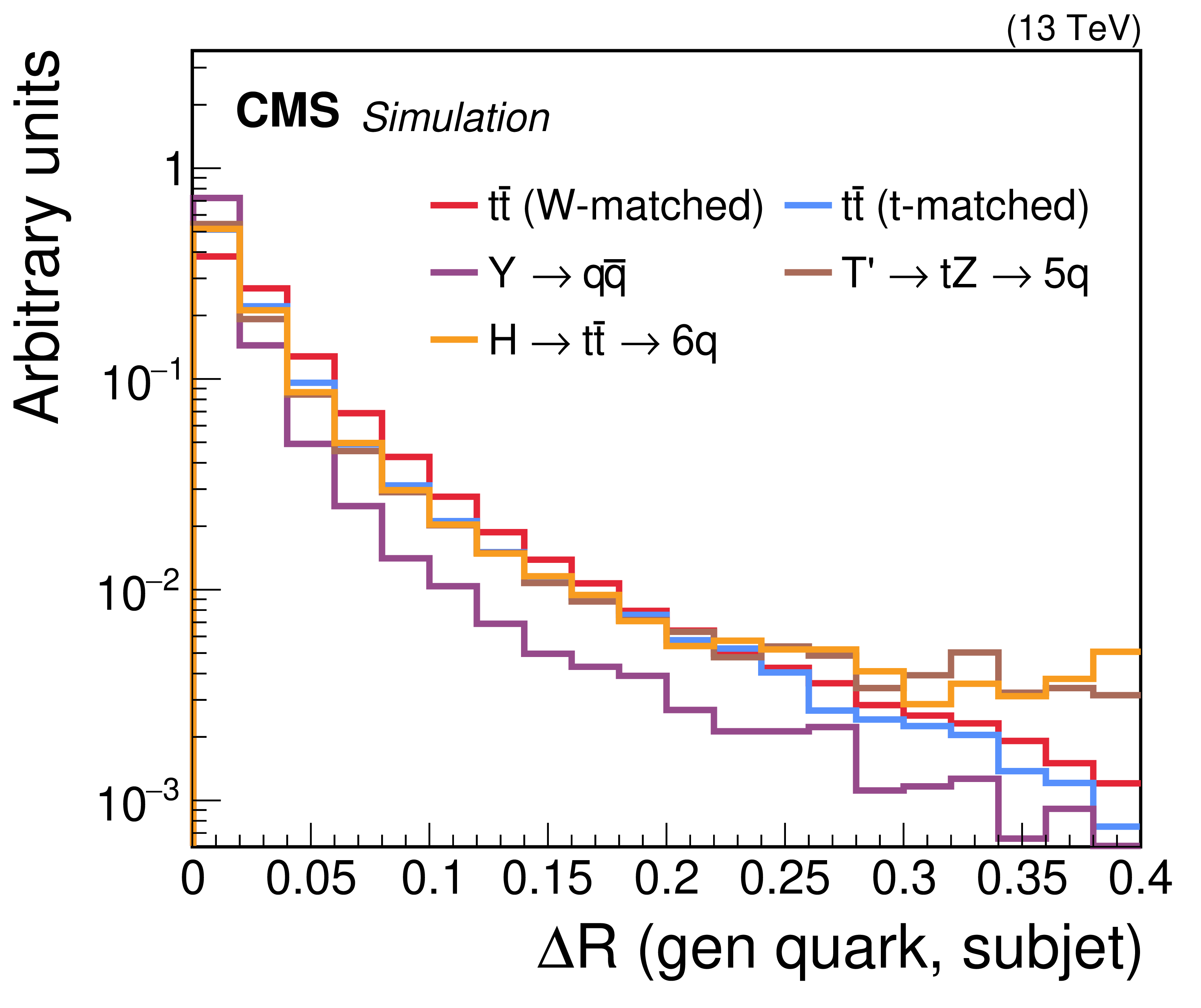
Figure 10:
Distributions of the $ \Delta R $ between subjets found by the reclustering procedure and closest generator-level quarks of the heavy resonance decay for various jet types. The $ \Delta R $ distributions for all signals peak towards zero, indicating that the reclustering procedure is performing well. |
png pdf |
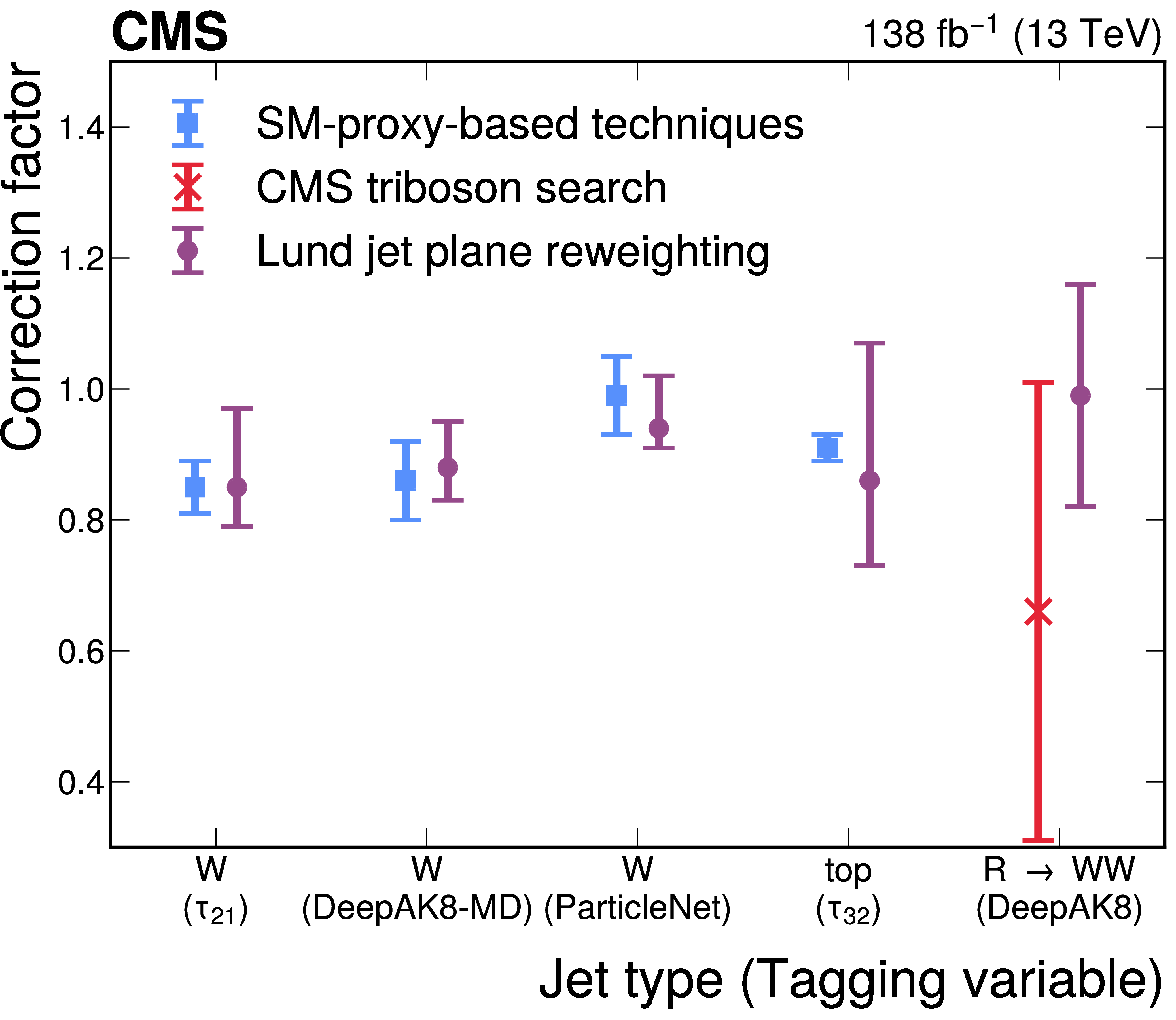
Figure 11:
A comparison of correction factors for jet tagging efficiencies of various types, using standard calibration techniques based on SM proxy objects (blue squares), an extension of SM-proxy-based techniques using hard gluon radiation [25] (red crosses), and the LJP reweighting technique (purple squares). The vertical error bars denote the uncertainty on each calibration technique. |
| Tables | |
png pdf |
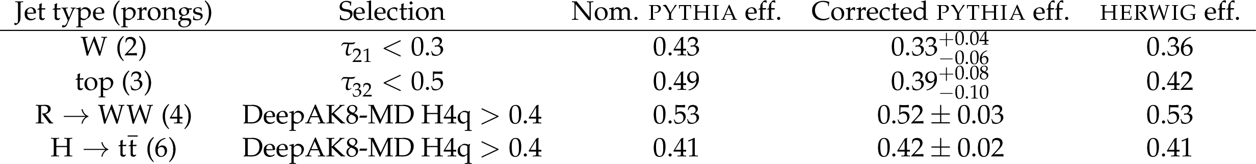
Table 1:
A comparison of the tagging efficiency in the nominal PYTHIA simulation, the corrected PYTHIA simulation and the HERWIG simulation for jets of various kinds. Uncertainties in the correction procedure are propagated to evaluate the uncertainty in the tagging efficiency in the corrected PYTHIA simulation. Details are given in the text. |
png pdf |
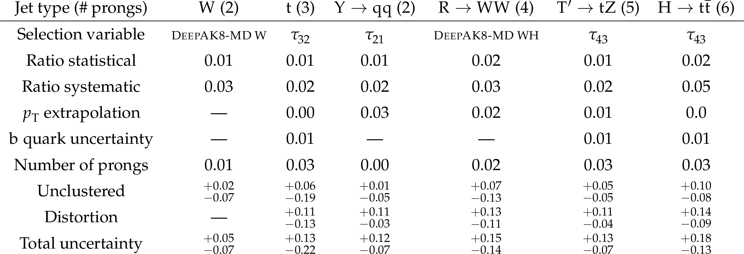
Table 2:
Uncertainties in the LJP reweighting scale factor for tagging jets from various processes. Uncertainties not applicable to a given process are denoted with a dash. |
png pdf |
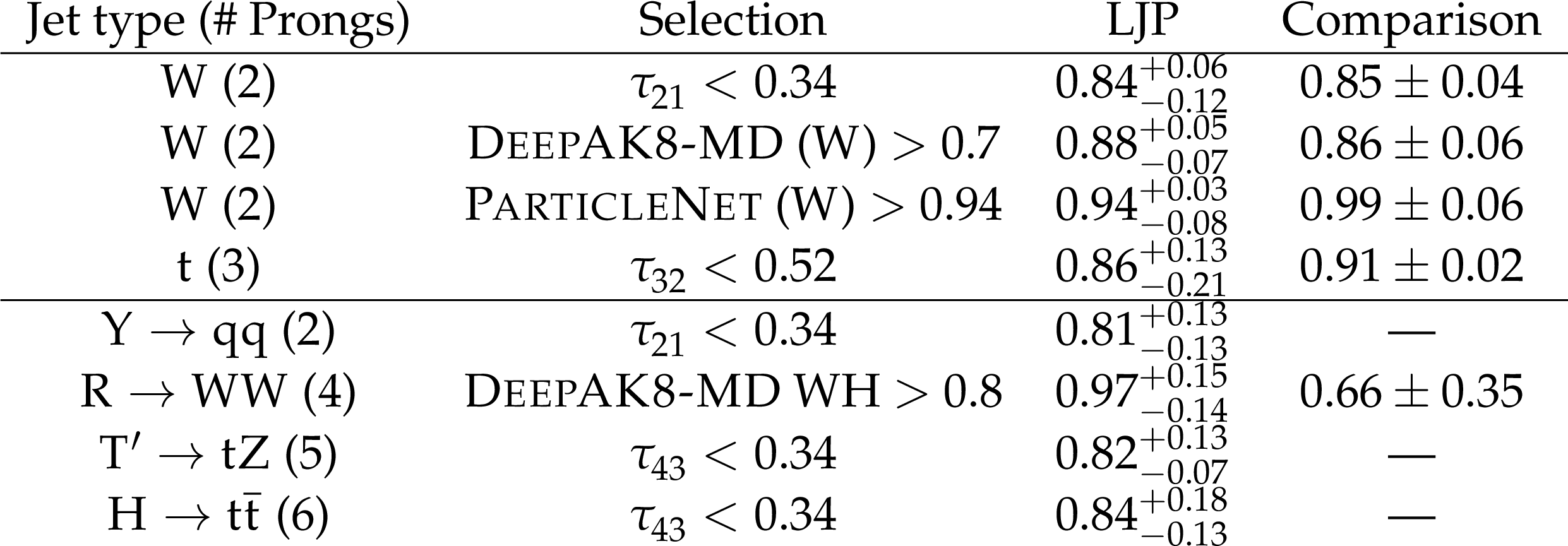
Table 3:
A comparison of scale factors derived using the LJP correction procedure and other methods. The scale factors derived with the LJP correction have larger uncertainties, but agree well with those from traditional methods. The comparison for the $ {\mathrm{R}} \to \mathrm{W}\mathrm{W} $ was taken from a recent search by the CMS Collaboration [25]. |
| Summary |
| A new method has been presented to improve the modeling in simulation of large-radius multiprong jets originating from the decay of heavy resonances into multiple quarks. The method is based on a reclustering of the multiprong jet into separate subjets for each prong. The emissions of each subjet are corrected using the ratio of the Lund jet plane (LJP) densities between data and simulation, derived from a sample of W jets. The correction for the full jet is computed by combining the corrections of each of the subjets. The method successfully improves the agreement between data and simulation of substructure observables of two-pronged W jets and three-pronged top quark jets. The LJP reweighting is also used to correct simulations using PYTHIA for the parton shower to match HERWIG, which validates that the correction performs well for jets with more than three prongs. The method can be used to correct the efficiency of substructure-based event selection criteria. Efficiencies for W and t tagging corrected with the LJP method agree well with the efficiencies measured directly in data. The main advance of the LJP method is that it can be applied to multiprong jets which could not be calibrated by previous methods. It enables for the first time the calibration of jet tagging efficiencies for high-prong jets for which there are no comparable standard model processes of a high enough yield. The calibration of large-radius jets with high prong multiplicities enables the proper interpretation of the results of searches targeting such signatures. |
| References | ||||
| 1 | M. Cacciari, G. P. Salam, and G. Soyez | The anti-$ k_{\mathrm{T}} $ jet clustering algorithm | JHEP 04 (2008) 063 | 0802.1189 |
| 2 | M. Cacciari, G. P. Salam, and G. Soyez | FastJet user manual | EPJC 72 (2012) 1896 | 1111.6097 |
| 3 | J. Thaler and K. Van Tilburg | Identifying boosted objects with $ N $-subjettiness | JHEP 03 (2011) 015 | 1011.2268 |
| 4 | P. T. Komiske, E. M. Metodiev, and J. Thaler | Energy flow polynomials: A complete linear basis for jet substructure | JHEP 04 (2018) 013 | 1712.07124 |
| 5 | A. J. Larkoski, S. Marzani, G. Soyez, and J. Thaler | Soft drop | JHEP 05 (2014) 146 | 1402.2657 |
| 6 | CMS Collaboration | Identification of heavy, energetic, hadronically decaying particles using machine-learning techniques | JINST 15 (2020) P06005 | CMS-JME-18-002 2004.08262 |
| 7 | CMS Collaboration | Identification of highly Lorentz-boosted heavy particles using graph neural networks and new mass decorrelation techniques | CMS Detector Performance Note CMS-DP-2020-002, 2020 CDS |
|
| 8 | ATLAS Collaboration | Performance of top-quark and $ W $-boson tagging with ATLAS in Run 2 of the LHC | EPJC 79 (2019) 375 | 1808.07858 |
| 9 | ATLAS Collaboration | Identification of hadronically-decaying top quarks using UFO jets with ATLAS in Run 2 | ATLAS PUB Note ATL-PHYS-PUB-2021-028, 2021 | |
| 10 | ATLAS Collaboration | Measurement of soft-drop jet observables in $ pp $ collisions with the ATLAS detector at $ \sqrt {s}= $ 13 TeV | PRD 101 (2020) 052007 | 1912.09837 |
| 11 | CMS Collaboration | Measurement of jet substructure observables in $ \mathrm{t\overline{t}} $ events from proton-proton collisions at $ \sqrt{s}= $ 13 TeV | PRD 98 (2018) 092014 | CMS-TOP-17-013 1808.07340 |
| 12 | CMS Collaboration | Identification of heavy-flavour jets with the CMS detector in pp collisions at 13 TeV | JINST 13 (2018) P05011 | CMS-BTV-16-002 1712.07158 |
| 13 | ATLAS Collaboration | Identification of boosted Higgs bosons decaying into $ b $-quark pairs with the ATLAS detector at 13 TeV | EPJC 79 (2019) 836 | 1906.11005 |
| 14 | Y. Bai and B. A. Dobrescu | Collider tests of the renormalizable coloron model | JHEP 04 (2018) 114 | 1802.03005 |
| 15 | J. A. Aguilar-Saavedra | Profile of multiboson signals | JHEP 05 (2017) 066 | 1703.06153 |
| 16 | K. Agashe, P. Du, S. Hong, and R. Sundrum | Flavor universal resonances and warped gravity | JHEP 01 (2017) 016 | 1608.00526 |
| 17 | K. S. Agashe et al. | LHC signals from cascade decays of warped vector resonances | JHEP 05 (2017) 078 | 1612.00047 |
| 18 | F. A. Dreyer, G. P. Salam, and G. Soyez | The Lund jet plane | JHEP 12 (2018) 064 | 1807.04758 |
| 19 | T. Sjostrand et al. | An introduction to PYTHIA 8.2 | Comput. Phys. Commun. 191 (2015) 159 | 1410.3012 |
| 20 | B. R. Webber | A QCD model for jet fragmentation including soft gluon interference | NPB 238 (1984) 492 | |
| 21 | S. Gieseke, P. Stephens, and B. Webber | New formalism for QCD parton showers | JHEP 12 (2003) 045 | hep-ph/0310083 |
| 22 | ATLAS Collaboration | Measurement of the Lund jet plane using charged particles in 13 TeV proton-proton collisions with the ATLAS detector | PRL 124 (2020) 222002 | 2004.03540 |
| 23 | CMS Collaboration | Measurement of the primary Lund jet plane density in proton-proton collisions at $ \sqrt{\textrm{s}} = $ 13 TeV | JHEP 05 (2024) 116 | CMS-SMP-22-007 2312.16343 |
| 24 | ATLAS Collaboration | Measurement of the Lund jet plane in hadronic decays of top quarks and W bosons with the ATLAS detector | EPJC 85 (2025) 416 | 2407.10879 |
| 25 | CMS Collaboration | Search for resonances decaying to three $ W $ bosons in the hadronic final state in proton-proton collisions at $ \sqrt s= $ 13 TeV | PRD 106 (2022) 012002 | 2112.13090 |
| 26 | CMS Collaboration | Model-agnostic search for dijet resonances with anomalous jet substructure in proton-proton collisions at $ \sqrt{s} = $ 13 TeV | Rept. Prog. Phys. 88 (2025) 067802 | CMS-EXO-22-026 2412.03747 |
| 27 | CMS Collaboration | The CMS experiment at the CERN LHC | JINST 3 (2008) S08004 | |
| 28 | CMS Collaboration | Development of the CMS detector for the CERN LHC Run 3 | JINST 19 (2024) P05064 | CMS-PRF-21-001 2309.05466 |
| 29 | CMS Collaboration | Description and performance of track and primary-vertex reconstruction with the CMS tracker | JINST 9 (2014) P10009 | CMS-TRK-11-001 1405.6569 |
| 30 | Tracker Group of the CMS Collaboration | The CMS Phase-1 pixel detector upgrade | JINST 16 (2021) P02027 | 2012.14304 |
| 31 | CMS Collaboration | Track impact parameter resolution for the full pseudo rapidity coverage in the 2017 dataset with the CMS Phase-1 Pixel detector | CMS Detector Performance Note CMS-DP-2020-049, 2020 CDS |
|
| 32 | CMS Collaboration | Performance of the CMS muon detector and muon reconstruction with proton-proton collisions at $ \sqrt{s}= $ 13 TeV | JINST 13 (2018) P06015 | CMS-MUO-16-001 1804.04528 |
| 33 | CMS Collaboration | Performance of the CMS Level-1 trigger in proton-proton collisions at $ \sqrt{s} = $ 13 TeV | JINST 15 (2020) P10017 | CMS-TRG-17-001 2006.10165 |
| 34 | CMS Collaboration | The CMS trigger system | JINST 12 (2017) P01020 | CMS-TRG-12-001 1609.02366 |
| 35 | CMS Collaboration | Particle-flow reconstruction and global event description with the CMS detector | JINST 12 (2017) P10003 | CMS-PRF-14-001 1706.04965 |
| 36 | D. Bertolini, P. Harris, M. Low, and N. Tran | Pileup per particle identification | JHEP 10 (2014) 059 | 1407.6013 |
| 37 | CMS Collaboration | Pileup mitigation at CMS in 13 TeV data | JINST 15 (2020) P09018 | CMS-JME-18-001 2003.00503 |
| 38 | CMS Collaboration | Jet energy scale and resolution in the CMS experiment in pp collisions at 8 TeV | JINST 12 (2017) P02014 | CMS-JME-13-004 1607.03663 |
| 39 | CMS Collaboration | Performance of missing transverse momentum reconstruction in proton-proton collisions at $ \sqrt{s} = $ 13 TeV using the CMS detector | JINST 14 (2019) P07004 | CMS-JME-17-001 1903.06078 |
| 40 | S. D. Ellis and D. E. Soper | Successive combination jet algorithm for hadron collisions | PRD 48 (1993) 3160 | hep-ph/9305266 |
| 41 | Y. L. Dokshitzer, G. D. Leder, S. Moretti, and B. R. Webber | Better jet clustering algorithms | JHEP 08 (1997) 001 | hep-ph/9707323 |
| 42 | M. Wobisch and T. Wengler | Hadronization corrections to jet cross sections in deep inelastic scattering | in Proc. Workshop on Monte Carlo Generators for HERA Physics, p. 270. 1998 | hep-ph/9907280 |
| 43 | CMS Collaboration | Precision luminosity measurement in proton-proton collisions at $ \sqrt{s} = $ 13 TeV in 2015 and 2016 at CMS | EPJC 81 (2021) 800 | CMS-LUM-17-003 2104.01927 |
| 44 | CMS Collaboration | CMS luminosity measurement for the 2017 data-taking period at $ \sqrt{s} = $ 13 TeV | CMS Physics Analysis Summary, 2018 link |
CMS-PAS-LUM-17-004 |
| 45 | CMS Collaboration | CMS luminosity measurement for the 2018 data-taking period at $ \sqrt{s} = $ 13 TeV | CMS Physics Analysis Summary, 2019 link |
CMS-PAS-LUM-18-002 |
| 46 | CMS Collaboration | Extraction and validation of a new set of CMS PYTHIA8 tunes from underlying-event measurements | EPJC 80 (2020) 4 | CMS-GEN-17-001 1903.12179 |
| 47 | NNPDF Collaboration | Parton distributions from high-precision collider data | EPJC 77 (2017) 663 | 1706.00428 |
| 48 | GEANT4 Collaboration | GEANT4 --- a simulation toolkit | NIM A 506 (2003) 250 | |
| 49 | P. Nason | A new method for combining NLO QCD with shower Monte Carlo algorithms | JHEP 11 (2004) 040 | hep-ph/0409146 |
| 50 | S. Frixione, P. Nason, and G. Ridolfi | A positive-weight next-to-leading-order Monte Carlo for heavy flavour hadroproduction | JHEP 09 (2007) 126 | 0707.3088 |
| 51 | S. Alioli, P. Nason, C. Oleari, and E. Re | A general framework for implementing NLO calculations in shower Monte Carlo programs: the POWHEG BOX | JHEP 06 (2010) 043 | 1002.2581 |
| 52 | R. Frederix and S. Frixione | Merging meets matching in MC@NLO | JHEP 12 (2012) 061 | 1209.6215 |
| 53 | J. Alwall et al. | Comparative study of various algorithms for the merging of parton showers and matrix elements in hadronic collisions | EPJC 53 (2007) 473 | 0706.2569 |
| 54 | M. Czakon and A. Mitov | Top++: A program for the calculation of the top-pair cross-section at hadron colliders | Comput. Phys. Commun. 185 (2014) 2930 | 1112.5675 |
| 55 | J. Campbell, T. Neumann, and Z. Sullivan | Single-top-quark production in the $ t $-channel at NNLO | JHEP 02 (2021) 040 | 2012.01574 |
| 56 | PDF4LHC Working Group Collaboration | The PDF4LHC21 combination of global PDF fits for the LHC Run III | JPG 49 (2022) 080501 | 2203.05506 |
| 57 | T. Gehrmann et al. | $ W^+W^- $ production at hadron colliders in next to next to leading order QCD | PRL 113 (2014) 212001 | 1408.5243 |
| 58 | F. Cascioli et al. | ZZ production at hadron colliders in NNLO QCD | PLB 735 (2014) 311 | 1405.2219 |
| 59 | J. M. Campbell, R. K. Ellis, and C. Williams | Vector boson pair production at the LHC | JHEP 07 (2011) 018 | 1105.0020 |
| 60 | CMS Collaboration | Measurement of differential cross sections for top quark pair production using the lepton+jets final state in proton-proton collisions at 13 TeV | PRD 95 (2017) 092001 | CMS-TOP-16-008 1610.04191 |
| 61 | Y. Okada and L. Panizzi | LHC signatures of vector-like quarks | Adv. High Energy Phys. 2013 (2013) 364936 | 1207.5607 |
| 62 | M. Buchkremer, G. Cacciapaglia, A. Deandrea, and L. Panizzi | Model independent framework for searches of top partners | NPB 876 (2013) 376 | 1305.4172 |
| 63 | A. Carvalho | Gravity particles from warped extra dimensions, predictions for LHC | 1404.0102 | |
| 64 | K. Agashe et al. | Dedicated strategies for triboson signals from cascade decays of vector resonances | PRD 99 (2019) 075016 | 1711.09920 |
| 65 | CMS Collaboration | Performance of the reconstruction and identification of high-momentum muons in proton-proton collisions at $ \sqrt{s} = $ 13 TeV | JINST 15 (2020) P02027 | CMS-MUO-17-001 1912.03516 |
| 66 | E. Bols et al. | Jet flavour classification using DeepJet | JINST 15 (2020) P12012 | 2008.10519 |
| 67 | CMS Collaboration | Performance of the DeepJet b tagging algorithm using 41.9/fb of data from proton-proton collisions at 13 TeV with Phase 1 CMS detector | CMS Detector Performance Note CMS-DP-2018-058, 2018 CDS |
|
| 68 | J. M. Butterworth, A. R. Davison, M. Rubin, and G. P. Salam | Jet substructure as a new Higgs-search channel at the LHC | PRL 100 (2008) 242001 | 0802.2470 |
| 69 | M. Dasgupta, A. Fregoso, S. Marzani, and G. P. Salam | Towards an understanding of jet substructure | JHEP 09 (2013) 029 | 1307.0007 |
| 70 | R. Fisher | On the interpretation of $ \chi^2 $ from contingency tables, and the calculation of P | J. R. Stat. Soc. 85 (1922) 87 | |
| 71 | H. Qu and L. Gouskos | ParticleNet: Jet tagging via particle clouds | PRD 101 (2020) 056019 | 1902.08570 |
| 72 | Y. L. Dokshitzer, V. A. Khoze, and S. I. Troian | On specific QCD properties of heavy quark fragmentation ('dead cone') | JPG 17 (1991) 1602 | |
| 73 | ALICE Collaboration | Direct observation of the dead-cone effect in quantum chromodynamics | Nature 605 (2022) 440 | 2106.05713 |
|
|
Compact Muon Solenoid LHC, CERN |
|

|

|

|

|

|