

Compact Muon Solenoid
LHC, CERN
| CMS-EXO-22-026 ; CERN-EP-2024-291 | ||
| Model-agnostic search for dijet resonances with anomalous jet substructure in proton-proton collisions at $ \sqrt{s} $ = 13 TeV | ||
| CMS Collaboration | ||
| 4 December 2024 | ||
| Rep. Prog. Phys. 88 (2025) 067802 | ||
| Abstract: This paper presents a model-agnostic search for narrow resonances in the dijet final state in the mass range 1.8-6 TeV. The signal is assumed to produce jets with substructure atypical of jets initiated by light quarks or gluons, with minimal additional assumptions. Search regions are obtained by utilizing multivariate machine-learning methods to select jets with anomalous substructure. A collection of complementary anomaly detection methods$-$based on unsupervised, weakly supervised, and semisupervised algorithms$-$are used in order to maximize the sensitivity to unknown new physics signatures. These algorithms are applied to data corresponding to an integrated luminosity of 138 fb$ ^{-1} $, recorded by the CMS experiment at the LHC, at a center-of-mass energy of 13 TeV. No significant excesses above background expectations are seen. Exclusion limits are derived on the production cross section of benchmark signal models varying in resonance mass, jet mass, and jet substructure. Many of these signatures have not been previously sought, making several of the limits reported on the corresponding benchmark models the first ever. When compared to benchmark inclusive and substructure-based search strategies, the anomaly detection methods are found to significantly enhance the sensitivity to a variety of models. | ||
| Links: e-print arXiv:2412.03747 [hep-ex] (PDF) ; CDS record ; inSPIRE record ; HepData record ; Physics Briefing ; CADI line (restricted) ; | ||
| Figures | |
png pdf |
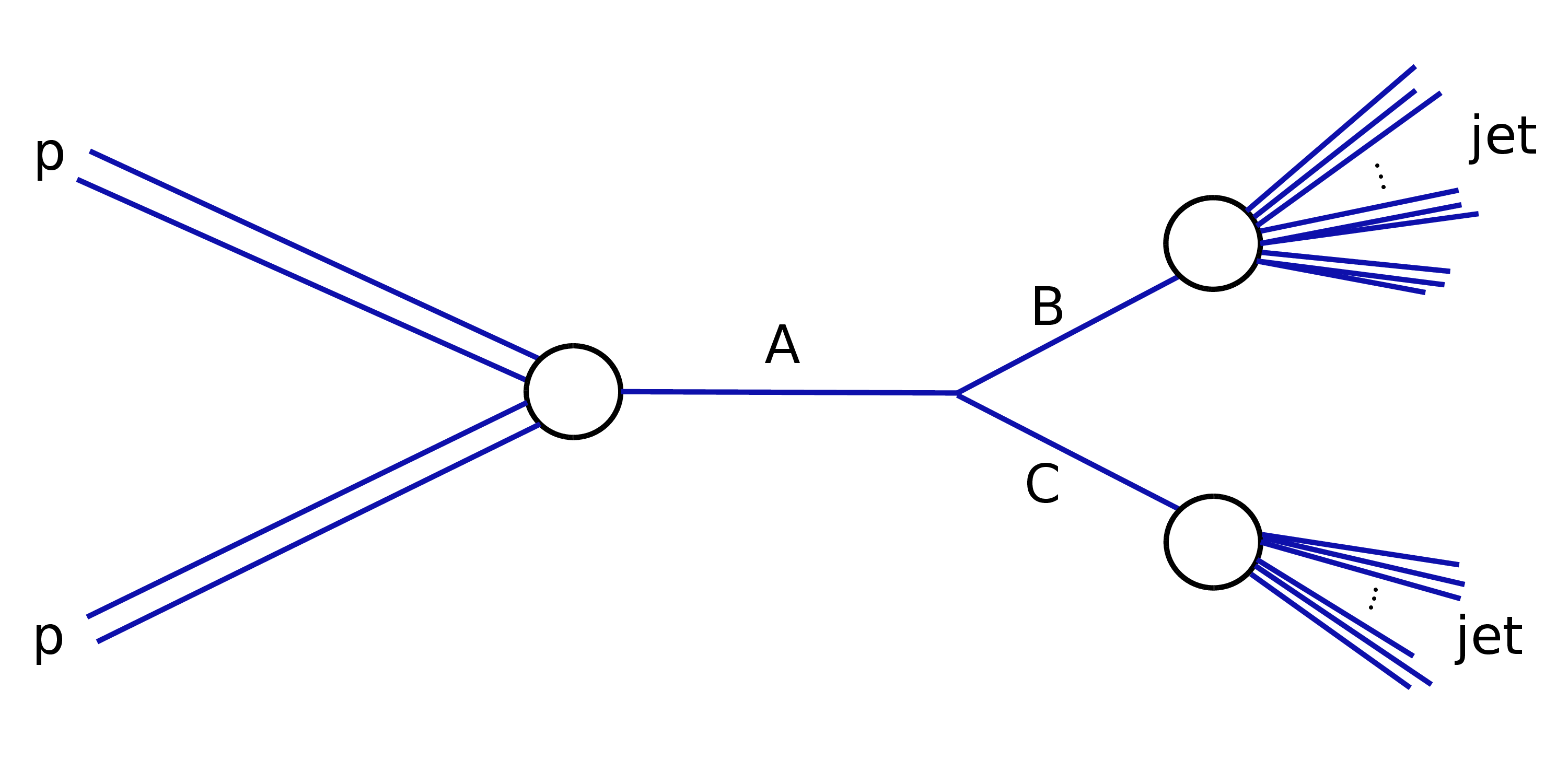
Figure 1:
Production of a dijet resonance, A, in a proton-proton collision. The A resonance decays to two resonances B and C, which in turn each decay to a jet with anomalous substructure arising from multiple subjets. |
png pdf |
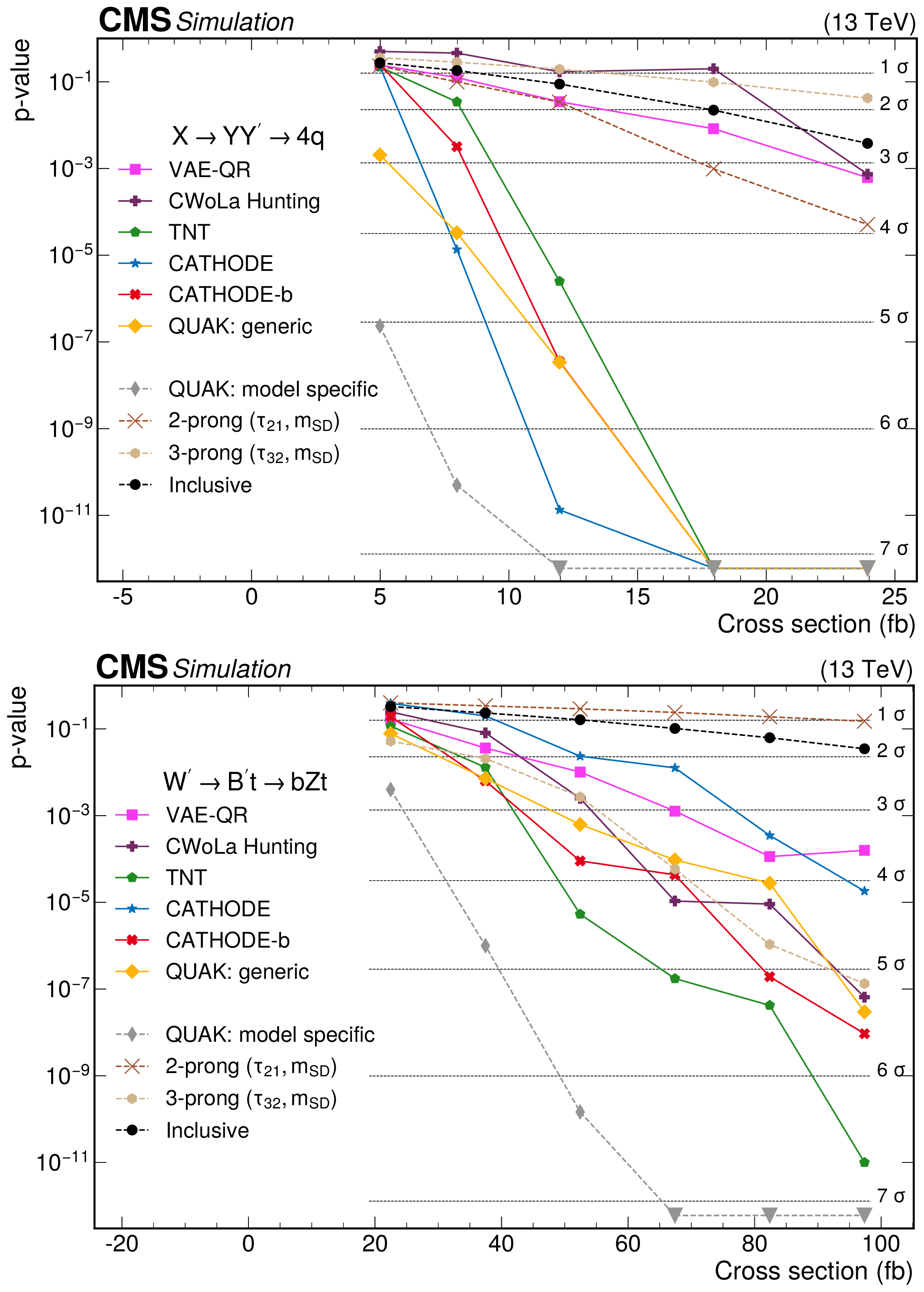
Figure 2:
The $ p $-values as a function of the injected signal cross sections for the different analysis procedures for two different signals: (upper) the 2-prong $ \mathrm{X}\to \mathrm{Y}\mathrm{Y'} \to 4 \mathrm{q} $ signal with $ m_\mathrm{X}= $ 3 TeV, $ m_\mathrm{Y}= $ 170 GeV, and $ M_\mathrm{Y'}= $ 170 GeV, and (lower) 3-prong $ \mathrm{W^{'}} \to \mathrm{B'}\mathrm{t} \to \mathrm{b} \mathrm{Z} \mathrm{t} $ signal with $ M_\mathrm{W'}= $ 3 TeV and $ M_\mathrm{B'}= $ 400 GeV. Significance values larger than 7$ \sigma $ are denoted with downwards facing triangles. |
png pdf |
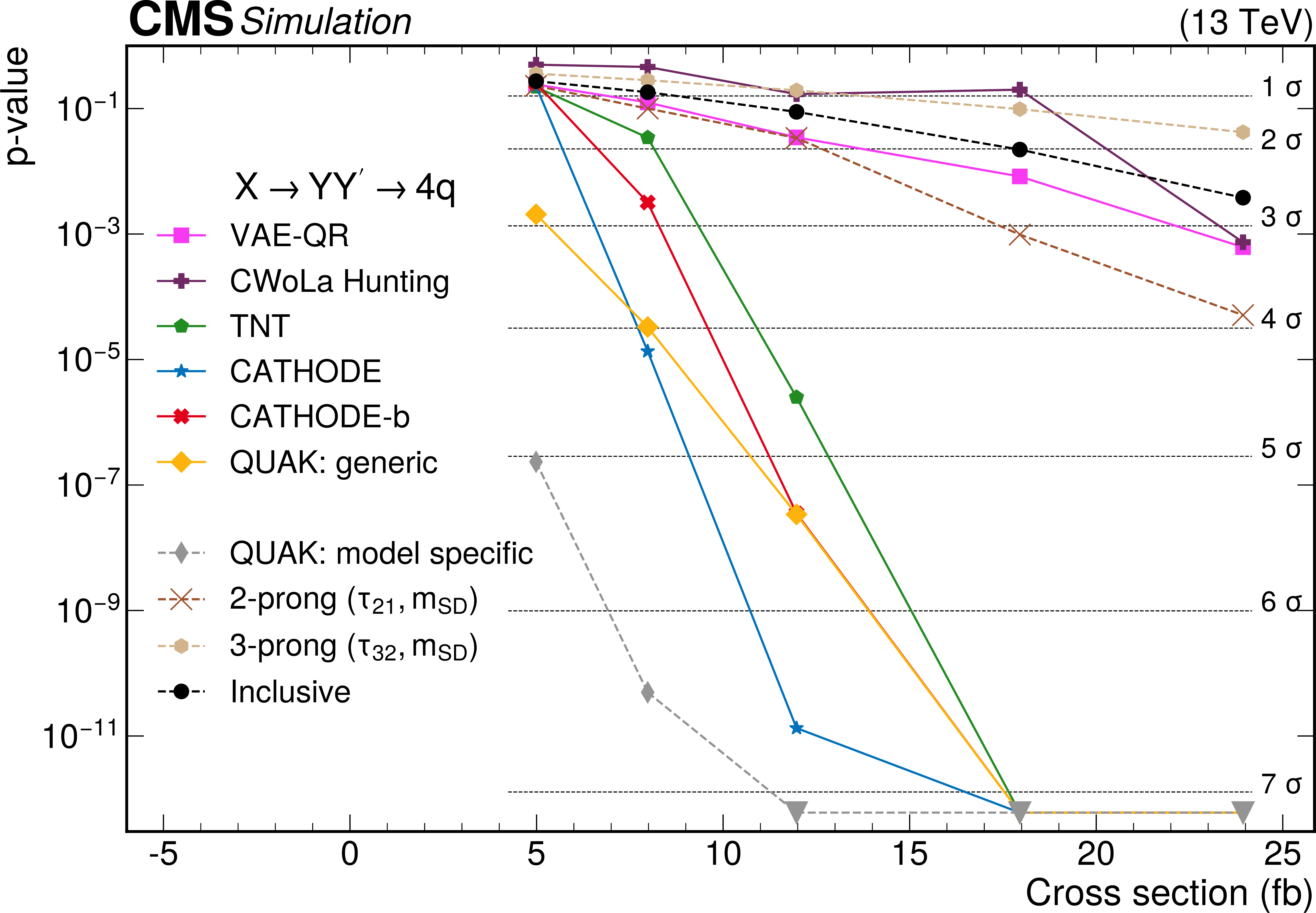
Figure 2-a:
The $ p $-values as a function of the injected signal cross sections for the different analysis procedures for two different signals: (upper) the 2-prong $ \mathrm{X}\to \mathrm{Y}\mathrm{Y'} \to 4 \mathrm{q} $ signal with $ m_\mathrm{X}= $ 3 TeV, $ m_\mathrm{Y}= $ 170 GeV, and $ M_\mathrm{Y'}= $ 170 GeV, and (lower) 3-prong $ \mathrm{W^{'}} \to \mathrm{B'}\mathrm{t} \to \mathrm{b} \mathrm{Z} \mathrm{t} $ signal with $ M_\mathrm{W'}= $ 3 TeV and $ M_\mathrm{B'}= $ 400 GeV. Significance values larger than 7$ \sigma $ are denoted with downwards facing triangles. |
png pdf |
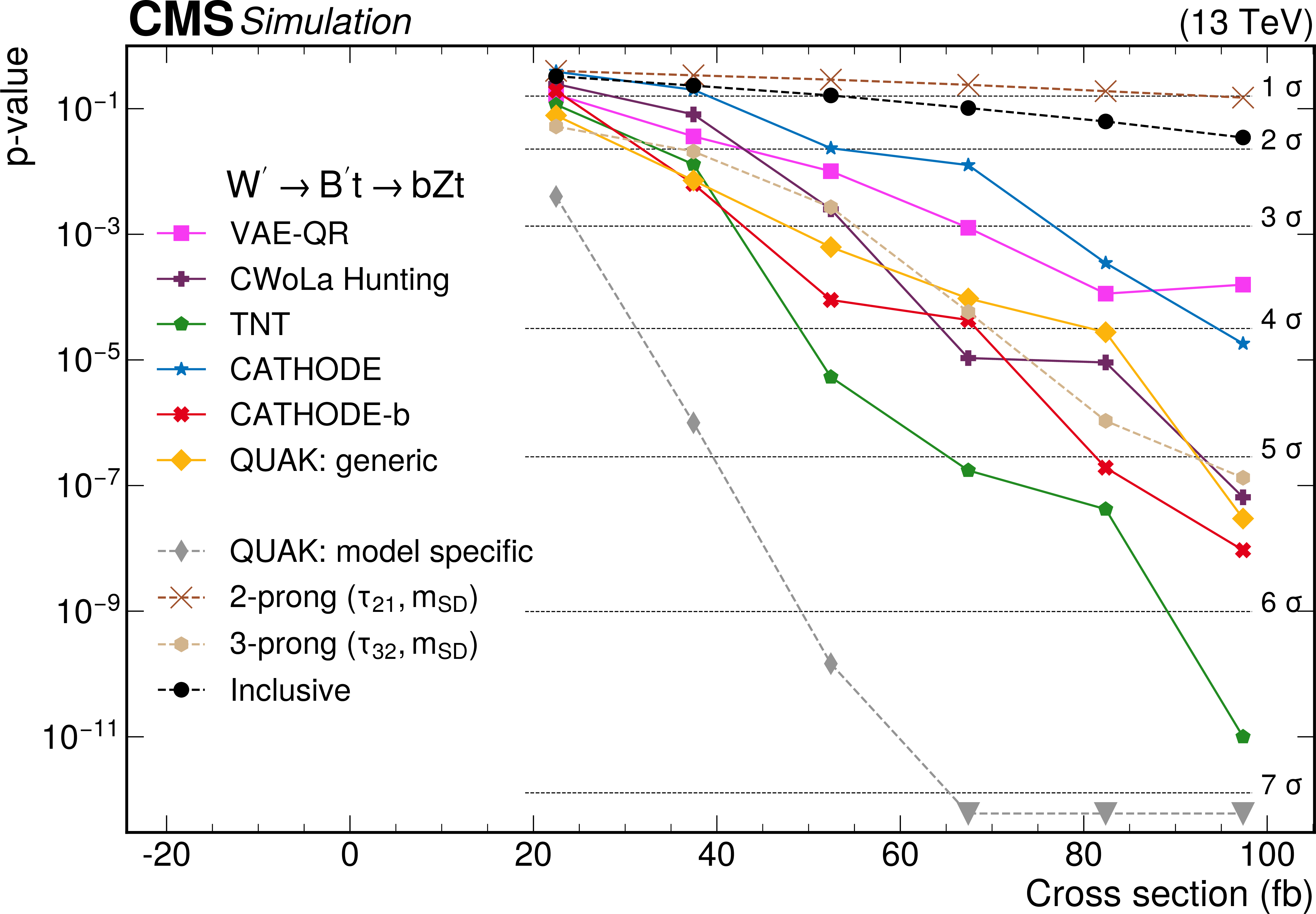
Figure 2-b:
The $ p $-values as a function of the injected signal cross sections for the different analysis procedures for two different signals: (upper) the 2-prong $ \mathrm{X}\to \mathrm{Y}\mathrm{Y'} \to 4 \mathrm{q} $ signal with $ m_\mathrm{X}= $ 3 TeV, $ m_\mathrm{Y}= $ 170 GeV, and $ M_\mathrm{Y'}= $ 170 GeV, and (lower) 3-prong $ \mathrm{W^{'}} \to \mathrm{B'}\mathrm{t} \to \mathrm{b} \mathrm{Z} \mathrm{t} $ signal with $ M_\mathrm{W'}= $ 3 TeV and $ M_\mathrm{B'}= $ 400 GeV. Significance values larger than 7$ \sigma $ are denoted with downwards facing triangles. |
png pdf |
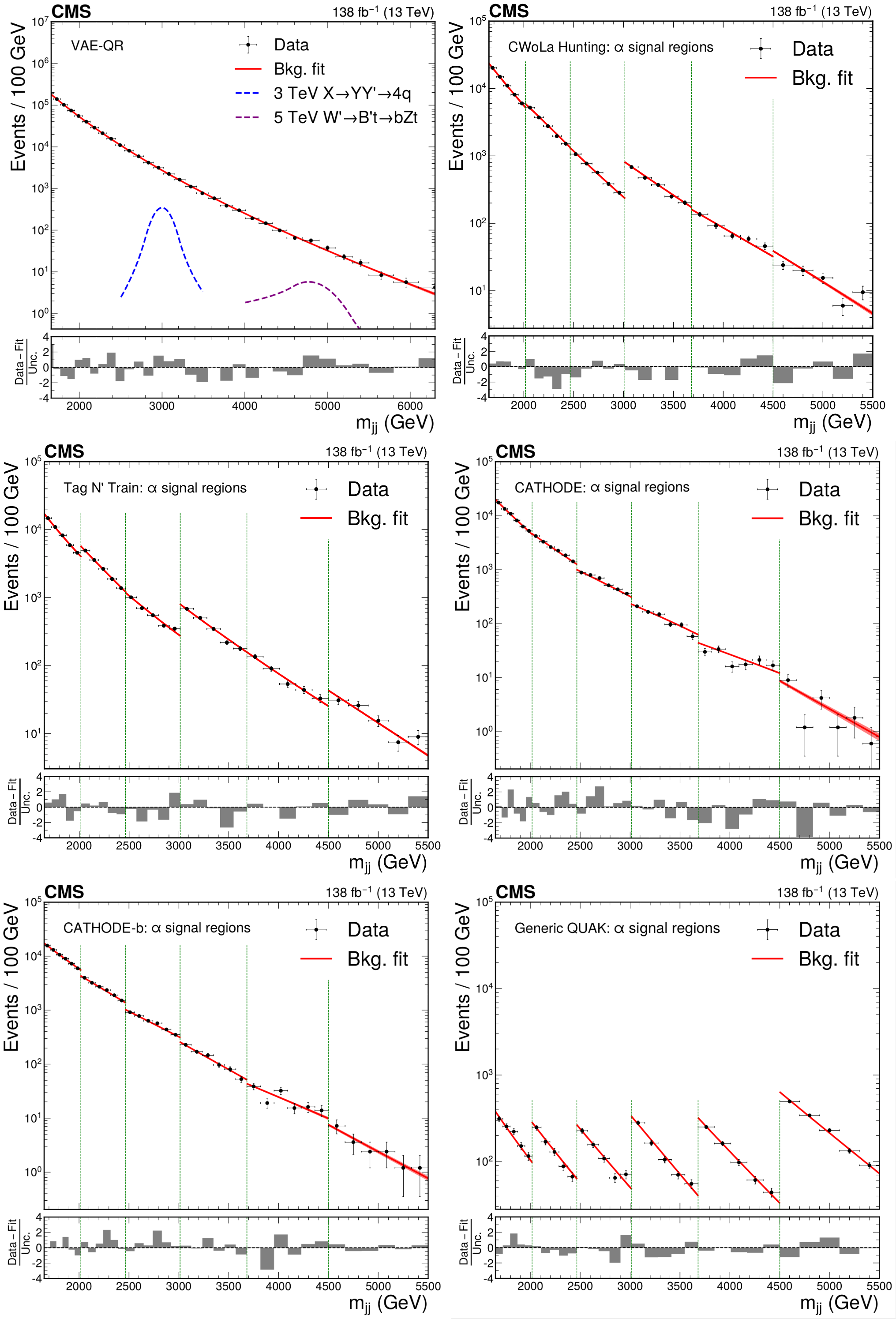
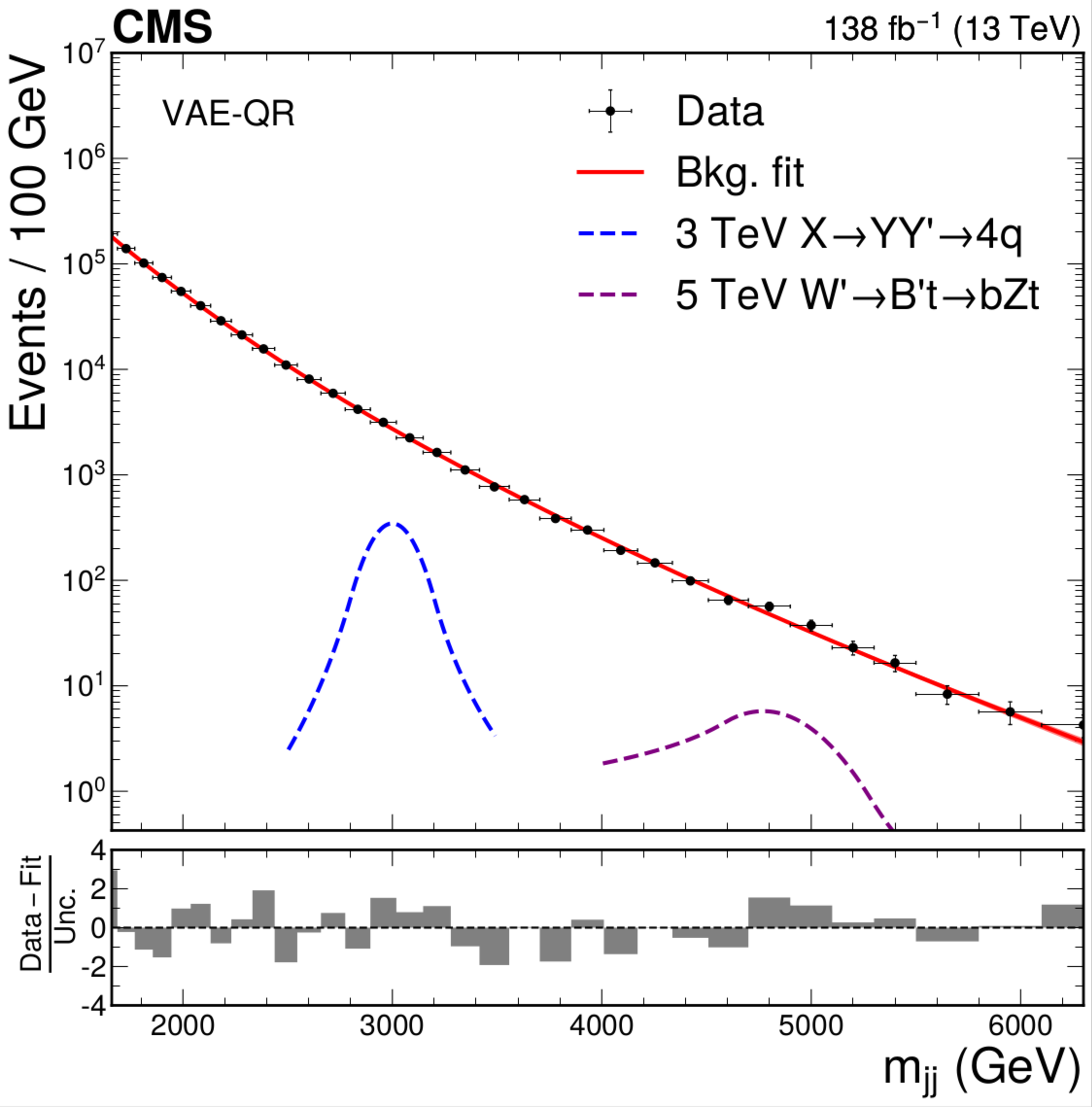
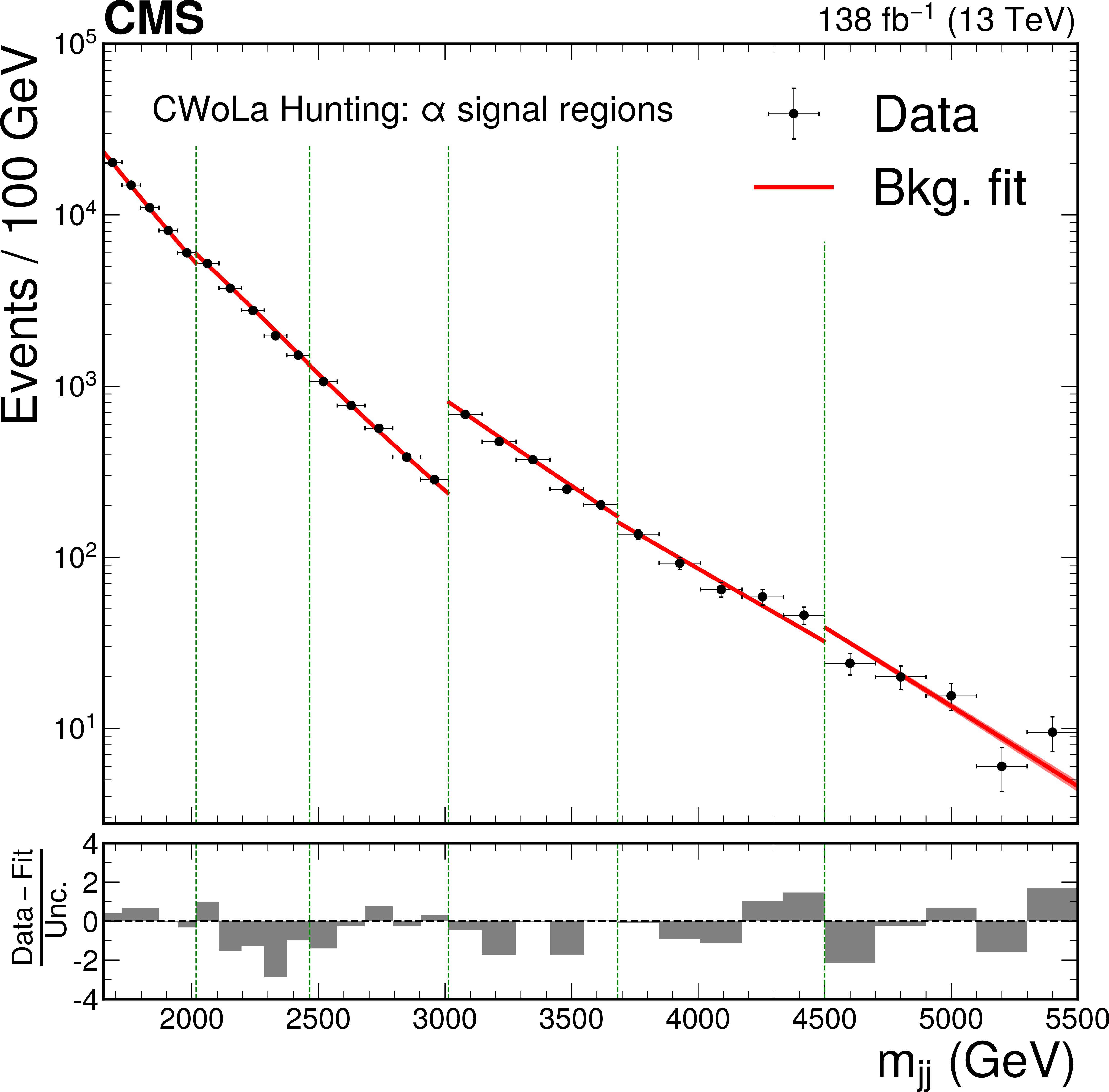
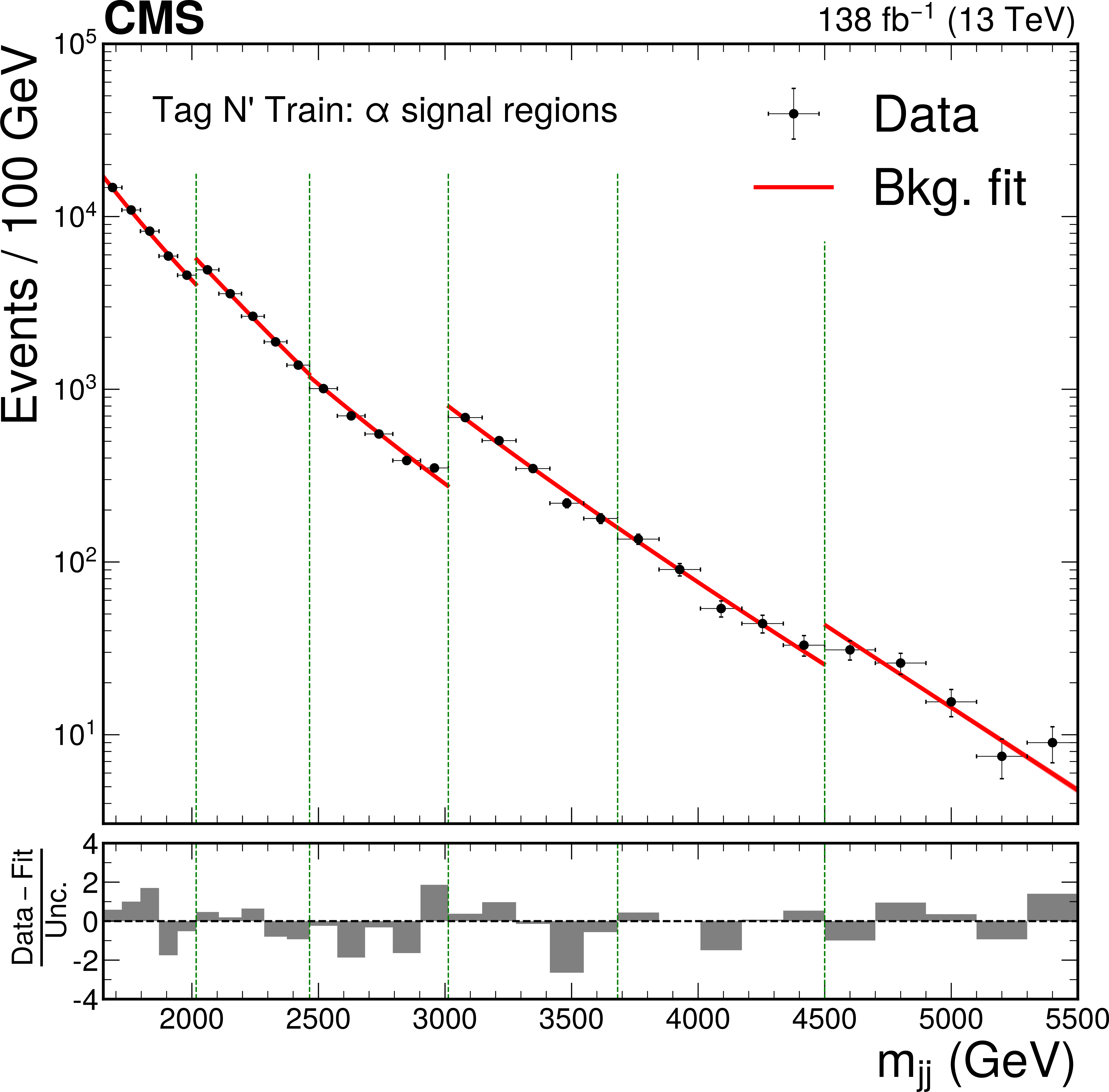
Figure 3:
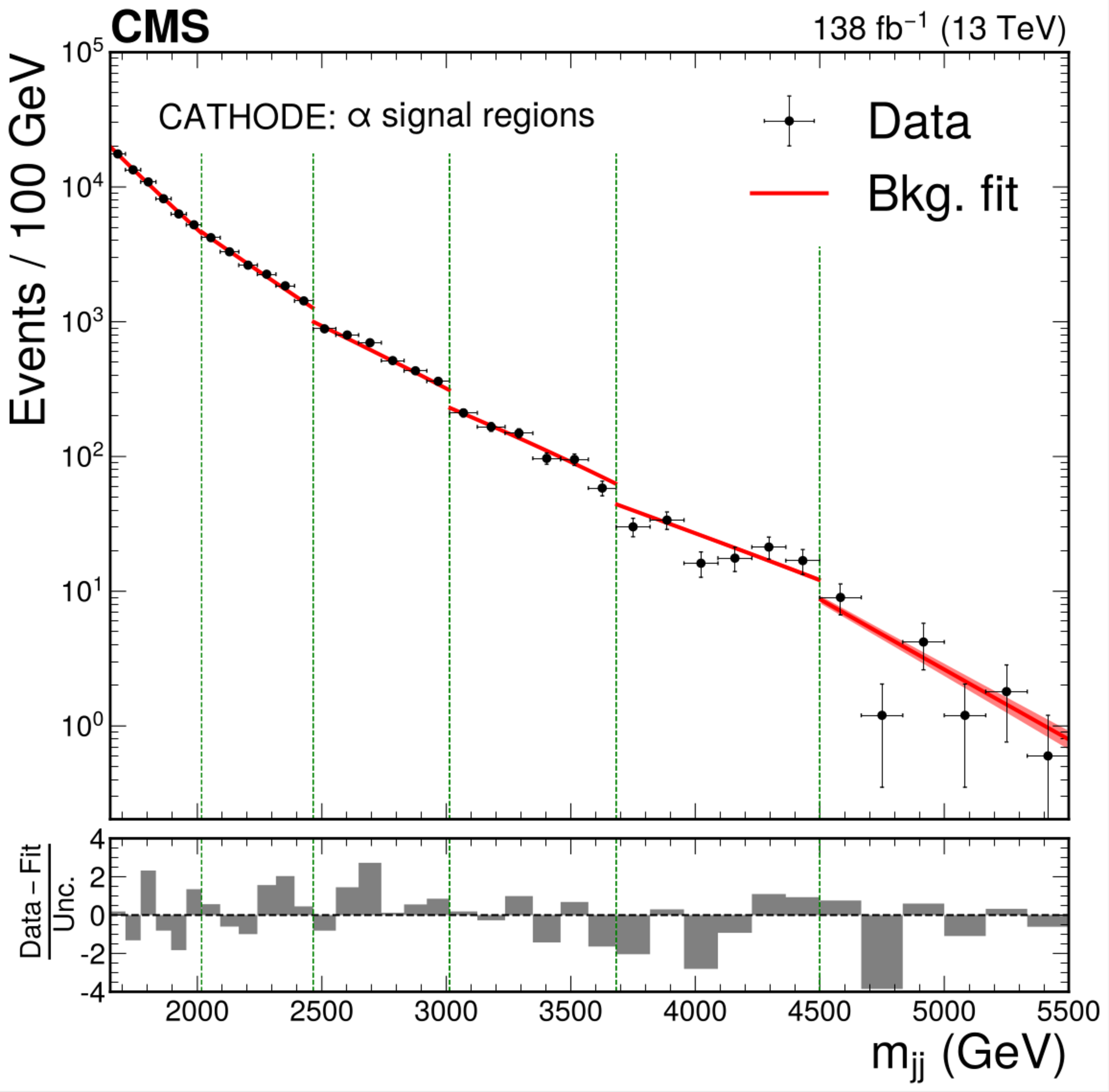
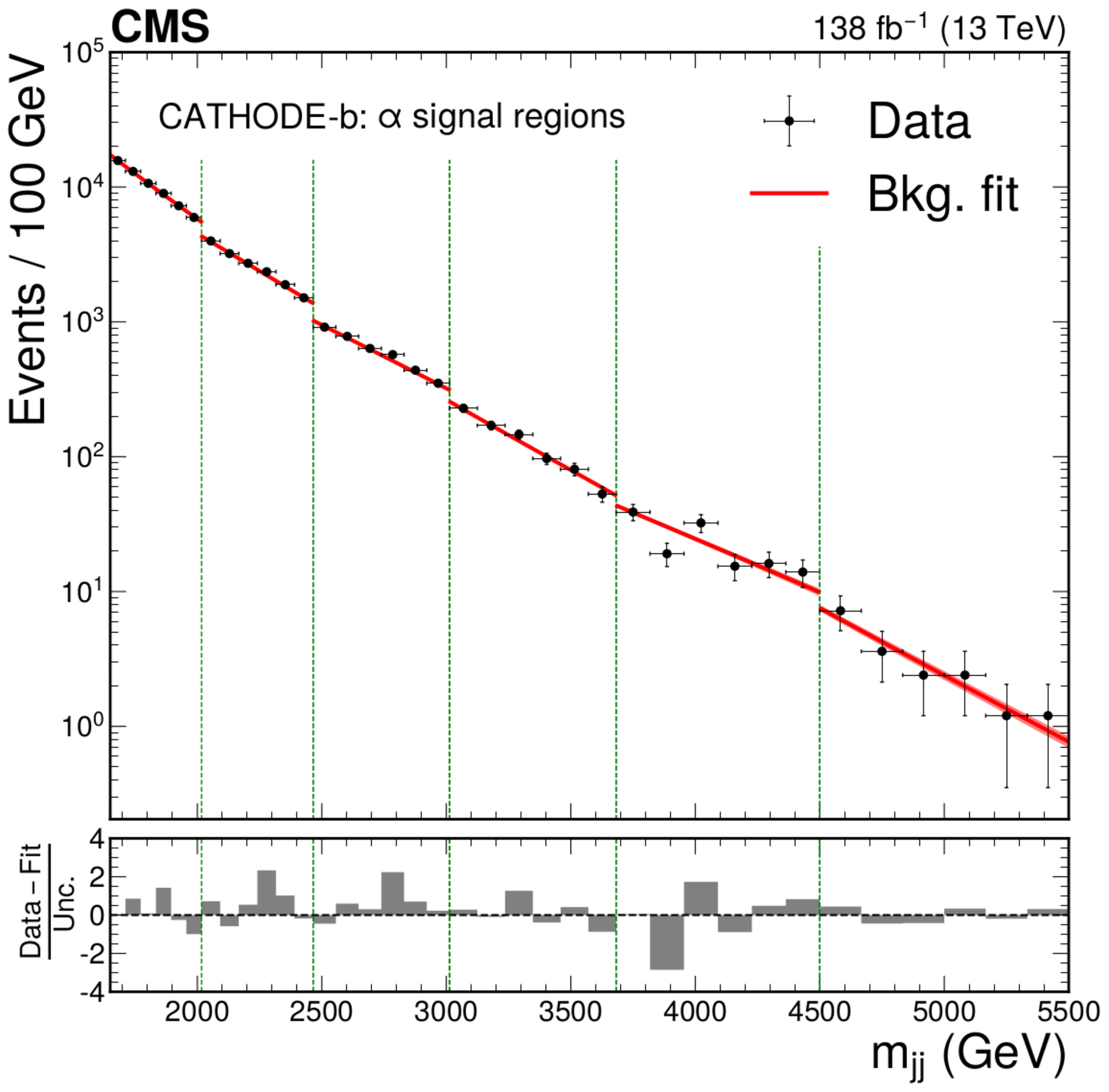
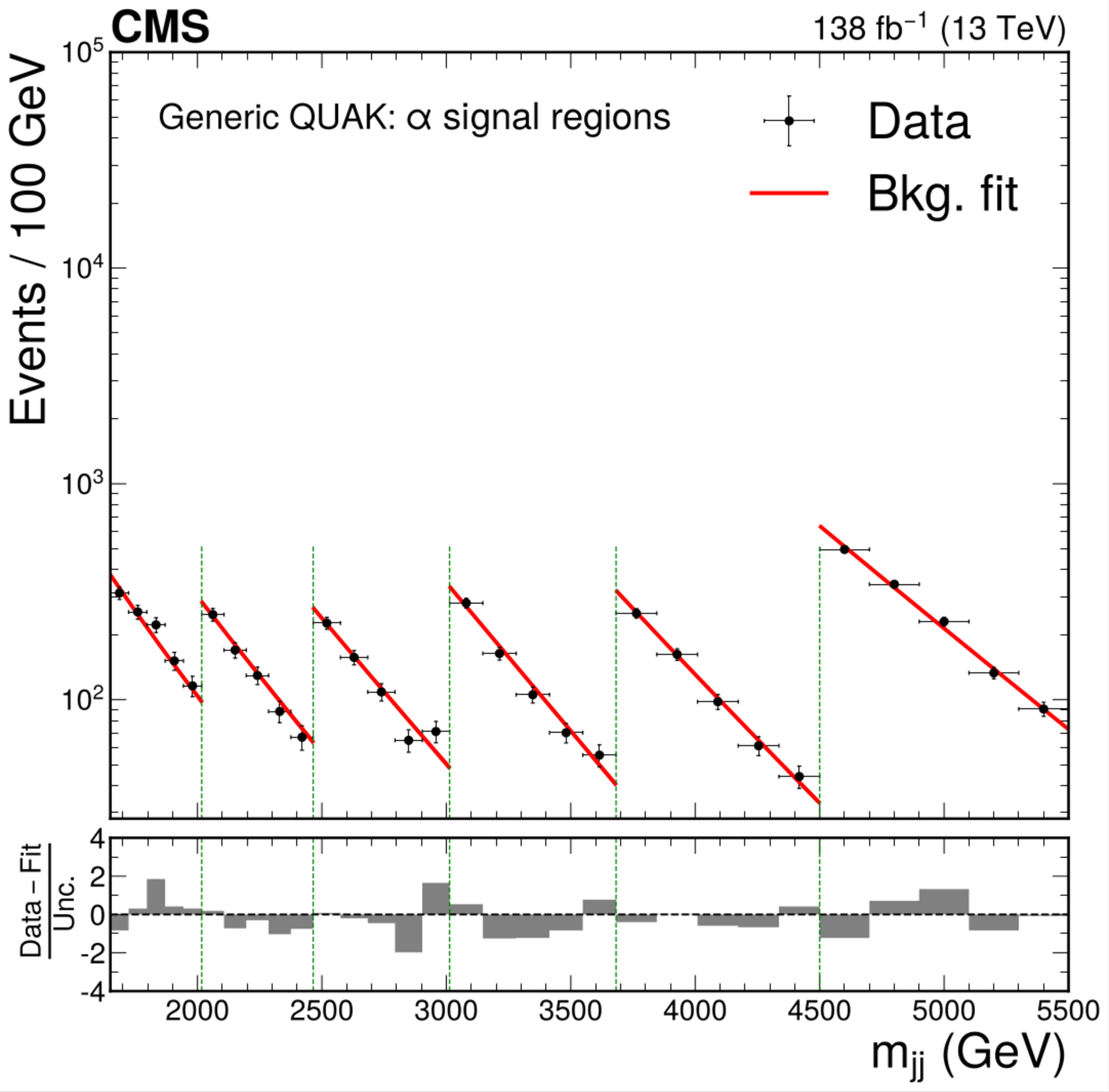
The dijet invariant mass spectrum and resulting background fit to the data for VAE-QR (upper left), CWoLa Hunting (upper right), TNT (middle left), CATHODE (middle right), CATHODE-b (lower left), and QUAK (lower right). The shapes of two benchmark signals are shown for the VAE-QR method; the signal shapes for the other methods are similar. For all methods besides the VAE-QR, separate selections are applied for different signal mass hypotheses and the resulting mass spectra are fit separately. The figures show the fitted and observed dijet mass distribution in the signal window of each selection, which results in a discontinuous distribution. The spectra in the $ \alpha $ signal regions (indicated by the vertical dotted lines) are shown for the weakly supervised methods and a similar selection of signal regions are shown for the QUAK} method. |
png pdf |
Figure 3-a:
The dijet invariant mass spectrum and resulting background fit to the data for VAE-QR (upper left), CWoLa Hunting (upper right), TNT (middle left), CATHODE (middle right), CATHODE-b (lower left), and QUAK (lower right). The shapes of two benchmark signals are shown for the VAE-QR method; the signal shapes for the other methods are similar. For all methods besides the VAE-QR, separate selections are applied for different signal mass hypotheses and the resulting mass spectra are fit separately. The figures show the fitted and observed dijet mass distribution in the signal window of each selection, which results in a discontinuous distribution. The spectra in the $ \alpha $ signal regions (indicated by the vertical dotted lines) are shown for the weakly supervised methods and a similar selection of signal regions are shown for the QUAK} method. |
png pdf |
Figure 3-b:
The dijet invariant mass spectrum and resulting background fit to the data for VAE-QR (upper left), CWoLa Hunting (upper right), TNT (middle left), CATHODE (middle right), CATHODE-b (lower left), and QUAK (lower right). The shapes of two benchmark signals are shown for the VAE-QR method; the signal shapes for the other methods are similar. For all methods besides the VAE-QR, separate selections are applied for different signal mass hypotheses and the resulting mass spectra are fit separately. The figures show the fitted and observed dijet mass distribution in the signal window of each selection, which results in a discontinuous distribution. The spectra in the $ \alpha $ signal regions (indicated by the vertical dotted lines) are shown for the weakly supervised methods and a similar selection of signal regions are shown for the QUAK} method. |
png pdf |
Figure 3-c:
The dijet invariant mass spectrum and resulting background fit to the data for VAE-QR (upper left), CWoLa Hunting (upper right), TNT (middle left), CATHODE (middle right), CATHODE-b (lower left), and QUAK (lower right). The shapes of two benchmark signals are shown for the VAE-QR method; the signal shapes for the other methods are similar. For all methods besides the VAE-QR, separate selections are applied for different signal mass hypotheses and the resulting mass spectra are fit separately. The figures show the fitted and observed dijet mass distribution in the signal window of each selection, which results in a discontinuous distribution. The spectra in the $ \alpha $ signal regions (indicated by the vertical dotted lines) are shown for the weakly supervised methods and a similar selection of signal regions are shown for the QUAK} method. |
png pdf |
Figure 3-d:
The dijet invariant mass spectrum and resulting background fit to the data for VAE-QR (upper left), CWoLa Hunting (upper right), TNT (middle left), CATHODE (middle right), CATHODE-b (lower left), and QUAK (lower right). The shapes of two benchmark signals are shown for the VAE-QR method; the signal shapes for the other methods are similar. For all methods besides the VAE-QR, separate selections are applied for different signal mass hypotheses and the resulting mass spectra are fit separately. The figures show the fitted and observed dijet mass distribution in the signal window of each selection, which results in a discontinuous distribution. The spectra in the $ \alpha $ signal regions (indicated by the vertical dotted lines) are shown for the weakly supervised methods and a similar selection of signal regions are shown for the QUAK} method. |
png pdf |
Figure 3-e:
The dijet invariant mass spectrum and resulting background fit to the data for VAE-QR (upper left), CWoLa Hunting (upper right), TNT (middle left), CATHODE (middle right), CATHODE-b (lower left), and QUAK (lower right). The shapes of two benchmark signals are shown for the VAE-QR method; the signal shapes for the other methods are similar. For all methods besides the VAE-QR, separate selections are applied for different signal mass hypotheses and the resulting mass spectra are fit separately. The figures show the fitted and observed dijet mass distribution in the signal window of each selection, which results in a discontinuous distribution. The spectra in the $ \alpha $ signal regions (indicated by the vertical dotted lines) are shown for the weakly supervised methods and a similar selection of signal regions are shown for the QUAK} method. |
png pdf |
Figure 3-f:
The dijet invariant mass spectrum and resulting background fit to the data for VAE-QR (upper left), CWoLa Hunting (upper right), TNT (middle left), CATHODE (middle right), CATHODE-b (lower left), and QUAK (lower right). The shapes of two benchmark signals are shown for the VAE-QR method; the signal shapes for the other methods are similar. For all methods besides the VAE-QR, separate selections are applied for different signal mass hypotheses and the resulting mass spectra are fit separately. The figures show the fitted and observed dijet mass distribution in the signal window of each selection, which results in a discontinuous distribution. The spectra in the $ \alpha $ signal regions (indicated by the vertical dotted lines) are shown for the weakly supervised methods and a similar selection of signal regions are shown for the QUAK} method. |
png pdf |
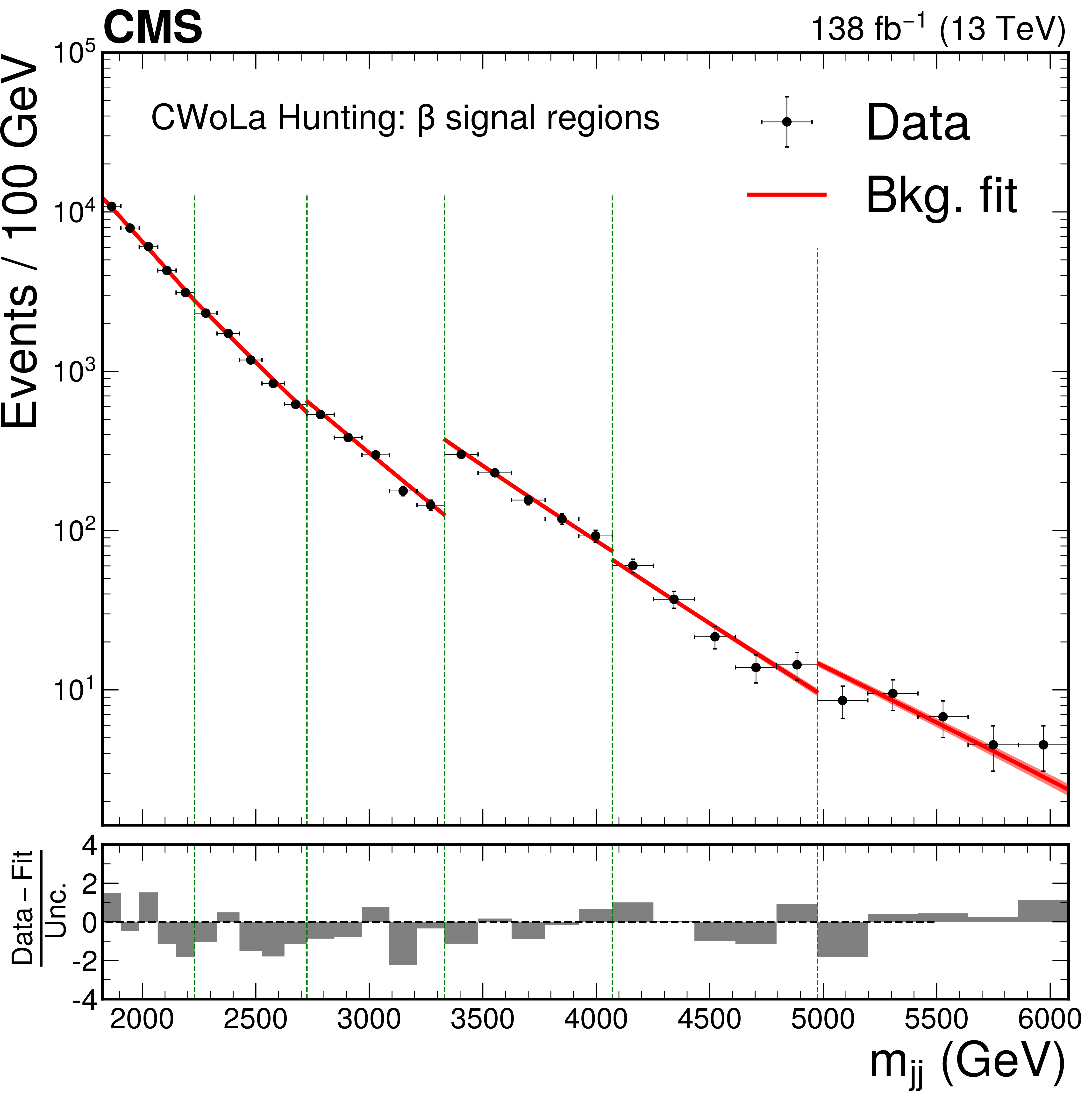
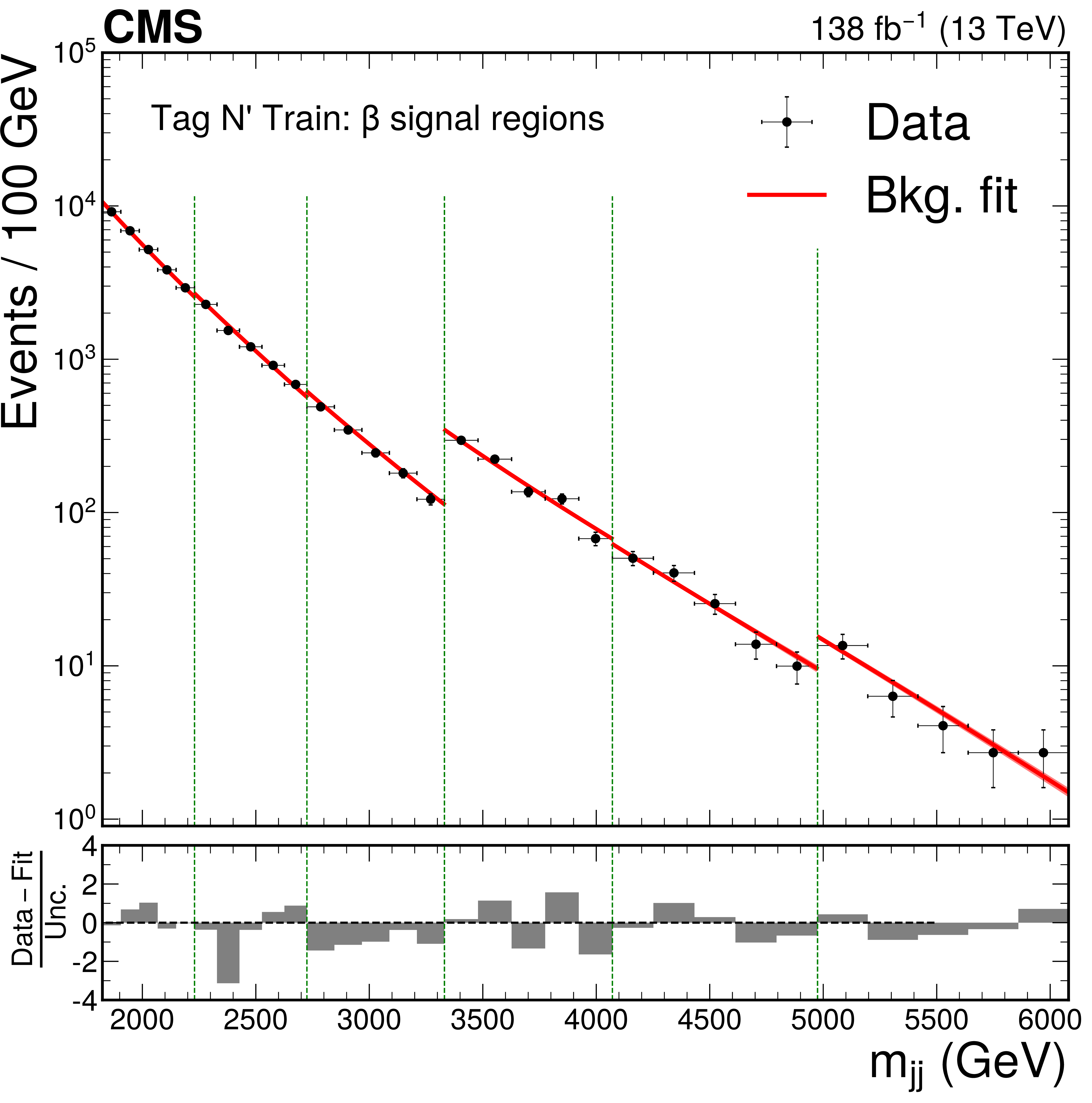
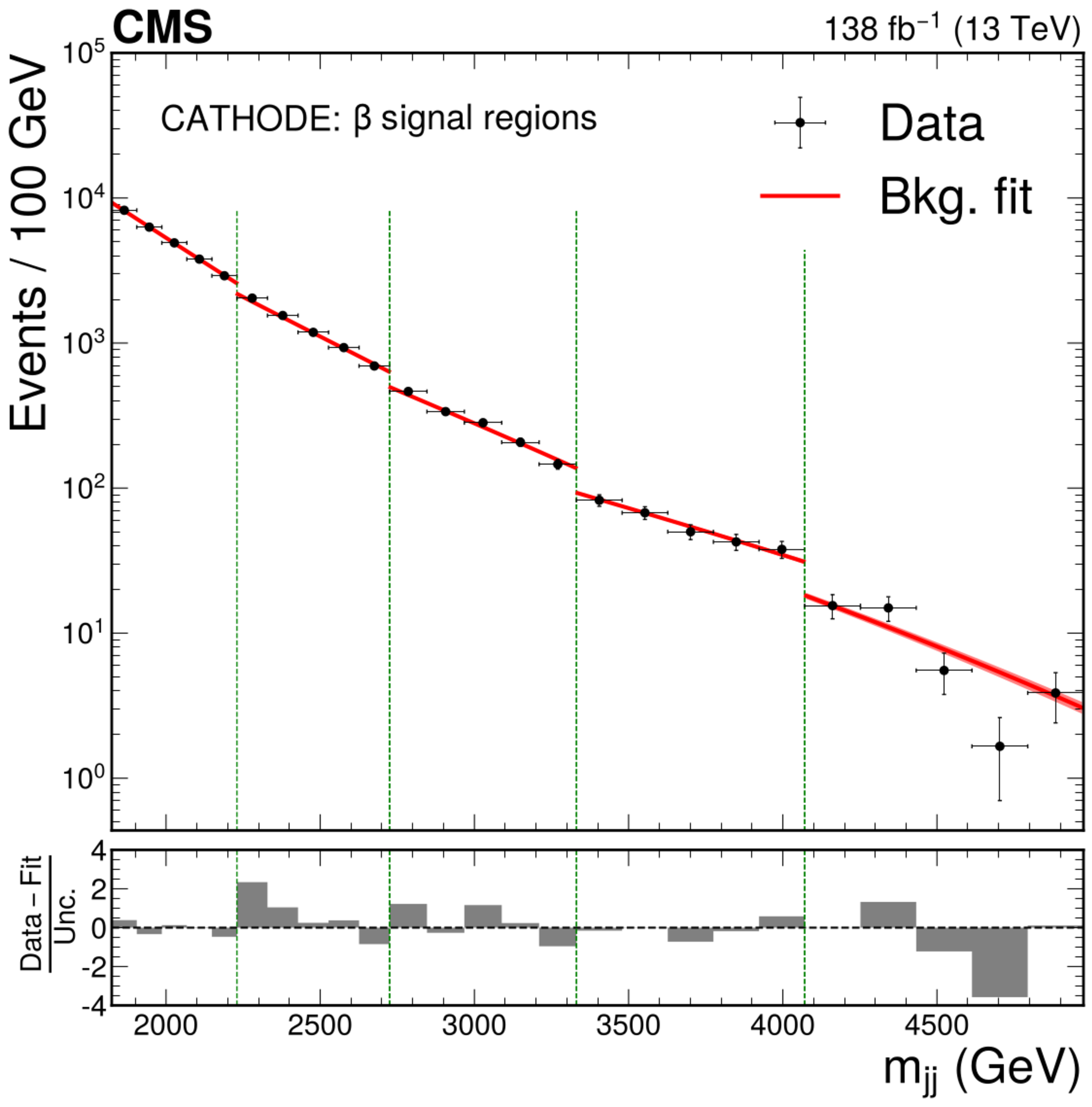
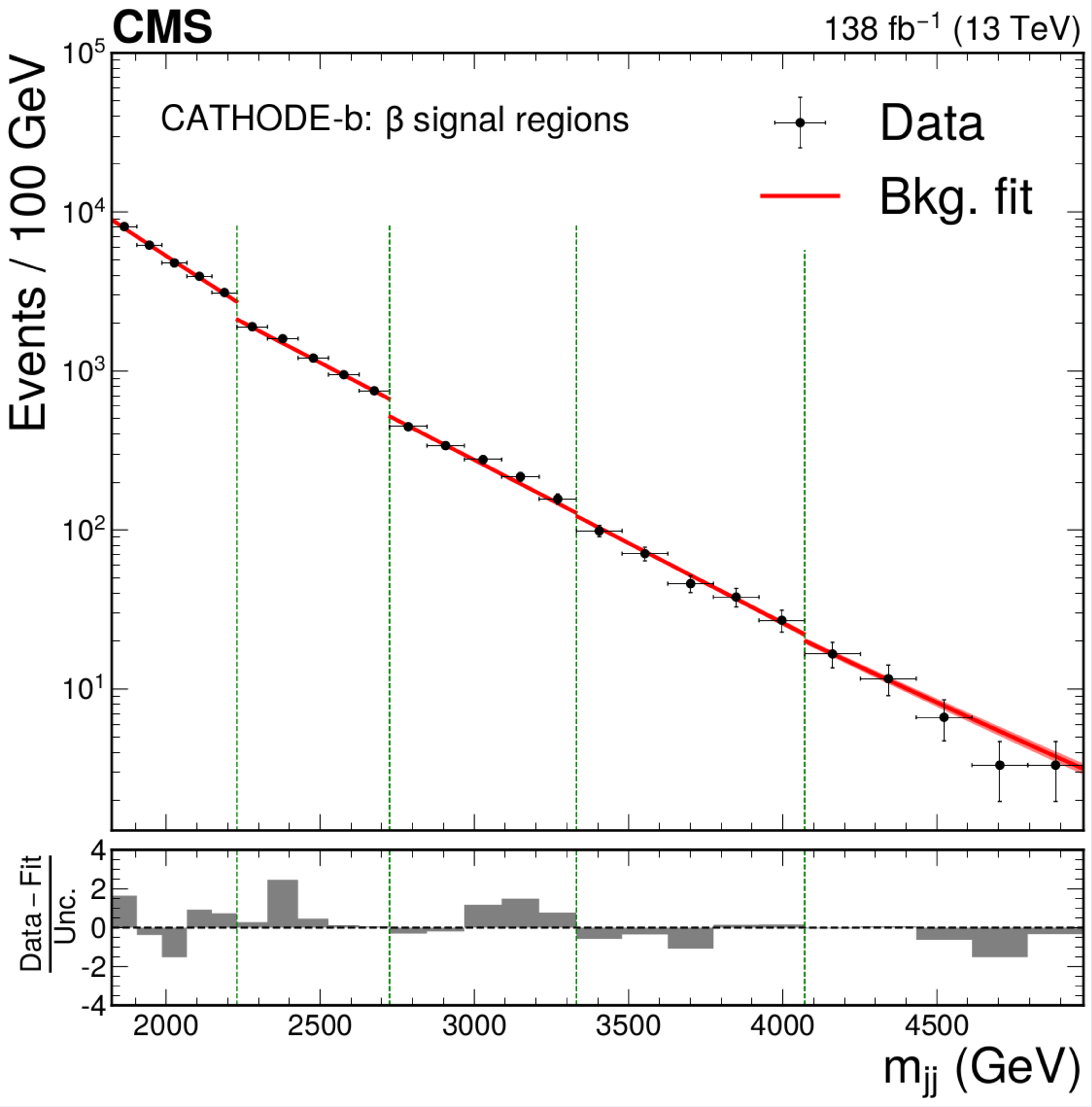
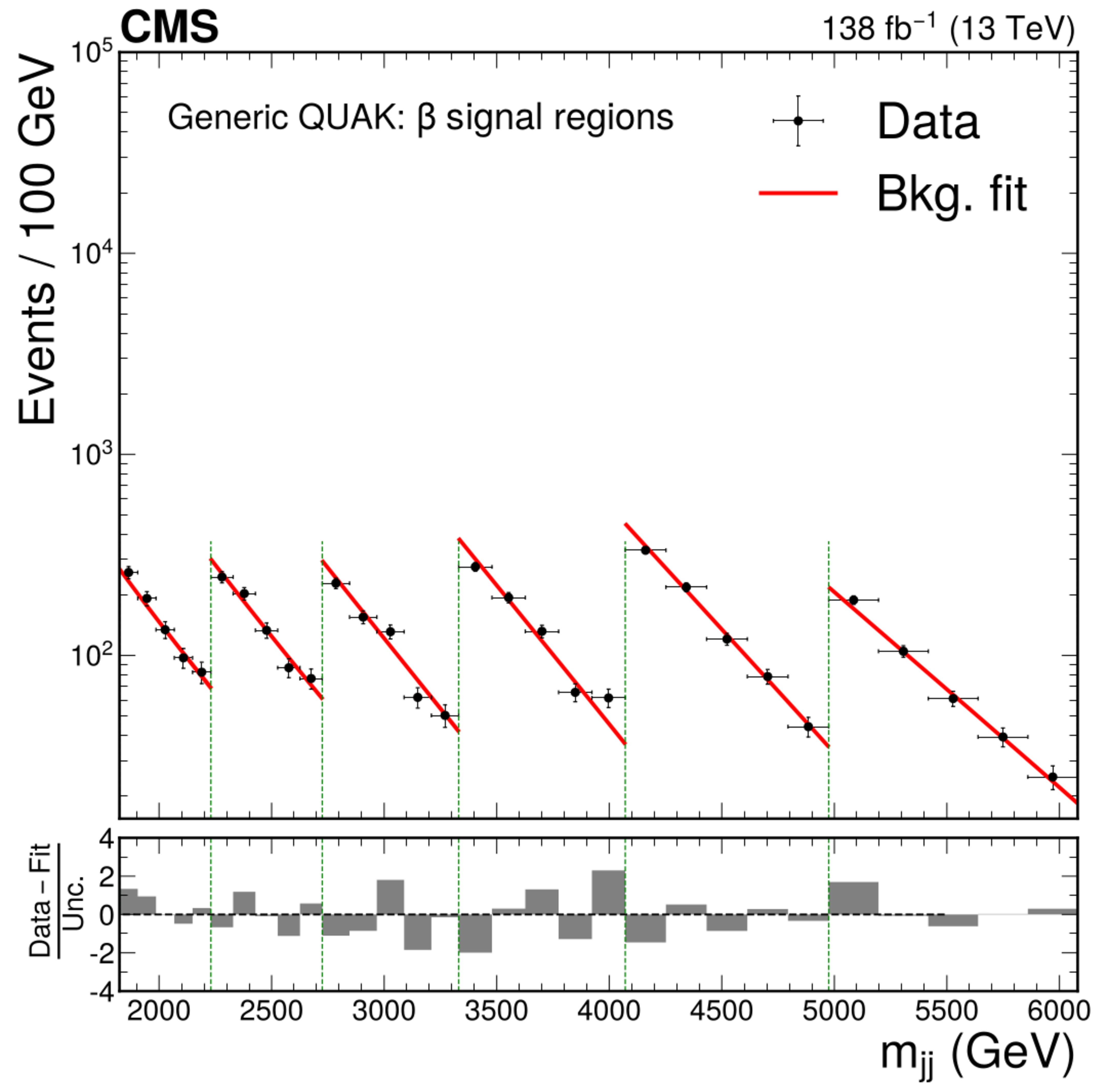
Figure 4:
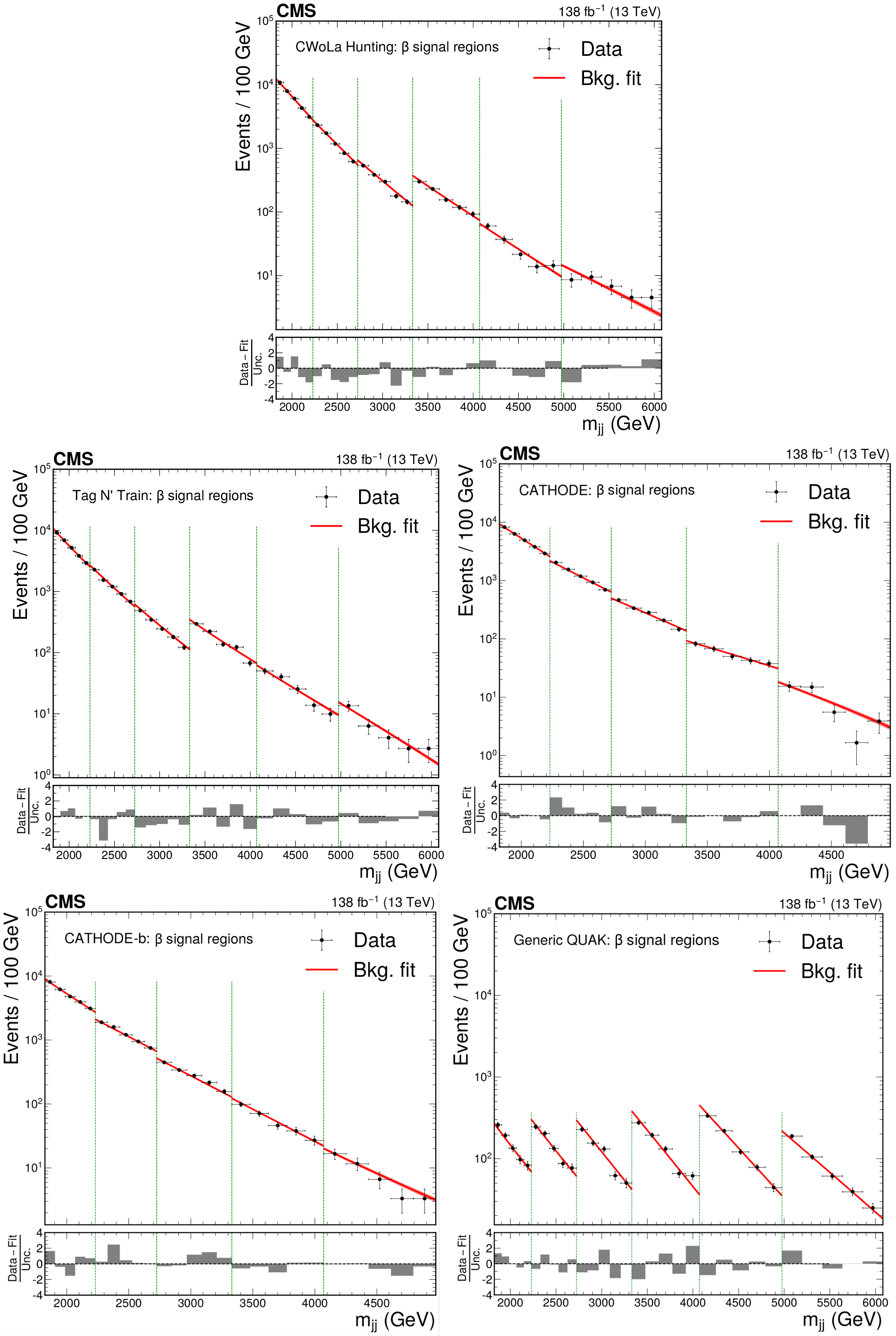
The dijet invariant mass spectrum and resulting background fit to the data for the $ \beta $ signal regions (indicated by the vertical dotted lines) of CWoLa Hunting (upper), TNT (middle left), CATHODE (middle right), CATHODE-b (lower left), and a similar selection of signal regions of QUAK (lower right). Separate selections are applied for different signal mass hypotheses and the resulting mass spectra are fit separately. The figures therefore show the fitted and observed dijet mass distribution in the signal window of each selection, which results in a discontinuous distribution. The CATHODE and CATHODE-b methods are not used in the highest mass window of the $ \beta $ signal regions due to the limited number of data events. They therefore have one fewer signal region shown than the other methods. |
png pdf |
Figure 4-a:
The dijet invariant mass spectrum and resulting background fit to the data for the $ \beta $ signal regions (indicated by the vertical dotted lines) of CWoLa Hunting (upper), TNT (middle left), CATHODE (middle right), CATHODE-b (lower left), and a similar selection of signal regions of QUAK (lower right). Separate selections are applied for different signal mass hypotheses and the resulting mass spectra are fit separately. The figures therefore show the fitted and observed dijet mass distribution in the signal window of each selection, which results in a discontinuous distribution. The CATHODE and CATHODE-b methods are not used in the highest mass window of the $ \beta $ signal regions due to the limited number of data events. They therefore have one fewer signal region shown than the other methods. |
png pdf |
Figure 4-b:
The dijet invariant mass spectrum and resulting background fit to the data for the $ \beta $ signal regions (indicated by the vertical dotted lines) of CWoLa Hunting (upper), TNT (middle left), CATHODE (middle right), CATHODE-b (lower left), and a similar selection of signal regions of QUAK (lower right). Separate selections are applied for different signal mass hypotheses and the resulting mass spectra are fit separately. The figures therefore show the fitted and observed dijet mass distribution in the signal window of each selection, which results in a discontinuous distribution. The CATHODE and CATHODE-b methods are not used in the highest mass window of the $ \beta $ signal regions due to the limited number of data events. They therefore have one fewer signal region shown than the other methods. |
png pdf |
Figure 4-c:
The dijet invariant mass spectrum and resulting background fit to the data for the $ \beta $ signal regions (indicated by the vertical dotted lines) of CWoLa Hunting (upper), TNT (middle left), CATHODE (middle right), CATHODE-b (lower left), and a similar selection of signal regions of QUAK (lower right). Separate selections are applied for different signal mass hypotheses and the resulting mass spectra are fit separately. The figures therefore show the fitted and observed dijet mass distribution in the signal window of each selection, which results in a discontinuous distribution. The CATHODE and CATHODE-b methods are not used in the highest mass window of the $ \beta $ signal regions due to the limited number of data events. They therefore have one fewer signal region shown than the other methods. |
png pdf |
Figure 4-d:
The dijet invariant mass spectrum and resulting background fit to the data for the $ \beta $ signal regions (indicated by the vertical dotted lines) of CWoLa Hunting (upper), TNT (middle left), CATHODE (middle right), CATHODE-b (lower left), and a similar selection of signal regions of QUAK (lower right). Separate selections are applied for different signal mass hypotheses and the resulting mass spectra are fit separately. The figures therefore show the fitted and observed dijet mass distribution in the signal window of each selection, which results in a discontinuous distribution. The CATHODE and CATHODE-b methods are not used in the highest mass window of the $ \beta $ signal regions due to the limited number of data events. They therefore have one fewer signal region shown than the other methods. |
png pdf |
Figure 4-e:
The dijet invariant mass spectrum and resulting background fit to the data for the $ \beta $ signal regions (indicated by the vertical dotted lines) of CWoLa Hunting (upper), TNT (middle left), CATHODE (middle right), CATHODE-b (lower left), and a similar selection of signal regions of QUAK (lower right). Separate selections are applied for different signal mass hypotheses and the resulting mass spectra are fit separately. The figures therefore show the fitted and observed dijet mass distribution in the signal window of each selection, which results in a discontinuous distribution. The CATHODE and CATHODE-b methods are not used in the highest mass window of the $ \beta $ signal regions due to the limited number of data events. They therefore have one fewer signal region shown than the other methods. |
png pdf |
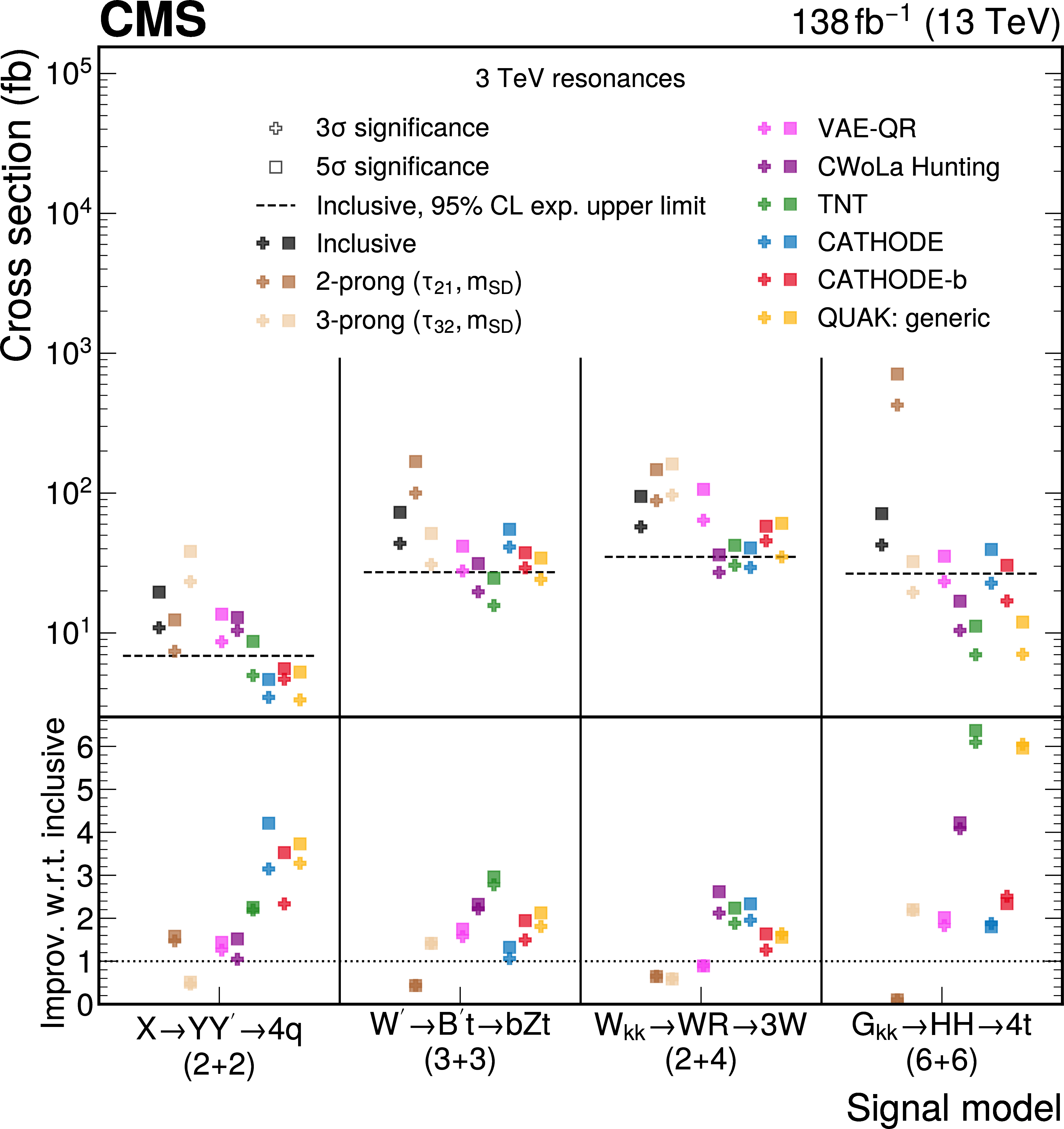
Figure 5:
The discovery sensitivity for the process $ \mathrm{A} \to \mathrm{BC} $, using the anomaly detection methods and a comparison to sensitivity of the inclusive search. In all signal processes, the mass of the heavy resonance is set to $ m_\mathrm{A}= $ 3 TeV. For the BSM daughter particles, the masses of the Y and Y' are set to 170 GeV, while the masses of the B', R, and H are set to 400 GeV. In the upper panel, for each method, the cross section, which would have led to an expected 3 $ \sigma $ (5 $ \sigma $) excess, is shown as a cross (square) marker. Sensitivities from six anomaly detection methods (six colors) are compared to an inclusive dijet search in which no substructure selection is made (black) and traditional substructure selections targeting 2-prong (dark brown) or 3-prong (tan) decays. The expected 95% confidence level upper limits from the inclusive search are also shown in the upper panel as a dashed line. For all signal models at least one anomaly detection method is able to achieve an expected 5 $ \sigma $ significance at a cross section at or below the upper limit of the inclusive search. Shown in the lower panel is the ratio of the cross section sensitivity from the inclusive search to the corresponding sensitivity for each method. |
png pdf |
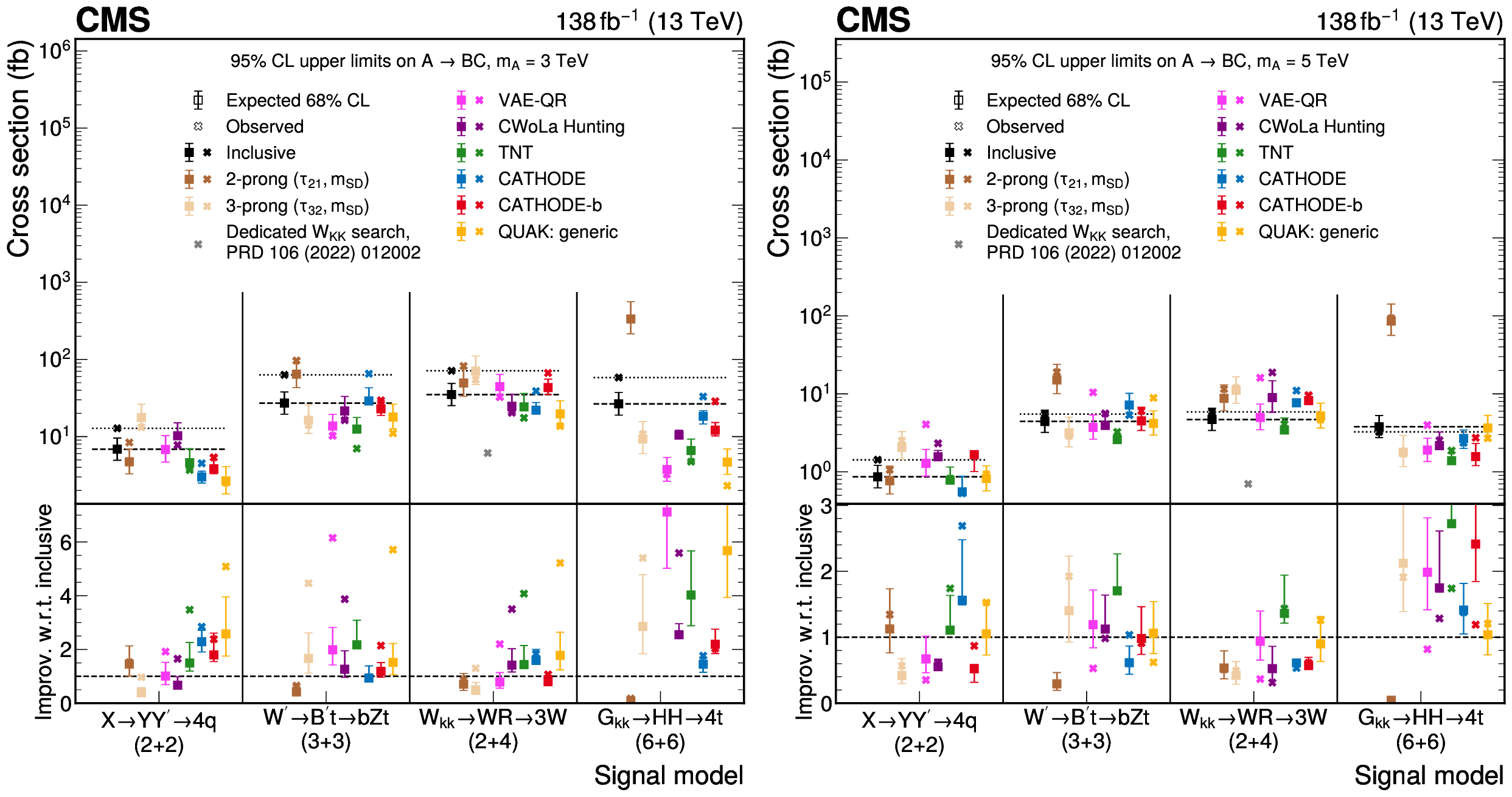
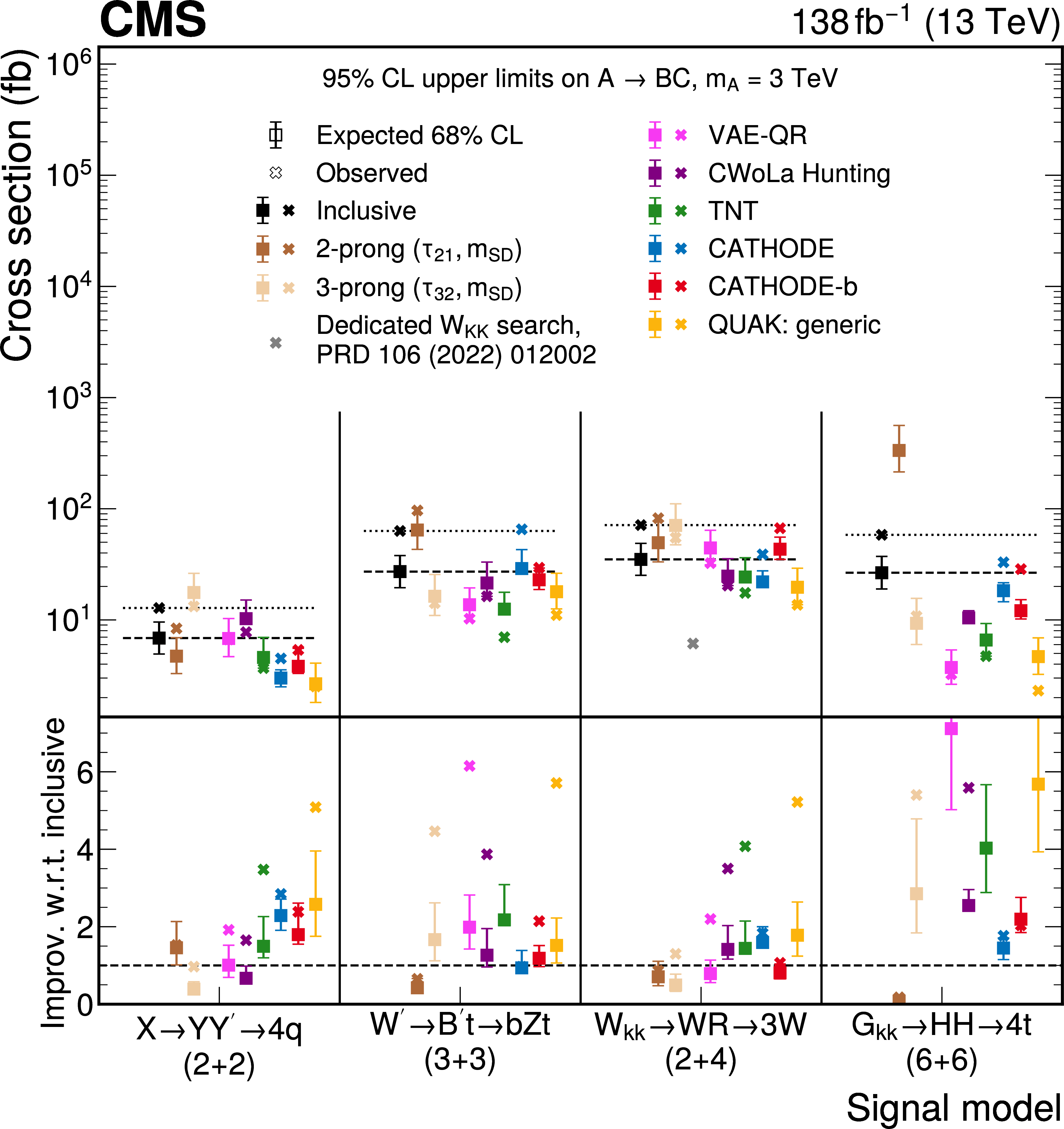
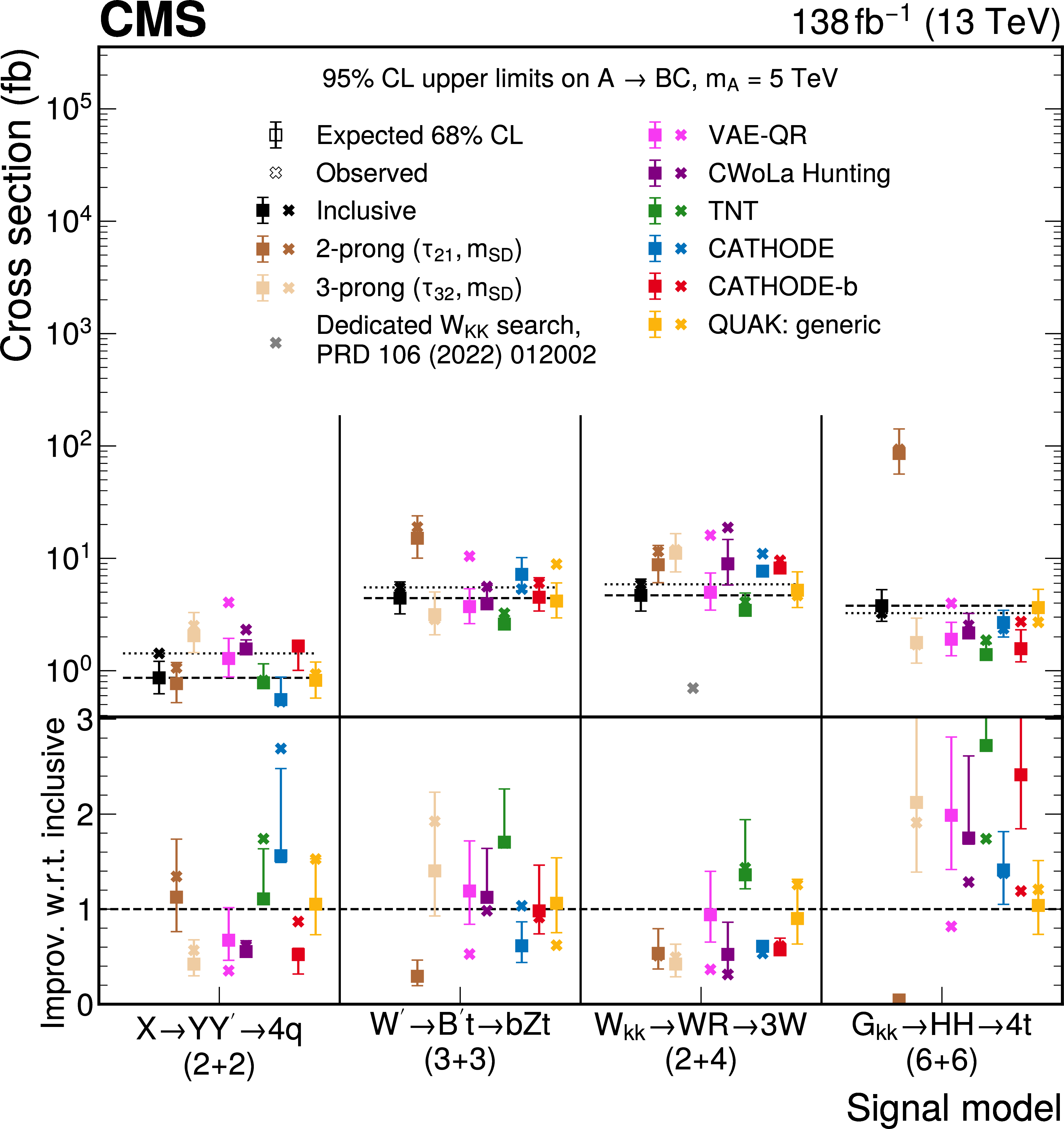
Figure 6:
The upper limit at 95% confidence level on the cross section for the process $ \mathrm{A} \to \mathrm{BC} $, is shown for each search method applied to a variety of signal models. For a resonance mass $ m_\mathrm{A}= $ 3 TeV (left) and $ m_\mathrm{A}= $ 5 TeV (right), we show for each signal model (columns), and search method (all colors), the observed limits (crosses), expected limits (squares), and their 68% expected central intervals (error bars). For the BSM daughter particles, the masses of the Y and Y' are set to 170 GeV, while the masses of the B', R, and H are set to 400 GeV. Limits from the anomaly detection methods (six colors) are compared to those from an inclusive dijet search in which no substructure selection is made (black markers and horizontal lines), traditional substructure selections targeting 2-prong (dark brown) or 3-prong decays (tan), and the observed limit from a previous CMS search [51] for the $ \mathrm{W}_\mathrm{KK} \to \mathrm{R}\mathrm{W} \to 3 \mathrm{W} $ model in the all-hadronic channel (gray). |
png pdf |
Figure 6-a:
The upper limit at 95% confidence level on the cross section for the process $ \mathrm{A} \to \mathrm{BC} $, is shown for each search method applied to a variety of signal models. For a resonance mass $ m_\mathrm{A}= $ 3 TeV (left) and $ m_\mathrm{A}= $ 5 TeV (right), we show for each signal model (columns), and search method (all colors), the observed limits (crosses), expected limits (squares), and their 68% expected central intervals (error bars). For the BSM daughter particles, the masses of the Y and Y' are set to 170 GeV, while the masses of the B', R, and H are set to 400 GeV. Limits from the anomaly detection methods (six colors) are compared to those from an inclusive dijet search in which no substructure selection is made (black markers and horizontal lines), traditional substructure selections targeting 2-prong (dark brown) or 3-prong decays (tan), and the observed limit from a previous CMS search [51] for the $ \mathrm{W}_\mathrm{KK} \to \mathrm{R}\mathrm{W} \to 3 \mathrm{W} $ model in the all-hadronic channel (gray). |
png pdf |
Figure 6-b:
The upper limit at 95% confidence level on the cross section for the process $ \mathrm{A} \to \mathrm{BC} $, is shown for each search method applied to a variety of signal models. For a resonance mass $ m_\mathrm{A}= $ 3 TeV (left) and $ m_\mathrm{A}= $ 5 TeV (right), we show for each signal model (columns), and search method (all colors), the observed limits (crosses), expected limits (squares), and their 68% expected central intervals (error bars). For the BSM daughter particles, the masses of the Y and Y' are set to 170 GeV, while the masses of the B', R, and H are set to 400 GeV. Limits from the anomaly detection methods (six colors) are compared to those from an inclusive dijet search in which no substructure selection is made (black markers and horizontal lines), traditional substructure selections targeting 2-prong (dark brown) or 3-prong decays (tan), and the observed limit from a previous CMS search [51] for the $ \mathrm{W}_\mathrm{KK} \to \mathrm{R}\mathrm{W} \to 3 \mathrm{W} $ model in the all-hadronic channel (gray). |
png pdf |
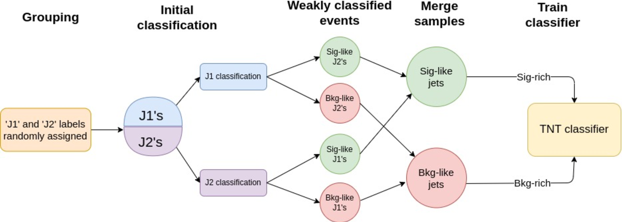
Figure 7:
A flowchart outlining how the samples for the weakly supervised training were constructed in the TNT method. The two jets in the dijet candidate were randomly assigned labels J1 and J2. For each event, the J1 (J2) jet is placed into either a signal-like or background-like sample based on the autoencoder scores evaluated on the J2 (J1) jet. The samples of signal-like (background-like) J1's and signal-like (background-like) J2's were merged together to construct a single sample of signal-like (background-like) jets. The TNT classifier is then trained to distinguish between these two samples. |
png pdf |
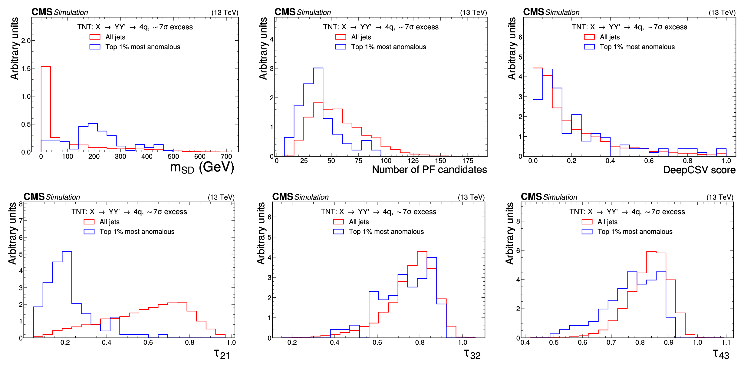
Figure 8:
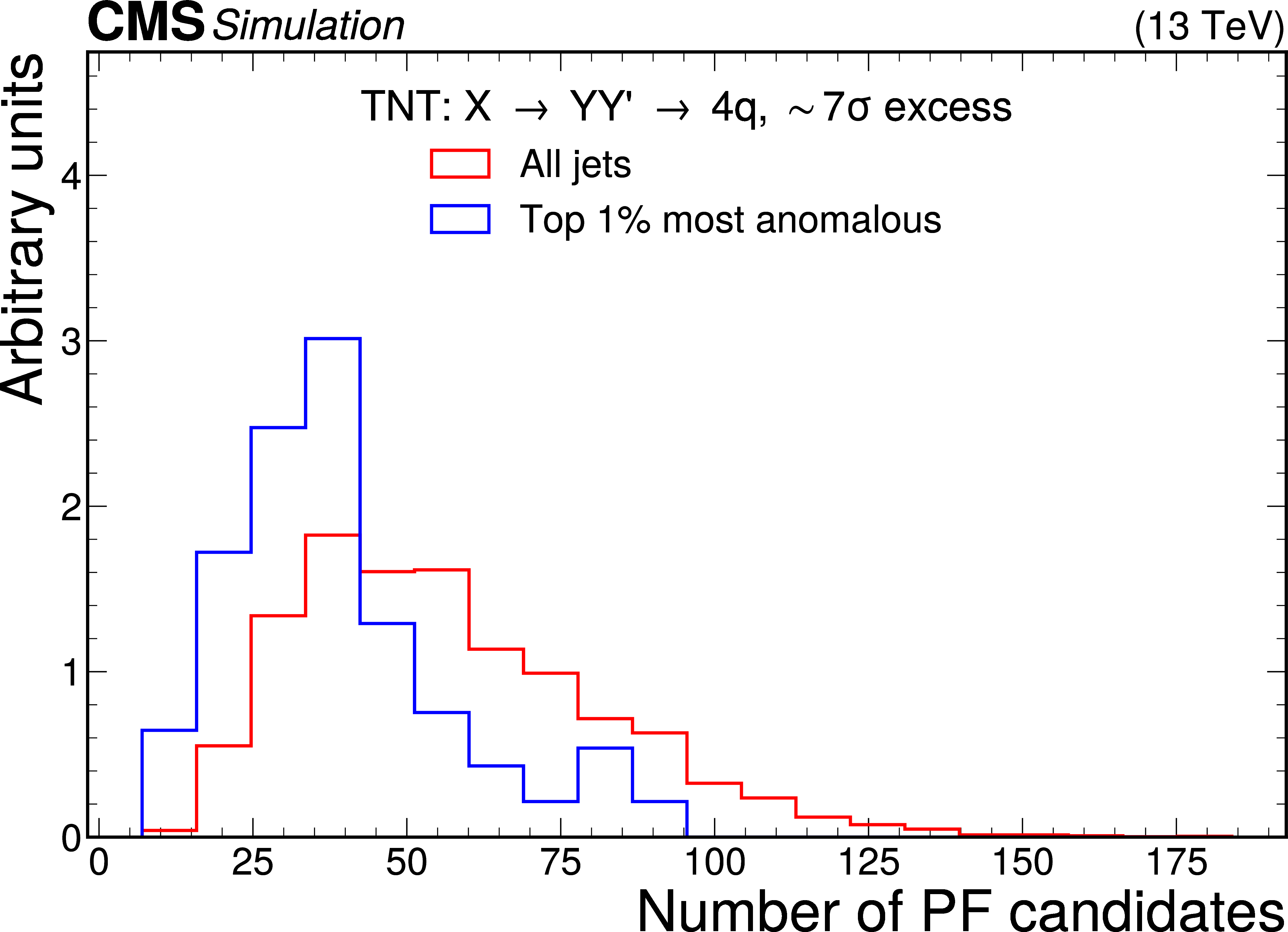
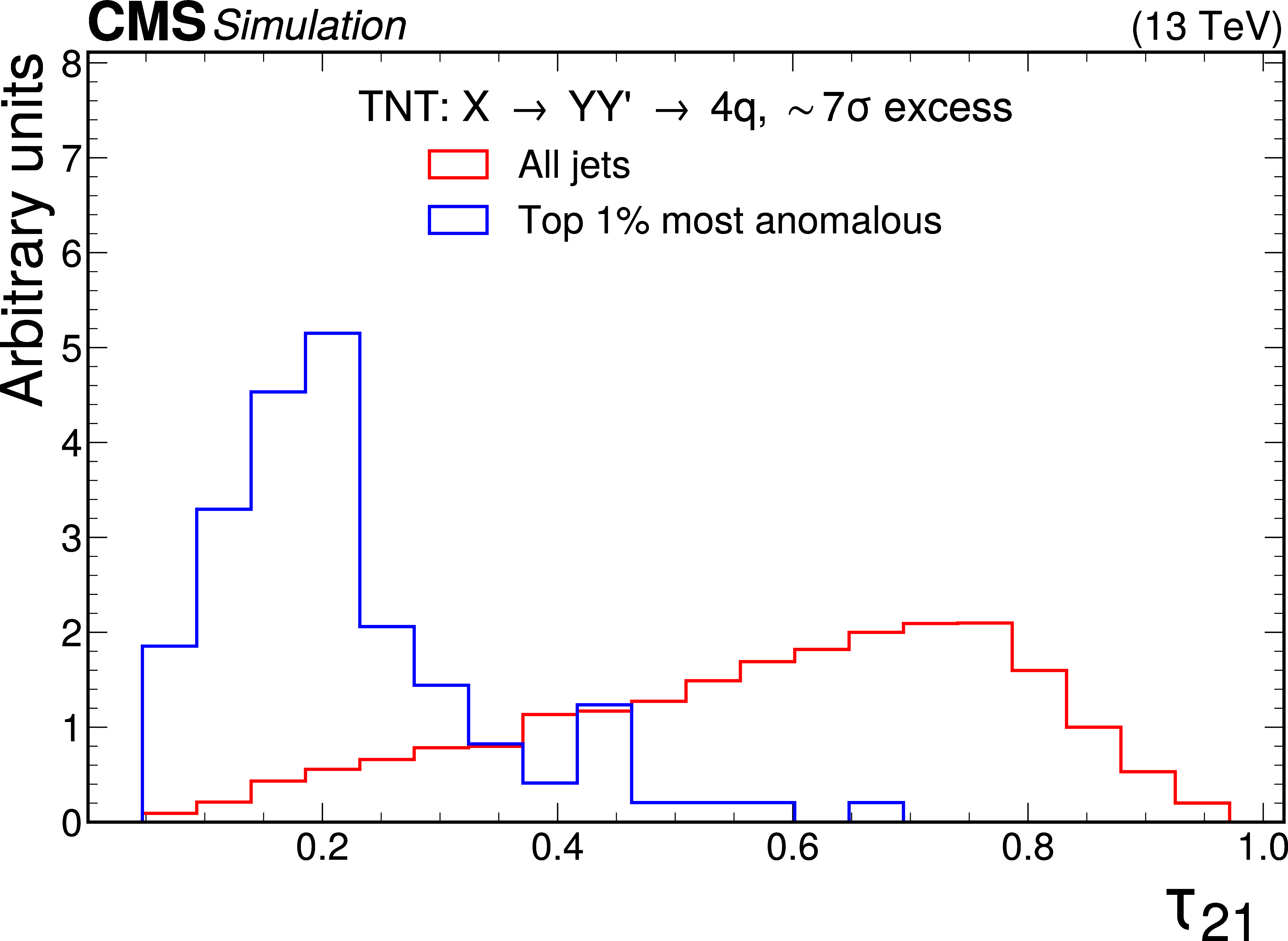
Excess interpretation example for the TNT method trained on a simulated sample, with an injection an $ \mathrm{X}\to \mathrm{Y}\mathrm{Y'} \to 4 \mathrm{q} $ signal with a cross section of 24 fb, $ M_\mathrm{X} $ = 3 TeV, and $ M_{\mathrm{Y}/\mathrm{Y'}} = $ 170 GeV. The plots compare the properties of the jets with the highest anomaly score (blue) as compared to those for all jets in the region of the excess (red). The two-pronged nature of the anomaly is evident from the low $ \tau_{21} $ scores, and the approximate mass of the Y and Y' resonance can be seen as a peak in the jet mass ($ m_\mathrm{SD} $) distribution. |
png pdf |
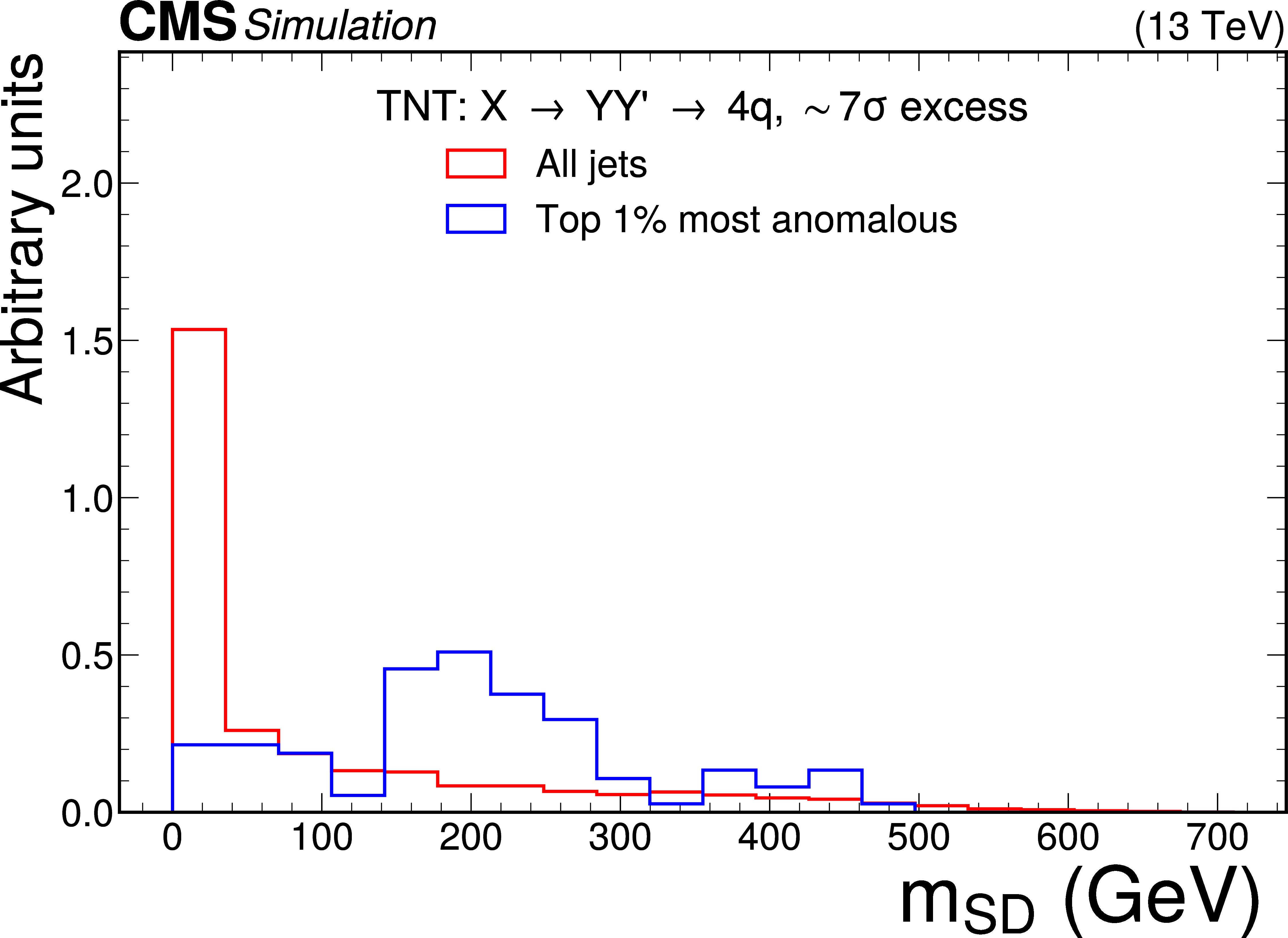
Figure 8-a:
Excess interpretation example for the TNT method trained on a simulated sample, with an injection an $ \mathrm{X}\to \mathrm{Y}\mathrm{Y'} \to 4 \mathrm{q} $ signal with a cross section of 24 fb, $ M_\mathrm{X} $ = 3 TeV, and $ M_{\mathrm{Y}/\mathrm{Y'}} = $ 170 GeV. The plots compare the properties of the jets with the highest anomaly score (blue) as compared to those for all jets in the region of the excess (red). The two-pronged nature of the anomaly is evident from the low $ \tau_{21} $ scores, and the approximate mass of the Y and Y' resonance can be seen as a peak in the jet mass ($ m_\mathrm{SD} $) distribution. |
png pdf |
Figure 8-b:
Excess interpretation example for the TNT method trained on a simulated sample, with an injection an $ \mathrm{X}\to \mathrm{Y}\mathrm{Y'} \to 4 \mathrm{q} $ signal with a cross section of 24 fb, $ M_\mathrm{X} $ = 3 TeV, and $ M_{\mathrm{Y}/\mathrm{Y'}} = $ 170 GeV. The plots compare the properties of the jets with the highest anomaly score (blue) as compared to those for all jets in the region of the excess (red). The two-pronged nature of the anomaly is evident from the low $ \tau_{21} $ scores, and the approximate mass of the Y and Y' resonance can be seen as a peak in the jet mass ($ m_\mathrm{SD} $) distribution. |
png pdf |
Figure 8-c:
Excess interpretation example for the TNT method trained on a simulated sample, with an injection an $ \mathrm{X}\to \mathrm{Y}\mathrm{Y'} \to 4 \mathrm{q} $ signal with a cross section of 24 fb, $ M_\mathrm{X} $ = 3 TeV, and $ M_{\mathrm{Y}/\mathrm{Y'}} = $ 170 GeV. The plots compare the properties of the jets with the highest anomaly score (blue) as compared to those for all jets in the region of the excess (red). The two-pronged nature of the anomaly is evident from the low $ \tau_{21} $ scores, and the approximate mass of the Y and Y' resonance can be seen as a peak in the jet mass ($ m_\mathrm{SD} $) distribution. |
png pdf |
Figure 8-d:
Excess interpretation example for the TNT method trained on a simulated sample, with an injection an $ \mathrm{X}\to \mathrm{Y}\mathrm{Y'} \to 4 \mathrm{q} $ signal with a cross section of 24 fb, $ M_\mathrm{X} $ = 3 TeV, and $ M_{\mathrm{Y}/\mathrm{Y'}} = $ 170 GeV. The plots compare the properties of the jets with the highest anomaly score (blue) as compared to those for all jets in the region of the excess (red). The two-pronged nature of the anomaly is evident from the low $ \tau_{21} $ scores, and the approximate mass of the Y and Y' resonance can be seen as a peak in the jet mass ($ m_\mathrm{SD} $) distribution. |
png pdf |
Figure 8-e:
Excess interpretation example for the TNT method trained on a simulated sample, with an injection an $ \mathrm{X}\to \mathrm{Y}\mathrm{Y'} \to 4 \mathrm{q} $ signal with a cross section of 24 fb, $ M_\mathrm{X} $ = 3 TeV, and $ M_{\mathrm{Y}/\mathrm{Y'}} = $ 170 GeV. The plots compare the properties of the jets with the highest anomaly score (blue) as compared to those for all jets in the region of the excess (red). The two-pronged nature of the anomaly is evident from the low $ \tau_{21} $ scores, and the approximate mass of the Y and Y' resonance can be seen as a peak in the jet mass ($ m_\mathrm{SD} $) distribution. |
png pdf |
Figure 8-f:
Excess interpretation example for the TNT method trained on a simulated sample, with an injection an $ \mathrm{X}\to \mathrm{Y}\mathrm{Y'} \to 4 \mathrm{q} $ signal with a cross section of 24 fb, $ M_\mathrm{X} $ = 3 TeV, and $ M_{\mathrm{Y}/\mathrm{Y'}} = $ 170 GeV. The plots compare the properties of the jets with the highest anomaly score (blue) as compared to those for all jets in the region of the excess (red). The two-pronged nature of the anomaly is evident from the low $ \tau_{21} $ scores, and the approximate mass of the Y and Y' resonance can be seen as a peak in the jet mass ($ m_\mathrm{SD} $) distribution. |
png pdf |
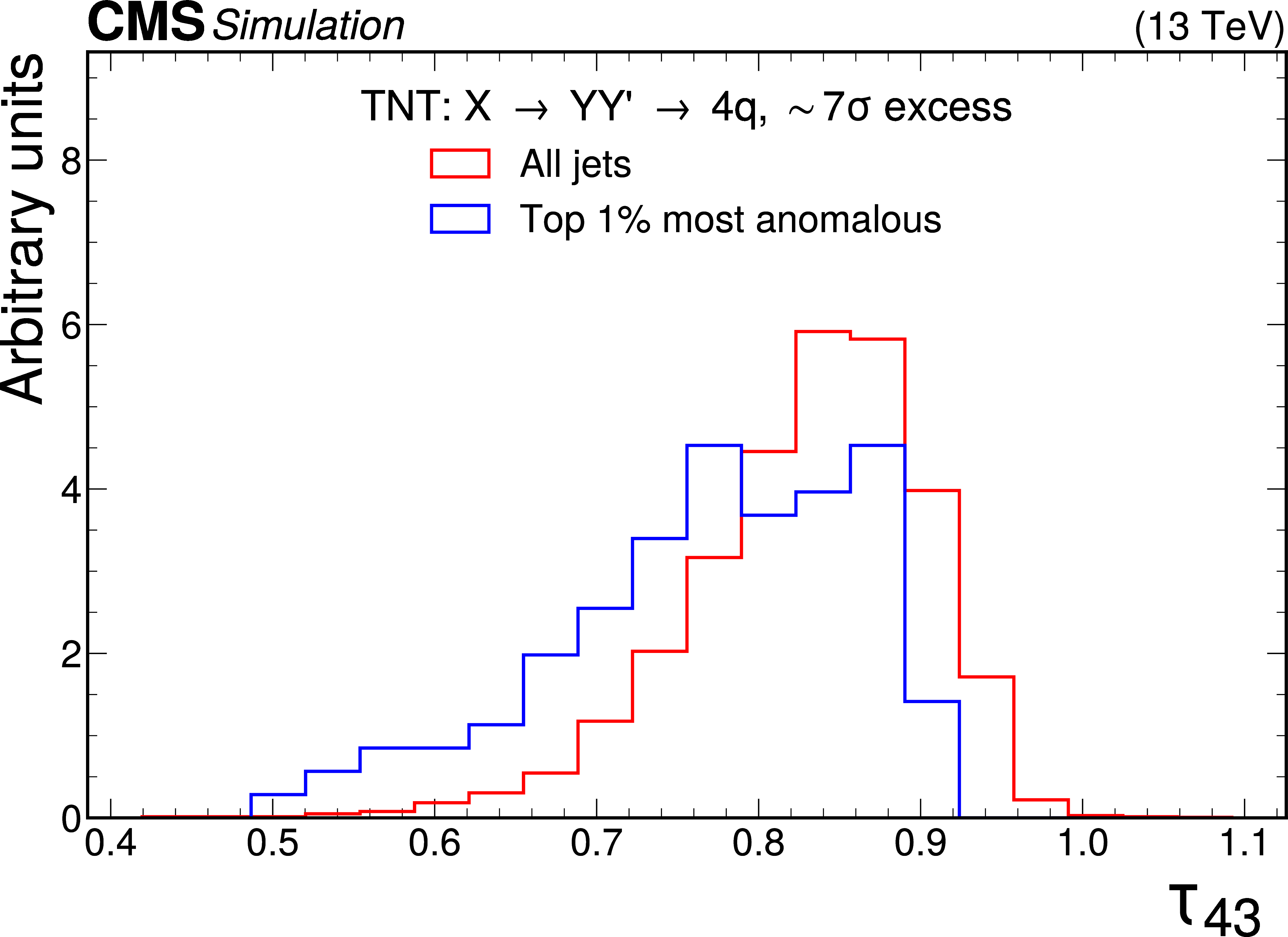
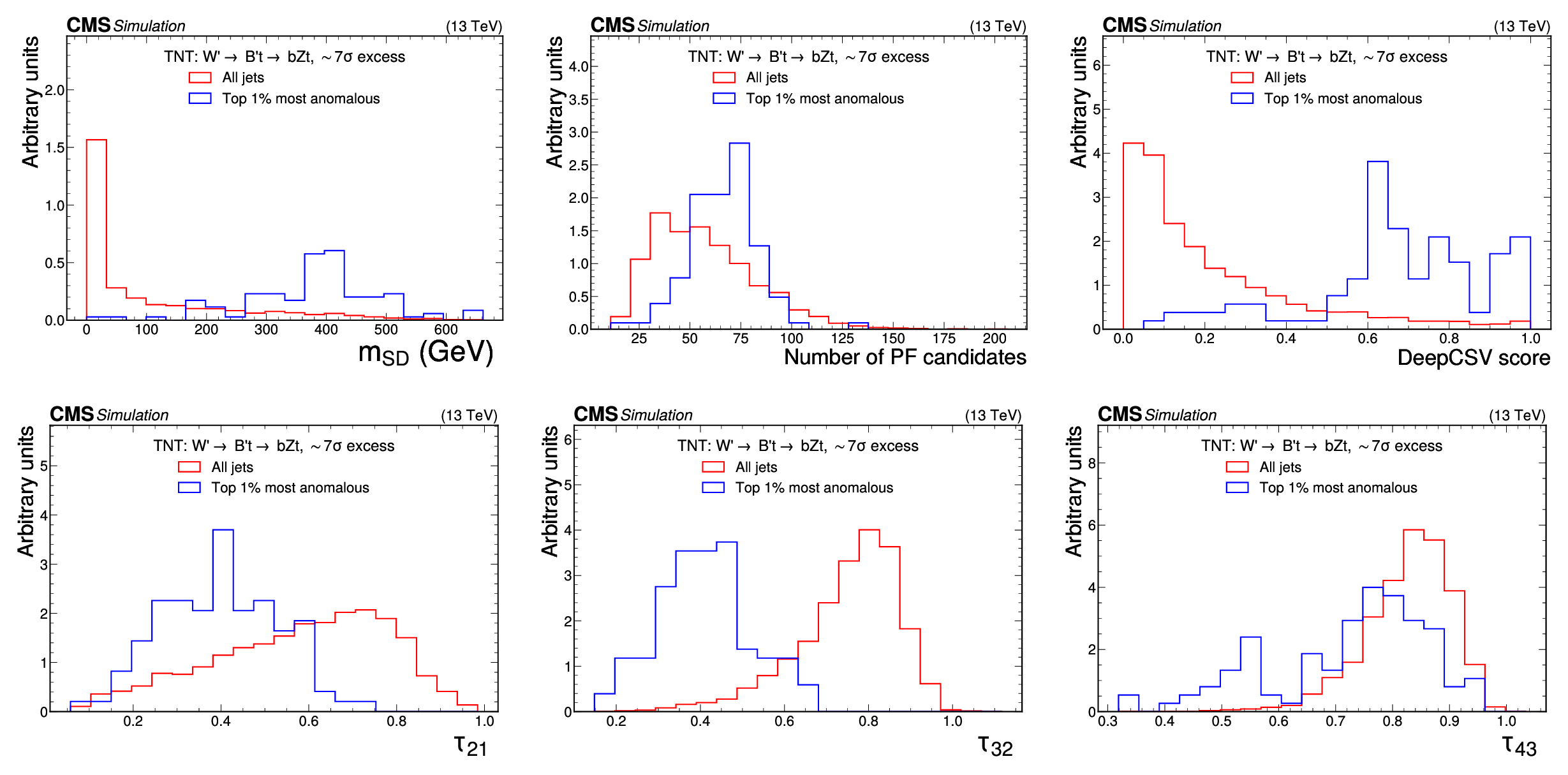
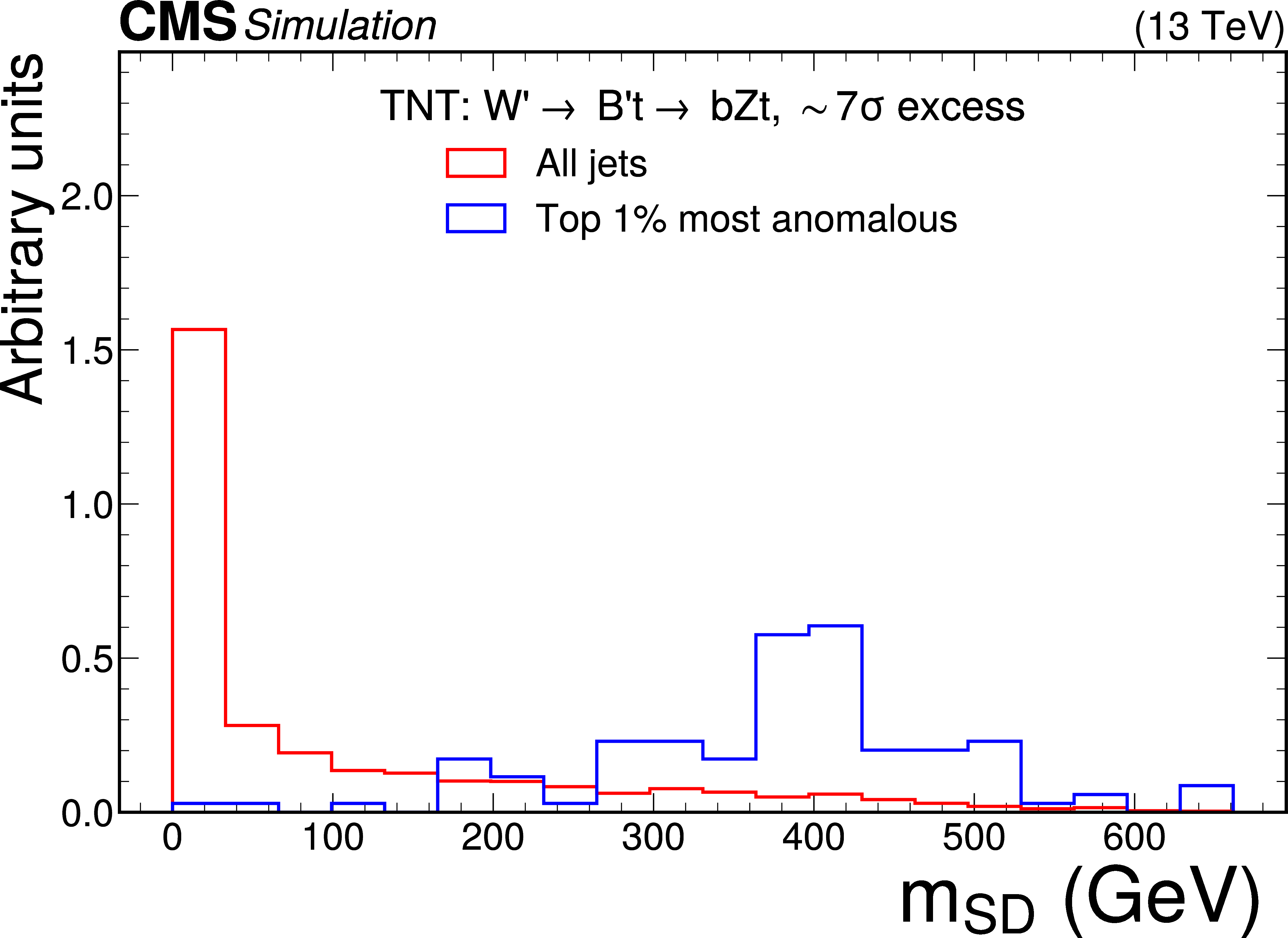
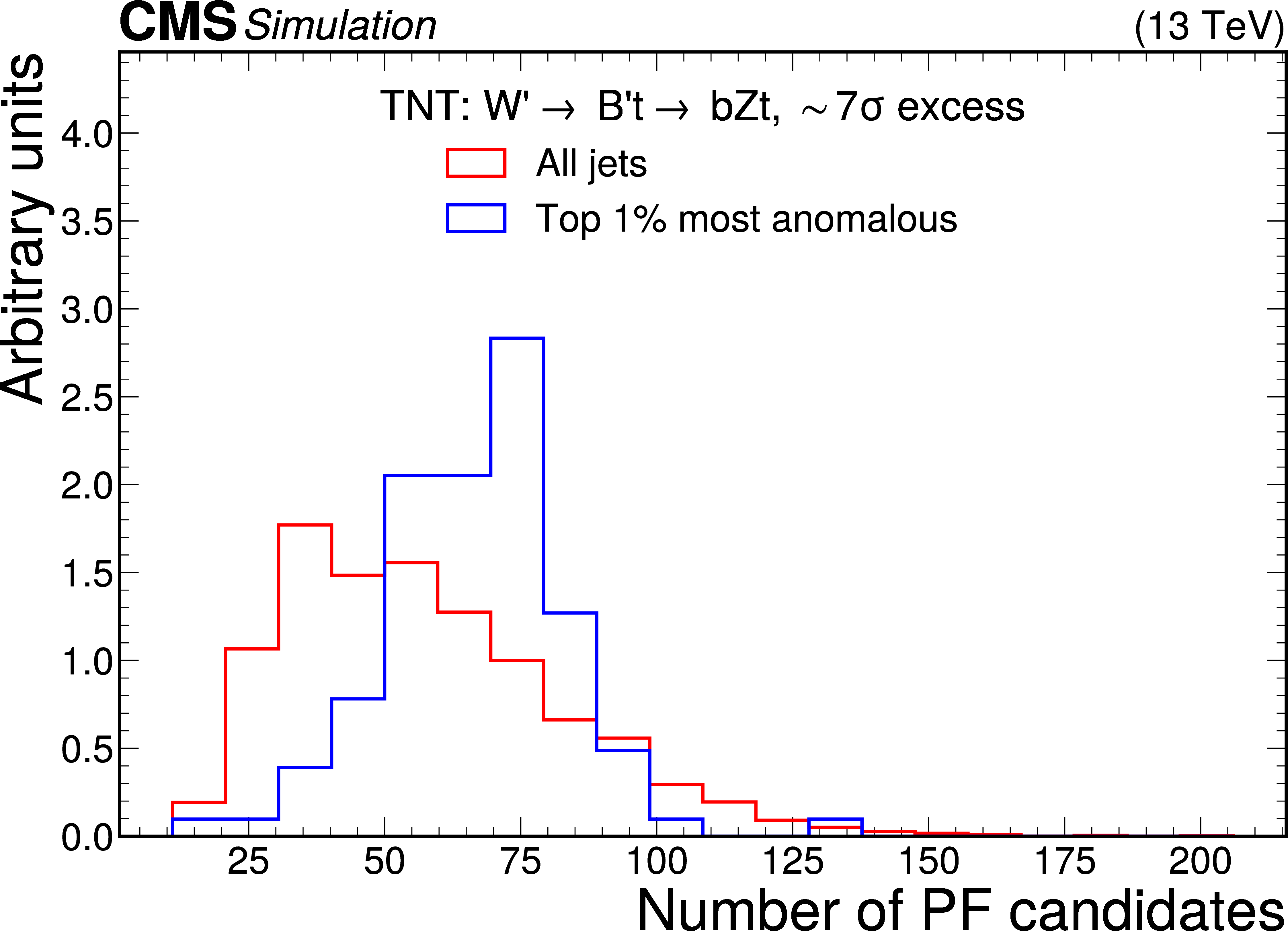
Figure 9:
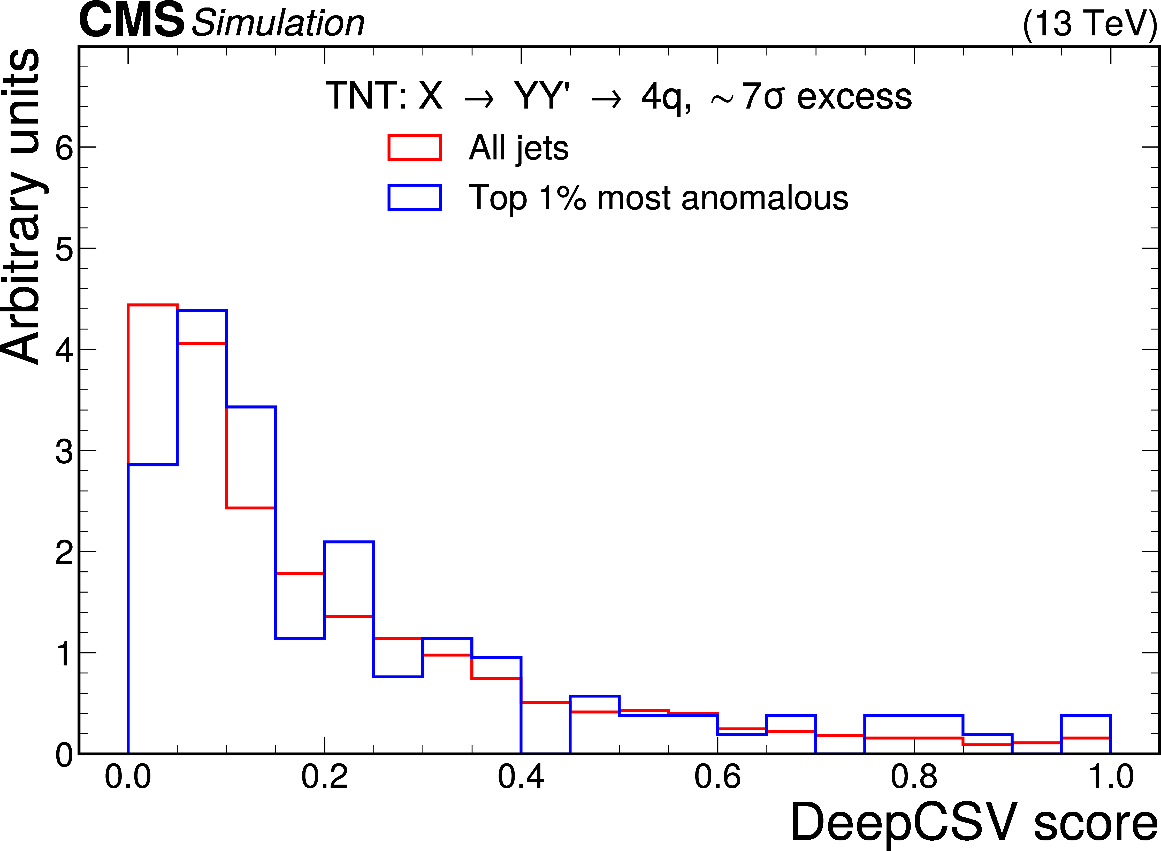
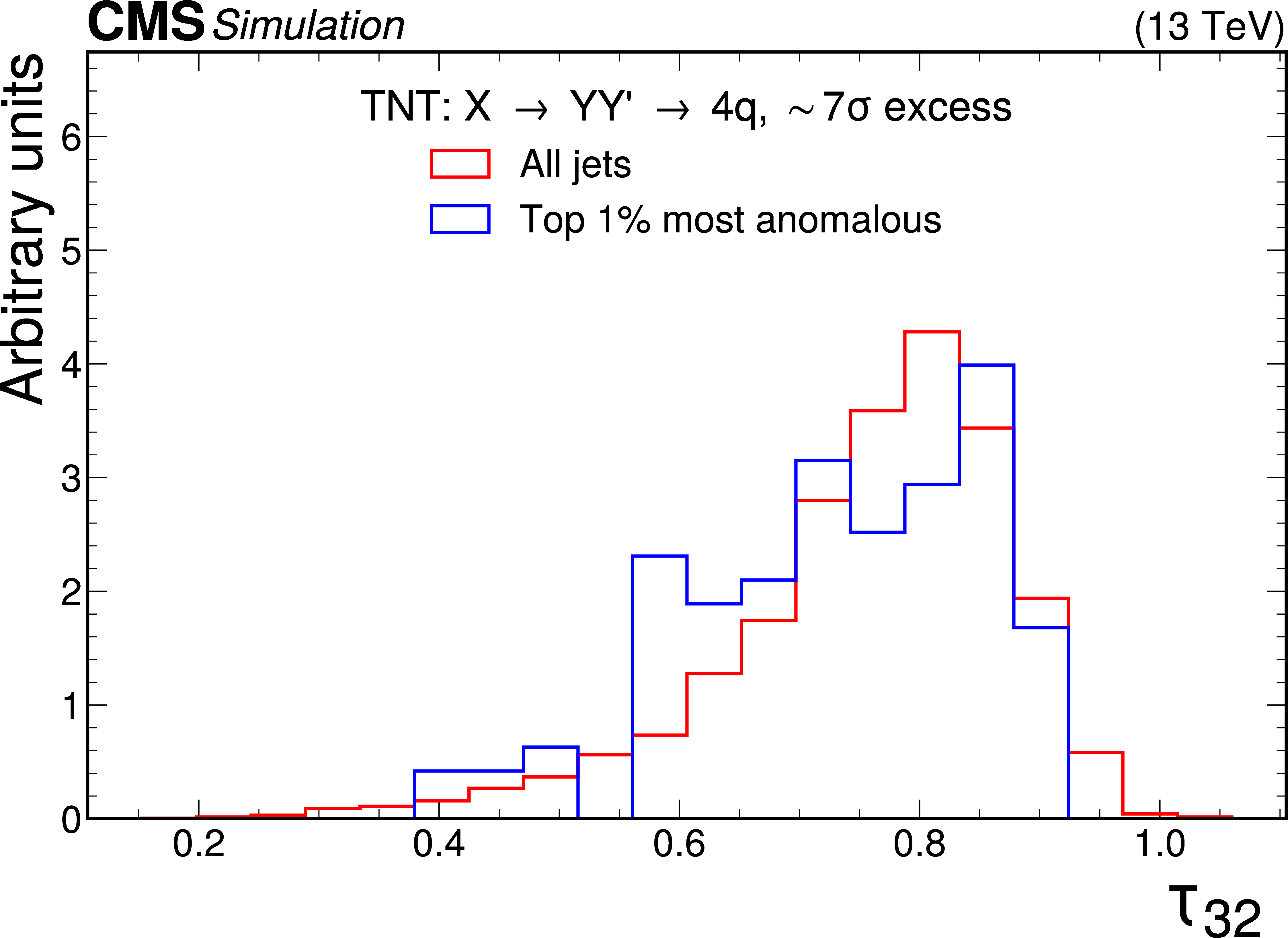
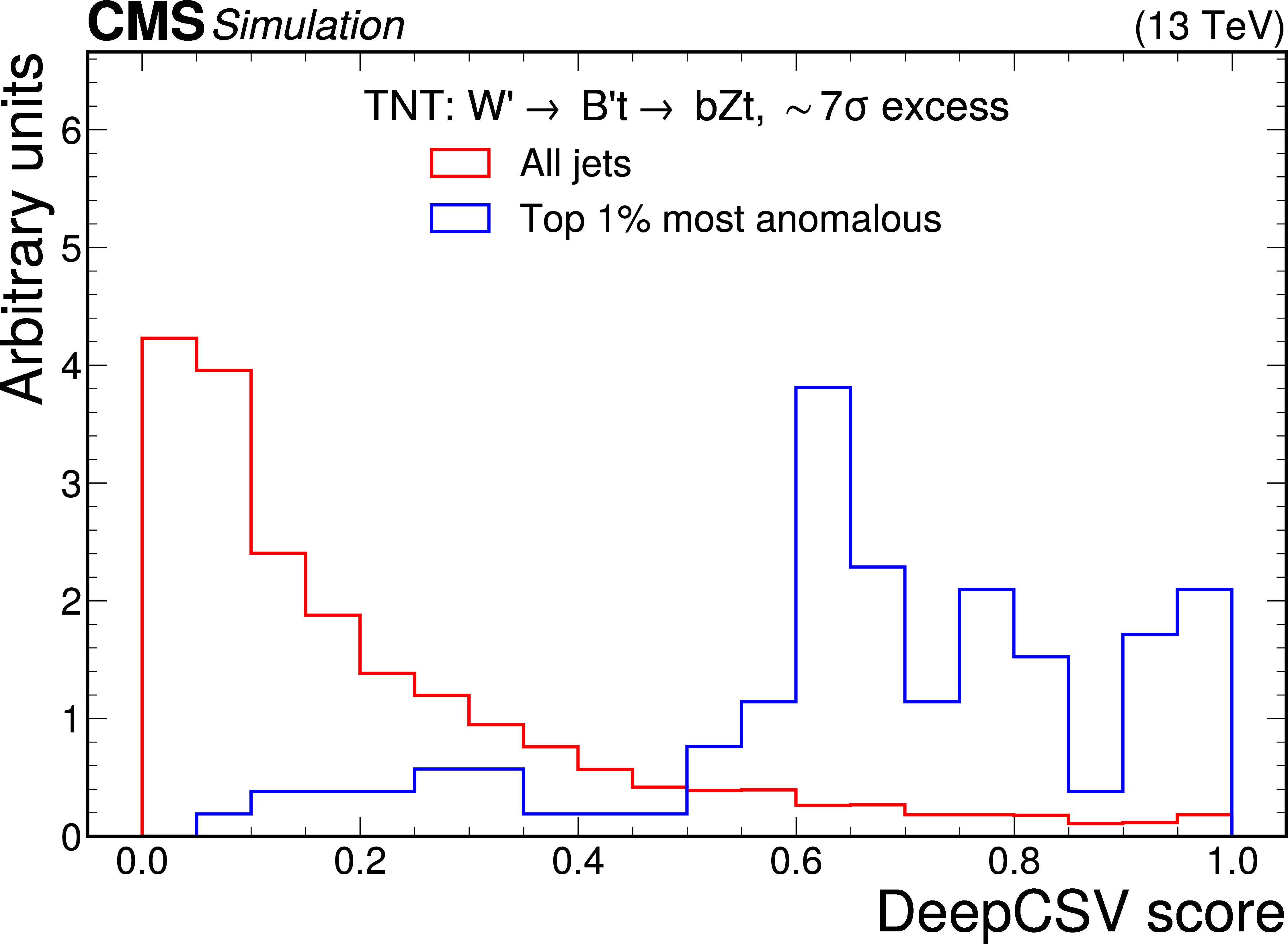
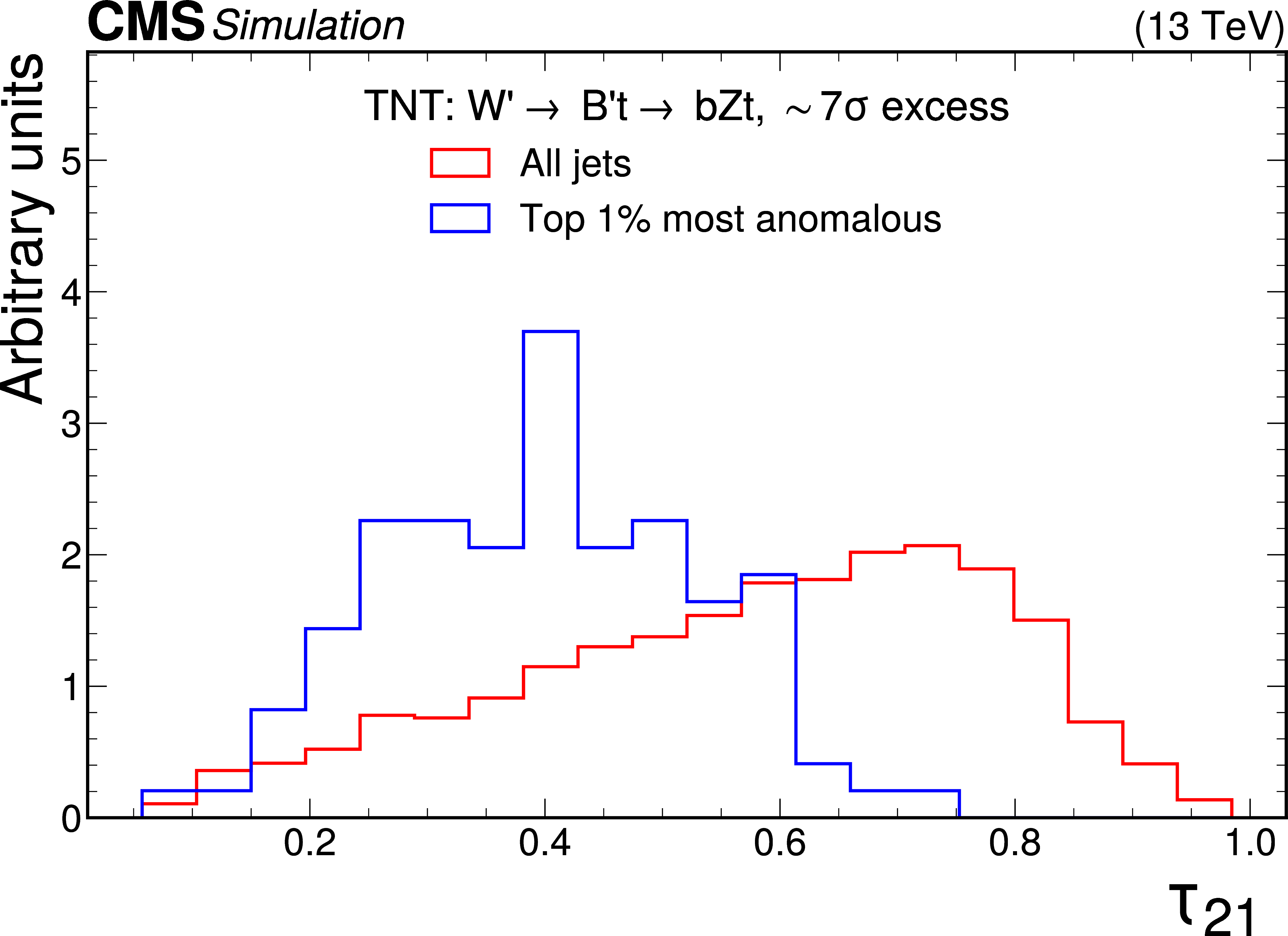
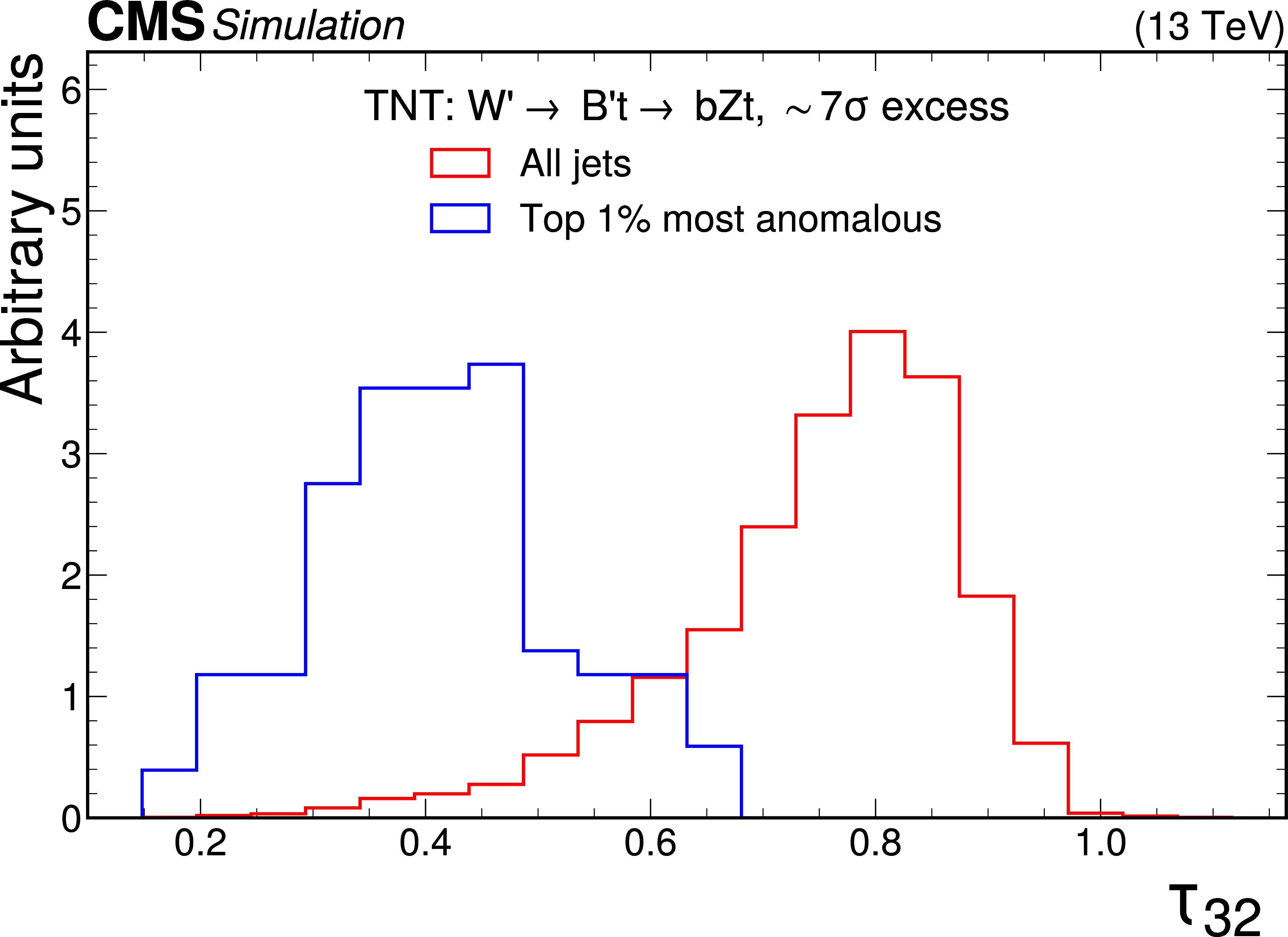
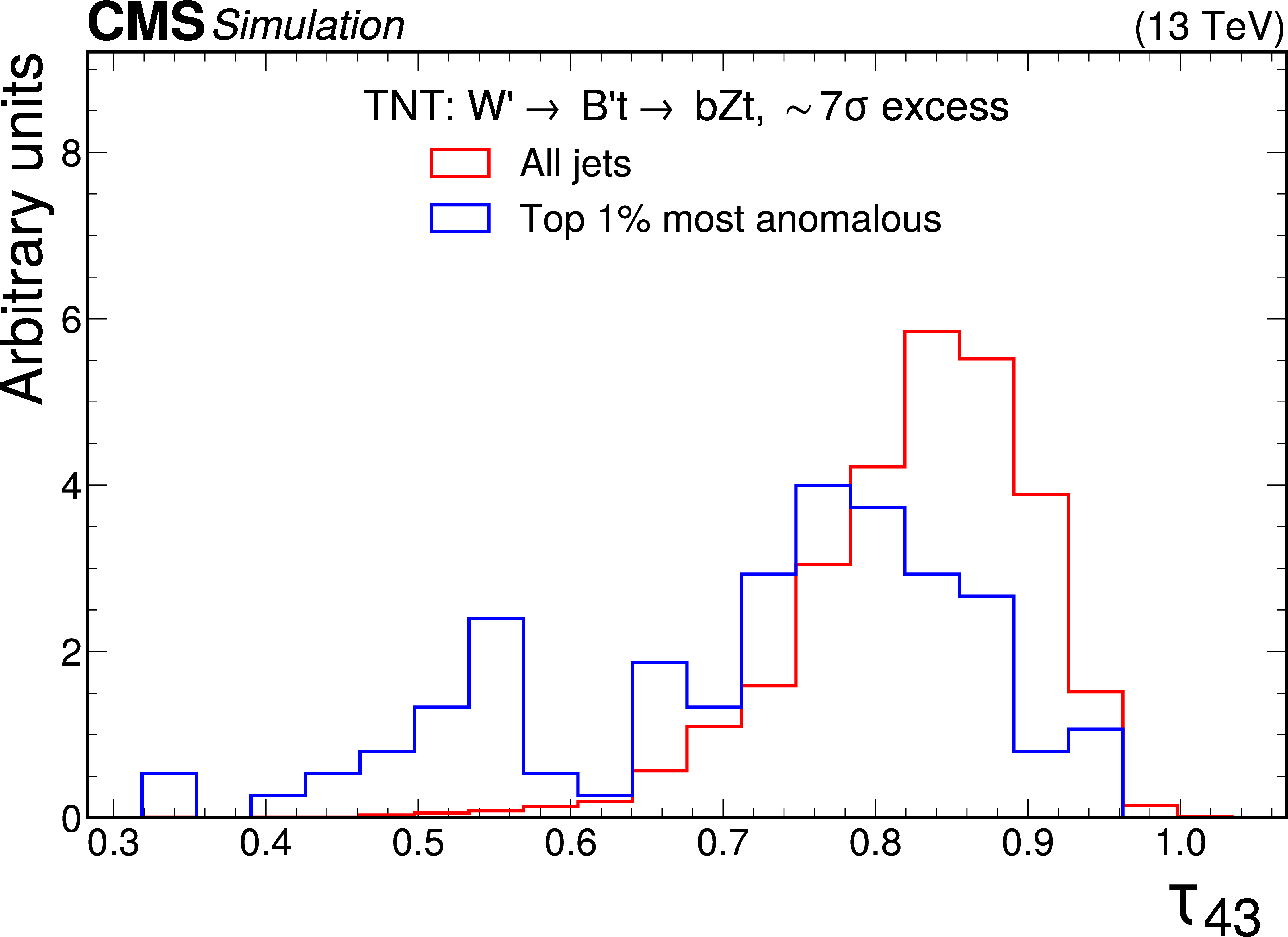
Excess interpretation example for the TNT method trained on a simulated sample, with an injection of a $ \mathrm{W^{'}} \to \mathrm{B'}\mathrm{t} \to \mathrm{b} \mathrm{Z} \mathrm{t} $ signal with a cross section of 97 fb, $ M_{\mathrm{W^{'}}} = $ 3 TeV, and $ M_{\mathrm{B'}} = $ 400 GeV. The plots compare the properties of the jets with the highest anomaly score (blue) as compared to those for all jets in the region of the excess (red). The three-pronged nature of the signal is clear from the low $ \tau_{32} $ scores, the presence of b tags from the high DEEPCSV score, and peaks in the jet mass ($ m_\mathrm{SD} $) at 170 GeV and 400 GeV indicate the top quark and $ B' $ resonances. |
png pdf |
Figure 9-a:
Excess interpretation example for the TNT method trained on a simulated sample, with an injection of a $ \mathrm{W^{'}} \to \mathrm{B'}\mathrm{t} \to \mathrm{b} \mathrm{Z} \mathrm{t} $ signal with a cross section of 97 fb, $ M_{\mathrm{W^{'}}} = $ 3 TeV, and $ M_{\mathrm{B'}} = $ 400 GeV. The plots compare the properties of the jets with the highest anomaly score (blue) as compared to those for all jets in the region of the excess (red). The three-pronged nature of the signal is clear from the low $ \tau_{32} $ scores, the presence of b tags from the high DEEPCSV score, and peaks in the jet mass ($ m_\mathrm{SD} $) at 170 GeV and 400 GeV indicate the top quark and $ B' $ resonances. |
png pdf |
Figure 9-b:
Excess interpretation example for the TNT method trained on a simulated sample, with an injection of a $ \mathrm{W^{'}} \to \mathrm{B'}\mathrm{t} \to \mathrm{b} \mathrm{Z} \mathrm{t} $ signal with a cross section of 97 fb, $ M_{\mathrm{W^{'}}} = $ 3 TeV, and $ M_{\mathrm{B'}} = $ 400 GeV. The plots compare the properties of the jets with the highest anomaly score (blue) as compared to those for all jets in the region of the excess (red). The three-pronged nature of the signal is clear from the low $ \tau_{32} $ scores, the presence of b tags from the high DEEPCSV score, and peaks in the jet mass ($ m_\mathrm{SD} $) at 170 GeV and 400 GeV indicate the top quark and $ B' $ resonances. |
png pdf |
Figure 9-c:
Excess interpretation example for the TNT method trained on a simulated sample, with an injection of a $ \mathrm{W^{'}} \to \mathrm{B'}\mathrm{t} \to \mathrm{b} \mathrm{Z} \mathrm{t} $ signal with a cross section of 97 fb, $ M_{\mathrm{W^{'}}} = $ 3 TeV, and $ M_{\mathrm{B'}} = $ 400 GeV. The plots compare the properties of the jets with the highest anomaly score (blue) as compared to those for all jets in the region of the excess (red). The three-pronged nature of the signal is clear from the low $ \tau_{32} $ scores, the presence of b tags from the high DEEPCSV score, and peaks in the jet mass ($ m_\mathrm{SD} $) at 170 GeV and 400 GeV indicate the top quark and $ B' $ resonances. |
png pdf |
Figure 9-d:
Excess interpretation example for the TNT method trained on a simulated sample, with an injection of a $ \mathrm{W^{'}} \to \mathrm{B'}\mathrm{t} \to \mathrm{b} \mathrm{Z} \mathrm{t} $ signal with a cross section of 97 fb, $ M_{\mathrm{W^{'}}} = $ 3 TeV, and $ M_{\mathrm{B'}} = $ 400 GeV. The plots compare the properties of the jets with the highest anomaly score (blue) as compared to those for all jets in the region of the excess (red). The three-pronged nature of the signal is clear from the low $ \tau_{32} $ scores, the presence of b tags from the high DEEPCSV score, and peaks in the jet mass ($ m_\mathrm{SD} $) at 170 GeV and 400 GeV indicate the top quark and $ B' $ resonances. |
png pdf |
Figure 9-e:
Excess interpretation example for the TNT method trained on a simulated sample, with an injection of a $ \mathrm{W^{'}} \to \mathrm{B'}\mathrm{t} \to \mathrm{b} \mathrm{Z} \mathrm{t} $ signal with a cross section of 97 fb, $ M_{\mathrm{W^{'}}} = $ 3 TeV, and $ M_{\mathrm{B'}} = $ 400 GeV. The plots compare the properties of the jets with the highest anomaly score (blue) as compared to those for all jets in the region of the excess (red). The three-pronged nature of the signal is clear from the low $ \tau_{32} $ scores, the presence of b tags from the high DEEPCSV score, and peaks in the jet mass ($ m_\mathrm{SD} $) at 170 GeV and 400 GeV indicate the top quark and $ B' $ resonances. |
png pdf |
Figure 9-f:
Excess interpretation example for the TNT method trained on a simulated sample, with an injection of a $ \mathrm{W^{'}} \to \mathrm{B'}\mathrm{t} \to \mathrm{b} \mathrm{Z} \mathrm{t} $ signal with a cross section of 97 fb, $ M_{\mathrm{W^{'}}} = $ 3 TeV, and $ M_{\mathrm{B'}} = $ 400 GeV. The plots compare the properties of the jets with the highest anomaly score (blue) as compared to those for all jets in the region of the excess (red). The three-pronged nature of the signal is clear from the low $ \tau_{32} $ scores, the presence of b tags from the high DEEPCSV score, and peaks in the jet mass ($ m_\mathrm{SD} $) at 170 GeV and 400 GeV indicate the top quark and $ B' $ resonances. |
png pdf |
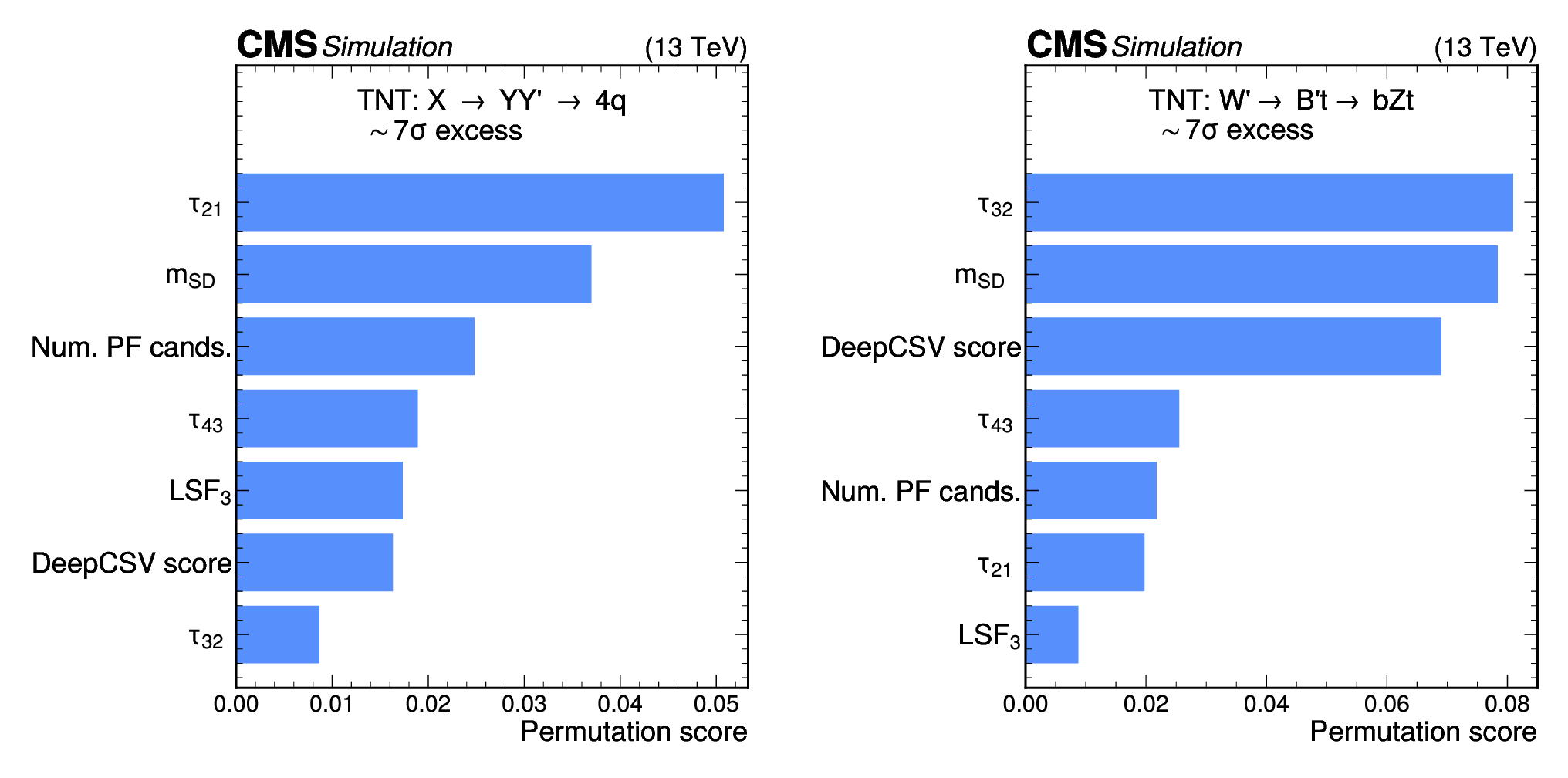
Figure 10:
Excess interpretation examples for the TNT method trained on a simulated sample, with an injection of an $ \mathrm{X}\to \mathrm{Y}\mathrm{Y'} \to 4 \mathrm{q} $ signal with a cross section of 24 fb (left) and a $ \mathrm{W^{'}} \to \mathrm{B'}\mathrm{t} \to \mathrm{b} \mathrm{Z} \mathrm{t} $ signal with a cross section of 97 fb (right). The sensitivity of the anomaly score to the different input observables is assessed to aid in the determination of the properties of the excess. For the $ \mathrm{X}\to \mathrm{Y}\mathrm{Y'} \to 4 \mathrm{q} $ injection, the $ \tau_{21} $ and jet masses are seen to be the most important observables. For the $ \mathrm{W^{'}} \to \mathrm{B'}\mathrm{t} \to \mathrm{b} \mathrm{Z} \mathrm{t} $ injection, the $ \tau_{32} $, jet masses, and b tagging score are seen to be the most important observables. |
png pdf |
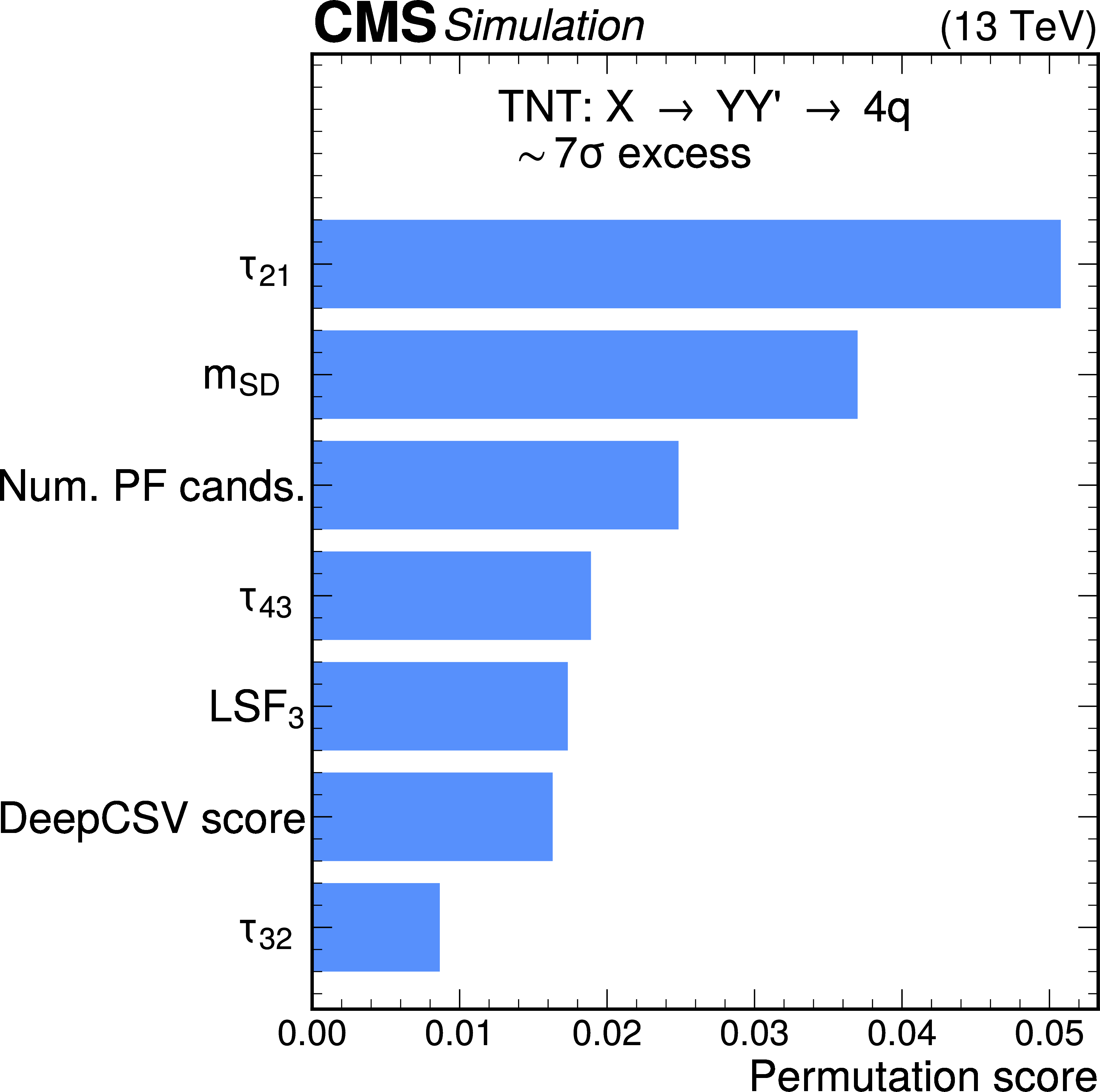
Figure 10-a:
Excess interpretation examples for the TNT method trained on a simulated sample, with an injection of an $ \mathrm{X}\to \mathrm{Y}\mathrm{Y'} \to 4 \mathrm{q} $ signal with a cross section of 24 fb (left) and a $ \mathrm{W^{'}} \to \mathrm{B'}\mathrm{t} \to \mathrm{b} \mathrm{Z} \mathrm{t} $ signal with a cross section of 97 fb (right). The sensitivity of the anomaly score to the different input observables is assessed to aid in the determination of the properties of the excess. For the $ \mathrm{X}\to \mathrm{Y}\mathrm{Y'} \to 4 \mathrm{q} $ injection, the $ \tau_{21} $ and jet masses are seen to be the most important observables. For the $ \mathrm{W^{'}} \to \mathrm{B'}\mathrm{t} \to \mathrm{b} \mathrm{Z} \mathrm{t} $ injection, the $ \tau_{32} $, jet masses, and b tagging score are seen to be the most important observables. |
png pdf |
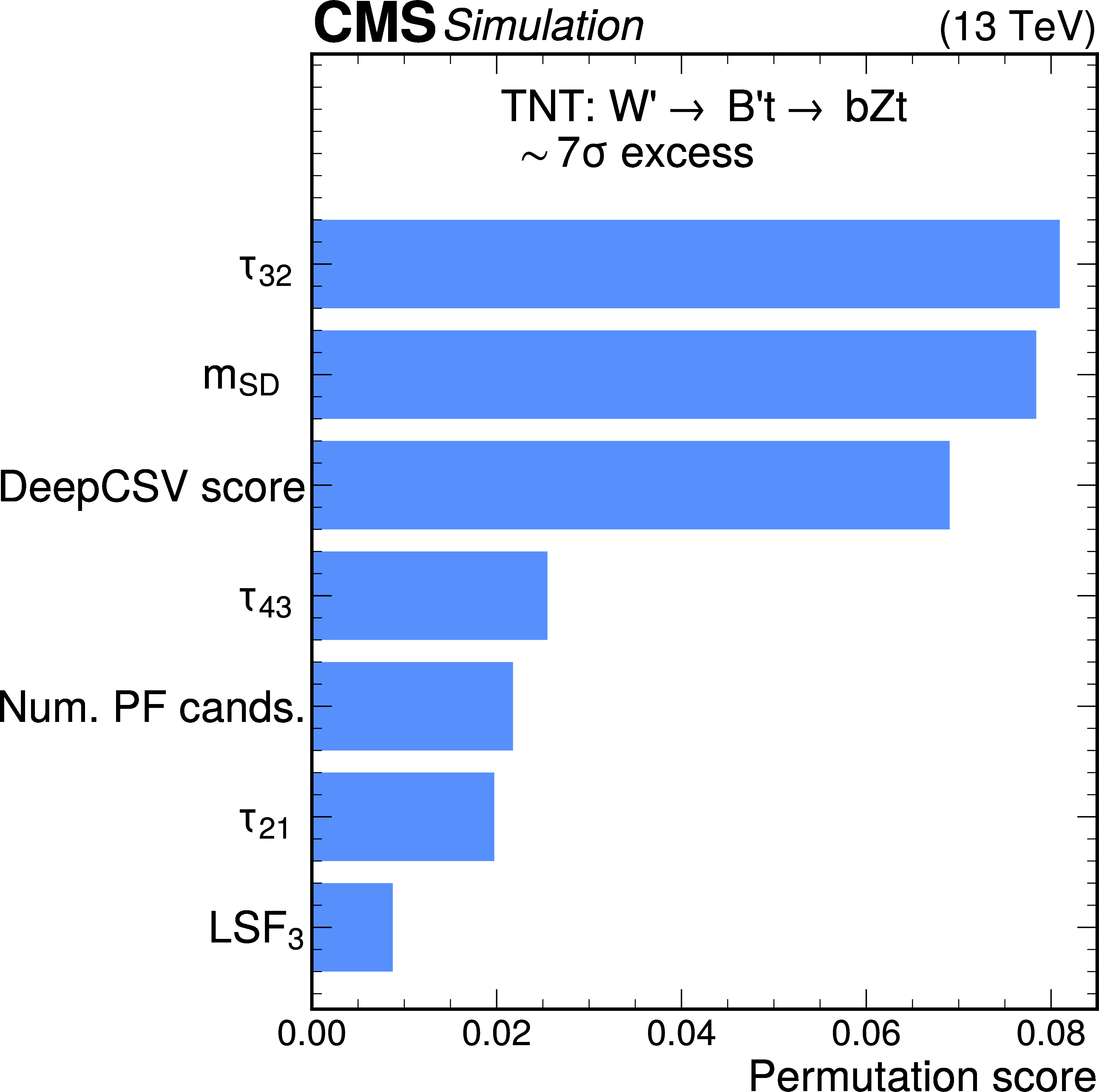
Figure 10-b:
Excess interpretation examples for the TNT method trained on a simulated sample, with an injection of an $ \mathrm{X}\to \mathrm{Y}\mathrm{Y'} \to 4 \mathrm{q} $ signal with a cross section of 24 fb (left) and a $ \mathrm{W^{'}} \to \mathrm{B'}\mathrm{t} \to \mathrm{b} \mathrm{Z} \mathrm{t} $ signal with a cross section of 97 fb (right). The sensitivity of the anomaly score to the different input observables is assessed to aid in the determination of the properties of the excess. For the $ \mathrm{X}\to \mathrm{Y}\mathrm{Y'} \to 4 \mathrm{q} $ injection, the $ \tau_{21} $ and jet masses are seen to be the most important observables. For the $ \mathrm{W^{'}} \to \mathrm{B'}\mathrm{t} \to \mathrm{b} \mathrm{Z} \mathrm{t} $ injection, the $ \tau_{32} $, jet masses, and b tagging score are seen to be the most important observables. |
png pdf |
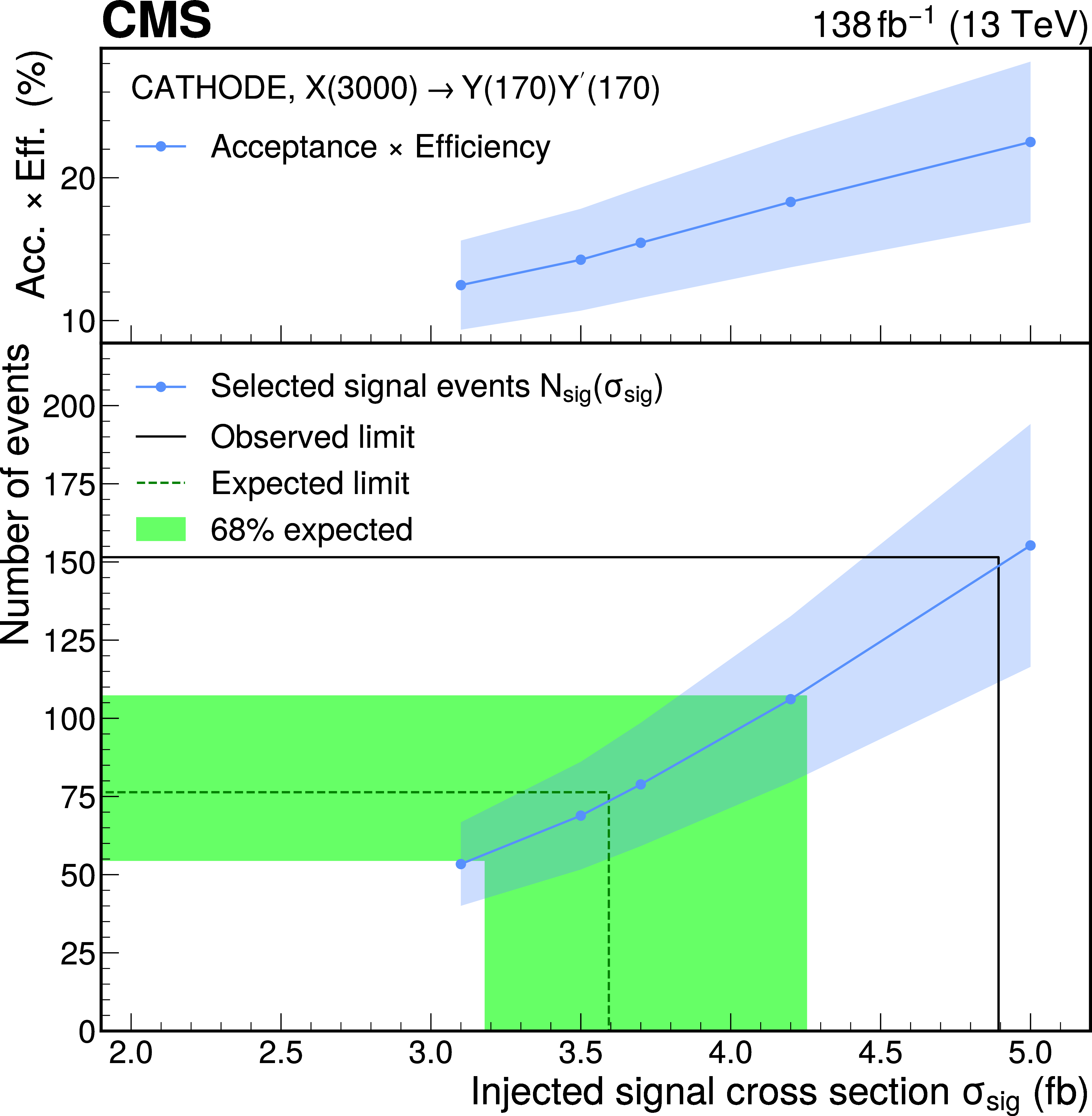
Figure 11:
Diagram of the limit-setting procedure for the $ \mathrm{X}\to \mathrm{Y}\mathrm{Y'} \to 4 \mathrm{q} $ signal at 3 TeV with the CATHODE method. The upper panel shows the estimated signal acceptance times efficiency as a function of the cross section injected in data. The shaded region in the upper panel shows the total statistical and systematic uncertainty in the efficiency. The resulting $ N_\text{sig}(\sigma_\text{sig}) $ curve and its corresponding uncertainty band from the efficiency are shown in blue in the lower panel. The expected and observed limits on the number of signal events are shown as a horizontal solid black line and green dashed lines, respectively, and connected to the corresponding limits on the cross section (vertical lines). The 68% confidence level band around the expected limit is displayed similarly. |
| Tables | |
png pdf |
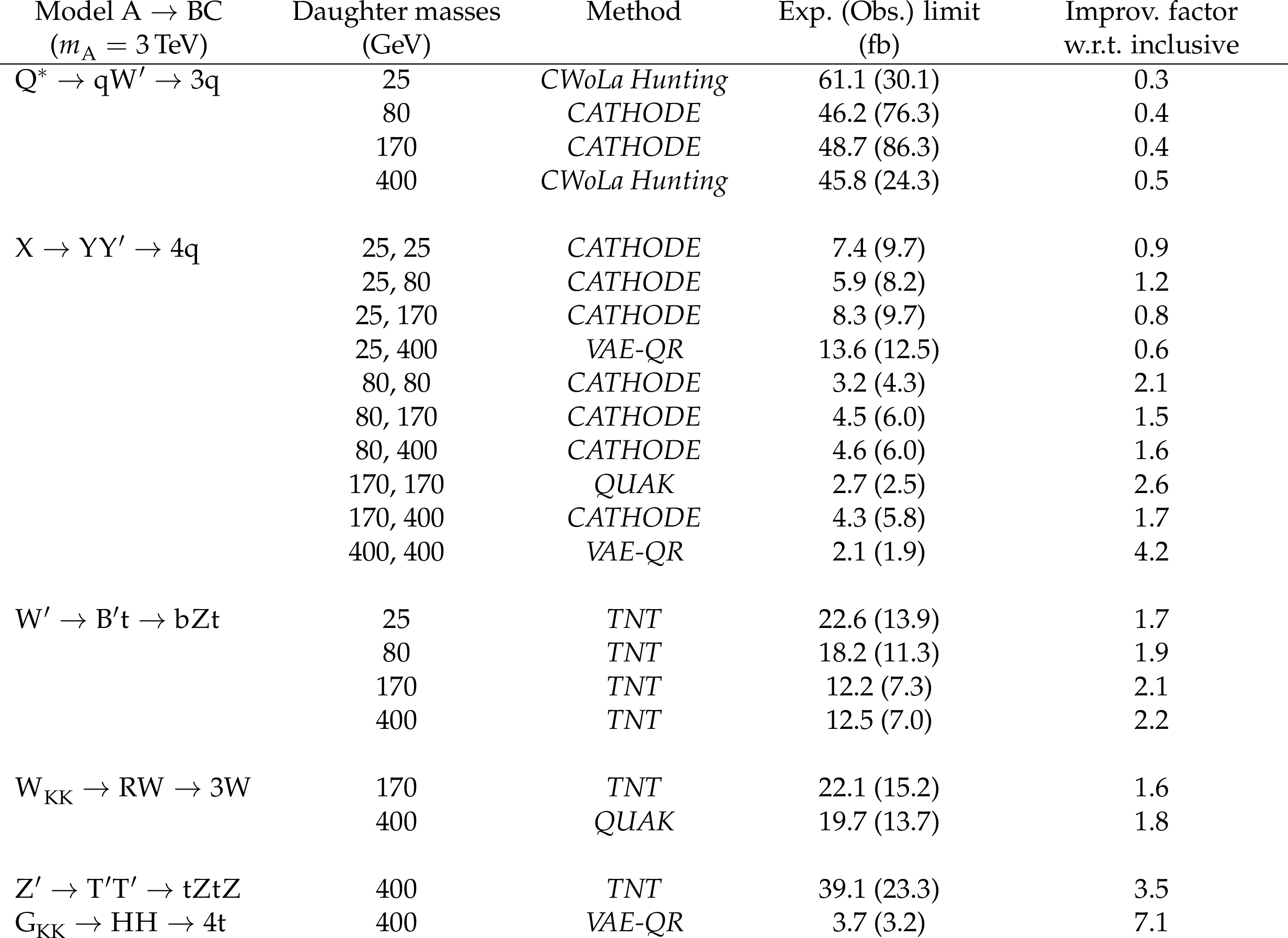
Table 1:
Limits on additional signal models and daughter mass combinations for a 3 TeV resonance mass. For each signal, the expected and observed 95% CL upper limits on the signal cross section from the best performing anomaly detection method are reported. The expected limit from the anomaly detection method is also compared to the expected limit of the inclusive search to quantify the improvement. For some signals the anomaly detection methods do not improve with respect to the inclusive search. This is indicated by an improvement factor less than one. |
png pdf |
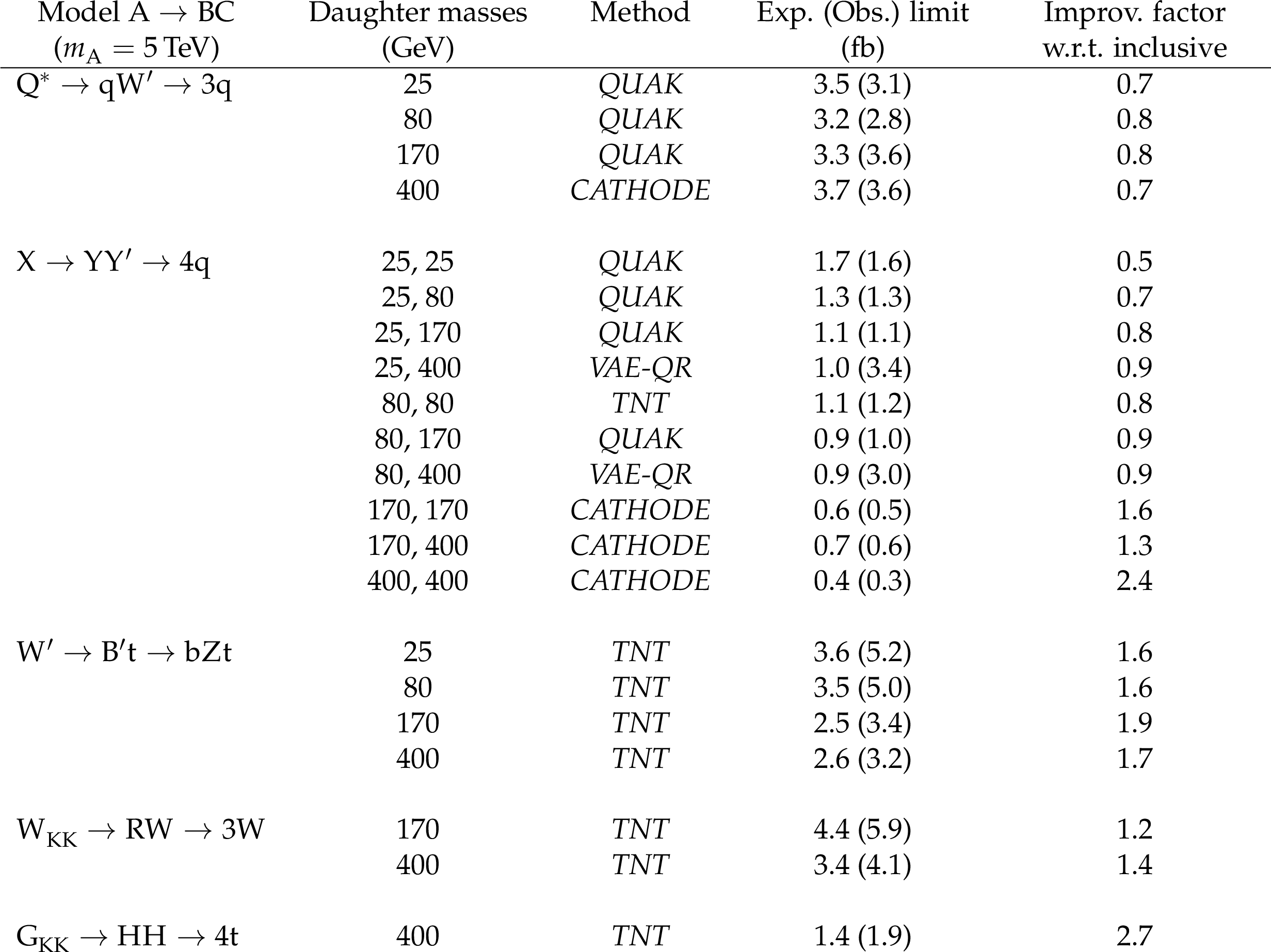
Table 2:
Limits on additional signal models and daughter mass combinations for a 5 TeV resonance mass. For each signal, the expected and observed 95% CL upper limits on the signal cross section from the best performing anomaly detection method are reported. The expected limit from the anomaly detection method is also compared to the expected limit of the inclusive search to quantify the improvement. For some signals the anomaly detection methods do not improve with respect to the inclusive search. This is indicated by an improvement factor less than one. |
png pdf |
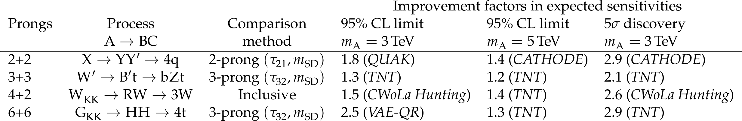
Table 3:
For the $ \mathrm{A} \to \mathrm{BC} $ searches, the sensitivity improvement of the anomaly detection methods with respect to the best performing comparison method. The considered comparison methods are the inclusive search, 2-prong targeted selection, and 3-prong targeted selection. The fourth and fifth columns list, for each signal model, improvement factors on the exclusion limit for the best performing anomaly detection method for signals at masses of $ m_\mathrm{A} = $ 3 and 5 TeV, respectively. This is quantified as the ratio of the expected upper limit on the production cross section obtained by the anomaly detection method as compared to that of the inclusive search. The sixth column lists the improvement factor on the 5 $ \sigma $ discovery potential for the best performing anomaly detection method for each signal at $ m_\mathrm{A} = $ 3 TeV. This is quantified as the ratio of the cross section that would have led to a 5 $ \sigma $ excess for the comparison method as compared to that of the anomaly detection method. |
| Summary |
| To summarize, we have presented a model-agnostic search for new resonances in the dijet final state. The search is based on 138 fb$ ^{-1} $ of data collected at $ \sqrt{s} = $ 13 TeV by the CMS experiment. Five separate anomaly detection methods were employed to improve sensitivity to signals that produce jets with substructure distinct from that of QCD multijet events. No significant excesses of events were observed by any of the methods. The performance of the anomaly detection techniques was illustrated on a set of benchmark narrow-resonance signals covering a wide range of substructure signatures. It was found that the anomaly detection methods improved the discovery sensitivity and expected limits on the benchmark signals. The anomaly detection methods were shown to enhance the sensitivity by larger factors, and on a much wider class of models, than traditional cutoff-based substructure selections, but fell short of the sensitivity of a dedicated model-specific search. The performance of the anomaly detection methods on a diverse set of benchmark models demonstrates the sensitivity of the employed techniques to a wide class of dijet resonances that have substructure and fall within the considered mass range. By construction, these approaches have sensitivity to an even broader class of models than the specific benchmarks studied. The anomaly detection methods employed in this search represent a significant step forward in the search for new particles at the LHC in a model-agnostic fashion. Further development and deployment of these techniques will play a crucial role in maximizing the discovery potential of LHC data. |
| References | ||||
| 1 | UA1 Collaboration | Two-jet mass distributions at the CERN proton-antiproton collider | PLB 209 (1988) 127 | |
| 2 | UA2 Collaboration | A measurement of two-jet decays of the W and Z bosons at the CERN $ p\bar{p} $ collider | Z Phys. C 49 (1991) 17 | |
| 3 | CDF Collaboration | Two-jet invariant-mass distribution at $ \sqrt{s}= $ 1.8 TeV | PRD 41 (1990) 1722 | |
| 4 | D0 Collaboration | Search for new particles in the two jet decay channel with the D0 detector | PRD 69 (2004) 111101 | hep-ex/0308033 |
| 5 | ATLAS Collaboration | Search for new particles in two-jet final states in 7 TeV proton-proton collisions with the ATLAS detector at the LHC | PRL 105 (2010) 161801 | 1008.2461 |
| 6 | ATLAS Collaboration | Search for new phenomena in dijet mass and angular distributions from $ pp $ collisions at $ \sqrt{s}= $ 13 TeV with the ATLAS detector | PLB 754 (2016) 302 | 1512.01530 |
| 7 | CMS Collaboration | Search for dijet resonances in 7 TeV pp collisions at CMS | PRL 105 (2010) 211801 | CMS-EXO-10-010 1010.0203 |
| 8 | CMS Collaboration | Search for high mass dijet resonances with a new background prediction method in proton-proton collisions at $ \sqrt{s} = $ 13 TeV | JHEP 05 (2020) 033 | CMS-EXO-19-012 1911.03947 |
| 9 | ATLAS Collaboration | Combination of searches for heavy resonances decaying into bosonic and leptonic final states using 36 fb$ ^{-1} $ of proton-proton collision data at $ \sqrt{s} = $ 13 TeV with the ATLAS detector | PRD 98 (2018) 052008 | 1808.02380 |
| 10 | CMS Collaboration | A multi-dimensional search for new heavy resonances decaying to boosted WW, WZ, or ZZ boson pairs in the dijet final state at 13 TeV | EPJC 80 (2020) 237 | 1906.05977 |
| 11 | CMS Collaboration | Search for new heavy resonances decaying to WW, WZ, ZZ, WH, or ZH boson pairs in the all-jets final state in proton-proton collisions at $ \sqrt{s} = $ 13 TeV | PLB 844 (2023) 137813 | 2210.00043 |
| 12 | ATLAS Collaboration | Search for resonant pair production of Higgs bosons in the $ b\bar{b}b\bar{b} $ final state using $ pp $ collisions at $ \sqrt{s} = $ 13 TeV with the ATLAS detector | PRD 105 (2022) 092002 | 2202.07288 |
| 13 | CMS Collaboration | Search for resonant pair production of Higgs bosons decaying to bottom quark-antiquark pairs in proton-proton collisions at 13 TeV | JHEP 08 (2018) 152 | CMS-HIG-17-009 1806.03548 |
| 14 | ATLAS Collaboration | Search for low-mass resonances decaying into two jets and produced in association with a photon using $ pp $ collisions at $ \sqrt{s} = $ 13 TeV with the ATLAS detector | PLB 795 (2019) 56 | 1901.10917 |
| 15 | ATLAS Collaboration | Search for resonances in the mass distribution of jet pairs with one or two jets identified as $ b $-jets in proton-proton collisions at $ \sqrt{s} = $ 13 TeV with the ATLAS detector | PRD 98 (2018) 032016 | 1805.09299 |
| 16 | CMS Collaboration | Search for low-mass resonances decaying into bottom quark-antiquark pairs in proton-proton collisions at $ \sqrt{s} = $ 13 TeV | PRD 99 (2019) 012005 | CMS-EXO-17-024 1810.11822 |
| 17 | CMS Collaboration | Search for narrow resonances in the b-tagged dijet mass spectrum in proton-proton collisions at $ \sqrt{s} = $ 13 TeV | PRD 108 (2023) 012009 | CMS-EXO-20-008 2205.01835 |
| 18 | ATLAS Collaboration | Search for heavy particles decaying into a top-quark pair in the fully hadronic final state in $ pp $ collisions at $ \sqrt{s} = $ 13 TeV with the ATLAS detector | PRD 99 (2019) 092004 | 1902.10077 |
| 19 | CMS Collaboration | Search for $ \mathrm{t}\overline{\mathrm{t}} $ resonances in highly boosted lepton+jets and fully hadronic final states in proton-proton collisions at $ \sqrt{s}= $ 13 TeV | JHEP 07 (2017) 001 | 1704.03366 |
| 20 | CMS Collaboration | Search for resonant $ \mathrm{t}\overline{\mathrm{t}} $ production in proton-proton collisions at $ \sqrt{s}= $ 13 TeV | JHEP 04 (2019) 031 | 1810.05905 |
| 21 | G. Kasieczka et al. | The LHC olympics 2020: A community challenge for anomaly detection in high energy physics | Rept. Prog. Phys. 84 (2021) 124201 | 2101.08320 |
| 22 | ATLAS Collaboration | Dijet resonance search with weak supervision using $ \sqrt{s}= $ 13 TeV $ pp $ collisions in the ATLAS detector | PRL 125 (2020) 131801 | 2005.02983 |
| 23 | ATLAS Collaboration | Anomaly detection search for new resonances decaying into a Higgs boson and a generic new particle $ X $ in hadronic final states using $ \sqrt{s} = $ 13 TeV $ pp $ collisions with the ATLAS detector | PRD 108 (2023) 052009 | 2306.03637 |
| 24 | ATLAS Collaboration | Search for new phenomena in two-body invariant mass distributions using unsupervised machine learning for anomaly detection at $ \sqrt{s} = $ 13 TeV with the ATLAS detector | PRL 132 (2024) 081801 | 2307.01612 |
| 25 | ATLAS Collaboration | Weakly supervised anomaly detection for resonant new physics in the dijet final state using proton-proton collisions at $ \sqrt{s}= $ 13 TeV with the ATLAS detector | 2502.09770 | |
| 26 | CMS Collaboration | The CMS experiment at the CERN LHC | JINST 3 (2008) S08004 | |
| 27 | CMS Collaboration | Development of the CMS detector for the CERN LHC Run 3 | JINST 19 (2024) P05064 | CMS-PRF-21-001 2309.05466 |
| 28 | CMS Collaboration | Precision luminosity measurement in proton-proton collisions at $ \sqrt{s} = $ 13 TeV in 2015 and 2016 at CMS | EPJC 81 (2021) 800 | CMS-LUM-17-003 2104.01927 |
| 29 | CMS Collaboration | CMS luminosity measurement for the 2017 data-taking period at $ \sqrt{s} = $ 13 TeV | CMS Physics Analysis Summary, 2018 link |
CMS-PAS-LUM-17-004 |
| 30 | CMS Collaboration | CMS luminosity measurement for the 2018 data-taking period at $ \sqrt{s} = $ 13 TeV | CMS Physics Analysis Summary, 2019 link |
CMS-PAS-LUM-18-002 |
| 31 | CMS Collaboration | HEPData record for this analysis | link | |
| 32 | CMS Collaboration | Performance of the CMS Level-1 trigger in proton-proton collisions at $ \sqrt{s} = $ 13 TeV | JINST 15 (2020) P10017 | CMS-TRG-17-001 2006.10165 |
| 33 | CMS Collaboration | The CMS trigger system | JINST 12 (2017) P01020 | CMS-TRG-12-001 1609.02366 |
| 34 | CMS Collaboration | Technical proposal for the Phase-II upgrade of the Compact Muon Solenoid | CMS Technical Proposal CERN-LHCC-2015-010, CMS-TDR-15-02, 2015 CDS |
|
| 35 | CMS Collaboration | Particle-flow reconstruction and global event description with the CMS detector | JINST 12 (2017) P10003 | CMS-PRF-14-001 1706.04965 |
| 36 | M. Cacciari, G. P. Salam, and G. Soyez | The anti-$ k_{\mathrm{T}} $ jet clustering algorithm | JHEP 04 (2008) 063 | 0802.1189 |
| 37 | M. Cacciari, G. P. Salam, and G. Soyez | FastJet user manual | EPJC 72 (2012) 1896 | 1111.6097 |
| 38 | CMS Collaboration | Pileup mitigation at CMS in 13 TeV data | JINST 15 (2020) P09018 | CMS-JME-18-001 2003.00503 |
| 39 | D. Bertolini, P. Harris, M. Low, and N. Tran | Pileup per particle identification | JHEP 10 (2014) 059 | 1407.6013 |
| 40 | CMS Collaboration | Jet energy scale and resolution in the CMS experiment in pp collisions at 8 TeV | JINST 12 (2017) P02014 | CMS-JME-13-004 1607.03663 |
| 41 | U. Baur, I. Hinchliffe, and D. Zeppenfeld | Excited quark production at hadron colliders | Int. J. Mod. Phys. A 2 (1987) 1285 | |
| 42 | U. Baur, M. Spira, and P. M. Zerwas | Excited quark and lepton production at hadron colliders | PRD 42 (1990) 815 | |
| 43 | D. Barducci et al. | Exploring Drell-Yan signals from the 4D composite higgs model at the LHC | JHEP 04 (2013) 152 | 1210.2927 |
| 44 | K. Agashe, P. Du, S. Hong, and R. Sundrum | Flavor universal resonances and warped gravity | JHEP 01 (2017) 016 | 1608.00526 |
| 45 | K. Agashe et al. | Dedicated strategies for triboson signals from cascade decays of vector resonances | PRD 99 (2019) 075016 | 1711.09920 |
| 46 | Y. Okada and L. Panizzi | LHC signatures of vector-like quarks | Adv. High Energy Phys. 2013 (2013) 364936 | 1207.5607 |
| 47 | M. Buchkremer, G. Cacciapaglia, A. Deandrea, and L. Panizzi | Model independent framework for searches of top partners | NPB 876 (2013) 376 | 1305.4172 |
| 48 | A. Carvalho | Gravity particles from warped extra dimensions, predictions for LHC | 1404.0102 | |
| 49 | CMS Collaboration | Search for a W' boson decaying to a vector-like quark and a top or bottom quark in the all-jets final state at $ \sqrt{\mathrm{s}} = $ 13 TeV | JHEP 09 (2022) 088 | 2202.12988 |
| 50 | CMS Collaboration | Search for resonances decaying to three W bosons in proton-proton collisions at $ \sqrt{s} = $ 13 TeV | PRL 129 (2022) 021802 | 2201.08476 |
| 51 | CMS Collaboration | Search for resonances decaying to three W bosons in the hadronic final state in proton-proton collisions at $ \sqrt s $ =13 TeV | PRD 106 (2022) 012002 | 2112.13090 |
| 52 | CMS Collaboration | Review of searches for vector-like quarks, vector-like leptons, and heavy neutral leptons in proton-proton collisions at $ \sqrt{s} = $ 13 TeV at the CMS experiment | Submitted to Physics Reports. In press, 2024 | CMS-EXO-23-006 2405.17605 |
| 53 | ATLAS Collaboration | Exploration at the high-energy frontier: ATLAS Run 2 searches investigating the exotic jungle beyond the Standard Model | Submitted to Physics Reports. In press, 2024 | 2403.09292 |
| 54 | J. Alwall et al. | The automated computation of tree-level and next-to-leading order differential cross sections, and their matching to parton shower simulations | JHEP 07 (2014) 079 | 1405.0301 |
| 55 | R. D. Ball et al. | A first unbiased global NLO determination of parton distributions and their uncertainties | NPB 838 (2010) 136 | 1002.4407 |
| 56 | NNPDF Collaboration | Parton distributions for the LHC Run II | JHEP 04 (2015) 040 | 1410.8849 |
| 57 | NNPDF Collaboration | Parton distributions from high-precision collider data | EPJC 77 (2017) 663 | 1706.00428 |
| 58 | T. Sjöstrand et al. | An introduction to PYTHIA 8.2 | Comput. Phys. Commun. 191 (2015) 159 | 1410.3012 |
| 59 | CMS Collaboration | Extraction and validation of a new set of CMS PYTHIA8 tunes from underlying-event measurements | EPJC 80 (2020) 4 | CMS-GEN-17-001 1903.12179 |
| 60 | P. Nason | A new method for combining NLO QCD with shower Monte Carlo algorithms | JHEP 11 (2004) 040 | hep-ph/0409146 |
| 61 | S. Frixione, P. Nason, and G. Ridolfi | A positive-weight next-to-leading-order Monte Carlo for heavy flavour hadroproduction | JHEP 09 (2007) 126 | 0707.3088 |
| 62 | S. Alioli, P. Nason, C. Oleari, and E. Re | A general framework for implementing NLO calculations in shower Monte Carlo programs: the POWHEG BOX | JHEP 06 (2010) 043 | 1002.2581 |
| 63 | J. Alwall et al. | Comparative study of various algorithms for the merging of parton showers and matrix elements in hadronic collisions | EPJC 53 (2008) 473 | 0706.2569 |
| 64 | D. P. Kingma and M. Welling | Auto-encoding variational Bayes | in Proc. 2nd Int. Conf. on Learning Representations. 201 (1900) 4 |
1312.6114 |
| 65 | Y. L. Dokshitzer, G. D. Leder, S. Moretti, and B. R. Webber | Better jet clustering algorithms | JHEP 08 (1997) 001 | hep-ph/9707323 |
| 66 | K. A. Wozniak et al. | New physics agnostic selections for new physics searches | EPJ Web Conf. 245 (2020) 06039 | |
| 67 | E. M. Metodiev, B. Nachman, and J. Thaler | Classification without labels: Learning from mixed samples in high energy physics | JHEP 10 (2017) 174 | 1708.02949 |
| 68 | J. H. Collins, K. Howe, and B. Nachman | Extending the search for new resonances with machine learning | PRD 99 (2019) 014038 | 1902.02634 |
| 69 | O. Amram and C. M. Suarez | Tag N\textquoteright Train: A technique to train improved classifiers on unlabeled data | JHEP 01 (2021) 153 | 2002.12376 |
| 70 | A. Hallin et al. | Classifying anomalies through outer density estimation | PRD 106 (2022) 055006 | 2109.00546 |
| 71 | A. J. Larkoski, S. Marzani, G. Soyez, and J. Thaler | Soft drop | JHEP 05 (2014) 146 | 1402.2657 |
| 72 | J. Thaler and K. Van Tilburg | Identifying Boosted Objects with N-subjettiness | JHEP 03 (2011) 015 | 1011.2268 |
| 73 | CMS Collaboration | Identification of heavy-flavour jets with the CMS detector in pp collisions at 13 TeV | JINST 13 (2018) P05011 | CMS-BTV-16-002 1712.07158 |
| 74 | C. Brust et al. | Identifying boosted new physics with non-isolated leptons | JHEP 04 (2015) 079 | 1410.0362 |
| 75 | M. Farina, Y. Nakai, and D. Shih | Searching for new physics with deep autoencoders | PRD 101 (2020) 075021 | 1808.08992 |
| 76 | T. Heimel, G. Kasieczka, T. Plehn, and J. M. Thompson | QCD or what? | SciPost Phys. 6 (2019) 030 | 1808.08979 |
| 77 | M. Germain, K. Gregor, I. Murray, and H. Larochelle | MADE: Masked autoencoder for distribution estimation | in Proc. 32nd Int. Conf. on Machine Learning Research - vol. 37, 2015 link |
1502.03509 |
| 78 | L. Dinh, D. Krueger, and Y. Bengio | NICE: Non-linear independent components estimation | in Proc. 3rd Int. Conf. on Learning Representations, ICLR, Y. Bengio and Y. LeCun, eds, 2015 link |
1410.8516 |
| 79 | D. J. Rezende and S. Mohamed | Variational inference with normalizing flows | in Proc. 32nd Int. Conf. on Machine Learning - vol. 37, 2016 link |
1505.05770 |
| 80 | L. Dinh, J. Sohl-Dickstein, and S. Bengio | Density estimation using real NVP | in Proc. Conf. on Learning Representations 2017 | 1605.08803 |
| 81 | D. P. Kingma and P. Dhariwal | Glow: Generative flow with invertible 1x1 convolutions | in Proc. 32nd Int. Conf. on Neural Information Processing Systems (NIPS), 2018 link |
1807.03039 |
| 82 | G. Papamakarios, T. Pavlakou, and I. Murray | Masked autoregressive flow for density estimation | in Advances in Neural Information Processing Systems, I. Guyon et al., eds., volume 30, 2017 link |
|
| 83 | C. Durkan, A. Bekasov, I. Murray, and G. Papamakarios | Neural spline flows | in Proc. 33rd Int. Conf. on Neural Information Processing Systems, 2019 | 1906.04032 |
| 84 | R. van den Berg, L. Hasenclever, J. M. Tomczak, and M. Welling | Sylvester normalizing flows for variational inference | in Proc. Conf. on Uncertainty in Artificial Intelligence (UAI), 2018 link |
1803.05649 |
| 85 | J. Brehmer and K. Cranmer | Flows for simultaneous manifold learning and density estimation | in Proc. 34th Conf. on Neural Information Processing Systems, 2020 | 2003.13913 |
| 86 | S. E. Park et al. | Quasi anomalous knowledge: Searching for new physics with embedded knowledge | JHEP 21 (2020) 030 | 2011.03550 |
| 87 | M. J. Oreglia | A study of the reactions $ {\psi^\prime\to\gamma\gamma\psi} $ | PhD thesis, Stanford University, SLAC-R-236, 1980 link |
|
| 88 | J. E. Gaiser | Charmonium spectroscopy from radiative decays of the $ \mathrm{J}/\psi $ and $ {\psi^\prime} $ | PhD thesis, Stanford University, SLAC-R-255, 1982 link |
|
| 89 | R. Fisher | On the interpretation of $ \chi^2 $ from contingency tables, and the calculation of p | J. R. Stat. Soc. 85 (1922) 87 | |
| 90 | ATLAS and CMS Collaborations, and LHC Higgs Combination Group | Procedure for the LHC Higgs boson search combination in Summer 2011 | Technical Report CMS-NOTE-2011-005, ATL-PHYS-PUB-2011-11, 2011 | |
| 91 | T. Junk | Confidence level computation for combining searches with small statistics | NIM A 434 (1999) 435 | hep-ex/9902006 |
| 92 | A. L. Read | Presentation of search results: The CL$ _{\text{s}} $ technique | JPG 28 (2002) 2693 | |
| 93 | G. Cowan, K. Cranmer, E. Gross, and O. Vitells | Asymptotic formulae for likelihood-based tests of new physics | EPJC 71 (2011) 1554 | 1007.1727 |
| 94 | CMS Collaboration | The CMS statistical analysis and combination tool: \textscCombine | Comput. Softw. Big Sci. 8 (2024) 19 | CMS-CAT-23-001 2404.06614 |
| 95 | W. Verkerke and D. P. Kirkby | The RooFit toolkit for data modeling | in (CHEP03), L. Lyons and M. Karagoz, eds, 2003 Proc. Comp. and High Energy Phys. 200 (2003) 3 |
physics/0306116 |
| 96 | L. Moneta et al. | The RooStats project | PoS ACAT 057, 2010 link |
1009.1003 |
| 97 | CMS Collaboration | A new method for correcting the substructure of multi-prong jets using Lund jet plane reweighting in the CMS experiment | CMS Physics Analysis Summary, 2025 link |
CMS-PAS-JME-23-001 |
| 98 | F. A. Dreyer, G. P. Salam, and G. Soyez | The Lund jet plane | JHEP 12 (2018) 064 | 1807.04758 |
| 99 | Y. LeCun et al. | Backpropagation applied to handwritten zip code recognition | Neural Comput. 1 (1989) 541 | |
| 100 | H. Fan, H. Su, and L. Guibas | A point set generation network for 3d object reconstruction from a single image | IEEE Conference on Computer Vision and Pattern Recognition (CVPR), 2017 link |
1612.00603 |
| 101 | S. Macaluso and D. Shih | Pulling out all the tops with computer vision and deep learning | JHEP 10 (2018) 121 | 1803.00107 |
| 102 | M. Rosenblatt | Remarks on some nonparametric estimates of a density function | Ann. Math. Stat. 27 (1956) 832 | |
| 103 | E. Parzen | On estimation of a probability density function and mode | Ann. Math. Stat. 33 (1962) 1065 | |
| 104 | K. Fukushima | Visual feature extraction by a multilayered network of analog threshold elements | IEEE Trans. Syst. Sci. Cybern. 5 (1969) 322 | |
| 105 | I. J. Good | Rational decisions | J. Roy. Stat. Soc. B 14 (1952) 107 | |
| 106 | G. E. P. Box and D. R. Cox | An analysis of transformations | J. R. Stat. Soc. 26 (1964) 211 | |
| 107 | L. Breimen | Random forests | Mach. Learn 45 (2001) 5 | |
|
|
Compact Muon Solenoid LHC, CERN |
|

|

|

|

|

|