

Compact Muon Solenoid
LHC, CERN
| CMS-HIG-20-011 ; CERN-EP-2025-214 | ||
| Combination of searches for nonresonant Higgs boson pair production in proton-proton collisions at $ \sqrt{s}= $ 13 TeV | ||
| CMS Collaboration | ||
| 8 October 2025 | ||
| Submitted to Reports on Progress in Physics | ||
| Abstract: This paper presents a combination of searches for the nonresonant production of Higgs boson pairs (HH) in proton-proton collisions at a centre-of-mass energy of 13 TeV. The data set was collected by the CMS experiment at the LHC from 2016 to 2018 and corresponds to a total integrated luminosity of 138 fb$ ^{-1} $. The observed (expected) upper limit on the inclusive HH production cross section relative to the standard model (SM) prediction is found to be 3.5 (2.5). Assuming all other Higgs boson couplings are equal to their SM values, the Higgs boson trilinear self-coupling modifier $ \kappa_\lambda=\lambda_3/\lambda_{3}^\text{SM} $ is constrained in the range $ -$1.35 $\leq \kappa_\lambda \leq $ 6.37 at 95% confidence level. Similarly, for the coupling modifier $ \kappa_{2\mathrm{V}} $, which governs the interaction between two vector bosons and two Higgs bosons, we have excluded $ \kappa_{2\mathrm{V}}= $ 0 at more than 5 standard deviations for all values of $ \kappa_\lambda $. At 95% confidence level assuming other couplings are equal to their SM values, $ \kappa_{2\mathrm{V}} $ is constrained in the range 0.64 $ \leq \kappa_{2\mathrm{V}} \leq $ 1.40. This work also studies HH production in several new physics scenarios, using the Higgs effective field theory (HEFT) framework. The HEFT framework is further exploited to study various ultraviolet complete models with an extended Higgs sector and set constraints on specific parameters. An extrapolation of the results to the integrated luminosity expected after the high-luminosity upgrade of the LHC is reported as well. | ||
| Links: e-print arXiv:2510.07527 [hep-ex] (PDF) ; CDS record ; inSPIRE record ; HepData record ; Physics Briefing ; CADI line (restricted) ; | ||
| Figures | |
png pdf |
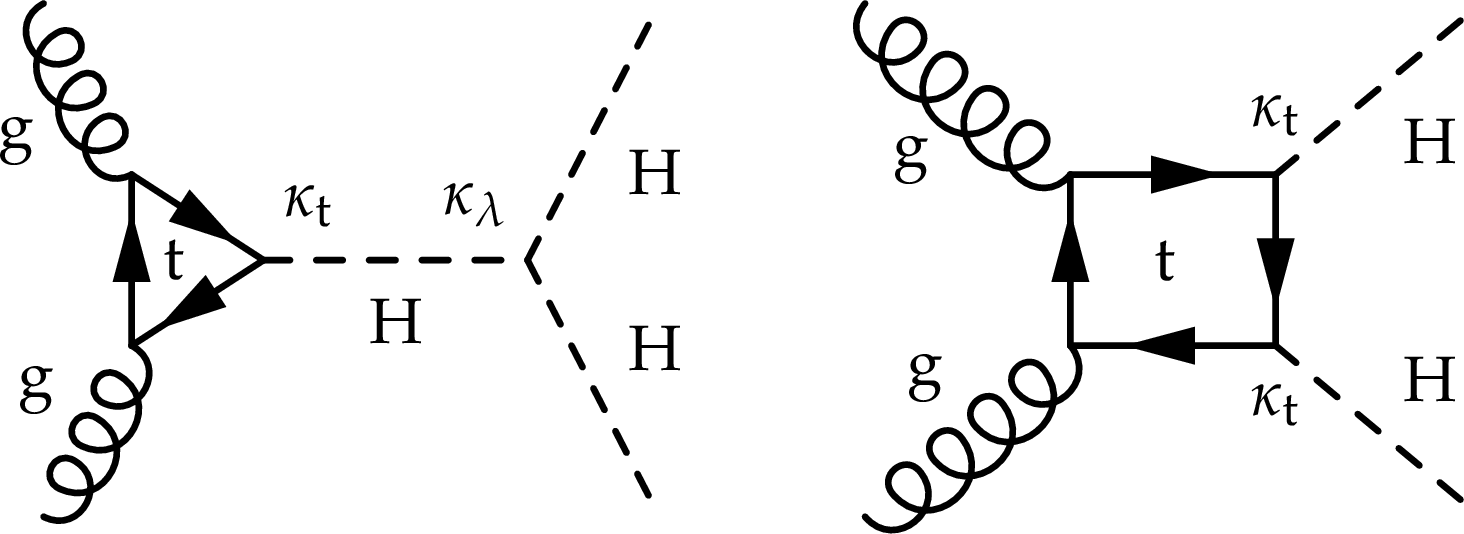
Figure 1:
Leading-order Feynman diagrams of nonresonant Higgs boson pair production via gluon-gluon fusion in the SM. The modifiers of the Higgs boson coupling with the top quark and the Higgs boson trilinear self-coupling are shown as $ \kappa_{\mathrm{t}} $ and $ \kappa_\lambda $, respectively. |

png pdf |
Figure 1-a:
Leading-order Feynman diagrams of nonresonant Higgs boson pair production via gluon-gluon fusion in the SM. The modifiers of the Higgs boson coupling with the top quark and the Higgs boson trilinear self-coupling are shown as $ \kappa_{\mathrm{t}} $ and $ \kappa_\lambda $, respectively. |

png pdf |
Figure 1-b:
Leading-order Feynman diagrams of nonresonant Higgs boson pair production via gluon-gluon fusion in the SM. The modifiers of the Higgs boson coupling with the top quark and the Higgs boson trilinear self-coupling are shown as $ \kappa_{\mathrm{t}} $ and $ \kappa_\lambda $, respectively. |

png pdf |
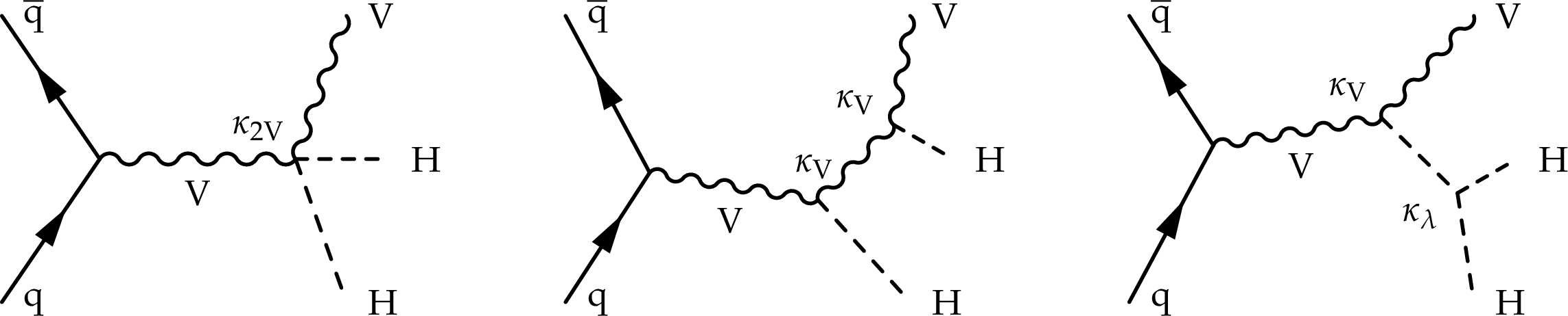
Figure 2:
Leading-order Feynman diagrams of nonresonant Higgs boson pair production via vector boson fusion in the SM. The modifiers of the Higgs boson coupling with a vector boson, the Higgs boson trilinear self-coupling, and the coupling between two Higgs bosons and two vector bosons are shown as $ \kappa_\mathrm{V} $, $ \kappa_\lambda $, and $ \kappa_{2\mathrm{V}} $, respectively. |

png pdf |
Figure 2-a:
Leading-order Feynman diagrams of nonresonant Higgs boson pair production via vector boson fusion in the SM. The modifiers of the Higgs boson coupling with a vector boson, the Higgs boson trilinear self-coupling, and the coupling between two Higgs bosons and two vector bosons are shown as $ \kappa_\mathrm{V} $, $ \kappa_\lambda $, and $ \kappa_{2\mathrm{V}} $, respectively. |

png pdf |
Figure 2-b:
Leading-order Feynman diagrams of nonresonant Higgs boson pair production via vector boson fusion in the SM. The modifiers of the Higgs boson coupling with a vector boson, the Higgs boson trilinear self-coupling, and the coupling between two Higgs bosons and two vector bosons are shown as $ \kappa_\mathrm{V} $, $ \kappa_\lambda $, and $ \kappa_{2\mathrm{V}} $, respectively. |

png pdf |
Figure 2-c:
Leading-order Feynman diagrams of nonresonant Higgs boson pair production via vector boson fusion in the SM. The modifiers of the Higgs boson coupling with a vector boson, the Higgs boson trilinear self-coupling, and the coupling between two Higgs bosons and two vector bosons are shown as $ \kappa_\mathrm{V} $, $ \kappa_\lambda $, and $ \kappa_{2\mathrm{V}} $, respectively. |
png pdf |
Figure 3:
Leading-order Feynman diagrams of nonresonant Higgs boson pair production via associated production with a vector boson in the SM. The modifiers of the Higgs boson coupling with a vector boson, the Higgs boson trilinear self-coupling, and the coupling between two Higgs bosons and two vector bosons are shown as $ \kappa_\mathrm{V} $, $ \kappa_\lambda $, and $ \kappa_{2\mathrm{V}} $, respectively. |

png pdf |
Figure 3-a:
Leading-order Feynman diagrams of nonresonant Higgs boson pair production via associated production with a vector boson in the SM. The modifiers of the Higgs boson coupling with a vector boson, the Higgs boson trilinear self-coupling, and the coupling between two Higgs bosons and two vector bosons are shown as $ \kappa_\mathrm{V} $, $ \kappa_\lambda $, and $ \kappa_{2\mathrm{V}} $, respectively. |

png pdf |
Figure 3-b:
Leading-order Feynman diagrams of nonresonant Higgs boson pair production via associated production with a vector boson in the SM. The modifiers of the Higgs boson coupling with a vector boson, the Higgs boson trilinear self-coupling, and the coupling between two Higgs bosons and two vector bosons are shown as $ \kappa_\mathrm{V} $, $ \kappa_\lambda $, and $ \kappa_{2\mathrm{V}} $, respectively. |

png pdf |
Figure 3-c:
Leading-order Feynman diagrams of nonresonant Higgs boson pair production via associated production with a vector boson in the SM. The modifiers of the Higgs boson coupling with a vector boson, the Higgs boson trilinear self-coupling, and the coupling between two Higgs bosons and two vector bosons are shown as $ \kappa_\mathrm{V} $, $ \kappa_\lambda $, and $ \kappa_{2\mathrm{V}} $, respectively. |

png pdf |
Figure 4:
Leading-order Feynman diagrams of nonresonant Higgs boson pair production via gluon-gluon fusion with anomalous Higgs boson couplings $ \text{c}_2 $, $ \text{c}_\mathrm{g} $, and $ \text{c}_{2\mathrm{g}} $. The Higgs boson trilinear self-coupling modifier is shown as $ \kappa_\lambda $. |

png pdf |
Figure 4-a:
Leading-order Feynman diagrams of nonresonant Higgs boson pair production via gluon-gluon fusion with anomalous Higgs boson couplings $ \text{c}_2 $, $ \text{c}_\mathrm{g} $, and $ \text{c}_{2\mathrm{g}} $. The Higgs boson trilinear self-coupling modifier is shown as $ \kappa_\lambda $. |

png pdf |
Figure 4-b:
Leading-order Feynman diagrams of nonresonant Higgs boson pair production via gluon-gluon fusion with anomalous Higgs boson couplings $ \text{c}_2 $, $ \text{c}_\mathrm{g} $, and $ \text{c}_{2\mathrm{g}} $. The Higgs boson trilinear self-coupling modifier is shown as $ \kappa_\lambda $. |

png pdf |
Figure 4-c:
Leading-order Feynman diagrams of nonresonant Higgs boson pair production via gluon-gluon fusion with anomalous Higgs boson couplings $ \text{c}_2 $, $ \text{c}_\mathrm{g} $, and $ \text{c}_{2\mathrm{g}} $. The Higgs boson trilinear self-coupling modifier is shown as $ \kappa_\lambda $. |

png pdf |
Figure 5:
Illustrations of the resolved (upper left) and boosted (upper right) topologies of the $ \mathrm{b}\overline{\mathrm{b}}\mathrm{b}\overline{\mathrm{b}} $ decay channel. The topology of VHH production when all Higgs bosons decay to b jets and the vector boson is either a Z boson that decays into two leptons (lower left) or a W boson decaying into a lepton and a neutrino, giving missing transverse momentum (lower right). |

png pdf |
Figure 5-a:
Illustrations of the resolved (upper left) and boosted (upper right) topologies of the $ \mathrm{b}\overline{\mathrm{b}}\mathrm{b}\overline{\mathrm{b}} $ decay channel. The topology of VHH production when all Higgs bosons decay to b jets and the vector boson is either a Z boson that decays into two leptons (lower left) or a W boson decaying into a lepton and a neutrino, giving missing transverse momentum (lower right). |

png pdf |
Figure 5-b:
Illustrations of the resolved (upper left) and boosted (upper right) topologies of the $ \mathrm{b}\overline{\mathrm{b}}\mathrm{b}\overline{\mathrm{b}} $ decay channel. The topology of VHH production when all Higgs bosons decay to b jets and the vector boson is either a Z boson that decays into two leptons (lower left) or a W boson decaying into a lepton and a neutrino, giving missing transverse momentum (lower right). |

png pdf |
Figure 5-c:
Illustrations of the resolved (upper left) and boosted (upper right) topologies of the $ \mathrm{b}\overline{\mathrm{b}}\mathrm{b}\overline{\mathrm{b}} $ decay channel. The topology of VHH production when all Higgs bosons decay to b jets and the vector boson is either a Z boson that decays into two leptons (lower left) or a W boson decaying into a lepton and a neutrino, giving missing transverse momentum (lower right). |

png pdf |
Figure 5-d:
Illustrations of the resolved (upper left) and boosted (upper right) topologies of the $ \mathrm{b}\overline{\mathrm{b}}\mathrm{b}\overline{\mathrm{b}} $ decay channel. The topology of VHH production when all Higgs bosons decay to b jets and the vector boson is either a Z boson that decays into two leptons (lower left) or a W boson decaying into a lepton and a neutrino, giving missing transverse momentum (lower right). |

png pdf |
Figure 6:
Illustrations of the resolved topology of the $ \mathrm{b}\overline{\mathrm{b}}\mathrm{W}\mathrm{W} $ decay channel in the final state with two leptons (upper left) and one lepton (upper right). The boosted topology of the fully hadronic $ \mathrm{b}\overline{\mathrm{b}}\mathrm{W}\mathrm{W} $ decay channel (lower). |

png pdf |
Figure 6-a:
Illustrations of the resolved topology of the $ \mathrm{b}\overline{\mathrm{b}}\mathrm{W}\mathrm{W} $ decay channel in the final state with two leptons (upper left) and one lepton (upper right). The boosted topology of the fully hadronic $ \mathrm{b}\overline{\mathrm{b}}\mathrm{W}\mathrm{W} $ decay channel (lower). |

png pdf |
Figure 6-b:
Illustrations of the resolved topology of the $ \mathrm{b}\overline{\mathrm{b}}\mathrm{W}\mathrm{W} $ decay channel in the final state with two leptons (upper left) and one lepton (upper right). The boosted topology of the fully hadronic $ \mathrm{b}\overline{\mathrm{b}}\mathrm{W}\mathrm{W} $ decay channel (lower). |

png pdf |
Figure 6-c:
Illustrations of the resolved topology of the $ \mathrm{b}\overline{\mathrm{b}}\mathrm{W}\mathrm{W} $ decay channel in the final state with two leptons (upper left) and one lepton (upper right). The boosted topology of the fully hadronic $ \mathrm{b}\overline{\mathrm{b}}\mathrm{W}\mathrm{W} $ decay channel (lower). |

png pdf |
Figure 7:
Distributions of the $ m_\text{reg}^{\mathrm{b}\overline{\mathrm{b}}} $ observable in the ggF (left) and VBF (right) signal regions of the all-hadronic $ \mathrm{b}\overline{\mathrm{b}}\mathrm{W}\mathrm{W} $ search, after a maximum likelihood fit of the background and SM HH signal to the data. |

png pdf |
Figure 7-a:
Distributions of the $ m_\text{reg}^{\mathrm{b}\overline{\mathrm{b}}} $ observable in the ggF (left) and VBF (right) signal regions of the all-hadronic $ \mathrm{b}\overline{\mathrm{b}}\mathrm{W}\mathrm{W} $ search, after a maximum likelihood fit of the background and SM HH signal to the data. |

png pdf |
Figure 7-b:
Distributions of the $ m_\text{reg}^{\mathrm{b}\overline{\mathrm{b}}} $ observable in the ggF (left) and VBF (right) signal regions of the all-hadronic $ \mathrm{b}\overline{\mathrm{b}}\mathrm{W}\mathrm{W} $ search, after a maximum likelihood fit of the background and SM HH signal to the data. |
png pdf |
Figure 8:
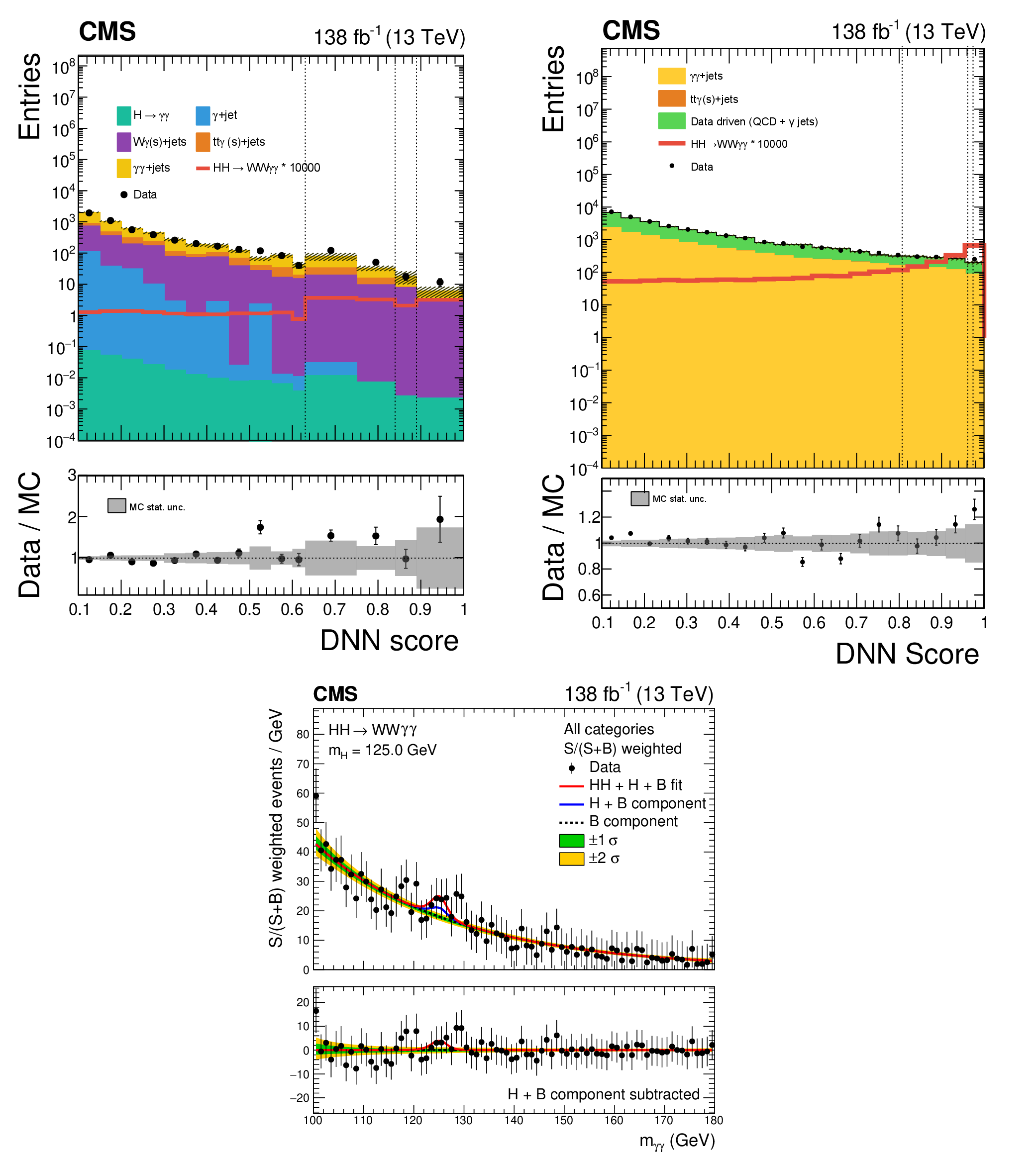
The distributions of DNN scores for the signal and main backgrounds in the 1\ell (upper left) and fully hadronic (upper right) channels of the $ \mathrm{W}\mathrm{W}\gamma\gamma $ analysis. The signal-plus-background (red), single H plus continuum background (blue), and continuum background (dashed black) fits for all channels weighted by $ S/(S+B) $ (lower). |

png pdf |
Figure 8-a:
The distributions of DNN scores for the signal and main backgrounds in the 1\ell (upper left) and fully hadronic (upper right) channels of the $ \mathrm{W}\mathrm{W}\gamma\gamma $ analysis. The signal-plus-background (red), single H plus continuum background (blue), and continuum background (dashed black) fits for all channels weighted by $ S/(S+B) $ (lower). |

png pdf |
Figure 8-b:
The distributions of DNN scores for the signal and main backgrounds in the 1\ell (upper left) and fully hadronic (upper right) channels of the $ \mathrm{W}\mathrm{W}\gamma\gamma $ analysis. The signal-plus-background (red), single H plus continuum background (blue), and continuum background (dashed black) fits for all channels weighted by $ S/(S+B) $ (lower). |

png pdf |
Figure 8-c:
The distributions of DNN scores for the signal and main backgrounds in the 1\ell (upper left) and fully hadronic (upper right) channels of the $ \mathrm{W}\mathrm{W}\gamma\gamma $ analysis. The signal-plus-background (red), single H plus continuum background (blue), and continuum background (dashed black) fits for all channels weighted by $ S/(S+B) $ (lower). |

png pdf |
Figure 9:
The upper limits at 95% CL on the inclusive signal strength $ \mu = \sigma_{\mathrm{H}\mathrm{H}} /\sigma_{\mathrm{H}\mathrm{H}} ^\text{SM} $ for each channel and their combination. The inner (green) and outer (yellow) bands indicate the 68 and 95% CL intervals, respectively, under the background-only hypothesis. The individual contributions within the $ \mathrm{b}\overline{\mathrm{b}}\mathrm{b}\overline{\mathrm{b}} $ and $ \mathrm{b}\overline{\mathrm{b}}\mathrm{W}\mathrm{W} $ channels have been combined in order to simplify the presentation of results. |

png pdf |
Figure 10:
The upper limits at 95% CL on the VBF signal strength $ \mu_{\text{VBF} {\mathrm{H}\mathrm{H}}} = \sigma_{\text{VBF} \mathrm{H}\mathrm{H}} /\sigma_{\text{VBF} \mathrm{H}\mathrm{H}} ^\text{SM} $ for each channel and their combination. The inner (green) and outer (yellow) bands indicate the 68 and 95% CL intervals, respectively, under the background-only hypothesis. The five contributing channels are indicated in the figure. The individual contributions within the $ \mathrm{b}\overline{\mathrm{b}}\mathrm{b}\overline{\mathrm{b}} $ and $ \mathrm{b}\overline{\mathrm{b}}\mathrm{W}\mathrm{W} $ channels have been combined in order to simplify the presentation of results. |
png pdf |
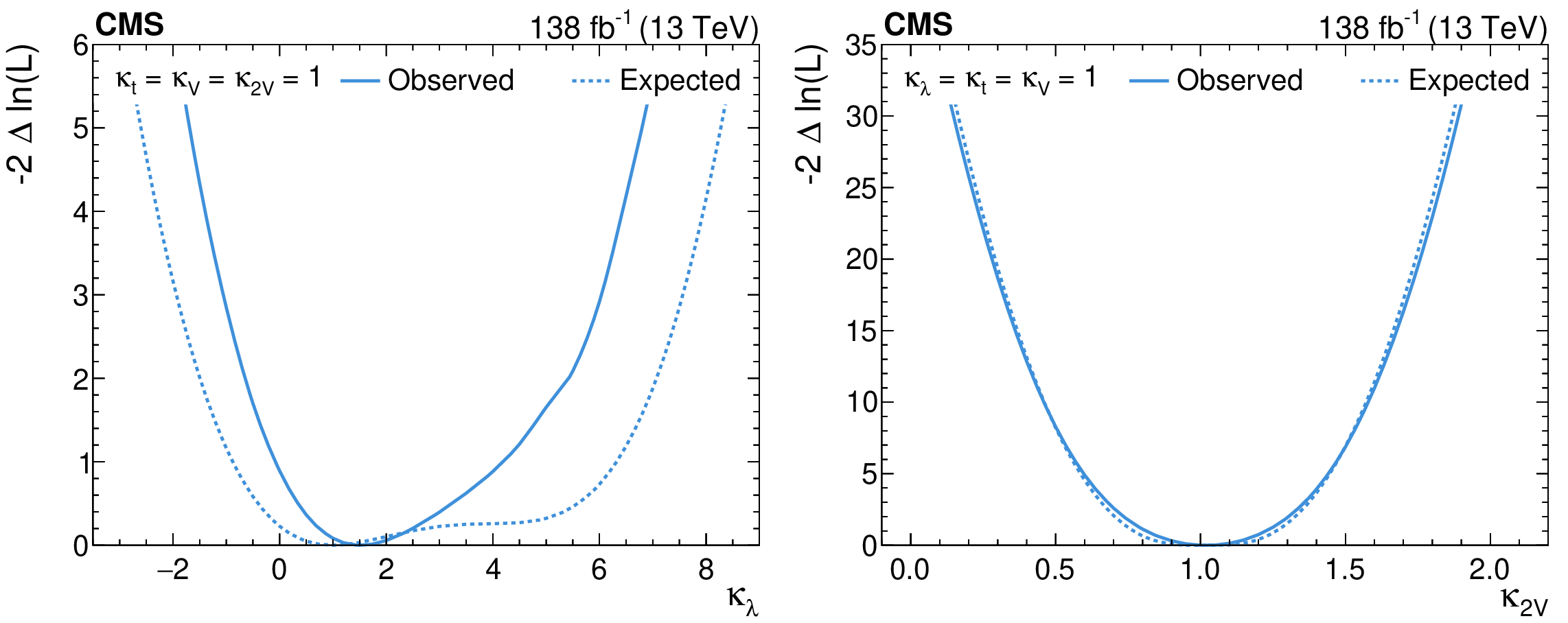
Figure 11:
The $ -2\Delta\ln(L) $ scan as functions of coupling modifiers $ \kappa_\lambda $ (left) and $ \kappa_{2\mathrm{V}} $ (right) for the combination of all channels when all the other parameters are fixed to their SM values. |

png pdf |
Figure 11-a:
The $ -2\Delta\ln(L) $ scan as functions of coupling modifiers $ \kappa_\lambda $ (left) and $ \kappa_{2\mathrm{V}} $ (right) for the combination of all channels when all the other parameters are fixed to their SM values. |

png pdf |
Figure 11-b:
The $ -2\Delta\ln(L) $ scan as functions of coupling modifiers $ \kappa_\lambda $ (left) and $ \kappa_{2\mathrm{V}} $ (right) for the combination of all channels when all the other parameters are fixed to their SM values. |
png pdf |
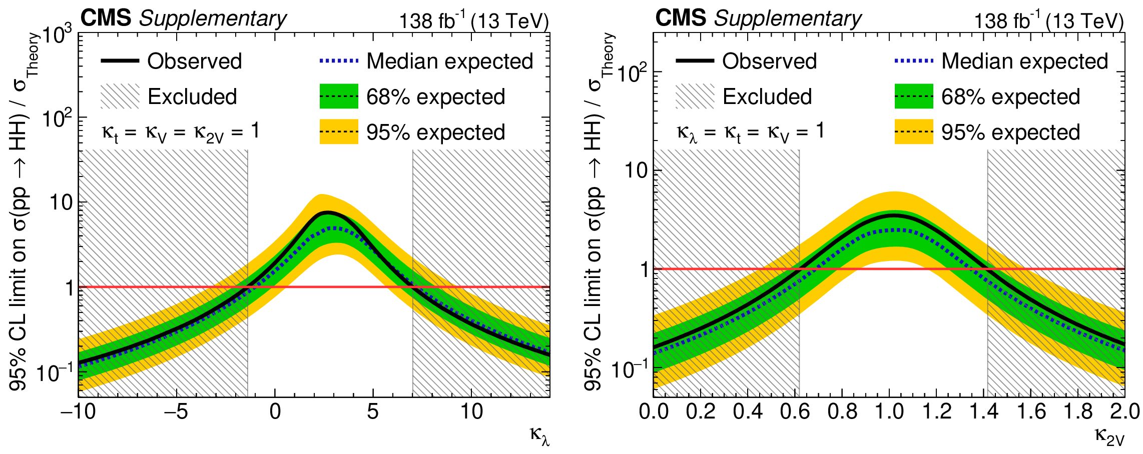
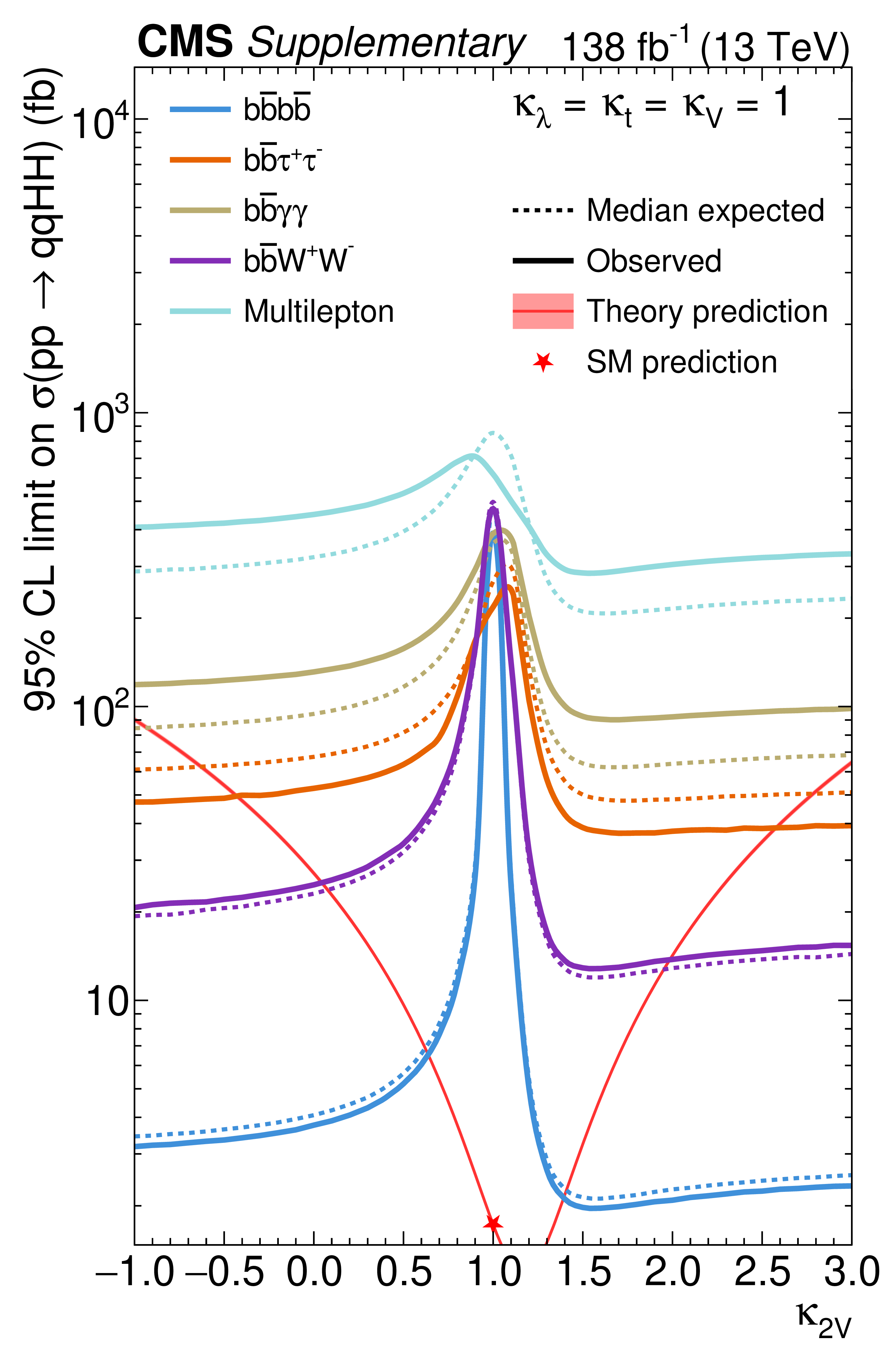
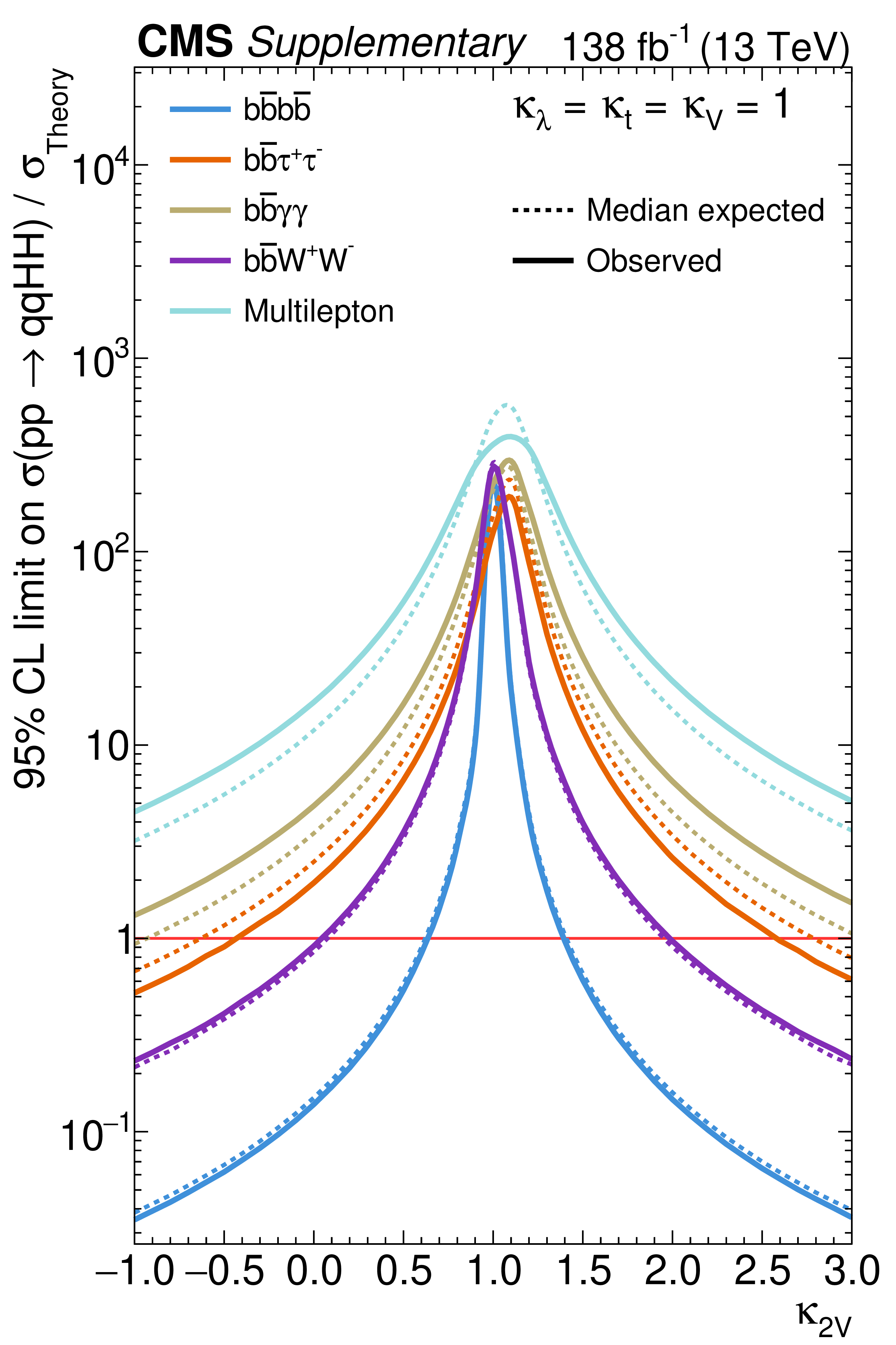
Figure 12:
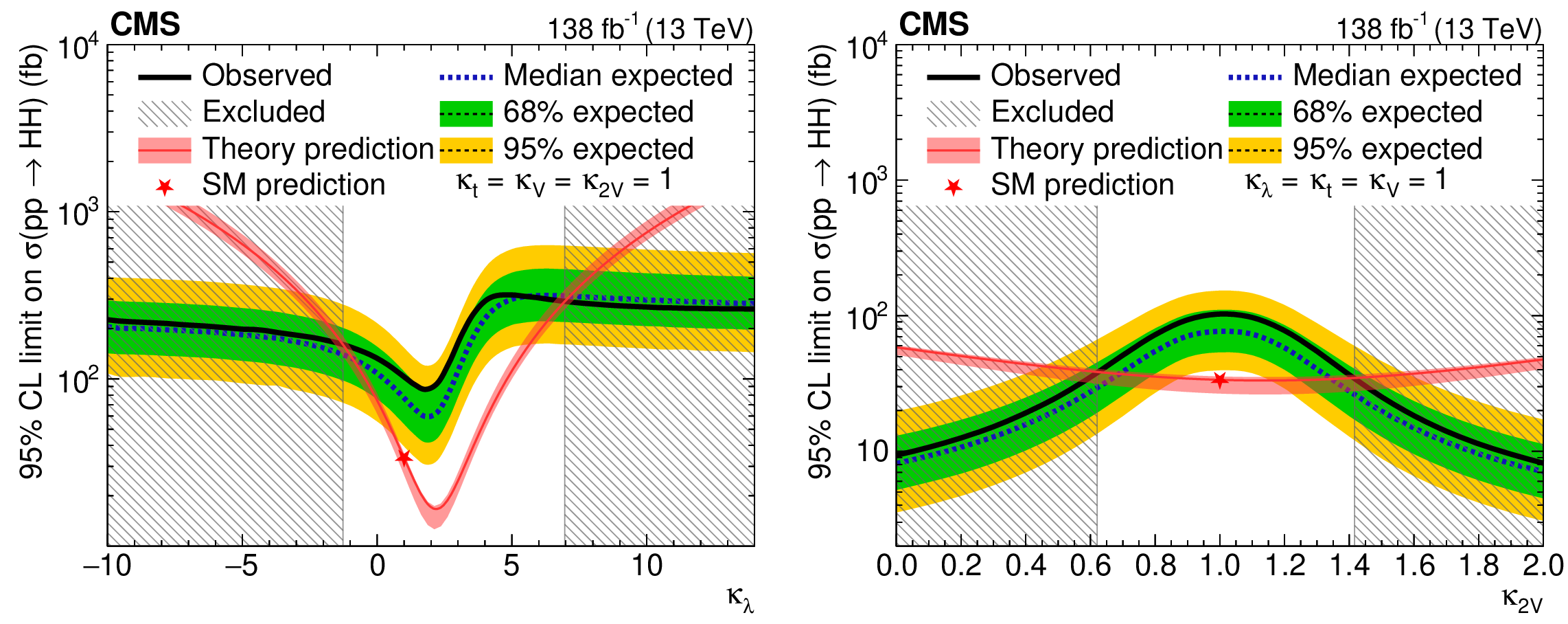
The 95% CL upper limits on the inclusive HH cross section as functions of $ \kappa_\lambda $ (left) and $ \kappa_{2\mathrm{V}} $ (right). All other couplings are set to the values predicted by the SM. The theoretical uncertainties in the ggF and VBFHH signal cross sections are not considered because here we directly constrain the measured cross section. The inner (green) band and the outer (yellow) band indicate the 68 and 95% CL intervals, respectively, under the background-only hypothesis. The star shows the limit at the SM value for $ \kappa_\lambda $ and $ \kappa_{2\mathrm{V}} $. |

png pdf |
Figure 12-a:
The 95% CL upper limits on the inclusive HH cross section as functions of $ \kappa_\lambda $ (left) and $ \kappa_{2\mathrm{V}} $ (right). All other couplings are set to the values predicted by the SM. The theoretical uncertainties in the ggF and VBFHH signal cross sections are not considered because here we directly constrain the measured cross section. The inner (green) band and the outer (yellow) band indicate the 68 and 95% CL intervals, respectively, under the background-only hypothesis. The star shows the limit at the SM value for $ \kappa_\lambda $ and $ \kappa_{2\mathrm{V}} $. |

png pdf |
Figure 12-b:
The 95% CL upper limits on the inclusive HH cross section as functions of $ \kappa_\lambda $ (left) and $ \kappa_{2\mathrm{V}} $ (right). All other couplings are set to the values predicted by the SM. The theoretical uncertainties in the ggF and VBFHH signal cross sections are not considered because here we directly constrain the measured cross section. The inner (green) band and the outer (yellow) band indicate the 68 and 95% CL intervals, respectively, under the background-only hypothesis. The star shows the limit at the SM value for $ \kappa_\lambda $ and $ \kappa_{2\mathrm{V}} $. |

png pdf |
Figure 13:
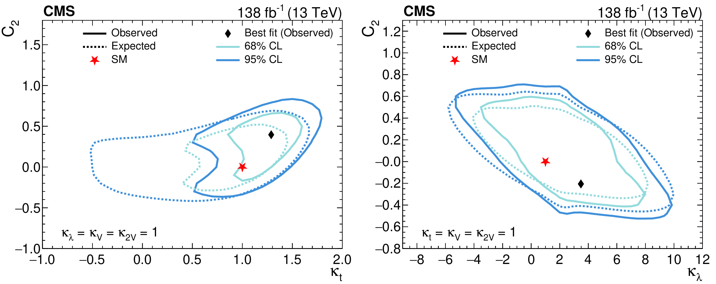
The 68 and 95% CL contours of $ -2\Delta\ln(L) $ in the ($ \kappa_\lambda $, $ \kappa_{2\mathrm{V}} $) (upper left), ($ \kappa_\mathrm{V} $, $ \kappa_{2\mathrm{V}} $) (upper right), and ($ \kappa_\lambda $, $ \kappa_{\mathrm{t}} $) (lower) planes for the combination of all channels when all the other parameters are fixed to their SM values. In the ($ \kappa_\lambda $, $ \kappa_{2\mathrm{V}} $) and ($ \kappa_\mathrm{V} $, $ \kappa_{2\mathrm{V}} $) planes, the 5 standard deviation CL contours are also shown. |

png pdf |
Figure 13-a:
The 68 and 95% CL contours of $ -2\Delta\ln(L) $ in the ($ \kappa_\lambda $, $ \kappa_{2\mathrm{V}} $) (upper left), ($ \kappa_\mathrm{V} $, $ \kappa_{2\mathrm{V}} $) (upper right), and ($ \kappa_\lambda $, $ \kappa_{\mathrm{t}} $) (lower) planes for the combination of all channels when all the other parameters are fixed to their SM values. In the ($ \kappa_\lambda $, $ \kappa_{2\mathrm{V}} $) and ($ \kappa_\mathrm{V} $, $ \kappa_{2\mathrm{V}} $) planes, the 5 standard deviation CL contours are also shown. |

png pdf |
Figure 13-b:
The 68 and 95% CL contours of $ -2\Delta\ln(L) $ in the ($ \kappa_\lambda $, $ \kappa_{2\mathrm{V}} $) (upper left), ($ \kappa_\mathrm{V} $, $ \kappa_{2\mathrm{V}} $) (upper right), and ($ \kappa_\lambda $, $ \kappa_{\mathrm{t}} $) (lower) planes for the combination of all channels when all the other parameters are fixed to their SM values. In the ($ \kappa_\lambda $, $ \kappa_{2\mathrm{V}} $) and ($ \kappa_\mathrm{V} $, $ \kappa_{2\mathrm{V}} $) planes, the 5 standard deviation CL contours are also shown. |

png pdf |
Figure 13-c:
The 68 and 95% CL contours of $ -2\Delta\ln(L) $ in the ($ \kappa_\lambda $, $ \kappa_{2\mathrm{V}} $) (upper left), ($ \kappa_\mathrm{V} $, $ \kappa_{2\mathrm{V}} $) (upper right), and ($ \kappa_\lambda $, $ \kappa_{\mathrm{t}} $) (lower) planes for the combination of all channels when all the other parameters are fixed to their SM values. In the ($ \kappa_\lambda $, $ \kappa_{2\mathrm{V}} $) and ($ \kappa_\mathrm{V} $, $ \kappa_{2\mathrm{V}} $) planes, the 5 standard deviation CL contours are also shown. |

png pdf |
Figure 14:
The upper limits at 95% CL on the HH production cross section for the two sets of HEFT benchmarks. The theoretical uncertainties in the ggFHH signal cross section are not considered because we directly constrain the measured cross section. |

png pdf |
Figure 15:
The upper limits at 95% CL on the HH cross section as a function of the $ \text{c}_2 $ coupling modifier (left). The theoretical uncertainties in the ggFHH signal cross section are not considered because we directly constrain the measured cross section. The $ -2\Delta\ln(L) $ scan as a function of the $ \text{c}_2 $ coupling modifier (right). |

png pdf |
Figure 15-a:
The upper limits at 95% CL on the HH cross section as a function of the $ \text{c}_2 $ coupling modifier (left). The theoretical uncertainties in the ggFHH signal cross section are not considered because we directly constrain the measured cross section. The $ -2\Delta\ln(L) $ scan as a function of the $ \text{c}_2 $ coupling modifier (right). |

png pdf |
Figure 15-b:
The upper limits at 95% CL on the HH cross section as a function of the $ \text{c}_2 $ coupling modifier (left). The theoretical uncertainties in the ggFHH signal cross section are not considered because we directly constrain the measured cross section. The $ -2\Delta\ln(L) $ scan as a function of the $ \text{c}_2 $ coupling modifier (right). |
png pdf |
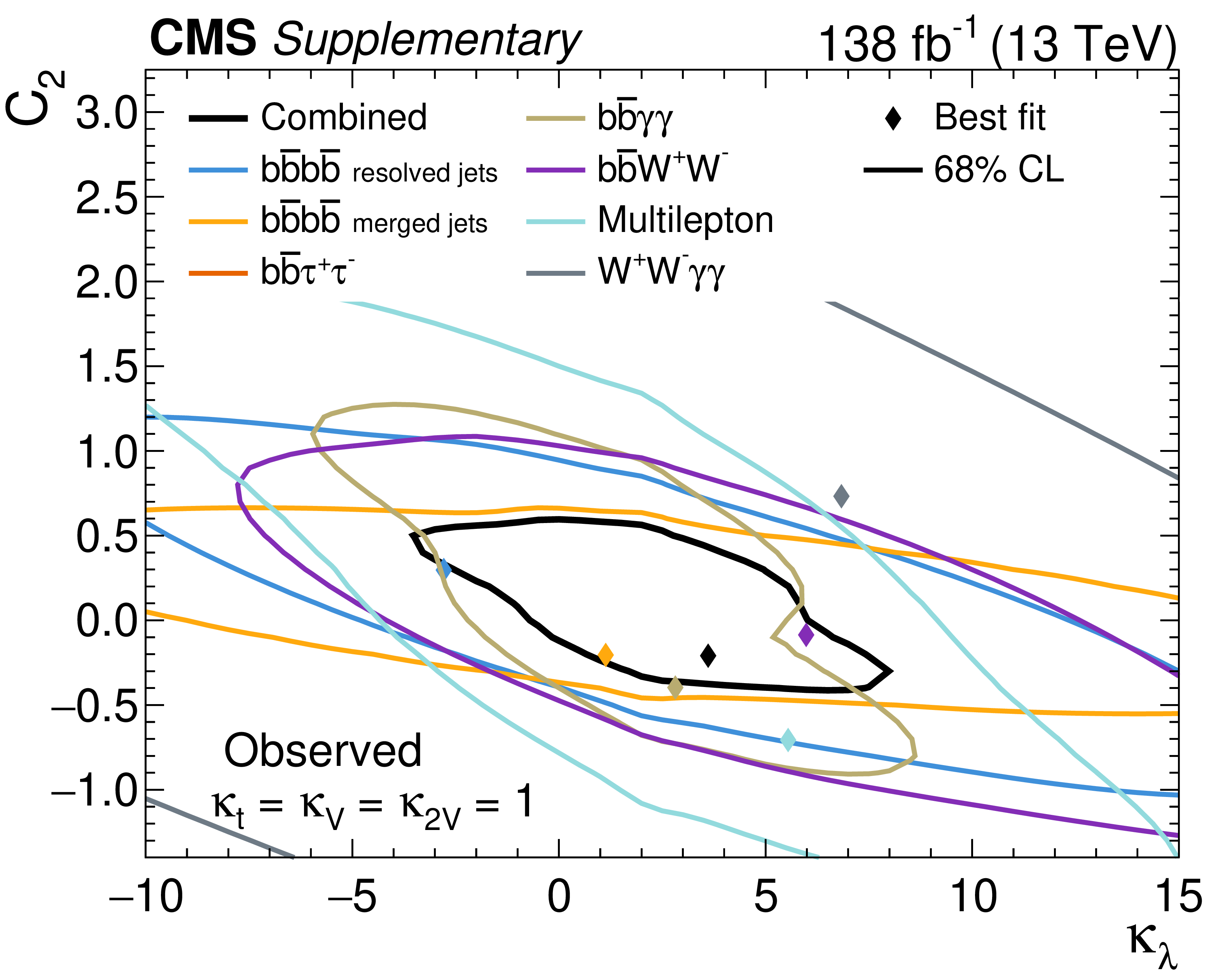
Figure 16:
The 68 and 95% CL contours of $ -2\Delta\ln(L) $ in the (c}_2, \kappa_{\mathrm{t}) (left) and $ (\text{c}_2, \kappa_\lambda) $ (right) planes for the combination of all channels when all the other parameters are fixed to their SM values. |

png pdf |
Figure 16-a:
The 68 and 95% CL contours of $ -2\Delta\ln(L) $ in the (c}_2, \kappa_{\mathrm{t}) (left) and $ (\text{c}_2, \kappa_\lambda) $ (right) planes for the combination of all channels when all the other parameters are fixed to their SM values. |

png pdf |
Figure 16-b:
The 68 and 95% CL contours of $ -2\Delta\ln(L) $ in the (c}_2, \kappa_{\mathrm{t}) (left) and $ (\text{c}_2, \kappa_\lambda) $ (right) planes for the combination of all channels when all the other parameters are fixed to their SM values. |
png pdf |
Figure 17:
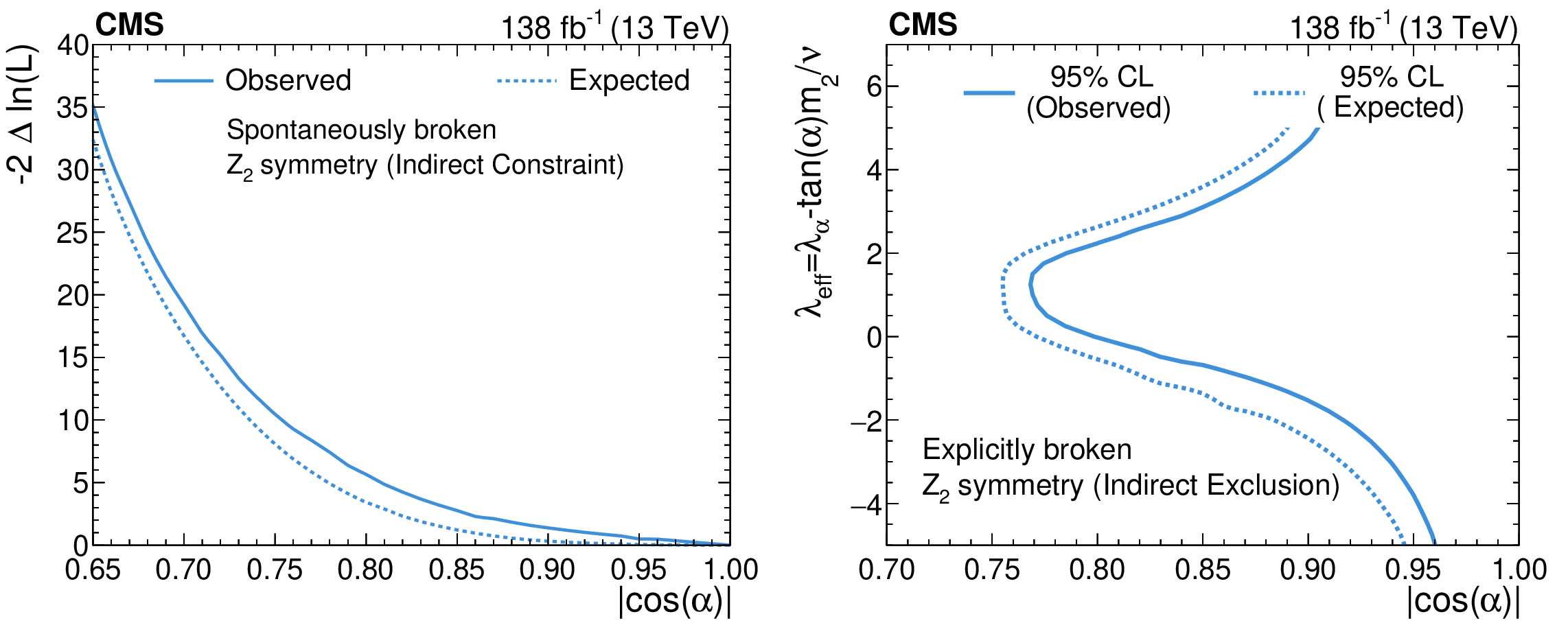
The $ -2\Delta\ln(L) $ scan for the combination of all channels as a function of $ |\cos{\alpha}| $ for singlet extensions of the SM with spontaneous $ Z_2 $ symmetry breaking (left). The $ |\cos{\alpha}| $ is constrained at 95% CL between 0.79 and 1. The 95% CL contour of $ -2\Delta\ln(L) $ in the ($ |\cos{\alpha}| $, $ \lambda_\text{eff} $) plane (right), where $ \lambda_\text{eff}=\lambda_\alpha-\tan{(\alpha)\frac{m_{2}}{\nu}} $ The ranges of $ |\cos{\alpha}| $ and $ \lambda_\text{eff} $ are chosen to guarantee the validity of the models. The excluded regions are below and to the left of the curves shown. |

png pdf |
Figure 17-a:
The $ -2\Delta\ln(L) $ scan for the combination of all channels as a function of $ |\cos{\alpha}| $ for singlet extensions of the SM with spontaneous $ Z_2 $ symmetry breaking (left). The $ |\cos{\alpha}| $ is constrained at 95% CL between 0.79 and 1. The 95% CL contour of $ -2\Delta\ln(L) $ in the ($ |\cos{\alpha}| $, $ \lambda_\text{eff} $) plane (right), where $ \lambda_\text{eff}=\lambda_\alpha-\tan{(\alpha)\frac{m_{2}}{\nu}} $ The ranges of $ |\cos{\alpha}| $ and $ \lambda_\text{eff} $ are chosen to guarantee the validity of the models. The excluded regions are below and to the left of the curves shown. |

png pdf |
Figure 17-b:
The $ -2\Delta\ln(L) $ scan for the combination of all channels as a function of $ |\cos{\alpha}| $ for singlet extensions of the SM with spontaneous $ Z_2 $ symmetry breaking (left). The $ |\cos{\alpha}| $ is constrained at 95% CL between 0.79 and 1. The 95% CL contour of $ -2\Delta\ln(L) $ in the ($ |\cos{\alpha}| $, $ \lambda_\text{eff} $) plane (right), where $ \lambda_\text{eff}=\lambda_\alpha-\tan{(\alpha)\frac{m_{2}}{\nu}} $ The ranges of $ |\cos{\alpha}| $ and $ \lambda_\text{eff} $ are chosen to guarantee the validity of the models. The excluded regions are below and to the left of the curves shown. |
png pdf |
Figure 18:
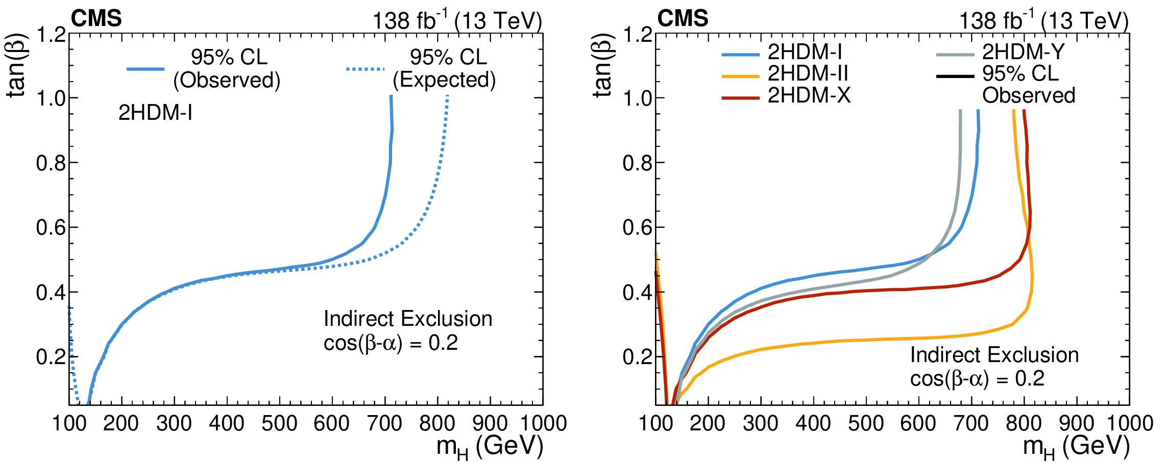
The 95% CL contour of $ -2\Delta\ln(L) $ for the combination of all channels in the ($ m_{\mathrm{H}} $, $ \tan\beta $) plane for a fixed value of $ |\cos(\beta-\alpha)|= $ 0.2 in the 2HDM-I model (left) and the four considered 2HDM models (right). In these and all other cases considered in this paper, $ m_{\mathrm{H}}=m_{\mathrm{A}} $. The ranges of $ m_{\mathrm{H}} $ and $ \tan\beta $ are chosen to guarantee the validity of the models. The excluded regions are below the curves shown. The value $ \tan\beta= $ 0.5 is excluded for $ m_{\mathrm{H}} > $ 800 GeV for all models considered. |

png pdf |
Figure 18-a:
The 95% CL contour of $ -2\Delta\ln(L) $ for the combination of all channels in the ($ m_{\mathrm{H}} $, $ \tan\beta $) plane for a fixed value of $ |\cos(\beta-\alpha)|= $ 0.2 in the 2HDM-I model (left) and the four considered 2HDM models (right). In these and all other cases considered in this paper, $ m_{\mathrm{H}}=m_{\mathrm{A}} $. The ranges of $ m_{\mathrm{H}} $ and $ \tan\beta $ are chosen to guarantee the validity of the models. The excluded regions are below the curves shown. The value $ \tan\beta= $ 0.5 is excluded for $ m_{\mathrm{H}} > $ 800 GeV for all models considered. |

png pdf |
Figure 18-b:
The 95% CL contour of $ -2\Delta\ln(L) $ for the combination of all channels in the ($ m_{\mathrm{H}} $, $ \tan\beta $) plane for a fixed value of $ |\cos(\beta-\alpha)|= $ 0.2 in the 2HDM-I model (left) and the four considered 2HDM models (right). In these and all other cases considered in this paper, $ m_{\mathrm{H}}=m_{\mathrm{A}} $. The ranges of $ m_{\mathrm{H}} $ and $ \tan\beta $ are chosen to guarantee the validity of the models. The excluded regions are below the curves shown. The value $ \tan\beta= $ 0.5 is excluded for $ m_{\mathrm{H}} > $ 800 GeV for all models considered. |

png pdf |
Figure 19:
The 95% CL contour of $ -2\Delta\ln(L) $ for the combination of all channels in the ($ \cos(\beta-\alpha) $, $ \tan\beta $) plane for a fixed value of $ m_{\mathrm{H}}= $ 1000 GeV in the 2HDM-I model (left) and the four considered 2HDM models (right). In these and all other cases considered in this paper, $ m_{\mathrm{H}}=m_{\mathrm{A}} $. The ranges of $ \cos(\beta-\alpha) $ and $ \tan\beta $ are chosen to guarantee the validity of the model. The excluded regions are below the curves shown. The value $ \tan\beta= $ 0.5 is excluded for $ \cos(\beta-\alpha) > $ 0.16 and $ \cos(\beta-\alpha) < - $ 0.13 for all models considered. |

png pdf |
Figure 19-a:
The 95% CL contour of $ -2\Delta\ln(L) $ for the combination of all channels in the ($ \cos(\beta-\alpha) $, $ \tan\beta $) plane for a fixed value of $ m_{\mathrm{H}}= $ 1000 GeV in the 2HDM-I model (left) and the four considered 2HDM models (right). In these and all other cases considered in this paper, $ m_{\mathrm{H}}=m_{\mathrm{A}} $. The ranges of $ \cos(\beta-\alpha) $ and $ \tan\beta $ are chosen to guarantee the validity of the model. The excluded regions are below the curves shown. The value $ \tan\beta= $ 0.5 is excluded for $ \cos(\beta-\alpha) > $ 0.16 and $ \cos(\beta-\alpha) < - $ 0.13 for all models considered. |

png pdf |
Figure 19-b:
The 95% CL contour of $ -2\Delta\ln(L) $ for the combination of all channels in the ($ \cos(\beta-\alpha) $, $ \tan\beta $) plane for a fixed value of $ m_{\mathrm{H}}= $ 1000 GeV in the 2HDM-I model (left) and the four considered 2HDM models (right). In these and all other cases considered in this paper, $ m_{\mathrm{H}}=m_{\mathrm{A}} $. The ranges of $ \cos(\beta-\alpha) $ and $ \tan\beta $ are chosen to guarantee the validity of the model. The excluded regions are below the curves shown. The value $ \tan\beta= $ 0.5 is excluded for $ \cos(\beta-\alpha) > $ 0.16 and $ \cos(\beta-\alpha) < - $ 0.13 for all models considered. |
png pdf |
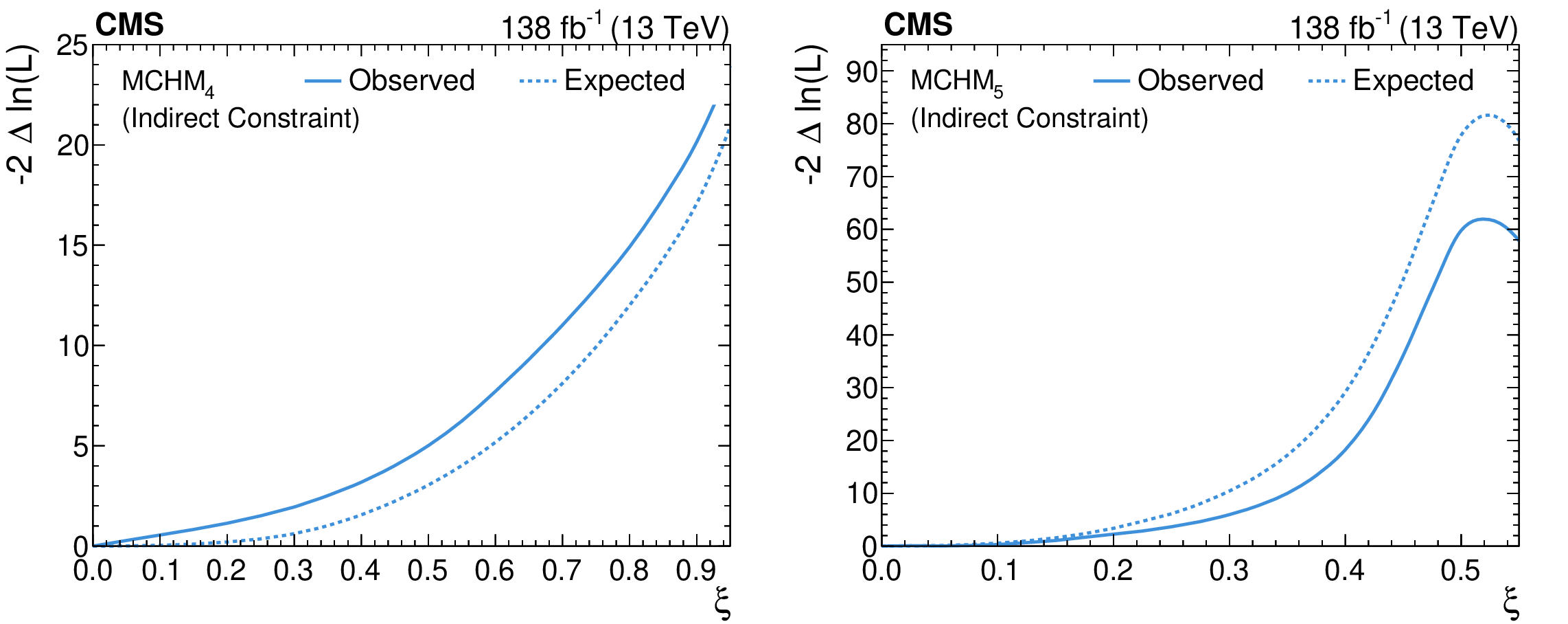
Figure 20:
The $ -2\Delta\ln(L) $ scan for the combination of all channels as a function of $ \xi $ for MCHM$ _4 $ (left) and MCHM$ _5 $ (right). The range of $ \xi $ is chosen to guarantee the validity of the model. At 95% CL, $ \xi $ is constrained to be between 0 and 0.45 in MCHM$ _4 $ and 0 and 0.26 in MCHM$ _5 $. |

png pdf |
Figure 20-a:
The $ -2\Delta\ln(L) $ scan for the combination of all channels as a function of $ \xi $ for MCHM$ _4 $ (left) and MCHM$ _5 $ (right). The range of $ \xi $ is chosen to guarantee the validity of the model. At 95% CL, $ \xi $ is constrained to be between 0 and 0.45 in MCHM$ _4 $ and 0 and 0.26 in MCHM$ _5 $. |

png pdf |
Figure 20-b:
The $ -2\Delta\ln(L) $ scan for the combination of all channels as a function of $ \xi $ for MCHM$ _4 $ (left) and MCHM$ _5 $ (right). The range of $ \xi $ is chosen to guarantee the validity of the model. At 95% CL, $ \xi $ is constrained to be between 0 and 0.45 in MCHM$ _4 $ and 0 and 0.26 in MCHM$ _5 $. |

png pdf |
Figure 21:
The expected upper limits at 95% CL on the HH signal strength from the combination of all the considered channels projected to different integrated luminosities (left), and under different assumptions on the systematic uncertainties for an integrated luminosity of 3000 fb$ ^{-1} $ (right). |

png pdf |
Figure 21-a:
The expected upper limits at 95% CL on the HH signal strength from the combination of all the considered channels projected to different integrated luminosities (left), and under different assumptions on the systematic uncertainties for an integrated luminosity of 3000 fb$ ^{-1} $ (right). |

png pdf |
Figure 21-b:
The expected upper limits at 95% CL on the HH signal strength from the combination of all the considered channels projected to different integrated luminosities (left), and under different assumptions on the systematic uncertainties for an integrated luminosity of 3000 fb$ ^{-1} $ (right). |

png pdf |
Figure 22:
The expected $ -2\Delta\ln(L) $ scan as a function of coupling modifier $ \kappa_\lambda $ for the combination of all contributing channels, projected to different integrated luminosities (left), and under different assumptions on the systematic uncertainties for an integrated luminosity of 3000 fb$ ^{-1} $ (right). All other parameters are fixed to their SM values. |

png pdf |
Figure 22-a:
The expected $ -2\Delta\ln(L) $ scan as a function of coupling modifier $ \kappa_\lambda $ for the combination of all contributing channels, projected to different integrated luminosities (left), and under different assumptions on the systematic uncertainties for an integrated luminosity of 3000 fb$ ^{-1} $ (right). All other parameters are fixed to their SM values. |

png pdf |
Figure 22-b:
The expected $ -2\Delta\ln(L) $ scan as a function of coupling modifier $ \kappa_\lambda $ for the combination of all contributing channels, projected to different integrated luminosities (left), and under different assumptions on the systematic uncertainties for an integrated luminosity of 3000 fb$ ^{-1} $ (right). All other parameters are fixed to their SM values. |
png pdf |
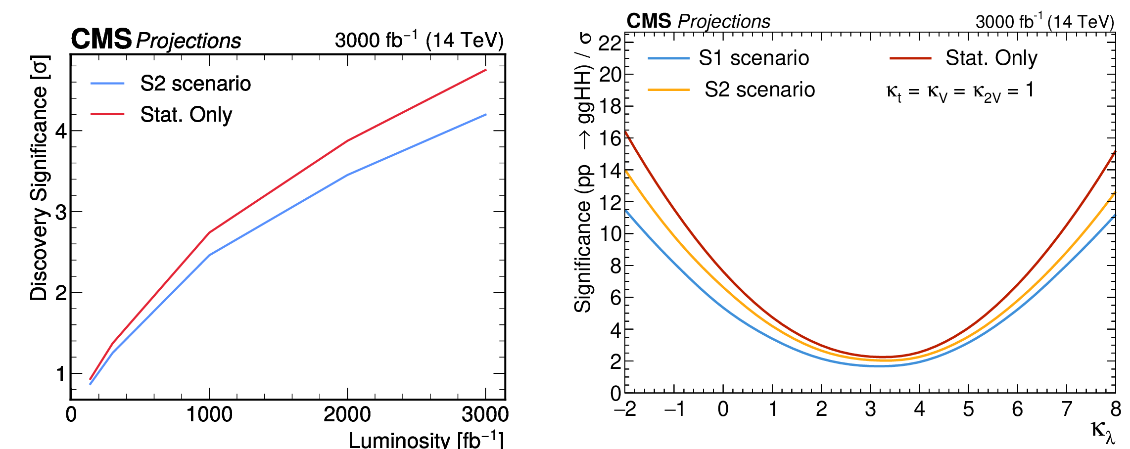
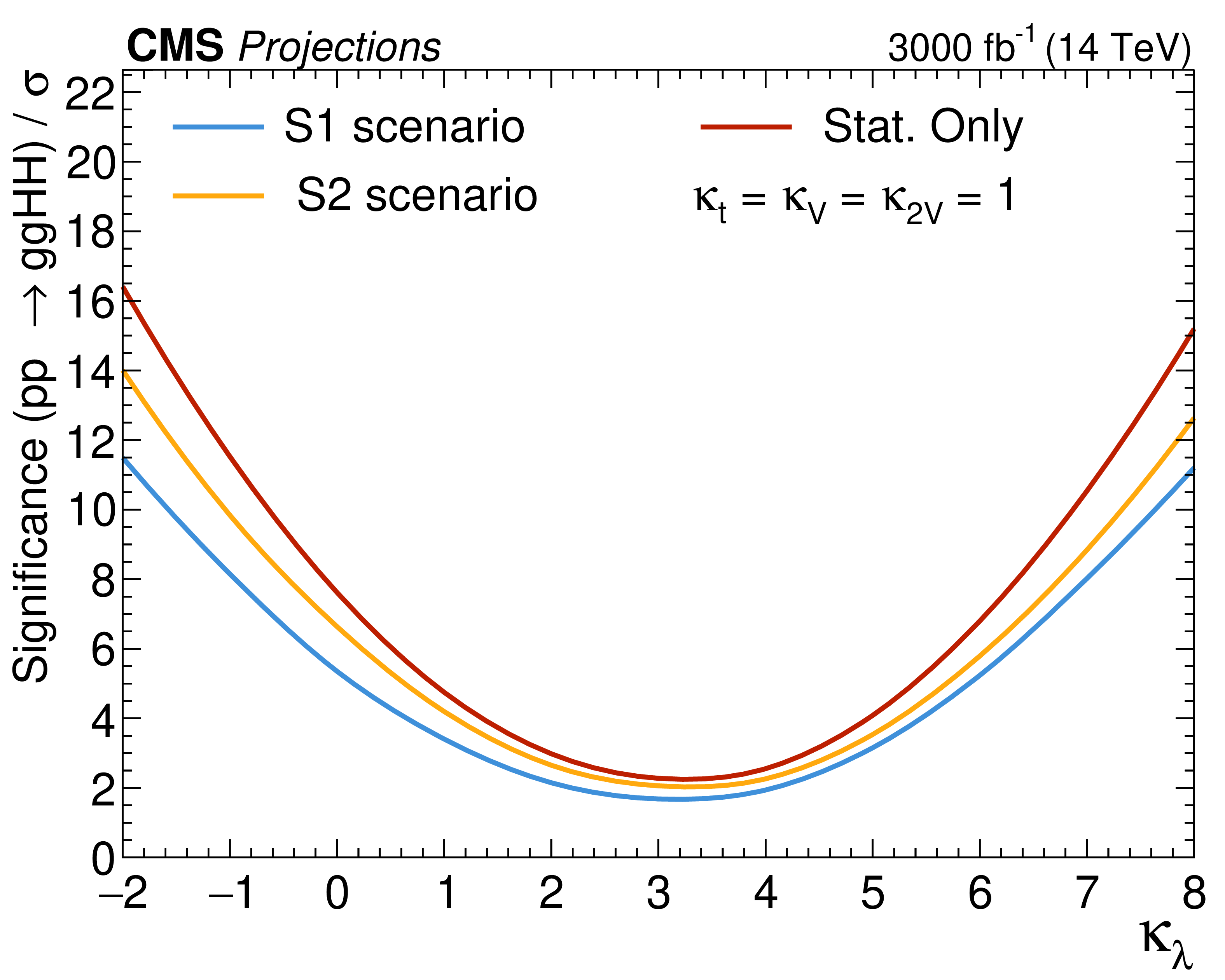
Figure 23:
The expected signal significance as a function of integrated luminosity for the nominal systematic uncertainty scenario S2 and for the scenario with statistical uncertainties only (left). The expected signal significance as a function of $ \kappa_\lambda $ under different assumptions on the systematic uncertainties for an integrated luminosity of 3000 fb$ ^{-1} $ (right). |

png pdf |
Figure 23-a:
The expected signal significance as a function of integrated luminosity for the nominal systematic uncertainty scenario S2 and for the scenario with statistical uncertainties only (left). The expected signal significance as a function of $ \kappa_\lambda $ under different assumptions on the systematic uncertainties for an integrated luminosity of 3000 fb$ ^{-1} $ (right). |
png pdf |
Figure 23-b:
The expected signal significance as a function of integrated luminosity for the nominal systematic uncertainty scenario S2 and for the scenario with statistical uncertainties only (left). The expected signal significance as a function of $ \kappa_\lambda $ under different assumptions on the systematic uncertainties for an integrated luminosity of 3000 fb$ ^{-1} $ (right). |
png pdf |
Figure A1:
The 95% CL upper limits on the inclusive HH signal strength as functions of $ \kappa_\lambda $ (left) and $ \kappa_{2\mathrm{V}} $ (right). All other couplings are set to the values predicted by the SM. The theoretical uncertainties in the HH ggF and VBF signal cross sections are considered in this case. The inner (green) band and the outer (yellow) band indicate the 68 and 95% CL intervals, respectively, under the background-only hypothesis. |

png pdf |
Figure A1-a:
The 95% CL upper limits on the inclusive HH signal strength as functions of $ \kappa_\lambda $ (left) and $ \kappa_{2\mathrm{V}} $ (right). All other couplings are set to the values predicted by the SM. The theoretical uncertainties in the HH ggF and VBF signal cross sections are considered in this case. The inner (green) band and the outer (yellow) band indicate the 68 and 95% CL intervals, respectively, under the background-only hypothesis. |

png pdf |
Figure A1-b:
The 95% CL upper limits on the inclusive HH signal strength as functions of $ \kappa_\lambda $ (left) and $ \kappa_{2\mathrm{V}} $ (right). All other couplings are set to the values predicted by the SM. The theoretical uncertainties in the HH ggF and VBF signal cross sections are considered in this case. The inner (green) band and the outer (yellow) band indicate the 68 and 95% CL intervals, respectively, under the background-only hypothesis. |

png pdf |
Figure A2:
The $ -2\Delta\ln(L) $ scan as functions of $ \kappa_\lambda $ (left) and $ \kappa_{2\mathrm{V}} $ (right) for all channels, when all the other parameters are fixed to their SM value. |

png pdf |
Figure A2-a:
The $ -2\Delta\ln(L) $ scan as functions of $ \kappa_\lambda $ (left) and $ \kappa_{2\mathrm{V}} $ (right) for all channels, when all the other parameters are fixed to their SM value. |

png pdf |
Figure A2-b:
The $ -2\Delta\ln(L) $ scan as functions of $ \kappa_\lambda $ (left) and $ \kappa_{2\mathrm{V}} $ (right) for all channels, when all the other parameters are fixed to their SM value. |

png pdf |
Figure A3:
The expected $ -2\Delta\ln(L) $ scan as a function of coupling modifier $ \kappa_\lambda $ for all channels and an integrated luminosity of 3000 fb$ ^{-1} $. All the other parameters are fixed to their SM values. |

png pdf |
Figure A4:
The 95% CL upper limits on the inclusive (left) and VBF (right) HH cross section as functions of $ \kappa_\lambda $ and $ \kappa_{2\mathrm{V}} $, respectively, for all channels. All other couplings are set to the values predicted by the SM. The theoretical uncertainties in the HH ggF and VBF signal cross sections are not considered because we directly constrain the measured cross section. |

png pdf |
Figure A4-a:
The 95% CL upper limits on the inclusive (left) and VBF (right) HH cross section as functions of $ \kappa_\lambda $ and $ \kappa_{2\mathrm{V}} $, respectively, for all channels. All other couplings are set to the values predicted by the SM. The theoretical uncertainties in the HH ggF and VBF signal cross sections are not considered because we directly constrain the measured cross section. |
png pdf |
Figure A4-b:
The 95% CL upper limits on the inclusive (left) and VBF (right) HH cross section as functions of $ \kappa_\lambda $ and $ \kappa_{2\mathrm{V}} $, respectively, for all channels. All other couplings are set to the values predicted by the SM. The theoretical uncertainties in the HH ggF and VBF signal cross sections are not considered because we directly constrain the measured cross section. |

png pdf |
Figure A5:
The 95% CL upper limits on the inclusive (left) and VBF (right) HH signal strength as functions of $ \kappa_\lambda $ and $ \kappa_{2\mathrm{V}} $, respectively, for all channels. All other couplings are set to the values predicted by the SM. The theoretical uncertainties in the HH ggF and VBF signal cross sections are considered in this case. |

png pdf |
Figure A5-a:
The 95% CL upper limits on the inclusive (left) and VBF (right) HH signal strength as functions of $ \kappa_\lambda $ and $ \kappa_{2\mathrm{V}} $, respectively, for all channels. All other couplings are set to the values predicted by the SM. The theoretical uncertainties in the HH ggF and VBF signal cross sections are considered in this case. |
png pdf |
Figure A5-b:
The 95% CL upper limits on the inclusive (left) and VBF (right) HH signal strength as functions of $ \kappa_\lambda $ and $ \kappa_{2\mathrm{V}} $, respectively, for all channels. All other couplings are set to the values predicted by the SM. The theoretical uncertainties in the HH ggF and VBF signal cross sections are considered in this case. |

png pdf |
Figure A6:
The best fit value for $ \kappa_\lambda $ (left) and $ \kappa_{2\mathrm{V}} $ (right) compared to the SM expectation for all channels and their combination, when all the other parameters are fixed to their SM values. |

png pdf |
Figure A6-a:
The best fit value for $ \kappa_\lambda $ (left) and $ \kappa_{2\mathrm{V}} $ (right) compared to the SM expectation for all channels and their combination, when all the other parameters are fixed to their SM values. |

png pdf |
Figure A6-b:
The best fit value for $ \kappa_\lambda $ (left) and $ \kappa_{2\mathrm{V}} $ (right) compared to the SM expectation for all channels and their combination, when all the other parameters are fixed to their SM values. |

png pdf |
Figure A7:
The 68%, 95%, and 5 standard deviation contours of $ -2\Delta\ln(L) $ in the ($ \kappa_\mathrm{V} $, $ \kappa_{2\mathrm{V}} $) plane for the combination of all channels when all the other parameters are fixed to their SM values. |

png pdf |
Figure A8:
The 95% CL upper limits on the inclusive HH signal strength as a function of the $ \text{c}_2 $ coupling modifier. All other couplings are set to the values predicted by the SM. The theoretical uncertainties in the ggFHH signal cross sections are considered in this case. The inner (green) band and the outer (yellow) band indicate the 68 and 95% CL intervals, respectively, under the background-only hypothesis. |

png pdf |
Figure A9:
The $ -2\Delta\ln(L) $ scan as a function of the $ \text{c}_2 $ coupling modifier for all channels, when all the other parameters are fixed to their SM values. |

png pdf |
Figure A10:
The 95% CL upper limits on the inclusive HH cross section as a function of the $ \text{c}_2 $ coupling modifier for all channels. All other couplings are set to the values predicted by the SM. The theoretical uncertainties in the HH ggF signal cross sections are not considered because we directly constrain the measured cross section. |

png pdf |
Figure A11:
The 95% CL upper limits on the HH signal strength as a function of the $ \text{c}_2 $ coupling modifier for all channels. All other couplings are set to the values predicted by the SM. The theoretical uncertainties in the ggFHH signal cross sections are considered in this case. |

png pdf |
Figure A12:
The best fit value for the $ \text{c}_2 $ coupling modifier compared to the SM expectation for all channels and their combination, when all the other parameters are fixed to their SM values. |
png pdf |
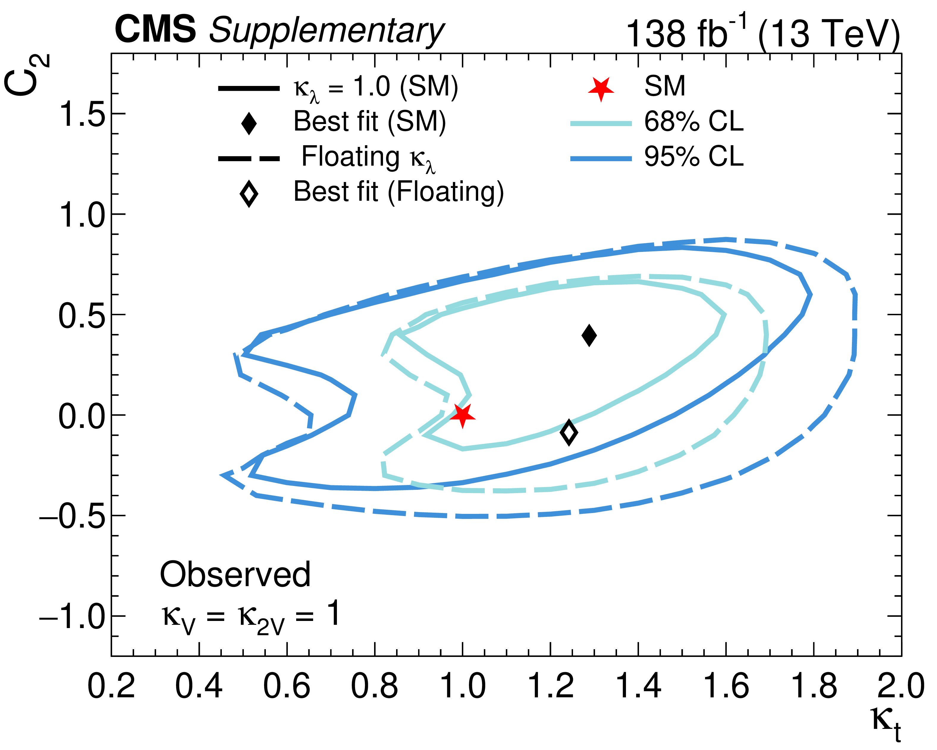
Figure A13:
The observed 68 and 95% CL contours of $ -2\Delta\ln(L) $ in the ($ \text{c}_2 $, $ \kappa_{\mathrm{t}} $) plane for the combination of all channels when $ \kappa_\lambda $ is allowed to vary. The range of $ \kappa_\lambda $ is set between-15 and 15 to avoid unphysical areas of the phase space. All the other parameters are fixed to their SM values. |

png pdf |
Figure A14:
The observed 68 and 95% CL contours of $ -2\Delta\ln(L) $ in the ($ \text{c}_2 $, $ \kappa_\lambda $) plane for the combination of all channels when $ \kappa_{\mathrm{t}} $ is allowed to vary. The range of $ \kappa_{\mathrm{t}} $ is set between 0.5 and 1.5 to avoid unphysical areas of the phase space. All the other parameters are fixed to their SM values. |
png pdf |
Figure A15:
The observed 68% CL contours of $ -2\Delta\ln(L) $ in the ($ \text{c}_2 $, $ \kappa_\lambda $) plane for all channels when all the other parameters are fixed to their SM value. The best fit value and 68% CL contour for the $ \mathrm{b}\overline{\mathrm{b}}\tau\tau $ channel are not within the range of the figure. |

png pdf |
Figure A16:
A bar chart showing the fraction of all HH events that are selected in each analysis. The numbers shown, correspond to the total of selected events per analysis. The results are calculated inclusively and per production mode. |

png pdf |
Figure A17:
A bar chart showing the selection efficiency for the HH signal per channel. The number of selected events per channel is also shown. |
| Tables | |

png pdf |
Table 1:
Values of the effective Lagrangian couplings for the Higgs effective field theory benchmarks proposed in Ref. [50] and referred to in this paper as JHEP04(2016)126. |

png pdf |
Table 2:
Values of the effective Lagrangian couplings for the Higgs effective field theory benchmarks proposed in Ref. [51] and referred to in this paper as JHEP03(2020)091. |

png pdf |
Table 3:
Summary of results for the HH analyses included in this combination. The second column is the observed (expected) 95% CL upper limit on the inclusive signal strength $ \mu= \sigma_{\mathrm{H}\mathrm{H}} /\sigma_{\mathrm{H}\mathrm{H}} ^\text{SM} $, with one exception where $ \mu_{\mathrm{V}\mathrm{H}\mathrm{H}}= \sigma_{\mathrm{V}\mathrm{H}\mathrm{H}}/\sigma_{\mathrm{V}\mathrm{H}\mathrm{H}}^\text{SM} $ is shown. The third (fourth) column is the allowed 68% CL interval for the coupling modifier $ \kappa_\lambda $ ($ \kappa_{2\mathrm{V}} $). The last column indicates whether the analysis is included in the results using the HEFT parametrisation. |

png pdf |
Table 4:
Summary of results on constraints to the coupling modifiers $ \kappa_\lambda $ and $ \kappa_{2\mathrm{V}} $. The ranges are either extracted using either the $ -2\Delta\ln(L) $ scan at 68% and 95% CL, or upper limits on the signal strength $ \mu $ at 95% CL. The theoretical uncertainties in the ggF and VBFHH signal cross sections are considered in all results tabulated here. |

png pdf |
Table 5:
Treatment of most important common systematic uncertainties in the S2 scenario. |

png pdf |
Table 6:
Expected significance for the HH signal projected to 2000 or 3000 fb$ ^{-1} $ under different assumptions of systematic uncertainties. |

png pdf |
Table A1:
Upper limits on the HH production cross section at 95% CL for the JHEP03(2020)91 BM1 benchmark. The theoretical uncertainties in the ggFHH signal cross section are not considered because we directly constrain the measured cross section. |

png pdf |
Table A2:
Upper limits on the HH production cross section at 95% CL for the JHEP03(2020)91 BM2 benchmark. The theoretical uncertainties in the HH ggF signal cross section are not considered because we directly constrain the measured cross section. |

png pdf |
Table A3:
Upper limits on the HH production cross section at 95% CL for the JHEP03(2020)91 BM3 benchmark. The theoretical uncertainties in the ggFHH signal cross section are not considered because we directly constrain the measured cross section. |

png pdf |
Table A4:
Upper limits on the HH production cross section at 95% CL for the JHEP03(2020)91 BM4 benchmark. The theoretical uncertainties in the ggFHH signal cross section are not considered because we directly constrain the measured cross section. |

png pdf |
Table A5:
Upper limits on the HH production cross section at 95% CL for the JHEP03(2020)91 BM5 benchmark. The theoretical uncertainties in the ggFHH signal cross section are not considered because we directly constrain the measured cross section. |

png pdf |
Table A6:
Upper limits on the HH production cross section at 95% CL for the JHEP03(2020)91 BM6 benchmark. The theoretical uncertainties in the HH ggF signal cross section are not considered because we directly constrain the measured cross section. |

png pdf |
Table A7:
Upper limits on the HH production cross section at 95% CL for the JHEP03(2020)91 BM7 benchmark. The theoretical uncertainties in the HH ggF signal cross section are not considered because we directly constrain the measured cross section. |

png pdf |
Table A8:
Upper limits on the HH production cross section at 95% CL for the JHEP04(2016)126 BM1 benchmark. The theoretical uncertainties in the HH ggF signal cross section are not considered because we directly constrain the measured cross section. |

png pdf |
Table A9:
Upper limits on the HH production cross section at 95% CL for the JHEP04(2016)126 BM2 benchmark. The theoretical uncertainties in the HH ggF signal cross section are not considered because we directly constrain the measured cross section. |

png pdf |
Table A10:
Upper limits on the HH production cross section at 95% CL for the JHEP04(2016)126 BM3 benchmark. The theoretical uncertainties in the HH ggF signal cross section are not considered because we directly constrain the measured cross section. |

png pdf |
Table A11:
Upper limits on the HH production cross section at 95% CL for the JHEP04(2016)126 BM4 benchmark. The theoretical uncertainties in the HH ggF signal cross section are not considered because we directly constrain the measured cross section. |

png pdf |
Table A12:
Upper limits on the HH production cross section at 95% CL for the JHEP04(2016)126 BM5 benchmark. The theoretical uncertainties in the HH ggF signal cross section are not considered because we directly constrain the measured cross section. |

png pdf |
Table A13:
Upper limits on the HH production cross section at 95% CL for the JHEP04(2016)126 BM6 benchmark. The theoretical uncertainties in the HH ggF signal cross section are not considered because we directly constrain the measured cross section. |

png pdf |
Table A14:
Upper limits on the HH production cross section at 95% CL for the JHEP04(2016)126 BM7 benchmark. The theoretical uncertainties in the HH ggF signal cross section are not considered because we directly constrain the measured cross section. |

png pdf |
Table A15:
Upper limits on the HH production cross section at 95% CL for the JHEP04(2016)126 BM8 benchmark. The theoretical uncertainties in the HH ggF signal cross section are not considered because we directly constrain the measured cross section. |

png pdf |
Table A16:
Upper limits on the HH production cross section at 95% CL for the JHEP04(2016)126 BM8a benchmark. The theoretical uncertainties in the HH ggF signal cross section are not considered because we directly constrain the measured cross section. |

png pdf |
Table A17:
Upper limits on the HH production cross section at 95% CL for the JHEP04(2016)126 BM9 benchmark. The theoretical uncertainties in the HH ggF signal cross section are not considered because we directly constrain the measured cross section. |

png pdf |
Table A18:
Upper limits on the HH production cross section at 95% CL for the JHEP04(2016)126 BM10 benchmark. The theoretical uncertainties in the HH ggF signal cross section are not considered because we directly constrain the measured cross section. |

png pdf |
Table A19:
Upper limits on the HH production cross section at 95% CL for the JHEP04(2016)126 BM11 benchmark. The theoretical uncertainties in the HH ggF signal cross section are not considered because we directly constrain the measured cross section. |

png pdf |
Table A20:
Upper limits on the HH production cross section at 95% CL for the JHEP04(2016)126 BM12 benchmark. The theoretical uncertainties in the HH ggF signal cross section are not considered because we directly constrain the measured cross section. |
| Summary |
| A combined search for nonresonant Higgs boson pair (HH) production was performed using the proton-proton collision data set produced by the LHC at $ \sqrt{s} = $ 13 TeV, and collected by the CMS experiment from 2016 to 2018 (Run 2), which corresponds to an integrated luminosity of 138 fb$ ^{-1} $. Searches for HH production via gluon-gluon (ggF) and vector boson fusion (VBF) production, were carried out in the $ \mathrm{b}\overline{\mathrm{b}}\gamma\gamma $, $ \mathrm{b}\overline{\mathrm{b}}\tau\tau $, $ \mathrm{b}\overline{\mathrm{b}}\mathrm{b}\overline{\mathrm{b}} $, $ \mathrm{b}\overline{\mathrm{b}}\mathrm{W}\mathrm{W} $, and multilepton channels. Additionally, searches for ggFHH production were conducted in the $ \mathrm{b}\overline{\mathrm{b}}\mathrm{Z}\mathrm{Z} $ (with both Z bosons decaying to leptons), $ \mathrm{W}\mathrm{W}\gamma\gamma $, and $ \tau\tau\gamma\gamma $ final states, which have clean signatures but relatively small branching fractions. We searched for the associated production mechanism with a vector boson in the $ \mathrm{b}\overline{\mathrm{b}}\mathrm{b}\overline{\mathrm{b}} $ final state, which has the largest branching fraction. The analyses of these channels were combined to probe the Higgs boson trilinear self-coupling and the quartic coupling between two vector bosons and two Higgs bosons ($ \mathrm{V}\mathrm{V}\mathrm{H}\mathrm{H} $), and to search for beyond the standard model (SM) physics scenarios in the Higgs effective field theory (HEFT) approach. The observed and expected upper limits at 95% confidence level (CL) on the cross section of ggFHH production were found to be 3.5 and 2.5 times the SM expectation, respectively. For VBF production, the observed and expected 95% CL upper limits are 79 and 91 times the SM expectation, respectively. When all other parameters are set to their SM values, we constrain the Higgs boson trilinear self-coupling modifier $ \kappa_\lambda $ in the range from $-$1.35 to 6.37 at 95% CL (expected 95% CL range is $-$2.24 to 7.89). Likewise, the $ \mathrm{V}\mathrm{V}\mathrm{H}\mathrm{H} $ coupling modifier $ \kappa_{2\mathrm{V}} $ is constrained in the range from 0.64 to 1.40 (0.62 to 1.41 expected). Two-dimensional measurements were also performed, including simultaneous measurements of $ \kappa_\lambda $ and $ \kappa_{2\mathrm{V}} $, $ \kappa_\lambda $ and the modifier of the Higgs boson coupling to the top quark ($ \kappa_{\mathrm{t}} $), and $ \kappa_{2\mathrm{V}} $ and the modifier of the Higgs boson coupling to vector bosons ($ \kappa_\mathrm{V} $). The results are in agreement with the SM predictions. Under the HEFT framework, the cross section of the nonresonant ggFHH pair production was parametrized as a function of anomalous couplings of the Higgs boson, involving the contact interactions between two Higgs and two top quarks, between two gluons and two Higgs bosons, and between two gluons and a Higgs boson. We performed searches for benchmark signals under different anomalous coupling scenarios and set upper limits on their cross sections at 95% CL. We exclude HH production at 95% CL when the coupling modifier of the contact interaction between two Higgs bosons and two top quarks is outside the range from $-$0.28 to 0.59 (expected 95% CL range is-0.17 to 0.47). The HEFT parametrisation is also exploited to study various ultraviolet complete models with an extended Higgs sector and set constraints on specific parameters. These results constitute the most stringent limits and constraints obtained from the searches for nonresonant HH production using the LHC Run-2 data set collected by the CMS experiment. Extrapolating our current results to the integrated luminosity anticipated of the High-Luminosity LHC, it is expected to see first evidence for HH production with $ \approx $2000 fb$ ^{-1} $ of data. |
| References | ||||
| 1 | CMS Collaboration | Observation of a new boson at a mass of 125 GeV with the CMS experiment at the LHC | PLB 716 (2012) 30 | CMS-HIG-12-028 1207.7235 |
| 2 | CMS Collaboration | Observation of a new boson with mass near 125 GeV in pp collisions at $ \sqrt{s} = $ 7 and 8 TeV | JHEP 06 (2013) 081 | CMS-HIG-12-036 1303.4571 |
| 3 | ATLAS Collaboration | Observation of a new particle in the search for the standard model Higgs boson with the ATLAS detector at the lhc | PLB 716 (2012) 1 | 1207.7214 |
| 4 | CMS Collaboration | A portrait of the Higgs boson by the CMS experiment ten years after the discovery | Nature 607 (2022) 60 | CMS-HIG-22-001 2207.00043 |
| 5 | ATLAS Collaboration | A detailed map of Higgs boson interactions by the ATLAS experiment ten years after the discovery | Nature 607 (2022) 52 | 2207.00092 |
| 6 | S. Dawson and C. W. Murphy | Standard model EFT and extended scalar sectors | PRD 96 (2017) 015041 | 1704.07851 |
| 7 | J. de Blas, M. Chala, M. Perez-Victoria, and J. Santiago | Observable effects of general new scalar particles | JHEP 04 (2015) 078 | 1412.8480 |
| 8 | T. D. Lee | A theory of spontaneous $ T $ violation | PRD 8 (1973) 1226 | |
| 9 | G. C. Branco et al. | Theory and phenomenology of two-Higgs-doublet models | Phys. Rep. 516 (2012) 1 | 1106.0034 |
| 10 | H. E. Haber and O. St \aa l | New LHC benchmarks for the $ CP $-conserving two-Higgs-doublet model | EPJC 75 (2015) 491 | 1507.04281 |
| 11 | F. Kling, J. M. No, and S. Su | Anatomy of exotic Higgs decays in 2HDM | JHEP 09 (2016) 093 | 1604.01406 |
| 12 | G. F. Giudice, C. Grojean, A. Pomarol, and R. Rattazzi | The strongly-interacting light Higgs | JHEP 06 (2007) 045 | hep-ph/0703164 |
| 13 | R. Grober and M. Muhlleitner | Composite Higgs boson pair production at the LHC | JHEP 06 (2011) 020 | 1012.1562 |
| 14 | R. Contino et al. | Effective Lagrangian for a light Higgs-like scalar | JHEP 07 (2013) 035 | 1303.3876 |
| 15 | R. Contino | The Higgs as a composite Nambu--Goldstone boson | in Theoretical Advanced Study Institute in Elementary Particle Physics: Physics of the Large and the Small, p. 235. 2011 link |
1005.4269 |
| 16 | P. Huang, A. J. Long, and L.-T. Wang | Probing the electroweak phase transition with Higgs factories and gravitational waves | PRD 94 (2016) 075008 | 1608.06619 |
| 17 | M. J. Ramsey-Musolf, I. Tenkanen, Tuomas V.\, and V. Q. Tran | Refining gravitational wave and collider physics dialogue via singlet scalar extension | 2409.17554 | |
| 18 | A. Mazumdar and G. White | Review of cosmic phase transitions: Their significance and experimental signatures | Rep. Prog. Phys. 82 (2019) 076901 | 1811.01948 |
| 19 | W. Zhang et al. | Probing electroweak phase transition in the singlet standard model via $ \mathrm{b}\mathrm{b}\gamma\gamma $ and 4 $ \ell $ channels | JHEP 12 (2023) 018 | 2303.03612 |
| 20 | A. V. Bednyakov, A. F. Pikelner, and V. N. Velizhanin | Stability of the electroweak vacuum: Gauge independence and radiative corrections | PRL 115 (2015) 201802 | 1507.08833 |
| 21 | P. Basler, L. Biermann, M. Muhlleitner et al. | Electroweak baryogenesis in the CP-violating two-Higgs doublet model | EPJC 83 (2023) 57 | 2108.03580 |
| 22 | D. E. Morrissey and M. J. Ramsey-Musolf | Electroweak baryogenesis: A review | New J. Phys. 14 (2012) 125003 | 1206.2942 |
| 23 | T. Plehn and M. Rauch | The quartic Higgs coupling at hadron colliders | PRD 72 (2005) 053008 | hep-ph/0507321 |
| 24 | A. Dainese et al. | Report from Working Group 2: Higgs physics at the HL-LHC and HE-LHC | CERN Yellow Rep. Monogr. 7 (2019) 221 | 1902.00134 |
| 25 | M. Chiesa et al. | Measuring the quartic Higgs self-coupling at a multi- TeVns muon collider | JHEP 09 (2020) 098 | 2003.13628 |
| 26 | H. Abouabid et al. | $ \mathrm{H}\mathrm{H}\mathrm{H} $ whitepaper | EPJC 84 (2024) 1183 | 2407.03015 |
| 27 | S. Borowka et al. | Higgs boson pair production in gluon fusion at next-to-leading order with full top-quark mass dependence | PRL 117 (2016) 012001 | 1604.06447 |
| 28 | J. Baglio et al. | Gluon fusion into Higgs pairs at NLO QCD and the top mass scheme | EPJC 79 (2019) 459 | 1811.05692 |
| 29 | F. A. Dreyer and A. Karlberg | Vector-boson fusion Higgs pair production at N$ ^3 $LO | PRD 98 (2018) 114016 | 1811.07906 |
| 30 | M. Grazzini et al. | Higgs boson pair production at NNLO with top quark mass effects | JHEP 05 (2018) 059 | 1803.02463 |
| 31 | L. Alasfar et al. | Effective field theory descriptions of Higgs boson pair production | SciPost Phys. Comm. Rep. 2, 2024 link |
2304.01968 |
| 32 | ATLAS Collaboration | Combination of searches for Higgs boson pair production in pp collisions at $ \sqrt{s}= $ 13 TeV with the ATLAS detector | PRL 133 (2024) 101801 | 2406.09971 |
| 33 | CMS Collaboration | HEPData record for this analysis | link | |
| 34 | CMS Collaboration | The CMS experiment at the CERN LHC | JINST 3 (2008) S08004 | |
| 35 | CMS Collaboration | Development of the CMS detector for the CERN LHC Run 3 | JINST 19 (2024) P05064 | CMS-PRF-21-001 2309.05466 |
| 36 | CMS Collaboration | Performance of the CMS Level-1 trigger in proton-proton collisions at $ \sqrt{s} = $ 13 TeV | JINST 15 (2020) P10017 | CMS-TRG-17-001 2006.10165 |
| 37 | CMS Collaboration | The CMS trigger system | JINST 12 (2017) P01020 | CMS-TRG-12-001 1609.02366 |
| 38 | CMS Collaboration | Performance of the CMS high-level trigger during LHC Run 2 | JINST 19 (2024) P11021 | CMS-TRG-19-001 2410.17038 |
| 39 | CMS Collaboration | Electron and photon reconstruction and identification with the CMS experiment at the CERN LHC | JINST 16 (2021) P05014 | CMS-EGM-17-001 2012.06888 |
| 40 | CMS Collaboration | Performance of the CMS muon detector and muon reconstruction with proton-proton collisions at $ \sqrt{s}= $ 13 TeV | JINST 13 (2018) P06015 | CMS-MUO-16-001 1804.04528 |
| 41 | CMS Collaboration | Description and performance of track and primary-vertex reconstruction with the CMS tracker | JINST 9 (2014) P10009 | CMS-TRK-11-001 1405.6569 |
| 42 | CMS Collaboration | Particle-flow reconstruction and global event description with the CMS detector | JINST 12 (2017) P10003 | CMS-PRF-14-001 1706.04965 |
| 43 | CMS Collaboration | Technical proposal for the Phase-II upgrade of the Compact Muon Solenoid | CMS Technical Proposal CERN-LHCC-2015-010, CMS-TDR-15-02, 2015 CDS |
|
| 44 | M. Cacciari, G. P. Salam, and G. Soyez | The anti-$ k_{\mathrm{T}} $ jet clustering algorithm | JHEP 04 (2008) 063 | 0802.1189 |
| 45 | M. Cacciari, G. P. Salam, and G. Soyez | FastJet user manual | EPJC 72 (2012) 1896 | 1111.6097 |
| 46 | CMS Collaboration | Performance of missing transverse momentum reconstruction in proton-proton collisions at $ \sqrt{s} = $ 13 TeV using the CMS detector | JINST 14 (2019) P07004 | CMS-JME-17-001 1903.06078 |
| 47 | G. Heinrich et al. | Probing the trilinear Higgs boson coupling in di-Higgs production at NLO QCD including parton shower effects | JHEP 06 (2019) 066 | 1903.08137 |
| 48 | D. de Florian et al. | Anomalous couplings in Higgs-boson pair production at approximate NNLO QCD | JHEP 09 (2021) 161 | 2106.14050 |
| 49 | A. Carvalho et al. | On the reinterpretation of non-resonant searches for Higgs boson pairs | JHEP 02 (2021) 049 | 1710.08261 |
| 50 | A. Carvalho et al. | Higgs pair production: Choosing benchmarks with cluster analysis | JHEP 04 (2016) 126 | 1507.02245 |
| 51 | M. Capozi and G. Heinrich | Exploring anomalous couplings in Higgs boson pair production through shape analysis | JHEP 03 (2020) 091 | 1908.08923 |
| 52 | CMS Collaboration | Constraints on the Higgs boson self-coupling from the combination of single and double Higgs boson production in proton-proton collisions at $ \sqrt{s}= $ 13 TeV | PLB 861 (2025) 139210 | CMS-HIG-23-006 2407.13554 |
| 53 | P. Nason | A new method for combining NLO QCD with shower Monte Carlo algorithms | JHEP 11 (2004) 040 | hep-ph/0409146 |
| 54 | S. Frixione, P. Nason, and C. Oleari | Matching NLO QCD computations with parton shower simulations: The POWHEG method | JHEP 11 (2007) 070 | 0709.2092 |
| 55 | S. Alioli, P. Nason, C. Oleari, and E. Re | A general framework for implementing NLO calculations in shower Monte Carlo programs: The POWHEG BOX | JHEP 06 (2010) 043 | 1002.2581 |
| 56 | S. Amoroso et al. | Les Houches 2019: Physics at TeVns colliders: Standard model working group report | in Proc. 11th Les Houches Workshop on Physics at TeVns Colliders: PhysTeV Les Houches. 2020 | 2003.01700 |
| 57 | J. Alwall et al. | The automated computation of tree-level and next-to-leading order differential cross sections, and their matching to parton shower simulations | JHEP 07 (2014) 079 | 1405.0301 |
| 58 | J. Alwall et al. | Comparative study of various algorithms for the merging of parton showers and matrix elements in hadronic collisions | EPJC 53 (2007) 473 | 0706.2569 |
| 59 | R. Frederix and S. Frixione | Merging meets matching in MC@NLO | JHEP 12 (2012) 061 | 1209.6215 |
| 60 | F. A. Dreyer and A. Karlberg | Fully differential vector-boson fusion Higgs pair production at next-to-next-to-leading order | PRD 99 (2019) 074028 | 1811.07918 |
| 61 | J. Baglio et al. | The measurement of the Higgs self-coupling at the LHC: theoretical status | JHEP 04 (2013) 151 | 1212.5581 |
| 62 | T. Sjostrand, S. Mrenna, and P. Z. Skands | A brief introduction to PYTHIA 8.1 | Comput. Phys. Commun. 178 (2008) 852 | 0710.3820 |
| 63 | NNPDF Collaboration | Parton distributions with QED corrections | NPB 877 (2013) 290 | 1308.0598 |
| 64 | NNPDF Collaboration | Parton distributions for the LHC Run II | JHEP 04 (2015) 040 | 1410.8849 |
| 65 | NNPDF Collaboration | Parton distributions from high-precision collider data | EPJC 77 (2017) 663 | 1706.00428 |
| 66 | GEANT4 Collaboration | GEANT 4---a simulation toolkit | NIM A 506 (2003) 250 | |
| 67 | CMS Collaboration | Search for Higgs Boson Pair Production in the Four b Quark Final State in Proton-Proton Collisions at $ \sqrt{s}= $ 13 TeV | PRL 129 (2022) 081802 | CMS-HIG-20-005 2202.09617 |
| 68 | CMS Collaboration | Search for nonresonant pair production of highly energetic Higgs bosons decaying to bottom quarks | PRL 131 (2023) 041803 | 2205.06667 |
| 69 | CMS Collaboration | Search for Higgs boson pair production with one associated vector boson in proton-proton collisions at $ \sqrt{s} = $ 13 TeV | JHEP 10 (2024) 061 | CMS-HIG-22-006 2404.08462 |
| 70 | CMS Collaboration | Search for nonresonant Higgs boson pair production in final state with two bottom quarks and two tau leptons in proton-proton collisions at $ \sqrt{s} = $ 13 TeV | PLB 842 (2023) 137531 | CMS-HIG-20-010 2206.09401 |
| 71 | CMS Collaboration | Search for nonresonant Higgs boson pair production in final states with two bottom quarks and two photons in proton-proton collisions at $ \sqrt{s} = $ 13 TeV | JHEP 03 (2021) 257 | CMS-HIG-19-018 2011.12373 |
| 72 | CMS Collaboration | Search for Higgs boson pair production in the $ \mathrm{b}\overline{\mathrm{b}}\mathrm{W}^{+}\mathrm{W}^{-} $ decay mode in proton-proton collisions at $ \sqrt{s} = $ 13 TeV | JHEP 07 (2024) 293 | CMS-HIG-21-005 2403.09430 |
| 73 | CMS Collaboration | Search for Higgs boson pairs decaying to $ \mathrm{W}\mathrm{W}^\ast\mathrm{W}\mathrm{W}^\ast $, $ \mathrm{W}\mathrm{W}^\ast\tau\tau $, and $ \tau\tau\tau\tau $ in proton-proton collisions at $ \sqrt{s} = $ 13 TeV | JHEP 07 (2023) 095 | CMS-HIG-21-002 2206.10268 |
| 74 | CMS Collaboration | Search for the nonresonant and resonant production of a Higgs boson in association with an additional scalar boson in the $ \gamma\gamma\tau\tau $ final state in proton-proton collisions at $ \sqrt{s} = $ 13 TeV | Submitted to \emphJHEP, 2025 | CMS-HIG-22-012 2506.23012 |
| 75 | CMS Collaboration | Search for nonresonant Higgs boson pair production in the four leptons plus twob jets final state in proton-proton collisions at $ \sqrt{s} = $ 13 TeV | JHEP 06 (2023) 130 | CMS-HIG-20-004 2206.10657 |
| 76 | E. Bols et al. | Jet flavour classification using DeepJet | JINST 15 (2020) P12012 | 2008.10519 |
| 77 | CMS Collaboration | A deep neural network for simultaneous estimation of b jet energy and resolution | Comput. Softw. Big Sci. 4 (2020) 10 | CMS-HIG-18-027 1912.06046 |
| 78 | A. J. Larkoski, S. Marzani, G. Soyez, and J. Thaler | Soft drop | JHEP 05 (2014) 146 | 1402.2657 |
| 79 | I. Henrion et al. | Neural message passing for jet physics | in Deep Learning for Physical Sciences Workshop at 31st Conf. on Neural Information Processing Systems. Long Beach, CA, USA, 2017 | |
| 80 | H. Qu and L. Gouskos | Jet tagging via particle clouds | PRD 101 (2020) 056019 | 1902.08570 |
| 81 | E. A. Moreno et al. | JEDI-net: A jet identification algorithm based on interaction networks | EPJC 80 (2020) 58 | 1908.05318 |
| 82 | E. A. Moreno et al. | Interaction networks for the identification of boosted $ \mathrm{H}\to\mathrm{b}\overline{\mathrm{b}} $ decays | PRD 102 (2020) 012010 | 1909.12285 |
| 83 | CMS Collaboration | Performance of heavy-flavour jet identification in boosted topologies in proton-proton collisions at $ \sqrt{s} = $ 13 TeV | CMS Physics Analysis Summary, 2023 CMS-PAS-BTV-22-001 |
CMS-PAS-BTV-22-001 |
| 84 | CMS Collaboration | Mass regression of highly-boosted jets using graph neural networks | CMS Detector Performance Note CMS-DP-2021-017, 2021 CDS |
|
| 85 | CMS Collaboration | Search for a massive resonance decaying to a pair of Higgs bosons in the four b quark final state in proton-proton collisions at $ \sqrt{s}= $ 13 TeV | PLB 781 (2018) 244 | 1710.04960 |
| 86 | CMS Collaboration | Search for production of Higgs boson pairs in the four b quark final state using large-area jets in proton-proton collisions at $ \sqrt{s}= $ 13 TeV | JHEP 01 (2019) 040 | 1808.01473 |
| 87 | CMS Collaboration | Inclusive search for highly boosted Higgs bosons decaying to bottom quark-antiquark pairs in proton-proton collisions at $ \sqrt{s} = $ 13 TeV | JHEP 12 (2020) 85 | CMS-HIG-19-003 2006.13251 |
| 88 | CMS Collaboration | Identification of heavy, energetic, hadronically decaying particles using machine-learning techniques | JINST 15 (2020) P06005 | CMS-JME-18-002 2004.08262 |
| 89 | CMS Collaboration | Identification of hadronic tau lepton decays using a deep neural network | JINST 17 (2022) P07023 | CMS-TAU-20-001 2201.08458 |
| 90 | L. Bianchini et al. | Reconstruction of the Higgs mass in events with Higgs bosons decaying into a pair of $ \tau $ leptons using matrix element techniques | NIM A 862 (2017) 54 | 1603.05910 |
| 91 | CMS Collaboration | Evidence for associated production of a Higgs boson with a top quark pair in final states with electrons, muons, and hadronically decaying $ \tau $ leptons at $ \sqrt{s} = $ 13 TeV | JHEP 08 (2018) 066 | CMS-HIG-17-018 1803.05485 |
| 92 | H. Qu, C. Li, and S. Qian | Particle transformer for jet tagging | in Proc. 39th Int. Conf. on Machine Learning, K. Chaudhuri et al., eds., volume 162, p. 18281. 2022 link |
2202.03772 |
| 93 | CMS Collaboration | Particle transformers for identifying Lorentz-boosted Higgs bosons decaying to a pair of W bosons | CMS Physics Analysis Summary, 2025 CMS-PAS-JME-25-001 |
CMS-PAS-JME-25-001 |
| 94 | CMS Collaboration | A new method for correcting the substructure of multi-prong jets using Lund jet plane reweighting in the CMS experiment | CMS Physics Analysis Summary, 2025 CMS-PAS-JME-23-001 |
CMS-PAS-JME-23-001 |
| 95 | F. A. Dreyer, G. P. Salam, and G. Soyez | The Lund jet plane | JHEP 12 (2018) 064 | 1807.04758 |
| 96 | CMS Collaboration | Measurement of the Higgs boson production rate in association with top quarks in final states with electrons, muons, and hadronically decaying tau leptons at $ \sqrt{s} = $ 13 TeV | EPJC 81 (2021) 378 | CMS-HIG-19-008 2011.03652 |
| 97 | LHC Higgs Cross Section Working Group | Handbook of LHC Higgs Cross Sections: 4. Deciphering the nature of the Higgs sector | CERN Yellow Rep. Monogr. 2 (2017) | 1610.07922 |
| 98 | S. Manzoni et al. | Taming a leading theoretical uncertainty in $ {\mathrm{H}\mathrm{H}} $ measurements via accurate simulations for $ \mathrm{b}\overline{\mathrm{b}}\mathrm{H} $ production | JHEP 09 (2023) 179 | 2307.09992 |
| 99 | J. Baglio et al. | $ \mathrm{g}\mathrm{g} \to {\mathrm{H}\mathrm{H}} $: Combined uncertainties | PRD 103 (2021) 056002 | 2008.11626 |
| 100 | L.-S. Ling et al. | NNLO QCD corrections to Higgs pair production via vector boson fusion at hadron colliders | PRD 89 (2014) 073001 | 1401.7754 |
| 101 | M. Czakon et al. | Top-pair production at the LHC through NNLO QCD and NLO EW | JHEP 10 (2017) 186 | 1705.04105 |
| 102 | CMS Collaboration | Precision luminosity measurement in proton-proton collisions at $ \sqrt{s} = $ 13 TeV in 2015 and 2016 at CMS | EPJC 81 (2021) 800 | CMS-LUM-17-003 2104.01927 |
| 103 | CMS Collaboration | CMS luminosity measurement for the 2017 data-taking period at $ \sqrt{s} = $ 13 TeV | CMS Physics Analysis Summary, 2018 CMS-PAS-LUM-17-004 |
CMS-PAS-LUM-17-004 |
| 104 | CMS Collaboration | CMS luminosity measurement for the 2018 data-taking period at $ \sqrt{s} = $ 13 TeV | CMS Physics Analysis Summary, 2019 CMS-PAS-LUM-18-002 |
CMS-PAS-LUM-18-002 |
| 105 | CMS Collaboration | Measurement of the inelastic proton-proton cross section at $ \sqrt{s}= $ 13 TeV | JHEP 07 (2018) 161 | CMS-FSQ-15-005 1802.02613 |
| 106 | R. Barlow and C. Beeston | Fitting using finite Monte Carlo samples | Comput. Phys. Commun. 77 (1993) 219 | |
| 107 | ATLAS and CMS Collaborations, and LHC Higgs Combination Group | Procedure for the LHC Higgs boson search combination in Summer 2011 | Technical Report CMS-NOTE-2011-005, ATL-PHYS-PUB-2011-11, 2011 | |
| 108 | G. Cowan, K. Cranmer, E. Gross, and O. Vitells | Asymptotic formulae for likelihood-based tests of new physics | EPJC 71 (2011) 1554 | 1007.1727 |
| 109 | T. Junk | Confidence level computation for combining searches with small statistics | NIM A 434 (1999) 435 | hep-ex/9902006 |
| 110 | A. L. Read | Presentation of search results: the $ \text{CL}_\text{s} $ technique | JPG 28 (2002) 2693 | |
| 111 | CMS Collaboration | The CMS statistical analysis and combination tool: Combine | Comput. Softw. Big Sci. 8 (2024) 19 | CMS-CAT-23-001 2404.06614 |
| 112 | W. Verkerke and D. P. Kirkby | The RooFit toolkit for data modeling | eConf, 2003 | physics/0306116 |
| 113 | L. Moneta et al. | The RooStats Project | PoS ACAT 057, 2010 link |
1009.1003 |
| 114 | I. Zurbano Fernandez et al. | High-Luminosity Large Hadron Collider (HL-LHC): Technical design report | CERN Yellow Rep. Monogr. 10 (2020) | |
| 115 | CMS Collaboration | The Phase-2 upgrade of the CMS level-1 trigger | CMS Technical Design Report CERN-LHCC-2020-004, CMS-TDR-021, 2020 CDS |
|
| 116 | CMS Collaboration | The Phase-2 upgrade of the CMS data acquisition and high level trigger | CMS Technical Design Report CERN-LHCC-2021-007, CMS-TDR-022, 2021 CDS |
|
|
|
Compact Muon Solenoid LHC, CERN |
|

|

|

|

|

|