

Compact Muon Solenoid
LHC, CERN
| CMS-HIG-22-012 ; CERN-EP-2025-116 | ||
| Search for the nonresonant and resonant production of a Higgs boson in association with an additional scalar boson in the $ \gamma\gamma\tau\tau $ final state in proton-proton collisions at $ \sqrt{s} = $ 13 TeV | ||
| CMS Collaboration | ||
| 29 June 2025 | ||
| JHEP 05 (2026) 186 | ||
| Abstract: The results of a search for the production of two scalar bosons in final states with two photons and two tau leptons are presented. The search considers both nonresonant production of a Higgs boson pair, HH, and resonant production via a new boson X which decays either to HH or to H and a new scalar Y. The analysis uses up to 138 fb$ ^{-1} $ of proton-proton collision data, recorded between 2016 and 2018 by the CMS experiment at the LHC at a center-of-mass energy of 13 TeV. No evidence for signal is found in the data. For the nonresonant production, the observed (expected) upper limit at 95% confidence level (CL) on the HH production cross section is set at 930 (740) fb, corresponding to 33 (26) times the standard model prediction. At 95% CL, HH production is observed (expected) to be excluded for values of $ \kappa_\lambda $ outside the range between-12 (-9.4) and 17 (15). Observed (expected) upper limits at 95% CL for the $ \mathrm{X} \to \mathrm{H}\mathrm{H} $ cross section are found to be within 160 to 2200 (200 to 1800) fb, depending on the mass of X. In the $ \mathrm{X} \to \mathrm{Y} (\tau\tau)\mathrm{H}(\gamma\gamma) $ search, the observed (expected) upper limits on the product of the production cross section and decay branching fractions vary between 0.059-1.2 fb (0.087-0.68 fb). For the $ \mathrm{X} \to \mathrm{Y} (\gamma\gamma)\mathrm{H}(\tau\tau) $ search the observed (expected) upper limits on the product of the production cross section and $ \mathrm{Y} \to \gamma\gamma $ branching fraction vary between 0.69-15 fb (0.73-8.3 fb) in the low Y mass search, tightening constraints on the next-to-minimal supersymmetric standard model, and between 0.64-10 fb (0.70-7.6 fb) in the high Y mass search. | ||
| Links: e-print arXiv:2506.23012 [hep-ex] (PDF) ; CDS record ; inSPIRE record ; HepData record ; CADI line (restricted) ; | ||
| Figures | |

png pdf |
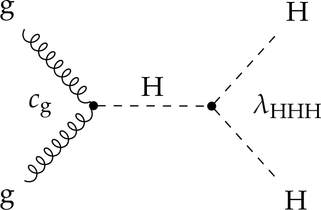
Figure 1:
Leading order Feynman diagrams of the nonresonant HH production via $ \mathrm{g}\mathrm{g}\mathrm{F} $. The two diagrams in the upper row correspond to SM processes, involving the top Yukawa coupling $ y_\mathrm{t} $, and the trilinear Higgs boson self-coupling $ \lambda_{\mathrm{H}\mathrm{H}\mathrm{H}} $. The diagrams in the lower row correspond to BSM processes involving contact interactions introduced in the effective field theory, namely $ c_2 $, $ c_{2\mathrm{g}} $ and $ c_{\mathrm{g}} $. |

png pdf |
Figure 1-a:
Leading order Feynman diagrams of the nonresonant HH production via $ \mathrm{g}\mathrm{g}\mathrm{F} $. The two diagrams in the upper row correspond to SM processes, involving the top Yukawa coupling $ y_\mathrm{t} $, and the trilinear Higgs boson self-coupling $ \lambda_{\mathrm{H}\mathrm{H}\mathrm{H}} $. The diagrams in the lower row correspond to BSM processes involving contact interactions introduced in the effective field theory, namely $ c_2 $, $ c_{2\mathrm{g}} $ and $ c_{\mathrm{g}} $. |

png pdf |
Figure 1-b:
Leading order Feynman diagrams of the nonresonant HH production via $ \mathrm{g}\mathrm{g}\mathrm{F} $. The two diagrams in the upper row correspond to SM processes, involving the top Yukawa coupling $ y_\mathrm{t} $, and the trilinear Higgs boson self-coupling $ \lambda_{\mathrm{H}\mathrm{H}\mathrm{H}} $. The diagrams in the lower row correspond to BSM processes involving contact interactions introduced in the effective field theory, namely $ c_2 $, $ c_{2\mathrm{g}} $ and $ c_{\mathrm{g}} $. |

png pdf |
Figure 1-c:
Leading order Feynman diagrams of the nonresonant HH production via $ \mathrm{g}\mathrm{g}\mathrm{F} $. The two diagrams in the upper row correspond to SM processes, involving the top Yukawa coupling $ y_\mathrm{t} $, and the trilinear Higgs boson self-coupling $ \lambda_{\mathrm{H}\mathrm{H}\mathrm{H}} $. The diagrams in the lower row correspond to BSM processes involving contact interactions introduced in the effective field theory, namely $ c_2 $, $ c_{2\mathrm{g}} $ and $ c_{\mathrm{g}} $. |

png pdf |
Figure 1-d:
Leading order Feynman diagrams of the nonresonant HH production via $ \mathrm{g}\mathrm{g}\mathrm{F} $. The two diagrams in the upper row correspond to SM processes, involving the top Yukawa coupling $ y_\mathrm{t} $, and the trilinear Higgs boson self-coupling $ \lambda_{\mathrm{H}\mathrm{H}\mathrm{H}} $. The diagrams in the lower row correspond to BSM processes involving contact interactions introduced in the effective field theory, namely $ c_2 $, $ c_{2\mathrm{g}} $ and $ c_{\mathrm{g}} $. |
png pdf |
Figure 1-e:
Leading order Feynman diagrams of the nonresonant HH production via $ \mathrm{g}\mathrm{g}\mathrm{F} $. The two diagrams in the upper row correspond to SM processes, involving the top Yukawa coupling $ y_\mathrm{t} $, and the trilinear Higgs boson self-coupling $ \lambda_{\mathrm{H}\mathrm{H}\mathrm{H}} $. The diagrams in the lower row correspond to BSM processes involving contact interactions introduced in the effective field theory, namely $ c_2 $, $ c_{2\mathrm{g}} $ and $ c_{\mathrm{g}} $. |
png pdf |
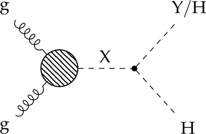
Figure 2:
Feynman diagram of the resonant production of a pair of SM Higgs bosons ($ \mathrm{X} \to \mathrm{H}\mathrm{H} $), or of a SM Higgs boson and a new scalar particle ($ \mathrm{X} \to \mathrm{Y} \mathrm{H} $). |
png pdf |
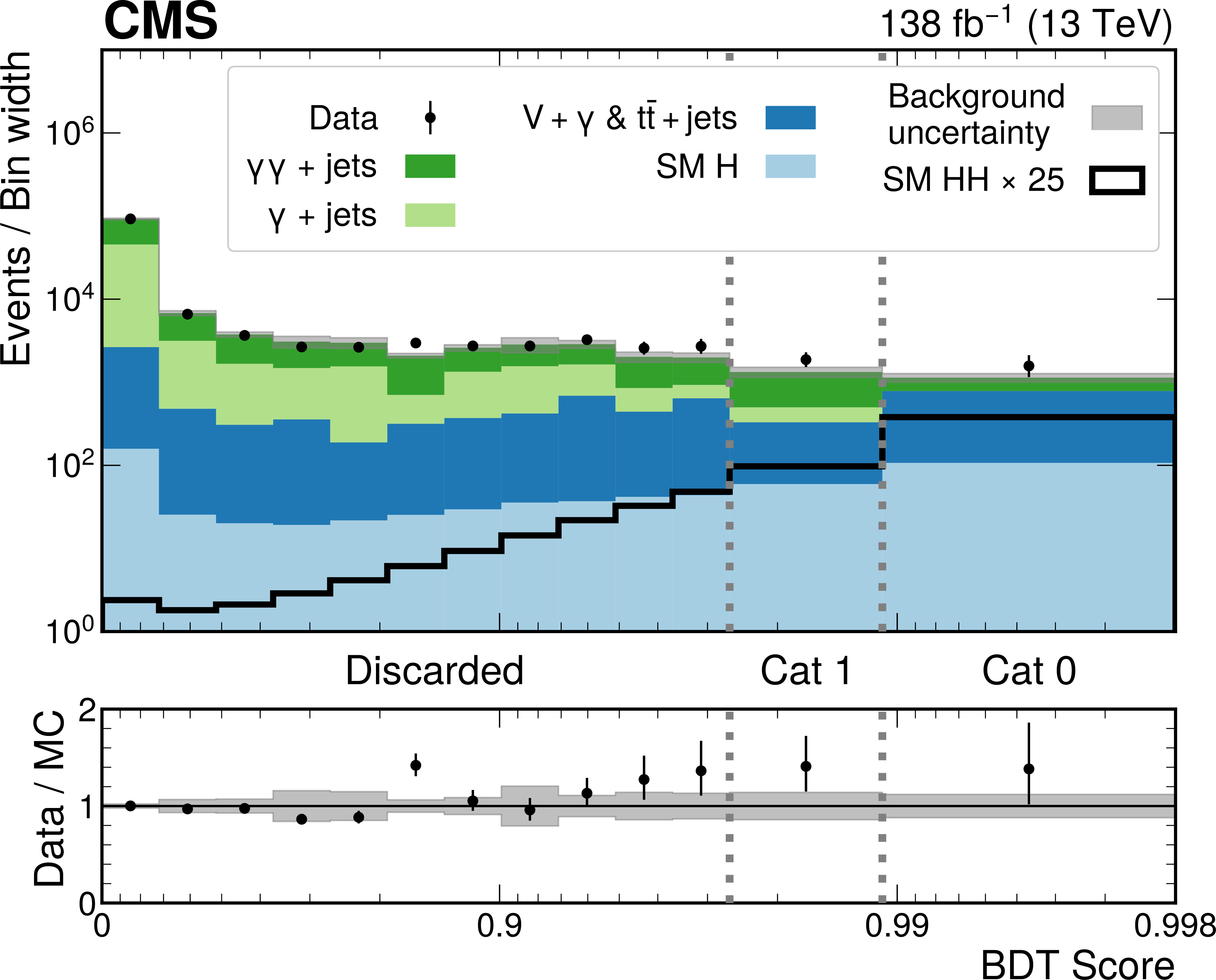
Figure 3:
Distribution of the BDT scores used for the nonresonant analysis event categorization from data (black points) and predictions from MC simulation (colored histograms). The ``SM H'' process includes $ \mathrm{g}\mathrm{g}\mathrm{H} $, $ \mathrm{VBF} $, VH, and $ {\mathrm{t}\overline{\mathrm{t}}} \mathrm{H} $, and the $ {\mathrm{t}\overline{\mathrm{t}}} + \text{jets} $ process also includes the $ {\mathrm{t}\overline{\mathrm{t}}} + \gamma $ and $ {\mathrm{t}\overline{\mathrm{t}}} + \gamma\gamma $ processes. The background histograms are stacked, while the signal distribution is shown separately. The normalization of the signal distribution is set to 25 times the SM prediction and the background MC simulation is normalized to data. The ratio of the data to the sum of the background predictions is shown in the lower panel. Statistical MC uncertainties for the background are represented by the gray shaded bands. The gray dotted lines represent the boundaries that define the two analysis categories (Cat 0 and Cat 1). The rest of the data, labeled as `discarded' is not used in the fit to data. |
png pdf |
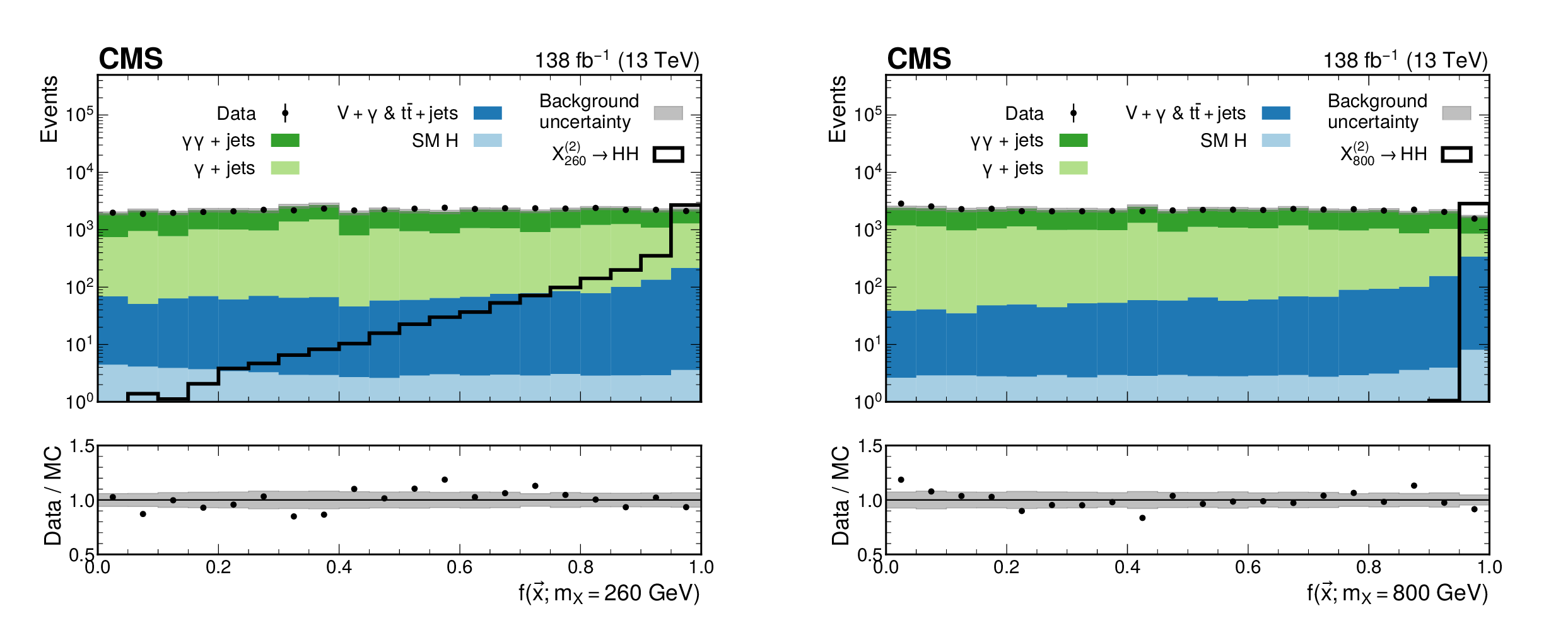
Figure 4:
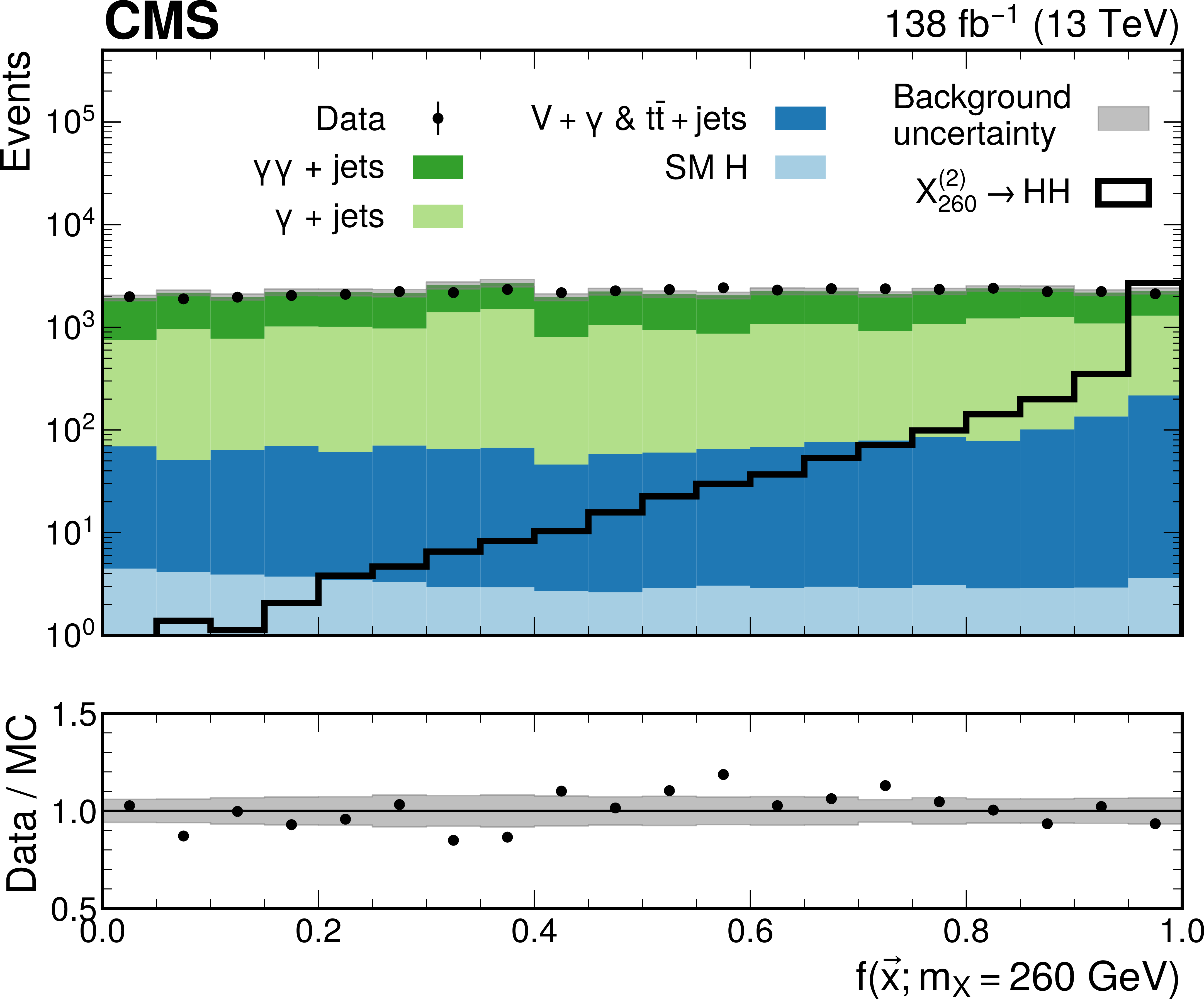
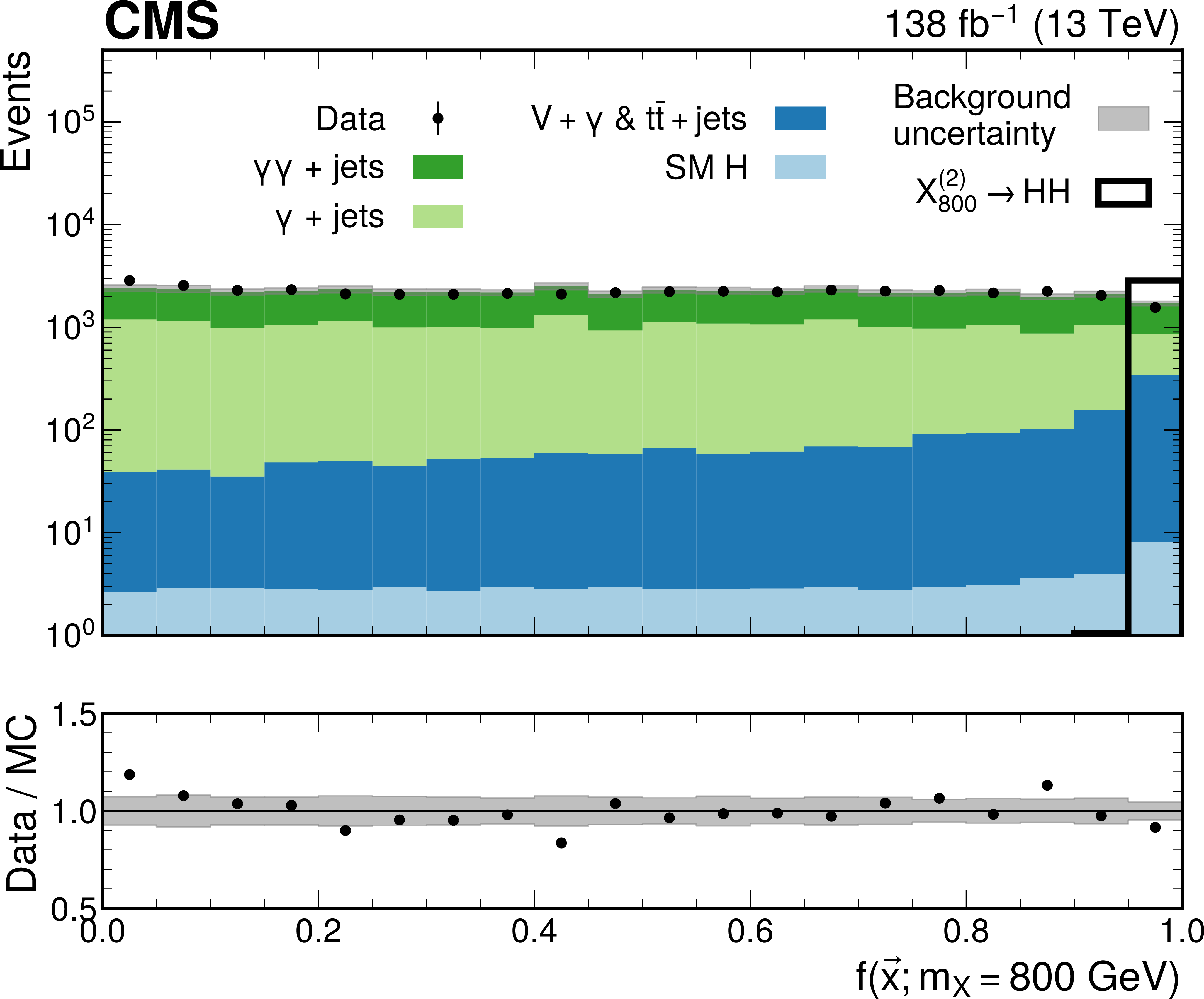
Transformed output of the pNN used in the $ \mathrm{X}{(2)} \to \mathrm{H}\mathrm{H} $ search, evaluated at $ m_{\mathrm{X}}= $ 260 GeV (left) and 800 GeV (right). The filled histograms represent the background simulation, and the data are shown by the black points. The ``SM H'' process includes $ \mathrm{g}\mathrm{g}\mathrm{H} $, $ \mathrm{VBF} $, VH, and $ {\mathrm{t}\overline{\mathrm{t}}} \mathrm{H} $, and the $ {\mathrm{t}\overline{\mathrm{t}}} + \text{jets} $ process also includes the $ {\mathrm{t}\overline{\mathrm{t}}} + \gamma $ and $ {\mathrm{t}\overline{\mathrm{t}}} + \gamma\gamma $ processes. The targeted signal distributions for which the pNN is evaluated are shown by the black unfilled histograms. The background MC simulation is normalized to data and the signal is normalized to an arbitrary cross section for representation purposes. The ratio of the data to the sum of the background predictions is shown in the lower panel. Statistical MC uncertainties for the background are represented by the gray shaded bands. |
png pdf |
Figure 4-a:
Transformed output of the pNN used in the $ \mathrm{X}{(2)} \to \mathrm{H}\mathrm{H} $ search, evaluated at $ m_{\mathrm{X}}= $ 260 GeV (left) and 800 GeV (right). The filled histograms represent the background simulation, and the data are shown by the black points. The ``SM H'' process includes $ \mathrm{g}\mathrm{g}\mathrm{H} $, $ \mathrm{VBF} $, VH, and $ {\mathrm{t}\overline{\mathrm{t}}} \mathrm{H} $, and the $ {\mathrm{t}\overline{\mathrm{t}}} + \text{jets} $ process also includes the $ {\mathrm{t}\overline{\mathrm{t}}} + \gamma $ and $ {\mathrm{t}\overline{\mathrm{t}}} + \gamma\gamma $ processes. The targeted signal distributions for which the pNN is evaluated are shown by the black unfilled histograms. The background MC simulation is normalized to data and the signal is normalized to an arbitrary cross section for representation purposes. The ratio of the data to the sum of the background predictions is shown in the lower panel. Statistical MC uncertainties for the background are represented by the gray shaded bands. |
png pdf |
Figure 4-b:
Transformed output of the pNN used in the $ \mathrm{X}{(2)} \to \mathrm{H}\mathrm{H} $ search, evaluated at $ m_{\mathrm{X}}= $ 260 GeV (left) and 800 GeV (right). The filled histograms represent the background simulation, and the data are shown by the black points. The ``SM H'' process includes $ \mathrm{g}\mathrm{g}\mathrm{H} $, $ \mathrm{VBF} $, VH, and $ {\mathrm{t}\overline{\mathrm{t}}} \mathrm{H} $, and the $ {\mathrm{t}\overline{\mathrm{t}}} + \text{jets} $ process also includes the $ {\mathrm{t}\overline{\mathrm{t}}} + \gamma $ and $ {\mathrm{t}\overline{\mathrm{t}}} + \gamma\gamma $ processes. The targeted signal distributions for which the pNN is evaluated are shown by the black unfilled histograms. The background MC simulation is normalized to data and the signal is normalized to an arbitrary cross section for representation purposes. The ratio of the data to the sum of the background predictions is shown in the lower panel. Statistical MC uncertainties for the background are represented by the gray shaded bands. |

png pdf |
Figure 5:
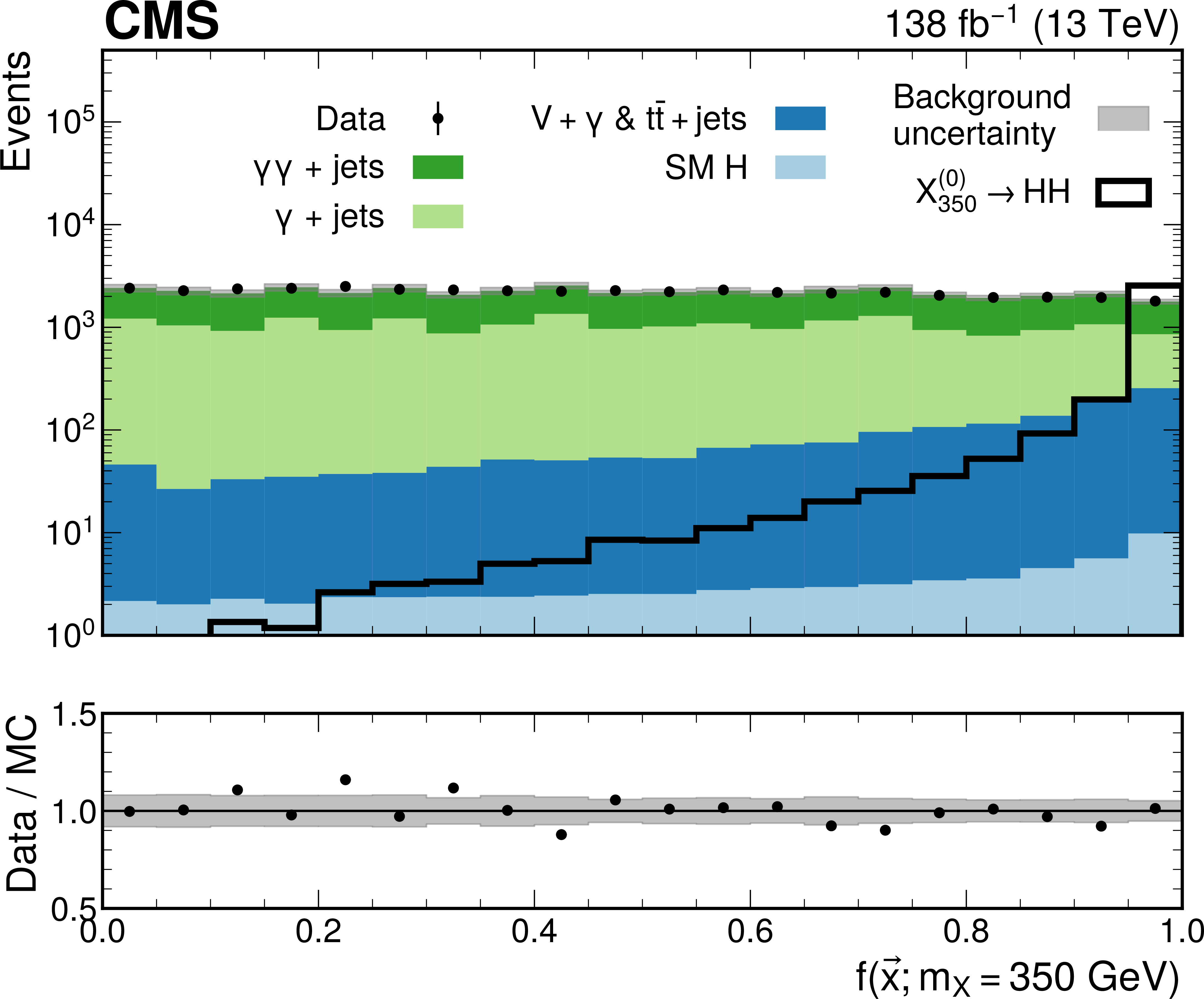
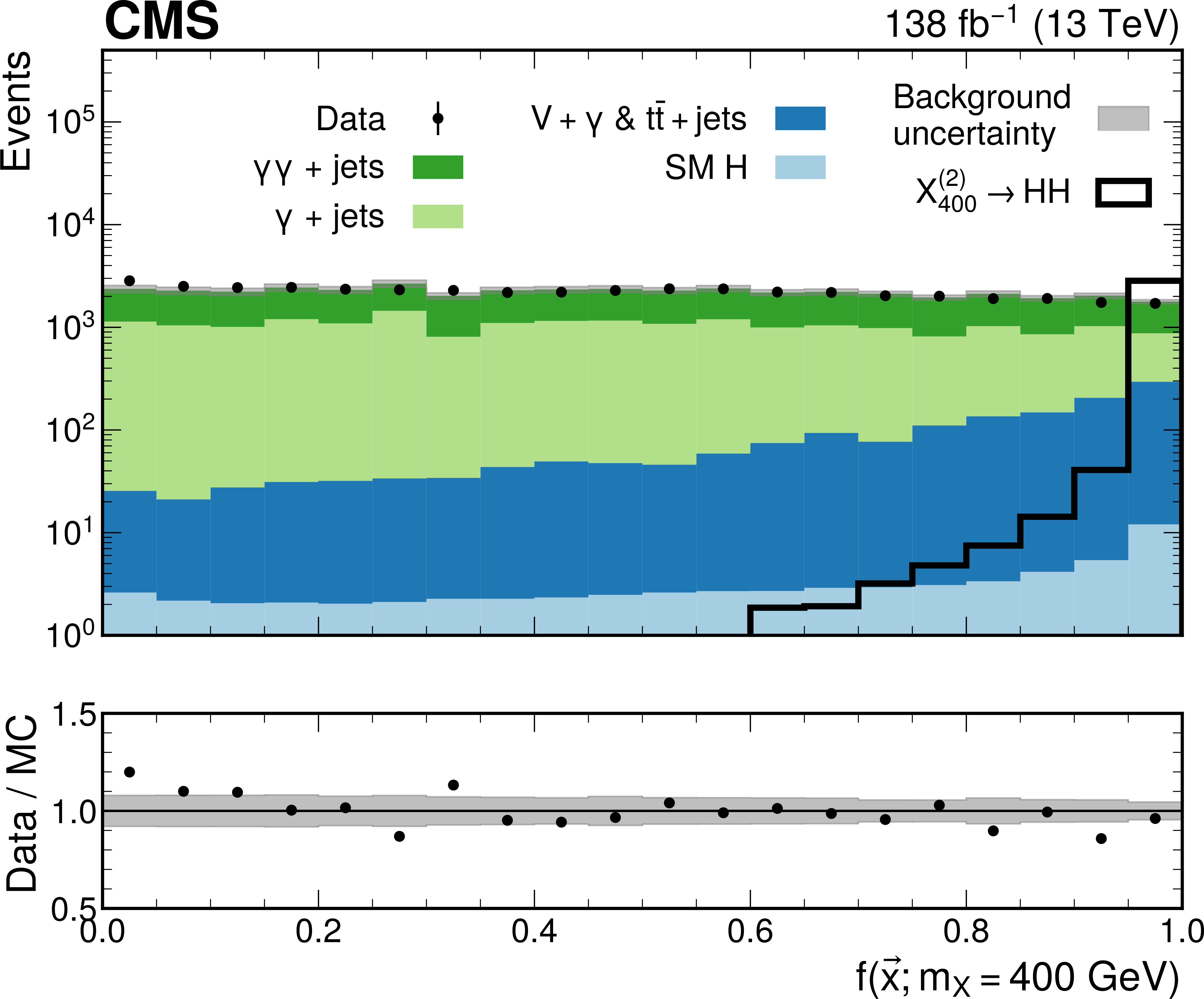
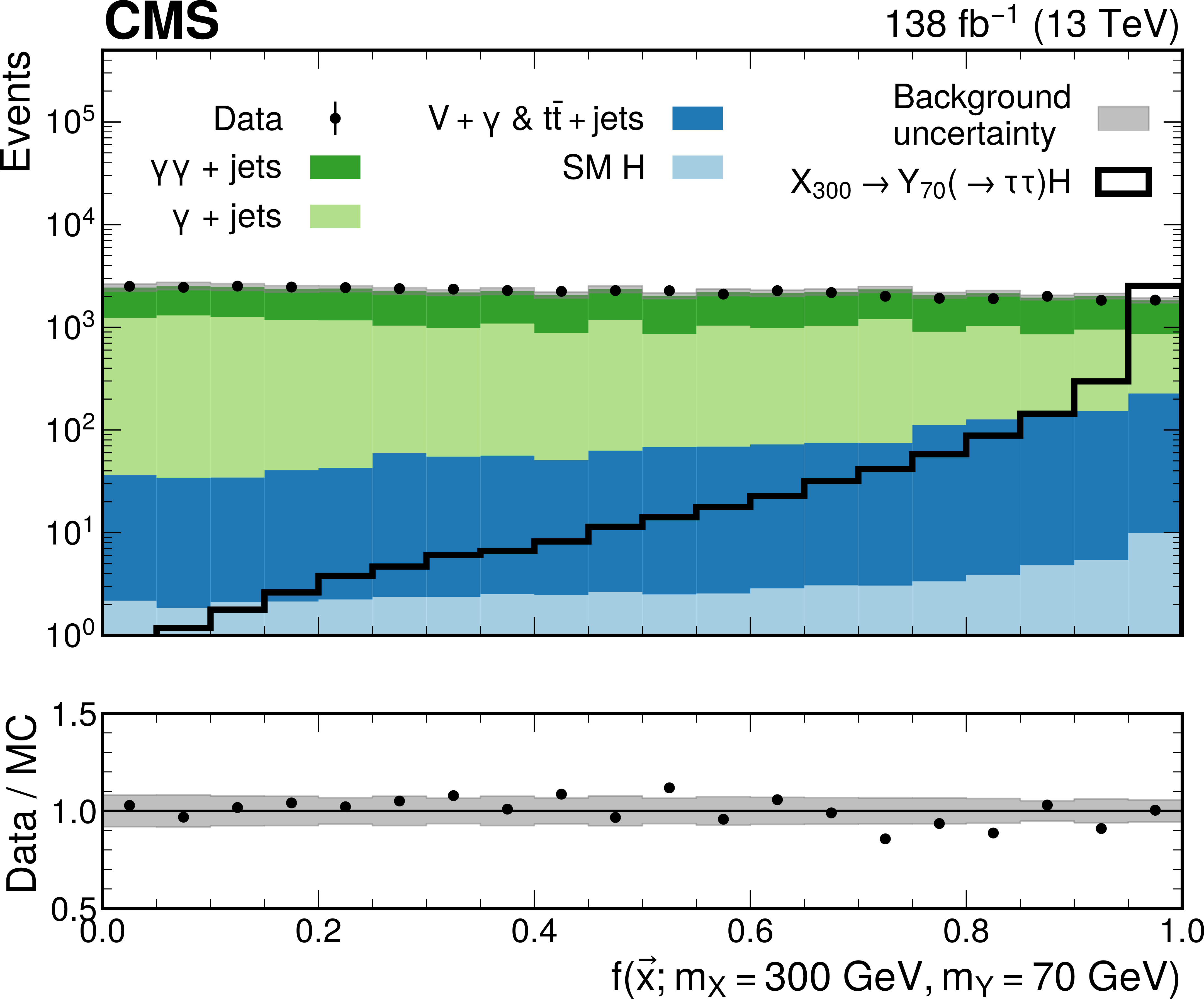
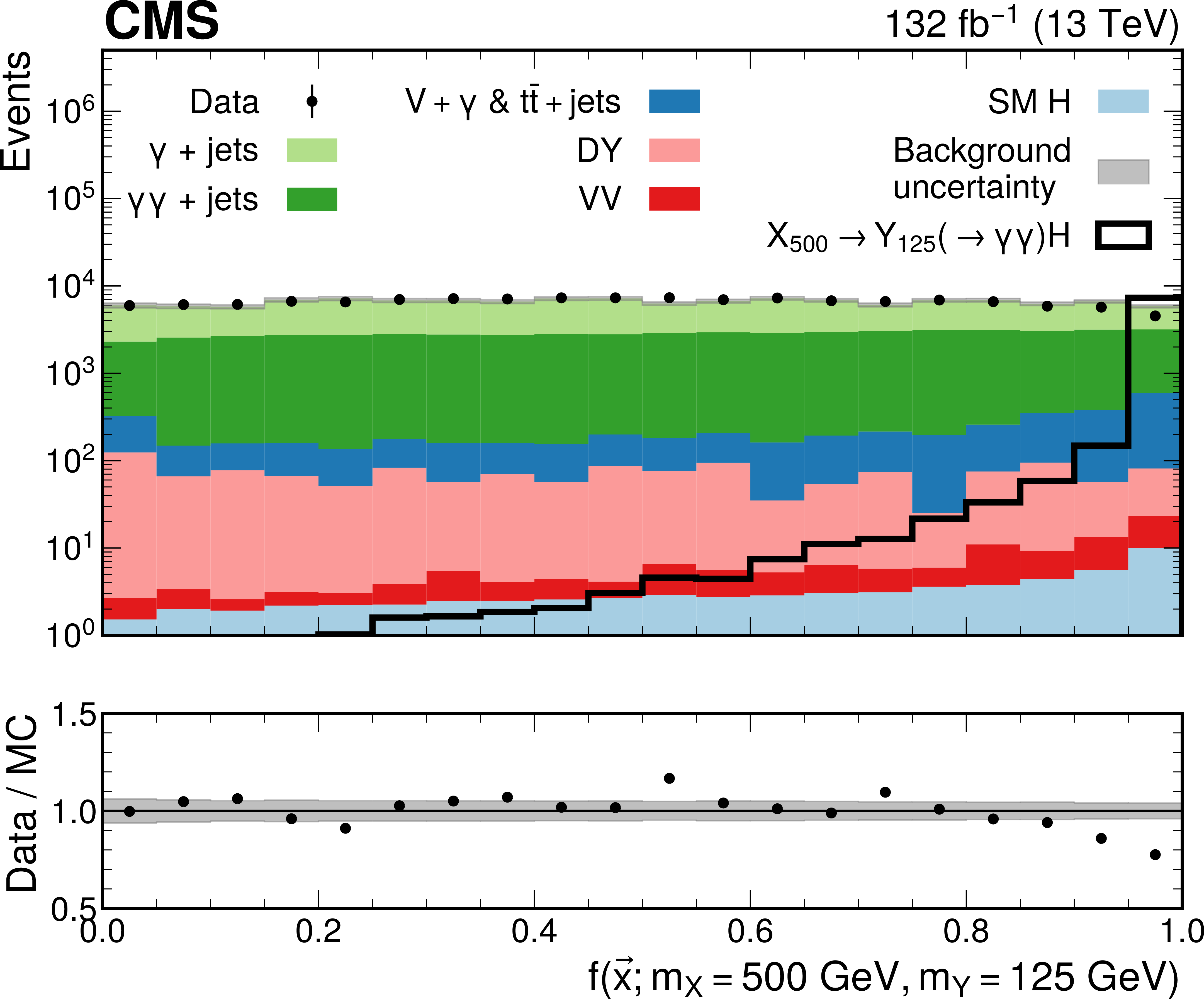
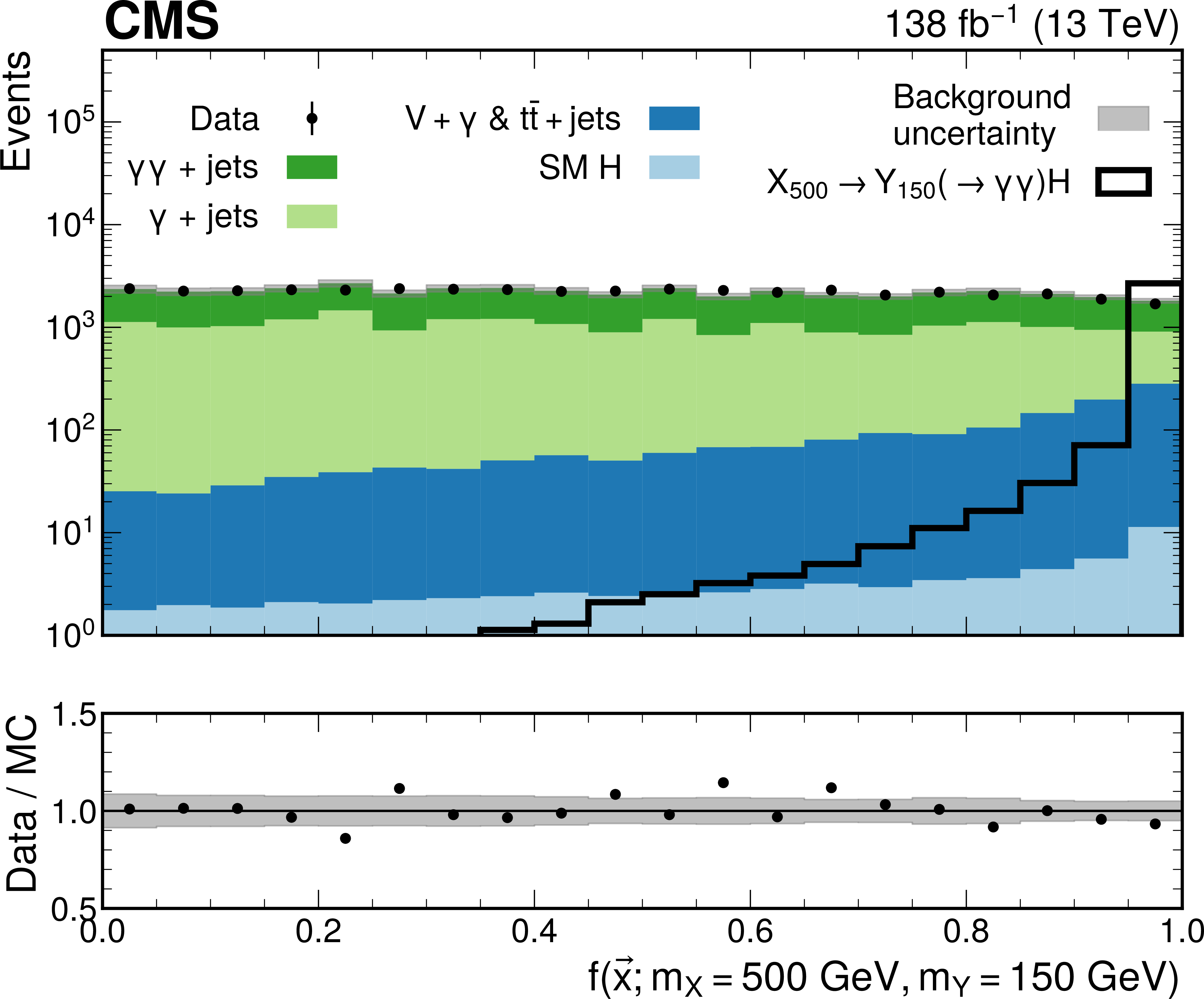
Transformed output of the pNNs used in the $ \mathrm{X}{(0)} \to \mathrm{H}\mathrm{H} $ (upper left), $ \mathrm{X}{(2)} \to \mathrm{H}\mathrm{H} $ (upper right), $ \mathrm{X} \to \mathrm{Y} (\tau\tau)\mathrm{H}(\gamma\gamma) $ (middle), low-mass $ \mathrm{X} \to \mathrm{Y} (\gamma\gamma)\mathrm{H}(\tau\tau) $ (lower left) and high-mass $ \mathrm{X} \to \mathrm{Y} (\gamma\gamma)\mathrm{H}(\tau\tau) $ (lower right) searches. The pNNs are evaluated at the mass points where the largest excess with respect to the background-only hypothesis is observed. If the MC simulation at this mass point is not available, then the sample produced at a mass point closest to the excess is shown. The filled histograms represent the background simulation, and the data are shown by the black points. The ``SM H'' process includes $ \mathrm{g}\mathrm{g}\mathrm{H} $, $ \mathrm{VBF} $, VH, and $ {\mathrm{t}\overline{\mathrm{t}}} \mathrm{H} $, and the $ {\mathrm{t}\overline{\mathrm{t}}} + \text{jets} $ process also includes the $ {\mathrm{t}\overline{\mathrm{t}}} + \gamma $ and $ {\mathrm{t}\overline{\mathrm{t}}} + \gamma\gamma $ processes. The targeted signal distributions for which the pNN is evaluated are shown by the black open histograms. The background MC simulation is normalized to data and the signal is normalized to an arbitrary cross section for representation purposes. The ratio of the data to the sum of the background predictions is shown in the lower panel. Statistical MC uncertainties for the background are represented by the gray shaded bands. |
png pdf |
Figure 5-a:
Transformed output of the pNNs used in the $ \mathrm{X}{(0)} \to \mathrm{H}\mathrm{H} $ (upper left), $ \mathrm{X}{(2)} \to \mathrm{H}\mathrm{H} $ (upper right), $ \mathrm{X} \to \mathrm{Y} (\tau\tau)\mathrm{H}(\gamma\gamma) $ (middle), low-mass $ \mathrm{X} \to \mathrm{Y} (\gamma\gamma)\mathrm{H}(\tau\tau) $ (lower left) and high-mass $ \mathrm{X} \to \mathrm{Y} (\gamma\gamma)\mathrm{H}(\tau\tau) $ (lower right) searches. The pNNs are evaluated at the mass points where the largest excess with respect to the background-only hypothesis is observed. If the MC simulation at this mass point is not available, then the sample produced at a mass point closest to the excess is shown. The filled histograms represent the background simulation, and the data are shown by the black points. The ``SM H'' process includes $ \mathrm{g}\mathrm{g}\mathrm{H} $, $ \mathrm{VBF} $, VH, and $ {\mathrm{t}\overline{\mathrm{t}}} \mathrm{H} $, and the $ {\mathrm{t}\overline{\mathrm{t}}} + \text{jets} $ process also includes the $ {\mathrm{t}\overline{\mathrm{t}}} + \gamma $ and $ {\mathrm{t}\overline{\mathrm{t}}} + \gamma\gamma $ processes. The targeted signal distributions for which the pNN is evaluated are shown by the black open histograms. The background MC simulation is normalized to data and the signal is normalized to an arbitrary cross section for representation purposes. The ratio of the data to the sum of the background predictions is shown in the lower panel. Statistical MC uncertainties for the background are represented by the gray shaded bands. |
png pdf |
Figure 5-b:
Transformed output of the pNNs used in the $ \mathrm{X}{(0)} \to \mathrm{H}\mathrm{H} $ (upper left), $ \mathrm{X}{(2)} \to \mathrm{H}\mathrm{H} $ (upper right), $ \mathrm{X} \to \mathrm{Y} (\tau\tau)\mathrm{H}(\gamma\gamma) $ (middle), low-mass $ \mathrm{X} \to \mathrm{Y} (\gamma\gamma)\mathrm{H}(\tau\tau) $ (lower left) and high-mass $ \mathrm{X} \to \mathrm{Y} (\gamma\gamma)\mathrm{H}(\tau\tau) $ (lower right) searches. The pNNs are evaluated at the mass points where the largest excess with respect to the background-only hypothesis is observed. If the MC simulation at this mass point is not available, then the sample produced at a mass point closest to the excess is shown. The filled histograms represent the background simulation, and the data are shown by the black points. The ``SM H'' process includes $ \mathrm{g}\mathrm{g}\mathrm{H} $, $ \mathrm{VBF} $, VH, and $ {\mathrm{t}\overline{\mathrm{t}}} \mathrm{H} $, and the $ {\mathrm{t}\overline{\mathrm{t}}} + \text{jets} $ process also includes the $ {\mathrm{t}\overline{\mathrm{t}}} + \gamma $ and $ {\mathrm{t}\overline{\mathrm{t}}} + \gamma\gamma $ processes. The targeted signal distributions for which the pNN is evaluated are shown by the black open histograms. The background MC simulation is normalized to data and the signal is normalized to an arbitrary cross section for representation purposes. The ratio of the data to the sum of the background predictions is shown in the lower panel. Statistical MC uncertainties for the background are represented by the gray shaded bands. |
png pdf |
Figure 5-c:
Transformed output of the pNNs used in the $ \mathrm{X}{(0)} \to \mathrm{H}\mathrm{H} $ (upper left), $ \mathrm{X}{(2)} \to \mathrm{H}\mathrm{H} $ (upper right), $ \mathrm{X} \to \mathrm{Y} (\tau\tau)\mathrm{H}(\gamma\gamma) $ (middle), low-mass $ \mathrm{X} \to \mathrm{Y} (\gamma\gamma)\mathrm{H}(\tau\tau) $ (lower left) and high-mass $ \mathrm{X} \to \mathrm{Y} (\gamma\gamma)\mathrm{H}(\tau\tau) $ (lower right) searches. The pNNs are evaluated at the mass points where the largest excess with respect to the background-only hypothesis is observed. If the MC simulation at this mass point is not available, then the sample produced at a mass point closest to the excess is shown. The filled histograms represent the background simulation, and the data are shown by the black points. The ``SM H'' process includes $ \mathrm{g}\mathrm{g}\mathrm{H} $, $ \mathrm{VBF} $, VH, and $ {\mathrm{t}\overline{\mathrm{t}}} \mathrm{H} $, and the $ {\mathrm{t}\overline{\mathrm{t}}} + \text{jets} $ process also includes the $ {\mathrm{t}\overline{\mathrm{t}}} + \gamma $ and $ {\mathrm{t}\overline{\mathrm{t}}} + \gamma\gamma $ processes. The targeted signal distributions for which the pNN is evaluated are shown by the black open histograms. The background MC simulation is normalized to data and the signal is normalized to an arbitrary cross section for representation purposes. The ratio of the data to the sum of the background predictions is shown in the lower panel. Statistical MC uncertainties for the background are represented by the gray shaded bands. |
png pdf |
Figure 5-d:
Transformed output of the pNNs used in the $ \mathrm{X}{(0)} \to \mathrm{H}\mathrm{H} $ (upper left), $ \mathrm{X}{(2)} \to \mathrm{H}\mathrm{H} $ (upper right), $ \mathrm{X} \to \mathrm{Y} (\tau\tau)\mathrm{H}(\gamma\gamma) $ (middle), low-mass $ \mathrm{X} \to \mathrm{Y} (\gamma\gamma)\mathrm{H}(\tau\tau) $ (lower left) and high-mass $ \mathrm{X} \to \mathrm{Y} (\gamma\gamma)\mathrm{H}(\tau\tau) $ (lower right) searches. The pNNs are evaluated at the mass points where the largest excess with respect to the background-only hypothesis is observed. If the MC simulation at this mass point is not available, then the sample produced at a mass point closest to the excess is shown. The filled histograms represent the background simulation, and the data are shown by the black points. The ``SM H'' process includes $ \mathrm{g}\mathrm{g}\mathrm{H} $, $ \mathrm{VBF} $, VH, and $ {\mathrm{t}\overline{\mathrm{t}}} \mathrm{H} $, and the $ {\mathrm{t}\overline{\mathrm{t}}} + \text{jets} $ process also includes the $ {\mathrm{t}\overline{\mathrm{t}}} + \gamma $ and $ {\mathrm{t}\overline{\mathrm{t}}} + \gamma\gamma $ processes. The targeted signal distributions for which the pNN is evaluated are shown by the black open histograms. The background MC simulation is normalized to data and the signal is normalized to an arbitrary cross section for representation purposes. The ratio of the data to the sum of the background predictions is shown in the lower panel. Statistical MC uncertainties for the background are represented by the gray shaded bands. |
png pdf |
Figure 5-e:
Transformed output of the pNNs used in the $ \mathrm{X}{(0)} \to \mathrm{H}\mathrm{H} $ (upper left), $ \mathrm{X}{(2)} \to \mathrm{H}\mathrm{H} $ (upper right), $ \mathrm{X} \to \mathrm{Y} (\tau\tau)\mathrm{H}(\gamma\gamma) $ (middle), low-mass $ \mathrm{X} \to \mathrm{Y} (\gamma\gamma)\mathrm{H}(\tau\tau) $ (lower left) and high-mass $ \mathrm{X} \to \mathrm{Y} (\gamma\gamma)\mathrm{H}(\tau\tau) $ (lower right) searches. The pNNs are evaluated at the mass points where the largest excess with respect to the background-only hypothesis is observed. If the MC simulation at this mass point is not available, then the sample produced at a mass point closest to the excess is shown. The filled histograms represent the background simulation, and the data are shown by the black points. The ``SM H'' process includes $ \mathrm{g}\mathrm{g}\mathrm{H} $, $ \mathrm{VBF} $, VH, and $ {\mathrm{t}\overline{\mathrm{t}}} \mathrm{H} $, and the $ {\mathrm{t}\overline{\mathrm{t}}} + \text{jets} $ process also includes the $ {\mathrm{t}\overline{\mathrm{t}}} + \gamma $ and $ {\mathrm{t}\overline{\mathrm{t}}} + \gamma\gamma $ processes. The targeted signal distributions for which the pNN is evaluated are shown by the black open histograms. The background MC simulation is normalized to data and the signal is normalized to an arbitrary cross section for representation purposes. The ratio of the data to the sum of the background predictions is shown in the lower panel. Statistical MC uncertainties for the background are represented by the gray shaded bands. |
png pdf |
Figure 6:
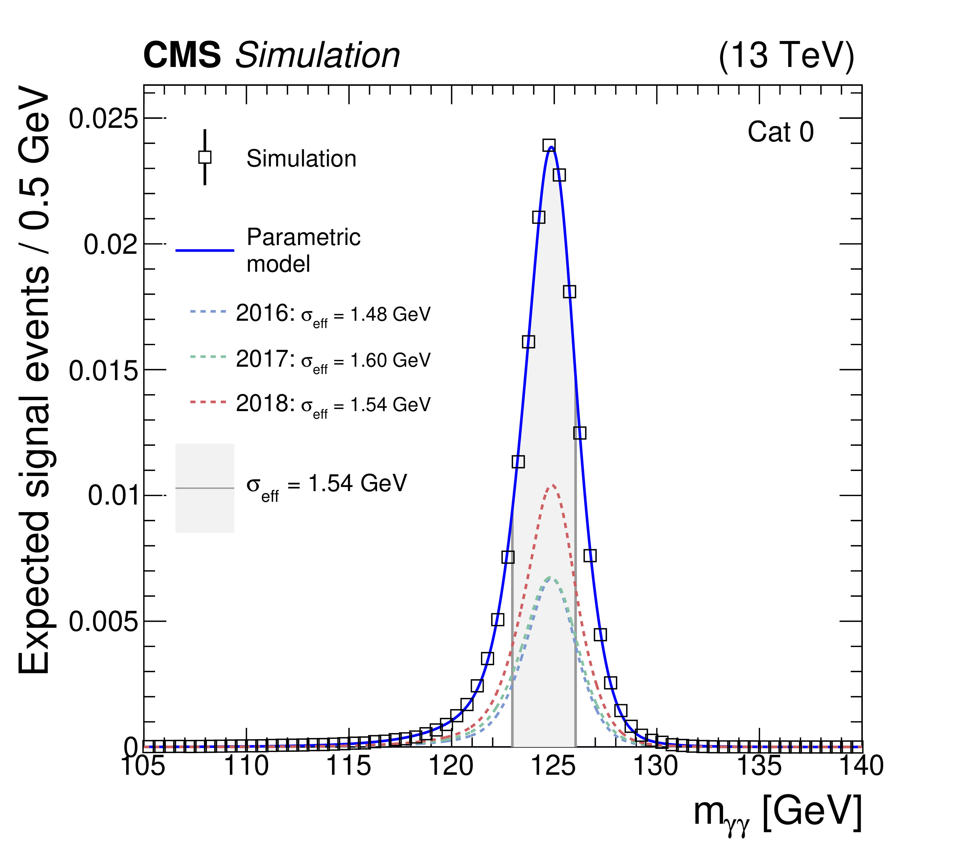
Signal model for the purest analysis category in the nonresonant search, shown for each year of simulated data, and for the sum of all years together. The open squares represent the weighted simulated events, whose uncertainty are smaller than the marker size, and the blue line is the corresponding model. The gray shaded areas correspond to the $ \sigma_{\text{eff}} $. The contribution from each year of data taking is illustrated with the dotted lines. |
png pdf |
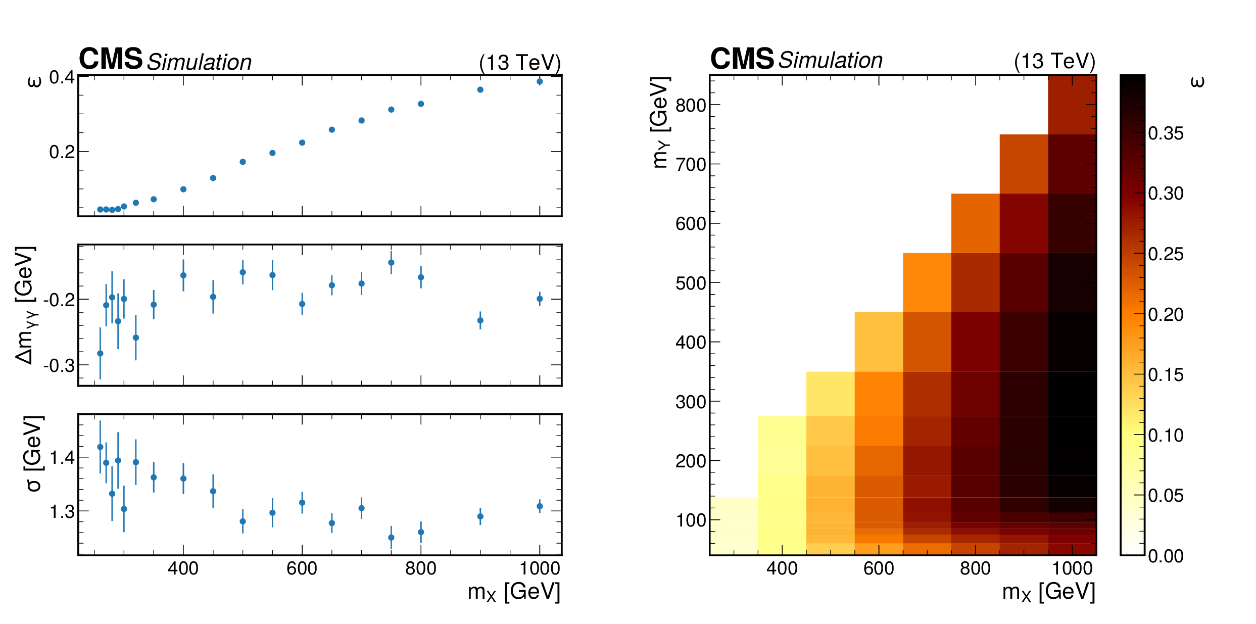
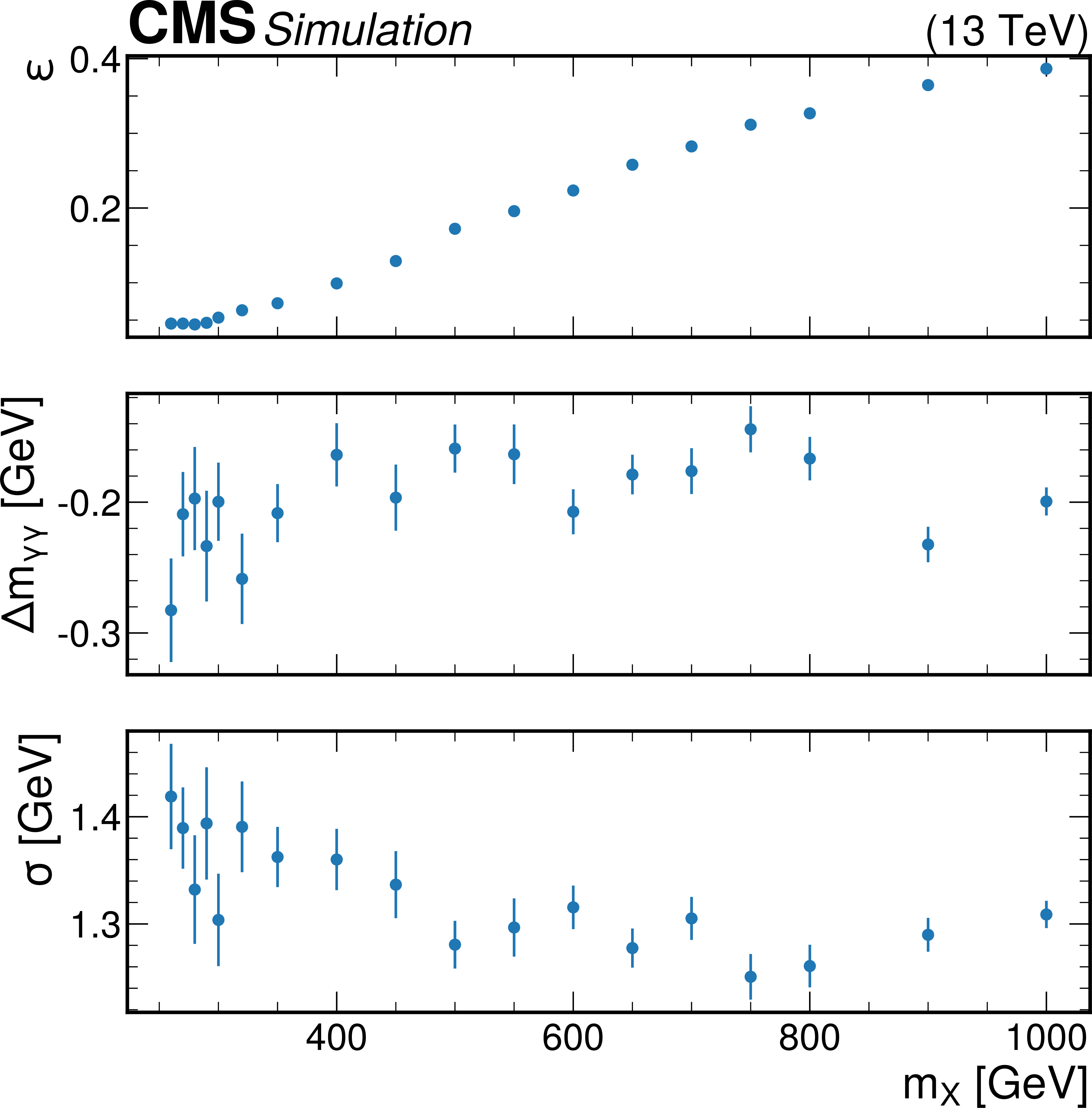
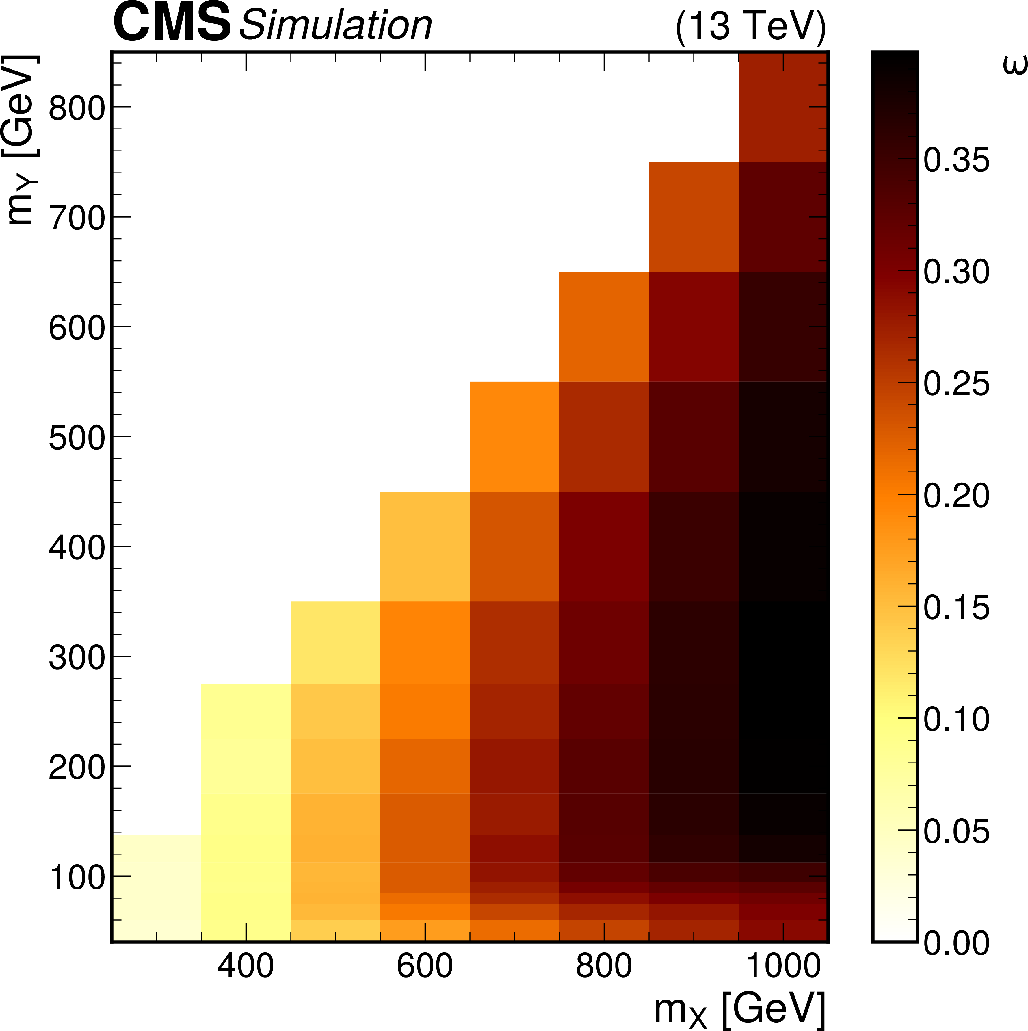
Figure 7:
Signal efficiency, $ \epsilon $, and interpolated DCB shape parameters, $ \Delta m_{\gamma\gamma} $ and $ \sigma $, for the highest purity analysis category in the $ \mathrm{X}{(2)} \to \mathrm{H}\mathrm{H} $ search, as functions of $ m_{\mathrm{X}} $ (left). The first shape parameter, $ \Delta m_{\gamma\gamma} $, is defined as $ \overline{m}_{\gamma\gamma}-m_{\mathrm{H}} $. Signal efficiency in the ($ m_{\mathrm{X}} $, $ m_{\mathrm{Y} } $) plane for the highest purity analysis category in the $ \mathrm{X} \to \mathrm{Y} (\tau\tau)\mathrm{H}(\gamma\gamma) $ search (right). |
png pdf |
Figure 7-a:
Signal efficiency, $ \epsilon $, and interpolated DCB shape parameters, $ \Delta m_{\gamma\gamma} $ and $ \sigma $, for the highest purity analysis category in the $ \mathrm{X}{(2)} \to \mathrm{H}\mathrm{H} $ search, as functions of $ m_{\mathrm{X}} $ (left). The first shape parameter, $ \Delta m_{\gamma\gamma} $, is defined as $ \overline{m}_{\gamma\gamma}-m_{\mathrm{H}} $. Signal efficiency in the ($ m_{\mathrm{X}} $, $ m_{\mathrm{Y} } $) plane for the highest purity analysis category in the $ \mathrm{X} \to \mathrm{Y} (\tau\tau)\mathrm{H}(\gamma\gamma) $ search (right). |
png pdf |
Figure 7-b:
Signal efficiency, $ \epsilon $, and interpolated DCB shape parameters, $ \Delta m_{\gamma\gamma} $ and $ \sigma $, for the highest purity analysis category in the $ \mathrm{X}{(2)} \to \mathrm{H}\mathrm{H} $ search, as functions of $ m_{\mathrm{X}} $ (left). The first shape parameter, $ \Delta m_{\gamma\gamma} $, is defined as $ \overline{m}_{\gamma\gamma}-m_{\mathrm{H}} $. Signal efficiency in the ($ m_{\mathrm{X}} $, $ m_{\mathrm{Y} } $) plane for the highest purity analysis category in the $ \mathrm{X} \to \mathrm{Y} (\tau\tau)\mathrm{H}(\gamma\gamma) $ search (right). |
png pdf |
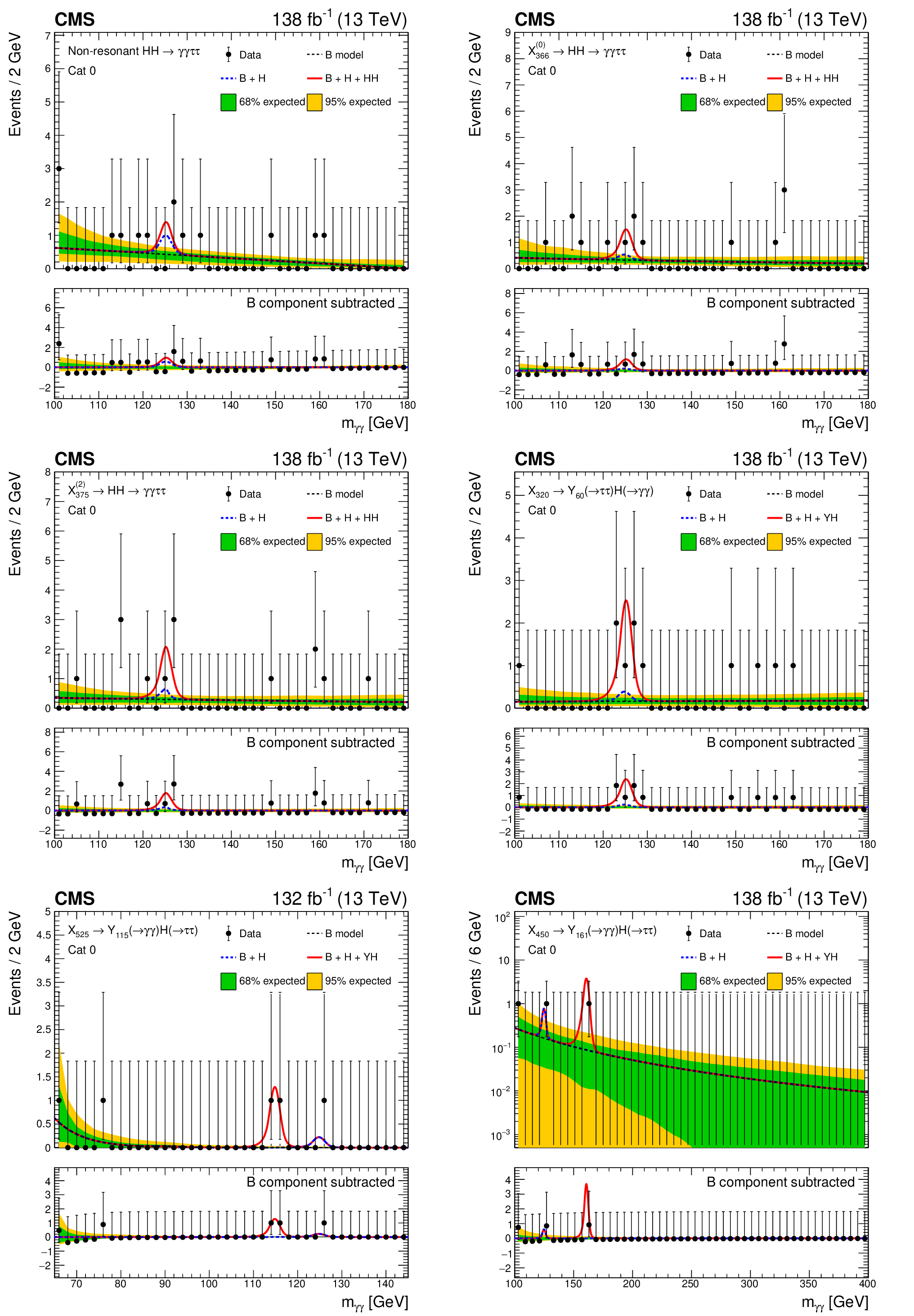
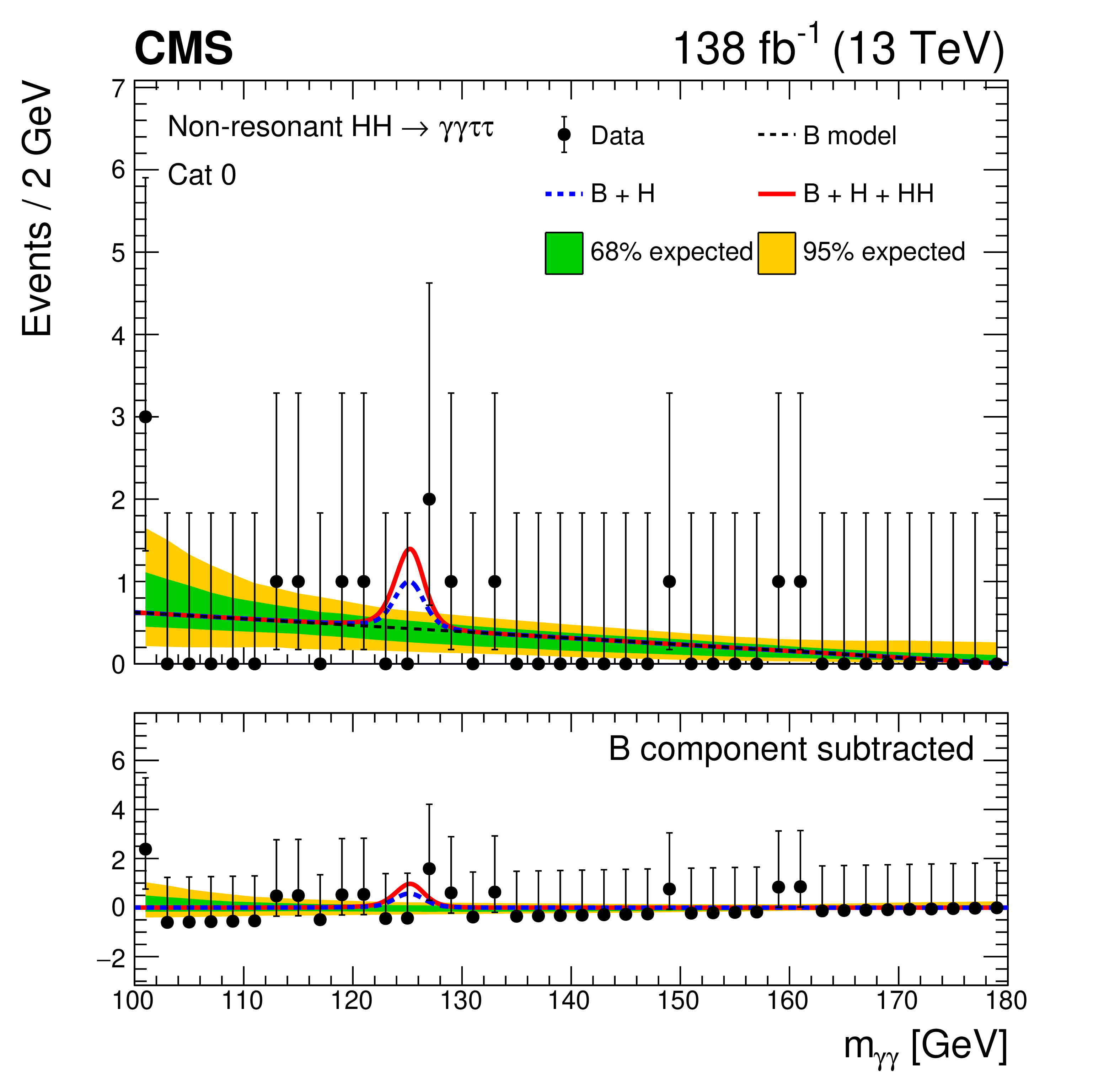
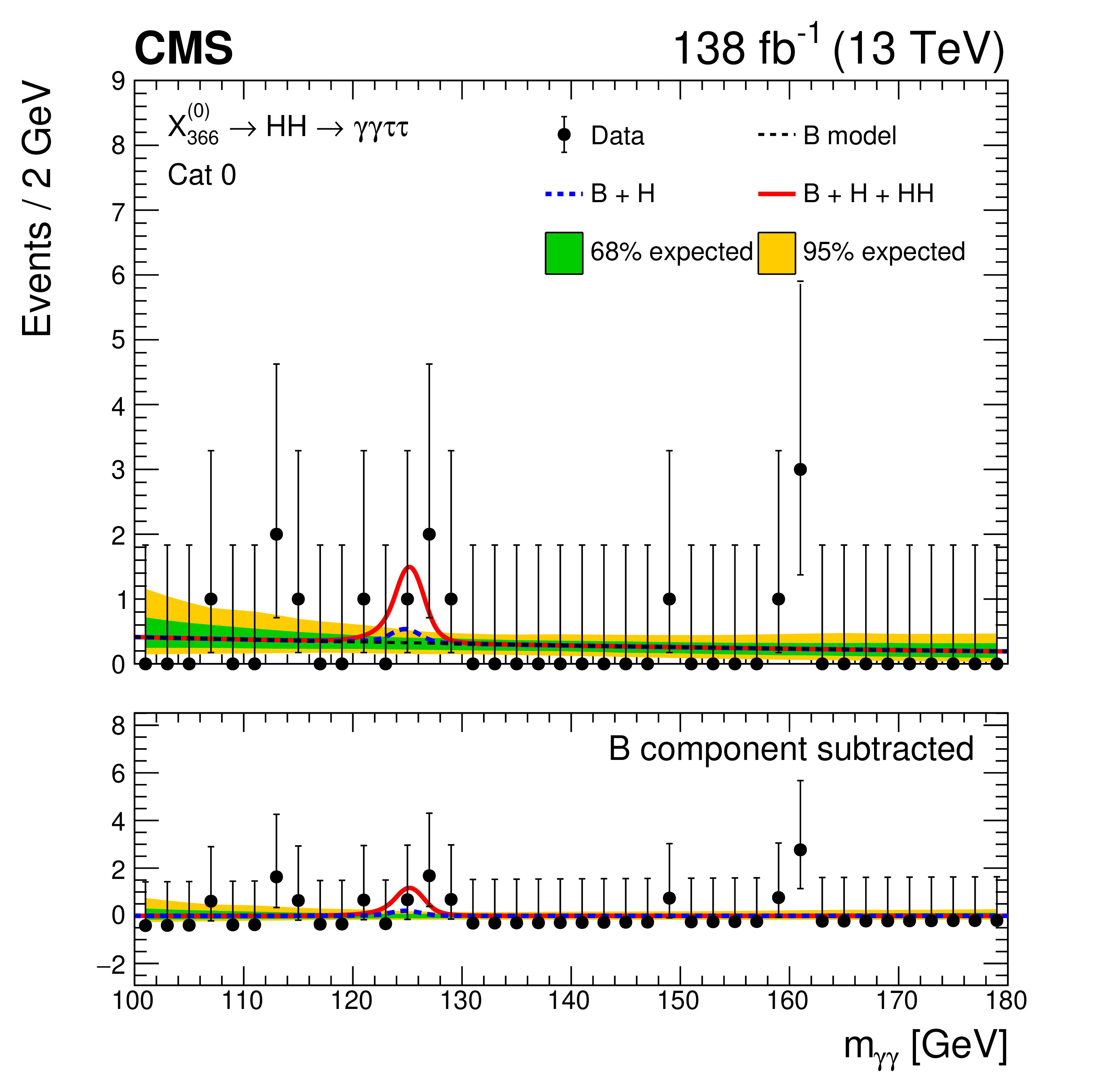
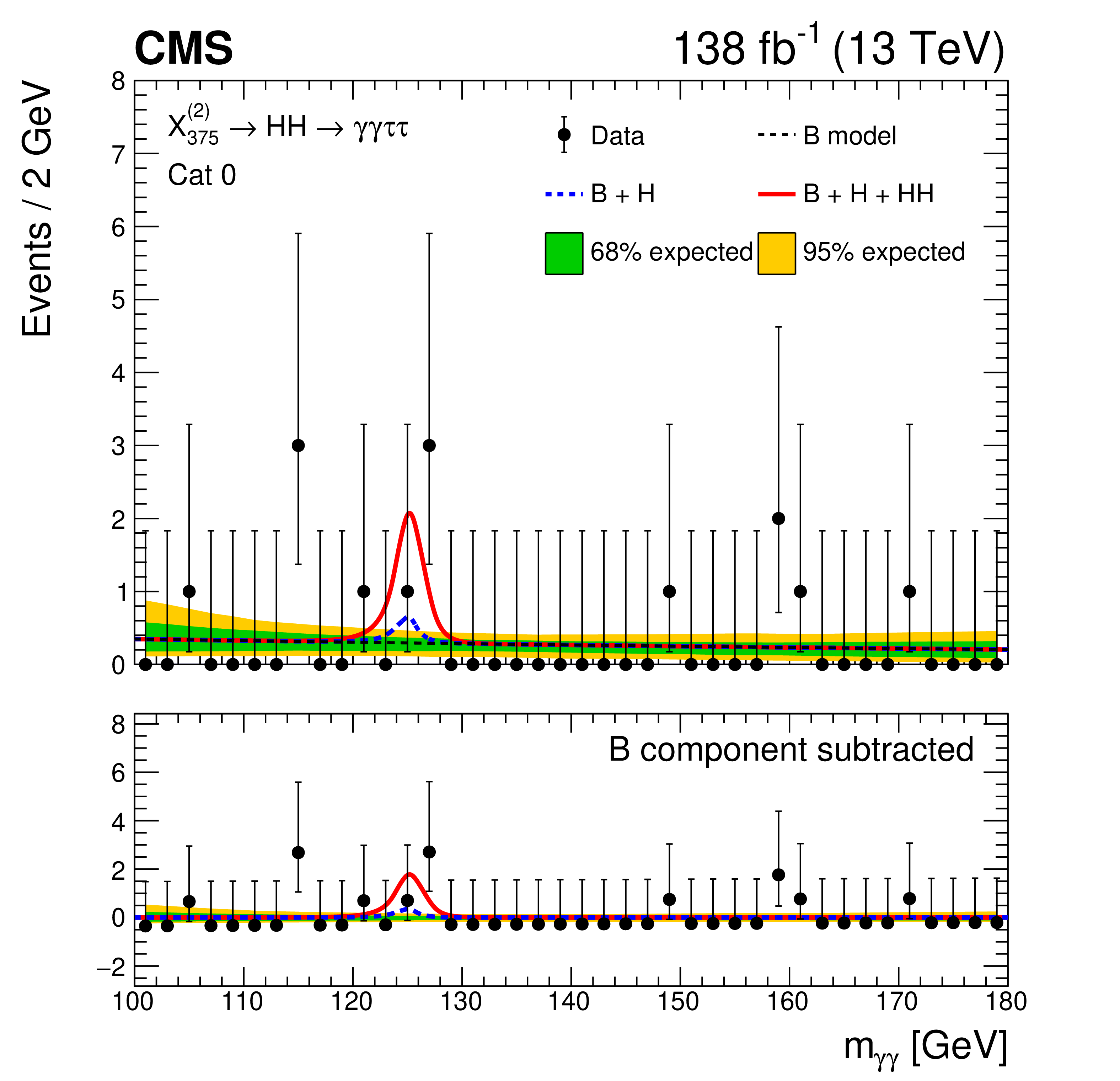
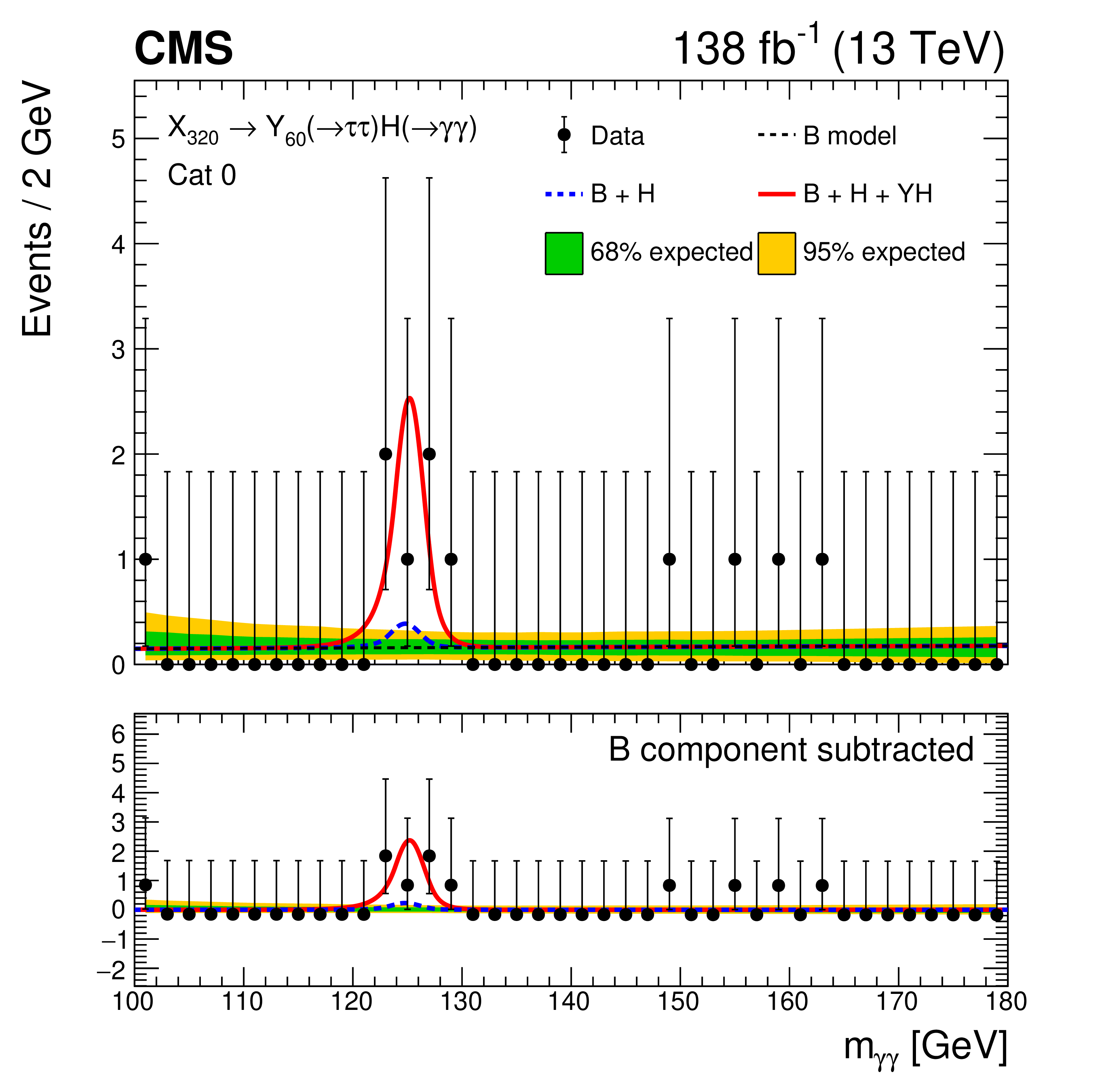
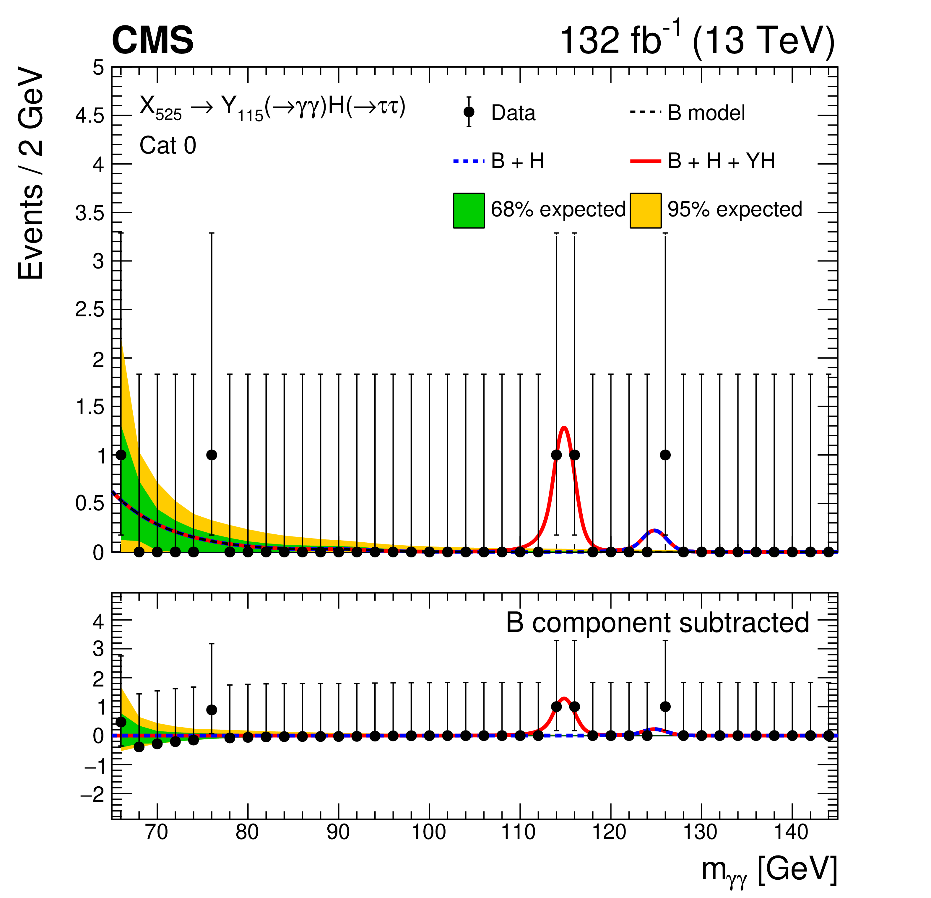
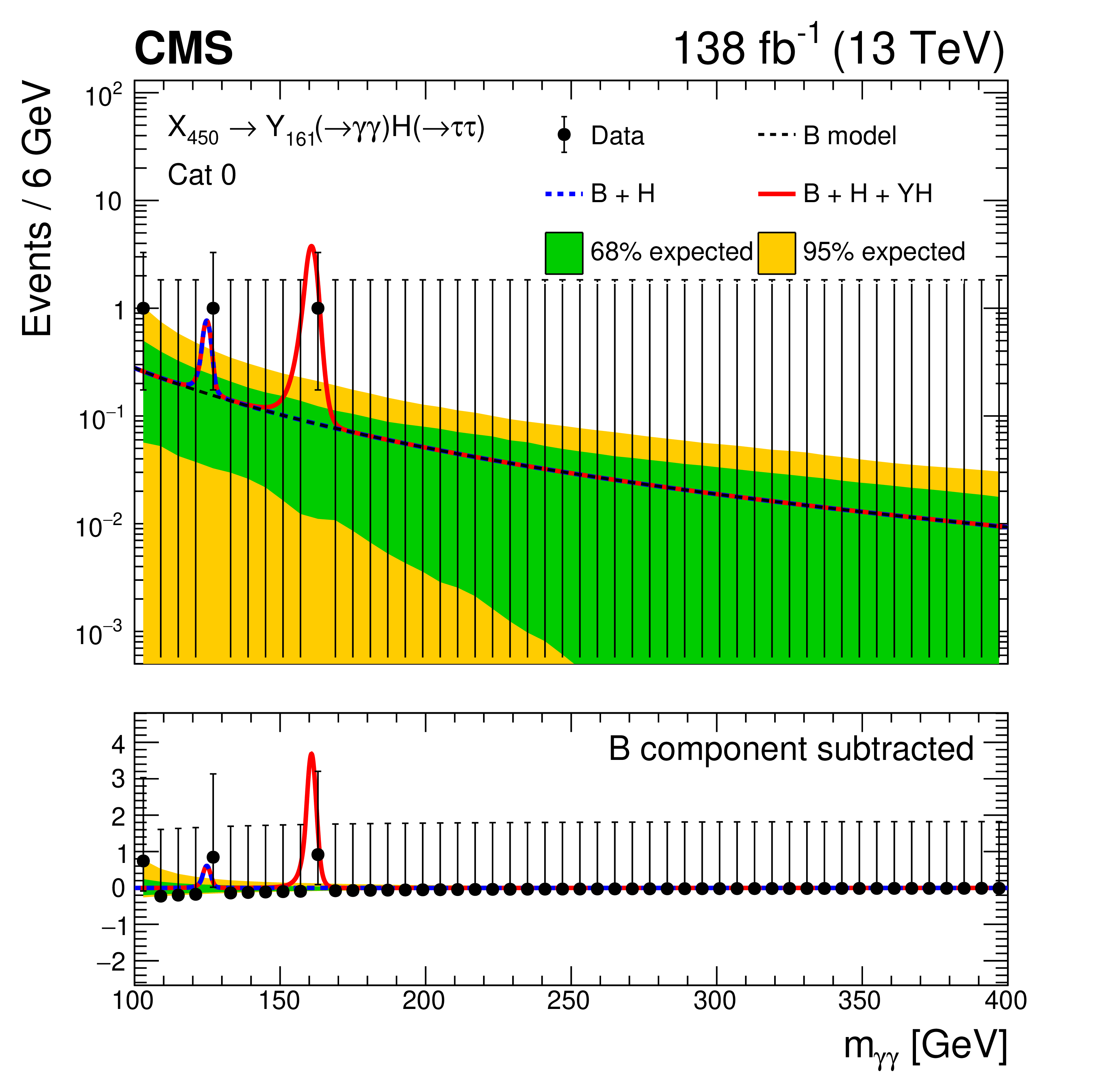
Figure 8:
Data points (black) and signal-plus-background models for the most sensitive analysis category in each search are shown: nonresonant (upper left), $ \mathrm{X}{(0)} \to \mathrm{H}\mathrm{H} $ (upper right), $ \mathrm{X}{(2)} \to \mathrm{H}\mathrm{H} $ (middle left), $ \mathrm{X} \to \mathrm{Y} (\tau\tau)\mathrm{H}(\gamma\gamma) $ (middle right), low-mass $ \mathrm{X} \to \mathrm{Y} (\gamma\gamma)\mathrm{H}(\tau\tau) $ (lower left) and the high-mass $ \mathrm{X} \to \mathrm{Y} (\gamma\gamma)\mathrm{H}(\tau\tau) $ (lower right). The analysis categories for the resonant searches correspond to the mass hypotheses where the largest excesses with respect to the background-only hypothesis are observed. The one (green) standard deviation and two (yellow) standard deviation bands show the uncertainties in the background component of the fit. The solid red line shows the sum of the fitted signal and background components, the solid blue line shows the continuum background and the background from single H production together, and the dashed black line shows only the continuum background component. The lower panel in each plot shows the residual signal yield after subtraction of the background. |
png pdf |
Figure 8-a:
Data points (black) and signal-plus-background models for the most sensitive analysis category in each search are shown: nonresonant (upper left), $ \mathrm{X}{(0)} \to \mathrm{H}\mathrm{H} $ (upper right), $ \mathrm{X}{(2)} \to \mathrm{H}\mathrm{H} $ (middle left), $ \mathrm{X} \to \mathrm{Y} (\tau\tau)\mathrm{H}(\gamma\gamma) $ (middle right), low-mass $ \mathrm{X} \to \mathrm{Y} (\gamma\gamma)\mathrm{H}(\tau\tau) $ (lower left) and the high-mass $ \mathrm{X} \to \mathrm{Y} (\gamma\gamma)\mathrm{H}(\tau\tau) $ (lower right). The analysis categories for the resonant searches correspond to the mass hypotheses where the largest excesses with respect to the background-only hypothesis are observed. The one (green) standard deviation and two (yellow) standard deviation bands show the uncertainties in the background component of the fit. The solid red line shows the sum of the fitted signal and background components, the solid blue line shows the continuum background and the background from single H production together, and the dashed black line shows only the continuum background component. The lower panel in each plot shows the residual signal yield after subtraction of the background. |
png pdf |
Figure 8-b:
Data points (black) and signal-plus-background models for the most sensitive analysis category in each search are shown: nonresonant (upper left), $ \mathrm{X}{(0)} \to \mathrm{H}\mathrm{H} $ (upper right), $ \mathrm{X}{(2)} \to \mathrm{H}\mathrm{H} $ (middle left), $ \mathrm{X} \to \mathrm{Y} (\tau\tau)\mathrm{H}(\gamma\gamma) $ (middle right), low-mass $ \mathrm{X} \to \mathrm{Y} (\gamma\gamma)\mathrm{H}(\tau\tau) $ (lower left) and the high-mass $ \mathrm{X} \to \mathrm{Y} (\gamma\gamma)\mathrm{H}(\tau\tau) $ (lower right). The analysis categories for the resonant searches correspond to the mass hypotheses where the largest excesses with respect to the background-only hypothesis are observed. The one (green) standard deviation and two (yellow) standard deviation bands show the uncertainties in the background component of the fit. The solid red line shows the sum of the fitted signal and background components, the solid blue line shows the continuum background and the background from single H production together, and the dashed black line shows only the continuum background component. The lower panel in each plot shows the residual signal yield after subtraction of the background. |
png pdf |
Figure 8-c:
Data points (black) and signal-plus-background models for the most sensitive analysis category in each search are shown: nonresonant (upper left), $ \mathrm{X}{(0)} \to \mathrm{H}\mathrm{H} $ (upper right), $ \mathrm{X}{(2)} \to \mathrm{H}\mathrm{H} $ (middle left), $ \mathrm{X} \to \mathrm{Y} (\tau\tau)\mathrm{H}(\gamma\gamma) $ (middle right), low-mass $ \mathrm{X} \to \mathrm{Y} (\gamma\gamma)\mathrm{H}(\tau\tau) $ (lower left) and the high-mass $ \mathrm{X} \to \mathrm{Y} (\gamma\gamma)\mathrm{H}(\tau\tau) $ (lower right). The analysis categories for the resonant searches correspond to the mass hypotheses where the largest excesses with respect to the background-only hypothesis are observed. The one (green) standard deviation and two (yellow) standard deviation bands show the uncertainties in the background component of the fit. The solid red line shows the sum of the fitted signal and background components, the solid blue line shows the continuum background and the background from single H production together, and the dashed black line shows only the continuum background component. The lower panel in each plot shows the residual signal yield after subtraction of the background. |
png pdf |
Figure 8-d:
Data points (black) and signal-plus-background models for the most sensitive analysis category in each search are shown: nonresonant (upper left), $ \mathrm{X}{(0)} \to \mathrm{H}\mathrm{H} $ (upper right), $ \mathrm{X}{(2)} \to \mathrm{H}\mathrm{H} $ (middle left), $ \mathrm{X} \to \mathrm{Y} (\tau\tau)\mathrm{H}(\gamma\gamma) $ (middle right), low-mass $ \mathrm{X} \to \mathrm{Y} (\gamma\gamma)\mathrm{H}(\tau\tau) $ (lower left) and the high-mass $ \mathrm{X} \to \mathrm{Y} (\gamma\gamma)\mathrm{H}(\tau\tau) $ (lower right). The analysis categories for the resonant searches correspond to the mass hypotheses where the largest excesses with respect to the background-only hypothesis are observed. The one (green) standard deviation and two (yellow) standard deviation bands show the uncertainties in the background component of the fit. The solid red line shows the sum of the fitted signal and background components, the solid blue line shows the continuum background and the background from single H production together, and the dashed black line shows only the continuum background component. The lower panel in each plot shows the residual signal yield after subtraction of the background. |
png pdf |
Figure 8-e:
Data points (black) and signal-plus-background models for the most sensitive analysis category in each search are shown: nonresonant (upper left), $ \mathrm{X}{(0)} \to \mathrm{H}\mathrm{H} $ (upper right), $ \mathrm{X}{(2)} \to \mathrm{H}\mathrm{H} $ (middle left), $ \mathrm{X} \to \mathrm{Y} (\tau\tau)\mathrm{H}(\gamma\gamma) $ (middle right), low-mass $ \mathrm{X} \to \mathrm{Y} (\gamma\gamma)\mathrm{H}(\tau\tau) $ (lower left) and the high-mass $ \mathrm{X} \to \mathrm{Y} (\gamma\gamma)\mathrm{H}(\tau\tau) $ (lower right). The analysis categories for the resonant searches correspond to the mass hypotheses where the largest excesses with respect to the background-only hypothesis are observed. The one (green) standard deviation and two (yellow) standard deviation bands show the uncertainties in the background component of the fit. The solid red line shows the sum of the fitted signal and background components, the solid blue line shows the continuum background and the background from single H production together, and the dashed black line shows only the continuum background component. The lower panel in each plot shows the residual signal yield after subtraction of the background. |
png pdf |
Figure 8-f:
Data points (black) and signal-plus-background models for the most sensitive analysis category in each search are shown: nonresonant (upper left), $ \mathrm{X}{(0)} \to \mathrm{H}\mathrm{H} $ (upper right), $ \mathrm{X}{(2)} \to \mathrm{H}\mathrm{H} $ (middle left), $ \mathrm{X} \to \mathrm{Y} (\tau\tau)\mathrm{H}(\gamma\gamma) $ (middle right), low-mass $ \mathrm{X} \to \mathrm{Y} (\gamma\gamma)\mathrm{H}(\tau\tau) $ (lower left) and the high-mass $ \mathrm{X} \to \mathrm{Y} (\gamma\gamma)\mathrm{H}(\tau\tau) $ (lower right). The analysis categories for the resonant searches correspond to the mass hypotheses where the largest excesses with respect to the background-only hypothesis are observed. The one (green) standard deviation and two (yellow) standard deviation bands show the uncertainties in the background component of the fit. The solid red line shows the sum of the fitted signal and background components, the solid blue line shows the continuum background and the background from single H production together, and the dashed black line shows only the continuum background component. The lower panel in each plot shows the residual signal yield after subtraction of the background. |
png pdf |
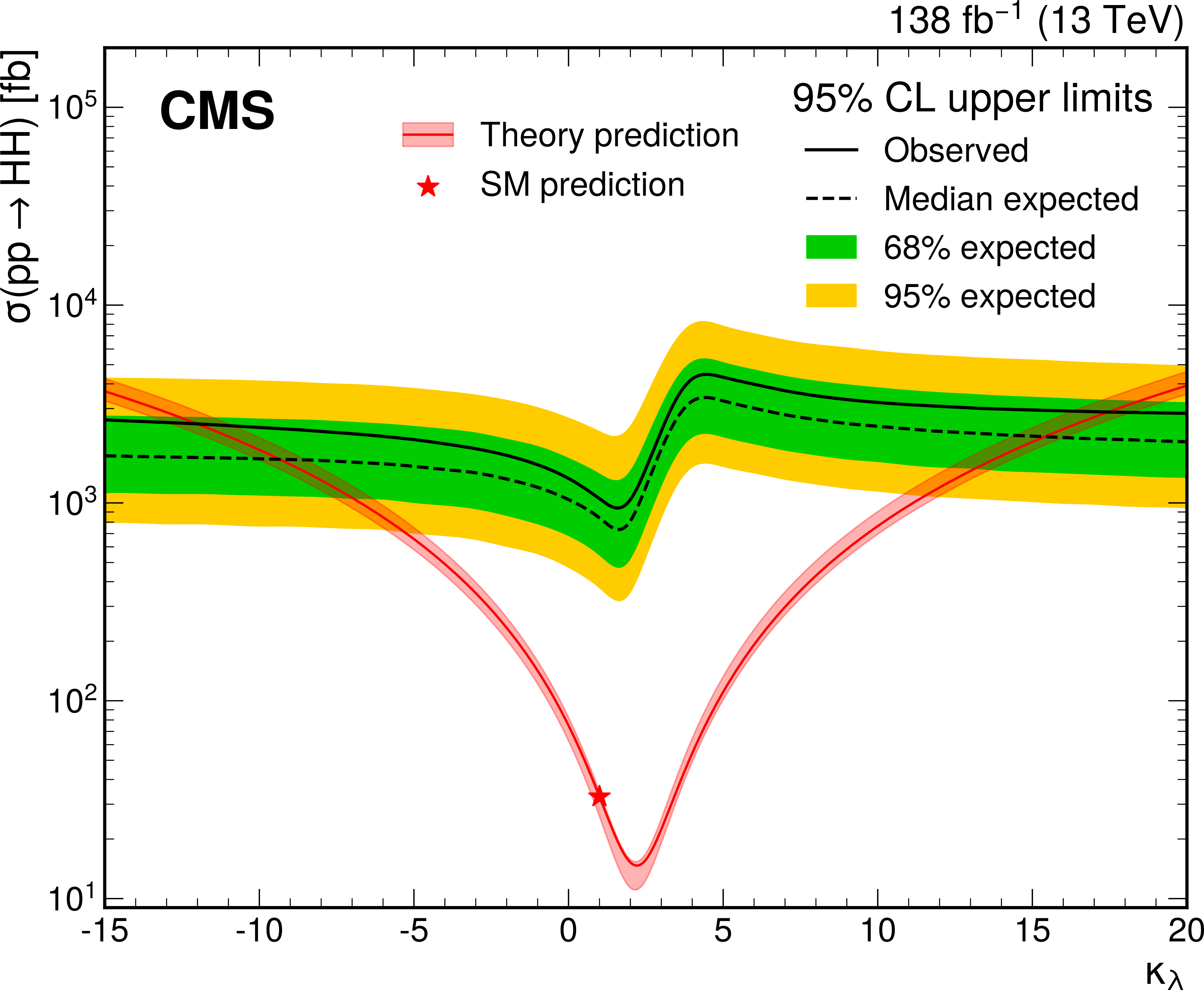
Figure 9:
Expected and observed upper limits on the nonresonant HH production cross section at 95% CL, obtained for different values of $ \kappa_\lambda $. The green and yellow bands represent the one and two standard deviations for the expected limit, respectively. The theoretical prediction with the uncertainty of the cross section as a function of $ \kappa_\lambda $ is shown by the red band. |
png pdf |
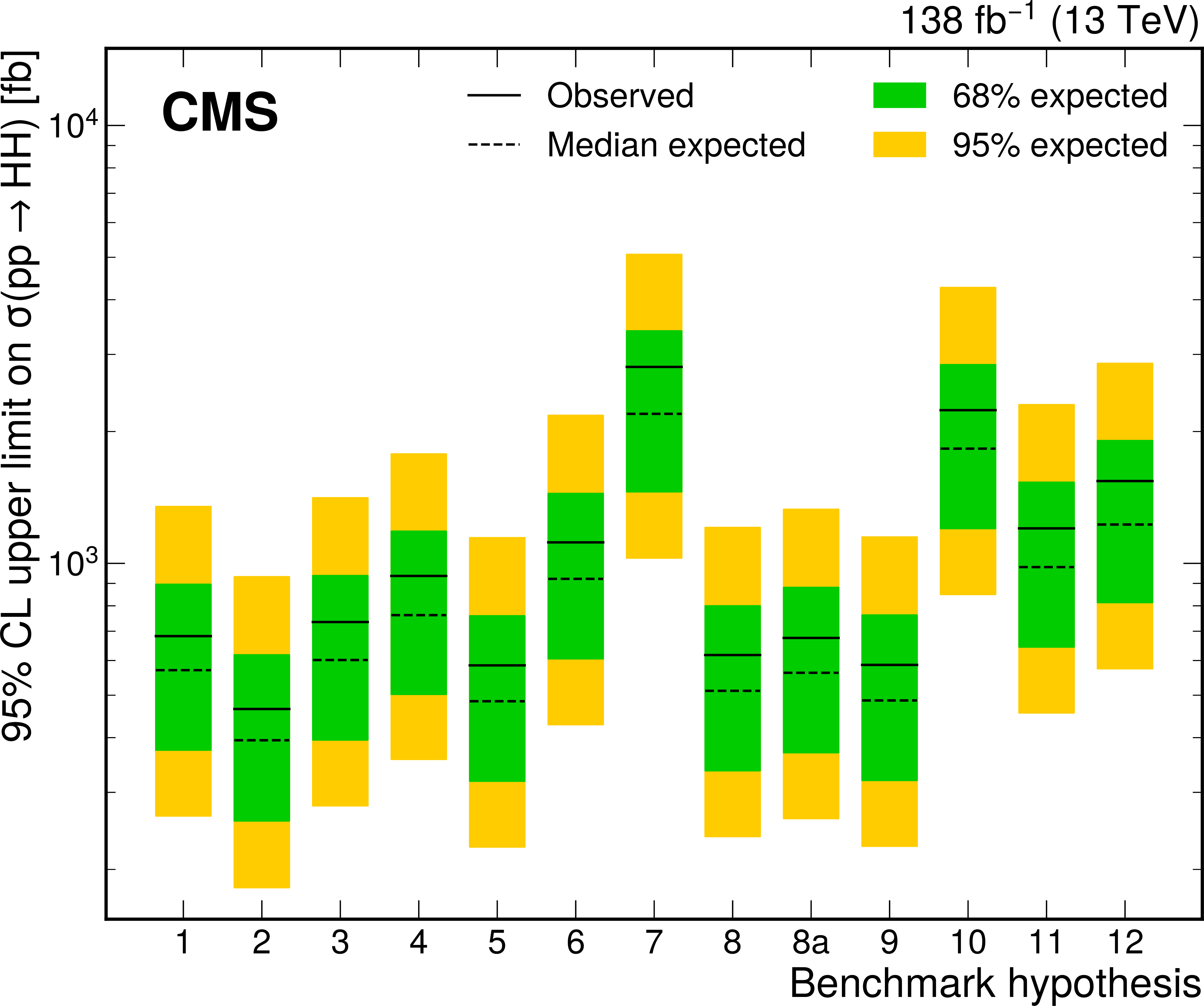
Figure 10:
Expected and observed upper limits on the nonresonant HH production cross section at 95% CL, for different thirteen BSM benchmark scenarios which consider different values of the couplings, $ \kappa_\lambda $, $ \kappa_\mathrm{t} $, $ c_{2\mathrm{g}} $, $ c_{\mathrm{g}} $, and $ c_2 $ (defined in Table 1). The green and yellow bands represent the one and two standard deviations for the expected limits, respectively. |
png pdf |
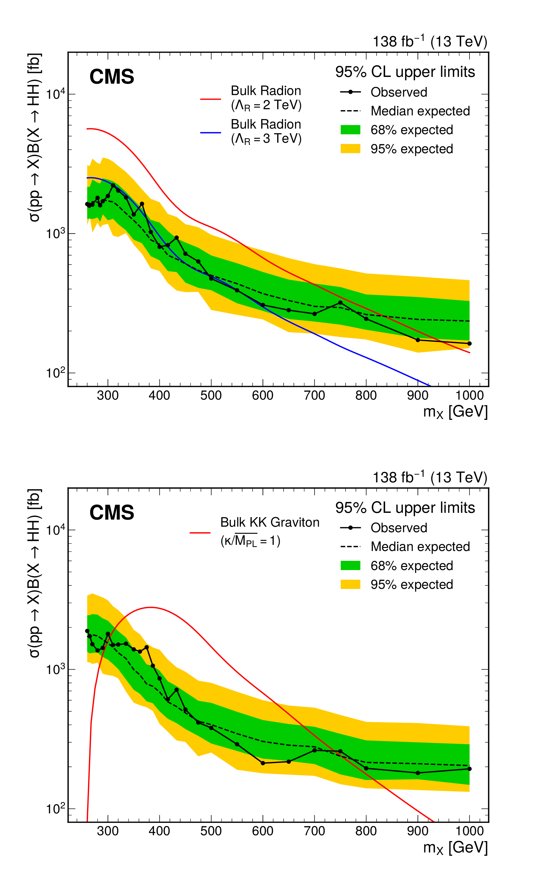
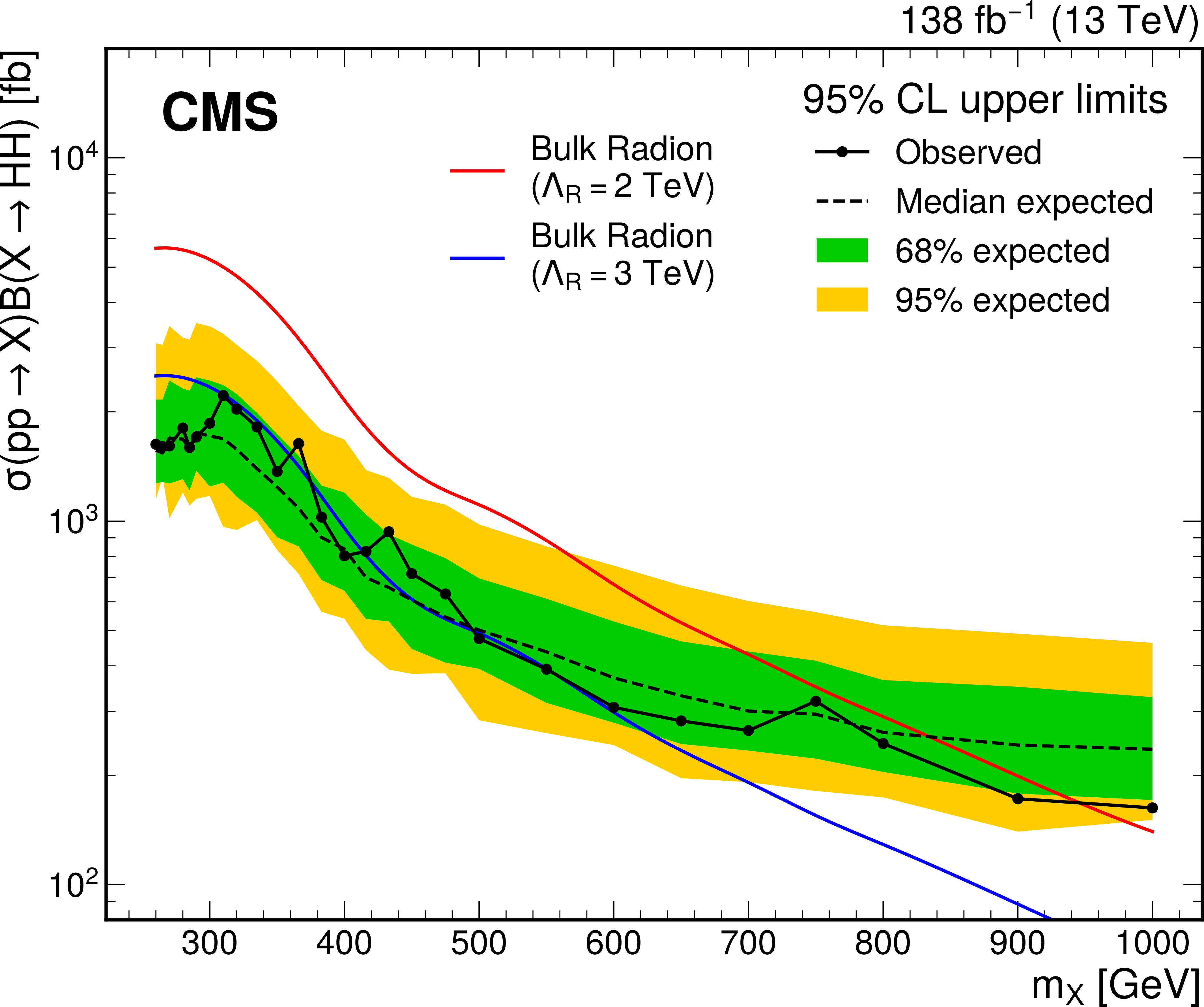
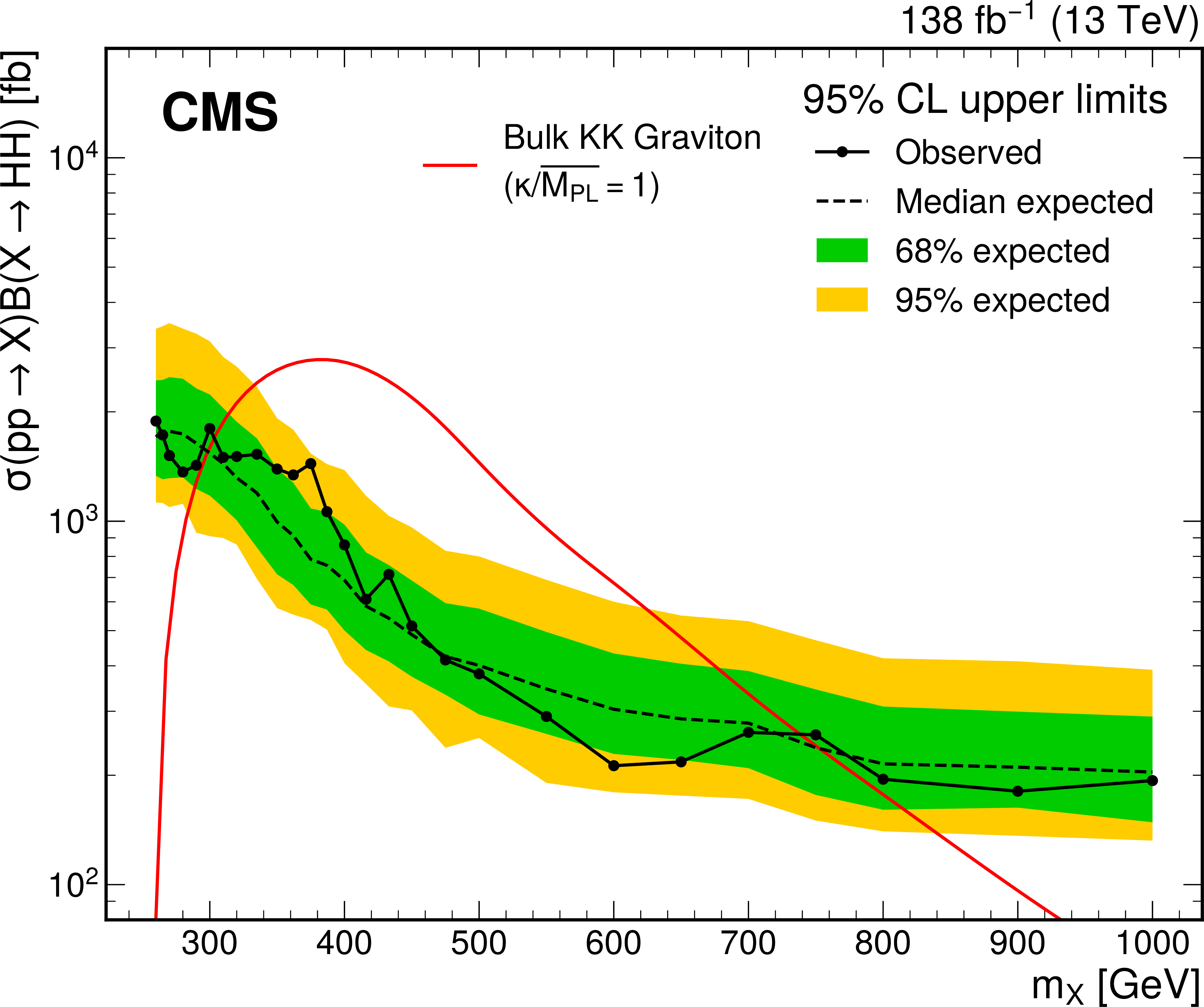
Figure 11:
Expected and observed 95% CL upper limit on the resonant production cross section, $ \sigma({\mathrm{p}\mathrm{p}} \to \mathrm{X} \to \mathrm{H}\mathrm{H}) $ for the spin-0 $ \mathrm{X}{(0)} \to \mathrm{H}\mathrm{H} $ search (upper plot) and spin-2 $ \mathrm{X}{(2)} \to \mathrm{H}\mathrm{H} $ search (lower plot). The dashed and solid black lines represent the expected and observed limits, respectively. The green and yellow bands represent the one and two standard deviations for the expected limit, respectively. The red and blue lines show the theoretical predictions with different energy scales and couplings [90]. |
png pdf |
Figure 11-a:
Expected and observed 95% CL upper limit on the resonant production cross section, $ \sigma({\mathrm{p}\mathrm{p}} \to \mathrm{X} \to \mathrm{H}\mathrm{H}) $ for the spin-0 $ \mathrm{X}{(0)} \to \mathrm{H}\mathrm{H} $ search (upper plot) and spin-2 $ \mathrm{X}{(2)} \to \mathrm{H}\mathrm{H} $ search (lower plot). The dashed and solid black lines represent the expected and observed limits, respectively. The green and yellow bands represent the one and two standard deviations for the expected limit, respectively. The red and blue lines show the theoretical predictions with different energy scales and couplings [90]. |
png pdf |
Figure 11-b:
Expected and observed 95% CL upper limit on the resonant production cross section, $ \sigma({\mathrm{p}\mathrm{p}} \to \mathrm{X} \to \mathrm{H}\mathrm{H}) $ for the spin-0 $ \mathrm{X}{(0)} \to \mathrm{H}\mathrm{H} $ search (upper plot) and spin-2 $ \mathrm{X}{(2)} \to \mathrm{H}\mathrm{H} $ search (lower plot). The dashed and solid black lines represent the expected and observed limits, respectively. The green and yellow bands represent the one and two standard deviations for the expected limit, respectively. The red and blue lines show the theoretical predictions with different energy scales and couplings [90]. |
png pdf |
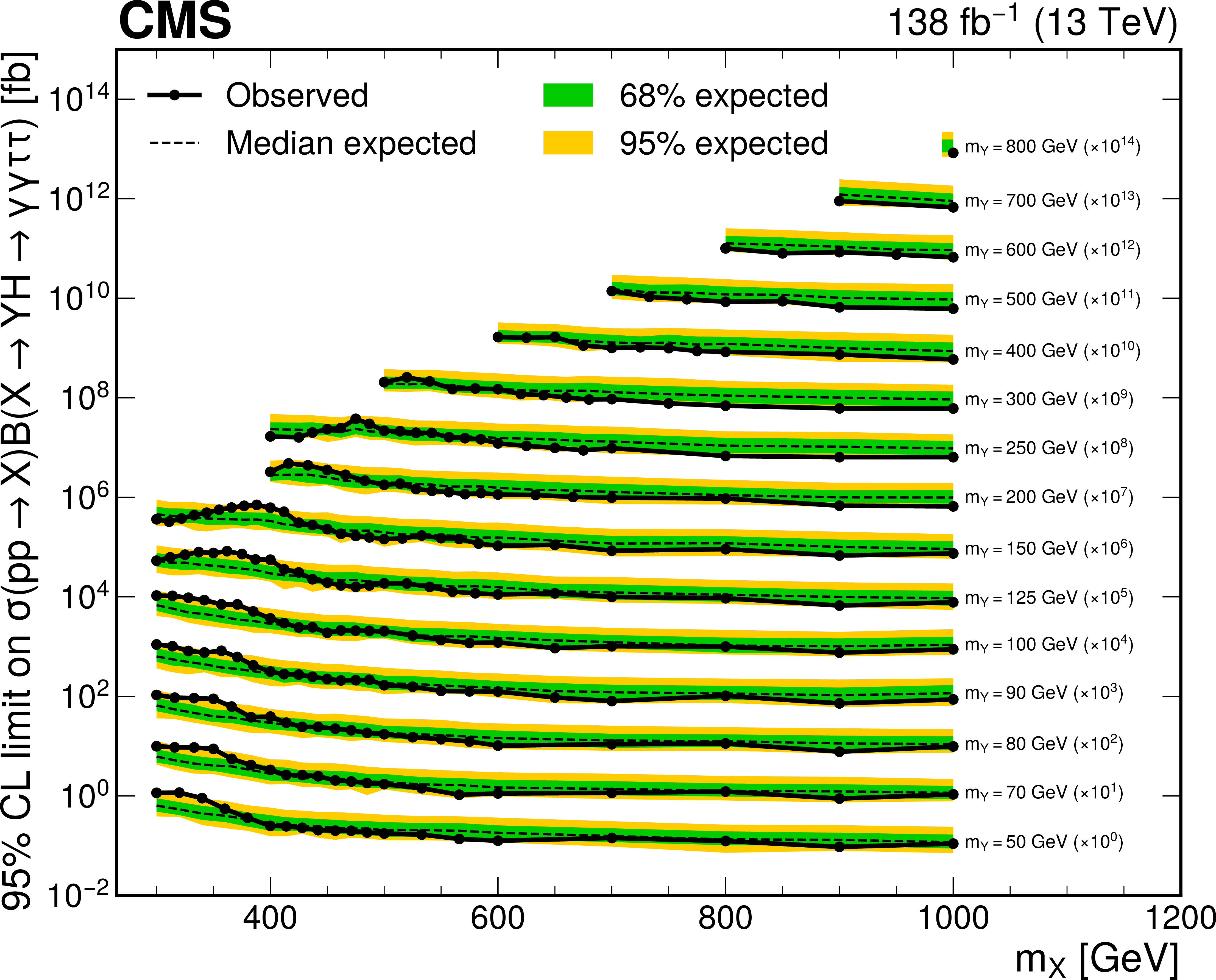
Figure 12:
Expected and observed 95% CL upper limit on $ \sigma({\mathrm{p}\mathrm{p}} \to \mathrm{X} \to \mathrm{Y} \mathrm{H} \to \gamma\gamma\tau\tau) $ for the $ \mathrm{X} \to \mathrm{Y} (\tau\tau)\mathrm{H}(\gamma\gamma) $ search as a function of $ m_{\mathrm{X}} $. The dashed and solid black lines represent the expected and observed limits, respectively. The green and yellow bands represent the one and two standard deviations for the expected limit, respectively. Limits are scaled by orders of 10, labeled in the plot. |
png pdf |
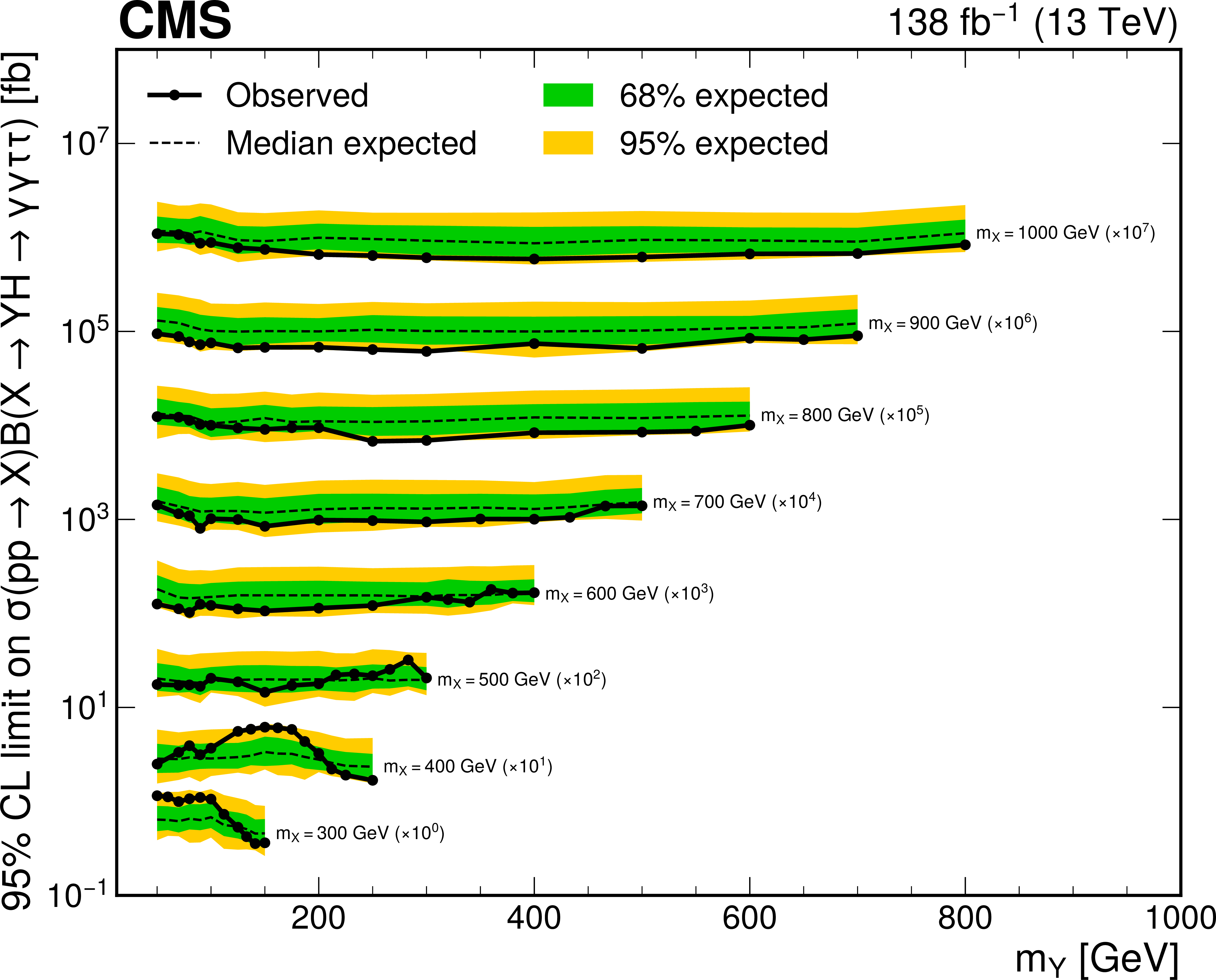
Figure 13:
Expected and observed 95% CL upper limit on $ \sigma({\mathrm{p}\mathrm{p}} \to \mathrm{X} \to \mathrm{Y} \mathrm{H} \to \gamma\gamma\tau\tau) $ for the $ \mathrm{X} \to \mathrm{Y} (\tau\tau)\mathrm{H}(\gamma\gamma) $ search as a function of $ m_{\mathrm{Y} } $. The dashed and solid black lines represent the expected and observed limits, respectively. The green and yellow bands represent the one and two standard deviations for the expected limit, respectively. Limits are scaled by orders of 10, labeled in the plot. |
png pdf |
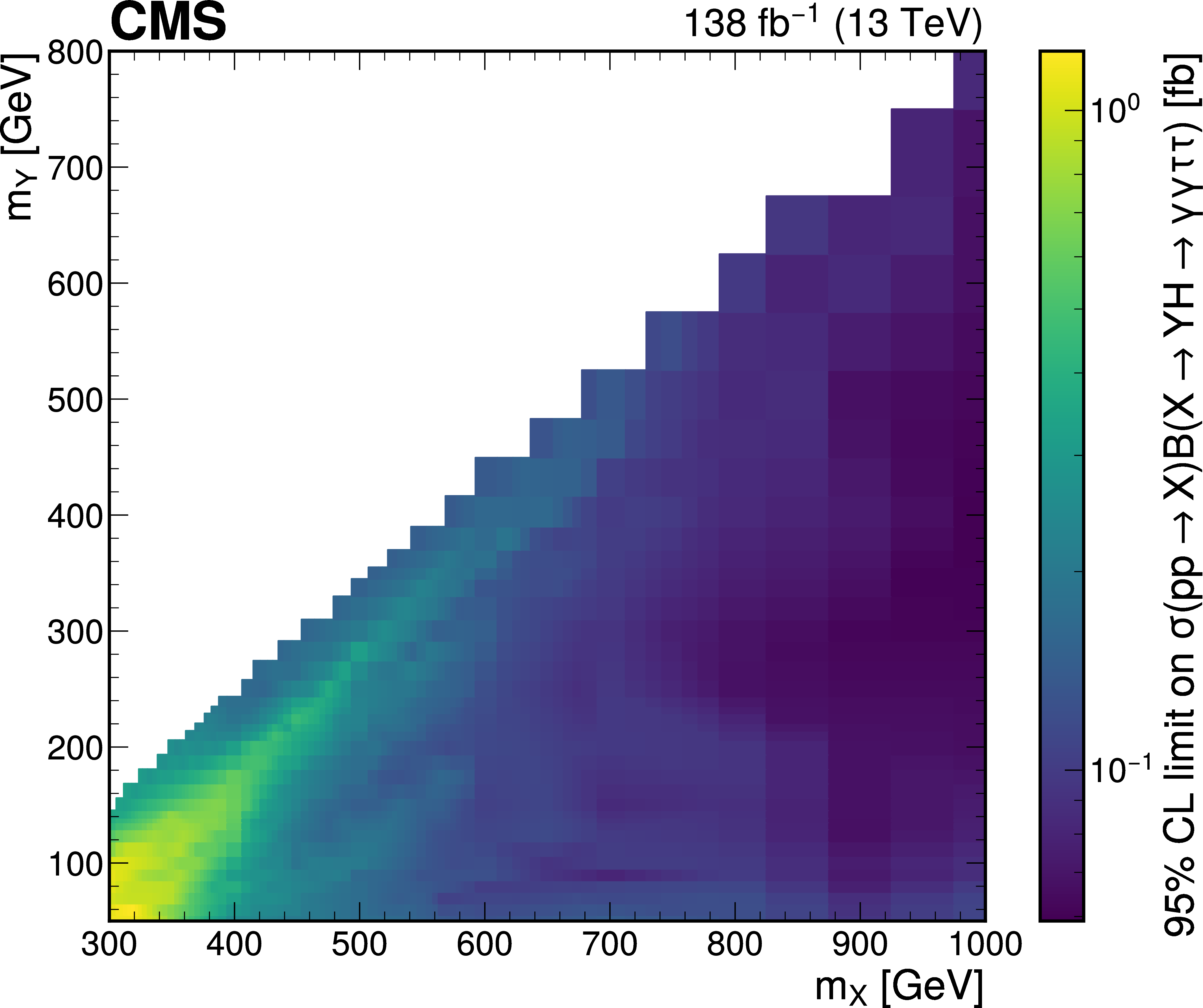
Figure 14:
Observed upper limits in the 2D ($ m_{\mathrm{X}} $, $ m_{\mathrm{Y} } $) plane for the $ \mathrm{X} \to \mathrm{Y} (\tau\tau)\mathrm{H}(\gamma\gamma) $ search. The values of the limits are shown by the color scale. |
png pdf |
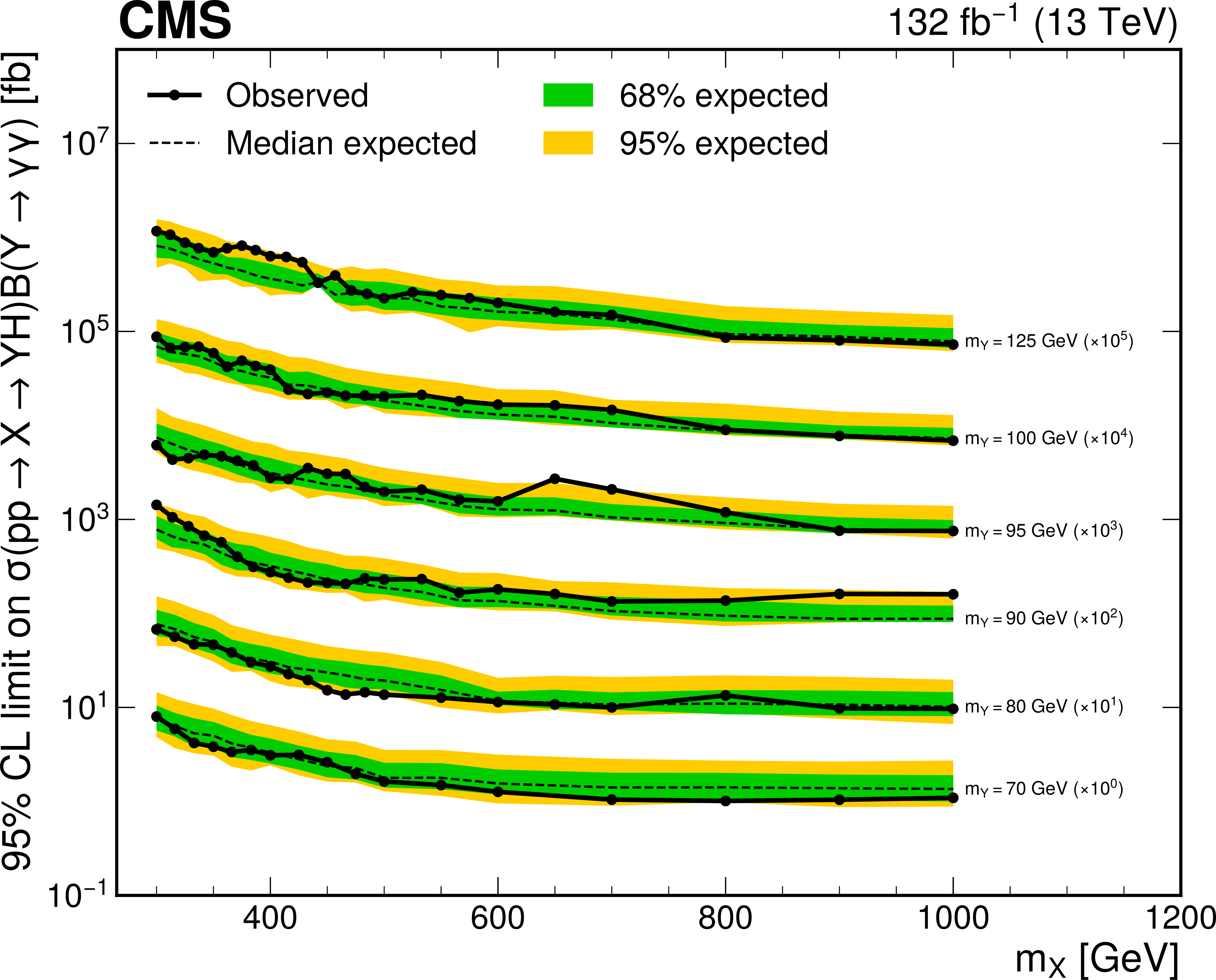
Figure 15:
Expected and observed 95% CL upper limit on $ \sigma({\mathrm{p}\mathrm{p}} \to \mathrm{X} \to \mathrm{Y} \mathrm{H})B(\mathrm{Y} \to \gamma\gamma) $ for the low-mass $ \mathrm{X} \to \mathrm{Y} (\gamma\gamma)\mathrm{H}(\tau\tau) $ search as a function of $ m_{\mathrm{X}} $. The dashed and solid black lines represent the expected and observed limits, respectively. The green and yellow bands represent the one and two standard deviations for the expected limit, respectively. Limits are scaled by orders of 10, labeled in the plot. |
png pdf |
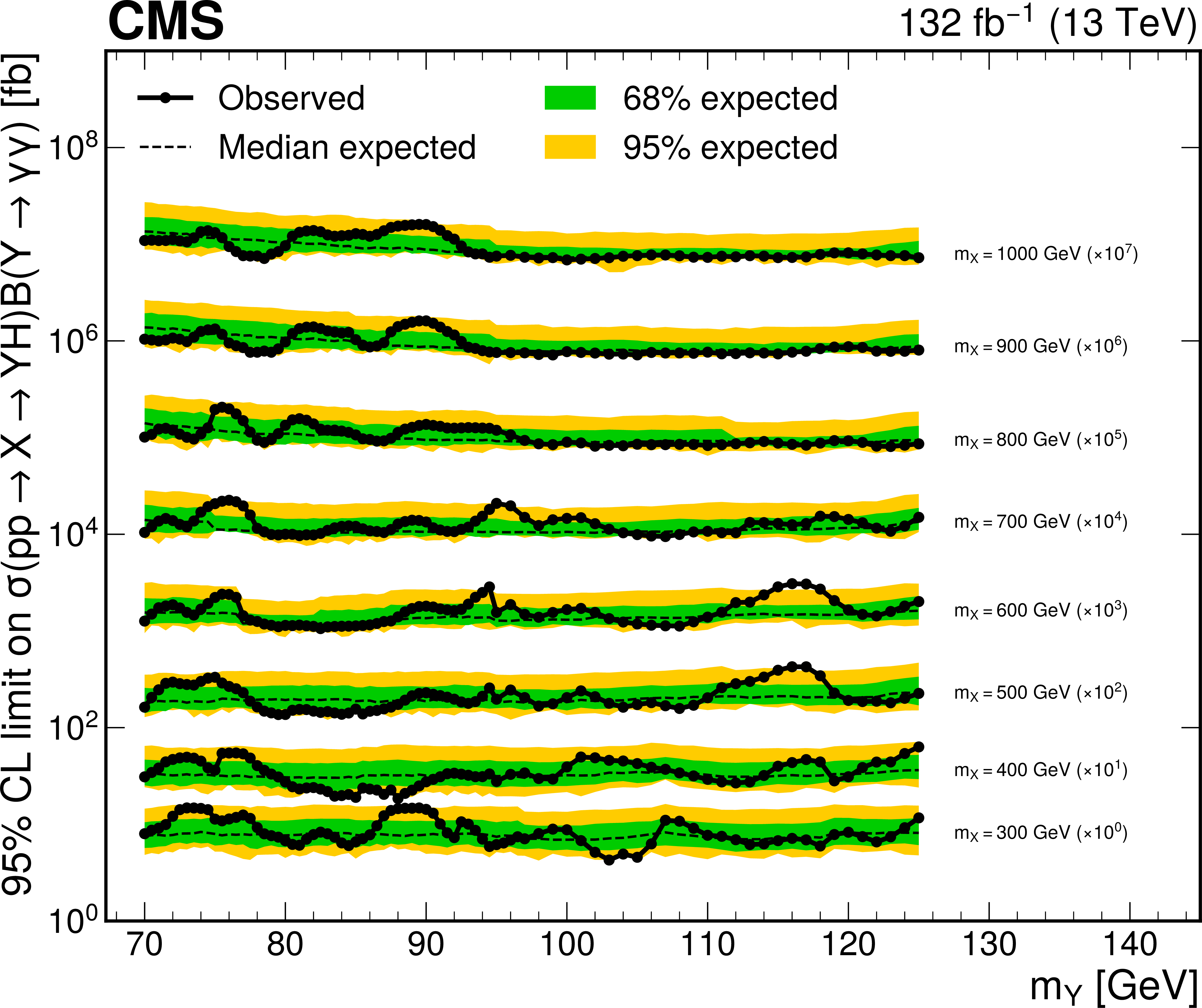
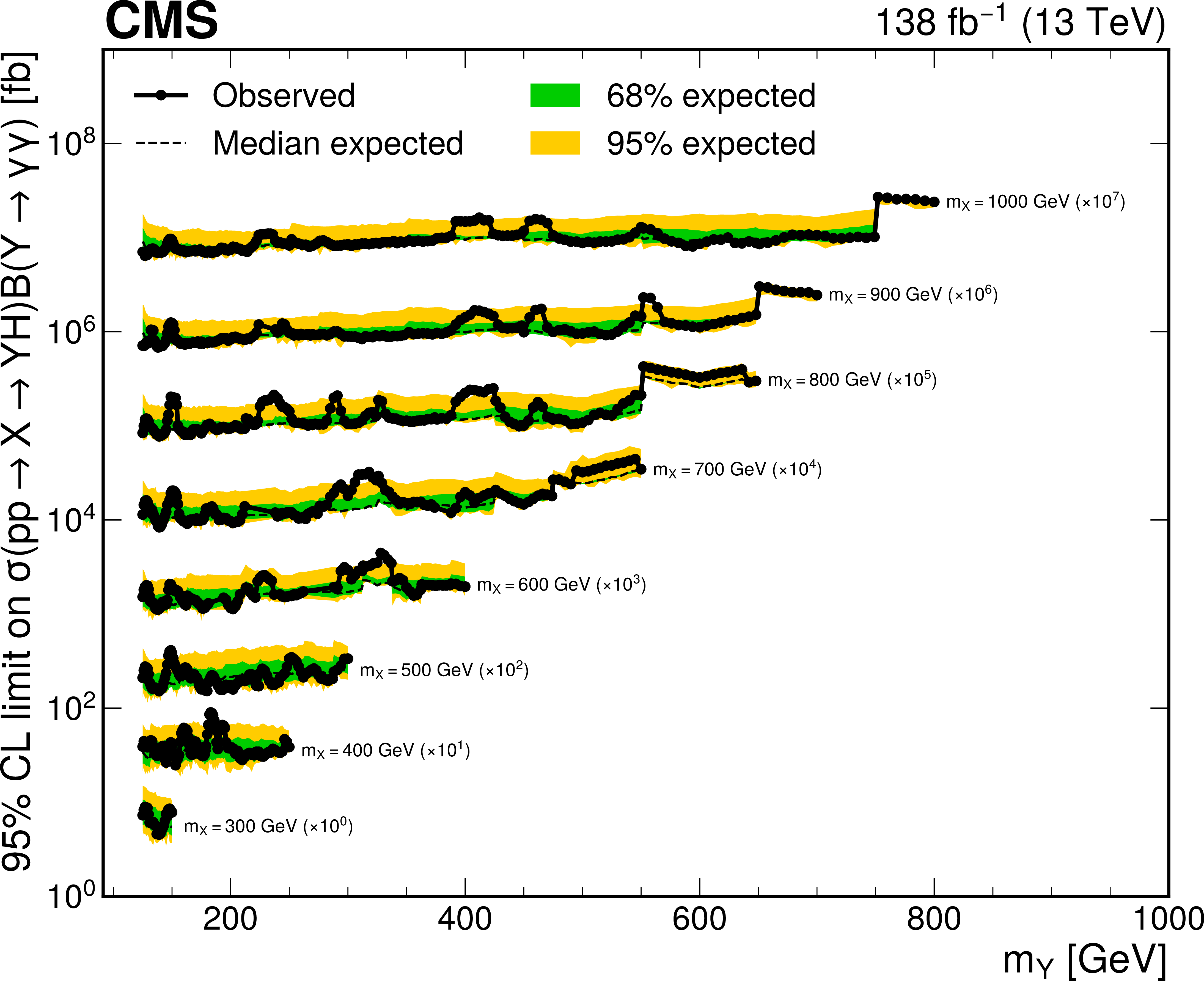
Figure 16:
Expected and observed 95% CL upper limit on $ \sigma({\mathrm{p}\mathrm{p}} \to \mathrm{X} \to \mathrm{Y} \mathrm{H})B(\mathrm{Y} \to \gamma\gamma) $ for the low-mass $ \mathrm{X} \to \mathrm{Y} (\gamma\gamma)\mathrm{H}(\tau\tau) $ search as a function of $ m_{\mathrm{Y} } $. The dashed and solid black lines represent the expected and observed limits, respectively. The green and yellow bands represent the one and two standard deviations for the expected limit, respectively. Limits are scaled by orders of 10, labeled in the plot. |
png pdf |
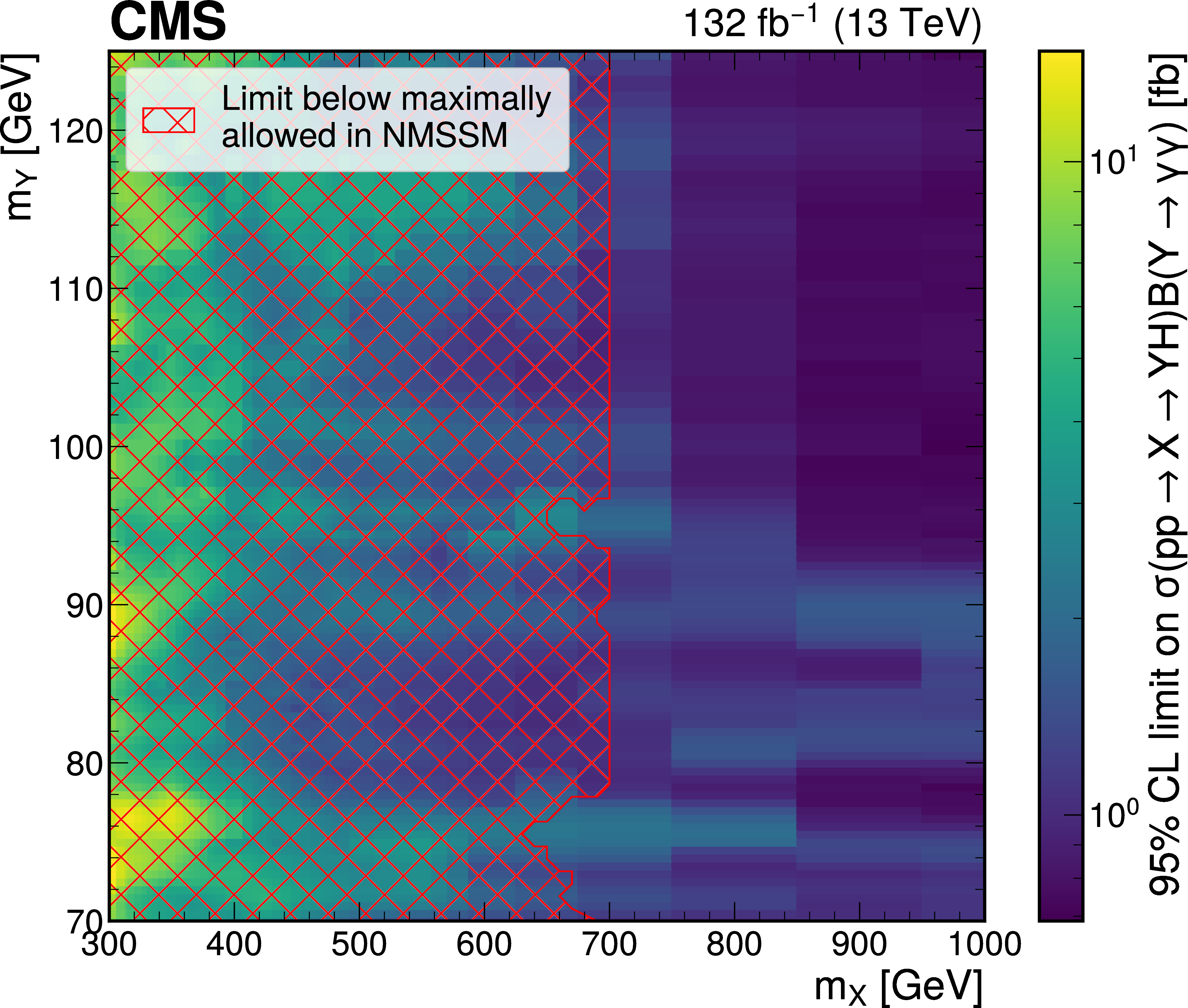
Figure 17:
Observed upper limits in the 2D ($ m_{\mathrm{X}} $, $ m_{\mathrm{Y} } $) plane for the low-mass $ \mathrm{X} \to \mathrm{Y} (\gamma\gamma)\mathrm{H}(\tau\tau) $ search. The values of the limits are shown by the color scale. The red hatched region indicates masses for which the observed limits exclude largest possible cross-section in the NMSSM from previous constraints, taken from Ref. [91]. |
png pdf |
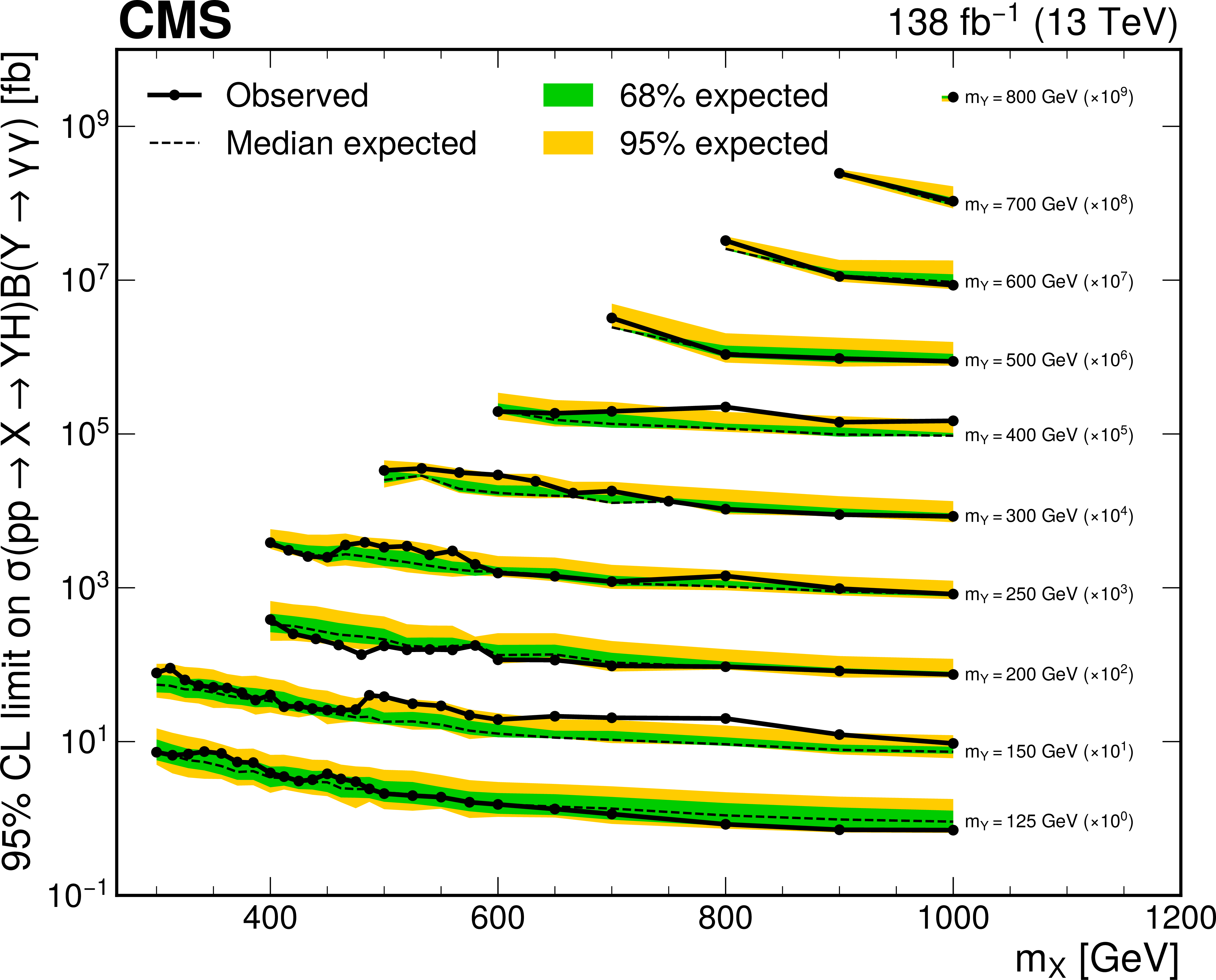
Figure 18:
Observed 95% CL upper limit on $ \sigma({\mathrm{p}\mathrm{p}} \to \mathrm{X} \to \mathrm{Y} \mathrm{H})B(\mathrm{Y} \to \gamma\gamma) $ for the high-mass $ \mathrm{X} \to \mathrm{Y} (\gamma\gamma)\mathrm{H}(\tau\tau) $ search as a function of $ m_{\mathrm{X}} $. The dashed and solid black lines represent the expected and observed limits, respectively. The green and yellow bands represent the one and two standard deviations for the expected limit, respectively. Limits are scaled by orders of 100, labeled in the plot. |
png pdf |
Figure 19:
Expected and observed 95% CL upper limit on $ \sigma({\mathrm{p}\mathrm{p}} \to \mathrm{X} \to \mathrm{Y} \mathrm{H})B(\mathrm{Y} \to \gamma\gamma) $ for the high-mass $ \mathrm{X} \to \mathrm{Y} (\gamma\gamma)\mathrm{H}(\tau\tau) $ search as a function of $ m_{\mathrm{Y} } $. The dashed and solid black lines represent the expected and observed limits, respectively. The green and yellow bands represent the one and two standard deviations for the expected limit, respectively. Limits are scaled by orders of 10, labeled in the plot. |
png pdf |
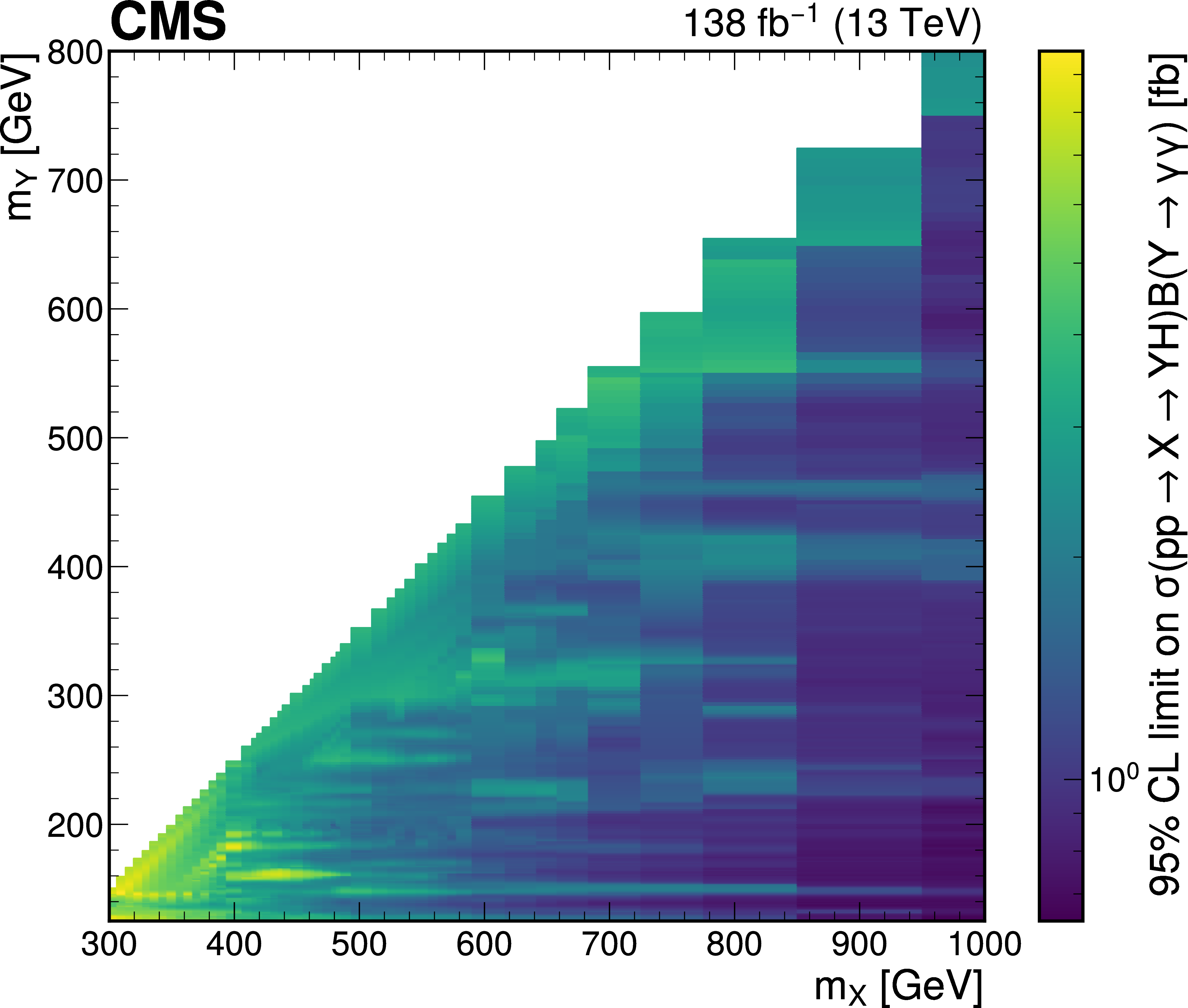
Figure 20:
Observed upper limits in the 2D ($ m_{\mathrm{X}} $, $ m_{\mathrm{Y} } $) plane for the high-mass $ \mathrm{X} \to \mathrm{Y} (\gamma\gamma)\mathrm{H}(\tau\tau) $ search. The values of the limits are shown by the color scale. |
| Tables | |
png pdf |
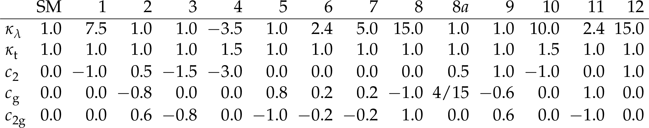
Table 1:
Parameter values of nonresonant BSM benchmark hypotheses. The first column corresponds to the SM sample, while the next 13 correspond to the benchmark hypotheses identified using the method from Refs. [24,25]. |

png pdf |
Table 2:
Additional photon requirements for barrel and endcap photons at different ranges of $ R_\mathrm{9} $, intended to mimic the HLT requirements. |
| Summary |
| A search for the production of two scalar bosons in the $ \gamma\gamma\tau\tau $ final state is presented. The search uses data from proton-proton collisions collected by the CMS experiment at the LHC in 2016-2018 at a center-of-mass energy of 13 TeV, corresponding to 138 or 132 fb$ ^{-1} $ of integrated luminosity, depending on the trigger path. In total, five searches are perfomed. One search targets the nonresonant production of a Higgs boson pair, HH, via gluon-gluon fusion, where no significant deviation from the background-only hypothesis is observed. Upper limits at 95% confidence level (CL) on the HH production cross section are extracted for production in the standard model (SM) and in several beyond-the-SM scenarios. The observed (expected) upper limit for the SM production is found to be 930 (740) fb, corresponding to 33 (26) times the SM prediction. The limit is also derived as a function of the Higgs boson self-coupling modifier, $ \kappa_\lambda $, assuming all other Higgs boson couplings are as predicted in the SM, and HH production is observed (expected) to be excluded at 95% CL outside the range between-12 (-9.4) and 17 (15). In addition, the limit is extracted for numerous beyond-the-SM benchmark scenarios and the results are consistent with the SM predictions. This analysis also targets the resonant production of two scalar bosons. Two searches are constructed to search for a resonance X decaying to a SM Higgs boson pair, $ \mathrm{X} \to \mathrm{H}\mathrm{H} $, for both the spin-0 resonance and spin-2 resonance scenarios. Furthermore, the analysis targets the $ \mathrm{X} \to \mathrm{Y} \mathrm{H} $ process, where Y is an additional, lighter (than X) scalar particle. Three searches are constructed, namely the $ \mathrm{X} \to \mathrm{Y} (\tau\tau)\mathrm{H}(\gamma\gamma) $, low-mass $ \mathrm{X} \to \mathrm{Y} (\gamma\gamma)\mathrm{H}(\tau\tau) $ and high-mass $ \mathrm{X} \to \mathrm{Y} (\gamma\gamma)\mathrm{H}(\tau\tau) $, which target the different decay chains in different mass regimes. The global significances of each search indicate that no significant deviation from the background-only hypothesis is observed, but some local excesses in the $ \mathrm{X} \to \mathrm{Y} (\gamma\gamma)\mathrm{H}(\tau\tau) $ search that are consistent with other CMS results warrant further measurements. In the $ \mathrm{X} \to \mathrm{H}\mathrm{H} $ search, upper limits at the 95% CL on the $ \mathrm{X} \to \mathrm{H}\mathrm{H} $ production cross section are observed (expected) to be within 160 to 2200 (200 to 1800) fb, depending on the mass of X. In the $ \mathrm{X} \to \mathrm{Y} (\tau\tau)\mathrm{H}(\gamma\gamma) $ search, upper limits at the 95% CL on the product of the production cross section and the decay branching fractions are observed (expected) to vary between 0.059-1.2 fb (0.087-0.68 fb), depending on the mass of X and Y. In the $ \mathrm{X} \to \mathrm{Y} (\gamma\gamma)\mathrm{H}(\tau\tau) $ search, the observed (expected) upper limits on the product of the production cross section and $ \mathrm{Y} \to \gamma\gamma $ branching fraction vary between 0.69-15 fb (0.73-8.3 fb) in the low Y mass search and between 0.64-10 fb (0.70-7.6 fb) in the high Y mass search. In the low Y mass search, these limits are compared to a set of maximally allowed cross sections in the next-to-minimal supersymmetric SM taken from Ref. [91]. A region in the ($ m_{\mathrm{X}} $, $ m_{\mathrm{Y} } $) parameter space where the observed limits are lower than the maximum allowed is found, meaning that these results can be used to provide tighter constraints on the next-to-minimal supersymmetric SM. |
| References | ||||
| 1 | ATLAS Collaboration | Observation of a new particle in the search for the standard model Higgs boson with the atlas detector at the LHC | PLB 716 (2012) 1 | 1207.7214 |
| 2 | CMS Collaboration | Observation of a new boson at a mass of 125 GeV with the CMS experiment at the LHC | PLB 716 (2012) 30 | CMS-HIG-12-028 1207.7235 |
| 3 | CMS Collaboration | Observation of a new boson with mass near 125 GeV in pp collisions at $ \sqrt{s} = $ 7 and 8 TeV | JHEP 06 (2013) 081 | CMS-HIG-12-036 1303.4571 |
| 4 | CMS Collaboration | A portrait of the Higgs boson by the CMS experiment ten years after the discovery | Nature 607 (2022) 60 | CMS-HIG-22-001 2207.00043 |
| 5 | ATLAS Collaboration | A detailed map of Higgs boson interactions by the ATLAS experiment ten years after the discovery | Nature 607 (2022) 52 | 2207.00092 |
| 6 | M. Grazzini et al. | Higgs boson pair production at NNLO with top quark mass effects | JHEP 05 (2018) 059 | 1803.02463 |
| 7 | S. Dawson, S. Dittmaier, and M. Spira | Neutral Higgs boson pair production at hadron colliders: QCD corrections | PRD 58 (1998) 115012 | hep-ph/9805244 |
| 8 | S. Borowka et al. | Higgs boson pair production in gluon fusion at next-to-leading order with full top-quark mass dependence | PRL 117 (2016) 012001 | 1604.06447 |
| 9 | J. Baglio et al. | Gluon fusion into Higgs pairs at NLO QCD and the top mass scheme | EPJC 79 (2019) 459 | 1811.05692 |
| 10 | D. de Florian and J. Mazzitelli | Higgs boson pair production at next-to-next-to-leading order in QCD | PRL 111 (2013) 201801 | 1309.6594 |
| 11 | D. Y. Shao, C. S. Li, H. T. Li, and J. Wang | Threshold resummation effects in Higgs boson pair production at the LHC | JHEP 07 (2013) 169 | 1301.1245 |
| 12 | D. de Florian and J. Mazzitelli | Higgs pair production at next-to-next-to-leading logarithmic accuracy at the LHC | JHEP 09 (2015) 053 | 1505.07122 |
| 13 | J. Baglio et al. | $ gg\to hh $: Combined uncertainties | PRD 103 (2021) 056002 | 2008.11626 |
| 14 | ATLAS Collaboration | Constraints on the Higgs boson self-coupling from single- and double-Higgs production with the ATLAS detector using pp collisions at s=13 TeV | PLB 843 (2023) 137745 | 2211.01216 |
| 15 | LHC Higgs Cross Section Working Group | Handbook of LHC Higgs cross sections: 4. Deciphering the nature of the Higgs sector | CERN Report CERN-2017-002-M, 2016 link |
1610.07922 |
| 16 | F. Goertz, A. Papaefstathiou, L. L. Yang, and J. Zurita | Higgs boson pair production in the D=6 extension of the SM | JHEP 04 (2015) 167 | 1410.3471 |
| 17 | L. Randall and R. Sundrum | A large mass hierarchy from a small extra dimension | PRL 83 (1999) 3370 | hep-ph/9905221 |
| 18 | W. D. Goldberger and M. B. Wise | Modulus stabilization with bulk fields | PRL 83 (1999) 4922 | hep-ph/9907447 |
| 19 | H. Davoudiasl, J. L. Hewett, and T. G. Rizzo | Phenomenology of the Randall-Sundrum gauge hierarchy model | PRL 84 (2000) 2080 | hep-ph/9909255 |
| 20 | A. Djouadi | The anatomy of electro-weak symmetry breaking. II. the Higgs bosons in the minimal supersymmetric model | Phys. Rept. 459 (2008) 1 | hep-ph/0503173 |
| 21 | CMS Collaboration | Search for a new resonance decaying into two spin-0 bosons in a final state with two photons and two bottom quarks in proton-proton collisions at $ \sqrt{s} = $ 13 TeV | JHEP 05 (2024) 316 | CMS-HIG-21-011 2310.01643 |
| 22 | CMS Collaboration | Searches for additional Higgs bosons and for vector leptoquarks in $ \tau\tau $ final states in proton-proton collisions at $ \sqrt{s} = $ 13 TeV | JHEP 07 (2023) 073 | CMS-HIG-21-001 2208.02717 |
| 23 | CMS Collaboration | Search for a standard model-like Higgs boson in the mass range between 70 and 110 GeV in the diphoton final state in proton-proton collisions at $ \sqrt{s} = $ 13 TeV | PLB 860 (2025) 139067 | CMS-HIG-20-002 2405.18149 |
| 24 | A. Carvalho et al. | Higgs pair production: Choosing benchmarks with cluster analysis | JHEP 04 (2016) 126 | 1507.02245 |
| 25 | G. Buchalla et al. | Higgs boson pair production in non-linear effective field theory with full $ m_t $-dependence at NLO QCD | JHEP 09 (2018) 057 | 1806.05162 |
| 26 | CMS Collaboration | HEPData record for this analysis | link | |
| 27 | CMS Collaboration | The CMS experiment at the CERN LHC | JINST 3 (2008) S08004 | |
| 28 | CMS Collaboration | Performance of the CMS level-1 trigger in proton-proton collisions at $ \sqrt{s} = $ 13 TeV | JINST 15 (2020) P10017 | CMS-TRG-17-001 2006.10165 |
| 29 | CMS Collaboration | The CMS trigger system | JINST 12 (2017) P01020 | CMS-TRG-12-001 1609.02366 |
| 30 | CMS Collaboration | Performance of the CMS high-level trigger during LHC run 2 | JINST 19 (2024) P11021 | CMS-TRG-19-001 2410.17038 |
| 31 | CMS Collaboration | Particle-flow reconstruction and global event description with the CMS detector | JINST 12 (2017) P10003 | CMS-PRF-14-001 1706.04965 |
| 32 | D. Contardo et al. | Technical proposal for the Phase-II upgrade of the CMS detector | technical report, Geneva, 2015 link |
|
| 33 | CMS Collaboration | Electron and photon reconstruction and identification with the CMS experiment at the CERN LHC | JINST 16 (2021) P05014 | CMS-EGM-17-001 2012.06888 |
| 34 | CMS Collaboration | Performance of photon reconstruction and identification with the CMS detector in proton-proton collisions at sqrt(s) = 8 TeV | JINST 10 (2015) P08010 | CMS-EGM-14-001 1502.02702 |
| 35 | CMS Collaboration | A measurement of the Higgs boson mass in the diphoton decay channel | PLB 805 (2020) 135425 | CMS-HIG-19-004 2002.06398 |
| 36 | CMS Collaboration | ECAL 2016 refined calibration and Run2 summary plots | CMS Detector Performance Summary CMS-DP-2020-021, 2020 CDS |
|
| 37 | CMS Collaboration | Performance of the CMS muon detector and muon reconstruction with proton-proton collisions at $ \sqrt{s}= $ 13 TeV | JINST 13 (2018) P06015 | CMS-MUO-16-001 1804.04528 |
| 38 | M. Cacciari, G. P. Salam, and G. Soyez | The anti-$ k_{\mathrm{T}} $ jet clustering algorithm | JHEP 04 (2008) 063 | 0802.1189 |
| 39 | M. Cacciari, G. P. Salam, and G. Soyez | FastJet user manual | EPJC 72 (2012) 1896 | 1111.6097 |
| 40 | CMS Collaboration | Pileup mitigation at CMS in 13 TeV data | JINST 15 (2020) P09018 | CMS-JME-18-001 2003.00503 |
| 41 | CMS Collaboration | Jet energy scale and resolution in the CMS experiment in pp collisions at 8 TeV | JINST 12 (2017) P02014 | CMS-JME-13-004 1607.03663 |
| 42 | CMS Collaboration | Identification of heavy-flavour jets with the CMS detector in pp collisions at 13 TeV | JINST 13 (2018) P05011 | CMS-BTV-16-002 1712.07158 |
| 43 | E. Bols et al. | Jet flavour classification using DeepJet | JINST 15 (2020) P12012 | 2008.10519 |
| 44 | CMS Collaboration | Performance of the DeepJet b tagging algorithm using 41.9 fb$ ^{-1} $ of data from proton-proton collisions at 13 TeV with Phase-1 CMS detector | CMS Detector Performance Note CMS-DP-2018-058, 2018 CDS |
|
| 45 | CMS Collaboration | Performance of reconstruction and identification of $ \tau $ leptons decaying to hadrons and $ \nu_\tau $ in pp collisions at $ \sqrt{s}= $ 13 TeV | JINST 13 (2018) P10005 | CMS-TAU-16-003 1809.02816 |
| 46 | CMS Collaboration | Identification of hadronic tau lepton decays using a deep neural network | JINST 17 (2022) P07023 | CMS-TAU-20-001 2201.08458 |
| 47 | CMS Collaboration | Performance of missing transverse momentum reconstruction in proton-proton collisions at $ \sqrt{s} = $ 13 TeV using the CMS detector | JINST 14 (2019) P07004 | CMS-JME-17-001 1903.06078 |
| 48 | CMS Collaboration | Precision luminosity measurement in proton-proton collisions at $ \sqrt{s} = $ 13 TeV in 2015 and 2016 at CMS | EPJC 81 (2021) 800 | CMS-LUM-17-003 2104.01927 |
| 49 | CMS Collaboration | CMS luminosity measurement for the 2017 data-taking period at $ \sqrt{s} = $ 13 TeV | CMS Physics Analysis Summary, 2018 CMS-PAS-LUM-17-004 |
CMS-PAS-LUM-17-004 |
| 50 | CMS Collaboration | CMS luminosity measurement for the 2018 data-taking period at $ \sqrt{s} = $ 13 TeV | CMS Physics Analysis Summary, 2019 CMS-PAS-LUM-18-002 |
CMS-PAS-LUM-18-002 |
| 51 | E. Bagnaschi, G. Degrassi, P. Slavich, and A. Vicini | Higgs production via gluon fusion in the POWHEG approach in the SM and in the MSSM | JHEP 02 (2012) 088 | 1111.2854 |
| 52 | G. Heinrich et al. | NLO predictions for Higgs boson pair production with full top quark mass dependence matched to parton showers | JHEP 08 (2017) 088 | 1703.09252 |
| 53 | G. Heinrich et al. | Probing the trilinear Higgs boson coupling in di-Higgs production at NLO QCD including parton shower effects | JHEP 06 (2019) 066 | 1903.08137 |
| 54 | S. Jones and S. Kuttimalai | Parton shower and NLO-matching uncertainties in Higgs boson pair production | JHEP 02 (2018) 176 | 1711.03319 |
| 55 | G. Heinrich, S. P. Jones, M. Kerner, and L. Scyboz | A non-linear EFT description of $ gg\to hh $ at NLO interfaced to POWHEG | JHEP 10 (2020) 021 | 2006.16877 |
| 56 | P. Nason | A new method for combining NLO QCD with shower Monte Carlo algorithms | JHEP 11 (2004) 040 | hep-ph/0409146 |
| 57 | S. Frixione, P. Nason, and C. Oleari | Matching NLO QCD computations with parton shower simulations: the POWHEG method | JHEP 11 (2007) 070 | 0709.2092 |
| 58 | S. Alioli, P. Nason, C. Oleari, and E. Re | A general framework for implementing NLO calculations in shower Monte Carlo programs: the POWHEG BOX | JHEP 06 (2010) 043 | 1002.2581 |
| 59 | D. de Florian et al. | Anomalous couplings in Higgs-boson pair production at approximate NNLO QCD | JHEP 09 (2021) 161 | 2106.14050 |
| 60 | A. Carvalho et al. | On the reinterpretation of non-resonant searches for Higgs boson pairs | JHEP 02 (2021) 049 | 1710.08261 |
| 61 | J. Alwall et al. | The automated computation of tree-level and next-to-leading order differential cross sections, and their matching to parton shower simulations | JHEP 07 (2014) 079 | 1405.0301 |
| 62 | E. Bothmann et al. | Event generation with SHERPA 2.2 | SciPost Phys. 7 (2019) 34 | 1905.09127 |
| 63 | J. Alwall et al. | Comparative study of various algorithms for the merging of parton showers and matrix elements in hadronic collisions | EPJC 53 (2008) 473 | 0706.2569 |
| 64 | R. Frederix and S. Frixione | Merging meets matching in MC@NLO | JHEP 12 (2012) 061 | 1209.6215 |
| 65 | CMS Collaboration | Event generator tunes obtained from underlying event and multiparton scattering measurements | EPJC 76 (2016) 155 | CMS-GEN-14-001 1512.00815 |
| 66 | CMS Collaboration | Extraction and validation of a new set of CMS PYTHIA8 tunes from underlying-event measurements | EPJC 80 (2020) 4 | CMS-GEN-17-001 1903.12179 |
| 67 | NNPDF Collaboration | Parton distributions from high-precision collider data | EPJC 77 (2017) 663 | 1706.00428 |
| 68 | \GEANTfour Collaboration | GEANT 4---a simulation toolkit | NIM A 506 (2003) 250 | |
| 69 | P. Baldi et al. | Parameterized neural networks for high-energy physics | EPJC 76 (2016) 235 | 1601.07913 |
| 70 | S. Choi and H. Oh | Improved extrapolation methods of data-driven background estimations in high energy physics | EPJC 81 (2021) 643 | 1906.10831 |
| 71 | CMS Collaboration | Performance of electron reconstruction and selection with the CMS detector in proton-proton collisions at \ensuremath\sqrts = 8 TeV | JINST 10 (2015) P06005 | CMS-EGM-13-001 1502.02701 |
| 72 | T. Chen and C. Guestrin | XGBoost: A Scalable Tree Boosting System | in nd ACM SIGKDD Intern. Conf. on Knowledge Discovery and Data Mining, KDD, . ACM, New York, NY, USA, 2016 Proc. 2 (2016) 785 |
1603.02754 |
| 73 | L. Bianchini, J. Conway, E. K. Friis, and C. Veelken | Reconstruction of the Higgs mass in $ h \to \tau\tau $ events by dynamical likelihood techniques | J. Phys. Conf. Ser. 513 (2014) 022035 | |
| 74 | P. D. Dauncey, M. Kenzie, N. Wardle, and G. J. Davies | Handling uncertainties in background shapes: the discrete profiling method | JINST 10 (2015) P04015 | 1408.6865 |
| 75 | M. J. Oreglia | A study of the reactions $ \psi^\prime \to \gamma \gamma \psi $ | PhD thesis, Stanford University, SLAC Report SLAC-R-236, 1980 link |
|
| 76 | J. E. Gaiser | Charmonium Spectroscopy From Radiative Decays of the $ j/\psi $ and $ \psi^\prime $ | Master's thesis, Stanford University, SLAC Report SLAC-R-255, 1982 link |
|
| 77 | P. Virtanen et al. | SciPy 1.0: Fundamental Algorithms for Scientific Computing in Python | Nature Methods 17 (2020) 261 | 1907.10121 |
| 78 | P. Alfeld | A trivariate clough-tocher scheme for tetrahedral data | Computer Aided Geometric Design 1 (1984) 169 | |
| 79 | R. A. Fisher | On the Interpretation of $ \chi^2 $ from Contingency Tables, and the Calculation of P | Journal of the Royal Statistical Society 85 (1922) 87 | |
| 80 | CMS Collaboration | Search for narrow resonances in the b-tagged dijet mass spectrum in proton-proton collisions at $ \sqrt{s}= $ 13TeV | PRD 108 (2023) 012009 | CMS-EXO-20-008 2205.01835 |
| 81 | CMS Collaboration | Measurements of Higgs boson production cross sections and couplings in the diphoton decay channel at $ \sqrt{\mathrm{s}} = $ 13 TeV | JHEP 07 (2021) 027 | CMS-HIG-19-015 2103.06956 |
| 82 | J. Butterworth et al. | PDF4LHC recommendations for LHC Run II | JPG 43 (2016) 023001 | 1510.03865 |
| 83 | LHC Higgs Cross Section Working Group | Handbook of LHC Higgs cross sections: 3. Higgs properties | CERN Report CERN-2013-004, 2013 link |
1307.1347 |
| 84 | CMS Collaboration | Measurement of the inclusive $ W $ and $ Z $ production cross sections in pp collisions at $ \sqrt{s}= $ 7 TeV | JHEP 10 (2011) 132 | CMS-EWK-10-005 1107.4789 |
| 85 | T. Junk | Confidence level computation for combining searches with small statistics | NIM A 434 (1999) 435 | hep-ex/9902006 |
| 86 | A. L. Read | Presentation of search results: The CL$ _{\text{s}} $ technique | JPG 28 (2002) 2693 | |
| 87 | ATLAS and CMS Collaborations, and LHC Higgs Combination Group | Procedure for the LHC Higgs boson search combination in Summer 2011 | Technical Report CMS-NOTE-2011-005, ATL-PHYS-PUB-2011-11, 2011 | |
| 88 | G. Cowan, K. Cranmer, E. Gross, and O. Vitells | Asymptotic formulae for likelihood-based tests of new physics | EPJC 71 (2011) 1554 | 1007.1727 |
| 89 | F. Maltoni, D. Pagani, A. Shivaji, and X. Zhao | Trilinear Higgs coupling determination via single-Higgs differential measurements at the LHC | EPJC 77 (2017) 887 | 1709.08649 |
| 90 | A. Carvalho | Gravity particles from warped extra dimensions, predictions for LHC | 3, 2014 | 1404.0102 |
| 91 | U. Ellwanger and C. Hugonie | Benchmark planes for Higgs-to-Higgs decays in the NMSSM | EPJC 82 (2022) 406 | 2203.05049 |
| 92 | U. Ellwanger, J. F. Gunion, and C. Hugonie | NMHDECAY: A Fortran code for the Higgs masses, couplings and decay widths in the NMSSM | JHEP 02 (2005) 066 | hep-ph/0406215 |
| 93 | U. Ellwanger and C. Hugonie | NMHDECAY 2.0: An Updated program for sparticle masses, Higgs masses, couplings and decay widths in the NMSSM | Comput. Phys. Commun. 175 (2006) 290 | hep-ph/0508022 |
| 94 | G. Belanger, F. Boudjema, A. Pukhov, and A. Semenov | micrOMEGAs$ \_ $3: A program for calculating dark matter observables | Comput. Phys. Commun. 185 (2014) 960 | 1305.0237 |
|
|
Compact Muon Solenoid LHC, CERN |
|

|

|

|

|

|