

Compact Muon Solenoid
LHC, CERN
| CMS-HIG-20-002 ; CERN-EP-2024-088 | ||
| Search for a standard model-like Higgs boson in the mass range between 70 and 110 GeV in the diphoton final state in proton-proton collisions at $ \sqrt{s}= $ 13 TeV | ||
| CMS Collaboration | ||
| 28 May 2024 | ||
| Phys. Lett. B 860 (2025) 139067 | ||
| Abstract: The results of a search for a standard model-like Higgs boson decaying into two photons in the mass range between 70 and 110 GeV are presented. The analysis uses the data set collected by the CMS experiment in proton-proton collisions at $ \sqrt{s}= $ 13 TeV corresponding to integrated luminosities of 36.3 fb$ ^{-1} $, 41.5 fb$ ^{-1} $ and 54.4 fb$ ^{-1} $ during the 2016, 2017, and 2018 LHC running periods, respectively. No significant excess over the background expectation is observed and 95% confidence level upper limits are set on the product of the cross section and branching fraction for decays of an additional Higgs boson into two photons. The maximum deviation with respect to the background is seen for a mass hypothesis of 95.4 GeV with a local (global) significance of 2.9 (1.3) standard deviations. The observed upper limit ranges from 15 to 73 fb. | ||
| Links: e-print arXiv:2405.18149 [hep-ex] (PDF) ; CDS record ; inSPIRE record ; HepData record ; Physics Briefing ; CADI line (restricted) ; | ||
| Figures & Tables | Summary | Additional Figures | References | CMS Publications |
|---|
| Figures | |
png pdf |
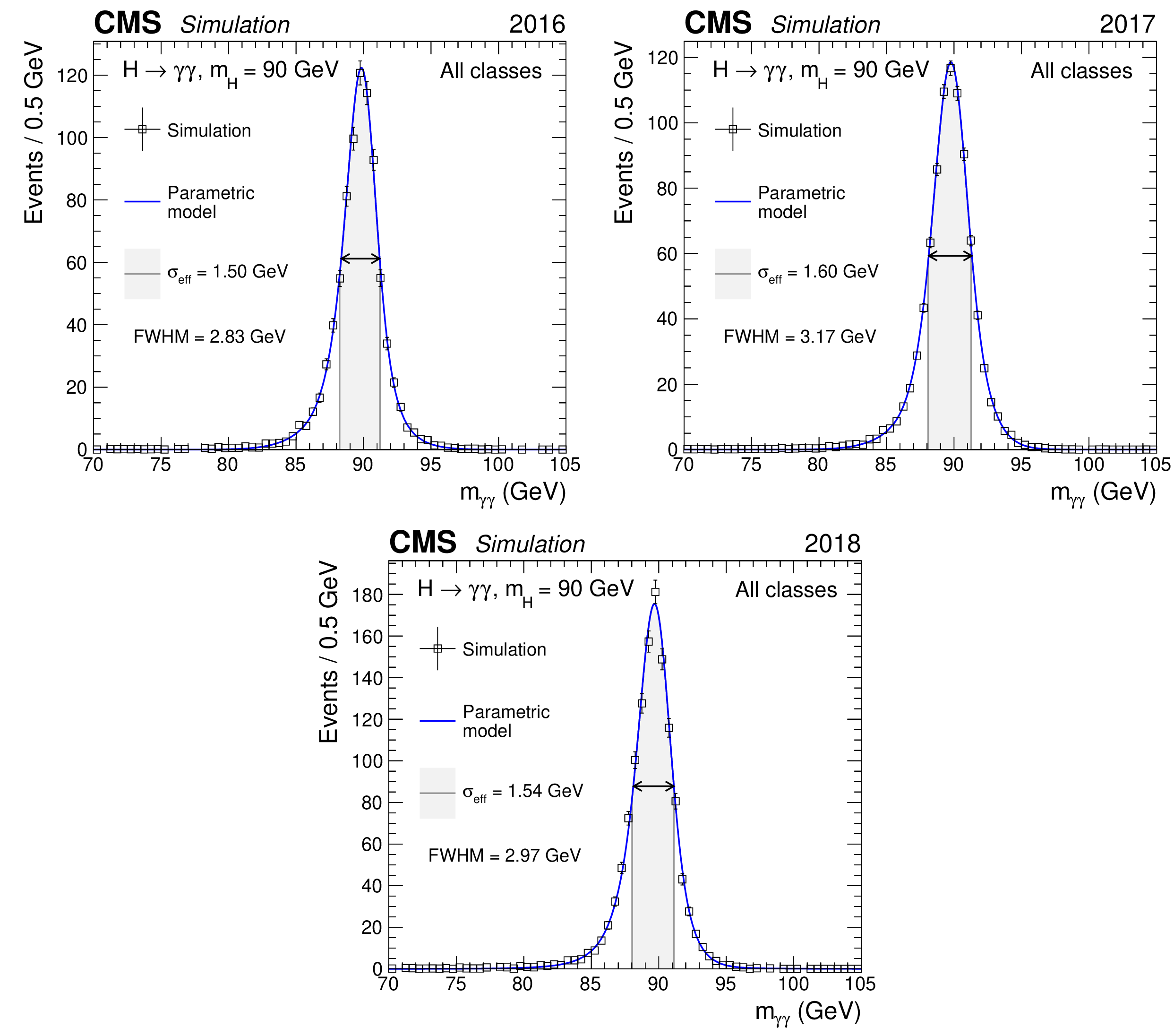
Figure 1:
Full parametrized signal shape, integrated over all event classes, in simulated signal events with $ m_{\mathrm{H}}= $ 90 GeV for 2016 (upper left), 2017 (upper right), and 2018 (lower). The open points are the weighted MC events and the blue lines the corresponding parametric models. Also shown are the $ \sigma_{\text{eff}} $ values and the shaded region limited by $ {\pm}\sigma_{\text{eff}} $, along with the FWHM values, indicated by the position of the arrows on each distribution. |

png pdf |
Figure 1-a:
Full parametrized signal shape, integrated over all event classes, in simulated signal events with $ m_{\mathrm{H}}= $ 90 GeV for 2016 (upper left), 2017 (upper right), and 2018 (lower). The open points are the weighted MC events and the blue lines the corresponding parametric models. Also shown are the $ \sigma_{\text{eff}} $ values and the shaded region limited by $ {\pm}\sigma_{\text{eff}} $, along with the FWHM values, indicated by the position of the arrows on each distribution. |

png pdf |
Figure 1-b:
Full parametrized signal shape, integrated over all event classes, in simulated signal events with $ m_{\mathrm{H}}= $ 90 GeV for 2016 (upper left), 2017 (upper right), and 2018 (lower). The open points are the weighted MC events and the blue lines the corresponding parametric models. Also shown are the $ \sigma_{\text{eff}} $ values and the shaded region limited by $ {\pm}\sigma_{\text{eff}} $, along with the FWHM values, indicated by the position of the arrows on each distribution. |
png pdf |
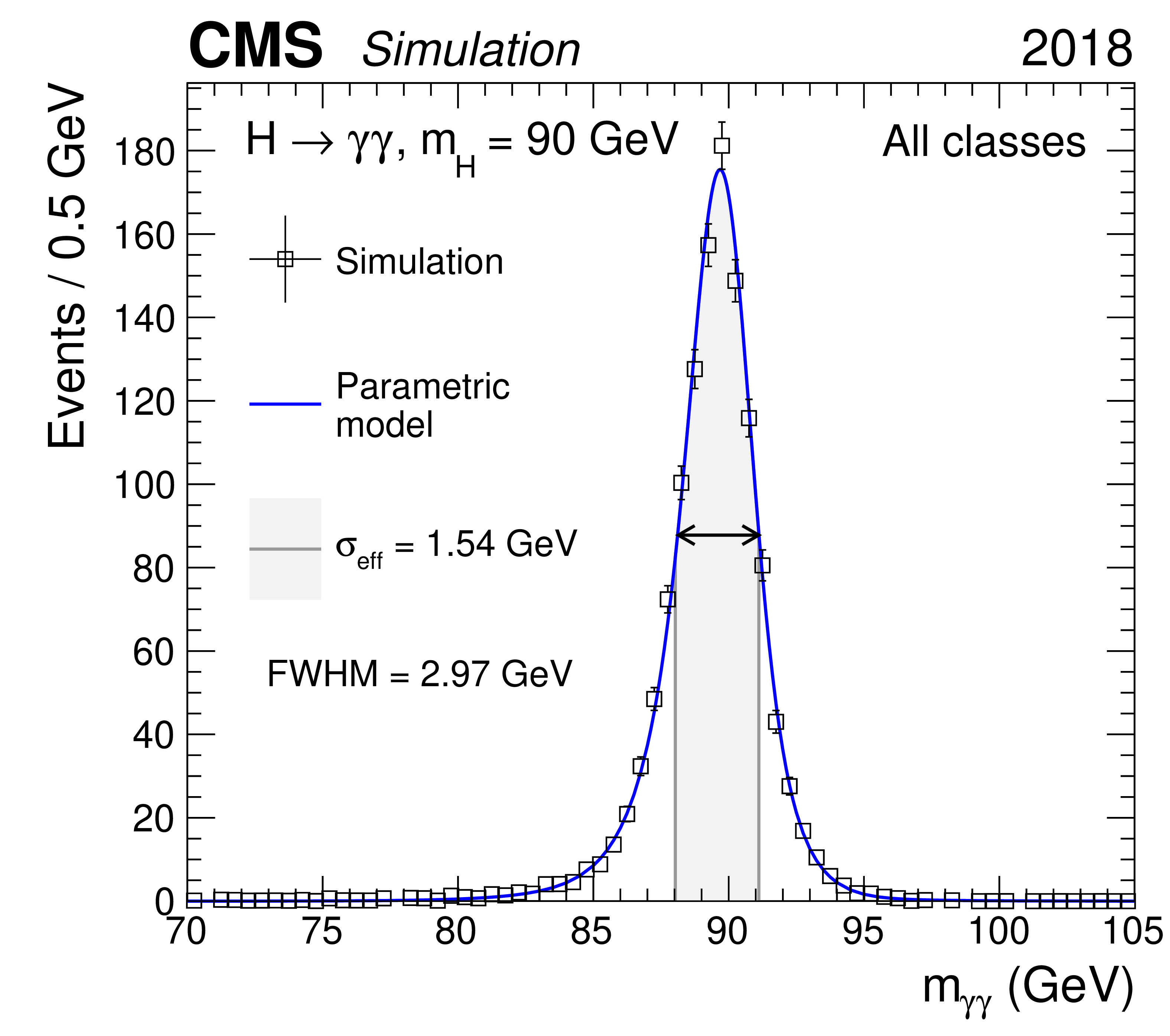
Figure 1-c:
Full parametrized signal shape, integrated over all event classes, in simulated signal events with $ m_{\mathrm{H}}= $ 90 GeV for 2016 (upper left), 2017 (upper right), and 2018 (lower). The open points are the weighted MC events and the blue lines the corresponding parametric models. Also shown are the $ \sigma_{\text{eff}} $ values and the shaded region limited by $ {\pm}\sigma_{\text{eff}} $, along with the FWHM values, indicated by the position of the arrows on each distribution. |

png pdf |
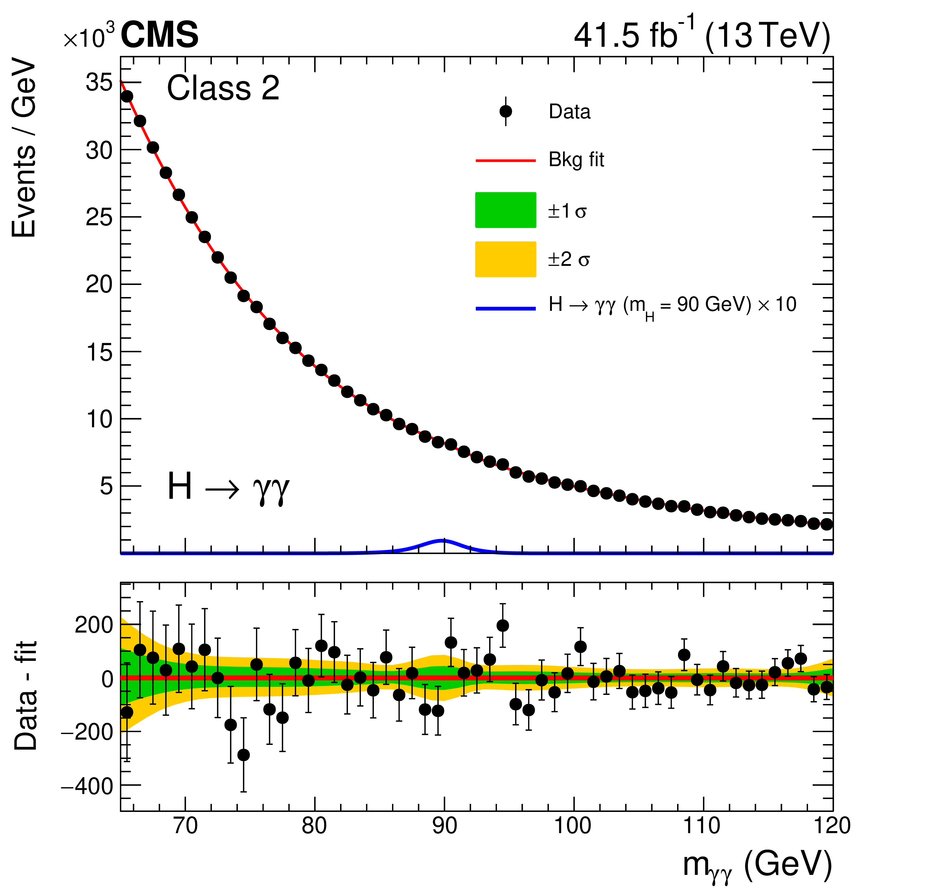
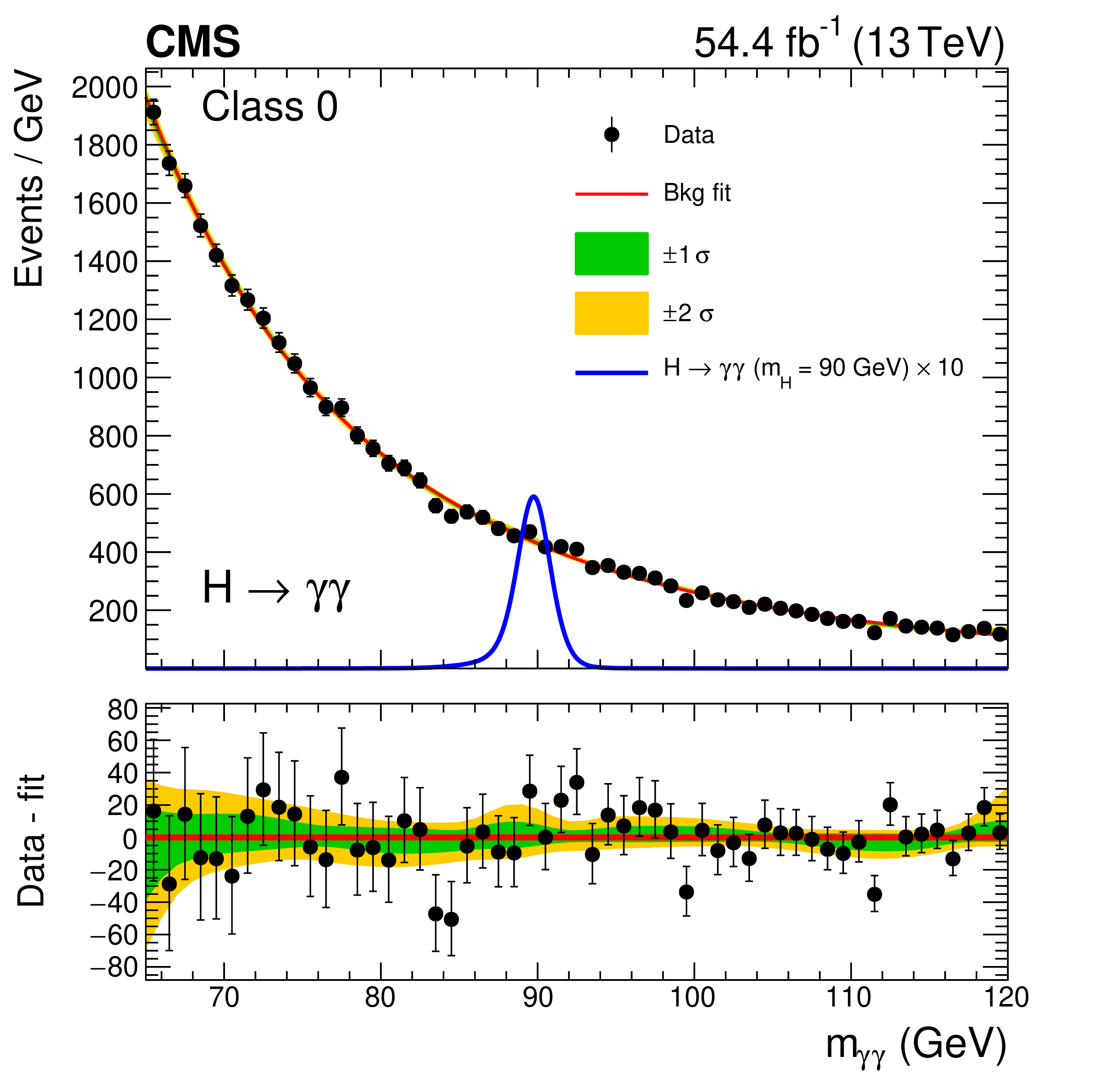
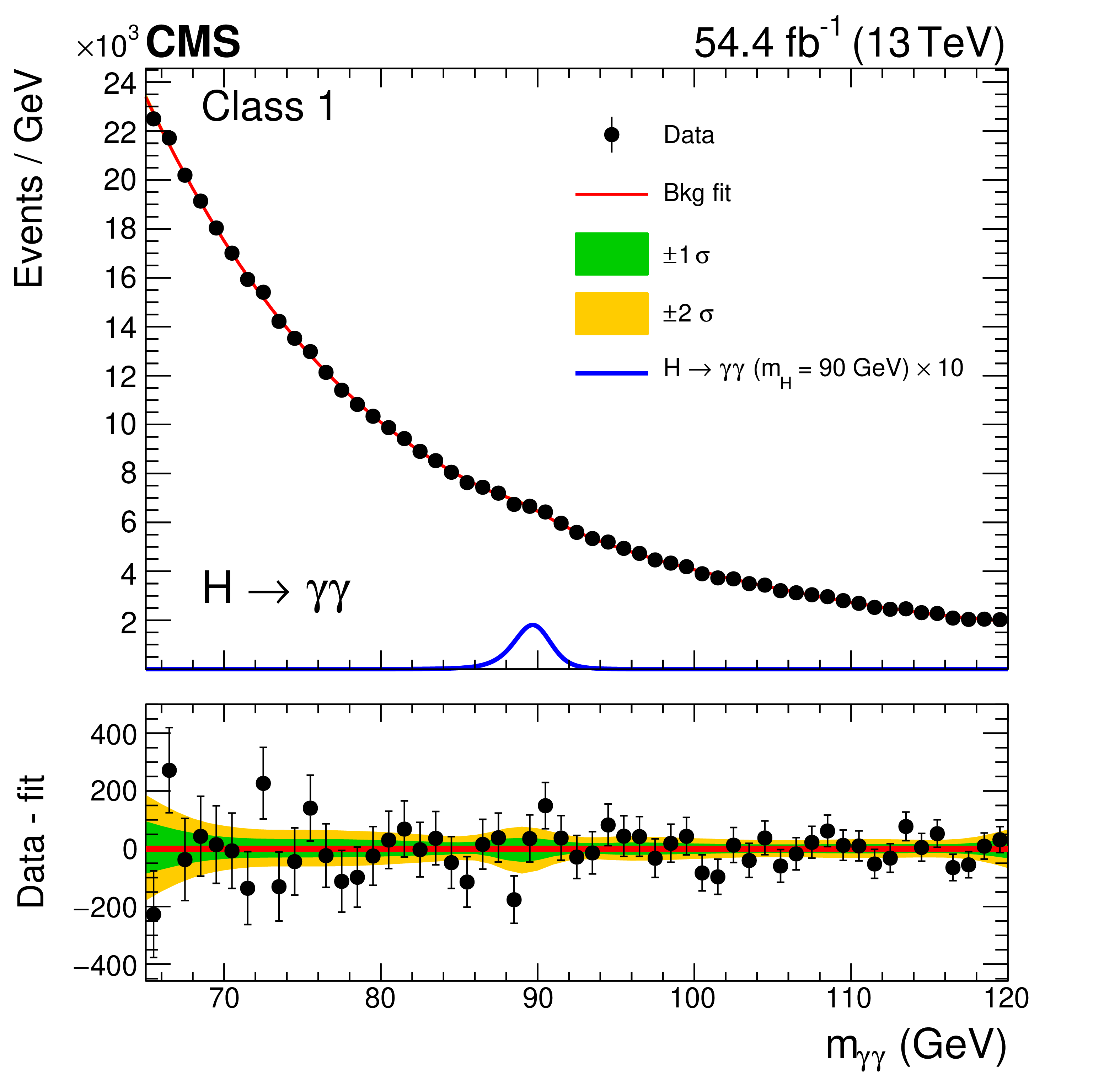
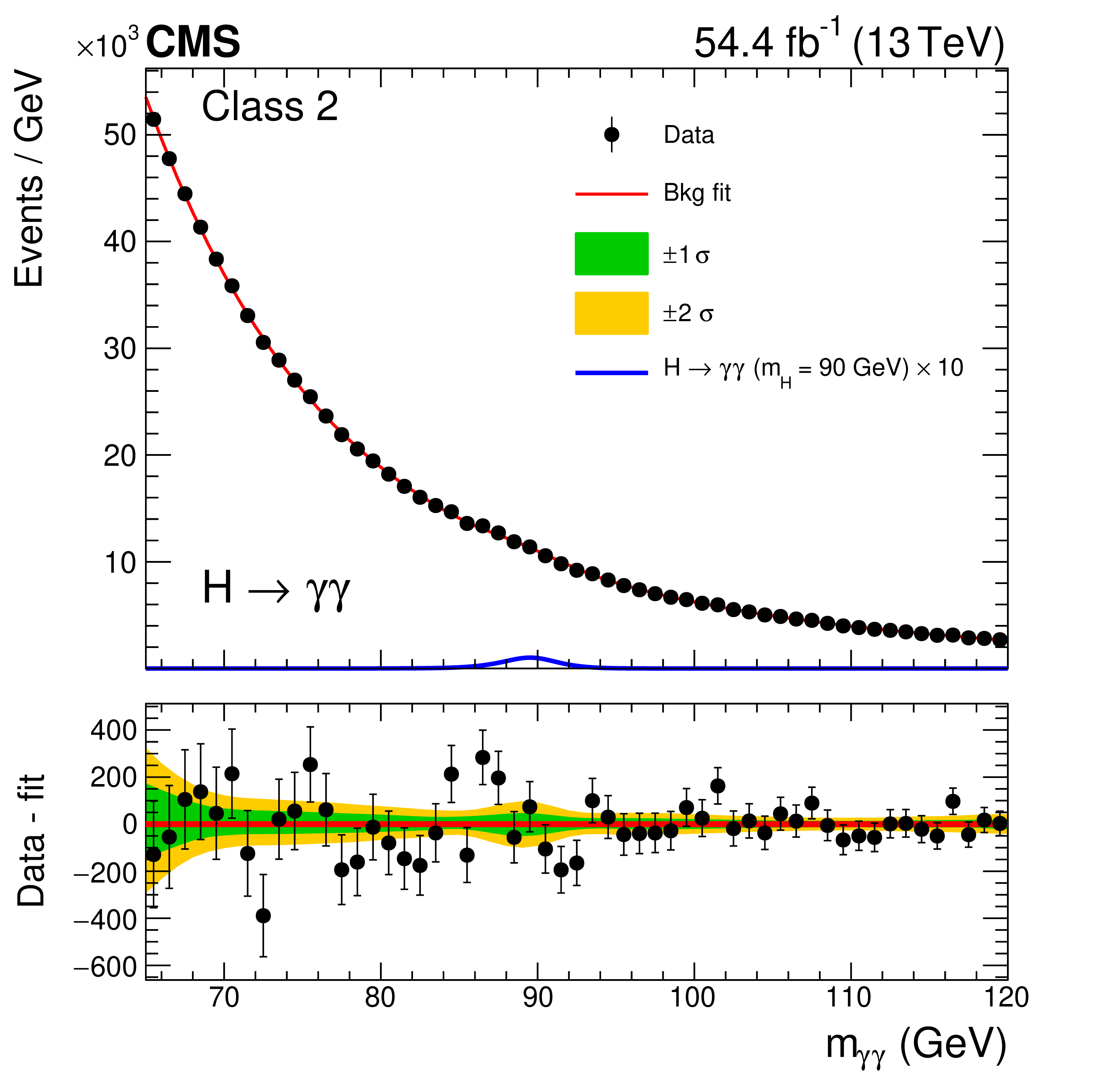
Figure 2:
Background model fits using the chosen background model parametrization to the 2016 data in the three event classes. The corresponding signal model for each class and $ m_{\mathrm{H}}= $ 90 GeV, multiplied by 10, is also shown. The one- and two-$ \sigma $ bands reflect the uncertainty in the background model normalization associated with the statistical uncertainties of the fits, and are shown for illustration purposes only. The difference between the data and the background model is shown in the lower panels. |

png pdf |
Figure 2-a:
Background model fits using the chosen background model parametrization to the 2016 data in the three event classes. The corresponding signal model for each class and $ m_{\mathrm{H}}= $ 90 GeV, multiplied by 10, is also shown. The one- and two-$ \sigma $ bands reflect the uncertainty in the background model normalization associated with the statistical uncertainties of the fits, and are shown for illustration purposes only. The difference between the data and the background model is shown in the lower panels. |

png pdf |
Figure 2-b:
Background model fits using the chosen background model parametrization to the 2016 data in the three event classes. The corresponding signal model for each class and $ m_{\mathrm{H}}= $ 90 GeV, multiplied by 10, is also shown. The one- and two-$ \sigma $ bands reflect the uncertainty in the background model normalization associated with the statistical uncertainties of the fits, and are shown for illustration purposes only. The difference between the data and the background model is shown in the lower panels. |

png pdf |
Figure 2-c:
Background model fits using the chosen background model parametrization to the 2016 data in the three event classes. The corresponding signal model for each class and $ m_{\mathrm{H}}= $ 90 GeV, multiplied by 10, is also shown. The one- and two-$ \sigma $ bands reflect the uncertainty in the background model normalization associated with the statistical uncertainties of the fits, and are shown for illustration purposes only. The difference between the data and the background model is shown in the lower panels. |

png pdf |
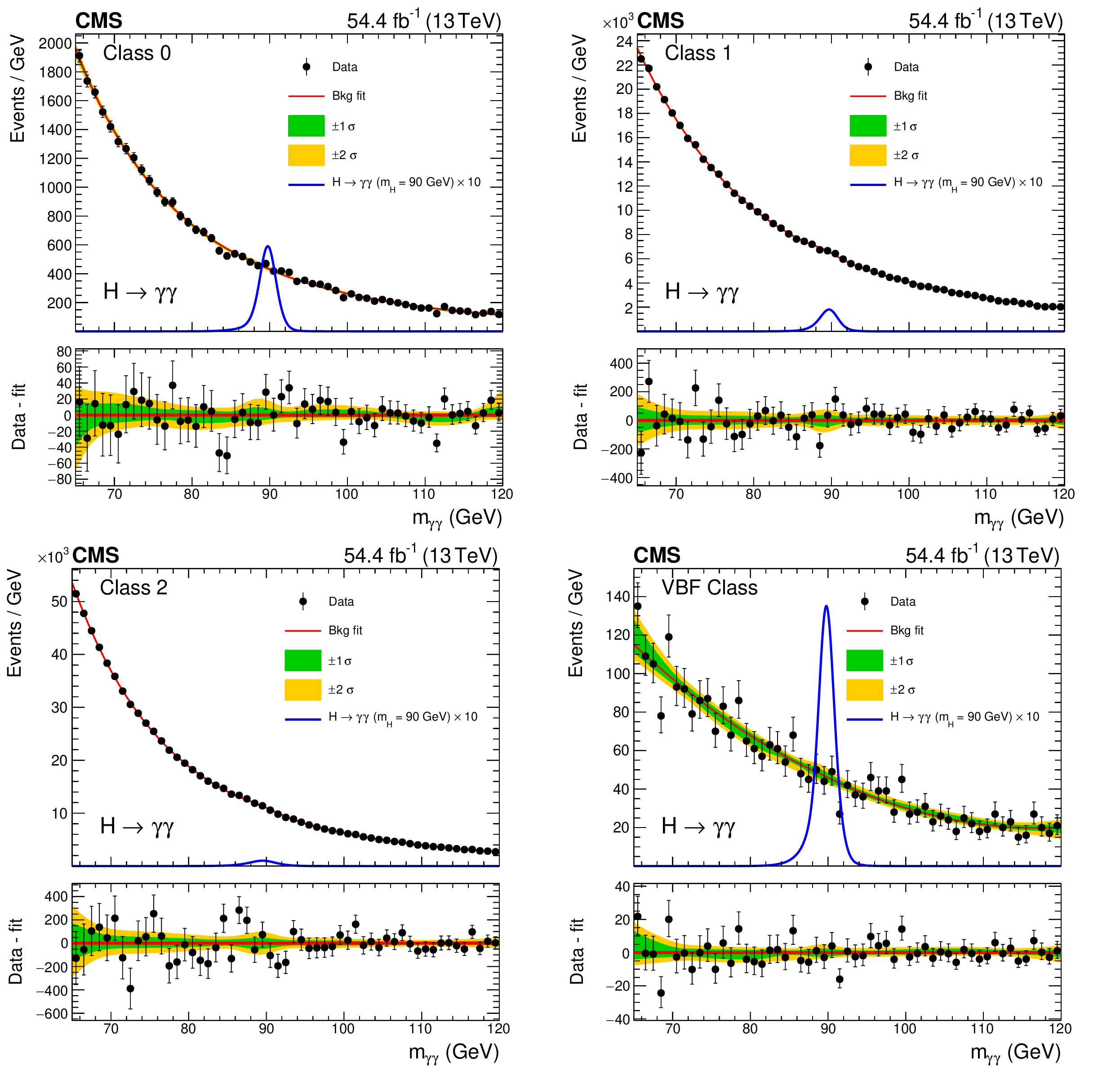
Figure 3:
Background model fits using the chosen background model parametrization to the 2017 data in the four event classes. The corresponding signal model for each class and $ m_{\mathrm{H}}= $ 90 GeV, multiplied by 10, is also shown. The one- and two-$ \sigma $ bands reflect the uncertainty in the background model normalization associated with the statistical uncertainties of the fits, and are shown for illustration purposes only. The difference between the data and the background model is shown in the lower panels. |

png pdf |
Figure 3-a:
Background model fits using the chosen background model parametrization to the 2017 data in the four event classes. The corresponding signal model for each class and $ m_{\mathrm{H}}= $ 90 GeV, multiplied by 10, is also shown. The one- and two-$ \sigma $ bands reflect the uncertainty in the background model normalization associated with the statistical uncertainties of the fits, and are shown for illustration purposes only. The difference between the data and the background model is shown in the lower panels. |

png pdf |
Figure 3-b:
Background model fits using the chosen background model parametrization to the 2017 data in the four event classes. The corresponding signal model for each class and $ m_{\mathrm{H}}= $ 90 GeV, multiplied by 10, is also shown. The one- and two-$ \sigma $ bands reflect the uncertainty in the background model normalization associated with the statistical uncertainties of the fits, and are shown for illustration purposes only. The difference between the data and the background model is shown in the lower panels. |
png pdf |
Figure 3-c:
Background model fits using the chosen background model parametrization to the 2017 data in the four event classes. The corresponding signal model for each class and $ m_{\mathrm{H}}= $ 90 GeV, multiplied by 10, is also shown. The one- and two-$ \sigma $ bands reflect the uncertainty in the background model normalization associated with the statistical uncertainties of the fits, and are shown for illustration purposes only. The difference between the data and the background model is shown in the lower panels. |

png pdf |
Figure 3-d:
Background model fits using the chosen background model parametrization to the 2017 data in the four event classes. The corresponding signal model for each class and $ m_{\mathrm{H}}= $ 90 GeV, multiplied by 10, is also shown. The one- and two-$ \sigma $ bands reflect the uncertainty in the background model normalization associated with the statistical uncertainties of the fits, and are shown for illustration purposes only. The difference between the data and the background model is shown in the lower panels. |
png pdf |
Figure 4:
Background model fits using the chosen background model parametrization to the 2018 data in the four event classes. The corresponding signal model for each class and $ m_{\mathrm{H}}= $ 90 GeV, multiplied by 10, is also shown. The one- and two-$ \sigma $ bands reflect the uncertainty in the background model normalization associated with the statistical uncertainties of the fits, and are shown for illustration purposes only. The difference between the data and the background model is shown in the lower panels. |
png pdf |
Figure 4-a:
Background model fits using the chosen background model parametrization to the 2018 data in the four event classes. The corresponding signal model for each class and $ m_{\mathrm{H}}= $ 90 GeV, multiplied by 10, is also shown. The one- and two-$ \sigma $ bands reflect the uncertainty in the background model normalization associated with the statistical uncertainties of the fits, and are shown for illustration purposes only. The difference between the data and the background model is shown in the lower panels. |
png pdf |
Figure 4-b:
Background model fits using the chosen background model parametrization to the 2018 data in the four event classes. The corresponding signal model for each class and $ m_{\mathrm{H}}= $ 90 GeV, multiplied by 10, is also shown. The one- and two-$ \sigma $ bands reflect the uncertainty in the background model normalization associated with the statistical uncertainties of the fits, and are shown for illustration purposes only. The difference between the data and the background model is shown in the lower panels. |
png pdf |
Figure 4-c:
Background model fits using the chosen background model parametrization to the 2018 data in the four event classes. The corresponding signal model for each class and $ m_{\mathrm{H}}= $ 90 GeV, multiplied by 10, is also shown. The one- and two-$ \sigma $ bands reflect the uncertainty in the background model normalization associated with the statistical uncertainties of the fits, and are shown for illustration purposes only. The difference between the data and the background model is shown in the lower panels. |

png pdf |
Figure 4-d:
Background model fits using the chosen background model parametrization to the 2018 data in the four event classes. The corresponding signal model for each class and $ m_{\mathrm{H}}= $ 90 GeV, multiplied by 10, is also shown. The one- and two-$ \sigma $ bands reflect the uncertainty in the background model normalization associated with the statistical uncertainties of the fits, and are shown for illustration purposes only. The difference between the data and the background model is shown in the lower panels. |
png pdf |
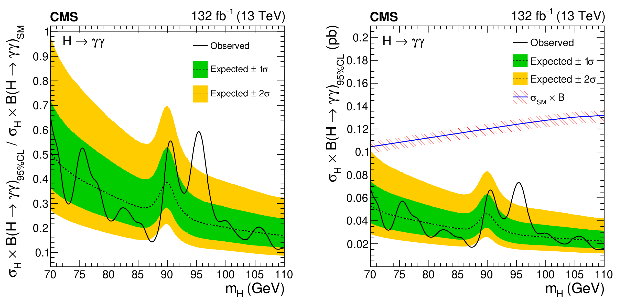
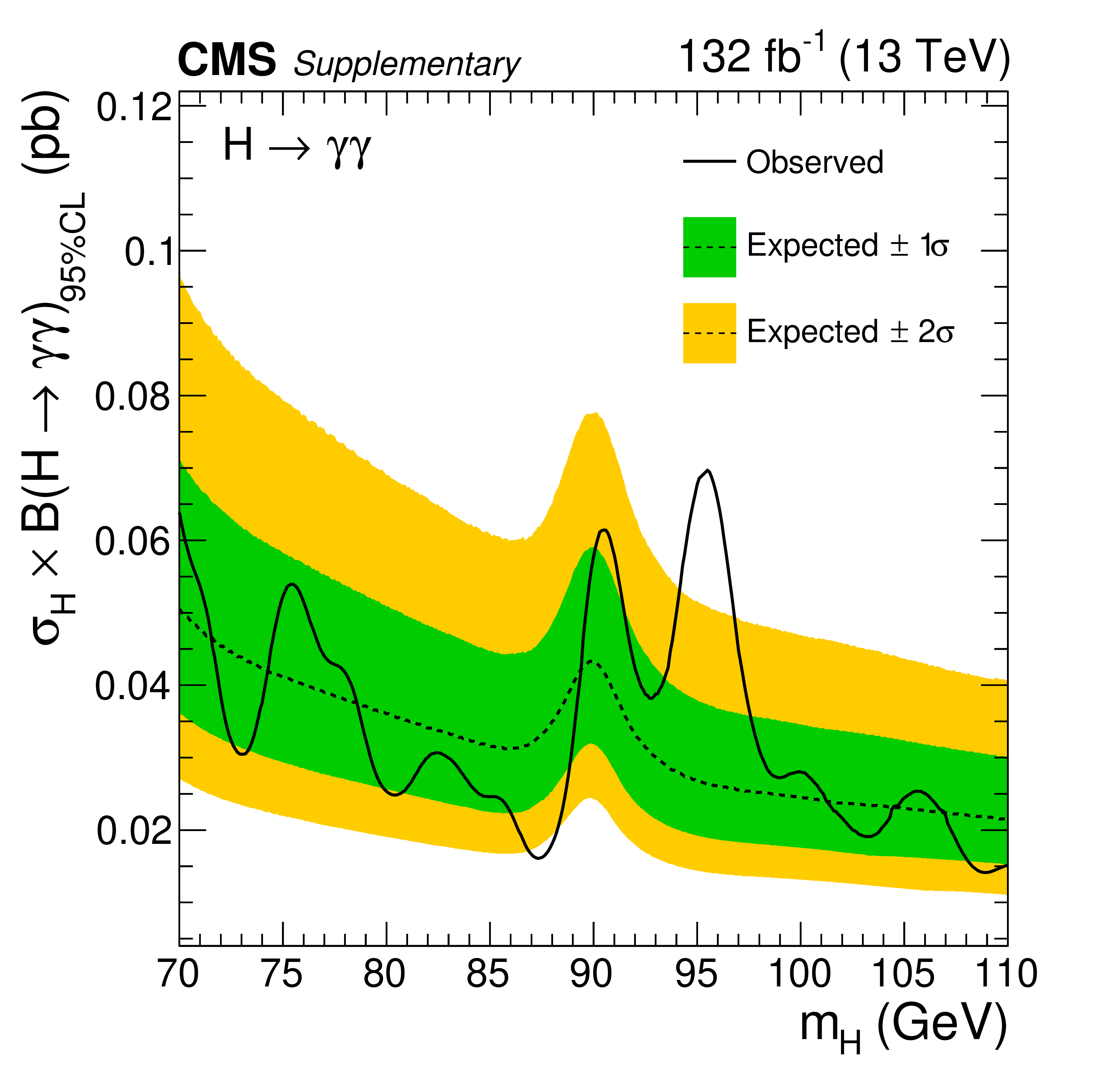
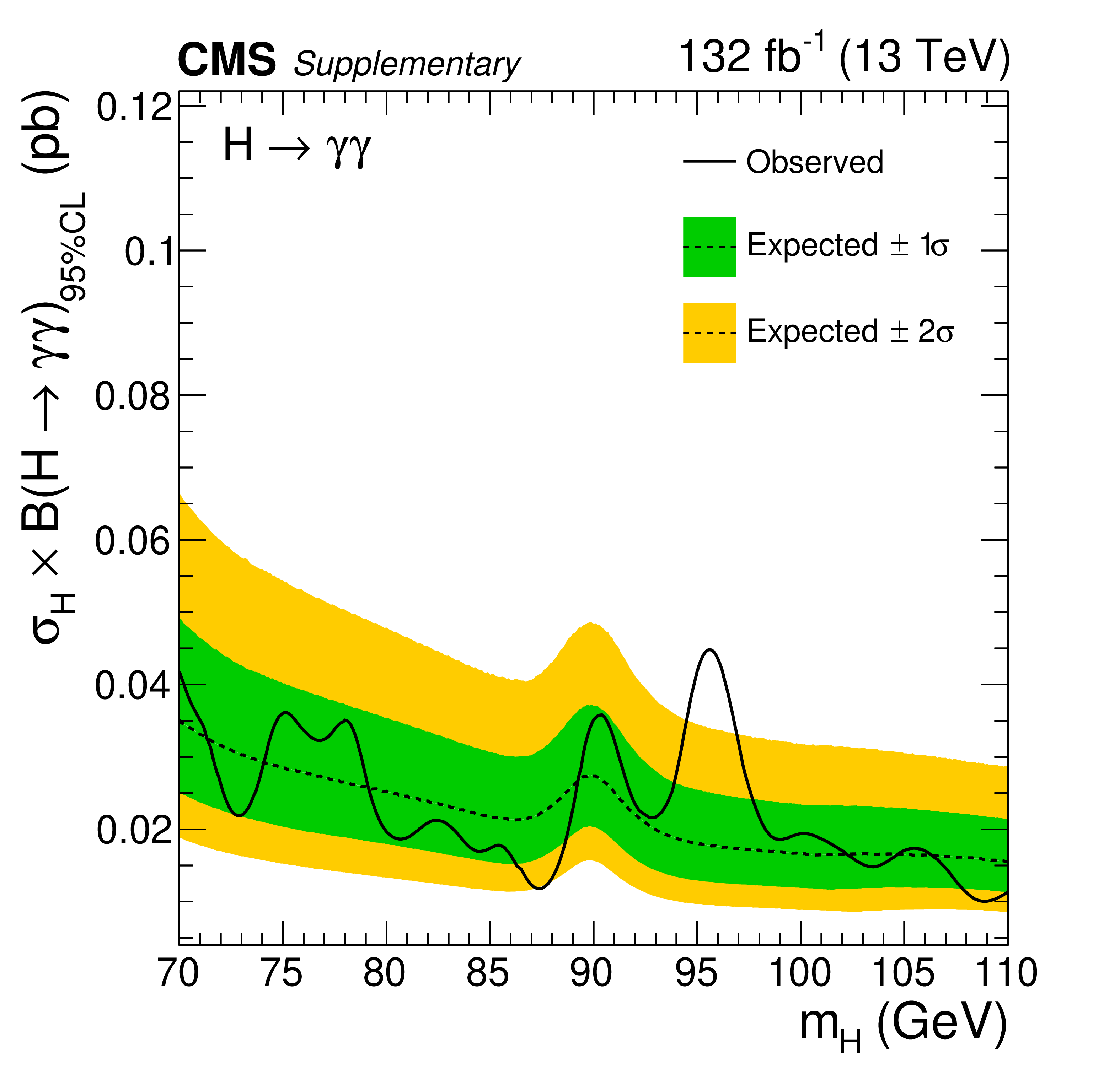
Figure 5:
Expected and observed exclusion limits (95% CL, in the asymptotic approximation) on the product of the production cross section and branching fraction into two photons for an additional SM-like Higgs boson, from the statistical combination of the 2016, 2017, and 2018 data sets. The inner and outer bands indicate the regions containing the distribution of limits located within $ {\pm}$1$\sigma $ and $ {\pm}$2$\sigma $, respectively, of the expectation under the background-only hypothesis. The limit is shown relative to the expected SM-like value (left). The corresponding theoretical prediction for the product of the cross section and branching fraction into two photons for an additional SM-like Higgs boson is shown as a solid line with a hatched band, indicating its uncertainty [64] (right). |

png pdf |
Figure 5-a:
Expected and observed exclusion limits (95% CL, in the asymptotic approximation) on the product of the production cross section and branching fraction into two photons for an additional SM-like Higgs boson, from the statistical combination of the 2016, 2017, and 2018 data sets. The inner and outer bands indicate the regions containing the distribution of limits located within $ {\pm}$1$\sigma $ and $ {\pm}$2$\sigma $, respectively, of the expectation under the background-only hypothesis. The limit is shown relative to the expected SM-like value (left). The corresponding theoretical prediction for the product of the cross section and branching fraction into two photons for an additional SM-like Higgs boson is shown as a solid line with a hatched band, indicating its uncertainty [64] (right). |

png pdf |
Figure 5-b:
Expected and observed exclusion limits (95% CL, in the asymptotic approximation) on the product of the production cross section and branching fraction into two photons for an additional SM-like Higgs boson, from the statistical combination of the 2016, 2017, and 2018 data sets. The inner and outer bands indicate the regions containing the distribution of limits located within $ {\pm}$1$\sigma $ and $ {\pm}$2$\sigma $, respectively, of the expectation under the background-only hypothesis. The limit is shown relative to the expected SM-like value (left). The corresponding theoretical prediction for the product of the cross section and branching fraction into two photons for an additional SM-like Higgs boson is shown as a solid line with a hatched band, indicating its uncertainty [64] (right). |

png pdf |
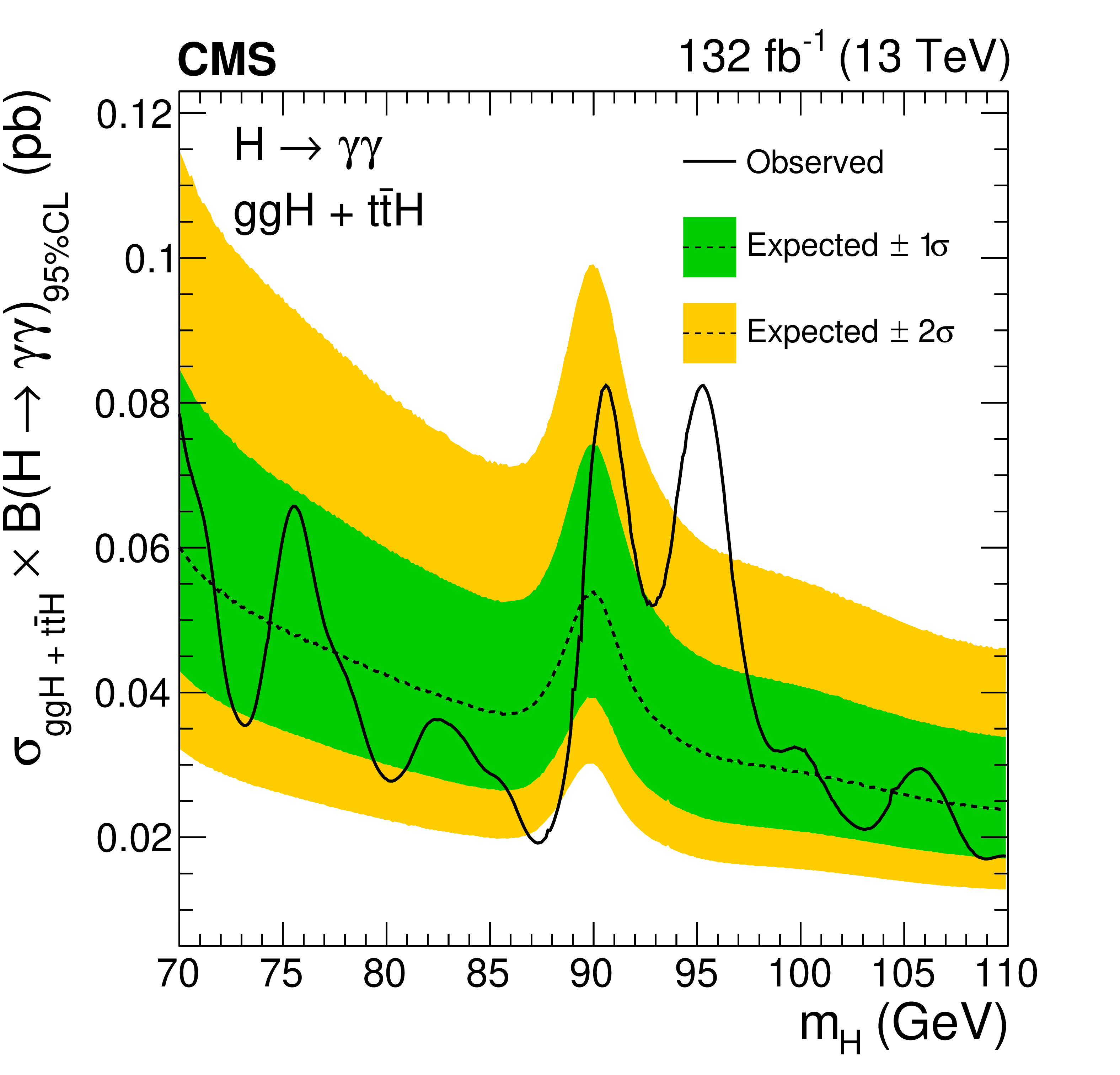
Figure 6:
Expected and observed exclusion limits (95% CL, in the asymptotic approximation) on the product of the production cross section and branching fraction into two photons for an additional SM-like Higgs boson, for the ggH plus $ {\mathrm{t}\overline{\mathrm{t}}} \mathrm{H} $ (upper left) and VBF plus VH (upper right) processes, and assuming 100% production via the VBF (lower left) or VH (lower right) processes, from the statistical combination of the 2016, 2017, and 2018 data sets. The inner and outer bands indicate the regions containing the distribution of limits located within $ \pm $1$\sigma $ and $ \pm $2$\sigma $, respectively, of the expectation under the background-only hypothesis. |
png pdf |
Figure 6-a:
Expected and observed exclusion limits (95% CL, in the asymptotic approximation) on the product of the production cross section and branching fraction into two photons for an additional SM-like Higgs boson, for the ggH plus $ {\mathrm{t}\overline{\mathrm{t}}} \mathrm{H} $ (upper left) and VBF plus VH (upper right) processes, and assuming 100% production via the VBF (lower left) or VH (lower right) processes, from the statistical combination of the 2016, 2017, and 2018 data sets. The inner and outer bands indicate the regions containing the distribution of limits located within $ \pm $1$\sigma $ and $ \pm $2$\sigma $, respectively, of the expectation under the background-only hypothesis. |

png pdf |
Figure 6-b:
Expected and observed exclusion limits (95% CL, in the asymptotic approximation) on the product of the production cross section and branching fraction into two photons for an additional SM-like Higgs boson, for the ggH plus $ {\mathrm{t}\overline{\mathrm{t}}} \mathrm{H} $ (upper left) and VBF plus VH (upper right) processes, and assuming 100% production via the VBF (lower left) or VH (lower right) processes, from the statistical combination of the 2016, 2017, and 2018 data sets. The inner and outer bands indicate the regions containing the distribution of limits located within $ \pm $1$\sigma $ and $ \pm $2$\sigma $, respectively, of the expectation under the background-only hypothesis. |

png pdf |
Figure 6-c:
Expected and observed exclusion limits (95% CL, in the asymptotic approximation) on the product of the production cross section and branching fraction into two photons for an additional SM-like Higgs boson, for the ggH plus $ {\mathrm{t}\overline{\mathrm{t}}} \mathrm{H} $ (upper left) and VBF plus VH (upper right) processes, and assuming 100% production via the VBF (lower left) or VH (lower right) processes, from the statistical combination of the 2016, 2017, and 2018 data sets. The inner and outer bands indicate the regions containing the distribution of limits located within $ \pm $1$\sigma $ and $ \pm $2$\sigma $, respectively, of the expectation under the background-only hypothesis. |

png pdf |
Figure 6-d:
Expected and observed exclusion limits (95% CL, in the asymptotic approximation) on the product of the production cross section and branching fraction into two photons for an additional SM-like Higgs boson, for the ggH plus $ {\mathrm{t}\overline{\mathrm{t}}} \mathrm{H} $ (upper left) and VBF plus VH (upper right) processes, and assuming 100% production via the VBF (lower left) or VH (lower right) processes, from the statistical combination of the 2016, 2017, and 2018 data sets. The inner and outer bands indicate the regions containing the distribution of limits located within $ \pm $1$\sigma $ and $ \pm $2$\sigma $, respectively, of the expectation under the background-only hypothesis. |

png pdf |
Figure 7:
The observed local $ p $-values for an additional SM-like Higgs boson as a function of $ m_{\mathrm{H}} $, from the analysis of the data from 2016, 2017, 2018, and their combination. |
| Tables | |
png pdf |
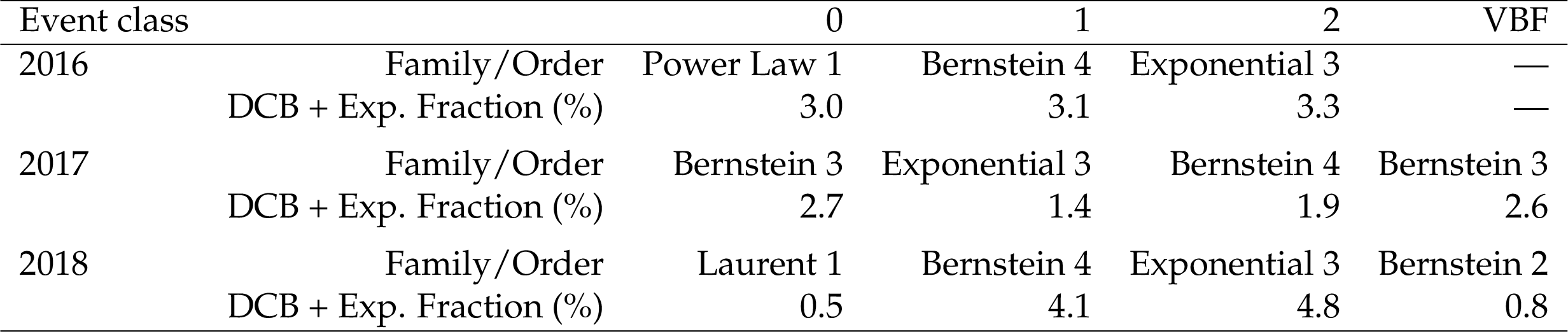
Table 1:
Families and orders of functions chosen as best fit when summed with the DCB + exponential function, by year and by event class, in the case of background-only fits. The DCB + exponential fractions for these models in the range 85 $ < m_{\gamma\gamma} < $ 95 GeV are also shown. |

png pdf |
Table 2:
The expected number of SM-like Higgs boson signal events ($ m_{\mathrm{H}}= $ 90 GeV) per event class and the corresponding percentage breakdown per production process, for the 2016, 2017, and 2018 data. The values of $ \sigma_{\text{eff}} $ and $ \sigma_{\text{HM}} $ are also shown, along with the number of background events (``Bkg.'') per GeV estimated from the background-only fit to the data, that includes the number, shown separately, from the DY process (``DY Bkg.''), in a $ \sigma_{\text{eff}} $ window centered on $ m_{\mathrm{H}}= $ 90 GeV. |
| Summary |
| A search for an additional, SM-like, low-mass Higgs boson decaying into two photons has been presented. It is based upon data samples corresponding to an integrated luminosity of 132 fb$ ^{-1} $ collected in pp collisions at a center-of-mass energy of 13 TeV in 2016-2018. The search is performed in a mass range between 70 and 110 GeV. The expected and observed 95% CL upper limits on the product of the production cross section and branching fraction into two photons for an additional SM-like Higgs boson as well as the expected and observed local $ p $-values are presented. The observed upper limit on the product of the production cross section and branching fraction for the full data set ranges from 15 to 73 fb. The results of the statistical combination of the analyses of the three data sets show no significant excess over the background expectation. The maximum deviation with respect to the background is seen for a mass hypothesis of 95.4 GeV with a local (global) significance of 2.9 (1.3) standard deviations. |
| Additional Figures | |

png pdf |
Additional Figure 1:
Signal efficiency $ \times $ acceptance for the analysis of the 2016 data set, as a function of mass hypothesis. |

png pdf |
Additional Figure 2:
Signal efficiency $ \times $ acceptance for the analysis of the 2017 data set, as a function of mass hypothesis. |
png pdf |
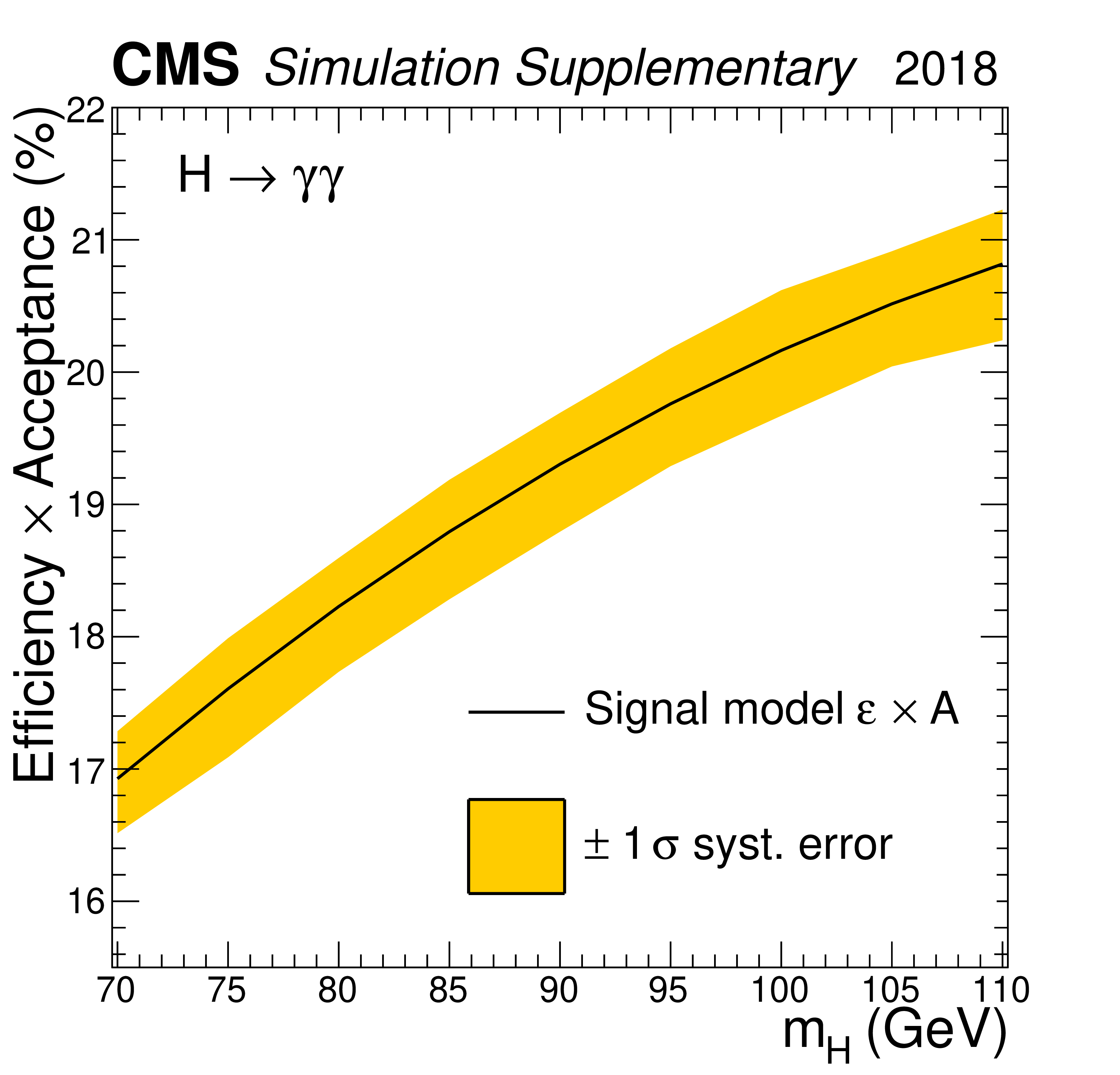
Additional Figure 3:
Signal efficiency $ \times $ acceptance for the analysis of the 2018 data set, as a function of mass hypothesis. |
png pdf |
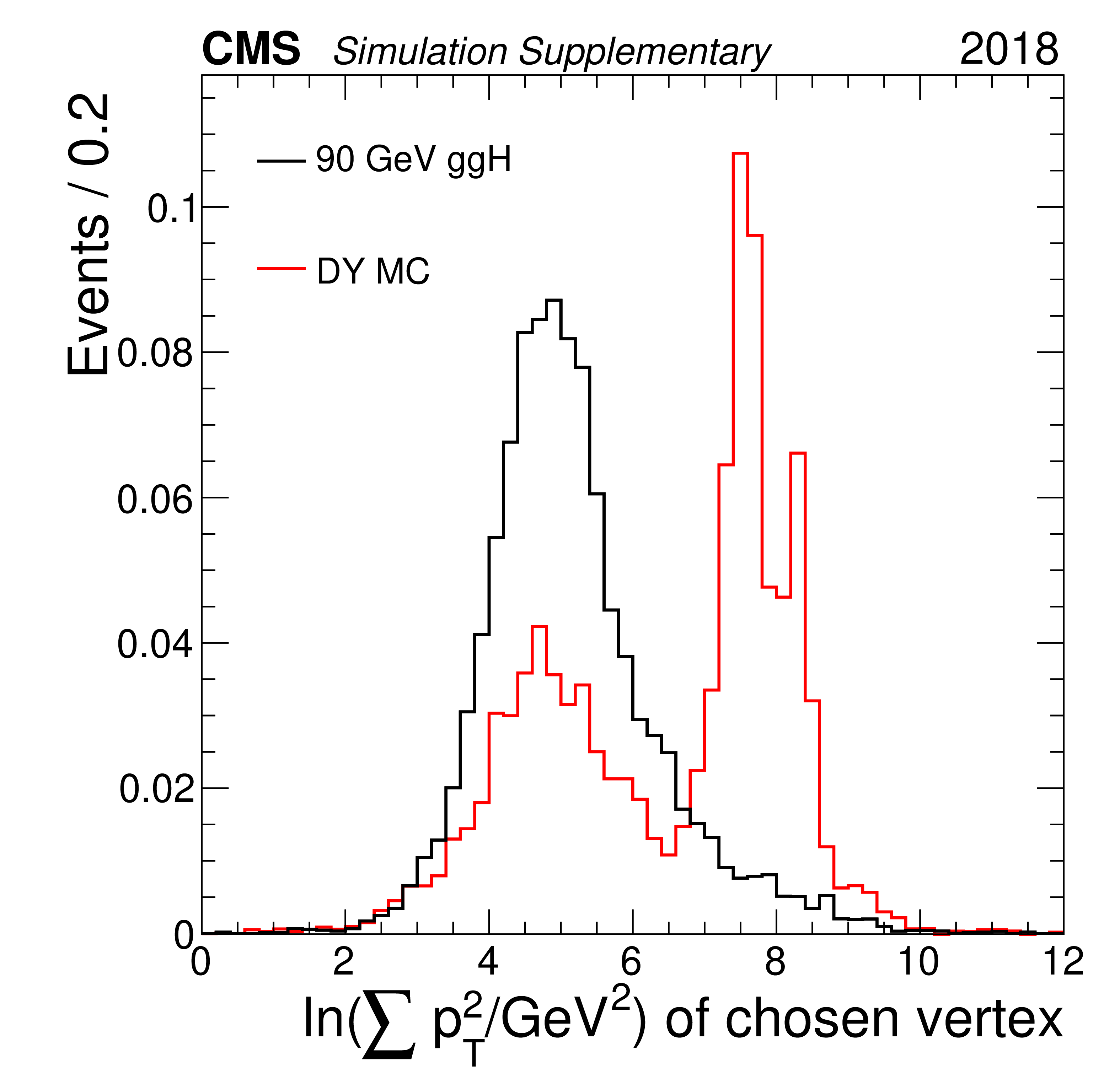
Additional Figure 4:
Distributions of the variable $\ln(\Sigma p_{\mathrm{T}}^{2}/\mathrm{GeV}^{2}) $ for simulated surviving Drell-Yan events (red) and simulated signal events corresponding to an SM-like Higgs boson with $ m_{H} $ = 90 GeV produced via the ggH process (black), with both distributions normalized to 1, for the analysis of the 2018 data set. The events are required to have survived the analysis preselection, the pixel detector-based electron veto, and have diphoton BDT classifier values greater than -0.364. This variable, corresponding to the natural logarithm of the sum of the squares of transverse momenta of all tracks associated with the chosen diphoton vertex, is used to suppress the surviving Drell-Yan background. For the simulated Drell-Yan events, the peak at $ \sim $8.3 reflects the contributions of the two electron tracks, while the peak at $ \sim $7.6 that of one electron track, the other either being out of the detector acceptance or not reconstructed due to significant bremsstrahlung. The peak at $ \sim $5 corresponds to the case where neither of the electron tracks is reconstructed, similar to that of signal events where the main contributions are from tracks from pileup and the underlying event. |
png pdf |
Additional Figure 5:
Two-dimensional distribution of $\ln(\Sigma p_{\mathrm{T}}^{2}/\mathrm{GeV}^{2}) $ versus diphoton transverse momentum ($ p_{\mathrm{T}}^{\gamma\gamma}/\mathrm{GeV} $) for simulated signal events corresponding to an SM-like Higgs boson with $ m_{H} $ = 90 GeV produced via the ggH process, with the distribution normalized to 1, for the analysis of the 2018 data set. The events are required to have survived the analysis preselection, the pixel detector-based electron veto, and have diphoton BDT classifier values greater than -0.364. The upper limit on $\ln(\Sigma p_{\mathrm{T}}^{2}/\mathrm{GeV}^{2}) $, $\ln(\Sigma p_{\mathrm{T}}^{2}/\mathrm{GeV}^{2}) = 0.016p_{\mathrm{T}}^{\gamma\gamma}/\mathrm{GeV} + $ 6.0, is shown as the white line. |

png pdf |
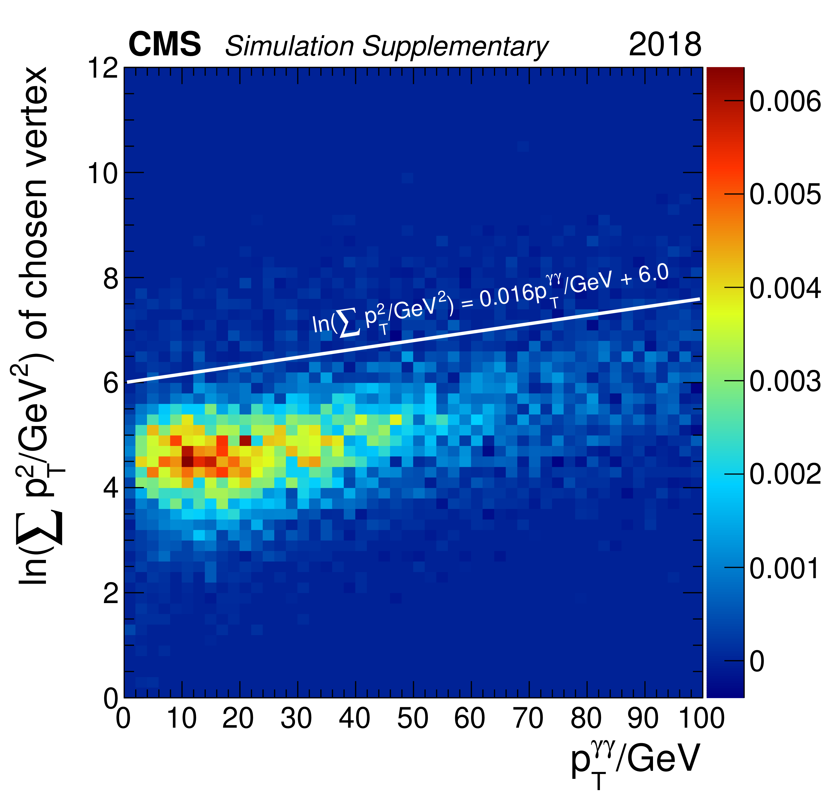
Additional Figure 6:
Two-dimensional distribution of $\ln(\Sigma p_{\mathrm{T}}^{2}/\mathrm{GeV}^{2}) $ versus diphoton transverse momentum ($ p_{\mathrm{T}}^{\gamma\gamma}/\mathrm{GeV} $) for simulated surviving Drell-Yan events, with the distribution normalized to 1, for the analysis of the 2018 data set. The events are required to have survived the analysis preselection, the pixel detector-based electron veto, and have diphoton BDT classifier values greater than -0.364. The upper limit on $\ln(\Sigma p_{\mathrm{T}}^{2}/\mathrm{GeV}^{2}) $, $\ln(\Sigma p_{\mathrm{T}}^{2}/\mathrm{GeV}^{2}) = 0.016p_{\mathrm{T}}^{\gamma\gamma}/\mathrm{GeV} + $ 6.0, is shown as the white line. |
png pdf |
Additional Figure 7:
Expected and observed exclusion limits (95% CL, in the asymptotic approximation) on the product of the production cross section and branching fraction into two photons relative to the value expected for an additional SM-like Higgs boson, from the analysis of the 2016 data set. The inner and outer bands indicate the regions containing the distribution of limits located within $ \pm $1 and 2$ \sigma $, respectively, of the expectation under the background-only hypothesis. |

png pdf |
Additional Figure 8:
Expected and observed exclusion limits (95% CL, in the asymptotic approximation) on the product of the production cross section and branching fraction into two photons, for an additional SM-like Higgs boson, from the analysis of the 2016 data set. The inner and outer bands indicate the regions containing the distribution of limits located within $ \pm $1 and 2$ \sigma $, respectively, of the expectation under the background-only hypothesis. The corresponding theoretical prediction for the product of the cross section and branching fraction into two photons for an additional SM-like Higgs boson is shown as a solid line with a hatched band, indicating its uncertainty. |

png pdf |
Additional Figure 9:
Expected and observed exclusion limits (95% CL, in the asymptotic approximation) on the product of the production cross section and branching fraction into two photons relative to the value expected for an additional SM-like Higgs boson, from the analysis of the 2017 data set. The inner and outer bands indicate the regions containing the distribution of limits located within $ \pm $1 and 2$ \sigma $, respectively, of the expectation under the background-only hypothesis. |

png pdf |
Additional Figure 10:
Expected and observed exclusion limits (95% CL, in the asymptotic approximation) on the product of the production cross section and branching fraction into two photons, for an additional SM-like Higgs boson, from the analysis of the 2017 data set. The inner and outer bands indicate the regions containing the distribution of limits located within $ \pm $1 and 2$ \sigma $, respectively, of the expectation under the background-only hypothesis. The corresponding theoretical prediction for the product of the cross section and branching fraction into two photons for an additional SM-like Higgs boson is shown as a solid line with a hatched band, indicating its uncertainty. |

png pdf |
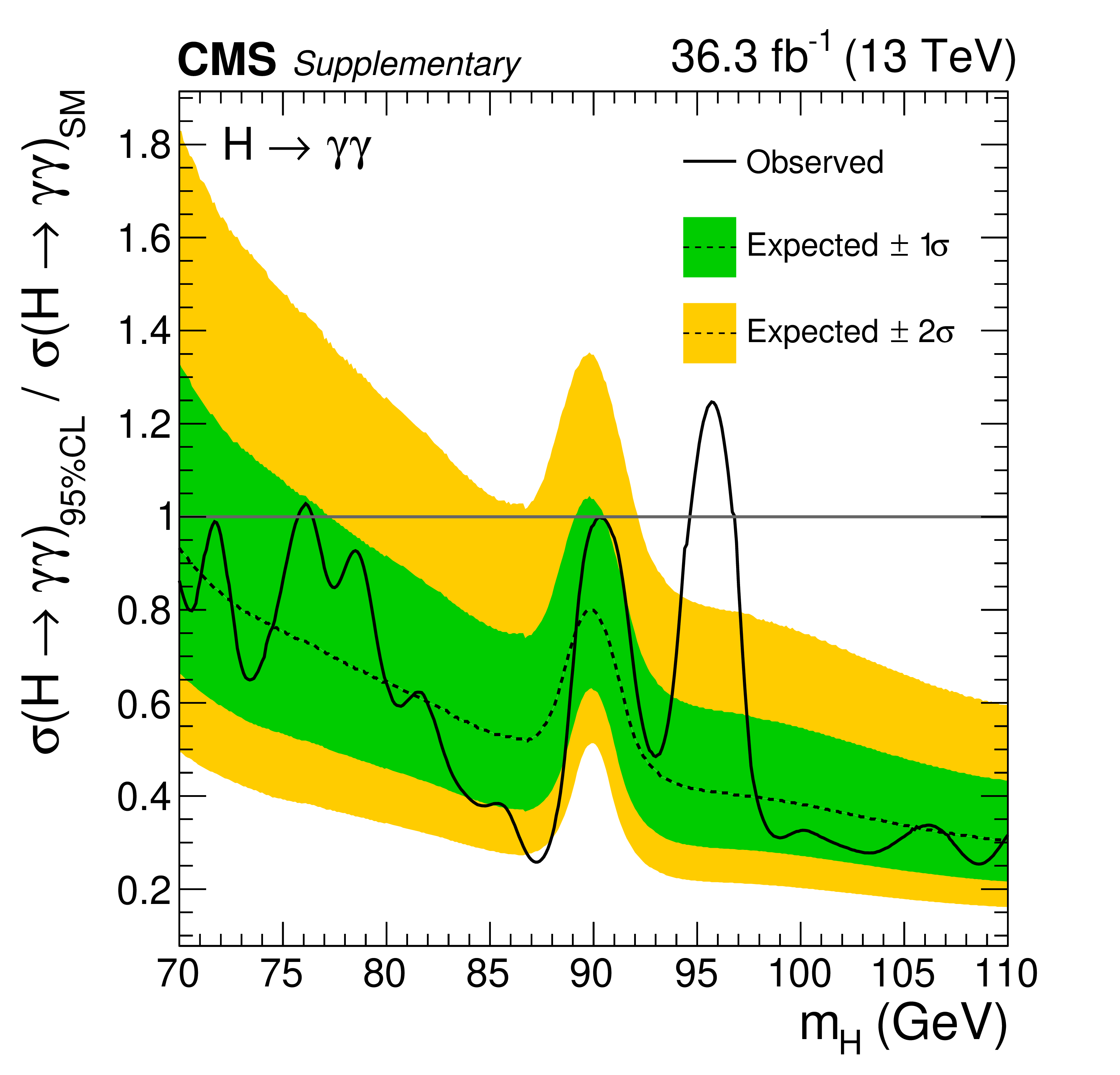
Additional Figure 11:
Expected and observed exclusion limits (95% CL, in the asymptotic approximation) on the product of the production cross section and branching fraction into two photons relative to the value expected for an additional SM-like Higgs boson, from the analysis of the 2018 data set. The inner and outer bands indicate the regions containing the distribution of limits located within $ \pm $1 and 2$ \sigma $, respectively, of the expectation under the background-only hypothesis. |

png pdf |
Additional Figure 12:
Expected and observed exclusion limits (95% CL, in the asymptotic approximation) on the product of the production cross section and branching fraction into two photons, for an additional SM-like Higgs boson, from the analysis of the 2018 data set. The inner and outer bands indicate the regions containing the distribution of limits located within $ \pm $1 and 2$ \sigma $, respectively, of the expectation under the background-only hypothesis. The corresponding theoretical prediction for the product of the cross section and branching fraction into two photons for an additional SM-like Higgs boson is shown as a solid line with a hatched band, indicating its uncertainty. |

png pdf |
Additional Figure 13:
Expected and observed exclusion limits (95% CL, in the asymptotic approximation) on the product of the production cross section and branching fraction into two photons for an additional SM-like Higgs boson, from the analysis of the combined data from 2016, 2017, and 2018. The inner and outer bands indicate the regions containing the distribution of limits located within $ \pm $1 and 2$ \sigma $, respectively, of the expectation under the background-only hypothesis. The corresponding theoretical predictions for the product of the cross section and branching fraction into two photons are shown as a solid blue line with a hatched red band indicating its uncertainty for an additional SM-like Higgs boson ($ \sigma_{SM} \times B $), and a solid red line with a hatched blue band indicating its uncertainty for a Higgs boson in the Fermiophobic model $ (\sigma \times B)_{FP} $. |

png pdf |
Additional Figure 14:
Values of the signal strength $ \widehat{\mu} $ measured individually for the eleven event classes in the analysis of the combined data from 2016, 2017, and 2018, and the overall combined value, with $ m_H $ fixed to that of the largest local p-value excess. The horizontal bars indicate $ \pm 1\sigma $ uncertainties in the values, and the vertical line and band indicate the value of the combined $ \widehat{\mu} $ in the fit to the data and its uncertainty. The $ \chi^2 $ probability of the values for the eleven event classes being compatible with the overall best-fit signal strength is 68%. |

png pdf |
Additional Figure 15:
Values of the signal strength $ \widehat{\mu} $ measured individually for each year, and the overall combined value, with $ m_H $ fixed to that of the largest local p-value excess. The horizontal bars indicate $ \pm 1\sigma $ uncertainties in the values, and the vertical line and band indicate the value of the combined $ \widehat{\mu} $ in the fit to the data and its uncertainty. The $ \chi^2 $ probability of the values for the three years being compatible with the overall best-fit signal strength is 6%. |
png pdf |
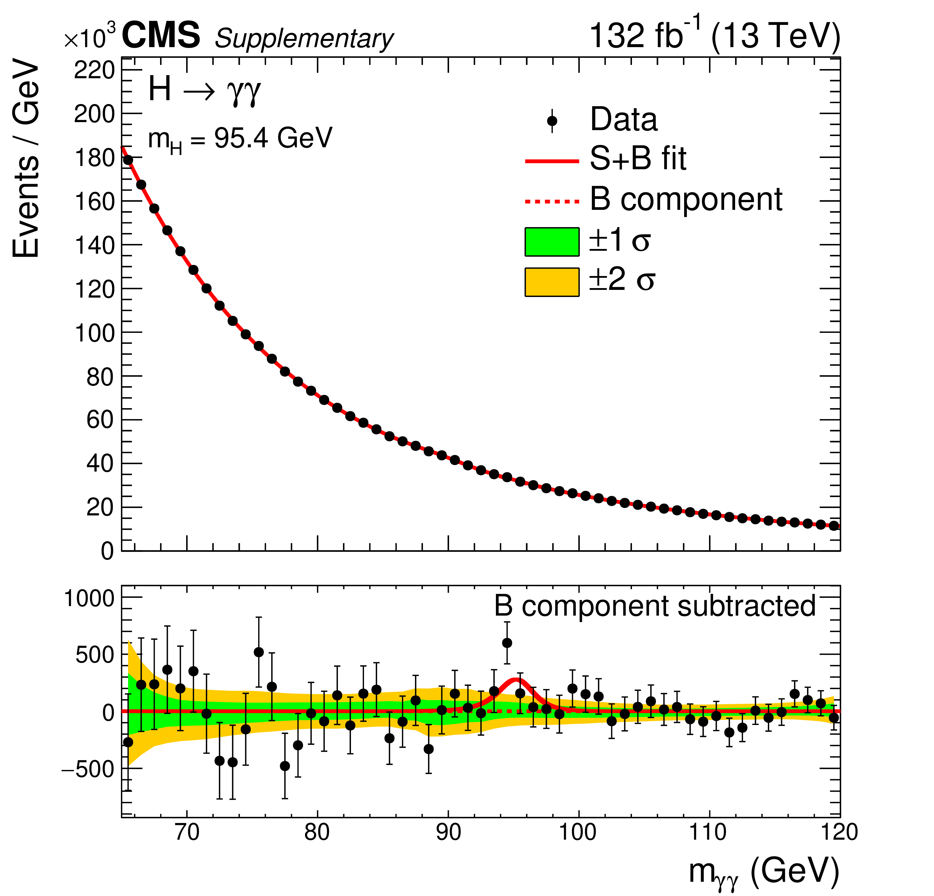
Additional Figure 16:
Events in all classes of the combined 13$ \mathrm{TeV} $ data set, binned as a function of $ m_{\gamma\gamma} $, together with the result of a fit of the signal-plus-background model, under a mass hypothesis of 95.4 GeV. The one- and two-$ \sigma $ uncertainty bands shown for the background component of the fit include the uncertainty due to the choice of fit function and the uncertainty in the fitted parameters. The distribution of the residual data after subtracting the fitted background component is shown in the lower panel. |
png pdf |
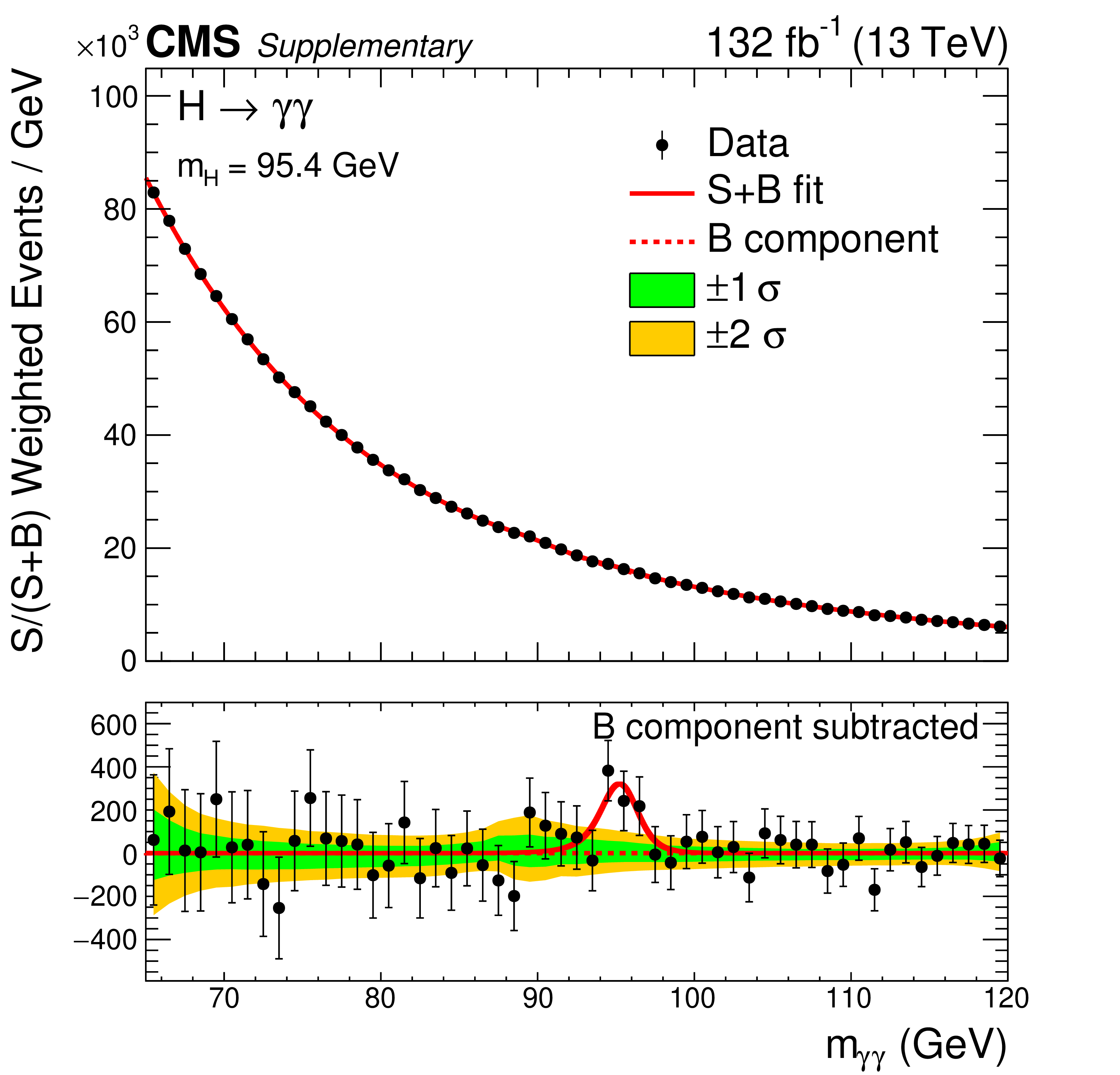
Additional Figure 17:
Events in all classes of the combined 13 TeV data set, binned as a function of $ m_{\gamma\gamma} $, together with the result of a fit of the signal-plus-background model, under a mass hypothesis of 95.4 GeV. Each event is weighted by the ratio S/(S+B) for its event class, where S and B are the numbers of expected signal and background events, respectively, in a $ \pm 1\sigma_{\text{eff}} m_{\gamma\gamma} $ window centred on $ m_{\mathrm{H}} $. The one- and two-$ \sigma $ uncertainty bands shown for the background component of the fit include the uncertainty due to the choice of fit function and the uncertainty in the fitted parameters. The distribution of the residual weighted data after subtracting the fitted background component is shown in the lower panel. |

png pdf |
Additional Figure 18:
Expected and observed exclusion limits (95% CL, in the asymptotic approximation) on the product of the production cross section and branching fraction into two photons, for an additional Higgs boson from the analysis of the combined data from 2016, 2017 and 2018, with assumption of the total cross section $ \sigma = (1-f)\times(\sigma_{SM}^{\mathrm{g}\mathrm{g}\mathrm{H}} + \sigma_{SM}^{{\mathrm{t}\overline{\mathrm{t}}} \mathrm{H}}) + f \times (\sigma_{SM}^{\mathrm{V}\mathrm{H}} + \sigma_{SM}^{VBF}) $ with the additional parameter $ f $ = 0.1, where $ \sigma_{SM}^{\mathrm{g}\mathrm{g}\mathrm{H}} $, $ \sigma_{SM}^{{\mathrm{t}\overline{\mathrm{t}}} \mathrm{H}} $, $ \sigma_{SM}^{\mathrm{V}\mathrm{H}} $ and $ \sigma_{SM}^{VBF} $ are the SM-like cross sections of the ggH, $ {\mathrm{t}\overline{\mathrm{t}}} \mathrm{H} $, VH and VBF production modes. The inner and outer bands indicate the regions containing the distribution of limits located within $ \pm $1 and 2$ \sigma $, respectively, of the expectation under the background-only hypothesis. The observed upper limit ranges from 17 to 82 fb. |

png pdf |
Additional Figure 19:
Expected and observed exclusion limits (95% CL, in the asymptotic approximation) on the product of the production cross section and branching fraction into two photons, for an additional Higgs boson from the analysis of the combined data from 2016, 2017 and 2018, with assumption of the total cross section $ \sigma = (1-f)\times(\sigma_{SM}^{\mathrm{g}\mathrm{g}\mathrm{H}} + \sigma_{SM}^{{\mathrm{t}\overline{\mathrm{t}}} \mathrm{H}}) + f\times(\sigma_{SM}^{\mathrm{V}\mathrm{H}} + \sigma_{SM}^{VBF}) $ with the additional parameter $ f $ = 0.2, where $ \sigma_{SM}^{\mathrm{g}\mathrm{g}\mathrm{H}} $, $ \sigma_{SM}^{{\mathrm{t}\overline{\mathrm{t}}} \mathrm{H}} $, $ \sigma_{SM}^{\mathrm{V}\mathrm{H}} $ and $ \sigma_{SM}^{VBF} $ are the SM-like cross sections of the ggH, $ {\mathrm{t}\overline{\mathrm{t}}} \mathrm{H} $, VH and VBF production modes. The inner and outer bands indicate the regions containing the distribution of limits located within $ \pm $1 and 2$ \sigma $, respectively, of the expectation under the background-only hypothesis. The observed upper limit ranges from 16 to 80 fb. |

png pdf |
Additional Figure 20:
Expected and observed exclusion limits (95% CL, in the asymptotic approximation) on the product of the production cross section and branching fraction into two photons, for an additional Higgs boson from the analysis of the combined data from 2016, 2017 and 2018, with assumption of the total cross section $ \sigma = (1-f)\times(\sigma_{SM}^{\mathrm{g}\mathrm{g}\mathrm{H}} + \sigma_{SM}^{{\mathrm{t}\overline{\mathrm{t}}} \mathrm{H}}) + f\times(\sigma_{SM}^{\mathrm{V}\mathrm{H}} + \sigma_{SM}^{VBF}) $ with the additional parameter $ f $ = 0.3, where $ \sigma_{SM}^{\mathrm{g}\mathrm{g}\mathrm{H}} $, $ \sigma_{SM}^{{\mathrm{t}\overline{\mathrm{t}}} \mathrm{H}} $, $ \sigma_{SM}^{\mathrm{V}\mathrm{H}} $ and $ \sigma_{SM}^{VBF} $ are the SM-like cross sections of the ggH, $ {\mathrm{t}\overline{\mathrm{t}}} \mathrm{H} $, VH and VBF production modes. The inner and outer bands indicate the regions containing the distribution of limits located within $ \pm $1 and 2$ \sigma $, respectively, of the expectation under the background-only hypothesis. The observed upper limit ranges from 16 to 79 fb. |

png pdf |
Additional Figure 21:
Expected and observed exclusion limits (95% CL, in the asymptotic approximation) on the product of the production cross section and branching fraction into two photons, for an additional Higgs boson from the analysis of the combined data from 2016, 2017 and 2018, with assumption of the total cross section $ \sigma = (1-f)\times(\sigma_{SM}^{\mathrm{g}\mathrm{g}\mathrm{H}} + \sigma_{SM}^{{\mathrm{t}\overline{\mathrm{t}}} \mathrm{H}}) + f\times(\sigma_{SM}^{\mathrm{V}\mathrm{H}} + \sigma_{SM}^{VBF}) $ with the additional parameter $ f $ = 0.4, where $ \sigma_{SM}^{\mathrm{g}\mathrm{g}\mathrm{H}} $, $ \sigma_{SM}^{{\mathrm{t}\overline{\mathrm{t}}} \mathrm{H}} $, $ \sigma_{SM}^{\mathrm{V}\mathrm{H}} $ and $ \sigma_{SM}^{VBF} $ are the SM-like cross sections of the ggH, $ {\mathrm{t}\overline{\mathrm{t}}} \mathrm{H} $, VH and VBF production modes. The inner and outer bands indicate the regions containing the distribution of limits located within $ \pm $1 and 2$ \sigma $, respectively, of the expectation under the background-only hypothesis. The observed upper limit ranges from 16 to 77 fb. |

png pdf |
Additional Figure 22:
Expected and observed exclusion limits (95% CL, in the asymptotic approximation) on the product of the production cross section and branching fraction into two photons, for an additional Higgs boson from the analysis of the combined data from 2016, 2017 and 2018, with assumption of the total cross section $ \sigma = (1-f)\times(\sigma_{SM}^{\mathrm{g}\mathrm{g}\mathrm{H}} + \sigma_{SM}^{{\mathrm{t}\overline{\mathrm{t}}} \mathrm{H}}) + f\times(\sigma_{SM}^{\mathrm{V}\mathrm{H}} + \sigma_{SM}^{VBF}) $ with the additional parameter $ f $ = 0.5, where $ \sigma_{SM}^{\mathrm{g}\mathrm{g}\mathrm{H}} $, $ \sigma_{SM}^{{\mathrm{t}\overline{\mathrm{t}}} \mathrm{H}} $, $ \sigma_{SM}^{\mathrm{V}\mathrm{H}} $ and $ \sigma_{SM}^{VBF} $ are the SM-like cross sections of the ggH, $ {\mathrm{t}\overline{\mathrm{t}}} \mathrm{H} $, VH and VBF production modes. The inner and outer bands indicate the regions containing the distribution of limits located within $ \pm $1 and 2$ \sigma $, respectively, of the expectation under the background-only hypothesis. The observed upper limit ranges from 15 to 74 fb. |
png pdf |
Additional Figure 23:
Expected and observed exclusion limits (95% CL, in the asymptotic approximation) on the product of the production cross section and branching fraction into two photons, for an additional Higgs boson from the analysis of the combined data from 2016, 2017 and 2018, with assumption of the total cross section $ \sigma = (1-f)\times(\sigma_{SM}^{\mathrm{g}\mathrm{g}\mathrm{H}} + \sigma_{SM}^{{\mathrm{t}\overline{\mathrm{t}}} \mathrm{H}}) + f\times(\sigma_{SM}^{\mathrm{V}\mathrm{H}} + \sigma_{SM}^{VBF}) $ with the additional parameter $ f $ = 0.6, where $ \sigma_{SM}^{\mathrm{g}\mathrm{g}\mathrm{H}} $, $ \sigma_{SM}^{{\mathrm{t}\overline{\mathrm{t}}} \mathrm{H}} $, $ \sigma_{SM}^{\mathrm{V}\mathrm{H}} $ and $ \sigma_{SM}^{VBF} $ are the SM-like cross sections of the ggH, $ {\mathrm{t}\overline{\mathrm{t}}} \mathrm{H} $, VH and VBF production modes. The inner and outer bands indicate the regions containing the distribution of limits located within $ \pm $1 and 2$ \sigma $, respectively, of the expectation under the background-only hypothesis. The observed upper limit ranges from 14 to 70 fb. |

png pdf |
Additional Figure 24:
Expected and observed exclusion limits (95% CL, in the asymptotic approximation) on the product of the production cross section and branching fraction into two photons, for an additional Higgs boson from the analysis of the combined data from 2016, 2017 and 2018, with assumption of the total cross section $ \sigma = (1-f)\times(\sigma_{SM}^{\mathrm{g}\mathrm{g}\mathrm{H}} + \sigma_{SM}^{{\mathrm{t}\overline{\mathrm{t}}} \mathrm{H}}) + f\times(\sigma_{SM}^{\mathrm{V}\mathrm{H}} + \sigma_{SM}^{VBF}) $ with the additional parameter $ f $ = 0.7, where $ \sigma_{SM}^{\mathrm{g}\mathrm{g}\mathrm{H}} $, $ \sigma_{SM}^{{\mathrm{t}\overline{\mathrm{t}}} \mathrm{H}} $, $ \sigma_{SM}^{\mathrm{V}\mathrm{H}} $ and $ \sigma_{SM}^{VBF} $ are the SM-like cross sections of the ggH, $ {\mathrm{t}\overline{\mathrm{t}}} \mathrm{H} $, VH and VBF production modes. The inner and outer bands indicate the regions containing the distribution of limits located within $ \pm $1 and 2$ \sigma $, respectively, of the expectation under the background-only hypothesis. The observed upper limit ranges from 13 to 64 fb. |

png pdf |
Additional Figure 25:
Expected and observed exclusion limits (95% CL, in the asymptotic approximation) on the product of the production cross section and branching fraction into two photons, for an additional Higgs boson from the analysis of the combined data from 2016, 2017 and 2018, with assumption of the total cross section $ \sigma = (1-f)\times(\sigma_{SM}^{\mathrm{g}\mathrm{g}\mathrm{H}} + \sigma_{SM}^{{\mathrm{t}\overline{\mathrm{t}}} \mathrm{H}}) + f\times(\sigma_{SM}^{\mathrm{V}\mathrm{H}} + \sigma_{SM}^{VBF}) $ with the additional parameter $ f $ = 0.8, where $ \sigma_{SM}^{\mathrm{g}\mathrm{g}\mathrm{H}} $, $ \sigma_{SM}^{{\mathrm{t}\overline{\mathrm{t}}} \mathrm{H}} $, $ \sigma_{SM}^{\mathrm{V}\mathrm{H}} $ and $ \sigma_{SM}^{VBF} $ are the SM-like cross sections of the ggH, $ {\mathrm{t}\overline{\mathrm{t}}} \mathrm{H} $, VH and VBF production modes. The inner and outer bands indicate the regions containing the distribution of limits located within $ \pm $1 and 2$ \sigma $, respectively, of the expectation under the background-only hypothesis. The observed upper limit ranges from 12 to 56 fb. |
png pdf |
Additional Figure 26:
Expected and observed exclusion limits (95% CL, in the asymptotic approximation) on the product of the production cross section and branching fraction into two photons, for an additional Higgs boson from the analysis of the combined data from 2016, 2017 and 2018, with assumption of the total cross section $ \sigma = (1-f)\times(\sigma_{SM}^{\mathrm{g}\mathrm{g}\mathrm{H}} + \sigma_{SM}^{{\mathrm{t}\overline{\mathrm{t}}} \mathrm{H}}) + f\times(\sigma_{SM}^{\mathrm{V}\mathrm{H}} + \sigma_{SM}^{VBF}) $ with the additional parameter $ f $ = 0.9, where $ \sigma_{SM}^{\mathrm{g}\mathrm{g}\mathrm{H}} $, $ \sigma_{SM}^{{\mathrm{t}\overline{\mathrm{t}}} \mathrm{H}} $, $ \sigma_{SM}^{\mathrm{V}\mathrm{H}} $ and $ \sigma_{SM}^{VBF} $ are the SM-like cross sections of the ggH, $ {\mathrm{t}\overline{\mathrm{t}}} \mathrm{H} $, VH and VBF production modes. The inner and outer bands indicate the regions containing the distribution of limits located within $ \pm $1 and 2$ \sigma $, respectively, of the expectation under the background-only hypothesis. The observed upper limit ranges from 10 to 45 fb. |
png pdf |
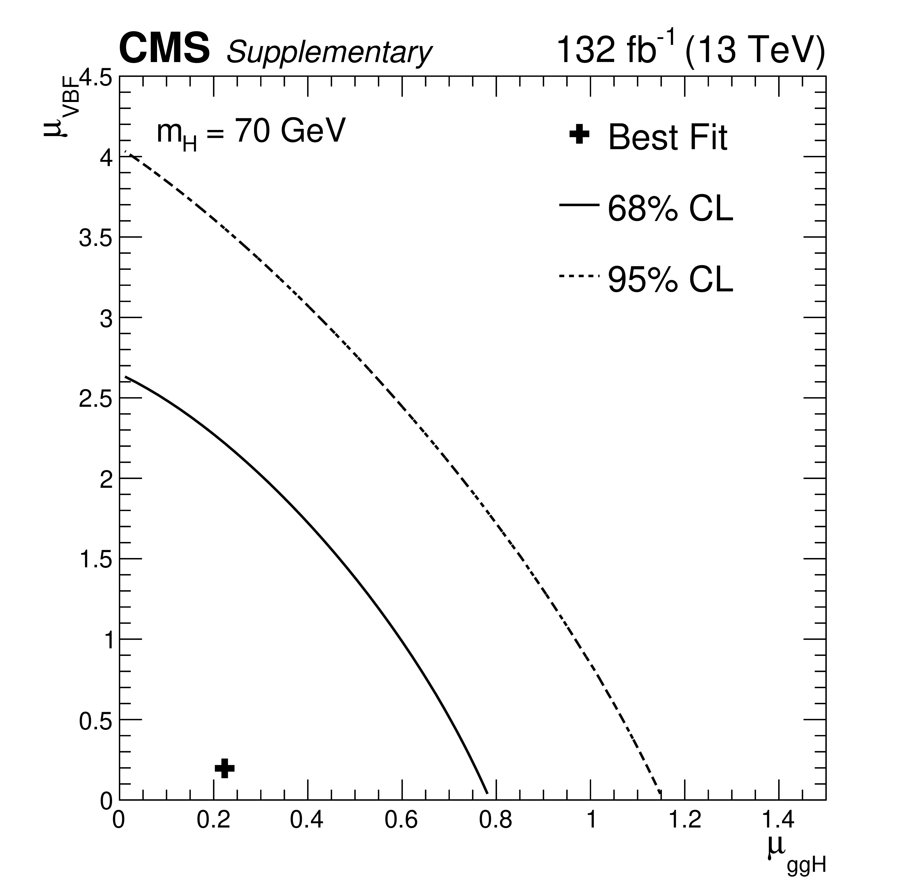
Additional Figure 27:
Maximum likelihood estimates, and 68 and 95% confidence level contours obtained from scans of the signal likelihood as a function of $ \mu_{ \mathrm{g}\mathrm{g}\mathrm{H} } $ versus $ \mu_{VBF} $ for $ m_{H} $ = 70 GeV, when considering only ggH and VBF production modes. The best-fit result is ($ \mu_{ \mathrm{g}\mathrm{g}\mathrm{H} } $, $ \mu_{VBF} $) = (0.22, 0.20). |

png pdf |
Additional Figure 28:
Maximum likelihood estimates, and 68 and 95% confidence level contours obtained from scans of the signal likelihood as a function of $ \mu_{ \mathrm{g}\mathrm{g}\mathrm{H} } $ versus $ \mu_{VBF} $ for $ m_{H} $ = 75 GeV, when considering only ggH and VBF production modes. The best-fit result is ($ \mu_{ \mathrm{g}\mathrm{g}\mathrm{H} } $, $ \mu_{VBF} $) = (0.14, 0.22). |

png pdf |
Additional Figure 29:
Maximum likelihood estimates, and 68 and 95% confidence level contours obtained from scans of the signal likelihood as a function of $ \mu_{ \mathrm{g}\mathrm{g}\mathrm{H} } $ versus $ \mu_{VBF} $ for $ m_{H} $ = 80 GeV, when considering only ggH and VBF production modes. The best-fit result is ($ \mu_{ \mathrm{g}\mathrm{g}\mathrm{H} } $, $ \mu_{VBF} $) = (0.0, 0.0). |

png pdf |
Additional Figure 30:
Maximum likelihood estimates, and 68 and 95% confidence level contours obtained from scans of the signal likelihood as a function of $ \mu_{ \mathrm{g}\mathrm{g}\mathrm{H} } $ versus $ \mu_{VBF} $ for $ m_{H} $ = 85 GeV, when considering only ggH and VBF production modes. The best-fit result is ($ \mu_{ \mathrm{g}\mathrm{g}\mathrm{H} } $, $ \mu_{VBF} $) = (0.0, 0.0). |

png pdf |
Additional Figure 31:
Maximum likelihood estimates, and 68 and 95% confidence level contours obtained from scans of the signal likelihood as a function of $ \mu_{ \mathrm{g}\mathrm{g}\mathrm{H} } $ versus $ \mu_{VBF} $ for $ m_{H} $ = 90 GeV, when considering only ggH and VBF production modes. The best-fit result is ($ \mu_{ \mathrm{g}\mathrm{g}\mathrm{H} } $, $ \mu_{VBF} $) = (0.28, 0.0). |
png pdf |
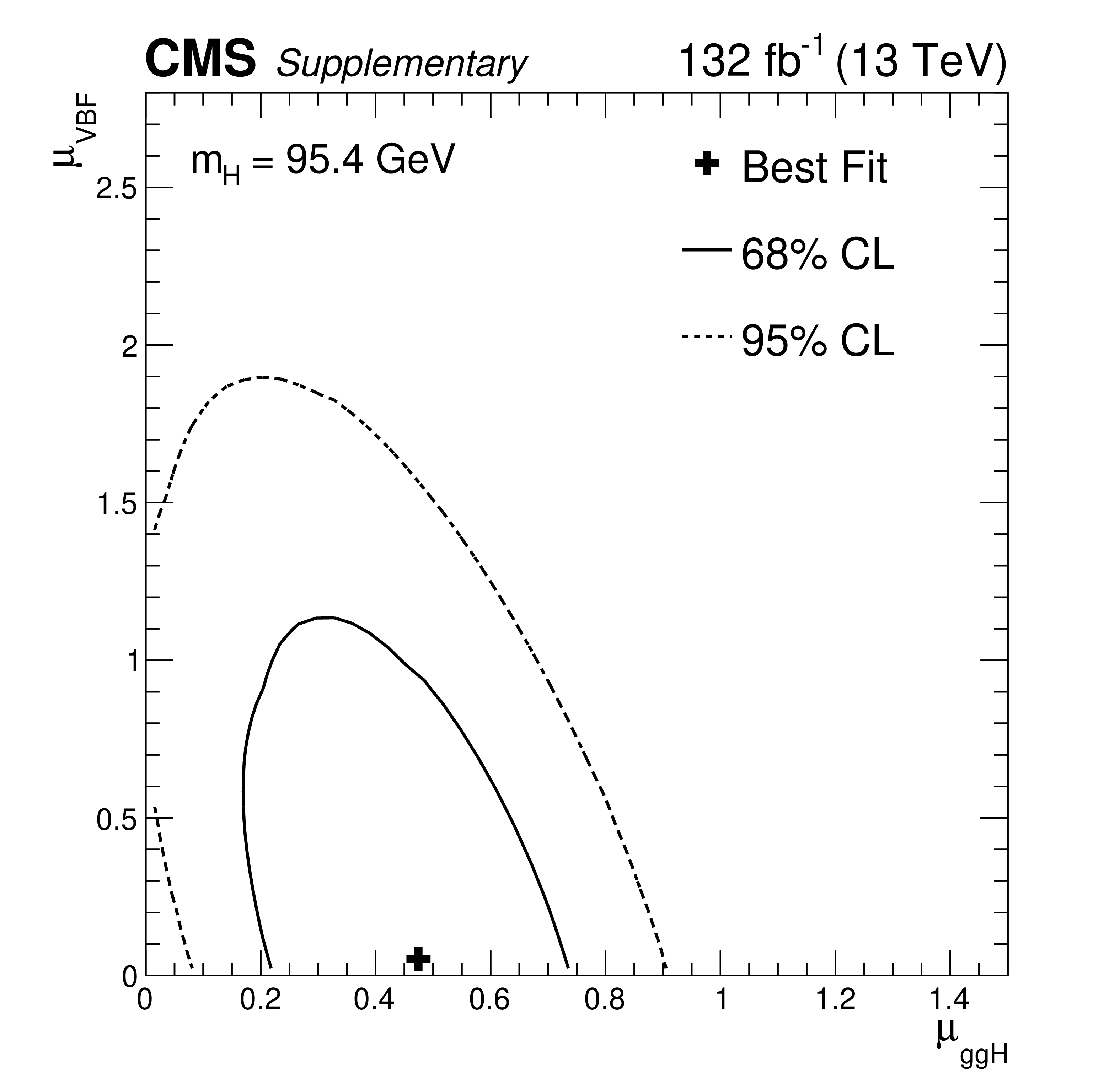
Additional Figure 32:
Maximum likelihood estimates, and 68 and 95% confidence level contours obtained from scans of the signal likelihood as a function of $ \mu_{ \mathrm{g}\mathrm{g}\mathrm{H} } $ versus $ \mu_{VBF} $ for $ m_{H} $ = 95.4 GeV, when considering only ggH and VBF production modes. The best-fit result is ($ \mu_{ \mathrm{g}\mathrm{g}\mathrm{H} } $, $ \mu_{VBF} $) = (0.47, 0.05). |

png pdf |
Additional Figure 33:
Maximum likelihood estimates, and 68 and 95% confidence level contours obtained from scans of the signal likelihood as a function of $ \mu_{ \mathrm{g}\mathrm{g}\mathrm{H} } $ versus $ \mu_{VBF} $ for $ m_{H} $ = 100 GeV, when considering only ggH and VBF production modes. The best-fit result is ($ \mu_{ \mathrm{g}\mathrm{g}\mathrm{H} } $, $ \mu_{VBF} $) = (0.0, 0.39). |
png pdf |
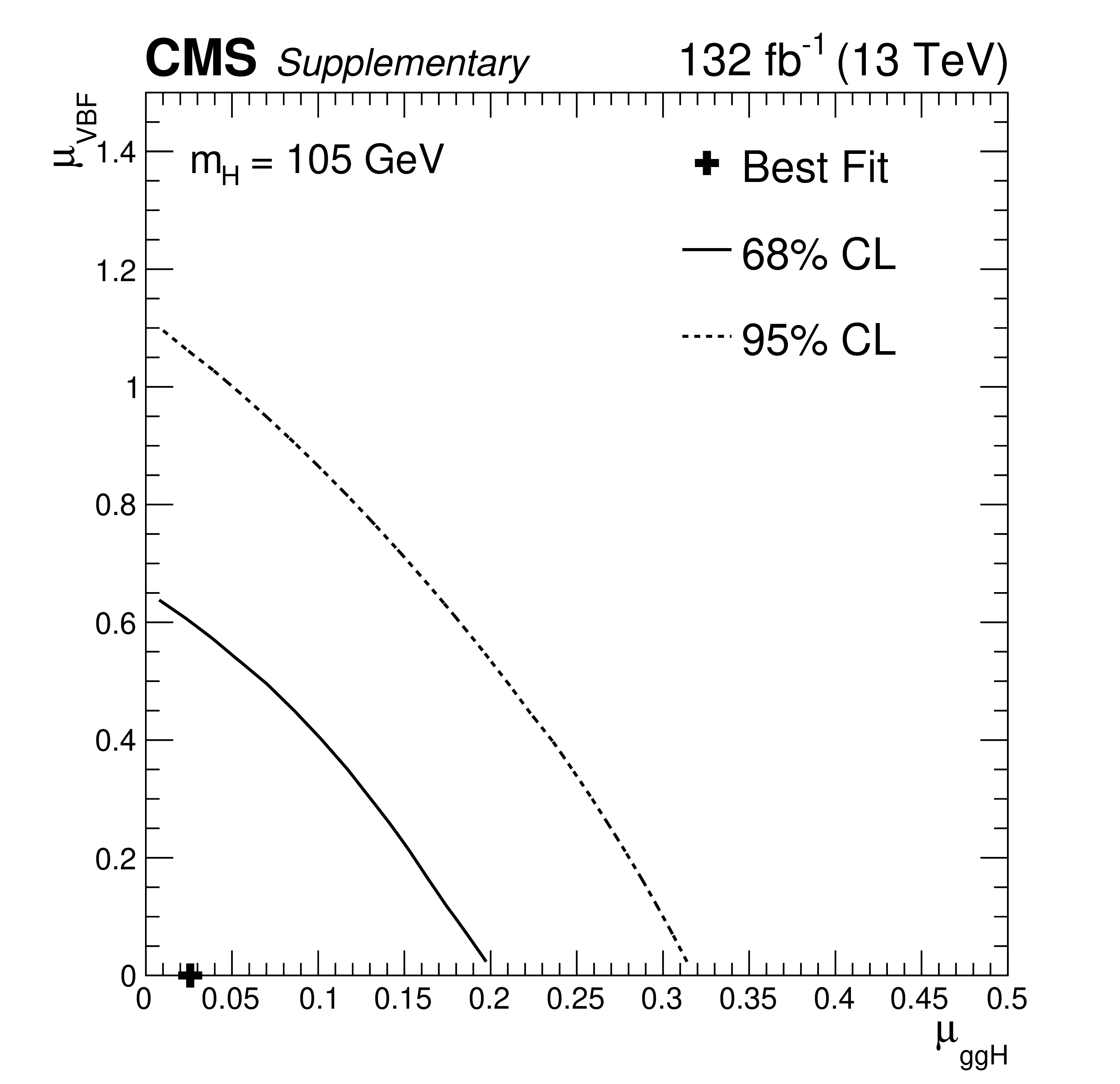
Additional Figure 34:
Maximum likelihood estimates, and 68 and 95% confidence level contours obtained from scans of the signal likelihood as a function of $ \mu_{ \mathrm{g}\mathrm{g}\mathrm{H} } $ versus $ \mu_{VBF} $ for $ m_{H} $ = 105 GeV, when considering only ggH and VBF production modes. The best-fit result is ($ \mu_{ \mathrm{g}\mathrm{g}\mathrm{H} } $, $ \mu_{VBF} $) = (0.03, 0.0). |

png pdf |
Additional Figure 35:
Maximum likelihood estimates, and 68 and 95% confidence level contours obtained from scans of the signal likelihood as a function of $ \mu_{ \mathrm{g}\mathrm{g}\mathrm{H} } $ versus $ \mu_{VBF} $ for $ m_{H} $ = 110 GeV, when considering only ggH and VBF production modes. The best-fit result is ($ \mu_{ \mathrm{g}\mathrm{g}\mathrm{H} } $, $ \mu_{VBF} $) = (0.0, 0.0). |
| References | ||||
| 1 | S. L. Glashow | Partial-symmetries of weak interactions | NP 22 (1961) 579 | |
| 2 | S. Weinberg | A model of leptons | PRL 19 (1967) 1264 | |
| 3 | A. Salam | Weak and electromagnetic interactions | in Elementary particle physics: relativistic groups and analyticity, N. Svartholm, ed., Almqvist & Wiksell, Stockholm, Proceedings of the eighth Nobel symposium, 1968 | |
| 4 | F. Englert and R. Brout | Broken symmetry and the mass of gauge vector mesons | PRL 13 (1964) 321 | |
| 5 | P. W. Higgs | Broken symmetries, massless particles and gauge fields | PL 12 (1964) 132 | |
| 6 | P. W. Higgs | Broken symmetries and the masses of gauge bosons | PRL 13 (1964) 508 | |
| 7 | G. S. Guralnik, C. R. Hagen, and T. W. B. Kibble | Global conservation laws and massless particles | PRL 13 (1964) 585 | |
| 8 | P. W. Higgs | Spontaneous symmetry breakdown without massless bosons | PR 145 (1966) 1156 | |
| 9 | T. W. B. Kibble | Symmetry breaking in non-Abelian gauge theories | PR 155 (1967) 1554 | |
| 10 | ATLAS Collaboration | Observation of a new particle in the search for the standard model Higgs boson with the ATLAS detector at the LHC | PLB 716 (2012) 1 | 1207.7214 |
| 11 | CMS Collaboration | Observation of a new boson at a mass of 125 GeV with the CMS experiment at the LHC | PLB 716 (2012) 30 | CMS-HIG-12-028 1207.7235 |
| 12 | CMS Collaboration | Observation of a new boson with mass near 125 GeV in pp collisions at $ \sqrt{s} = $ 7 and 8 TeV | JHEP 06 (2013) 081 | CMS-HIG-12-036 1303.4571 |
| 13 | ATLAS Collaboration | A detailed map of Higgs boson interactions by the ATLAS experiment ten years after the discovery | Nature 607 (2022) 52 | 2207.00092 |
| 14 | CMS Collaboration | A portrait of the Higgs boson by the CMS experiment ten years after the discovery | Nature 607 (2022) 60 | CMS-HIG-22-001 2207.00043 |
| 15 | A. Celis, V. Ilisie, and A. Pich | LHC constraints on two-Higgs-doublet models | JHEP 07 (2013) 053 | 1302.4022 |
| 16 | B. Coleppa, F. Kling, and S. Su | Constraining type II 2HDM in light of LHC Higgs searches | JHEP 01 (2014) 161 | 1305.0002 |
| 17 | S. Chang et al. | Two-Higgs-doublet models for the LHC Higgs boson data at $ \sqrt{s}= $ 7 and 8 TeV | JHEP 09 (2014) 101 | 1310.3374 |
| 18 | J. Bernon et al. | Scrutinizing the alignment limit in two-Higgs-doublet models. II. $ m_{\mathrm{H}}= $ 125 GeV | PRD 93 (2016) 035027 | 1511.03682 |
| 19 | G. Cacciapaglia et al. | Search for a lighter Higgs boson in two-Higgs-doublet models | JHEP 12 (2016) 68 | 1607.08653 |
| 20 | P. Fayet | Supergauge invariant extension of the Higgs mechanism and a model for the electron and its neutrino | NPB 90 (1975) 104 | |
| 21 | R. Barbieri, S. Ferrara, and C. A. Savoy | Gauge models with spontaneously broken local supersymmetry | PLB 119 (1982) 343 | |
| 22 | M. Dine, W. Fischler, and M. Srednicki | A simple solution to the strong CP problem with a harmless axion | PLB 104 (1981) 199 | |
| 23 | H. P. Nilles, M. Srednicki, and D. Wyler | Weak interaction breakdown induced by supergravity | PLB 120 (1983) 346 | |
| 24 | J. M. Frère, D. R. T. Jones, and S. Raby | Fermion masses and induction of the weak scale by supergravity | NPB 222 (1983) 11 | |
| 25 | J. P. Derendinger and C. A. Savoy | Quantum effects and SU(2) x U(1) breaking in supergravity gauge theories | NPB 237 (1984) 307 | |
| 26 | J. Ellis et al. | Higgs bosons in a nonminimal supersymmetric model | PRD 39 (1989) 844 | |
| 27 | M. Drees | Supersymmetric models with extended Higgs sector | Int. J. Mod. Phys. A 4 (1989) 3635 | |
| 28 | U. Ellwanger, M. Rausch de Traubenberg, and C. A. Savoy | Particle spectrum in supersymmetric models with a gauge singlet | PLB 315 (1993) 331 | hep-ph/9307322 |
| 29 | U. Ellwanger, M. Rausch de Traubenberg, and C. A. Savoy | Higgs phenomenology of the supersymmetric model with a gauge singlet | Z. Phys. C 67 (1995) 665 | hep-ph/9502206 |
| 30 | U. Ellwanger, M. Rausch de Traubenberg, and C. A. Savoy | Phenomenology of supersymmetric models with a singlet | NPB 492 (1997) 21 | hep-ph/9611251 |
| 31 | T. Elliott, S. F. King, and P. L. White | Unification constraints in the next-to-minimal supersymmetric standard model | PLB 351 (1995) 213 | hep-ph/9406303 |
| 32 | S. F. King and P. L. White | Resolving the constrained minimal and next-to-minimal supersymmetric standard models | PRD 52 (1995) 4183 | hep-ph/9505326 |
| 33 | F. Franke | Neutralinos and Higgs bosons in the next-to-minimal supersymmetric standard model | Int. J. Mod. Phys. A 12 (1997) 479 | hep-ph/9512366 |
| 34 | M. Maniatis | The next-to-minimal supersymmetric extension of the standard model reviewed | Int. J. Mod. Phys. A 25 (2010) 3505 | 0906.0777 |
| 35 | U. Ellwanger, C. Hugonie, and A. M. Teixeira | The next-to-minimal supersymmetric standard model | Phys. Rept. 496 (2010) 1 | 0910.1785 |
| 36 | J.-W. Fan et al. | Study of diphoton decays of the lightest scalar Higgs boson in the next-to-minimal supersymmetric standard model | Chin. Phys. C 38 (2014) 073101 | 1309.6394 |
| 37 | U. Ellwanger and M. Rodriguez-Vazquez | Discovery prospects of a light scalar in the NMSSM | JHEP 02 (2016) 096 | 1512.04281 |
| 38 | M. Guchait and J. Kumar | Diphoton signal of light pseudoscalar in NMSSM at the LHC | PRD 95 (2017) 035036 | 1608.05693 |
| 39 | J. Cao et al. | Diphoton signal of the light Higgs boson in natural NMSSM | PRD 95 (2017) 116001 | 1612.08522 |
| 40 | J.-Q. Tao et al. | Search for a lighter Higgs boson in the next-to-minimal supersymmetric standard model | Chin. Phys. C 42 (2018) 103107 | 1805.11438 |
| 41 | H. Georgi and M. Machacek | Doubly-charged Higgs bosons | NPB 262 (1985) 463 | |
| 42 | H. E. Logan and V. Rentala | All the generalized Georgi-Machacek models | PRD 92 (2015) 075011 | 1502.01275 |
| 43 | A. Ismail, B. Keeshan, H. E. Logan, and Y. Wu | Benchmark for LHC searches for low-mass custodial fiveplet scalars in the Georgi-Machacek model | PRD 103 (2021) 095010 | 2003.05536 |
| 44 | C. Wang et al. | Search for a lighter neutral custodial fiveplet scalar in the Georgi-Machacek model | Chin. Phys. C 46 (2022) 083107 | 2204.09198 |
| 45 | ALEPH Collaboration, DELPHI Collaboration, L3 Collaboration, OPAL Collaboration and the LEP working group for Higgs boson searches | Search for the standard model Higgs boson at LEP | PLB 565 (2003) 61 | hep-ex/0306033 |
| 46 | ATLAS Collaboration | Search for scalar diphoton resonances in the mass range 65-600 GeV with the ATLAS detector in pp collision data at $ \sqrt{s} = $ 8 TeV | PRL 113 (2014) 171801 | 1407.6583 |
| 47 | ATLAS Collaboration | Search for boosted diphoton resonances in the 10 to 70 GeV mass range using 138 fb$ ^{-1} $ of 13 TeV pp collisions with the ATLAS detector | JHEP 07 (2023) 155 | 2211.04172 |
| 48 | CMS Collaboration | Search for a standard model-like Higgs boson in the mass range between 70 and 110 GeV in the diphoton final state in proton-proton collisions at $ \sqrt{s}= $ 8 and 13 TeV | PLB 793 (2019) 320 | CMS-HIG-17-013 1811.08459 |
| 49 | CMS Collaboration | HEPData record for this analysis | link | |
| 50 | CMS Collaboration | Observation of the diphoton decay of the Higgs boson and measurement of its properties | EPJC 74 (2014) 3076 | CMS-HIG-13-001 1407.0558 |
| 51 | CMS Collaboration | Measurements of Higgs boson properties in the diphoton decay channel in proton-proton collisions at $ \sqrt{s} = $ 13 TeV | JHEP 11 (2018) 185 | CMS-HIG-16-040 1804.02716 |
| 52 | CMS Collaboration | The CMS experiment at the CERN LHC | JINST 3 (2008) S08004 | |
| 53 | CMS Collaboration | Performance of photon reconstruction and identification with the CMS detector in proton-proton collisions at $ \sqrt{s}= $ 8 TeV | JINST 10 (2015) P08010 | CMS-EGM-14-001 1502.02702 |
| 54 | CMS Collaboration | A measurement of the Higgs boson mass in the diphoton decay channel | PLB 805 (2020) 135425 | CMS-HIG-19-004 2002.06398 |
| 55 | CMS Collaboration | Particle-flow reconstruction and global event description with the CMS detector | JINST 12 (2017) P10003 | CMS-PRF-14-001 1706.04965 |
| 56 | J. Alwall et al. | The automated computation of tree-level and next-to-leading order differential cross sections, and their matching to parton shower simulations | JHEP 07 (2014) 079 | 1405.0301 |
| 57 | R. Frederix and S. Frixione | Merging meets matching in MC@NLO | JHEP 12 (2012) 061 | 1209.6215 |
| 58 | NNPDF Collaboration | Parton distributions for the LHC run II | JHEP 04 (2015) 040 | 1410.8849 |
| 59 | NNPDF Collaboration | Parton distributions from high-precision collider data | EPJC 77 (2017) 663 | 1706.00428 |
| 60 | K. Hamilton, P. Nason, E. Re, and G. Zanderighi | NNLOPS simulation of Higgs boson production | JHEP 10 (2013) 222 | 1309.0017 |
| 61 | T. Sjöstrand et al. | An introduction to PYTHIA 8.2 | Comput. Phys. Commun. 191 (2015) 159 | 1410.3012 |
| 62 | CMS Collaboration | Event generator tunes obtained from underlying event and multiparton scattering measurements | EPJC 76 (2016) 155 | CMS-GEN-14-001 1512.00815 |
| 63 | CMS Collaboration | Extraction and validation of a new set of CMS PYTHIA8 tunes from underlying-event measurements | EPJC 80 (2020) 4 | CMS-GEN-17-001 1903.12179 |
| 64 | LHC Higgs Cross Section Working Group | Handbook of LHC Higgs cross sections: 4. deciphering the nature of the Higgs sector | CERN, 2016 link |
1610.07922 |
| 65 | GEANT4 Collaboration | GEANT 4---a simulation toolkit | NIM A 506 (2003) 250 | |
| 66 | T. Gleisberg et al. | Event generation with SHERPA 1.1 | JHEP 02 (2009) 007 | 0811.4622 |
| 67 | CMS Collaboration | Performance of the CMS Level-1 trigger in proton-proton collisions at $ \sqrt{s} = $ 13\,TeV | JINST 15 (2020) P10017 | CMS-TRG-17-001 2006.10165 |
| 68 | CMS Collaboration | The CMS trigger system | JINST 12 (2017) P01020 | CMS-TRG-12-001 1609.02366 |
| 69 | CMS Collaboration | Electron and photon reconstruction and identification with the CMS experiment at the CERN LHC | JINST 16 (2021) P05014 | CMS-EGM-17-001 2012.06888 |
| 70 | CMS Collaboration | Measurement of the inclusive W and Z production cross sections in pp collisions at $ \sqrt{s}= $ 7 TeV | JHEP 10 (2011) 132 | CMS-EWK-10-005 1107.4789 |
| 71 | CMS Collaboration | Energy calibration and resolution of the CMS electromagnetic calorimeter in pp collisions at $ \sqrt{s} = $ 7 TeV | JINST 8 (2013) P09009 | CMS-EGM-11-001 1306.2016 |
| 72 | M. Cacciari, G. P. Salam, and G. Soyez | The anti-$ k_{\mathrm{T}} $ jet clustering algorithm | JHEP 04 (2008) 063 | 0802.1189 |
| 73 | M. Cacciari, G. P. Salam, and G. Soyez | FastJet user manual | EPJC 72 (2012) 1896 | 1111.6097 |
| 74 | CMS Collaboration | Pileup mitigation at CMS in 13 TeV data | JINST 15 (2020) P09018 | CMS-JME-18-001 2003.00503 |
| 75 | CMS Collaboration | Jet energy scale and resolution in the CMS experiment in pp collisions at 8 TeV | JINST 12 (2017) P02014 | CMS-JME-13-004 1607.03663 |
| 76 | A. Hoecker et al. | TMVA---toolkit for multivariate data analysis | physics/0703039 | |
| 77 | F. Pedregosa et al. | Scikit-learn: machine learning in Python | J. Machine Learning Res. 12 (2011) 2825 | 1201.0490 |
| 78 | R. A. Fisher | On the interpretation of $ \chi^{2} $ from contingency tables, and the calculation of $ p $ | J. Royal Stat. Soc 85 (1922) 87 | |
| 79 | P. D. Dauncey, M. Kenzie, N. Wardle, and G. J. Davies | Handling uncertainties in background shapes: the discrete profiling method | JINST 10 (2015) P04015 | 1408.6865 |
| 80 | M. Oreglia | A study of the reactions $ \psi^\prime \to \gamma \gamma \psi $ | PhD thesis, Stanford University, SLAC Report SLAC-R-236, 1980 link |
|
| 81 | T. Skwarnicki | A study of the radiative CASCADE transitions between the Upsilon-prime and Upsilon resonances | PhD thesis, Cracow, INP, 1986 link |
|
| 82 | CMS Collaboration | Precision luminosity measurement in proton-proton collisions at $ \sqrt{s} = $ 13 TeV in 2015 and 2016 at CMS | EPJC 81 (2021) 800 | CMS-LUM-17-003 2104.01927 |
| 83 | CMS Collaboration | CMS luminosity measurement for the 2017 data-taking period at $ \sqrt{s} = $ 13 TeV | CMS Physics Analysis Summary, 2018 CMS-PAS-LUM-17-004 |
CMS-PAS-LUM-17-004 |
| 84 | CMS Collaboration | CMS luminosity measurement for the 2018 data-taking period at $ \sqrt{s} = $ 13 TeV | CMS Physics Analysis Summary, 2019 CMS-PAS-LUM-18-002 |
CMS-PAS-LUM-18-002 |
| 85 | S. Carrazza et al. | An unbiased Hessian representation for Monte Carlo PDFs | EPJC 75 (2015) 369 | 1505.06736 |
| 86 | J. Gao and P. Nadolsky | A meta-analysis of parton distribution functions | JHEP 07 (2014) 035 | 1401.0013 |
| 87 | J. Butterworth et al. | PDF4LHC recommendations for LHC Run II | JPG 43 (2016) 023001 | 1510.03865 |
| 88 | CMS Collaboration | Measurements of Higgs boson production cross sections and couplings in the diphoton decay channel at $ \sqrt{\mathrm{s}} = $ 13 TeV | JHEP 07 (2021) 027 | CMS-HIG-19-015 2103.06956 |
| 89 | ATLAS and CMS Collaborations, LHC Higgs Combination Group | Procedure for the LHC Higgs boson search combination in Summer 2011 | CMS Note CMS-NOTE-2011-005, ATL-PHYS-PUB-2011-11, CERN, 2011 link |
|
| 90 | T. Junk | Confidence level computation for combining searches with small statistics | NIM A 434 (1999) 435 | hep-ex/9902006 |
| 91 | A. L. Read | Presentation of search results: the $ \text{CL}_\text{s} $ technique | JPG 28 (2002) 2693 | |
| 92 | G. Cowan, K. Cranmer, E. Gross, and O. Vitells | Asymptotic formulae for likelihood-based tests of new physics | EPJC 71 (2011) 1554 | 1007.1727 |
| 93 | L. Demortier | P-values and nuisance parameters | in Statistical issues for LHC physics. Proceedings, Workshop, PHYSTAT-LHC, Geneva, 2007 link |
|
|
|
Compact Muon Solenoid LHC, CERN |
|

|

|

|

|

|