

Compact Muon Solenoid
LHC, CERN
| CMS-EXO-23-016 ; CERN-EP-2025-282 | ||
| Strategy and performance of the CMS long-lived particle trigger program in proton-proton collisions at $ \sqrt{s}= $ 13.6 TeV | ||
| CMS Collaboration | ||
| 24 January 2026 | ||
| Submitted to Physics Reports | ||
| Abstract: In the physics program of the CMS experiment during the CERN LHC Run 3, which started in 2022, the long-lived particle triggers have been improved and extended to expand the scope of the corresponding searches. These dedicated triggers and their performance are described in this paper, using several theoretical benchmark models that extend the standard model of particle physics. The results are based on proton-proton collision data collected with the CMS detector during 2022--2024 at a center-of-mass energy of 13.6 TeV, corresponding to integrated luminosities of up to 123 fb$ ^{-1} $. | ||
| Links: e-print arXiv:2601.17544 [hep-ex] (PDF) ; CDS record ; inSPIRE record ; Physics Briefing ; CADI line (restricted) ; | ||
| Figures | |
png pdf |
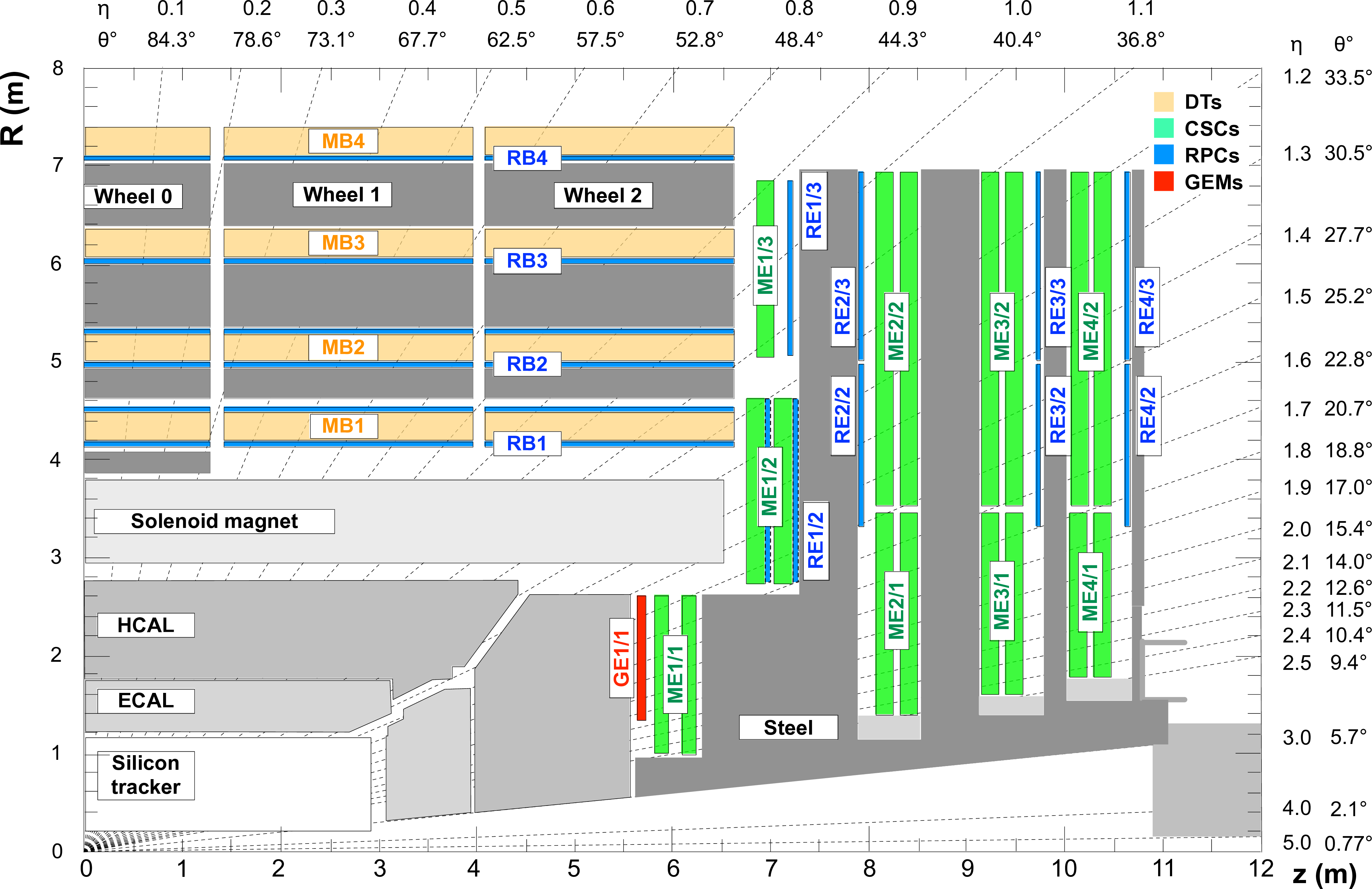
Figure 1:
Schematic view in the $ R-z $ plane of a CMS detector quadrant at the start of Run 3, with the axis parallel to the beam ($ z $) running horizontally and the radius ($ R $) increasing upward. The nominal interaction point (IP) is in the lower left corner. The locations of the various muon detectors and the steel flux-return yoke (dark areas) are shown, along with the silicon tracker, the electromagnetic calorimeter (ECAL), and the hadronic calorimeter (HCAL). The locations of the various muon detectors are shown in color: drift tubes (DTs) with labels MB, cathode strip chambers (CSCs) with labels ME, resistive plate chambers (RPCs) with labels RB and RE, and gas electron multipliers (GEMs) with labels GE. The M denotes muon, B stands for barrel, and E for endcap. Figure taken from Ref. [24]. |
png pdf |
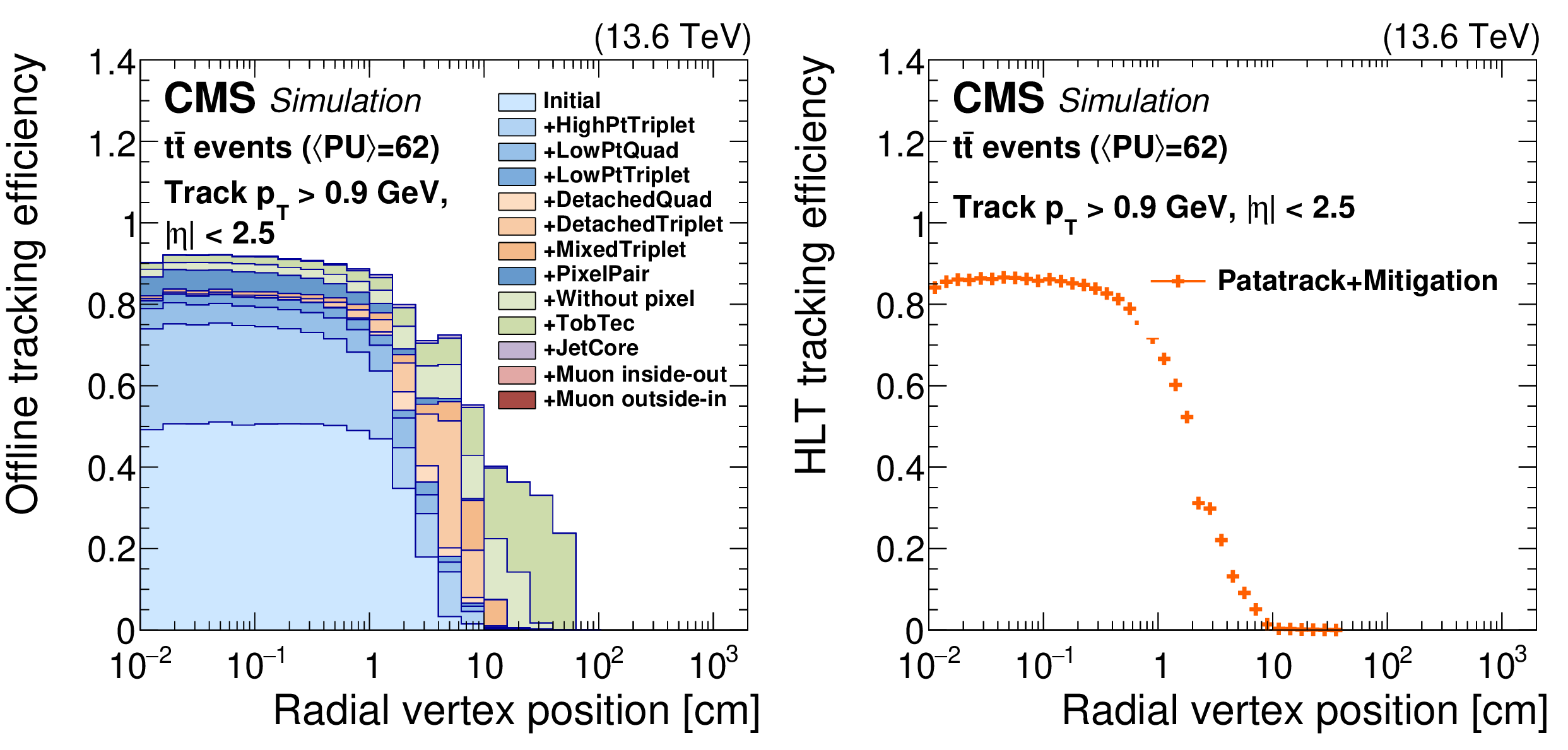
Figure 2:
The offline standard tracking efficiency during Run 3 (left) for different tracking iterations, as a function of simulated radial position of the track production vertex. The overall standard tracking efficiency at the HLT during Run 3 (right), as a function of the simulated radial position of the track production vertex. The standard tracking at the HLT includes the nominal PATATRACK global iteration plus the additional iteration that mitigates the pixel detector issues. For both plots, a $ \mathrm{t} \overline{\mathrm{t}} $ simulation under 2025 conditions with an average PU of 62 is used, and the tracks are required to have $ p_{\mathrm{T}} > $ 0.9 GeV and $ |\eta| < $ 2.5. The tracking efficiency is defined as the number of simulated tracks (with the aforementioned selection requirements) geometrically matched to a reconstructed track, divided by the total simulated tracks passing the selections. |
png pdf |
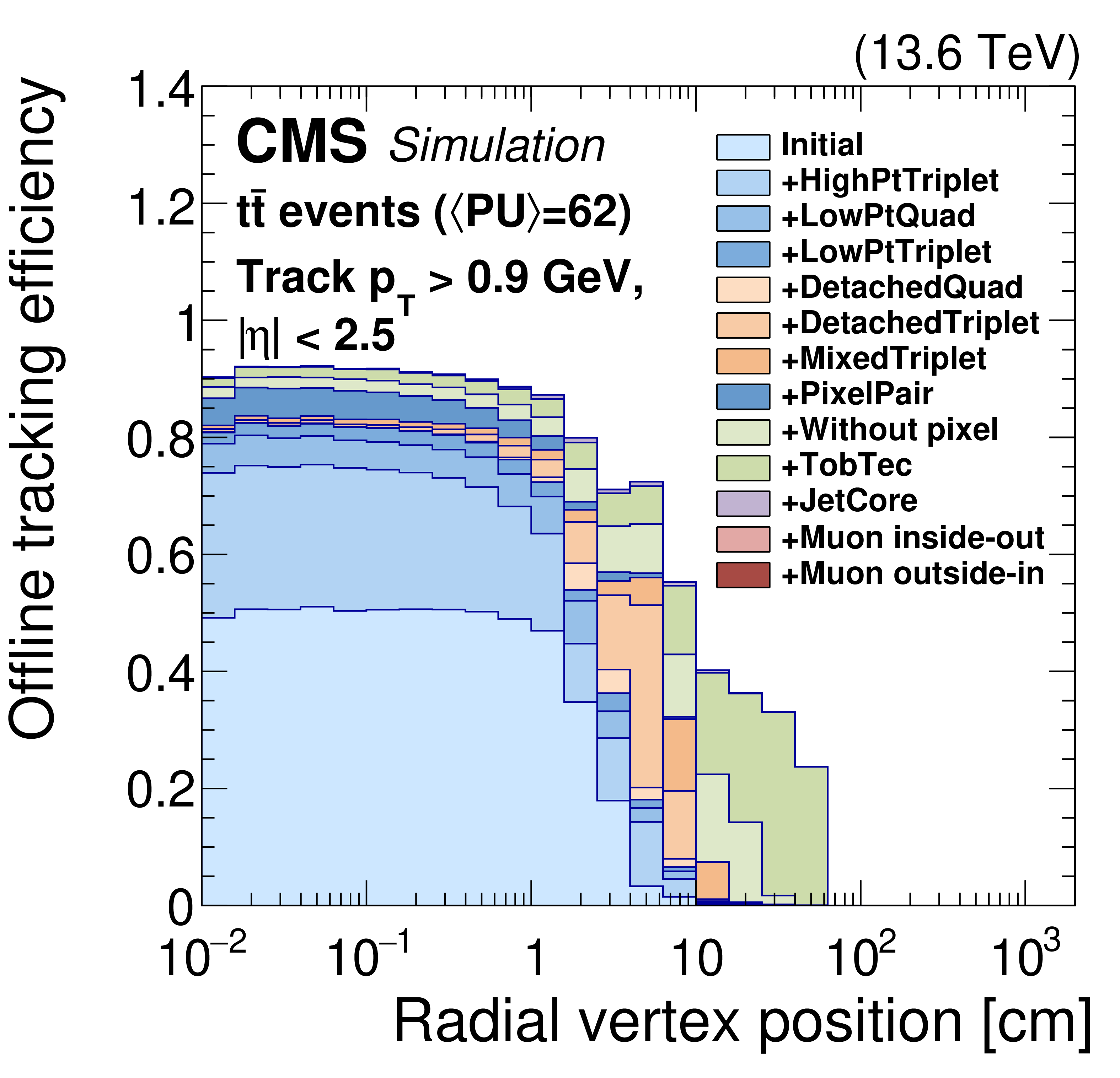
Figure 2-a:
The offline standard tracking efficiency during Run 3 (left) for different tracking iterations, as a function of simulated radial position of the track production vertex. The overall standard tracking efficiency at the HLT during Run 3 (right), as a function of the simulated radial position of the track production vertex. The standard tracking at the HLT includes the nominal PATATRACK global iteration plus the additional iteration that mitigates the pixel detector issues. For both plots, a $ \mathrm{t} \overline{\mathrm{t}} $ simulation under 2025 conditions with an average PU of 62 is used, and the tracks are required to have $ p_{\mathrm{T}} > $ 0.9 GeV and $ |\eta| < $ 2.5. The tracking efficiency is defined as the number of simulated tracks (with the aforementioned selection requirements) geometrically matched to a reconstructed track, divided by the total simulated tracks passing the selections. |
png pdf |
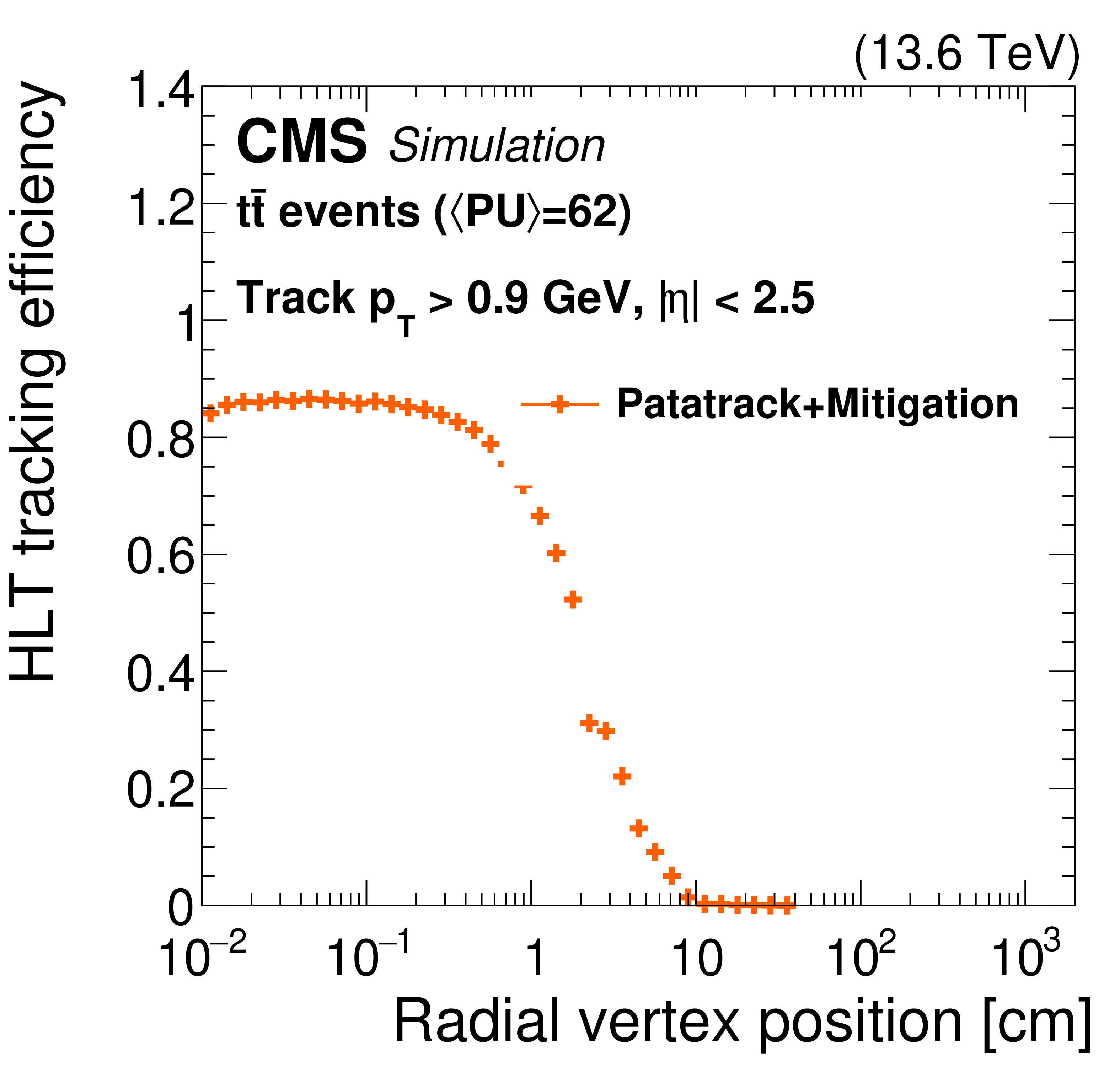
Figure 2-b:
The offline standard tracking efficiency during Run 3 (left) for different tracking iterations, as a function of simulated radial position of the track production vertex. The overall standard tracking efficiency at the HLT during Run 3 (right), as a function of the simulated radial position of the track production vertex. The standard tracking at the HLT includes the nominal PATATRACK global iteration plus the additional iteration that mitigates the pixel detector issues. For both plots, a $ \mathrm{t} \overline{\mathrm{t}} $ simulation under 2025 conditions with an average PU of 62 is used, and the tracks are required to have $ p_{\mathrm{T}} > $ 0.9 GeV and $ |\eta| < $ 2.5. The tracking efficiency is defined as the number of simulated tracks (with the aforementioned selection requirements) geometrically matched to a reconstructed track, divided by the total simulated tracks passing the selections. |
png pdf |
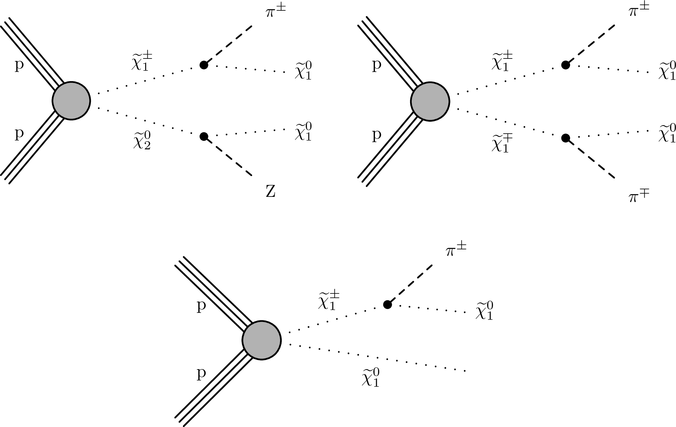
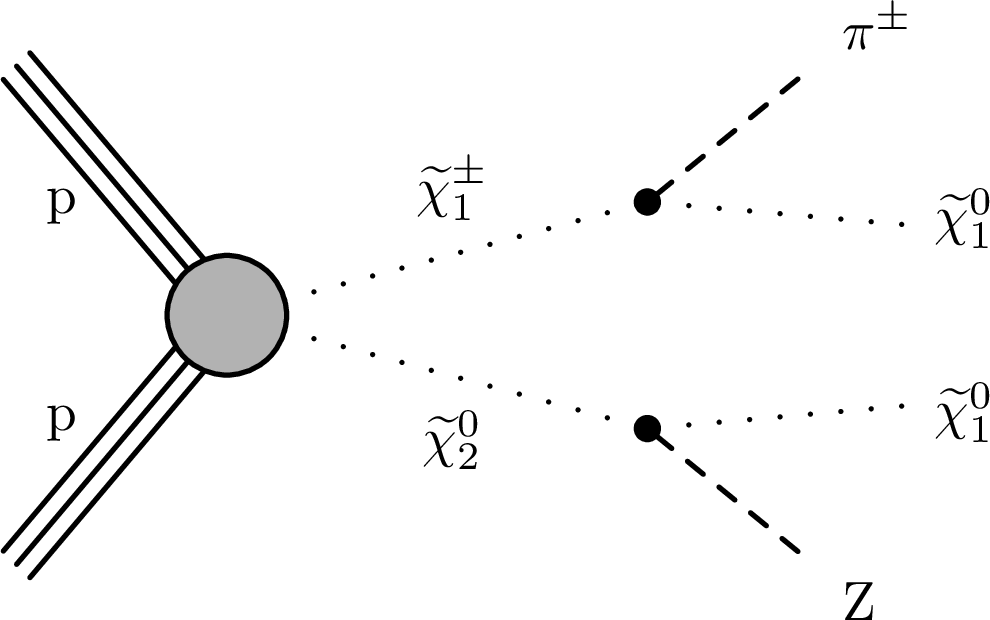
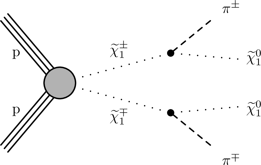
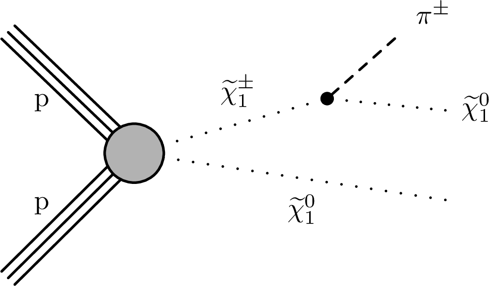
Figure 3:
Diagrams for the AMSB $ \tilde{\chi}_{1}^{\pm} \to \tilde{\chi}_{1}^{0}+\mathrm{X} $ process. The $ \mathrm{X} $ particle is shown here as a charged pion $ \pi^{\pm} $, but $ \mathrm{X} $ can also be an electron or a muon, depending on the type of neutralino $ \tilde{\chi}_{1}^{0} $. |
png pdf |
Figure 3-a:
Diagrams for the AMSB $ \tilde{\chi}_{1}^{\pm} \to \tilde{\chi}_{1}^{0}+\mathrm{X} $ process. The $ \mathrm{X} $ particle is shown here as a charged pion $ \pi^{\pm} $, but $ \mathrm{X} $ can also be an electron or a muon, depending on the type of neutralino $ \tilde{\chi}_{1}^{0} $. |
png pdf |
Figure 3-b:
Diagrams for the AMSB $ \tilde{\chi}_{1}^{\pm} \to \tilde{\chi}_{1}^{0}+\mathrm{X} $ process. The $ \mathrm{X} $ particle is shown here as a charged pion $ \pi^{\pm} $, but $ \mathrm{X} $ can also be an electron or a muon, depending on the type of neutralino $ \tilde{\chi}_{1}^{0} $. |
png pdf |
Figure 3-c:
Diagrams for the AMSB $ \tilde{\chi}_{1}^{\pm} \to \tilde{\chi}_{1}^{0}+\mathrm{X} $ process. The $ \mathrm{X} $ particle is shown here as a charged pion $ \pi^{\pm} $, but $ \mathrm{X} $ can also be an electron or a muon, depending on the type of neutralino $ \tilde{\chi}_{1}^{0} $. |
png pdf |
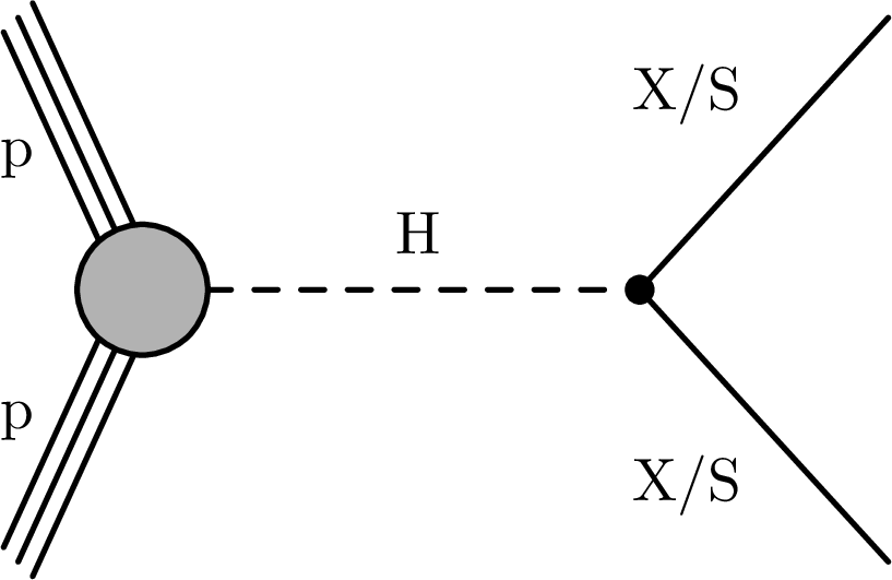
Figure 4:
Diagram for the $ \mathrm{H} \to \mathrm{X}\mathrm{X} $ or $ \mathrm{H} \to \text{S}\text{S} $ process. |
png pdf |
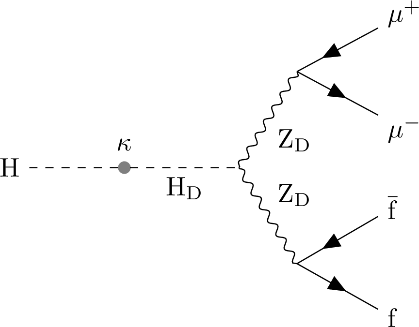
Figure 5:
Diagram for the $ \mathrm{H} \to \mathrm{Z}_\text{D}\mathrm{Z}_\text{D} $ process. |
png pdf |
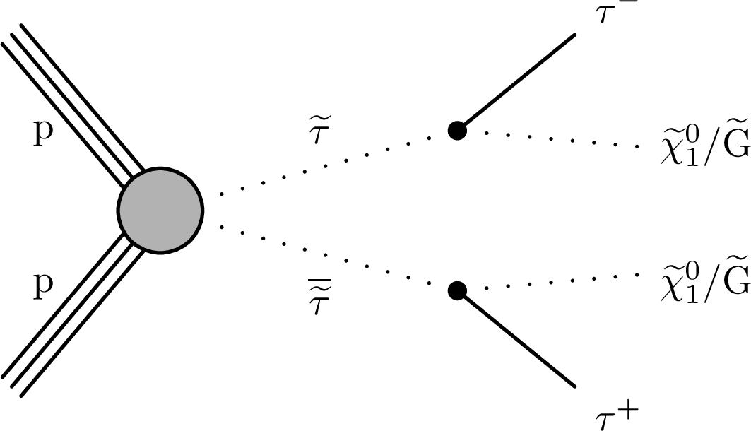
Figure 6:
Diagram for the direct $ \tilde{\tau} $ pair production process, with each $ \tilde{\tau} $ decaying to a $ \tau $ lepton and a neutralino $ \tilde{\chi}_{1}^{0} $ (or a gravitino $ \tilde{\mathrm{G}} $). |
png pdf |
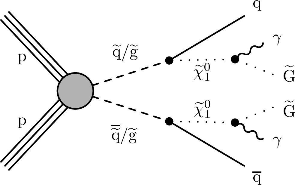
Figure 7:
Diagram for the GMSB SPS8 benchmark model, where pair-produced squarks $ \tilde{\mathrm{q}} $ and gluinos $ \mathrm{\widetilde{g}} $ undergo cascade decays and eventually produce a gravitino $ \tilde{\mathrm{G}} $. |
png pdf |
Figure 8:
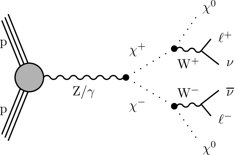
Diagram for the singlet-triplet Higgs portal dark matter benchmark model, where a charged dark partner particle $ \chi^{\pm} $ in a compressed dark sector decays via an off-shell W boson and produces a stable neutral dark matter candidate $ \chi^{0} $. |
png pdf |
Figure 9:
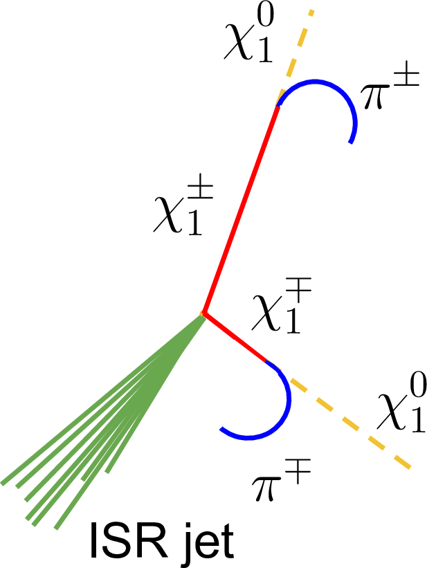
Diagram of a disappearing-track event. Each $ \tilde{\chi}_{1}^{\pm} $ (solid red lines) is an LLP that decays in the tracker and recoils off an ISR jet (multiple solid green lines), while the $ \tilde{\chi}_{1}^{0} $ (dashed yellow line) is undetected, and the $ \pi^{\pm} $ (blue curve) is not reconstructed because of its low $ p_{\mathrm{T}} $. The recoil of the disappearing track against the ISR jet produces measurable calorimeter and PF $ p_{\mathrm{T}}^\text{miss} $. |
png pdf |
Figure 10:
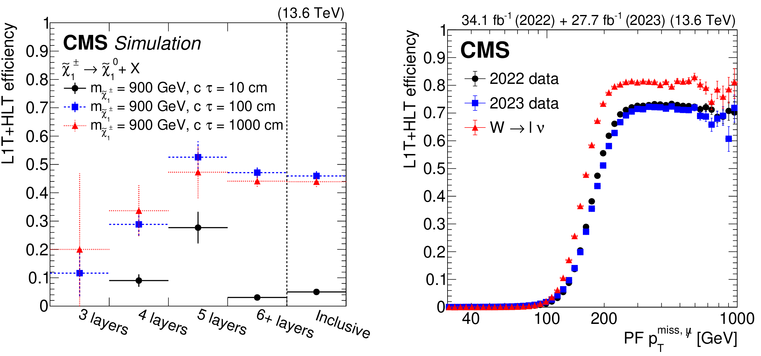
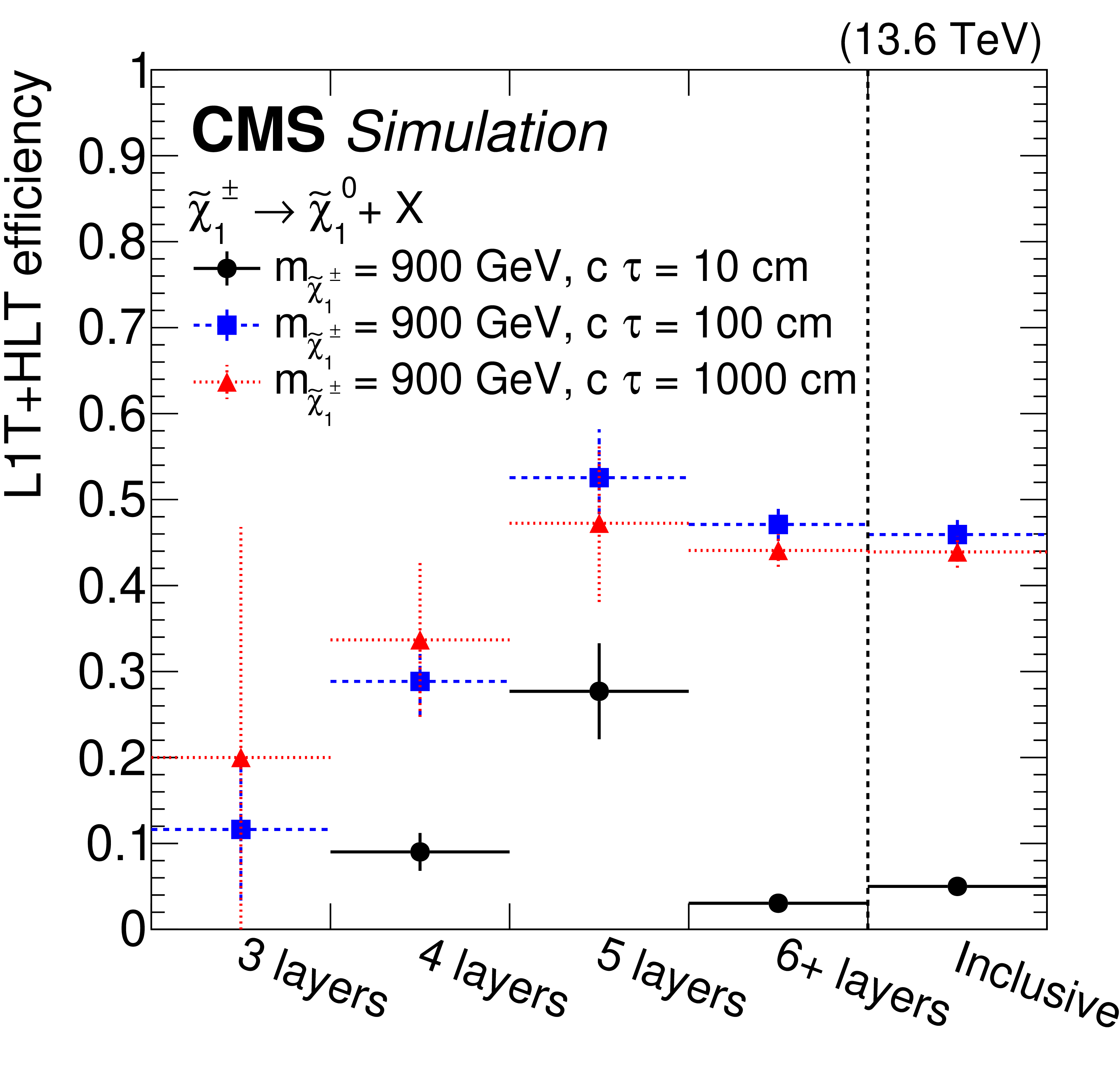
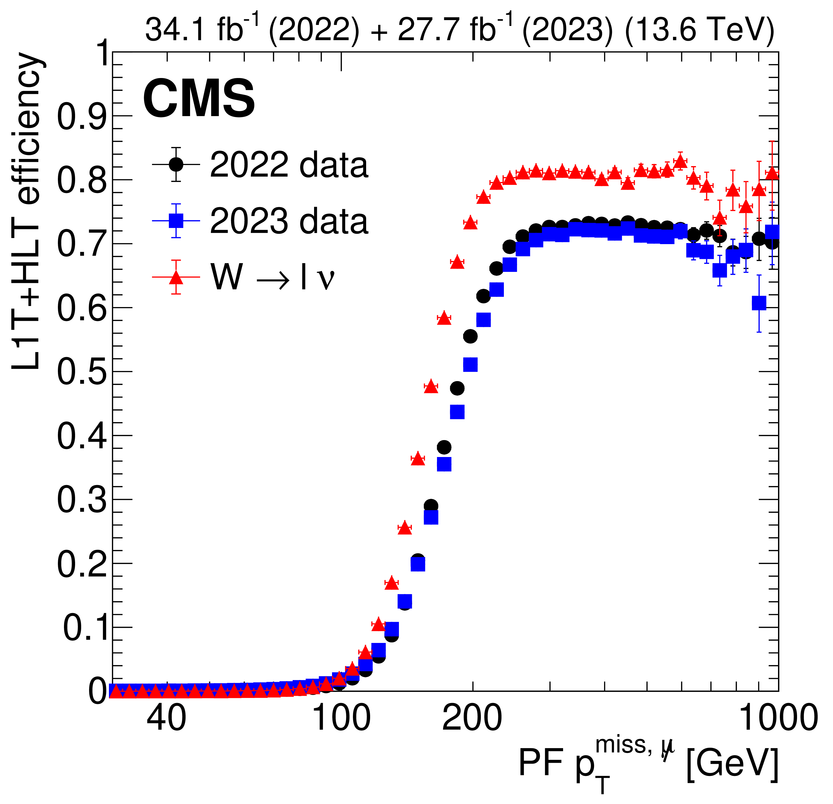
The L1T+HLT efficiency of the disappearing-track trigger: Efficiency as a function of the number of tracker layers with valid measurements for tracks that pass the offline requirements described in Table 3, in $ \tilde{\chi}_{1}^{\pm} \to \tilde{\chi}_{1}^{0}+\mathrm{X} $ simulated events for 2022 conditions, where $ m_{\tilde{\chi}_{1}^{\pm}}= $ 900 GeV and $ \tilde{\chi}_{1}^{0} $ is nearly mass-degenerate with $ \tilde{\chi}_{1}^{\pm} $ (left). The efficiency is shown for LLPs with $ c\tau= $ 10, 100, and 1000$ \text{cm} $ in black circles, blue squares, and red triangles, respectively. Comparison of efficiencies calculated with 2022 data (black circles), 2023 data (blue squares), and $ \mathrm{W} \to \ell\nu $ simulation (red triangles), as a function of offline reconstructed PF $ p_{\mathrm{T}}^{\text{miss}, \not{\mu}} $ (right). The efficiency rises to a plateau of less than 100% because of the isolated track leg of the algorithm. |
png pdf |
Figure 10-a:
The L1T+HLT efficiency of the disappearing-track trigger: Efficiency as a function of the number of tracker layers with valid measurements for tracks that pass the offline requirements described in Table 3, in $ \tilde{\chi}_{1}^{\pm} \to \tilde{\chi}_{1}^{0}+\mathrm{X} $ simulated events for 2022 conditions, where $ m_{\tilde{\chi}_{1}^{\pm}}= $ 900 GeV and $ \tilde{\chi}_{1}^{0} $ is nearly mass-degenerate with $ \tilde{\chi}_{1}^{\pm} $ (left). The efficiency is shown for LLPs with $ c\tau= $ 10, 100, and 1000$ \text{cm} $ in black circles, blue squares, and red triangles, respectively. Comparison of efficiencies calculated with 2022 data (black circles), 2023 data (blue squares), and $ \mathrm{W} \to \ell\nu $ simulation (red triangles), as a function of offline reconstructed PF $ p_{\mathrm{T}}^{\text{miss}, \not{\mu}} $ (right). The efficiency rises to a plateau of less than 100% because of the isolated track leg of the algorithm. |
png pdf |
Figure 10-b:
The L1T+HLT efficiency of the disappearing-track trigger: Efficiency as a function of the number of tracker layers with valid measurements for tracks that pass the offline requirements described in Table 3, in $ \tilde{\chi}_{1}^{\pm} \to \tilde{\chi}_{1}^{0}+\mathrm{X} $ simulated events for 2022 conditions, where $ m_{\tilde{\chi}_{1}^{\pm}}= $ 900 GeV and $ \tilde{\chi}_{1}^{0} $ is nearly mass-degenerate with $ \tilde{\chi}_{1}^{\pm} $ (left). The efficiency is shown for LLPs with $ c\tau= $ 10, 100, and 1000$ \text{cm} $ in black circles, blue squares, and red triangles, respectively. Comparison of efficiencies calculated with 2022 data (black circles), 2023 data (blue squares), and $ \mathrm{W} \to \ell\nu $ simulation (red triangles), as a function of offline reconstructed PF $ p_{\mathrm{T}}^{\text{miss}, \not{\mu}} $ (right). The efficiency rises to a plateau of less than 100% because of the isolated track leg of the algorithm. |
png pdf |
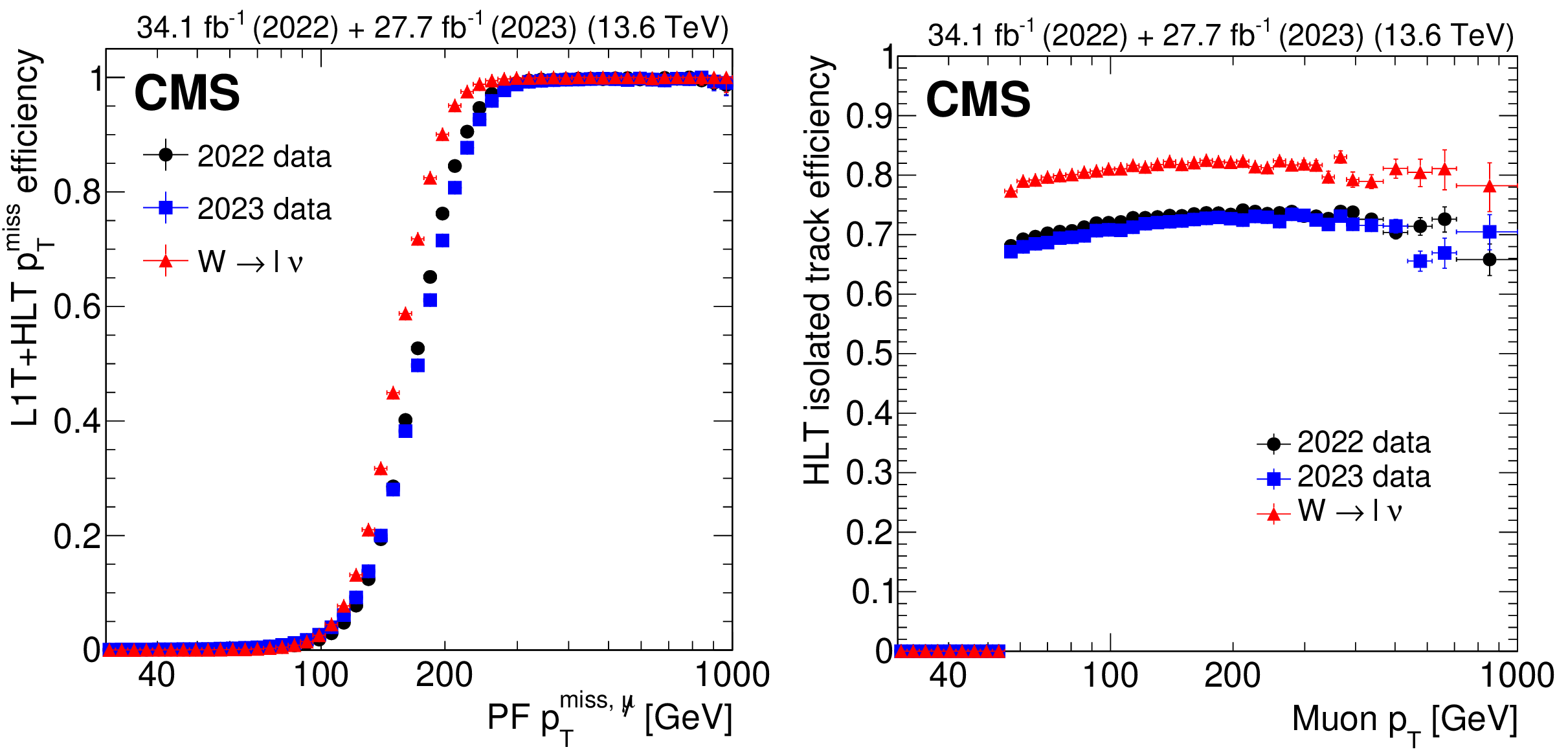
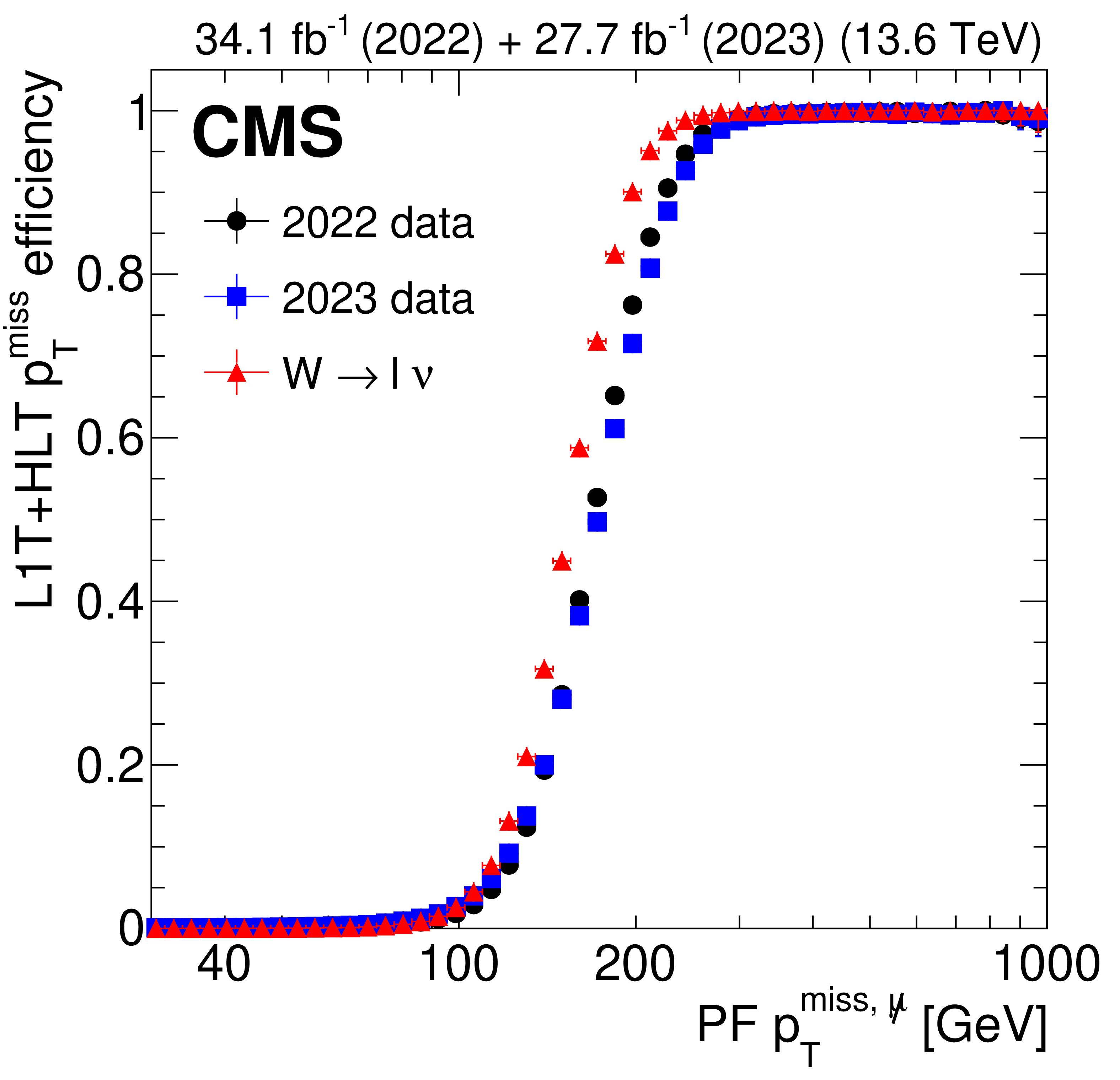
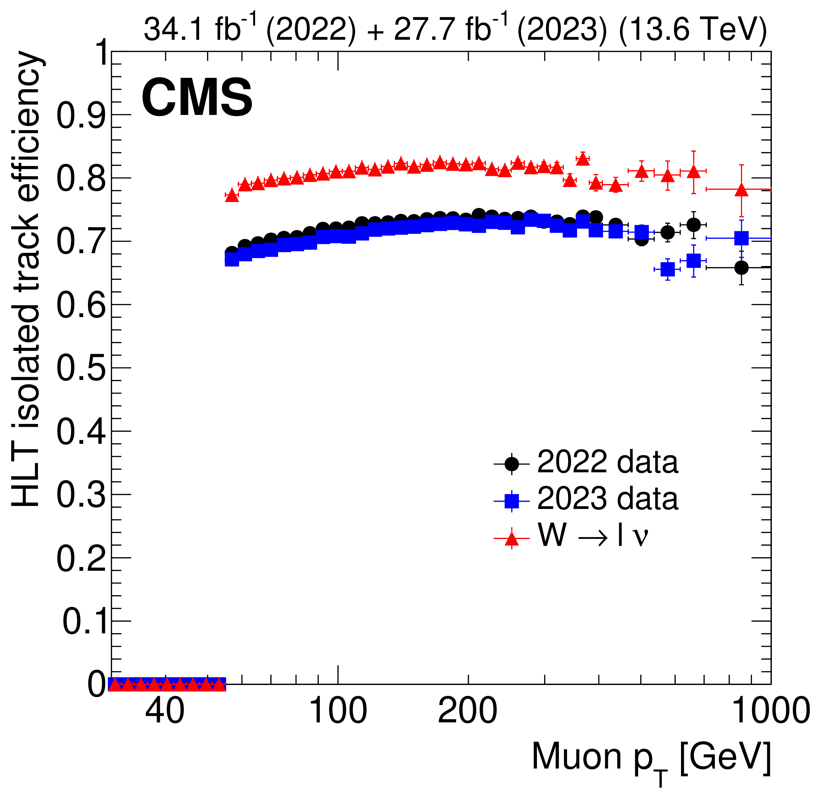
Figure 11:
The L1T+HLT efficiency of each leg of the disappearing-track trigger in 2022 data (black circles), 2023 data (blue squares), and $ \mathrm{W} \to \ell\nu $ simulation (red triangles). Efficiency of the L1T+HLT $ p_{\mathrm{T}}^\text{miss} $ leg as a function of offline reconstructed PF $ p_{\mathrm{T}}^{\text{miss}, \not{\mu}} $ (left). Efficiency of the full HLT path, taking into account only events that already passed through the $ p_{\mathrm{T}}^\text{miss} $ leg, as a function of the selected muon $ p_{\mathrm{T}} $ (right). |
png pdf |
Figure 11-a:
The L1T+HLT efficiency of each leg of the disappearing-track trigger in 2022 data (black circles), 2023 data (blue squares), and $ \mathrm{W} \to \ell\nu $ simulation (red triangles). Efficiency of the L1T+HLT $ p_{\mathrm{T}}^\text{miss} $ leg as a function of offline reconstructed PF $ p_{\mathrm{T}}^{\text{miss}, \not{\mu}} $ (left). Efficiency of the full HLT path, taking into account only events that already passed through the $ p_{\mathrm{T}}^\text{miss} $ leg, as a function of the selected muon $ p_{\mathrm{T}} $ (right). |
png pdf |
Figure 11-b:
The L1T+HLT efficiency of each leg of the disappearing-track trigger in 2022 data (black circles), 2023 data (blue squares), and $ \mathrm{W} \to \ell\nu $ simulation (red triangles). Efficiency of the L1T+HLT $ p_{\mathrm{T}}^\text{miss} $ leg as a function of offline reconstructed PF $ p_{\mathrm{T}}^{\text{miss}, \not{\mu}} $ (left). Efficiency of the full HLT path, taking into account only events that already passed through the $ p_{\mathrm{T}}^\text{miss} $ leg, as a function of the selected muon $ p_{\mathrm{T}} $ (right). |
png pdf |
Figure 12:
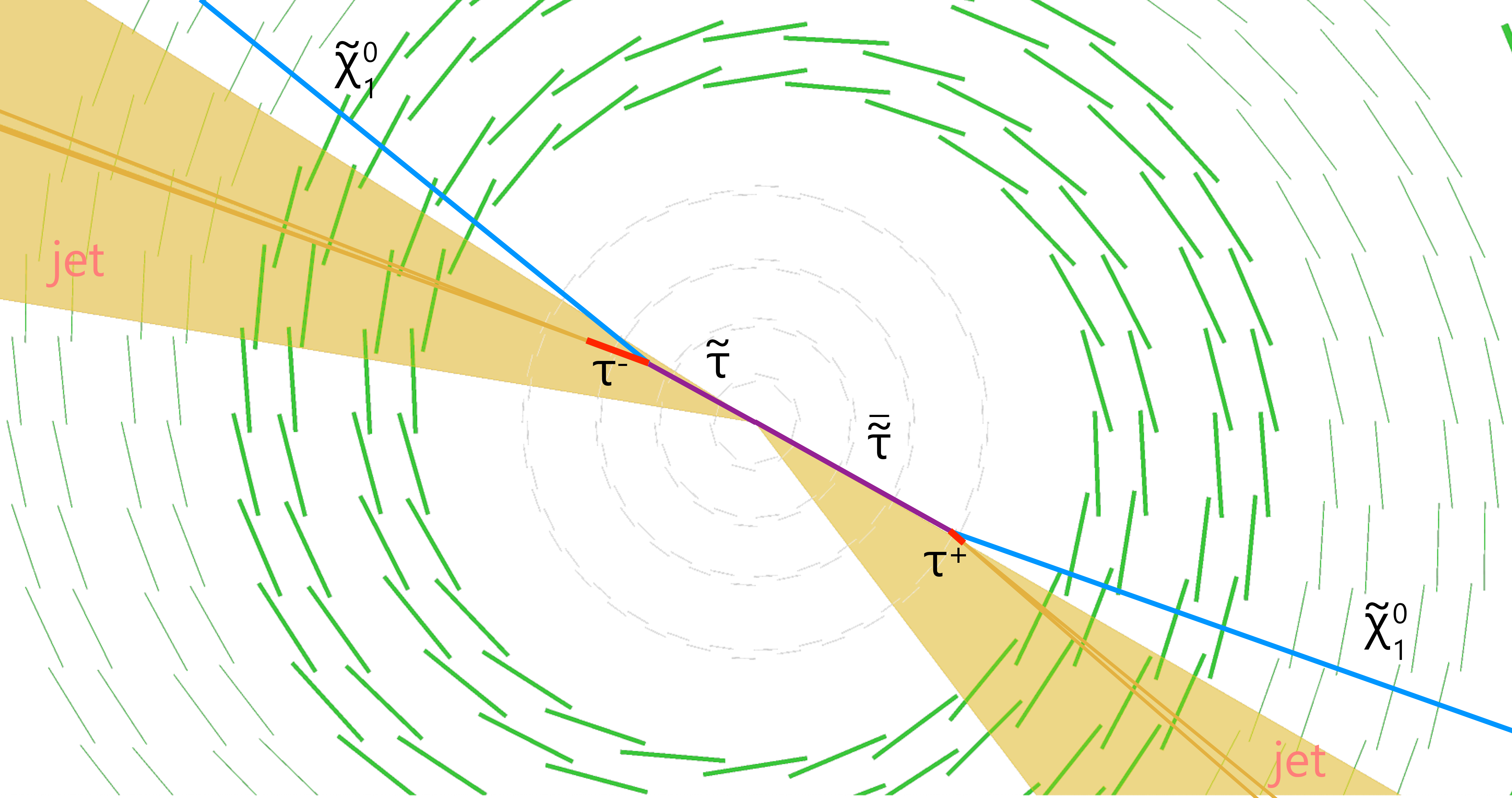
Event display of simulated $ \tilde{\tau} $ pair production in a GMSB benchmark model, followed by the decay of each $ \tilde{\tau} $ to a $ \tau $ lepton and a neutralino $ \tilde{\chi}_{1}^{0} $, with the $ \tau $ leptons decaying hadronically. The magenta lines indicate the $ \tilde{\tau} $ particles, the light blue lines indicate the neutralinos, and the red lines indicate the $ \tau $ leptons decaying hadronically. The shaded dark yellow cones show the two reconstructed jets, and the orange lines inside the jets are the hadrons from the $ \tau $ decay. |
png pdf |
Figure 13:
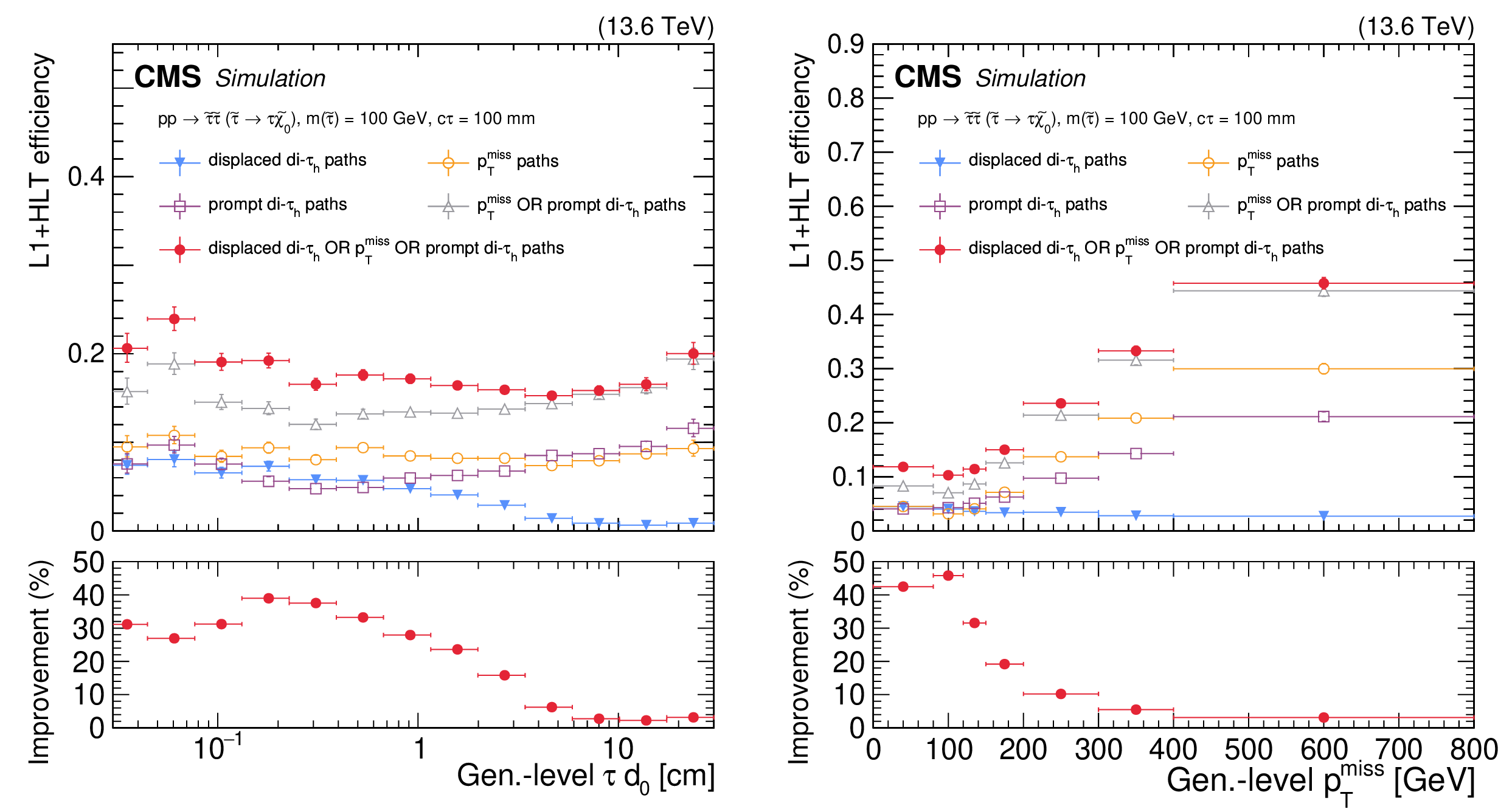
The L1T+HLT efficiency of the displaced $ \tau_\mathrm{h} $ trigger, for simulated $ \mathrm{p}\mathrm{p} \to \tilde{\tau}\tilde{\tau} (\tilde{\tau} \to \tau\tilde{\chi}_{1}^{0}) $ events, where the $ \tilde{\tau} $ has $ c\tau = 10 \text{cm} $ and each $ \tau $ decays hadronically. The efficiency is shown as a function of the $ d_{\text{0}} $ of the highest $ p_{\mathrm{T}} \tau $ lepton in the event (left) and as a function of $ p_{\mathrm{T}}^\text{miss} $ (right). The efficiency is shown for the displaced di-$ \tau_\mathrm{h} $ trigger path (blue filled triangles), the previously available $ p_{\mathrm{T}}^\text{miss} $-based paths (orange open circles), the previously available prompt di-$ \tau_\mathrm{h} $ paths (purple open squares), the combination of the $ p_{\mathrm{T}}^\text{miss} $-based and prompt di-$ \tau_\mathrm{h} $ paths (gray open triangles), and the combination of the $ p_{\mathrm{T}}^\text{miss} $-based, prompt di-$ \tau_\mathrm{h} $, and displaced di-$ \tau_\mathrm{h} $ paths (red filled circles), using 2022 data-taking conditions. The efficiency is evaluated with respect to events that contain at least two generator-level $ \tau $ leptons, where the visible component of the $ \tau $ lepton $ p_{\mathrm{T}} $ is greater than 30 GeV and $ |\eta| < $ 2.1. The lower panels show the ratio (improvement in %) of the trigger efficiency given by the combination of the displaced di-$ \tau_\mathrm{h} $ trigger path with the $ p_{\mathrm{T}}^\text{miss} $-based and prompt di-$ \tau_\mathrm{h} $ paths to that of the combination of the previously available $ p_{\mathrm{T}}^\text{miss} $-based and prompt di-$ \tau_\mathrm{h} $ paths. |
png pdf |
Figure 13-a:
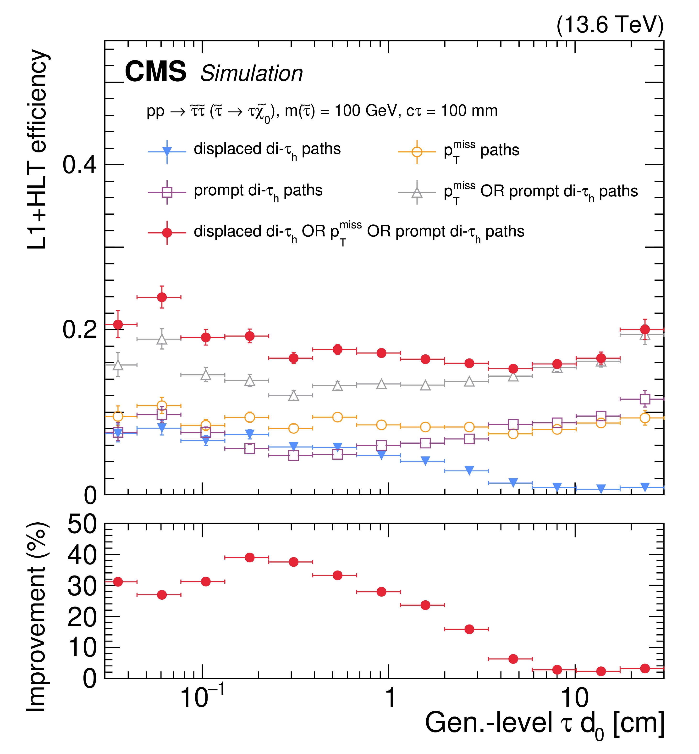
The L1T+HLT efficiency of the displaced $ \tau_\mathrm{h} $ trigger, for simulated $ \mathrm{p}\mathrm{p} \to \tilde{\tau}\tilde{\tau} (\tilde{\tau} \to \tau\tilde{\chi}_{1}^{0}) $ events, where the $ \tilde{\tau} $ has $ c\tau = 10 \text{cm} $ and each $ \tau $ decays hadronically. The efficiency is shown as a function of the $ d_{\text{0}} $ of the highest $ p_{\mathrm{T}} \tau $ lepton in the event (left) and as a function of $ p_{\mathrm{T}}^\text{miss} $ (right). The efficiency is shown for the displaced di-$ \tau_\mathrm{h} $ trigger path (blue filled triangles), the previously available $ p_{\mathrm{T}}^\text{miss} $-based paths (orange open circles), the previously available prompt di-$ \tau_\mathrm{h} $ paths (purple open squares), the combination of the $ p_{\mathrm{T}}^\text{miss} $-based and prompt di-$ \tau_\mathrm{h} $ paths (gray open triangles), and the combination of the $ p_{\mathrm{T}}^\text{miss} $-based, prompt di-$ \tau_\mathrm{h} $, and displaced di-$ \tau_\mathrm{h} $ paths (red filled circles), using 2022 data-taking conditions. The efficiency is evaluated with respect to events that contain at least two generator-level $ \tau $ leptons, where the visible component of the $ \tau $ lepton $ p_{\mathrm{T}} $ is greater than 30 GeV and $ |\eta| < $ 2.1. The lower panels show the ratio (improvement in %) of the trigger efficiency given by the combination of the displaced di-$ \tau_\mathrm{h} $ trigger path with the $ p_{\mathrm{T}}^\text{miss} $-based and prompt di-$ \tau_\mathrm{h} $ paths to that of the combination of the previously available $ p_{\mathrm{T}}^\text{miss} $-based and prompt di-$ \tau_\mathrm{h} $ paths. |
png pdf |
Figure 13-b:
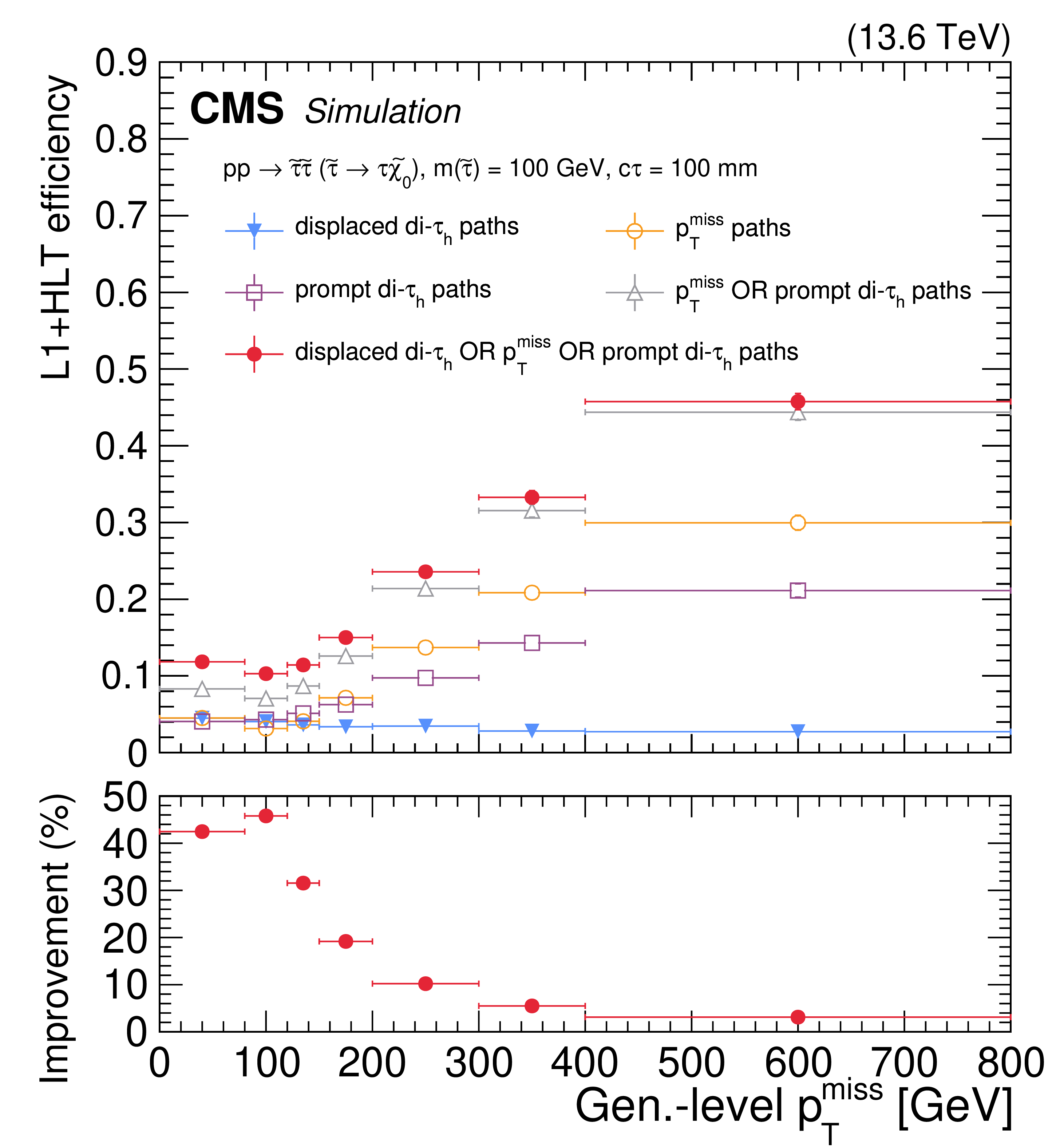
The L1T+HLT efficiency of the displaced $ \tau_\mathrm{h} $ trigger, for simulated $ \mathrm{p}\mathrm{p} \to \tilde{\tau}\tilde{\tau} (\tilde{\tau} \to \tau\tilde{\chi}_{1}^{0}) $ events, where the $ \tilde{\tau} $ has $ c\tau = 10 \text{cm} $ and each $ \tau $ decays hadronically. The efficiency is shown as a function of the $ d_{\text{0}} $ of the highest $ p_{\mathrm{T}} \tau $ lepton in the event (left) and as a function of $ p_{\mathrm{T}}^\text{miss} $ (right). The efficiency is shown for the displaced di-$ \tau_\mathrm{h} $ trigger path (blue filled triangles), the previously available $ p_{\mathrm{T}}^\text{miss} $-based paths (orange open circles), the previously available prompt di-$ \tau_\mathrm{h} $ paths (purple open squares), the combination of the $ p_{\mathrm{T}}^\text{miss} $-based and prompt di-$ \tau_\mathrm{h} $ paths (gray open triangles), and the combination of the $ p_{\mathrm{T}}^\text{miss} $-based, prompt di-$ \tau_\mathrm{h} $, and displaced di-$ \tau_\mathrm{h} $ paths (red filled circles), using 2022 data-taking conditions. The efficiency is evaluated with respect to events that contain at least two generator-level $ \tau $ leptons, where the visible component of the $ \tau $ lepton $ p_{\mathrm{T}} $ is greater than 30 GeV and $ |\eta| < $ 2.1. The lower panels show the ratio (improvement in %) of the trigger efficiency given by the combination of the displaced di-$ \tau_\mathrm{h} $ trigger path with the $ p_{\mathrm{T}}^\text{miss} $-based and prompt di-$ \tau_\mathrm{h} $ paths to that of the combination of the previously available $ p_{\mathrm{T}}^\text{miss} $-based and prompt di-$ \tau_\mathrm{h} $ paths. |
png pdf |
Figure 14:
Total rate of the displaced $ \tau_\mathrm{h} $ trigger for a few representative runs in 2022 (left) and 2023 (right) data, as a function of PU. |
png pdf |
Figure 14-a:
Total rate of the displaced $ \tau_\mathrm{h} $ trigger for a few representative runs in 2022 (left) and 2023 (right) data, as a function of PU. |
png pdf |
Figure 14-b:
Total rate of the displaced $ \tau_\mathrm{h} $ trigger for a few representative runs in 2022 (left) and 2023 (right) data, as a function of PU. |
png pdf |
Figure 15:
Event display of a simulated pair of displaced jets arising from an LLP decay, producing displaced vertices and tracks. The simulated process is $ \mathrm{H} \to \text{S}\text{S} \to \mathrm{q}\overline{\mathrm{q}}\mathrm{q}\overline{\mathrm{q}} $. The blue curves indicate the reconstructed tracks. The yellow cones indicate two reconstructed jets, with a number of associated displaced tracks. The jets are reconstructed using the standard algorithms described in Section 4.5, which assume they originate from the PV. The blue point indicates the displaced vertex induced by the LLP decay. |
png pdf |
Figure 16:
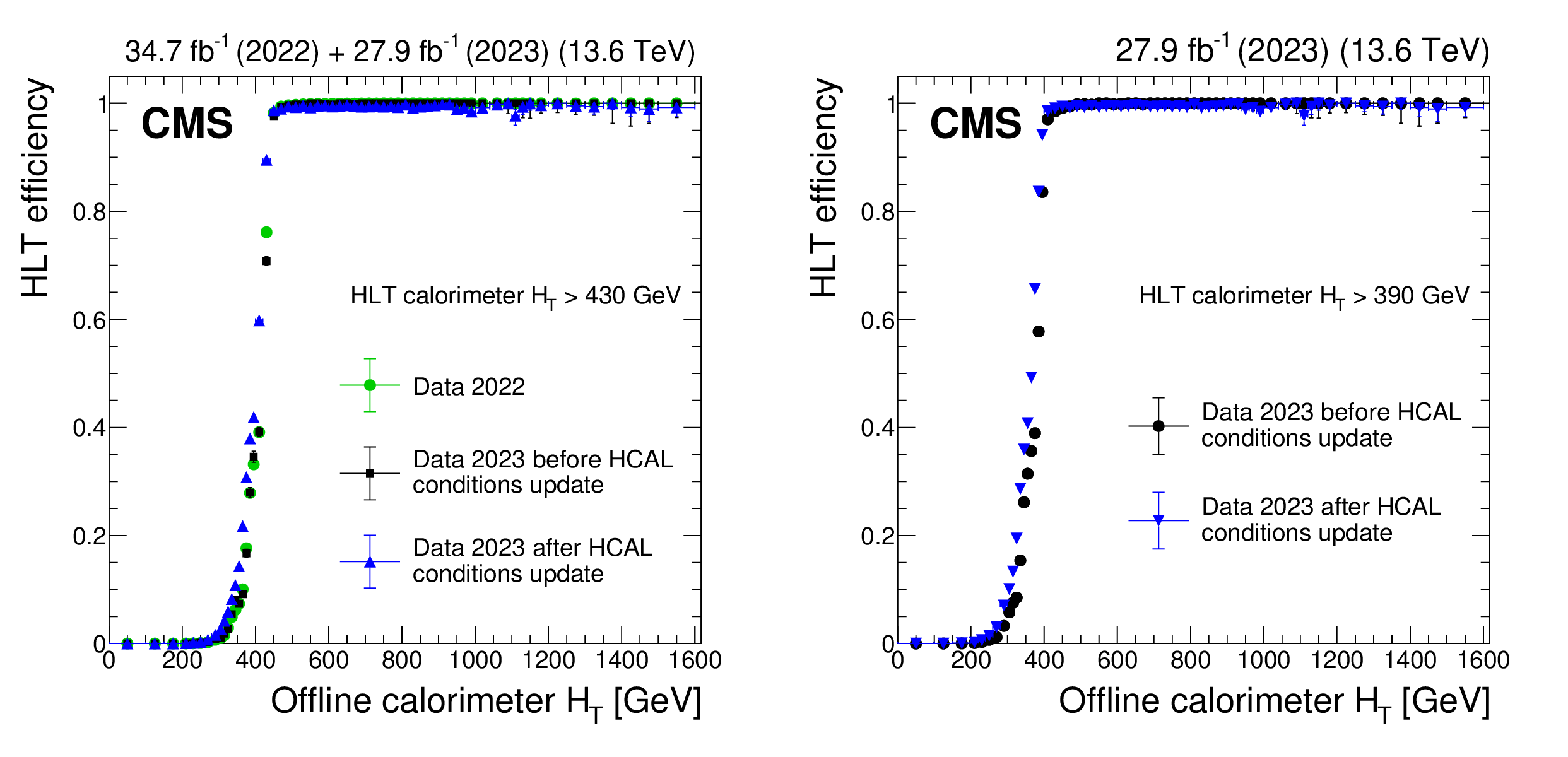
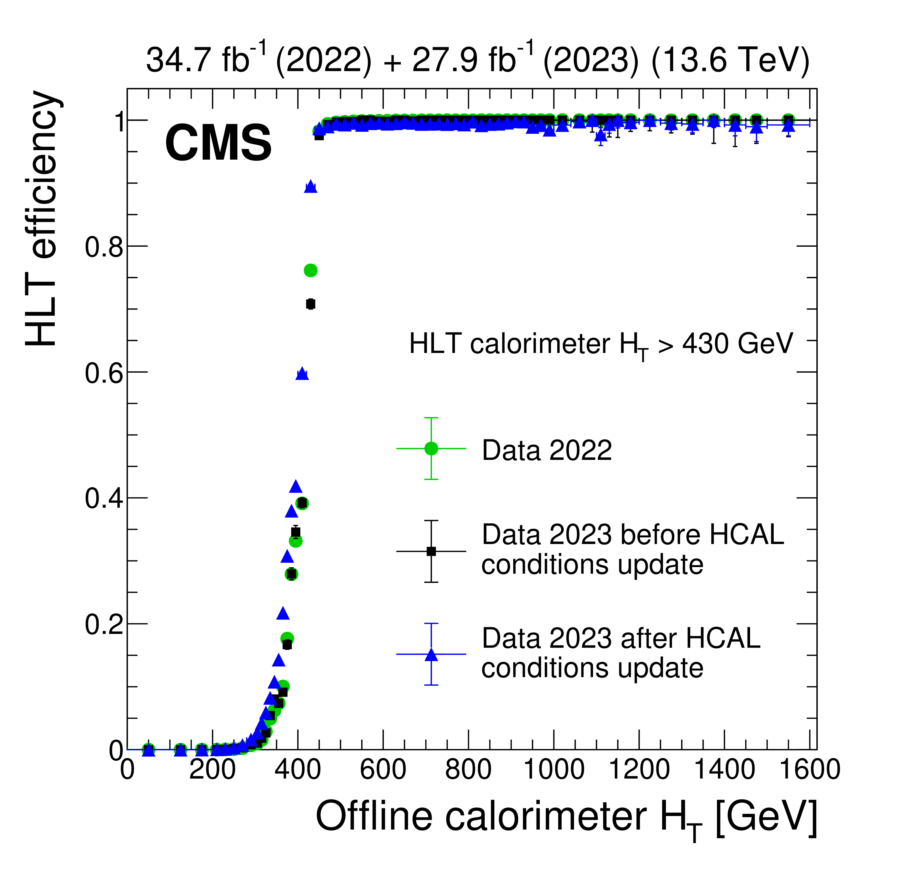
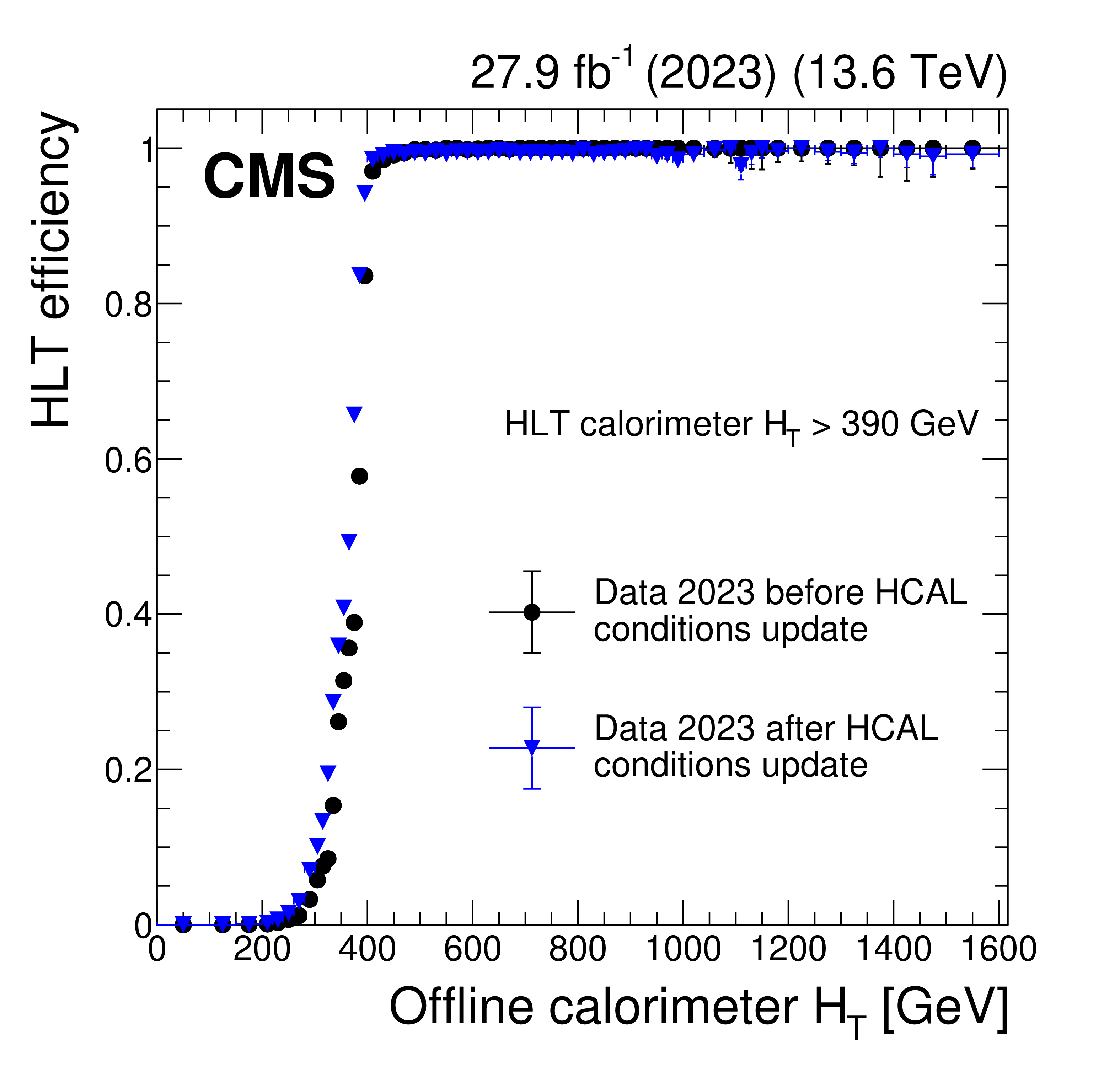
The HLT efficiency for a given event passing the main displaced-jet trigger to satisfy HLT calorimeter $ H_{\mathrm{T}} > $ 430 GeV (left) and $ H_{\mathrm{T}} > $ 390 GeV (right) as a function of the offline calorimeter $ H_{\mathrm{T}} $. For this trigger, the minimum calorimeter $ H_{\mathrm{T}} $ threshold was 430 $ (390) \text{Ge\hspace{-.08em}V} $ in 2022 (2023 and later). The measurements are performed with data collected in 2022 (green circles), in 2023 before an update of the HCAL gain values and energy response corrections (black squares), and in 2023 after the update (blue triangles). |
png pdf |
Figure 16-a:
The HLT efficiency for a given event passing the main displaced-jet trigger to satisfy HLT calorimeter $ H_{\mathrm{T}} > $ 430 GeV (left) and $ H_{\mathrm{T}} > $ 390 GeV (right) as a function of the offline calorimeter $ H_{\mathrm{T}} $. For this trigger, the minimum calorimeter $ H_{\mathrm{T}} $ threshold was 430 $ (390) \text{Ge\hspace{-.08em}V} $ in 2022 (2023 and later). The measurements are performed with data collected in 2022 (green circles), in 2023 before an update of the HCAL gain values and energy response corrections (black squares), and in 2023 after the update (blue triangles). |
png pdf |
Figure 16-b:
The HLT efficiency for a given event passing the main displaced-jet trigger to satisfy HLT calorimeter $ H_{\mathrm{T}} > $ 430 GeV (left) and $ H_{\mathrm{T}} > $ 390 GeV (right) as a function of the offline calorimeter $ H_{\mathrm{T}} $. For this trigger, the minimum calorimeter $ H_{\mathrm{T}} $ threshold was 430 $ (390) \text{Ge\hspace{-.08em}V} $ in 2022 (2023 and later). The measurements are performed with data collected in 2022 (green circles), in 2023 before an update of the HCAL gain values and energy response corrections (black squares), and in 2023 after the update (blue triangles). |
png pdf |
Figure 17:
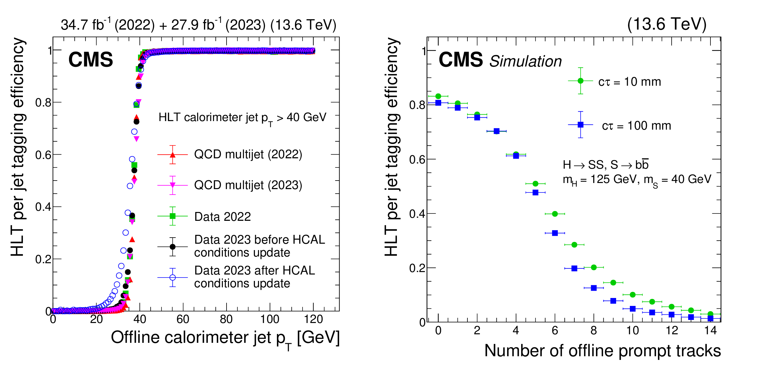
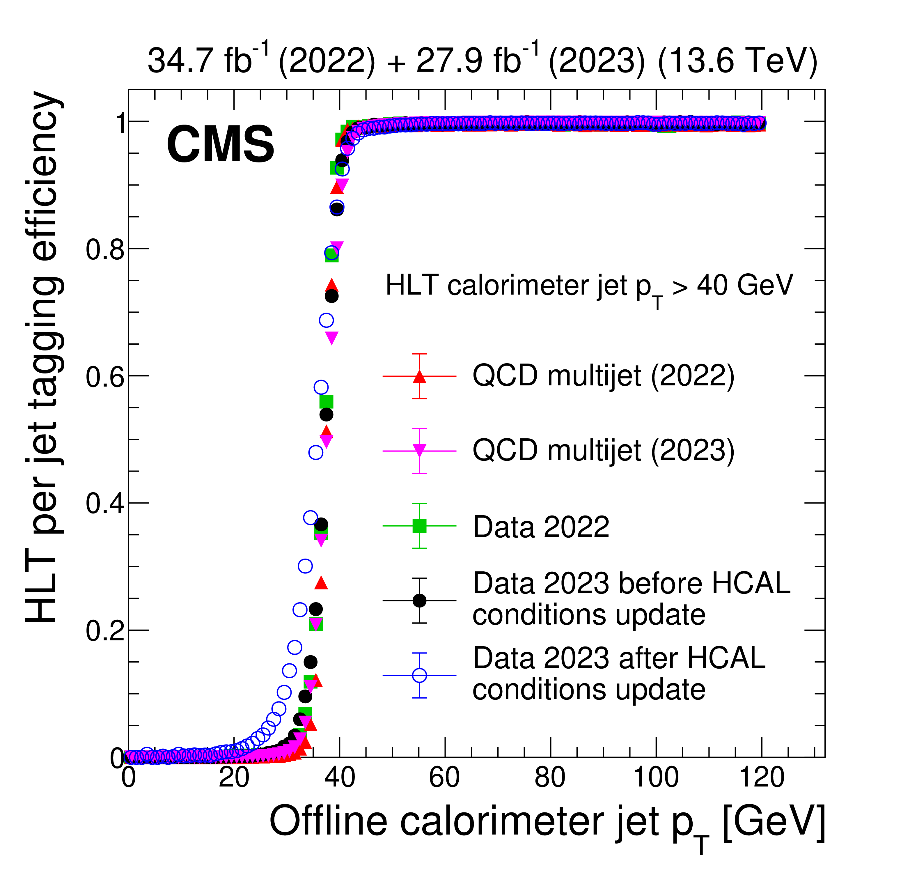
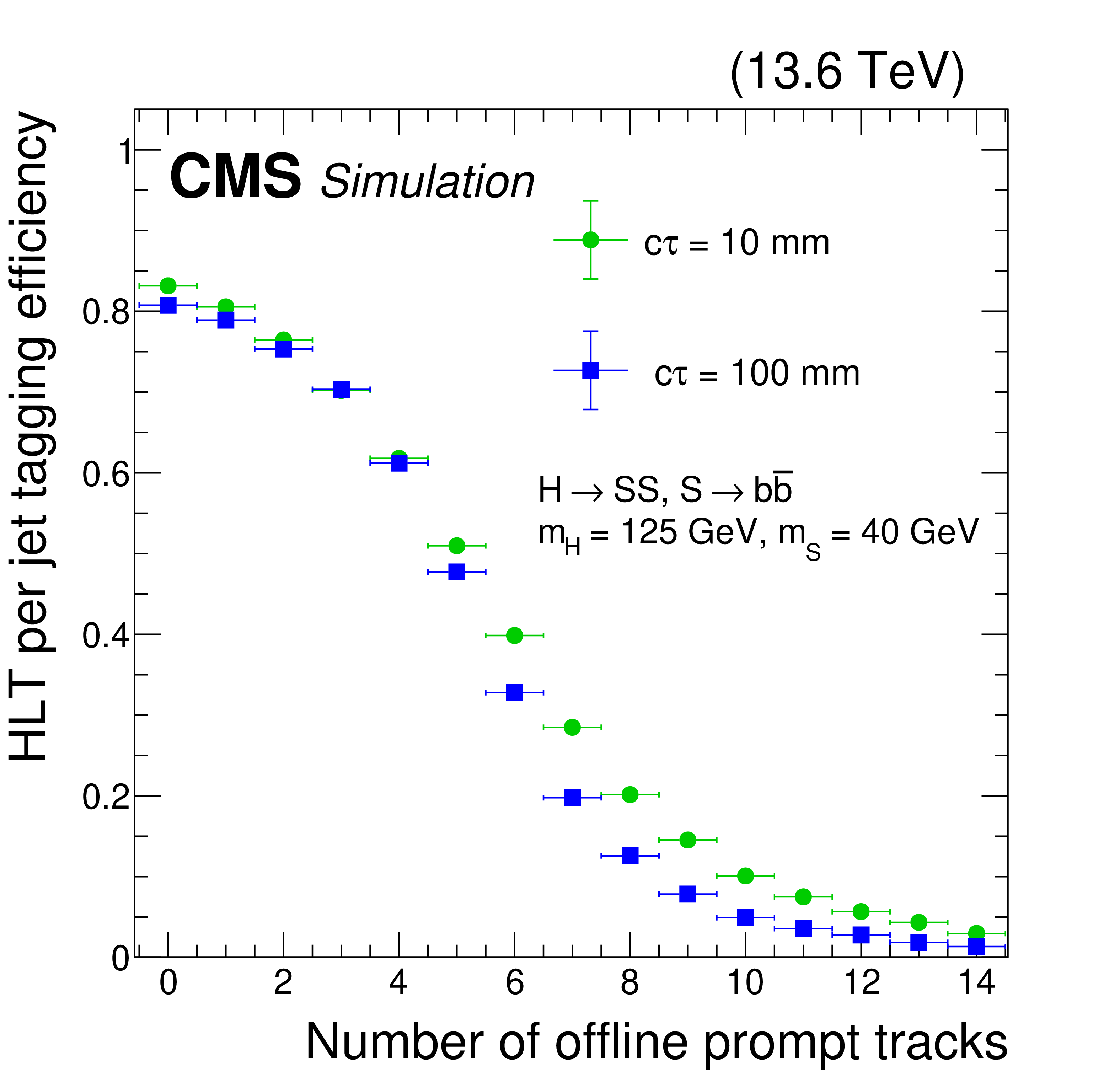
The HLT efficiency of the main displaced-jet trigger: Efficiency of an offline calorimeter jet to (left) pass the online $ p_{\mathrm{T}} $ requirement in the displaced-jet triggers and (right) to have at most one HLT prompt track. In the left plot, the HLT calorimeter jets must have $ p_{\mathrm{T}} > $ 40 GeV. The efficiency is shown for data collected in 2022 (green squares), in 2023 before an update of the HCAL gains and energy response corrections (black filled circles), and in 2023 after the update (blue open circles). The efficiencies measured with QCD multijet simulations are also shown, for 2022 (red triangles) and 2023 (purple triangles) conditions. These measurements are performed using events collected with a prescaled trigger that requires $ H_{\mathrm{T}} > $ 425 GeV at the HLT. An offline $ H_{\mathrm{T}} > $ 450 GeV selection is also applied to ensure the prescaled trigger reaches its plateau. The efficiency is $ {>} 96% $ when the offline jet has $ p_{\mathrm{T}} > $ 40 GeV. The efficiency threshold is lower for the later 2023 data following updates to the HCAL energy corrections and readout gains, although the $ p_{\mathrm{T}} $ value at the start of the plateau is unchanged. The efficiency in the right plot is shown for 2022 conditions, as a function of the number of offline prompt tracks, in simulated $ \mathrm{H}\to\text{S}\text{S} $, $ \text{S}\to\mathrm{b}\overline{\mathrm{b}} $ signal events where $ m_{\mathrm{H}}= $ 125 GeV and $ m_{\text{S}}= $ 40 GeV. Two proper decay lengths of the $ \text{S} $ particle are shown: $ c\tau=10 \text{mm} $ (green circles) and $ c\tau=100 \text{mm} $ (blue squares). For jets in signal events, when the number of offline prompt tracks is $ {<} $ 4, the tagging efficiency is larger than 70%. |
png pdf |
Figure 17-a:
The HLT efficiency of the main displaced-jet trigger: Efficiency of an offline calorimeter jet to (left) pass the online $ p_{\mathrm{T}} $ requirement in the displaced-jet triggers and (right) to have at most one HLT prompt track. In the left plot, the HLT calorimeter jets must have $ p_{\mathrm{T}} > $ 40 GeV. The efficiency is shown for data collected in 2022 (green squares), in 2023 before an update of the HCAL gains and energy response corrections (black filled circles), and in 2023 after the update (blue open circles). The efficiencies measured with QCD multijet simulations are also shown, for 2022 (red triangles) and 2023 (purple triangles) conditions. These measurements are performed using events collected with a prescaled trigger that requires $ H_{\mathrm{T}} > $ 425 GeV at the HLT. An offline $ H_{\mathrm{T}} > $ 450 GeV selection is also applied to ensure the prescaled trigger reaches its plateau. The efficiency is $ {>} 96% $ when the offline jet has $ p_{\mathrm{T}} > $ 40 GeV. The efficiency threshold is lower for the later 2023 data following updates to the HCAL energy corrections and readout gains, although the $ p_{\mathrm{T}} $ value at the start of the plateau is unchanged. The efficiency in the right plot is shown for 2022 conditions, as a function of the number of offline prompt tracks, in simulated $ \mathrm{H}\to\text{S}\text{S} $, $ \text{S}\to\mathrm{b}\overline{\mathrm{b}} $ signal events where $ m_{\mathrm{H}}= $ 125 GeV and $ m_{\text{S}}= $ 40 GeV. Two proper decay lengths of the $ \text{S} $ particle are shown: $ c\tau=10 \text{mm} $ (green circles) and $ c\tau=100 \text{mm} $ (blue squares). For jets in signal events, when the number of offline prompt tracks is $ {<} $ 4, the tagging efficiency is larger than 70%. |
png pdf |
Figure 17-b:
The HLT efficiency of the main displaced-jet trigger: Efficiency of an offline calorimeter jet to (left) pass the online $ p_{\mathrm{T}} $ requirement in the displaced-jet triggers and (right) to have at most one HLT prompt track. In the left plot, the HLT calorimeter jets must have $ p_{\mathrm{T}} > $ 40 GeV. The efficiency is shown for data collected in 2022 (green squares), in 2023 before an update of the HCAL gains and energy response corrections (black filled circles), and in 2023 after the update (blue open circles). The efficiencies measured with QCD multijet simulations are also shown, for 2022 (red triangles) and 2023 (purple triangles) conditions. These measurements are performed using events collected with a prescaled trigger that requires $ H_{\mathrm{T}} > $ 425 GeV at the HLT. An offline $ H_{\mathrm{T}} > $ 450 GeV selection is also applied to ensure the prescaled trigger reaches its plateau. The efficiency is $ {>} 96% $ when the offline jet has $ p_{\mathrm{T}} > $ 40 GeV. The efficiency threshold is lower for the later 2023 data following updates to the HCAL energy corrections and readout gains, although the $ p_{\mathrm{T}} $ value at the start of the plateau is unchanged. The efficiency in the right plot is shown for 2022 conditions, as a function of the number of offline prompt tracks, in simulated $ \mathrm{H}\to\text{S}\text{S} $, $ \text{S}\to\mathrm{b}\overline{\mathrm{b}} $ signal events where $ m_{\mathrm{H}}= $ 125 GeV and $ m_{\text{S}}= $ 40 GeV. Two proper decay lengths of the $ \text{S} $ particle are shown: $ c\tau=10 \text{mm} $ (green circles) and $ c\tau=100 \text{mm} $ (blue squares). For jets in signal events, when the number of offline prompt tracks is $ {<} $ 4, the tagging efficiency is larger than 70%. |
png pdf |
Figure 18:
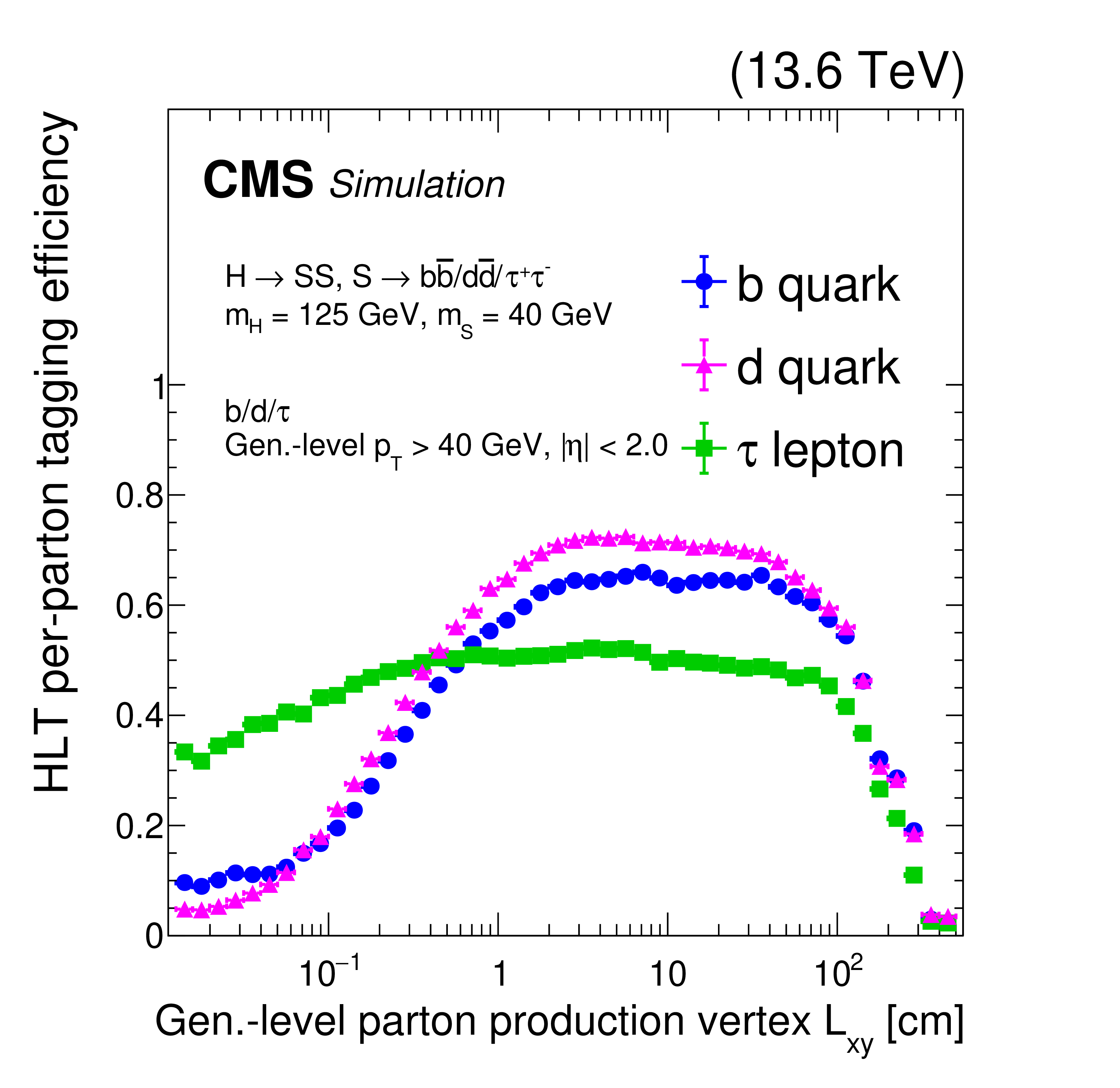
The HLT efficiency of the main displaced-jet trigger for 2022 conditions, for $ \mathrm{H}\to\text{S}\text{S} $ signal events where $ m_{\mathrm{H}}= $ 125 GeV and $ m_{\text{S}}= $ 40 GeV. The per-parton (quark or lepton) HLT displaced-jet tagging efficiency as a function of the generator-level $ L_{\text{xy}} $ of the parton is shown for displaced b quarks (blue circles), d quarks (purple triangles), and $ \tau $ leptons (green squares) with $ p_{\mathrm{T}} > $ 40 GeV and $ |\eta| < $ 2.0. Events are required to satisfy the HLT $ H_{\mathrm{T}} > $ 430 GeV requirement. |
png pdf |
Figure 19:
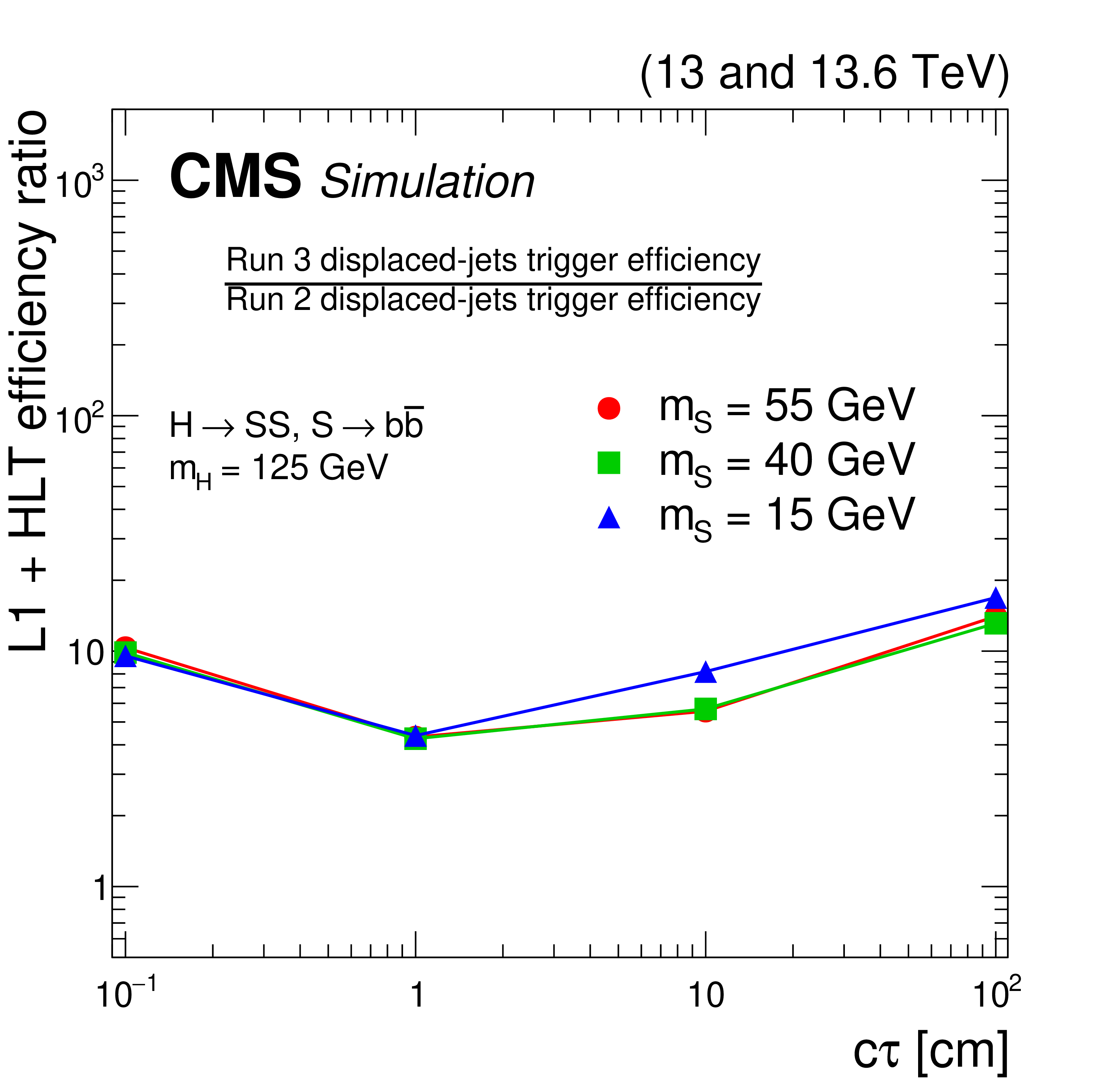
The ratio between the Run 3 displaced-jet trigger efficiency and the Run 2 displaced-jet trigger efficiency as a function of LLP $ c\tau $, in simulated $ \mathrm{H}\to\text{S}\text{S} $, $ \text{S}\to\mathrm{b}\overline{\mathrm{b}} $ signal events where $ m_{\mathrm{H}}= $ 125 GeV and $ m_{\text{S}}= $ 15 (blue triangles), 40 (green squares), or 55 (red circles) GeV. The Run 3 displaced-jet trigger efficiencies are measured for 2022 conditions. |
png pdf |
Figure 20:
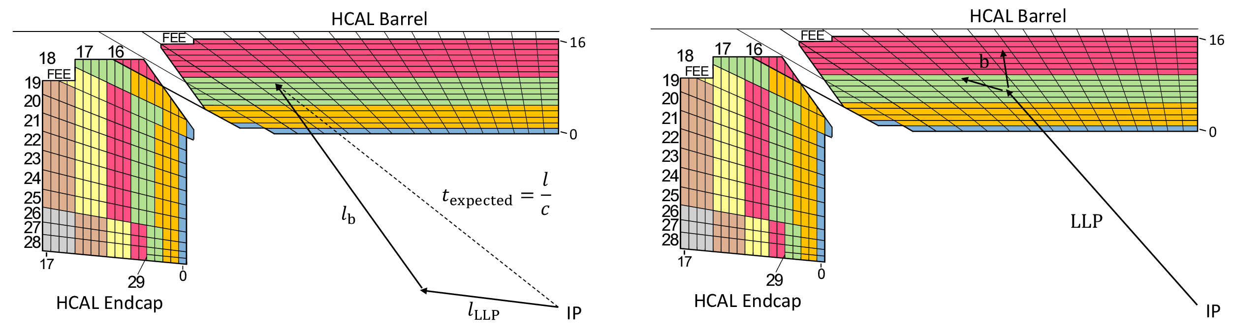
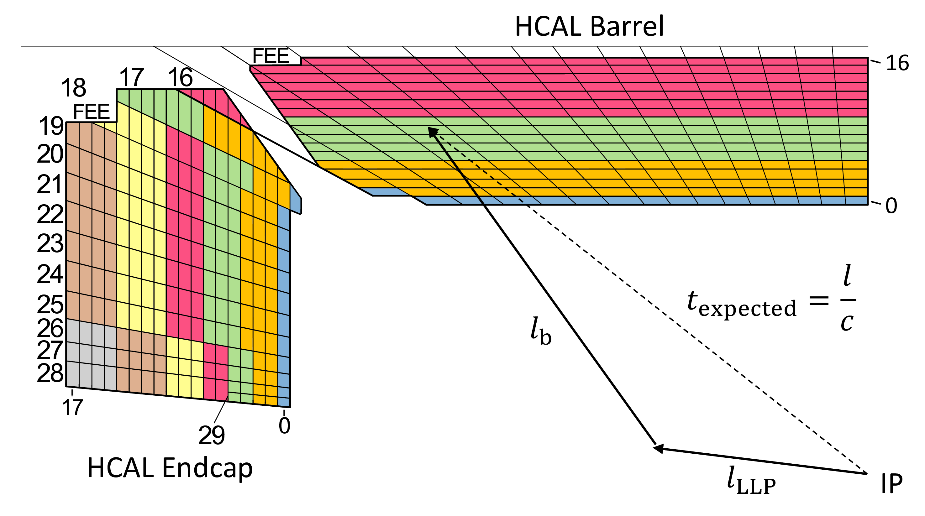
Diagram showing the lateral view of a quadrant of the CMS HCAL barrel and endcap in Run 3. The distinct depth segmentation is indicated by the different colors, where the HCAL barrel consists of 4 depths and the HCAL endcap has up to 7 depths. A delayed-jet signature is shown (left), where the time delay results from a combination of the low LLP velocity because of its relatively high mass and the path length difference with respect to a promptly decaying particle. A time delay consists of the path length difference between a particle traveling from the IP directly to the calorimeter ($ l $), as compared to the LLP path ($ l_{\text{LLP}} $) plus the b quark path ($ l_{\mathrm{b}} $). Additionally, the LLP may also have a significantly lower velocity, while other particles are assumed in this example to be highly relativistic. Thus, the difference in time of arrival at the calorimeter is $ \Delta t = \frac{l_{\text{LLP}}}{v_{\text{LLP}}} + \frac{l_{\mathrm{b}}}{c} - \frac{l}{c} $. A displaced-jet signature is also depicted (right), resulting from an LLP decaying within the HCAL volume to produce significant energy deposits deeper in the HCAL with minimal energy deposits in shallower calorimeter layers. |
png pdf |
Figure 20-a:
Diagram showing the lateral view of a quadrant of the CMS HCAL barrel and endcap in Run 3. The distinct depth segmentation is indicated by the different colors, where the HCAL barrel consists of 4 depths and the HCAL endcap has up to 7 depths. A delayed-jet signature is shown (left), where the time delay results from a combination of the low LLP velocity because of its relatively high mass and the path length difference with respect to a promptly decaying particle. A time delay consists of the path length difference between a particle traveling from the IP directly to the calorimeter ($ l $), as compared to the LLP path ($ l_{\text{LLP}} $) plus the b quark path ($ l_{\mathrm{b}} $). Additionally, the LLP may also have a significantly lower velocity, while other particles are assumed in this example to be highly relativistic. Thus, the difference in time of arrival at the calorimeter is $ \Delta t = \frac{l_{\text{LLP}}}{v_{\text{LLP}}} + \frac{l_{\mathrm{b}}}{c} - \frac{l}{c} $. A displaced-jet signature is also depicted (right), resulting from an LLP decaying within the HCAL volume to produce significant energy deposits deeper in the HCAL with minimal energy deposits in shallower calorimeter layers. |
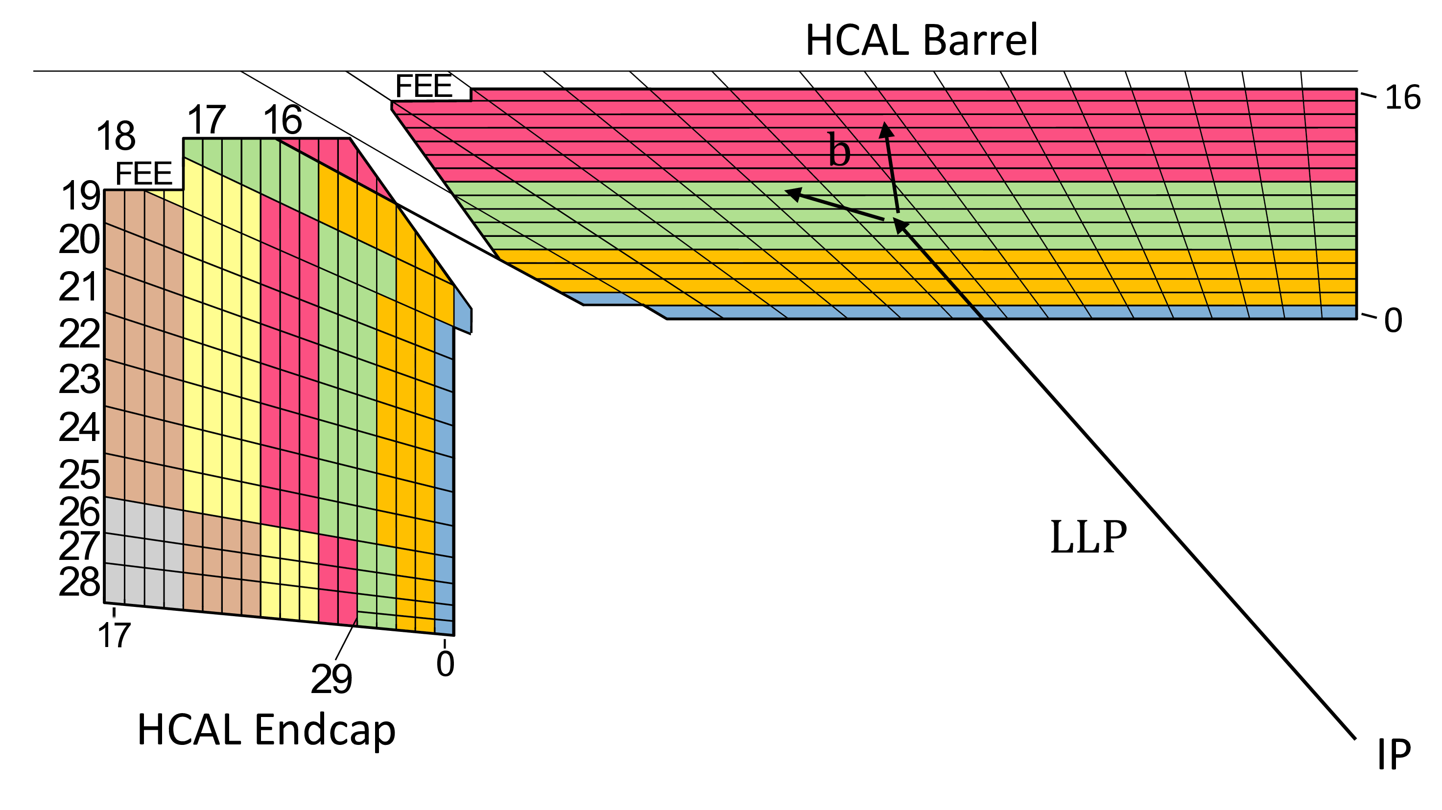
png pdf |
Figure 20-b:
Diagram showing the lateral view of a quadrant of the CMS HCAL barrel and endcap in Run 3. The distinct depth segmentation is indicated by the different colors, where the HCAL barrel consists of 4 depths and the HCAL endcap has up to 7 depths. A delayed-jet signature is shown (left), where the time delay results from a combination of the low LLP velocity because of its relatively high mass and the path length difference with respect to a promptly decaying particle. A time delay consists of the path length difference between a particle traveling from the IP directly to the calorimeter ($ l $), as compared to the LLP path ($ l_{\text{LLP}} $) plus the b quark path ($ l_{\mathrm{b}} $). Additionally, the LLP may also have a significantly lower velocity, while other particles are assumed in this example to be highly relativistic. Thus, the difference in time of arrival at the calorimeter is $ \Delta t = \frac{l_{\text{LLP}}}{v_{\text{LLP}}} + \frac{l_{\mathrm{b}}}{c} - \frac{l}{c} $. A displaced-jet signature is also depicted (right), resulting from an LLP decaying within the HCAL volume to produce significant energy deposits deeper in the HCAL with minimal energy deposits in shallower calorimeter layers. |
png pdf |
Figure 21:
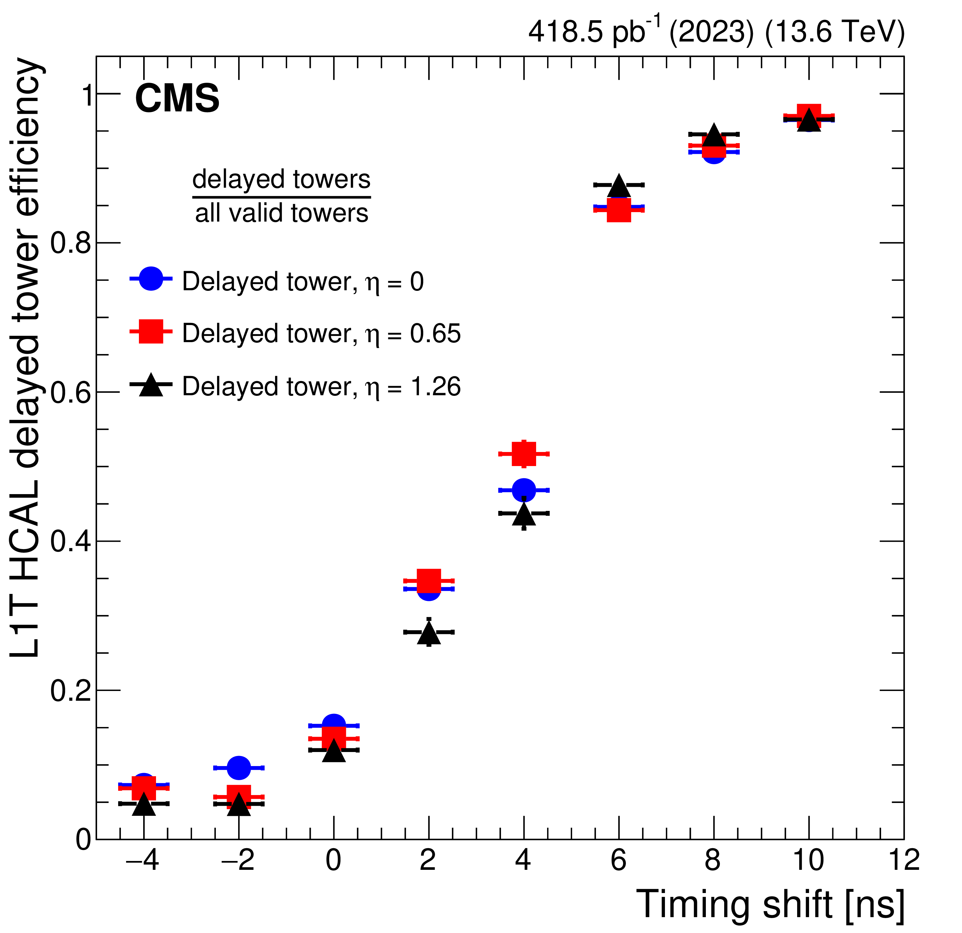
The L1T HCAL trigger tower efficiency of the delayed timing towers in the 2023 HCAL timing-scan data, with efficiencies split by trigger towers centered at $ \eta\approx $ 0 (blue circles), 0.65 (red squares), 1.26 (black triangles), and with width $ \Delta \eta = $ 0.087. The sharp rise in efficiency between timing delays of 0--6\unitns is expected, as the prompt timing range includes pulses up to and including those recorded at a 6\unitns arrival time (digitized in half-ns steps by the TDC), demonstrating the timing trigger performance. The delayed timing towers must have at least one delayed cell, no prompt cells, and energy $ {>} $ 4 GeV. The efficiency is calculated relative to towers with any valid timing code, meaning the tower contains at least one cell with energy $ {>} $ 4 GeV and a TDC code of prompt, slightly delayed, or very delayed. Multiple delayed or displaced towers are required for the HCAL-based displaced- and delayed-jet L1T to pass. |
png pdf |
Figure 22:
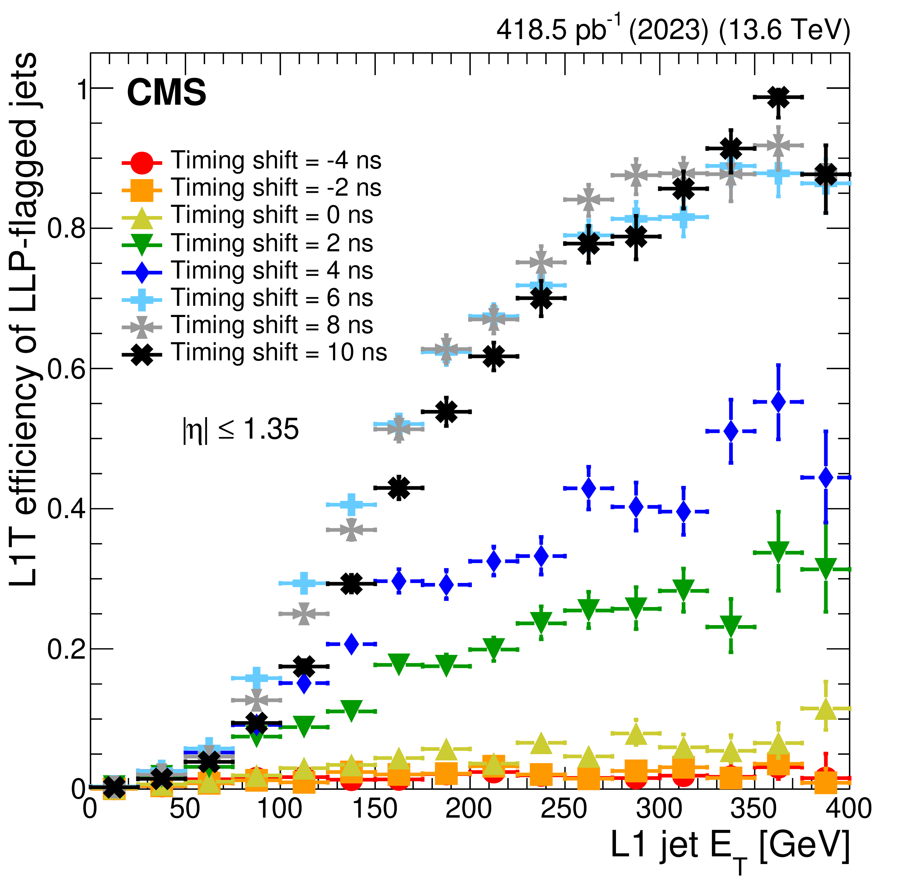
The L1T efficiency of the LLP jet trigger in 2023 HCAL timing-scan data as a function of L1 jet $ E_{\mathrm{T}} $. The results are inclusive in $ \eta $ for the HCAL barrel, corresponding to $ |\eta| < $ 1.35. The fraction of LLP-flagged L1 jets is compared to all L1 jets from a data set of events enriched in jets or $ p_{\mathrm{T}}^\text{miss} $. No explicit selection criterion is applied on the jet $ E_{\mathrm{T}} $, though the implicit requirement for a jet to have at least two cells with $ E_{\mathrm{T}} > $ 4 GeV shapes the resulting jet trigger efficiency curve. While the trigger configuration is based on the presence of both delayed and displaced towers, the timing scan demonstrates the ability of the trigger to select delayed jets only. |
png pdf |
Figure 23:
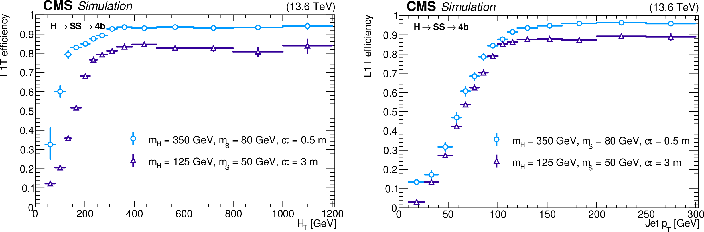
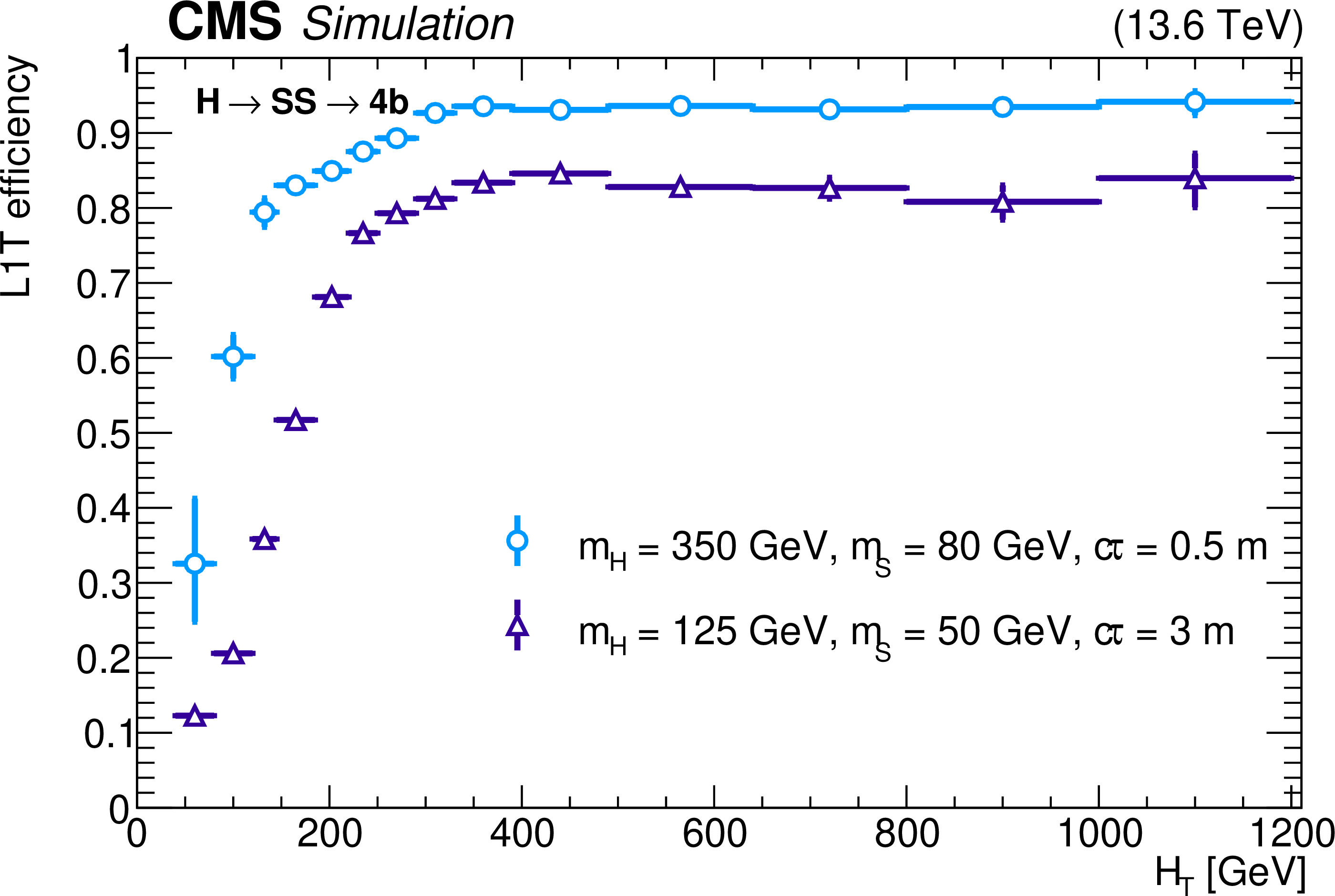
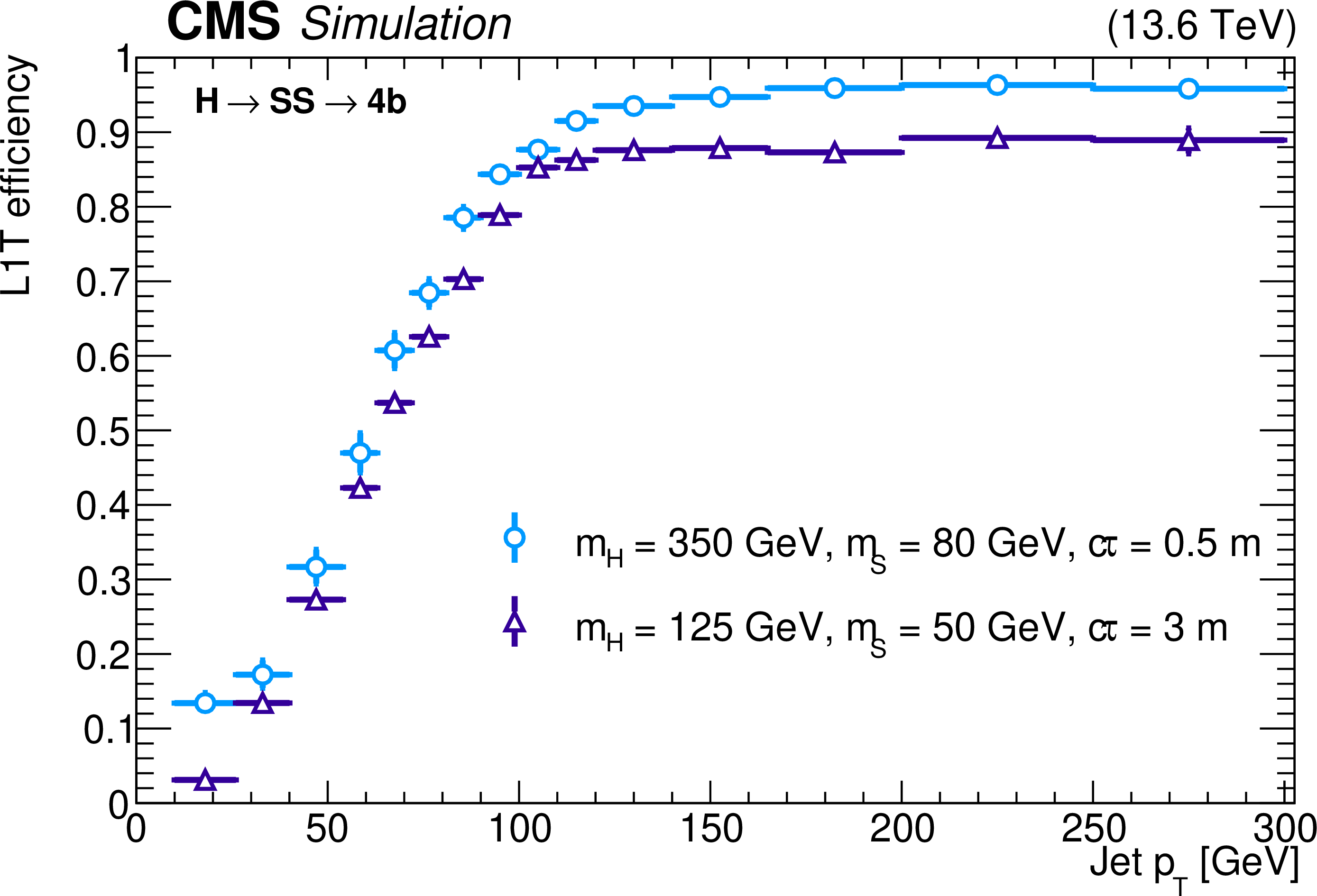
The L1T efficiency of the HCAL-based LLP jet triggers, as a function of event $ H_{\mathrm{T}} $ (left) and jet $ p_{\mathrm{T}} $ (right), for $ \mathrm{H} \to \text{S}\text{S} \to \mathrm{b}\overline{\mathrm{b}}\mathrm{b}\overline{\mathrm{b}} $ events with $ m_{\mathrm{H}}= $ 350 GeV, $ m_{\text{S}}= $ 80 GeV, and $ c\tau_{\text{S}}= $ 0.5 m (light blue circles) and $ m_{\mathrm{H}}= $ 125 GeV, $ m_{\text{S}}= $ 50 GeV, and $ c\tau_{\text{S}}= $ 3 m (purple triangles), for 2023 conditions. The trigger efficiency is evaluated for LLPs decaying in HB depths 3 or 4, corresponding to 214.2 $ < R < 295 \text{cm} $ and $ |\eta| < $ 1.26. These LLPs are also required to be matched to an offline jet with $ p_{\mathrm{T}} > $ 40 GeV in HB. |
png pdf |
Figure 23-a:
The L1T efficiency of the HCAL-based LLP jet triggers, as a function of event $ H_{\mathrm{T}} $ (left) and jet $ p_{\mathrm{T}} $ (right), for $ \mathrm{H} \to \text{S}\text{S} \to \mathrm{b}\overline{\mathrm{b}}\mathrm{b}\overline{\mathrm{b}} $ events with $ m_{\mathrm{H}}= $ 350 GeV, $ m_{\text{S}}= $ 80 GeV, and $ c\tau_{\text{S}}= $ 0.5 m (light blue circles) and $ m_{\mathrm{H}}= $ 125 GeV, $ m_{\text{S}}= $ 50 GeV, and $ c\tau_{\text{S}}= $ 3 m (purple triangles), for 2023 conditions. The trigger efficiency is evaluated for LLPs decaying in HB depths 3 or 4, corresponding to 214.2 $ < R < 295 \text{cm} $ and $ |\eta| < $ 1.26. These LLPs are also required to be matched to an offline jet with $ p_{\mathrm{T}} > $ 40 GeV in HB. |
png pdf |
Figure 23-b:
The L1T efficiency of the HCAL-based LLP jet triggers, as a function of event $ H_{\mathrm{T}} $ (left) and jet $ p_{\mathrm{T}} $ (right), for $ \mathrm{H} \to \text{S}\text{S} \to \mathrm{b}\overline{\mathrm{b}}\mathrm{b}\overline{\mathrm{b}} $ events with $ m_{\mathrm{H}}= $ 350 GeV, $ m_{\text{S}}= $ 80 GeV, and $ c\tau_{\text{S}}= $ 0.5 m (light blue circles) and $ m_{\mathrm{H}}= $ 125 GeV, $ m_{\text{S}}= $ 50 GeV, and $ c\tau_{\text{S}}= $ 3 m (purple triangles), for 2023 conditions. The trigger efficiency is evaluated for LLPs decaying in HB depths 3 or 4, corresponding to 214.2 $ < R < 295 \text{cm} $ and $ |\eta| < $ 1.26. These LLPs are also required to be matched to an offline jet with $ p_{\mathrm{T}} > $ 40 GeV in HB. |
png pdf |
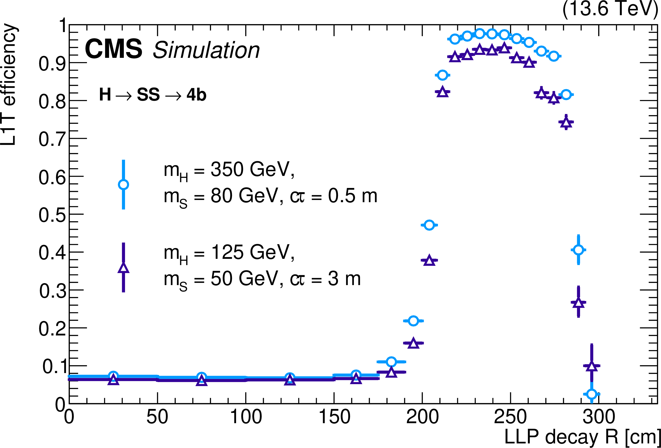
Figure 24:
The L1T efficiency of the HCAL-based LLP jet triggers as a function of LLP decay radial position $ R $ for $ \mathrm{H} \to \text{S}\text{S} \to \mathrm{b}\overline{\mathrm{b}}\mathrm{b}\overline{\mathrm{b}} $ events with $ m_{\mathrm{H}}= $ 350 GeV, $ m_{\text{S}}= $ 80 GeV, and $ c\tau_{\text{S}}= $ 0.5 m (light blue circles) and $ m_{\mathrm{H}}= $ 125 GeV, $ m_{\text{S}}= $ 50 GeV, and $ c\tau_{\text{S}}= $ 3 m (purple triangles), for 2023 conditions. The trigger efficiency is evaluated for LLPs within $ |\eta| < $ 1.26 where either the LLP or its decay products are matched to an offline jet in HB with $ p_{\mathrm{T}} > $ 100 GeV. |
png pdf |
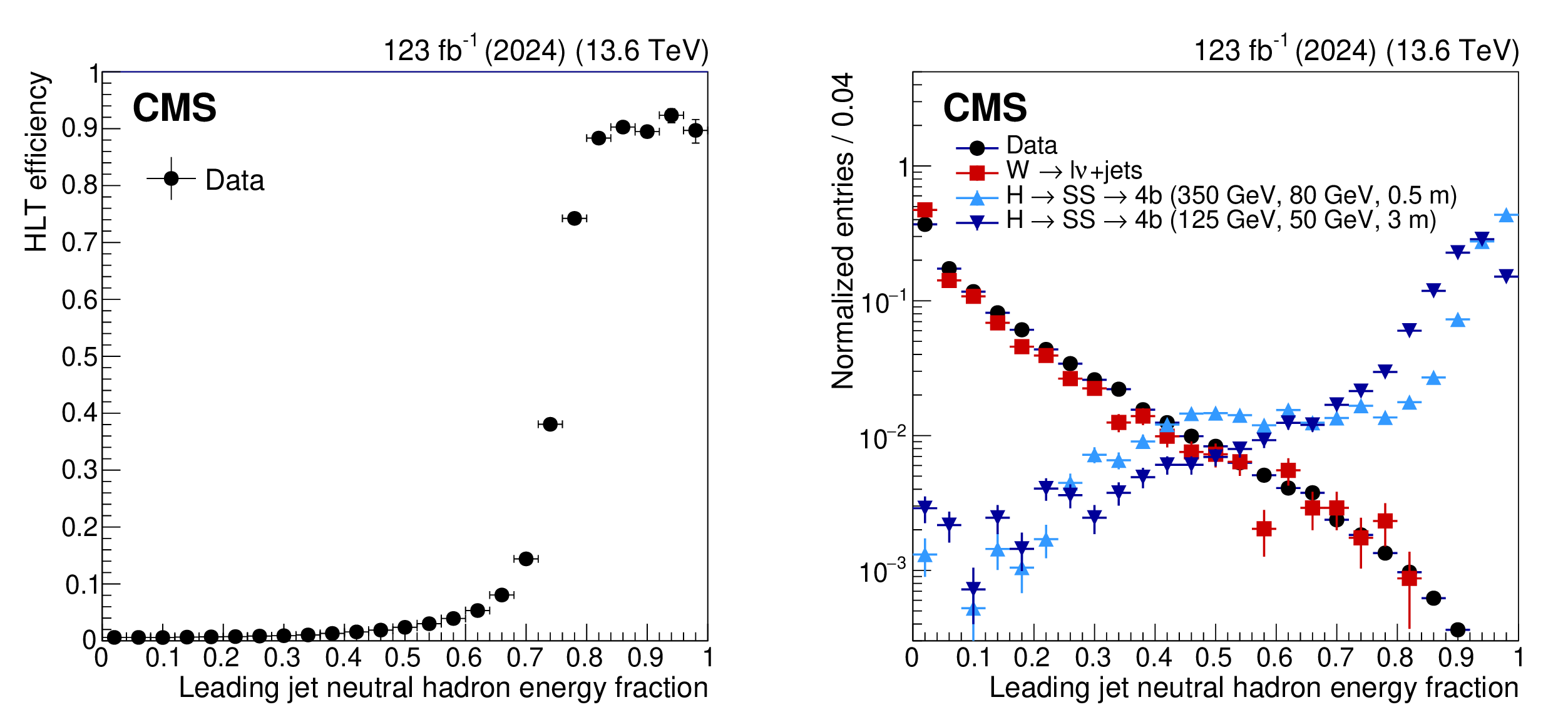
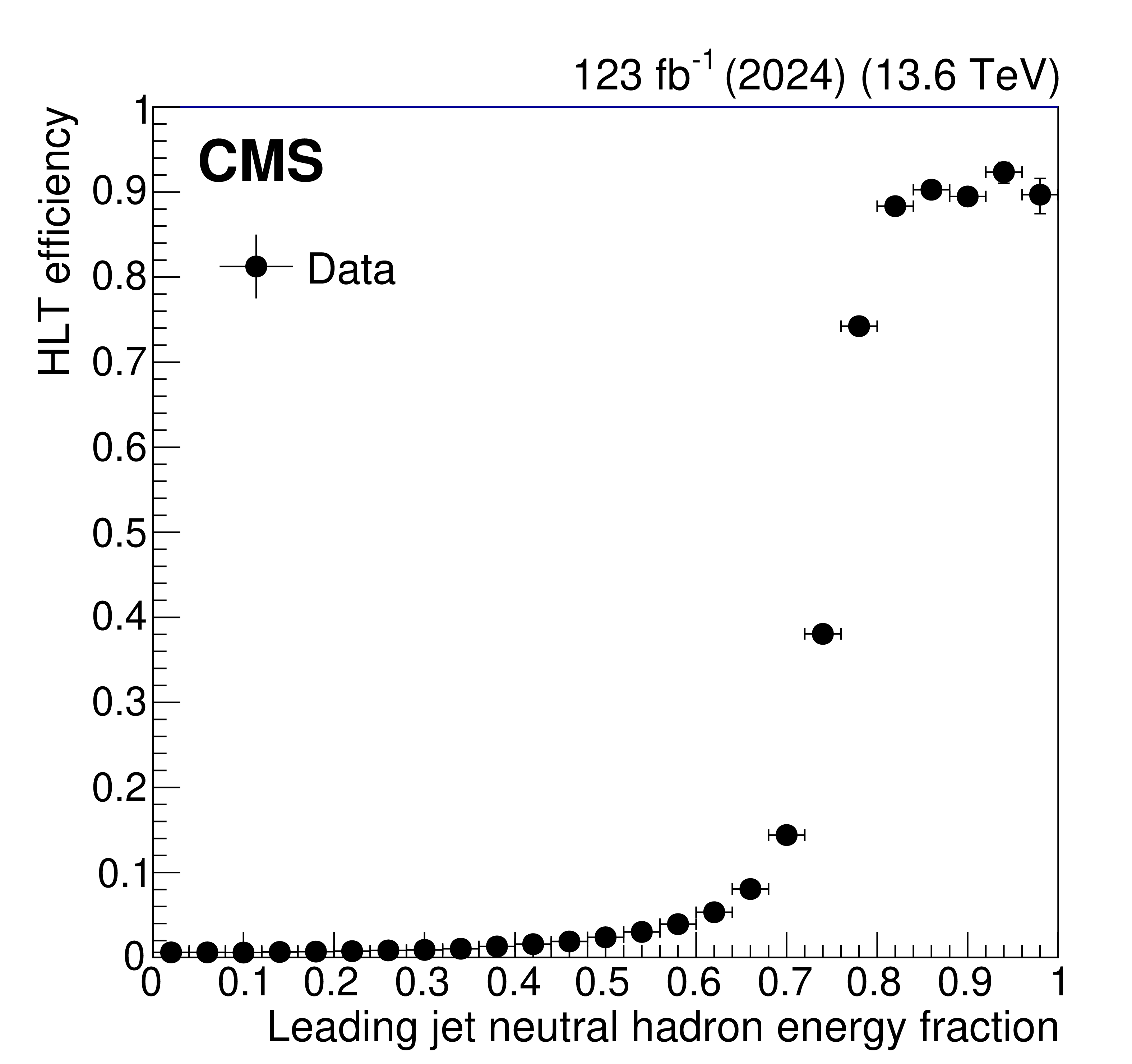
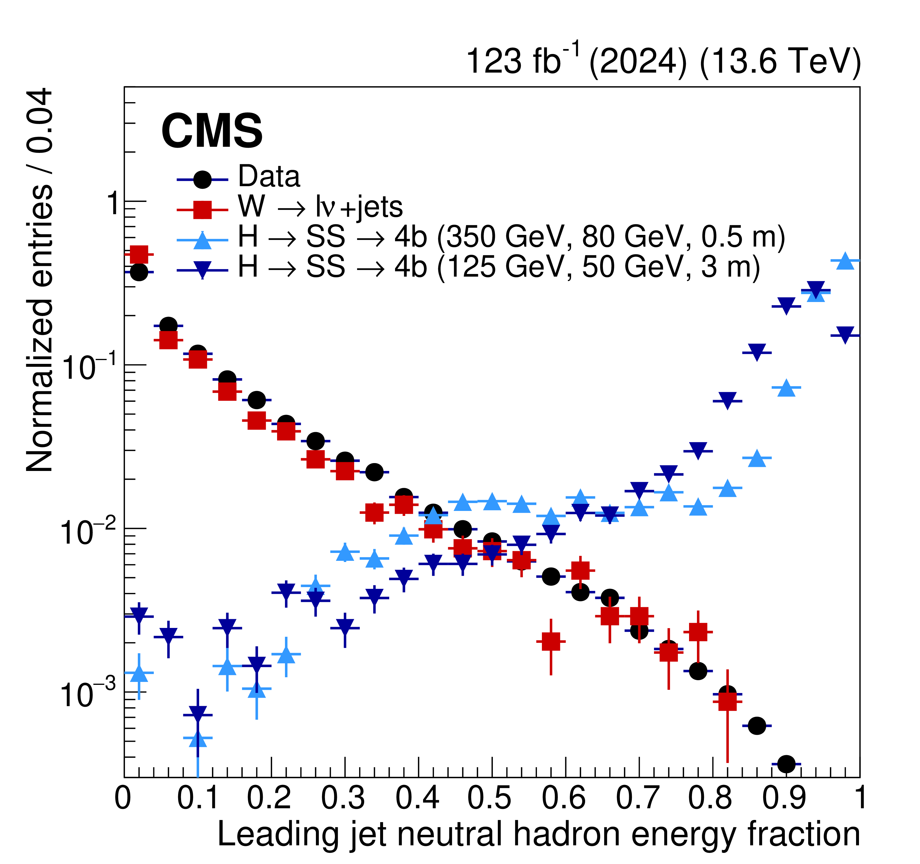
Figure 25:
The HLT efficiency of the CalRatio trigger as a function of the leading PF jet NHEF in 2024 data, measured with respect to a logical OR of the HCAL-based LLP L1 jet triggers (left). Distribution of the leading PF jet NHEF (right) in 2024 data (black circles), $ \mathrm{W} \to \ell\nu $ background simulation for 2024 conditions (red squares), and $ \mathrm{H} \to \text{S}\text{S} \to \mathrm{b}\overline{\mathrm{b}}\mathrm{b}\overline{\mathrm{b}} $ signal simulation for 2023 conditions (blue and purple triangles). Events are required to have $ H_{\mathrm{T}} > $ 200 GeV and the leading jet is required to have $ p_{\mathrm{T}} > $ 60 GeV and $ |\eta| < $ 1.5; these requirements are equivalent to the respective HLT jet object selections. The signal distributions additionally require the leading jet to be matched to an LLP decaying anywhere inside the barrel calorimeter volume (129 $ < R < 295 \text{cm} $). The clear separation between the displaced signal and the prompt background in the right plot motivates the development of the CalRatio trigger. |
png pdf |
Figure 25-a:
The HLT efficiency of the CalRatio trigger as a function of the leading PF jet NHEF in 2024 data, measured with respect to a logical OR of the HCAL-based LLP L1 jet triggers (left). Distribution of the leading PF jet NHEF (right) in 2024 data (black circles), $ \mathrm{W} \to \ell\nu $ background simulation for 2024 conditions (red squares), and $ \mathrm{H} \to \text{S}\text{S} \to \mathrm{b}\overline{\mathrm{b}}\mathrm{b}\overline{\mathrm{b}} $ signal simulation for 2023 conditions (blue and purple triangles). Events are required to have $ H_{\mathrm{T}} > $ 200 GeV and the leading jet is required to have $ p_{\mathrm{T}} > $ 60 GeV and $ |\eta| < $ 1.5; these requirements are equivalent to the respective HLT jet object selections. The signal distributions additionally require the leading jet to be matched to an LLP decaying anywhere inside the barrel calorimeter volume (129 $ < R < 295 \text{cm} $). The clear separation between the displaced signal and the prompt background in the right plot motivates the development of the CalRatio trigger. |
png pdf |
Figure 25-b:
The HLT efficiency of the CalRatio trigger as a function of the leading PF jet NHEF in 2024 data, measured with respect to a logical OR of the HCAL-based LLP L1 jet triggers (left). Distribution of the leading PF jet NHEF (right) in 2024 data (black circles), $ \mathrm{W} \to \ell\nu $ background simulation for 2024 conditions (red squares), and $ \mathrm{H} \to \text{S}\text{S} \to \mathrm{b}\overline{\mathrm{b}}\mathrm{b}\overline{\mathrm{b}} $ signal simulation for 2023 conditions (blue and purple triangles). Events are required to have $ H_{\mathrm{T}} > $ 200 GeV and the leading jet is required to have $ p_{\mathrm{T}} > $ 60 GeV and $ |\eta| < $ 1.5; these requirements are equivalent to the respective HLT jet object selections. The signal distributions additionally require the leading jet to be matched to an LLP decaying anywhere inside the barrel calorimeter volume (129 $ < R < 295 \text{cm} $). The clear separation between the displaced signal and the prompt background in the right plot motivates the development of the CalRatio trigger. |
png pdf |
Figure 26:
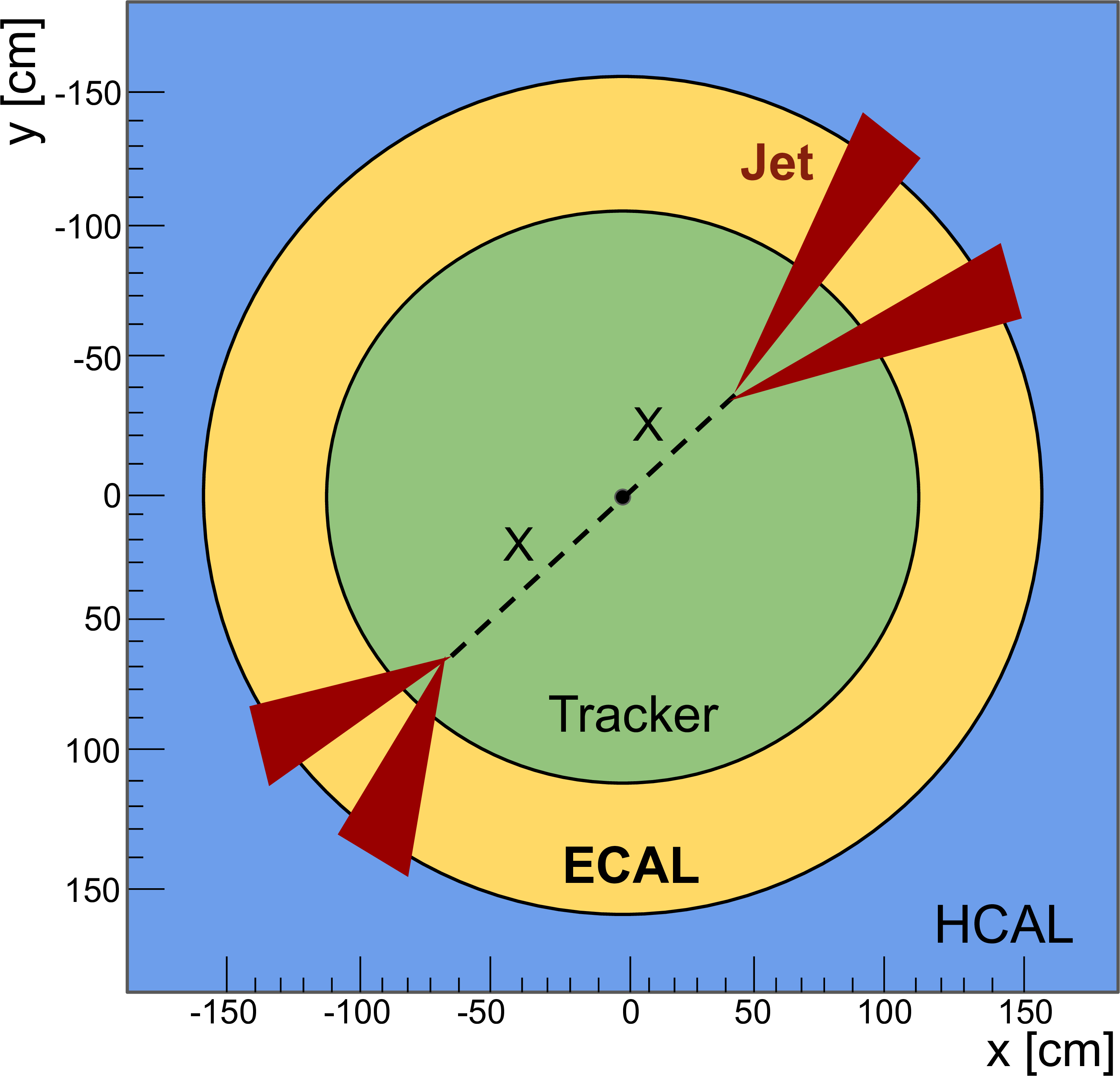
Diagram of a typical delayed-jet signal event. |
png pdf |
Figure 27:
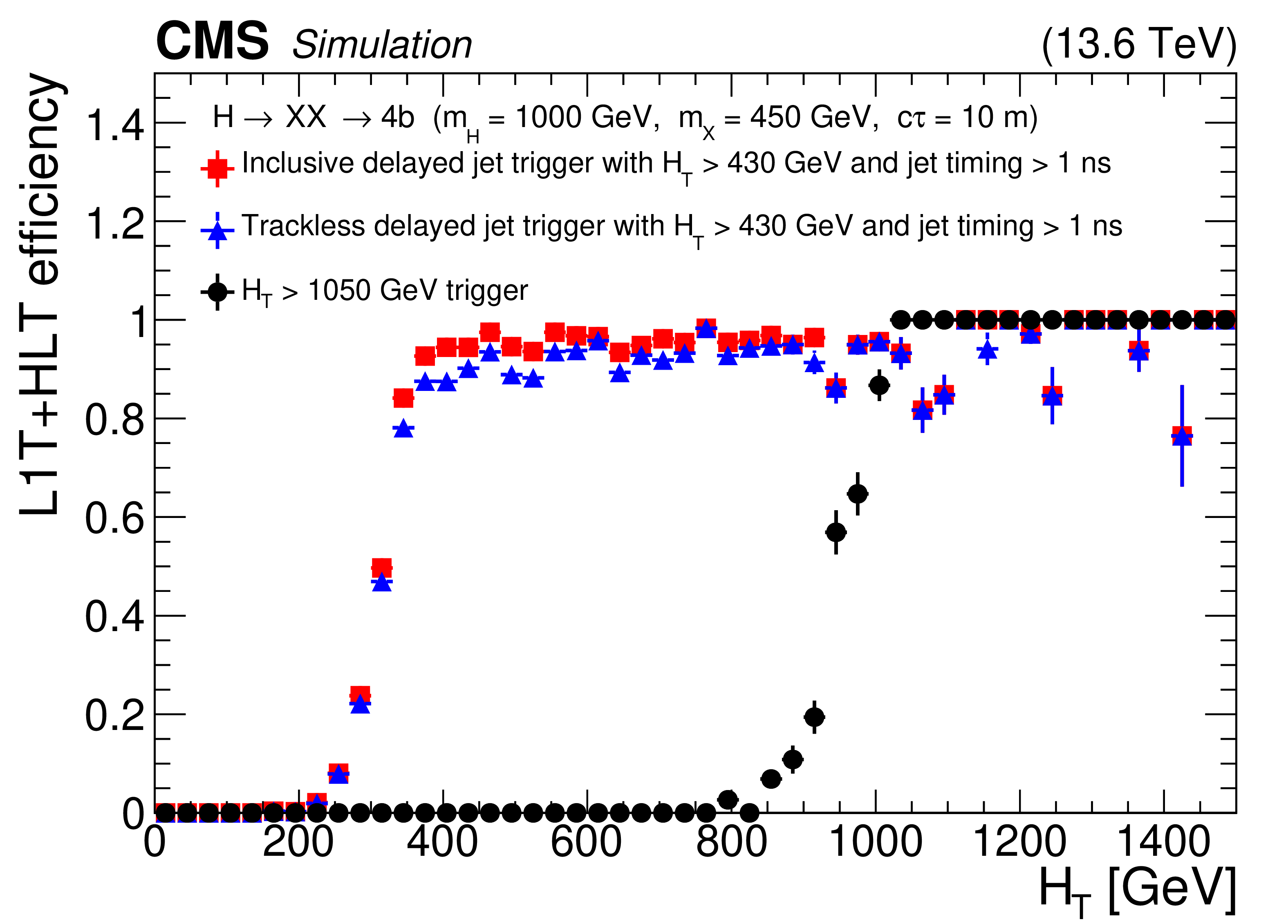
The L1T+HLT efficiency of the inclusive and trackless delayed-jet triggers introduced in Run 3 in red squares (blue triangles), for 2022 conditions, and the $ H_{\mathrm{T}} $ trigger (black circles), which was the most appropriate path available in Run 2, for a $ \mathrm{H} \to \mathrm{X}\mathrm{X} \to 4\mathrm{b} $ signal with $ m_{\mathrm{H}}= $ 1000 GeV, $ m_{\mathrm{X}}= $ 450 GeV, and $ c\tau= $ 10 m. The addition of these delayed-jet triggers results in a significant improvement in the efficiency of the signal for 430 $ < H_{\mathrm{T}} < $ 1050 GeV. These plots include events with jets with $ p_{\mathrm{T}} > $ 40 GeV, number of ECAL cells $ > $ 5, barrel region with $ |\eta| < $ 1.48, and jet timing $ > $ 1 ns. |
png pdf |
Figure 28:
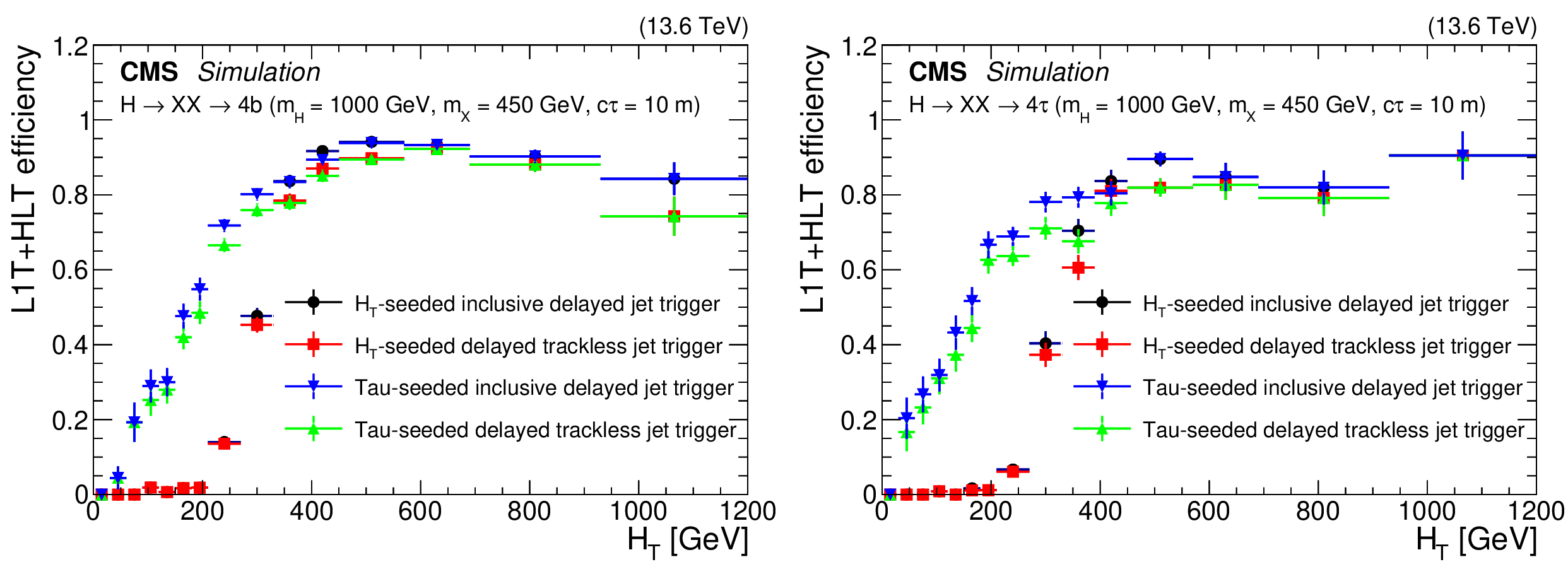
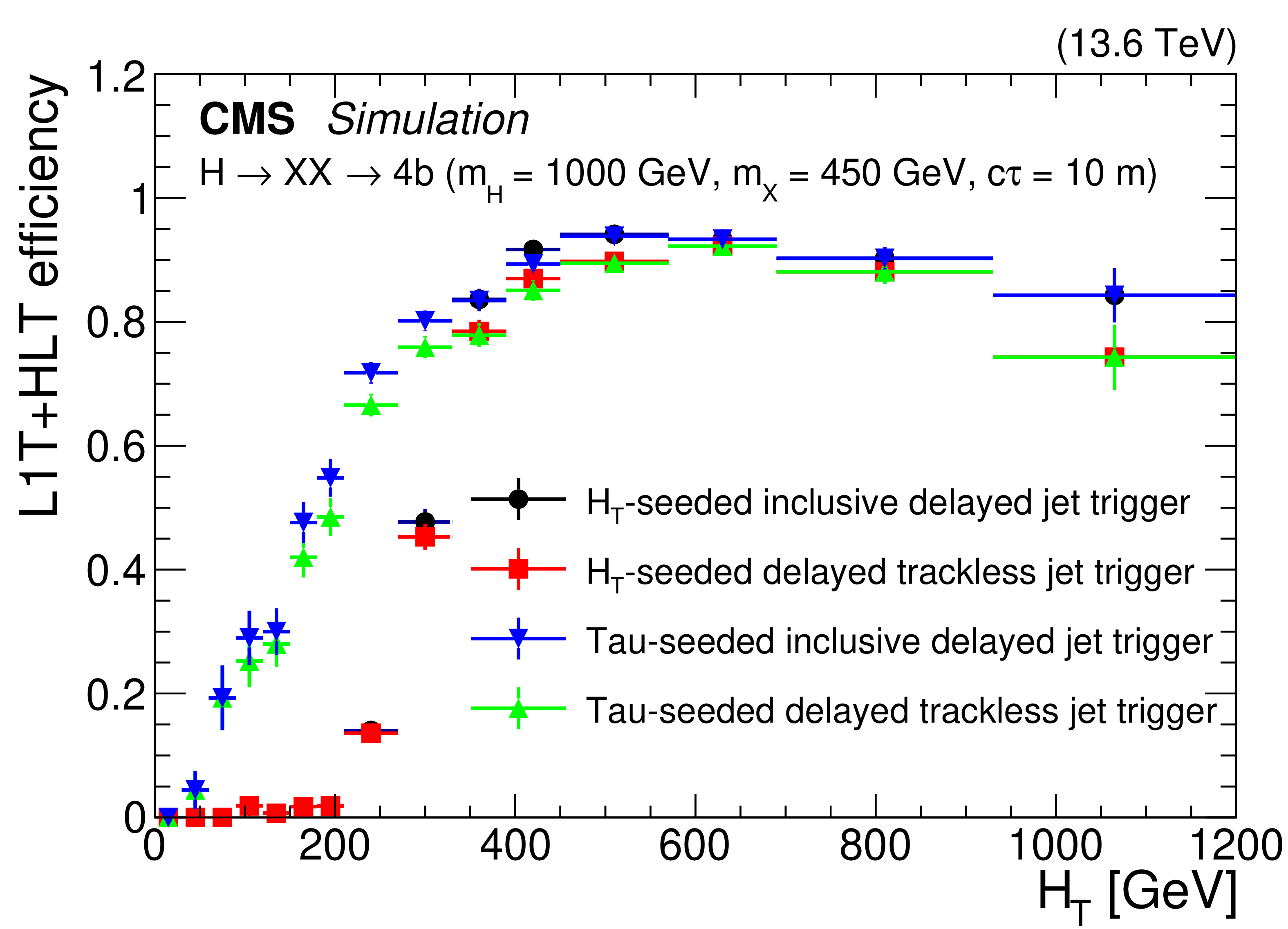
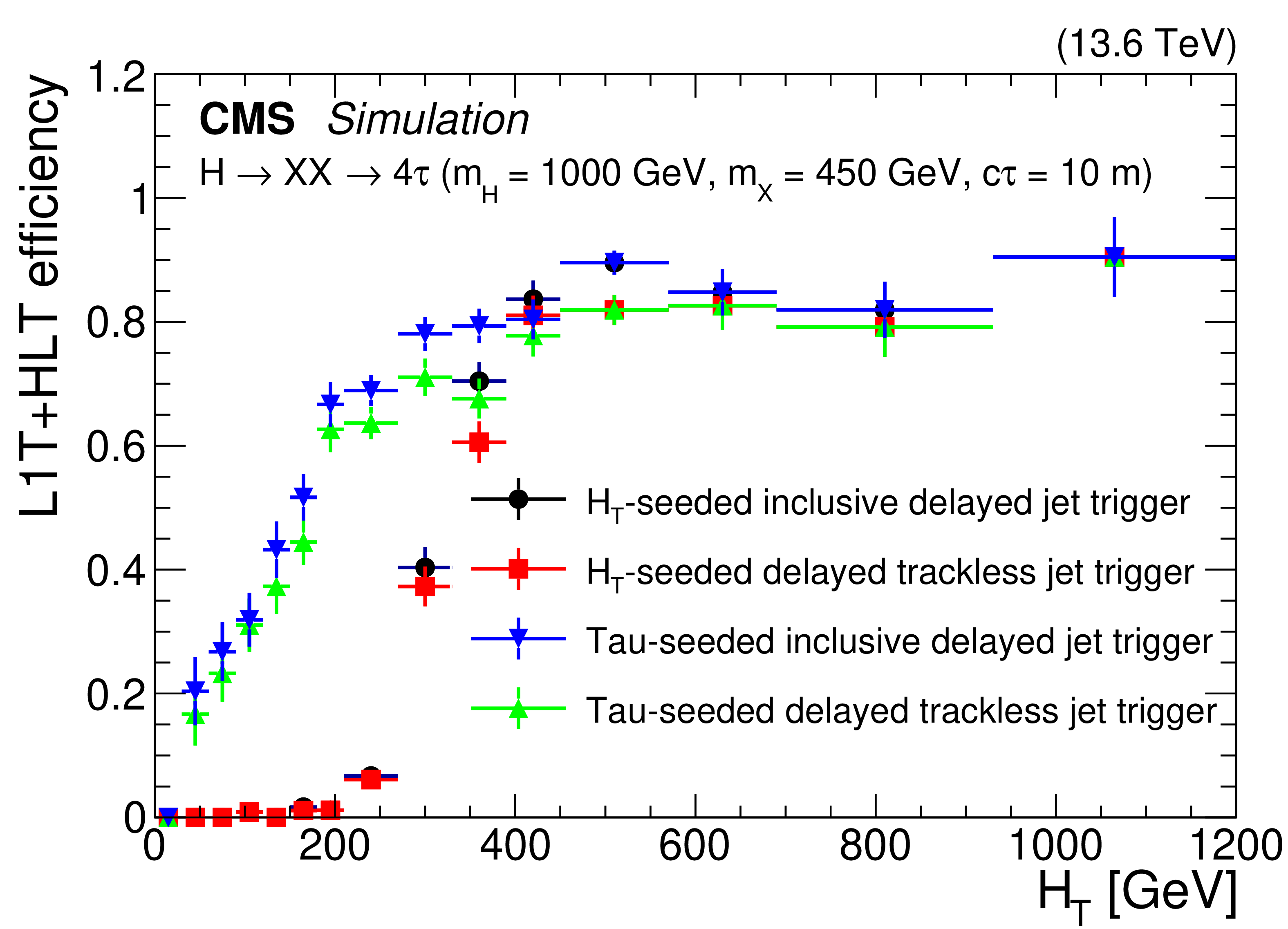
The L1T+HLT efficiency of the delayed-jet triggers for signal models with $ \mathrm{H} \to \mathrm{X}\mathrm{X} \to 4\mathrm{b} $ (left) and $ \mathrm{H} \to \mathrm{X}\mathrm{X} \to 4\tau $ (right), with $ m_{\mathrm{H}}= $ 1000 GeV, $ m_{\mathrm{X}}= $ 450 GeV and $ c\tau= $ 10 m, for 2022 conditions. The improvement from the tau triggers (blue and green triangles) is evident in the $ H_{\mathrm{T}} < $ 430 GeV region compared to the $ H_{\mathrm{T}} $-seeded triggers (black circles and red squares). These plots include events with jets with $ p_{\mathrm{T}} > $ 40 GeV, number of ECAL cells $ > $ 5, barrel region with $ |\eta| < $ 1.48, and jet timing $ > $ 2 ns. |
png pdf |
Figure 28-a:
The L1T+HLT efficiency of the delayed-jet triggers for signal models with $ \mathrm{H} \to \mathrm{X}\mathrm{X} \to 4\mathrm{b} $ (left) and $ \mathrm{H} \to \mathrm{X}\mathrm{X} \to 4\tau $ (right), with $ m_{\mathrm{H}}= $ 1000 GeV, $ m_{\mathrm{X}}= $ 450 GeV and $ c\tau= $ 10 m, for 2022 conditions. The improvement from the tau triggers (blue and green triangles) is evident in the $ H_{\mathrm{T}} < $ 430 GeV region compared to the $ H_{\mathrm{T}} $-seeded triggers (black circles and red squares). These plots include events with jets with $ p_{\mathrm{T}} > $ 40 GeV, number of ECAL cells $ > $ 5, barrel region with $ |\eta| < $ 1.48, and jet timing $ > $ 2 ns. |
png pdf |
Figure 28-b:
The L1T+HLT efficiency of the delayed-jet triggers for signal models with $ \mathrm{H} \to \mathrm{X}\mathrm{X} \to 4\mathrm{b} $ (left) and $ \mathrm{H} \to \mathrm{X}\mathrm{X} \to 4\tau $ (right), with $ m_{\mathrm{H}}= $ 1000 GeV, $ m_{\mathrm{X}}= $ 450 GeV and $ c\tau= $ 10 m, for 2022 conditions. The improvement from the tau triggers (blue and green triangles) is evident in the $ H_{\mathrm{T}} < $ 430 GeV region compared to the $ H_{\mathrm{T}} $-seeded triggers (black circles and red squares). These plots include events with jets with $ p_{\mathrm{T}} > $ 40 GeV, number of ECAL cells $ > $ 5, barrel region with $ |\eta| < $ 1.48, and jet timing $ > $ 2 ns. |
png pdf |
Figure 29:
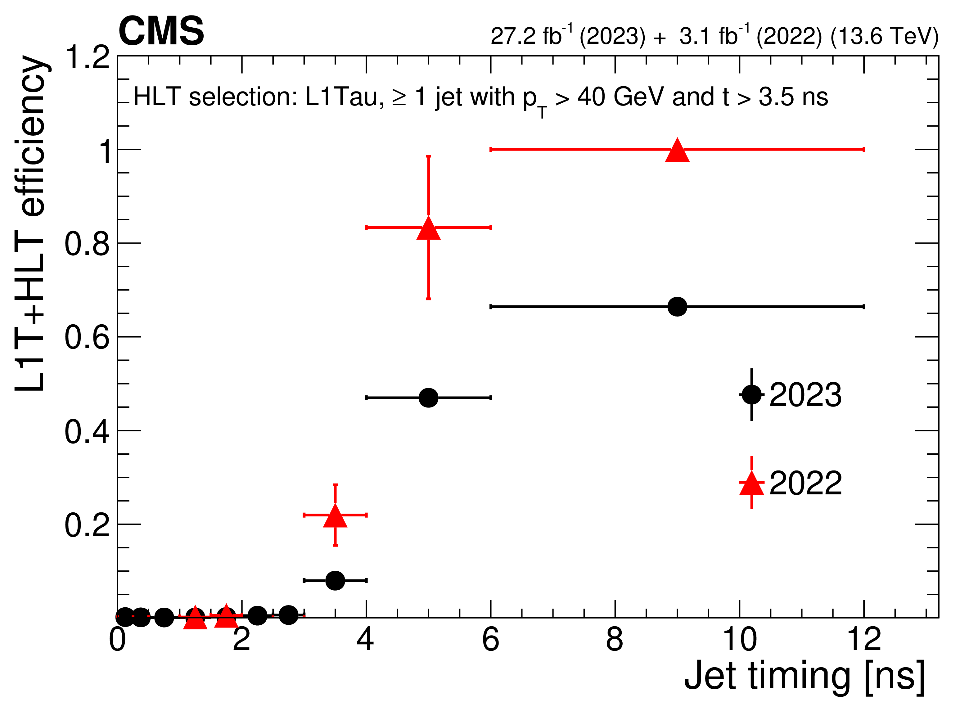
The L1T+HLT efficiency of the delayed-jet triggers as a function of jet timing for 2022 (red triangles) and 2023 (black circles) data-taking periods for the $ H_{\mathrm{T}} $-seeded trigger (left) and the $ \tau $-seeded trigger (right). A clear rise in efficiency is evident around the threshold values. The plots include events that pass the $ p_{\mathrm{T}}^\text{miss} > $ 200 GeV trigger and have at least one barrel jet with $ p_{\mathrm{T}} > $ 50 GeV, number of ECAL cells $ > $ 8, and ECAL energy $ > $ 25 GeV. The $ H_{\mathrm{T}} $ is calculated using the scalar sum of jets with offline $ p_{\mathrm{T}} > $ 40 GeV, and this is different from the $ H_{\mathrm{T}} $ calculation used at the HLT level, contributing to the trigger inefficiencies. The maximum jet time accepted by the trigger is 12.5\unitns. |
png pdf |
Figure 30:
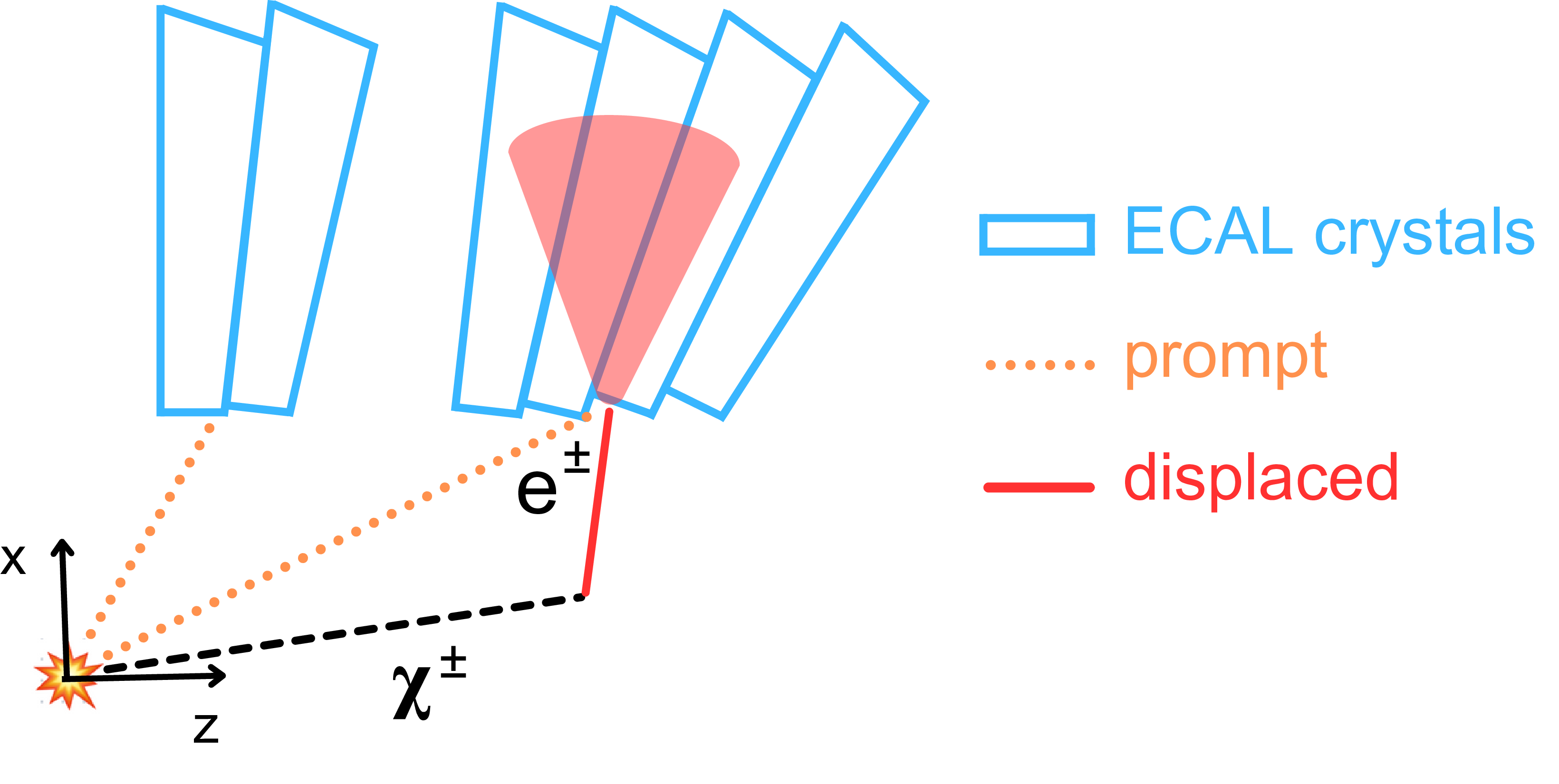
Diagram of a prompt (orange dotted line) and displaced (red solid line) electron, which comes from the decay of a chargino, reaching the ECAL in the $ x-z $ plane. The time measurement is shifted so that all prompt electron signals register the same time, no matter where they are located in the ECAL. An electron produced at a displaced vertex thus arrives delayed compared to a prompt particle. |
png pdf |
Figure 31:
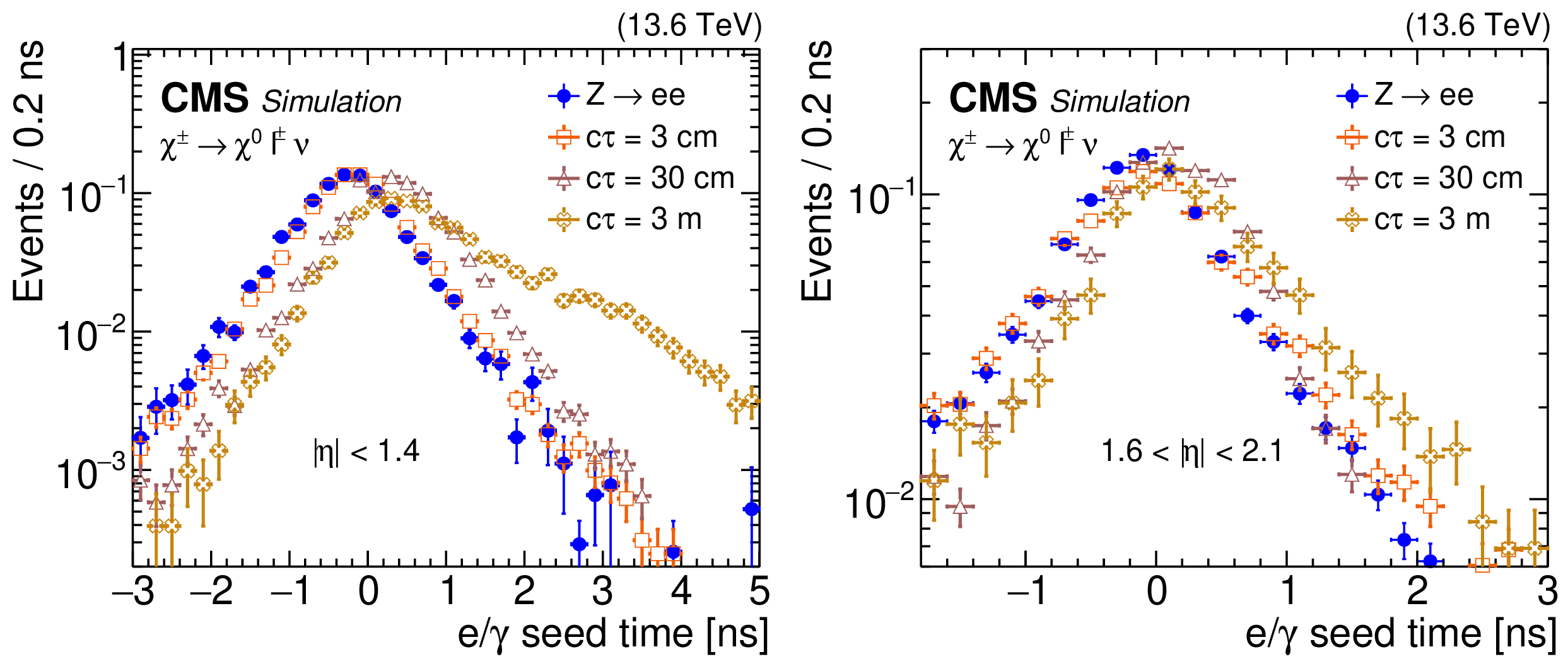
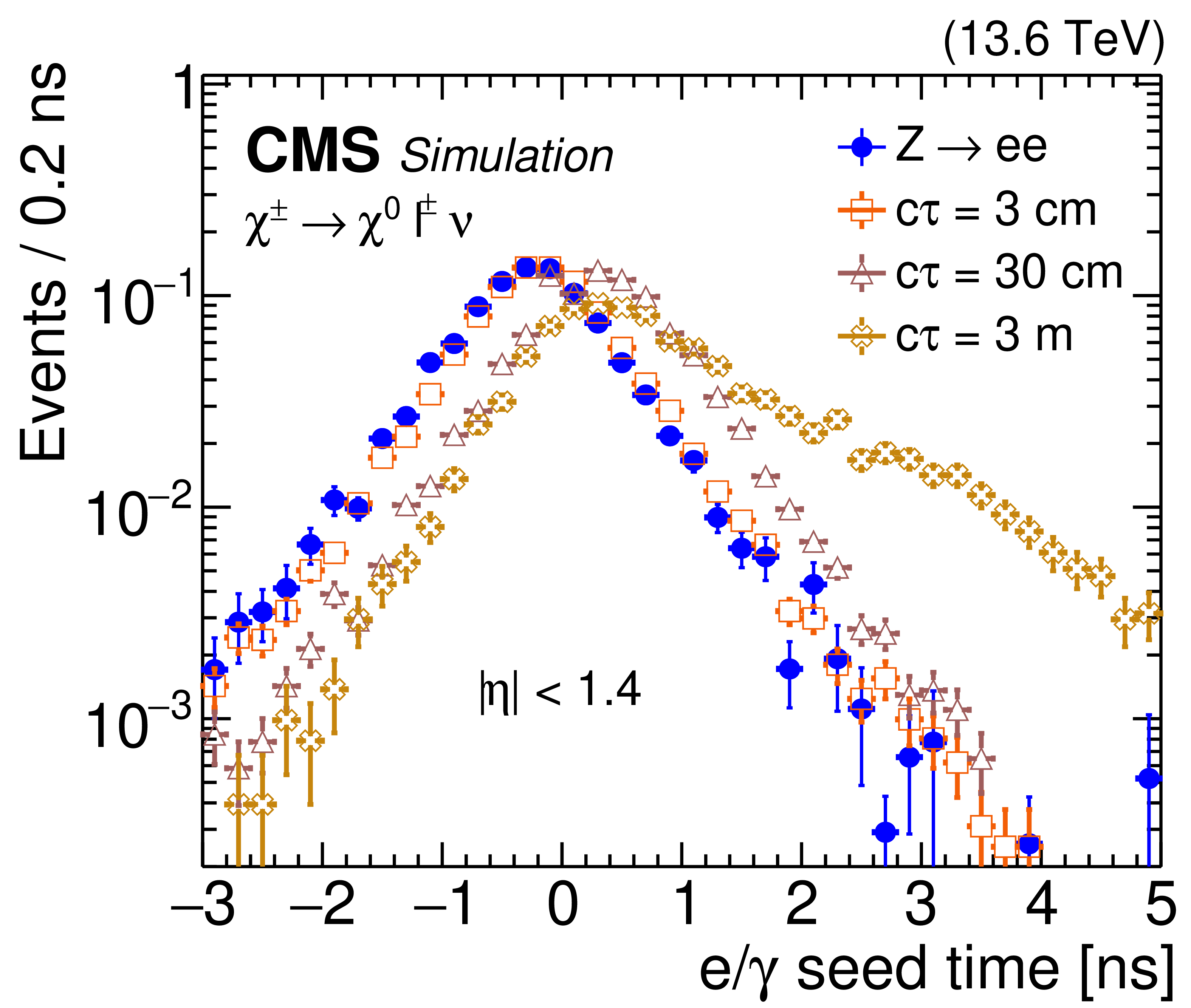
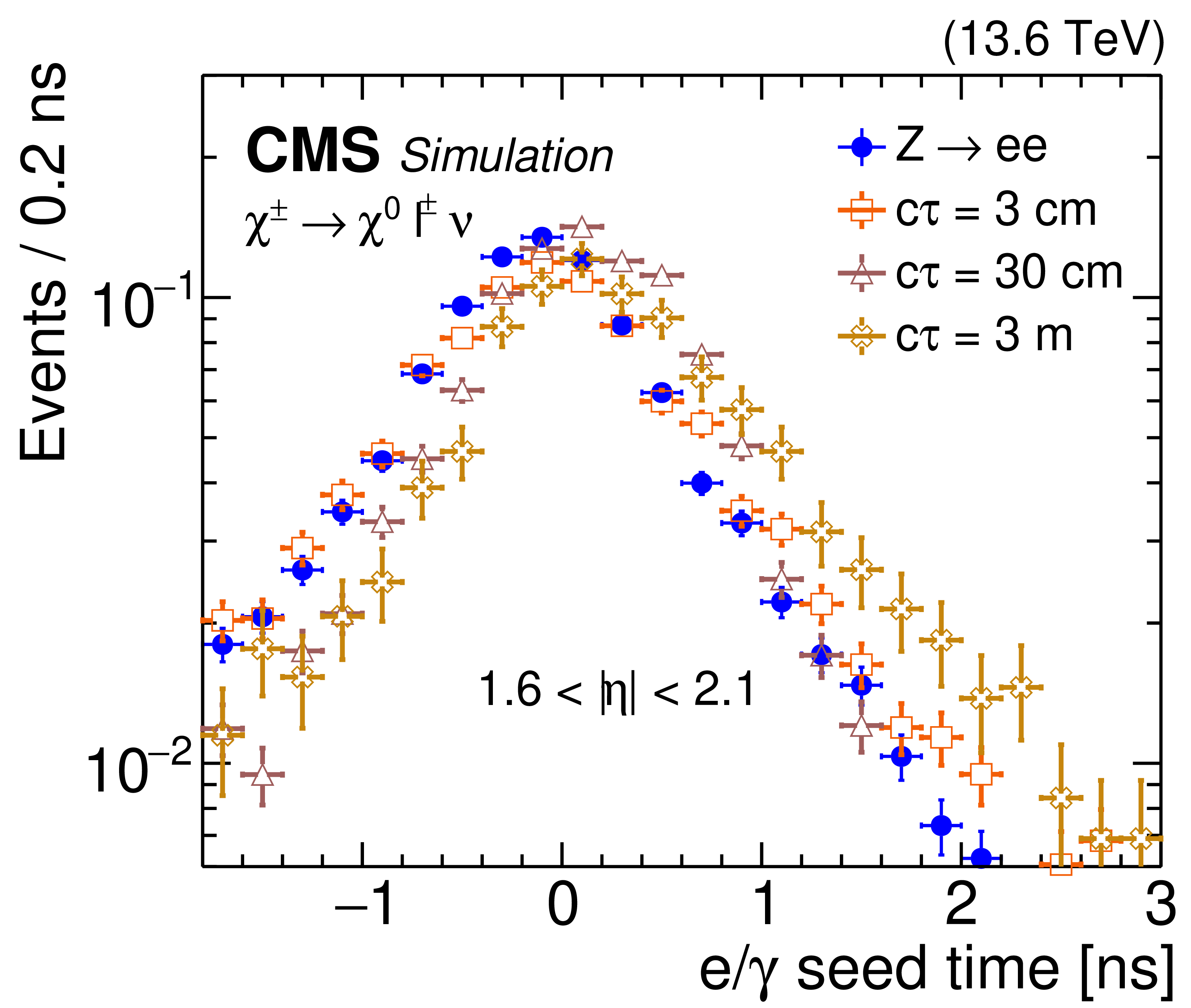
The ECAL time delay of the $ \mathrm{e}/\gamma $ L1 seeds in the barrel (left) and endcap (right). The distributions are shown for $ \mathrm{Z} \to \mathrm{e}\mathrm{e} $ simulation (filled blue circles) and $ \chi^{0} c\tau $ values of 3$ \text{cm} $ (open red squares), 30$ \text{cm} $ (open purple triangles) and 3\unitm (open yellow crosses), assuming the singlet-triplet Higgs dark portal model ($ \chi^{\pm} \to \chi^{0} \ell \nu $, where the $ \chi^{\pm} $ has a mass of 220 GeV and the $ \chi^{0} $ has a mass of 200 GeV), for 2023 conditions. The distributions are normalized to unity. |
png pdf |
Figure 31-a:
The ECAL time delay of the $ \mathrm{e}/\gamma $ L1 seeds in the barrel (left) and endcap (right). The distributions are shown for $ \mathrm{Z} \to \mathrm{e}\mathrm{e} $ simulation (filled blue circles) and $ \chi^{0} c\tau $ values of 3$ \text{cm} $ (open red squares), 30$ \text{cm} $ (open purple triangles) and 3\unitm (open yellow crosses), assuming the singlet-triplet Higgs dark portal model ($ \chi^{\pm} \to \chi^{0} \ell \nu $, where the $ \chi^{\pm} $ has a mass of 220 GeV and the $ \chi^{0} $ has a mass of 200 GeV), for 2023 conditions. The distributions are normalized to unity. |
png pdf |
Figure 31-b:
The ECAL time delay of the $ \mathrm{e}/\gamma $ L1 seeds in the barrel (left) and endcap (right). The distributions are shown for $ \mathrm{Z} \to \mathrm{e}\mathrm{e} $ simulation (filled blue circles) and $ \chi^{0} c\tau $ values of 3$ \text{cm} $ (open red squares), 30$ \text{cm} $ (open purple triangles) and 3\unitm (open yellow crosses), assuming the singlet-triplet Higgs dark portal model ($ \chi^{\pm} \to \chi^{0} \ell \nu $, where the $ \chi^{\pm} $ has a mass of 220 GeV and the $ \chi^{0} $ has a mass of 200 GeV), for 2023 conditions. The distributions are normalized to unity. |
png pdf |
Figure 32:
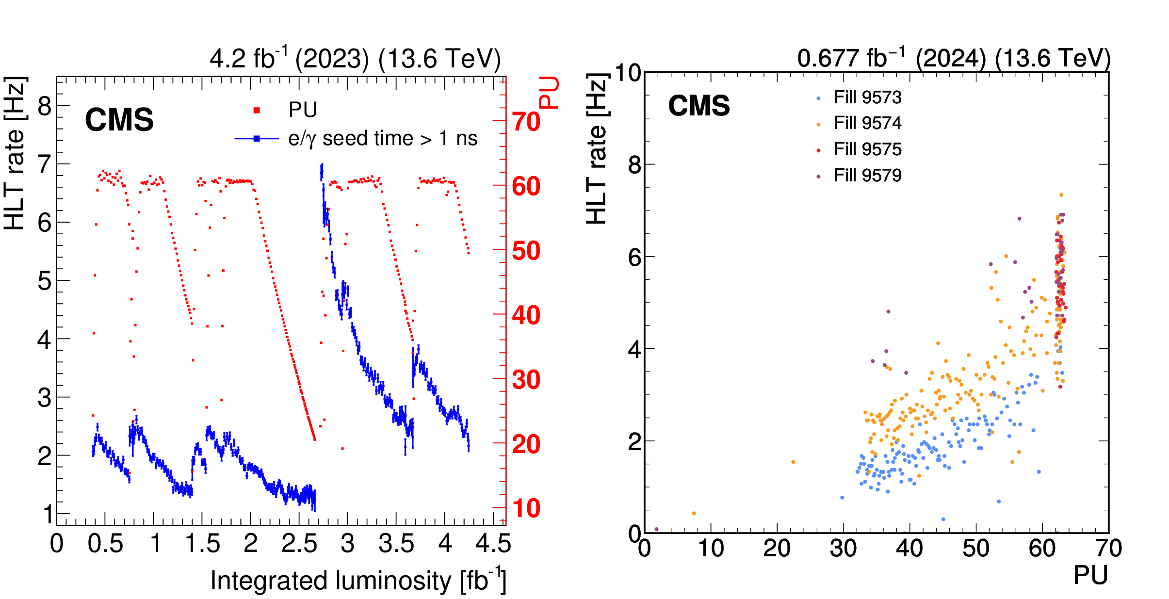
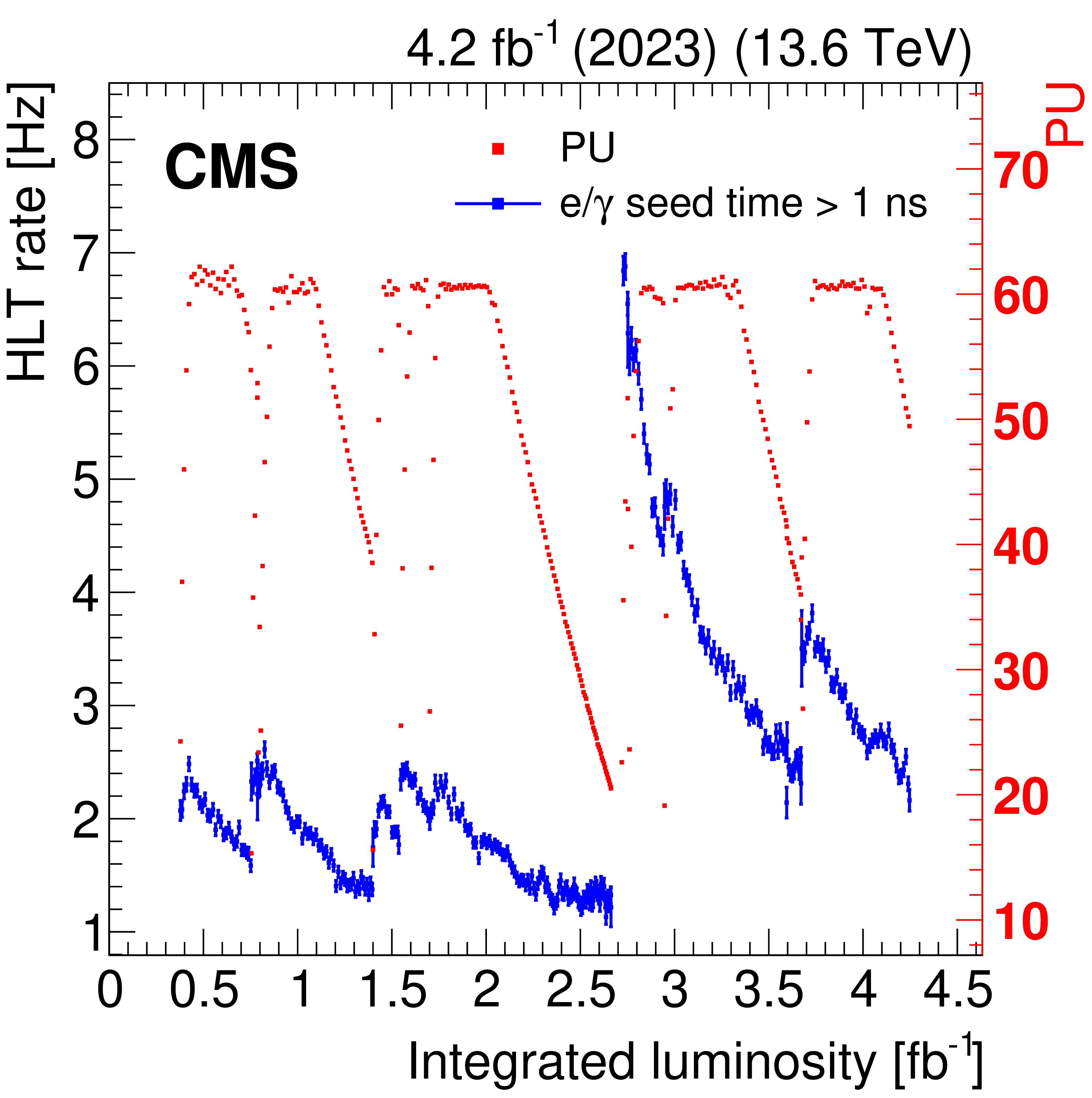
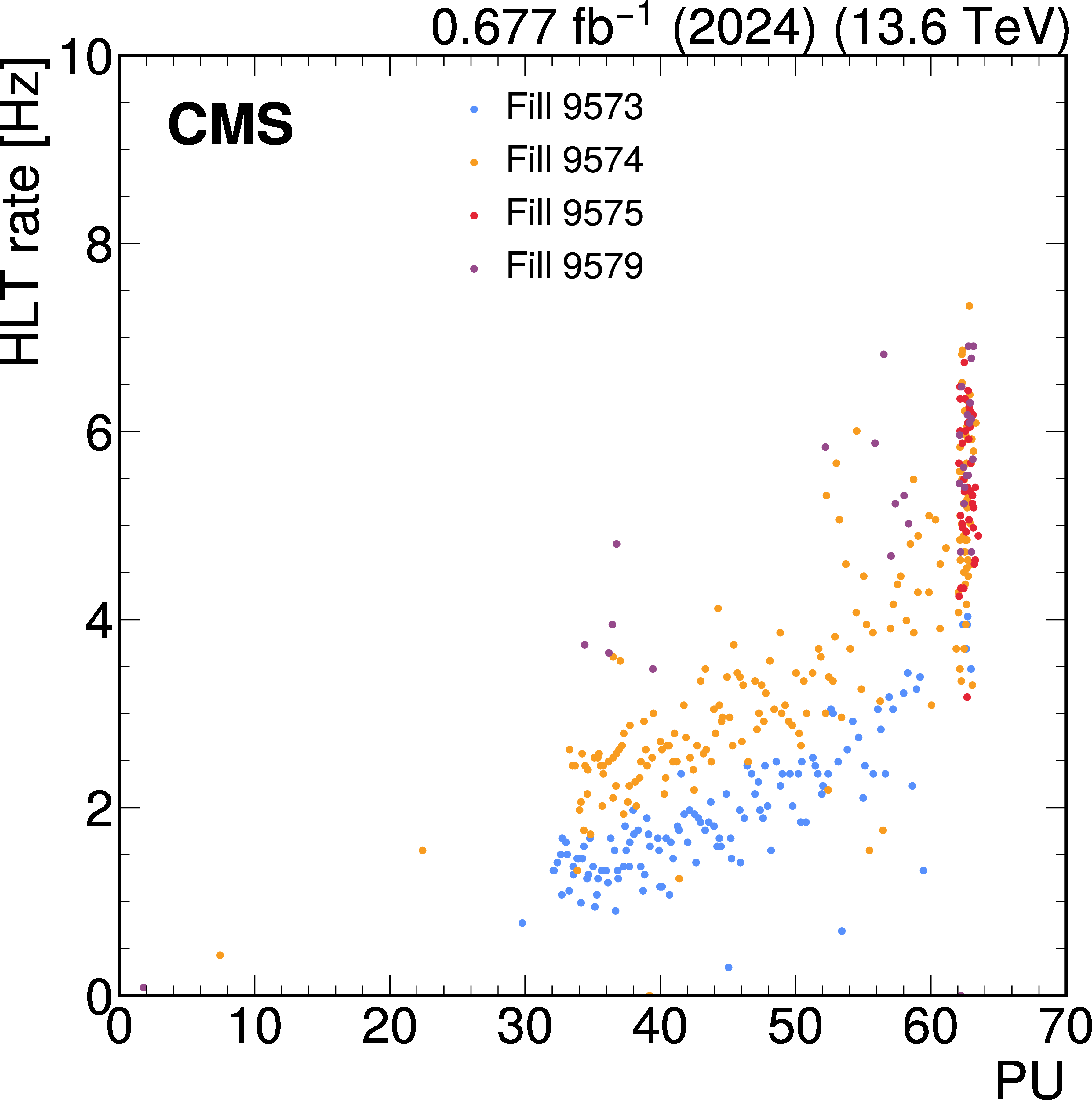
The HLT rate (blue points) of the delayed-diphoton trigger for a few representative runs in the first data collected in 2023, corresponding to an integrated luminosity of 4.2 fb$ ^{-1} $, compared with the PU during the same data-taking period (red points), as a function of integrated luminosity (left). The rate decreases nonlinearly during a single fill as a result of the increasing crystal opacity. It recovers by the start of the next fill with $ {<}1% $ reduction in rate between the fills. The rate generally increased throughout the year because of periodic online calibrations to mitigate the loss in trigger efficiency, which is a result of the ECAL crystal radiation damage. The delayed-diphoton trigger rate is shown as a function of PU for selected fills in 2024 data, at an instantaneous luminosity of approximately \instL1.8 (right). The trigger rate displays a linear dependency on PU. |
png pdf |
Figure 32-a:
The HLT rate (blue points) of the delayed-diphoton trigger for a few representative runs in the first data collected in 2023, corresponding to an integrated luminosity of 4.2 fb$ ^{-1} $, compared with the PU during the same data-taking period (red points), as a function of integrated luminosity (left). The rate decreases nonlinearly during a single fill as a result of the increasing crystal opacity. It recovers by the start of the next fill with $ {<}1% $ reduction in rate between the fills. The rate generally increased throughout the year because of periodic online calibrations to mitigate the loss in trigger efficiency, which is a result of the ECAL crystal radiation damage. The delayed-diphoton trigger rate is shown as a function of PU for selected fills in 2024 data, at an instantaneous luminosity of approximately \instL1.8 (right). The trigger rate displays a linear dependency on PU. |
png pdf |
Figure 32-b:
The HLT rate (blue points) of the delayed-diphoton trigger for a few representative runs in the first data collected in 2023, corresponding to an integrated luminosity of 4.2 fb$ ^{-1} $, compared with the PU during the same data-taking period (red points), as a function of integrated luminosity (left). The rate decreases nonlinearly during a single fill as a result of the increasing crystal opacity. It recovers by the start of the next fill with $ {<}1% $ reduction in rate between the fills. The rate generally increased throughout the year because of periodic online calibrations to mitigate the loss in trigger efficiency, which is a result of the ECAL crystal radiation damage. The delayed-diphoton trigger rate is shown as a function of PU for selected fills in 2024 data, at an instantaneous luminosity of approximately \instL1.8 (right). The trigger rate displays a linear dependency on PU. |
png pdf |
Figure 33:
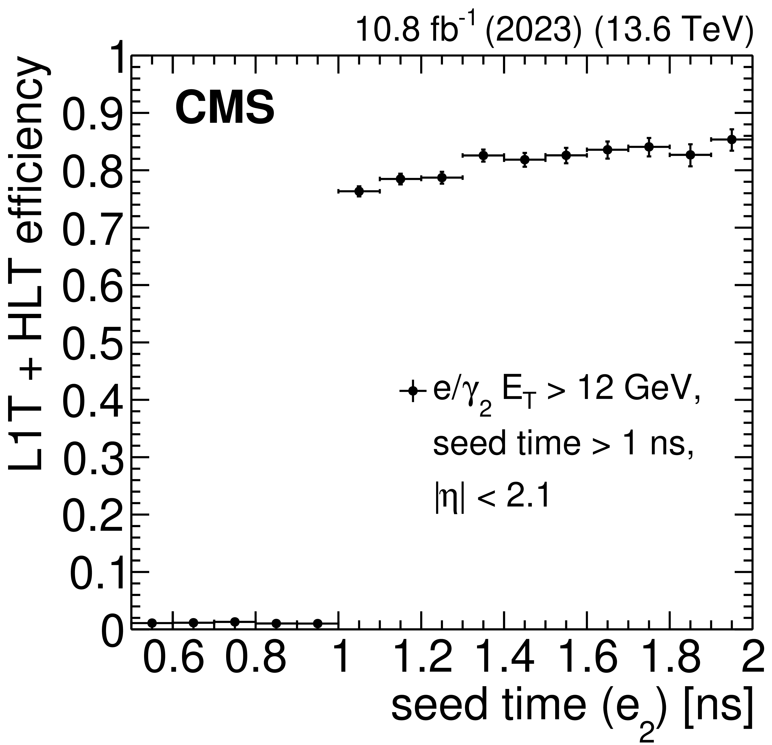
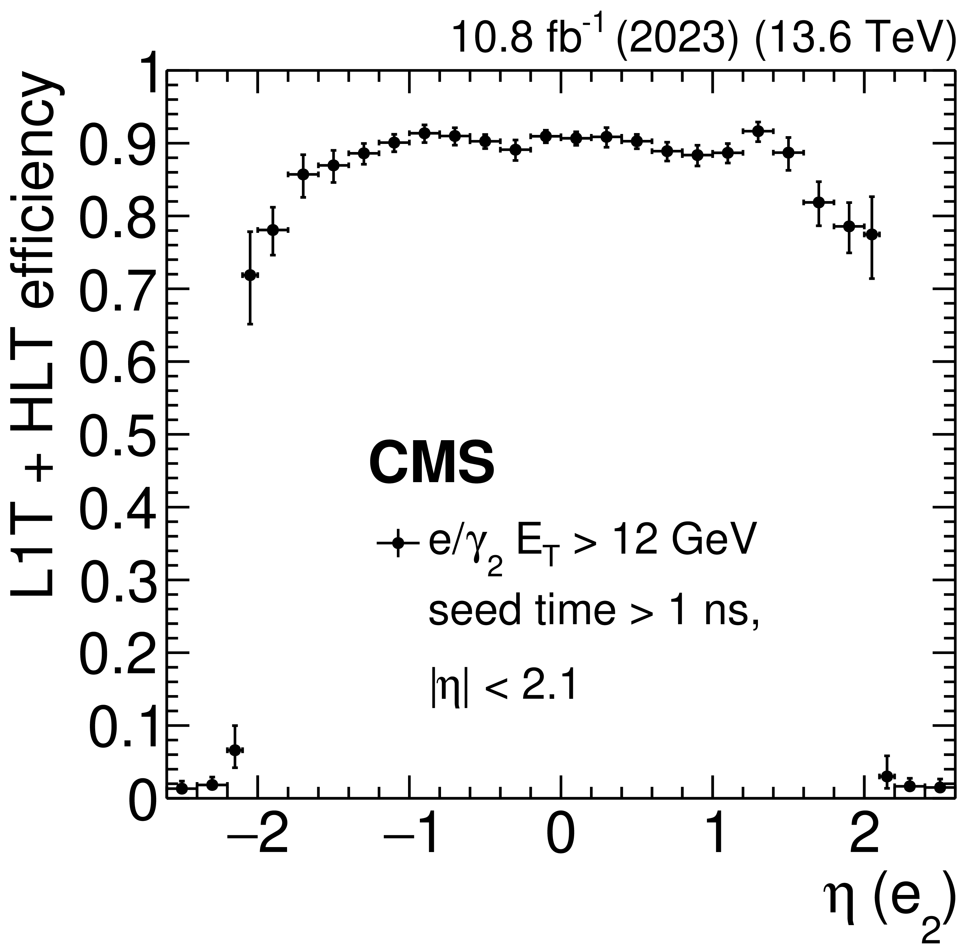
The L1T+HLT efficiency of the delayed-diphoton trigger as a function of the subleading probe electron ($ \mathrm{e}_2 $) supercluster seed time, measured with data collected in 2023. At the HLT, the subleading $ \mathrm{e}/\gamma $ supercluster ($ \mathrm{e}/\gamma_2 $) is required to have $ E_{\mathrm{T}} > $ 12 GeV, $ |\eta| < $ 2.1, and a seed time $ {>} $ 1 ns. The trigger reaches maximum efficiency above 1\unitns. |
png pdf |
Figure 34:
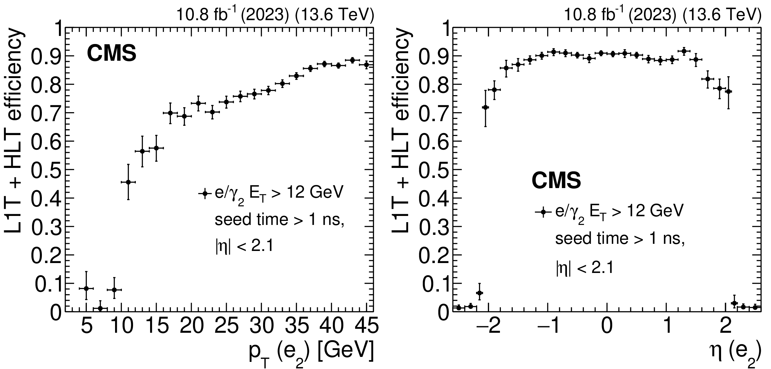
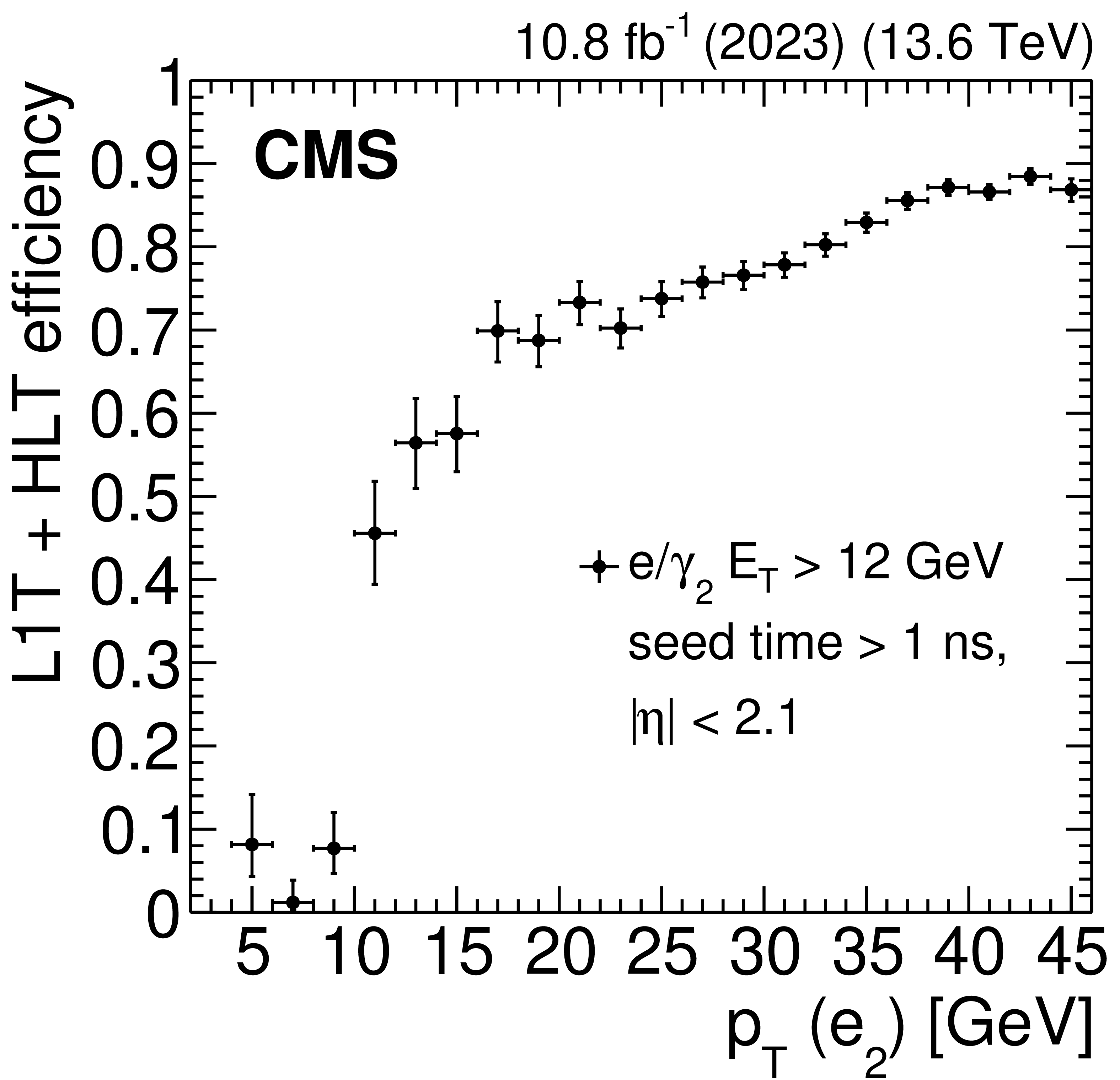
The L1T+HLT efficiency of the delayed-diphoton trigger as a function of subleading probe electron ($ \mathrm{e}_2 $) $ p_{\mathrm{T}} $ (left) and $ \eta $ (right), measured with data collected in 2023. At the HLT, the subleading $ \mathrm{e}/\gamma $ supercluster ($ \mathrm{e}/\gamma_2 $) is required to have $ E_{\mathrm{T}} > $ 12 GeV, $ |\eta| < $ 2.1, and a seed time $ {>} $ 1 ns. The efficiency rises sharply for $ p_{\mathrm{T}} > $ 12 GeV and plateaus for $ p_{\mathrm{T}} > $ 35 GeV. The slow rise in between is from additional L1 $ H_{\mathrm{T}} $ requirements. The trigger is efficient in the region $ |\eta| < $ 2.1. |
png pdf |
Figure 34-a:
The L1T+HLT efficiency of the delayed-diphoton trigger as a function of subleading probe electron ($ \mathrm{e}_2 $) $ p_{\mathrm{T}} $ (left) and $ \eta $ (right), measured with data collected in 2023. At the HLT, the subleading $ \mathrm{e}/\gamma $ supercluster ($ \mathrm{e}/\gamma_2 $) is required to have $ E_{\mathrm{T}} > $ 12 GeV, $ |\eta| < $ 2.1, and a seed time $ {>} $ 1 ns. The efficiency rises sharply for $ p_{\mathrm{T}} > $ 12 GeV and plateaus for $ p_{\mathrm{T}} > $ 35 GeV. The slow rise in between is from additional L1 $ H_{\mathrm{T}} $ requirements. The trigger is efficient in the region $ |\eta| < $ 2.1. |
png pdf |
Figure 34-b:
The L1T+HLT efficiency of the delayed-diphoton trigger as a function of subleading probe electron ($ \mathrm{e}_2 $) $ p_{\mathrm{T}} $ (left) and $ \eta $ (right), measured with data collected in 2023. At the HLT, the subleading $ \mathrm{e}/\gamma $ supercluster ($ \mathrm{e}/\gamma_2 $) is required to have $ E_{\mathrm{T}} > $ 12 GeV, $ |\eta| < $ 2.1, and a seed time $ {>} $ 1 ns. The efficiency rises sharply for $ p_{\mathrm{T}} > $ 12 GeV and plateaus for $ p_{\mathrm{T}} > $ 35 GeV. The slow rise in between is from additional L1 $ H_{\mathrm{T}} $ requirements. The trigger is efficient in the region $ |\eta| < $ 2.1. |
png pdf |
Figure 35:
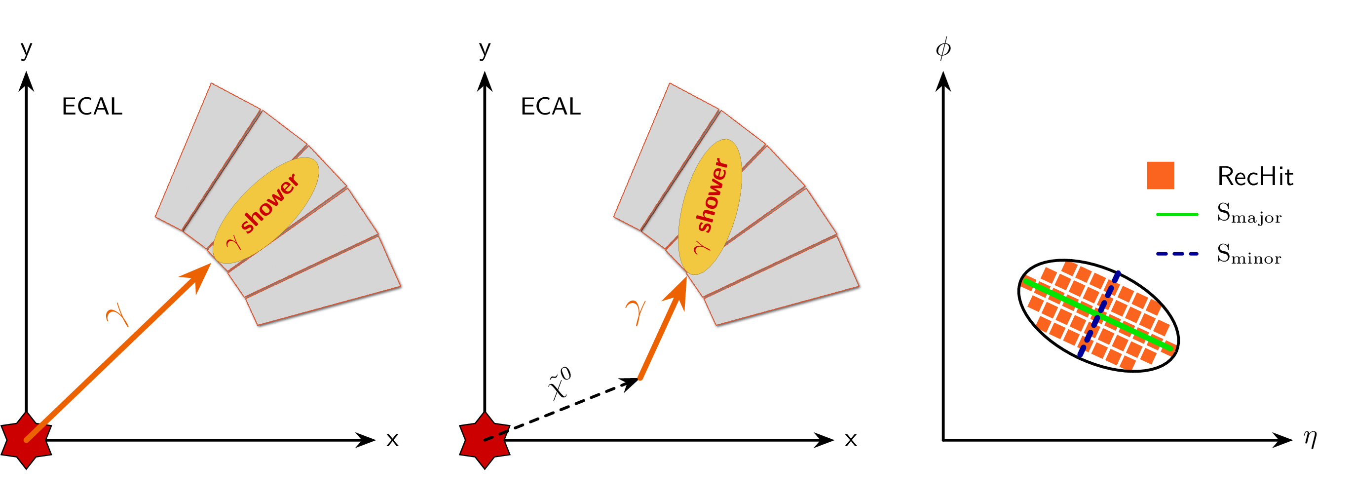
Diagrams of a promptly decaying photon in the $ x-y $ plane showering in the ECAL (left), a delayed photon produced from a long-lived neutralino $ \tilde{\chi}^{0} $ in the $ x-y $ plane showering later in the ECAL (middle), and an elliptical shower in the $ \eta-\phi $ plane produced from a delayed photon (right). The lengths of the major ($ S_{\text{major}} $) and minor ($ S_{\text{minor}} $) axes of the shower and the reconstructed hits (RecHits) that compose the shower are labeled. |
png pdf |
Figure 36:
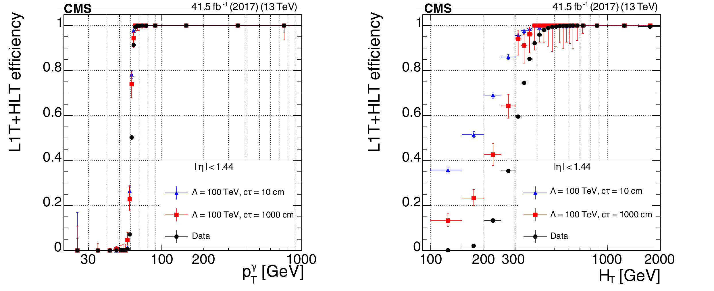
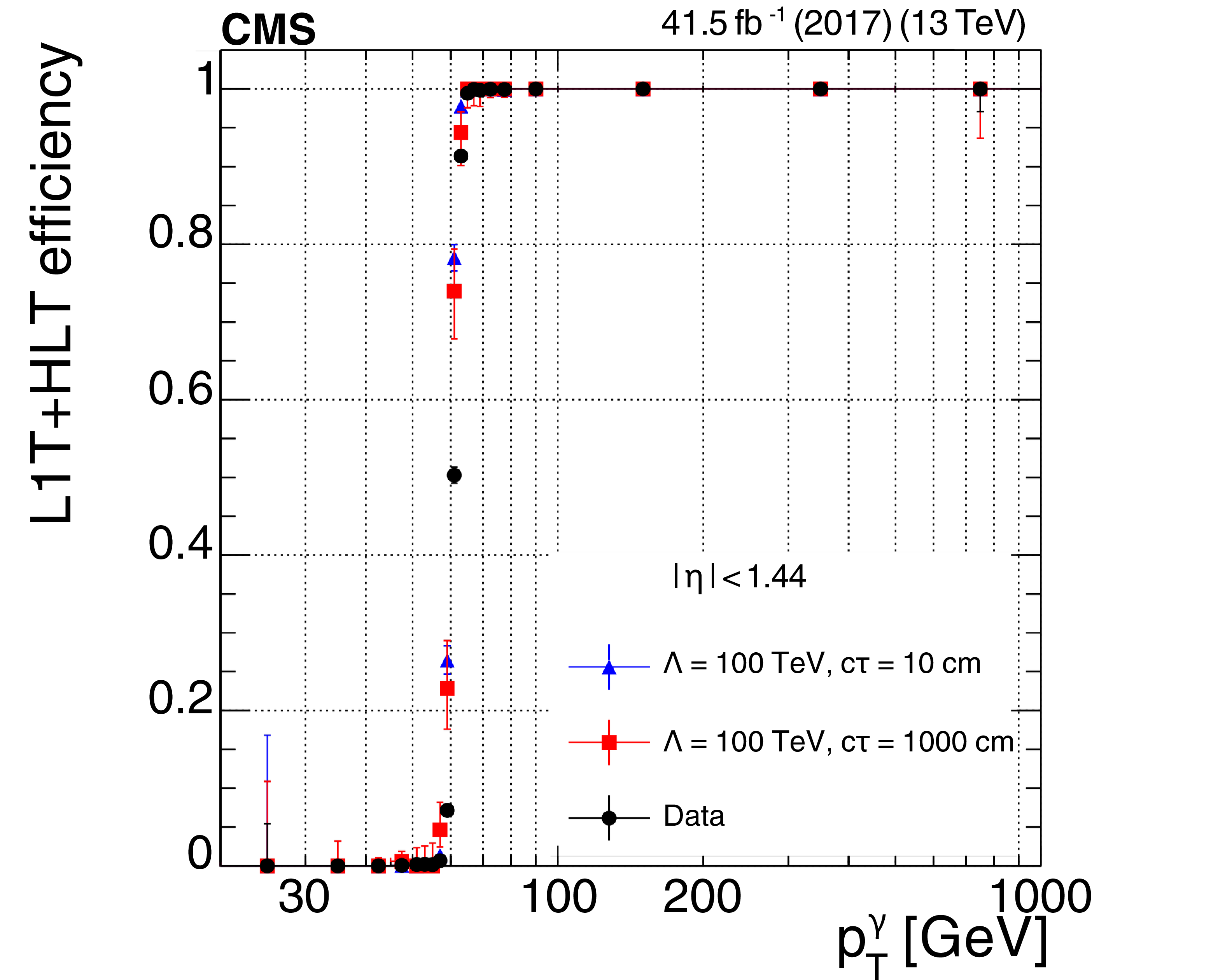
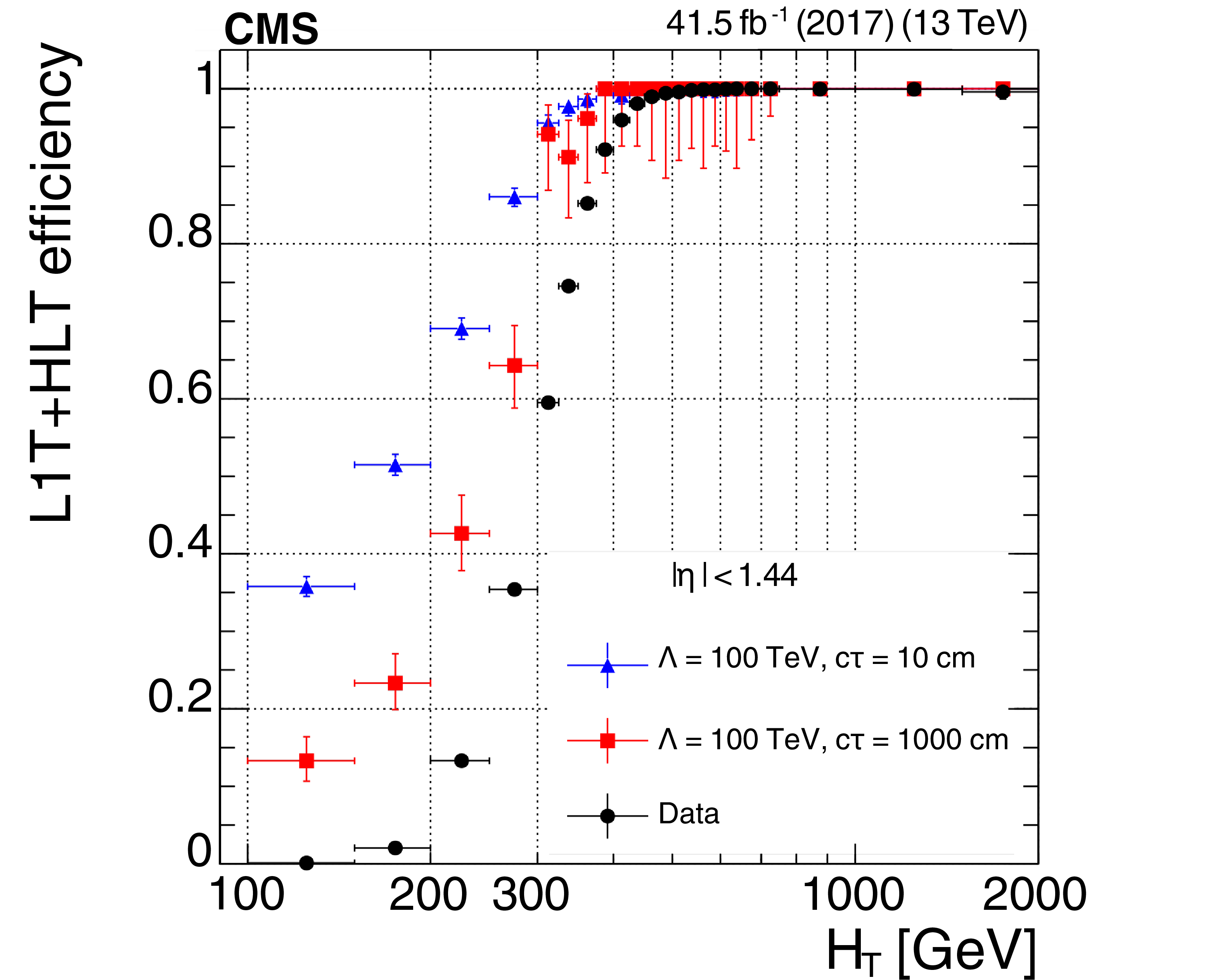
The L1T+HLT efficiency of the displaced-photon + $ H_{\mathrm{T}} $ trigger as a function of photon $ p_{\mathrm{T}} $ (left) and event $ H_{\mathrm{T}} $ (right), for 2017 data (black circles) and GMSB signals with $ \Lambda = $ 100 TeV and $ c\tau=10 \text{cm} $ (blue triangles) or $ c\tau=1000 \text{cm} $ (red squares). |
png pdf |
Figure 36-a:
The L1T+HLT efficiency of the displaced-photon + $ H_{\mathrm{T}} $ trigger as a function of photon $ p_{\mathrm{T}} $ (left) and event $ H_{\mathrm{T}} $ (right), for 2017 data (black circles) and GMSB signals with $ \Lambda = $ 100 TeV and $ c\tau=10 \text{cm} $ (blue triangles) or $ c\tau=1000 \text{cm} $ (red squares). |
png pdf |
Figure 36-b:
The L1T+HLT efficiency of the displaced-photon + $ H_{\mathrm{T}} $ trigger as a function of photon $ p_{\mathrm{T}} $ (left) and event $ H_{\mathrm{T}} $ (right), for 2017 data (black circles) and GMSB signals with $ \Lambda = $ 100 TeV and $ c\tau=10 \text{cm} $ (blue triangles) or $ c\tau=1000 \text{cm} $ (red squares). |
png pdf |
Figure 37:
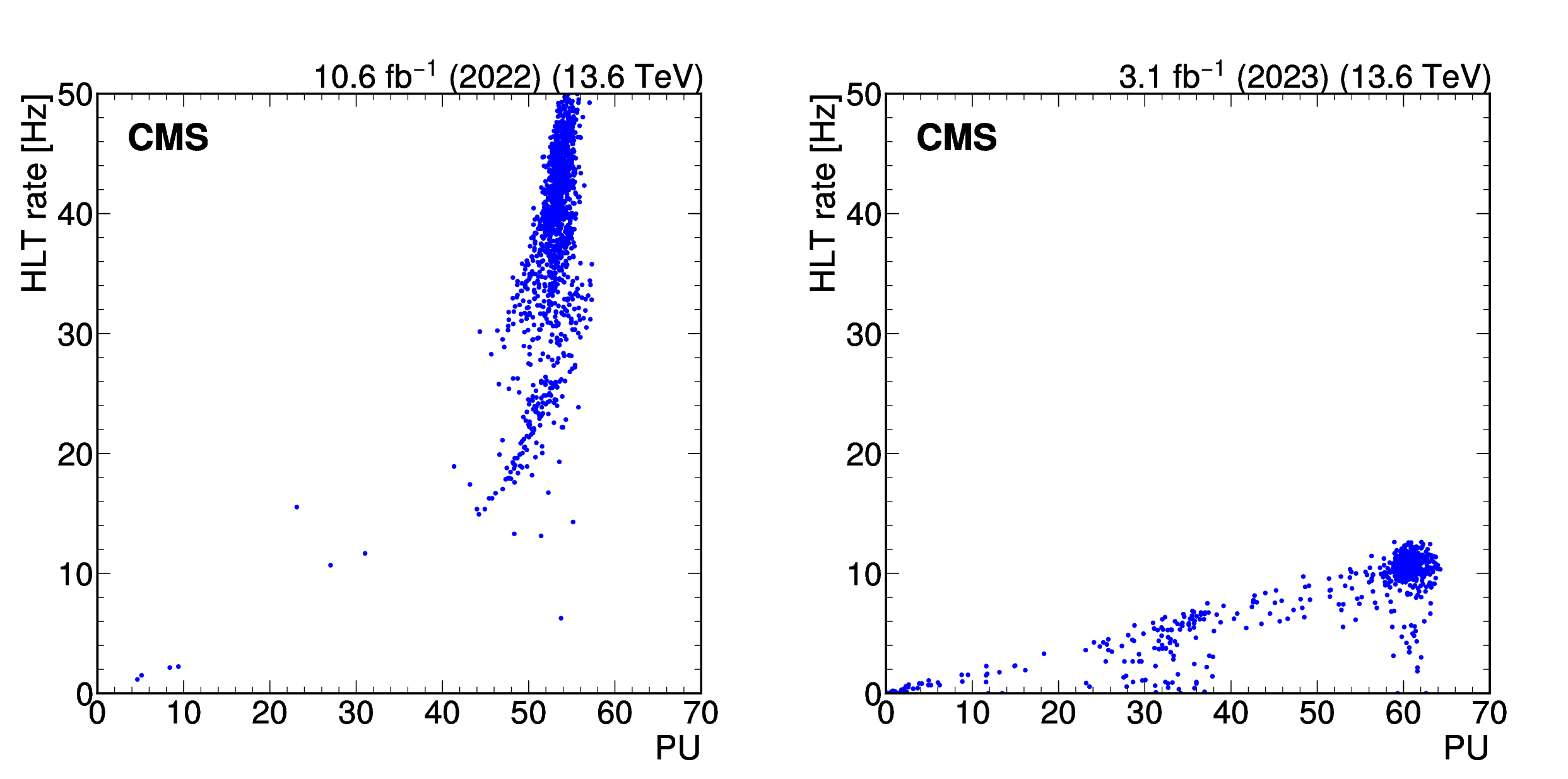
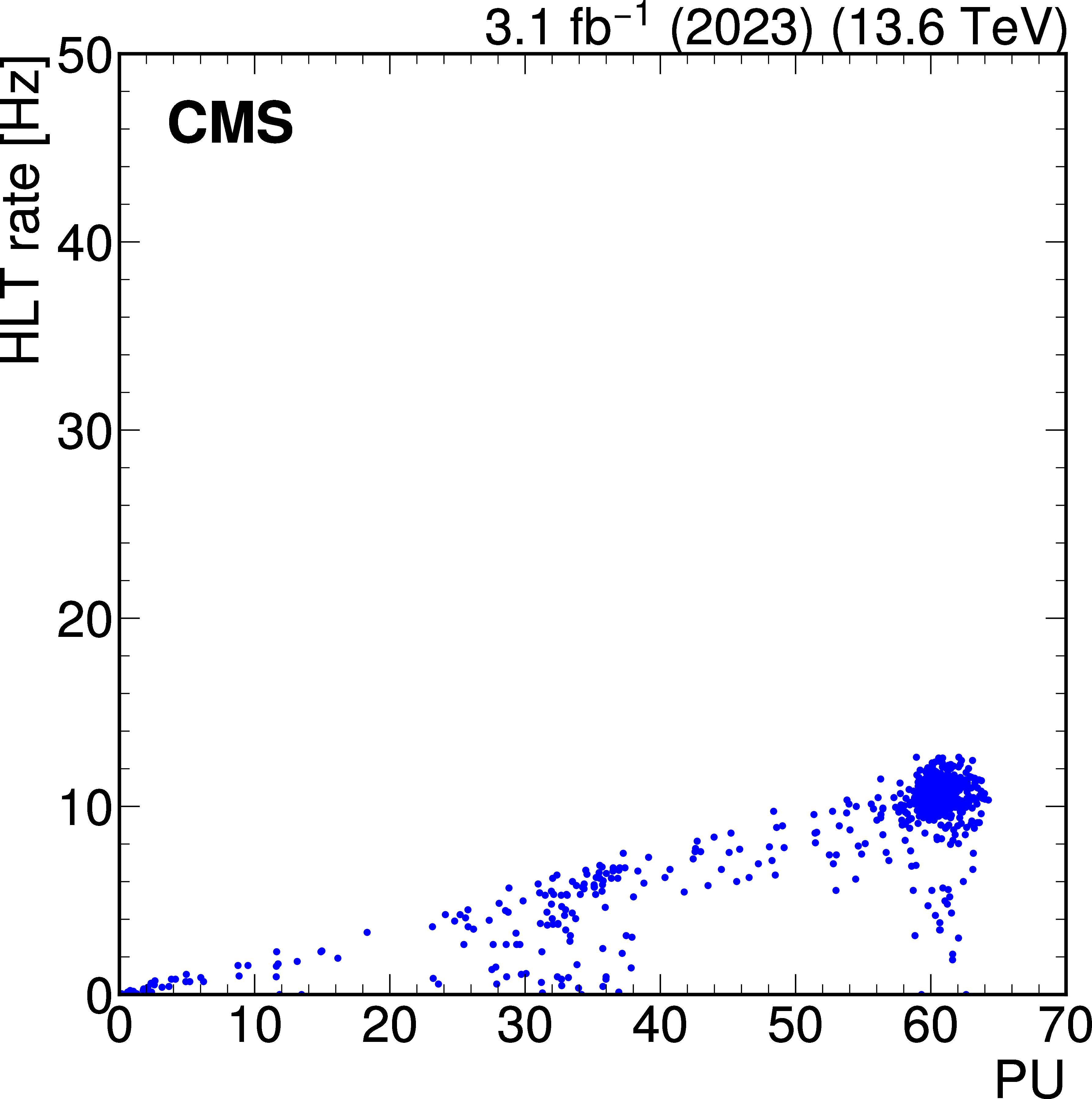
Total rate of the displaced-photon + $ H_{\mathrm{T}} $ HLT path for a few representative runs in 2022 data (left), at an instantaneous luminosity of approximately \instL1.8, and 2023 data (right), at an instantaneous luminosity of approximately \instL2.0, as a function of PU. The rate vs PU behavior was nonlinear in 2022, and the jet $ p_{\mathrm{T}} $ was increased to restore a linear dependence for 2023 data taking. |
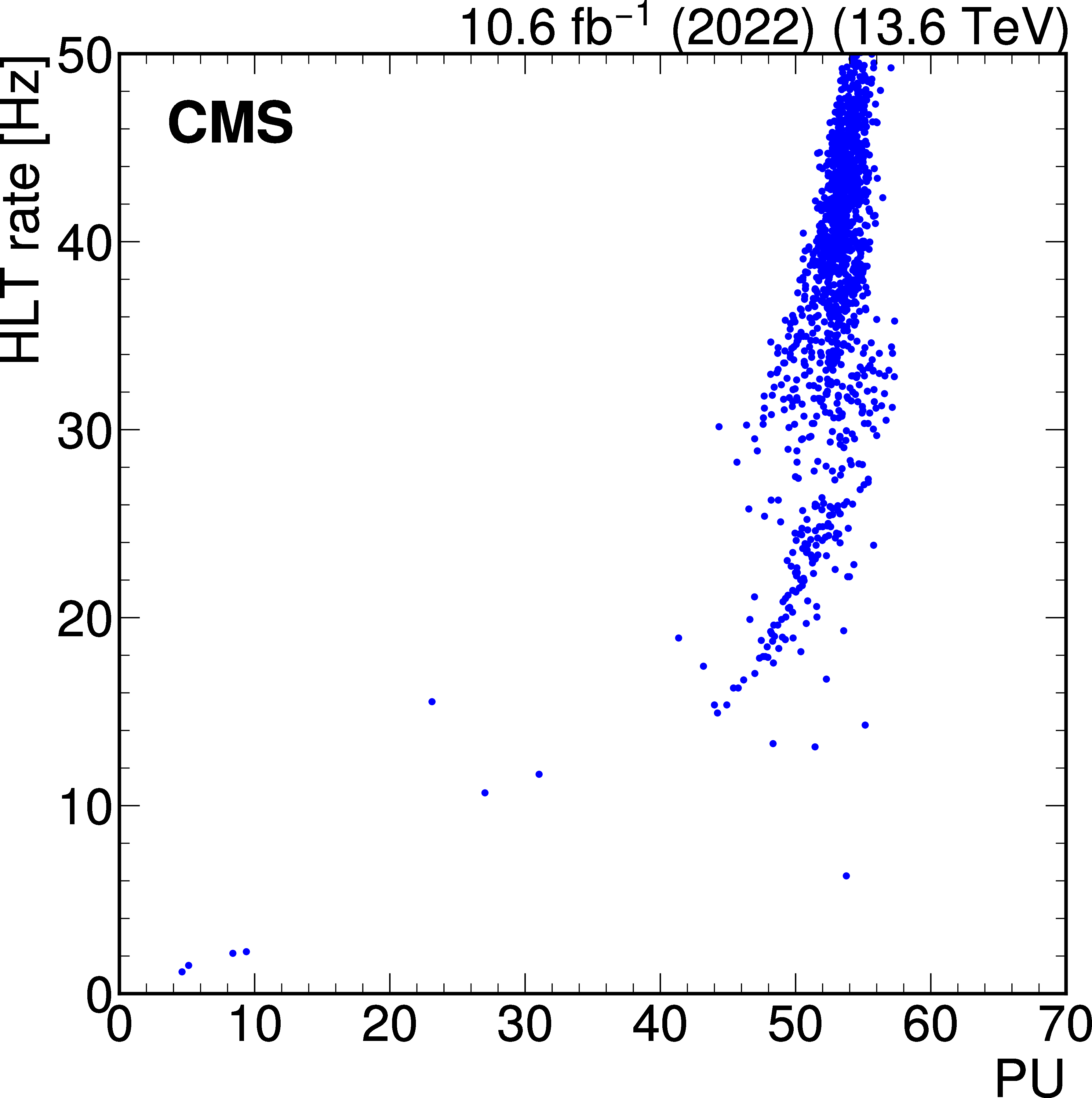
png pdf |
Figure 37-a:
Total rate of the displaced-photon + $ H_{\mathrm{T}} $ HLT path for a few representative runs in 2022 data (left), at an instantaneous luminosity of approximately \instL1.8, and 2023 data (right), at an instantaneous luminosity of approximately \instL2.0, as a function of PU. The rate vs PU behavior was nonlinear in 2022, and the jet $ p_{\mathrm{T}} $ was increased to restore a linear dependence for 2023 data taking. |
png pdf |
Figure 37-b:
Total rate of the displaced-photon + $ H_{\mathrm{T}} $ HLT path for a few representative runs in 2022 data (left), at an instantaneous luminosity of approximately \instL1.8, and 2023 data (right), at an instantaneous luminosity of approximately \instL2.0, as a function of PU. The rate vs PU behavior was nonlinear in 2022, and the jet $ p_{\mathrm{T}} $ was increased to restore a linear dependence for 2023 data taking. |
png pdf |
Figure 38:
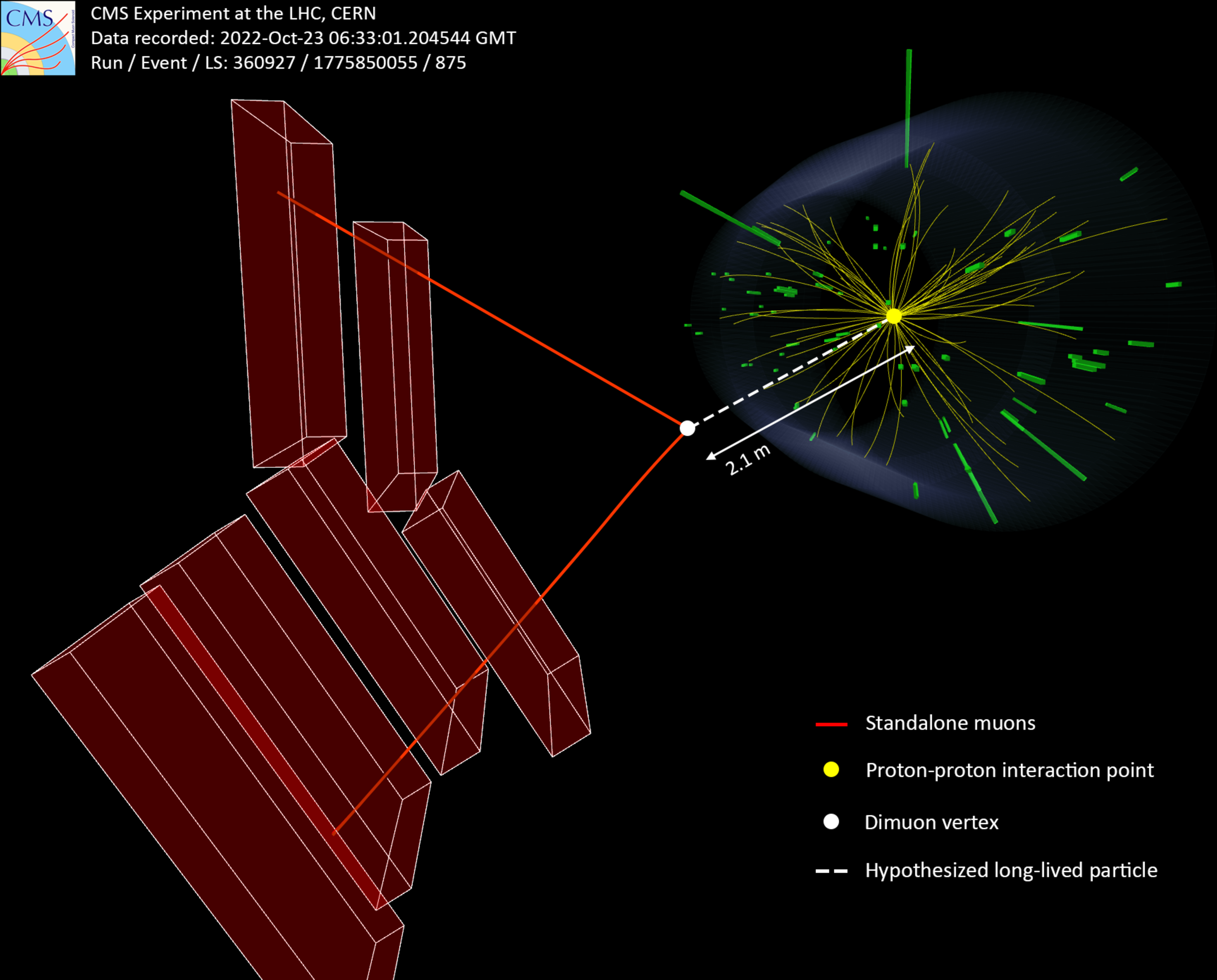
A Run 3 data event containing a candidate LLP decay into a pair of muons away from the IP, reconstructed in the CMS detector. The red lines correspond to the two muons, which are detected only in the muon system. The muon tracks are used to calculate a dimuon vertex, indicated by the white circle, where the LLP is hypothesized to have decayed. |
png pdf |
Figure 39:
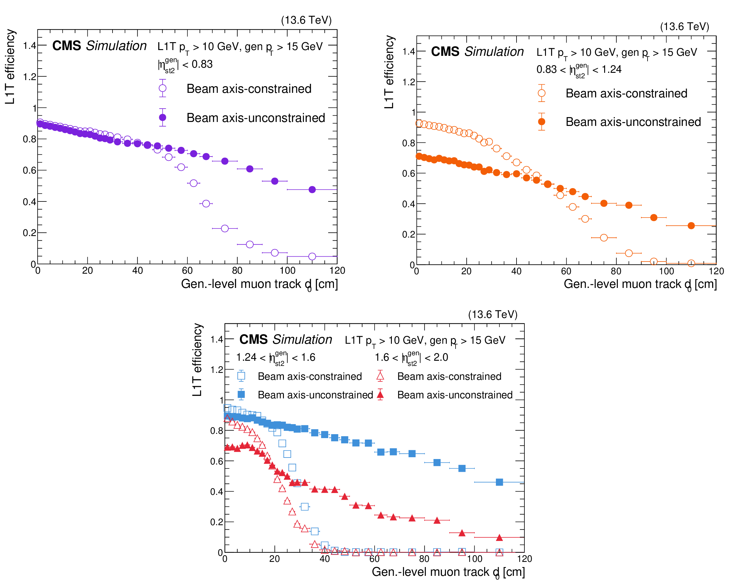
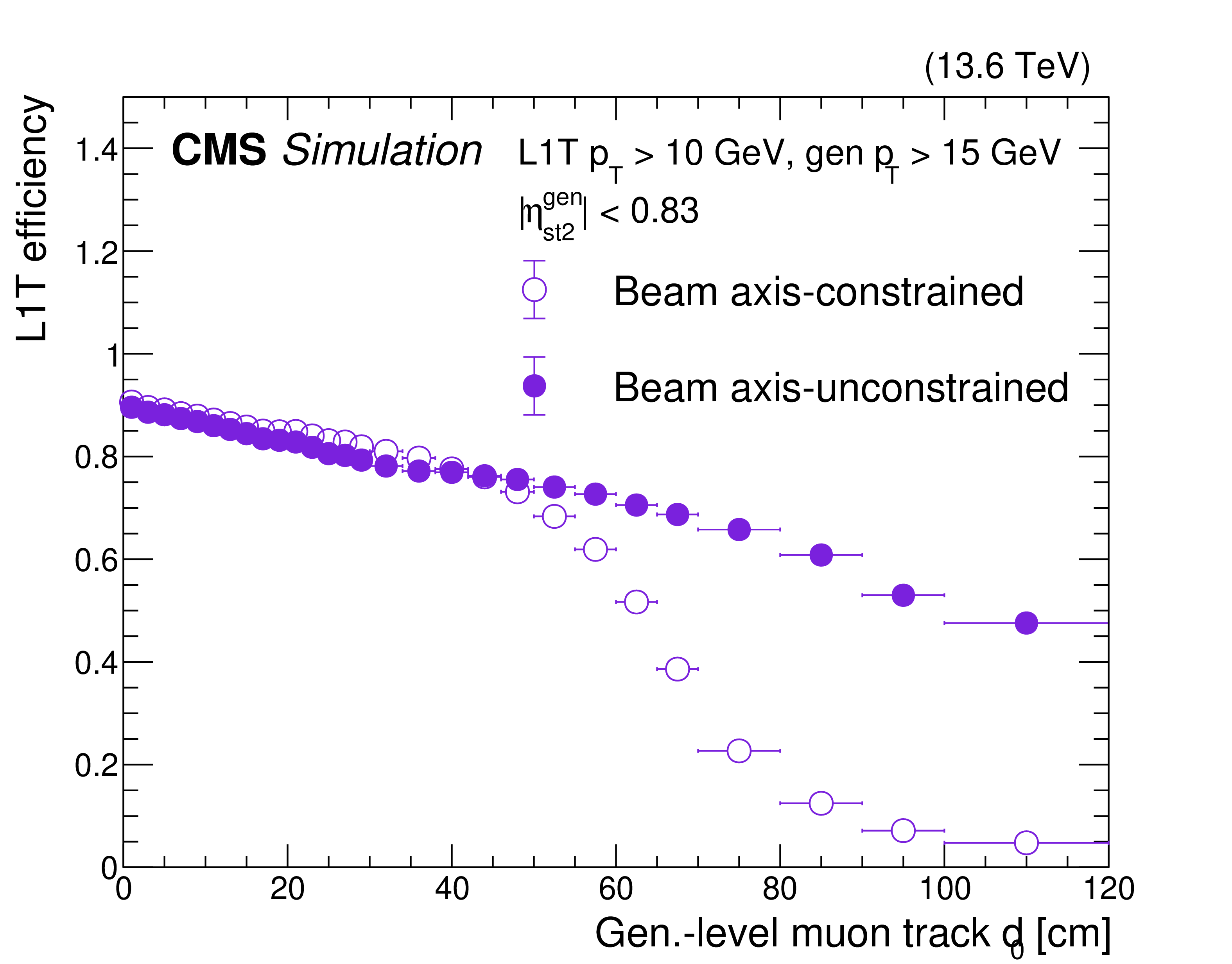
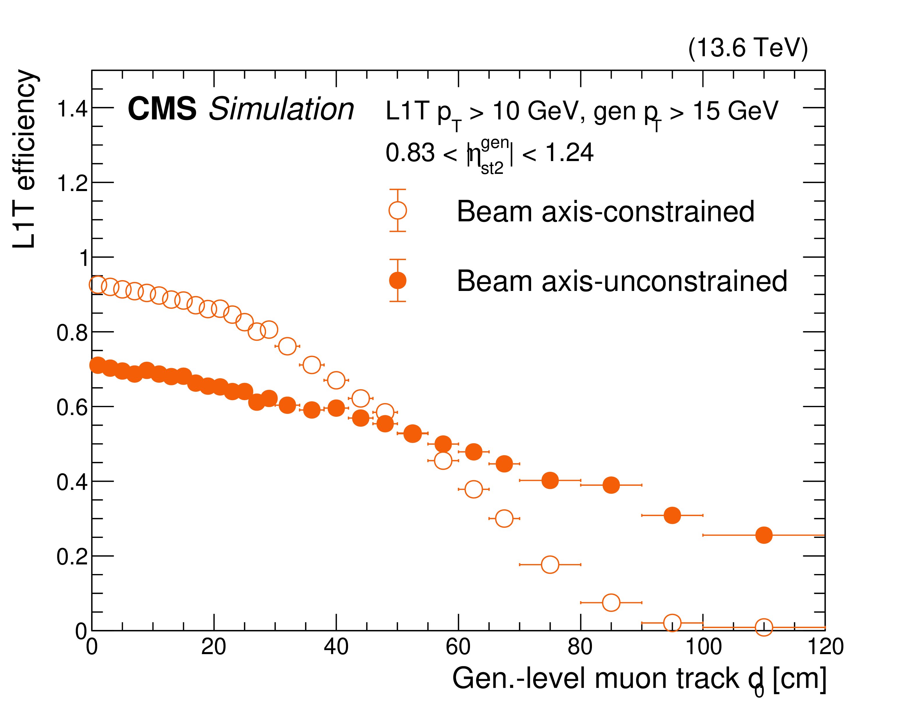
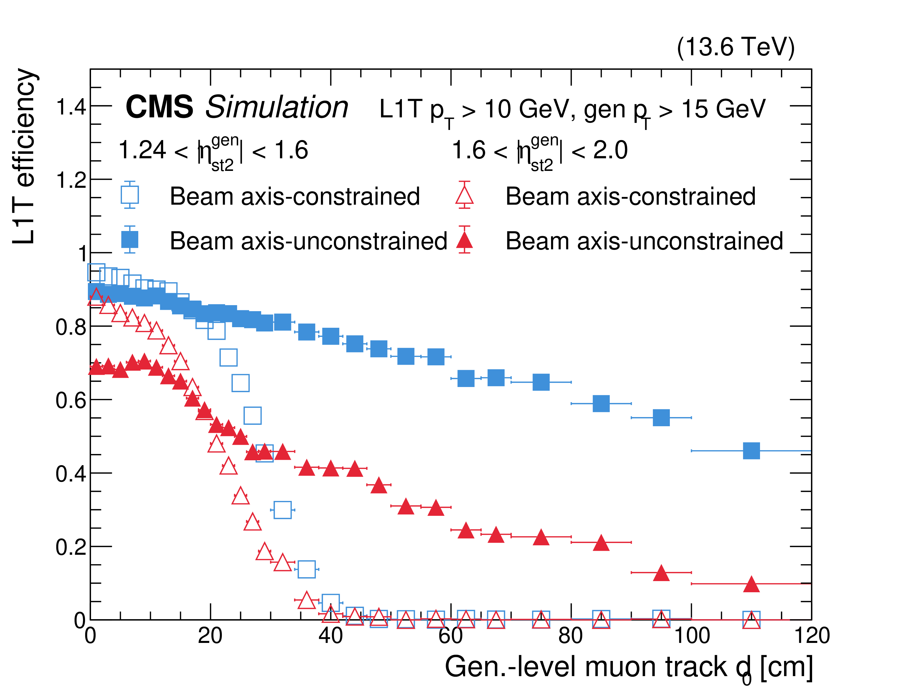
The BMTF (upper left), OMTF (upper right), and EMTF (lower) L1T efficiencies for beam axis-constrained (open circles, squares, and triangles) and beam axis-unconstrained (filled circles, squares, and triangles) $ p_{\mathrm{T}} $ assignment algorithms for L1T $ p_{\mathrm{T}} > $ 10 GeV with respect to generator-level muon track $ d_{\text{0}} $, obtained using a sample which produces LLPs that decay to dimuons. The L1T algorithms and data-taking conditions correspond to 2024. A selection on the generator-level muon track $ p_{\mathrm{T}} > $ 15 GeV is applied to show the performance at the efficiency plateau. The generator-level muon tracks are extrapolated to the second muon station to determine the $ \eta^{\text{gen}}_{\text{st2}} $ values that are used in the plot. Both the new vertex-unconstrained algorithm performance and the default beam axis-constrained algorithm performance are shown. In the EMTF plot, the different colors and symbols show different $ |\eta| $ regions: 1.24 $ < \eta^{\text{gen}}_{\text{st2}} < $ 1.6 (blue squares), 1.6 $ < \eta^{\text{gen}}_{\text{st2}} < $ 2.0 (red triangles). |
png pdf |
Figure 39-a:
The BMTF (upper left), OMTF (upper right), and EMTF (lower) L1T efficiencies for beam axis-constrained (open circles, squares, and triangles) and beam axis-unconstrained (filled circles, squares, and triangles) $ p_{\mathrm{T}} $ assignment algorithms for L1T $ p_{\mathrm{T}} > $ 10 GeV with respect to generator-level muon track $ d_{\text{0}} $, obtained using a sample which produces LLPs that decay to dimuons. The L1T algorithms and data-taking conditions correspond to 2024. A selection on the generator-level muon track $ p_{\mathrm{T}} > $ 15 GeV is applied to show the performance at the efficiency plateau. The generator-level muon tracks are extrapolated to the second muon station to determine the $ \eta^{\text{gen}}_{\text{st2}} $ values that are used in the plot. Both the new vertex-unconstrained algorithm performance and the default beam axis-constrained algorithm performance are shown. In the EMTF plot, the different colors and symbols show different $ |\eta| $ regions: 1.24 $ < \eta^{\text{gen}}_{\text{st2}} < $ 1.6 (blue squares), 1.6 $ < \eta^{\text{gen}}_{\text{st2}} < $ 2.0 (red triangles). |
png pdf |
Figure 39-b:
The BMTF (upper left), OMTF (upper right), and EMTF (lower) L1T efficiencies for beam axis-constrained (open circles, squares, and triangles) and beam axis-unconstrained (filled circles, squares, and triangles) $ p_{\mathrm{T}} $ assignment algorithms for L1T $ p_{\mathrm{T}} > $ 10 GeV with respect to generator-level muon track $ d_{\text{0}} $, obtained using a sample which produces LLPs that decay to dimuons. The L1T algorithms and data-taking conditions correspond to 2024. A selection on the generator-level muon track $ p_{\mathrm{T}} > $ 15 GeV is applied to show the performance at the efficiency plateau. The generator-level muon tracks are extrapolated to the second muon station to determine the $ \eta^{\text{gen}}_{\text{st2}} $ values that are used in the plot. Both the new vertex-unconstrained algorithm performance and the default beam axis-constrained algorithm performance are shown. In the EMTF plot, the different colors and symbols show different $ |\eta| $ regions: 1.24 $ < \eta^{\text{gen}}_{\text{st2}} < $ 1.6 (blue squares), 1.6 $ < \eta^{\text{gen}}_{\text{st2}} < $ 2.0 (red triangles). |
png pdf |
Figure 39-c:
The BMTF (upper left), OMTF (upper right), and EMTF (lower) L1T efficiencies for beam axis-constrained (open circles, squares, and triangles) and beam axis-unconstrained (filled circles, squares, and triangles) $ p_{\mathrm{T}} $ assignment algorithms for L1T $ p_{\mathrm{T}} > $ 10 GeV with respect to generator-level muon track $ d_{\text{0}} $, obtained using a sample which produces LLPs that decay to dimuons. The L1T algorithms and data-taking conditions correspond to 2024. A selection on the generator-level muon track $ p_{\mathrm{T}} > $ 15 GeV is applied to show the performance at the efficiency plateau. The generator-level muon tracks are extrapolated to the second muon station to determine the $ \eta^{\text{gen}}_{\text{st2}} $ values that are used in the plot. Both the new vertex-unconstrained algorithm performance and the default beam axis-constrained algorithm performance are shown. In the EMTF plot, the different colors and symbols show different $ |\eta| $ regions: 1.24 $ < \eta^{\text{gen}}_{\text{st2}} < $ 1.6 (blue squares), 1.6 $ < \eta^{\text{gen}}_{\text{st2}} < $ 2.0 (red triangles). |
png pdf |
Figure 40:
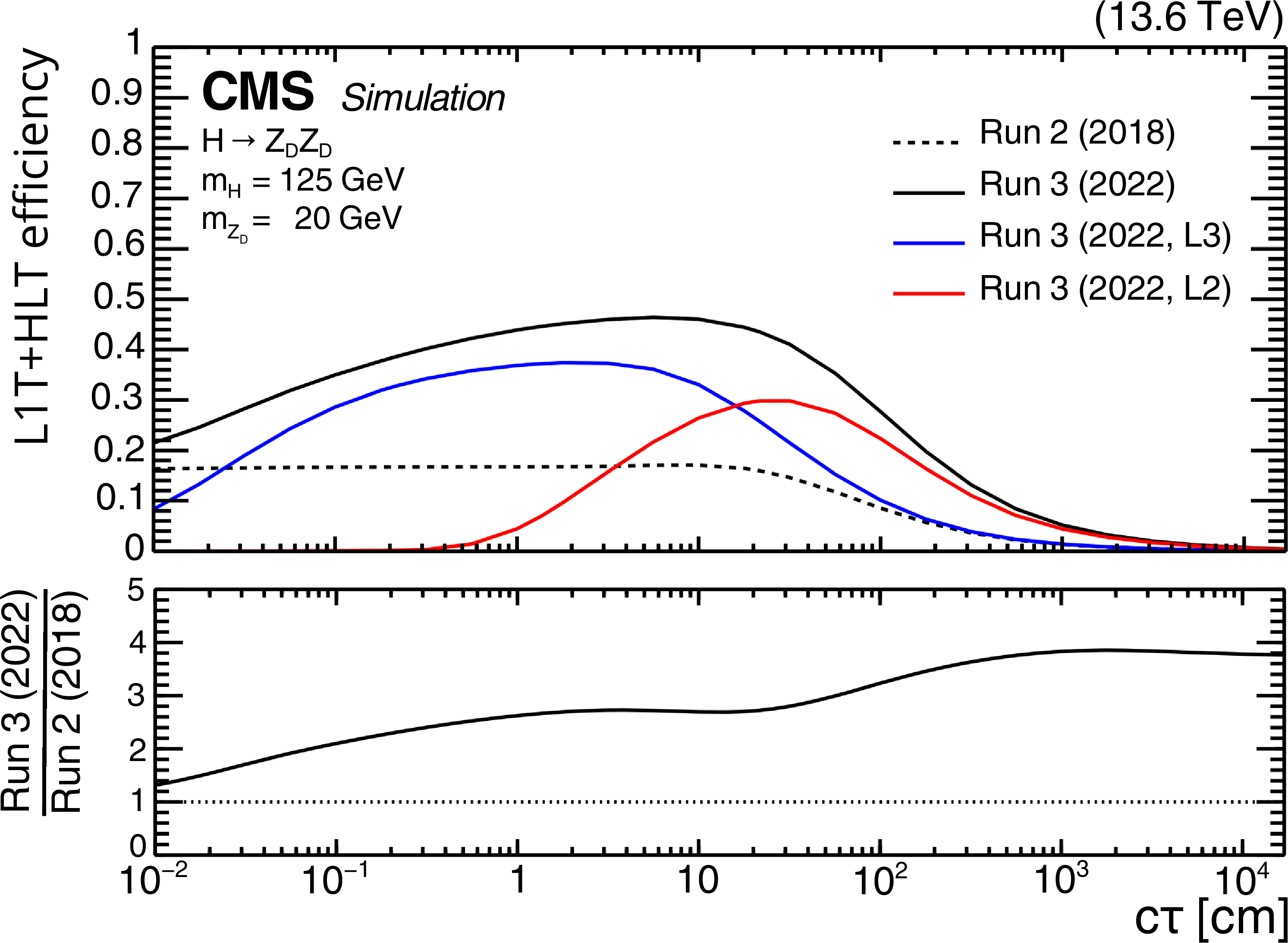
The L1T+HLT efficiencies of the various displaced-dimuon triggers and their logical OR as a function of $ c\tau $ for the HAHM signal events with $ m_{\mathrm{H}}= $ 125 GeV and $ m_{\mathrm{Z}_\text{D}} = $ 20 GeV, for 2022 conditions. The efficiency is defined as the fraction of simulated events that satisfy the detector acceptance and the requirements of the following sets of triggers: the Run 2 (2018) triggers (dashed black); the Run 3 (2022, L3) triggers (blue); the Run 3 (2022, L2) triggers (red); and the logical OR of all these triggers (Run 3 (2022), solid black). The lower panel shows the ratio of the overall Run 3 (2022) efficiency to the Run 2 (2018) efficiency. Figure adapted from Ref. [12]. |
png pdf |
Figure 41:
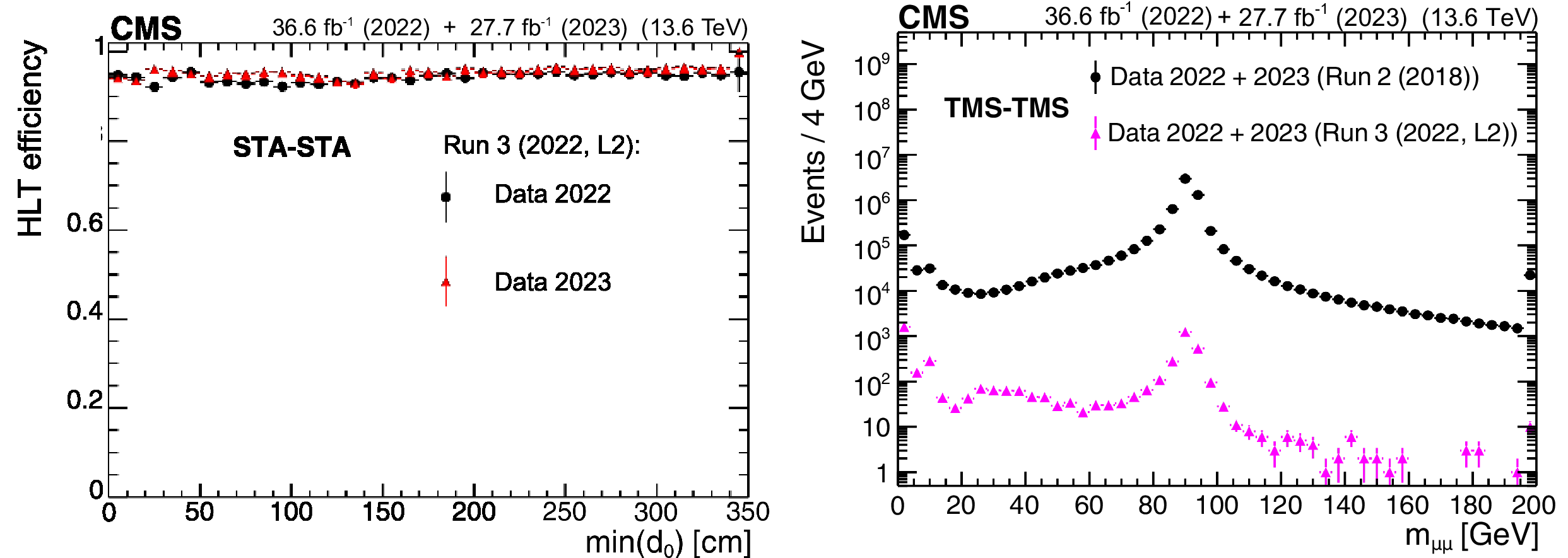
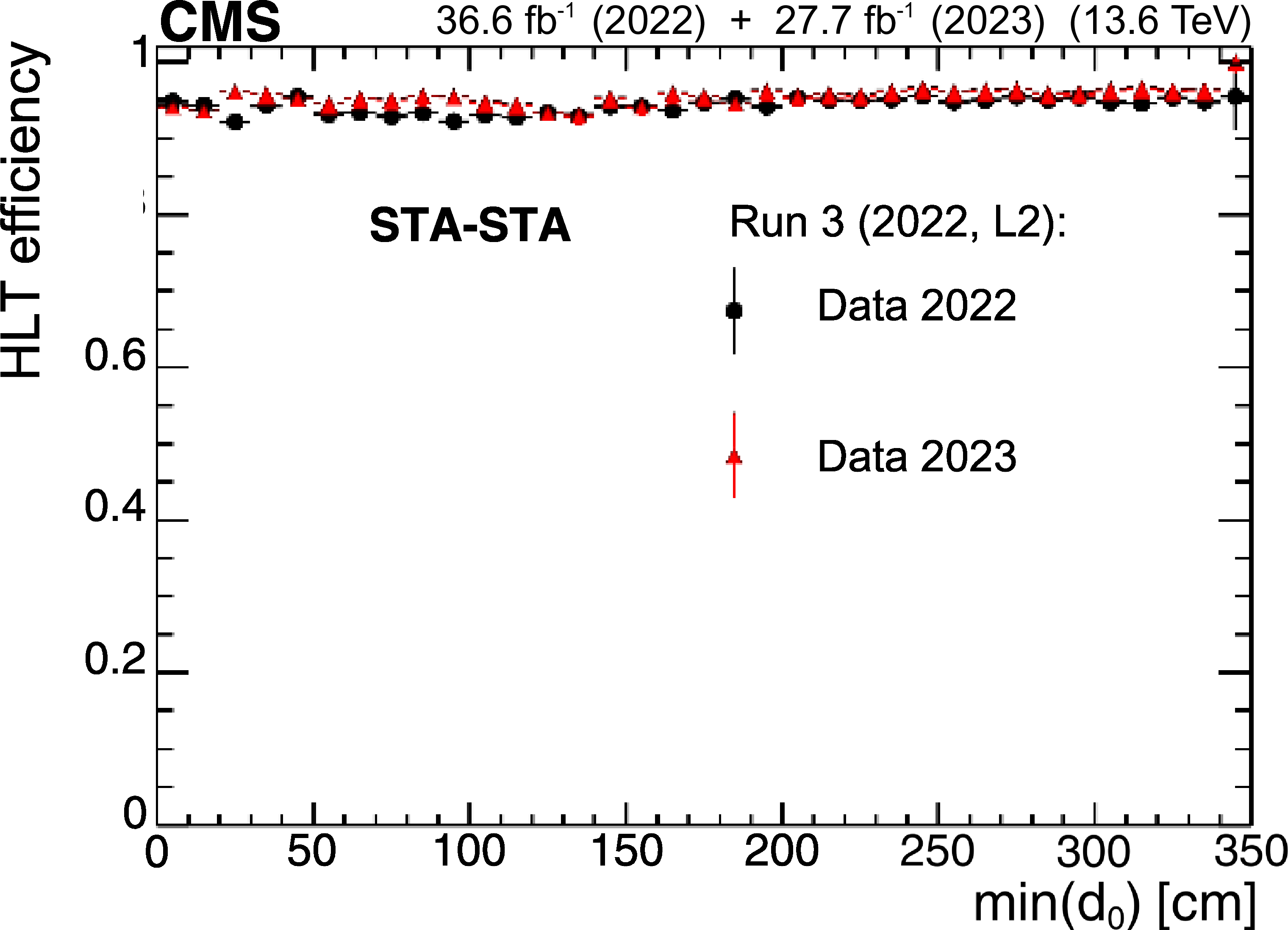
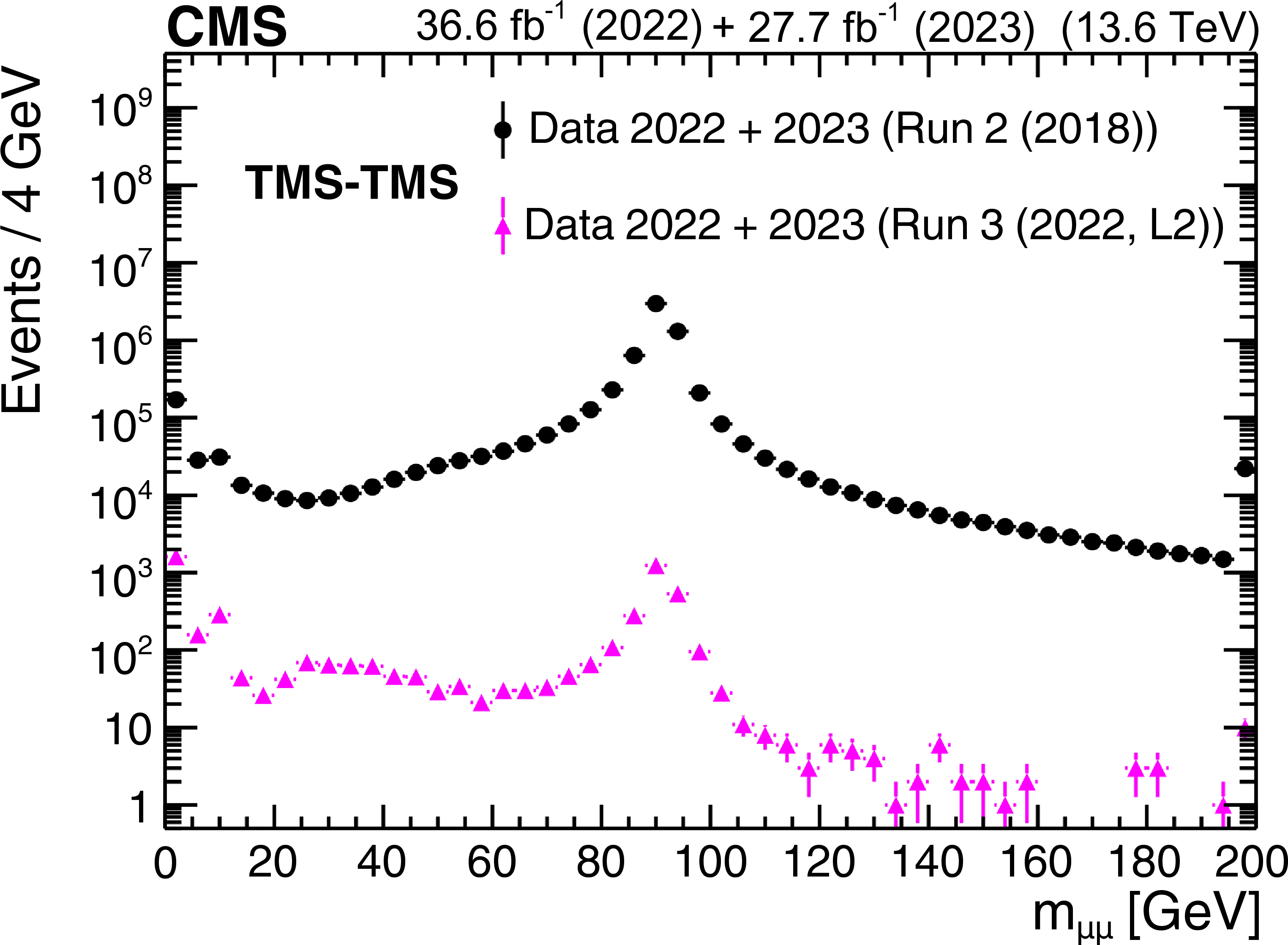
The HLT efficiency (left), defined as the fraction of events recorded by the Run 2 (2018) triggers that also satisfy the requirements of the Run 3 (2022, L2) triggers, as a function of offline-reconstructed $ \text{min}(d_{\text{0}}) $ of the two muons forming STA-STA dimuons in events enriched in cosmic ray muons. The black circles represent efficiencies during the 2022 data-taking period, and the red triangles represent the 2023 period. For displaced muons, the efficiency of the online $ \text{min}(d_{\text{0}}) $ requirement is larger than 95% in all data-taking periods. The invariant mass distribution for TMS-TMS dimuons (right) in events recorded by the Run 2 (2018) triggers in the combined 2022 and 2023 data set (black circles), and in the subset of events also selected by the Run 3 (2022, L2) triggers (pink triangles), illustrating the prompt muon rejection of the Run 3 (2022, L2) triggers. |
png pdf |
Figure 41-a:
The HLT efficiency (left), defined as the fraction of events recorded by the Run 2 (2018) triggers that also satisfy the requirements of the Run 3 (2022, L2) triggers, as a function of offline-reconstructed $ \text{min}(d_{\text{0}}) $ of the two muons forming STA-STA dimuons in events enriched in cosmic ray muons. The black circles represent efficiencies during the 2022 data-taking period, and the red triangles represent the 2023 period. For displaced muons, the efficiency of the online $ \text{min}(d_{\text{0}}) $ requirement is larger than 95% in all data-taking periods. The invariant mass distribution for TMS-TMS dimuons (right) in events recorded by the Run 2 (2018) triggers in the combined 2022 and 2023 data set (black circles), and in the subset of events also selected by the Run 3 (2022, L2) triggers (pink triangles), illustrating the prompt muon rejection of the Run 3 (2022, L2) triggers. |
png pdf |
Figure 41-b:
The HLT efficiency (left), defined as the fraction of events recorded by the Run 2 (2018) triggers that also satisfy the requirements of the Run 3 (2022, L2) triggers, as a function of offline-reconstructed $ \text{min}(d_{\text{0}}) $ of the two muons forming STA-STA dimuons in events enriched in cosmic ray muons. The black circles represent efficiencies during the 2022 data-taking period, and the red triangles represent the 2023 period. For displaced muons, the efficiency of the online $ \text{min}(d_{\text{0}}) $ requirement is larger than 95% in all data-taking periods. The invariant mass distribution for TMS-TMS dimuons (right) in events recorded by the Run 2 (2018) triggers in the combined 2022 and 2023 data set (black circles), and in the subset of events also selected by the Run 3 (2022, L2) triggers (pink triangles), illustrating the prompt muon rejection of the Run 3 (2022, L2) triggers. |
png pdf |
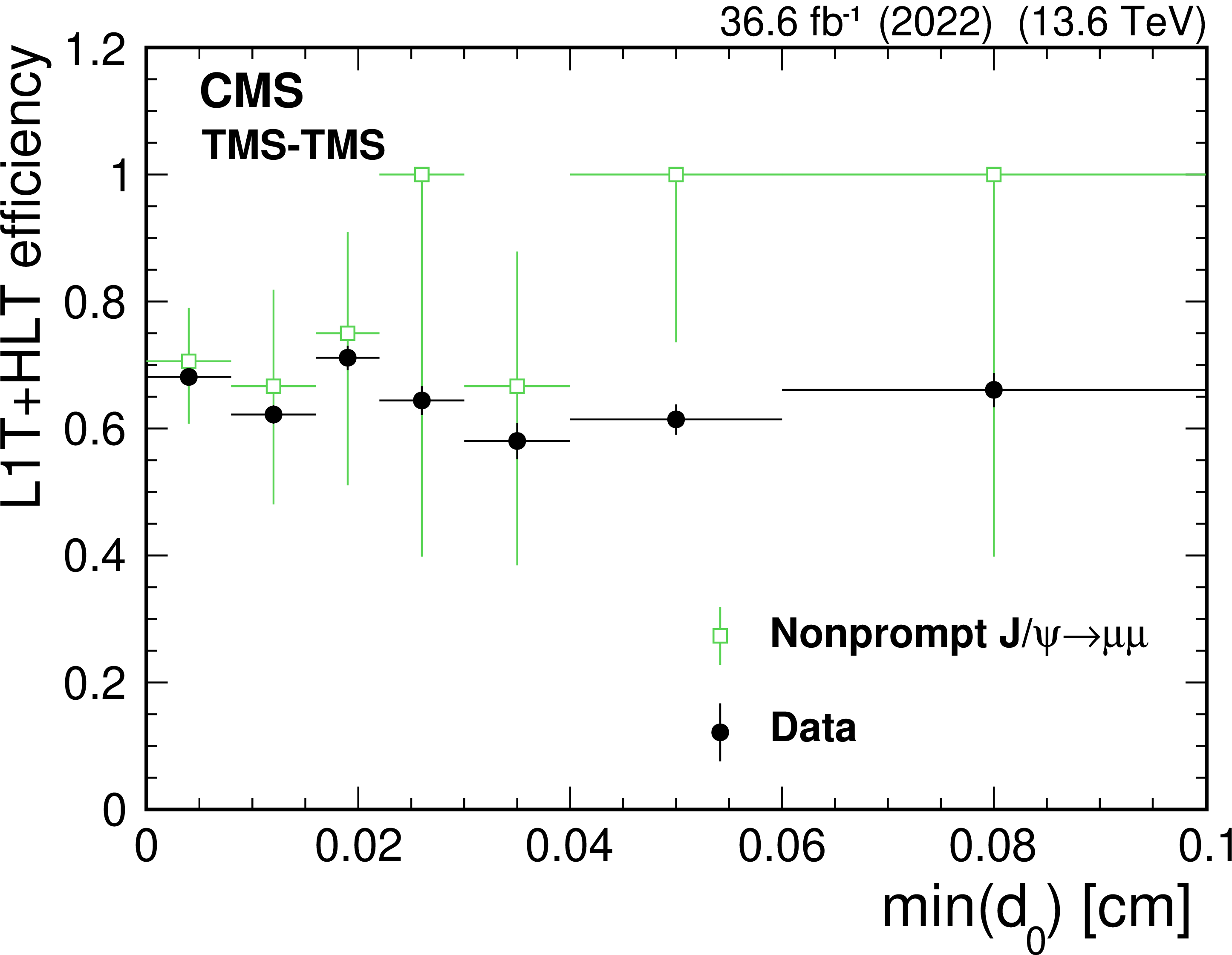
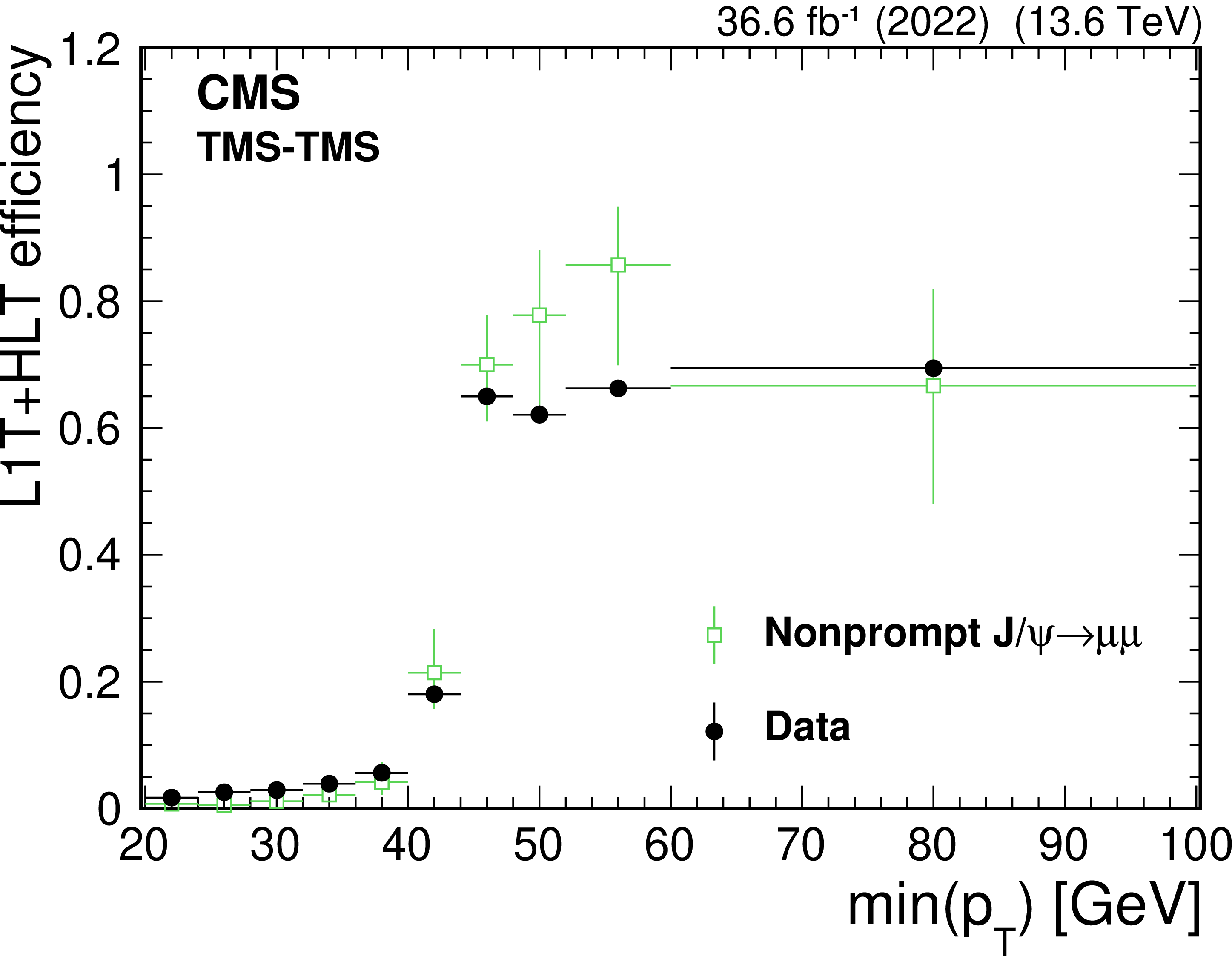
Figure 42:
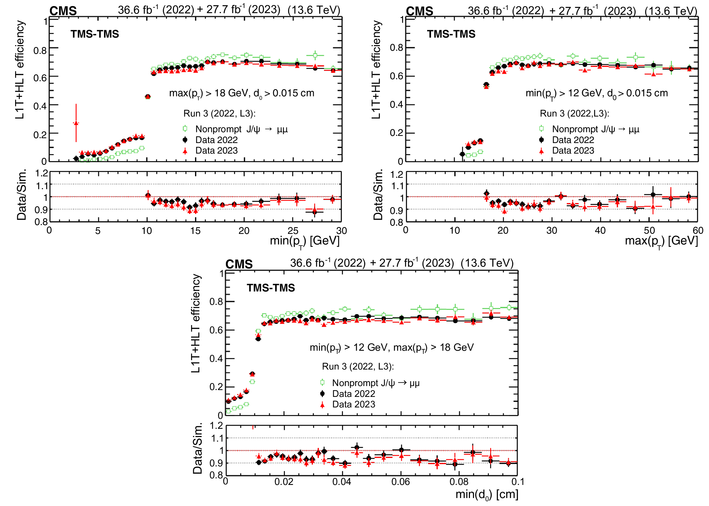
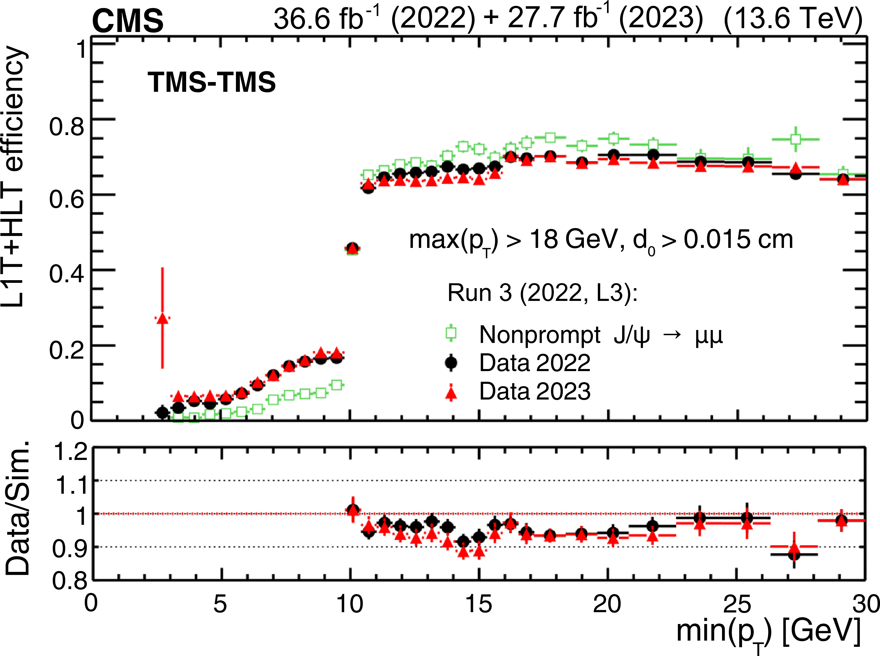
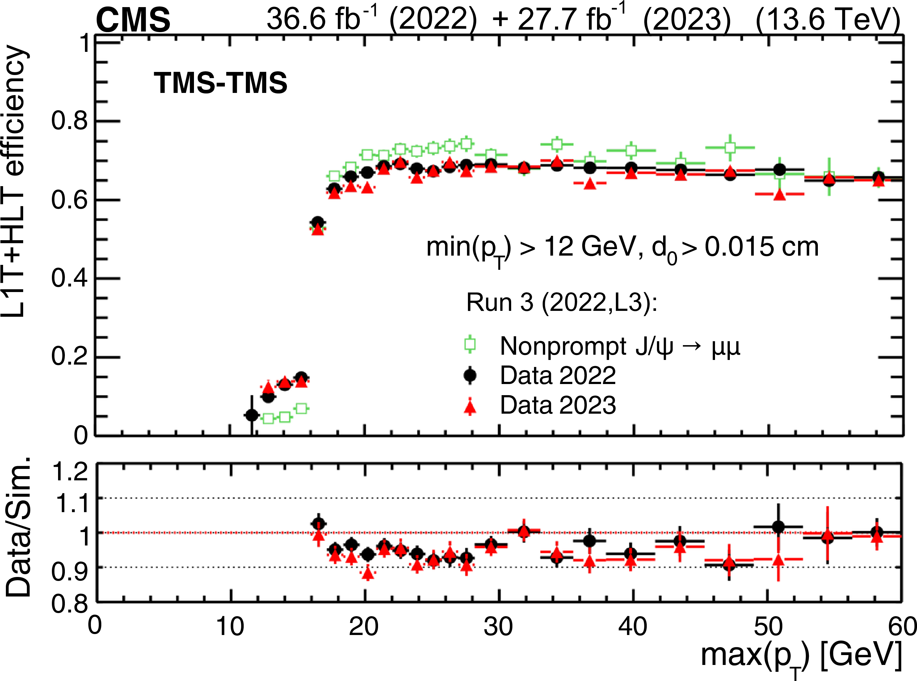
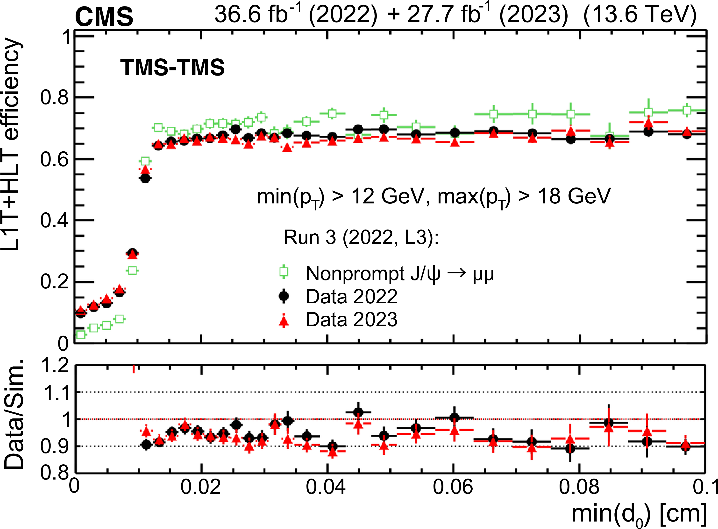
The L1T+HLT efficiency of the Run 3 (2022, L3) triggers in 2022 data (filled black circles), 2023 data (filled red triangles), and simulation (open green squares) as a function of $ \text{min}(p_{\mathrm{T}}) $ (upper left), $ \text{max}(p_{\mathrm{T}}) $ (upper right), and $ \text{min}(d_{\text{0}}) $ (lower) of the two muons forming TMS-TMS dimuons in events enriched in $ \mathrm{J}/\psi\to\mu\mu $ events. The efficiency in data is the fraction of $ \mathrm{J}/\psi\to\mu\mu $ events recorded by the triggers based on the information from jets and $ p_{\mathrm{T}}^\text{miss} $ that also satisfy the requirements of the Run 3 (2022, L3) triggers. It is compared to the efficiency of the Run 3 (2022, L3) triggers in a combination of simulated samples of $ \mathrm{J}/\psi\to\mu\mu $ events produced in various b hadron decays. The lower panels show the ratio of the data to simulated events. |
png pdf |
Figure 42-a:
The L1T+HLT efficiency of the Run 3 (2022, L3) triggers in 2022 data (filled black circles), 2023 data (filled red triangles), and simulation (open green squares) as a function of $ \text{min}(p_{\mathrm{T}}) $ (upper left), $ \text{max}(p_{\mathrm{T}}) $ (upper right), and $ \text{min}(d_{\text{0}}) $ (lower) of the two muons forming TMS-TMS dimuons in events enriched in $ \mathrm{J}/\psi\to\mu\mu $ events. The efficiency in data is the fraction of $ \mathrm{J}/\psi\to\mu\mu $ events recorded by the triggers based on the information from jets and $ p_{\mathrm{T}}^\text{miss} $ that also satisfy the requirements of the Run 3 (2022, L3) triggers. It is compared to the efficiency of the Run 3 (2022, L3) triggers in a combination of simulated samples of $ \mathrm{J}/\psi\to\mu\mu $ events produced in various b hadron decays. The lower panels show the ratio of the data to simulated events. |
png pdf |
Figure 42-b:
The L1T+HLT efficiency of the Run 3 (2022, L3) triggers in 2022 data (filled black circles), 2023 data (filled red triangles), and simulation (open green squares) as a function of $ \text{min}(p_{\mathrm{T}}) $ (upper left), $ \text{max}(p_{\mathrm{T}}) $ (upper right), and $ \text{min}(d_{\text{0}}) $ (lower) of the two muons forming TMS-TMS dimuons in events enriched in $ \mathrm{J}/\psi\to\mu\mu $ events. The efficiency in data is the fraction of $ \mathrm{J}/\psi\to\mu\mu $ events recorded by the triggers based on the information from jets and $ p_{\mathrm{T}}^\text{miss} $ that also satisfy the requirements of the Run 3 (2022, L3) triggers. It is compared to the efficiency of the Run 3 (2022, L3) triggers in a combination of simulated samples of $ \mathrm{J}/\psi\to\mu\mu $ events produced in various b hadron decays. The lower panels show the ratio of the data to simulated events. |
png pdf |
Figure 42-c:
The L1T+HLT efficiency of the Run 3 (2022, L3) triggers in 2022 data (filled black circles), 2023 data (filled red triangles), and simulation (open green squares) as a function of $ \text{min}(p_{\mathrm{T}}) $ (upper left), $ \text{max}(p_{\mathrm{T}}) $ (upper right), and $ \text{min}(d_{\text{0}}) $ (lower) of the two muons forming TMS-TMS dimuons in events enriched in $ \mathrm{J}/\psi\to\mu\mu $ events. The efficiency in data is the fraction of $ \mathrm{J}/\psi\to\mu\mu $ events recorded by the triggers based on the information from jets and $ p_{\mathrm{T}}^\text{miss} $ that also satisfy the requirements of the Run 3 (2022, L3) triggers. It is compared to the efficiency of the Run 3 (2022, L3) triggers in a combination of simulated samples of $ \mathrm{J}/\psi\to\mu\mu $ events produced in various b hadron decays. The lower panels show the ratio of the data to simulated events. |
png pdf |
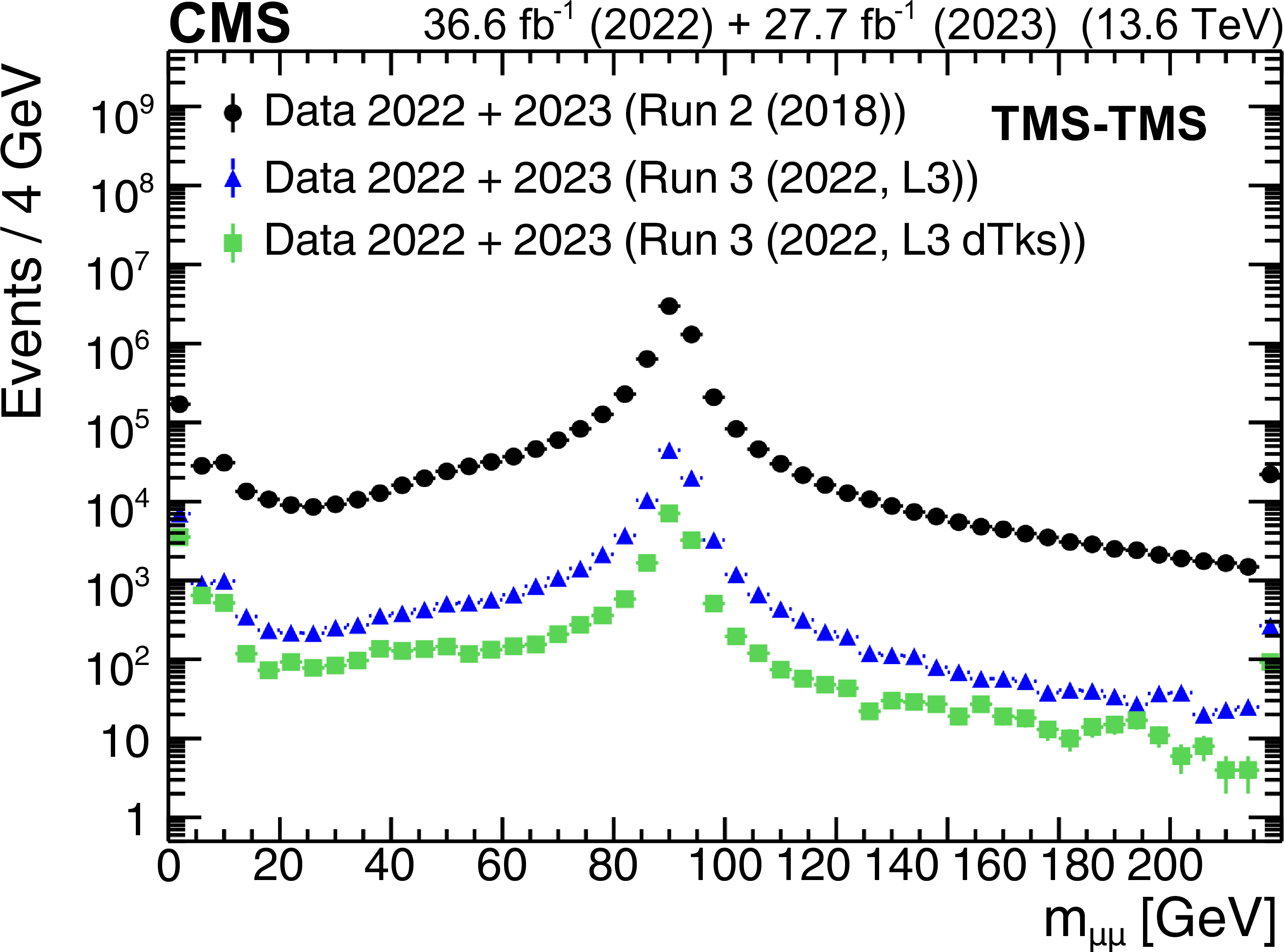
Figure 43:
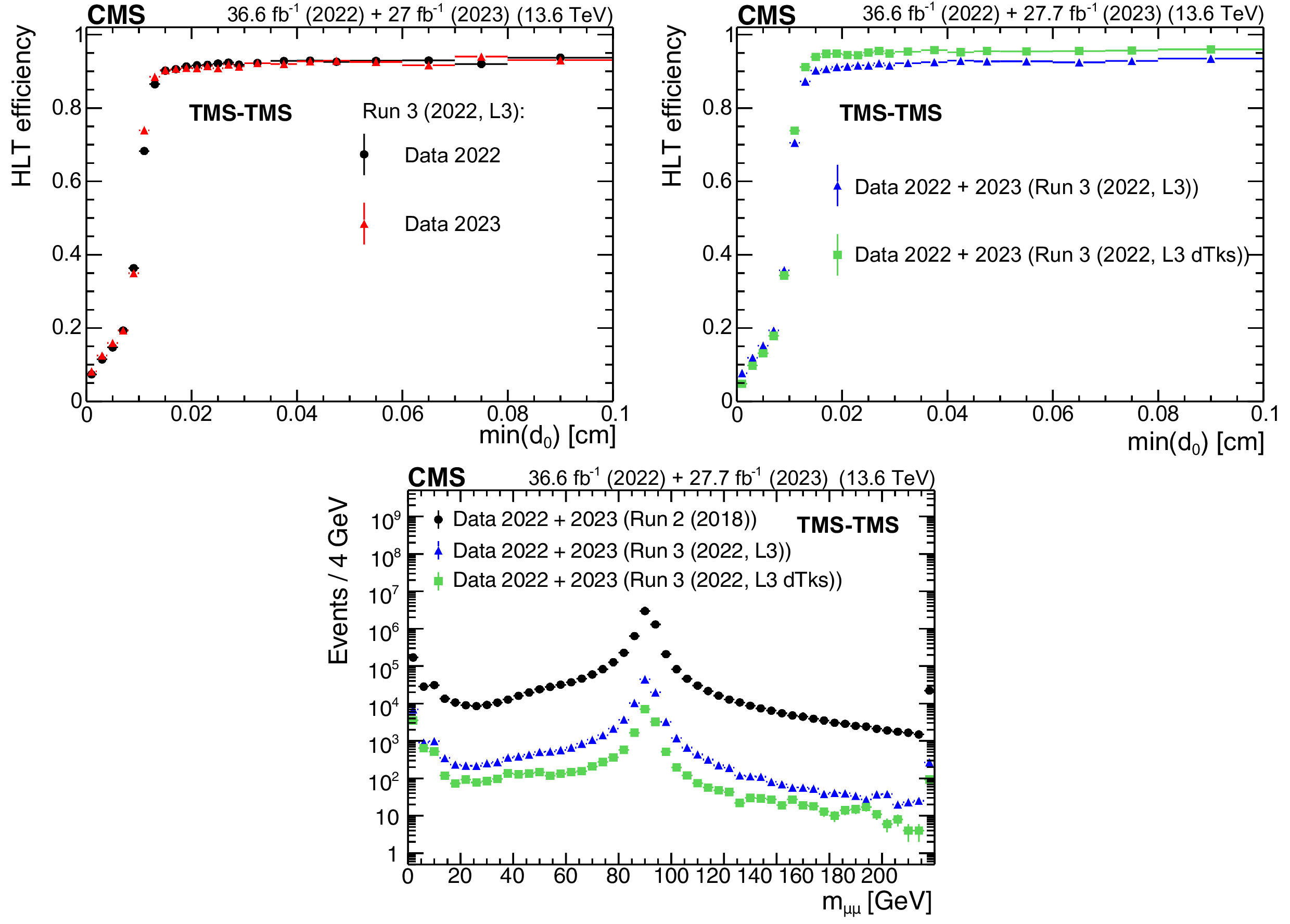
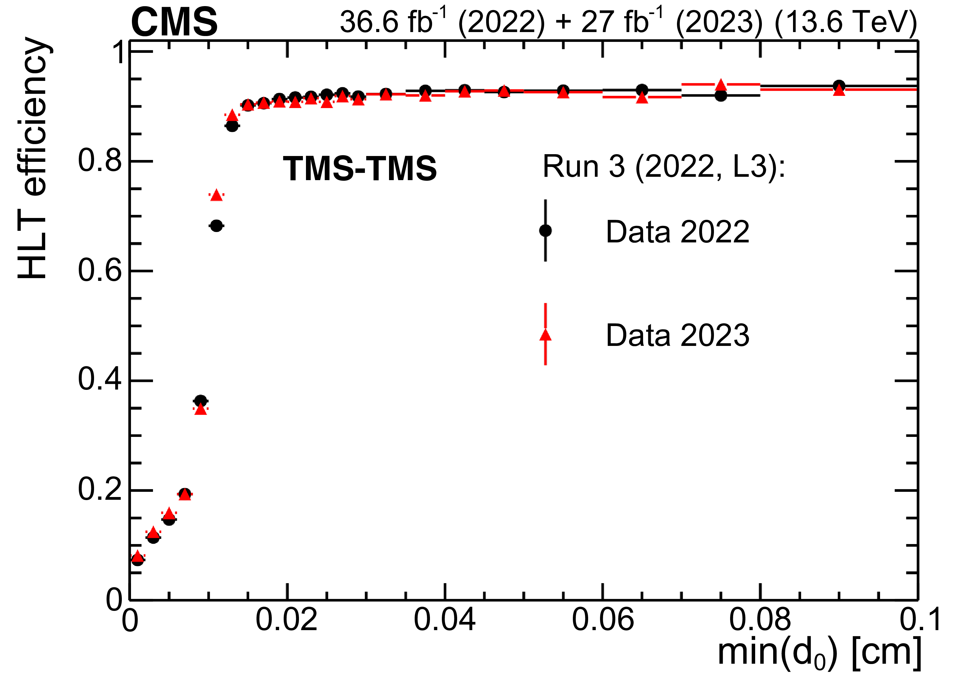
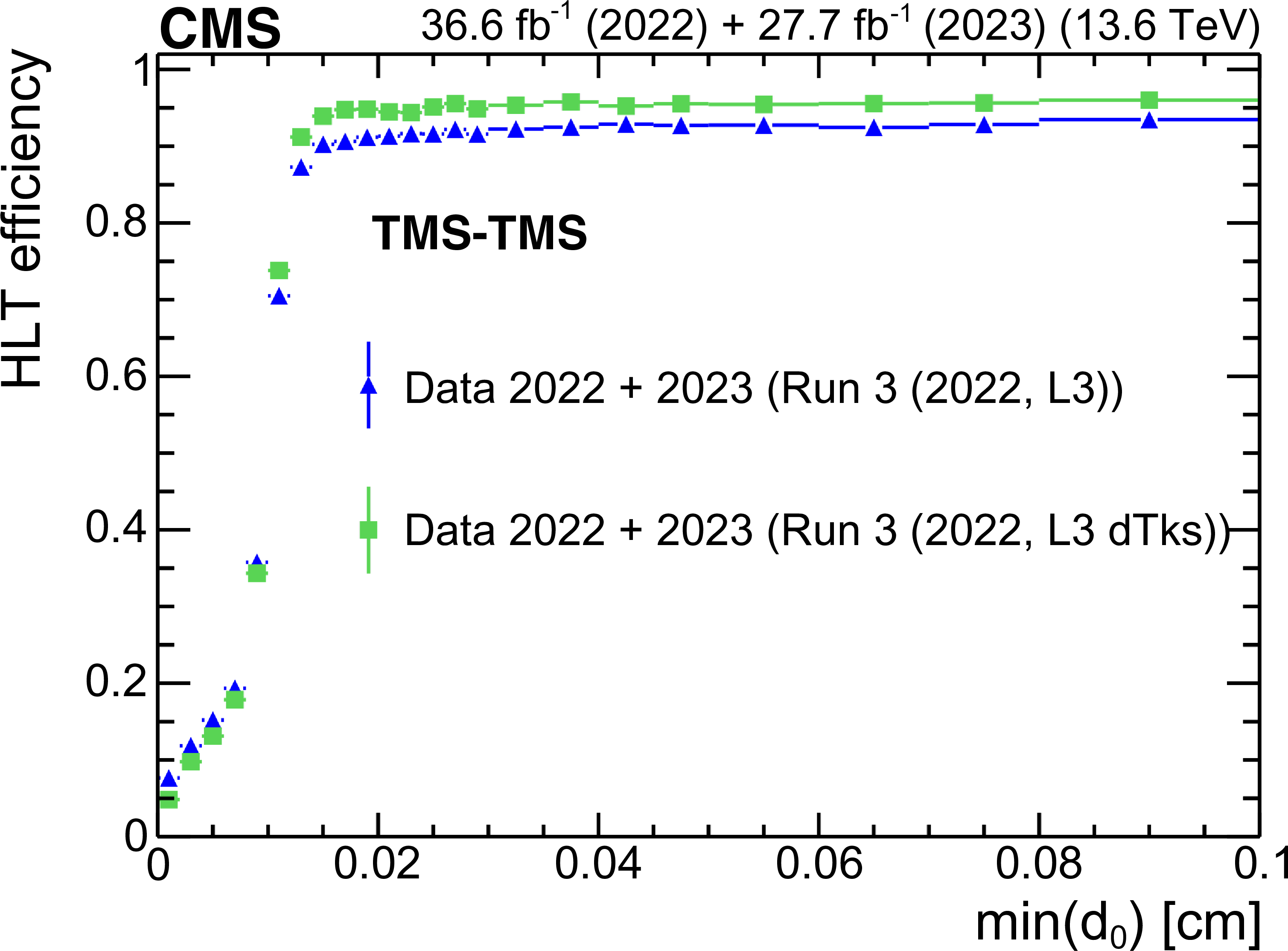
The HLT efficiency (upper left), defined as the fraction of events recorded by the Run 2 (2018) triggers that also satisfy the requirements of the Run 3 (2022, L3) triggers, as a function of offline-reconstructed $ \text{min}(d_{\text{0}}) $ of the two muons forming TMS-TMS dimuons in events enriched in $ \mathrm{J}/\psi\to\mu\mu $, for the 2022 and 2023 data-taking periods. The black circles represent efficiencies during the 2022 data-taking period, and the red triangles represent the 2023 period. For dimuons with offline $ \text{min}(d_{\text{0}}) > 0.012 \text{cm} $, the combined efficiency of the L3 muon reconstruction and the online $ \text{min}(d_{\text{0}}) $ requirement is larger than 90% in all data-taking periods. The HLT efficiency of the Run 3 (2022, L3) triggers (upper right), shown with blue triangles, and the Run 3 (2022, L3 dTks) triggers, shown with green squares, for $ \mathrm{J}/\psi\to\mu\mu $ events in the 2022 and 2023 data sets. Invariant mass distribution for TMS-TMS dimuons (lower) in events recorded by the Run 2 (2018) triggers in the combined 2022 and 2023 data set (black circles), and in the subset of events also selected by the Run 3 (2022, L3) trigger (blue triangles) and Run 3 (2022, L3 dTks) trigger (green squares), illustrating the prompt muon rejection of the L3 triggers. |
png pdf |
Figure 43-a:
The HLT efficiency (upper left), defined as the fraction of events recorded by the Run 2 (2018) triggers that also satisfy the requirements of the Run 3 (2022, L3) triggers, as a function of offline-reconstructed $ \text{min}(d_{\text{0}}) $ of the two muons forming TMS-TMS dimuons in events enriched in $ \mathrm{J}/\psi\to\mu\mu $, for the 2022 and 2023 data-taking periods. The black circles represent efficiencies during the 2022 data-taking period, and the red triangles represent the 2023 period. For dimuons with offline $ \text{min}(d_{\text{0}}) > 0.012 \text{cm} $, the combined efficiency of the L3 muon reconstruction and the online $ \text{min}(d_{\text{0}}) $ requirement is larger than 90% in all data-taking periods. The HLT efficiency of the Run 3 (2022, L3) triggers (upper right), shown with blue triangles, and the Run 3 (2022, L3 dTks) triggers, shown with green squares, for $ \mathrm{J}/\psi\to\mu\mu $ events in the 2022 and 2023 data sets. Invariant mass distribution for TMS-TMS dimuons (lower) in events recorded by the Run 2 (2018) triggers in the combined 2022 and 2023 data set (black circles), and in the subset of events also selected by the Run 3 (2022, L3) trigger (blue triangles) and Run 3 (2022, L3 dTks) trigger (green squares), illustrating the prompt muon rejection of the L3 triggers. |
png pdf |
Figure 43-b:
The HLT efficiency (upper left), defined as the fraction of events recorded by the Run 2 (2018) triggers that also satisfy the requirements of the Run 3 (2022, L3) triggers, as a function of offline-reconstructed $ \text{min}(d_{\text{0}}) $ of the two muons forming TMS-TMS dimuons in events enriched in $ \mathrm{J}/\psi\to\mu\mu $, for the 2022 and 2023 data-taking periods. The black circles represent efficiencies during the 2022 data-taking period, and the red triangles represent the 2023 period. For dimuons with offline $ \text{min}(d_{\text{0}}) > 0.012 \text{cm} $, the combined efficiency of the L3 muon reconstruction and the online $ \text{min}(d_{\text{0}}) $ requirement is larger than 90% in all data-taking periods. The HLT efficiency of the Run 3 (2022, L3) triggers (upper right), shown with blue triangles, and the Run 3 (2022, L3 dTks) triggers, shown with green squares, for $ \mathrm{J}/\psi\to\mu\mu $ events in the 2022 and 2023 data sets. Invariant mass distribution for TMS-TMS dimuons (lower) in events recorded by the Run 2 (2018) triggers in the combined 2022 and 2023 data set (black circles), and in the subset of events also selected by the Run 3 (2022, L3) trigger (blue triangles) and Run 3 (2022, L3 dTks) trigger (green squares), illustrating the prompt muon rejection of the L3 triggers. |
png pdf |
Figure 43-c:
The HLT efficiency (upper left), defined as the fraction of events recorded by the Run 2 (2018) triggers that also satisfy the requirements of the Run 3 (2022, L3) triggers, as a function of offline-reconstructed $ \text{min}(d_{\text{0}}) $ of the two muons forming TMS-TMS dimuons in events enriched in $ \mathrm{J}/\psi\to\mu\mu $, for the 2022 and 2023 data-taking periods. The black circles represent efficiencies during the 2022 data-taking period, and the red triangles represent the 2023 period. For dimuons with offline $ \text{min}(d_{\text{0}}) > 0.012 \text{cm} $, the combined efficiency of the L3 muon reconstruction and the online $ \text{min}(d_{\text{0}}) $ requirement is larger than 90% in all data-taking periods. The HLT efficiency of the Run 3 (2022, L3) triggers (upper right), shown with blue triangles, and the Run 3 (2022, L3 dTks) triggers, shown with green squares, for $ \mathrm{J}/\psi\to\mu\mu $ events in the 2022 and 2023 data sets. Invariant mass distribution for TMS-TMS dimuons (lower) in events recorded by the Run 2 (2018) triggers in the combined 2022 and 2023 data set (black circles), and in the subset of events also selected by the Run 3 (2022, L3) trigger (blue triangles) and Run 3 (2022, L3 dTks) trigger (green squares), illustrating the prompt muon rejection of the L3 triggers. |
png pdf |
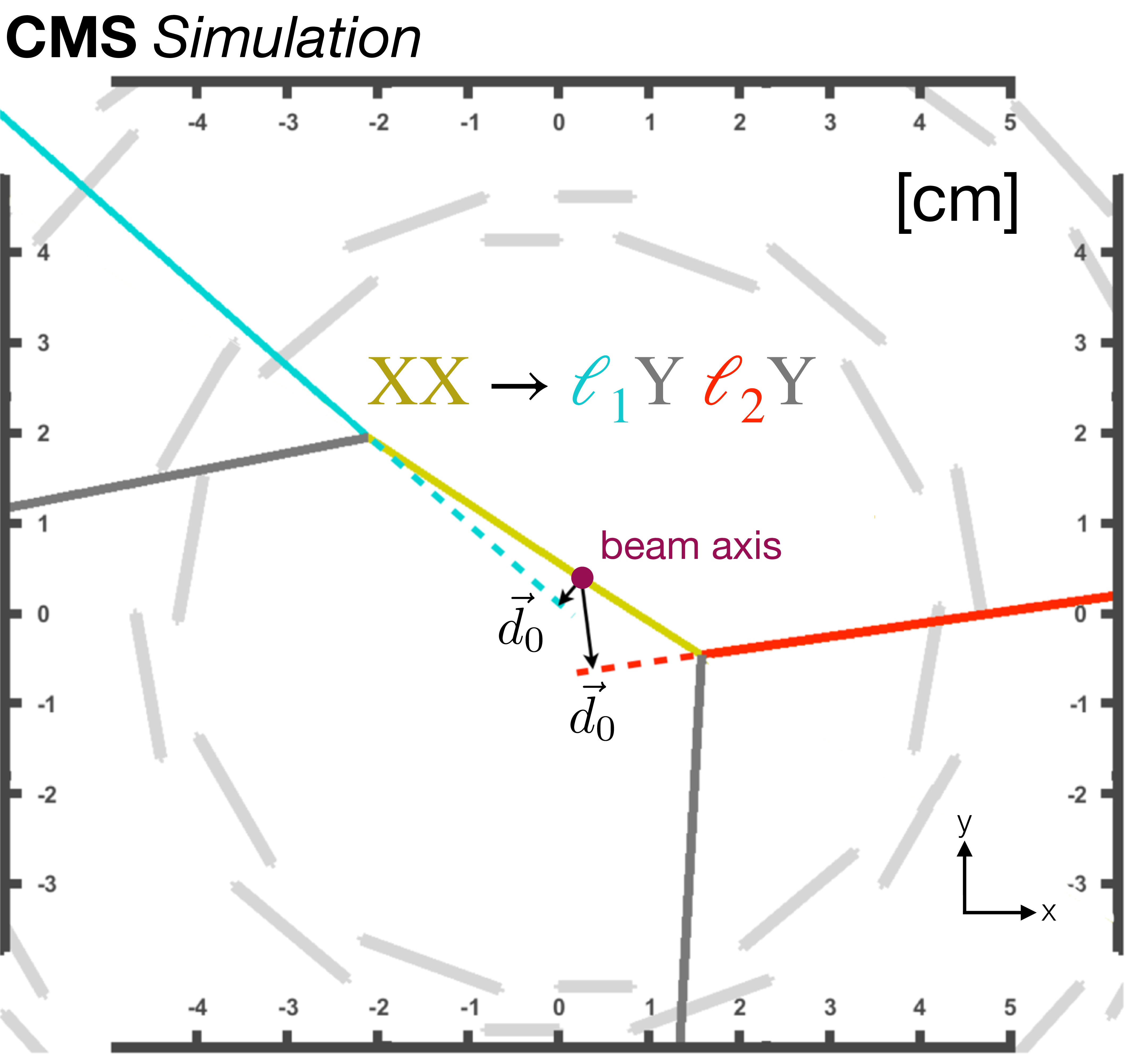
Figure 44:
Diagram of a simulated signal event in the inclusive displaced-lepton search [127], from a transverse view of the IP. The cyan and red solid lines indicate the trajectories of the two leptons, and the two dashed lines indicate the extrapolation of the trajectories towards their point of closest approach to the beam axis. The black arrows, which point from the beam axis and are orthogonal to the cyan and red dotted lines, indicate the lepton $ d_{\text{0}} $ vectors. Figure adapted from Ref. [131]. |
png pdf |
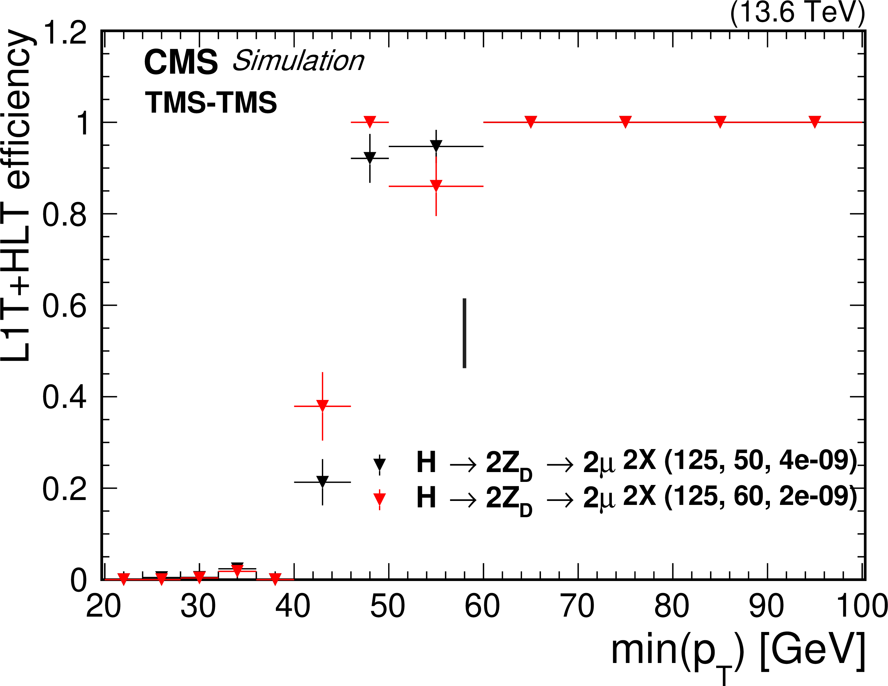
Figure 45:
The L1T+HLT efficiency of the double displaced L3 muon trigger as a function of $ \text{min}(p_{\mathrm{T}}) $ of the two global or tracker muons in the event. The efficiency is plotted for HAHM signal events for 2022 conditions with $ m_{\mathrm{Z}_\text{D}} = $ 50 GeV and $ \epsilon = 4 \times 10^{-9} $ (black triangles), $ m_{\mathrm{Z}_\text{D}} = $ 60 GeV and $ \epsilon = 2 \times 10^{-9} $ (red triangles), and $ m_{\mathrm{H}}= $ 125 GeV in both cases. The events are required to have at least two good global or tracker muons with $ p_{\mathrm{T}} > $ 23 GeV. |
png pdf |
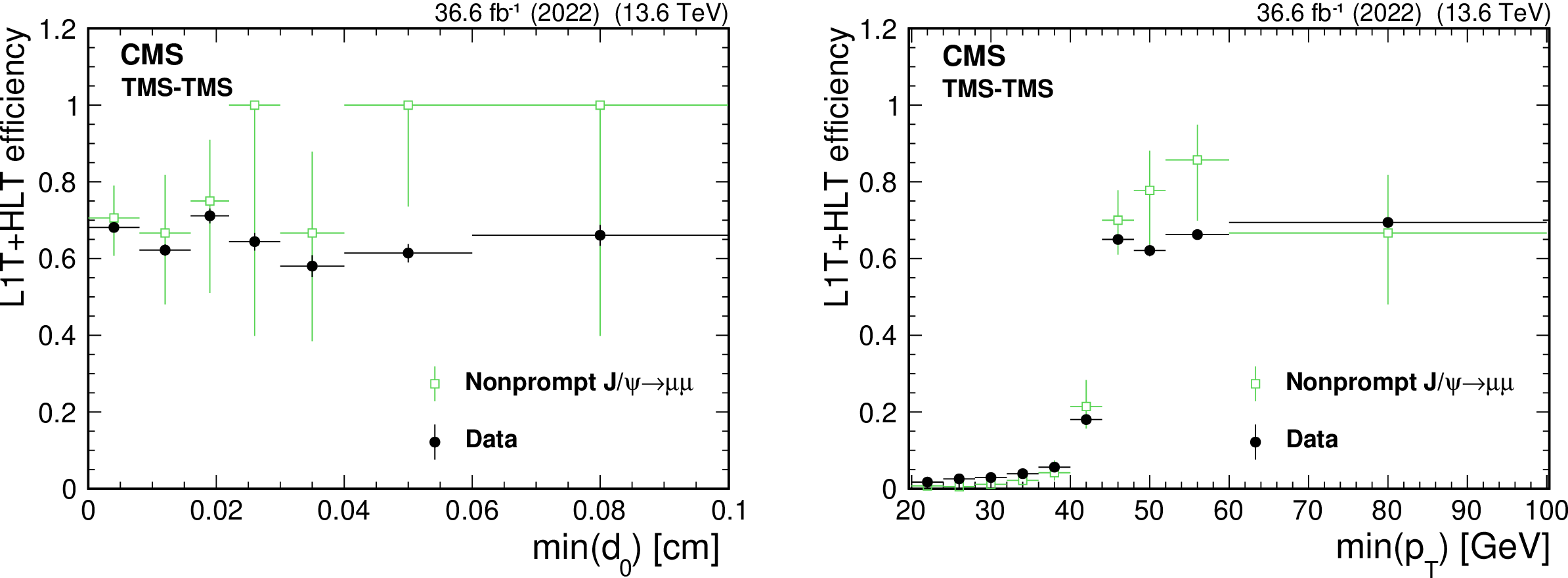
Figure 46:
The L1T+HLT efficiency of the double displaced L3 muon trigger in 2022, as a function of $ \text{min}(d_{\text{0}}) $ (left) and $ \text{min}(p_{\mathrm{T}}) $ (right) of the two global or tracker muons in the event. The efficiency is plotted for simulated $ \mathrm{J}/\psi\to\mu\mu $ events produced in various b hadron decays (open green squares) and data enriched in $ \mathrm{J}/\psi\to\mu\mu $ events recorded by jet- and $ p_{\mathrm{T}}^\text{miss} $-based triggers (filled black circles). The events are required to have at least two good global or tracker muons compatible with the $ \mathrm{J}/\psi $ meson mass and with $ p_{\mathrm{T}} > $ 45 GeV (left) or $ p_{\mathrm{T}} > $ 23 GeV (right). |
png pdf |
Figure 46-a:
The L1T+HLT efficiency of the double displaced L3 muon trigger in 2022, as a function of $ \text{min}(d_{\text{0}}) $ (left) and $ \text{min}(p_{\mathrm{T}}) $ (right) of the two global or tracker muons in the event. The efficiency is plotted for simulated $ \mathrm{J}/\psi\to\mu\mu $ events produced in various b hadron decays (open green squares) and data enriched in $ \mathrm{J}/\psi\to\mu\mu $ events recorded by jet- and $ p_{\mathrm{T}}^\text{miss} $-based triggers (filled black circles). The events are required to have at least two good global or tracker muons compatible with the $ \mathrm{J}/\psi $ meson mass and with $ p_{\mathrm{T}} > $ 45 GeV (left) or $ p_{\mathrm{T}} > $ 23 GeV (right). |
png pdf |
Figure 46-b:
The L1T+HLT efficiency of the double displaced L3 muon trigger in 2022, as a function of $ \text{min}(d_{\text{0}}) $ (left) and $ \text{min}(p_{\mathrm{T}}) $ (right) of the two global or tracker muons in the event. The efficiency is plotted for simulated $ \mathrm{J}/\psi\to\mu\mu $ events produced in various b hadron decays (open green squares) and data enriched in $ \mathrm{J}/\psi\to\mu\mu $ events recorded by jet- and $ p_{\mathrm{T}}^\text{miss} $-based triggers (filled black circles). The events are required to have at least two good global or tracker muons compatible with the $ \mathrm{J}/\psi $ meson mass and with $ p_{\mathrm{T}} > $ 45 GeV (left) or $ p_{\mathrm{T}} > $ 23 GeV (right). |
png pdf |
Figure 47:
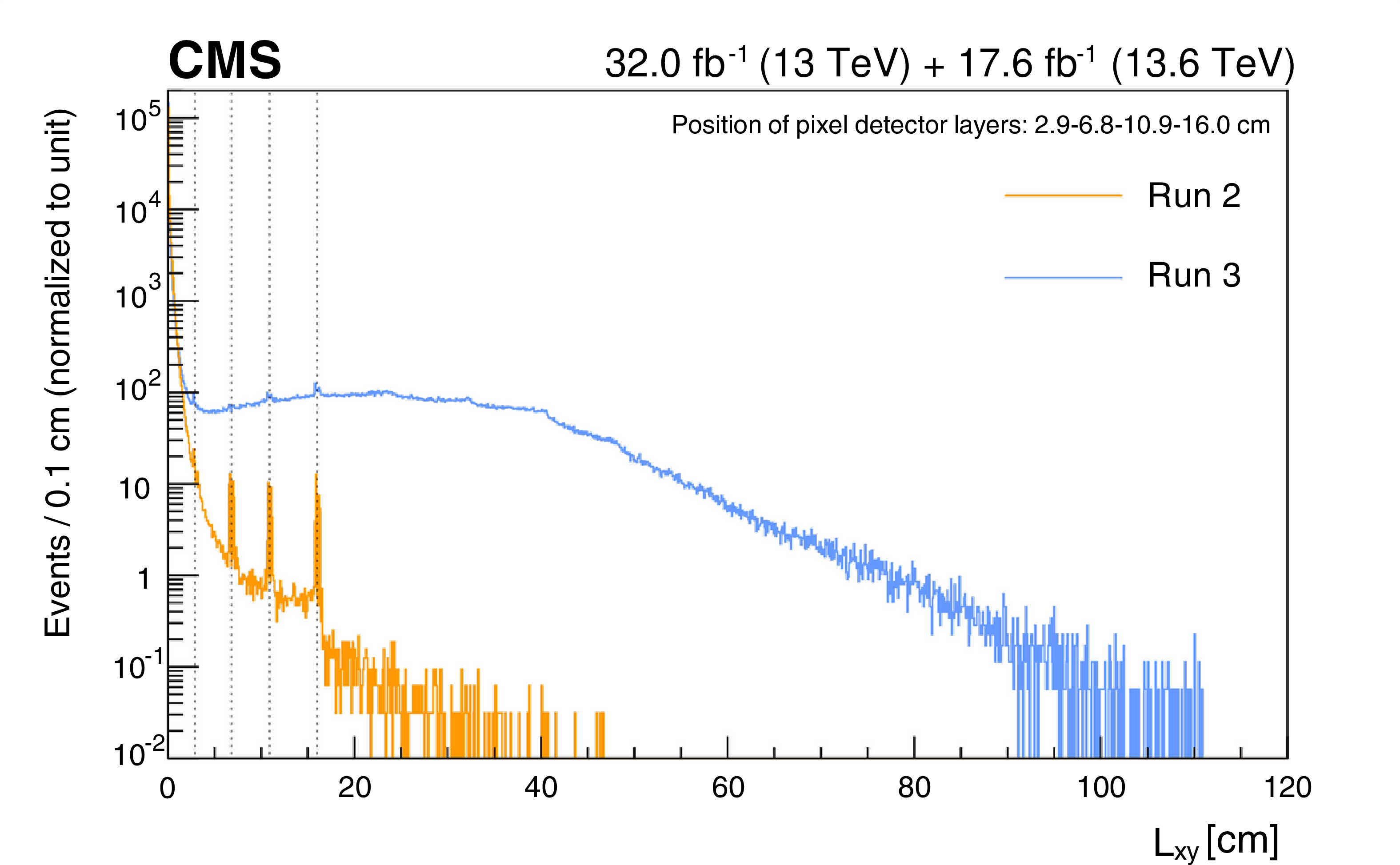
Comparison between the $ L_{\text{xy}} $ distribution for dimuon scouting events for Run 2 (orange) and Run 3 (blue) events in data that contain dimuon pairs with a common displaced vertex and a minimal selection on the vertex quality. The blue Run 3 line is obtained from the vertex-unconstrained muon reconstruction algorithm. The dashed vertical lines, at radii of 2.9, 6.8, 10.9, and 16.0$ \text{cm} $, correspond to the positions of the pixel detector layers where photons undergo conversion processes in the material, causing the observed peaks in the $ L_{\text{xy}} $ distribution. Figure taken from Ref. [45]. |
png pdf |
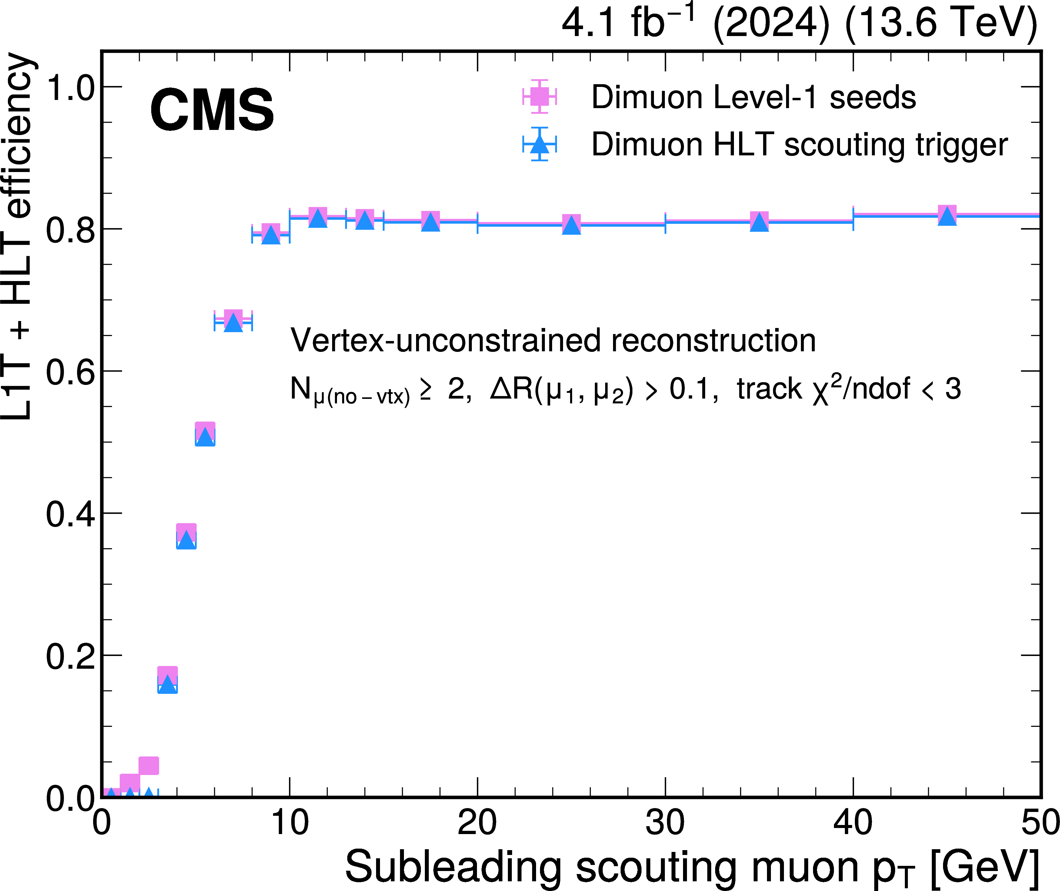
Figure 48:
The L1T+HLT efficiency of the dimuon scouting trigger as a function of the subleading muon $ p_{\mathrm{T}} $, for 2024 data. The efficiency of the L1T dimuon seeds (pink squares) and the HLT dimuon scouting trigger with the vertex-unconstrained reconstruction algorithm (blue triangles) is shown. The events in the denominator are required to have at least two vertex-unconstrained muons ($ N_{\mu $ (no-vtx) $ } > $ 2) and additionally to have $ \chi^2/N_{\text{dof}} < $ 3 and $ \Delta R > $ 0.1. |
png pdf |
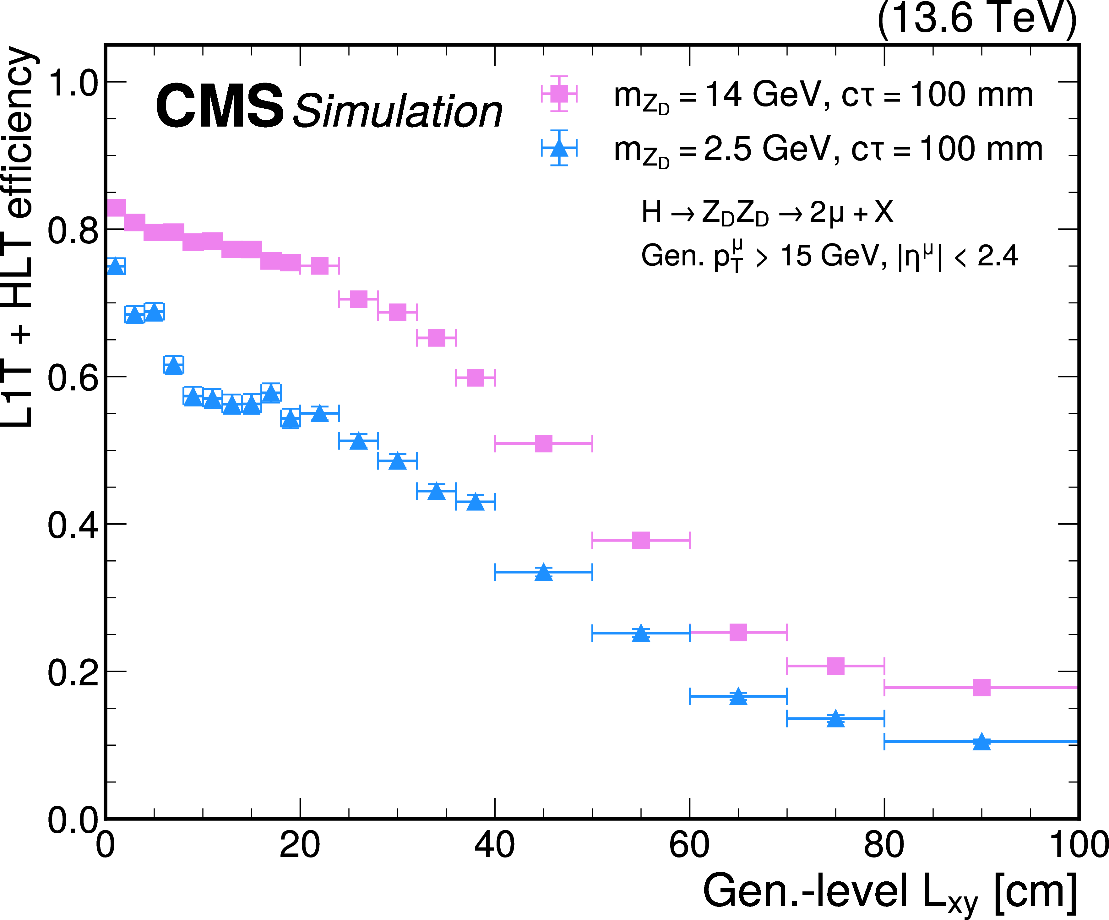
Figure 49:
The L1T+HLT efficiency of the dimuon scouting trigger as a function of the generator-level $ L_{\text{xy}} $, for HAHM signal events, for 2024 conditions. The efficiency is shown for $ m_{\mathrm{Z}_\text{D}} = $ 14 GeV and $ c\tau=100 \text{mm} $ (pink squares) and $ m_{\mathrm{Z}_\text{D}} = $ 2.5 GeV and $ c\tau=100 \text{mm} $ (blue triangles). The muons are required to have $ p_{\mathrm{T}} > $ 15 GeV and $ |\eta| < $ 2.4 at the generator level. |
png pdf |
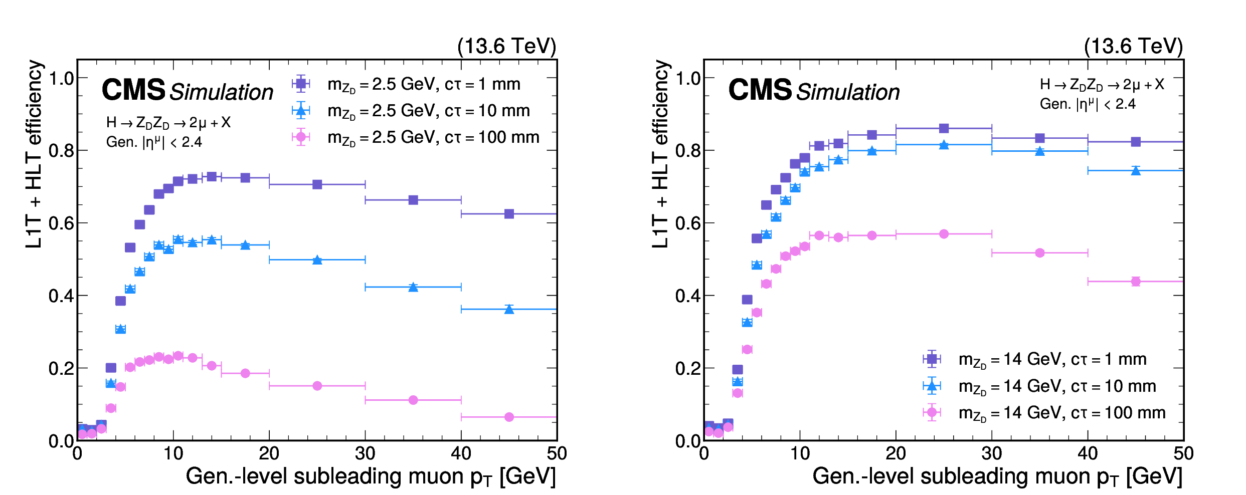
Figure 50:
The L1T+HLT efficiency of the dimuon scouting trigger as a function of the generator-level subleading muon $ p_{\mathrm{T}} $, for HAHM signal events for 2024 conditions. The efficiency is shown for $ \mathrm{Z}_\text{D} $ masses of 2.5 (left) and 14 GeV (right), and $ c\tau $ values of 1 (purple squares), 10 (blue triangles), and 100$ \text{mm} $ (pink circles). The muons are required to have $ |\eta| < $ 2.4 at the generator level. |
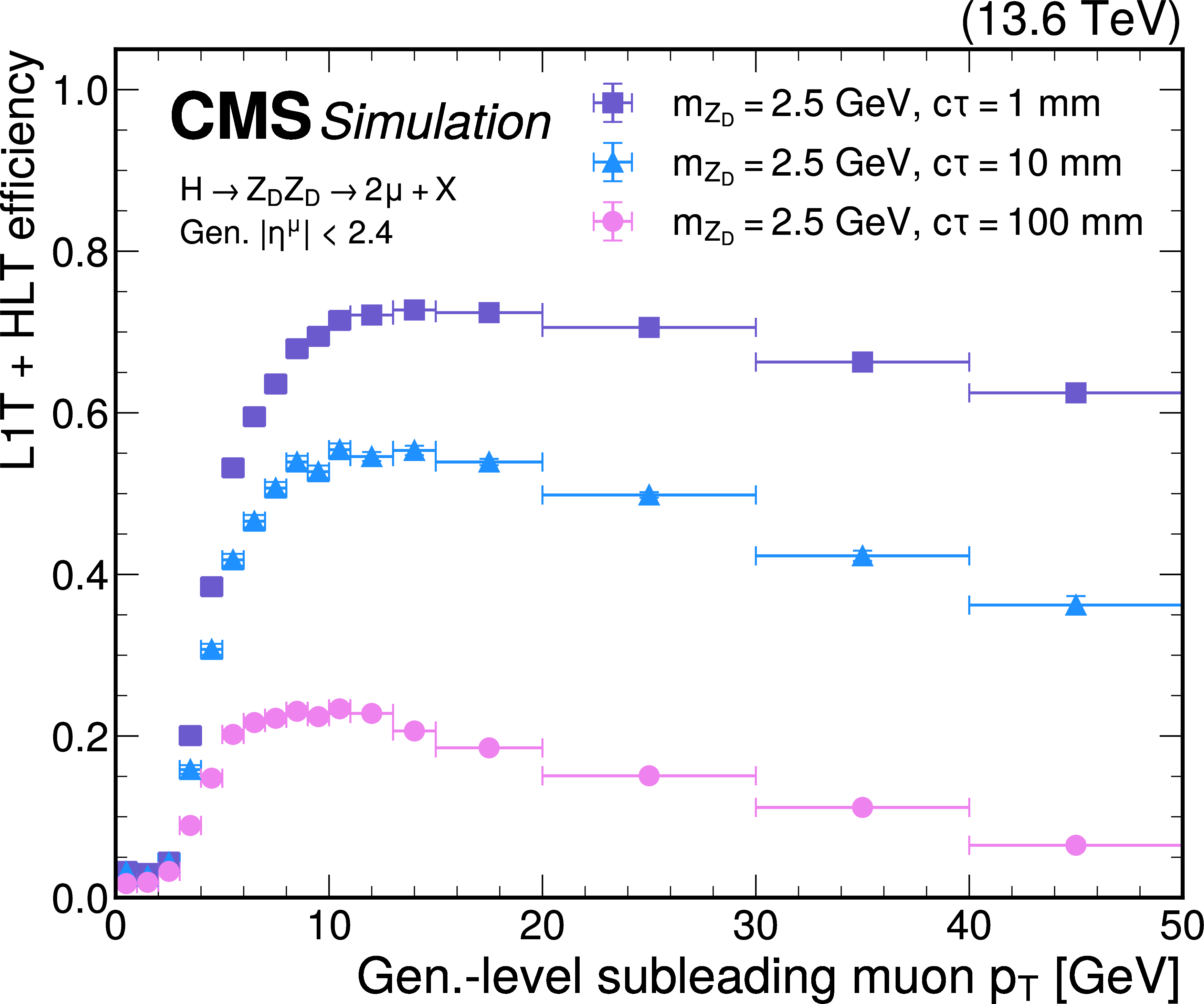
png pdf |
Figure 50-a:
The L1T+HLT efficiency of the dimuon scouting trigger as a function of the generator-level subleading muon $ p_{\mathrm{T}} $, for HAHM signal events for 2024 conditions. The efficiency is shown for $ \mathrm{Z}_\text{D} $ masses of 2.5 (left) and 14 GeV (right), and $ c\tau $ values of 1 (purple squares), 10 (blue triangles), and 100$ \text{mm} $ (pink circles). The muons are required to have $ |\eta| < $ 2.4 at the generator level. |
png pdf |
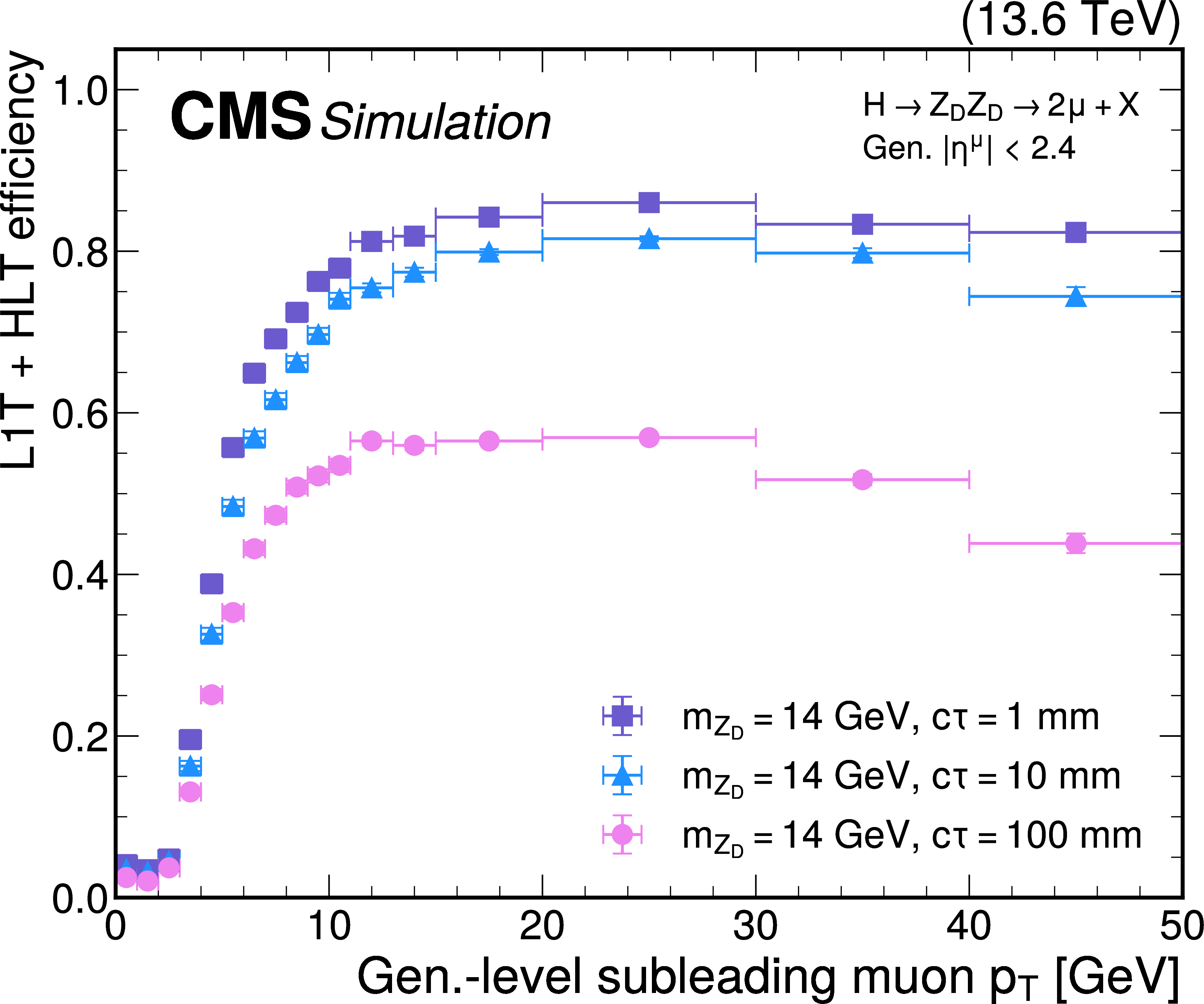
Figure 50-b:
The L1T+HLT efficiency of the dimuon scouting trigger as a function of the generator-level subleading muon $ p_{\mathrm{T}} $, for HAHM signal events for 2024 conditions. The efficiency is shown for $ \mathrm{Z}_\text{D} $ masses of 2.5 (left) and 14 GeV (right), and $ c\tau $ values of 1 (purple squares), 10 (blue triangles), and 100$ \text{mm} $ (pink circles). The muons are required to have $ |\eta| < $ 2.4 at the generator level. |
png pdf |
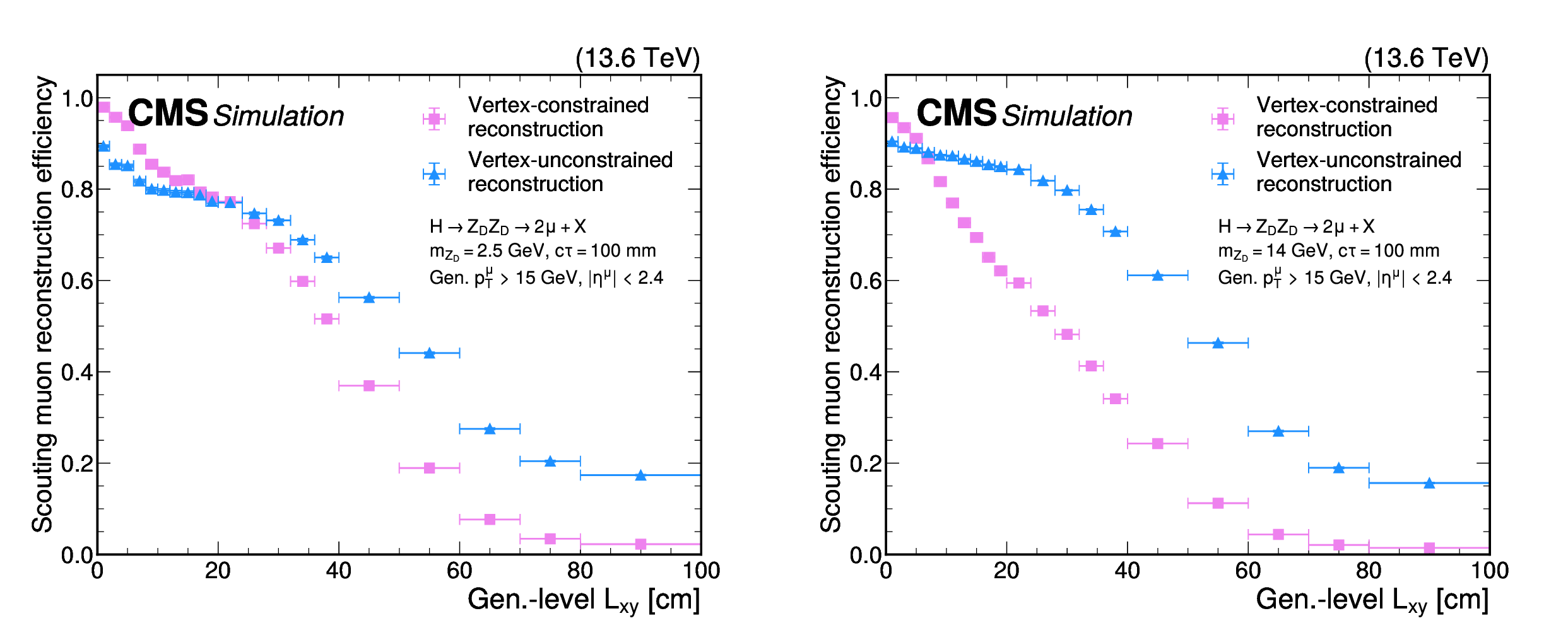
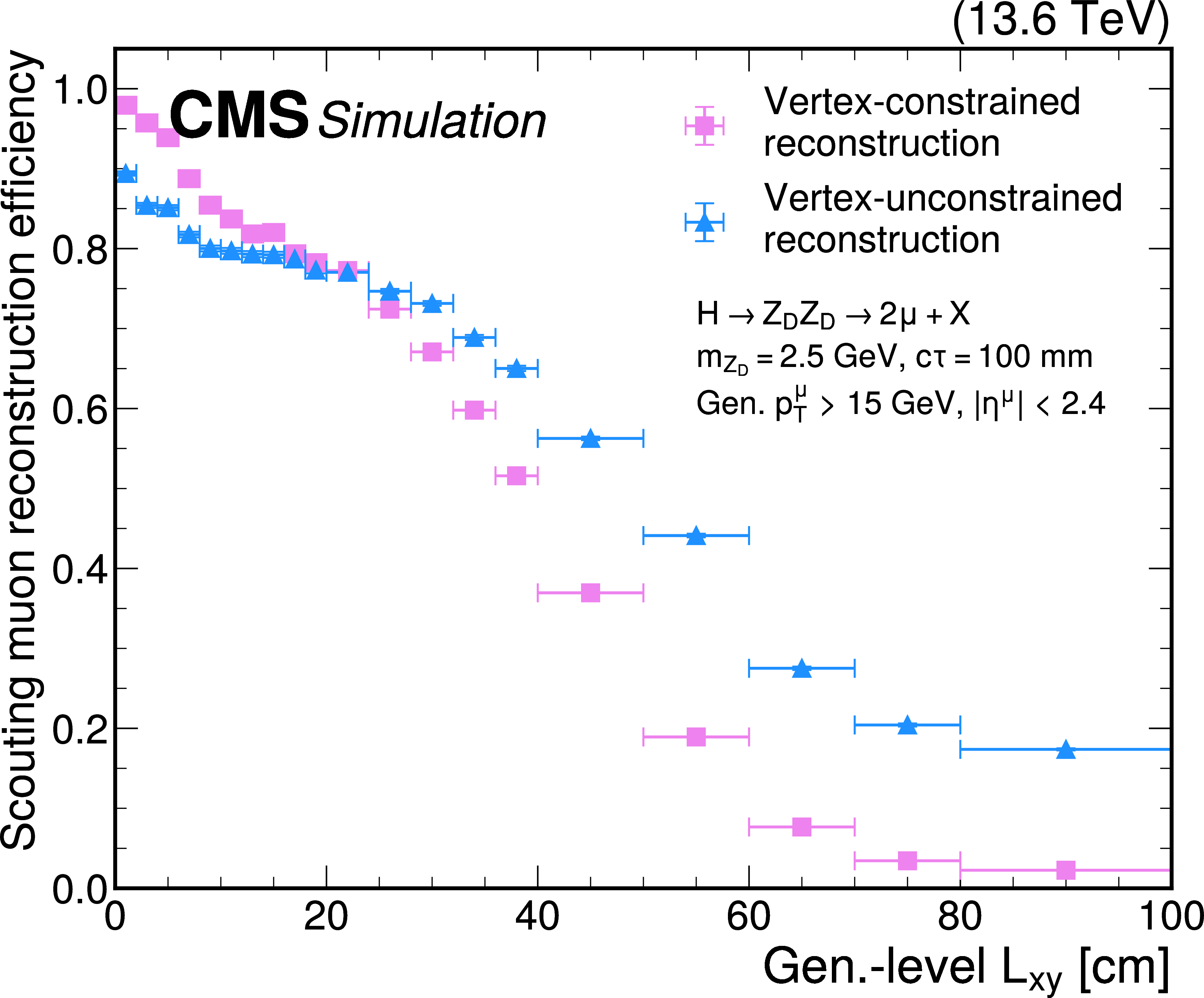
Figure 51:
Scouting muon reconstruction efficiency of the vertex-constrained (pink circles) and vertex-unconstrained (blue triangles) algorithms as a function of the generator-level $ L_{\text{xy}} $, for HAHM signal events for 2024 conditions. This efficiency is representative of the reconstruction efficiency of the L2 and L3 HLT muon reconstruction employed for scouting data. The efficiency is shown for $ m_{\mathrm{Z}_\text{D}} = $ 2.5 GeV and $ c\tau=100 \text{mm} $ (left) and $ m_{\mathrm{Z}_\text{D}} = $ 14 GeV and $ c\tau=100 \text{mm} $ (right). The muons are required to have $ p_{\mathrm{T}} > $ 15 GeV and $ |\eta| < $ 2.4 at the generator level. |
png pdf |
Figure 51-a:
Scouting muon reconstruction efficiency of the vertex-constrained (pink circles) and vertex-unconstrained (blue triangles) algorithms as a function of the generator-level $ L_{\text{xy}} $, for HAHM signal events for 2024 conditions. This efficiency is representative of the reconstruction efficiency of the L2 and L3 HLT muon reconstruction employed for scouting data. The efficiency is shown for $ m_{\mathrm{Z}_\text{D}} = $ 2.5 GeV and $ c\tau=100 \text{mm} $ (left) and $ m_{\mathrm{Z}_\text{D}} = $ 14 GeV and $ c\tau=100 \text{mm} $ (right). The muons are required to have $ p_{\mathrm{T}} > $ 15 GeV and $ |\eta| < $ 2.4 at the generator level. |
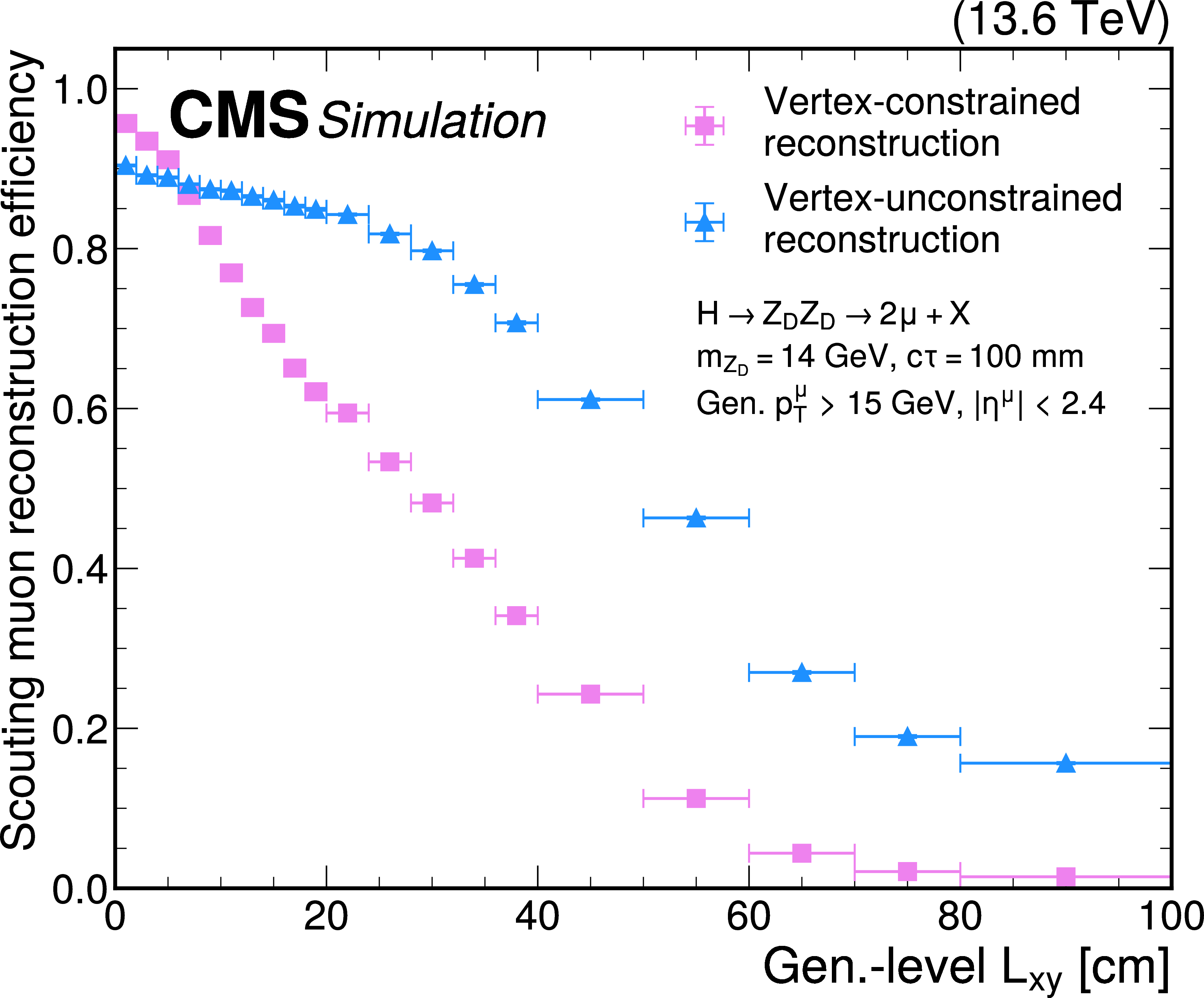
png pdf |
Figure 51-b:
Scouting muon reconstruction efficiency of the vertex-constrained (pink circles) and vertex-unconstrained (blue triangles) algorithms as a function of the generator-level $ L_{\text{xy}} $, for HAHM signal events for 2024 conditions. This efficiency is representative of the reconstruction efficiency of the L2 and L3 HLT muon reconstruction employed for scouting data. The efficiency is shown for $ m_{\mathrm{Z}_\text{D}} = $ 2.5 GeV and $ c\tau=100 \text{mm} $ (left) and $ m_{\mathrm{Z}_\text{D}} = $ 14 GeV and $ c\tau=100 \text{mm} $ (right). The muons are required to have $ p_{\mathrm{T}} > $ 15 GeV and $ |\eta| < $ 2.4 at the generator level. |

png pdf |
Figure 52:
The $ p_{\mathrm{T}} $ resolution of scouting muons with respect to offline muons, as a function of the scouting muon $ p_{\mathrm{T}} $, for 2024 data events. The root mean square (RMS) of the difference of the scouting muon $ p_{\mathrm{T}} $ and the offline muon $ p_{\mathrm{T}} $, divided by the offline muon $ p_{\mathrm{T}} $, is plotted. The dimuon $ \Delta R $ is required to be greater than 0.2, and the scouting muon $ p_{\mathrm{T}} $ is required to be greater than 3 GeV. The resolution is shown for muons in the barrel (filled blue circles) and the endcaps (filled purple triangles) that are reconstructed with both the vertex-unconstrained reconstruction algorithm, as well as for muons in the barrel (filled red squares) and the endcaps (open orange squares) that are reconstructed with the vertex-constrained reconstruction algorithm. A special monitoring data set is used that collects events triggered by a mixture of HLT paths (both scouting and standard triggers) with a very high prescaling factor, in which all information about the muon objects is stored from the offline and scouting reconstruction. |
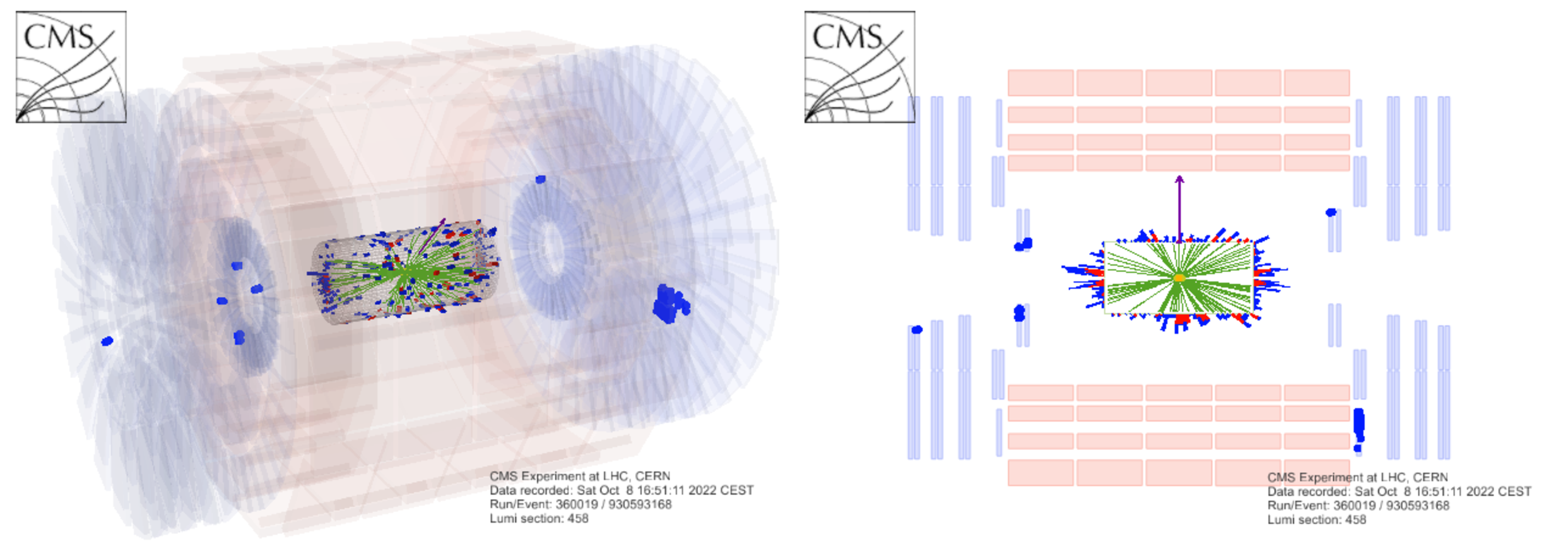
png pdf |
Figure 53:
Event display of a collision triggered by the CSC MDS trigger in Run 3 data. The CSC reconstructed hits are represented by blue dots in the muon endcap region. This event features a CSC cluster of 210 hits in the ME1/3 ring. The event was recorded on October 8th, 2022. |
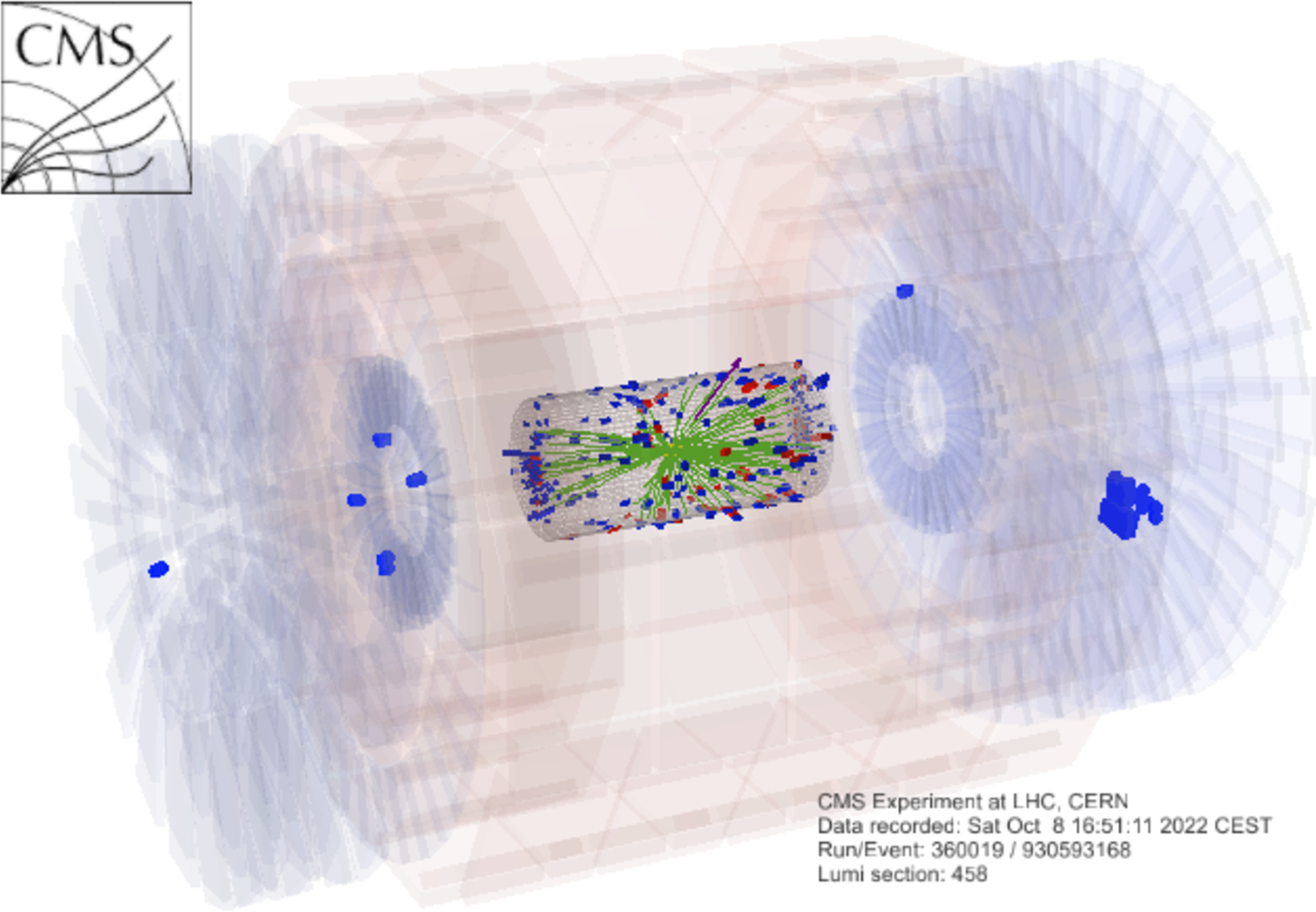
png pdf |
Figure 53-a:
Event display of a collision triggered by the CSC MDS trigger in Run 3 data. The CSC reconstructed hits are represented by blue dots in the muon endcap region. This event features a CSC cluster of 210 hits in the ME1/3 ring. The event was recorded on October 8th, 2022. |
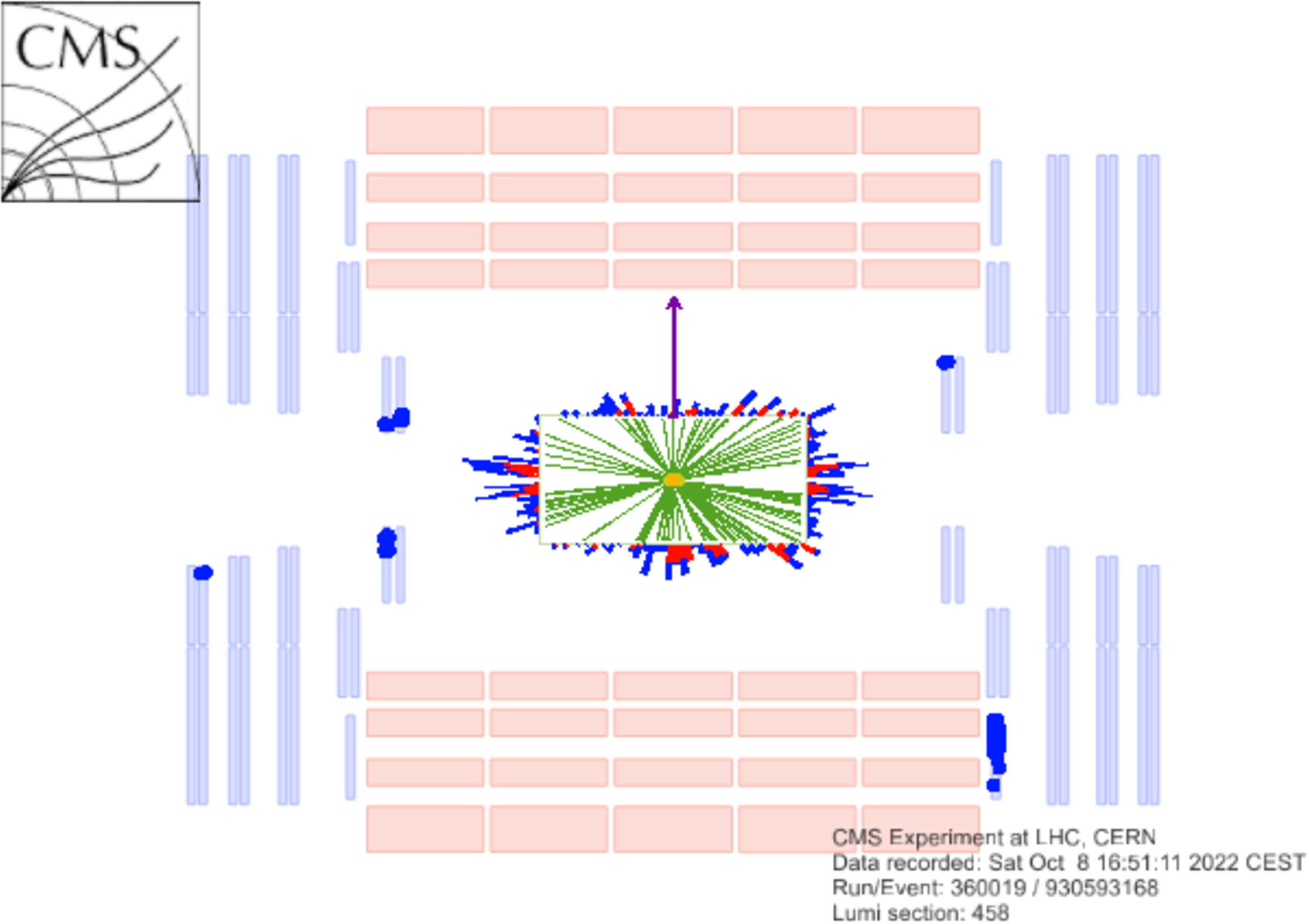
png pdf |
Figure 53-b:
Event display of a collision triggered by the CSC MDS trigger in Run 3 data. The CSC reconstructed hits are represented by blue dots in the muon endcap region. This event features a CSC cluster of 210 hits in the ME1/3 ring. The event was recorded on October 8th, 2022. |
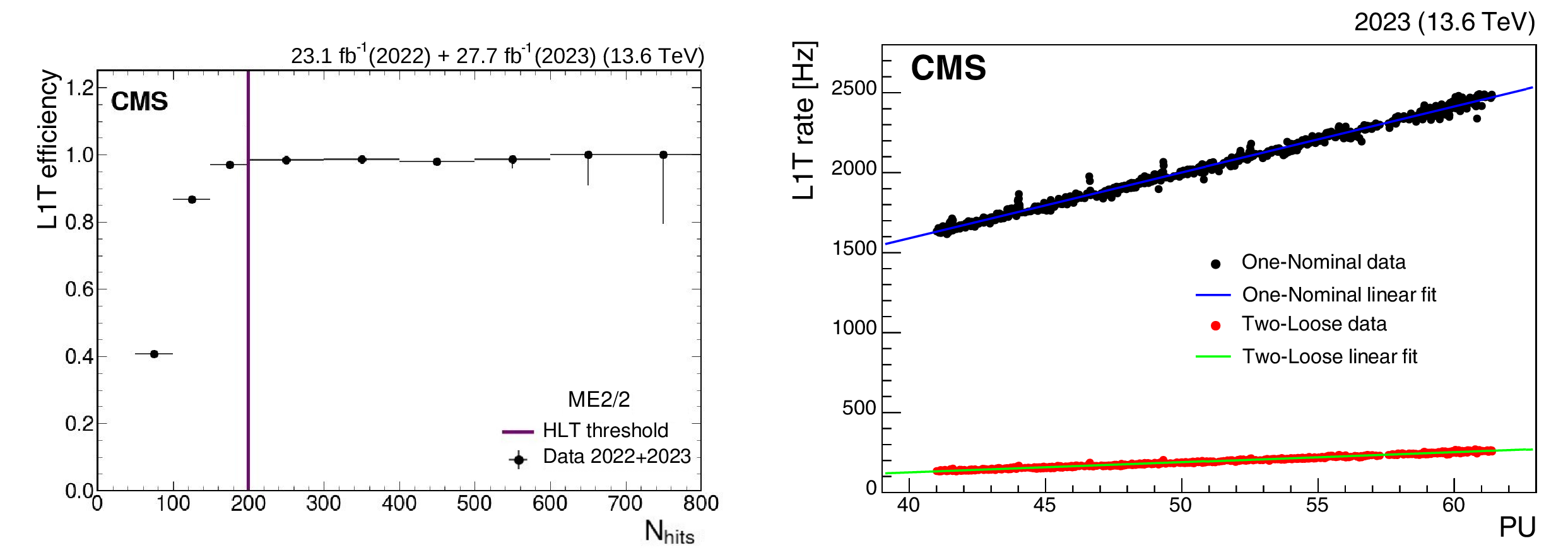
png pdf |
Figure 54:
The L1T efficiency of the One-Nominal CSC MDS trigger in a single CSC ring (ME2/2, indicated in Fig. 1) as a function of the number of hits in the cluster, measured with muon bremsstrahlung-induced electromagnetic showers using data taken in 2022 and 2023 (left). The efficiency is defined as the fraction of events that pass the One-Nominal CSC MDS trigger, given that an uncorrelated trigger selects the data and that a muon is matched to a CSC cluster. The L1T rate as a function of PU for the One-Nominal and Two-Loose seed for a 2023 data-taking run (right). The rate dependence on PU is extracted by a linear fit. |
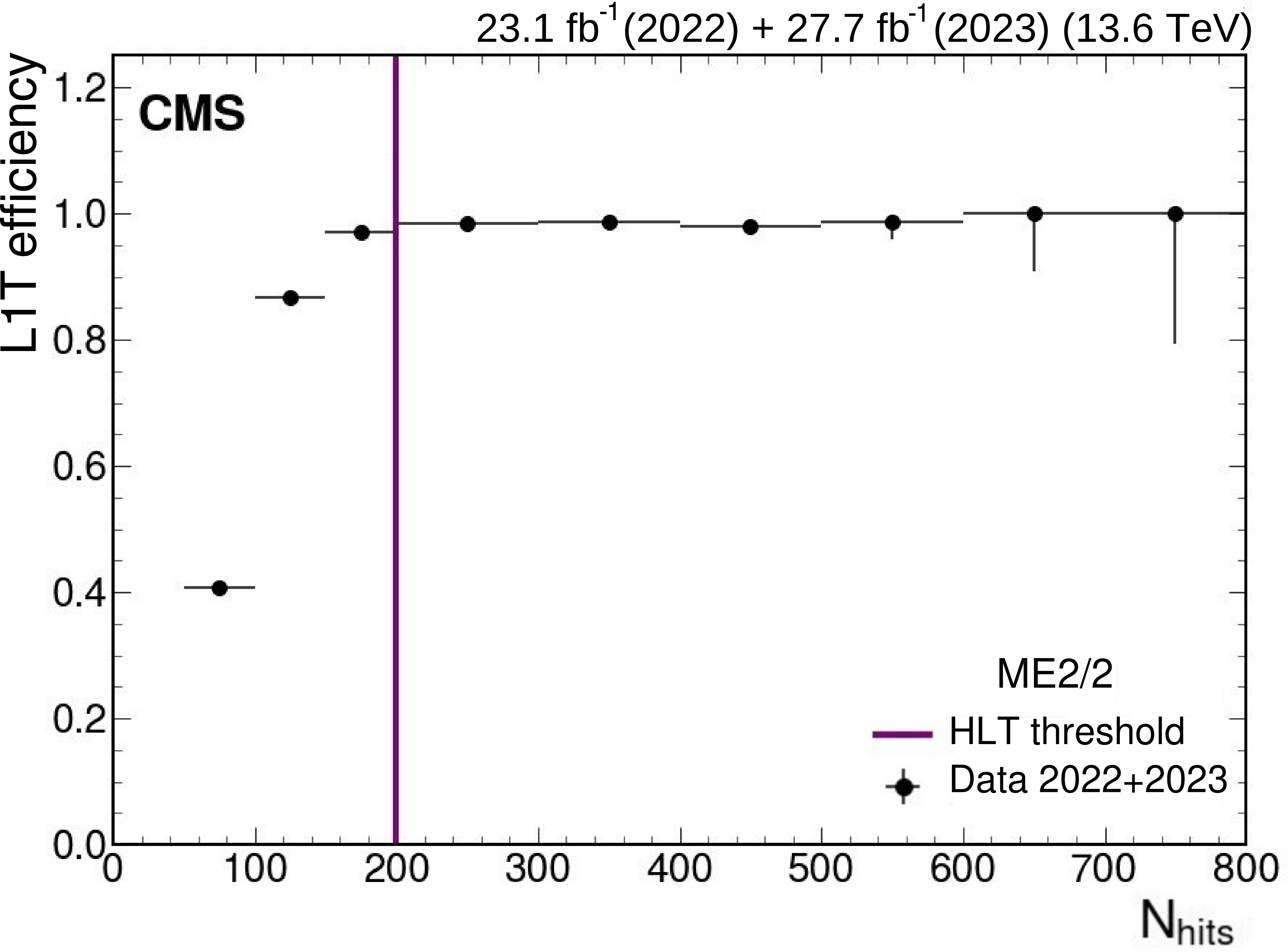
png pdf |
Figure 54-a:
The L1T efficiency of the One-Nominal CSC MDS trigger in a single CSC ring (ME2/2, indicated in Fig. 1) as a function of the number of hits in the cluster, measured with muon bremsstrahlung-induced electromagnetic showers using data taken in 2022 and 2023 (left). The efficiency is defined as the fraction of events that pass the One-Nominal CSC MDS trigger, given that an uncorrelated trigger selects the data and that a muon is matched to a CSC cluster. The L1T rate as a function of PU for the One-Nominal and Two-Loose seed for a 2023 data-taking run (right). The rate dependence on PU is extracted by a linear fit. |
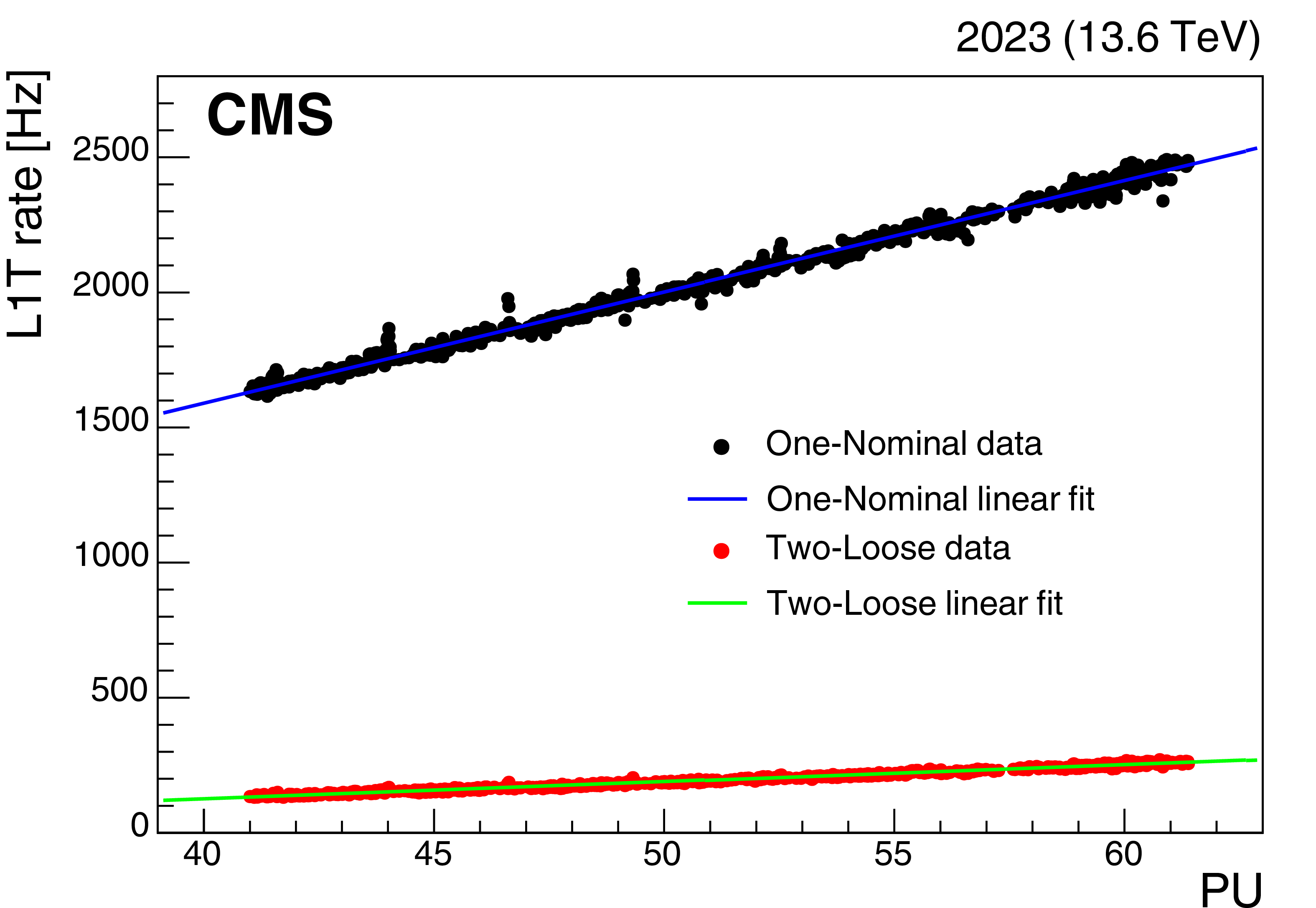
png pdf |
Figure 54-b:
The L1T efficiency of the One-Nominal CSC MDS trigger in a single CSC ring (ME2/2, indicated in Fig. 1) as a function of the number of hits in the cluster, measured with muon bremsstrahlung-induced electromagnetic showers using data taken in 2022 and 2023 (left). The efficiency is defined as the fraction of events that pass the One-Nominal CSC MDS trigger, given that an uncorrelated trigger selects the data and that a muon is matched to a CSC cluster. The L1T rate as a function of PU for the One-Nominal and Two-Loose seed for a 2023 data-taking run (right). The rate dependence on PU is extracted by a linear fit. |
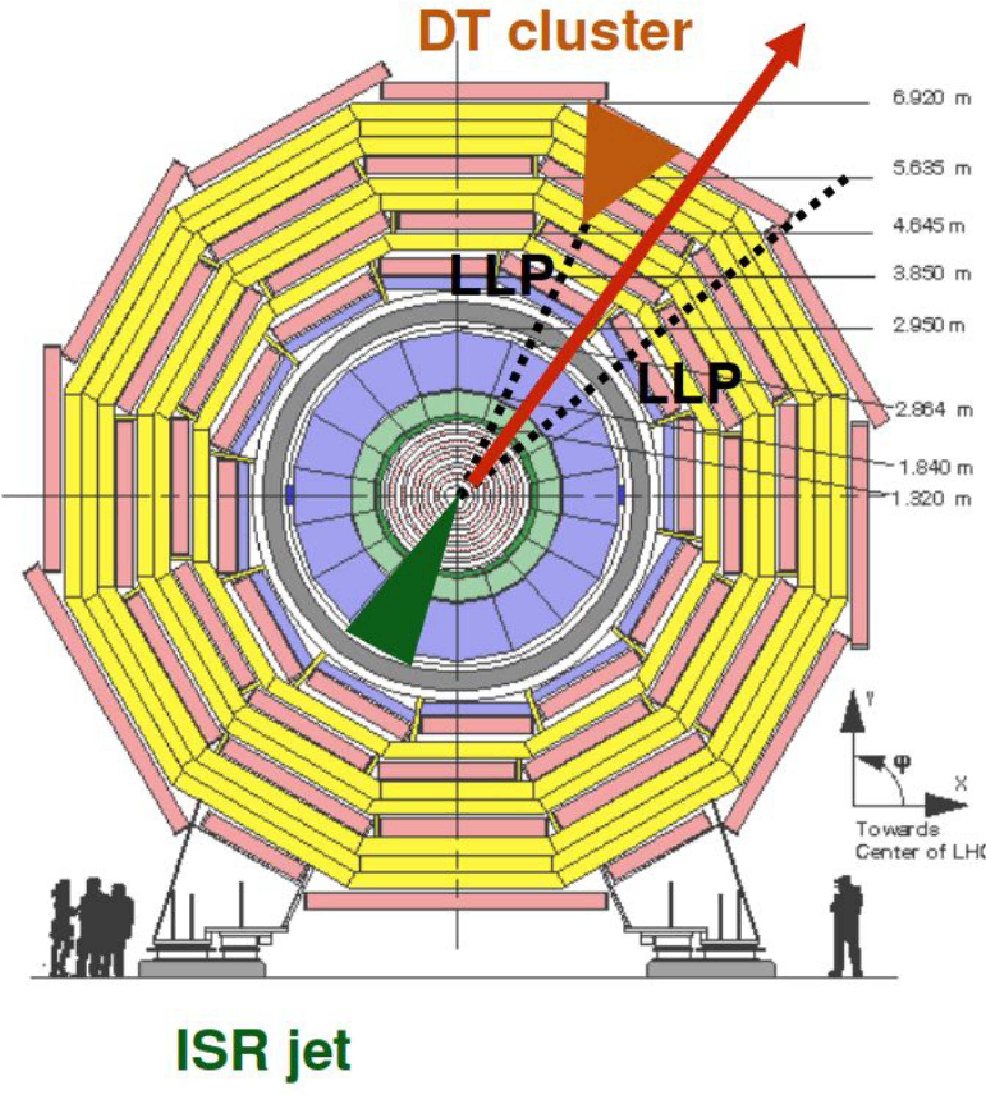
png pdf |
Figure 55:
Diagram of the MDS signature in the DTs. The LLP decays in the DTs, opposite a jet from ISR. |
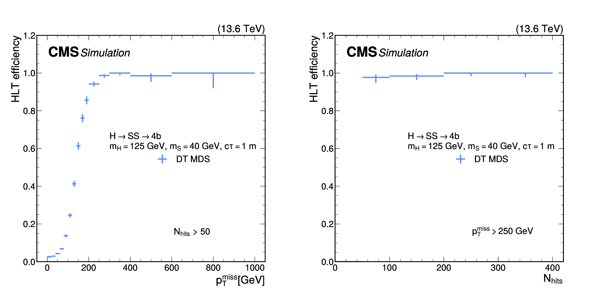
png pdf |
Figure 56:
The HLT efficiency of the DT MDS triggers as a function of $ p_{\mathrm{T}}^\text{miss} $ (left) and the number of hits in the cluster (right), for simulated $ \mathrm{H} \to \text{S}\text{S} \to \mathrm{b}\overline{\mathrm{b}}\mathrm{b}\overline{\mathrm{b}} $ events with $ m_{\mathrm{H}}= $ 125 GeV, $ m_{\text{S}} = $ 40 GeV, and $ c\tau_{\text{S}}= $ 1 m, for 2023 conditions. Events are required to have at least one cluster with more than 50 hits (left) and $ p_{\mathrm{T}}^\text{miss} > $ 250 GeV (right). |
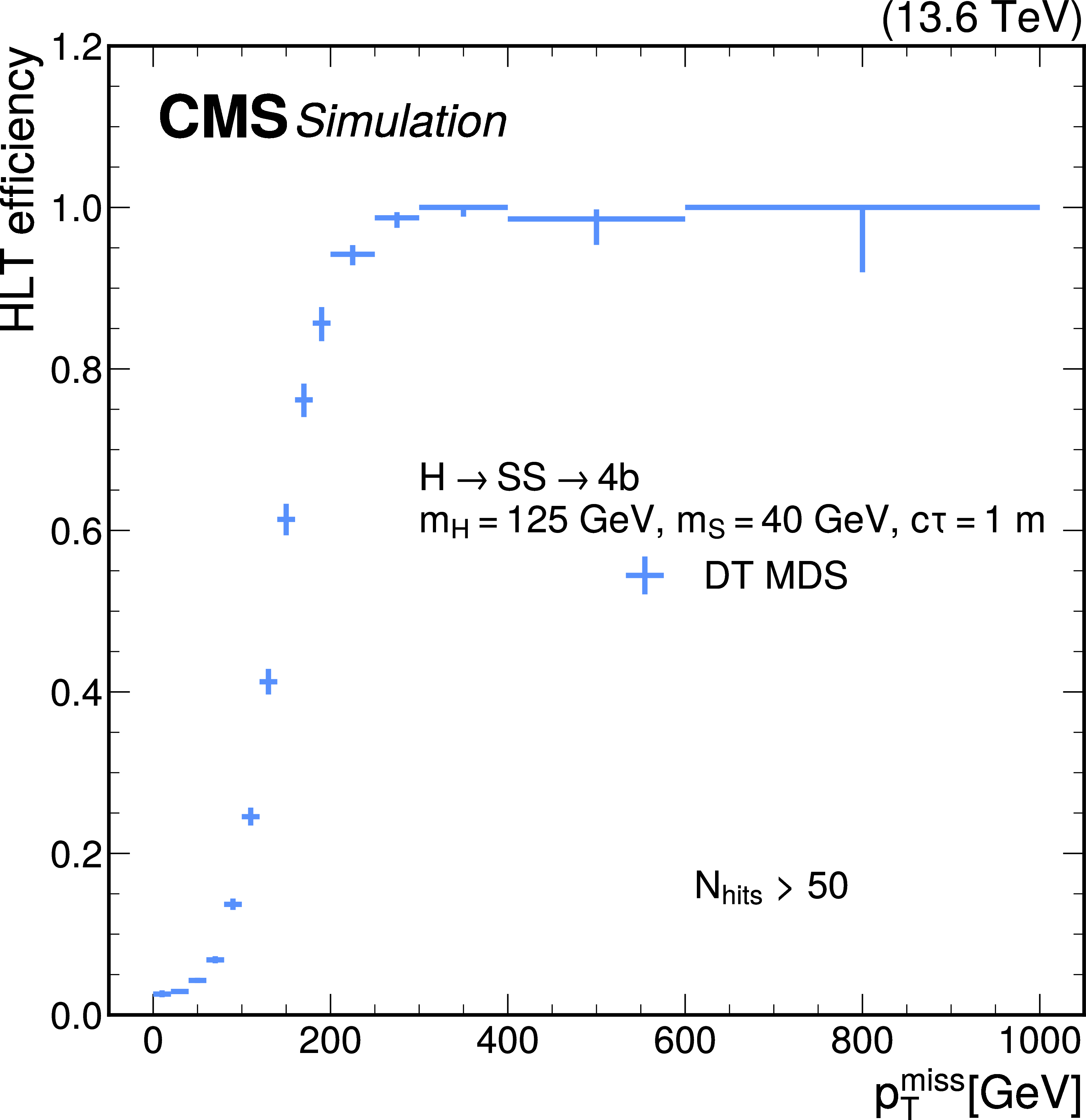
png pdf |
Figure 56-a:
The HLT efficiency of the DT MDS triggers as a function of $ p_{\mathrm{T}}^\text{miss} $ (left) and the number of hits in the cluster (right), for simulated $ \mathrm{H} \to \text{S}\text{S} \to \mathrm{b}\overline{\mathrm{b}}\mathrm{b}\overline{\mathrm{b}} $ events with $ m_{\mathrm{H}}= $ 125 GeV, $ m_{\text{S}} = $ 40 GeV, and $ c\tau_{\text{S}}= $ 1 m, for 2023 conditions. Events are required to have at least one cluster with more than 50 hits (left) and $ p_{\mathrm{T}}^\text{miss} > $ 250 GeV (right). |
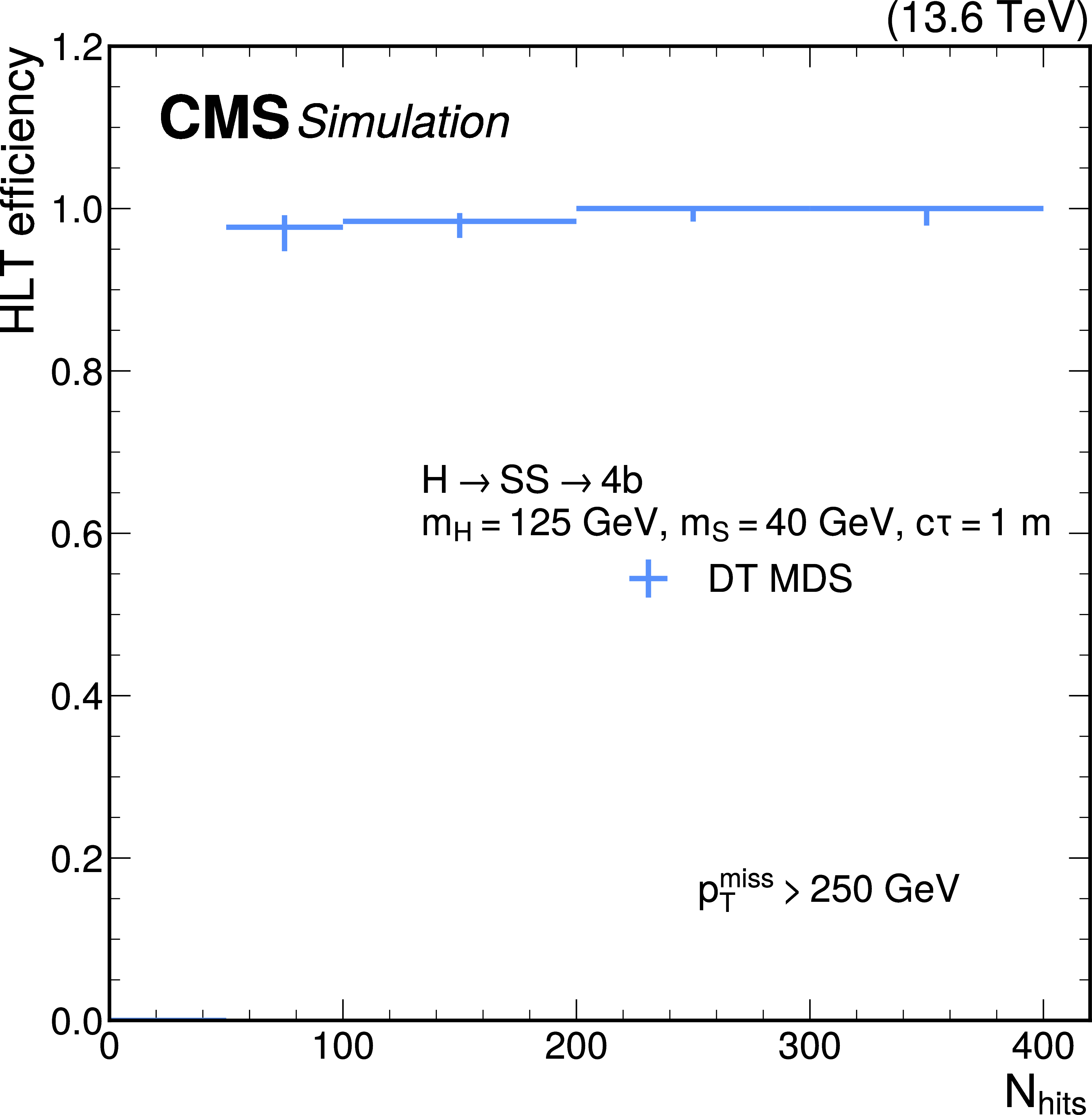
png pdf |
Figure 56-b:
The HLT efficiency of the DT MDS triggers as a function of $ p_{\mathrm{T}}^\text{miss} $ (left) and the number of hits in the cluster (right), for simulated $ \mathrm{H} \to \text{S}\text{S} \to \mathrm{b}\overline{\mathrm{b}}\mathrm{b}\overline{\mathrm{b}} $ events with $ m_{\mathrm{H}}= $ 125 GeV, $ m_{\text{S}} = $ 40 GeV, and $ c\tau_{\text{S}}= $ 1 m, for 2023 conditions. Events are required to have at least one cluster with more than 50 hits (left) and $ p_{\mathrm{T}}^\text{miss} > $ 250 GeV (right). |
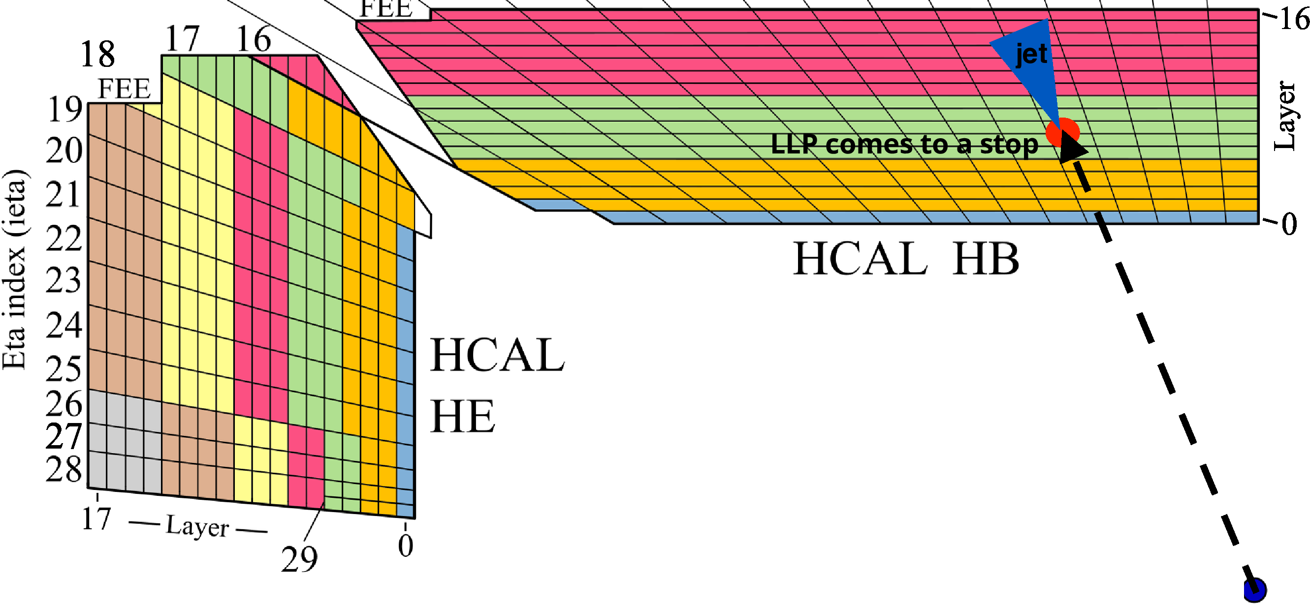
png pdf |
Figure 57:
Diagram of a stopped-particle event, which can be selected by the jet No-BPTX triggers. The dotted black arrow indicates the LLP, such as a gluino, that travels through the detector before coming to a stop in the dense material of the HCAL. After some time, this stopped particle decays hadronically, producing a significant energy deposit in the HCAL. |
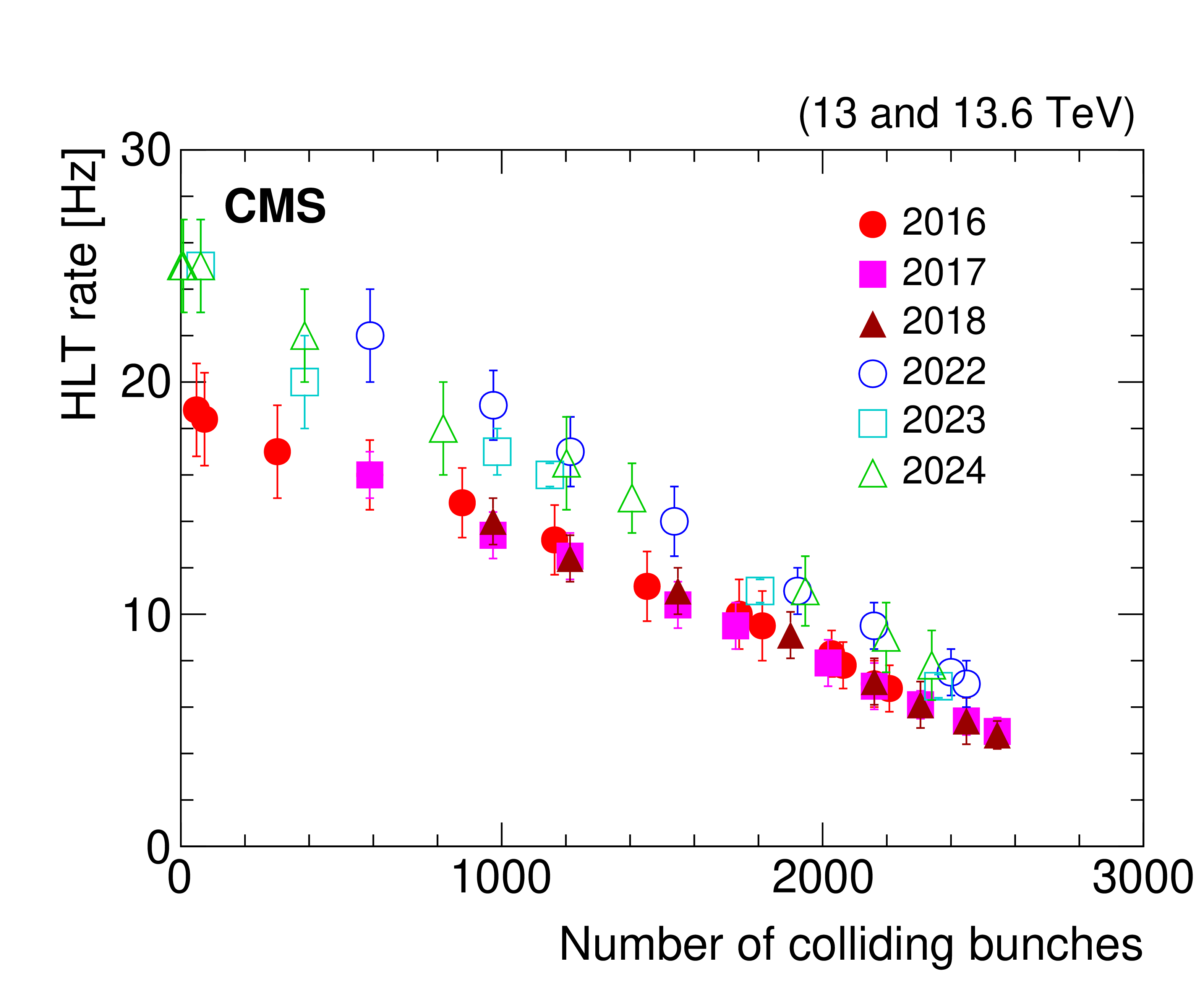
png pdf |
Figure 58:
Rate of the main muon No-BPTX HLT path as a function of the number of colliding bunches, for different years in Run 2 and Run 3. |
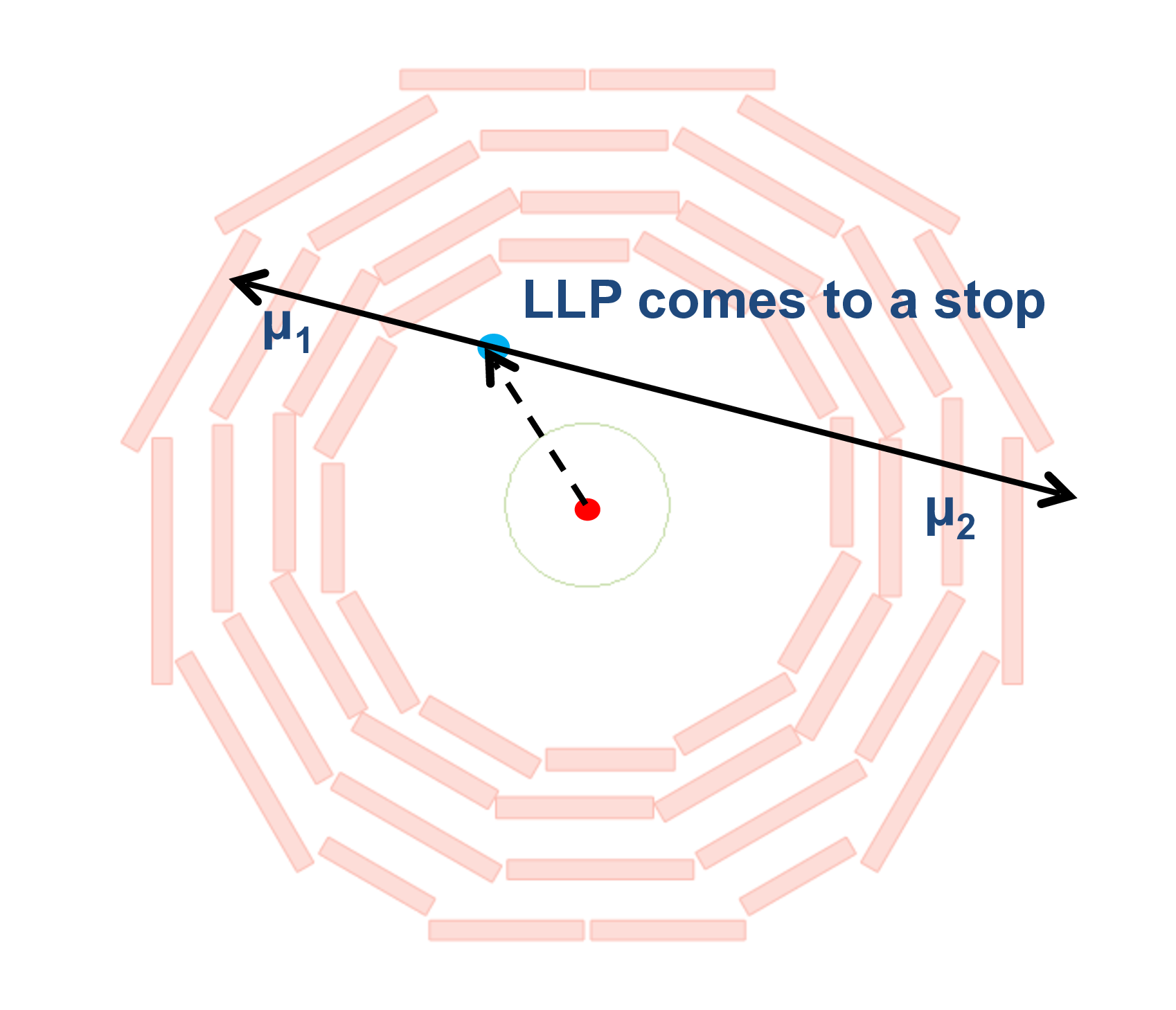
png pdf |
Figure 59:
Diagram of a stopped-particle event, which can be selected by the muon No-BPTX triggers. The dotted black arrow indicates the LLP that travels through the detector before coming to a stop in the steel yoke in the muon system. After some time, this stopped particle decays to two back-to-back muons. |
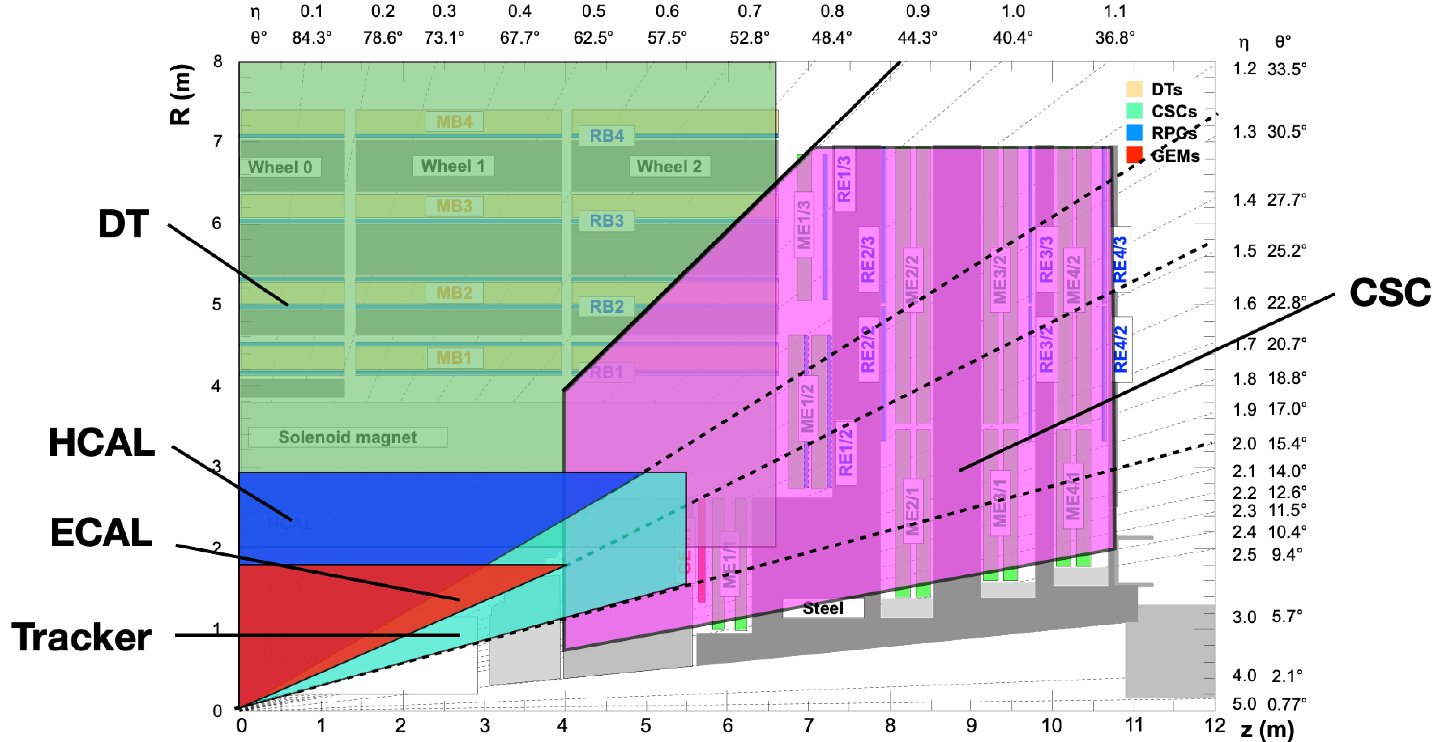
png pdf |
Figure 60:
The fiducial regions defined for the calculation of each trigger acceptance in Figs. 61 and 62. The ``Tracker'' region labeled in this figure refers to the fiducial region of the displaced-jet triggers using the tracker, which is larger than the physical volume of the tracker detector. The text contains the exact definitions of each region. |
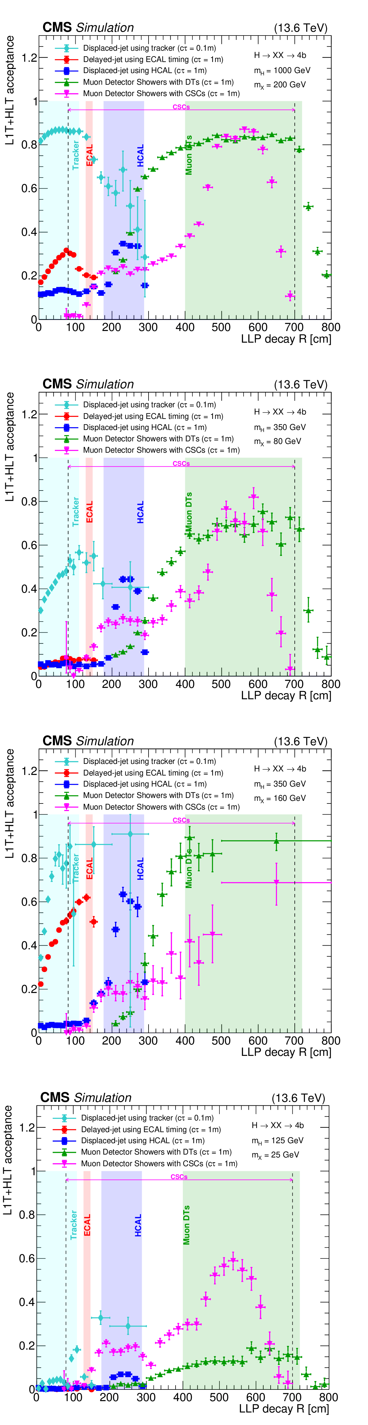
png pdf |
Figure 61:
The L1T+HLT acceptances for various LLP triggers using different subdetectors, as functions of the LLP decay radial position, for $ \mathrm{H} \to \mathrm{X}\mathrm{X} \to \mathrm{b}\overline{\mathrm{b}}\mathrm{b}\overline{\mathrm{b}} $ events for 2023 conditions. The plots correspond to different signal models with $ m_{\mathrm{H}}= $ 1000 GeV and $ m_{\mathrm{X}}= $ 200 GeV on the upper left; $ m_{\mathrm{H}}= $ 350 GeV and $ m_{\mathrm{X}}= $ 80 GeV on the upper right; $ m_{\mathrm{H}}= $ 350 GeV and $ m_{\mathrm{X}}= $ 160 GeV on the lower left; and $ m_{\mathrm{H}}= $ 125 GeV and $ m_{\mathrm{X}}= $ 25 GeV on the lower right. In each of these plots, the $ c\tau $ is 0.1\unitm for the displaced-jet triggers using the tracker and 1\unitm for the other triggers. The acceptance is shown for the displaced-jet triggers using the tracker (cyan diamonds), for the delayed-jet triggers using ECAL timing (red circles), for the displaced-jet triggers using the HCAL (blue squares), for the MDS triggers with the DTs (green triangles), and for the MDS triggers with the CSCs (pink triangles). The boundaries of the tracker, ECAL, HCAL, DTs, and CSCs are also shown in the figures. |
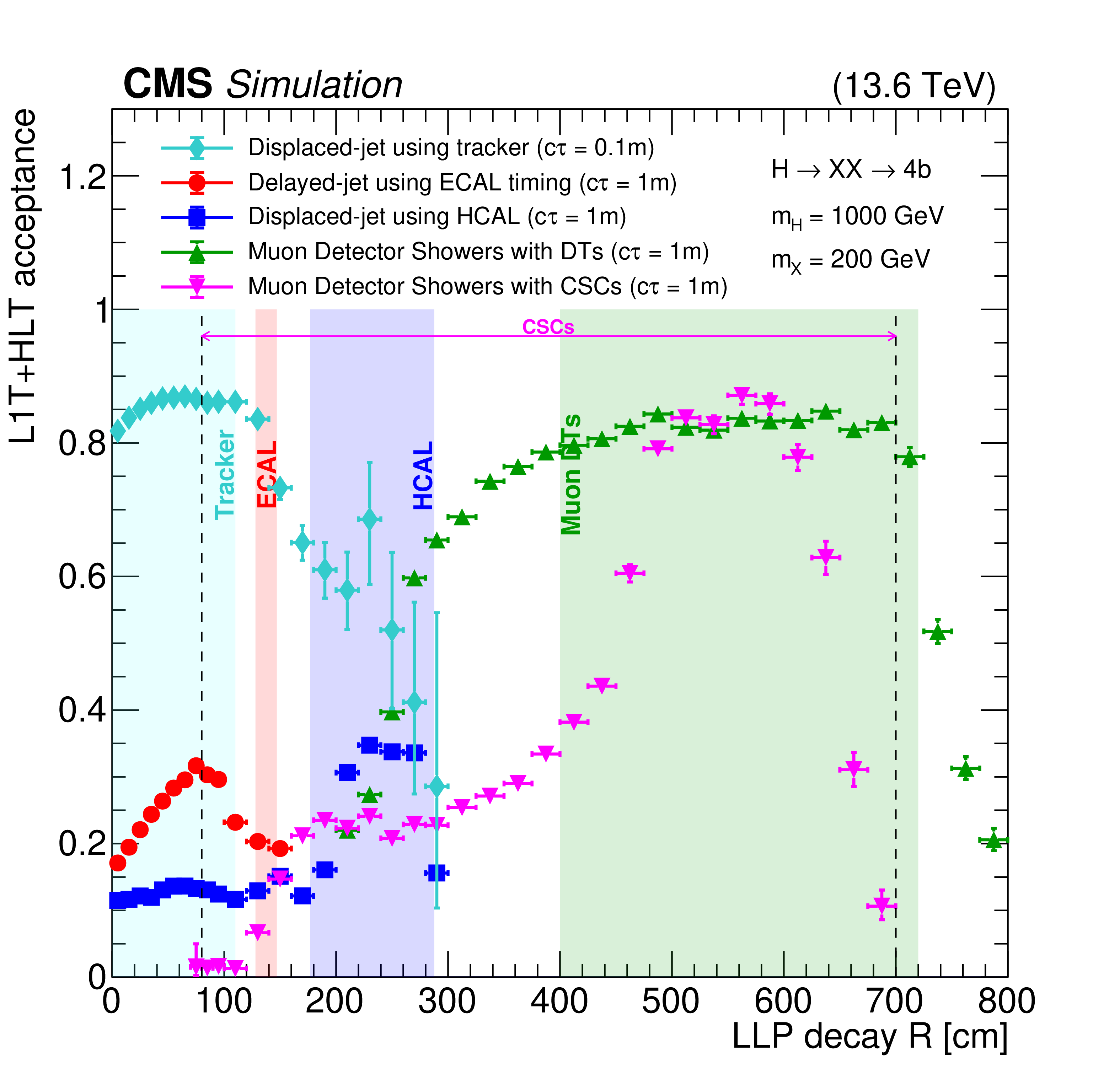
png pdf |
Figure 61-a:
The L1T+HLT acceptances for various LLP triggers using different subdetectors, as functions of the LLP decay radial position, for $ \mathrm{H} \to \mathrm{X}\mathrm{X} \to \mathrm{b}\overline{\mathrm{b}}\mathrm{b}\overline{\mathrm{b}} $ events for 2023 conditions. The plots correspond to different signal models with $ m_{\mathrm{H}}= $ 1000 GeV and $ m_{\mathrm{X}}= $ 200 GeV on the upper left; $ m_{\mathrm{H}}= $ 350 GeV and $ m_{\mathrm{X}}= $ 80 GeV on the upper right; $ m_{\mathrm{H}}= $ 350 GeV and $ m_{\mathrm{X}}= $ 160 GeV on the lower left; and $ m_{\mathrm{H}}= $ 125 GeV and $ m_{\mathrm{X}}= $ 25 GeV on the lower right. In each of these plots, the $ c\tau $ is 0.1\unitm for the displaced-jet triggers using the tracker and 1\unitm for the other triggers. The acceptance is shown for the displaced-jet triggers using the tracker (cyan diamonds), for the delayed-jet triggers using ECAL timing (red circles), for the displaced-jet triggers using the HCAL (blue squares), for the MDS triggers with the DTs (green triangles), and for the MDS triggers with the CSCs (pink triangles). The boundaries of the tracker, ECAL, HCAL, DTs, and CSCs are also shown in the figures. |
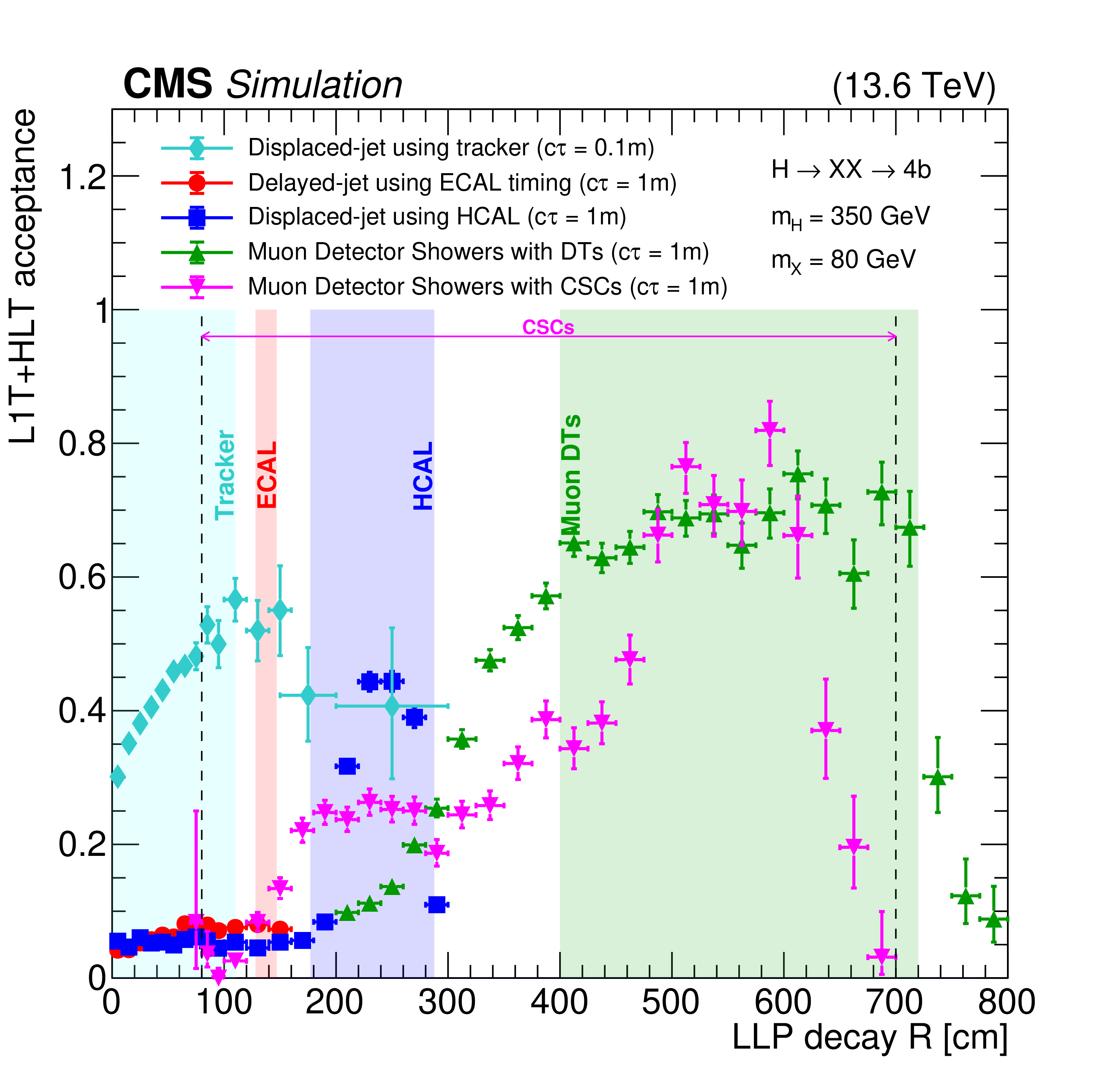
png pdf |
Figure 61-b:
The L1T+HLT acceptances for various LLP triggers using different subdetectors, as functions of the LLP decay radial position, for $ \mathrm{H} \to \mathrm{X}\mathrm{X} \to \mathrm{b}\overline{\mathrm{b}}\mathrm{b}\overline{\mathrm{b}} $ events for 2023 conditions. The plots correspond to different signal models with $ m_{\mathrm{H}}= $ 1000 GeV and $ m_{\mathrm{X}}= $ 200 GeV on the upper left; $ m_{\mathrm{H}}= $ 350 GeV and $ m_{\mathrm{X}}= $ 80 GeV on the upper right; $ m_{\mathrm{H}}= $ 350 GeV and $ m_{\mathrm{X}}= $ 160 GeV on the lower left; and $ m_{\mathrm{H}}= $ 125 GeV and $ m_{\mathrm{X}}= $ 25 GeV on the lower right. In each of these plots, the $ c\tau $ is 0.1\unitm for the displaced-jet triggers using the tracker and 1\unitm for the other triggers. The acceptance is shown for the displaced-jet triggers using the tracker (cyan diamonds), for the delayed-jet triggers using ECAL timing (red circles), for the displaced-jet triggers using the HCAL (blue squares), for the MDS triggers with the DTs (green triangles), and for the MDS triggers with the CSCs (pink triangles). The boundaries of the tracker, ECAL, HCAL, DTs, and CSCs are also shown in the figures. |
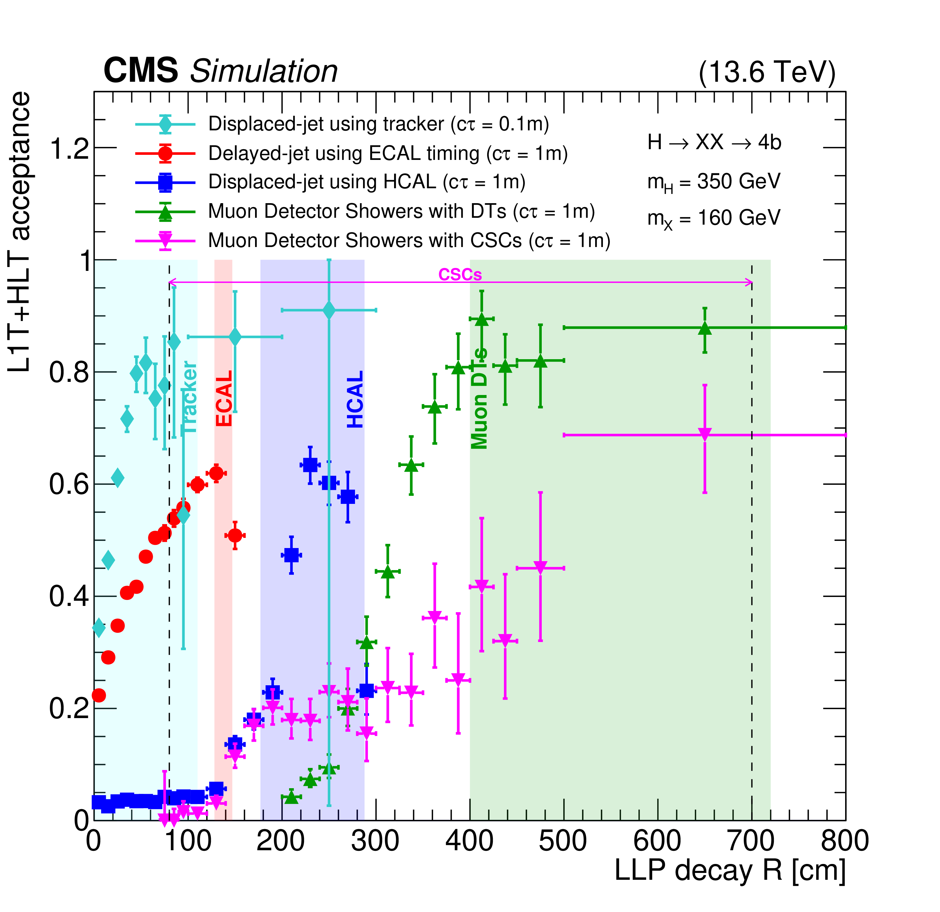
png pdf |
Figure 61-c:
The L1T+HLT acceptances for various LLP triggers using different subdetectors, as functions of the LLP decay radial position, for $ \mathrm{H} \to \mathrm{X}\mathrm{X} \to \mathrm{b}\overline{\mathrm{b}}\mathrm{b}\overline{\mathrm{b}} $ events for 2023 conditions. The plots correspond to different signal models with $ m_{\mathrm{H}}= $ 1000 GeV and $ m_{\mathrm{X}}= $ 200 GeV on the upper left; $ m_{\mathrm{H}}= $ 350 GeV and $ m_{\mathrm{X}}= $ 80 GeV on the upper right; $ m_{\mathrm{H}}= $ 350 GeV and $ m_{\mathrm{X}}= $ 160 GeV on the lower left; and $ m_{\mathrm{H}}= $ 125 GeV and $ m_{\mathrm{X}}= $ 25 GeV on the lower right. In each of these plots, the $ c\tau $ is 0.1\unitm for the displaced-jet triggers using the tracker and 1\unitm for the other triggers. The acceptance is shown for the displaced-jet triggers using the tracker (cyan diamonds), for the delayed-jet triggers using ECAL timing (red circles), for the displaced-jet triggers using the HCAL (blue squares), for the MDS triggers with the DTs (green triangles), and for the MDS triggers with the CSCs (pink triangles). The boundaries of the tracker, ECAL, HCAL, DTs, and CSCs are also shown in the figures. |
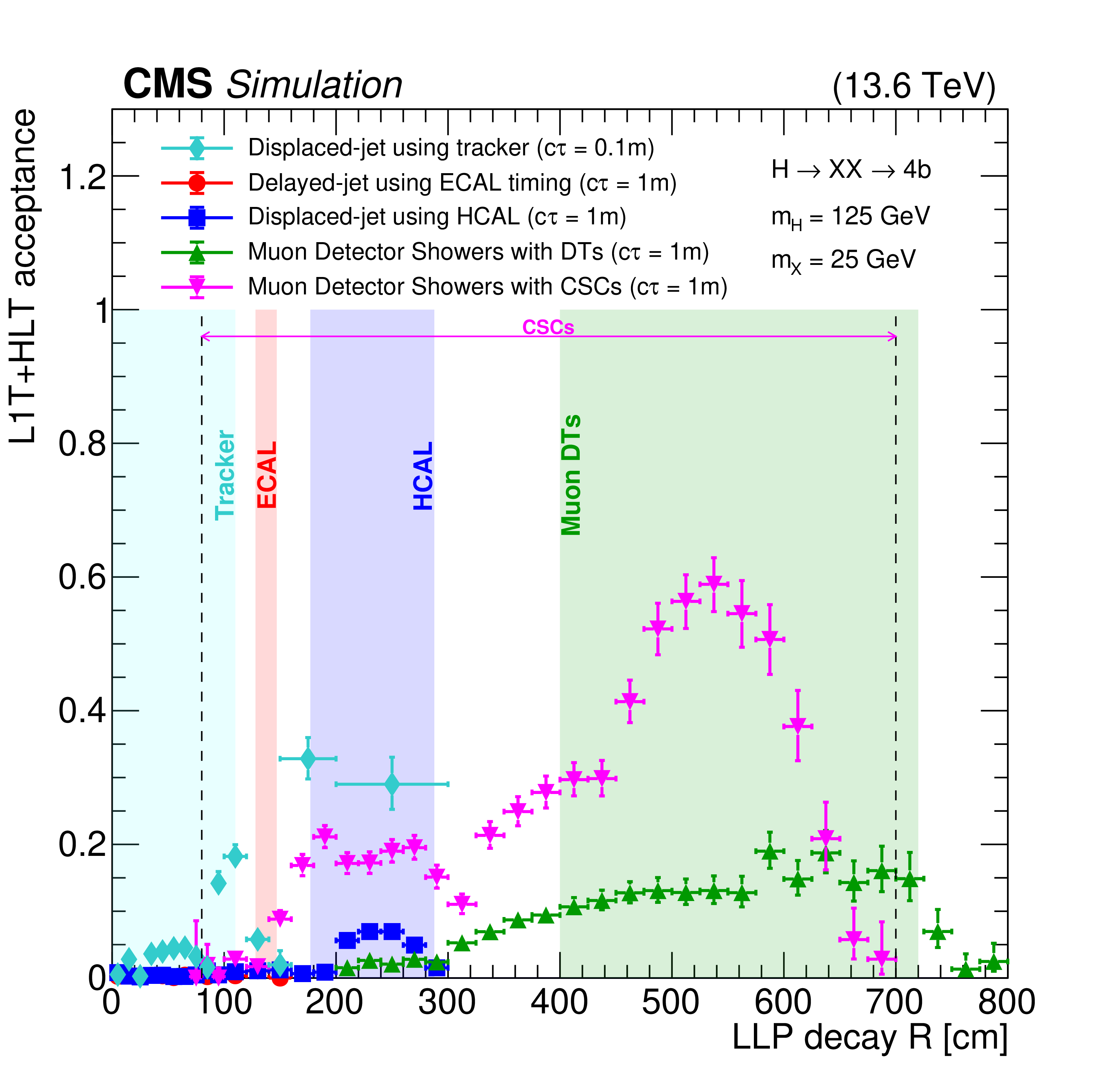
png pdf |
Figure 61-d:
The L1T+HLT acceptances for various LLP triggers using different subdetectors, as functions of the LLP decay radial position, for $ \mathrm{H} \to \mathrm{X}\mathrm{X} \to \mathrm{b}\overline{\mathrm{b}}\mathrm{b}\overline{\mathrm{b}} $ events for 2023 conditions. The plots correspond to different signal models with $ m_{\mathrm{H}}= $ 1000 GeV and $ m_{\mathrm{X}}= $ 200 GeV on the upper left; $ m_{\mathrm{H}}= $ 350 GeV and $ m_{\mathrm{X}}= $ 80 GeV on the upper right; $ m_{\mathrm{H}}= $ 350 GeV and $ m_{\mathrm{X}}= $ 160 GeV on the lower left; and $ m_{\mathrm{H}}= $ 125 GeV and $ m_{\mathrm{X}}= $ 25 GeV on the lower right. In each of these plots, the $ c\tau $ is 0.1\unitm for the displaced-jet triggers using the tracker and 1\unitm for the other triggers. The acceptance is shown for the displaced-jet triggers using the tracker (cyan diamonds), for the delayed-jet triggers using ECAL timing (red circles), for the displaced-jet triggers using the HCAL (blue squares), for the MDS triggers with the DTs (green triangles), and for the MDS triggers with the CSCs (pink triangles). The boundaries of the tracker, ECAL, HCAL, DTs, and CSCs are also shown in the figures. |
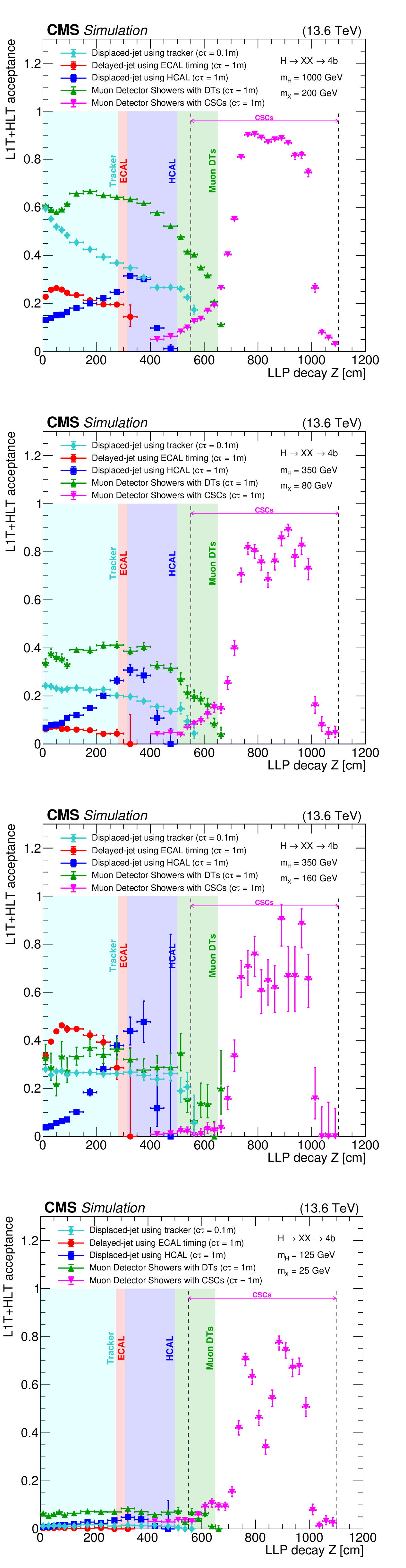
png pdf |
Figure 62:
The L1T+HLT acceptances for various LLP triggers using different subdetectors, as functions of the $ z $ position of the LLP decay, for $ \mathrm{H} \to \mathrm{X}\mathrm{X} \to \mathrm{b}\overline{\mathrm{b}}\mathrm{b}\overline{\mathrm{b}} $ events for 2023 conditions. The plots correspond to different signal points with $ m_{\mathrm{H}}= $ 1000 GeV and $ m_{\mathrm{X}}= $ 200 GeV on the upper left; $ m_{\mathrm{H}}= $ 350 GeV and $ m_{\mathrm{X}}= $ 80 GeV on the upper right; $ m_{\mathrm{H}}= $ 350 GeV and $ m_{\mathrm{X}}= $ 160 GeV on the lower left; and $ m_{\mathrm{H}}= $ 125 GeV and $ m_{\mathrm{X}}= $ 25 GeV on the lower right. In each of these plots, the $ c\tau $ is 0.1\unitm for the displaced-jet triggers using the tracker and 1\unitm for the other triggers. The acceptance is shown for the displaced-jet triggers using the tracker (cyan diamonds), for the delayed-jet triggers using ECAL timing (red circles), for the displaced-jet triggers using the HCAL (blue squares), for the MDS triggers with the DTs (green triangles), and for the MDS triggers with the CSCs (pink triangles). The boundaries of the tracker, ECAL, HCAL, DTs, and CSCs are also shown in the figures. |
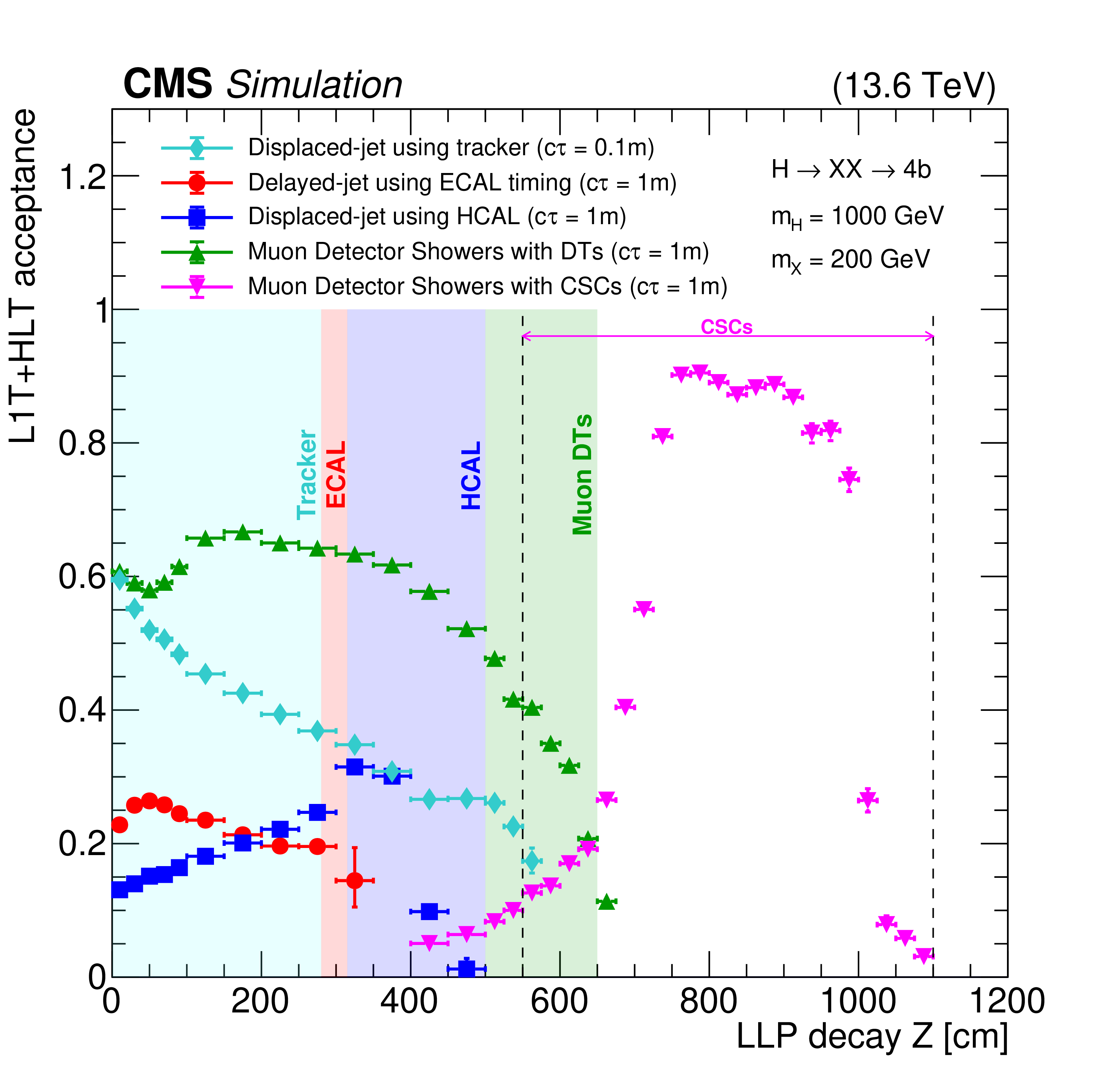
png pdf |
Figure 62-a:
The L1T+HLT acceptances for various LLP triggers using different subdetectors, as functions of the $ z $ position of the LLP decay, for $ \mathrm{H} \to \mathrm{X}\mathrm{X} \to \mathrm{b}\overline{\mathrm{b}}\mathrm{b}\overline{\mathrm{b}} $ events for 2023 conditions. The plots correspond to different signal points with $ m_{\mathrm{H}}= $ 1000 GeV and $ m_{\mathrm{X}}= $ 200 GeV on the upper left; $ m_{\mathrm{H}}= $ 350 GeV and $ m_{\mathrm{X}}= $ 80 GeV on the upper right; $ m_{\mathrm{H}}= $ 350 GeV and $ m_{\mathrm{X}}= $ 160 GeV on the lower left; and $ m_{\mathrm{H}}= $ 125 GeV and $ m_{\mathrm{X}}= $ 25 GeV on the lower right. In each of these plots, the $ c\tau $ is 0.1\unitm for the displaced-jet triggers using the tracker and 1\unitm for the other triggers. The acceptance is shown for the displaced-jet triggers using the tracker (cyan diamonds), for the delayed-jet triggers using ECAL timing (red circles), for the displaced-jet triggers using the HCAL (blue squares), for the MDS triggers with the DTs (green triangles), and for the MDS triggers with the CSCs (pink triangles). The boundaries of the tracker, ECAL, HCAL, DTs, and CSCs are also shown in the figures. |
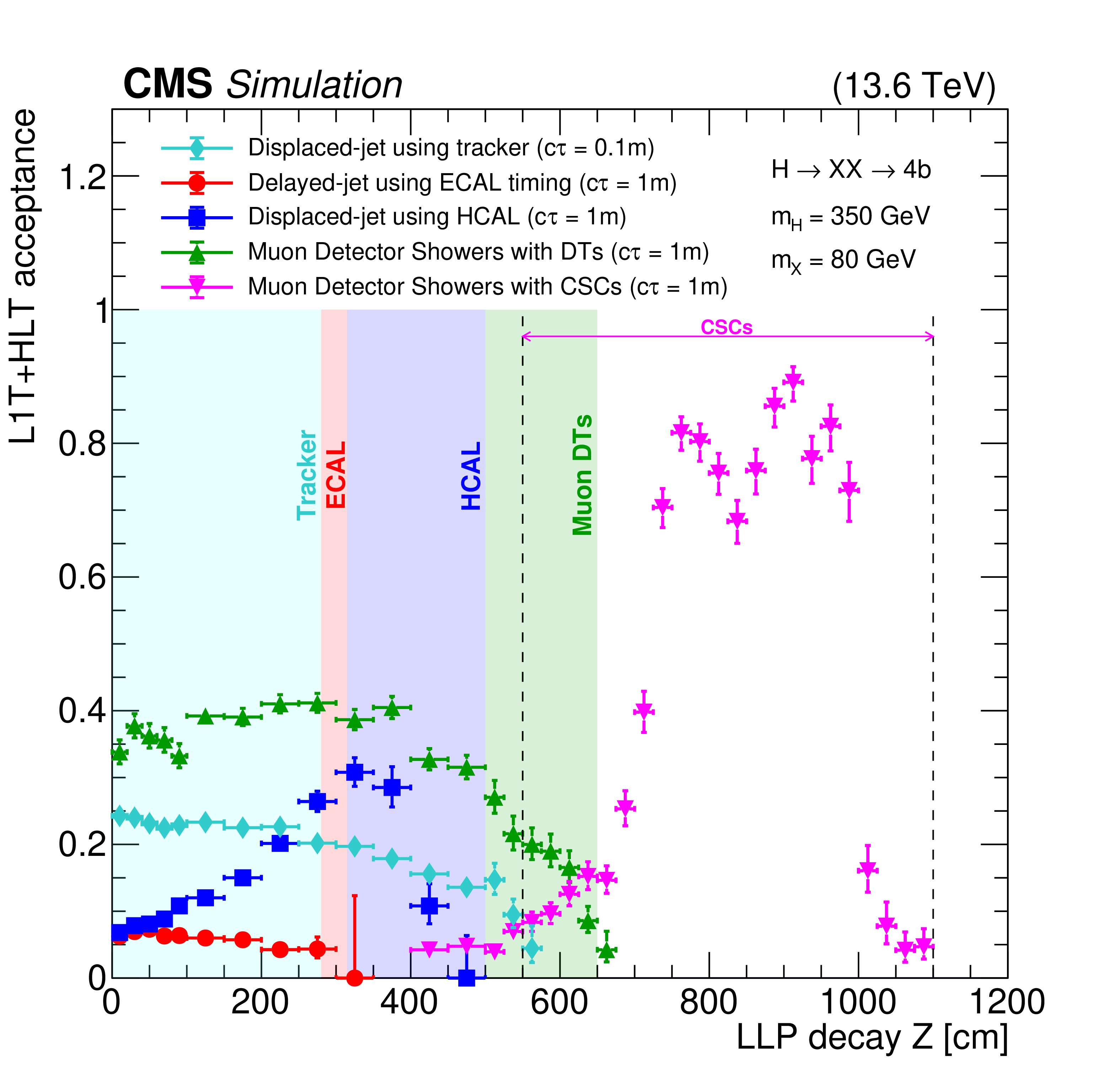
png pdf |
Figure 62-b:
The L1T+HLT acceptances for various LLP triggers using different subdetectors, as functions of the $ z $ position of the LLP decay, for $ \mathrm{H} \to \mathrm{X}\mathrm{X} \to \mathrm{b}\overline{\mathrm{b}}\mathrm{b}\overline{\mathrm{b}} $ events for 2023 conditions. The plots correspond to different signal points with $ m_{\mathrm{H}}= $ 1000 GeV and $ m_{\mathrm{X}}= $ 200 GeV on the upper left; $ m_{\mathrm{H}}= $ 350 GeV and $ m_{\mathrm{X}}= $ 80 GeV on the upper right; $ m_{\mathrm{H}}= $ 350 GeV and $ m_{\mathrm{X}}= $ 160 GeV on the lower left; and $ m_{\mathrm{H}}= $ 125 GeV and $ m_{\mathrm{X}}= $ 25 GeV on the lower right. In each of these plots, the $ c\tau $ is 0.1\unitm for the displaced-jet triggers using the tracker and 1\unitm for the other triggers. The acceptance is shown for the displaced-jet triggers using the tracker (cyan diamonds), for the delayed-jet triggers using ECAL timing (red circles), for the displaced-jet triggers using the HCAL (blue squares), for the MDS triggers with the DTs (green triangles), and for the MDS triggers with the CSCs (pink triangles). The boundaries of the tracker, ECAL, HCAL, DTs, and CSCs are also shown in the figures. |
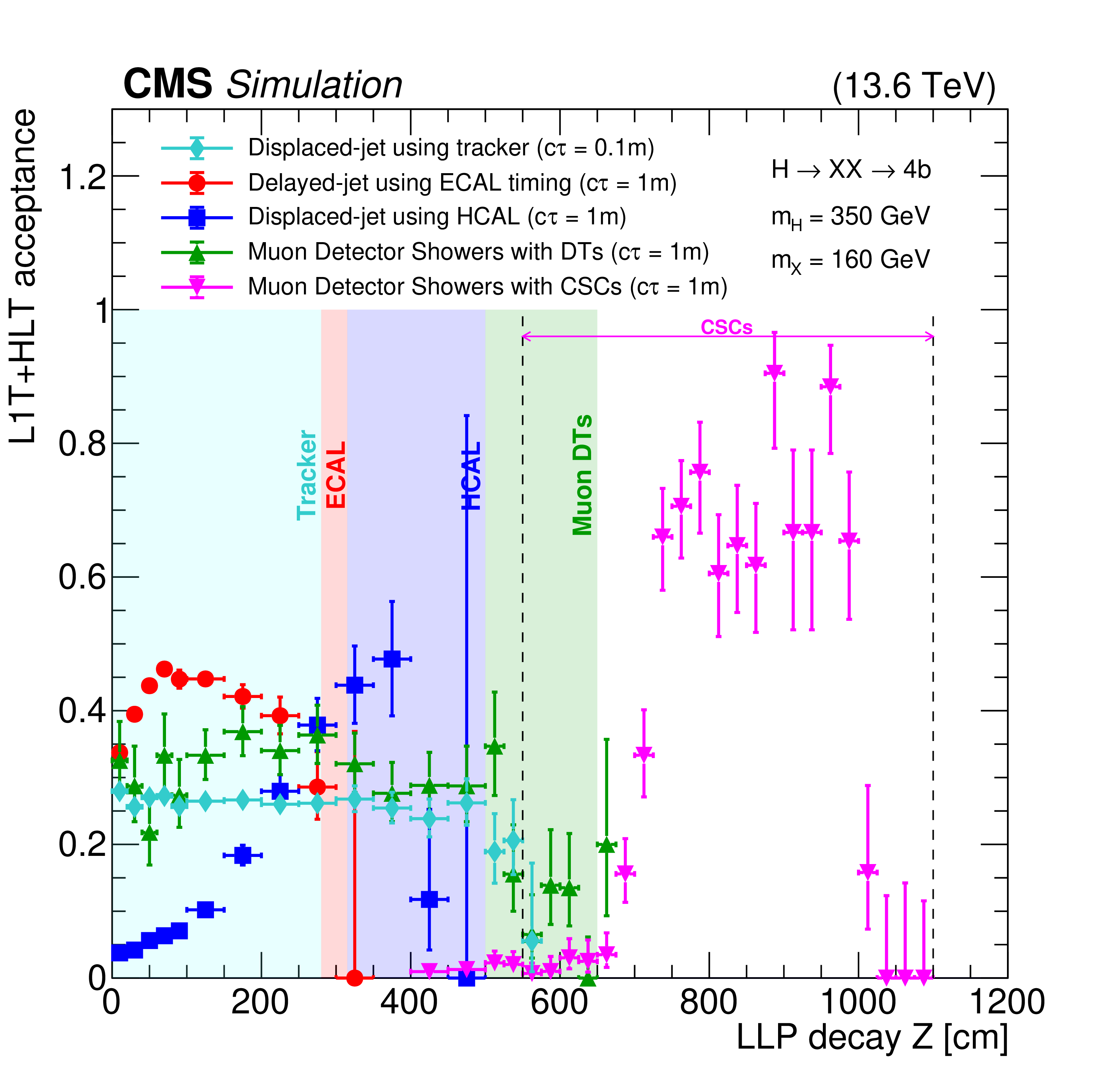
png pdf |
Figure 62-c:
The L1T+HLT acceptances for various LLP triggers using different subdetectors, as functions of the $ z $ position of the LLP decay, for $ \mathrm{H} \to \mathrm{X}\mathrm{X} \to \mathrm{b}\overline{\mathrm{b}}\mathrm{b}\overline{\mathrm{b}} $ events for 2023 conditions. The plots correspond to different signal points with $ m_{\mathrm{H}}= $ 1000 GeV and $ m_{\mathrm{X}}= $ 200 GeV on the upper left; $ m_{\mathrm{H}}= $ 350 GeV and $ m_{\mathrm{X}}= $ 80 GeV on the upper right; $ m_{\mathrm{H}}= $ 350 GeV and $ m_{\mathrm{X}}= $ 160 GeV on the lower left; and $ m_{\mathrm{H}}= $ 125 GeV and $ m_{\mathrm{X}}= $ 25 GeV on the lower right. In each of these plots, the $ c\tau $ is 0.1\unitm for the displaced-jet triggers using the tracker and 1\unitm for the other triggers. The acceptance is shown for the displaced-jet triggers using the tracker (cyan diamonds), for the delayed-jet triggers using ECAL timing (red circles), for the displaced-jet triggers using the HCAL (blue squares), for the MDS triggers with the DTs (green triangles), and for the MDS triggers with the CSCs (pink triangles). The boundaries of the tracker, ECAL, HCAL, DTs, and CSCs are also shown in the figures. |
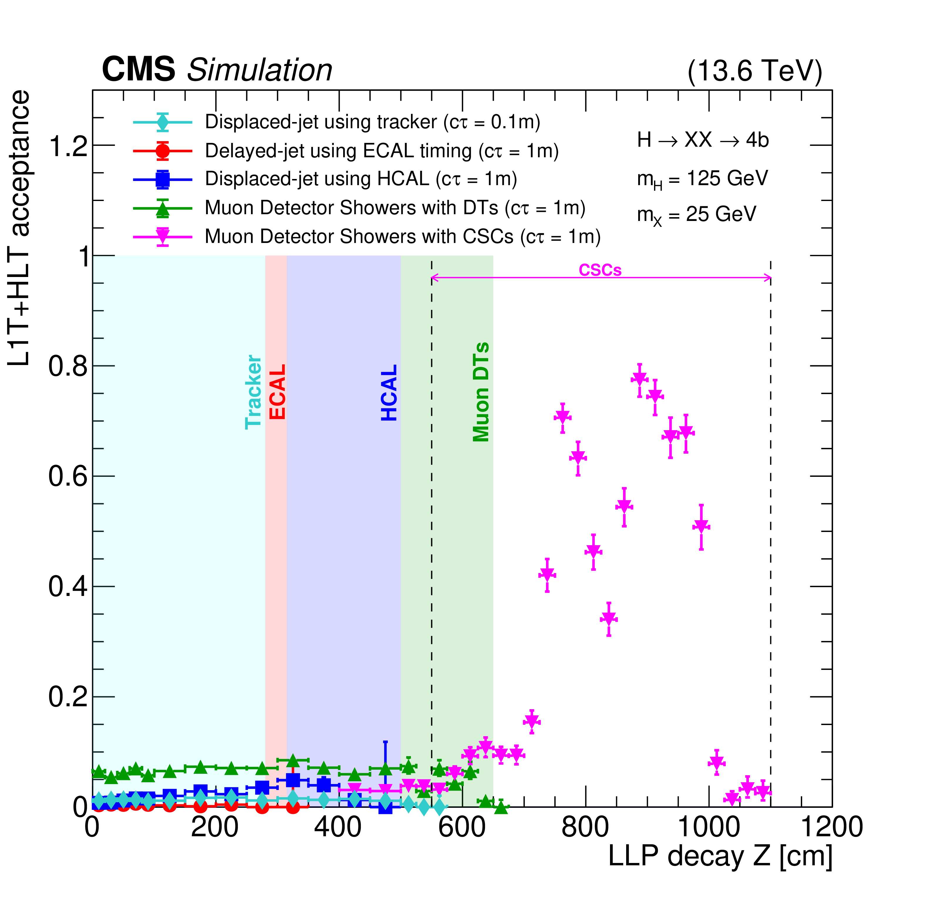
png pdf |
Figure 62-d:
The L1T+HLT acceptances for various LLP triggers using different subdetectors, as functions of the $ z $ position of the LLP decay, for $ \mathrm{H} \to \mathrm{X}\mathrm{X} \to \mathrm{b}\overline{\mathrm{b}}\mathrm{b}\overline{\mathrm{b}} $ events for 2023 conditions. The plots correspond to different signal points with $ m_{\mathrm{H}}= $ 1000 GeV and $ m_{\mathrm{X}}= $ 200 GeV on the upper left; $ m_{\mathrm{H}}= $ 350 GeV and $ m_{\mathrm{X}}= $ 80 GeV on the upper right; $ m_{\mathrm{H}}= $ 350 GeV and $ m_{\mathrm{X}}= $ 160 GeV on the lower left; and $ m_{\mathrm{H}}= $ 125 GeV and $ m_{\mathrm{X}}= $ 25 GeV on the lower right. In each of these plots, the $ c\tau $ is 0.1\unitm for the displaced-jet triggers using the tracker and 1\unitm for the other triggers. The acceptance is shown for the displaced-jet triggers using the tracker (cyan diamonds), for the delayed-jet triggers using ECAL timing (red circles), for the displaced-jet triggers using the HCAL (blue squares), for the MDS triggers with the DTs (green triangles), and for the MDS triggers with the CSCs (pink triangles). The boundaries of the tracker, ECAL, HCAL, DTs, and CSCs are also shown in the figures. |
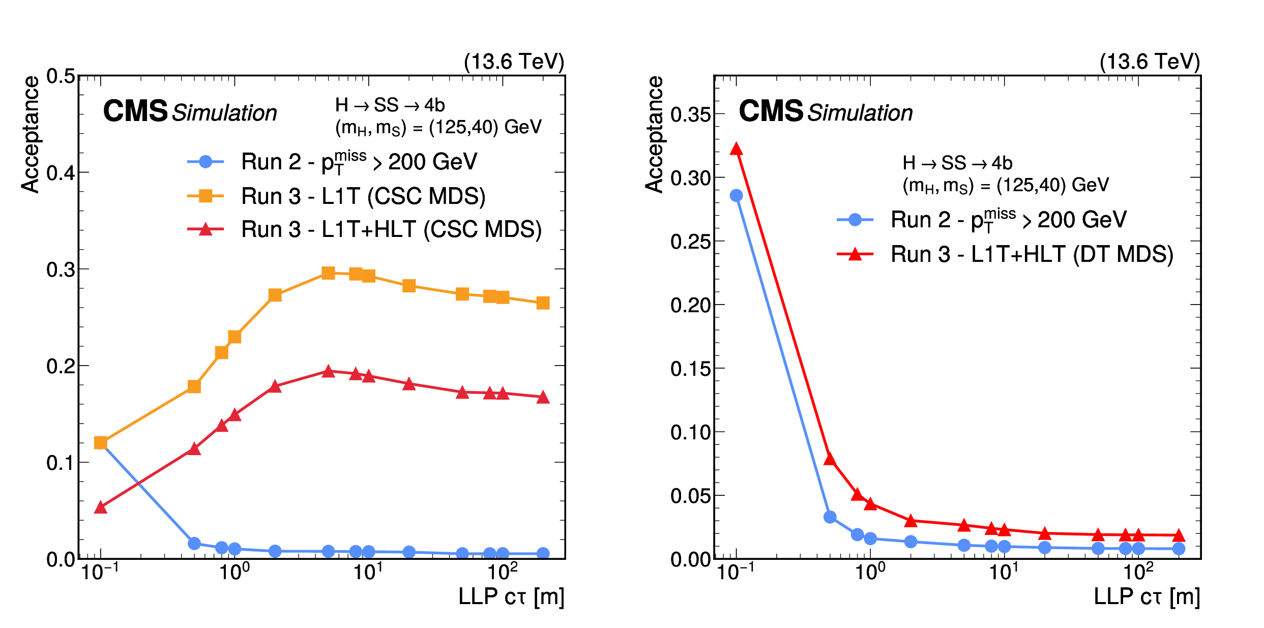
png pdf |
Figure 63:
Comparison of the acceptances in Run 2 and Run 3 for the CSC (left) and DT (right) MDS triggers at the L1T and HLT as functions of the LLP lifetime, for $ \mathrm{H} \to \text{S}\text{S} \to \mathrm{b}\overline{\mathrm{b}}\mathrm{b}\overline{\mathrm{b}} $ events with $ m_{\mathrm{H}}= $ 125 GeV and $ m_{\text{S}} = $ 40 GeV, for 2023 conditions. The acceptance is defined as the fraction of events that pass the specified selection, given an LLP decay in the fiducial region of the CSCs (left) or the DTs (right). The left plot compares the acceptance of the Run 2 strategy of triggering on $ p_{\mathrm{T}}^\text{miss} $ (blue circles), which corresponds to an offline requirement of $ {>} $ 200 GeV, with that of the Run 3 strategy of triggering on the MDS signature in the CSCs, where the L1T (L1T+HLT) acceptance is shown with orange squares (red triangles). The right plot compares the acceptance of the Run 2 strategy of triggering on $ p_{\mathrm{T}}^\text{miss} $ (blue circles) with the Run 3 strategy of triggering on the MDS signature in the DTs (red triangles), for L1T+HLT. |
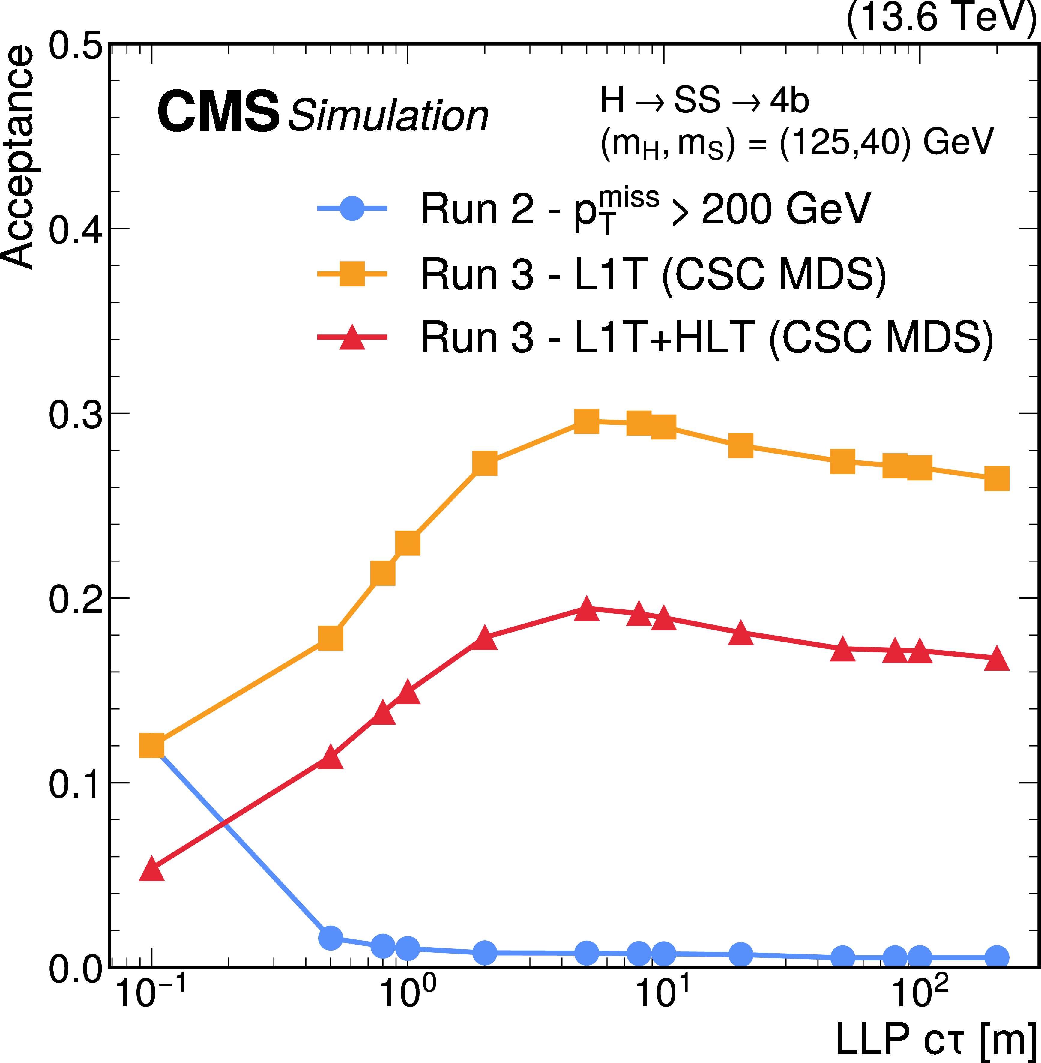
png pdf |
Figure 63-a:
Comparison of the acceptances in Run 2 and Run 3 for the CSC (left) and DT (right) MDS triggers at the L1T and HLT as functions of the LLP lifetime, for $ \mathrm{H} \to \text{S}\text{S} \to \mathrm{b}\overline{\mathrm{b}}\mathrm{b}\overline{\mathrm{b}} $ events with $ m_{\mathrm{H}}= $ 125 GeV and $ m_{\text{S}} = $ 40 GeV, for 2023 conditions. The acceptance is defined as the fraction of events that pass the specified selection, given an LLP decay in the fiducial region of the CSCs (left) or the DTs (right). The left plot compares the acceptance of the Run 2 strategy of triggering on $ p_{\mathrm{T}}^\text{miss} $ (blue circles), which corresponds to an offline requirement of $ {>} $ 200 GeV, with that of the Run 3 strategy of triggering on the MDS signature in the CSCs, where the L1T (L1T+HLT) acceptance is shown with orange squares (red triangles). The right plot compares the acceptance of the Run 2 strategy of triggering on $ p_{\mathrm{T}}^\text{miss} $ (blue circles) with the Run 3 strategy of triggering on the MDS signature in the DTs (red triangles), for L1T+HLT. |
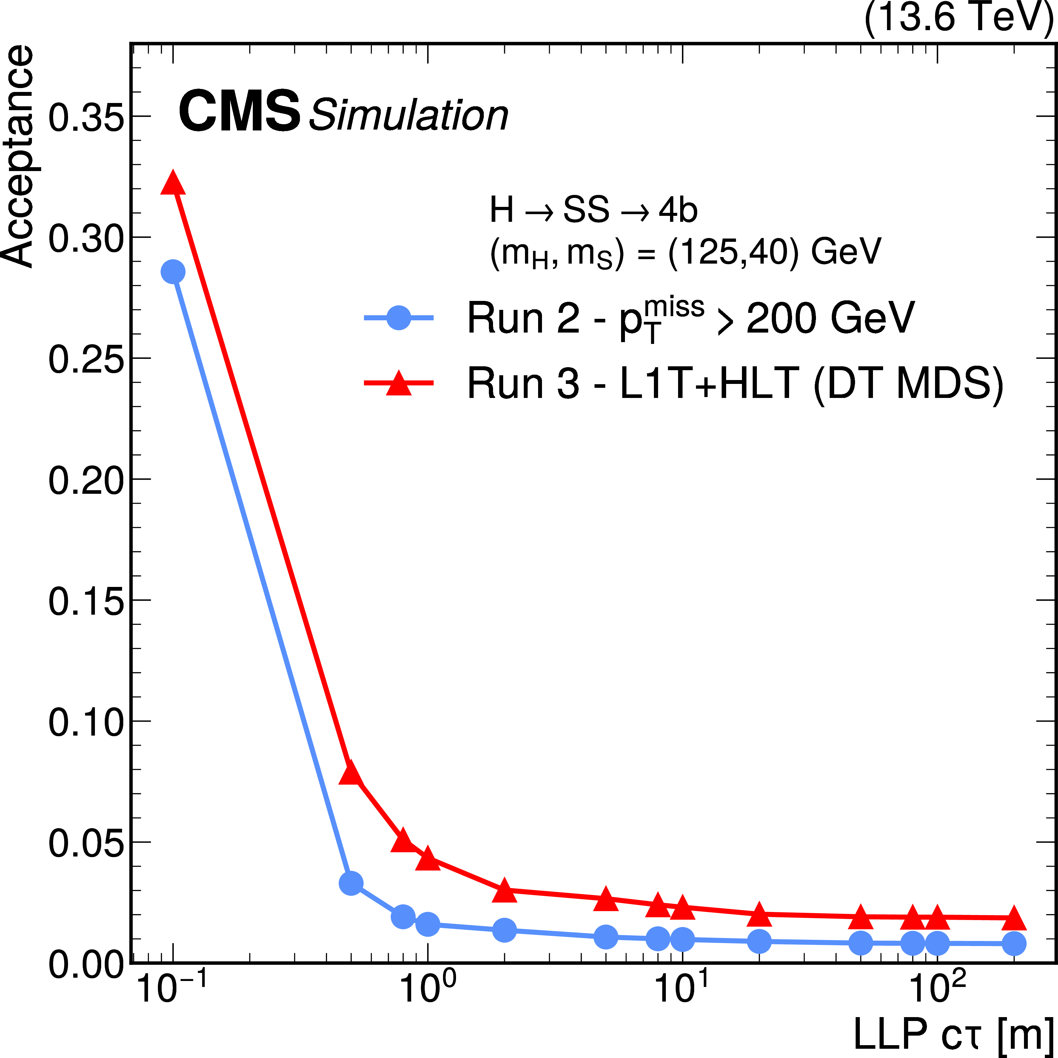
png pdf |
Figure 63-b:
Comparison of the acceptances in Run 2 and Run 3 for the CSC (left) and DT (right) MDS triggers at the L1T and HLT as functions of the LLP lifetime, for $ \mathrm{H} \to \text{S}\text{S} \to \mathrm{b}\overline{\mathrm{b}}\mathrm{b}\overline{\mathrm{b}} $ events with $ m_{\mathrm{H}}= $ 125 GeV and $ m_{\text{S}} = $ 40 GeV, for 2023 conditions. The acceptance is defined as the fraction of events that pass the specified selection, given an LLP decay in the fiducial region of the CSCs (left) or the DTs (right). The left plot compares the acceptance of the Run 2 strategy of triggering on $ p_{\mathrm{T}}^\text{miss} $ (blue circles), which corresponds to an offline requirement of $ {>} $ 200 GeV, with that of the Run 3 strategy of triggering on the MDS signature in the CSCs, where the L1T (L1T+HLT) acceptance is shown with orange squares (red triangles). The right plot compares the acceptance of the Run 2 strategy of triggering on $ p_{\mathrm{T}}^\text{miss} $ (blue circles) with the Run 3 strategy of triggering on the MDS signature in the DTs (red triangles), for L1T+HLT. |
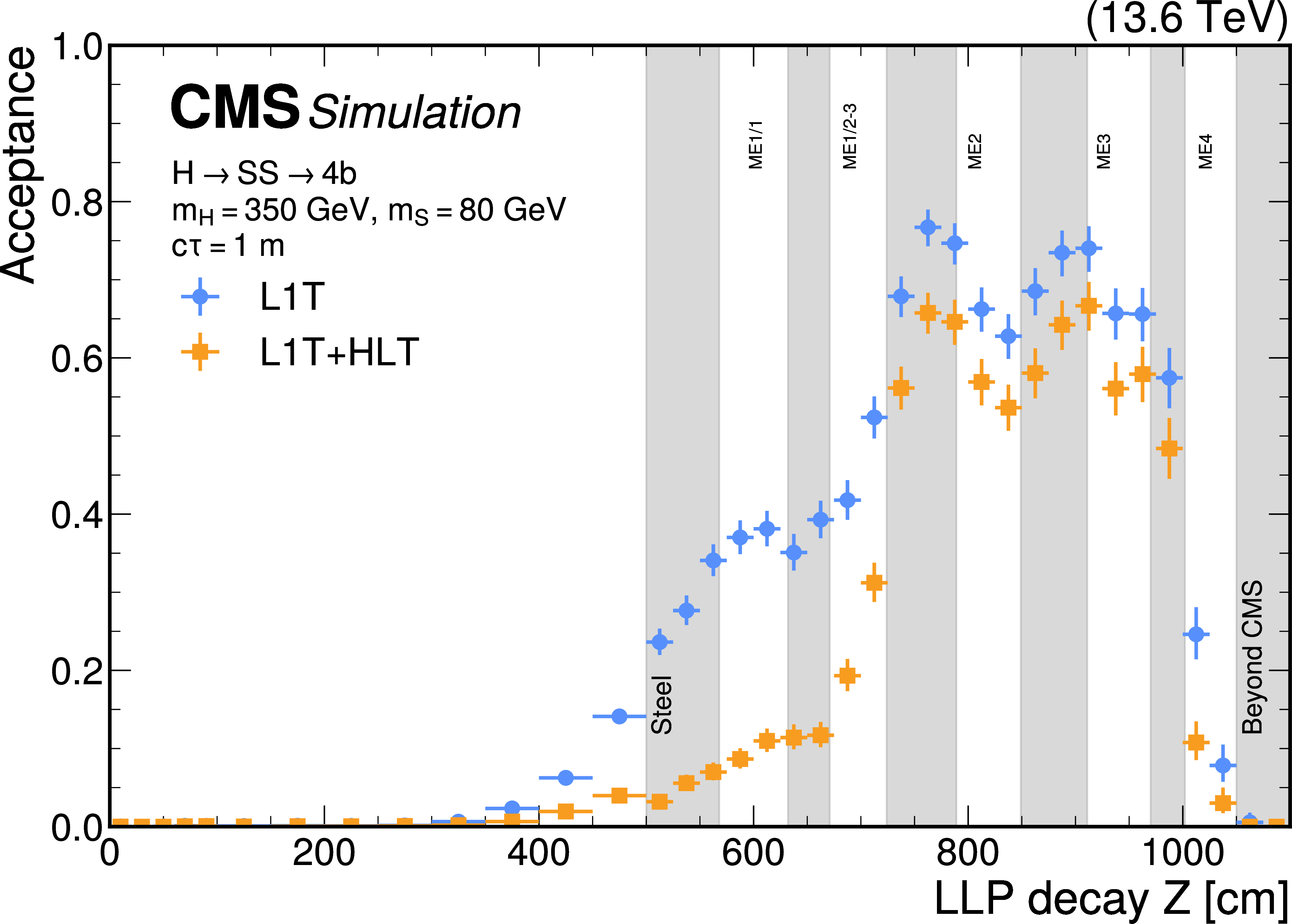
png pdf |
Figure 64:
The L1T (blue circles) and L1T+HLT (orange squares) acceptances for the CSC MDS trigger as functions of the LLP decay position in the $ z $-direction, for $ \mathrm{H} \to \text{S}\text{S} \to \mathrm{b}\overline{\mathrm{b}}\mathrm{b}\overline{\mathrm{b}} $ events with $ m_{\mathrm{H}}= $ 350 GeV, $ m_{\text{S}}= $ 80 GeV, and $ c\tau_{\text{S}}= $ 1 m, for 2023 conditions. |
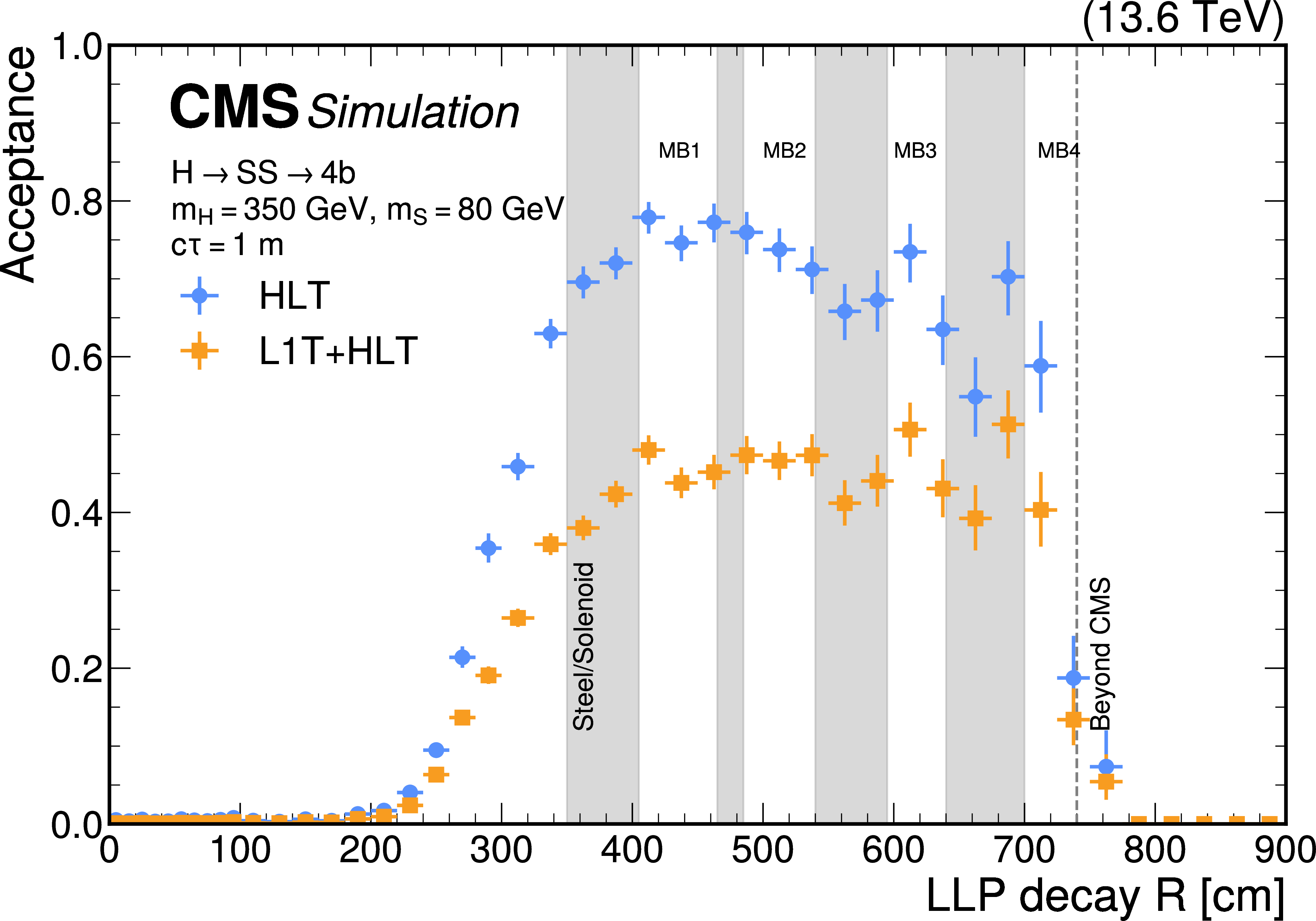
png pdf |
Figure 65:
The HLT (blue circles) and L1T+HLT (orange squares) acceptances for the DT MDS trigger as functions of the LLP decay position in the radial direction, for $ \mathrm{H} \to \text{S}\text{S} \to \mathrm{b}\overline{\mathrm{b}}\mathrm{b}\overline{\mathrm{b}} $ events with $ m_{\mathrm{H}}= $ 350 GeV, $ m_{\text{S}}= $ 80 GeV, and $ c\tau_{\text{S}}= $ 1 m, for 2023 conditions. |
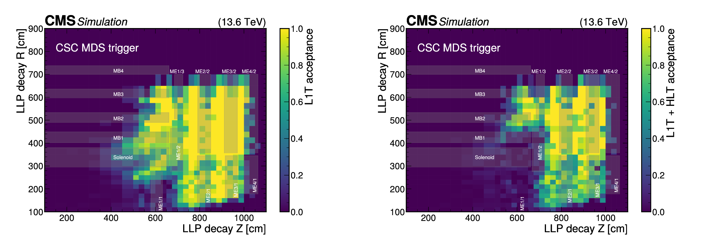
png pdf |
Figure 66:
The L1T (left) and L1T+HLT (right) acceptances for the CSC MDS trigger as functions of the LLP decay position, for $ \mathrm{H} \to \text{S}\text{S} \to \mathrm{b}\overline{\mathrm{b}}\mathrm{b}\overline{\mathrm{b}} $ events with $ m_{\mathrm{H}}= $ 350 GeV, $ m_{\text{S}}= $ 80 GeV, and $ c\tau_{\text{S}}= $ 1 m, for 2023 conditions. |
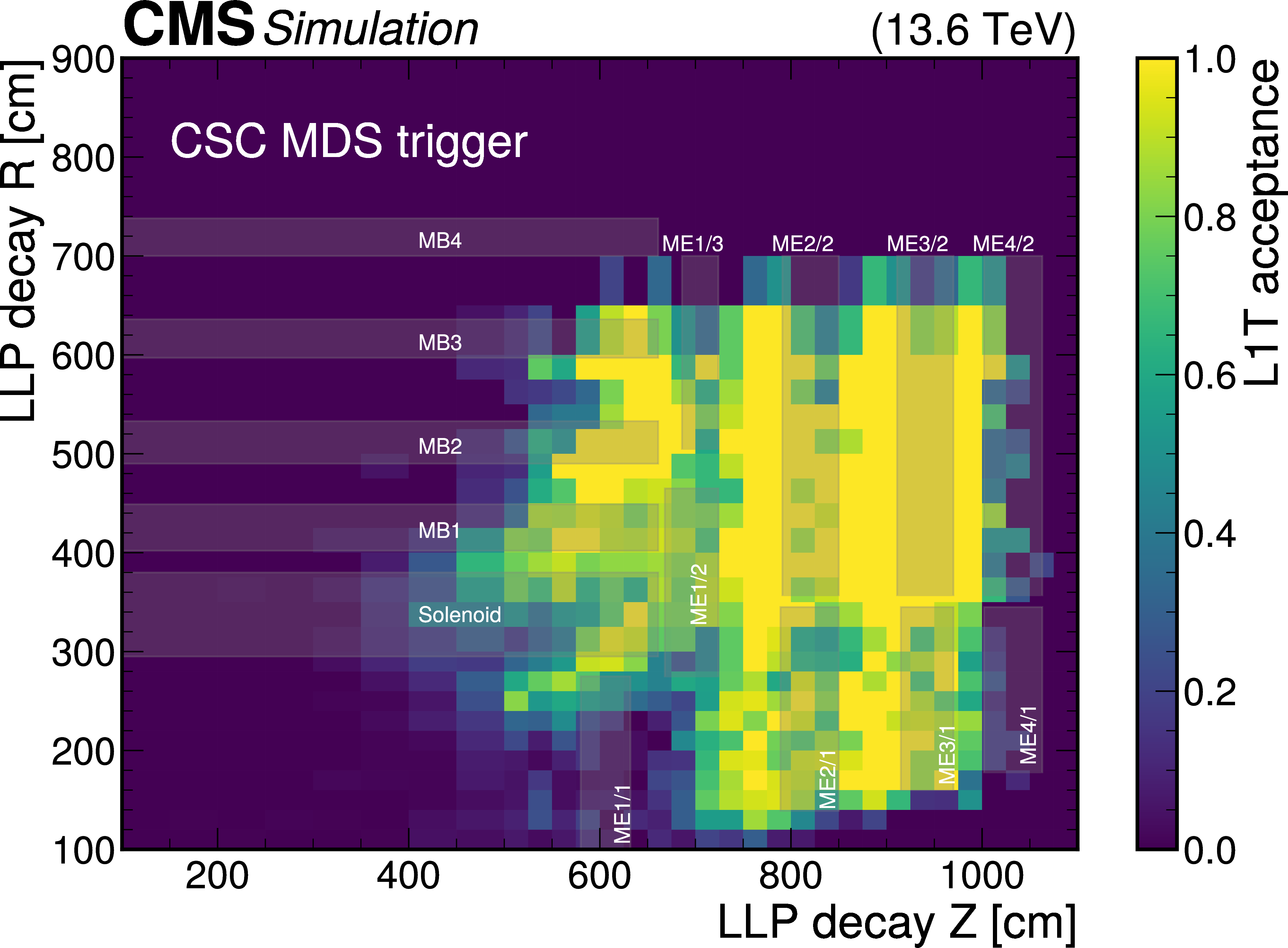
png pdf |
Figure 66-a:
The L1T (left) and L1T+HLT (right) acceptances for the CSC MDS trigger as functions of the LLP decay position, for $ \mathrm{H} \to \text{S}\text{S} \to \mathrm{b}\overline{\mathrm{b}}\mathrm{b}\overline{\mathrm{b}} $ events with $ m_{\mathrm{H}}= $ 350 GeV, $ m_{\text{S}}= $ 80 GeV, and $ c\tau_{\text{S}}= $ 1 m, for 2023 conditions. |
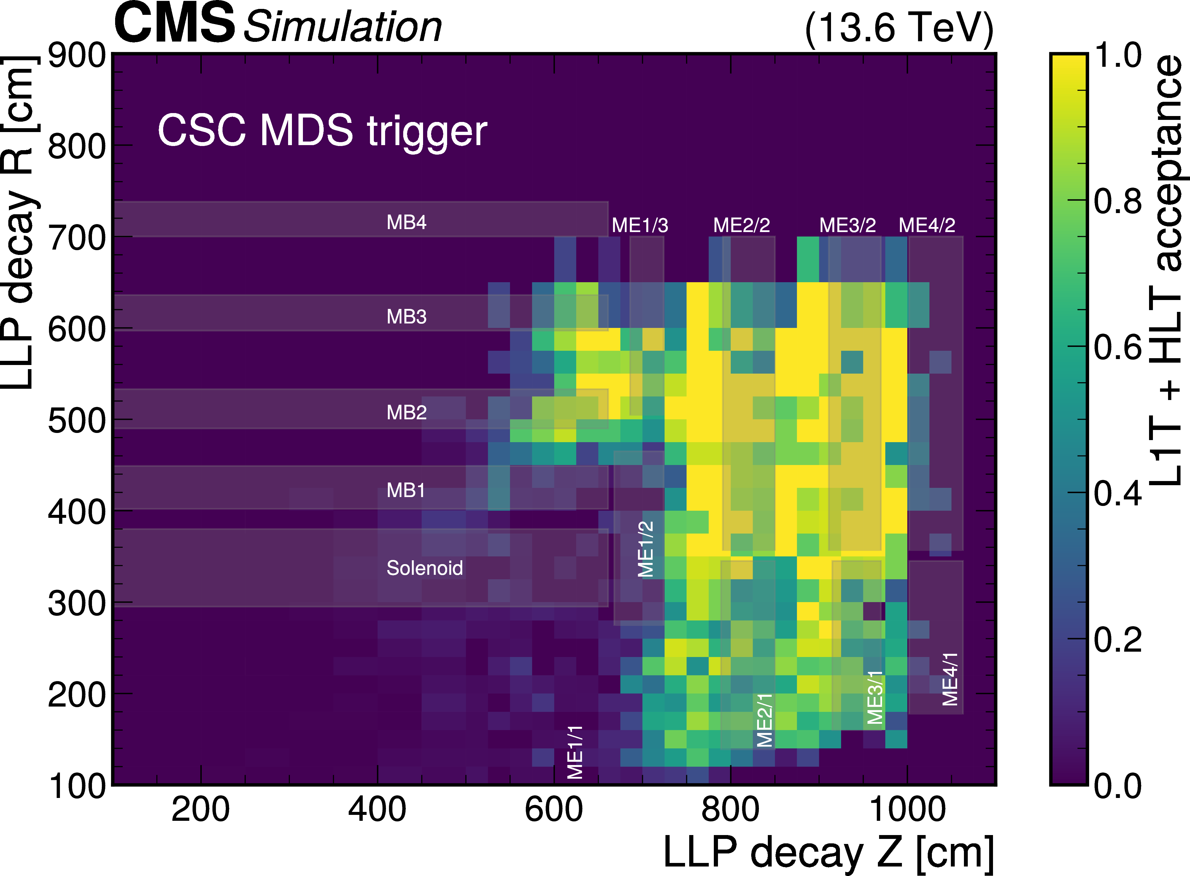
png pdf |
Figure 66-b:
The L1T (left) and L1T+HLT (right) acceptances for the CSC MDS trigger as functions of the LLP decay position, for $ \mathrm{H} \to \text{S}\text{S} \to \mathrm{b}\overline{\mathrm{b}}\mathrm{b}\overline{\mathrm{b}} $ events with $ m_{\mathrm{H}}= $ 350 GeV, $ m_{\text{S}}= $ 80 GeV, and $ c\tau_{\text{S}}= $ 1 m, for 2023 conditions. |
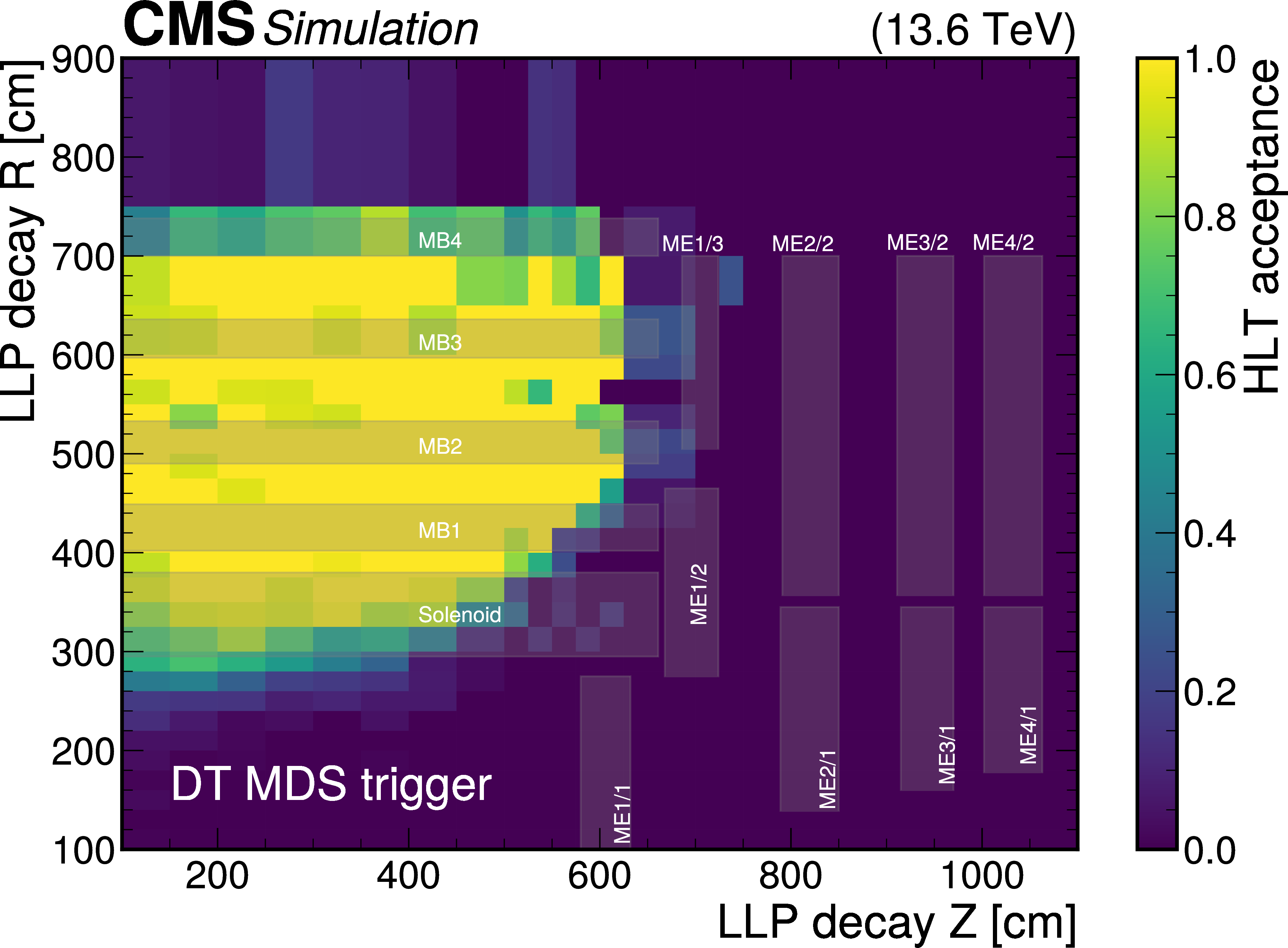
png pdf |
Figure 67:
The HLT acceptance for the DT MDS trigger as a function of the LLP decay position, for $ \mathrm{H} \to \text{S}\text{S} \to \mathrm{b}\overline{\mathrm{b}}\mathrm{b}\overline{\mathrm{b}} $ events with $ m_{\mathrm{H}}= $ 350 GeV, $ m_{\text{S}}= $ 80 GeV, and $ c\tau_{\text{S}}= $ 1 m, for 2023 conditions. The L1T acceptance that is based on the $ p_{\mathrm{T}}^\text{miss} $ trigger is not included. |
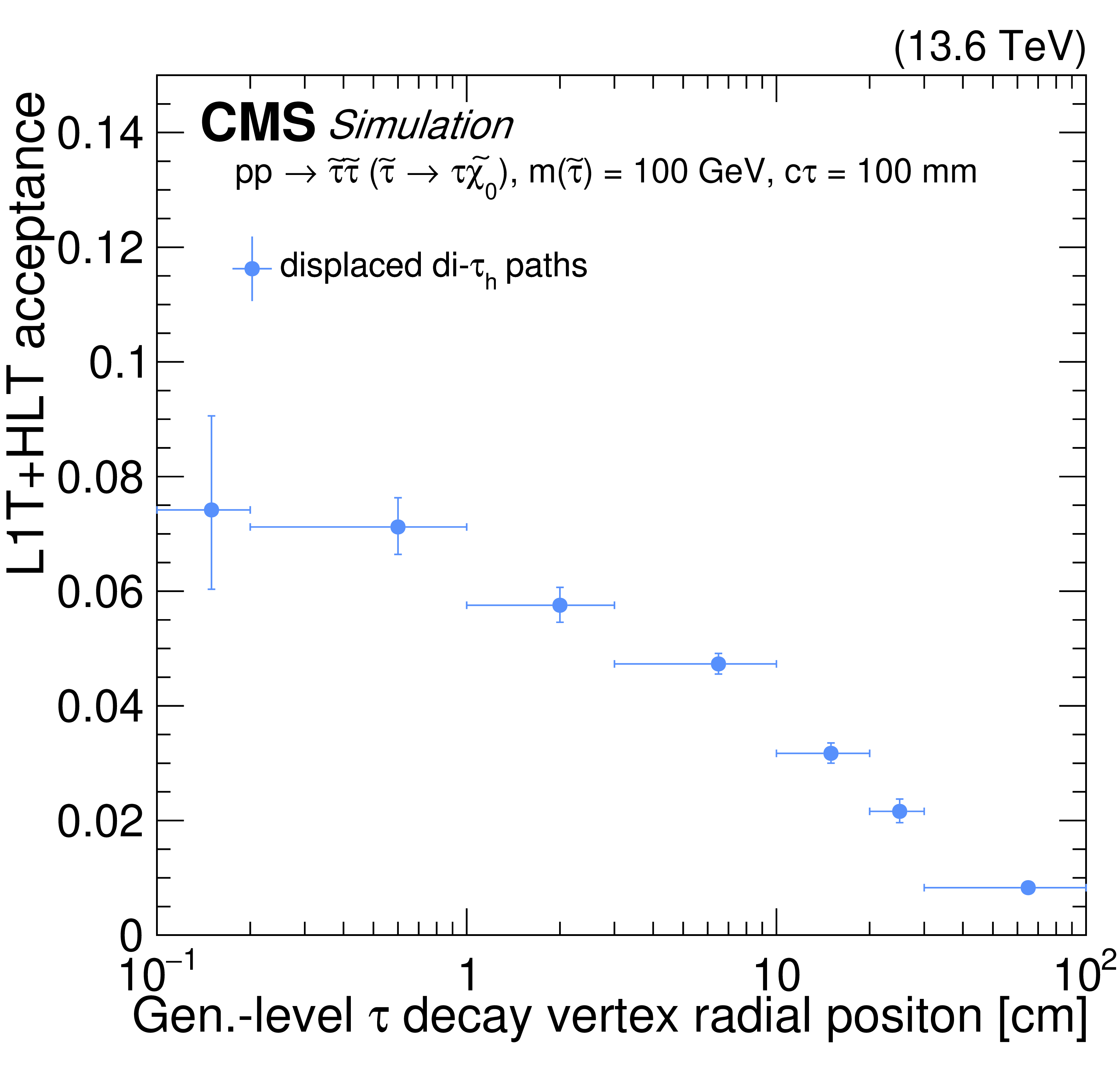
png pdf |
Figure 68:
The L1T+HLT acceptance of the displaced $ \tau_\mathrm{h} $ trigger, for simulated $ \mathrm{p}\mathrm{p} \to \tilde{\tau}\tilde{\tau} (\tilde{\tau} \to \tau\tilde{\chi}_{1}^{0}) $ events, where each $ \tau $ decays hadronically and the $ \tilde{\tau} $ has a simulated $ c\tau $ of 10$ \text{cm} $. The acceptance is shown for the displaced di-$ \tau_\mathrm{h} $ trigger path for 2022 data-taking conditions and is plotted with respect to the generator-level $ \tau $ lepton decay vertex radial position. Selections on the visible component of the generator-level $ \tau $ lepton $ p_{\mathrm{T}} $ ($ p_{\mathrm{T}}(\tau) > $ 30 GeV), its $ \eta $ ($ |\eta(\tau)| < $ 2.1), and its decay vertex radial position ($ R < 115 \text{cm} $) are applied. |
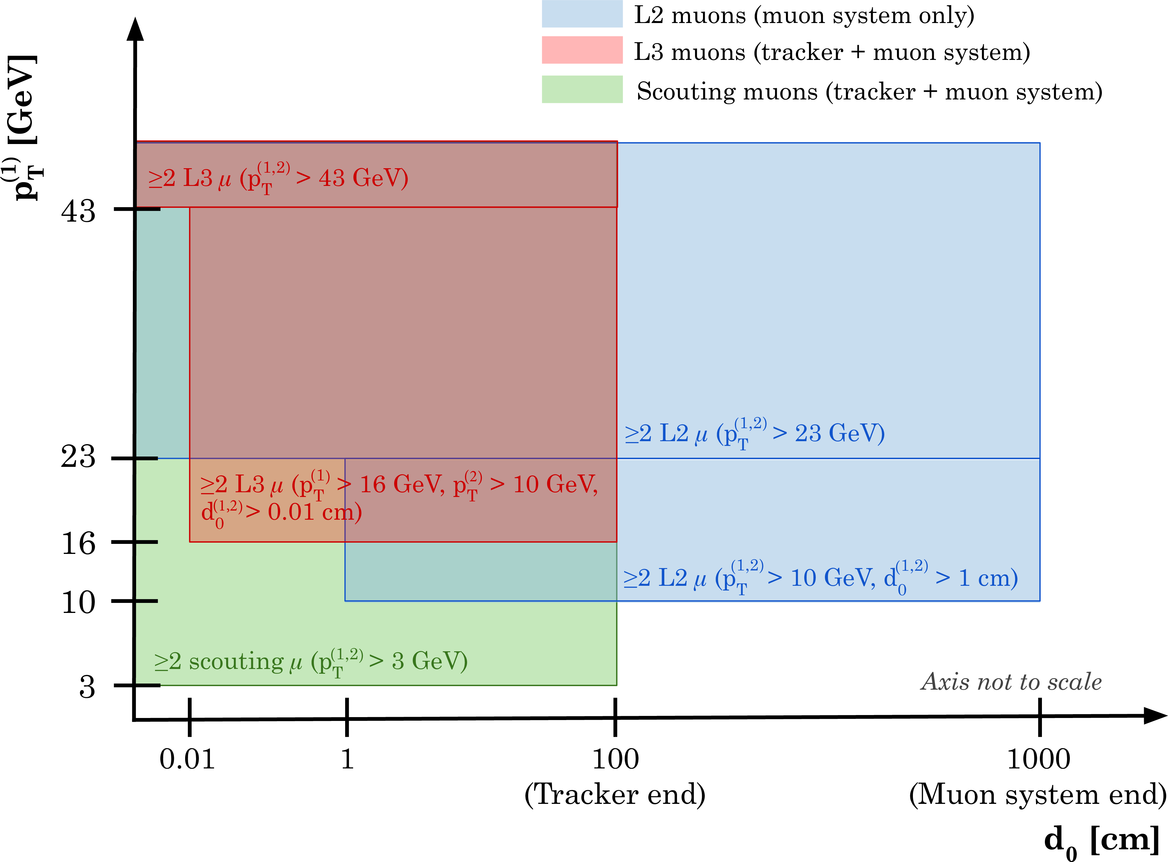
png pdf |
Figure 69:
Diagram of the overlapping coverage, in the HLT muon $ p_{\mathrm{T}}-d_{\text{0}} $ plane, of the dimuon triggers that target displaced signatures via L2 muons (shown in blue), L3 muons (shown in red), and scouting muons (shown in green). The displaced-dimuon triggers, the double displaced L3 muon triggers, and the dimuon scouting triggers are shown. The $ p_{\mathrm{T}} $ of the highest $ p_{\mathrm{T}} $ muon ($ p_{\mathrm{T}}^{1} $) is shown on the $ y $-axis, and the minimum $ p_{\mathrm{T}} $ thresholds on each triggered muon ($ p_{\mathrm{T}}^{1,2} $) are indicated within the colored parts of the diagram. The value of 100 $ (1000) \text{cm} $ given on the $ x $ axis for the effective end of the tracker (muon system) is approximate. |
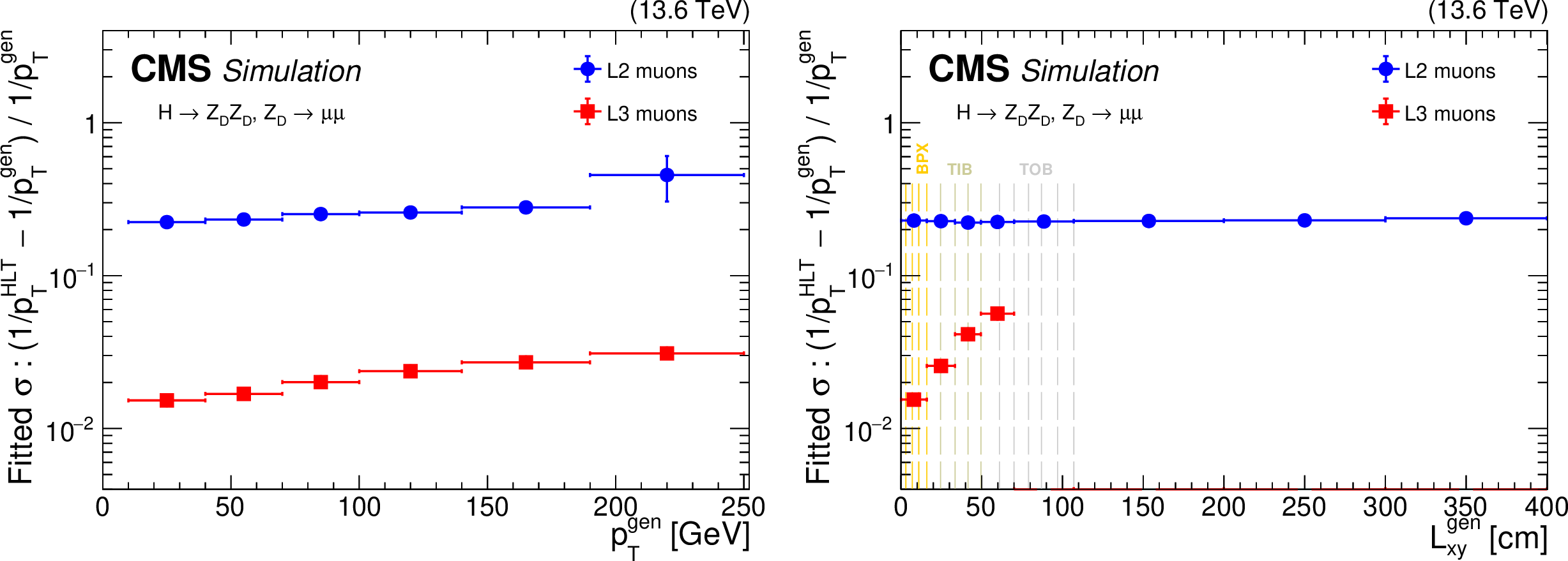
png pdf |
Figure 70:
Inverse L2 (blue circles) and L3 (red squares) muon $ p_{\mathrm{T}} $ resolution ($ (1/p_{\mathrm{T}}^{\text{HLT}}-1/p_{\mathrm{T}}^{\text{gen}})/(1/p_{\mathrm{T}}^{\text{gen}}) $) as a function of the generator-level muon $ p_{\mathrm{T}} $ (left) and the generator-level $ L_{\text{xy}} $ (right), for simulated HAHM signal events, where the dark Higgs boson ($ \mathrm{H}_{\text{D}} $) mixes with the SM Higgs boson (H) and decays to a pair of long-lived dark photons ($ \mathrm{Z}_\text{D} $), for various values of $ m_{\mathrm{Z}_\text{D}} $ and $ \epsilon $. Conditions for 2022 data-taking are shown. The muons must have $ p_{\mathrm{T}} > $ 10 GeV, and the L2 and L3 muons are geometrically matched to the generator-level muons. In the plot on the right, the dashed vertical lines indicate the radial positions of the layers of the tracking detectors, with BPX, TIB, and TOB denoting the barrel pixel, tracker inner barrel, and tracker outer barrel, respectively. |
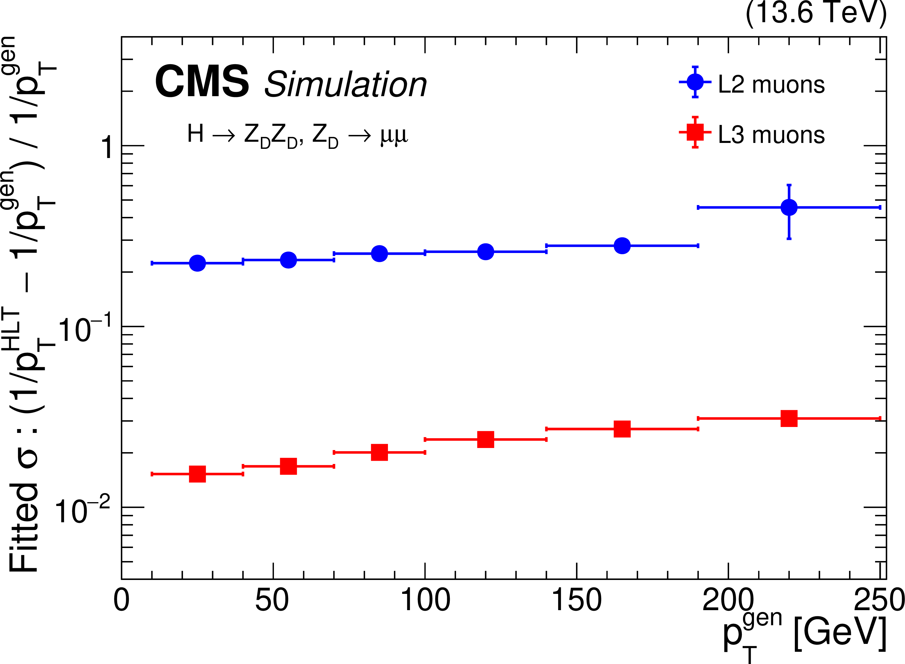
png pdf |
Figure 70-a:
Inverse L2 (blue circles) and L3 (red squares) muon $ p_{\mathrm{T}} $ resolution ($ (1/p_{\mathrm{T}}^{\text{HLT}}-1/p_{\mathrm{T}}^{\text{gen}})/(1/p_{\mathrm{T}}^{\text{gen}}) $) as a function of the generator-level muon $ p_{\mathrm{T}} $ (left) and the generator-level $ L_{\text{xy}} $ (right), for simulated HAHM signal events, where the dark Higgs boson ($ \mathrm{H}_{\text{D}} $) mixes with the SM Higgs boson (H) and decays to a pair of long-lived dark photons ($ \mathrm{Z}_\text{D} $), for various values of $ m_{\mathrm{Z}_\text{D}} $ and $ \epsilon $. Conditions for 2022 data-taking are shown. The muons must have $ p_{\mathrm{T}} > $ 10 GeV, and the L2 and L3 muons are geometrically matched to the generator-level muons. In the plot on the right, the dashed vertical lines indicate the radial positions of the layers of the tracking detectors, with BPX, TIB, and TOB denoting the barrel pixel, tracker inner barrel, and tracker outer barrel, respectively. |
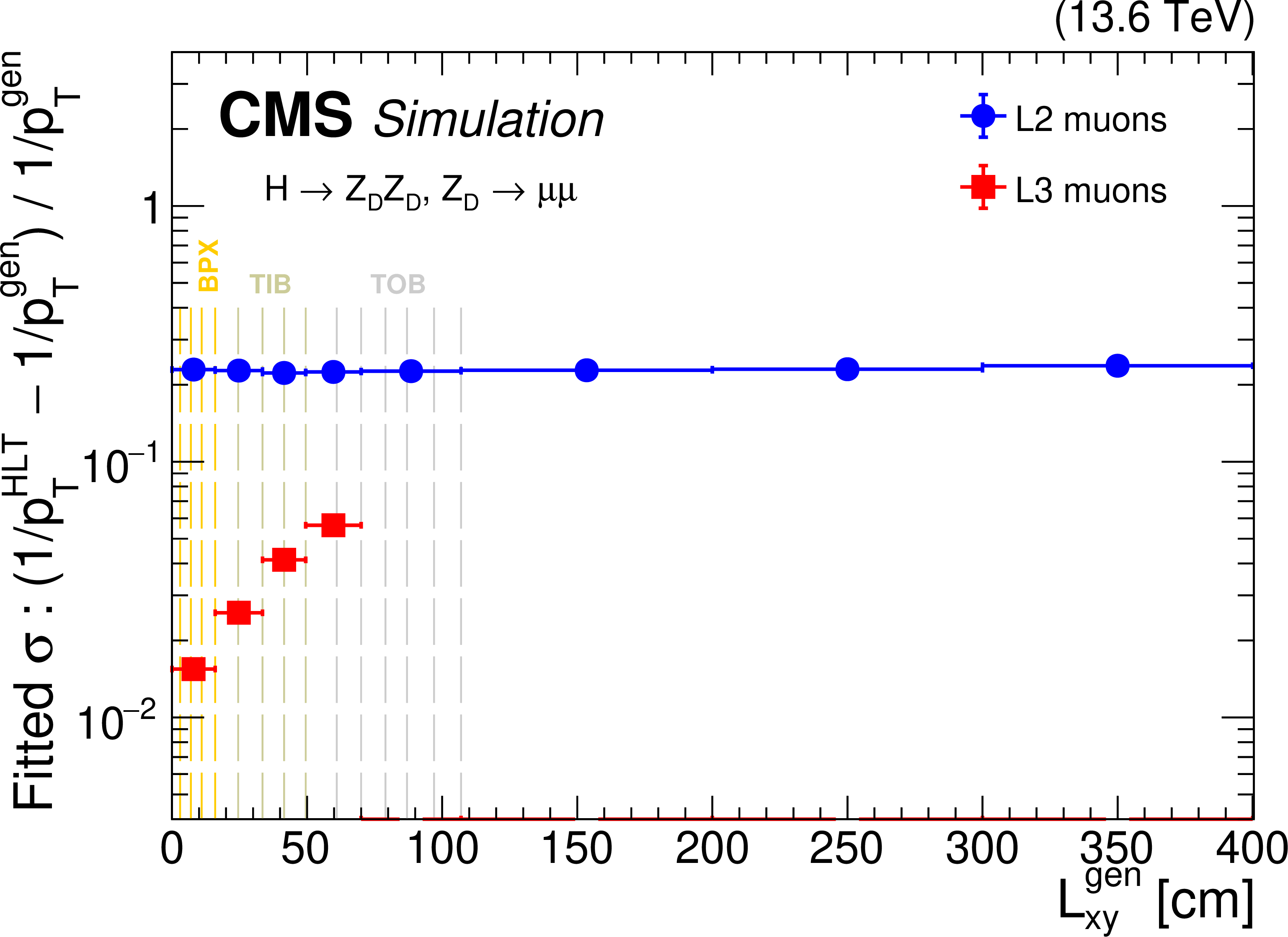
png pdf |
Figure 70-b:
Inverse L2 (blue circles) and L3 (red squares) muon $ p_{\mathrm{T}} $ resolution ($ (1/p_{\mathrm{T}}^{\text{HLT}}-1/p_{\mathrm{T}}^{\text{gen}})/(1/p_{\mathrm{T}}^{\text{gen}}) $) as a function of the generator-level muon $ p_{\mathrm{T}} $ (left) and the generator-level $ L_{\text{xy}} $ (right), for simulated HAHM signal events, where the dark Higgs boson ($ \mathrm{H}_{\text{D}} $) mixes with the SM Higgs boson (H) and decays to a pair of long-lived dark photons ($ \mathrm{Z}_\text{D} $), for various values of $ m_{\mathrm{Z}_\text{D}} $ and $ \epsilon $. Conditions for 2022 data-taking are shown. The muons must have $ p_{\mathrm{T}} > $ 10 GeV, and the L2 and L3 muons are geometrically matched to the generator-level muons. In the plot on the right, the dashed vertical lines indicate the radial positions of the layers of the tracking detectors, with BPX, TIB, and TOB denoting the barrel pixel, tracker inner barrel, and tracker outer barrel, respectively. |
| Tables | |
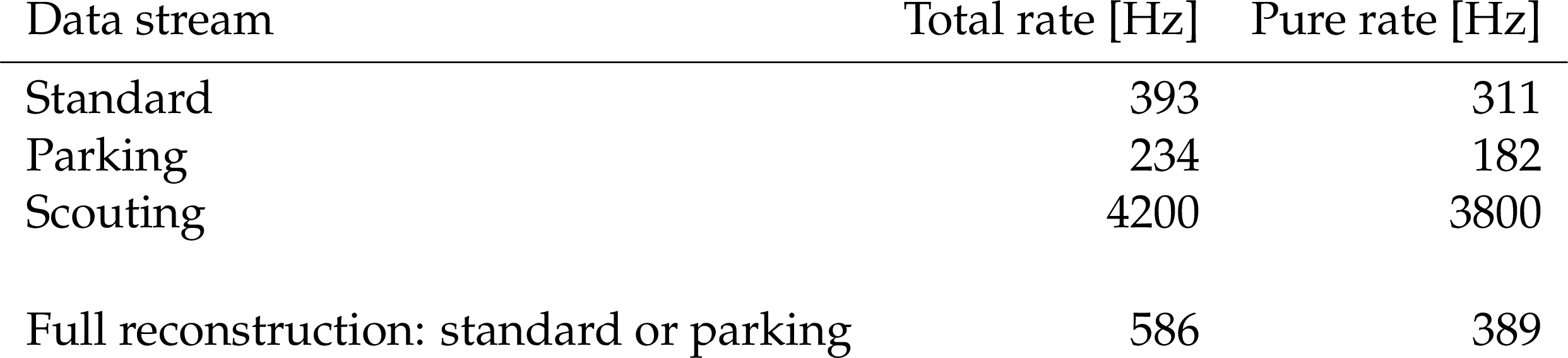
png pdf |
Table 1:
The total and pure HLT rate of all dedicated LLP triggers, as calculated from 2024 data for an instantaneous luminosity of \instL2.1, with a mean PU of 63.6. Rates are reported for triggers in the standard, parking, and scouting data-taking streams separately, as well as for the combined standard and parked data to show the rate of all events that are fully reconstructed. The total rates include events that may or may not have been selected by other triggers, while the pure rates correspond to events that pass dedicated LLP HLT paths and do not pass non-LLP HLT paths. The pure rates are measured separately with standard and parked data. The combined rates are less than the sum of the separate standard and parking rates because some events overlap. Each rate shown has a statistical uncertainty of less than 1%. |

png pdf |
Table 2:
The LLP triggers and their total HLT rates in Run 3, calculated from 2024 data for an instantaneous luminosity of \instL2.1, with a mean PU of 63.6. Triggers implemented for the first time in Run 3 are indicated by a dagger ($ ^\dagger $). Rate values in parentheses correspond to the parked data rates; all others are standard data rates, except for dimuon scouting. Nearly all rates shown have a statistical uncertainty of less than 1\unitHz. ``Disp.'' is an abbreviation for ``displaced''; ``req.'' for ``requirement''; and ``NHEF'' for ``neutral hadron energy fraction''. The terms used in this table are explained in the corresponding subsection within Section 6. |
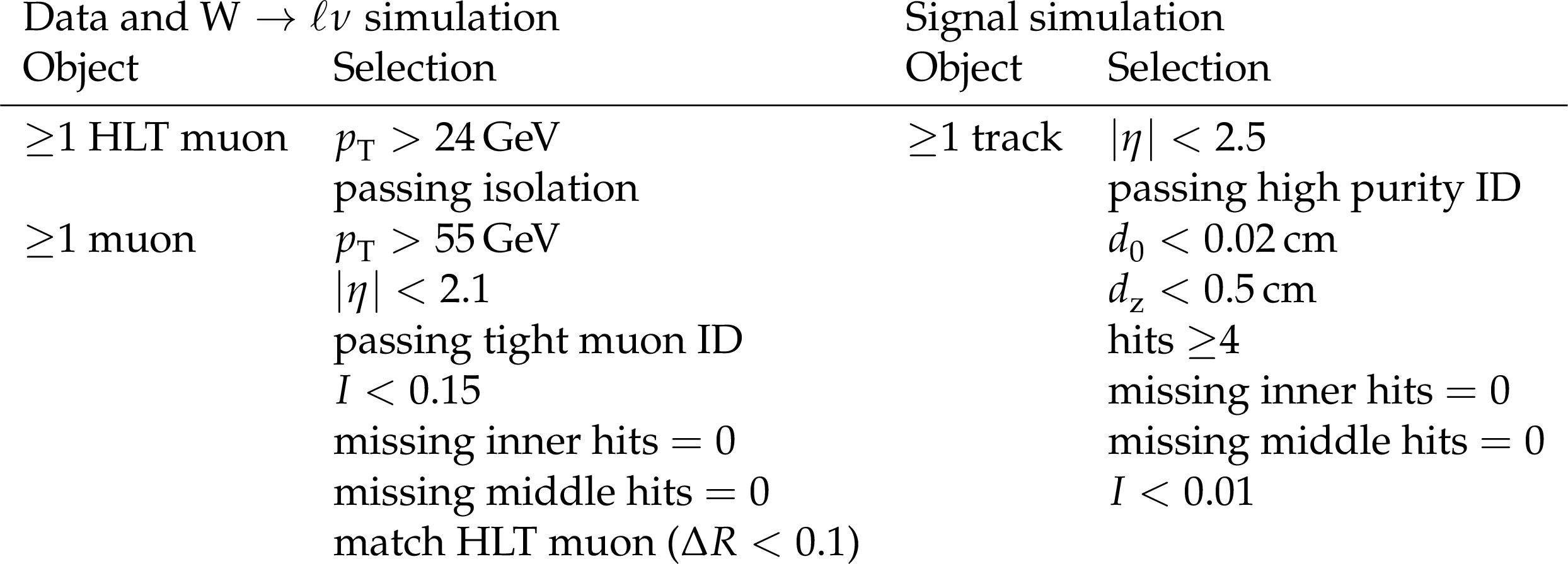
png pdf |
Table 3:
Offline event requirements for the disappearing-track trigger efficiency calculation, for data and $ \mathrm{W} \to \ell\nu $ simulation (left) and signal simulation (right). The selection criteria are applied sequentially over the given objects, and an event is selected if at least one object per event passes all requirements. |
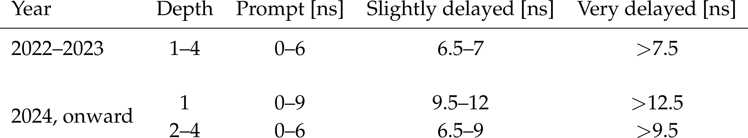
png pdf |
Table 4:
The prompt and delayed ranges of the HB TDC timing encoding in 2022--2023 and from 2024 onward. The timing ranges were changed in 2024 to account for the different behavior observed in depth 1. |

png pdf |
Table 5:
The L1T minimum thresholds for $ H_{\mathrm{T}} $ and jet $ p_{\mathrm{T}} $, comparing the thresholds of the standard trigger to those of the HCAL-based LLP jet trigger, for unprescaled paths that are used to seed LLP HLTs. The dedicated LLP L1Ts enable significantly lower energy requirements. |

png pdf |
Table 6:
The L1T CSC MDS trigger efficiency $ \epsilon $ in $ \mathrm{H} \to \text{S}\text{S} \to \mathrm{b}\overline{\mathrm{b}}\mathrm{b}\overline{\mathrm{b}} $ events, for different choices of $ m_{\mathrm{H}} $, $ m_{\text{S}} $, and $ c\tau_{\text{S}} $, for simulated events with at least 1 (middle columns) and exactly 2 (right columns) LLPs decaying within the CSC detector acceptance. The $ \epsilon_{\text{acc}} $ refers to the percentage of events within the CSC detector acceptance. The $ \epsilon_{\text{1-N}} $, $ \epsilon_{\text{1-T}} $, and $ \epsilon_{\text{2-L}} $ denote the efficiencies for the One-Nominal, One-Tight, and Two-Loose algorithms, respectively. |
| Summary |
| The CMS Run 3 long-lived particle (LLP) trigger program at the LHC, which includes many dedicated triggers designed to select different LLP signatures, has been presented. These dedicated LLP triggers extend the standard CMS trigger program and provide crucial access to the unconventional event signatures of LLPs. For 2022 data taking, some LLP triggers have been improved, such as the tracker-based displaced-jet, displaced-muon, and dimuon-scouting triggers. Other LLP triggers, such as the displaced-tau trigger, the delayed-jet trigger using the electromagnetic calorimeter timing, the displaced-jet trigger using the hadronic calorimeter, and the muon detector shower trigger, were newly added in 2022. The performance of these triggers has been shown for several new physics models and with 2022--2024 proton-proton collision data collected at $ \sqrt{s}= $ 13.6 TeV. These triggers greatly improve the CMS sensitivity to LLPs, including those predicted by theories of physics beyond the standard model, enhancing the ability of the experiment to search for new phenomena. At the time of writing, two CMS LLP analyses based on early Run 3 data collected with dedicated LLP triggers have been published: a search for displaced dimuons [12] and a search for displaced jets [11]. The Run 3 displaced dimuon search has comparable or better sensitivity than the previous Run 2 search at $ \sqrt{s}= $ 13 TeV, with only 38% of the integrated luminosity, and the Run 3 displaced jets search achieves an order-of-magnitude improvement over the previous Run 2 results. With the improvements in trigger performance and acceptance demonstrated in this paper, future Run 3 analyses are expected to outperform previous searches. The complementary nature of the trigger algorithms and their high signal acceptance will play a central role in probing a substantially larger LLP parameter space. |
| References | ||||
| 1 | Particle Data Group , S. Navas et al. | Review of particle physics | PRD 110 (2024) 030001 | |
| 2 | J. Alimena et al. | Searching for long-lived particles beyond the standard model at the Large Hadron Collider | JPG 47 (2020) 090501 | 1903.04497 |
| 3 | L. Lee, C. Ohm, A. Soffer, and T.-T. Yu | Collider searches for long-lived particles beyond the standard model | Prog. Part. Nucl. Phys. 106 (2019) 210 | 1810.12602 |
| 4 | D. Curtin et al. | Long-lived particles at the energy frontier: The MATHUSLA physics case | Rept. Prog. Phys. 82 (2019) 116201 | 1806.07396 |
| 5 | ATLAS Collaboration | Search for displaced vertices of oppositely charged leptons from decays of long-lived particles in pp collisions at $ \sqrt {s} = $ 13 TeV with the ATLAS detector | PLB 801 (2020) 135114 | 1907.10037 |
| 6 | ATLAS Collaboration | Search for heavy neutral leptons in decays of W bosons produced in 13 TeV pp collisions using prompt and displaced signatures with the ATLAS detector | JHEP 10 (2019) 265 | 1905.09787 |
| 7 | LHCb Collaboration | Search for $ a'\to\mu^+\mu^- $ decays | PRL 124 (2020) 041801 | 1910.06926 |
| 8 | CMS Collaboration | Search for b hadron decays to long-lived particles in the CMS endcap muon detectors | PRD 113 (2026) 012009 | CMS-EXO-24-004 2508.06363 |
| 9 | CMS Collaboration | Search for long-lived particles decaying in the CMS endcap muon detectors in proton-proton collisions at $ \sqrt{s} = $ 13 TeV | PRL 127 (2021) 261804 | CMS-EXO-20-015 2107.04838 |
| 10 | CMS Collaboration | Search for long-lived particles decaying in the CMS muon detectors in proton-proton collisions at $ \sqrt{s} = $ 13 TeV | PRD 110 (2024) 032007 | CMS-EXO-21-008 2402.01898 |
| 11 | CMS Collaboration | Search for light long-lived particles decaying to displaced jets in proton-proton collisions at $ \sqrt{s} = $ 13.6 TeV | Rep. Prog. Phys. 88 (2025) 037801 | CMS-EXO-23-013 2409.10806 |
| 12 | CMS Collaboration | Search for long-lived particles decaying to final states with a pair of muons in proton-proton collisions at $ \sqrt{s} = $ 13.6 TeV | JHEP 05 (2024) 047 | CMS-EXO-23-014 2402.14491 |
| 13 | CMS Collaboration | Search for long-lived particles using delayed photons in proton-proton collisions at $ \sqrt{s}= $ 13 TeV | PRD 100 (2019) 112003 | CMS-EXO-19-005 1909.06166 |
| 14 | CMS Collaboration | Search for long-lived particles using nonprompt jets and missing transverse momentum with proton-proton collisions at $ \sqrt{s} = $ 13 TeV | PLB 797 (2019) 134876 | CMS-EXO-19-001 1906.06441 |
| 15 | CMS Collaboration | Search for decays of stopped exotic long-lived particles produced in proton-proton collisions at $ \sqrt{s}= $ 13 TeV | JHEP 05 (2018) 127 | CMS-EXO-16-004 1801.00359 |
| 16 | ATLAS Collaboration | A search for the decays of stopped long-lived particles at $ \sqrt{\mathrm{s}} = $ 13 TeV with the ATLAS detector | JHEP 07 (2021) 173 | 2104.03050 |
| 17 | CMS Collaboration | Search for disappearing tracks in proton-proton collisions at $ \sqrt{s} = $ 13 TeV | PLB 806 (2020) 135502 | CMS-EXO-19-010 2004.05153 |
| 18 | ATLAS Collaboration | Search for long-lived charginos based on a disappearing-track signature in pp collisions at $ \sqrt{s}= $ 13 TeV with the ATLAS detector | JHEP 06 (2018) 022 | 1712.02118 |
| 19 | ATLAS Collaboration | Search for magnetic monopoles and stable high-electric-charge objects in 13 TeV proton-proton collisions with the ATLAS detector | PRL 124 (2020) 031802 | 1905.10130 |
| 20 | CMS Collaboration | Search for heavy long-lived charged particles with large ionization energy loss in proton-proton collisions at $ \sqrt{s} = $ 13 TeV | JHEP 04 (2025) 109 | CMS-EXO-18-002 2410.09164 |
| 21 | CMS Collaboration | Description and performance of track and primary-vertex reconstruction with the CMS tracker | JINST 9 (2014) P10009 | CMS-TRK-11-001 1405.6569 |
| 22 | CMS Collaboration | HEPData record for this analysis | link | |
| 23 | CMS Collaboration | The CMS experiment at the CERN LHC | JINST 3 (2008) S08004 | |
| 24 | CMS Collaboration | Development of the CMS detector for the CERN LHC Run 3 | JINST 19 (2024) P05064 | CMS-PRF-21-001 2309.05466 |
| 25 | CMS Collaboration | Performance of the CMS Level-1 trigger in proton-proton collisions at $ \sqrt{s} = $ 13 TeV | JINST 15 (2020) P10017 | CMS-TRG-17-001 2006.10165 |
| 26 | CMS Collaboration | The CMS trigger system | JINST 12 (2017) P01020 | CMS-TRG-12-001 1609.02366 |
| 27 | CMS Collaboration | Performance of the CMS high-level trigger during LHC Run 2 | JINST 19 (2024) P11021 | CMS-TRG-19-001 2410.17038 |
| 28 | CMS Collaboration | Electron and photon reconstruction and identification with the CMS experiment at the CERN LHC | JINST 16 (2021) P05014 | CMS-EGM-17-001 2012.06888 |
| 29 | CMS Collaboration | Performance of the CMS muon detector and muon reconstruction with proton-proton collisions at $ \sqrt{s}= $ 13 TeV | JINST 13 (2018) P06015 | CMS-MUO-16-001 1804.04528 |
| 30 | CMS Collaboration | Precision luminosity measurement in proton-proton collisions at $ \sqrt{s} = $ 13 TeV in 2015 and 2016 at CMS | EPJC 81 (2021) 800 | CMS-LUM-17-003 2104.01927 |
| 31 | CMS Collaboration | CMS luminosity measurement for the 2017 data-taking period at $ \sqrt{s} = $ 13 TeV | CMS Physics Analysis Summary, 2018 link |
CMS-PAS-LUM-17-004 |
| 32 | CMS Collaboration | CMS luminosity measurement for the 2018 data-taking period at $ \sqrt{s} = $ 13 TeV | CMS Physics Analysis Summary, 2019 link |
CMS-PAS-LUM-18-002 |
| 33 | CMS Collaboration | Luminosity measurement in proton-proton collisions at 13.6 TeV in 2022 at CMS | CMS Physics Analysis Summary, 2024 CMS-PAS-LUM-22-001 |
CMS-PAS-LUM-22-001 |
| 34 | Tracker Group of the CMS Collaboration | The CMS phase-1 pixel detector upgrade | JINST 16 (2021) P02027 | 2012.14304 |
| 35 | CMS Collaboration | Track impact parameter resolution for the full pseudo rapidity coverage in the 2017 dataset with the CMS phase-1 pixel detector | CMS Detector Performance Summary CMS-DP-2020-049, 2020 CDS |
|
| 36 | CMS Collaboration | Time reconstruction and performance of the CMS electromagnetic calorimeter | JINST 5 (2010) T03011 | CMS-CFT-09-006 0911.4044 |
| 37 | CMS Collaboration | Performance of the CMS electromagnetic calorimeter in pp collisions at $ \sqrt{s} = $ 13 TeV | JINST 19 (2024) P09004 | CMS-EGM-18-002 2403.15518 |
| 38 | CMS Collaboration | CMS technical design report for the Phase 1 upgrade of the hadron calorimeter | CMS Technical Proposal CERN-LHCC-2012-015, CMS-TDR-010, 2012 link |
|
| 39 | CMS Collaboration | Measurements with silicon photomultipliers of dose-rate effects in the radiation damage of plastic scintillator tiles in the CMS hadron endcap calorimeter | JINST 15 (2020) P06009 | CMS-PRF-18-003 2001.06553 |
| 40 | CMS Collaboration | Jet energy scale and resolution in the CMS experiment in pp collisions at 8 TeV | JINST 12 (2017) P02014 | CMS-JME-13-004 1607.03663 |
| 41 | CMS Collaboration | The Phase 2 upgrade of the CMS muon detectors | CMS Technical Proposal CERN-LHCC-2017-012, CMS-TDR-016, 2017 CDS |
|
| 42 | CMS Collaboration | CMS technical design report for the Level-1 trigger upgrade | CMS Technical Proposal CERN-LHCC-2013-011, CMS-TDR-012, 2013 CDS |
|
| 43 | J. Duarte et al. | Fast inference of deep neural networks in FPGAs for particle physics | JINST 13 (2018) P07027 | 1804.06913 |
| 44 | CMS Collaboration | Using the CMS threaded framework in a production environment | J. Phys. Conf. Ser. 664 (2015) 072026 | |
| 45 | CMS Collaboration | Enriching the physics program of the CMS experiment via data scouting and data parking | Phys. Rept. 1115 (2025) 678 | CMS-EXO-23-007 2403.16134 |
| 46 | A. Bocci et al. | Heterogeneous reconstruction of tracks and primary vertices with the CMS pixel tracker | Front. Big Data 3 (2020) 601728 | 2008.13461 |
| 47 | CMS Collaboration | Developing GPU-compliant algorithms for CMS ECAL local reconstruction during LHC Run 3 and Phase 2 | J. Phys. Conf. Ser. 2438 (2023) 012027 | |
| 48 | CMS Collaboration | Heterogeneous computing for the local reconstruction algorithms of the CMS calorimeters | J. Phys. Conf. Ser. 1525 (2020) 012040 | |
| 49 | CMS Collaboration | 2024 HLT timing and throughput results | CMS Detector Performance Summary CMS-DP-2024-082; CERN-CMS-DP-2024-082, 2024 CDS |
|
| 50 | CMS Collaboration | Performance of Run 3 HLT track reconstruction | CMS Detector Performance Summary CMS-DP-2022-014; CERN-CMS-DP-2022-014, 2022 link |
|
| 51 | S. Lantz et al. | Speeding up particle track reconstruction using a parallel Kalman filter algorithm | JINST 15 (2020) P09030 | 2006.00071 |
| 52 | CMS Collaboration | Performance of Run 3 track reconstruction with the mkFit algorithm | CMS Detector Performance Summary CCMS-DP-2022-018, 2022 CDS |
|
| 53 | E. Bols et al. | Jet flavour classification using DeepJet | JINST 15 (2020) P12012 | 2008.10519 |
| 54 | H. Qu and L. Gouskos | ParticleNet: Jet tagging via particle clouds | PRD 101 (2020) 056019 | 1902.08570 |
| 55 | CMS Collaboration | Particle-flow reconstruction and global event description with the CMS detector | JINST 12 (2017) P10003 | CMS-PRF-14-001 1706.04965 |
| 56 | CMS Collaboration | The Phase-2 upgrade of the CMS Level-1 trigger | CMS Technical Design Report CERN-LHCC-2020-004, CMS-TDR-021, 2020 CDS |
|
| 57 | CMS Collaboration | The Level 1 scouting system of the CMS experiment | CMS Conference Report CMS-CR-2023-024, 2023 CDS |
|
| 58 | CMS Collaboration | Technical proposal for the Phase-II upgrade of the Compact Muon Solenoid | CMS Technical Proposal CERN-LHCC-2015-010, CMS-TDR-15-02, 2015 CDS |
|
| 59 | R. Fr \"u hwirth | Application of Kalman filtering to track and vertex fitting | NIM A 262 (1987) 444 | |
| 60 | CMS Collaboration | Performance of track reconstruction at the CMS High-Level Trigger in 2022 data | CMS Detector Performance Summary CMS-DP-2023-028; CERN-CMS-DP-2023-028, 2023 CDS |
|
| 61 | CMS Collaboration | Performance of track reconstruction at the CMS high-level trigger in 2023 data | CMS Detector Performance Summary CMS-DP-2024-013, CERN-CMS-DP-2024-013, 2024 CDS |
|
| 62 | K. Rose | Deterministic annealing for clustering, compression, classification, regression, and related optimization problems | IEEE Proc. 86 (1998) 2210 | |
| 63 | R. Fr \"u hwirth, W. Waltenberger, and P. Vanlaer | Adaptive vertex fitting | JPG 34 (2007) N343 | |
| 64 | CMS Collaboration | Performance of CMS muon reconstruction in pp collision events at $ \sqrt{s}= $ 7 TeV | JINST 7 (2012) P10002 | CMS-MUO-10-004 1206.4071 |
| 65 | CMS Collaboration | Identification of low-momentum muons in the CMS detector using multivariate techniques in proton-proton collisions at $ \sqrt{s} = $ 13.6 TeV | JINST 20 (2025) P04021 | CMS-MUO-24-001 2412.17590 |
| 66 | CMS Collaboration | Performance of the CMS muon trigger system in proton-proton collisions at $ \sqrt{s} = $ 13 TeV | JINST 16 (2021) P07001 | CMS-MUO-19-001 2102.04790 |
| 67 | W. Adam, R. Fr \"u hwirth, A. Strandlie, and T. Todorov | Reconstruction of electrons with the Gaussian-sum filter in the CMS tracker at LHC | JPG 31 (2005) N9 | physics/0306087 |
| 68 | CMS Collaboration | Performance of photon reconstruction and identification with the CMS detector in proton-proton collisions at $ \sqrt{s} = $ 8 TeV | JINST 10 (2015) P08010 | CMS-EGM-14-001 1502.02702 |
| 69 | CMS Collaboration | Performance of electron reconstruction and selection with the CMS detector in proton-proton collisions at $ \sqrt{s} = $ 8 TeV | JINST 10 (2015) P06005 | CMS-EGM-13-001 1502.02701 |
| 70 | CMS Collaboration | ECAL 2016 refined calibration and Run 2 summary plots | CMS Detector Performance Summary CMS-DP-2020-021, 2020 CDS |
|
| 71 | M. Cacciari, G. P. Salam, and G. Soyez | The anti-$ k_{\mathrm{T}} $ jet clustering algorithm | JHEP 04 (2008) 063 | 0802.1189 |
| 72 | M. Cacciari, G. P. Salam, and G. Soyez | FastJet user manual | EPJC 72 (2012) 1896 | 1111.6097 |
| 73 | CMS Collaboration | Pileup mitigation at CMS in 13 TeV data | JINST 15 (2020) P09018 | CMS-JME-18-001 2003.00503 |
| 74 | D. Bertolini, P. Harris, M. Low, and N. Tran | Pileup per particle identification | JHEP 10 (2014) 059 | 1407.6013 |
| 75 | CMS Collaboration | Performance of reconstruction and identification of $ \tau $ leptons decaying to hadrons and $ \nu_\tau $ in pp collisions at $ \sqrt{s}= $ 13 TeV | JINST 13 (2018) P10005 | CMS-TAU-16-003 1809.02816 |
| 76 | CMS Collaboration | Identification of hadronic tau lepton decays using a deep neural network | JINST 17 (2022) P07023 | CMS-TAU-20-001 2201.08458 |
| 77 | CMS Collaboration | Performance of missing transverse momentum reconstruction in proton-proton collisions at $ \sqrt{s} = $ 13 TeV using the CMS detector | JINST 14 (2019) P07004 | CMS-JME-17-001 1903.06078 |
| 78 | J. Alwall et al. | The automated computation of tree-level and next-to-leading order differential cross sections, and their matching to parton shower simulations | JHEP 07 (2014) 079 | 1405.0301 |
| 79 | C. Bierlich et al. | A comprehensive guide to the physics and usage of PYTHIA 8.3 | SciPost Phys. Codeb. 2022 (2022) 8 | 2203.11601 |
| 80 | J. Alwall et al. | Comparative study of various algorithms for the merging of parton showers and matrix elements in hadronic collisions | EPJC 53 (2008) 473 | 0706.2569 |
| 81 | R. Frederix and S. Frixione | Merging meets matching in MC@NLO | JHEP 12 (2012) 061 | 1209.6215 |
| 82 | NNPDF Collaboration | Parton distributions from high-precision collider data | EPJC 77 (2017) 663 | 1706.00428 |
| 83 | CMS Collaboration | Extraction and validation of a new set of CMS PYTHIA8 tunes from underlying-event measurements | EPJC 80 (2020) 4 | CMS-GEN-17-001 1903.12179 |
| 84 | GEANT4 Collaboration | GEANT 4---a simulation toolkit | NIM A 506 (2003) 250 | |
| 85 | G. F. Giudice, M. A. Luty, H. Murayama, and R. Rattazzi | Gaugino mass without singlets | JHEP 12 (1998) 027 | hep-ph/9810442 |
| 86 | L. Randall and R. Sundrum | Out of this world supersymmetry breaking | NPB 557 (1999) 79 | hep-th/9810155 |
| 87 | Z. Chacko, H.-S. Goh, and R. Harnik | The twin Higgs: Natural electroweak breaking from mirror symmetry | PRL 96 (2006) 231802 | hep-ph/0506256 |
| 88 | D. Curtin and C. B. Verhaaren | Discovering uncolored naturalness in exotic Higgs decays | JHEP 12 (2015) 072 | 1506.06141 |
| 89 | H.-C. Cheng, S. Jung, E. Salvioni, and Y. Tsai | Exotic quarks in twin Higgs models | JHEP 03 (2016) 074 | 1512.02647 |
| 90 | D. Curtin, R. Essig, S. Gori, and J. Shelton | Illuminating dark photons with high-energy colliders | JHEP 02 (2015) 157 | 1412.0018 |
| 91 | B. C. Allanach et al. | The Snowmass points and slopes: Benchmarks for SUSY searches | EPJC 25 (2002) 113 | hep-ph/0202233 |
| 92 | F. Blekman et al. | Soft displaced leptons at the LHC | JHEP 11 (2020) 112 | 2007.03708 |
| 93 | CMS Collaboration | Performance of long lived particle triggers in Run 3 | CMS Detector Performance Summary CMS-DP-2023-043, 2023 CDS |
|
| 94 | CMS Collaboration | Level-1 trigger algorithm for long-lived particle jets in Run 3 | CMS Detector Performance Summary CMS-DP-2024-058, 2024 link |
|
| 95 | CMS Collaboration | CSC high multiplicity trigger in Run 3 | CMS Detector Performance Summary CMS-DP-2022-062, CERN-CMS-DP-2022-062, 2022 link |
|
| 96 | CMS Collaboration | High multiplicity trigger for long-lived particles in CMS detector in 2022 and 2023 | CMS Detector Performance Summary CMS-DP-2024-099, CERN-CMS-DP-2024-099, 2024 CDS |
|
| 97 | CMS Collaboration | Displaced photons HLT trigger on 2017 data at 13 TeV | CMS Detector Performance Summary CMS-DP-2020-015; CERN-CMS-DP-2020-015, 2020 CDS |
|
| 98 | CMS Collaboration | A DNN for CMS track classification and selection | EPJ Web Conf. 295 (2024) 03001 | 2311.05157 |
| 99 | M. Buican, P. Meade, N. Seiberg, and D. Shih | Exploring general gauge mediation | JHEP 03 (2009) 016 | 0812.3668 |
| 100 | P. Meade, N. Seiberg, and D. Shih | General gauge mediation | Prog. Theor. Phys. Suppl. 177 (2009) 143 | 0801.3278 |
| 101 | G. F. Giudice and R. Rattazzi | Theories with gauge mediated supersymmetry breaking | Phys. Rept. 322 (1999) 419 | hep-ph/9801271 |
| 102 | CMS Collaboration | Search for direct pair production of supersymmetric partners of $ \tau $ leptons in the final state with two hadronically decaying $ \tau $ leptons and missing transverse momentum in proton-proton collisions at $ \sqrt{s} = $ 13 TeV | PRD 108 (2023) 012011 | CMS-SUS-21-001 2207.02254 |
| 103 | CMS Collaboration | Search for long-lived particles using displaced jets in proton-proton collisions at $ \sqrt{s} = $ 13 TeV | PRD 104 (2021) 012015 | CMS-EXO-19-021 2012.01581 |
| 104 | N. Arkani-Hamed and S. Dimopoulos | Supersymmetric unification without low energy supersymmetry and signatures for fine-tuning at the LHC | JHEP 06 (2005) 073 | hep-th/0405159 |
| 105 | G. F. Giudice and A. Romanino | Split supersymmetry | NPB 699 (2004) 65 | hep-ph/0406088 |
| 106 | J. L. Hewett, B. Lillie, M. Masip, and T. G. Rizzo | Signatures of long-lived gluinos in split supersymmetry | JHEP 09 (2004) 070 | hep-ph/0408248 |
| 107 | N. Arkani-Hamed, S. Dimopoulos, G. F. Giudice, and A. Romanino | Aspects of split supersymmetry | NPB 709 (2005) 3 | hep-ph/0409232 |
| 108 | P. Gambino, G. F. Giudice, and P. Slavich | Gluino decays in split supersymmetry | NPB 726 (2005) 35 | hep-ph/0506214 |
| 109 | A. Arvanitaki, N. Craig, S. Dimopoulos, and G. Villadoro | Mini-split | JHEP 02 (2013) 126 | 1210.0555 |
| 110 | N. Arkani-Hamed et al. | Simply unnatural supersymmetry | 1212.6971 | |
| 111 | P. Fayet | Supergauge invariant extension of the Higgs mechanism and a model for the electron and its neutrino | NPB 90 (1975) 104 | |
| 112 | G. R. Farrar and P. Fayet | Phenomenology of the production, decay, and detection of new hadronic states associated with supersymmetry | PLB 76 (1978) 575 | |
| 113 | S. Weinberg | Supersymmetry at ordinary energies: 1. Masses and conservation laws | PRD 26 (1982) 287 | |
| 114 | L. J. Hall and M. Suzuki | Explicit $ R $-parity breaking in supersymmetric models | NPB 231 (1984) 419 | |
| 115 | R. Barbier et al. | $ R $-parity violating supersymmetry | Phys. Rept. 420 (2005) 1 | hep-ph/0406039 |
| 116 | C. Csaki, E. Kuflik, and T. Volansky | Dynamical $ R $-parity violation | PRL 112 (2014) 131801 | 1309.5957 |
| 117 | C. Csaki, E. Kuflik, O. Slone, and T. Volansky | Models of dynamical $ R $-parity violation | JHEP 06 (2015) 045 | 1502.03096 |
| 118 | ATLAS Collaboration | Search for light long-lived particles in $ pp $ collisions at $ \sqrt{s}= $ 13 TeV using displaced vertices in the ATLAS inner detector | PRL 133 (2024) 161803 | 2403.15332 |
| 119 | CMS Collaboration | A novel timing trigger with the CMS hadron calorimeter | CMS Detector Performance Summary CERN-CMS-DN-2023-022, 2023 CDS |
|
| 120 | M. J. Strassler and K. M. Zurek | Echoes of a hidden valley at hadron colliders | PLB 651 (2007) 374 | hep-ph/0604261 |
| 121 | CMS Collaboration | The CMS electromagnetic calorimeter project: Technical Design Report | CMS Technical Design Report CERN-LHCC-97-033, CMS-TDR-4, 1997 CDS |
|
| 122 | CMS Collaboration | Measurement of the inclusive W and Z production cross sections in pp collisions at $ \sqrt{s}= $ 7 TeV | JHEP 10 (2011) 132 | CMS-EWK-10-005 1107.4789 |
| 123 | CMS Collaboration | Search for long-lived particles decaying to a pair of muons in proton-proton collisions at $ \sqrt{s} = $ 13 TeV | JHEP 05 (2023) 228 | CMS-EXO-21-006 2205.08582 |
| 124 | CMS Collaboration | The algorithm of the CMS Level-1 overlap muon track finder trigger | NIM A 936 (2019) 368 | |
| 125 | CMS Collaboration | Boosted decision trees in the Level-1 muon endcap trigger at CMS | J. Phys. Conf. Ser. 1085 (2018) 042042 | |
| 126 | J. Alwall, P. Schuster, and N. Toro | Simplified models for a first characterization of new physics at the LHC | PRD 79 (2009) 075020 | 0810.3921 |
| 127 | CMS Collaboration | Search for long-lived particles decaying to leptons with large impact parameter in proton-proton collisions at $ \sqrt{s} = $ 13 TeV | EPJC 82 (2022) 153 | CMS-EXO-18-003 2110.04809 |
| 128 | P. W. Graham, D. E. Kaplan, S. Rajendran, and P. Saraswat | Displaced supersymmetry | JHEP 07 (2012) 149 | 1204.6038 |
| 129 | J. A. Evans and J. Shelton | Long-lived staus and displaced leptons at the LHC | JHEP 04 (2016) 056 | 1601.01326 |
| 130 | M. J. Strassler and K. M. Zurek | Discovering the Higgs through highly-displaced vertices | PLB 661 (2008) 263 | hep-ph/0605193 |
| 131 | CMS Collaboration | Dark sector searches with the CMS experiment | Phys. Rept. 1115 (2025) 448 | CMS-EXO-23-005 2405.13778 |
| 132 | CMS Collaboration | Search for long-lived particles decaying into muon pairs in proton-proton collisions at $ \sqrt{s} = $ 13 TeV collected with a dedicated high-rate data stream | JHEP 04 (2022) 062 | CMS-EXO-20-014 2112.13769 |
| 133 | Y. L. Dokshitzer, G. D. Leder, S. Moretti, and B. R. Webber | Better jet clustering algorithms | JHEP 08 (1997) 001 | hep-ph/9707323 |
| 134 | M. Wobisch and T. Wengler | Hadronization corrections to jet cross-sections in deep inelastic scattering | in Proc. Workshop on Monte Carlo Generators for HERA Physics (Plenary Starting Meeting), 1998 | hep-ph/9907280 |
| 135 | R. Bailey and P. Collier | Standard filling schemes for various LHC operation modes | Technical Report LHC-PROJECT-NOTE-323, 2003 | |
| 136 | CMS Collaboration | Search for decays of stopped long-lived particles produced in proton-proton collisions at $ \sqrt{s} = $ 8 TeV | EPJC 75 (2015) 151 | CMS-EXO-12-036 1501.05603 |
| 137 | D. Abercrombie et al. | Dark matter benchmark models for early LHC Run 2 searches: Report of the ATLAS/CMS dark matter forum | Phys. Dark Univ. 27 (2020) 100371 | 1507.00966 |
| 138 | L. M. Carpenter, R. Colburn, J. Goodman, and T. Linden | Indirect detection constraints on s and t channel simplified models of dark matter | PRD 94 (2016) 055027 | 1606.04138 |
| 139 | L. Covi and F. Dradi | Long-lived stop at the LHC with or without $ R $-parity | JCAP 10 (2014) 039 | 1403.4923 |
| 140 | P. Langacker and G. Steigman | Requiem for a fractionally charged, massive particle | PRD 84 (2011) 065040 | 1107.3131 |
| 141 | CMS Collaboration | Technical proposal for the Phase-II upgrade of the CMS detector | CMS Technical Proposal CERN-LHCC-2015-010, LHCC-P-008, CMS-TDR-15-02, 2015 link |
|
| 142 | CMS Collaboration | The Phase-2 upgrade of the CMS tracker | CMS Technical Design Report CERN-LHCC-2017-009, CMS-TDR-014, 2017 link |
|
| 143 | CMS Collaboration | The Phase-2 upgrade of the CMS barrel calorimeters | CMS Technical Design Report CERN-LHCC-2017-011, CMS-TDR-015, 2017 CDS |
|
| 144 | CMS Collaboration | The Phase-2 upgrade of the CMS endcap calorimeter | CMS Technical Design Report CERN-LHCC-2017-023, CMS-TDR-019, 2017 link |
|
| 145 | CMS Collaboration | The Phase-2 upgrade of the CMS muon detectors | CMS Technical Design Report CERN-LHCC-2017-012, CMS-TDR-016, 2017 CDS |
|
| 146 | CMS Collaboration | A MIP timing detector for the CMS Phase-2 upgrade | CMS Technical Design Report CERN-LHCC-2019-003, CMS-TDR-020, 2019 CDS |
|
| 147 | CMS Collaboration | Update of the MTD physics case | CMS Detector Performance Summary CMS-DP-2022-025, 2022 CDS |
|
| 148 | CMS Collaboration | Snowmass white paper contribution: Physics with the Phase-2 ATLAS and CMS detectors | CMS Physics Analysis Summary, 2022 CMS-PAS-FTR-22-001 |
|
| 149 | A. Dainese | Report on the physics at the HL-LHC, and perspectives for the HE-LHC | et al., eds.,, volume 7/ of CERN Yellow Reports: Monographs. CERN,, ISBN 978-92-9083-549-3, 2019 link |
|
| 150 | CMS Collaboration | Search for dark matter in final states with a Higgs boson decaying to a pair of b jets and missing transverse momentum at the HL-LHC | CMS Physics Analysis Summary, 2022 CMS-PAS-FTR-22-005 |
CMS-PAS-FTR-22-005 |
|
|
Compact Muon Solenoid LHC, CERN |
|

|

|

|

|

|