

Compact Muon Solenoid
LHC, CERN
| CMS-PAS-LUM-22-001 | ||
| Luminosity measurement in proton-proton collisions at 13.6 TeV in 2022 at CMS | ||
| CMS Collaboration | ||
| 5 March 2024 | ||
| Abstract: The measurement of the integrated luminosity for the proton-proton collisions data-taking period at a center-of-mass energy of 13.6 TeV in 2022 with the CMS experiment at the CERN LHC is reported. The absolute scale of the luminosity measurement is calibrated from beam-separation scans with the van der Meer scan method. The precision of the calibration is limited by the knowledge of the factorization of the bunch proton density during the van der Meer scans. Continuous rate measurements with various CMS subdetectors provide a stable and linear luminosity measurement. Considering both calibration and integration sources, the integrated luminosity measurement has a total uncertainty of 1.4%. | ||
| Links: CDS record (PDF) ; CADI line (restricted) ; | ||
| Figures | |
png pdf |
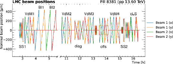
Figure 1:
Nominal horizontal and vertical positions of the proton beams during LHC fill 8381 as a function of time. The scan pairs are labelled with the abbreviations introduced in the text. |

png pdf |
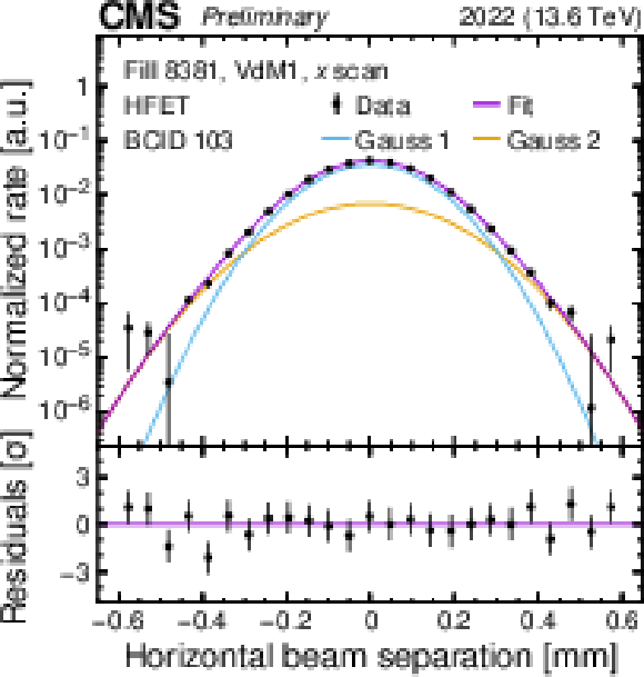
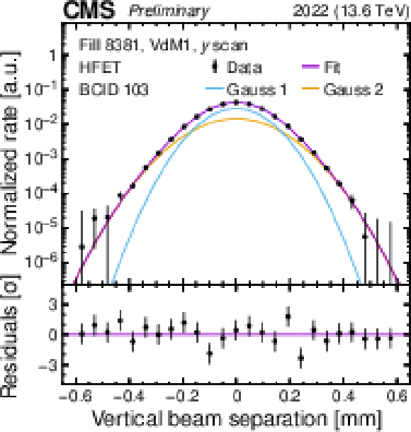
Figure 2:
Double-Gaussian fits to the HFET data recorded during the first vdM scan pair (vdM1), shown for the $ x $ (left) and $ y $ (right) scan. In the bottom panels, the difference between the measured rate and the fit divided by the statistical uncertainty is shown. |
png pdf |
Figure 2-a:
Double-Gaussian fits to the HFET data recorded during the first vdM scan pair (vdM1), shown for the $ x $ (left) and $ y $ (right) scan. In the bottom panels, the difference between the measured rate and the fit divided by the statistical uncertainty is shown. |
png pdf |
Figure 2-b:
Double-Gaussian fits to the HFET data recorded during the first vdM scan pair (vdM1), shown for the $ x $ (left) and $ y $ (right) scan. In the bottom panels, the difference between the measured rate and the fit divided by the statistical uncertainty is shown. |

png pdf |
Figure 3:
Residual beam position deviations after subtracting nominal positions, linear orbit drift, and beam-beam deflection from the DOROS BPM measurement, for the scans in $ x $ (left) and $ y $ (right). The beams moving in a scan from negative to positive (positive to negative) coordinate values are shown in purple (blue). |
png pdf |
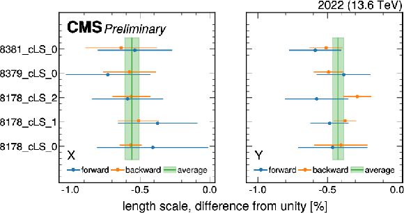
Figure 4:
Length scale factors in $ x $ (left) and $ y $ (right) obtained for the fits of the forward (blue) and backward (orange) scans in the different fills, after applying the orbit drift correction. The green band indicates the average and its uncertainty. |

png pdf |
Figure 5:
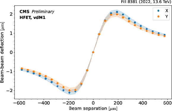
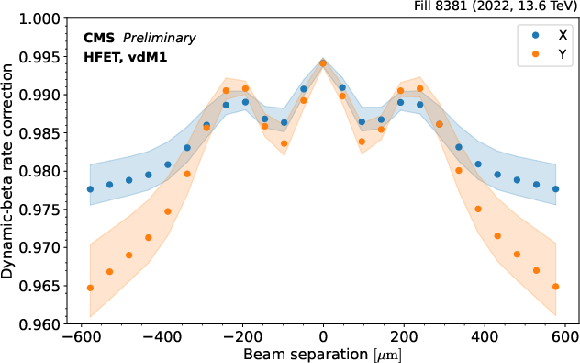
Beam-beam deflection (left) and multiplicative dynamic-$ \beta $ correction for the rate (right) shown for the first vdM scan pair in fill 8381, as an average effect over all bunch crossings with bands covering the minimum and maximum values used for the per-bunch correction. |
png pdf |
Figure 5-a:
Beam-beam deflection (left) and multiplicative dynamic-$ \beta $ correction for the rate (right) shown for the first vdM scan pair in fill 8381, as an average effect over all bunch crossings with bands covering the minimum and maximum values used for the per-bunch correction. |
png pdf |
Figure 5-b:
Beam-beam deflection (left) and multiplicative dynamic-$ \beta $ correction for the rate (right) shown for the first vdM scan pair in fill 8381, as an average effect over all bunch crossings with bands covering the minimum and maximum values used for the per-bunch correction. |
png pdf |
Figure 6:
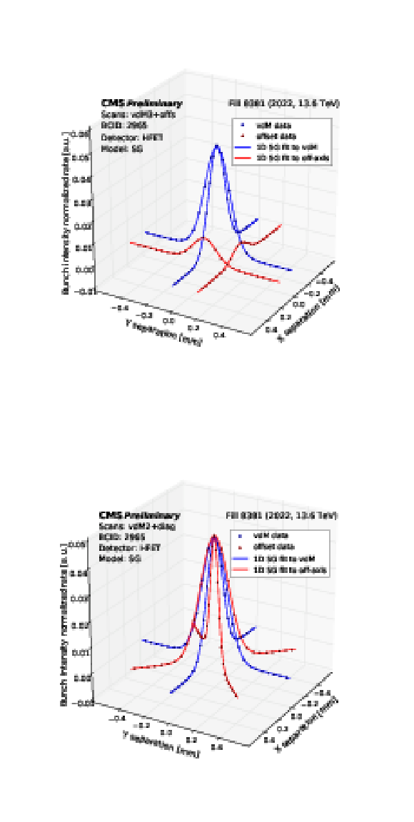
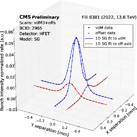
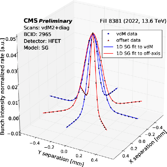
Illustration of the 2D shape determination using the combined analysis of a vdM scan pair with an offs (left) or diag (right) scan pair. |
png pdf |
Figure 6-a:
Illustration of the 2D shape determination using the combined analysis of a vdM scan pair with an offs (left) or diag (right) scan pair. |
png pdf |
Figure 6-b:
Illustration of the 2D shape determination using the combined analysis of a vdM scan pair with an offs (left) or diag (right) scan pair. |
png pdf |
Figure 7:
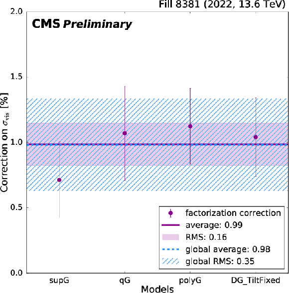
Dependence of averaged predictions on the fit model, uncertainties are defined by the RMS over all the averaged measurements. Final result with corresponding RMS is shown in purple for comparison. |
png pdf |
Figure 8:
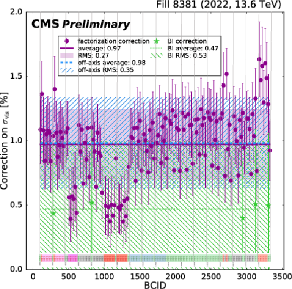
Averaged predictions of on-axis - off-axis scan pairs, all detectors, and fit models for each colliding bunch pair (BCID). Uncertainties were defined by the RMS over all the averaged measurements. The color-code is used along the $ x $-axis of the figure indicating different collision patterns. Final result with corresponding RMS are compared to the BI method (shown in green). |
png pdf |
Figure 9:
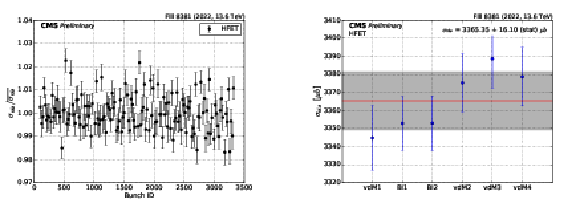
Results for $ \sigma_{\mathrm{vis}} $ from the vdM scan pair analysis using HFET data, as a function of the bunch crossing (left) and the scan pair (right). On the left, the $ \sigma_{\mathrm{vis}} $ values are shown divided by the average $ \sigma_{\mathrm{vis}} $, denoted as $ \overline{\sigma_{\mathrm{vis}}} $. On the right, the statistical uncertainty in the average $ \sigma_{\mathrm{vis}} $ is indicated with the grey band. |
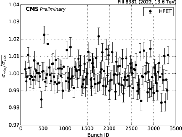
png pdf |
Figure 9-a:
Results for $ \sigma_{\mathrm{vis}} $ from the vdM scan pair analysis using HFET data, as a function of the bunch crossing (left) and the scan pair (right). On the left, the $ \sigma_{\mathrm{vis}} $ values are shown divided by the average $ \sigma_{\mathrm{vis}} $, denoted as $ \overline{\sigma_{\mathrm{vis}}} $. On the right, the statistical uncertainty in the average $ \sigma_{\mathrm{vis}} $ is indicated with the grey band. |
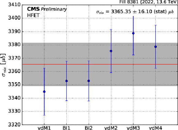
png pdf |
Figure 9-b:
Results for $ \sigma_{\mathrm{vis}} $ from the vdM scan pair analysis using HFET data, as a function of the bunch crossing (left) and the scan pair (right). On the left, the $ \sigma_{\mathrm{vis}} $ values are shown divided by the average $ \sigma_{\mathrm{vis}} $, denoted as $ \overline{\sigma_{\mathrm{vis}}} $. On the right, the statistical uncertainty in the average $ \sigma_{\mathrm{vis}} $ is indicated with the grey band. |
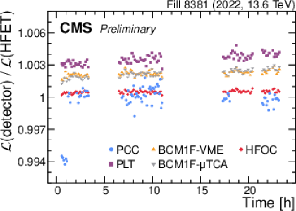
png pdf |
Figure 10:
Ratio between the luminosity measurements provided by HFET, HFOC, PCC, PLT, BCM1F VME, and BCM1F $\mu$TCA during LHC fill 8381 as a function of time. For the ratio involving PCC, only times where the full CMS detector recorded data are included. |
png pdf |
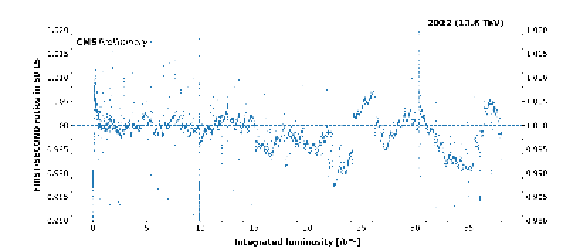
Figure 11:
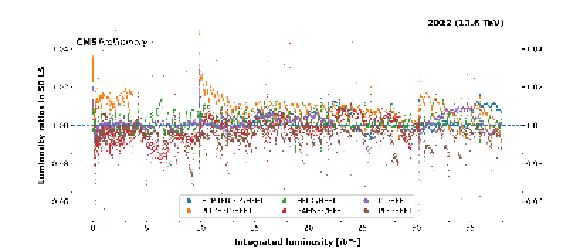
Ratio of the luminosity measured in time windows of 50 LS (about 20 min) between all the luminosity detectors and HFET as a function of the integrated luminosity. |
png pdf |
Figure 12:
Ratio of the luminosity measured in time windows of 50 LS (about 20 min) between best and second-best luminosity detector as a function of the integrated luminosity. |
png pdf |
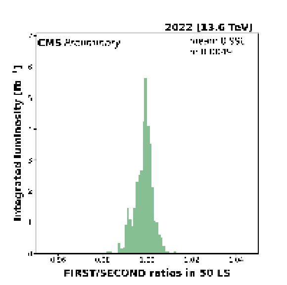
Figure 13:
Histogram of the ratio of the measured luminosity between the best and second-best luminosity detector, as evaluated in time windows of 50 LS (about 20 min). |
png pdf |
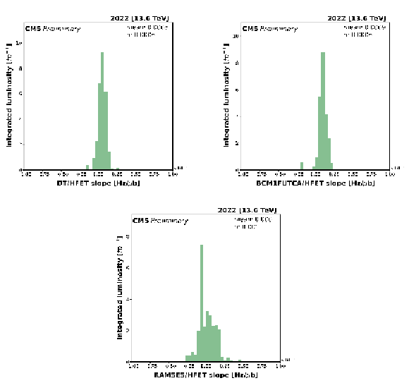
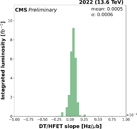
Figure 14:
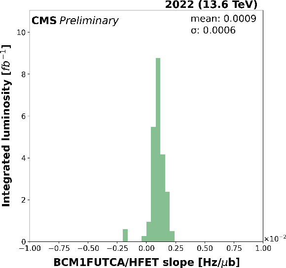
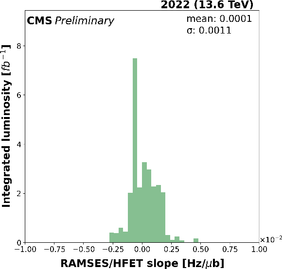
Distribution of relative non-linearity slopes between different detectors, evaluated separately for each fill. Each entry is weighted with the integrated luminosity of the fill. |
png |
Figure 14-a:
Distribution of relative non-linearity slopes between different detectors, evaluated separately for each fill. Each entry is weighted with the integrated luminosity of the fill. |
png |
Figure 14-b:
Distribution of relative non-linearity slopes between different detectors, evaluated separately for each fill. Each entry is weighted with the integrated luminosity of the fill. |
png |
Figure 14-c:
Distribution of relative non-linearity slopes between different detectors, evaluated separately for each fill. Each entry is weighted with the integrated luminosity of the fill. |
png pdf |
Figure 15:
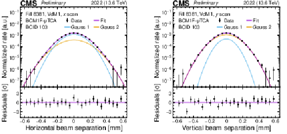
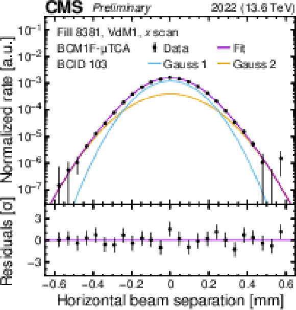
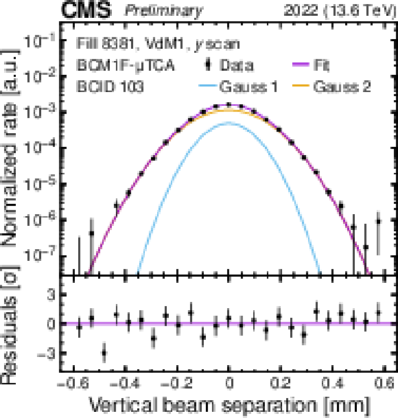
Double-Gaussian fits to the BCM1F $\mu$TCA data recorded during the first vdM scan pair (vdM1), shown for the $ x $ (left) and $ y $ (right) scan. In the bottom panels, the difference between the measured rate and the fit divided by the statistical uncertainty is shown. |
png pdf |
Figure 15-a:
Double-Gaussian fits to the BCM1F $\mu$TCA data recorded during the first vdM scan pair (vdM1), shown for the $ x $ (left) and $ y $ (right) scan. In the bottom panels, the difference between the measured rate and the fit divided by the statistical uncertainty is shown. |
png pdf |
Figure 15-b:
Double-Gaussian fits to the BCM1F $\mu$TCA data recorded during the first vdM scan pair (vdM1), shown for the $ x $ (left) and $ y $ (right) scan. In the bottom panels, the difference between the measured rate and the fit divided by the statistical uncertainty is shown. |
png pdf |
Figure 16:
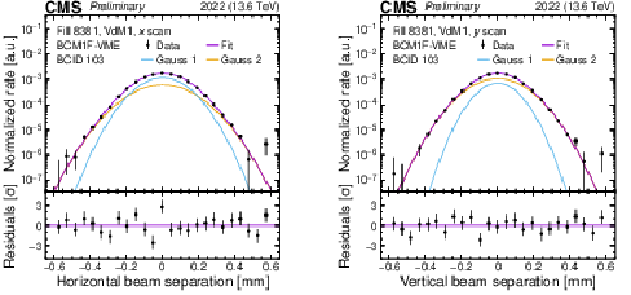
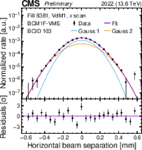
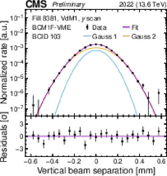
Double-Gaussian fits to the BCM1F VME data recorded during the first vdM scan pair (vdM1), shown for the $ x $ (left) and $ y $ (right) scan. In the bottom panels, the difference between the measured rate and the fit divided by the statistical uncertainty is shown. |
png pdf |
Figure 16-a:
Double-Gaussian fits to the BCM1F VME data recorded during the first vdM scan pair (vdM1), shown for the $ x $ (left) and $ y $ (right) scan. In the bottom panels, the difference between the measured rate and the fit divided by the statistical uncertainty is shown. |
png pdf |
Figure 16-b:
Double-Gaussian fits to the BCM1F VME data recorded during the first vdM scan pair (vdM1), shown for the $ x $ (left) and $ y $ (right) scan. In the bottom panels, the difference between the measured rate and the fit divided by the statistical uncertainty is shown. |
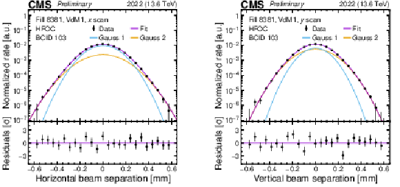
png pdf |
Figure 17:
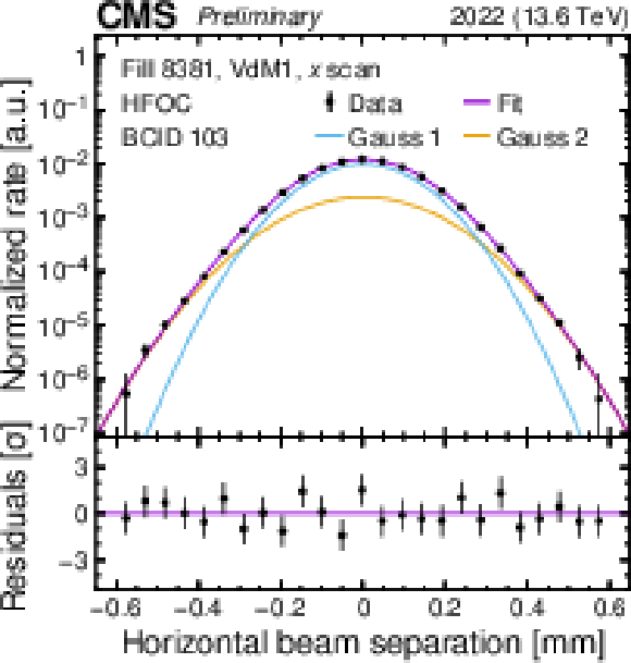
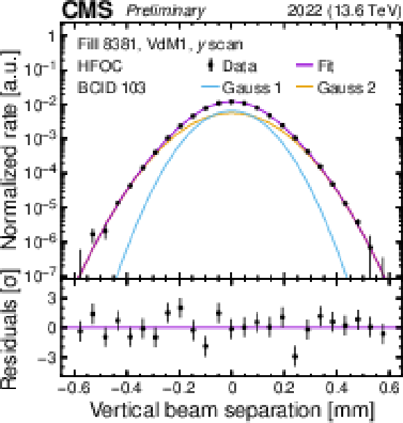
Double-Gaussian fits to the HFOC data recorded during the first vdM scan pair (vdM1), shown for the $ x $ (left) and $ y $ (right) scan. In the bottom panels, the difference between the measured rate and the fit divided by the statistical uncertainty is shown. |
png pdf |
Figure 17-a:
Double-Gaussian fits to the HFOC data recorded during the first vdM scan pair (vdM1), shown for the $ x $ (left) and $ y $ (right) scan. In the bottom panels, the difference between the measured rate and the fit divided by the statistical uncertainty is shown. |
png pdf |
Figure 17-b:
Double-Gaussian fits to the HFOC data recorded during the first vdM scan pair (vdM1), shown for the $ x $ (left) and $ y $ (right) scan. In the bottom panels, the difference between the measured rate and the fit divided by the statistical uncertainty is shown. |
png pdf |
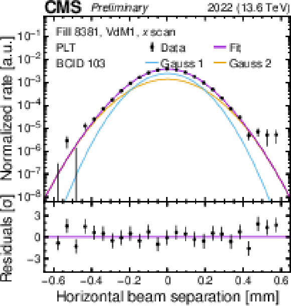
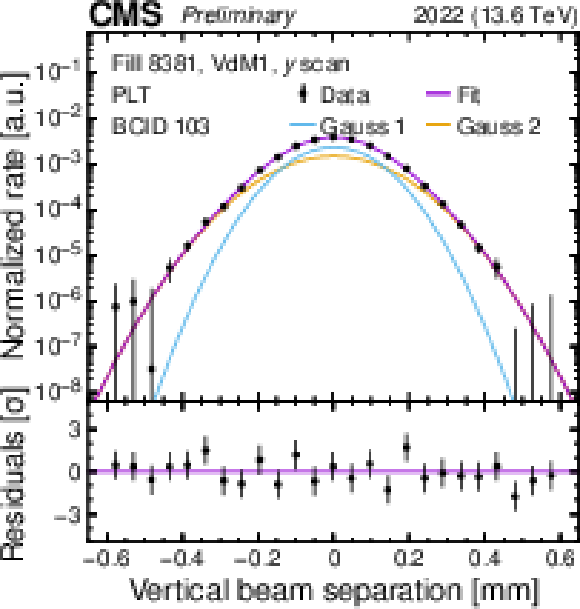
Figure 18:
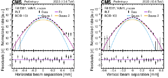
Double-Gaussian fits to the PLT data recorded during the first vdM scan pair (vdM1), shown for the $ x $ (left) and $ y $ (right) scan. In the bottom panels, the difference between the measured rate and the fit divided by the statistical uncertainty is shown. |
png pdf |
Figure 18-a:
Double-Gaussian fits to the PLT data recorded during the first vdM scan pair (vdM1), shown for the $ x $ (left) and $ y $ (right) scan. In the bottom panels, the difference between the measured rate and the fit divided by the statistical uncertainty is shown. |
png pdf |
Figure 18-b:
Double-Gaussian fits to the PLT data recorded during the first vdM scan pair (vdM1), shown for the $ x $ (left) and $ y $ (right) scan. In the bottom panels, the difference between the measured rate and the fit divided by the statistical uncertainty is shown. |
png pdf |
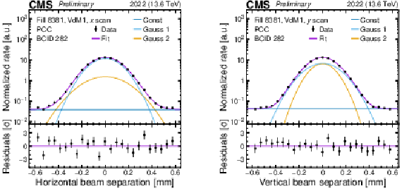
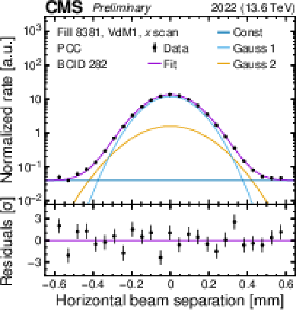
Figure 19:
Double-Gaussian plus constant fits to the PCC data recorded during the first vdM scan pair (vdM1), shown for the $ x $ (left) and $ y $ (right) scan. In the bottom panels, the difference between the measured rate and the fit divided by the statistical uncertainty is shown. |
png pdf |
Figure 19-a:
Double-Gaussian plus constant fits to the PCC data recorded during the first vdM scan pair (vdM1), shown for the $ x $ (left) and $ y $ (right) scan. In the bottom panels, the difference between the measured rate and the fit divided by the statistical uncertainty is shown. |
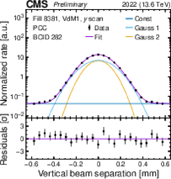
png pdf |
Figure 19-b:
Double-Gaussian plus constant fits to the PCC data recorded during the first vdM scan pair (vdM1), shown for the $ x $ (left) and $ y $ (right) scan. In the bottom panels, the difference between the measured rate and the fit divided by the statistical uncertainty is shown. |
png pdf |
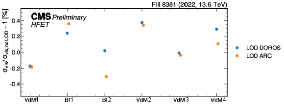
Figure 20:
The ratio of the measured HFET visible cross section with and without linear orbit drift (LOD) corrections (either DOROS or ARC), shown for each vdM scan pair. The value is expressed as the difference from unity and in percentage. |
png pdf |
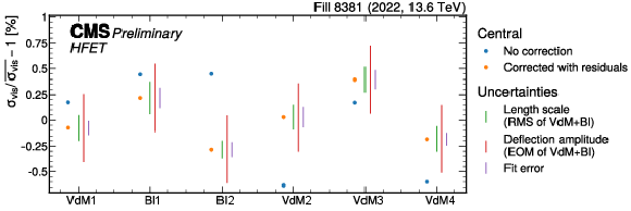
Figure 21:
The ratio of the measured HFET visible cross section with (orange) and without (blue) residual orbit drift corrections, shown for each vdM scan pair. The value is expressed as the difference from unity and in percentage. The dominant uncertainties (bars) originating from the observed per-scan variation in the length scale (quantified by the RMS) and deflection amplitude (quantified by the EOM) are indicated. |
png pdf |
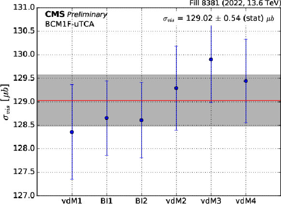
Figure 22:
Results for $ \sigma_{\mathrm{vis}} $ from the vdM scan pair analysis using BCM1F $\mu$TCA data, as a function of the scan pair. |
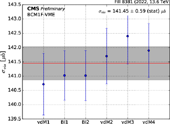
png pdf |
Figure 23:
Results for $ \sigma_{\mathrm{vis}} $ from the vdM scan pair analysis using BCM1F VME data, as a function of the scan pair. |
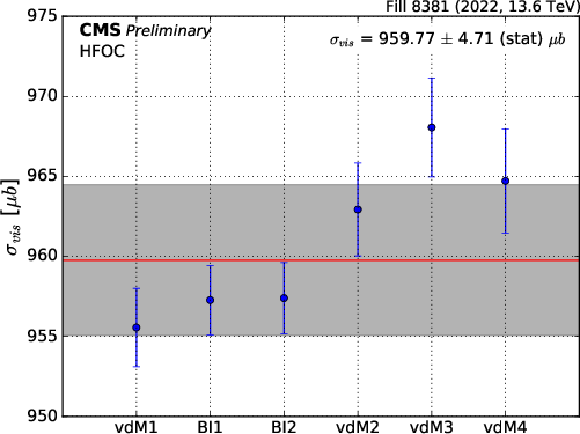
png pdf |
Figure 24:
Results for $ \sigma_{\mathrm{vis}} $ from the vdM scan pair analysis using HFOC data, as a function of the scan pair. |
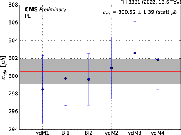
png pdf |
Figure 25:
Results for $ \sigma_{\mathrm{vis}} $ from the vdM scan pair analysis using PLT data, as a function of the scan pair. |
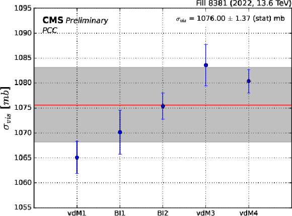
png pdf |
Figure 26:
Results for $ \sigma_{\mathrm{vis}} $ from the vdM scan pair analysis using PCC data, as a function of the scan pair. |
png pdf |
Figure 27:
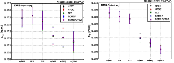
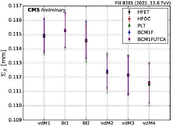
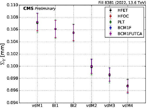
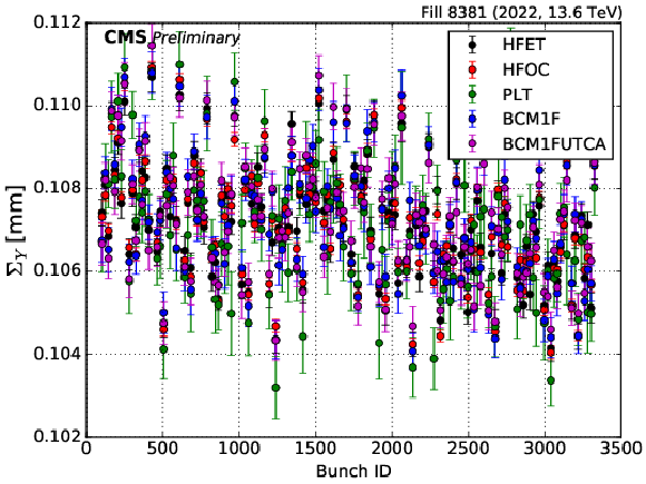
Average $ \Sigma $ values in both transverse plans measured during all vdM scans, by all the online luminometers. |
png pdf |
Figure 27-a:
Average $ \Sigma $ values in both transverse plans measured during all vdM scans, by all the online luminometers. |
png pdf |
Figure 27-b:
Average $ \Sigma $ values in both transverse plans measured during all vdM scans, by all the online luminometers. |
png pdf |
Figure 28:
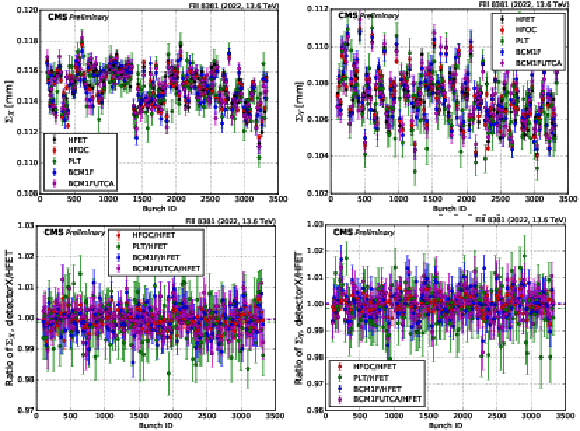
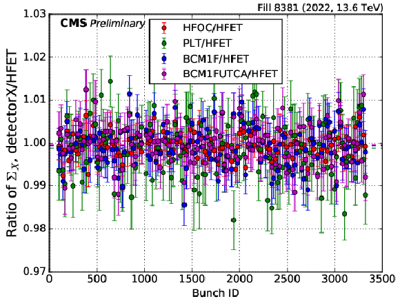
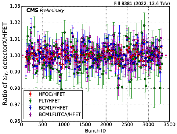
Measured $ \Sigma $ during the vdM scan, by all the online luminometers (upper row). Ratios of the measured values by different systems with respect to HFET are also shown (lower row). |
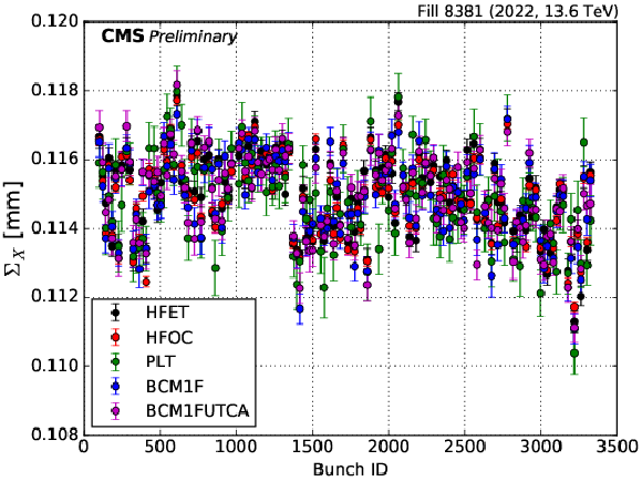
png pdf |
Figure 28-a:
Measured $ \Sigma $ during the vdM scan, by all the online luminometers (upper row). Ratios of the measured values by different systems with respect to HFET are also shown (lower row). |
png pdf |
Figure 28-b:
Measured $ \Sigma $ during the vdM scan, by all the online luminometers (upper row). Ratios of the measured values by different systems with respect to HFET are also shown (lower row). |
png pdf |
Figure 28-c:
Measured $ \Sigma $ during the vdM scan, by all the online luminometers (upper row). Ratios of the measured values by different systems with respect to HFET are also shown (lower row). |
png pdf |
Figure 28-d:
Measured $ \Sigma $ during the vdM scan, by all the online luminometers (upper row). Ratios of the measured values by different systems with respect to HFET are also shown (lower row). |
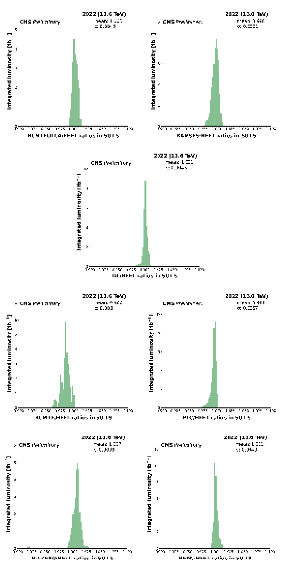
png pdf |
Figure 29:
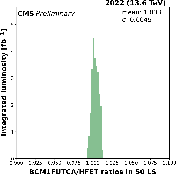
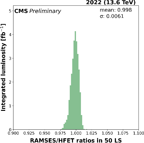
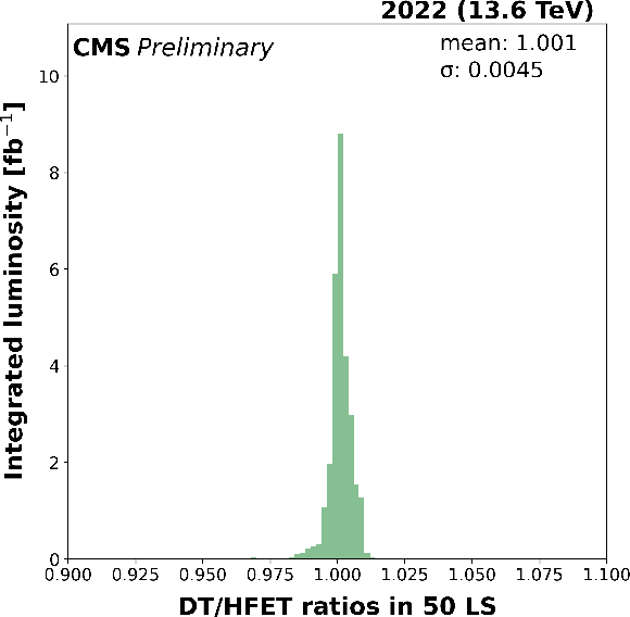
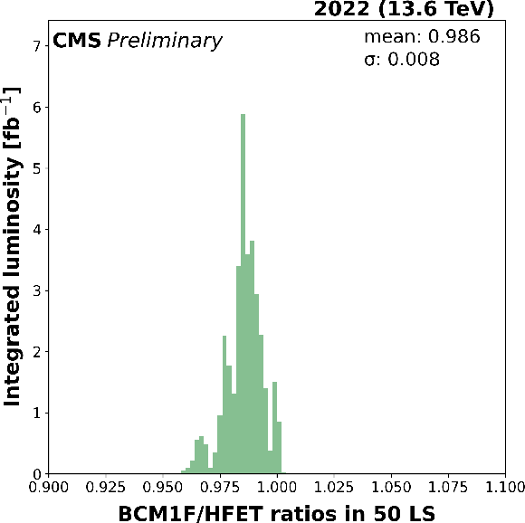
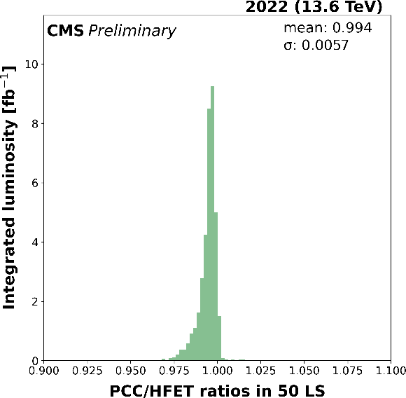
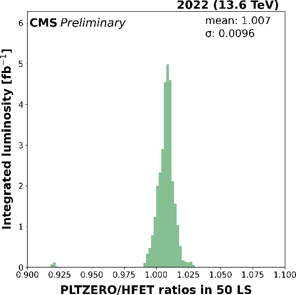
Histograms of the ratio of the measured luminosity between different CMS luminometers and HFET. |
png |
Figure 29-a:
Histograms of the ratio of the measured luminosity between different CMS luminometers and HFET. |
png |
Figure 29-b:
Histograms of the ratio of the measured luminosity between different CMS luminometers and HFET. |
png |
Figure 29-c:
Histograms of the ratio of the measured luminosity between different CMS luminometers and HFET. |
png |
Figure 29-d:
Histograms of the ratio of the measured luminosity between different CMS luminometers and HFET. |
png |
Figure 29-e:
Histograms of the ratio of the measured luminosity between different CMS luminometers and HFET. |
png |
Figure 29-f:
Histograms of the ratio of the measured luminosity between different CMS luminometers and HFET. |

png |
Figure 29-g:
Histograms of the ratio of the measured luminosity between different CMS luminometers and HFET. |
png pdf |
Figure 30:
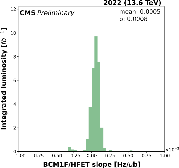
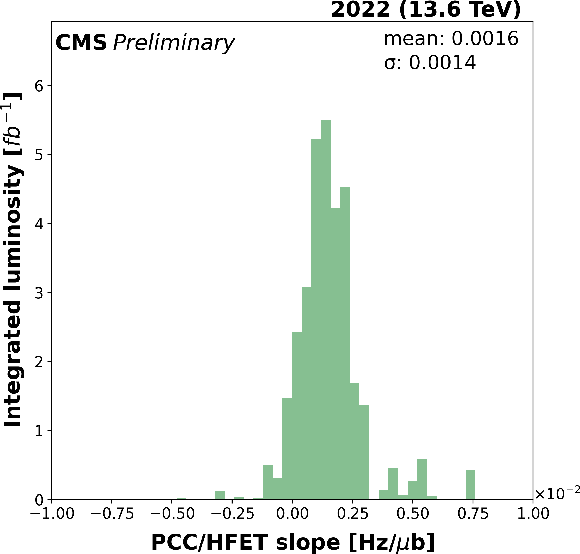
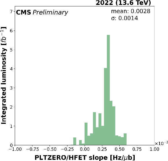
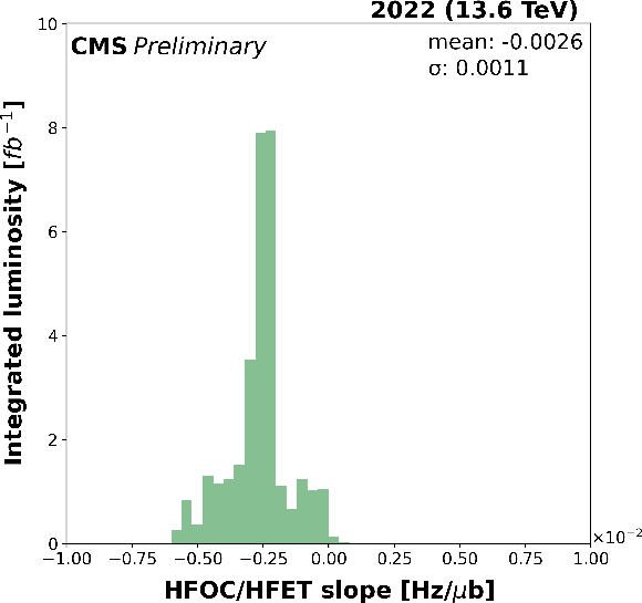
Distribution of relative non-linearity slopes between different detectors, evaluated separately for each fill. Each entry is weighted with the integrated luminosity of the fill. |
png |
Figure 30-a:
Distribution of relative non-linearity slopes between different detectors, evaluated separately for each fill. Each entry is weighted with the integrated luminosity of the fill. |
png |
Figure 30-b:
Distribution of relative non-linearity slopes between different detectors, evaluated separately for each fill. Each entry is weighted with the integrated luminosity of the fill. |
png |
Figure 30-c:
Distribution of relative non-linearity slopes between different detectors, evaluated separately for each fill. Each entry is weighted with the integrated luminosity of the fill. |
png |
Figure 30-d:
Distribution of relative non-linearity slopes between different detectors, evaluated separately for each fill. Each entry is weighted with the integrated luminosity of the fill. |
| Tables | |
png pdf |
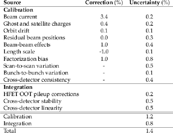
Table 1:
Summary of the calibration corrections and all contributions to the systematic uncertainty of the CMS luminosity measurement for 13.6 TeV pp collisions in 2022. |
| Summary |
| The calibration and measurement of the integrated luminosity of the proton-proton collision data at $ \sqrt{s}= $ 13.6 TeV recorded with the CMS experiment in 2022 has been performed. The absolute luminosity calibration is obtained with the van der Meer scan method, and several systematic effects are considered. The integration is performed with various independent luminosity detectors. The primary luminosity measurement is provided by an transverse-energy-based method using the forward hadron calorimeter. The integrated luminosity delivered to the CMS experiment is measured to 41.5 fb$ ^{-1} $, with a relative uncertainty of 1.4%. All contributions to the total systematic uncertainty are summarized in Table 1. The dominant contribution to the systematic uncertainty arises from the estimation of the factorization bias in the vdM calibration, and the overall detector stability and linearity. |
| References | ||||
| 1 | M. Hostettler et al. | Luminosity scans for beam diagnostics | Phys. Rev. Accel. Beams 21 (2018) 102801 | 1804.10099 |
| 2 | F. Antoniouet al. | Can we predict luminosity? | in Proc. 7th Evian Workshop on LHC Beam Operation: Evian Les Bains, France, 2016 | |
| 3 | CMS Collaboration | Measurement of the $ \mathrm{t} \overline{\mathrm{t}} $ production cross section, the top quark mass, and the strong coupling constant using dilepton events in $ {\mathrm{p}\mathrm{p}} $ collisions at $ \sqrt{s}= $ 13 TeV | EPJC 79 (2019) 368 | CMS-TOP-17-001 1812.10505 |
| 4 | CMS Collaboration | Measurement of the inclusive and differential $ {{\mathrm{t}\overline{\mathrm{t}}} \gamma} $ cross sections in the dilepton channel and effective field theory interpretation in proton-proton collisions at $ \sqrt{s}= $ 13 TeV | JHEP 05 (2022) 091 | CMS-TOP-21-004 2201.07301 |
| 5 | CMS Collaboration | Measurement of the mass dependence of the transverse momentum of lepton pairs in Drell--Yan production in proton-proton collisions at $ \sqrt{s}= $ 13 TeV | EPJC 83 (2023) 628 | CMS-SMP-20-003 2205.04897 |
| 6 | CMS Collaboration | First measurement of the top quark pair production cross section in proton-proton collisions at $ \sqrt{s}= $ 13.6 TeV | JHEP 08 (2023) 204 | CMS-TOP-22-012 2303.10680 |
| 7 | S. van der Meer | Calibration of the effective beam height in the ISR | ISR Report CERN-ISR-PO-68-31, 1968 | |
| 8 | C. Rubbia | Measurement of the luminosity of $ {\mathrm{p}\overline{\mathrm{p}}} $ collider with a (generalized) Van der Meer method | Technical Report CERN-pp-Note-38, 1977 | |
| 9 | P. Grafström and W. Kozanecki | Luminosity determination at proton colliders | Prog. Part. Nucl. Phys. 81 (2015) 97 | |
| 10 | CMS Collaboration | Precision luminosity measurement in proton-proton collisions at $ \sqrt{s}= $ 13 TeV in 2015 and 2016 at CMS | EPJC 81 (2021) 800 | CMS-LUM-17-003 2104.01927 |
| 11 | CMS Collaboration | CMS luminosity calibration for the $ {\mathrm{p}\mathrm{p}} $ reference run at $ \sqrt{s}= $ 5.02 TeV | CMS Physics Analysis Summary, 2016 CMS-PAS-LUM-16-001 |
CMS-PAS-LUM-16-001 |
| 12 | CMS Collaboration | CMS luminosity measurement for the 2017 data-taking period at $ \sqrt{s}= $ 13 TeV | CMS Physics Analysis Summary, 2018 CMS-PAS-LUM-17-004 |
CMS-PAS-LUM-17-004 |
| 13 | CMS Collaboration | CMS luminosity measurement using 2016 proton-nucleus collisions at $ \sqrt{\smash[b]{s_{_{\mathrm{NN}}}}}= $ 8.16 TeV | CMS Physics Analysis Summary, 2018 CMS-PAS-LUM-17-002 |
CMS-PAS-LUM-17-002 |
| 14 | CMS Collaboration | CMS luminosity measurement for the 2018 data-taking period at $ \sqrt{s}= $ 13 TeV | CMS Physics Analysis Summary, 2019 CMS-PAS-LUM-18-002 |
CMS-PAS-LUM-18-002 |
| 15 | CMS Collaboration | Luminosity measurement in proton-proton collisions at 5.02 TeV in 2017 at CMS | CMS Physics Analysis Summary, 2021 CMS-PAS-LUM-19-001 |
CMS-PAS-LUM-19-001 |
| 16 | CMS Collaboration | CMS luminosity measurement using nucleus-nucleus collisions at $ \sqrt{\smash[b]{s_{_{\mathrm{NN}}}}}= $ 5.02 TeV in 2018 | CMS Physics Analysis Summary, 2022 CMS-PAS-LUM-18-001 |
CMS-PAS-LUM-18-001 |
| 17 | ALICE Collaboration | Measurement of visible cross sections in proton-lead collisions at $ \sqrt{\smash[b]{s_{_{\mathrm{NN}}}}}= $ 5.02 TeV in van der Meer scans with the ALICE detector | JINST 9 (2014) P11003 | 1405.1849 |
| 18 | LHCb Collaboration | Precision luminosity measurements at LHCb | JINST 9 (2014) P12005 | 1410.0149 |
| 19 | ATLAS Collaboration | Luminosity determination in pp collisions at $ \sqrt{s}= $ 8 TeV using the ATLAS detector at the LHC | EPJC 76 (2016) 653 | 1608.03953 |
| 20 | ALICE Collaboration | ALICE luminosity determination for Pb--Pb collisions at $ \sqrt{\smash[b]{s_{_{\mathrm{NN}}}}}= $ 5.02 TeV | JINST 19 (2024) P02039 | 2204.10148 |
| 21 | ATLAS Collaboration | Luminosity determination in pp collisions at $ \sqrt{s}= $ 13 TeV using the ATLAS detector at the LHC | EPJC 83 (2023) 982 | 2212.09379 |
| 22 | CMS Collaboration | The CMS experiment at the CERN LHC | JINST 3 (2008) S08004 | |
| 23 | CMS Collaboration | Development of the CMS detector for the CERN LHC Run 3 | Accepted by JINST, 2023 | CMS-PRF-21-001 2309.05466 |
| 24 | CMS Collaboration | The CMS trigger system | JINST 12 (2017) P01020 | CMS-TRG-12-001 1609.02366 |
| 25 | CMS Collaboration | Performance of the CMS Level-1 trigger in proton-proton collisions at $ \sqrt{s}= $ 13 TeV | JINST 15 (2020) P10017 | CMS-TRG-17-001 2006.10165 |
| 26 | CMS Collaboration | Electron and photon reconstruction and identification with the CMS experiment at the CERN LHC | JINST 16 (2021) P05014 | CMS-EGM-17-001 2012.06888 |
| 27 | CMS Collaboration | Performance of the CMS muon detector and muon reconstruction with proton-proton collisions at $ \sqrt{s}= $ 13 TeV | JINST 13 (2018) P06015 | CMS-MUO-16-001 1804.04528 |
| 28 | CMS Collaboration | Description and performance of track and primary-vertex reconstruction with the CMS tracker | JINST 9 (2014) P10009 | CMS-TRK-11-001 1405.6569 |
| 29 | CMS Collaboration | Particle-flow reconstruction and global event description with the CMS detector | JINST 12 (2017) P10003 | CMS-PRF-14-001 1706.04965 |
| 30 | CMS Collaboration | Performance of reconstruction and identification of $ \tau $ leptons decaying to hadrons and $ \nu_{\!\tau} $ in $ {\mathrm{p}\mathrm{p}} $ collisions at $ \sqrt{s}= $ 13 TeV | JINST 13 (2018) P10005 | CMS-TAU-16-003 1809.02816 |
| 31 | CMS Collaboration | Jet energy scale and resolution in the CMS experiment in $ {\mathrm{p}\mathrm{p}} $ collisions at 8 TeV | JINST 12 (2017) P02014 | CMS-JME-13-004 1607.03663 |
| 32 | CMS Collaboration | Performance of missing transverse momentum reconstruction in proton-proton collisions at $ \sqrt{s}= $ 13 TeV using the CMS detector | JINST 14 (2019) P07004 | CMS-JME-17-001 1903.06078 |
| 33 | CMS Tracker Group Collaboration | The CMS Phase-1 pixel detector upgrade | JINST 16 (2021) P02027 | 2012.14304 |
| 34 | CMS BRIL Collaboration | The Pixel Luminosity Telescope: a detector for luminosity measurement at CMS using silicon pixel sensors | EPJC 83 (2023) 673 | 2206.08870 |
| 35 | J. Wańczyk on behalf of the CMS Collaboration | Upgraded CMS fast beam condition monitor for LHC Run 3 online luminosity and beam induced background measurements | in Proc. 11th International Beam Instrumentation Conference (IBIC ): Cracow, Poland, 2018 link |
|
| 36 | G. Segura Millan, D. Perrin, and L. Scibile | RAMSES: the LHC radiation monitoring system for the environment and safety | in Proc. 10th International Conference on Accelerator and Large Experimental Physics Control Systems (ICALEPCS ): Geneva, Switzerland, 2005 link |
|
| 37 | A. Ledeul et al. | CERN supervision, control, and data acquisition system for radiation and environmental protection | in Proc. 12th International Workshop on Emerging Technologies and Scientific Facilities Controls (PCaPAC): Hsinchu City, Taiwan, 2018 link |
|
| 38 | J. Wańczyk | Measurements and estimates of the radiation levels in the CMS experimental cavern using Medipix and RAMSES monitors, and the FLUKA Monte Carlo code | Master's thesis, AGH University of Science and Technology Cracow, 2019 CERN-THESIS-2019-212 |
|
| 39 | LHCf Collaboration | The LHCf detector at the CERN Large Hadron Collider | JINST 3 (2008) S08006 | |
| 40 | G. Anders et al. | Study of the relative LHC bunch populations for luminosity calibration | Technical Report CERN-ATS-Note-2012-028 PERF, 2012 | |
| 41 | C. Barschel et al. | Results of the LHC DCCT calibration studies | Technical Report CERN-ATS-Note-2012-026 PERF, 2012 | |
| 42 | A. Alici et al. | Study of the LHC ghost charge and satellite bunches for luminosity calibration. | Technical Report CERN-ATS-Note-2012-029 PERF, 2012 | |
| 43 | P. Hopchev | Absolute luminosity measurements at LHCb | PhD thesis, Université Grenoble Alpes, . CERN-THESIS-2011-210, 2011 link |
|
| 44 | M. Gasior, J. Olexa, and R. Steinhagen | BPM electronics based on compensated diode detectors---results from development systems | in Proc. 15th Beam Instrumentation Workshop (BIW12): Newport News, USA, 2012 [Conf. Proc. C151 MOPG010] |
|
| 45 | W. Kozanecki, T. Pieloni, and J. Wenninger | Observation of beam-beam deflections with LHC orbit data | CERN Accelerator Note CERN-ACC-NOTE-2013-0006, 2013 | |
| 46 | A. Babaev et al. | Impact of beam-beam effects on absolute luminosity calibrations at the CERN Large Hadron Collider | EPJC 84 (2024) 17 | 2306.10394 |
| 47 | CMSnoop | A study of beam-beam effects in hadron colliders with a large number of bunches | \hrefT.~Pieloni, . PhD thesis, \'Ecole Polytechnique Fédérale de Lausanne, . CERN-THESIS-2010-056, THESE-4211-2008, 2008 link |
|
| 48 | V. Balagura | Van der Meer scan luminosity measurement and beam-beam correction | EPJC 81 (2021) 26 | 2012.07752 |
| 49 | M. Klute, C. Medlock, and J. Salfeld-Nebgen | Beam imaging and luminosity calibration | JINST 12 (2017) P03018 | 1603.03566 |
| 50 | J. Knolle | Measuring luminosity and the $ {\mathrm{t}\overline{\mathrm{t}}} \mathrm{Z} $ production cross section with the CMS experiment | PhD thesis, Universität Hamburg, CERN-THESIS-2020-185, DESY-THESIS-2020-020, 2020 link |
|

|
Compact Muon Solenoid LHC, CERN |

|

|

|

|

|

|