

Compact Muon Solenoid
LHC, CERN
| CMS-PAS-LUM-18-001 | ||
| CMS luminosity measurement using nucleus-nucleus collisions at ${\sqrt {\smash [b]{s_{_{\mathrm {NN}}}}}} = $ 5.02 TeV in 2018 | ||
| CMS Collaboration | ||
| May 2022 | ||
| Abstract: The measurement of the luminosity delivered to the CMS experiment during the lead-lead (PbPb) data-taking period in 2018 at nucleon-nucleon center-of-mass energy of 5.02 TeV is presented. Three subdetectors are used: the Fast Beam Conditions Monitor, the forward hadron calorimeter, and the Pixel Luminosity Telescope. The absolute luminosity is determined by integrating the subdetector rate as a function of beam separation, using the so-called van der Meer (vdM) technique. Adding in quadrature independent sources of systematic uncertainty we estimate an overall vdM precision of 1.3%, with the dominant source related to the transverse factorizability of the bunch density profiles. The total uncertainty of 1.5% is then obtained including time stability of the vdM-calibrated subdetector response. Short vdM-like scans, performed regularly in CMS during the PbPb data-taking period, are studied. | ||
| Links: CDS record (PDF) ; CADI line (restricted) ; | ||
| Figures | |

png pdf |
Figure 1:
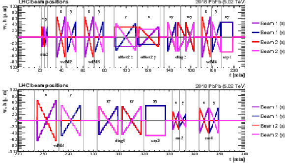
Horizontal and vertical beam displacements derived from the LHC magnet currents during the vdM scan program in fill 7442. |
png pdf |
Figure 2:
Horizontal and vertical beam displacements derived from the LHC magnet currents during the vdM scan program in fill 7443 ; for illustration, it is split into two parts (top and bottom). We repeated the second part of the diag2 scan. |

png pdf |
Figure 2-a:
Horizontal and vertical beam displacements derived from the LHC magnet currents during the vdM scan program in fill 7443 ; for illustration, it is split into two parts (top and bottom). We repeated the second part of the diag2 scan. |

png pdf |
Figure 2-b:
Horizontal and vertical beam displacements derived from the LHC magnet currents during the vdM scan program in fill 7443 ; for illustration, it is split into two parts (top and bottom). We repeated the second part of the diag2 scan. |
png pdf |
Figure 3:
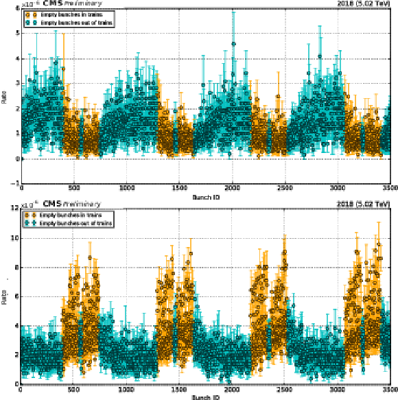
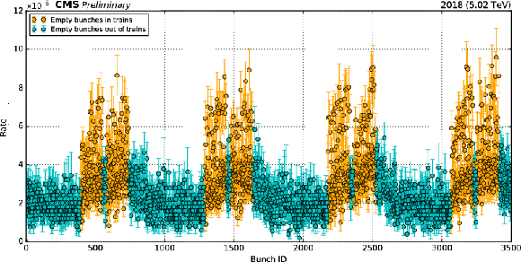
The rate from empty BCIDs as recorded by BCM1F in and out of trains at maximum beam separation (top) and head-on (bottom) during the vdM2 scan. |

png pdf |
Figure 3-a:
The rate from empty BCIDs as recorded by BCM1F in and out of trains at maximum beam separation (top) and head-on (bottom) during the vdM2 scan. |
png pdf |
Figure 3-b:
The rate from empty BCIDs as recorded by BCM1F in and out of trains at maximum beam separation (top) and head-on (bottom) during the vdM2 scan. |
png pdf |
Figure 4:
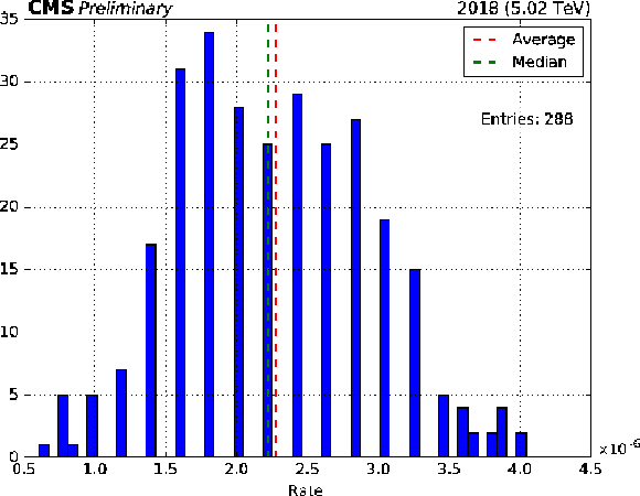
The rate from colliding BCIDs as recorded by BCM1F during a portion (30 s) of the sep1 scan. |

png pdf |
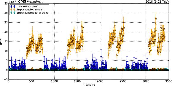
Figure 5:
Head-on rate from unpaired and empty BCIDs in and out of trains as recorded by HFOC during the vdM2 scan. |
png pdf |
Figure 6:
Head-on rate from unpaired and empty BCIDs in and out of trains as recorded by PLT in the vdM2 scan. |

png pdf |
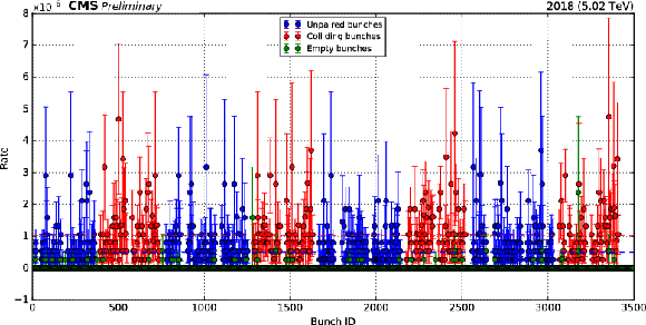
Figure 7:
Rate from unpaired, colliding, or empty BCIDs as recorded by PLT during a portion (30 s) of the sep1 scan (left) and its distribution considering colliding BCIDs only (right). |
png pdf |
Figure 7-a:
Rate from unpaired, colliding, or empty BCIDs as recorded by PLT during a portion (30 s) of the sep1 scan (left) and its distribution considering colliding BCIDs only (right). |

png pdf |
Figure 7-b:
Rate from unpaired, colliding, or empty BCIDs as recorded by PLT during a portion (30 s) of the sep1 scan (left) and its distribution considering colliding BCIDs only (right). |

png pdf |
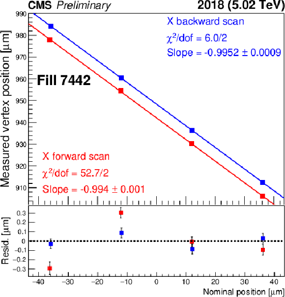
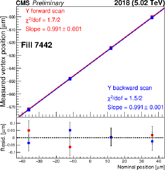
Figure 8:
The measured and fitted beamspot positions, considering the impact due to the orbit drift, as a function of the beam centroid offsets, shown for forward (red) and backward (blue) LSC scans separately in horizontal (left) and vertical (right) directions in fills 7442 (top) and 7483 (bottom). |
png pdf |
Figure 8-a:
The measured and fitted beamspot positions, considering the impact due to the orbit drift, as a function of the beam centroid offsets, shown for forward (red) and backward (blue) LSC scans separately in horizontal (left) and vertical (right) directions in fills 7442 (top) and 7483 (bottom). |
png pdf |
Figure 8-b:
The measured and fitted beamspot positions, considering the impact due to the orbit drift, as a function of the beam centroid offsets, shown for forward (red) and backward (blue) LSC scans separately in horizontal (left) and vertical (right) directions in fills 7442 (top) and 7483 (bottom). |
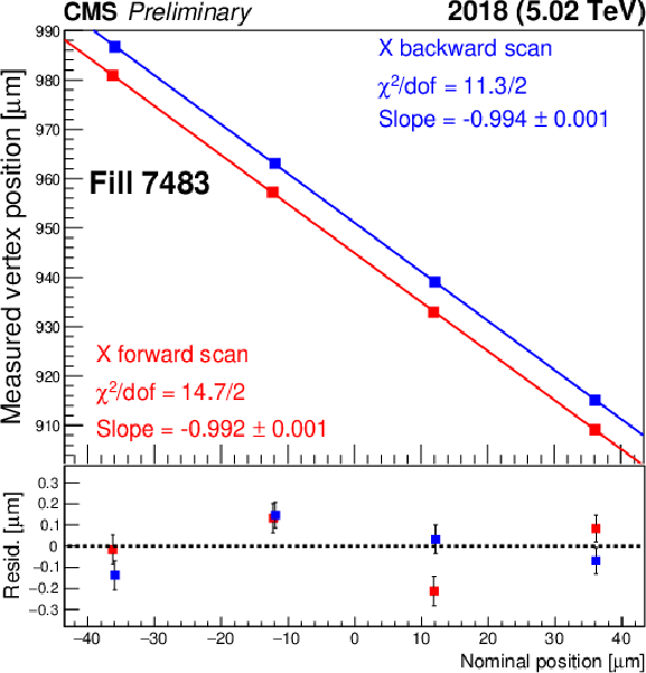
png pdf |
Figure 8-c:
The measured and fitted beamspot positions, considering the impact due to the orbit drift, as a function of the beam centroid offsets, shown for forward (red) and backward (blue) LSC scans separately in horizontal (left) and vertical (right) directions in fills 7442 (top) and 7483 (bottom). |

png pdf |
Figure 8-d:
The measured and fitted beamspot positions, considering the impact due to the orbit drift, as a function of the beam centroid offsets, shown for forward (red) and backward (blue) LSC scans separately in horizontal (left) and vertical (right) directions in fills 7442 (top) and 7483 (bottom). |

png pdf |
Figure 9:
Difference of the horizontal and vertical beam positions before, in the middle, and after each scan as measured by the DOROS and arc BPMs in fill 7443 ; for illustration, it is split into two parts (top and bottom). |

png pdf |
Figure 9-a:
Difference of the horizontal and vertical beam positions before, in the middle, and after each scan as measured by the DOROS and arc BPMs in fill 7443 ; for illustration, it is split into two parts (top and bottom). |

png pdf |
Figure 9-b:
Difference of the horizontal and vertical beam positions before, in the middle, and after each scan as measured by the DOROS and arc BPMs in fill 7443 ; for illustration, it is split into two parts (top and bottom). |
png pdf |
Figure 10:
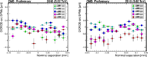
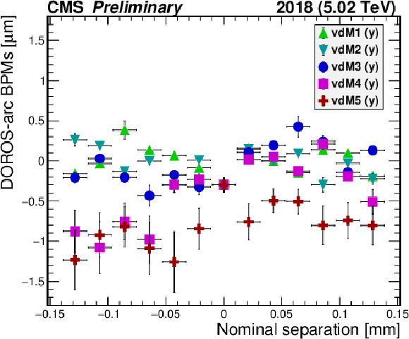
The absolute difference in the displacement of the two beams as measured by the DOROS and arc BPMs during vdM1-5 scans as a function of the nominal beam separation in $x$ (left) and $y$ (right), respectively. The values and the statistical uncertainty in the measured beam positions are shown. |

png pdf |
Figure 10-a:
The absolute difference in the displacement of the two beams as measured by the DOROS and arc BPMs during vdM1-5 scans as a function of the nominal beam separation in $x$ (left) and $y$ (right), respectively. The values and the statistical uncertainty in the measured beam positions are shown. |
png pdf |
Figure 10-b:
The absolute difference in the displacement of the two beams as measured by the DOROS and arc BPMs during vdM1-5 scans as a function of the nominal beam separation in $x$ (left) and $y$ (right), respectively. The values and the statistical uncertainty in the measured beam positions are shown. |

png pdf |
Figure 11:
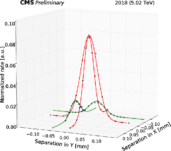
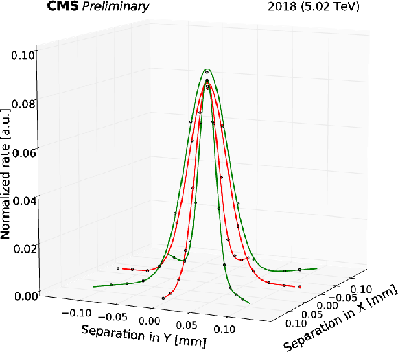
The corrected beam separation in $x$ and $y$ and the normalized collision rate for vdM+offset (left) and vdM+diagonal (right) scan combinations. The solid lines are illustrative two-dimensional fits, with red (blue or green) representing the fit components to vdM (offset or diagonal) scans. |
png pdf |
Figure 11-a:
The corrected beam separation in $x$ and $y$ and the normalized collision rate for vdM+offset (left) and vdM+diagonal (right) scan combinations. The solid lines are illustrative two-dimensional fits, with red (blue or green) representing the fit components to vdM (offset or diagonal) scans. |
png pdf |
Figure 11-b:
The corrected beam separation in $x$ and $y$ and the normalized collision rate for vdM+offset (left) and vdM+diagonal (right) scan combinations. The solid lines are illustrative two-dimensional fits, with red (blue or green) representing the fit components to vdM (offset or diagonal) scans. |
png pdf |
Figure 12:
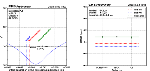
Example of the $\chi ^2$ minimization (performed collectively to all BCIDs) to obtain the best-fit offset value and its uncertainty, using PLT (left). Comparison including all luminometers (right). |
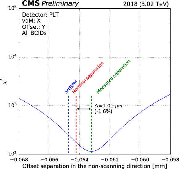
png pdf |
Figure 12-a:
Example of the $\chi ^2$ minimization (performed collectively to all BCIDs) to obtain the best-fit offset value and its uncertainty, using PLT (left). Comparison including all luminometers (right). |

png pdf |
Figure 12-b:
Example of the $\chi ^2$ minimization (performed collectively to all BCIDs) to obtain the best-fit offset value and its uncertainty, using PLT (left). Comparison including all luminometers (right). |

png pdf |
Figure 13:
Calculated correction for the different fit models and all studied vdM+offset and vdM+diagonal scan combinations in fill 7443. The error bars correspond to sources of systematic uncertainty added in quadrature for the fit models. The dashed lines show the first-order polynomial fit to all scan combinations, with the solid area denoting the total uncertainty, correlated among the scan combinations. The hatched areas denote subcomponents of the total uncertainty: the fit (blue) and model (orange) sources of uncertainty, respectively. The vertical lines mark the time of vdM2-5 relative to the second partner in the scan combinations. |
png pdf |
Figure 14:
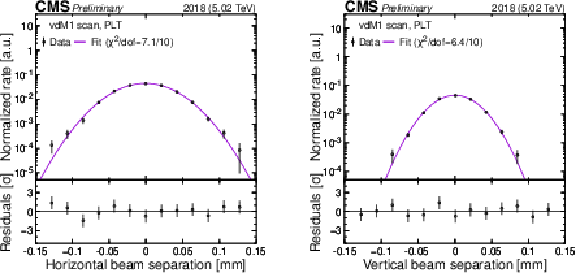
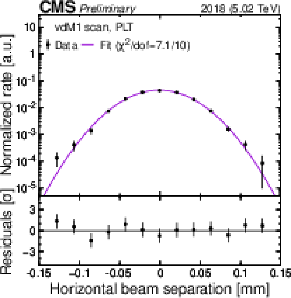
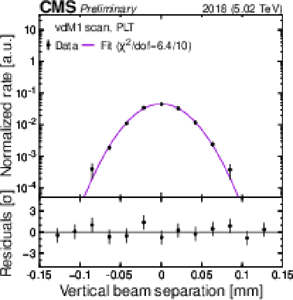
Examples of scan distributions, i.e., the normalized rate recorded by PLT in BCID 546 as a function of beam separation ($\Delta $) in $x$ (left) and $y$ (right), respectively. The black curve corresponds to the single-Gaussian fit. The values and the statistical uncertainty in the fitted parameters are shown in the legend, along with the reduced $\chi ^2$. The bottom panels include the residuals, i.e., the difference between the measured and fitted values divided by the statistical uncertainty. |
png pdf |
Figure 14-a:
Examples of scan distributions, i.e., the normalized rate recorded by PLT in BCID 546 as a function of beam separation ($\Delta $) in $x$ (left) and $y$ (right), respectively. The black curve corresponds to the single-Gaussian fit. The values and the statistical uncertainty in the fitted parameters are shown in the legend, along with the reduced $\chi ^2$. The bottom panels include the residuals, i.e., the difference between the measured and fitted values divided by the statistical uncertainty. |
png pdf |
Figure 14-b:
Examples of scan distributions, i.e., the normalized rate recorded by PLT in BCID 546 as a function of beam separation ($\Delta $) in $x$ (left) and $y$ (right), respectively. The black curve corresponds to the single-Gaussian fit. The values and the statistical uncertainty in the fitted parameters are shown in the legend, along with the reduced $\chi ^2$. The bottom panels include the residuals, i.e., the difference between the measured and fitted values divided by the statistical uncertainty. |
png pdf |
Figure 15:
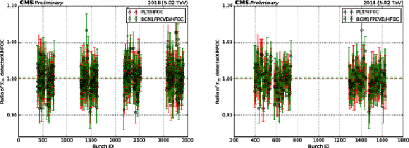
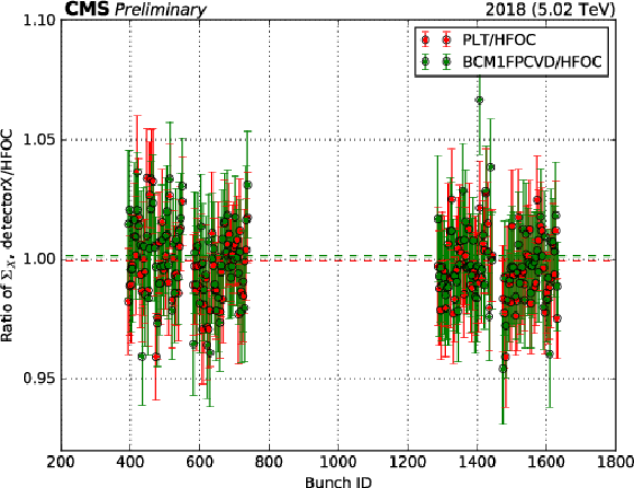
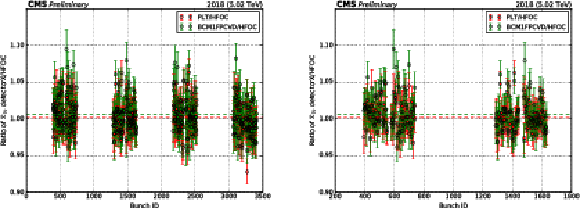
Cross-detector comparison of the fitted $\Sigma _{x}$ as a function of BCID for the vdM5 scan. The horizontal dashed lines indicate the averaged values of the corresponding set of points (left). Zoom into two groups of BCID for the same scan (right). |

png pdf |
Figure 15-a:
Cross-detector comparison of the fitted $\Sigma _{x}$ as a function of BCID for the vdM5 scan. The horizontal dashed lines indicate the averaged values of the corresponding set of points (left). Zoom into two groups of BCID for the same scan (right). |
png pdf |
Figure 15-b:
Cross-detector comparison of the fitted $\Sigma _{x}$ as a function of BCID for the vdM5 scan. The horizontal dashed lines indicate the averaged values of the corresponding set of points (left). Zoom into two groups of BCID for the same scan (right). |

png pdf |
Figure 16:
Measured ${\sigma _{\text {vis}}}$ after all corrections are applied separately for BCM1F, HFOC, and PLT as a function of BCID in vdM1 (left) and 5 (right) scans (zooming into the first half of BCIDs). The dashed lines and filled bands indicate the luminometer-dependent average ${\sigma _{\text {vis}}}$ and its standard deviation for all BCIDs, respectively. |

png pdf |
Figure 16-a:
Measured ${\sigma _{\text {vis}}}$ after all corrections are applied separately for BCM1F, HFOC, and PLT as a function of BCID in vdM1 (left) and 5 (right) scans (zooming into the first half of BCIDs). The dashed lines and filled bands indicate the luminometer-dependent average ${\sigma _{\text {vis}}}$ and its standard deviation for all BCIDs, respectively. |
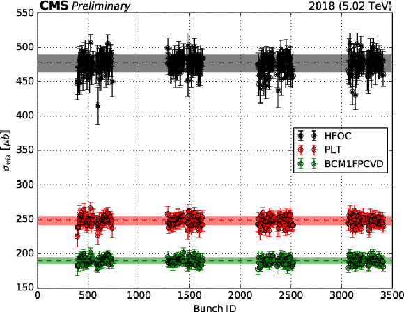
png pdf |
Figure 16-b:
Measured ${\sigma _{\text {vis}}}$ after all corrections are applied separately for BCM1F, HFOC, and PLT as a function of BCID in vdM1 (left) and 5 (right) scans (zooming into the first half of BCIDs). The dashed lines and filled bands indicate the luminometer-dependent average ${\sigma _{\text {vis}}}$ and its standard deviation for all BCIDs, respectively. |
png pdf |
Figure 17:
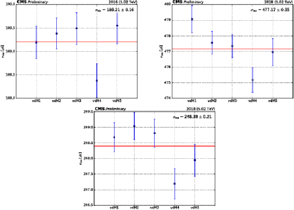
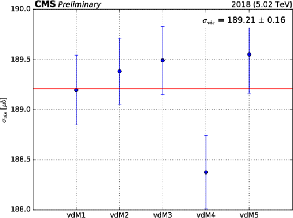
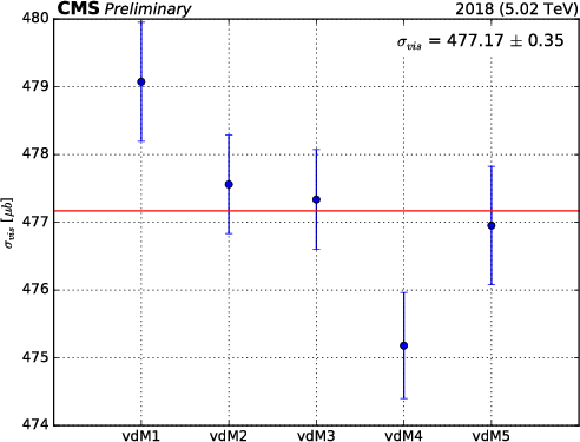
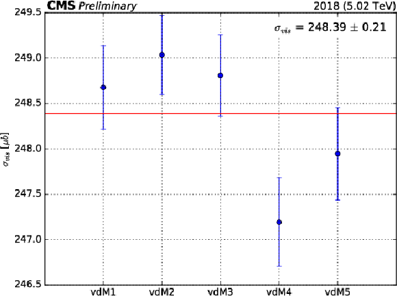
Measured ${\sigma _{\text {vis}}}$ separately for BCM1F (top left), HFOC (top right), and PLT (bottom) averaged over all BCIDs separately for vdM1-5 scans, after all corrections are applied. The uncertainty is of statistical nature. |
png pdf |
Figure 17-a:
Measured ${\sigma _{\text {vis}}}$ separately for BCM1F (top left), HFOC (top right), and PLT (bottom) averaged over all BCIDs separately for vdM1-5 scans, after all corrections are applied. The uncertainty is of statistical nature. |
png pdf |
Figure 17-b:
Measured ${\sigma _{\text {vis}}}$ separately for BCM1F (top left), HFOC (top right), and PLT (bottom) averaged over all BCIDs separately for vdM1-5 scans, after all corrections are applied. The uncertainty is of statistical nature. |
png pdf |
Figure 17-c:
Measured ${\sigma _{\text {vis}}}$ separately for BCM1F (top left), HFOC (top right), and PLT (bottom) averaged over all BCIDs separately for vdM1-5 scans, after all corrections are applied. The uncertainty is of statistical nature. |
png pdf |
Figure 18:
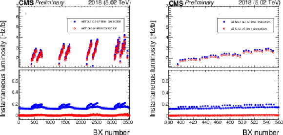
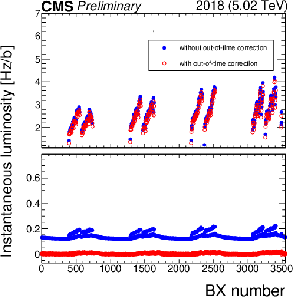
The instantaneous luminosity as recorded by HFOC before (filled points) and after (open points) afterglow corrections are applied, separately for colliding (top) and empty or unpaired (bottom) bunches. On the right, we zoom into a range of bunches for the same fill, i.e., 7443. |
png pdf |
Figure 18-a:
The instantaneous luminosity as recorded by HFOC before (filled points) and after (open points) afterglow corrections are applied, separately for colliding (top) and empty or unpaired (bottom) bunches. On the right, we zoom into a range of bunches for the same fill, i.e., 7443. |

png pdf |
Figure 18-b:
The instantaneous luminosity as recorded by HFOC before (filled points) and after (open points) afterglow corrections are applied, separately for colliding (top) and empty or unpaired (bottom) bunches. On the right, we zoom into a range of bunches for the same fill, i.e., 7443. |
png pdf |
Figure 19:
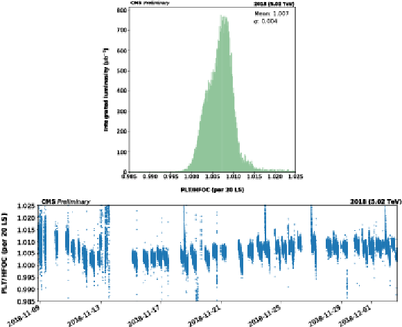
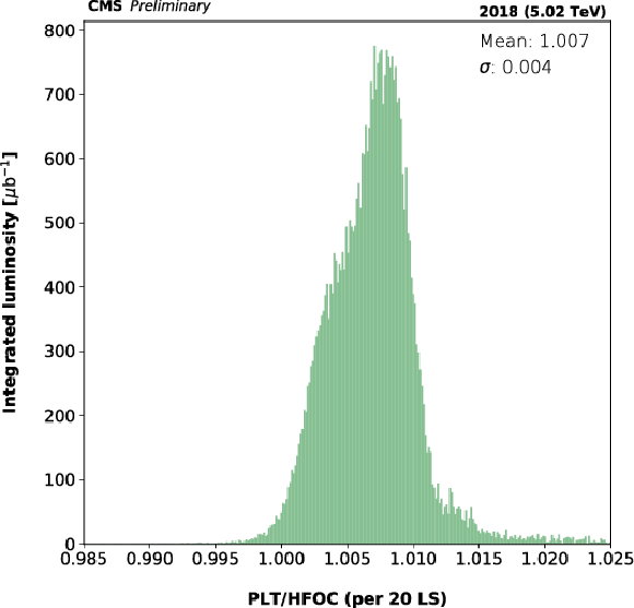
Cross-detector comparison using the PLT over HFOC luminosity ratio, cumulatively (top) and as a function of time (bottom). |
png pdf |
Figure 19-a:
Cross-detector comparison using the PLT over HFOC luminosity ratio, cumulatively (top) and as a function of time (bottom). |

png pdf |
Figure 19-b:
Cross-detector comparison using the PLT over HFOC luminosity ratio, cumulatively (top) and as a function of time (bottom). |
png pdf |
Figure 20:
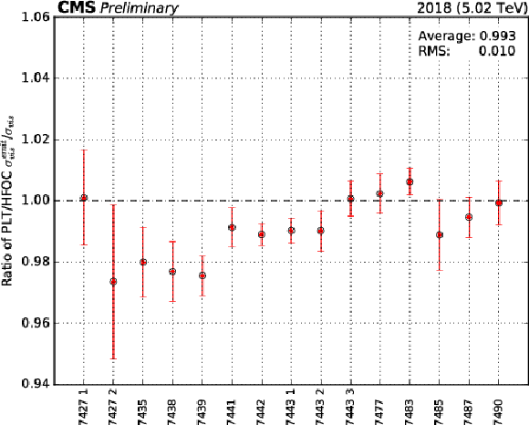
The ratio of ${\sigma _{\text {vis}}}$-normalized PLT to HFOC cross sections from emittance scans recorded during fills 7442-7443 and routine data-taking conditions. The uncertainty is of statistical nature only. |
png pdf |
Figure 21:
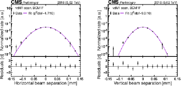
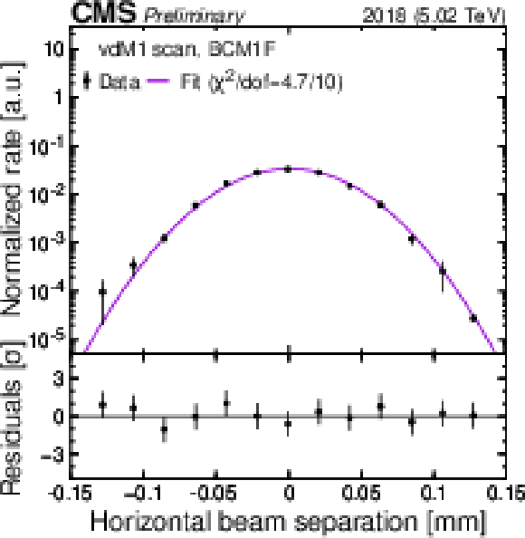
Examples of scan distributions, i.e., the normalized rate recorded by BCM1F in BCID 546 as a function of beam separation ($\Delta $) in $x$ (left) and $y$ (right), respectively. The black curve corresponding to the single-Gaussian fit. The values and the statistical uncertainty in the fitted parameters are shown in the legend, along with the reduced $\chi ^2$. The bottom panels include the residuals, i.e., the difference between the measured and fitted values divided by the statistical uncertainty. |
png pdf |
Figure 21-a:
Examples of scan distributions, i.e., the normalized rate recorded by BCM1F in BCID 546 as a function of beam separation ($\Delta $) in $x$ (left) and $y$ (right), respectively. The black curve corresponding to the single-Gaussian fit. The values and the statistical uncertainty in the fitted parameters are shown in the legend, along with the reduced $\chi ^2$. The bottom panels include the residuals, i.e., the difference between the measured and fitted values divided by the statistical uncertainty. |
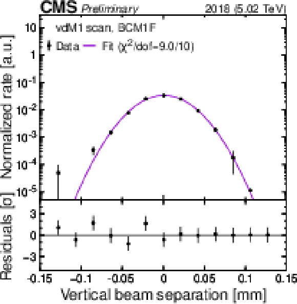
png pdf |
Figure 21-b:
Examples of scan distributions, i.e., the normalized rate recorded by BCM1F in BCID 546 as a function of beam separation ($\Delta $) in $x$ (left) and $y$ (right), respectively. The black curve corresponding to the single-Gaussian fit. The values and the statistical uncertainty in the fitted parameters are shown in the legend, along with the reduced $\chi ^2$. The bottom panels include the residuals, i.e., the difference between the measured and fitted values divided by the statistical uncertainty. |

png pdf |
Figure 22:
Examples of scan distributions, i.e., the normalized rate recorded by HFOC in BCID 546 as a function of beam separation ($\Delta $) in $x$ (left) and $y$ (right), respectively. The black curve corresponding to the single-Gaussian fit. The values and the statistical uncertainty in the fitted parameters are shown in the legend, along with the reduced $\chi ^2$. The bottom panels include the residuals, i.e., the difference between the measured and fitted values divided by the statistical uncertainty. |

png pdf |
Figure 22-a:
Examples of scan distributions, i.e., the normalized rate recorded by HFOC in BCID 546 as a function of beam separation ($\Delta $) in $x$ (left) and $y$ (right), respectively. The black curve corresponding to the single-Gaussian fit. The values and the statistical uncertainty in the fitted parameters are shown in the legend, along with the reduced $\chi ^2$. The bottom panels include the residuals, i.e., the difference between the measured and fitted values divided by the statistical uncertainty. |
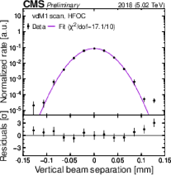
png pdf |
Figure 22-b:
Examples of scan distributions, i.e., the normalized rate recorded by HFOC in BCID 546 as a function of beam separation ($\Delta $) in $x$ (left) and $y$ (right), respectively. The black curve corresponding to the single-Gaussian fit. The values and the statistical uncertainty in the fitted parameters are shown in the legend, along with the reduced $\chi ^2$. The bottom panels include the residuals, i.e., the difference between the measured and fitted values divided by the statistical uncertainty. |
png pdf |
Figure 23:
Cross-detector comparison of the fitted $\Sigma _{y}$ as a function of BCID separately for the vdM5 scan. The horizontal dashed lines indicate the averaged values of the corresponding set of points (left). Zoom into two trains for the same scan (right). |

png pdf |
Figure 23-a:
Cross-detector comparison of the fitted $\Sigma _{y}$ as a function of BCID separately for the vdM5 scan. The horizontal dashed lines indicate the averaged values of the corresponding set of points (left). Zoom into two trains for the same scan (right). |
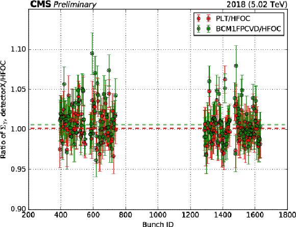
png pdf |
Figure 23-b:
Cross-detector comparison of the fitted $\Sigma _{y}$ as a function of BCID separately for the vdM5 scan. The horizontal dashed lines indicate the averaged values of the corresponding set of points (left). Zoom into two trains for the same scan (right). |
png pdf |
Figure 24:
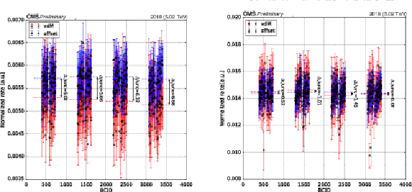
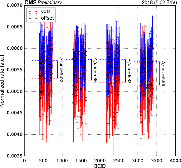
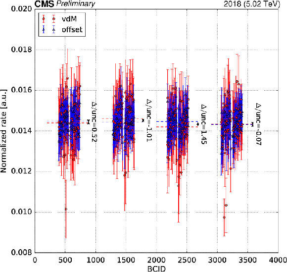
The luminometer rate comparison between vdM ($x$ direction, red) and offset ($y$ direction, blue) scans as a function of BCID at the intersection of the two scans before (left) and after (right) the implementation of the best-fit offset value. The difference $\Delta $ of the averaged values (divided by their uncertainty) between the vdM and offset scans is given separately per each BCID group. |
png pdf |
Figure 24-a:
The luminometer rate comparison between vdM ($x$ direction, red) and offset ($y$ direction, blue) scans as a function of BCID at the intersection of the two scans before (left) and after (right) the implementation of the best-fit offset value. The difference $\Delta $ of the averaged values (divided by their uncertainty) between the vdM and offset scans is given separately per each BCID group. |
png pdf |
Figure 24-b:
The luminometer rate comparison between vdM ($x$ direction, red) and offset ($y$ direction, blue) scans as a function of BCID at the intersection of the two scans before (left) and after (right) the implementation of the best-fit offset value. The difference $\Delta $ of the averaged values (divided by their uncertainty) between the vdM and offset scans is given separately per each BCID group. |
png pdf |
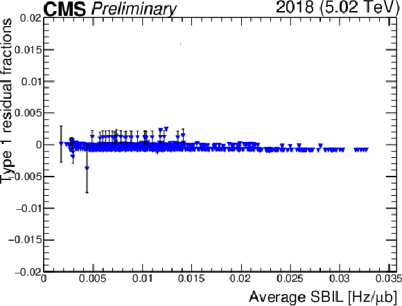
Figure 25:
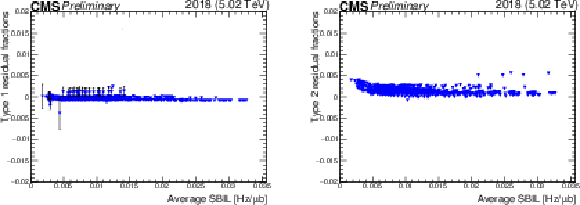
Left: the type 1 residual fractions as a function of time for the 5.02 TeV PbPb data set in 2018; Right: the type 2 residual fractions as a function of time for the same data set. |
png pdf |
Figure 25-a:
Left: the type 1 residual fractions as a function of time for the 5.02 TeV PbPb data set in 2018; Right: the type 2 residual fractions as a function of time for the same data set. |

png pdf |
Figure 25-b:
Left: the type 1 residual fractions as a function of time for the 5.02 TeV PbPb data set in 2018; Right: the type 2 residual fractions as a function of time for the same data set. |
| Tables | |

png pdf |
Table 1:
Summary of the LHC conditions at IP5 for the scan sessions in PbPb collisions in 2018. The column $ {\mathcal {L}} _{\text {init}}$ corresponds to the initial instantaneous luminosity, with all other variables defined in the text. The columns corresponding to "No. of scans'' indicate the total number of vdM, LSC, or other (i.e., emittance, offset, diagonal, and large beam separation) scans that were performed in either transverse coordinate, counting only scans used for analysis. |

png pdf |
Table 2:
Summary of noncollision rate per luminometer, its contribution relative to the (averaged over BCIDs and vdM1-5 scans) head-on rate, and impact on ${\sigma _{\text {vis}}}$. For HFOC, two methods are cross checked, while no associated correction on ${\sigma _{\text {vis}}}$ is reported ("---''). |

png pdf |
Table 3:
Ghost fraction per beam, average satellites fraction per beam and total impact on ${\sigma _{\text {vis}}}$. |
png pdf |
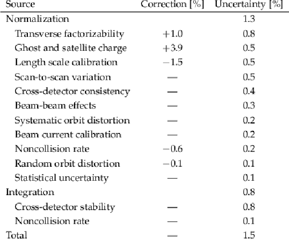
Table 4:
Summary of the sources of uncertainty impacting the CMS luminosity measurement for ${\sqrt {\smash [b]{s_{_{\mathrm {NN}}}}}} = $ 5.02 TeV PbPb collisions. When applicable, the average correction applied to ${\sigma _{\text {vis}}}$ of the Pixel Luminosity Telescope is shown. |
| Summary |
|
The measurement of the luminosity delivered to the CMS experiment during the lead-lead (PbPb) data-taking period in 2018 at nucleon-nucleon center-of-mass energy of 5.02 TeV is presented. Three subdetectors are used: the Fast Beam Conditions Monitor, the forward hadron calorimeter, and the Pixel Luminosity Telescope. Two groups of uncertainty are formed: that is, "normalization'' and "integration''. The former is related to the visible cross section (${\sigma_{\text{vis}}} $) as determined from the van der Meer (vdM) scan procedure, while the latter to the dependency of the measurements from luminosity subdetectors on the PbPb data-taking conditions. The dominant sources of uncertainty contributing to the normalization and integration are associated to the transverse factorizability of the colliding bunch densities and cross-detector stability, respectively. The stability is found to be consistent with the analysis of short vdM-like scans, performed regularly during the PbPb data-taking period. The sources of uncertainty in the normalization (1.3%) and integration (0.8%) are treated as uncorrelated, and are summed in quadrature. Table 4 summarizes the sources of corrections along with the associated systematic or statistical uncertainty. In summary, the total uncertainty in the luminosity delivered to the CMS experiment with nucleus-nucleus collisions at $ {\sqrt {\smash [b]{s_{_{\mathrm {NN}}}}}}= $ 5.02 TeV in November 2018 is estimated to be 1.5%. |
| References | ||||
| 1 | CMS Collaboration | Observation of top quark production in proton-nucleus collisions | PRL 119 (2017) 242001 | CMS-HIN-17-002 1709.07411 |
| 2 | ATLAS Collaboration | Observation of light-by-light scattering in ultraperipheral PbPb collisions with the ATLAS detector | PRL 123 (2019) 052001 | 1904.03536 |
| 3 | CMS Collaboration | Evidence for fop quark production in nucleus-nucleus collisions | PRL 125 (2020) 222001 | CMS-HIN-19-001 2006.11110 |
| 4 | CMS Collaboration | Observation of nuclear modifications in $ \mathrm{W} ^\pm $ boson production in pPb collisions at $ {\sqrt {\smash [b]{s_{_{\mathrm {NN}}}}}} = $ 8.16 TeV | PLB 800 (2020) 135048 | CMS-HIN-17-007 1905.01486 |
| 5 | S. van der Meer | Calibration of the effective beam height in the ISR | CERN-ISR-PO-68-31 | |
| 6 | ALICE Collaboration | Measurement of visible cross sections in proton-lead collisions at $ {\sqrt {\smash [b]{s_{_{\mathrm {NN}}}}}} = $ 5.02 TeV in van der Meer scans with the ALICE detector | JINST 9 (2014) P11003 | 1405.1849 |
| 7 | ATLAS Collaboration | Improved luminosity determination in proton-proton collisions at $ \sqrt{s} = $ 7 TeV using the ATLAS detector at the LHC | EPJC 73 (2013) 2518 | 1302.4393 |
| 8 | LHCb Collaboration | Precision luminosity measurements at LHCb | JINST 9 (2014) P12005 | 1410.0149 |
| 9 | CMS Collaboration | Precision luminosity measurement in proton-proton collisions at $ \sqrt{s} = $ 13 TeV in 2015 and 2016 at CMS | EPJC 81 (2021) 800 | CMS-LUM-17-003 2104.01927 |
| 10 | CMS Collaboration | CMS luminosity calibration for the proton-proton reference run at $ \sqrt{s} = $ 5.02 TeV | CMS-PAS-LUM-16-001 | CMS-PAS-LUM-16-001 |
| 11 | CMS Collaboration | CMS luminosity measurement for the 2017 data-taking period at $ \sqrt{s} = $ 13 TeV | CMS-PAS-LUM-17-004 | CMS-PAS-LUM-17-004 |
| 12 | CMS Collaboration | CMS luminosity measurement for the 2018 data-taking period at $ \sqrt{s} = $ 13 TeV | CMS-PAS-LUM-18-002 | CMS-PAS-LUM-18-002 |
| 13 | CMS Collaboration | Luminosity measurement in proton-proton collisions at 5.02 TeV in 2017 at CMS | CMS-PAS-LUM-19-001 | CMS-PAS-LUM-19-001 |
| 14 | CMS Collaboration | CMS luminosity measurement using 2016 proton-nucleus collisions at $ {\sqrt {\smash [b]{s_{_{\mathrm {NN}}}}}} = $ 8.16 TeV | CMS-PAS-LUM-17-002 | CMS-PAS-LUM-17-002 |
| 15 | ALICE Collaboration | ALICE luminosity determination for Pb-Pb collisions at $ {\sqrt {\smash [b]{s_{_{\mathrm {NN}}}}}}=$ 5.02 TeV | 2022. Submitted to JINST | 2204.10148 |
| 16 | CMS Collaboration | The CMS experiment at the CERN LHC | JINST 3 (2008) S08004 | CMS-00-001 |
| 17 | CMS Collaboration, M. Guthoff | The new Fast Beam Condition Monitor using poly-crystalline diamond sensors for luminosity measurement at CMS | in Proc. 14th Pisa Meeting on Advanced Detectors: Frontier Detectors for Frontier Physics 2019 [NIMA 936 (2019) 717] | |
| 18 | CMS Collaboration, A. Kornmayer | The CMS Pixel Luminosity Telescope | in Proc. 13th Pisa Meeting on Advanced Detectors: Frontier Detectors for Frontier Physics 2015 [NIMA 824 (2016) 304] | |
| 19 | CMS Collaboration, P. Lujan | Performance of the Pixel Luminosity Telescope for luminosity measurement at CMS during Run 2 | in Proc. European Physical Society Conference on High Energy Physics (EPS-HEP 2017) 2017 [PoS 314 (2017) 504] | |
| 20 | O. S. Bruning et al. | LHC design report v.1: The LHC main ring | CERN (2004) | |
| 21 | C. Barschel et al. | Results of the LHC DCCT calibration studies | CERN-ATS-Note-2012-026 PERF | |
| 22 | D. Belohrad et al. | The LHC Fast BCT system: A comparison of design parameters with initial performance | CERN-BE-2010-010 | |
| 23 | M. Gasior, J. Olexa, and R. Steinhagen | BPM electronics based on compensated diode detectors -- Results from development systems | in 2012 Beam Instrumentation Workshop (BIW2012) 2012 [Conf. Proc. C1204151 (2012) MOPG010] | |
| 24 | CMS Collaboration | The CMS trigger system | JINST 12 (2017) P01020 | CMS-TRG-12-001 1609.02366 |
| 25 | A. Jeff et al. | Longitudinal density monitor for the LHC | PRST Accel. Beams 15 (2012) 032803 | |
| 26 | C. Barschel | PhD thesis, RWTH Aachen University, 2014 CERN-THESIS-2013-301 | ||
| 27 | W. Kozanecki, T. Pieloni, and J. Wenninger | Observation of beam-beam deflections with LHC orbit data | CERN-ACC-NOTE-2013-0006 | |
| 28 | CMS Collaboration, A. Babaev | Beam-dynamic effects at the CMS BRIL Van der Meer scans | in Proc. 12th Symposium on Radiation from Relativistic Electrons in Periodic Structures (RREPS 17) 2018 [JINST 13 (2018) C03028] | |

|
Compact Muon Solenoid LHC, CERN |

|

|

|

|

|

|