

Compact Muon Solenoid
LHC, CERN
| CMS-PAS-B2G-20-007 | ||
| Search for heavy resonances decaying to a pair of boosted Higgs bosons in final states with leptons and a bottom quark-antiquark pair at $\sqrt{s} = $ 13 TeV | ||
| CMS Collaboration | ||
| July 2021 | ||
| Abstract: A search for new heavy resonances decaying to a pair of Higgs bosons in proton-proton collisions at a center-of-mass energy of 13 TeV is presented. Data were collected by the CMS detector at the LHC from 2016 to 2018, corresponding to an integrated luminosity of 138 fb$^{-1}$. The search considers resonances with a mass between 0.8 and 4.5 TeV using events in which one Higgs boson decays into a bottom quark-antiquark pair and the other decays into final states with either one or two charged leptons. Specifically, these include the single-lepton final state of the $\mathrm{HH} \rightarrow \mathrm{b\bar{b}WW^*} \rightarrow \mathrm{b\bar{b}}\ell \nu \mathrm{q\bar{q}}$ decay and the dilepton final states of both the $\mathrm{HH} \rightarrow \mathrm{b\bar{b}WW^*} \rightarrow \mathrm{b\bar{b}}\ell \nu \ell \nu$ and $\mathrm{HH} \rightarrow \mathrm{b\bar{b}}\tau \tau \rightarrow \mathrm{b\bar{b}}\ell \nu \nu \ell \nu \nu$ decays, where $\ell$ in the final state corresponds to $e$ or $\mu$. The signal is extracted using a two-dimensional maximum likelihood fit of the $\mathrm{H} \rightarrow \mathrm{b\bar{b}}$ jet mass and $\mathrm{HH}$ invariant mass distributions. No significant excess above the standard model expectation is observed in data. Model-independent exclusion limits are placed on the the product of the cross section and branching fraction ($\sigma \mathcal{B}$) for spin-0 and spin-2 massive bosons decaying to $\mathrm{HH}$. The results are interpreted in the context of radion and bulk graviton production in models with a warped extra spatial dimension. | ||
|
Links:
CDS record (PDF) ;
CADI line (restricted) ;
These preliminary results are superseded in this paper, JHEP 05 (2022) 005. The superseded preliminary plots can be found here. |
||
| Figures | |
png pdf |
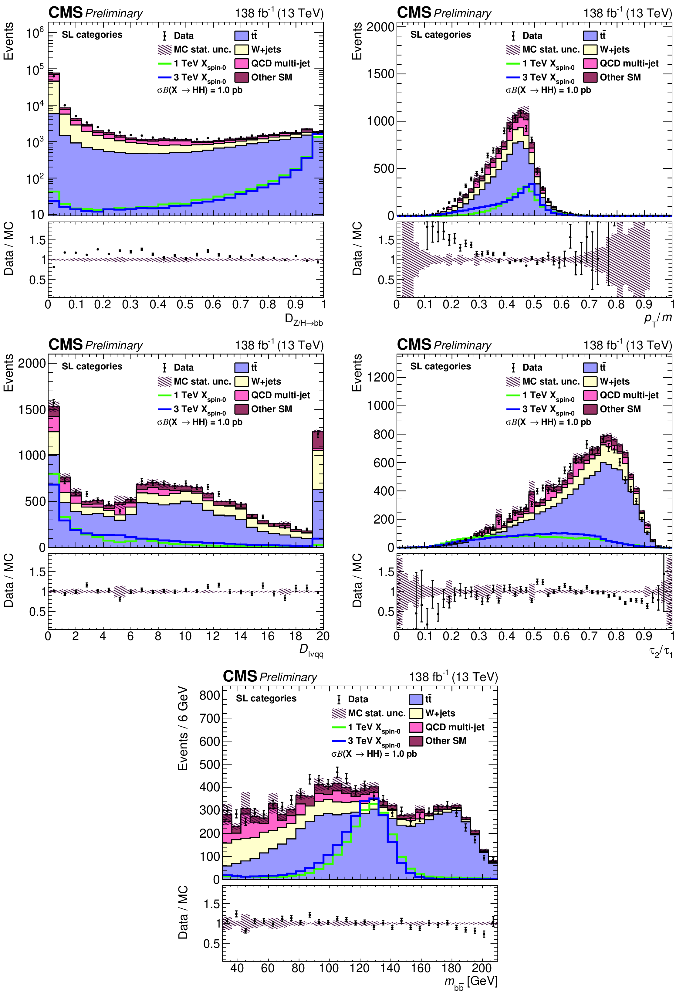
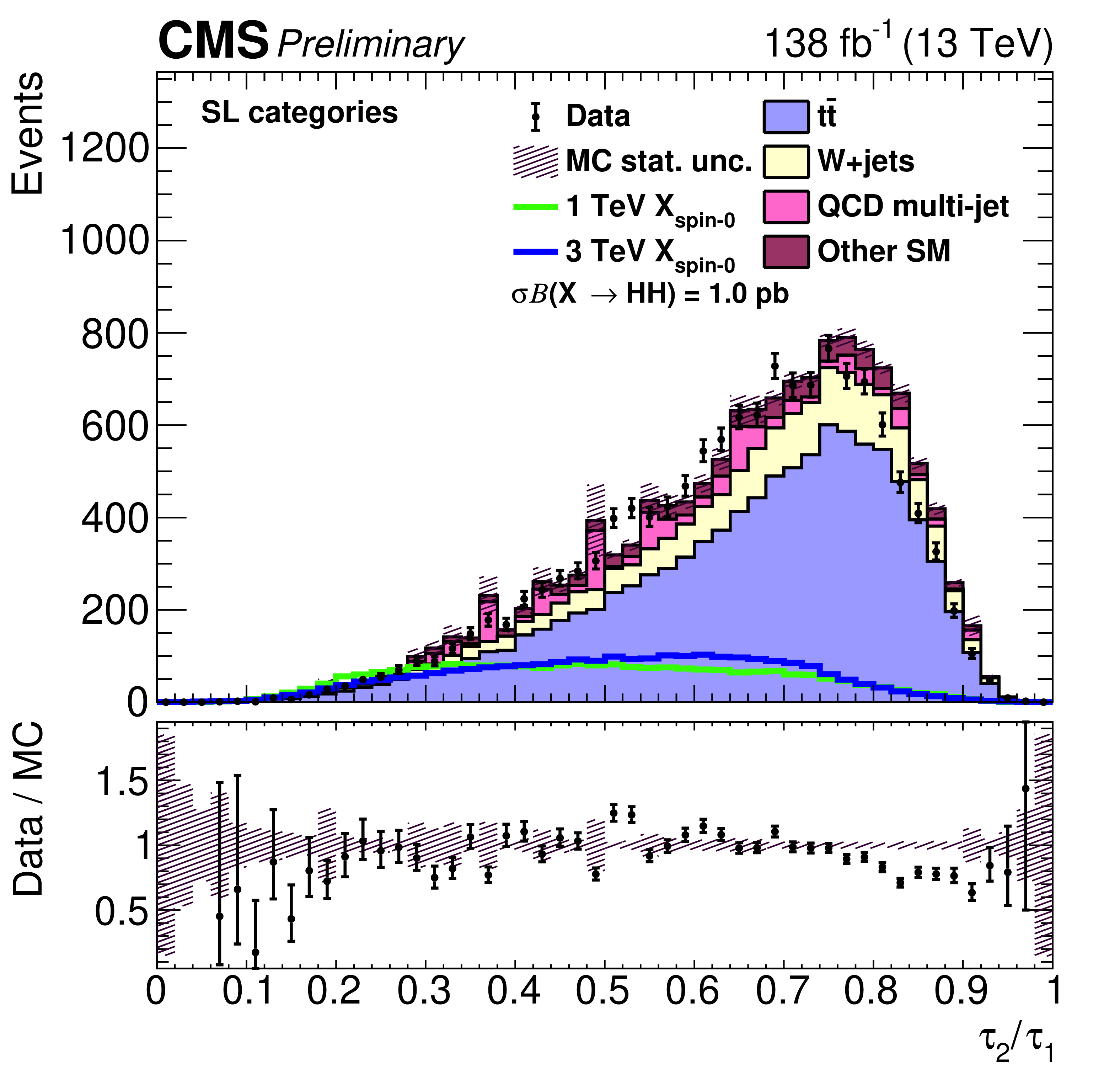
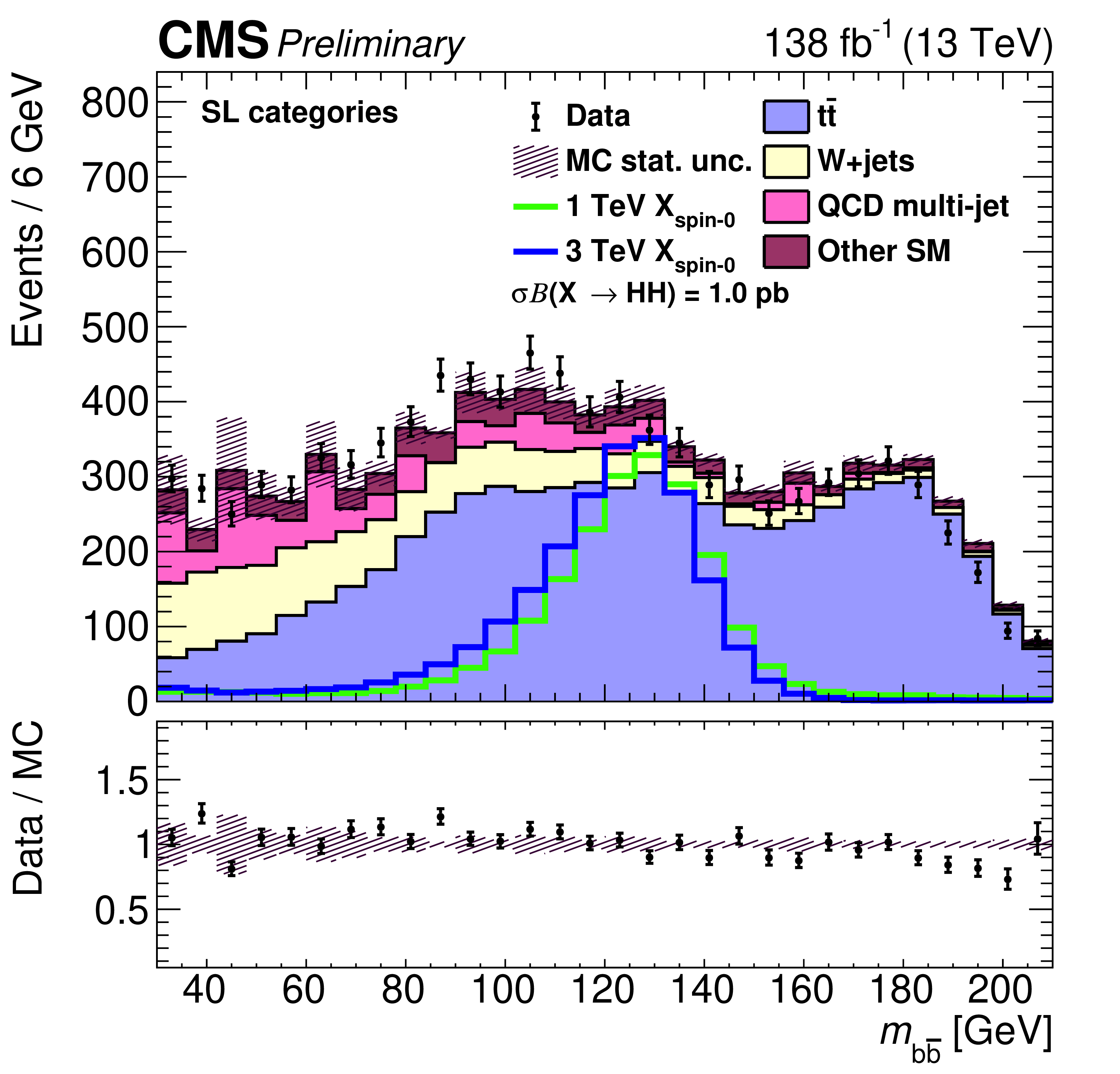
Figure 1:
Single-lepton channel variables: distributions of important variables are shown for data (points), simulated SM processes (filled histograms), and simulated signal (solid lines). The statistical uncertainty of the simulated sample is shown as the hatched band. Spin-0 signals for $ {m_{\mathrm{X}}} $ of 1.0 and 3.0 TeV are displayed. For both signal models, $\sigma \mathcal {B} (\mathrm{X} \to {\mathrm{H} \mathrm{H}})$ is set to 1.0 pb. The bottom panes of each plot show the ratio of the data to the sum of all background processes. |
png pdf |
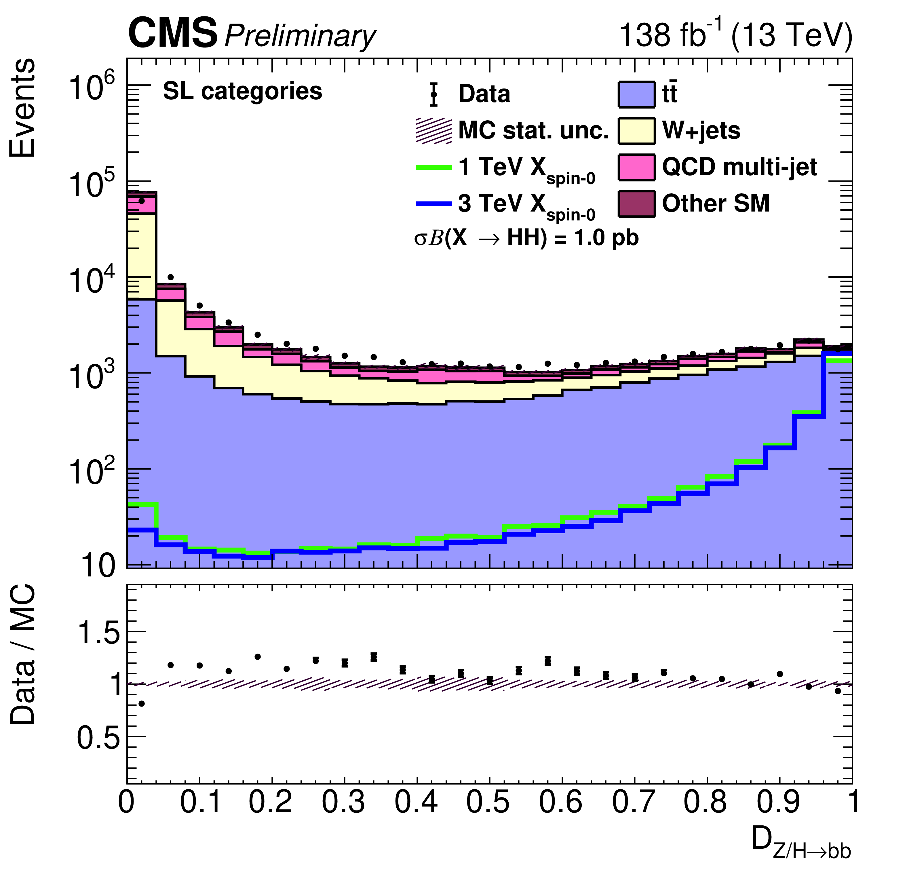
Figure 1-a:
Single-lepton channel variables: distributions of important variables are shown for data (points), simulated SM processes (filled histograms), and simulated signal (solid lines). The statistical uncertainty of the simulated sample is shown as the hatched band. Spin-0 signals for $ {m_{\mathrm{X}}} $ of 1.0 and 3.0 TeV are displayed. For both signal models, $\sigma \mathcal {B} (\mathrm{X} \to {\mathrm{H} \mathrm{H}})$ is set to 1.0 pb. The bottom panes of each plot show the ratio of the data to the sum of all background processes. |
png pdf |
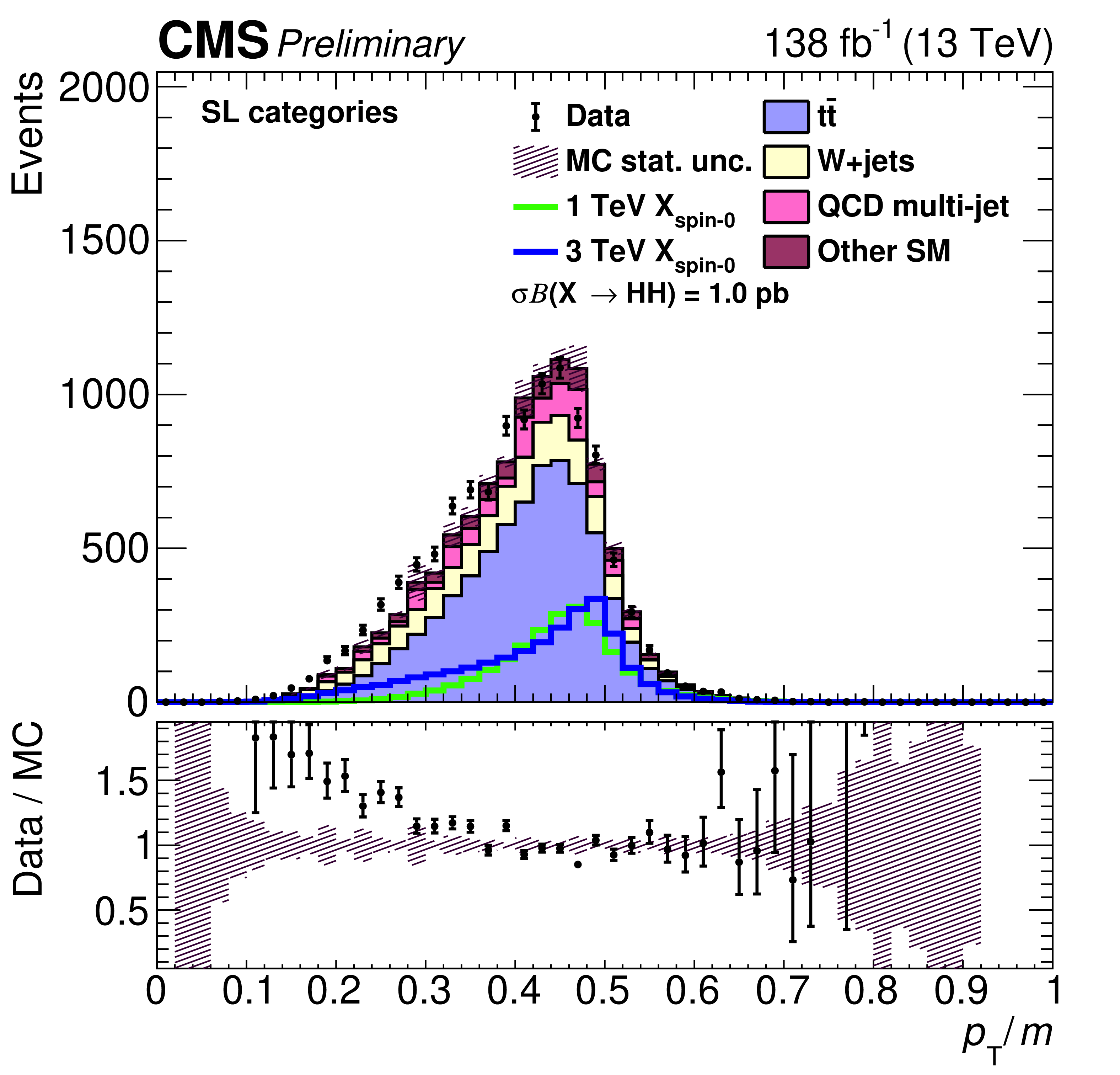
Figure 1-b:
Single-lepton channel variables: distributions of important variables are shown for data (points), simulated SM processes (filled histograms), and simulated signal (solid lines). The statistical uncertainty of the simulated sample is shown as the hatched band. Spin-0 signals for $ {m_{\mathrm{X}}} $ of 1.0 and 3.0 TeV are displayed. For both signal models, $\sigma \mathcal {B} (\mathrm{X} \to {\mathrm{H} \mathrm{H}})$ is set to 1.0 pb. The bottom panes of each plot show the ratio of the data to the sum of all background processes. |
png pdf |
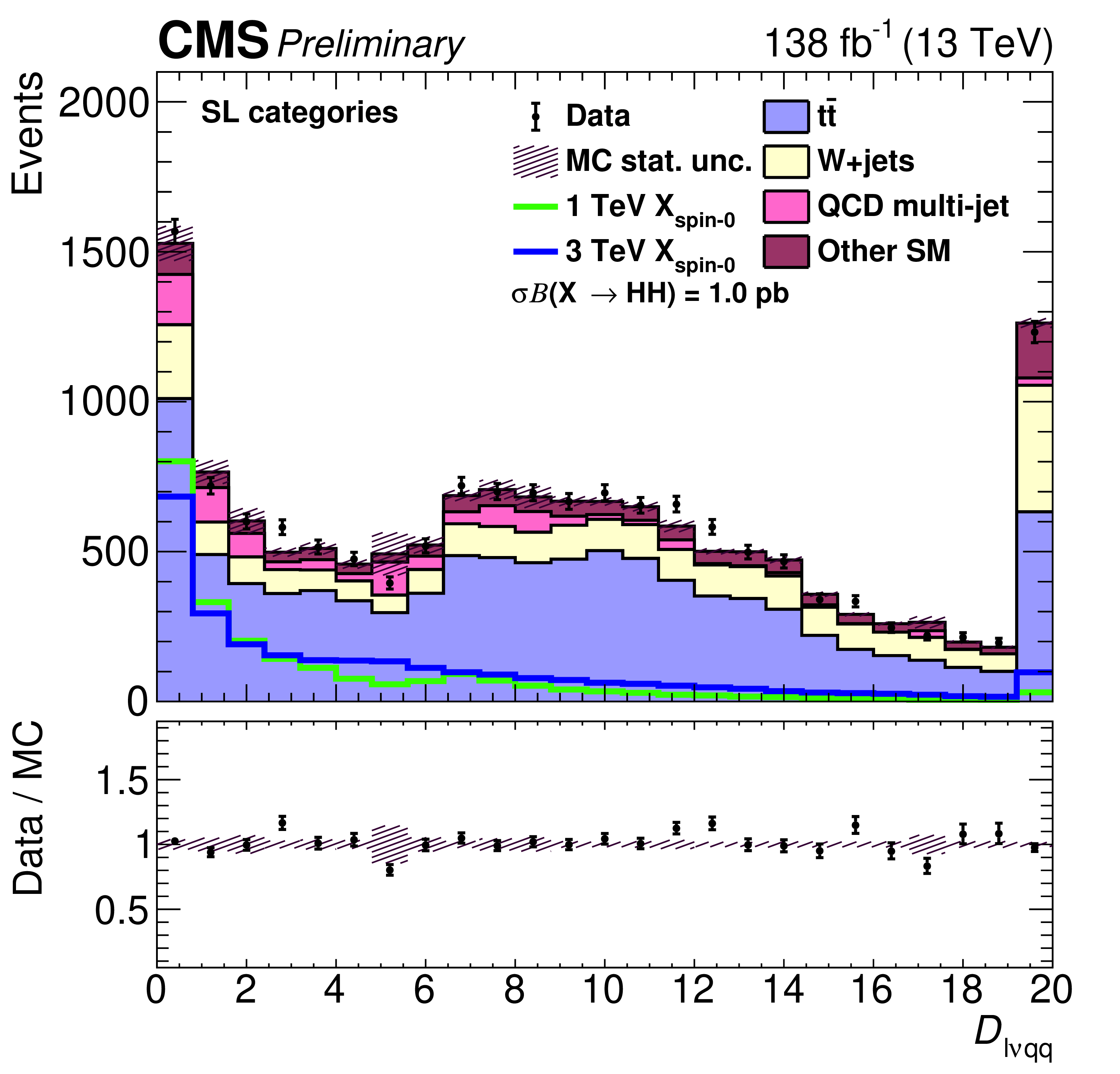
Figure 1-c:
Single-lepton channel variables: distributions of important variables are shown for data (points), simulated SM processes (filled histograms), and simulated signal (solid lines). The statistical uncertainty of the simulated sample is shown as the hatched band. Spin-0 signals for $ {m_{\mathrm{X}}} $ of 1.0 and 3.0 TeV are displayed. For both signal models, $\sigma \mathcal {B} (\mathrm{X} \to {\mathrm{H} \mathrm{H}})$ is set to 1.0 pb. The bottom panes of each plot show the ratio of the data to the sum of all background processes. |
png pdf |
Figure 1-d:
Single-lepton channel variables: distributions of important variables are shown for data (points), simulated SM processes (filled histograms), and simulated signal (solid lines). The statistical uncertainty of the simulated sample is shown as the hatched band. Spin-0 signals for $ {m_{\mathrm{X}}} $ of 1.0 and 3.0 TeV are displayed. For both signal models, $\sigma \mathcal {B} (\mathrm{X} \to {\mathrm{H} \mathrm{H}})$ is set to 1.0 pb. The bottom panes of each plot show the ratio of the data to the sum of all background processes. |
png pdf |
Figure 1-e:
Single-lepton channel variables: distributions of important variables are shown for data (points), simulated SM processes (filled histograms), and simulated signal (solid lines). The statistical uncertainty of the simulated sample is shown as the hatched band. Spin-0 signals for $ {m_{\mathrm{X}}} $ of 1.0 and 3.0 TeV are displayed. For both signal models, $\sigma \mathcal {B} (\mathrm{X} \to {\mathrm{H} \mathrm{H}})$ is set to 1.0 pb. The bottom panes of each plot show the ratio of the data to the sum of all background processes. |
png pdf |
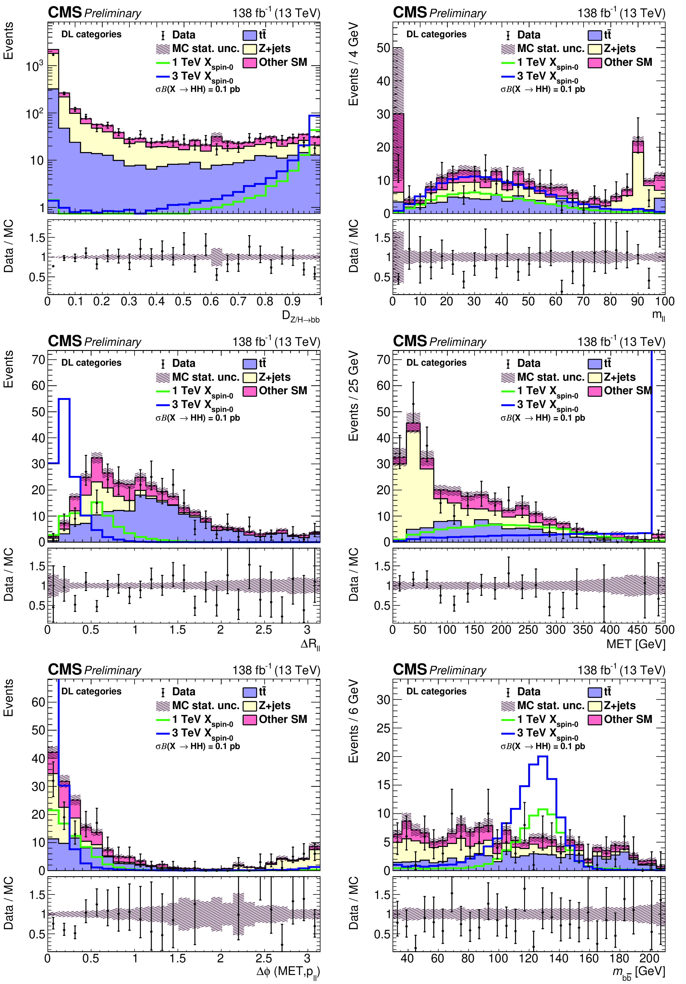
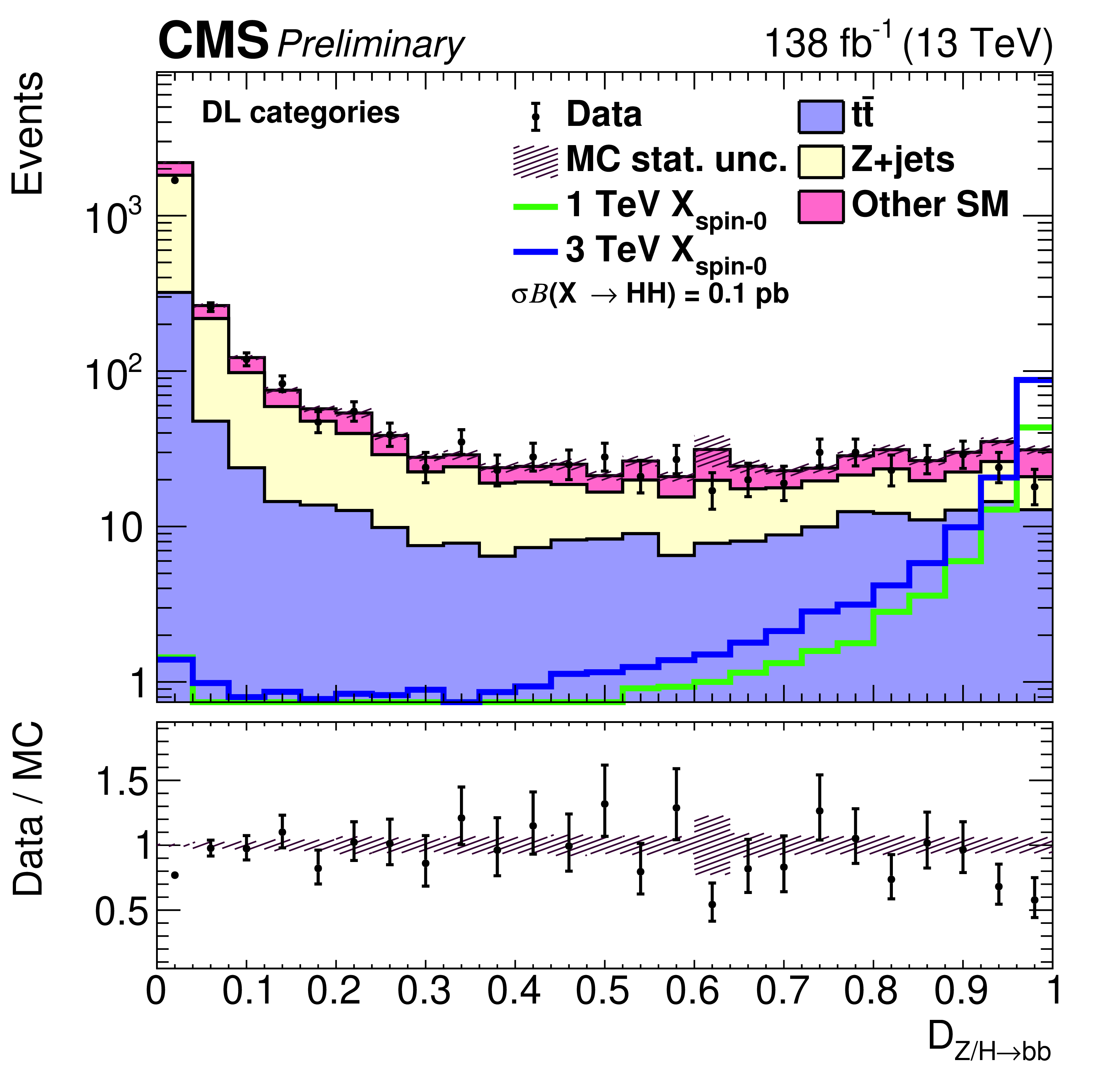
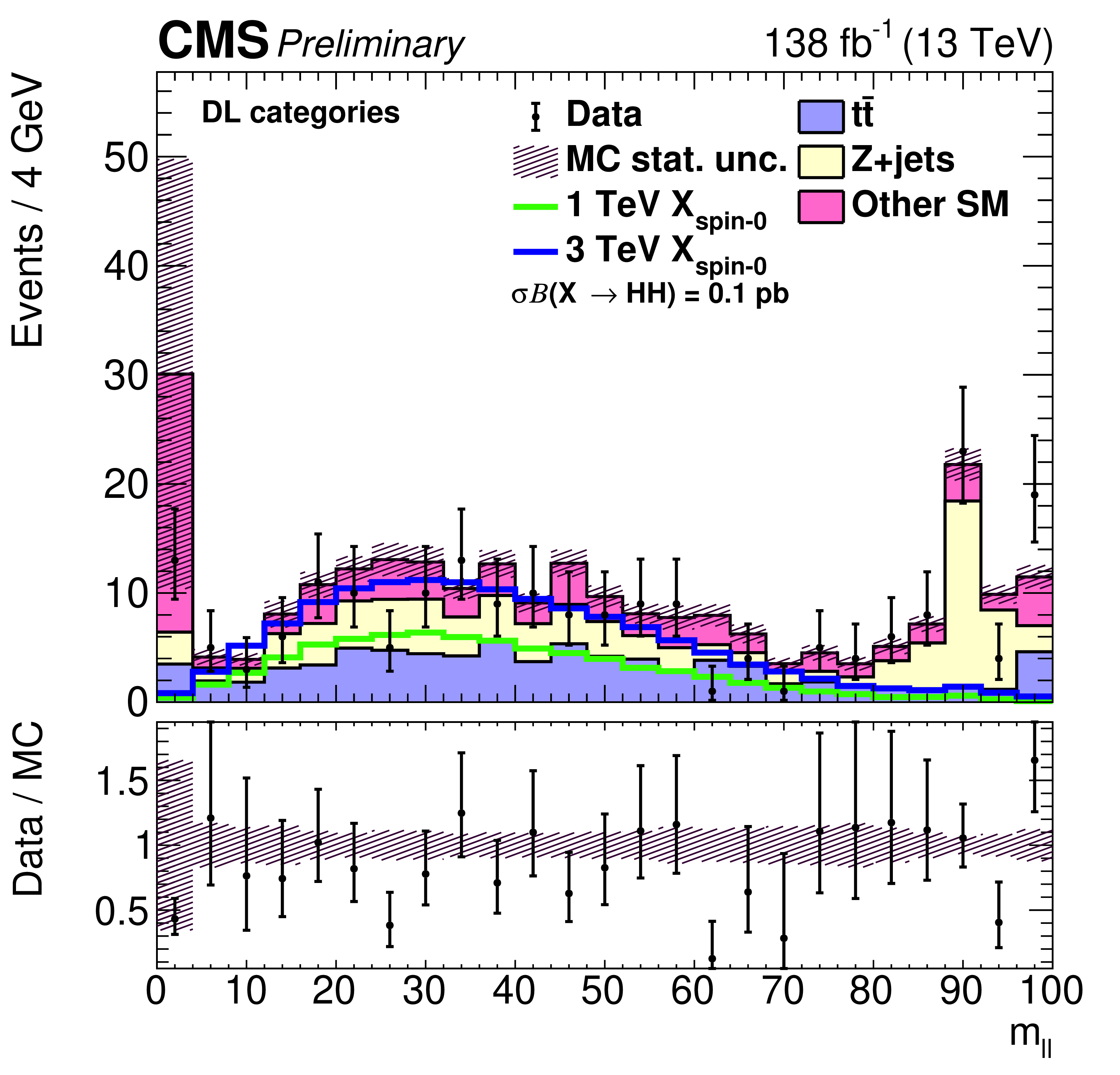
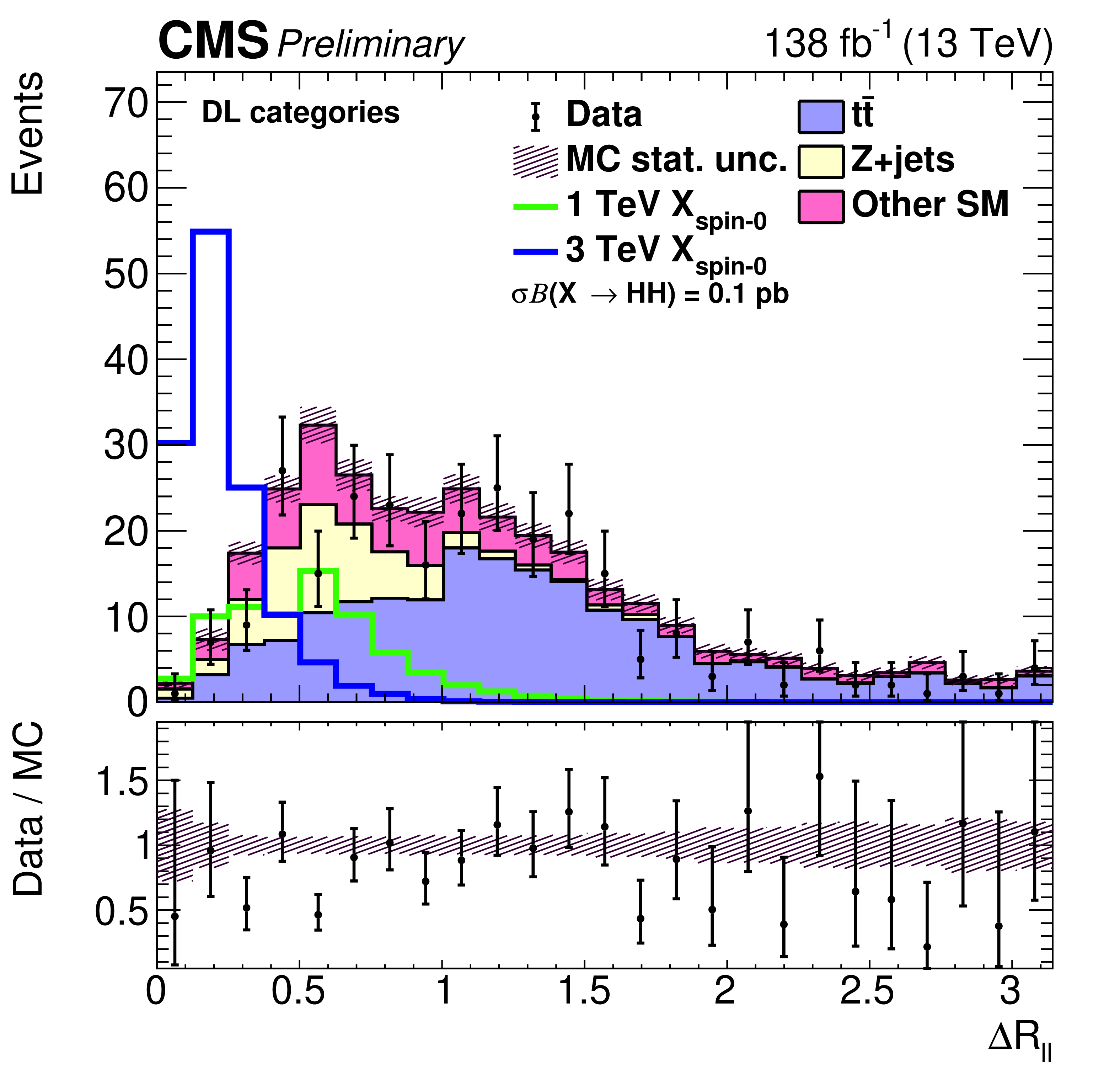
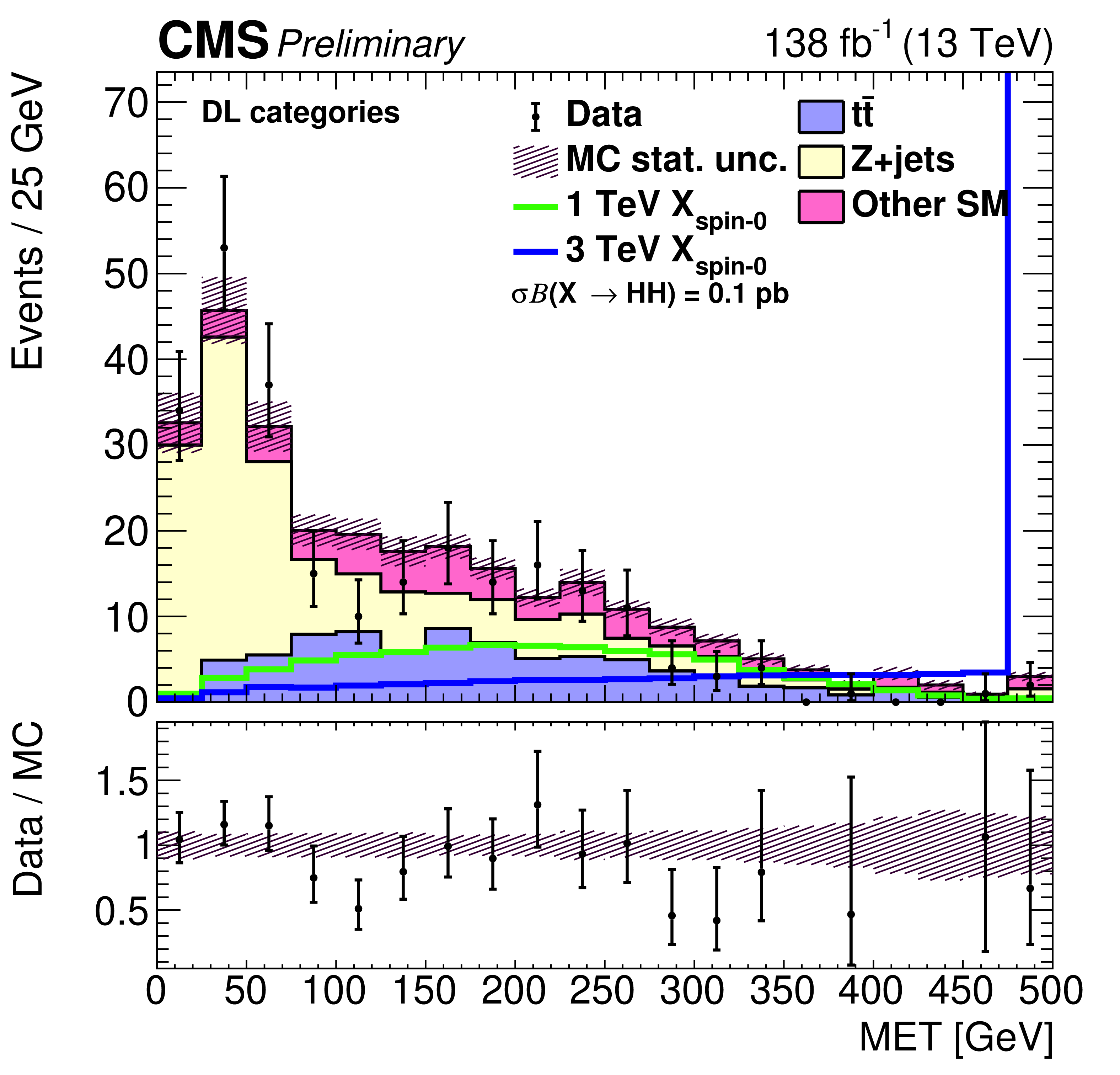
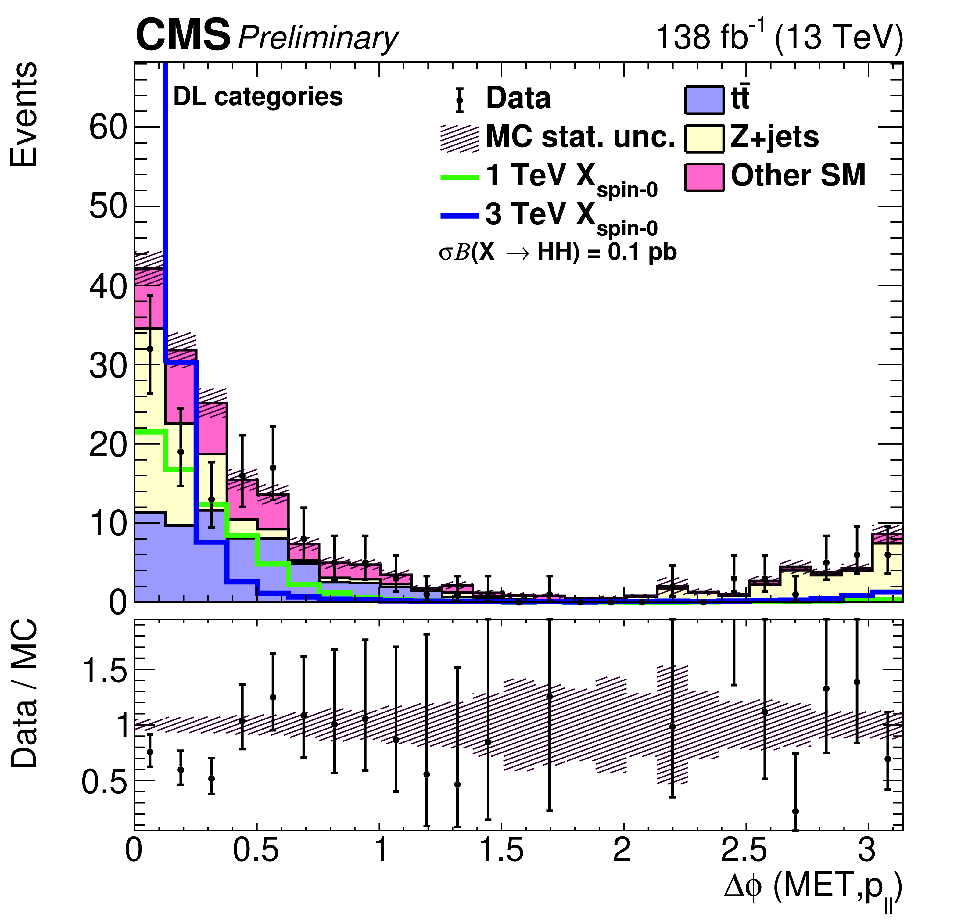
Figure 2:
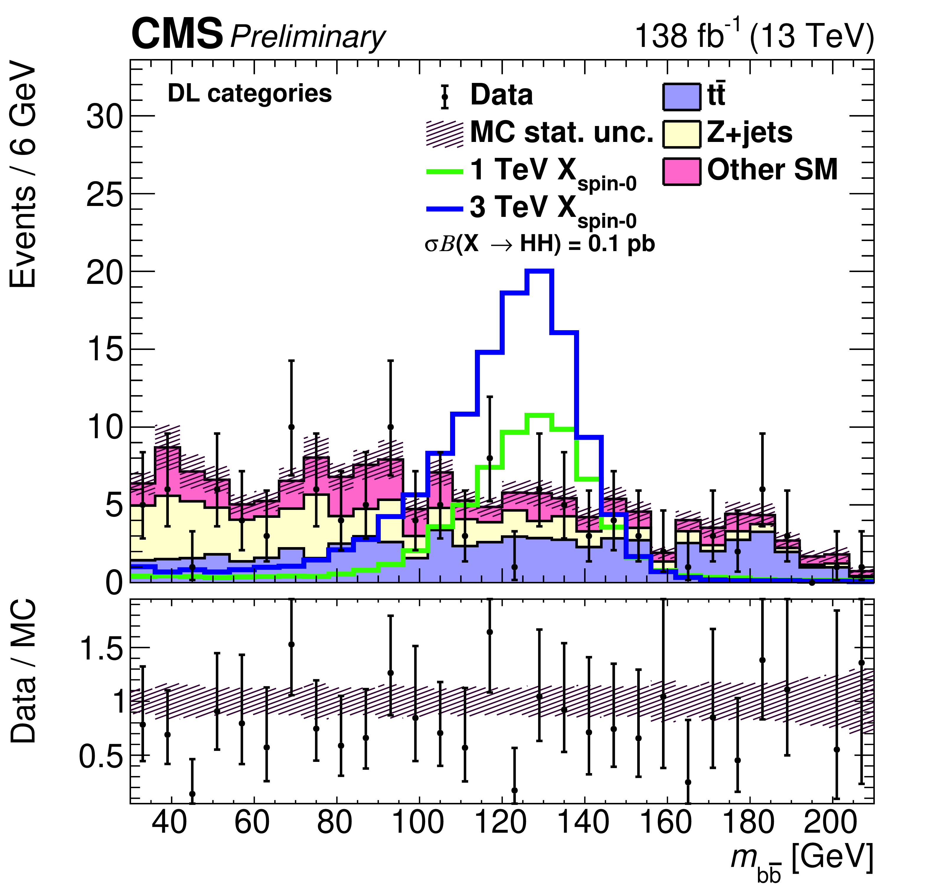
Dilepton channel variables: distributions of important variables are shown for data (points), simulated SM processes (filled histograms), and simulated signal (solid lines). The statistical uncertainty of the simulated sample is shown as the hatched band. Spin-0 signals for $ {m_{\mathrm{X}}} $ of 1.0 and 3.0 TeV are displayed. For both signal models, $\sigma \mathcal {B} (\mathrm{X} \to {\mathrm{H} \mathrm{H}})$ is set to 0.1 pb. The bottom panes of each plot show the ratio of the data to the sum of all background processes. |
png pdf |
Figure 2-a:
Dilepton channel variables: distributions of important variables are shown for data (points), simulated SM processes (filled histograms), and simulated signal (solid lines). The statistical uncertainty of the simulated sample is shown as the hatched band. Spin-0 signals for $ {m_{\mathrm{X}}} $ of 1.0 and 3.0 TeV are displayed. For both signal models, $\sigma \mathcal {B} (\mathrm{X} \to {\mathrm{H} \mathrm{H}})$ is set to 0.1 pb. The bottom panes of each plot show the ratio of the data to the sum of all background processes. |
png pdf |
Figure 2-b:
Dilepton channel variables: distributions of important variables are shown for data (points), simulated SM processes (filled histograms), and simulated signal (solid lines). The statistical uncertainty of the simulated sample is shown as the hatched band. Spin-0 signals for $ {m_{\mathrm{X}}} $ of 1.0 and 3.0 TeV are displayed. For both signal models, $\sigma \mathcal {B} (\mathrm{X} \to {\mathrm{H} \mathrm{H}})$ is set to 0.1 pb. The bottom panes of each plot show the ratio of the data to the sum of all background processes. |
png pdf |
Figure 2-c:
Dilepton channel variables: distributions of important variables are shown for data (points), simulated SM processes (filled histograms), and simulated signal (solid lines). The statistical uncertainty of the simulated sample is shown as the hatched band. Spin-0 signals for $ {m_{\mathrm{X}}} $ of 1.0 and 3.0 TeV are displayed. For both signal models, $\sigma \mathcal {B} (\mathrm{X} \to {\mathrm{H} \mathrm{H}})$ is set to 0.1 pb. The bottom panes of each plot show the ratio of the data to the sum of all background processes. |
png pdf |
Figure 2-d:
Dilepton channel variables: distributions of important variables are shown for data (points), simulated SM processes (filled histograms), and simulated signal (solid lines). The statistical uncertainty of the simulated sample is shown as the hatched band. Spin-0 signals for $ {m_{\mathrm{X}}} $ of 1.0 and 3.0 TeV are displayed. For both signal models, $\sigma \mathcal {B} (\mathrm{X} \to {\mathrm{H} \mathrm{H}})$ is set to 0.1 pb. The bottom panes of each plot show the ratio of the data to the sum of all background processes. |
png pdf |
Figure 2-e:
Dilepton channel variables: distributions of important variables are shown for data (points), simulated SM processes (filled histograms), and simulated signal (solid lines). The statistical uncertainty of the simulated sample is shown as the hatched band. Spin-0 signals for $ {m_{\mathrm{X}}} $ of 1.0 and 3.0 TeV are displayed. For both signal models, $\sigma \mathcal {B} (\mathrm{X} \to {\mathrm{H} \mathrm{H}})$ is set to 0.1 pb. The bottom panes of each plot show the ratio of the data to the sum of all background processes. |
png pdf |
Figure 2-f:
Dilepton channel variables: distributions of important variables are shown for data (points), simulated SM processes (filled histograms), and simulated signal (solid lines). The statistical uncertainty of the simulated sample is shown as the hatched band. Spin-0 signals for $ {m_{\mathrm{X}}} $ of 1.0 and 3.0 TeV are displayed. For both signal models, $\sigma \mathcal {B} (\mathrm{X} \to {\mathrm{H} \mathrm{H}})$ is set to 0.1 pb. The bottom panes of each plot show the ratio of the data to the sum of all background processes. |
png pdf |
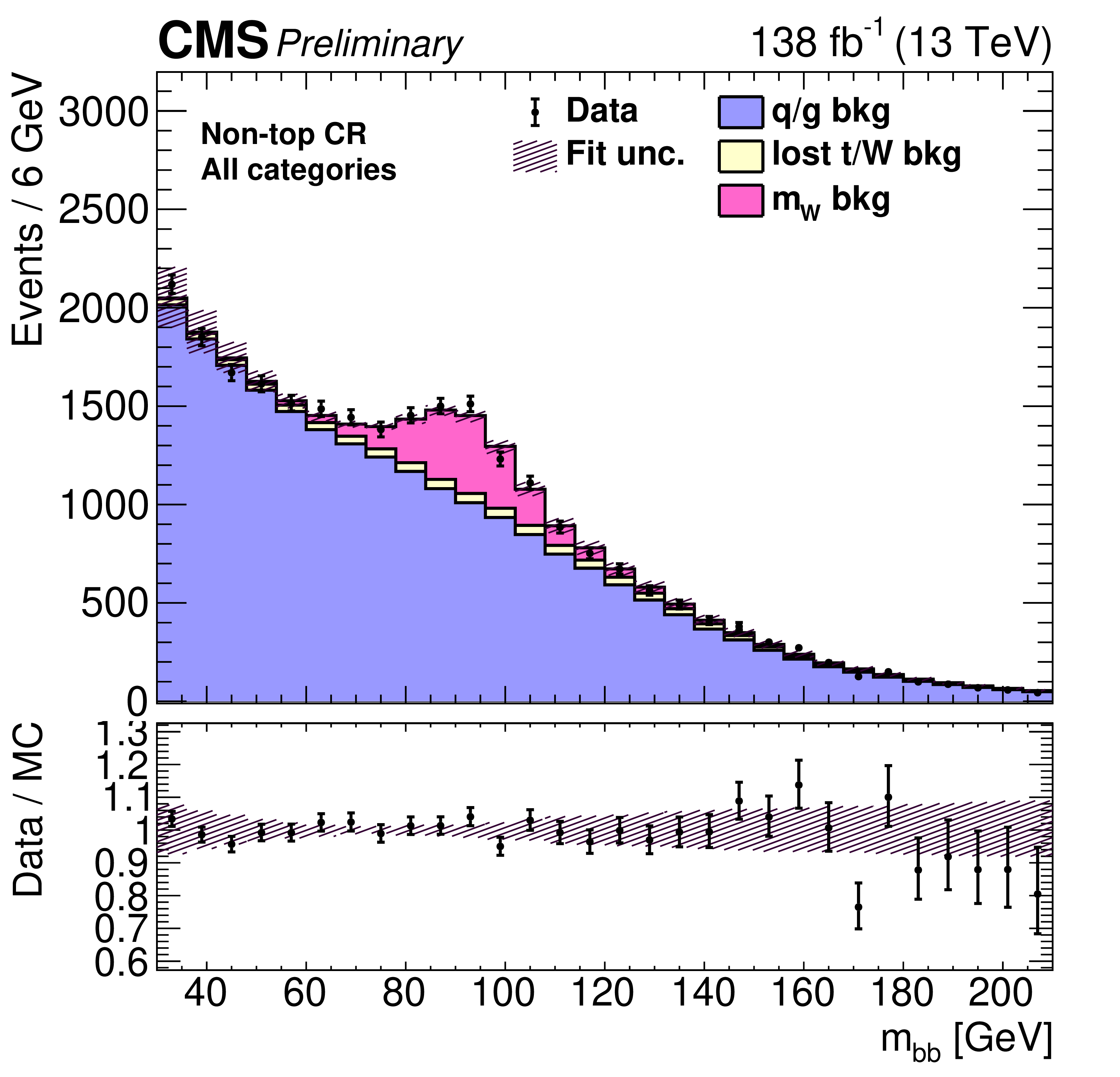
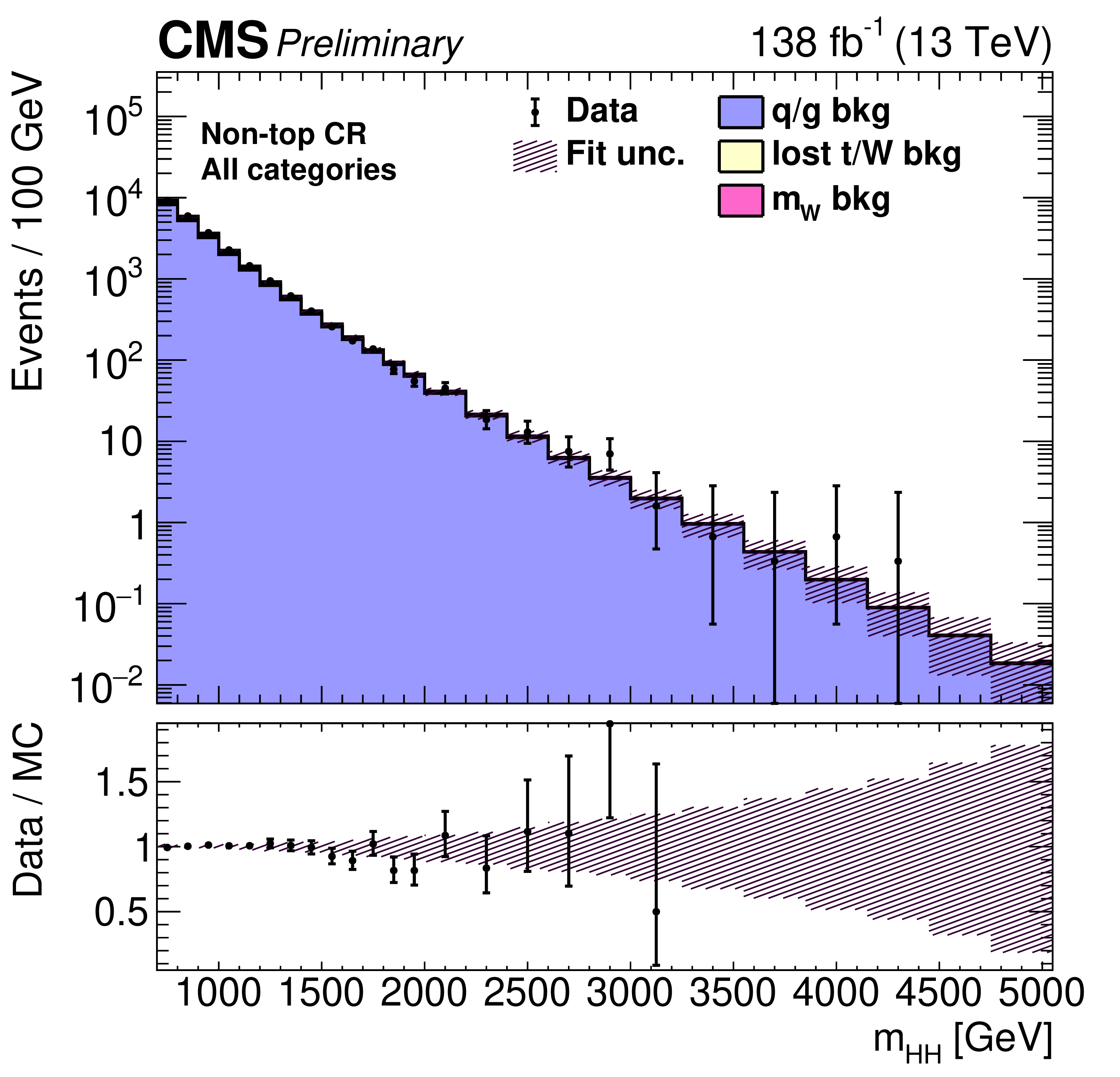
Figure 3:
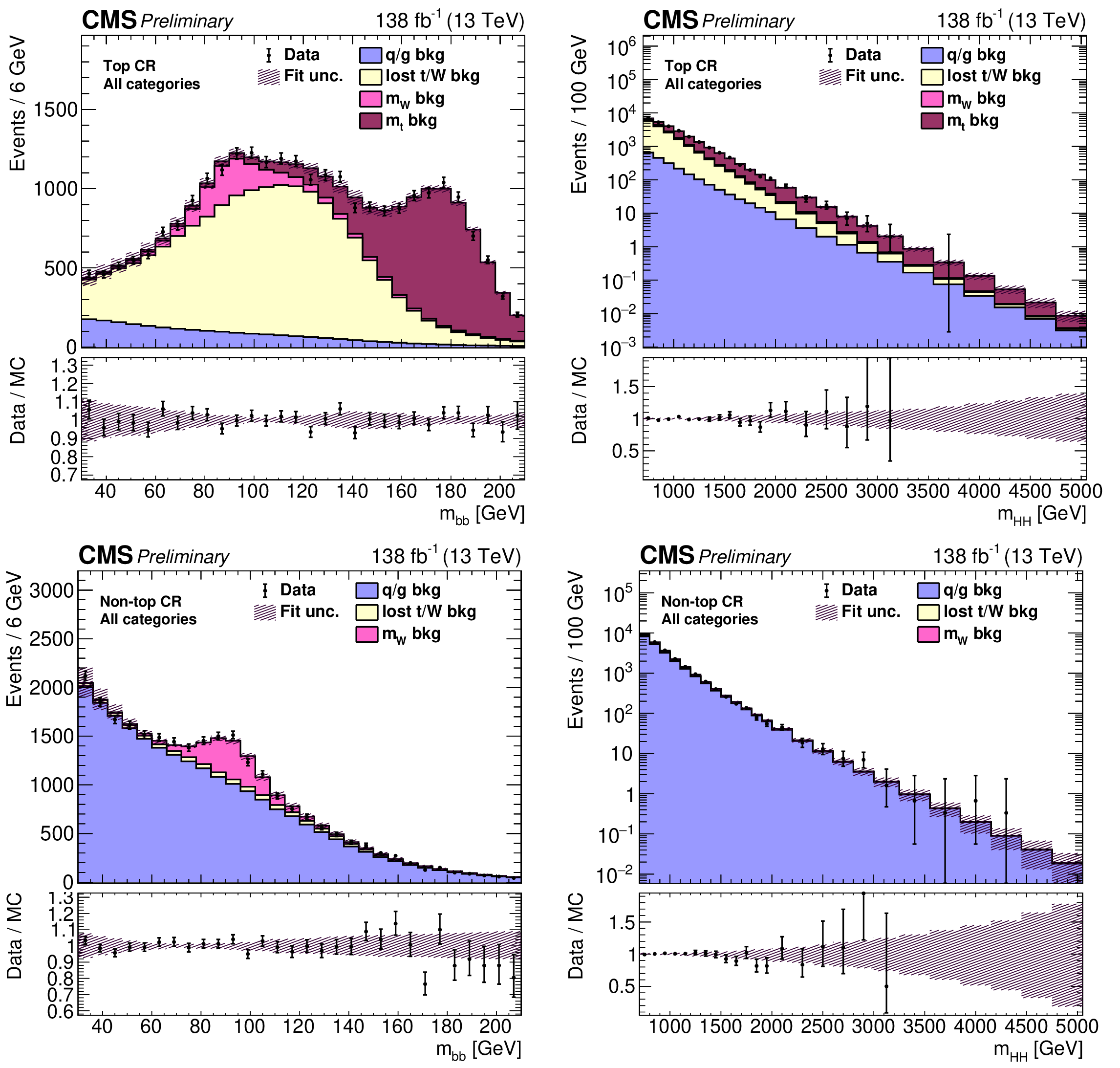
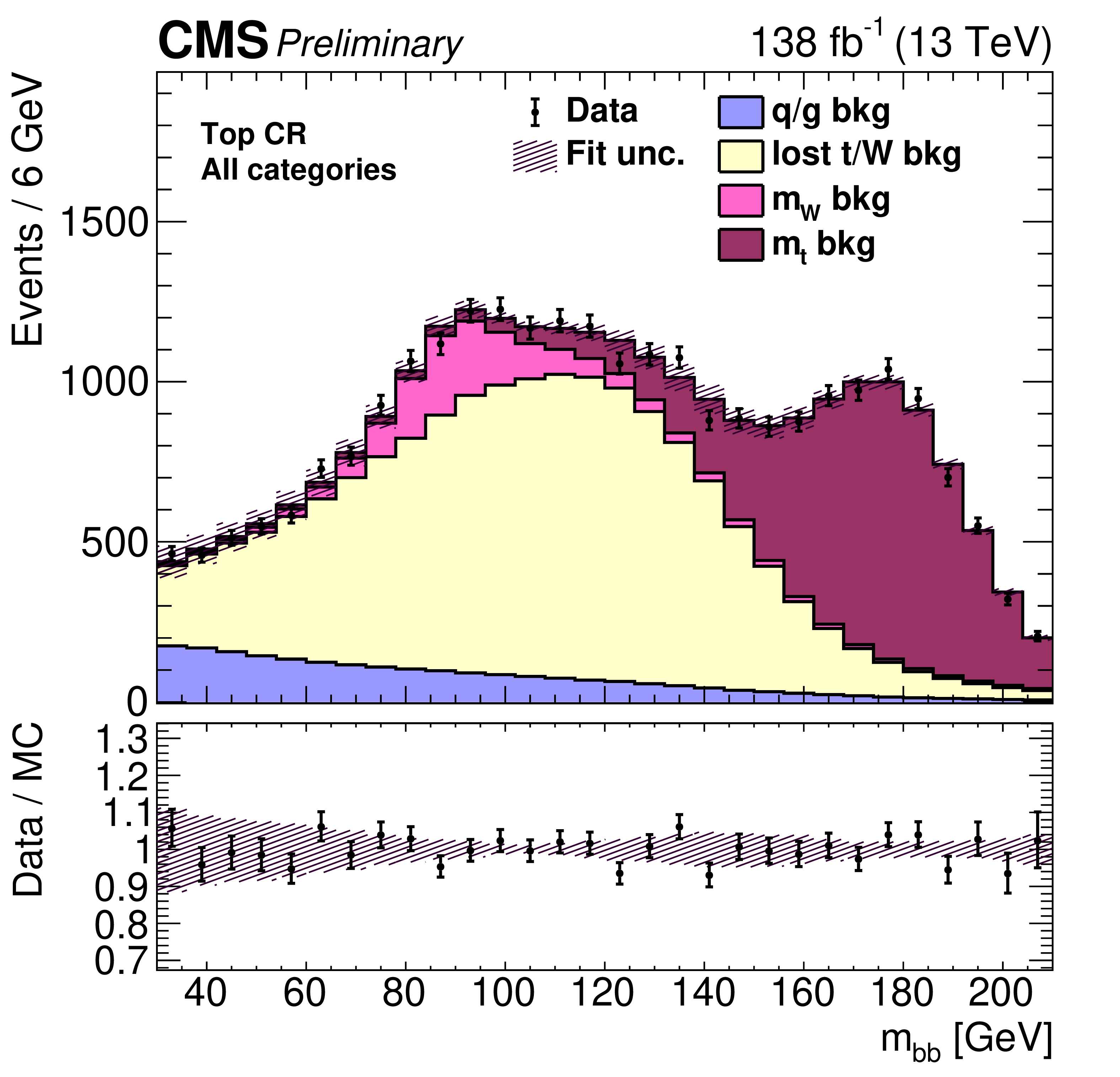
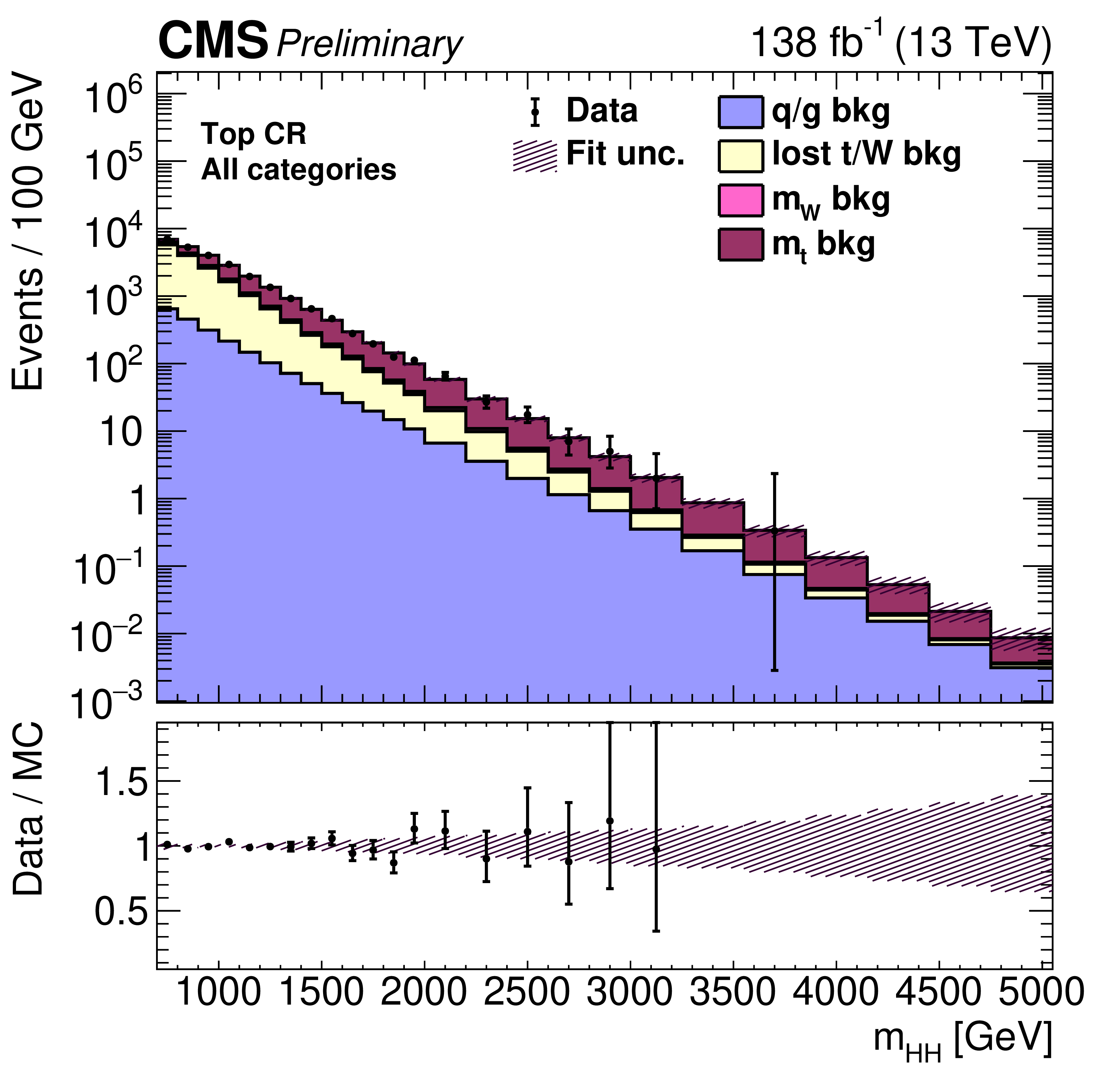
The post-fit model compared to data in the top CR (upper plots) and non-top CR (lower plots), projected into ${m_{\mathrm{b} {}\mathrm{\bar{b}}}}$ (left) and ${m_{\mathrm{H} \mathrm{H}}}$ (right). Events from all categories are combined. The fit result is the filled histogram, with the different colors indicating different background categories. The background shape uncertainty is shown as the hatched band. The bottom panes of each plot show ratio of the data to the fit result. |
png pdf |
Figure 3-a:
The post-fit model compared to data in the top CR (upper plots) and non-top CR (lower plots), projected into ${m_{\mathrm{b} {}\mathrm{\bar{b}}}}$ (left) and ${m_{\mathrm{H} \mathrm{H}}}$ (right). Events from all categories are combined. The fit result is the filled histogram, with the different colors indicating different background categories. The background shape uncertainty is shown as the hatched band. The bottom panes of each plot show ratio of the data to the fit result. |
png pdf |
Figure 3-b:
The post-fit model compared to data in the top CR (upper plots) and non-top CR (lower plots), projected into ${m_{\mathrm{b} {}\mathrm{\bar{b}}}}$ (left) and ${m_{\mathrm{H} \mathrm{H}}}$ (right). Events from all categories are combined. The fit result is the filled histogram, with the different colors indicating different background categories. The background shape uncertainty is shown as the hatched band. The bottom panes of each plot show ratio of the data to the fit result. |
png pdf |
Figure 3-c:
The post-fit model compared to data in the top CR (upper plots) and non-top CR (lower plots), projected into ${m_{\mathrm{b} {}\mathrm{\bar{b}}}}$ (left) and ${m_{\mathrm{H} \mathrm{H}}}$ (right). Events from all categories are combined. The fit result is the filled histogram, with the different colors indicating different background categories. The background shape uncertainty is shown as the hatched band. The bottom panes of each plot show ratio of the data to the fit result. |
png pdf |
Figure 3-d:
The post-fit model compared to data in the top CR (upper plots) and non-top CR (lower plots), projected into ${m_{\mathrm{b} {}\mathrm{\bar{b}}}}$ (left) and ${m_{\mathrm{H} \mathrm{H}}}$ (right). Events from all categories are combined. The fit result is the filled histogram, with the different colors indicating different background categories. The background shape uncertainty is shown as the hatched band. The bottom panes of each plot show ratio of the data to the fit result. |
png pdf |
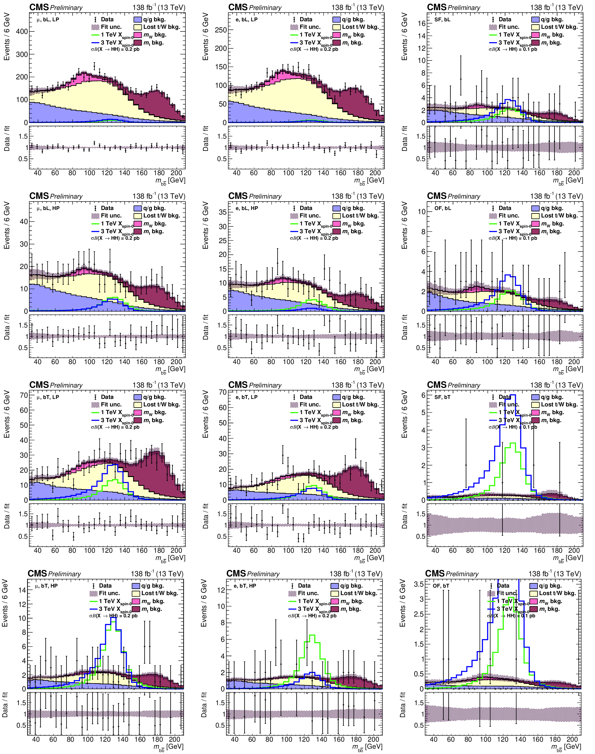
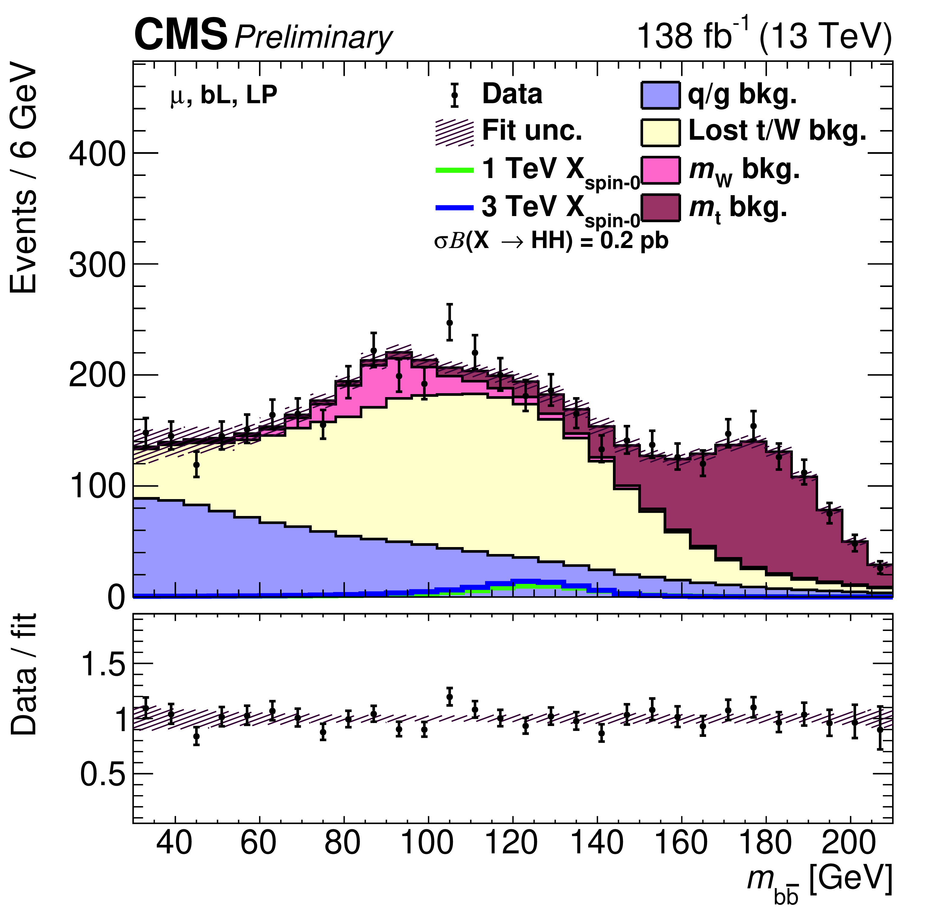
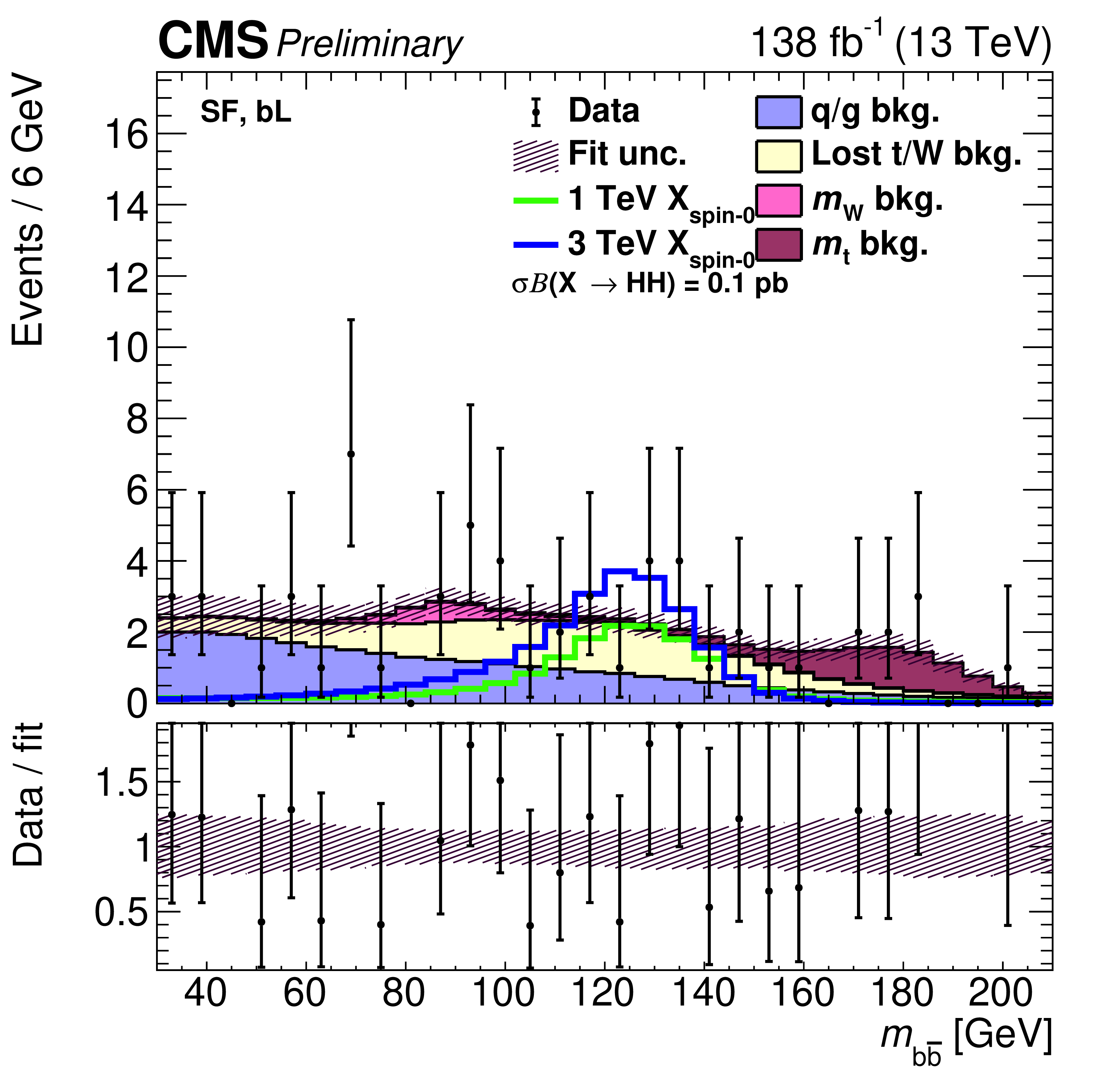
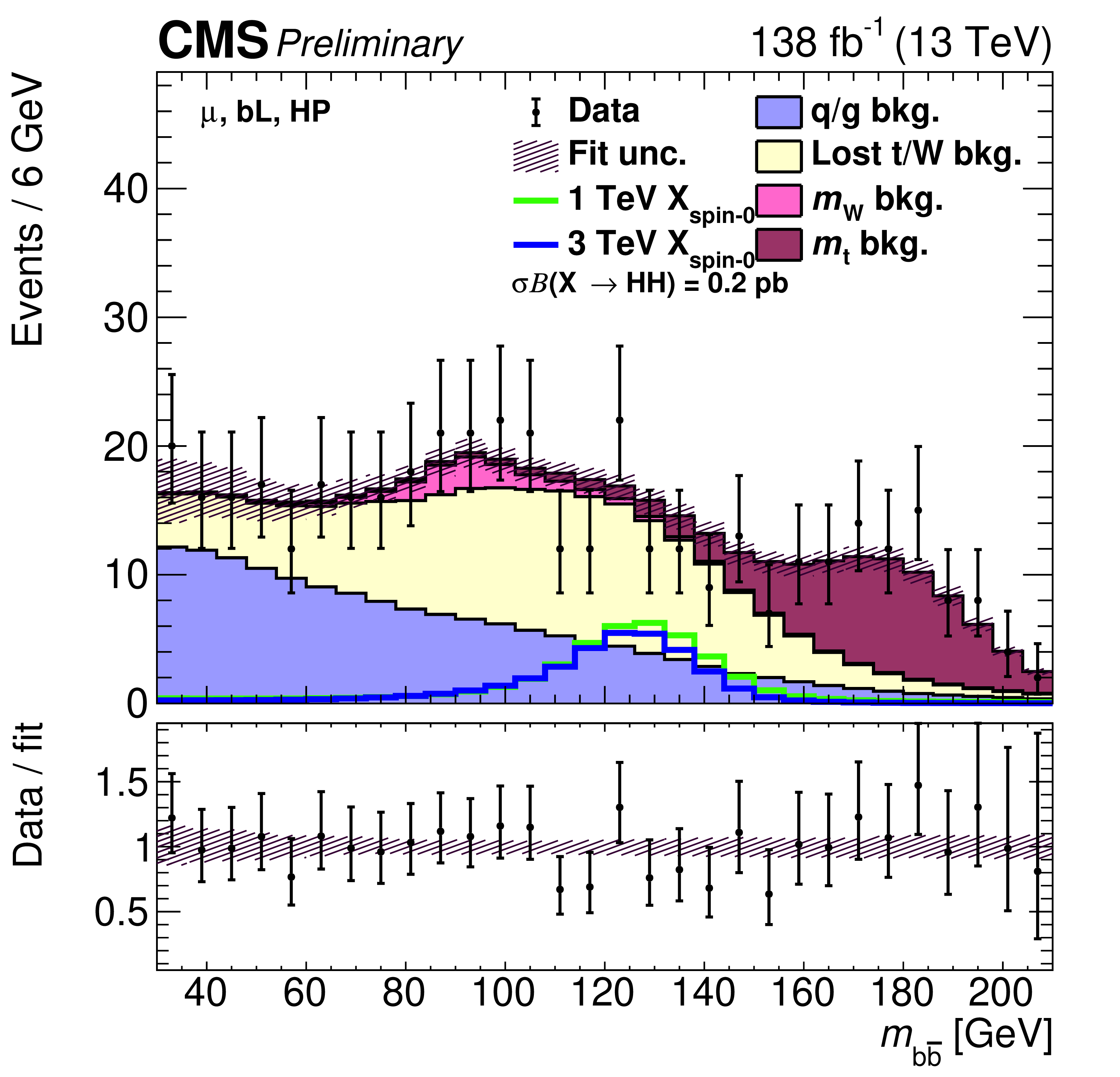
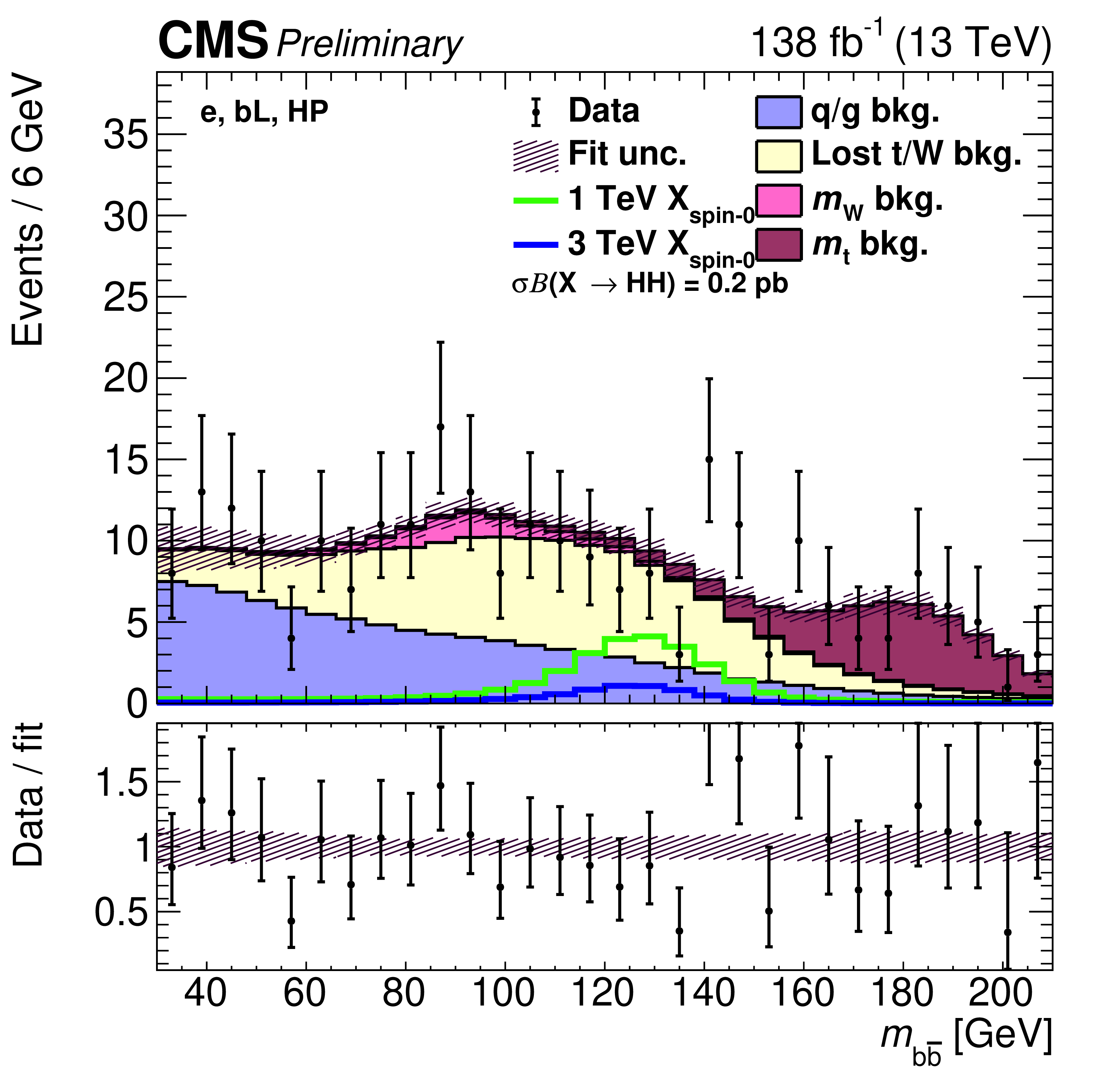
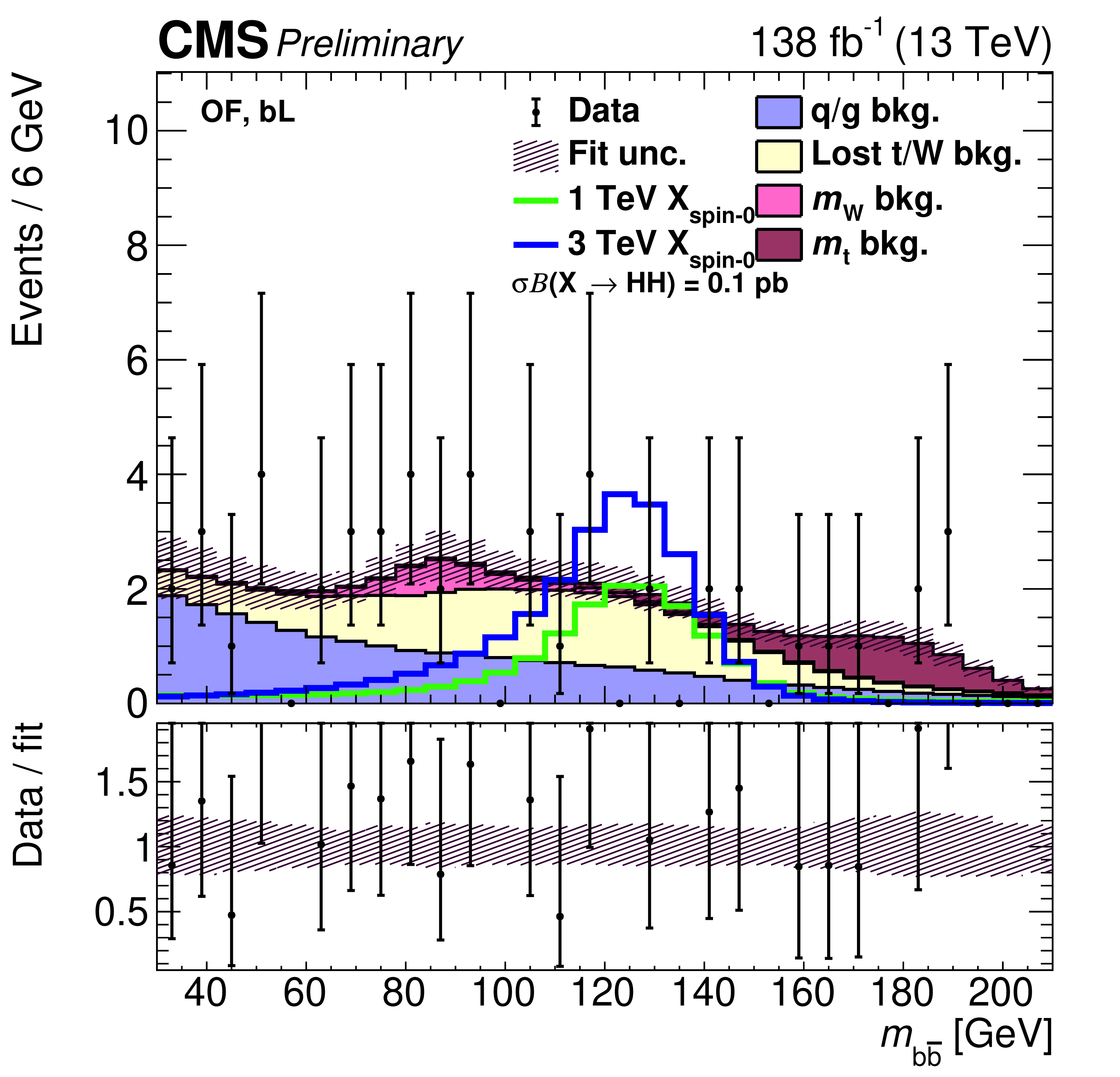
Figure 4:
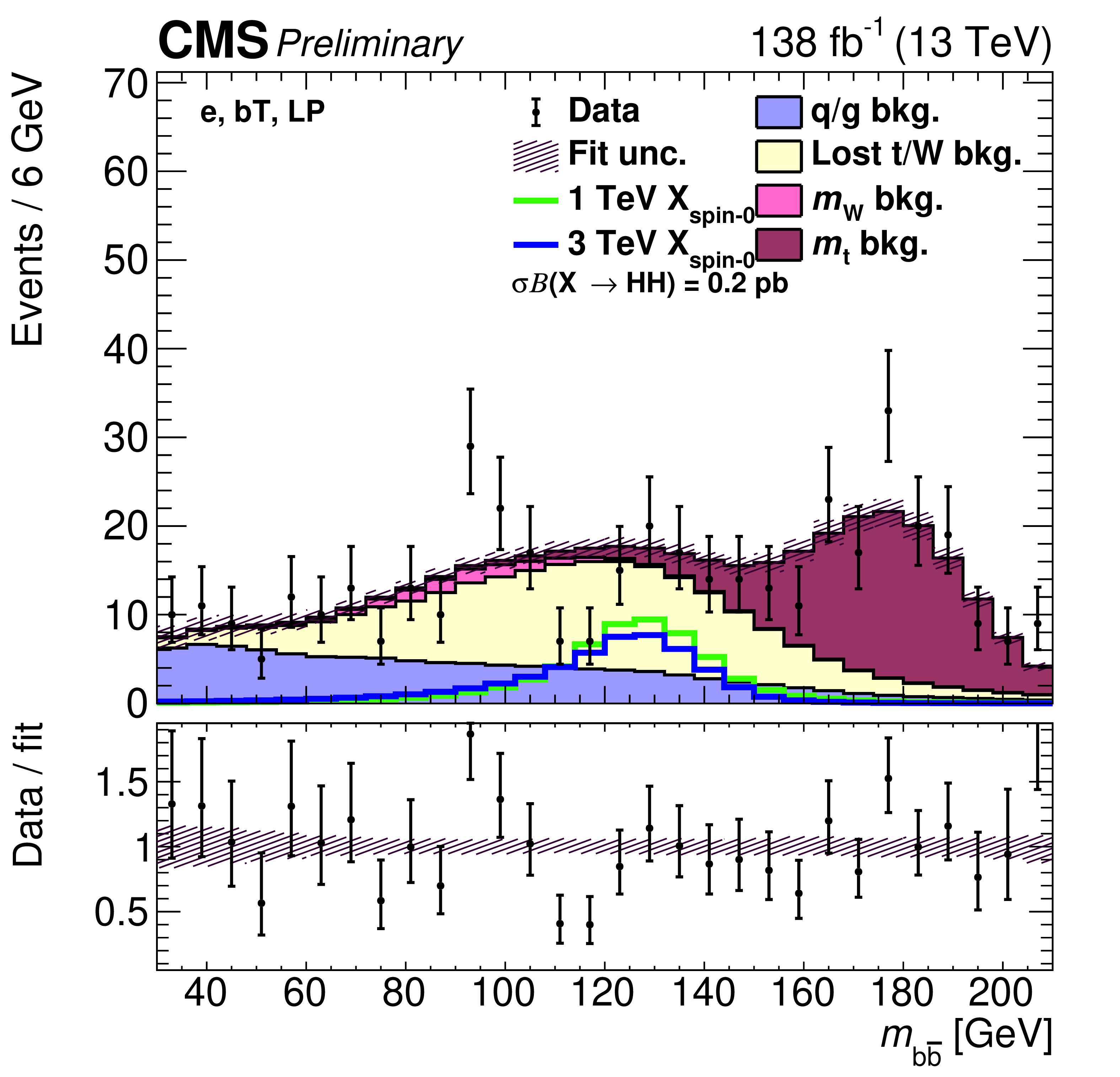
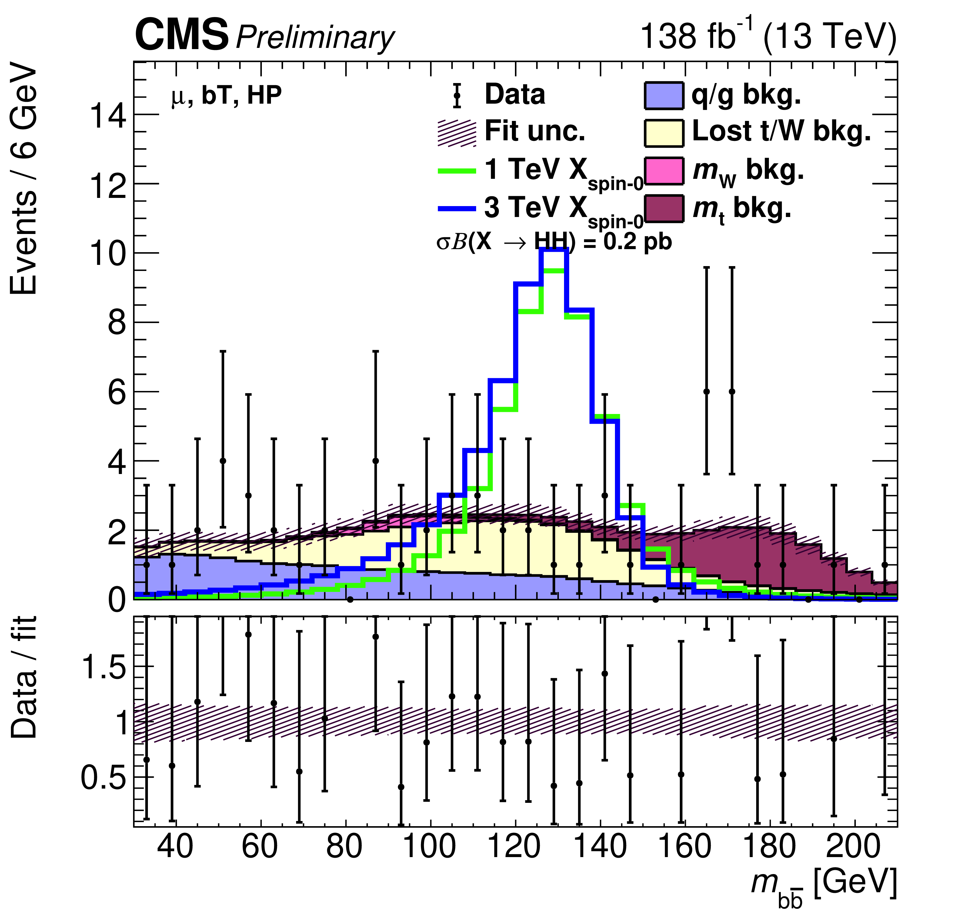
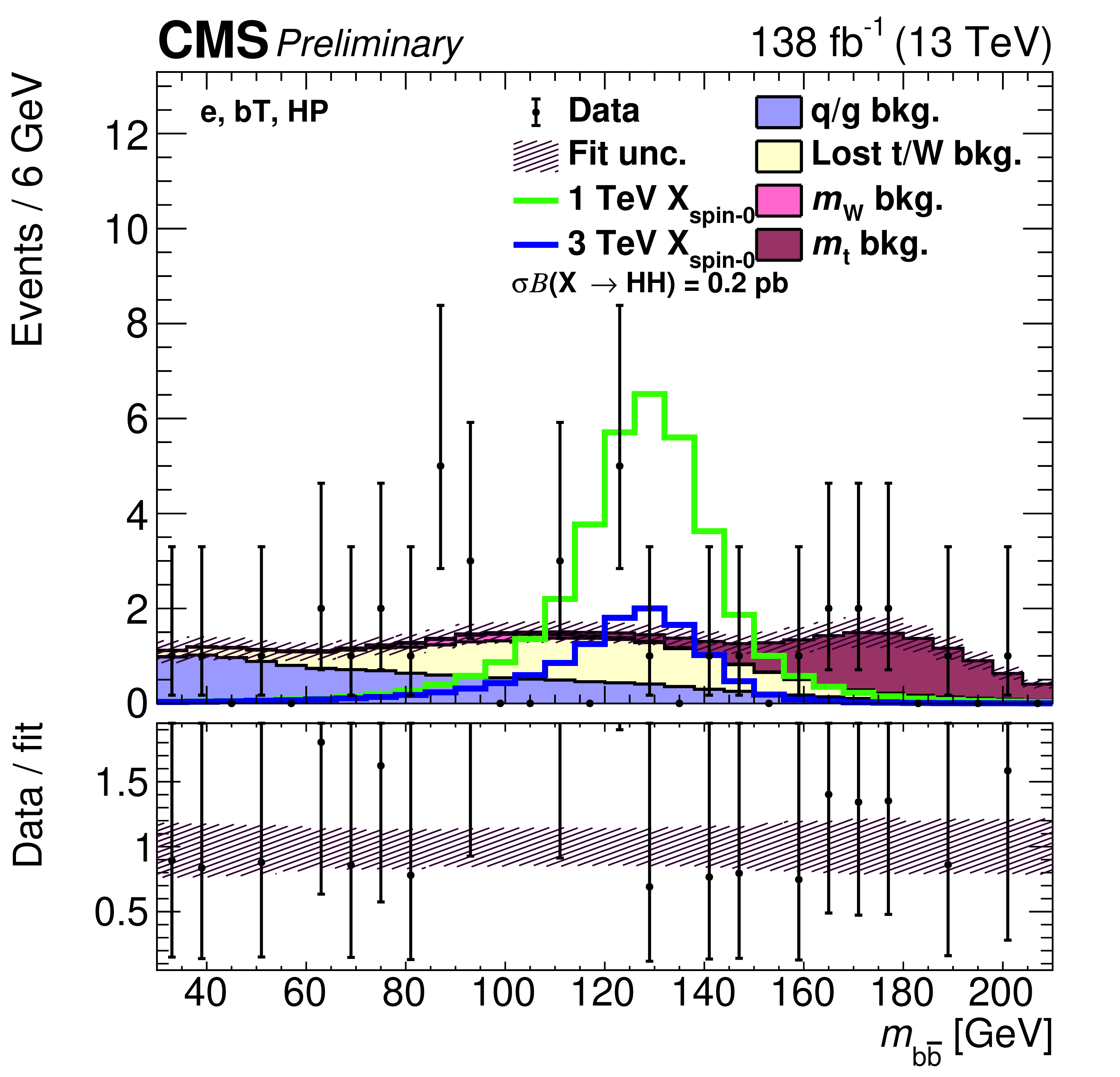
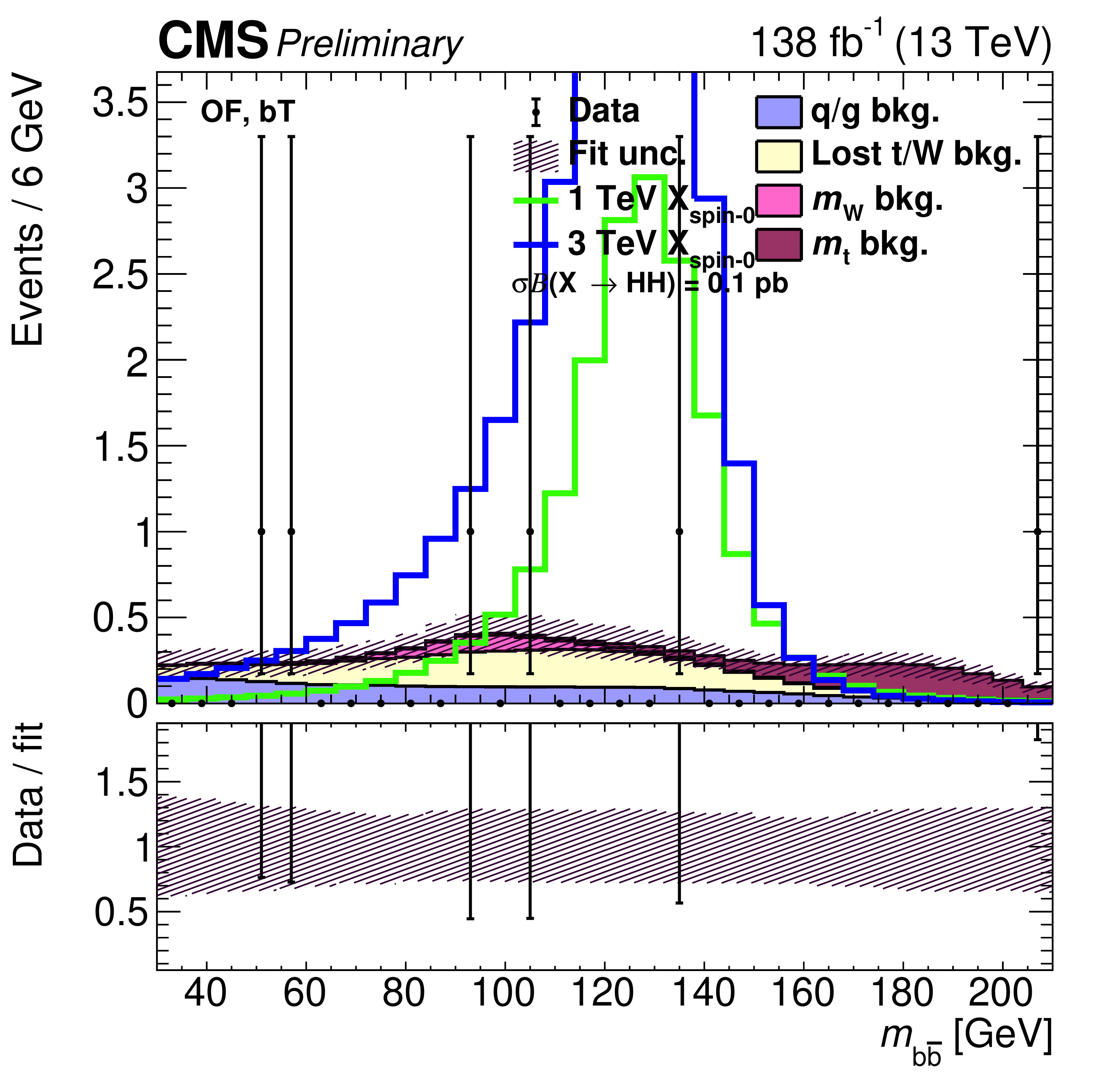
The fit result compared to data projected into ${m_{\mathrm{b} {}\mathrm{\bar{b}}}}$ for both the single- and dilepton channels. The label for each search category is in the upper left of each plot. The fit result is the filled histogram, with the different colors indicating different background categories. The background shape uncertainty from the fit is shown as the hatched band. Example spin-0 signal distributions for $ {m_{\mathrm{X}}} =$ 1.0 and 3.0 TeV are shown as solid lines, with $\sigma \mathcal {B} (\mathrm{X} \to {\mathrm{H} \mathrm{H}})$ set to 0.2 and 0.1 pb for the SL and DL channels, respectively. The bottom panes show the ratio of the data to the fit result. |
png pdf |
Figure 4-a:
The fit result compared to data projected into ${m_{\mathrm{b} {}\mathrm{\bar{b}}}}$ for both the single- and dilepton channels. The label for each search category is in the upper left of each plot. The fit result is the filled histogram, with the different colors indicating different background categories. The background shape uncertainty from the fit is shown as the hatched band. Example spin-0 signal distributions for $ {m_{\mathrm{X}}} =$ 1.0 and 3.0 TeV are shown as solid lines, with $\sigma \mathcal {B} (\mathrm{X} \to {\mathrm{H} \mathrm{H}})$ set to 0.2 and 0.1 pb for the SL and DL channels, respectively. The bottom panes show the ratio of the data to the fit result. |

png pdf |
Figure 4-b:
The fit result compared to data projected into ${m_{\mathrm{b} {}\mathrm{\bar{b}}}}$ for both the single- and dilepton channels. The label for each search category is in the upper left of each plot. The fit result is the filled histogram, with the different colors indicating different background categories. The background shape uncertainty from the fit is shown as the hatched band. Example spin-0 signal distributions for $ {m_{\mathrm{X}}} =$ 1.0 and 3.0 TeV are shown as solid lines, with $\sigma \mathcal {B} (\mathrm{X} \to {\mathrm{H} \mathrm{H}})$ set to 0.2 and 0.1 pb for the SL and DL channels, respectively. The bottom panes show the ratio of the data to the fit result. |
png pdf |
Figure 4-c:
The fit result compared to data projected into ${m_{\mathrm{b} {}\mathrm{\bar{b}}}}$ for both the single- and dilepton channels. The label for each search category is in the upper left of each plot. The fit result is the filled histogram, with the different colors indicating different background categories. The background shape uncertainty from the fit is shown as the hatched band. Example spin-0 signal distributions for $ {m_{\mathrm{X}}} =$ 1.0 and 3.0 TeV are shown as solid lines, with $\sigma \mathcal {B} (\mathrm{X} \to {\mathrm{H} \mathrm{H}})$ set to 0.2 and 0.1 pb for the SL and DL channels, respectively. The bottom panes show the ratio of the data to the fit result. |
png pdf |
Figure 4-d:
The fit result compared to data projected into ${m_{\mathrm{b} {}\mathrm{\bar{b}}}}$ for both the single- and dilepton channels. The label for each search category is in the upper left of each plot. The fit result is the filled histogram, with the different colors indicating different background categories. The background shape uncertainty from the fit is shown as the hatched band. Example spin-0 signal distributions for $ {m_{\mathrm{X}}} =$ 1.0 and 3.0 TeV are shown as solid lines, with $\sigma \mathcal {B} (\mathrm{X} \to {\mathrm{H} \mathrm{H}})$ set to 0.2 and 0.1 pb for the SL and DL channels, respectively. The bottom panes show the ratio of the data to the fit result. |
png pdf |
Figure 4-e:
The fit result compared to data projected into ${m_{\mathrm{b} {}\mathrm{\bar{b}}}}$ for both the single- and dilepton channels. The label for each search category is in the upper left of each plot. The fit result is the filled histogram, with the different colors indicating different background categories. The background shape uncertainty from the fit is shown as the hatched band. Example spin-0 signal distributions for $ {m_{\mathrm{X}}} =$ 1.0 and 3.0 TeV are shown as solid lines, with $\sigma \mathcal {B} (\mathrm{X} \to {\mathrm{H} \mathrm{H}})$ set to 0.2 and 0.1 pb for the SL and DL channels, respectively. The bottom panes show the ratio of the data to the fit result. |
png pdf |
Figure 4-f:
The fit result compared to data projected into ${m_{\mathrm{b} {}\mathrm{\bar{b}}}}$ for both the single- and dilepton channels. The label for each search category is in the upper left of each plot. The fit result is the filled histogram, with the different colors indicating different background categories. The background shape uncertainty from the fit is shown as the hatched band. Example spin-0 signal distributions for $ {m_{\mathrm{X}}} =$ 1.0 and 3.0 TeV are shown as solid lines, with $\sigma \mathcal {B} (\mathrm{X} \to {\mathrm{H} \mathrm{H}})$ set to 0.2 and 0.1 pb for the SL and DL channels, respectively. The bottom panes show the ratio of the data to the fit result. |

png pdf |
Figure 4-g:
The fit result compared to data projected into ${m_{\mathrm{b} {}\mathrm{\bar{b}}}}$ for both the single- and dilepton channels. The label for each search category is in the upper left of each plot. The fit result is the filled histogram, with the different colors indicating different background categories. The background shape uncertainty from the fit is shown as the hatched band. Example spin-0 signal distributions for $ {m_{\mathrm{X}}} =$ 1.0 and 3.0 TeV are shown as solid lines, with $\sigma \mathcal {B} (\mathrm{X} \to {\mathrm{H} \mathrm{H}})$ set to 0.2 and 0.1 pb for the SL and DL channels, respectively. The bottom panes show the ratio of the data to the fit result. |
png pdf |
Figure 4-h:
The fit result compared to data projected into ${m_{\mathrm{b} {}\mathrm{\bar{b}}}}$ for both the single- and dilepton channels. The label for each search category is in the upper left of each plot. The fit result is the filled histogram, with the different colors indicating different background categories. The background shape uncertainty from the fit is shown as the hatched band. Example spin-0 signal distributions for $ {m_{\mathrm{X}}} =$ 1.0 and 3.0 TeV are shown as solid lines, with $\sigma \mathcal {B} (\mathrm{X} \to {\mathrm{H} \mathrm{H}})$ set to 0.2 and 0.1 pb for the SL and DL channels, respectively. The bottom panes show the ratio of the data to the fit result. |

png pdf |
Figure 4-i:
The fit result compared to data projected into ${m_{\mathrm{b} {}\mathrm{\bar{b}}}}$ for both the single- and dilepton channels. The label for each search category is in the upper left of each plot. The fit result is the filled histogram, with the different colors indicating different background categories. The background shape uncertainty from the fit is shown as the hatched band. Example spin-0 signal distributions for $ {m_{\mathrm{X}}} =$ 1.0 and 3.0 TeV are shown as solid lines, with $\sigma \mathcal {B} (\mathrm{X} \to {\mathrm{H} \mathrm{H}})$ set to 0.2 and 0.1 pb for the SL and DL channels, respectively. The bottom panes show the ratio of the data to the fit result. |
png pdf |
Figure 4-j:
The fit result compared to data projected into ${m_{\mathrm{b} {}\mathrm{\bar{b}}}}$ for both the single- and dilepton channels. The label for each search category is in the upper left of each plot. The fit result is the filled histogram, with the different colors indicating different background categories. The background shape uncertainty from the fit is shown as the hatched band. Example spin-0 signal distributions for $ {m_{\mathrm{X}}} =$ 1.0 and 3.0 TeV are shown as solid lines, with $\sigma \mathcal {B} (\mathrm{X} \to {\mathrm{H} \mathrm{H}})$ set to 0.2 and 0.1 pb for the SL and DL channels, respectively. The bottom panes show the ratio of the data to the fit result. |
png pdf |
Figure 4-k:
The fit result compared to data projected into ${m_{\mathrm{b} {}\mathrm{\bar{b}}}}$ for both the single- and dilepton channels. The label for each search category is in the upper left of each plot. The fit result is the filled histogram, with the different colors indicating different background categories. The background shape uncertainty from the fit is shown as the hatched band. Example spin-0 signal distributions for $ {m_{\mathrm{X}}} =$ 1.0 and 3.0 TeV are shown as solid lines, with $\sigma \mathcal {B} (\mathrm{X} \to {\mathrm{H} \mathrm{H}})$ set to 0.2 and 0.1 pb for the SL and DL channels, respectively. The bottom panes show the ratio of the data to the fit result. |
png pdf |
Figure 4-l:
The fit result compared to data projected into ${m_{\mathrm{b} {}\mathrm{\bar{b}}}}$ for both the single- and dilepton channels. The label for each search category is in the upper left of each plot. The fit result is the filled histogram, with the different colors indicating different background categories. The background shape uncertainty from the fit is shown as the hatched band. Example spin-0 signal distributions for $ {m_{\mathrm{X}}} =$ 1.0 and 3.0 TeV are shown as solid lines, with $\sigma \mathcal {B} (\mathrm{X} \to {\mathrm{H} \mathrm{H}})$ set to 0.2 and 0.1 pb for the SL and DL channels, respectively. The bottom panes show the ratio of the data to the fit result. |
png pdf |
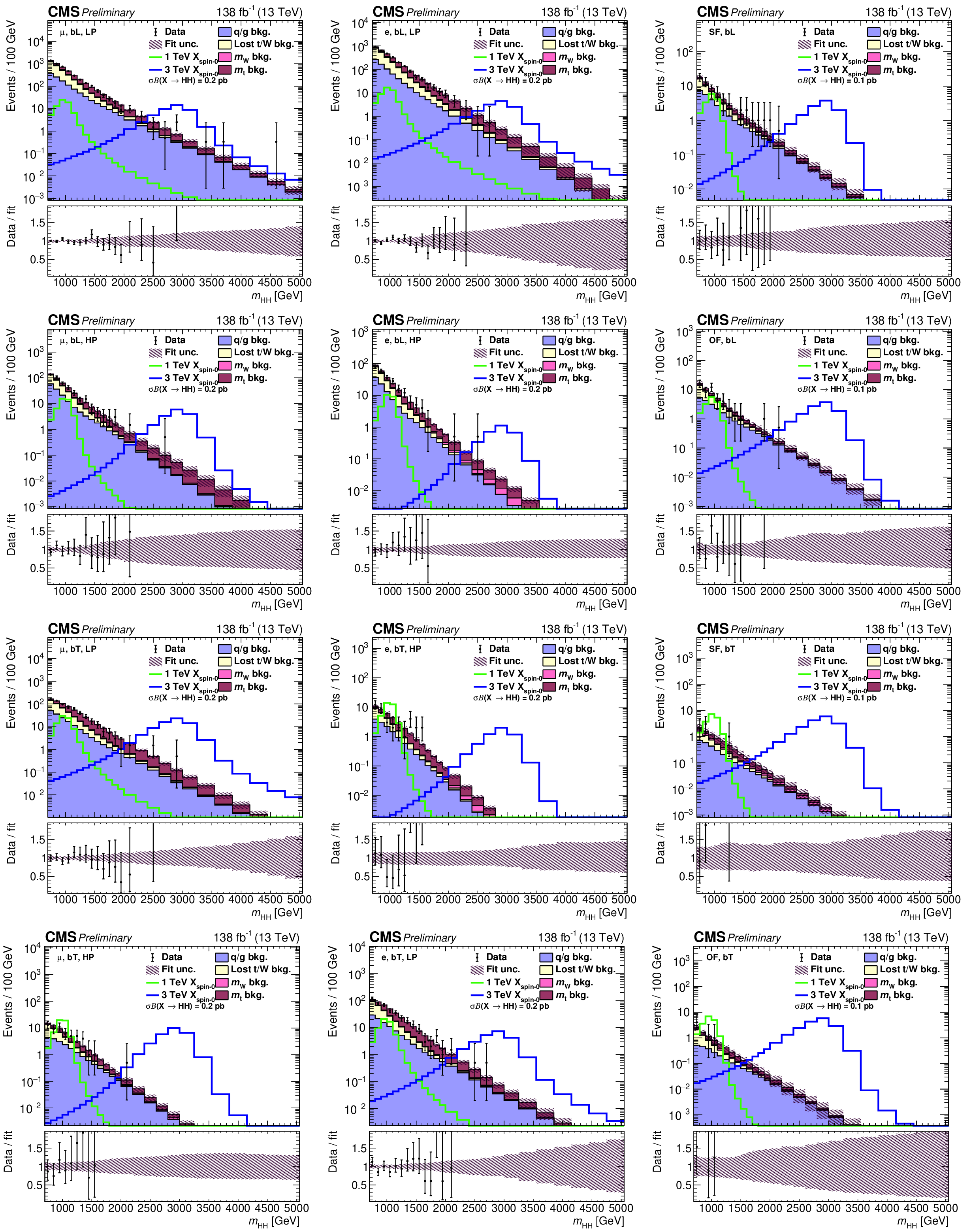
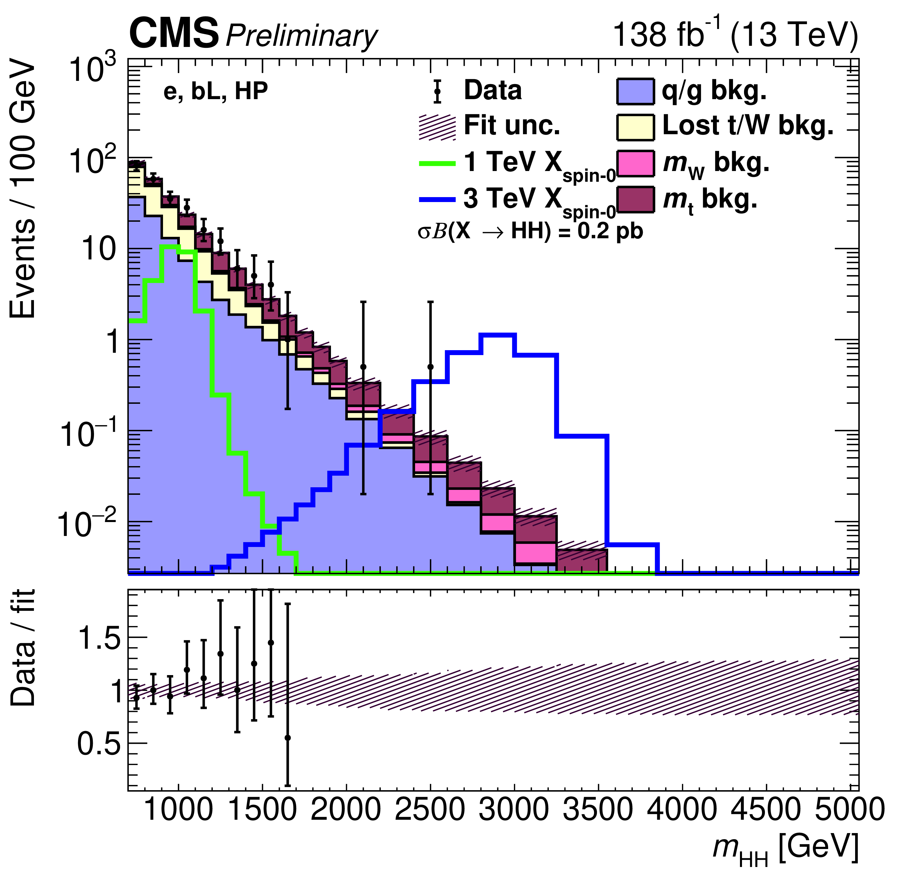
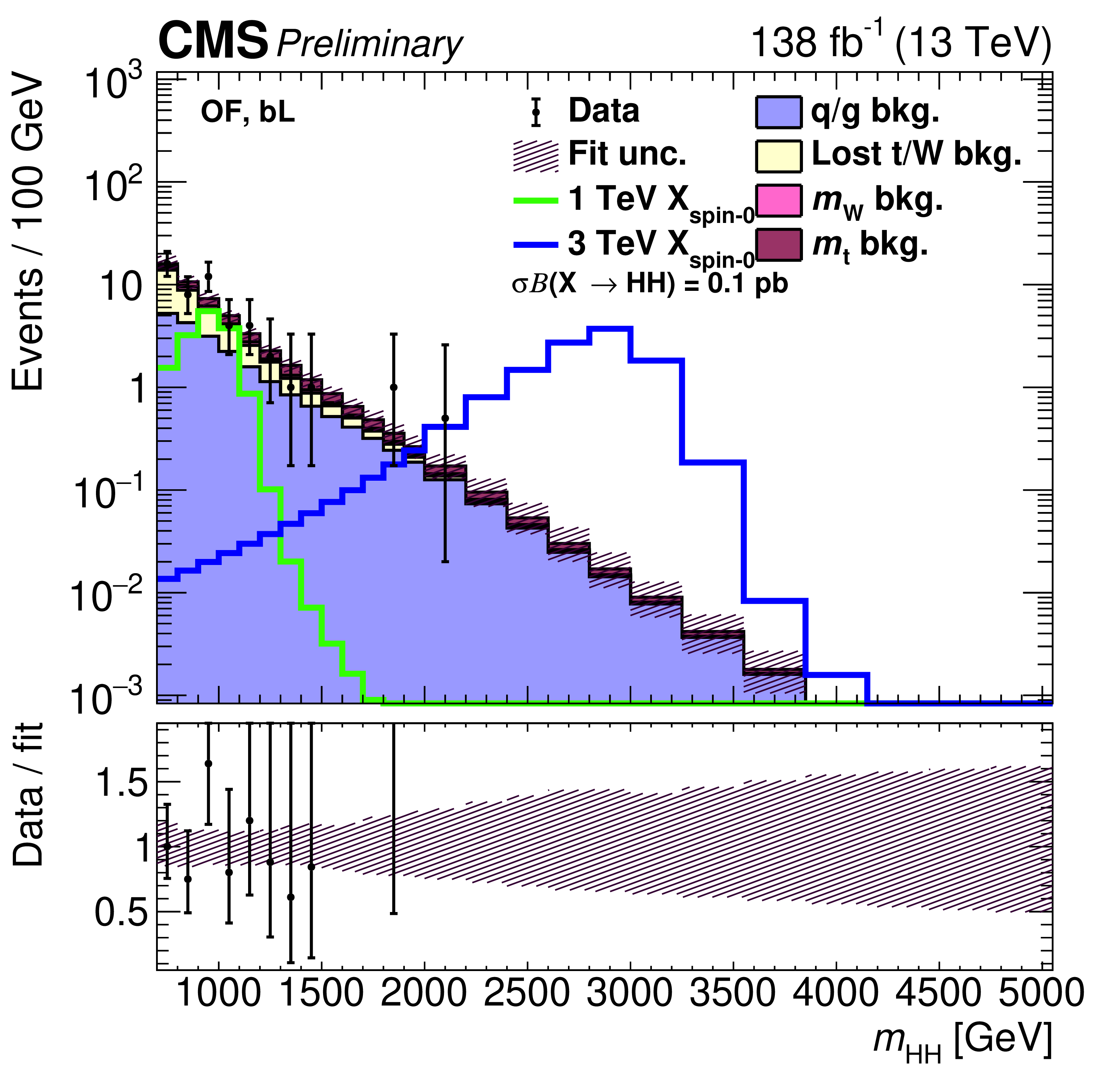
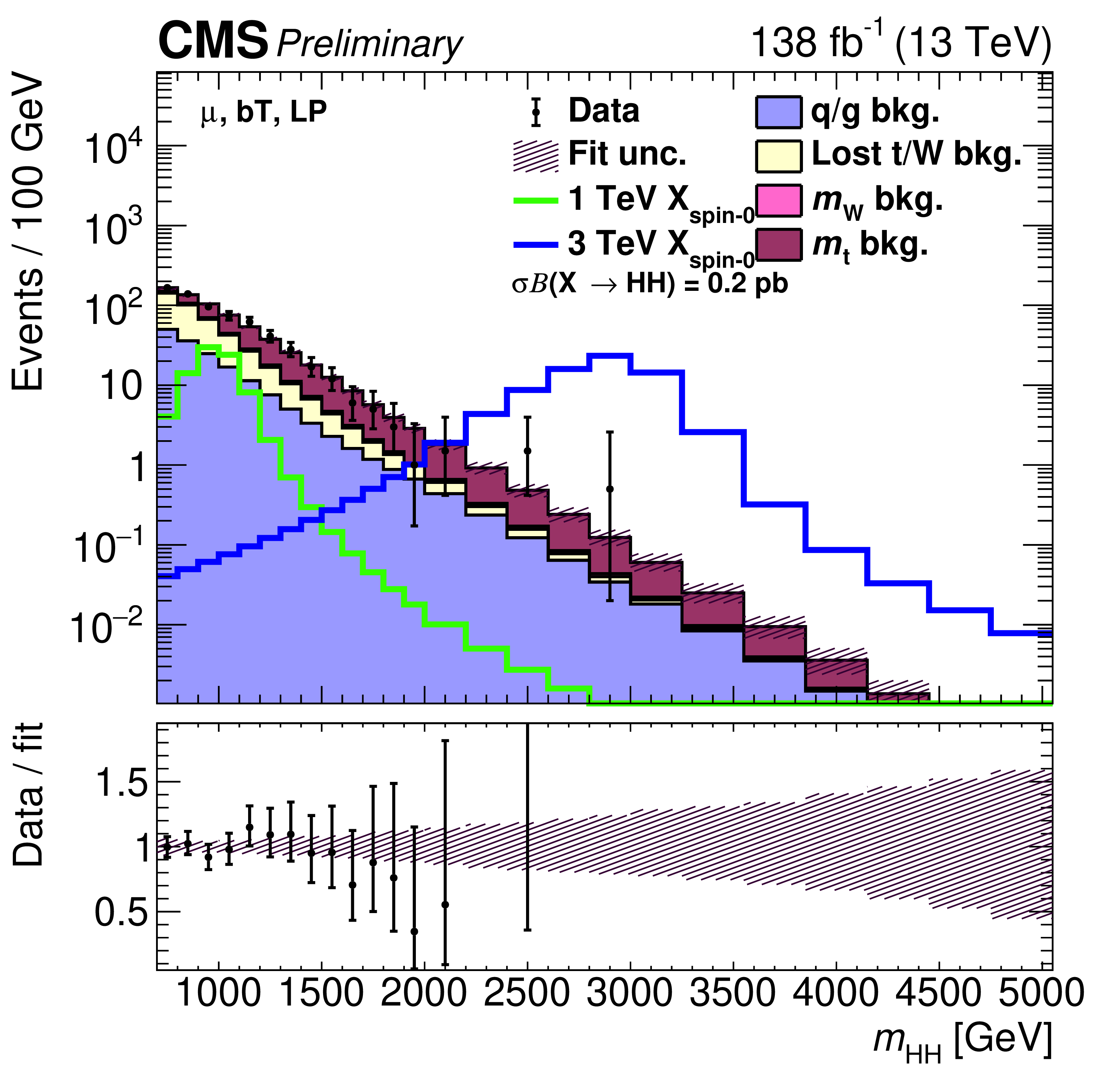
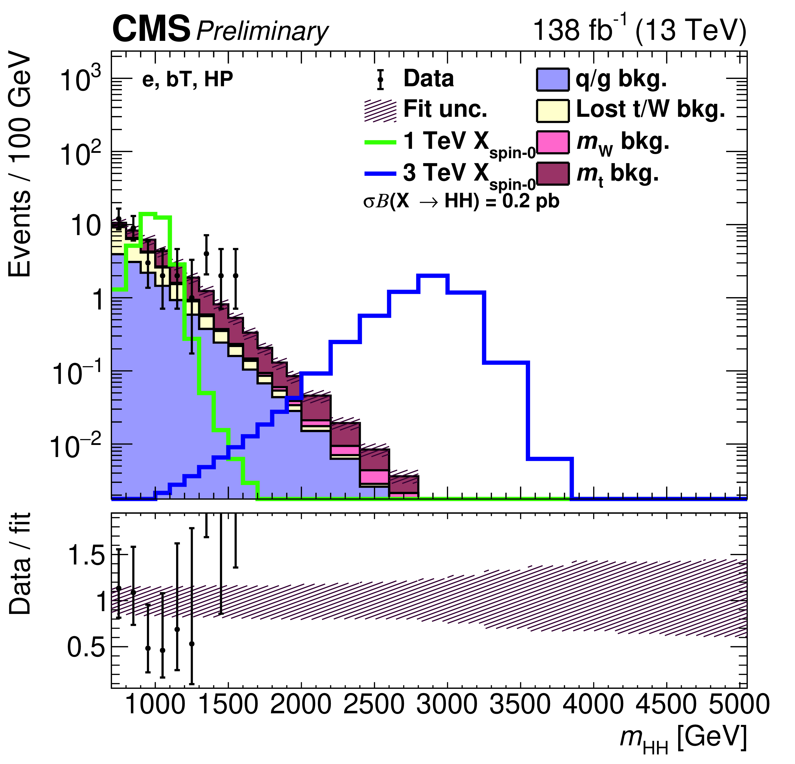
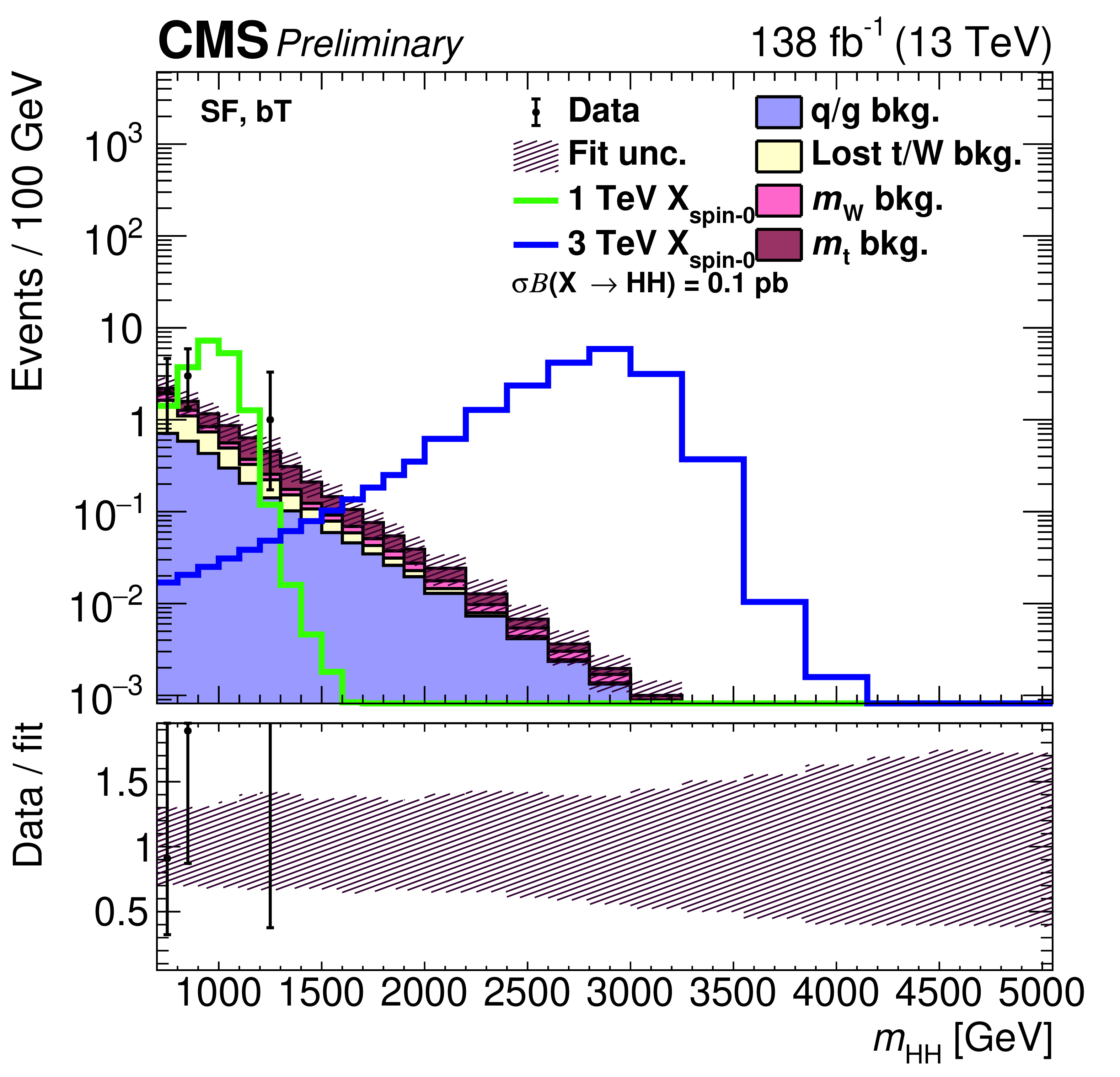
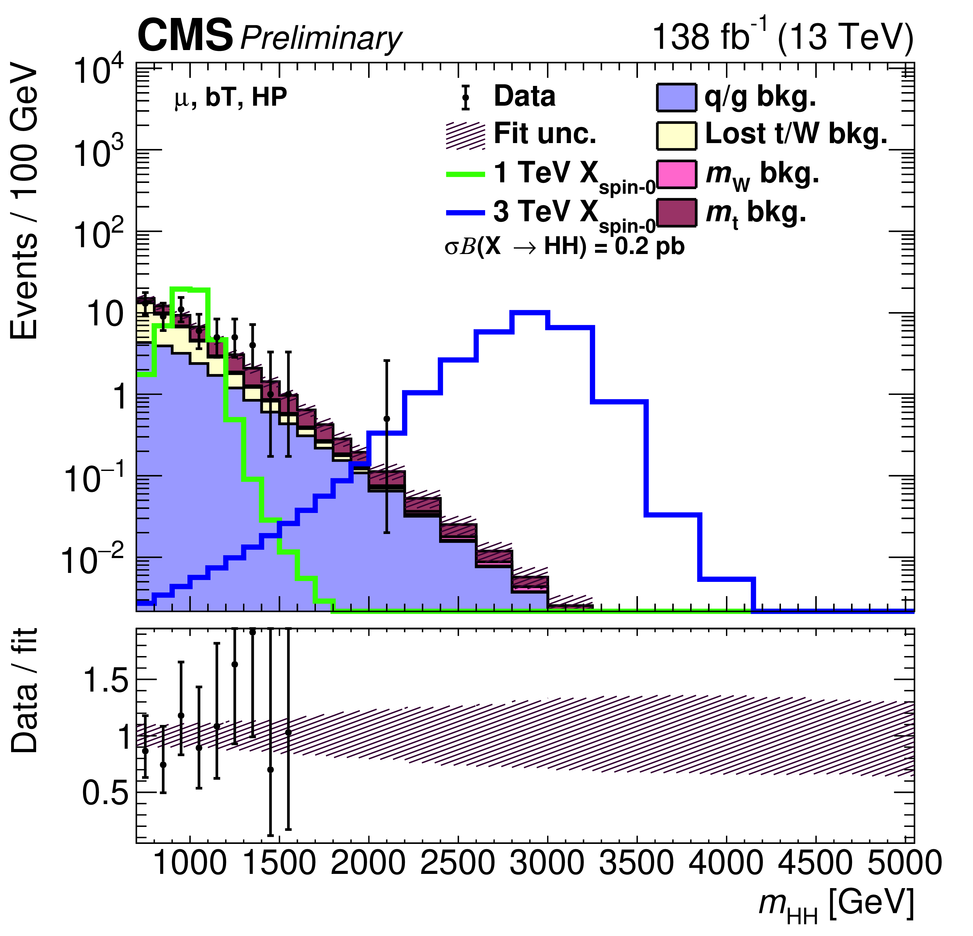
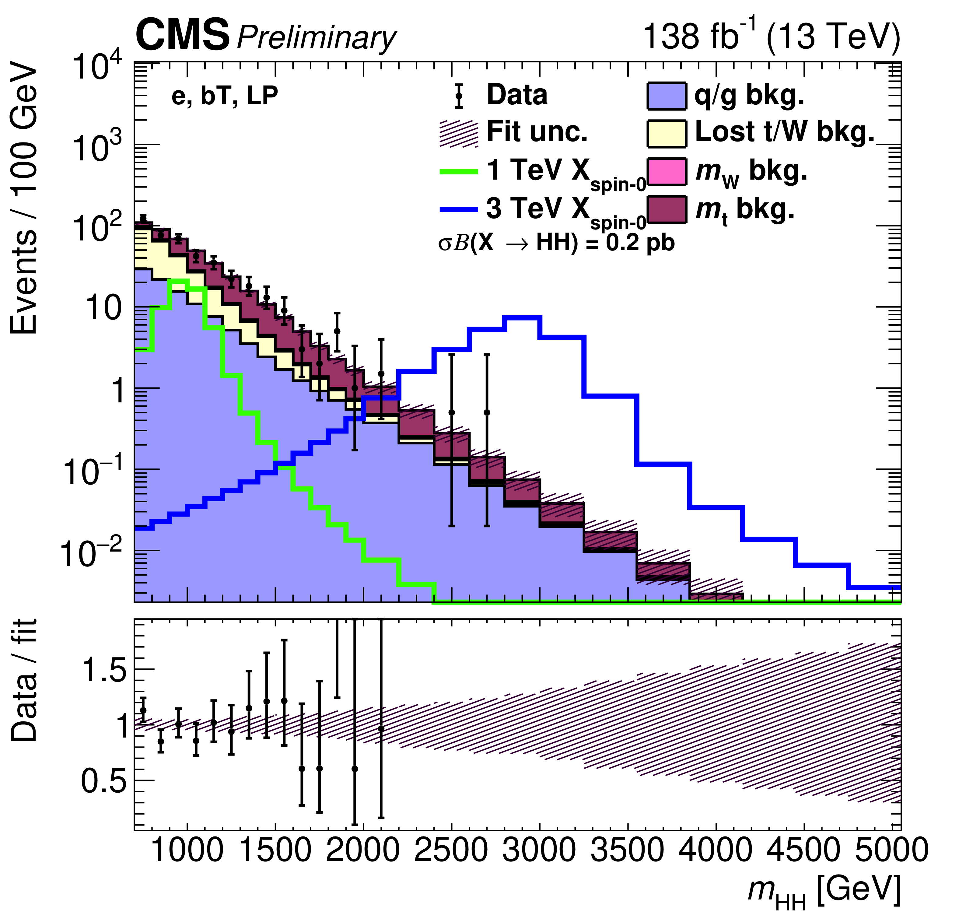
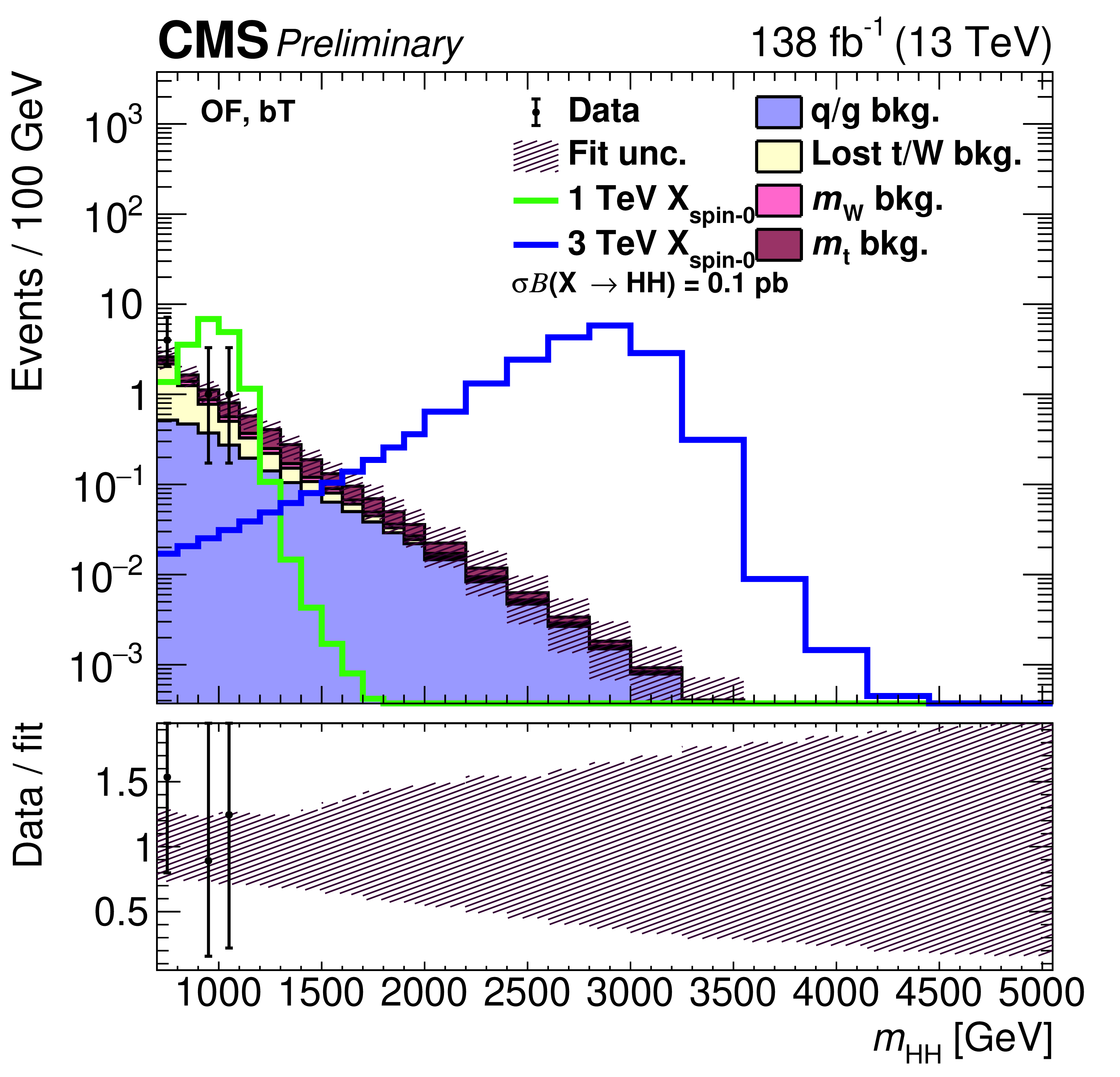
Figure 5:
The fit result compared to data projected into ${m_{\mathrm{H} \mathrm{H}}}$ for both the single- and dilepton channels. The label for each search category is in the upper left of each plot. The fit result is the filled histogram, with the different colors indicating different background categories. The background shape uncertainty from the fit is shown as the hatched band. Example spin-0 signal distributions for $ {m_{\mathrm{X}}} =$ 1.0 and 3.0 TeV are shown as solid lines, with $\sigma \mathcal {B} (\mathrm{X} \to {\mathrm{H} \mathrm{H}})$ set to 0.2 and 0.1 pb for the SL and DL channels, respectively. The bottom panes of each plot show the ratio of the data to the fit result. |
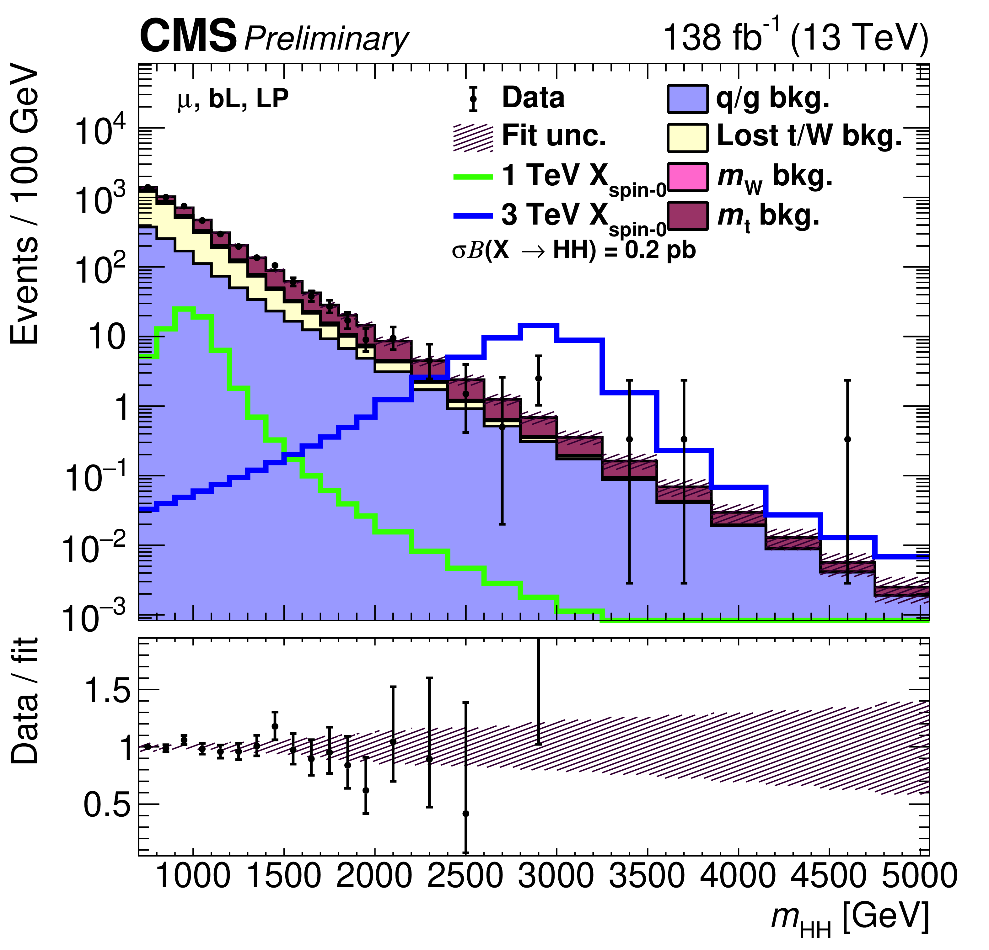
png pdf |
Figure 5-a:
The fit result compared to data projected into ${m_{\mathrm{H} \mathrm{H}}}$ for both the single- and dilepton channels. The label for each search category is in the upper left of each plot. The fit result is the filled histogram, with the different colors indicating different background categories. The background shape uncertainty from the fit is shown as the hatched band. Example spin-0 signal distributions for $ {m_{\mathrm{X}}} =$ 1.0 and 3.0 TeV are shown as solid lines, with $\sigma \mathcal {B} (\mathrm{X} \to {\mathrm{H} \mathrm{H}})$ set to 0.2 and 0.1 pb for the SL and DL channels, respectively. The bottom panes of each plot show the ratio of the data to the fit result. |
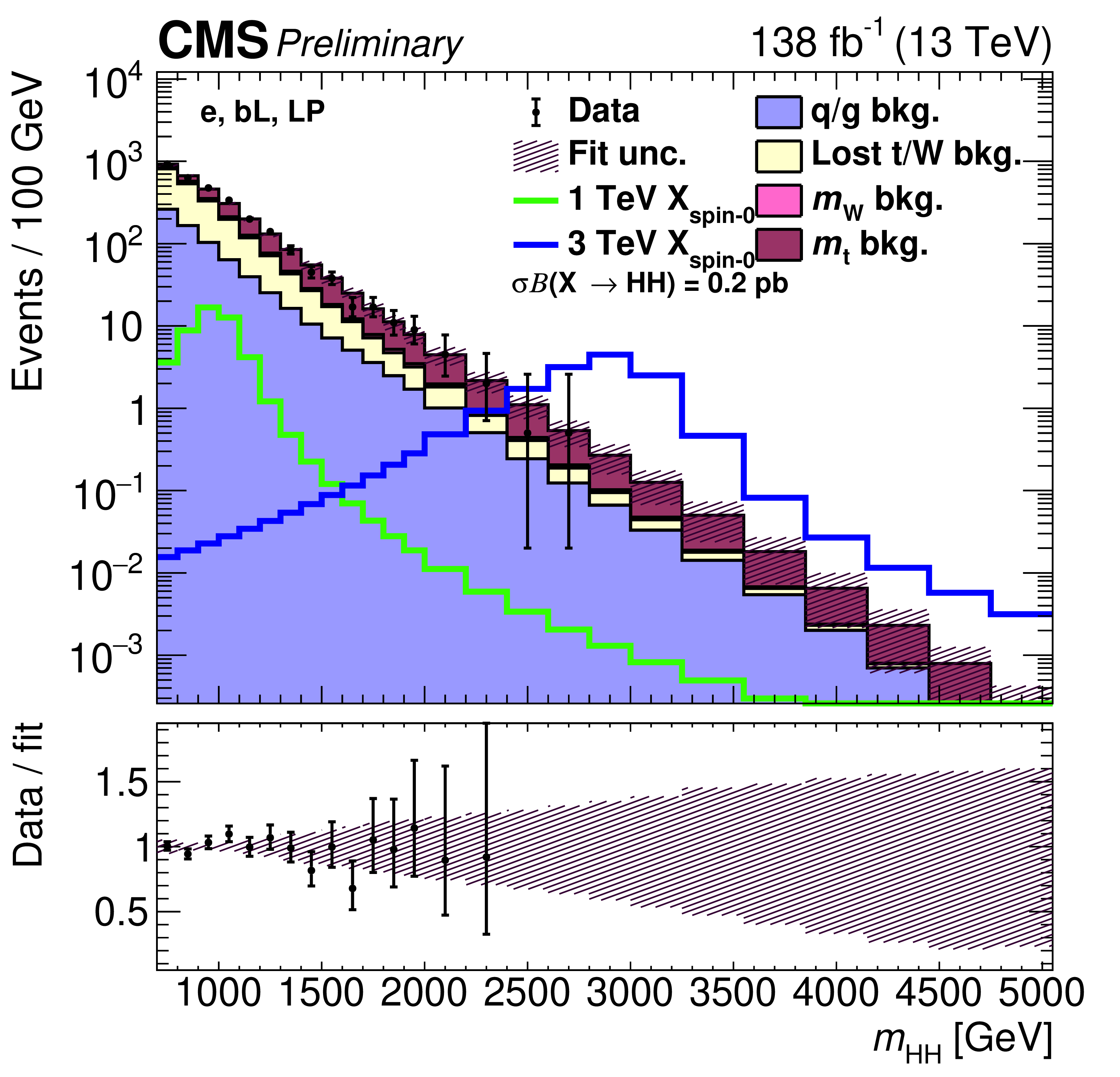
png pdf |
Figure 5-b:
The fit result compared to data projected into ${m_{\mathrm{H} \mathrm{H}}}$ for both the single- and dilepton channels. The label for each search category is in the upper left of each plot. The fit result is the filled histogram, with the different colors indicating different background categories. The background shape uncertainty from the fit is shown as the hatched band. Example spin-0 signal distributions for $ {m_{\mathrm{X}}} =$ 1.0 and 3.0 TeV are shown as solid lines, with $\sigma \mathcal {B} (\mathrm{X} \to {\mathrm{H} \mathrm{H}})$ set to 0.2 and 0.1 pb for the SL and DL channels, respectively. The bottom panes of each plot show the ratio of the data to the fit result. |

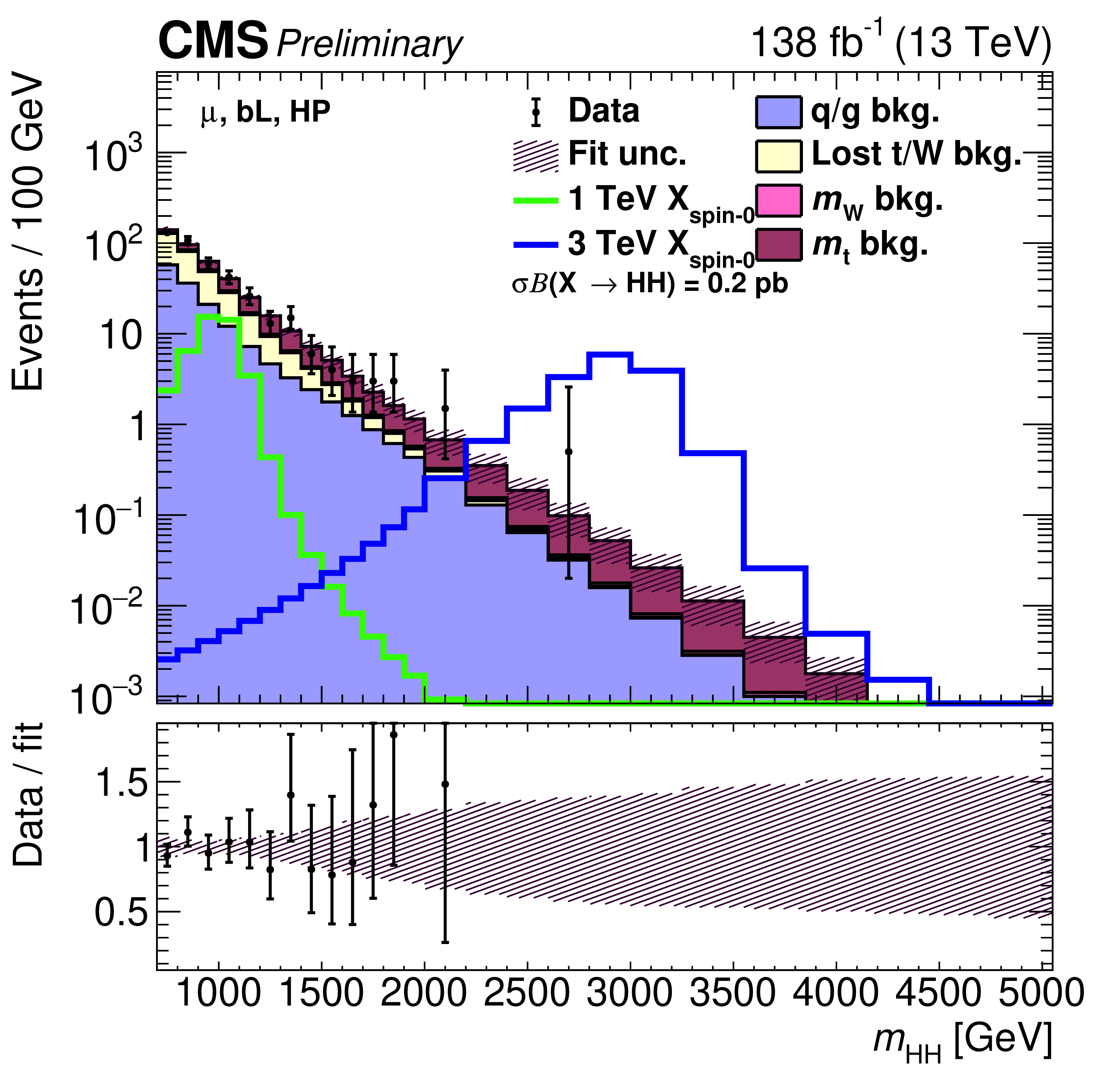
png pdf |
Figure 5-c:
The fit result compared to data projected into ${m_{\mathrm{H} \mathrm{H}}}$ for both the single- and dilepton channels. The label for each search category is in the upper left of each plot. The fit result is the filled histogram, with the different colors indicating different background categories. The background shape uncertainty from the fit is shown as the hatched band. Example spin-0 signal distributions for $ {m_{\mathrm{X}}} =$ 1.0 and 3.0 TeV are shown as solid lines, with $\sigma \mathcal {B} (\mathrm{X} \to {\mathrm{H} \mathrm{H}})$ set to 0.2 and 0.1 pb for the SL and DL channels, respectively. The bottom panes of each plot show the ratio of the data to the fit result. |
png pdf |
Figure 5-d:
The fit result compared to data projected into ${m_{\mathrm{H} \mathrm{H}}}$ for both the single- and dilepton channels. The label for each search category is in the upper left of each plot. The fit result is the filled histogram, with the different colors indicating different background categories. The background shape uncertainty from the fit is shown as the hatched band. Example spin-0 signal distributions for $ {m_{\mathrm{X}}} =$ 1.0 and 3.0 TeV are shown as solid lines, with $\sigma \mathcal {B} (\mathrm{X} \to {\mathrm{H} \mathrm{H}})$ set to 0.2 and 0.1 pb for the SL and DL channels, respectively. The bottom panes of each plot show the ratio of the data to the fit result. |
png pdf |
Figure 5-e:
The fit result compared to data projected into ${m_{\mathrm{H} \mathrm{H}}}$ for both the single- and dilepton channels. The label for each search category is in the upper left of each plot. The fit result is the filled histogram, with the different colors indicating different background categories. The background shape uncertainty from the fit is shown as the hatched band. Example spin-0 signal distributions for $ {m_{\mathrm{X}}} =$ 1.0 and 3.0 TeV are shown as solid lines, with $\sigma \mathcal {B} (\mathrm{X} \to {\mathrm{H} \mathrm{H}})$ set to 0.2 and 0.1 pb for the SL and DL channels, respectively. The bottom panes of each plot show the ratio of the data to the fit result. |
png pdf |
Figure 5-f:
The fit result compared to data projected into ${m_{\mathrm{H} \mathrm{H}}}$ for both the single- and dilepton channels. The label for each search category is in the upper left of each plot. The fit result is the filled histogram, with the different colors indicating different background categories. The background shape uncertainty from the fit is shown as the hatched band. Example spin-0 signal distributions for $ {m_{\mathrm{X}}} =$ 1.0 and 3.0 TeV are shown as solid lines, with $\sigma \mathcal {B} (\mathrm{X} \to {\mathrm{H} \mathrm{H}})$ set to 0.2 and 0.1 pb for the SL and DL channels, respectively. The bottom panes of each plot show the ratio of the data to the fit result. |
png pdf |
Figure 5-g:
The fit result compared to data projected into ${m_{\mathrm{H} \mathrm{H}}}$ for both the single- and dilepton channels. The label for each search category is in the upper left of each plot. The fit result is the filled histogram, with the different colors indicating different background categories. The background shape uncertainty from the fit is shown as the hatched band. Example spin-0 signal distributions for $ {m_{\mathrm{X}}} =$ 1.0 and 3.0 TeV are shown as solid lines, with $\sigma \mathcal {B} (\mathrm{X} \to {\mathrm{H} \mathrm{H}})$ set to 0.2 and 0.1 pb for the SL and DL channels, respectively. The bottom panes of each plot show the ratio of the data to the fit result. |
png pdf |
Figure 5-h:
The fit result compared to data projected into ${m_{\mathrm{H} \mathrm{H}}}$ for both the single- and dilepton channels. The label for each search category is in the upper left of each plot. The fit result is the filled histogram, with the different colors indicating different background categories. The background shape uncertainty from the fit is shown as the hatched band. Example spin-0 signal distributions for $ {m_{\mathrm{X}}} =$ 1.0 and 3.0 TeV are shown as solid lines, with $\sigma \mathcal {B} (\mathrm{X} \to {\mathrm{H} \mathrm{H}})$ set to 0.2 and 0.1 pb for the SL and DL channels, respectively. The bottom panes of each plot show the ratio of the data to the fit result. |
png pdf |
Figure 5-i:
The fit result compared to data projected into ${m_{\mathrm{H} \mathrm{H}}}$ for both the single- and dilepton channels. The label for each search category is in the upper left of each plot. The fit result is the filled histogram, with the different colors indicating different background categories. The background shape uncertainty from the fit is shown as the hatched band. Example spin-0 signal distributions for $ {m_{\mathrm{X}}} =$ 1.0 and 3.0 TeV are shown as solid lines, with $\sigma \mathcal {B} (\mathrm{X} \to {\mathrm{H} \mathrm{H}})$ set to 0.2 and 0.1 pb for the SL and DL channels, respectively. The bottom panes of each plot show the ratio of the data to the fit result. |
png pdf |
Figure 5-j:
The fit result compared to data projected into ${m_{\mathrm{H} \mathrm{H}}}$ for both the single- and dilepton channels. The label for each search category is in the upper left of each plot. The fit result is the filled histogram, with the different colors indicating different background categories. The background shape uncertainty from the fit is shown as the hatched band. Example spin-0 signal distributions for $ {m_{\mathrm{X}}} =$ 1.0 and 3.0 TeV are shown as solid lines, with $\sigma \mathcal {B} (\mathrm{X} \to {\mathrm{H} \mathrm{H}})$ set to 0.2 and 0.1 pb for the SL and DL channels, respectively. The bottom panes of each plot show the ratio of the data to the fit result. |
png pdf |
Figure 5-k:
The fit result compared to data projected into ${m_{\mathrm{H} \mathrm{H}}}$ for both the single- and dilepton channels. The label for each search category is in the upper left of each plot. The fit result is the filled histogram, with the different colors indicating different background categories. The background shape uncertainty from the fit is shown as the hatched band. Example spin-0 signal distributions for $ {m_{\mathrm{X}}} =$ 1.0 and 3.0 TeV are shown as solid lines, with $\sigma \mathcal {B} (\mathrm{X} \to {\mathrm{H} \mathrm{H}})$ set to 0.2 and 0.1 pb for the SL and DL channels, respectively. The bottom panes of each plot show the ratio of the data to the fit result. |
png pdf |
Figure 5-l:
The fit result compared to data projected into ${m_{\mathrm{H} \mathrm{H}}}$ for both the single- and dilepton channels. The label for each search category is in the upper left of each plot. The fit result is the filled histogram, with the different colors indicating different background categories. The background shape uncertainty from the fit is shown as the hatched band. Example spin-0 signal distributions for $ {m_{\mathrm{X}}} =$ 1.0 and 3.0 TeV are shown as solid lines, with $\sigma \mathcal {B} (\mathrm{X} \to {\mathrm{H} \mathrm{H}})$ set to 0.2 and 0.1 pb for the SL and DL channels, respectively. The bottom panes of each plot show the ratio of the data to the fit result. |
png pdf |
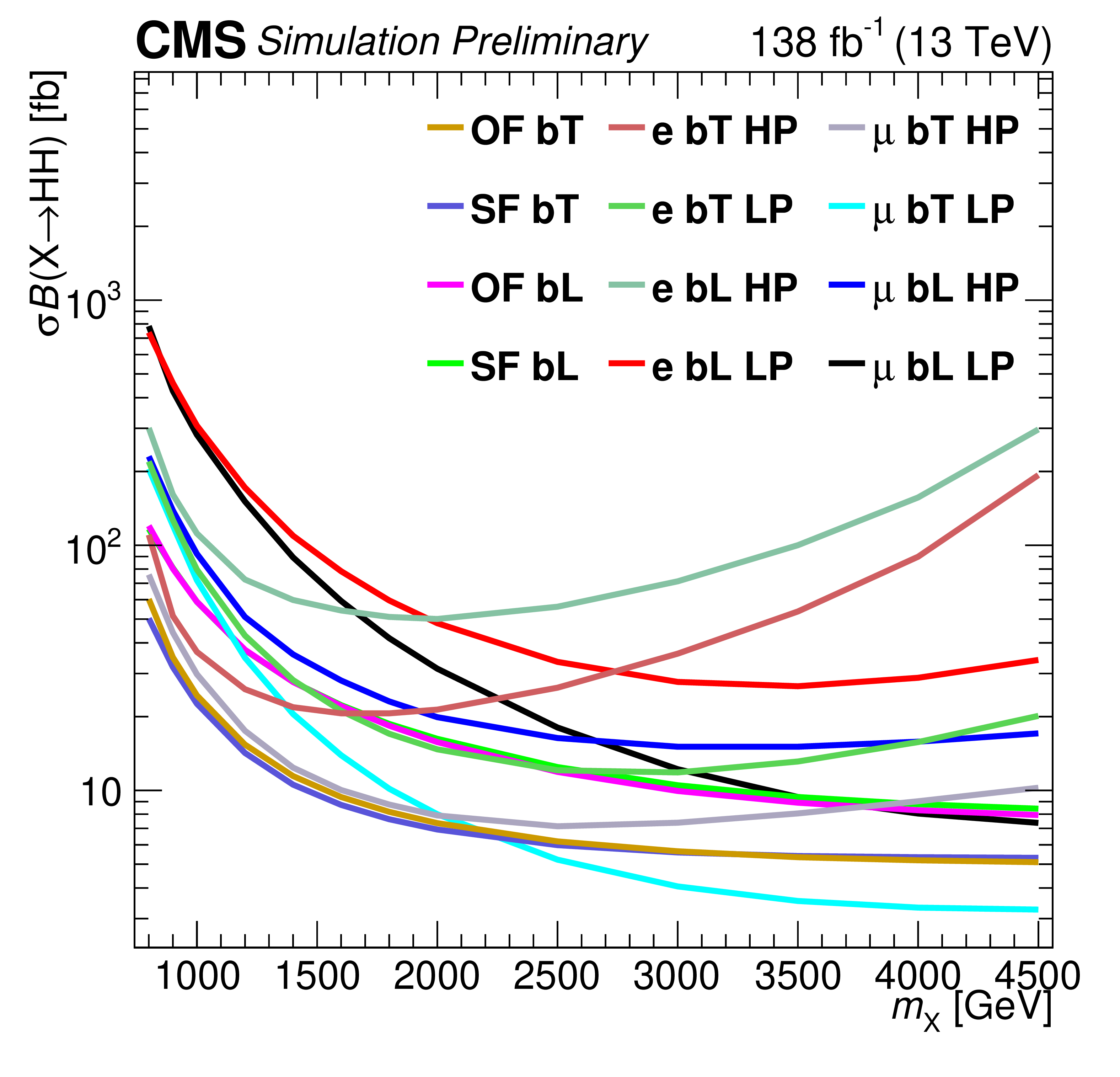
Figure 6:
Expected upper limits at 95% confidence level (CL) for each of the 12 search categories individually. |
png pdf |
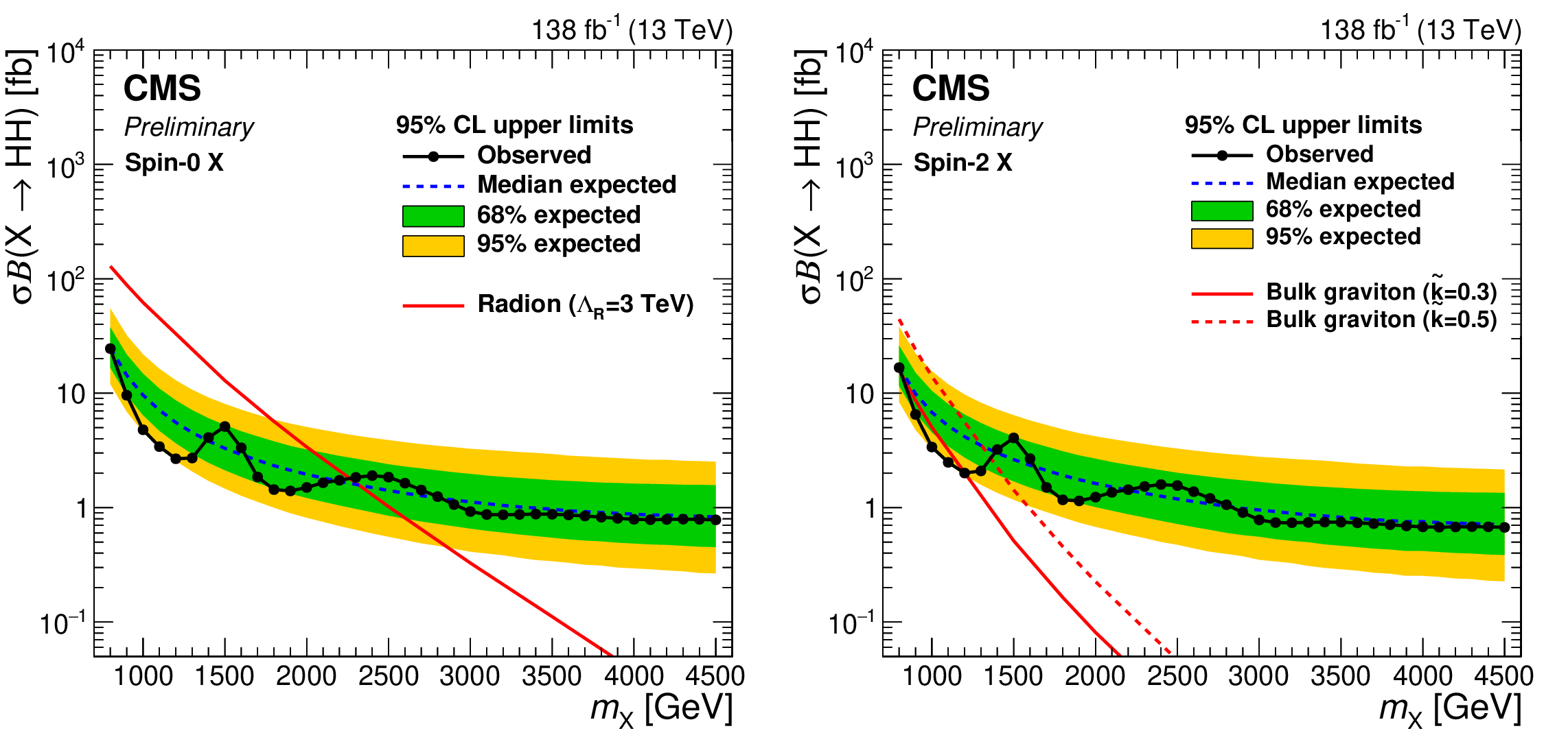
Figure 7:
Observed and expected 95% CL upper limits on the product of the cross section and branching fraction to $\mathrm{H} \mathrm{H} $ for a generic spin-0 (left) and spin-2 (right) boson X, as a function of mass. Example radion and bulk graviton predictions are also shown. The $\mathrm{H} \mathrm{H} $ branching fraction is assumed to be 25 and 10%, respectively. |
png pdf |
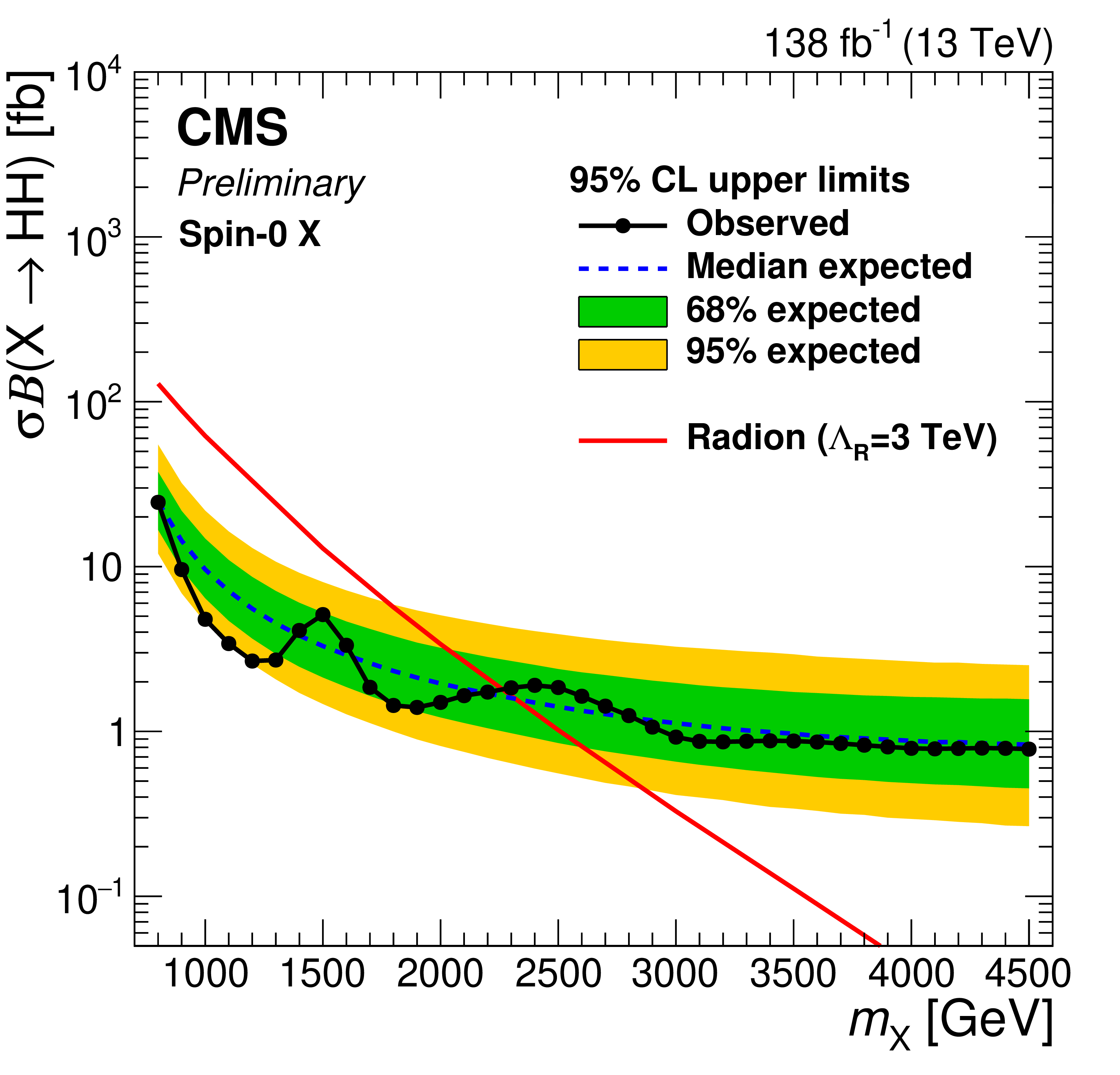
Figure 7-a:
Observed and expected 95% CL upper limits on the product of the cross section and branching fraction to $\mathrm{H} \mathrm{H} $ for a generic spin-0 (left) and spin-2 (right) boson X, as a function of mass. Example radion and bulk graviton predictions are also shown. The $\mathrm{H} \mathrm{H} $ branching fraction is assumed to be 25 and 10%, respectively. |
png pdf |
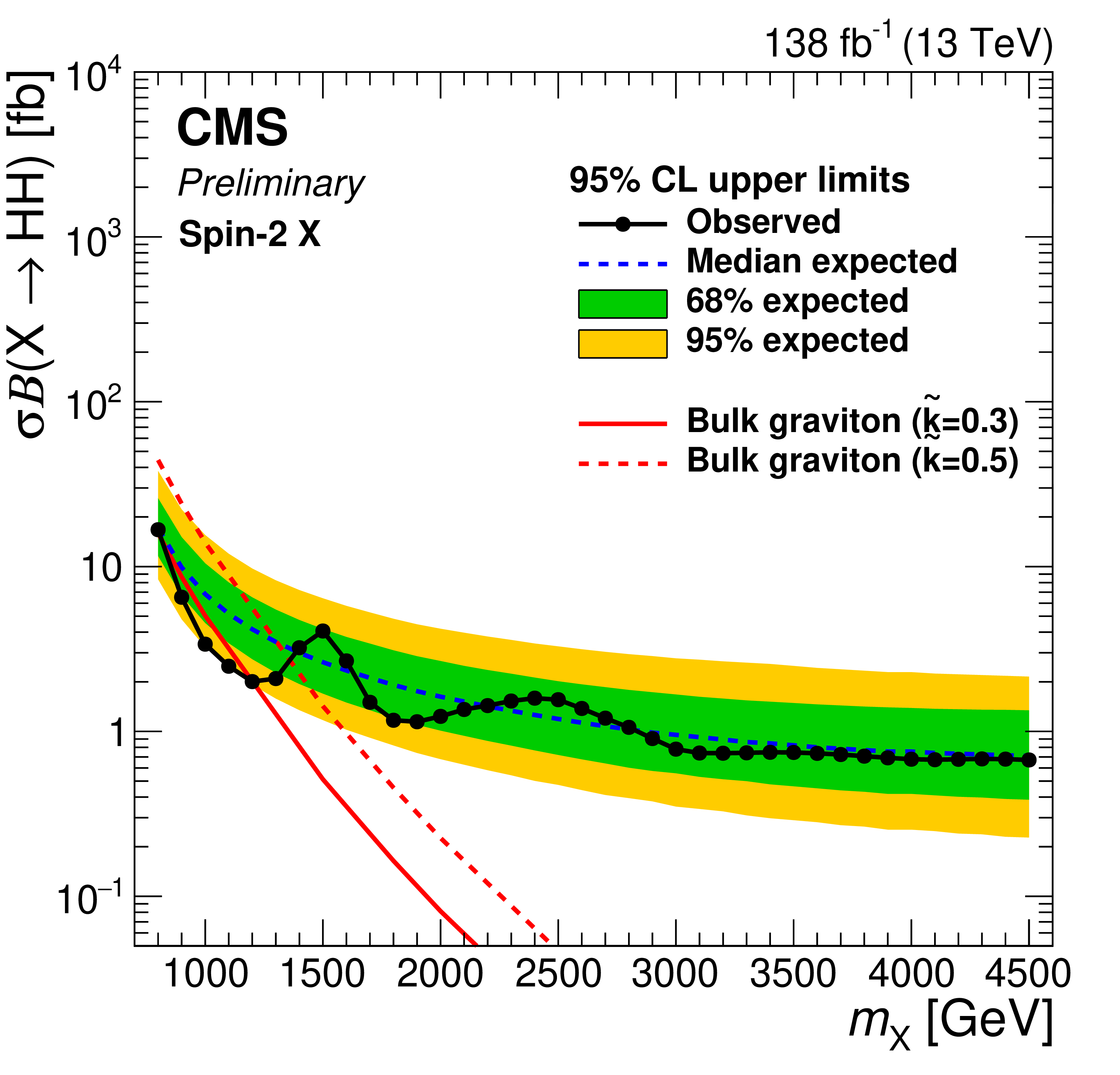
Figure 7-b:
Observed and expected 95% CL upper limits on the product of the cross section and branching fraction to $\mathrm{H} \mathrm{H} $ for a generic spin-0 (left) and spin-2 (right) boson X, as a function of mass. Example radion and bulk graviton predictions are also shown. The $\mathrm{H} \mathrm{H} $ branching fraction is assumed to be 25 and 10%, respectively. |
| Tables | |
png pdf |
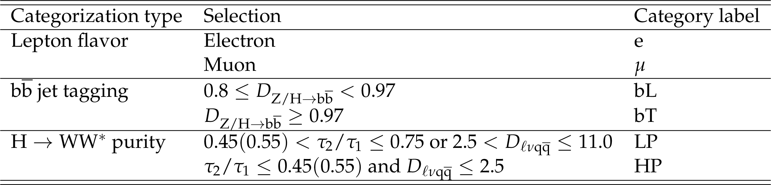
Table 1:
SL channel event categorization and corresponding category labels. All combinations of the two lepton flavor, two ${\mathrm{b\bar{b}}} $ jet tagging, and two ${\mathrm{H} \to \mathrm{W} \mathrm{W} ^*}$ decay purity selections are used to form eight independent event categories. The lower ${\tau _{2}/\tau _{1}}$ working point is 0.55 in 2016 and 0.45 in 2017 and 2018. |
png pdf |
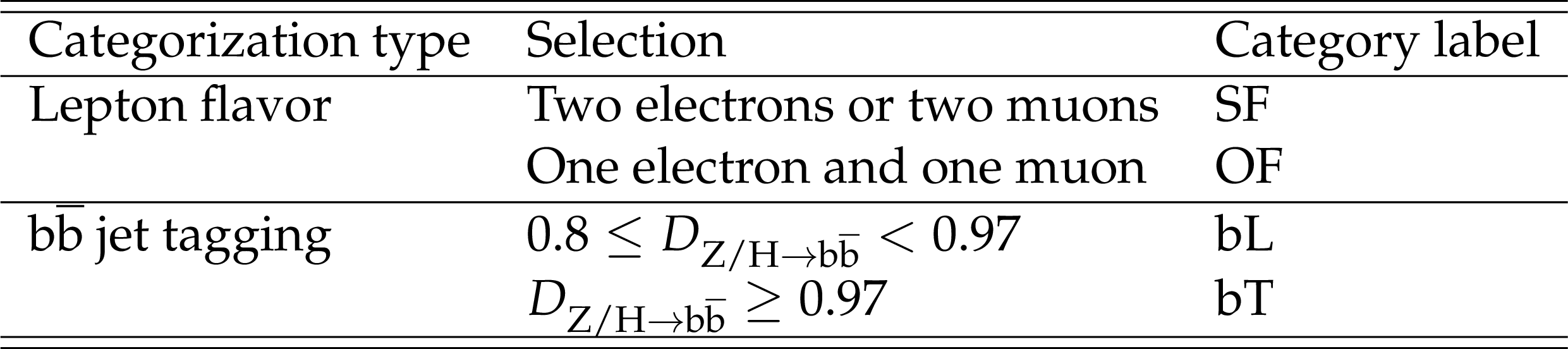
Table 2:
DL channel event categorization and corresponding category labels. All combinations of the two lepton flavor and two ${\mathrm{b\bar{b}}} $ jet tagging selections are used to form four independent event categories. |
png pdf |
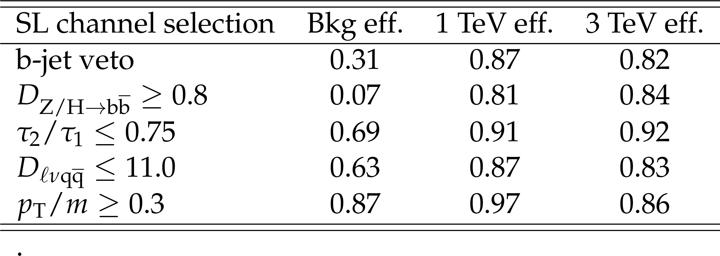
Table 3:
SL channel: the efficiency of each selection criterion with the rest of the full selection applied. The efficiencies for the total expected SM background and signal at 1.0 TeV and 3.0 TeV are shown. |
png pdf |
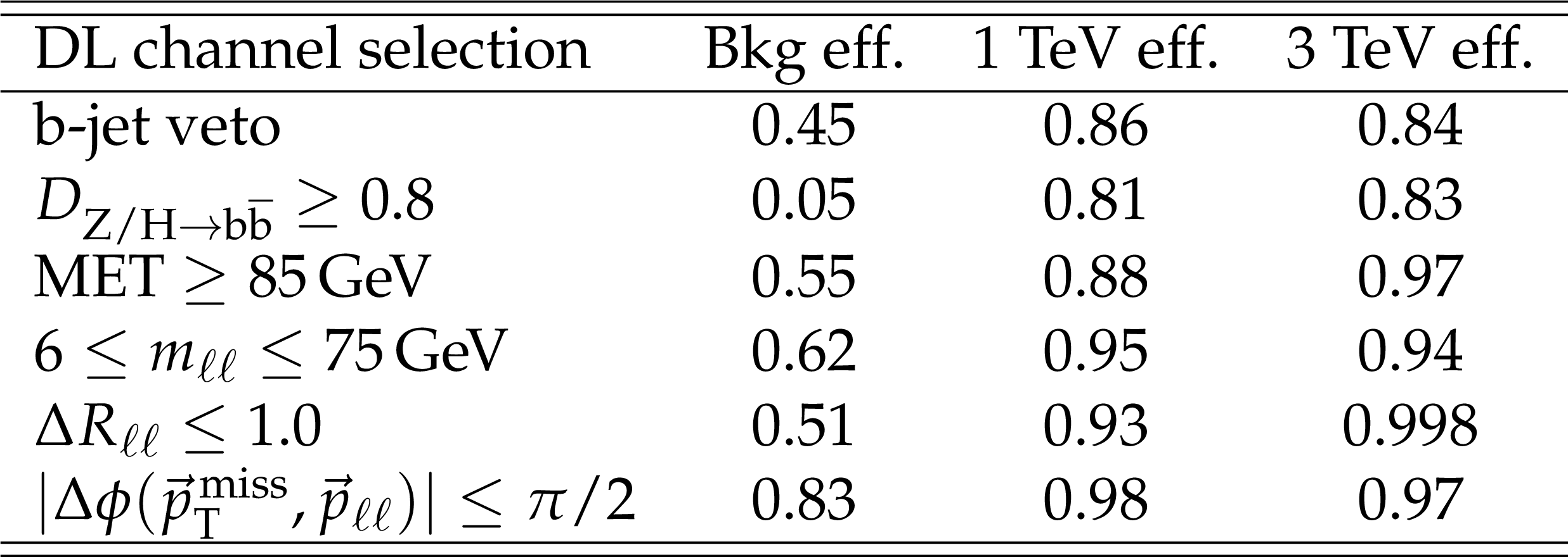
Table 4:
DL channel: the efficiency of each selection criterion with the rest of the full selection applied. The efficiencies for the total expected SM background and signal at 1.0 TeV and 3.0 TeV are shown. |
png pdf |
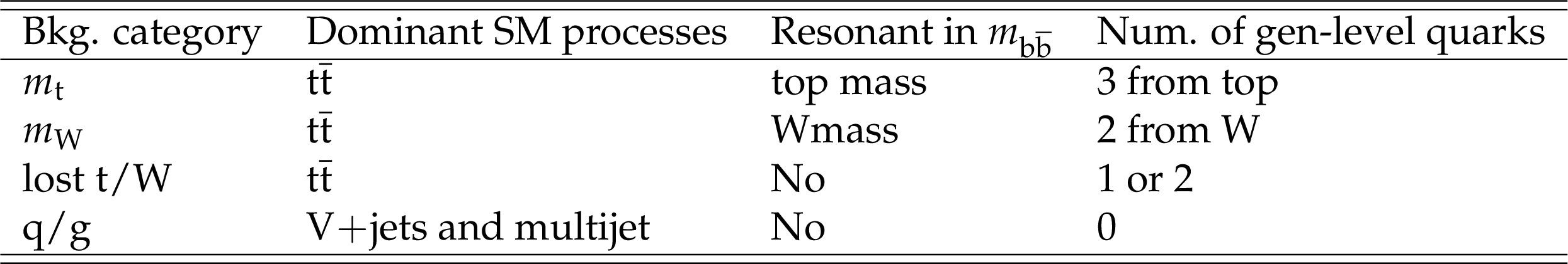
Table 5:
The four background components with their kinematical properties and defining number of generator-level quarks within $ {\Delta R} < $ 0.8 of the ${\mathrm{b\bar{b}}} $ jet axis. |
png pdf |
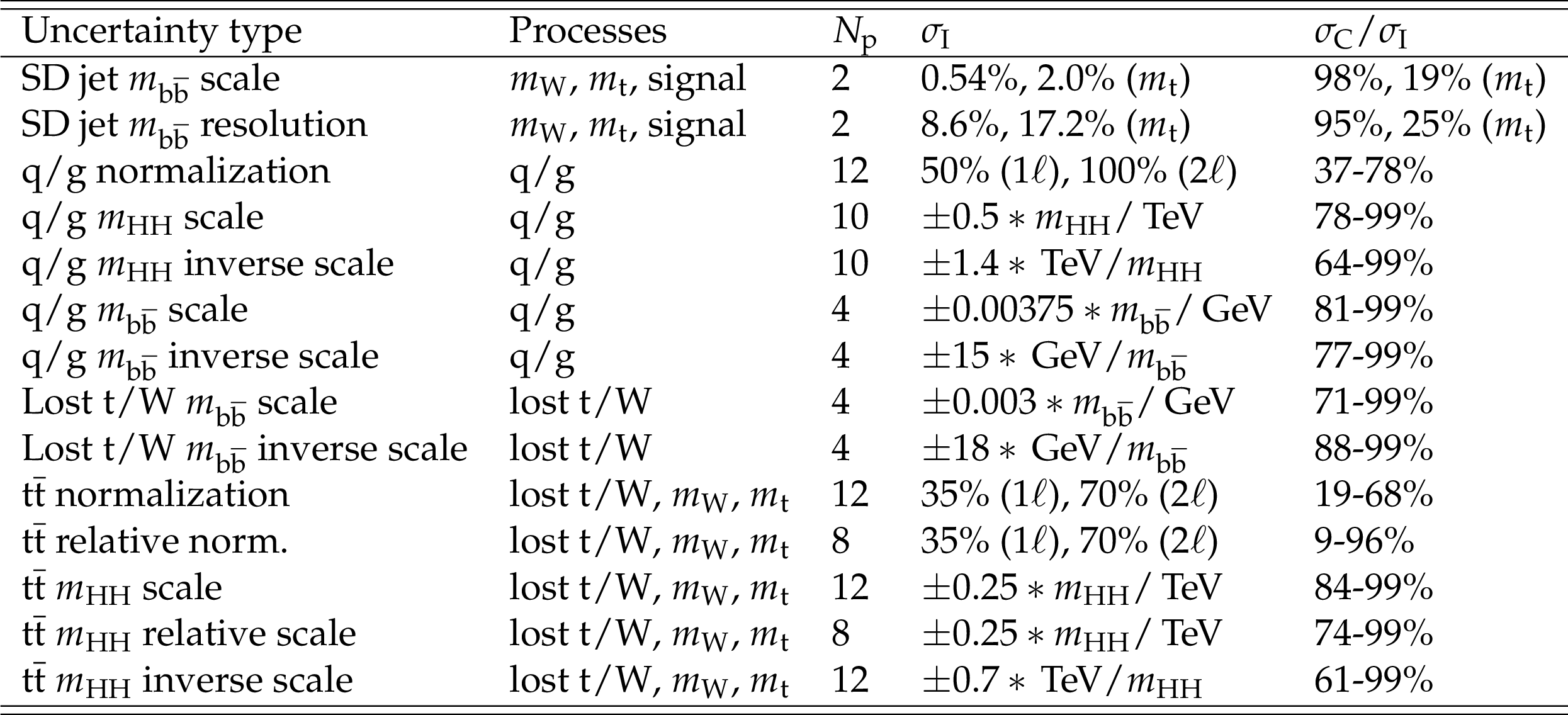
Table 6:
Background systematic uncertainties included in the maximum likelihood fit. The $N_{\text {p}}$ column indicates the number of nuisance parameters used to model the uncertainty. In the last two columns, $\sigma _{\text {I}}$ refers to the initial estimate of the uncertainty, and $\sigma _{\text {C}}$ refers to the constrained uncertainty obtained post-fit. For the ${\mathrm{q} /\mathrm{g}}, {\mathrm{t} {}\mathrm{\bar{t}}}$, and ${\text {lost} \mathrm{t} /\mathrm{W}}$ shape uncertainties, "scale'' uncertainties are those implemented with alternative templates with multiplicative parameters proportional to mass $m$, and "inverse scale'' are for proportional to 1/$m$. |
png pdf |
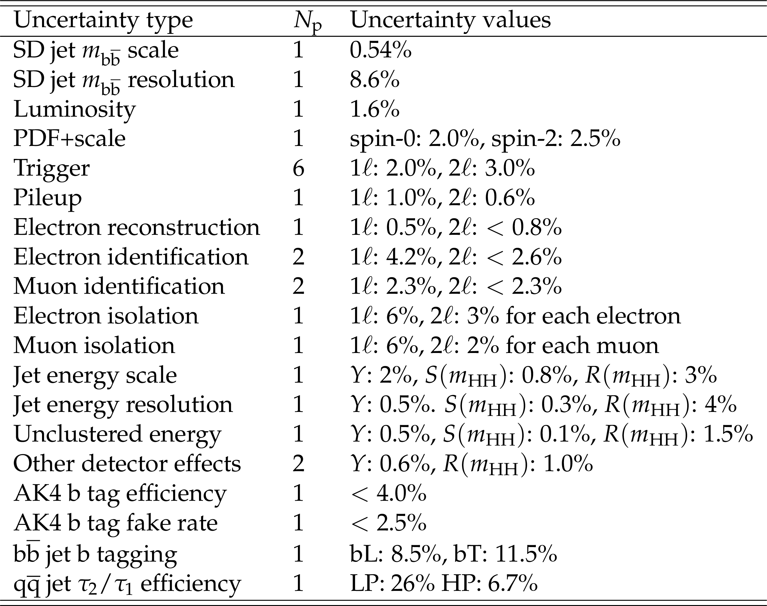
Table 7:
Signal systematic uncertainties included in the maximum likelihood fit. The $N_{\text {p}}$ column indicates the number of nuisance parameters used to model the uncertainty. In the "Uncertainty values'' column, some uncertainties are noted to affect both the yield ($Y$) and ${m_{\mathrm{H} \mathrm{H}}}$ shape ($S$ for scale, $R$ for resolution) of the signal. All other uncertainties, except the SD jet mass uncertainties, are uncertainties on the signal yield. |
png pdf |
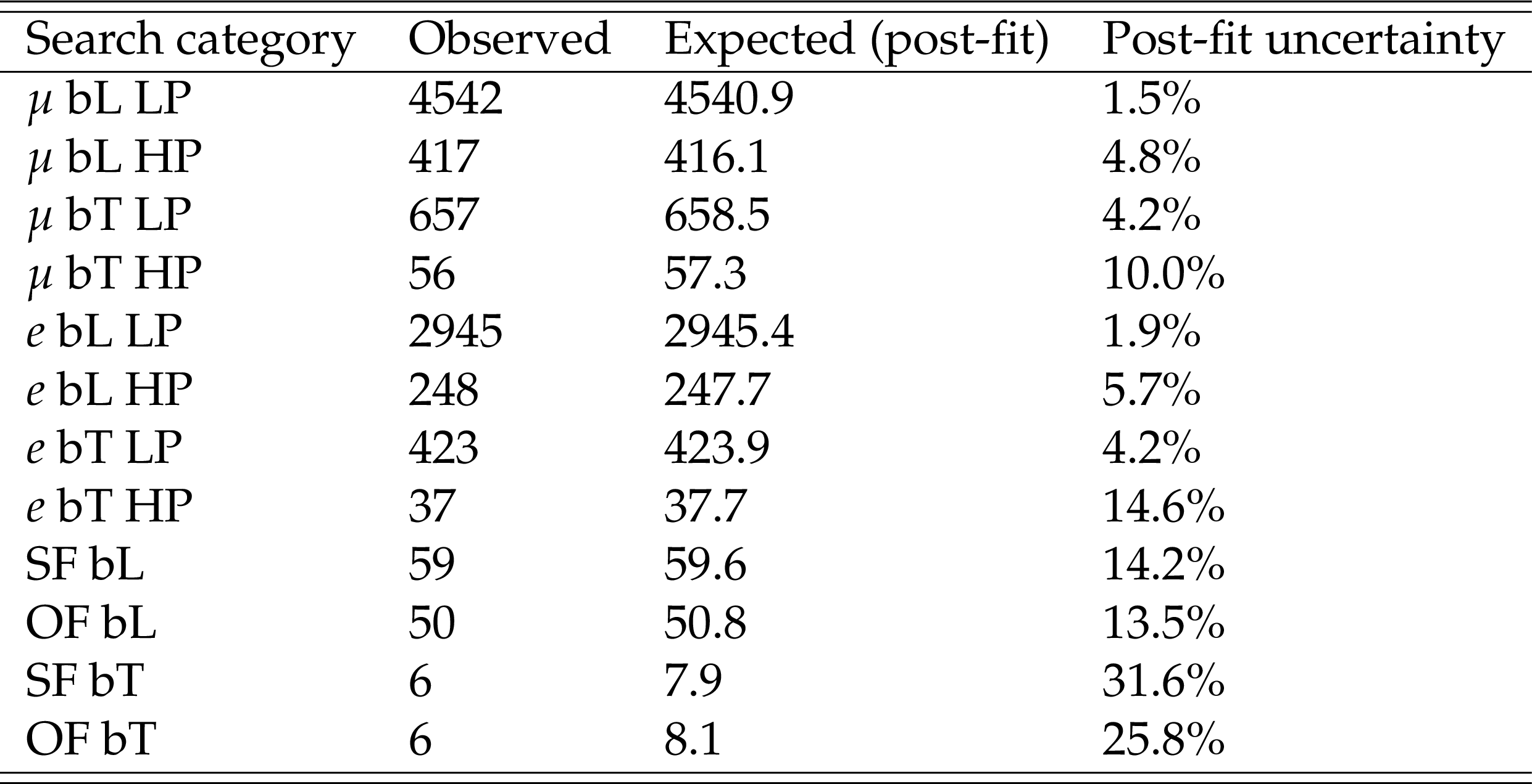
Table 8:
Event yields broken down by search category. For each category, shown are the event yields observed in data, expected after a fit to the B-only model, and the corresponding relative uncertainty. |
| Summary |
| A search has been presented for new bosons decaying to a pair of Higgs bosons (H) where one decays into a bottom quark pair ($\mathrm{b\bar{b}}$) and the other decays via one of three different modes into final states with leptons. The large Lorentz boost of the Higgs bosons produces a distinct experimental signature with one large-radius jet with substructure consistent with the decay $\mathrm{H}\to\mathrm{b\bar{b}}$. For the Higgs boson that does not decay to $\mathrm{b\bar{b}}$, considered are the single-lepton decay $\mathrm{H}\to{\mathrm{W}\mathrm{W}^*\to\ell\mathrm{g}n\mathrm{q\bar{q}}} $ and the dilepton decays $\mathrm{H}\to{\mathrm{W}\mathrm{W}^*\to\ell\nu\ell\nu} $ and $\mathrm{H}\to{\tau\tau \to\ell\nu\nu\ell\nu\nu} $. In the single-lepton channel, the experimental signature also contains a second large-radius jet with a nearby lepton, which is consistent with the decay of ${\mathrm{H}\to\mathrm{W}\mathrm{W}^*} $. In the dilepton channel, the experimental signature contains two leptons and significant missing transverse momentum. This search uses a sample of proton-proton collisions at $\sqrt{s} = $ 13 TeV collected by the CMS detector at the LHC. The primary Standard Model backgrounds -- production of top quark pairs and $\mathrm{Z}/\gamma^*$+jets in the dilepton channel only -- are suppressed by reconstructing the HH decay chain and applying selections to discriminate signal from background. The signal and background yields are estimated by a two-dimensional template fit in the plane of the ${\mathrm{b\bar{b}} }$ jet mass and the HH resonance mass. The templates are validated in a variety of data control regions and are shown to model the data well. The data are consistent with the expected Standard Model background. Upper limits are set on the product of the cross section and branching fraction for new bosons decaying to HH. The observed limit at 95% confidence level for a spin-0 boson ranges from 24.5 fb at 0.8 TeV to 0.78 fb at 4.5 TeV, while the limit for a spin-2 boson is 16.7 fb at 0.8 TeV and 0.67 fb at 4.5 TeV. This search produces the most stringent exclusion limits to date for $\mathrm{X}\to{\mathrm{H}\mathrm{H}} $ production modes with leptons in the final state. The current sensitivity to $\mathrm{X\to{\mathrm{H}\mathrm{H}}} $ production is stronger than or comparable to those from searches in other channels for HH resonances with masses above 800 GeV. |
| References | ||||
| 1 | ATLAS Collaboration | Observation of a new particle in the search for the standard model Higgs boson with the ATLAS detector at the LHC | PLB 716 (2012) 01 | 1207.7214 |
| 2 | CMS Collaboration | Observation of a new boson at a mass of 125 GeV with the CMS experiment at the LHC | PLB 716 (2012) 30 | CMS-HIG-12-028 1207.7235 |
| 3 | CMS Collaboration | Observation of a new boson with mass near 125 GeV in pp collisions at $ \sqrt{s} = $ 7 and 8 TeV | JHEP 06 (2013) 081 | CMS-HIG-12-036 1303.4571 |
| 4 | F. Englert and R. Brout | Broken symmetry and the mass of gauge vector mesons | PRL 13 (1964) 321 | |
| 5 | P. W. Higgs | Broken symmetries and the masses of gauge bosons | PRL 13 (1964) 508 | |
| 6 | G. C. Branco et al. | Theory and phenomenology of two-Higgs-doublet models | PR 516 (2012) 1--102 | 1106.0034 |
| 7 | P. Ramond | Dual theory for free fermions | PRD 3 (1971) 2415 | |
| 8 | Y. A. Golfand and E. P. Likhtman | Extension of the algebra of Poincar$ \'e $ group generators and violation of P invariance | JEPTL 13 (1971)323 | |
| 9 | A. Neveu and J. H. Schwarz | Factorizable dual model of pions | NPB 31 (1971) 86 | |
| 10 | D. V. Volkov and V. P. Akulov | Possible universal neutrino interaction | JEPTL 16 (1972)438 | |
| 11 | J. Wess and B. Zumino | A Lagrangian model invariant under supergauge transformations | PLB 49 (1974) 52 | |
| 12 | J. Wess and B. Zumino | Supergauge transformations in four dimensions | NPB 70 (1974) 39 | |
| 13 | P. Fayet | Supergauge invariant extension of the Higgs mechanism and a model for the electron and its neutrino | NPB 90 (1975) 104 | |
| 14 | H. P. Nilles | Supersymmetry, supergravity and particle physics | Phys. Rep. 110 (1984) 1 | |
| 15 | L. Randall and R. Sundrum | A large mass hierarchy from a small extra dimension | PRL 83 (1999) 3370 | hep-ph/9905221 |
| 16 | W. D. Goldberger and M. B. Wise | Modulus stabilization with bulk fields | PRL 83 (1999) 4922 | hep-ph/9907447 |
| 17 | O. DeWolfe, D. Z. Freedman, S. S. Gubser, and A. Karch | Modeling the fifth dimension with scalars and gravity | PRD 62 (2000) 046008 | hep-th/9909134 |
| 18 | C. Csaki, M. Graesser, L. Randall, and J. Terning | Cosmology of brane models with radion stabilization | PRD 62 (2000) 045015 | hep-ph/9911406 |
| 19 | C. Csaki, M. L. Graesser, and G. D. Kribs | Radion dynamics and electroweak physics | PRD 63 (2001) 065002 | hep-th/0008151 |
| 20 | H. Davoudiasl, J. L. Hewett, and T. G. Rizzo | Phenomenology of the Randall-Sundrum gauge hierarchy model | PRL 84 (2000) 2080 | hep-ph/9909255 |
| 21 | K. Agashe, H. Davoudiasl, G. Perez, and A. Soni | Warped gravitons at the LHC and beyond | PRD 76 (2007) 036006 | hep-ph/0701186 |
| 22 | A. L. Fitzpatrick, J. Kaplan, L. Randall, and L.-T. Wang | Searching for the Kaluza-Klein graviton in bulk RS models | JHEP 09 (2007) 013 | hep-ph/0701150 |
| 23 | ATLAS Collaboration | Searches for Higgs boson pair production in the $ hh\to bb\tau\tau, \gamma\gamma WW^*, \gamma\gamma bb, bbbb $ channels with the ATLAS detector | PRD 92 (2015) 092004 | 1509.04670 |
| 24 | ATLAS Collaboration | Search for a new resonance decaying to a $ W $ or $ Z $ boson and a Higgs boson in the $ \ell \ell / \ell \nu / \nu \nu + b \bar{b} $ final states with the ATLAS detector | EPJC 75 (2015) 263 | 1503.08089 |
| 25 | ATLAS Collaboration | Search for Higgs boson pair production in the $ b\bar{b}b\bar{b} $ final state from pp collisions at $ \sqrt{s} = $ 8 TeV with the ATLAS detector | EPJC 75 (2015) 412 | 1506.00285 |
| 26 | ATLAS Collaboration | Search for Higgs boson pair production in the $ \gamma\gamma b\bar{b} $ final state using pp collision data at $ \sqrt{s}= $ 8 TeV from the ATLAS detector | PRL 114 (2015) 081802 | 1406.5053 |
| 27 | ATLAS Collaboration | Search for $ W\!Z $ resonances in the fully leptonic channel using pp collisions at $ \sqrt{s} = 8{TeV} $ with the ATLAS detector | PLB 737 (2014) 223 | 1406.4456 |
| 28 | ATLAS Collaboration | Search for heavy resonances decaying to a $ W $ or $ Z $ boson and a Higgs boson in the $ q\bar{q}^{(\prime)}b\bar{b} $ final state in $ pp $ collisions at $ \sqrt{s} = $ 13 TeV with the ATLAS detector | PLB 774 (2017) 494 | 1707.06958 |
| 29 | ATLAS Collaboration | Search for $ WW/WZ $ resonance production in $ \ell \nu qq $ final states in $ pp $ collisions at $ \sqrt{s} = $ 13 TeV with the ATLAS detector | JHEP 03 (2018) 042 | 1710.07235 |
| 30 | ATLAS Collaboration | Search for resonant $ WZ $ production in the fully leptonic final state in proton-proton collisions at $ \sqrt{s} = $ 13 TeV with the ATLAS detector | PLB 787 (2018) 68 | 1806.01532 |
| 31 | ATLAS Collaboration | Search for heavy resonances decaying into $ WW $ in the $ e\nu\mu\nu $ final state in $ pp $ collisions at $ \sqrt{s}= $ 13 TeV with the ATLAS detector | EPJC 78 (2018) 24 | 1710.01123 |
| 32 | ATLAS Collaboration | Searches for heavy $ ZZ $ and $ ZW $ resonances in the $ \ell\ell qq $ and $ \nu\nu qq $ final states in $ pp $ collisions at $ \sqrt{s}= $ 13 TeV with the ATLAS detector | JHEP 03 (2018) 009 | 1708.09638 |
| 33 | ATLAS Collaboration | Search for heavy ZZ resonances in the $ \ell ^+\ell ^-\ell ^+\ell ^- $ and $ \ell ^+\ell ^-\nu \bar{\nu} $ final states using proton-proton collisions at $ \sqrt{s}= $ 13 TeV with the ATLAS detector | EPJC 78 (2018) 293 | 1712.06386 |
| 34 | ATLAS Collaboration | Search for heavy resonances decaying into a $ W $ or $ Z $ boson and a Higgs boson in final states with leptons and $ b $-jets in 36 fb$ ^{-1} $ of $ \sqrt s = $ 13 TeV pp collisions with the ATLAS detector | JHEP 03 (2018) 174 | 1712.06518 |
| 35 | ATLAS Collaboration | Search for diboson resonances with boson-tagged jets in $ pp $ collisions at $ \sqrt{s}= $ 13 TeV with the ATLAS detector | PLB 777 (2018) 91--113 | 1708.04445 |
| 36 | ATLAS Collaboration | Search for Higgs boson pair production in the $ b\bar{b}WW^{*} $ decay mode at $ \sqrt{s}= $ 13 TeV with the ATLAS detector | 1811.04671 | |
| 37 | ATLAS Collaboration | Search for pair production of Higgs bosons in the $ b\bar{b}b\bar{b} $ final state using proton-proton collisions at $ \sqrt{s} = $ 13 TeV with the ATLAS detector | JHEP 01 (2019) 030 | 1804.06174 |
| 38 | ATLAS Collaboration | Search for resonant and non-resonant Higgs boson pair production in the $ {b\bar{b}\tau^+\tau^-} $ decay channel in $ pp $ collisions at $ \sqrt{s}= $ 13 TeV with the ATLAS detector | PRL 121 (2018) 191801 | 1808.00336 |
| 39 | CMS Collaboration | Combination of searches for heavy resonances decaying to WW, WZ, ZZ, WH, and ZH boson pairs in proton-proton collisions at $ \sqrt{s}= $ 8 and 13 TeV | PLB 774 (2017) 533 | CMS-B2G-16-007 1705.09171 |
| 40 | CMS Collaboration | Search for a heavy resonance decaying into a Z boson and a vector boson in the $ \nu\overline{\nu}\mathrm{q}\overline{\mathrm{q}} $ final state | JHEP 07 (2018) 075 | CMS-B2G-17-005 1803.03838 |
| 41 | CMS Collaboration | Search for heavy resonances decaying into two Higgs bosons or into a Higgs boson and a W or Z boson in proton-proton collisions at 13 TeV | CMS-B2G-17-006 1808.01365 |
|
| 42 | CMS Collaboration | Search for a heavy resonance decaying into a Z boson and a Z or W boson in 2$ \ell $2q final states at $ \sqrt{s}= $ 13 TeV | JHEP 09 (2018) 101 | CMS-B2G-17-013 1803.10093 |
| 43 | CMS Collaboration | Search for production of Higgs boson pairs in the four b quark final state using large-area jets in proton-proton collisions at $ \sqrt{s}= $ 13 TeV | CMS-B2G-17-019 1808.01473 |
|
| 44 | CMS Collaboration | Searches for a heavy scalar boson H decaying to a pair of 125 GeV Higgs bosons hh or for a heavy pseudoscalar boson A decaying to Zh, in the final states with $ \text{h} \to \tau \tau $ | PLB 755 (2016) 217 | CMS-HIG-14-034 1510.01181 |
| 45 | CMS Collaboration | Search for massive resonances decaying into $ WW $, $ WZ $, $ ZZ $, $ qW $, and $ qZ $ with dijet final states at $ \sqrt{s}= $ 13 TeV | PRD 97 (2018) 072006 | CMS-B2G-17-001 1708.05379 |
| 46 | CMS Collaboration | Search for heavy resonances that decay into a vector boson and a Higgs boson in hadronic final states at $ \sqrt{s} = $ 13 TeV | EPJC 77 (2017) 636 | CMS-B2G-17-002 1707.01303 |
| 47 | CMS Collaboration | Search for heavy resonances decaying into a vector boson and a Higgs boson in final states with charged leptons, neutrinos and b quarks at $ \sqrt{s}= $ 13 TeV | CMS-B2G-17-004 1807.02826 |
|
| 48 | CMS Collaboration | Search for resonant pair production of Higgs bosons decaying to two bottom quark-antiquark pairs in proton-proton collisions at 8 TeV | PLB 749 (2015) 560 | CMS-HIG-14-013 1503.04114 |
| 49 | CMS Collaboration | Search for heavy resonances decaying into a vector boson and a Higgs boson in final states with charged leptons, neutrinos, and b quarks | PLB 768 (2017) 137 | CMS-B2G-16-003 1610.08066 |
| 50 | CMS Collaboration | Search for a massive resonance decaying to a pair of Higgs bosons in the four b quark final state in proton-proton collisions at $ \sqrt{s}= $ 13 TeV | PLB 781 (2018) 244--269 | 1710.04960 |
| 51 | CMS Collaboration | Search for a heavy resonance decaying to a pair of vector bosons in the lepton plus merged jet final state at $ \sqrt{s}= $ 13 TeV | JHEP 05 (2018) 088 | CMS-B2G-16-029 1802.09407 |
| 52 | CMS Collaboration | Search for massive resonances decaying into WW, WZ or ZZ bosons in proton-proton collisions at $ \sqrt s = $ 13 TeV | JHEP 03 (2017) 162 | CMS-B2G-16-004 1612.09159 |
| 53 | CMS Collaboration | Search for ZZ resonances in the 2$ \ell 2 \nu $ final state in proton-proton collisions at 13 TeV | JHEP 03 (2018) 003 | CMS-B2G-16-023 1711.04370 |
| 54 | CMS Collaboration | Search for new resonances decaying via WZ to leptons in proton-proton collisions at $ \sqrt{s} = $ 13 TeV | PLB 740 (2015) 83 | CMS-EXO-12-025 1407.3476 |
| 55 | CMS Collaboration | Search for massive WH resonances decaying into the $ \ell \nu \mathrm{b} \overline{\mathrm{b}} $ final state at $ \sqrt{s} = $ 8 TeV | EPJC 76 (2016) 237 | CMS-EXO-14-010 1601.06431 |
| 56 | CMS Collaboration | Search for a massive resonance decaying into a Higgs boson and a W or Z boson in hadronic final states in proton-proton collisions at $ \sqrt{s} = $ 8 TeV | JHEP 02 (2016) 145 | CMS-EXO-14-009 1506.01443 |
| 57 | CMS Collaboration | Search for narrow high-mass resonances in proton-proton collisions at $ \sqrt{s} = $ 8 TeV decaying to a Z and a Higgs boson | PLB 748 (2015) 255 | CMS-EXO-13-007 1502.04994 |
| 58 | CMS Collaboration | Search for resonances decaying to a pair of Higgs bosons in the $ b\bar{b} q\bar{q} \ell \nu $ final state in proton-proton collisions at $ \sqrt{s} = $ 13 Tev | Journal of High Energy Physics 10 (2019) 125 | 1904.04193 |
| 59 | CMS Collaboration | Performance of the CMS Level-1 trigger in proton-proton collisions at $ \sqrt{s} = $ 13 TeV | JINST 15 (2020) P10017 | CMS-TRG-17-001 2006.10165 |
| 60 | CMS Collaboration | The CMS trigger system | JINST 12 (2017) P01020 | CMS-TRG-12-001 1609.02366 |
| 61 | LHC Higgs Cross Sections Working Group | LHC HXSWG Yellow Report | link | |
| 62 | J. Alwall et al. | The automated computation of tree-level and next-to-leading order differential cross sections, and their matching to parton shower simulations | JHEP 07 (2014) 079 | 1405.0301 |
| 63 | J. Alwall et al. | Comparative study of various algorithms for the merging of parton showers and matrix elements in hadronic collisions | EPJC 53 (2008) 473 | 0706.2569 |
| 64 | Y. Li and F. Petriello | Combining QCD and electroweak corrections to dilepton production in FEWZ | PRD 86 (2012) 094034 | 1208.5967 |
| 65 | R. Frederix and S. Frixione | Merging meets matching in MC@NLO | JHEP 12 (2012) 61 | 1209.6215 |
| 66 | P. Nason | A new method for combining NLO QCD with shower Monte Carlo algorithms | JHEP 11 (2004) 040 | hep-ph/0409146 |
| 67 | S. Frixione, P. Nason, and C. Oleari | Matching NLO QCD computations with parton shower simulations: the POWHEG method | JHEP 11 (2007) 070 | 0709.2092 |
| 68 | S. Alioli, P. Nason, C. Oleari, and E. Re | A general framework for implementing NLO calculations in shower Monte Carlo programs: the POWHEG BOX | JHEP 06 (2010) 043 | 1002.2581 |
| 69 | E. Re | Single-top $ Wt $-channel production matched with parton showers using the POWHEG method | EPJC 71 (2011) 1547 | 1009.2450 |
| 70 | T. Melia, P. Nason, R. Rontsch, and G. Zanderighi | $ W^+W^- $, $ WZ $ and $ ZZ $ production in the POWHEG BOX | JHEP 11 (2011) 078 | 1107.5051 |
| 71 | P. Nason and G. Zanderighi | $ W^+ W^- $ , $ W Z $ and $ Z Z $ production in the POWHEG-BOX-V2 | EPJC 74 (2014) 2702 | 1311.1365 |
| 72 | R. Frederix, E. Re, and P. Torrielli | Single-top t-channel hadroproduction in the four-flavour scheme with POWHEG and aMC@NLO | JHEP 09 (2012) 130 | 1207.5391 |
| 73 | H. B. Hartanto, B. Jager, L. Reina, and D. Wackeroth | Higgs boson production in association with top quarks in the POWHEG BOX | PRD 91 (2015) 094003 | 1501.04498 |
| 74 | M. Czakon and A. Mitov | Top++: A program for the calculation of the top-pair cross-section at hadron colliders | CPC 185 (2014) 2930 | 1112.5675 |
| 75 | T. Sjostrand et al. | An introduction to PYTHIA 8.2 | CPC 191 (2015) 159 | 1410.3012 |
| 76 | CMS Collaboration | Event generator tunes obtained from underlying event and multiparton scattering measurements | EPJC 76 (2016) 155 | CMS-GEN-14-001 1512.00815 |
| 77 | CMS Collaboration | Extraction and validation of a new set of cms pythia8 tunes from underlying-event measurements | EPJC 80 (2020) 4 | CMS-GEN-17-001 1903.12179 |
| 78 | NNPDF Collaboration | Parton distributions for the LHC Run II | JHEP 04 (2015) 040 | 1410.8849 |
| 79 | NNPDF Collaboration | Parton distributions from high-precision collider data | EPJC 77 (2017) | 1706.00428 |
| 80 | GEANT4 Collaboration | GEANT4--a simulation toolkit | NIMA 506 (2003) 250 | |
| 81 | CMS Collaboration | Particle-flow reconstruction and global event description with the CMS detector | JINST 12 (2017) P10003 | CMS-PRF-14-001 1706.04965 |
| 82 | CMS Collaboration | Performance of missing transverse momentum reconstruction in proton-proton collisions at $ \sqrt{s} = $ 13 TeV using the CMS detector | JINST 14 (2019) P07004 | CMS-JME-17-001 1903.06078 |
| 83 | M. Cacciari, G. P. Salam, and G. Soyez | The anti-$ k_t $ jet clustering algorithm | JHEP 04 (2008) 063 | 0802.1189 |
| 84 | M. Cacciari, G. P. Salam, and G. Soyez | FastJet user manual | EPJC 72 (2012) 1896 | 1111.6097 |
| 85 | CMS Collaboration | SWGuideMuonIdRun2 | link | |
| 86 | CMS Collaboration | MultivariateElectronIdentificationRun2 | link | |
| 87 | CMS Collaboration | CutBasedElectronIdentificationRun2 | link | |
| 88 | CMS Collaboration | Pileup mitigation at CMS in 13 TeV data | JINST 15 (2020) P09018 | CMS-JME-18-001 2003.00503 |
| 89 | D. Bertolini, P. Harris, M. Low, and N. Tran | Pileup per particle identification | JHEP 10 (2014) 059 | 1407.6013 |
| 90 | Y. L. Dokshitzer, G. D. Leder, S. Moretti, and B. R. Webber | Better jet clustering algorithms | JHEP 08 (1997) 001 | hep-ph/9707323 |
| 91 | M. Wobisch and T. Wengler | Hadronization corrections to jet cross-sections in deep inelastic scattering | in Proceedings of the Workshop on Monte Carlo Generators for HERA Physics, Hamburg, Germany, p. 270 1998 | hep-ph/9907280 |
| 92 | M. Dasgupta, A. Fregoso, S. Marzani, and G. P. Salam | Towards an understanding of jet substructure | JHEP 09 (2013) 029 | 1307.0007 |
| 93 | J. M. Butterworth, A. R. Davison, M. Rubin, and G. P. Salam | Jet substructure as a new Higgs search channel at the LHC | PRL 100 (2008) 242001 | 0802.2470 |
| 94 | A. J. Larkoski, S. Marzani, G. Soyez, and J. Thaler | Soft drop | JHEP 05 (2014) 146 | 1402.2657 |
| 95 | CMS Collaboration | Identification of heavy-flavour jets with the CMS detector in pp collisions at 13 TeV | JINST 13 (2018) P05011 | CMS-BTV-16-002 1712.07158 |
| 96 | E. Bols et al. | Jet Flavour Classification Using DeepJet | JINST 15 (2020), no. 12, P12012 | 2008.10519 |
| 97 | CMS Collaboration | Performance of the DeepJet b tagging algorithm using 41.9/fb of data from proton-proton collisions at 13 TeV with Phase 1 CMS detector | CDS | |
| 98 | CMS Collaboration | Identification of heavy, energetic, hadronically decaying particles using machine-learning techniques | JINST 15 (2020) P06005 | |
| 99 | J. Thaler and K. Van Tilburg | Identifying boosted objects with N-subjettiness | JHEP 03 (2011) 015 | 1011.2268 |
| 100 | CMS Collaboration | Measurement of normalized differential $ \mathrm{t}\overline{\mathrm{t}} $ cross sections in the dilepton channel from pp collisions at $ \sqrt{s}= $ 13 TeV | JHEP 04 (2018) 060 | CMS-TOP-16-007 1708.07638 |
| 101 | CMS Collaboration | Measurement of differential cross sections for top quark pair production using the lepton+jets final state in proton-proton collisions at 13 TeV | PRD 95 (2017) 092001 | CMS-TOP-16-008 1610.04191 |
| 102 | M. Rosenblatt | Remarks on some nonparametric estimates of a density function | Ann. Math. Stat. 27 (1956)832.http://www.jstor.org/stable/2237390 | |
| 103 | B. Silverman | Density estimation for statistics and data analysis | Chapman and Hall, 1986 ISBN 0412246201 | |
| 104 | D. Scott | Multivariate density estimation: theory, practice, and visualization | John Wiley and Sons, 1992 ISBN 0471547700 | |
| 105 | M. J. Oreglia | A study of the reactions $\psi' \to \gamma\gamma \psi$ | PhD thesis, Stanford University, 1980 SLAC Report SLAC-R-236, see Appendix D | |
| 106 | J. Gaiser | Charmonium Spectroscopy From Radiative Decays of the $\mathrm{J}/\psi$ and $\psi'$ | PhD thesis, SLAC | |
| 107 | M. Cacciari et al. | The $ \mathrm{t\bar{t}} $ cross-section at 1.8 TeV and 1.96$ TeV: $ A study of the systematics due to parton densities and scale dependence | JHEP 04 (2004) 068 | hep-ph/0303085 |
| 108 | S. Catani, D. de Florian, M. Grazzini, and P. Nason | Soft gluon resummation for Higgs boson production at hadron colliders | JHEP 07 (2003) 028 | hep-ph/0306211 |
| 109 | S. Baker and R. D. Cousins | Clarification of the use of chi square and likelihood functions in fits to histograms | NIM221 (1984) 437 | |
| 110 | G. Cowan, K. Cranmer, E. Gross, and O. Vitells | Asymptotic formulae for likelihood-based tests of new physics | EPJC 71 (2011) 1554 | 1007.1727 |
| 111 | T. Junk | Confidence level computation for combining searches with small statistics | NIMA 434 (1999) 435 | hep-ex/9902006 |
| 112 | A. L. Read | Presentation of search results: The CLs technique | JPG 28 (2002) 2693 | |
| 113 | A. Oliveira | Gravity particles from warped extra dimensions, predictions for LHC | 1404.0102 | |
| 114 | M. Gouzevitch et al. | Scale-invariant resonance tagging in multijet events and new physics in Higgs pair production | JHEP 07 (2013) 148 | 1303.6636 |
|
|
Compact Muon Solenoid LHC, CERN |
|

|

|

|

|

|