

Compact Muon Solenoid
LHC, CERN
| CMS-HIG-25-018 ; CERN-EP-2026-091 | ||
| Search for Higgs boson pair production in the $ \mathrm{b}\overline{\mathrm{b}}\mathrm{W}\mathrm{W} $ decay channel with two leptons in the final state using proton-proton collision data at $ \sqrt{s}= $ 13.6 TeV | ||
| CMS Collaboration | ||
| 2 April 2026 | ||
| Accepted for publication in the Journal of High Energy Physics | ||
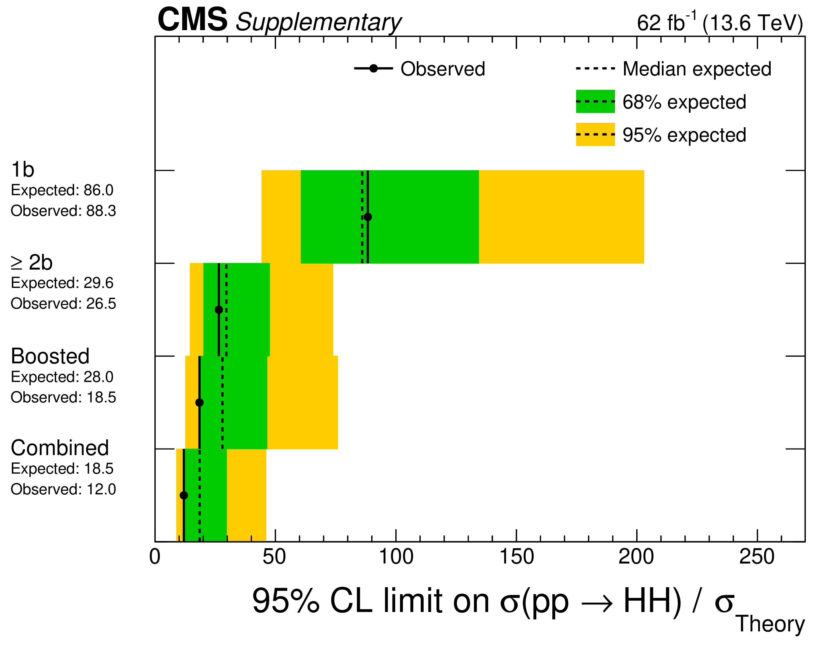
| Abstract: A search for Higgs boson pair production is presented, targeting final states where one Higgs boson decays to a pair of bottom quarks and the other Higgs boson decays to two W bosons, both of which decay leptonically, to an electron or a muon, and a neutrino. For the first time, the search is conducted with proton-proton collision data from the LHC at $ \sqrt{s}= $ 13.6 TeV, recorded with the CMS detector in 2022 and 2023 and corresponding to an integrated luminosity of 62 fb$^{-1}$. The results are consistent with the standard model predictions. An upper limit of 12.0 times the standard model prediction at 95% confidence level is set on the Higgs boson pair production cross section, with an expected limit of 18.5. The results are also used to constrain the strength of the trilinear self-coupling of the Higgs boson, as well as of the quartic coupling between two Higgs bosons and two vector bosons. | ||
| Links: e-print arXiv:2604.02127 [hep-ex] (PDF) ; CDS record ; inSPIRE record ; HepData record ; CADI line (restricted) ; | ||
| Figures & Tables | Summary | Additional Figures | References | CMS Publications |
|---|
| Figures | |
png pdf |
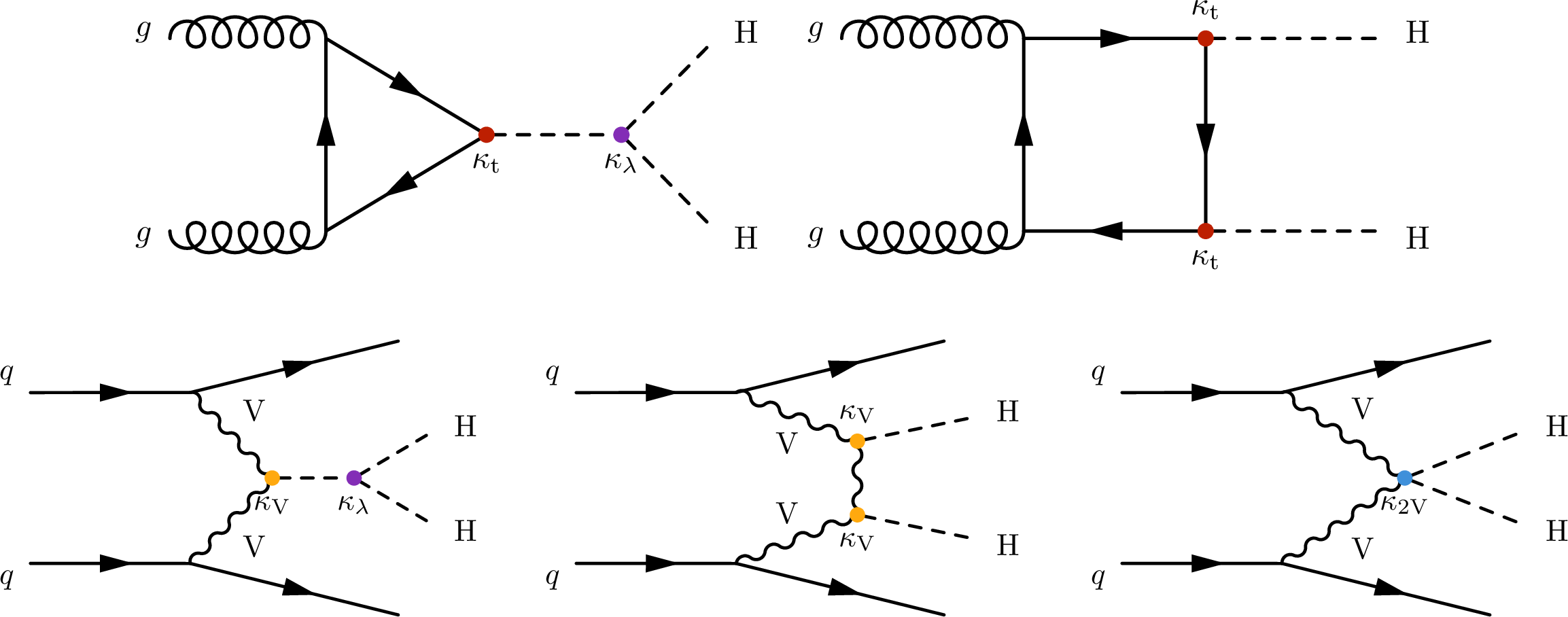
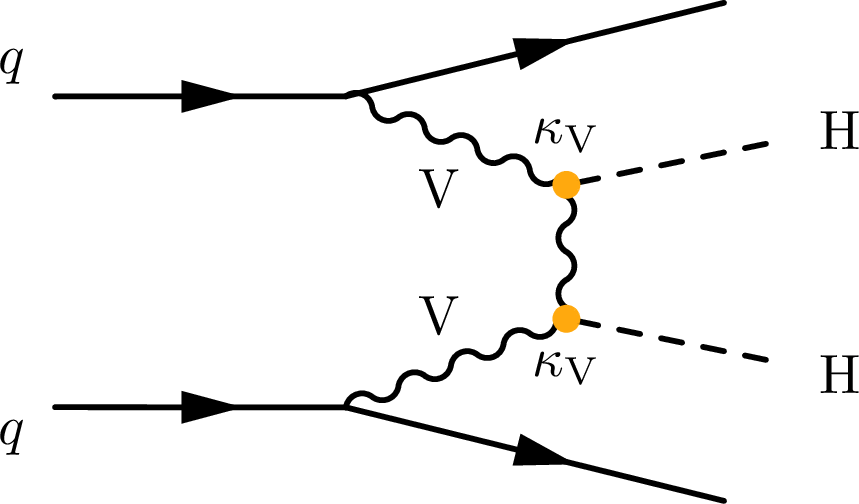
Figure 1:
Leading-order Feynman diagrams of HH production in the $ \mathrm{g}\mathrm{g}\text{F} $ production mode assuming top quarks in the fermion loop (top row) and in the $ \text{VBF} $ production mode (bottom row) in the SM. |
png pdf |
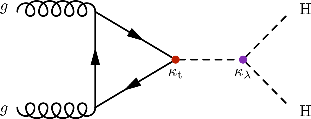
Figure 1-a:
Leading-order Feynman diagrams of HH production in the $ \mathrm{g}\mathrm{g}\text{F} $ production mode assuming top quarks in the fermion loop (top row) and in the $ \text{VBF} $ production mode (bottom row) in the SM. |
png pdf |
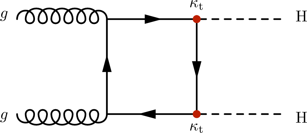
Figure 1-b:
Leading-order Feynman diagrams of HH production in the $ \mathrm{g}\mathrm{g}\text{F} $ production mode assuming top quarks in the fermion loop (top row) and in the $ \text{VBF} $ production mode (bottom row) in the SM. |
png pdf |
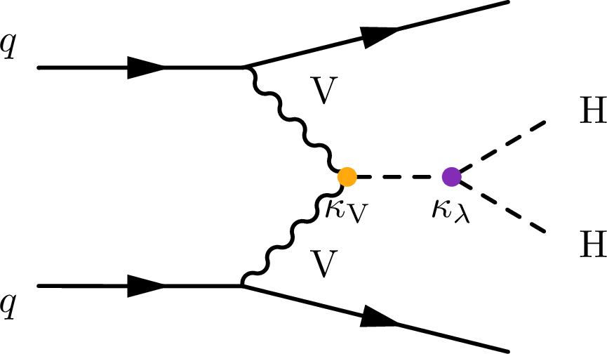
Figure 1-c:
Leading-order Feynman diagrams of HH production in the $ \mathrm{g}\mathrm{g}\text{F} $ production mode assuming top quarks in the fermion loop (top row) and in the $ \text{VBF} $ production mode (bottom row) in the SM. |
png pdf |
Figure 1-d:
Leading-order Feynman diagrams of HH production in the $ \mathrm{g}\mathrm{g}\text{F} $ production mode assuming top quarks in the fermion loop (top row) and in the $ \text{VBF} $ production mode (bottom row) in the SM. |
png pdf |
Figure 1-e:
Leading-order Feynman diagrams of HH production in the $ \mathrm{g}\mathrm{g}\text{F} $ production mode assuming top quarks in the fermion loop (top row) and in the $ \text{VBF} $ production mode (bottom row) in the SM. |
png pdf |
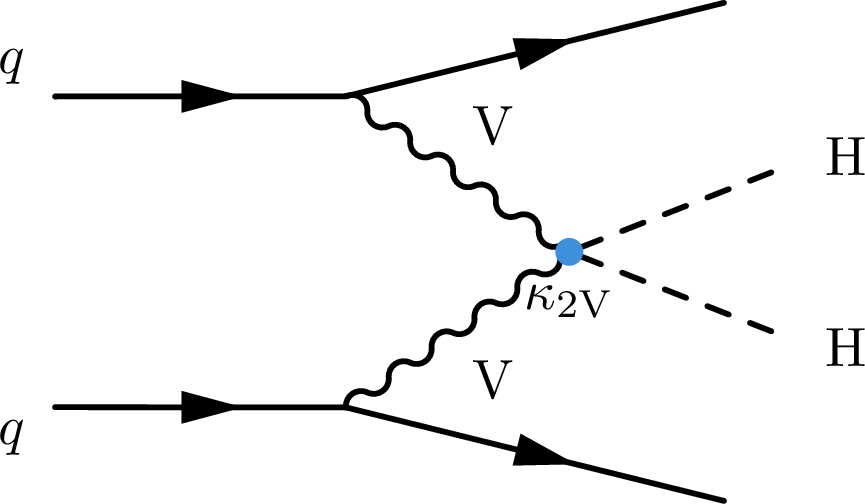
Figure 2:
Illustration of the event categorisation: SRs are depicted in red, background CRs in blue. Details of the NNs are described in the text. The binary NN output distributions (O) and the event yields (Y) in the CRs enter the final fit as sensitive observables. |
png pdf |
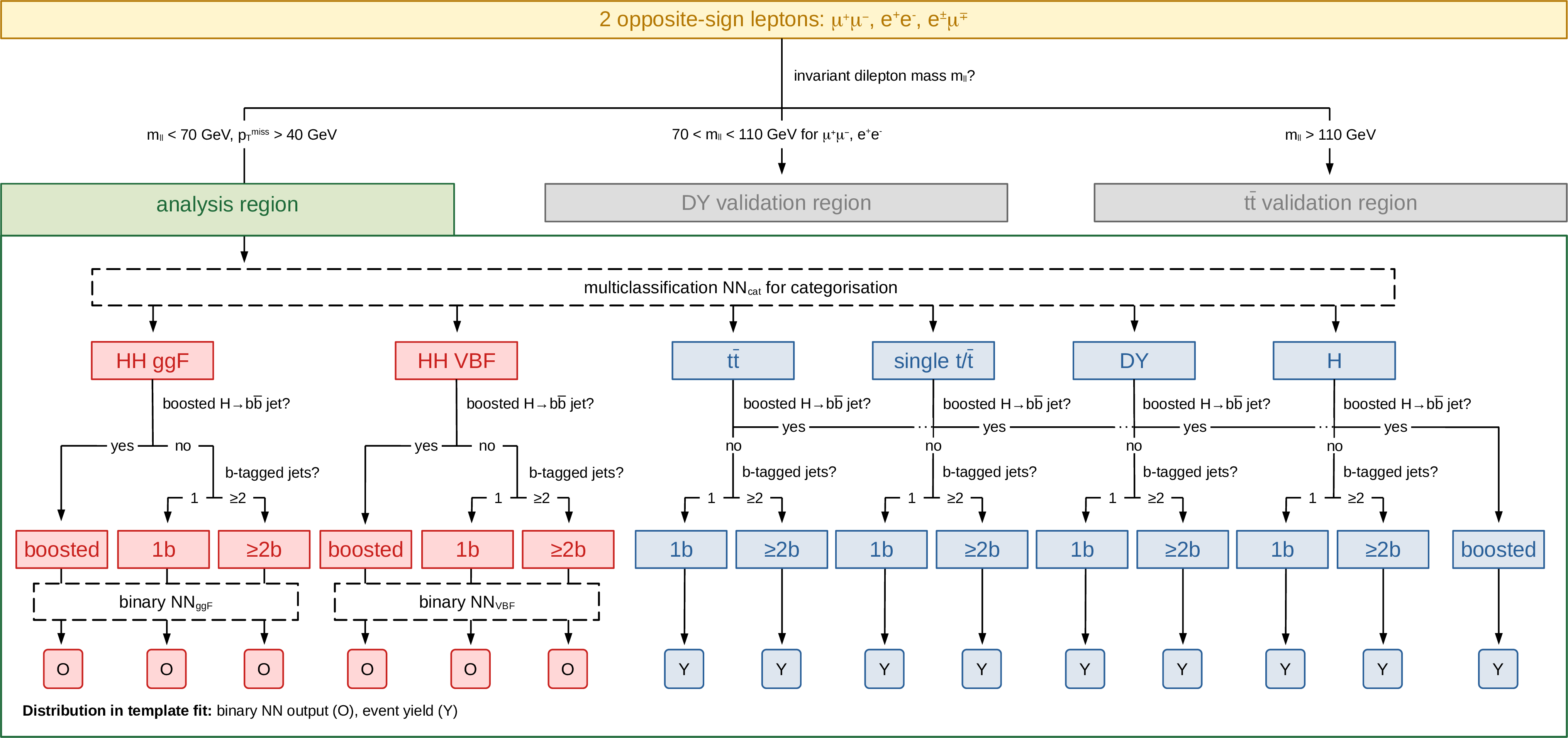
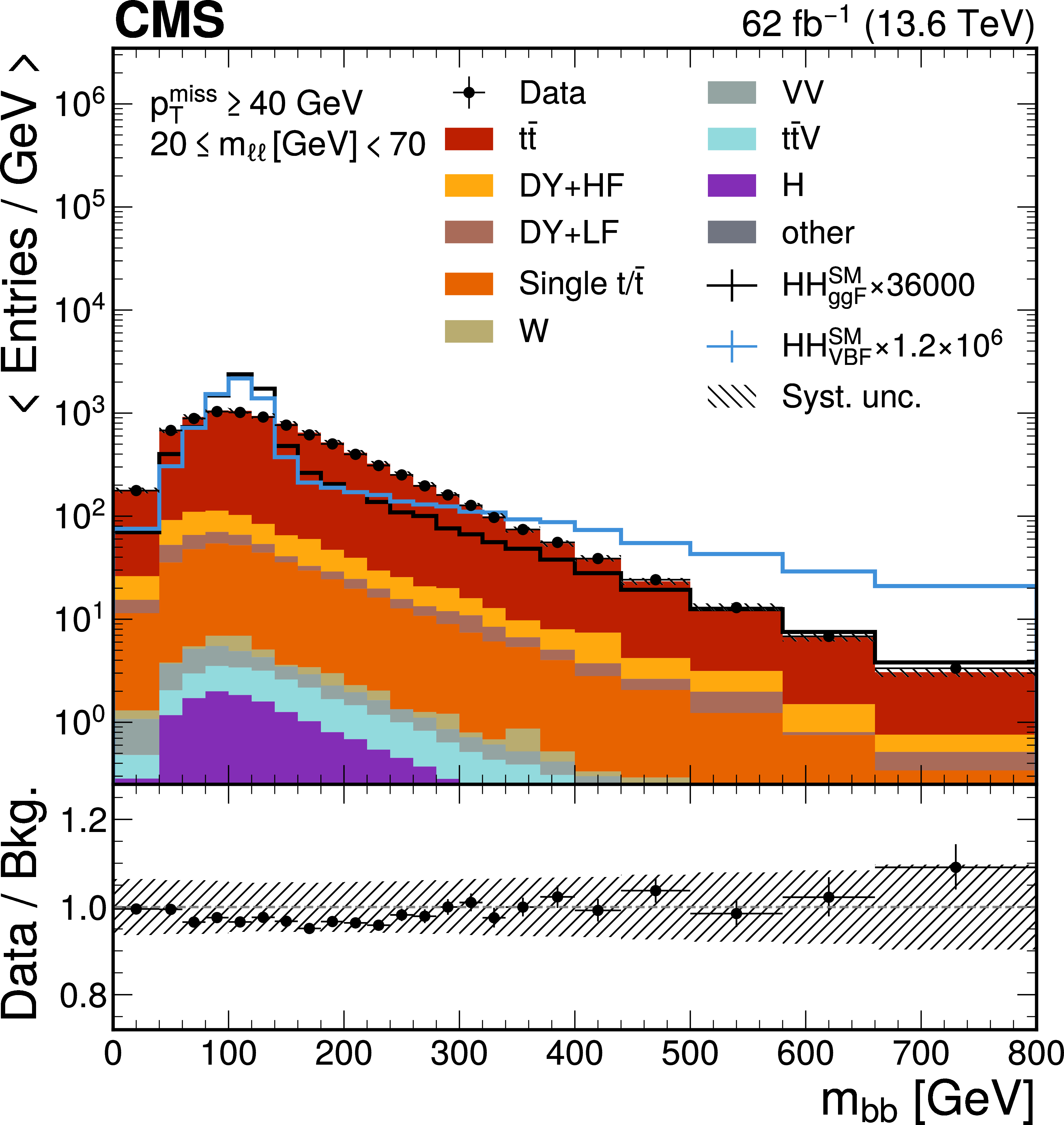
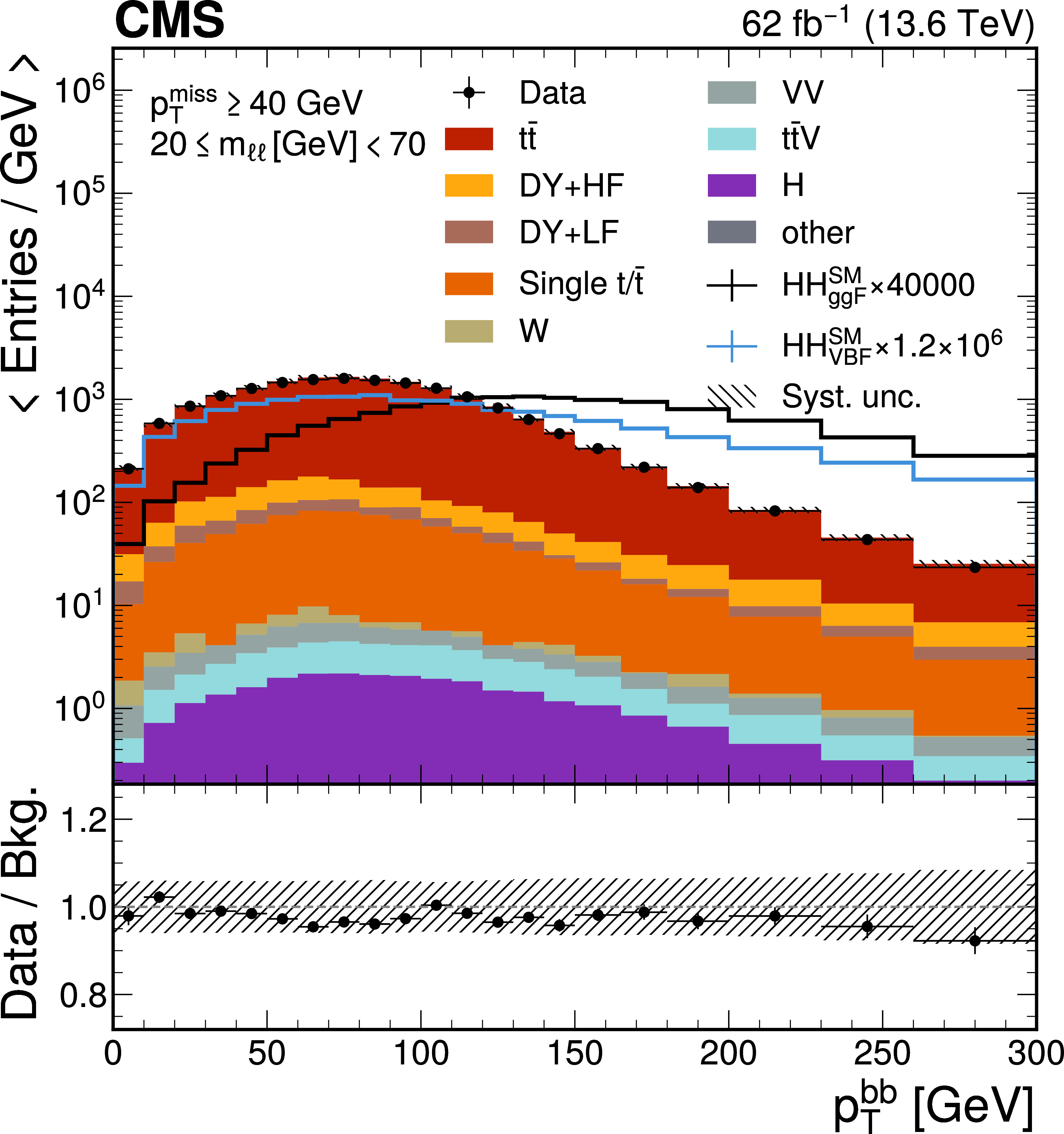
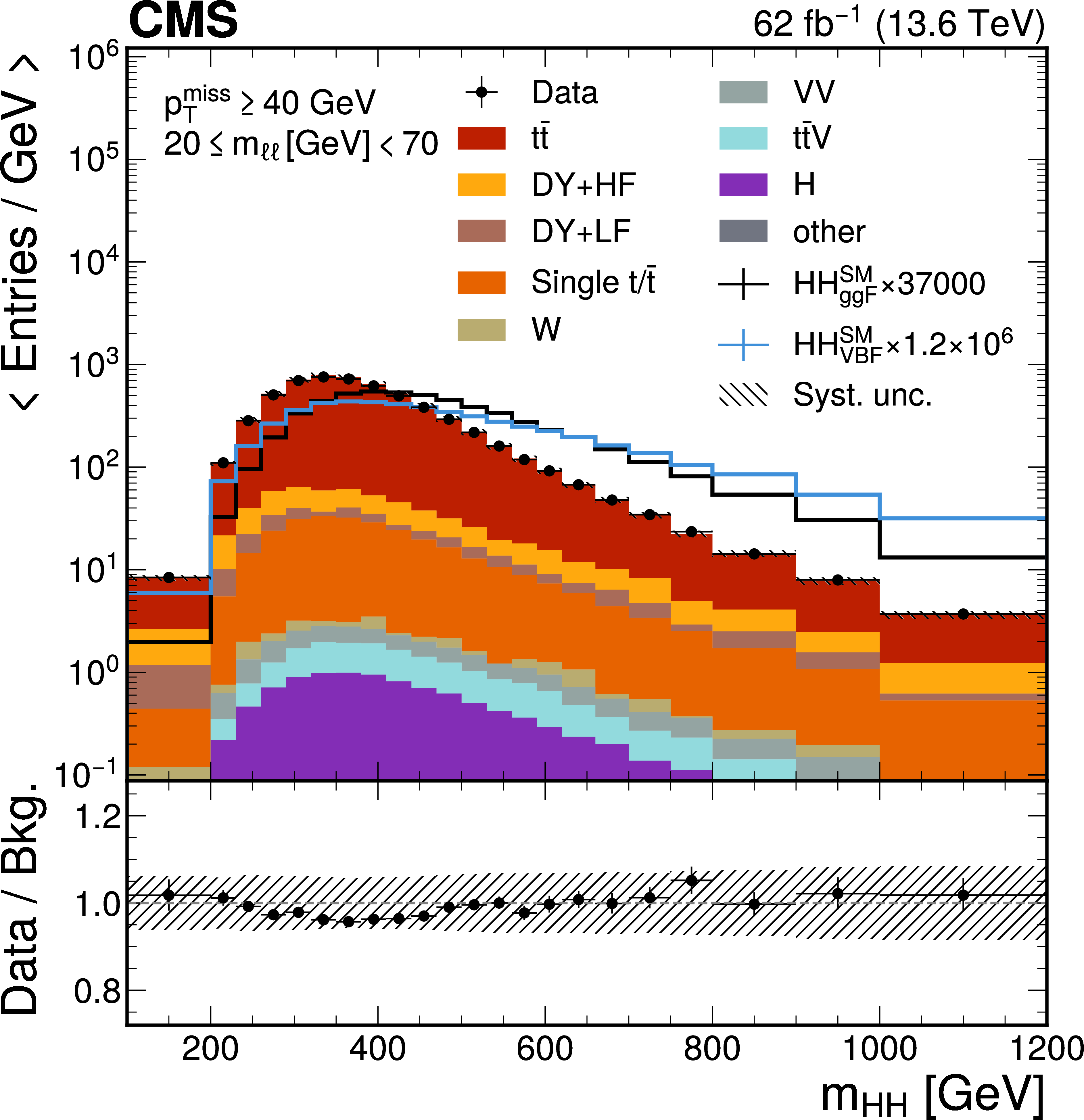
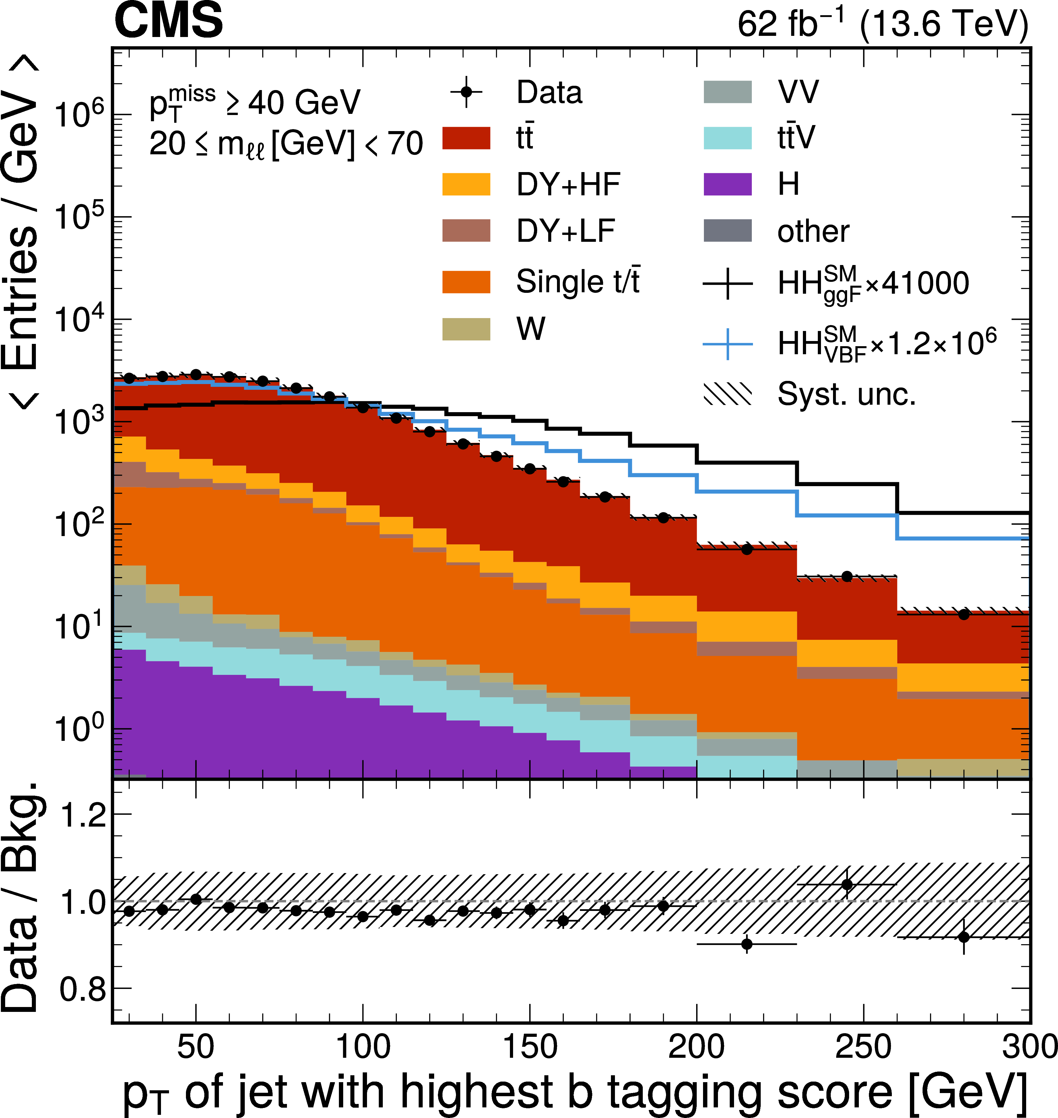
Figure 3:
Invariant mass (upper left) and $ p_{\mathrm{T}} $ (upper right) of the H candidate decaying to $ \mathrm{b}\overline{\mathrm{b}} $, reconstructed as the invariant mass and $ p_{\mathrm{T}} $, respectively, of the two jets with the highest b tagging score; invariant mass of the HH system (lower left), reconstructed as the invariant mass of the two jets with the highest b tagging score, the two leptons, and $ p_{\mathrm{T}}^\text{miss} $; and $ p_{\mathrm{T}} $ of the jet with the highest b tagging score (lower right), for events in the analysis region observed in data (markers) and predicted by the background model (stacked histograms) prior to the fit to data. The HH signal distributions in the $ \mathrm{g}\mathrm{g}\text{F} $ and $ \text{VBF} $ production channels as predicted in the SM, scaled to the total background yield for better visibility, are overlaid (solid lines). The uncertainty band represents the total systematic uncertainty. |
png pdf |
Figure 3-a:
Invariant mass (upper left) and $ p_{\mathrm{T}} $ (upper right) of the H candidate decaying to $ \mathrm{b}\overline{\mathrm{b}} $, reconstructed as the invariant mass and $ p_{\mathrm{T}} $, respectively, of the two jets with the highest b tagging score; invariant mass of the HH system (lower left), reconstructed as the invariant mass of the two jets with the highest b tagging score, the two leptons, and $ p_{\mathrm{T}}^\text{miss} $; and $ p_{\mathrm{T}} $ of the jet with the highest b tagging score (lower right), for events in the analysis region observed in data (markers) and predicted by the background model (stacked histograms) prior to the fit to data. The HH signal distributions in the $ \mathrm{g}\mathrm{g}\text{F} $ and $ \text{VBF} $ production channels as predicted in the SM, scaled to the total background yield for better visibility, are overlaid (solid lines). The uncertainty band represents the total systematic uncertainty. |
png pdf |
Figure 3-b:
Invariant mass (upper left) and $ p_{\mathrm{T}} $ (upper right) of the H candidate decaying to $ \mathrm{b}\overline{\mathrm{b}} $, reconstructed as the invariant mass and $ p_{\mathrm{T}} $, respectively, of the two jets with the highest b tagging score; invariant mass of the HH system (lower left), reconstructed as the invariant mass of the two jets with the highest b tagging score, the two leptons, and $ p_{\mathrm{T}}^\text{miss} $; and $ p_{\mathrm{T}} $ of the jet with the highest b tagging score (lower right), for events in the analysis region observed in data (markers) and predicted by the background model (stacked histograms) prior to the fit to data. The HH signal distributions in the $ \mathrm{g}\mathrm{g}\text{F} $ and $ \text{VBF} $ production channels as predicted in the SM, scaled to the total background yield for better visibility, are overlaid (solid lines). The uncertainty band represents the total systematic uncertainty. |
png pdf |
Figure 3-c:
Invariant mass (upper left) and $ p_{\mathrm{T}} $ (upper right) of the H candidate decaying to $ \mathrm{b}\overline{\mathrm{b}} $, reconstructed as the invariant mass and $ p_{\mathrm{T}} $, respectively, of the two jets with the highest b tagging score; invariant mass of the HH system (lower left), reconstructed as the invariant mass of the two jets with the highest b tagging score, the two leptons, and $ p_{\mathrm{T}}^\text{miss} $; and $ p_{\mathrm{T}} $ of the jet with the highest b tagging score (lower right), for events in the analysis region observed in data (markers) and predicted by the background model (stacked histograms) prior to the fit to data. The HH signal distributions in the $ \mathrm{g}\mathrm{g}\text{F} $ and $ \text{VBF} $ production channels as predicted in the SM, scaled to the total background yield for better visibility, are overlaid (solid lines). The uncertainty band represents the total systematic uncertainty. |
png pdf |
Figure 3-d:
Invariant mass (upper left) and $ p_{\mathrm{T}} $ (upper right) of the H candidate decaying to $ \mathrm{b}\overline{\mathrm{b}} $, reconstructed as the invariant mass and $ p_{\mathrm{T}} $, respectively, of the two jets with the highest b tagging score; invariant mass of the HH system (lower left), reconstructed as the invariant mass of the two jets with the highest b tagging score, the two leptons, and $ p_{\mathrm{T}}^\text{miss} $; and $ p_{\mathrm{T}} $ of the jet with the highest b tagging score (lower right), for events in the analysis region observed in data (markers) and predicted by the background model (stacked histograms) prior to the fit to data. The HH signal distributions in the $ \mathrm{g}\mathrm{g}\text{F} $ and $ \text{VBF} $ production channels as predicted in the SM, scaled to the total background yield for better visibility, are overlaid (solid lines). The uncertainty band represents the total systematic uncertainty. |
png pdf |
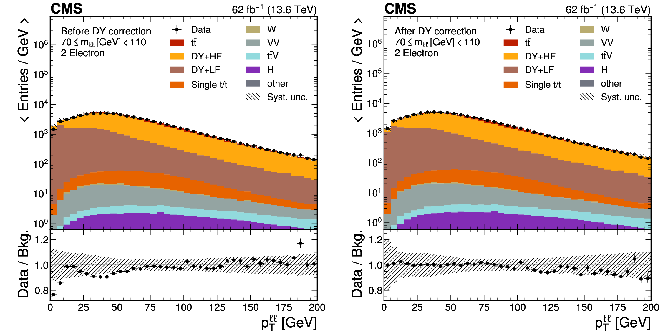
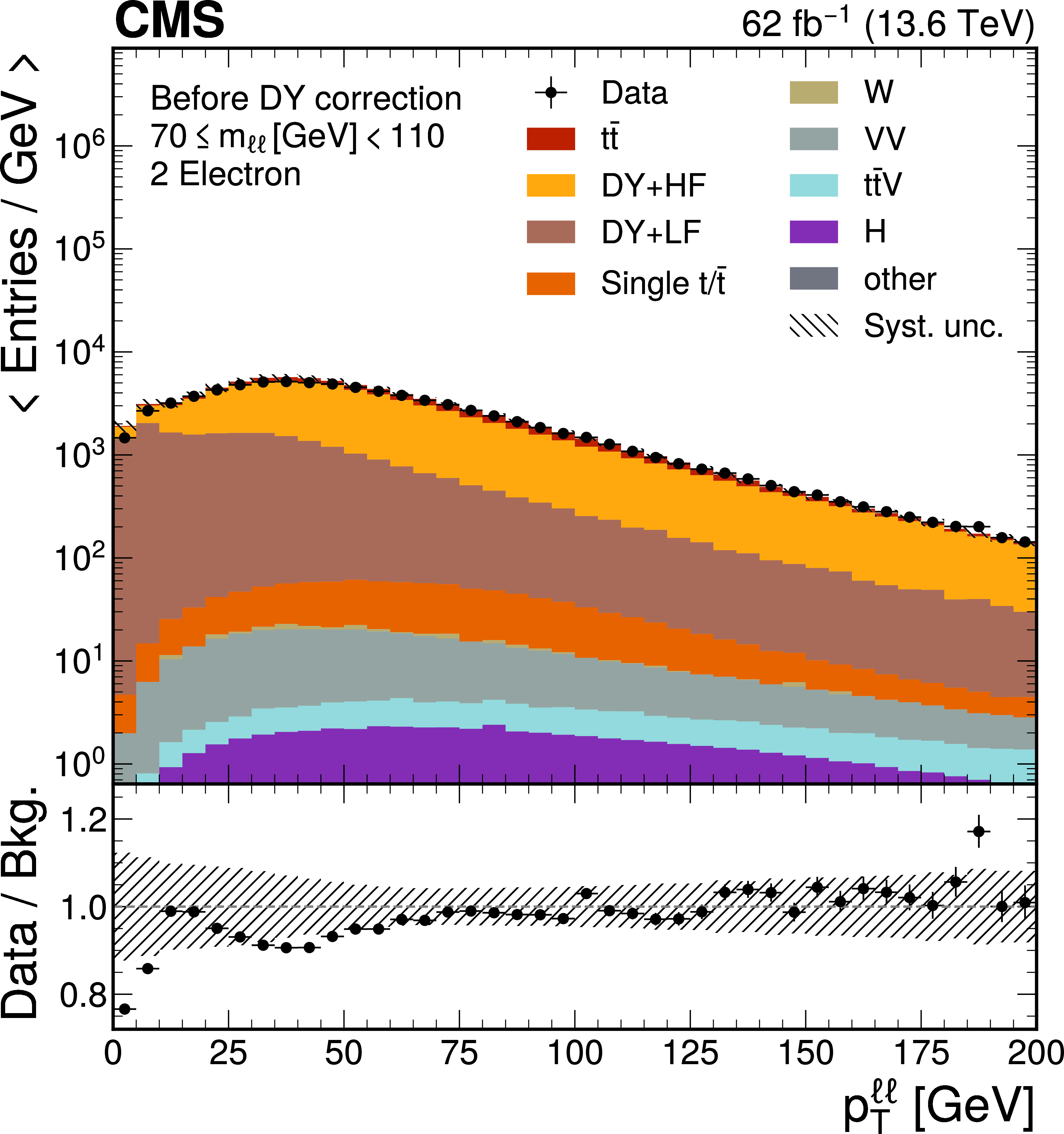
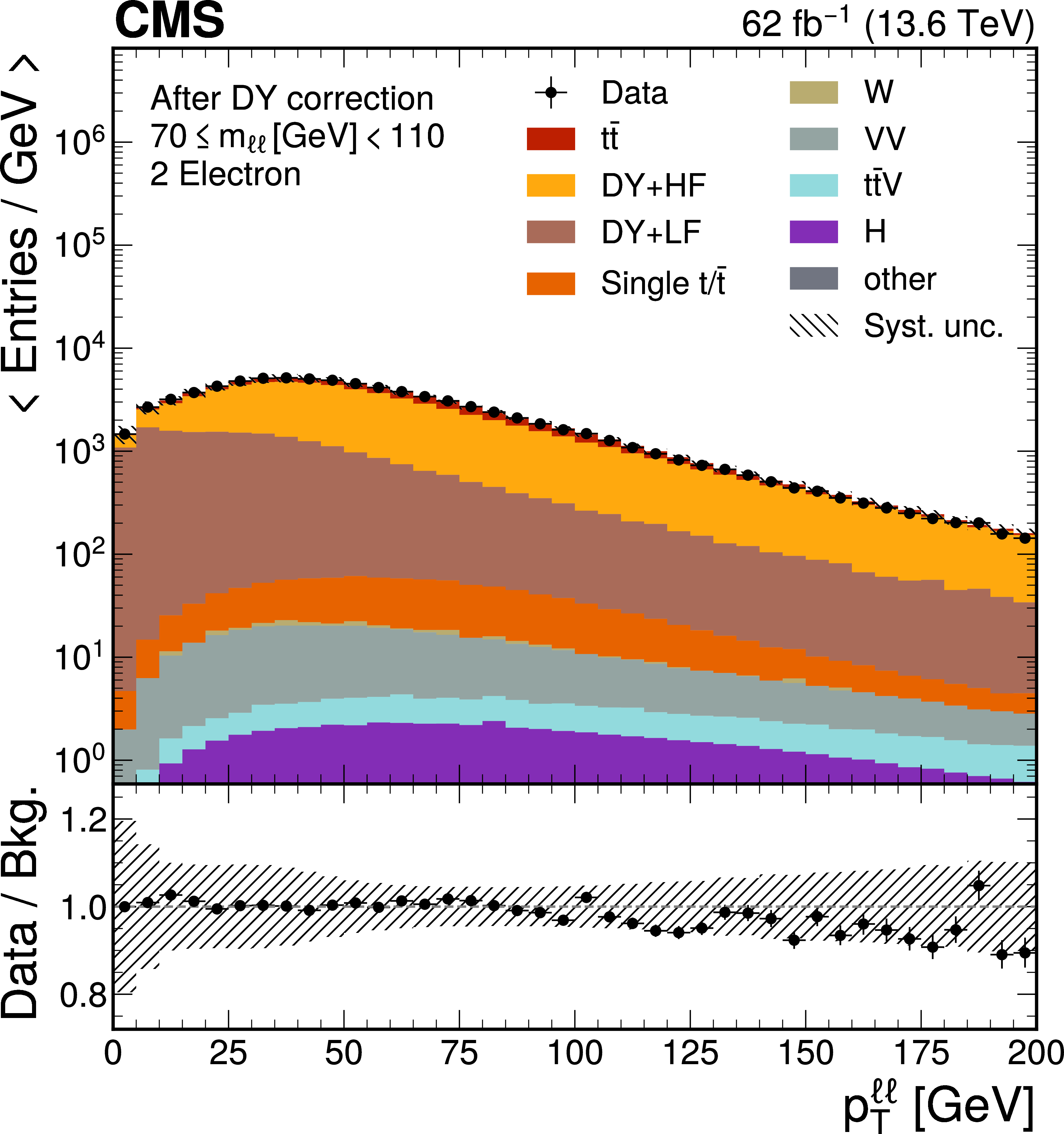
Figure 4:
The $ p_{\mathrm{T}} $ of the dilepton system in $ \mathrm{e}^+\mathrm{e}^- $ events in the DY validation region before (left) and after (right) application of the DY corrections. The uncertainty band shows the total systematic uncertainty. |
png pdf |
Figure 4-a:
The $ p_{\mathrm{T}} $ of the dilepton system in $ \mathrm{e}^+\mathrm{e}^- $ events in the DY validation region before (left) and after (right) application of the DY corrections. The uncertainty band shows the total systematic uncertainty. |
png pdf |
Figure 4-b:
The $ p_{\mathrm{T}} $ of the dilepton system in $ \mathrm{e}^+\mathrm{e}^- $ events in the DY validation region before (left) and after (right) application of the DY corrections. The uncertainty band shows the total systematic uncertainty. |
png pdf |
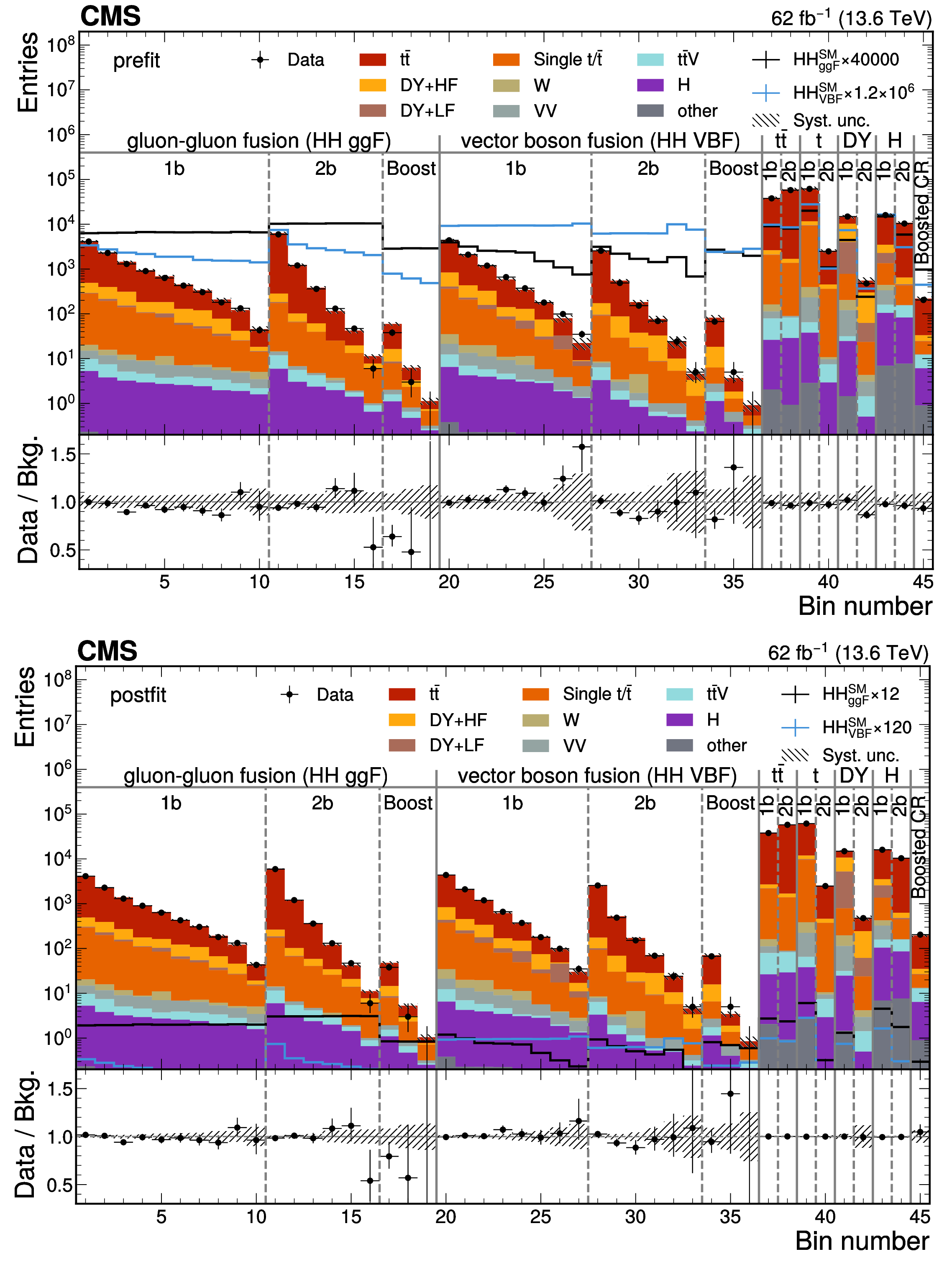
Figure 5:
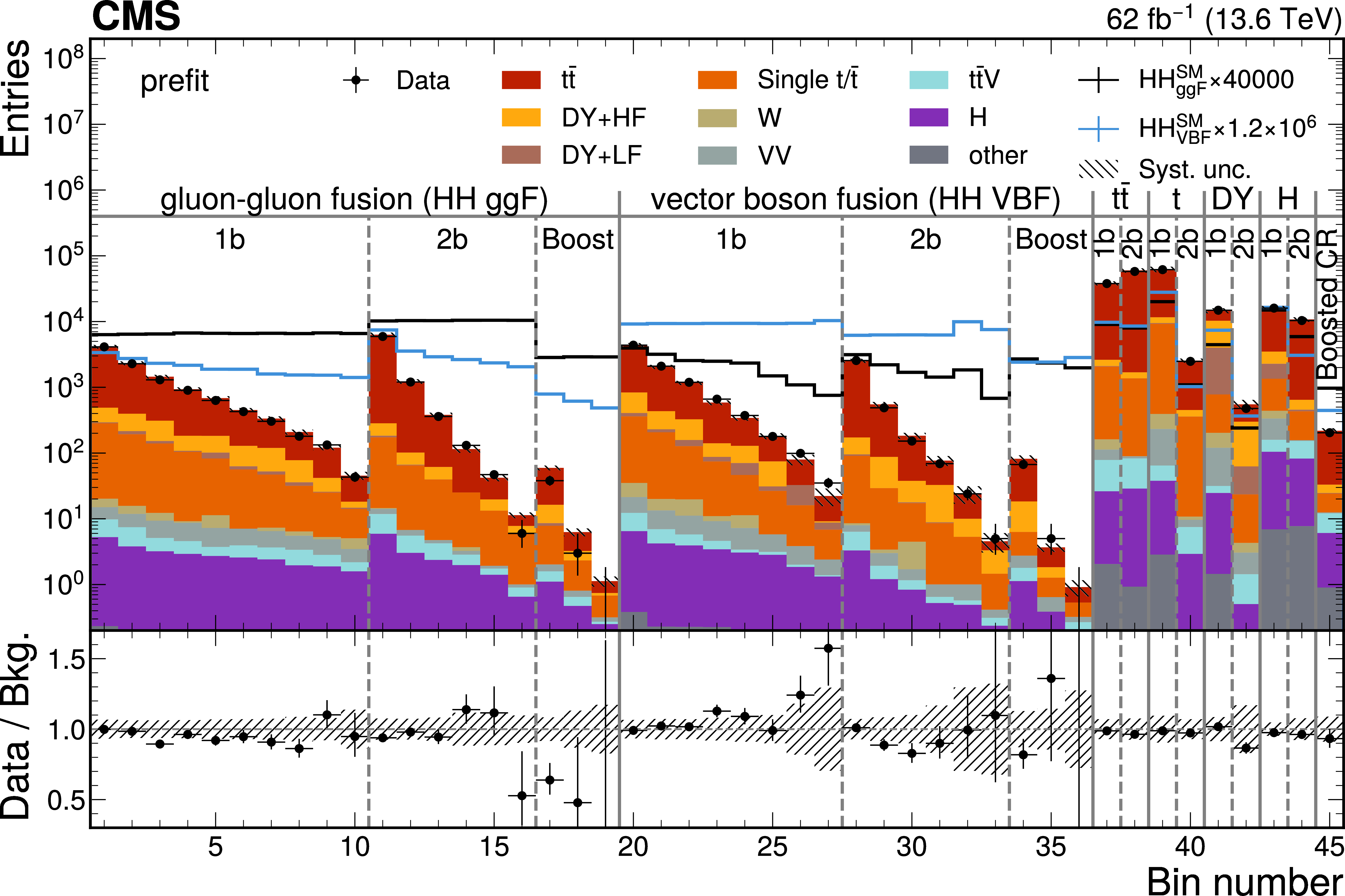
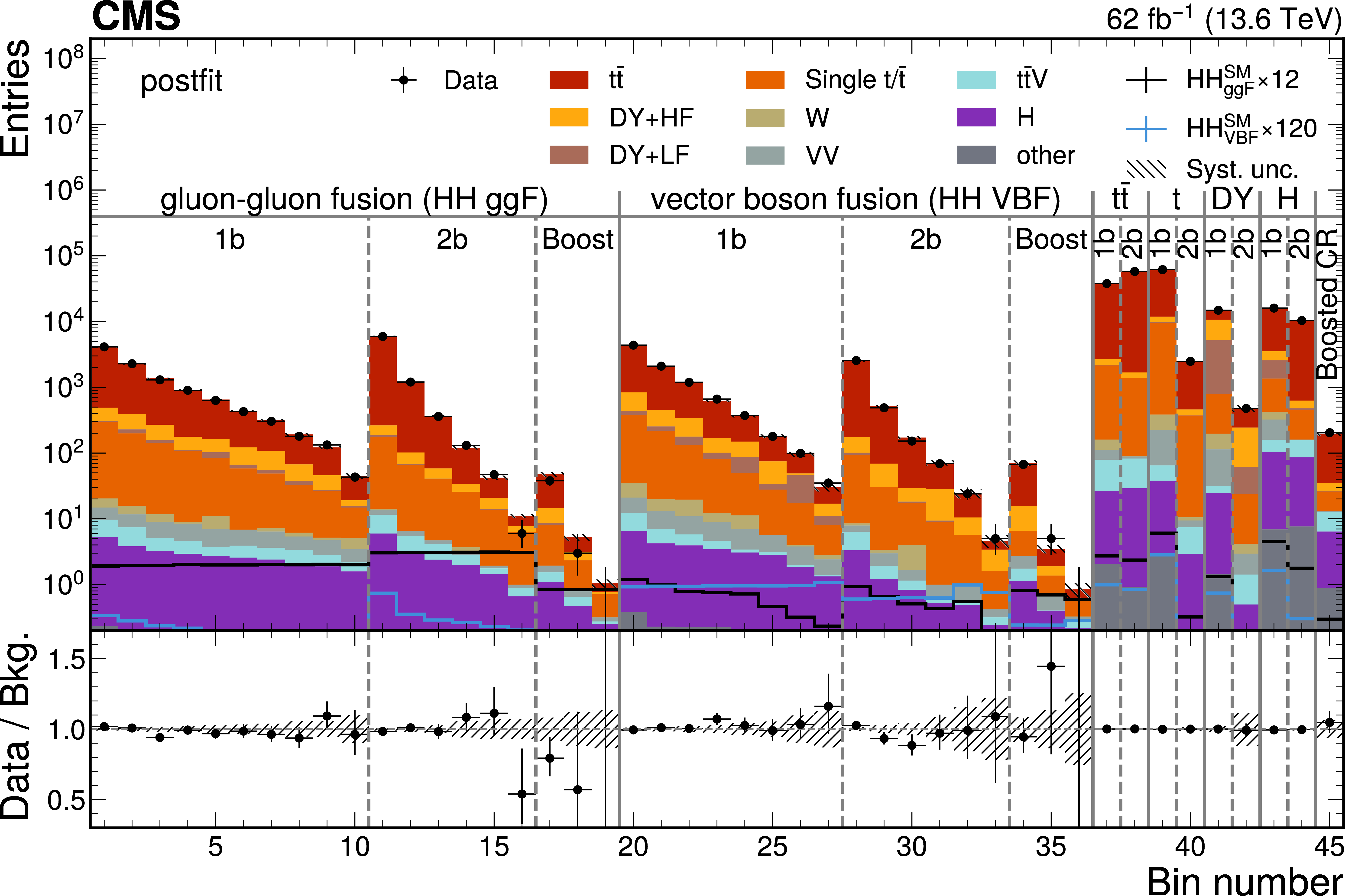
Observed (points) and expected (filled histograms) yields in each discriminant (NN score or category yield) bin before (upper) and after (lower) the fit to data. The HH signal distributions in the $ \mathrm{g}\mathrm{g}\text{F} $ and $ \text{VBF} $ production channels are overlaid (solid lines), scaled to the total background yield (top) or the observed upper limit for $ \mathrm{g}\mathrm{g}\text{F} $ and the observed upper limit times 10 for $ \text{VBF} $ (bottom). The uncertainty bands include the total uncertainty of the fit model. The lower panels show the ratio of the data to the expected background yields. |
png pdf |
Figure 5-a:
Observed (points) and expected (filled histograms) yields in each discriminant (NN score or category yield) bin before (upper) and after (lower) the fit to data. The HH signal distributions in the $ \mathrm{g}\mathrm{g}\text{F} $ and $ \text{VBF} $ production channels are overlaid (solid lines), scaled to the total background yield (top) or the observed upper limit for $ \mathrm{g}\mathrm{g}\text{F} $ and the observed upper limit times 10 for $ \text{VBF} $ (bottom). The uncertainty bands include the total uncertainty of the fit model. The lower panels show the ratio of the data to the expected background yields. |
png pdf |
Figure 5-b:
Observed (points) and expected (filled histograms) yields in each discriminant (NN score or category yield) bin before (upper) and after (lower) the fit to data. The HH signal distributions in the $ \mathrm{g}\mathrm{g}\text{F} $ and $ \text{VBF} $ production channels are overlaid (solid lines), scaled to the total background yield (top) or the observed upper limit for $ \mathrm{g}\mathrm{g}\text{F} $ and the observed upper limit times 10 for $ \text{VBF} $ (bottom). The uncertainty bands include the total uncertainty of the fit model. The lower panels show the ratio of the data to the expected background yields. |
png pdf |
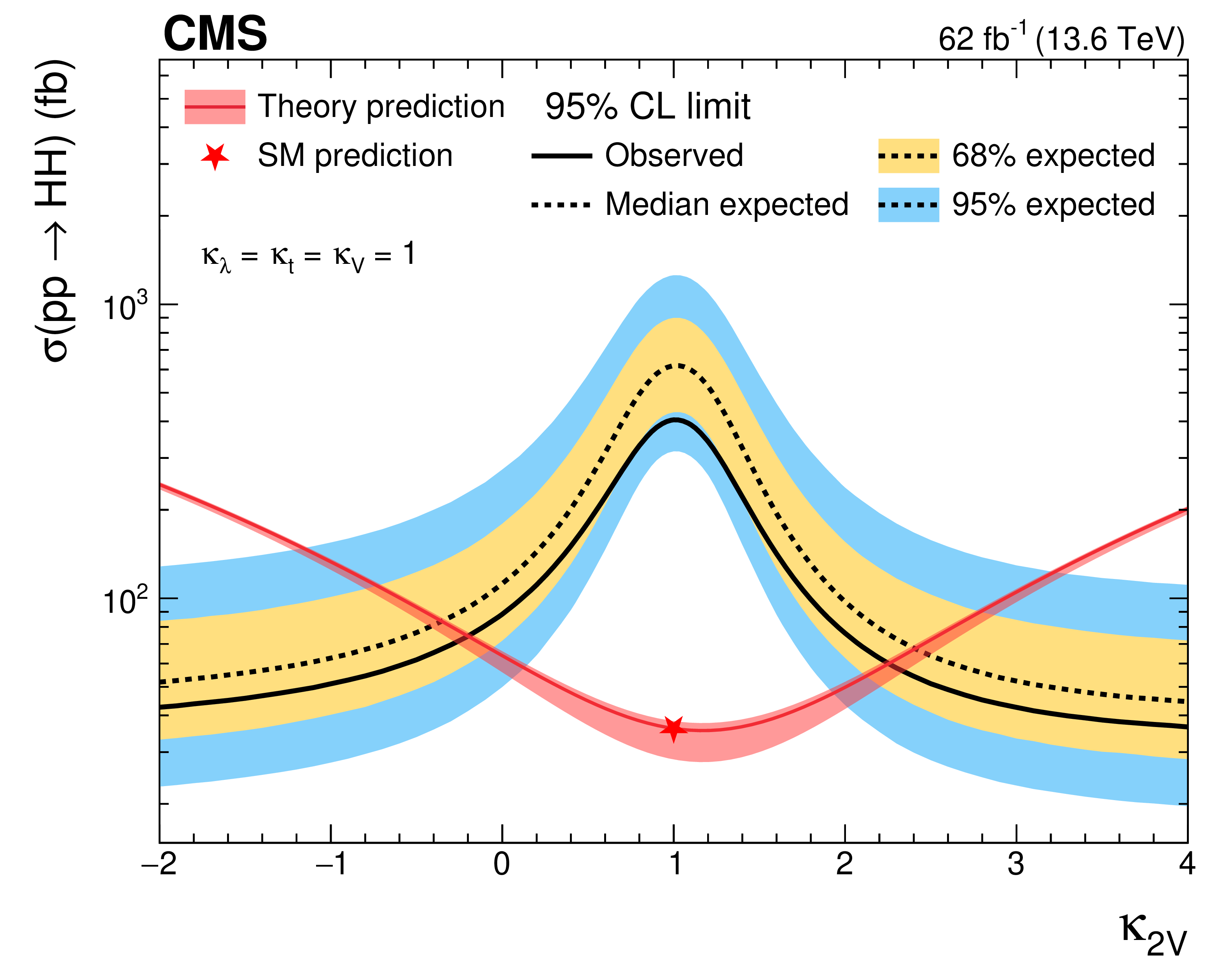
Figure 6:
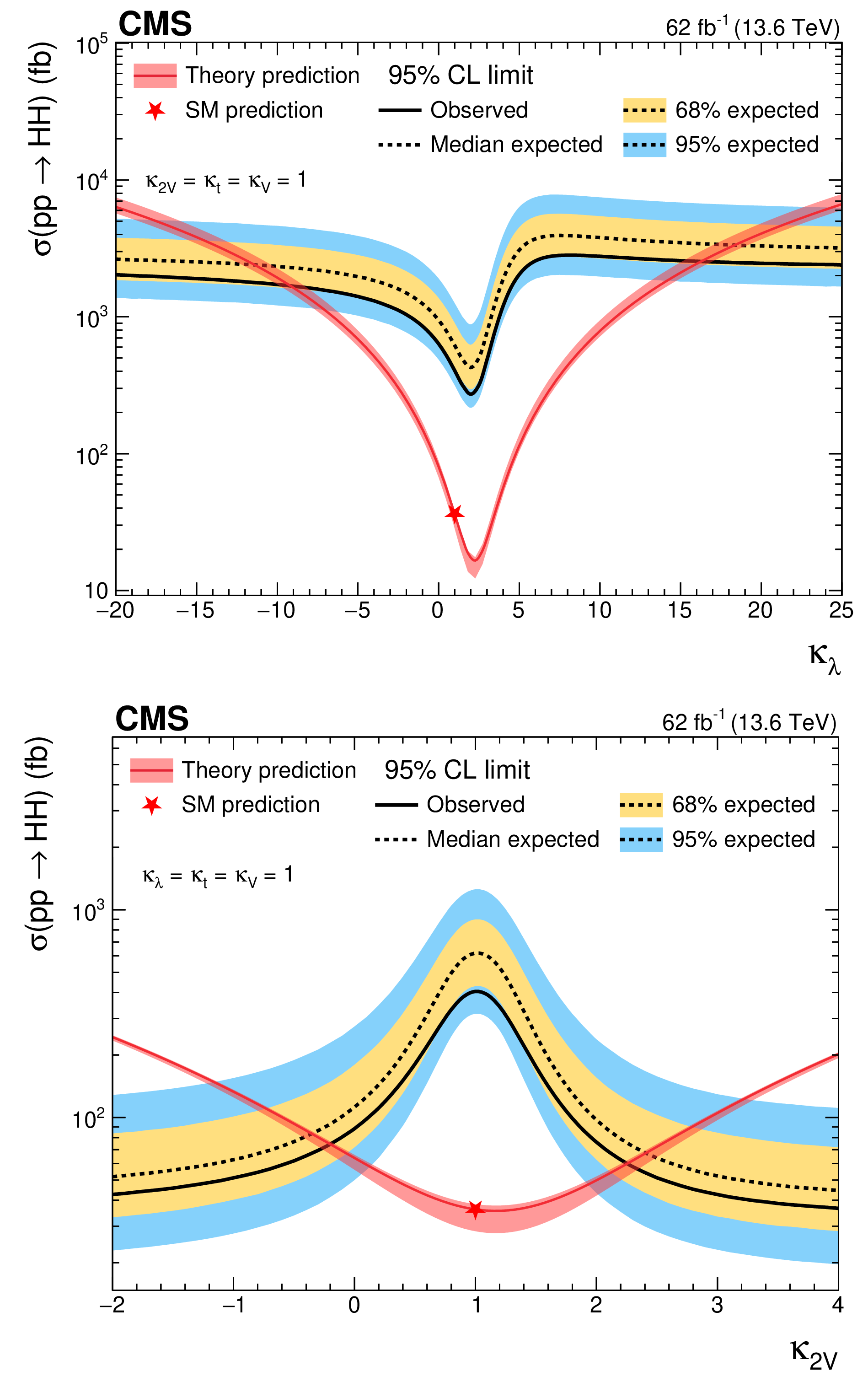
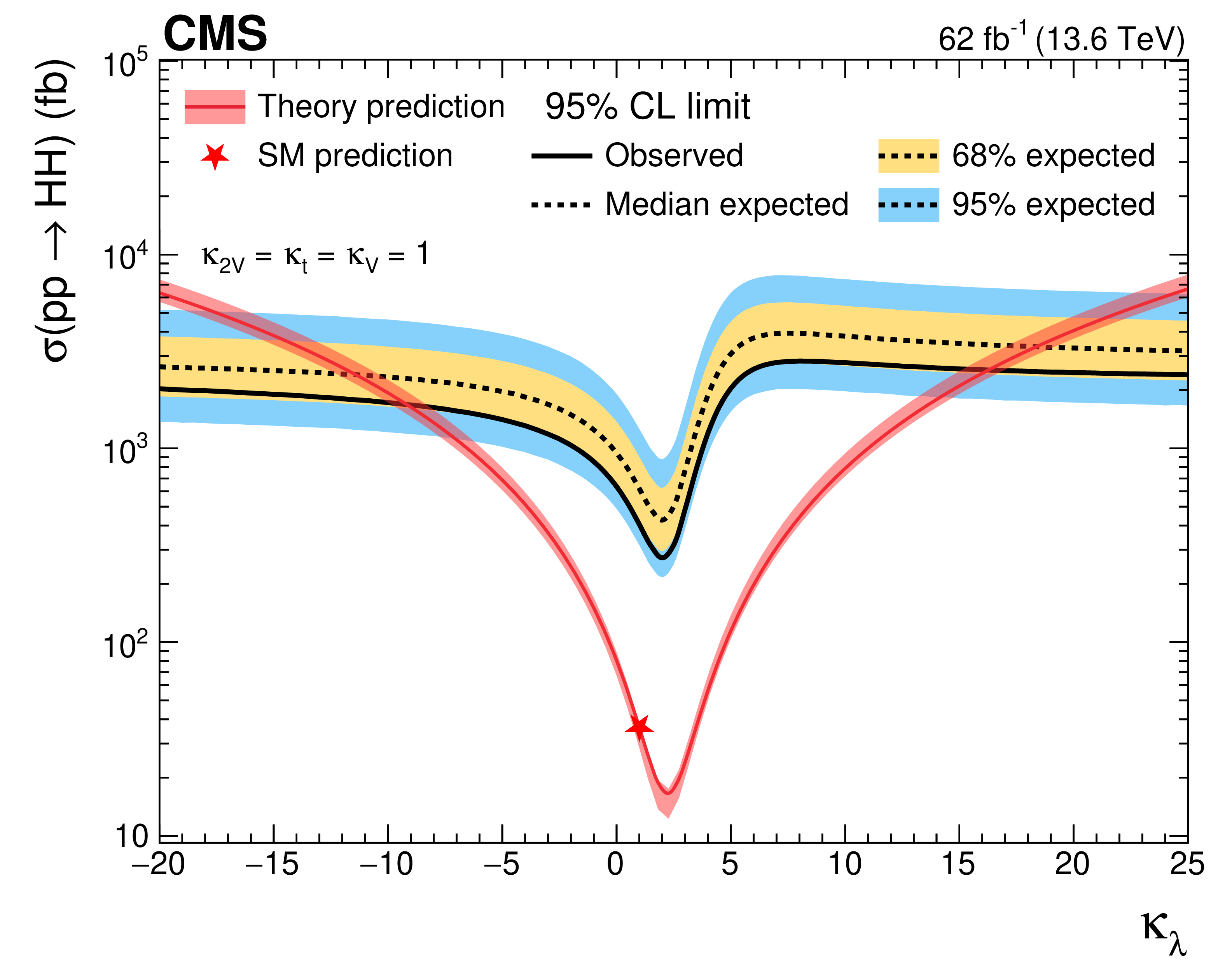
Observed (solid black line) and median expected (dashed black line) upper limits at the 95% CL on the inclusive HH production cross section as a function of $ \kappa_{\lambda} $ (upper) and $ \kappa_{2\mathrm{V}} $ (lower); in both cases, all respective other couplings are fixed to the SM prediction. The yellow (blue) bands show the 68% (95%) confidence level intervals of the expected limit. The predicted cross section is overlaid (red curve), and the SM prediction is indicated (red star). |
png pdf |
Figure 6-a:
Observed (solid black line) and median expected (dashed black line) upper limits at the 95% CL on the inclusive HH production cross section as a function of $ \kappa_{\lambda} $ (upper) and $ \kappa_{2\mathrm{V}} $ (lower); in both cases, all respective other couplings are fixed to the SM prediction. The yellow (blue) bands show the 68% (95%) confidence level intervals of the expected limit. The predicted cross section is overlaid (red curve), and the SM prediction is indicated (red star). |
png pdf |
Figure 6-b:
Observed (solid black line) and median expected (dashed black line) upper limits at the 95% CL on the inclusive HH production cross section as a function of $ \kappa_{\lambda} $ (upper) and $ \kappa_{2\mathrm{V}} $ (lower); in both cases, all respective other couplings are fixed to the SM prediction. The yellow (blue) bands show the 68% (95%) confidence level intervals of the expected limit. The predicted cross section is overlaid (red curve), and the SM prediction is indicated (red star). |
png pdf |
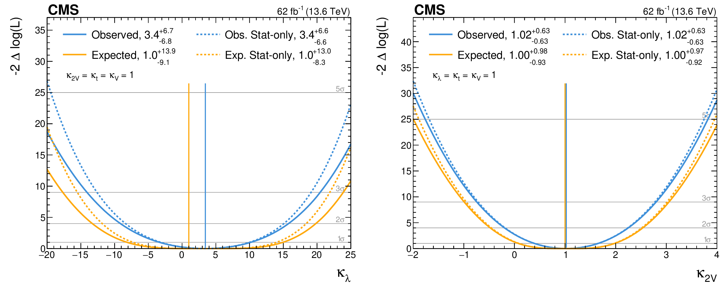
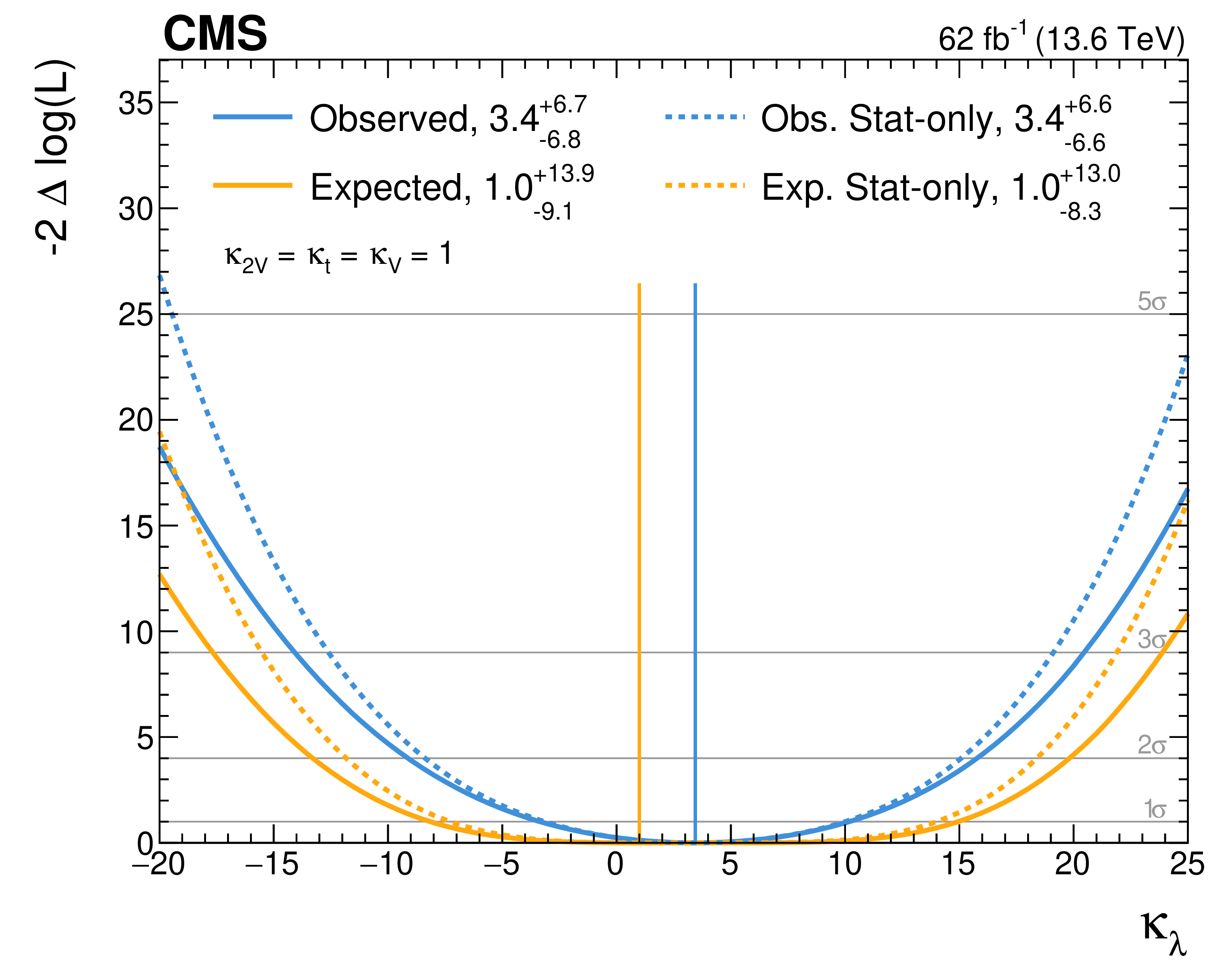
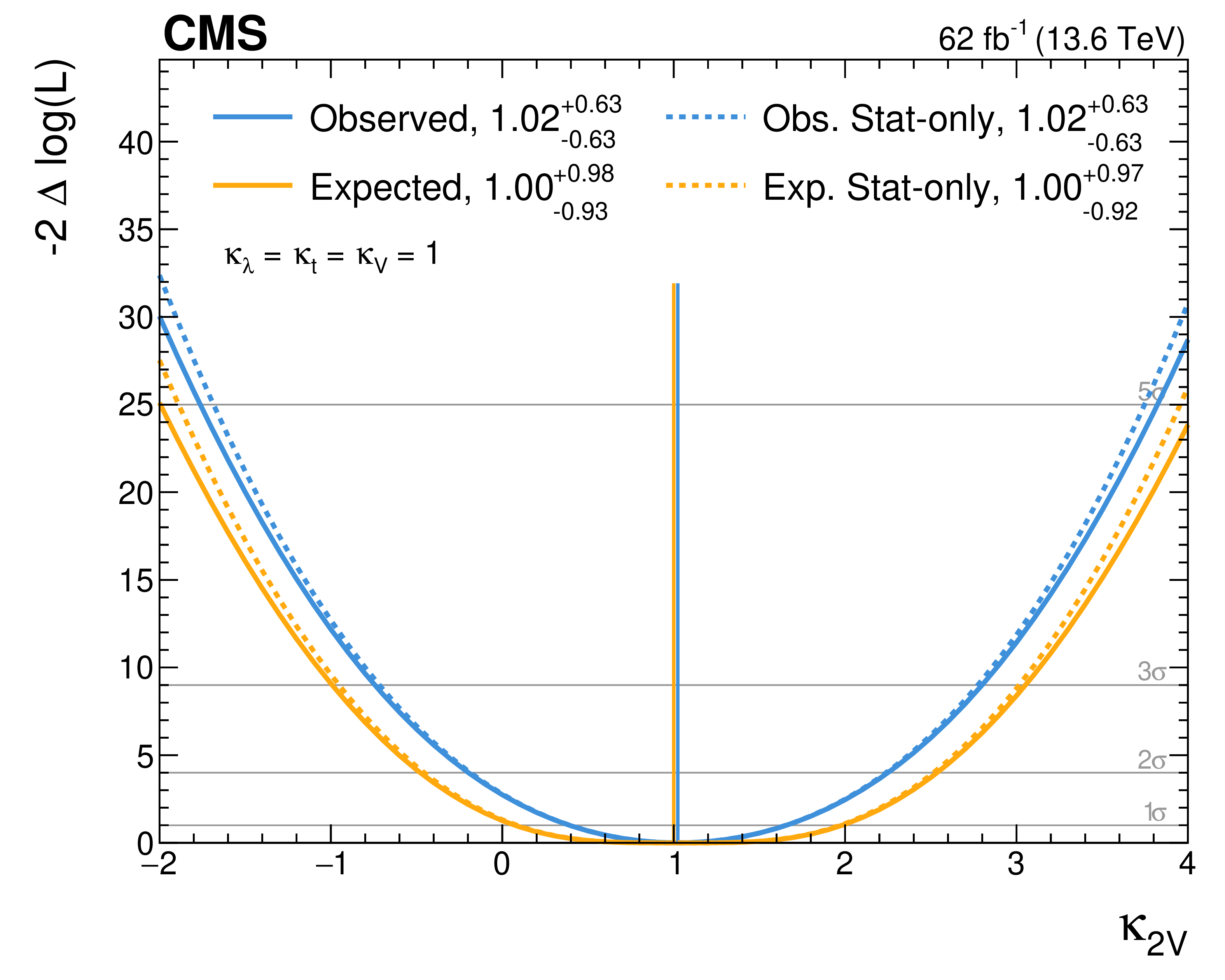
Figure 7:
Observed (blue) and expected (orange) negative log-likelihood values as a function of $ \kappa_{\lambda} $ (left) and $ \kappa_{2\mathrm{V}} $ (right), assuming all other couplings conform to the SM prediction. The solid lines include the full uncertainty model, and the dashed lines only include statistical uncertainties, which include the uncertainty components due to the $ \mathrm{t} \overline{\mathrm{t}} $ and $ \text{DY} $ background normalisations. The vertical lines indicate the best fit value. |
png pdf |
Figure 7-a:
Observed (blue) and expected (orange) negative log-likelihood values as a function of $ \kappa_{\lambda} $ (left) and $ \kappa_{2\mathrm{V}} $ (right), assuming all other couplings conform to the SM prediction. The solid lines include the full uncertainty model, and the dashed lines only include statistical uncertainties, which include the uncertainty components due to the $ \mathrm{t} \overline{\mathrm{t}} $ and $ \text{DY} $ background normalisations. The vertical lines indicate the best fit value. |
png pdf |
Figure 7-b:
Observed (blue) and expected (orange) negative log-likelihood values as a function of $ \kappa_{\lambda} $ (left) and $ \kappa_{2\mathrm{V}} $ (right), assuming all other couplings conform to the SM prediction. The solid lines include the full uncertainty model, and the dashed lines only include statistical uncertainties, which include the uncertainty components due to the $ \mathrm{t} \overline{\mathrm{t}} $ and $ \text{DY} $ background normalisations. The vertical lines indicate the best fit value. |
png pdf |
Figure 8:
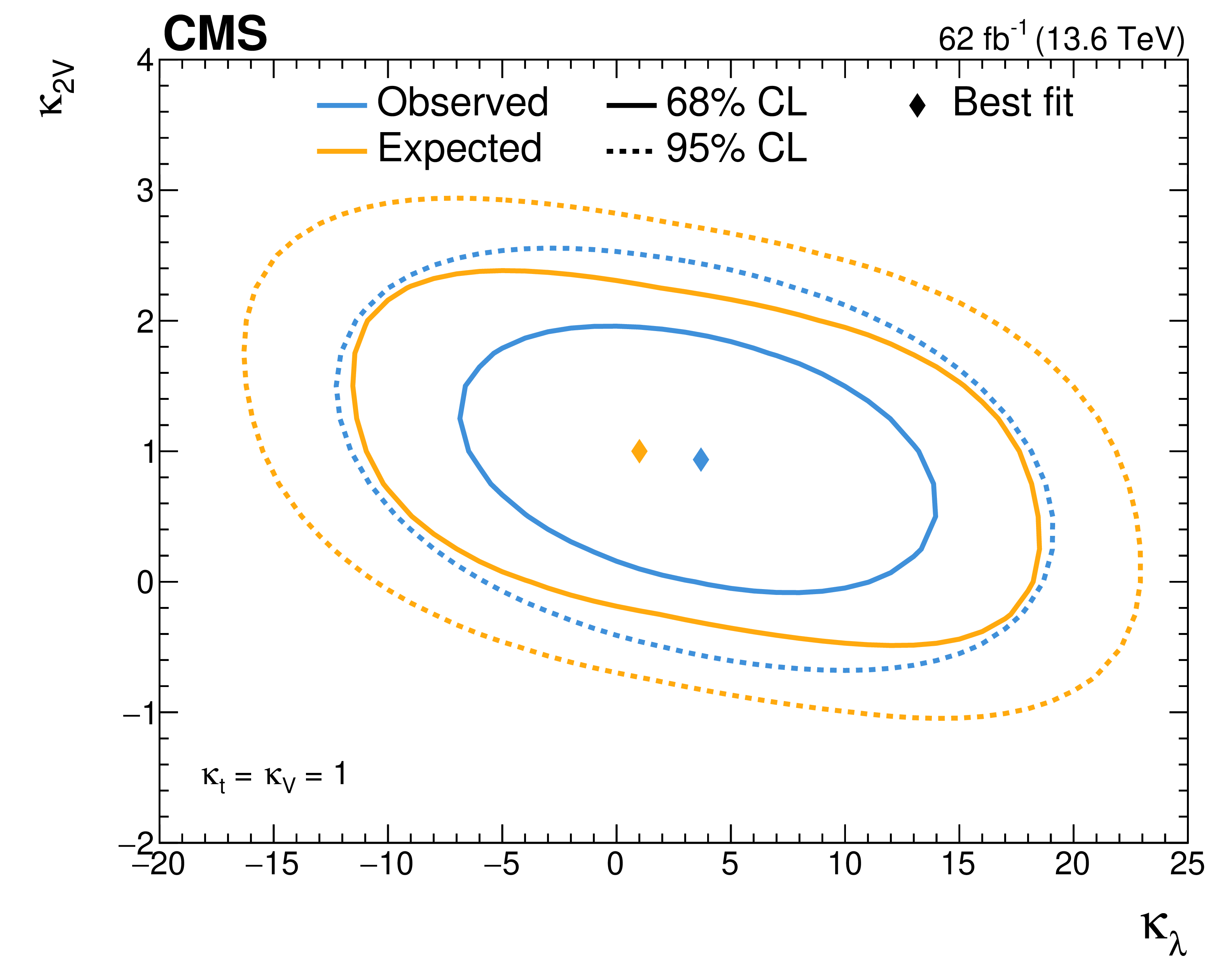
Observed (blue) and expected (orange) negative log-likelihood contours as a function of $ \kappa_{\lambda} $ and $ \kappa_{2\mathrm{V}} $, assuming all other couplings conform to the SM prediction. Shown are the best fit point (marker) and the 68% (solid lines) and 95% (dashed lines) CL contours. |
png pdf |
Figure 9:
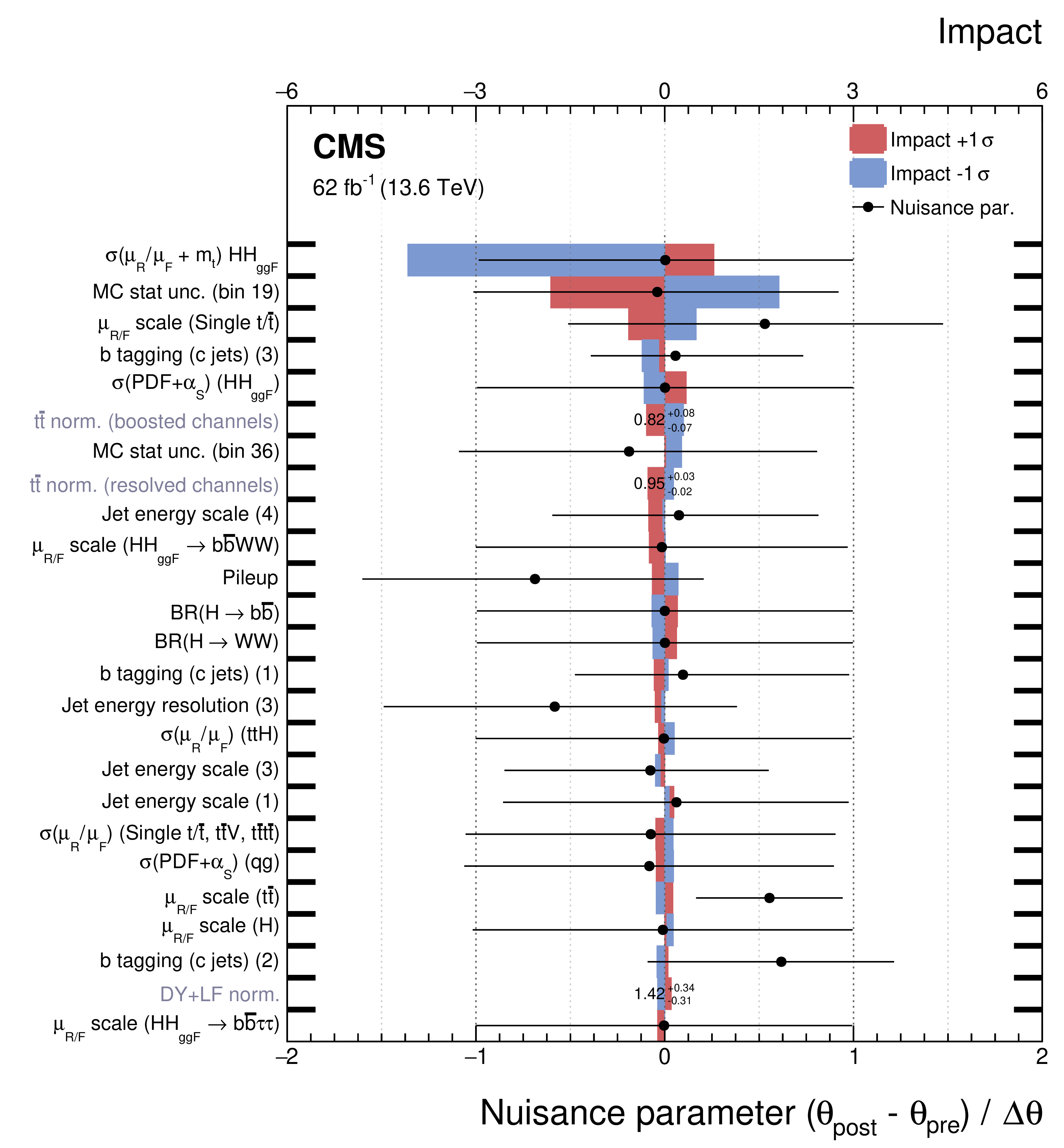
Best fit values of the background normalisation and nuisance parameters (black markers). The nuisance parameter values are shown as the difference of their best fit values, $ \theta_{\text{post}} $, and prefit values, $ \theta_{\text{pre}} $, relative to the prefit uncertainties $ \Delta\theta $. The impact (coloured areas) of the nuisance parameters on the HH signal strength is computed as the difference of the nominal best fit value of the signal strength and the best fit value obtained when fixing the nuisance parameter under scrutiny to its best fit value $ \theta_{\text{post}} $ plus/minus its postfit uncertainty. The nuisance parameters are ordered by their impact, and only the 25 highest-ranked parameters are shown. The number in parentheses for the jet energy scale and b tagging uncertainties correspond to a numbering of the data-taking period to which they are associated. The MC stat unc. refers to the systematic uncertainty due to the limited number of simulated events; in this case, the number in parentheses refers to the bin numbers shown in Fig. 5. |
| Tables | |
png pdf |
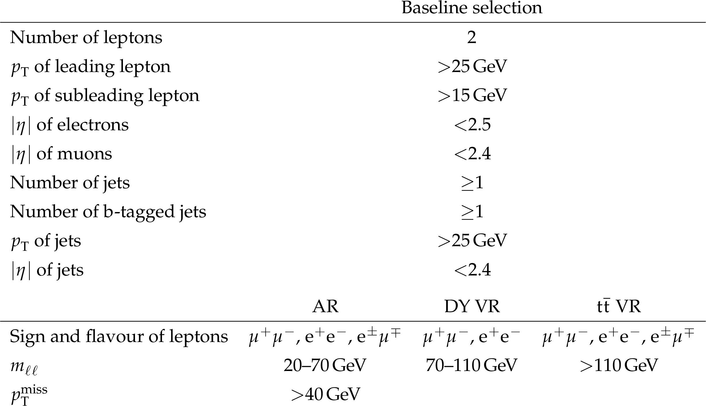
Table 1:
Event selection criteria in the analysis region (AR) and the $ \text{DY} $ and $ \mathrm{t} \overline{\mathrm{t}} $ validation regions (VR). |
png pdf |
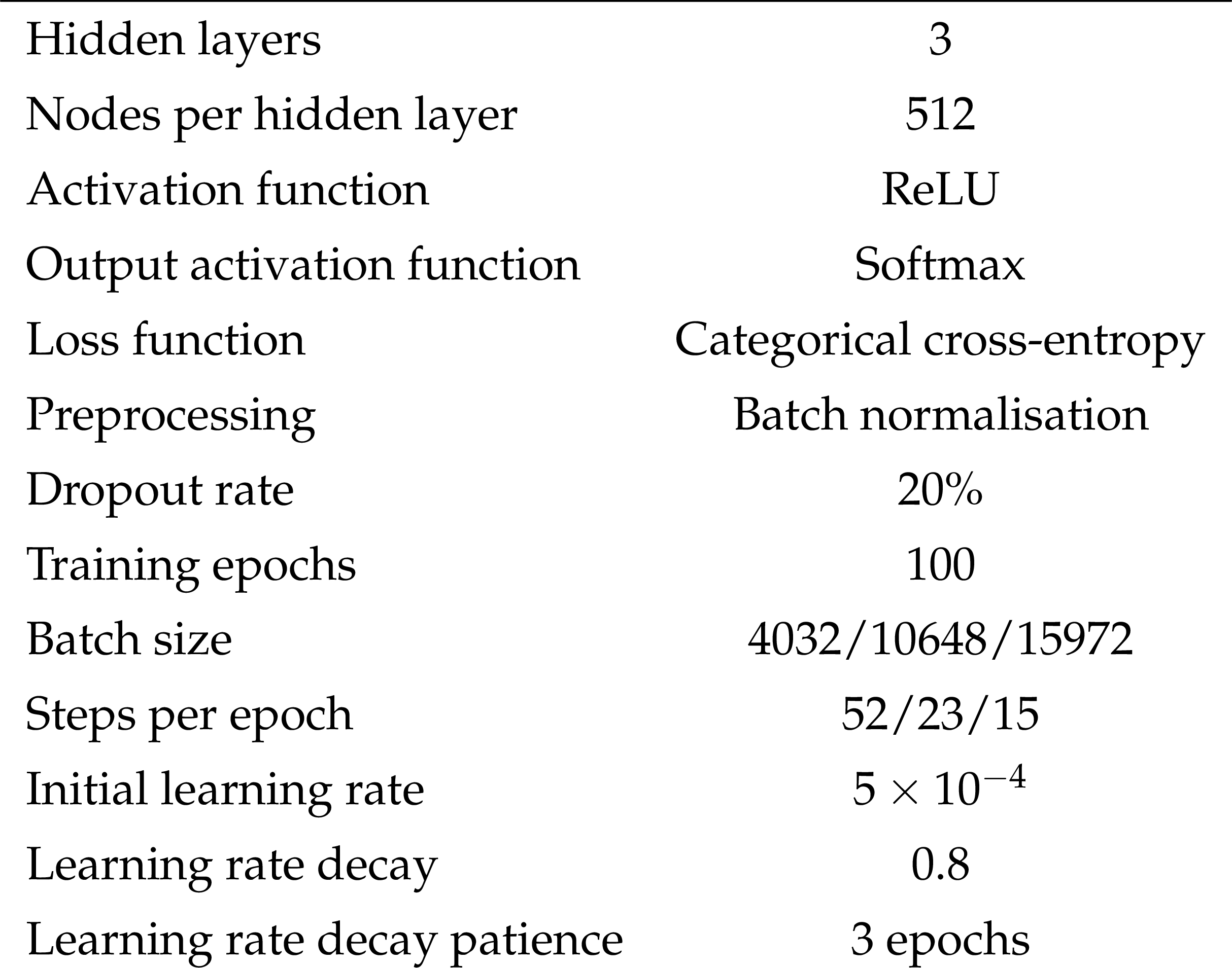
Table 2:
Hyperparameters of the neural networks. Where they differ for the multiclassification $ \text{NN}_{\text{cat}} $ and the binary $ \text{NN}_{\text{ggF}} $ and $ \text{NN}_{\text{VBF}} $, they are listed as ``$ \text{NN}_{\text{cat}} $/$ \text{NN}_{\text{ggF}} $/$ \text{NN}_{\text{VBF}} $'', otherwise they are the same for all networks. |
png pdf |
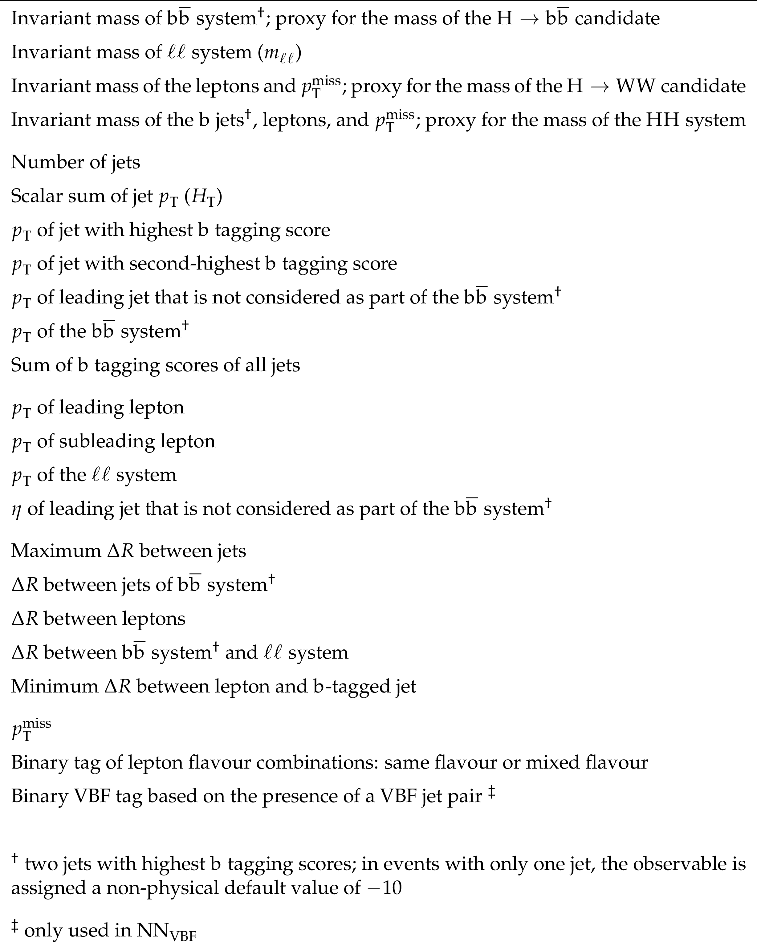
Table 3:
Observables used as input variables to the NNs. |
| Summary |
| A search has been presented for Higgs boson pair production in the $ \mathrm{b}\overline{\mathrm{b}}\mathrm{W}\mathrm{W} $ decay channel with two leptons in the final state, conducted with 62 fb$^{-1}$ of proton-proton collision data collected at $ \sqrt{s}= $ 13.6 TeV. The data are consistent with standard model predictions. An upper limit is set on the Higgs boson pair production cross section of 12.0 times the standard model prediction at the 95% confidence level, with an expectation of 18.5. Compared to a previous search by the CMS Collaboration with 138 fb$ ^{-1} $ of Run 2 data collected at $ \sqrt{s}= $ 13 TeV in final states with one or two leptons, the sensitivity is significantly improved through a refined classification strategy, additional triggers, and an enhanced b tagging algorithm. This yields a comparable overall expected sensitivity despite the smaller analysed data set and restriction to the two-lepton channel, with a 30% sensitivity increase in the two-lepton final state alone. The cross section limit is further used to constrain the trilinear self-coupling of the Higgs boson and the quartic coupling between two Higgs bosons and two vector bosons to $ [-9.1,15.7] $ ($ [-13.3,19.8] $ expected) and $ [-0.20,2.25] $ ($ [-0.48,2.54] $ expected) times the standard model expectation, respectively, at 95% confidence level. The presented search is the first result on Higgs boson pair production in the $ \mathrm{b}\overline{\mathrm{b}}\mathrm{W}\mathrm{W} $ decay channel with $ \sqrt{s}= $ 13.6 TeV data. |
| Additional Figures | |
png pdf |
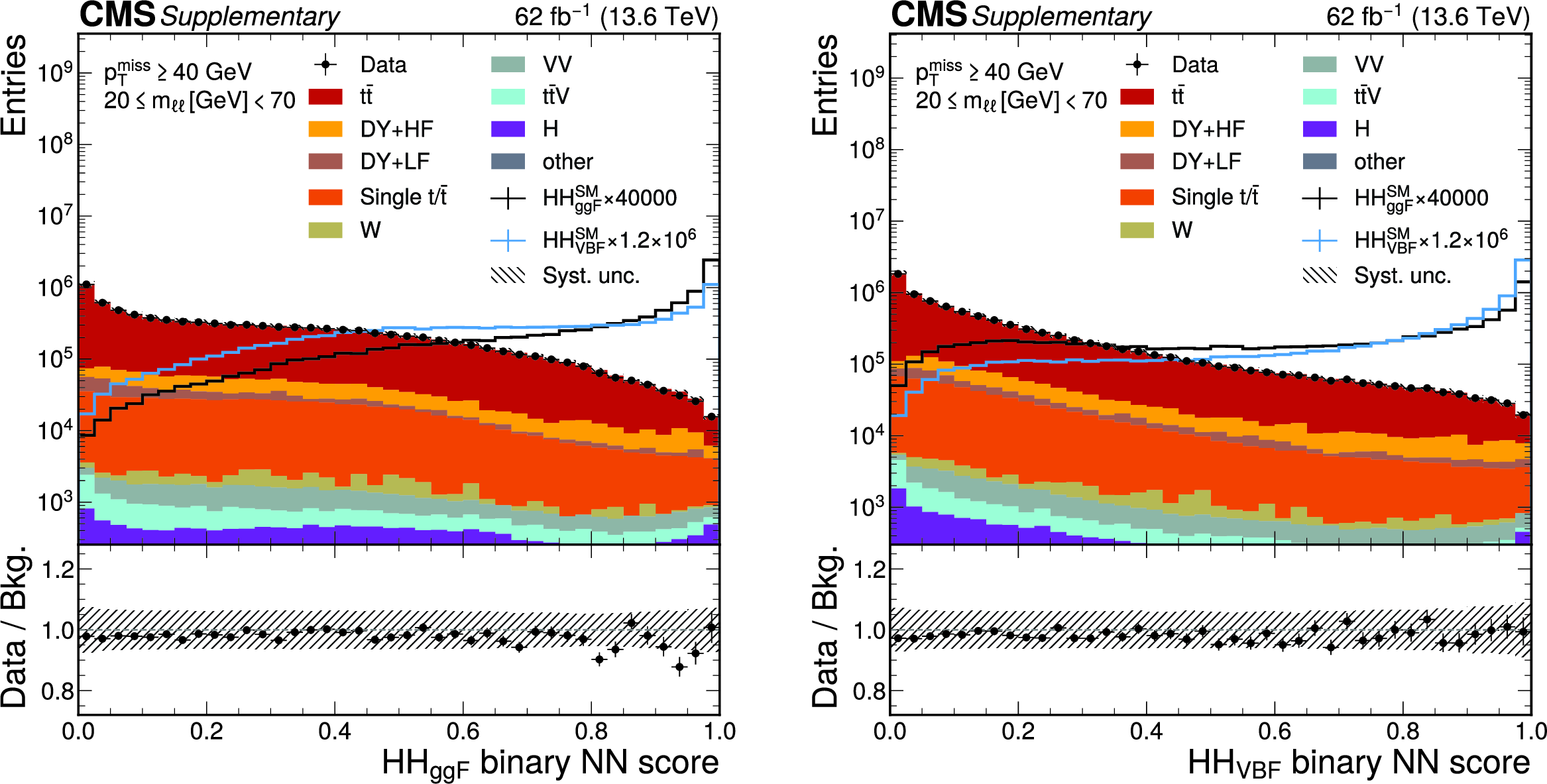
Additional Figure 1:
Distribution of the output score of the binary NN$_{ggF}$ (left) and NN$_{VBF}$ (right) classifiers for all events in the analysis region, i.e. before categorisation by the NN$_{cat}$, observed in data (markers) and predicted by the background model (stacked histograms) prior to the fit to data. The HH signal distributions in the ggF and VBF production channels as predicted in the SM, scaled to the total background yield for better visibility, are overlayed (solid lines). The uncertainty band represents the total systematic uncertainty. |
png pdf |
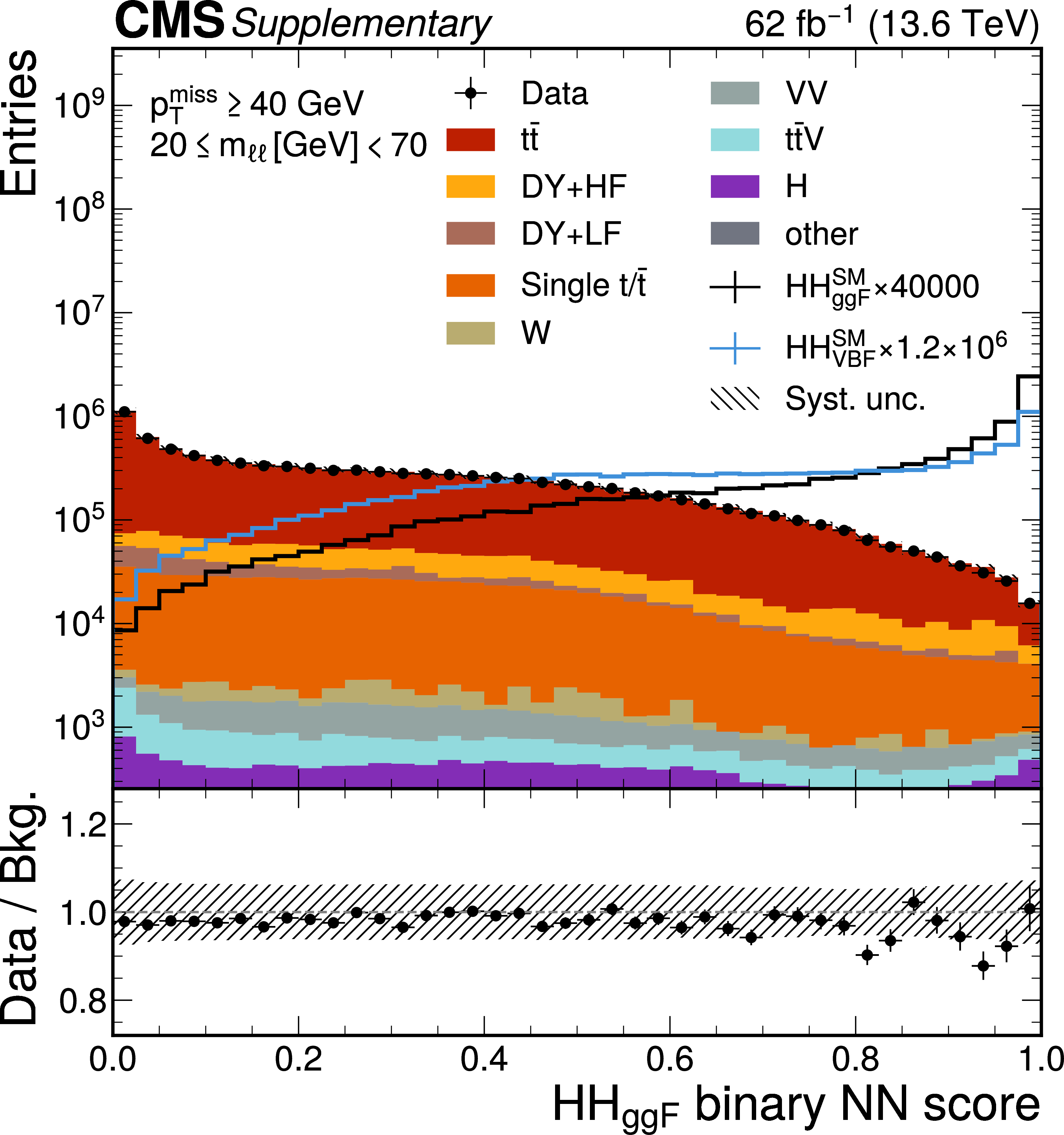
Additional Figure 1-a:
Distribution of the output score of the binary NN$_{ggF}$ (left) and NN$_{VBF}$ (right) classifiers for all events in the analysis region, i.e. before categorisation by the NN$_{cat}$, observed in data (markers) and predicted by the background model (stacked histograms) prior to the fit to data. The HH signal distributions in the ggF and VBF production channels as predicted in the SM, scaled to the total background yield for better visibility, are overlayed (solid lines). The uncertainty band represents the total systematic uncertainty. |
png pdf |
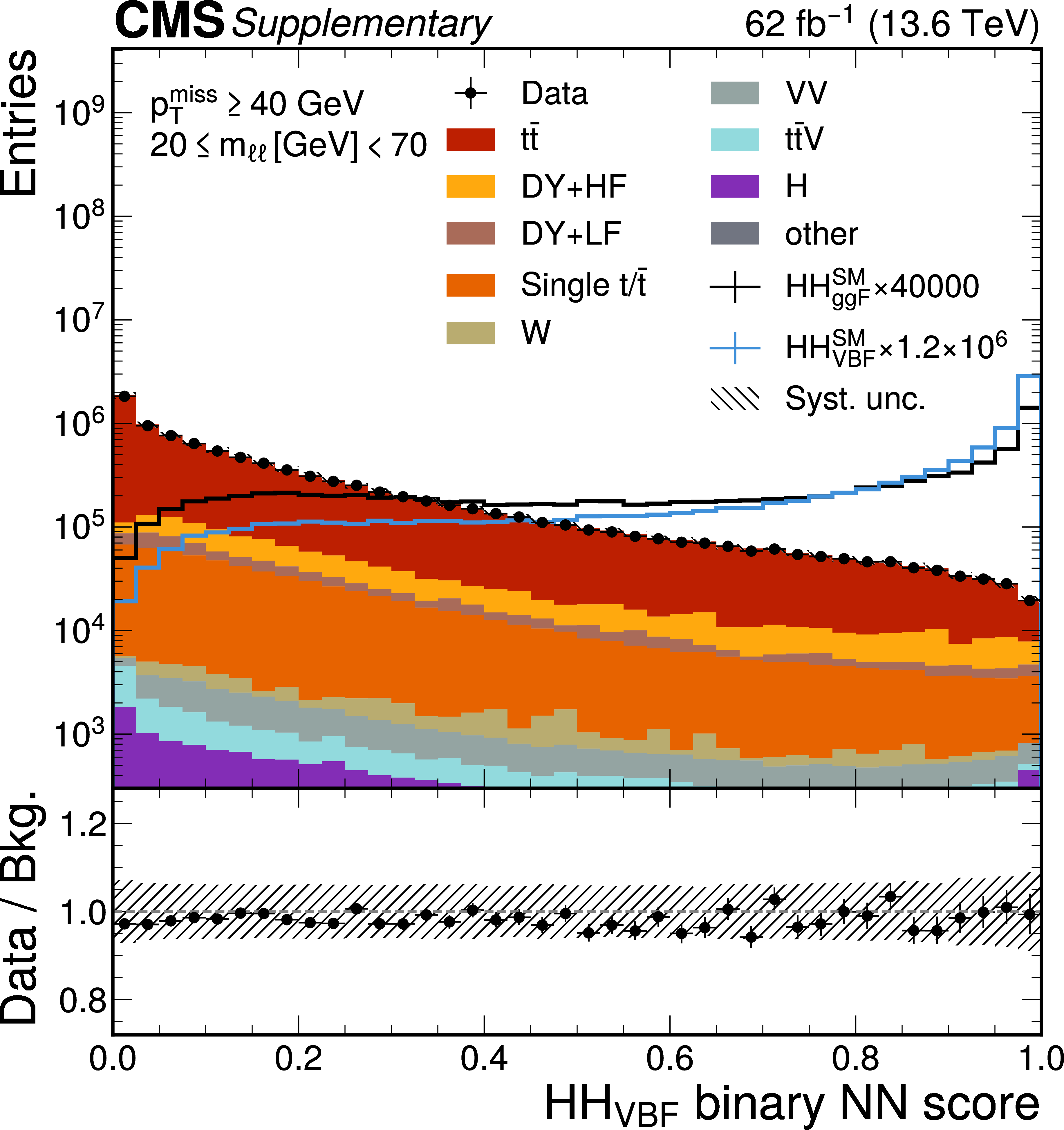
Additional Figure 1-b:
Distribution of the output score of the binary NN$_{ggF}$ (left) and NN$_{VBF}$ (right) classifiers for all events in the analysis region, i.e. before categorisation by the NN$_{cat}$, observed in data (markers) and predicted by the background model (stacked histograms) prior to the fit to data. The HH signal distributions in the ggF and VBF production channels as predicted in the SM, scaled to the total background yield for better visibility, are overlayed (solid lines). The uncertainty band represents the total systematic uncertainty. |
png pdf |
Additional Figure 2:
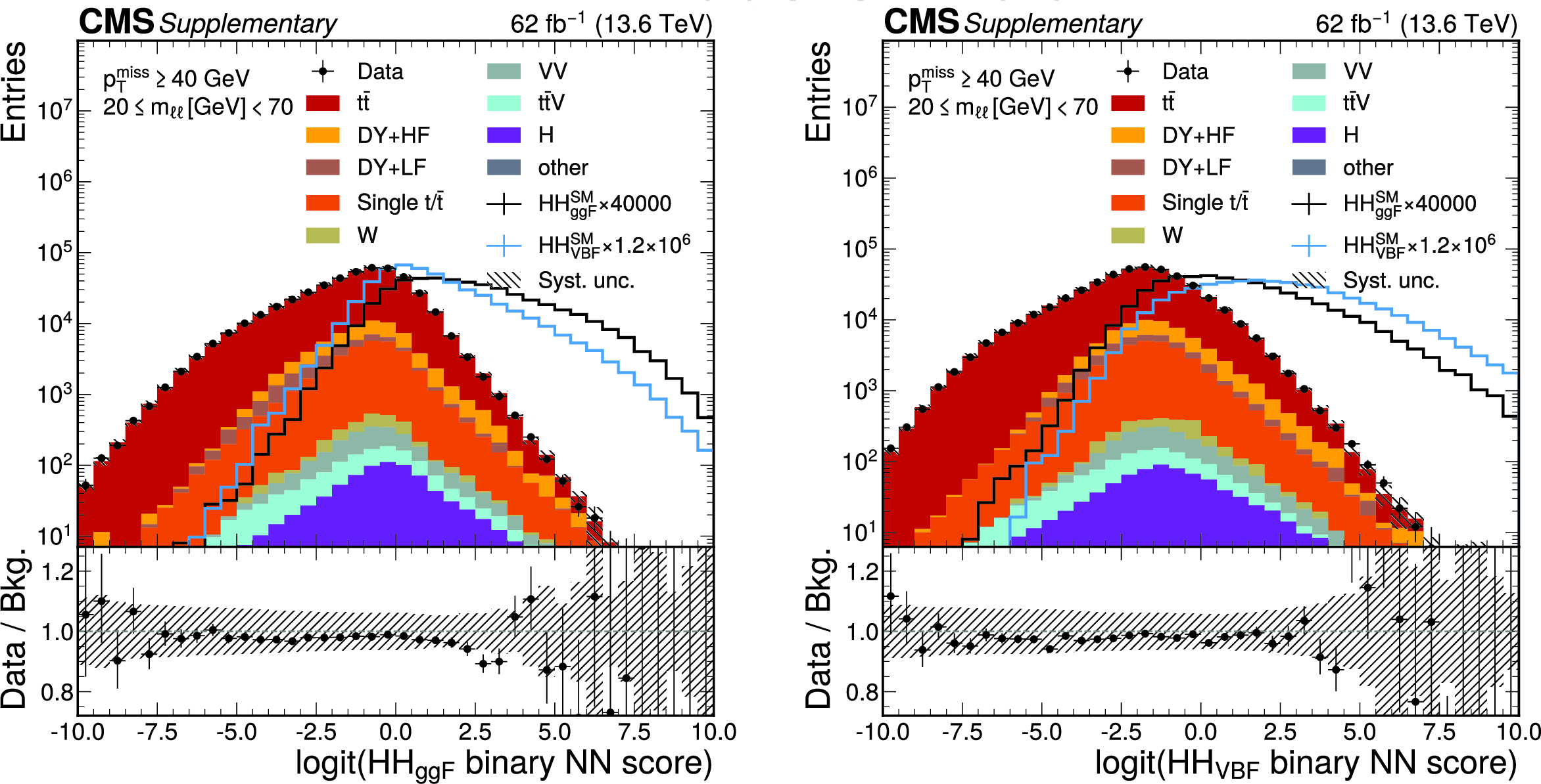
Distribution of the output score of the binary NN$_{ggF}$ (left) and NN$_{VBF}$ (right) classifiers after logit transformation ($\mathrm{logit}(x) = \log(x/(1-x))$) for all events in the analysis region, i.e. before categorisation by the NN$_{cat}$, observed in data (markers) and predicted by the background model (stacked histograms) prior to the fit to data. The HH signal distributions in the ggF and VBF production channels as predicted in the SM, scaled to the total background yield for better visibility, are overlayed (solid lines). The uncertainty band represents the total systematic uncertainty. |
png pdf |
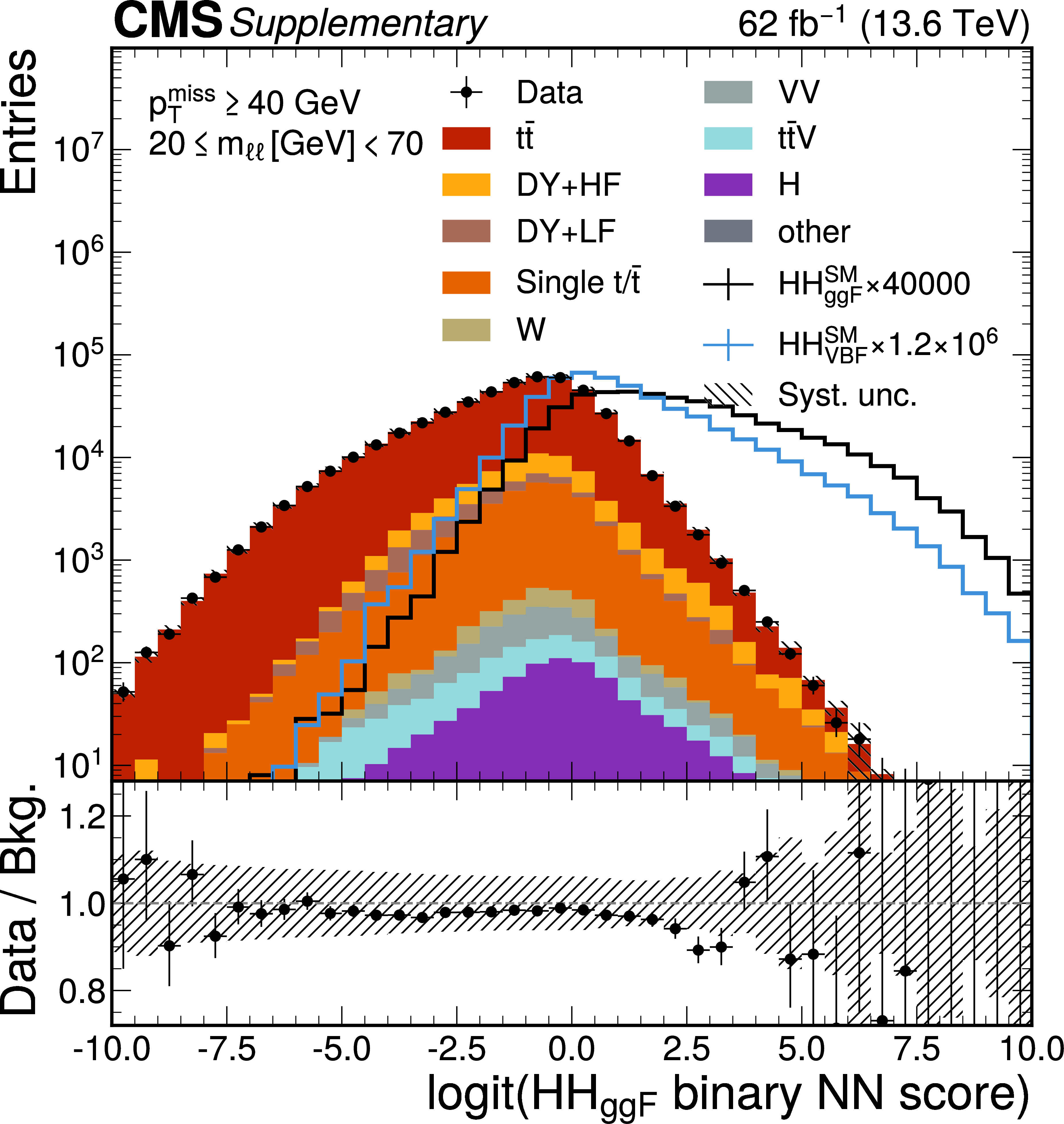
Additional Figure 2-a:
Distribution of the output score of the binary NN$_{ggF}$ (left) and NN$_{VBF}$ (right) classifiers after logit transformation ($\mathrm{logit}(x) = \log(x/(1-x))$) for all events in the analysis region, i.e. before categorisation by the NN$_{cat}$, observed in data (markers) and predicted by the background model (stacked histograms) prior to the fit to data. The HH signal distributions in the ggF and VBF production channels as predicted in the SM, scaled to the total background yield for better visibility, are overlayed (solid lines). The uncertainty band represents the total systematic uncertainty. |
png pdf |
Additional Figure 2-b:
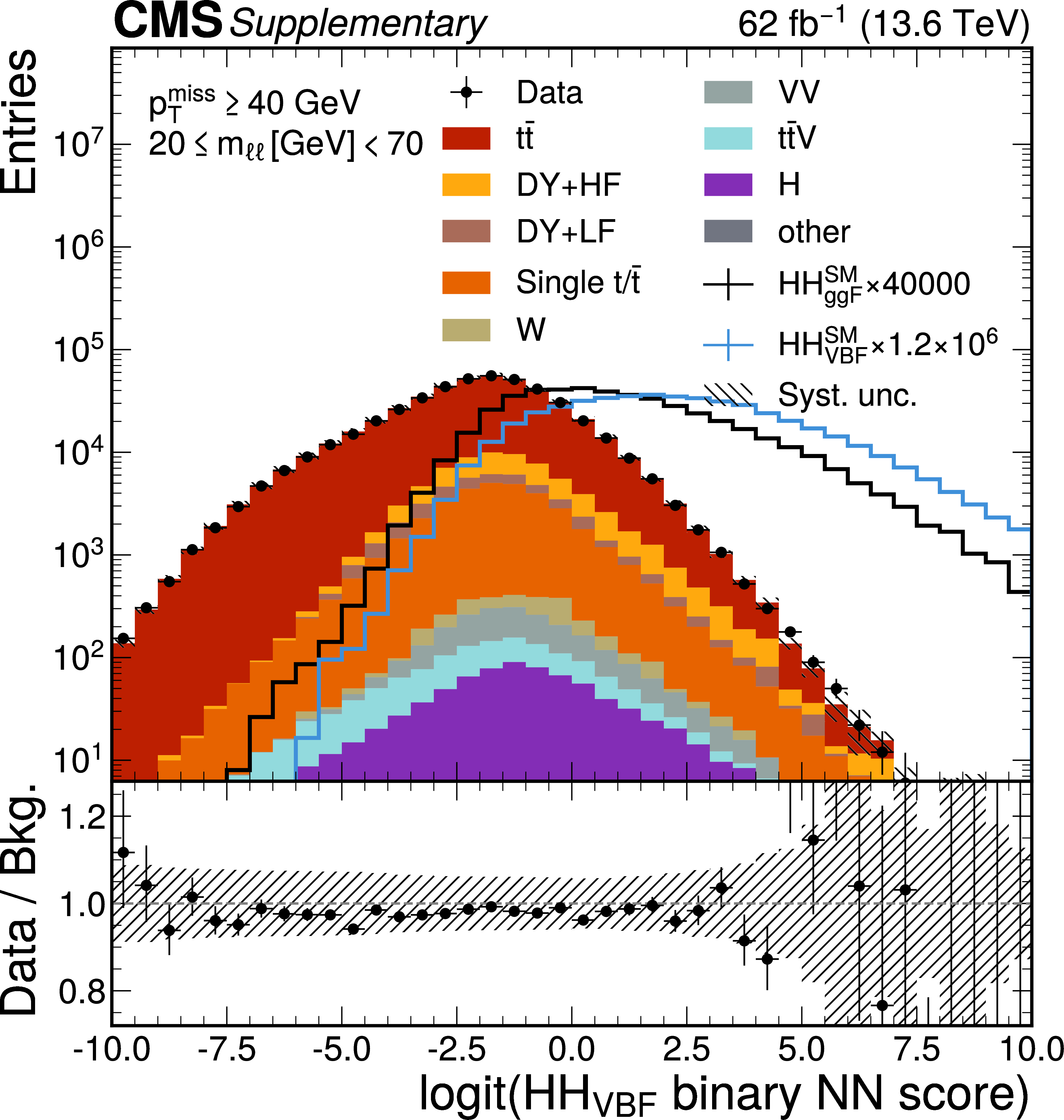
Distribution of the output score of the binary NN$_{ggF}$ (left) and NN$_{VBF}$ (right) classifiers after logit transformation ($\mathrm{logit}(x) = \log(x/(1-x))$) for all events in the analysis region, i.e. before categorisation by the NN$_{cat}$, observed in data (markers) and predicted by the background model (stacked histograms) prior to the fit to data. The HH signal distributions in the ggF and VBF production channels as predicted in the SM, scaled to the total background yield for better visibility, are overlayed (solid lines). The uncertainty band represents the total systematic uncertainty. |
png pdf |
Additional Figure 3:
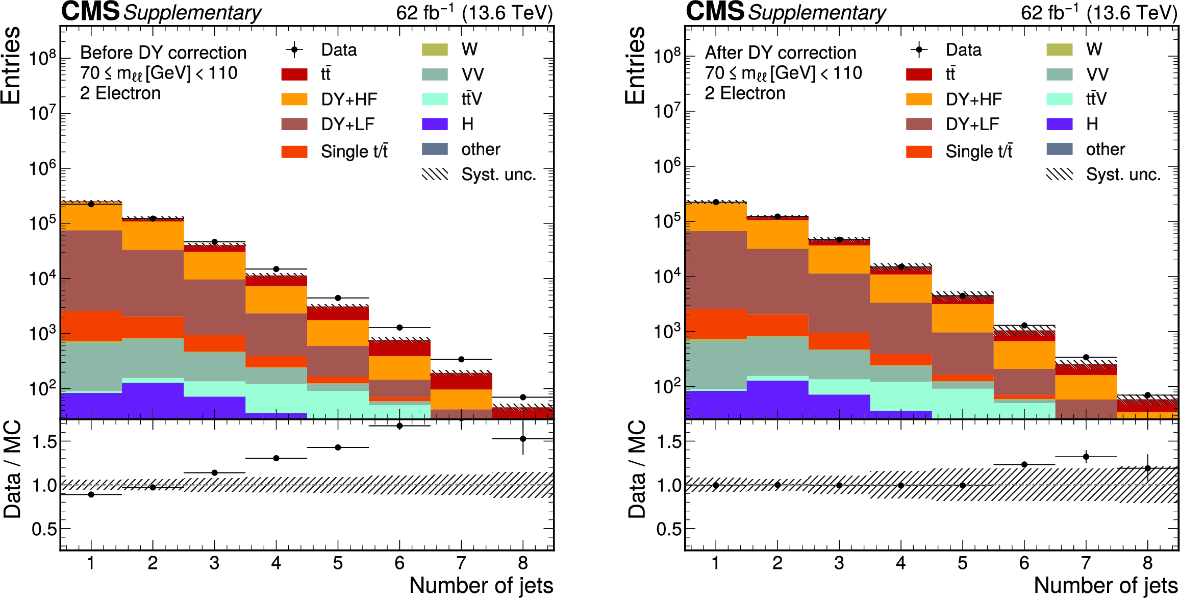
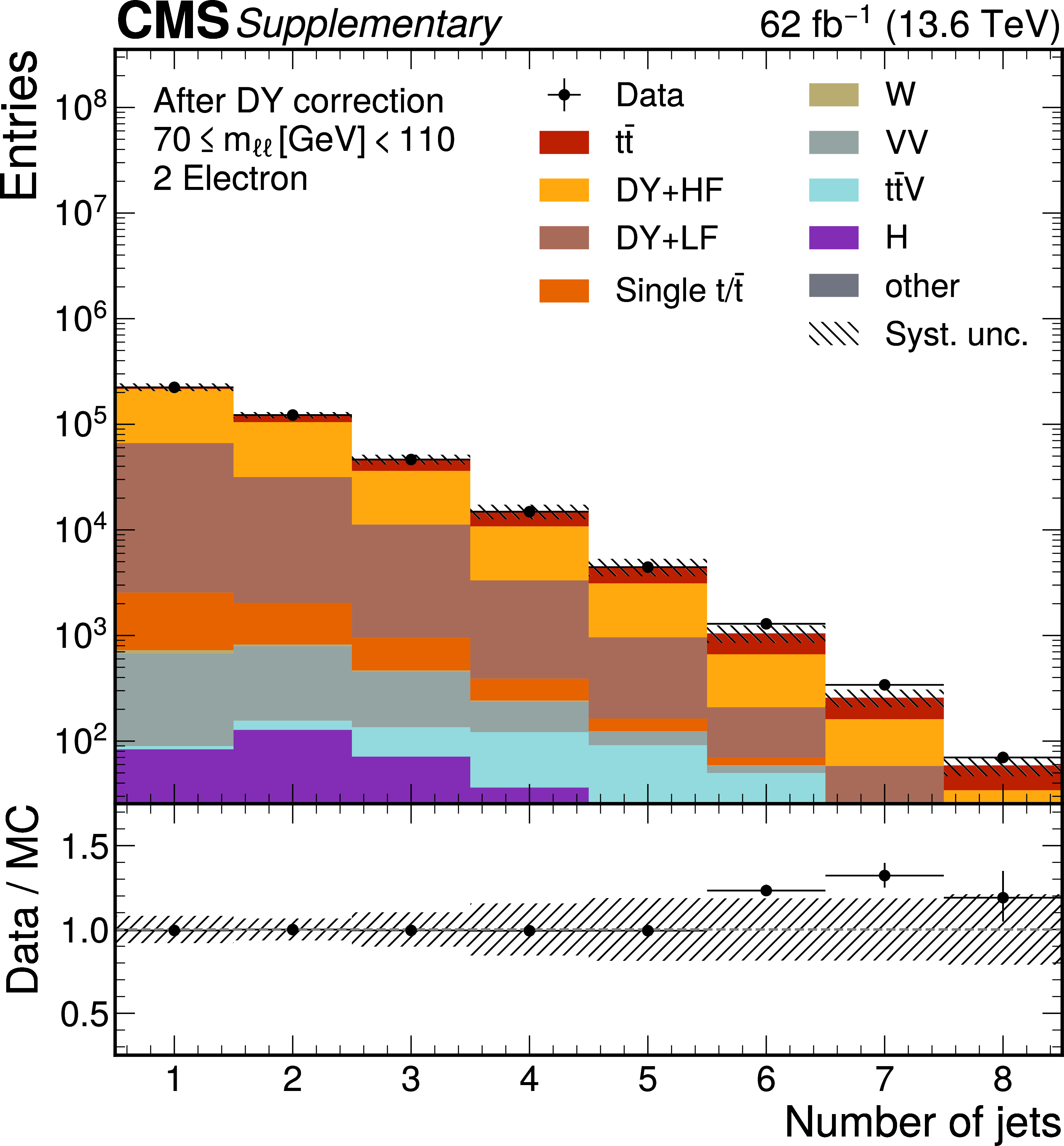
Jet multiplicity in the $e^{+}e^{-}$ channel in the DY validation region before (left) and after (right) application of the DY corrections. For events with $\geq$6 jets, the correction factors derived for events with 5 jets are used. The uncertainty band represents the total systematic uncertainty. |

png pdf |
Additional Figure 3-a:
Jet multiplicity in the $e^{+}e^{-}$ channel in the DY validation region before (left) and after (right) application of the DY corrections. For events with $\geq$6 jets, the correction factors derived for events with 5 jets are used. The uncertainty band represents the total systematic uncertainty. |
png pdf |
Additional Figure 3-b:
Jet multiplicity in the $e^{+}e^{-}$ channel in the DY validation region before (left) and after (right) application of the DY corrections. For events with $\geq$6 jets, the correction factors derived for events with 5 jets are used. The uncertainty band represents the total systematic uncertainty. |
png pdf |
Additional Figure 4:
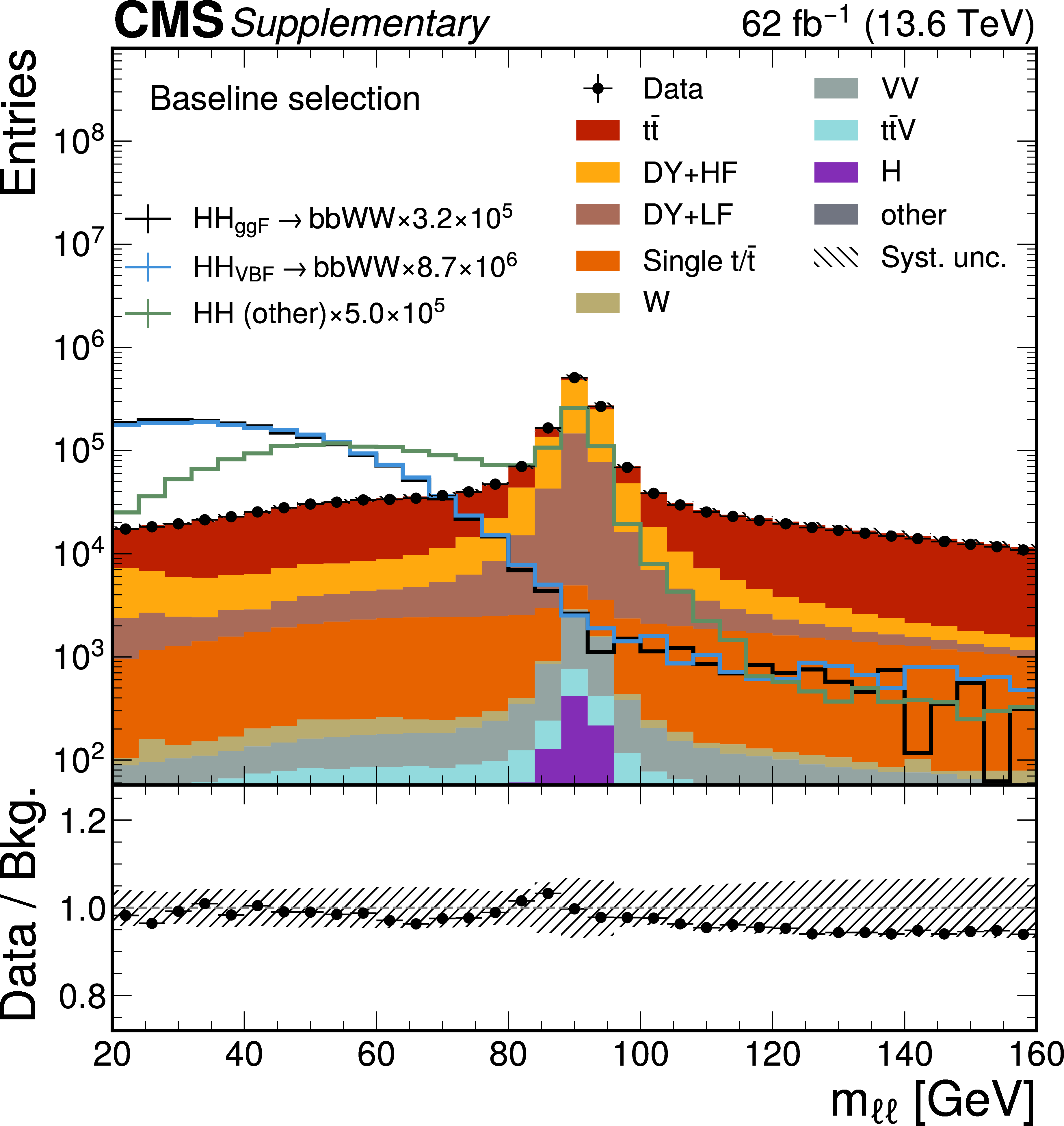
Invariant mass of the dilepton system for events passing the baseline selection observed in data (markers) and predicted by the background model (stacked histograms) prior to the fit to data. Overlaid are the HH signal distributions predicted in the SM (solid lines) for the bbWW decay mode, split into the the ggF and VBF production channels, and for other decay modes relevant in this analysis ($b\bar{b}\tau\tau$, $\b\bar{b}ZZ$). The HH distributions are individually scaled to the total background yield for better visibility. The uncertainty band represents the total systematic uncertainty. |
png pdf |
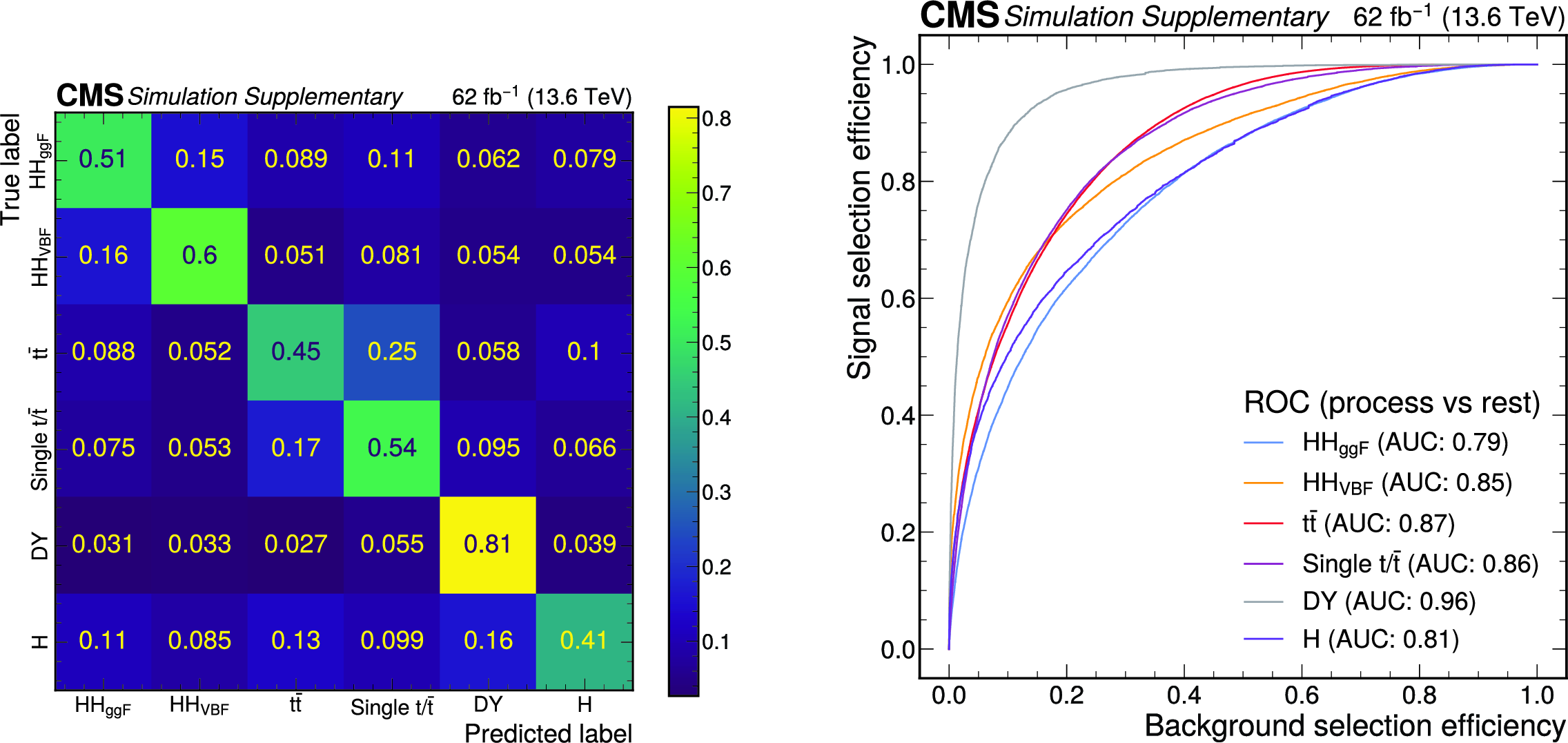
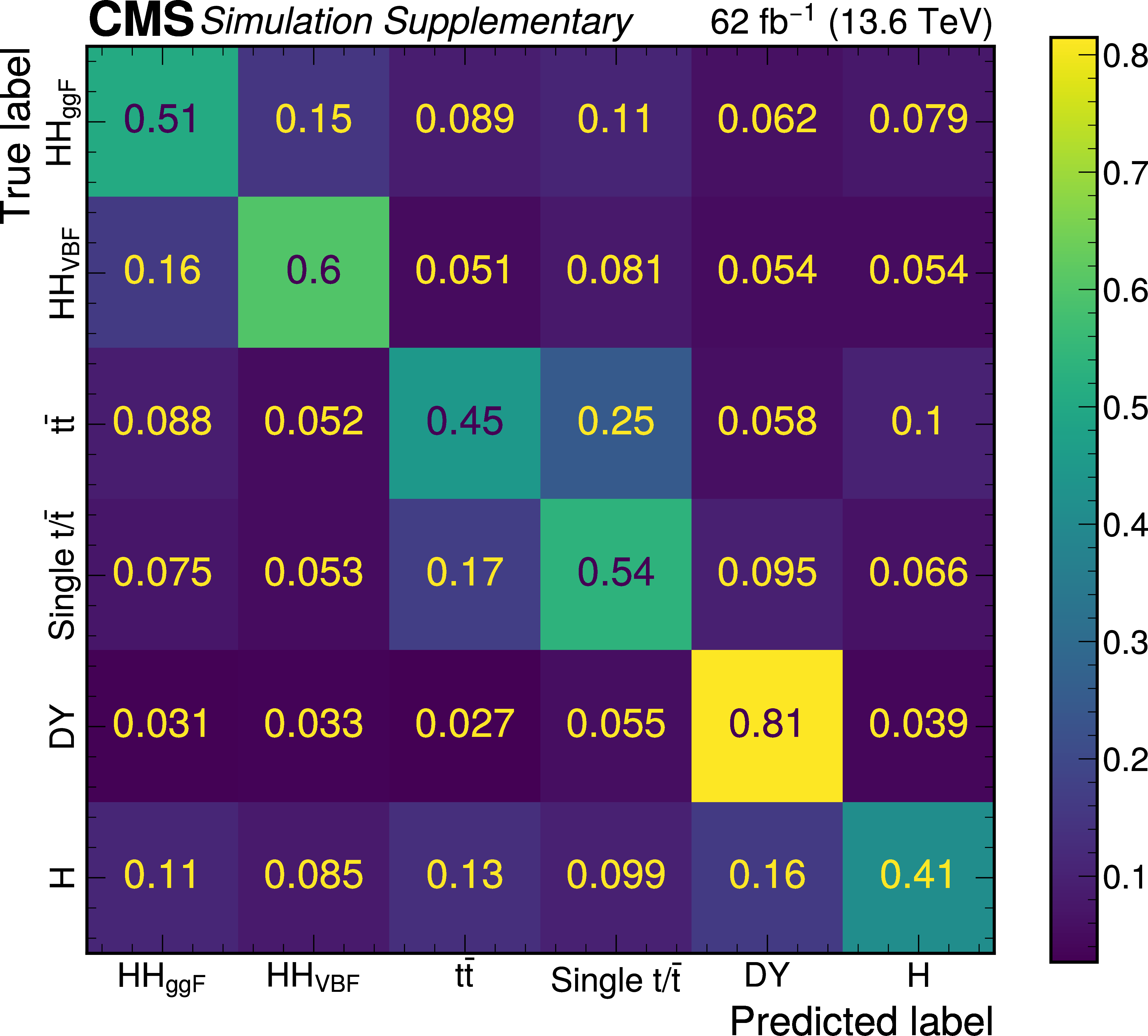
Additional Figure 5:
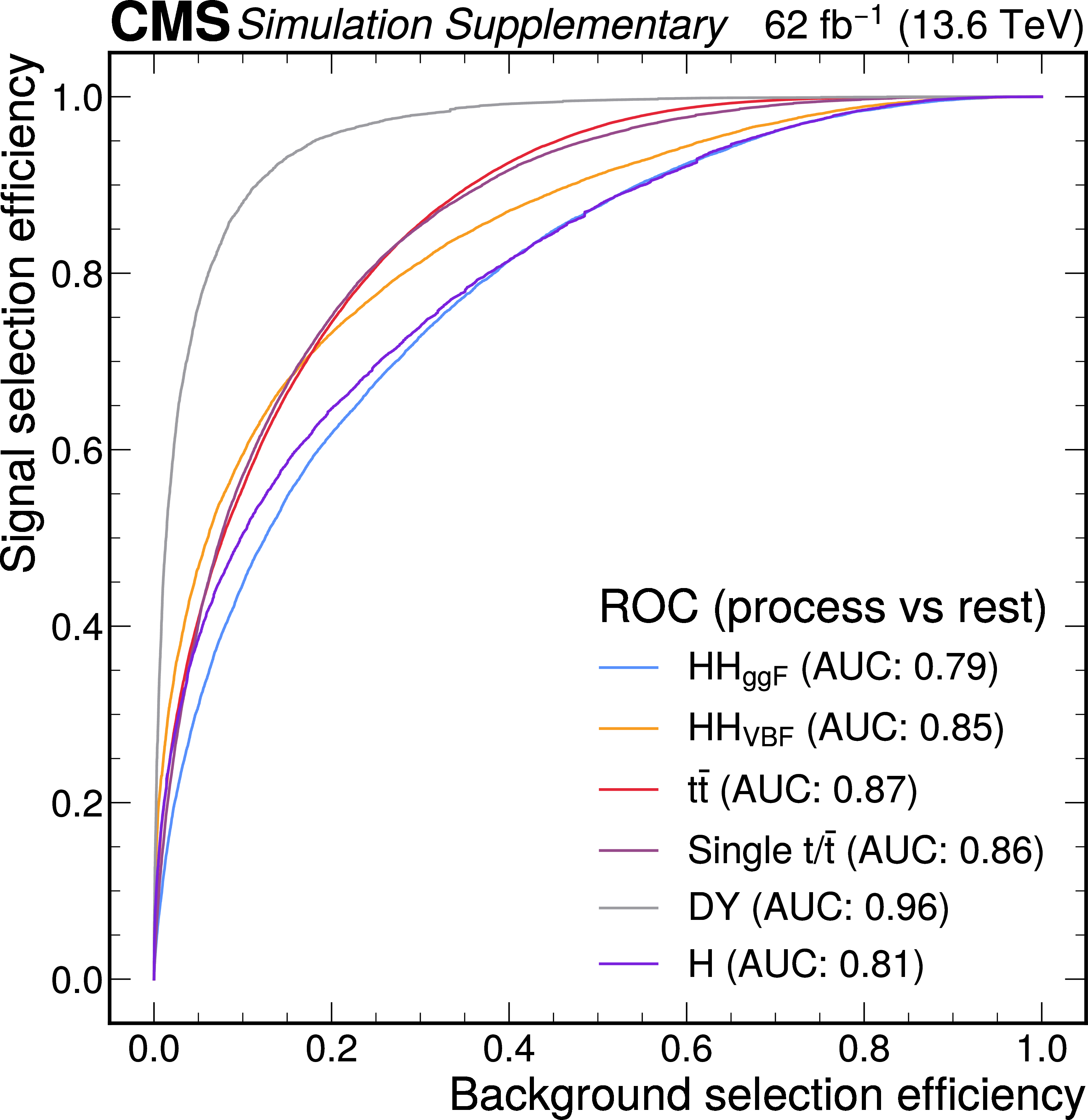
Confusion matrix (left) and ROC curve (right) of the NN$_{cat}$ classifier evaluated on the test set. |
png pdf |
Additional Figure 5-a:
Confusion matrix (left) and ROC curve (right) of the NN$_{cat}$ classifier evaluated on the test set. |
png pdf |
Additional Figure 5-b:
Confusion matrix (left) and ROC curve (right) of the NN$_{cat}$ classifier evaluated on the test set. |
png pdf |
Additional Figure 6:
Observed (solid black line) and median expected (dashed black line) upper limits at the 95% CL on the inclusive HH production cross section, normalised to the SM prediction, with all couplings fixed to their SM prediction. The green (yellow) bands show the 68% (95%) confidence level intervals of the expected limit. |
| References | ||||
| 1 | ATLAS Collaboration | Observation of a new particle in the search for the standard model Higgs boson with the ATLAS detector at the LHC | PLB 716 (2012) 1 | 1207.7214 |
| 2 | CMS Collaboration | Observation of a new boson at a mass of 125 GeV with the CMS experiment at the LHC | PLB 716 (2012) 30 | CMS-HIG-12-028 1207.7235 |
| 3 | CMS Collaboration | Observation of a new boson with mass near 125 GeV in pp collisions at $ \sqrt{s}= $ 7 and 8 TeV | JHEP 06 (2013) 081 | CMS-HIG-12-036 1303.4571 |
| 4 | F. Englert and R. Brout | Broken symmetry and the mass of gauge vector mesons | PRL 13 (1964) 321 | |
| 5 | P. W. Higgs | Broken symmetries, massless particles and gauge fields | PL 12 (1964) 132 | |
| 6 | P. W. Higgs | Broken symmetries and the masses of gauge bosons | PRL 13 (1964) 508 | |
| 7 | G. S. Guralnik, C. R. Hagen, and T. W. B. Kibble | Global conservation laws and massless particles | PRL 13 (1964) 585 | |
| 8 | P. W. Higgs | Spontaneous symmetry breakdown without massless bosons | PR 145 (1966) 1156 | |
| 9 | T. W. B. Kibble | Symmetry breaking in non-Abelian gauge theories | PR 155 (1967) 1554 | |
| 10 | S. Weinberg | A model of leptons | PRL 19 (1967) 1264 | |
| 11 | A. Salam | Weak and electromagnetic interactions | Conf. Proc. C 680519 (1968) 367 | |
| 12 | ATLAS Collaboration | A detailed map of Higgs boson interactions by the ATLAS experiment ten years after the discovery | Nature 607 (2022) 52 | 2207.00092 |
| 13 | CMS Collaboration | A portrait of the Higgs boson by the CMS experiment ten years after the discovery | [Corrigendum: doi:10./s41586-023-06164-8], 2022 Nature 607 (2022) 60 |
CMS-HIG-22-001 2207.00043 |
| 14 | G. Heinrich et al. | Probing the trilinear Higgs boson coupling in di-Higgs production at NLO QCD including parton shower effects | JHEP 06 (2019) 066 | 1903.08137 |
| 15 | M. Grazzini et al. | Higgs boson pair production at NNLO with top quark mass effects | JHEP 05 (2018) 059 | 1803.02463 |
| 16 | A. Karlberg et al. | Ad interim recommendations for the Higgs boson production cross sections at $ \sqrt{s}= $ 13.6 TeV | 2402.09955 | |
| 17 | J. Baglio et al. | $ \mathrm{g}\mathrm{g}\to\mathrm{H}\mathrm{H} $: Combined uncertainties | PRD 103 (2021) 056002 | 2008.11626 |
| 18 | F. A. Dreyer, A. Karlberg, J.-N. Lang, and M. Pellen | Precise predictions for double-Higgs production via vector-boson fusion | EPJC 80 (2020) 1037 | 2005.13341 |
| 19 | F. A. Dreyer and A. Karlberg | Vector-boson fusion Higgs pair production at N$ ^3 $LO | PRD 98 (2018) 114016 | 1811.07906 |
| 20 | F. Bishara, R. Contino, and J. Rojo | Higgs pair production in vector-boson fusion at the LHC and beyond | EPJC 77 (2017) 481 | 1611.03860 |
| 21 | ATLAS Collaboration | Combination of searches for Higgs boson pair production in pp collisions at $ \sqrt{s}= $ 13 TeV with the ATLAS detector | PRL 133 (2024) 101801 | 2406.09971 |
| 22 | CMS Collaboration | Combination of searches for nonresonant Higgs boson pair production in proton-proton collisions at $ \sqrt{s}= $ 13 TeV | Submitted to Reports on Progress in Physics, 2025 | CMS-HIG-20-011 2510.07527 |
| 23 | ATLAS and CMS Collaborations | Combination of ATLAS and CMS searches for Higgs boson pair production at $ \sqrt{s}= $ 13 TeV | Submitted to Physics Review Letters, 2026 | 2602.23991 |
| 24 | ATLAS Collaboration | Study of Higgs boson pair production in the $ HH \rightarrow b \overline{b} \gamma\gamma $ final state with 308 fb$ ^{-1} $ of data collected at $ \sqrt{s}= $ 13 TeV and 13.6 TeV by the ATLAS experiment | Submitted to Phys. Lett. B., 2025 | 2507.03495 |
| 25 | CMS Collaboration | Search for Higgs boson pair production in the $ \textrm{b}\overline{\textrm{b}}{\textrm{W}}^{+}{\textrm{W}}^{-} $ decay mode in proton-proton collisions at $ \sqrt{s}= $ 13 TeV | JHEP 07 (2024) 293 | CMS-HIG-21-005 2403.09430 |
| 26 | ATLAS Collaboration | Search for non-resonant Higgs boson pair production in the 2 $ b+2\ell+{E}_{\textrm{T}}^{\textrm{miss}} $ final state in pp collisions at $ \sqrt{s}= $ 13 TeV with the ATLAS detector | JHEP 02 (2024) 037 | 2310.11286 |
| 27 | LHC Higgs Cross Section Working Group | Handbook of LHC Higgs cross sections: 3. Higgs properties | link | 1307.1347 |
| 28 | CMS Collaboration | HEPData record for this analysis | link | |
| 29 | CMS Collaboration | The CMS experiment at the CERN LHC | JINST 3 (2008) S08004 | |
| 30 | CMS Collaboration | Development of the CMS detector for the CERN LHC Run 3 | JINST 19 (2024) P05064 | CMS-PRF-21-001 2309.05466 |
| 31 | CMS Collaboration | Performance of the CMS level-1 trigger in proton-proton collisions at $ \sqrt{s}= $ 13 TeV | JINST 15 (2020) P10017 | CMS-TRG-17-001 2006.10165 |
| 32 | CMS Collaboration | The CMS trigger system | JINST 12 (2017) P01020 | CMS-TRG-12-001 1609.02366 |
| 33 | CMS Collaboration | Performance of the CMS high-level trigger during LHC Run 2 | JINST 19 (2024) P11021 | CMS-TRG-19-001 2410.17038 |
| 34 | CMS Collaboration | Electron and photon reconstruction and identification with the CMS experiment at the CERN LHC | JINST 16 (2021) P05014 | CMS-EGM-17-001 2012.06888 |
| 35 | CMS Collaboration | Performance of the CMS muon detector and muon reconstruction with proton-proton collisions at $ \sqrt{s}= $ 13 TeV | JINST 13 (2018) P06015 | CMS-MUO-16-001 1804.04528 |
| 36 | CMS Collaboration | Description and performance of track and primary-vertex reconstruction with the CMS tracker | JINST 9 (2014) P10009 | CMS-TRK-11-001 1405.6569 |
| 37 | CMS Collaboration | Particle-flow reconstruction and global event description with the CMS detector | JINST 12 (2017) P10003 | CMS-PRF-14-001 1706.04965 |
| 38 | CMS Collaboration | Jet energy scale and resolution in the CMS experiment in pp collisions at 8 TeV | JINST 12 (2017) P02014 | CMS-JME-13-004 1607.03663 |
| 39 | CMS Collaboration | Performance of missing transverse momentum reconstruction in proton-proton collisions at $ \sqrt{s}= $ 13 TeV using the CMS detector | JINST 14 (2019) P07004 | CMS-JME-17-001 1903.06078 |
| 40 | CMS Collaboration | ECAL 2016 refined calibration and Run 2 summary plots | CMS Detector Performance Summary CMS-DP-2020-021 CDS |
|
| 41 | CMS Collaboration | Pileup mitigation at CMS in 13 TeV data | JINST 15 (2020) P09018 | CMS-JME-18-001 2003.00503 |
| 42 | M. Cacciari, G. P. Salam, and G. Soyez | The anti-$ k_{\mathrm{T}} $ jet clustering algorithm | JHEP 04 (2008) 063 | 0802.1189 |
| 43 | M. Cacciari, G. P. Salam, and G. Soyez | FastJet user manual | EPJC 72 (2012) 1896 | 1111.6097 |
| 44 | D. Bertolini, P. Harris, M. Low, and N. Tran | Pileup per particle identification | JHEP 10 (2014) 059 | 1407.6013 |
| 45 | H. Qu and L. Gouskos | ParticleNet: Jet tagging via particle clouds | PRD 101 (2020) 056019 | 1902.08570 |
| 46 | CMS Collaboration | Run 3 commissioning results of heavy-flavor jet tagging at $ \sqrt{s}= $ 13.6 TeV with CMS data using a modern framework for data processing | CMS Detector Performance Summary CMS-DP-2024-024 CDS |
|
| 47 | CMS Collaboration | Performance of heavy-flavour jet identification in Lorentz-boosted topologies in proton-proton collisions at $ \sqrt{s}= $ 13 TeV | JINST 20 (2025) P11006 | CMS-BTV-22-001 2510.10228 |
| 48 | CMS Collaboration | Identification of heavy-flavour jets with the CMS detector in pp collisions at 13 TeV | JINST 13 (2018) P05011 | CMS-BTV-16-002 1712.07158 |
| 49 | CMS Collaboration | Performance summary of AK4 jet b tagging with data from 2022 proton-proton collisions at $ \sqrt{s}= $ 13.6 TeV with the CMS detector | CMS Detector Performance Summary CMS-DP-2024-025 CDS |
|
| 50 | P. Nason | A new method for combining NLO QCD with shower Monte Carlo algorithms | JHEP 11 (2004) 040 | hep-ph/0409146 |
| 51 | S. Frixione, P. Nason, and C. Oleari | Matching NLO QCD computations with parton shower simulations: The POWHEG method | JHEP 11 (2007) 070 | 0709.2092 |
| 52 | S. Alioli, P. Nason, C. Oleari, and E. Re | A general framework for implementing NLO calculations in shower Monte Carlo programs: The POWHEG BOX | JHEP 06 (2010) 043 | 1002.2581 |
| 53 | T. Je \v z o and P. Nason | On the treatment of resonances in next-to-leading order calculations matched to a parton shower | JHEP 12 (2015) 065 | 1509.09071 |
| 54 | J. Alwall et al. | The automated computation of tree-level and next-to-leading order differential cross sections, and their matching to parton shower simulations | JHEP 07 (2014) 079 | 1405.0301 |
| 55 | GEANT4 Collaboration | GEANT 4---a simulation toolkit | NIM A 506 (2003) 250 | |
| 56 | NNPDF Collaboration | Parton distributions from high-precision collider data | EPJC 77 (2017) 663 | 1706.00428 |
| 57 | C. Bierlich et al. | A comprehensive guide to the physics and usage of PYTHIA 8.3 | SciPost Phys. Codeb. 2022 (2022) 8 | 2203.11601 |
| 58 | CMS Collaboration | Extraction and validation of a new set of CMS PYTHIA 8 tunes from underlying-event measurements | EPJC 80 (2020) 4 | CMS-GEN-17-001 1903.12179 |
| 59 | E. Bagnaschi, G. Degrassi, P. Slavich, and A. Vicini | Higgs production via gluon fusion in the POWHEG approach in the SM and in the MSSM | JHEP 02 (2012) 088 | 1111.2854 |
| 60 | G. Heinrich et al. | NLO predictions for Higgs boson pair production with full top quark mass dependence matched to parton showers | JHEP 08 (2017) 088 | 1703.09252 |
| 61 | S. Frixione, P. Nason, and G. Ridolfi | A positive-weight next-to-leading-order Monte Carlo for heavy flavour hadroproduction | JHEP 09 (2007) 126 | 0707.3088 |
| 62 | CMS Collaboration | Measurement of differential cross sections for the production of top quark pairs and of additional jets in lepton+jets events from pp collisions at $ \sqrt{s}= $ 13 TeV | PRD 97 (2018) 112003 | CMS-TOP-17-002 1803.08856 |
| 63 | CMS Collaboration | Differential cross section measurements for the production of top quark pairs and of additional jets using dilepton events from pp collisions at $ \sqrt{s}= $ 13 TeV | JHEP 02 (2025) 064 | CMS-TOP-20-006 2402.08486 |
| 64 | M. Czakon et al. | Top-pair production at the LHC through NNLO QCD and NLO EW | JHEP 10 (2017) 186 | 1705.04105 |
| 65 | CMS Collaboration | Measurement of inclusive and differential cross sections of single top quark production in association with a W boson in proton-proton collisions at $ \sqrt{s}= $ 13.6 TeV | JHEP 01 (2025) 107 | CMS-TOP-23-008 2409.06444 |
| 66 | M. Beneke, P. Falgari, S. Klein, and C. Schwinn | Hadronic top-quark pair production with NNLL threshold resummation | NPB 855 (2012) 695 | 1109.1536 |
| 67 | M. Cacciari et al. | Top-pair production at hadron colliders with next-to-next-to-leading logarithmic soft-gluon resummation | PLB 710 (2012) 612 | 1111.5869 |
| 68 | P. B ä rnreuther, M. Czakon, and A. Mitov | Percent-level-precision physics at the Tevatron: Next-to-next-to-leading order QCD corrections to $ \mathrm{q}\overline{\mathrm{q}}\to{\mathrm{t}\overline{\mathrm{t}}} \text{+X} $ | PRL 109 (2012) 132001 | 1204.5201 |
| 69 | M. Czakon and A. Mitov | NNLO corrections to top-pair production at hadron colliders: The all-fermionic scattering channels | JHEP 12 (2012) 054 | 1207.0236 |
| 70 | M. Czakon and A. Mitov | NNLO corrections to top pair production at hadron colliders: The quark-gluon reaction | JHEP 01 (2013) 080 | 1210.6832 |
| 71 | M. Czakon, P. Fiedler, and A. Mitov | Total top-quark pair-production cross section at hadron colliders through $ \mathcal{O}(\alpha_s^4) $ | PRL 110 (2013) 252004 | 1303.6254 |
| 72 | M. Czakon and A. Mitov | Top++: A program for the calculation of the top-pair cross-section at hadron colliders | Comput. Phys. Commun. 185 (2014) 2930 | 1112.5675 |
| 73 | S. Alioli, P. Nason, C. Oleari, and E. Re | NLO single-top production matched with shower in POWHEG: $ s $- and $ t $-channel contributions | JHEP 09 (2009) 111 | 0907.4076 |
| 74 | E. Re | Single-top Wt-channel production matched with parton showers using the POWHEG method | EPJC 71 (2011) 1547 | 1009.2450 |
| 75 | M. Aliev et al. | HATHOR: HAdronic Top and Heavy quarks crOss section calculatoR | Comput. Phys. Commun. 182 (2011) 1034 | 1007.1327 |
| 76 | P. Kant et al. | HatHor for single top-quark production: Updated predictions and uncertainty estimates for single top-quark production in hadronic collisions | Comput. Phys. Commun. 191 (2015) 74 | 1406.4403 |
| 77 | N. Kidonakis | Two-loop soft anomalous dimensions for single top quark associated production with $ \mathrm{W^-} $ or $ \mathrm{H}^{-} $ | PRD 82 (2010) 054018 | 1005.4451 |
| 78 | R. Frederix and S. Frixione | Merging meets matching in MC@NLO | JHEP 12 (2012) 061 | 1209.6215 |
| 79 | S. Alioli, P. Nason, C. Oleari, and E. Re | NLO Higgs boson production via gluon fusion matched with shower in POWHEG | JHEP 04 (2009) 002 | 0812.0578 |
| 80 | P. Nason and C. Oleari | NLO Higgs boson production via vector-boson fusion matched with shower in POWHEG | JHEP 02 (2010) 037 | 0911.5299 |
| 81 | K. Mimasu, V. Sanz, and C. Williams | Higher order QCD predictions for associated Higgs production with anomalous couplings to gauge bosons | JHEP 08 (2016) 039 | 1512.02572 |
| 82 | S. P. Jones, M. Kerner, and G. Luisoni | Next-to-leading-order QCD corrections to Higgs boson plus jet production with full top-quark mass dependence | PRL 120 (2018) 162001 | 1802.00349 |
| 83 | H. B. Hartanto, B. Jager, L. Reina, and D. Wackeroth | Higgs boson production in association with top quarks in the POWHEG BOX | PRD 91 (2015) 094003 | 1501.04498 |
| 84 | P. Nason and G. Zanderighi | $ \mathrm{W^+}\mathrm{W^-} $, WZ and ZZ production in the POWHEG-BOX-V2 | EPJC 74 (2014) 2702 | 1311.1365 |
| 85 | M. Erdmann, J. Glombitza, G. Kasieczka, and U. Klemradt | Deep Learning for Physics Research | World Scientific, 2021 link |
|
| 86 | A. Ghorbani and J. Zou | Data Shapley: Equitable valuation of data for machine learning | link | 1904.02868 |
| 87 | M. Cacciari et al. | The $ \mathrm{t} \overline{\mathrm{t}} $ cross-section at 1.8 TeV and 1.96 TeV: A study of the systematics due to parton densities and scale dependence | JHEP 04 (2004) 068 | hep-ph/0303085 |
| 88 | PDF4LHC Working Group Collaboration | The PDF4LHC21 combination of global PDF fits for the LHC Run III | JPG 49 (2022) 080501 | 2203.05506 |
| 89 | CMS Collaboration | Luminosity measurement in proton-proton collisions at 13.6 TeV in 2022 at CMS | CMS Physics Analysis Summary CMS-PAS-LUM-22-001 |
CMS-PAS-LUM-22-001 |
| 90 | CMS Collaboration | Measurement of the offline integrated luminosity for the CMS proton-proton collision dataset recorded in 2023 | CMS Detector Performance Summary CMS-DP-2024-068 CDS |
|
| 91 | J. S. Conway | Incorporating nuisance parameters in likelihoods for multisource spectra | in Proc. Workshop on statistical issues related to discovery claims in search experiments and unfolding, 2011 link |
1103.0354 |
| 92 | CMS Collaboration | The CMS statistical analysis and combination tool: \scshape Combine | Comput. Softw. Big Sci. 8 (2024) 19 | CMS-CAT-23-001 2404.06614 |
| 93 | CMS Collaboration | First measurement of the top quark pair production cross section in proton-proton collisions at $ \sqrt{s}= $ 13.6 TeV | JHEP 08 (2023) 204 | CMS-TOP-22-012 2303.10680 |
| 94 | T. Junk | Confidence level computation for combining searches with small statistics | NIM A 434 (1999) 435 | hep-ex/9902006 |
| 95 | A. L. Read | Presentation of search results: The $ \text{CL}_\text{s} $ technique | JPG 28 (2002) 2693 | |
| 96 | G. Cowan, K. Cranmer, E. Gross, and O. Vitells | Asymptotic formulae for likelihood-based tests of new physics | EPJC 71 (2011) 1554 | 1007.1727 |
|
|
Compact Muon Solenoid LHC, CERN |
|

|

|

|

|

|