

Compact Muon Solenoid
LHC, CERN
| CMS-HIG-24-002 ; CERN-EP-2026-116 | ||
| Search for a new heavy scalar resonance decaying to a pair of Z bosons in the four-lepton final state in proton-proton collisions at $ \sqrt{s} = $ 13 TeV | ||
| CMS Collaboration | ||
| 25 May 2026 | ||
| Submitted to the Journal of High Energy Physics | ||
| Abstract: A search for a new heavy scalar resonance decaying to two Z bosons, each subsequently decaying to a pair of electrons or muons, is presented. The results are based on a proton-proton collision data set collected by the CMS experiment at the LHC at a center-of-mass energy of 13 TeV, corresponding to an integrated luminosity of 138 fb$ ^{-1} $. The search is performed over a wide range of resonance masses from 130 GeV to 3 TeV, considering both narrow- and broad-width scenarios, and considering the gluon fusion and vector boson fusion production processes. For the broad-width scenario, the interference between the new resonance, the 125 GeV Higgs boson production, and the continuum background is taken into account. No significant excess with respect to the standard model background expectation is observed in the examined phase space. Upper limits at the 95% confidence level are set on the product of the heavy scalar resonance production cross section and the branching fraction for its decay into two Z bosons. The exclusion limits range from 0.05--0.1 pb in the low-mass region to 0.005 pb in the high-mass region. | ||
| Links: e-print arXiv:2605.26462 [hep-ex] (PDF) ; CDS record ; inSPIRE record ; HepData record ; Physics Briefing ; CADI line (restricted) ; | ||
| Figures | |
png pdf |
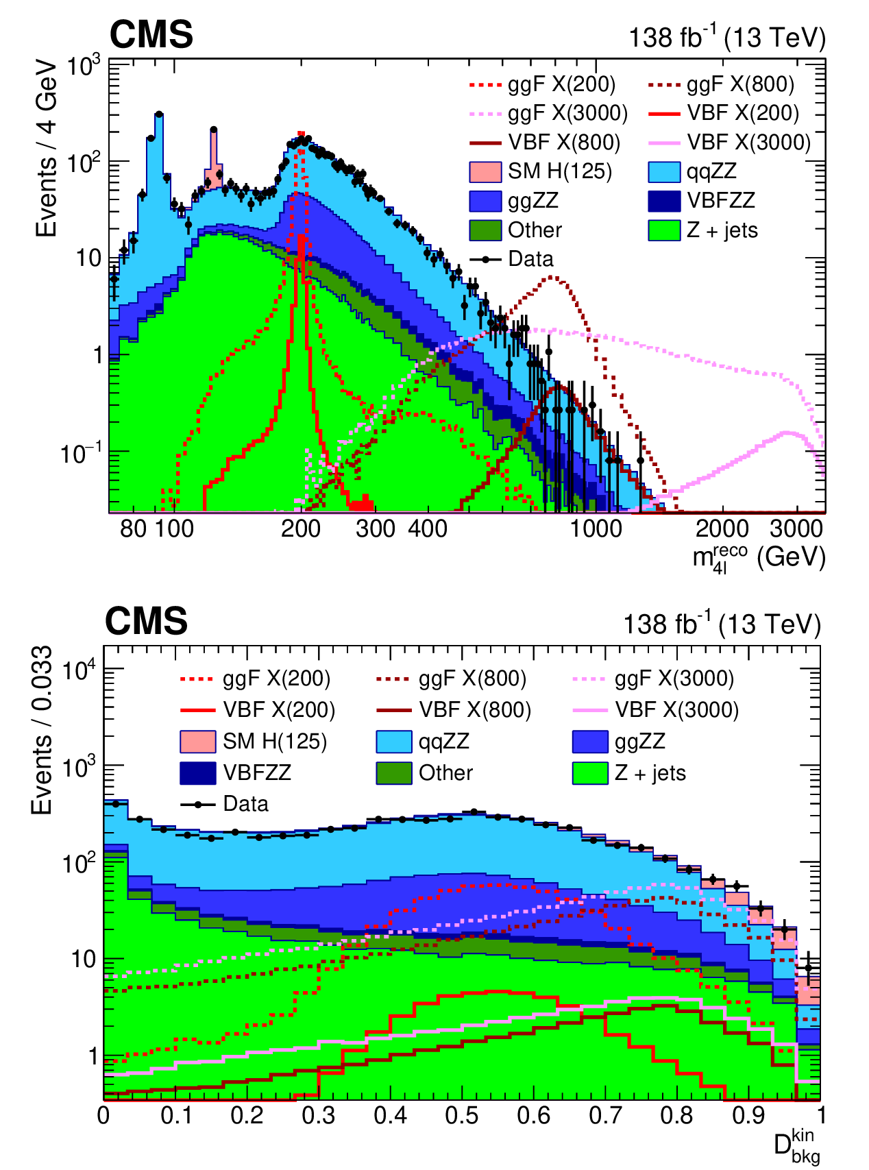
Figure 1:
Left: the $ m_{4\ell}^{\text{reco}} $ distributions for signal and background processes estimated from the MC simulation, alongside observed data. Red and pink open histograms show the lineshapes for different signal masses. Right: The $ D_\text{bkg}^{\text{kin}} $ distributions for signal and background processes estimated from the MC simulation, together with the observed data. The masses of the X resonances written in the legends are in GeV units. |
png pdf |
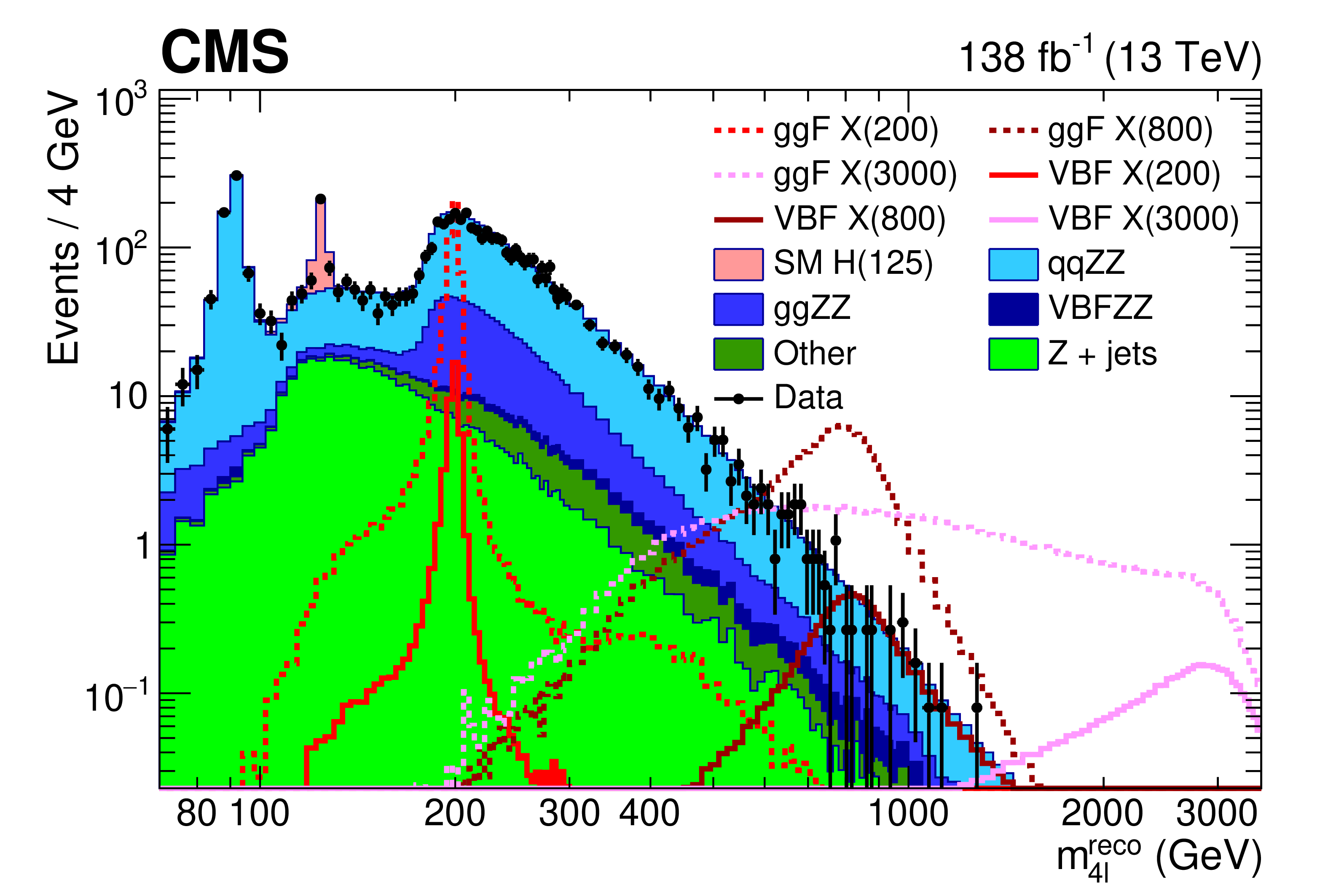
Figure 1-a:
Left: the $ m_{4\ell}^{\text{reco}} $ distributions for signal and background processes estimated from the MC simulation, alongside observed data. Red and pink open histograms show the lineshapes for different signal masses. Right: The $ D_\text{bkg}^{\text{kin}} $ distributions for signal and background processes estimated from the MC simulation, together with the observed data. The masses of the X resonances written in the legends are in GeV units. |
png pdf |
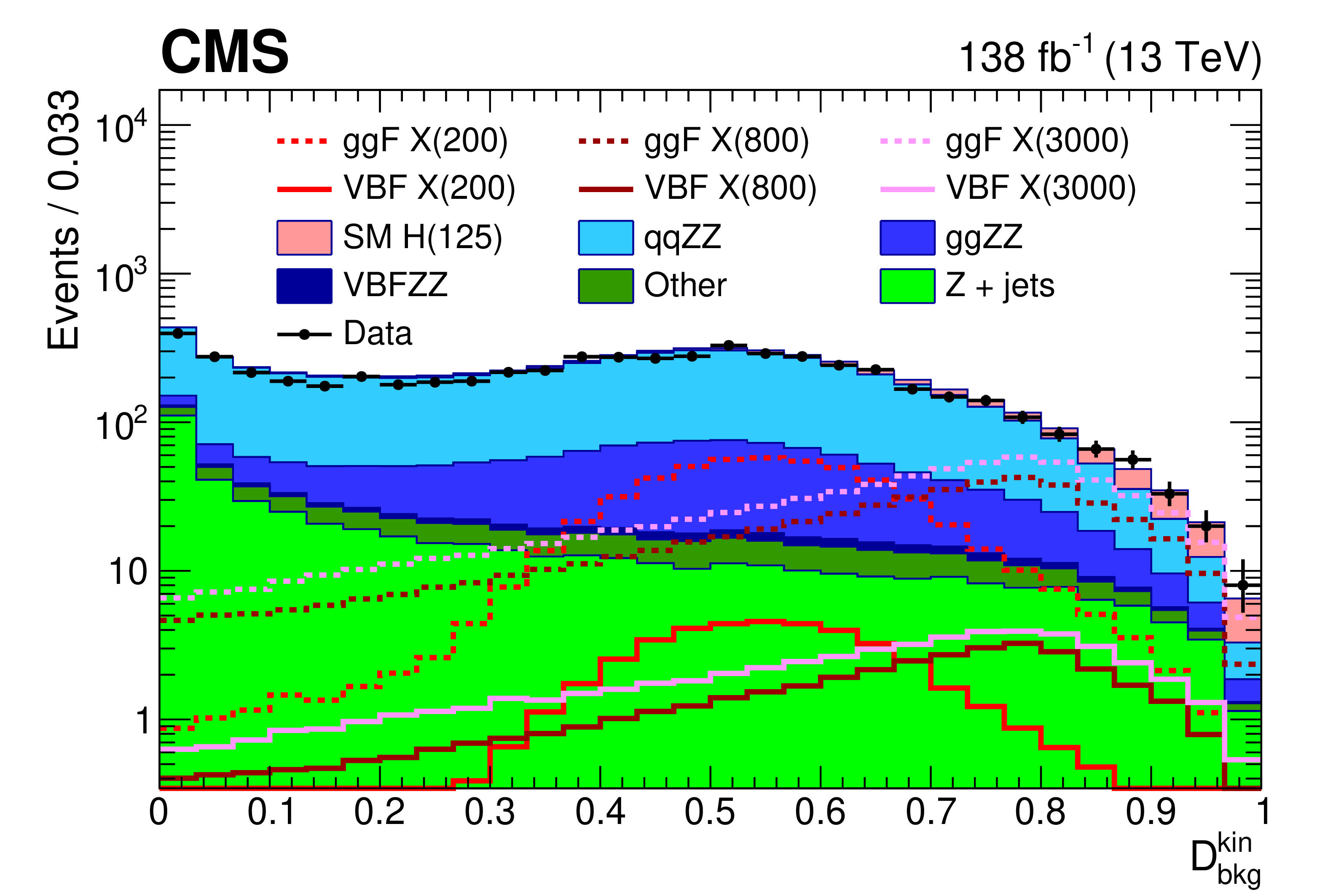
Figure 1-b:
Left: the $ m_{4\ell}^{\text{reco}} $ distributions for signal and background processes estimated from the MC simulation, alongside observed data. Red and pink open histograms show the lineshapes for different signal masses. Right: The $ D_\text{bkg}^{\text{kin}} $ distributions for signal and background processes estimated from the MC simulation, together with the observed data. The masses of the X resonances written in the legends are in GeV units. |
png pdf |
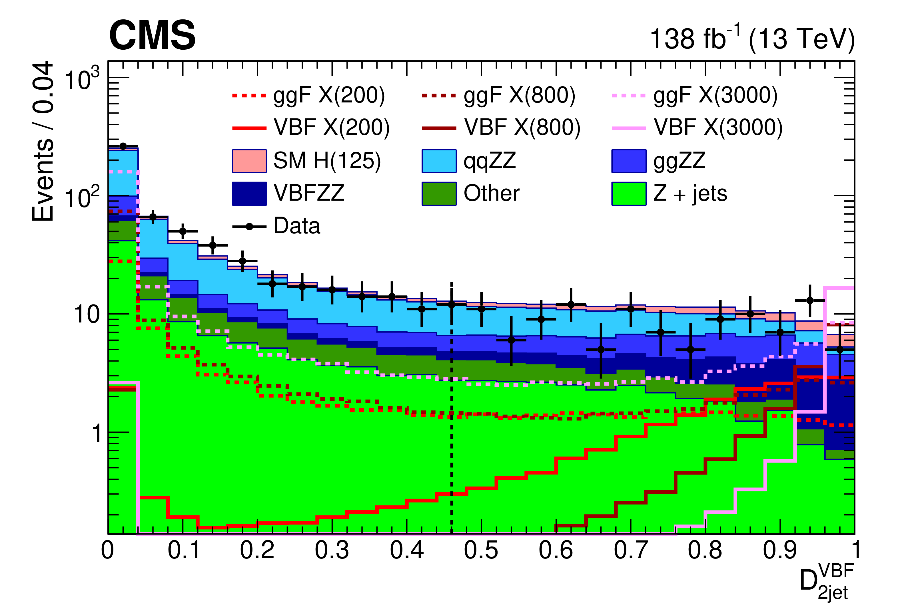
Figure 2:
The $ D_\text{2jet}^{\text{VBF}} $ distributions for signal, background, and observed data. Only events passing the lepton and jet multiplicity requirements for the VBF-tagged category are shown. The dotted vertical line represents the threshold of $ D_\text{2jet}^{\text{VBF}}= $ 0.46. |
png pdf |
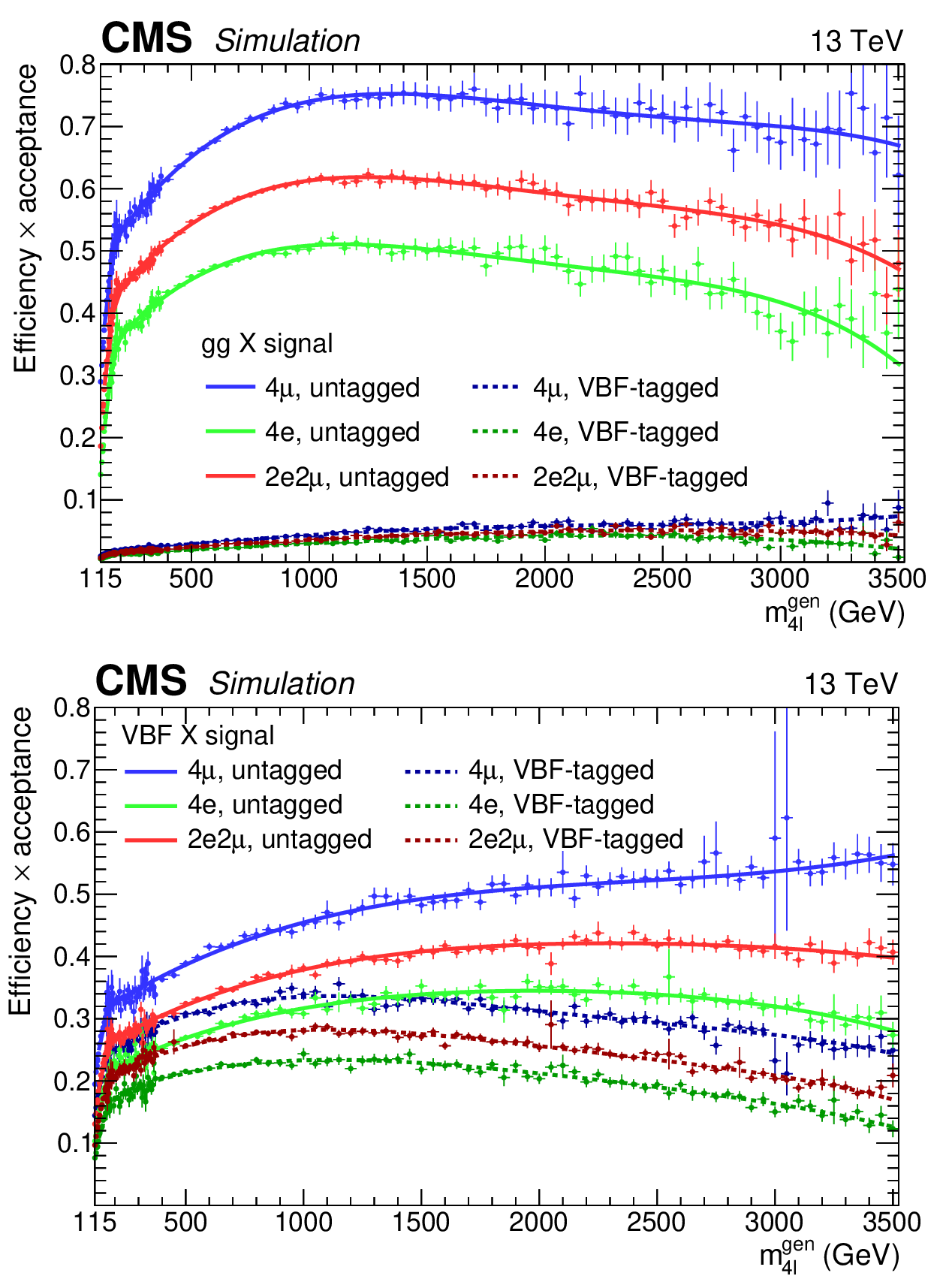
Figure 3:
The product of signal efficiency and acceptance, as a function of $ m_{4\ell}^{\text{gen}} $, computed for the 2018 data set. The left panel shows the results for ggF signals, and the right panel shows those for VBF signals. The points are values computed from simulation, which are fitted with the corresponding curves. In each panel, the product of efficiency and acceptance for each final state and category is shown: green points and curves represent the 4 e final state, red points and curves indicate the 2 $ \mathrm{e}2\mu $ final state, and blue points and curves the 4 $ \mu $ final state; the solid lines with lighter colors represent the untagged category, and the efficiencies for the VBF-tagged categories are shown in dashed lines with darker colors. |
png pdf |
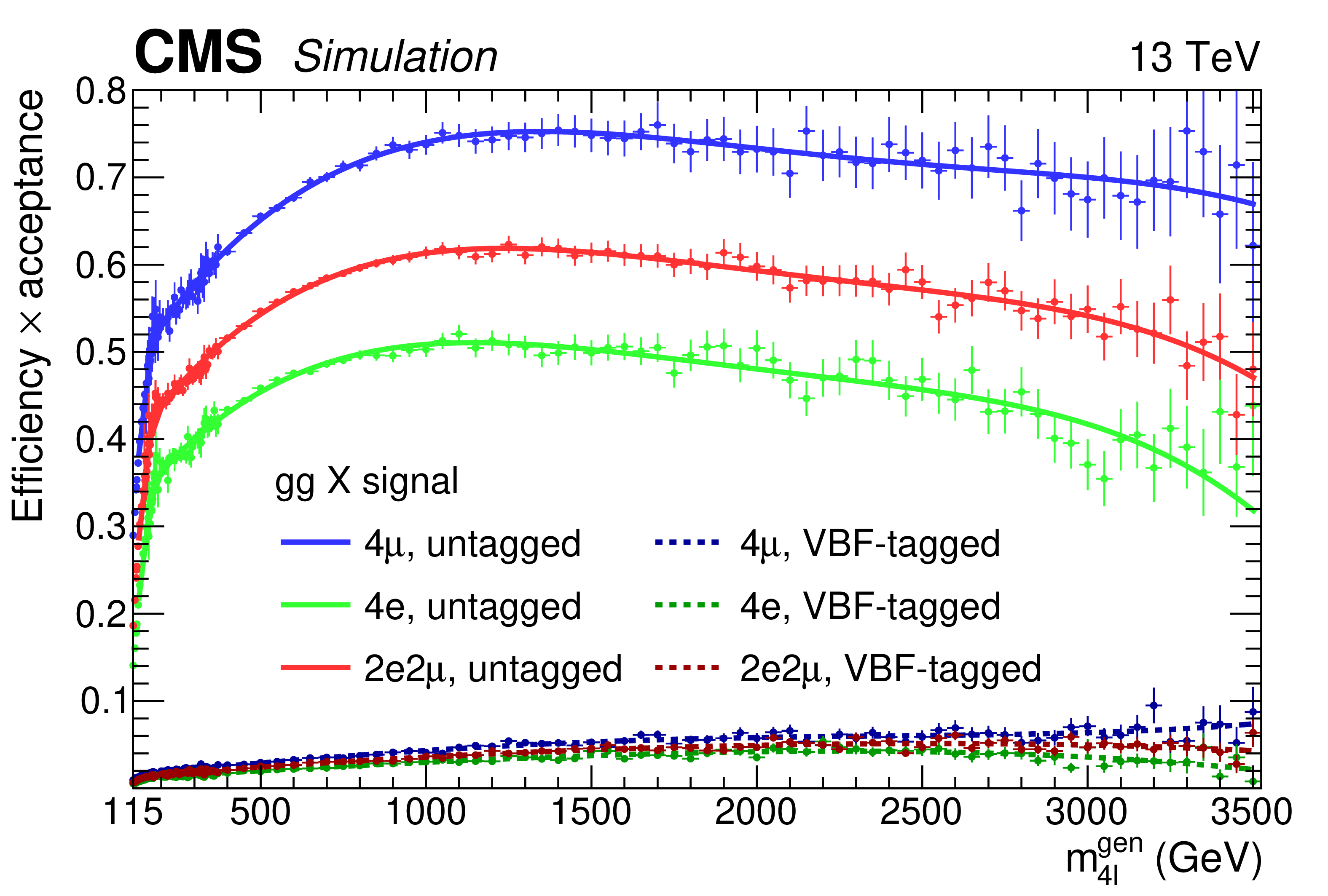
Figure 3-a:
The product of signal efficiency and acceptance, as a function of $ m_{4\ell}^{\text{gen}} $, computed for the 2018 data set. The left panel shows the results for ggF signals, and the right panel shows those for VBF signals. The points are values computed from simulation, which are fitted with the corresponding curves. In each panel, the product of efficiency and acceptance for each final state and category is shown: green points and curves represent the 4 e final state, red points and curves indicate the 2 $ \mathrm{e}2\mu $ final state, and blue points and curves the 4 $ \mu $ final state; the solid lines with lighter colors represent the untagged category, and the efficiencies for the VBF-tagged categories are shown in dashed lines with darker colors. |
png pdf |
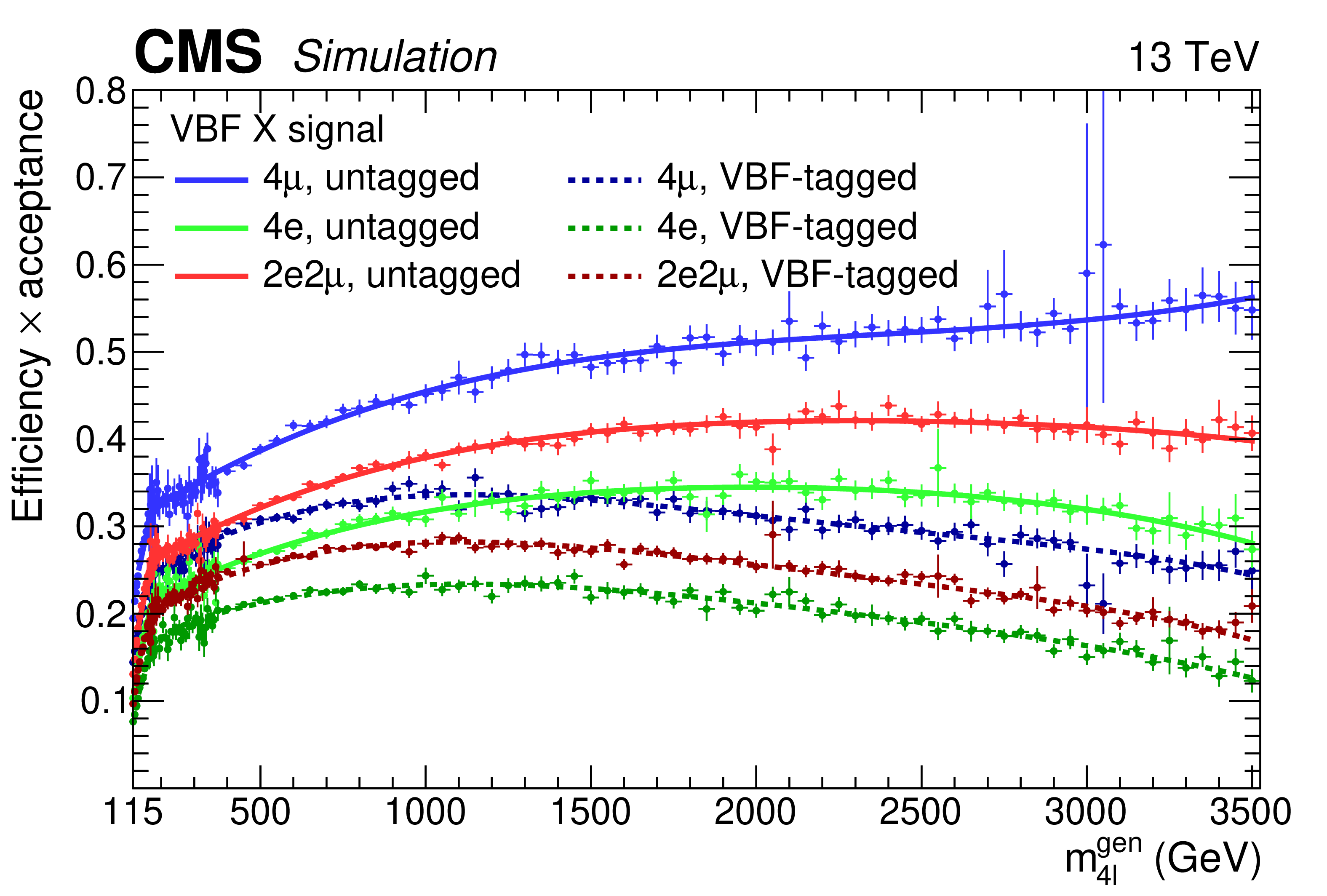
Figure 3-b:
The product of signal efficiency and acceptance, as a function of $ m_{4\ell}^{\text{gen}} $, computed for the 2018 data set. The left panel shows the results for ggF signals, and the right panel shows those for VBF signals. The points are values computed from simulation, which are fitted with the corresponding curves. In each panel, the product of efficiency and acceptance for each final state and category is shown: green points and curves represent the 4 e final state, red points and curves indicate the 2 $ \mathrm{e}2\mu $ final state, and blue points and curves the 4 $ \mu $ final state; the solid lines with lighter colors represent the untagged category, and the efficiencies for the VBF-tagged categories are shown in dashed lines with darker colors. |
png pdf |
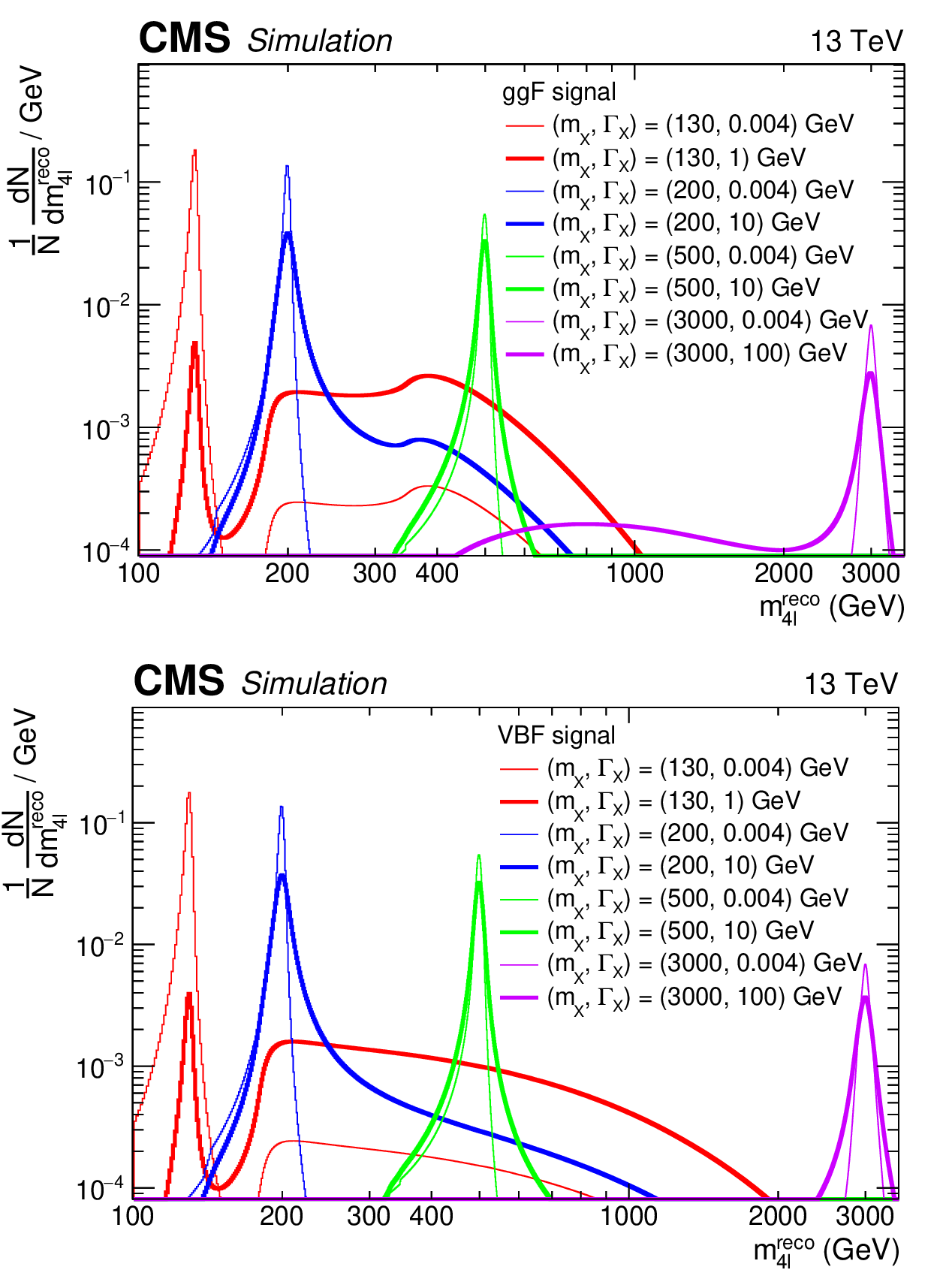
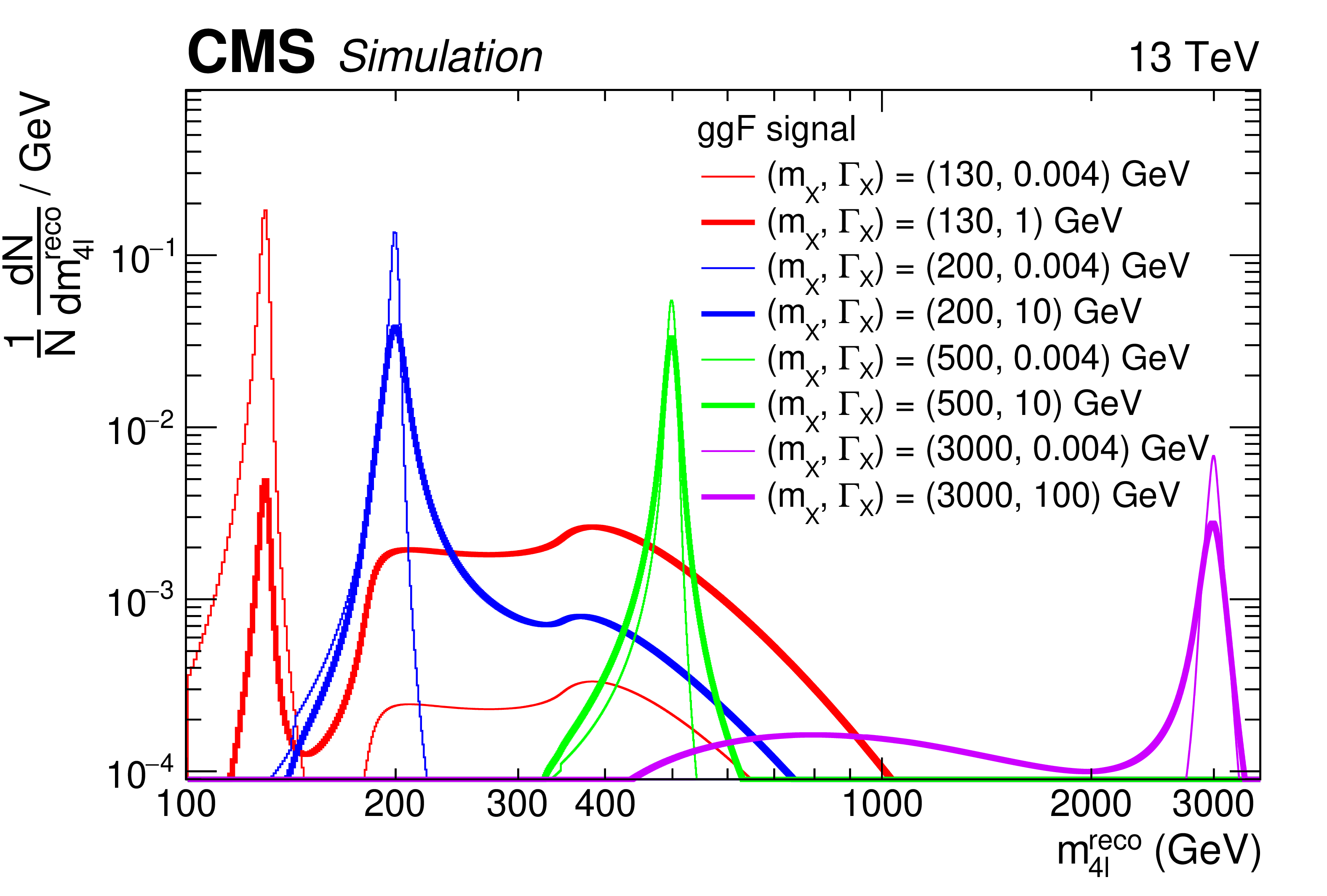
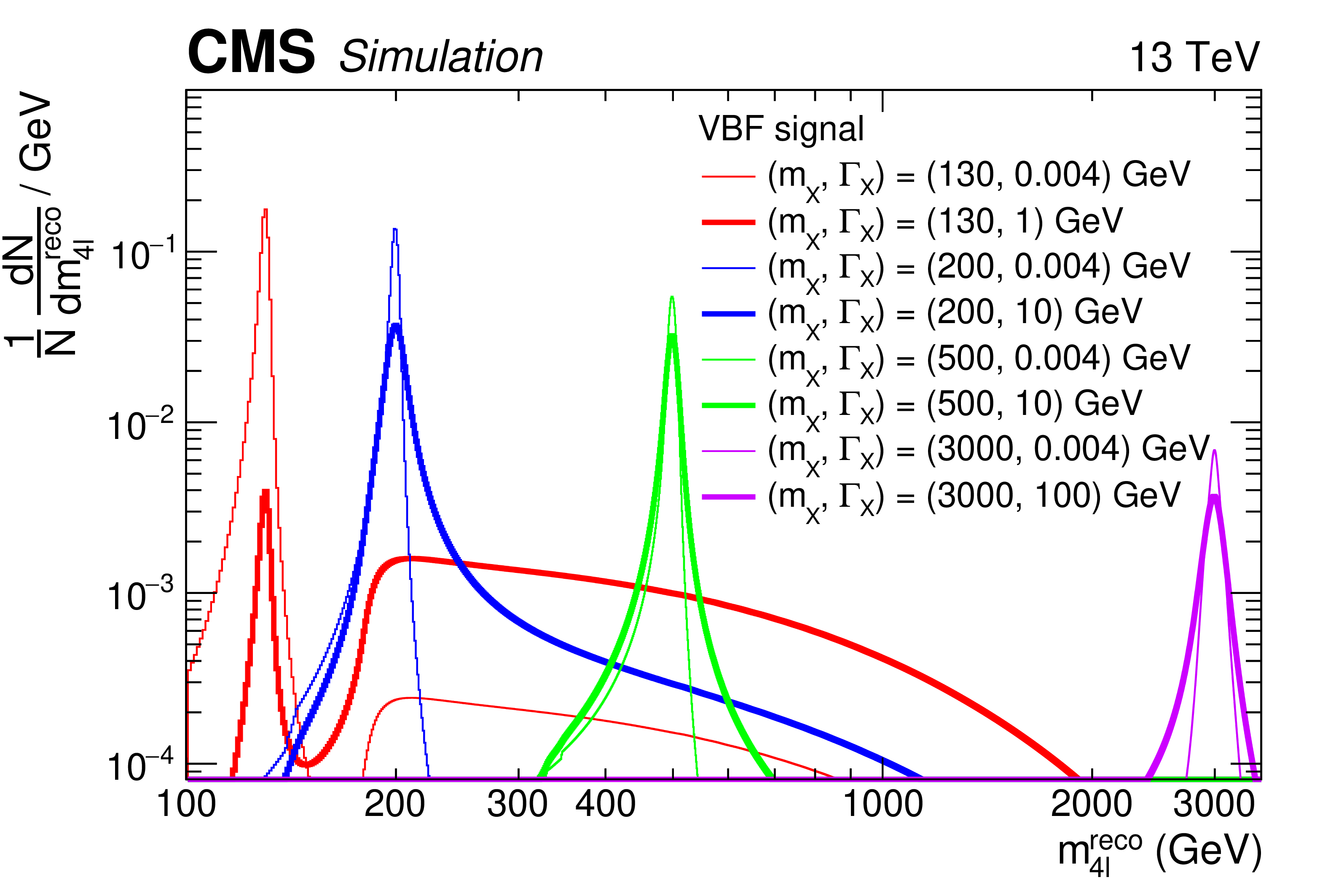
Figure 4:
The $ m_{4\ell}^{\text{reco}} $ distributions for several values of $ m_{\mathrm{X}} $ and $ \Gamma_{\mathrm{X}} $ obtained from the signal model, for the ggF (left) and VBF (right) signal processes. All final states and categories are combined. |
png pdf |
Figure 4-a:
The $ m_{4\ell}^{\text{reco}} $ distributions for several values of $ m_{\mathrm{X}} $ and $ \Gamma_{\mathrm{X}} $ obtained from the signal model, for the ggF (left) and VBF (right) signal processes. All final states and categories are combined. |
png pdf |
Figure 4-b:
The $ m_{4\ell}^{\text{reco}} $ distributions for several values of $ m_{\mathrm{X}} $ and $ \Gamma_{\mathrm{X}} $ obtained from the signal model, for the ggF (left) and VBF (right) signal processes. All final states and categories are combined. |
png pdf |
Figure 5:
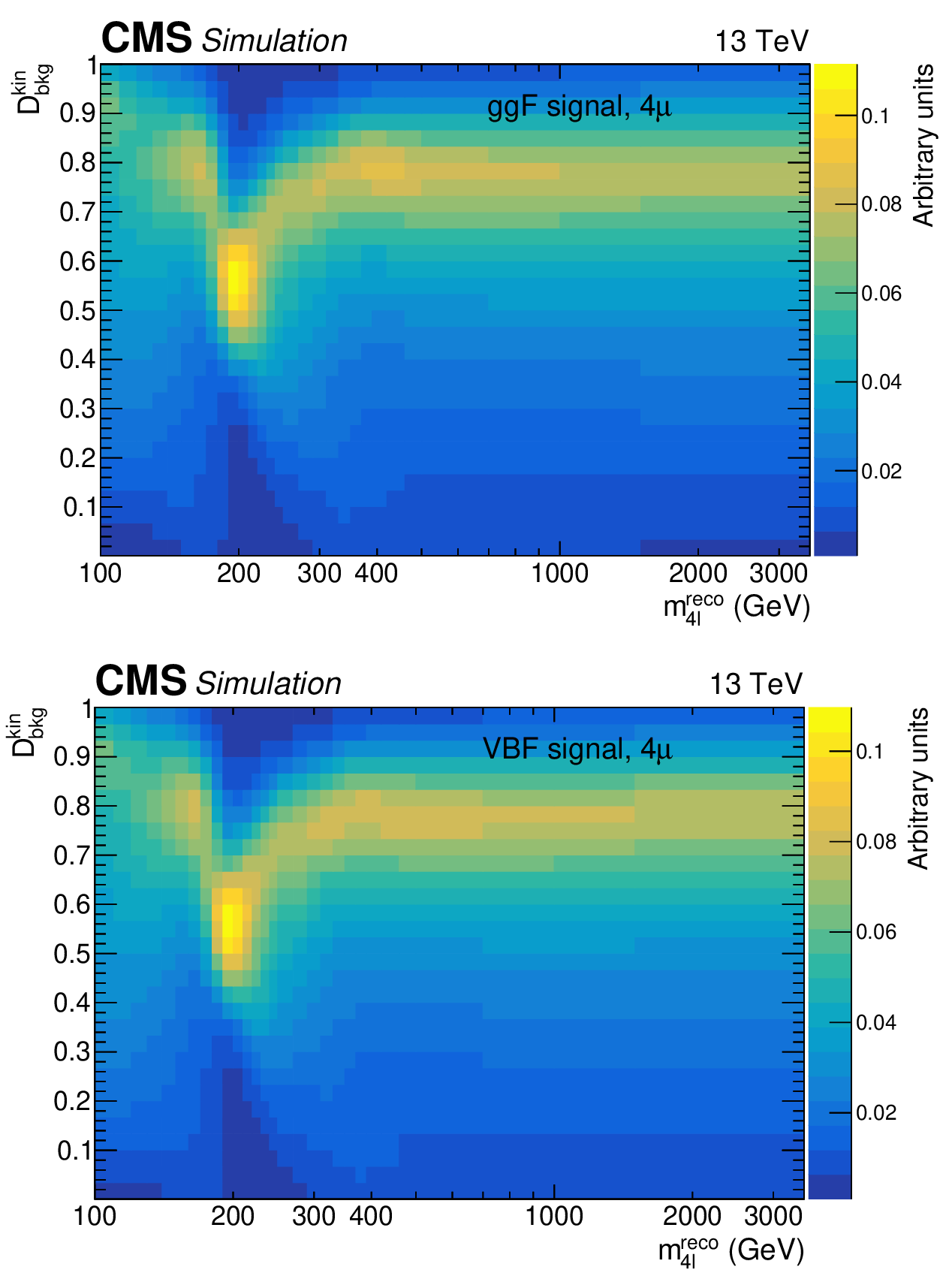
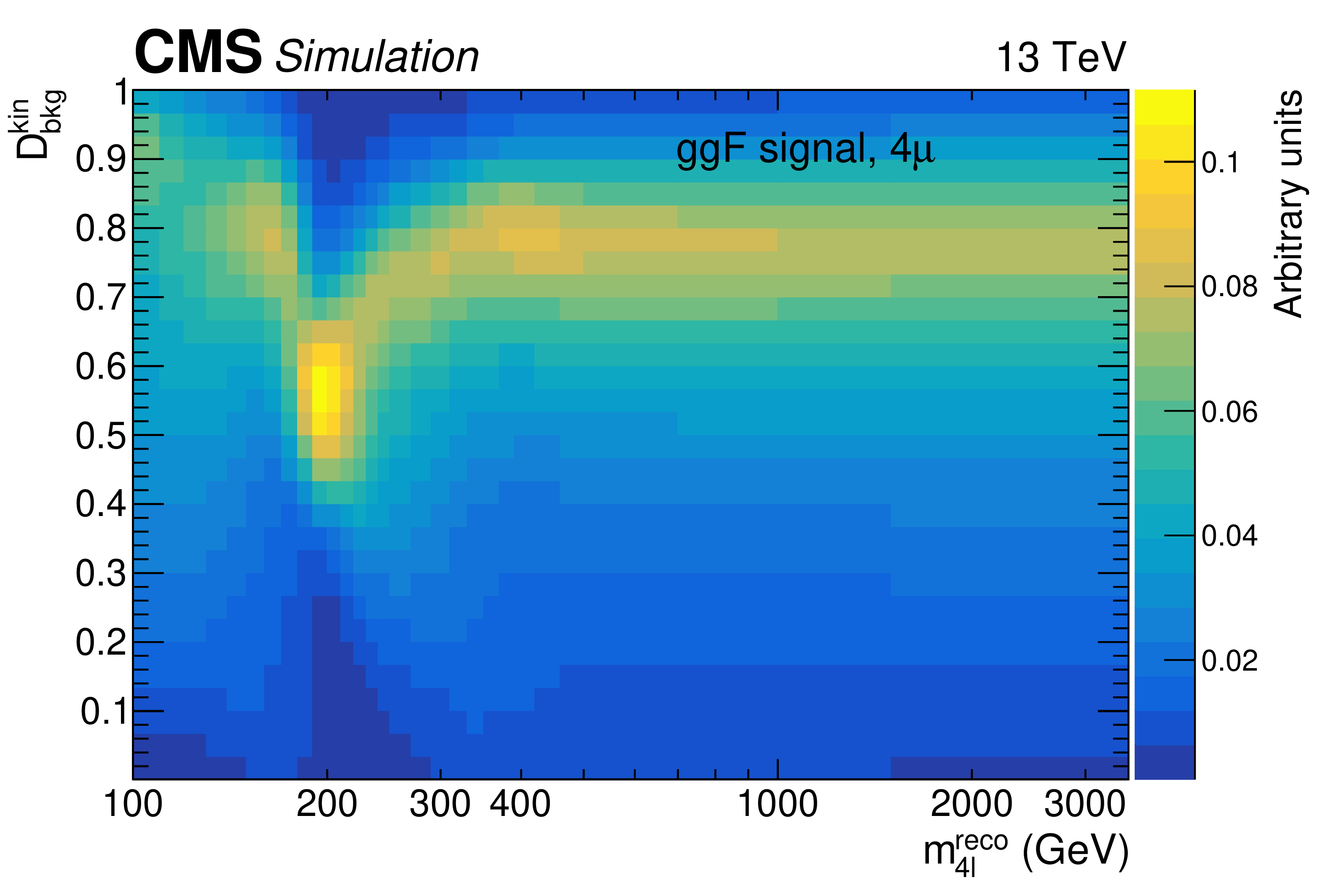
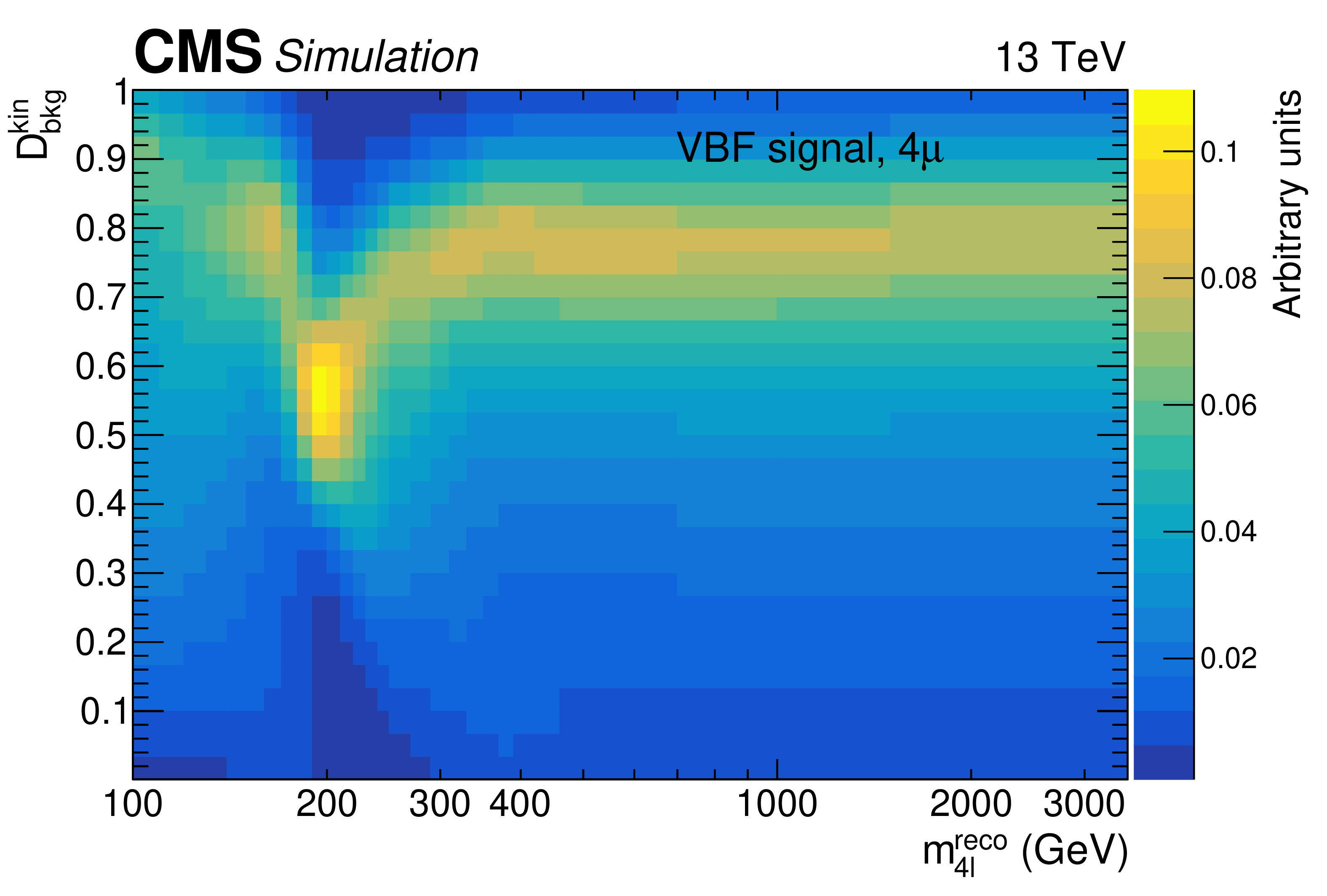
Expected distributions of $ m_{4\ell}^{\text{gen}} $ vs. $ D_\text{bkg}^{\text{kin}} $ for the ggF (left) and VBF (right) production mechanisms, in the 4 $ \mu $ final state. The distributions are estimated from the signal simulation. |
png pdf |
Figure 5-a:
Expected distributions of $ m_{4\ell}^{\text{gen}} $ vs. $ D_\text{bkg}^{\text{kin}} $ for the ggF (left) and VBF (right) production mechanisms, in the 4 $ \mu $ final state. The distributions are estimated from the signal simulation. |
png pdf |
Figure 5-b:
Expected distributions of $ m_{4\ell}^{\text{gen}} $ vs. $ D_\text{bkg}^{\text{kin}} $ for the ggF (left) and VBF (right) production mechanisms, in the 4 $ \mu $ final state. The distributions are estimated from the signal simulation. |
png pdf |
Figure 6:
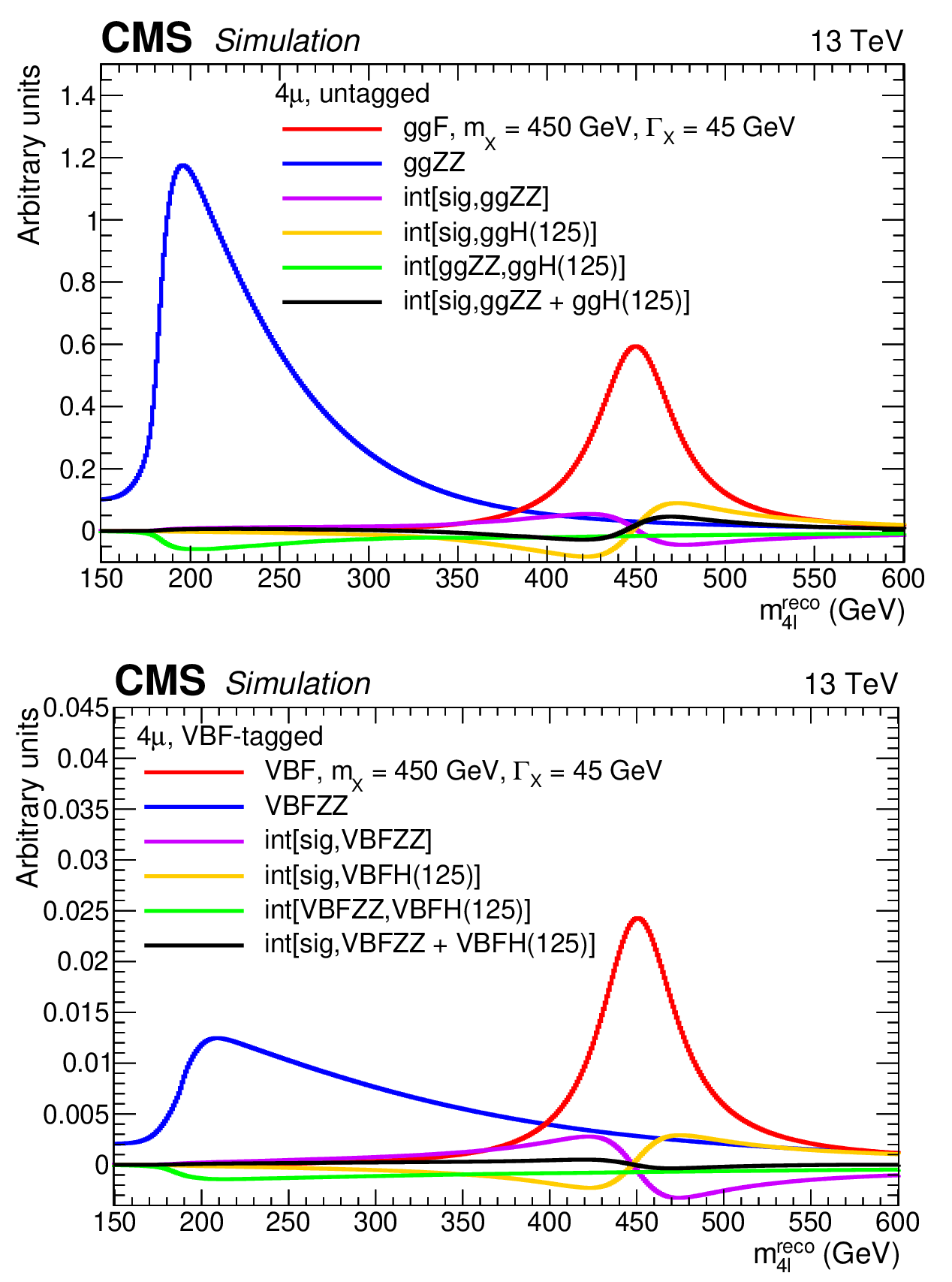
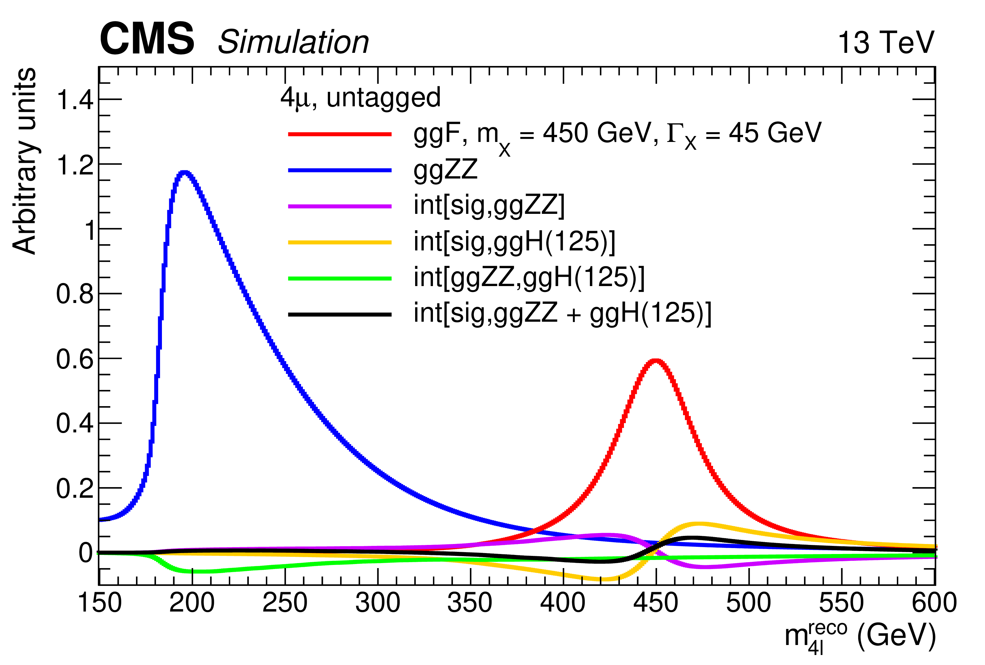
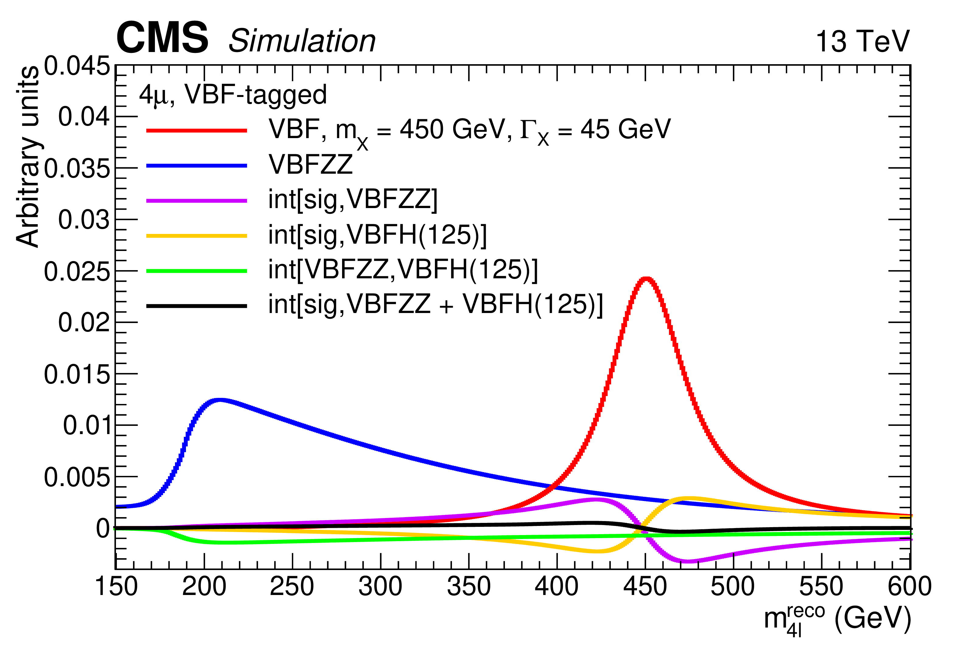
The left (right) plot depicts the lineshapes for the ggF (VBF) signal with $ m_{\mathrm{X}}= $ 450 GeV, $ \Gamma_{\mathrm{X}}= $ 45 GeV as the red curve, the $ \mathrm{g}\mathrm{g}\mathrm{Z}\mathrm{Z} $ (VBFZZ) background as the blue curve, and interferences as the violet, orange, and green curves. The black curve shows the interference between the signal and all other SM processes. The notation "int[A,B]" indicates the interference between A and B. Results are shown for the 4 $ \mu $ final state, for the untagged category (left) and the VBF-tagged category (right). |
png pdf |
Figure 6-a:
The left (right) plot depicts the lineshapes for the ggF (VBF) signal with $ m_{\mathrm{X}}= $ 450 GeV, $ \Gamma_{\mathrm{X}}= $ 45 GeV as the red curve, the $ \mathrm{g}\mathrm{g}\mathrm{Z}\mathrm{Z} $ (VBFZZ) background as the blue curve, and interferences as the violet, orange, and green curves. The black curve shows the interference between the signal and all other SM processes. The notation "int[A,B]" indicates the interference between A and B. Results are shown for the 4 $ \mu $ final state, for the untagged category (left) and the VBF-tagged category (right). |
png pdf |
Figure 6-b:
The left (right) plot depicts the lineshapes for the ggF (VBF) signal with $ m_{\mathrm{X}}= $ 450 GeV, $ \Gamma_{\mathrm{X}}= $ 45 GeV as the red curve, the $ \mathrm{g}\mathrm{g}\mathrm{Z}\mathrm{Z} $ (VBFZZ) background as the blue curve, and interferences as the violet, orange, and green curves. The black curve shows the interference between the signal and all other SM processes. The notation "int[A,B]" indicates the interference between A and B. Results are shown for the 4 $ \mu $ final state, for the untagged category (left) and the VBF-tagged category (right). |
png pdf |
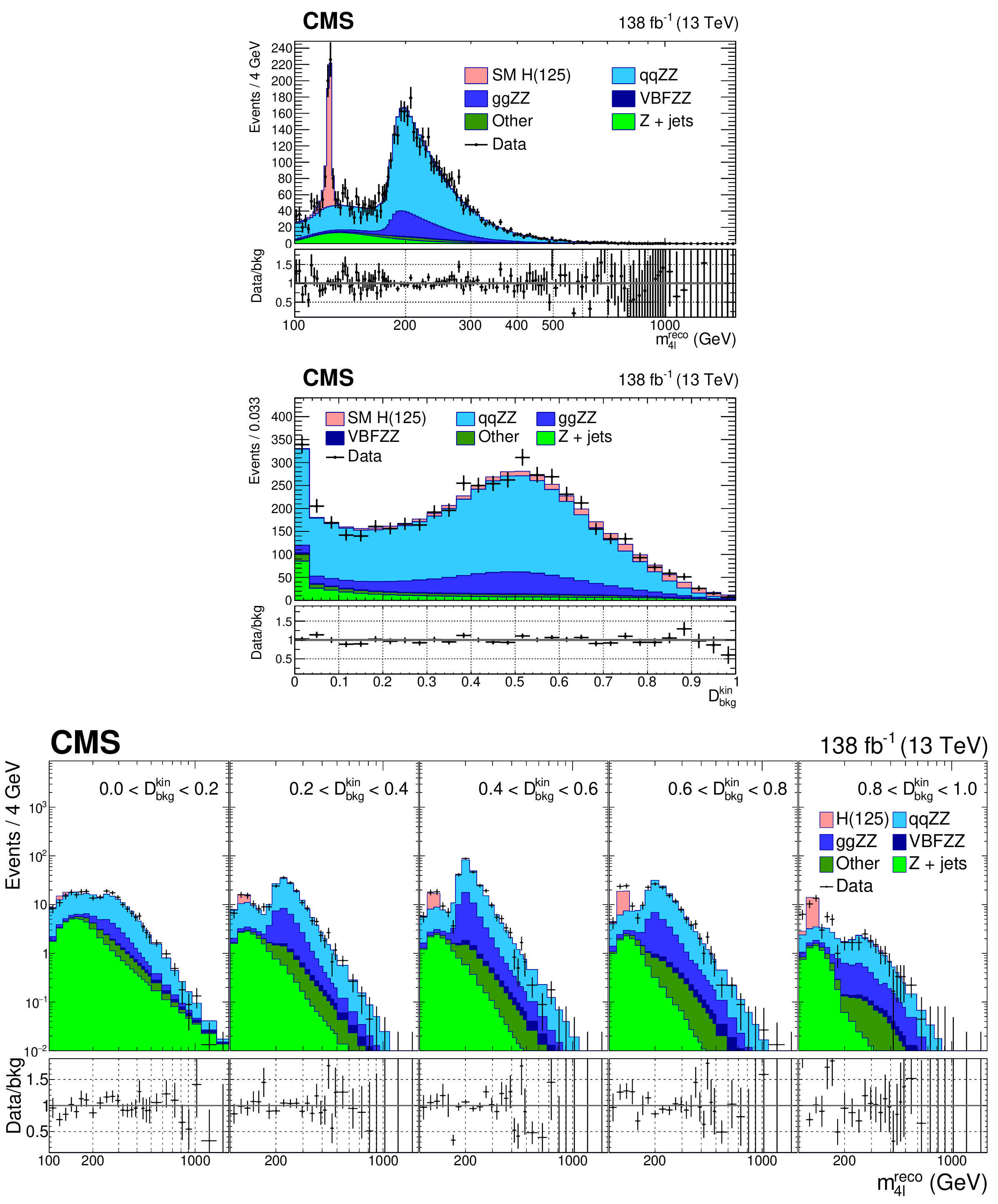
Figure 7:
The $ m_{4\ell}^{\text{reco}} $ and $ D_\text{bkg}^{\text{kin}} $ distributions with the 2016--2018 data set, for backgrounds and observed data. The distributions for backgrounds are extracted from the statistical model, with all nuisance parameters at their best fit values. The upper left (right) panel shows the distribution of $ m_{4\ell}^{\text{reco}} $ ($ D_\text{bkg}^{\text{kin}} $); the lower panel shows the distribution of $ m_{4\ell}^{\text{reco}} $ in bins of $ D_\text{bkg}^{\text{kin}} $. |
png pdf |
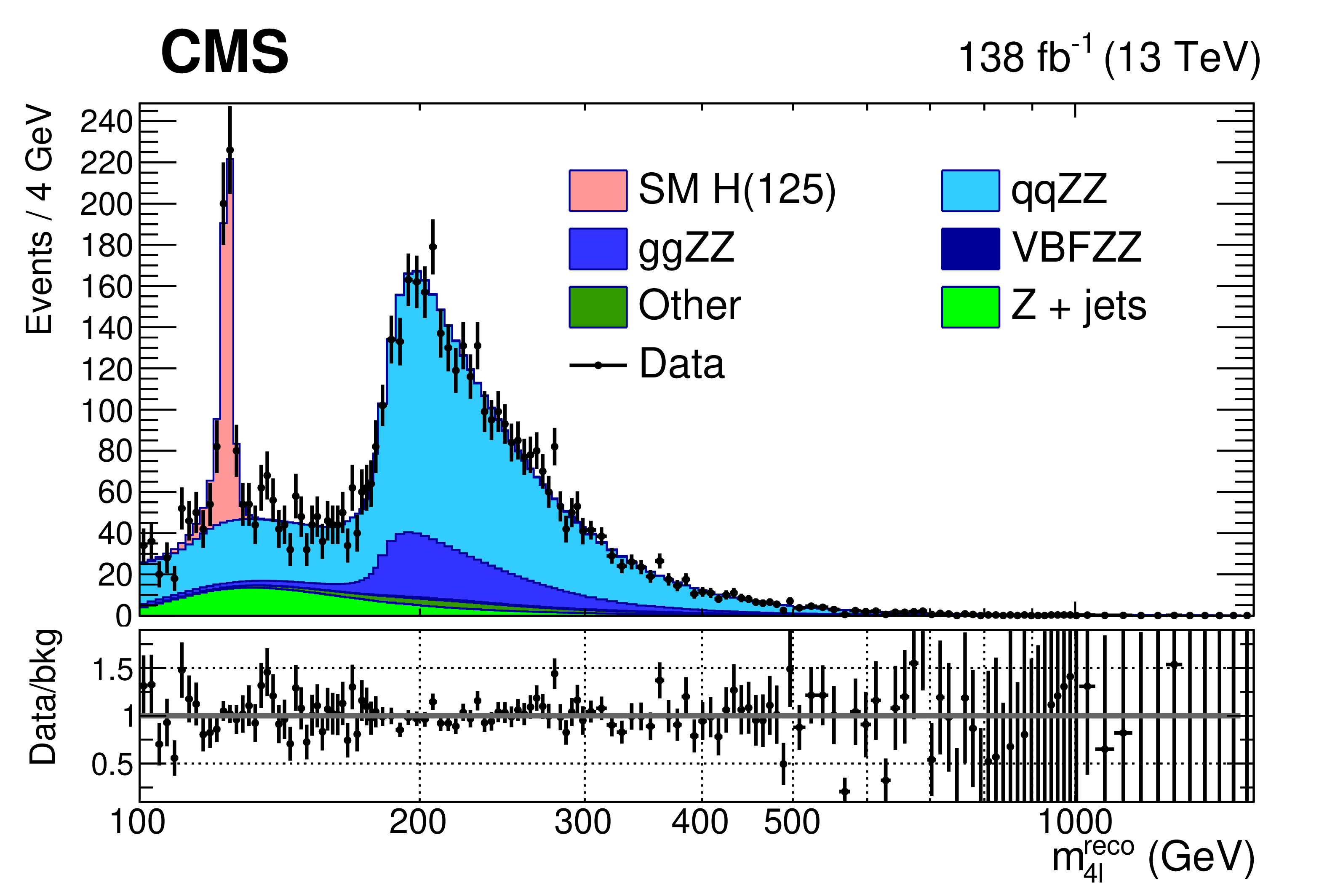
Figure 7-a:
The $ m_{4\ell}^{\text{reco}} $ and $ D_\text{bkg}^{\text{kin}} $ distributions with the 2016--2018 data set, for backgrounds and observed data. The distributions for backgrounds are extracted from the statistical model, with all nuisance parameters at their best fit values. The upper left (right) panel shows the distribution of $ m_{4\ell}^{\text{reco}} $ ($ D_\text{bkg}^{\text{kin}} $); the lower panel shows the distribution of $ m_{4\ell}^{\text{reco}} $ in bins of $ D_\text{bkg}^{\text{kin}} $. |
png pdf |
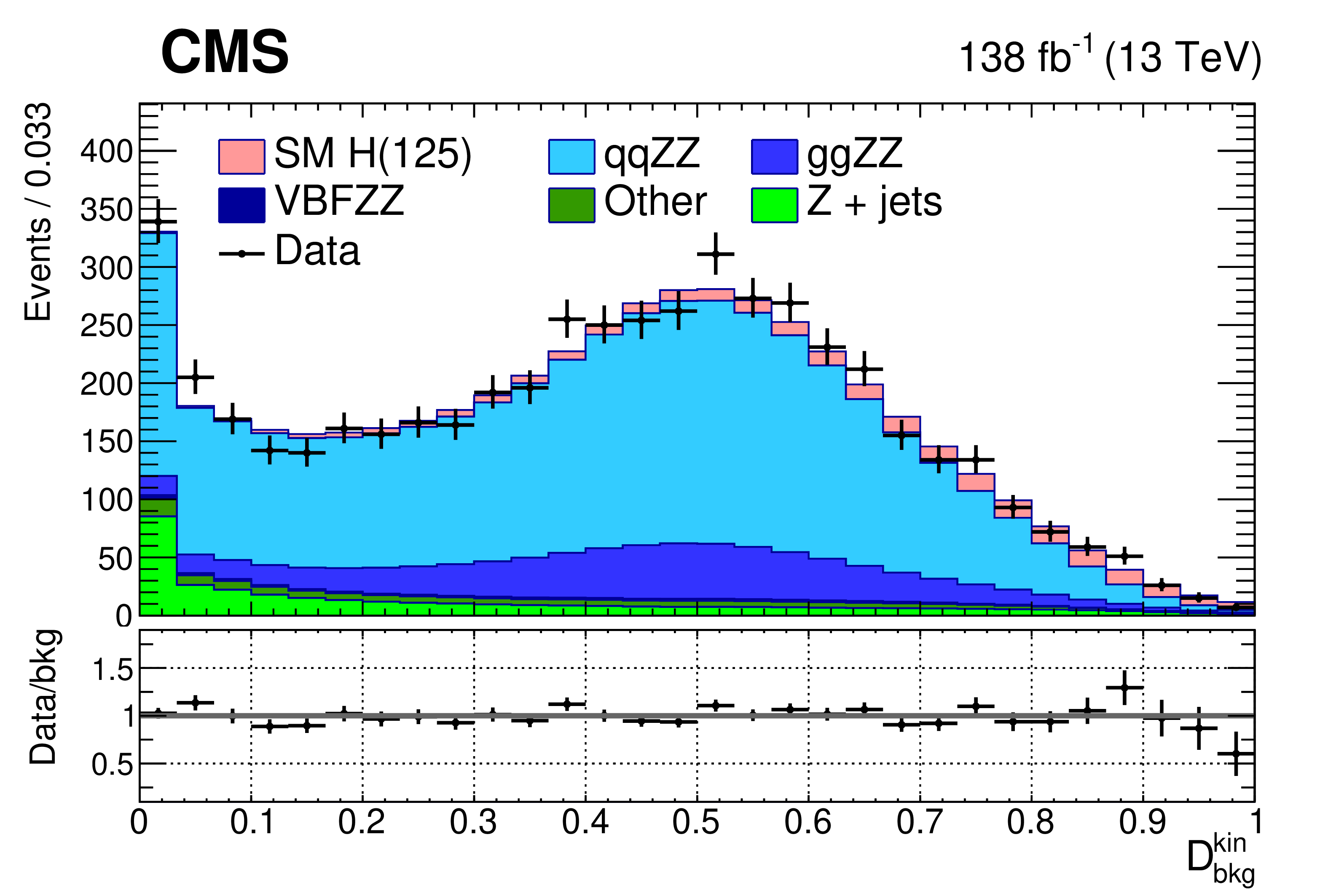
Figure 7-b:
The $ m_{4\ell}^{\text{reco}} $ and $ D_\text{bkg}^{\text{kin}} $ distributions with the 2016--2018 data set, for backgrounds and observed data. The distributions for backgrounds are extracted from the statistical model, with all nuisance parameters at their best fit values. The upper left (right) panel shows the distribution of $ m_{4\ell}^{\text{reco}} $ ($ D_\text{bkg}^{\text{kin}} $); the lower panel shows the distribution of $ m_{4\ell}^{\text{reco}} $ in bins of $ D_\text{bkg}^{\text{kin}} $. |
png pdf |
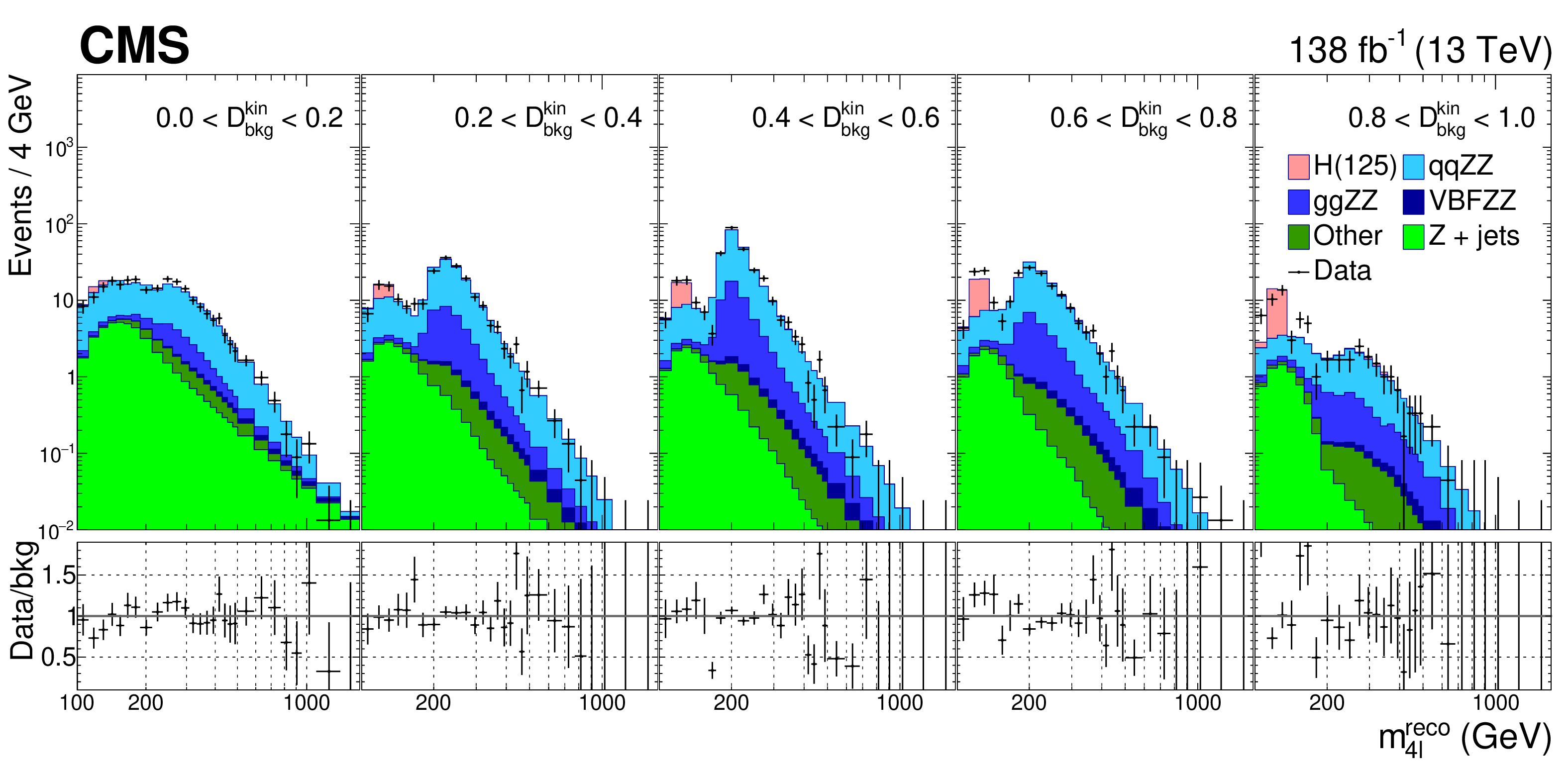
Figure 7-c:
The $ m_{4\ell}^{\text{reco}} $ and $ D_\text{bkg}^{\text{kin}} $ distributions with the 2016--2018 data set, for backgrounds and observed data. The distributions for backgrounds are extracted from the statistical model, with all nuisance parameters at their best fit values. The upper left (right) panel shows the distribution of $ m_{4\ell}^{\text{reco}} $ ($ D_\text{bkg}^{\text{kin}} $); the lower panel shows the distribution of $ m_{4\ell}^{\text{reco}} $ in bins of $ D_\text{bkg}^{\text{kin}} $. |
png pdf |
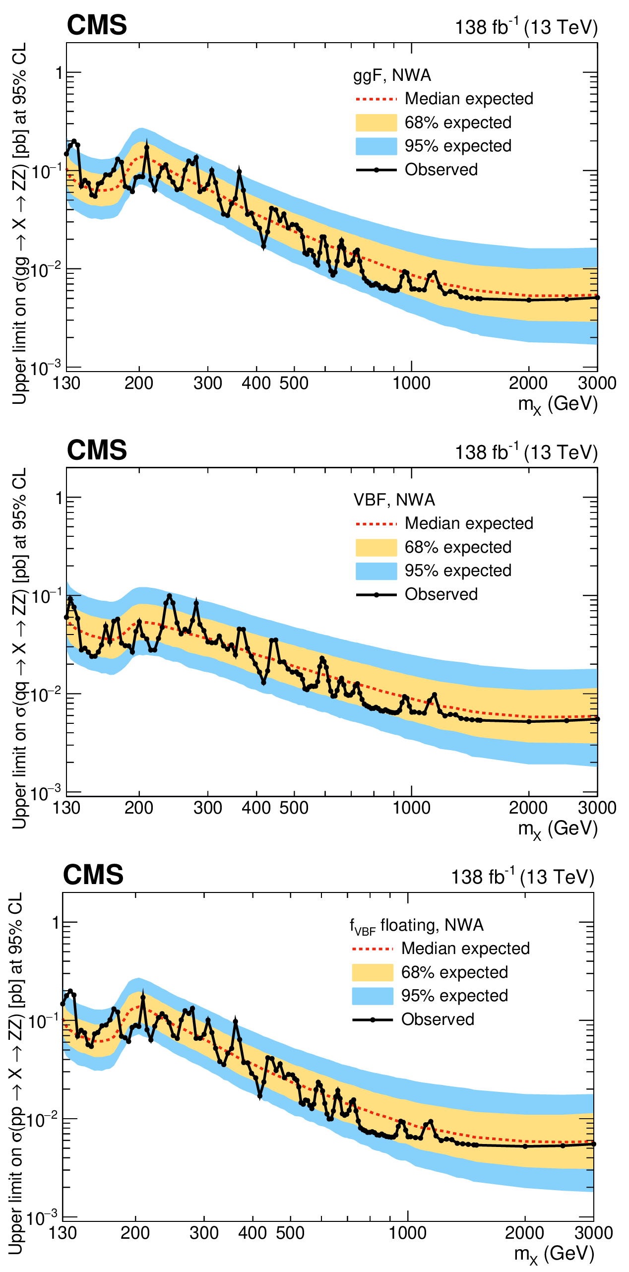
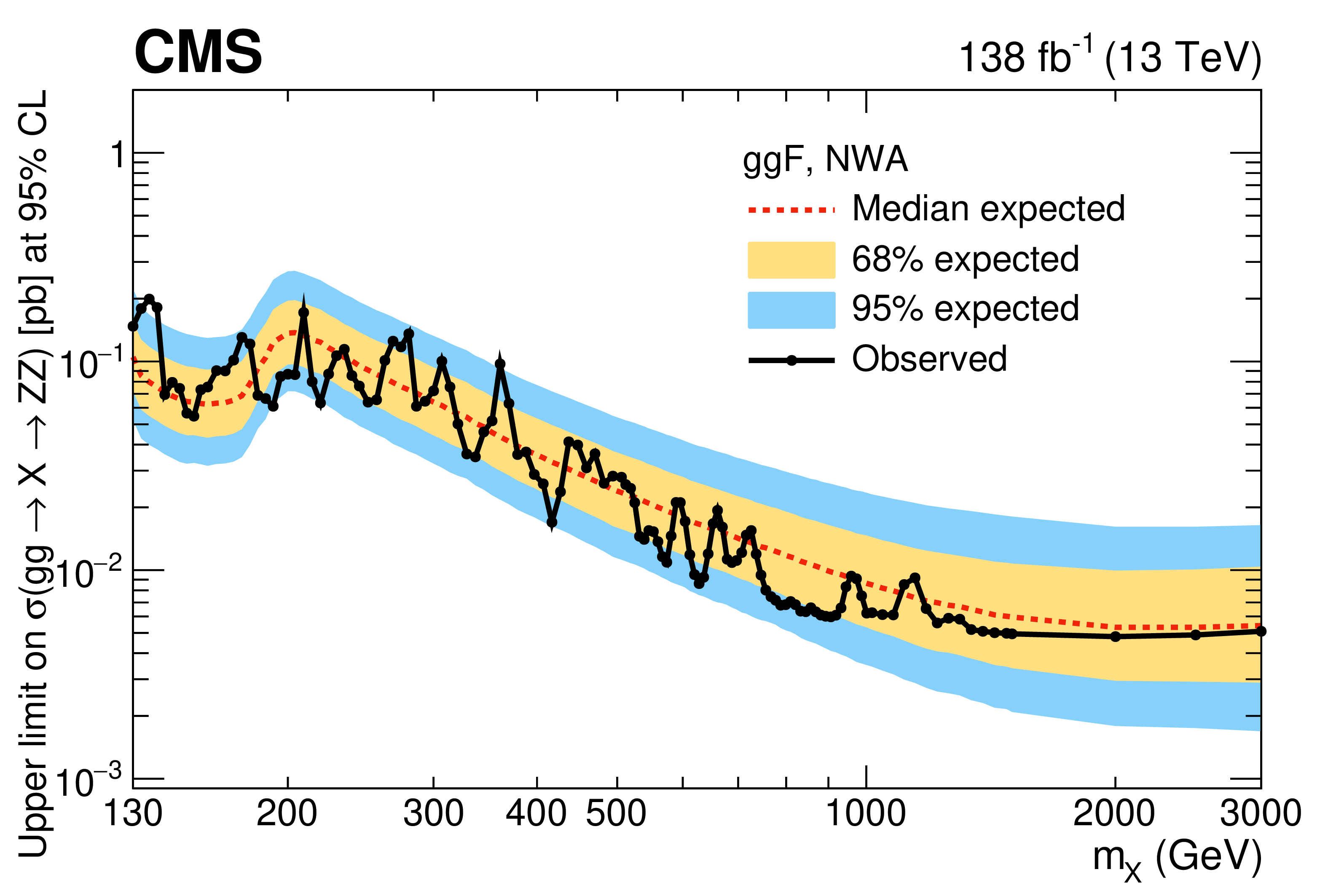
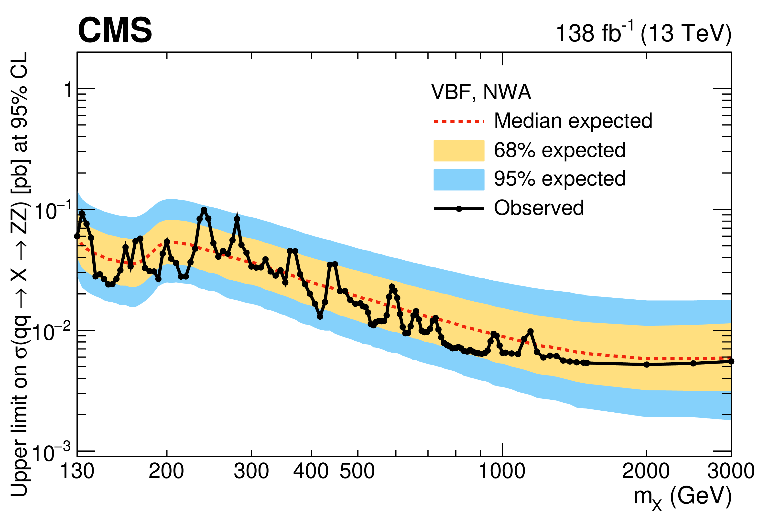
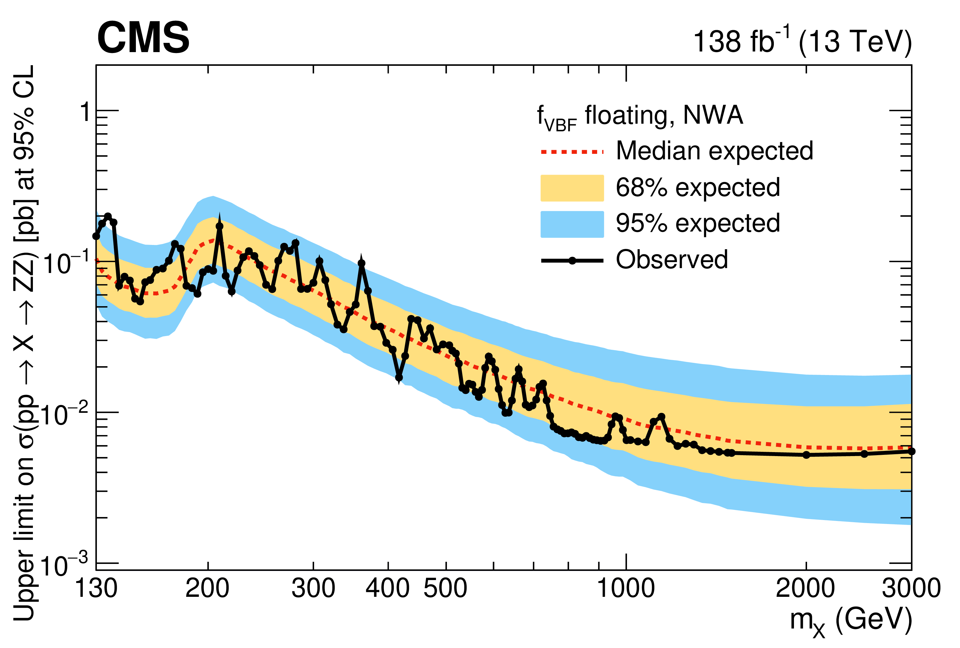
Figure 8:
Observed and expected upper limits on $ \sigma(\mathrm{p}\mathrm{p}\to\mathrm{X}\to\mathrm{Z}\mathrm{Z}) $ with $ m_{\mathrm{X}} $ from 130 GeV to 3 TeV in the narrow-width approximation, for the ggF (upper left) and VBF (upper right) production, and with $ f_\text{VBF} $ as a free parameter in the fit (lower). |
png pdf |
Figure 8-a:
Observed and expected upper limits on $ \sigma(\mathrm{p}\mathrm{p}\to\mathrm{X}\to\mathrm{Z}\mathrm{Z}) $ with $ m_{\mathrm{X}} $ from 130 GeV to 3 TeV in the narrow-width approximation, for the ggF (upper left) and VBF (upper right) production, and with $ f_\text{VBF} $ as a free parameter in the fit (lower). |
png pdf |
Figure 8-b:
Observed and expected upper limits on $ \sigma(\mathrm{p}\mathrm{p}\to\mathrm{X}\to\mathrm{Z}\mathrm{Z}) $ with $ m_{\mathrm{X}} $ from 130 GeV to 3 TeV in the narrow-width approximation, for the ggF (upper left) and VBF (upper right) production, and with $ f_\text{VBF} $ as a free parameter in the fit (lower). |
png pdf |
Figure 8-c:
Observed and expected upper limits on $ \sigma(\mathrm{p}\mathrm{p}\to\mathrm{X}\to\mathrm{Z}\mathrm{Z}) $ with $ m_{\mathrm{X}} $ from 130 GeV to 3 TeV in the narrow-width approximation, for the ggF (upper left) and VBF (upper right) production, and with $ f_\text{VBF} $ as a free parameter in the fit (lower). |
png pdf |
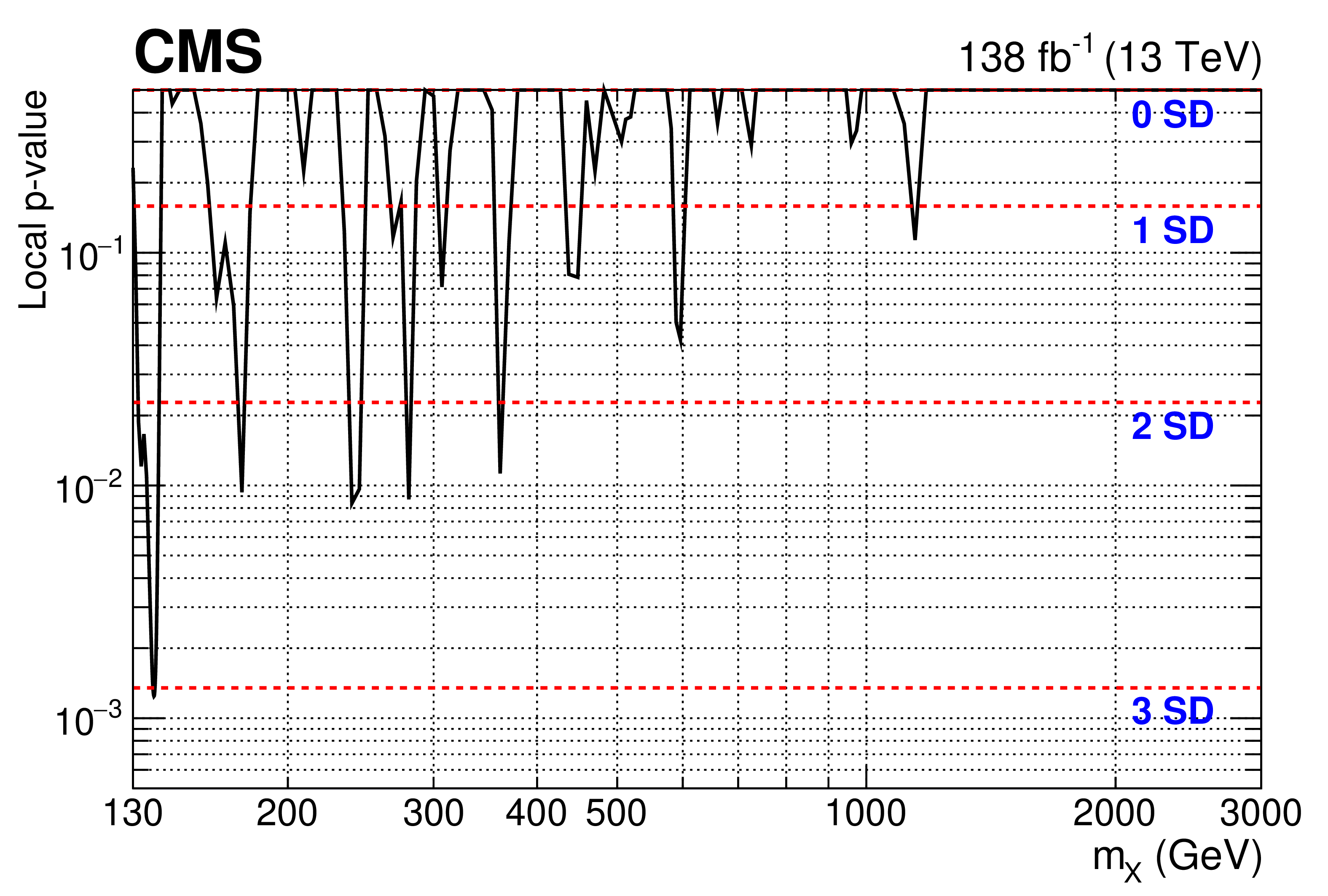
Figure 9:
Local $ p $-value as a function of $ m_{\mathrm{X}} $, with $ f_\text{VBF} $ floating. |
png pdf |
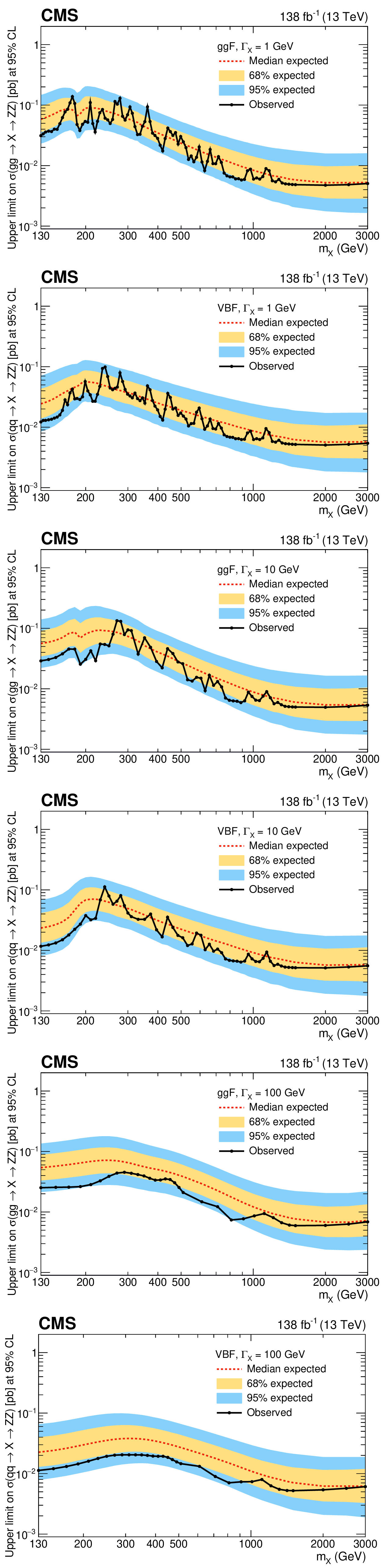
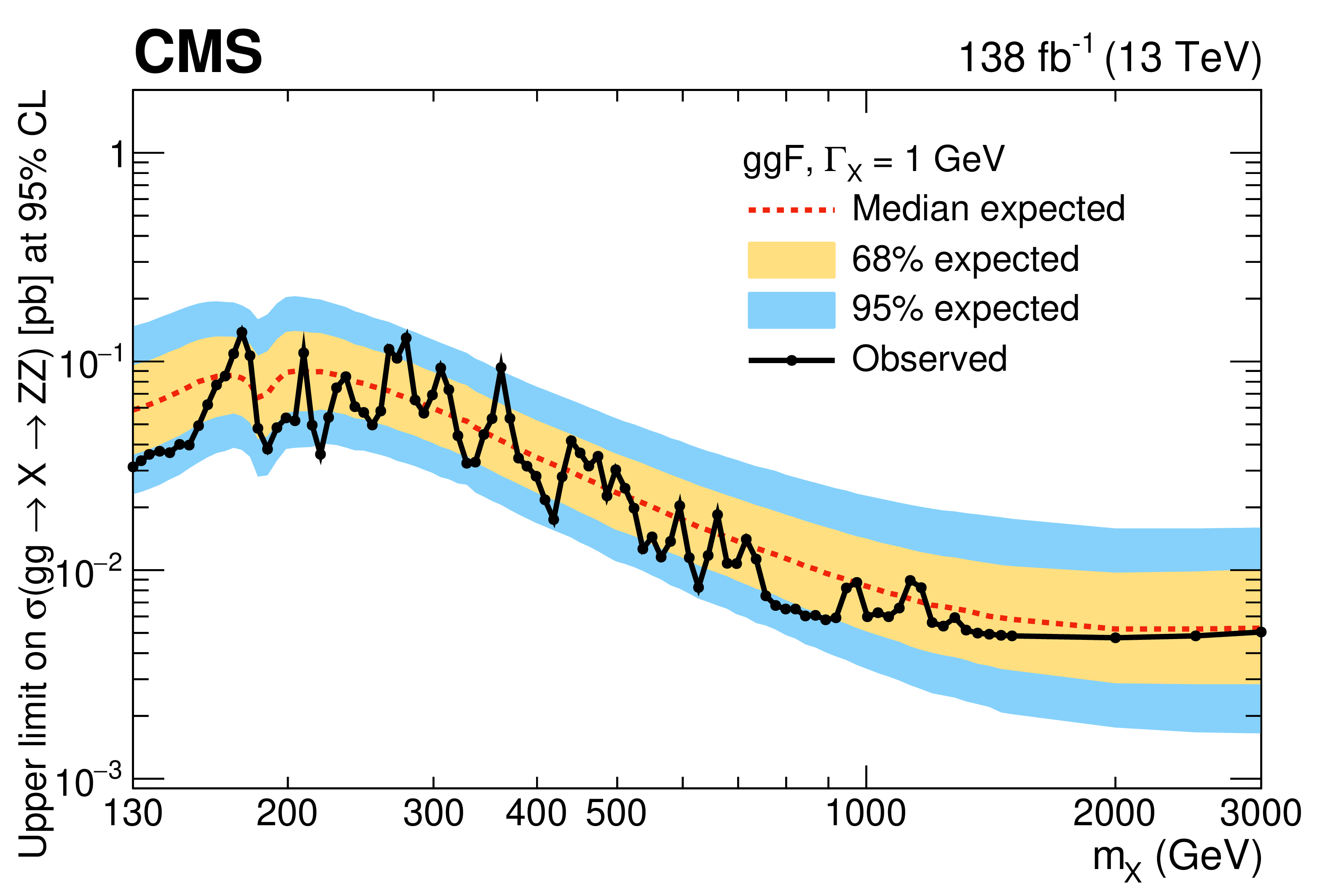
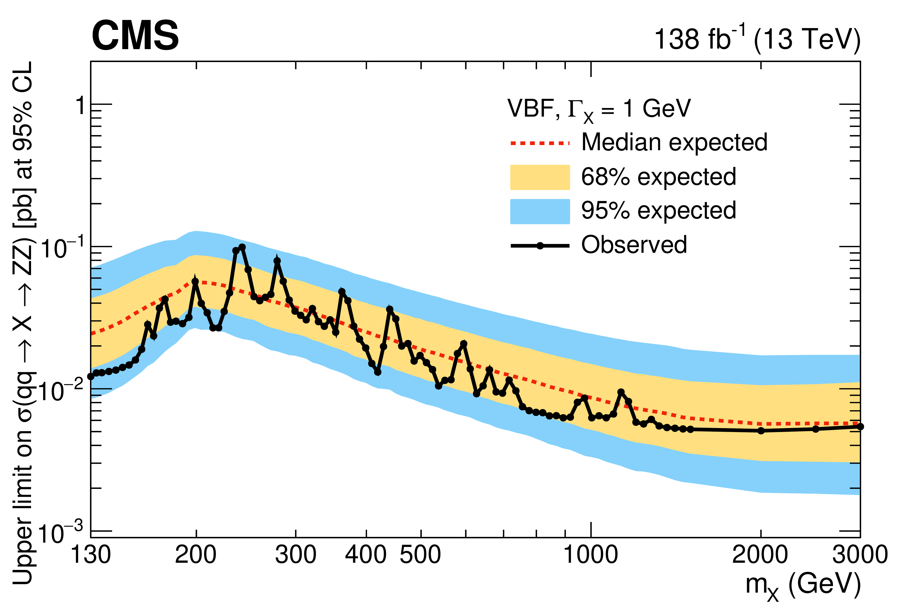
Figure 10:
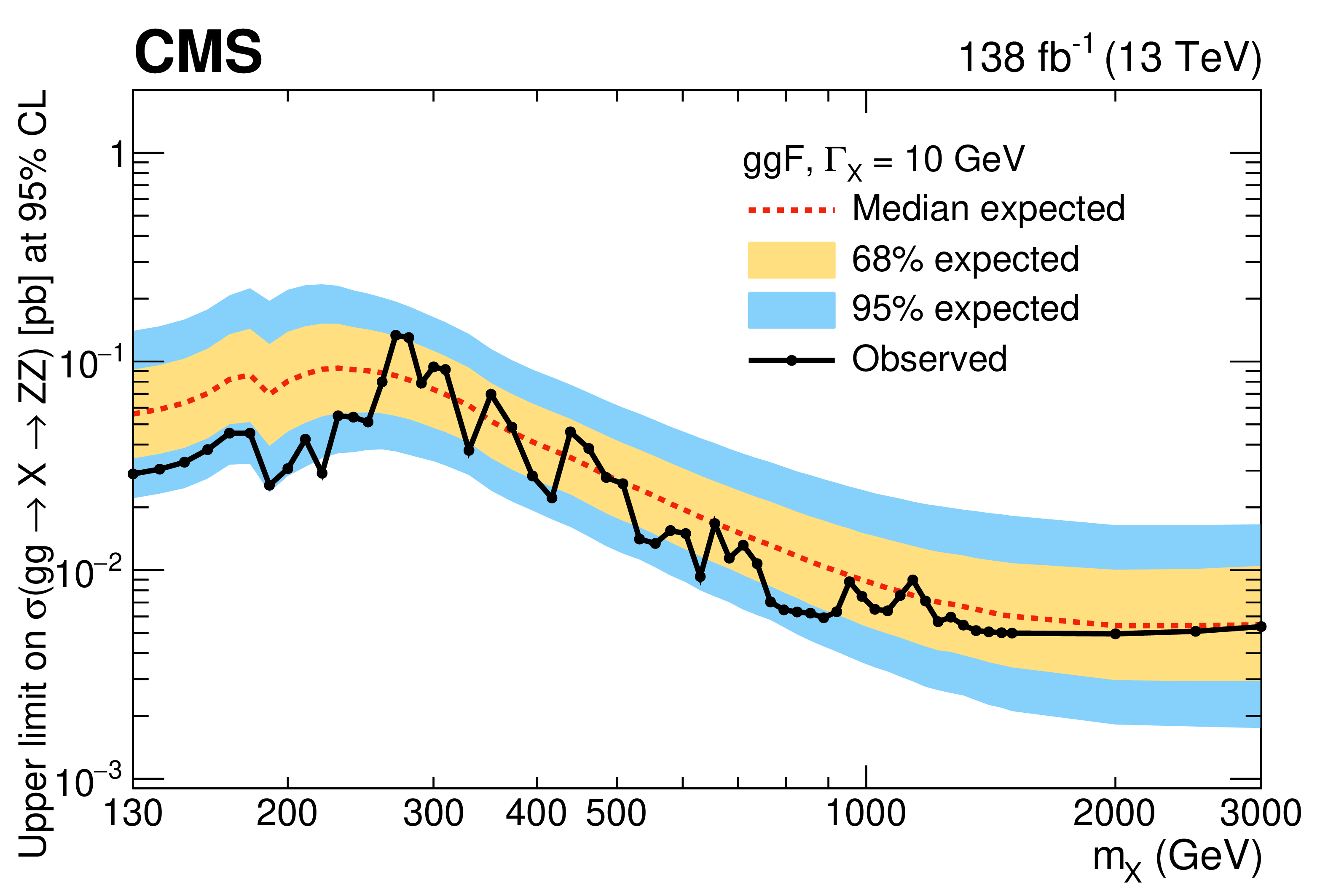
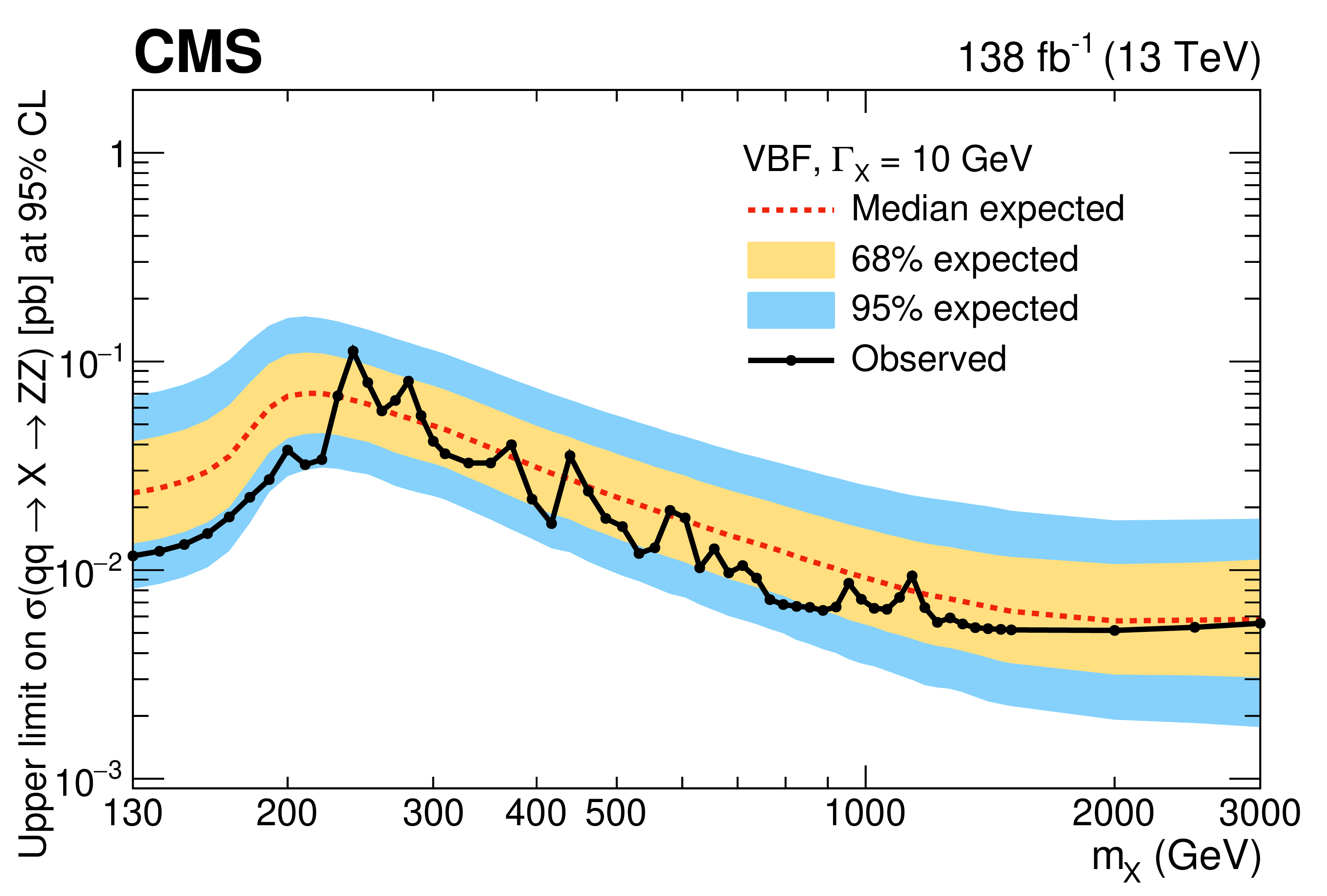
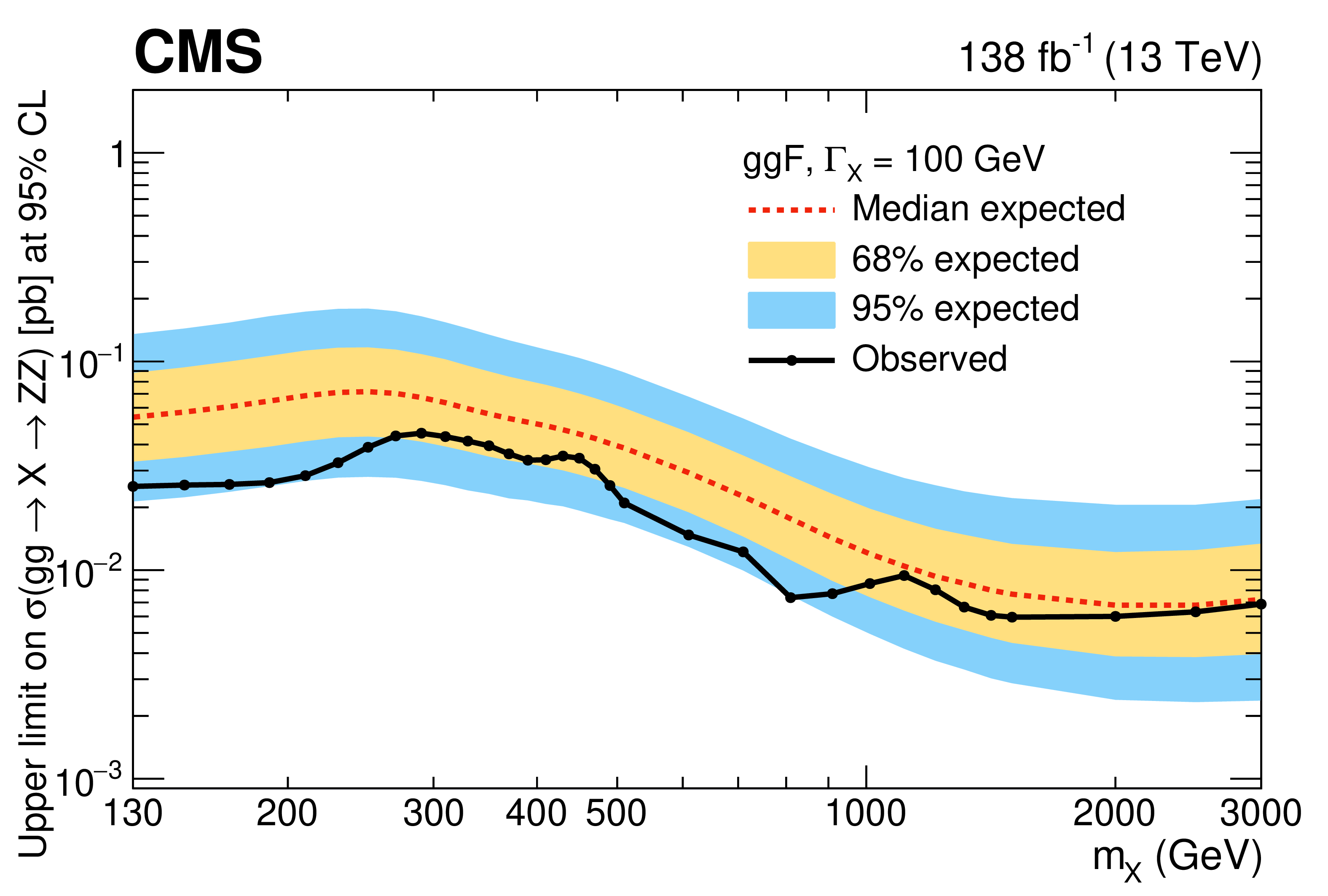
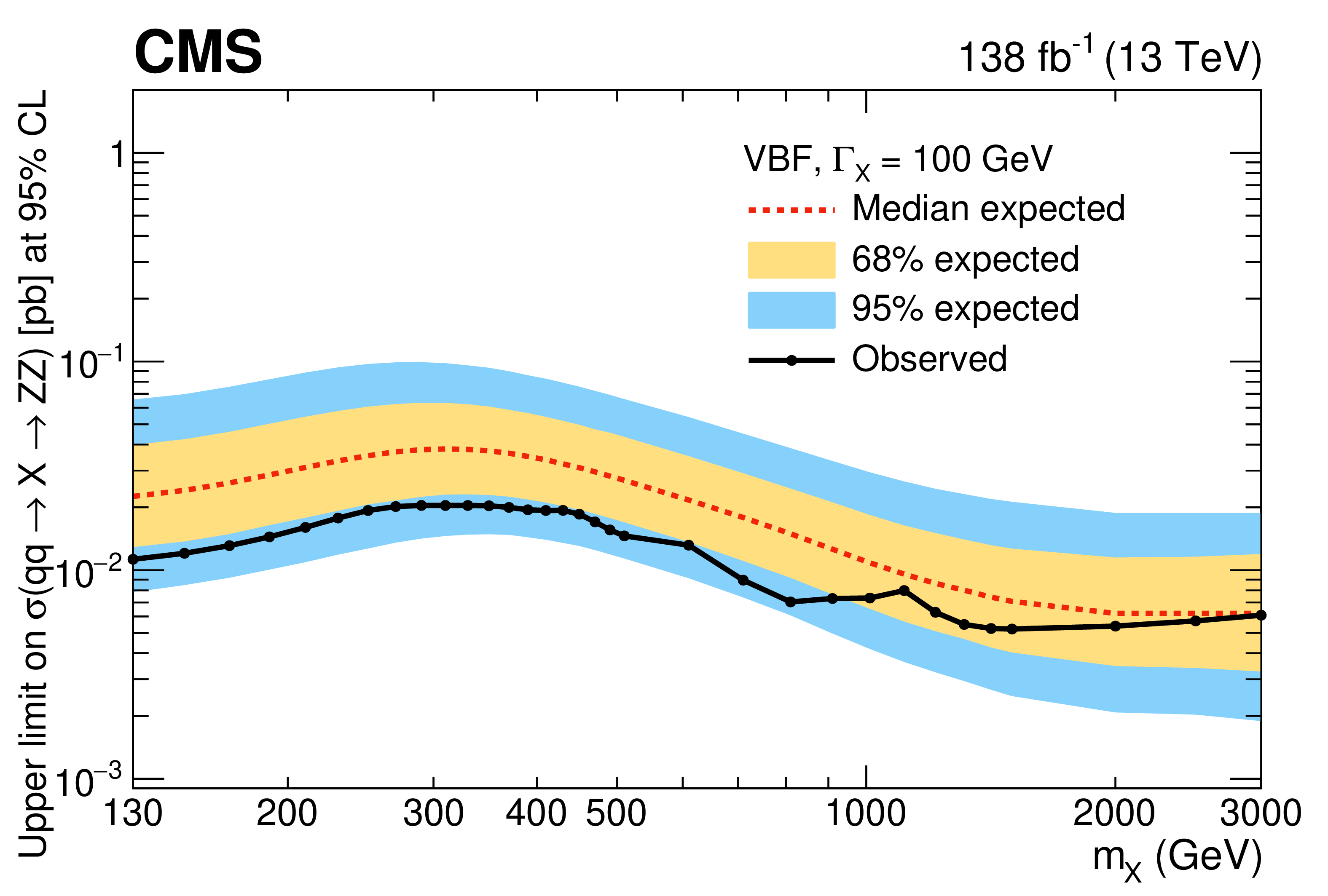
Observed and expected upper limits on $ \sigma(\mathrm{p}\mathrm{p}\to\mathrm{X}\to\mathrm{Z}\mathrm{Z}) $ with $ m_{\mathrm{X}} $ from 130 GeV to 3 TeV and $ \Gamma_{\mathrm{X}} $ equal to 1 (upper), 10 (middle), and 100 (lower) GeV. The left column shows the results for pure ggF production and the right column shows the results for pure VBF production. |
png pdf |
Figure 10-a:
Observed and expected upper limits on $ \sigma(\mathrm{p}\mathrm{p}\to\mathrm{X}\to\mathrm{Z}\mathrm{Z}) $ with $ m_{\mathrm{X}} $ from 130 GeV to 3 TeV and $ \Gamma_{\mathrm{X}} $ equal to 1 (upper), 10 (middle), and 100 (lower) GeV. The left column shows the results for pure ggF production and the right column shows the results for pure VBF production. |
png pdf |
Figure 10-b:
Observed and expected upper limits on $ \sigma(\mathrm{p}\mathrm{p}\to\mathrm{X}\to\mathrm{Z}\mathrm{Z}) $ with $ m_{\mathrm{X}} $ from 130 GeV to 3 TeV and $ \Gamma_{\mathrm{X}} $ equal to 1 (upper), 10 (middle), and 100 (lower) GeV. The left column shows the results for pure ggF production and the right column shows the results for pure VBF production. |
png pdf |
Figure 10-c:
Observed and expected upper limits on $ \sigma(\mathrm{p}\mathrm{p}\to\mathrm{X}\to\mathrm{Z}\mathrm{Z}) $ with $ m_{\mathrm{X}} $ from 130 GeV to 3 TeV and $ \Gamma_{\mathrm{X}} $ equal to 1 (upper), 10 (middle), and 100 (lower) GeV. The left column shows the results for pure ggF production and the right column shows the results for pure VBF production. |
png pdf |
Figure 10-d:
Observed and expected upper limits on $ \sigma(\mathrm{p}\mathrm{p}\to\mathrm{X}\to\mathrm{Z}\mathrm{Z}) $ with $ m_{\mathrm{X}} $ from 130 GeV to 3 TeV and $ \Gamma_{\mathrm{X}} $ equal to 1 (upper), 10 (middle), and 100 (lower) GeV. The left column shows the results for pure ggF production and the right column shows the results for pure VBF production. |
png pdf |
Figure 10-e:
Observed and expected upper limits on $ \sigma(\mathrm{p}\mathrm{p}\to\mathrm{X}\to\mathrm{Z}\mathrm{Z}) $ with $ m_{\mathrm{X}} $ from 130 GeV to 3 TeV and $ \Gamma_{\mathrm{X}} $ equal to 1 (upper), 10 (middle), and 100 (lower) GeV. The left column shows the results for pure ggF production and the right column shows the results for pure VBF production. |
png pdf |
Figure 10-f:
Observed and expected upper limits on $ \sigma(\mathrm{p}\mathrm{p}\to\mathrm{X}\to\mathrm{Z}\mathrm{Z}) $ with $ m_{\mathrm{X}} $ from 130 GeV to 3 TeV and $ \Gamma_{\mathrm{X}} $ equal to 1 (upper), 10 (middle), and 100 (lower) GeV. The left column shows the results for pure ggF production and the right column shows the results for pure VBF production. |
png pdf |
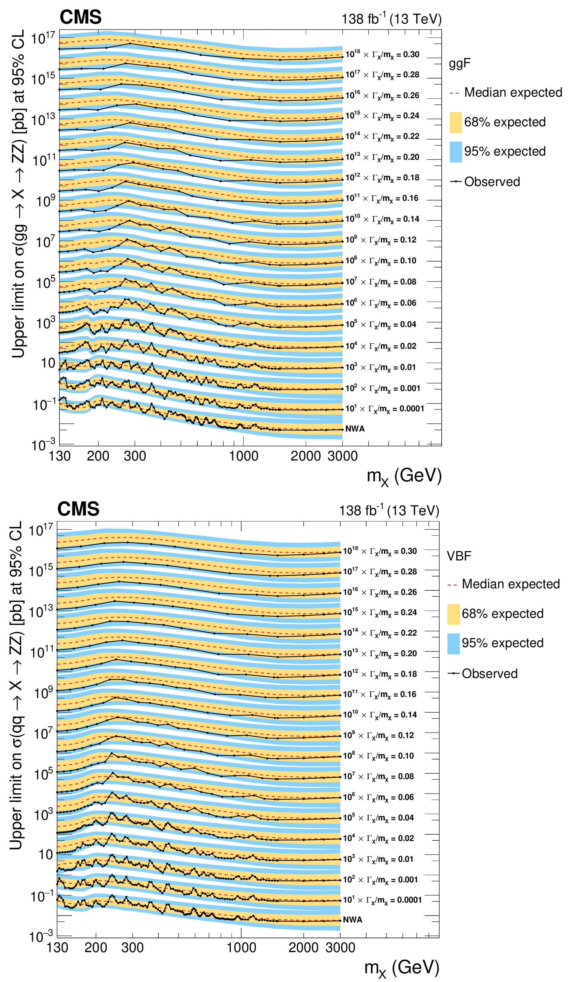
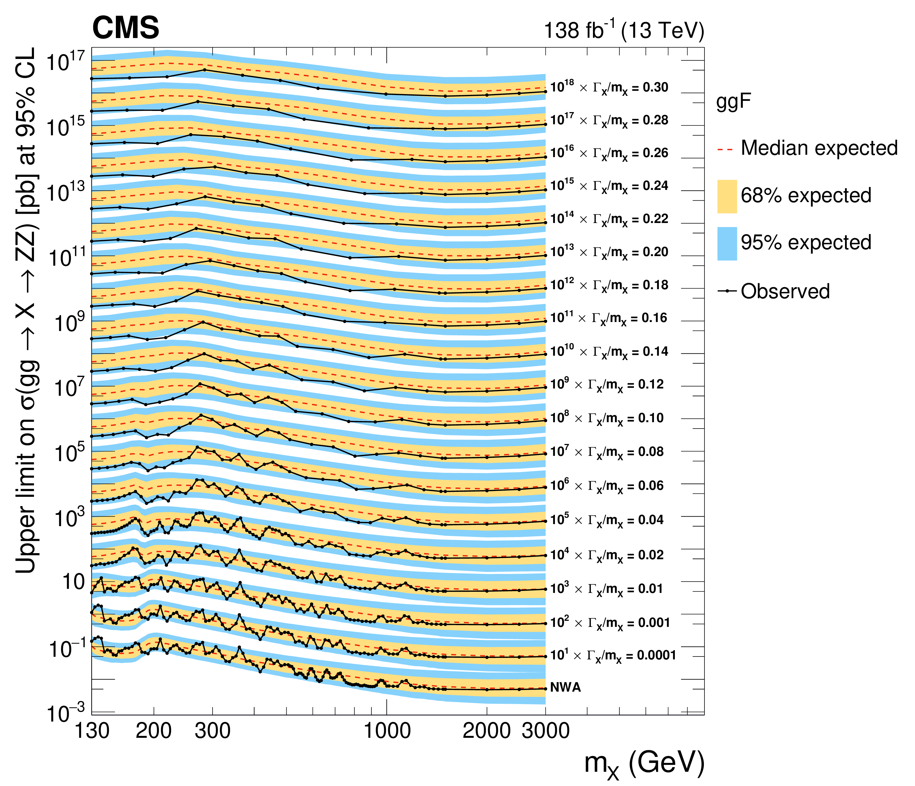
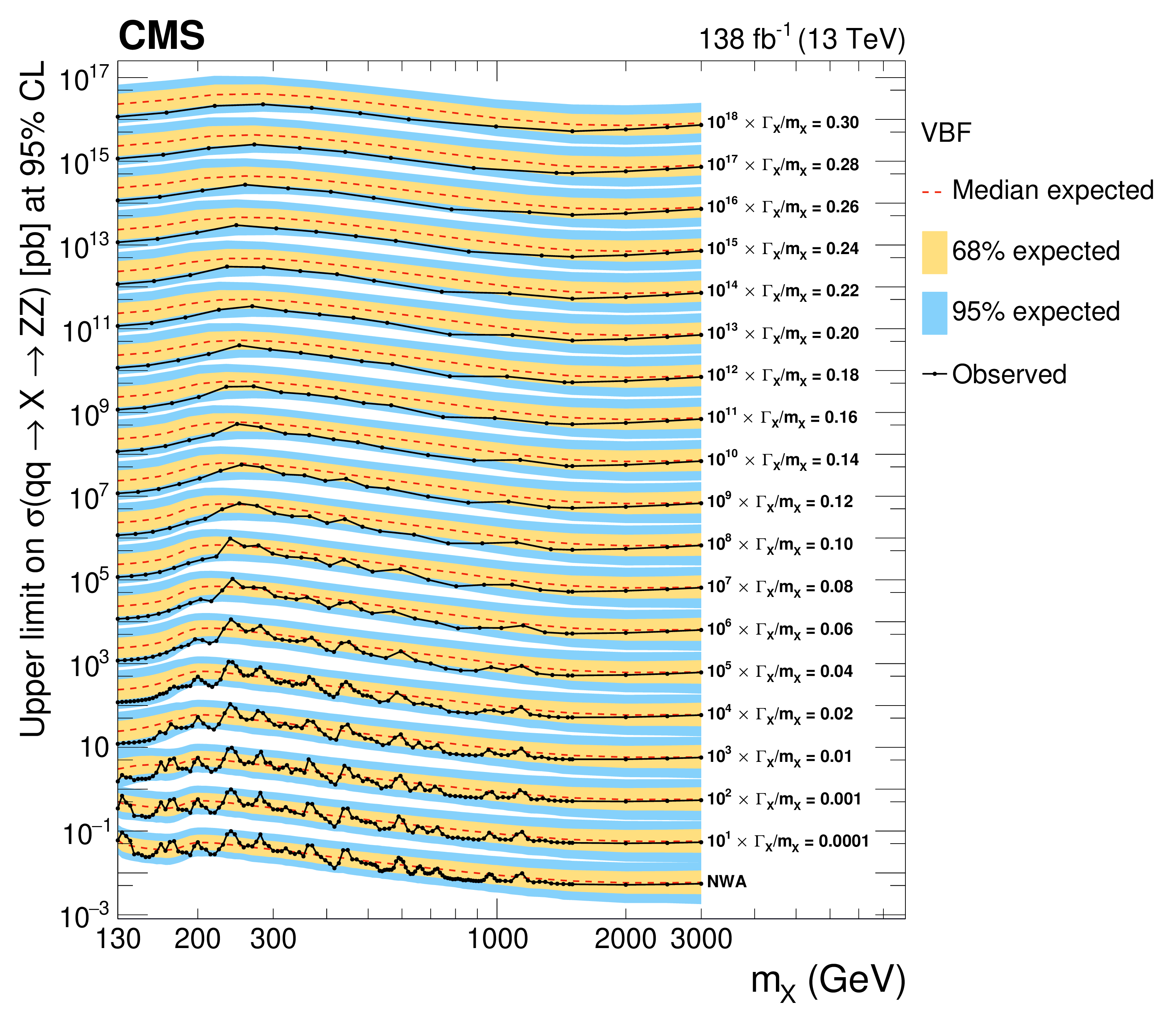
Figure 11:
Observed and expected 95% CL upper limits on $ \sigma(\mathrm{p}\mathrm{p}\to X\to ZZ) $ with $ m_{\mathrm{X}} $ from 130 GeV to 3 TeV and $ \Gamma_{\mathrm{X}}/m_{\mathrm{X}} $ up to 30%. The upper panel shows the results for pure ggF production, and the lower panel shows the results for pure VBF production. |
png pdf |
Figure 11-a:
Observed and expected 95% CL upper limits on $ \sigma(\mathrm{p}\mathrm{p}\to X\to ZZ) $ with $ m_{\mathrm{X}} $ from 130 GeV to 3 TeV and $ \Gamma_{\mathrm{X}}/m_{\mathrm{X}} $ up to 30%. The upper panel shows the results for pure ggF production, and the lower panel shows the results for pure VBF production. |
png pdf |
Figure 11-b:
Observed and expected 95% CL upper limits on $ \sigma(\mathrm{p}\mathrm{p}\to X\to ZZ) $ with $ m_{\mathrm{X}} $ from 130 GeV to 3 TeV and $ \Gamma_{\mathrm{X}}/m_{\mathrm{X}} $ up to 30%. The upper panel shows the results for pure ggF production, and the lower panel shows the results for pure VBF production. |
| Tables | |
png pdf |
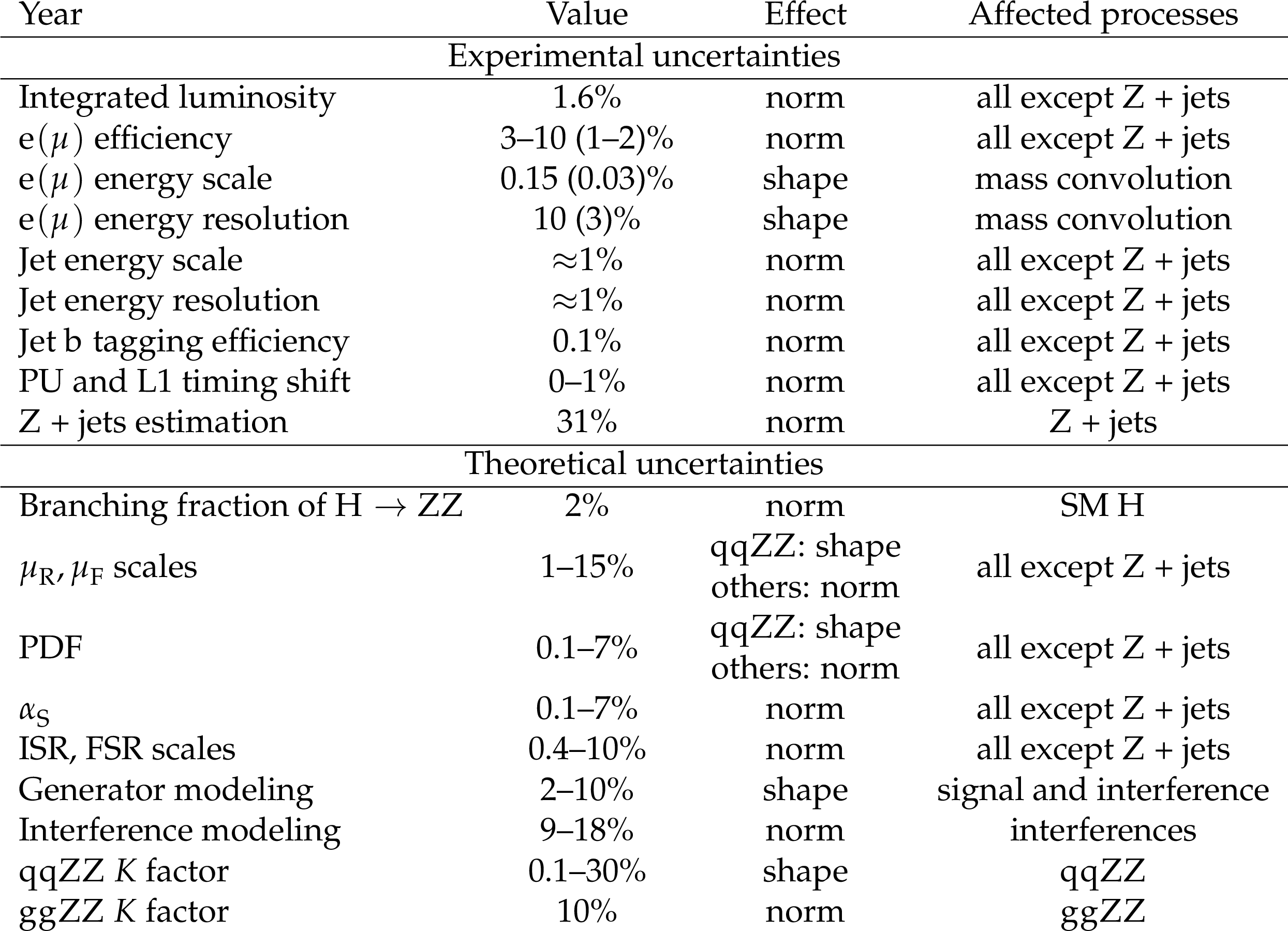
Table 1:
Summary of the experimental and theoretical uncertainties used in this analysis. Uncertainties affecting only the normalization are marked as ``norm'' in the table. Those affecting observable shapes are indicated as ``shape''. |
| Summary |
| A search for a spin-0 resonance decaying to a pair of Z bosons in the four-lepton final state, where the leptons are muons or electrons, is performed at the CMS experiment. The data set used was collected in 2016--2018 and corresponds to an integrated luminosity of 138 fb$ ^{-1} $. The searched-for resonance can be produced via gluon fusion or vector boson fusion. The mass of the sought resonance is scanned over a range from 130 GeV to 3 TeV, and different decay width assumptions are tested. No significant excess over the standard model background expectation is observed. The largest fluctuation is seen at a mass of 137.8 GeV under the narrow-width assumption, reaching a global significance of 1.8 standard deviations. Upper limits at 95% confidence level on the production cross section multiplied by the decay branching fraction of $ \mathrm{X}\to\mathrm{Z}\mathrm{Z} $ are set for various masses, decay widths, and production mechanisms. The exclusion limits range from 0.05--0.1 pb in the low-mass region to 0.005 pb in the high-mass region. |
| References | ||||
| 1 | ATLAS Collaboration | Observation of a new particle in the search for the standard model Higgs boson with the ATLAS detector at the LHC | PLB 716 (2012) 1 | 1207.7214 |
| 2 | CMS Collaboration | Observation of a new boson at a mass of 125 GeV with the CMS experiment at the LHC | PLB 716 (2012) 30 | CMS-HIG-12-028 1207.7235 |
| 3 | CMS Collaboration | Observation of a new boson with mass near 125 GeV in pp collisions at $ \sqrt{s}= $ 7 and 8 TeV | JHEP 06 (2013) 81 | CMS-HIG-12-036 1303.4571 |
| 4 | G. C. Branco et al. | Theory and phenomenology of two-Higgs-doublet models | Phys. Rept. 516 (2012) 1 | 1106.0034 |
| 5 | L. Randall and R. Sundrum | Large mass hierarchy from a small extra dimension | PRL 83 (1999) 3370 | hep-ph/9905221 |
| 6 | W. D. Goldberger and M. B. Wise | Modulus stabilization with bulk fields | PRL 83 (1999) 4922 | hep-ph/9907447 |
| 7 | A. Carvalho | Gravity particles from warped extra dimensions, predictions for LHC | 1404.0102 | |
| 8 | CMS Collaboration | Search for a Higgs boson in the mass range from 145 to 1000 GeV decaying to a pair of W or Z bosons | JHEP 10 (2015) 144 | CMS-HIG-13-031 1504.00936 |
| 9 | CMS Collaboration | Search for a new scalar resonance decaying to a pair of Z bosons in proton-proton collisions at $ \sqrt{s} = $ 13 TeV | JHEP 06 (2018) 127 | CMS-HIG-17-012 1804.01939 |
| 10 | ATLAS Collaboration | Search for an additional, heavy Higgs boson in the $ h\rightarrow zz $ decay channel at $ \sqrt{s} = $ 8 TeV in $ pp $ collision data with the ATLAS detector | EPJC 76 (2016) 45 | 1507.05930 |
| 11 | ATLAS Collaboration | Search for heavy resonances decaying into a pair of Z bosons in the $ \ell ^+\ell ^-\ell '^+\ell '^- $ and $ \ell ^+\ell ^-\nu {{\bar{\nu }}} $ final states using 139 fb$ ^{-1} $ of proton-proton collisions at $ \sqrt{s} = $ 13 TeV with the ATLAS detector | EPJC 81 (2021) 332 | 2009.14791 |
| 12 | CMS Collaboration | HEPData record for this analysis | link | |
| 13 | CMS Collaboration | The CMS experiment at the CERN LHC | JINST 3 (2008) S08004 | |
| 14 | CMS Collaboration | Development of the CMS detector for the CERN LHC Run 3 | JINST 19 (2024) P05064 | CMS-PRF-21-001 2309.05466 |
| 15 | CMS Collaboration | Performance of the CMS Level-1 trigger in proton-proton collisions at $ \sqrt{s} = $ 13 TeV | JINST 15 (2020) P10017 | CMS-TRG-17-001 2006.10165 |
| 16 | CMS Collaboration | The CMS trigger system | JINST 12 (2017) P01020 | CMS-TRG-12-001 1609.02366 |
| 17 | CMS Collaboration | Performance of the CMS high-level trigger during LHC Run 2 | JINST 19 (2024) P11021 | CMS-TRG-19-001 2410.17038 |
| 18 | CMS Collaboration | Electron and photon reconstruction and identification with the CMS experiment at the CERN LHC | JINST 16 (2021) P05014 | CMS-EGM-17-001 2012.06888 |
| 19 | CMS Collaboration | Performance of the CMS muon detector and muon reconstruction with proton-proton collisions at $ \sqrt{s} = $ 13 TeV | JINST 13 (2018) P06015 | CMS-MUO-16-001 1804.04528 |
| 20 | CMS Collaboration | Description and performance of track and primary-vertex reconstruction with the CMS tracker | JINST 9 (2014) P10009 | CMS-TRK-11-001 1405.6569 |
| 21 | CMS Collaboration | Precision luminosity measurement in proton-proton collisions at $ \sqrt{s} = $ 13 TeV in 2015 and 2016 at CMS | EPJC 81 (2021) 800 | CMS-LUM-17-003 2104.01927 |
| 22 | CMS Collaboration | CMS luminosity measurement for the 2017 data-taking period at $ \sqrt{s} = $ 13 TeV | CMS Physics Analysis Summary, 2018 CMS-PAS-LUM-17-004 |
CMS-PAS-LUM-17-004 |
| 23 | CMS Collaboration | CMS luminosity measurement for the 2018 data-taking period at $ \sqrt{s} = $ 13 TeV | CMS Physics Analysis Summary, 2019 CMS-PAS-LUM-18-002 |
CMS-PAS-LUM-18-002 |
| 24 | CMS Collaboration | Measurements of production cross sections of the Higgs boson in the four-lepton final state in proton-proton collisions at $ \sqrt{s} = $ 13 TeV | EPJC 81 (2021) 488 | CMS-HIG-19-001 2103.04956 |
| 25 | CMS Collaboration | Measurement of the inclusive W and Z production cross sections in pp collisions at $ \sqrt{s}= $ 7 TeV with the CMS experiment | JHEP 10 (2011) 132 | CMS-EWK-10-005 1107.4789 |
| 26 | S. Alioli, P. Nason, C. Oleari, and E. Re | NLO vector-boson production matched with shower in POWHEG | JHEP 07 (2008) 060 | 0805.4802 |
| 27 | P. Nason | A new method for combining NLO QCD with shower Monte Carlo algorithms | JHEP 11 (2004) 040 | hep-ph/0409146 |
| 28 | S. Frixione, P. Nason, and C. Oleari | Matching NLO QCD computations with parton shower simulations: the POWHEG method | JHEP 11 (2007) 070 | 0709.2092 |
| 29 | Y. Gao et al. | Spin determination of single-produced resonances at hadron colliders | PRD 81 (2010) 075022 | 1001.3396 |
| 30 | S. Bolognesi et al. | Spin and parity of a single-produced resonance at the LHC | PRD 86 (2012) 095031 | 1208.4018 |
| 31 | I. Anderson et al. | Constraining anomalous HVV interactions at proton and lepton colliders | PRD 89 (2014) 035007 | 1309.4819 |
| 32 | A. V. Gritsan, R. Roentsch, M. Schulze, and M. Xiao | Constraining anomalous Higgs boson couplings to the heavy flavor fermions using matrix element techniques | PRD 94 (2016) 055023 | 1606.03107 |
| 33 | S. Goria, G. Passarino, and D. Rosco | The Higgs-boson lineshape | NPB 864 (2012) 530 | 1112.5517 |
| 34 | G. Passarino, C. Sturm, and S. Uccirati | Higgs pseudo-observables, second Riemann sheet and all that | NPB 834 (2010) 77 | 1001.3360 |
| 35 | K. Hamilton, P. Nason, E. Re, and G. Zanderighi | NNLOPS simulation of Higgs boson production | JHEP 10 (2013) 222 | 1309.0017 |
| 36 | M. Grazzini, S. Kallweit, and D. Rathlev | ZZ production at the LHC: fiducial cross sections and distributions in NNLO QCD | PLB 750 (2015) 407 | 1507.06257 |
| 37 | J. M. Campbell and R. K. Ellis | MCFM for the Tevatron and the LHC | Nucl. Phys. B Proc. Suppl. 20 (2010) 5 | 1007.3492 |
| 38 | J. M. Campbell, R. K. Ellis, and C. Williams | Vector boson pair production at the LHC | JHEP 07 (2011) 018 | 1105.0020 |
| 39 | J. M. Campbell, R. K. Ellis, and C. Williams | Bounding the Higgs width at the LHC using full analytic results for $ \mathrm{g}\mathrm{g}\to \mathrm{e^-}\mathrm{e^+} \mu^- \mu^+ $ | JHEP 04 (2014) 060 | 1311.3589 |
| 40 | M. Bonvini et al. | Signal-background interference effects for $ \mathrm{g}\mathrm{g} \to \mathrm{H} \to \mathrm{W}^+\mathrm{W}^- $ beyond leading order | PRD 88 (2013) 034032 | 1304.3053 |
| 41 | K. Melnikov and M. Dowling | Production of two Z bosons in gluon fusion in the heavy top quark approximation | PLB 744 (2015) 43 | 1503.01274 |
| 42 | C. S. Li, H. T. Li, D. Y. Shao, and J. Wang | Soft gluon resummation in the signal-background interference process of $ gg(\to h^*) \to ZZ $ | JHEP 08 (2015) 65 | 1504.02388 |
| 43 | S. Catani and M. Grazzini | Next-to-next-to-leading-order subtraction formalism in hadron collisions and its application to Higgs-boson production at the Large Hadron Collider | PRL 98 (2007) 222002 | hep-ph/0703012 |
| 44 | M. Grazzini | NNLO predictions for the Higgs boson signal in the $ \mathrm{H}\to \mathrm{W}\mathrm{W}\to \ell\nu l\nu $ and $ \mathrm{H} \to\mathrm{Z}\mathrm{Z} \to 4\ell $ decay channels | JHEP 02 (2008) 043 | 0801.3232 |
| 45 | M. Grazzini and H. Sargsyan | Heavy-quark mass effects in Higgs boson production at the LHC | JHEP 09 (2013) 129 | 1306.4581 |
| 46 | J. Alwall et al. | The automated computation of tree-level and next-to-leading order differential cross sections, and their matching to parton shower simulations | JHEP 07 (2014) 079 | 1405.0301 |
| 47 | S. Frixione, P. Nason, and G. Ridolfi | A positive-weight next-to-leading-order Monte Carlo for heavy flavour hadroproduction | JHEP 09 (2007) 126 | 0707.3088 |
| 48 | A. V. Gritsan et al. | New features in the JHU generator framework: constraining Higgs boson properties from on-shell and off-shell production | PRD 102 (2020) 056022 | 2002.09888 |
| 49 | T. Sj$\ddot \text o $strand et al. | An introduction to PYTHIA 8.2 | Comp. Phys. Commun. 191 (2015) 159 | 1410.3012 |
| 50 | CMS Collaboration | Extraction and validation of a new set of CMS PYTHIA8 tunes from underlying-event measurements | EPJC 80 (2020) 4 | CMS-GEN-17-001 1903.12179 |
| 51 | NNPDF Collaboration | Parton distributions for the LHC Run II | JHEP 04 (2015) 040 | 1410.8849 |
| 52 | GEANT4 Collaboration | GEANT 4---a simulation toolkit | NIM A 506 (2003) 250 | |
| 53 | CMS Collaboration | Particle-flow reconstruction and global event description with the CMS detector | JINST 12 (2017) P10003 | CMS-PRF-14-001 1706.04965 |
| 54 | CMS Collaboration | Technical proposal for the Phase-II upgrade of the Compact Muon Solenoid | CMS Technical Proposal CERN-LHCC-2015-010, CMS-TDR-15-02, 2015 link |
|
| 55 | T. Chen and C. Guestrin | XGBoost: A scalable tree boosting system | in 22nd ACM SIGKDD Int. Conf. on Knowledge Discovery and Data Mining, KDD '16, 2016 Proc. 2 (2016) 785 |
1603.02754 |
| 56 | CMS Collaboration | Measurements of inclusive and differential cross sections for the Higgs boson production and decay to four-leptons in proton-proton collisions at $ \sqrt{s} = $ 13 TeV | JHEP 08 (2023) 40 | CMS-HIG-21-009 2305.07532 |
| 57 | CMS Collaboration | Studies of Higgs boson production in the four-lepton final state at $ \sqrt{s} = $ 13 TeV | CMS Physics Analysis Summary, 2016 CMS-PAS-HIG-15-004 |
CMS-PAS-HIG-15-004 |
| 58 | M. Cacciari, G. P. Salam, and G. Soyez | The anti-$ k_{\mathrm{T}} $ jet clustering algorithm | JHEP 04 (2008) 063 | 0802.1189 |
| 59 | CMS Collaboration | Jet energy scale and resolution in the CMS experiment in pp collisions at 8 TeV | JINST 12 (2017) P02014 | CMS-JME-13-004 1607.03663 |
| 60 | CMS Collaboration | Pileup mitigation at CMS in 13 TeV data | JINST 15 (2020) P09018 | CMS-JME-18-001 2003.00503 |
| 61 | CMS Collaboration | Identification of heavy-flavour jets with the CMS detector in pp collisions at 13 TeV | JINST 13 (2018) P05011 | CMS-BTV-16-002 1712.07158 |
| 62 | CMS Collaboration | Heavy flavor identification at CMS with deep neural networks | CMS Detector Performance Note CMS-DP-2017-005, 2017 CDS |
|
| 63 | CMS Collaboration | Performance summary of AK4 jet b tagging with data from proton-proton collisions at 13 TeV with the CMS detector | CMS Detector Performance Note CMS-DP-2023-005, 2023 CDS |
|
| 64 | Particle Data Group | Review of particle physics | PRD 110 (2024) 030001 | |
| 65 | N. Kauer and G. Passarino | Inadequacy of zero-width approximation for a light Higgs boson signal | JHEP 08 (2012) 116 | 1206.4803 |
| 66 | L. D. Landau | On the energy loss of fast particles by ionisation | J. Phys. (USSR) 8 417, 1944 link |
|
| 67 | CMS Collaboration | Measurement of the Higgs boson mass and width using the four-lepton final state in proton-proton collisions at $ \sqrt{s} = $ 13 TeV | PRD 111 (2025) 092014 | CMS-HIG-21-019 2409.13663 |
| 68 | LHC Higgs Cross Section Working Group | Handbook of LHC Higgs cross sections: 4. deciphering the nature of the Higgs sector | CERN Yellow Reports: Monographs. 201 (1900) 7 | |
| 69 | J. Butterworth et al. | PDF4LHC recommendations for LHC Run II | JPG 43 (2016) 023001 | 1510.03865 |
| 70 | CMS Collaboration | The CMS statistical analysis and combination tool: Combine | Comput. Softw. Big Sci. 8 (2024) 19 | CMS-CAT-23-001 2404.06614 |
| 71 | T. Junk | Confidence level computation for combining searches with small statistics | NIM A 434 (1999) 435 | hep-ex/9902006 |
| 72 | A. L. Read | Presentation of search results: The $ CL_s $ technique | JPG 28 (2002) 2693 | |
| 73 | ATLAS and CMS Collaborations, and LHC Higgs Combination Group | Procedure for the LHC Higgs boson search combination in Summer 2011 | Technical Report CMS-NOTE-2011-005, ATL-PHYS-PUB-2011-11, 2011 | |
| 74 | G. Cowan, K. Cranmer, E. Gross, and O. Vitells | Asymptotic formulae for likelihood-based tests of new physics | EPJC 71 (2011) 1554 | 1007.1727 |
| 75 | L. Demortier | P values and nuisance parameters | in Proc. Workshop, PHYSTAT-LHC, Geneva, Switzerland , 2007, 23 link |
|
| 76 | E. Gross and O. Vitells | Trial factors for the look elsewhere effect in high energy physics | EPJC 70 (2010) 525 | 1005.1891 |
| 77 | ATLAS Collaboration | Search for resonances decaying into photon pairs in 139 fb$ ^{-1} $ of pp collisions at $ \sqrt{s} = $ 13 TeV with the ATLAS detector | PLB 822 (2021) 136651 | 2102.13405 |
| 78 | CMS Collaboration | Search for a new resonance decaying into two spin-0 bosons in a final state with two photons and two bottom quarks in proton-proton collisions at $ \sqrt{s} = $ 13 TeV | JHEP 05 (2024) 316 | CMS-HIG-21-011 2310.01643 |
| 79 | M. Consoli, L. Cosmai, and F. Fabbri | Theoretical arguments and experimental signals for a second resonance of the Higgs field | Universe 9 (2023) 99 | |
| 80 | M. Consoli and G. Rupp | Second resonance of the Higgs field: motivations, experimental signals, unitarity constraints | EPJC 84 (2024) 951 | 2308.01429 |
|
|
Compact Muon Solenoid LHC, CERN |
|

|

|

|

|

|