

Compact Muon Solenoid
LHC, CERN
| CMS-HIG-21-019 ; CERN-EP-2024-210 | ||
| Measurement of the Higgs boson mass and width using the four-lepton final state in proton-proton collisions at $ \sqrt{s} = $ 13 TeV | ||
| CMS Collaboration | ||
| 20 September 2024 | ||
| PRD 111 (2025) 092014 | ||
| Abstract: A measurement of the Higgs boson mass and width via its decay to two Z bosons is presented. Proton-proton collision data collected by the CMS experiment, corresponding to an integrated luminosity of 138 fb$ ^{-1} $ at a center-of-mass energy of 13 TeV is used. The invariant mass distribution of four leptons in the on-shell Higgs boson decay is used to measure its mass and contrain its width. This yields the most precise single measurement of the Higgs boson mass to date, 125.04 $ \pm $ 0.12 GeV, and an upper limit on the width $ \Gamma_{\mathrm{H}} < $ 330 MeV at 95% confidence level. A combination of the on- and off-shell Higgs boson production decaying to four leptons is used to determine the Higgs boson width, assuming that no new virtual particles affect the production, a premise that is tested by adding new heavy particles in the gluon fusion loop model. This result is combined with a previous CMS analysis of the off-shell Higgs boson production with decay to two leptons and two neutrinos, giving a measured Higgs boson width of 3.0 $ ^{+2.0}_{-1.5} $ MeV, in agreement with the standard model prediction of 4.1 MeV. The strength of the off-shell Higgs boson production is also reported. The scenario of no off-shell Higgs boson production is excluded at a confidence level corresponding to 3.8 standard deviations. | ||
| Links: e-print arXiv:2409.13663 [hep-ex] (PDF) ; CDS record ; inSPIRE record ; HepData record ; CADI line (restricted) ; | ||
| Figures & Tables | Summary | Additional Figures & Tables | References | CMS Publications |
|---|
| Figures | |
png pdf |
Figure 1:
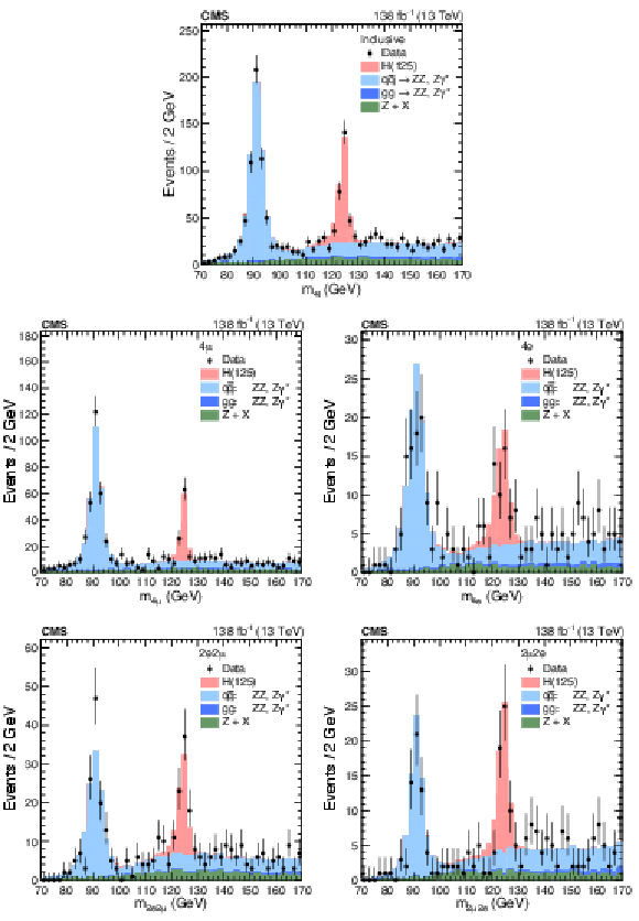
The observed (points) and predicted (stacked histograms) $ m_{4\ell} $ distributions in the inclusive (upper), 4$ \mu $ (middle left), 4e (middle right), 2e2$ \mu $ (lower left) and 2$ \mu$2e (lower right) final states, defined such that the first lepton pair is taken to be the one with the mass closest to the nominal Z boson mass. The predictions for the Higgs boson signal and the three main backgrounds are given by the different colors. The vertical bars on the points show the statistical uncertainties in the data. |
png pdf |
Figure 1-a:
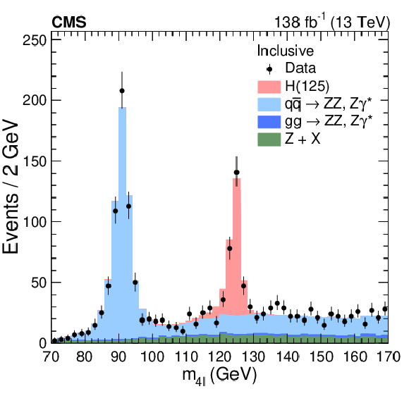
The observed (points) and predicted (stacked histograms) $ m_{4\ell} $ distributions in the inclusive (upper), 4$ \mu $ (middle left), 4e (middle right), 2e2$ \mu $ (lower left) and 2$ \mu$2e (lower right) final states, defined such that the first lepton pair is taken to be the one with the mass closest to the nominal Z boson mass. The predictions for the Higgs boson signal and the three main backgrounds are given by the different colors. The vertical bars on the points show the statistical uncertainties in the data. |

png pdf |
Figure 1-b:
The observed (points) and predicted (stacked histograms) $ m_{4\ell} $ distributions in the inclusive (upper), 4$ \mu $ (middle left), 4e (middle right), 2e2$ \mu $ (lower left) and 2$ \mu$2e (lower right) final states, defined such that the first lepton pair is taken to be the one with the mass closest to the nominal Z boson mass. The predictions for the Higgs boson signal and the three main backgrounds are given by the different colors. The vertical bars on the points show the statistical uncertainties in the data. |
png pdf |
Figure 1-c:
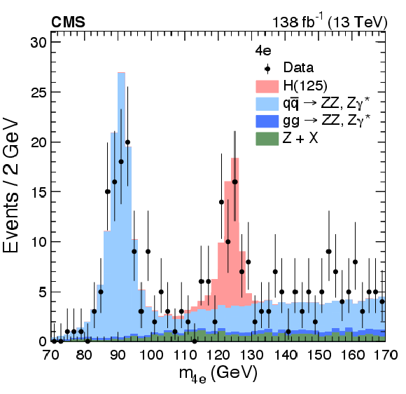
The observed (points) and predicted (stacked histograms) $ m_{4\ell} $ distributions in the inclusive (upper), 4$ \mu $ (middle left), 4e (middle right), 2e2$ \mu $ (lower left) and 2$ \mu$2e (lower right) final states, defined such that the first lepton pair is taken to be the one with the mass closest to the nominal Z boson mass. The predictions for the Higgs boson signal and the three main backgrounds are given by the different colors. The vertical bars on the points show the statistical uncertainties in the data. |
png pdf |
Figure 1-d:
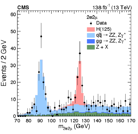
The observed (points) and predicted (stacked histograms) $ m_{4\ell} $ distributions in the inclusive (upper), 4$ \mu $ (middle left), 4e (middle right), 2e2$ \mu $ (lower left) and 2$ \mu$2e (lower right) final states, defined such that the first lepton pair is taken to be the one with the mass closest to the nominal Z boson mass. The predictions for the Higgs boson signal and the three main backgrounds are given by the different colors. The vertical bars on the points show the statistical uncertainties in the data. |
png pdf |
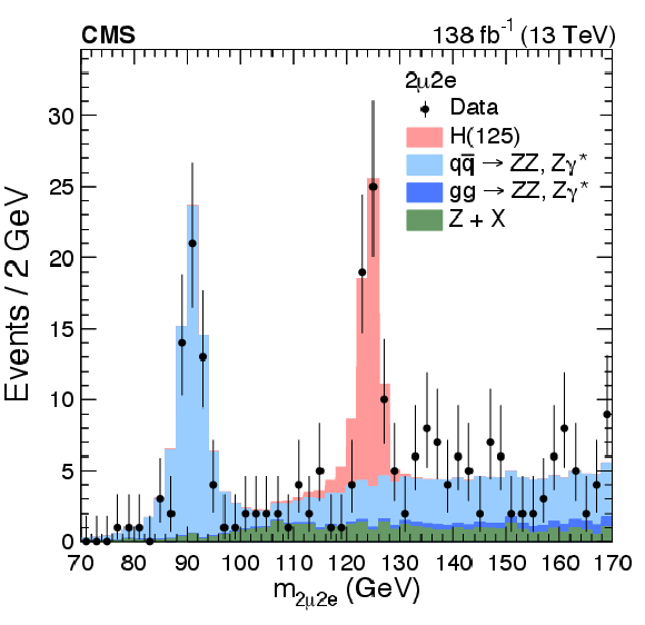
Figure 1-e:
The observed (points) and predicted (stacked histograms) $ m_{4\ell} $ distributions in the inclusive (upper), 4$ \mu $ (middle left), 4e (middle right), 2e2$ \mu $ (lower left) and 2$ \mu$2e (lower right) final states, defined such that the first lepton pair is taken to be the one with the mass closest to the nominal Z boson mass. The predictions for the Higgs boson signal and the three main backgrounds are given by the different colors. The vertical bars on the points show the statistical uncertainties in the data. |
png pdf |
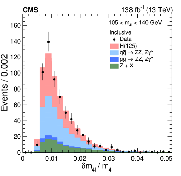
Figure 2:
Distributions of the observed (points) and predicted (stacked histograms) relative per-event mass uncertainty of the four-lepton system, in the inclusive final state. The predictions for the Higgs boson signal and the three main backgrounds are given by the different colors. The vertical bars on the points show the statistical uncertainties in the data. |
png pdf |
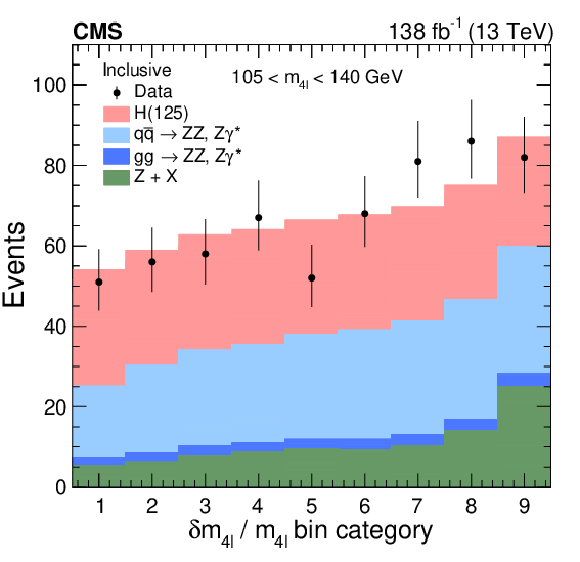
Figure 3:
Observed (points) and predicted (stacked histograms) yields of four-lepton events in each of the 9 $ \delta m_{4\ell}/m_{4\ell} $ bin categories for the inclusive final state. The bins are shown in the order of increasing $ \delta m_{4\ell}/m_{4\ell} $. The predictions for the Higgs boson signal and the three main backgrounds are given by the different colors. The vertical bars on the points show the statistical uncertainties in the data. |
png pdf |
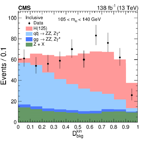
Figure 4:
Distributions of the observed (points) and predicted (stacked histograms) $ {\mathcal{D}}^{\text{kin}}_{\text{bkg}} $ of the four-lepton system, in the inclusive final state. The predictions for the Higgs boson signal and the three main backgrounds are given by the different colors. The vertical bars on the points show the statistical uncertainties in the data. |
png pdf |
Figure 5:
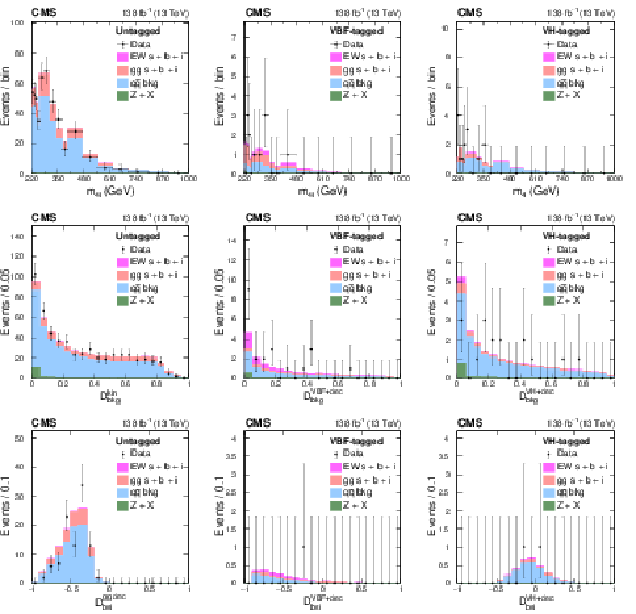
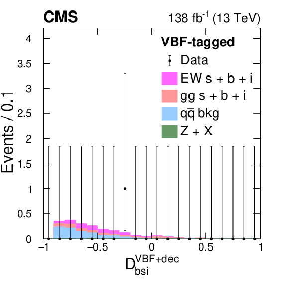
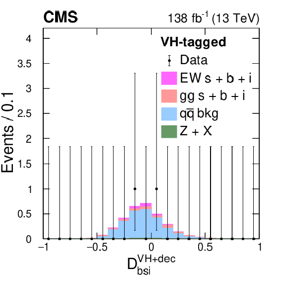
Off-shell data (points) and pre-fit distributions (histograms) for the Untagged (left), $ \mathrm{VBF} $-tagged (middle), and VH-tagged (right) categories. The upper row shows $ m_{4\ell} $ distributions with a requirement on $ {\mathcal{D}}^{\text{kin}}_{\text{bkg}} > $ 0.6 (left), $ \mathcal{D}^{{\mathrm{VBF}}+{\text{dec}}}_\text{bkg} > $ 0.6 (middle), or $ \mathcal{D}^{{\mathrm{V}\mathrm{H}}+{\text{dec}}}_\text{bkg} > $ 0.6 (right) applied for illustration purposes to enhance signal over background contributions. The middle row shows $ \mathcal{D}^\text{kin}_\text{bkg} $ (left), $ \mathcal{D}^{{\mathrm{VBF}}+{\text{dec}}}_\text{bkg} $ (middle), $ \mathcal{D}^{{\mathrm{V}\mathrm{H}}+{\text{dec}}}_\text{bkg} $ (right) distributions, where an additional requirement $ m_{4\ell} > $ 340 GeV is applied to enhance signal-over-background contributions. The lower row plots the $ \mathcal{D}_\text{bsi} $ with both the $ m_{4\ell} $ and $ {\mathcal{D}}^{\text{kin}}_{\text{bkg}} $ requirements specified above. Contributions from the four processes are shown by the different colors, where ``s'', ``b'', and ``i'' refer to the signal, background, and interference contributions, respectively. The vertical bars on the points give the statistical uncertainties in the data, and the horizontal bars represent the bin widths. For the prefit distributions, the different cross sections are set to their SM values. |

png pdf |
Figure 5-a:
Off-shell data (points) and pre-fit distributions (histograms) for the Untagged (left), $ \mathrm{VBF} $-tagged (middle), and VH-tagged (right) categories. The upper row shows $ m_{4\ell} $ distributions with a requirement on $ {\mathcal{D}}^{\text{kin}}_{\text{bkg}} > $ 0.6 (left), $ \mathcal{D}^{{\mathrm{VBF}}+{\text{dec}}}_\text{bkg} > $ 0.6 (middle), or $ \mathcal{D}^{{\mathrm{V}\mathrm{H}}+{\text{dec}}}_\text{bkg} > $ 0.6 (right) applied for illustration purposes to enhance signal over background contributions. The middle row shows $ \mathcal{D}^\text{kin}_\text{bkg} $ (left), $ \mathcal{D}^{{\mathrm{VBF}}+{\text{dec}}}_\text{bkg} $ (middle), $ \mathcal{D}^{{\mathrm{V}\mathrm{H}}+{\text{dec}}}_\text{bkg} $ (right) distributions, where an additional requirement $ m_{4\ell} > $ 340 GeV is applied to enhance signal-over-background contributions. The lower row plots the $ \mathcal{D}_\text{bsi} $ with both the $ m_{4\ell} $ and $ {\mathcal{D}}^{\text{kin}}_{\text{bkg}} $ requirements specified above. Contributions from the four processes are shown by the different colors, where ``s'', ``b'', and ``i'' refer to the signal, background, and interference contributions, respectively. The vertical bars on the points give the statistical uncertainties in the data, and the horizontal bars represent the bin widths. For the prefit distributions, the different cross sections are set to their SM values. |
png pdf |
Figure 5-b:
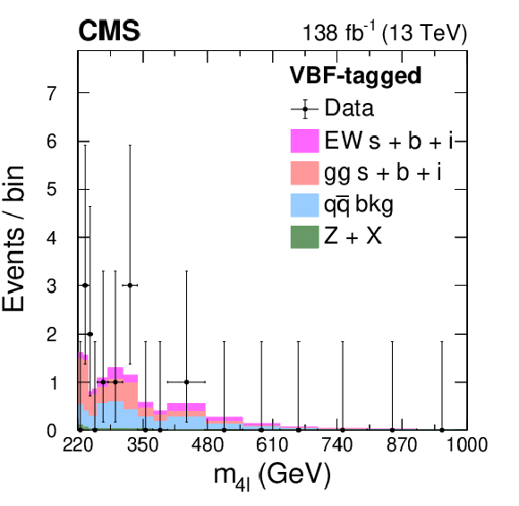
Off-shell data (points) and pre-fit distributions (histograms) for the Untagged (left), $ \mathrm{VBF} $-tagged (middle), and VH-tagged (right) categories. The upper row shows $ m_{4\ell} $ distributions with a requirement on $ {\mathcal{D}}^{\text{kin}}_{\text{bkg}} > $ 0.6 (left), $ \mathcal{D}^{{\mathrm{VBF}}+{\text{dec}}}_\text{bkg} > $ 0.6 (middle), or $ \mathcal{D}^{{\mathrm{V}\mathrm{H}}+{\text{dec}}}_\text{bkg} > $ 0.6 (right) applied for illustration purposes to enhance signal over background contributions. The middle row shows $ \mathcal{D}^\text{kin}_\text{bkg} $ (left), $ \mathcal{D}^{{\mathrm{VBF}}+{\text{dec}}}_\text{bkg} $ (middle), $ \mathcal{D}^{{\mathrm{V}\mathrm{H}}+{\text{dec}}}_\text{bkg} $ (right) distributions, where an additional requirement $ m_{4\ell} > $ 340 GeV is applied to enhance signal-over-background contributions. The lower row plots the $ \mathcal{D}_\text{bsi} $ with both the $ m_{4\ell} $ and $ {\mathcal{D}}^{\text{kin}}_{\text{bkg}} $ requirements specified above. Contributions from the four processes are shown by the different colors, where ``s'', ``b'', and ``i'' refer to the signal, background, and interference contributions, respectively. The vertical bars on the points give the statistical uncertainties in the data, and the horizontal bars represent the bin widths. For the prefit distributions, the different cross sections are set to their SM values. |

png pdf |
Figure 5-c:
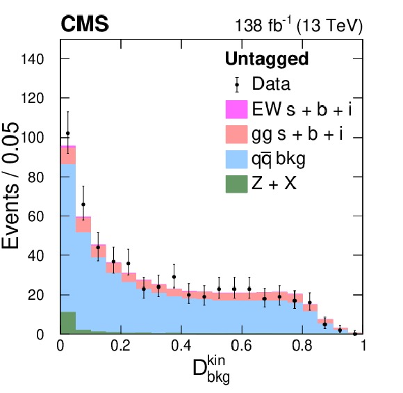
Off-shell data (points) and pre-fit distributions (histograms) for the Untagged (left), $ \mathrm{VBF} $-tagged (middle), and VH-tagged (right) categories. The upper row shows $ m_{4\ell} $ distributions with a requirement on $ {\mathcal{D}}^{\text{kin}}_{\text{bkg}} > $ 0.6 (left), $ \mathcal{D}^{{\mathrm{VBF}}+{\text{dec}}}_\text{bkg} > $ 0.6 (middle), or $ \mathcal{D}^{{\mathrm{V}\mathrm{H}}+{\text{dec}}}_\text{bkg} > $ 0.6 (right) applied for illustration purposes to enhance signal over background contributions. The middle row shows $ \mathcal{D}^\text{kin}_\text{bkg} $ (left), $ \mathcal{D}^{{\mathrm{VBF}}+{\text{dec}}}_\text{bkg} $ (middle), $ \mathcal{D}^{{\mathrm{V}\mathrm{H}}+{\text{dec}}}_\text{bkg} $ (right) distributions, where an additional requirement $ m_{4\ell} > $ 340 GeV is applied to enhance signal-over-background contributions. The lower row plots the $ \mathcal{D}_\text{bsi} $ with both the $ m_{4\ell} $ and $ {\mathcal{D}}^{\text{kin}}_{\text{bkg}} $ requirements specified above. Contributions from the four processes are shown by the different colors, where ``s'', ``b'', and ``i'' refer to the signal, background, and interference contributions, respectively. The vertical bars on the points give the statistical uncertainties in the data, and the horizontal bars represent the bin widths. For the prefit distributions, the different cross sections are set to their SM values. |
png pdf |
Figure 5-d:
Off-shell data (points) and pre-fit distributions (histograms) for the Untagged (left), $ \mathrm{VBF} $-tagged (middle), and VH-tagged (right) categories. The upper row shows $ m_{4\ell} $ distributions with a requirement on $ {\mathcal{D}}^{\text{kin}}_{\text{bkg}} > $ 0.6 (left), $ \mathcal{D}^{{\mathrm{VBF}}+{\text{dec}}}_\text{bkg} > $ 0.6 (middle), or $ \mathcal{D}^{{\mathrm{V}\mathrm{H}}+{\text{dec}}}_\text{bkg} > $ 0.6 (right) applied for illustration purposes to enhance signal over background contributions. The middle row shows $ \mathcal{D}^\text{kin}_\text{bkg} $ (left), $ \mathcal{D}^{{\mathrm{VBF}}+{\text{dec}}}_\text{bkg} $ (middle), $ \mathcal{D}^{{\mathrm{V}\mathrm{H}}+{\text{dec}}}_\text{bkg} $ (right) distributions, where an additional requirement $ m_{4\ell} > $ 340 GeV is applied to enhance signal-over-background contributions. The lower row plots the $ \mathcal{D}_\text{bsi} $ with both the $ m_{4\ell} $ and $ {\mathcal{D}}^{\text{kin}}_{\text{bkg}} $ requirements specified above. Contributions from the four processes are shown by the different colors, where ``s'', ``b'', and ``i'' refer to the signal, background, and interference contributions, respectively. The vertical bars on the points give the statistical uncertainties in the data, and the horizontal bars represent the bin widths. For the prefit distributions, the different cross sections are set to their SM values. |

png pdf |
Figure 5-e:
Off-shell data (points) and pre-fit distributions (histograms) for the Untagged (left), $ \mathrm{VBF} $-tagged (middle), and VH-tagged (right) categories. The upper row shows $ m_{4\ell} $ distributions with a requirement on $ {\mathcal{D}}^{\text{kin}}_{\text{bkg}} > $ 0.6 (left), $ \mathcal{D}^{{\mathrm{VBF}}+{\text{dec}}}_\text{bkg} > $ 0.6 (middle), or $ \mathcal{D}^{{\mathrm{V}\mathrm{H}}+{\text{dec}}}_\text{bkg} > $ 0.6 (right) applied for illustration purposes to enhance signal over background contributions. The middle row shows $ \mathcal{D}^\text{kin}_\text{bkg} $ (left), $ \mathcal{D}^{{\mathrm{VBF}}+{\text{dec}}}_\text{bkg} $ (middle), $ \mathcal{D}^{{\mathrm{V}\mathrm{H}}+{\text{dec}}}_\text{bkg} $ (right) distributions, where an additional requirement $ m_{4\ell} > $ 340 GeV is applied to enhance signal-over-background contributions. The lower row plots the $ \mathcal{D}_\text{bsi} $ with both the $ m_{4\ell} $ and $ {\mathcal{D}}^{\text{kin}}_{\text{bkg}} $ requirements specified above. Contributions from the four processes are shown by the different colors, where ``s'', ``b'', and ``i'' refer to the signal, background, and interference contributions, respectively. The vertical bars on the points give the statistical uncertainties in the data, and the horizontal bars represent the bin widths. For the prefit distributions, the different cross sections are set to their SM values. |

png pdf |
Figure 5-f:
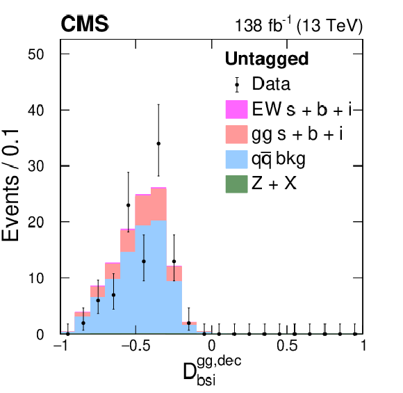
Off-shell data (points) and pre-fit distributions (histograms) for the Untagged (left), $ \mathrm{VBF} $-tagged (middle), and VH-tagged (right) categories. The upper row shows $ m_{4\ell} $ distributions with a requirement on $ {\mathcal{D}}^{\text{kin}}_{\text{bkg}} > $ 0.6 (left), $ \mathcal{D}^{{\mathrm{VBF}}+{\text{dec}}}_\text{bkg} > $ 0.6 (middle), or $ \mathcal{D}^{{\mathrm{V}\mathrm{H}}+{\text{dec}}}_\text{bkg} > $ 0.6 (right) applied for illustration purposes to enhance signal over background contributions. The middle row shows $ \mathcal{D}^\text{kin}_\text{bkg} $ (left), $ \mathcal{D}^{{\mathrm{VBF}}+{\text{dec}}}_\text{bkg} $ (middle), $ \mathcal{D}^{{\mathrm{V}\mathrm{H}}+{\text{dec}}}_\text{bkg} $ (right) distributions, where an additional requirement $ m_{4\ell} > $ 340 GeV is applied to enhance signal-over-background contributions. The lower row plots the $ \mathcal{D}_\text{bsi} $ with both the $ m_{4\ell} $ and $ {\mathcal{D}}^{\text{kin}}_{\text{bkg}} $ requirements specified above. Contributions from the four processes are shown by the different colors, where ``s'', ``b'', and ``i'' refer to the signal, background, and interference contributions, respectively. The vertical bars on the points give the statistical uncertainties in the data, and the horizontal bars represent the bin widths. For the prefit distributions, the different cross sections are set to their SM values. |
png pdf |
Figure 5-g:
Off-shell data (points) and pre-fit distributions (histograms) for the Untagged (left), $ \mathrm{VBF} $-tagged (middle), and VH-tagged (right) categories. The upper row shows $ m_{4\ell} $ distributions with a requirement on $ {\mathcal{D}}^{\text{kin}}_{\text{bkg}} > $ 0.6 (left), $ \mathcal{D}^{{\mathrm{VBF}}+{\text{dec}}}_\text{bkg} > $ 0.6 (middle), or $ \mathcal{D}^{{\mathrm{V}\mathrm{H}}+{\text{dec}}}_\text{bkg} > $ 0.6 (right) applied for illustration purposes to enhance signal over background contributions. The middle row shows $ \mathcal{D}^\text{kin}_\text{bkg} $ (left), $ \mathcal{D}^{{\mathrm{VBF}}+{\text{dec}}}_\text{bkg} $ (middle), $ \mathcal{D}^{{\mathrm{V}\mathrm{H}}+{\text{dec}}}_\text{bkg} $ (right) distributions, where an additional requirement $ m_{4\ell} > $ 340 GeV is applied to enhance signal-over-background contributions. The lower row plots the $ \mathcal{D}_\text{bsi} $ with both the $ m_{4\ell} $ and $ {\mathcal{D}}^{\text{kin}}_{\text{bkg}} $ requirements specified above. Contributions from the four processes are shown by the different colors, where ``s'', ``b'', and ``i'' refer to the signal, background, and interference contributions, respectively. The vertical bars on the points give the statistical uncertainties in the data, and the horizontal bars represent the bin widths. For the prefit distributions, the different cross sections are set to their SM values. |
png pdf |
Figure 5-h:
Off-shell data (points) and pre-fit distributions (histograms) for the Untagged (left), $ \mathrm{VBF} $-tagged (middle), and VH-tagged (right) categories. The upper row shows $ m_{4\ell} $ distributions with a requirement on $ {\mathcal{D}}^{\text{kin}}_{\text{bkg}} > $ 0.6 (left), $ \mathcal{D}^{{\mathrm{VBF}}+{\text{dec}}}_\text{bkg} > $ 0.6 (middle), or $ \mathcal{D}^{{\mathrm{V}\mathrm{H}}+{\text{dec}}}_\text{bkg} > $ 0.6 (right) applied for illustration purposes to enhance signal over background contributions. The middle row shows $ \mathcal{D}^\text{kin}_\text{bkg} $ (left), $ \mathcal{D}^{{\mathrm{VBF}}+{\text{dec}}}_\text{bkg} $ (middle), $ \mathcal{D}^{{\mathrm{V}\mathrm{H}}+{\text{dec}}}_\text{bkg} $ (right) distributions, where an additional requirement $ m_{4\ell} > $ 340 GeV is applied to enhance signal-over-background contributions. The lower row plots the $ \mathcal{D}_\text{bsi} $ with both the $ m_{4\ell} $ and $ {\mathcal{D}}^{\text{kin}}_{\text{bkg}} $ requirements specified above. Contributions from the four processes are shown by the different colors, where ``s'', ``b'', and ``i'' refer to the signal, background, and interference contributions, respectively. The vertical bars on the points give the statistical uncertainties in the data, and the horizontal bars represent the bin widths. For the prefit distributions, the different cross sections are set to their SM values. |
png pdf |
Figure 5-i:
Off-shell data (points) and pre-fit distributions (histograms) for the Untagged (left), $ \mathrm{VBF} $-tagged (middle), and VH-tagged (right) categories. The upper row shows $ m_{4\ell} $ distributions with a requirement on $ {\mathcal{D}}^{\text{kin}}_{\text{bkg}} > $ 0.6 (left), $ \mathcal{D}^{{\mathrm{VBF}}+{\text{dec}}}_\text{bkg} > $ 0.6 (middle), or $ \mathcal{D}^{{\mathrm{V}\mathrm{H}}+{\text{dec}}}_\text{bkg} > $ 0.6 (right) applied for illustration purposes to enhance signal over background contributions. The middle row shows $ \mathcal{D}^\text{kin}_\text{bkg} $ (left), $ \mathcal{D}^{{\mathrm{VBF}}+{\text{dec}}}_\text{bkg} $ (middle), $ \mathcal{D}^{{\mathrm{V}\mathrm{H}}+{\text{dec}}}_\text{bkg} $ (right) distributions, where an additional requirement $ m_{4\ell} > $ 340 GeV is applied to enhance signal-over-background contributions. The lower row plots the $ \mathcal{D}_\text{bsi} $ with both the $ m_{4\ell} $ and $ {\mathcal{D}}^{\text{kin}}_{\text{bkg}} $ requirements specified above. Contributions from the four processes are shown by the different colors, where ``s'', ``b'', and ``i'' refer to the signal, background, and interference contributions, respectively. The vertical bars on the points give the statistical uncertainties in the data, and the horizontal bars represent the bin widths. For the prefit distributions, the different cross sections are set to their SM values. |

png pdf |
Figure 7:
Illustration of how the on-shell statistical model is constructed, combining the $ m_4\ell $ distributions from all data-taking years and all final states. The red, blue, and brown lines show the results of the fit to the signal, background, and their sum, respectively.. The solid black points with vertical bars show the data and the associated statistical uncertainties. |
png pdf |
Figure 8:
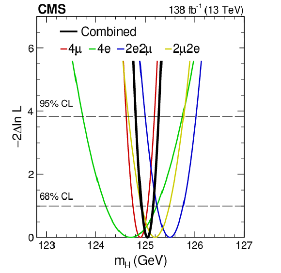
The profile likelihood from the $ m_{\mathrm{H}} $ fit using the $ \mathcal{N} $-2D$ '_\text{BS} $ model for each of the 4$ \ell $ categories and combined. The change in likelihood corresponding to 68 and 95% CLs are shown by the dashed horizontal lines. Both statistical and systematic uncertainties are included in the fits. |

png pdf |
Figure 9:
Summary of the CMS Higgs boson mass measurements using the four-lepton final state. The red vertical line and the gray column represent the best fit value and the total uncertainty, respectively, as measured by combining the Runs 1 and 2 data. The yellow band and horizontal black bars show the statistical and total uncertainties in each measurement, respectively. The value of each measurement is given, along with the total and statistical only (in parentheses) uncertainties. |

png pdf |
Figure 10:
Distribution of 1 $ -\text{CL} $ vs. $ \Gamma_\mathrm{H} $ from the fit in the measurement of the Higgs boson width using on-shell production only. The CL values shown by the points are extracted using the Feldman-Cousins approach. The vertical bars on the points represent the spread of the simulated pseudo-experiment values. The 68 and 95% CL values are shown by the dashed horizontal lines. |
png pdf |
Figure 11:
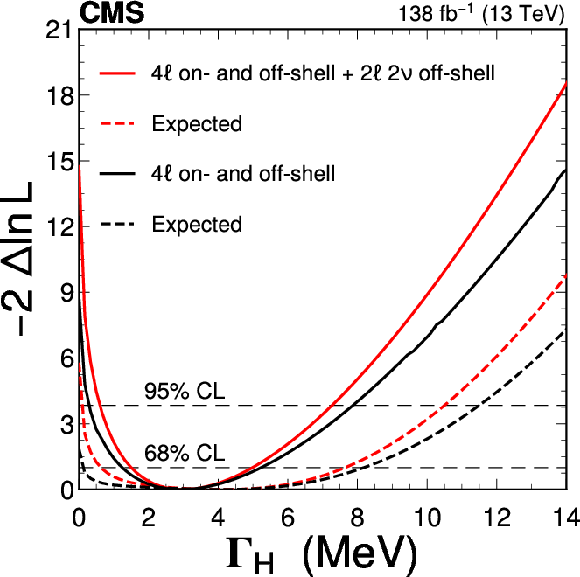
Observed (solid) and expected (dashed) profile likelihood projections from the Higgs boson width fit using on- and off-shell production from this analysis. The analysis of the off-shell $ \mathrm{H}\to\mathrm{Z}\mathrm{Z}\to4\ell $ channel combined with the on-shell $ \mathrm{H}\to\mathrm{Z}\mathrm{Z}\to4\ell $ channel [83] is shown in black. The full combination of $ \mathrm{H}\to\mathrm{Z}\mathrm{Z}\to4\ell $ with the off-shell $ \mathrm{H}\to\mathrm{Z}\mathrm{Z}\to2\ell2\nu $ [24] is given in red. The black horizontal dashed lines show the 68 and 95% CL values. |
png pdf |
Figure 12:
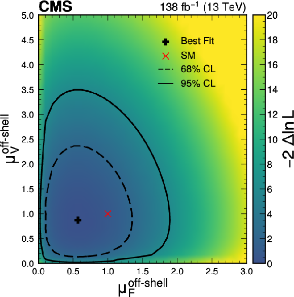
Observed 2D profile likelihood projection of the off-shell signal strength parameters ($ \mu^\text{off-shell }_{\mathrm{F}} $, $ \mu^\text{off-shell }_{\mathrm{V}} $) from the fit to the combined off-shell $ \mathrm{H}\to\mathrm{Z}\mathrm{Z}\to4\ell $ and 2 $ \ell2\nu $ channels. The best fit value is shown by the black cross and the SM prediction by the red x. The 68 and 95% CL contours are given by the dashed and solid curves, respectively. The color scale to the right of the plot relates the quantitative values. |
| Tables | |

png pdf |
Table 1:
Summary of the three production categories in the off-shell $ m_{4\ell} $ region and the observables used in the fits. |

png pdf |
Table 2:
The observed and expected yields for the Higgs boson signal and background contributions in the on-shell region 105 $ < m_{4\ell} < $ 140 GeV, for each of the four-lepton categories and the total. |

png pdf |
Table 3:
Observed and expected yields for the Higgs boson signal and background contributions in the off-shell region $ m_{4\ell} > $ 220 GeV, for each of the four-lepton categories and the total. The yields from interference of the signal and background and the ZH cross-feed are also shown. |

png pdf |
Table 4:
Best fit values for the mass of the Higgs boson measured in the inclusive 4$ \ell $ final state and separately for different flavor categories using the 1D approach. Uncertainties are separated into statistical and systematic uncertainties. Expected uncertainties are also given assuming $ m_{\mathrm{H}} = $ 125.38 GeV [88]. |

png pdf |
Table 5:
Best fit values for the mass of the Higgs boson measured in the inclusive 4$ \ell $ final state and separately for different flavor categories, using the final fit configuration ($ \mathcal{N} $-2D'$ _\text{BS} $). Uncertainties are separated into statistical and systematic uncertainties. Expected uncertainties are also given assuming $ m_{\mathrm{H}} = $ 125.38 GeV [88]. |

png pdf |
Table 6:
Summary of the total Higgs boson width $ \Gamma_\mathrm{H} $ measurement, showing the 68% CL (central values with uncertainties) and 95% CL (in square brackets) intervals for the $ \mathrm{H}\to\mathrm{Z}\mathrm{Z}\to4\ell $ channel alone and in combination with the off-shell $ \mathrm{H}\to\mathrm{Z}\mathrm{Z}\to2\ell2\nu $ channel. |

png pdf |
Table 7:
Measured values of the signal strengths $ \mu^\text{off-shell } $, $ \mu_{\mathrm{F}}^\text{off-shell } $, and $ \mu_{\mathrm{V}}^\text{off-shell } $, and their 68% and 95% (in square brackets) CL intervals from the combined fit to the off-shell $ \mathrm{H}\to\mathrm{Z}\mathrm{Z}\to4\ell $ and 2 $ \ell2\nu $ channels. |

png pdf |
Table 8:
Summary of the Higgs boson mass and total width $ \Gamma_\mathrm{H} $ measurements, showing the allowed 68% CL (central values with uncertainties) and 95% CL (in square brackets) intervals. Uncertainties are reported as a combination of statistical and systematic uncertainties. The first two rows display the outcomes of the analysis conducted within the on-shell $ \mathrm{H}\to\mathrm{Z}\mathrm{Z}\to4\ell $ region, where the width is restricted to be positive. The third row incorporates results from the off-shell $ \mathrm{H}\to\mathrm{Z}\mathrm{Z}\to4\ell $ region combined with the on-shell $ \mathrm{H}\to\mathrm{Z}\mathrm{Z}\to4\ell $ [83] and off-shell $ \mathrm{H}\to\mathrm{Z}\mathrm{Z}\to2\ell2\nu $ [24]. |
| Summary |
| A measurement of the Higgs boson mass ($ m_{\mathrm{H}} $) and width ($ \Gamma_\mathrm{H} $) using the decays to two Z bosons is presented. The data sample comes from proton-proton collisions at the LHC recorded by the CMS experiment at a center-of-mass energy of 13 TeV, corresponding to an integrated luminosity of 138 fb$ ^{-1} $. On-shell Higgs boson production with the $ \mathrm{H}\to 4\ell $ decay ($ \ell = \mathrm{e} $, $ \mu $) is used to measure its mass and constrain its width. The mass measurement yields $ m_{\mathrm{H}}= $ 125.04 $ \pm $ 0.11 (stat) $ \pm $ 0.05 (syst) GeV $ = $ 125.04 $ \pm $ 0.12 GeV, in agreement with the expected precision of $ \pm $0.12 GeV. From on-shell production events, an upper limit of $ \Gamma_\mathrm{H} < $ 330 MeV is set at 95% confidence level. The mass measurement is further improved combining data from Runs 1 and 2, leading to the most precise single measurement of the mass to date in this channel, $ m_{\mathrm{H}}= $ 125.08 $ \pm $ 0.10 (stat) $ \pm $ 0.05 (syst) GeV $ = $ 125.08 $ \pm $ 0.12 GeV. Using on- and off-shell Higgs boson production with the decay to four leptons, and combining them with a separate analysis with Higgs boson decay to two leptons plus two neutrinos, we measure $ \Gamma_\mathrm{H}= $ 3.0 $ ^{+2.0}_{-1.5} $ MeV, consistent with the standard model prediction of 4.1 MeV. These results are summarized in Table 8. The strength of the off-shell Higgs boson production is also reported, and the scenario of no off-shell Higgs boson production is excluded at a confidence level corresponding to 3.8 standard deviations. Results of the measurements are tabulated in the HEPData record for this analysis [97]. |
| Additional Figures | |

png pdf |
Additional Figure 1:
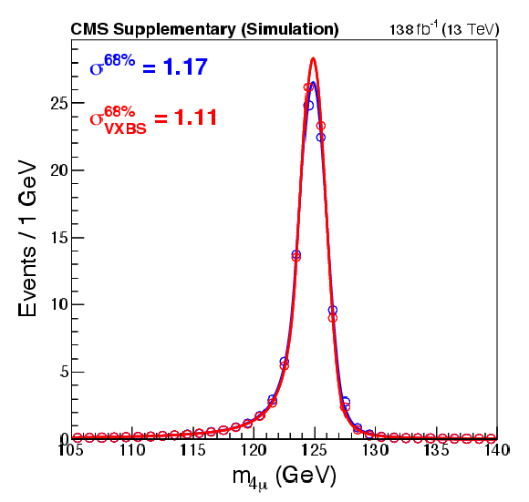
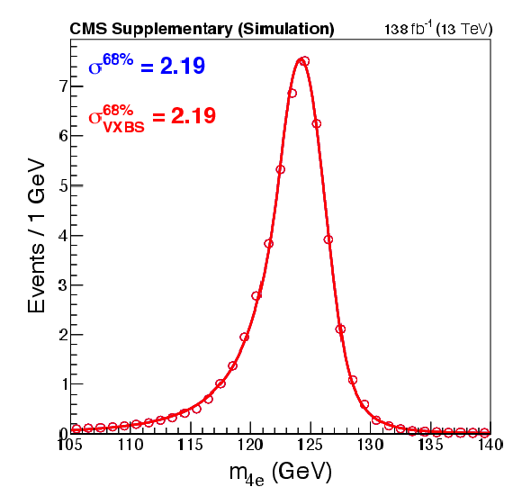
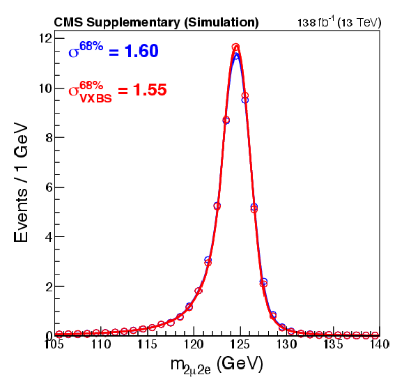
Comparison of the four-lepton invariant mass line shape with (red) and without (blue) the beam spot contraint, split per final state, merging all years. Top row: 4 $ \mu $ and 4e; bottom row: 2e2$ \mu $ and 2$ \mu $2e. $ \sigma^{68\%} $, defined as the Gaussian width used to fit the smallest invariant mass window containing 68% of the signal event, is also shown. |
png pdf |
Additional Figure 1-a:
Comparison of the four-lepton invariant mass line shape with (red) and without (blue) the beam spot contraint, split per final state, merging all years. Top row: 4 $ \mu $ and 4e; bottom row: 2e2$ \mu $ and 2$ \mu $2e. $ \sigma^{68\%} $, defined as the Gaussian width used to fit the smallest invariant mass window containing 68% of the signal event, is also shown. |
png pdf |
Additional Figure 1-b:
Comparison of the four-lepton invariant mass line shape with (red) and without (blue) the beam spot contraint, split per final state, merging all years. Top row: 4 $ \mu $ and 4e; bottom row: 2e2$ \mu $ and 2$ \mu $2e. $ \sigma^{68\%} $, defined as the Gaussian width used to fit the smallest invariant mass window containing 68% of the signal event, is also shown. |

png pdf |
Additional Figure 1-c:
Comparison of the four-lepton invariant mass line shape with (red) and without (blue) the beam spot contraint, split per final state, merging all years. Top row: 4 $ \mu $ and 4e; bottom row: 2e2$ \mu $ and 2$ \mu $2e. $ \sigma^{68\%} $, defined as the Gaussian width used to fit the smallest invariant mass window containing 68% of the signal event, is also shown. |
png pdf |
Additional Figure 1-d:
Comparison of the four-lepton invariant mass line shape with (red) and without (blue) the beam spot contraint, split per final state, merging all years. Top row: 4 $ \mu $ and 4e; bottom row: 2e2$ \mu $ and 2$ \mu $2e. $ \sigma^{68\%} $, defined as the Gaussian width used to fit the smallest invariant mass window containing 68% of the signal event, is also shown. |

png pdf |
Additional Figure 2:
Difference between data and simulation in $ Z(J/\psi) \rightarrow 2\ell $, normalized to simulation, as a function of $ p_{\mathrm{T}} $ and $ |\eta| $ for muons (left) and electron (right), regardless of the second lepton. From top to bottom: 2018, 2017, 2016 pre- and post-VFP. |
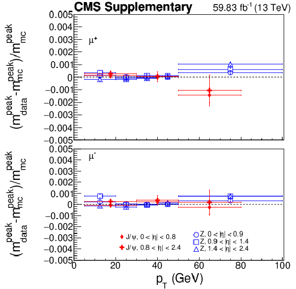
png pdf |
Additional Figure 2-a:
Difference between data and simulation in $ Z(J/\psi) \rightarrow 2\ell $, normalized to simulation, as a function of $ p_{\mathrm{T}} $ and $ |\eta| $ for muons (left) and electron (right), regardless of the second lepton. From top to bottom: 2018, 2017, 2016 pre- and post-VFP. |
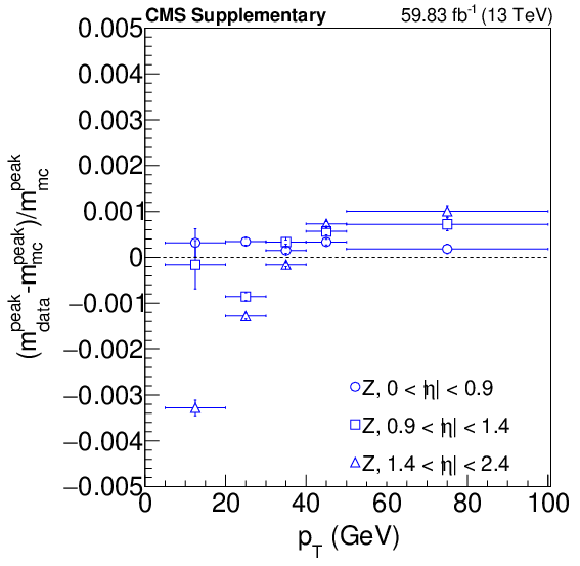
png pdf |
Additional Figure 2-b:
Difference between data and simulation in $ Z(J/\psi) \rightarrow 2\ell $, normalized to simulation, as a function of $ p_{\mathrm{T}} $ and $ |\eta| $ for muons (left) and electron (right), regardless of the second lepton. From top to bottom: 2018, 2017, 2016 pre- and post-VFP. |
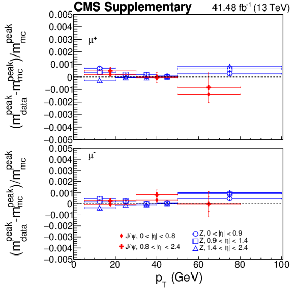
png pdf |
Additional Figure 2-c:
Difference between data and simulation in $ Z(J/\psi) \rightarrow 2\ell $, normalized to simulation, as a function of $ p_{\mathrm{T}} $ and $ |\eta| $ for muons (left) and electron (right), regardless of the second lepton. From top to bottom: 2018, 2017, 2016 pre- and post-VFP. |

png pdf |
Additional Figure 2-d:
Difference between data and simulation in $ Z(J/\psi) \rightarrow 2\ell $, normalized to simulation, as a function of $ p_{\mathrm{T}} $ and $ |\eta| $ for muons (left) and electron (right), regardless of the second lepton. From top to bottom: 2018, 2017, 2016 pre- and post-VFP. |

png pdf |
Additional Figure 2-e:
Difference between data and simulation in $ Z(J/\psi) \rightarrow 2\ell $, normalized to simulation, as a function of $ p_{\mathrm{T}} $ and $ |\eta| $ for muons (left) and electron (right), regardless of the second lepton. From top to bottom: 2018, 2017, 2016 pre- and post-VFP. |
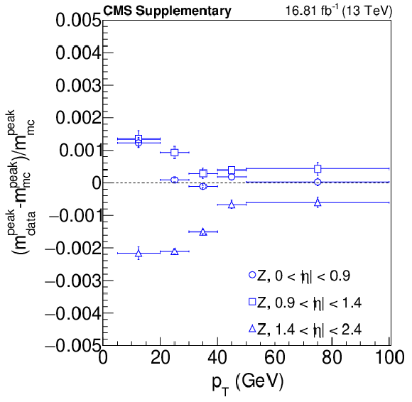
png pdf |
Additional Figure 2-f:
Difference between data and simulation in $ Z(J/\psi) \rightarrow 2\ell $, normalized to simulation, as a function of $ p_{\mathrm{T}} $ and $ |\eta| $ for muons (left) and electron (right), regardless of the second lepton. From top to bottom: 2018, 2017, 2016 pre- and post-VFP. |
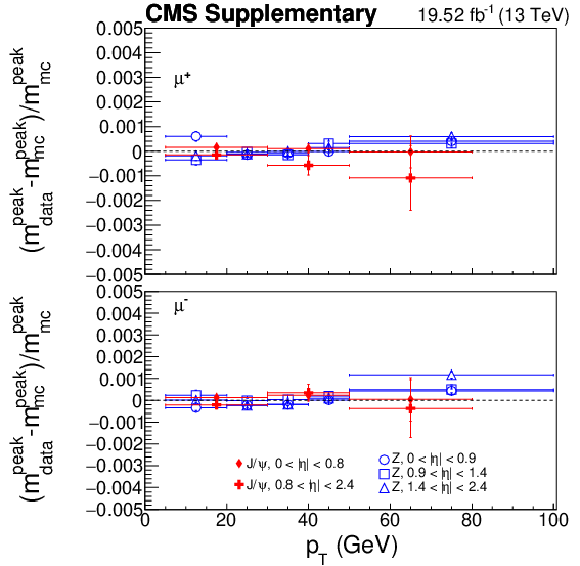
png pdf |
Additional Figure 2-g:
Difference between data and simulation in $ Z(J/\psi) \rightarrow 2\ell $, normalized to simulation, as a function of $ p_{\mathrm{T}} $ and $ |\eta| $ for muons (left) and electron (right), regardless of the second lepton. From top to bottom: 2018, 2017, 2016 pre- and post-VFP. |
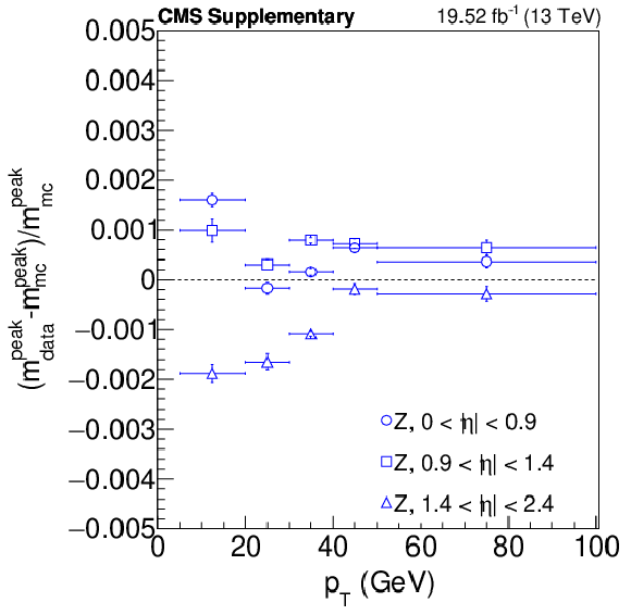
png pdf |
Additional Figure 2-h:
Difference between data and simulation in $ Z(J/\psi) \rightarrow 2\ell $, normalized to simulation, as a function of $ p_{\mathrm{T}} $ and $ |\eta| $ for muons (left) and electron (right), regardless of the second lepton. From top to bottom: 2018, 2017, 2016 pre- and post-VFP. |
png pdf |
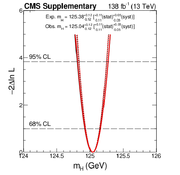
Additional Figure 3:
The observed (expected) likelihood scan as a function of $ m_{\mathrm{H}} $ is shown in black (red) using the $ \mathcal{N}--2D'_\text{BS} $ approach. The scans are shown both with (solid line) and without (dashed line) systematic uncertainties. Expected likelihood has been obtained with the hypothesis $ m_\mathrm{H} = $ 125.38 GeV and then shifted towards the observed central value of 125.04 GeV. |
png pdf |
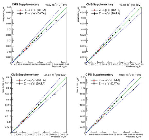
Additional Figure 4:
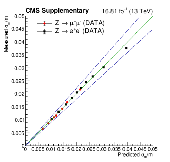
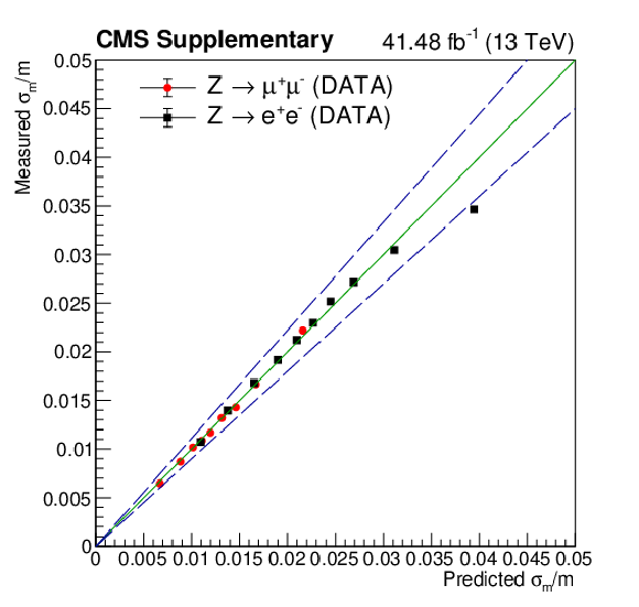
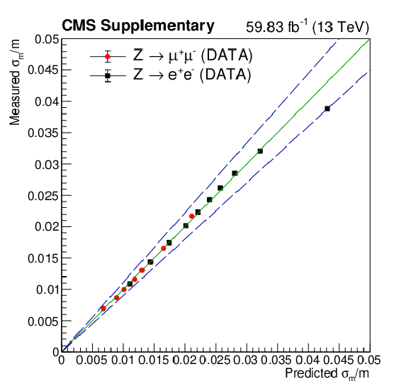
Comparison of measured mass resolution with the predicted dilepton mass resolution using the event-by-event mass uncertainty for $ \mathrm{Z}\rightarrow\ell\ell $ events in data. The dashed lines denote the $ \pm$10%, the biggest value used as the systematic uncertainty on the resolution. Top row: 2016; bottom row 2017 (left) and 2018 (right). |

png pdf |
Additional Figure 4-a:
Comparison of measured mass resolution with the predicted dilepton mass resolution using the event-by-event mass uncertainty for $ \mathrm{Z}\rightarrow\ell\ell $ events in data. The dashed lines denote the $ \pm$10%, the biggest value used as the systematic uncertainty on the resolution. Top row: 2016; bottom row 2017 (left) and 2018 (right). |
png pdf |
Additional Figure 4-b:
Comparison of measured mass resolution with the predicted dilepton mass resolution using the event-by-event mass uncertainty for $ \mathrm{Z}\rightarrow\ell\ell $ events in data. The dashed lines denote the $ \pm$10%, the biggest value used as the systematic uncertainty on the resolution. Top row: 2016; bottom row 2017 (left) and 2018 (right). |
png pdf |
Additional Figure 4-c:
Comparison of measured mass resolution with the predicted dilepton mass resolution using the event-by-event mass uncertainty for $ \mathrm{Z}\rightarrow\ell\ell $ events in data. The dashed lines denote the $ \pm$10%, the biggest value used as the systematic uncertainty on the resolution. Top row: 2016; bottom row 2017 (left) and 2018 (right). |
png pdf |
Additional Figure 4-d:
Comparison of measured mass resolution with the predicted dilepton mass resolution using the event-by-event mass uncertainty for $ \mathrm{Z}\rightarrow\ell\ell $ events in data. The dashed lines denote the $ \pm$10%, the biggest value used as the systematic uncertainty on the resolution. Top row: 2016; bottom row 2017 (left) and 2018 (right). |
png pdf |
Additional Figure 5:
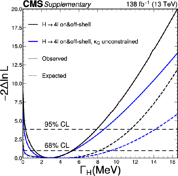
Observed (solid) and expected (dashed) profile likelihood projection on the Higgs boson width using on-shell and off-shell production. The analysis of $ \mathrm{H}\to\mathrm{Z}\mathrm{Z}\to4\ell $, considering an unconstrained (blue) coupling strength $ \kappa_\mathrm{Q} $, is presented alongside the same analysis with this coupling constrained to zero (black). |
png pdf |
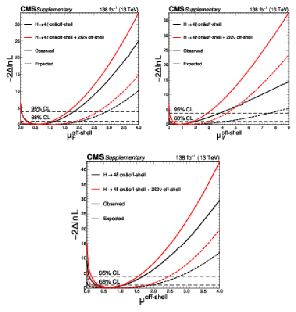
Additional Figure 6:
Observed (solid) and expected (dashed) profile likelihood projection on the coupling strength terms using on-shell and off-shell production for both $ \mathrm{H}\to\mathrm{Z}\mathrm{Z}\to4\ell $ (black) and the combination with $ \mathrm{H}\to\mathrm{Z}\mathrm{Z}\to2\ell2\nu $ (red). |
png pdf |
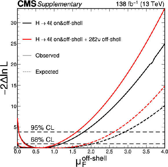
Additional Figure 6-a:
Observed (solid) and expected (dashed) profile likelihood projection on the coupling strength terms using on-shell and off-shell production for both $ \mathrm{H}\to\mathrm{Z}\mathrm{Z}\to4\ell $ (black) and the combination with $ \mathrm{H}\to\mathrm{Z}\mathrm{Z}\to2\ell2\nu $ (red). |
png pdf |
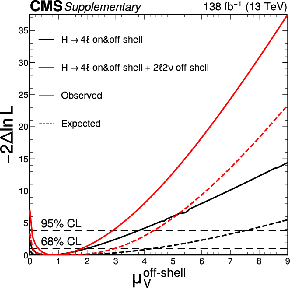
Additional Figure 6-b:
Observed (solid) and expected (dashed) profile likelihood projection on the coupling strength terms using on-shell and off-shell production for both $ \mathrm{H}\to\mathrm{Z}\mathrm{Z}\to4\ell $ (black) and the combination with $ \mathrm{H}\to\mathrm{Z}\mathrm{Z}\to2\ell2\nu $ (red). |

png pdf |
Additional Figure 6-c:
Observed (solid) and expected (dashed) profile likelihood projection on the coupling strength terms using on-shell and off-shell production for both $ \mathrm{H}\to\mathrm{Z}\mathrm{Z}\to4\ell $ (black) and the combination with $ \mathrm{H}\to\mathrm{Z}\mathrm{Z}\to2\ell2\nu $ (red). |
| Additional Tables | |

png pdf |
Additional Table 1:
Features of the different approaches used in the on-shell analysis. |

png pdf |
Additional Table 2:
Systematic uncertainty table for the Higgs boson mass measurement. |
| References | ||||
| 1 | S. L. Glashow | Partial-symmetries of weak interactions | NP 22 (1961) 579 | |
| 2 | F. Englert and R. Brout | Broken symmetry and the mass of gauge vector mesons | PRL 13 (1964) 321 | |
| 3 | P. W. Higgs | Broken symmetries, massless particles and gauge fields | PL 12 (1964) 132 | |
| 4 | P. W. Higgs | Broken symmetries and the masses of gauge bosons | PRL 13 (1964) 508 | |
| 5 | G. S. Guralnik, C. R. Hagen, and T. W. B. Kibble | Global conservation laws and massless particles | PRL 13 (1964) 585 | |
| 6 | S. Weinberg | A model of leptons | PRL 19 (1967) 1264 | |
| 7 | A. Salam | Weak and electromagnetic interactions | in Elementary particle physics: relativistic groups and analyticity, N. Svartholm, ed., Almqvist & Wiksell, Stockholm. Proceedings of the eighth Nobel symposium, 1968 | |
| 8 | ATLAS Collaboration | Observation of a new particle in the search for the Standard Model Higgs boson with the ATLAS detector at the LHC | PLB 716 (2012) 1 | 1207.7214 |
| 9 | CMS Collaboration | Observation of a new boson at a mass of 125 GeV with the CMS experiment at the LHC | PLB 716 (2012) 30 | CMS-HIG-12-028 1207.7235 |
| 10 | CMS Collaboration | Observation of a new boson with mass near 125 GeV in pp collisions at $ \sqrt{s}= $ 7 and 8 TeV | JHEP 06 (2013) 081 | CMS-HIG-12-036 1303.4571 |
| 11 | ATLAS Collaboration | A detailed map of Higgs boson interactions by the atlas experiment ten years after the discovery | Nature 607 (2022) 52 | |
| 12 | CMS Collaboration | A portrait of the Higgs boson by the CMS experiment ten years after the discovery | Nature 607 (2022) 60 | |
| 13 | LHC Higgs Cross Section Working Group | Handbook of LHC Higgs cross sections: 4. deciphering the nature of the Higgs sector | link | 1610.07922 |
| 14 | ATLAS and CMS Collaborations | Combined measurement of the Higgs boson mass in pp collisions at $ \sqrt{s}= $ 7 and 8 TeV with the ATLAS and CMS experiments | PRL 114 (2015) 191803 | 1503.07589 |
| 15 | ATLAS Collaboration | Combined measurement of the Higgs boson mass from the H$ \to\gamma\gamma $ and H$ \to $ Z$ Z^{*} \to 4\ell $ decay channels with the ATLAS detector using $ \sqrt{s} $ = 7, 8 and 13 TeV pp collision data | PRL 131 (2023) 251802 | 2308.04775 |
| 16 | CMS Collaboration | Precise determination of the mass of the Higgs boson and tests of compatibility of its couplings with the standard model predictions using proton collisions at 7 and 8 TeV | EPJC 75 (2015) 212 | CMS-HIG-14-009 1412.8662 |
| 17 | CMS Collaboration | Measurements of properties of the Higgs boson decaying into the four-lepton final state in pp collisions at $ \sqrt{s}= $ 13 TeV | JHEP 11 (2017) 047 | CMS-HIG-16-041 1706.09936 |
| 18 | CMS Collaboration | Constraints on the Higgs boson width from off-shell production and decay to Z-boson pairs | PLB 736 (2014) 64 | CMS-HIG-14-002 1405.3455 |
| 19 | ATLAS Collaboration | Constraints on the off-shell Higgs boson signal strength in the high-mass ZZ and WW final states with the ATLAS detector | EPJC 75 (2015) 335 | 1503.01060 |
| 20 | CMS Collaboration | Limits on the Higgs boson lifetime and width from its decay to four charged leptons | PRD 92 (2015) 072010 | CMS-HIG-14-036 1507.06656 |
| 21 | CMS Collaboration | Search for Higgs boson off-shell production in proton-proton collisions at 7 and 8 TeV and derivation of constraints on its total decay width | JHEP 09 (2016) 051 | CMS-HIG-14-032 1605.02329 |
| 22 | ATLAS Collaboration | Constraints on off-shell Higgs boson production and the Higgs boson total width in $ \mathrm{Z}\mathrm{Z}\to4\ell $ and $ \mathrm{Z}\mathrm{Z}\to2\ell2\nu $ final states with the ATLAS detector | PLB 786 (2018) 223 | 1808.01191 |
| 23 | CMS Collaboration | Measurements of the Higgs boson width and anomalous HVV couplings from on-shell and off-shell production in the four-lepton final state | Phys. Rev. D 11200 (2019) 3 | CMS-HIG-18-002 1901.00174 |
| 24 | CMS Collaboration | Measurement of the Higgs boson width and evidence of its off-shell contributions to ZZ production | Nature Phys. 18 (2022) 1329 | CMS-HIG-21-013 2202.06923 |
| 25 | F. Caola and K. Melnikov | Constraining the Higgs boson width with ZZ production at the LHC | PRD 88 (2013) 054024 | 1307.4935 |
| 26 | N. Kauer and G. Passarino | Inadequacy of zero-width approximation for a light Higgs boson signal | JHEP 08 (2012) 116 | 1206.4803 |
| 27 | J. M. Campbell, R. K. Ellis, and C. Williams | Bounding the Higgs width at the LHC using full analytic results for $ \mathrm{g}\mathrm{g}\to \mathrm{e}^{-}\mathrm{e}^{+} \mu^{-} \mu^{+} $ | JHEP 04 (2014) 060 | 1311.3589 |
| 28 | ATLAS Collaboration | Evidence of off-shell Higgs boson production from ZZ leptonic decay channels and constraints on its total width with the ATLAS detector | PLB 846 (2023) 138223 | 2304.01532 |
| 29 | B. W. Lee, C. Quigg, and H. B. Thacker | Strength of weak interactions at very high-energies and the Higgs boson mass | PRL 38 (1977) 883 | |
| 30 | CMS Collaboration | Search for a new scalar resonance decaying to a pair of Z bosons in proton-proton collisions at $ \sqrt{s}= $ 13 TeV | JHEP 06 (2018) 127 | CMS-HIG-17-012 1804.01939 |
| 31 | CMS Collaboration | The CMS experiment at the CERN LHC | JINST 3 (2008) S08004 | |
| 32 | CMS Collaboration | Development of the CMS detector for the CERN LHC Run 3 | JINST 19 (2024) P05064 | |
| 33 | CMS Collaboration | Performance of the CMS Level-1 trigger in proton-proton collisions at $ \sqrt{s} = $ 13 TeV | JINST 15 (2020) P10017 | CMS-TRG-17-001 2006.10165 |
| 34 | CMS Collaboration | Performance of the CMS high-level trigger during LHC Run 2 | JINST 19 (2024) P11021 | CMS-TRG-19-001 |
| 35 | CMS Collaboration | Technical proposal for the phase-II upgrade of the CMS detector | CMS Technical proposal CERN-LHCC-2015-010, CMS-TDR-15-02, CERN, 2015 CDS |
|
| 36 | CMS Collaboration | Electron and photon reconstruction and identification with the CMS experiment at the CERN LHC | JINST 16 (2021) P05014 | CMS-EGM-17-001 2012.06888 |
| 37 | CMS Collaboration | ECAL 2016 refined calibration and Run 2 summary plots | CMS Detector Performance Summary CMS-DP-2020-021, CERN, 2020 CDS |
|
| 38 | CMS Collaboration | Performance of the CMS muon detector and muon reconstruction with proton-proton collisions at $ \sqrt{s}= $ 13 TeV | JINST 13 (2018) P06015 | CMS-MUO-16-001 1804.04528 |
| 39 | CMS Collaboration | Measurements of production cross sections of the Higgs boson in the four-lepton final state in proton-proton collisions at $ \sqrt{s} = $ 13 TeV | EPJC 81 (2021) 488 | CMS-HIG-19-001 2103.04956 |
| 40 | S. Frixione, P. Nason, and C. Oleari | Matching NLO QCD computations with parton shower simulations: the POWHEG method | JHEP 11 (2007) 070 | 0709.2092 |
| 41 | E. Bagnaschi, G. Degrassi, P. Slavich, and A. Vicini | Higgs production via gluon fusion in the POWHEG approach in the SM and in the MSSM | JHEP 02 (2012) 088 | 1111.2854 |
| 42 | P. Nason and C. Oleari | NLO Higgs boson production via vector-boson fusion matched with shower in POWHEG | JHEP 02 (2010) 037 | 0911.5299 |
| 43 | G. Luisoni, P. Nason, C. Oleari, and F. Tramontano | $ \mathrm{H}\mathrm{W}^{\pm} $/$\mathrm{HZ}$ + 0 and 1 jet at NLO with the POWHEG BOX interfaced to GoSam and their merging within MiNLO | JHEP 10 (2013) 083 | 1306.2542 |
| 44 | H. B. Hartanto, B. Jager, L. Reina, and D. Wackeroth | Higgs boson production in association with top quarks in the POWHEG BOX | PRD 91 (2015) 094003 | 1501.04498 |
| 45 | P. Nason | A new method for combining NLO QCD with shower Monte Carlo algorithms | JHEP 11 (2004) 040 | hep-ph/0409146 |
| 46 | S. Alioli, P. Nason, C. Oleari, and E. Re | A general framework for implementing NLO calculations in shower Monte Carlo programs: the POWHEG BOX | JHEP 06 (2010) 043 | 1002.2581 |
| 47 | K. Hamilton, P. Nason, and G. Zanderighi | MINLO: multi-scale improved NLO | JHEP 10 (2012) 155 | 1206.3572 |
| 48 | Y. Gao et al. | Spin determination of single-produced resonances at hadron colliders | PRD 81 (2010) 075022 | 1001.3396 |
| 49 | S. Bolognesi et al. | Spin and parity of a single-produced resonance at the LHC | PRD 86 (2012) 095031 | 1208.4018 |
| 50 | I. Anderson et al. | Constraining anomalous $ \mathrm{H}\mathrm{V}\mathrm{V} $ interactions at proton and lepton colliders | PRD 89 (2014) 035007 | 1309.4819 |
| 51 | A. V. Gritsan, R. Röntsch, M. Schulze, and M. Xiao | Constraining anomalous Higgs boson couplings to the heavy flavor fermions using matrix element techniques | PRD 94 (2016) 055023 | 1606.03107 |
| 52 | A. V. Gritsan et al. | New features in the JHU generator framework: constraining Higgs boson properties from on-shell and off-shell production | PRD 102 (2020) 056022 | 2002.09888 |
| 53 | J. M. Campbell and R. K. Ellis | MCFM for the Tevatron and the LHC | Nucl. Phys. Proc. Suppl. 205-206 (2010) 10 | 1007.3492 |
| 54 | J. M. Campbell, R. K. Ellis, and C. Williams | Vector boson pair production at the LHC | JHEP 07 (2011) 018 | 1105.0020 |
| 55 | J. M. Campbell and R. K. Ellis | Higgs constraints from vector boson fusion and scattering | JHEP 04 (2015) 030 | 1502.02990 |
| 56 | A. Ballestrero et al. | PHANTOM: a Monte Carlo event generator for six parton final states at high energy colliders | Comput. Phys. Commun. 180 (2009) 401 | 0801.3359 |
| 57 | S. Catani and M. Grazzini | An NNLO subtraction formalism in hadron collisions and its application to Higgs boson production at the LHC | PRL 98 (2007) 222002 | hep-ph/0703012 |
| 58 | M. Grazzini | NNLO predictions for the Higgs boson signal in the $ \mathrm{H} \to \mathrm{W}\mathrm{W} \to\ell\nu\ell\nu $ and $ \mathrm{H} \to \mathrm{Z}\mathrm{Z} \to 4\ell $ decay channels | JHEP 02 (2008) 043 | 0801.3232 |
| 59 | M. Grazzini and H. Sargsyan | Heavy-quark mass effects in Higgs boson production at the LHC | JHEP 09 (2013) 129 | 1306.4581 |
| 60 | F. Caola, K. Melnikov, R. Röntsch, and L. Tancredi | QCD corrections to ZZ production in gluon fusion at the LHC | PRD 92 (2015) 094028 | 1509.06734 |
| 61 | K. Melnikov and M. Dowling | Production of two Z-bosons in gluon fusion in the heavy top quark approximation | PLB 744 (2015) 43 | 1503.01274 |
| 62 | J. M. Campbell, R. K. Ellis, M. Czakon, and S. Kirchner | Two loop correction to interference in $ \mathrm{g}\mathrm{g} \to \mathrm{Z}\mathrm{Z} $ | JHEP 08 (2016) 011 | 1605.01380 |
| 63 | F. Caola et al. | QCD corrections to vector boson pair production in gluon fusion including interference effects with off-shell Higgs at the LHC | JHEP 07 (2016) 087 | 1605.04610 |
| 64 | M. Grazzini, S. Kallweit, and D. Rathlev | ZZ production at the LHC: fiducial cross sections and distributions in NNLO QCD | PLB 750 (2015) 407 | 1507.06257 |
| 65 | A. Bierweiler, T. Kasprzik, and J. H. Kühn | Vector-boson pair production at the LHC to $ \mathcal{O}(\alpha^3) $ accuracy | JHEP 12 (2013) 071 | 1305.5402 |
| 66 | J. Alwall et al. | The automated computation of tree-level and next-to-leading order differential cross sections, and their matching to parton shower simulations | JHEP 07 (2014) 079 | 1405.0301 |
| 67 | T. Sjöstrand et al. | An introduction to PYTHIA 8.2 | Comput. Phys. Commun. 191 (2015) 159 | 1410.3012 |
| 68 | CMS Collaboration | Event generator tunes obtained from underlying event and multiparton scattering measurements | EPJC 76 (2016) 155 | CMS-GEN-14-001 1512.00815 |
| 69 | CMS Collaboration | Extraction and validation of a new set of CMS PYTHIA8 tunes from underlying-event measurements | EPJC 80 (2020) 4 | CMS-GEN-17-001 1903.12179 |
| 70 | NNPDF Collaboration | Unbiased global determination of parton distributions and their uncertainties at NNLO and at LO | NPB 855 (2012) 153 | 1107.2652 |
| 71 | GEANT4 Collaboration | GEANT 4 --- a simulation toolkit | NIM A 506 (2003) 250 | |
| 72 | CMS Collaboration | Particle-flow reconstruction and global event description with the CMS detector | JINST 12 (2017) P10003 | CMS-PRF-14-001 1706.04965 |
| 73 | CMS Collaboration | Pileup mitigation at CMS in 13 TeV data | JINST 15 (2020) P09018 | CMS-JME-18-001 2003.00503 |
| 74 | T. Chen and C. Guestrin | XGBoost: A scalable tree boosting system | 1603.02754 | |
| 75 | CMS Collaboration | Measurements of inclusive and differential cross sections for the Higgs boson production and decay to four-leptons in proton-proton collisions at $ \sqrt{s} $ = 13 TeV | JHEP 08 (2023) 040 | CMS-HIG-21-009 2305.07532 |
| 76 | CMS Collaboration | Measurement of the inclusive W and Z production cross sections in pp collisions at $ \sqrt{s}= $ 7 TeV | JHEP 10 (2011) 132 | CMS-EWK-10-005 1107.4789 |
| 77 | A. Bodek et al. | Extracting muon momentum scale corrections for hadron collider experiments | EPJC 72 (2012) | |
| 78 | M. Cacciari, G. P. Salam, and G. Soyez | The anti-$ k_{\mathrm{T}} $ jet clustering algorithm | JHEP 04 (2008) 063 | 0802.1189 |
| 79 | M. Cacciari, G. P. Salam, and G. Soyez | FastJet user manual | EPJC 72 (2012) 1896 | 1111.6097 |
| 80 | CMS Collaboration | Identification of heavy-flavour jets with the CMS detector in pp collisions at 13 TeV | JINST 13 (2018) P05011 | CMS-BTV-16-002 1712.07158 |
| 81 | T. Skwarnicki | A study of the radiative CASCADE transitions between the Upsilon-Prime and Upsilon resonances | PhD thesis, Cracow, INP, 1986 link |
|
| 82 | CMS Collaboration | Constraints on anomalous Higgs boson couplings using production and decay information in the four-lepton final state | PLB 775 (2017) 1 | CMS-HIG-17-011 1707.00541 |
| 83 | CMS Collaboration | Constraints on anomalous Higgs boson couplings to vector bosons and fermions in its production and decay using the four-lepton final state | PRD 104 (2021) 052004 | CMS-HIG-19-009 2104.12152 |
| 84 | M. Oreglia | A study of the reactions $ \psi^\prime \to \gamma \gamma \psi $ | PhD thesis, Stanford University, SLAC Report SLAC-R-236, 1980 link |
|
| 85 | CMS Collaboration | Precision luminosity measurement in proton-proton collisions at $ \sqrt{s} = $ 13 TeV in 2015 and 2016 at CMS | EPJC 81 (2021) 800 | CMS-LUM-17-003 2104.01927 |
| 86 | CMS Collaboration | CMS luminosity measurement for the 2017 data-taking period at $ \sqrt{s} = $ 13 TeV | CMS Physics Analysis Summary , CERN, 2018 CMS-PAS-LUM-17-004 |
CMS-PAS-LUM-17-004 |
| 87 | CMS Collaboration | CMS luminosity measurement for the 2018 data-taking period at $ \sqrt{s} = $ 13 TeV | CMS Physics Analysis Summary, CERN, 2019 CMS-PAS-LUM-18-002 |
CMS-PAS-LUM-18-002 |
| 88 | CMS Collaboration | The CMS statistical analysis and combination tool: combine | Comput. Softw. Big Sci. 8 (2024) 19 | CMS-CAT-23-001 2404.06614 |
| 89 | W. Verkerke and D. P. Kirkby | The RooFit toolkit for data modeling | in Proceedings of the 13$^\text{th$ International Conference for Computing in High-Energy and Nuclear Physics (CHEP03), 2003 Proceedings of the 1 (2003) 3 |
physics/0306116 |
| 90 | L. Moneta et al. | The RooStats project | PoS ACAT 057, 2010 link |
1009.1003 |
| 91 | CMS Collaboration | A measurement of the Higgs boson mass in the diphoton decay channel | PLB 805 (2020) 135425 | CMS-HIG-19-004 2002.06398 |
| 92 | Particle Data Group , K. A. Olive et al. | Review of Particle Physics | Chin. Phys. C 38 (2014) 090001 | |
| 93 | CMS Collaboration | Measurement of the properties of a Higgs boson in the four-lepton final state | PRD 89 (2014) 092007 | CMS-HIG-13-002 1312.5353 |
| 94 | G. J. Feldman and R. D. Cousins | Unified approach to the classical statistical analysis of small signals | PRD 57 (1998) 3873 | physics/9711021 |
| 95 | S. S. Wilks | The large-sample distribution of the likelihood ratio for testing composite hypotheses | Annals Math. Statist. 9 (1938) 60 | |
| 96 | J. Davis et al. | Constraining anomalous Higgs boson couplings to virtual photons | PRD 105 (2022) 096027 | 2109.13363 |
| 97 | CMS Collaboration | HEPData record for this analysis | link | |

|
Compact Muon Solenoid LHC, CERN |

|

|

|

|

|

|