CMS-HIG-14-036

CMS-HIG-14-036 ; CERN-PH-EP-2015-159
Limits on the Higgs boson lifetime and width from its decay to four charged leptons
CMS Collaboration
23 July 2015
Phys. Rev. D 92 (2015) 072010
Abstract: Constraints on the lifetime and width of the Higgs boson are obtained from $\mathrm{H} \to \mathrm{ZZ} \to 4\ell$ events using data recorded by the CMS experiment during the LHC run 1 with an integrated luminosity of 5.1 and 19.7 fb $^{-1}$ at a center-of-mass energy of 7 and 8 TeV, respectively. The measurement of the Higgs boson lifetime is derived from its flight distance in the CMS detector with an upper bound of $\tau_{\mathrm{H}} < 1.9 \times 10^{-13}$ s at the 95\% confidence level (CL), corresponding to a lower bound on the width of $\Gamma_{\mathrm{H}} > 3.5 \times 10^{-9}$ MeV. The measurement of the width is obtained from an off-shell production technique, generalized to include anomalous couplings of the Higgs boson to two electroweak bosons. From this measurement, a joint constraint is set on the Higgs boson width and a parameter $f_{\Lambda Q}$ that expresses an anomalous coupling contribution as an on-shell cross-section fraction. The limit on the Higgs boson width is $\Gamma_{\mathrm{H}} < 46$ MeV with $f_{\Lambda Q}$ unconstrained and $\Gamma_{\mathrm{H}} < 26$ MeV for $f_{\Lambda Q}=0$ at the 95% CL. The constraint $f_{\Lambda Q} < 3.8 \times 10^{-3}$ at the 95% CL is obtained for the expected standard model Higgs boson width.
Links: e-print arXiv:1507.06656 [hep-ex] (PDF) ; CDS record ; inSPIRE record ; CADI line (restricted) ;

Figures & Tables	Summary	Additional Figures	CMS Publications

Figures
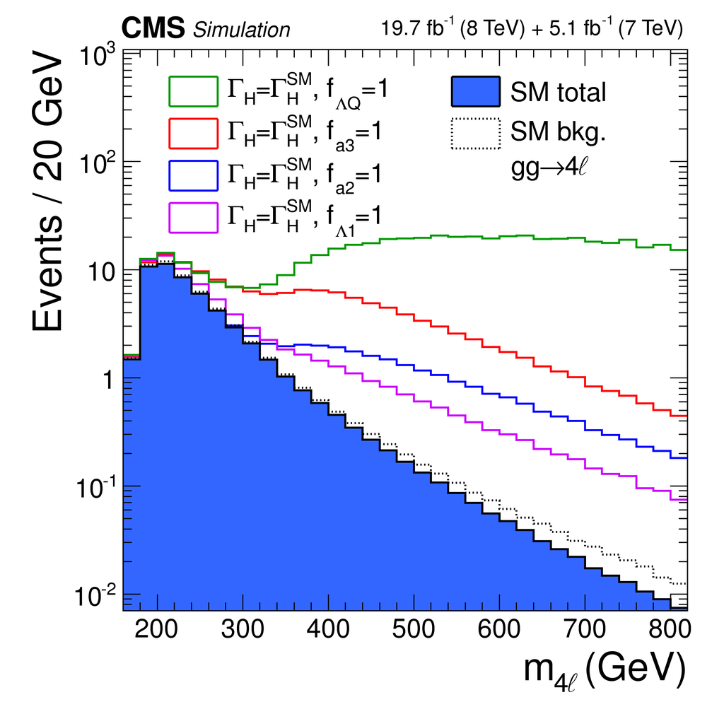
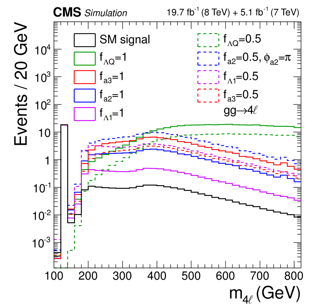
png pdf	Figure 1: The ${m_{4\ell }}$ distributions in the off-shell region in the simulation of the ${\mathrm {g}} {\mathrm {g}} \to 4\ell$ process with the $\Lambda _{Q}$ ( ${f_{\Lambda Q}} =1$ ), $a_3$ ( $f_{a3}=1$ ), $a_2$ ( $f_{a2}=1$ ), and $\Lambda _{1}$ ( $f_{\Lambda 1}=1$ ) terms, as open histograms, as well as the $a_1$ term (SM), as the filled histogram, from Eq.(4) in decreasing order of enhancement at high ${m_{4\ell }}$ . The on-shell signal yield and the width ${\Gamma _{ {\mathrm {H}} }}$ are constrained to the SM expectations. In all cases, the background and its interference with different signal hypotheses are included except in the case of the pure background (dotted), which has greater off-shell yield than the SM signal-background contribution due to destructive interference.
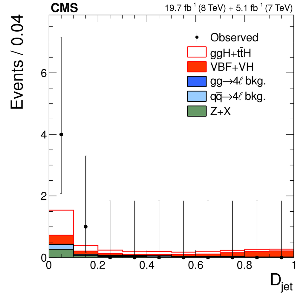
png pdf	Figure 2-a: Distributions of the four-lepton invariant mass $\mathcal {D}_\text {jet}$ (a) and ${m_{4\ell }}$ (b) in the on-shell region of the ${\mathrm {H}}$ boson width analysis. The $\mathcal {D}_\text {jet}$ distributions show events in the dijet category with a requirement 120 $< {m_{4\ell }} <$ 130 GeV. The ${m_{4\ell }}$ distributions combine the nondijet and dijet categories, the former with an additional requirement $\mathcal {D}^\text {kin} _\text {bkg} >$ 0.5 to suppress the dominant $\to 4\ell$ background. The points with error bars represent the observed data, and the histograms represent the expected contributions from the SM backgrounds and the ${\mathrm {H}}$ boson signal. The contribution from the VBF and ${\mathrm {V}} {\mathrm {H}}$ production is shown separately.
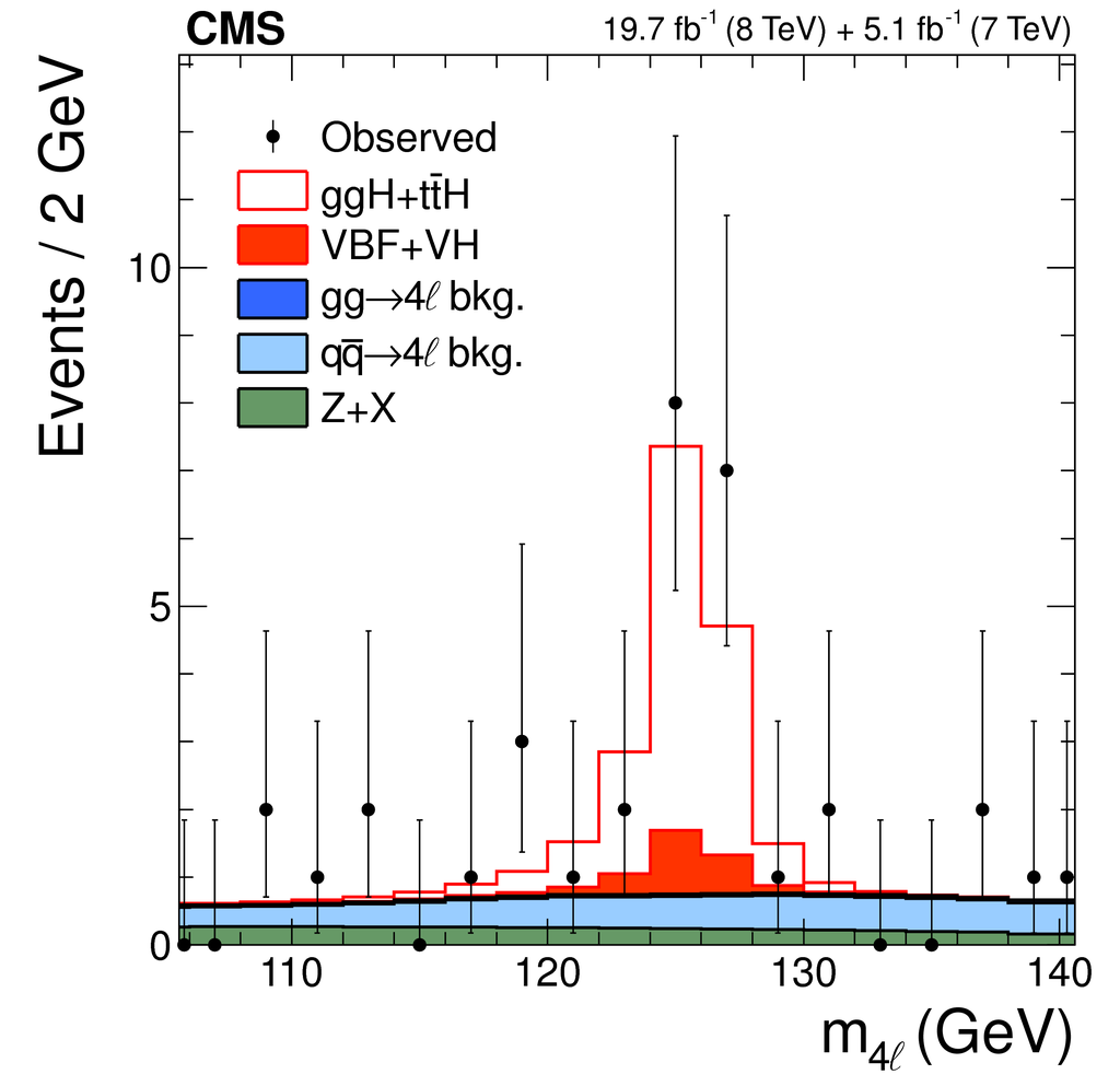
png pdf	Figure 2-b: Distributions of the four-lepton invariant mass $\mathcal {D}_\text {jet}$ (a) and ${m_{4\ell }}$ (b) in the on-shell region of the ${\mathrm {H}}$ boson width analysis. The $\mathcal {D}_\text {jet}$ distributions show events in the dijet category with a requirement 120 $< {m_{4\ell }} <$ 130 GeV. The ${m_{4\ell }}$ distributions combine the nondijet and dijet categories, the former with an additional requirement $\mathcal {D}^\text {kin} _\text {bkg} >$ 0.5 to suppress the dominant $\to 4\ell$ background. The points with error bars represent the observed data, and the histograms represent the expected contributions from the SM backgrounds and the ${\mathrm {H}}$ boson signal. The contribution from the VBF and ${\mathrm {V}} {\mathrm {H}}$ production is shown separately.
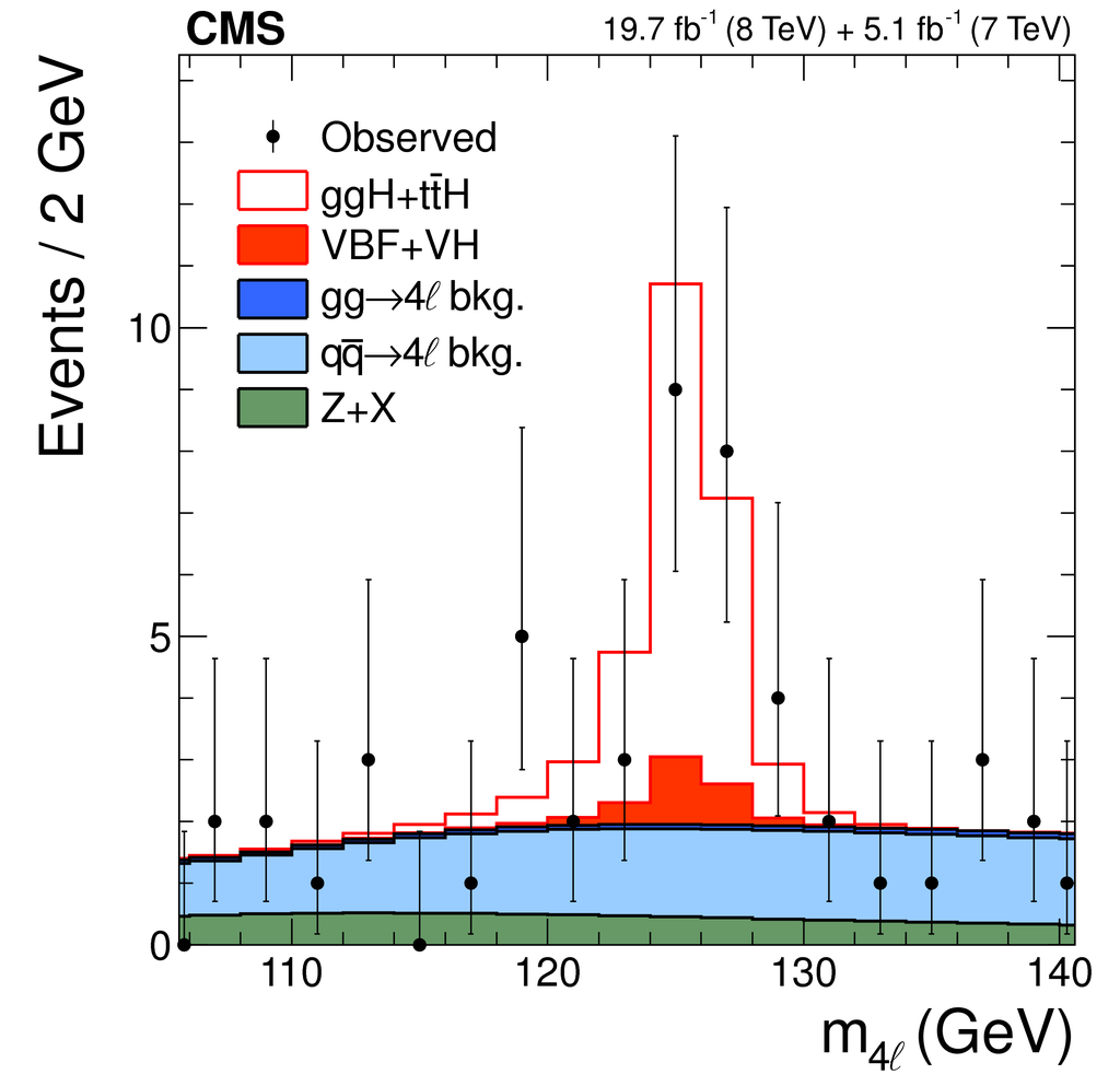
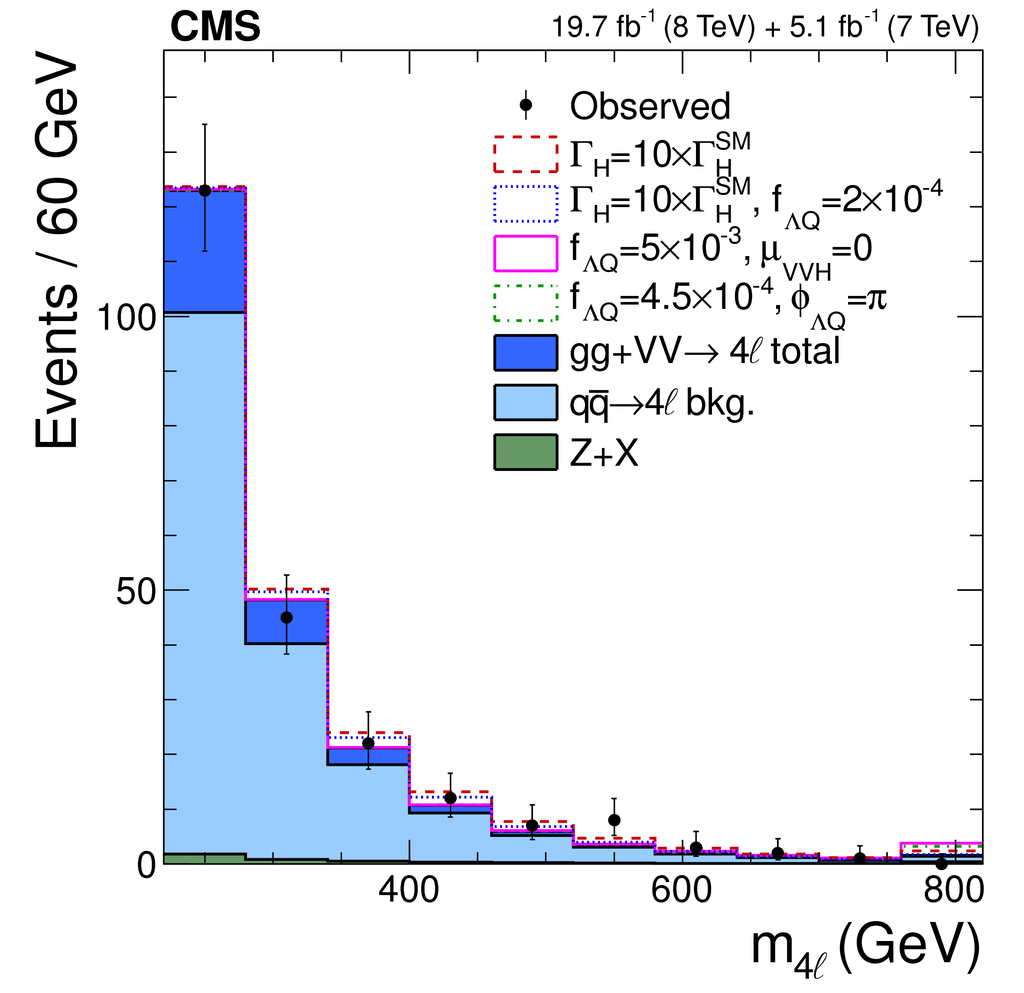
png pdf	Figure 3-a: Distributions of the four-lepton invariant mass ${m_{4\ell }}$ in the on-shell (a) and off-shell (b) regions of the ${\mathrm {H}}$ boson width analysis for all observed and expected events. The points with error bars represent the observed data in both on-shell and off-shell region distributions. The histograms for the on-shell region represent the expected contributions from the SM backgrounds and the ${\mathrm {H}}$ boson signal with the contribution from the VBF and ${\mathrm {V}} {\mathrm {H}}$ production shown separately. The filled histograms for the off-shell region represent the expected contributions from the SM backgrounds and ${\mathrm {H}}$ boson signal, combining gluon fusion, VBF, and ${\mathrm {V}} {\mathrm {H}}$ processes. Alternative ${\mathrm {H}}$ boson width and coupling scenarios are shown as open histograms with the assumption ${\phi _{\Lambda Q}} =$ 0 unless specified otherwise, and the overflow bin includes events up to ${m_{4\ell }} =$ 1600 GeV.
png pdf	Figure 3-b: Distributions of the four-lepton invariant mass ${m_{4\ell }}$ in the on-shell (a) and off-shell (b) regions of the ${\mathrm {H}}$ boson width analysis for all observed and expected events. The points with error bars represent the observed data in both on-shell and off-shell region distributions. The histograms for the on-shell region represent the expected contributions from the SM backgrounds and the ${\mathrm {H}}$ boson signal with the contribution from the VBF and ${\mathrm {V}} {\mathrm {H}}$ production shown separately. The filled histograms for the off-shell region represent the expected contributions from the SM backgrounds and ${\mathrm {H}}$ boson signal, combining gluon fusion, VBF, and ${\mathrm {V}} {\mathrm {H}}$ processes. Alternative ${\mathrm {H}}$ boson width and coupling scenarios are shown as open histograms with the assumption ${\phi _{\Lambda Q}} =$ 0 unless specified otherwise, and the overflow bin includes events up to ${m_{4\ell }} =$ 1600 GeV.
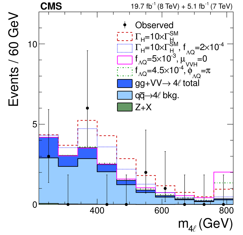
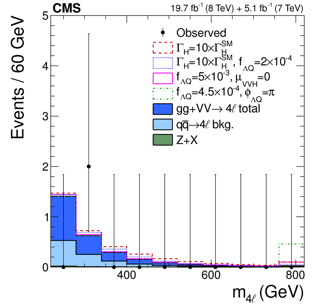
png pdf	Figure 4-a: Distribution of the four-lepton invariant mass ${m_{4\ell }}$ in the off-shell region in the nondijet (a) and dijet (b) categories. A requirement $\mathcal {D}_{ {\mathrm {g}} {\mathrm {g}}} >$ 2/3 is applied in the nondijet category to suppress the dominant $\to 4\ell$ background. The points with error bars represent the observed data, and the filled histograms represent the expected contributions from the SM backgrounds and ${\mathrm {H}}$ boson signal, combining gluon fusion, VBF, and ${\mathrm {V}} {\mathrm {H}}$ processes. Alternative ${\mathrm {H}}$ boson width and coupling scenarios are shown as open histograms. The overflow bins include events up to ${m_{4\ell }} =$ 1600 GeV, and ${\phi _{\Lambda Q}} =$ 0 is assumed where it is unspecified.
png pdf	Figure 4-b: Distribution of the four-lepton invariant mass ${m_{4\ell }}$ in the off-shell region in the nondijet (a) and dijet (b) categories. A requirement $\mathcal {D}_{ {\mathrm {g}} {\mathrm {g}}} >$ 2/3 is applied in the nondijet category to suppress the dominant $\to 4\ell$ background. The points with error bars represent the observed data, and the filled histograms represent the expected contributions from the SM backgrounds and ${\mathrm {H}}$ boson signal, combining gluon fusion, VBF, and ${\mathrm {V}} {\mathrm {H}}$ processes. Alternative ${\mathrm {H}}$ boson width and coupling scenarios are shown as open histograms. The overflow bins include events up to ${m_{4\ell }} =$ 1600 GeV, and ${\phi _{\Lambda Q}} =$ 0 is assumed where it is unspecified.
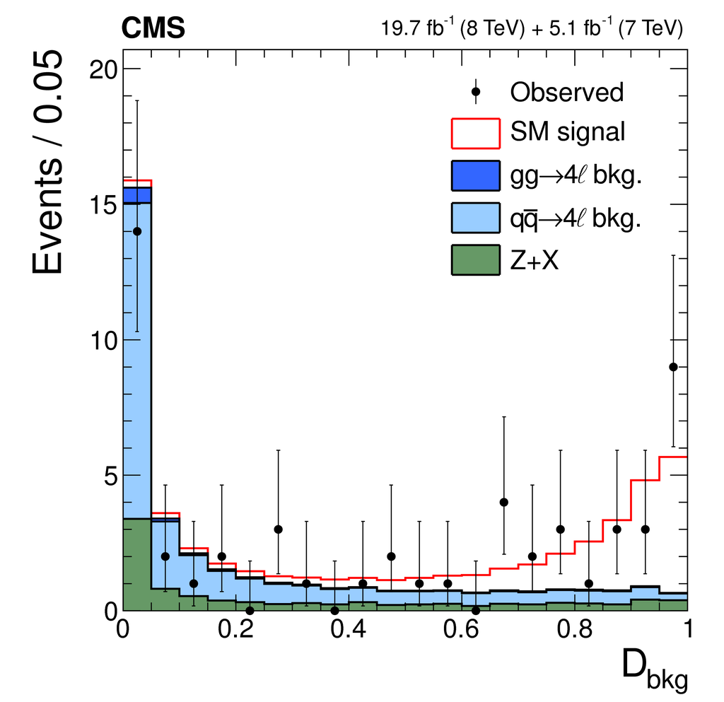
png pdf	Figure 5-a: Distributions of $\mathcal {D}_\text {bkg}$ (a) and $c {\Delta t}$ (b) in the lifetime analysis with $\mathcal {D}_\text {bkg} >$ 0.5 required for the latter to suppress the background. The points with error bars represent the observed data, and the filled histograms stacked on top of each other represent the expected contributions from the SM backgrounds. Stacked on the total background contribution, the open histograms show the combination of all production mechanisms expected in the SM for the ${\mathrm {H}}$ boson signal with either the SM lifetime or $c\tau _ {\mathrm {H}} =$ 100 $\mu$ m. Each signal contribution in the different open histograms are the same as the total number of events expected from the combination of all production mechanisms in the SM. All signal distributions are shown with the total number of events expected in the SM. The first and last bins of the $c {\Delta t}$ distributions include all events beyond ${\| c {\Delta t} \| }>$ 500 $\mu$ m.
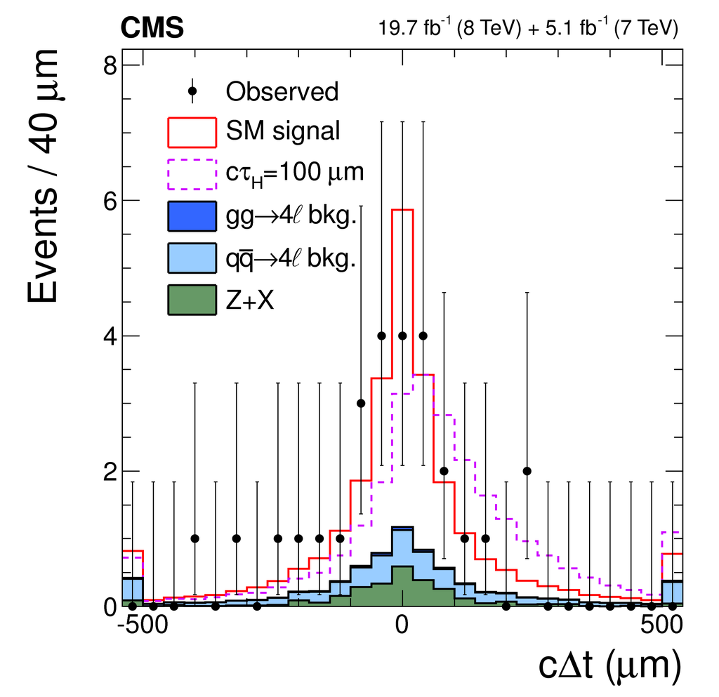
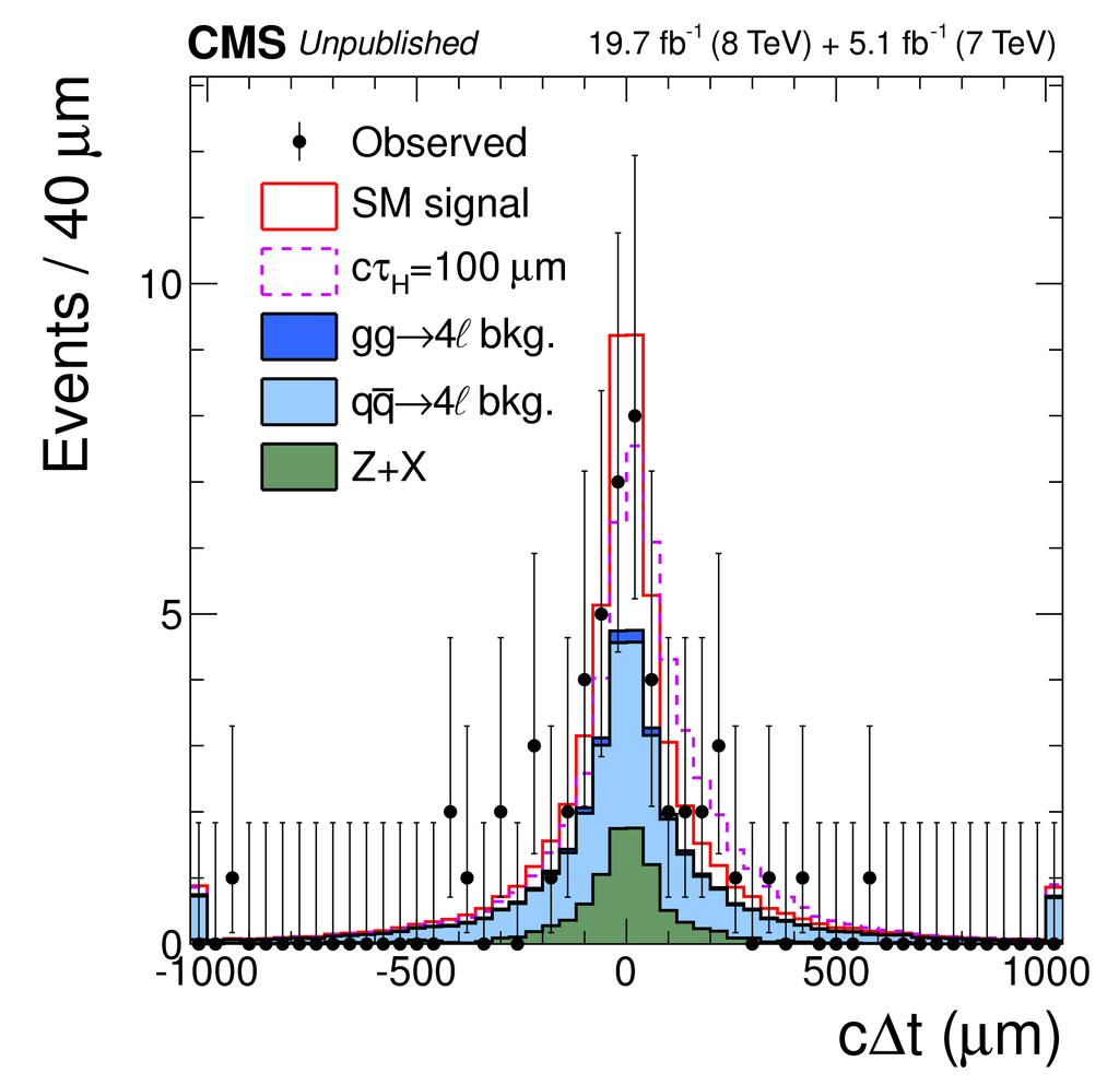
png pdf	Figure 5-b: Distributions of $\mathcal {D}_\text {bkg}$ (a) and $c {\Delta t}$ (b) in the lifetime analysis with $\mathcal {D}_\text {bkg} >$ 0.5 required for the latter to suppress the background. The points with error bars represent the observed data, and the filled histograms stacked on top of each other represent the expected contributions from the SM backgrounds. Stacked on the total background contribution, the open histograms show the combination of all production mechanisms expected in the SM for the ${\mathrm {H}}$ boson signal with either the SM lifetime or $c\tau _ {\mathrm {H}} =$ 100 $\mu$ m. Each signal contribution in the different open histograms are the same as the total number of events expected from the combination of all production mechanisms in the SM. All signal distributions are shown with the total number of events expected in the SM. The first and last bins of the $c {\Delta t}$ distributions include all events beyond ${\| c {\Delta t} \| }>$ 500 $\mu$ m.
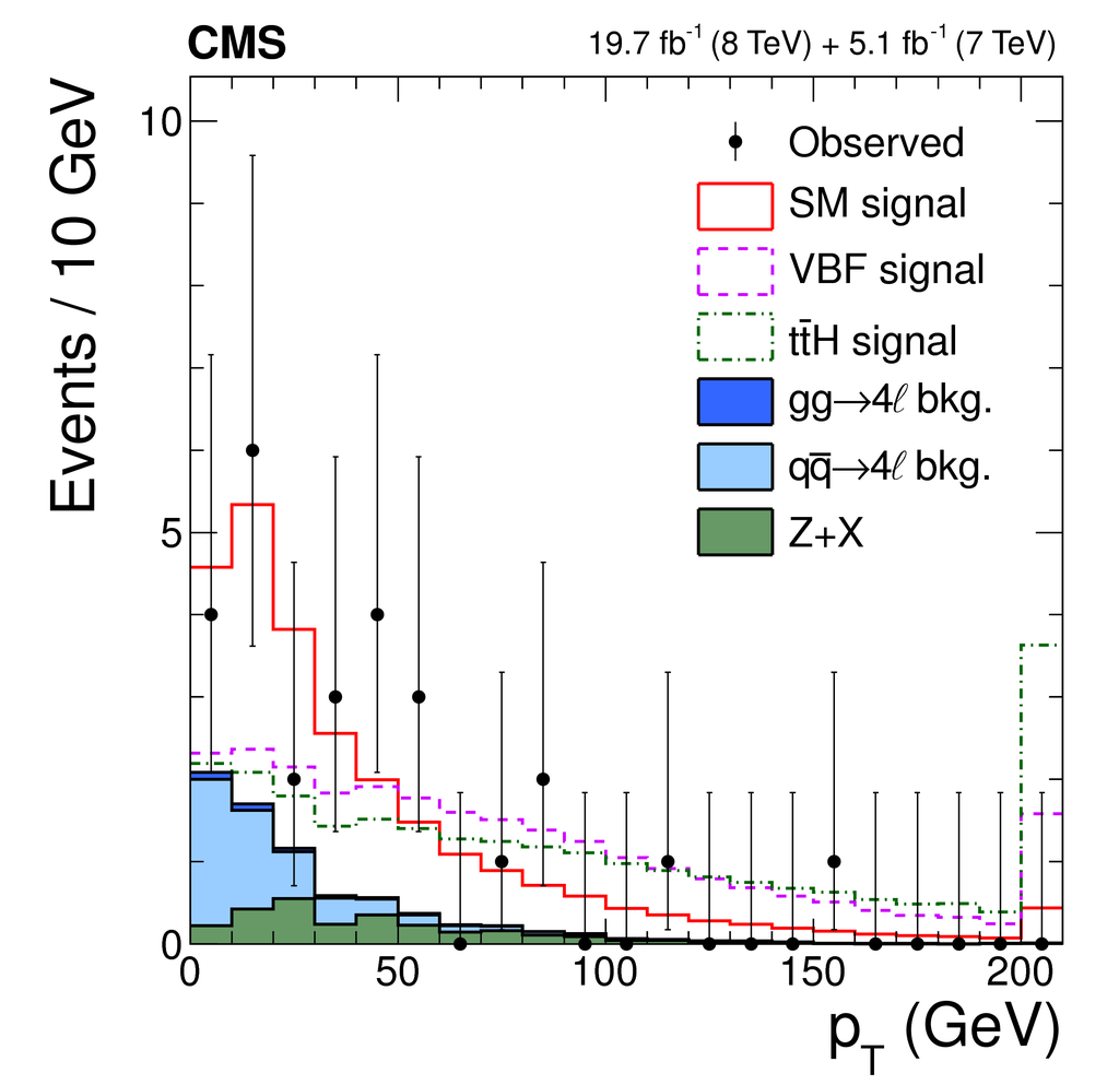
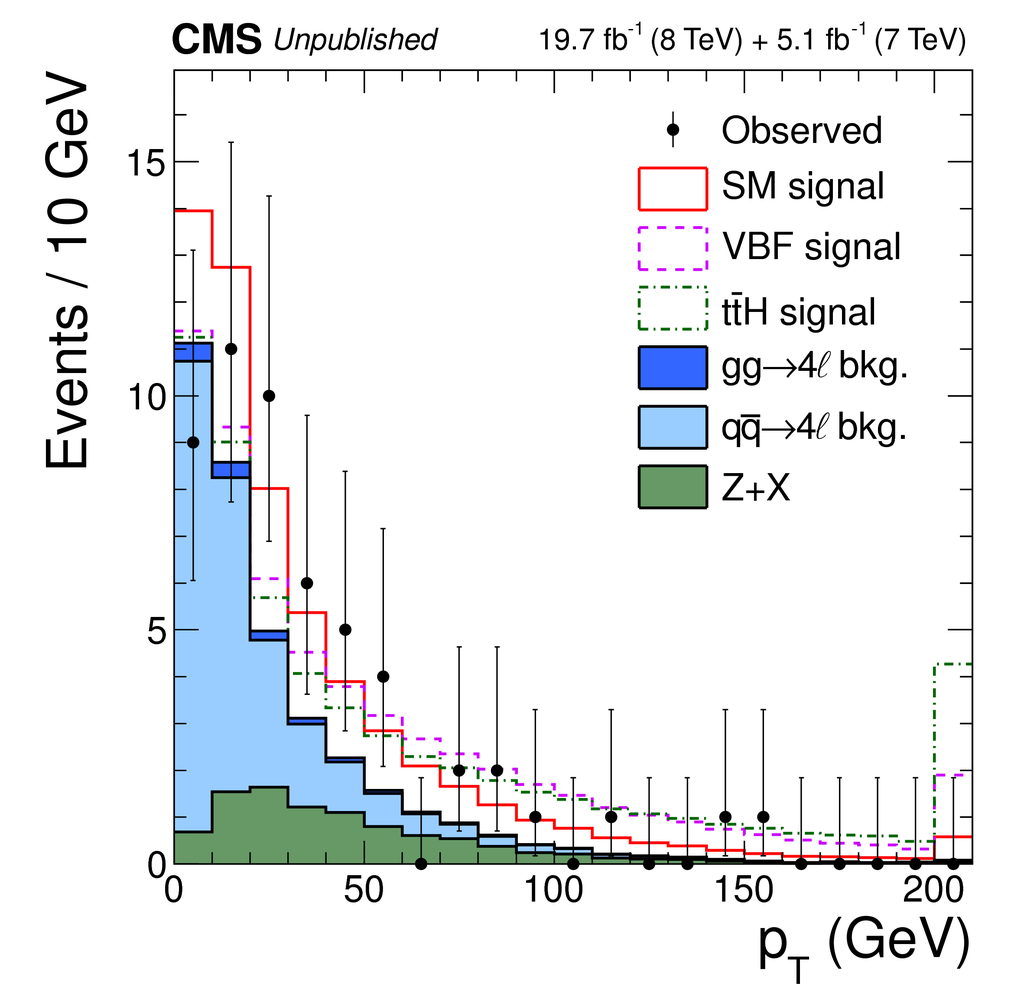
png pdf	Figure 6: Distributions of the four-lepton ${p_{\mathrm {T}}}$ with the selection used in the lifetime analysis and the requirement $\mathcal {D}_\text {bkg} >$ 0.5 to suppress the backgrounds. The points with error bars represent the observed data, and the filled histograms stacked on top of each other represent the expected contributions from the SM backgrounds. Stacked on the total background contribution, the open histograms show the ${\mathrm {H}}$ boson signal either with the combination of all production mechanisms expected in the SM, or for the VBF or ${\mathrm {t}\overline {\mathrm {t}}} {\mathrm {H}}$ production mechanisms. Each signal contribution in the different open histograms is normalized to the total number of events expected from the combination of all production mechanisms in the SM. The overflow bin includes all events beyond ${p_{\mathrm {T}}} >$ 200 GeV.
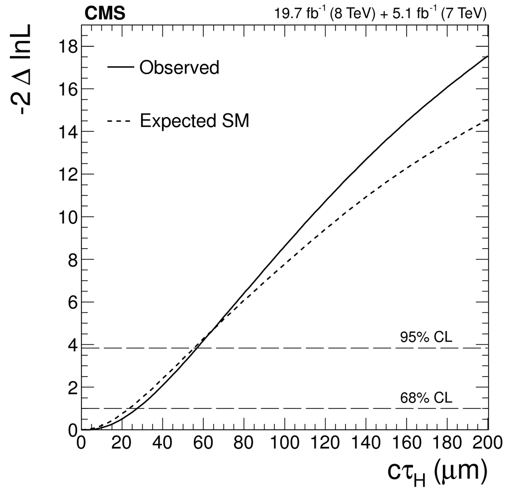
png pdf	Figure 7: Observed (solid) and expected (dashed) distributions of $-2 \ln (\mathcal {L}/\mathcal {L}_\text {max})$ as a function of the ${\mathrm {H}}$ boson average lifetime $c\tau _ {\mathrm {H}}$ .
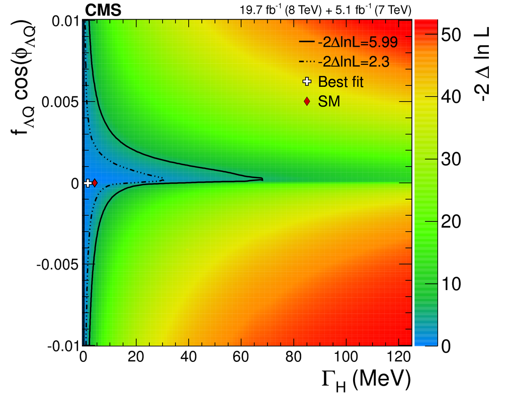
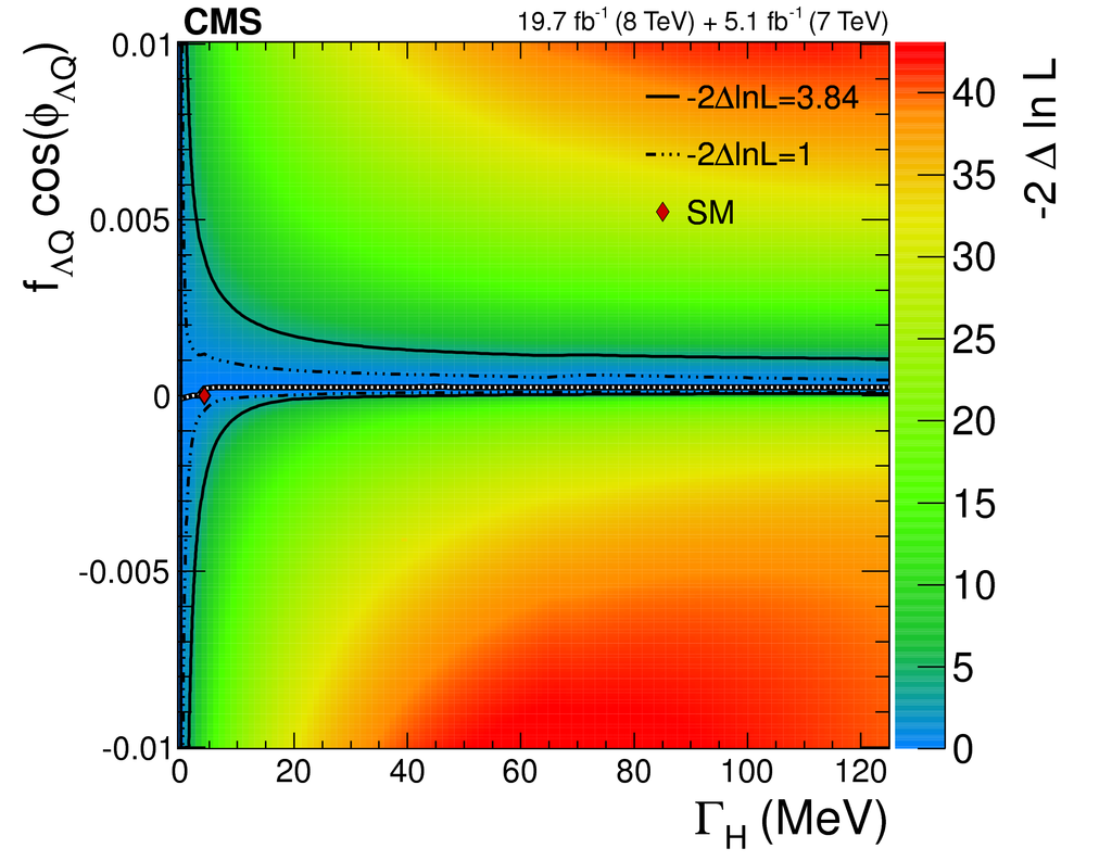
png pdf	Figure 8-a: Observed distribution of $-2\ \ln (\mathcal {L}/\mathcal {L}_\text {max})$ as a function of ${\Gamma _{ {\mathrm {H}} }}$ and ${f_{\Lambda Q}} \cos {\phi _{\Lambda Q}}$ with the assumption ${\phi _{\Lambda Q}} =0$ or $\pi$ (top panel). The bottom panel shows the observed conditional likelihood scan as a function of ${f_{\Lambda Q}} \cos {\phi _{\Lambda Q}}$ for a given ${\Gamma _{ {\mathrm {H}} }}$ . The likelihood contours are shown for the two-parameter 68% and 95% CLs (a) and for the one-parameter 68% and 95% CLs (b). The black curve with white dots on the bottom panel shows the ${f_{\Lambda Q}} \cos {\phi _{\Lambda Q}}$ minima at each ${\Gamma _{ {\mathrm {H}} }}$ value.
png pdf	Figure 8-b: Observed distribution of $-2\ \ln (\mathcal {L}/\mathcal {L}_\text {max})$ as a function of ${\Gamma _{ {\mathrm {H}} }}$ and ${f_{\Lambda Q}} \cos {\phi _{\Lambda Q}}$ with the assumption ${\phi _{\Lambda Q}} =0$ or $\pi$ (top panel). The bottom panel shows the observed conditional likelihood scan as a function of ${f_{\Lambda Q}} \cos {\phi _{\Lambda Q}}$ for a given ${\Gamma _{ {\mathrm {H}} }}$ . The likelihood contours are shown for the two-parameter 68% and 95% CLs (a) and for the one-parameter 68% and 95% CLs (b). The black curve with white dots on the bottom panel shows the ${f_{\Lambda Q}} \cos {\phi _{\Lambda Q}}$ minima at each ${\Gamma _{ {\mathrm {H}} }}$ value.
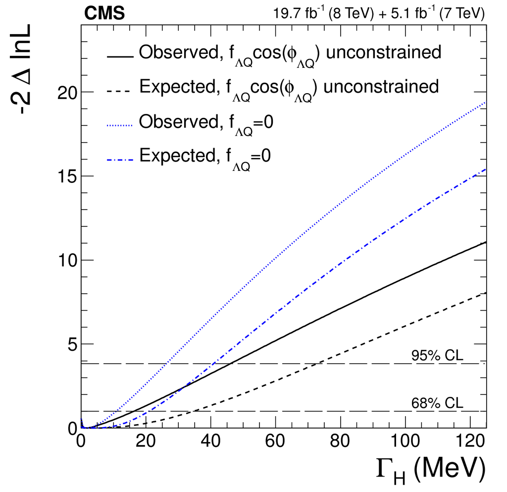
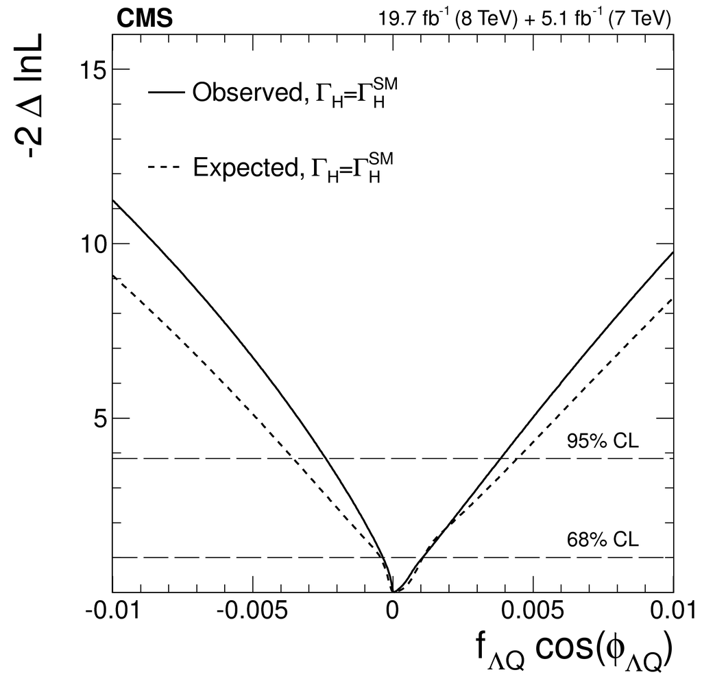
png pdf	Figure 9-a: Observed (solid) and expected (dashed) distributions of $-2 \ln (\mathcal {L}/\mathcal {L}_\text {max})$ as a function of ${\Gamma _{ {\mathrm {H}} }}$ (a) and ${f_{\Lambda Q}} \cos {\phi _{\Lambda Q}}$ (b). On the top panel, the ${f_{\Lambda Q}}$ value is either constrained to zero (blue) or left unconstrained (black, weaker limit), while ${\Gamma _{ {\mathrm {H}} }} = {\Gamma _{ {\mathrm {H}} }^{\mathrm {SM}}}$ and ${\phi _{\Lambda Q}} =0$ or $\pi$ are assumed on the bottom.
png pdf	Figure 9-b: Observed (solid) and expected (dashed) distributions of $-2 \ln (\mathcal {L}/\mathcal {L}_\text {max})$ as a function of ${\Gamma _{ {\mathrm {H}} }}$ (a) and ${f_{\Lambda Q}} \cos {\phi _{\Lambda Q}}$ (b). On the top panel, the ${f_{\Lambda Q}}$ value is either constrained to zero (blue) or left unconstrained (black, weaker limit), while ${\Gamma _{ {\mathrm {H}} }} = {\Gamma _{ {\mathrm {H}} }^{\mathrm {SM}}}$ and ${\phi _{\Lambda Q}} =0$ or $\pi$ are assumed on the bottom.

Tables
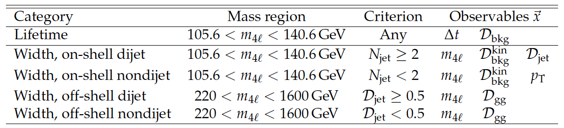
png pdf	Table 1: List of observables, $\vec{x}$ , and categories of events used in the analyses of the ${\mathrm {H}}$ boson lifetime and width. The $\mathcal {D}_\text {jet}<$ 0.5 requirement is defined for $N_\text {jet} \ge 2$ , but by convention this category also includes events with less than two selected jets, $N_\text {jet}<$ 2.
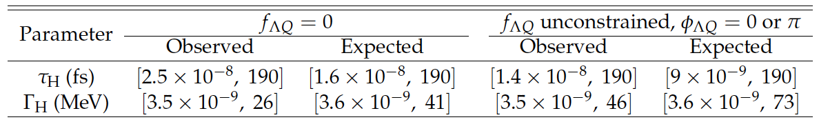
png pdf	Table 2: Observed and expected allowed intervals at the 95% CL on the ${\mathrm {H}}$ boson average lifetime $\tau _ {\mathrm {H}}$ and width ${\Gamma _{ {\mathrm {H}} }}$ obtained combining the width and lifetime analyses. The constraints are separated into the two conditions used in the width measurement, with either the constraint ${f_{\Lambda Q}} =$ 0, or ${f_{\Lambda Q}}$ left unconstrained and ${\phi _{\Lambda Q}} =$ 0 or $\pi$ . The upper (lower) limits on ${\mathrm {H}}$ boson average lifetime $\tau _ {\mathrm {H}}$ are related to the lower (upper) limits on ${\mathrm {H}}$ boson width ${\Gamma _{ {\mathrm {H}} }}$ through Eq.(2).
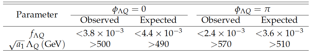
png pdf	Table 3: Observed and expected allowed intervals at the 95% CL on the ${f_{\Lambda Q}}$ on-shell effective cross-section fraction and its interpretation in terms of the anomalous coupling parameter $\Lambda _Q$ assuming ${\Gamma _{ {\mathrm {H}} }} = {\Gamma _{ {\mathrm {H}} }^{\mathrm {SM}}}$ . Results are presented assuming either ${\phi _{\Lambda Q}} =$ 0 or ${\phi _{\Lambda Q}} =\pi$ . The allowed intervals on ${f_{\Lambda Q}}$ are also translated to the equivalent quantity $\sqrt {a_1} {\Lambda _Q}$ through Eq.(5), where the coefficient $a_1$ is allowed to be different from its SM value $a_1=$ 2.

Summary

Constraints on the lifetime and the width of the H boson are obtained from

$\mathrm{ H \to ZZ \to 4\ell }$ events using the data recorded by the CMS experiment during the LHC run 1. The measurement of the H boson lifetime is derived from its flight distance in the CMS detector with the upper bound

$\tau_{\mathrm{H}} <$ 190 fs at the 95% CL, corresponding to a lower bound on the width

$\Gamma_{\mathrm{H}} > 3.5\, 10^{-9}$ MeV. The measurement of the width is obtained from an off-shell production technique, generalized to include additional anomalous couplings of the H boson to two electroweak bosons. This measurement provides a joint constraint on the H boson width and a parameter that quantifies an anomalous coupling contribution through an on-shell crosssection fraction

$f_{\Lambda Q}$ . The observed limit on the H boson width is

$\Gamma_{\mathrm{H}} <$ 46 MeV at the 95% CL with

$f_{\Lambda Q}$ left unconstrained while it is

$\Gamma_{\mathrm{H}} <$ 26 MeV at the 95% CL for

$f_{\Lambda Q} =$ 0. The constraint

$f_{\Lambda Q} < 3.8 \, 10^{-3}$ at the 95% CL is obtained assuming the H boson width expected in the SM, and the fLQ constraints given any other width value are also presented. Table 2 summarizes the width and corresponding lifetime limits, and Table 3 summarizes the limits on

$f_{\Lambda Q}$ under the different

$\phi_{\Lambda Q}$ scenarios that can be interpreted from this analysis, and provides the corresponding limits on

$\sqrt{a_1} f_{\Lambda Q}$ .

Additional Figures
png pdf	Additional Figure 1: The $m_{4\ell}$ distributions in the off-shell region in the simulation of the $\mathrm{g}\mathrm{g}\to 4\ell$ process with the $\Lambda _{Q}$ ( $f_{\Lambda Q}=1$ ), $a_3$ ( $f_{a3}=1$ ), $a_2$ ( $f_{a2}=1$ ), $\Lambda _{1}$ ( $f_{\Lambda 1}=1$ ), and the $a_1$ (SM) terms (solid open histograms) as well as equal on-shell mixtures with the SM term ( $f_{\Lambda Q}=0.5$ ; $f_{a3}=0.5$ ; $f_{a2}=0.5$ as dashed open histograms). The $f_{a2}=0.5$ mixture is shown with $arg(a_{2}/a{1})=\phi_{a2}=\pi$ so that the interference has the same destructive interference as in the $\Lambda _{Q}$ and $\Lambda _{1}$ cases. The on-shell signal yield and the width $\Gamma_{\mathrm{H}}$ are constrained to the SM expectations except the case of $f_{\Lambda Q}=0.5$ , which has complete destructive interference in the on-shell signal region and is therefore normalized with half of the factor used in $f_{\Lambda Q}=1$ for illustration. The on-shell regions is shown in a single bin. The background and its interference with different signal hypotheses are excluded.
png pdf	Additional Figure 2-a: Distributions of $c\Delta t$ in the lifetime analysis in the on-shell region (a) and the sideband $m_{4\ell}$ regions (b). No $\mathcal{D}_\text{bkg}$ requirement is applied. The points with error bars represent the observed data, and the filled histograms stacked on top of each other represent the expected contributions from the SM backgrounds. Stacked on the total background contribution, the open histograms, where present, show the combination of all production mechanisms expected in the SM for the $\mathrm {H}$ boson signal with either the SM lifetime or $c\tau_\mathrm{H}=$ 100 $\mu$ m. Each signal contribution in the different open histograms are the same as the total number of events expected from the combination of all production mechanisms in the SM. All distributions are shown with the total number of events expected in the SM. The first and last bins of the $c\Delta t$ distributions include all events beyond $\|c\Delta t\|>$ 1000 $\mu$ m.
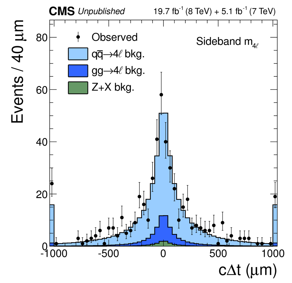
png pdf	Additional Figure 2-b: Distributions of $c\Delta t$ in the lifetime analysis in the on-shell region (a) and the sideband $m_{4\ell}$ regions (b). No $\mathcal{D}_\text{bkg}$ requirement is applied. The points with error bars represent the observed data, and the filled histograms stacked on top of each other represent the expected contributions from the SM backgrounds. Stacked on the total background contribution, the open histograms, where present, show the combination of all production mechanisms expected in the SM for the $\mathrm {H}$ boson signal with either the SM lifetime or $c\tau_\mathrm{H}=$ 100 $\mu$ m. Each signal contribution in the different open histograms are the same as the total number of events expected from the combination of all production mechanisms in the SM. All distributions are shown with the total number of events expected in the SM. The first and last bins of the $c\Delta t$ distributions include all events beyond $\|c\Delta t\|>$ 1000 $\mu$ m.
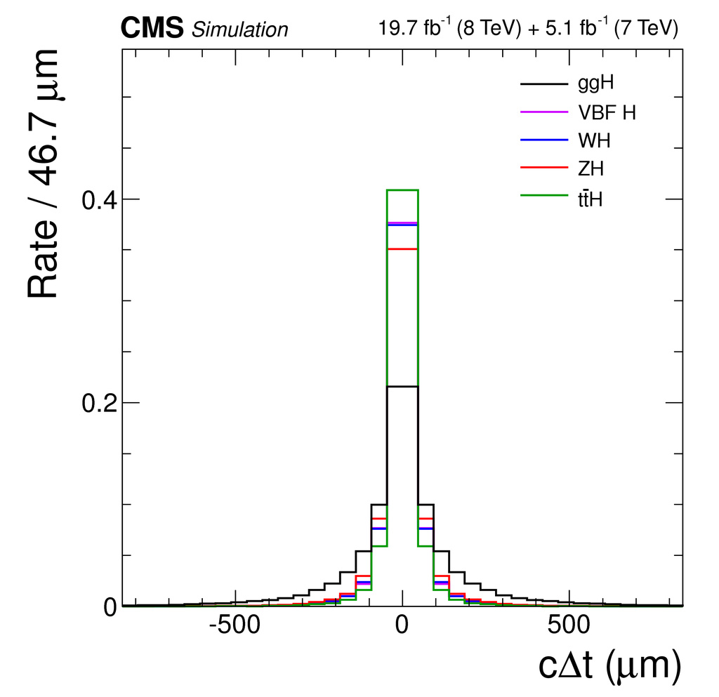
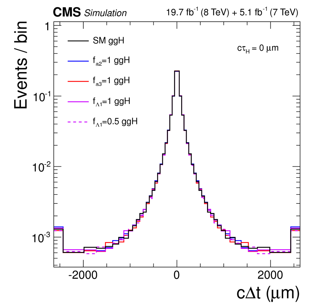
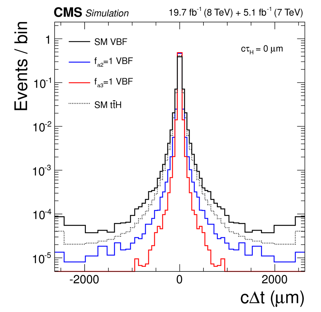
png pdf	Additional Figure 3-a: Panel a: Distributions of the four-lepton $p_{\mathrm{T}}$ with the selection used in the lifetime analysis without the requirement $\mathcal{D}_\text{bkg} >$ 0.5 to suppress the background. The points with error bars represent the observed data, and the filled histograms stacked on top of each other represent the expected contributions from the SM backgrounds. Stacked on the total background contribution, the open histograms show the $\mathrm{H}$ boson signal either with the combination of all production mechanisms expected in the SM, or for the VBF or $\mathrm{t}\overline{\mathrm{t}}\mathrm{H}$ production mechanisms. Each signal contribution in the different open histograms is normalized to the total number of events expected from the combination of all production mechanisms in the SM. The overflow bin includes all events beyond $p_{\mathrm{T}}>$ 200 GeV. Panel b: Distributions of $c\Delta t$ in the lifetime analysis in the on-shell region for the different $\mathrm{H}$ boson production mechanisms, area-normalized to illustrate shape differences. Bottom panels: Distributions of $c\Delta t$ in the lifetime analysis in the on-shell region for different $\mathrm{H}\mathrm{V}\mathrm{V}$ couplings, including SM couplings, in decay for $\mathrm{H}$ boson production through gluon fusion ( $\mathrm{g}\mathrm{g}\mathrm{H}$ ) (a), and in production and decay for $\mathrm{H}$ boson production through weak vector boson fusion (VBF) (b). Panel (b) compares the different $c\Delta t$ distributions to the SM $\mathrm{t}\overline{\mathrm{t}}\mathrm{H}$ distribution (dotted black). The histograms are shown using variable bins up to $\|c\Delta t\|>$ 2000 $\mu$ m, and the first and last bins include all events outside this region. All distributions are area-normalized to illustrate the shape differences.
png pdf	Additional Figure 3-b: Panel a: Distributions of the four-lepton $p_{\mathrm{T}}$ with the selection used in the lifetime analysis without the requirement $\mathcal{D}_\text{bkg} >$ 0.5 to suppress the background. The points with error bars represent the observed data, and the filled histograms stacked on top of each other represent the expected contributions from the SM backgrounds. Stacked on the total background contribution, the open histograms show the $\mathrm{H}$ boson signal either with the combination of all production mechanisms expected in the SM, or for the VBF or $\mathrm{t}\overline{\mathrm{t}}\mathrm{H}$ production mechanisms. Each signal contribution in the different open histograms is normalized to the total number of events expected from the combination of all production mechanisms in the SM. The overflow bin includes all events beyond $p_{\mathrm{T}}>$ 200 GeV. Panel b: Distributions of $c\Delta t$ in the lifetime analysis in the on-shell region for the different $\mathrm{H}$ boson production mechanisms, area-normalized to illustrate shape differences. Bottom panels: Distributions of $c\Delta t$ in the lifetime analysis in the on-shell region for different $\mathrm{H}\mathrm{V}\mathrm{V}$ couplings, including SM couplings, in decay for $\mathrm{H}$ boson production through gluon fusion ( $\mathrm{g}\mathrm{g}\mathrm{H}$ ) (a), and in production and decay for $\mathrm{H}$ boson production through weak vector boson fusion (VBF) (b). Panel (b) compares the different $c\Delta t$ distributions to the SM $\mathrm{t}\overline{\mathrm{t}}\mathrm{H}$ distribution (dotted black). The histograms are shown using variable bins up to $\|c\Delta t\|>$ 2000 $\mu$ m, and the first and last bins include all events outside this region. All distributions are area-normalized to illustrate the shape differences.
png pdf	Additional Figure 3-c: Panel a: Distributions of the four-lepton $p_{\mathrm{T}}$ with the selection used in the lifetime analysis without the requirement $\mathcal{D}_\text{bkg} >$ 0.5 to suppress the background. The points with error bars represent the observed data, and the filled histograms stacked on top of each other represent the expected contributions from the SM backgrounds. Stacked on the total background contribution, the open histograms show the $\mathrm{H}$ boson signal either with the combination of all production mechanisms expected in the SM, or for the VBF or $\mathrm{t}\overline{\mathrm{t}}\mathrm{H}$ production mechanisms. Each signal contribution in the different open histograms is normalized to the total number of events expected from the combination of all production mechanisms in the SM. The overflow bin includes all events beyond $p_{\mathrm{T}}>$ 200 GeV. Panel b: Distributions of $c\Delta t$ in the lifetime analysis in the on-shell region for the different $\mathrm{H}$ boson production mechanisms, area-normalized to illustrate shape differences. Bottom panels: Distributions of $c\Delta t$ in the lifetime analysis in the on-shell region for different $\mathrm{H}\mathrm{V}\mathrm{V}$ couplings, including SM couplings, in decay for $\mathrm{H}$ boson production through gluon fusion ( $\mathrm{g}\mathrm{g}\mathrm{H}$ ) (a), and in production and decay for $\mathrm{H}$ boson production through weak vector boson fusion (VBF) (b). Panel (b) compares the different $c\Delta t$ distributions to the SM $\mathrm{t}\overline{\mathrm{t}}\mathrm{H}$ distribution (dotted black). The histograms are shown using variable bins up to $\|c\Delta t\|>$ 2000 $\mu$ m, and the first and last bins include all events outside this region. All distributions are area-normalized to illustrate the shape differences.
png pdf	Additional Figure 3-d: Panel a: Distributions of the four-lepton $p_{\mathrm{T}}$ with the selection used in the lifetime analysis without the requirement $\mathcal{D}_\text{bkg} >$ 0.5 to suppress the background. The points with error bars represent the observed data, and the filled histograms stacked on top of each other represent the expected contributions from the SM backgrounds. Stacked on the total background contribution, the open histograms show the $\mathrm{H}$ boson signal either with the combination of all production mechanisms expected in the SM, or for the VBF or $\mathrm{t}\overline{\mathrm{t}}\mathrm{H}$ production mechanisms. Each signal contribution in the different open histograms is normalized to the total number of events expected from the combination of all production mechanisms in the SM. The overflow bin includes all events beyond $p_{\mathrm{T}}>$ 200 GeV. Panel b: Distributions of $c\Delta t$ in the lifetime analysis in the on-shell region for the different $\mathrm{H}$ boson production mechanisms, area-normalized to illustrate shape differences. Bottom panels: Distributions of $c\Delta t$ in the lifetime analysis in the on-shell region for different $\mathrm{H}\mathrm{V}\mathrm{V}$ couplings, including SM couplings, in decay for $\mathrm{H}$ boson production through gluon fusion ( $\mathrm{g}\mathrm{g}\mathrm{H}$ ) (a), and in production and decay for $\mathrm{H}$ boson production through weak vector boson fusion (VBF) (b). Panel (b) compares the different $c\Delta t$ distributions to the SM $\mathrm{t}\overline{\mathrm{t}}\mathrm{H}$ distribution (dotted black). The histograms are shown using variable bins up to $\|c\Delta t\|>$ 2000 $\mu$ m, and the first and last bins include all events outside this region. All distributions are area-normalized to illustrate the shape differences.
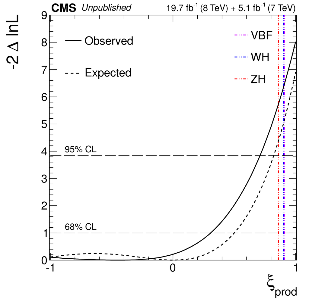
png pdf	Additional Figure 4: Observed (solid) and expected (dashed) distributions of $-2\ \ln(\mathcal{L}/\mathcal{L}_\text{max})$ as a function of the nuisance parameter $\xi_{prod}$ , controlling the full variation of the $\mathrm{H}$ boson $c\Delta t$ parameterization from the two extremes: production completely through gluon fusion ( $\xi_{prod}=-1$ ), and production completely through $\mathrm{t}\overline{\mathrm{t}}\mathrm{H}$ ( $\xi_{prod}=1$ ). The SM mixture of the different $\mathrm{H}$ boson production mechanisms corresponds to $\xi_{prod}=0$ , and the average $\mathrm{H}$ boson lifetime $c\tau_{\mathrm{H}}$ is unconstrained in these likelihood scans. Each pure $\mathrm{H}$ boson production scenario through the VBF or $\mathrm{V}\mathrm{H}$ processes with SM $\mathrm{H}\mathrm{V}\mathrm{V}$ couplings are shown with the vertical dot-dashed lines in color.
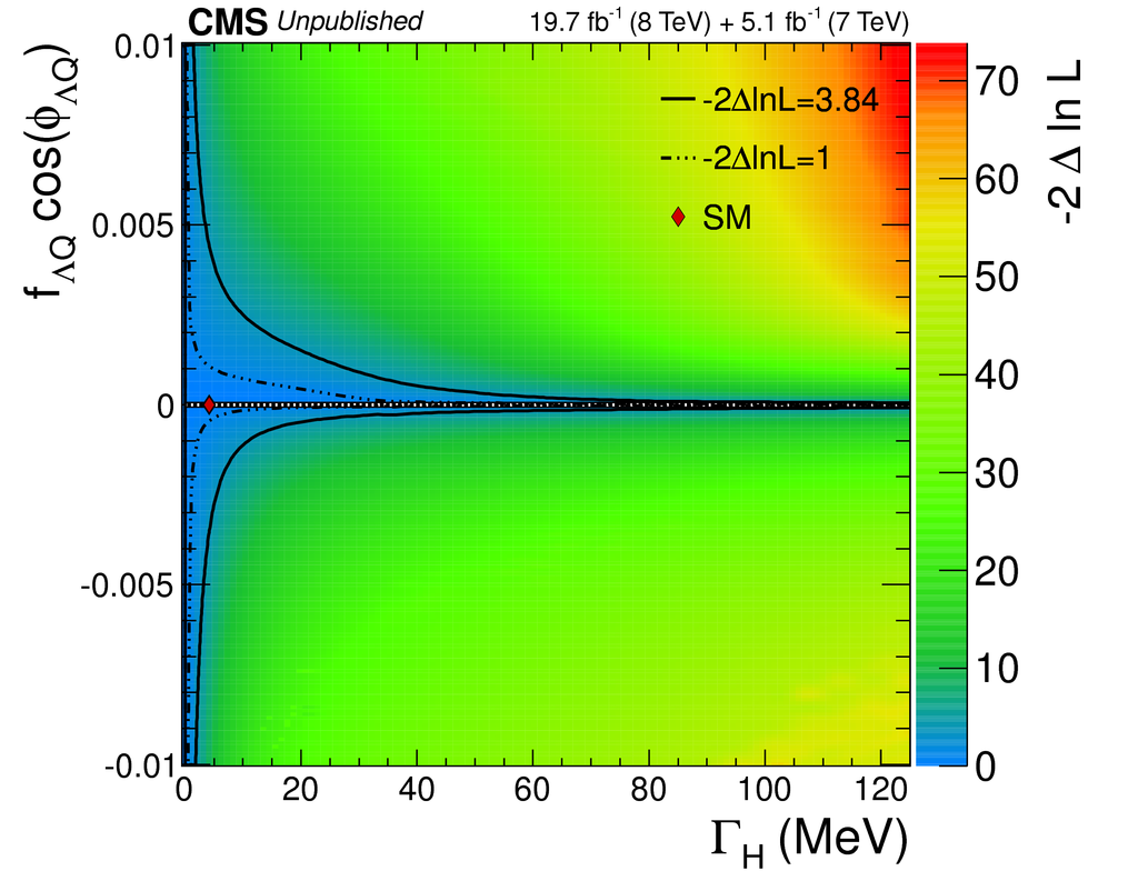
png pdf	Additional Figure 5-a: Expected distribution of $-2\ \ln(\mathcal{L}/\mathcal{L}_\text{max})$ as a function of $\Gamma_{\mathrm{H}}$ and $f_{\Lambda Q} \cos \phi_{\Lambda Q}$ with the assumption $\phi_{\Lambda Q}=0$ or $\pi$ (a). Panel (b) shows the conditional likelihood scan as a function of $f_{\Lambda Q} \cos \phi_{\Lambda Q}$ for a given $\Gamma_{\mathrm{H}}$ . The likelihood contours are shown for the two-parameter 68% and 95% CLs (a) and for the one-parameter 68% and 95% CLs (b). The black curve with white dots on Panel (b) shows the $f_{\Lambda Q} \cos \phi_{\Lambda Q}$ minima at each $\Gamma_{\mathrm{H}}$ value.
png pdf	Additional Figure 5-b: Expected distribution of $-2\ \ln(\mathcal{L}/\mathcal{L}_\text{max})$ as a function of $\Gamma_{\mathrm{H}}$ and $f_{\Lambda Q} \cos \phi_{\Lambda Q}$ with the assumption $\phi_{\Lambda Q}=0$ or $\pi$ (a). Panel (b) shows the conditional likelihood scan as a function of $f_{\Lambda Q} \cos \phi_{\Lambda Q}$ for a given $\Gamma_{\mathrm{H}}$ . The likelihood contours are shown for the two-parameter 68% and 95% CLs (a) and for the one-parameter 68% and 95% CLs (b). The black curve with white dots on Panel (b) shows the $f_{\Lambda Q} \cos \phi_{\Lambda Q}$ minima at each $\Gamma_{\mathrm{H}}$ value.
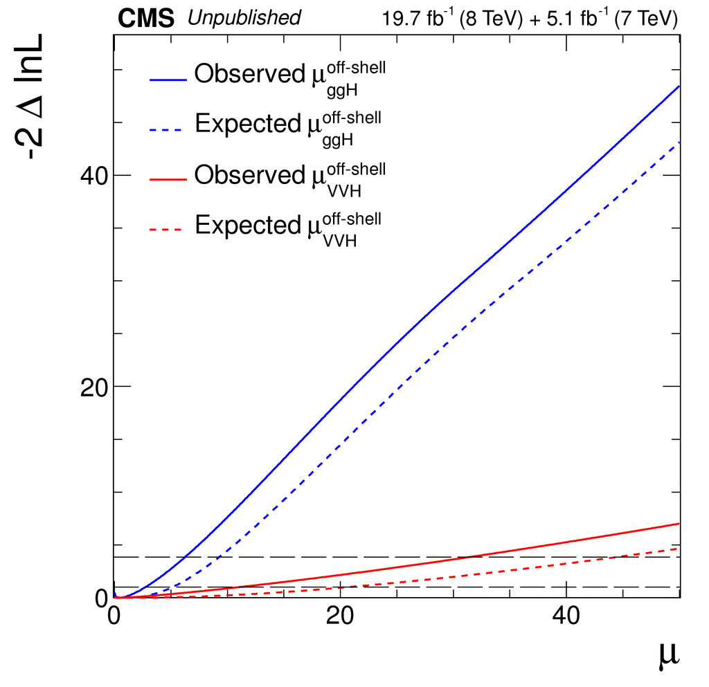
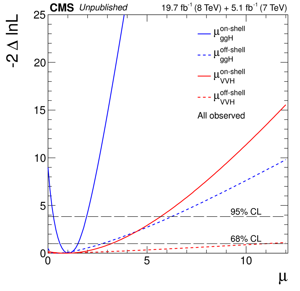
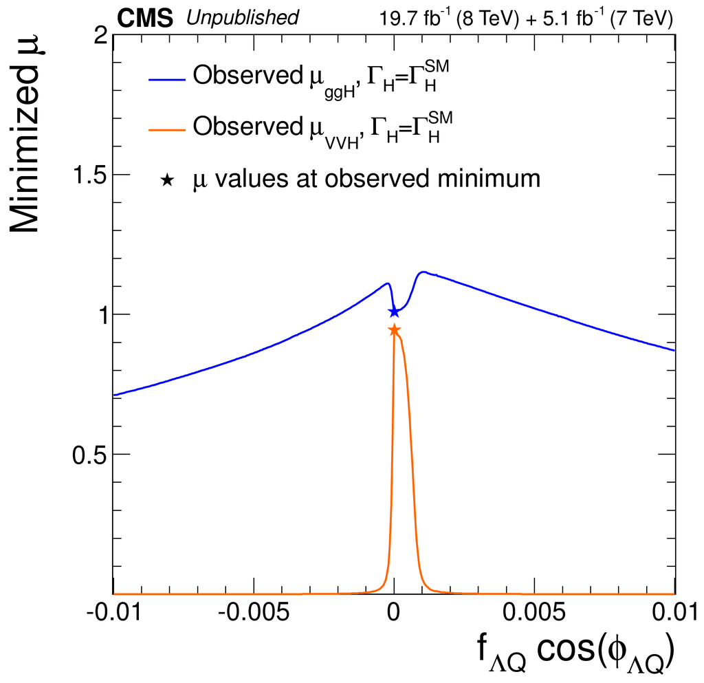
png pdf	Additional Figure 6-a: Observed (solid) and expected (dashed) distributions of $-2\ \ln(\mathcal{L}/\mathcal{L}_\text{max})$ as a function of offshell $\mu_{\mathrm{g}\mathrm{g}\mathrm{H}}$ or $\mu_{\mathrm{V}\mathrm{V}\mathrm{H}}$ (a), and observed distributions of $-2\ \ln(\mathcal{L}/\mathcal{L}_\text{max})$ as a function of onshell (solid) and offshell (dashed) $\mu_{\mathrm{g}\mathrm{g}\mathrm{H}}$ (blue) or $\mu_{\mathrm{V}\mathrm{V}\mathrm{H}}$ (red) (b). The $f_{\Lambda Q} =0$ is assumed, and onshell and offshell $\mu$ parameters are alternative parameterizations from the overall $\mu$ and $\Gamma_{\mathrm{H}}$ . Panel (c) shows the observed minima of the overall $\mu_{\mathrm{g}\mathrm{g}\mathrm{H}}$ (blue) and $\mu_{\mathrm{V}\mathrm{V}\mathrm{H}}$ (orange) at each $f_{\Lambda Q} \cos \phi_{\Lambda Q}$ value when the constraint $\Gamma_{\mathrm{H}}=\Gamma_{\mathrm{H}}^{\mathrm{SM}}$ is applied.
png pdf	Additional Figure 6-b: Observed (solid) and expected (dashed) distributions of $-2\ \ln(\mathcal{L}/\mathcal{L}_\text{max})$ as a function of offshell $\mu_{\mathrm{g}\mathrm{g}\mathrm{H}}$ or $\mu_{\mathrm{V}\mathrm{V}\mathrm{H}}$ (a), and observed distributions of $-2\ \ln(\mathcal{L}/\mathcal{L}_\text{max})$ as a function of onshell (solid) and offshell (dashed) $\mu_{\mathrm{g}\mathrm{g}\mathrm{H}}$ (blue) or $\mu_{\mathrm{V}\mathrm{V}\mathrm{H}}$ (red) (b). The $f_{\Lambda Q} =0$ is assumed, and onshell and offshell $\mu$ parameters are alternative parameterizations from the overall $\mu$ and $\Gamma_{\mathrm{H}}$ . Panel (c) shows the observed minima of the overall $\mu_{\mathrm{g}\mathrm{g}\mathrm{H}}$ (blue) and $\mu_{\mathrm{V}\mathrm{V}\mathrm{H}}$ (orange) at each $f_{\Lambda Q} \cos \phi_{\Lambda Q}$ value when the constraint $\Gamma_{\mathrm{H}}=\Gamma_{\mathrm{H}}^{\mathrm{SM}}$ is applied.
png pdf	Additional Figure 6-c: Observed (solid) and expected (dashed) distributions of $-2\ \ln(\mathcal{L}/\mathcal{L}_\text{max})$ as a function of offshell $\mu_{\mathrm{g}\mathrm{g}\mathrm{H}}$ or $\mu_{\mathrm{V}\mathrm{V}\mathrm{H}}$ (a), and observed distributions of $-2\ \ln(\mathcal{L}/\mathcal{L}_\text{max})$ as a function of onshell (solid) and offshell (dashed) $\mu_{\mathrm{g}\mathrm{g}\mathrm{H}}$ (blue) or $\mu_{\mathrm{V}\mathrm{V}\mathrm{H}}$ (red) (b). The $f_{\Lambda Q} =0$ is assumed, and onshell and offshell $\mu$ parameters are alternative parameterizations from the overall $\mu$ and $\Gamma_{\mathrm{H}}$ . Panel (c) shows the observed minima of the overall $\mu_{\mathrm{g}\mathrm{g}\mathrm{H}}$ (blue) and $\mu_{\mathrm{V}\mathrm{V}\mathrm{H}}$ (orange) at each $f_{\Lambda Q} \cos \phi_{\Lambda Q}$ value when the constraint $\Gamma_{\mathrm{H}}=\Gamma_{\mathrm{H}}^{\mathrm{SM}}$ is applied.