

Compact Muon Solenoid
LHC, CERN
| CMS-EXO-24-025 ; CERN-EP-2025-251 | ||
| Search for exotic Higgs boson decays $ \mathrm{H}\to \mathcal{A}\mathcal{A} $ with $ \mathcal{A}\to\gamma\gamma $ in events with a semi-merged topology in proton-proton collisions at $ \sqrt{s} = $ 13 TeV | ||
| CMS Collaboration | ||
| 30 December 2025 | ||
| Accepted for publication in J. High Energy Phys. | ||
| Abstract: A search for exotic Higgs boson decays $ \mathrm{H}\to \mathcal{A}\mathcal{A} $, with $ \mathcal{A}\to\gamma\gamma $ is presented, using events with a semi-merged topology. One of the hypothetical particles, $ \mathcal{A} $, is assumed to decay promptly into a semi-merged diphoton system reconstructed as a single photon-like object, while the other $ \mathcal{A} $ decays into two resolved photons. The search is performed using proton-proton collision data collected by the CMS experiment at $ \sqrt{s} = $ 13 TeV, corresponding to an integrated luminosity of 138 fb$ ^{-1} $. The data agree with the standard model background expectation. Upper limits are set on the product of the Higgs boson production cross section and the branching fraction, $ \sigma(\mathrm{p}\mathrm{p} \to \mathrm{H}) \mathcal{B}(\mathrm{H}\to \mathcal{A}\mathcal{A} \to 4\gamma) $, which range from 0.264 to 0.005$ $ pb at 95% confidence level, for $ \mathcal{A} $ masses in the range 1 $ < m_{\mathcal{A}} < $ 15 GeV. These limits are the most stringent to date in the 1-5 GeV $ m_{\mathcal{A}} $ range. | ||
| Links: e-print arXiv:2601.00183 [hep-ex] (PDF) ; CDS record ; inSPIRE record ; Physics Briefing ; CADI line (restricted) ; | ||
| Figures | |
png pdf |
Figure 1:
Energy deposit maps in the ECAL from simulated $ \mathrm{H}\to \mathcal{A}\mathcal{A} \to 4\gamma $ events corresponding to the 2017 data-taking conditions for the masses $ m_{\mathcal{A}} = $ 3 (left), 5 (middle), and 15 (right) GeV, shown in the relative ECAL crystal index coordinates ($ i\eta^{'}, i\phi^{'} $). Each image displays the ECAL deposits from a single $ \mathcal{A}\to\gamma\gamma $ decay of the merged leg. A close-up of the merged-photon candidate in the center of each image is shown, and the generator-level photon separation $ \Delta R_{\text{gen}}(\gamma\gamma) $ is indicated above each panel for the corresponding mass point. |
png pdf |
Figure 1-a:
Energy deposit maps in the ECAL from simulated $ \mathrm{H}\to \mathcal{A}\mathcal{A} \to 4\gamma $ events corresponding to the 2017 data-taking conditions for the masses $ m_{\mathcal{A}} = $ 3 (left), 5 (middle), and 15 (right) GeV, shown in the relative ECAL crystal index coordinates ($ i\eta^{'}, i\phi^{'} $). Each image displays the ECAL deposits from a single $ \mathcal{A}\to\gamma\gamma $ decay of the merged leg. A close-up of the merged-photon candidate in the center of each image is shown, and the generator-level photon separation $ \Delta R_{\text{gen}}(\gamma\gamma) $ is indicated above each panel for the corresponding mass point. |
png pdf |
Figure 1-b:
Energy deposit maps in the ECAL from simulated $ \mathrm{H}\to \mathcal{A}\mathcal{A} \to 4\gamma $ events corresponding to the 2017 data-taking conditions for the masses $ m_{\mathcal{A}} = $ 3 (left), 5 (middle), and 15 (right) GeV, shown in the relative ECAL crystal index coordinates ($ i\eta^{'}, i\phi^{'} $). Each image displays the ECAL deposits from a single $ \mathcal{A}\to\gamma\gamma $ decay of the merged leg. A close-up of the merged-photon candidate in the center of each image is shown, and the generator-level photon separation $ \Delta R_{\text{gen}}(\gamma\gamma) $ is indicated above each panel for the corresponding mass point. |

png pdf |
Figure 1-c:
Energy deposit maps in the ECAL from simulated $ \mathrm{H}\to \mathcal{A}\mathcal{A} \to 4\gamma $ events corresponding to the 2017 data-taking conditions for the masses $ m_{\mathcal{A}} = $ 3 (left), 5 (middle), and 15 (right) GeV, shown in the relative ECAL crystal index coordinates ($ i\eta^{'}, i\phi^{'} $). Each image displays the ECAL deposits from a single $ \mathcal{A}\to\gamma\gamma $ decay of the merged leg. A close-up of the merged-photon candidate in the center of each image is shown, and the generator-level photon separation $ \Delta R_{\text{gen}}(\gamma\gamma) $ is indicated above each panel for the corresponding mass point. |
png pdf |
Figure 2:
Illustration of the network architecture used for the mass regression. Input energy and position of the calorimeter deposits are processed by an MLP, followed by EdgeConv and clustering + pooling layers with residual connections. The final graph representation is passed through an output MLP to predict the object mass. |
png pdf |
Figure 3:
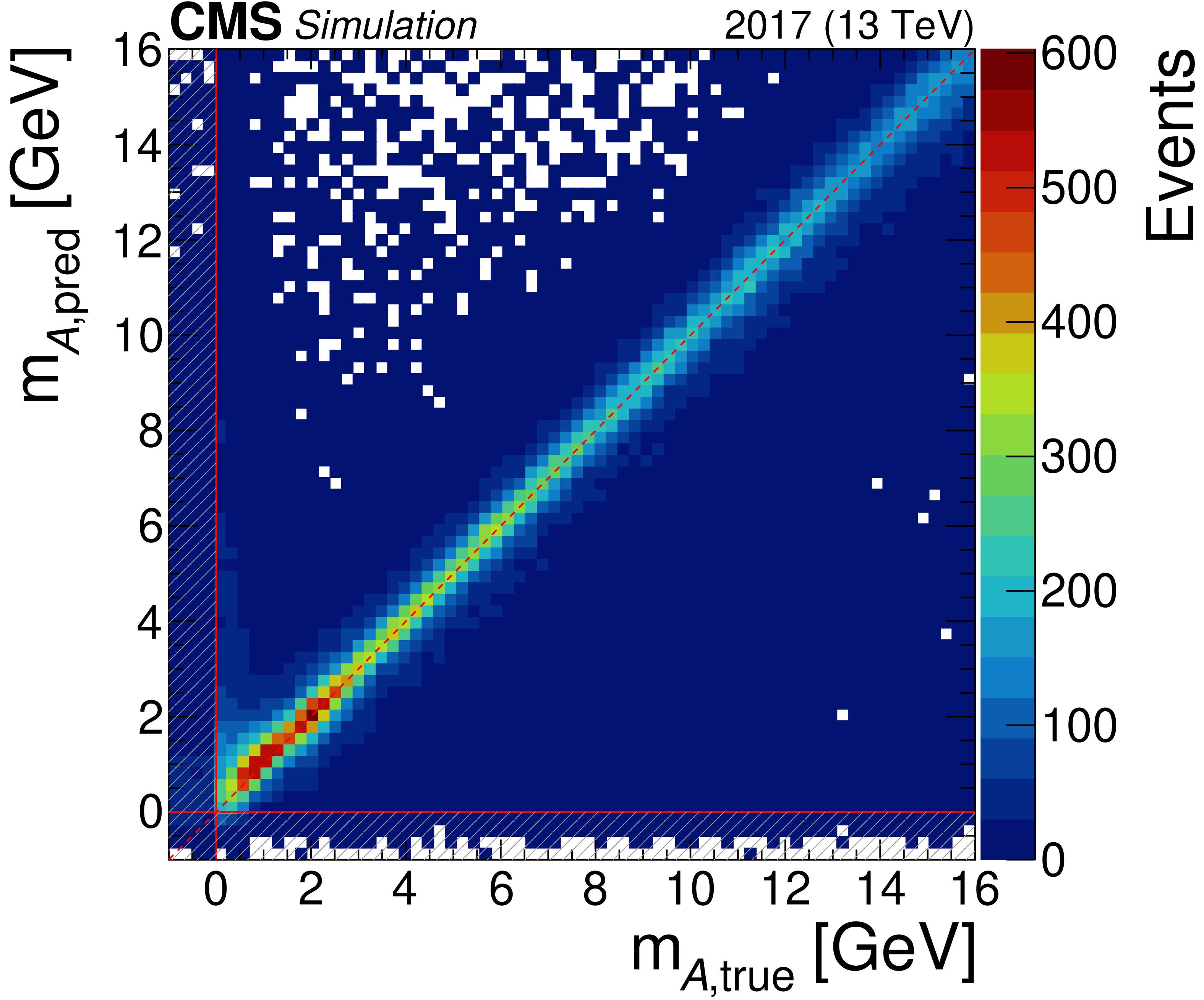
True vs. predicted mass from the mass regression during training validation using simulated $ \mathcal{A}\to\gamma\gamma $ samples corresponding to the 2017 data-taking conditions generated with a continuous uniform distribution in mass and $ p_{\mathrm{T}} $. As discussed in Section 5.2, the training includes domain continuation, which introduces negative target mass labels to improve linearity near the boundary; regions below and to the left of the solid red lines correspond to these negative mass predictions, which are not considered in the final selection. |
png pdf |
Figure 4:
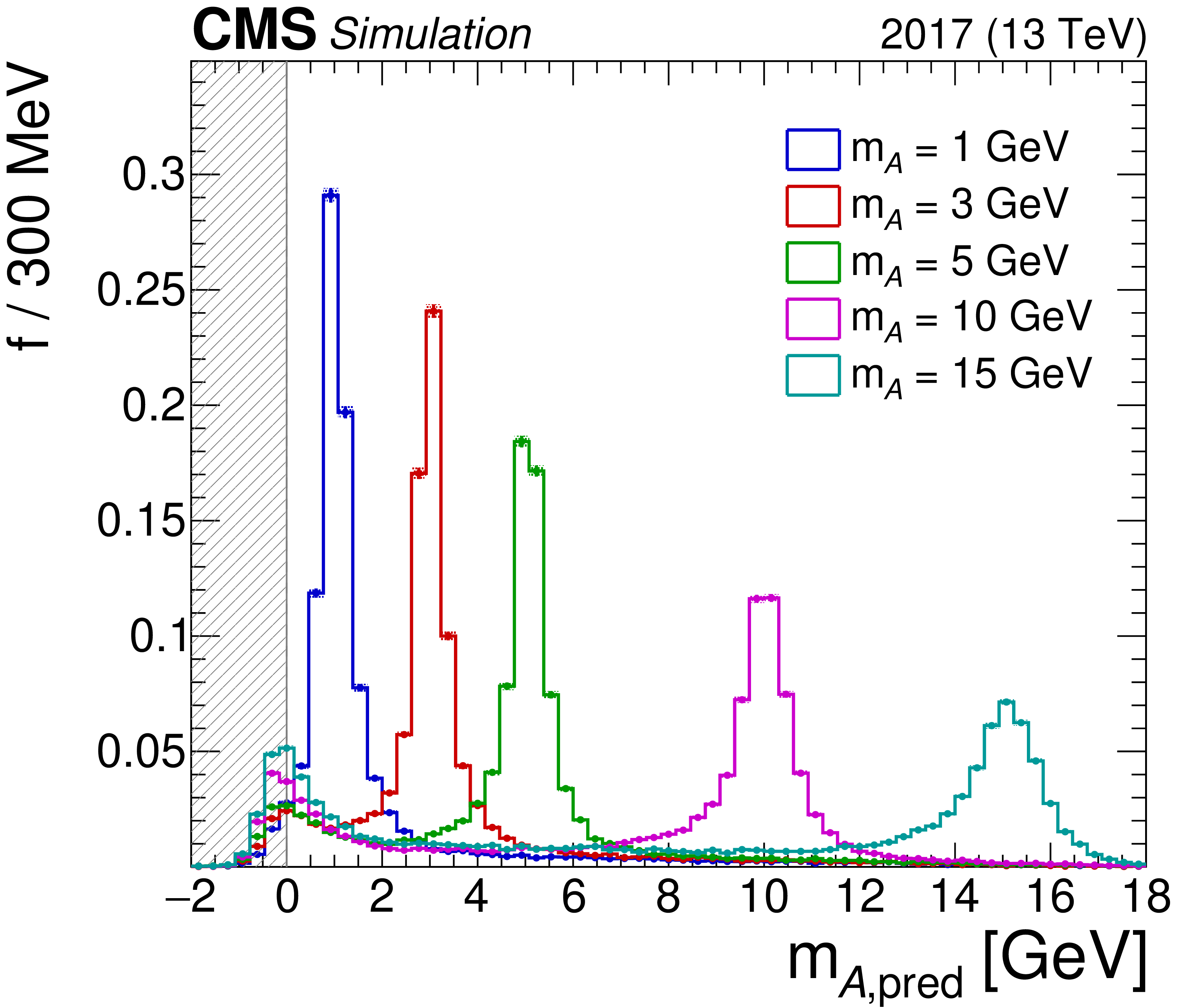
Predicted mass distribution from the mass regression on the merged leg of the simulated $ \mathrm{H}\to \mathcal{A}\mathcal{A} \to 4\gamma $ events corresponding to the 2017 data-taking conditions, which pass the event selection criteria, for different simulated mass points. The variable $ f $ denotes the fraction of events per bin. The area of each distribution is normalized to unity. Negative mass predictions shown in the hatched region are not considered for final selections. |
png pdf |
Figure 5:
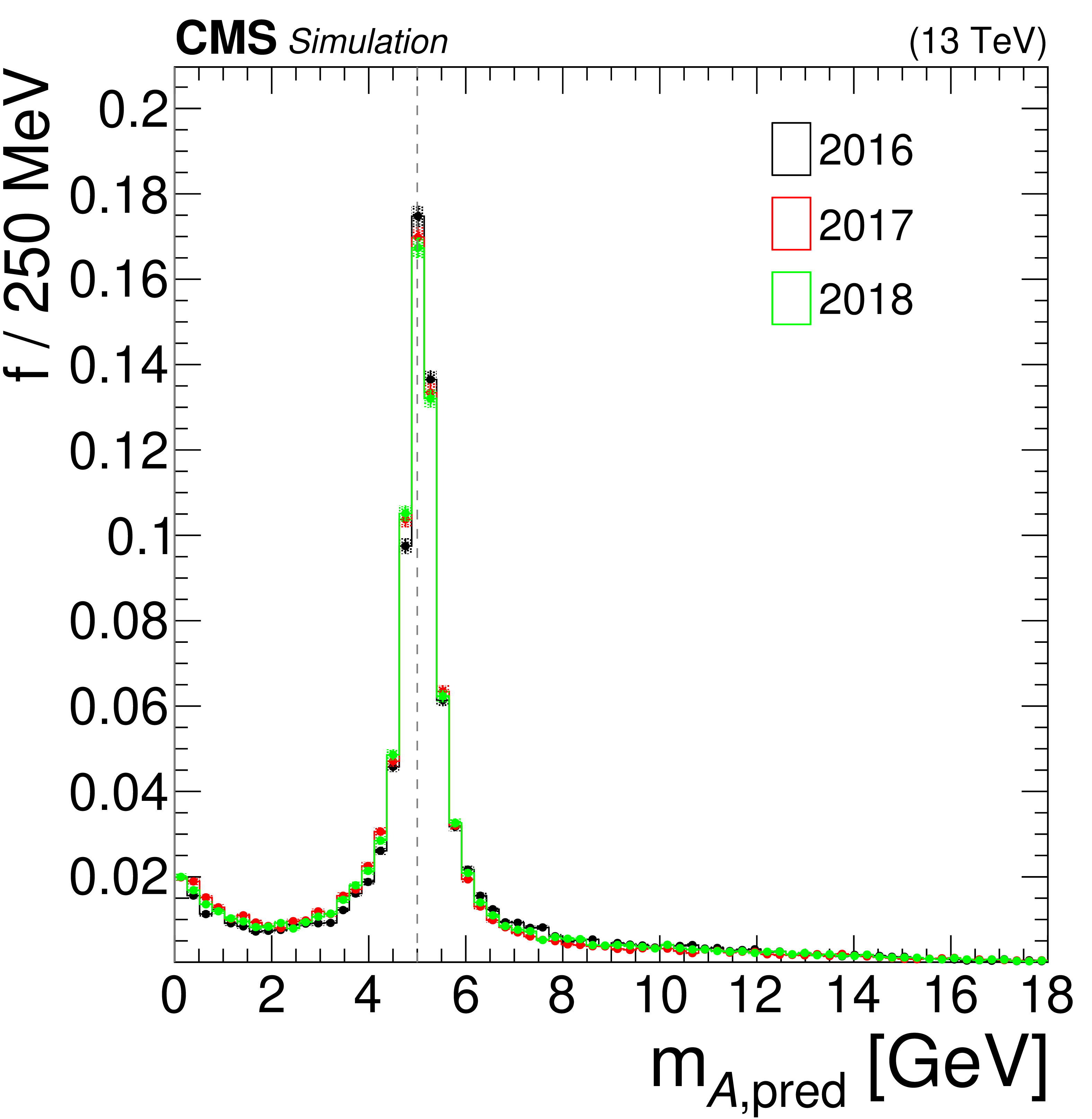
Predicted mass distribution from the mass regression on the merged leg of the simulated $ \mathrm{H}\to \mathcal{A}\mathcal{A} \to 4\gamma $ events with $ m_{\mathcal{A}} = $ 5 GeV, reconstructed under detector conditions corresponding to the 2016, 2017, and 2018 data-taking periods. The same regression and event selection are applied in all cases. The variable $ f $ denotes the fraction of events per bin. The area of each distribution is normalized to unity. |
png pdf |
Figure 6:
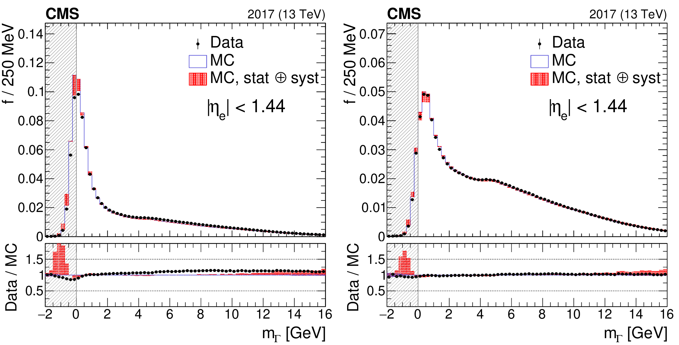
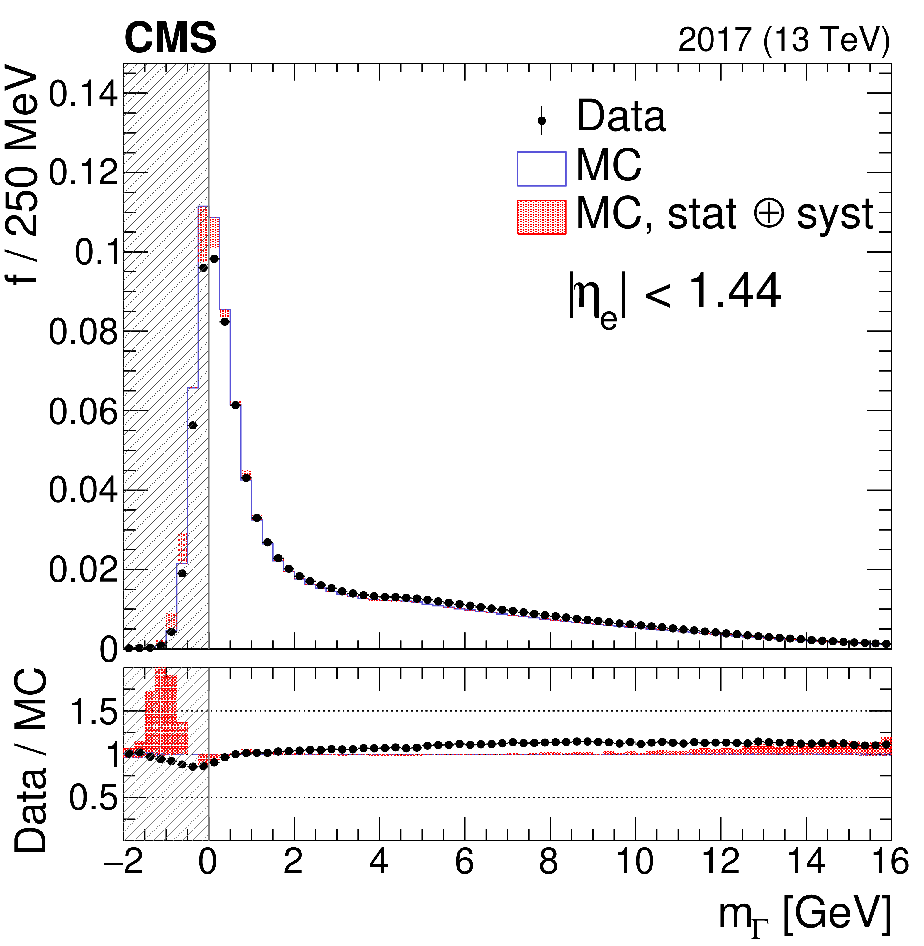
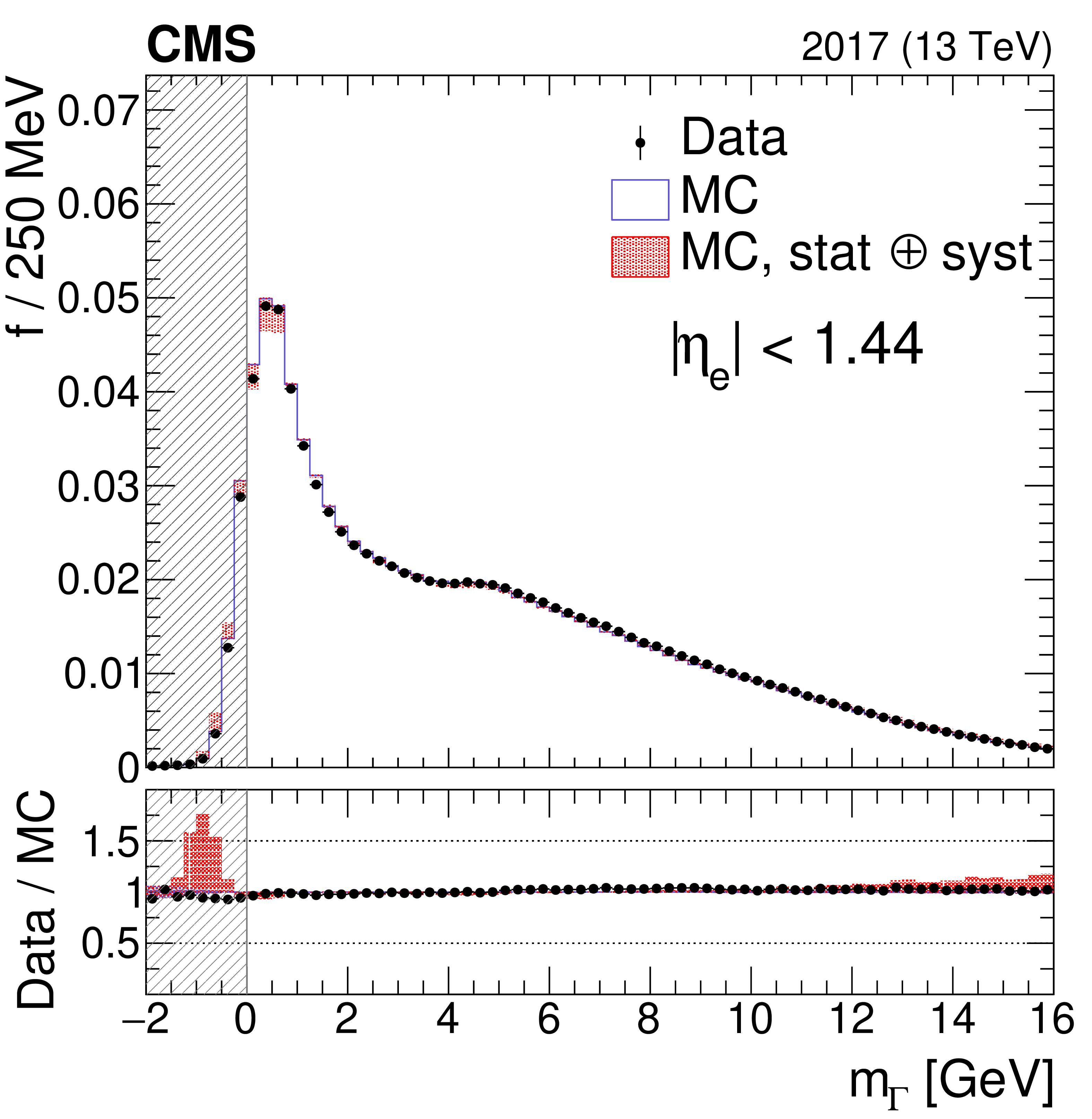
Regressed mass for $ \mathrm{Z} \to \mathrm{e}^+\mathrm{e}^- $ electrons in the 2017 data vs. simulation for all events passing the selections (left), showing a peak at zero, and for a subset of those events with a soft photon-like deposit near the electron (right), showing a peak away from zero. The variable $ f $ denotes the fraction of events per bin. The area of each distribution is normalized to unity. In the upper panels of each plot, the coverage of the best fit scale and smearing estimates in simulated events (``MC, stat $ \oplus $ syst''), plus statistical uncertainties added in quadrature, are plotted as the red bands around the original simulated sample, which are shown as the blue lines (``MC''). The data events are shown as black points, with statistical uncertainties indicated by the error bars. In the lower panels of each plot, the ratio of data to simulation is shown with the black points, where the error bars represent the statistical uncertainties in the data. The red-filled area represents the combined statistical and systematic uncertainty in the best fit corrected simulation, shown relative to the nominal prediction as an uncertainty envelope around unity. The gray hatched regions correspond to events that do not enter the selection. |
png pdf |
Figure 6-a:
Regressed mass for $ \mathrm{Z} \to \mathrm{e}^+\mathrm{e}^- $ electrons in the 2017 data vs. simulation for all events passing the selections (left), showing a peak at zero, and for a subset of those events with a soft photon-like deposit near the electron (right), showing a peak away from zero. The variable $ f $ denotes the fraction of events per bin. The area of each distribution is normalized to unity. In the upper panels of each plot, the coverage of the best fit scale and smearing estimates in simulated events (``MC, stat $ \oplus $ syst''), plus statistical uncertainties added in quadrature, are plotted as the red bands around the original simulated sample, which are shown as the blue lines (``MC''). The data events are shown as black points, with statistical uncertainties indicated by the error bars. In the lower panels of each plot, the ratio of data to simulation is shown with the black points, where the error bars represent the statistical uncertainties in the data. The red-filled area represents the combined statistical and systematic uncertainty in the best fit corrected simulation, shown relative to the nominal prediction as an uncertainty envelope around unity. The gray hatched regions correspond to events that do not enter the selection. |
png pdf |
Figure 6-b:
Regressed mass for $ \mathrm{Z} \to \mathrm{e}^+\mathrm{e}^- $ electrons in the 2017 data vs. simulation for all events passing the selections (left), showing a peak at zero, and for a subset of those events with a soft photon-like deposit near the electron (right), showing a peak away from zero. The variable $ f $ denotes the fraction of events per bin. The area of each distribution is normalized to unity. In the upper panels of each plot, the coverage of the best fit scale and smearing estimates in simulated events (``MC, stat $ \oplus $ syst''), plus statistical uncertainties added in quadrature, are plotted as the red bands around the original simulated sample, which are shown as the blue lines (``MC''). The data events are shown as black points, with statistical uncertainties indicated by the error bars. In the lower panels of each plot, the ratio of data to simulation is shown with the black points, where the error bars represent the statistical uncertainties in the data. The red-filled area represents the combined statistical and systematic uncertainty in the best fit corrected simulation, shown relative to the nominal prediction as an uncertainty envelope around unity. The gray hatched regions correspond to events that do not enter the selection. |
png pdf |
Figure 7:
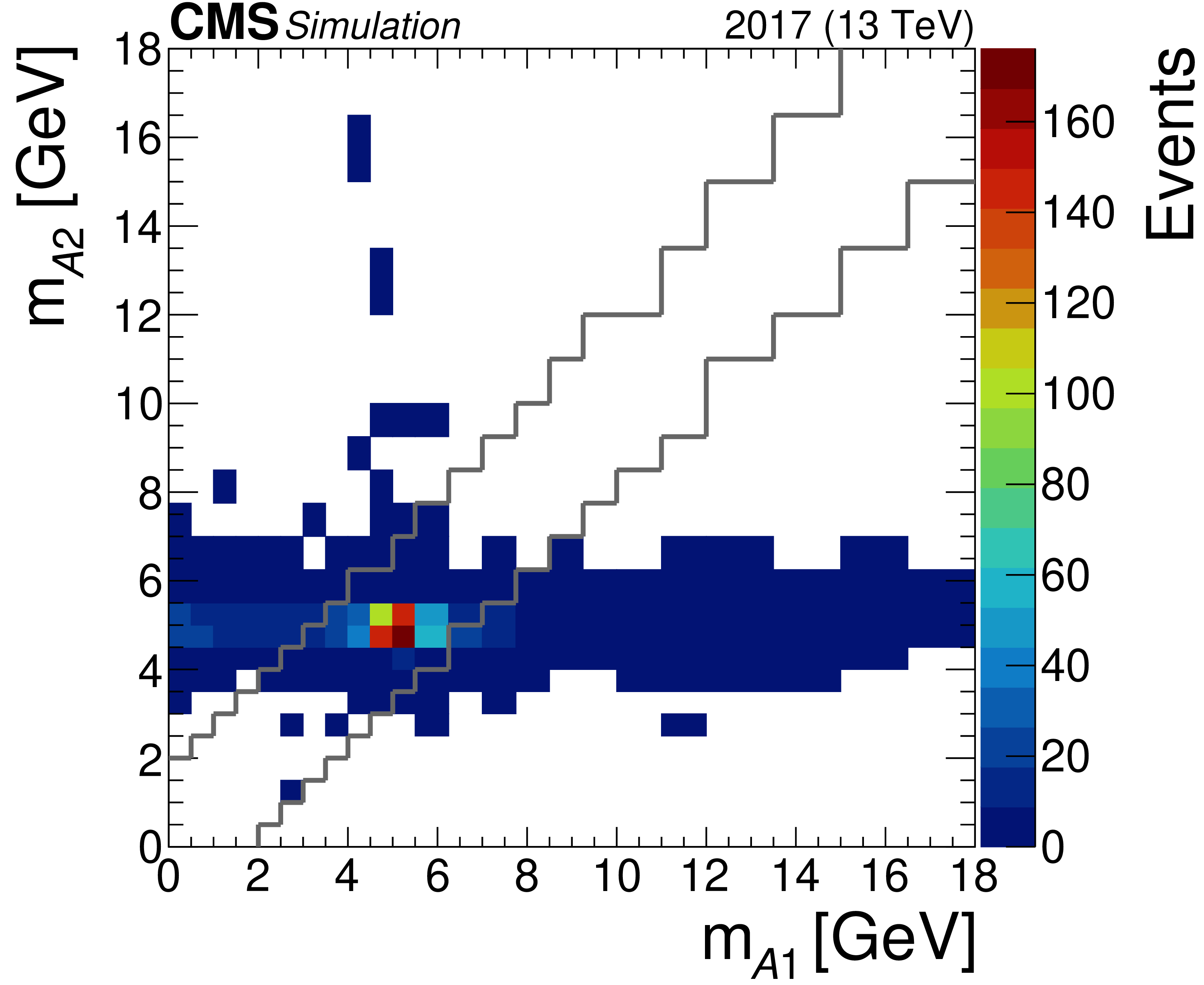
The 2 $ \mathrm{D} m_{\mathcal{A}} $ distribution of the signal model from 2017 simulation for the $ m_{\mathcal{A}}= $ 5 GeV hypothesis, normalized to $ \sigma(\mathrm{p}\mathrm{p} \to \mathrm{H})\mathcal{B} (\mathrm{H}\to \mathcal{A}\mathcal{A} \to 4\gamma) = $ 1 pb. The region enclosed by the jagged lines defines the $ m_{\mathcal{A}}$-SR region, while the area outside corresponds to the $ m_{\mathcal{A}}$-SB region. |
png pdf |
Figure 8:
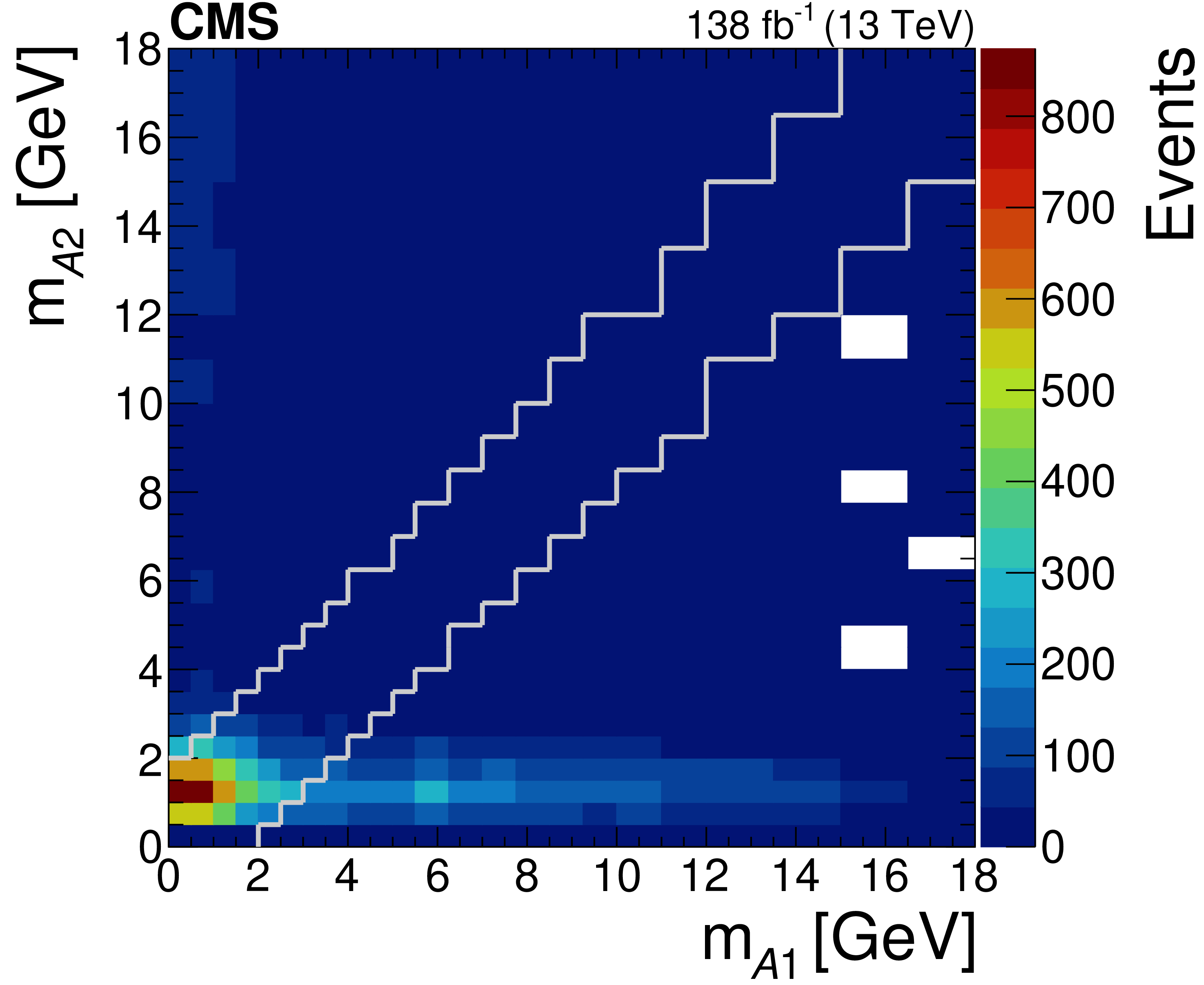
The 2 $ \mathrm{D} m_{\mathcal{A}} $ distribution of the background model constructed from data sidebands. The region enclosed by the jagged lines defines the $ m_{\mathcal{A}}$-SR region, while the area outside corresponds to the $ m_{\mathcal{A}}$-SB region. |
png pdf |
Figure 9:
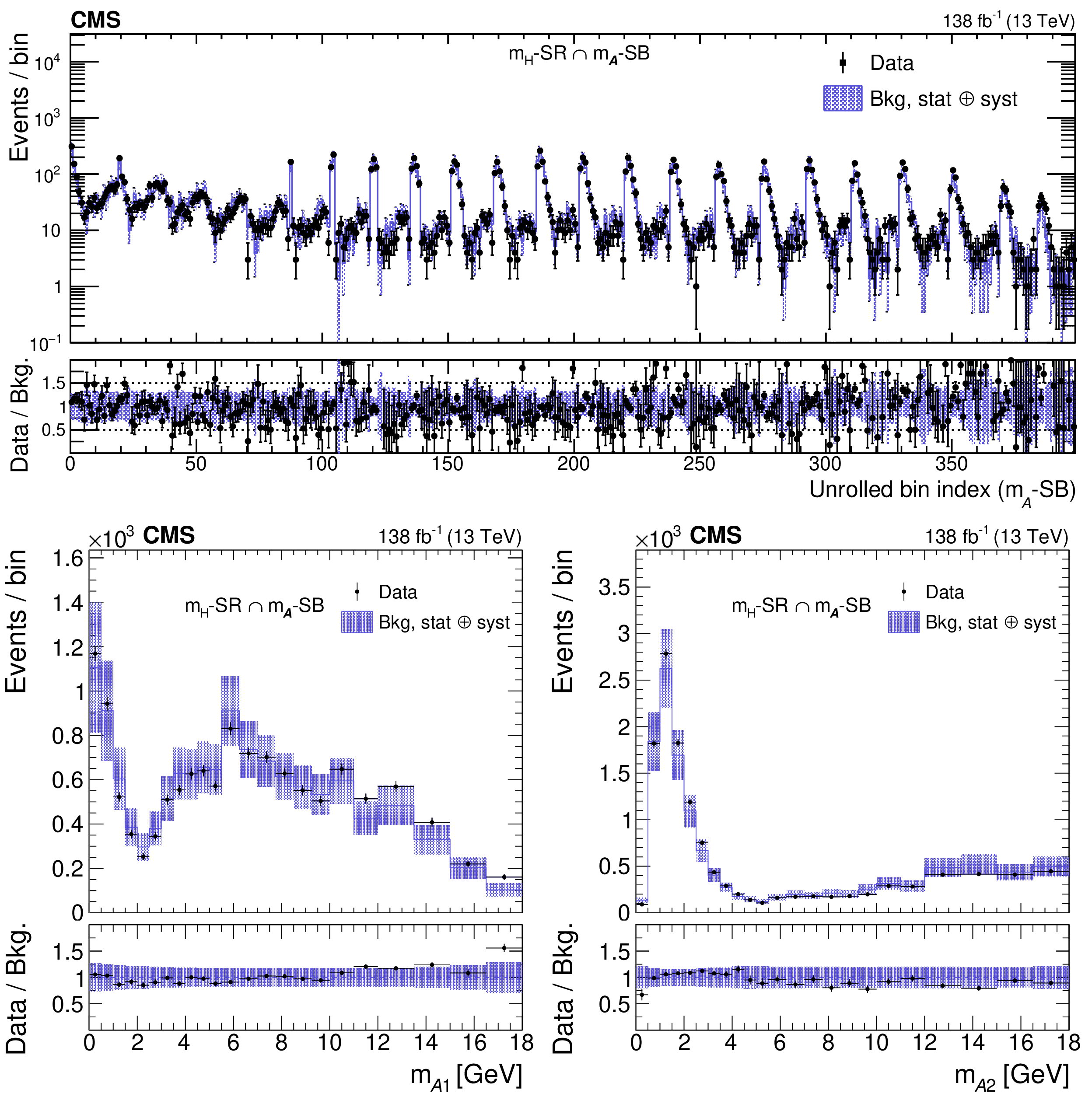
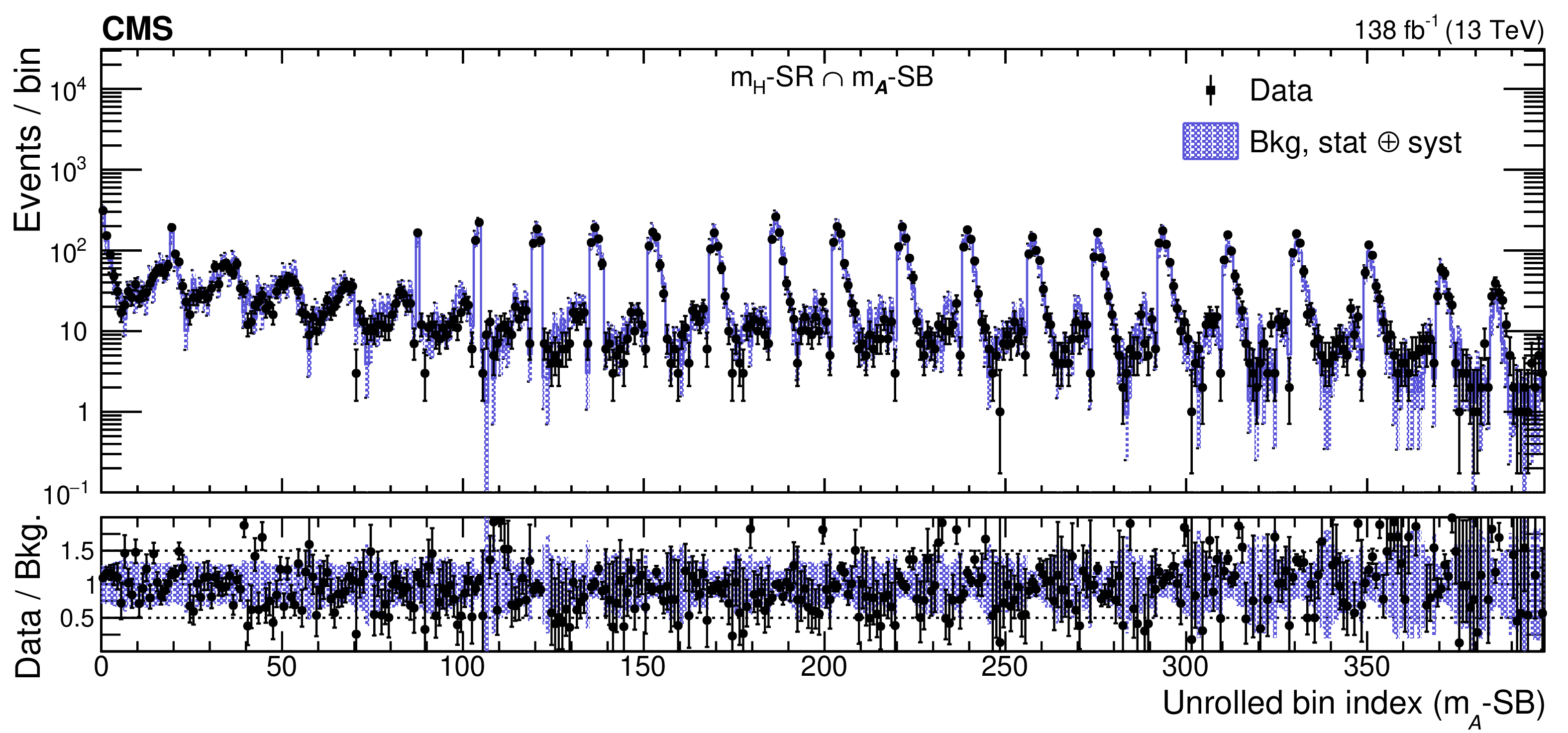
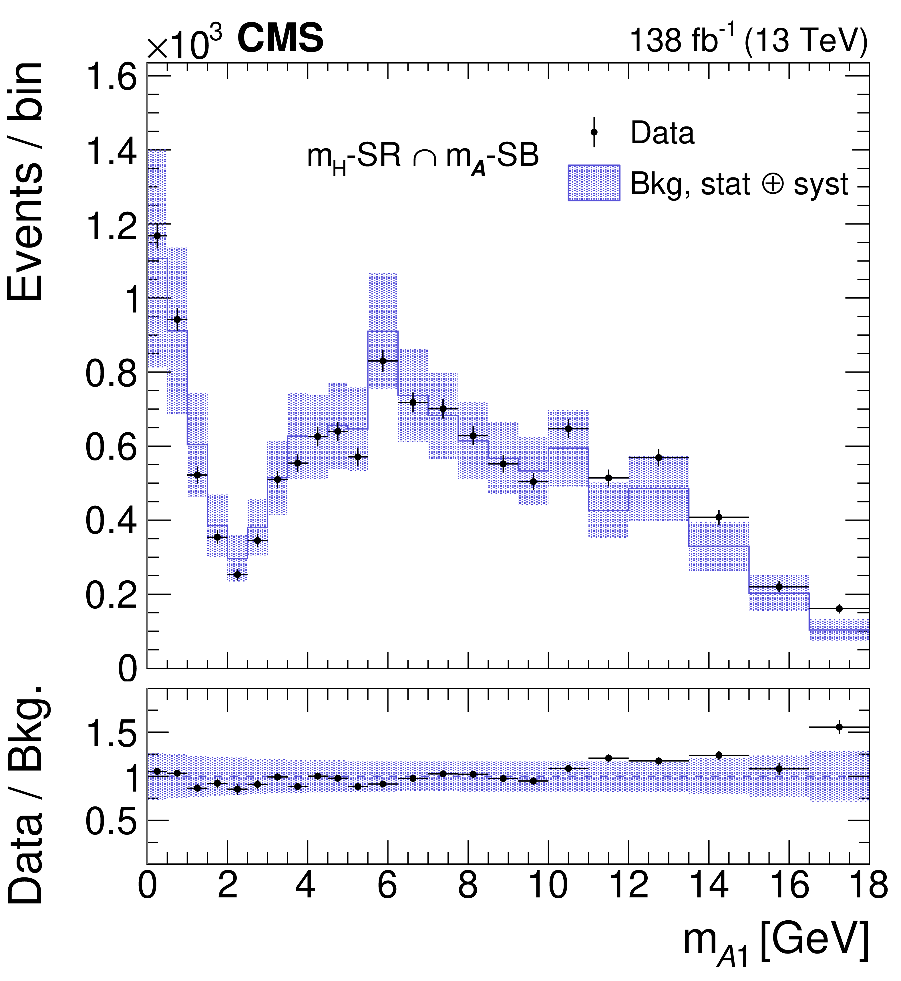
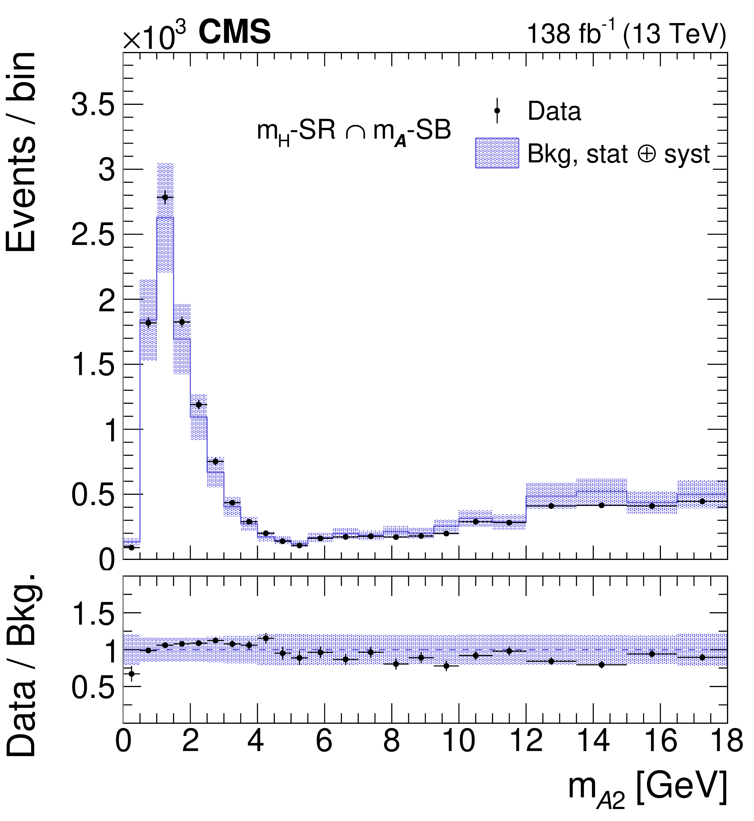
Expected background versus observed data 2 $ \mathrm{D} m_{\mathcal{A}} $ spectra in the $ m_{\mathrm{H}}$-SR $\cap\ m_{\mathcal{A}}$-SB region. Upper plot: unrolled spectra made by scanning along bins of increasing $ m_{\mathcal{A}2} $ at fixed $ m_{\mathcal{A}1} $ before incrementing in $ m_{\mathcal{A}1} $. Only the bins in the $ m_{\mathcal{A}}$-SB region are included, with the x-axis corresponding to the unrolled bin index of the selected bins, listed sequentially. Lower plot: projected 1D $ m_{\mathcal{A}} $ spectra corresponding to merged (left) and resolved (right) candidates. In the upper panels of each plot, the black points with error bars (``Data'') are the observed data values, with the error bars corresponding to statistical uncertainties. The blue line corresponds to the background model, with the blue band corresponding to its statistical uncertainties and systematic uncertainties added in quadrature (``Bkg, stat $ \oplus $ syst''). In the lower panel of the same plot, the ratio of the observed data over the estimated background value is shown as black points, with error bars corresponding to statistical uncertainties in the former. The ratio of the statistical plus systematic uncertainties in the background over the background prediction is shown as the blue band. |
png pdf |
Figure 9-a:
Expected background versus observed data 2 $ \mathrm{D} m_{\mathcal{A}} $ spectra in the $ m_{\mathrm{H}}$-SR $\cap\ m_{\mathcal{A}}$-SB region. Upper plot: unrolled spectra made by scanning along bins of increasing $ m_{\mathcal{A}2} $ at fixed $ m_{\mathcal{A}1} $ before incrementing in $ m_{\mathcal{A}1} $. Only the bins in the $ m_{\mathcal{A}}$-SB region are included, with the x-axis corresponding to the unrolled bin index of the selected bins, listed sequentially. Lower plot: projected 1D $ m_{\mathcal{A}} $ spectra corresponding to merged (left) and resolved (right) candidates. In the upper panels of each plot, the black points with error bars (``Data'') are the observed data values, with the error bars corresponding to statistical uncertainties. The blue line corresponds to the background model, with the blue band corresponding to its statistical uncertainties and systematic uncertainties added in quadrature (``Bkg, stat $ \oplus $ syst''). In the lower panel of the same plot, the ratio of the observed data over the estimated background value is shown as black points, with error bars corresponding to statistical uncertainties in the former. The ratio of the statistical plus systematic uncertainties in the background over the background prediction is shown as the blue band. |
png pdf |
Figure 9-b:
Expected background versus observed data 2 $ \mathrm{D} m_{\mathcal{A}} $ spectra in the $ m_{\mathrm{H}}$-SR $\cap\ m_{\mathcal{A}}$-SB region. Upper plot: unrolled spectra made by scanning along bins of increasing $ m_{\mathcal{A}2} $ at fixed $ m_{\mathcal{A}1} $ before incrementing in $ m_{\mathcal{A}1} $. Only the bins in the $ m_{\mathcal{A}}$-SB region are included, with the x-axis corresponding to the unrolled bin index of the selected bins, listed sequentially. Lower plot: projected 1D $ m_{\mathcal{A}} $ spectra corresponding to merged (left) and resolved (right) candidates. In the upper panels of each plot, the black points with error bars (``Data'') are the observed data values, with the error bars corresponding to statistical uncertainties. The blue line corresponds to the background model, with the blue band corresponding to its statistical uncertainties and systematic uncertainties added in quadrature (``Bkg, stat $ \oplus $ syst''). In the lower panel of the same plot, the ratio of the observed data over the estimated background value is shown as black points, with error bars corresponding to statistical uncertainties in the former. The ratio of the statistical plus systematic uncertainties in the background over the background prediction is shown as the blue band. |
png pdf |
Figure 9-c:
Expected background versus observed data 2 $ \mathrm{D} m_{\mathcal{A}} $ spectra in the $ m_{\mathrm{H}}$-SR $\cap\ m_{\mathcal{A}}$-SB region. Upper plot: unrolled spectra made by scanning along bins of increasing $ m_{\mathcal{A}2} $ at fixed $ m_{\mathcal{A}1} $ before incrementing in $ m_{\mathcal{A}1} $. Only the bins in the $ m_{\mathcal{A}}$-SB region are included, with the x-axis corresponding to the unrolled bin index of the selected bins, listed sequentially. Lower plot: projected 1D $ m_{\mathcal{A}} $ spectra corresponding to merged (left) and resolved (right) candidates. In the upper panels of each plot, the black points with error bars (``Data'') are the observed data values, with the error bars corresponding to statistical uncertainties. The blue line corresponds to the background model, with the blue band corresponding to its statistical uncertainties and systematic uncertainties added in quadrature (``Bkg, stat $ \oplus $ syst''). In the lower panel of the same plot, the ratio of the observed data over the estimated background value is shown as black points, with error bars corresponding to statistical uncertainties in the former. The ratio of the statistical plus systematic uncertainties in the background over the background prediction is shown as the blue band. |
png pdf |
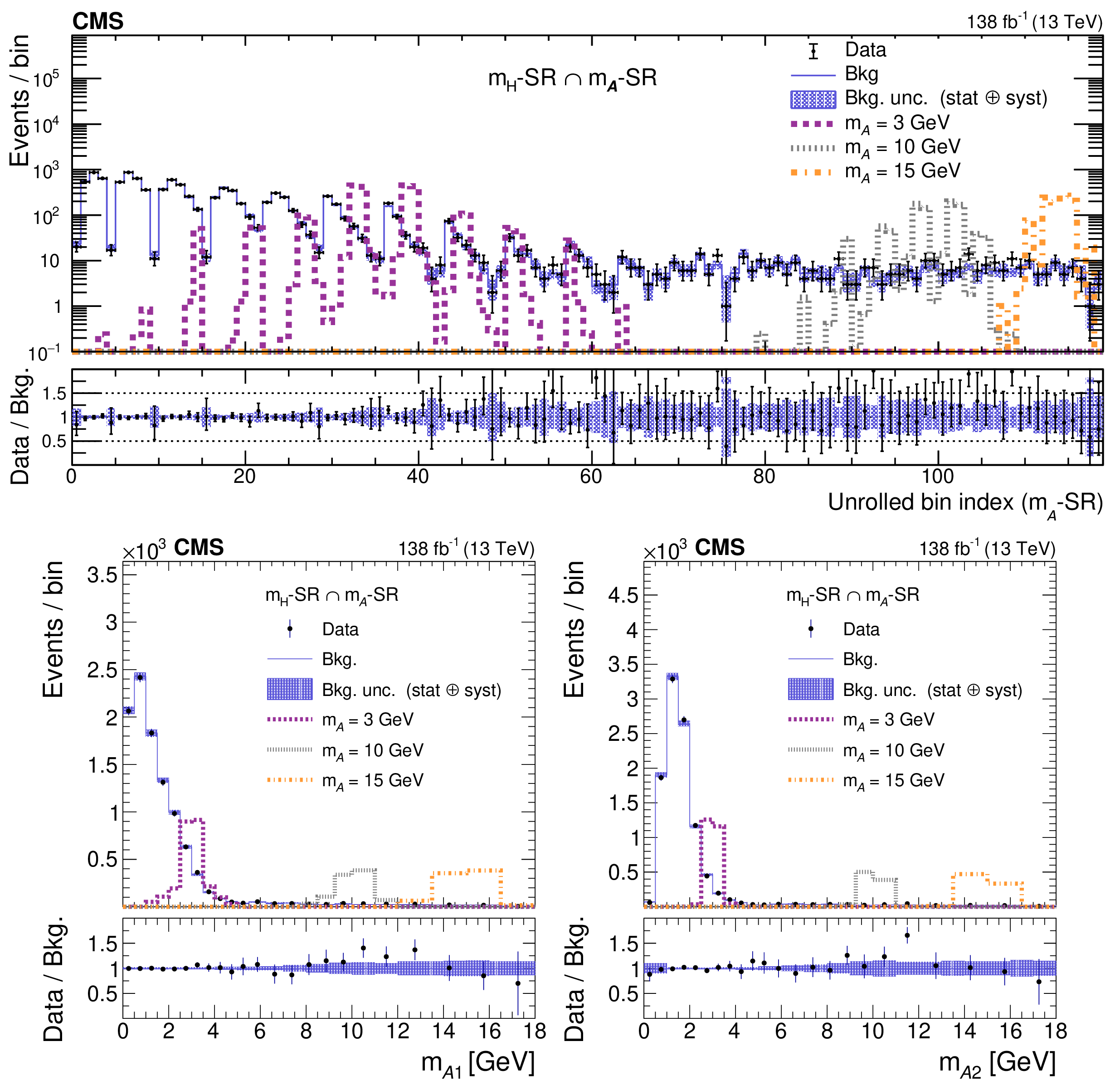
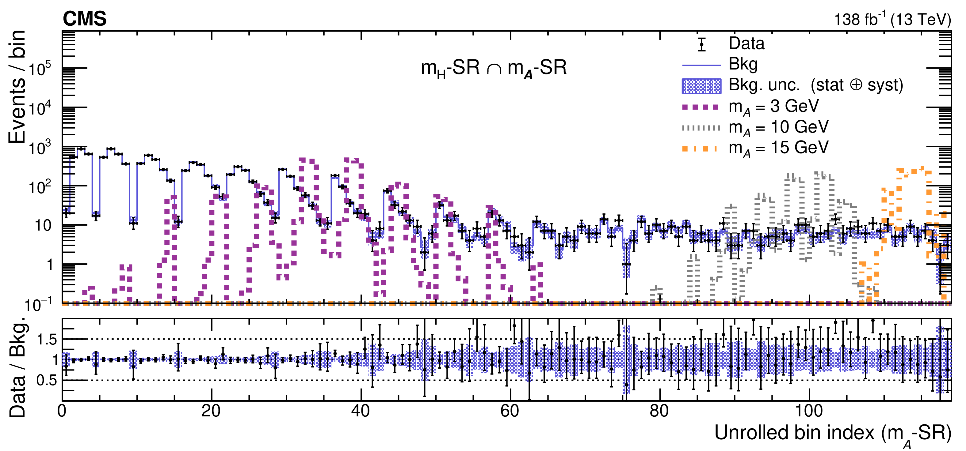
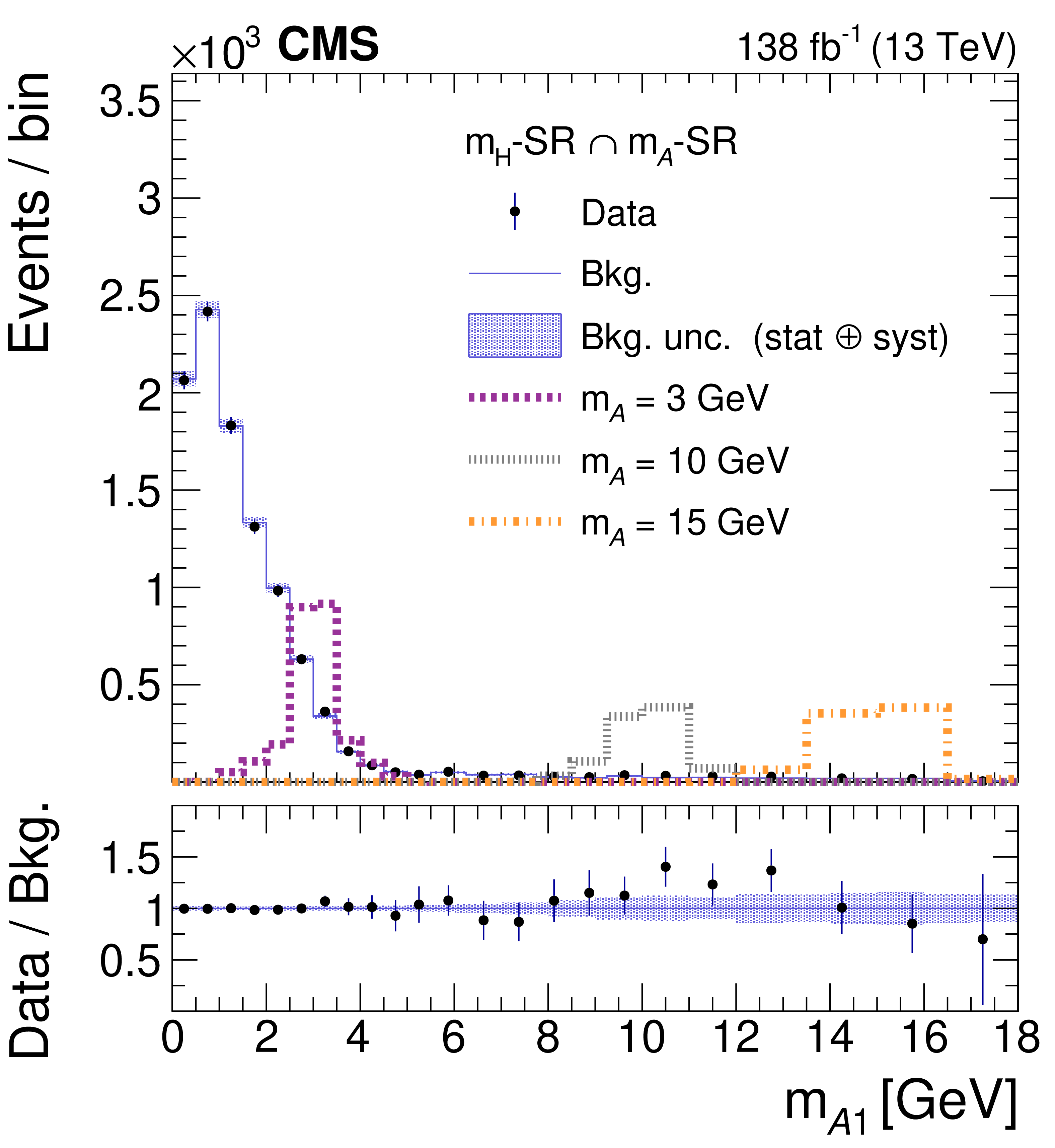
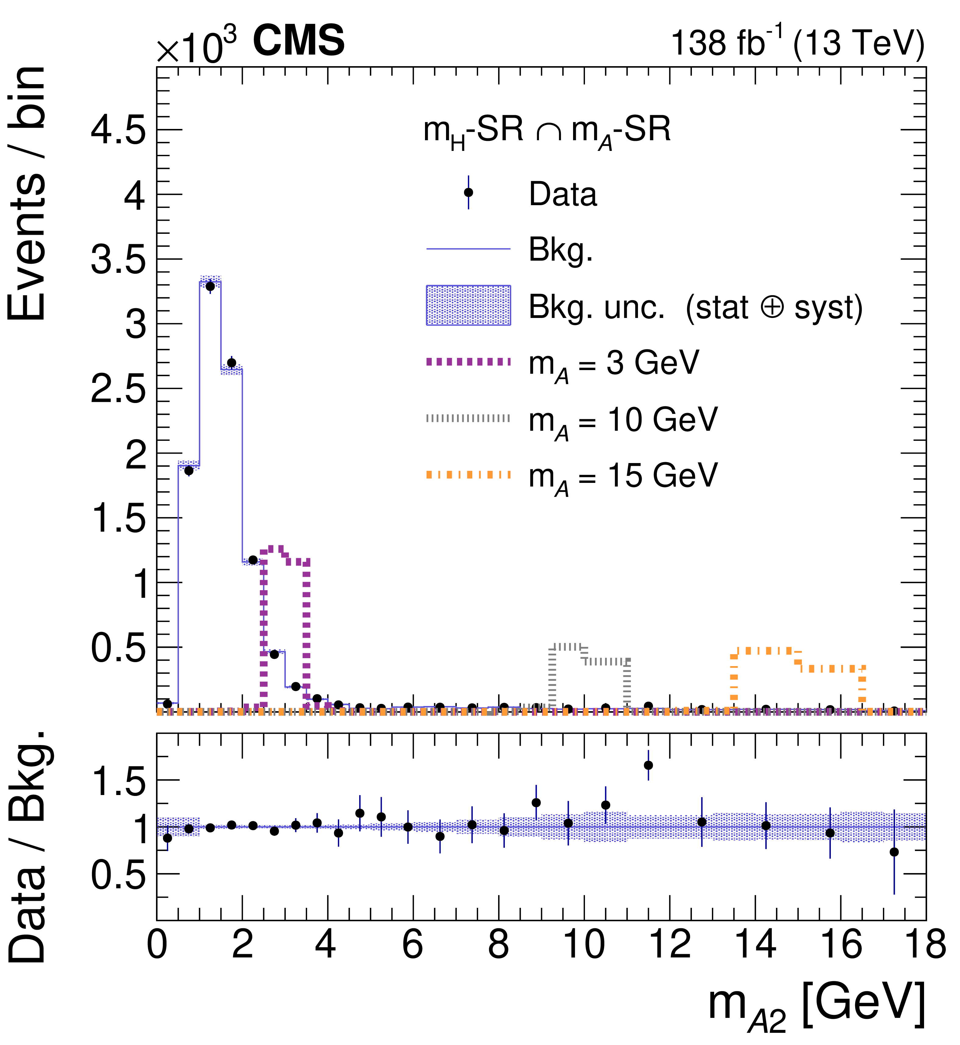
Figure 10:
The 2 $ \mathrm{D} m_{\mathcal{A}} $ spectra in the final signal region. Upper plot: The unrolled 2 $ \mathrm{D} m_{\mathcal{A}} $ distribution made by scanning along bins of increasing $ m_{\mathcal{A}2} $ at fixed $ m_{\mathcal{A}1} $ before incrementing in $ m_{\mathcal{A}1} $. Only the bins in the $ m_{\mathcal{A}}$-SR region are included, with the x-axis corresponding to the unrolled bin index of the selected bins, listed sequentially. Lower plot: 1D projections on the $ m_{\mathcal{A}1} $ (left) and $ m_{\mathcal{A}2} $ (right) axes of the 2 $ \mathrm{D} m_{\mathcal{A}} $ distribution. The data distributions (black points) are plotted against the total predicted background distributions (blue curves) after fitting to the data. The statistical plus systematic uncertainties in the background distribution are plotted as the blue band. The corresponding distributions of simulated $ \mathrm{H}\to \mathcal{A}\mathcal{A} \to 4\gamma $ events for $ m_{\mathcal{A}} = $ 3 (purple curve), 10 (gray curve), and 15 GeV (orange curve) are also overlaid on top. They are each normalized to the value of the expected upper limit to the signal cross section times 50. The lower panels of each plot show the ratio of the observed data over the predicted background as the black points, with the error bars representing the statistical uncertainties in the former. The ratio of the statistical plus systematic uncertainties in the background over the background prediction is shown as the blue band. |
png pdf |
Figure 10-a:
The 2 $ \mathrm{D} m_{\mathcal{A}} $ spectra in the final signal region. Upper plot: The unrolled 2 $ \mathrm{D} m_{\mathcal{A}} $ distribution made by scanning along bins of increasing $ m_{\mathcal{A}2} $ at fixed $ m_{\mathcal{A}1} $ before incrementing in $ m_{\mathcal{A}1} $. Only the bins in the $ m_{\mathcal{A}}$-SR region are included, with the x-axis corresponding to the unrolled bin index of the selected bins, listed sequentially. Lower plot: 1D projections on the $ m_{\mathcal{A}1} $ (left) and $ m_{\mathcal{A}2} $ (right) axes of the 2 $ \mathrm{D} m_{\mathcal{A}} $ distribution. The data distributions (black points) are plotted against the total predicted background distributions (blue curves) after fitting to the data. The statistical plus systematic uncertainties in the background distribution are plotted as the blue band. The corresponding distributions of simulated $ \mathrm{H}\to \mathcal{A}\mathcal{A} \to 4\gamma $ events for $ m_{\mathcal{A}} = $ 3 (purple curve), 10 (gray curve), and 15 GeV (orange curve) are also overlaid on top. They are each normalized to the value of the expected upper limit to the signal cross section times 50. The lower panels of each plot show the ratio of the observed data over the predicted background as the black points, with the error bars representing the statistical uncertainties in the former. The ratio of the statistical plus systematic uncertainties in the background over the background prediction is shown as the blue band. |
png pdf |
Figure 10-b:
The 2 $ \mathrm{D} m_{\mathcal{A}} $ spectra in the final signal region. Upper plot: The unrolled 2 $ \mathrm{D} m_{\mathcal{A}} $ distribution made by scanning along bins of increasing $ m_{\mathcal{A}2} $ at fixed $ m_{\mathcal{A}1} $ before incrementing in $ m_{\mathcal{A}1} $. Only the bins in the $ m_{\mathcal{A}}$-SR region are included, with the x-axis corresponding to the unrolled bin index of the selected bins, listed sequentially. Lower plot: 1D projections on the $ m_{\mathcal{A}1} $ (left) and $ m_{\mathcal{A}2} $ (right) axes of the 2 $ \mathrm{D} m_{\mathcal{A}} $ distribution. The data distributions (black points) are plotted against the total predicted background distributions (blue curves) after fitting to the data. The statistical plus systematic uncertainties in the background distribution are plotted as the blue band. The corresponding distributions of simulated $ \mathrm{H}\to \mathcal{A}\mathcal{A} \to 4\gamma $ events for $ m_{\mathcal{A}} = $ 3 (purple curve), 10 (gray curve), and 15 GeV (orange curve) are also overlaid on top. They are each normalized to the value of the expected upper limit to the signal cross section times 50. The lower panels of each plot show the ratio of the observed data over the predicted background as the black points, with the error bars representing the statistical uncertainties in the former. The ratio of the statistical plus systematic uncertainties in the background over the background prediction is shown as the blue band. |
png pdf |
Figure 10-c:
The 2 $ \mathrm{D} m_{\mathcal{A}} $ spectra in the final signal region. Upper plot: The unrolled 2 $ \mathrm{D} m_{\mathcal{A}} $ distribution made by scanning along bins of increasing $ m_{\mathcal{A}2} $ at fixed $ m_{\mathcal{A}1} $ before incrementing in $ m_{\mathcal{A}1} $. Only the bins in the $ m_{\mathcal{A}}$-SR region are included, with the x-axis corresponding to the unrolled bin index of the selected bins, listed sequentially. Lower plot: 1D projections on the $ m_{\mathcal{A}1} $ (left) and $ m_{\mathcal{A}2} $ (right) axes of the 2 $ \mathrm{D} m_{\mathcal{A}} $ distribution. The data distributions (black points) are plotted against the total predicted background distributions (blue curves) after fitting to the data. The statistical plus systematic uncertainties in the background distribution are plotted as the blue band. The corresponding distributions of simulated $ \mathrm{H}\to \mathcal{A}\mathcal{A} \to 4\gamma $ events for $ m_{\mathcal{A}} = $ 3 (purple curve), 10 (gray curve), and 15 GeV (orange curve) are also overlaid on top. They are each normalized to the value of the expected upper limit to the signal cross section times 50. The lower panels of each plot show the ratio of the observed data over the predicted background as the black points, with the error bars representing the statistical uncertainties in the former. The ratio of the statistical plus systematic uncertainties in the background over the background prediction is shown as the blue band. |
png pdf |
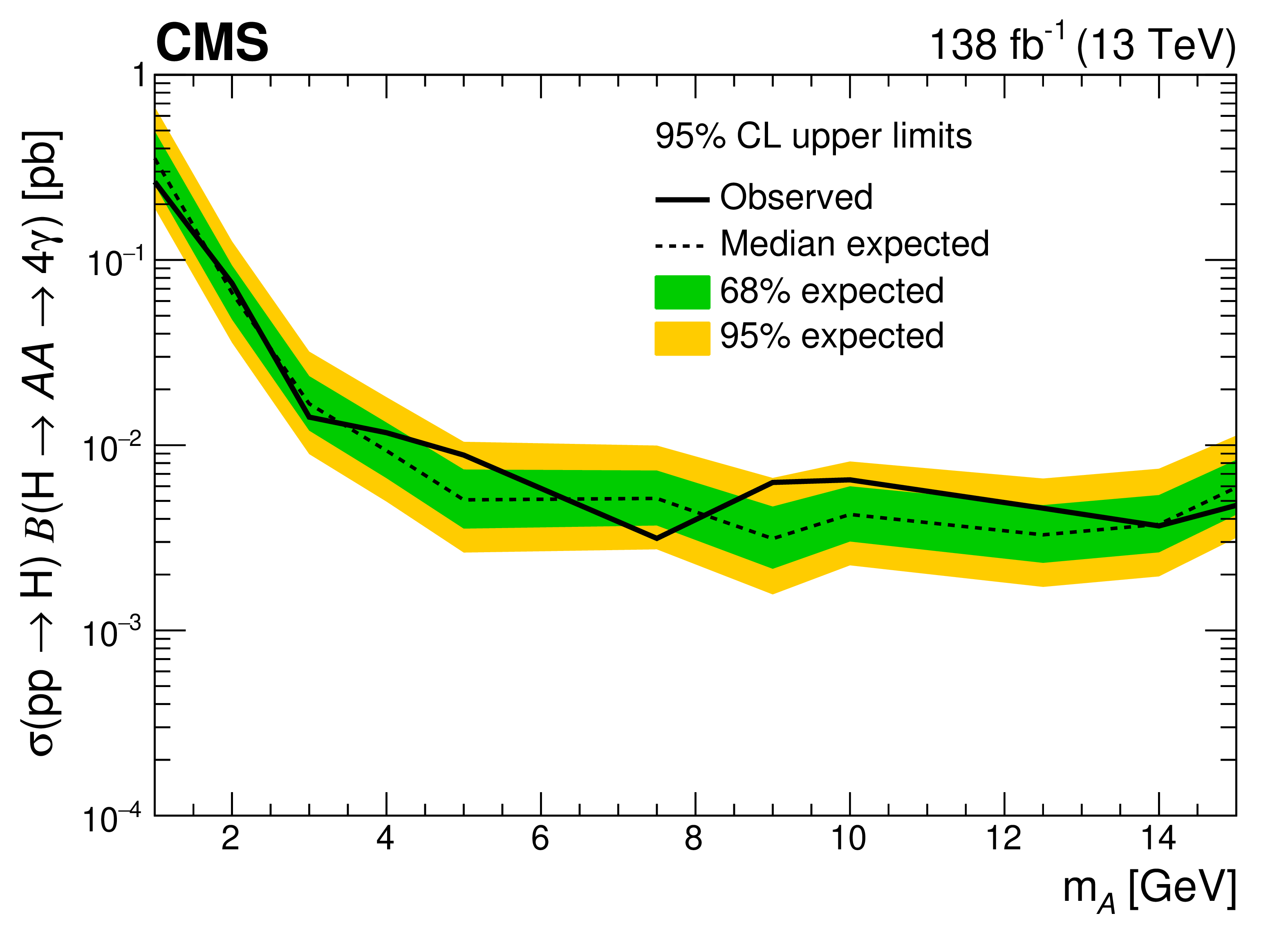
Figure 11:
Observed (solid black line) and median expected (dashed black line) upper limits at 95% CL on the signal cross section times branching fraction $ \sigma(\mathrm{p}\mathrm{p} \to \mathrm{H}) \mathcal{B}(\mathrm{H}\to \mathcal{A}\mathcal{A} \to 4\gamma) $ at various $ m_{\mathcal{A}} $ mass points. The 68 and 95% confidence intervals around the median expected limit are shown as the green and yellow bands, respectively. |
png pdf |
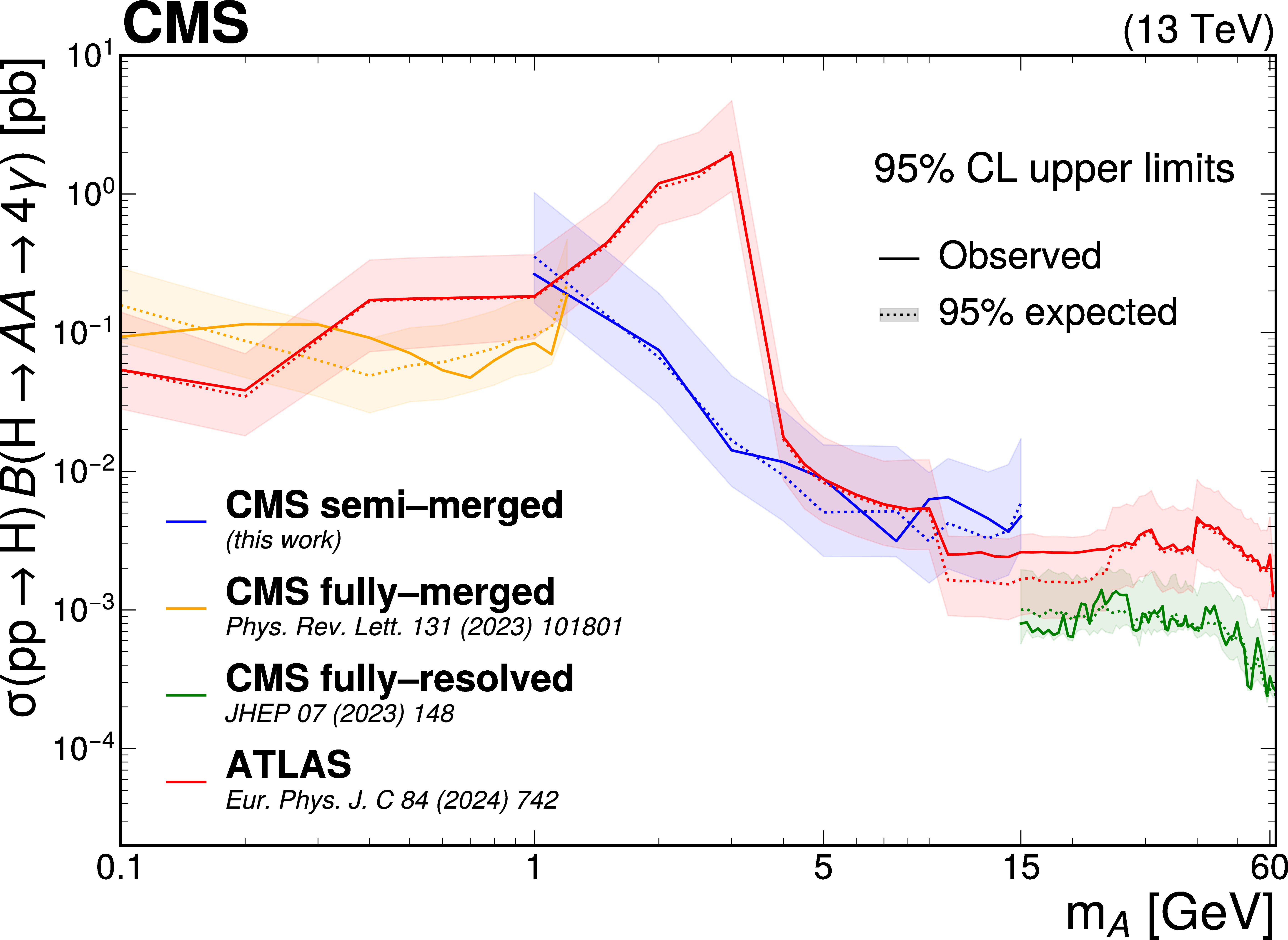
Figure 12:
Observed (solid line) and expected (dashed line) upper limits, including the 95% CL interval around the expected limit, from this search (CMS semi-merged) compared to the previous CMS and ATLAS searches [20,19,21], over the full $ m_{\mathcal{A}} $ range of 0.1 to 60 GeV. The limits are shown in terms of $ \sigma(\mathrm{p}\mathrm{p} \to \mathrm{H}) \mathcal{B}(\mathrm{H}\to \mathcal{A}\mathcal{A} \to 4\gamma) $. |
| Summary |
| A search for the exotic decay of the Higgs boson of the form $ \mathrm{H}\to \mathcal{A}\mathcal{A} \to 4\gamma $ in events with three photon-like objects has been performed using proton-proton collision data collected by the CMS experiment at $ \sqrt{s} = $ 13 TeV corresponding to an integrated luminosity of 138 fb$ ^{-1} $. One of the hypothetical particles, $ \mathcal{A} $, is assumed to decay promptly to one semi-merged diphoton candidate reconstructed as a single photon-like object, while the other $ \mathcal{A} $ decays into a pair of resolved photons. No excess above the estimated background is found. Upper limits are set on the product of the Higgs boson production cross section and branching fraction, $ \sigma(\mathrm{p}\mathrm{p} \to \mathrm{H}) \mathcal{B}(\mathrm{H}\to \mathcal{A}\mathcal{A} \to 4\gamma) $, ranging from 0.264 to 0.005$ $ pb at 95% confidence level for masses of $ \mathcal{A} $ in the range 1-15 GeV. These limits are the most stringent to date in the 1-5 GeV mass range. |
| References | ||||
| 1 | ATLAS Collaboration | Observation of a new particle in the search for the standard model Higgs boson with the ATLAS detector at the LHC | PLB 716 (2012) 1 | 1207.7214 |
| 2 | CMS Collaboration | Observation of a new boson at a mass of 125 GeV with the CMS experiment at the LHC | PLB 716 (2012) 30 | CMS-HIG-12-028 1207.7235 |
| 3 | CMS Collaboration | Observation of a new boson with mass near 125 GeV in pp collisions at $ \sqrt{s} = $ 7 and 8 TeV | JHEP 06 (2013) 081 | CMS-HIG-12-036 1303.4571 |
| 4 | CMS Collaboration | Combined measurements and interpretations of Higgs boson production and decay at $ \sqrt{s}= $ 13 TeV | CMS Physics Analysis Summary, 2025 CMS-PAS-HIG-21-018 |
CMS-PAS-HIG-21-018 |
| 5 | D. Curtin et al. | Exotic decays of the 125 GeV Higgs boson | PRD 90 (2014) 075004 | 1312.4992 |
| 6 | D. Curtin, R. Essig, S. Gori, and J. Shelton | Illuminating dark photons with high-energy colliders | JHEP 02 (2015) 157 | 1412.0018 |
| 7 | F. Chadha-Day, J. Ellis, and D. J. E. Marsh | Axion dark matter: What is it and why now? | abj3618, 2022 Sci. Adv. 8 (2022) |
2105.01406 |
| 8 | R. D. Peccei and H. R. Quinn | CP conservation in the presence of instantons | PRL 38 (1977) 1440 | |
| 9 | M. Bauer, M. Neubert, and A. Thamm | Collider probes of axion-like particles | JHEP 12 (2017) 044 | 1708.00443 |
| 10 | R. D. Peccei | The strong CP problem and axions | in Axions, M. Kuster, G. Raffelt, and B. Beltran, eds. Springer Berlin Heidelberg, 2008 link |
hep-ph/0607268 |
| 11 | CMS Collaboration | Search for exotic decays of the Higgs boson to a pair of pseudoscalars in the $ \mu\mu $bb and $ \tau\tau $bb final states | EPJC 84 (2024) 493 | CMS-HIG-22-007 2402.13358 |
| 12 | CMS Collaboration | Search for the decay of the Higgs boson to a pair of light pseudoscalar bosons in the final state with four bottom quarks in proton-proton collisions at $ \sqrt{s} = $ 13 TeV | JHEP 06 (2024) 097 | CMS-HIG-18-026 2403.10341 |
| 13 | CMS Collaboration | Search for light pseudoscalar boson pairs produced from Higgs boson decays using the 4$ \tau $ and 2$ \mu $2$ \tau $ final states in proton-proton collisions at $ \sqrt{s} = $ 13 TeV | Submitted to JHEP, 2025 | CMS-SUS-24-002 2508.06947 |
| 14 | ATLAS Collaboration | Search for Higgs boson exotic decays into Lorentz-boosted light bosons in the four-\ensuremath\tau final state at $ \sqrt{s}= $ 13 TeV with the ATLAS detector | PLB 870 (2025) 139843 | 2503.05463 |
| 15 | CMS Collaboration | Search for light long-lived particles decaying to displaced jets in proton-proton collisions at $ \sqrt{s} = $ 13.6 TeV | Rept. Prog. Phys. 88 (2025) 037801 | CMS-EXO-23-013 2409.10806 |
| 16 | CMS Collaboration | A search for pair production of new light bosons decaying into muons in proton-proton collisions at 13 TeV | PLB 796 (2019) 131 | CMS-HIG-18-003 1812.00380 |
| 17 | CMS Collaboration | Particle-flow reconstruction and global event description with the CMS detector | JINST 12 (2017) P10003 | CMS-PRF-14-001 1706.04965 |
| 18 | CMS Collaboration | Reconstruction of decays to merged photons using end-to-end deep learning with domain continuation in the CMS detector | PRD 108 (2023) 052002 | CMS-EGM-20-001 2204.12313 |
| 19 | CMS Collaboration | Search for the exotic decay of the Higgs boson into two light pseudoscalars with four photons in the final state in proton-proton collisions at $ \sqrt{s} = $ 13 TeV | JHEP 07 (2023) 148 | CMS-HIG-21-003 2208.01469 |
| 20 | CMS Collaboration | Search for exotic Higgs boson decays $ \rm{H} \to \mathcal{A}\mathcal{A} \to $ 4\ensuremath\gamma with events containing two merged diphotons in proton-proton collisions at $ \sqrt{s} = $ 13 TeV | PRL 131 (2023) 101801 | CMS-HIG-21-016 2209.06197 |
| 21 | ATLAS Collaboration | Search for short- and long-lived axion-like particles in $ \rm{H} \to a a \to $ 4$\gamma$ decays with the ATLAS experiment at the LHC | EPJC 84 (2024) 742 | 2312.03306 |
| 22 | CMS Collaboration | Electron and photon reconstruction and identification with the CMS experiment at the CERN LHC | JINST 16 (2021) P05014 | CMS-EGM-17-001 2012.06888 |
| 23 | CMS Collaboration | HEPData record for this analysis | link | |
| 24 | CMS Collaboration | The CMS experiment at the CERN LHC | JINST 3 (2008) S08004 | |
| 25 | CMS Collaboration | Development of the CMS detector for the CERN LHC Run 3 | JINST 19 (2024) P05064 | CMS-PRF-21-001 2309.05466 |
| 26 | CMS Collaboration | Performance of the CMS Level-1 trigger in proton-proton collisions at $ \sqrt{s} = $ 13 TeV | JINST 15 (2020) P10017 | CMS-TRG-17-001 2006.10165 |
| 27 | CMS Collaboration | The CMS trigger system | JINST 12 (2017) P01020 | CMS-TRG-12-001 1609.02366 |
| 28 | CMS Collaboration | Performance of the CMS high-level trigger during LHC Run 2 | JINST 19 (2024) P11021 | CMS-TRG-19-001 2410.17038 |
| 29 | CMS Collaboration | Performance of the CMS muon detector and muon reconstruction with proton-proton collisions at $ \sqrt{s}= $ 13 TeV | JINST 13 (2018) P06015 | CMS-MUO-16-001 1804.04528 |
| 30 | CMS Collaboration | Description and performance of track and primary-vertex reconstruction with the CMS tracker | JINST 9 (2014) P10009 | CMS-TRK-11-001 1405.6569 |
| 31 | CMS Collaboration | Performance of reconstruction and identification of $ \tau $ leptons decaying to hadrons and $ \nu_\tau $ in pp collisions at $ \sqrt{s}= $ 13 TeV | JINST 13 (2018) P10005 | CMS-TAU-16-003 1809.02816 |
| 32 | CMS Collaboration | Jet energy scale and resolution in the CMS experiment in pp collisions at 8 TeV | JINST 12 (2017) P02014 | CMS-JME-13-004 1607.03663 |
| 33 | CMS Collaboration | Performance of missing transverse momentum reconstruction in proton-proton collisions at $ \sqrt{s} = $ 13 TeV using the CMS detector | JINST 14 (2019) P07004 | CMS-JME-17-001 1903.06078 |
| 34 | CMS Collaboration | Pileup mitigation at CMS in 13 TeV data | JINST 15 (2020) P09018 | CMS-JME-18-001 2003.00503 |
| 35 | J. Alwall et al. | The automated computation of tree-level and next-to-leading order differential cross sections, and their matching to parton shower simulations | JHEP 07 (2014) 079 | 1405.0301 |
| 36 | NNPDF Collaboration | Parton distributions from high-precision collider data | EPJC 77 (2017) 663 | 1706.00428 |
| 37 | T. Sjostrand et al. | An introduction to PYTHIA 8.2 | Comput. Phys. Commun. 191 (2015) 159 | 1410.3012 |
| 38 | CMS Collaboration | Extraction and validation of a new set of CMS PYTHIA8 tunes from underlying-event measurements | EPJC 80 (2020) 4 | CMS-GEN-17-001 1903.12179 |
| 39 | GEANT4 Collaboration | GEANT 4---a simulation toolkit | NIM A 506 (2003) 250 | |
| 40 | CMS Collaboration | Search for a standard model-like Higgs boson in the mass range between 70 and 110 GeV in the diphoton final state in proton-proton collisions at $ \sqrt{s}= $ 13 TeV | PLB 860 (2025) 139067 | CMS-HIG-20-002 2405.18149 |
| 41 | ATLAS Collaboration | Jet reconstruction and performance using particle flow with the ATLAS detector | EPJC 77 (2017) 466 | 1703.10485 |
| 42 | CMS Collaboration | Observation of the diphoton decay of the Higgs boson and measurement of its properties | EPJC 74 (2014) 3076 | CMS-HIG-13-001 1407.0558 |
| 43 | CMS Collaboration | Performance of photon reconstruction and identification with the CMS detector in proton-proton collisions at $ \sqrt{s} = $ 8 TeV | JINST 10 (2015) P08010 | CMS-EGM-14-001 1502.02702 |
| 44 | X. Ju and B. Nachman | Supervised jet clustering with graph neural networks for Lorentz boosted bosons | PRD 102 (2020) 075014 | 2008.06064 |
| 45 | ATLAS Collaboration | Performance of top-quark and W-boson tagging with ATLAS in Run 2 of the LHC | EPJC 79 (2019) 375 | 1808.07858 |
| 46 | P. T. Komiske, E. M. Metodiev, and J. Thaler | Energy flow networks: Deep sets for particle jets | JHEP 01 (2019) 121 | 1810.05165 |
| 47 | S. Ghosh et al. | A simulation study to distinguish prompt photon from $ \pi^0 $ and beam halo in a granular calorimeter using deep networks | JINST 14 (2019) P01011 | 1808.03987 |
| 48 | L. Uboldi et al. | Extracting low energy signals from raw LArTPC waveforms using deep learning techniques \textemdash A proof of concept | NIM A 1028 (2022) 166371 | 2106.09911 |
| 49 | M. Andrews et al. | End-to-end jet classification of quarks and gluons with the CMS Open Data | NIM A 977 (2020) 164304 | 1902.08276 |
| 50 | MicroBooNE Collaboration | Deep neural network for pixel-level electromagnetic particle identification in the MicroBooNE liquid argon time projection chamber | PRD 99 (2019) 092001 | 1808.07269 |
| 51 | X. Ju et al. | Graph neural networks for particle reconstruction in high energy physics detectors | Exa.TrkX Collaboration, in rd Annual Conf. Neural Information Processing Systems, 2020 Proc. 3 (2020) 3 |
2003.11603 |
| 52 | CMS Collaboration | Mini-AOD: A new analysis data format for CMS | J. Phys. Conf. Ser. 664 (2015) 072052 | 1702.04685 |
| 53 | CMS Collaboration | The NanoAOD event data format in CMS | J. Phys. Conf. Ser. 1525 (2020) 012038 | |
| 54 | L. Gray, T. Klijnsma, and S. Ghosh | A dynamic reduction network for point clouds | 2003.08013 | |
| 55 | I. Goodfellow, Y. Bengio, and A. Courville | Deep Learning | MIT Press, 2016 link |
|
| 56 | Y. Wang et al. | Dynamic graph CNN for learning on point clouds | 1801.07829 | |
| 57 | CMS Collaboration | Measurement of the inclusive W and Z production cross sections in pp collisions at $ \sqrt{s}= $ 7 TeV | JHEP 10 (2011) 132 | CMS-EWK-10-005 1107.4789 |
| 58 | LHC Higgs Cross Section Working Group | Handbook of LHC Higgs cross sections: 4. Deciphering the nature of the Higgs sector | CERN Yellow Rep. Monogr. 2 (2017) 1 | 1610.07922 |
| 59 | CMS Collaboration | Precision luminosity measurement in proton-proton collisions at $ \sqrt{s} = $ 13 TeV in 2015 and 2016 at CMS | EPJC 81 (2021) 800 | CMS-LUM-17-003 2104.01927 |
| 60 | CMS Collaboration | CMS luminosity measurement for the 2017 data-taking period at $ \sqrt{s} = $ 13 TeV | CMS Physics Analysis Summary, 2018 link |
CMS-PAS-LUM-17-004 |
| 61 | CMS Collaboration | CMS luminosity measurement for the 2018 data-taking period at $ \sqrt{s} = $ 13 TeV | CMS Physics Analysis Summary, 2019 link |
CMS-PAS-LUM-18-002 |
| 62 | ATLAS and CMS Collaborations, and LHC Higgs Combination Group | Procedure for the LHC Higgs boson search combination in Summer 2011 | Technical Report CMS-NOTE-2011-005, ATL-PHYS-PUB-2011-11, 2011 | |
| 63 | T. Junk | Confidence level computation for combining searches with small statistics | NIM A 434 (1999) 435 | hep-ex/9902006 |
| 64 | A. L. Read | Presentation of search results: The $ {CL_s} $ technique | JPG 28 (2002) 2693 | |
| 65 | G. Cowan, K. Cranmer, E. Gross, and O. Vitells | Asymptotic formulae for likelihood-based tests of new physics | EPJC 71 (2011) 1554 | 1007.1727 |
| 66 | CMS Collaboration | The CMS statistical analysis and combination tool: Combine | Comput. Softw. Big Sci. 8 (2024) 19 | CMS-CAT-23-001 2404.06614 |
|
|
Compact Muon Solenoid LHC, CERN |
|

|

|

|

|

|