

Compact Muon Solenoid
LHC, CERN
| CMS-SUS-24-002 ; CERN-EP-2025-129 | ||
| Search for light pseudoscalar boson pairs produced from Higgs boson decays using the 4$ \tau $ and 2$ \mu2\tau $ final states in proton-proton collisions at $ \sqrt{s}= $ 13 TeV | ||
| CMS Collaboration | ||
| 9 August 2025 | ||
| Accepted for publication in JHEP | ||
| Abstract: A search for a pair of light pseudoscalar bosons ($ \mathrm{a}_{1} $) produced in the decay of the 125 GeV Higgs boson is presented. The analysis examines decay modes where one $ \mathrm{a}_{1} $ decays into a pair of tau leptons and the other decays into either another pair of tau leptons or a pair of muons. The $ \mathrm{a}_{1} $ boson mass probed in this study ranges from 4 to 15 GeV. The data sample was recorded by the CMS experiment in proton-proton collisions at a center-of-mass energy of 13 TeV and corresponds to an integrated luminosity of 138 fb$ ^{-1} $. No excess above standard model (SM) expectations is observed. The study combines the 4$ \tau $ and 2$ \mu2\tau $ channels to set upper limits at 95% confidence level (CL) on the product of the Higgs boson production cross section and the branching fraction to the 4$ \tau $ final state, relative to the Higgs boson production cross section predicted by the SM. In this interpretation, the $ \mathrm{a}_{1} $ boson is assumed to have Yukawa-like couplings to fermions, with coupling strengths proportional to the respective fermion masses. The observed (expected) upper limits range between 0.007 (0.011) and 0.079 (0.066) across the mass range considered. The results are also interpreted in the context of models with two Higgs doublets and an additional complex singlet field (2HD+S). The tightest constraints are obtained for the Type III 2HD+S model. In this case, assuming the Higgs boson production cross section equals the SM prediction, values of the branching ratio for the Higgs boson decay into a pair of $ \mathrm{a}_{1} $ bosons exceeding 16% are excluded at 95% CL for $ \mathrm{a}_{1} $ boson masses between 5 and 15 GeV and $ \tan\beta > $ 2, with the exception of scenarios in which the $ \mathrm{a}_{1} $ boson mixes with charm or bottom quark-antiquark bound states. | ||
| Links: e-print arXiv:2508.06947 [hep-ex] (PDF) ; CDS record ; inSPIRE record ; HepData record ; CADI line (restricted) ; | ||
| Figures | |
png pdf |
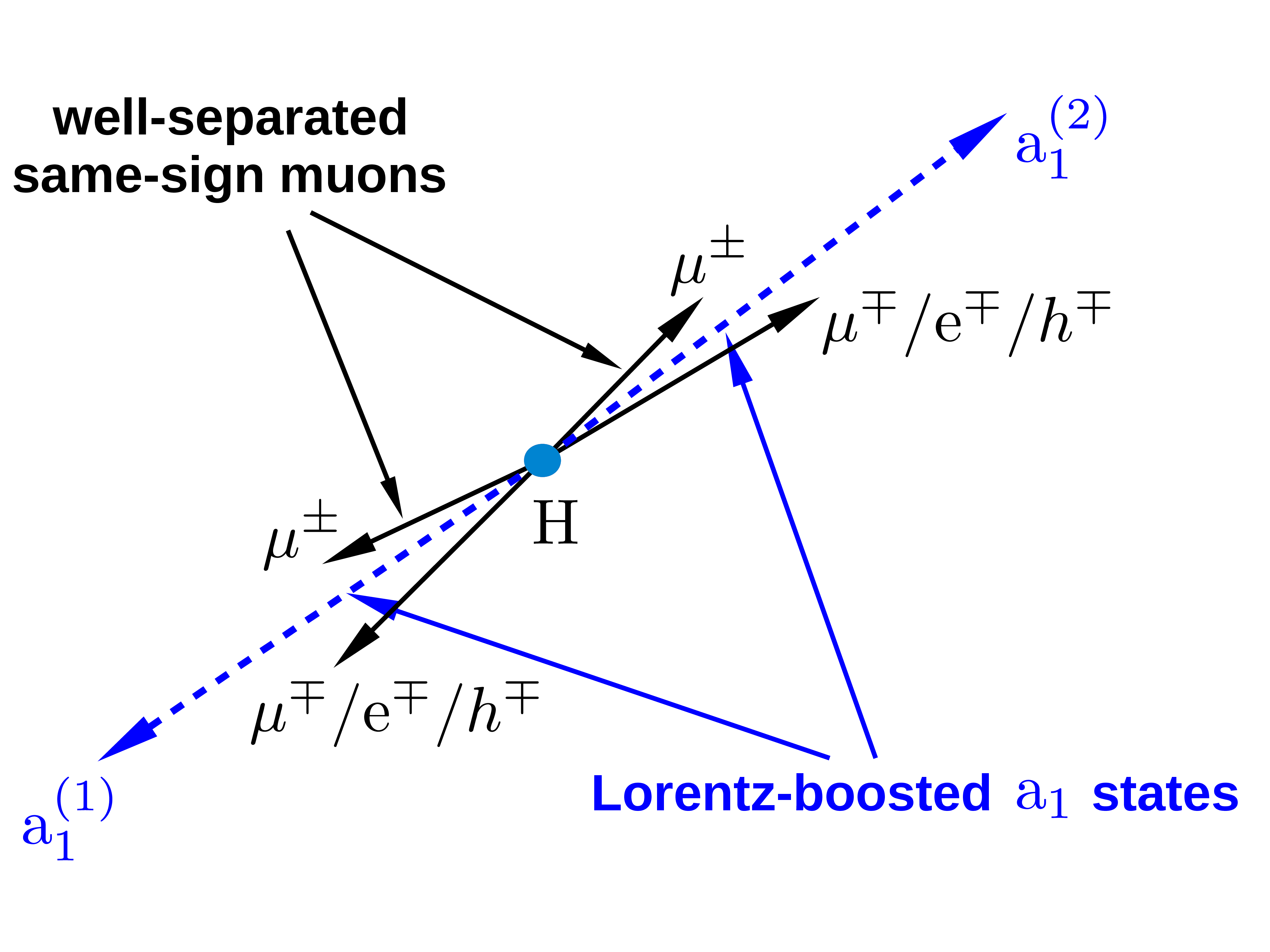
Figure 1:
Illustration of the signal topology. The Higgs boson decays into two $ \mathrm{a}_{1} $ bosons, one of which further decays into a pair of tau leptons, and the other into a pair of muons or tau leptons. In the case of $ \mathrm{a}_{1} \to \tau \tau $ decays, one tau lepton is required to decay to a muon, and the other to a single charged particle---either an electron, a muon, or a charged hadron ($ h $). The targeted final state consists of one muon and one oppositely charged track arising from each $ \mathrm{a}_{1} $ boson decay. |
png pdf |
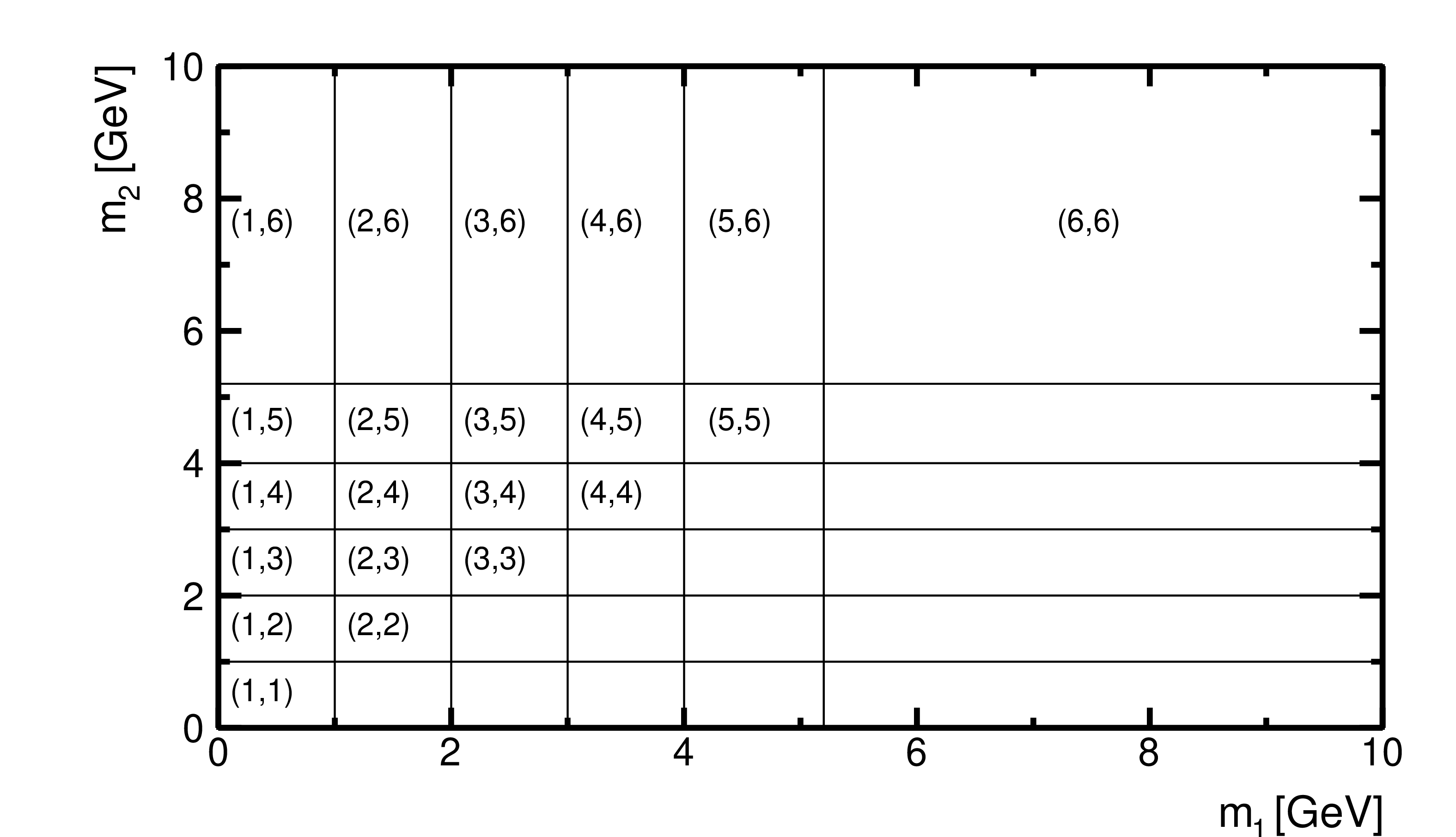
Figure 2:
Binning of the 2D ($ m_1,m_2$) distribution. Each bin is labeled $ (i,j) $, where $ i $ is the bin index along $ m_1 $ ($ x $ axis) and $ j $ is the bin index along $ m_2$ ($ y $ axis). Bins $ (i,6) $ with $ i=1,..., $ 5 include all events with $ m_2 > $ 5.2 GeV, while bin $ (6,6) $ contains all events with $ m_1 $ and $ m_2 > $ 5.2 GeV. |
png pdf |
Figure 3:
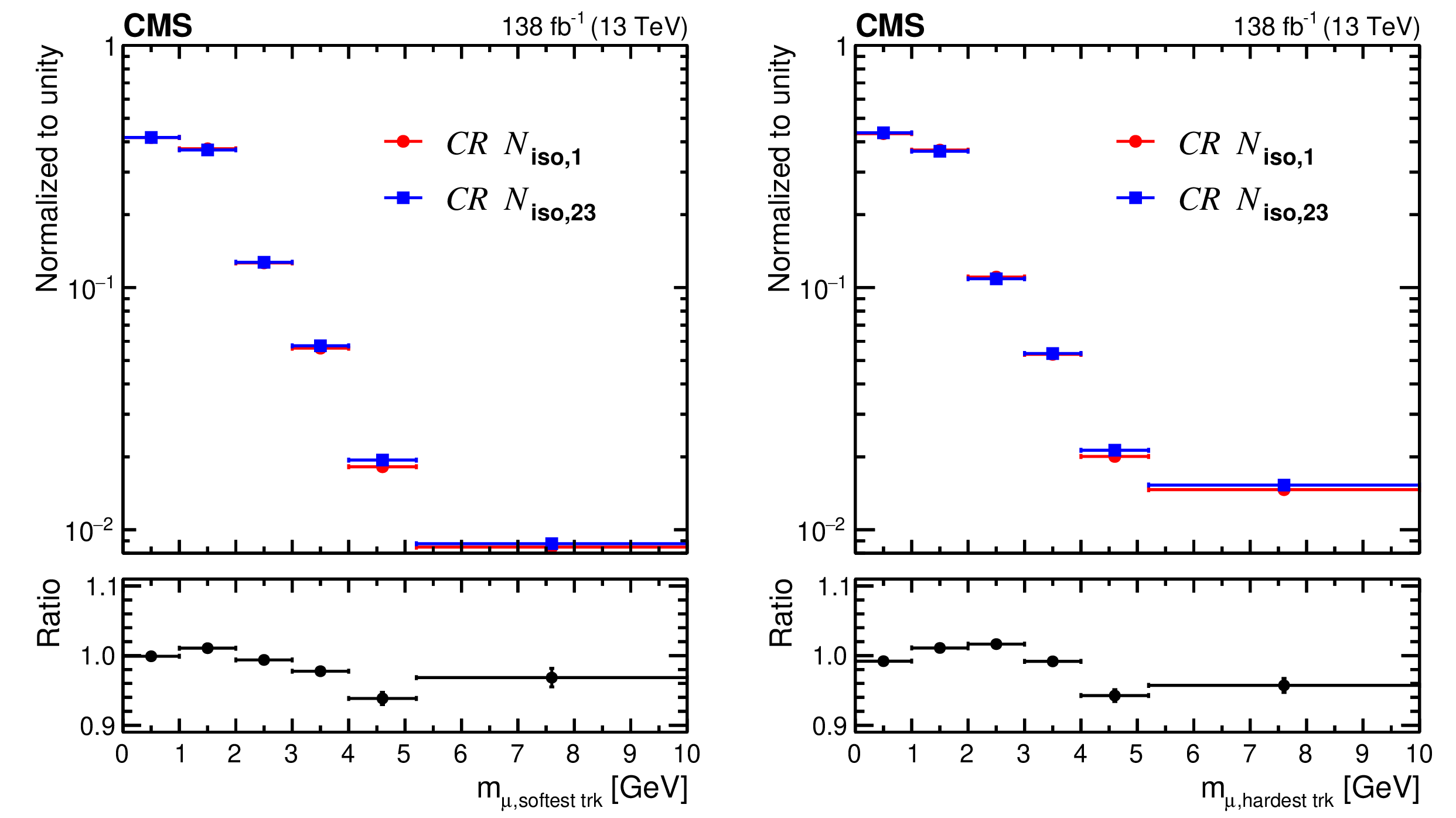
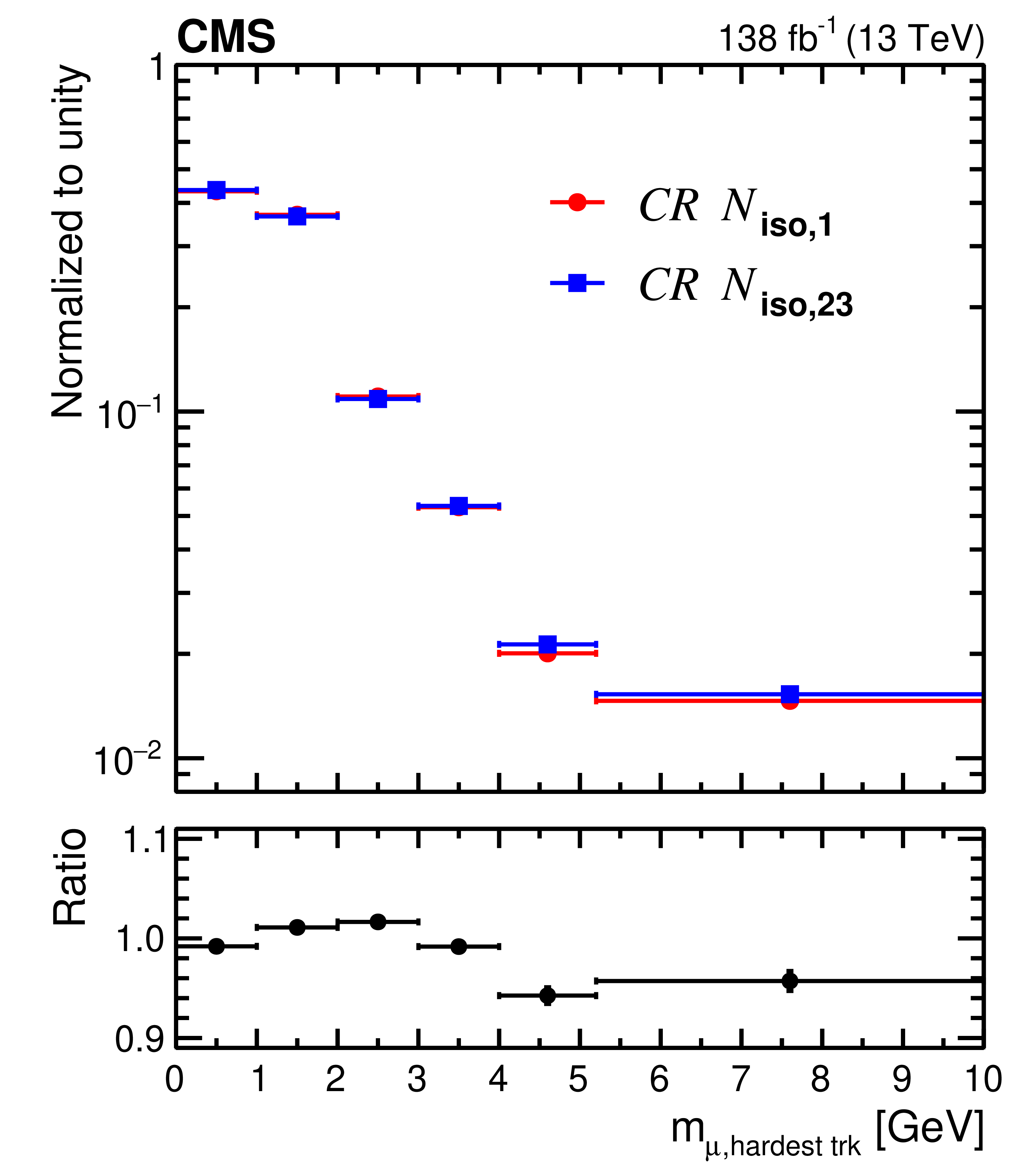
The observed invariant mass distribution, normalized to unity, of the first muon and the softest (left) or hardest (right) accompanying signal track for different isolation requirements imposed on the second muon: one isolation track ($ \textit{CR}\: N_{{\text{iso}},1} $; circles) or two to three isolation tracks ($ \textit{CR}\: N_{{\text{iso}},23} $; squares). Vertical bars represent statistical uncertainties, which are smaller than the marker size in most cases and thus imperceptible. The horizontal bars show the bin width. The lower panels show the ratio of the distribution in $ \textit{CR}\: N_{{\text{iso}},23} $ to that in $ \textit{CR}\: N_{{\text{iso}},1} $. The last bin in both distributions includes all entries with invariant mass of the muon+track system greater than 5.2 GeV. |
png pdf |
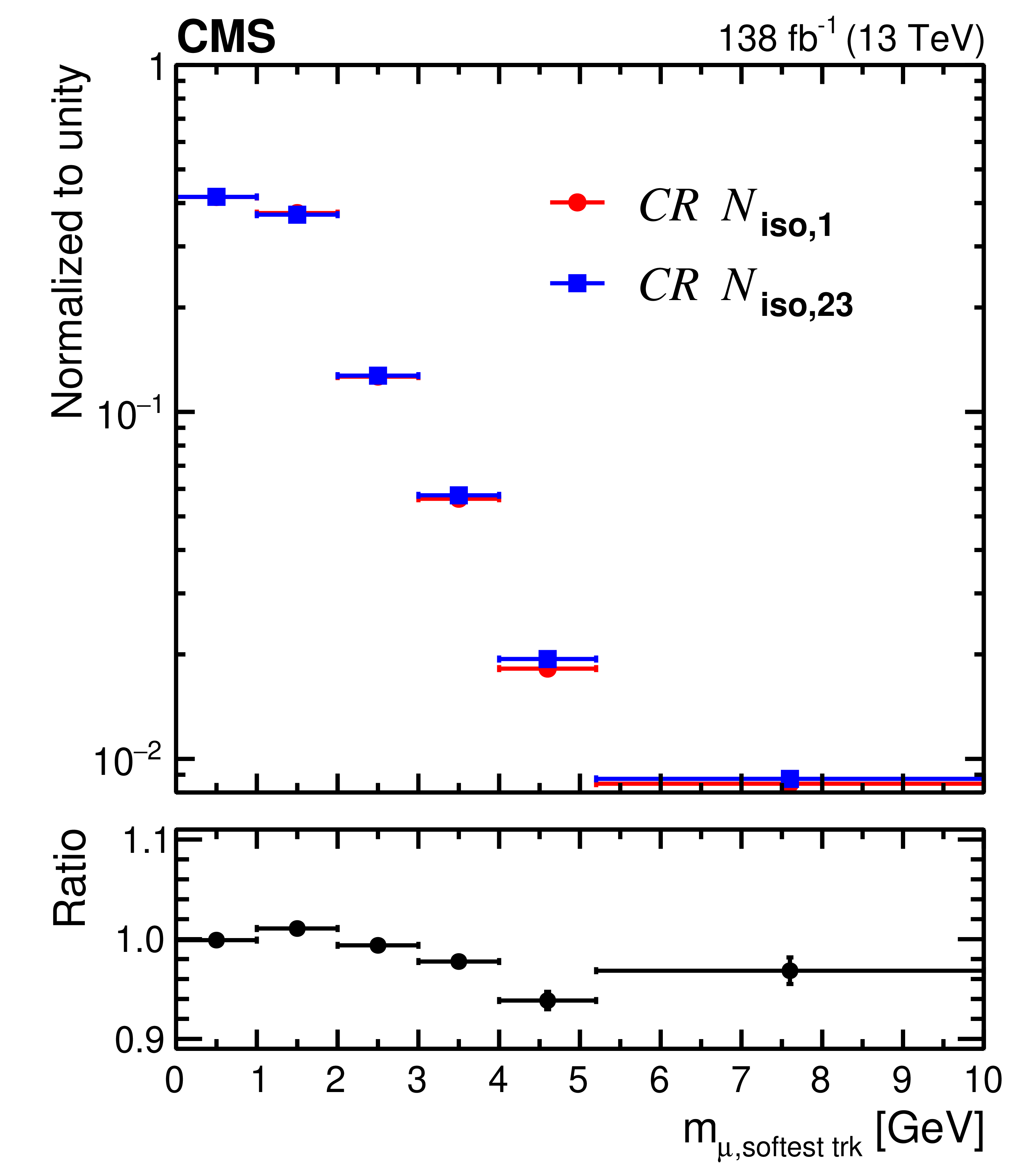
Figure 3-a:
The observed invariant mass distribution, normalized to unity, of the first muon and the softest (left) or hardest (right) accompanying signal track for different isolation requirements imposed on the second muon: one isolation track ($ \textit{CR}\: N_{{\text{iso}},1} $; circles) or two to three isolation tracks ($ \textit{CR}\: N_{{\text{iso}},23} $; squares). Vertical bars represent statistical uncertainties, which are smaller than the marker size in most cases and thus imperceptible. The horizontal bars show the bin width. The lower panels show the ratio of the distribution in $ \textit{CR}\: N_{{\text{iso}},23} $ to that in $ \textit{CR}\: N_{{\text{iso}},1} $. The last bin in both distributions includes all entries with invariant mass of the muon+track system greater than 5.2 GeV. |
png pdf |
Figure 3-b:
The observed invariant mass distribution, normalized to unity, of the first muon and the softest (left) or hardest (right) accompanying signal track for different isolation requirements imposed on the second muon: one isolation track ($ \textit{CR}\: N_{{\text{iso}},1} $; circles) or two to three isolation tracks ($ \textit{CR}\: N_{{\text{iso}},23} $; squares). Vertical bars represent statistical uncertainties, which are smaller than the marker size in most cases and thus imperceptible. The horizontal bars show the bin width. The lower panels show the ratio of the distribution in $ \textit{CR}\: N_{{\text{iso}},23} $ to that in $ \textit{CR}\: N_{{\text{iso}},1} $. The last bin in both distributions includes all entries with invariant mass of the muon+track system greater than 5.2 GeV. |
png pdf |
Figure 4:
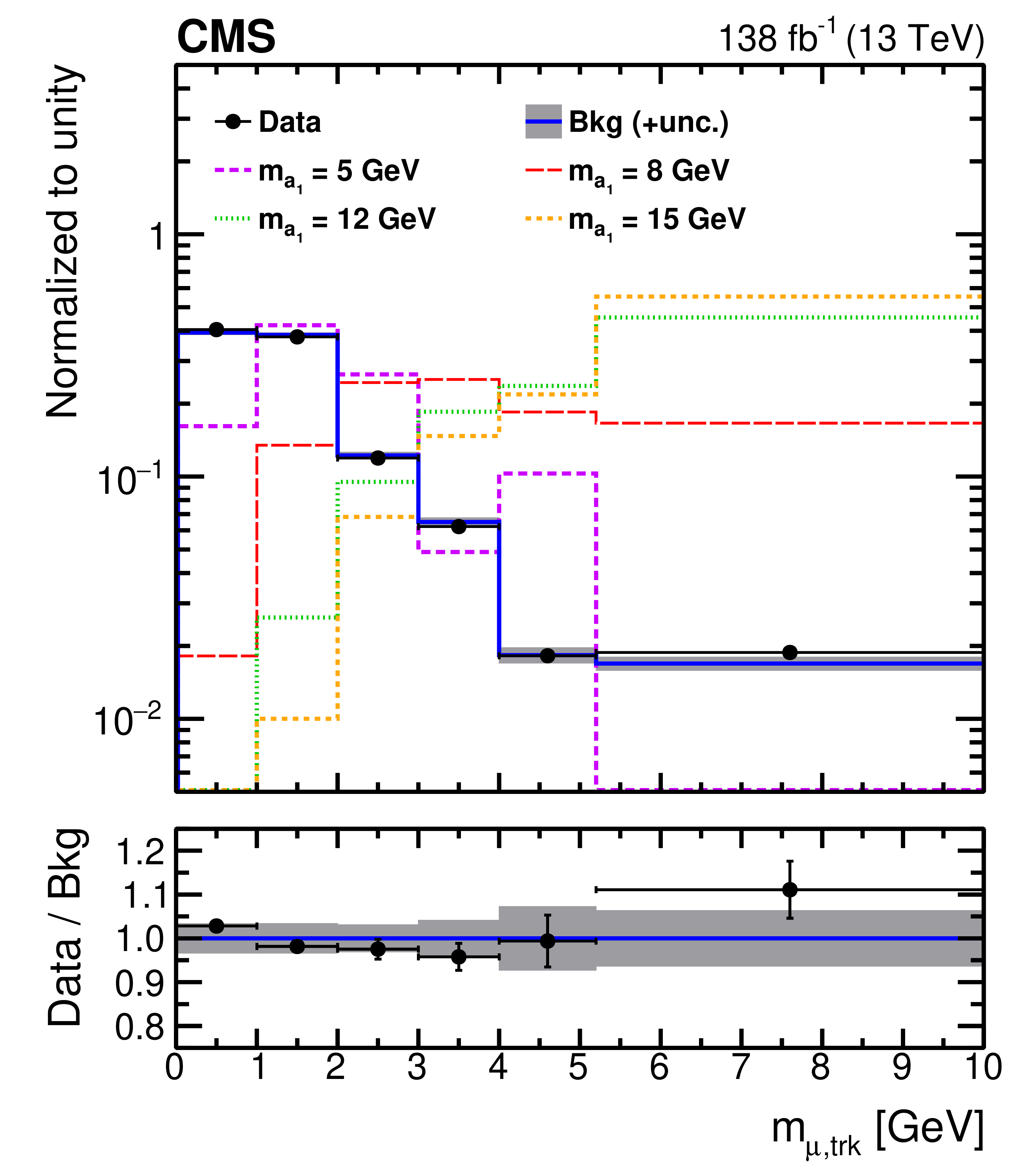
Invariant mass distribution of the muon+track pair, normalized to unity, for events passing the signal selection. Events in data are represented by black points with the vertical bars representing the statistical uncertainty and the horizontal bars the bin width. The expected background distribution derived from $ \textit{CR}\: N_{23} $ is shown by the solid blue histogram, with the grey band giving the uncertainty in the background prediction, including systematic and statistical components. Also shown are normalized distributions from signal simulations for four mass hypotheses, $ m_{\mathrm{a}_{1}} $= 5, 8, 12, and 15 GeV (dashed colored histograms). The lower panel displays the ratio of the data to the expected background. |
png pdf |
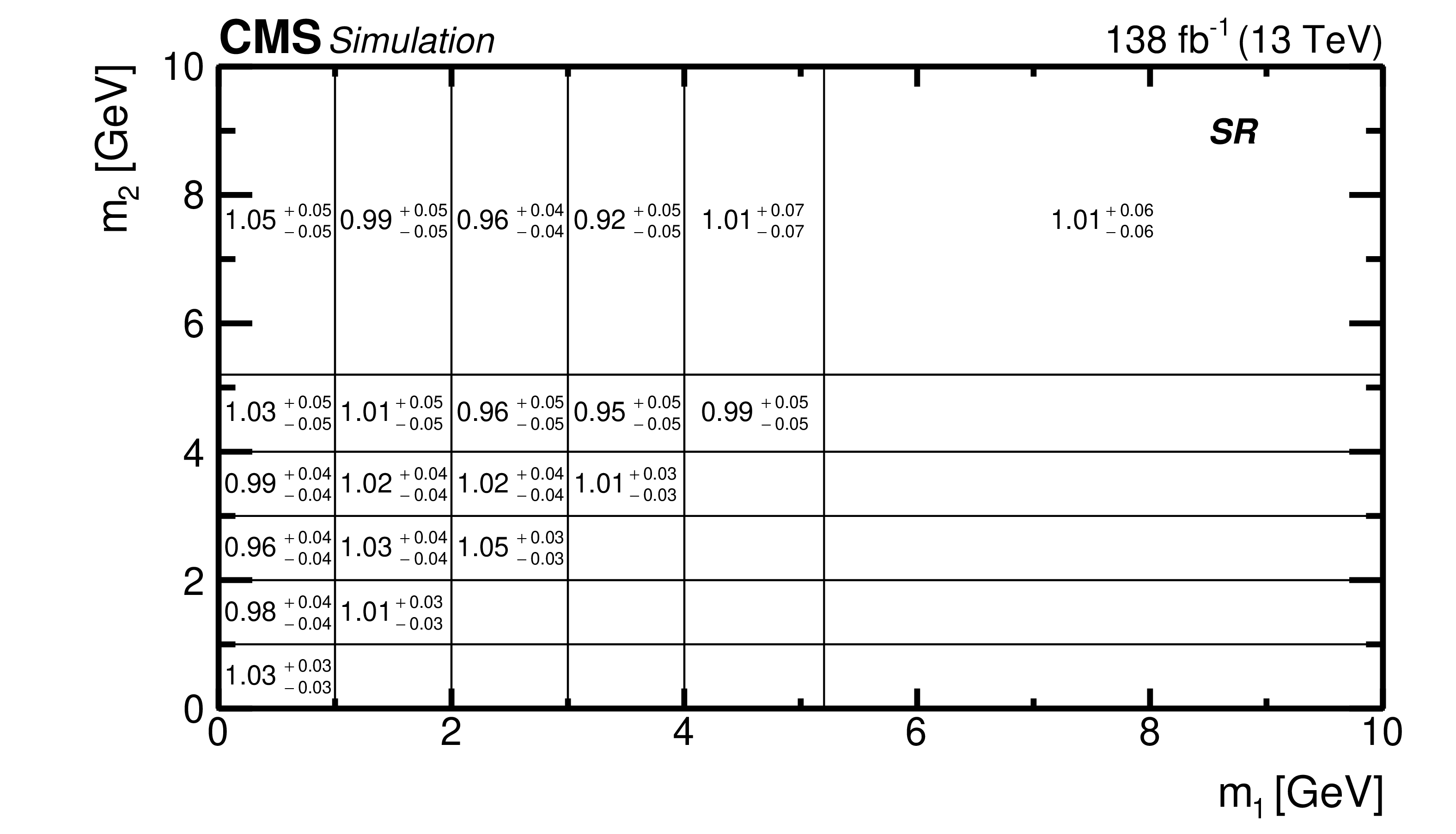
Figure 5:
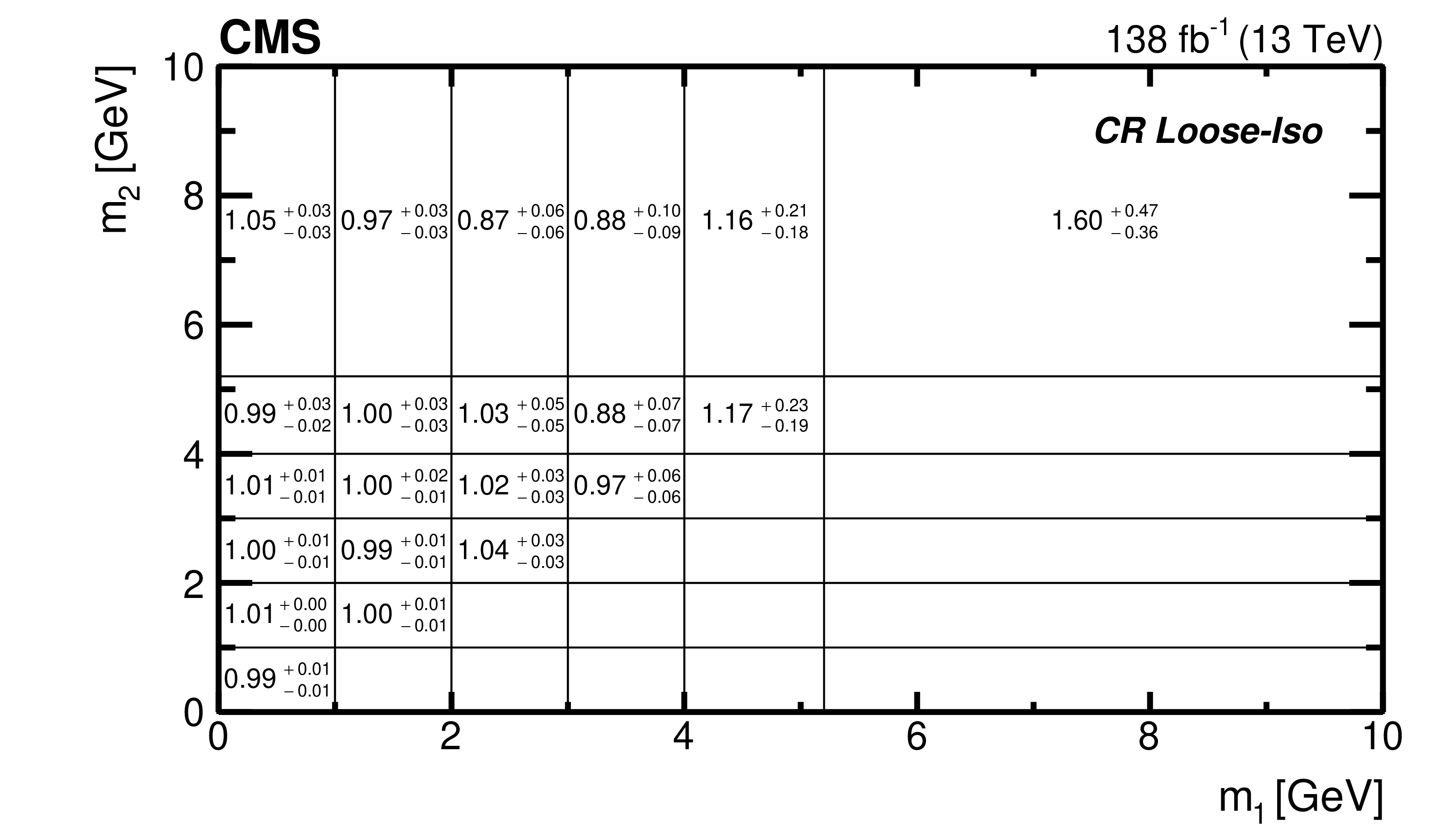
The correlation factors $ C(i,j)^{\textit{CR}}_{\text{data}} $ with their statistical uncertainties. |
png pdf |
Figure 6:
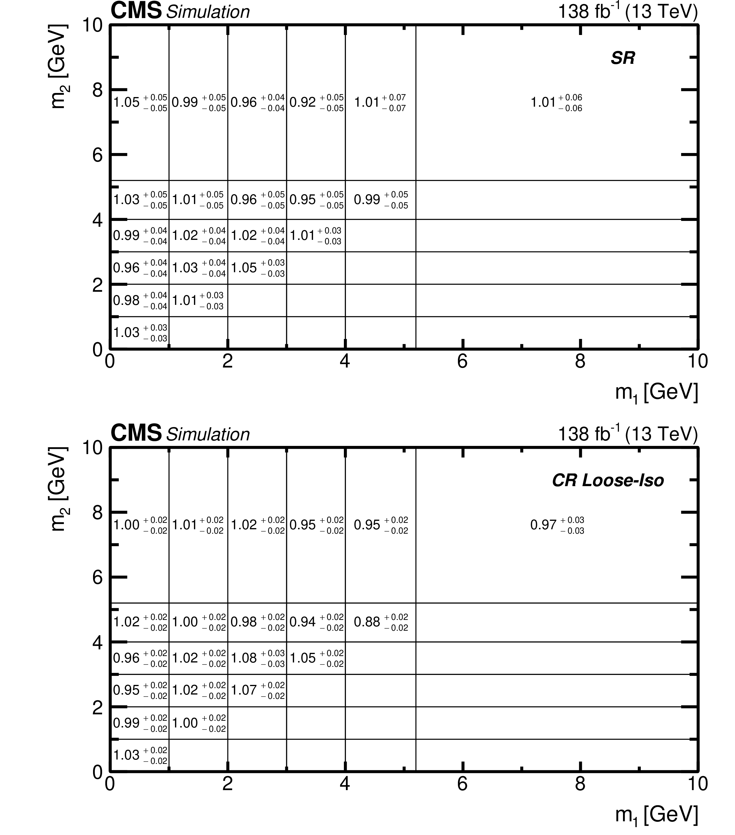
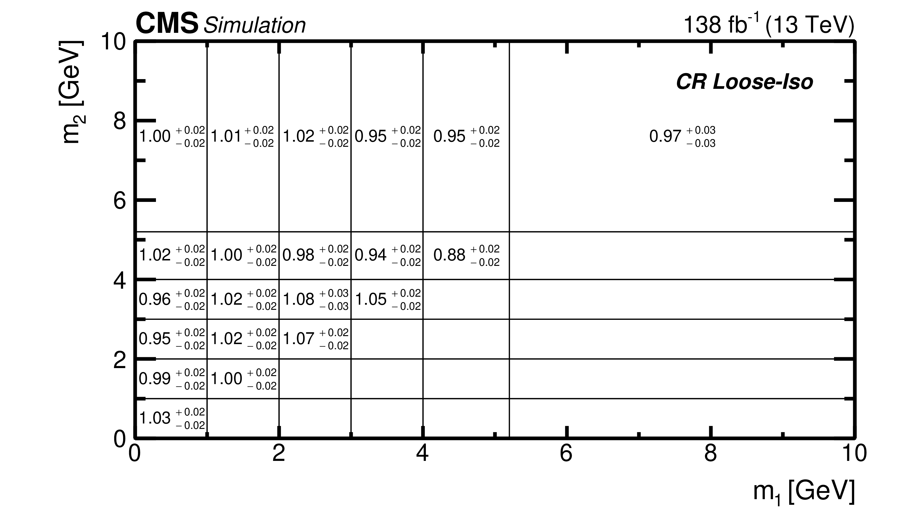
The correlation factors $ C(i,j)^{\textit{CR}}_{\text{MC}} $ (top) and $ C(i,j)^{\textit{CR}}_{\text{MC}} $ (bottom) with their statistical uncertainties. |
png pdf |
Figure 6-a:
The correlation factors $ C(i,j)^{\textit{CR}}_{\text{MC}} $ (top) and $ C(i,j)^{\textit{CR}}_{\text{MC}} $ (bottom) with their statistical uncertainties. |
png pdf |
Figure 6-b:
The correlation factors $ C(i,j)^{\textit{CR}}_{\text{MC}} $ (top) and $ C(i,j)^{\textit{CR}}_{\text{MC}} $ (bottom) with their statistical uncertainties. |
png pdf |
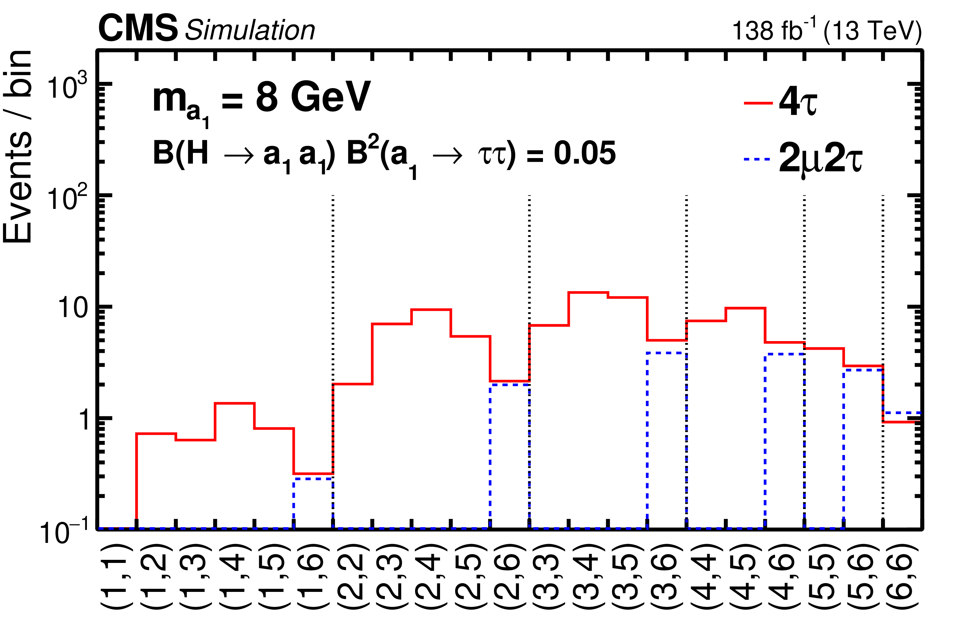
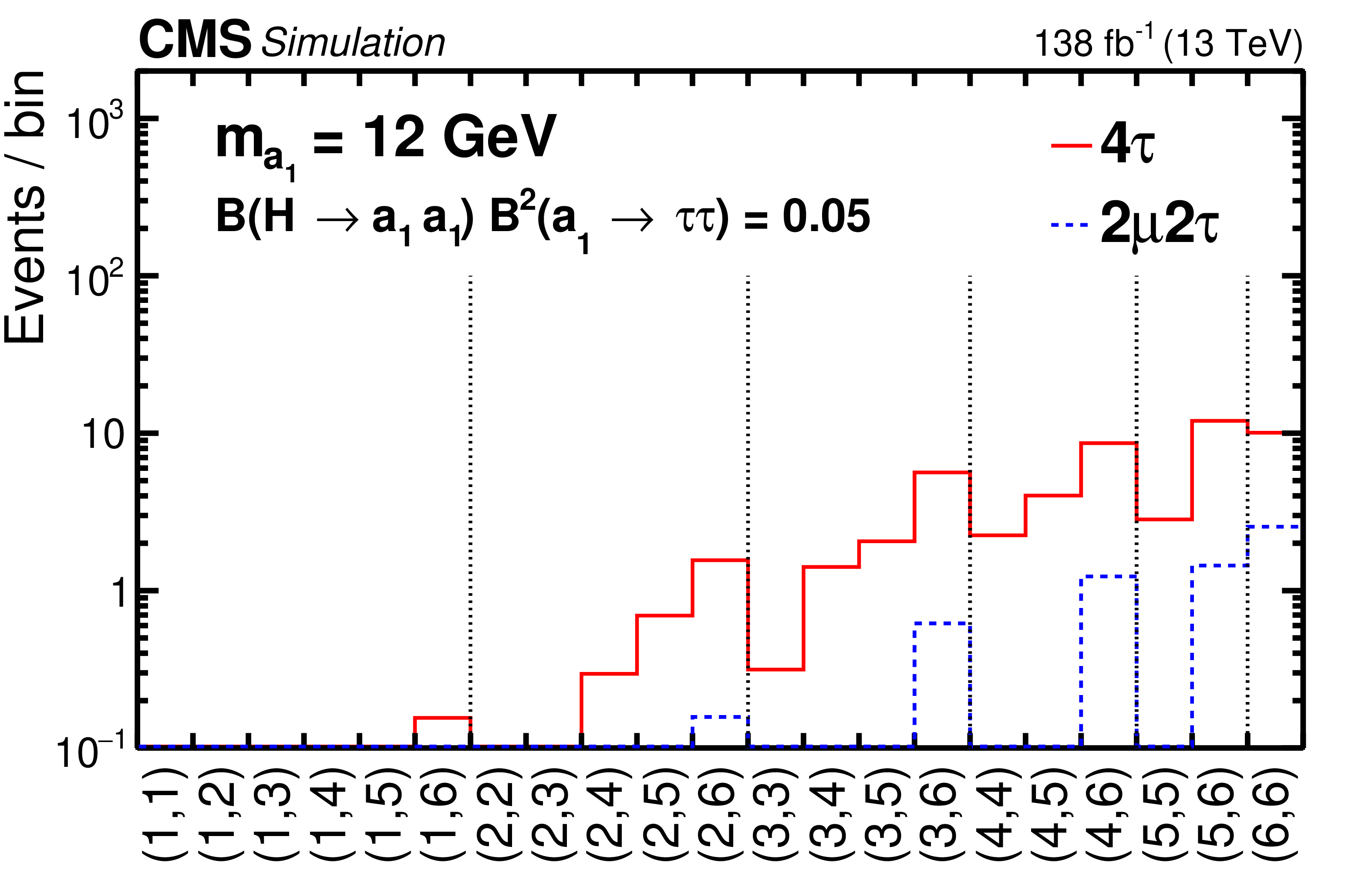
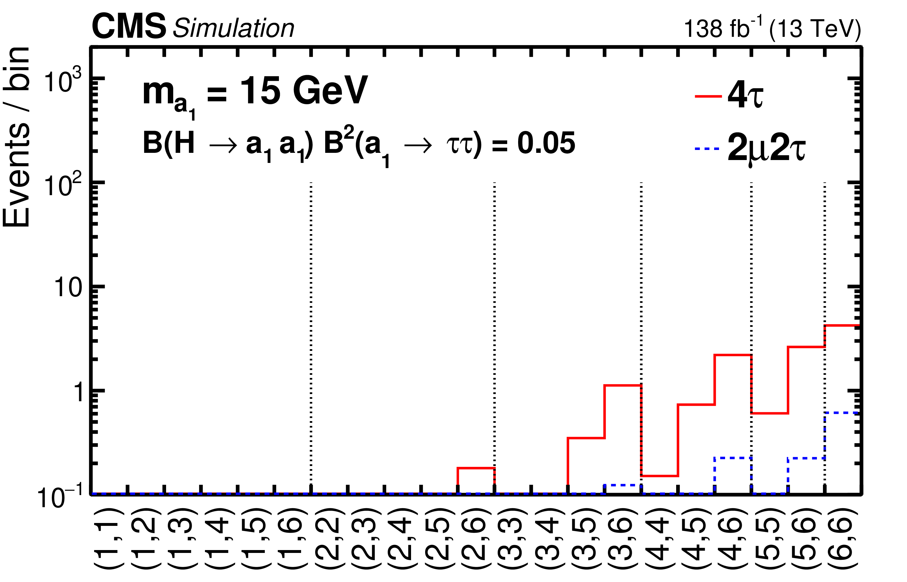
Figure 7:
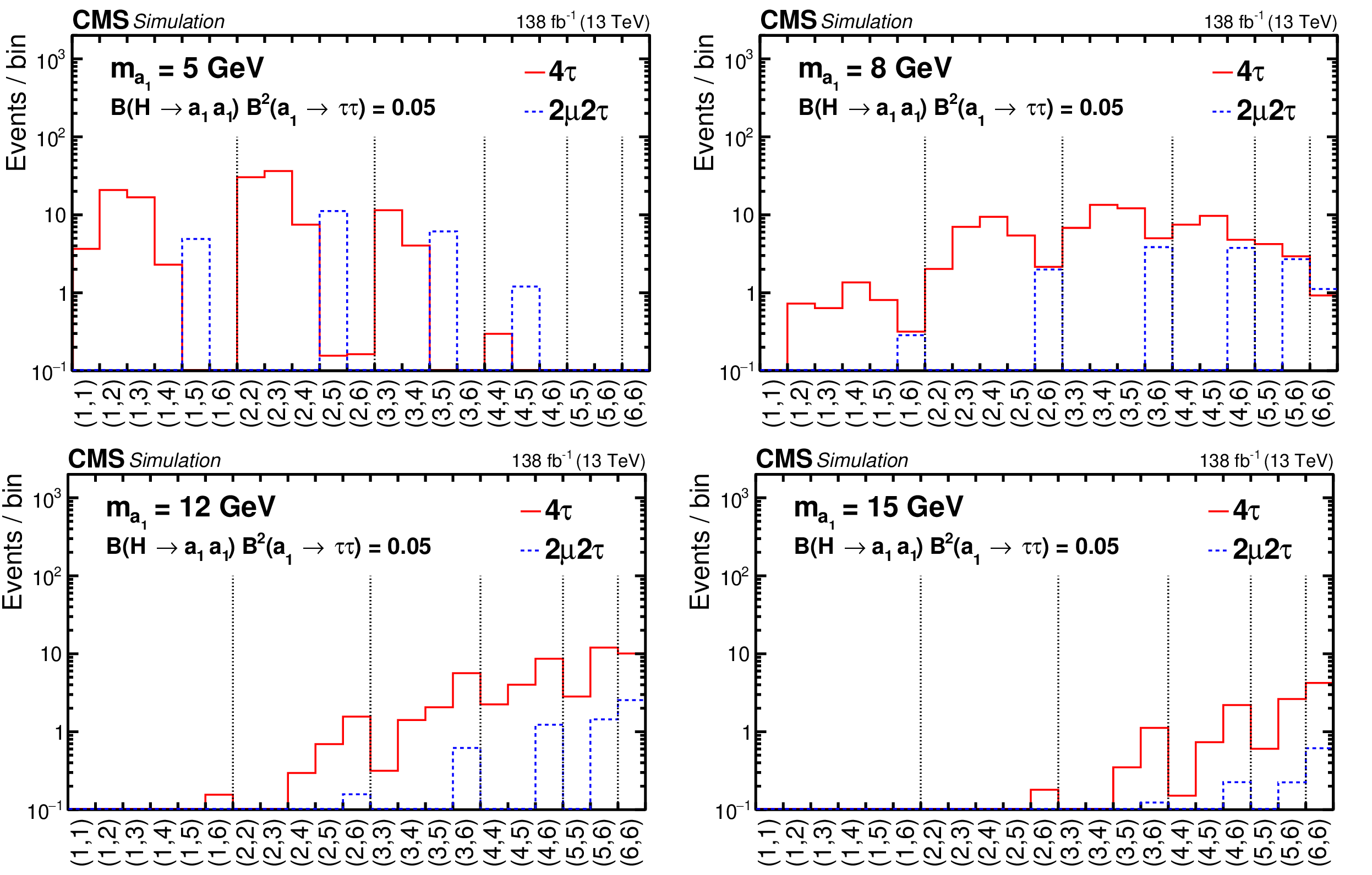
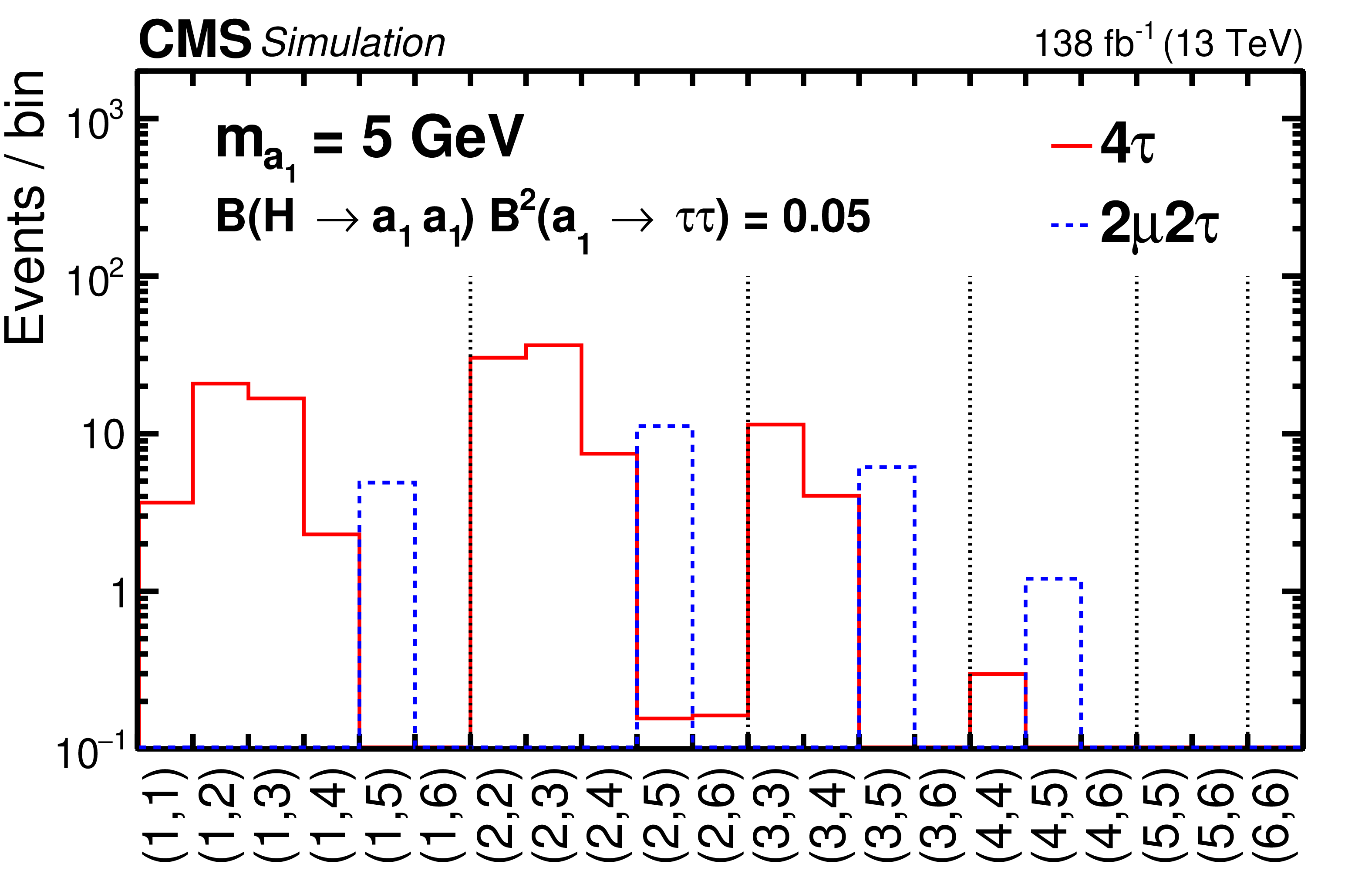
The simulated signal $ (m_1, m_2) $ distribution, converted into a 1D array, for $ m_{\mathrm{a}_1} $ values of 5 (upper left), 8 (upper right), 12 (lower left), and 15 GeV (lower right). The contributions of the $ \mathrm{H}\to\mathrm{a}_{1}\mathrm{a}_{1}\to 4\tau $ (red histograms) and 2$ \mu2\tau $ (blue histograms) decays are shown. The distributions are normalized assuming SM Higgs production cross section and $ {\mathcal{B}} (\mathrm{H}\to\mathrm{a}_{1}\mathrm{a}_{1}){\mathcal{B}}^{2}(\mathrm{a}_{1}\to \tau\tau) $ = 0.05. The bin notation follows that of Fig. 2. |
png pdf |
Figure 7-a:
The simulated signal $ (m_1, m_2) $ distribution, converted into a 1D array, for $ m_{\mathrm{a}_1} $ values of 5 (upper left), 8 (upper right), 12 (lower left), and 15 GeV (lower right). The contributions of the $ \mathrm{H}\to\mathrm{a}_{1}\mathrm{a}_{1}\to 4\tau $ (red histograms) and 2$ \mu2\tau $ (blue histograms) decays are shown. The distributions are normalized assuming SM Higgs production cross section and $ {\mathcal{B}} (\mathrm{H}\to\mathrm{a}_{1}\mathrm{a}_{1}){\mathcal{B}}^{2}(\mathrm{a}_{1}\to \tau\tau) $ = 0.05. The bin notation follows that of Fig. 2. |
png pdf |
Figure 7-b:
The simulated signal $ (m_1, m_2) $ distribution, converted into a 1D array, for $ m_{\mathrm{a}_1} $ values of 5 (upper left), 8 (upper right), 12 (lower left), and 15 GeV (lower right). The contributions of the $ \mathrm{H}\to\mathrm{a}_{1}\mathrm{a}_{1}\to 4\tau $ (red histograms) and 2$ \mu2\tau $ (blue histograms) decays are shown. The distributions are normalized assuming SM Higgs production cross section and $ {\mathcal{B}} (\mathrm{H}\to\mathrm{a}_{1}\mathrm{a}_{1}){\mathcal{B}}^{2}(\mathrm{a}_{1}\to \tau\tau) $ = 0.05. The bin notation follows that of Fig. 2. |
png pdf |
Figure 7-c:
The simulated signal $ (m_1, m_2) $ distribution, converted into a 1D array, for $ m_{\mathrm{a}_1} $ values of 5 (upper left), 8 (upper right), 12 (lower left), and 15 GeV (lower right). The contributions of the $ \mathrm{H}\to\mathrm{a}_{1}\mathrm{a}_{1}\to 4\tau $ (red histograms) and 2$ \mu2\tau $ (blue histograms) decays are shown. The distributions are normalized assuming SM Higgs production cross section and $ {\mathcal{B}} (\mathrm{H}\to\mathrm{a}_{1}\mathrm{a}_{1}){\mathcal{B}}^{2}(\mathrm{a}_{1}\to \tau\tau) $ = 0.05. The bin notation follows that of Fig. 2. |
png pdf |
Figure 7-d:
The simulated signal $ (m_1, m_2) $ distribution, converted into a 1D array, for $ m_{\mathrm{a}_1} $ values of 5 (upper left), 8 (upper right), 12 (lower left), and 15 GeV (lower right). The contributions of the $ \mathrm{H}\to\mathrm{a}_{1}\mathrm{a}_{1}\to 4\tau $ (red histograms) and 2$ \mu2\tau $ (blue histograms) decays are shown. The distributions are normalized assuming SM Higgs production cross section and $ {\mathcal{B}} (\mathrm{H}\to\mathrm{a}_{1}\mathrm{a}_{1}){\mathcal{B}}^{2}(\mathrm{a}_{1}\to \tau\tau) $ = 0.05. The bin notation follows that of Fig. 2. |
png pdf |
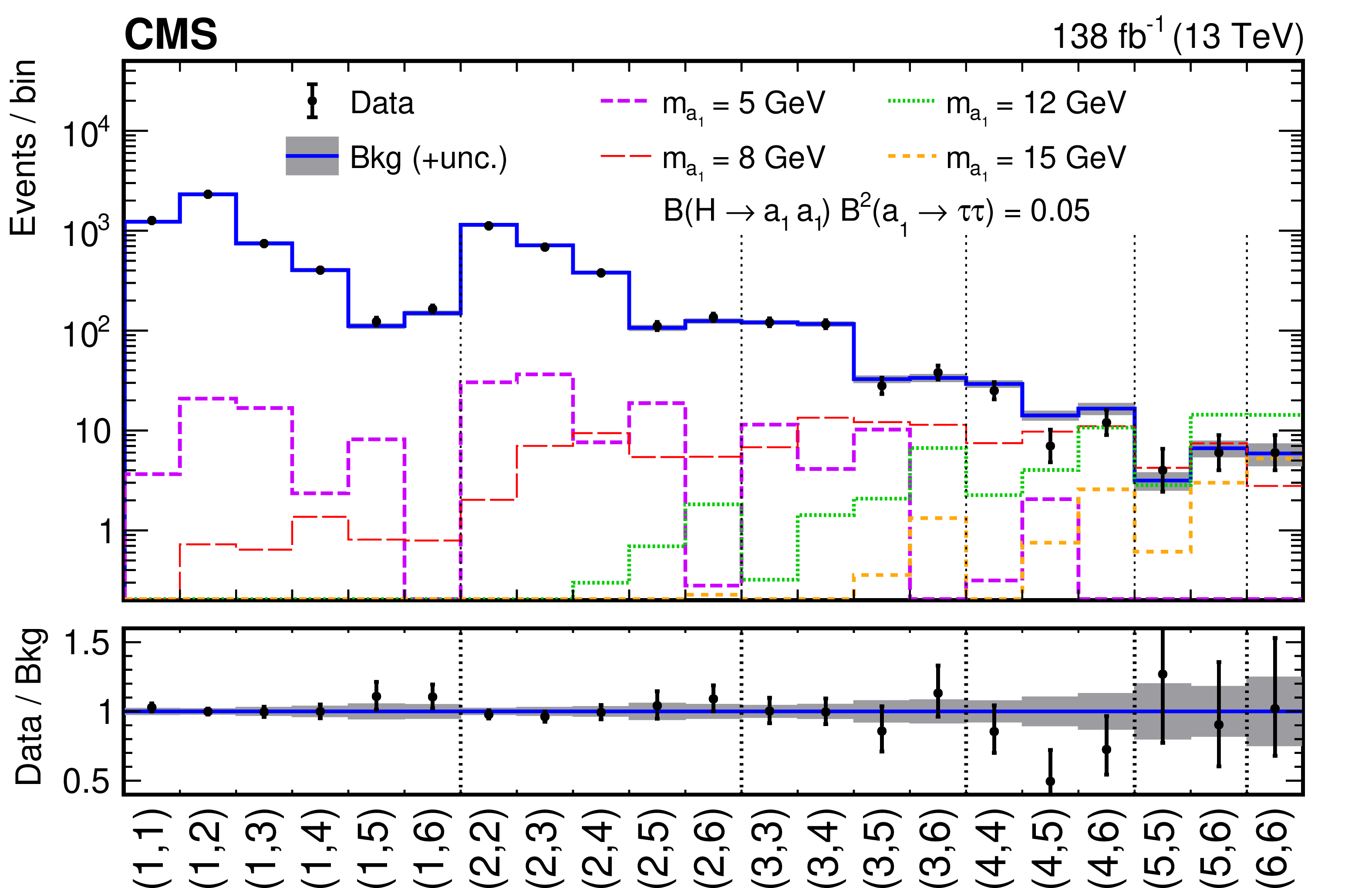
Figure 8:
The unrolled ($ m_1,m_2$) distribution used to extract the signal. The observed number of events in data is represented by the points, with the vertical bars giving the statistical uncertainty. The background is shown as the blue histogram, with its uncertainty depicted by the shaded grey band. The normalization for the background is obtained by fitting the observed data under the background-only hypothesis. Signal expectations for the 4$ \tau $ and 2$ \mu2\tau $ final states are shown as dashed histograms for the mass hypotheses $ m_{\mathrm{a}_{1}} $= 5, 8, 12, and 15 GeV. The relative normalization of the 4$ \tau $ and 2$ \mu2\tau $ final states is given by Eq. (1). The signal normalization is computed assuming that the Higgs boson is produced in pp collisions with a rate predicted by the SM and decays into the $ \mathrm{a}_{1} \mathrm{a}_{1} \to 4\tau $ final state with a branching fraction of 5%. The lower plot shows the ratio of the observed data events to the expected background yield in each bin of the ($ m_1,m_2$) distribution. |
png pdf |
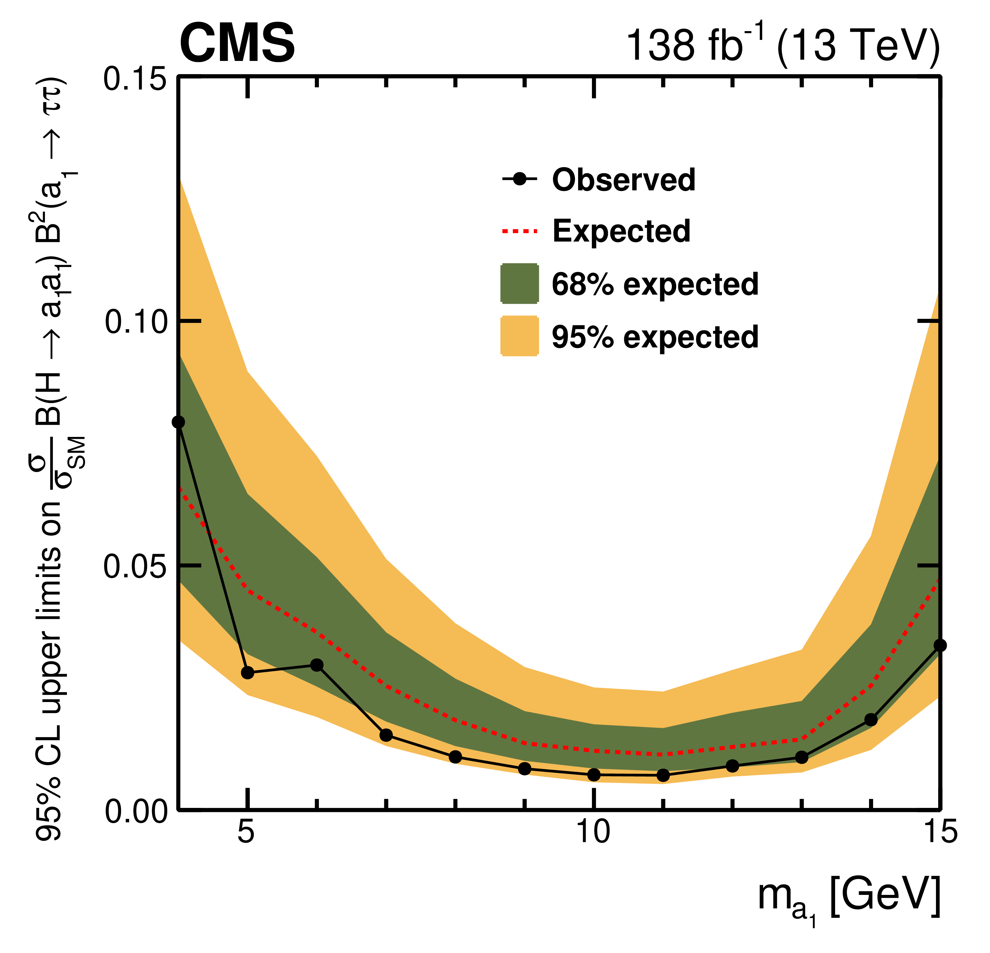
Figure 9:
The observed (points) and expected (red line) 95% CL upper limits on the product of the signal cross section and the branching fractions $ \sigma (\mathrm{p}\mathrm{p} \to \mathrm{H}+\mathrm{X}) {\mathcal{B}} (\mathrm{H} \to \mathrm{a}_{1} \mathrm{a}_{1}) {\mathcal{B}}^{2} (\mathrm{a}_{1} \to \tau \tau) $, relative to the inclusive Higgs boson production cross section $ \sigma_\text{SM} $ predicted in the SM. The green and yellow bands indicate the regions containing 68 and 95% of the expected limit ranges under the background-only hypothesis. |
png pdf |
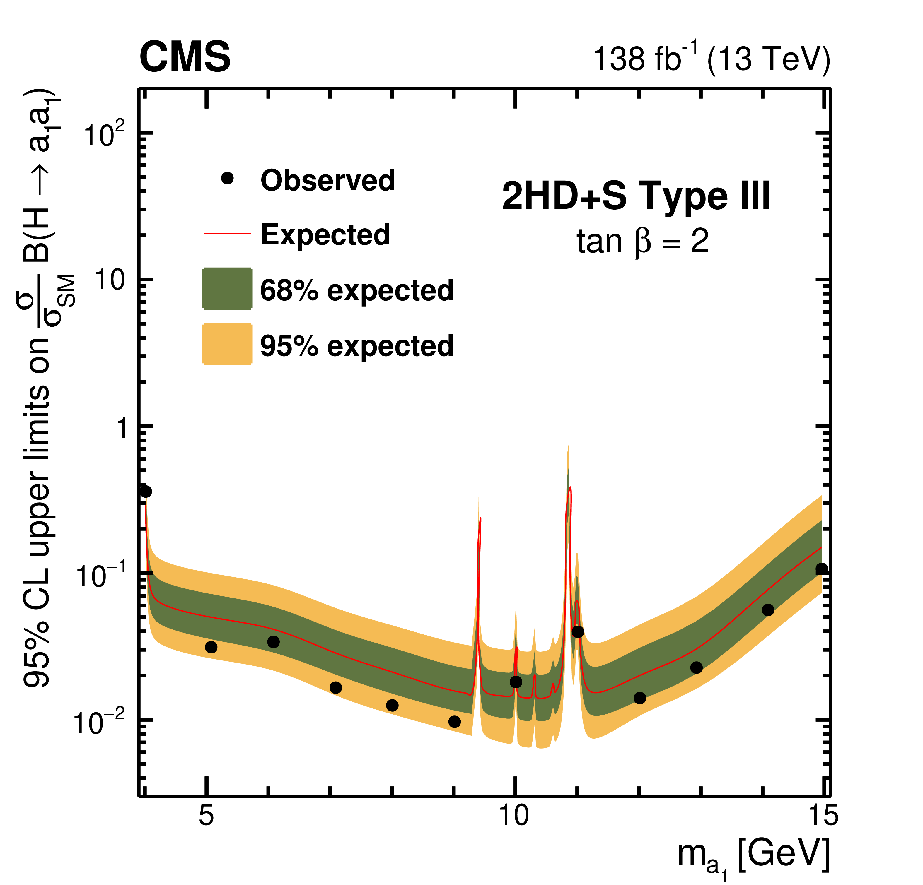
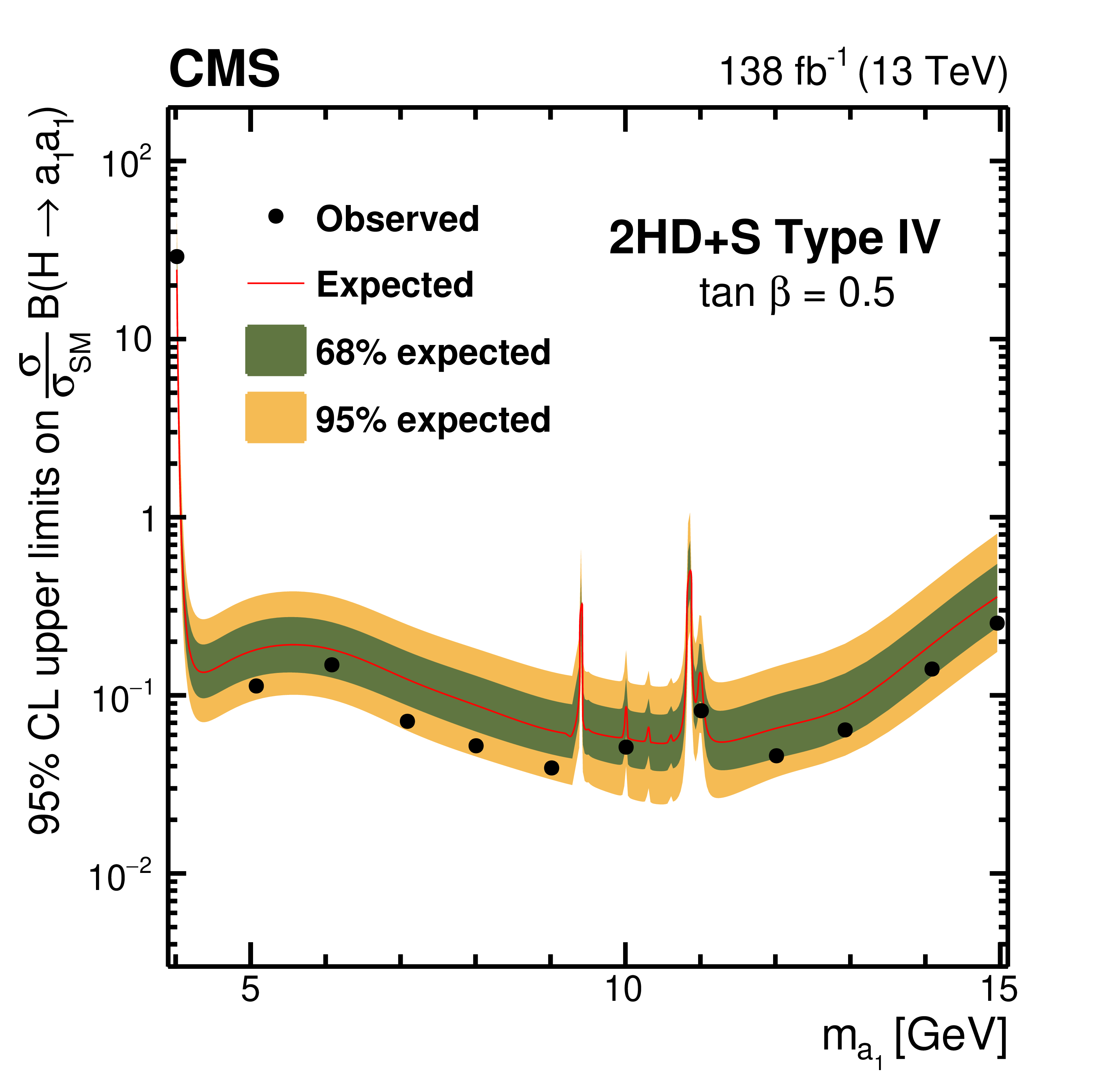
Figure 10:
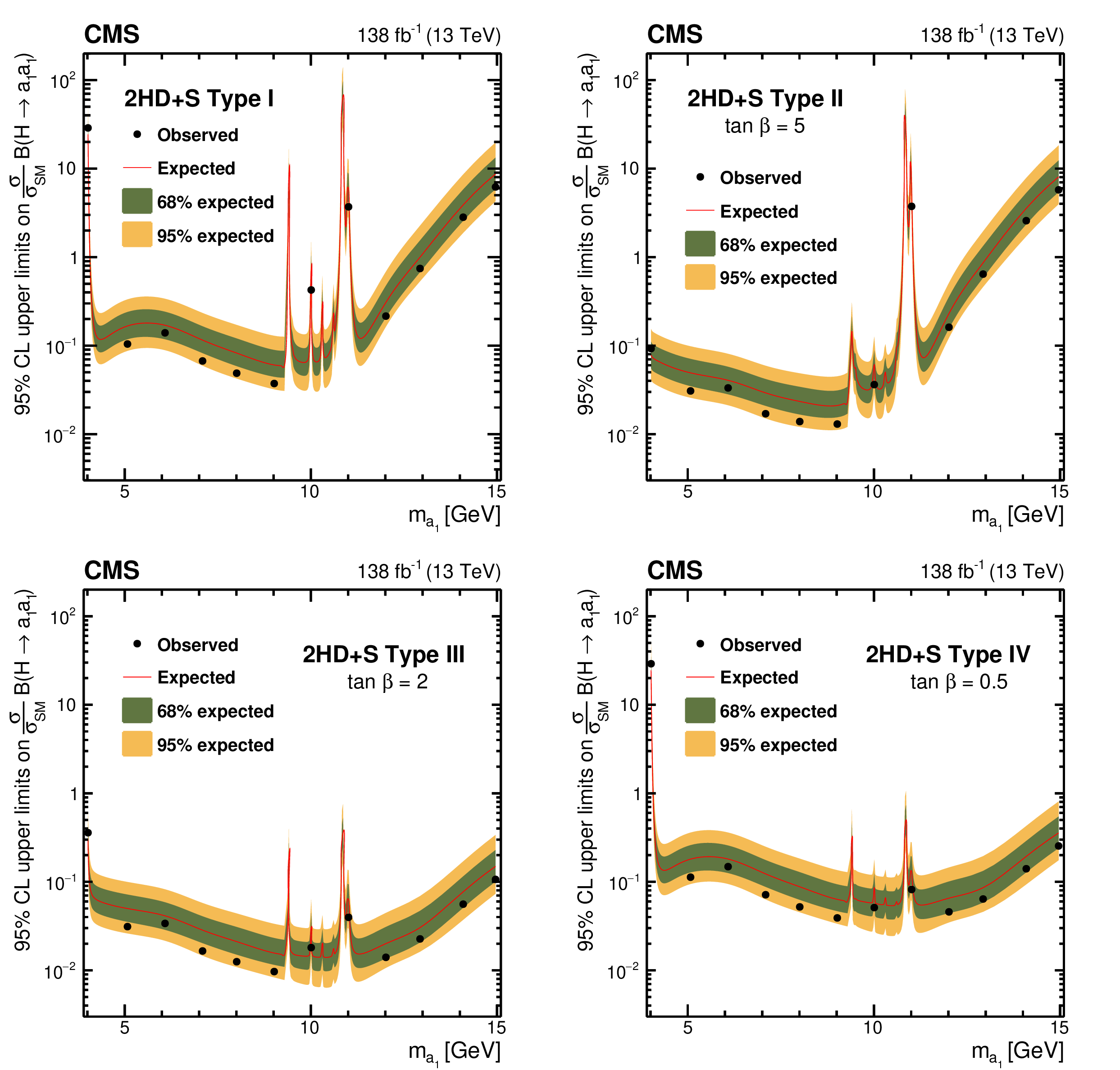
The observed (points) and expected (red line) 95% CL upper limits on $ \sigma (\mathrm{p}\mathrm{p} \to \mathrm{H}+\mathrm{X}) {\mathcal{B}} (\mathrm{H} \to \mathrm{a}_{1} \mathrm{a}_{1}) $, relative to $ \sigma_\text{SM} $, as a function of $ m_{\mathrm{a}_{1}} $ for different 2HD+S models at benchmark $ \tan\beta $ values: Type I ($ \tan\beta $ independent; upper left), Type II ($ \tan\beta = $ 5; upper right), Type III ($ \tan\beta = $ 2; lower left), and Type IV ($ \tan\beta = $ 0.5; lower right). |
png pdf |
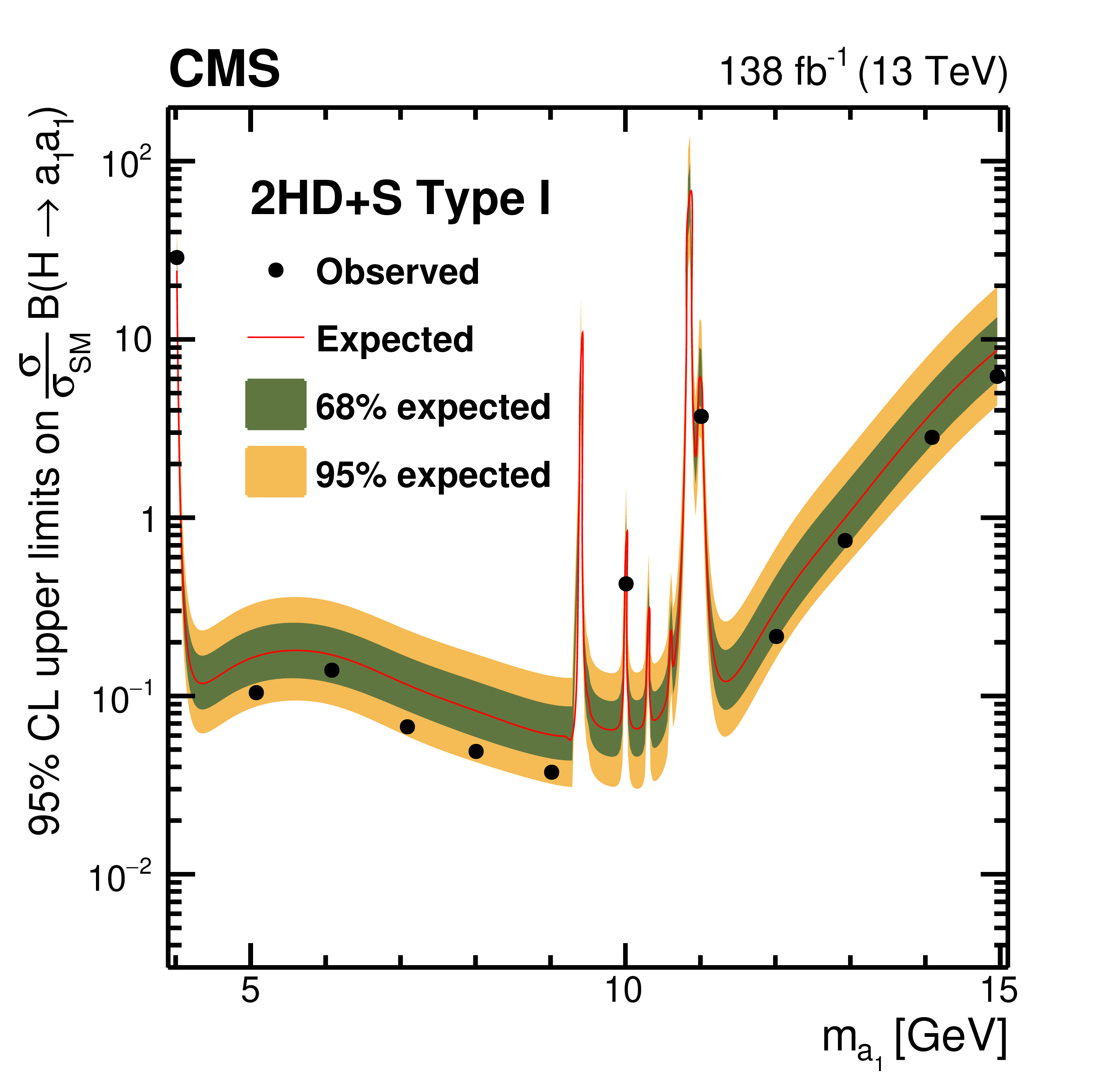
Figure 10-a:
The observed (points) and expected (red line) 95% CL upper limits on $ \sigma (\mathrm{p}\mathrm{p} \to \mathrm{H}+\mathrm{X}) {\mathcal{B}} (\mathrm{H} \to \mathrm{a}_{1} \mathrm{a}_{1}) $, relative to $ \sigma_\text{SM} $, as a function of $ m_{\mathrm{a}_{1}} $ for different 2HD+S models at benchmark $ \tan\beta $ values: Type I ($ \tan\beta $ independent; upper left), Type II ($ \tan\beta = $ 5; upper right), Type III ($ \tan\beta = $ 2; lower left), and Type IV ($ \tan\beta = $ 0.5; lower right). |
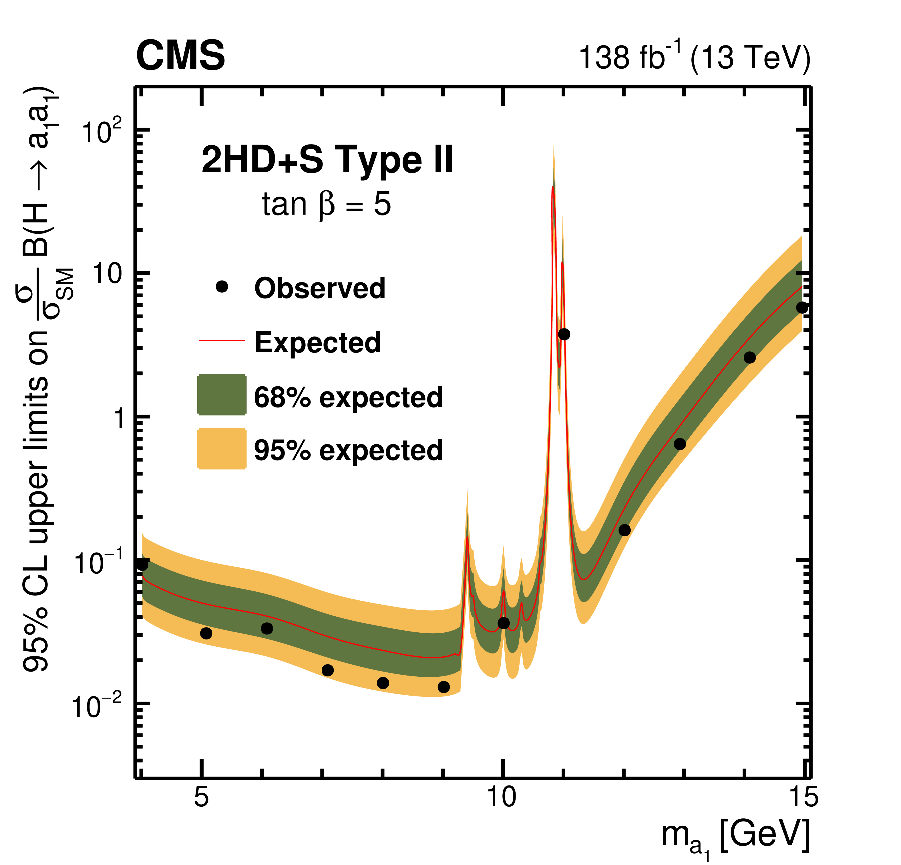
png pdf |
Figure 10-b:
The observed (points) and expected (red line) 95% CL upper limits on $ \sigma (\mathrm{p}\mathrm{p} \to \mathrm{H}+\mathrm{X}) {\mathcal{B}} (\mathrm{H} \to \mathrm{a}_{1} \mathrm{a}_{1}) $, relative to $ \sigma_\text{SM} $, as a function of $ m_{\mathrm{a}_{1}} $ for different 2HD+S models at benchmark $ \tan\beta $ values: Type I ($ \tan\beta $ independent; upper left), Type II ($ \tan\beta = $ 5; upper right), Type III ($ \tan\beta = $ 2; lower left), and Type IV ($ \tan\beta = $ 0.5; lower right). |
png pdf |
Figure 10-c:
The observed (points) and expected (red line) 95% CL upper limits on $ \sigma (\mathrm{p}\mathrm{p} \to \mathrm{H}+\mathrm{X}) {\mathcal{B}} (\mathrm{H} \to \mathrm{a}_{1} \mathrm{a}_{1}) $, relative to $ \sigma_\text{SM} $, as a function of $ m_{\mathrm{a}_{1}} $ for different 2HD+S models at benchmark $ \tan\beta $ values: Type I ($ \tan\beta $ independent; upper left), Type II ($ \tan\beta = $ 5; upper right), Type III ($ \tan\beta = $ 2; lower left), and Type IV ($ \tan\beta = $ 0.5; lower right). |
png pdf |
Figure 10-d:
The observed (points) and expected (red line) 95% CL upper limits on $ \sigma (\mathrm{p}\mathrm{p} \to \mathrm{H}+\mathrm{X}) {\mathcal{B}} (\mathrm{H} \to \mathrm{a}_{1} \mathrm{a}_{1}) $, relative to $ \sigma_\text{SM} $, as a function of $ m_{\mathrm{a}_{1}} $ for different 2HD+S models at benchmark $ \tan\beta $ values: Type I ($ \tan\beta $ independent; upper left), Type II ($ \tan\beta = $ 5; upper right), Type III ($ \tan\beta = $ 2; lower left), and Type IV ($ \tan\beta = $ 0.5; lower right). |
png pdf |
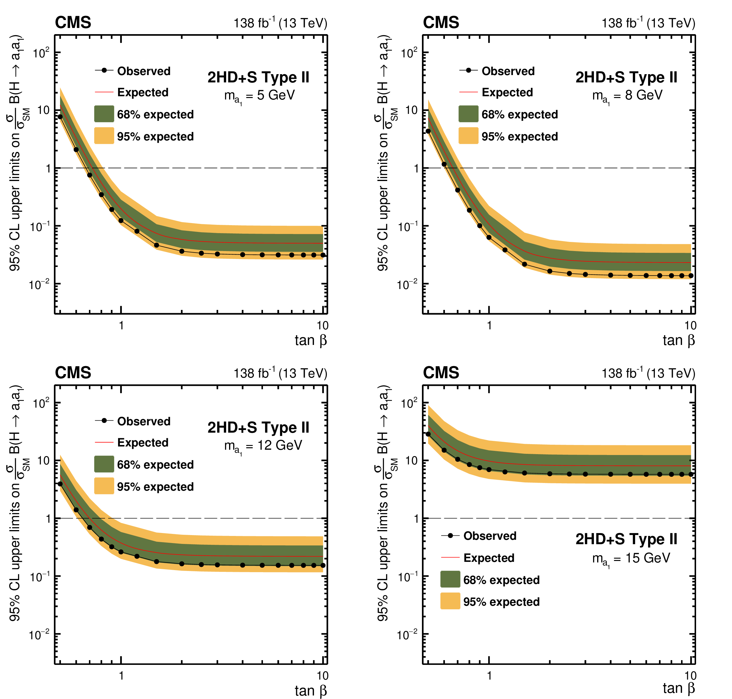
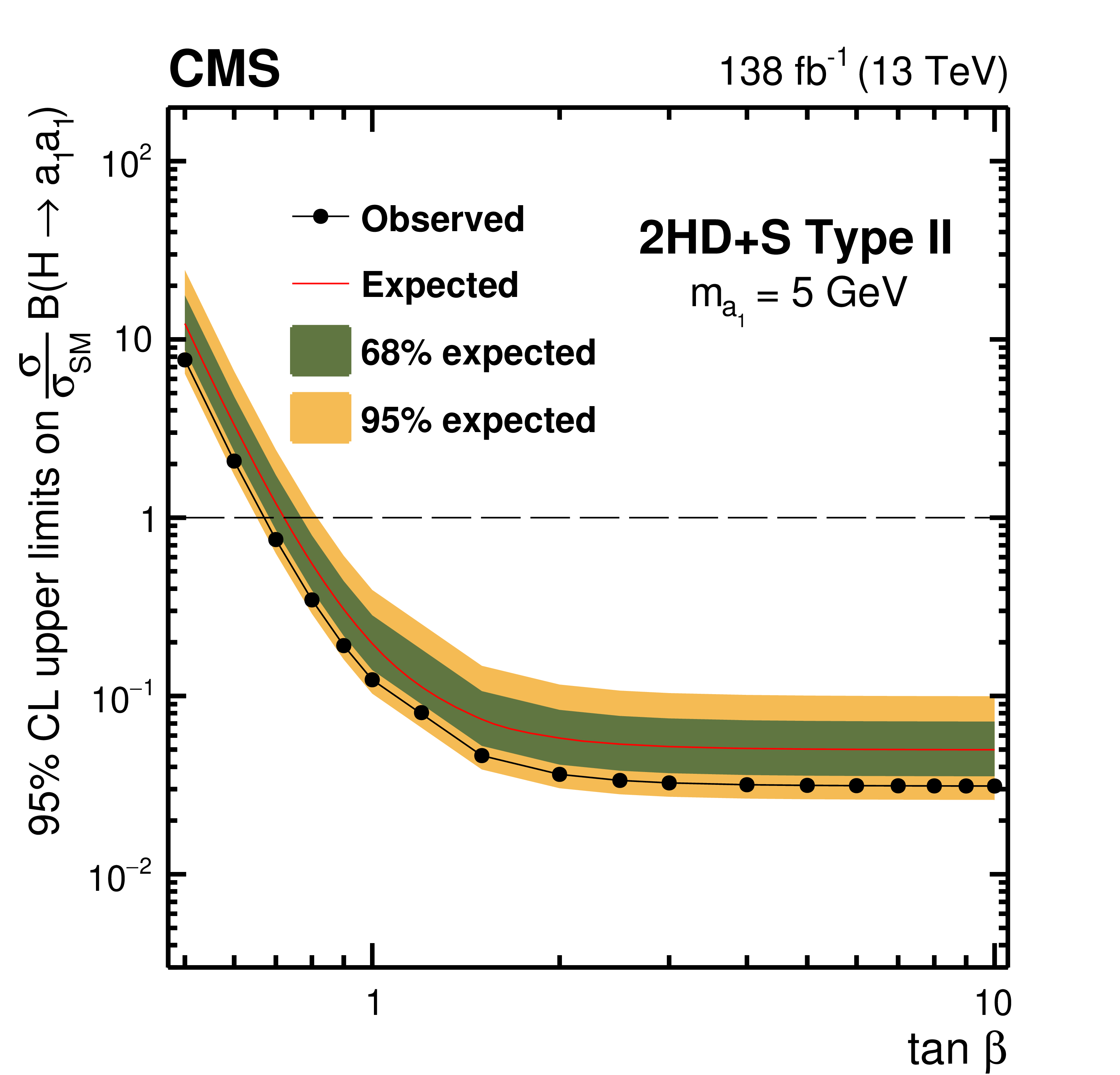
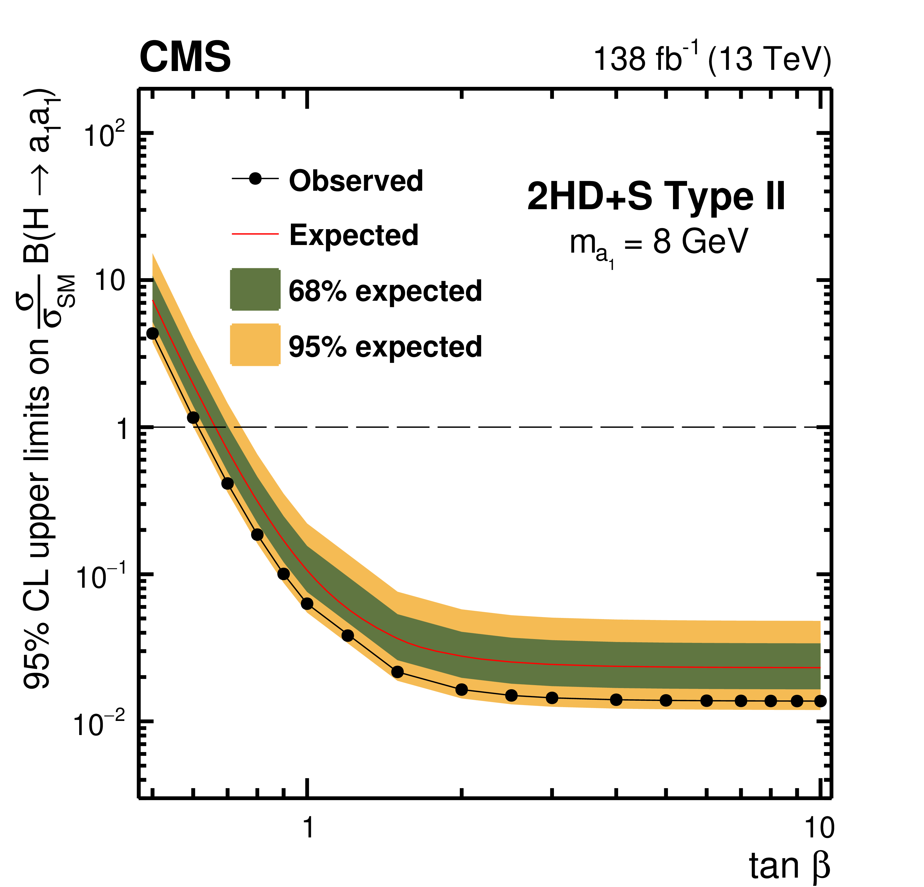
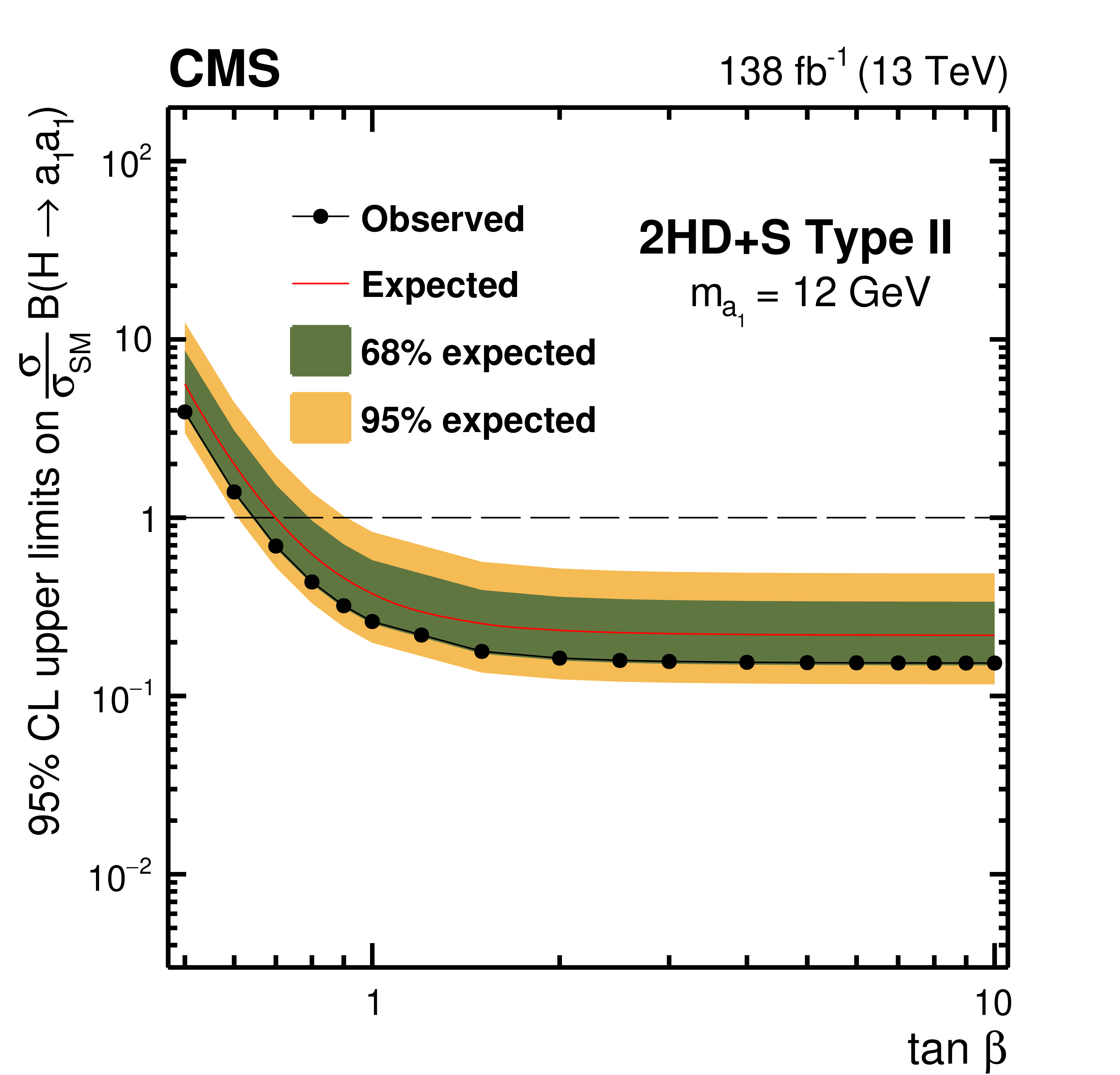
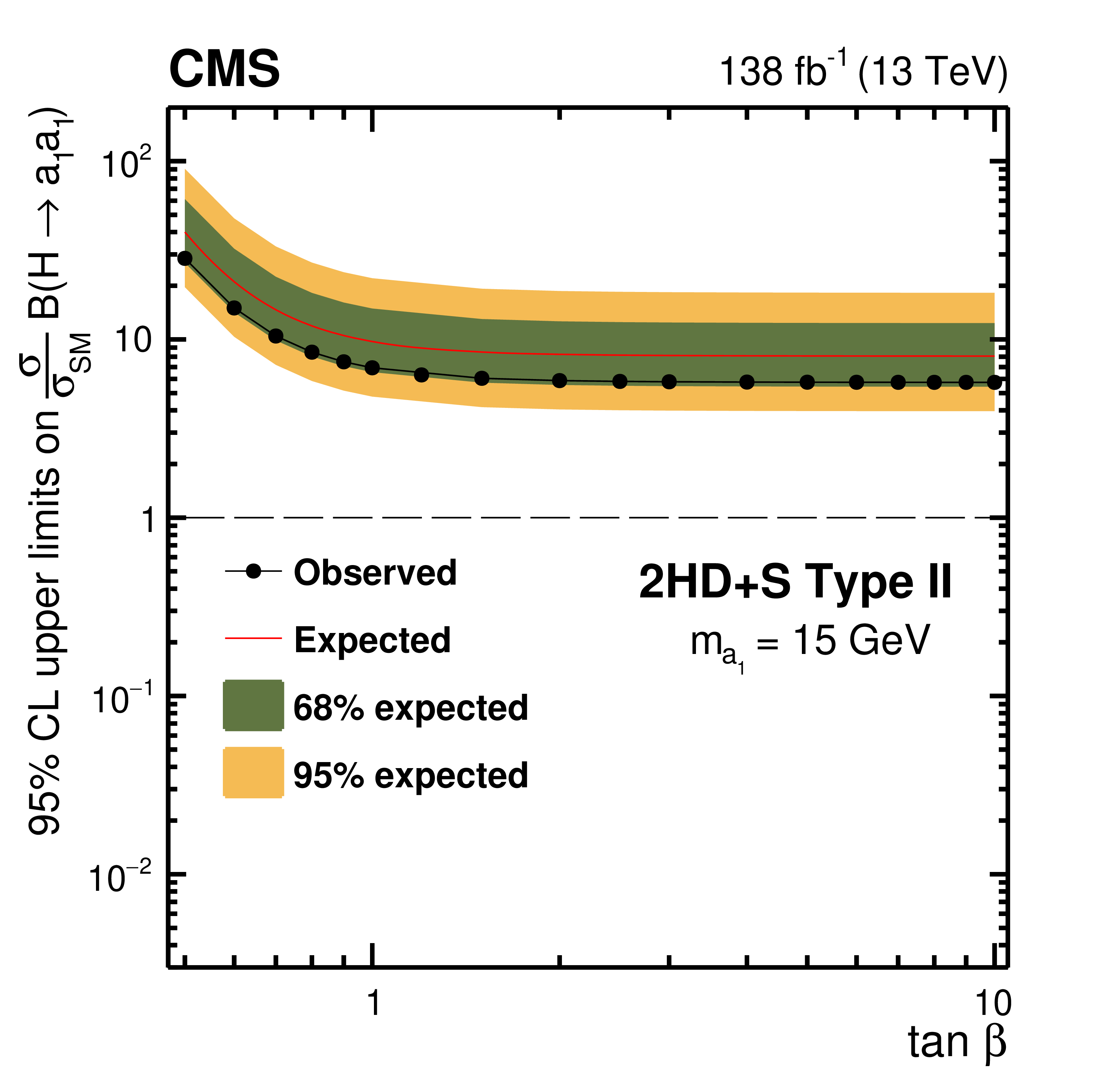
Figure 11:
The observed (points) and expected (red line) 95% CL upper limits on $ \sigma (\mathrm{p}\mathrm{p} \to \mathrm{H}+\mathrm{X}) {\mathcal{B}} (\mathrm{H} \to \mathrm{a}_{1} \mathrm{a}_{1}) $, relative to $ \sigma_\text{SM} $, as a function of $ \tan\beta $ for the Type II 2HD+S model with $ m_{\mathrm{a}_{1}} $= 5 GeV (upper left), $ m_{\mathrm{a}_{1}} $= 8 GeV (upper right), $ m_{\mathrm{a}_{1}} $= 12 GeV (lower left), and $ m_{\mathrm{a}_{1}} $= 15 GeV (lower right). |
png pdf |
Figure 11-a:
The observed (points) and expected (red line) 95% CL upper limits on $ \sigma (\mathrm{p}\mathrm{p} \to \mathrm{H}+\mathrm{X}) {\mathcal{B}} (\mathrm{H} \to \mathrm{a}_{1} \mathrm{a}_{1}) $, relative to $ \sigma_\text{SM} $, as a function of $ \tan\beta $ for the Type II 2HD+S model with $ m_{\mathrm{a}_{1}} $= 5 GeV (upper left), $ m_{\mathrm{a}_{1}} $= 8 GeV (upper right), $ m_{\mathrm{a}_{1}} $= 12 GeV (lower left), and $ m_{\mathrm{a}_{1}} $= 15 GeV (lower right). |
png pdf |
Figure 11-b:
The observed (points) and expected (red line) 95% CL upper limits on $ \sigma (\mathrm{p}\mathrm{p} \to \mathrm{H}+\mathrm{X}) {\mathcal{B}} (\mathrm{H} \to \mathrm{a}_{1} \mathrm{a}_{1}) $, relative to $ \sigma_\text{SM} $, as a function of $ \tan\beta $ for the Type II 2HD+S model with $ m_{\mathrm{a}_{1}} $= 5 GeV (upper left), $ m_{\mathrm{a}_{1}} $= 8 GeV (upper right), $ m_{\mathrm{a}_{1}} $= 12 GeV (lower left), and $ m_{\mathrm{a}_{1}} $= 15 GeV (lower right). |
png pdf |
Figure 11-c:
The observed (points) and expected (red line) 95% CL upper limits on $ \sigma (\mathrm{p}\mathrm{p} \to \mathrm{H}+\mathrm{X}) {\mathcal{B}} (\mathrm{H} \to \mathrm{a}_{1} \mathrm{a}_{1}) $, relative to $ \sigma_\text{SM} $, as a function of $ \tan\beta $ for the Type II 2HD+S model with $ m_{\mathrm{a}_{1}} $= 5 GeV (upper left), $ m_{\mathrm{a}_{1}} $= 8 GeV (upper right), $ m_{\mathrm{a}_{1}} $= 12 GeV (lower left), and $ m_{\mathrm{a}_{1}} $= 15 GeV (lower right). |
png pdf |
Figure 11-d:
The observed (points) and expected (red line) 95% CL upper limits on $ \sigma (\mathrm{p}\mathrm{p} \to \mathrm{H}+\mathrm{X}) {\mathcal{B}} (\mathrm{H} \to \mathrm{a}_{1} \mathrm{a}_{1}) $, relative to $ \sigma_\text{SM} $, as a function of $ \tan\beta $ for the Type II 2HD+S model with $ m_{\mathrm{a}_{1}} $= 5 GeV (upper left), $ m_{\mathrm{a}_{1}} $= 8 GeV (upper right), $ m_{\mathrm{a}_{1}} $= 12 GeV (lower left), and $ m_{\mathrm{a}_{1}} $= 15 GeV (lower right). |
png pdf |
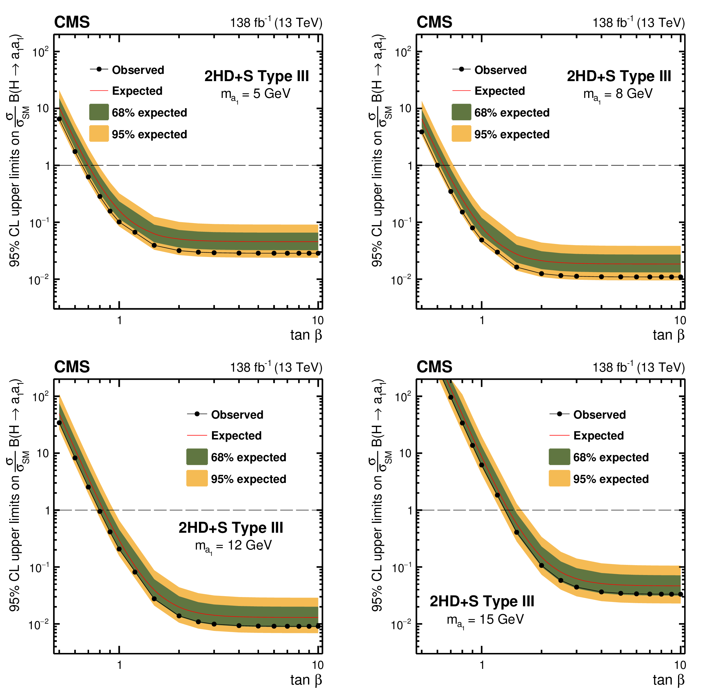
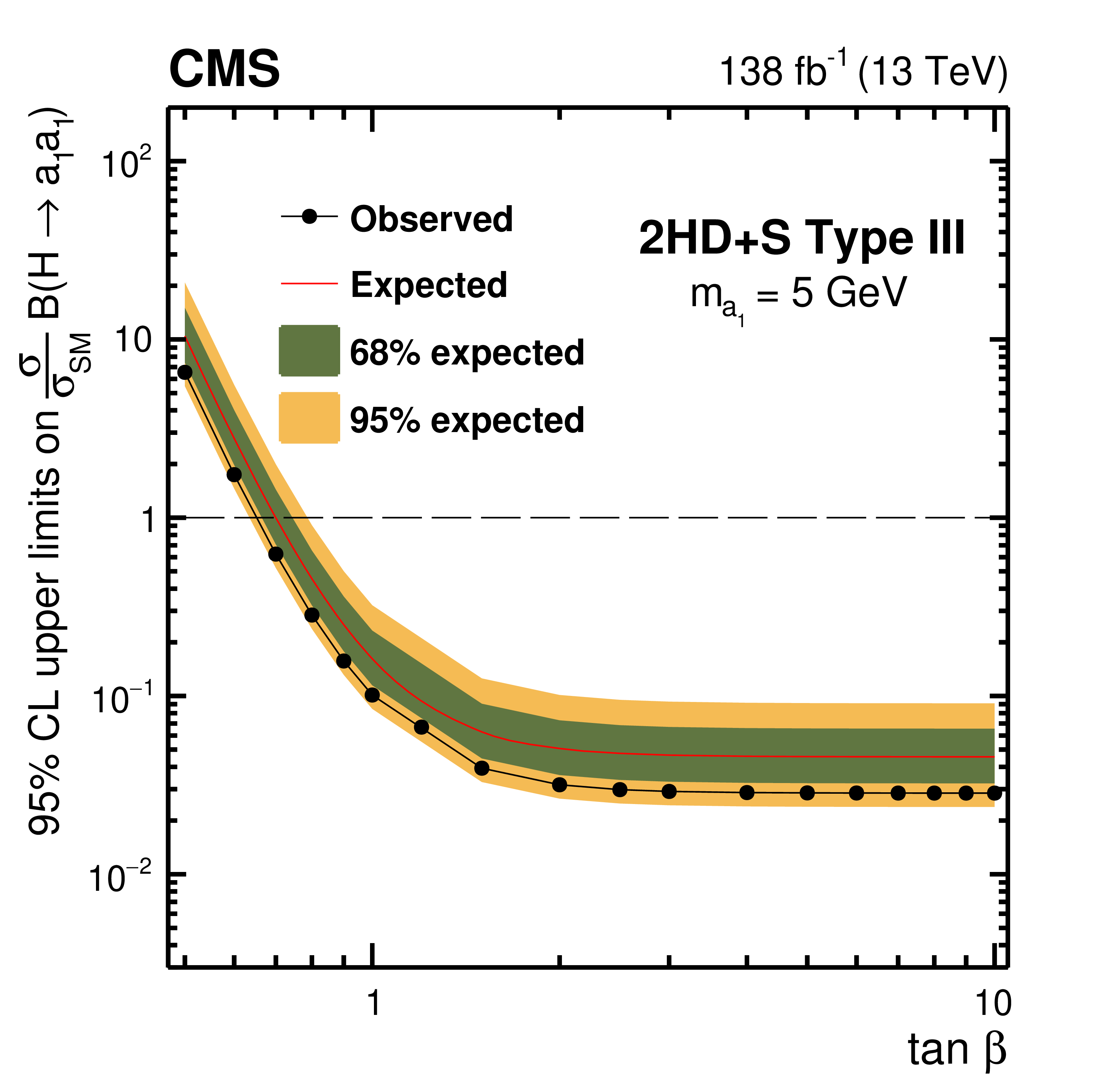
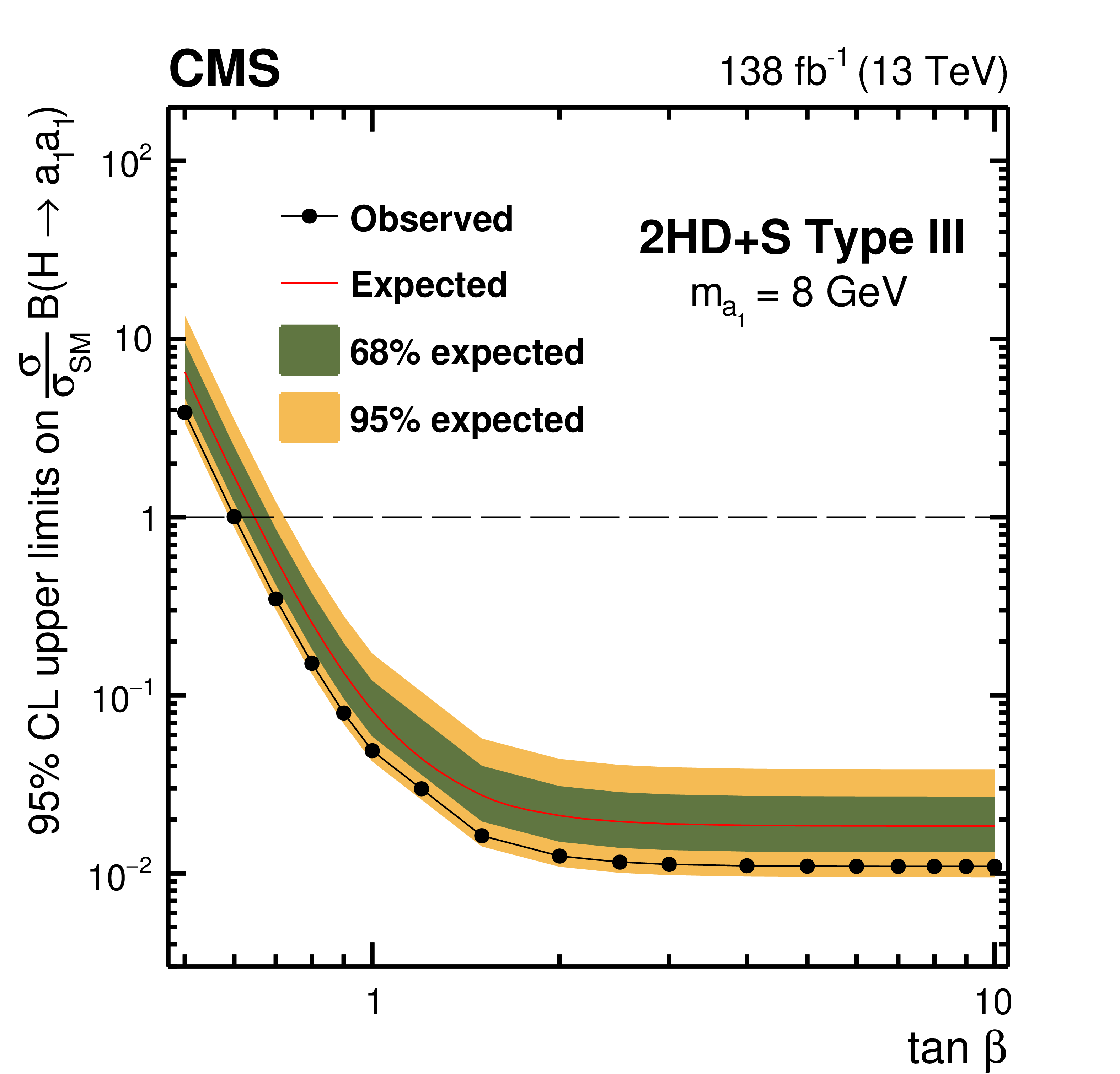
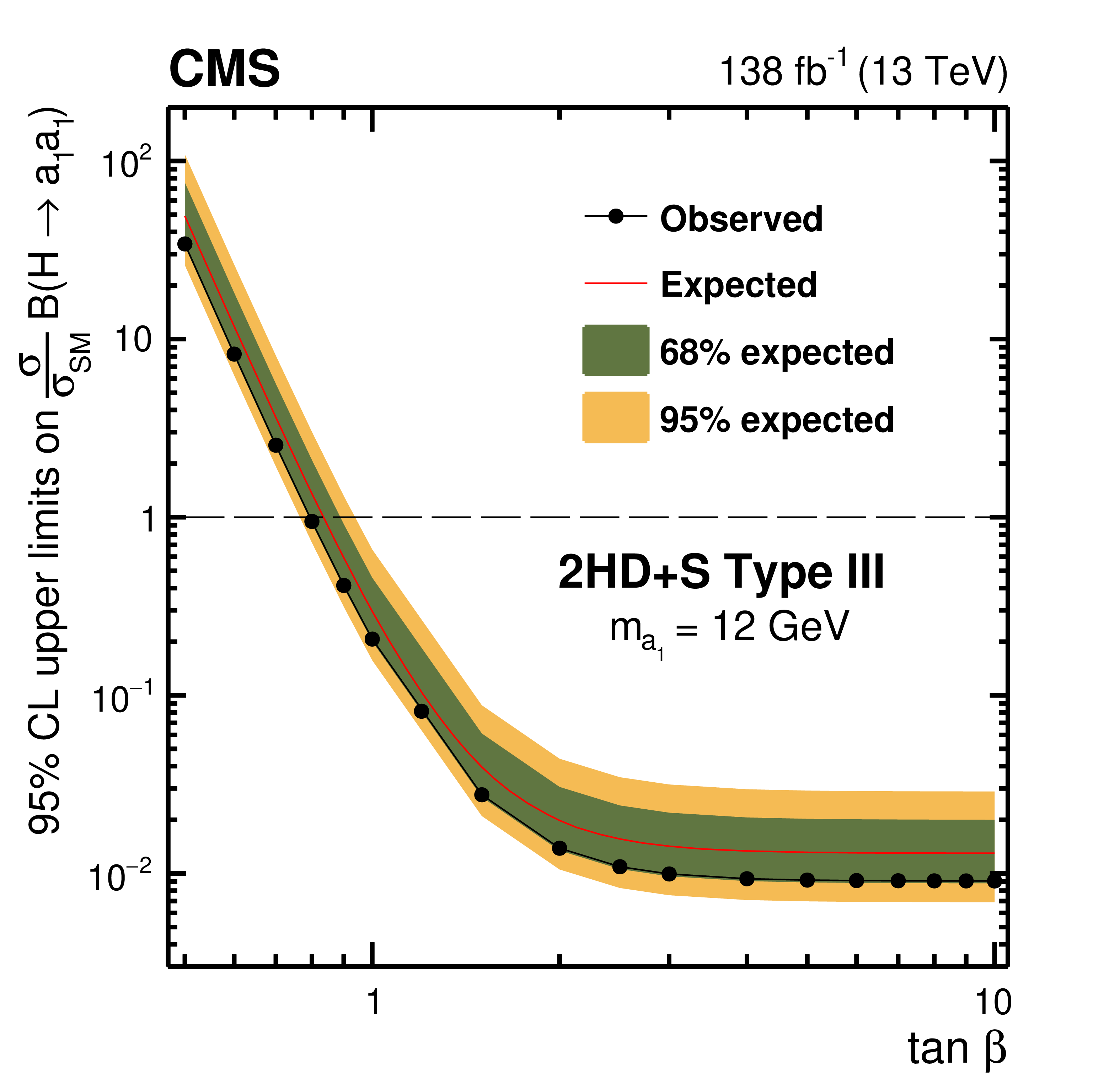
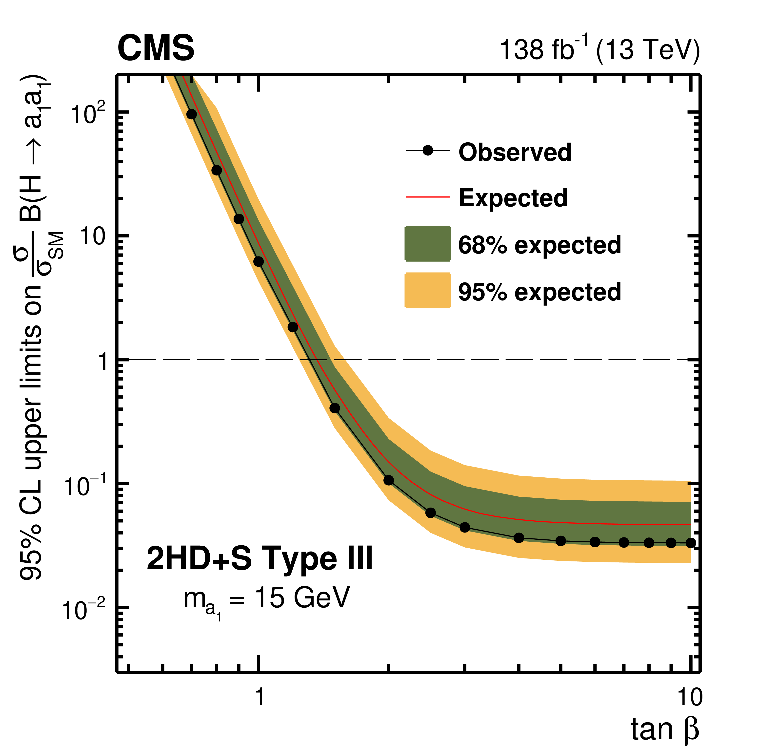
Figure 12:
The observed (points) and expected (red line) 95% CL upper limits on $ \sigma (\mathrm{p}\mathrm{p} \to \mathrm{H}+\mathrm{X}) {\mathcal{B}} (\mathrm{H} \to \mathrm{a}_{1} \mathrm{a}_{1}) $, relative to $ \sigma_\text{SM} $, as a function of $ \tan\beta $ for the Type III 2HD+S model with $ m_{\mathrm{a}_{1}} $= 5 GeV (upper left), $ m_{\mathrm{a}_{1}} $= 8 GeV (upper right), $ m_{\mathrm{a}_{1}} $= 12 GeV (lower left), and $ m_{\mathrm{a}_{1}} $= 15 GeV (lower right). |
png pdf |
Figure 12-a:
The observed (points) and expected (red line) 95% CL upper limits on $ \sigma (\mathrm{p}\mathrm{p} \to \mathrm{H}+\mathrm{X}) {\mathcal{B}} (\mathrm{H} \to \mathrm{a}_{1} \mathrm{a}_{1}) $, relative to $ \sigma_\text{SM} $, as a function of $ \tan\beta $ for the Type III 2HD+S model with $ m_{\mathrm{a}_{1}} $= 5 GeV (upper left), $ m_{\mathrm{a}_{1}} $= 8 GeV (upper right), $ m_{\mathrm{a}_{1}} $= 12 GeV (lower left), and $ m_{\mathrm{a}_{1}} $= 15 GeV (lower right). |
png pdf |
Figure 12-b:
The observed (points) and expected (red line) 95% CL upper limits on $ \sigma (\mathrm{p}\mathrm{p} \to \mathrm{H}+\mathrm{X}) {\mathcal{B}} (\mathrm{H} \to \mathrm{a}_{1} \mathrm{a}_{1}) $, relative to $ \sigma_\text{SM} $, as a function of $ \tan\beta $ for the Type III 2HD+S model with $ m_{\mathrm{a}_{1}} $= 5 GeV (upper left), $ m_{\mathrm{a}_{1}} $= 8 GeV (upper right), $ m_{\mathrm{a}_{1}} $= 12 GeV (lower left), and $ m_{\mathrm{a}_{1}} $= 15 GeV (lower right). |
png pdf |
Figure 12-c:
The observed (points) and expected (red line) 95% CL upper limits on $ \sigma (\mathrm{p}\mathrm{p} \to \mathrm{H}+\mathrm{X}) {\mathcal{B}} (\mathrm{H} \to \mathrm{a}_{1} \mathrm{a}_{1}) $, relative to $ \sigma_\text{SM} $, as a function of $ \tan\beta $ for the Type III 2HD+S model with $ m_{\mathrm{a}_{1}} $= 5 GeV (upper left), $ m_{\mathrm{a}_{1}} $= 8 GeV (upper right), $ m_{\mathrm{a}_{1}} $= 12 GeV (lower left), and $ m_{\mathrm{a}_{1}} $= 15 GeV (lower right). |
png pdf |
Figure 12-d:
The observed (points) and expected (red line) 95% CL upper limits on $ \sigma (\mathrm{p}\mathrm{p} \to \mathrm{H}+\mathrm{X}) {\mathcal{B}} (\mathrm{H} \to \mathrm{a}_{1} \mathrm{a}_{1}) $, relative to $ \sigma_\text{SM} $, as a function of $ \tan\beta $ for the Type III 2HD+S model with $ m_{\mathrm{a}_{1}} $= 5 GeV (upper left), $ m_{\mathrm{a}_{1}} $= 8 GeV (upper right), $ m_{\mathrm{a}_{1}} $= 12 GeV (lower left), and $ m_{\mathrm{a}_{1}} $= 15 GeV (lower right). |
| Tables | |
png pdf |
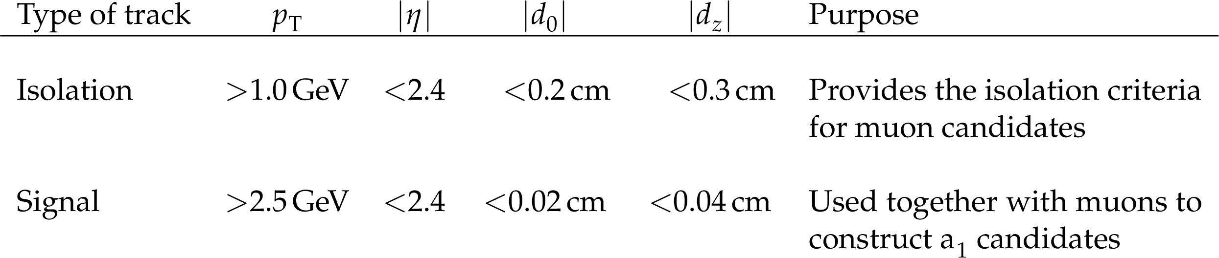
Table 1:
The purpose and selection criteria for the two types of tracks used in the selection procedure. |
png pdf |
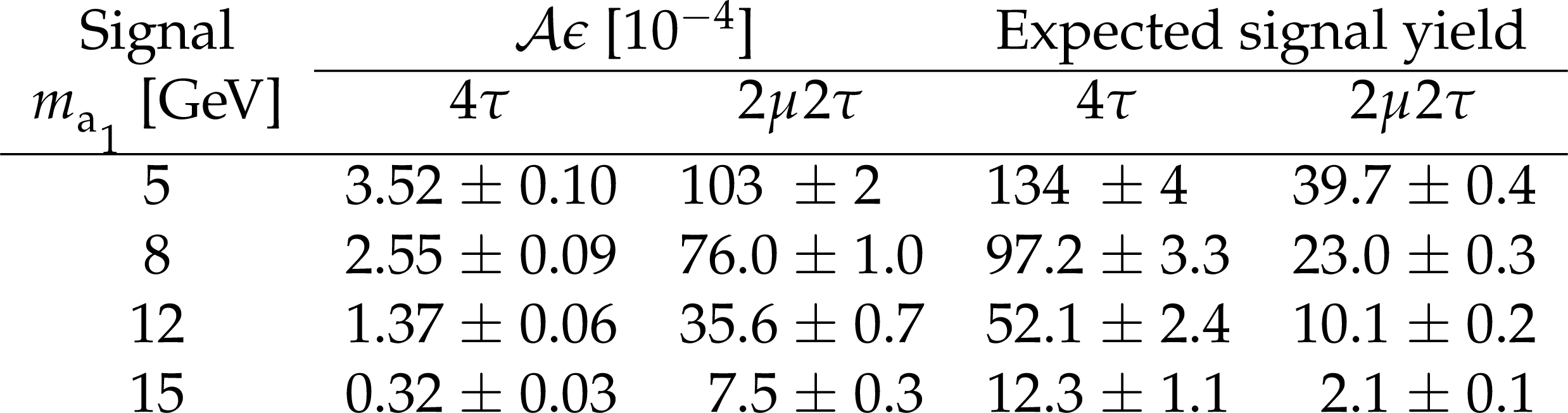
Table 2:
Signal acceptance times selection efficiency $ {\mathcal{A}}\epsilon $, defined in the text, and the number of expected signal events after selection in the $ \textit{SR} $, computed using simulated signal samples for representative mass hypotheses. The Higgs boson cross sections from $ {\mathrm{g}\mathrm{g}}\text{F} $, VBF, and VH production mechanisms are set to the SM predictions [62]. The number of expected signal events is computed for a benchmark value of the branching fraction $ {\mathcal{B}}(\mathrm{H} \to \mathrm{a}_{1} \mathrm{a}_{1}) {\mathcal{B}}^{2} (\mathrm{a}_{1} \to \tau \tau)= $ 0.05. The quoted uncertainties in the predictions from simulation include only the statistical component. In data, 7803 events are selected in the $ \textit{SR} $. |
png pdf |
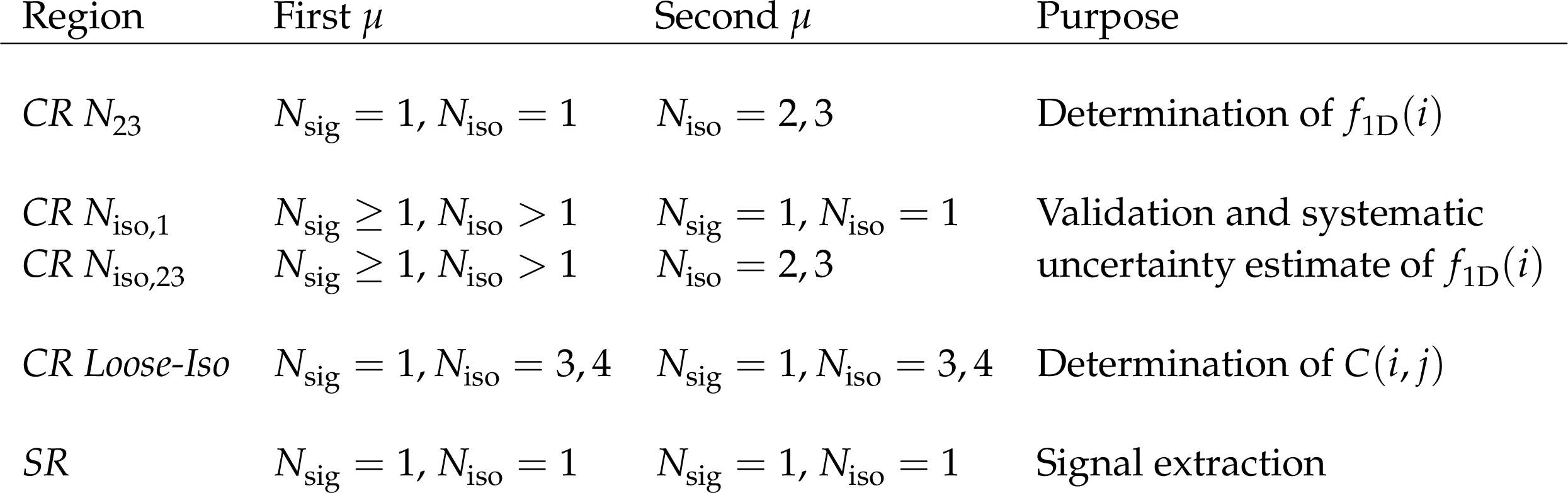
Table 3:
Definition of the \CRs used to construct and validate the background model. The last row defines the $ \textit{SR} $. The symbols $ N_\text{iso} $ and $ N_\text{sig} $ denote the number of isolation and signal tracks, respectively, within a cone of $ \Delta R= $ 0.5 around the muon momentum direction. In cases where $ N_\text{sig} $ is not mentioned, there is no explicit requirement on the number of signal tracks. |

png pdf |
Table 4:
Summary of systematic uncertainties affecting the estimation of signal and background. The terms ISR and FSR refer to initial- and final-state radiation, and the symbols $ \mu_\text{R} $ and $ \mu_\text{F} $ denote the renormalization and factorization scales, respectively. The impact of shape-altering and bin-by-bin uncertainties is quoted in terms of relative variations of yields across all bins of the modeled $ (m_1,m_2) $ distributions. For the normalization (norm.) uncertainties, the impact on the overall estimated yield is reported. The last column indicates how a given uncertainty is correlated across the data-taking years. Bin-by-bin statistical uncertainties for simulated signal samples are quoted for the most populated bins containing 80% of the total yield of selected signal events. |
| Summary |
| A search for a pair of light pseudoscalar bosons ($ \mathrm{a}_{1} $) produced in decays of the 125 GeV Higgs boson (H), $ \mathrm{H}\to\mathrm{a}_{1}\mathrm{a}_{1} $, in final states with two muons and two charged-particle tracks is presented. The search is performed using data from proton-proton collisions at a center-of-mass energy of 13 TeV, collected by the CMS experiment at the LHC between 2016 and 2018, and corresponding to an integrated luminosity of 138 fb$ ^{-1} $. The analysis exploits the gluon-gluon fusion, vector boson fusion, and Higgs-strahlung production modes, and targets the $ \mathrm{H}\to \mathrm{a}_{1} \mathrm{a}_{1} \to 4\tau $ and 2$ \mu2\tau $ decay channels. Masses of the $ \mathrm{a}_{1} $ boson ($ m_{\mathrm{a}_{1}} $) in the range 4--15 GeV are examined. No excess of data above the standard model (SM) background prediction is found. Upper limits on the product of the inclusive signal cross section and the branching fraction, $ \sigma (\mathrm{p}\mathrm{p} \to \mathrm{H}+\mathrm{X}) {\mathcal{B}} (\mathrm{H} \to \mathrm{a}_{1} \mathrm{a}_{1}) \mathcal{B}^2(\mathrm{a}_{1} \to \tau\tau) $, relative to the SM Higgs boson production cross section $ \sigma_\text{SM} $, are set at 95% confidence level (CL) by combining the 4$ \tau $ and 2$ \mu2\tau $ decay channels, assuming Yukawa-like couplings of $ \mathrm{a}_{1} $ to fermions. The observed limits range from 0.007 at $ m_{\mathrm{a}_{1}}= $ 11 GeV to 0.079 at $ m_{\mathrm{a}_{1}}= $ 4 GeV. The expected limits in the absence of signal span from 0.011 at $ m_{\mathrm{a}_{1}}= $ 11 GeV to 0.066 at $ m_{\mathrm{a}_{1}}= $ 4 GeV. The results are a significant improvement over the previous CMS analysis at 13 TeV [29], exceeding the anticipated improvement from the larger data sample alone. The sensitivity is enhanced by a factor of 2 to 4, depending on $ m_{\mathrm{a}_1} $, which can be attributed to the introduction of a veto for b-tagged jets and further optimization of the selection criteria targeting the $ \mathrm{a}_{1}\to\tau\tau $ and $ \mu\mu $ decays. The analysis also exceeds the sensitivity of a similar search performed by the ATLAS Collaboration in the same channel using a comparable amount of integrated luminosity [33]. The results of the search are also interpreted in the context of various models with two Higgs doublets and an additional complex singlet field (2HD+S). For the Type II 2HD+S scenario, realized in the next-to-minimal supersymmetric SM, 95% CL upper limits between 0.013 and 0.092 are set on $ \sigma (\mathrm{p}\mathrm{p} \to \mathrm{H}+\mathrm{X}) {\mathcal{B}} (\mathrm{H} \to \mathrm{a}_{1} \mathrm{a}_{1}) $, relative to $ \sigma_\text{SM} $, for 4$ < m_{\mathrm{a}_{1}} < $ 9 GeV and $ \tan\beta > $ 5. The analysis sets the most stringent constraints to date for the Type III 2HD+S scenario. Upper limits in the range 0.010--0.057 are obtained for probed mass hypotheses in the ranges 5 $ < m_{\mathrm{a}_{1}} < $ 9 GeV and 12$ < m_{\mathrm{a}_{1}} < $ 14 GeV for $ \tan\beta > $ 2. |
| References | ||||
| 1 | ATLAS Collaboration | Observation of a new particle in the search for the standard model Higgs boson with the ATLAS detector at the LHC | PLB 716 (2012) 1 | 1207.7214 |
| 2 | CMS Collaboration | Observation of a new boson at a mass of 125 GeV with the CMS experiment at the LHC | PLB 716 (2012) 30 | CMS-HIG-12-028 1207.7235 |
| 3 | CMS Collaboration | Observation of a new boson with mass near 125 GeV in pp collisions at $ \sqrt{s} = $ 7 and 8 TeV | JHEP 06 (2013) 081 | CMS-HIG-12-036 1303.4571 |
| 4 | ATLAS Collaboration | A detailed map of Higgs boson interactions by the ATLAS experiment ten years after the discovery | Nature 607 (2022) 52 | 2207.00092 |
| 5 | CMS Collaboration | A portrait of the Higgs boson by the CMS experiment ten years after the discovery. | Nature 607 (2022) 60 | CMS-HIG-22-001 2207.00043 |
| 6 | T. D. Lee | A theory of spontaneous T violation | PRD 8 (1973) 1226 | |
| 7 | G. C. Branco et al. | Theory and phenomenology of two-Higgs-doublet models | Phys. Rept. 516 (2012) 1 | 1106.0034 |
| 8 | D. Curtin et al. | Exotic decays of the 125 GeV Higgs boson | PRD 90 (2014) 075004 | 1312.4992 |
| 9 | P. Fayet | Supergauge invariant extension of the Higgs mechanism and a model for the electron and its neutrino | NPB 90 (1975) 104 | |
| 10 | P. Fayet | Spontaneously broken supersymmetric theories of weak, electromagnetic and strong interactions | PLB 69 (1977) 489 | |
| 11 | U. Ellwanger, C. Hugonie, and A. M. Teixeira | The next-to-minimal supersymmetric standard model | Phys. Rept. 496 (2010) 1 | 0910.1785 |
| 12 | M. Maniatis | The next-to-minimal supersymmetric extension of the standard model reviewed | Int. J. Mod. Phys. A 25 (2010) 3505 | 0906.0777 |
| 13 | J. E. Kim and H. P. Nilles | The $ \mu $-problem and the strong CP-problem | PLB 138 (1984) 150 | |
| 14 | S. Ramos-Sanchez | The $ \mu $-problem, the NMSSM and string theory | Fortsch. Phys. 58 (2010) 748 | 1003.1307 |
| 15 | ATLAS Collaboration | Search for new light gauge bosons in Higgs boson decays to four-lepton final states in pp collisions at $ \sqrt{s} = $ 8 TeV with the ATLAS detector at the LHC | PRD 92 (2015) 092001 | 1505.07645 |
| 16 | CMS Collaboration | Search for a non-standard-model Higgs boson decaying to a pair of new light bosons in four-muon Final States | PLB 726 (2013) 564 | CMS-EXO-12-012 1210.7619 |
| 17 | CMS Collaboration | A search for pair production of new light bosons decaying into muons | PLB 752 (2016) 146 | CMS-HIG-13-010 1506.00424 |
| 18 | CMS Collaboration | Search for light bosons in decays of the 125 GeV Higgs boson in proton-proton collisions at $ \sqrt{s} = $ 8 TeV | JHEP 10 (2017) 076 | CMS-HIG-16-015 1701.02032 |
| 19 | CMS Collaboration | Search for a very light NMSSM Higgs boson produced in decays of the 125 GeV scalar boson and decaying into $ \tau $ leptons in pp collisions at $ \sqrt{s} = $ 8 TeV | JHEP 01 (2016) 079 | CMS-HIG-14-019 1510.06534 |
| 20 | ATLAS Collaboration | Search for new phenomena in events with at least three photons collected in pp collisions at $ \sqrt{s} = $ 8 TeV with the ATLAS detector | EPJC 76 (2016) 210 | 1509.05051 |
| 21 | ATLAS Collaboration | Search for Higgs boson decays to beyond-the-standard-model light bosons in four-lepton events with the ATLAS detector at $ \sqrt{s} = $ 13 TeV | JHEP 06 (2018) 166 | 1802.03388 |
| 22 | CMS Collaboration | A search for pair production of new light bosons decaying into muons in proton-proton collisions at 13 TeV | PLB 796 (2019) 131 | CMS-HIG-18-003 1812.00380 |
| 23 | ATLAS Collaboration | Search for Higgs bosons decaying to aa in the $ \mu\mu\tau\tau $ final state in pp collisions at $ \sqrt{s} = $ 8 TeV with the ATLAS experiment | PRD 92 (2015) 052002 | 1505.01609 |
| 24 | CMS Collaboration | Search for an exotic decay of the Higgs boson to a pair of light pseudoscalars in the final state of two muons and two $ \tau $ leptons in proton-proton collisions at $ \sqrt{s} = $ 13 TeV | JHEP 11 (2018) 018 | CMS-HIG-17-029 1805.04865 |
| 25 | CMS Collaboration | Search for a light pseudoscalar Higgs boson in the boosted $ \mu\mu\tau\tau $ final state in proton-proton collisions at $ \sqrt{s} = $ 13 TeV | JHEP 08 (2020) 139 | CMS-HIG-18-024 2005.08694 |
| 26 | ATLAS Collaboration | Search for Higgs boson decays into a pair of light bosons in the bb$ \mu\mu $ final state in pp collision at $ \sqrt{s} = $ 13 TeV with the ATLAS detector | PLB 790 (2019) 1 | 1807.00539 |
| 27 | CMS Collaboration | Search for exotic decays of the Higgs boson to a pair of pseudoscalars in the $ \mu\mu $bb and $ \tau\tau $bb final states | EPJC 84 (2024) 493 | CMS-HIG-22-007 2402.13358 |
| 28 | ATLAS Collaboration | Search for Higgs boson decays into pairs of light (pseudo)scalar particles in the $ \gamma\gamma \mathrm{jj} $ final state in pp collisions at $ \sqrt{s} = $ 13 TeV with the ATLAS detector | PLB 782 (2018) 750 | 1803.11145 |
| 29 | CMS Collaboration | Search for light pseudoscalar boson pairs produced from decays of the 125 GeV Higgs boson in final states with two muons and two nearby tracks in pp collisions at $ \sqrt{s} = $ 13 TeV | PLB 800 (2020) 135087 | CMS-HIG-18-006 1907.07235 |
| 30 | CMS Collaboration | Search for the decay of the Higgs boson to a pair of light pseudoscalar bosons in the final state with four bottom quarks in proton-proton collisions at $ \sqrt{\textrm{s}} = $ 13 TeV | JHEP 06 (2024) 097 | CMS-HIG-18-026 2403.10341 |
| 31 | CMS Collaboration | Search for the exotic decay of the Higgs boson into two light pseudoscalars with four photons in the final state in proton-proton collisions at $ \sqrt{s} = $ 13 TeV | JHEP 07 (2023) 148 | CMS-HIG-21-003 2208.01469 |
| 32 | CMS Collaboration | Search for exotic Higgs boson decays $ \mathrm{H} \to \mathcal{A}\mathcal{A} \to 4\gamma $ with events containing two merged diphotons in proton-proton collisions at $ \sqrt{s} = $ 13 TeV | PRL 131 (2023) 101801 | CMS-HIG-21-016 2209.06197 |
| 33 | ATLAS Collaboration | Search for Higgs boson exotic decays into Lorentz-boosted light bosons in the four-$ \tau $ final state at $ \sqrt{s} = $ 13 TeV with the ATLAS detector | Submitted to Phys. Lett. B, 2025 | 2503.05463 |
| 34 | CMS Collaboration | Identification of hadronic tau lepton decays using a deep neural network | JINST 17 (2022) P07023 | CMS-TAU-20-001 2201.08458 |
| 35 | CMS Collaboration | HEPData record for this analysis | link | |
| 36 | CMS Collaboration | The CMS experiment at the CERN LHC | JINST 3 (2008) S08004 | |
| 37 | CMS Collaboration | Development of the CMS detector for the CERN LHC Run 3 | JINST 19 (2024) P05064 | CMS-PRF-21-001 2309.05466 |
| 38 | CMS Collaboration | Performance of the CMS Level-1 trigger in proton-proton collisions at $ \sqrt{s} = $ 13 TeV | JINST 15 (2020) P10017 | CMS-TRG-17-001 2006.10165 |
| 39 | CMS Collaboration | The CMS trigger system | JINST 12 (2017) P01020 | CMS-TRG-12-001 1609.02366 |
| 40 | CMS Collaboration | Performance of the CMS high-level trigger during LHC Run 2 | JINST 19 (2024) P11021 | CMS-TRG-19-001 2410.17038 |
| 41 | T. Sjöstrand et al. | An introduction to PYTHIA 8.2 | Comput. Phys. Commun. 191 (2015) 159 | 1410.3012 |
| 42 | J. Alwall et al. | The automated computation of tree-level and next-to-leading order differential cross sections, and their matching to parton shower simulations | JHEP 07 (2014) 079 | 1405.0301 |
| 43 | G. Bozzi, S. Catani, D. de Florian, and M. Grazzini | Transverse-momentum resummation and the spectrum of the Higgs boson at the LHC | NPB 737 (2006) 73 | hep-ph/0508068 |
| 44 | D. de Florian, G. Ferrera, M. Grazzini, and D. Tommasini | Transverse-momentum resummation: Higgs boson production at the Tevatron and the LHC | JHEP 11 (2011) 064 | 1109.2109 |
| 45 | S. Alioli, P. Nason, C. Oleari, and E. Re | NLO Higgs boson production via gluon fusion matched with shower in POWHEG | JHEP 04 (2009) 002 | 0812.0578 |
| 46 | P. Nason | A new method for combining NLO QCD with shower Monte Carlo algorithms | JHEP 11 (2004) 040 | hep-ph/0409146 |
| 47 | S. Frixione, P. Nason, and C. Oleari | Matching NLO QCD computations with parton shower simulations: the POWHEG method | JHEP 11 (2007) 070 | 0709.2092 |
| 48 | CMS Collaboration | Extraction and validation of a new set of CMS PYTHIA8 tunes from underlying-event measurements | EPJC 80 (2020) 4 | CMS-GEN-17-001 1903.12179 |
| 49 | J. Alwall et al. | Comparative study of various algorithms for the merging of parton showers and matrix elements in hadronic collisions | EPJC 53 (2008) 473 | 0706.2569 |
| 50 | GEANT4 Collaboration | GEANT4---a simulation toolkit | NIM A 506 (2003) 250 | |
| 51 | J. Allison et al. | GEANT4 developments and applications | IEEE Trans. Nucl. Sci. 53 (2006) 270 | |
| 52 | CMS Collaboration | Description and performance of track and primary-vertex reconstruction with the CMS tracker | JINST 9 (2014) P10009 | CMS-TRK-11-001 1405.6569 |
| 53 | CMS Collaboration | Technical proposal for the Phase-II upgrade of the Compact Muon Solenoid | CMS Technical Proposal CERN-LHCC-2015-010, CMS-TDR-15-02, 2015 CDS |
|
| 54 | CMS Collaboration | Particle-flow reconstruction and global event description with the CMS detector | JINST 12 (2017) P10003 | CMS-PRF-14-001 1706.04965 |
| 55 | CMS Collaboration | Performance of the CMS muon detector and muon reconstruction with proton-proton collisions at $ \sqrt{s} = $ 13 TeV | JINST 13 (2018) P06015 | CMS-MUO-16-001 1804.04528 |
| 56 | M. Cacciari, G. P. Salam, and G. Soyez | The anti-$ k_{\mathrm{T}} $ jet clustering algorithm | JHEP 04 (2008) 063 | 0802.1189 |
| 57 | M. Cacciari, G. P. Salam, and G. Soyez | FastJet user manual | EPJC 72 (2012) 1896 | 1111.6097 |
| 58 | CMS Collaboration | Jet energy scale and resolution in the CMS experiment in pp collisions at 8 TeV | JINST 12 (2017) P02014 | CMS-JME-13-004 1607.03663 |
| 59 | E. Bols et al. | Jet Flavour Classification Using DeepJet | JINST 15 (2020) P12012 | 2008.10519 |
| 60 | CMS Collaboration | Performance summary of AK4 jet b tagging with data from proton-proton collisions at 13 TeV with the CMS detector | CMS Detector Performance Summary CMS-DP-2023-005, 2023 CDS |
|
| 61 | CMS Collaboration | Identification of heavy-flavour jets with the CMS detector in pp collisions at 13 TeV | JINST 13 (2018) P05011 | CMS-BTV-16-002 1712.07158 |
| 62 | LHC Higgs Cross Section Working Group | Handbook of LHC Higgs cross sections: 4. Deciphering the nature of the Higgs sector | CERN Report CERN-2017-002-M, 2017 link |
1610.07922 |
| 63 | M. Lisanti and J. G. Wacker | Discovering the Higgs boson with low mass muon pairs | PRD 79 (2010) 115006 | 0903.1377 |
| 64 | R. J. Barlow and C. Beeston | Fitting using finite Monte Carlo samples | Comput. Phys. Commun. 77 (1993) 219 | |
| 65 | CMS Collaboration | Precision luminosity measurement in proton-proton collisions at $ \sqrt{s} = $ 13 TeV in 2015 and 2016 at CMS | EPJC 81 (2021) 800 | CMS-LUM-17-003 2104.01927 |
| 66 | CMS Collaboration | CMS luminosity measurement for the 2017 data-taking period at $ \sqrt{s} = $ 13 TeV | CMS Physics Analysis Summary, 2018 link |
CMS-PAS-LUM-17-004 |
| 67 | CMS Collaboration | CMS luminosity measurement for the 2018 data-taking period at $ \sqrt{s} = $ 13 TeV | CMS Physics Analysis Summary, 2019 link |
CMS-PAS-LUM-18-002 |
| 68 | CMS Collaboration | Measurement of the inclusive $ W $ and $ Z $ production cross sections in pp collisions at $ \sqrt{s} = $ 7 TeV | JHEP 10 (2011) 132 | CMS-EWK-10-005 1107.4789 |
| 69 | NNPDF Collaboration | Parton distributions for the LHC Run II | JHEP 04 (2015) 040 | 1410.8849 |
| 70 | CMS Collaboration | The CMS statistical analysis and combination tool: Combine | Comput. Softw. Big Sci. 8 (2024) 19 | CMS-CAT-23-001 2404.06614 |
| 71 | W. Verkerke and D. P. Kirkby | The RooFit toolkit for data modeling | in Statistical Problems in Particle Physics, Astrophysics and Cosmology, Proceedings, 2003 link |
physics/0306116 |
| 72 | L. Moneta et al. | The RooStats Project | PoS ACAT 057, 2010 link |
1009.1003 |
| 73 | J. K. Lindsey | Parametric Statistical Inference | Oxford University Press, ISBN 978023598, 1996 link |
|
| 74 | R. D. Cousins | Lectures on statistics in theory: prelude to statistics in practice | 1807.05996 | |
| 75 | T. Junk | Confidence level computation for combining searches with small statistics | NIM A 434 (1999) 435 | hep-ex/9902006 |
| 76 | A. L. Read | Presentation of search results: the $ \text{CL}_\text{s} $ technique | JPG 28 (2002) 2693 | |
| 77 | G. Cowan, K. Cranmer, E. Gross, and O. Vitells | Asymptotic formulae for likelihood-based tests of new physics | EPJC 71 (2011) 1554 | 1007.1727 |
| 78 | ATLAS and CMS Collaborations, and LHC Higgs Combination Group | Procedure for the LHC Higgs boson search combination in Summer 2011 | Technical Report CMS-NOTE-2011-005, ATL-PHYS-PUB-2011-11, 2011 | |
| 79 | U. Haisch, J. F. Kamenik, A. Malinauskas, and M. Spira | Collider constraints on light pseudoscalars | JHEP 03 (2018) 178 | 1802.02156 |
| 80 | M. Baumgart and A. Katz | Implications of a new light scalar near the bottomonium regime | JHEP 08 (2012) 133 | 1204.6032 |
|
|
Compact Muon Solenoid LHC, CERN |
|

|

|

|

|

|