

Compact Muon Solenoid
LHC, CERN
| CMS-HIG-22-007 ; CERN-EP-2023-284 | ||
| Search for exotic decays of the Higgs boson to a pair of pseudoscalars in the $ \mu\mu\mathrm{b}\mathrm{b} $ and $ \tau\tau\mathrm{b}\mathrm{b} $ final states | ||
| CMS Collaboration | ||
| 21 February 2024 | ||
| Eur. Phys. J. C 84 (2024) 493 | ||
| Abstract: A search for exotic decays of the Higgs boson (H) with a mass of 125 GeV to a pair of light pseudoscalars $ a_{1} $ is performed in final states where one pseudoscalar decays to two b quarks and the other to a pair of muons or $ \tau $ leptons. A data sample of proton-proton collisions at $ \sqrt{s}= $ 13 TeV corresponding to an integrated luminosity of 138 fb$ ^{-1} $ recorded with the CMS detector is analyzed. No statistically significant excess is observed over the standard model backgrounds. Upper limits are set at 95% confidence level (CL) on the Higgs boson branching fraction to $ \mu\mu\mathrm{b}\mathrm{b} $ and to $ \tau\tau\mathrm{b}\mathrm{b} $, via a pair of $ a_{1} $s. The limits depend on the pseudoscalar mass $ m_{a_{1}} $ and are observed to be in the range (0.17-3.3) $ \times $ 10$^{-4} $ and (1.7-7.7) $ \times $ 10$^{-2} $ in the $ \mu\mu\mathrm{b}\mathrm{b} $ and $ \tau\tau\mathrm{b}\mathrm{b} $ final states, respectively. In the framework of models with two Higgs doublets and a complex scalar singlet (2HDM+S), the results of the two final states are combined to determine model-independent upper limits on the branching fraction $ \mathcal{B}(\mathrm{H}\to a_{1} a_{1} \to \ell\ell\mathrm{b}\mathrm{b}) $ at 95% CL, with $ \ell $ being a muon or a $ \tau $ lepton. For different types of 2HDM+S, upper bounds on the branching fraction $ \mathcal{B}(\mathrm{H}\to a_{1} a_{1} ) $ are extracted from the combination of the two channels. In most of the Type II 2HDM+S parameter space, $ \mathcal{B}(\mathrm{H}\to a_{1} a_{1} ) $ values above 0.23 are excluded at 95% CL for $ m_{a_{1}} $ values between 15 and 60 GeV. | ||
| Links: e-print arXiv:2402.13358 [hep-ex] (PDF) ; CDS record ; inSPIRE record ; HepData record ; CADI line (restricted) ; | ||
| Figures | |
png pdf |
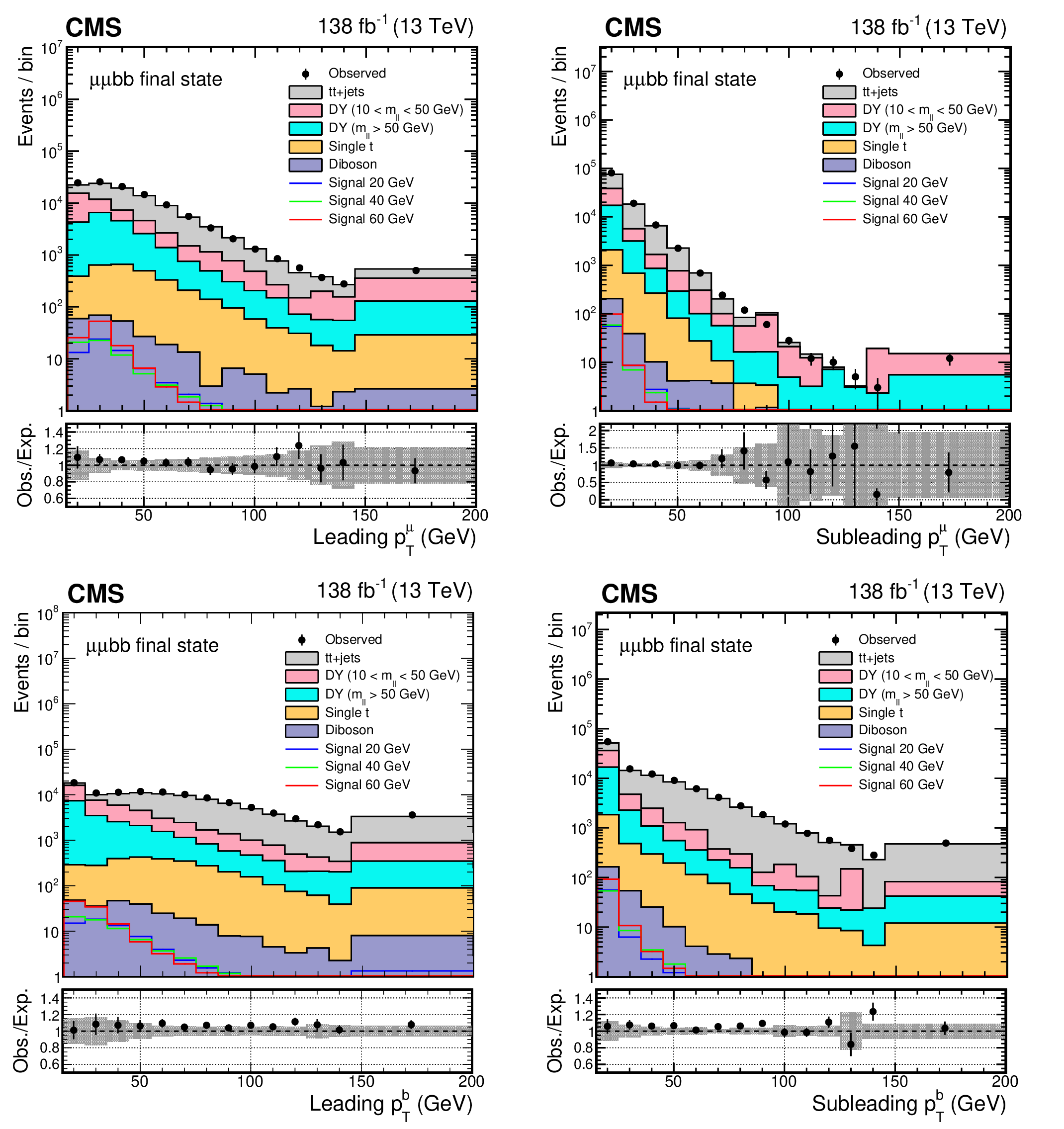
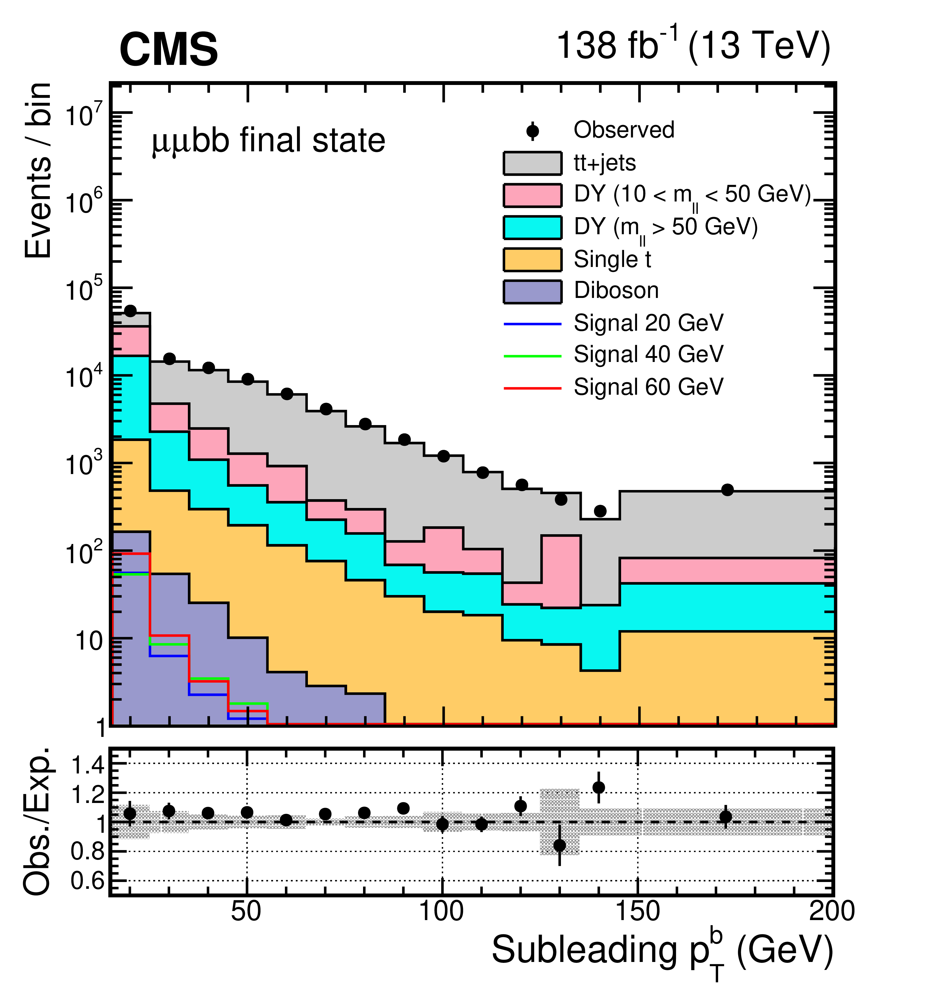
Figure 1:
The distributions of leading and subleading (upper) muon $ p_{\mathrm{T}} $ and (lower) b jet $ p_{\mathrm{T}} $ in the selected events. The uncertainty band in the lower panel represents the limited size of the simulated samples together with a 30% uncertainty in the low-mass DY cross section. Simulated samples are normalized using the corresponding theoretical cross sections. To evaluate the normalization of the signal, SM Higgs boson cross sections are multiplied by the $ \mathcal{B}(a_{1} a_{1} \to\mu\mu\mathrm{b}\mathrm{b}) $ value that is calculated in the Type III model with $ \tan\beta = $ 2. |
png pdf |
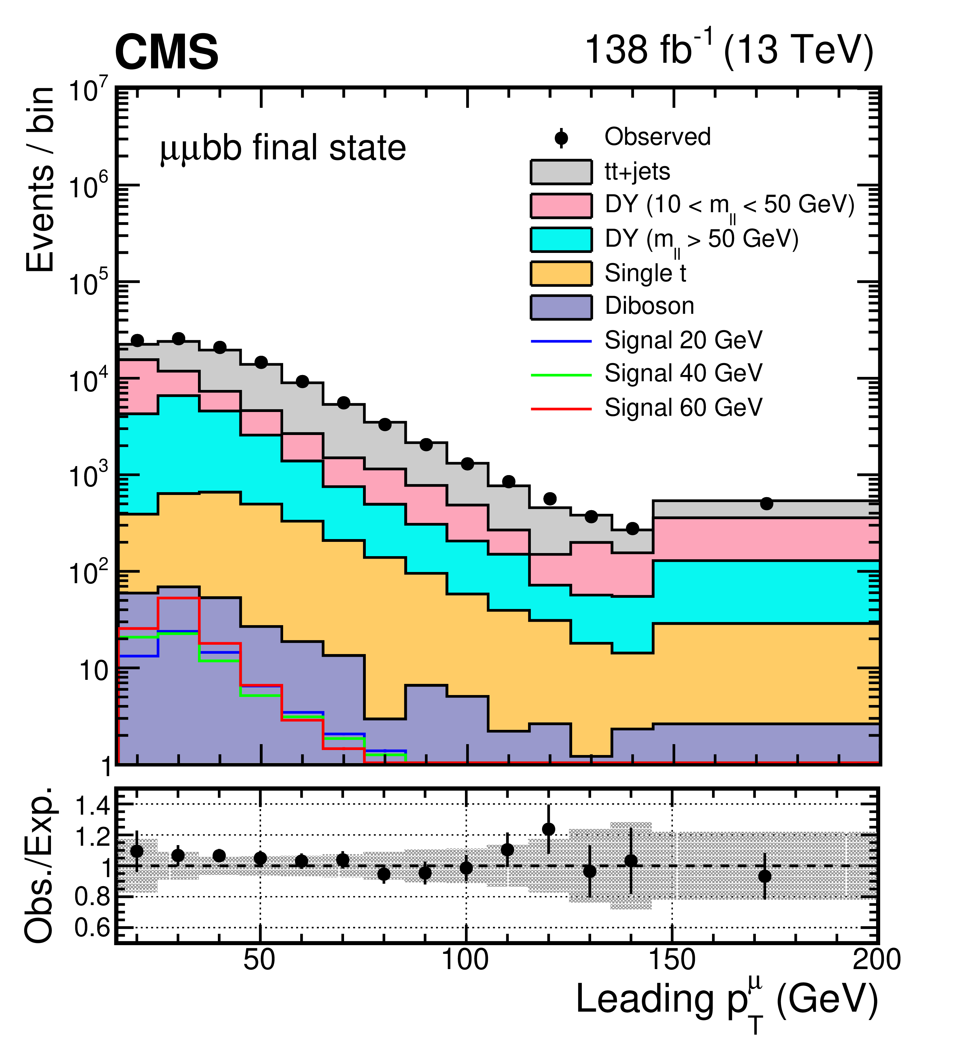
Figure 1-a:
The distributions of leading and subleading (upper) muon $ p_{\mathrm{T}} $ and (lower) b jet $ p_{\mathrm{T}} $ in the selected events. The uncertainty band in the lower panel represents the limited size of the simulated samples together with a 30% uncertainty in the low-mass DY cross section. Simulated samples are normalized using the corresponding theoretical cross sections. To evaluate the normalization of the signal, SM Higgs boson cross sections are multiplied by the $ \mathcal{B}(a_{1} a_{1} \to\mu\mu\mathrm{b}\mathrm{b}) $ value that is calculated in the Type III model with $ \tan\beta = $ 2. |
png pdf |
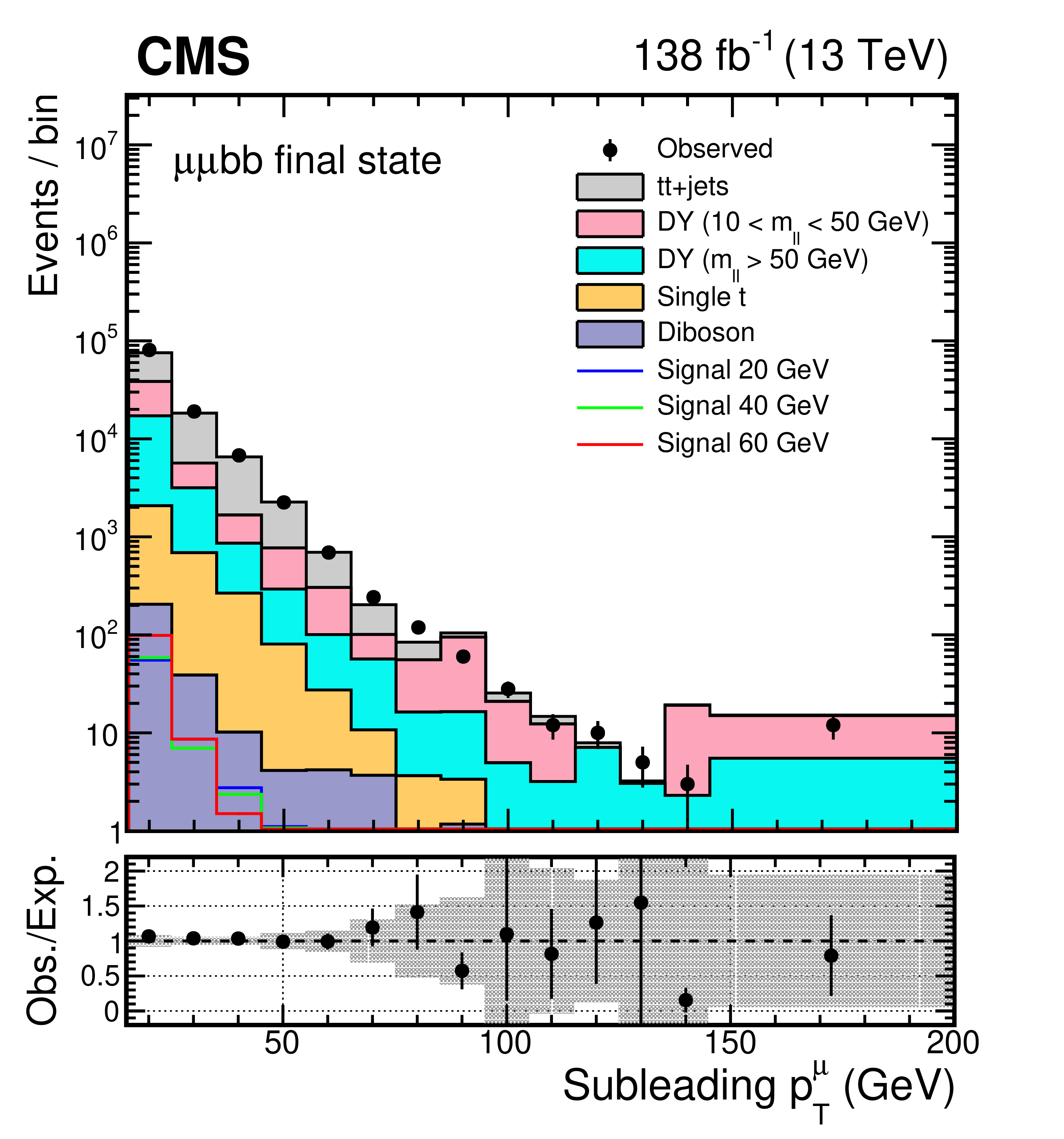
Figure 1-b:
The distributions of leading and subleading (upper) muon $ p_{\mathrm{T}} $ and (lower) b jet $ p_{\mathrm{T}} $ in the selected events. The uncertainty band in the lower panel represents the limited size of the simulated samples together with a 30% uncertainty in the low-mass DY cross section. Simulated samples are normalized using the corresponding theoretical cross sections. To evaluate the normalization of the signal, SM Higgs boson cross sections are multiplied by the $ \mathcal{B}(a_{1} a_{1} \to\mu\mu\mathrm{b}\mathrm{b}) $ value that is calculated in the Type III model with $ \tan\beta = $ 2. |
png pdf |
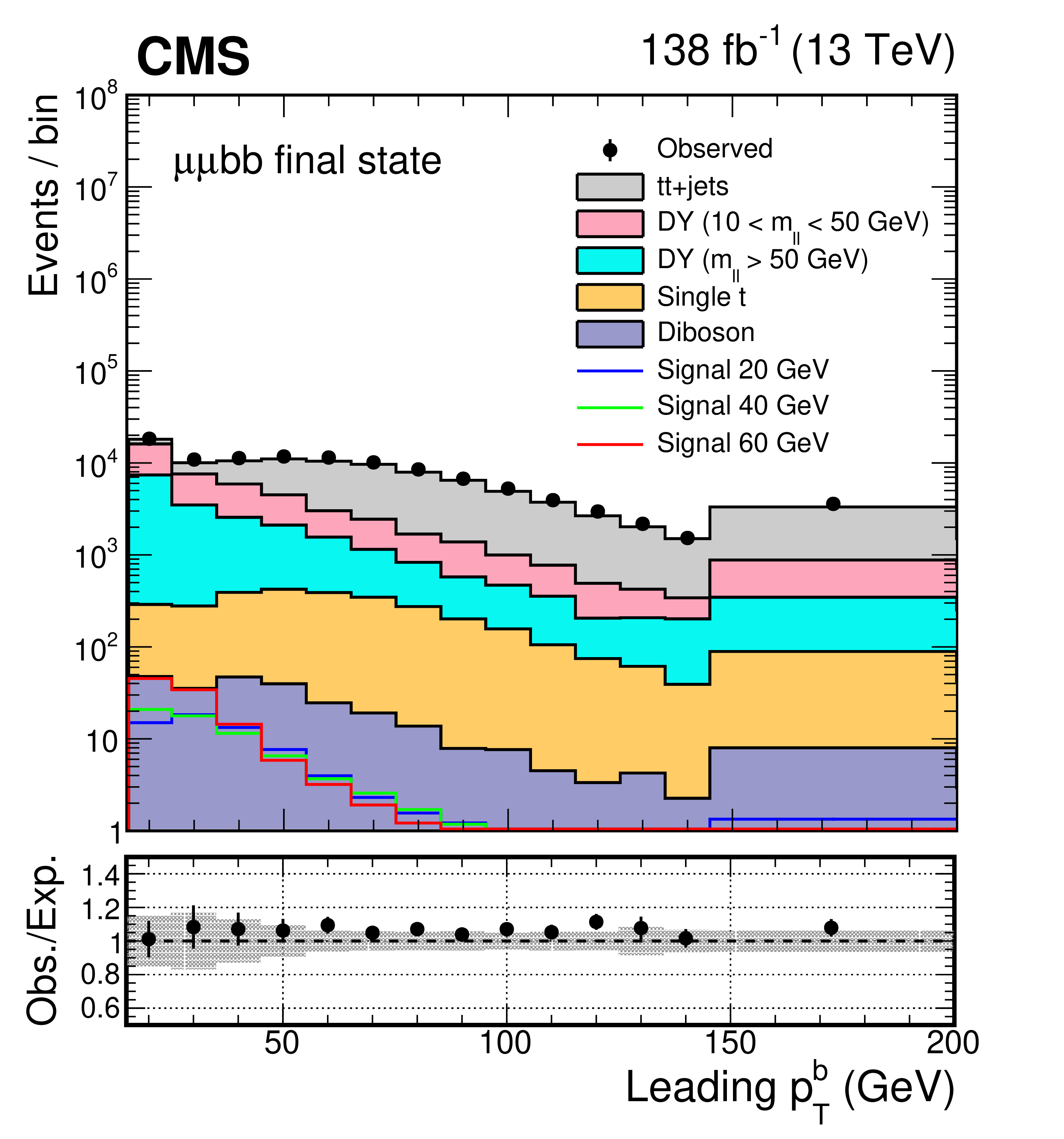
Figure 1-c:
The distributions of leading and subleading (upper) muon $ p_{\mathrm{T}} $ and (lower) b jet $ p_{\mathrm{T}} $ in the selected events. The uncertainty band in the lower panel represents the limited size of the simulated samples together with a 30% uncertainty in the low-mass DY cross section. Simulated samples are normalized using the corresponding theoretical cross sections. To evaluate the normalization of the signal, SM Higgs boson cross sections are multiplied by the $ \mathcal{B}(a_{1} a_{1} \to\mu\mu\mathrm{b}\mathrm{b}) $ value that is calculated in the Type III model with $ \tan\beta = $ 2. |
png pdf |
Figure 1-d:
The distributions of leading and subleading (upper) muon $ p_{\mathrm{T}} $ and (lower) b jet $ p_{\mathrm{T}} $ in the selected events. The uncertainty band in the lower panel represents the limited size of the simulated samples together with a 30% uncertainty in the low-mass DY cross section. Simulated samples are normalized using the corresponding theoretical cross sections. To evaluate the normalization of the signal, SM Higgs boson cross sections are multiplied by the $ \mathcal{B}(a_{1} a_{1} \to\mu\mu\mathrm{b}\mathrm{b}) $ value that is calculated in the Type III model with $ \tan\beta = $ 2. |
png pdf |
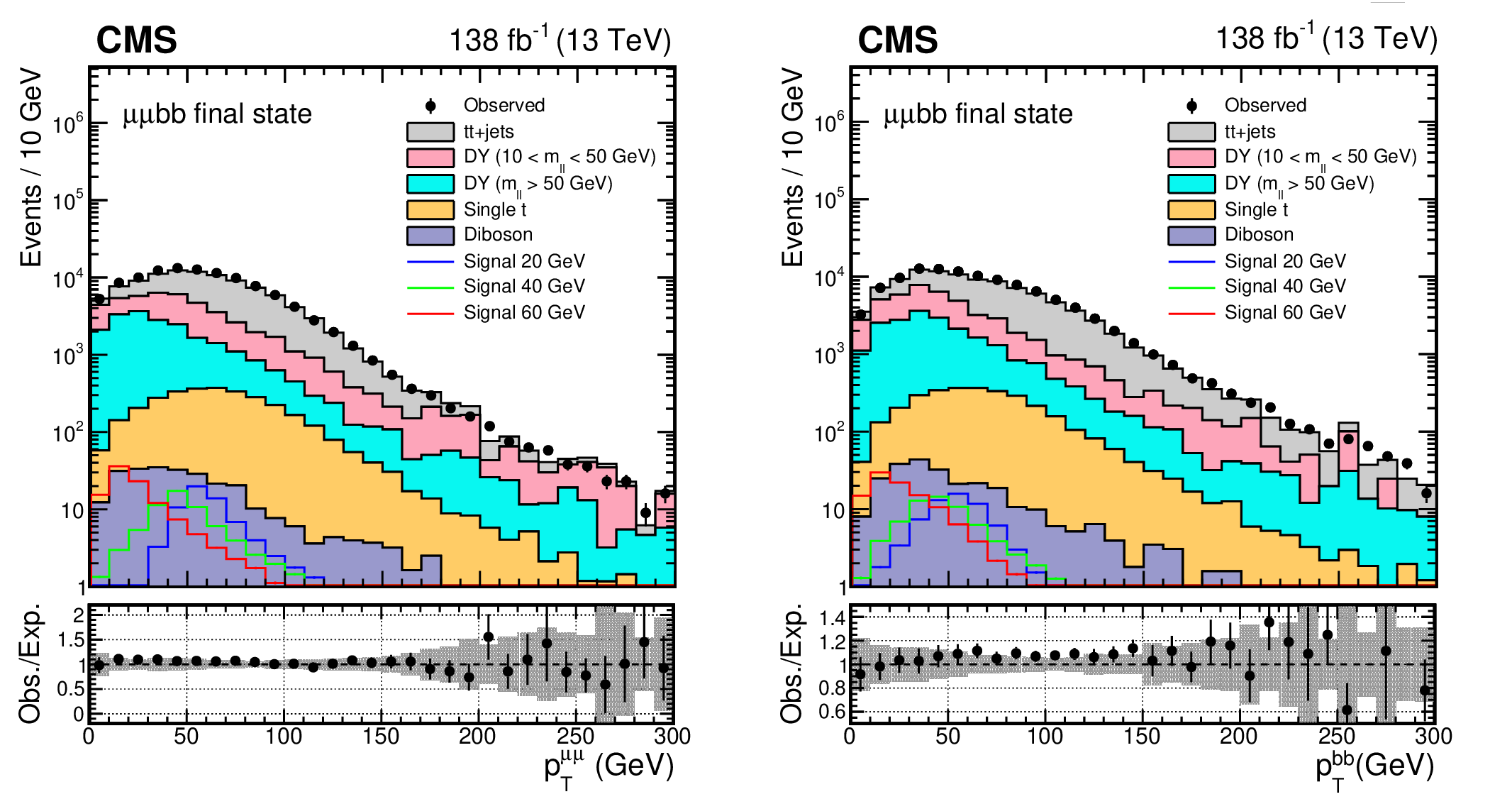
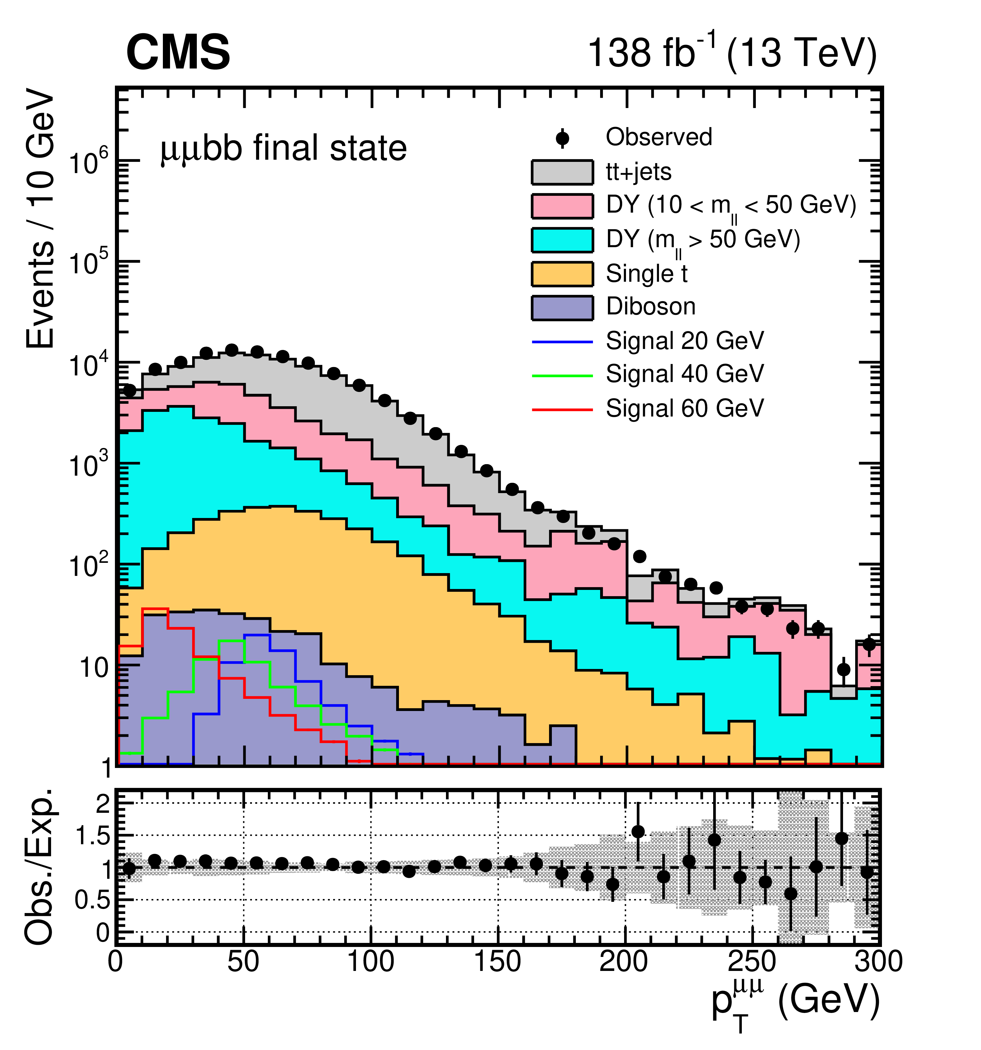
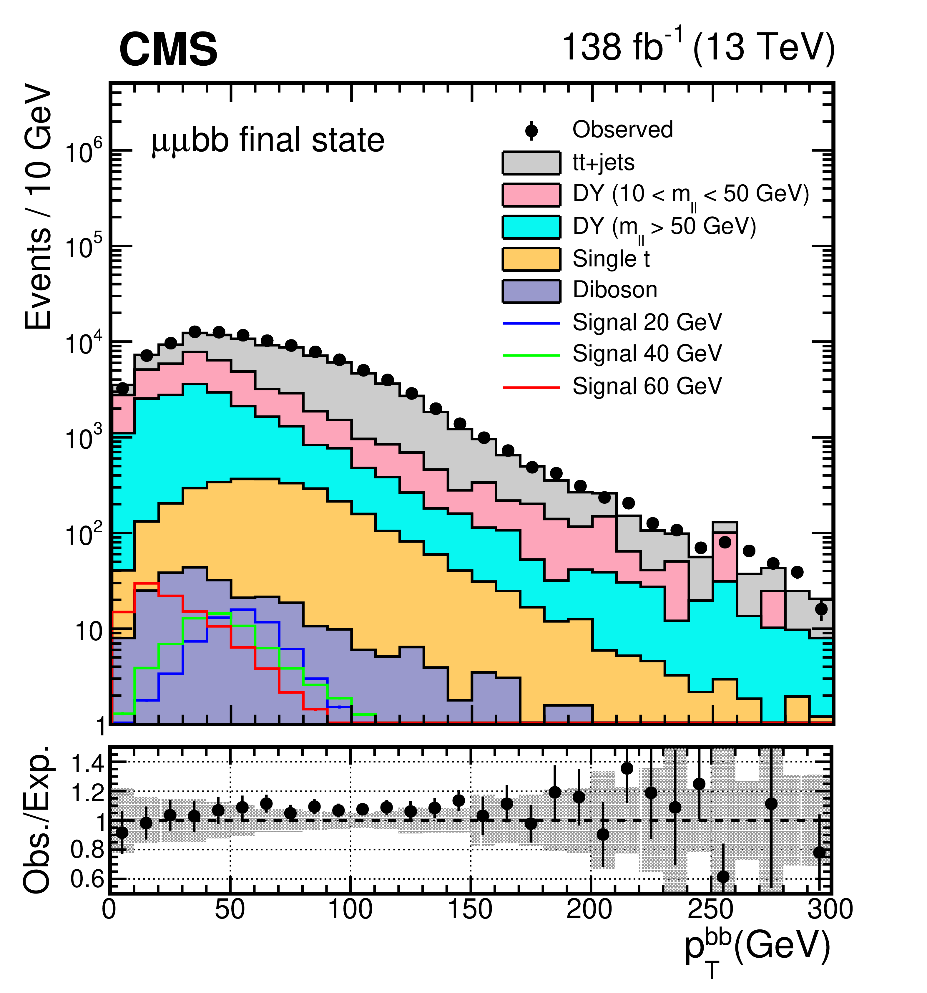
Figure 2:
The $ p_{\mathrm{T}} $ distributions of the (left) dimuon systems and (right) di-b-jet system. The uncertainty band in the lower panel represents the limited size of the simulated samples together with a 30% uncertainty in the low-mass DY cross section. Simulated samples are normalized to using the corresponding theoretical cross sections. To evaluate the normalization of the signal, SM Higgs boson cross sections are multiplied by the $ \mathcal{B}(a_{1} a_{1} \to\mu\mu\mathrm{b}\mathrm{b}) $ value that is calculated in the Type III model with $ \tan\beta = $ 2. |
png pdf |
Figure 2-a:
The $ p_{\mathrm{T}} $ distributions of the (left) dimuon systems and (right) di-b-jet system. The uncertainty band in the lower panel represents the limited size of the simulated samples together with a 30% uncertainty in the low-mass DY cross section. Simulated samples are normalized to using the corresponding theoretical cross sections. To evaluate the normalization of the signal, SM Higgs boson cross sections are multiplied by the $ \mathcal{B}(a_{1} a_{1} \to\mu\mu\mathrm{b}\mathrm{b}) $ value that is calculated in the Type III model with $ \tan\beta = $ 2. |
png pdf |
Figure 2-b:
The $ p_{\mathrm{T}} $ distributions of the (left) dimuon systems and (right) di-b-jet system. The uncertainty band in the lower panel represents the limited size of the simulated samples together with a 30% uncertainty in the low-mass DY cross section. Simulated samples are normalized to using the corresponding theoretical cross sections. To evaluate the normalization of the signal, SM Higgs boson cross sections are multiplied by the $ \mathcal{B}(a_{1} a_{1} \to\mu\mu\mathrm{b}\mathrm{b}) $ value that is calculated in the Type III model with $ \tan\beta = $ 2. |
png pdf |
Figure 3:
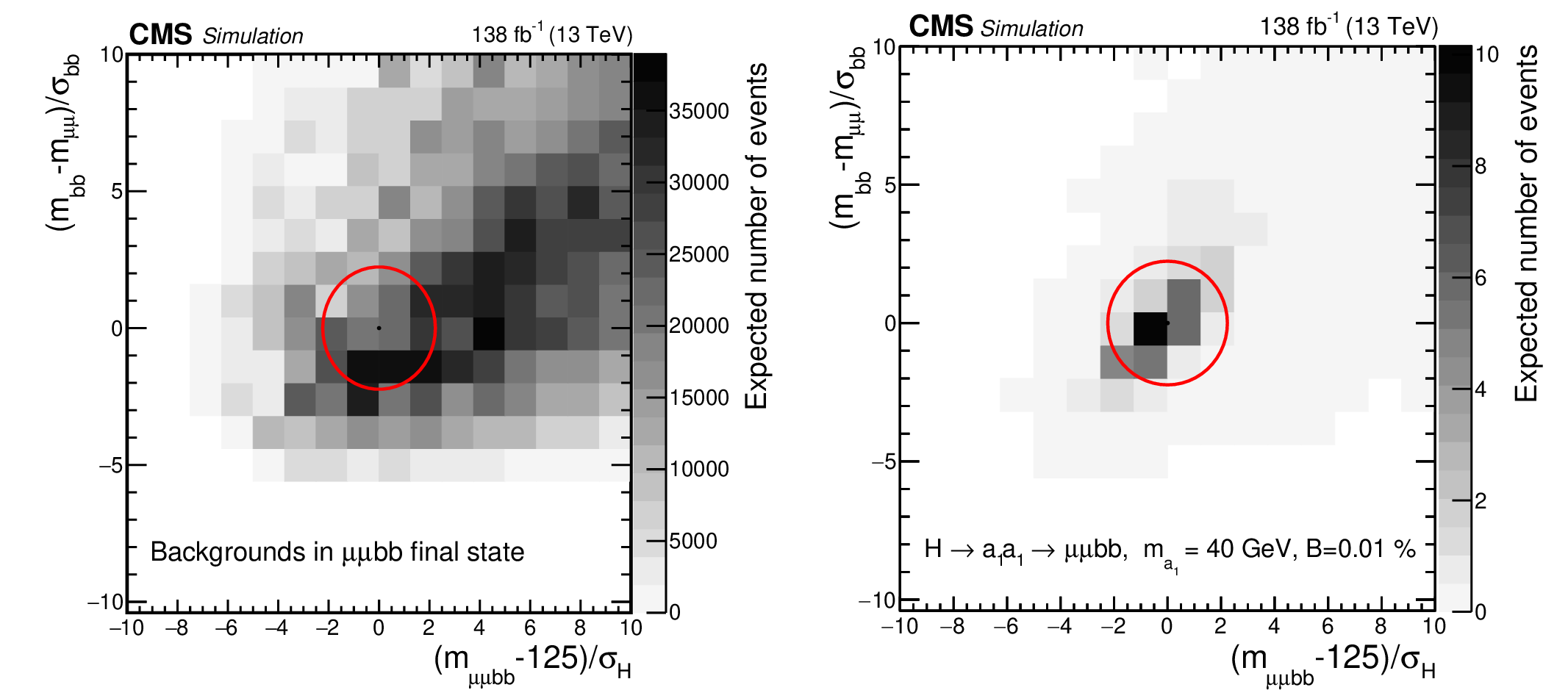
The distribution of $ \chi_{\mathrm{b}\mathrm{b}} $ versus $ \chi_{\mathrm{H}} $ as defined in Eq. (1) for (left) simulated background processes and (right) the signal process with $ m_{a_{1}} = $ 40 GeV. The contours indicate lines of constant $ \chi_\text{tot}^2 $. The gray scale represents the expected yields in data. To evaluate the yield of the signal, SM Higgs boson cross sections are multiplied by the $ \mathcal{B}(a_{1} a_{1} \to\mu\mu\mathrm{b}\mathrm{b}) $ value that is calculated in the Type III model with $ \tan\beta= $ 2. |
png pdf |
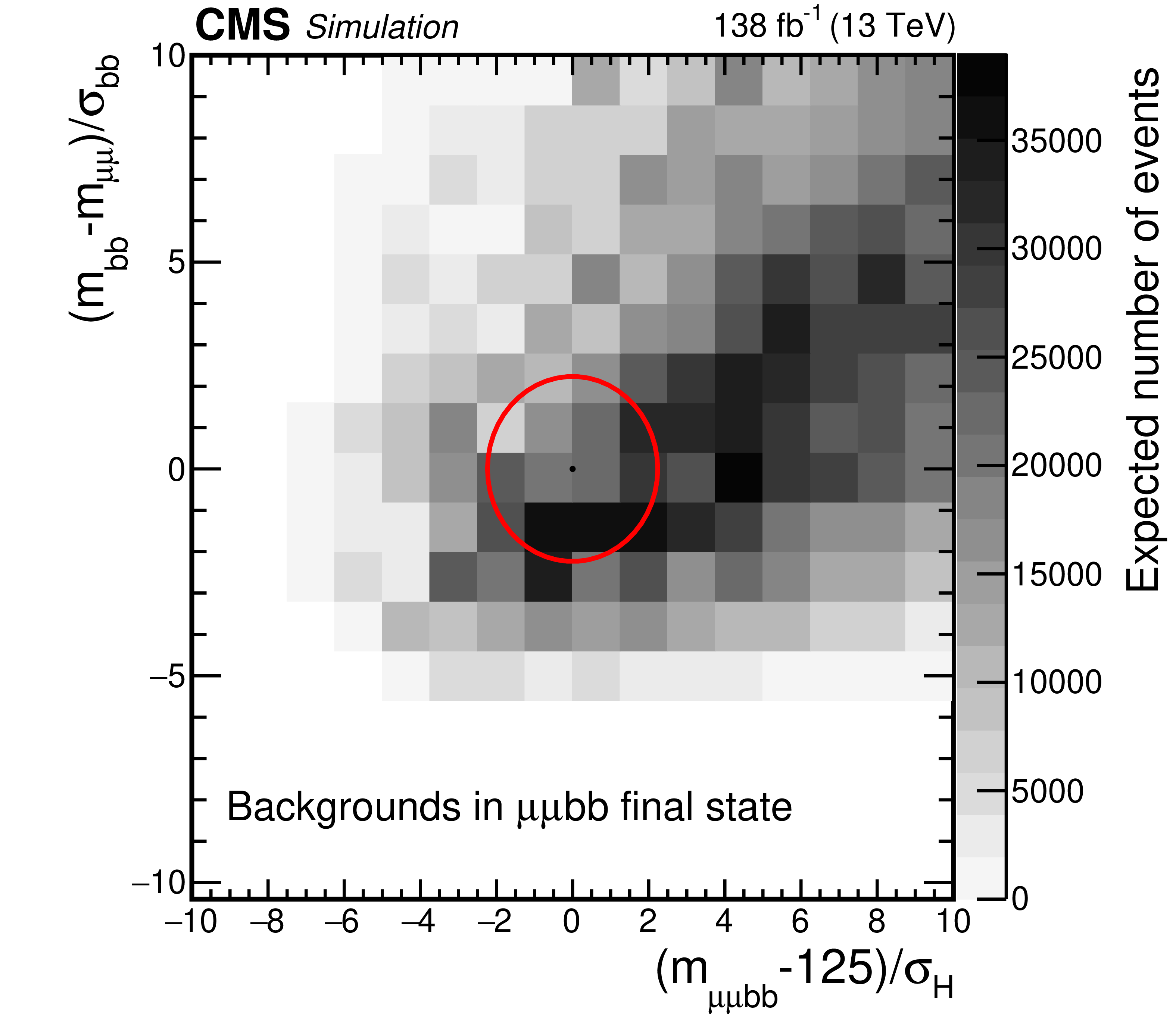
Figure 3-a:
The distribution of $ \chi_{\mathrm{b}\mathrm{b}} $ versus $ \chi_{\mathrm{H}} $ as defined in Eq. (1) for (left) simulated background processes and (right) the signal process with $ m_{a_{1}} = $ 40 GeV. The contours indicate lines of constant $ \chi_\text{tot}^2 $. The gray scale represents the expected yields in data. To evaluate the yield of the signal, SM Higgs boson cross sections are multiplied by the $ \mathcal{B}(a_{1} a_{1} \to\mu\mu\mathrm{b}\mathrm{b}) $ value that is calculated in the Type III model with $ \tan\beta= $ 2. |
png pdf |
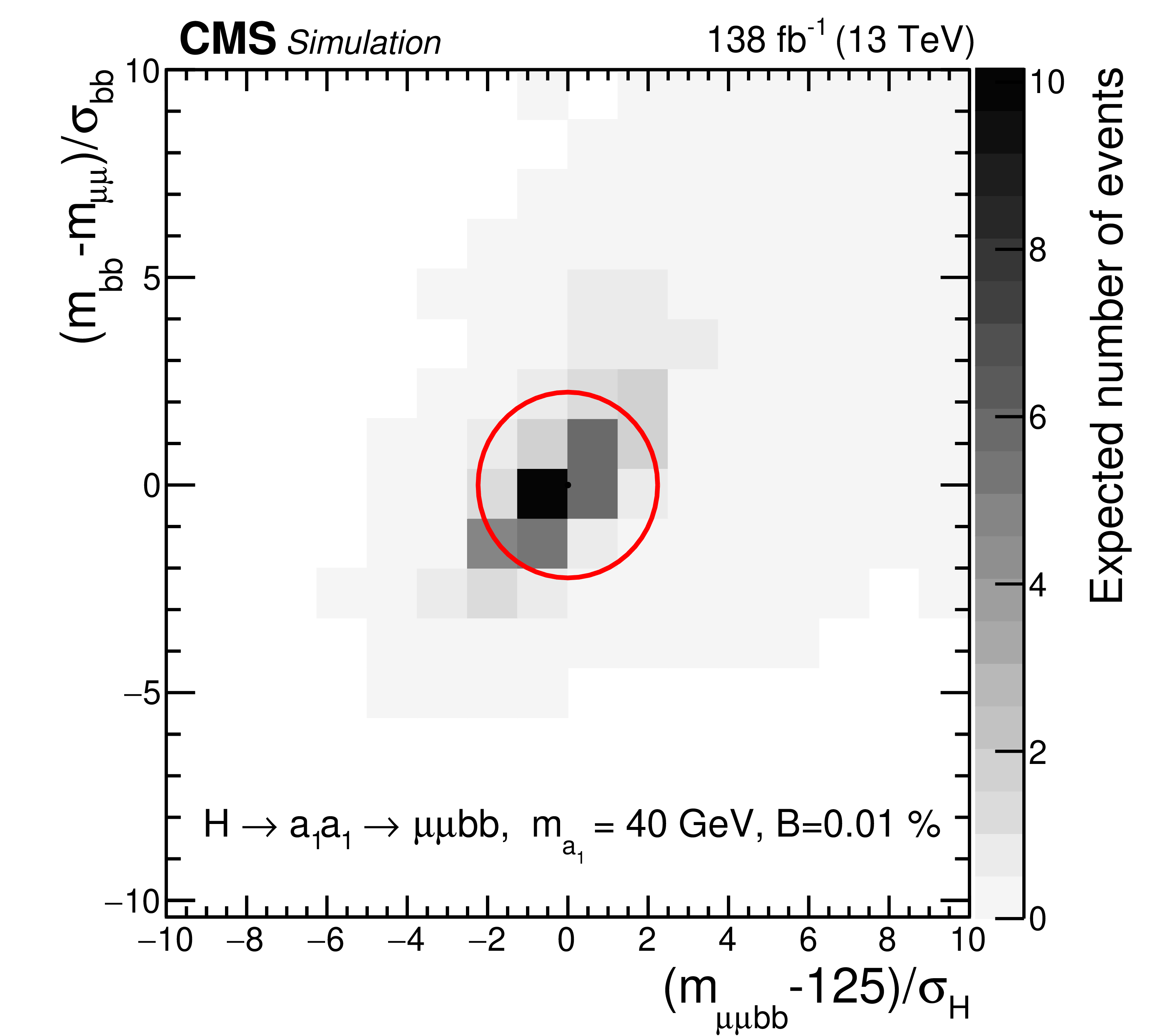
Figure 3-b:
The distribution of $ \chi_{\mathrm{b}\mathrm{b}} $ versus $ \chi_{\mathrm{H}} $ as defined in Eq. (1) for (left) simulated background processes and (right) the signal process with $ m_{a_{1}} = $ 40 GeV. The contours indicate lines of constant $ \chi_\text{tot}^2 $. The gray scale represents the expected yields in data. To evaluate the yield of the signal, SM Higgs boson cross sections are multiplied by the $ \mathcal{B}(a_{1} a_{1} \to\mu\mu\mathrm{b}\mathrm{b}) $ value that is calculated in the Type III model with $ \tan\beta= $ 2. |
png pdf |
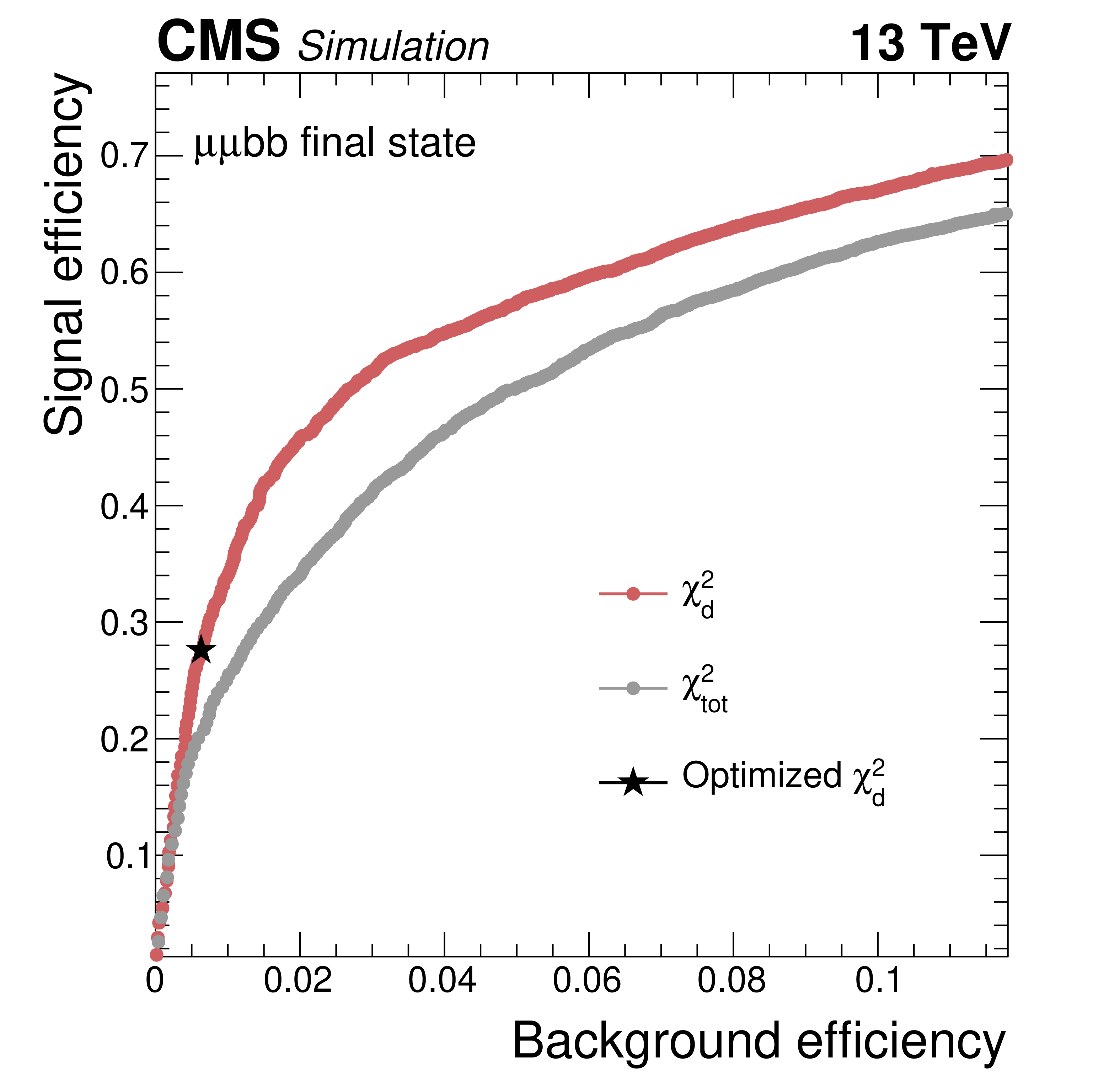
Figure 4:
Signal ($ m_{a_{1}}= $ 40 GeV) versus background efficiency for different thresholds on $ \chi_\text{tot}^2 $ (gray) and $ \chi_\mathrm{d}^2 $ (red) variables. The black star indicates signal efficiency versus that of background for the optimized $ \chi_\mathrm{d}^2 $ requirement. |
png pdf |
Figure 5:
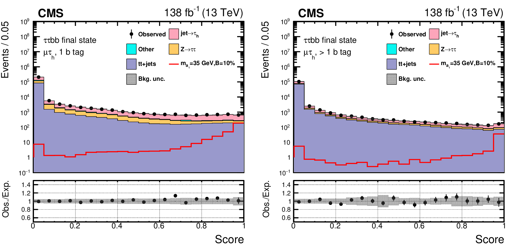
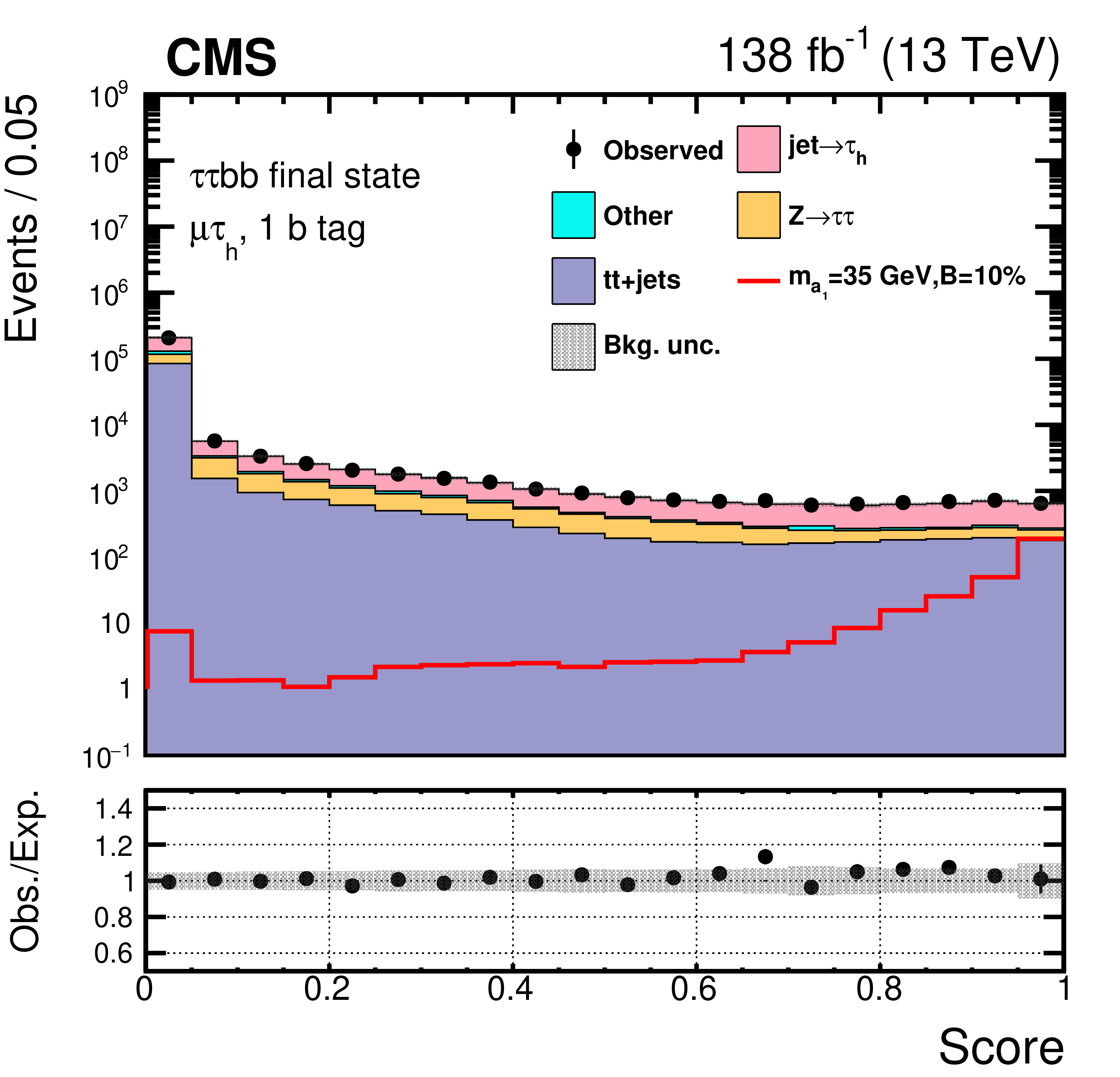
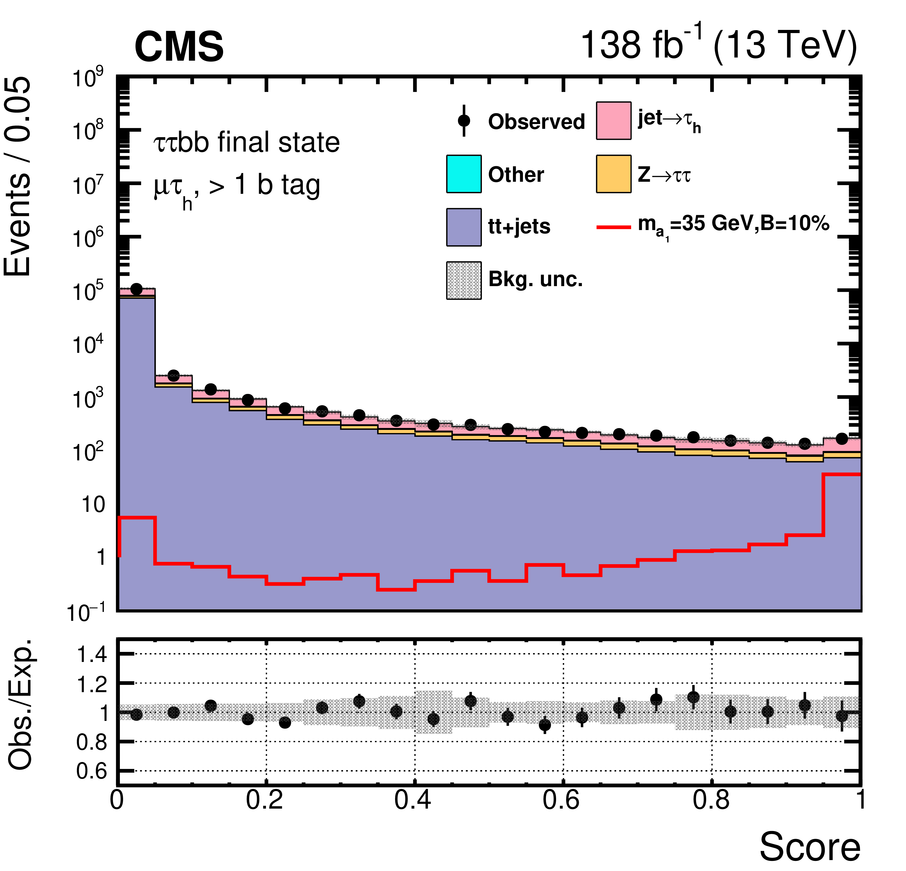
Pre-fit distributions of the DNN score for the $ \mu\hspace{-.04em}\tau_\mathrm{h} $ channel divided into events with one (left) or at least two (right) b jets. The shape of the $ \mathrm{H}\to a_{1} a_{1} $ signal, where $ m_{a_{1}} = $ 35 GeV, is indicated assuming $ \mathcal{B}(\mathrm{H}\to a_{1} a_{1} \to\tau\tau{\mathrm{b}}{\mathrm{b}}) $ to be 10%. The lower panel shows the ratio of the observed data to the expected yields. The gray band represents the unconstrained statistical and systematic uncertainties. |
png pdf |
Figure 5-a:
Pre-fit distributions of the DNN score for the $ \mu\hspace{-.04em}\tau_\mathrm{h} $ channel divided into events with one (left) or at least two (right) b jets. The shape of the $ \mathrm{H}\to a_{1} a_{1} $ signal, where $ m_{a_{1}} = $ 35 GeV, is indicated assuming $ \mathcal{B}(\mathrm{H}\to a_{1} a_{1} \to\tau\tau{\mathrm{b}}{\mathrm{b}}) $ to be 10%. The lower panel shows the ratio of the observed data to the expected yields. The gray band represents the unconstrained statistical and systematic uncertainties. |
png pdf |
Figure 5-b:
Pre-fit distributions of the DNN score for the $ \mu\hspace{-.04em}\tau_\mathrm{h} $ channel divided into events with one (left) or at least two (right) b jets. The shape of the $ \mathrm{H}\to a_{1} a_{1} $ signal, where $ m_{a_{1}} = $ 35 GeV, is indicated assuming $ \mathcal{B}(\mathrm{H}\to a_{1} a_{1} \to\tau\tau{\mathrm{b}}{\mathrm{b}}) $ to be 10%. The lower panel shows the ratio of the observed data to the expected yields. The gray band represents the unconstrained statistical and systematic uncertainties. |
png pdf |
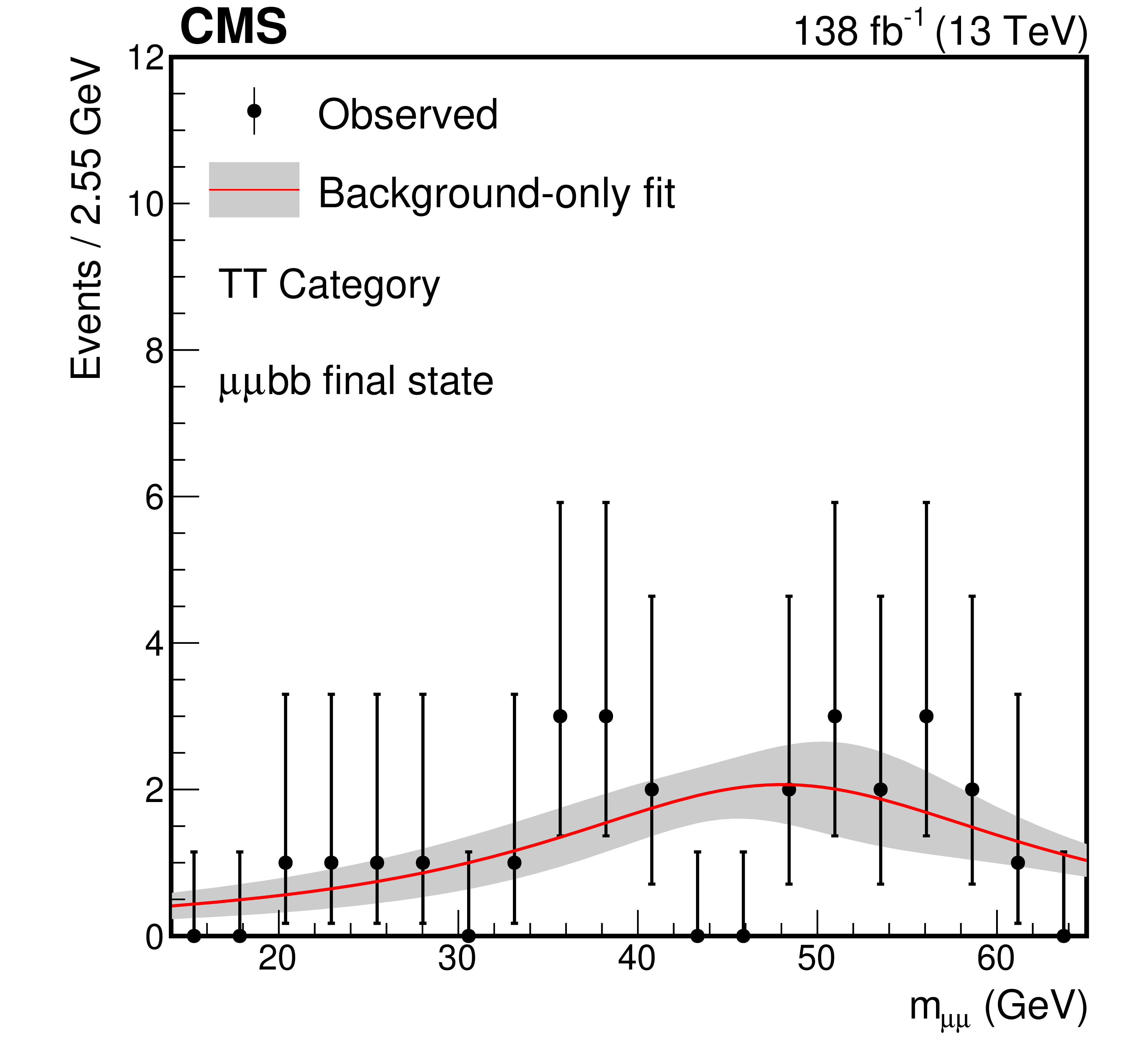
Figure 6:
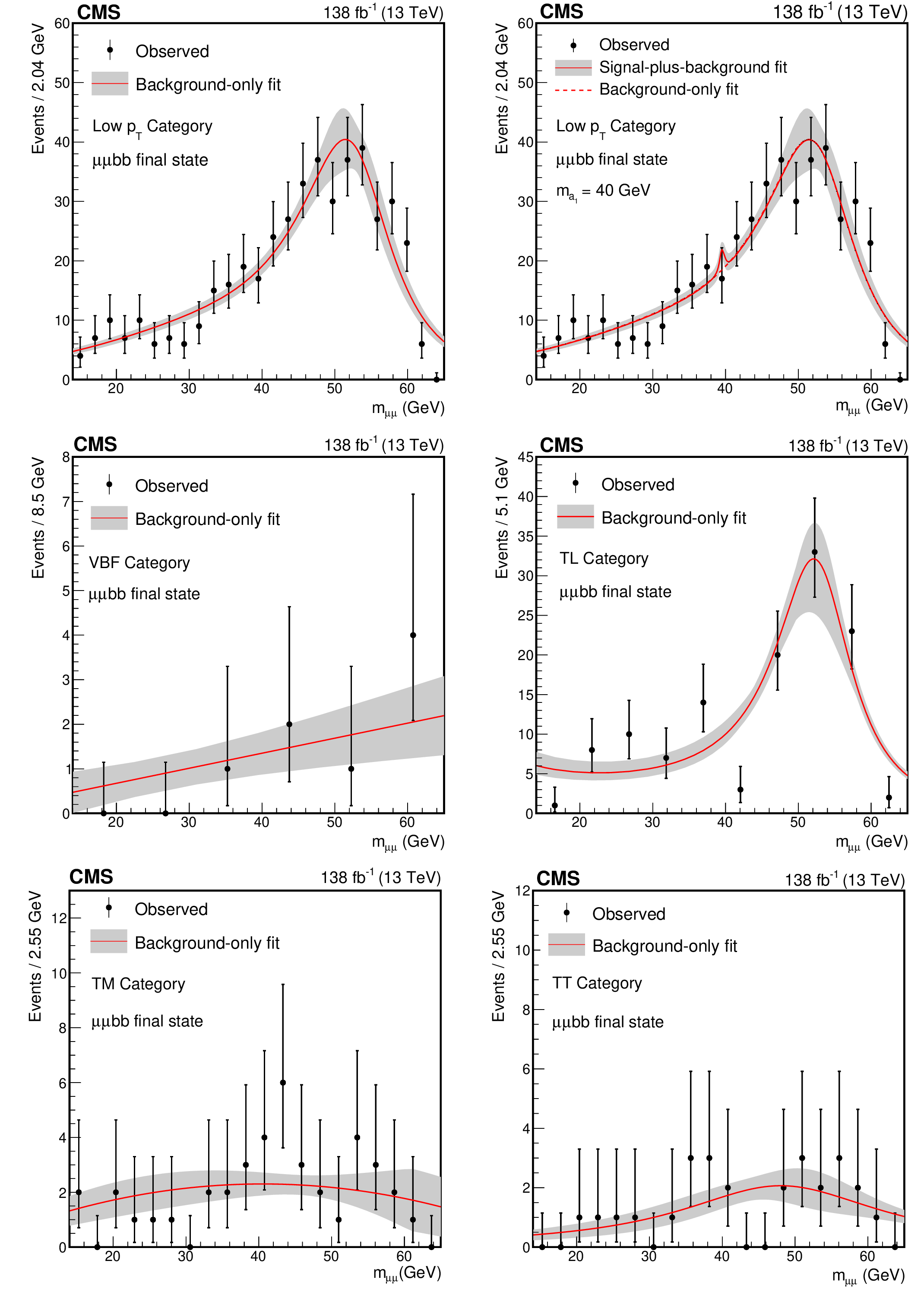
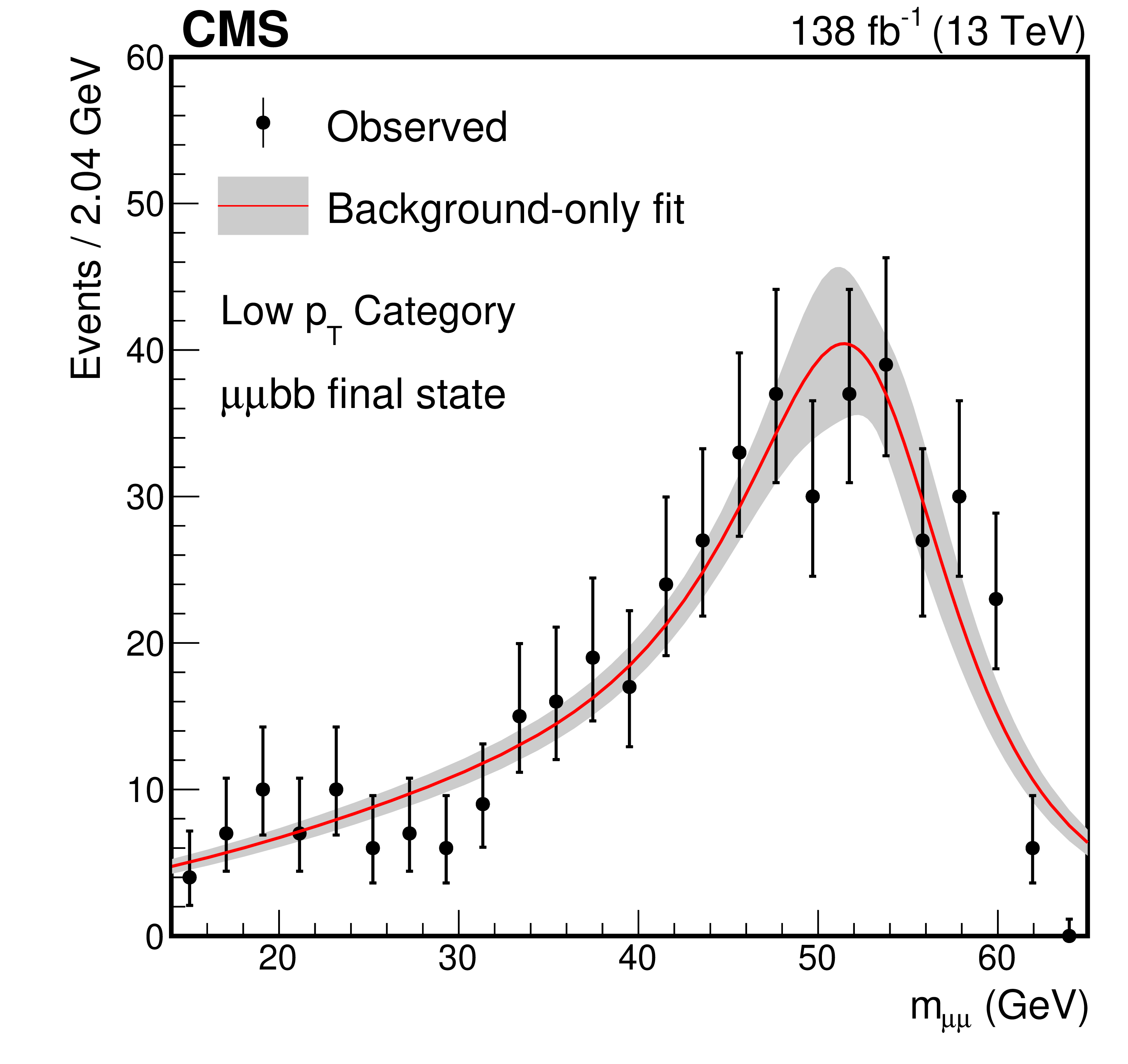
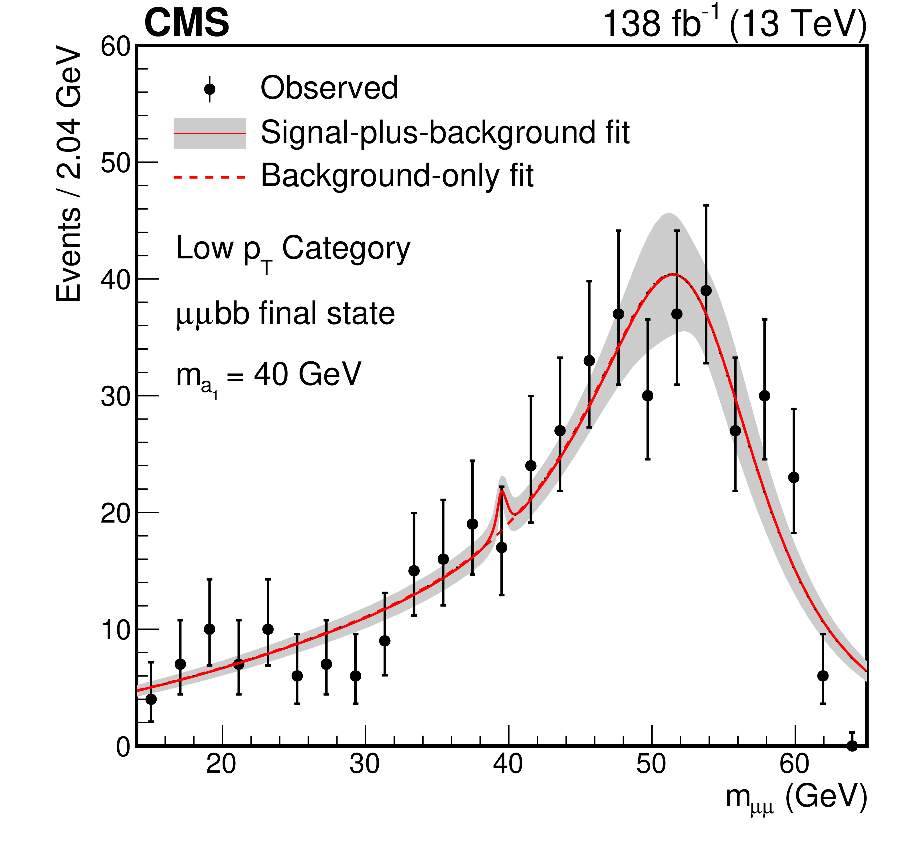
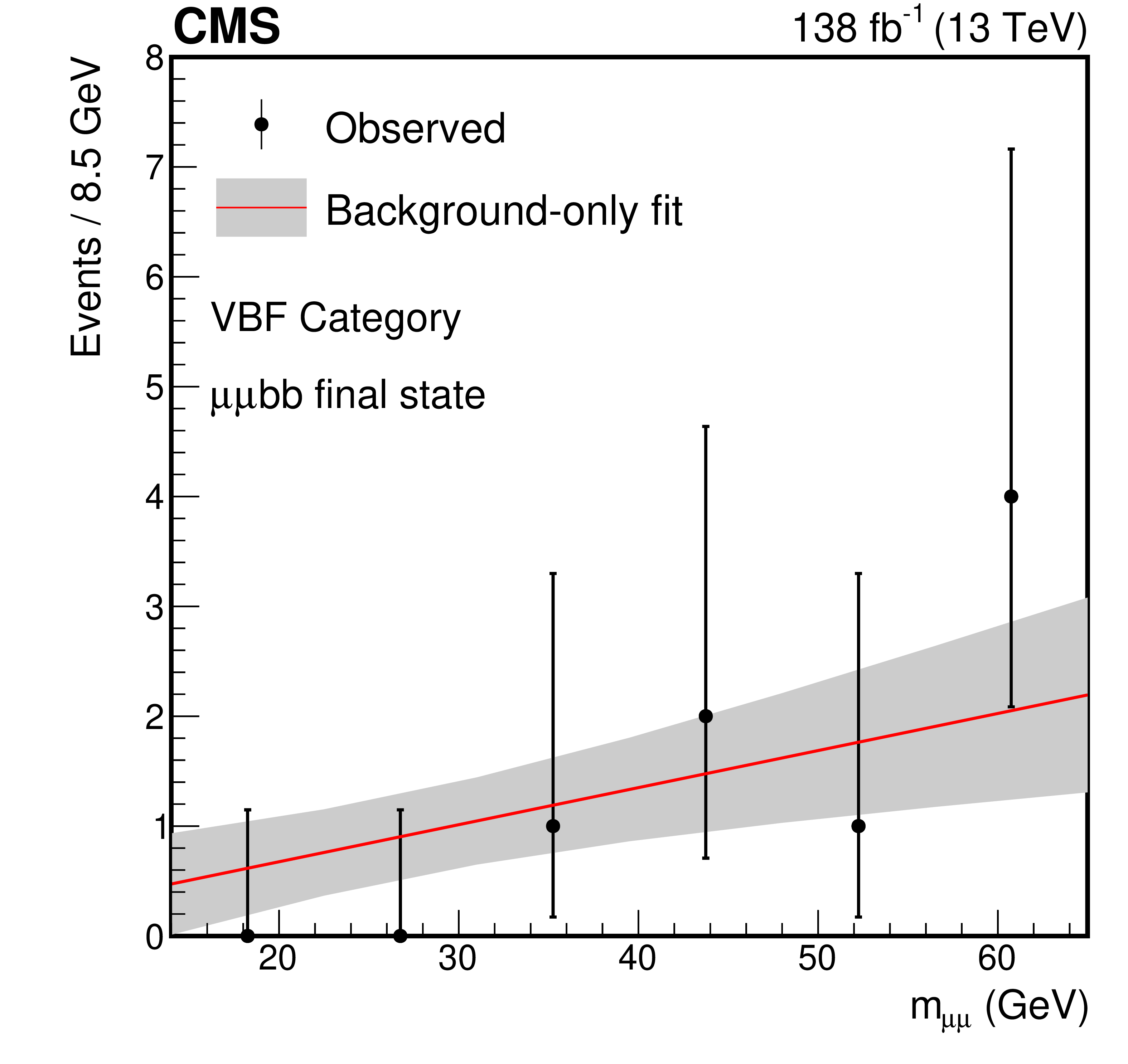
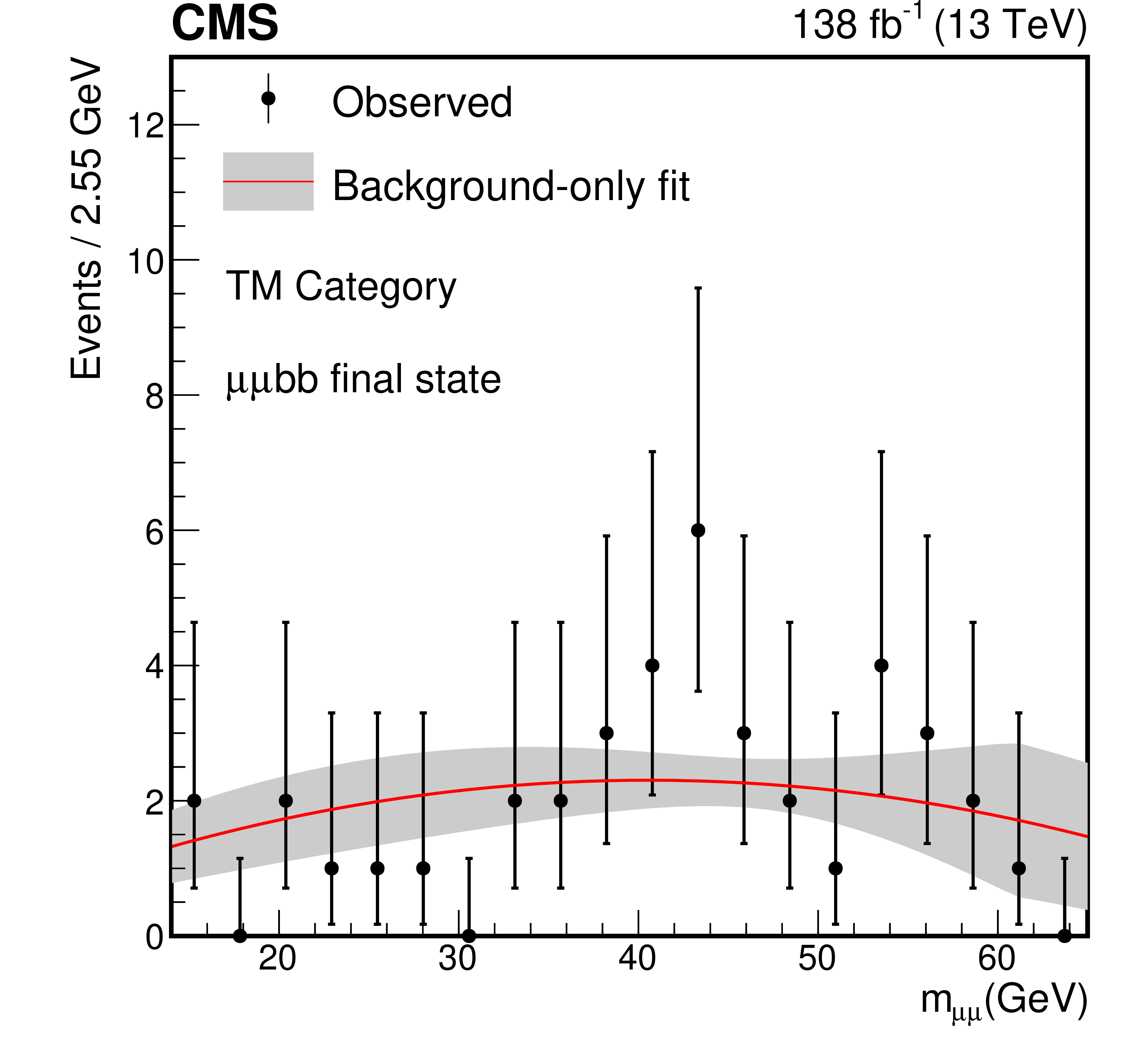
The best fit background models for the $ \mu\mu\mathrm{b}\mathrm{b} $ channel together with a 68% CL uncertainty band from the fit to the data under the background-only hypothesis for the (upper left) Low $ p_{\mathrm{T}} $ category, (middle left) VBF category, (middle right) TL category, (lower left) TM category, and (lower right) TT category. For comparison, the signal-plus-background is shown for the (upper right) Low $ p_{\mathrm{T}} $ category for a signal with $ m_{a_{1}} = $ 40 GeV. The expected signal yield is evaluated assuming the SM production of the Higgs boson and a $ \mathcal{B}(a_{1} a_{1} \to\mu\mu\mathrm{b}\mathrm{b}) $ as predicted in the Type III 2HDM+S with $ \tan\beta= $ 2. The bin widths depend on statistics, irrelevant for the final fit. |
png pdf |
Figure 6-a:
The best fit background models for the $ \mu\mu\mathrm{b}\mathrm{b} $ channel together with a 68% CL uncertainty band from the fit to the data under the background-only hypothesis for the (upper left) Low $ p_{\mathrm{T}} $ category, (middle left) VBF category, (middle right) TL category, (lower left) TM category, and (lower right) TT category. For comparison, the signal-plus-background is shown for the (upper right) Low $ p_{\mathrm{T}} $ category for a signal with $ m_{a_{1}} = $ 40 GeV. The expected signal yield is evaluated assuming the SM production of the Higgs boson and a $ \mathcal{B}(a_{1} a_{1} \to\mu\mu\mathrm{b}\mathrm{b}) $ as predicted in the Type III 2HDM+S with $ \tan\beta= $ 2. The bin widths depend on statistics, irrelevant for the final fit. |
png pdf |
Figure 6-b:
The best fit background models for the $ \mu\mu\mathrm{b}\mathrm{b} $ channel together with a 68% CL uncertainty band from the fit to the data under the background-only hypothesis for the (upper left) Low $ p_{\mathrm{T}} $ category, (middle left) VBF category, (middle right) TL category, (lower left) TM category, and (lower right) TT category. For comparison, the signal-plus-background is shown for the (upper right) Low $ p_{\mathrm{T}} $ category for a signal with $ m_{a_{1}} = $ 40 GeV. The expected signal yield is evaluated assuming the SM production of the Higgs boson and a $ \mathcal{B}(a_{1} a_{1} \to\mu\mu\mathrm{b}\mathrm{b}) $ as predicted in the Type III 2HDM+S with $ \tan\beta= $ 2. The bin widths depend on statistics, irrelevant for the final fit. |
png pdf |
Figure 6-c:
The best fit background models for the $ \mu\mu\mathrm{b}\mathrm{b} $ channel together with a 68% CL uncertainty band from the fit to the data under the background-only hypothesis for the (upper left) Low $ p_{\mathrm{T}} $ category, (middle left) VBF category, (middle right) TL category, (lower left) TM category, and (lower right) TT category. For comparison, the signal-plus-background is shown for the (upper right) Low $ p_{\mathrm{T}} $ category for a signal with $ m_{a_{1}} = $ 40 GeV. The expected signal yield is evaluated assuming the SM production of the Higgs boson and a $ \mathcal{B}(a_{1} a_{1} \to\mu\mu\mathrm{b}\mathrm{b}) $ as predicted in the Type III 2HDM+S with $ \tan\beta= $ 2. The bin widths depend on statistics, irrelevant for the final fit. |

png pdf |
Figure 6-d:
The best fit background models for the $ \mu\mu\mathrm{b}\mathrm{b} $ channel together with a 68% CL uncertainty band from the fit to the data under the background-only hypothesis for the (upper left) Low $ p_{\mathrm{T}} $ category, (middle left) VBF category, (middle right) TL category, (lower left) TM category, and (lower right) TT category. For comparison, the signal-plus-background is shown for the (upper right) Low $ p_{\mathrm{T}} $ category for a signal with $ m_{a_{1}} = $ 40 GeV. The expected signal yield is evaluated assuming the SM production of the Higgs boson and a $ \mathcal{B}(a_{1} a_{1} \to\mu\mu\mathrm{b}\mathrm{b}) $ as predicted in the Type III 2HDM+S with $ \tan\beta= $ 2. The bin widths depend on statistics, irrelevant for the final fit. |
png pdf |
Figure 6-e:
The best fit background models for the $ \mu\mu\mathrm{b}\mathrm{b} $ channel together with a 68% CL uncertainty band from the fit to the data under the background-only hypothesis for the (upper left) Low $ p_{\mathrm{T}} $ category, (middle left) VBF category, (middle right) TL category, (lower left) TM category, and (lower right) TT category. For comparison, the signal-plus-background is shown for the (upper right) Low $ p_{\mathrm{T}} $ category for a signal with $ m_{a_{1}} = $ 40 GeV. The expected signal yield is evaluated assuming the SM production of the Higgs boson and a $ \mathcal{B}(a_{1} a_{1} \to\mu\mu\mathrm{b}\mathrm{b}) $ as predicted in the Type III 2HDM+S with $ \tan\beta= $ 2. The bin widths depend on statistics, irrelevant for the final fit. |
png pdf |
Figure 6-f:
The best fit background models for the $ \mu\mu\mathrm{b}\mathrm{b} $ channel together with a 68% CL uncertainty band from the fit to the data under the background-only hypothesis for the (upper left) Low $ p_{\mathrm{T}} $ category, (middle left) VBF category, (middle right) TL category, (lower left) TM category, and (lower right) TT category. For comparison, the signal-plus-background is shown for the (upper right) Low $ p_{\mathrm{T}} $ category for a signal with $ m_{a_{1}} = $ 40 GeV. The expected signal yield is evaluated assuming the SM production of the Higgs boson and a $ \mathcal{B}(a_{1} a_{1} \to\mu\mu\mathrm{b}\mathrm{b}) $ as predicted in the Type III 2HDM+S with $ \tan\beta= $ 2. The bin widths depend on statistics, irrelevant for the final fit. |
png pdf |
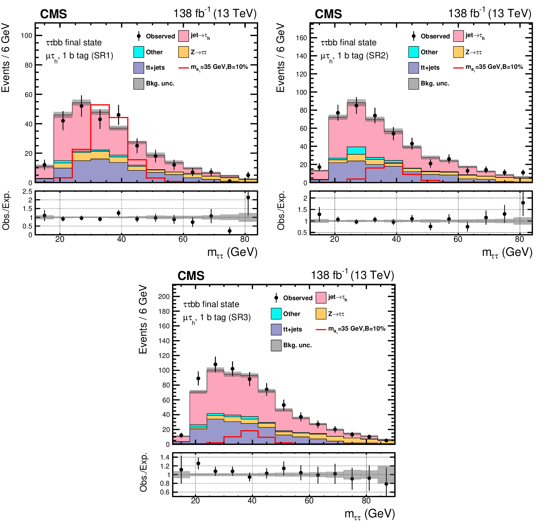
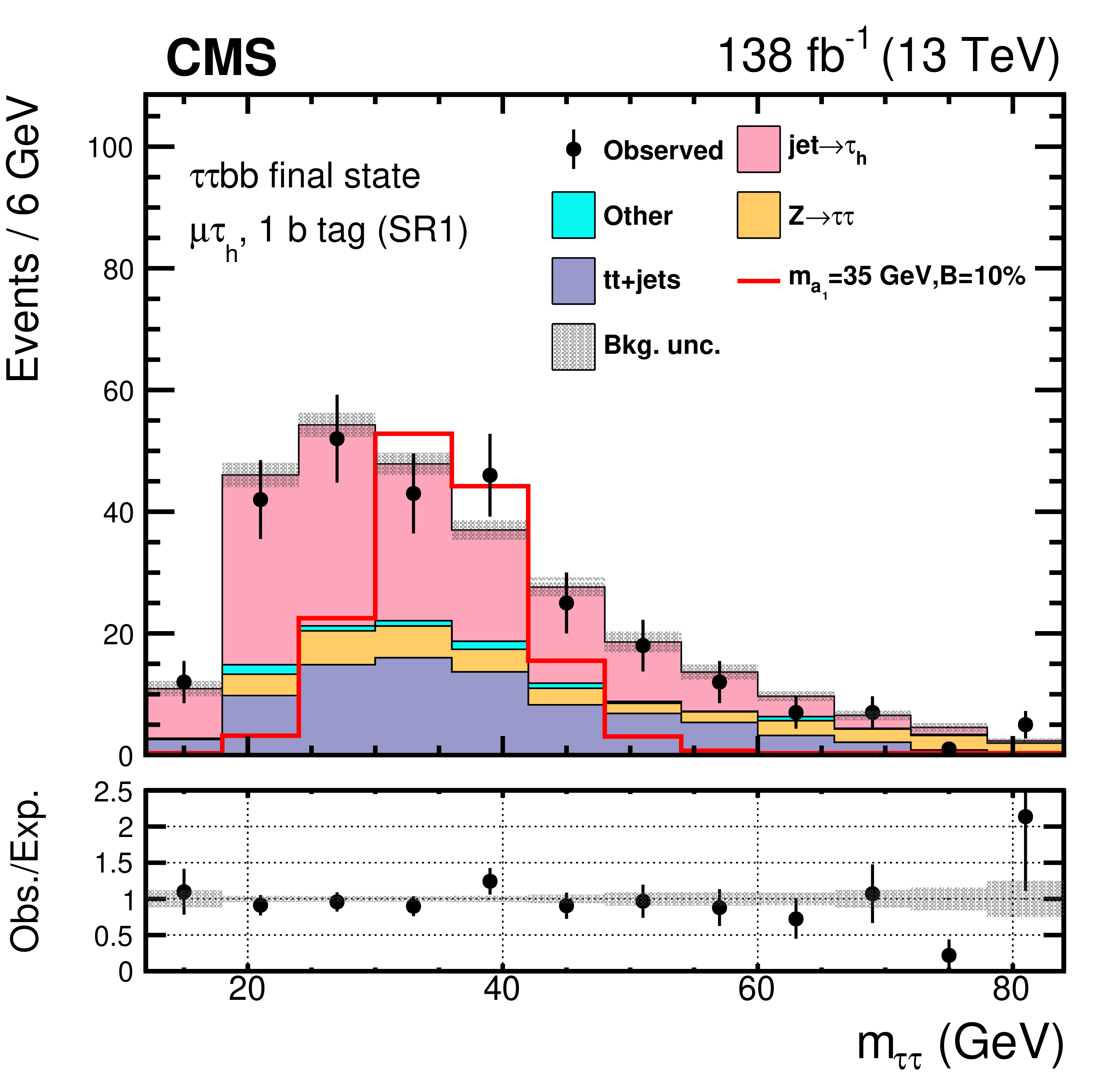
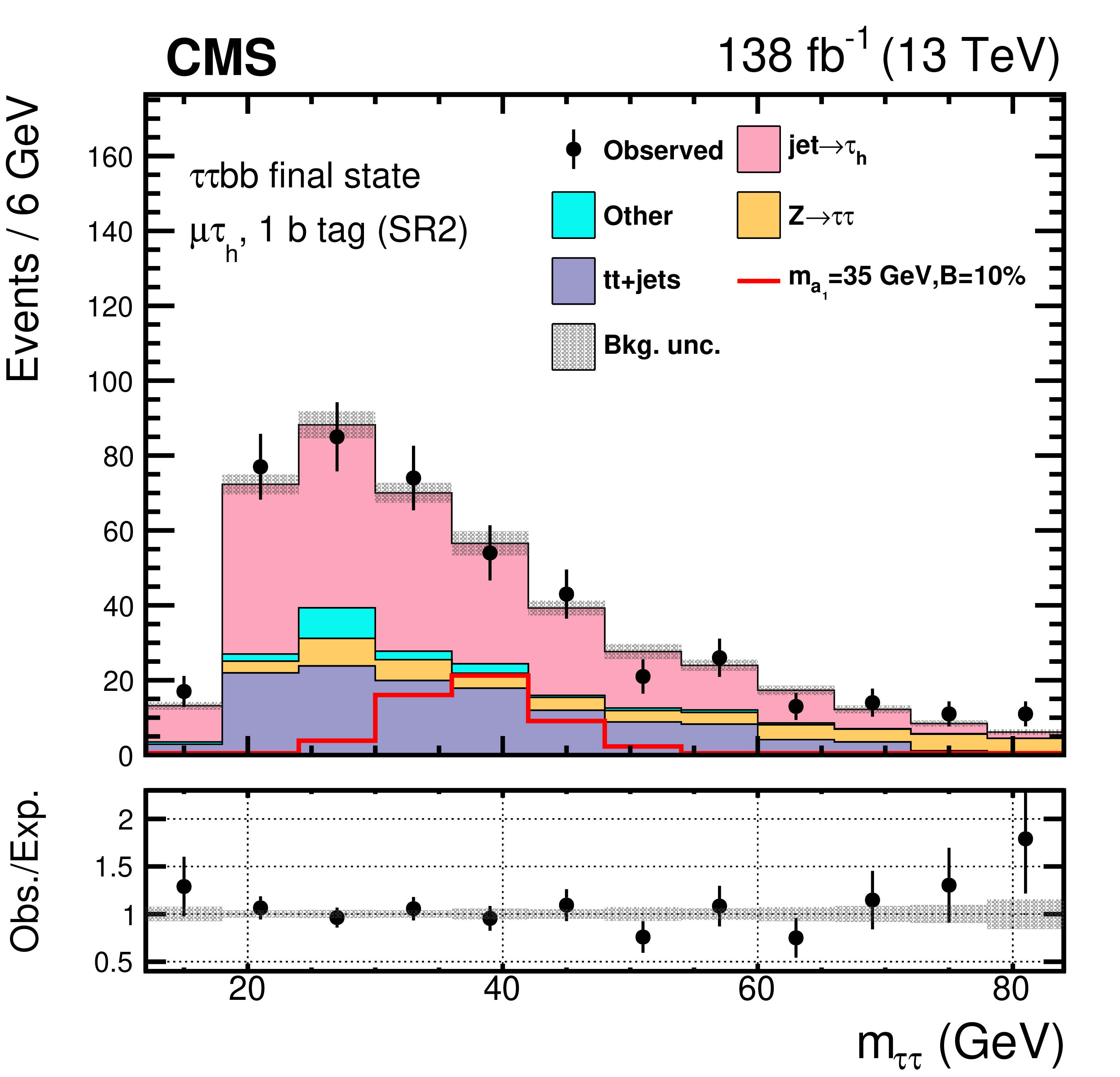
Figure 7:
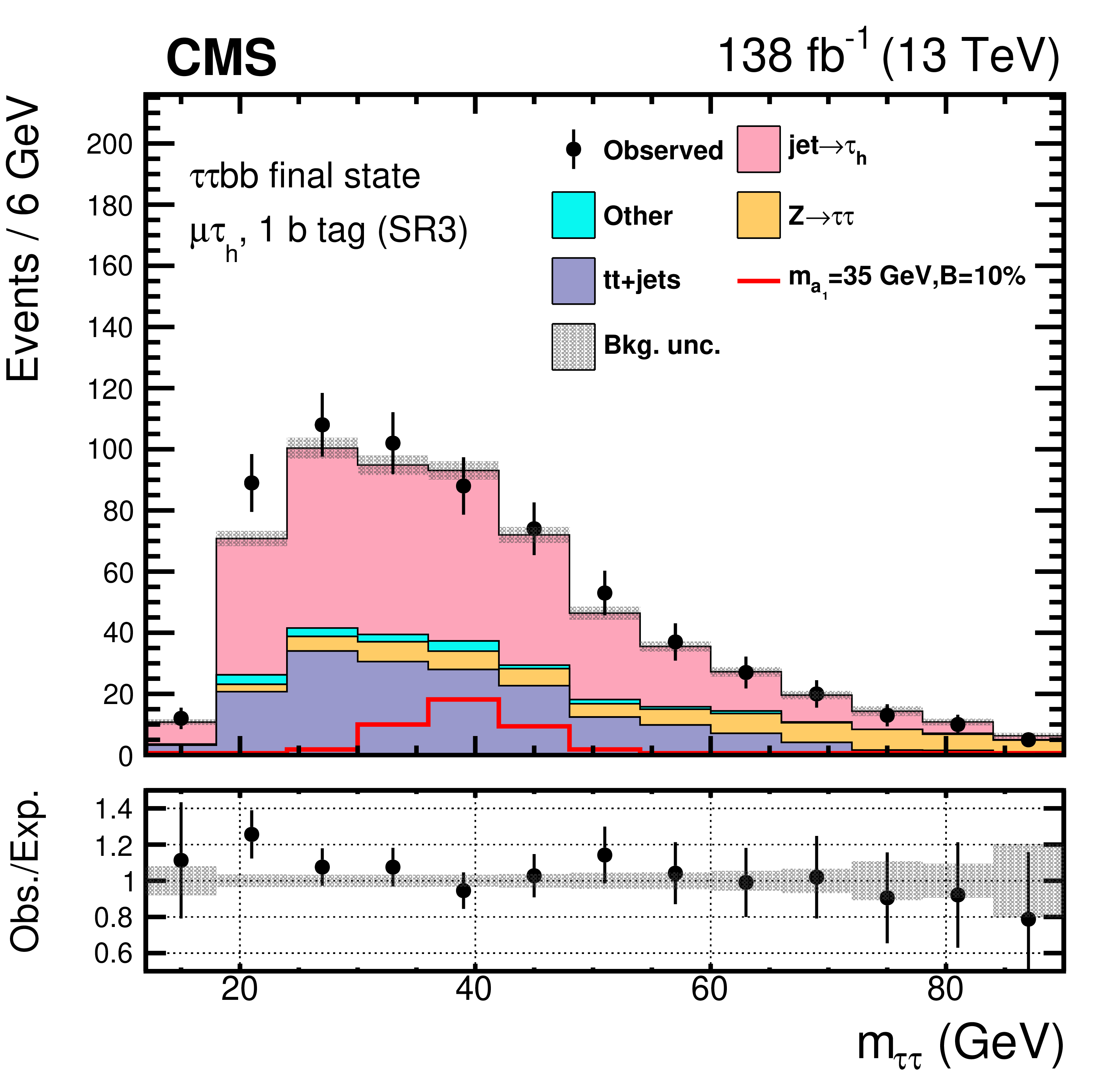
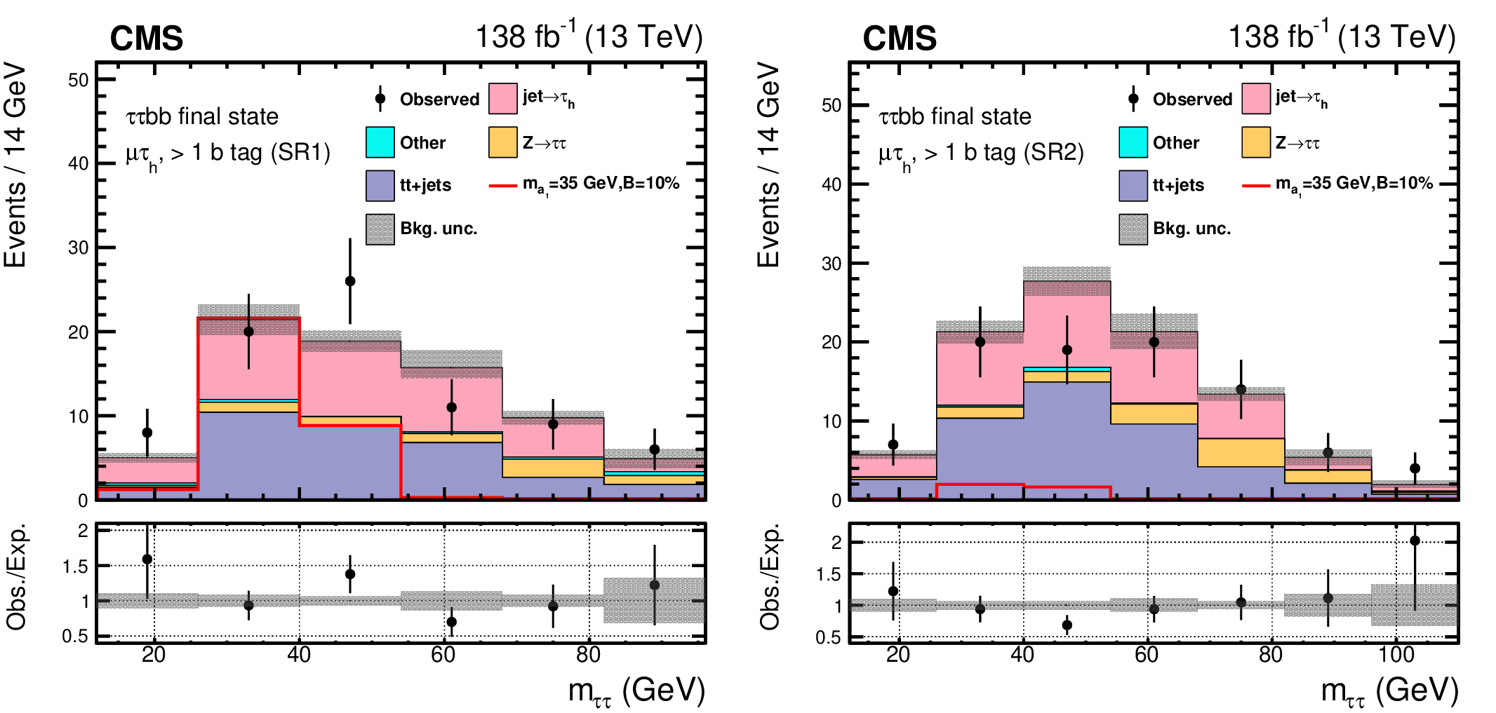
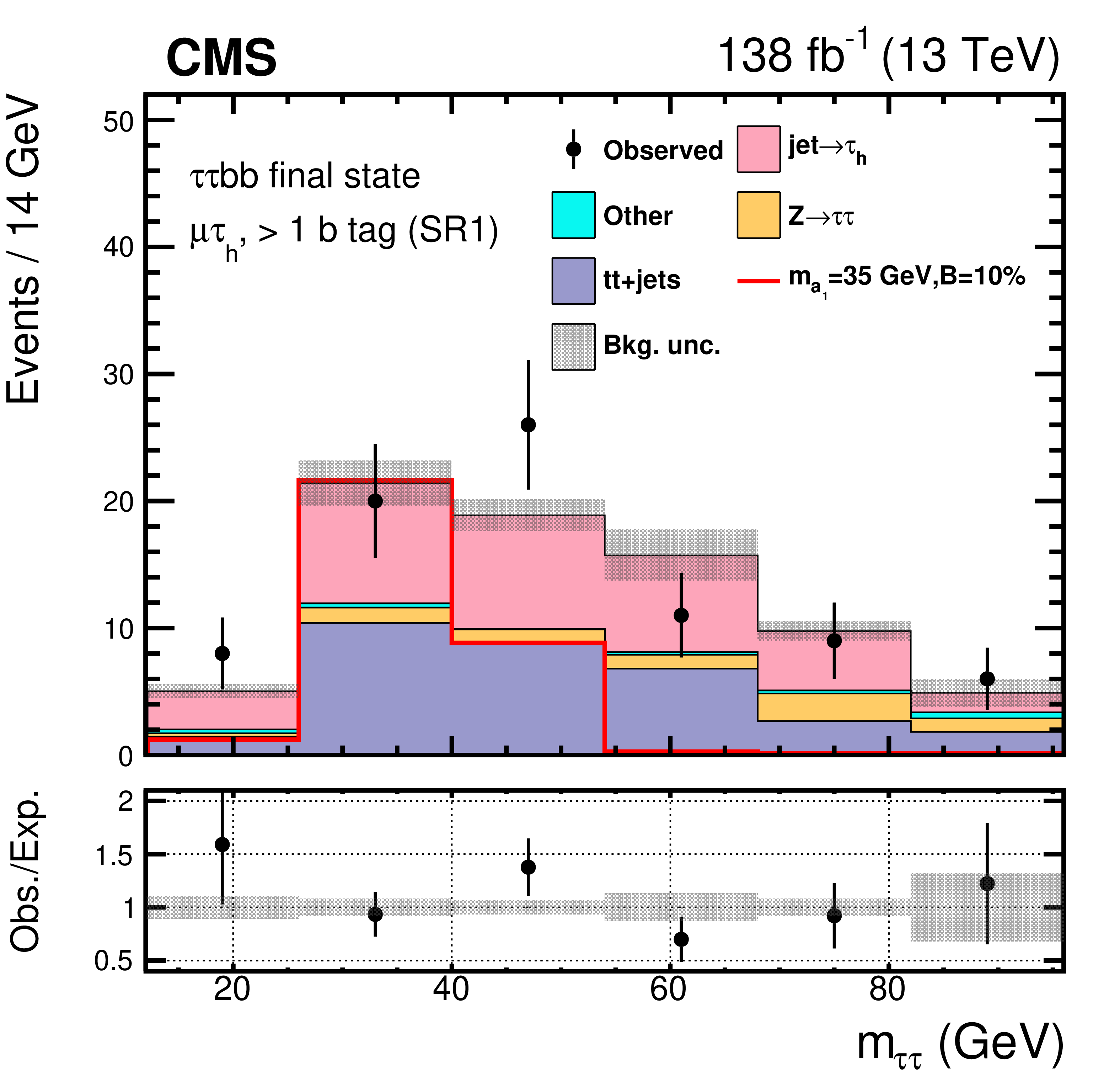
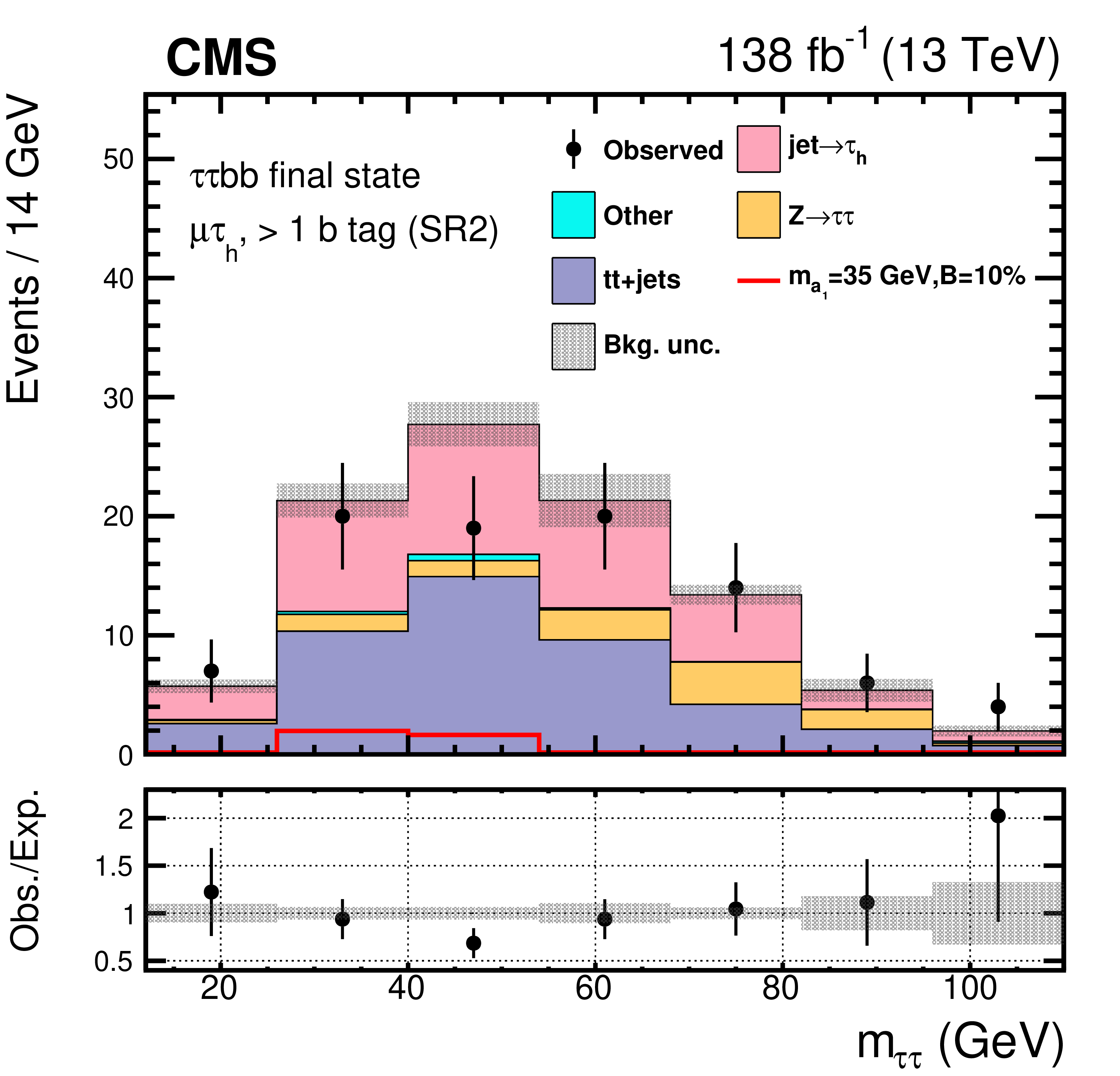
Post-fit distributions of $ m_{\tau\tau} $ for the $ \mu\hspace{-.04em}\tau_\mathrm{h} $ channel signal regions in events with exactly one b tagged jet: SR1 (upper left ), SR2 (upper right), and SR3 (lower). The shape of the $ \mathrm{H}\to a_{1} a_{1} $ signal, where $ m_{a_{1}} = $ 35 GeV, is indicated assuming $ \mathcal{B}(\mathrm{H}\to a_{1} a_{1} \to\tau\tau{\mathrm{b}}{\mathrm{b}}) $ to be 10%. |
png pdf |
Figure 7-a:
Post-fit distributions of $ m_{\tau\tau} $ for the $ \mu\hspace{-.04em}\tau_\mathrm{h} $ channel signal regions in events with exactly one b tagged jet: SR1 (upper left ), SR2 (upper right), and SR3 (lower). The shape of the $ \mathrm{H}\to a_{1} a_{1} $ signal, where $ m_{a_{1}} = $ 35 GeV, is indicated assuming $ \mathcal{B}(\mathrm{H}\to a_{1} a_{1} \to\tau\tau{\mathrm{b}}{\mathrm{b}}) $ to be 10%. |
png pdf |
Figure 7-b:
Post-fit distributions of $ m_{\tau\tau} $ for the $ \mu\hspace{-.04em}\tau_\mathrm{h} $ channel signal regions in events with exactly one b tagged jet: SR1 (upper left ), SR2 (upper right), and SR3 (lower). The shape of the $ \mathrm{H}\to a_{1} a_{1} $ signal, where $ m_{a_{1}} = $ 35 GeV, is indicated assuming $ \mathcal{B}(\mathrm{H}\to a_{1} a_{1} \to\tau\tau{\mathrm{b}}{\mathrm{b}}) $ to be 10%. |
png pdf |
Figure 7-c:
Post-fit distributions of $ m_{\tau\tau} $ for the $ \mu\hspace{-.04em}\tau_\mathrm{h} $ channel signal regions in events with exactly one b tagged jet: SR1 (upper left ), SR2 (upper right), and SR3 (lower). The shape of the $ \mathrm{H}\to a_{1} a_{1} $ signal, where $ m_{a_{1}} = $ 35 GeV, is indicated assuming $ \mathcal{B}(\mathrm{H}\to a_{1} a_{1} \to\tau\tau{\mathrm{b}}{\mathrm{b}}) $ to be 10%. |
png pdf |
Figure 8:
Post-fit distributions of the $ m_{\tau\tau} $ for the $ \mu\hspace{-.04em}\tau_\mathrm{h} $ channel signal regions in events with at least two b tagged jets: SR1 (left) and SR2 (right). The shape of the $ \mathrm{H}\to a_{1} a_{1} $ signal, where $ m_{a_{1}} = $ 35 GeV, is indicated assuming $ \mathcal{B}(\mathrm{H}\to a_{1} a_{1} \to\tau\tau{\mathrm{b}}{\mathrm{b}}) $ to be 10%. |
png pdf |
Figure 8-a:
Post-fit distributions of the $ m_{\tau\tau} $ for the $ \mu\hspace{-.04em}\tau_\mathrm{h} $ channel signal regions in events with at least two b tagged jets: SR1 (left) and SR2 (right). The shape of the $ \mathrm{H}\to a_{1} a_{1} $ signal, where $ m_{a_{1}} = $ 35 GeV, is indicated assuming $ \mathcal{B}(\mathrm{H}\to a_{1} a_{1} \to\tau\tau{\mathrm{b}}{\mathrm{b}}) $ to be 10%. |
png pdf |
Figure 8-b:
Post-fit distributions of the $ m_{\tau\tau} $ for the $ \mu\hspace{-.04em}\tau_\mathrm{h} $ channel signal regions in events with at least two b tagged jets: SR1 (left) and SR2 (right). The shape of the $ \mathrm{H}\to a_{1} a_{1} $ signal, where $ m_{a_{1}} = $ 35 GeV, is indicated assuming $ \mathcal{B}(\mathrm{H}\to a_{1} a_{1} \to\tau\tau{\mathrm{b}}{\mathrm{b}}) $ to be 10%. |
png pdf |
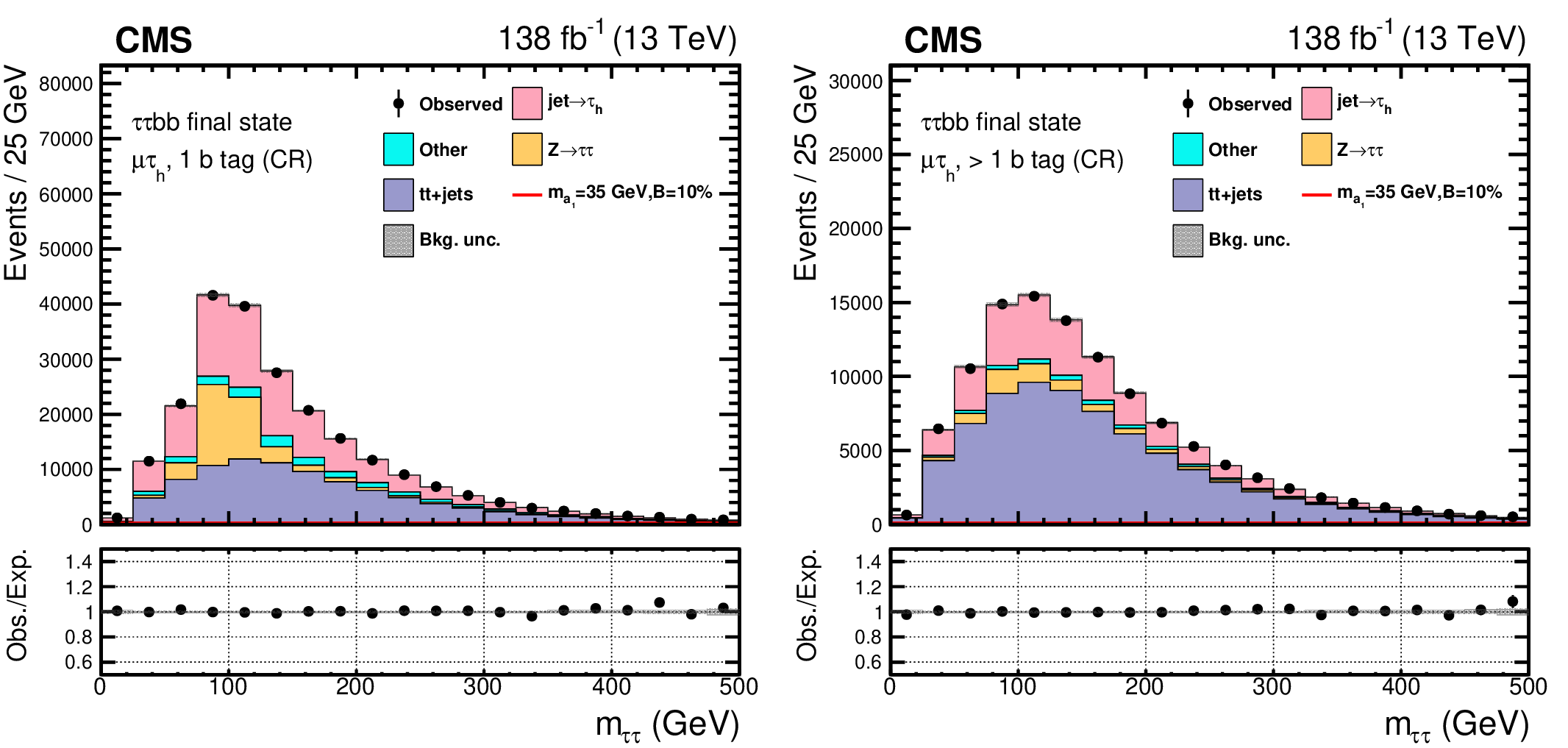
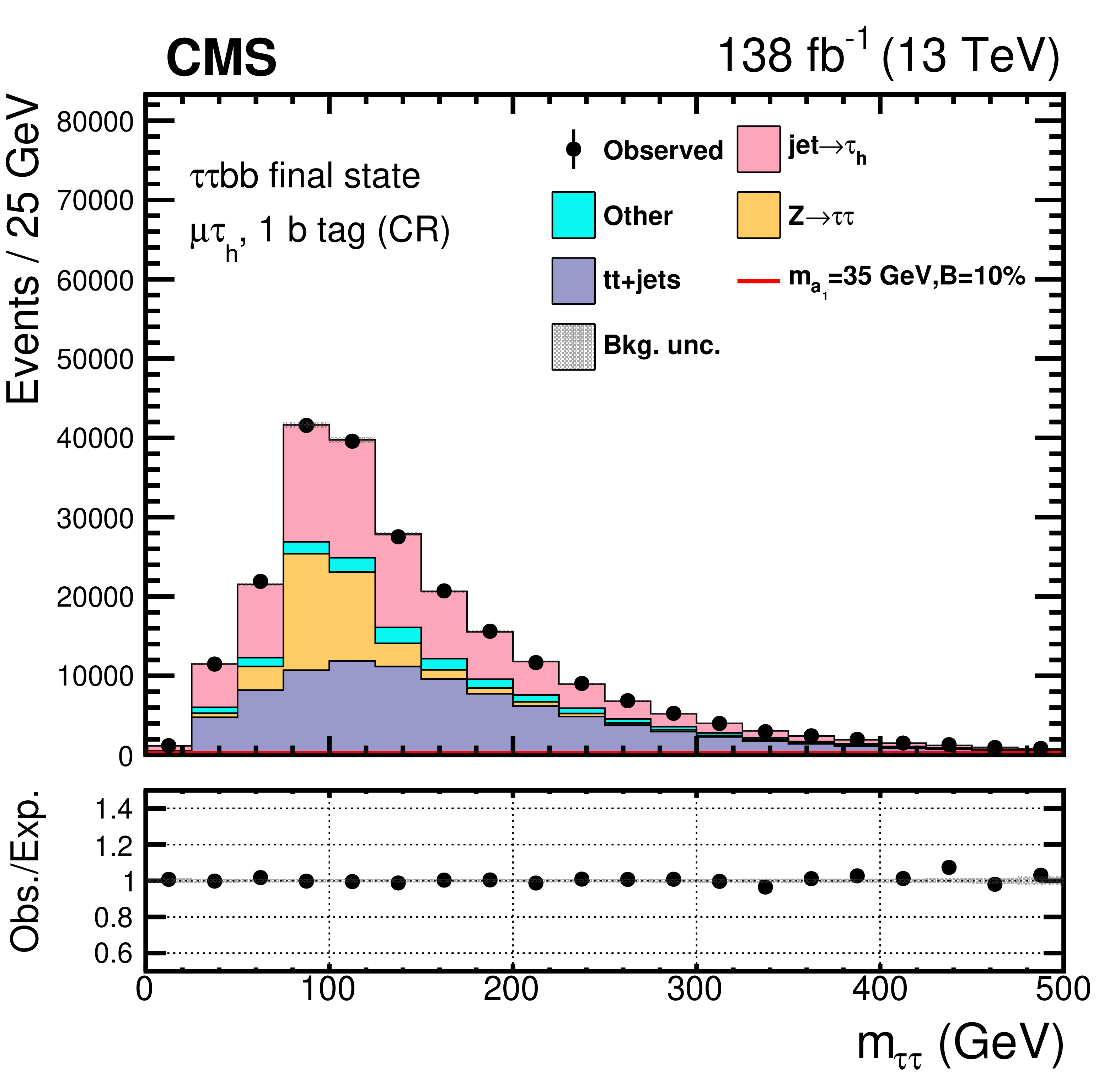
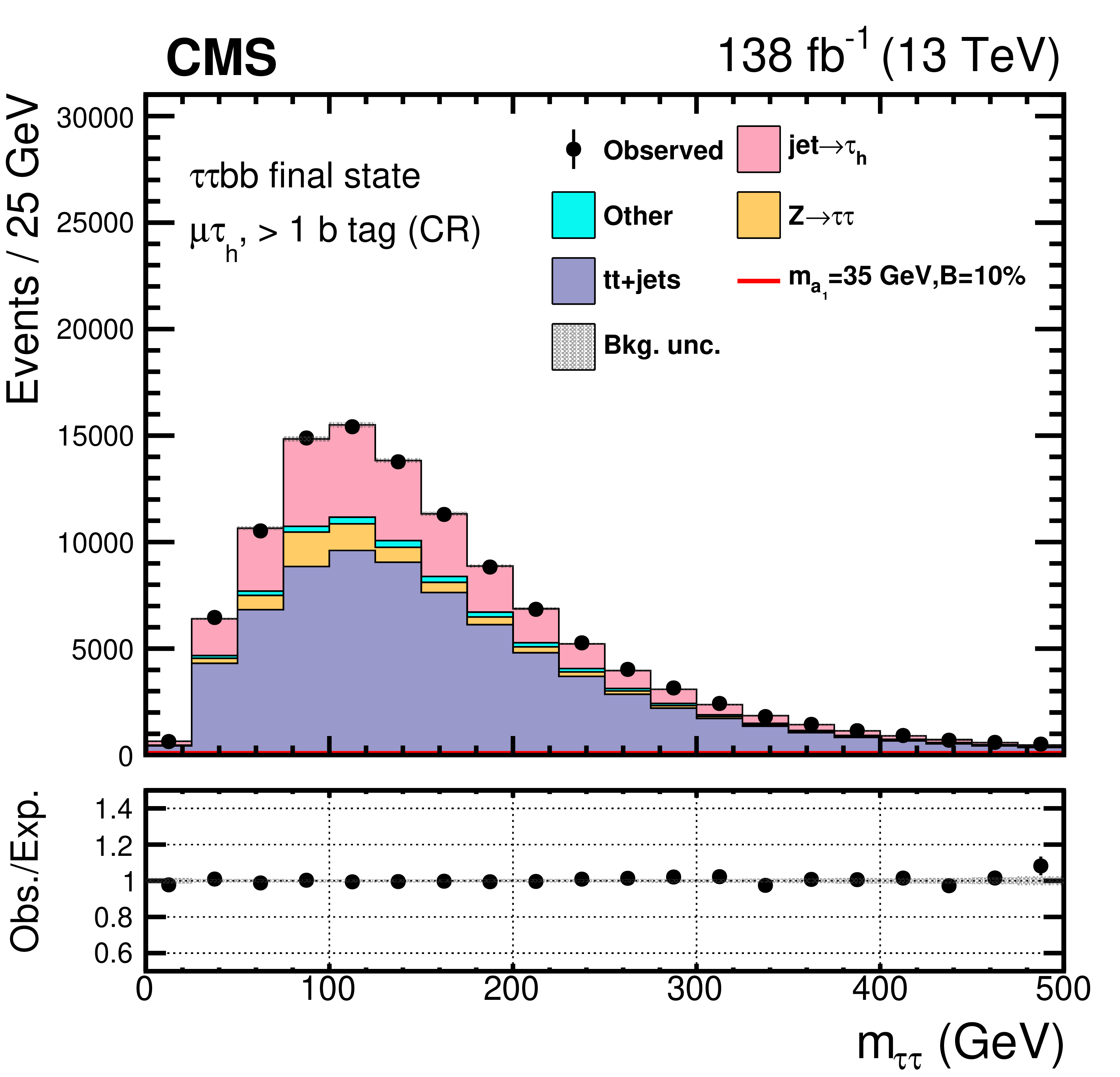
Figure 9:
Post-fit distributions of the $ m_{\tau\tau} $ for the $ \mu\hspace{-.04em}\tau_\mathrm{h} $ channel control regions in events with exactly one b tagged jet (left) and at least two b tagged jets (right). The contamination from the $ \mathrm{H}\to a_{1} a_{1} $ signal, where $ m_{a_{1}} = $ 35 GeV, is barely visible assuming $ \mathcal{B}(\mathrm{H}\to a_{1} a_{1} \to\tau\tau{\mathrm{b}}{\mathrm{b}}) $ to be 10%. |
png pdf |
Figure 9-a:
Post-fit distributions of the $ m_{\tau\tau} $ for the $ \mu\hspace{-.04em}\tau_\mathrm{h} $ channel control regions in events with exactly one b tagged jet (left) and at least two b tagged jets (right). The contamination from the $ \mathrm{H}\to a_{1} a_{1} $ signal, where $ m_{a_{1}} = $ 35 GeV, is barely visible assuming $ \mathcal{B}(\mathrm{H}\to a_{1} a_{1} \to\tau\tau{\mathrm{b}}{\mathrm{b}}) $ to be 10%. |
png pdf |
Figure 9-b:
Post-fit distributions of the $ m_{\tau\tau} $ for the $ \mu\hspace{-.04em}\tau_\mathrm{h} $ channel control regions in events with exactly one b tagged jet (left) and at least two b tagged jets (right). The contamination from the $ \mathrm{H}\to a_{1} a_{1} $ signal, where $ m_{a_{1}} = $ 35 GeV, is barely visible assuming $ \mathcal{B}(\mathrm{H}\to a_{1} a_{1} \to\tau\tau{\mathrm{b}}{\mathrm{b}}) $ to be 10%. |
png pdf |
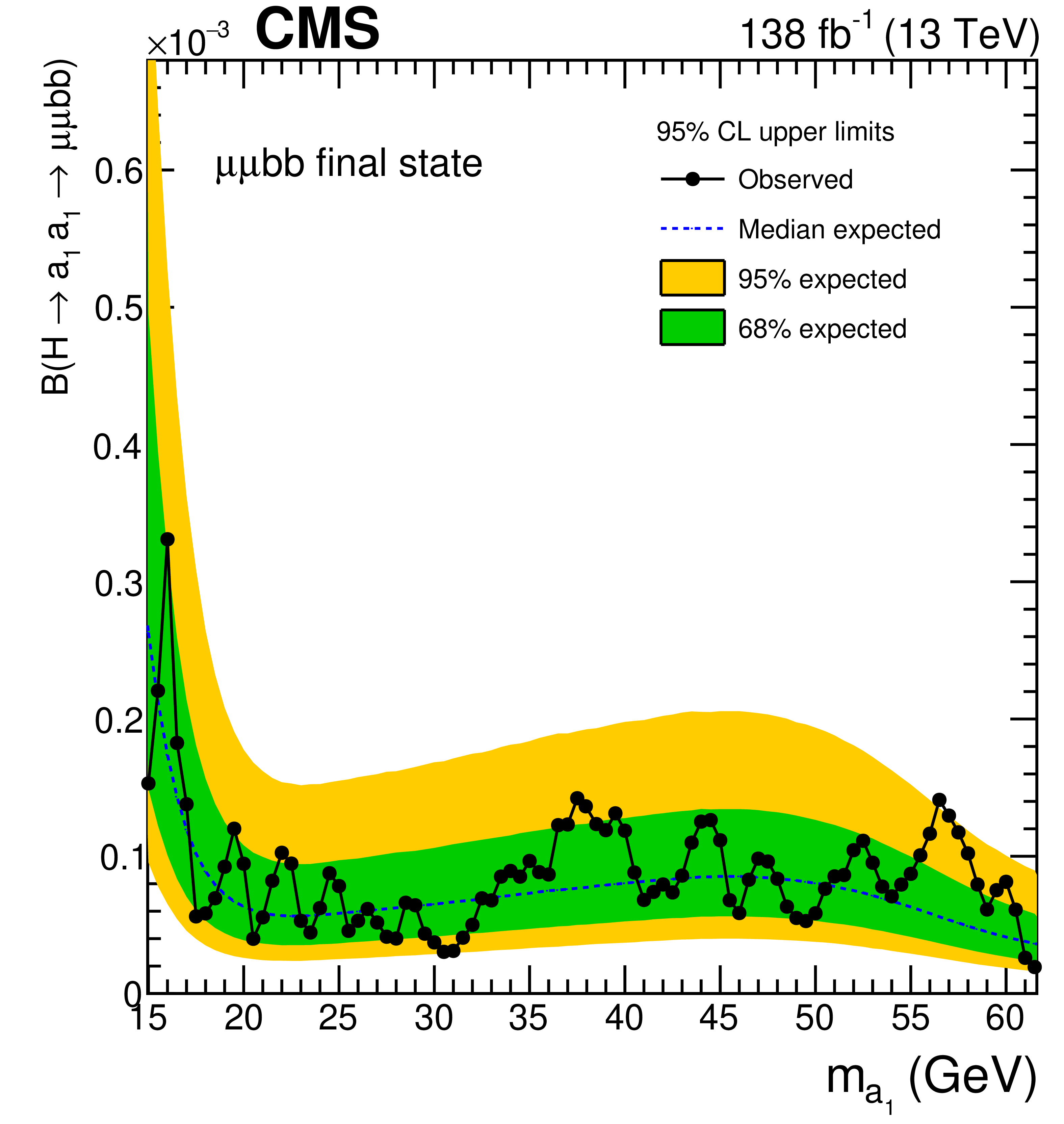
Figure 10:
Observed and expected upper limits at 95% CL on $ \mathcal{B}(\mathrm{H}\to a_{1} a_{1} \to \mu\mu\mathrm{b}\mathrm{b}) $ as functions of $ m_{a_{1}} $. The inner and outer bands indicate the regions containing the distribution of limits located within 68 and 95% confidence intervals, respectively, of the expectation under the background-only hypothesis. |
png pdf |
Figure 11:
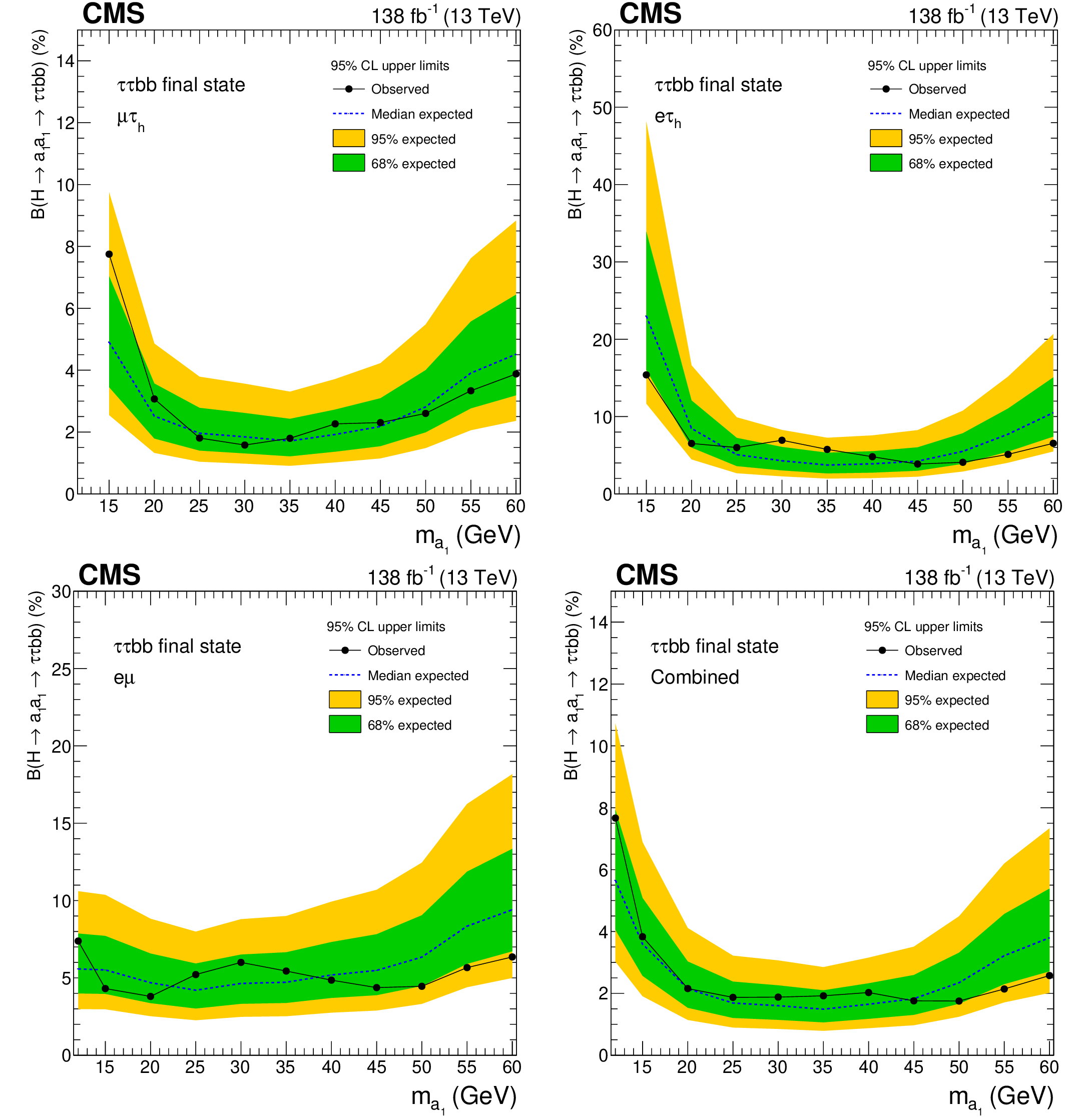
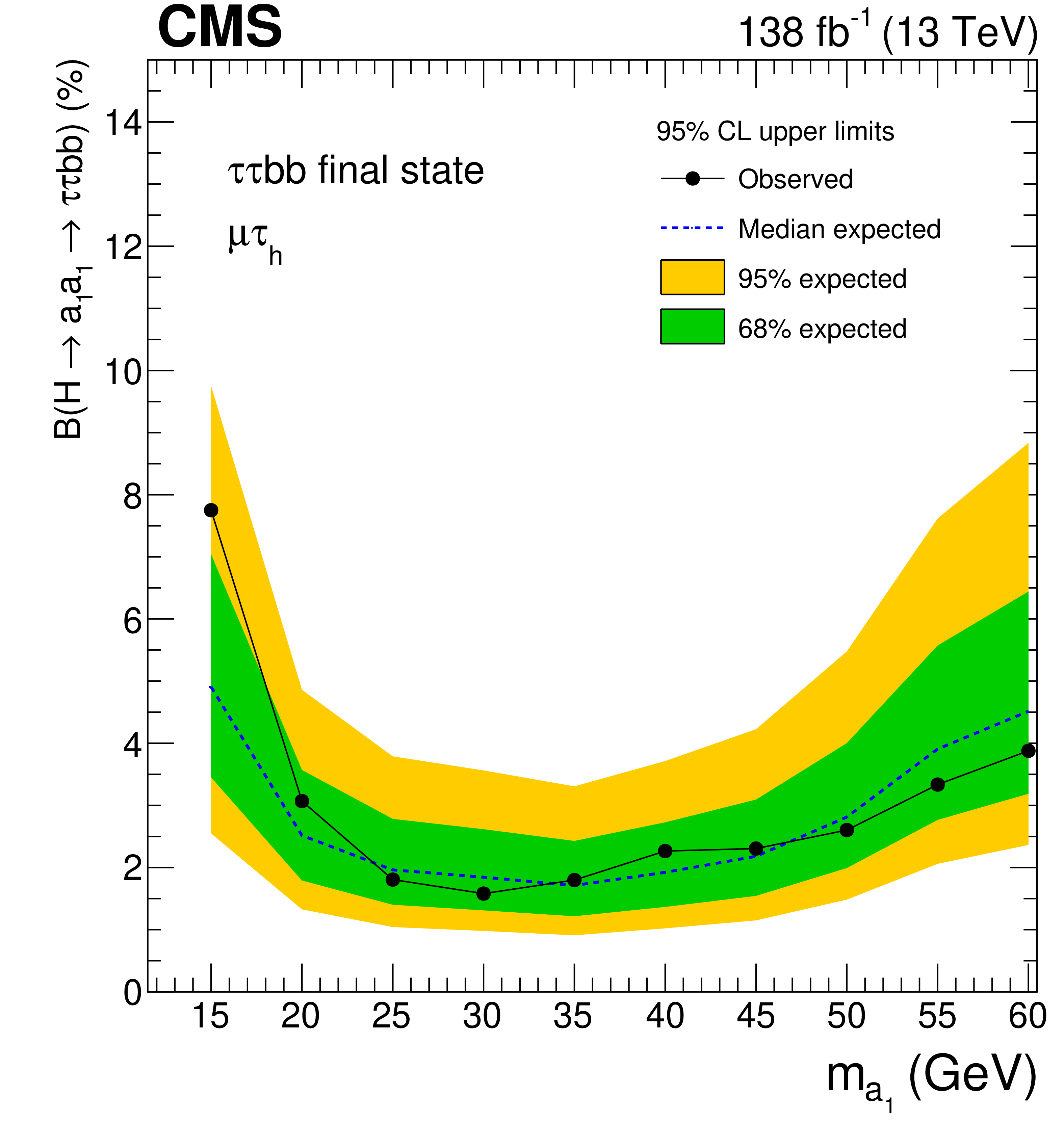
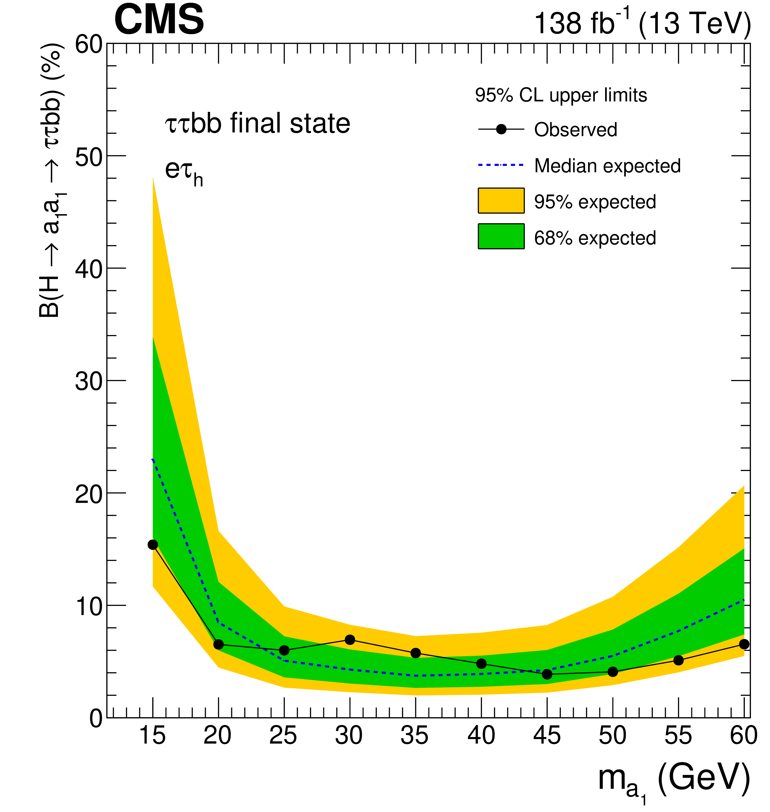
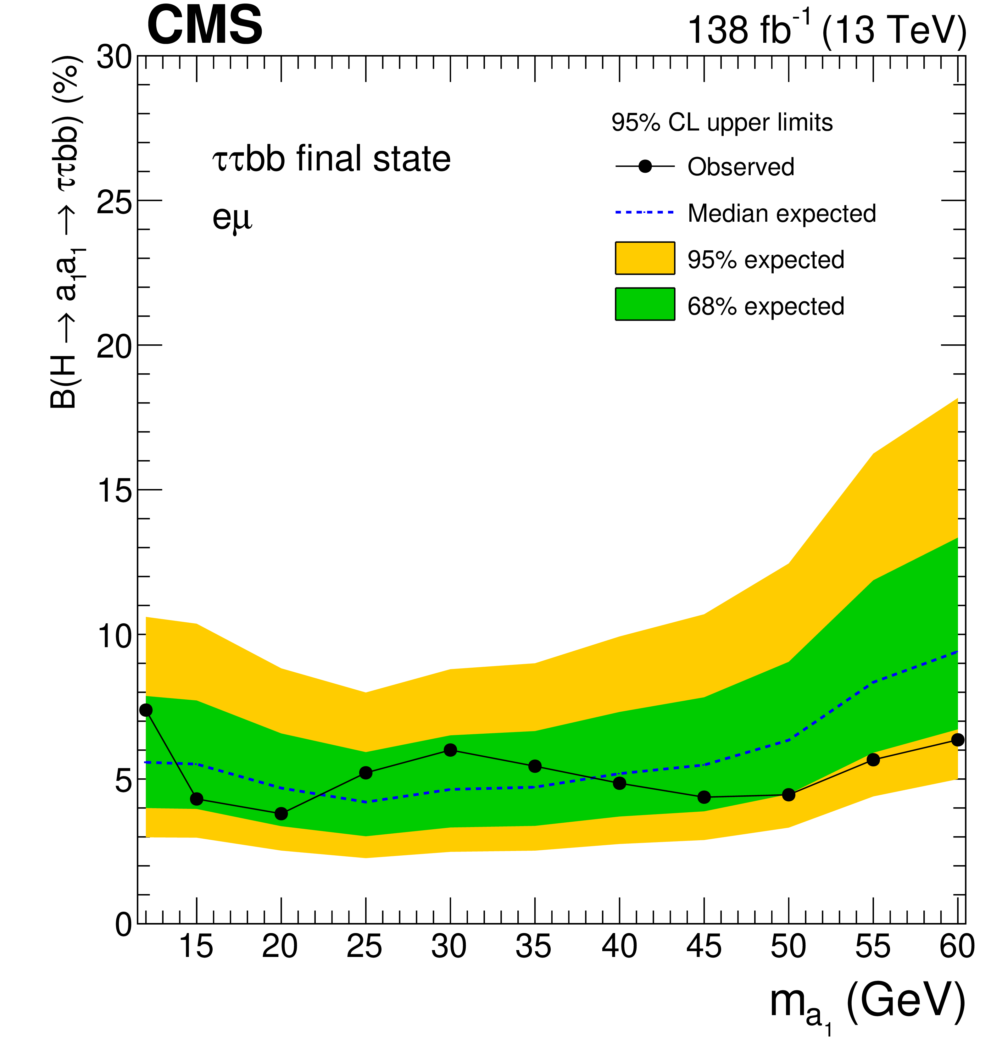
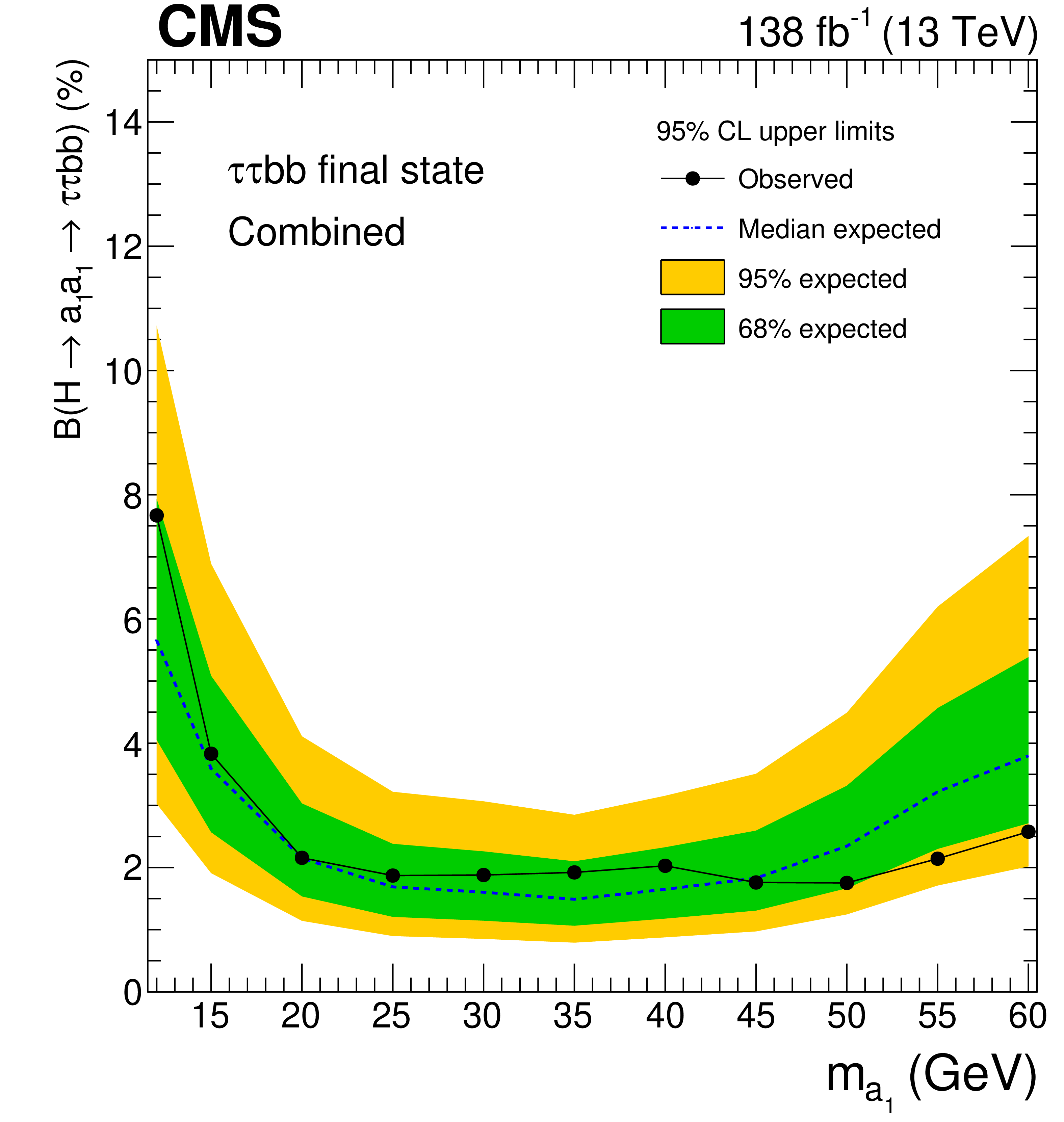
Observed and expected 95% CL exclusion limits on $ \mathcal{B}(\mathrm{H}\to a_{1} a_{1} \to\tau\tau{\mathrm{b}}{\mathrm{b}}) $ in percent, for the (upper left) $ \mu\hspace{-.04em}\tau_\mathrm{h} $, (upper right) $ \mathrm{e}\hspace{-.04em}\tau_\mathrm{h} $, (lower left) $ \mathrm{e}\hspace{-.04em}\mu $ channels, and (lower right) for the combination of all the channels. |
png pdf |
Figure 11-a:
Observed and expected 95% CL exclusion limits on $ \mathcal{B}(\mathrm{H}\to a_{1} a_{1} \to\tau\tau{\mathrm{b}}{\mathrm{b}}) $ in percent, for the (upper left) $ \mu\hspace{-.04em}\tau_\mathrm{h} $, (upper right) $ \mathrm{e}\hspace{-.04em}\tau_\mathrm{h} $, (lower left) $ \mathrm{e}\hspace{-.04em}\mu $ channels, and (lower right) for the combination of all the channels. |
png pdf |
Figure 11-b:
Observed and expected 95% CL exclusion limits on $ \mathcal{B}(\mathrm{H}\to a_{1} a_{1} \to\tau\tau{\mathrm{b}}{\mathrm{b}}) $ in percent, for the (upper left) $ \mu\hspace{-.04em}\tau_\mathrm{h} $, (upper right) $ \mathrm{e}\hspace{-.04em}\tau_\mathrm{h} $, (lower left) $ \mathrm{e}\hspace{-.04em}\mu $ channels, and (lower right) for the combination of all the channels. |
png pdf |
Figure 11-c:
Observed and expected 95% CL exclusion limits on $ \mathcal{B}(\mathrm{H}\to a_{1} a_{1} \to\tau\tau{\mathrm{b}}{\mathrm{b}}) $ in percent, for the (upper left) $ \mu\hspace{-.04em}\tau_\mathrm{h} $, (upper right) $ \mathrm{e}\hspace{-.04em}\tau_\mathrm{h} $, (lower left) $ \mathrm{e}\hspace{-.04em}\mu $ channels, and (lower right) for the combination of all the channels. |
png pdf |
Figure 11-d:
Observed and expected 95% CL exclusion limits on $ \mathcal{B}(\mathrm{H}\to a_{1} a_{1} \to\tau\tau{\mathrm{b}}{\mathrm{b}}) $ in percent, for the (upper left) $ \mu\hspace{-.04em}\tau_\mathrm{h} $, (upper right) $ \mathrm{e}\hspace{-.04em}\tau_\mathrm{h} $, (lower left) $ \mathrm{e}\hspace{-.04em}\mu $ channels, and (lower right) for the combination of all the channels. |
png pdf |
Figure 12:
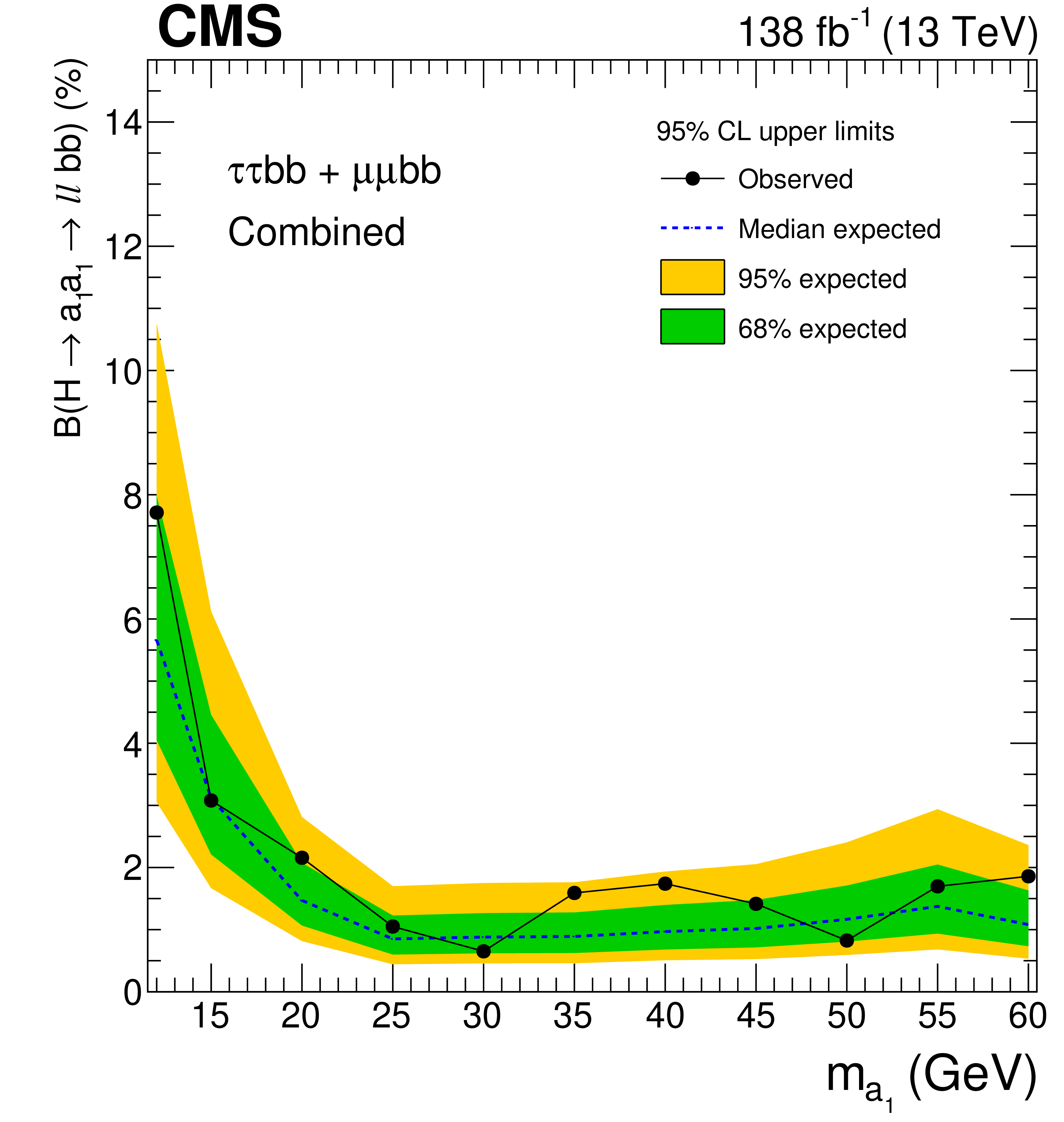
Observed and expected 95% CL upper limits on $ \mathcal{B}(\mathrm{H}\to a_{1} a_{1} \to \ell\ell\mathrm{b}\mathrm{b}) $ in %, where $ \ell $ stands for muons or $ \tau $ leptons, obtained from the combination of the $ \mu\mu\mathrm{b}\mathrm{b} $ and $ \tau\tau{\mathrm{b}}{\mathrm{b}} $ channels. The results are obtained as functions of $ m_{a_{1}} $ for 2HDM+S models, independent of the type and $ \tan\beta $ parameter. |
png pdf |
Figure 13:
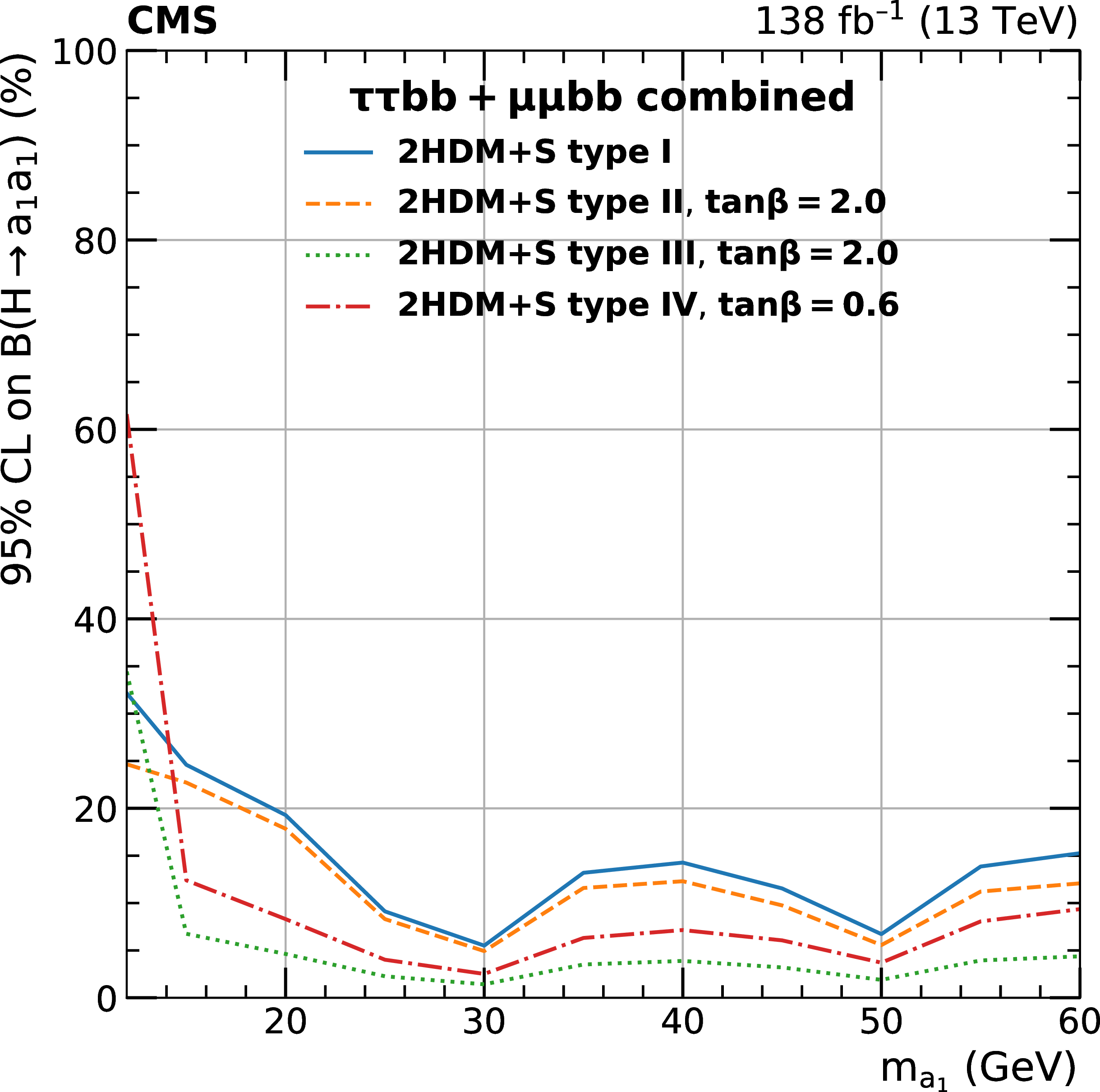
Observed and expected 95% CL upper limits on $ \mathcal{B}(\mathrm{H}\to a_{1} a_{1} ) $ in %, obtained from the combination of the $ \mu\mu\mathrm{b}\mathrm{b} $ and $ \tau\tau{\mathrm{b}}{\mathrm{b}} $ channels. The results are obtained as functions of $ m_{a_{1}} $ for 2HDM+S Type I (independent of $ \tan\beta $), Type II ($ \tan\beta= $ 2.0), Type III ($ \tan\beta= $ 2.0), and Type IV ($ \tan\beta= $ 0.6), respectively. |
png pdf |
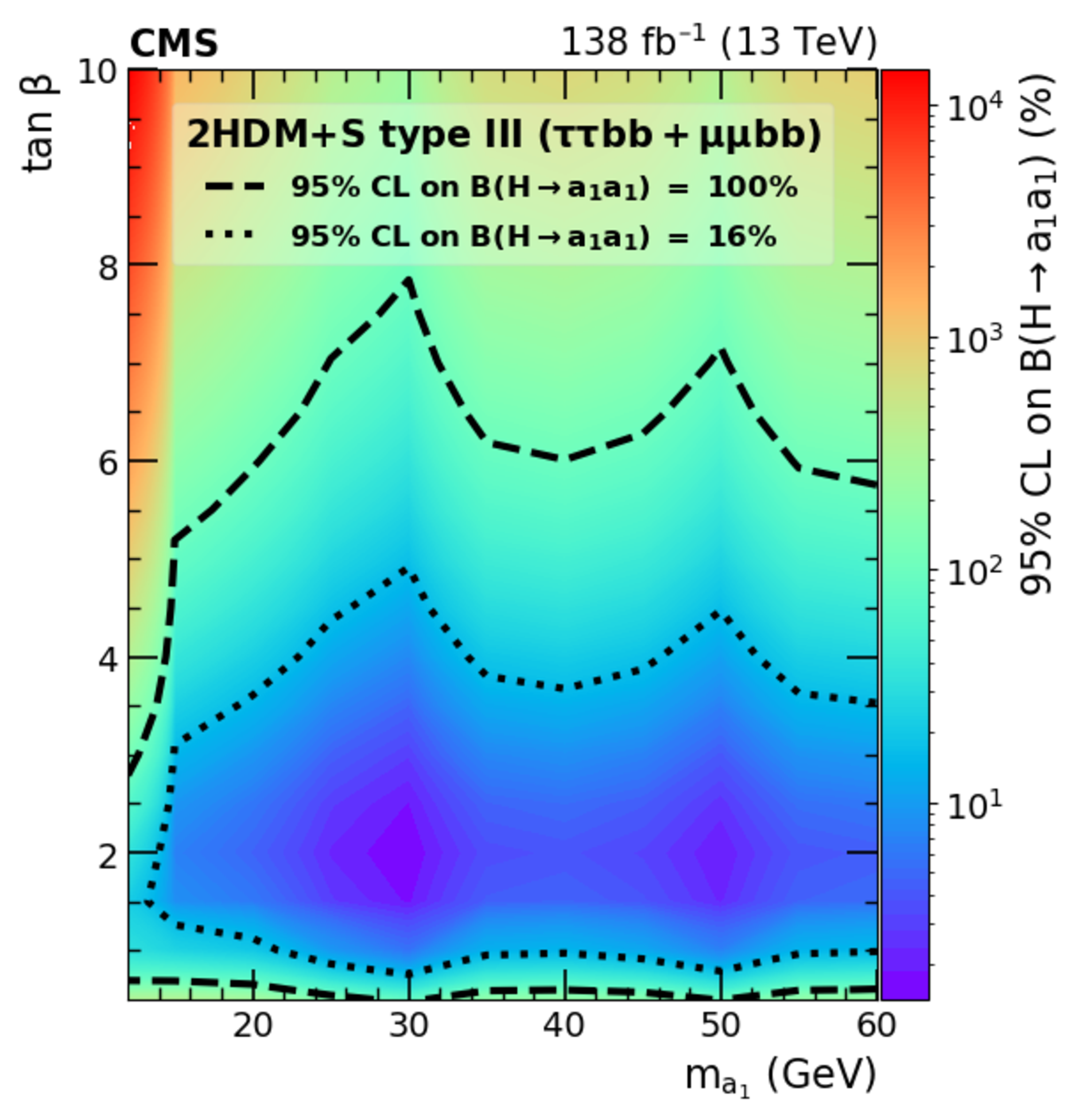
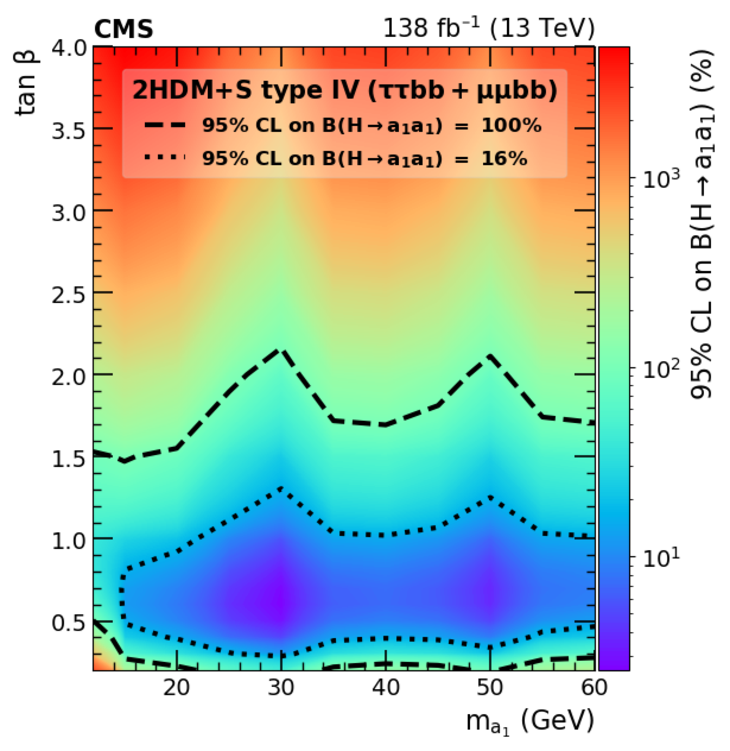
Figure 14:
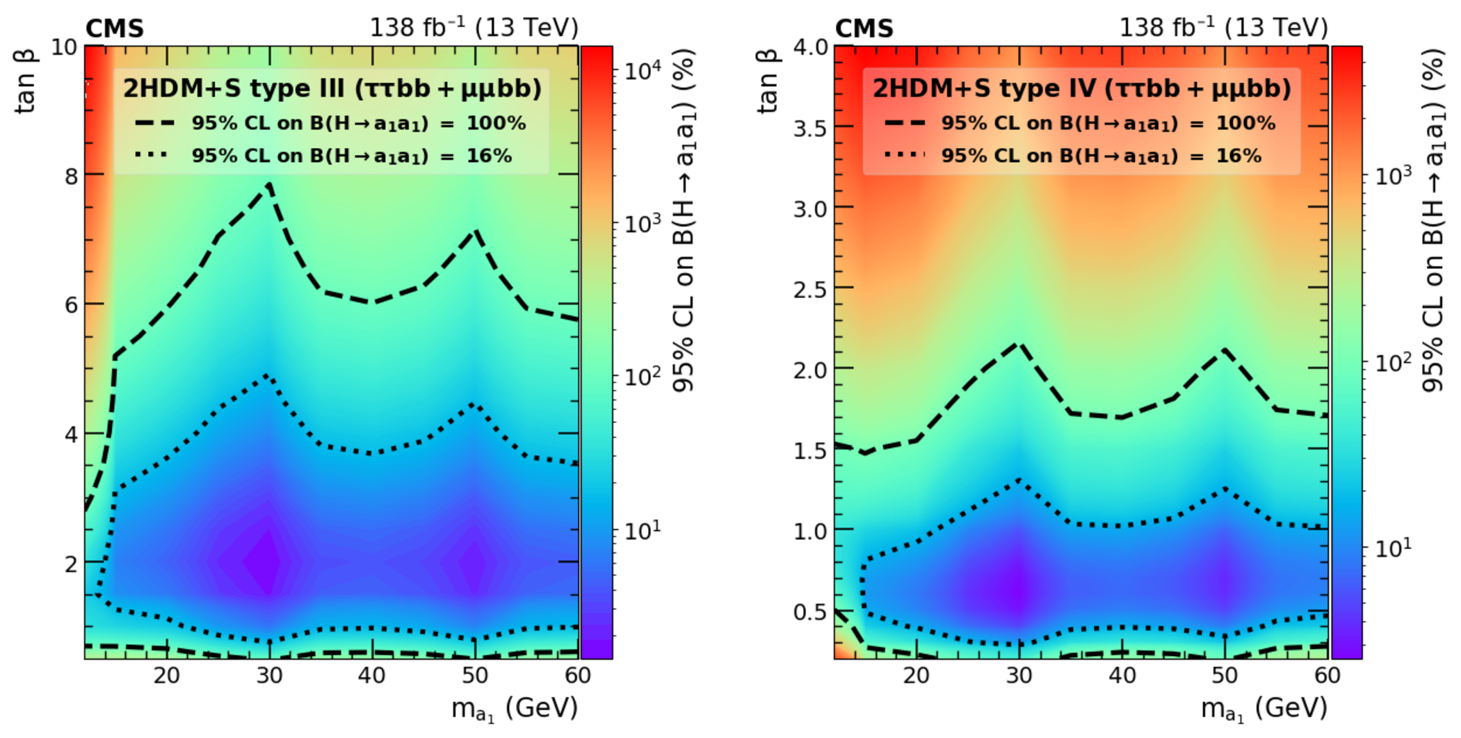
Observed 95% CL upper limits on $ \mathcal{B}(\mathrm{H}\to a_{1} a_{1} ) $ in %, for the combination of the $ \mu\mu\mathrm{b}\mathrm{b} $ and $ \tau\tau{\mathrm{b}}{\mathrm{b}} $ channels for Type III (left) and Type IV (right) 2HDM+S in the $ \tan\beta \mbox{\textsl{vs.}} m_{a_{1}} $ parameter space. The limits are calculated in a grid of 5 GeV in $ m_{a_{1}} $ and 0.1-0.5 in $ \tan\beta $, interpolating the points in between. The contours corresponding to branching fractions of 100 and 16% are drawn using dashed lines, where 16% refers to the combined upper limit on Higgs boson to undetected particle decays from previous Run 2 results [15]. All points inside the contour are allowed within that upper limit. |
png pdf |
Figure 14-a:
Observed 95% CL upper limits on $ \mathcal{B}(\mathrm{H}\to a_{1} a_{1} ) $ in %, for the combination of the $ \mu\mu\mathrm{b}\mathrm{b} $ and $ \tau\tau{\mathrm{b}}{\mathrm{b}} $ channels for Type III (left) and Type IV (right) 2HDM+S in the $ \tan\beta \mbox{\textsl{vs.}} m_{a_{1}} $ parameter space. The limits are calculated in a grid of 5 GeV in $ m_{a_{1}} $ and 0.1-0.5 in $ \tan\beta $, interpolating the points in between. The contours corresponding to branching fractions of 100 and 16% are drawn using dashed lines, where 16% refers to the combined upper limit on Higgs boson to undetected particle decays from previous Run 2 results [15]. All points inside the contour are allowed within that upper limit. |
png pdf |
Figure 14-b:
Observed 95% CL upper limits on $ \mathcal{B}(\mathrm{H}\to a_{1} a_{1} ) $ in %, for the combination of the $ \mu\mu\mathrm{b}\mathrm{b} $ and $ \tau\tau{\mathrm{b}}{\mathrm{b}} $ channels for Type III (left) and Type IV (right) 2HDM+S in the $ \tan\beta \mbox{\textsl{vs.}} m_{a_{1}} $ parameter space. The limits are calculated in a grid of 5 GeV in $ m_{a_{1}} $ and 0.1-0.5 in $ \tan\beta $, interpolating the points in between. The contours corresponding to branching fractions of 100 and 16% are drawn using dashed lines, where 16% refers to the combined upper limit on Higgs boson to undetected particle decays from previous Run 2 results [15]. All points inside the contour are allowed within that upper limit. |
| Tables | |
png pdf |
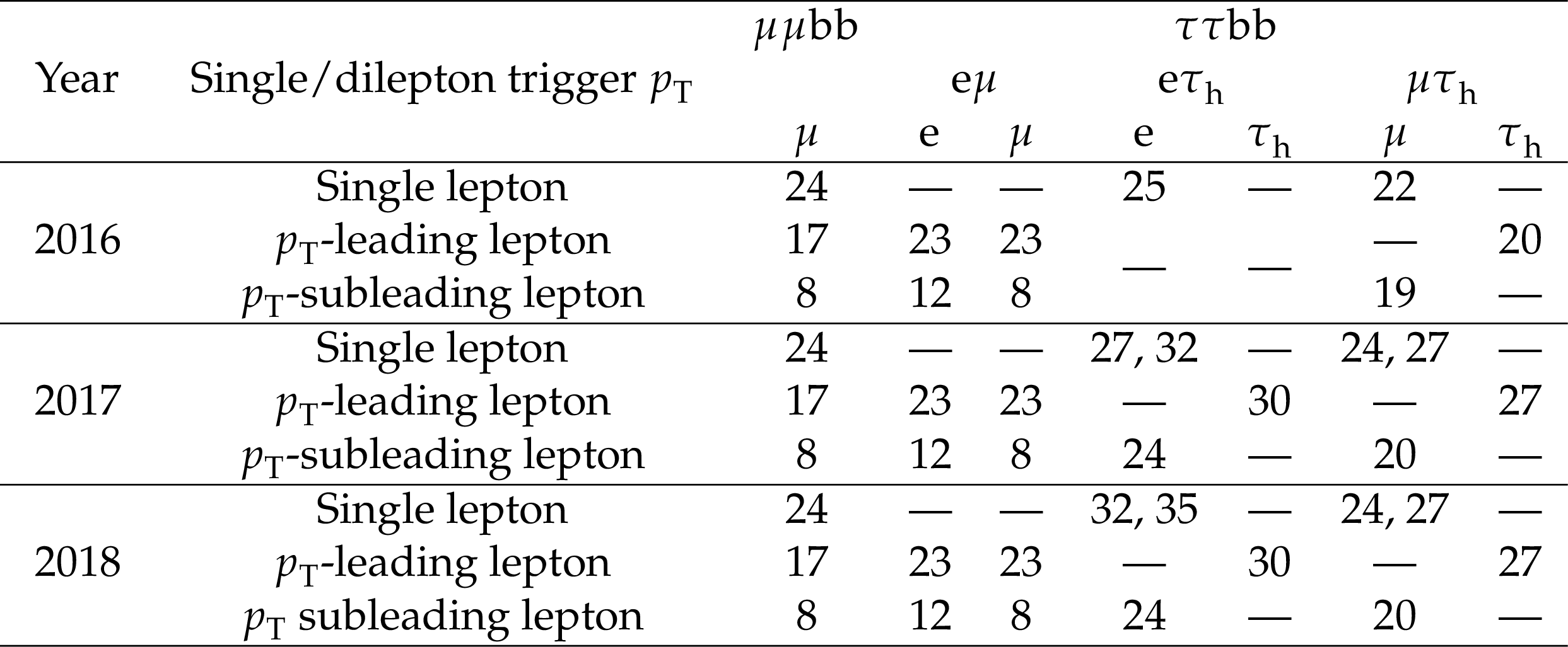
Table 1:
The electron, muon, and $ \tau_\mathrm{h} p_{\mathrm{T}} $ thresholds in GeV at trigger level for the $ \mu\mu\mathrm{b}\mathrm{b} $ and $ \tau\tau{\mathrm{b}}{\mathrm{b}} $ channels. |
png pdf |
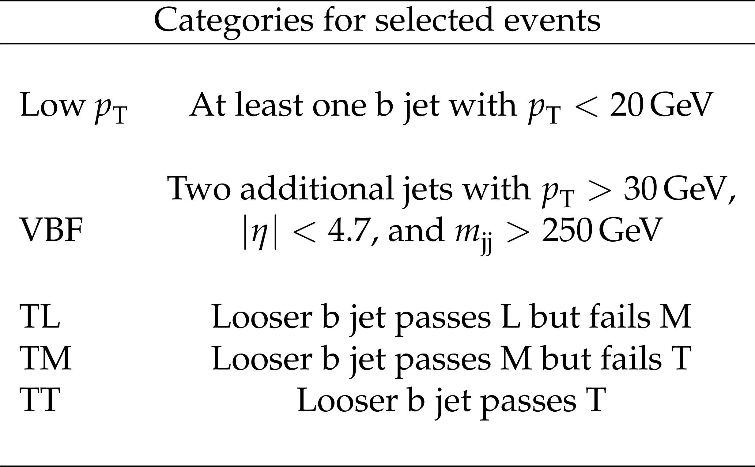
Table 3:
Summary of the categorization requirements in the $ \mu\mu\mathrm{b}\mathrm{b} $ channel. Events in these categories contain two muons and two b jets. As stated in the text, L, M, and T stand for the loose, medium, and tight b tagging criteria, respectively. |
png pdf |
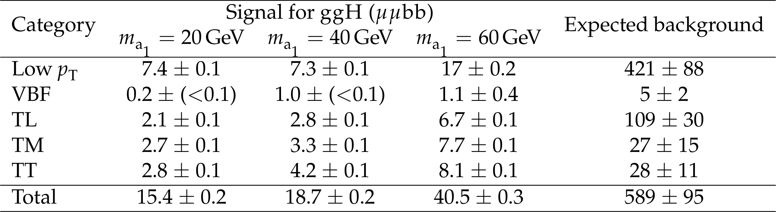
Table 4:
The expected yields for backgrounds and different signal hypotheses in each category of the $ \mu\mu\mathrm{b}\mathrm{b} $ channel. |
| Summary |
| A search for an exotic decay of the 125 GeV Higgs boson (H) to a pair of light pseudoscalar bosons (a_{1} ) in the final state with two b quarks and two muons or two $ \tau $ leptons has been presented. The results are based on a data sample of proton-proton collisions corresponding to an integrated luminosity of 138 fb$^{-1}$, accumulated by the CMS experiment at the LHC during Run 2 at a center-of-mass energy of 13 TeV. Final states with at least one leptonic $ \tau $ decay are studied in the $ \tau\tau{\mathrm{b}}{\mathrm{b}} $ channel, excluding those with two muons or two electrons. The results show significant improvement, with respect to the earlier CMS analyses at 13 TeV, beyond what is merely expected from the increase in the size of the data sample. A more thorough analysis of the signal properties using a single discriminating variable improves the $ \mu\mu\mathrm{b}\mathrm{b} $ analysis, while the $ \tau\tau{\mathrm{b}}{\mathrm{b}} $ analysis gains from a deep neural network based signal categorization. No significant excess in the data over the standard model backgrounds is observed. Upper limits are set, at 95% confidence level, on branching fractions $ \mathcal{B}(\mathrm{H}\to a_{1} a_{1} \to\mu\mu\mathrm{b}\mathrm{b}) $ and $ \mathcal{B}(\mathrm{H}\to a_{1} a_{1} \to\tau\tau{\mathrm{b}}{\mathrm{b}}) $, in the $ \mu\mu\mathrm{b}\mathrm{b} $ and $ \tau\tau{\mathrm{b}}{\mathrm{b}} $ analyses, respectively. Both analyses provide the most stringent expected limits to date. In the $ \mu\mu\mathrm{b}\mathrm{b} $ channel, the observed limits are in the range (0.17-3.3) $ \times $ 10$^{-4} $ for a pseudoscalar mass, $ m_{a_{1}} $, between 15 and 62.5 GeV. Combining all final states in the $ \tau\tau{\mathrm{b}}{\mathrm{b}} $ channel, limits are observed to be in the range 1.7-7.7% for $ m_{a_{1}} $ between 12 and 60 GeV. By combining the $ \mu\mu\mathrm{b}\mathrm{b} $ and $ \tau\tau{\mathrm{b}}{\mathrm{b}} $ channels, model-independent limits are set on the branching fraction $ \mathcal{B}(\mathrm{H}\to a_{1} a_{1} \to \ell\ell\mathrm{b}\mathrm{b}) $, where $ \ell $ stands for muons or $ \tau $ leptons. The observed upper limits range between 0.6 and 7.7% depending on the $ m_{a_{1}} $. The results can also be interpreted in different types of 2HDM+S models. For $ m_{a_{1}} $ values between 15 and 60 GeV, $ \mathcal{B}(\mathrm{H}\to a_{1} a_{1} ) $ values above 23% are excluded, at 95% confidence level, in most of the Type II scenarios. In Types III and IV, observed upper limits as low as 1 and 3% are obtained, respectively, for $ \tan\beta= $ 2.0 and 0.5. |
| References | ||||
| 1 | ATLAS Collaboration | Observation of a new particle in the search for the Standard Model Higgs boson with the ATLAS detector at the LHC | PLB 716 (2012) 1 | 1207.7214 |
| 2 | CMS Collaboration | Observation of a new boson at a mass of 125 GeV with the CMS experiment at the LHC | PLB 716 (2012) 30 | CMS-HIG-12-028 1207.7235 |
| 3 | CMS Collaboration | Observation of a new boson with mass near 125 GeV in $ pp $ collisions at $ \sqrt{s} $ = 7 and 8 TeV | JHEP 06 (2013) 081 | CMS-HIG-12-036 1303.4571 |
| 4 | F. Englert and R. Brout | Broken Symmetry and the Mass of Gauge Vector Mesons | PRL 13 (1964) 321 | |
| 5 | P. W. Higgs | Broken symmetries, massless particles and gauge fields | PL 12 (1964) 132 | |
| 6 | P. W. Higgs | Broken symmetries and the masses of gauge bosons | PRL 13 (1964) 508 | |
| 7 | G. S. Guralnik, C. R. Hagen, and T. W. B. Kibble | Global conservation laws and massless particles | PRL 13 (1964) 585 | |
| 8 | P. W. Higgs | Spontaneous symmetry breakdown without massless bosons | PR 145 (1966) 1156 | |
| 9 | T. W. B. Kibble | Symmetry breaking in non-abelian gauge theories | PR 155 (1967) 1554 | |
| 10 | G. C. Branco et al. | Theory and phenomenology of two-Higgs-doublet models | Phys. Rept. 516 (2012) 1 | 1106.0034 |
| 11 | A. Djouadi | The Anatomy of electro-weak symmetry breaking. II. The Higgs bosons in the minimal supersymmetric model | Phys. Rept. 459 (2008) 1 | hep-ph/0503173 |
| 12 | T. Robens and T. Stefaniak | Status of the Higgs Singlet Extension of the Standard Model after LHC Run 1 | EPJC 75 (2015) 104 | 1501.02234 |
| 13 | T. Robens, T. Stefaniak, and J. Wittbrodt | Two-real-scalar-singlet extension of the SM: LHC phenomenology and benchmark scenarios | EPJC 80 (2020) 151 | 1908.08554 |
| 14 | ATLAS Collaboration | A detailed map of Higgs boson interactions by the ATLAS experiment ten years after the discovery | Nature 607 (2022) 52 | 2207.00092 |
| 15 | CMS Collaboration | A portrait of the Higgs boson by the CMS experiment ten years after the discovery | Nature 607 (2022) 60 | CMS-HIG-22-001 2207.00043 |
| 16 | D. Curtin et al. | Exotic decays of the 125 GeV Higgs boson | PRD 90 (2014) 075004 | 1312.4992 |
| 17 | B. Grzadkowski and P. Osland | Tempered Two-Higgs-Doublet Model | PRD 82 (2010) 125026 | 0910.4068 |
| 18 | A. Drozd, B. Grzadkowski, J. F. Gunion, and Y. Jiang | Extending two-Higgs-doublet models by a singlet scalar field - the Case for Dark Matter | JHEP 11 (2014) 105 | 1408.2106 |
| 19 | S. Ramos-Sanchez | The $ \mu $-problem, the NMSSM and string theory | Fortschritte der Phys. 58 (2010) 748 | 1003.1307 |
| 20 | D. de Florian et al. | Handbook of LHC Higgs cross sections: 4. Deciphering the nature of the Higgs sector | CERN Report CERN-2017-002-M, 2016 link |
1610.07922 |
| 21 | ATLAS Collaboration | Search for Higgs boson decays into a pair of pseudoscalar particles in the $ bb\mu\mu $ final state with the ATLAS detector in $ pp $ collisions at $ \sqrt{s}= $ 13 TeV | PRD 105 (2022) 012006 | 2110.00313 |
| 22 | ATLAS Collaboration | Search for Higgs boson decays into a pair of light bosons in the $ \mathrm{b}\mathrm{b}\mu\mu $ final state in pp collision at $ \sqrt{s} = $ 13 TeV with the ATLAS detector | PLB 790 (2019) 1 | 1807.00539 |
| 23 | CMS Collaboration | Search for an exotic decay of the Higgs boson to a pair of light pseudoscalars in the final state with two muons and two b quarks in pp collisions at 13 TeV | PLB 795 (2019) 398 | CMS-HIG-18-011 1812.06359 |
| 24 | CMS Collaboration | Search for light bosons in decays of the 125 GeV Higgs boson in proton-proton collisions at $ \sqrt{s}= $ 8 TeV | JHEP 10 (2017) 076 | CMS-HIG-16-015 1701.02032 |
| 25 | CMS Collaboration | Search for an exotic decay of the Higgs boson to a pair of light pseudoscalars in the final state with two b quarks and two $ \tau $ leptons in proton-proton collisions at $ \sqrt{s}= $ 13 TeV | PLB 785 (2018) 462 | CMS-HIG-17-024 1805.10191 |
| 26 | CMS Collaboration | HEPData record for this analysis | link | |
| 27 | CMS Collaboration | The CMS trigger system | JINST 12 (2017) P01020 | CMS-TRG-12-001 1609.02366 |
| 28 | CMS Collaboration | The CMS experiment at the CERN LHC | JINST 3 (2008) S08004 | |
| 29 | T. Sjöstrand et al. | An Introduction to PYTHIA 8.2 | Comput. Phys. Commun. 191 (2015) 159 | 1410.3012 |
| 30 | NNPDF Collaboration | Parton distributions from high-precision collider data | EPJC 77 (2017) 663 | 1706.00428 |
| 31 | J. Alwall, S. de Visscher, and F. Maltoni | QCD radiation in the production of heavy colored particles at the LHC | JHEP 02 (2009) 017 | 0810.5350 |
| 32 | J. Alwall et al. | Comparative study of various algorithms for the merging of parton showers and matrix elements in hadronic collisions | EPJC 53 (2008) 473 | 0706.2569 |
| 33 | R. Frederix and S. Frixione | Merging meets matching in MC@NLO | JHEP 12 (2012) 061 | 1209.6215 |
| 34 | J. Alwall et al. | The automated computation of tree-level and next-to-leading order differential cross sections, and their matching to parton shower simulations | JHEP 07 (2014) 079 | 1405.0301 |
| 35 | P. Skands, S. Carrazza, and J. Rojo | Tuning PYTHIA 8.1: the Monash 2013 Tune | EPJC 74 (2014) 3024 | 1404.5630 |
| 36 | CMS Collaboration | Extraction and validation of a new set of CMS PYTHIA8 tunes from underlying-event measurements | EPJC 80 (2020) 4 | CMS-GEN-17-001 1903.12179 |
| 37 | GEANT4 Collaboration | GEANT4--a simulation toolkit | NIM A 506 (2003) 250 | |
| 38 | J. Allison et al. | Geant4 developments and applications | IEEE Trans. Nucl. Sci. 53 (2006) 270 | |
| 39 | CMS Collaboration | Measurements of Higgs boson production in the decay channel with a pair of $ \tau $ leptons in proton-proton collisions at $ \sqrt{s}= $ 13 TeV | no.~7, 562, 2023 EPJC 83 (2023) |
CMS-HIG-19-010 2204.12957 |
| 40 | P. Nason | A New method for combining NLO QCD with shower Monte Carlo algorithms | JHEP 11 (2004) 040 | hep-ph/0409146 |
| 41 | S. Frixione, P. Nason, and C. Oleari | Matching NLO QCD computations with Parton Shower simulations: the POWHEG method | JHEP 11 (2007) 070 | 0709.2092 |
| 42 | S. Alioli, P. Nason, C. Oleari, and E. Re | A general framework for implementing NLO calculations in shower Monte Carlo programs: the POWHEG BOX | JHEP 06 (2010) 043 | 1002.2581 |
| 43 | S. Alioli et al. | Jet pair production in POWHEG | JHEP 04 (2011) 081 | 1012.3380 |
| 44 | M. Czakon et al. | Top-pair production at the LHC through NNLO QCD and NLO EW | JHEP 10 (2017) 186 | 1705.04105 |
| 45 | M. Czakon and A. Mitov | Top++: A Program for the Calculation of the Top-Pair Cross-Section at Hadron Colliders | Comput. Phys. Commun. 185 (2014) 2930 | 1112.5675 |
| 46 | M. Botje et al. | The PDF4LHC Working Group interim recommendations | 1101.0538 | |
| 47 | A. D. Martin, W. J. Stirling, R. S. Thorne, and G. Watt | Uncertainties on alpha(S) in global PDF analyses and implications for predicted hadronic cross sections | EPJC 64 (2009) 653 | 0905.3531 |
| 48 | J. Gao et al. | CT10 next-to-next-to-leading order global analysis of QCD | no.~3, 033009, 2014 PRD 89 (2014) |
1302.6246 |
| 49 | R. D. Ball et al. | Parton distributions with LHC data | NPB 867 (2013) 244 | 1207.1303 |
| 50 | J. Campbell, T. Neumann, and Z. Sullivan | Single-top-quark production in the $ t $-channel at NNLO | JHEP 02 (2021) 040 | 2012.01574 |
| 51 | PDF4LHC Working Group Collaboration | The PDF4LHC21 combination of global PDF fits for the LHC Run III | no.~8, 080501, 2022 JPG 49 (2022) |
2203.05506 |
| 52 | K. Melnikov and F. Petriello | Electroweak gauge boson production at hadron colliders through $ O(\alpha_s^2) $ | PRD 74 (2006) 114017 | hep-ph/0609070 |
| 53 | A. D. Martin, W. J. Stirling, R. S. Thorne, and G. Watt | Parton distributions for the LHC | --285, 2009 EPJC 63 (2009) 189 |
0901.0002 |
| 54 | S. Alioli, P. Nason, C. Oleari, and E. Re | NLO Higgs boson production via gluon fusion matched with shower in POWHEG | JHEP 04 (2009) 002 | 0812.0578 |
| 55 | E. Bagnaschi, G. Degrassi, P. Slavich, and A. Vicini | Higgs production via gluon fusion in the POWHEG approach in the SM and in the MSSM | JHEP 02 (2012) 088 | 1111.2854 |
| 56 | P. Nason and C. Oleari | NLO Higgs boson production via vector-boson fusion matched with shower in POWHEG | JHEP 02 (2010) 037 | 0911.5299 |
| 57 | G. Luisoni, P. Nason, C. Oleari, and F. Tramontano | $ \mathrm{H}\mathrm{W}^{\pm} $/HZ + 0 and 1 jet at NLO with the POWHEG BOX interfaced to GoSam and their merging within MiNLO | JHEP 10 (2013) 083 | 1306.2542 |
| 58 | H. B. Hartanto, B. Jager, L. Reina, and D. Wackeroth | Higgs boson production in association with top quarks in the POWHEG BOX | PRD 91 (2015) 094003 | 1501.04498 |
| 59 | CMS Collaboration | Particle-flow reconstruction and global event description with the CMS detector | JINST 12 (2017) P10003 | CMS-PRF-14-001 1706.04965 |
| 60 | CMS Collaboration | Technical proposal for the Phase-II upgrade of the Compact Muon Solenoid | CMS Technical Proposal CERN-LHCC-2015-010, CMS-TDR-15-02, 2015 CDS |
|
| 61 | CMS Collaboration | Performance of the CMS muon detector and muon reconstruction with proton-proton collisions at $ \sqrt{s}= $ 13 TeV | JINST 13 (2018) P06015 | CMS-MUO-16-001 1804.04528 |
| 62 | CMS Collaboration | Electron and photon reconstruction and identification with the CMS experiment at the CERN LHC | JINST 16 (2021) P05014 | CMS-EGM-17-001 2012.06888 |
| 63 | M. Cacciari, G. P. Salam, and G. Soyez | The anti-$ k_t $ jet clustering algorithm | JHEP 04 (2008) 063 | 0802.1189 |
| 64 | M. Cacciari, G. P. Salam, and G. Soyez | FastJet User Manual | EPJC 72 (2012) 1896 | 1111.6097 |
| 65 | CMS Collaboration | Jet algorithms performance in 13 TeV data | CMS Physics Analysis Summary, 2017 CMS-PAS-JME-16-003 |
CMS-PAS-JME-16-003 |
| 66 | CMS Collaboration | Determination of Jet Energy Calibration and Transverse Momentum Resolution in CMS | JINST 6 (2011) P11002 | CMS-JME-10-011 1107.4277 |
| 67 | E. Bols et al. | Jet Flavour Classification Using DeepJet | JINST 15 (2020) P12012 | 2008.10519 |
| 68 | CMS Collaboration | Identification of heavy-flavour jets with the CMS detector in pp collisions at 13 TeV | JINST 13 (2018) P05011 | CMS-BTV-16-002 1712.07158 |
| 69 | CMS Collaboration | Performance of the DeepJet b tagging algorithm using 41.9/fb of data from proton-proton collisions at 13 TeV with Phase 1 CMS detector | CMS Detector Performance Note CMS-DP-2018-058, 2018 CDS |
|
| 70 | CMS Collaboration | Performance of reconstruction and identification of $ \tau $ leptons decaying to hadrons and $ \nu_\tau $ in pp collisions at $ \sqrt{s}= $ 13 TeV | JINST 13 (2018) P10005 | CMS-TAU-16-003 1809.02816 |
| 71 | CMS Collaboration | Identification of hadronic tau lepton decays using a deep neural network | JINST 17 (2022) P07023 | CMS-TAU-20-001 2201.08458 |
| 72 | CMS Collaboration | Performance of missing transverse momentum reconstruction in proton-proton collisions at $ \sqrt{s} = $ 13\,TeV using the CMS detector | JINST 14 (2019) P07004 | CMS-JME-17-001 1903.06078 |
| 73 | J. Lever, M. Krzywinski, and N. Altman | Principal component analysis | Nature Methods 14 (2017) 641 | |
| 74 | CDF Collaboration | Search for neutral Higgs bosons of the minimal supersymmetric standard model decaying to $ \tau $ pairs in $ \mathrm{p}\bar{\mathrm{p}} $ collisions at $ \sqrt{s} = $ 1.96 TeV | PRL 96 (2006) 011802 | hep-ex/0508051 |
| 75 | L. Bianchini et al. | Reconstruction of the Higgs mass in events with Higgs bosons decaying into a pair of tau leptons using matrix element technique | NIM A 862 (2017) 54 | 1603.05910 |
| 76 | P. D. Dauncey, M. Kenzie, N. Wardle, and G. J. Davies | Handling uncertainties in background shapes: the discrete profiling method | JINST 10 (2015) P04015 | 1408.6865 |
| 77 | CMS Collaboration | Observation of the diphoton decay of the Higgs boson and measurement of its properties | EPJC 74 (2014) 3076 | CMS-HIG-13-001 1407.0558 |
| 78 | ATLAS, CMS Collaboration | Combined Measurement of the Higgs Boson Mass in $ pp $ Collisions at $ \sqrt{s}= $ 7 and 8 TeV with the ATLAS and CMS Experiments | PRL 114 (2015) 191803 | 1503.07589 |
| 79 | CMS Collaboration | An embedding technique to determine $ \tau\tau $ backgrounds in proton-proton collision data | JINST 14 (2019) P06032 | CMS-TAU-18-001 1903.01216 |
| 80 | M. J. Oreglia | A study of the reactions $ \psi^\prime \to \gamma \gamma \psi $ | PhD thesis, Stanford University, . SLAC Report SLAC-R-236, 1980 link |
|
| 81 | T. Junk | Confidence level computation for combining searches with small statistics | NIM A 434 (1999) 435 | hep-ex/9902006 |
| 82 | A. L. Read | Presentation of search results: The CL$ _{\text{s}} $ technique | JPG 28 (2002) 2693 | |
| 83 | G. Cowan, K. Cranmer, E. Gross, and O. Vitells | Asymptotic formulae for likelihood-based tests of new physics | EPJC 71 (2011) 1554 | 1007.1727 |
| 84 | U. Haisch, J. F. Kamenik, A. Malinauskas, and M. Spira | Collider constraints on light pseudoscalars | JHEP 03 (2018) 178 | 1802.02156 |
| 85 | CMS Collaboration | Precision luminosity measurement in proton-proton collisions at $ \sqrt{s} = $ 13 TeV in 2015 and 2016 at CMS | EPJC 81 (2021) 800 | CMS-LUM-17-003 2104.01927 |
| 86 | CMS Collaboration | CMS luminosity measurement for the 2017 data-taking period at $ \sqrt{s}= $ 13 TeV | CMS Physics Analysis Summary, 2018 CMS-PAS-LUM-17-004 |
CMS-PAS-LUM-17-004 |
| 87 | CMS Collaboration | CMS luminosity measurement for the 2018 data-taking period at $ \sqrt{s}= $ 13 TeV | CMS Physics Analysis Summary, 2019 CMS-PAS-LUM-18-002 |
CMS-PAS-LUM-18-002 |
| 88 | CMS Collaboration | Measurement of the inelastic proton-proton cross section at $ \sqrt{s}= $ 13 TeV | JHEP 07 (2018) 161 | CMS-FSQ-15-005 1802.02613 |
| 89 | CMS Collaboration | Performance of the CMS Level-1 trigger in proton-proton collisions at $ \sqrt{s} = $ 13\,TeV | JINST 15 (2020) P10017 | CMS-TRG-17-001 2006.10165 |
| 90 | CMS Collaboration | Jet energy scale and resolution in the CMS experiment in pp collisions at 8 TeV | no.~02, P0, 2017 JINST 12 (2017) |
CMS-JME-13-004 1607.03663 |
| 91 | CMS Collaboration | Measurement of the Inclusive $ W $ and $ Z $ Production Cross Sections in $ pp $ Collisions at $ \sqrt{s}= $ 7 TeV | JHEP 10 (2011) 132 | CMS-EWK-10-005 1107.4789 |
| 92 | CMS Collaboration | Measurement of the inclusive and differential Higgs boson production cross sections in the decay mode to a pair of $ \tau $ leptons in pp collisions at $ \sqrt{s} = $ 13 TeV | PRL 128 (2022) 081805 | CMS-HIG-20-015 2107.11486 |
| 93 | CMS Collaboration | Performance of electron reconstruction and selection with the CMS detector in proton-proton collisions at $ \sqrt{s} = $ 8 TeV | JINST 10 (2015) P06005 | CMS-EGM-13-001 1502.02701 |
| 94 | R. J. Barlow and C. Beeston | Fitting using finite Monte Carlo samples | Comput. Phys. Commun. 77 (1993) 219 | |
| 95 | J. Butterworth et al. | PDF4LHC recommendations for LHC Run II | JPG 43 (2016) 023001 | 1510.03865 |
|
|
Compact Muon Solenoid LHC, CERN |
|

|

|

|

|

|