

Compact Muon Solenoid
LHC, CERN
| CMS-PAS-TAU-25-001 | ||
| A machine-learning method for the estimation of the background from jets misidentified as hadronic tau lepton decays | ||
| CMS Collaboration | ||
| 2026-05-18 | ||
| Abstract: Backgrounds arising from quark- and gluon-initiated jets misidentified as hadronically decaying tau leptons constitute a major experimental challenge for analyses involving tau leptons. The MUFFIN (MUltivariate Fake-Factor INference) approach, a machine-learning-based method for estimating this background directly from data, is presented. Boosted decision tree reweighting is used to learn multidimensional, per-object correction factors directly from data, thereby modelling the jet to hadronic tau lepton misidentification probability across the phase space without relying on low-dimensional parametrisations. Performance studies are presented using proton-proton collision data collected by the CMS experiment at the CERN LHC at $ \sqrt{s}= $ 13.6 TeV, corresponding to an integrated luminosity of 62.4 fb$ ^{-1} $. Compared to low-dimensional parametrisation methods, improved modelling of key kinematic observables is achieved, particularly in regions of high transverse momentum. The improved modelling leads to a reduction of up to 70% in the systematic uncertainty associated with jets being misidentified as hadronically decaying tau leptons. The MUFFIN method provides a robust and scalable method to background estimation in precision measurements and searches for beyond the standard model physics involving tau lepton final states. | ||
| Links: CDS record (PDF) ; CADI line (restricted) ; | ||
| Figures | |
png pdf |
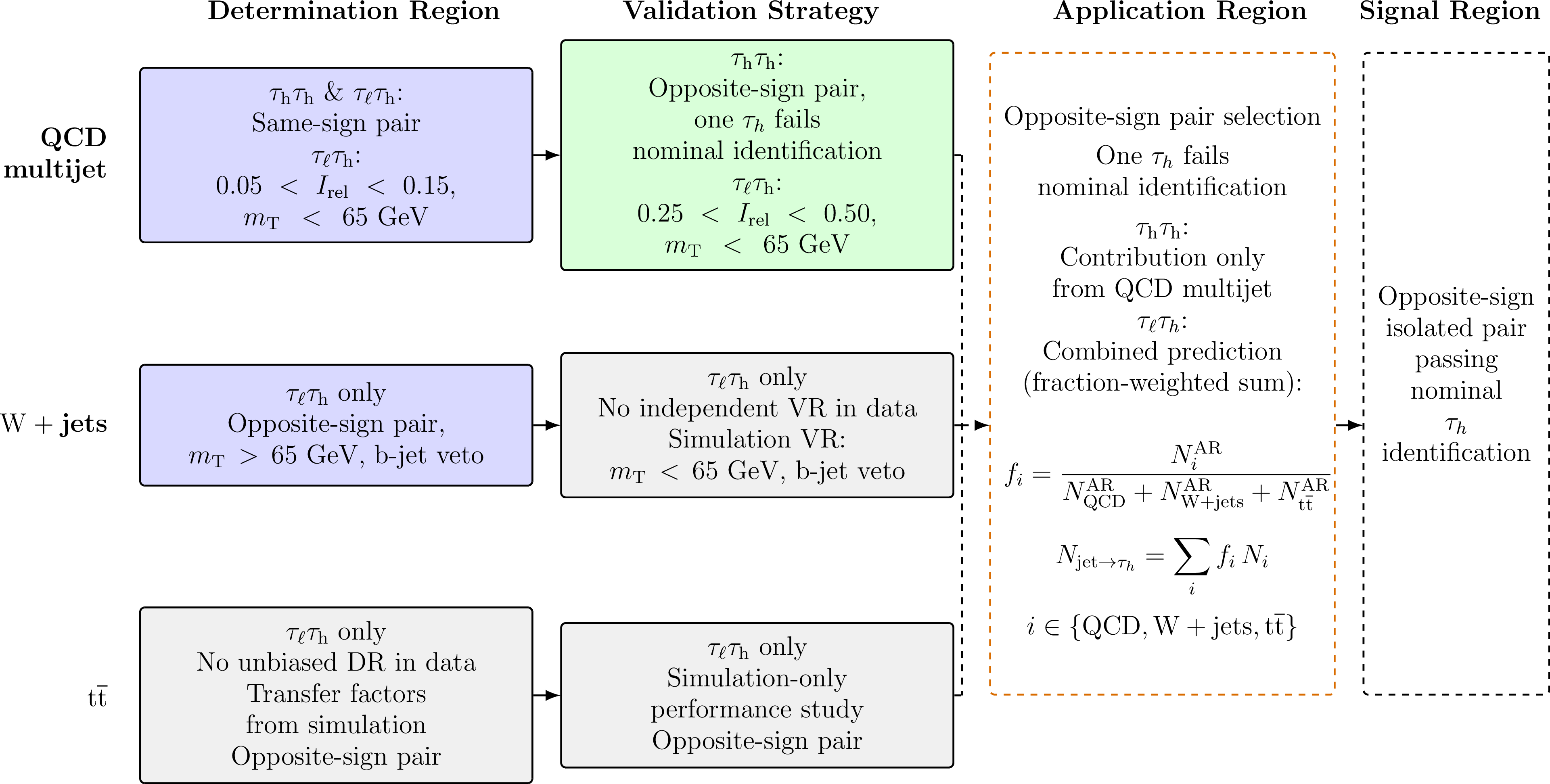
Figure 1:
Schematic overview of the determination regions (DR), validation regions (VR), application region (AR), and signal region (SR) used in the estimation of the $ \text{jet}\to\tau_\mathrm{h} $ backgrounds. For each process, transfer factors are derived in dedicated DRs enriched in jets misidentified as $ \tau_h $ candidates. The performance of the method is assessed in VRs, where available, or through simulation-based studies in cases without an unbiased DR. The prediction is then applied in a common AR, defined by opposite-sign events with one $ \tau_h $ candidate failing the nominal identification requirement. In the $ \tau_h\tau_h $ channel, the AR is dominated by QCD multijet events, while in the $ \tau_\ell\tau_h $ channels a combined prediction is constructed from QCD multijet, $ \mathrm{W}+\text{jets} $, and $ \mathrm{t} \overline{\mathrm{t}} $ contributions using relative fractions derived in the AR. The final estimate is obtained in the SR, defined by opposite-sign isolated events passing the nominal $ \tau_h $ identification requirements. |
png pdf |
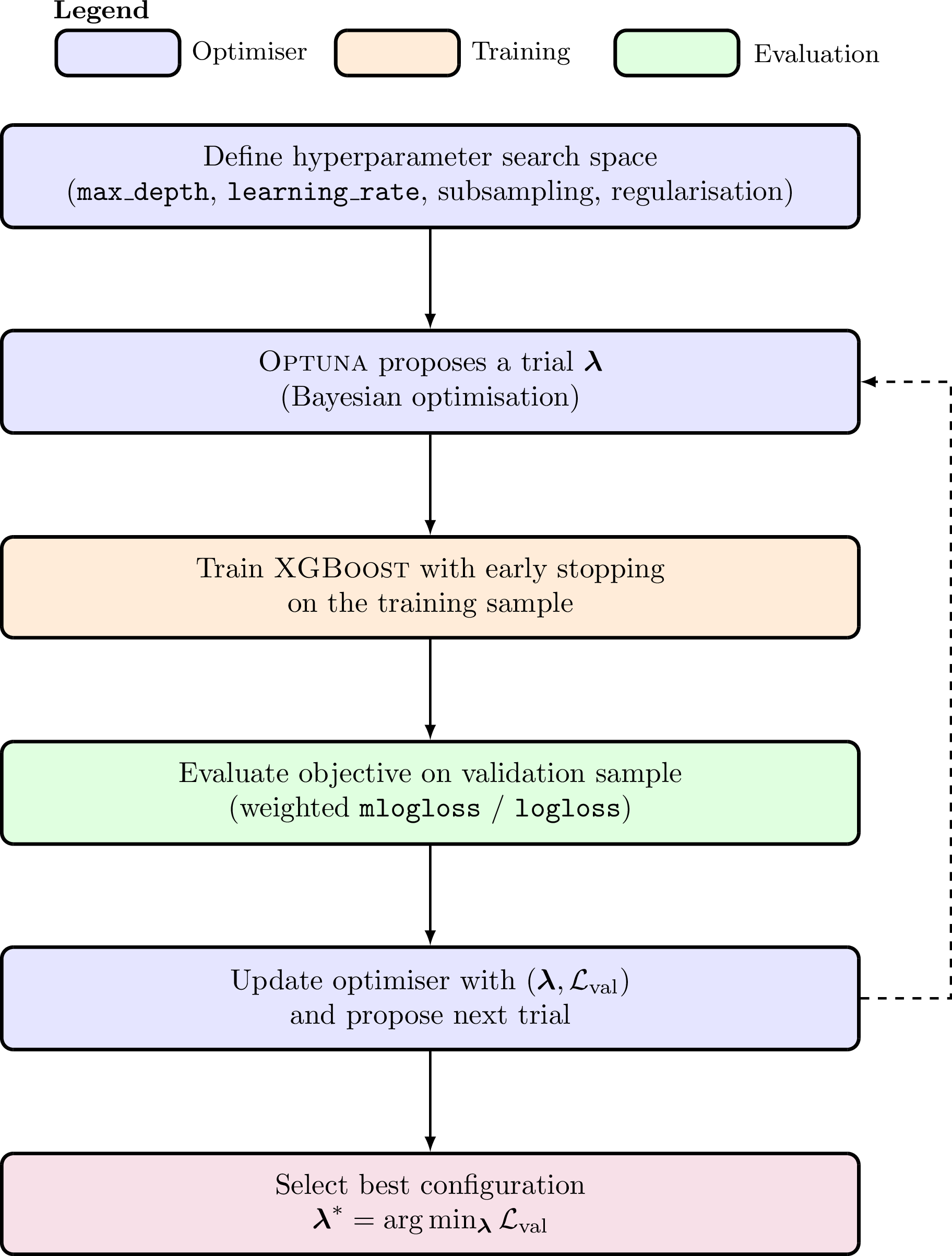
Figure 2:
Schematic overview of the hyperparameter optimisation procedure used to configure the BDT models. For each trial, Optuna proposes a hyperparameter set, the model is trained with early stopping, and the validation loss is used as the optimisation objective. |
png pdf |
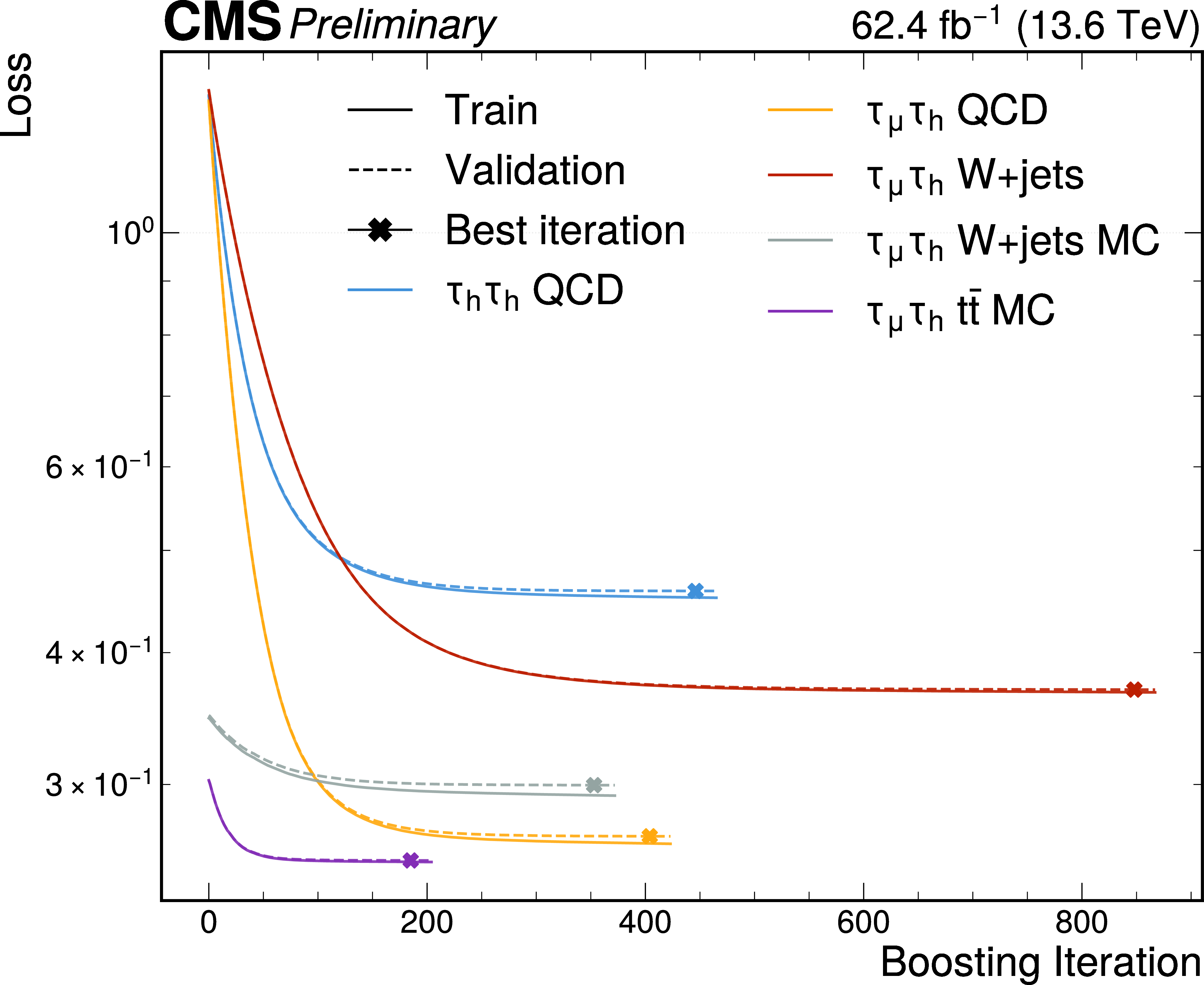
Figure 3:
Log-scale representation of the loss versus boosting iteration for all BDT models in the $ \tau_\mathrm{h}\tau_\mathrm{h} $ and $ \tau_\mathrm{\mu}\hspace{-.04em}\tau_\mathrm{h} $ channels. Solid (dashed) lines correspond to the training (validation) loss, while cross markers indicate the early-stopping iteration. |
png pdf |
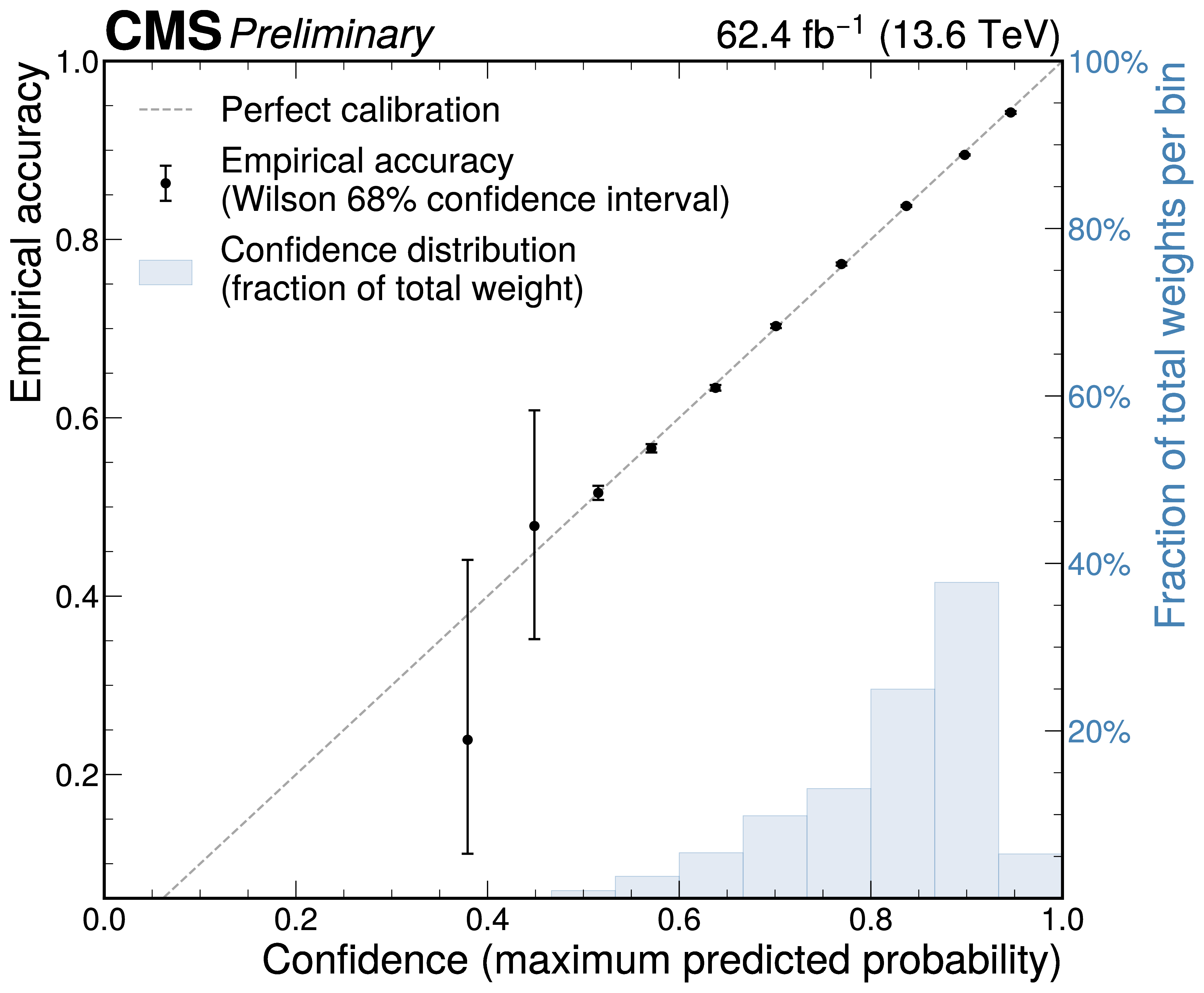
Figure 4:
Reliability diagram for the QCD multijet BDT in the $ \tau_\mathrm{h}\tau_\mathrm{h} $ channel after temperature scaling ($ T^\ast = $ 0.999) evaluated on the validation dataset. Points show the empirical accuracy in each confidence bin, defined as the event-weight-averaged fraction of correctly classified events, with Wilson score 68% confidence intervals computed using the effective sample size $ n_\text{eff} = (\sum_i w_i)^2 / \sum_i w_i^2 $. The dashed diagonal line indicates perfect calibration. The shaded histogram (right axis) shows the distribution of confidence scores, normalised to the total event weight per bin. The model is well-calibrated across the full confidence range, with the bulk of events ($ > 30% $ per bin) concentrated at high confidence values ($ > $ 0.8). |
png pdf |
Figure 5:
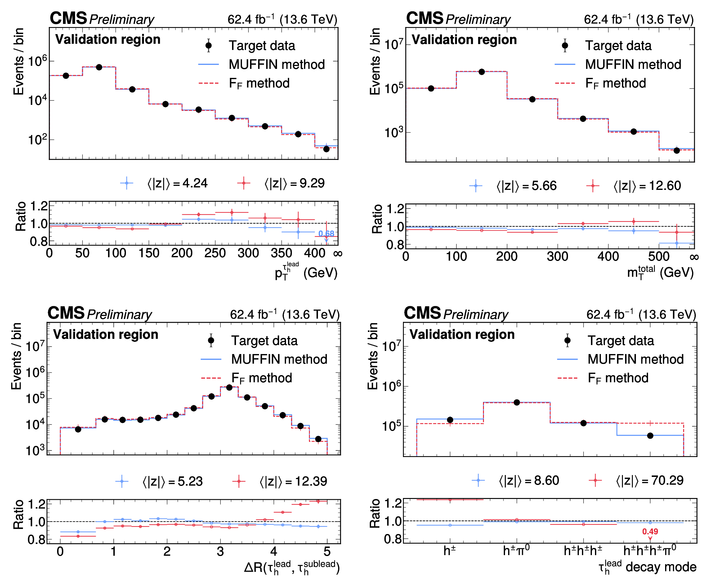
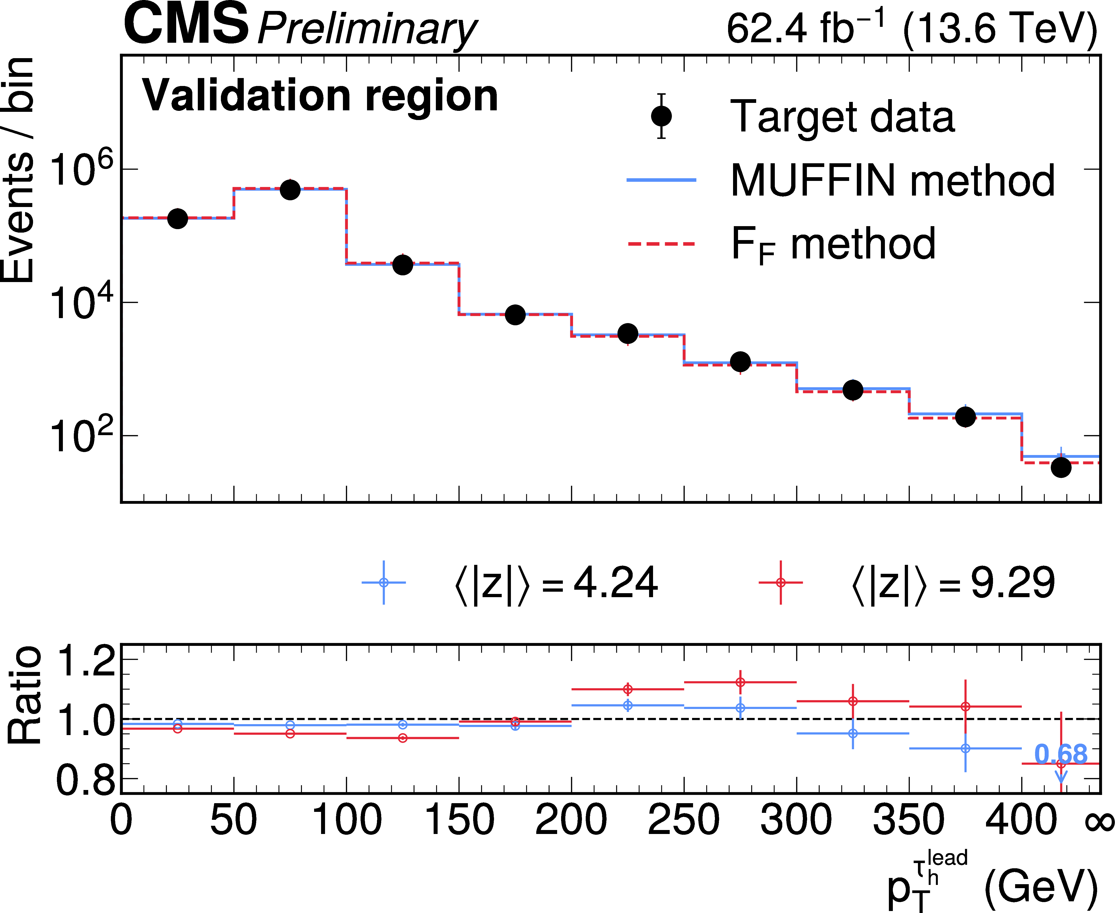
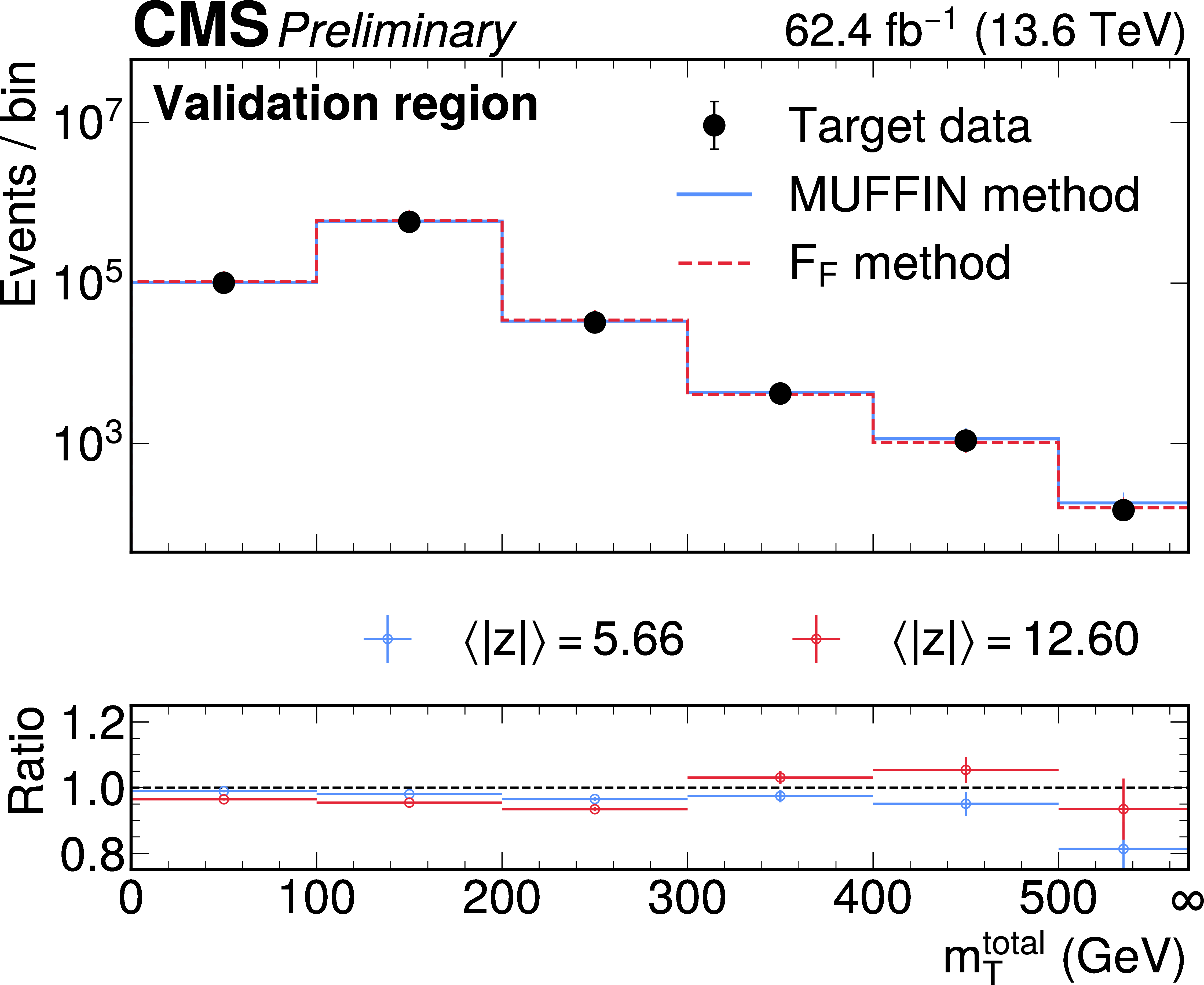
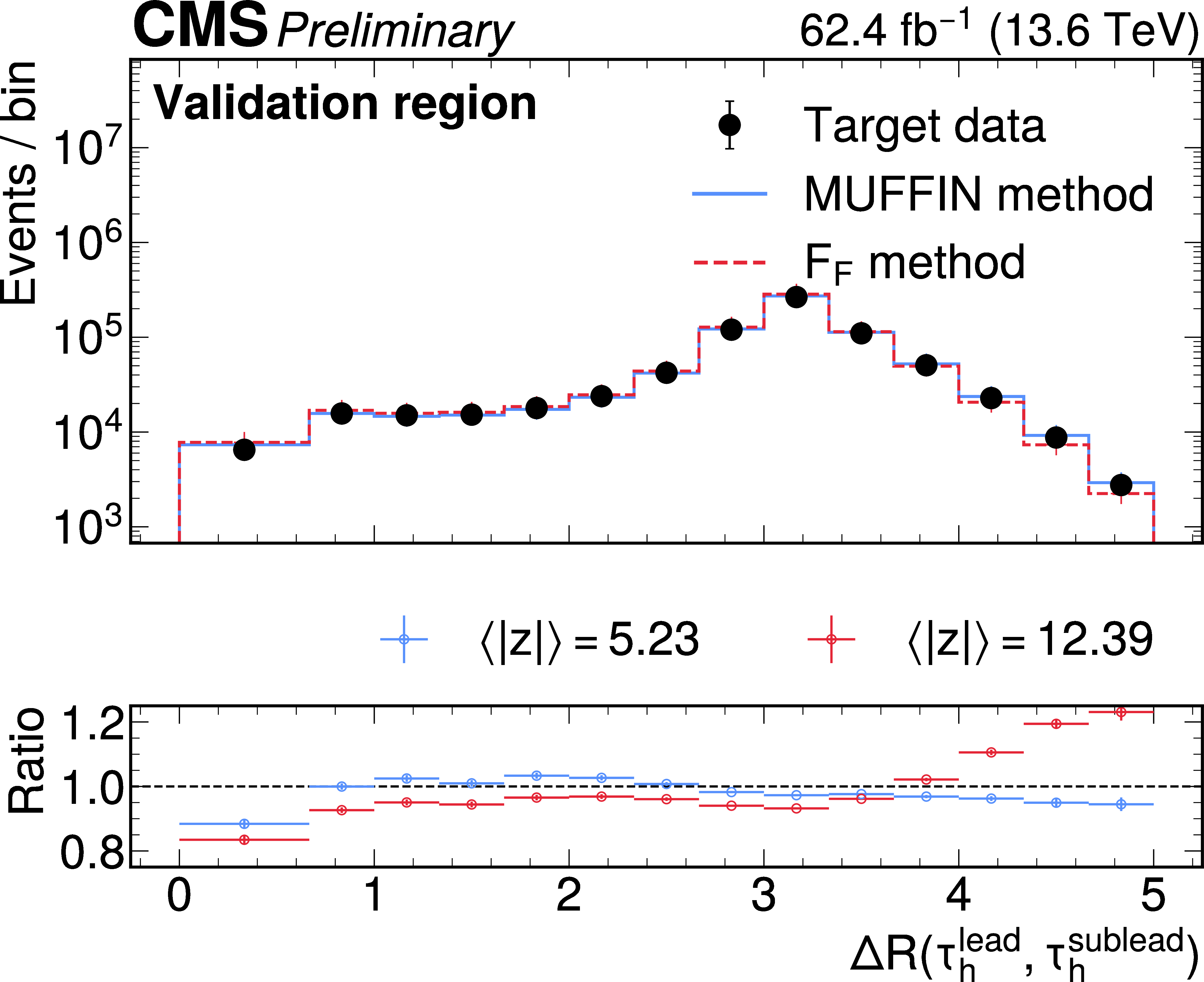
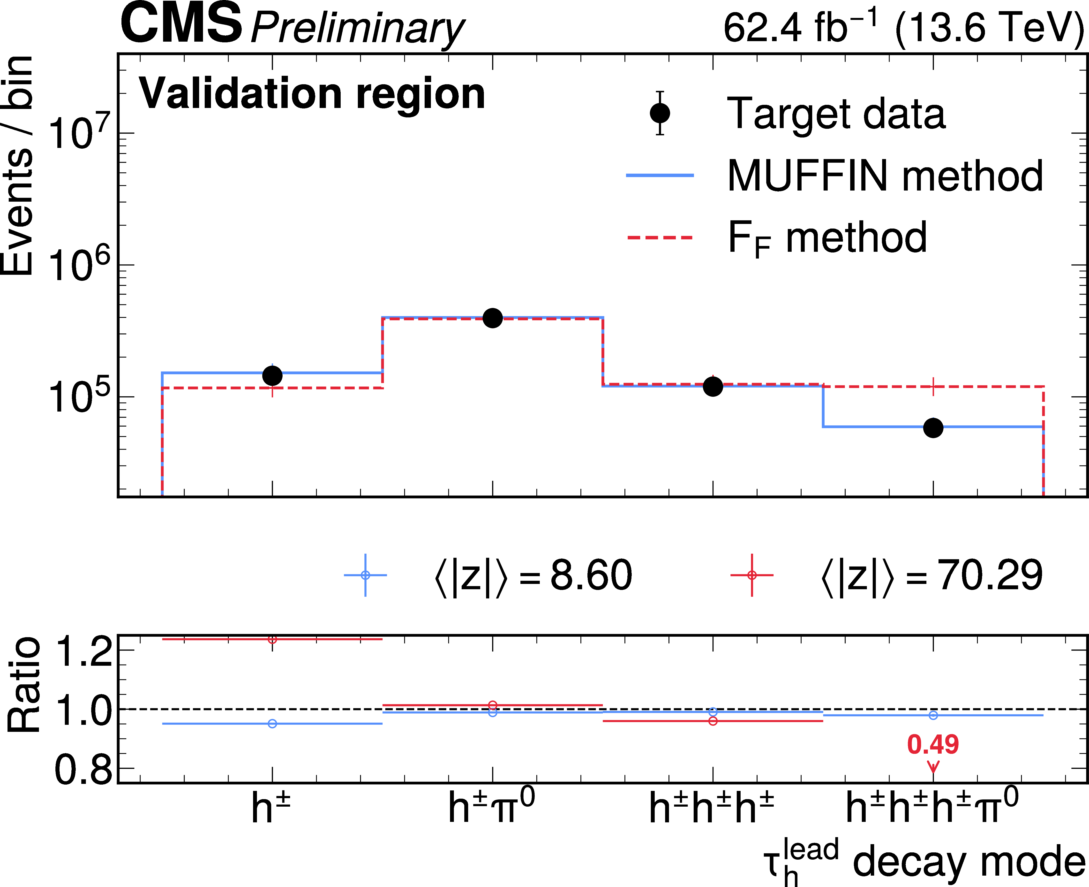
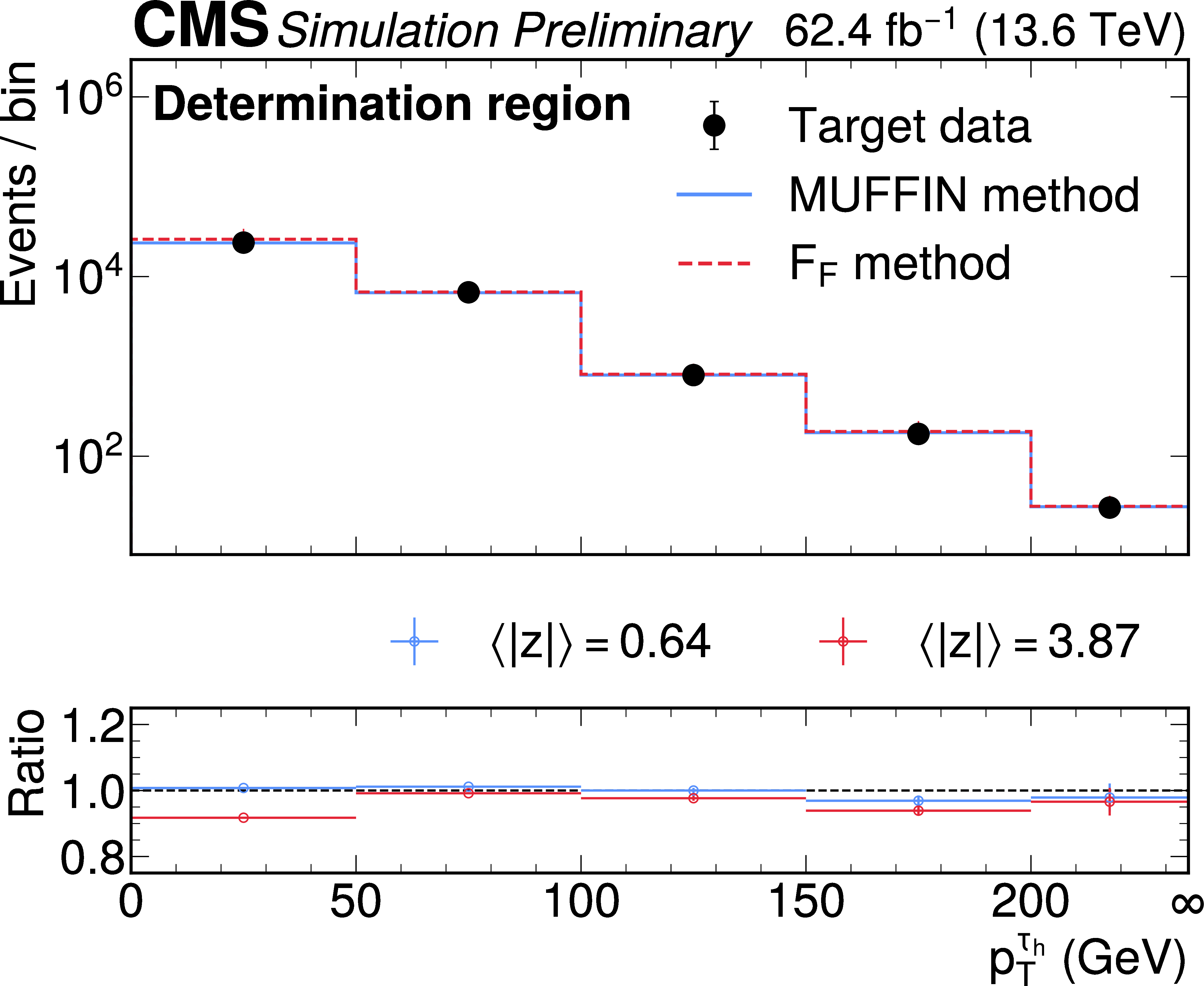
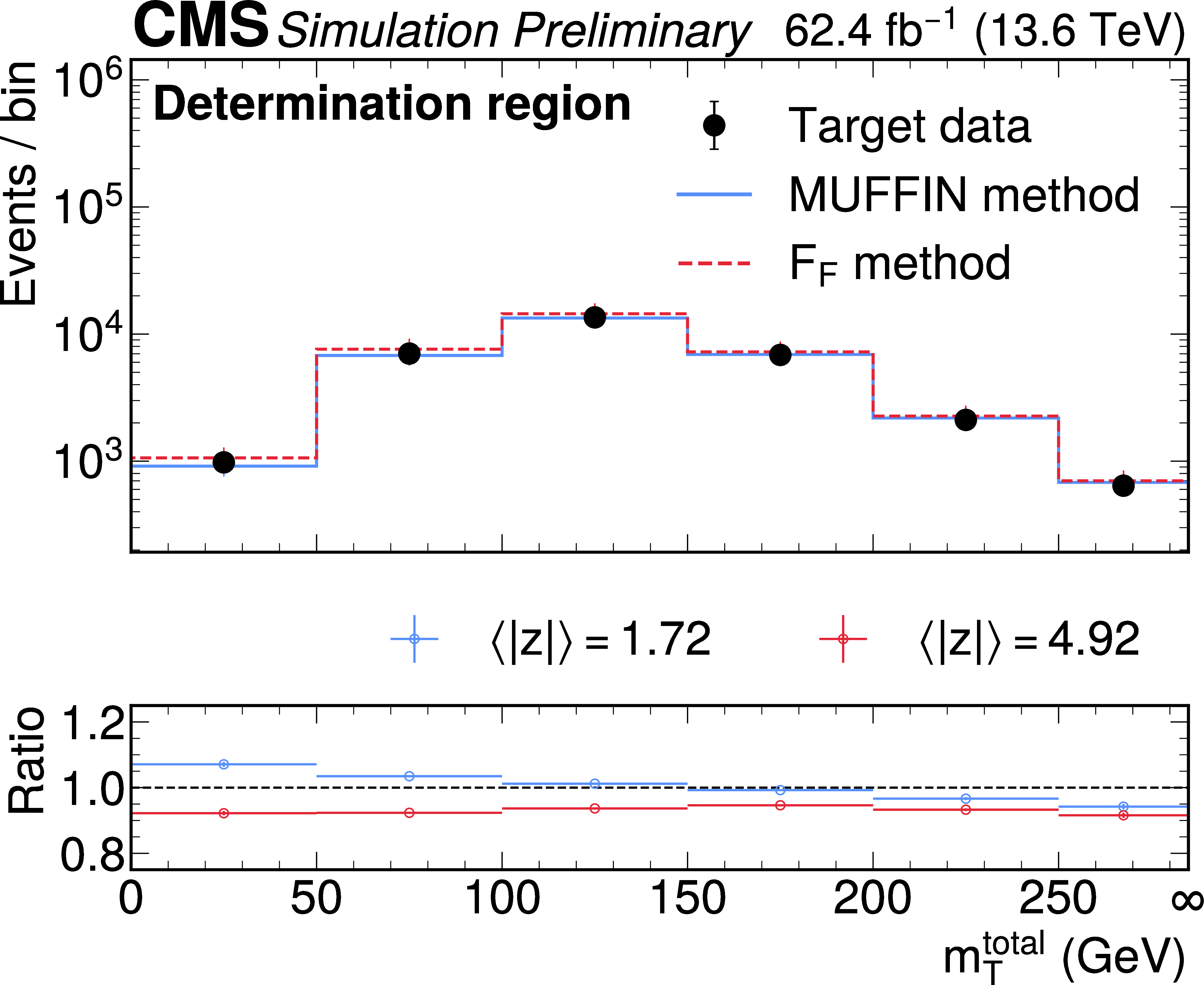
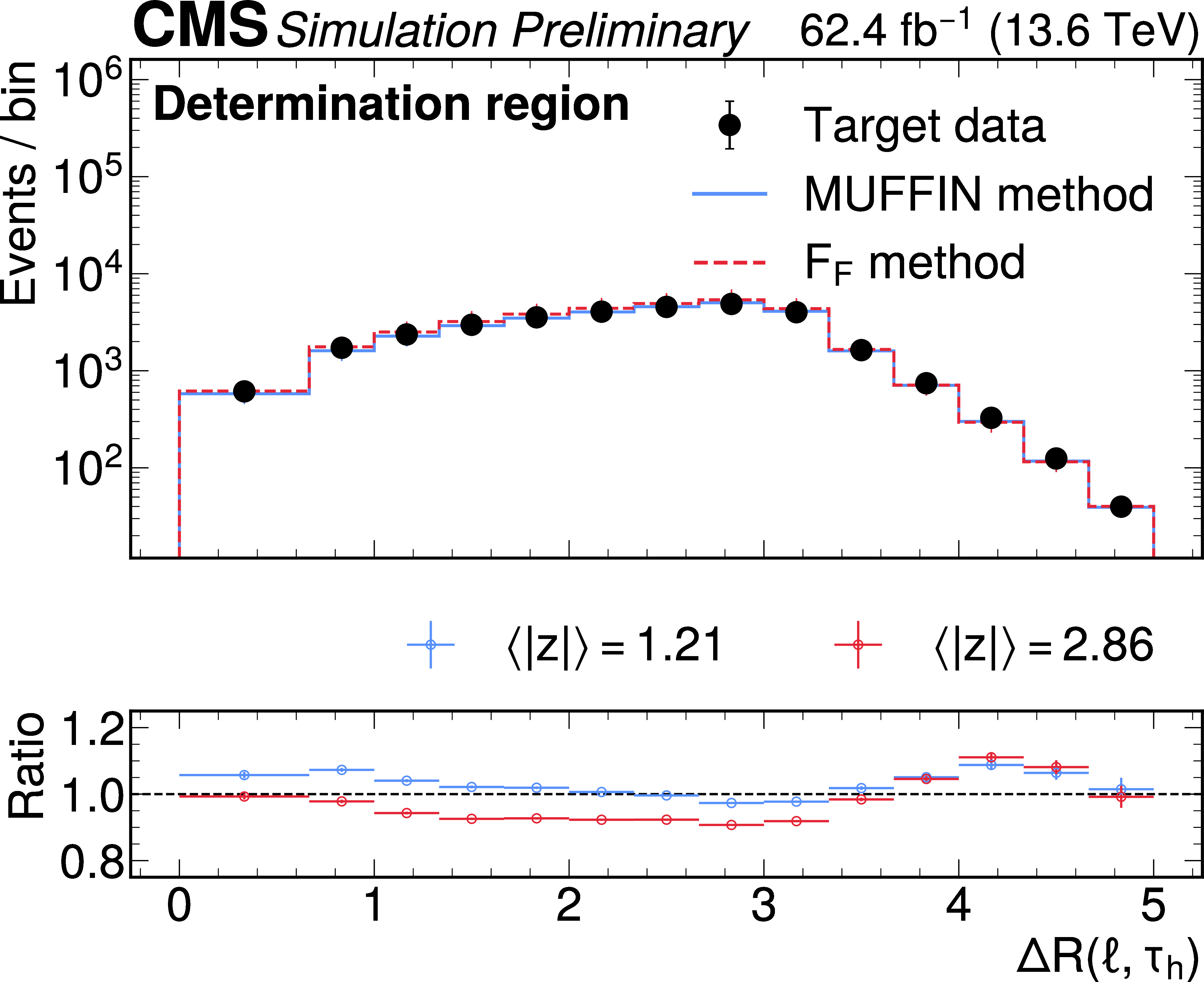
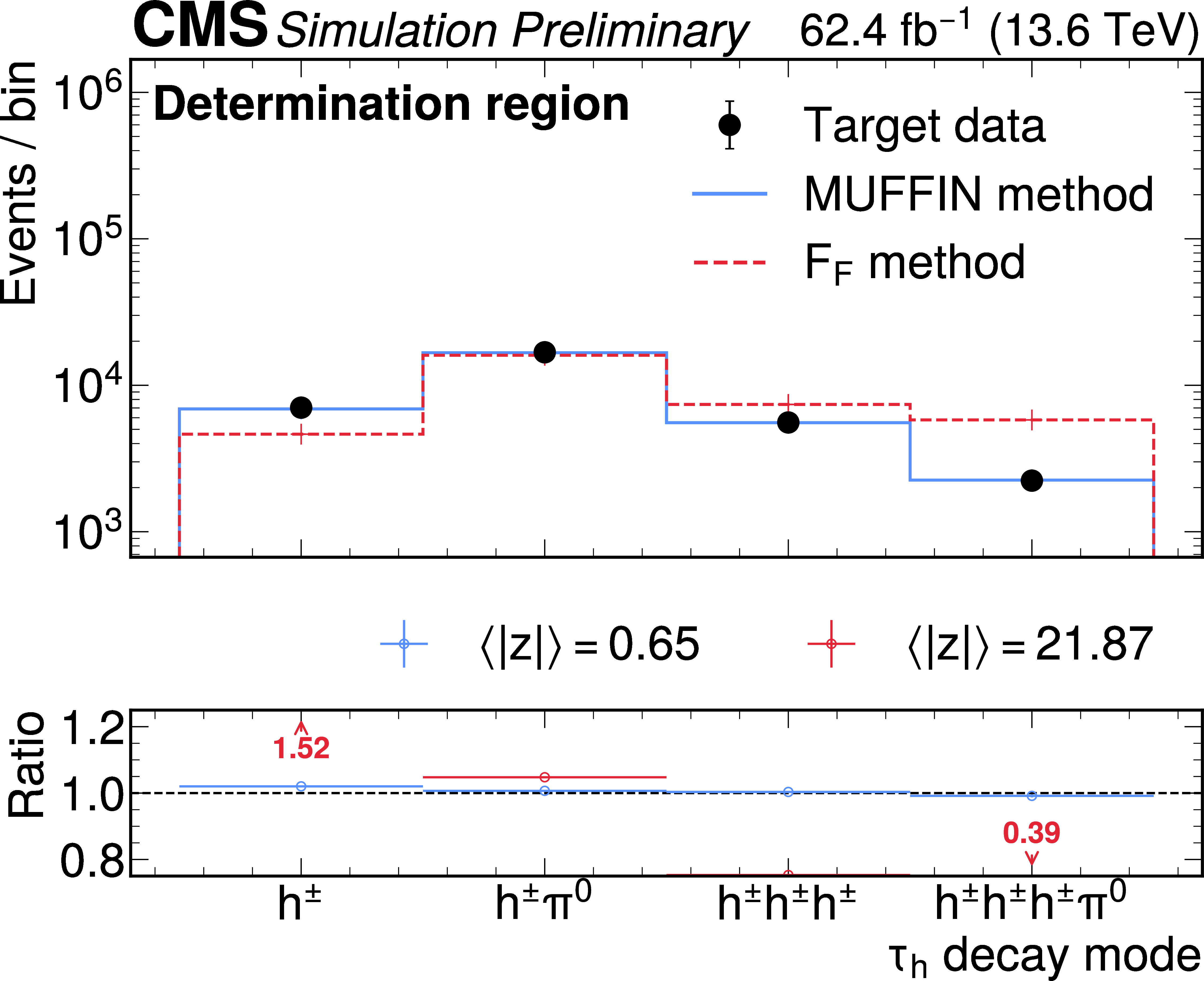
Distributions of representative observables in the $ \tau_\mathrm{h}\tau_\mathrm{h} $ application region comparing the MUFFIN prediction (blue) and $ F_{\text{F}} $ estimate (red, dashed) to the target distribution (black markers) for $ p_{\mathrm{T}}^{\tau_\mathrm{h}} $, $ m_{\mathrm{T}}^{\text{total}} $, $ \Delta R $, and decay mode. The ratio panels display the target-to-prediction ratio, with the corresponding $ \langle|z|\rangle $ values quoted in each panel. Arrows indicate bins outside the plotted range. Overflow contributions are included in the final bin ($ \infty $) of each mass and $ p_{\mathrm{T}} $ distribution. |
png pdf |
Figure 5-a:
Distributions of representative observables in the $ \tau_\mathrm{h}\tau_\mathrm{h} $ application region comparing the MUFFIN prediction (blue) and $ F_{\text{F}} $ estimate (red, dashed) to the target distribution (black markers) for $ p_{\mathrm{T}}^{\tau_\mathrm{h}} $, $ m_{\mathrm{T}}^{\text{total}} $, $ \Delta R $, and decay mode. The ratio panels display the target-to-prediction ratio, with the corresponding $ \langle|z|\rangle $ values quoted in each panel. Arrows indicate bins outside the plotted range. Overflow contributions are included in the final bin ($ \infty $) of each mass and $ p_{\mathrm{T}} $ distribution. |
png pdf |
Figure 5-b:
Distributions of representative observables in the $ \tau_\mathrm{h}\tau_\mathrm{h} $ application region comparing the MUFFIN prediction (blue) and $ F_{\text{F}} $ estimate (red, dashed) to the target distribution (black markers) for $ p_{\mathrm{T}}^{\tau_\mathrm{h}} $, $ m_{\mathrm{T}}^{\text{total}} $, $ \Delta R $, and decay mode. The ratio panels display the target-to-prediction ratio, with the corresponding $ \langle|z|\rangle $ values quoted in each panel. Arrows indicate bins outside the plotted range. Overflow contributions are included in the final bin ($ \infty $) of each mass and $ p_{\mathrm{T}} $ distribution. |
png pdf |
Figure 5-c:
Distributions of representative observables in the $ \tau_\mathrm{h}\tau_\mathrm{h} $ application region comparing the MUFFIN prediction (blue) and $ F_{\text{F}} $ estimate (red, dashed) to the target distribution (black markers) for $ p_{\mathrm{T}}^{\tau_\mathrm{h}} $, $ m_{\mathrm{T}}^{\text{total}} $, $ \Delta R $, and decay mode. The ratio panels display the target-to-prediction ratio, with the corresponding $ \langle|z|\rangle $ values quoted in each panel. Arrows indicate bins outside the plotted range. Overflow contributions are included in the final bin ($ \infty $) of each mass and $ p_{\mathrm{T}} $ distribution. |
png pdf |
Figure 5-d:
Distributions of representative observables in the $ \tau_\mathrm{h}\tau_\mathrm{h} $ application region comparing the MUFFIN prediction (blue) and $ F_{\text{F}} $ estimate (red, dashed) to the target distribution (black markers) for $ p_{\mathrm{T}}^{\tau_\mathrm{h}} $, $ m_{\mathrm{T}}^{\text{total}} $, $ \Delta R $, and decay mode. The ratio panels display the target-to-prediction ratio, with the corresponding $ \langle|z|\rangle $ values quoted in each panel. Arrows indicate bins outside the plotted range. Overflow contributions are included in the final bin ($ \infty $) of each mass and $ p_{\mathrm{T}} $ distribution. |
png pdf |
Figure 6:
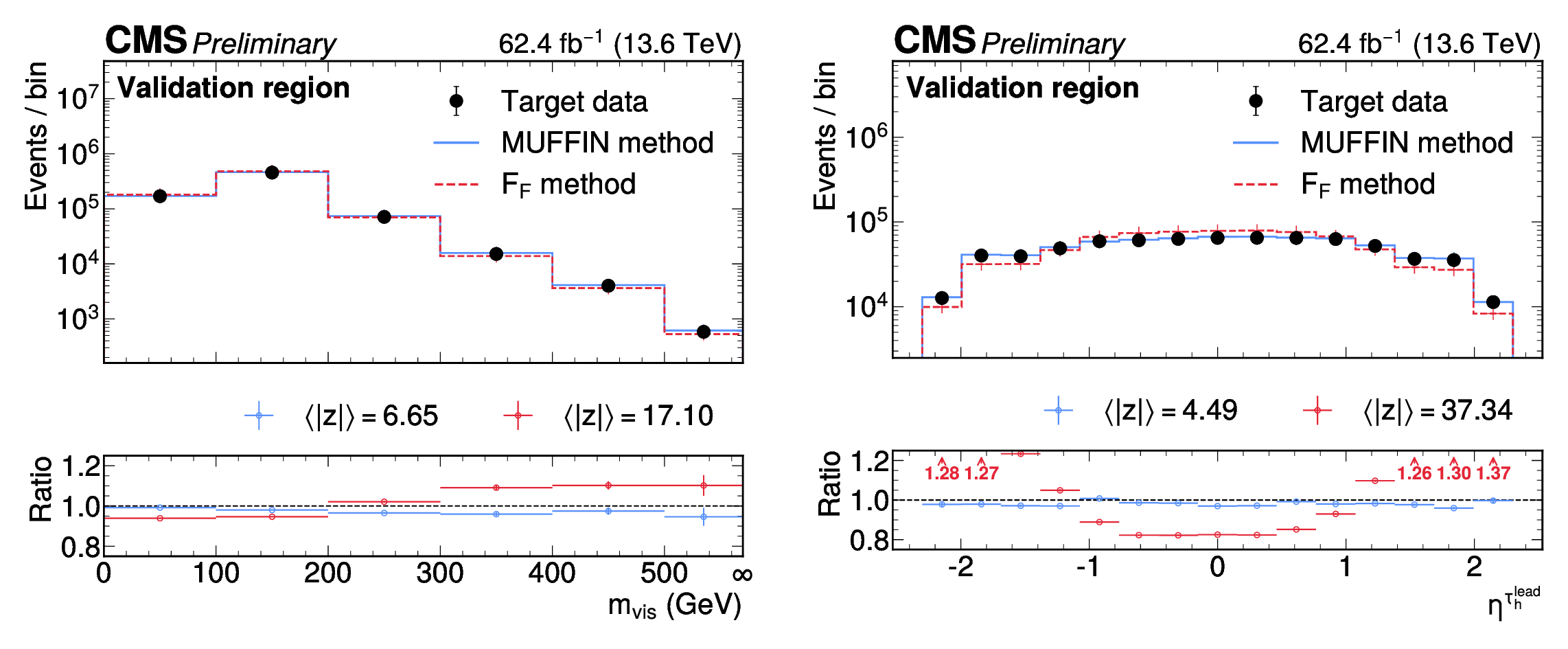
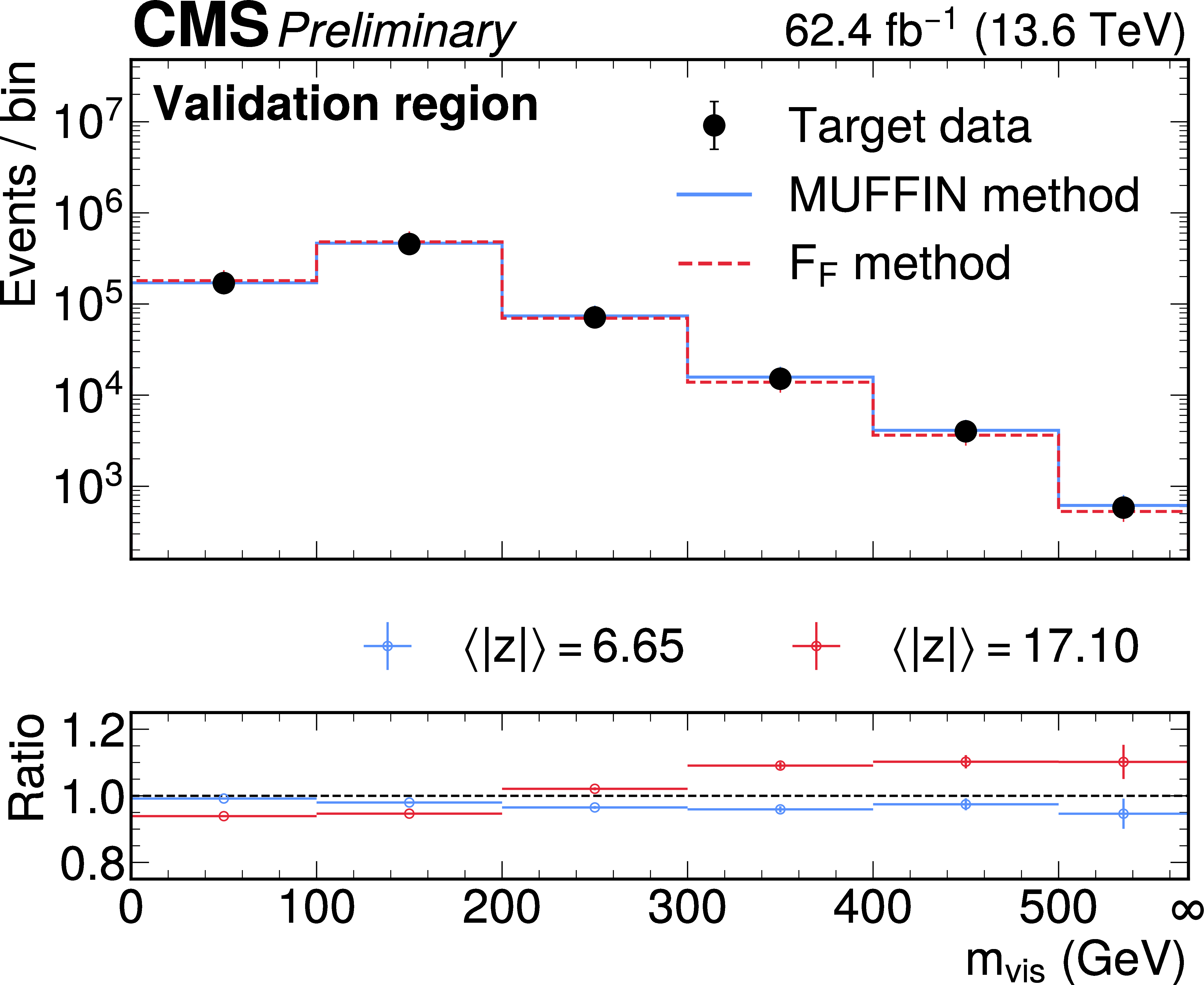
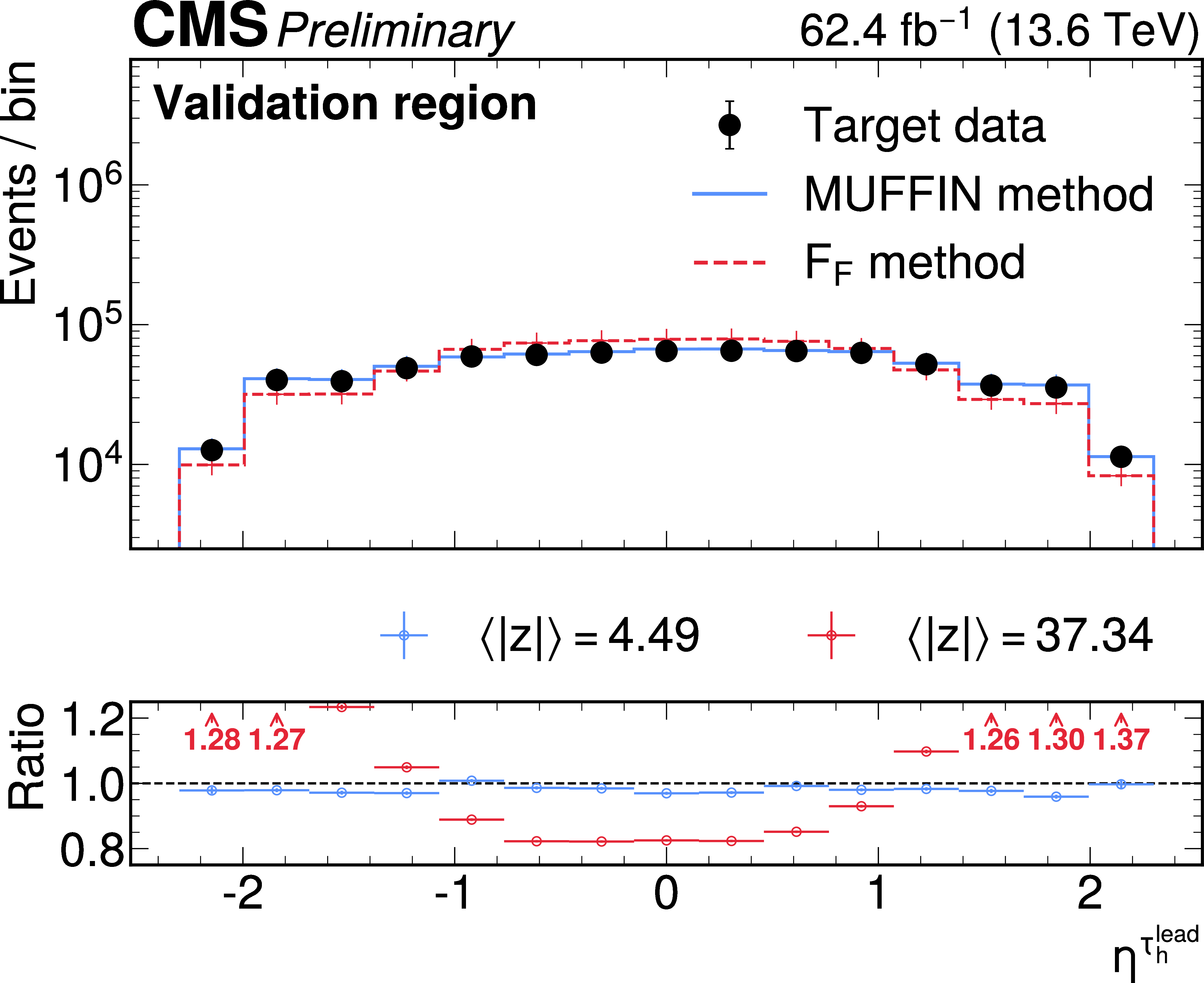
Comparison of the visible mass $ m_{\mathrm{vis}} $ and $ \eta $ distributions in the same $ \tau_\mathrm{h}\tau_\mathrm{h} $ application region with the MUFFIN (blue) and $ F_{\text{F}} $ (red, dashed) predictions. The ratio panels highlight residual deviations and the corresponding $ \langle|z|\rangle $ metric values. Overflow contributions are included in the final bin ($ \infty $) where applicable. |
png pdf |
Figure 6-a:
Comparison of the visible mass $ m_{\mathrm{vis}} $ and $ \eta $ distributions in the same $ \tau_\mathrm{h}\tau_\mathrm{h} $ application region with the MUFFIN (blue) and $ F_{\text{F}} $ (red, dashed) predictions. The ratio panels highlight residual deviations and the corresponding $ \langle|z|\rangle $ metric values. Overflow contributions are included in the final bin ($ \infty $) where applicable. |
png pdf |
Figure 6-b:
Comparison of the visible mass $ m_{\mathrm{vis}} $ and $ \eta $ distributions in the same $ \tau_\mathrm{h}\tau_\mathrm{h} $ application region with the MUFFIN (blue) and $ F_{\text{F}} $ (red, dashed) predictions. The ratio panels highlight residual deviations and the corresponding $ \langle|z|\rangle $ metric values. Overflow contributions are included in the final bin ($ \infty $) where applicable. |
png pdf |
Figure 7:
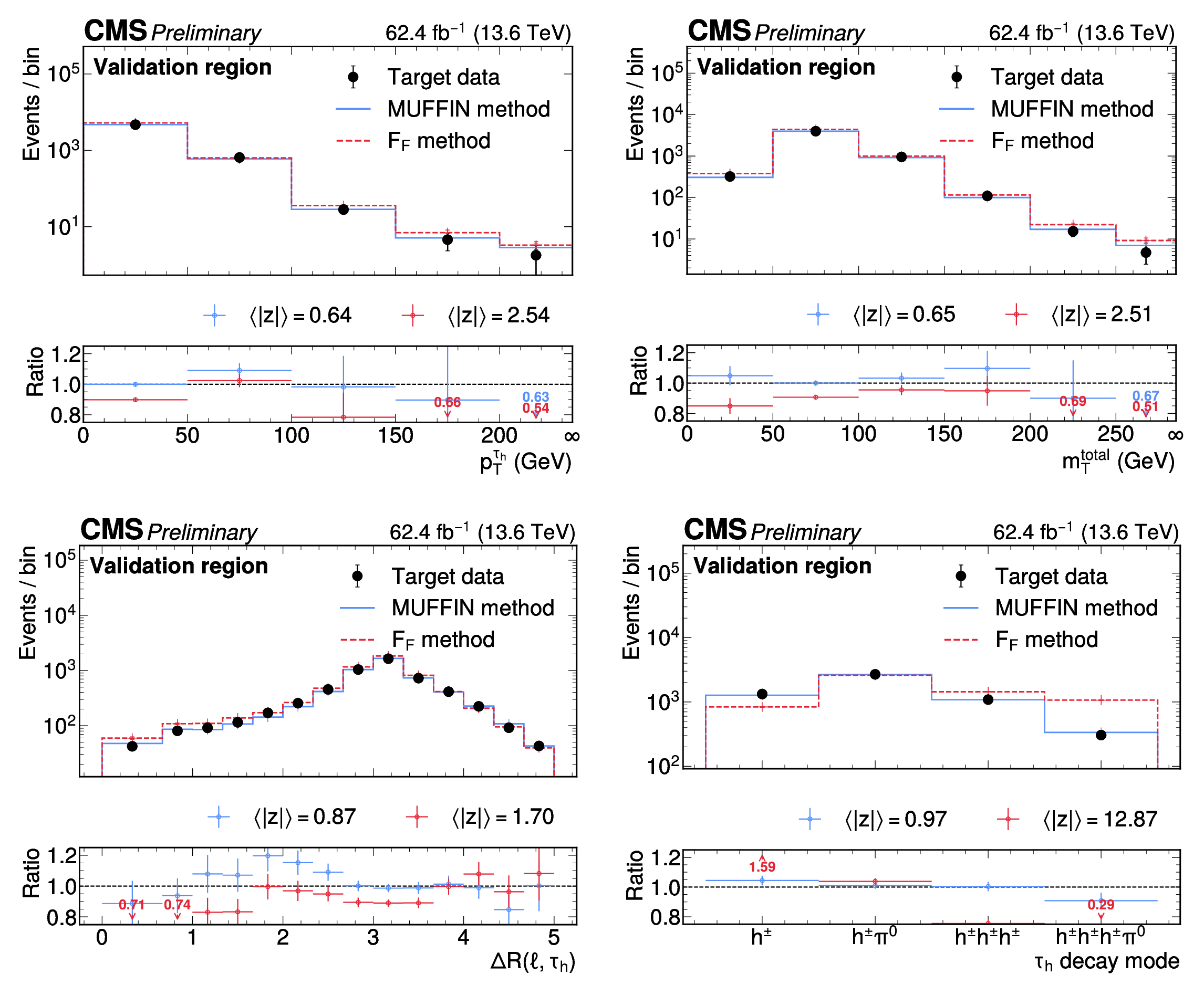
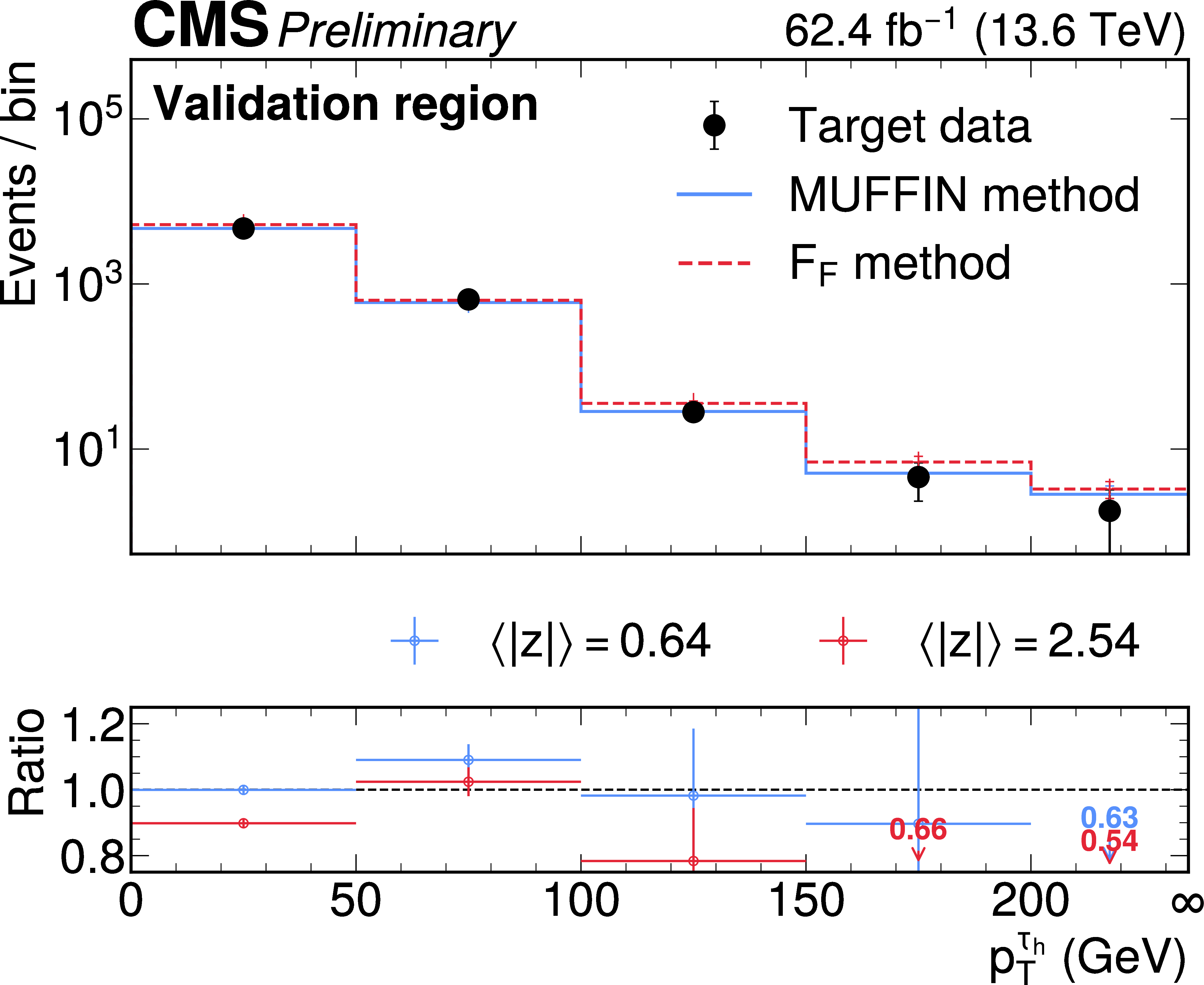
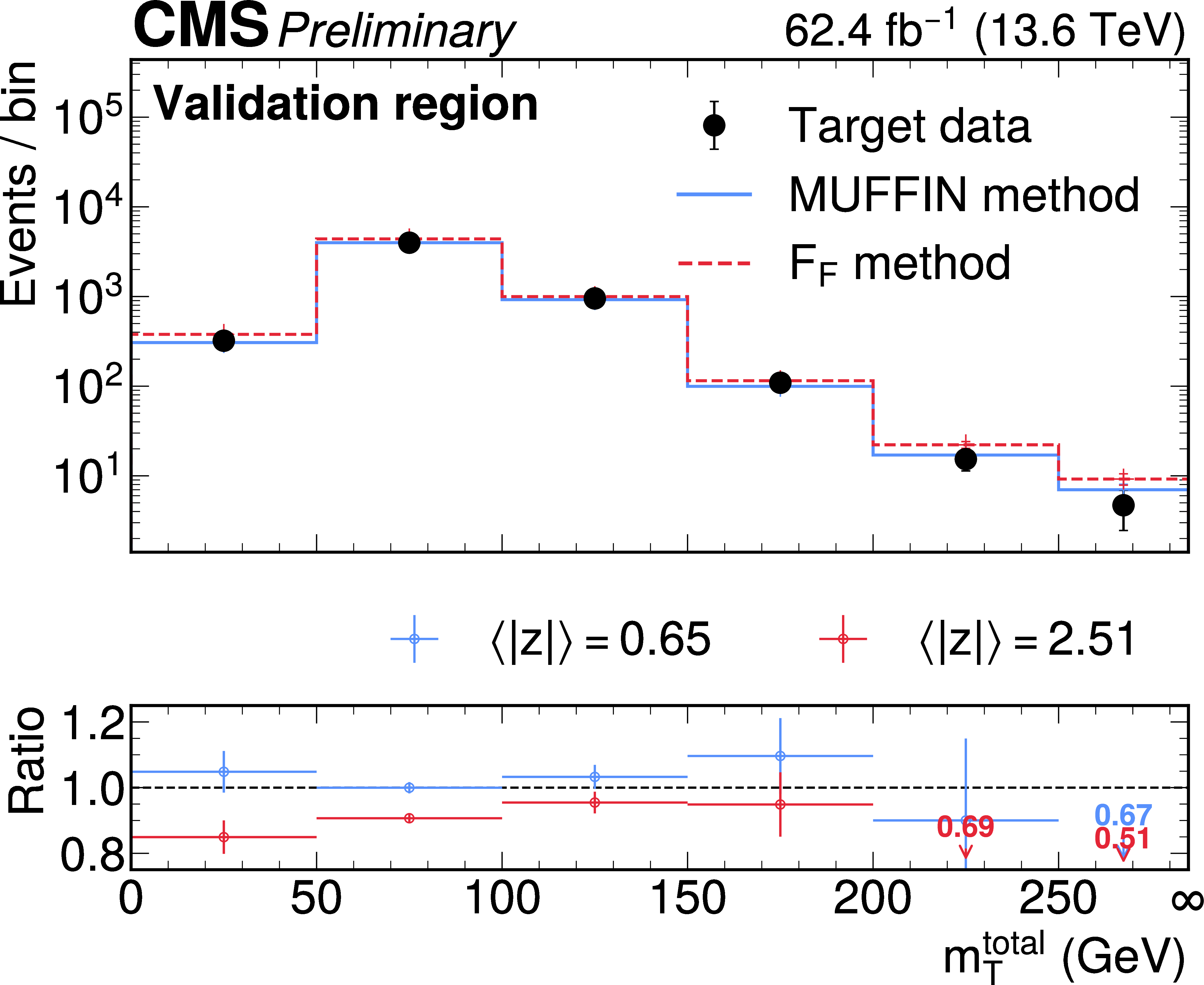
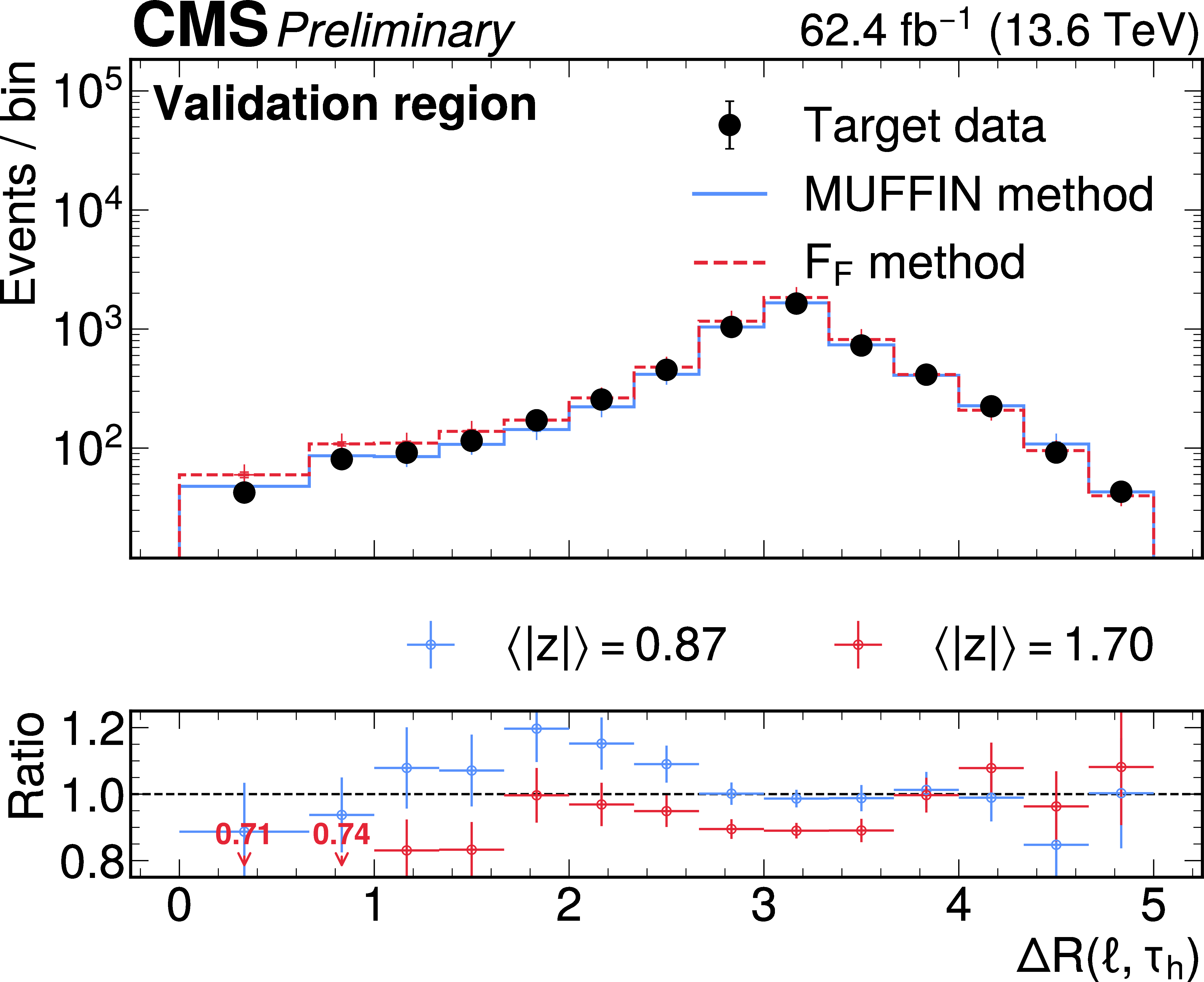
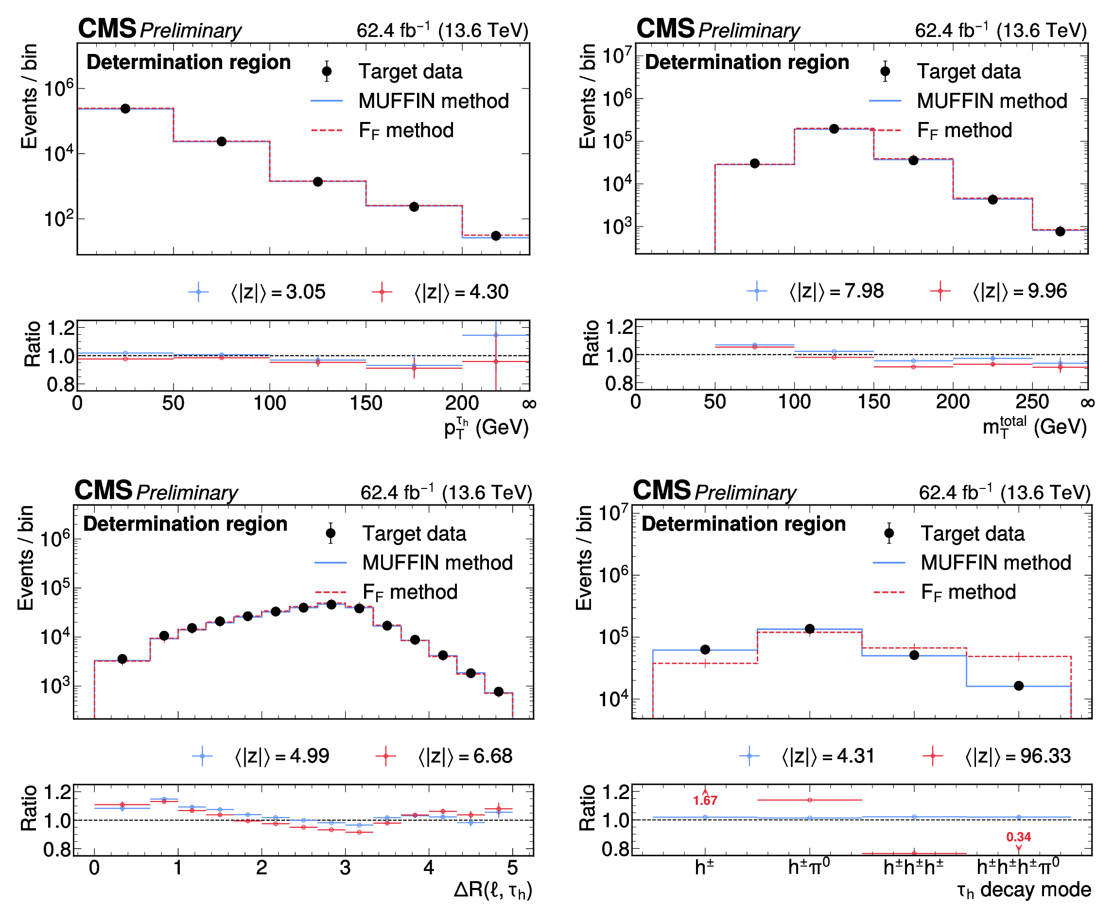
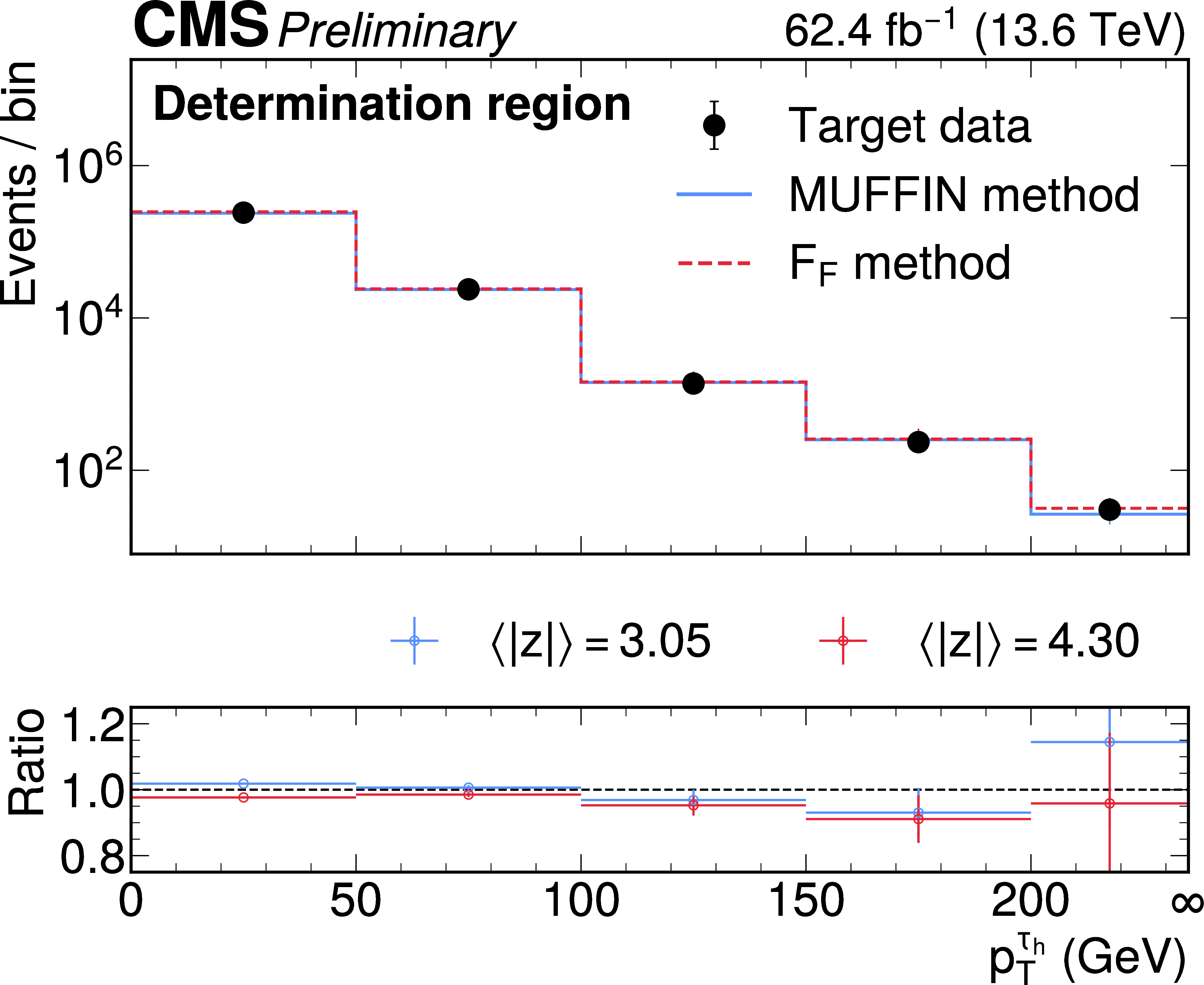
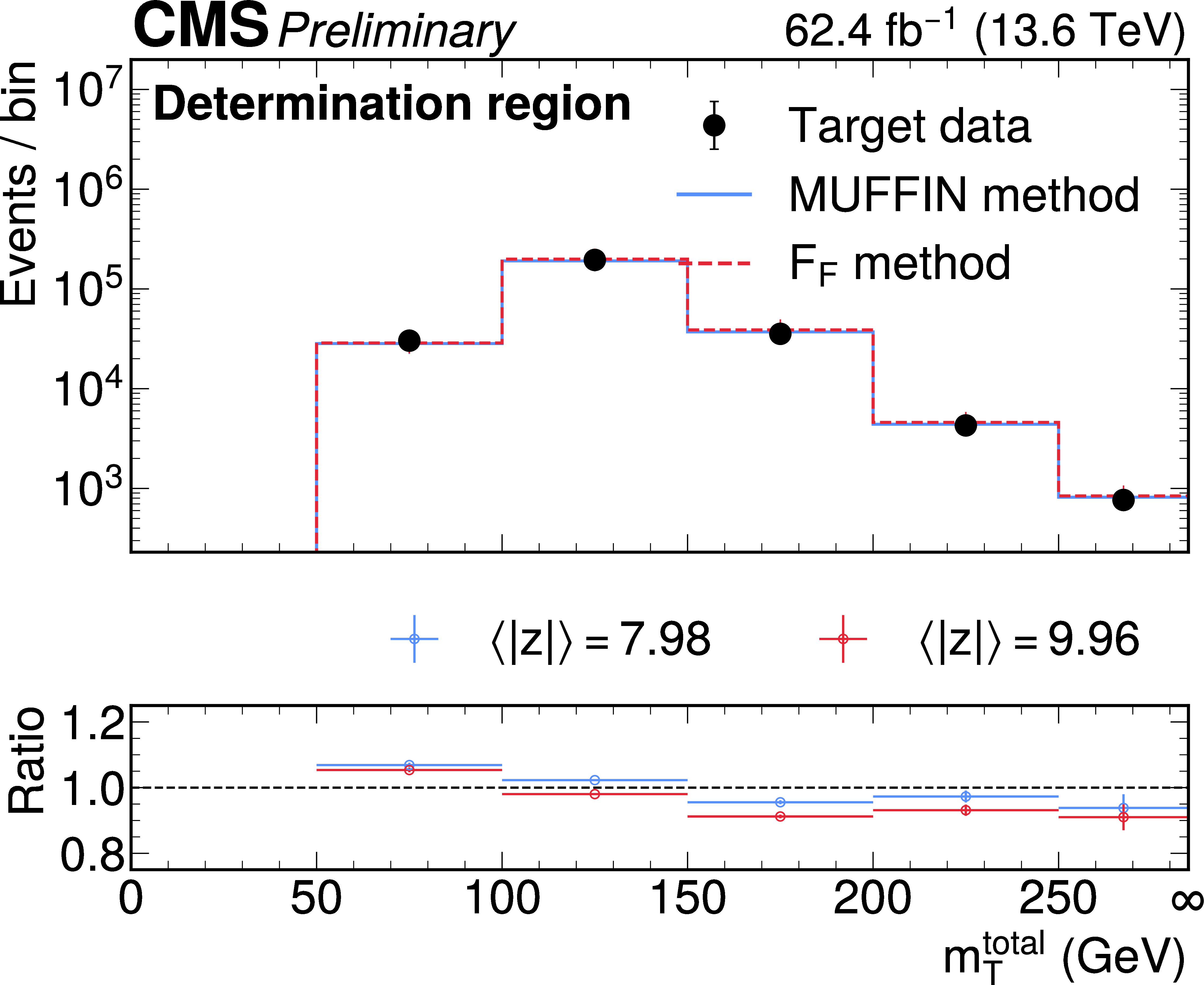
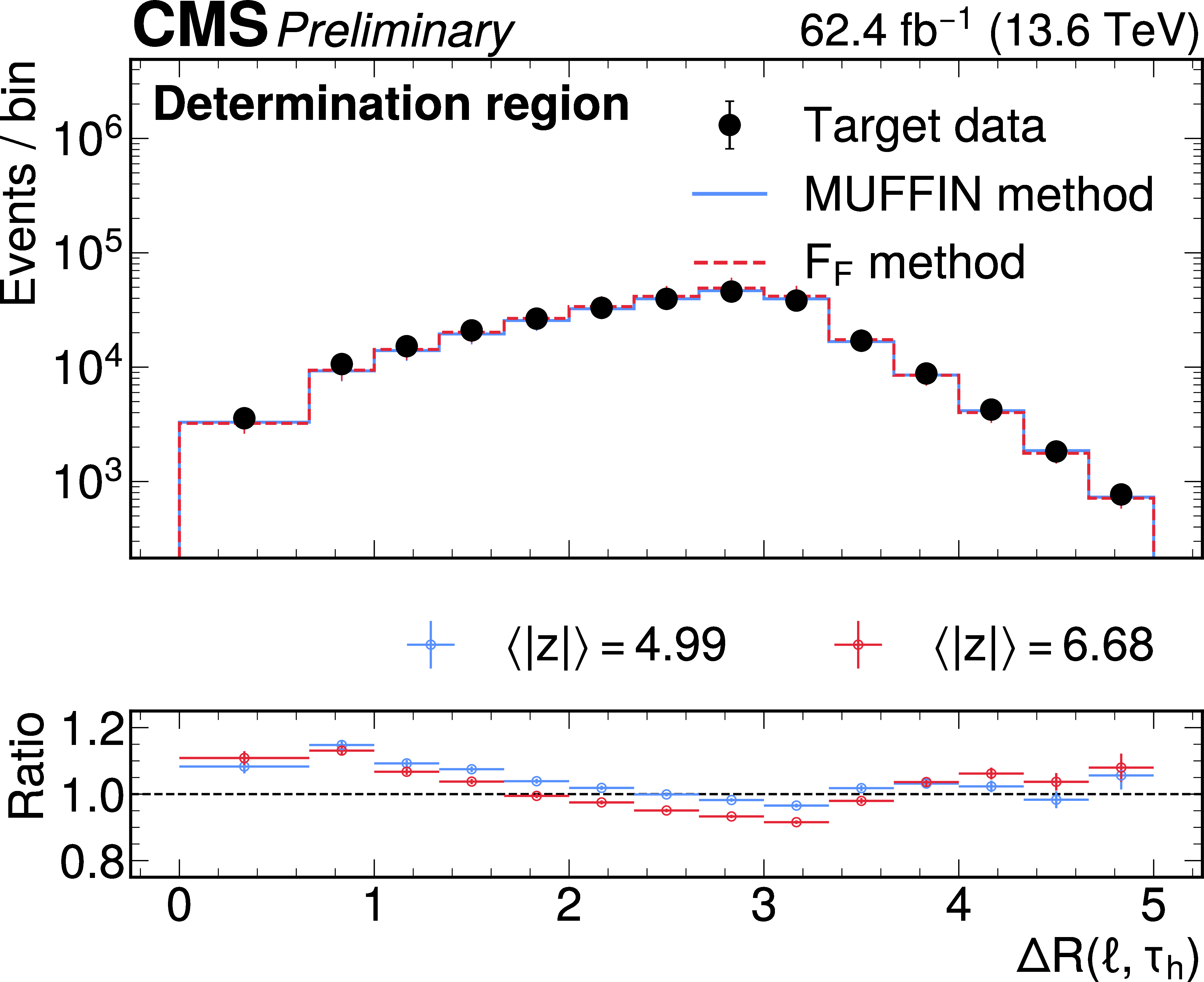
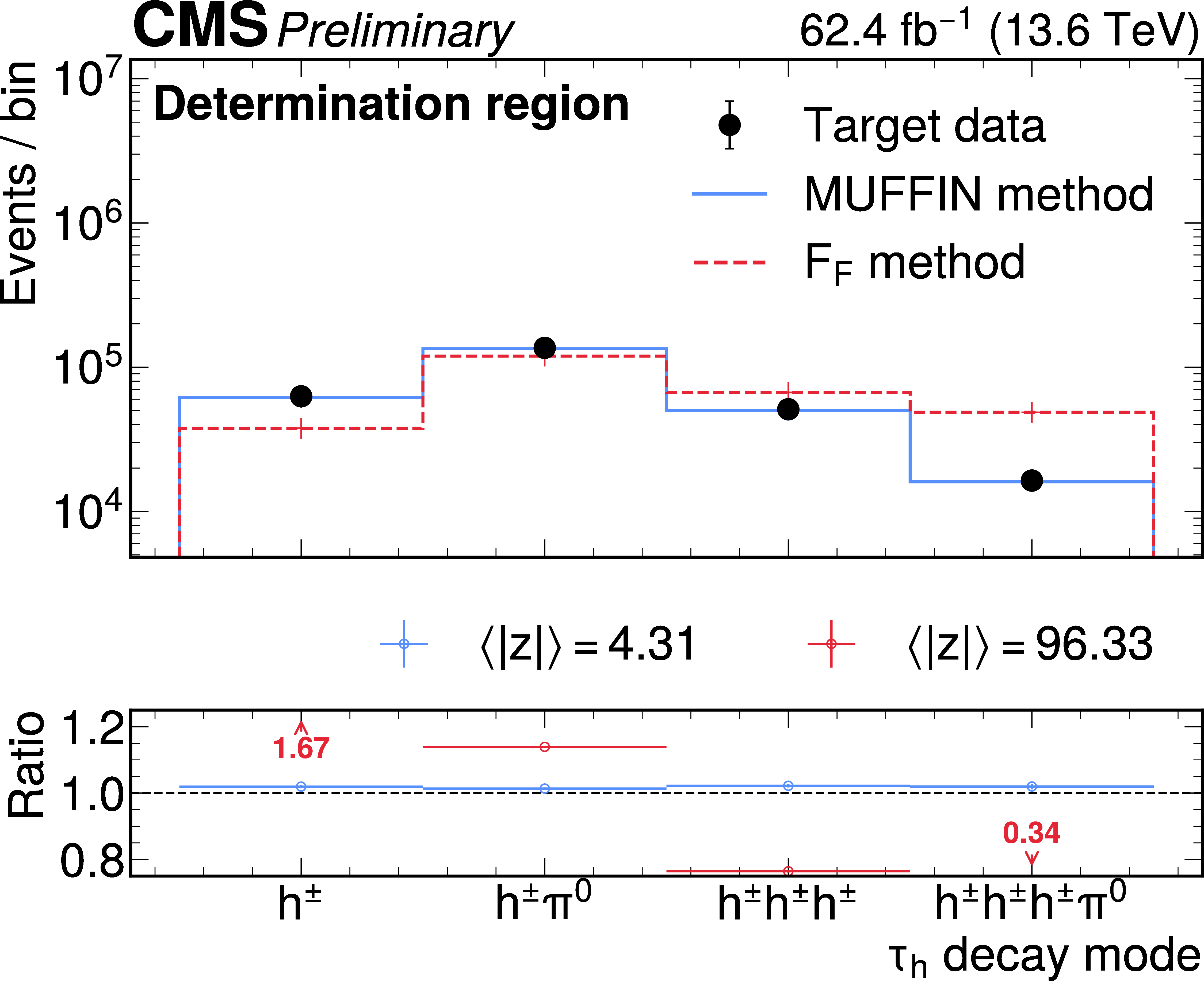
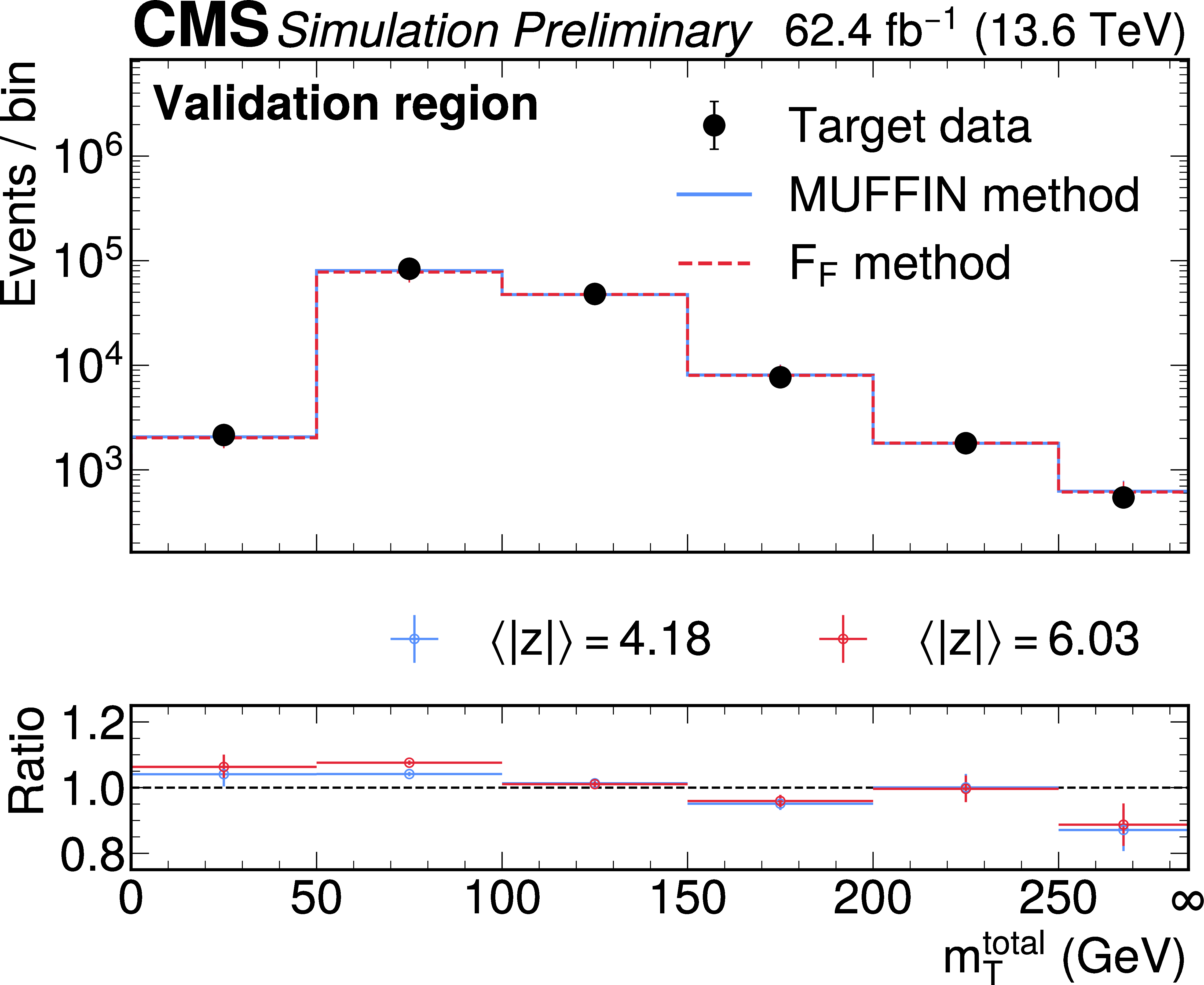
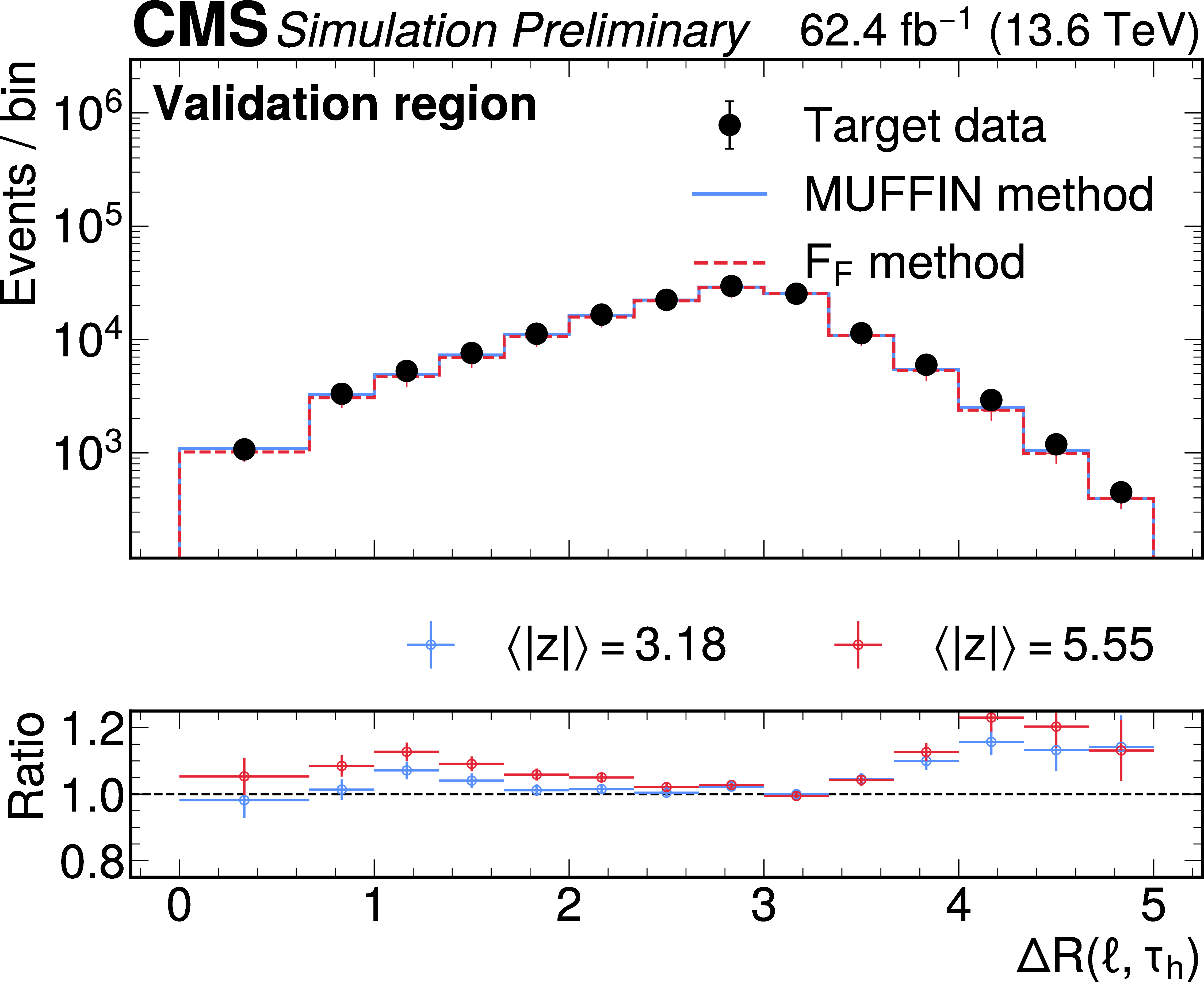
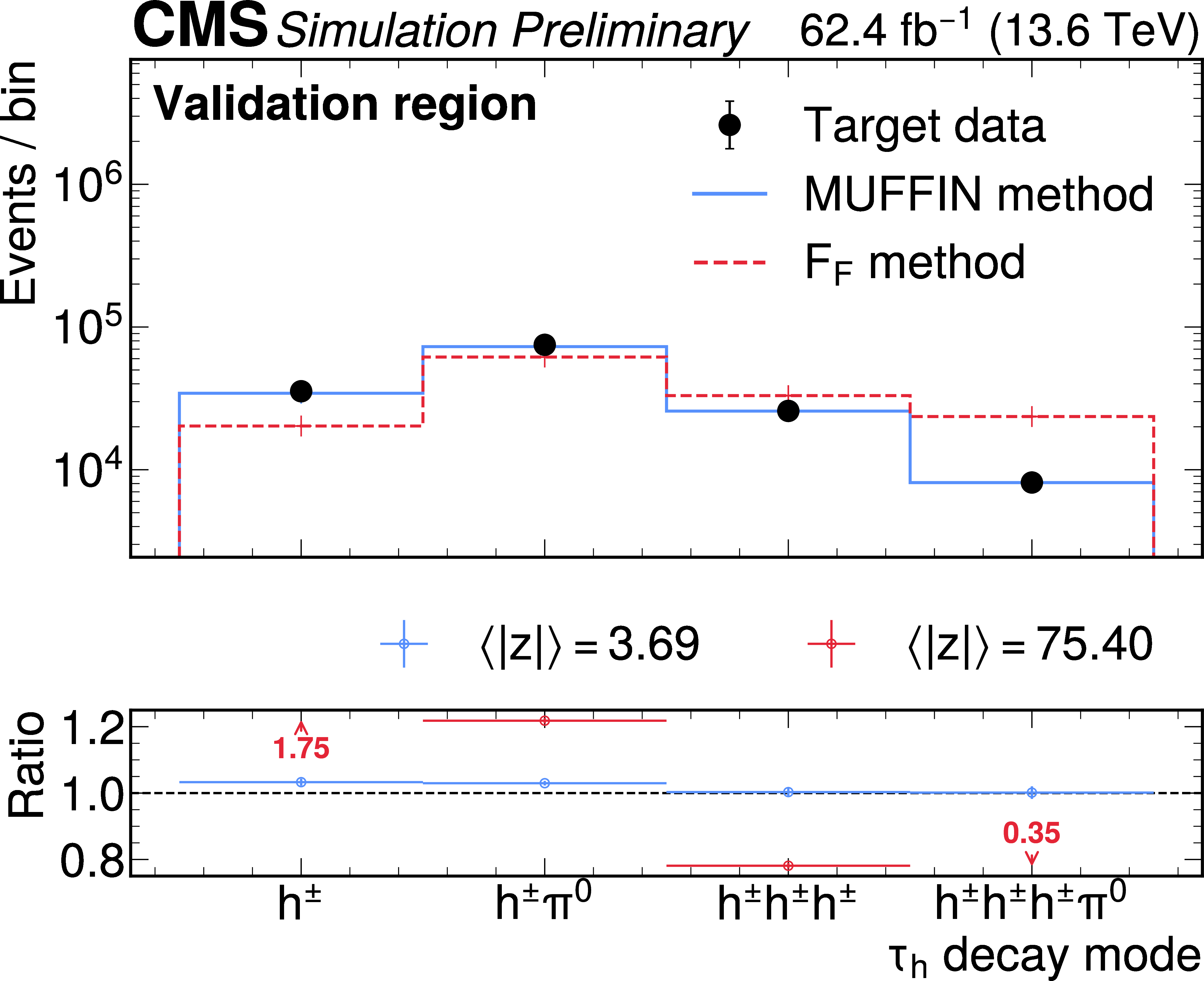
Validation of the QCD multijet background modelling in the $ \tau_\mathrm{\mu}\hspace{-.04em}\tau_\mathrm{h} $ validation region. Predictions from MUFFIN (blue) and $ F_{\text{F}} $ (red, dashed) are compared to data for $ p_{\mathrm{T}}^{\tau_\mathrm{h}} $, $ m_{\mathrm{T}}^{\text{total}} $, $ \Delta R $, and $ \tau_\mathrm{h} $ decay mode. The lower panels show the data-to-prediction ratio, with $ \langle|z|\rangle $ values indicating the overall level of agreement. Overflow events are included in the final bin ($ \infty $). |
png pdf |
Figure 7-a:
Validation of the QCD multijet background modelling in the $ \tau_\mathrm{\mu}\hspace{-.04em}\tau_\mathrm{h} $ validation region. Predictions from MUFFIN (blue) and $ F_{\text{F}} $ (red, dashed) are compared to data for $ p_{\mathrm{T}}^{\tau_\mathrm{h}} $, $ m_{\mathrm{T}}^{\text{total}} $, $ \Delta R $, and $ \tau_\mathrm{h} $ decay mode. The lower panels show the data-to-prediction ratio, with $ \langle|z|\rangle $ values indicating the overall level of agreement. Overflow events are included in the final bin ($ \infty $). |
png pdf |
Figure 7-b:
Validation of the QCD multijet background modelling in the $ \tau_\mathrm{\mu}\hspace{-.04em}\tau_\mathrm{h} $ validation region. Predictions from MUFFIN (blue) and $ F_{\text{F}} $ (red, dashed) are compared to data for $ p_{\mathrm{T}}^{\tau_\mathrm{h}} $, $ m_{\mathrm{T}}^{\text{total}} $, $ \Delta R $, and $ \tau_\mathrm{h} $ decay mode. The lower panels show the data-to-prediction ratio, with $ \langle|z|\rangle $ values indicating the overall level of agreement. Overflow events are included in the final bin ($ \infty $). |
png pdf |
Figure 7-c:
Validation of the QCD multijet background modelling in the $ \tau_\mathrm{\mu}\hspace{-.04em}\tau_\mathrm{h} $ validation region. Predictions from MUFFIN (blue) and $ F_{\text{F}} $ (red, dashed) are compared to data for $ p_{\mathrm{T}}^{\tau_\mathrm{h}} $, $ m_{\mathrm{T}}^{\text{total}} $, $ \Delta R $, and $ \tau_\mathrm{h} $ decay mode. The lower panels show the data-to-prediction ratio, with $ \langle|z|\rangle $ values indicating the overall level of agreement. Overflow events are included in the final bin ($ \infty $). |
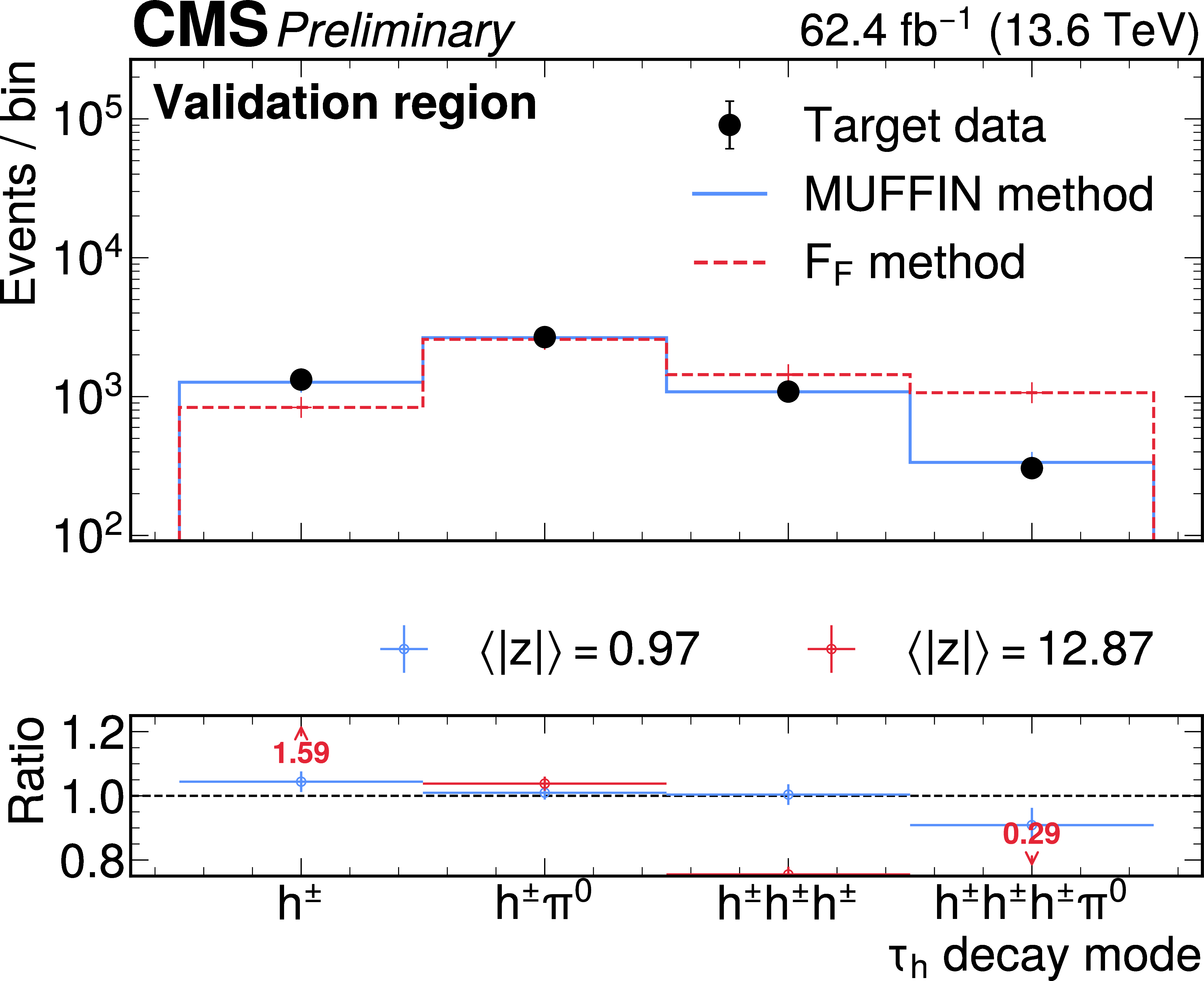
png pdf |
Figure 7-d:
Validation of the QCD multijet background modelling in the $ \tau_\mathrm{\mu}\hspace{-.04em}\tau_\mathrm{h} $ validation region. Predictions from MUFFIN (blue) and $ F_{\text{F}} $ (red, dashed) are compared to data for $ p_{\mathrm{T}}^{\tau_\mathrm{h}} $, $ m_{\mathrm{T}}^{\text{total}} $, $ \Delta R $, and $ \tau_\mathrm{h} $ decay mode. The lower panels show the data-to-prediction ratio, with $ \langle|z|\rangle $ values indicating the overall level of agreement. Overflow events are included in the final bin ($ \infty $). |
png pdf |
Figure 8:
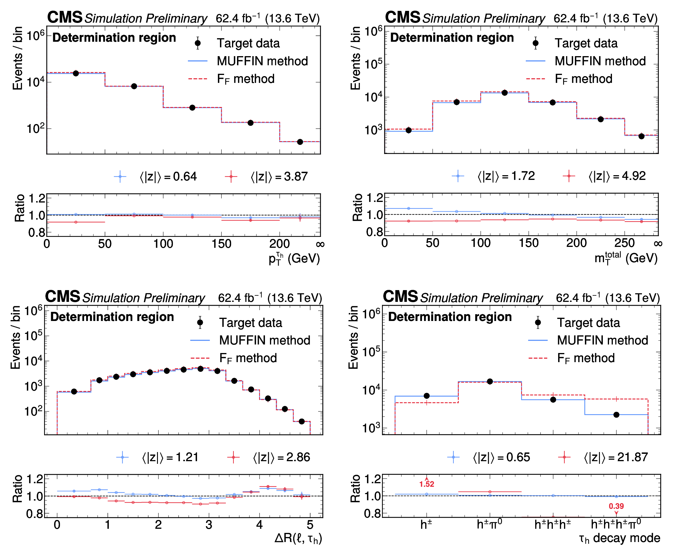
Comparison of $ p_{\mathrm{T}}^{\tau_\mathrm{h}} $, $ m_{\mathrm{T}}^{\text{total}} $, $ \Delta R $, and $ \tau_\mathrm{h} $ decay mode in the $ \mathrm{W}+\text{jets} $ determination region of the $ \tau_\mathrm{\mu}\hspace{-.04em}\tau_\mathrm{h} $ channel, showing MUFFIN (blue) and $ F_{\text{F}} $ (red, dashed). The ratio panels report the $ \langle|z|\rangle $ values for each method; arrows mark bins outside the plotted range; overflow is included in the last bin ($ \infty $) where applicable. |
png pdf |
Figure 8-a:
Comparison of $ p_{\mathrm{T}}^{\tau_\mathrm{h}} $, $ m_{\mathrm{T}}^{\text{total}} $, $ \Delta R $, and $ \tau_\mathrm{h} $ decay mode in the $ \mathrm{W}+\text{jets} $ determination region of the $ \tau_\mathrm{\mu}\hspace{-.04em}\tau_\mathrm{h} $ channel, showing MUFFIN (blue) and $ F_{\text{F}} $ (red, dashed). The ratio panels report the $ \langle|z|\rangle $ values for each method; arrows mark bins outside the plotted range; overflow is included in the last bin ($ \infty $) where applicable. |
png pdf |
Figure 8-b:
Comparison of $ p_{\mathrm{T}}^{\tau_\mathrm{h}} $, $ m_{\mathrm{T}}^{\text{total}} $, $ \Delta R $, and $ \tau_\mathrm{h} $ decay mode in the $ \mathrm{W}+\text{jets} $ determination region of the $ \tau_\mathrm{\mu}\hspace{-.04em}\tau_\mathrm{h} $ channel, showing MUFFIN (blue) and $ F_{\text{F}} $ (red, dashed). The ratio panels report the $ \langle|z|\rangle $ values for each method; arrows mark bins outside the plotted range; overflow is included in the last bin ($ \infty $) where applicable. |
png pdf |
Figure 8-c:
Comparison of $ p_{\mathrm{T}}^{\tau_\mathrm{h}} $, $ m_{\mathrm{T}}^{\text{total}} $, $ \Delta R $, and $ \tau_\mathrm{h} $ decay mode in the $ \mathrm{W}+\text{jets} $ determination region of the $ \tau_\mathrm{\mu}\hspace{-.04em}\tau_\mathrm{h} $ channel, showing MUFFIN (blue) and $ F_{\text{F}} $ (red, dashed). The ratio panels report the $ \langle|z|\rangle $ values for each method; arrows mark bins outside the plotted range; overflow is included in the last bin ($ \infty $) where applicable. |
png pdf |
Figure 8-d:
Comparison of $ p_{\mathrm{T}}^{\tau_\mathrm{h}} $, $ m_{\mathrm{T}}^{\text{total}} $, $ \Delta R $, and $ \tau_\mathrm{h} $ decay mode in the $ \mathrm{W}+\text{jets} $ determination region of the $ \tau_\mathrm{\mu}\hspace{-.04em}\tau_\mathrm{h} $ channel, showing MUFFIN (blue) and $ F_{\text{F}} $ (red, dashed). The ratio panels report the $ \langle|z|\rangle $ values for each method; arrows mark bins outside the plotted range; overflow is included in the last bin ($ \infty $) where applicable. |
png pdf |
Figure 9:
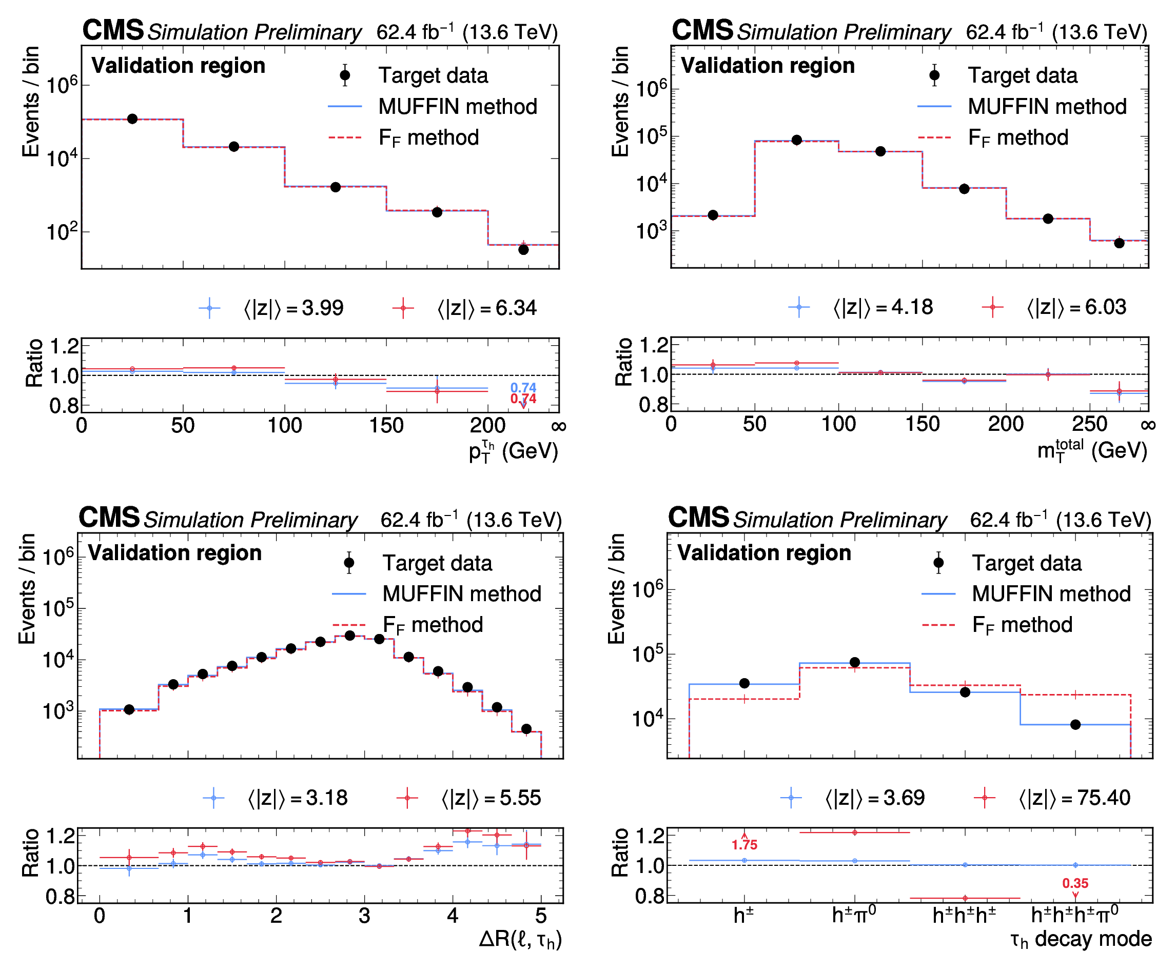
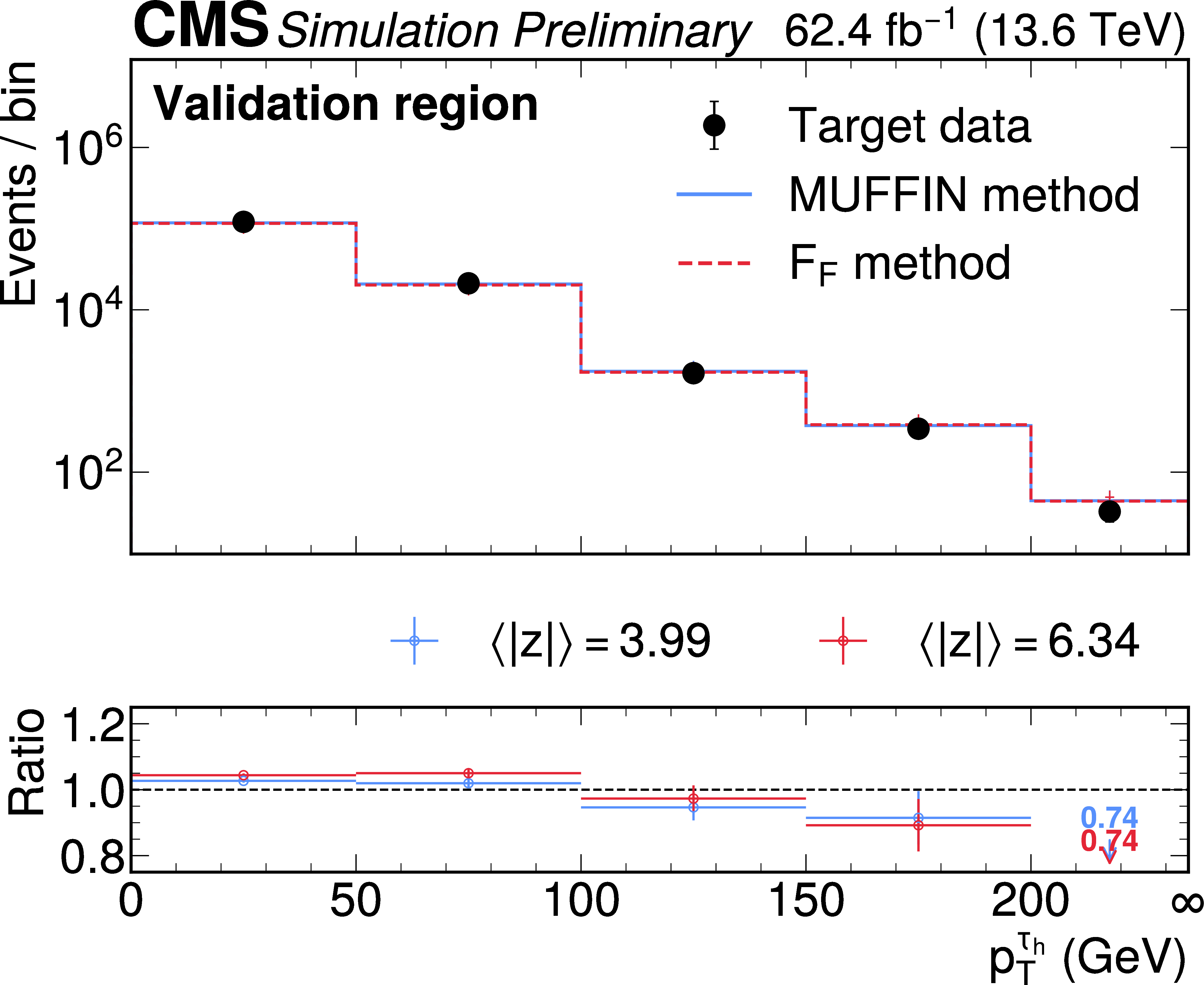
Comparison of $ p_{\mathrm{T}}^{\tau_\mathrm{h}} $, $ m_{\mathrm{T}}^{\text{total}} $, $ \Delta R $, and $ \tau_\mathrm{h} $ decay mode for MUFFIN (blue) and $ F_{\text{F}} $ (red, dashed) using simulated $ \mathrm{W}+\text{jets} $ events. Ratio panels show agreement with respect to the simulated target and report the corresponding $ \langle|z|\rangle $ values. Overflow is included in the final bin ($ \infty $) where applicable. |
png pdf |
Figure 9-a:
Comparison of $ p_{\mathrm{T}}^{\tau_\mathrm{h}} $, $ m_{\mathrm{T}}^{\text{total}} $, $ \Delta R $, and $ \tau_\mathrm{h} $ decay mode for MUFFIN (blue) and $ F_{\text{F}} $ (red, dashed) using simulated $ \mathrm{W}+\text{jets} $ events. Ratio panels show agreement with respect to the simulated target and report the corresponding $ \langle|z|\rangle $ values. Overflow is included in the final bin ($ \infty $) where applicable. |
png pdf |
Figure 9-b:
Comparison of $ p_{\mathrm{T}}^{\tau_\mathrm{h}} $, $ m_{\mathrm{T}}^{\text{total}} $, $ \Delta R $, and $ \tau_\mathrm{h} $ decay mode for MUFFIN (blue) and $ F_{\text{F}} $ (red, dashed) using simulated $ \mathrm{W}+\text{jets} $ events. Ratio panels show agreement with respect to the simulated target and report the corresponding $ \langle|z|\rangle $ values. Overflow is included in the final bin ($ \infty $) where applicable. |
png pdf |
Figure 9-c:
Comparison of $ p_{\mathrm{T}}^{\tau_\mathrm{h}} $, $ m_{\mathrm{T}}^{\text{total}} $, $ \Delta R $, and $ \tau_\mathrm{h} $ decay mode for MUFFIN (blue) and $ F_{\text{F}} $ (red, dashed) using simulated $ \mathrm{W}+\text{jets} $ events. Ratio panels show agreement with respect to the simulated target and report the corresponding $ \langle|z|\rangle $ values. Overflow is included in the final bin ($ \infty $) where applicable. |
png pdf |
Figure 9-d:
Comparison of $ p_{\mathrm{T}}^{\tau_\mathrm{h}} $, $ m_{\mathrm{T}}^{\text{total}} $, $ \Delta R $, and $ \tau_\mathrm{h} $ decay mode for MUFFIN (blue) and $ F_{\text{F}} $ (red, dashed) using simulated $ \mathrm{W}+\text{jets} $ events. Ratio panels show agreement with respect to the simulated target and report the corresponding $ \langle|z|\rangle $ values. Overflow is included in the final bin ($ \infty $) where applicable. |
png pdf |
Figure 10:
Comparison of $ p_{\mathrm{T}}^{\tau_\mathrm{h}} $, $ m_{\mathrm{T}}^{\text{total}} $, $ \Delta R $, and $ \tau_\mathrm{h} $ decay mode for MUFFIN (blue) and $ F_{\text{F}} $ (red, dashed) in simulated $ \mathrm{t} \overline{\mathrm{t}} $ for the $ \tau_\mathrm{\mu}\hspace{-.04em}\tau_\mathrm{h} $ channel. The ratio panels show agreement with respect to the simulated target and report the corresponding $ \langle|z|\rangle $ values. Overflow is included in the final bin ($ \infty $) where applicable. |
png pdf |
Figure 10-a:
Comparison of $ p_{\mathrm{T}}^{\tau_\mathrm{h}} $, $ m_{\mathrm{T}}^{\text{total}} $, $ \Delta R $, and $ \tau_\mathrm{h} $ decay mode for MUFFIN (blue) and $ F_{\text{F}} $ (red, dashed) in simulated $ \mathrm{t} \overline{\mathrm{t}} $ for the $ \tau_\mathrm{\mu}\hspace{-.04em}\tau_\mathrm{h} $ channel. The ratio panels show agreement with respect to the simulated target and report the corresponding $ \langle|z|\rangle $ values. Overflow is included in the final bin ($ \infty $) where applicable. |
png pdf |
Figure 10-b:
Comparison of $ p_{\mathrm{T}}^{\tau_\mathrm{h}} $, $ m_{\mathrm{T}}^{\text{total}} $, $ \Delta R $, and $ \tau_\mathrm{h} $ decay mode for MUFFIN (blue) and $ F_{\text{F}} $ (red, dashed) in simulated $ \mathrm{t} \overline{\mathrm{t}} $ for the $ \tau_\mathrm{\mu}\hspace{-.04em}\tau_\mathrm{h} $ channel. The ratio panels show agreement with respect to the simulated target and report the corresponding $ \langle|z|\rangle $ values. Overflow is included in the final bin ($ \infty $) where applicable. |
png pdf |
Figure 10-c:
Comparison of $ p_{\mathrm{T}}^{\tau_\mathrm{h}} $, $ m_{\mathrm{T}}^{\text{total}} $, $ \Delta R $, and $ \tau_\mathrm{h} $ decay mode for MUFFIN (blue) and $ F_{\text{F}} $ (red, dashed) in simulated $ \mathrm{t} \overline{\mathrm{t}} $ for the $ \tau_\mathrm{\mu}\hspace{-.04em}\tau_\mathrm{h} $ channel. The ratio panels show agreement with respect to the simulated target and report the corresponding $ \langle|z|\rangle $ values. Overflow is included in the final bin ($ \infty $) where applicable. |
png pdf |
Figure 10-d:
Comparison of $ p_{\mathrm{T}}^{\tau_\mathrm{h}} $, $ m_{\mathrm{T}}^{\text{total}} $, $ \Delta R $, and $ \tau_\mathrm{h} $ decay mode for MUFFIN (blue) and $ F_{\text{F}} $ (red, dashed) in simulated $ \mathrm{t} \overline{\mathrm{t}} $ for the $ \tau_\mathrm{\mu}\hspace{-.04em}\tau_\mathrm{h} $ channel. The ratio panels show agreement with respect to the simulated target and report the corresponding $ \langle|z|\rangle $ values. Overflow is included in the final bin ($ \infty $) where applicable. |
png pdf |
Figure 11:
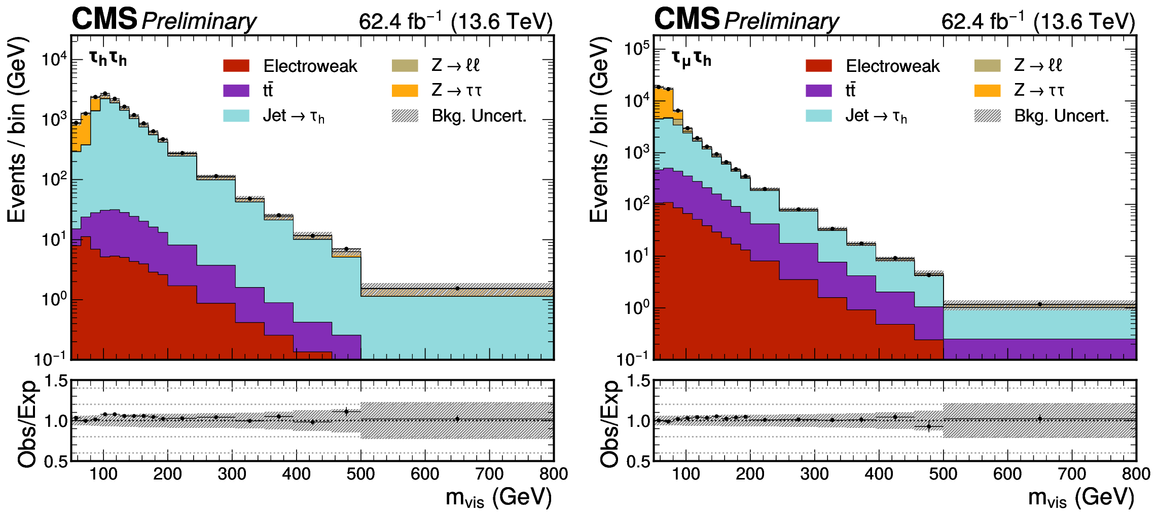
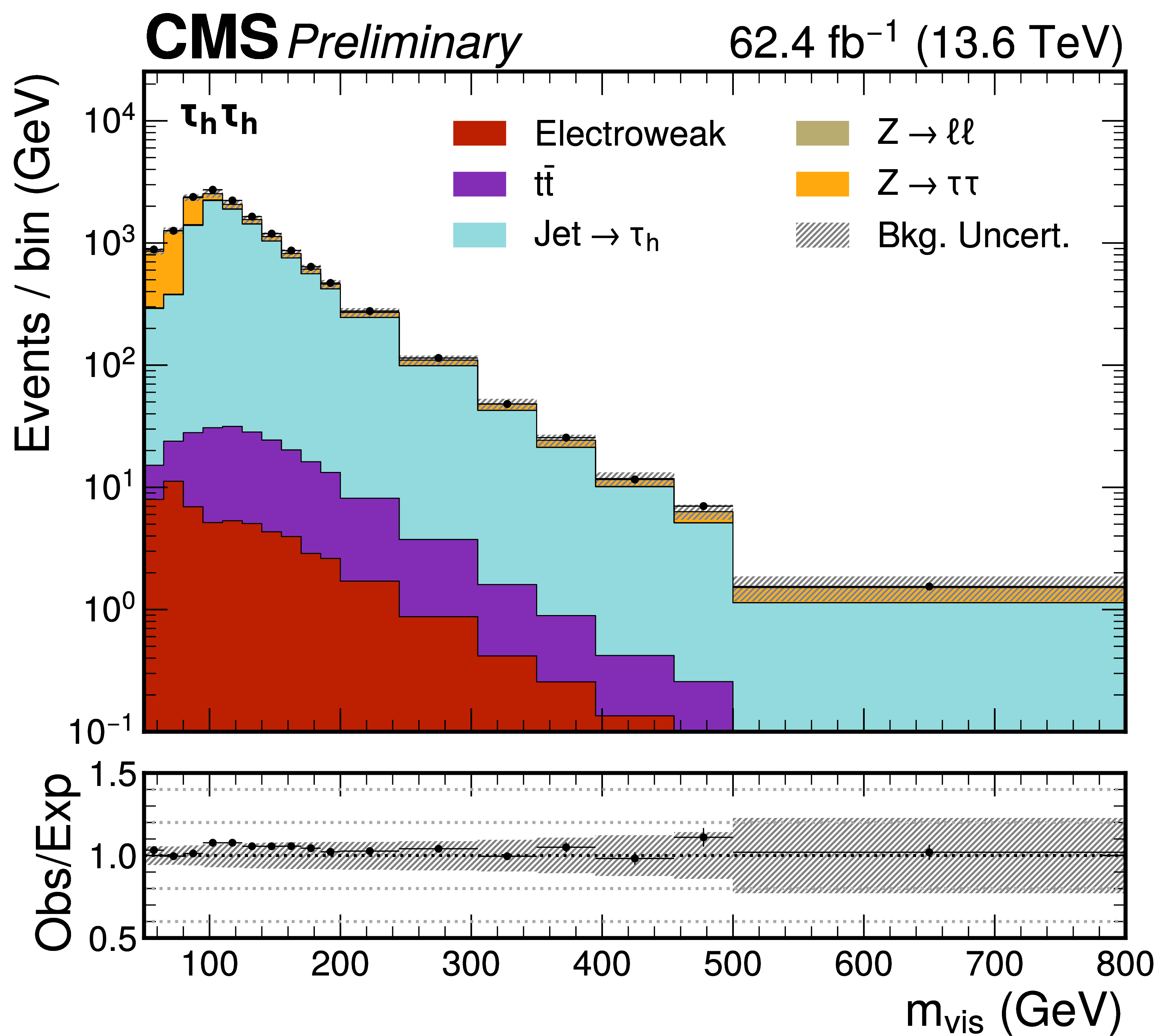
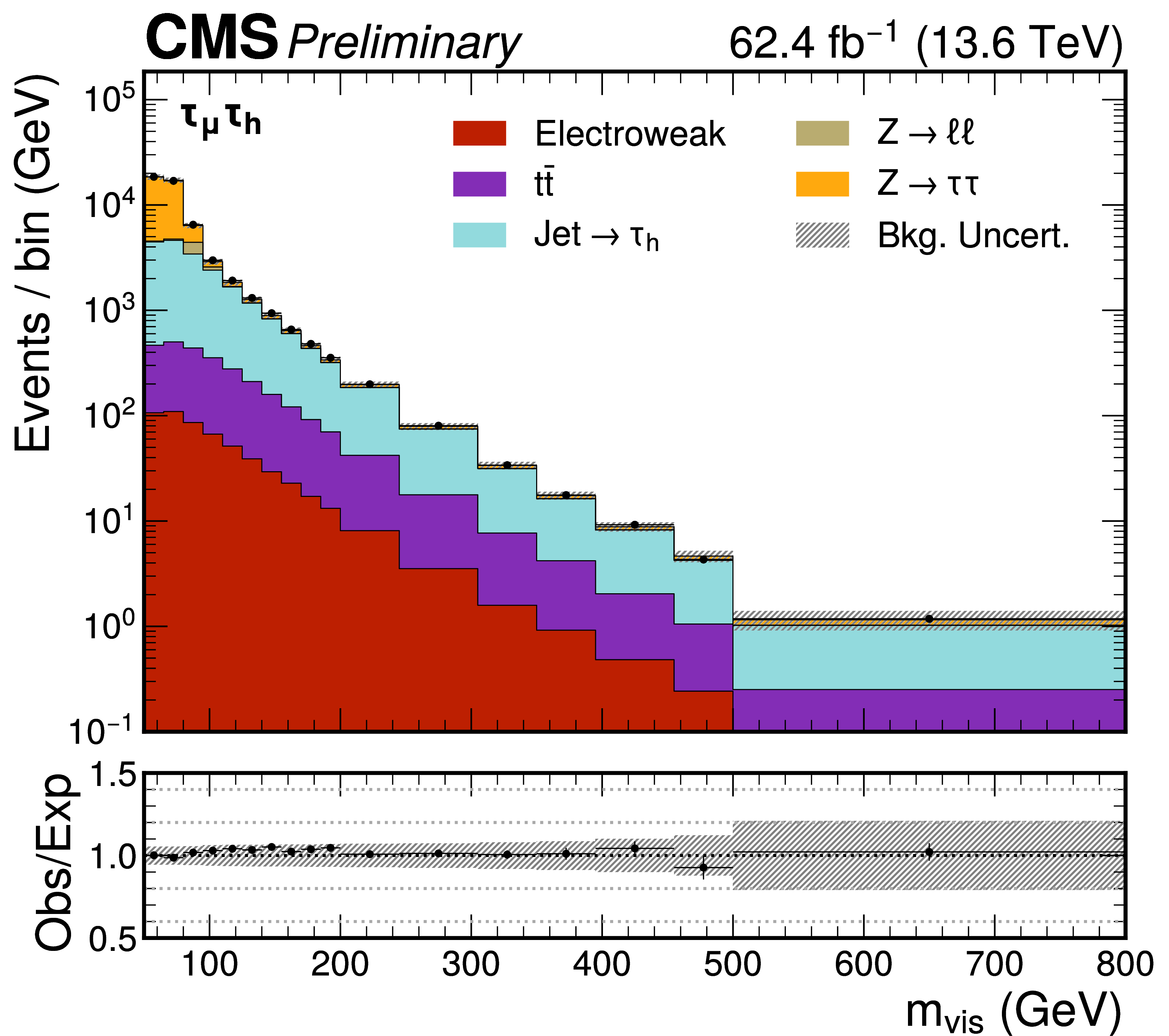
Distributions of the visible mass in the $ \tau_\mathrm{h}\tau_\mathrm{h} $ channel (left) and the $ \tau_\mathrm{\mu}\hspace{-.04em}\tau_\mathrm{h} $ channel (right) in the SRs, as defined in Section 5, of physics analyses targeting Higgs boson decays to $ \tau $ lepton pairs. The MUFFIN method is used to estimate the $ \text{jet}\to\tau_\mathrm{h} $ background contributions. The lower panels show the ratio of data to the total background prediction, with shaded bands representing the combined statistical and systematic uncertainties from the MUFFIN method. |
png pdf |
Figure 11-a:
Distributions of the visible mass in the $ \tau_\mathrm{h}\tau_\mathrm{h} $ channel (left) and the $ \tau_\mathrm{\mu}\hspace{-.04em}\tau_\mathrm{h} $ channel (right) in the SRs, as defined in Section 5, of physics analyses targeting Higgs boson decays to $ \tau $ lepton pairs. The MUFFIN method is used to estimate the $ \text{jet}\to\tau_\mathrm{h} $ background contributions. The lower panels show the ratio of data to the total background prediction, with shaded bands representing the combined statistical and systematic uncertainties from the MUFFIN method. |
png pdf |
Figure 11-b:
Distributions of the visible mass in the $ \tau_\mathrm{h}\tau_\mathrm{h} $ channel (left) and the $ \tau_\mathrm{\mu}\hspace{-.04em}\tau_\mathrm{h} $ channel (right) in the SRs, as defined in Section 5, of physics analyses targeting Higgs boson decays to $ \tau $ lepton pairs. The MUFFIN method is used to estimate the $ \text{jet}\to\tau_\mathrm{h} $ background contributions. The lower panels show the ratio of data to the total background prediction, with shaded bands representing the combined statistical and systematic uncertainties from the MUFFIN method. |
png pdf |
Figure 12:
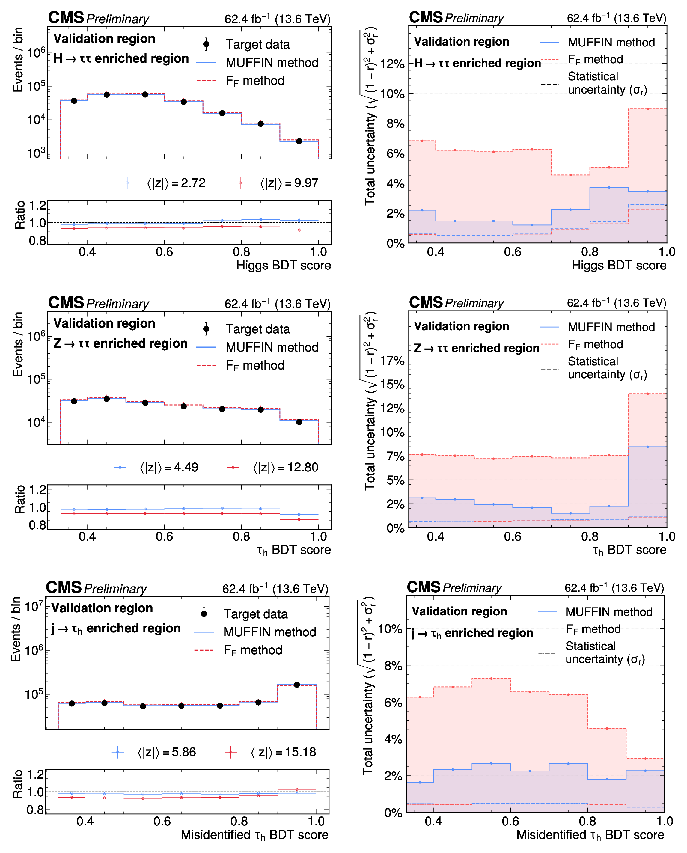
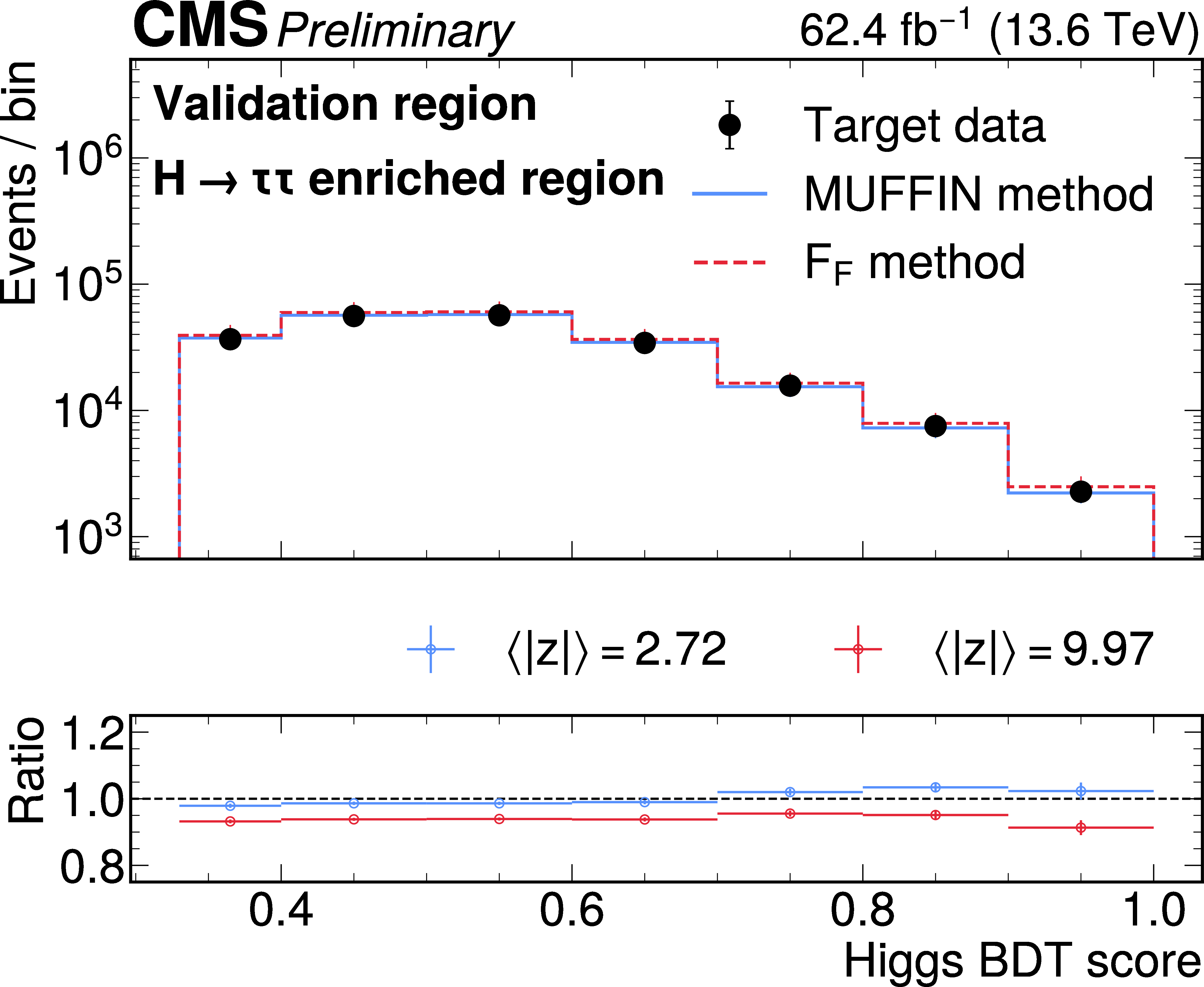
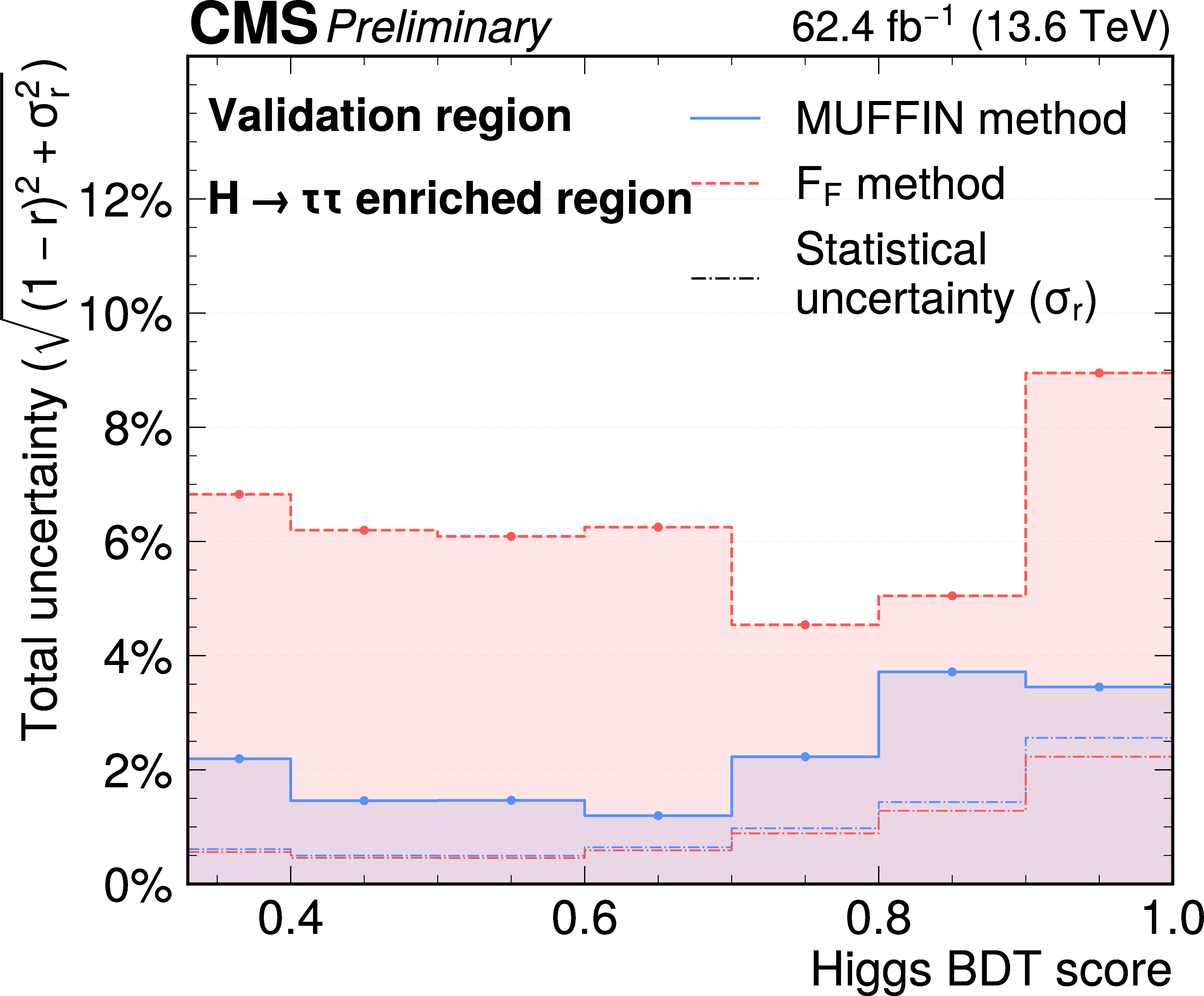
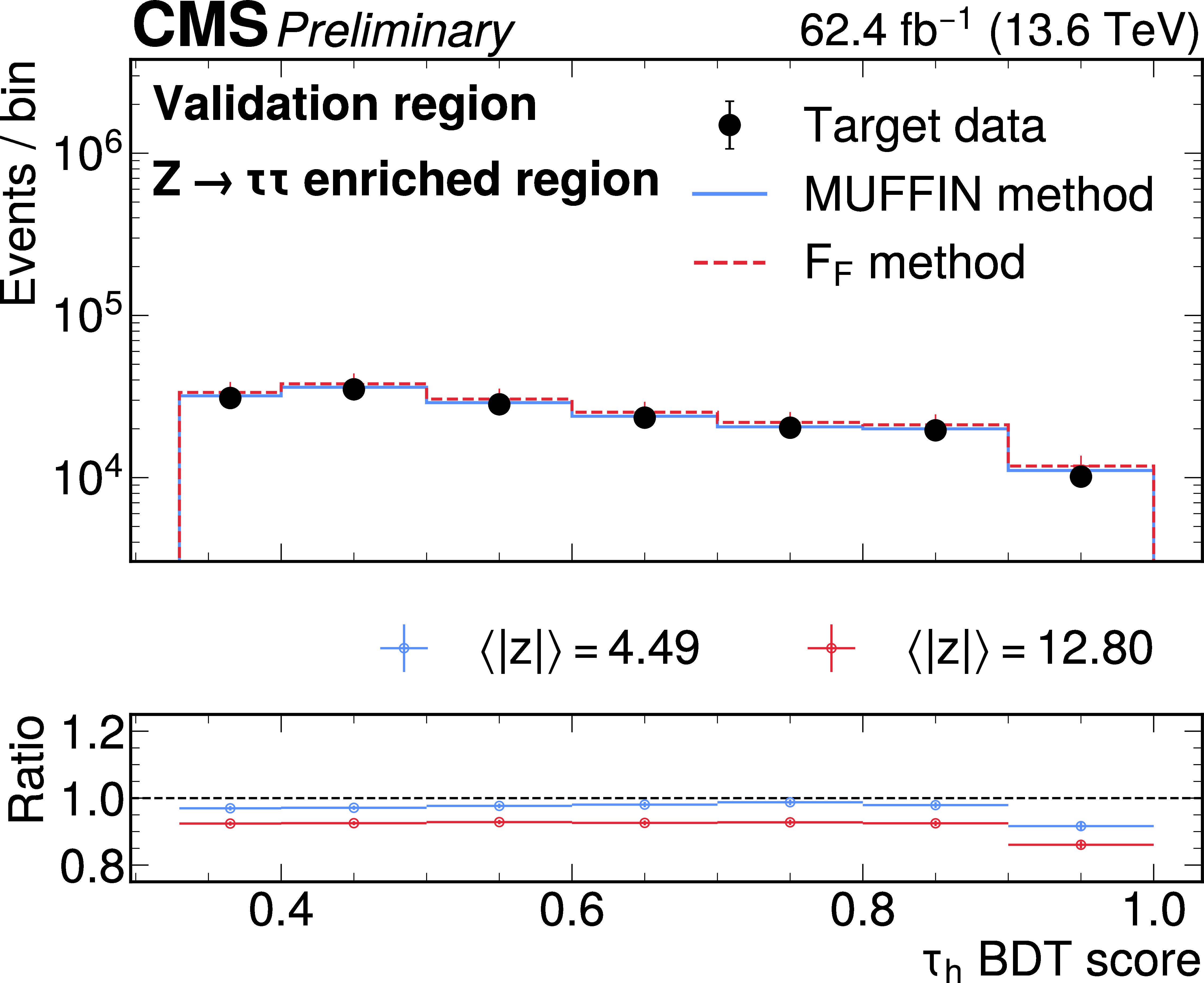
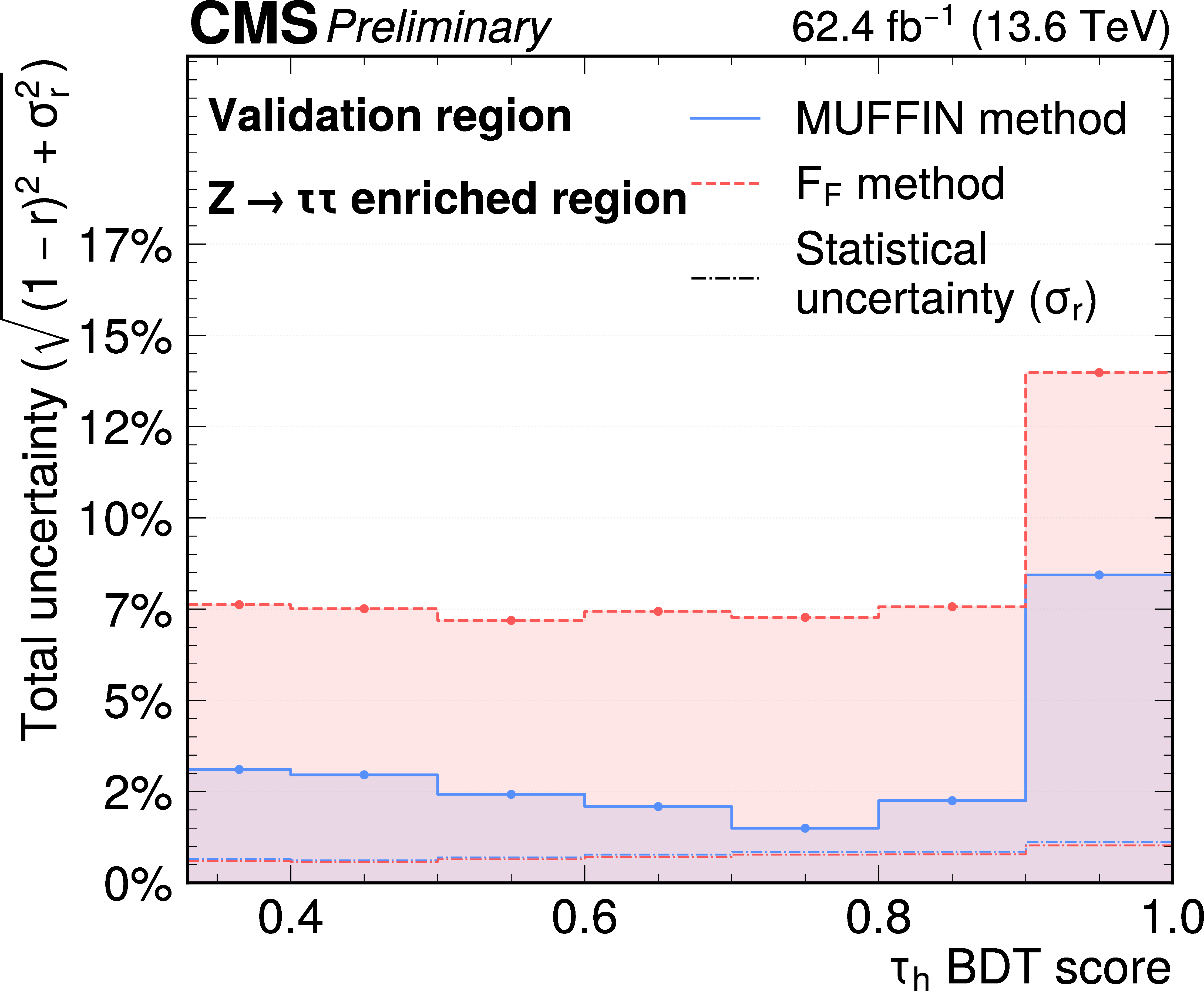
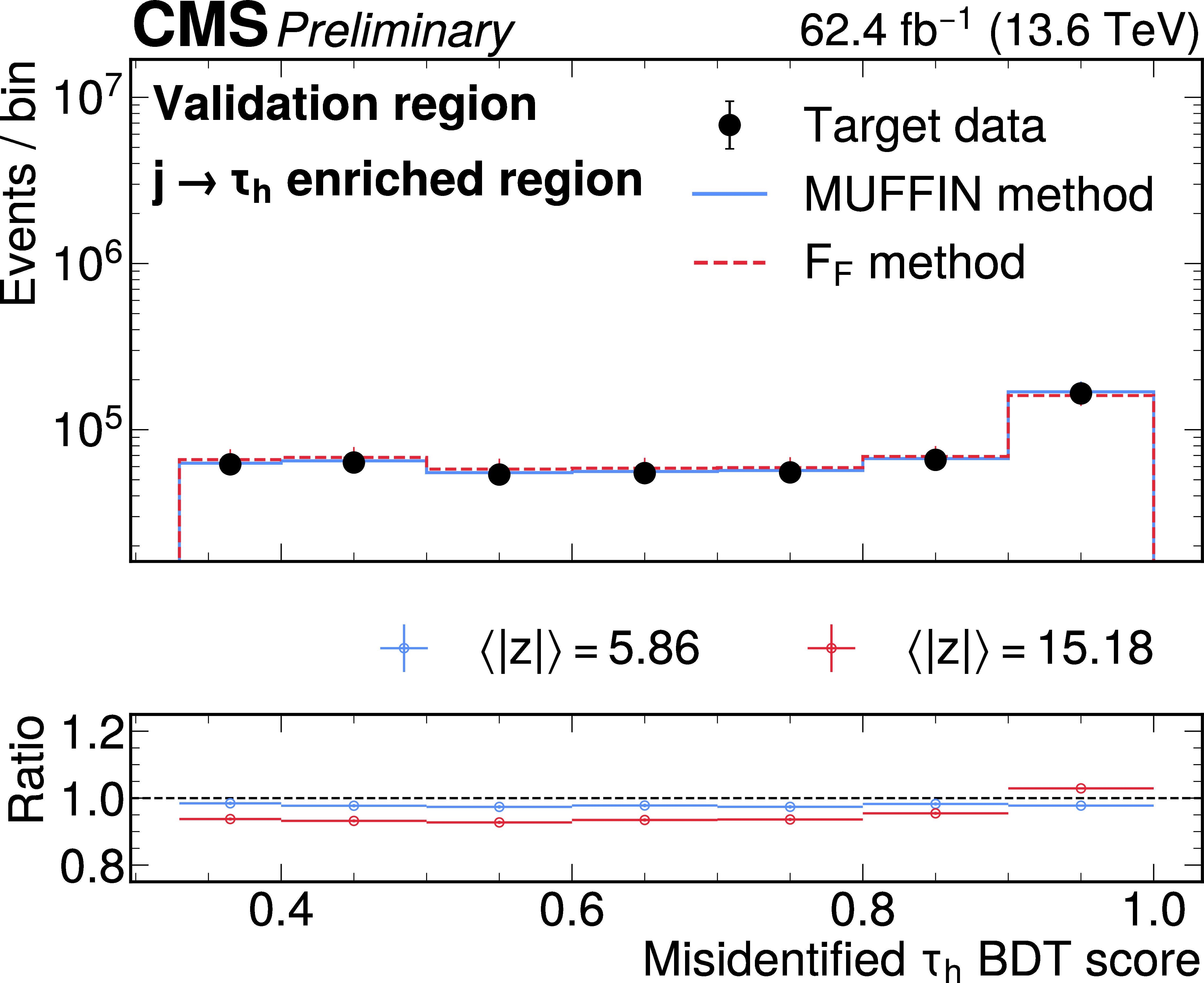
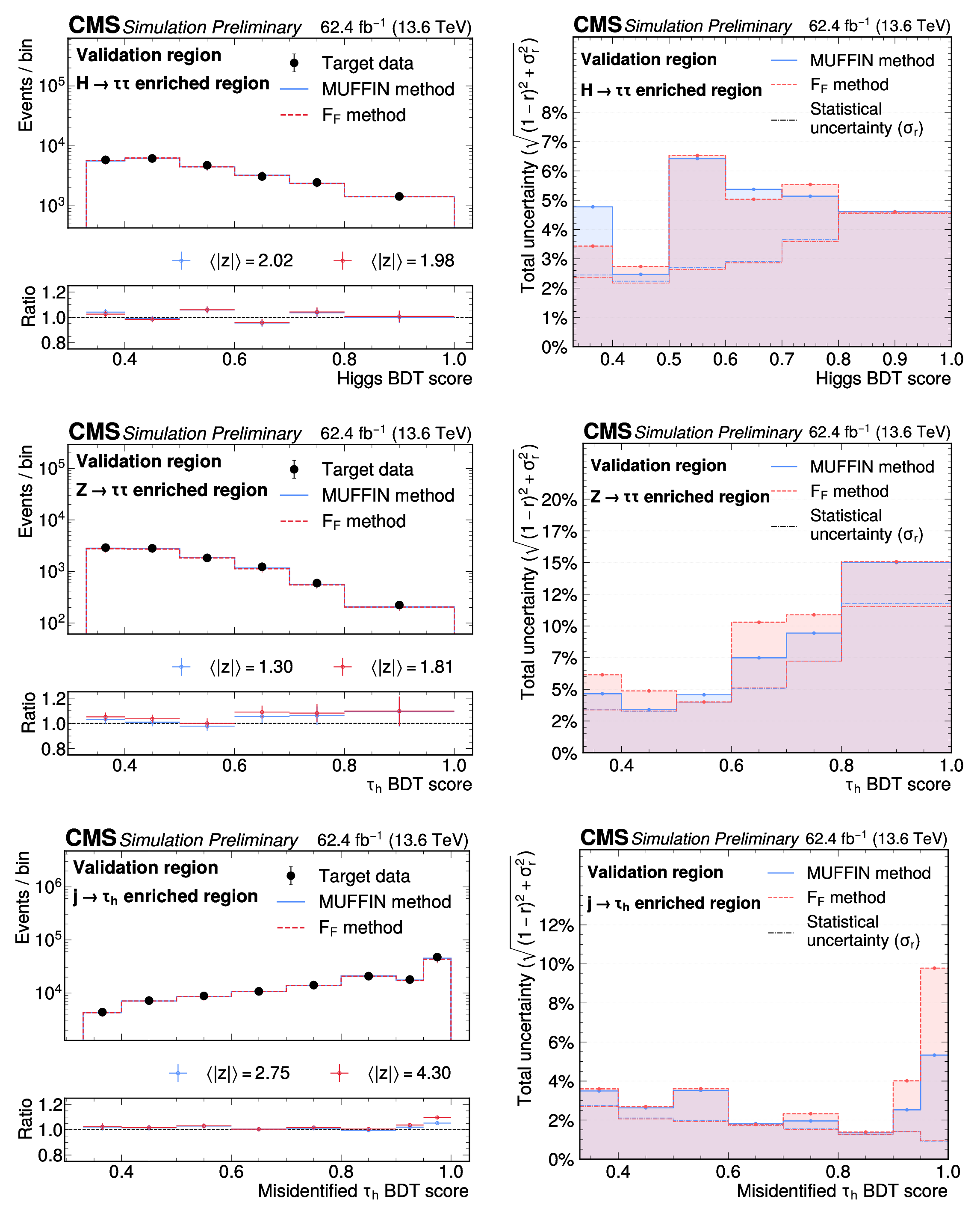
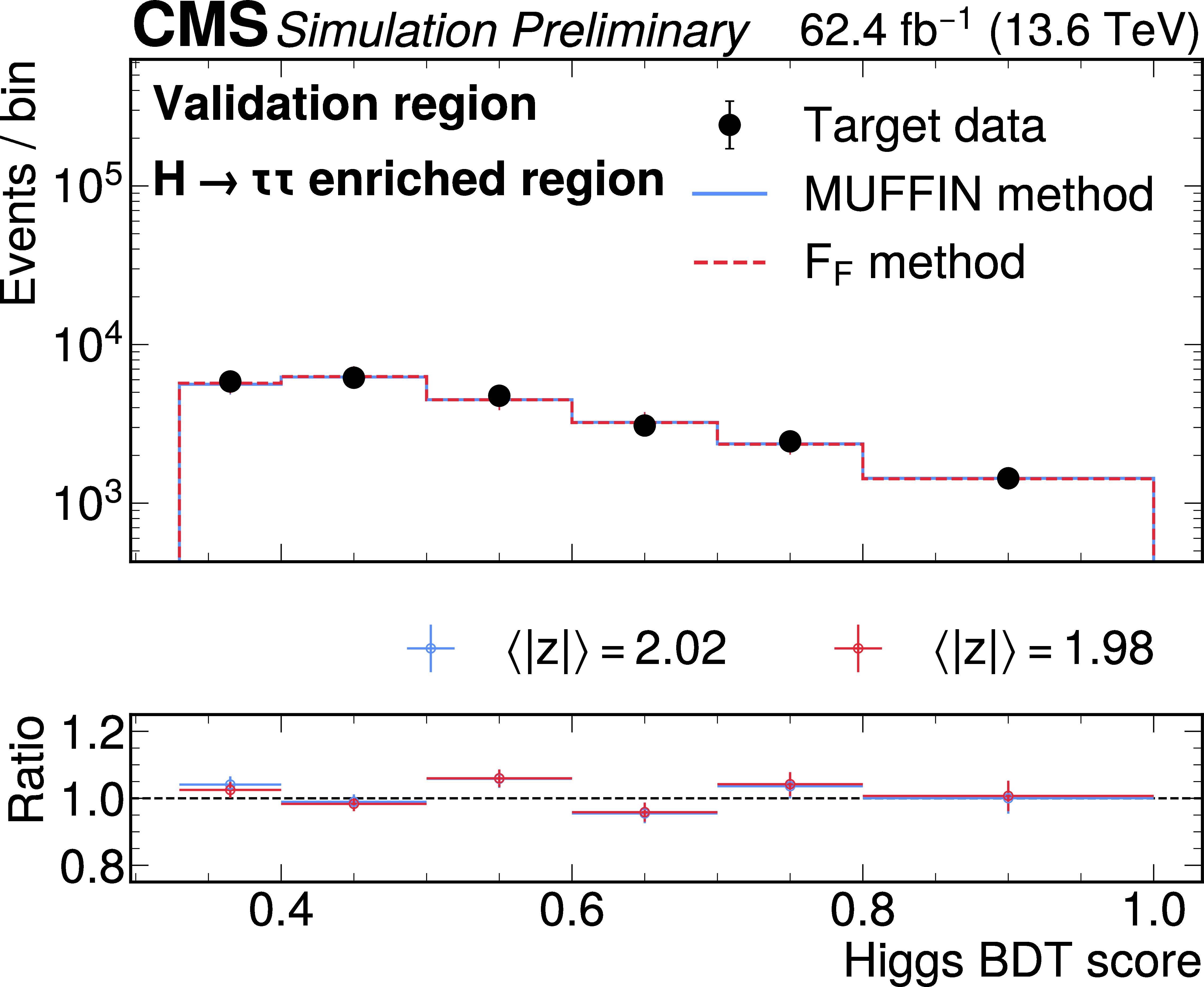
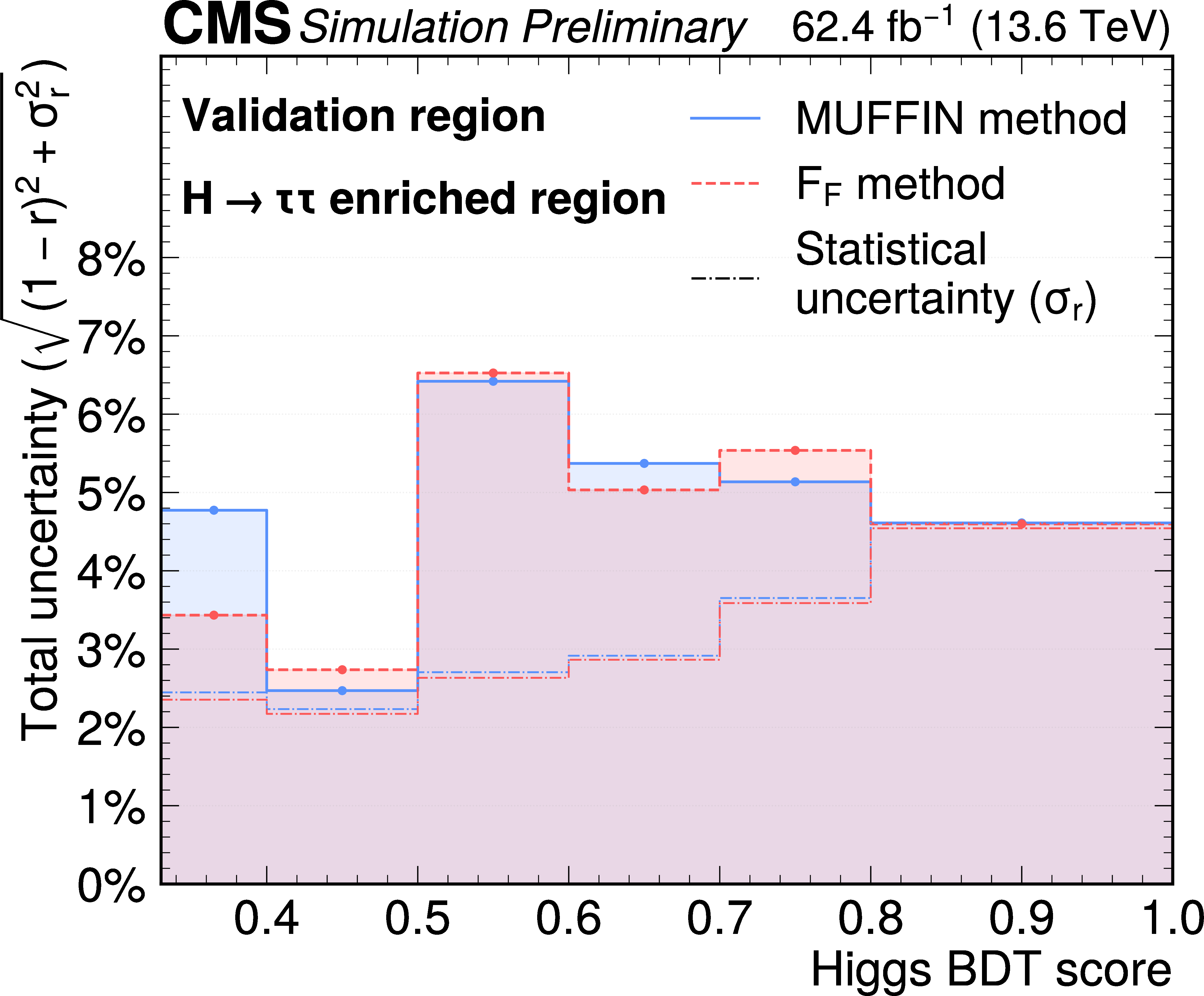
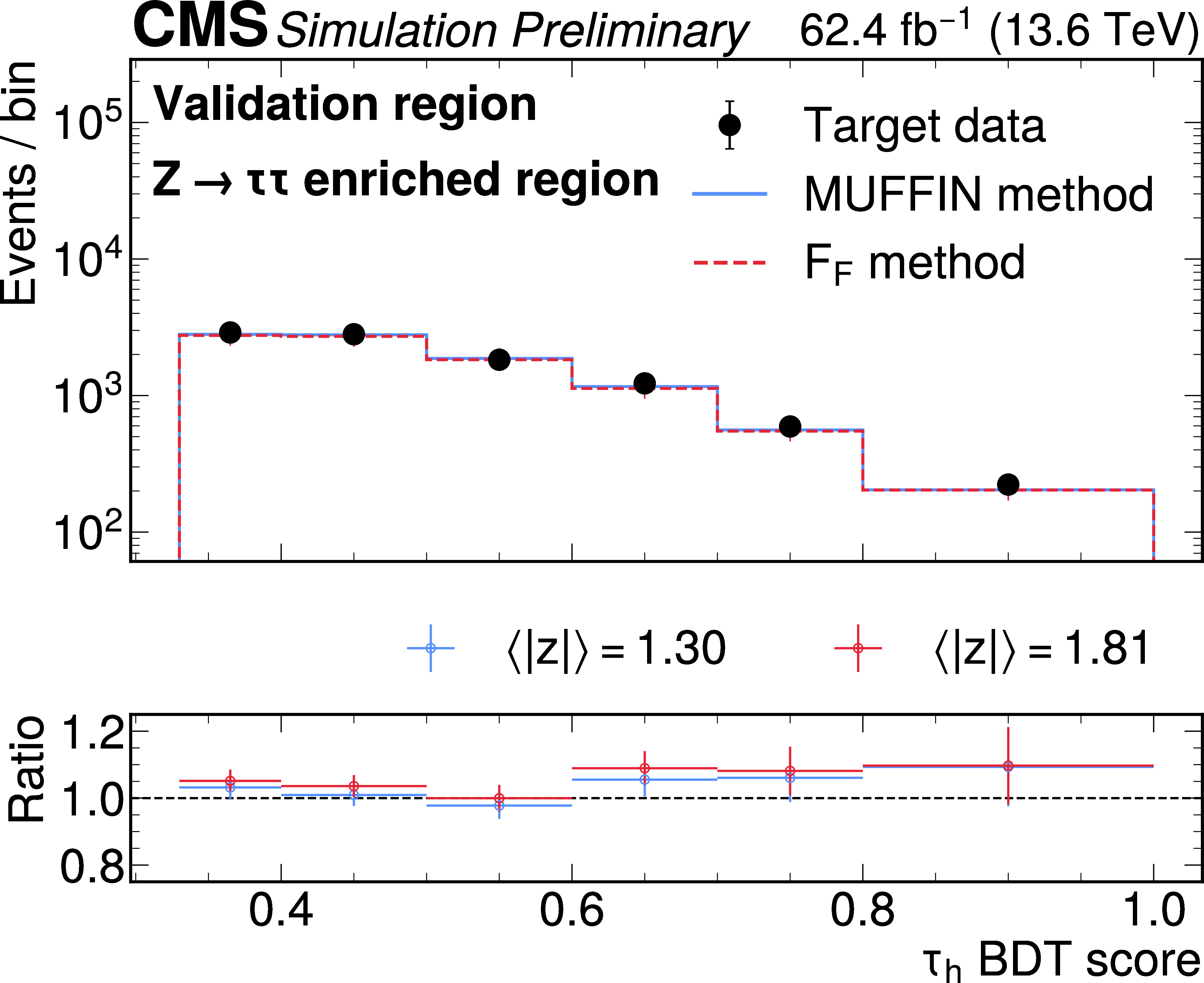
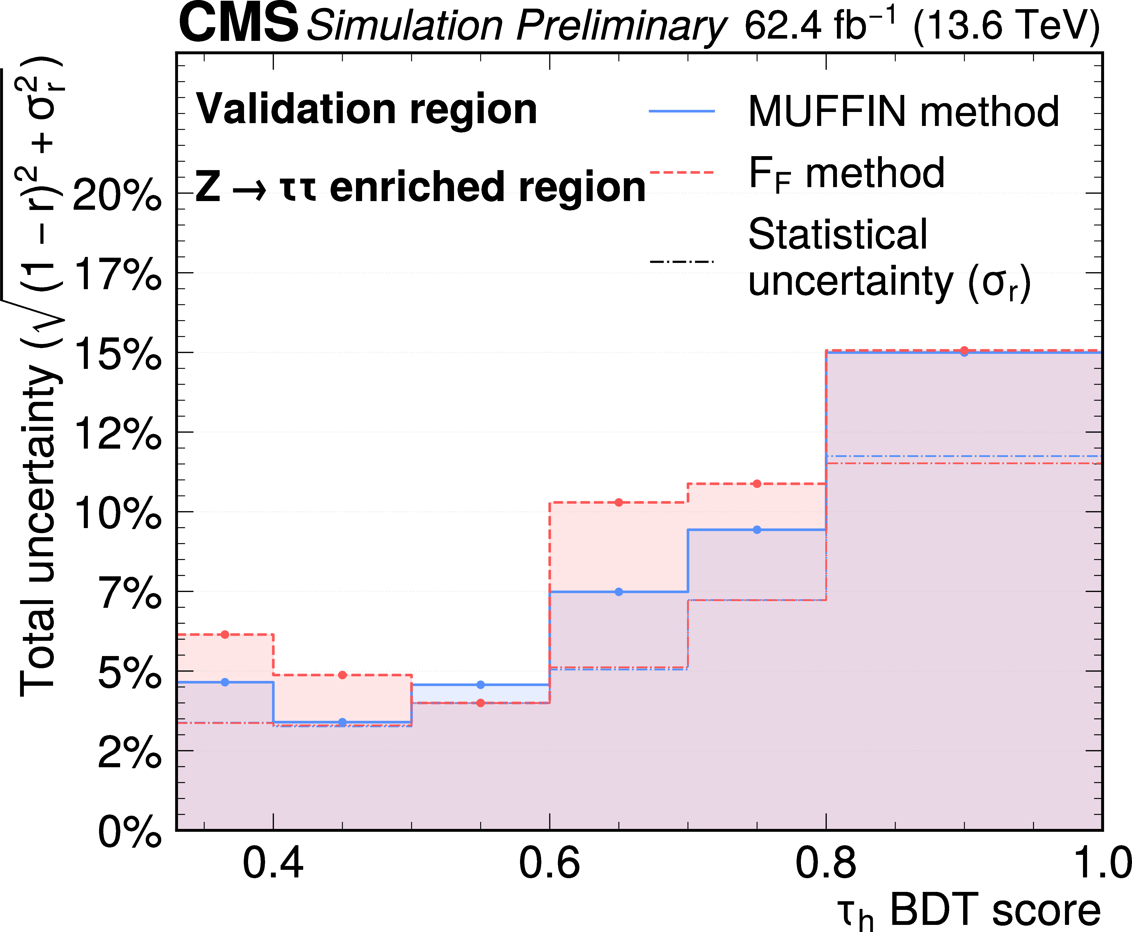
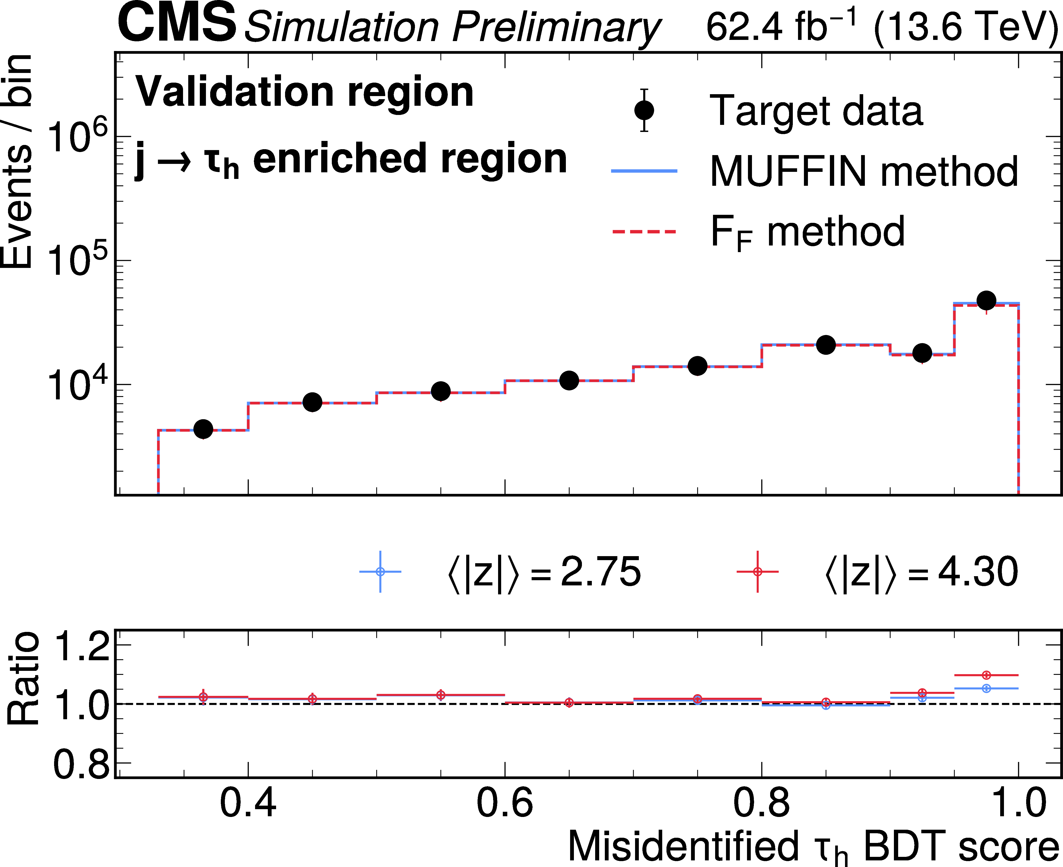
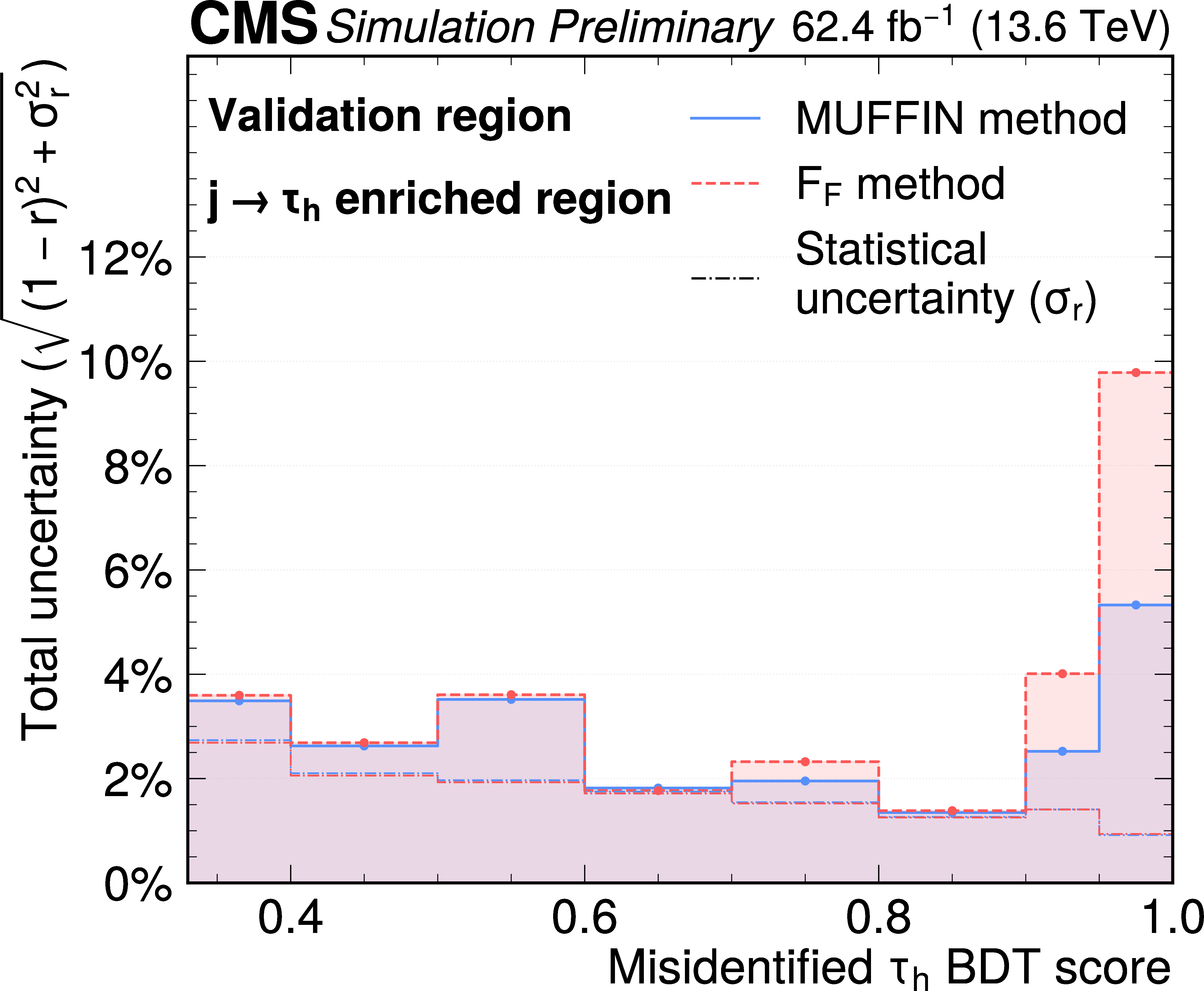
BDT-score validation in a $ H(125)\to\tau\tau CP $ validation region in the $ \tau_\mathrm{h}\tau_\mathrm{h} $ channel for the Higgs-enriched, $ \tau $-enriched, and jet-misidentification-enriched categories. MUFFIN (blue) and $ F_{\text{F}} $ (red, dashed) predictions are compared at the distribution level (left) and through the corresponding non-closure evaluation (right). |
png pdf |
Figure 12-a:
BDT-score validation in a $ H(125)\to\tau\tau CP $ validation region in the $ \tau_\mathrm{h}\tau_\mathrm{h} $ channel for the Higgs-enriched, $ \tau $-enriched, and jet-misidentification-enriched categories. MUFFIN (blue) and $ F_{\text{F}} $ (red, dashed) predictions are compared at the distribution level (left) and through the corresponding non-closure evaluation (right). |
png pdf |
Figure 12-b:
BDT-score validation in a $ H(125)\to\tau\tau CP $ validation region in the $ \tau_\mathrm{h}\tau_\mathrm{h} $ channel for the Higgs-enriched, $ \tau $-enriched, and jet-misidentification-enriched categories. MUFFIN (blue) and $ F_{\text{F}} $ (red, dashed) predictions are compared at the distribution level (left) and through the corresponding non-closure evaluation (right). |
png pdf |
Figure 12-c:
BDT-score validation in a $ H(125)\to\tau\tau CP $ validation region in the $ \tau_\mathrm{h}\tau_\mathrm{h} $ channel for the Higgs-enriched, $ \tau $-enriched, and jet-misidentification-enriched categories. MUFFIN (blue) and $ F_{\text{F}} $ (red, dashed) predictions are compared at the distribution level (left) and through the corresponding non-closure evaluation (right). |
png pdf |
Figure 12-d:
BDT-score validation in a $ H(125)\to\tau\tau CP $ validation region in the $ \tau_\mathrm{h}\tau_\mathrm{h} $ channel for the Higgs-enriched, $ \tau $-enriched, and jet-misidentification-enriched categories. MUFFIN (blue) and $ F_{\text{F}} $ (red, dashed) predictions are compared at the distribution level (left) and through the corresponding non-closure evaluation (right). |
png pdf |
Figure 12-e:
BDT-score validation in a $ H(125)\to\tau\tau CP $ validation region in the $ \tau_\mathrm{h}\tau_\mathrm{h} $ channel for the Higgs-enriched, $ \tau $-enriched, and jet-misidentification-enriched categories. MUFFIN (blue) and $ F_{\text{F}} $ (red, dashed) predictions are compared at the distribution level (left) and through the corresponding non-closure evaluation (right). |

png pdf |
Figure 12-f:
BDT-score validation in a $ H(125)\to\tau\tau CP $ validation region in the $ \tau_\mathrm{h}\tau_\mathrm{h} $ channel for the Higgs-enriched, $ \tau $-enriched, and jet-misidentification-enriched categories. MUFFIN (blue) and $ F_{\text{F}} $ (red, dashed) predictions are compared at the distribution level (left) and through the corresponding non-closure evaluation (right). |
png pdf |
Figure 13:
BDT-score validation in a $ \mathrm{W}+\text{jets} $-enriched validation region in the $ \tau_\mathrm{\mu}\hspace{-.04em}\tau_\mathrm{h} $ channel for the Higgs-enriched, $ \tau $-enriched, and jet-misidentification-enriched categories. MUFFIN (blue) and $ F_{\text{F}} $ (red, dashed) predictions are compared at the distribution level (left) and through the corresponding non-closure evaluation (right). |
png pdf |
Figure 13-a:
BDT-score validation in a $ \mathrm{W}+\text{jets} $-enriched validation region in the $ \tau_\mathrm{\mu}\hspace{-.04em}\tau_\mathrm{h} $ channel for the Higgs-enriched, $ \tau $-enriched, and jet-misidentification-enriched categories. MUFFIN (blue) and $ F_{\text{F}} $ (red, dashed) predictions are compared at the distribution level (left) and through the corresponding non-closure evaluation (right). |
png pdf |
Figure 13-b:
BDT-score validation in a $ \mathrm{W}+\text{jets} $-enriched validation region in the $ \tau_\mathrm{\mu}\hspace{-.04em}\tau_\mathrm{h} $ channel for the Higgs-enriched, $ \tau $-enriched, and jet-misidentification-enriched categories. MUFFIN (blue) and $ F_{\text{F}} $ (red, dashed) predictions are compared at the distribution level (left) and through the corresponding non-closure evaluation (right). |
png pdf |
Figure 13-c:
BDT-score validation in a $ \mathrm{W}+\text{jets} $-enriched validation region in the $ \tau_\mathrm{\mu}\hspace{-.04em}\tau_\mathrm{h} $ channel for the Higgs-enriched, $ \tau $-enriched, and jet-misidentification-enriched categories. MUFFIN (blue) and $ F_{\text{F}} $ (red, dashed) predictions are compared at the distribution level (left) and through the corresponding non-closure evaluation (right). |
png pdf |
Figure 13-d:
BDT-score validation in a $ \mathrm{W}+\text{jets} $-enriched validation region in the $ \tau_\mathrm{\mu}\hspace{-.04em}\tau_\mathrm{h} $ channel for the Higgs-enriched, $ \tau $-enriched, and jet-misidentification-enriched categories. MUFFIN (blue) and $ F_{\text{F}} $ (red, dashed) predictions are compared at the distribution level (left) and through the corresponding non-closure evaluation (right). |
png pdf |
Figure 13-e:
BDT-score validation in a $ \mathrm{W}+\text{jets} $-enriched validation region in the $ \tau_\mathrm{\mu}\hspace{-.04em}\tau_\mathrm{h} $ channel for the Higgs-enriched, $ \tau $-enriched, and jet-misidentification-enriched categories. MUFFIN (blue) and $ F_{\text{F}} $ (red, dashed) predictions are compared at the distribution level (left) and through the corresponding non-closure evaluation (right). |
png pdf |
Figure 13-f:
BDT-score validation in a $ \mathrm{W}+\text{jets} $-enriched validation region in the $ \tau_\mathrm{\mu}\hspace{-.04em}\tau_\mathrm{h} $ channel for the Higgs-enriched, $ \tau $-enriched, and jet-misidentification-enriched categories. MUFFIN (blue) and $ F_{\text{F}} $ (red, dashed) predictions are compared at the distribution level (left) and through the corresponding non-closure evaluation (right). |
png pdf |
Figure 14:
STXS-inspired category-by-category yield closure for a $ \tau_\mathrm{h}\tau_\mathrm{h} $ (top) and $ \tau_\mathrm{\mu}\hspace{-.04em}\tau_\mathrm{h} $ (bottom) validation region. Points show the ratio of observed to predicted yields per STXS category (non-closure), for the MUFFIN (blue) and $ F_{\text{F}} $ (red) methods, where deviations from unity are interpreted as systematic uncertainties in the $ \text{jet}\to\tau_\mathrm{h} $ background estimate. The right panel shows the total uncertainty per category, with the hatched grey bars indicating the statistical component. Only statistical uncertainties are shown; the observed non-closure along with the statistical uncertainty define the systematic uncertainty that would be assigned in a real analysis. The MUFFIN method achieves significantly improved per-category agreement, particularly in the high-$ p_{\mathrm{T}} $ and multi-jet categories. |
png pdf |
Figure 14-a:
STXS-inspired category-by-category yield closure for a $ \tau_\mathrm{h}\tau_\mathrm{h} $ (top) and $ \tau_\mathrm{\mu}\hspace{-.04em}\tau_\mathrm{h} $ (bottom) validation region. Points show the ratio of observed to predicted yields per STXS category (non-closure), for the MUFFIN (blue) and $ F_{\text{F}} $ (red) methods, where deviations from unity are interpreted as systematic uncertainties in the $ \text{jet}\to\tau_\mathrm{h} $ background estimate. The right panel shows the total uncertainty per category, with the hatched grey bars indicating the statistical component. Only statistical uncertainties are shown; the observed non-closure along with the statistical uncertainty define the systematic uncertainty that would be assigned in a real analysis. The MUFFIN method achieves significantly improved per-category agreement, particularly in the high-$ p_{\mathrm{T}} $ and multi-jet categories. |
png pdf |
Figure 14-b:
STXS-inspired category-by-category yield closure for a $ \tau_\mathrm{h}\tau_\mathrm{h} $ (top) and $ \tau_\mathrm{\mu}\hspace{-.04em}\tau_\mathrm{h} $ (bottom) validation region. Points show the ratio of observed to predicted yields per STXS category (non-closure), for the MUFFIN (blue) and $ F_{\text{F}} $ (red) methods, where deviations from unity are interpreted as systematic uncertainties in the $ \text{jet}\to\tau_\mathrm{h} $ background estimate. The right panel shows the total uncertainty per category, with the hatched grey bars indicating the statistical component. Only statistical uncertainties are shown; the observed non-closure along with the statistical uncertainty define the systematic uncertainty that would be assigned in a real analysis. The MUFFIN method achieves significantly improved per-category agreement, particularly in the high-$ p_{\mathrm{T}} $ and multi-jet categories. |
png pdf |
Figure 15:
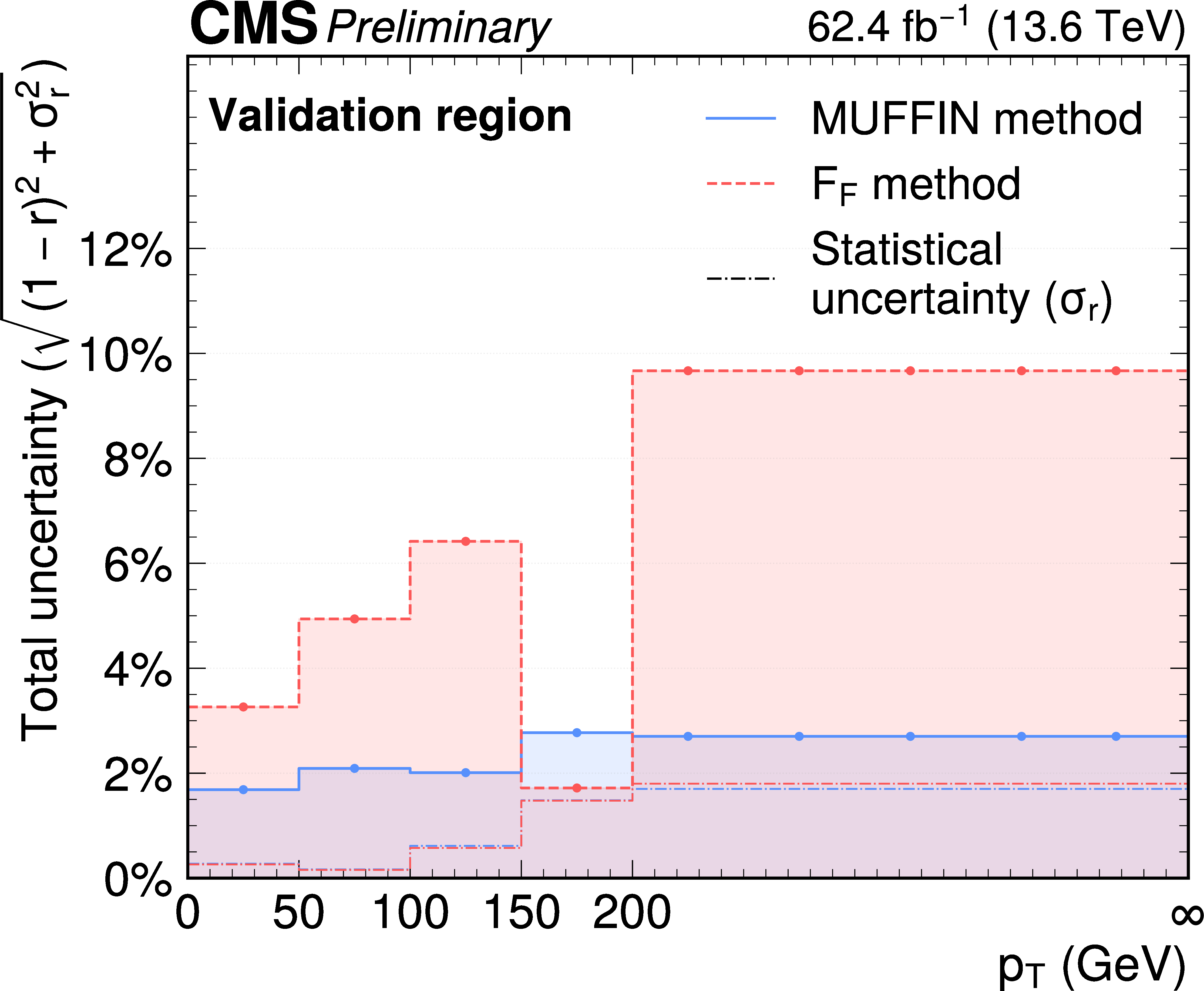
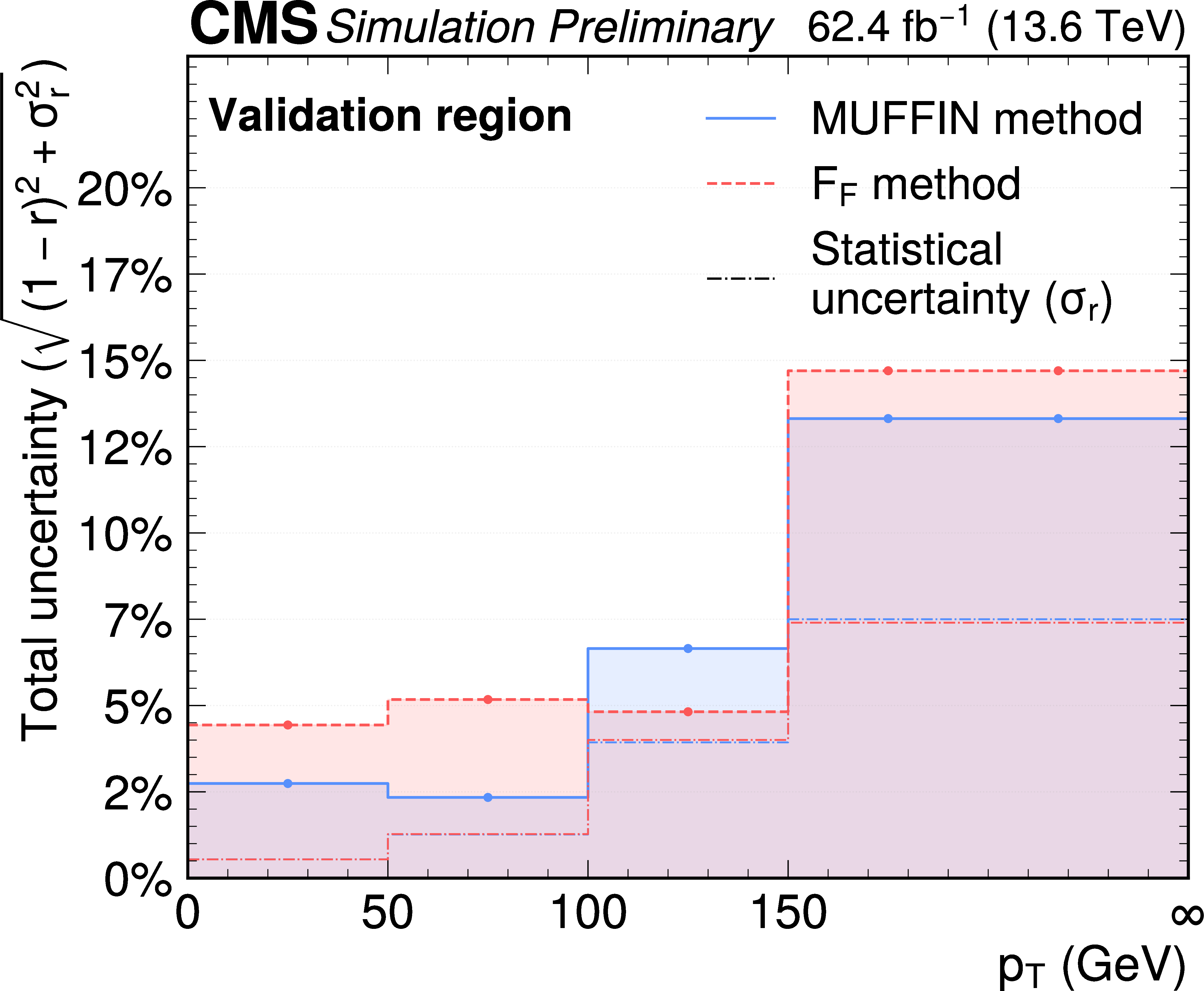
Closure in the high-$ p_{\mathrm{T}} $ tails of the kinematic distributions for a $ \tau_\mathrm{h}\tau_\mathrm{h} $ QCD multijet-dominated (left) and $ \tau_\mathrm{\mu}\hspace{-.04em}\tau_\mathrm{h} $ $ \mathrm{W}+\text{jets} $ (right) validation regions. The dashed lines indicate the statistical component of the uncertainty. The MUFFIN method achieves significantly improved agreement in both tails, leading to substantially reduced systematic uncertainties for the $ \tau_\mathrm{h}\tau_\mathrm{h} $ channel and moderate improvements in the $ \tau_\mathrm{\mu}\hspace{-.04em}\tau_\mathrm{h} $ channel. Overflow is included in the final bin ($ \infty $). |
png pdf |
Figure 15-a:
Closure in the high-$ p_{\mathrm{T}} $ tails of the kinematic distributions for a $ \tau_\mathrm{h}\tau_\mathrm{h} $ QCD multijet-dominated (left) and $ \tau_\mathrm{\mu}\hspace{-.04em}\tau_\mathrm{h} $ $ \mathrm{W}+\text{jets} $ (right) validation regions. The dashed lines indicate the statistical component of the uncertainty. The MUFFIN method achieves significantly improved agreement in both tails, leading to substantially reduced systematic uncertainties for the $ \tau_\mathrm{h}\tau_\mathrm{h} $ channel and moderate improvements in the $ \tau_\mathrm{\mu}\hspace{-.04em}\tau_\mathrm{h} $ channel. Overflow is included in the final bin ($ \infty $). |
png pdf |
Figure 15-b:
Closure in the high-$ p_{\mathrm{T}} $ tails of the kinematic distributions for a $ \tau_\mathrm{h}\tau_\mathrm{h} $ QCD multijet-dominated (left) and $ \tau_\mathrm{\mu}\hspace{-.04em}\tau_\mathrm{h} $ $ \mathrm{W}+\text{jets} $ (right) validation regions. The dashed lines indicate the statistical component of the uncertainty. The MUFFIN method achieves significantly improved agreement in both tails, leading to substantially reduced systematic uncertainties for the $ \tau_\mathrm{h}\tau_\mathrm{h} $ channel and moderate improvements in the $ \tau_\mathrm{\mu}\hspace{-.04em}\tau_\mathrm{h} $ channel. Overflow is included in the final bin ($ \infty $). |
| Tables | |
png pdf |
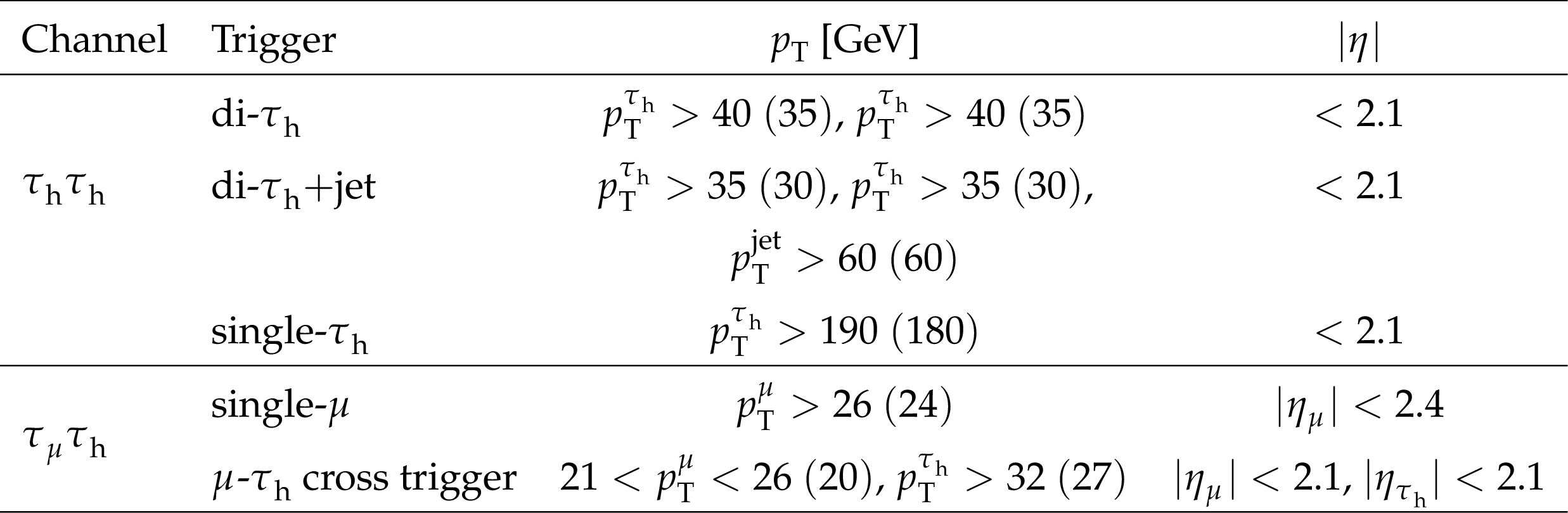
Table 1:
Online trigger and offline selection requirements applied in the $ \tau_\mathrm{\mu}\hspace{-.04em}\tau_\mathrm{h} $ and $ \tau_\mathrm{h}\tau_\mathrm{h} $ channels. All $ p_{\mathrm{T}} $ values are given in GeVns. Online trigger thresholds are indicated in brackets. |
png pdf |
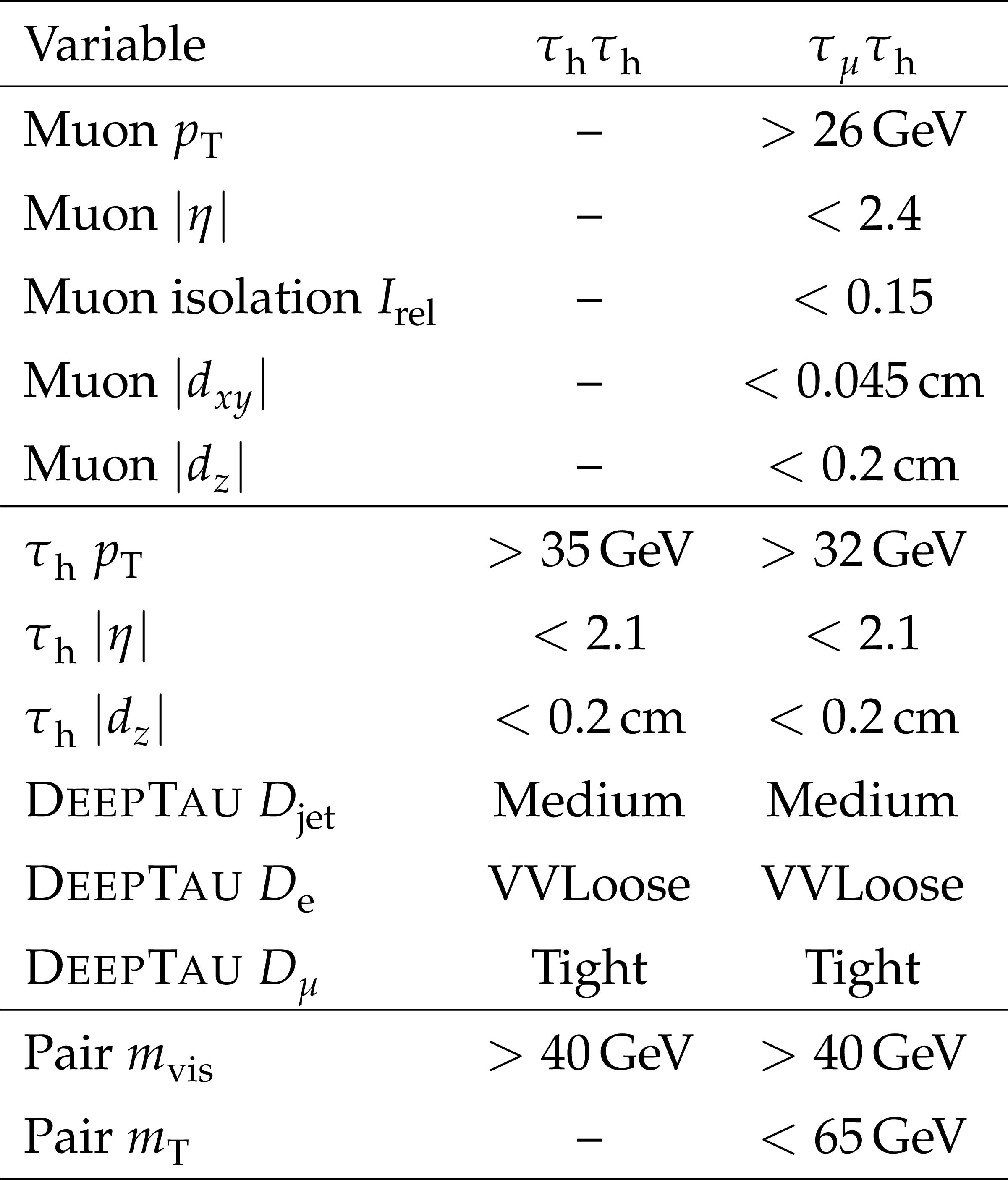
Table 2:
Offline selection requirements in the $ \tau_\mathrm{h}\tau_\mathrm{h} $ and $ \tau_\mathrm{\mu}\hspace{-.04em}\tau_\mathrm{h} $ channels. A dash indicates that the requirement is not applied in that channel. |
png pdf |
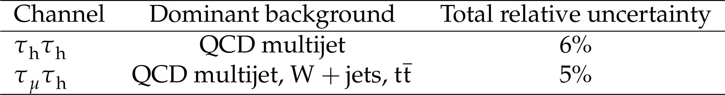
Table 3:
Total relative uncertainty in the $ \text{jet}\to\tau_\mathrm{h} $ background yield in representative inclusive SR selections for each channel. |
| Summary |
| In this note, a machine-learning-based alternative to the $F_F$ method for estimating backgrounds from jets misidentified as hadronically decaying $\tau$ leptons is presented, referred to as MUFFIN (MUltivariate Fake-Factor INference). This method is a generalisation of the previous $F-F$ method by replacing low-dimensional transfer factors with multidimensional, per-object reweighting functions learned directly from data, while preserving the fully data-driven nature of the background estimation. The method has been developed and validated using CMS Run~3 data (collected in 2022--2023) and is benchmarked against the $F-F$ method using a series of closure tests. Across the analysis channels and observables considered, the MUFFIN method has demonstrated improved or comparable modelling performance, increased stability in regions sensitive to correlations between multiple variables, and a reduced reliance on additional non-closure corrections. At the same time, the method has provided a more unified and reproducible workflow for background estimation. These results indicate that the MUFFIN method constitutes a robust and flexible alternative for future analyses involving hadronic $\tau$ leptons. As analyses increasingly exploit fine-grained categorisation and multidimensional phase space information, the method presented here provides a natural framework to improve background modelling precision and to enhance the sensitivity of measurements and searches involving hadronic $\tau$ final states. Looking forward, further improvement in the performance of the MUFFIN method is expected as larger datasets become available. The use of boosted decision trees allows the straightforward inclusion of additional input features, such as an explicit data-taking era label, enabling the model to capture era-dependent detector conditions, trigger configurations, and reconstruction performance in a unified training. Training on larger, combined datasets therefore offers a natural path to increasing statistical precision while maintaining robustness against changing experimental conditions, without requiring separate derivations or corrections for individual eras. |
| References | ||||
| 1 | CMS Collaboration | Observation of the Higgs boson decay to a pair of $ \tau $ leptons with the CMS detector | PLB 779 (2018) 283 | CMS-HIG-16-043 1708.00373 |
| 2 | ATLAS Collaboration | Cross-section measurements of the Higgs boson decaying into a pair of $ \tau $-leptons in proton-proton collisions at $ \sqrt{s}= $ 13 TeV with the ATLAS detector | PRD 99 (2019) 072001 | 1811.08856 |
| 3 | CMS Collaboration | Search for nonresonant Higgs boson pair production in final state with two bottom quarks and two tau leptons in proton-proton collisions at $ \sqrt{s}= $ 13 TeV | PLB 842 (2023) 137531 | CMS-HIG-20-010 2206.09401 |
| 4 | CMS Collaboration | Analysis of the CP structure of the Yukawa coupling between the Higgs boson and $ \tau $ leptons in proton-proton collisions at $ \sqrt{s}= $ 13 TeV | JHEP 06 (2022) 012 | CMS-HIG-20-006 2110.04836 |
| 5 | CMS Collaboration | Measurements of Higgs boson production in the decay channel with a pair of $ \tau $ leptons in proton-proton collisions at $ \sqrt{s}= $ 13 TeV | EPJC 83 (2023) 562 | CMS-HIG-19-010 2204.12957 |
| 6 | CMS Collaboration | Constraints on anomalous Higgs boson couplings to vector bosons and fermions from the production of Higgs bosons using the \ensuremath\tau\ensuremath\tau final state | PRD 108 (2023) 032013 | CMS-HIG-20-007 2205.05120 |
| 7 | ATLAS Collaboration | Measurement of the CP properties of Higgs boson interactions with $ \tau $-leptons with the ATLAS detector | EPJC 83 (2023) 563 | 2212.05833 |
| 8 | ATLAS Collaboration | Search for the nonresonant production of Higgs boson pairs via gluon fusion and vector-boson fusion in the $ b\bar{b}\tau^+\tau^- $ final state in proton-proton collisions at $ \sqrt{s}= $ 13 TeV with the ATLAS detector | PRD 110 (2024) 032012 | 2404.12660 |
| 9 | ATLAS Collaboration | Differential cross-section measurements of Higgs boson production in the $ H \to \tau^+\tau^- $ decay channel in pp collisions at $ \sqrt{s}= $ 13 TeV with the ATLAS detector | JHEP 03 (2025) 010 | 2407.16320 |
| 10 | ATLAS Collaboration | Probing the Higgs boson CP properties in vector-boson fusion production in the $ H \to \tau^+\tau^- $ channel with the ATLAS detector | JHEP 10 (2025) 092 | 2506.19395 |
| 11 | CMS Collaboration | Search for heavy neutral resonances decaying to tau lepton pairs in proton-proton collisions at $ \sqrt{s}= $ 13 TeV | PRD 111 (2025) 112004 | CMS-EXO-21-016 2412.04357 |
| 12 | CMS Collaboration | Searches for additional Higgs bosons and for vector leptoquarks in $ \tau\tau $ final states in proton-proton collisions at $ \sqrt{s}= $ 13 TeV | JHEP 07 (2023) 073 | CMS-HIG-21-001 2208.02717 |
| 13 | ATLAS Collaboration | Search for heavy Higgs bosons decaying into two tau leptons with the ATLAS detector using pp collisions at $ \sqrt{s}= $ 13 TeV | PRL 125 (2020) 051801 | 2002.12223 |
| 14 | CMS Collaboration | Search for a third-generation leptoquark coupled to a \ensuremath\tau lepton and a b quark through single, pair, and nonresonant production in proton-proton collisions at $ \sqrt{s} = $ 13 TeV | JHEP 05 (2024) 311 | CMS-EXO-19-016 2308.07826 |
| 15 | ATLAS Collaboration | Search for pair-produced scalar and vector leptoquarks decaying into third-generation quarks and first- or second-generation leptons in pp collisions with the ATLAS detector | JHEP 06 (2023) 188 | 2210.04517 |
| 16 | CMS Collaboration | Search for singly and pair-produced leptoquarks coupling to third-generation fermions in proton-proton collisions at $ \sqrt{s}= $ 13 TeV | PLB 819 (2021) 136446 | CMS-EXO-19-015 2012.04178 |
| 17 | CMS Collaboration | Search for the pair production of long-lived supersymmetric partners of the tau lepton in proton-proton collisions at $ \sqrt{s}= $ 13 TeV | Submitted to JHEP, 2026 link |
CMS-EXO-24-020 2601.17576 |
| 18 | ATLAS Collaboration | Search for direct stau production in events with two hadronic $ \tau $-leptons in $ \sqrt{s} = $ 13 TeV $ pp $ collisions with the ATLAS detector | PRD 101 (2020) 032009 | 1911.06660 |
| 19 | ATLAS Collaboration | Search for lepton-flavour violation in high-mass dilepton final states using 139 fb$ ^{-1} $ of pp collisions at $ \sqrt{s} = $ 13 TeV with the ATLAS detector | JHEP 23 (2020) 082 | 2307.08567 |
| 20 | ATLAS Collaboration | Estimation of backgrounds from jets misidentified as $ \tau $-leptons using the Universal Fake Factor method with the ATLAS detector | EPJC 85 (2025) 1441 | 2502.04156 |
| 21 | CMS Collaboration | Measurement of the $ \mathrm{Z}\gamma^{*} \to \tau\tau $ cross section in pp collisions at $ \sqrt{s} = $ 13 TeV and validation of $ \tau $ lepton analysis techniques | EPJC 78 (2018) 708 | CMS-HIG-15-007 1801.03535 |
| 22 | CMS Collaboration | Search for additional neutral MSSM Higgs bosons in the $ \tau\tau $ final state in proton-proton collisions at $ \sqrt{s}= $ 13 TeV | JHEP 09 (2018) 007 | CMS-HIG-17-020 1803.06553 |
| 23 | A. Rogozhnikov | Reweighting with Boosted Decision Trees | J. Phys. Conf. Ser. 762 (2016) 012036 | 1608.05806 |
| 24 | CMS Collaboration | The CMS experiment at the CERN LHC | JINST 3 (2008) S08004 | |
| 25 | CMS Collaboration | Development of the CMS detector for the CERN LHC Run 3 | JINST 19 (2024) P05064 | CMS-PRF-21-001 2309.05466 |
| 26 | CMS Collaboration | Performance of the CMS Level-1 trigger in proton-proton collisions at $ \sqrt{s} = $ 13 TeV | JINST 15 (2020) P10017 | CMS-TRG-17-001 2006.10165 |
| 27 | CMS Collaboration | The CMS trigger system | JINST 12 (2017) P01020 | CMS-TRG-12-001 1609.02366 |
| 28 | CMS Collaboration | Performance of the CMS high-level trigger during LHC Run 2 | JINST 19 (2024) P11021 | CMS-TRG-19-001 2410.17038 |
| 29 | CMS Collaboration | Electron and photon reconstruction and identification with the CMS experiment at the CERN LHC | JINST 16 (2021) P05014 | CMS-EGM-17-001 2012.06888 |
| 30 | CMS Collaboration | Performance of the CMS muon detector and muon reconstruction with proton-proton collisions at $ \sqrt{s}= $ 13 TeV | JINST 13 (2018) P06015 | CMS-MUO-16-001 1804.04528 |
| 31 | CMS Collaboration | Description and performance of track and primary-vertex reconstruction with the CMS tracker | JINST 9 (2014) P10009 | CMS-TRK-11-001 1405.6569 |
| 32 | CMS Collaboration | Luminosity measurement in proton-proton collisions at 13.6 TeV in 2022 at CMS | CMS Physics Analysis Summary, CERN, Geneva, 2024 CMS-PAS-LUM-22-001 |
CMS-PAS-LUM-22-001 |
| 33 | J. Alwall et al. | The automated computation of tree-level and next-to-leading order differential cross sections, and their matching to parton shower simulations | JHEP 07 (2014) 079 | 1405.0301 |
| 34 | R. Frederix and S. Frixione | Merging meets matching in MC@NLO | JHEP 12 (2012) 061 | 1209.6215 |
| 35 | J. Alwall et al. | Comparative study of various algorithms for the merging of parton showers and matrix elements in hadronic collisions | EPJC 53 (2008) 473 | 0706.2569 |
| 36 | M. Grazzini, S. Kallweit, and M. Wiesemann | Fully differential NNLO computations with MATRIX | EPJC 78 (2018) 537 | 1711.06631 |
| 37 | M. Grazzini et al. | NNLO QCD + NLO EW with Matrix+OpenLoops: precise predictions for vector-boson pair production | JHEP 02 (2020) 087 | 1912.00068 |
| 38 | S. Alioli, P. Nason, C. Oleari, and E. Re | A general framework for implementing NLO calculations in shower Monte Carlo programs: the POWHEG BOX | JHEP 06 (2010) 043 | 1002.2581 |
| 39 | S. Alioli, S.-O. Moch, and P. Uwer | Hadronic top-quark pair-production with one jet and parton showering | JHEP 01 (2012) 137 | 1110.5251 |
| 40 | E. Re | Single-top $ Wt $-channel production matched with parton showers using the POWHEG method | EPJC 71 (2011) 1547 | 1009.2450 |
| 41 | R. Frederix, E. Re, and P. Torrielli | Single-top $ t $-channel hadroproduction in the four-flavour scheme with POWHEG and MC@NLO | JHEP 09 (2012) 130 | 1207.5391 |
| 42 | M. Czakon and A. Mitov | Top++: A program for the calculation of the top-pair cross-section at hadron colliders | Comput. Phys. Commun. 185 (2014) 2930 | 1112.5675 |
| 43 | J. Campbell, T. Neumann, and Z. Sullivan | Single-top-quark production in the $ t $-channel at NNLO | JHEP 02 (2021) 040 | 2012.01574 |
| 44 | N. Kidonakis and N. Yamanaka | Higher-order corrections for $ tW $ production at high-energy hadron colliders | JHEP 05 (2021) 278 | 2102.11300 |
| 45 | NNPDF Collaboration | Parton distributions from high-precision collider data | EPJC 77 (2017) 663 | 1706.00428 |
| 46 | C. Bierlich et al. | A comprehensive guide to the physics and usage of PYTHIA 8.3 | SciPost Phys. Codeb. 2022 (2022) 8 | 2203.11601 |
| 47 | CMS Collaboration | Extraction and validation of a new set of CMS PYTHIA8 tunes from underlying-event measurements | EPJC 80 (2020) 4 | CMS-GEN-17-001 1903.12179 |
| 48 | GEANT4 Collaboration | GEANT 4---a simulation toolkit | NIM A 506 (2003) 250 | |
| 49 | CMS Collaboration | Particle-flow reconstruction and global event description with the CMS detector | JINST 12 (2017) P10003 | CMS-PRF-14-001 1706.04965 |
| 50 | M. Cacciari, G. P. Salam, and G. Soyez | The anti-$ k_{\mathrm{t}} $ jet clustering algorithm | JHEP 04 (2008) 063 | 0802.1189 |
| 51 | M. Cacciari, G. P. Salam, and G. Soyez | FastJet user manual | EPJC 72 (2012) 1896 | 1111.6097 |
| 52 | CMS Collaboration | Jet energy scale and resolution in the CMS experiment in pp collisions at 8 TeV | JINST 12 (2017) P02014 | CMS-JME-13-004 1607.03663 |
| 53 | E. Bols et al. | Jet flavour classification using DeepJet | JINST 15 (2020) P12012 | 2008.10519 |
| 54 | CMS Collaboration | Pileup mitigation at CMS in 13 TeV data | JINST 15 (2020) P09018 | CMS-JME-18-001 2003.00503 |
| 55 | D. Bertolini, P. Harris, M. Low, and N. Tran | Pileup per particle identification | JHEP 10 (2014) 059 | 1407.6013 |
| 56 | CMS Collaboration | Performance of missing transverse momentum reconstruction in proton-proton collisions at $ \sqrt{s} = $ 13 TeV using the CMS detector | JINST 14 (2019) P07004 | CMS-JME-17-001 1903.06078 |
| 57 | CMS Collaboration | ECAL 2016 refined calibration and Run2 summary plots | CMS Detector Performance Summary CERN-CMS-DP-2020-021, 2020 CDS |
|
| 58 | CMS Collaboration | Performance of reconstruction and identification of $ \tau $ leptons decaying to hadrons and $ \nu_\tau $ in pp collisions at $ \sqrt{s}= $ 13 TeV | JINST 13 (2018) P10005 | CMS-TAU-16-003 1809.02816 |
| 59 | CMS Collaboration | Identification of hadronic tau lepton decays using a deep neural network | JINST 17 (2022) P07023 | CMS-TAU-20-001 2201.08458 |
| 60 | CMS Collaboration | Identification of tau leptons using a convolutional neural network with domain adaptation | JINST 20 (2025) P12032 | CMS-TAU-24-001 2511.05468 |
| 61 | CMS Collaboration | High-level hadronic tau lepton triggers of the CMS experiment in proton-proton collisions at \ensuremath\sqrt(s) = 13.6 TeV | JINST 21 (2026) P04002 | CMS-TAU-24-002 2602.11359 |
| 62 | T. Chen and C. Guestrin | XGBoost: A Scalable Tree Boosting System | in nd ACM SIGKDD Int. Conf. on Knowledge Discovery and Data Mining, 2016 Proc. 2 (2016) 785 |
|
| 63 | T. Akiba et al. | Optuna: A Next-generation Hyperparameter Optimization Framework | in th ACM SIGKDD Int. Conf. on Knowledge Discovery and Data Mining, 2019 Proc. 2 (2019) 2623 |
1907.10902 |
| 64 | C. Guo, G. Pleiss, Y. Sun, and K. Q. Weinberger | On Calibration of Modern Neural Networks | in th Int. Conf. on Machine Learning, 2017 Proc. 3 (2017) 1321 |
1706.04599 |
| 65 | J. C. Platt | Probabilistic Outputs for Support Vector Machines and Comparisons to Regularized Likelihood Methods | in Advances in Large Margin Classifiers, A. J. Smola, P. Bartlett, B. Schölkopf, and D. Schuurmans, eds., MIT Press, Cambridge, MA, 1999 | |
| 66 | G. Cowan | Statistical Data Analysis in Particle Physics | Oxford University Press, Oxford, ISBN 978-0-19-850560-5, 1998 | |
| 67 | Particle Data Group Collaboration | Review of particle physics | PRD 110 (2024) 030001 | |
| 68 | ATLAS Collaboration | Search for neutral Higgs bosons of the minimal supersymmetric standard model in pp collisions at $ \sqrt{s} = $ 8 TeV with the ATLAS detector | JHEP 11 (2014) 056 | 1409.6064 |
| 69 | CMS Collaboration | Analysis of the CP structure of the Yukawa coupling between the Higgs boson and tau leptons in proton-proton collisions at $ \sqrt{s}= $ 13.6 TeV | CMS Physics Analysis Summary, CERN, Geneva, 2026 CMS-PAS-HIG-25-012 |
CMS-PAS-HIG-25-012 |
| 70 | A. Kalinowski and W. Matyszkiewicz | Efficient tau-pair invariant mass reconstruction with simplified matrix element techniques | NIM A 1086 (2026) 171318 | 2509.26069 |
|
|
Compact Muon Solenoid LHC, CERN |
|

|

|

|

|

|