

Compact Muon Solenoid
LHC, CERN
| CMS-EXO-24-020 ; CERN-EP-2025-296 | ||
| Search for the pair production of long-lived supersymmetric partners of the tau lepton in proton-proton collisions at $ \sqrt{s}= $ 13 TeV | ||
| CMS Collaboration | ||
| 24 January 2026 | ||
| Accepted for publication in the Journal of High Energy Physics | ||
| Abstract: Gauge-mediated supersymmetry-breaking models provide a strong motivation to search for a supersymmetric partner of the tau lepton (stau) with a macroscopic lifetime. Long-lived stau decays produce tau leptons that are displaced from the primary proton-proton interaction vertex, leading to an unconventional signature. This paper presents a search for the direct production of long-lived staus decaying within the CMS tracker volume in proton-proton collisions at $ \sqrt{s}= $ 13 TeV, performed for the first time with an identification algorithm based on a graph neural network dedicated to displaced tau leptons. The data sample, corresponding to an integrated luminosity of 138 fb$ ^{-1} $, was recorded with the CMS experiment at the CERN LHC between 2016 and 2018. This search excludes, at 95% confidence level, stau masses, $ m_{\tilde{\tau}} $, in the 126-260 (90-425) GeV range for a proper decay length of 50$ \text{mm} $ in the maximally mixed (mass-degenerate) scenario, while for $ m_{\tilde{\tau}} = $ 200 GeV, stau proper decay lengths are excluded in the range 21-94 (6-333)$ \text{mm} $. These results improve the exclusion limits compared to previous searches, and extend the parameter space explored in the context of supersymmetry. | ||
| Links: e-print arXiv:2601.17576 [hep-ex] (PDF) ; CDS record ; inSPIRE record ; CADI line (restricted) ; | ||
| Figures | |
png pdf |
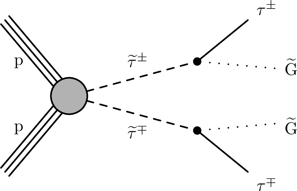
Figure 1:
Diagram of stau pair production in pp collisions at the LHC, and the decay that leads to a final state with pairs of tau leptons accompanied by gravitinos. |
png pdf |
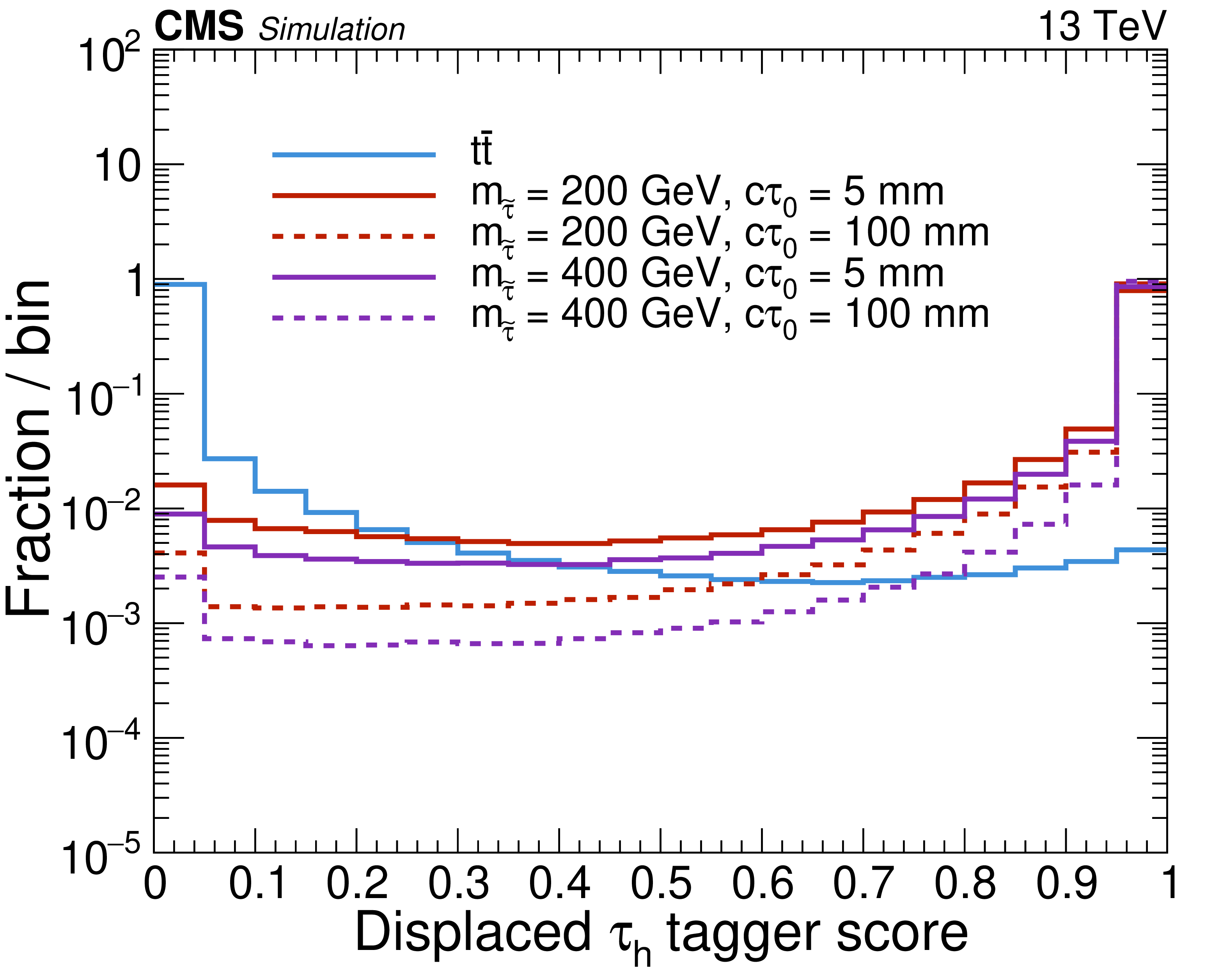
Figure 2:
Distributions of DISTAU score for signal and background jets. The background jets are taken from simulated $ \mathrm{t} \overline{\mathrm{t}} $ events where both top quarks decay hadronically, while signal jets are sampled from four representative $ (m_{\tilde{\tau}} [{\text{GeV}}],\ c\tau_{0} [{\text{mm}}]) $ hypotheses: (200, 5), (200, 100), (400, 5), and (400, 100). Each distribution is normalized such that its integral is unity. |
png pdf |
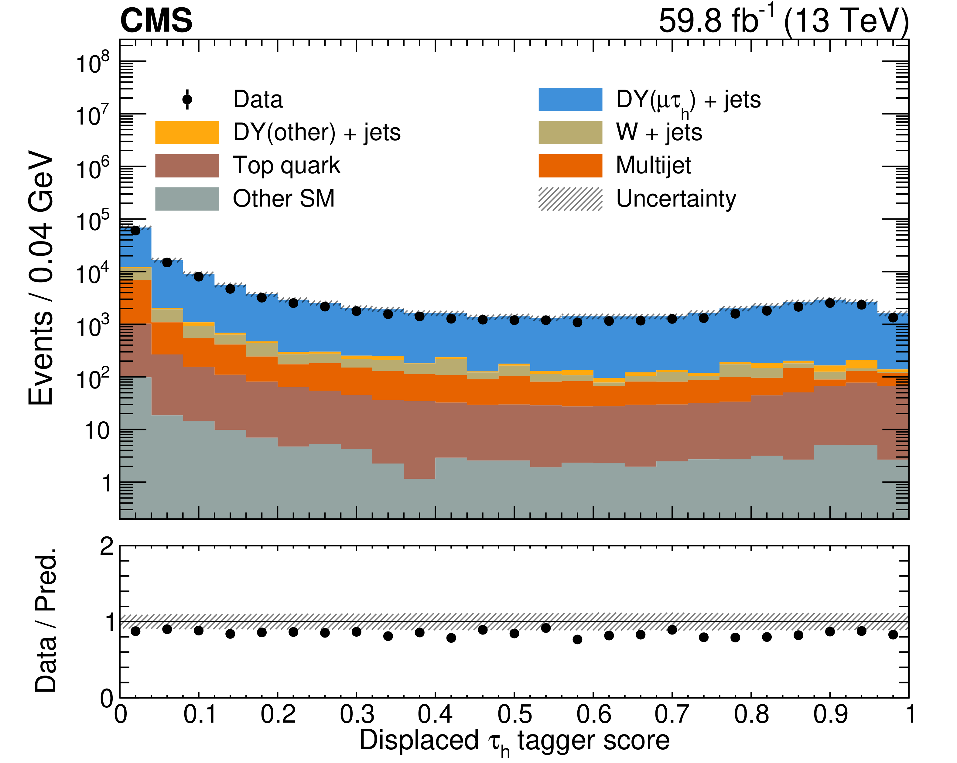
Figure 3:
Distributions of DISTAU score for $ \tau_\mathrm{h}^\text{dis} $ probes in the $ \mu\tau_\mathrm{h} $ CR described in Section 4.2, for data and predicted SM processes, corresponding to the 2018 data-taking period. Here DY($ \mu\tau_\mathrm{h} $) represents events from the $ \mathrm{Z}/\gamma^{*}\to\tau\tau $ process, where one of the tau leptons decays to a muon and the other decays hadronically. Events from other decay modes of $ \mathrm{Z}/\gamma^{*} $ are denoted as DY(other). Processes denoted as ``Top quark'' comprise $ \mathrm{t} \overline{\mathrm{t}} $, single top, and \ttbarV, and other SM processes include events from diboson production. Uncertainties in the simulation are shown as a grey band and include only the statistical uncertainty in the number of simulated events. Simulation is not fully calibrated to describe data, as the distribution is shown to illustrate the general behavior of the classifier and is not directly used for the measurement of simulation-to-data correction factors. The results for the 2016 and 2017 data-taking periods are similar in behavior. |
png pdf |
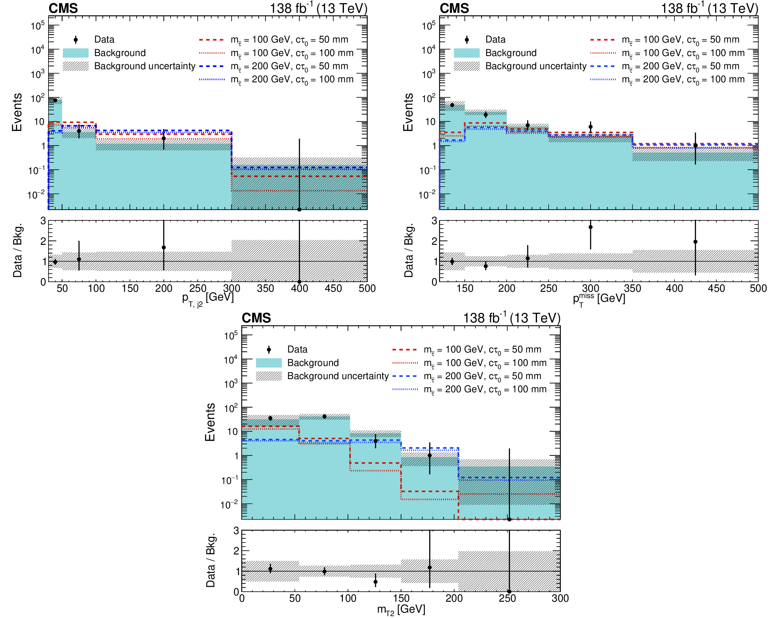
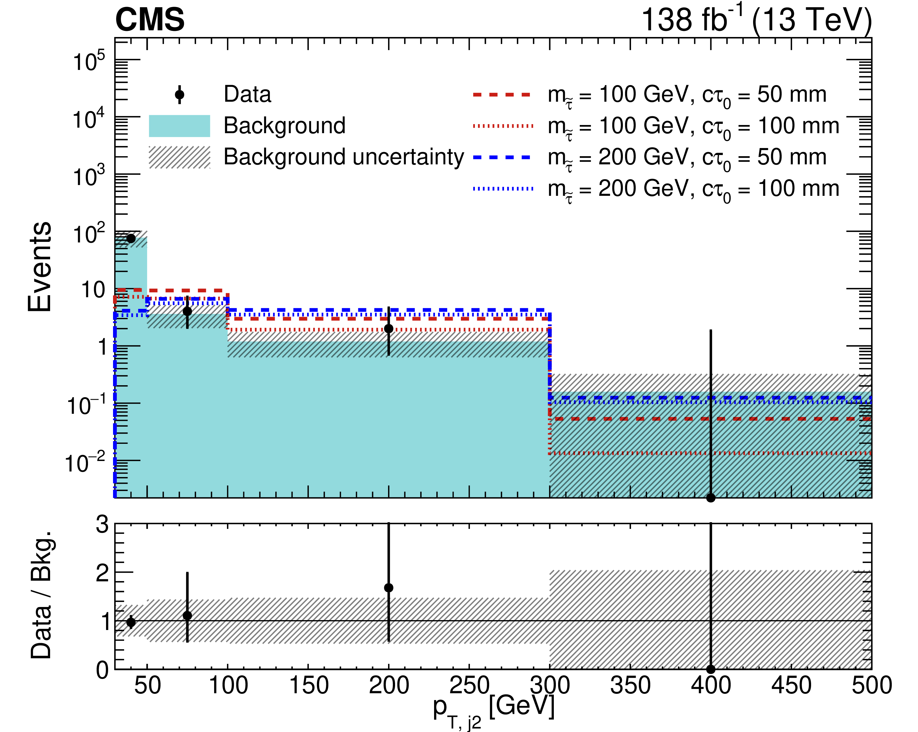
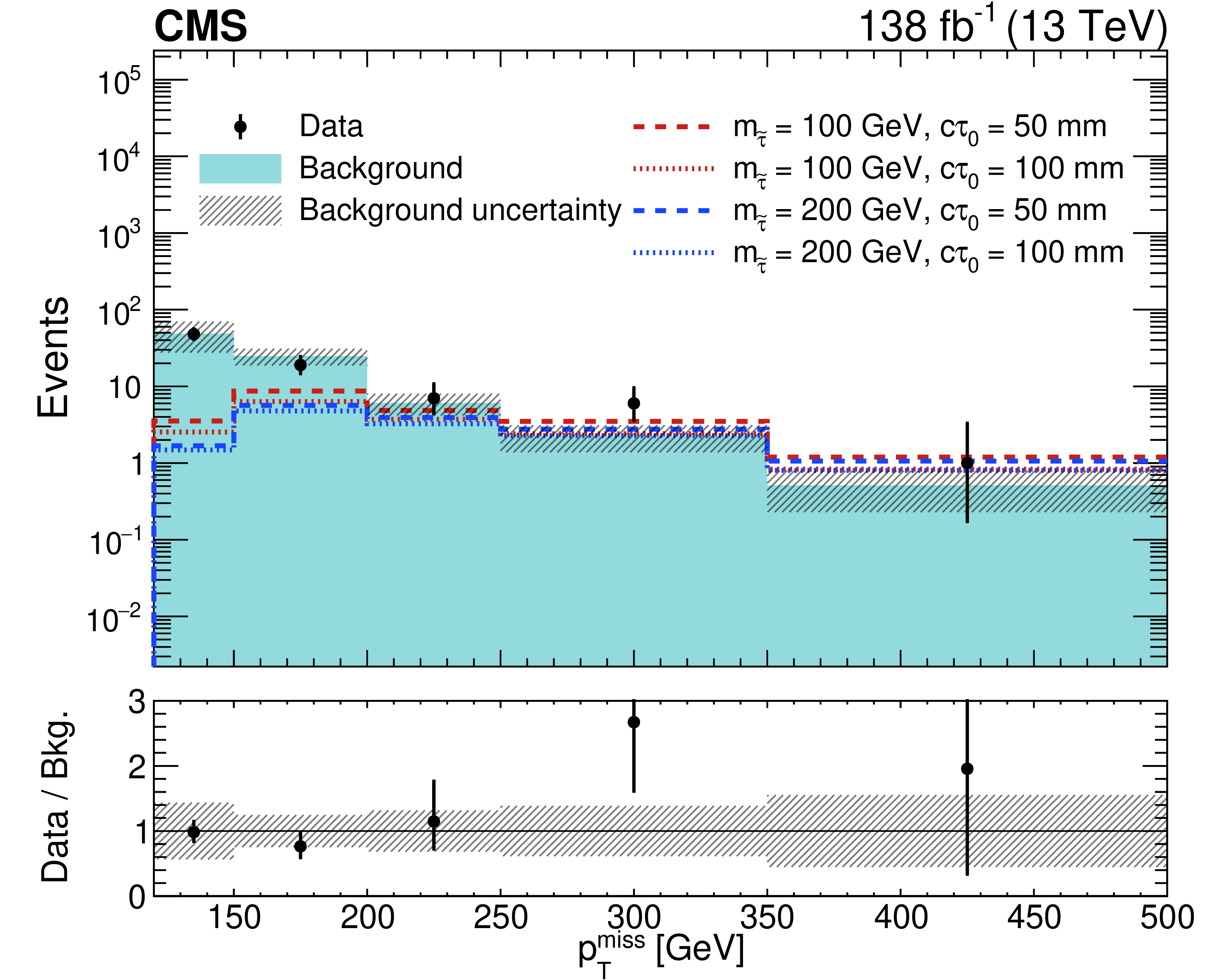
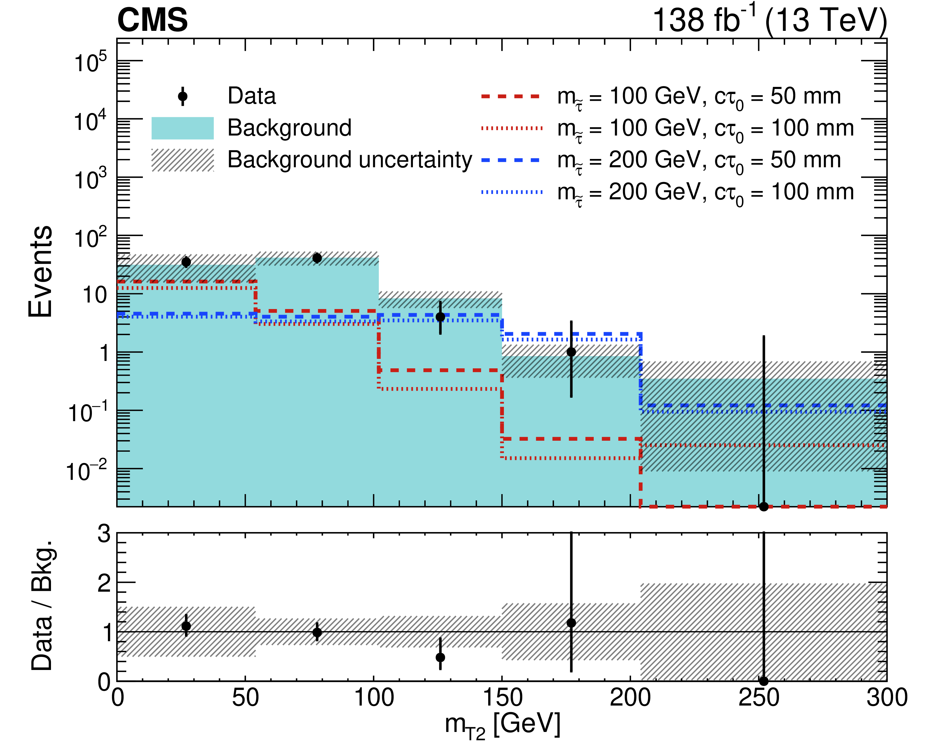
Figure 4:
Distributions of the variables used to define the signal region for data and the predicted background: $ p_{\text{T,j2}} $ (upper left), $ p_{\mathrm{T}}^\text{miss} $ (upper right), and $ m_{\mathrm{T2}} $ (lower). The signal distributions expected in the maximally mixed scenario for four representative sets of $ (m_{\tilde{\tau}} [{\text{GeV}}],\ c\tau_{0} [{\text{mm}}]) $ values are overlaid: (100, 50), (100, 100), (200, 50), and (200, 100). In bins where the observed yield is zero, the Garwood interval at 68% CL is shown as a positive uncertainty. The lower panel indicates the ratio of the observed number of events to the total predicted number of background events. The shaded bands indicate the statistical and systematic uncertainties in the predicted backgrounds, added in quadrature. The last bin includes the overflow. |
png pdf |
Figure 4-a:
Distributions of the variables used to define the signal region for data and the predicted background: $ p_{\text{T,j2}} $ (upper left), $ p_{\mathrm{T}}^\text{miss} $ (upper right), and $ m_{\mathrm{T2}} $ (lower). The signal distributions expected in the maximally mixed scenario for four representative sets of $ (m_{\tilde{\tau}} [{\text{GeV}}],\ c\tau_{0} [{\text{mm}}]) $ values are overlaid: (100, 50), (100, 100), (200, 50), and (200, 100). In bins where the observed yield is zero, the Garwood interval at 68% CL is shown as a positive uncertainty. The lower panel indicates the ratio of the observed number of events to the total predicted number of background events. The shaded bands indicate the statistical and systematic uncertainties in the predicted backgrounds, added in quadrature. The last bin includes the overflow. |
png pdf |
Figure 4-b:
Distributions of the variables used to define the signal region for data and the predicted background: $ p_{\text{T,j2}} $ (upper left), $ p_{\mathrm{T}}^\text{miss} $ (upper right), and $ m_{\mathrm{T2}} $ (lower). The signal distributions expected in the maximally mixed scenario for four representative sets of $ (m_{\tilde{\tau}} [{\text{GeV}}],\ c\tau_{0} [{\text{mm}}]) $ values are overlaid: (100, 50), (100, 100), (200, 50), and (200, 100). In bins where the observed yield is zero, the Garwood interval at 68% CL is shown as a positive uncertainty. The lower panel indicates the ratio of the observed number of events to the total predicted number of background events. The shaded bands indicate the statistical and systematic uncertainties in the predicted backgrounds, added in quadrature. The last bin includes the overflow. |
png pdf |
Figure 4-c:
Distributions of the variables used to define the signal region for data and the predicted background: $ p_{\text{T,j2}} $ (upper left), $ p_{\mathrm{T}}^\text{miss} $ (upper right), and $ m_{\mathrm{T2}} $ (lower). The signal distributions expected in the maximally mixed scenario for four representative sets of $ (m_{\tilde{\tau}} [{\text{GeV}}],\ c\tau_{0} [{\text{mm}}]) $ values are overlaid: (100, 50), (100, 100), (200, 50), and (200, 100). In bins where the observed yield is zero, the Garwood interval at 68% CL is shown as a positive uncertainty. The lower panel indicates the ratio of the observed number of events to the total predicted number of background events. The shaded bands indicate the statistical and systematic uncertainties in the predicted backgrounds, added in quadrature. The last bin includes the overflow. |
png pdf |
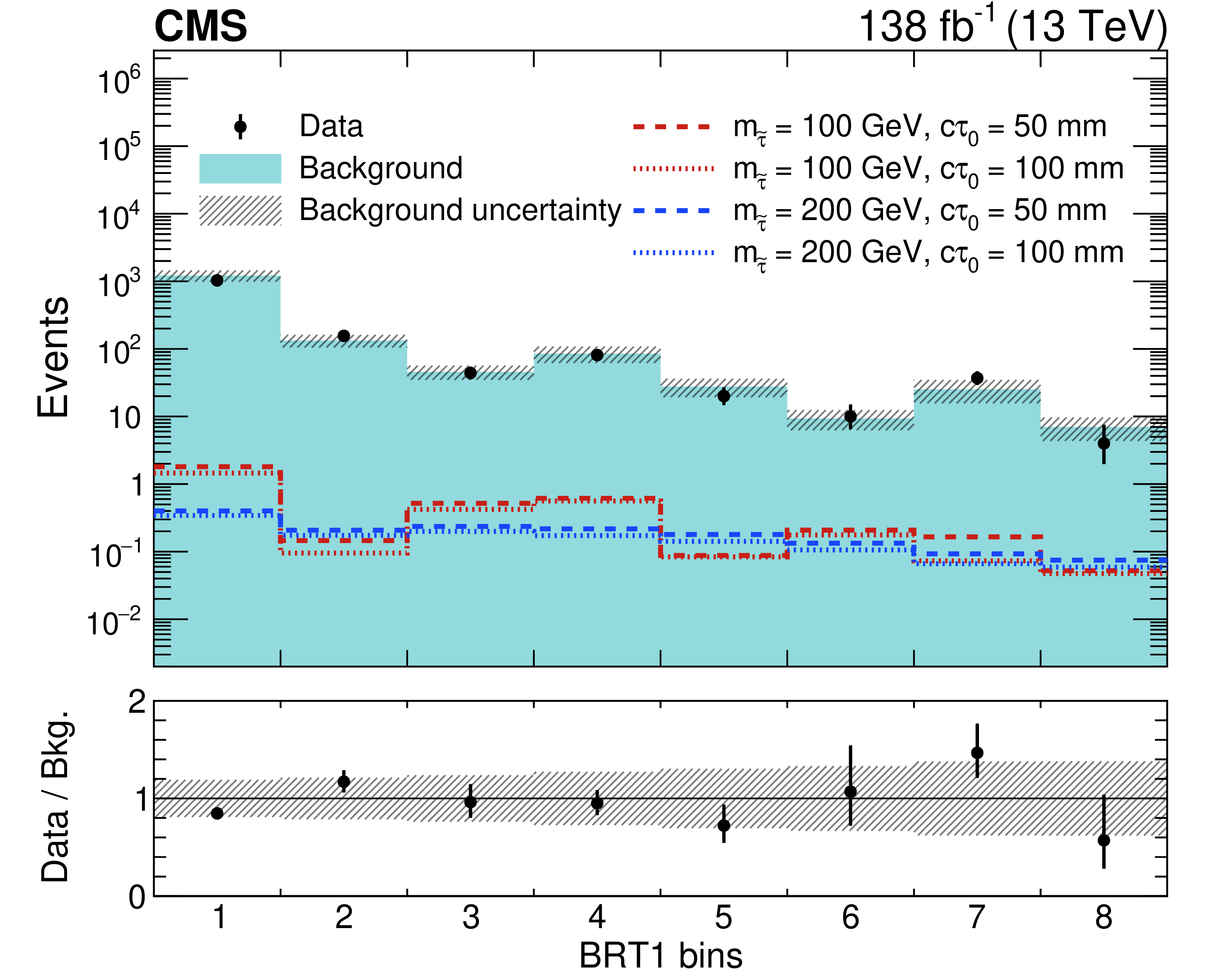
Figure 5:
Observed and predicted event yields in the eight BRT1 bins, as defined in Table 2. The signal yields expected in the maximally mixed scenario for four representative sets of $ (m_{\tilde{\tau}} [{ \text{GeV}}],\ c\tau_{0} [{ \text{mm}}]) $ values are overlaid: (100, 50), (100, 100), (200, 50), and (200, 100). The lower panel indicates the ratio of the observed number of events to the total predicted number of background events in each bin. The shaded bands indicate the statistical and systematic uncertainties in the background, added in quadrature. |
png pdf |
Figure 6:
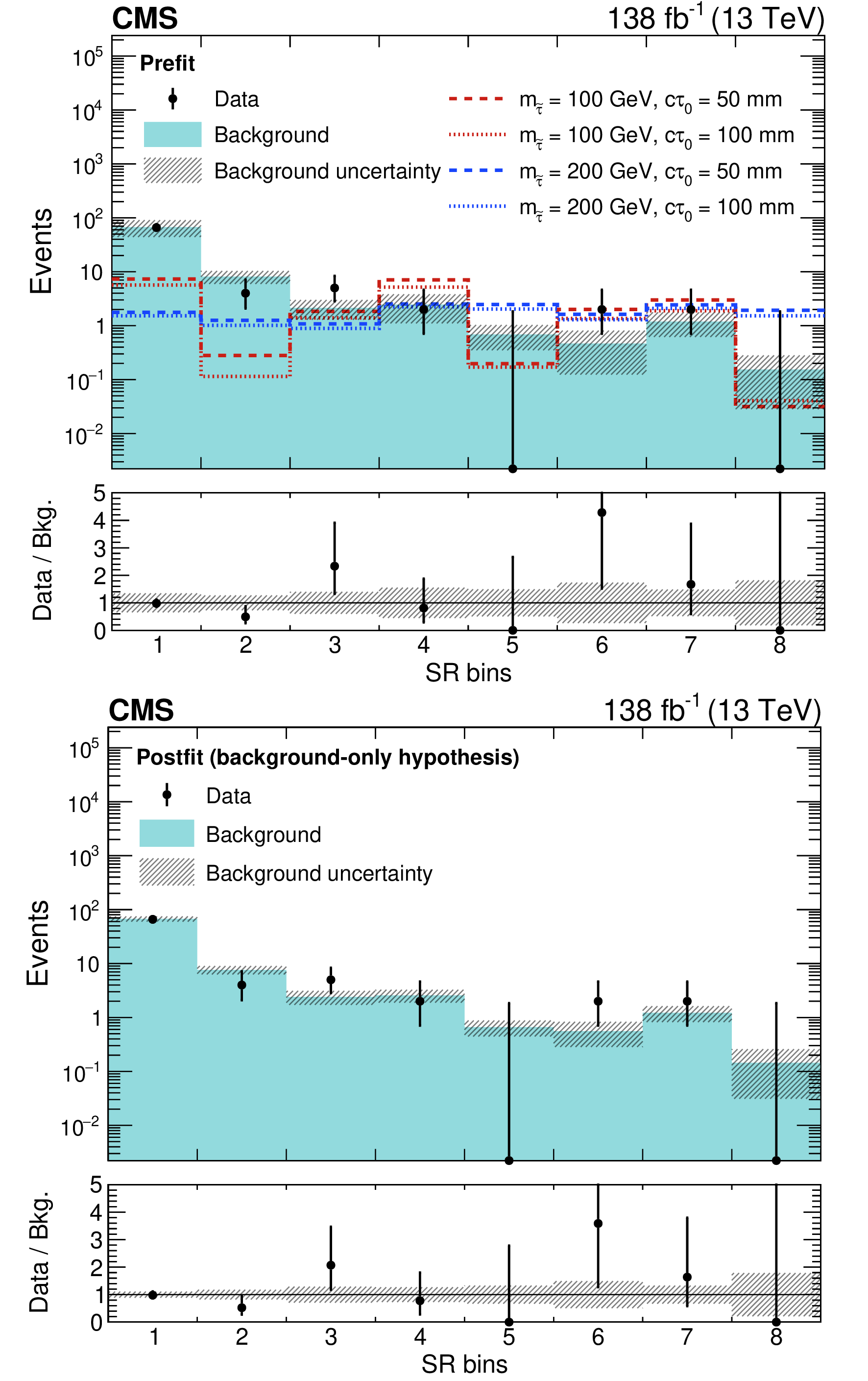
Observed and predicted event yields in the eight SR bins as defined in Table 2. The signal yields expected in the maximally mixed scenario for four representative sets of $ (m_{\tilde{\tau}} [{\text{GeV}}],\ c\tau_{0} [{\text{mm}}]) $ values are overlaid: (100, 50), (100, 100), (200, 50), and (200, 100). In bins where the observed yield is zero, the Garwood interval at 68% CL is shown as a positive uncertainty. The lower panel indicates the ratio of the observed number of events to the total predicted number of background events in each bin. The shaded bands indicate the statistical and systematic uncertainties in the background prediction, added in quadrature. The predicted yields and uncertainties shown in the upper (lower) panel are before (after) the maximum likelihood fit to data under the background-only hypothesis, as described in Section 8. |
png pdf |
Figure 6-a:
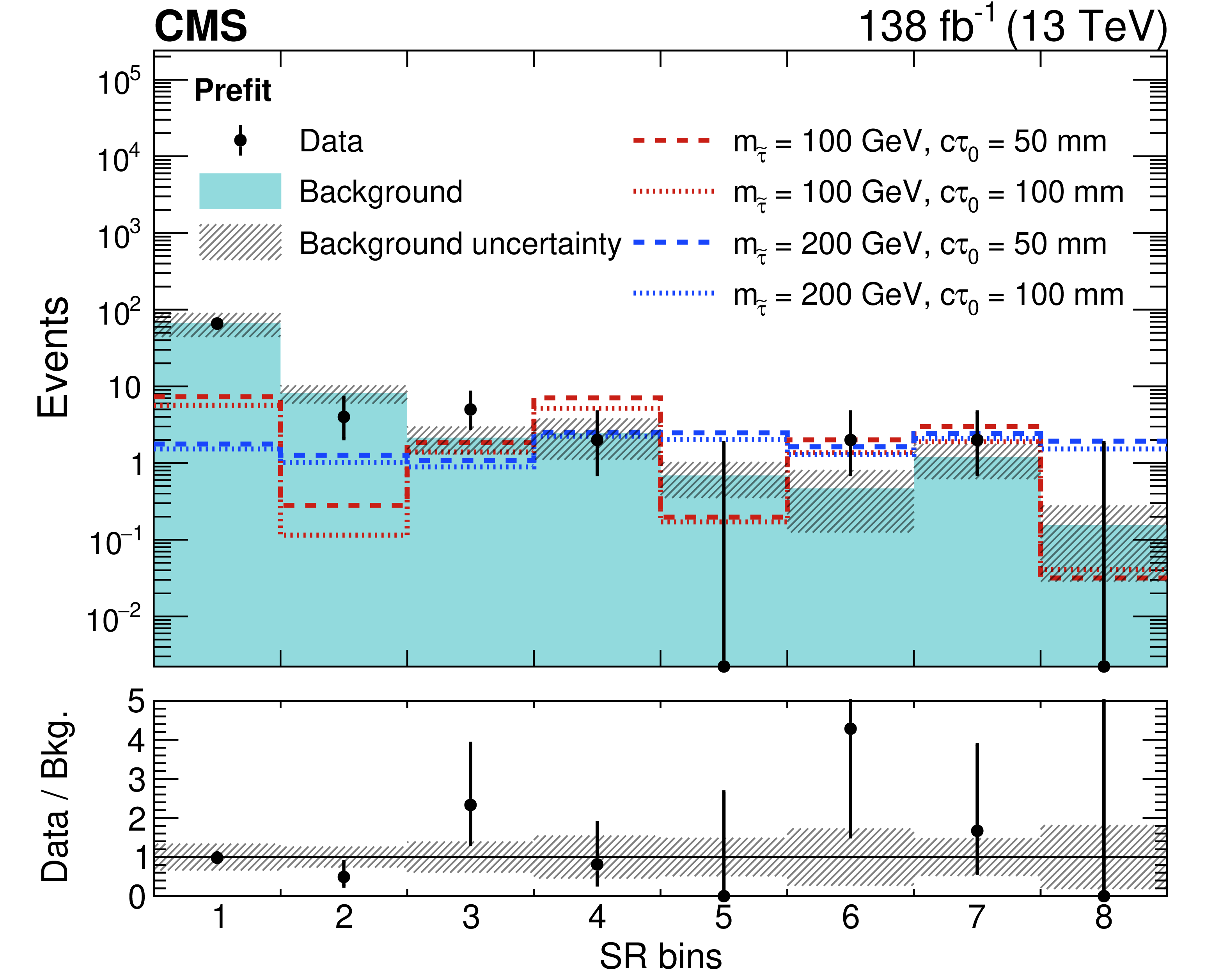
Observed and predicted event yields in the eight SR bins as defined in Table 2. The signal yields expected in the maximally mixed scenario for four representative sets of $ (m_{\tilde{\tau}} [{\text{GeV}}],\ c\tau_{0} [{\text{mm}}]) $ values are overlaid: (100, 50), (100, 100), (200, 50), and (200, 100). In bins where the observed yield is zero, the Garwood interval at 68% CL is shown as a positive uncertainty. The lower panel indicates the ratio of the observed number of events to the total predicted number of background events in each bin. The shaded bands indicate the statistical and systematic uncertainties in the background prediction, added in quadrature. The predicted yields and uncertainties shown in the upper (lower) panel are before (after) the maximum likelihood fit to data under the background-only hypothesis, as described in Section 8. |
png pdf |
Figure 6-b:
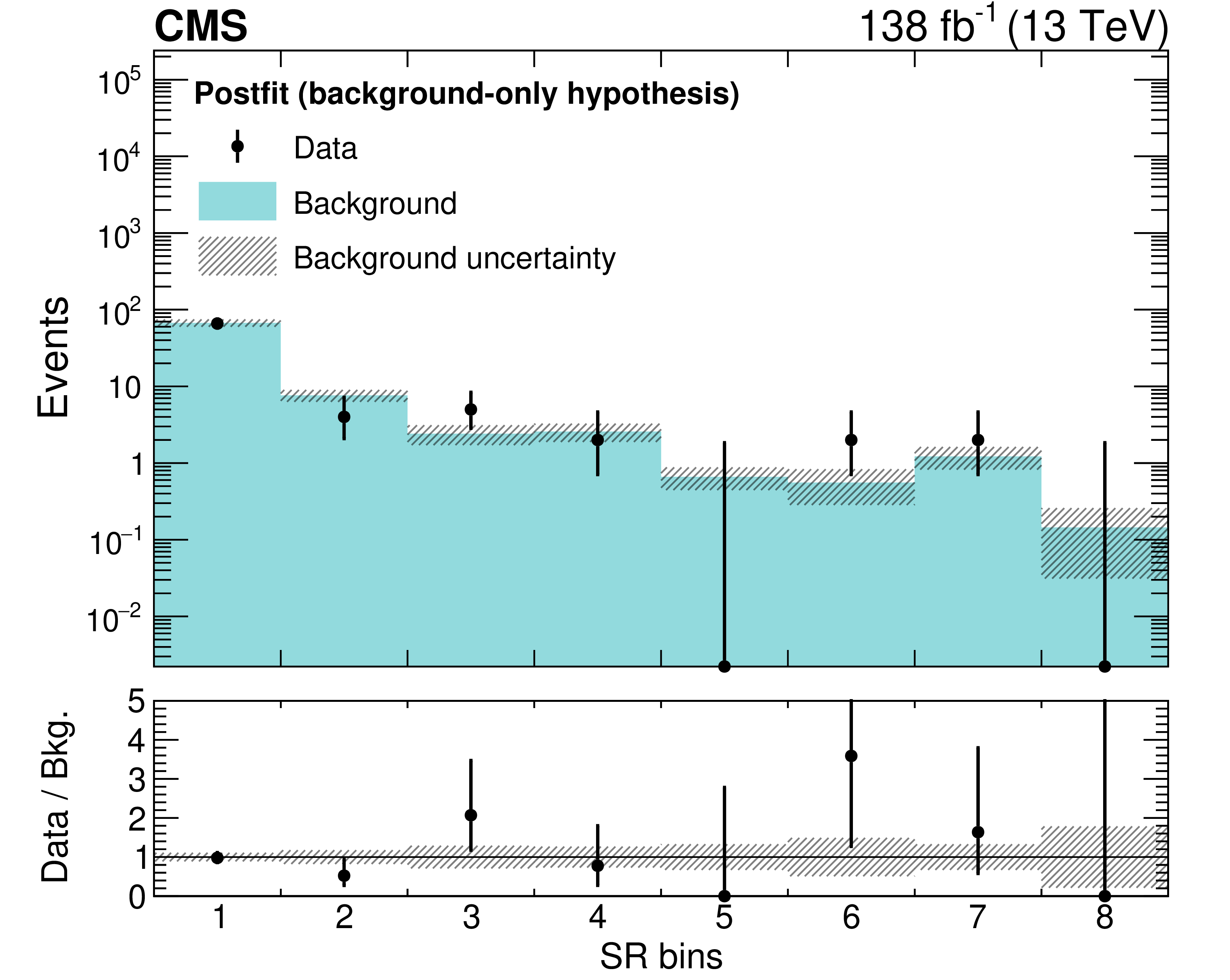
Observed and predicted event yields in the eight SR bins as defined in Table 2. The signal yields expected in the maximally mixed scenario for four representative sets of $ (m_{\tilde{\tau}} [{\text{GeV}}],\ c\tau_{0} [{\text{mm}}]) $ values are overlaid: (100, 50), (100, 100), (200, 50), and (200, 100). In bins where the observed yield is zero, the Garwood interval at 68% CL is shown as a positive uncertainty. The lower panel indicates the ratio of the observed number of events to the total predicted number of background events in each bin. The shaded bands indicate the statistical and systematic uncertainties in the background prediction, added in quadrature. The predicted yields and uncertainties shown in the upper (lower) panel are before (after) the maximum likelihood fit to data under the background-only hypothesis, as described in Section 8. |
png pdf |
Figure 7:
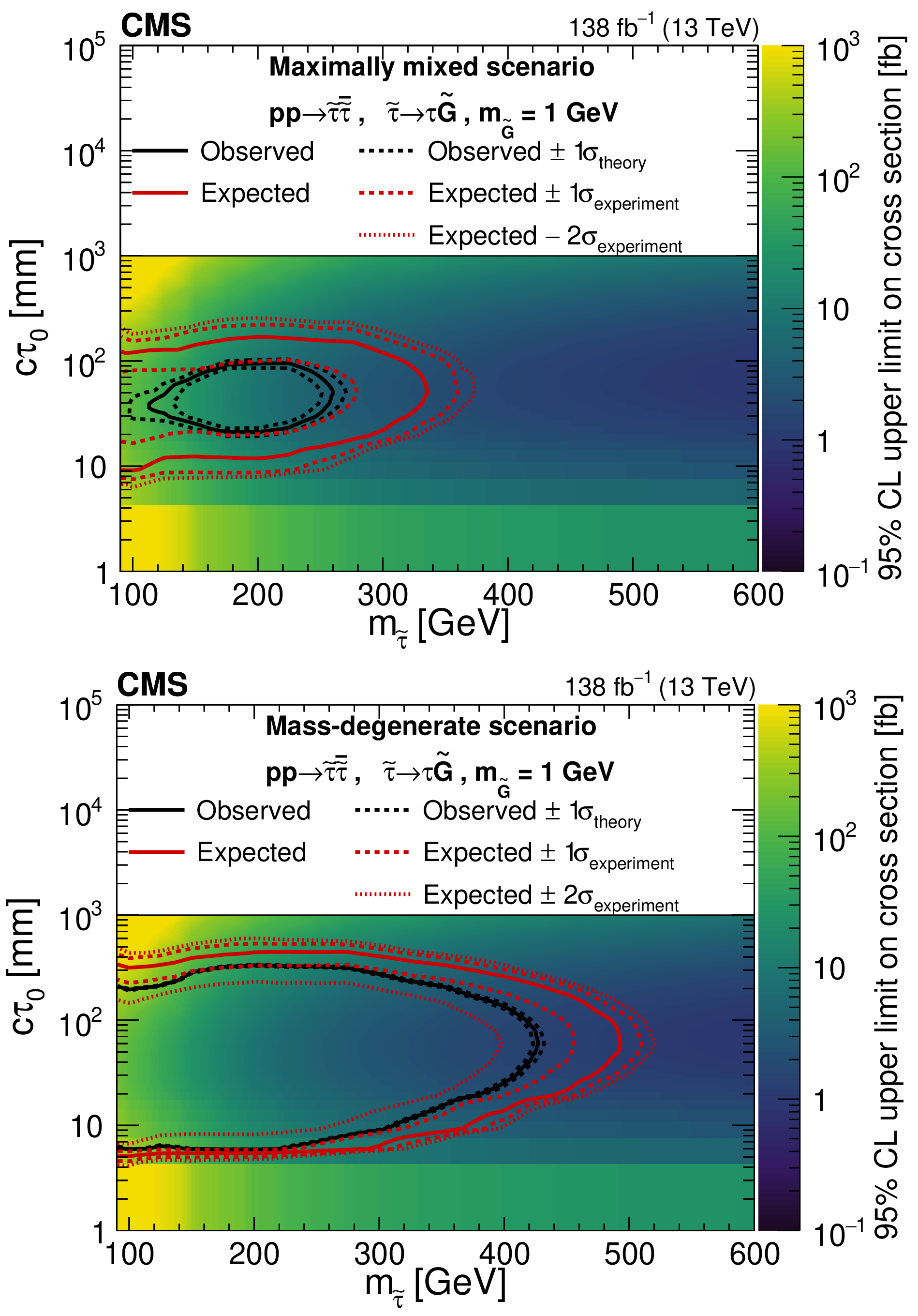
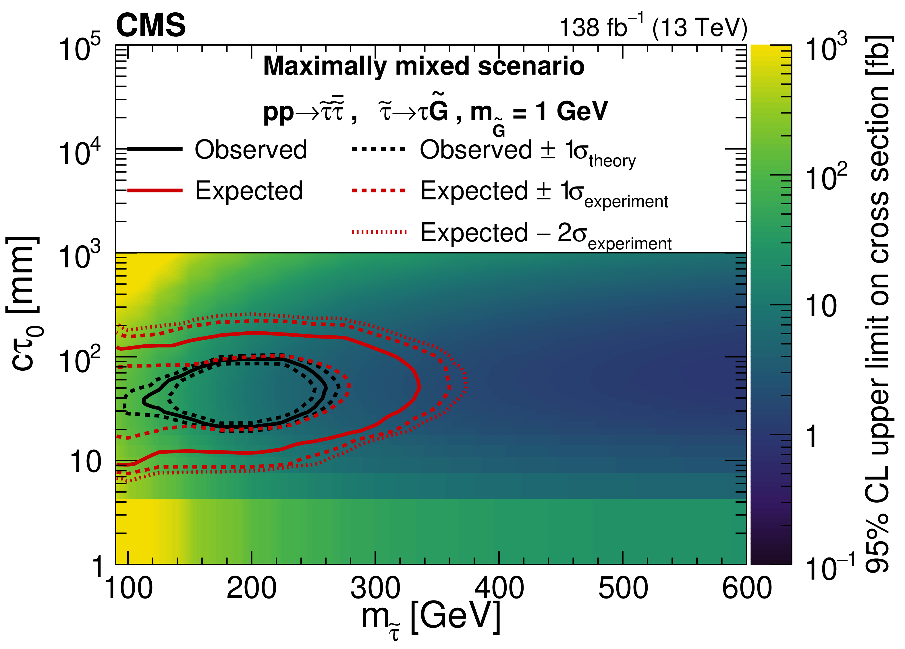
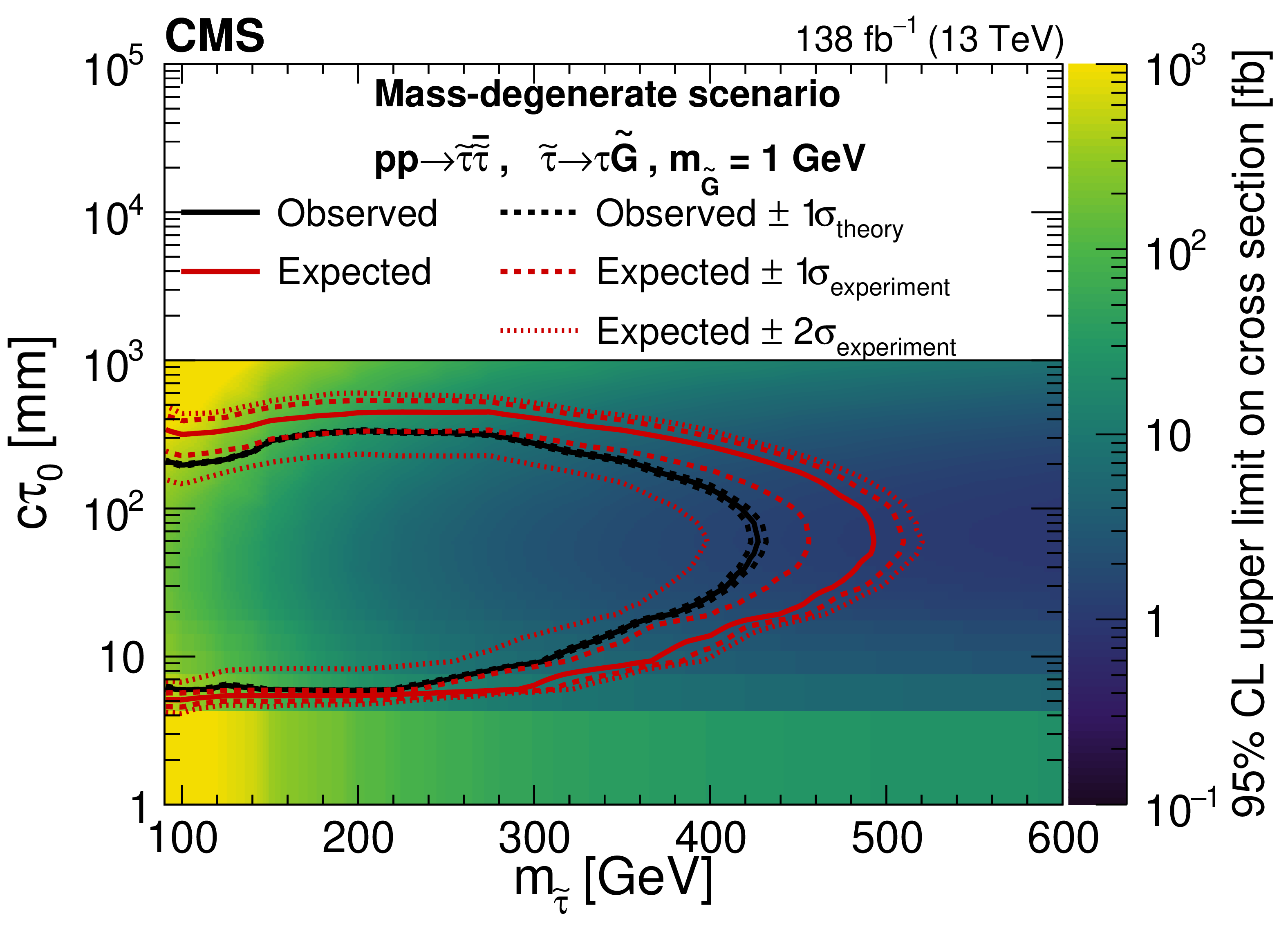
Exclusion limits at 95% CL for the pair production of long-lived staus decaying to a $ \tau $ lepton and a nearly massless gravitino ($ m_\tilde{\mathrm{G}}= $ 1 GeV), displayed in the plane of $ m_{\tilde{\tau}} $ and $ c\tau_{0} $. The maximally mixed (mass-degenerate) scenario is presented in the upper (lower) panel. The color axis represents the observed upper limit on the cross section. The signal cross sections are evaluated using NLO$ + $NLL calculations. The black (red) lines represent the observed (expected) limits on $ m_{\tilde{\tau}} $ and $ c\tau_{0} $ and enclose the region excluded at 95% CL. The solid lines represent the central values. The dashed (dotted) red lines indicate the region containing 68% (95%) of the distribution of limits expected under the background-only hypothesis accounting for experimental uncertainties ($ \sigma_\text{experiment} $). The red dotted line corresponding to ``Expected$ +2\sigma_\text{experiment} $" is not shown for the maximally mixed scenario, as it does not exclude any points in this plane. The dashed black lines show the change in the observed limit from the variation of the signal cross sections within their theoretical uncertainties ($ \sigma_\text{theory} $). |
png pdf |
Figure 7-a:
Exclusion limits at 95% CL for the pair production of long-lived staus decaying to a $ \tau $ lepton and a nearly massless gravitino ($ m_\tilde{\mathrm{G}}= $ 1 GeV), displayed in the plane of $ m_{\tilde{\tau}} $ and $ c\tau_{0} $. The maximally mixed (mass-degenerate) scenario is presented in the upper (lower) panel. The color axis represents the observed upper limit on the cross section. The signal cross sections are evaluated using NLO$ + $NLL calculations. The black (red) lines represent the observed (expected) limits on $ m_{\tilde{\tau}} $ and $ c\tau_{0} $ and enclose the region excluded at 95% CL. The solid lines represent the central values. The dashed (dotted) red lines indicate the region containing 68% (95%) of the distribution of limits expected under the background-only hypothesis accounting for experimental uncertainties ($ \sigma_\text{experiment} $). The red dotted line corresponding to ``Expected$ +2\sigma_\text{experiment} $" is not shown for the maximally mixed scenario, as it does not exclude any points in this plane. The dashed black lines show the change in the observed limit from the variation of the signal cross sections within their theoretical uncertainties ($ \sigma_\text{theory} $). |
png pdf |
Figure 7-b:
Exclusion limits at 95% CL for the pair production of long-lived staus decaying to a $ \tau $ lepton and a nearly massless gravitino ($ m_\tilde{\mathrm{G}}= $ 1 GeV), displayed in the plane of $ m_{\tilde{\tau}} $ and $ c\tau_{0} $. The maximally mixed (mass-degenerate) scenario is presented in the upper (lower) panel. The color axis represents the observed upper limit on the cross section. The signal cross sections are evaluated using NLO$ + $NLL calculations. The black (red) lines represent the observed (expected) limits on $ m_{\tilde{\tau}} $ and $ c\tau_{0} $ and enclose the region excluded at 95% CL. The solid lines represent the central values. The dashed (dotted) red lines indicate the region containing 68% (95%) of the distribution of limits expected under the background-only hypothesis accounting for experimental uncertainties ($ \sigma_\text{experiment} $). The red dotted line corresponding to ``Expected$ +2\sigma_\text{experiment} $" is not shown for the maximally mixed scenario, as it does not exclude any points in this plane. The dashed black lines show the change in the observed limit from the variation of the signal cross sections within their theoretical uncertainties ($ \sigma_\text{theory} $). |
png pdf |
Figure 8:
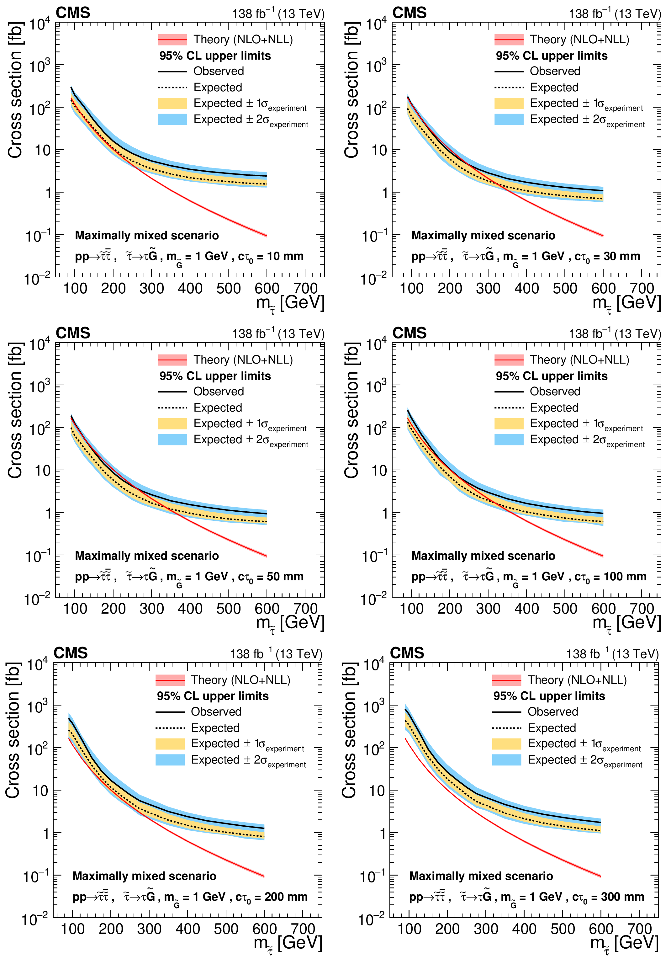
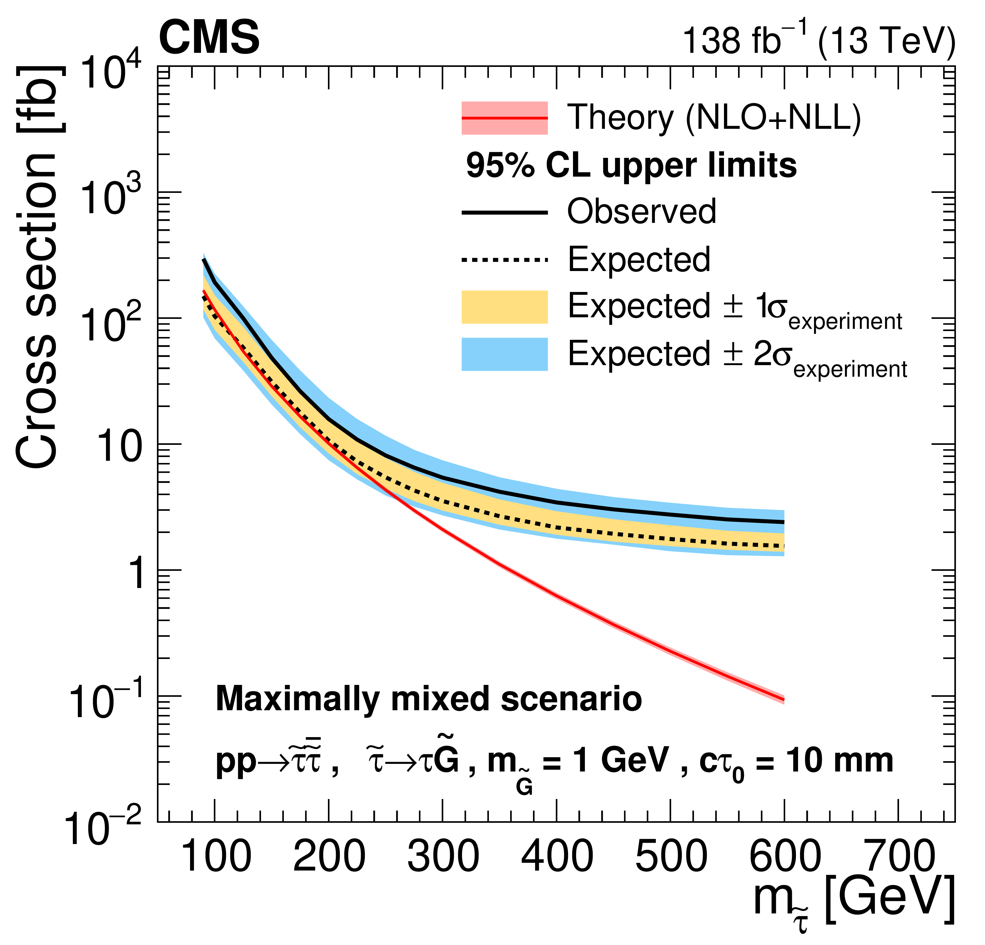
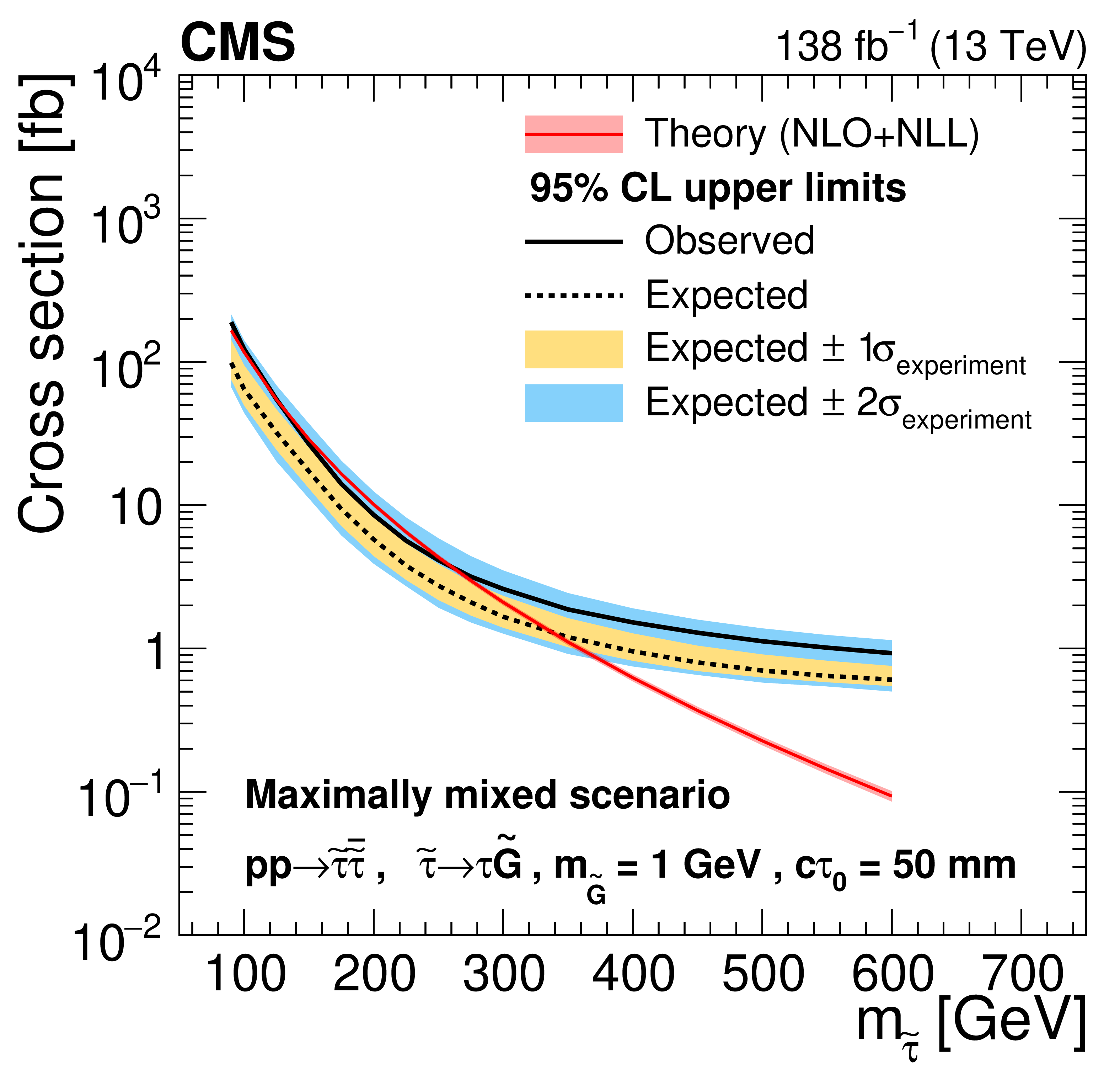
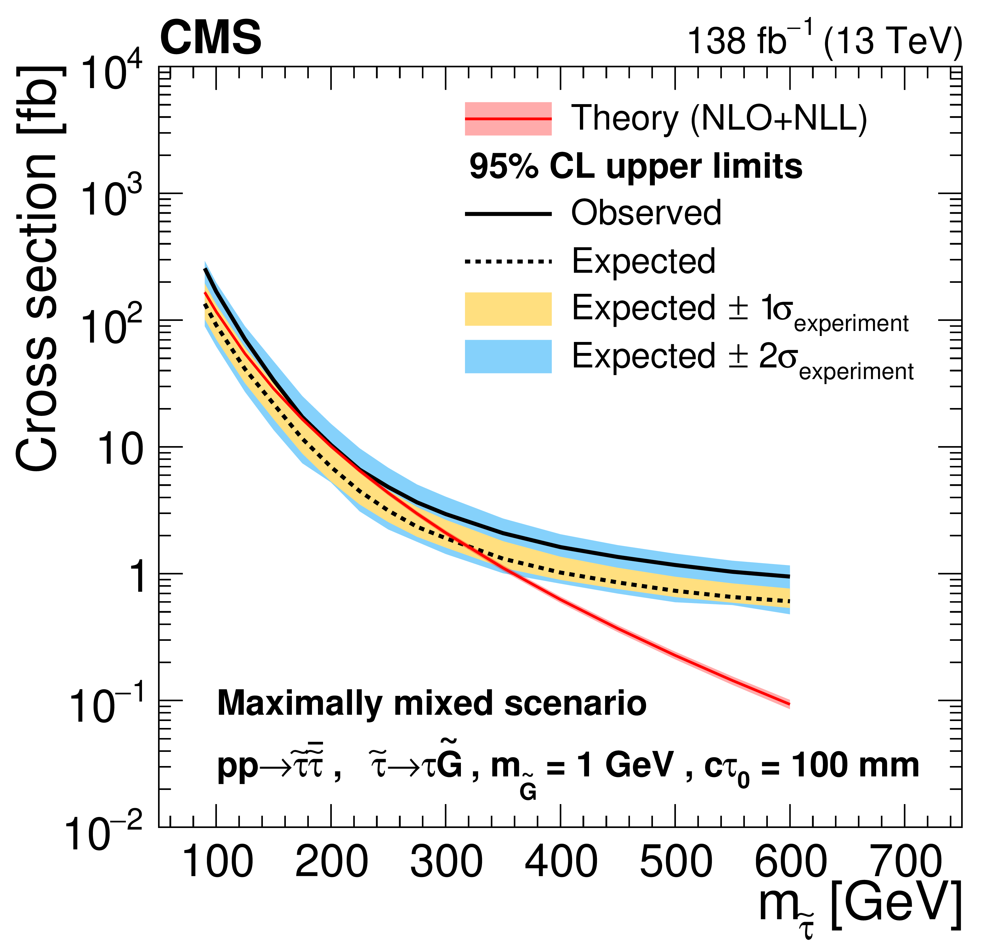
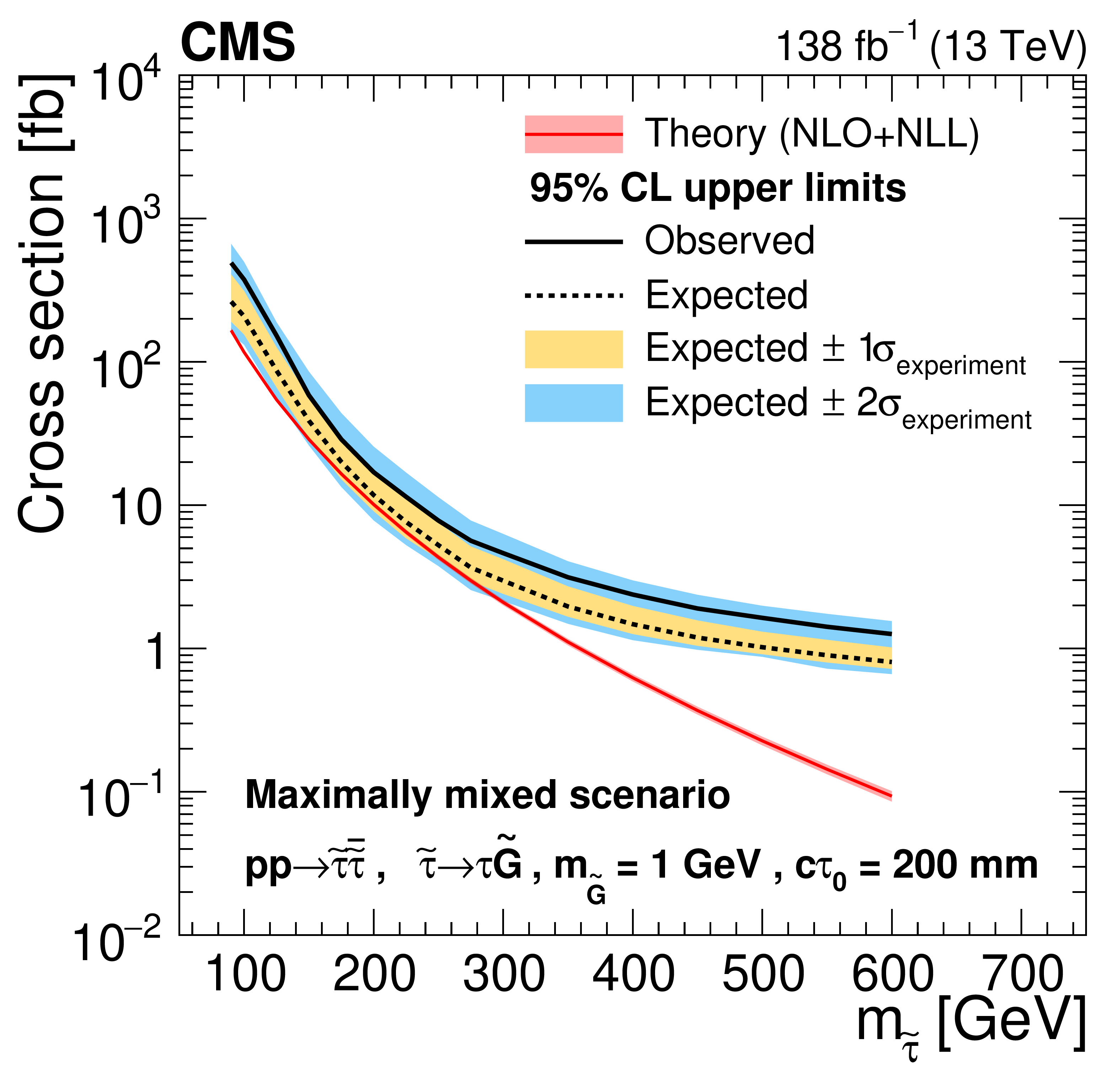
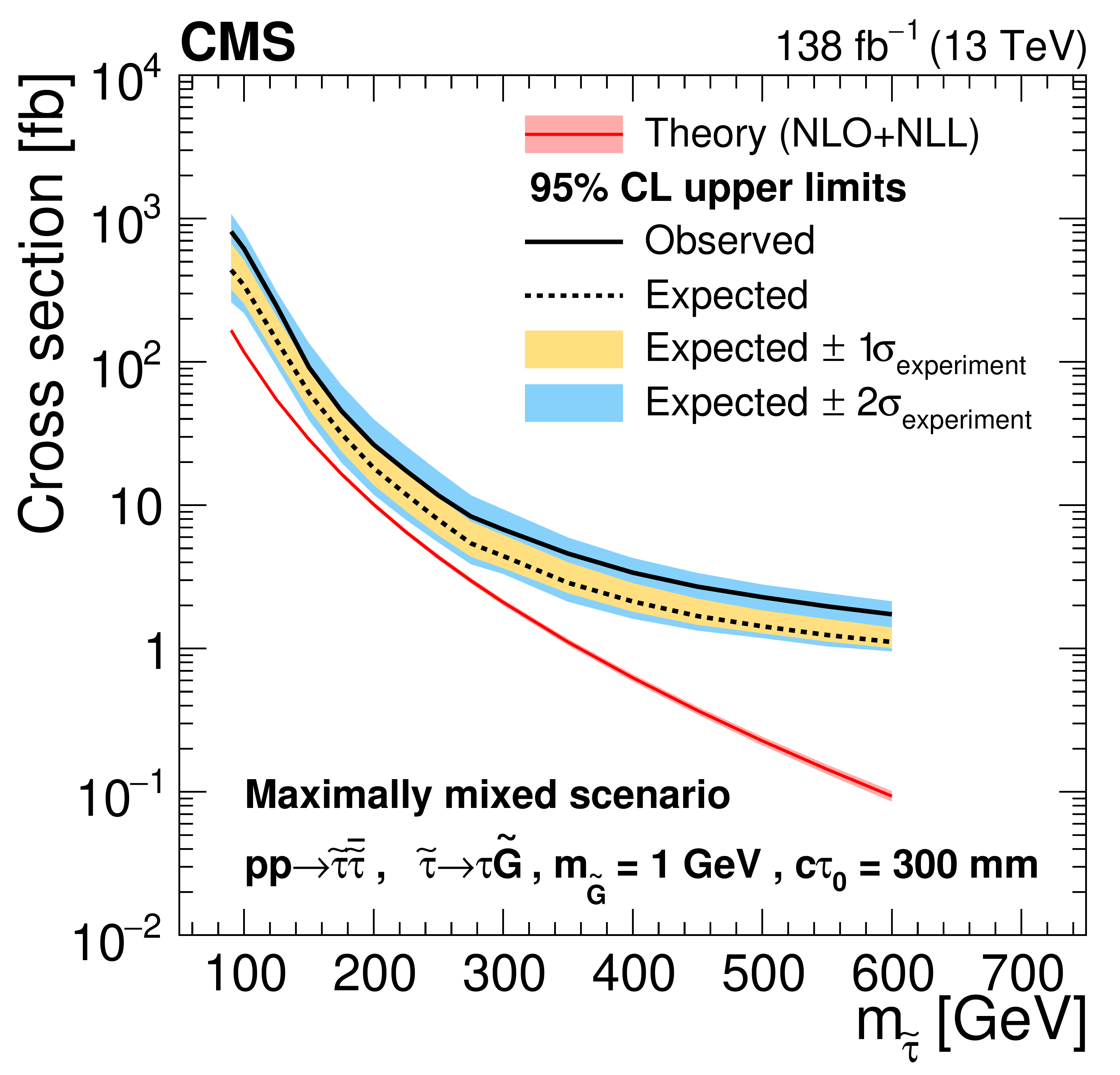
Cross section upper limits at 95% CL for the pair production of long-lived staus decaying to a $ \tau $ lepton and a nearly massless gravitino ($ m_\tilde{\mathrm{G}}= $ 1 GeV) in the maximally mixed scenario, as a function of $ m_{\tilde{\tau}} $, for $ c\tau_{0}= $ 10, 30, 50, 100, 200, and 300$ \text{mm} $ (left to right, upper to lower). The inner (yellow) and outer (blue) bands indicate the regions containing 68 and 95%, respectively, of the distribution of limits expected under the background-only hypothesis. The central values of the expected upper limits are denoted by the dashed black line. The solid black line represents the observed upper limits. The signal cross sections and uncertainties evaluated using NLO$ + $NLL calculations are shown as a red line and shaded band. |
png pdf |
Figure 8-a:
Cross section upper limits at 95% CL for the pair production of long-lived staus decaying to a $ \tau $ lepton and a nearly massless gravitino ($ m_\tilde{\mathrm{G}}= $ 1 GeV) in the maximally mixed scenario, as a function of $ m_{\tilde{\tau}} $, for $ c\tau_{0}= $ 10, 30, 50, 100, 200, and 300$ \text{mm} $ (left to right, upper to lower). The inner (yellow) and outer (blue) bands indicate the regions containing 68 and 95%, respectively, of the distribution of limits expected under the background-only hypothesis. The central values of the expected upper limits are denoted by the dashed black line. The solid black line represents the observed upper limits. The signal cross sections and uncertainties evaluated using NLO$ + $NLL calculations are shown as a red line and shaded band. |

png pdf |
Figure 8-b:
Cross section upper limits at 95% CL for the pair production of long-lived staus decaying to a $ \tau $ lepton and a nearly massless gravitino ($ m_\tilde{\mathrm{G}}= $ 1 GeV) in the maximally mixed scenario, as a function of $ m_{\tilde{\tau}} $, for $ c\tau_{0}= $ 10, 30, 50, 100, 200, and 300$ \text{mm} $ (left to right, upper to lower). The inner (yellow) and outer (blue) bands indicate the regions containing 68 and 95%, respectively, of the distribution of limits expected under the background-only hypothesis. The central values of the expected upper limits are denoted by the dashed black line. The solid black line represents the observed upper limits. The signal cross sections and uncertainties evaluated using NLO$ + $NLL calculations are shown as a red line and shaded band. |
png pdf |
Figure 8-c:
Cross section upper limits at 95% CL for the pair production of long-lived staus decaying to a $ \tau $ lepton and a nearly massless gravitino ($ m_\tilde{\mathrm{G}}= $ 1 GeV) in the maximally mixed scenario, as a function of $ m_{\tilde{\tau}} $, for $ c\tau_{0}= $ 10, 30, 50, 100, 200, and 300$ \text{mm} $ (left to right, upper to lower). The inner (yellow) and outer (blue) bands indicate the regions containing 68 and 95%, respectively, of the distribution of limits expected under the background-only hypothesis. The central values of the expected upper limits are denoted by the dashed black line. The solid black line represents the observed upper limits. The signal cross sections and uncertainties evaluated using NLO$ + $NLL calculations are shown as a red line and shaded band. |
png pdf |
Figure 8-d:
Cross section upper limits at 95% CL for the pair production of long-lived staus decaying to a $ \tau $ lepton and a nearly massless gravitino ($ m_\tilde{\mathrm{G}}= $ 1 GeV) in the maximally mixed scenario, as a function of $ m_{\tilde{\tau}} $, for $ c\tau_{0}= $ 10, 30, 50, 100, 200, and 300$ \text{mm} $ (left to right, upper to lower). The inner (yellow) and outer (blue) bands indicate the regions containing 68 and 95%, respectively, of the distribution of limits expected under the background-only hypothesis. The central values of the expected upper limits are denoted by the dashed black line. The solid black line represents the observed upper limits. The signal cross sections and uncertainties evaluated using NLO$ + $NLL calculations are shown as a red line and shaded band. |
png pdf |
Figure 8-e:
Cross section upper limits at 95% CL for the pair production of long-lived staus decaying to a $ \tau $ lepton and a nearly massless gravitino ($ m_\tilde{\mathrm{G}}= $ 1 GeV) in the maximally mixed scenario, as a function of $ m_{\tilde{\tau}} $, for $ c\tau_{0}= $ 10, 30, 50, 100, 200, and 300$ \text{mm} $ (left to right, upper to lower). The inner (yellow) and outer (blue) bands indicate the regions containing 68 and 95%, respectively, of the distribution of limits expected under the background-only hypothesis. The central values of the expected upper limits are denoted by the dashed black line. The solid black line represents the observed upper limits. The signal cross sections and uncertainties evaluated using NLO$ + $NLL calculations are shown as a red line and shaded band. |
png pdf |
Figure 8-f:
Cross section upper limits at 95% CL for the pair production of long-lived staus decaying to a $ \tau $ lepton and a nearly massless gravitino ($ m_\tilde{\mathrm{G}}= $ 1 GeV) in the maximally mixed scenario, as a function of $ m_{\tilde{\tau}} $, for $ c\tau_{0}= $ 10, 30, 50, 100, 200, and 300$ \text{mm} $ (left to right, upper to lower). The inner (yellow) and outer (blue) bands indicate the regions containing 68 and 95%, respectively, of the distribution of limits expected under the background-only hypothesis. The central values of the expected upper limits are denoted by the dashed black line. The solid black line represents the observed upper limits. The signal cross sections and uncertainties evaluated using NLO$ + $NLL calculations are shown as a red line and shaded band. |
png pdf |
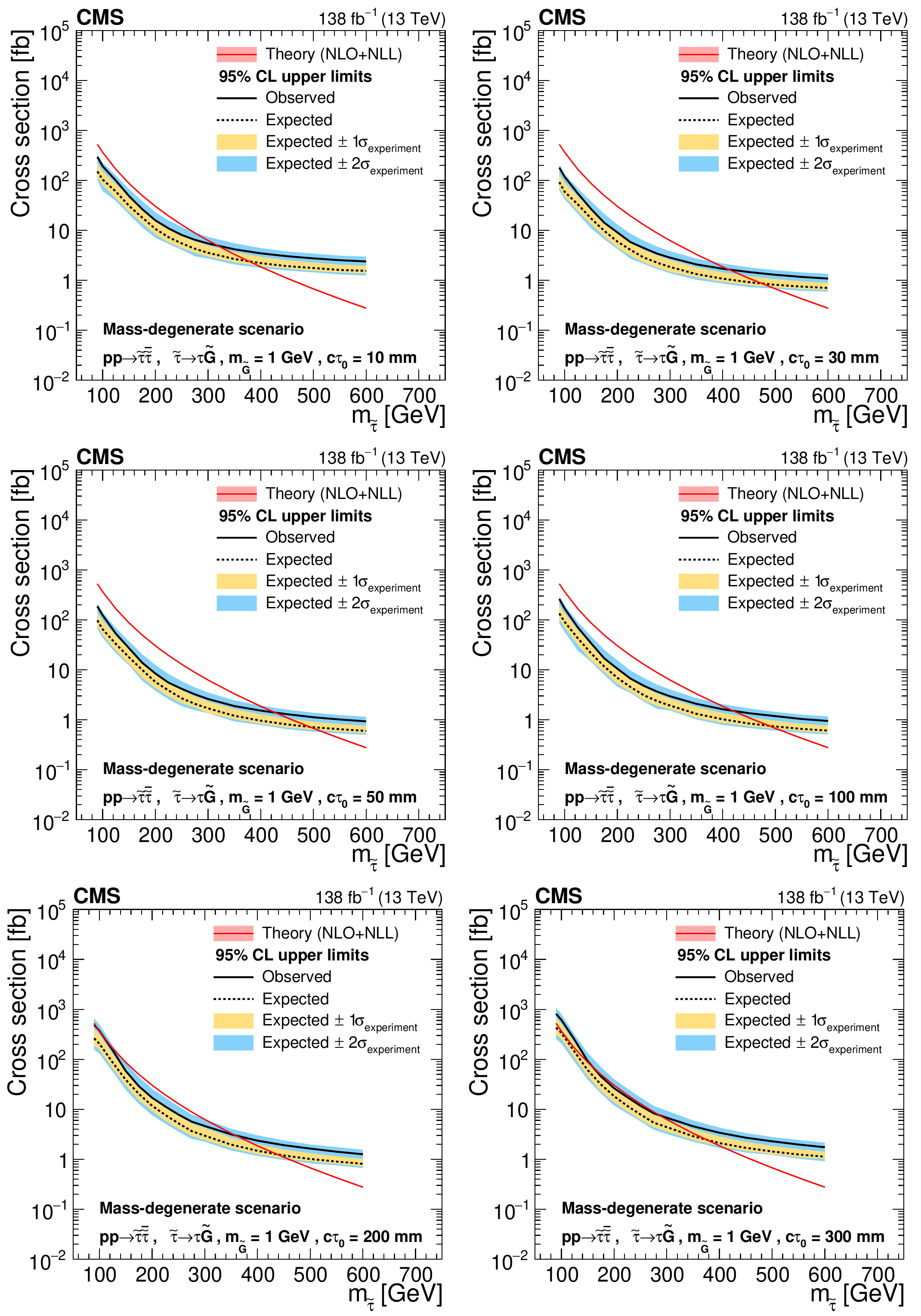
Figure 9:
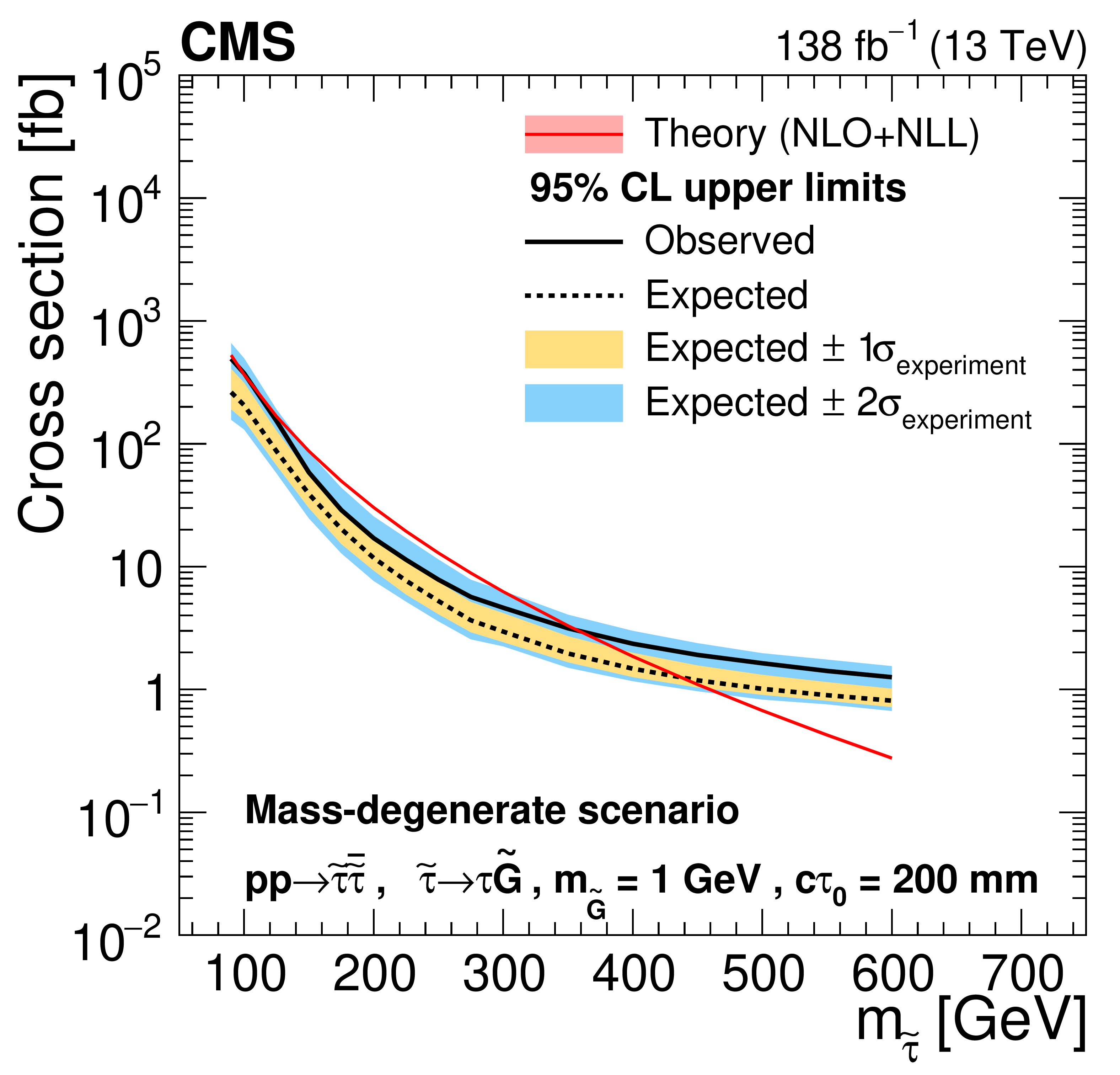
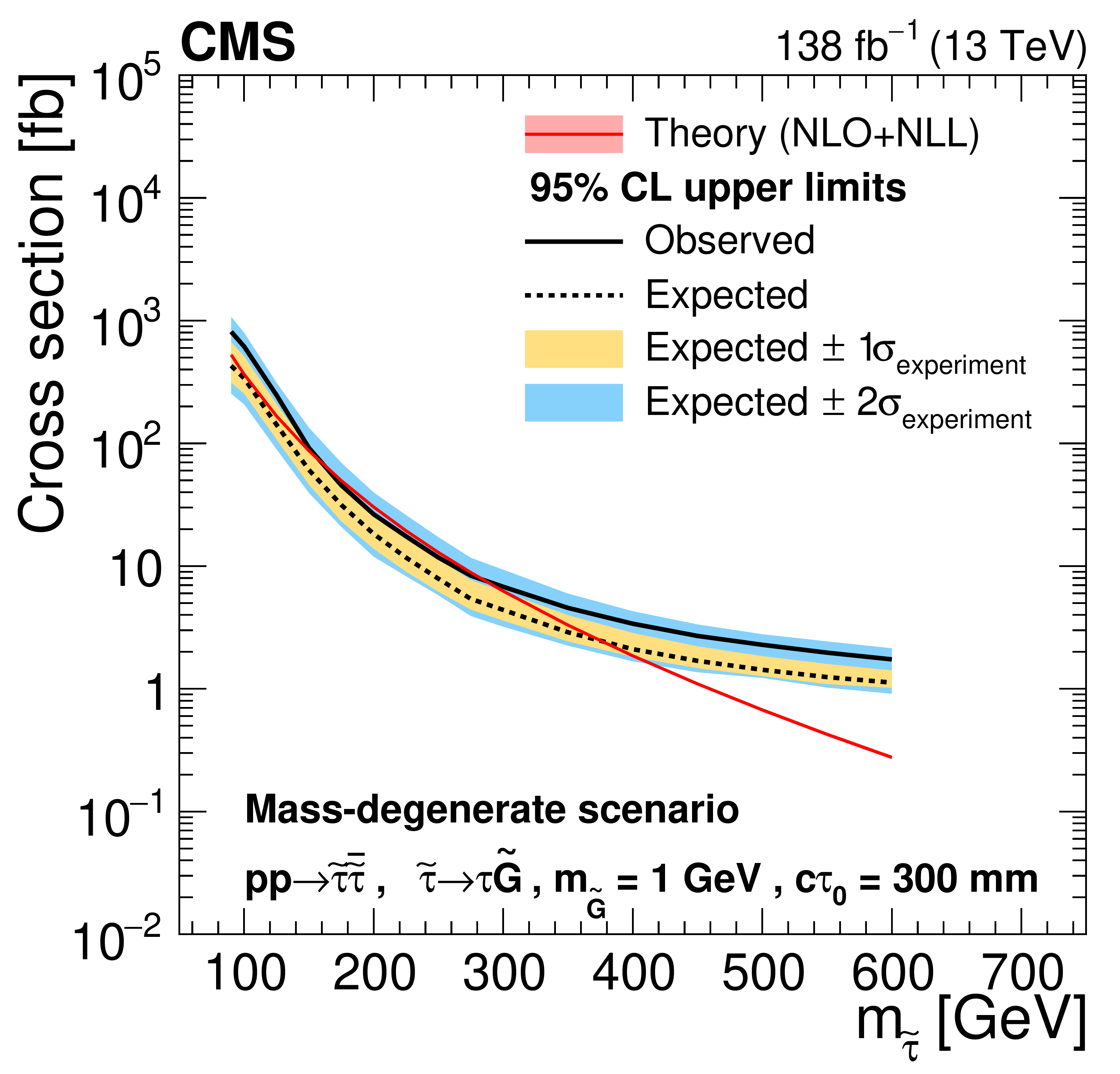
Cross section upper limits at 95% CL for the pair production of long-lived staus decaying to a $ \tau $ lepton and a nearly massless gravitino ($ m_\tilde{\mathrm{G}}= $ 1 GeV) in the mass-degenerate scenario, as a function of $ m_{\tilde{\tau}} $, for $ c\tau_{0}= $ 10, 30, 50, 100, 200, and 300$ \text{mm} $ (left to right, upper to lower). The inner (yellow) and outer (blue) bands indicate the regions containing 68 and 95%, respectively, of the distribution of limits expected under the background-only hypothesis. The central values of the expected upper limits are denoted by the dashed black line. The solid black line represents the observed upper limits. The signal cross sections and uncertainties evaluated using NLO$ + $NLL calculations are shown as a red line and shaded band. |
png pdf |
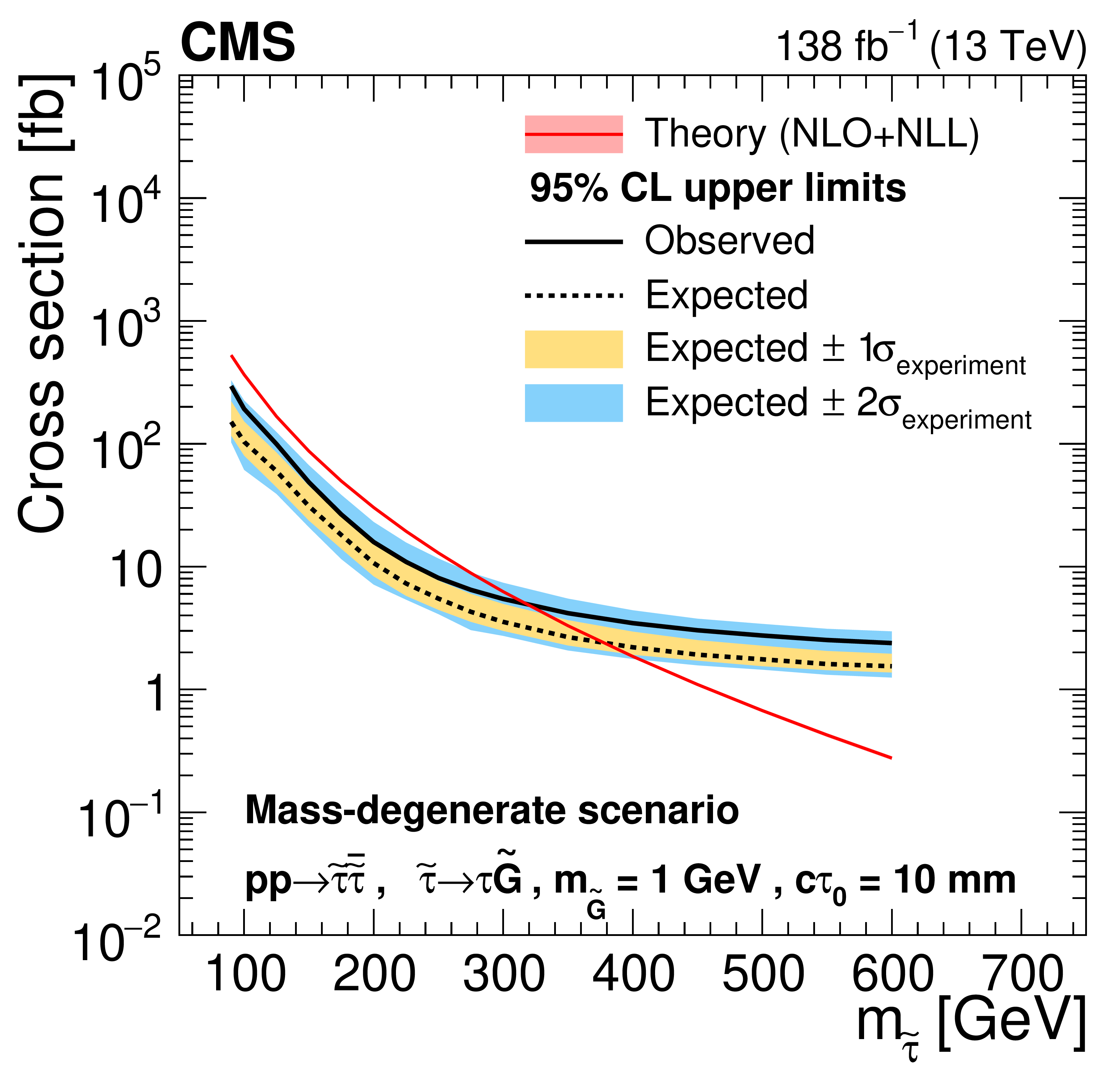
Figure 9-a:
Cross section upper limits at 95% CL for the pair production of long-lived staus decaying to a $ \tau $ lepton and a nearly massless gravitino ($ m_\tilde{\mathrm{G}}= $ 1 GeV) in the mass-degenerate scenario, as a function of $ m_{\tilde{\tau}} $, for $ c\tau_{0}= $ 10, 30, 50, 100, 200, and 300$ \text{mm} $ (left to right, upper to lower). The inner (yellow) and outer (blue) bands indicate the regions containing 68 and 95%, respectively, of the distribution of limits expected under the background-only hypothesis. The central values of the expected upper limits are denoted by the dashed black line. The solid black line represents the observed upper limits. The signal cross sections and uncertainties evaluated using NLO$ + $NLL calculations are shown as a red line and shaded band. |
png pdf |
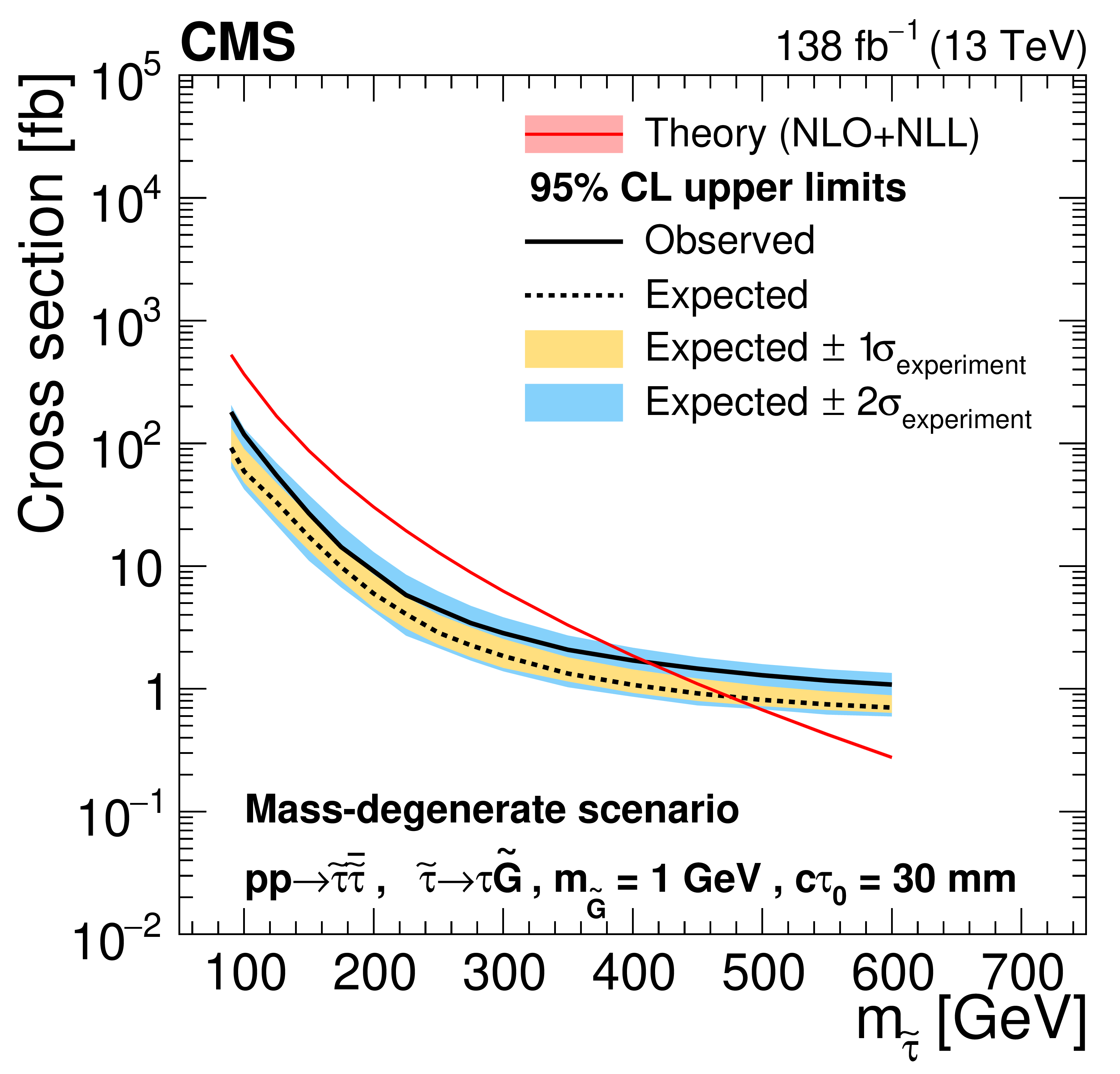
Figure 9-b:
Cross section upper limits at 95% CL for the pair production of long-lived staus decaying to a $ \tau $ lepton and a nearly massless gravitino ($ m_\tilde{\mathrm{G}}= $ 1 GeV) in the mass-degenerate scenario, as a function of $ m_{\tilde{\tau}} $, for $ c\tau_{0}= $ 10, 30, 50, 100, 200, and 300$ \text{mm} $ (left to right, upper to lower). The inner (yellow) and outer (blue) bands indicate the regions containing 68 and 95%, respectively, of the distribution of limits expected under the background-only hypothesis. The central values of the expected upper limits are denoted by the dashed black line. The solid black line represents the observed upper limits. The signal cross sections and uncertainties evaluated using NLO$ + $NLL calculations are shown as a red line and shaded band. |

png pdf |
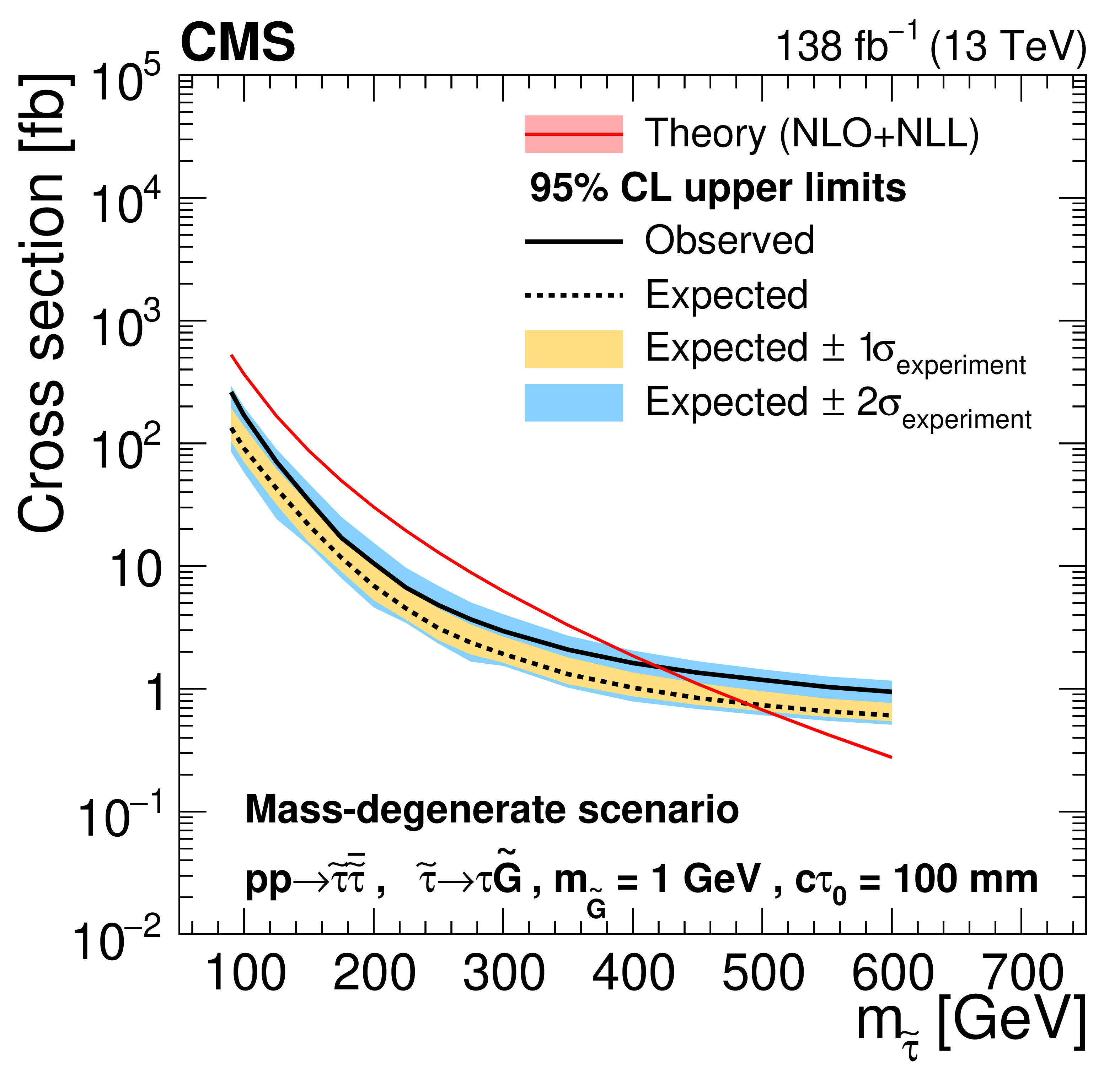
Figure 9-c:
Cross section upper limits at 95% CL for the pair production of long-lived staus decaying to a $ \tau $ lepton and a nearly massless gravitino ($ m_\tilde{\mathrm{G}}= $ 1 GeV) in the mass-degenerate scenario, as a function of $ m_{\tilde{\tau}} $, for $ c\tau_{0}= $ 10, 30, 50, 100, 200, and 300$ \text{mm} $ (left to right, upper to lower). The inner (yellow) and outer (blue) bands indicate the regions containing 68 and 95%, respectively, of the distribution of limits expected under the background-only hypothesis. The central values of the expected upper limits are denoted by the dashed black line. The solid black line represents the observed upper limits. The signal cross sections and uncertainties evaluated using NLO$ + $NLL calculations are shown as a red line and shaded band. |
png pdf |
Figure 9-d:
Cross section upper limits at 95% CL for the pair production of long-lived staus decaying to a $ \tau $ lepton and a nearly massless gravitino ($ m_\tilde{\mathrm{G}}= $ 1 GeV) in the mass-degenerate scenario, as a function of $ m_{\tilde{\tau}} $, for $ c\tau_{0}= $ 10, 30, 50, 100, 200, and 300$ \text{mm} $ (left to right, upper to lower). The inner (yellow) and outer (blue) bands indicate the regions containing 68 and 95%, respectively, of the distribution of limits expected under the background-only hypothesis. The central values of the expected upper limits are denoted by the dashed black line. The solid black line represents the observed upper limits. The signal cross sections and uncertainties evaluated using NLO$ + $NLL calculations are shown as a red line and shaded band. |
png pdf |
Figure 9-e:
Cross section upper limits at 95% CL for the pair production of long-lived staus decaying to a $ \tau $ lepton and a nearly massless gravitino ($ m_\tilde{\mathrm{G}}= $ 1 GeV) in the mass-degenerate scenario, as a function of $ m_{\tilde{\tau}} $, for $ c\tau_{0}= $ 10, 30, 50, 100, 200, and 300$ \text{mm} $ (left to right, upper to lower). The inner (yellow) and outer (blue) bands indicate the regions containing 68 and 95%, respectively, of the distribution of limits expected under the background-only hypothesis. The central values of the expected upper limits are denoted by the dashed black line. The solid black line represents the observed upper limits. The signal cross sections and uncertainties evaluated using NLO$ + $NLL calculations are shown as a red line and shaded band. |
png pdf |
Figure 9-f:
Cross section upper limits at 95% CL for the pair production of long-lived staus decaying to a $ \tau $ lepton and a nearly massless gravitino ($ m_\tilde{\mathrm{G}}= $ 1 GeV) in the mass-degenerate scenario, as a function of $ m_{\tilde{\tau}} $, for $ c\tau_{0}= $ 10, 30, 50, 100, 200, and 300$ \text{mm} $ (left to right, upper to lower). The inner (yellow) and outer (blue) bands indicate the regions containing 68 and 95%, respectively, of the distribution of limits expected under the background-only hypothesis. The central values of the expected upper limits are denoted by the dashed black line. The solid black line represents the observed upper limits. The signal cross sections and uncertainties evaluated using NLO$ + $NLL calculations are shown as a red line and shaded band. |
| Tables | |
png pdf |
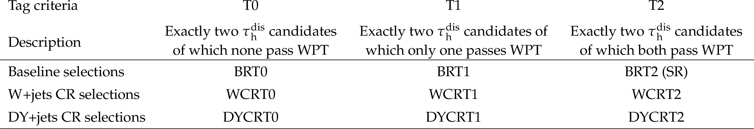
Table 1:
Signal and control region definitions. |
png pdf |
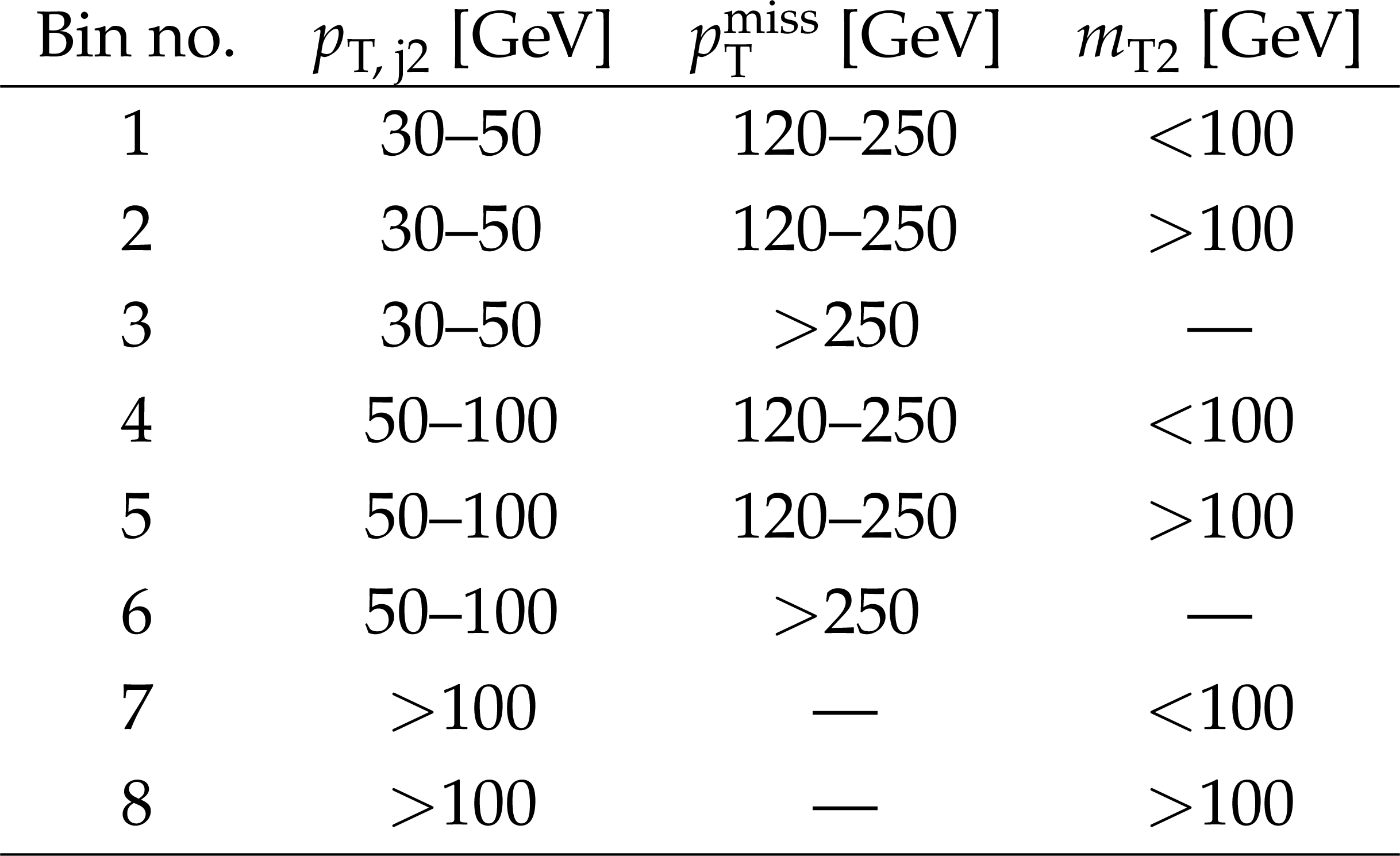
Table 2:
The $ p_{\text{T,j2}} $, $ p_{\mathrm{T}}^\text{miss} $, and $ m_{\mathrm{T2}} $ requirements for each of the eight analysis bins. |
png pdf |
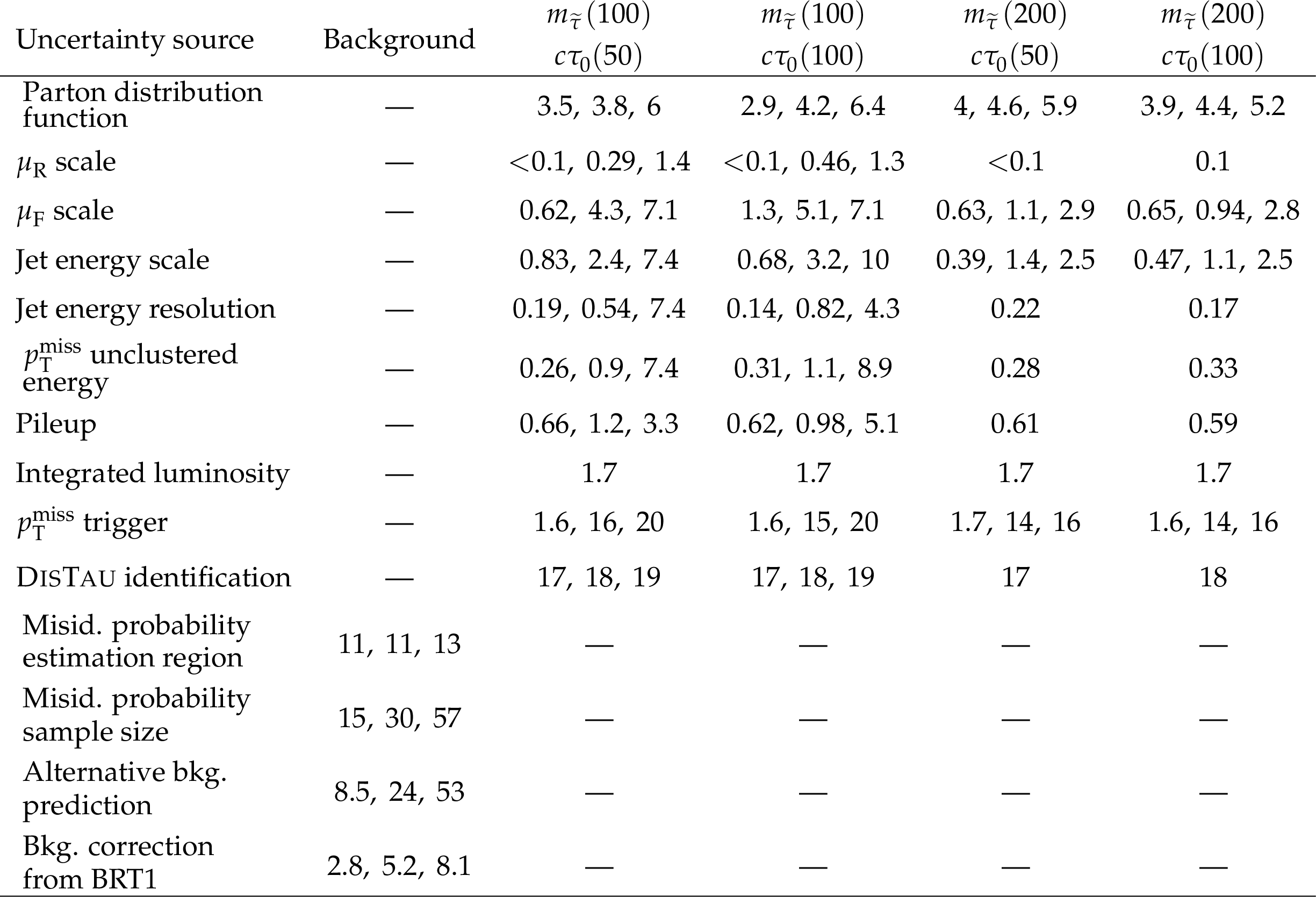
Table 3:
Relative systematic uncertainties expressed as a percentage (%) of the signal and background yields in the SR, from various sources considered in this search, after accounting for their correlations between the data-taking periods. The three values correspond to the minimum, median, and maximum values across the eight SR bins, as defined in Table 2. For cases where the minimum and maximum values differ by less than 1, only the median is shown. In the header row, $ m_{\tilde{\tau}} $ and $ c\tau_{0} $ are in units of GeV and $ \text{mm} $, respectively. The uncertainty values shown here are prior to the maximum likelihood fit described in Section 8. |
png pdf |
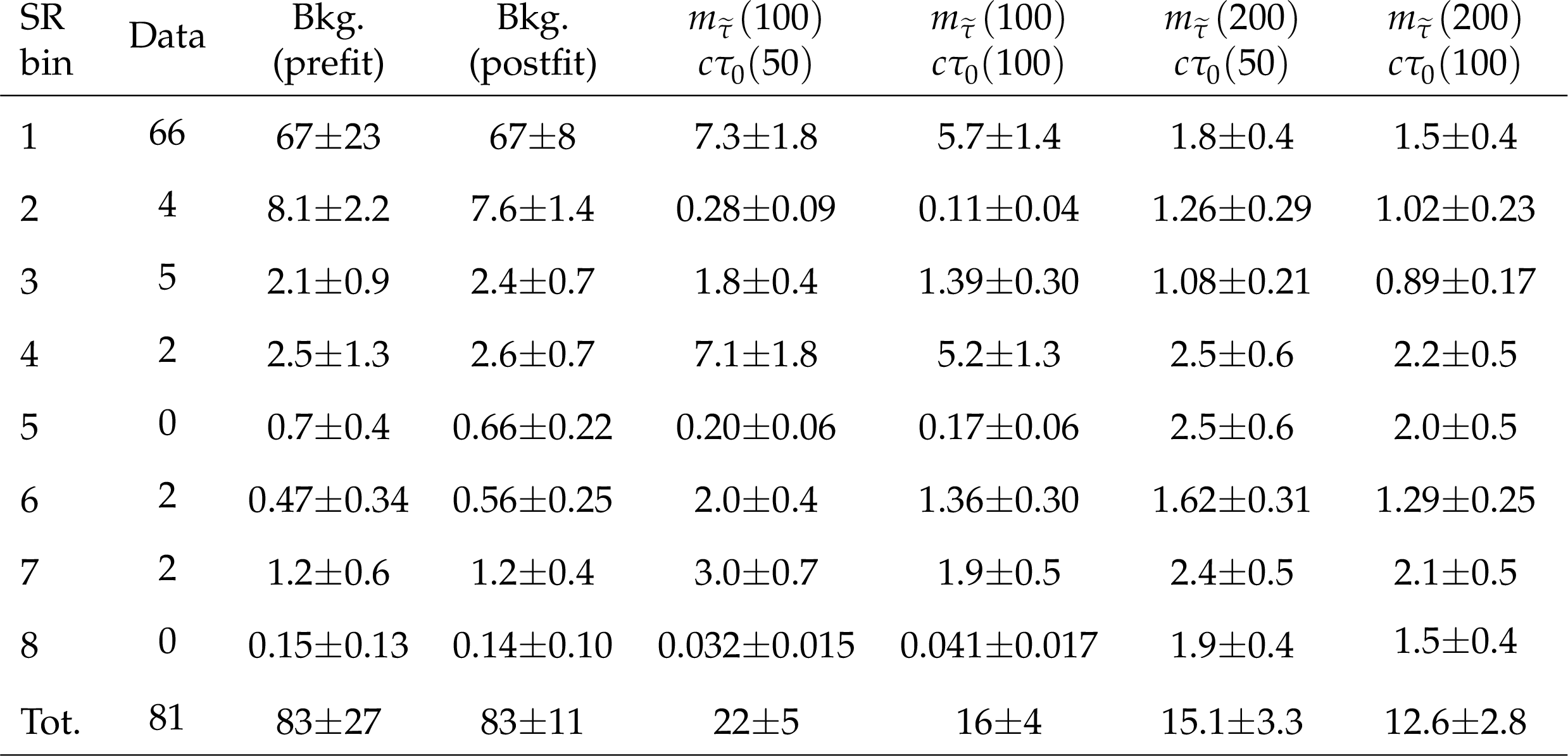
Table 4:
Predicted background and signal yields in the eight SR bins, as defined in Table 2, are shown alongside the background yields obtained from the maximum likelihood fit to data under the background-only hypothesis and the number of events observed in the recorded data. All yields, except for the number of recorded events, are quoted with uncertainties obtained by adding statistical and systematic components in quadrature. Signal and predicted background uncertainties correspond to the prefit values, while the postfit background uncertainties are taken from the fit described in Section 8. In the header row, $ m_{\tilde{\tau}} $ and $ c\tau_{0} $ are in units of GeVns and $ \text{mm} $, respectively. |
| Summary |
| A search for the direct pair production of long-lived superpartners of the tau lepton (staus) has been performed in final states with two hadronically decaying tau leptons ($ \tau_\mathrm{h} $) using data collected by the CMS detector in 2016--2018, corresponding to an integrated luminosity of 138 fb$ ^{-1} $. The potentially large background from misidentified jets in the fully hadronic final state is efficiently suppressed by the DISTAU neural network algorithm, specifically designed to identify displaced $ \tau_\mathrm{h} $ candidates. In the maximally mixed (mass-degenerate) scenario, stau masses, $ m_{\tilde{\tau}} $, in the 126-260 (90-425) GeV range are excluded for a proper decay length, $ c\tau_{0} $, of 50$ \text{mm} $, and stau proper decay lengths in the range 21-94 (6-333)$ \text{mm} $ are excluded for $ m_{\tilde{\tau}} = $ 200 GeV. The development of a dedicated algorithm targeting displaced $ \tau_\mathrm{h} $ signatures has led to a significant improvement in the experimental sensitivity. These results improve the exclusion limits compared to previous searches [33,34,35,36,37,38,39], and extend the parameter space explored in the context of supersymmetry. |
| References | ||||
| 1 | P. Ramond | Dual theory for free fermions | PRD 3 (1971) 2415 | |
| 2 | Yu. A. Golfand and E. P. Likhtman | Extension of the algebra of Poincaré group generators and violation of p invariance | JETP Lett. 13 (1971) 323 | |
| 3 | A. Neveu and J. H. Schwarz | Factorizable dual model of pions | NPB 31 (1971) 86 | |
| 4 | D. V. Volkov and V. P. Akulov | Possible universal neutrino interaction | JETP Lett. 16 (1972) 438 | |
| 5 | J. Wess and B. Zumino | A Lagrangian model invariant under supergauge transformations | PLB 49 (1974) 52 | |
| 6 | J. Wess and B. Zumino | Supergauge transformations in four dimensions | NPB 70 (1974) 39 | |
| 7 | P. Fayet | Supergauge invariant extension of the Higgs mechanism and a model for the electron and its neutrino | NPB 90 (1975) 104 | |
| 8 | H. P. Nilles | Supersymmetry, supergravity and particle physics | Phys. Rept. 110 (1984) 1 | |
| 9 | G. 't Hooft | Naturalness, chiral symmetry, and spontaneous chiral symmetry breaking | NATO Sci. Ser. B 59 (1980) 135 | |
| 10 | E. Witten | Dynamical breaking of supersymmetry | NPB 188 (1981) 513 | |
| 11 | M. Dine, W. Fischler, and M. Srednicki | Supersymmetric technicolor | NPB 189 (1981) 575 | |
| 12 | S. Dimopoulos and S. Raby | Supercolor | NPB 192 (1981) 353 | |
| 13 | S. Dimopoulos and H. Georgi | Softly broken supersymmetry and SU(5) | NPB 193 (1981) 150 | |
| 14 | R. K. Kaul and P. Majumdar | Cancellation of quadratically divergent mass corrections in globally supersymmetric spontaneously broken gauge theories | NPB 199 (1982) 36 | |
| 15 | ATLAS Collaboration | Observation of a new particle in the search for the standard model Higgs boson with the ATLAS detector at the LHC | PLB 716 (2012) 1 | 1207.7214 |
| 16 | CMS Collaboration | Observation of a new boson at a mass of 125 GeV with the CMS experiment at the LHC | PLB 716 (2012) 30 | CMS-HIG-12-028 1207.7235 |
| 17 | CMS Collaboration | Observation of a new boson with mass near 125 GeV in $ pp $ collisions at $ \sqrt{s} = $ 7 and 8 TeV | JHEP 06 (2013) 081 | CMS-HIG-12-036 1303.4571 |
| 18 | ATLAS Collaboration | Measurement of the Higgs boson mass from the $ \textrm{H}\rightarrow \gamma\gamma $ and $ \textrm{H} \rightarrow \textrm{ZZ}^{*} \rightarrow 4\ell $ channels with the ATLAS detector using 25 fb$ ^{-1} $ of $ pp $ collision data | PRD 90 (2014) 052004 | 1406.3827 |
| 19 | CMS Collaboration | Precise determination of the mass of the higgs boson and tests of compatibility of its couplings with the standard model predictions using proton collisions at 7 and 8 TeV | EPJC 75 (2015) 212 | CMS-HIG-14-009 1412.8662 |
| 20 | ATLAS and CMS Collaborations | Combined measurement of the Higgs boson mass in pp collisions at $ \sqrt{s}= $ 7 and 8 TeV with the ATLAS and CMS experiments | PRL 114 (2015) 191803 | 1503.07589 |
| 21 | G. R. Farrar and P. Fayet | Phenomenology of the production, decay, and detection of new hadronic states associated with supersymmetry | PLB 76 (1978) 575 | |
| 22 | C. Boehm, A. Djouadi, and M. Drees | Light scalar top quarks and supersymmetric dark matter | PRD 62 (2000) 035012 | hep-ph/9911496 |
| 23 | C. Bal \'a zs, M. Carena, and C. E. M. Wagner | Dark matter, light stops and electroweak baryogenesis | PRD 70 (2004) 015007 | hep-ph/403224 |
| 24 | G. Jungman, M. Kamionkowski, and K. Griest | Supersymmetric dark matter | Phys. Rept. 267 (1996) 195 | hep-ph/9506380 |
| 25 | Particle Data Group , S. Navas et al. | Review of particle physics | PRD 110 (2024) 030001 | |
| 26 | G. F. Giudice and R. Rattazzi | Theories with gauge mediated supersymmetry breaking | Phys. Rept. 322 (1999) 419 | hep-ph/9801271 |
| 27 | P. Meade, N. Seiberg, and D. Shih | General gauge mediation | Prog. Theor. Phys. Suppl. 177 (2009) 143 | 0801.3278 |
| 28 | J. A. Evans and J. Shelton | Long-lived staus and displaced leptons at the LHC | JHEP 04 (2016) 056 | 1601.01326 |
| 29 | ALEPH Collaboration | Search for scalar leptons in $ e^+ e^- $ collisions at center-of-mass energies up to 209 GeV | PLB 526 (2002) 206 | hep-ex/0112011 |
| 30 | DELPHI Collaboration | Searches for supersymmetric particles in $ e^+ e^- $ collisions up to 208 GeV and interpretation of the results within the MSSM | EPJC 31 (2003) 421 | hep-ex/0311019 |
| 31 | L3 Collaboration | Search for scalar leptons and scalar quarks at LEP | PLB 580 (2004) 37 | hep-ex/0310007 |
| 32 | OPAL Collaboration | Search for anomalous production of dilepton events with missing transverse momentum in e+ e- collisions at $ \sqrt{s} = $ 183--209 GeV | EPJC 32 (2004) 453 | hep-ex/0309014 |
| 33 | ATLAS Collaboration | Search for direct stau production in events with two hadronic $ \tau $-leptons in $ \sqrt{s} = $ 13 TeV $ pp $ collisions with the ATLAS detector | PRD 101 (2020) 032009 | 1911.06660 |
| 34 | CMS Collaboration | Search for direct pair production of supersymmetric partners to the $ \tau $ lepton in proton-proton collisions at $ \sqrt{s}= $ 13 TeV | EPJC 80 (2020) 189 | CMS-SUS-18-006 1907.13179 |
| 35 | ATLAS Collaboration | Search for displaced leptons in $ \sqrt{s} = $ 13 TeV $ pp $ collisions with the ATLAS detector | PRL 127 (2021) 051802 | 2011.07812 |
| 36 | CMS Collaboration | Search for direct pair production of supersymmetric partners of $ \tau $ leptons in the final state with two hadronically decaying $ \tau $ leptons and missing transverse momentum in proton-proton collisions at $ \sqrt{s} = $ 13 TeV | PRD 108 (2023) 012011 | CMS-SUS-21-001 2207.02254 |
| 37 | CMS Collaboration | Search for long-lived particles decaying to leptons with large impact parameter in proton--proton collisions at $ \sqrt{s} = $ 13 TeV | EPJC 82 (2022) 153 | CMS-EXO-18-003 2110.04809 |
| 38 | ATLAS Collaboration | Search for electroweak production of supersymmetric particles in final states with two \ensuremath\tau-leptons in $ \sqrt{s} = $ 13 TeV pp collisions with the ATLAS detector | JHEP 05 (2024) 150 | 2402.00603 |
| 39 | ATLAS Collaboration | Search for long-lived charged particles using large specific ionisation loss and time of flight in 140 fb$ ^{-1} $ of pp collisions at $ \sqrt{s} = $ 13 TeV with the ATLAS detector | JHEP 07 (2025) 140 | 2502.06694 |
| 40 | ATLAS Collaboration | Search for the direct production of charginos, neutralinos and staus in final states with at least two hadronically decaying taus and missing transverse momentum in $ pp $ collisions at $ \sqrt{s} = $ 8 TeV with the ATLAS detector | JHEP 10 (2014) 096 | 1407.0350 |
| 41 | ATLAS Collaboration | Search for the electroweak production of supersymmetric particles in $ \sqrt{s}= $ 8 TeV $ pp $ collisions with the ATLAS detector | PRD 93 (2016) 052002 | 1509.07152 |
| 42 | CMS Collaboration | Search for electroweak production of charginos in final states with two \ensuremath\tau leptons in pp collisions at $ \sqrt{s}= $ 8 TeV | JHEP 04 (2017) 018 | CMS-SUS-14-022 1610.04870 |
| 43 | CMS Collaboration | Performance of reconstruction and identification of $ \tau $ leptons decaying to hadrons and v$ _\tau $ in pp collisions at $ \sqrt{s}= $ 13 TeV | JINST 13 (2018) P10005 | CMS-TAU-16-003 1809.02816 |
| 44 | CMS Collaboration | Identification of hadronic tau lepton decays using a deep neural network | JINST 17 (2022) P07023 | CMS-TAU-20-001 2201.08458 |
| 45 | CMS Collaboration | Tau lepton identification in displaced topologies using machine learning at CMS | CMS Detector Performance Summary CMS-DP-2024-053, 2024 CDS |
|
| 46 | J. Alwall, P. Schuster, and N. Toro | Simplified models for a first characterization of new physics at the LHC | PRD 79 (2009) 075020 | 0810.3921 |
| 47 | LHC New Physics Working Group | Simplified models for LHC new physics searches | JPG 39 (2012) 105005 | 1105.2838 |
| 48 | H. Qu and L. Gouskos | Jet tagging via particle clouds | PRD 101 (2020) 056019 | 1902.08570 |
| 49 | CMS Collaboration | HEPData record for this analysis | link | |
| 50 | CMS Collaboration | The CMS experiment at the CERN LHC | JINST 3 (2008) S08004 | |
| 51 | CMS Collaboration | Development of the CMS detector for the CERN LHC Run 3 | JINST 19 (2024) P05064 | CMS-PRF-21-001 2309.05466 |
| 52 | CMS Collaboration | Performance of the CMS level-1 trigger in proton-proton collisions at $ \sqrt{s} = $ 13 TeV | JINST 15 (2020) P10017 | CMS-TRG-17-001 2006.10165 |
| 53 | CMS Collaboration | The CMS trigger system | JINST 12 (2017) P01020 | CMS-TRG-12-001 1609.02366 |
| 54 | CMS Collaboration | Performance of the CMS high-level trigger during LHC Run 2 | JINST 19 (2024) P11021 | CMS-TRG-19-001 2410.17038 |
| 55 | J. Alwall et al. | The automated computation of tree-level and next-to-leading order differential cross sections, and their matching to parton shower simulations | JHEP 07 (2014) 079 | 1405.0301 |
| 56 | NNPDF Collaboration | Parton distributions for the LHC Run II | JHEP 04 (2015) 040 | 1410.8849 |
| 57 | NNPDF Collaboration | Parton distributions from high-precision collider data | EPJC 77 (2017) 663 | 1706.00428 |
| 58 | B. Fuks, M. Klasen, D. R. Lamprea, and M. Rothering | Revisiting slepton pair production at the Large Hadron Collider | JHEP 01 (2014) 168 | 1310.2621 |
| 59 | B. Fuks, M. Klasen, D. R. Lamprea, and M. Rothering | Precision predictions for electroweak superpartner production at hadron colliders with Resummino | EPJC 73 (2013) 2480 | 1304.0790 |
| 60 | J. Fiaschi, B. Fuks, M. Klasen, and A. Neuwirth | Electroweak superpartner production at 13.6 Tev with Resummino | EPJC 83 (2023) 707 | 2304.11915 |
| 61 | J. Fiaschi and M. Klasen | Slepton pair production at the LHC in NLO+NLL with resummation-improved parton densities | JHEP 03 (2018) 094 | 1801.10357 |
| 62 | G. Bozzi, B. Fuks, and M. Klasen | Joint resummation for slepton pair production at hadron colliders | NPB 794 (2008) 46 | 0709.3057 |
| 63 | G. Bozzi, B. Fuks, and M. Klasen | Transverse-momentum resummation for slepton-pair production at the CERN LHC | PRD 74 (2006) 015001 | hep-ph/0603074 |
| 64 | A. P. Neuwirth | HEPi | link | |
| 65 | C. Oleari | The POWHEG-BOX | Nucl. Phys. B Proc. Suppl. 20 (2010) 5 | 1007.3893 |
| 66 | P. Nason | A new method for combining NLO QCD with shower Monte Carlo algorithms | JHEP 11 (2004) 040 | hep-ph/0409146 |
| 67 | S. Frixione, P. Nason, and C. Oleari | Matching NLO QCD computations with parton shower simulations: the POWHEG method | JHEP 11 (2007) 070 | 0709.2092 |
| 68 | S. Alioli, P. Nason, C. Oleari, and E. Re | A general framework for implementing NLO calculations in shower Monte Carlo programs: the POWHEG BOX | JHEP 06 (2010) 043 | 1002.2581 |
| 69 | S. Frixione, P. Nason, and G. Ridolfi | A positive-weight next-to-leading-order Monte Carlo for heavy flavour hadroproduction | JHEP 09 (2007) 126 | 0707.3088 |
| 70 | GEANT4 Collaboration | GEANT 4 -- a simulation toolkit | NIM A 506 (2003) 250 | |
| 71 | T. Sjöstrand et al. | An introduction to PYTHIA 8.2 | Comput. Phys. Commun. 191 (2015) 159 | 1410.3012 |
| 72 | CMS Collaboration | Extraction and validation of a new set of CMS PYTHIA8 tunes from underlying-event measurements | EPJC 80 (2020) 4 | CMS-GEN-17-001 1903.12179 |
| 73 | CMS Collaboration | Particle-flow reconstruction and global event description with the CMS detector | JINST 12 (2017) P10003 | CMS-PRF-14-001 1706.04965 |
| 74 | CMS Collaboration | Technical proposal for the Phase-II upgrade of the Compact Muon Solenoid | CMS Technical proposal CERN-LHCC-2015-010, CMS-TDR-15-02, 2015 CDS |
|
| 75 | M. Cacciari, G. P. Salam, and G. Soyez | The anti-$ k_{\mathrm{T}} $ jet clustering algorithm | JHEP 04 (2008) 063 | 0802.1189 |
| 76 | M. Cacciari, G. P. Salam, and G. Soyez | FastJet user manual | EPJC 72 (2012) 1896 | 1111.6097 |
| 77 | CMS Collaboration | Jet energy scale and resolution in the CMS experiment in pp collisions at 8 TeV | JINST 12 (2017) P02014 | CMS-JME-13-004 1607.03663 |
| 78 | CMS Collaboration | Jet algorithms performance in 13 TeV data | CMS Physics Analysis Summary, 2017 CMS-PAS-JME-16-003 |
CMS-PAS-JME-16-003 |
| 79 | CMS Collaboration | Identification of heavy-flavour jets with the CMS detector in pp collisions at 13 TeV | JINST 13 (2018) P05011 | CMS-BTV-16-002 1712.07158 |
| 80 | CMS Collaboration | Performance summary of AK4 jet b tagging with data from proton-proton collisions at 13 TeV with the CMS detector | CMS Detector Performance Note CMS-DP-2023-005, 2023 CDS |
|
| 81 | E. Bols et al. | Jet flavour classification using DeepJet | JINST 15 (2020) P12012 | 2008.10519 |
| 82 | CMS Collaboration | Electron and photon reconstruction and identification with the CMS experiment at the CERN LHC | JINST 16 (2021) P05014 | CMS-EGM-17-001 2012.06888 |
| 83 | CMS Collaboration | Performance of electron reconstruction and selection with the CMS detector in proton-proton collisions at $ \sqrt{s} = $ 8 TeV | JINST 10 (2015) P06005 | CMS-EGM-13-001 1502.02701 |
| 84 | CMS Collaboration | Performance of the CMS muon detector and muon reconstruction with proton-proton collisions at $ \sqrt{s} = $ 13 TeV | JINST 13 (2018) P06015 | CMS-MUO-16-001 1804.04528 |
| 85 | CMS Collaboration | Pileup mitigation at CMS in 13 TeV data | JINST 15 (2020) P09018 | CMS-JME-18-001 2003.00503 |
| 86 | CMS Collaboration | Performance of missing transverse momentum reconstruction in proton-proton collisions at $ \sqrt{s} = $ 13 TeV using the CMS detector | JINST 14 (2019) P07004 | CMS-JME-17-001 1903.06078 |
| 87 | Y. Wang et al. | Dynamic graph CNN for learning on point clouds | ACM Trans. Graph. 38 (2019) | |
| 88 | CMS Collaboration | Observation of the Higgs boson decay to a pair of $ \tau $ leptons with the CMS detector | PLB 779 (2018) 283 | CMS-HIG-16-043 1708.00373 |
| 89 | CMS Collaboration | Search for neutral MSSM Higgs bosons decaying to a pair of tau leptons in pp collisions | JHEP 10 (2014) 160 | CMS-HIG-13-021 1408.3316 |
| 90 | CMS Collaboration | Measurements of Inclusive $ W $ and $ Z $ Cross Sections in $ pp $ Collisions at $ \sqrt{s}= $ 7 TeV | JHEP 01 (2011) 080 | CMS-EWK-10-002 1012.2466 |
| 91 | C. G. Lester and D. J. Summers | Measuring masses of semiinvisibly decaying particles pair produced at hadron colliders | PLB 463 (1999) 99 | hep-ph/9906349 |
| 92 | A. Barr, C. Lester, and P. Stephens | $ m_{\mathrm{T2}} $: The truth behind the glamour | JPG 29 (2003) 2343 | hep-ph/0304226 |
| 93 | A. J. Barr and C. Gwenlan | The race for supersymmetry: Using $ m_{\mathrm{T2}} $ for discovery | PRD 80 (2009) 074007 | 0907.2713 |
| 94 | CMS Collaboration | Search for long-lived particles using out-of-time trackless jets in proton-proton collisions at $ \sqrt{s} = $ 13 TeV | JHEP 07 (2023) 210 | CMS-EXO-21-014 2212.06695 |
| 95 | CMS Collaboration | Search for top squark pair production in a final state with at least one hadronically decaying tau lepton in proton-proton collisions at $ \sqrt{s} = $ 13 TeV | JHEP 07 (2023) 110 | CMS-SUS-21-004 2304.07174 |
| 96 | J. Butterworth et al. | PDF4LHC recommendations for LHC Run II | JPG 43 (2016) 023001 | 1510.03865 |
| 97 | A. Kalogeropoulos and J. Alwall | The SysCalc code: A tool to derive theoretical systematic uncertainties | 1801.08401 | |
| 98 | CMS Collaboration | Measurement of the inelastic proton-proton cross section at $ \sqrt{s}= $ 13 TeV | JHEP 07 (2018) 161 | CMS-FSQ-15-005 1802.02613 |
| 99 | CMS Collaboration | Precision luminosity measurement in proton-proton collisions at $ \sqrt{s} = $ 13 TeV in 2015 and 2016 at CMS | EPJC 81 (2021) 800 | CMS-LUM-17-003 2104.01927 |
| 100 | CMS Collaboration | CMS luminosity measurement for the 2017 data-taking period at $ \sqrt{s} = $ 13 TeV | CMS Physics Analysis Summary, 2018 CMS-PAS-LUM-17-004 |
CMS-PAS-LUM-17-004 |
| 101 | CMS Collaboration | CMS luminosity measurement for the 2018 data-taking period at $ \sqrt{s} = $ 13 TeV | CMS Physics Analysis Summary, 2019 CMS-PAS-LUM-18-002 |
CMS-PAS-LUM-18-002 |
| 102 | CMS Collaboration | Operation and performance of the CMS silicon strip tracker with proton-proton collisions at the CERN LHC | JINST 20 (2025) P08027 | CMS-TRK-20-002 2506.17195 |
| 103 | ATLAS and CMS Collaborations, and the LHC Higgs Combination Group | Procedure for the LHC Higgs boson search combination in summer 2011 | Technical Report CMS-NOTE-2011-005, ATL-PHYS-PUB-2011-11, 2011 | |
| 104 | T. Junk | Confidence level computation for combining searches with small statistics | NIM A 434 (1999) 435 | hep-ex/9902006 |
| 105 | A. L. Read | Presentation of search results: the $ \text{CL}_\text{s} $ technique | JPG 28 (2002) 2693 | |
| 106 | CMS Collaboration | The CMS statistical analysis and combination tool: Combine | Comput. Softw. Big Sci. 8 (2024) 19 | CMS-CAT-23-001 2404.06614 |
|
|
Compact Muon Solenoid LHC, CERN |
|

|

|

|

|

|