
Compact Muon Solenoid
LHC, CERN
 Visit us: CMS Public Website, CMS Physics ;
Contact us: CMS Publications Committee
Visit us: CMS Public Website, CMS Physics ;
Contact us: CMS Publications Committee
| CMS-PAS-SMP-25-002 | ||
| Constraints on Effective Field Theory operators from multiboson production measurements at $ \sqrt{s} = $ 13 TeV | ||
| CMS Collaboration | ||
| 2026-07-30 | ||
| Abstract: A search for new physics in electroweak multiboson production is performed through a statistical combination of ten CMS measurements using proton-proton collision data collected at $ \sqrt{s}= $ 13 TeV during 2016--2018, corresponding to an integrated luminosity of 138 fb$ ^{-1} $. The combination encompasses six vector boson scattering channels: same-sign $ \mathrm{WW} $ production in fully leptonic and $ \ell\tau_\mathrm{h} $ final states, opposite-sign $ \mathrm{WW} $, $ \mathrm{WZ} $, and two VBS channels with a hadronically decaying vector boson ($ \mathrm{WV} $ and $ \mathrm{ZV} $); two vector boson fusion channels ($ \mathrm{Wjj} $ and $ \mathrm{Zjj} $), inclusive $ \mathrm{W^+W^-} $ diboson production, and triboson VVV (no $ \gamma $) production. Within the standard model effective field theory framework, potential contributions from physics beyond the standard model are parameterized in terms of six CP-even bosonic dimension-six operators of the Warsaw basis: $ \mathcal{O}_{W} $, $ \mathcal{O}_{HW} $, $ \mathcal{O}_{HWB} $, $ \mathcal{O}_{H\square} $, $ \mathcal{O}_{HB} $, and $ \mathcal{O}_{HD} $. Their effects are introduced through event-by-event reweighting of leading-order Monte Carlo simulations, enabling a consistent propagation of EFT effects to detector level with a consistent treatment of systematic uncertainties. Constraints on the associated Wilson coefficients are extracted using a binned profile likelihood fit, in scenarios ranging from individual coefficients to the fully profiled six-dimensional fit. No significant deviations from the standard model are observed. The combination improves substantially upon any individual analysis and constitutes the first detector-level combination of direct EFT measurements targeting bosonic dimension-six operators at the LHC. | ||
| Links: CDS record (PDF) ; CADI line (restricted) ; | ||
| Figures | |
png pdf |
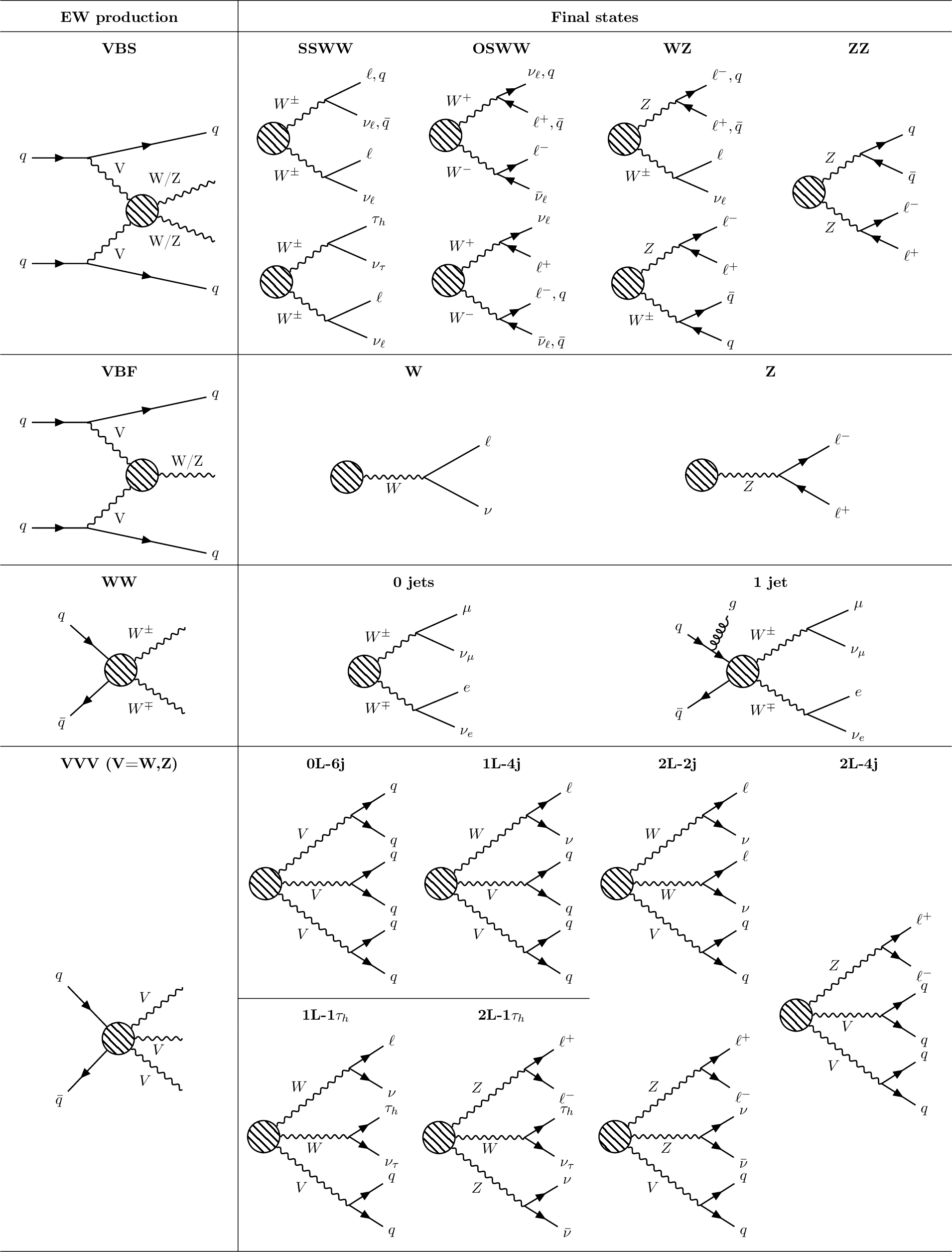
Figure 1:
Representative SM diagrams for the EW production processes considered in this combination. Each row corresponds to one of the four production mechanisms entering the combination -- VBS, VBF, diboson $ \mathrm{W^+}\mathrm{W^-} $, and triboson VVV -- with the generic production diagram shown on the left; the shaded blob denotes the EW production amplitude, summing the multiple diagrams contributing to each process. The dimension-six operators of Table 1 can affect both this production amplitude and the subsequent decay vertices of the vector bosons. The columns on the right show the specific decay topologies corresponding to the final states of each analysis listed in Table 2. |
png pdf |
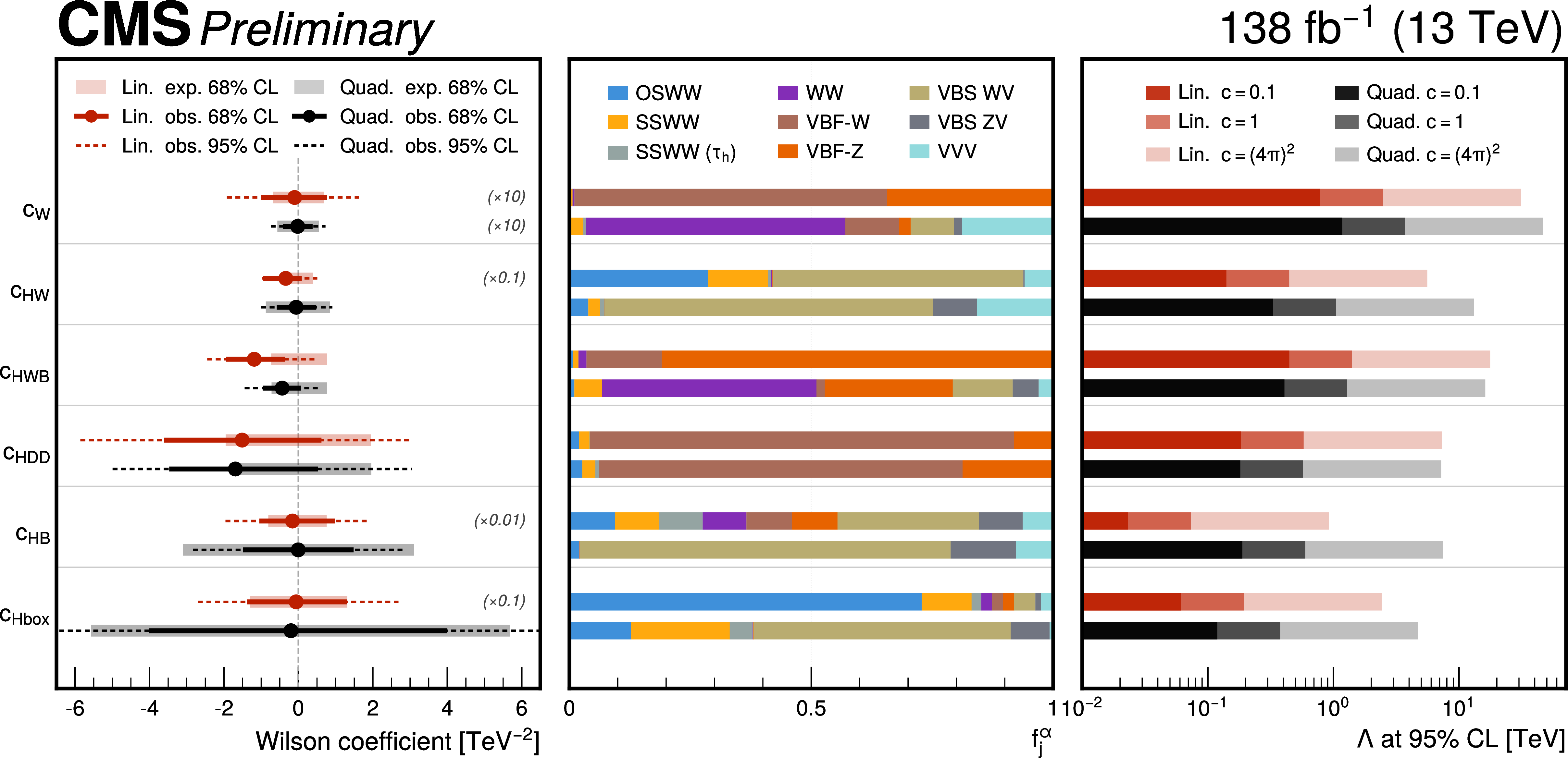
Figure 2:
Summary of the expected and observed one-dimensional 68% and 95% CL intervals, considering both linear-only and linear + quadratic SMEFT contributions (left panel). Results for the Wilson coefficient under analysis are obtained by fixing to zero the coefficients of the rest of the operators. The central panel shows the fractional contribution $ f_j^{\alpha} $ of each analysis $ \alpha $ to the combined limit on each Wilson coefficient $ c_j $, while the right panel shows the limits on the energy scale $ \Lambda $. |
png pdf |
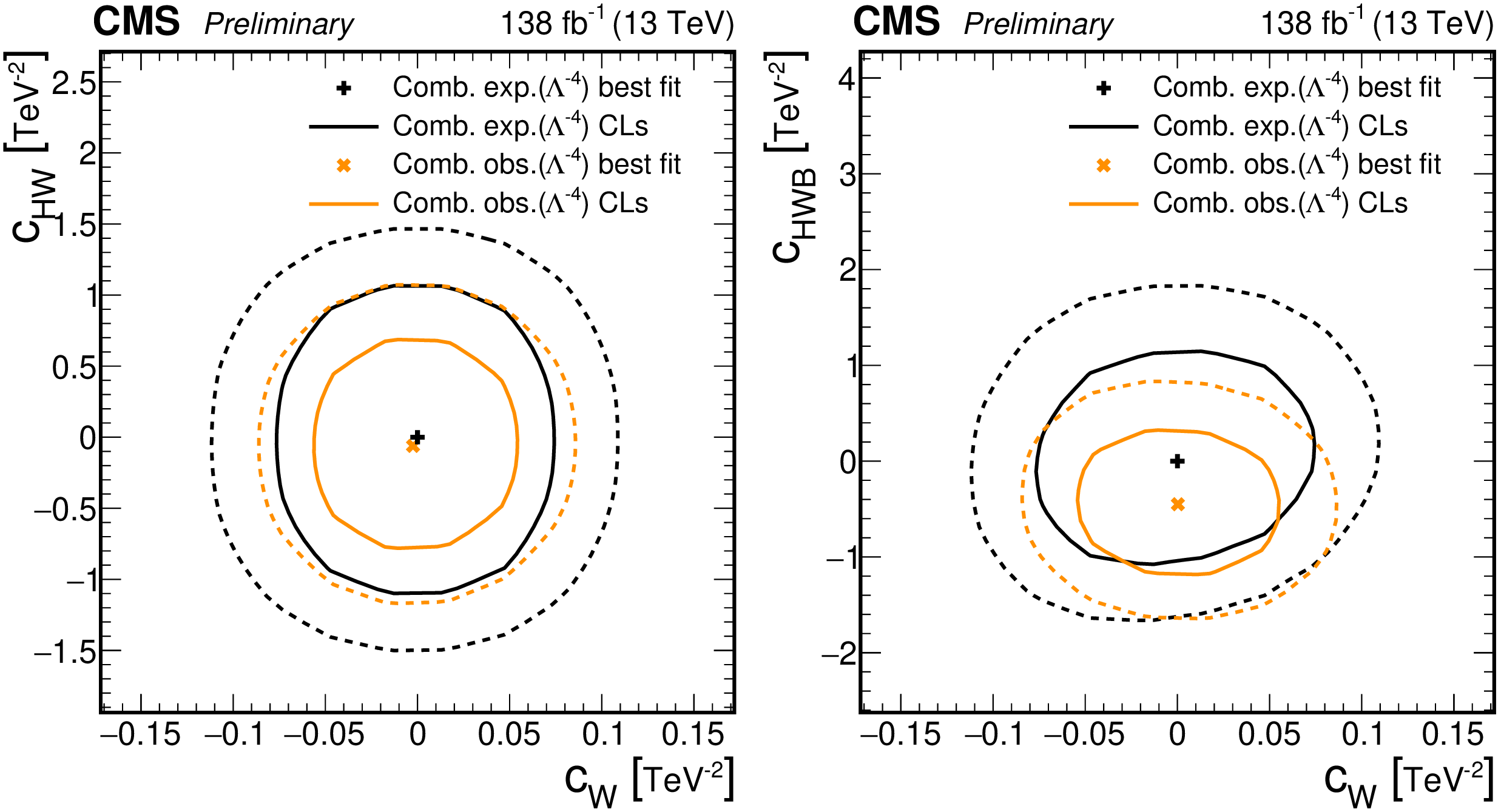
Figure 3:
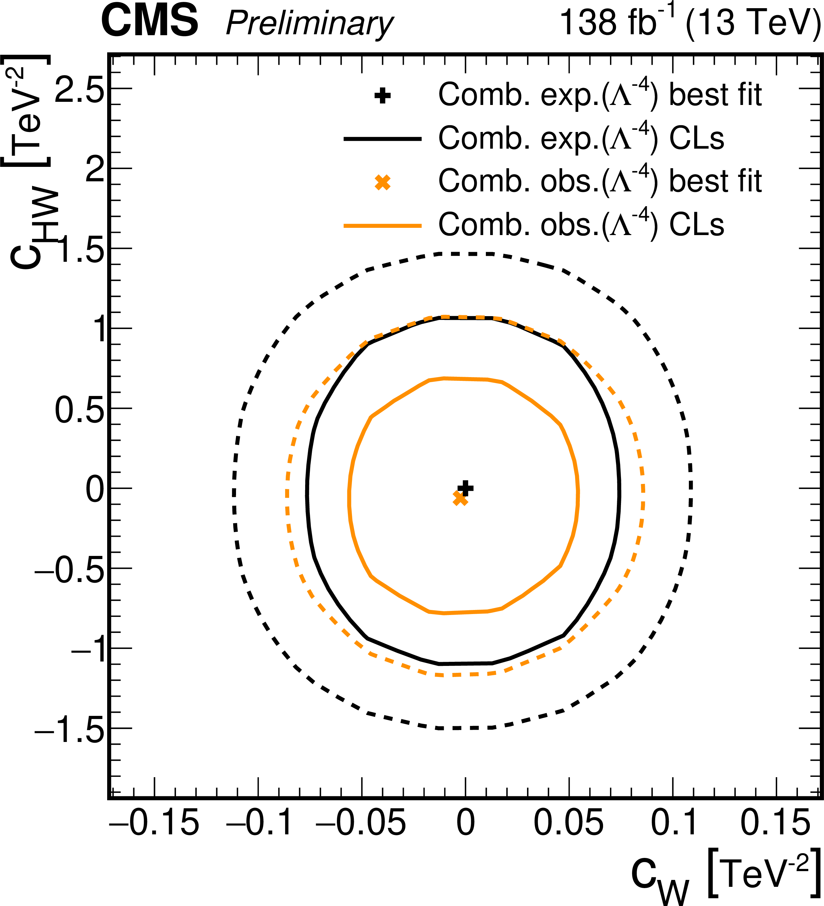
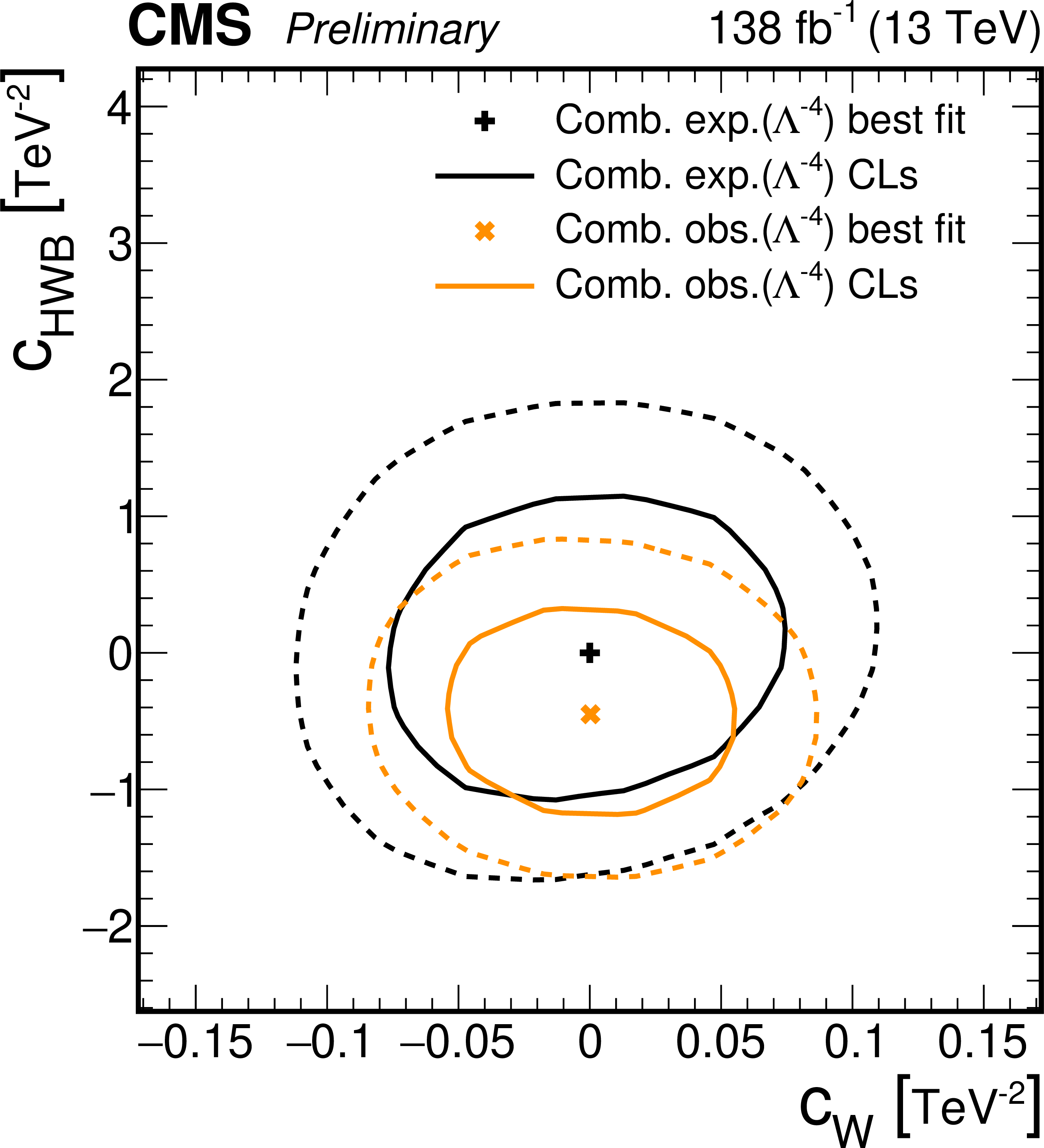
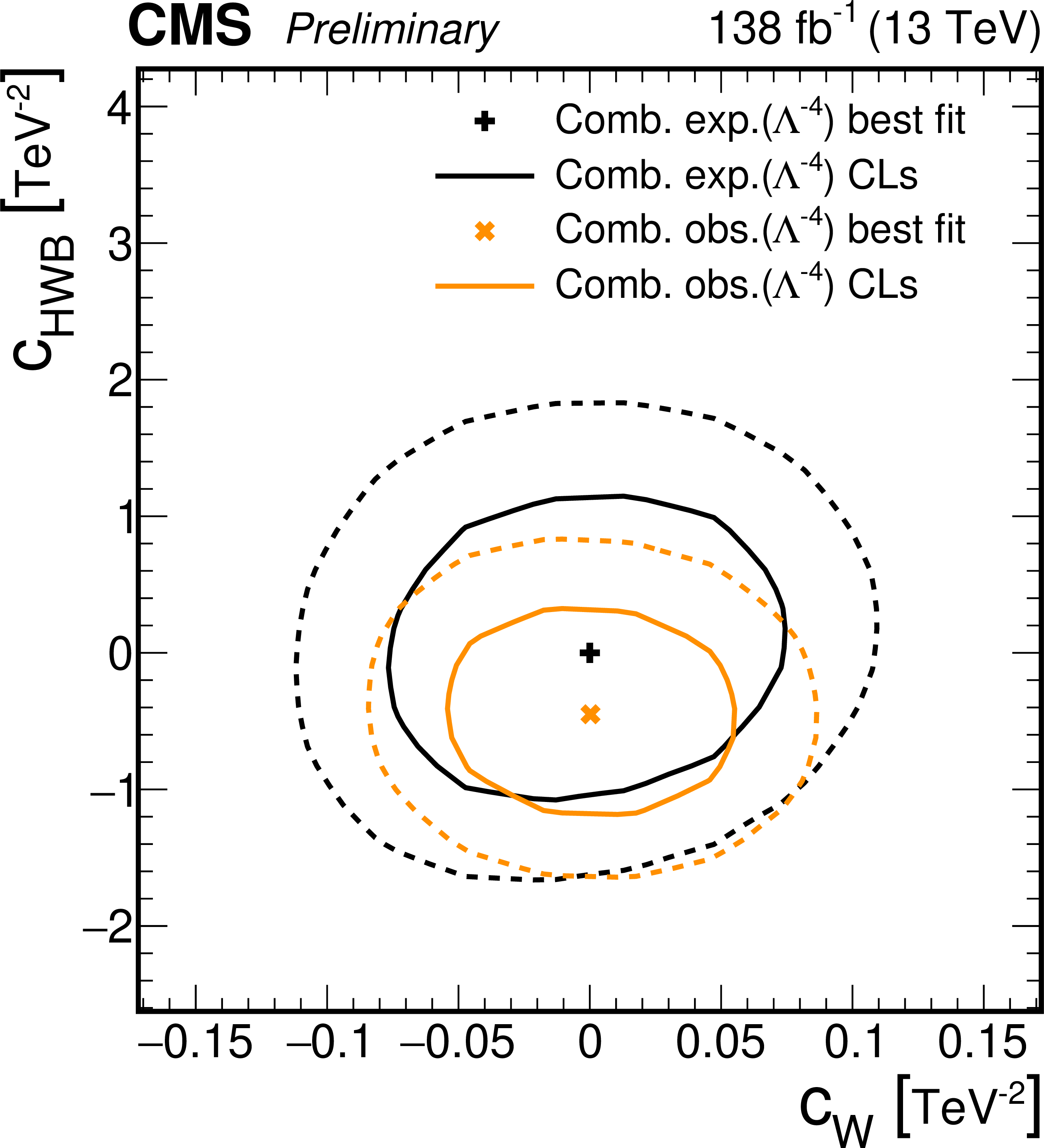
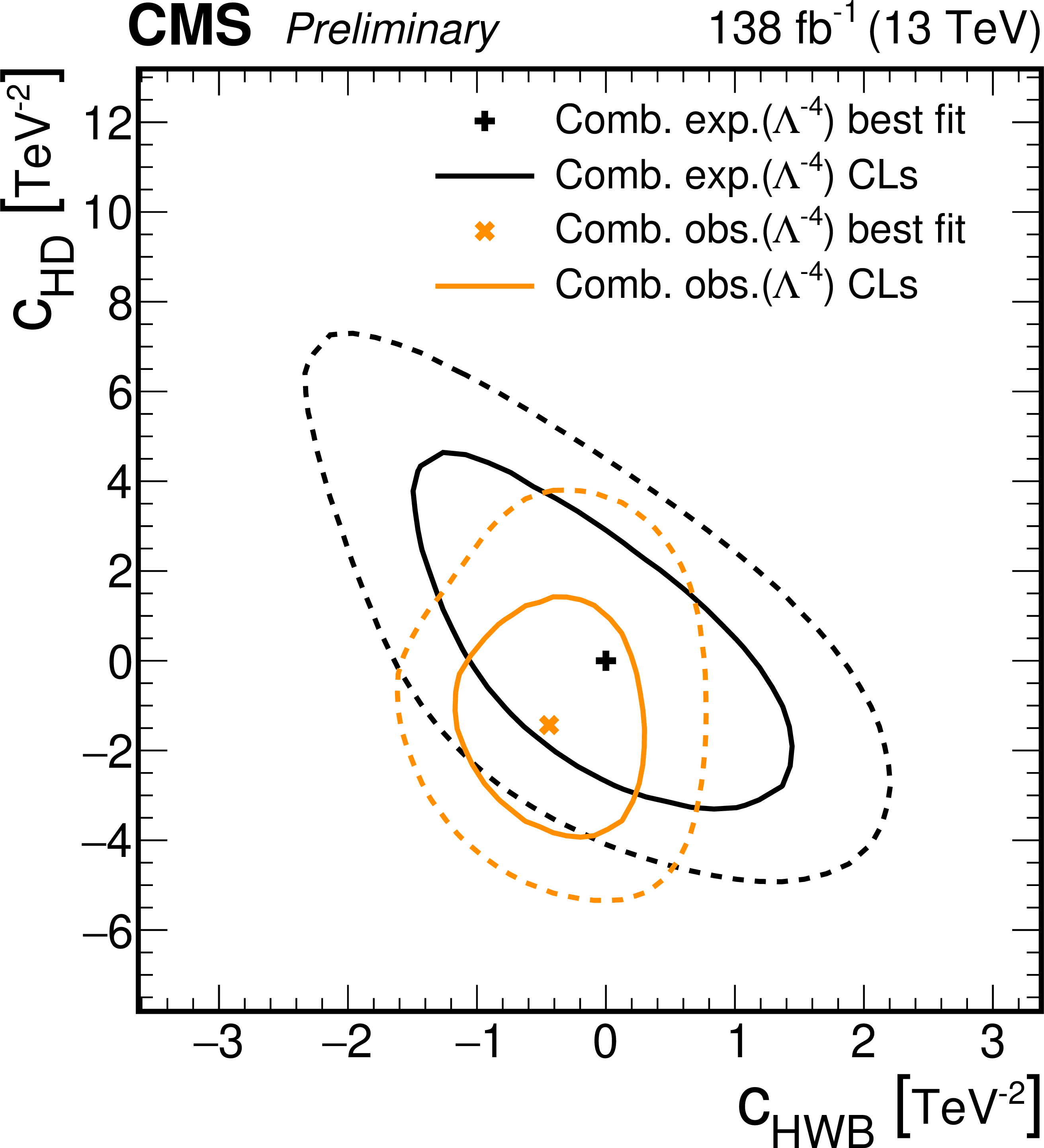
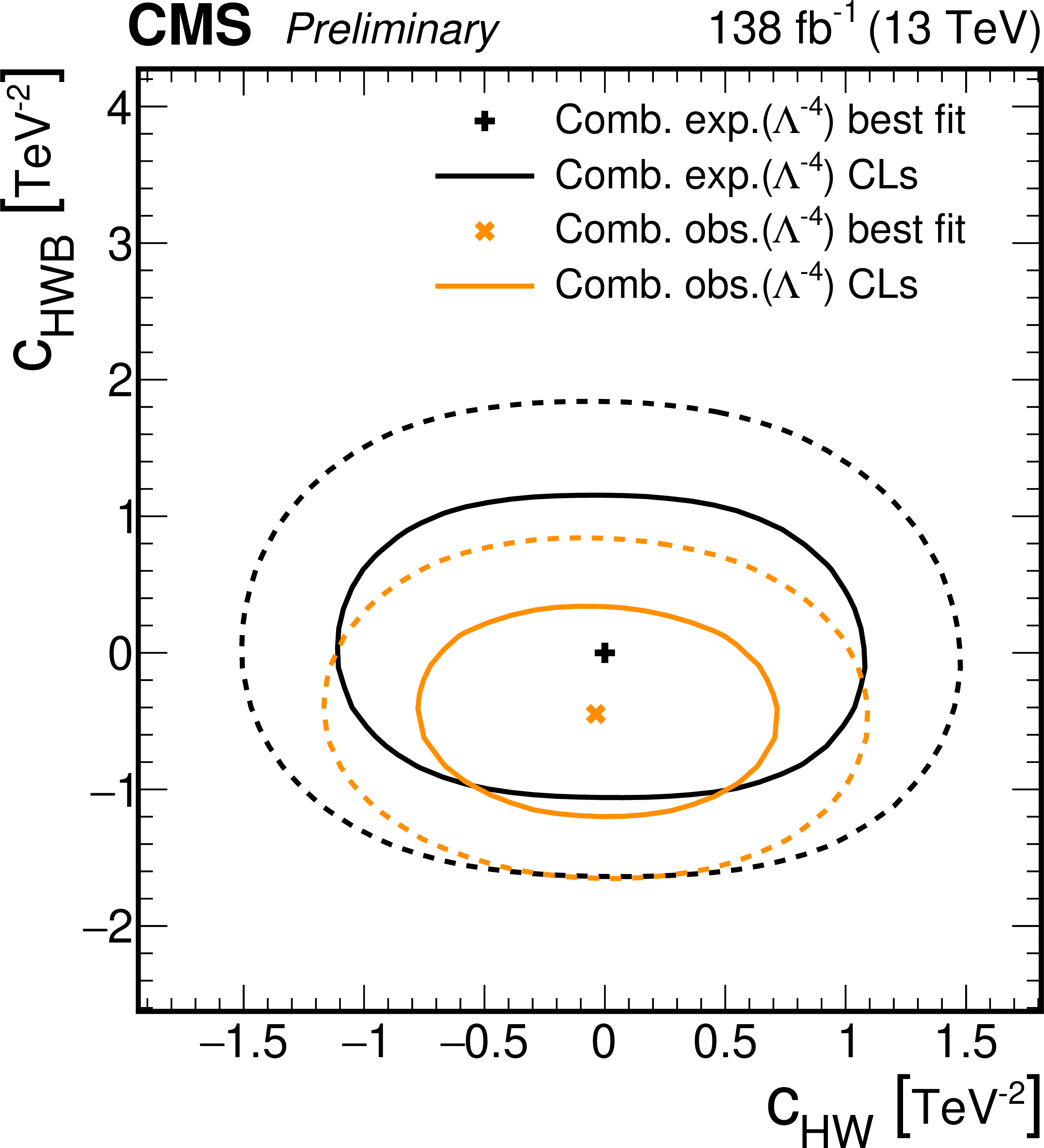
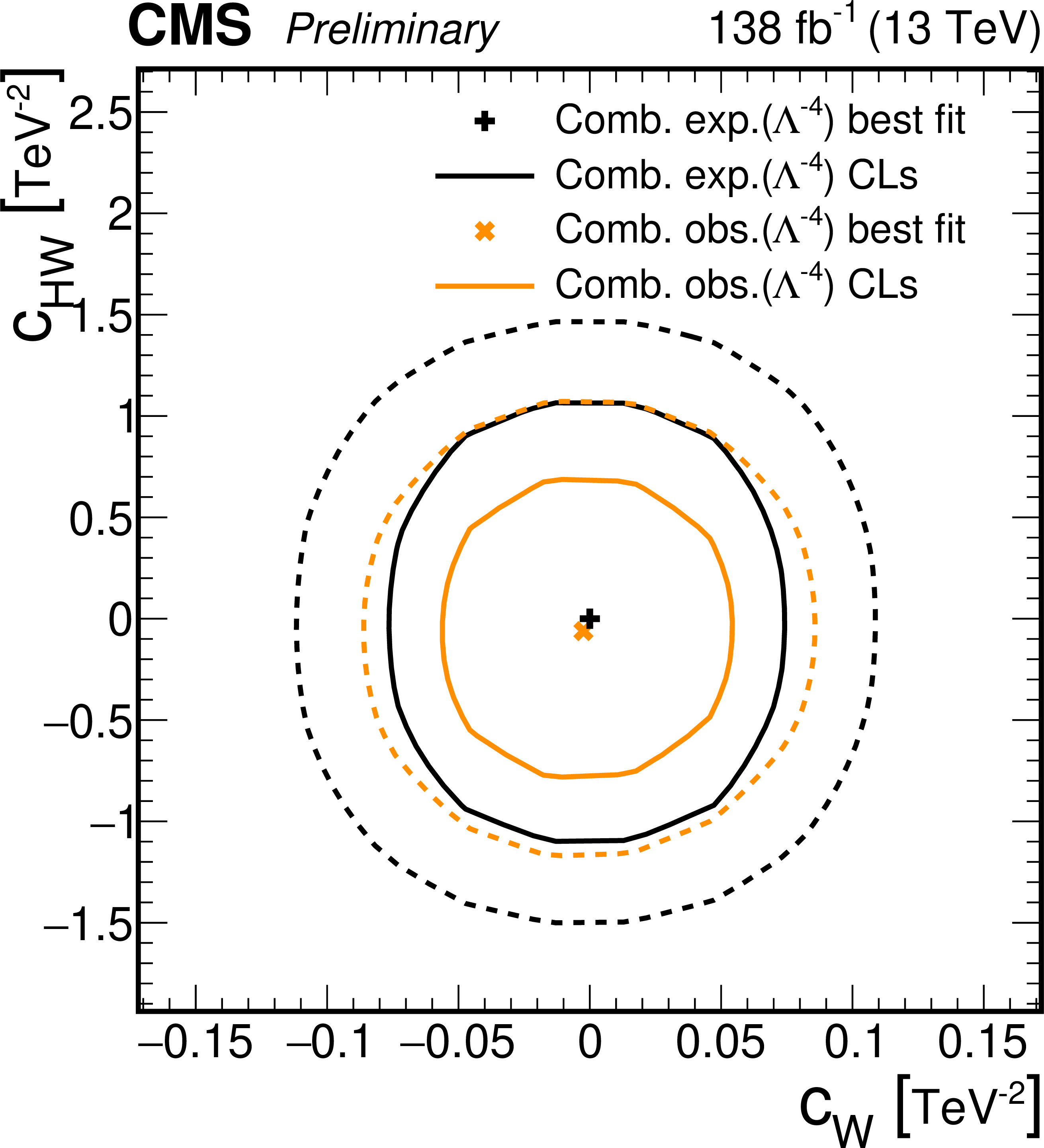
68% (solid line) and 95% (dashed line) CL contours for $ -2\ln\Delta\mathcal{L} $ as functions of the reported dim-6 Wilson coefficient pairs, both expected (black) and observed (orange). All results are obtained by considering the combination of all the channels, fixing the operators not under analysis to zero. A full table showing all pairs of operatoprs is reported in appendix 15. |
png pdf |
Figure 3-a:
68% (solid line) and 95% (dashed line) CL contours for $ -2\ln\Delta\mathcal{L} $ as functions of the reported dim-6 Wilson coefficient pairs, both expected (black) and observed (orange). All results are obtained by considering the combination of all the channels, fixing the operators not under analysis to zero. A full table showing all pairs of operatoprs is reported in appendix 15. |
png pdf |
Figure 3-b:
68% (solid line) and 95% (dashed line) CL contours for $ -2\ln\Delta\mathcal{L} $ as functions of the reported dim-6 Wilson coefficient pairs, both expected (black) and observed (orange). All results are obtained by considering the combination of all the channels, fixing the operators not under analysis to zero. A full table showing all pairs of operatoprs is reported in appendix 15. |
png pdf |
Figure 4:
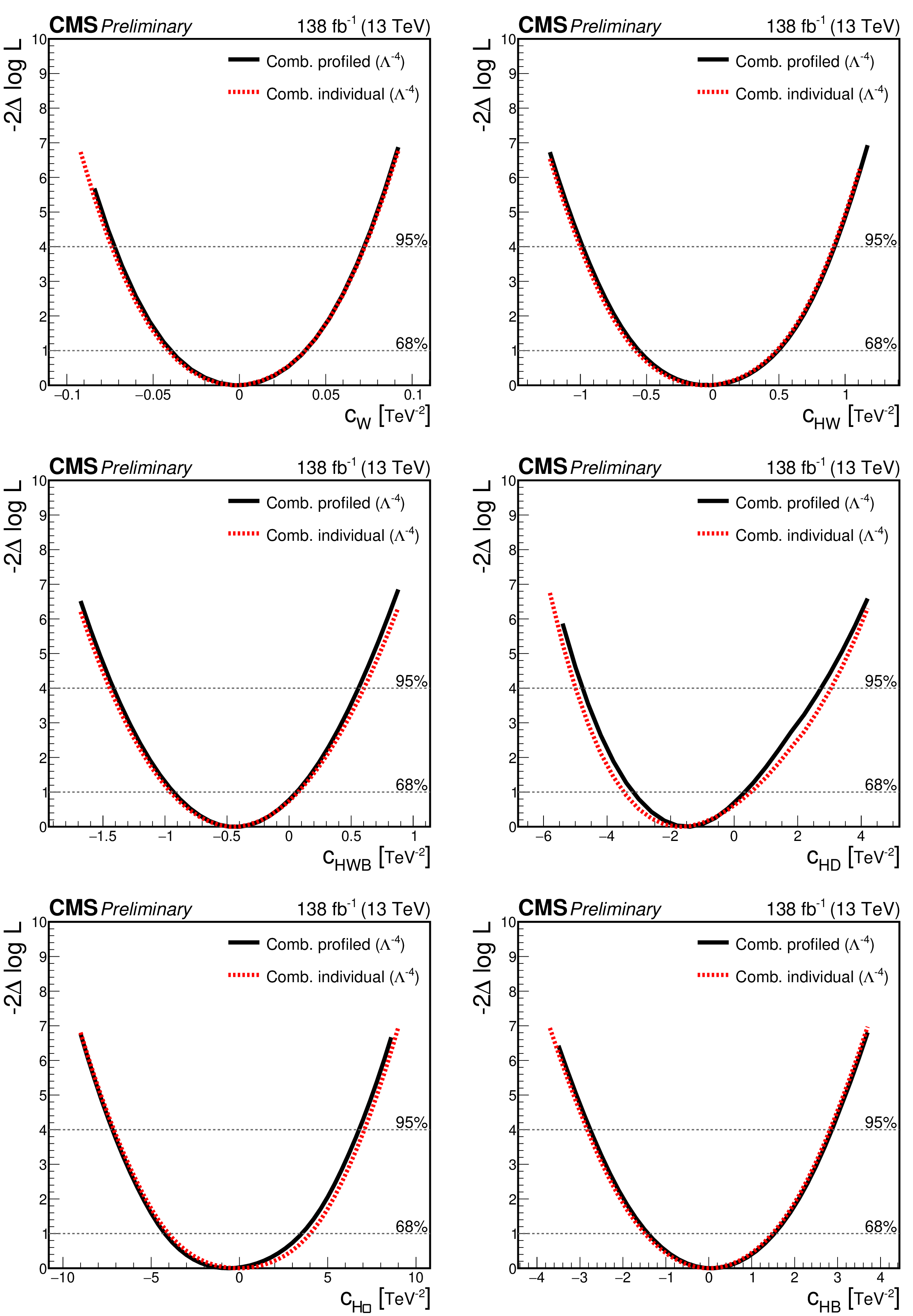
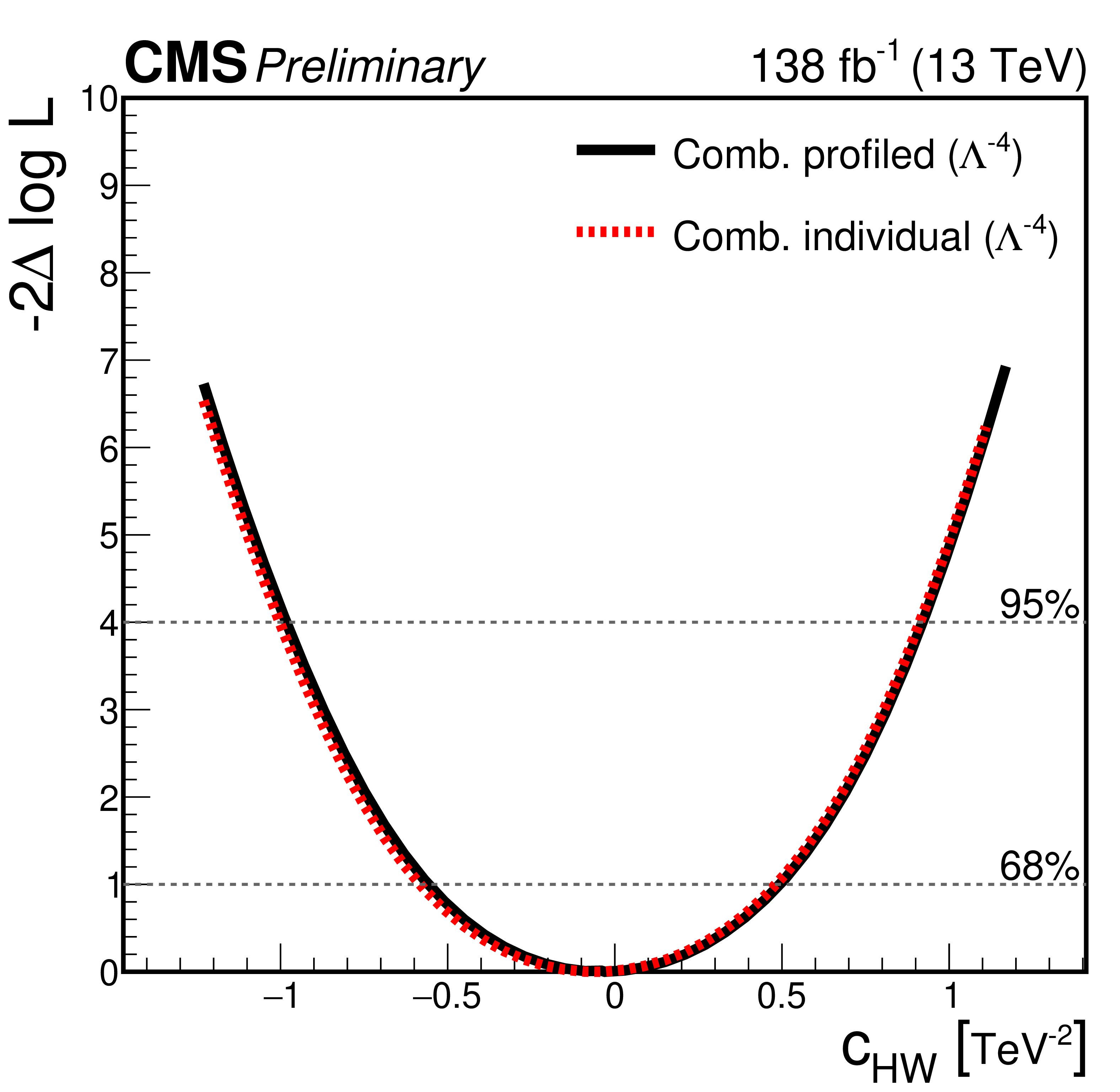
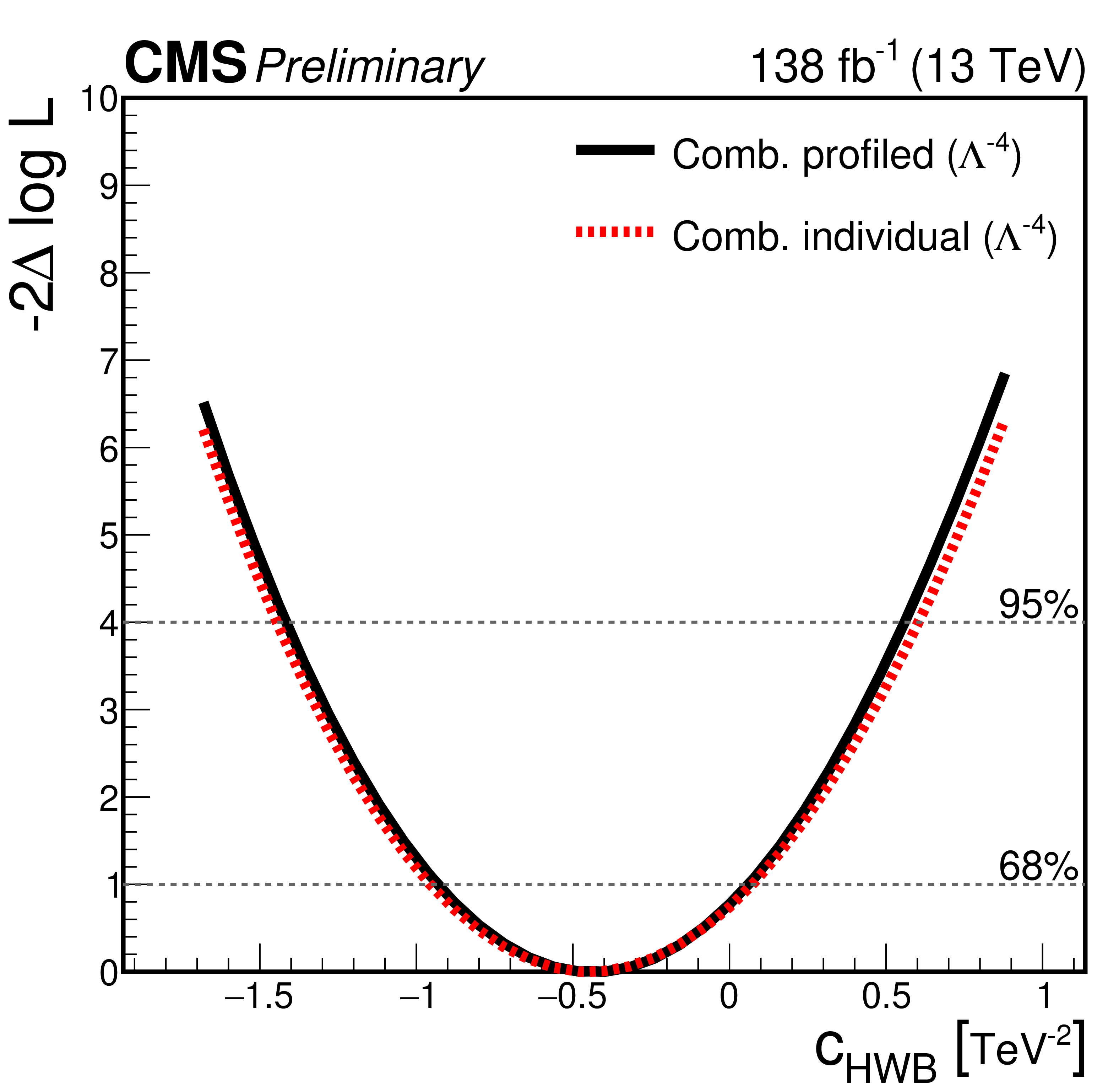
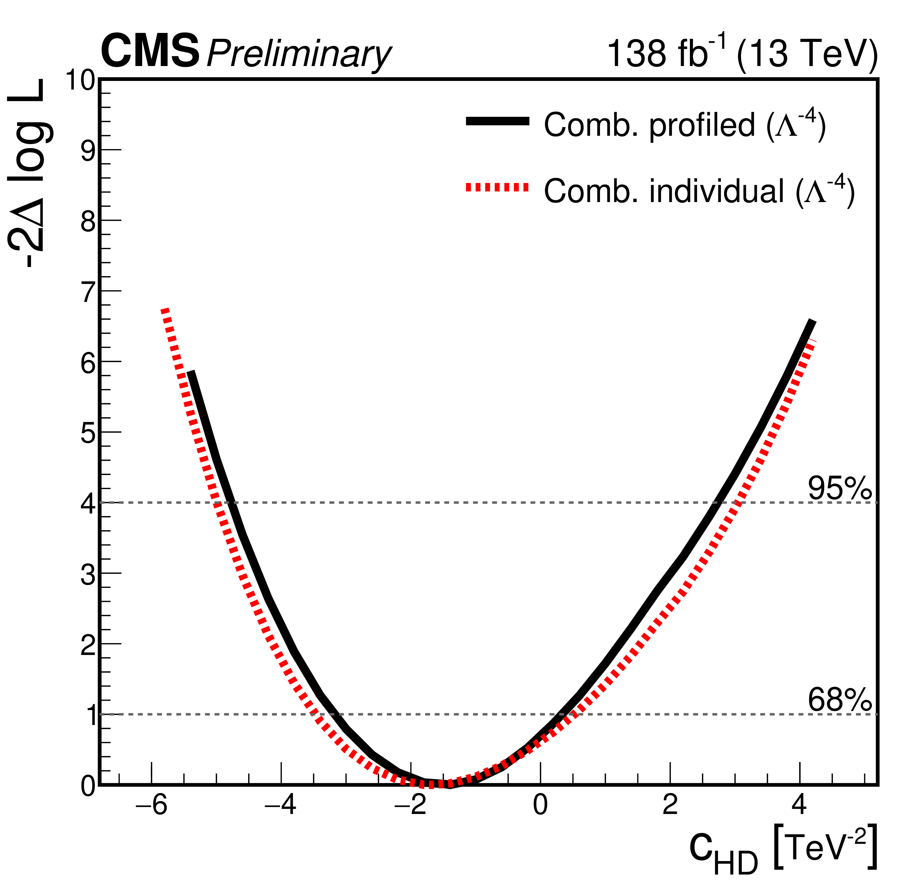
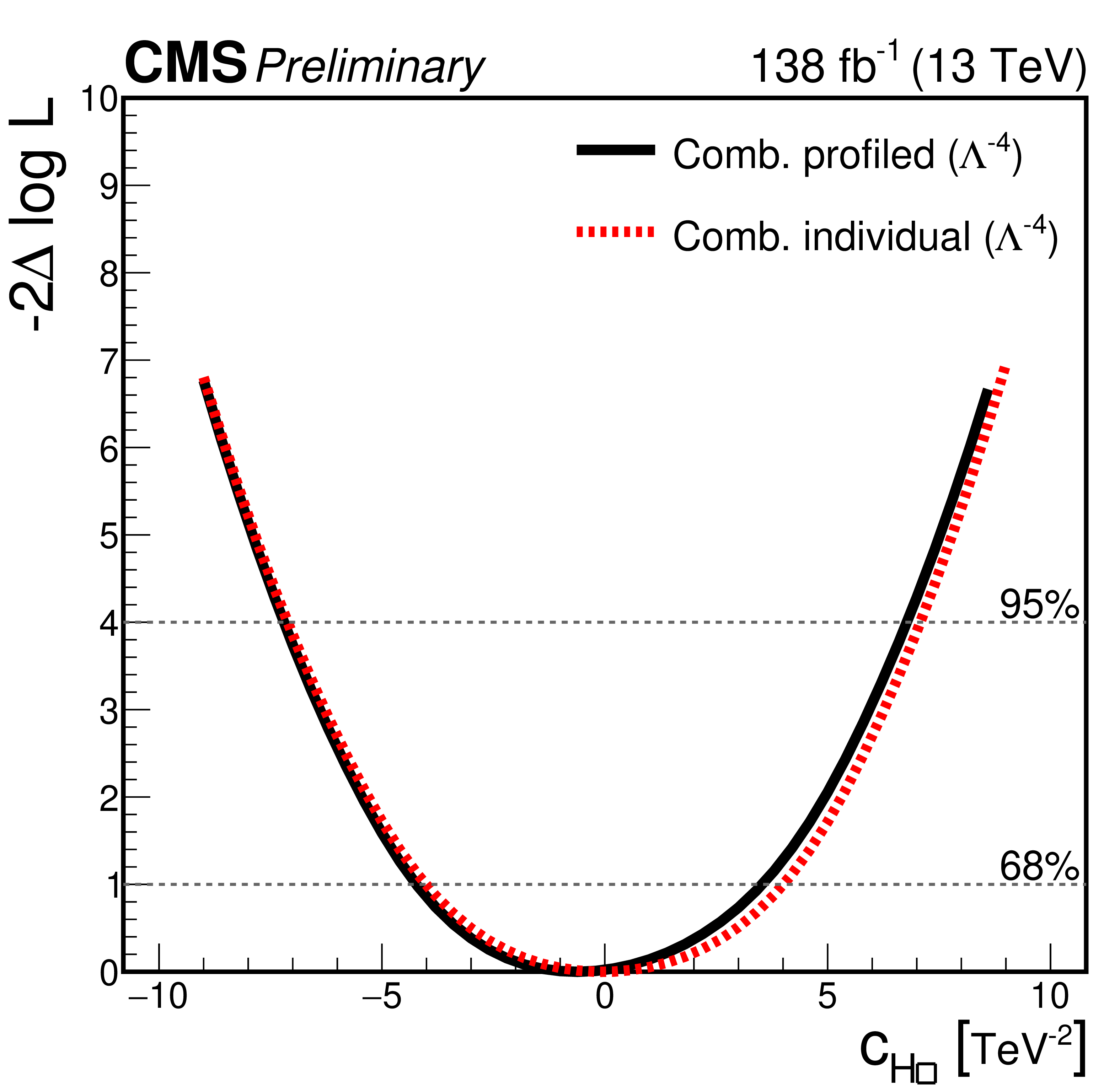
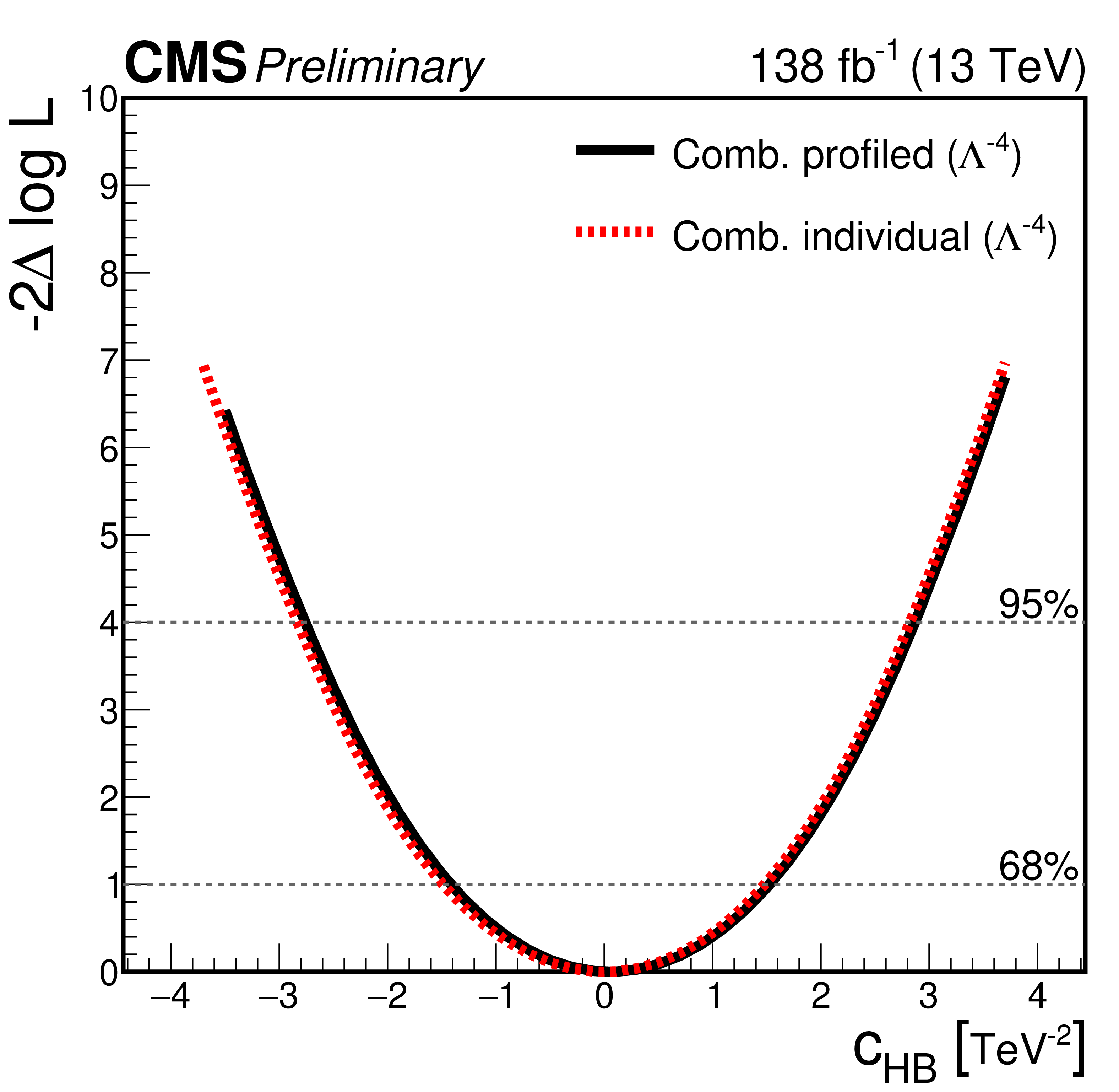
$ -2\ln\Delta\mathcal{L} $ observed scans for the six bosonic operators, fully profiled. The profiled combination fits (solid black line) were performed leaving all of the operators not under study freely floating, as well as all of the nuisance parameters. They are shown in comparison to the individual fit (red dashed line), in which all of the operators not under study are fixed to zero. Horizontal lines represent the 95% and 68% CL. |
png pdf |
Figure 4-a:
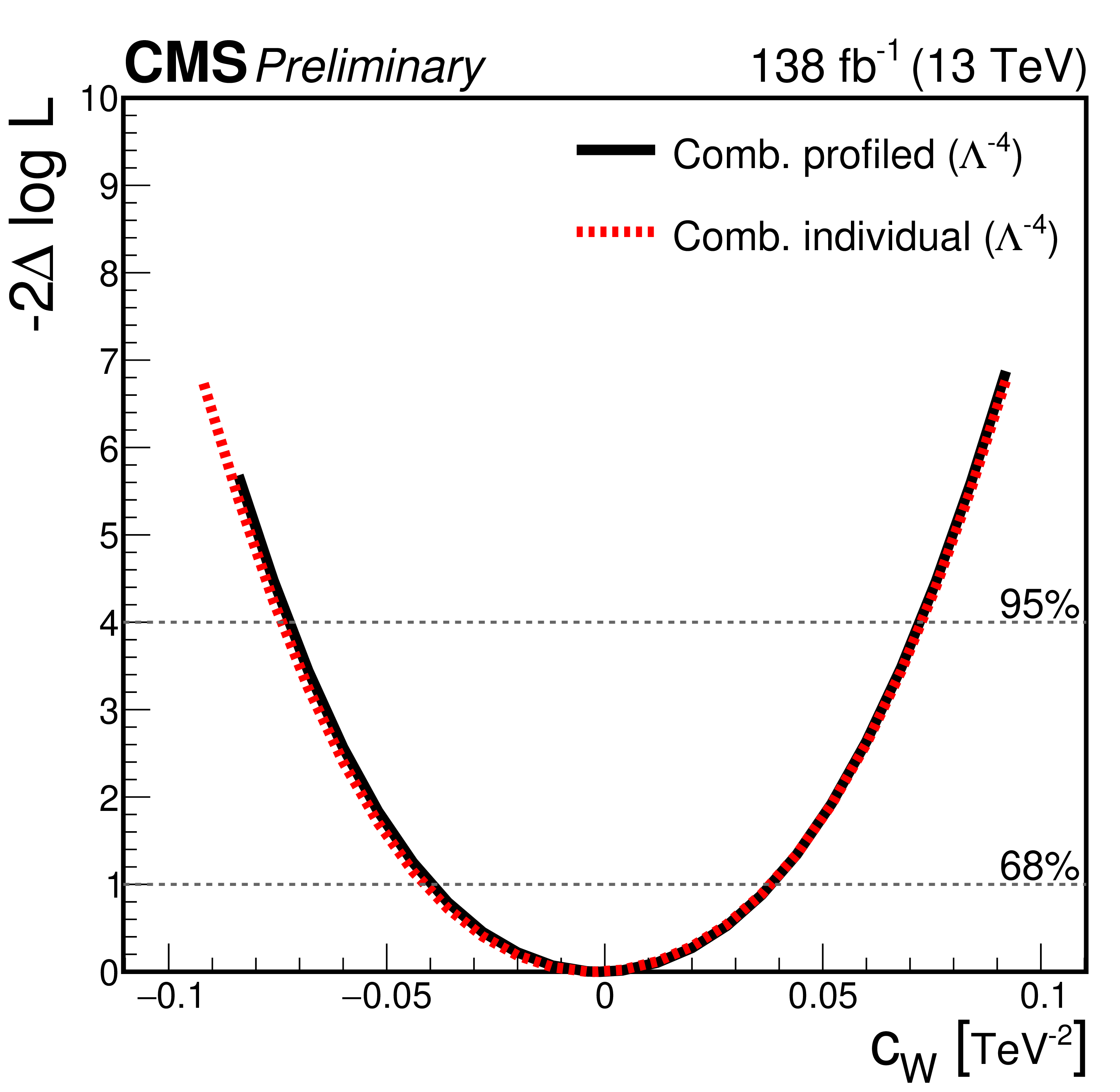
$ -2\ln\Delta\mathcal{L} $ observed scans for the six bosonic operators, fully profiled. The profiled combination fits (solid black line) were performed leaving all of the operators not under study freely floating, as well as all of the nuisance parameters. They are shown in comparison to the individual fit (red dashed line), in which all of the operators not under study are fixed to zero. Horizontal lines represent the 95% and 68% CL. |
png pdf |
Figure 4-b:
$ -2\ln\Delta\mathcal{L} $ observed scans for the six bosonic operators, fully profiled. The profiled combination fits (solid black line) were performed leaving all of the operators not under study freely floating, as well as all of the nuisance parameters. They are shown in comparison to the individual fit (red dashed line), in which all of the operators not under study are fixed to zero. Horizontal lines represent the 95% and 68% CL. |
png pdf |
Figure 4-c:
$ -2\ln\Delta\mathcal{L} $ observed scans for the six bosonic operators, fully profiled. The profiled combination fits (solid black line) were performed leaving all of the operators not under study freely floating, as well as all of the nuisance parameters. They are shown in comparison to the individual fit (red dashed line), in which all of the operators not under study are fixed to zero. Horizontal lines represent the 95% and 68% CL. |
png pdf |
Figure 4-d:
$ -2\ln\Delta\mathcal{L} $ observed scans for the six bosonic operators, fully profiled. The profiled combination fits (solid black line) were performed leaving all of the operators not under study freely floating, as well as all of the nuisance parameters. They are shown in comparison to the individual fit (red dashed line), in which all of the operators not under study are fixed to zero. Horizontal lines represent the 95% and 68% CL. |
png pdf |
Figure 4-e:
$ -2\ln\Delta\mathcal{L} $ observed scans for the six bosonic operators, fully profiled. The profiled combination fits (solid black line) were performed leaving all of the operators not under study freely floating, as well as all of the nuisance parameters. They are shown in comparison to the individual fit (red dashed line), in which all of the operators not under study are fixed to zero. Horizontal lines represent the 95% and 68% CL. |
png pdf |
Figure 4-f:
$ -2\ln\Delta\mathcal{L} $ observed scans for the six bosonic operators, fully profiled. The profiled combination fits (solid black line) were performed leaving all of the operators not under study freely floating, as well as all of the nuisance parameters. They are shown in comparison to the individual fit (red dashed line), in which all of the operators not under study are fixed to zero. Horizontal lines represent the 95% and 68% CL. |
png pdf |
Figure 5:
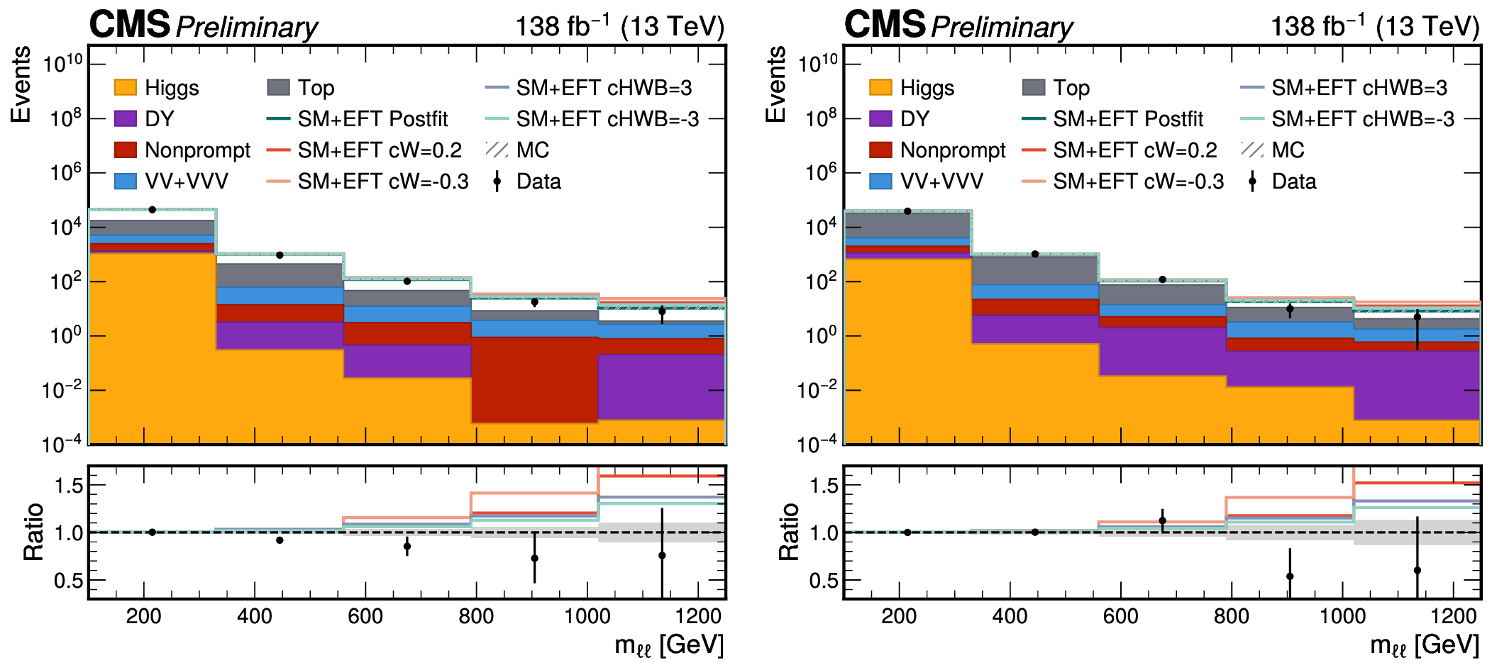
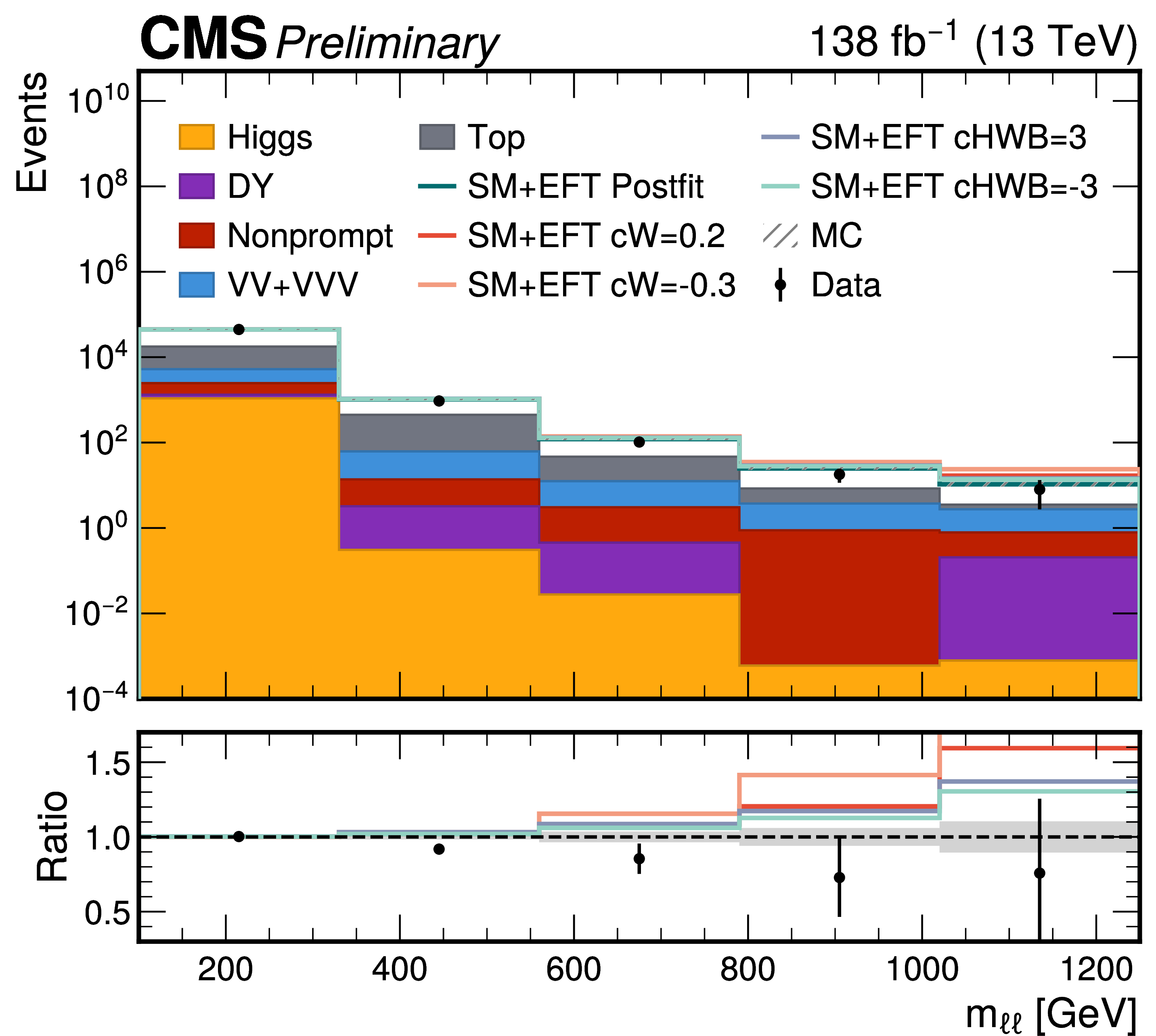
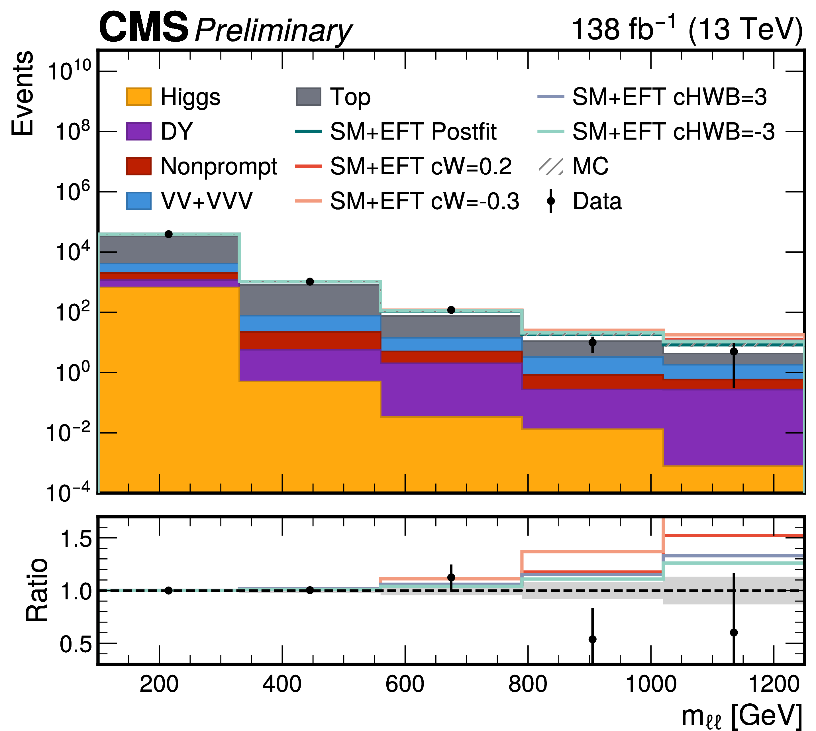
Distributions of the dilepton invariant mass $ m_{\ell\ell} $ used to extract the SMEFT signal in the $ \mathrm{W^+}\mathrm{W^-} $ analysis. Left: the $ m_{\ell\ell} $ distribution in the 0-jet signal region after the combined fit. Right: the $ m_{\ell\ell} $ distribution in the 1-jet signal region after the combined fit. The lower panels show the ratio to the best-fit prediction. Different SMEFT scenarios, each corresponding to a distinct value of a Wilson coefficient, are shown as solid coloured lines. |
png pdf |
Figure 5-a:
Distributions of the dilepton invariant mass $ m_{\ell\ell} $ used to extract the SMEFT signal in the $ \mathrm{W^+}\mathrm{W^-} $ analysis. Left: the $ m_{\ell\ell} $ distribution in the 0-jet signal region after the combined fit. Right: the $ m_{\ell\ell} $ distribution in the 1-jet signal region after the combined fit. The lower panels show the ratio to the best-fit prediction. Different SMEFT scenarios, each corresponding to a distinct value of a Wilson coefficient, are shown as solid coloured lines. |
png pdf |
Figure 5-b:
Distributions of the dilepton invariant mass $ m_{\ell\ell} $ used to extract the SMEFT signal in the $ \mathrm{W^+}\mathrm{W^-} $ analysis. Left: the $ m_{\ell\ell} $ distribution in the 0-jet signal region after the combined fit. Right: the $ m_{\ell\ell} $ distribution in the 1-jet signal region after the combined fit. The lower panels show the ratio to the best-fit prediction. Different SMEFT scenarios, each corresponding to a distinct value of a Wilson coefficient, are shown as solid coloured lines. |
png pdf |
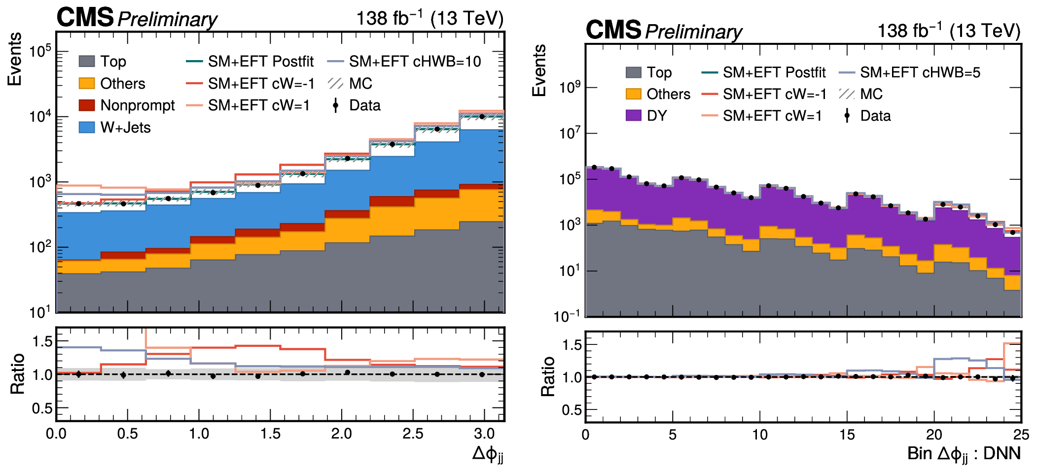
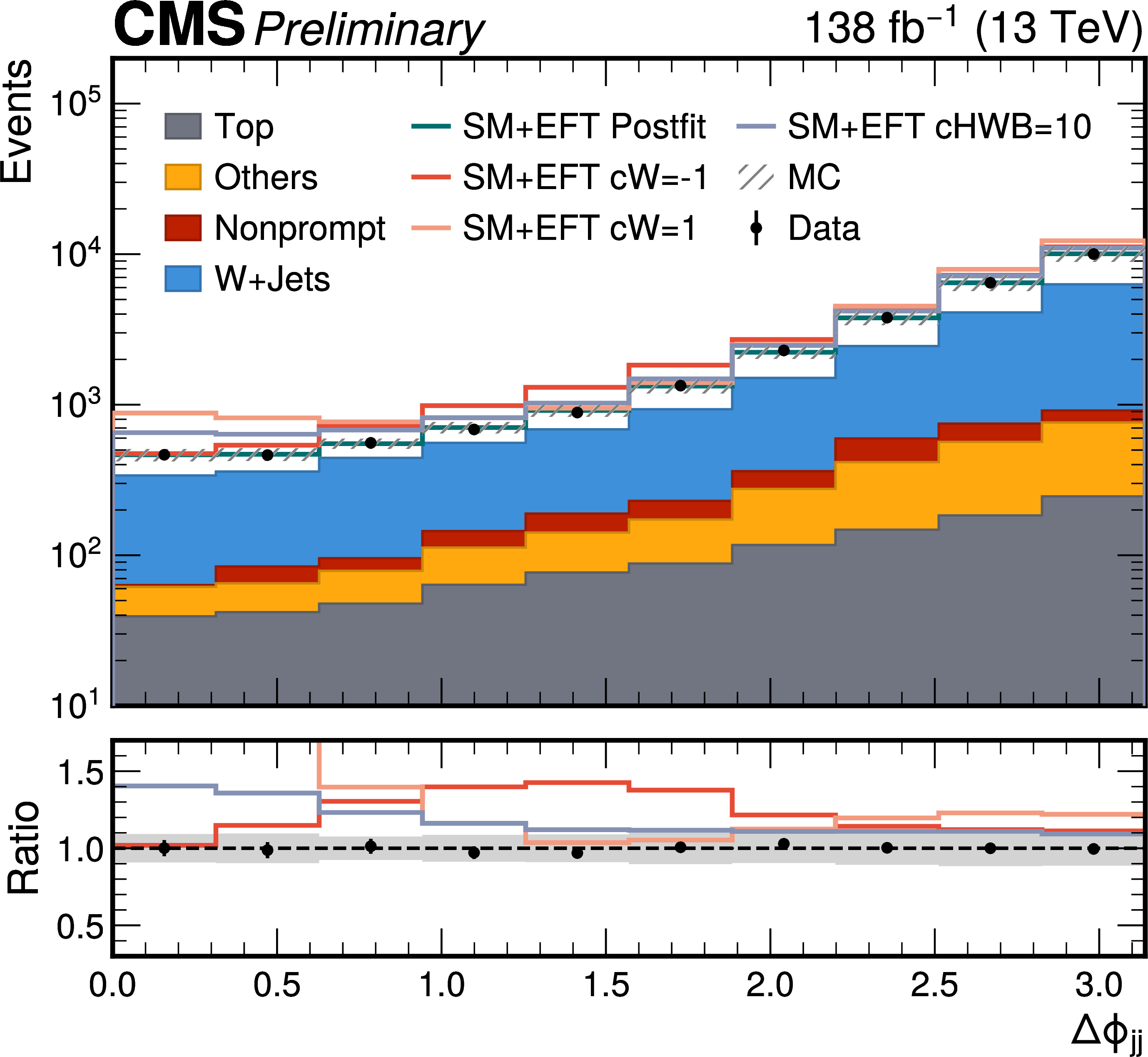
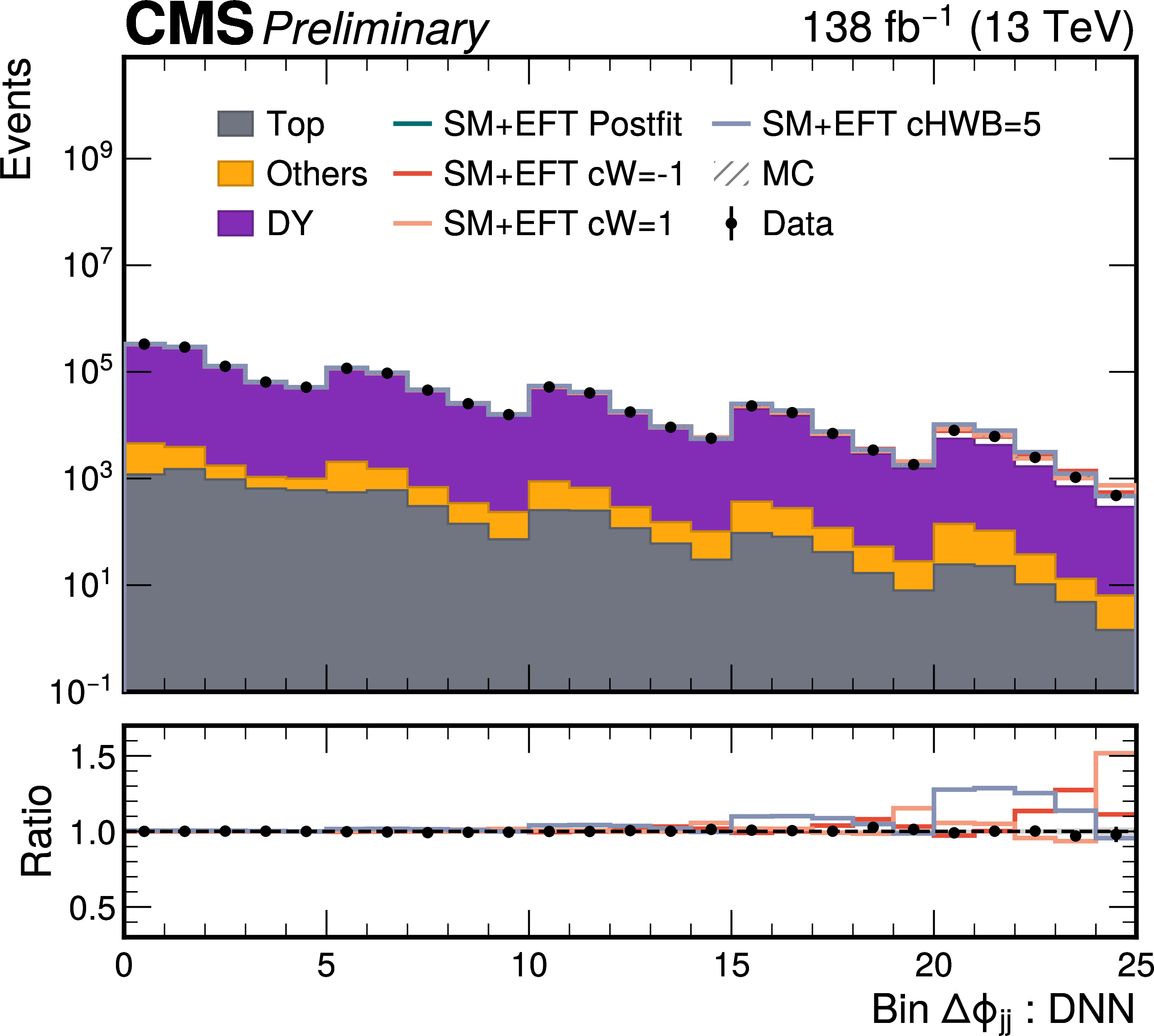
Figure 6:
Distributions of the observables used to extract the SMEFT signal in the VBF analyses. Left: the $ \Delta\phi{{\mathrm{j}}{\mathrm{j}}} $ distribution in the VBF-W signal region after the combined fit. Right: the $ \Delta\phi{{\mathrm{j}}{\mathrm{j}}} $ distribution in windows of DNN score used to discriminate the VBF signal from the SM backgrounds in the VBF-Z analysis. The lower panels show the ratio to the best-fit prediction. Different SMEFT scenarios, each corresponding to a distinct value of a Wilson coefficient, are shown as solid coloured lines. |
png pdf |
Figure 6-a:
Distributions of the observables used to extract the SMEFT signal in the VBF analyses. Left: the $ \Delta\phi{{\mathrm{j}}{\mathrm{j}}} $ distribution in the VBF-W signal region after the combined fit. Right: the $ \Delta\phi{{\mathrm{j}}{\mathrm{j}}} $ distribution in windows of DNN score used to discriminate the VBF signal from the SM backgrounds in the VBF-Z analysis. The lower panels show the ratio to the best-fit prediction. Different SMEFT scenarios, each corresponding to a distinct value of a Wilson coefficient, are shown as solid coloured lines. |
png pdf |
Figure 6-b:
Distributions of the observables used to extract the SMEFT signal in the VBF analyses. Left: the $ \Delta\phi{{\mathrm{j}}{\mathrm{j}}} $ distribution in the VBF-W signal region after the combined fit. Right: the $ \Delta\phi{{\mathrm{j}}{\mathrm{j}}} $ distribution in windows of DNN score used to discriminate the VBF signal from the SM backgrounds in the VBF-Z analysis. The lower panels show the ratio to the best-fit prediction. Different SMEFT scenarios, each corresponding to a distinct value of a Wilson coefficient, are shown as solid coloured lines. |
png pdf |
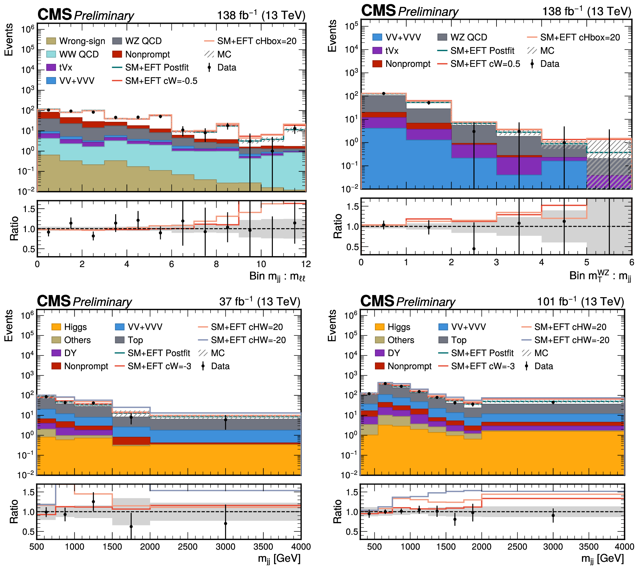
Figure 7:
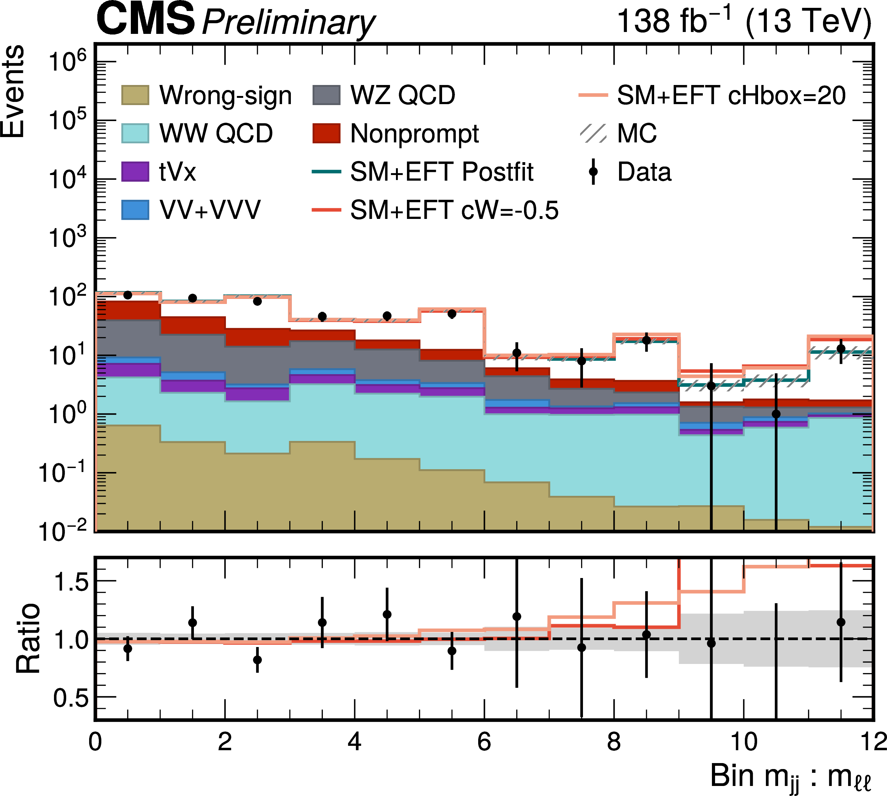
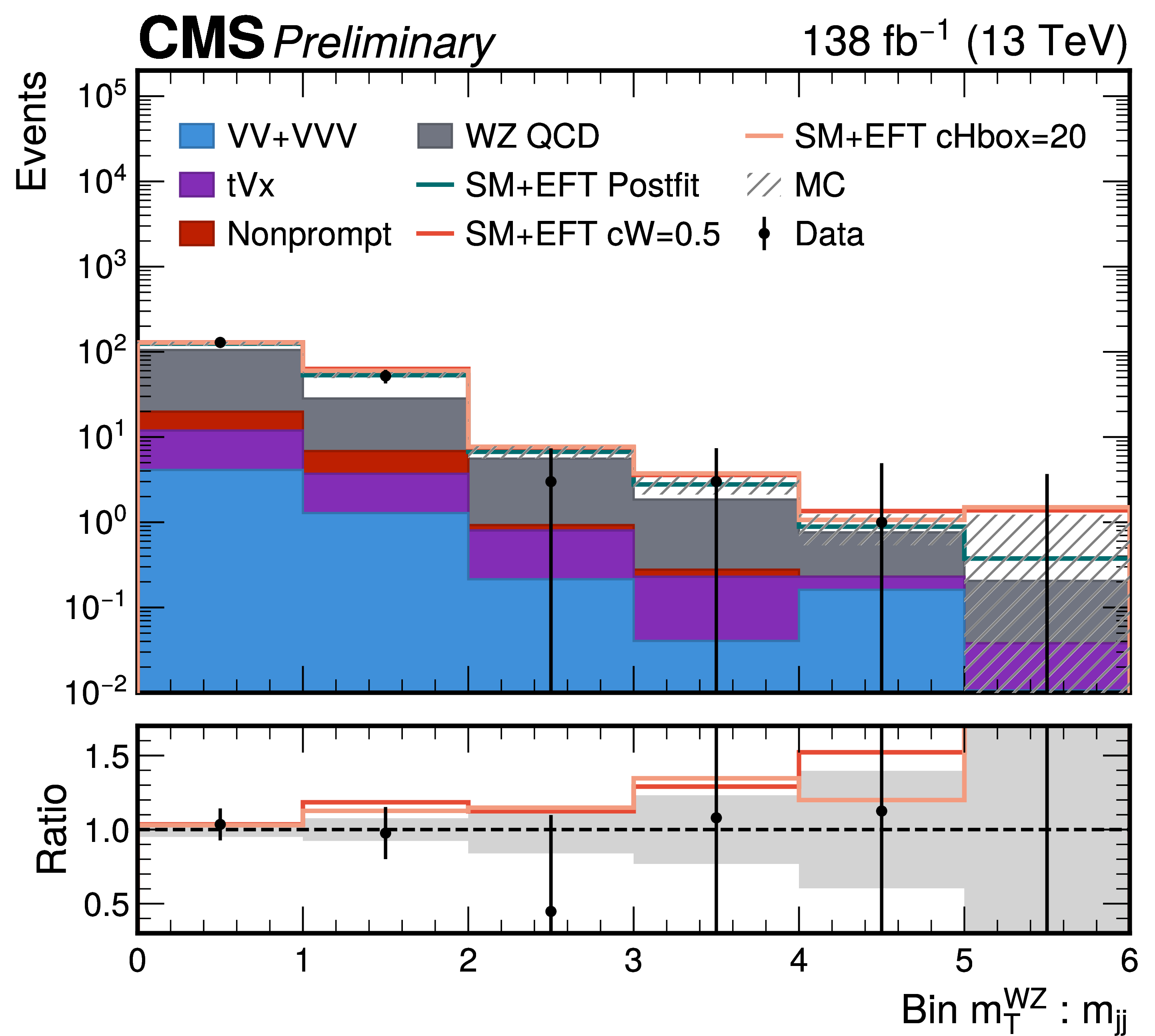
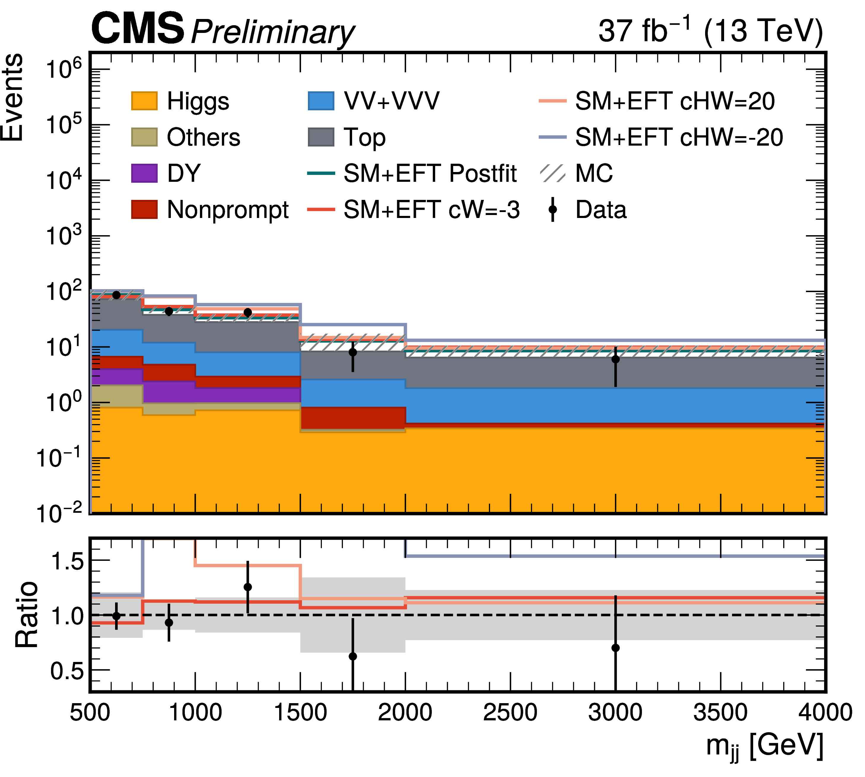
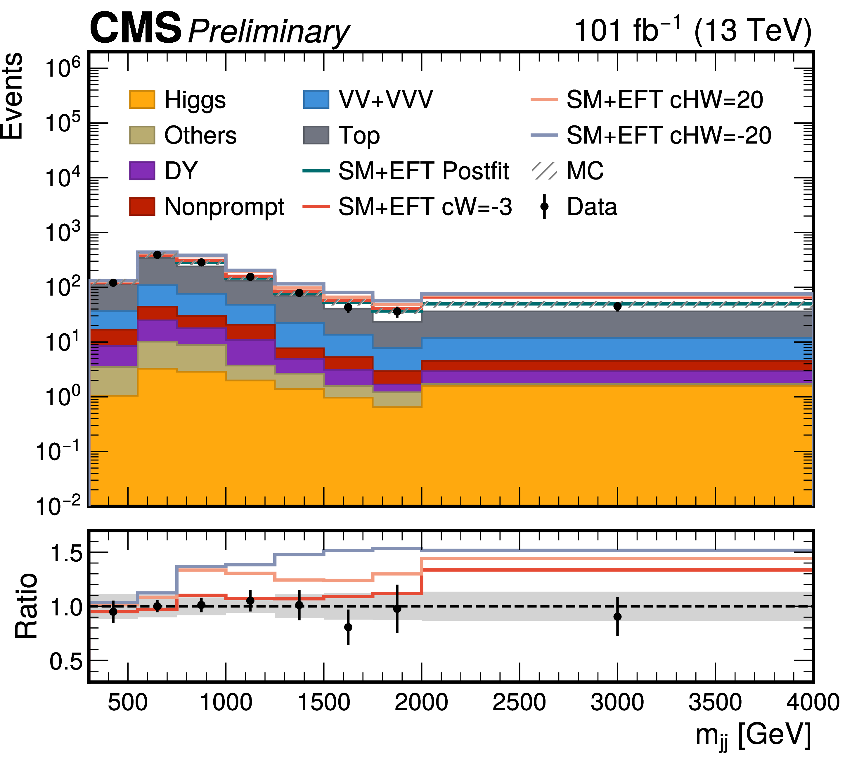
Distributions of the observables used to extract the SMEFT signal in the SSWW, WZ and OSWW analyses. Top left: the $ m_{jj} $ distribution in windows of $ m_{\ell\ell} $ in the SSWW signal region, after the combined fit. Top right: the $ m_{T}^{WZ} $ distribution in windows of $ m_{jj} $ in the WZ signal region, after the combined fit. Bottom: the $ m_{jj} $ distribution in the OSWW signal region, for the 2016 data taking period (left) and 2017 and 2018 (right). The lower panels of each plot show the ratio to the best-fit prediction. Different SMEFT scenarios, each corresponding to a distinct value of a Wilson coefficient, are shown as solid coloured lines. |
png pdf |
Figure 7-a:
Distributions of the observables used to extract the SMEFT signal in the SSWW, WZ and OSWW analyses. Top left: the $ m_{jj} $ distribution in windows of $ m_{\ell\ell} $ in the SSWW signal region, after the combined fit. Top right: the $ m_{T}^{WZ} $ distribution in windows of $ m_{jj} $ in the WZ signal region, after the combined fit. Bottom: the $ m_{jj} $ distribution in the OSWW signal region, for the 2016 data taking period (left) and 2017 and 2018 (right). The lower panels of each plot show the ratio to the best-fit prediction. Different SMEFT scenarios, each corresponding to a distinct value of a Wilson coefficient, are shown as solid coloured lines. |
png pdf |
Figure 7-b:
Distributions of the observables used to extract the SMEFT signal in the SSWW, WZ and OSWW analyses. Top left: the $ m_{jj} $ distribution in windows of $ m_{\ell\ell} $ in the SSWW signal region, after the combined fit. Top right: the $ m_{T}^{WZ} $ distribution in windows of $ m_{jj} $ in the WZ signal region, after the combined fit. Bottom: the $ m_{jj} $ distribution in the OSWW signal region, for the 2016 data taking period (left) and 2017 and 2018 (right). The lower panels of each plot show the ratio to the best-fit prediction. Different SMEFT scenarios, each corresponding to a distinct value of a Wilson coefficient, are shown as solid coloured lines. |
png pdf |
Figure 7-c:
Distributions of the observables used to extract the SMEFT signal in the SSWW, WZ and OSWW analyses. Top left: the $ m_{jj} $ distribution in windows of $ m_{\ell\ell} $ in the SSWW signal region, after the combined fit. Top right: the $ m_{T}^{WZ} $ distribution in windows of $ m_{jj} $ in the WZ signal region, after the combined fit. Bottom: the $ m_{jj} $ distribution in the OSWW signal region, for the 2016 data taking period (left) and 2017 and 2018 (right). The lower panels of each plot show the ratio to the best-fit prediction. Different SMEFT scenarios, each corresponding to a distinct value of a Wilson coefficient, are shown as solid coloured lines. |
png pdf |
Figure 7-d:
Distributions of the observables used to extract the SMEFT signal in the SSWW, WZ and OSWW analyses. Top left: the $ m_{jj} $ distribution in windows of $ m_{\ell\ell} $ in the SSWW signal region, after the combined fit. Top right: the $ m_{T}^{WZ} $ distribution in windows of $ m_{jj} $ in the WZ signal region, after the combined fit. Bottom: the $ m_{jj} $ distribution in the OSWW signal region, for the 2016 data taking period (left) and 2017 and 2018 (right). The lower panels of each plot show the ratio to the best-fit prediction. Different SMEFT scenarios, each corresponding to a distinct value of a Wilson coefficient, are shown as solid coloured lines. |
png pdf |
Figure 8:
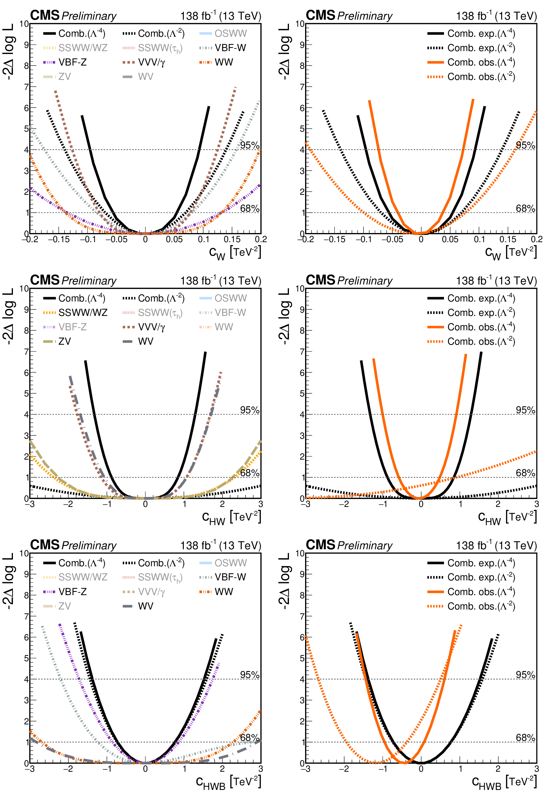
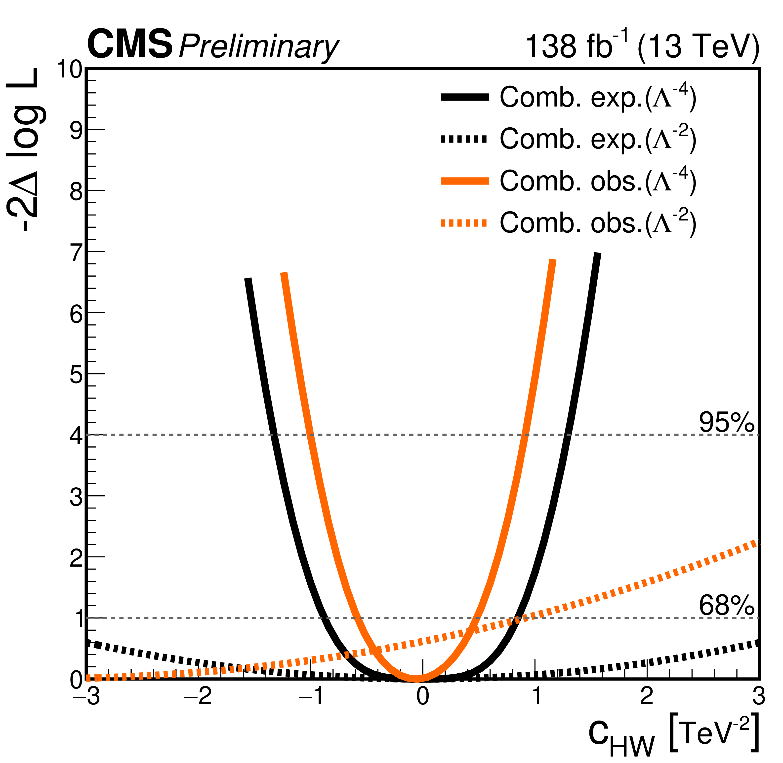
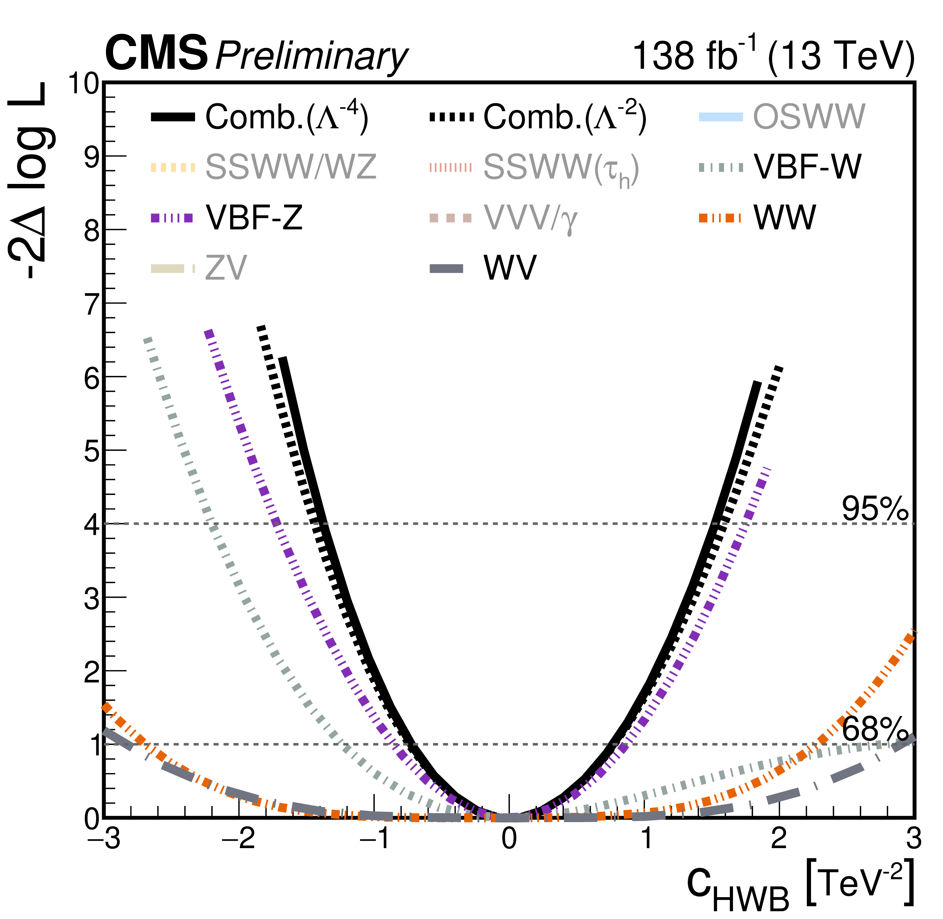
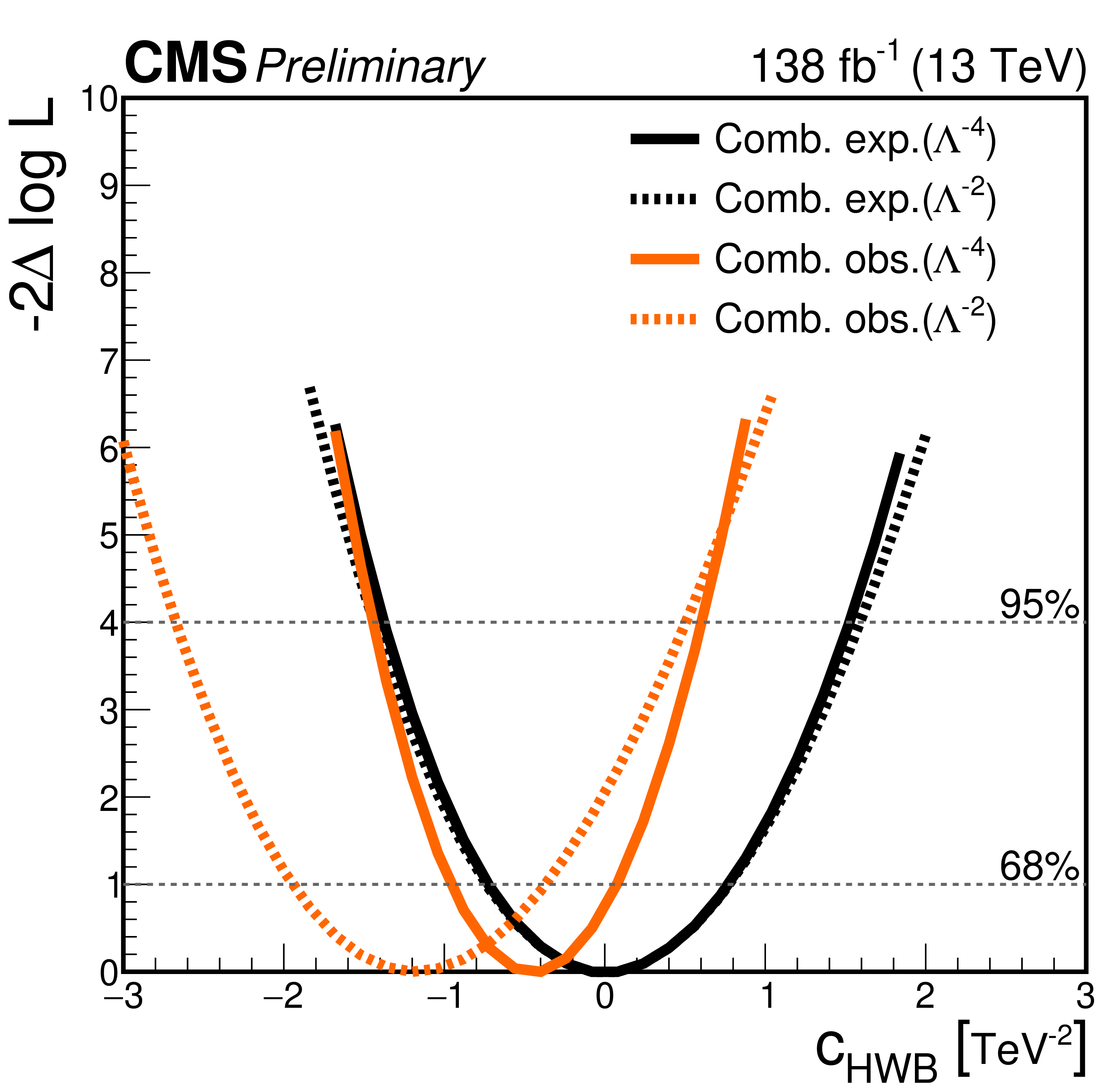
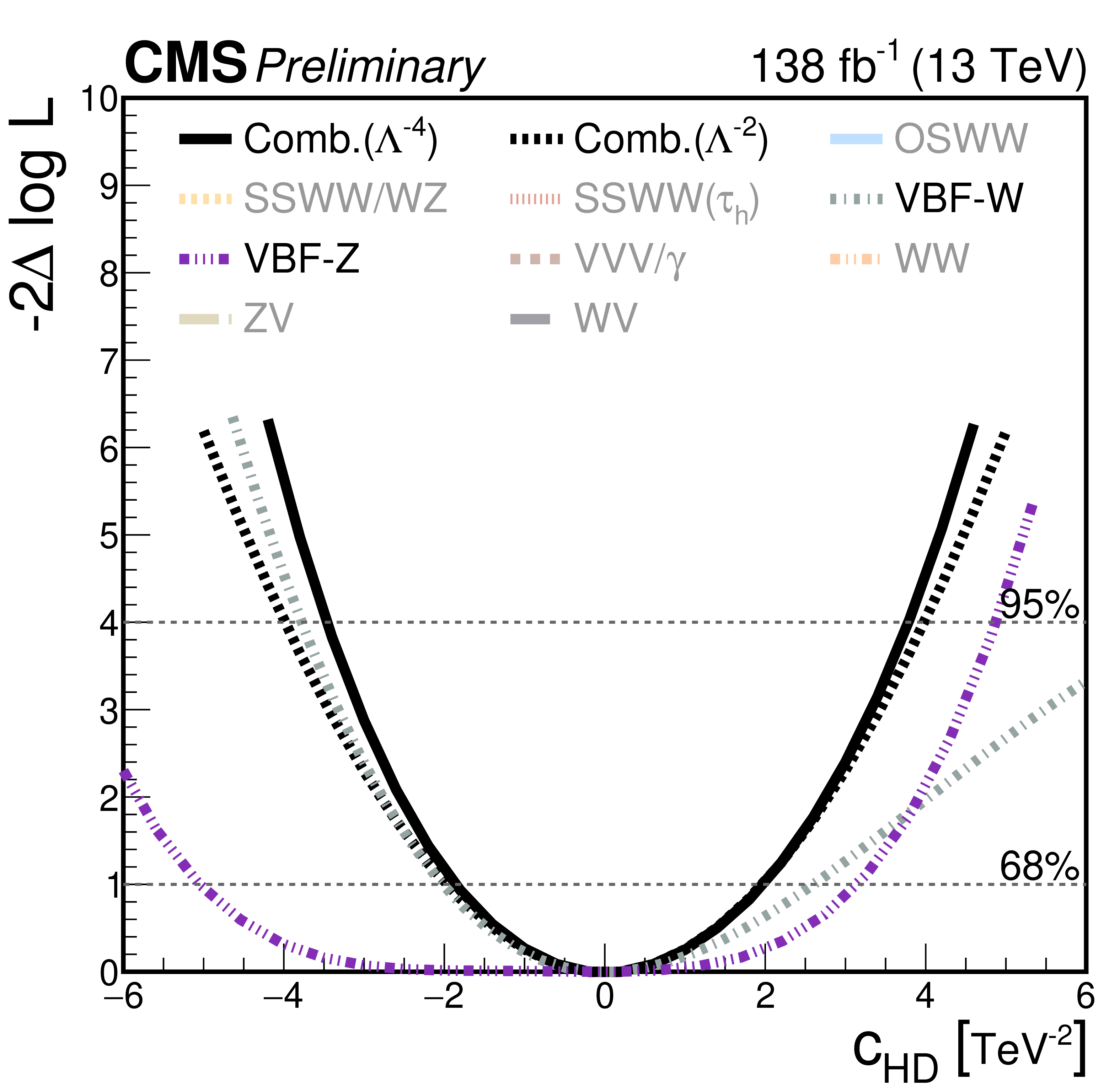
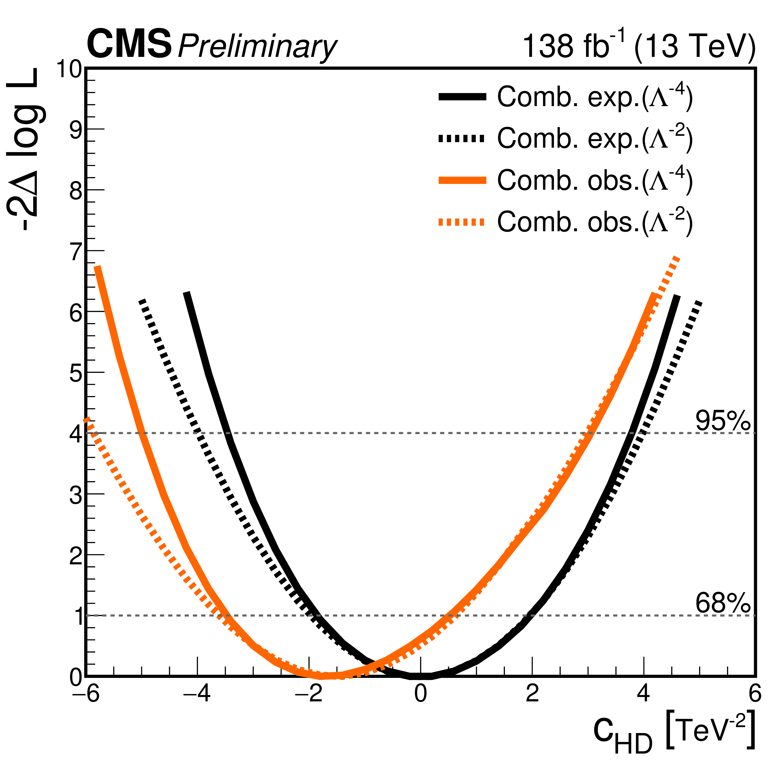
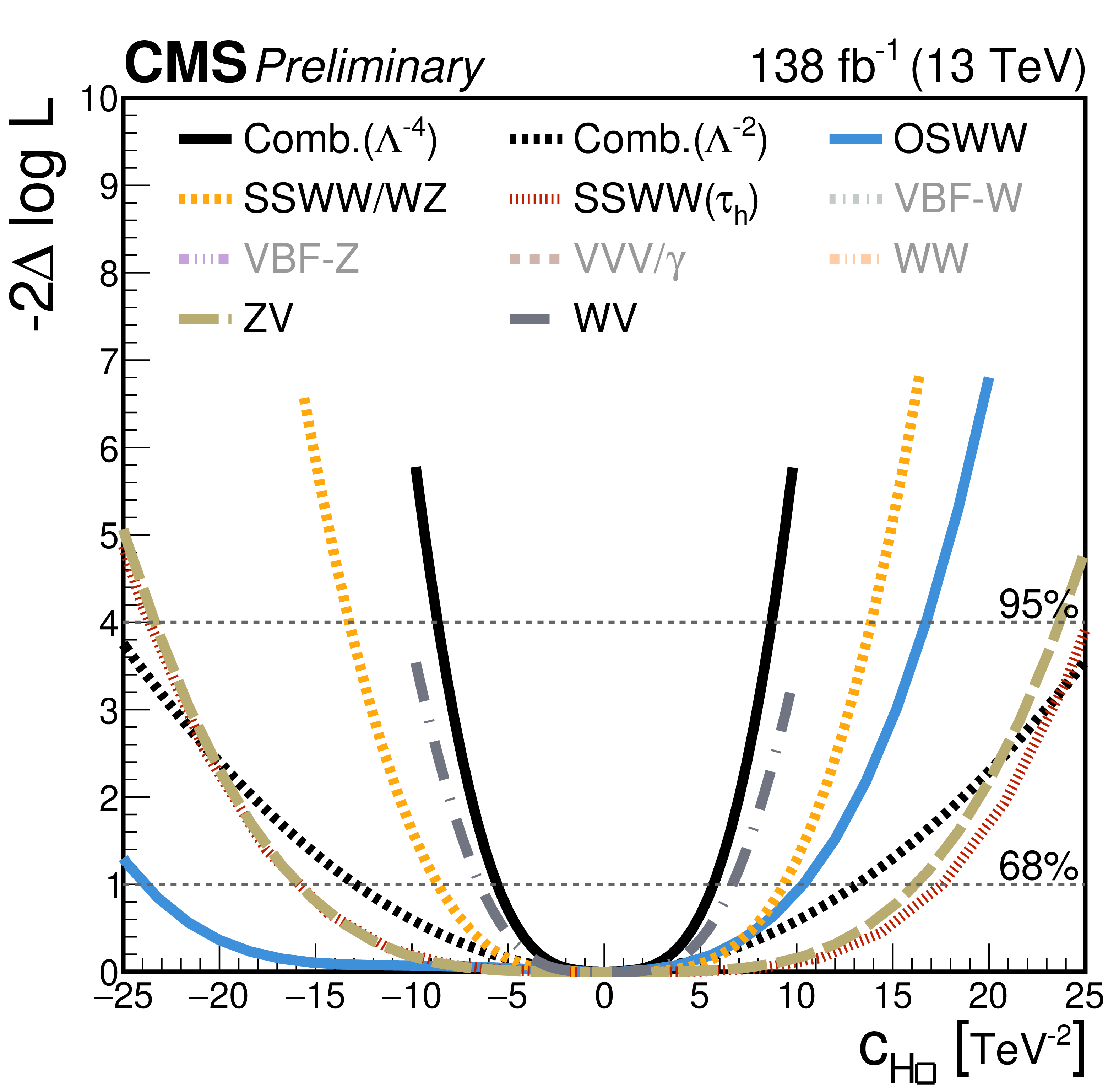
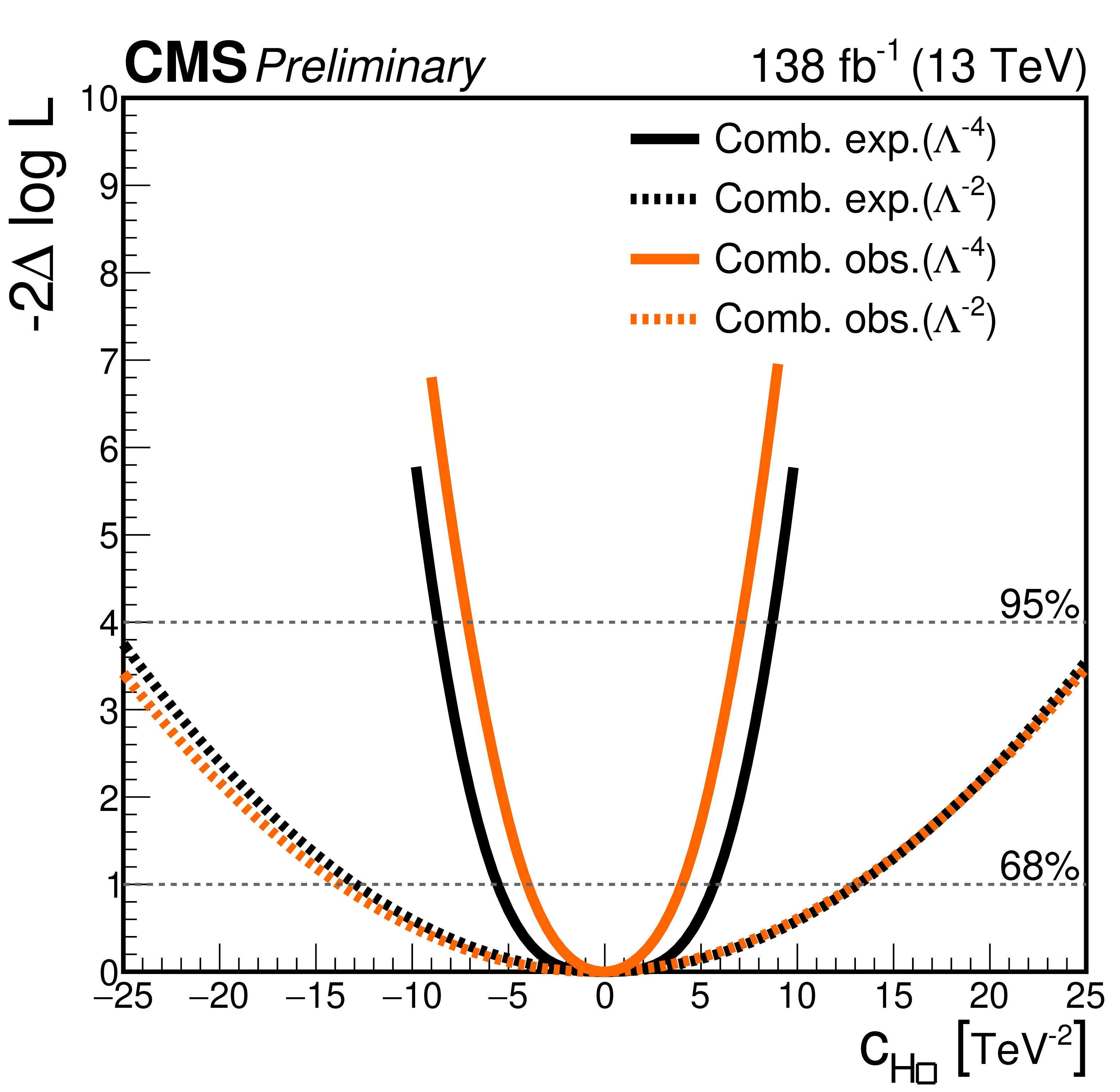
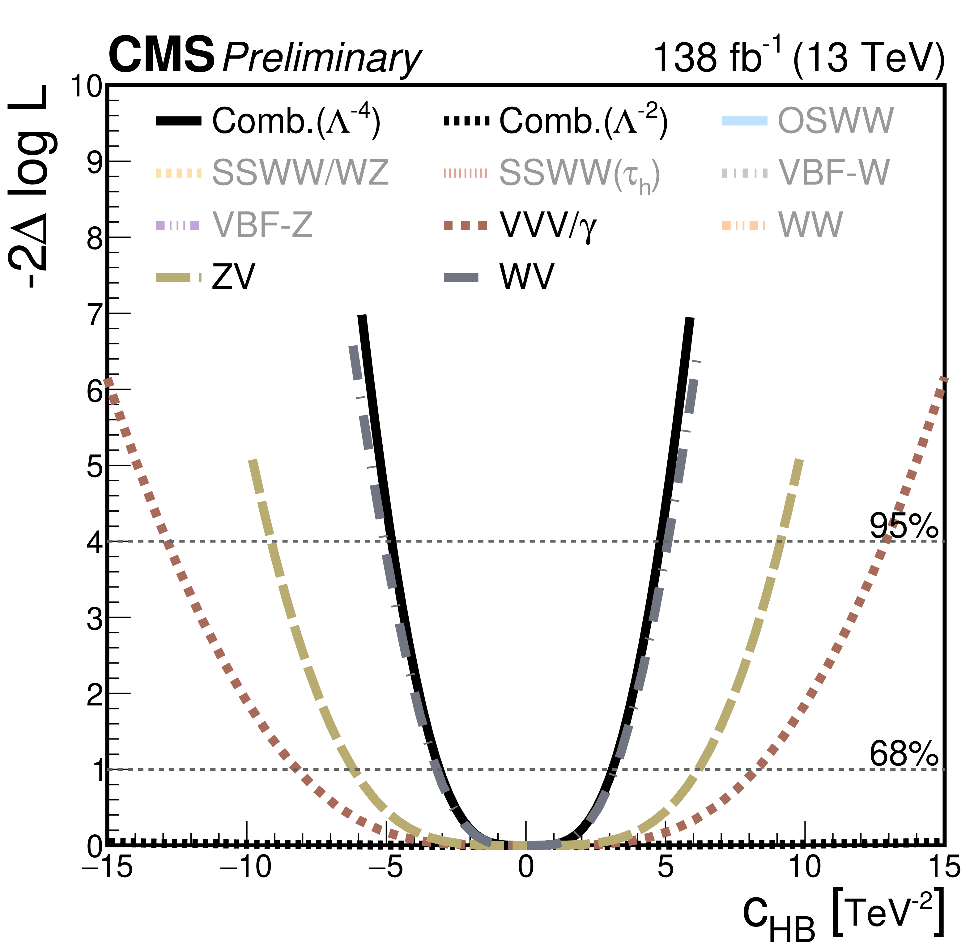
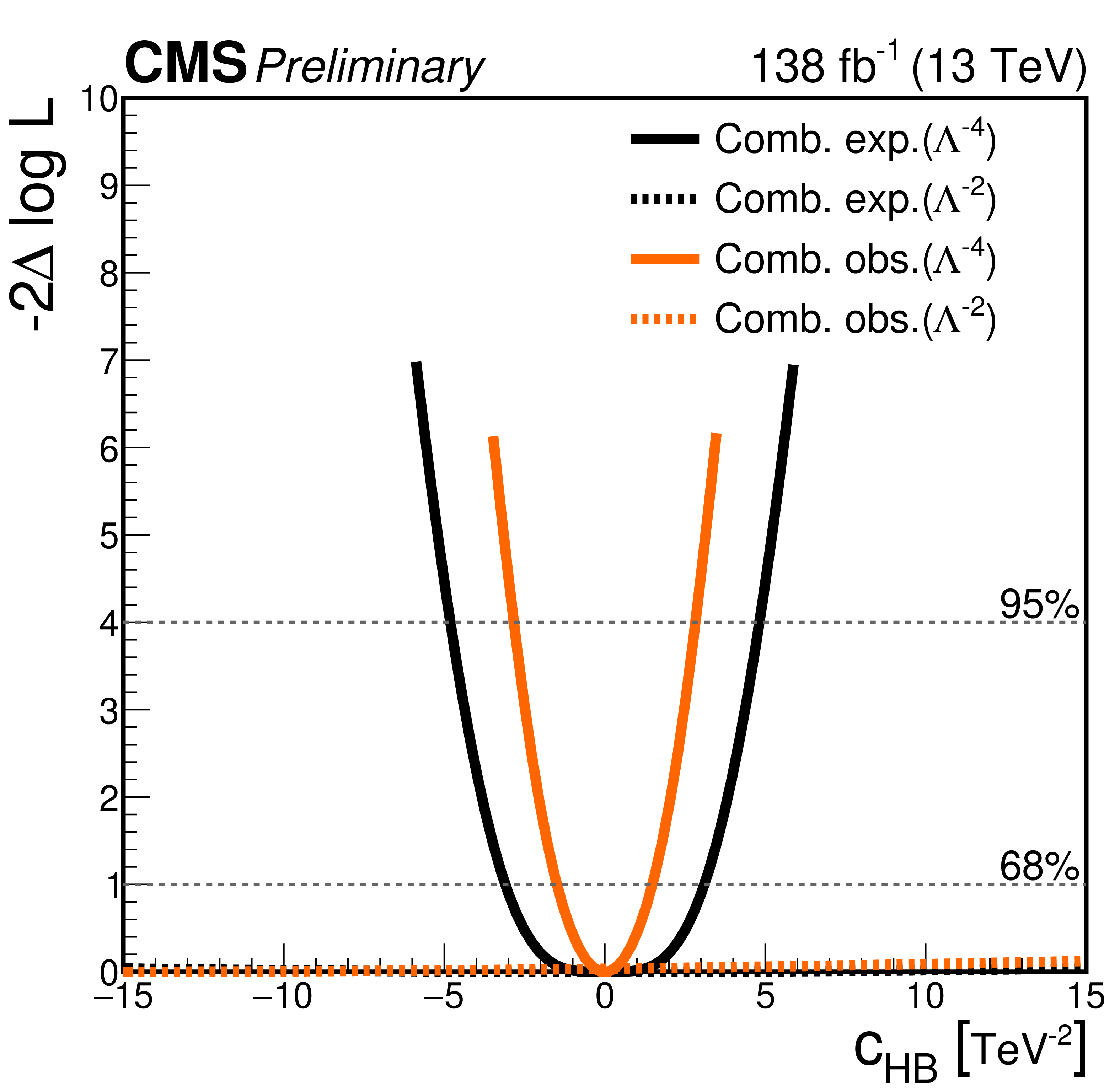
$ -2\ln\Delta\mathcal{L} $ profiles for individual bosonic operators. On the left, the combined fits (black solid line) are compared to the individual fits in each channel (colored lines). Only the likelihood scans of the most sensitive channels are shown. On the right, the observed fits (orange lines) are compared to the expected fits (black lines), both considering the linear+quadratic (solid) and linear (dashed) SMEFT contributions. Horizontal lines represent the 95% and 68% CL. Results for the Wilson coefficient under analysis are obtained by fixing to zero the coefficients of the rest of the operators. |
png pdf |
Figure 8-a:
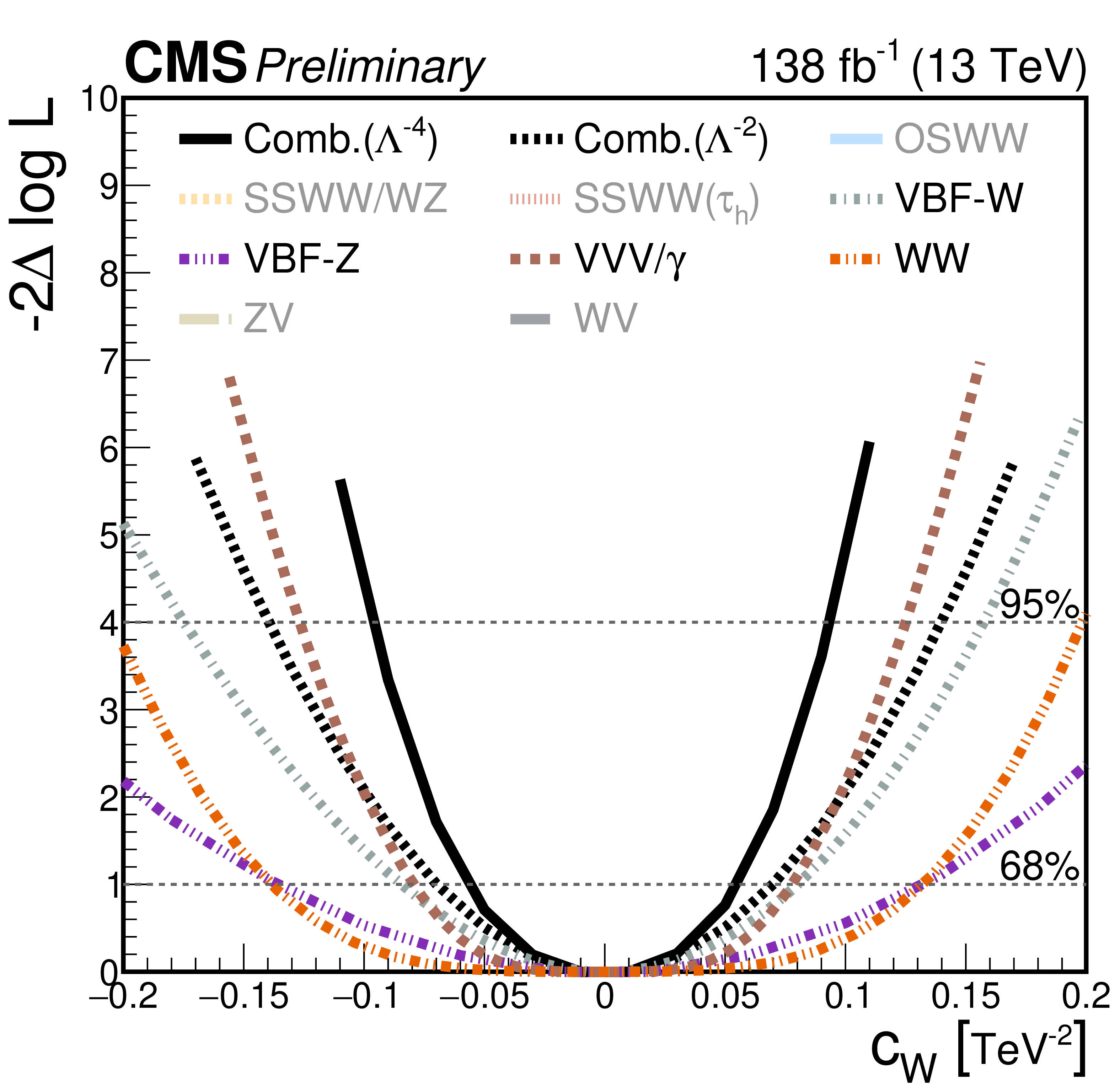
$ -2\ln\Delta\mathcal{L} $ profiles for individual bosonic operators. On the left, the combined fits (black solid line) are compared to the individual fits in each channel (colored lines). Only the likelihood scans of the most sensitive channels are shown. On the right, the observed fits (orange lines) are compared to the expected fits (black lines), both considering the linear+quadratic (solid) and linear (dashed) SMEFT contributions. Horizontal lines represent the 95% and 68% CL. Results for the Wilson coefficient under analysis are obtained by fixing to zero the coefficients of the rest of the operators. |
png pdf |
Figure 8-b:
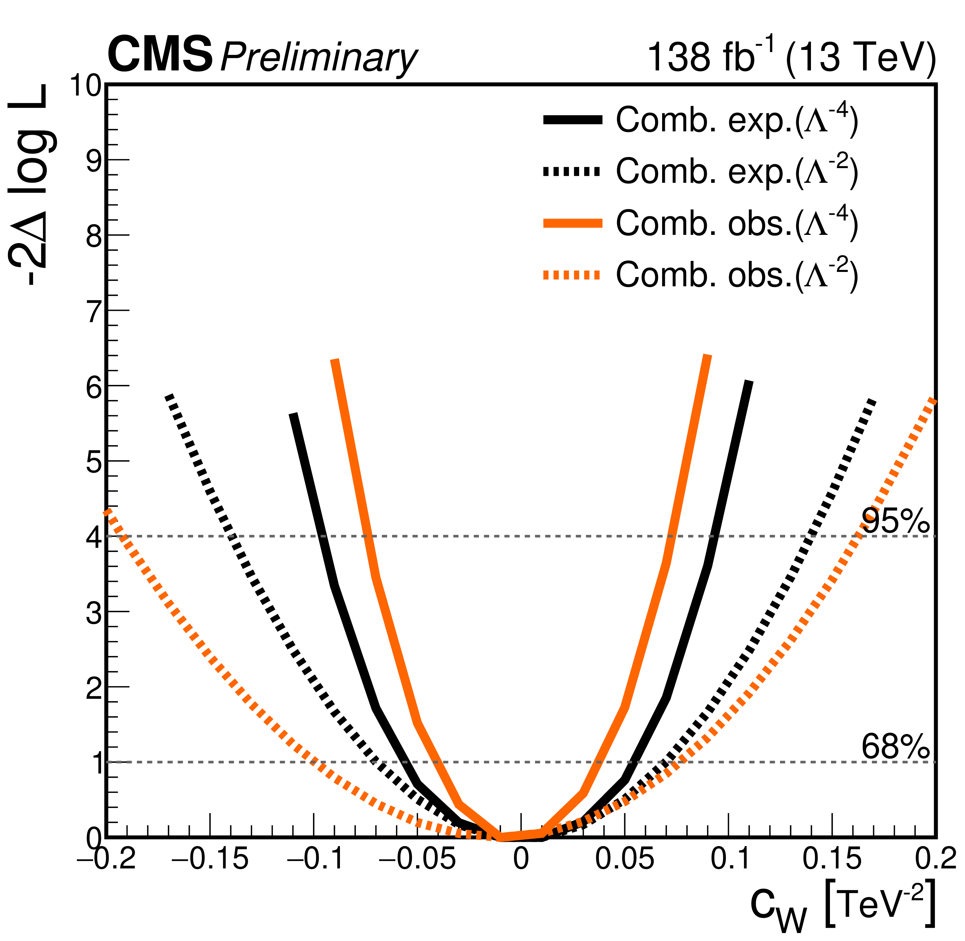
$ -2\ln\Delta\mathcal{L} $ profiles for individual bosonic operators. On the left, the combined fits (black solid line) are compared to the individual fits in each channel (colored lines). Only the likelihood scans of the most sensitive channels are shown. On the right, the observed fits (orange lines) are compared to the expected fits (black lines), both considering the linear+quadratic (solid) and linear (dashed) SMEFT contributions. Horizontal lines represent the 95% and 68% CL. Results for the Wilson coefficient under analysis are obtained by fixing to zero the coefficients of the rest of the operators. |
png pdf |
Figure 8-c:
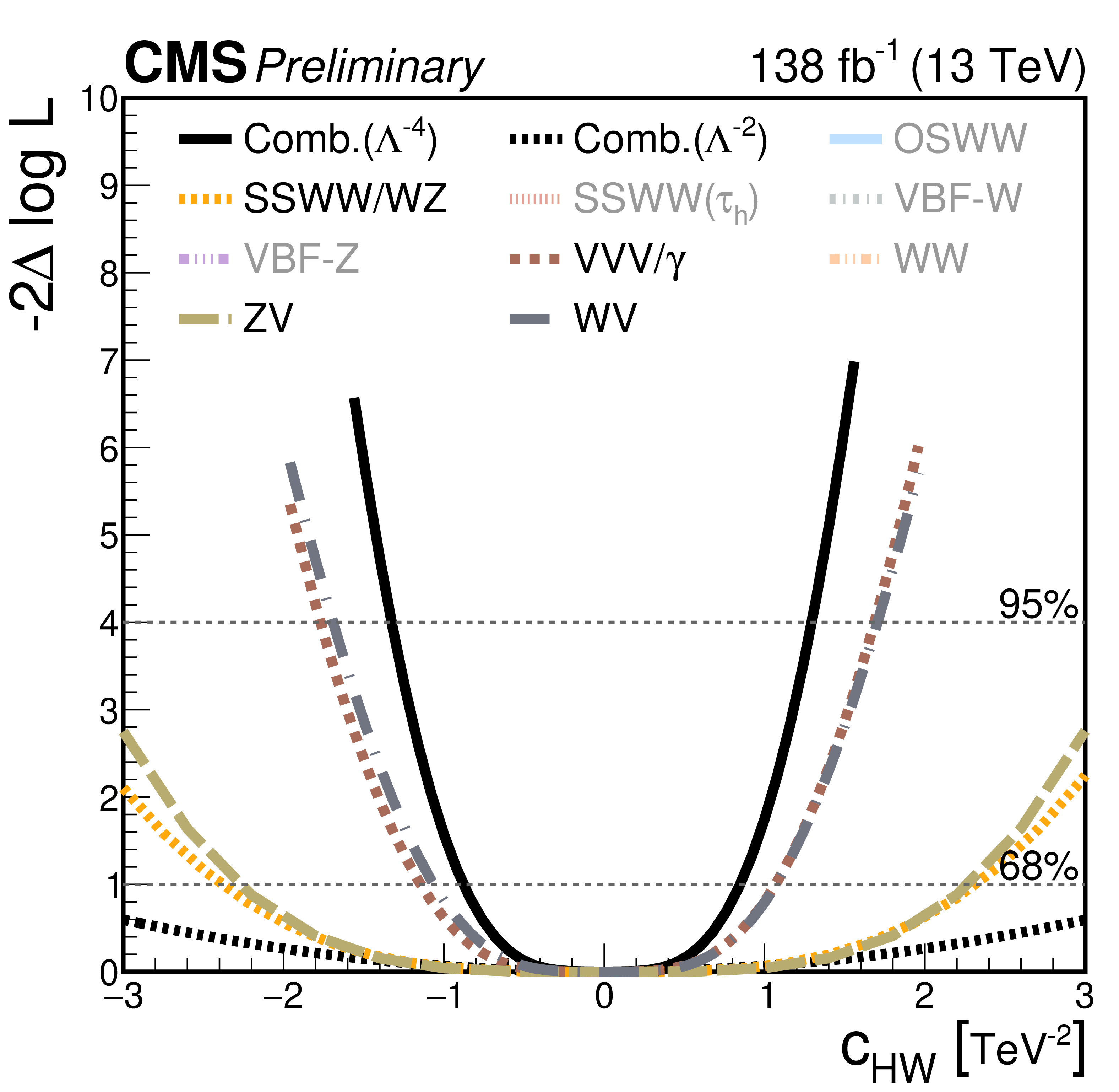
$ -2\ln\Delta\mathcal{L} $ profiles for individual bosonic operators. On the left, the combined fits (black solid line) are compared to the individual fits in each channel (colored lines). Only the likelihood scans of the most sensitive channels are shown. On the right, the observed fits (orange lines) are compared to the expected fits (black lines), both considering the linear+quadratic (solid) and linear (dashed) SMEFT contributions. Horizontal lines represent the 95% and 68% CL. Results for the Wilson coefficient under analysis are obtained by fixing to zero the coefficients of the rest of the operators. |
png pdf |
Figure 8-d:
$ -2\ln\Delta\mathcal{L} $ profiles for individual bosonic operators. On the left, the combined fits (black solid line) are compared to the individual fits in each channel (colored lines). Only the likelihood scans of the most sensitive channels are shown. On the right, the observed fits (orange lines) are compared to the expected fits (black lines), both considering the linear+quadratic (solid) and linear (dashed) SMEFT contributions. Horizontal lines represent the 95% and 68% CL. Results for the Wilson coefficient under analysis are obtained by fixing to zero the coefficients of the rest of the operators. |
png pdf |
Figure 8-e:
$ -2\ln\Delta\mathcal{L} $ profiles for individual bosonic operators. On the left, the combined fits (black solid line) are compared to the individual fits in each channel (colored lines). Only the likelihood scans of the most sensitive channels are shown. On the right, the observed fits (orange lines) are compared to the expected fits (black lines), both considering the linear+quadratic (solid) and linear (dashed) SMEFT contributions. Horizontal lines represent the 95% and 68% CL. Results for the Wilson coefficient under analysis are obtained by fixing to zero the coefficients of the rest of the operators. |
png pdf |
Figure 8-f:
$ -2\ln\Delta\mathcal{L} $ profiles for individual bosonic operators. On the left, the combined fits (black solid line) are compared to the individual fits in each channel (colored lines). Only the likelihood scans of the most sensitive channels are shown. On the right, the observed fits (orange lines) are compared to the expected fits (black lines), both considering the linear+quadratic (solid) and linear (dashed) SMEFT contributions. Horizontal lines represent the 95% and 68% CL. Results for the Wilson coefficient under analysis are obtained by fixing to zero the coefficients of the rest of the operators. |
png pdf |
Figure 9:
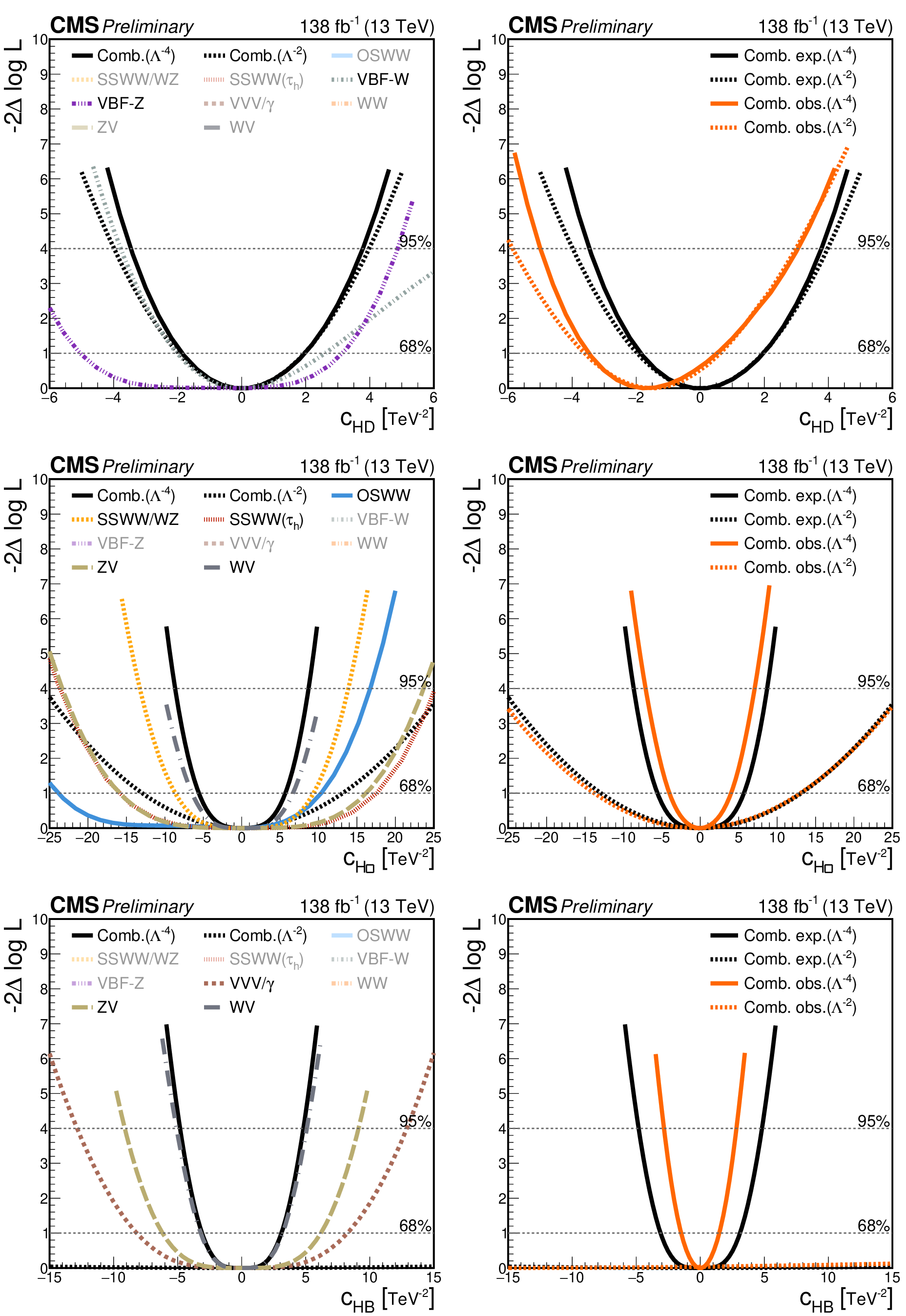
$ -2\ln\Delta\mathcal{L} $ profiles for individual bosonic operators. On the left, the combined fits (black solid line) are compared to the individual fits in each channel (colored lines). Only the likelihood scans of the most sensitive channels are shown. On the right, the observed fits (orange lines) are compared to the expected fits (black lines), both considering the linear+quadratic (solid) and linear (dashed) SMEFT contributions. Horizontal lines represent the 95% and 68% CL. Results for the Wilson coefficient under analysis are obtained by fixing to zero the coefficients of the rest of the operators. |
png pdf |
Figure 9-a:
$ -2\ln\Delta\mathcal{L} $ profiles for individual bosonic operators. On the left, the combined fits (black solid line) are compared to the individual fits in each channel (colored lines). Only the likelihood scans of the most sensitive channels are shown. On the right, the observed fits (orange lines) are compared to the expected fits (black lines), both considering the linear+quadratic (solid) and linear (dashed) SMEFT contributions. Horizontal lines represent the 95% and 68% CL. Results for the Wilson coefficient under analysis are obtained by fixing to zero the coefficients of the rest of the operators. |
png pdf |
Figure 9-b:
$ -2\ln\Delta\mathcal{L} $ profiles for individual bosonic operators. On the left, the combined fits (black solid line) are compared to the individual fits in each channel (colored lines). Only the likelihood scans of the most sensitive channels are shown. On the right, the observed fits (orange lines) are compared to the expected fits (black lines), both considering the linear+quadratic (solid) and linear (dashed) SMEFT contributions. Horizontal lines represent the 95% and 68% CL. Results for the Wilson coefficient under analysis are obtained by fixing to zero the coefficients of the rest of the operators. |
png pdf |
Figure 9-c:
$ -2\ln\Delta\mathcal{L} $ profiles for individual bosonic operators. On the left, the combined fits (black solid line) are compared to the individual fits in each channel (colored lines). Only the likelihood scans of the most sensitive channels are shown. On the right, the observed fits (orange lines) are compared to the expected fits (black lines), both considering the linear+quadratic (solid) and linear (dashed) SMEFT contributions. Horizontal lines represent the 95% and 68% CL. Results for the Wilson coefficient under analysis are obtained by fixing to zero the coefficients of the rest of the operators. |
png pdf |
Figure 9-d:
$ -2\ln\Delta\mathcal{L} $ profiles for individual bosonic operators. On the left, the combined fits (black solid line) are compared to the individual fits in each channel (colored lines). Only the likelihood scans of the most sensitive channels are shown. On the right, the observed fits (orange lines) are compared to the expected fits (black lines), both considering the linear+quadratic (solid) and linear (dashed) SMEFT contributions. Horizontal lines represent the 95% and 68% CL. Results for the Wilson coefficient under analysis are obtained by fixing to zero the coefficients of the rest of the operators. |
png pdf |
Figure 9-e:
$ -2\ln\Delta\mathcal{L} $ profiles for individual bosonic operators. On the left, the combined fits (black solid line) are compared to the individual fits in each channel (colored lines). Only the likelihood scans of the most sensitive channels are shown. On the right, the observed fits (orange lines) are compared to the expected fits (black lines), both considering the linear+quadratic (solid) and linear (dashed) SMEFT contributions. Horizontal lines represent the 95% and 68% CL. Results for the Wilson coefficient under analysis are obtained by fixing to zero the coefficients of the rest of the operators. |
png pdf |
Figure 9-f:
$ -2\ln\Delta\mathcal{L} $ profiles for individual bosonic operators. On the left, the combined fits (black solid line) are compared to the individual fits in each channel (colored lines). Only the likelihood scans of the most sensitive channels are shown. On the right, the observed fits (orange lines) are compared to the expected fits (black lines), both considering the linear+quadratic (solid) and linear (dashed) SMEFT contributions. Horizontal lines represent the 95% and 68% CL. Results for the Wilson coefficient under analysis are obtained by fixing to zero the coefficients of the rest of the operators. |
png pdf |
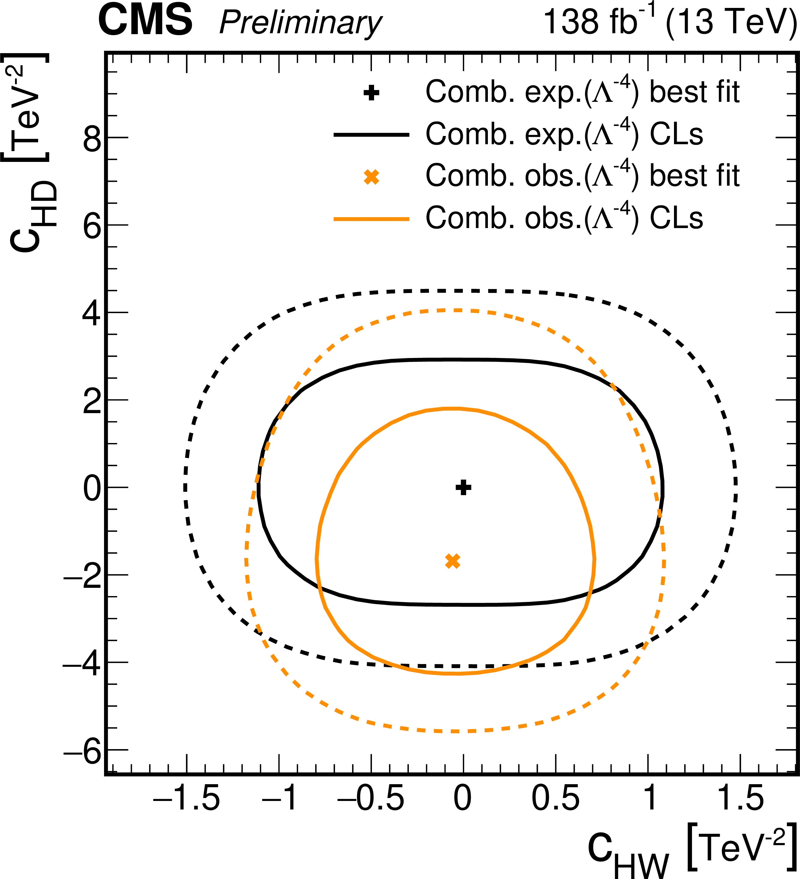
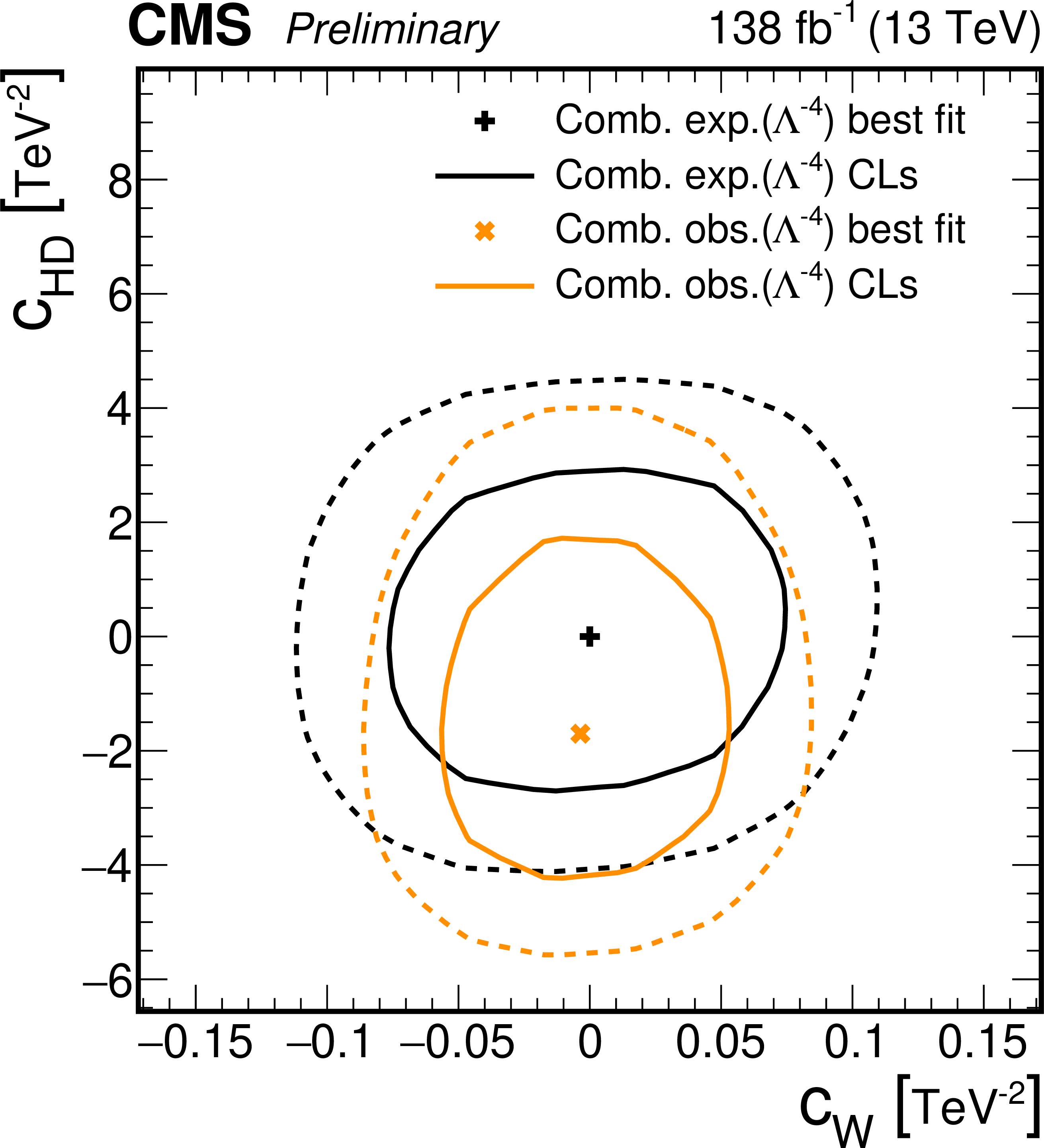
Figure 10:
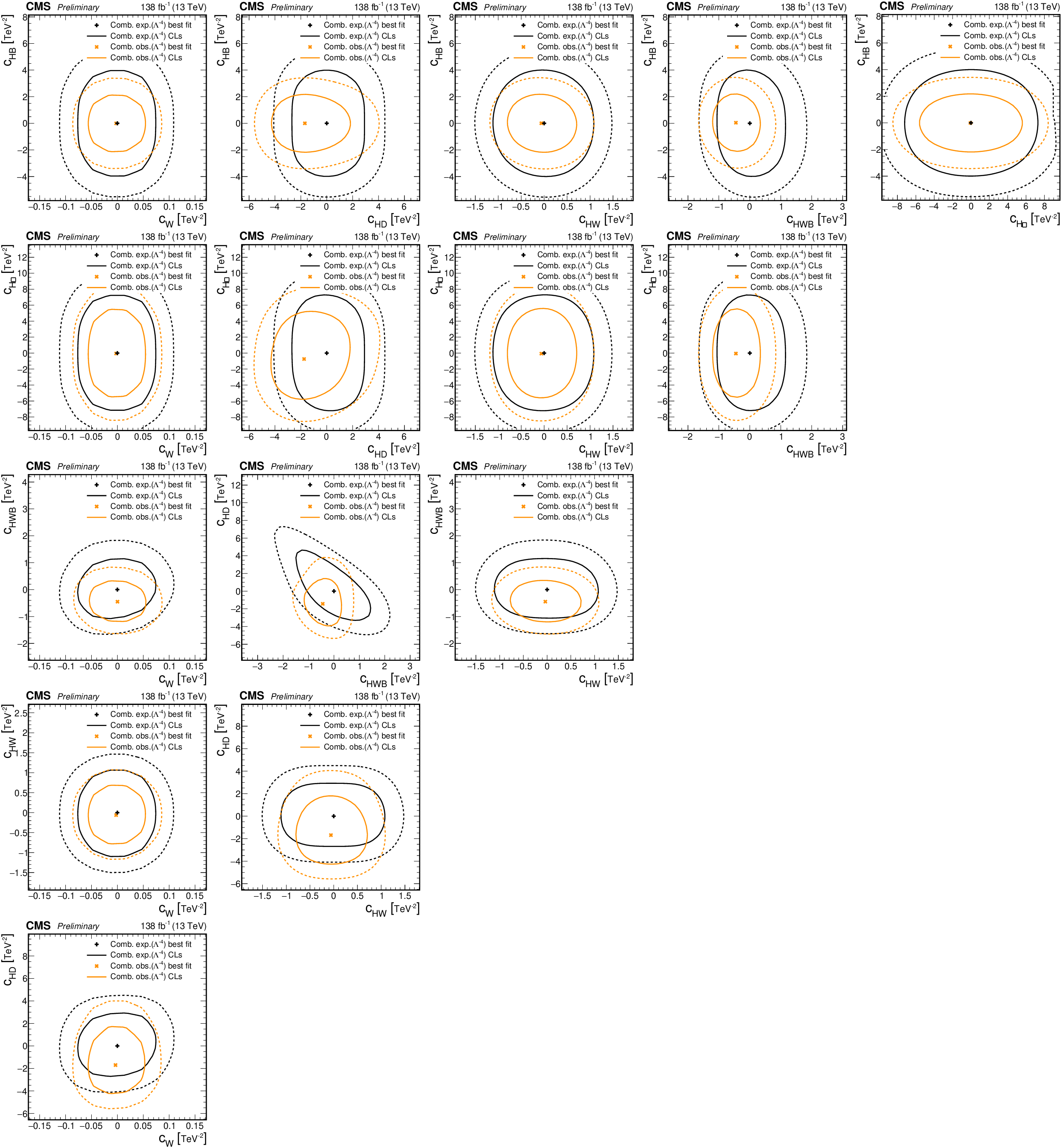
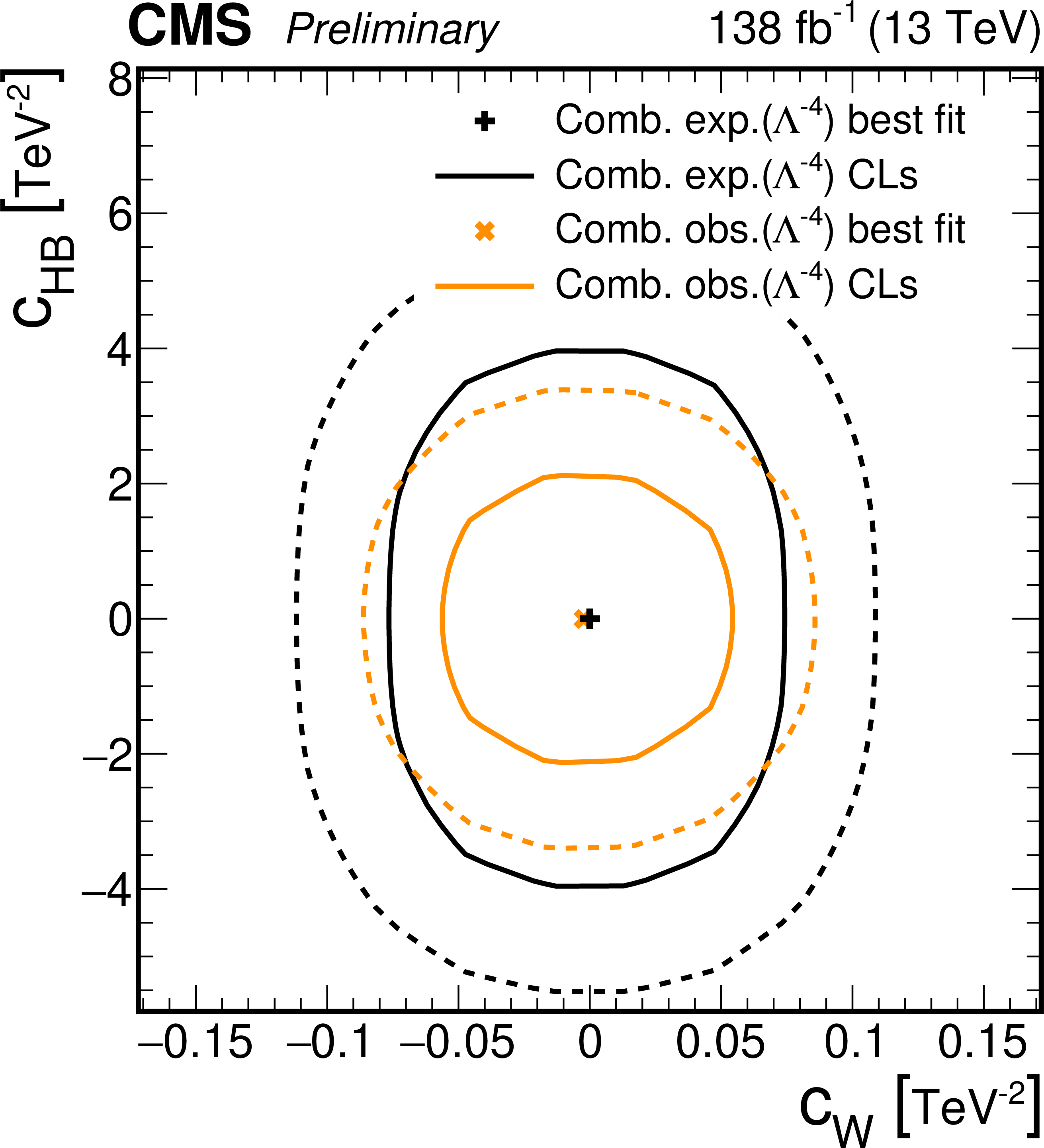
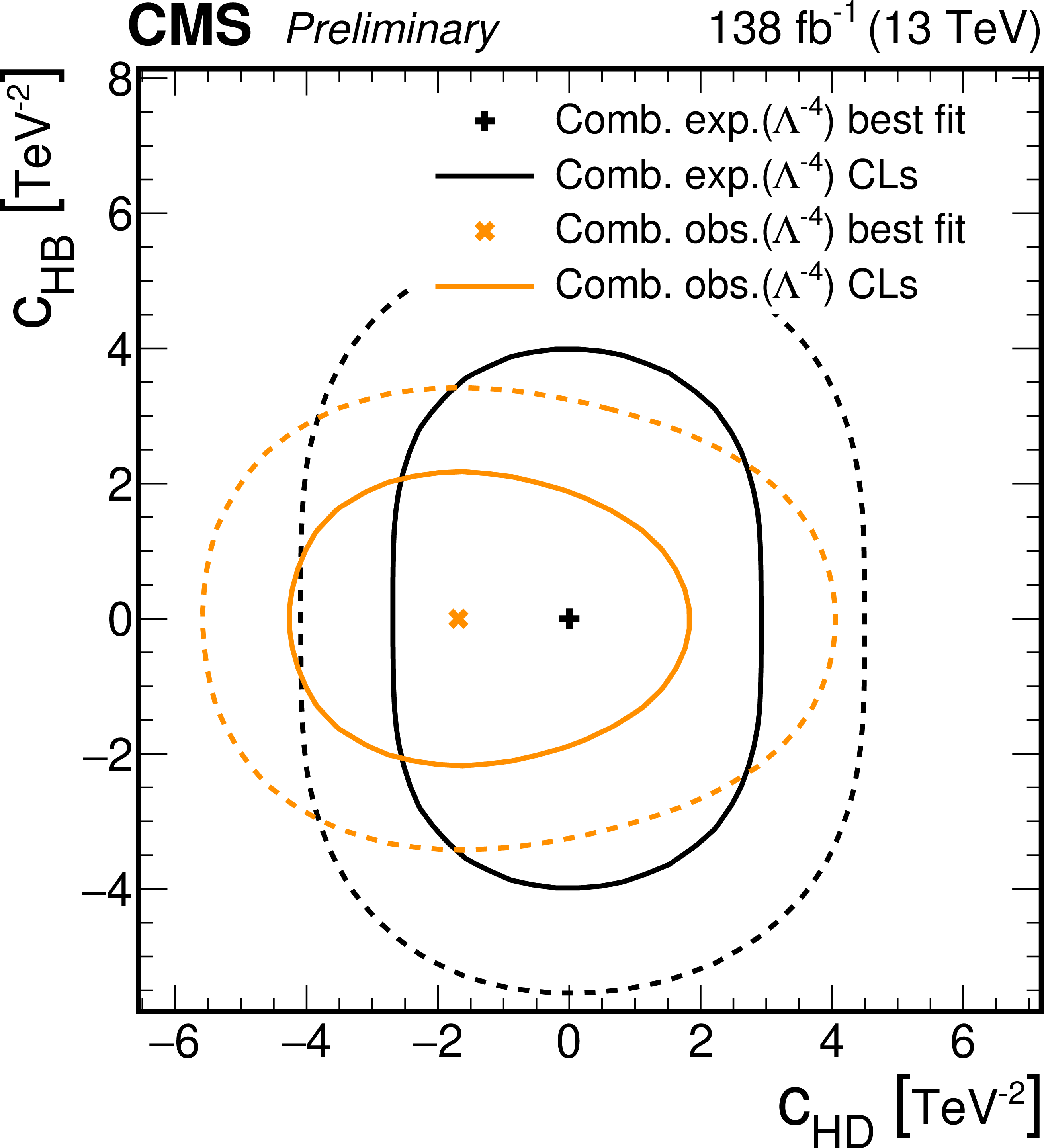
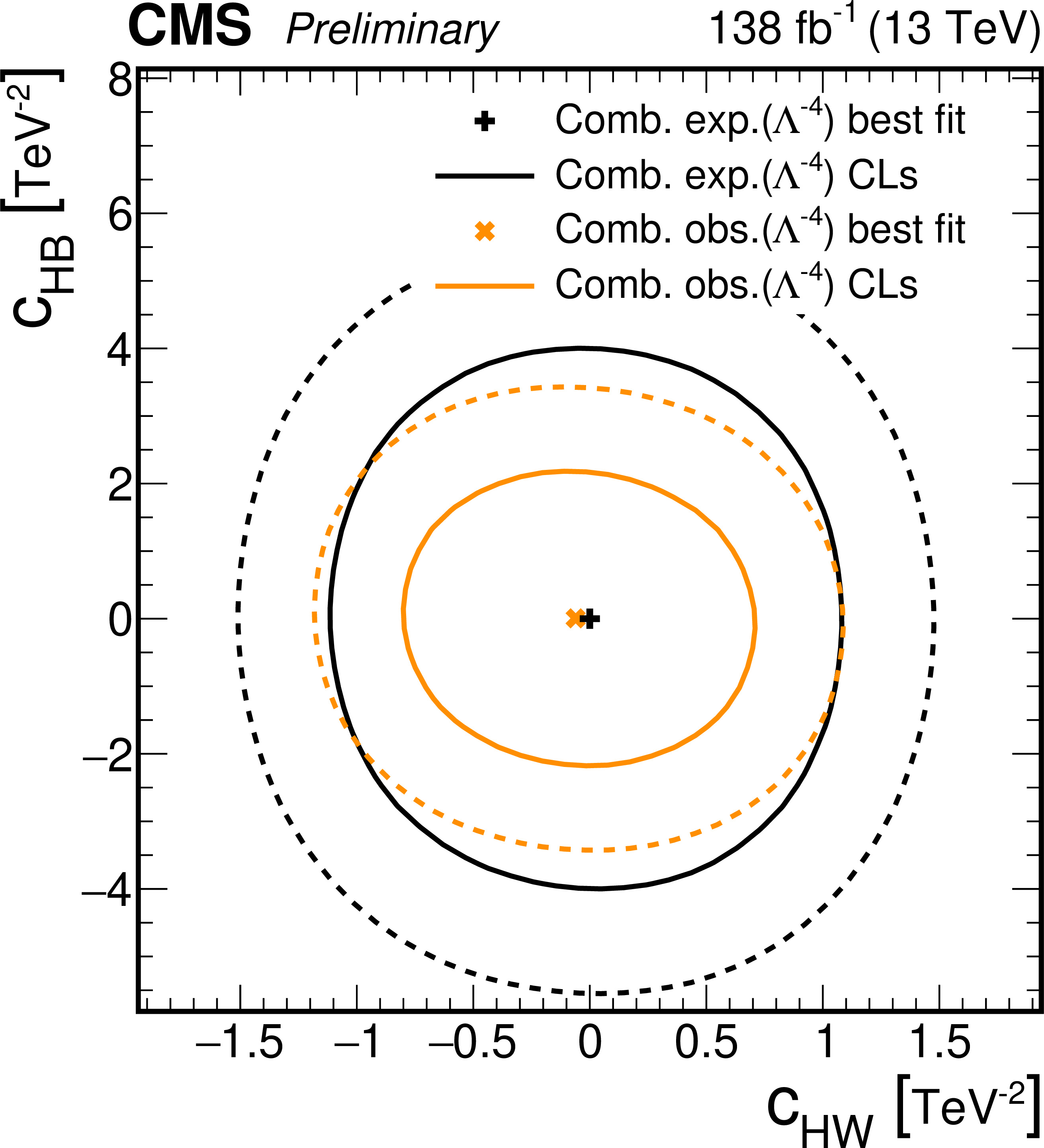
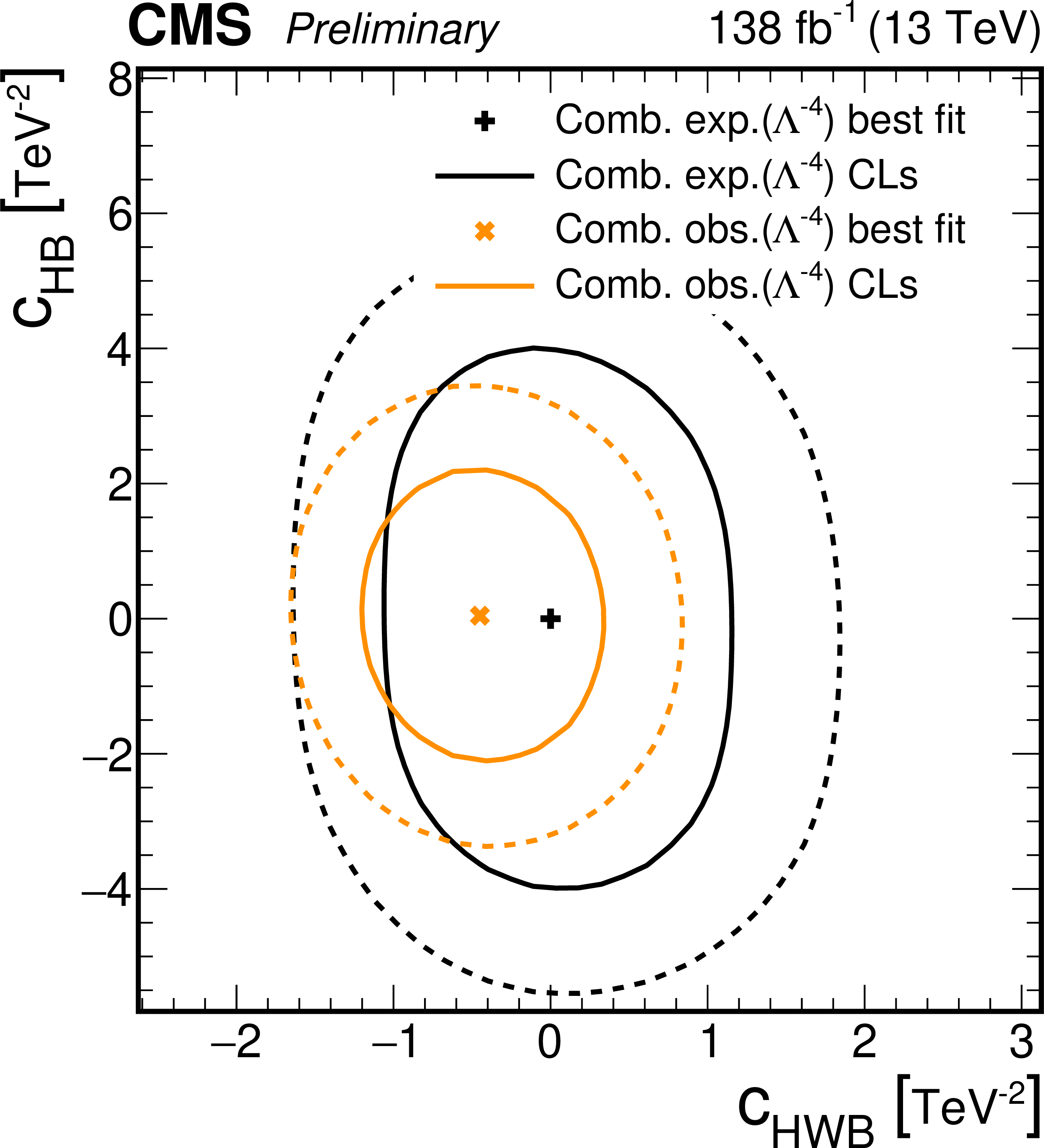
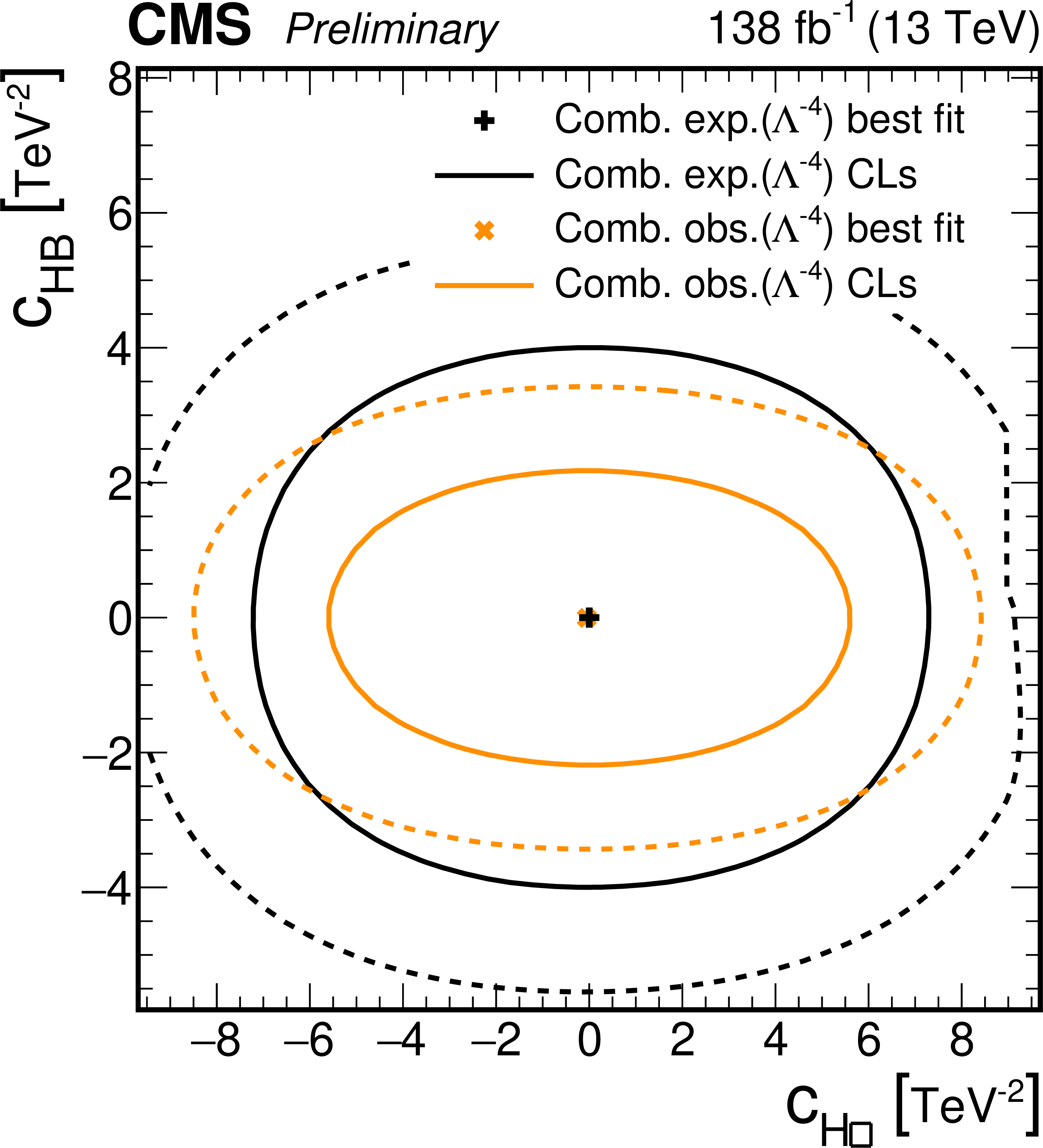
68% (solid line) and 95% (dashed line) CL contours for $ -2\ln\Delta\mathcal{L} $ as functions of the reported dim-6 Wilson coefficient pairs. Expected results are reported in black, while observed ones are reported in orange. All results are obtained by considering the combination of all the channels, fixing the operators not under analysis to zero. |
png pdf |
Figure 10-a:
68% (solid line) and 95% (dashed line) CL contours for $ -2\ln\Delta\mathcal{L} $ as functions of the reported dim-6 Wilson coefficient pairs. Expected results are reported in black, while observed ones are reported in orange. All results are obtained by considering the combination of all the channels, fixing the operators not under analysis to zero. |
png pdf |
Figure 10-b:
68% (solid line) and 95% (dashed line) CL contours for $ -2\ln\Delta\mathcal{L} $ as functions of the reported dim-6 Wilson coefficient pairs. Expected results are reported in black, while observed ones are reported in orange. All results are obtained by considering the combination of all the channels, fixing the operators not under analysis to zero. |
png pdf |
Figure 10-c:
68% (solid line) and 95% (dashed line) CL contours for $ -2\ln\Delta\mathcal{L} $ as functions of the reported dim-6 Wilson coefficient pairs. Expected results are reported in black, while observed ones are reported in orange. All results are obtained by considering the combination of all the channels, fixing the operators not under analysis to zero. |
png pdf |
Figure 10-d:
68% (solid line) and 95% (dashed line) CL contours for $ -2\ln\Delta\mathcal{L} $ as functions of the reported dim-6 Wilson coefficient pairs. Expected results are reported in black, while observed ones are reported in orange. All results are obtained by considering the combination of all the channels, fixing the operators not under analysis to zero. |
png pdf |
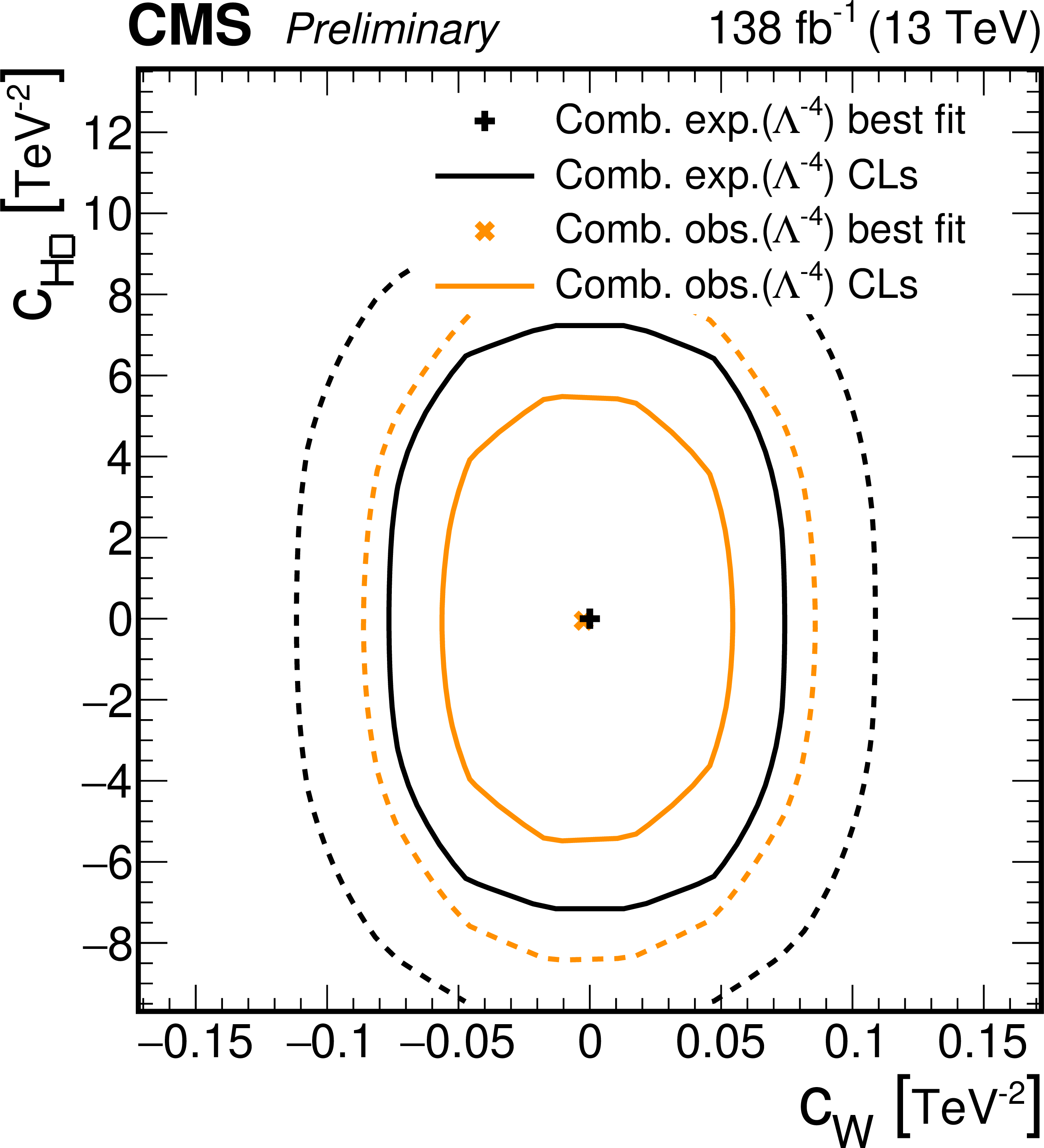
Figure 10-e:
68% (solid line) and 95% (dashed line) CL contours for $ -2\ln\Delta\mathcal{L} $ as functions of the reported dim-6 Wilson coefficient pairs. Expected results are reported in black, while observed ones are reported in orange. All results are obtained by considering the combination of all the channels, fixing the operators not under analysis to zero. |
png pdf |
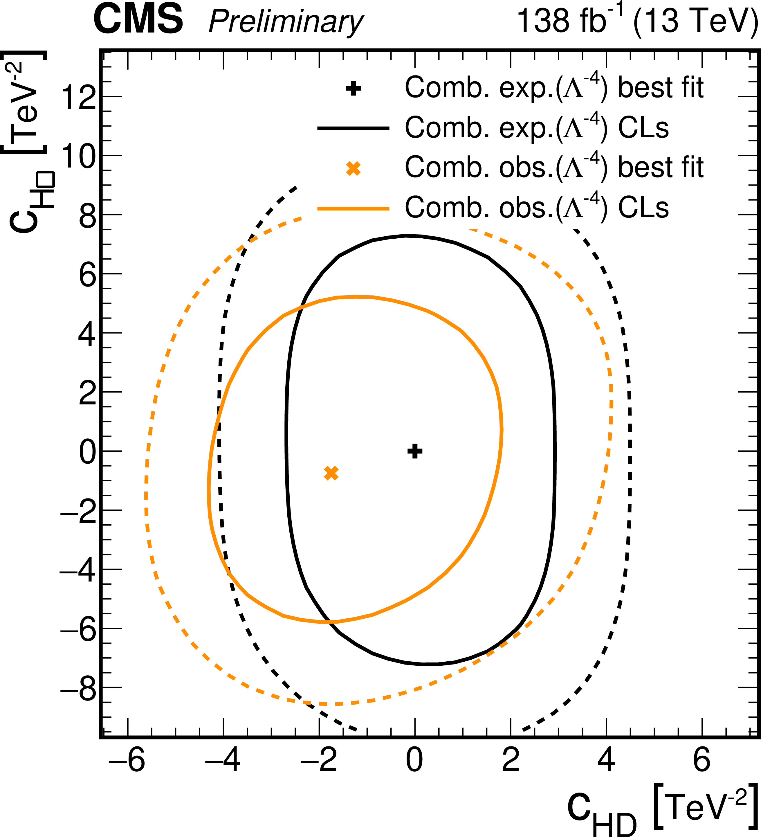
Figure 10-f:
68% (solid line) and 95% (dashed line) CL contours for $ -2\ln\Delta\mathcal{L} $ as functions of the reported dim-6 Wilson coefficient pairs. Expected results are reported in black, while observed ones are reported in orange. All results are obtained by considering the combination of all the channels, fixing the operators not under analysis to zero. |
png pdf |
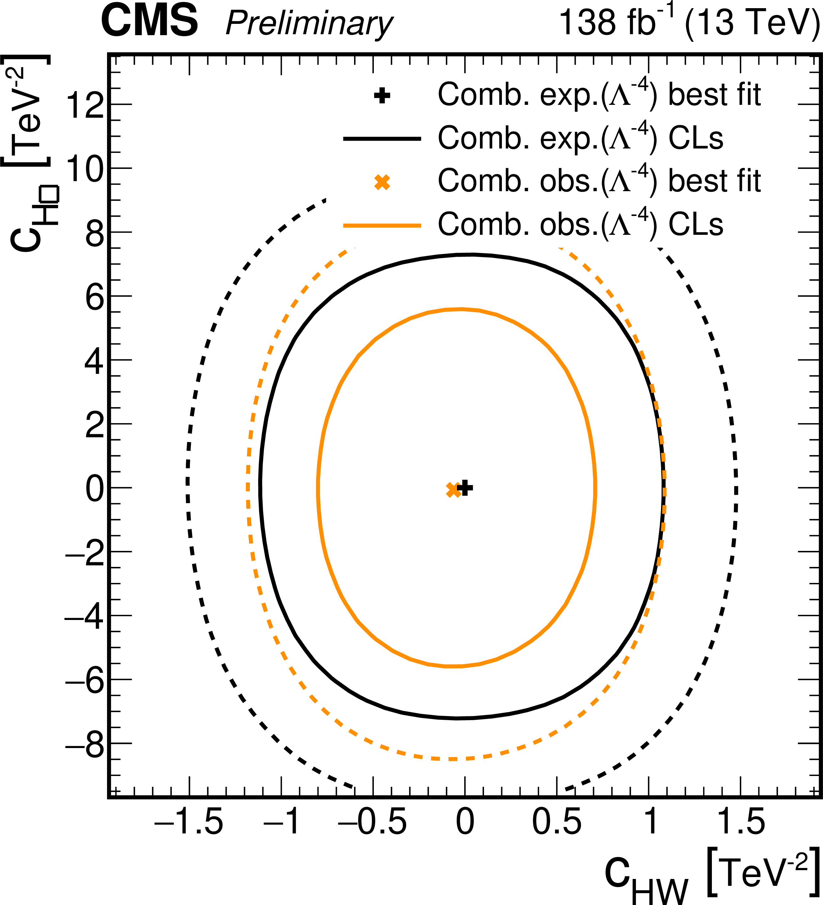
Figure 10-g:
68% (solid line) and 95% (dashed line) CL contours for $ -2\ln\Delta\mathcal{L} $ as functions of the reported dim-6 Wilson coefficient pairs. Expected results are reported in black, while observed ones are reported in orange. All results are obtained by considering the combination of all the channels, fixing the operators not under analysis to zero. |
png pdf |
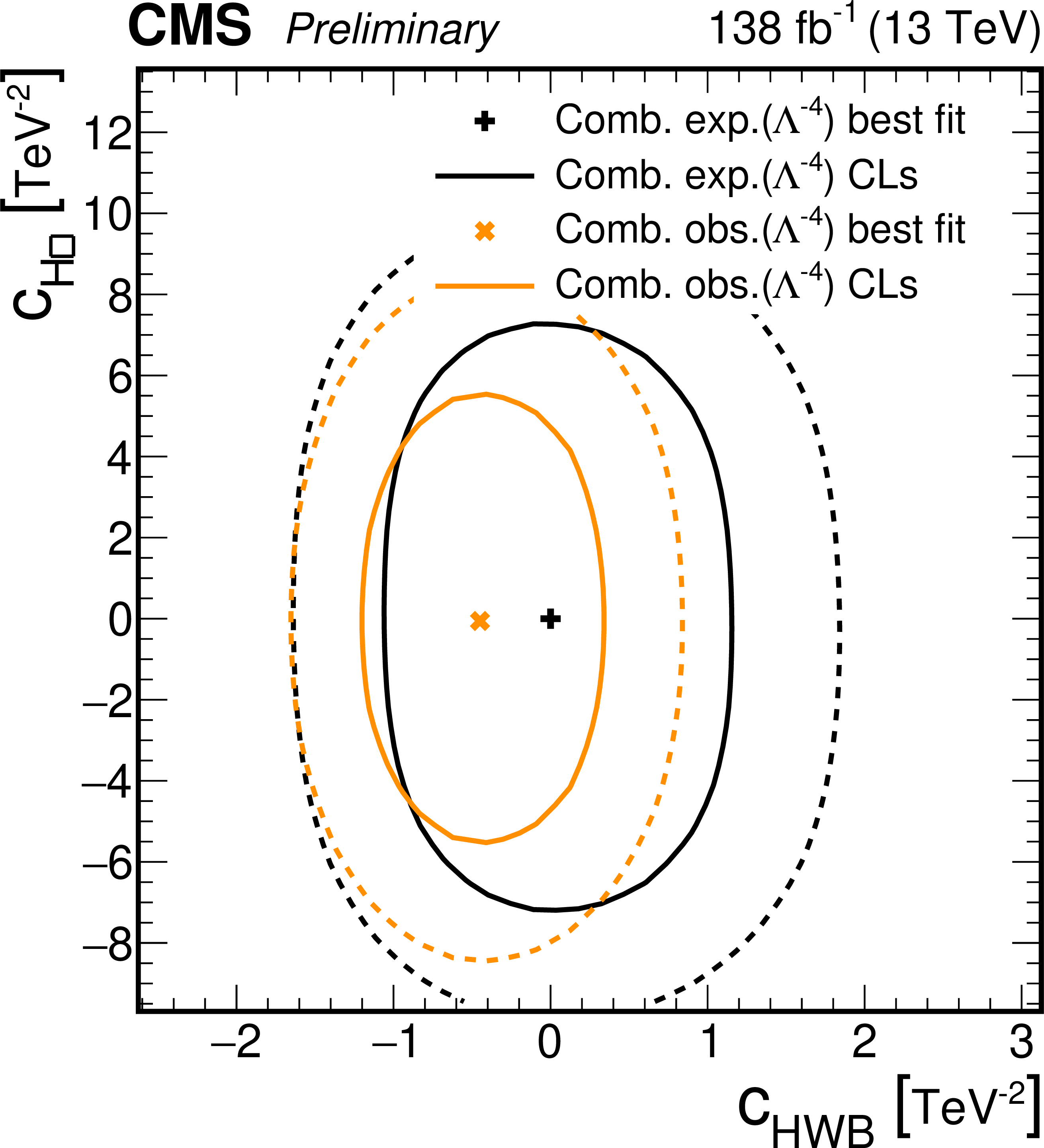
Figure 10-h:
68% (solid line) and 95% (dashed line) CL contours for $ -2\ln\Delta\mathcal{L} $ as functions of the reported dim-6 Wilson coefficient pairs. Expected results are reported in black, while observed ones are reported in orange. All results are obtained by considering the combination of all the channels, fixing the operators not under analysis to zero. |
png pdf |
Figure 10-i:
68% (solid line) and 95% (dashed line) CL contours for $ -2\ln\Delta\mathcal{L} $ as functions of the reported dim-6 Wilson coefficient pairs. Expected results are reported in black, while observed ones are reported in orange. All results are obtained by considering the combination of all the channels, fixing the operators not under analysis to zero. |
png pdf |
Figure 10-j:
68% (solid line) and 95% (dashed line) CL contours for $ -2\ln\Delta\mathcal{L} $ as functions of the reported dim-6 Wilson coefficient pairs. Expected results are reported in black, while observed ones are reported in orange. All results are obtained by considering the combination of all the channels, fixing the operators not under analysis to zero. |
png pdf |
Figure 10-k:
68% (solid line) and 95% (dashed line) CL contours for $ -2\ln\Delta\mathcal{L} $ as functions of the reported dim-6 Wilson coefficient pairs. Expected results are reported in black, while observed ones are reported in orange. All results are obtained by considering the combination of all the channels, fixing the operators not under analysis to zero. |
png pdf |
Figure 10-l:
68% (solid line) and 95% (dashed line) CL contours for $ -2\ln\Delta\mathcal{L} $ as functions of the reported dim-6 Wilson coefficient pairs. Expected results are reported in black, while observed ones are reported in orange. All results are obtained by considering the combination of all the channels, fixing the operators not under analysis to zero. |
png pdf |
Figure 10-m:
68% (solid line) and 95% (dashed line) CL contours for $ -2\ln\Delta\mathcal{L} $ as functions of the reported dim-6 Wilson coefficient pairs. Expected results are reported in black, while observed ones are reported in orange. All results are obtained by considering the combination of all the channels, fixing the operators not under analysis to zero. |
png pdf |
Figure 10-n:
68% (solid line) and 95% (dashed line) CL contours for $ -2\ln\Delta\mathcal{L} $ as functions of the reported dim-6 Wilson coefficient pairs. Expected results are reported in black, while observed ones are reported in orange. All results are obtained by considering the combination of all the channels, fixing the operators not under analysis to zero. |
png pdf |
Figure 10-o:
68% (solid line) and 95% (dashed line) CL contours for $ -2\ln\Delta\mathcal{L} $ as functions of the reported dim-6 Wilson coefficient pairs. Expected results are reported in black, while observed ones are reported in orange. All results are obtained by considering the combination of all the channels, fixing the operators not under analysis to zero. |
| Tables | |
png pdf |
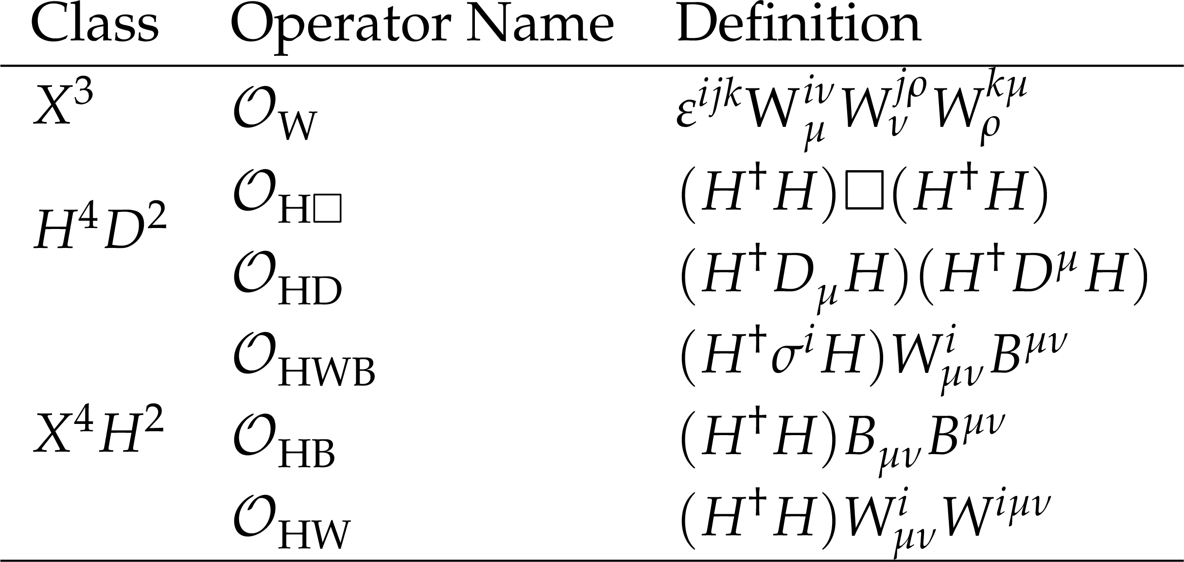
Table 1:
The subset of Warsaw basis operators considered in this work, following the definitions of [1,none]. Repeated indices are summed over. These purely bosonic operators are independent of the flavour symmetry imposed on the SMEFT Lagrangian. The symbol $ H $ refers to the Higgs doublet; $ D_\mu $ is a covariant derivative and $ \square = D^\mu D_\mu $ the d'Alembert operator; $ W^i_{\mu\nu} $ and $ B_{\mu\nu} $ are the $ \mathrm{SU}(2)_L $ and $ \mathrm{U}(1)_Y $ field strength tensors; $ i,j,k $ are $ \mathrm{SU}(2) $ adjoint indices. |
png pdf |
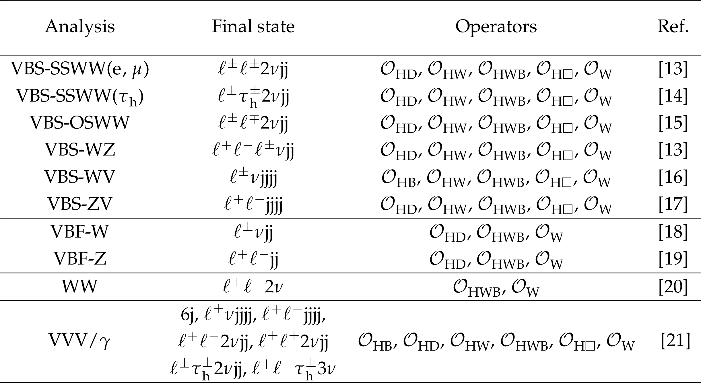
Table 2:
Summary of the analyses considered in the combination and the reference to the specific CMS study on that final state. The final state for each analysis is specified, where $ {\ell}^{\pm} $ denotes a light lepton (e, $ \mu $) and $ \tau_\mathrm{h} $ represents a hadronically decaying $ \tau $ lepton. The last two columns indicate the operators contributing as vertex corrections to the diagrams associated with each specific final state and the single CMS publication on that final state. |
png pdf |
Table 3:
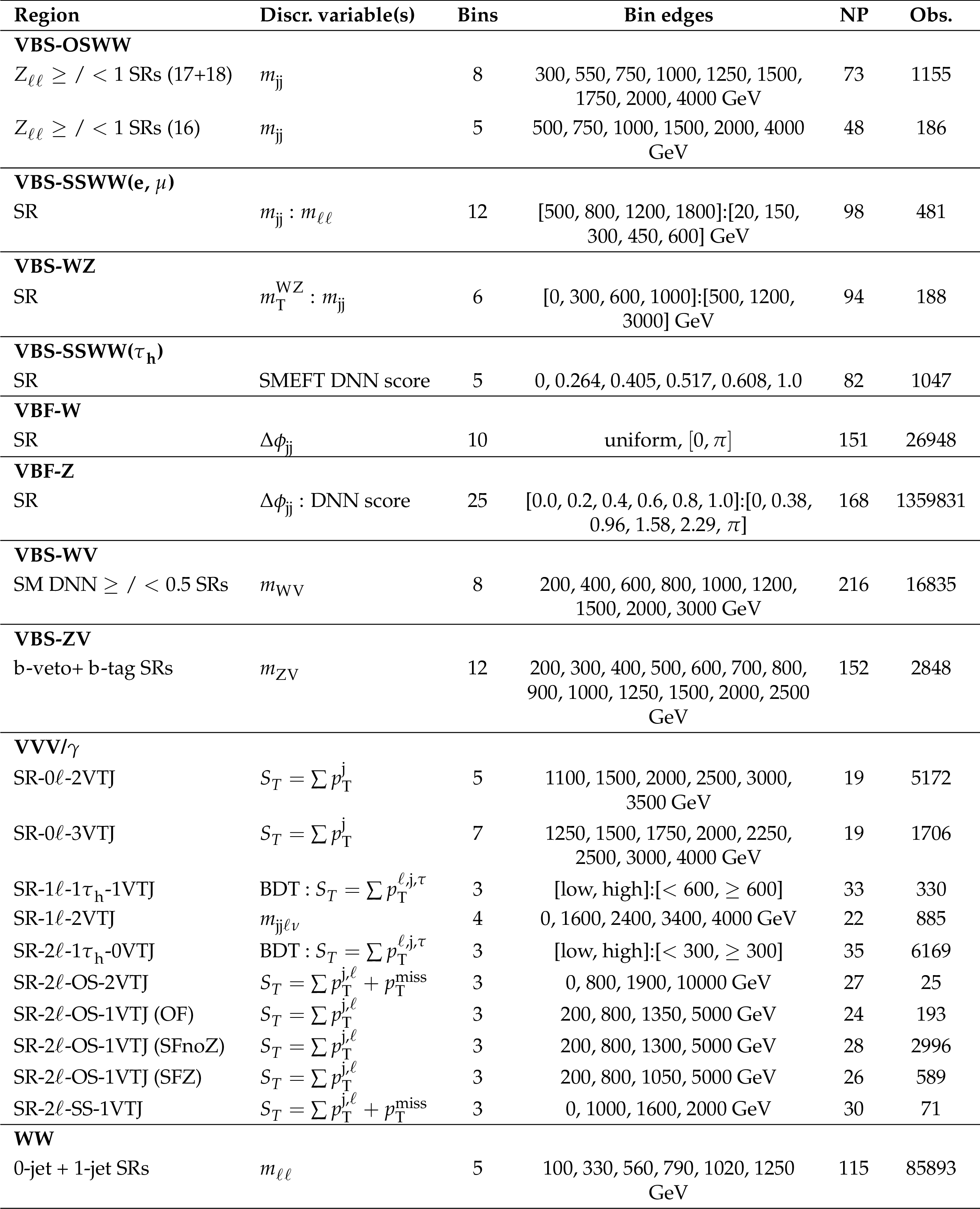
Summary of the signal regions (SRs) entering the combined fit. Some rows merge multiple SRs sharing an identical discriminating variable and binning, with yields summed accordingly. SRs are further split by the Zeppenfeld variable [50] (VBS-OSWW), DNN score or b-tag multiplicity (VBS-WV/ZV), and, for VVV$ /\gamma $, by lepton/$ \tau_\mathrm{h} $/VTJ multiplicity, lepton charge (SS: same-sign, OS: opposite-sign), flavor (OF: opposite-, SF: same-flavor), and $ m_{\ell\ell} $ proximity to the Z pole (Z/noZ); a BDT separates signal in the $ \tau_\mathrm{h} $ channels. Full definitions are given in the original references of Table 2. The second column gives the discriminating variable, with a colon for bidimensional observables; $ m $/$ m_{\mathrm{T}} $ denote invariant/transverse mass of the sub/superscripted system. Remaining columns: number of bins and edges, nuisance parameters (NP), and observed events. |
png pdf |
Table 4:
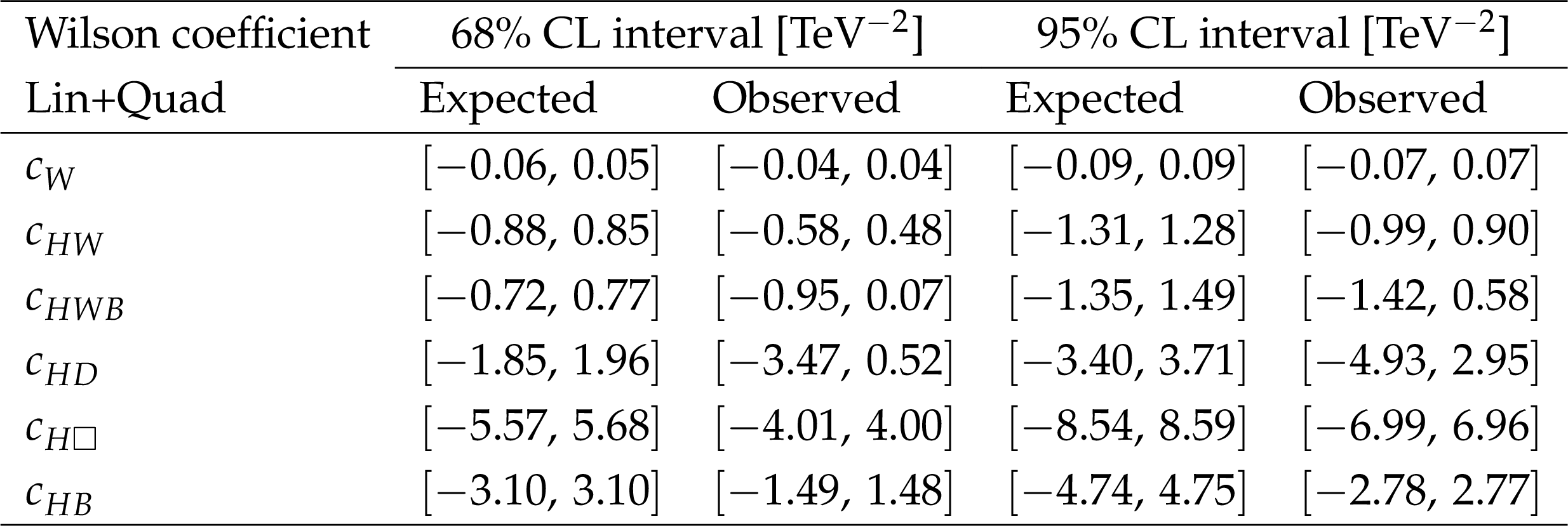
Observed 68% and 95% 1D confidence level (CL) intervals on the Wilson coefficients associated with the SMEFT dim-6 operators considered. All CL are reported for the fits including both linear and quadratic SMEFT components. The results reported here are obtained by fixing the Wilson coefficients other than the one of interest to their SM values in the fit procedure. |
png pdf |
Table 5:
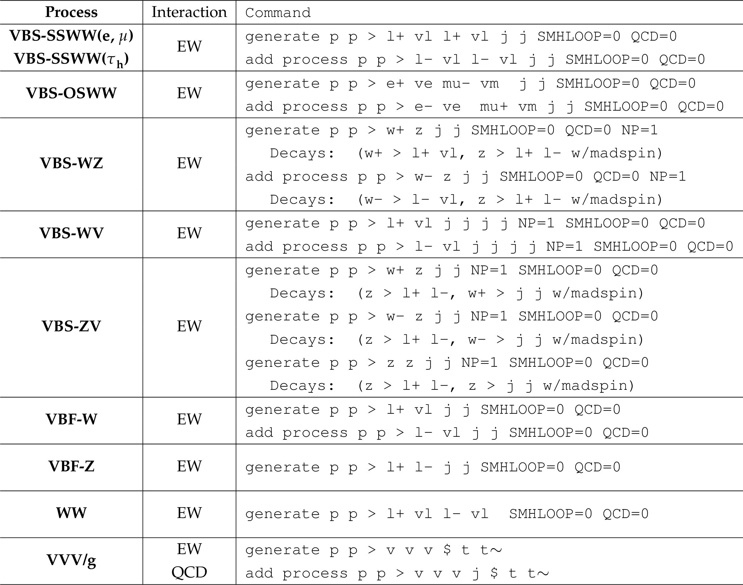
MadGraph-5_aMC@NLO commands for generating SM components of the processes of interest. Where relevant, charge conjugate processes were included. The shortcut l- stands for electron, muon, or tau lepton. |
| Summary |
| A search for physics beyond the standard model is performed in the framework of the standard model effective field theory (SMEFT) through a statistical combination of ten CMS measurements of electroweak (EW) processes. The combination includes vector boson scattering (VBS), vector boson fusion (VBF), diboson, and triboson production, probing final states with one, two, and three EW gauge bosons. The analyses use the full Run 2 proton-proton collision dataset recorded by the CMS experiment at the CERN LHC at $ \sqrt{s}= $ 13 TeV, corresponding to an integrated luminosity of 138 fb$ ^{-1} $. For all measurements, the SMEFT parametrization is propagated directly to detector level through event-by-event reweighting, allowing a consistent treatment of detector effects and systematic uncertainties while avoiding the model assumptions required by unfolding. Six Wilson coefficients associated with bosonic dimension-six operators are constrained: $ c_W $, $ c_{HW} $, $ c_{HWB} $, $ c_{H\square} $, $ c_{HB} $, and $ c_{HD} $. Limits are extracted in single-parameter, two-parameter, and global profiling scenarios. The combination significantly improves the sensitivity to all six operators compared with the individual measurements, with no single analysis dominating any constraint. The strongest limit is obtained for $ c_W $, while the remaining coefficients are constrained through complementary sensitivity of the VBS, VBF, diboson, and triboson channels. No evidence for deviations from the standard model is observed. These results provide competitive constraints on bosonic dimension-six operators and constitute the first statistical combination of direct detector-level SMEFT measurements of bosonic operators. |
| References | ||||
| 1 | W. Buchm ü ller and D. Wyler | Effective lagrangian analysis of new interactions and flavour conservation | NPB 268 (1986) 621 | |
| 2 | B. Grzadkowski, M. Iskrzy \'n ski, M. Misiak, and J. Rosiek | Dimension-six terms in the Standard Model Lagrangian | JHEP 10 (2010) 085 | 1008.4884 |
| 3 | ATLAS Collaboration | Effective field theory interpretation of ATLAS measurements involving the Higgs boson, electroweak bosons and the top quark | 2604.21670 | |
| 4 | ATLAS Collaboration | Top EFT summary plots April 2024 | technical report, CERN, Geneva, All figures including auxiliary figures are available at https://atlas.web.cern.ch/Atlas/GROUPS/PHYSICS/PUBNOTES/ATL-PHYS-PUB-2024-004, 2024 | |
| 5 | R. Covarelli, M. Pellen, and M. Zaro | Vector-Boson scattering at the LHC: Unraveling the electroweak sector | Int. J. Mod. Phys. A 36 (2021) 2130009 | 2102.10991 |
| 6 | CMS Collaboration | Combined effective field theory interpretation of Higgs boson, electroweak vector boson, top quark, and multijet measurements | EPJC 86 (2026) 331 | CMS-SMP-24-003 2504.02958 |
| 7 | R. Bellan et al. | A sensitivity study of VBS and diboson WW to dimension-6 EFT operators at the LHC | JHEP 05 (2022) 039 | 2108.03199 |
| 8 | CMS Collaboration | The CMS experiment at the CERN LHC | JINST 3 (2008) 8004 | |
| 9 | CMS Collaboration | Description and performance of track and primary-vertex reconstruction with the CMS tracker | JINST 9 (2014) 10009 | CMS-TRK-11-001 1405.6569 |
| 10 | CMS Tracker Group Collaboration | The CMS phase-1 pixel detector upgrade | JINST 16 (2021) P02027 | 2012.14304 |
| 11 | CMS Collaboration | Track impact parameter resolution for the full pseudo rapidity coverage in the 2017 dataset with the CMS phase-1 pixel detector | CMS Detector Performance Summary CMS-DP-2020-049, CERN, 2020 CDS |
|
| 12 | CMS Collaboration | The CMS trigger system | JINST 12 (2017) P01020 | CMS-TRG-12-001 1609.02366 |
| 13 | CMS Collaboration | Measurements of production cross sections of WZ and same-sign WW boson pairs in association with two jets in proton-proton collisions at $ \sqrt{s} = $ 13 TeV | PLB 809 (2020) 135710 | CMS-SMP-19-012 2005.01173 |
| 14 | CMS Collaboration | Study of same-sign W boson scattering and anomalous couplings in events with one tau lepton from pp collisions at $ \sqrt{s}= $ 13 TeV | JHEP 10 (2025) 219 | CMS-SMP-22-008 2410.04210 |
| 15 | CMS Collaboration | Observation of electroweak W+W\ensuremath- pair production in association with two jets in proton-proton collisions at s=13TeV | PLB 841 (2023) 137495 | CMS-SMP-21-001 2205.05711 |
| 16 | CMS Collaboration | Evidence for WW/WZ vector boson scattering in the decay channel \ensuremath\ell\ensuremath\nuqq produced in association with two jets in proton-proton collisions at s=13 TeV | PLB 834 (2022) 137438 | CMS-SMP-20-013 2112.05259 |
| 17 | CMS Collaboration | Vector boson scattering and anomalous quartic couplings in final states with \ensuremath\ell\ensuremath\nuqq or \ensuremath\ell\ensuremath\ellqq plus jets using proton-proton collisions at $ \sqrt{s}= $ 13 TeV | JHEP 03 (2026) 022 | CMS-SMP-22-011 2510.00118 |
| 18 | CMS Collaboration | Measurement of electroweak production of a W boson and two forward jets in proton-proton collisions at $ \sqrt{s}= $ 8 TeV | JHEP 11 (2016) 147 | CMS-SMP-13-012 1607.06975 |
| 19 | CMS Collaboration | Electroweak production of two jets in association with a Z boson in proton-proton collisions at $ \sqrt{s}= $ 13 $ \text {TeV} $ | EPJC 78 (2018) 589 | CMS-SMP-16-018 1712.09814 |
| 20 | CMS Collaboration | $ \mathrm{W^+}\mathrm{W^-} $ boson pair production in proton-proton collisions at $ \sqrt{s} = $ 13 TeV | PRD 102 (2020) 092001 | CMS-SMP-18-004 2009.00119 |
| 21 | CMS Collaboration | Search for new physics in triple boson production in proton-proton collisions at $ \sqrt{s} = $ 13 TeV using the effective field theory approach | CMS-SMP-24-017 2605.15023 |
|
| 22 | J. Alwall et al. | The automated computation of tree-level and next-to-leading order differential cross sections, and their matching to parton shower simulations | JHEP 07 (2014) 079 | 1405.0301 |
| 23 | I. Brivio | SMEFTsim 3.0 \textemdash a practical guide | JHEP 04 (2021) 073 | 2012.11343 |
| 24 | I. Brivio, Y. Jiang, and M. Trott | The SMEFTsim package, theory and tools | JHEP 12 (2017) 070 | 1709.06492 |
| 25 | P. Artoisenet, R. Frederix, O. Mattelaer, and R. Rietkerk | Automatic spin-entangled decays of heavy resonances in Monte Carlo simulations | JHEP 03 (2013) 015 | 1212.3460 |
| 26 | P. Nason | A New method for combining NLO QCD with shower Monte Carlo algorithms | JHEP 11 (2004) 040 | hep-ph/0409146 |
| 27 | S. Frixione, P. Nason, and C. Oleari | Matching NLO QCD computations with Parton Shower simulations: the POWHEG method | JHEP 11 (2007) 070 | 0709.2092 |
| 28 | S. Alioli, P. Nason, C. Oleari, and E. Re | A general framework for implementing NLO calculations in shower Monte Carlo programs: the POWHEG BOX | JHEP 06 (2010) 043 | 1002.2581 |
| 29 | C. Bierlich et al. | A comprehensive guide to the physics and usage of PYTHIA 8.3 | SciPost Phys. Codeb. 2022 (2022) 8 | 2203.11601 |
| 30 | J. Alwall et al. | Comparative study of various algorithms for the merging of parton showers and matrix elements in hadronic collisions | EPJC 53 (2008) 473 | 0706.2569 |
| 31 | S. Bolognesi et al. | On the Spin and Parity of a Single-Produced Resonance at the LHC | PRD 86 (2012) 095031 | 1208.4018 |
| 32 | K. Hamilton, P. Nason, and G. Zanderighi | Finite quark-mass effects in the NNLOPS POWHEG+MiNLO Higgs generator | JHEP 05 (2015) 140 | 1501.04637 |
| 33 | NNPDF Collaboration | Parton distributions from high-precision collider data | EPJC 77 (2017) 663 | 1706.00428 |
| 34 | CMS Collaboration | Extraction and validation of a new set of CMS PYTHIA8 tunes from underlying-event measurements | EPJC 80 (2020) 4 | CMS-GEN-17-001 1903.12179 |
| 35 | GEANT4 Collaboration | GEANT 4---a simulation toolkit | NIM A 506 (2003) 250 | |
| 36 | CMS Collaboration | Particle-flow reconstruction and global event description with the CMS detector | JINST 12 (2017) P10003 | CMS-PRF-14-001 1706.04965 |
| 37 | ATLAS and CMS Collaborations, and the LHC Higgs Combination Group | Procedure for the lhc Higgs boson search combination in summer 2011 | Technical Report CMS-NOTE-2011-005, ATL-PHYS-PUB-2011-11, CERN, 2011 | |
| 38 | ATLAS, CMS Collaboration | Measurements of the Higgs boson production and decay rates and constraints on its couplings from a combined ATLAS and CMS analysis of the LHC pp collision data at $ \sqrt{s}= $ 7 and 8 TeV | JHEP 08 (2016) 045 | 1606.02266 |
| 39 | CMS Collaboration | The CMS statistical analysis and combination tool: Combine | Submitted to Comput. Softw. Big Sci, 2024 | CMS-CAT-23-001 2404.06614 |
| 40 | W. Verkerke and D. P. Kirkby | The RooFit toolkit for data modeling | physics/0306116 | |
| 41 | L. Moneta et al. | The RooStats Project | link | 1009.1003 |
| 42 | CMS Collaboration | Precision luminosity measurement in proton-proton collisions at $ \sqrt{s}= $ 13 TeV in 2015 and 2016 at CMS | EPJC 81 (2021) 800 | CMS-LUM-17-003 2104.01927 |
| 43 | CMS Collaboration | CMS luminosity measurement for the 2017 data-taking period at $ \sqrt{s}= $ 13 TeV | CMS Physics Analysis Summary, CERN, 2018 CMS-PAS-LUM-17-004 |
CMS-PAS-LUM-17-004 |
| 44 | CMS Collaboration | CMS luminosity measurement for the 2018 data-taking period at $ \sqrt{s}= $ 13 TeV | CMS Physics Analysis Summary, CERN, 2019 CMS-PAS-LUM-18-002 |
CMS-PAS-LUM-18-002 |
| 45 | CMS Collaboration | Identification of heavy-flavour jets with the CMS detector in pp collisions at 13 TeV | JINST 13 (2018) P05011 | CMS-BTV-16-002 1712.07158 |
| 46 | CMS Collaboration | Performance of reconstruction and identification of $ \tau $ leptons decaying to hadrons and $ \nu_\tau $ in pp collisions at $ \sqrt{s}= $ 13 TeV | JINST 13 (2018) P10005 | CMS-TAU-16-003 1809.02816 |
| 47 | CMS Collaboration | Jet energy scale and resolution in the CMS experiment in pp collisions at 8 TeV | JINST 12 (2017) P02014 | CMS-JME-13-004 1607.03663 |
| 48 | CMS Collaboration | Measurement of the inelastic proton-proton cross section at $ \sqrt{s}= $ 13 TeV | JHEP 07 (2018) 161 | CMS-FSQ-15-005 1802.02613 |
| 49 | J. Butterworth et al. | PDF4LHC recommendations for LHC Run II | JPG 43 (2016) 023001 | 1510.03865 |
| 50 | D. L. Rainwater, R. Szalapski, and D. Zeppenfeld | Probing color singlet exchange in $ Z $ + two jet events at the CERN LHC | PRD 54 (1996) 6680 | hep-ph/9605444 |
| 51 | CMS Collaboration | Electron and photon reconstruction and identification with the CMS experiment at the CERN LHC | JINST 16 (2021) P05014 | CMS-EGM-17-001 2012.06888 |
| 52 | CMS Collaboration | Performance of the CMS muon detector and muon reconstruction with proton-proton collisions at $ \sqrt{s}= $ 13 TeV | JINST 13 (2018) P06015 | CMS-MUO-16-001 1804.04528 |
| 53 | CMS Collaboration | Measurement of the Higgs boson production rate in association with top quarks in final states with electrons, muons, and hadronically decaying tau leptons at $ \sqrt{s} = $ 13 TeV | EPJC 81 (2021) 378 | CMS-HIG-19-008 2011.03652 |
| 54 | M. Cacciari, G. P. Salam, and G. Soyez | The anti-$ k_{\mathrm{T}} $ jet clustering algorithm | JHEP 04 (2008) 063 | 0802.1189 |
| 55 | M. Cacciari, G. P. Salam, and G. Soyez | FastJet user manual | EPJC 72 (2012) 1896 | 1111.6097 |
| 56 | D. Bertolini, P. Harris, M. Low, and N. Tran | Pileup per particle identification | JHEP 10 (2014) 059 | 1407.6013 |
| 57 | CMS Collaboration | Pileup mitigation at CMS in 13 TeV data | JINST 15 (2020) P09018 | CMS-JME-18-001 2003.00503 |
| 58 | E. Bols et al. | Jet Flavour Classification Using DeepJet | JINST 15 (2020) P12012 | 2008.10519 |
| 59 | CMS Collaboration | Performance of the DeepJet b tagging algorithm using 41.9 fb$ ^{-1} $ of data from proton-proton collisions at 13 TeV with Phase 1 CMS detector | CMS Detector Performance Summary CMS-DP-2018-058, CERN, 2018 CDS |
|
| 60 | P. F. Monni et al. | MiNNLO$ _{PS} $: a new method to match NNLO QCD to parton showers | JHEP 05 (2020) 143 | 1908.06987 |
| 61 | P. F. Monni, E. Re, and M. Wiesemann | MiNNLO$ _{PS} $: optimizing 2 $ \rightarrow $ 1 hadronic processes | EPJC 80 (2020) 1075 | 2006.04133 |
| 62 | M. Grazzini et al. | NNLO QCD + NLO EW with Matrix+OpenLoops: precise predictions for vector-boson pair production | JHEP 02 (2020) 087 | 1912.00068 |
| 63 | M. Grazzini, S. Kallweit, and M. Wiesemann | Fully differential NNLO computations with MATRIX | EPJC 78 (2018) 537 | 1711.06631 |
| 64 | J. M. Campbell and R. K. Ellis | MCFM for the Tevatron and the LHC | Nucl. Phys. B Proc. Suppl. 20 (2010) 5 | 1007.3492 |
| 65 | CMS Collaboration | Performance of missing transverse momentum reconstruction in proton-proton collisions at $ \sqrt{s} = $ 13 TeV using the CMS detector | JINST 14 (2019) P07004 | CMS-JME-17-001 1903.06078 |
|
|
Compact Muon Solenoid LHC, CERN |

|
|
|
|
|
|