

Compact Muon Solenoid
LHC, CERN
| CMS-SMP-22-008 ; CERN-EP-2024-234 | ||
| Study of same-sign W boson scattering and anomalous couplings in events with one tau lepton from pp collisions at $ \sqrt{s} = $ 13 TeV | ||
| CMS Collaboration | ||
| 5 October 2024 | ||
| JHEP 2510 (2025) 219 | ||
| Abstract: A first study is presented of the cross section for the scattering of same-sign W boson pairs via the detection of a $ \tau $ lepton. The data from proton-proton collisions at the center-of-mass energy of 13 TeV were collected by the CMS detector at the LHC, and correspond to an integrated luminosity of 138 fb$ ^{-1} $. Events were selected that contain two jets with large pseudorapidity and large invariant mass, one $ \tau $ lepton, one light lepton (e or $ \mu $), and significant missing transverse momentum. The measured cross section for electroweak same-sign WW scattering is 1.44 $ ^{+0.63}_{-0.56} $ times the standard model prediction. In addition, a search is presented for the indirect effects of processes beyond the standard model via the effective field theory framework, in terms of dimension-6 and dimension-8 operators. | ||
| Links: e-print arXiv:2410.04210 [hep-ex] (PDF) ; CDS record ; inSPIRE record ; HepData record ; CADI line (restricted) ; | ||
| Figures | |

png pdf |
Figure 1:
Representative tree-level Feynman diagrams contributing to the process $ \mathrm{q}\mathrm{q}^\prime \to \tau^{\pm}\nu_{\!\tau} \ell^{\pm} \nu_{\ell} jj $, $ \ell=$ e, $\mu $, leading to cross sections of order $ \alpha_\text{EW}^6 $ (left) and $ \alpha_\mathrm{S}^{2}\alpha_\text{EW}^4 $ (right). |

png pdf |
Figure 1-a:
Representative tree-level Feynman diagrams contributing to the process $ \mathrm{q}\mathrm{q}^\prime \to \tau^{\pm}\nu_{\!\tau} \ell^{\pm} \nu_{\ell} jj $, $ \ell=$ e, $\mu $, leading to cross sections of order $ \alpha_\text{EW}^6 $ (left) and $ \alpha_\mathrm{S}^{2}\alpha_\text{EW}^4 $ (right). |

png pdf |
Figure 1-b:
Representative tree-level Feynman diagrams contributing to the process $ \mathrm{q}\mathrm{q}^\prime \to \tau^{\pm}\nu_{\!\tau} \ell^{\pm} \nu_{\ell} jj $, $ \ell=$ e, $\mu $, leading to cross sections of order $ \alpha_\text{EW}^6 $ (left) and $ \alpha_\mathrm{S}^{2}\alpha_\text{EW}^4 $ (right). |

png pdf |
Figure 2:
Distributions in the invariant mass of the dijet system for the data and the pre-fit background prediction for the (left) $ \mathrm{e}\tau_\mathrm{h} $ and (right) $ \mu\tau_\mathrm{h} $ nonprompt VRs. The stacked filled histograms show the background components, with the overflow count included in the last bin. The expectation for the EW SSWW signal is shown by the dashed red line. The hatched error band shows the bin-by-bin statistical uncertainty. The lower panels show the ratio of data to the total background prediction, with statistical uncertainties indicated by error bars and shading, respectively. In all the panels, the vertical bars represent the statistical uncertainty assigned to the observed number of events. |

png pdf |
Figure 2-a:
Distributions in the invariant mass of the dijet system for the data and the pre-fit background prediction for the (left) $ \mathrm{e}\tau_\mathrm{h} $ and (right) $ \mu\tau_\mathrm{h} $ nonprompt VRs. The stacked filled histograms show the background components, with the overflow count included in the last bin. The expectation for the EW SSWW signal is shown by the dashed red line. The hatched error band shows the bin-by-bin statistical uncertainty. The lower panels show the ratio of data to the total background prediction, with statistical uncertainties indicated by error bars and shading, respectively. In all the panels, the vertical bars represent the statistical uncertainty assigned to the observed number of events. |

png pdf |
Figure 2-b:
Distributions in the invariant mass of the dijet system for the data and the pre-fit background prediction for the (left) $ \mathrm{e}\tau_\mathrm{h} $ and (right) $ \mu\tau_\mathrm{h} $ nonprompt VRs. The stacked filled histograms show the background components, with the overflow count included in the last bin. The expectation for the EW SSWW signal is shown by the dashed red line. The hatched error band shows the bin-by-bin statistical uncertainty. The lower panels show the ratio of data to the total background prediction, with statistical uncertainties indicated by error bars and shading, respectively. In all the panels, the vertical bars represent the statistical uncertainty assigned to the observed number of events. |

png pdf |
Figure 3:
Distributions in $ m_{\circ 1} $ transverse mass for the data and the pre-fit background prediction for the (left) $ \mathrm{e}\tau_\mathrm{h} $ and (right) $ \mu\tau_\mathrm{h} $ SRs. The stacked filled histograms show the background components, and the overflow count is included in the last bin. The expectations for the EW SSWW signal, the $ \mathcal{O}_{W} $ dim-6 operator with $ c_{W} = $ 1 TeV$^{-2}$, and the $ \mathcal{Q}_{T1} $ dim-8 operator with $ f_{T1} = $ 1 TeV$^{-4}$ are shown by the dashed red, blue, and green lines, respectively. For the latter two, the interference with SM and pure EFT contributions are summed together with the SM contribution. The hatched error band shows the bin-by-bin statistical uncertainty. The lower panels show the ratio of data to the total background prediction, with statistical uncertainties indicated by error bars and shading, respectively. In all the panels, the vertical bars represent the statistical uncertainty assigned to the observed number of events. |

png pdf |
Figure 3-a:
Distributions in $ m_{\circ 1} $ transverse mass for the data and the pre-fit background prediction for the (left) $ \mathrm{e}\tau_\mathrm{h} $ and (right) $ \mu\tau_\mathrm{h} $ SRs. The stacked filled histograms show the background components, and the overflow count is included in the last bin. The expectations for the EW SSWW signal, the $ \mathcal{O}_{W} $ dim-6 operator with $ c_{W} = $ 1 TeV$^{-2}$, and the $ \mathcal{Q}_{T1} $ dim-8 operator with $ f_{T1} = $ 1 TeV$^{-4}$ are shown by the dashed red, blue, and green lines, respectively. For the latter two, the interference with SM and pure EFT contributions are summed together with the SM contribution. The hatched error band shows the bin-by-bin statistical uncertainty. The lower panels show the ratio of data to the total background prediction, with statistical uncertainties indicated by error bars and shading, respectively. In all the panels, the vertical bars represent the statistical uncertainty assigned to the observed number of events. |

png pdf |
Figure 3-b:
Distributions in $ m_{\circ 1} $ transverse mass for the data and the pre-fit background prediction for the (left) $ \mathrm{e}\tau_\mathrm{h} $ and (right) $ \mu\tau_\mathrm{h} $ SRs. The stacked filled histograms show the background components, and the overflow count is included in the last bin. The expectations for the EW SSWW signal, the $ \mathcal{O}_{W} $ dim-6 operator with $ c_{W} = $ 1 TeV$^{-2}$, and the $ \mathcal{Q}_{T1} $ dim-8 operator with $ f_{T1} = $ 1 TeV$^{-4}$ are shown by the dashed red, blue, and green lines, respectively. For the latter two, the interference with SM and pure EFT contributions are summed together with the SM contribution. The hatched error band shows the bin-by-bin statistical uncertainty. The lower panels show the ratio of data to the total background prediction, with statistical uncertainties indicated by error bars and shading, respectively. In all the panels, the vertical bars represent the statistical uncertainty assigned to the observed number of events. |

png pdf |
Figure 4:
Distribution of the DNN output for the (left) $ \mathrm{e}\tau_\mathrm{h} $ and (right) $ \mu\tau_\mathrm{h} $ SR. The data points are overlaid on the post-fit background plus signal (stacked histograms). The overflow is included in the last bin. The middle panels show ratios of the data to the pre-fit background prediction and post-fit background yield in yellow and green, respectively. The corresponding colored bands indicate the systematic component of the uncertainty. The lower panels show the distributions of the pulls, defined in the text. The vertical bars represent the statistical uncertainty assigned to the observed number of events for the upper panel, and its propagation to the quantities shown in the middle panel. |

png pdf |
Figure 4-a:
Distribution of the DNN output for the (left) $ \mathrm{e}\tau_\mathrm{h} $ and (right) $ \mu\tau_\mathrm{h} $ SR. The data points are overlaid on the post-fit background plus signal (stacked histograms). The overflow is included in the last bin. The middle panels show ratios of the data to the pre-fit background prediction and post-fit background yield in yellow and green, respectively. The corresponding colored bands indicate the systematic component of the uncertainty. The lower panels show the distributions of the pulls, defined in the text. The vertical bars represent the statistical uncertainty assigned to the observed number of events for the upper panel, and its propagation to the quantities shown in the middle panel. |

png pdf |
Figure 4-b:
Distribution of the DNN output for the (left) $ \mathrm{e}\tau_\mathrm{h} $ and (right) $ \mu\tau_\mathrm{h} $ SR. The data points are overlaid on the post-fit background plus signal (stacked histograms). The overflow is included in the last bin. The middle panels show ratios of the data to the pre-fit background prediction and post-fit background yield in yellow and green, respectively. The corresponding colored bands indicate the systematic component of the uncertainty. The lower panels show the distributions of the pulls, defined in the text. The vertical bars represent the statistical uncertainty assigned to the observed number of events for the upper panel, and its propagation to the quantities shown in the middle panel. |

png pdf |
Figure 5:
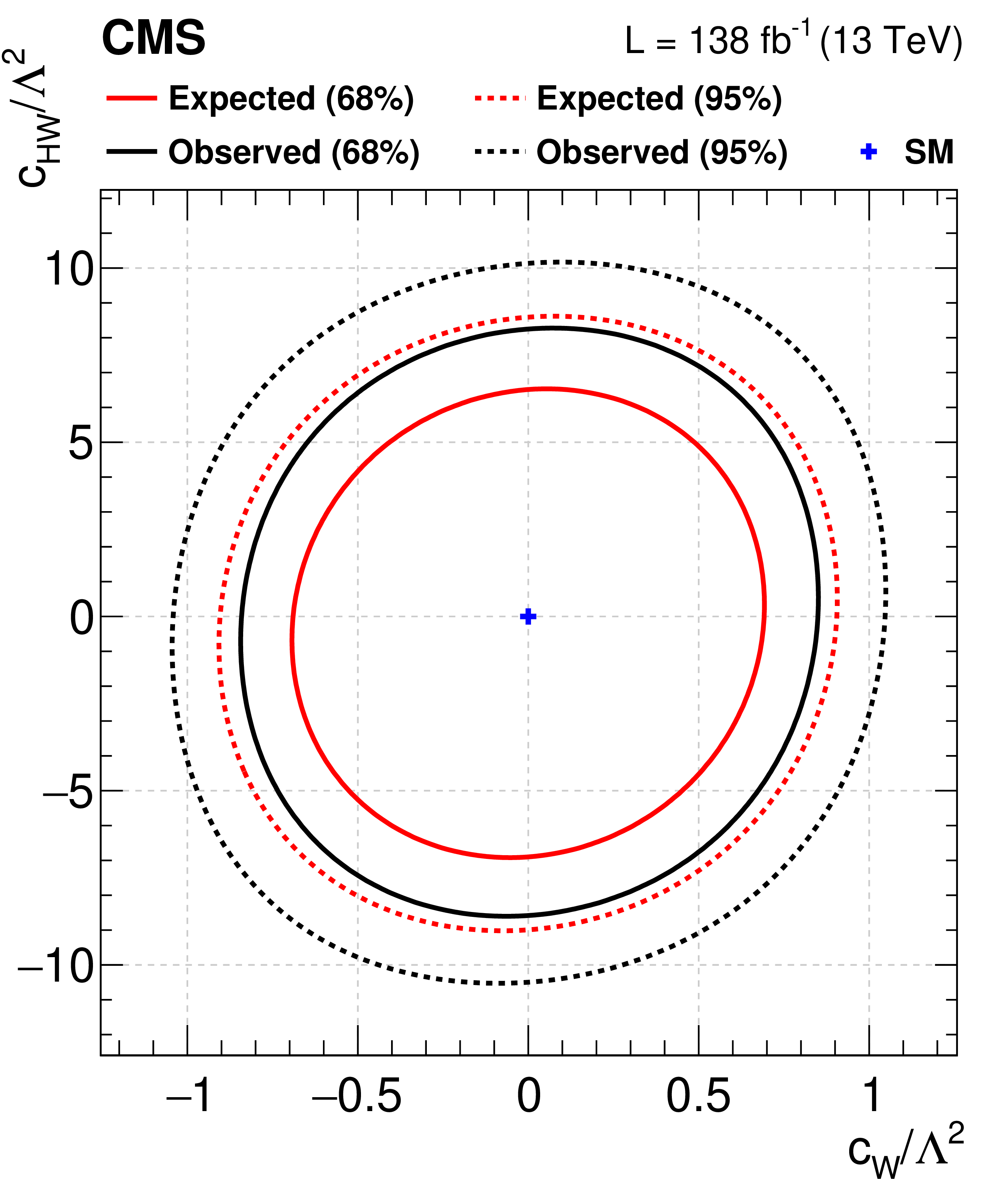
Observed (black) and expected (red) 68 (solid) and 95% (dashed) CL contours for $ -2\ln\Delta\mathcal{L} $ as functions of the reported dim-6 bosonic (upper two rows) and mixed (lower row) Wilson coefficient pairs. When there are two contours for the same CL value, the constrained set of Wilson coefficient values is represented by the area between the two of them if they are concentric, otherwise it consists of the internal areas of the contours. |
png pdf |
Figure 5-a:
Observed (black) and expected (red) 68 (solid) and 95% (dashed) CL contours for $ -2\ln\Delta\mathcal{L} $ as functions of the reported dim-6 bosonic (upper two rows) and mixed (lower row) Wilson coefficient pairs. When there are two contours for the same CL value, the constrained set of Wilson coefficient values is represented by the area between the two of them if they are concentric, otherwise it consists of the internal areas of the contours. |

png pdf |
Figure 5-b:
Observed (black) and expected (red) 68 (solid) and 95% (dashed) CL contours for $ -2\ln\Delta\mathcal{L} $ as functions of the reported dim-6 bosonic (upper two rows) and mixed (lower row) Wilson coefficient pairs. When there are two contours for the same CL value, the constrained set of Wilson coefficient values is represented by the area between the two of them if they are concentric, otherwise it consists of the internal areas of the contours. |

png pdf |
Figure 5-c:
Observed (black) and expected (red) 68 (solid) and 95% (dashed) CL contours for $ -2\ln\Delta\mathcal{L} $ as functions of the reported dim-6 bosonic (upper two rows) and mixed (lower row) Wilson coefficient pairs. When there are two contours for the same CL value, the constrained set of Wilson coefficient values is represented by the area between the two of them if they are concentric, otherwise it consists of the internal areas of the contours. |

png pdf |
Figure 5-d:
Observed (black) and expected (red) 68 (solid) and 95% (dashed) CL contours for $ -2\ln\Delta\mathcal{L} $ as functions of the reported dim-6 bosonic (upper two rows) and mixed (lower row) Wilson coefficient pairs. When there are two contours for the same CL value, the constrained set of Wilson coefficient values is represented by the area between the two of them if they are concentric, otherwise it consists of the internal areas of the contours. |

png pdf |
Figure 5-e:
Observed (black) and expected (red) 68 (solid) and 95% (dashed) CL contours for $ -2\ln\Delta\mathcal{L} $ as functions of the reported dim-6 bosonic (upper two rows) and mixed (lower row) Wilson coefficient pairs. When there are two contours for the same CL value, the constrained set of Wilson coefficient values is represented by the area between the two of them if they are concentric, otherwise it consists of the internal areas of the contours. |

png pdf |
Figure 5-f:
Observed (black) and expected (red) 68 (solid) and 95% (dashed) CL contours for $ -2\ln\Delta\mathcal{L} $ as functions of the reported dim-6 bosonic (upper two rows) and mixed (lower row) Wilson coefficient pairs. When there are two contours for the same CL value, the constrained set of Wilson coefficient values is represented by the area between the two of them if they are concentric, otherwise it consists of the internal areas of the contours. |

png pdf |
Figure 5-g:
Observed (black) and expected (red) 68 (solid) and 95% (dashed) CL contours for $ -2\ln\Delta\mathcal{L} $ as functions of the reported dim-6 bosonic (upper two rows) and mixed (lower row) Wilson coefficient pairs. When there are two contours for the same CL value, the constrained set of Wilson coefficient values is represented by the area between the two of them if they are concentric, otherwise it consists of the internal areas of the contours. |

png pdf |
Figure 6:
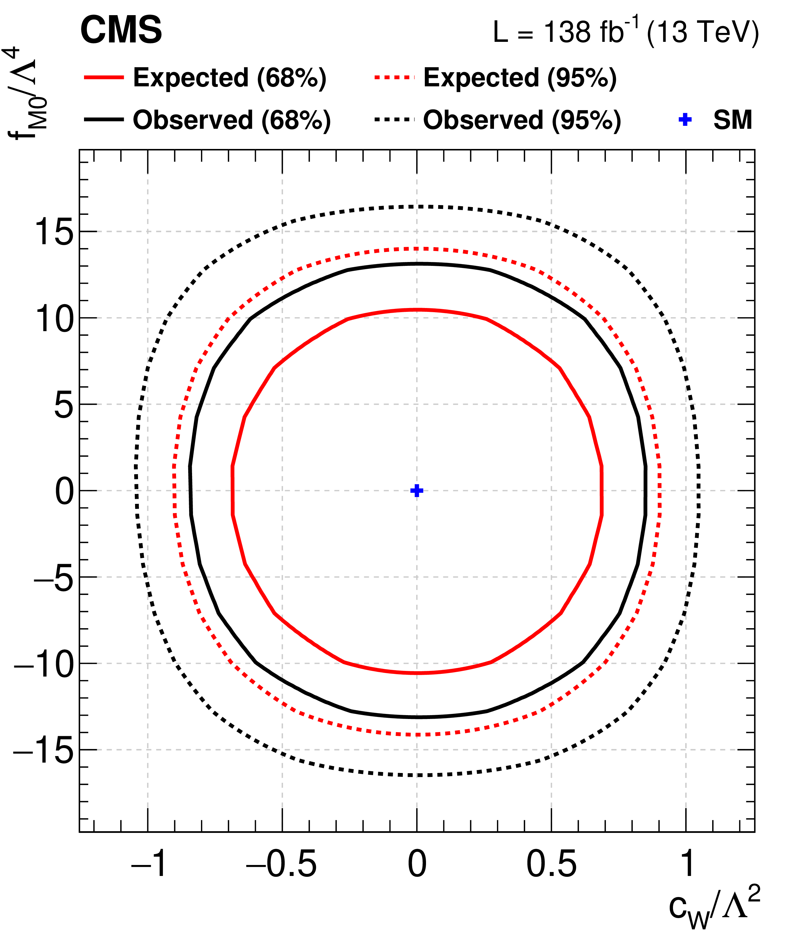
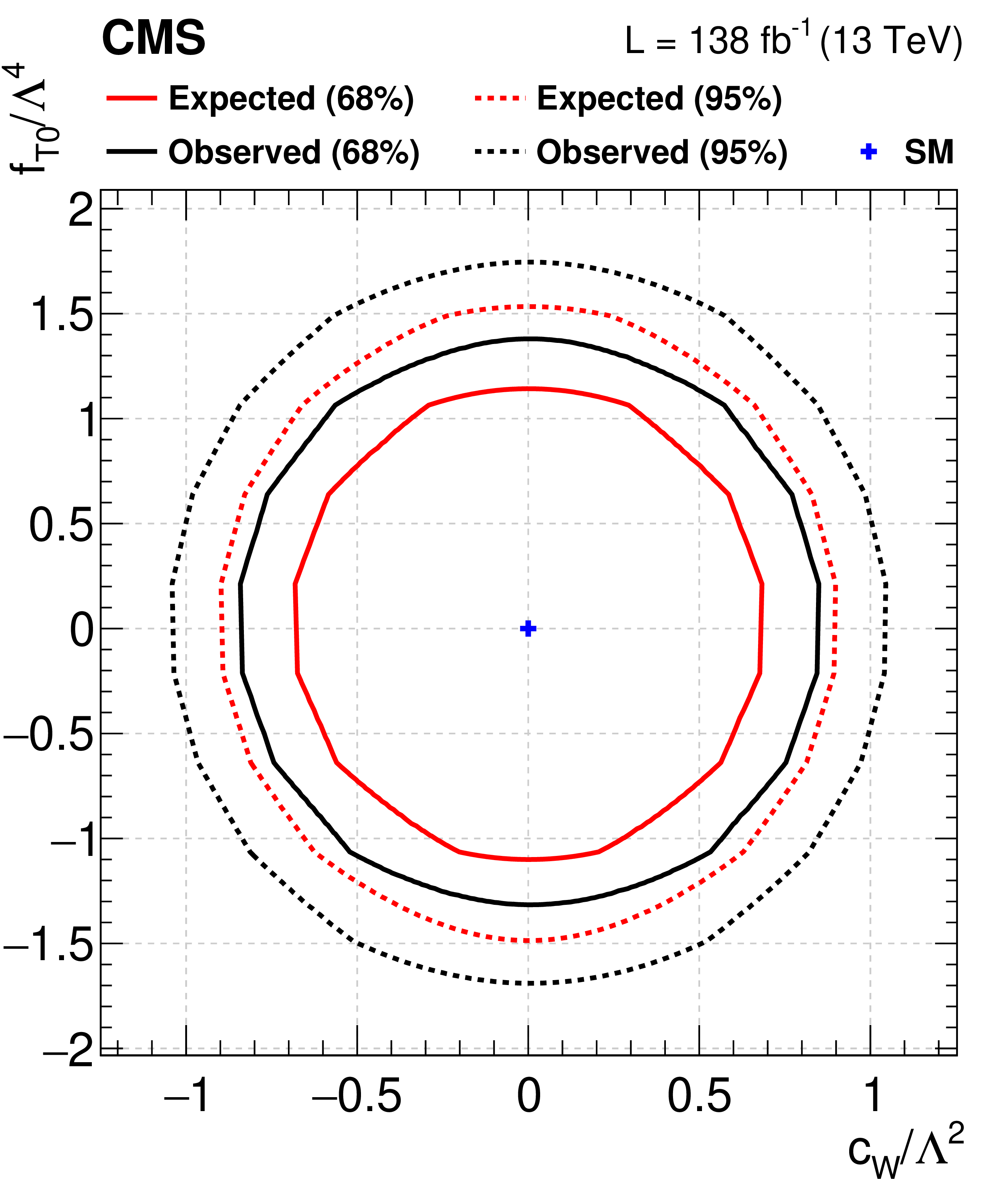
Observed (black) and expected (red) 68 (solid) and 95% (dashed) CL contours for $ -2\ln\Delta\mathcal{L} $ as functions of the reported (dim-6, dim-8) Wilson coefficient pairs. |

png pdf |
Figure 6-a:
Observed (black) and expected (red) 68 (solid) and 95% (dashed) CL contours for $ -2\ln\Delta\mathcal{L} $ as functions of the reported (dim-6, dim-8) Wilson coefficient pairs. |

png pdf |
Figure 6-b:
Observed (black) and expected (red) 68 (solid) and 95% (dashed) CL contours for $ -2\ln\Delta\mathcal{L} $ as functions of the reported (dim-6, dim-8) Wilson coefficient pairs. |

png pdf |
Figure 6-c:
Observed (black) and expected (red) 68 (solid) and 95% (dashed) CL contours for $ -2\ln\Delta\mathcal{L} $ as functions of the reported (dim-6, dim-8) Wilson coefficient pairs. |
png pdf |
Figure 6-d:
Observed (black) and expected (red) 68 (solid) and 95% (dashed) CL contours for $ -2\ln\Delta\mathcal{L} $ as functions of the reported (dim-6, dim-8) Wilson coefficient pairs. |

png pdf |
Figure 6-e:
Observed (black) and expected (red) 68 (solid) and 95% (dashed) CL contours for $ -2\ln\Delta\mathcal{L} $ as functions of the reported (dim-6, dim-8) Wilson coefficient pairs. |

png pdf |
Figure 6-f:
Observed (black) and expected (red) 68 (solid) and 95% (dashed) CL contours for $ -2\ln\Delta\mathcal{L} $ as functions of the reported (dim-6, dim-8) Wilson coefficient pairs. |
png pdf |
Figure 6-g:
Observed (black) and expected (red) 68 (solid) and 95% (dashed) CL contours for $ -2\ln\Delta\mathcal{L} $ as functions of the reported (dim-6, dim-8) Wilson coefficient pairs. |

png pdf |
Figure 6-h:
Observed (black) and expected (red) 68 (solid) and 95% (dashed) CL contours for $ -2\ln\Delta\mathcal{L} $ as functions of the reported (dim-6, dim-8) Wilson coefficient pairs. |

png pdf |
Figure 6-i:
Observed (black) and expected (red) 68 (solid) and 95% (dashed) CL contours for $ -2\ln\Delta\mathcal{L} $ as functions of the reported (dim-6, dim-8) Wilson coefficient pairs. |
| Tables | |

png pdf |
Table 1:
Definitions of the SR, CRs, and VR defined for this analysis. The $ \checkmark $ symbol indicates that the requirement described in the column heading is applied in that region, whereas the $ \times $ symbol means that the opposite selection is applied. The symbols T and L refer to the tight and loose selection rules, respectively. The SR and three CRs (nonprompt, $ \mathrm{t} \overline{\mathrm{t}} $, OS) are selected from an inclusive lepton trigger. |

png pdf |
Table 2:
List of the input variables for the three DNN models developed in this study. The check mark indicates that the variable is included in the DNN model identified in the column header. |

png pdf |
Table 3:
The impact of each systematic uncertainty, together with the impact of the data statistical uncertainty, on the signal strength $ \mu $, as extracted from the fit to measure the SM SSWW VBS signal with the DNN output distributions. Upper and lower uncertainties are given for the various sources. |

png pdf |
Table 4:
Observed and expected 68 and 95% 1D confidence level (CL) intervals on the Wilson coefficients associated with the EFT dim-6 and dim-8 operators considered. The results reported here are obtained by fixing the Wilson coefficients other than the one of interest to their SM values in the fit procedure. These limits are reported in units of TeV$^{-2}$ (TeV$^{-4}$) for the dim-6 (dim-8) Wilson coefficients. |
| Summary |
| Electroweak (EW) production of a same-sign W boson pair in association with two jets, with a hadronically decaying $ \tau $ lepton in the final state, is investigated for the first time, together with an interpretation of possible deviations from the standard model expectations in terms of effective field theory (EFT) operators of dimension 6 and 8. The analysis is performed with a sample of proton-proton collisions at $ \sqrt{s} = $ 13 TeV recorded by the CMS experiment at the CERN LHC in 2016--2018, corresponding to an integrated luminosity of 138 fb$ ^{-1} $. Events are selected with the requirement of one $ \tau $ lepton together with one light lepton (e or $ \mu $) of the same sign, missing transverse momentum, and two jets with large pseudorapidity separation and large dijet invariant mass. Deep neural network algorithms are employed to discriminate different types of signal events from the main backgrounds, significantly boosting the sensitivity of the search. The amplitude for same-sign WW production includes terms that account for strong interactions between partons with W boson radiation. A small fraction of these QCD-mediated events falls within the acceptance of the search. The measured cross section for EW same-sign WW scattering, extracted with the QCD-mediated amplitudes fixed to the standard model (SM) expectations, is 1.44 $ ^{+0.63}_{-0.56} $ times the SM prediction. The observed (expected) significance of the EW signal is 2.7 (1.9) standard deviations. A measurement of the combined EW and residual QCD-mediated contributions yields an observed (expected) significance of 2.9 (2.0) standard deviations. Also presented are the limits on dimension-6 EFT operator contributions, including both one operator and two operators active at the same time, extracted with a reconstruction-level strategy for the first time in vector boson scattering. This is the first study of the combined effects of EFT operators with different dimensions, showing that focusing on one dimensionality can lead to an overestimate of the sensitivity to the corresponding EFT operator class, and that the contributions of terms combining operators with different dimensions should not be neglected, in accordance with the latest recommendations from the EFT theory community. |
| References | ||||
| 1 | ATLAS and CMS Collaborations | Measurements of the Higgs boson production and decay rates and constraints on its couplings from a combined ATLAS and CMS analysis of the LHC pp collision data at $ \sqrt{s}= $ 7 and 8 TeV | JHEP 08 (2016) 045 | 1606.02266 |
| 2 | P. W. Higgs | Broken symmetries, massless particles and gauge fields | PL 12 (1964) 132 | |
| 3 | P. W. Higgs | Broken symmetries and the masses of gauge bosons | PRL 13 (1964) 508 | |
| 4 | F. Englert and R. Brout | Broken symmetry and the mass of gauge vector mesons | PRL 13 (1964) 321 | |
| 5 | J. Chang, K. Cheung, C.-T. Lu, and T.-C. Yuan | WW scattering in the era of post-Higgs-boson discovery | PRD 87 (2013) 093005 | 1303.6335 |
| 6 | W. Kilian, T. Ohl, J. Reuter, and M. Sekulla | High-energy vector boson scattering after the Higgs boson discovery | PRD 91 (2015) 96007 | 1408.6207 |
| 7 | C. Garcia-Garcia, M. Herrero, and R. A. Morales | Unitarization effects in EFT predictions of WZ scattering at the LHC | PRD 100 (2019) 096003 | 1907.06668 |
| 8 | ATLAS Collaboration | Evidence for electroweak production of $ W^{\pm}W^{\pm} $jj in pp collisions at $ \sqrt{s}= $ 8 TeV with the ATLAS Detector | PRL 113 (2014) 141803 | 1405.6241 |
| 9 | CMS Collaboration | Observation of electroweak production of same-sign $ W $ boson pairs in the two jet and two same-sign lepton final state in proton-proton collisions at $ \sqrt{s} = $ 13 TeV | PRL 120 (2018) 081801 | CMS-SMP-17-004 1709.05822 |
| 10 | R. Covarelli, M. Pellen, and M. Zaro | Vector-boson scattering at the LHC: unraveling the electroweak sector | Int. J. Mod. Phys. A 36 (2021) 2130009 | 2102.10991 |
| 11 | C.-W. Chiang, N. G. Deshpande, X.-G. He, and J. Jiang | Family $ SU(2)_l\times SU(2)_h \times U(1) $ model | PRD 81 (2010) 015006 | 0911.1480 |
| 12 | A. Hayreter, X.-G. He, and G. Valencia | LHC constraints on $ W^\prime $, $ Z^\prime $ that couple mainly to third generation fermions | EPJC 80 (2020) 912 | 1912.06344 |
| 13 | R. Calabrese et al. | Top-flavor scheme in the context of W' searches at LHC | PRD 104 (2021) 055006 | 2104.06720 |
| 14 | CMS Collaboration | Search for a W' boson decaying to a $ \tau $ lepton and a neutrino in proton-proton collisions at $ \sqrt{s} = $ 13 TeV | PLB 792 (2019) 107 | CMS-EXO-17-008 1807.11421 |
| 15 | ATLAS Collaboration | Search for high-mass resonances in final states with a \ensuremath\tau-lepton and missing transverse momentum with the ATLAS detector | PRD 109 (2024) 112008 | 2402.16576 |
| 16 | W. Buchmuller and D. Wyler | Effective lagrangian analysis of new interactions and flavour conservation | NPB 268 (1986) 621 | |
| 17 | B. Grzadkowski, M. Iskrzynski, M. Misiak, and J. Rosiek | Dimension-six terms in the Standard Model Lagrangian | JHEP 10 (2010) 085 | 1008.4884 |
| 18 | CMS Collaboration | Study of exclusive two-photon production of W$ ^+ $W$ ^- $ in pp collisions at $ \sqrt{s} = $ 7 TeV and constraints on anomalous quartic gauge couplings | JHEP 07 (2013) 116 | CMS-FSQ-12-010 1305.5596 |
| 19 | CMS Collaboration | Evidence for exclusive $ \gamma\gamma \to W^+ W^- $ production and constraints on anomalous quartic gauge couplings in $ pp $ collisions at $ \sqrt{s}= $ 7 and 8 TeV | JHEP 08 (2016) 119 | CMS-FSQ-13-008 1604.04464 |
| 20 | ATLAS Collaboration | Measurement of $ W^{\pm}W^{\pm} $ vector-boson scattering and limits on anomalous quartic gauge couplings with the ATLAS detector | PRD 96 (2017) 012007 | 1611.02428 |
| 21 | ATLAS Collaboration | Search for anomalous electroweak production of $ WW/WZ $ in association with a high-mass dijet system in $ pp $ collisions at $ \sqrt{s}= $ 8 TeV with the ATLAS detector | PRD 95 (2017) 032001 | 1609.05122 |
| 22 | ATLAS Collaboration | Measurement of $ WW/WZ \to \ell \nu q q^{\prime} $ production with the hadronically decaying boson reconstructed as one or two jets in $ pp $ collisions at $ \sqrt{s}= $ 8 TeV with ATLAS, and constraints on anomalous gauge couplings | EPJC 77 (2017) 563 | 1706.01702 |
| 23 | CMS Collaboration | Measurement of electroweak WZ boson production and search for new physics in WZ + two jets events in pp collisions at $ \sqrt{s} = $ 13TeV | PLB 795 (2019) 281 | CMS-SMP-18-001 1901.04060 |
| 24 | CMS Collaboration | Search for anomalous electroweak production of vector boson pairs in association with two jets in proton-proton collisions at 13 TeV | PLB 798 (2019) 134985 | CMS-SMP-18-006 1905.07445 |
| 25 | ATLAS Collaboration | Measurements of $ W^+W^-+\ge 1 $jet production cross-sections in $ pp $ collisions at $ \sqrt{s}=13 $TeV with the ATLAS detector | JHEP 06 (2021) 003 | 2103.10319 |
| 26 | CMS, TOTEM Collaboration | Search for high-mass exclusive $ \gamma\gamma\to $ WW and $ \gamma\gamma\to $ ZZ production in proton-proton collisions at $ \sqrt{s} = $ 13 TeV | JHEP 07 (2023) 229 | 2211.16320 |
| 27 | ATLAS Collaboration | Measurement and interpretation of same-sign W boson pair production in association with two jets in pp collisions at $ \sqrt{s} = $ 13 TeV with the ATLAS detector | JHEP 04 (2024) 026 | 2312.00420 |
| 28 | ATLAS Collaboration | Differential cross-section measurements of the production of four charged leptons in association with two jets using the ATLAS detector | JHEP 01 (2024) 004 | 2308.12324 |
| 29 | J. J. Ethier, R. Gomez-Ambrosio, G. Magni, and J. Rojo | SMEFT analysis of vector boson scattering and diboson data from the LHC Run II | EPJC 81 (2021) 560 | 2101.03180 |
| 30 | O. J. P. \'E boli and M. C. Gonzalez-Garcia | Classifying the bosonic quartic couplings | PRD 93 (2016) 093013 | 1604.03555 |
| 31 | A. Falkowski et al. | Anomalous triple gauge couplings in the effective field theory approach at the LHC | JHEP 02 (2017) 115 | 1609.06312 |
| 32 | R. Bellan et al. | A sensitivity study of VBS and diboson WW to dimension-6 EFT operators at the LHC | JHEP 05 (2022) 039 | 2108.03199 |
| 33 | E. d. S. Almeida, O. J. P. \'E boli, and M. C. Gonzalez\textendash Garcia | Unitarity constraints on anomalous quartic couplings | PRD 101 (2020) 113003 | 2004.05174 |
| 34 | CMS Collaboration | The CMS experiment at the CERN LHC | JINST 3 (2008) 8004 | |
| 35 | CMS Collaboration | Description and performance of track and primary-vertex reconstruction with the CMS tracker | JINST 9 (2014) 10009 | CMS-TRK-11-001 1405.6569 |
| 36 | CMS Collaboration | The CMS phase-1 pixel detector upgrade | JINST 16 (2021) P02027 | 2012.14304 |
| 37 | CMS Collaboration | Track impact parameter resolution for the full pseudo rapidity coverage in the 2017 dataset with the CMS phase-1 pixel detector | CMS Detector Performance Summary CMS-DP-2020-049, 2020 CDS |
|
| 38 | CMS Collaboration | The CMS trigger system | JINST 12 (2017) P01020 | CMS-TRG-12-001 1609.02366 |
| 39 | J. Alwall et al. | The automated computation of tree-level and next-to-leading order differential cross sections, and their matching to parton shower simulations | JHEP 07 (2014) 079 | 1405.0301 |
| 40 | CMS Collaboration | Measurements of production cross sections of WZ and same-sign WW boson pairs in association with two jets in proton-proton collisions at $ \sqrt{s} = $ 13 TeV | PLB 809 (2020) 135710 | CMS-SMP-19-012 2005.01173 |
| 41 | B. Biedermann, A. Denner, and M. Pellen | Large electroweak corrections to vector-boson scattering at the Large Hadron Collider | PRL 118 (2017) 261801 | 1611.02951 |
| 42 | B. Biedermann, A. Denner, and M. Pellen | Complete NLO corrections to W$ ^{+} $W$ ^{+} $ scattering and its irreducible background at the LHC | JHEP 10 (2017) 124 | 1708.00268 |
| 43 | I. Brivio | SMEFTsim 3.0 \textemdash a practical guide | JHEP 04 (2021) 073 | 2012.11343 |
| 44 | I. Brivio, Y. Jiang, and M. Trott | The SMEFTsim package, theory and tools | JHEP 12 (2017) 070 | 1709.06492 |
| 45 | O. Mattelaer | On the maximal use of Monte Carlo samples: re-weighting events at NLO accuracy | EPJC 76 (2016) 674 | 1607.00763 |
| 46 | P. Nason | A new method for combining NLO QCD with shower Monte Carlo algorithms | JHEP 11 (2004) 040 | hep-ph/0409146 |
| 47 | S. Frixione, P. Nason, and C. Oleari | Matching NLO QCD computations with parton shower simulations: the POWHEG method | JHEP 11 (2007) 070 | 0709.2092 |
| 48 | S. Alioli, P. Nason, C. Oleari, and E. Re | A general framework for implementing NLO calculations in shower Monte Carlo programs: the POWHEG BOX | JHEP 06 (2010) 043 | 1002.2581 |
| 49 | NNPDF Collaboration | Parton distributions from high-precision collider data | EPJC 77 (2017) 663 | 1706.00428 |
| 50 | C. Bierlich et al. | A comprehensive guide to the physics and usage of PYTHIA 8.3 | SciPost Phys. Codeb. 2022 (2022) 8 | 2203.11601 |
| 51 | CMS Collaboration | Extraction and validation of a new set of CMS PYTHIA8 tunes from underlying-event measurements | EPJC 80 (2020) 4 | CMS-GEN-17-001 1903.12179 |
| 52 | GEANT4 Collaboration | GEANT4: A simulation toolkit | NIMA 506 (2003) 250 | |
| 53 | CMS Collaboration | Particle-flow reconstruction and global event description with the CMS detector | JINST 12 (2017) P10003 | CMS-PRF-14-001 1706.04965 |
| 54 | M. Cacciari, G. P. Salam, and G. Soyez | The anti-$ k_{\mathrm{T}} $ jet clustering algorithm | JHEP 04 (2008) 063 | 0802.1189 |
| 55 | M. Cacciari, G. P. Salam, and G. Soyez | FastJet user manual | EPJC 72 (2012) 1896 | 1111.6097 |
| 56 | M. Cacciari and G. P. Salam | Pileup subtraction using jet areas | PLB 659 (2008) 119 | 0707.1378 |
| 57 | CMS Collaboration | Jet performance in pp collisions at $ \sqrt{s} = $ 7 TeV | CMS Physics Analysis Summary, 2010 link |
|
| 58 | CMS Collaboration | Jet algorithms performance in 13 TeV data | CMS Physics Analysis Summary, 2017 CMS-PAS-JME-16-003 |
CMS-PAS-JME-16-003 |
| 59 | CMS Collaboration | Technical proposal for the Phase-II upgrade of the Compact Muon Solenoid | CMS Technical Proposal CERN-LHCC-2015-010, CMS-TDR-15-02, 2015 CDS |
|
| 60 | E. Bols et al. | Jet flavour classification using DeepJet | JINST 15 (2020) P12012 | 2008.10519 |
| 61 | CMS Collaboration | Identification of heavy-flavour jets with the CMS detector in pp collisions at 13 TeV | JINST 13 (2018) P05011 | CMS-BTV-16-002 1712.07158 |
| 62 | CMS Collaboration | Measurement of the single top quark and antiquark production cross sections in the $ t $ channel and their ratio in proton-proton collisions at $ \sqrt{s}= $ 13 TeV | PLB 800 (2020) 135042 | CMS-TOP-17-011 1812.10514 |
| 63 | CMS Collaboration | Electron and photon reconstruction and identification with the CMS experiment at the CERN LHC | JINST 16 (2021) P05014 | CMS-EGM-17-001 2012.06888 |
| 64 | CMS Collaboration | Performance of the CMS muon detector and muon reconstruction with proton-proton collisions at $ \sqrt{s}= $ 13 TeV | JINST 13 (2018) P06015 | CMS-MUO-16-001 1804.04528 |
| 65 | CMS Collaboration | Performance of reconstruction and identification of $ \tau $ leptons decaying to hadrons and $ \nu_\tau $ in pp collisions at $ \sqrt{s}= $ 13 TeV | JINST 13 (2018) P10005 | CMS-TAU-16-003 1809.02816 |
| 66 | CMS Collaboration | Identification of hadronic tau lepton decays using a deep neural network | JINST 17 (2022) P07023 | CMS-TAU-20-001 2201.08458 |
| 67 | CMS Collaboration | Measurement of Higgs boson production and properties in the WW Decay channel with leptonic final states | JHEP 01 (2014) 096 | CMS-HIG-13-023 1312.1129 |
| 68 | D. P. Kingma and J. Ba | Adam: A method for stochastic optimization | Proceedings of the 3rd International Conference for Learning Representations, San Diego, 2017 link |
1412.6980 |
| 69 | I. Goodfellow, Y. Bengio, and A. Courville | Deep learning | MIT Press, 2016 link |
|
| 70 | A. J. Barr et al. | Guide to transverse projections and mass-constraining variables | PRD 84 (2011) 095031 | 1105.2977 |
| 71 | D. L. Rainwater, R. Szalapski, and D. Zeppenfeld | Probing color singlet exchange in $ Z $ + two jet events at the CERN LHC | PRD 54 (1996) 6680 | hep-ph/9605444 |
| 72 | G. Cowan, K. Cranmer, E. Gross, and O. Vitells | Asymptotic formulae for likelihood-based tests of new physics | EPJC 71 (2011) 1554 | 1007.1727 |
| 73 | CMS Collaboration | The CMS statistical analysis and combination tool: Combine | Submitted to Comput. Softw. Big Sci, 2024 | CMS-CAT-23-001 2404.06614 |
| 74 | W. Verkerke and D. Kirkby | The roofit toolkit for data modeling | link | |
| 75 | L. Moneta et al. | The RooStats project | PoS ACAT 057, 2010 link |
1009.1003 |
| 76 | CMS Collaboration | Precision luminosity measurement in proton-proton collisions at $ \sqrt{s}= $ 13 TeV in 2015 and 2016 at CMS | EPJC 81 (2021) 800 | CMS-LUM-17-003 2104.01927 |
| 77 | CMS Collaboration | CMS luminosity measurement for the 2017 data-taking period at $ \sqrt{s}= $ 13 TeV | CMS Physics Analysis Summary, 2018 CMS-PAS-LUM-17-004 |
CMS-PAS-LUM-17-004 |
| 78 | CMS Collaboration | CMS luminosity measurement for the 2018 data-taking period at $ \sqrt{s}= $ 13 TeV | CMS Physics Analysis Summary, 2019 CMS-PAS-LUM-18-002 |
CMS-PAS-LUM-18-002 |
| 79 | M. Cacciari et al. | The $ \mathrm{t} \overline{\mathrm{t}} $ cross-section at 1.8-TeV and 1.96-TeV: a study of the systematics due to parton densities and scale dependence | JHEP 04 (2004) 068 | hep-ph/0303085 |
| 80 | S. Catani, D. de Florian, M. Grazzini, and P. Nason | Soft gluon resummation for Higgs boson production at hadron colliders | JHEP 07 (2003) 028 | hep-ph/0306211 |
| 81 | J. Butterworth et al. | PDF4LHC recommendations for LHC Run II | JPG 43 (2016) 023001 | 1510.03865 |
| 82 | CMS Collaboration | Measurement of the inelastic proton-proton cross section at $ \sqrt{s}= $ 13 TeV | JHEP 07 (2018) 161 | CMS-FSQ-15-005 1802.02613 |
| 83 | CMS Collaboration | Performance of the CMS electromagnetic calorimeter in pp collisions at $ \sqrt{s}= $ 13 TeV | JINST 19 (2024) P09004 | CMS-EGM-18-002 2403.15518 |
| 84 | CMS Collaboration | Jet energy scale and resolution in the CMS experiment in pp collisions at 8 TeV | JINST 12 (2017) P02014 | CMS-JME-13-004 1607.03663 |
| 85 | J. S. Conway | Incorporating nuisance parameters in likelihoods for multisource spectra | in PHYSTAT 2011, p. 115. 2011 link |
1103.0354 |
| 86 | CMS Collaboration | HEPData record for this analysis | link | |
| 87 | C. Hays, A. Martin, V. Sanz, and J. Setford | On the impact of dimension-eight SMEFT operators on Higgs measurements | JHEP 02 (2019) 123 | 1808.00442 |
| 88 | S. Dawson, M. Forslund, and M. Schnubel | SMEFT matching to Z' models at dimension eight | PRD 110 (2024) 015002 | 2404.01375 |
| 89 | T. Corbett et al. | Impact of dimension-eight SMEFT operators in the electroweak precision observables and triple gauge couplings analysis in universal SMEFT | PRD 107 (2023) 115013 | 2304.03305 |
| 90 | CMS Collaboration | Combined effective field theory interpretation of Higgs boson, electroweak vector boson, top quark, and multi-jet measurements | Submitted to EPJC, 2025 | CMS-SMP-24-003 2504.02958 |
| 91 | ATLAS Collaboration | Combined effective field theory interpretation of Higgs boson and weak boson production and decay with ATLAS data and electroweak precision observables | Technical Report ATL-PHYS-PUB-2022-037, 2022 | |
|
|
Compact Muon Solenoid LHC, CERN |
|

|

|

|

|

|