

Compact Muon Solenoid
LHC, CERN
| CMS-SMP-23-005 ; CERN-EP-2024-127 | ||
| Observation of $ {\gamma\gamma\to\tau\tau} $ in proton-proton collisions and limits on the anomalous electromagnetic moments of the $ \tau $ lepton | ||
| CMS Collaboration | ||
| 6 June 2024 | ||
| Rep. Prog. Phys. 87 (2024) 107801 | ||
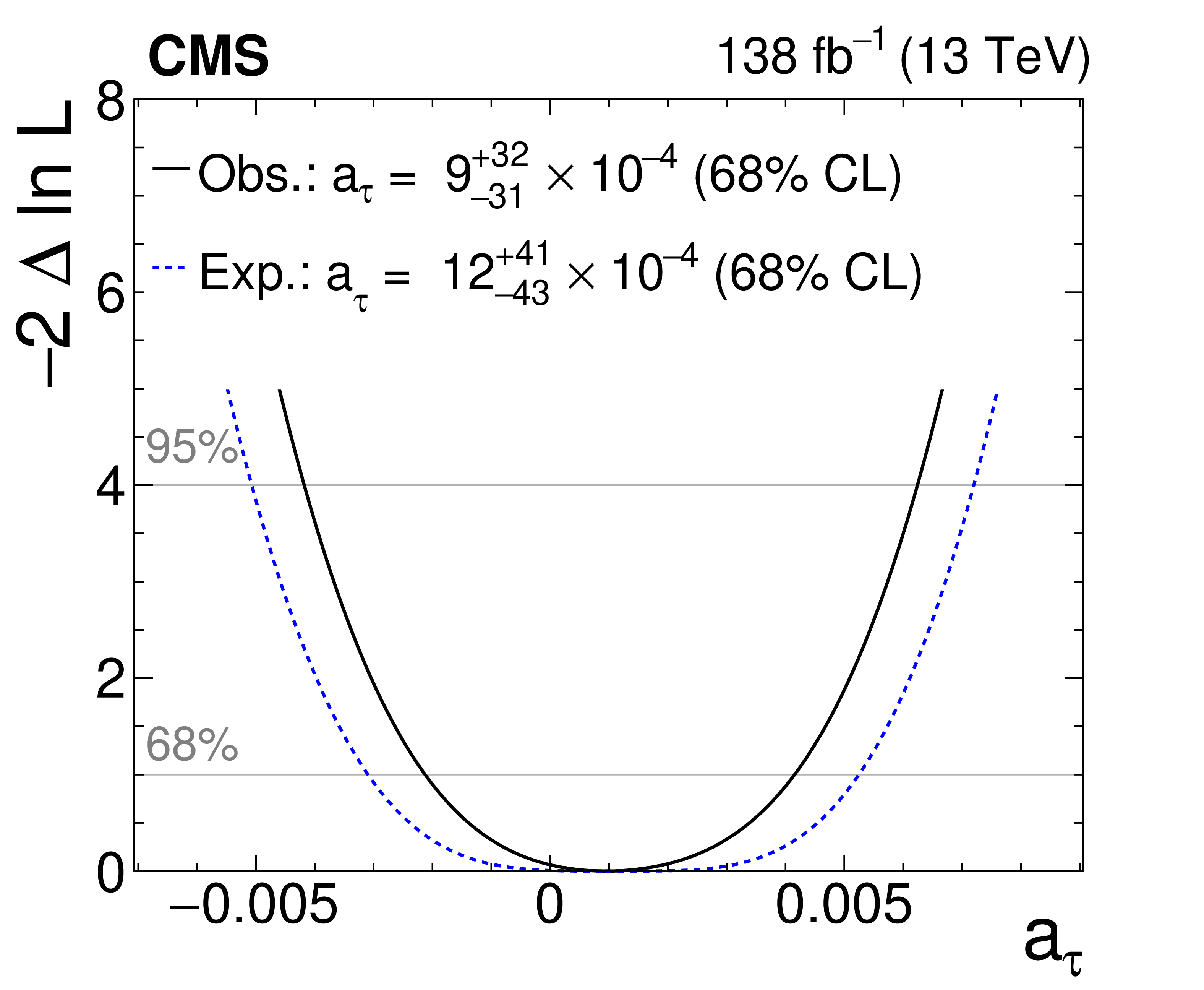
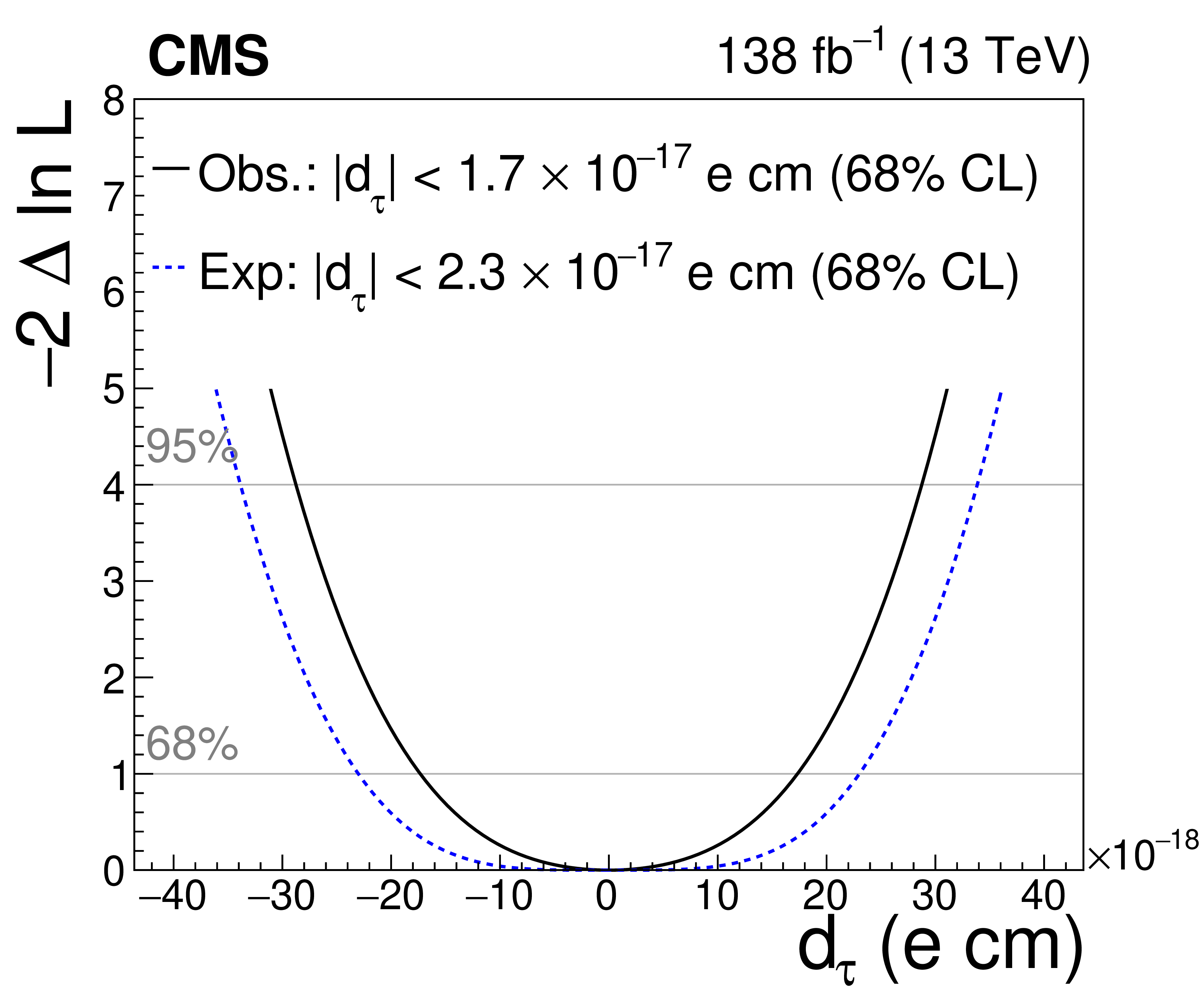
| Abstract: The production of a pair of $ \tau $ leptons via photon-photon fusion, $ {\gamma\gamma\to\tau\tau} $, is observed for the first time in proton-proton collisions, with a significance of 5.3 standard deviations. This observation is based on a data set recorded with the CMS detector at the LHC at a center-of-mass energy of 13 TeV and corresponding to an integrated luminosity of 138 fb$ ^{-1} $. Events with a pair of $ \tau $ leptons produced via photon-photon fusion are selected by requiring them to be back-to-back in the azimuthal direction and to have a minimum number of charged hadrons associated with their production vertex. The $ \tau $ leptons are reconstructed in their leptonic and hadronic decay modes. The measured fiducial cross section of $ {\gamma\gamma\to\tau\tau} $ is $ \sigma^\text{fid}_\text{obs}= $ 12.4$ ^{+3.8}_{-3.1} $ fb. Constraints are set on the contributions to the anomalous magnetic moment ($ a_{\tau} $) and electric dipole moments ($ d_{\tau} $) of the $ \tau $ lepton originating from potential effects of new physics on the $ \gamma\tau\tau $ vertex: $ a_{\tau}= $ 0.0009$_{-0.0031}^{+0.0032} $ and $ |d_{\tau}| < $ 2.9$\times $10$^{-17}$ e.cm (95% confidence level), consistent with the standard model. | ||
| Links: e-print arXiv:2406.03975 [hep-ex] (PDF) ; CDS record ; inSPIRE record ; HepData record ; Physics Briefing ; CADI line (restricted) ; | ||
| Figures & Tables | Summary | Additional Figures | References | CMS Publications |
|---|
| Highlighted with a CERN Courier article. |
| Figures | |
png pdf |
Figure 1:
Feynman diagrams for the production of $ \tau $ lepton pairs by photon-photon fusion. The exclusive (left), single proton dissociation (middle), and double proton dissociation (right) topologies are shown. |

png pdf |
Figure 1-a:
Feynman diagrams for the production of $ \tau $ lepton pairs by photon-photon fusion. The exclusive (left), single proton dissociation (middle), and double proton dissociation (right) topologies are shown. |
png pdf |
Figure 1-b:
Feynman diagrams for the production of $ \tau $ lepton pairs by photon-photon fusion. The exclusive (left), single proton dissociation (middle), and double proton dissociation (right) topologies are shown. |
png pdf |
Figure 1-c:
Feynman diagrams for the production of $ \tau $ lepton pairs by photon-photon fusion. The exclusive (left), single proton dissociation (middle), and double proton dissociation (right) topologies are shown. |

png pdf |
Figure 2:
Schematic view of the 0.1 cm wide windows probed along the $ z $ axis to derive corrections to the pileup track density in simulation. Windows within 1 cm from the dimuon vertex, illustrated with the red box, are discarded so as not to count tracks from the hard-scattering interaction. The green curve indicates the probability distribution of z-coordinates for PU vertices in the beamspot. |
png pdf |
Figure 3:
Distribution of $ N_\text{tracks}^\text{PU} $ in windows of 0.1 cm width along the $ z $ axis for the observed events (black), uncorrected simulation (red), and beamspot-corrected simulation (blue) for data collected in 2017. The windows shown here are located at the beamspot center (upper left), and one (upper right) or two (lower) beamspot widths away from the center. The ratio of beamspot-corrected simulation to observation (lower plots) is taken as a residual correction to the simulations. The last bin includes the overflow. Similar distributions and corrections are derived independently for the other data-taking periods. |
png pdf |
Figure 3-a:
Distribution of $ N_\text{tracks}^\text{PU} $ in windows of 0.1 cm width along the $ z $ axis for the observed events (black), uncorrected simulation (red), and beamspot-corrected simulation (blue) for data collected in 2017. The windows shown here are located at the beamspot center (upper left), and one (upper right) or two (lower) beamspot widths away from the center. The ratio of beamspot-corrected simulation to observation (lower plots) is taken as a residual correction to the simulations. The last bin includes the overflow. Similar distributions and corrections are derived independently for the other data-taking periods. |

png pdf |
Figure 3-b:
Distribution of $ N_\text{tracks}^\text{PU} $ in windows of 0.1 cm width along the $ z $ axis for the observed events (black), uncorrected simulation (red), and beamspot-corrected simulation (blue) for data collected in 2017. The windows shown here are located at the beamspot center (upper left), and one (upper right) or two (lower) beamspot widths away from the center. The ratio of beamspot-corrected simulation to observation (lower plots) is taken as a residual correction to the simulations. The last bin includes the overflow. Similar distributions and corrections are derived independently for the other data-taking periods. |

png pdf |
Figure 3-c:
Distribution of $ N_\text{tracks}^\text{PU} $ in windows of 0.1 cm width along the $ z $ axis for the observed events (black), uncorrected simulation (red), and beamspot-corrected simulation (blue) for data collected in 2017. The windows shown here are located at the beamspot center (upper left), and one (upper right) or two (lower) beamspot widths away from the center. The ratio of beamspot-corrected simulation to observation (lower plots) is taken as a residual correction to the simulations. The last bin includes the overflow. Similar distributions and corrections are derived independently for the other data-taking periods. |
png pdf |
Figure 4:
Distribution of the number of reconstructed tracks in a 0.1 cm wide window in the $ z $ direction, centered on the dimuon reconstructed vertex, for acoplanarity $ A < $ 0.015, in data collected in 2017. The DY simulation is split into several components based on the number of reconstructed tracks originating from the hard interaction. The red line shows the simulation before the correction. The black points show the observed data after subtracting the expected background contribution from the $ {\gamma\gamma\to\mu\mu} $ and $ {\gamma\gamma\to\mathrm{W}\mathrm{W}} $ processes (dashed orange line). The last bin includes the overflow. Similar distributions and corrections are derived independently for the other data-taking periods. The ratios between the observed data, from which the exclusive background contributions have been subtracted, and the DY prediction before (red) and after the corrections (black), are shown in the lower panel. The region with the selection requirement $ N_\text{tracks}= $ 0 or 1 used in the SR is highlighted with the orange shaded area in the lower panel. |
png pdf |
Figure 5:
Measurement of the scale factor for the elastic exclusive signal in $ \mu\mu $ events for $ N_\text{tracks}= $ 0 (left) or 1 (right), and $ A < $ 0.015. The shape of the inclusive background (blue) is estimated from the observed data in the 3 $ \leq N_\text{tracks}\leq $ 7 sideband, and rescaled to fit the observed data in 75 $ < m_{\mu\mu} < $ 105 GeV. The scale factor is fitted in the lower ratio panel with constant (red) and linear (blue) functions. The vertical error bars indicate the statistical uncertainty in the number of observed events. |
png pdf |
Figure 5-a:
Measurement of the scale factor for the elastic exclusive signal in $ \mu\mu $ events for $ N_\text{tracks}= $ 0 (left) or 1 (right), and $ A < $ 0.015. The shape of the inclusive background (blue) is estimated from the observed data in the 3 $ \leq N_\text{tracks}\leq $ 7 sideband, and rescaled to fit the observed data in 75 $ < m_{\mu\mu} < $ 105 GeV. The scale factor is fitted in the lower ratio panel with constant (red) and linear (blue) functions. The vertical error bars indicate the statistical uncertainty in the number of observed events. |

png pdf |
Figure 5-b:
Measurement of the scale factor for the elastic exclusive signal in $ \mu\mu $ events for $ N_\text{tracks}= $ 0 (left) or 1 (right), and $ A < $ 0.015. The shape of the inclusive background (blue) is estimated from the observed data in the 3 $ \leq N_\text{tracks}\leq $ 7 sideband, and rescaled to fit the observed data in 75 $ < m_{\mu\mu} < $ 105 GeV. The scale factor is fitted in the lower ratio panel with constant (red) and linear (blue) functions. The vertical error bars indicate the statistical uncertainty in the number of observed events. |
png pdf |
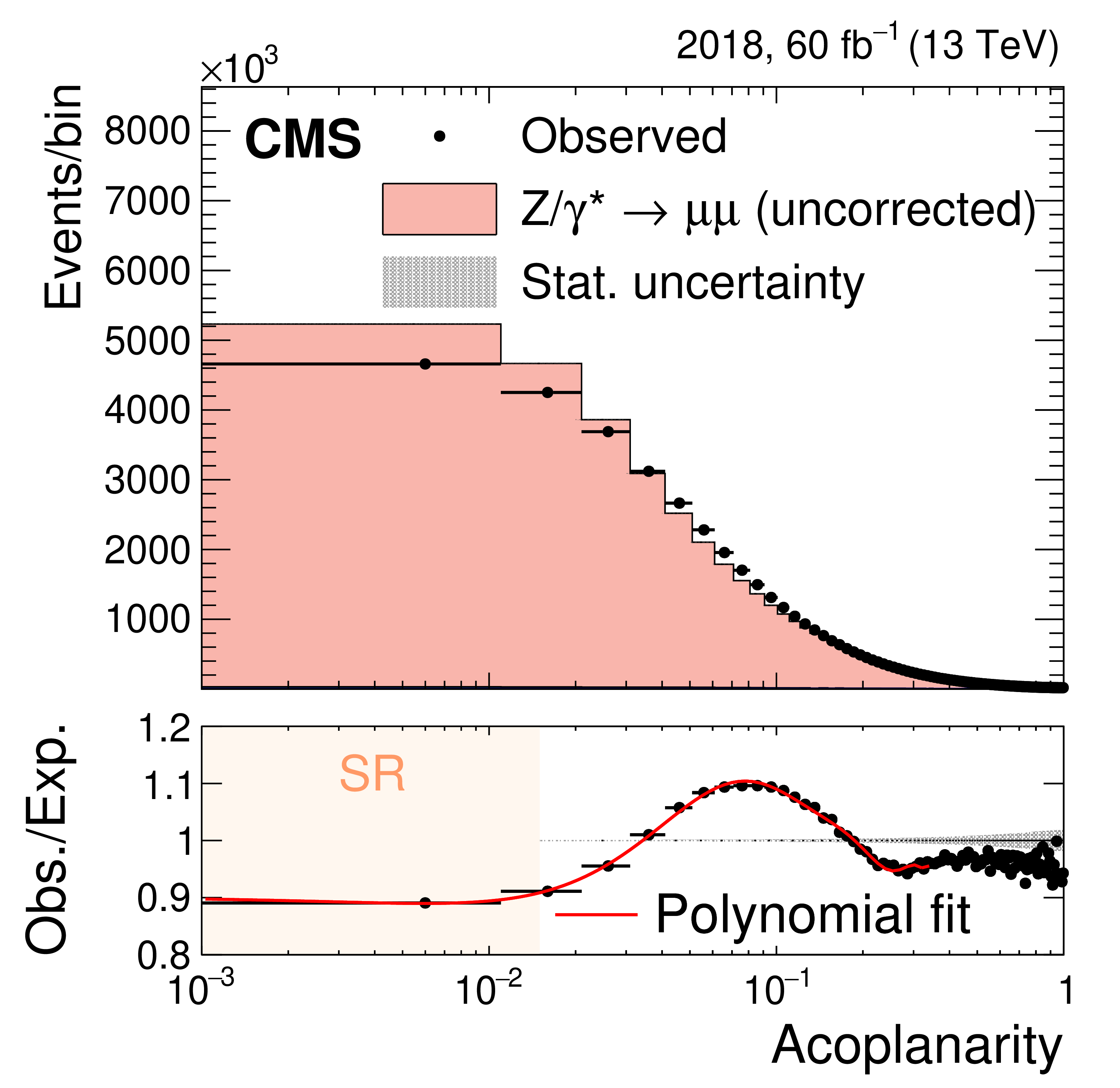
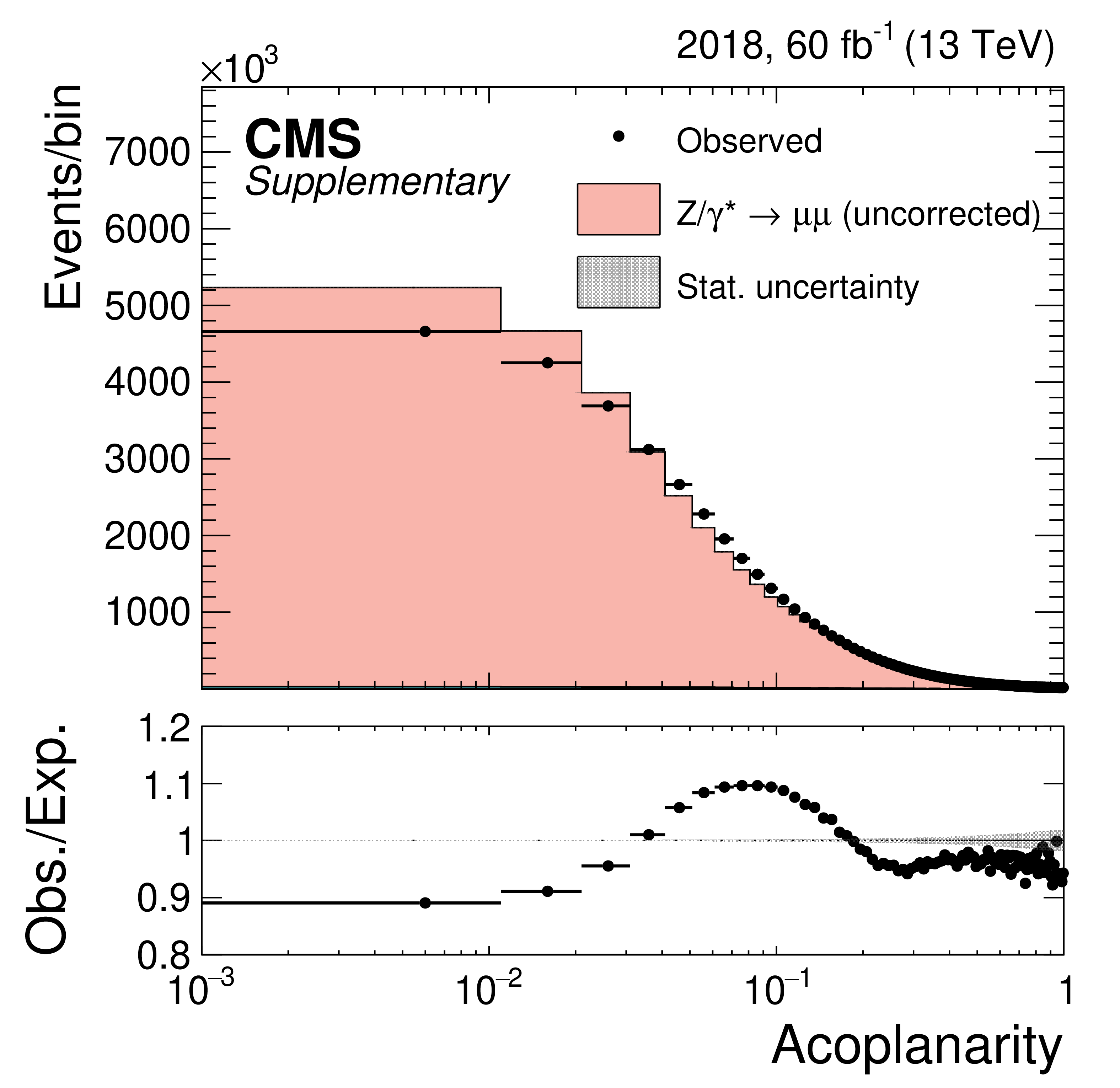
Figure 6:
Acoplanarity distribution for the observed events and in DY simulation before correction, in the 2018 data-taking period. The background prediction is normalized to match the observed yield and only the statistical uncertainty is shown. The data-to-simulation ratio is fitted with a polynomial to obtain the correction. The selection criterion $ A < $ 0.015 used in the SR is highlighted with the orange shaded area in the lower panel. |
png pdf |
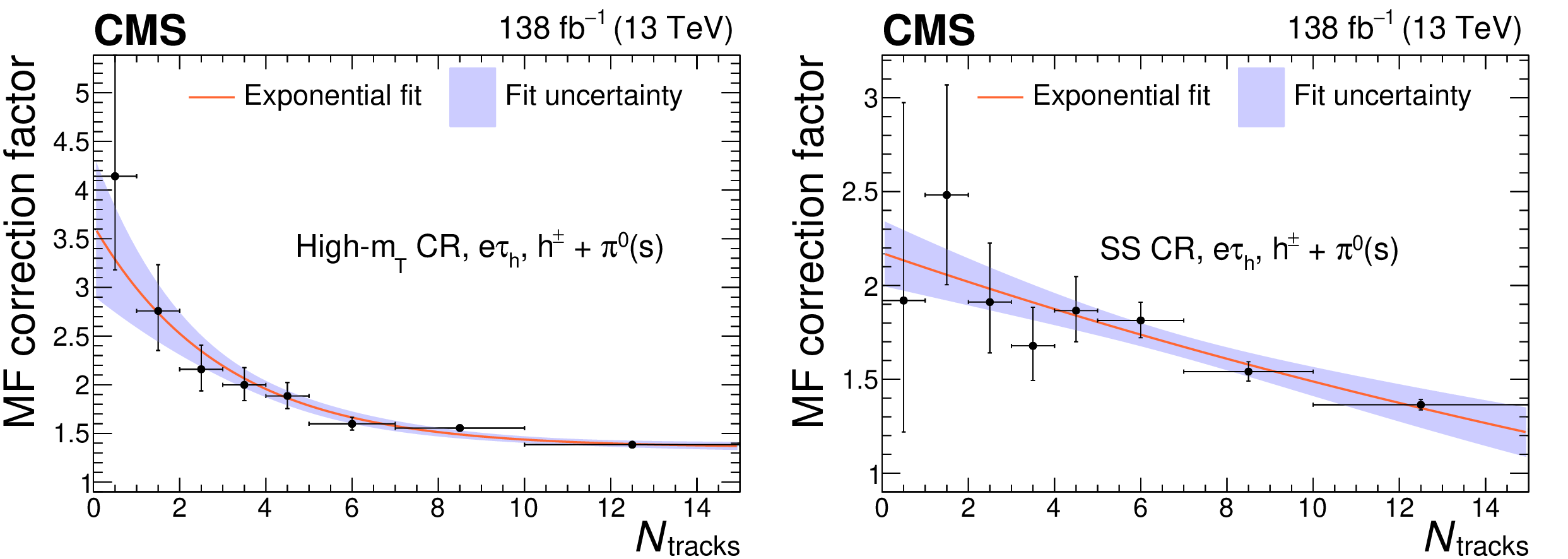
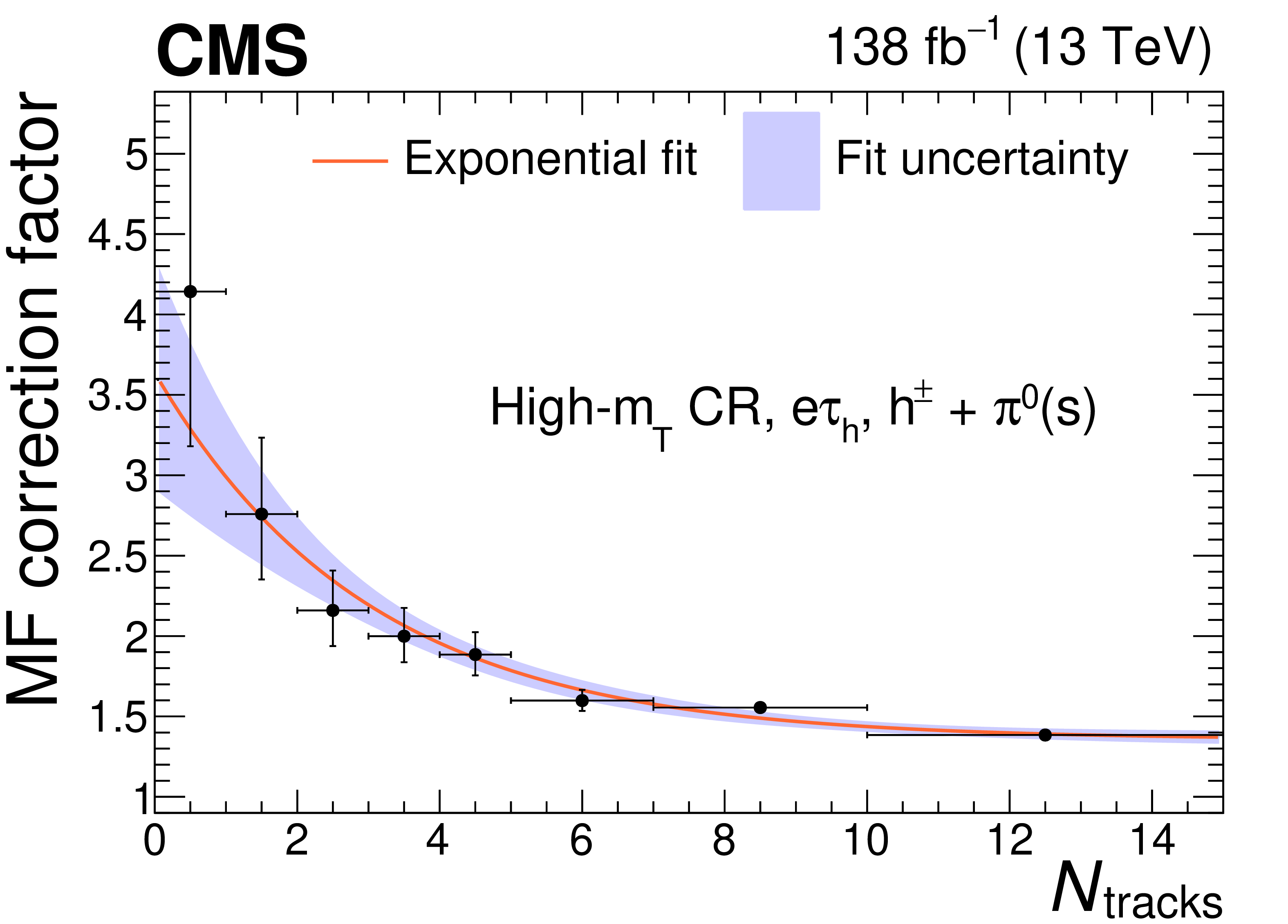
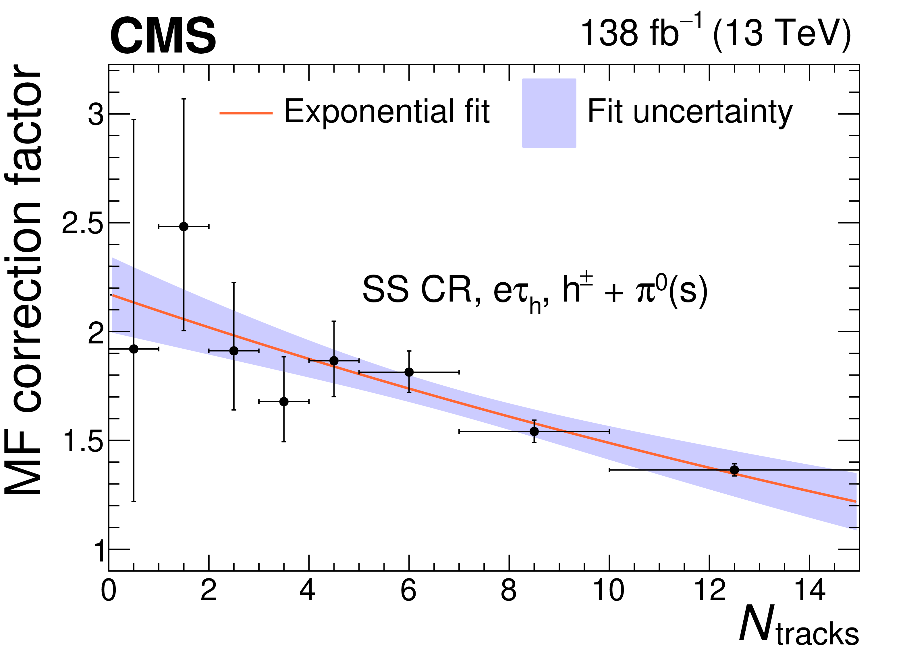
Figure 7:
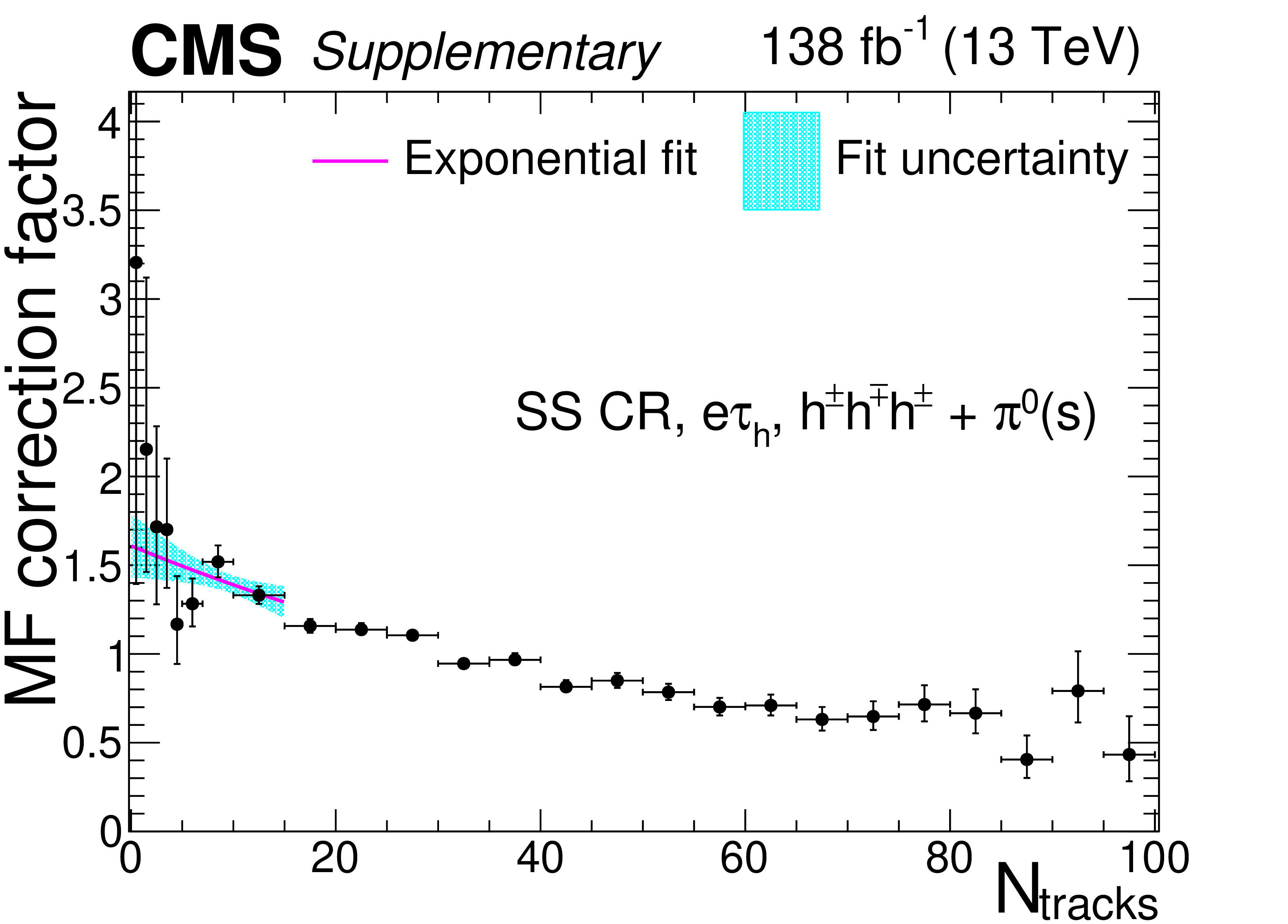
Multiplicative $ N_\text{tracks} $-dependent corrections to the $ \tau_{\mathrm{h}} $ MFs, $ \omega(N_\text{tracks}, \text{DM}^{\tau_{\mathrm{h}}}) $, in the $ \mathrm{e}\tau_{\mathrm{h}} $ final state, in the high-$ m_{\mathrm{T}} $ (left) and SS (right) CRs, for the $ \mathrm{h}^\pm+\pi^{0} $(s) DM. The purple shaded area corresponds to the fit uncertainty. The vertical error bars indicate the statistical uncertainty in the MF correction factors measured in individual $ N_\text{tracks} $ ranges. |
png pdf |
Figure 7-a:
Multiplicative $ N_\text{tracks} $-dependent corrections to the $ \tau_{\mathrm{h}} $ MFs, $ \omega(N_\text{tracks}, \text{DM}^{\tau_{\mathrm{h}}}) $, in the $ \mathrm{e}\tau_{\mathrm{h}} $ final state, in the high-$ m_{\mathrm{T}} $ (left) and SS (right) CRs, for the $ \mathrm{h}^\pm+\pi^{0} $(s) DM. The purple shaded area corresponds to the fit uncertainty. The vertical error bars indicate the statistical uncertainty in the MF correction factors measured in individual $ N_\text{tracks} $ ranges. |
png pdf |
Figure 7-b:
Multiplicative $ N_\text{tracks} $-dependent corrections to the $ \tau_{\mathrm{h}} $ MFs, $ \omega(N_\text{tracks}, \text{DM}^{\tau_{\mathrm{h}}}) $, in the $ \mathrm{e}\tau_{\mathrm{h}} $ final state, in the high-$ m_{\mathrm{T}} $ (left) and SS (right) CRs, for the $ \mathrm{h}^\pm+\pi^{0} $(s) DM. The purple shaded area corresponds to the fit uncertainty. The vertical error bars indicate the statistical uncertainty in the MF correction factors measured in individual $ N_\text{tracks} $ ranges. |
png pdf |
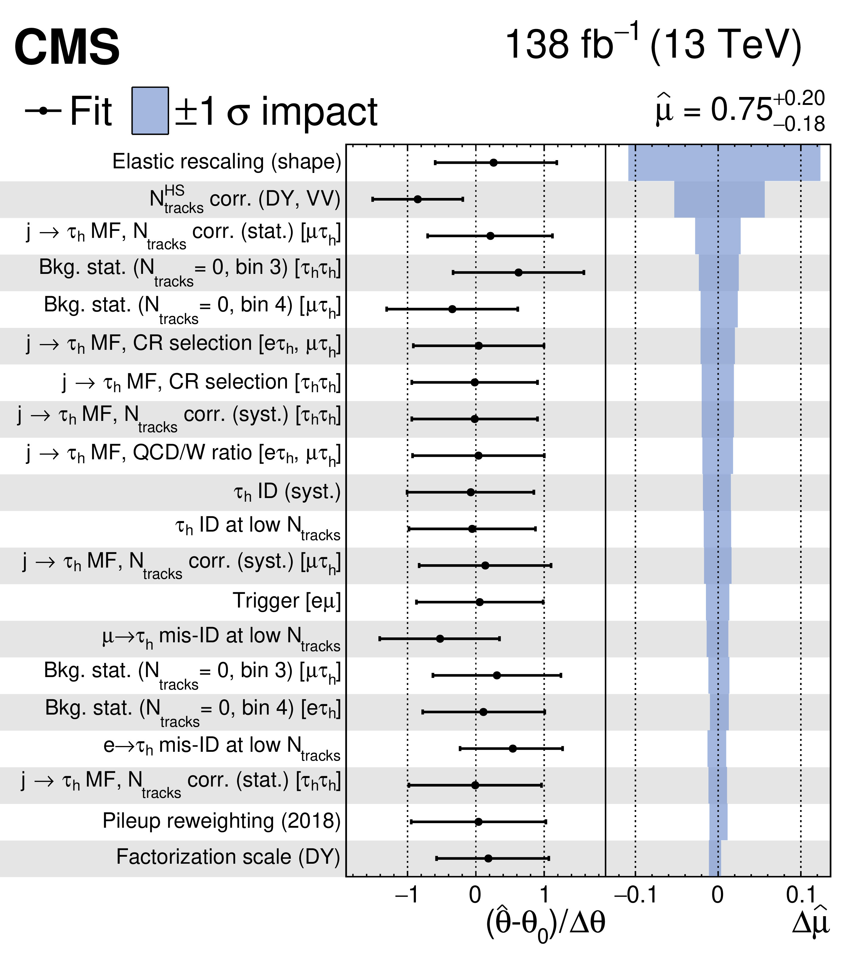
Figure 8:
Postfit values of the nuisance parameters (black markers), shown as the difference of their best-fit values, $ \hat{\theta} $, and prefit values, $ \theta_0 $, relative to the prefit uncertainties $ \Delta\theta $. The horizontal error bars indicate the uncertainties in these measured postfit values. The impact $ \Delta\hat{\mu} $ of the nuisance parameter on the signal strength is computed as the difference of the nominal best fit value of $ \mu $ and the best fit value obtained when fixing the nuisance parameter under scrutiny to its best fit value $ \hat{\theta} $ plus/minus its postfit uncertainty (blue shaded area). The nuisance parameters are ordered by their impact, and only the 20 highest ranked parameters are shown. |

png pdf |
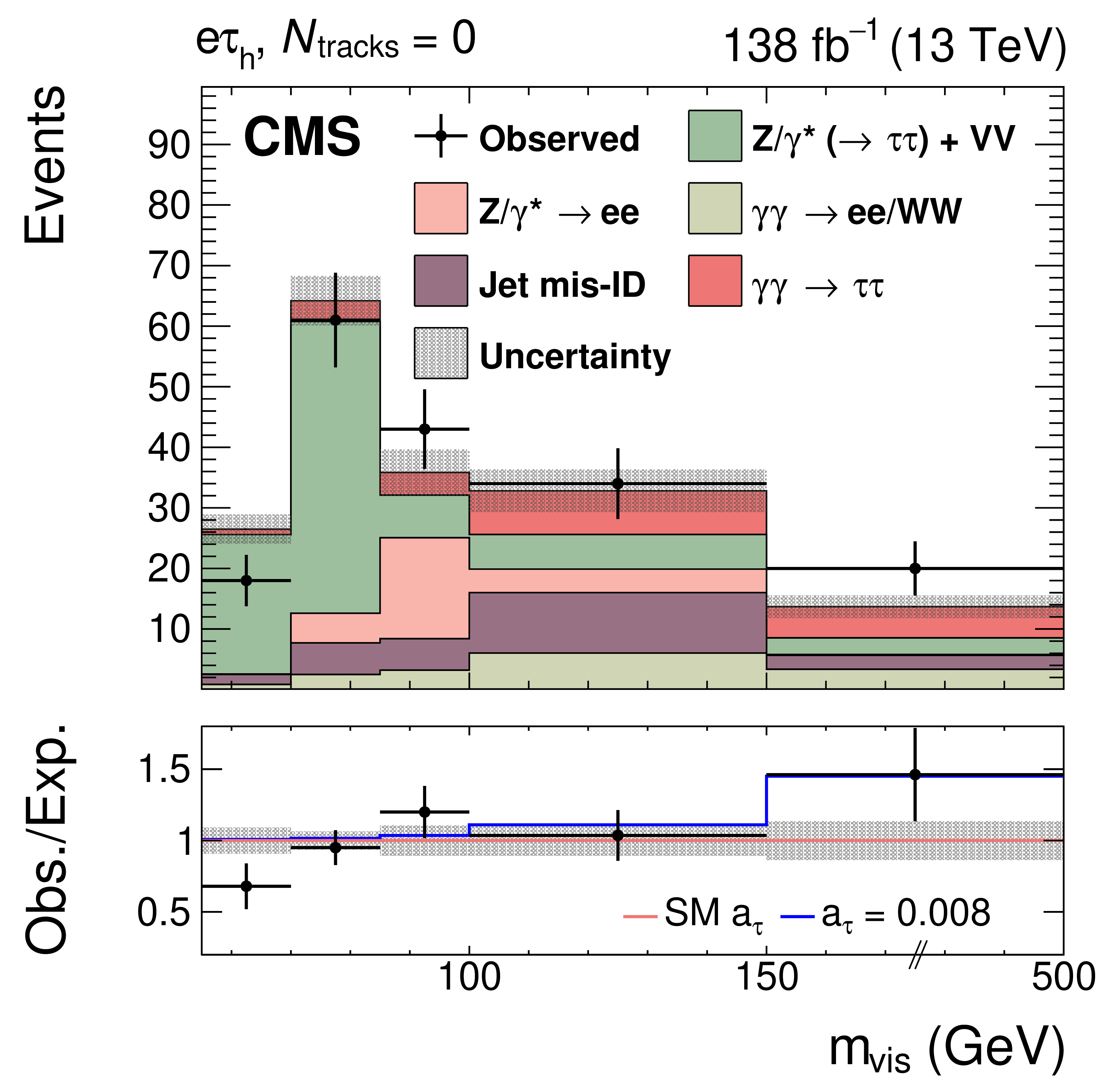
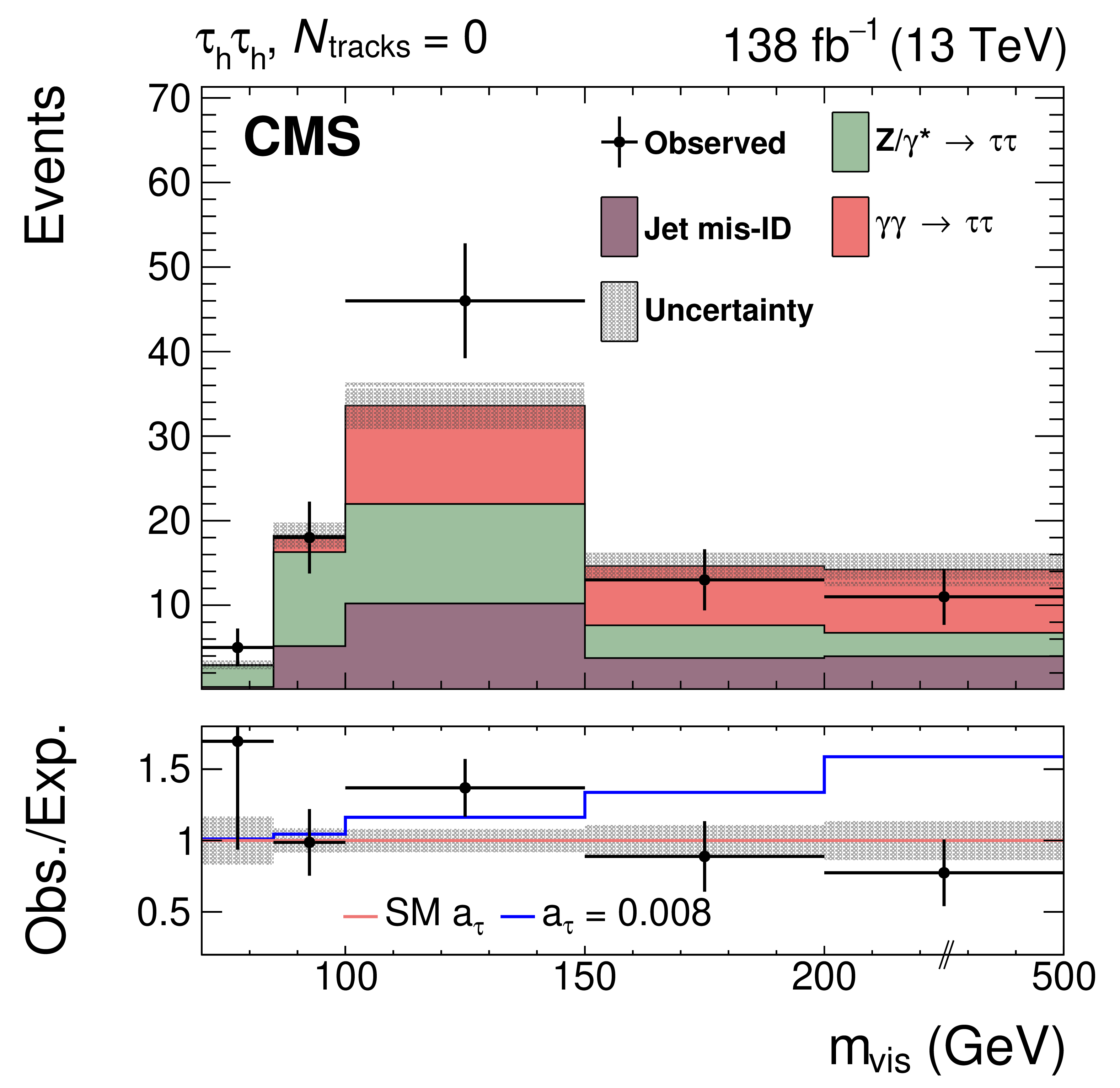
Figure 9:
Observed and predicted $ m_\text{vis} $ distributions in the $ \mathrm{e}\mu $ (upper left), $ \mathrm{e}\tau_{\mathrm{h}} $ (upper right), $ \mu\tau_{\mathrm{h}} $ (lower left), and $ \tau_{\mathrm{h}}\tau_{\mathrm{h}} $ (lower right) final states for events with $ N_\text{tracks}= $ 0, the lower panels showing the observed/expected ratio. The observed data and their associated Poissonian statistical uncertainty are shown with black markers with vertical error bars. The minor inclusive diboson background contribution is drawn together with the DY background in the $ \mathrm{e}\mu $, $ \mathrm{e}\tau_{\mathrm{h}} $, and $ \mu\tau_{\mathrm{h}} $ final states. The predicted background distributions correspond to the result of the global fit. The signal distribution is normalized to its best fit signal strength. The uncertainty band accounts for all sources of background and signal uncertainty, systematic as well as statistical, after the global fit. In the fit, $ a_{\tau} $ and $ d_{\tau} $ are fixed to their SM values. The ratio of the total predictions for an illustrative value of $ a_{\tau}= $ 0.008 to those with SM electromagnetic couplings is shown with a blue line in the lower panel of each plot. |

png pdf |
Figure 9-a:
Observed and predicted $ m_\text{vis} $ distributions in the $ \mathrm{e}\mu $ (upper left), $ \mathrm{e}\tau_{\mathrm{h}} $ (upper right), $ \mu\tau_{\mathrm{h}} $ (lower left), and $ \tau_{\mathrm{h}}\tau_{\mathrm{h}} $ (lower right) final states for events with $ N_\text{tracks}= $ 0, the lower panels showing the observed/expected ratio. The observed data and their associated Poissonian statistical uncertainty are shown with black markers with vertical error bars. The minor inclusive diboson background contribution is drawn together with the DY background in the $ \mathrm{e}\mu $, $ \mathrm{e}\tau_{\mathrm{h}} $, and $ \mu\tau_{\mathrm{h}} $ final states. The predicted background distributions correspond to the result of the global fit. The signal distribution is normalized to its best fit signal strength. The uncertainty band accounts for all sources of background and signal uncertainty, systematic as well as statistical, after the global fit. In the fit, $ a_{\tau} $ and $ d_{\tau} $ are fixed to their SM values. The ratio of the total predictions for an illustrative value of $ a_{\tau}= $ 0.008 to those with SM electromagnetic couplings is shown with a blue line in the lower panel of each plot. |
png pdf |
Figure 9-b:
Observed and predicted $ m_\text{vis} $ distributions in the $ \mathrm{e}\mu $ (upper left), $ \mathrm{e}\tau_{\mathrm{h}} $ (upper right), $ \mu\tau_{\mathrm{h}} $ (lower left), and $ \tau_{\mathrm{h}}\tau_{\mathrm{h}} $ (lower right) final states for events with $ N_\text{tracks}= $ 0, the lower panels showing the observed/expected ratio. The observed data and their associated Poissonian statistical uncertainty are shown with black markers with vertical error bars. The minor inclusive diboson background contribution is drawn together with the DY background in the $ \mathrm{e}\mu $, $ \mathrm{e}\tau_{\mathrm{h}} $, and $ \mu\tau_{\mathrm{h}} $ final states. The predicted background distributions correspond to the result of the global fit. The signal distribution is normalized to its best fit signal strength. The uncertainty band accounts for all sources of background and signal uncertainty, systematic as well as statistical, after the global fit. In the fit, $ a_{\tau} $ and $ d_{\tau} $ are fixed to their SM values. The ratio of the total predictions for an illustrative value of $ a_{\tau}= $ 0.008 to those with SM electromagnetic couplings is shown with a blue line in the lower panel of each plot. |

png pdf |
Figure 9-c:
Observed and predicted $ m_\text{vis} $ distributions in the $ \mathrm{e}\mu $ (upper left), $ \mathrm{e}\tau_{\mathrm{h}} $ (upper right), $ \mu\tau_{\mathrm{h}} $ (lower left), and $ \tau_{\mathrm{h}}\tau_{\mathrm{h}} $ (lower right) final states for events with $ N_\text{tracks}= $ 0, the lower panels showing the observed/expected ratio. The observed data and their associated Poissonian statistical uncertainty are shown with black markers with vertical error bars. The minor inclusive diboson background contribution is drawn together with the DY background in the $ \mathrm{e}\mu $, $ \mathrm{e}\tau_{\mathrm{h}} $, and $ \mu\tau_{\mathrm{h}} $ final states. The predicted background distributions correspond to the result of the global fit. The signal distribution is normalized to its best fit signal strength. The uncertainty band accounts for all sources of background and signal uncertainty, systematic as well as statistical, after the global fit. In the fit, $ a_{\tau} $ and $ d_{\tau} $ are fixed to their SM values. The ratio of the total predictions for an illustrative value of $ a_{\tau}= $ 0.008 to those with SM electromagnetic couplings is shown with a blue line in the lower panel of each plot. |
png pdf |
Figure 9-d:
Observed and predicted $ m_\text{vis} $ distributions in the $ \mathrm{e}\mu $ (upper left), $ \mathrm{e}\tau_{\mathrm{h}} $ (upper right), $ \mu\tau_{\mathrm{h}} $ (lower left), and $ \tau_{\mathrm{h}}\tau_{\mathrm{h}} $ (lower right) final states for events with $ N_\text{tracks}= $ 0, the lower panels showing the observed/expected ratio. The observed data and their associated Poissonian statistical uncertainty are shown with black markers with vertical error bars. The minor inclusive diboson background contribution is drawn together with the DY background in the $ \mathrm{e}\mu $, $ \mathrm{e}\tau_{\mathrm{h}} $, and $ \mu\tau_{\mathrm{h}} $ final states. The predicted background distributions correspond to the result of the global fit. The signal distribution is normalized to its best fit signal strength. The uncertainty band accounts for all sources of background and signal uncertainty, systematic as well as statistical, after the global fit. In the fit, $ a_{\tau} $ and $ d_{\tau} $ are fixed to their SM values. The ratio of the total predictions for an illustrative value of $ a_{\tau}= $ 0.008 to those with SM electromagnetic couplings is shown with a blue line in the lower panel of each plot. |
png pdf |
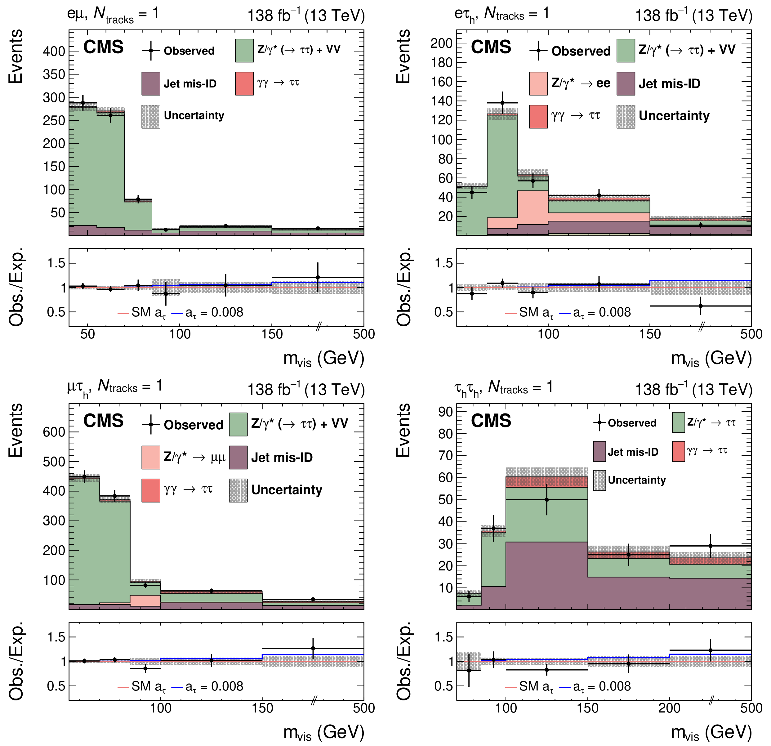
Figure 10:
Observed and predicted $ m_\text{vis} $ distributions in the $ \mathrm{e}\mu $ (upper left), $ \mathrm{e}\tau_{\mathrm{h}} $ (upper right), $ \mu\tau_{\mathrm{h}} $ (lower left), and $ \tau_{\mathrm{h}}\tau_{\mathrm{h}} $ (lower right) final states for events with $ N_\text{tracks}= $ 1. The description of the histograms is the same as in Fig. 9. |

png pdf |
Figure 10-a:
Observed and predicted $ m_\text{vis} $ distributions in the $ \mathrm{e}\mu $ (upper left), $ \mathrm{e}\tau_{\mathrm{h}} $ (upper right), $ \mu\tau_{\mathrm{h}} $ (lower left), and $ \tau_{\mathrm{h}}\tau_{\mathrm{h}} $ (lower right) final states for events with $ N_\text{tracks}= $ 1. The description of the histograms is the same as in Fig. 9. |
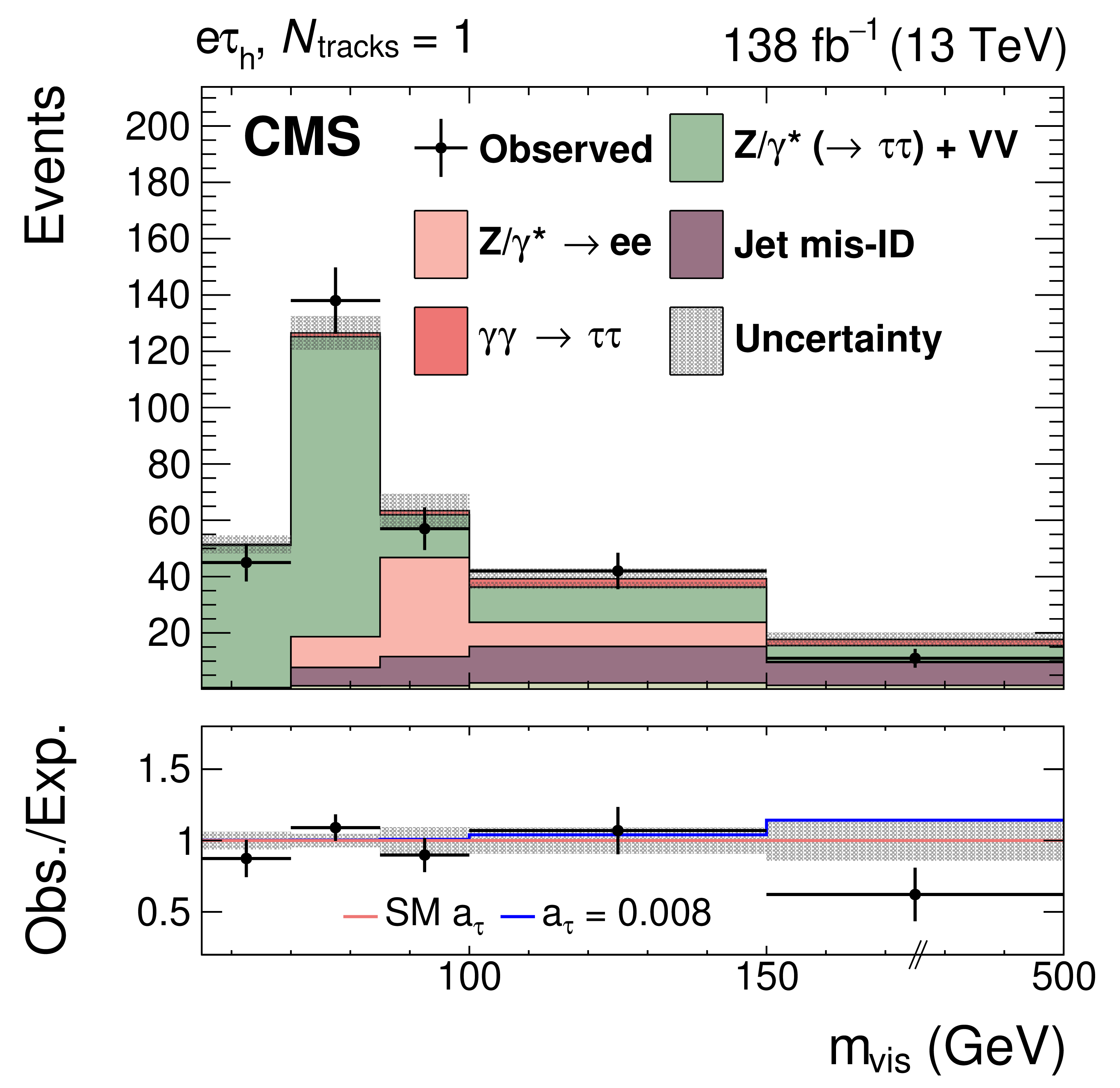
png pdf |
Figure 10-b:
Observed and predicted $ m_\text{vis} $ distributions in the $ \mathrm{e}\mu $ (upper left), $ \mathrm{e}\tau_{\mathrm{h}} $ (upper right), $ \mu\tau_{\mathrm{h}} $ (lower left), and $ \tau_{\mathrm{h}}\tau_{\mathrm{h}} $ (lower right) final states for events with $ N_\text{tracks}= $ 1. The description of the histograms is the same as in Fig. 9. |
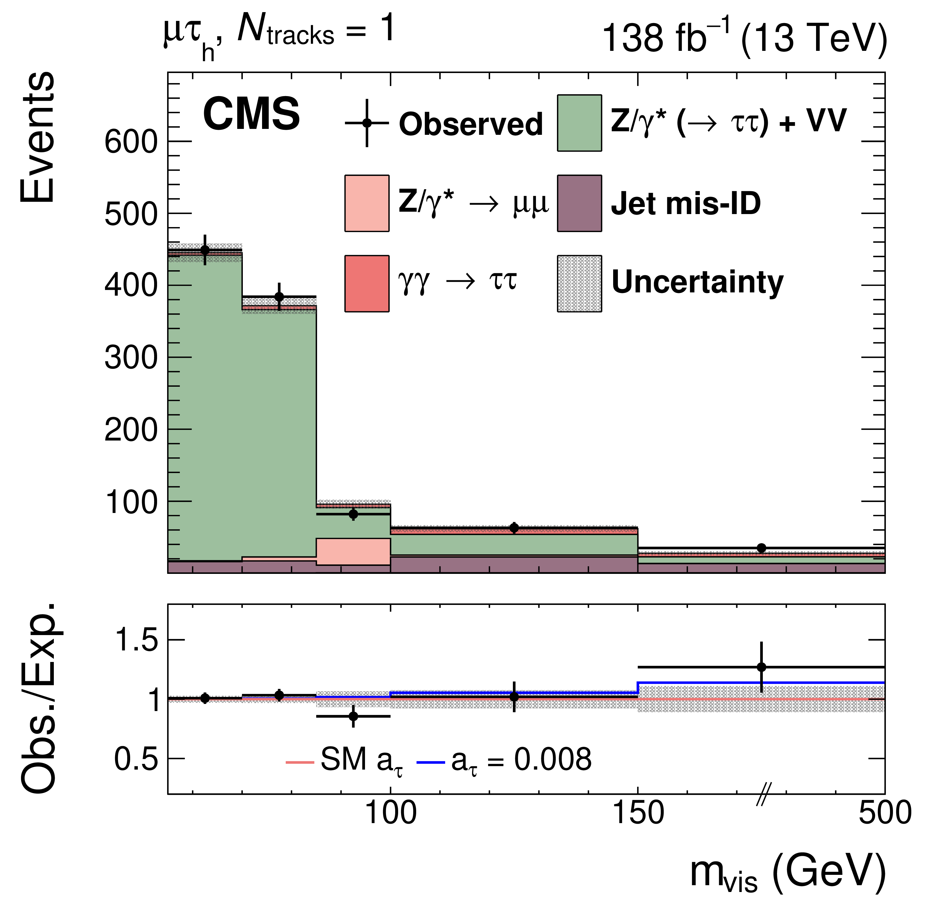
png pdf |
Figure 10-c:
Observed and predicted $ m_\text{vis} $ distributions in the $ \mathrm{e}\mu $ (upper left), $ \mathrm{e}\tau_{\mathrm{h}} $ (upper right), $ \mu\tau_{\mathrm{h}} $ (lower left), and $ \tau_{\mathrm{h}}\tau_{\mathrm{h}} $ (lower right) final states for events with $ N_\text{tracks}= $ 1. The description of the histograms is the same as in Fig. 9. |

png pdf |
Figure 10-d:
Observed and predicted $ m_\text{vis} $ distributions in the $ \mathrm{e}\mu $ (upper left), $ \mathrm{e}\tau_{\mathrm{h}} $ (upper right), $ \mu\tau_{\mathrm{h}} $ (lower left), and $ \tau_{\mathrm{h}}\tau_{\mathrm{h}} $ (lower right) final states for events with $ N_\text{tracks}= $ 1. The description of the histograms is the same as in Fig. 9. |
png pdf |
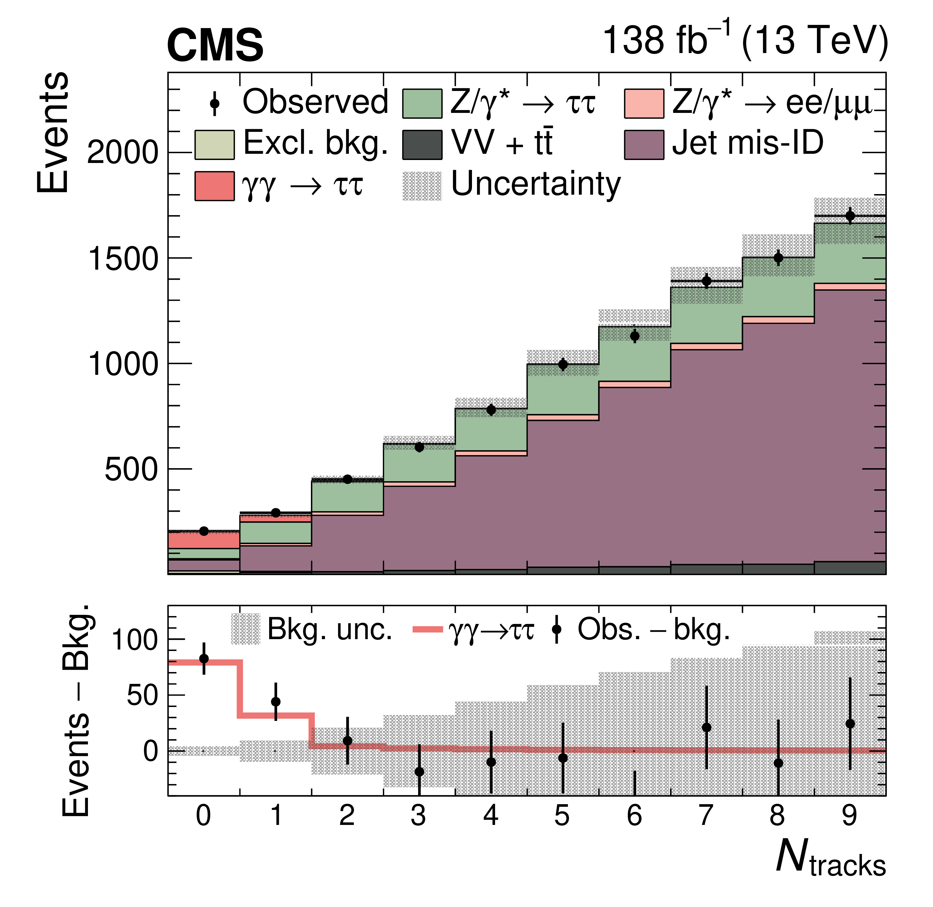
Figure 11:
Observed and predicted $ N_\text{tracks} $ distributions for events passing the SR selection but with the relaxed requirement $ N_\text{tracks} < $ 10 and the additional requirement $ m_\text{vis} > $ 100 GeV, combining the $ \mathrm{e}\mu $, $ \mathrm{e}\tau_{\mathrm{h}} $, $ \mu\tau_{\mathrm{h}} $, and $ \tau_{\mathrm{h}}\tau_{\mathrm{h}} $ final states together. The acoplanarity requirement $ A < $ 0.015 is applied. The observed data and their associated Poissonian statistical uncertainty are shown with black markers with vertical error bars. The inclusive diboson background contribution is drawn together with that of the $ {\mathrm{t}\overline{\mathrm{t}}} $ process. The predicted distributions are adjusted to the result of the global fit performed with the $ m_\text{vis} $ distributions in the SRs, and the signal distribution is normalized to its best fit signal strength. The lower panel shows the difference between the observed events and the backgrounds, as well as the signal contribution. Systematic uncertainties are assumed to be uncorrelated between final states to draw the uncertainty band. |
png pdf |
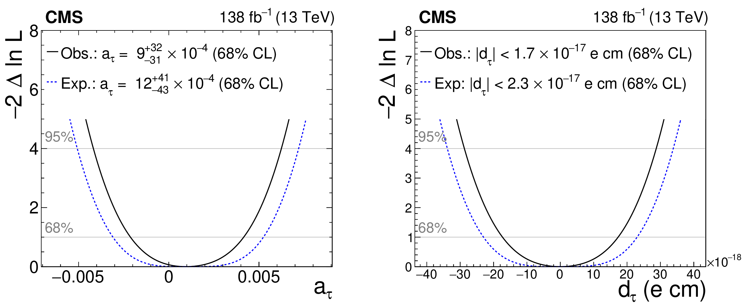
Figure 12:
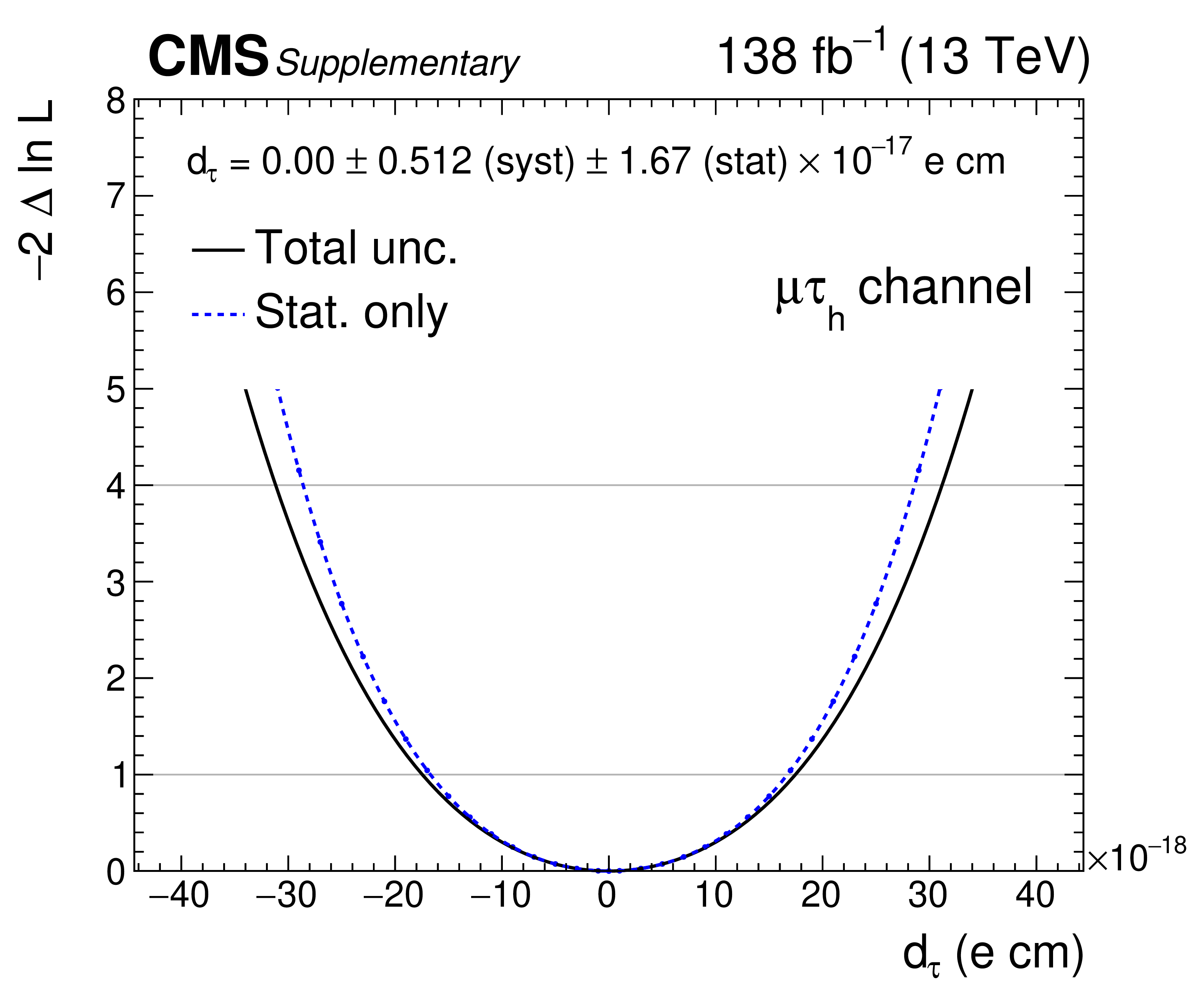
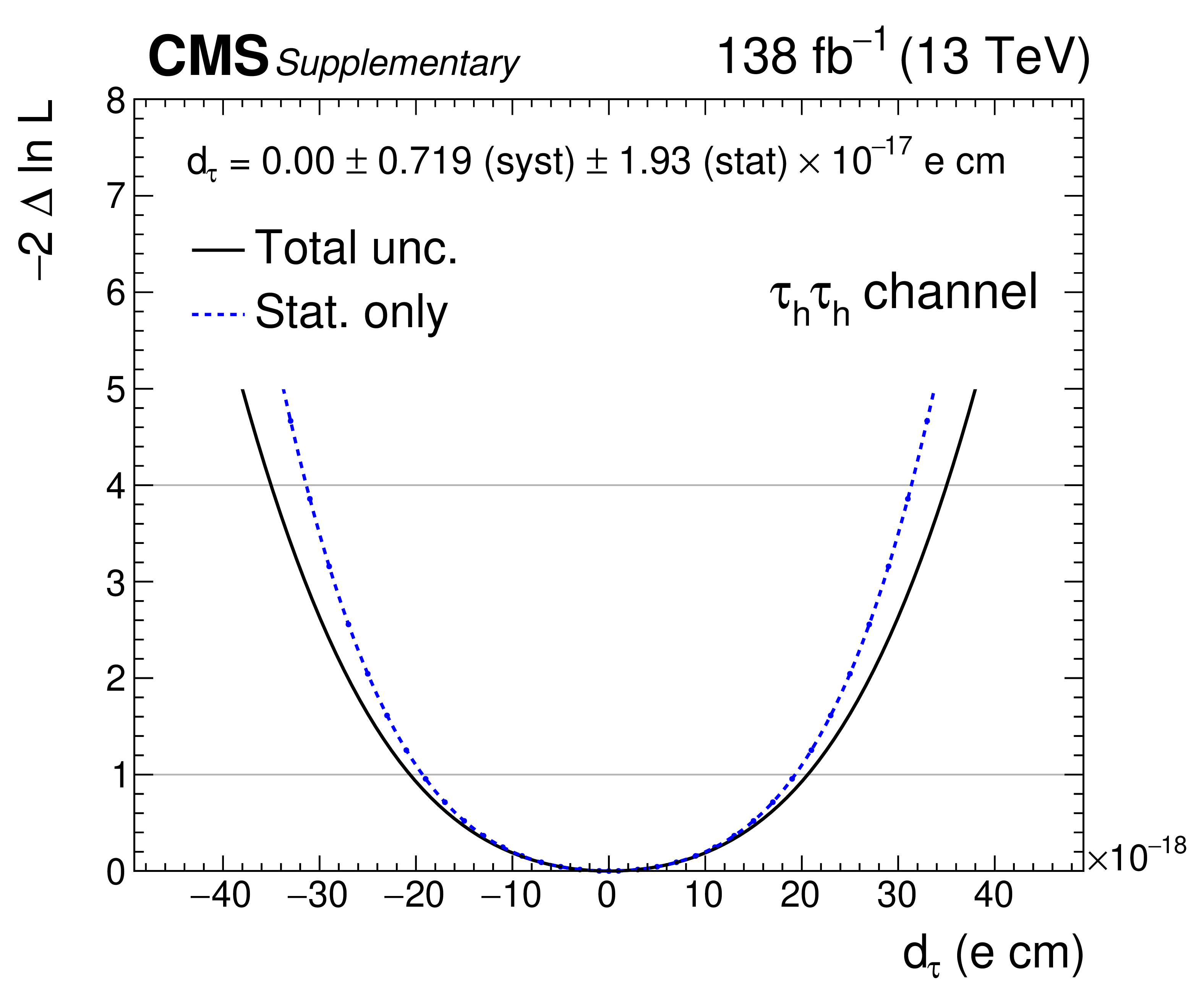
Expected and observed negative log-likelihood as a function of $ a_{\tau} $ (left) and $ d_{\tau} $ (right), for the combination of all SRs in all data-taking periods. |
png pdf |
Figure 12-a:
Expected and observed negative log-likelihood as a function of $ a_{\tau} $ (left) and $ d_{\tau} $ (right), for the combination of all SRs in all data-taking periods. |
png pdf |
Figure 12-b:
Expected and observed negative log-likelihood as a function of $ a_{\tau} $ (left) and $ d_{\tau} $ (right), for the combination of all SRs in all data-taking periods. |

png pdf |
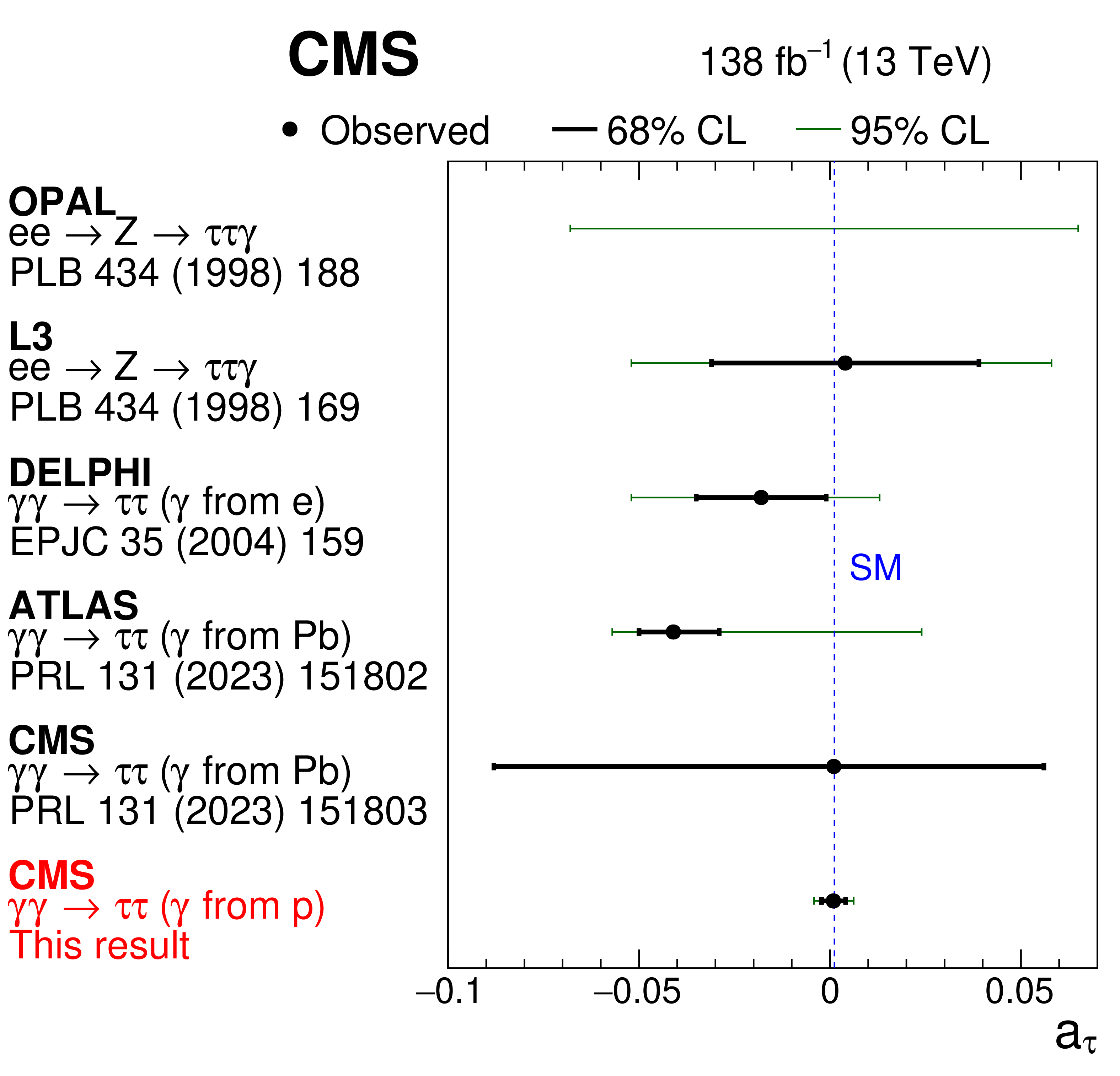
Figure 13:
Measurements of $ a_{\tau} $ (left) and $ d_{\tau} $ (right) performed in this analysis, compared with previous results from the OPAL, L3, DELPHI, ARGUS, Belle, ATLAS, and CMS experiments [25,26,24,28,27,9,10]. Confidence intervals at 68 and 95% CL are shown with thick black and thin green lines, respectively. The SM values of the $ \tau $ anomalous electromagnetic moments, $ a_{\tau}=$ 1.2$\times$10$^{-3} $ and $ d_{\tau}=-$7.3$\times$10$^{-38}$ e.cm, are indicated with the dashed blue lines. |
png pdf |
Figure 13-a:
Measurements of $ a_{\tau} $ (left) and $ d_{\tau} $ (right) performed in this analysis, compared with previous results from the OPAL, L3, DELPHI, ARGUS, Belle, ATLAS, and CMS experiments [25,26,24,28,27,9,10]. Confidence intervals at 68 and 95% CL are shown with thick black and thin green lines, respectively. The SM values of the $ \tau $ anomalous electromagnetic moments, $ a_{\tau}=$ 1.2$\times$10$^{-3} $ and $ d_{\tau}=-$7.3$\times$10$^{-38}$ e.cm, are indicated with the dashed blue lines. |

png pdf |
Figure 13-b:
Measurements of $ a_{\tau} $ (left) and $ d_{\tau} $ (right) performed in this analysis, compared with previous results from the OPAL, L3, DELPHI, ARGUS, Belle, ATLAS, and CMS experiments [25,26,24,28,27,9,10]. Confidence intervals at 68 and 95% CL are shown with thick black and thin green lines, respectively. The SM values of the $ \tau $ anomalous electromagnetic moments, $ a_{\tau}=$ 1.2$\times$10$^{-3} $ and $ d_{\tau}=-$7.3$\times$10$^{-38}$ e.cm, are indicated with the dashed blue lines. |
png pdf |
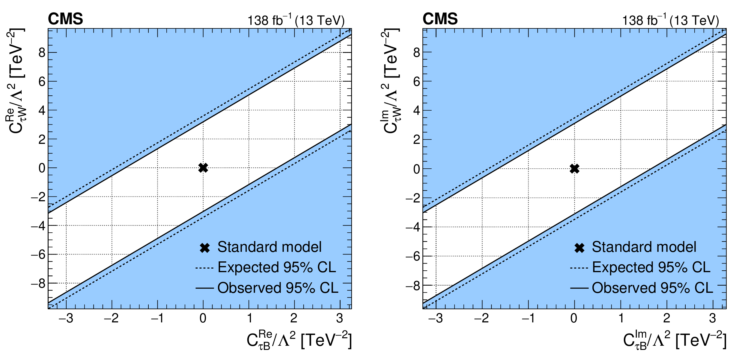
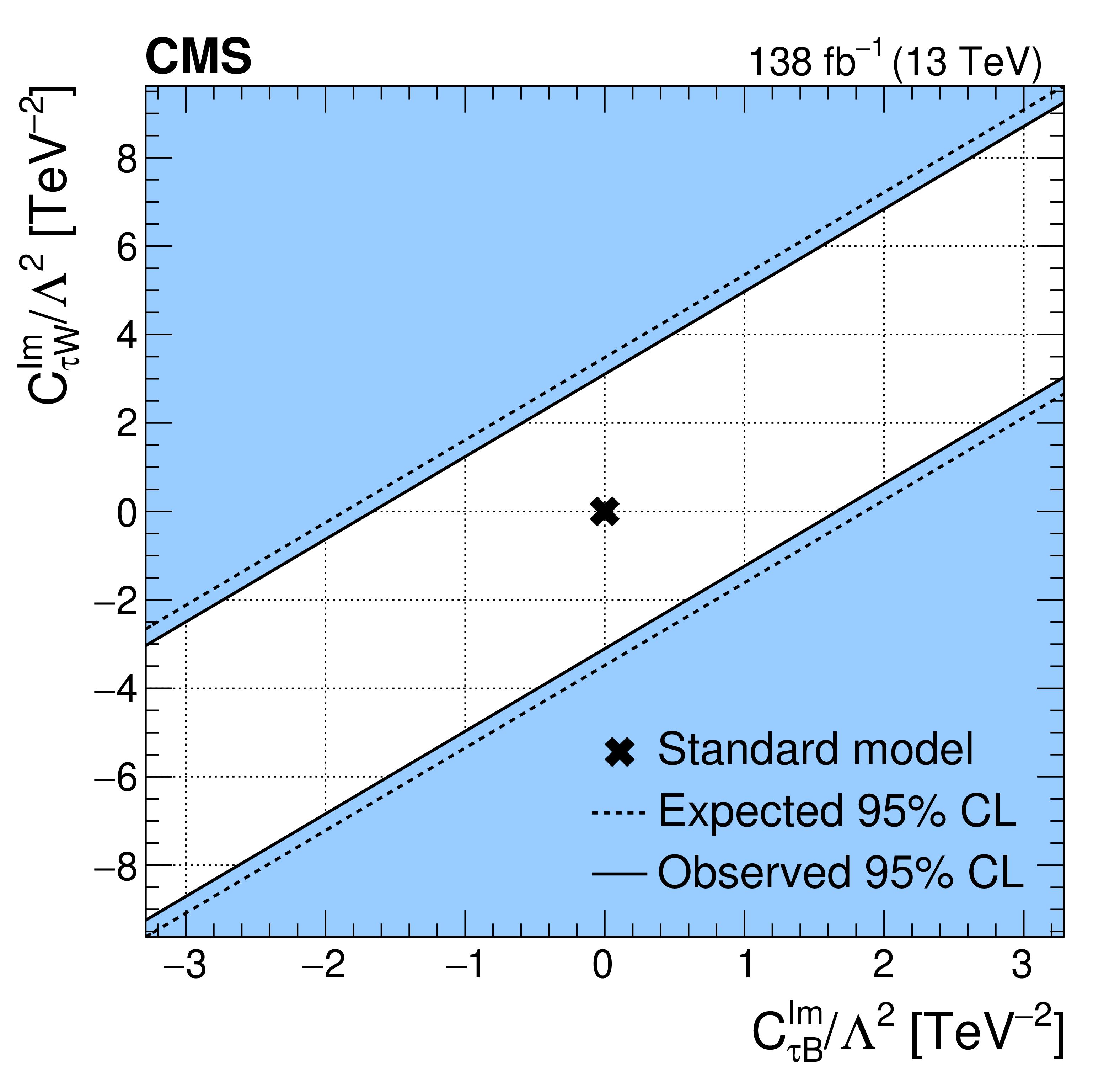
Figure 14:
Expected and observed 95% CL constraints on the real (left) and imaginary (right) parts of the Wilson coefficients $ C_{\tau B} $ and $ C_{\tau W} $ divided by $ \Lambda^2 $. The SM value is indicated with a cross. The blue shaded areas indicate excluded regions. |

png pdf |
Figure 14-a:
Expected and observed 95% CL constraints on the real (left) and imaginary (right) parts of the Wilson coefficients $ C_{\tau B} $ and $ C_{\tau W} $ divided by $ \Lambda^2 $. The SM value is indicated with a cross. The blue shaded areas indicate excluded regions. |
png pdf |
Figure 14-b:
Expected and observed 95% CL constraints on the real (left) and imaginary (right) parts of the Wilson coefficients $ C_{\tau B} $ and $ C_{\tau W} $ divided by $ \Lambda^2 $. The SM value is indicated with a cross. The blue shaded areas indicate excluded regions. |
| Tables | |
png pdf |
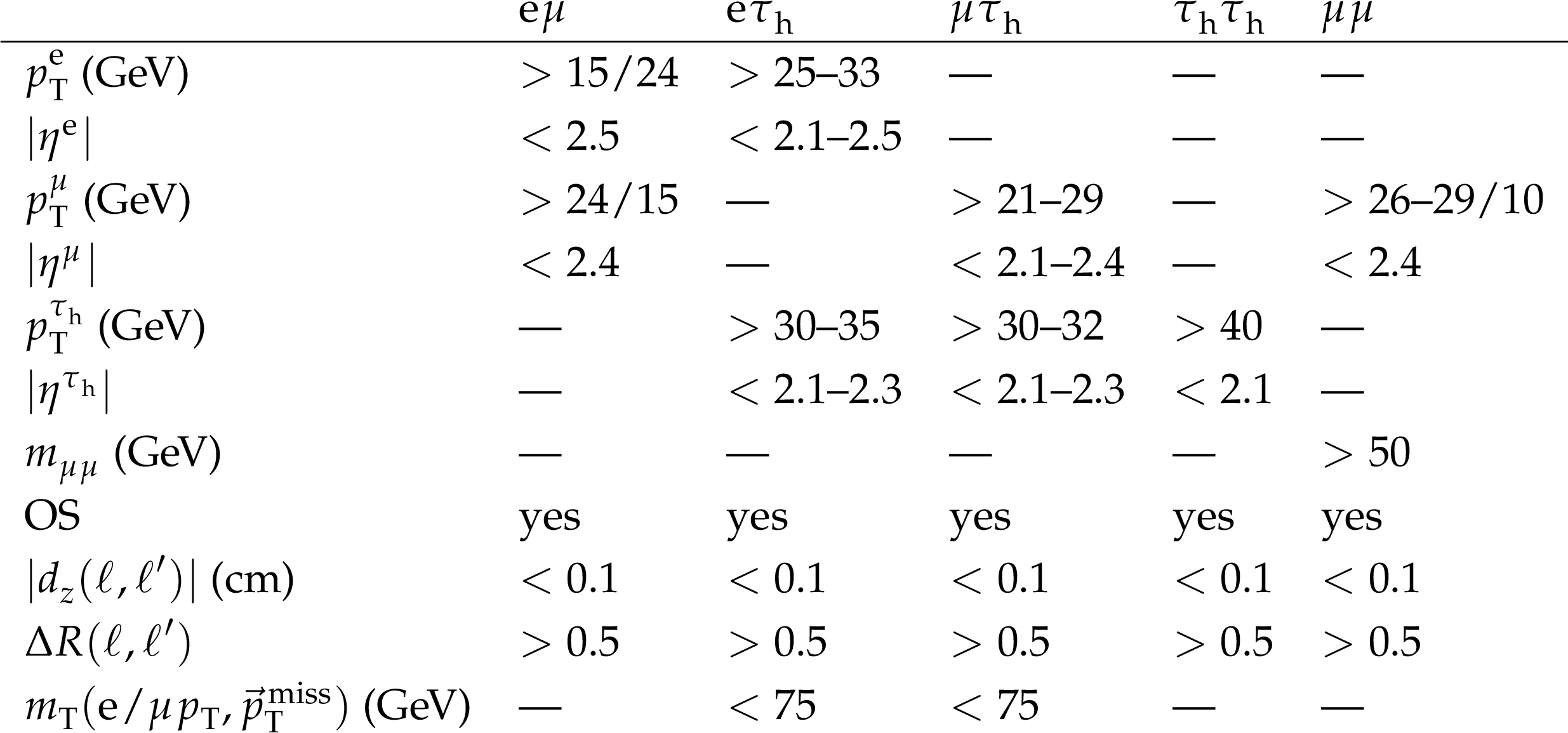
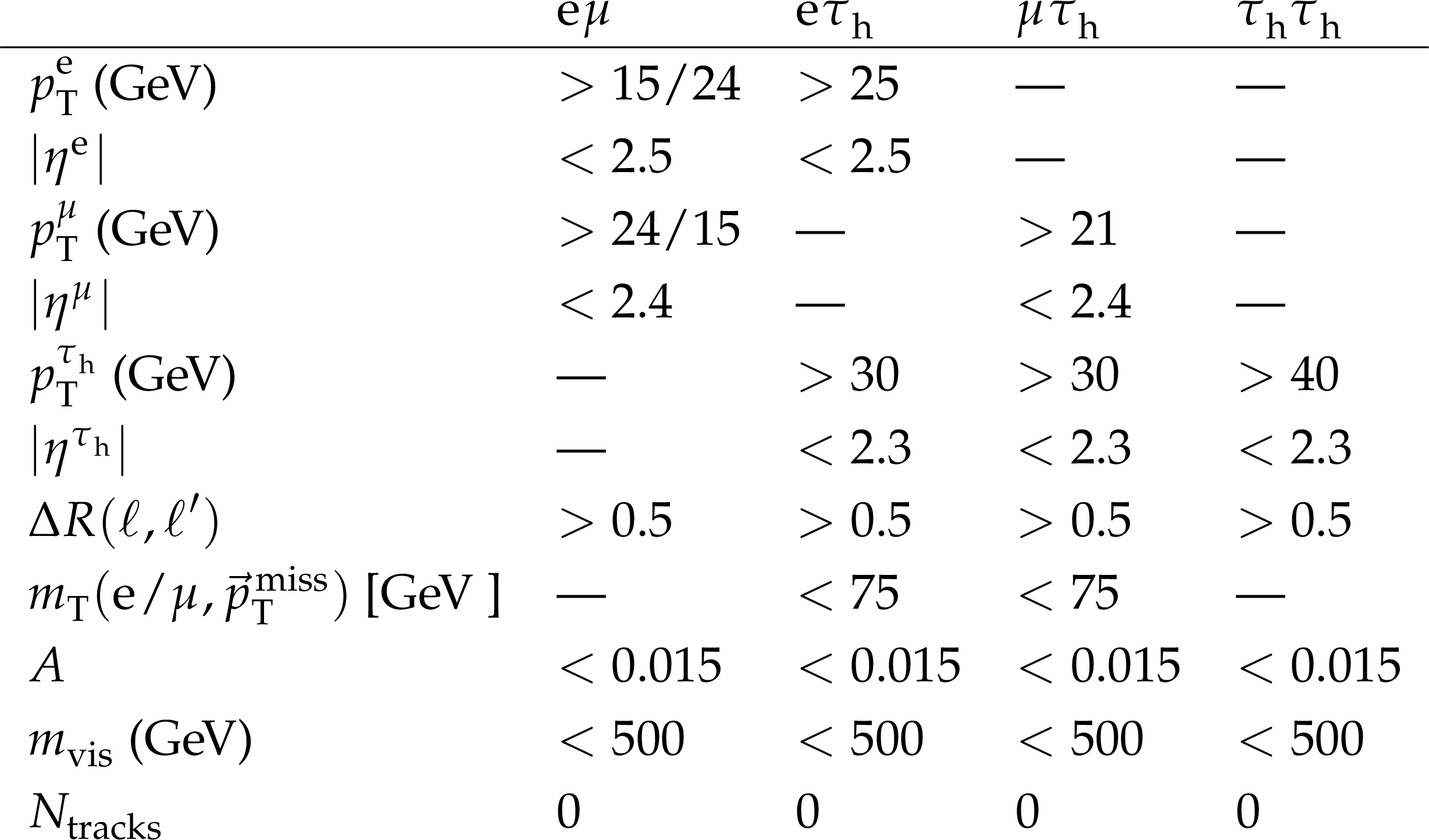
Table 1:
Baseline selection criteria used in the different final states. The electrons, muons, and $ \tau_{\mathrm{h}} $ are required to be well identified and isolated. The $ p_{\mathrm{T}} $ and pseudorapidity ranges correspond to different sets of triggers, and different data-taking periods. |
png pdf |
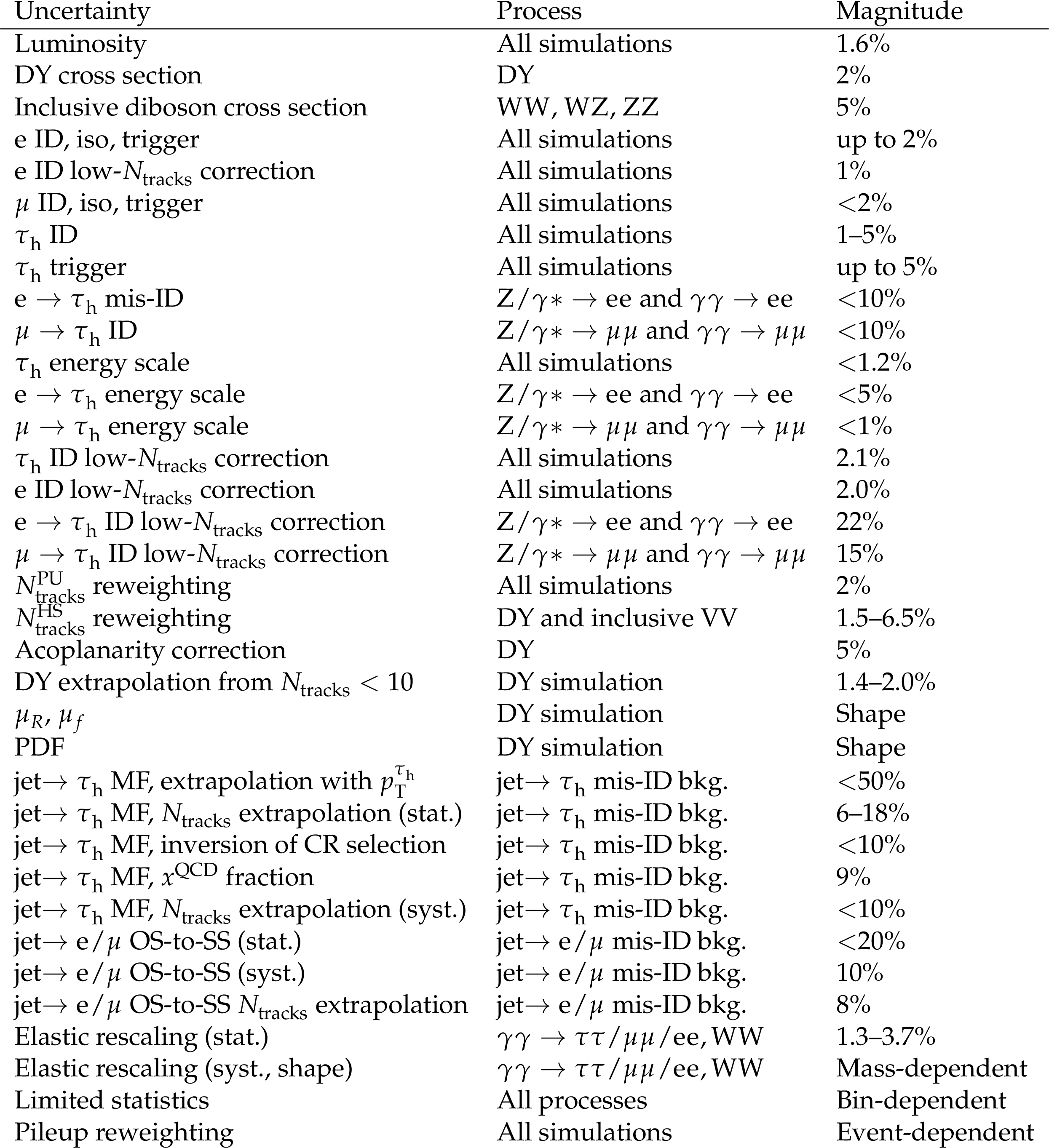
Table 2:
Summary of the systematic uncertainties considered in the analysis. The sources of the uncertainties, the processes they affect, and their magnitudes are indicated. |
png pdf |
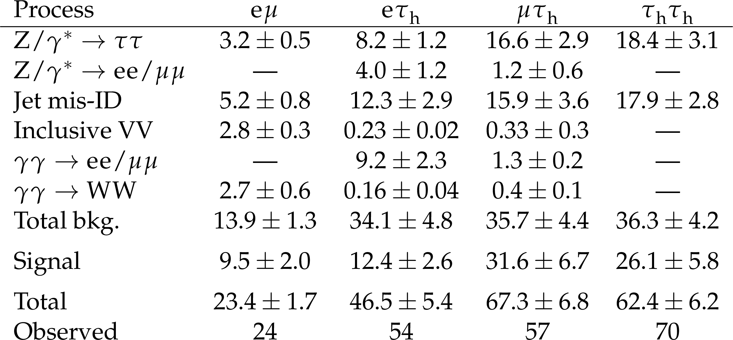
Table 3:
Observed and predicted event yields per final state in the signal-enriched phase space with $ m_\text{vis} > $ 100 GeV and $ N_\text{tracks}= $ 0. The signal and background yields are the result of the global fit including all sources of uncertainties. |
png pdf |
Table 4:
Selection criteria to define the fiducial cross section. Events where the two $ \tau $ leptons decay both to electrons or to muons, with neutrinos, are considered to be outside the fiducial region. All requirements are applied using generator-level quantities, as detailed in the text. |
| Summary |
| The photon-fusion production of a pair of $ \tau $ leptons, $ {\gamma\gamma\to\tau\tau} $, has been observed for the first time in proton-proton collisions, with a significance of 5.3 standard deviations. The $ \tau $ leptons are reconstructed in their leptonic and hadronic decay modes. The signal has been identified by requiring low track activity around the di-$ \tau $ vertex and low azimuthal acoplanarity between the $ \tau $ candidates. Data in a control region with two muons were used to determine corrections for the simulations to accurately model the track multiplicity and to predict the signal contribution in the final state of two $ \tau $ leptons. The signal strength, fiducial cross section, and constraints on the anomalous electromagnetic moments of the $ \tau $ lepton have been extracted using the di-$ \tau $ invariant mass distributions in four di-$ \tau $ final states. The measured fiducial cross section of $ {\gamma\gamma\to\tau\tau} $ is $ \sigma^\text{fid}_\text{obs}= $ 12.4$ ^{+3.8}_{-3.1} $ fb. The anomalous $ \tau $ magnetic moment is determined to be $ a_{\tau}= $ 0.0009$_{-0.0031}^{+0.0032} $, whereas the electric dipole moment of the $ \tau $ lepton is constrained to $ |d_{\tau}| < $ 2.9$\times $10$^{-17}$ e.cm at 95% confidence level. They are both in good agreement with the predictions of the standard model of particle physics, and the measurements do not show any evidence for the presence of new physics that would modify the electromagnetic moments of the $ \tau $ lepton. This is the most stringent limit on the $ \tau $ lepton magnetic moment to date, improving on the previous best constraints by nearly an order of magnitude. |
| Additional Figures | |
png pdf |
Additional Figure 1:
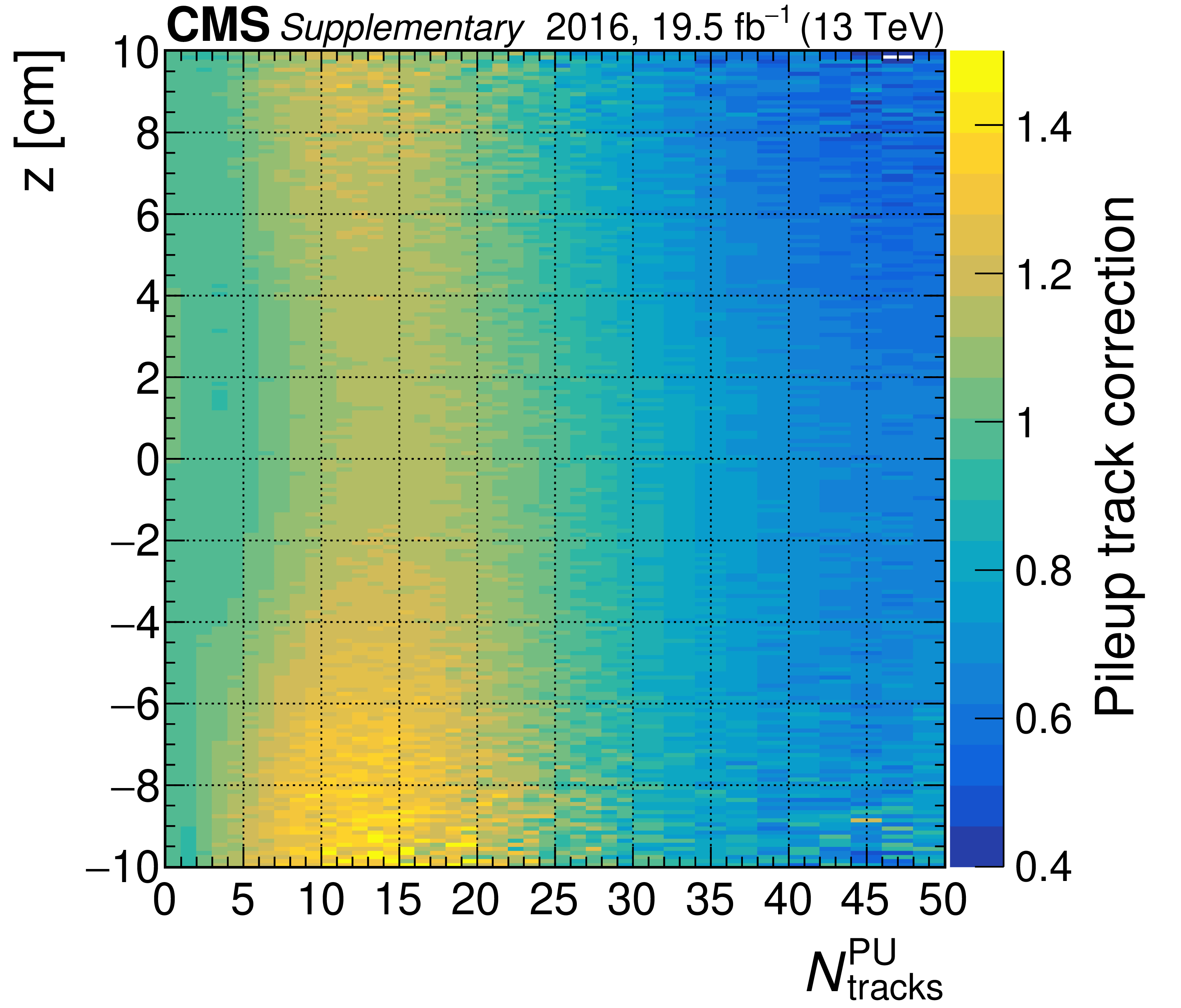
Event weights applied to simulations in the 2016 pre-VFP data-taking period as a function of the dilepton vertex position along the $ z $ axis and the pileup track multiplicity in a 0.1 cm-wide window around the dilepton vertex, where VFP stands for preamplifier feedback bias corrections due to inefficiencies in the strip modules of the tracker during the 2016 data-taking period. |

png pdf |
Additional Figure 2:
Event weights applied to simulations in the 2016 post-VFP data-taking period as a function of the dilepton vertex position along the $ z $ axis and the pileup track multiplicity in a 0.1 cm-wide window around the dilepton vertex, where VFP stands for preamplifier feedback bias corrections due to inefficiencies in the strip modules of the tracker during the 2016 data-taking period. |
png pdf |
Additional Figure 3:
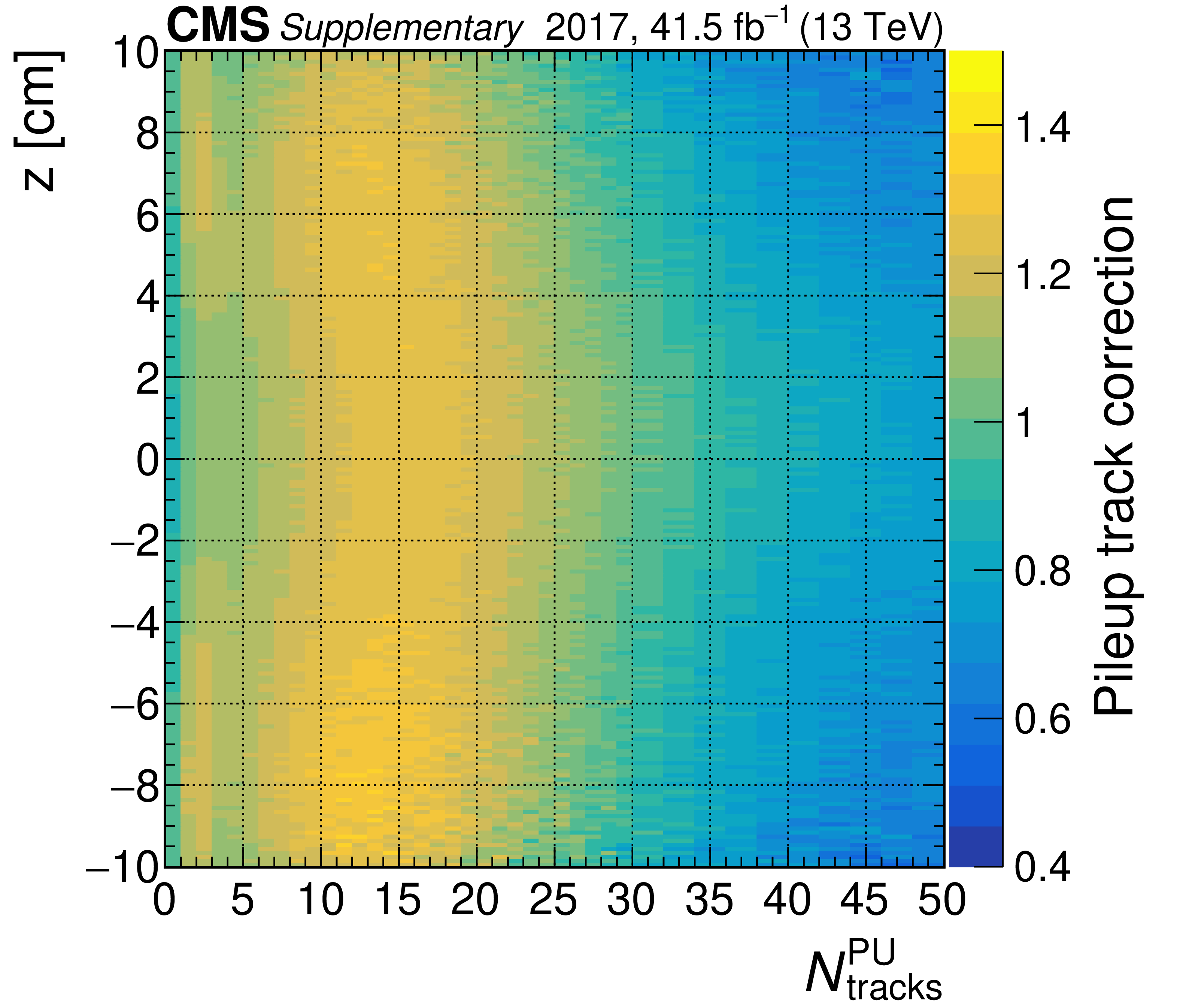
Event weights applied to simulations in the 2017 data-taking period as a function of the dilepton vertex position along the $ z $ axis and the pileup track multiplicity in a 0.1 cm-wide window around the dilepton vertex. |

png pdf |
Additional Figure 4:
Event weights applied to simulations in the 2018 data-taking period as a function of the dilepton vertex position along the $ z $ axis and the pileup track multiplicity in a 0.1 cm-wide window around the dilepton vertex. |
png pdf |
Additional Figure 5:
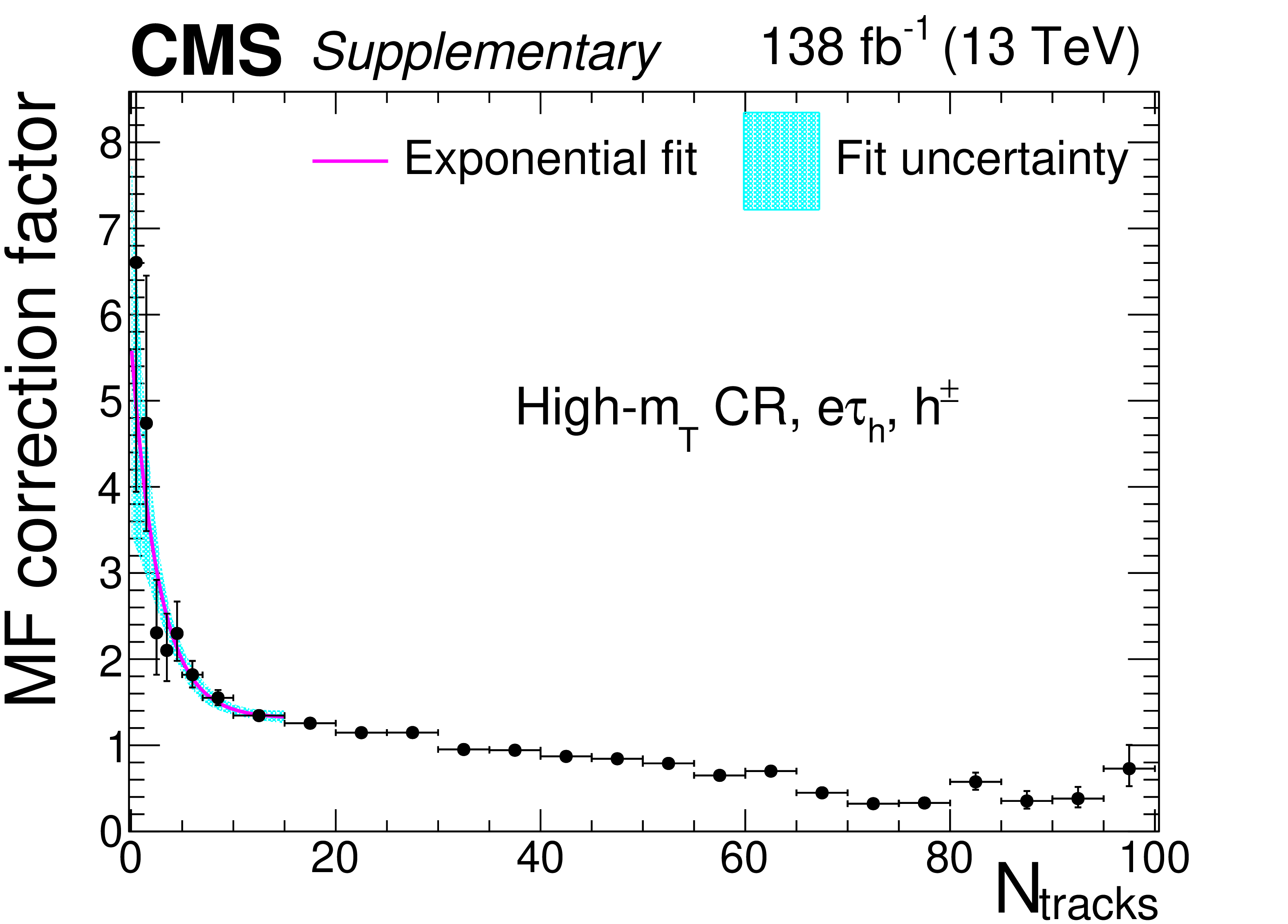
Multiplicative $ N_\text{tracks} $-dependent corrections to the $ \tau_{\mathrm{h}} $ misidentification factors in the $ \mathrm{e}\tau_{\mathrm{h}} $ final state in the high-$ m_{\mathrm{T}} $ CR, for the $ h^\pm $ decay mode. The cyan shaded area corresponds to the fit uncertainty. |
png pdf |
Additional Figure 6:
Multiplicative $ N_\text{tracks} $-dependent corrections to the $ \tau_{\mathrm{h}} $ misidentification factors in the $ \mathrm{e}\tau_{\mathrm{h}} $ final state in the high-$ m_{\mathrm{T}} $ CR, for the $ h^\pm h^\mp h^\pm $ decay mode. The cyan shaded area corresponds to the fit uncertainty. |
png pdf |
Additional Figure 7:
Multiplicative $ N_\text{tracks} $-dependent corrections to the $ \tau_{\mathrm{h}} $ misidentification factors in the $ \mathrm{e}\tau_{\mathrm{h}} $ final state in the high-$ m_{\mathrm{T}} $ CR, for the $ h^\pm h^\mp h^\pm+\pi^{0} $(s) decay mode. The cyan shaded area corresponds to the fit uncertainty. |
png pdf |
Additional Figure 8:
Multiplicative $ N_\text{tracks} $-dependent corrections to the $ \tau_{\mathrm{h}} $ misidentification factors in the $ \mathrm{e}\tau_{\mathrm{h}} $ final state in the same-sign CR, for the $ h^\pm $ decay mode. The cyan shaded area corresponds to the fit uncertainty. |
png pdf |
Additional Figure 9:
Multiplicative $ N_\text{tracks} $-dependent corrections to the $ \tau_{\mathrm{h}} $ misidentification factors in the $ \mathrm{e}\tau_{\mathrm{h}} $ final state in the same-sign CR, for the $ h^\pm h^\mp h^\pm $ decay mode. The cyan shaded area corresponds to the fit uncertainty. |
png pdf |
Additional Figure 10:
Multiplicative $ N_\text{tracks} $-dependent corrections to the $ \tau_{\mathrm{h}} $ misidentification factors in the $ \mathrm{e}\tau_{\mathrm{h}} $ final state in the same-sign CR, for the $ h^\pm h^\mp h^\pm+\pi^{0} $(s) decay mode. The cyan shaded area corresponds to the fit uncertainty. |

png pdf |
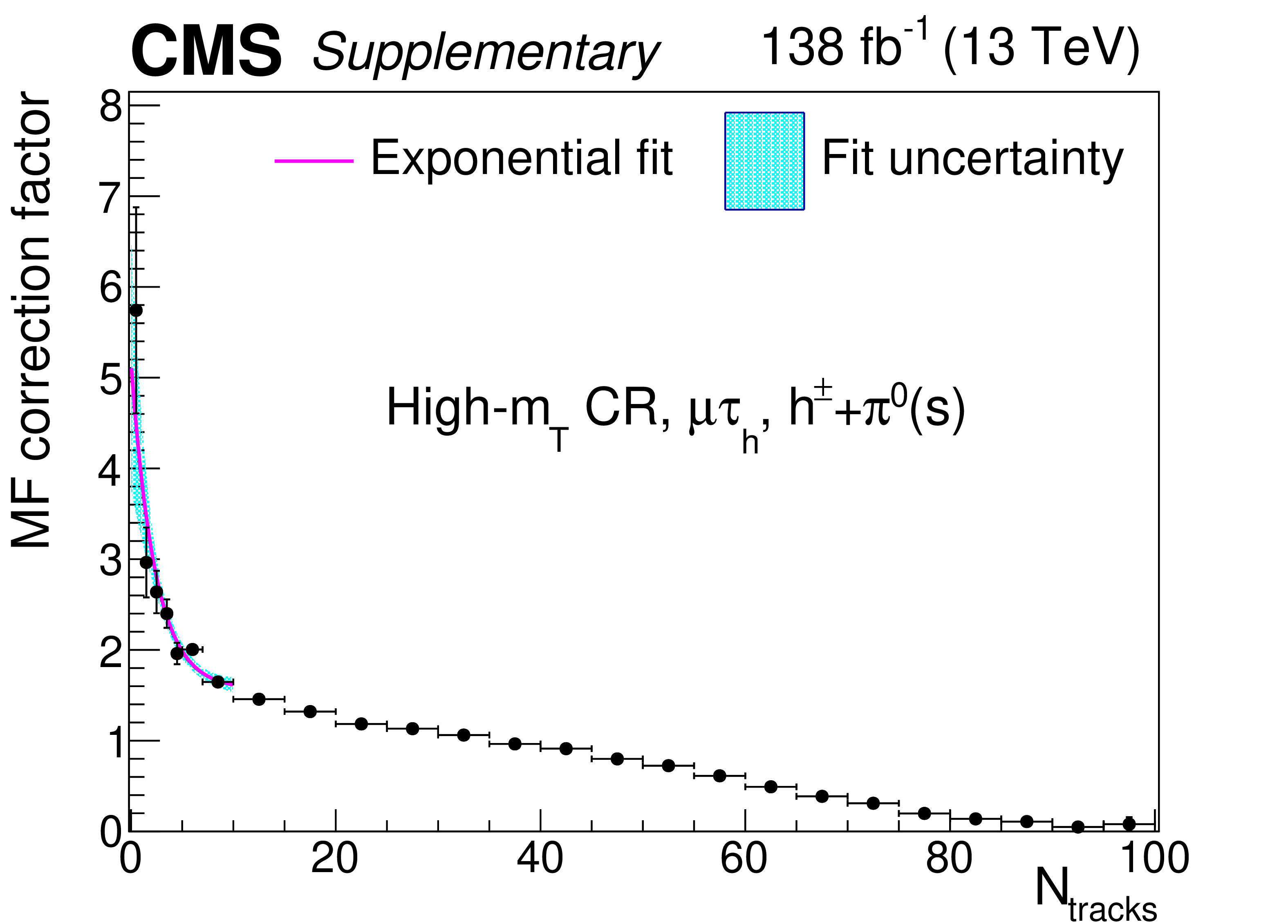
Additional Figure 11:
Multiplicative $ N_\text{tracks} $-dependent corrections to the $ \tau_{\mathrm{h}} $ misidentification factors in the $ \mu\tau_{\mathrm{h}} $ final state in the high-$ m_{\mathrm{T}} $ CR, for the $ h^\pm $ decay mode. The cyan shaded area corresponds to the fit uncertainty. |
png pdf |
Additional Figure 12:
Multiplicative $ N_\text{tracks} $-dependent corrections to the $ \tau_{\mathrm{h}} $ misidentification factors in the $ \mu\tau_{\mathrm{h}} $ final state in the high-$ m_{\mathrm{T}} $ CR, for the $ h^\pm+\pi^{0} $(s) decay mode. The cyan shaded area corresponds to the fit uncertainty. |
png pdf |
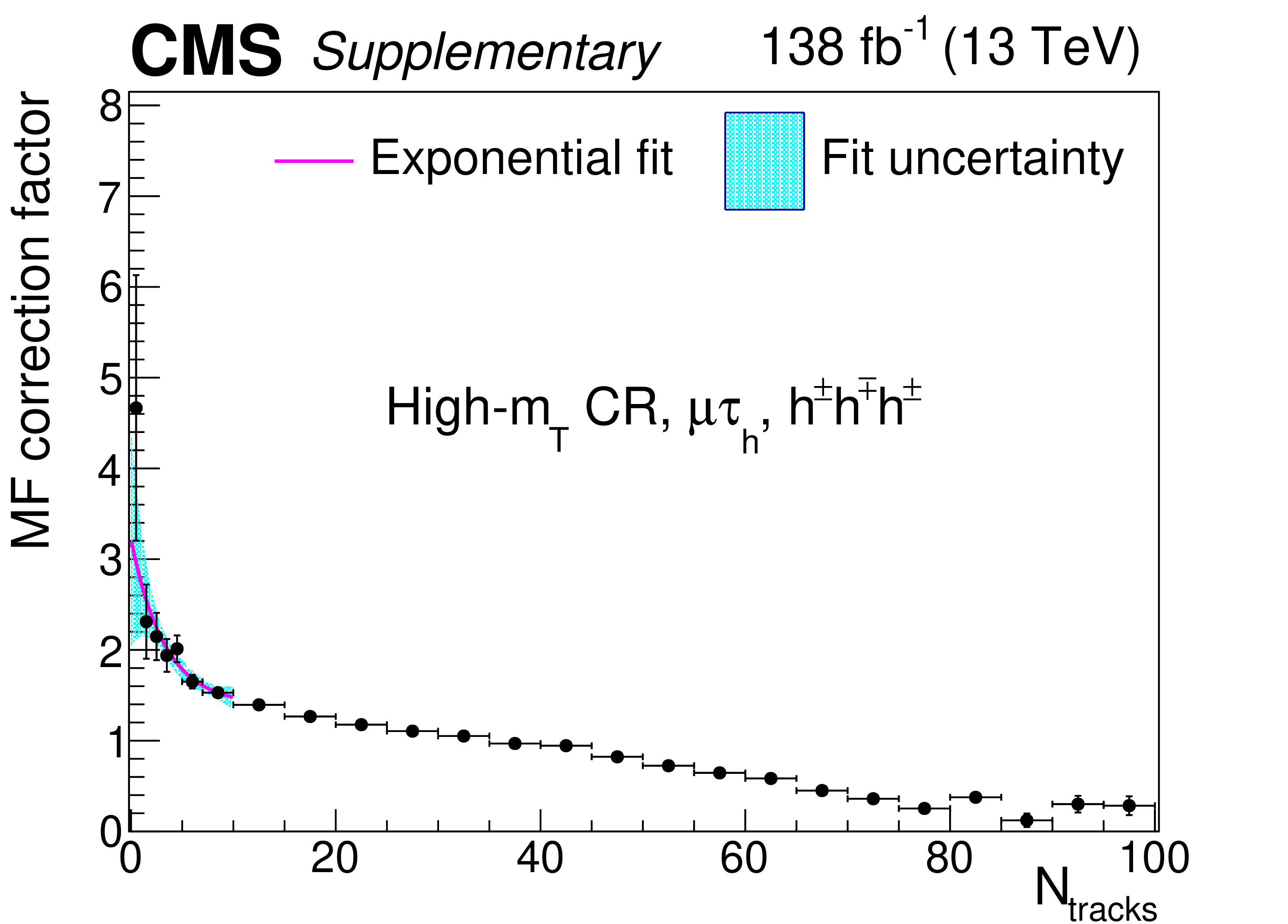
Additional Figure 13:
Multiplicative $ N_\text{tracks} $-dependent corrections to the $ \tau_{\mathrm{h}} $ misidentification factors in the $ \mu\tau_{\mathrm{h}} $ final state in the high-$ m_{\mathrm{T}} $ CR, for the $ h^\pm h^\mp h^\pm $ decay mode. The cyan shaded area corresponds to the fit uncertainty. |
png pdf |
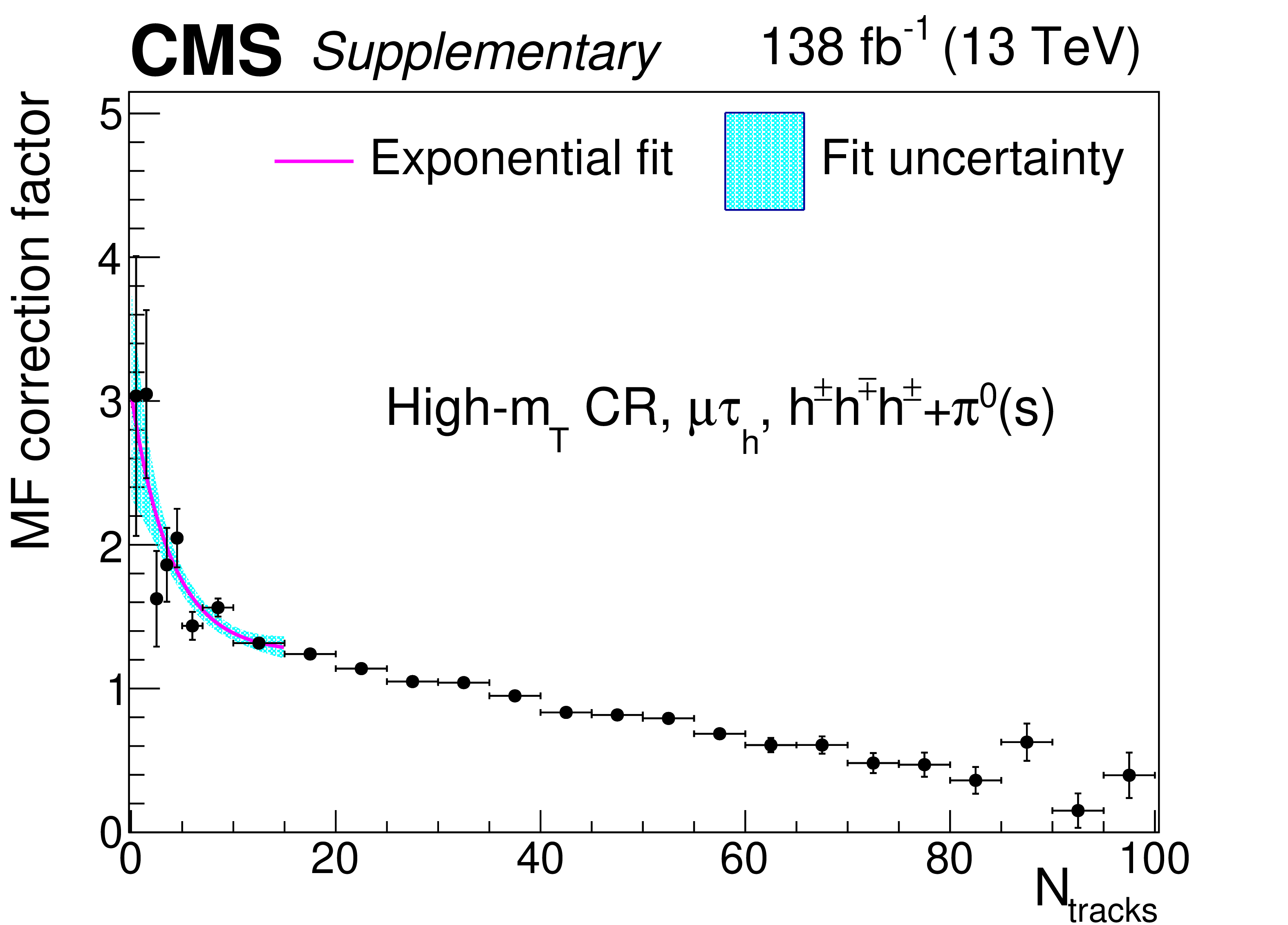
Additional Figure 14:
Multiplicative $ N_\text{tracks} $-dependent corrections to the $ \tau_{\mathrm{h}} $ misidentification factors in the $ \mu\tau_{\mathrm{h}} $ final state in the high-$ m_{\mathrm{T}} $ CR, for the $ h^\pm h^\mp h^\pm+\pi^{0} $(s) decay mode. The cyan shaded area corresponds to the fit uncertainty. |
png pdf |
Additional Figure 15:
Multiplicative $ N_\text{tracks} $-dependent corrections to the $ \tau_{\mathrm{h}} $ misidentification factors in the $ \mu\tau_{\mathrm{h}} $ final state in the same-sign CR, for the $ h^\pm $ decay mode. The cyan shaded area corresponds to the fit uncertainty. |
png pdf |
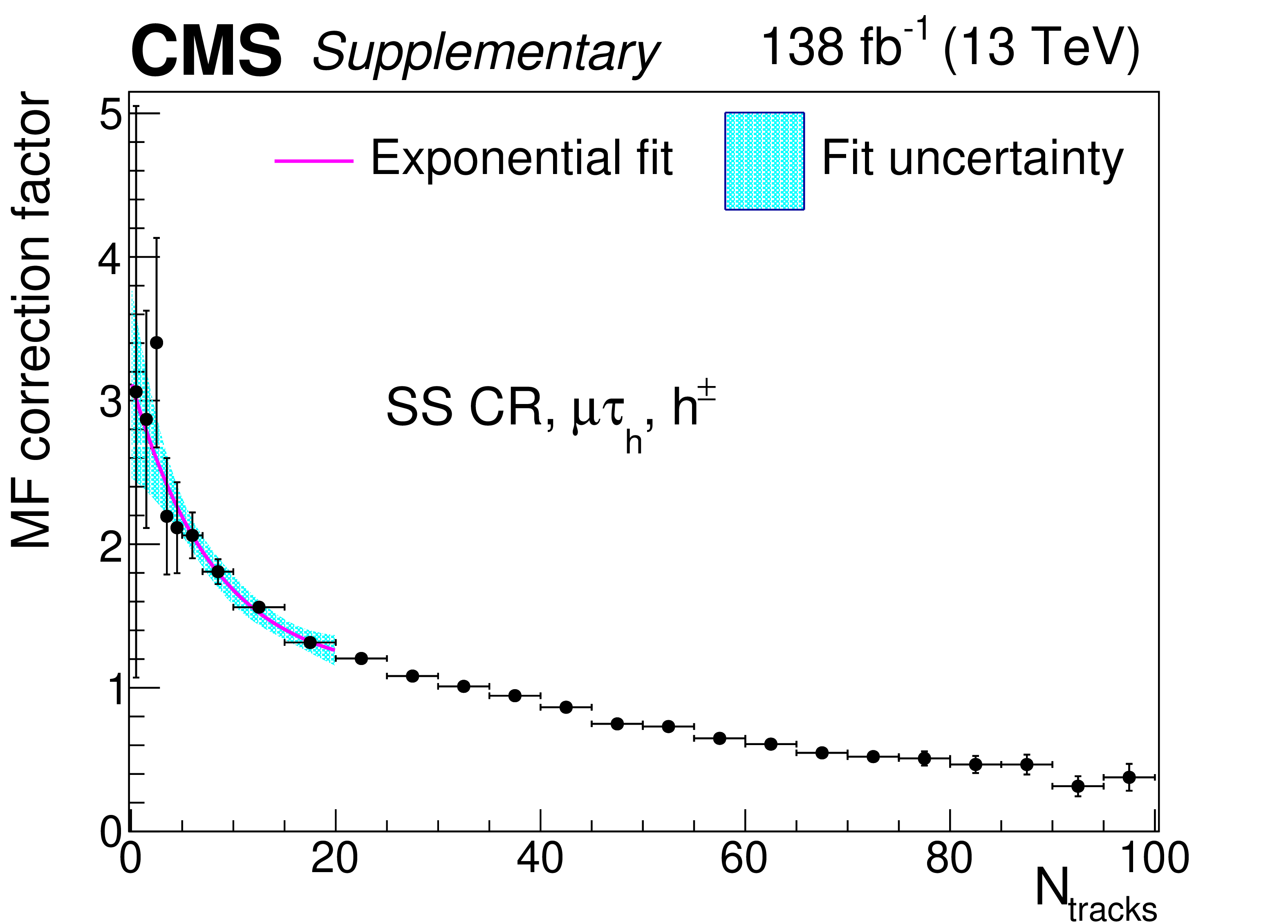
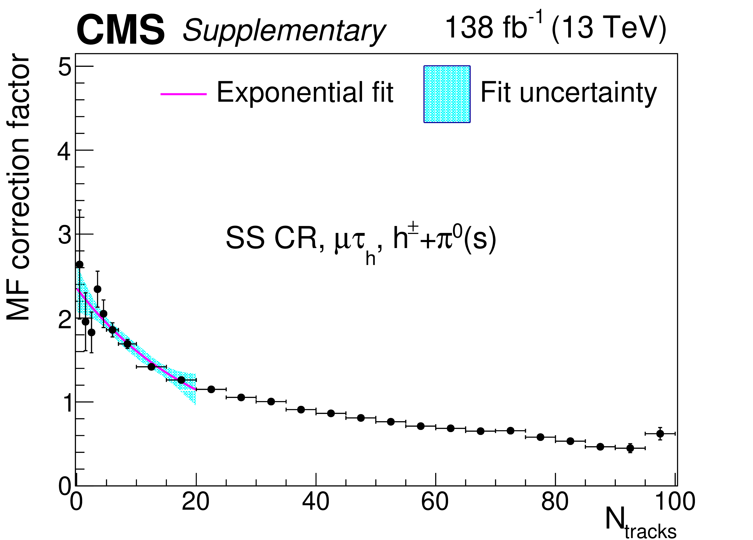
Additional Figure 16:
Multiplicative $ N_\text{tracks} $-dependent corrections to the $ \tau_{\mathrm{h}} $ misidentification factors in the $ \mu\tau_{\mathrm{h}} $ final state in the same-sign CR, for the $ h^\pm+\pi^{0} $ decay mode. The cyan shaded area corresponds to the fit uncertainty. |

png pdf |
Additional Figure 17:
Multiplicative $ N_\text{tracks} $-dependent corrections to the $ \tau_{\mathrm{h}} $ misidentification factors in the $ \mu\tau_{\mathrm{h}} $ final state in the same-sign CR, for the $ h^\pm h^\mp h^\pm $ decay mode. The cyan shaded area corresponds to the fit uncertainty. |
png pdf |
Additional Figure 18:
Multiplicative $ N_\text{tracks} $-dependent corrections to the $ \tau_{\mathrm{h}} $ misidentification factors in the $ \mu\tau_{\mathrm{h}} $ final state in the same-sign CR, for the $ h^\pm h^\mp h^\pm+\pi^{0} $(s) decay mode. The cyan shaded area corresponds to the fit uncertainty. |
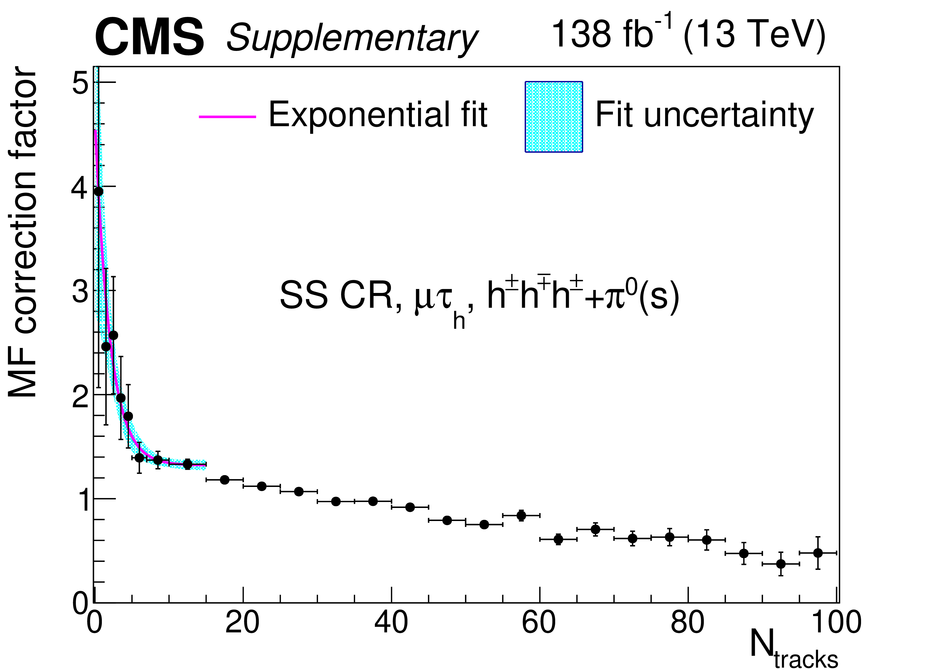
png pdf |
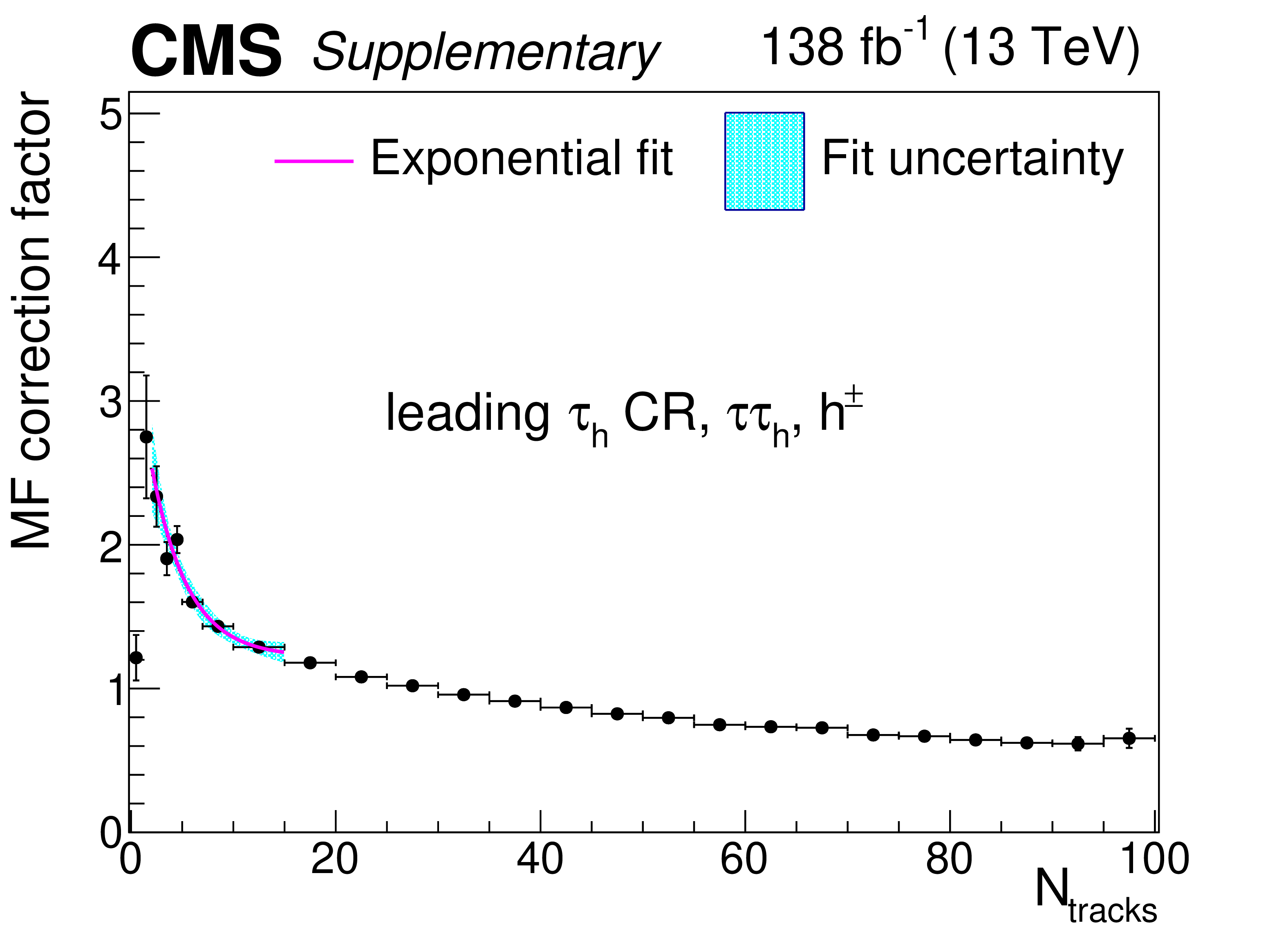
Additional Figure 19:
Multiplicative $ N_\text{tracks} $-dependent corrections to the leading $ \tau_{\mathrm{h}} $ misidentification factors in the $ \tau_{\mathrm{h}}\tau_{\mathrm{h}} $ final state in the same-sign CR, for the $ h^\pm $ decay mode. The cyan shaded area corresponds to the fit uncertainty. |
png pdf |
Additional Figure 20:
Multiplicative $ N_\text{tracks} $-dependent corrections to the leading $ \tau_{\mathrm{h}} $ misidentification factors in the $ \tau_{\mathrm{h}}\tau_{\mathrm{h}} $ final state in the same-sign CR, for the $ h^\pm+\pi^{0} $ decay mode. The cyan shaded area corresponds to the fit uncertainty. |
png pdf |
Additional Figure 21:
Multiplicative $ N_\text{tracks} $-dependent corrections to the leading $ \tau_{\mathrm{h}} $ misidentification factors in the $ \tau_{\mathrm{h}}\tau_{\mathrm{h}} $ final state in the same-sign CR, for the $ h^\pm h^\mp h^\pm $ decay mode. The cyan shaded area corresponds to the fit uncertainty. |
png pdf |
Additional Figure 22:
Multiplicative $ N_\text{tracks} $-dependent corrections to the leading $ \tau_{\mathrm{h}} $ misidentification factors in the $ \tau_{\mathrm{h}}\tau_{\mathrm{h}} $ final state in the same-sign CR, for the $ h^\pm h^\mp h^\pm+\pi^{0} $(s) decay mode. The cyan shaded area corresponds to the fit uncertainty. |
png pdf |
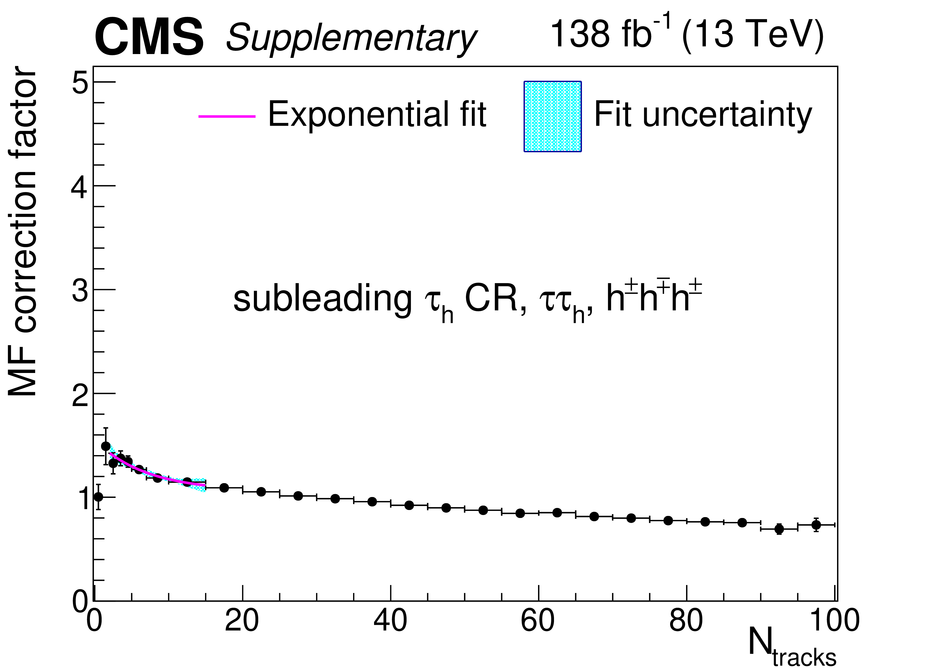
Additional Figure 23:
Multiplicative $ N_\text{tracks} $-dependent corrections to the subleading $ \tau_{\mathrm{h}} $ misidentification factors in the $ \tau_{\mathrm{h}}\tau_{\mathrm{h}} $ final state in the same-sign CR, for the $ h^\pm $ decay mode. The cyan shaded area corresponds to the fit uncertainty. |

png pdf |
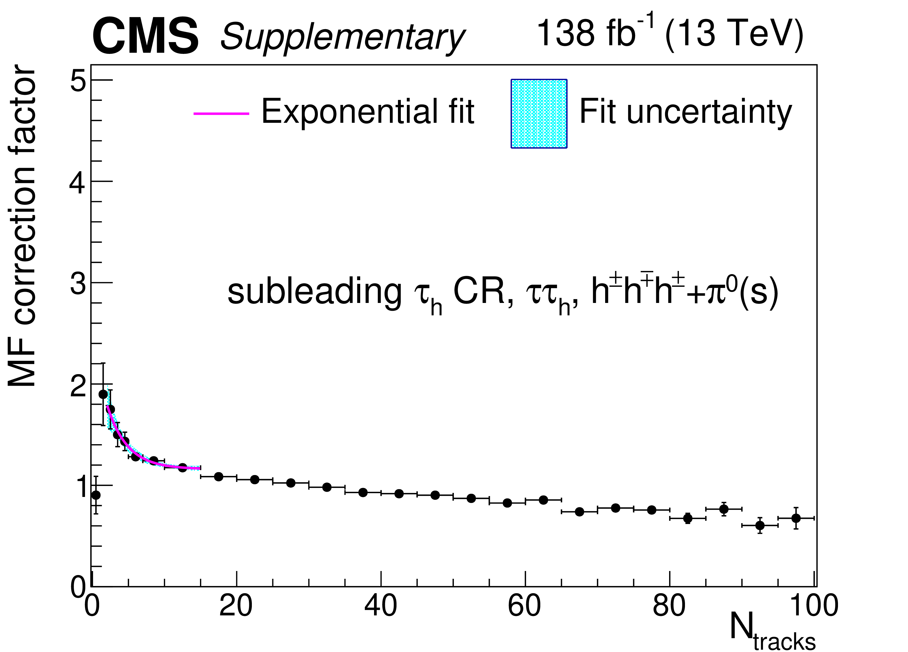
Additional Figure 24:
Multiplicative $ N_\text{tracks} $-dependent corrections to the subleading $ \tau_{\mathrm{h}} $ misidentification factors in the $ \tau_{\mathrm{h}}\tau_{\mathrm{h}} $ final state in the same-sign CR, for the $ h^\pm+\pi^{0} $ decay mode. The cyan shaded area corresponds to the fit uncertainty. |
png pdf |
Additional Figure 25:
Multiplicative $ N_\text{tracks} $-dependent corrections to the subleading $ \tau_{\mathrm{h}} $ misidentification factors in the $ \tau_{\mathrm{h}}\tau_{\mathrm{h}} $ final state in the same-sign CR, for the $ h^\pm h^\mp h^\pm $ decay mode. The cyan shaded area corresponds to the fit uncertainty. |
png pdf |
Additional Figure 26:
Multiplicative $ N_\text{tracks} $-dependent corrections to the subleading $ \tau_{\mathrm{h}} $ misidentification factors in the $ \tau_{\mathrm{h}}\tau_{\mathrm{h}} $ final state in the same-sign CR, for the $ h^\pm h^\mp h^\pm+\pi^{0} $(s) decay mode. The cyan shaded area corresponds to the fit uncertainty. |
png pdf |
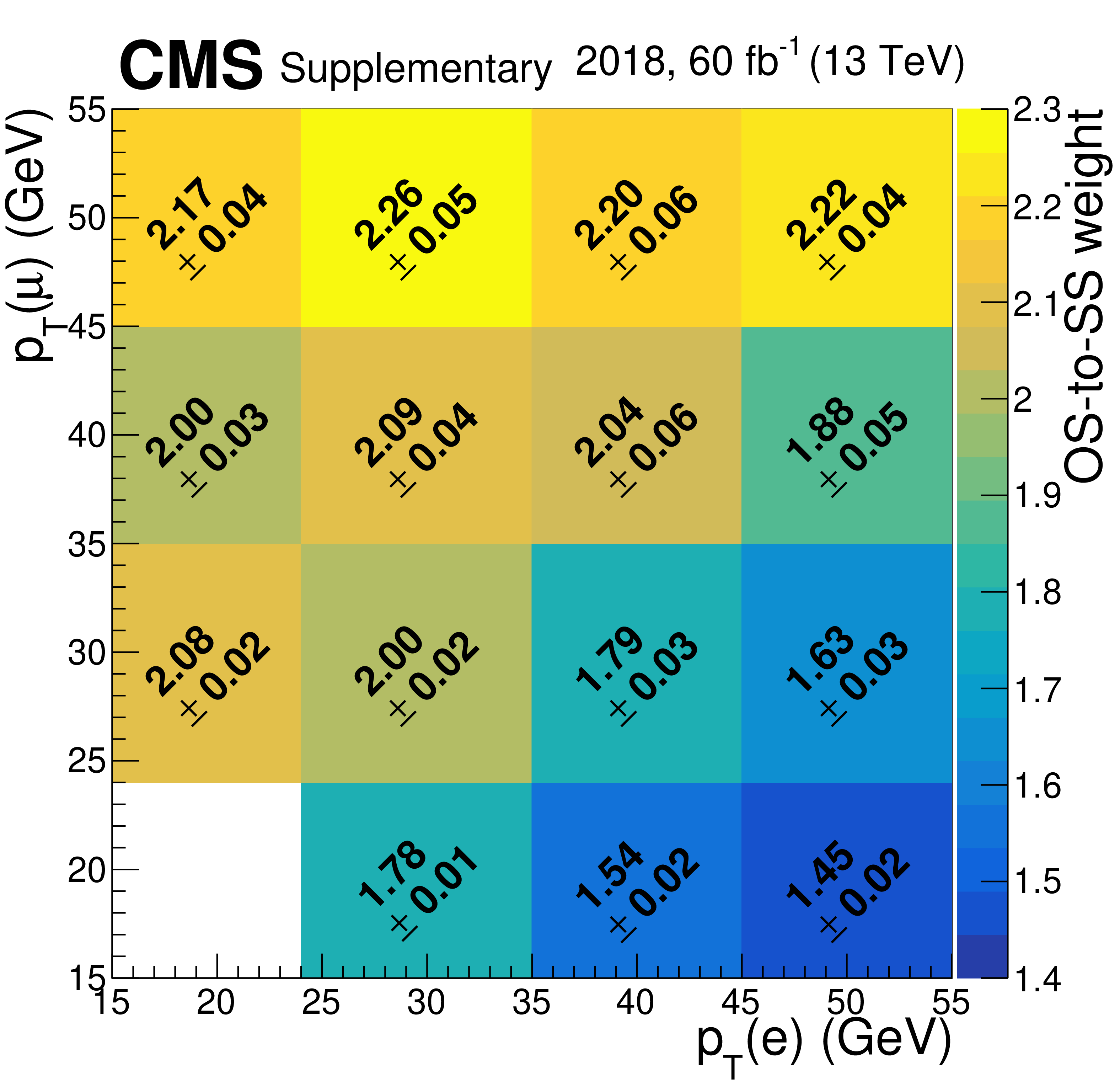
Additional Figure 27:
OS-to-SS scale factors used to estimate the mis-ID background in the $ \mathrm{e}\mu $ final state. They are measured in an $ \mathrm{e}\mu $ CR with inverted muon isolation. |
png pdf |
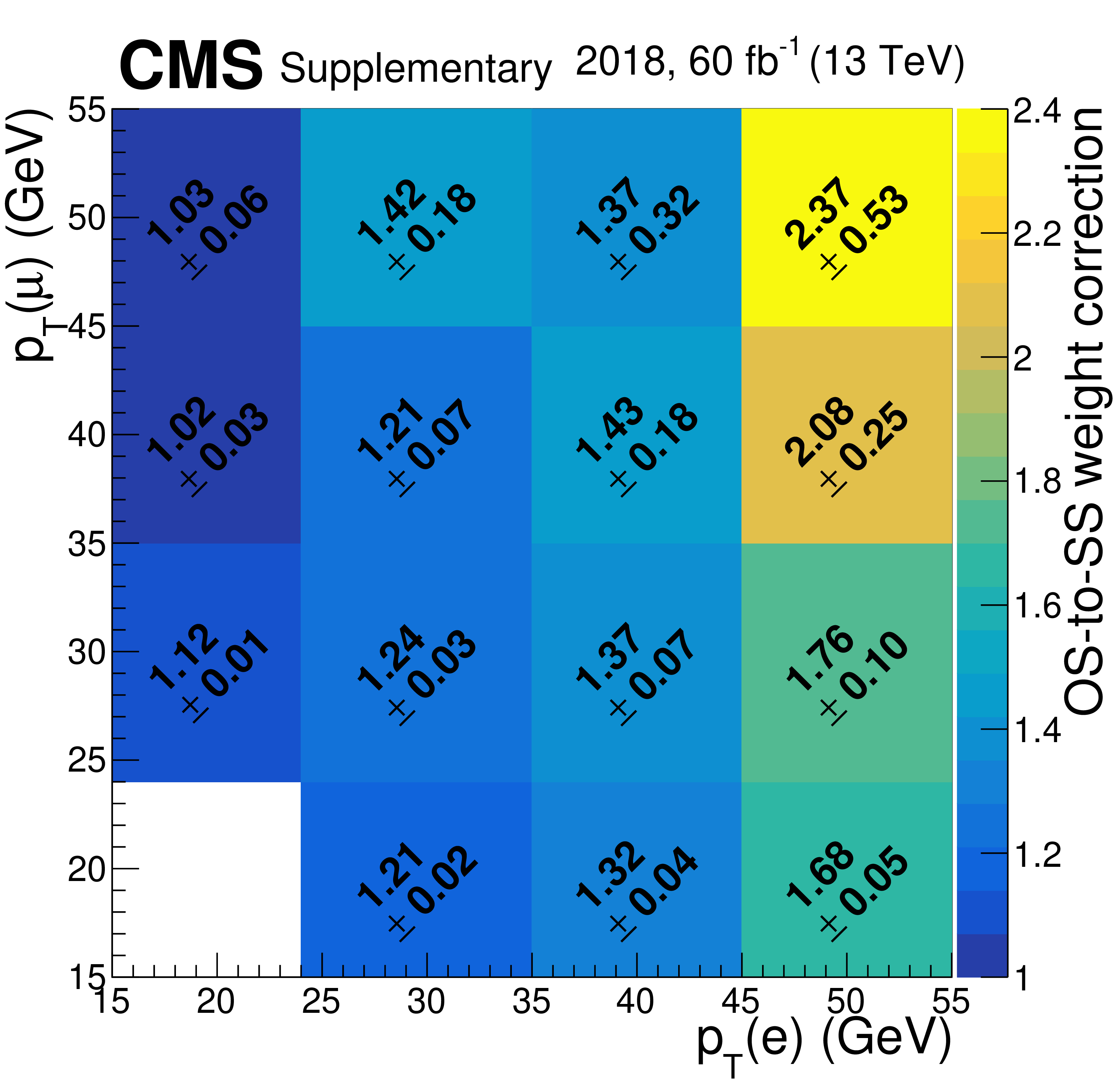
Additional Figure 28:
Correction to the OS-to-SS scale factors in the $ \mathrm{e}\mu $ final state to account for the inversion of the muon isolation. They are measured as the ratio of the OS-to-SS scale factors measured in these two CRs: a CR with inverted electron isolation and nominal muon isolation, and a region with inverted electron and muon isolations. |
png pdf |
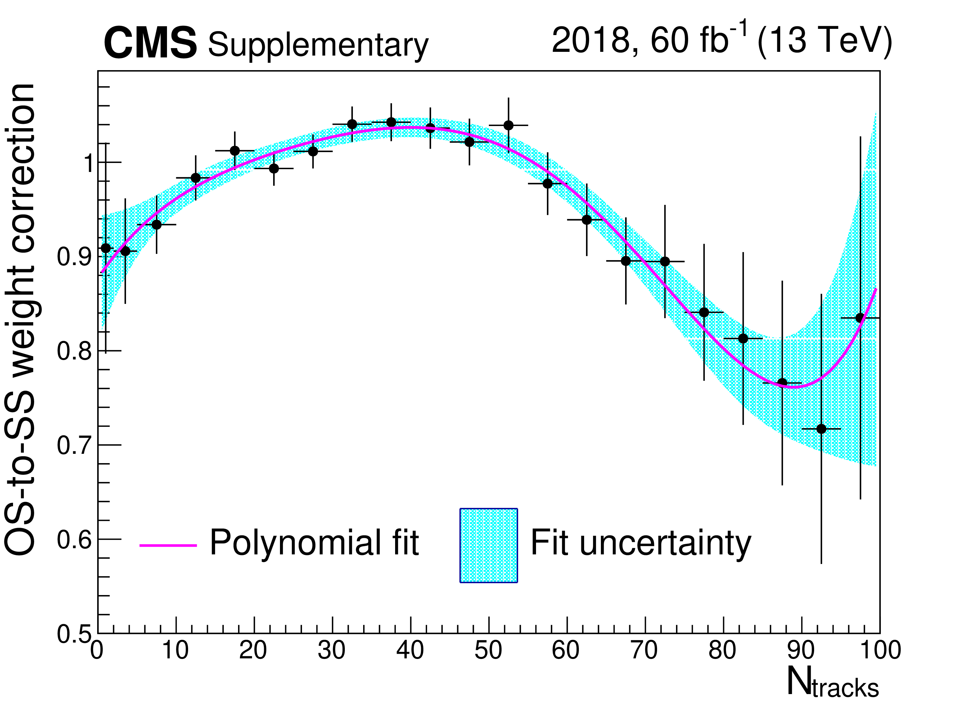
Additional Figure 29:
Multiplicative $ N_\text{tracks} $-dependent correction to the OS-to-SS scale factors used to estimate the jet mis-ID background in the $ \mathrm{e}\mu $ final state. The cyan shaded area corresponds to the fit uncertainty. This correction was measured for the 2018 data-taking period and corrections in the other data-taking periods are similar. The cyan shaded area corresponds to the fit uncertainty. |
png pdf |
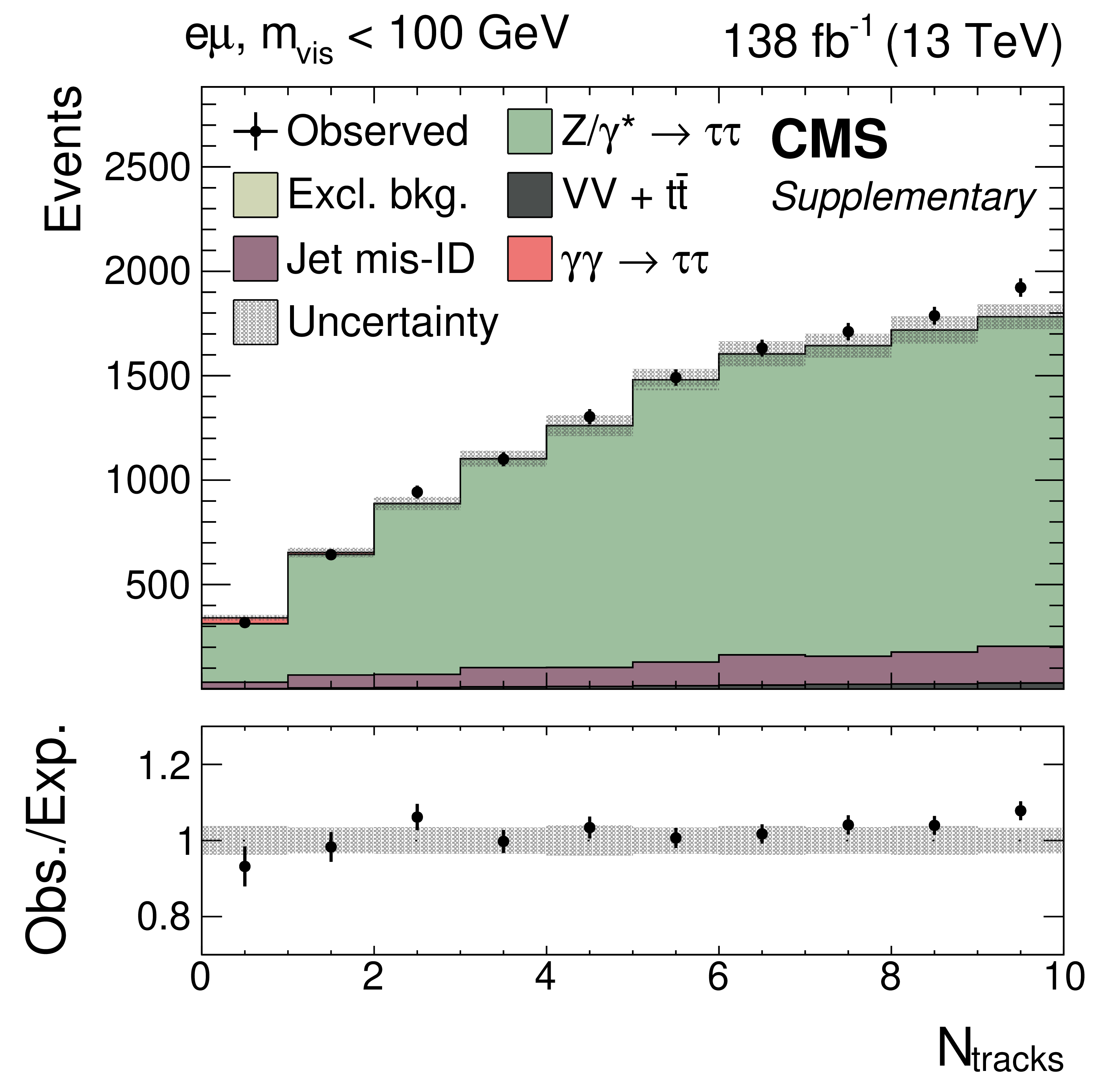
Additional Figure 30:
Observed and predicted $ N_\text{tracks} $ distributions in the $ \mathrm{e}\mu $ final state for events passing the SR selection with the additional requirement $ m_\text{vis} < $ 100 GeV. The inclusive diboson background contribution is drawn together with the $ {\mathrm{t}\overline{\mathrm{t}}} $ process. The predicted distributions are adjusted to the result of the global fit performed with the $ m_\text{vis} $ distributions in the SRs, and the signal distribution is normalized to its best fit signal strength. The uncertainty band accounts for all sources of background and signal uncertainty, systematic as well as statistical. |
png pdf |
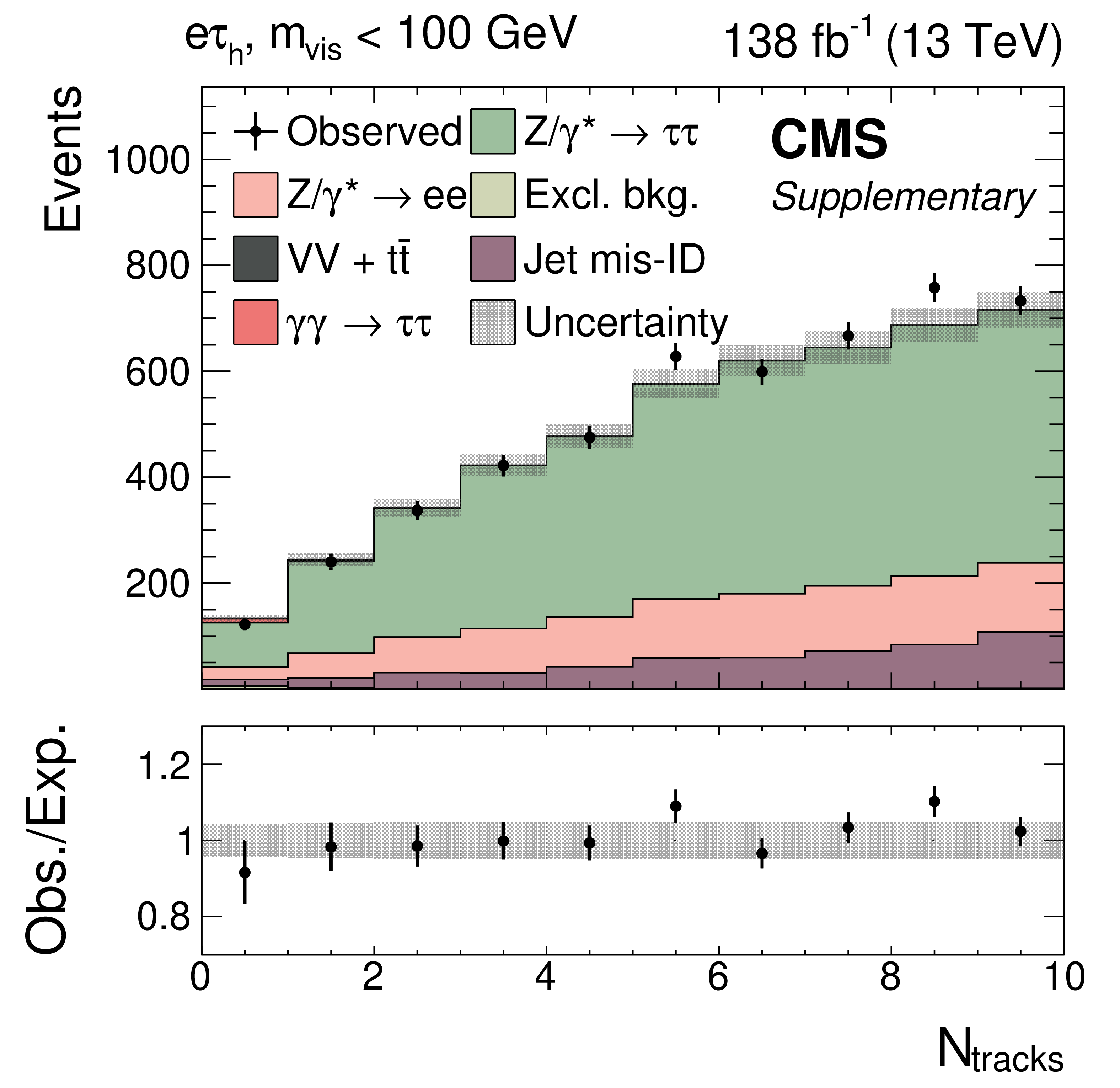
Additional Figure 31:
Observed and predicted $ N_\text{tracks} $ distributions in the $ \mathrm{e}\tau_{\mathrm{h}} $ final state for events passing the SR selection with the additional requirement $ m_\text{vis} < $ 100 GeV. The inclusive diboson background contribution is drawn together with the $ {\mathrm{t}\overline{\mathrm{t}}} $ process. The predicted distributions are adjusted to the result of the global fit performed with the $ m_\text{vis} $ distributions in the SRs, and the signal distribution is normalized to its best fit signal strength. The uncertainty band accounts for all sources of background and signal uncertainty, systematic as well as statistical. |
png pdf |
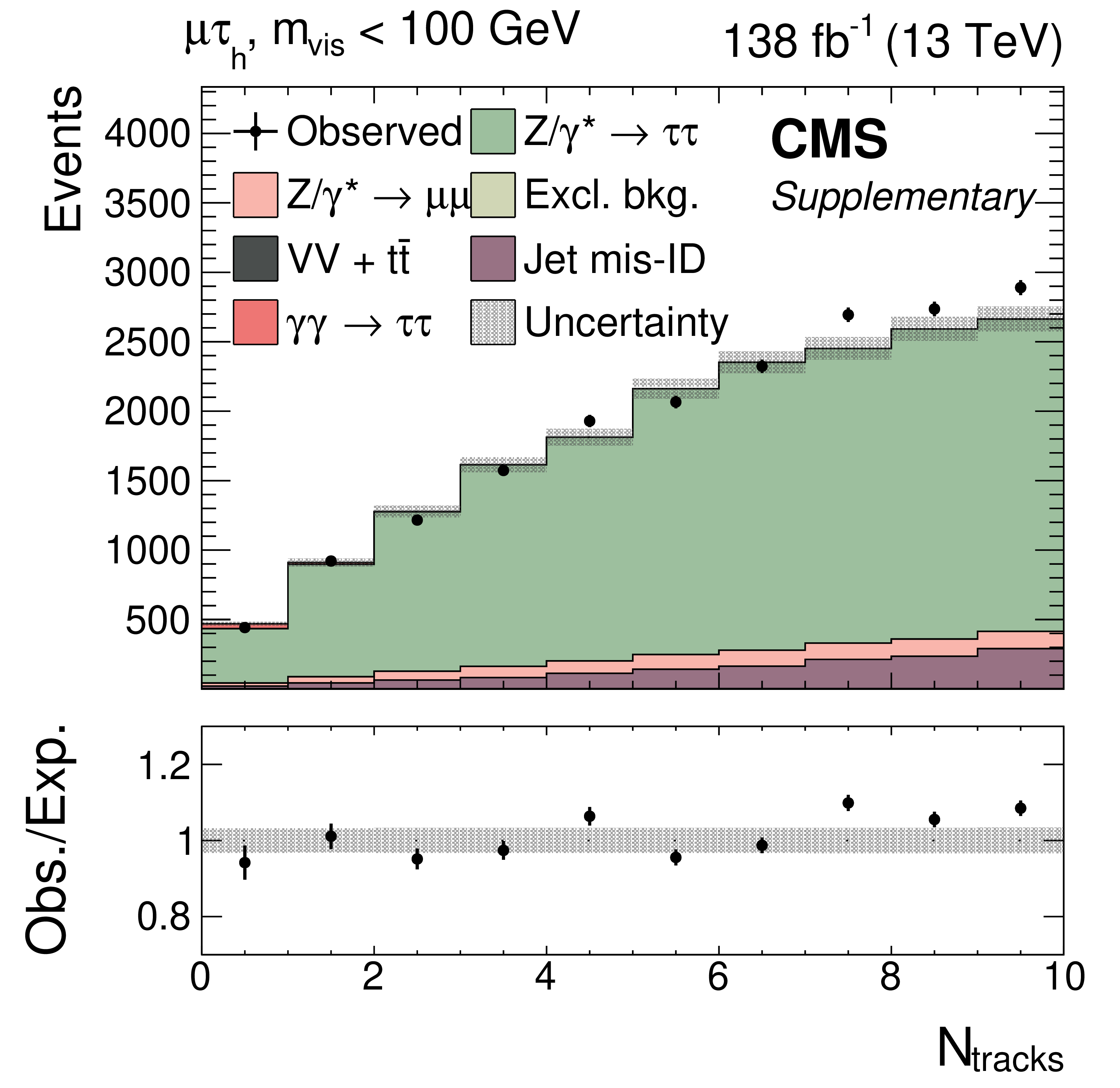
Additional Figure 32:
Observed and predicted $ N_\text{tracks} $ distributions in the $ \mu\tau_{\mathrm{h}} $ final state for events passing the SR selection with the additional requirement $ m_\text{vis} < $ 100 GeV. The inclusive diboson background contribution is drawn together with the $ {\mathrm{t}\overline{\mathrm{t}}} $ process. The predicted distributions are adjusted to the result of the global fit performed with the $ m_\text{vis} $ distributions in the SRs, and the signal distribution is normalized to its best fit signal strength. The uncertainty band accounts for all sources of background and signal uncertainty, systematic as well as statistical. |
png pdf |
Additional Figure 33:
Observed and predicted $ N_\text{tracks} $ distributions for events in the $ \tau_{\mathrm{h}}\tau_{\mathrm{h}} $ final state passing the SR selection with the additional requirement $ m_\text{vis} < $ 100 GeV. The predicted distributions are adjusted to the result of the global fit performed with the $ m_\text{vis} $ distributions in the SRs, and the signal distribution is normalized to its best fit signal strength. The uncertainty band accounts for all sources of background and signal uncertainty, systematic as well as statistical. |
png pdf |
Additional Figure 34:
Observed negative log-likelihood scans as a function of the signal strength $ \mu $, assuming SM values for $ a_{\tau} $ and $ d_{\tau} $, for the combination of all SRs in all data-taking periods. The scan with statistical uncertainty in data only is shown with the dashed blue line while the scan including all uncertainties is shown with the solid black line. For the fit with statistical uncertainty only, the nuisance parameters are frozen to their best-fit values. |
png pdf |
Additional Figure 35:
Observed negative log-likelihood scans as a function of $ a_{\tau} $, for the combination of all SRs in all data-taking periods. The scan with statistical uncertainty in data only is shown with the dashed blue line while the scan including all uncertainties is shown with the solid black line. For the fit with statistical uncertainty only, the nuisance parameters are frozen to their best-fit values. |
png pdf |
Additional Figure 36:
Observed negative log-likelihood scans as a function of $ d_{\tau} $, for the combination of all SRs in all data-taking periods. The scan with statistical uncertainty in data only is shown with the dashed blue line while the scan including all uncertainties is shown with the solid black line. For the fit with statistical uncertainty only, the nuisance parameters are frozen to their best-fit values. |
png pdf |
Additional Figure 37:
Observed negative log-likelihood scans as a function of $ a_{\tau} $, for the combination of all SRs in the $ \mathrm{e}\mu $ final state. The scan with statistical uncertainty in data only is shown with the dashed blue line while the scan including all uncertainties is shown with the solid black line. For the fit with statistical uncertainty only, the nuisance parameters are frozen to their best-fit values. |
png pdf |
Additional Figure 38:
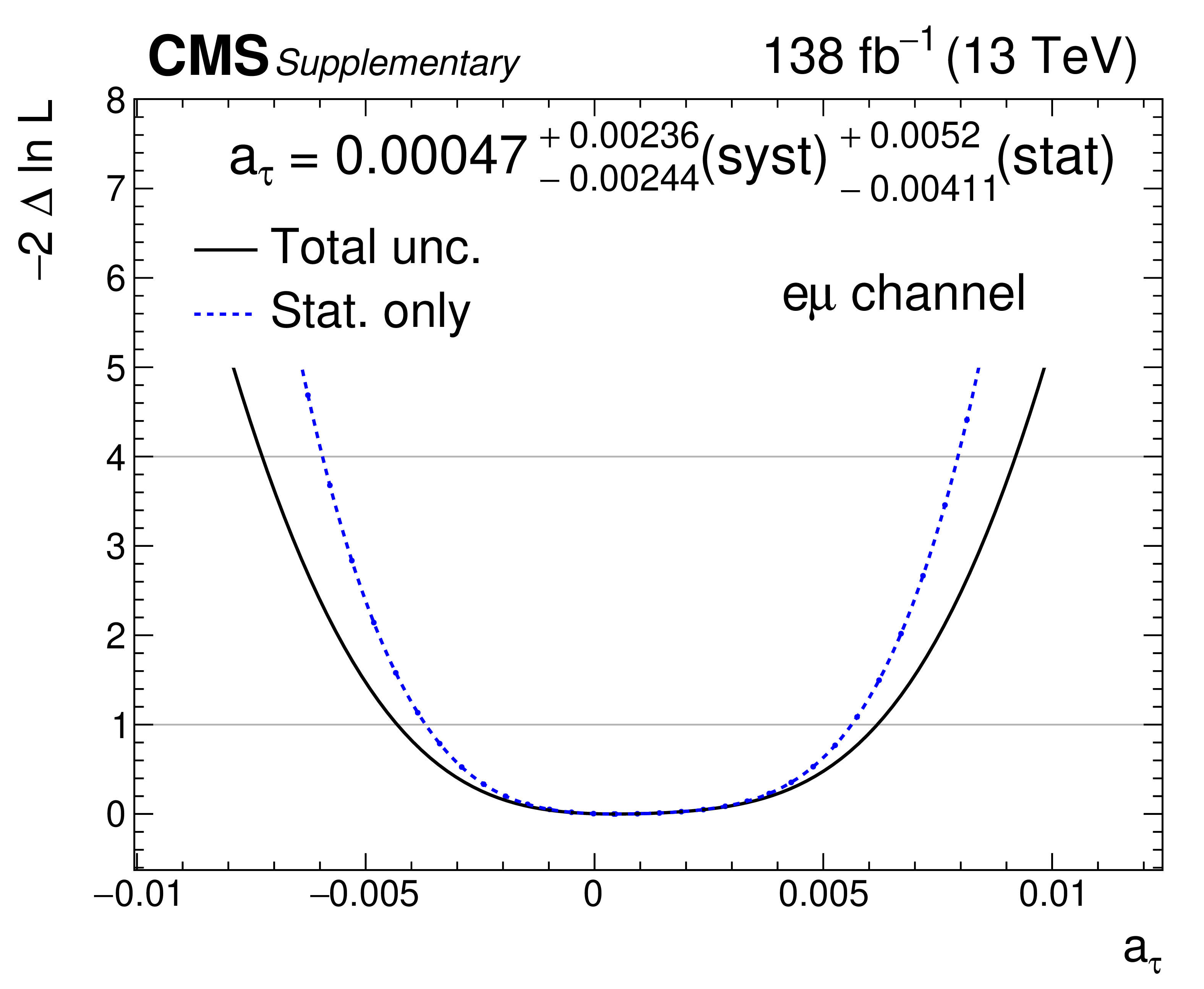
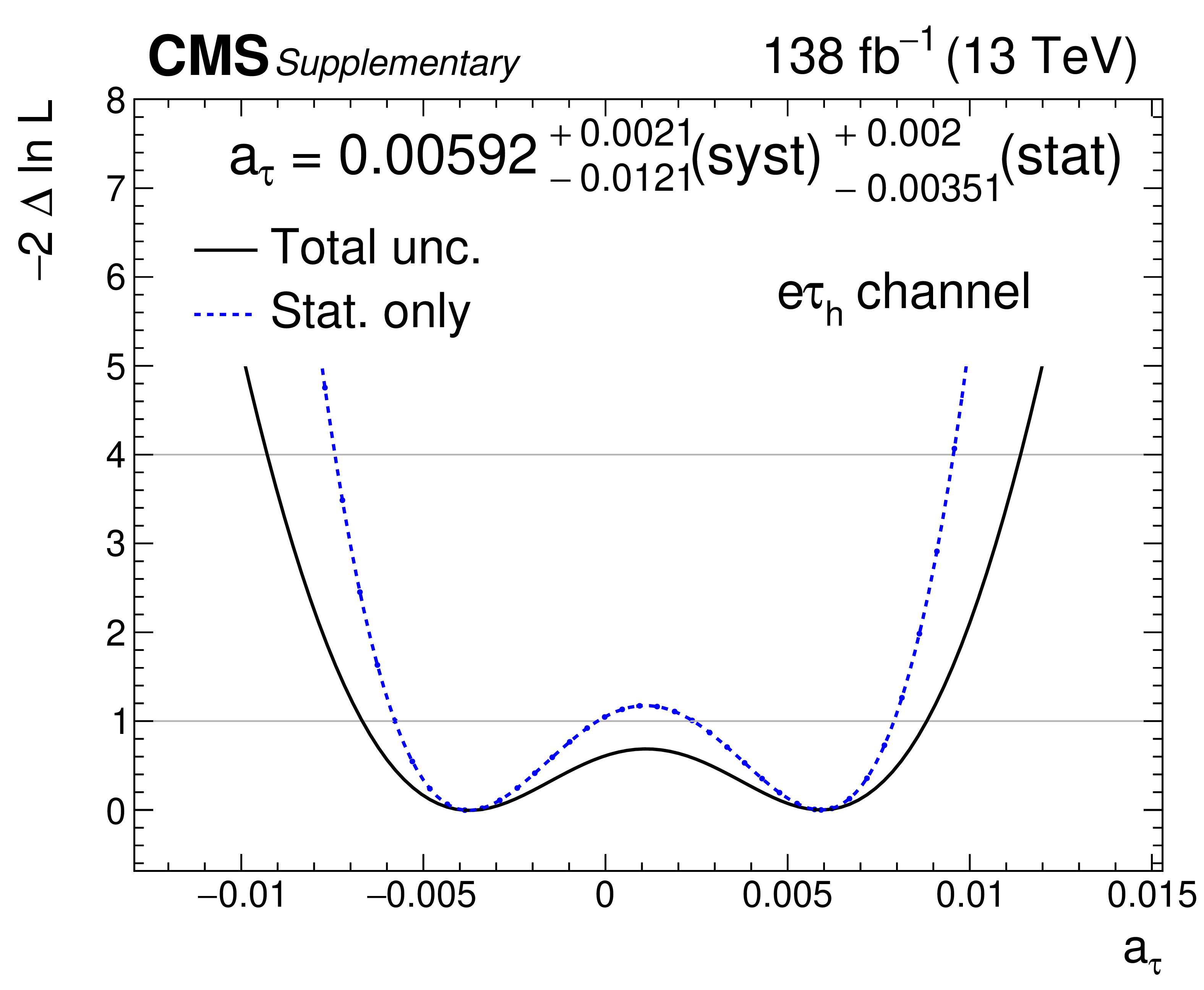
Observed negative log-likelihood scans as a function of $ a_{\tau} $, for the combination of all SRs in the $ \mathrm{e}\tau_{\mathrm{h}} $ final state. The scan with statistical uncertainty in data only is shown with the dashed blue line while the scan including all uncertainties is shown with the solid black line. For the fit with statistical uncertainty only, the nuisance parameters are frozen to their best-fit values. The double-minimum structure corresponds to an excess of observed events that can be described by non-zero value of $ \delta a_{\tau} $, where BSM effects only moderately depend on the sign of $ \delta a_{\tau} $. |

png pdf |
Additional Figure 39:
Observed negative log-likelihood scans as a function of $ a_{\tau} $, for the combination of all SRs in the $ \mu\tau_{\mathrm{h}} $ final state. The scan with statistical uncertainty in data only is shown with the dashed blue line while the scan including all uncertainties is shown with the solid black line. For the fit with statistical uncertainty only, the nuisance parameters are frozen to their best-fit values. |
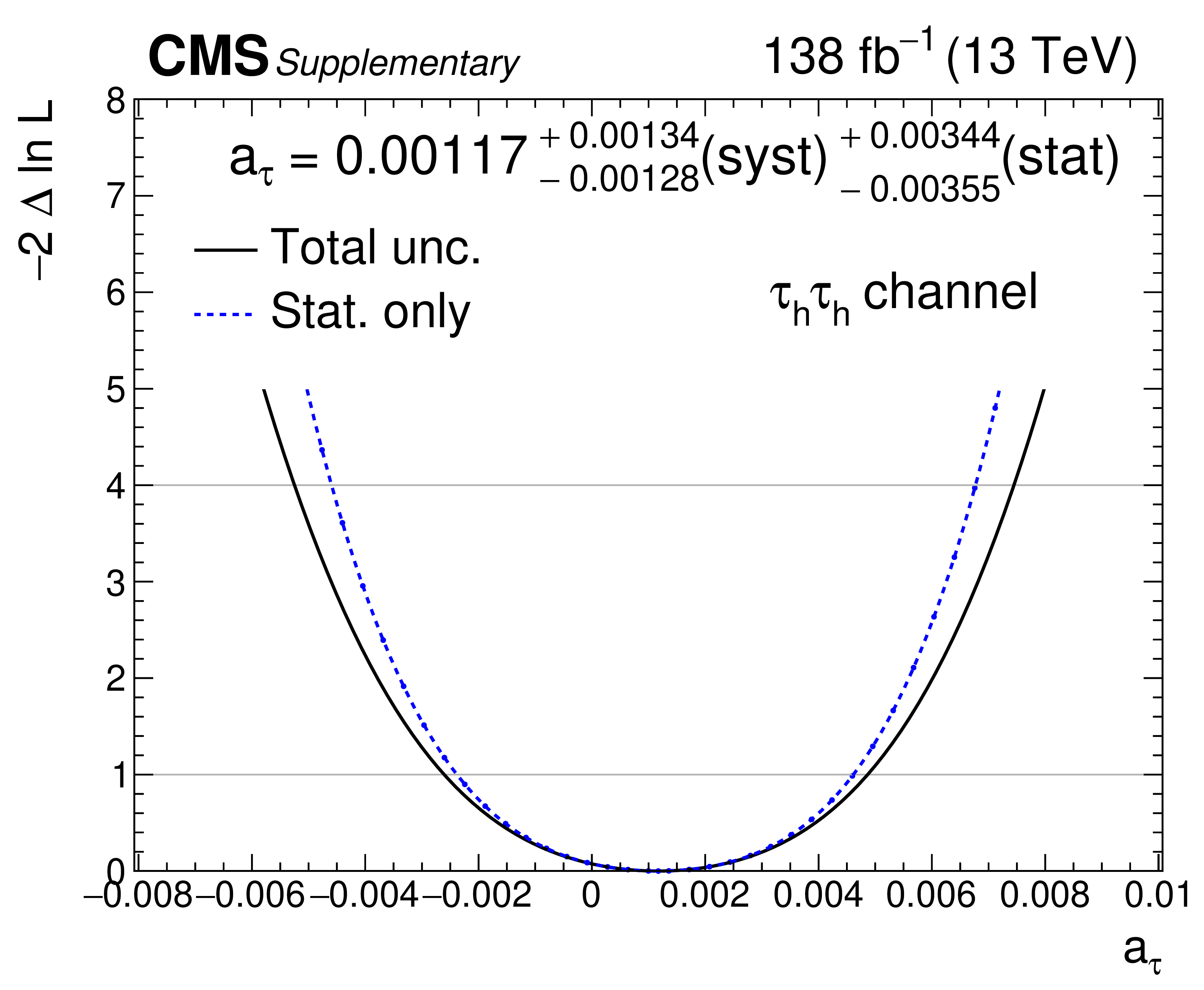
png pdf |
Additional Figure 40:
Observed negative log-likelihood scans as a function of $ a_{\tau} $, for the combination of all SRs in the $ \tau_{\mathrm{h}}\tau_{\mathrm{h}} $ final state. The scan with statistical uncertainty in data only is shown with the dashed blue line while the scan including all uncertainties is shown with the solid black line. For the fit with statistical uncertainty only, the nuisance parameters are frozen to their best-fit values. |

png pdf |
Additional Figure 41:
Observed negative log-likelihood scans as a function of $ d_{\tau} $, for the combination of all SRs in the $ \mathrm{e}\mu $ final state. The scan with statistical uncertainty in data only is shown with the dashed blue line while the scan including all uncertainties is shown with the solid black line. For the fit with statistical uncertainty only, the nuisance parameters are frozen to their best-fit values. |
png pdf |
Additional Figure 42:
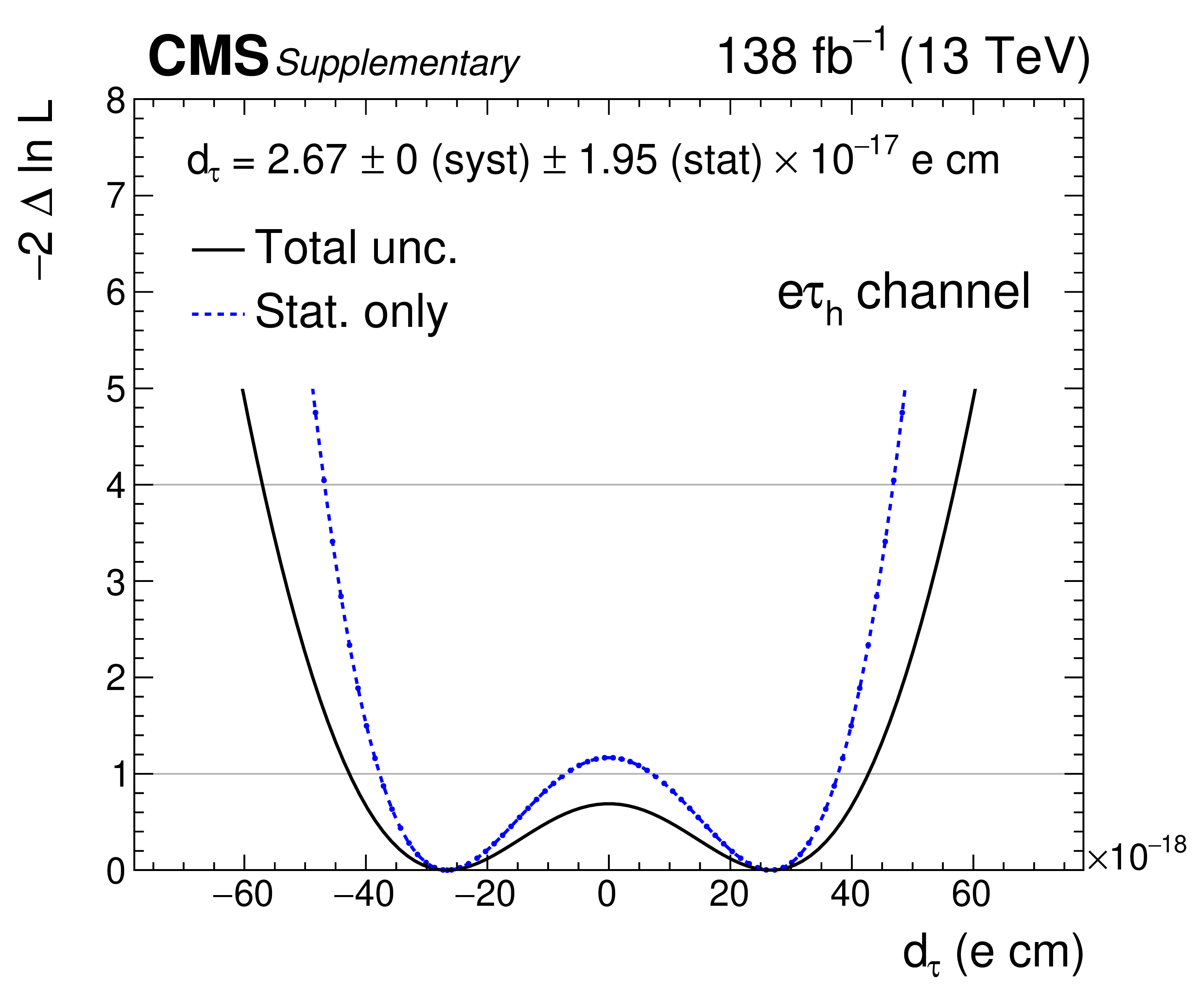
Observed negative log-likelihood scans as a function of $ a_{\tau} $, for the combination of all SRs in the $ \mathrm{e}\tau_{\mathrm{h}} $ final state. The scan with statistical uncertainty in data only is shown with the dashed blue line while the scan including all uncertainties is shown with the solid black line. For the fit with statistical uncertainty only, the nuisance parameters are frozen to their best-fit values. The double-minimum structure corresponds to an excess of observed events that can be described by BSM values of $ d_{\tau} $, where BSM effects do not depend on the sign of $ d_{\tau} $. |
png pdf |
Additional Figure 43:
Observed negative log-likelihood scans as a function of $ d_{\tau} $, for the combination of all SRs in the $ \mu\tau_{\mathrm{h}} $ final state. The scan with statistical uncertainty in data only is shown with the dashed blue line while the scan including all uncertainties is shown with the solid black line. For the fit with statistical uncertainty only, the nuisance parameters are frozen to their best-fit values. |
png pdf |
Additional Figure 44:
Observed negative log-likelihood scans as a function of $ d_{\tau} $, for the combination of all SRs in the $ \tau_{\mathrm{h}}\tau_{\mathrm{h}} $ final state. The scan with statistical uncertainty in data only is shown with the dashed blue line while the scan including all uncertainties is shown with the solid black line. For the fit with statistical uncertainty only, the nuisance parameters are frozen to their best-fit values. |
png pdf |
Additional Figure 45:
Acoplanarity distribution in data and in simulation before correction, in the 2018 data-taking period. The background prediction is normalized to match the data yield and only the statistical uncertainty is shown. |
png |
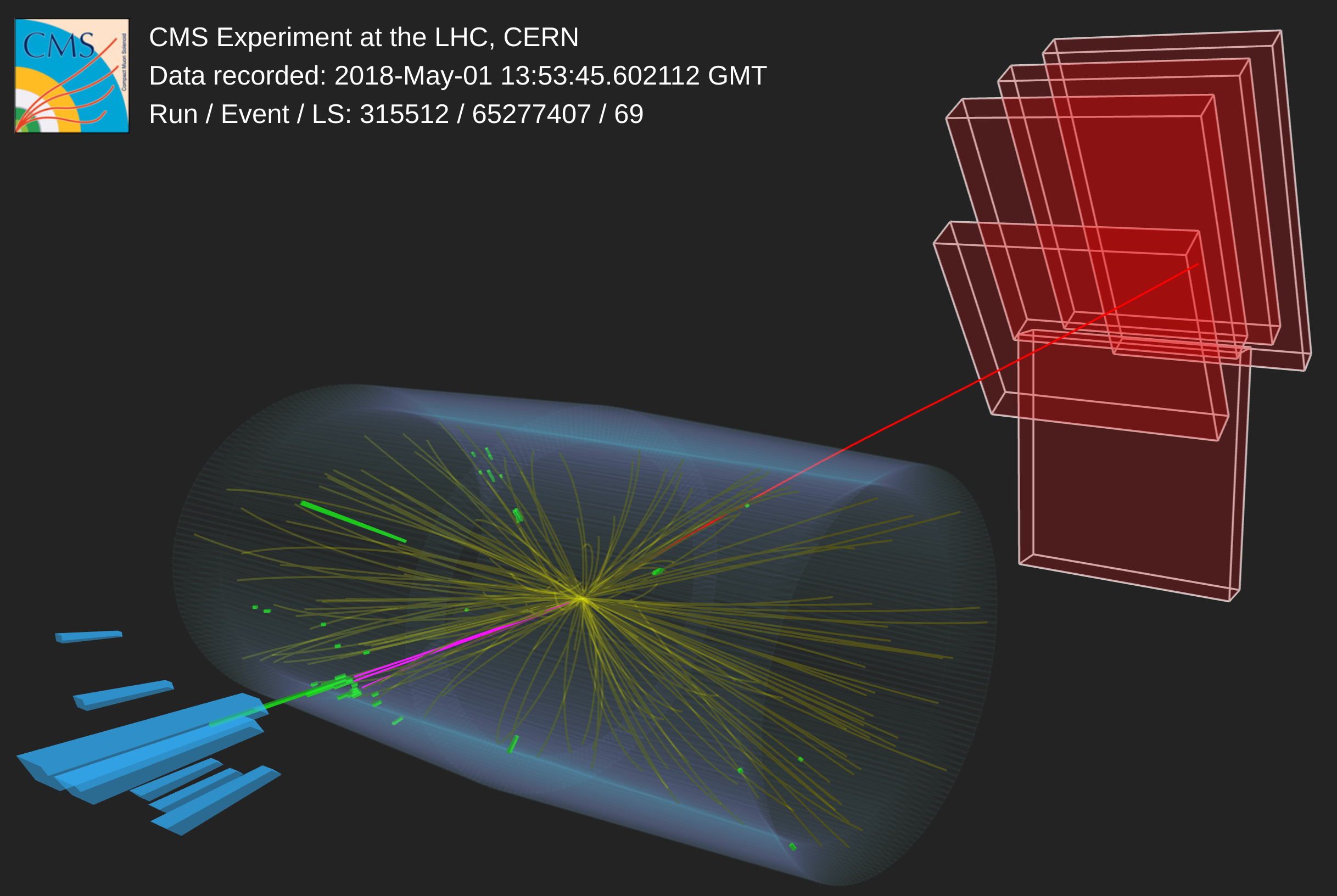
Additional Figure 46:
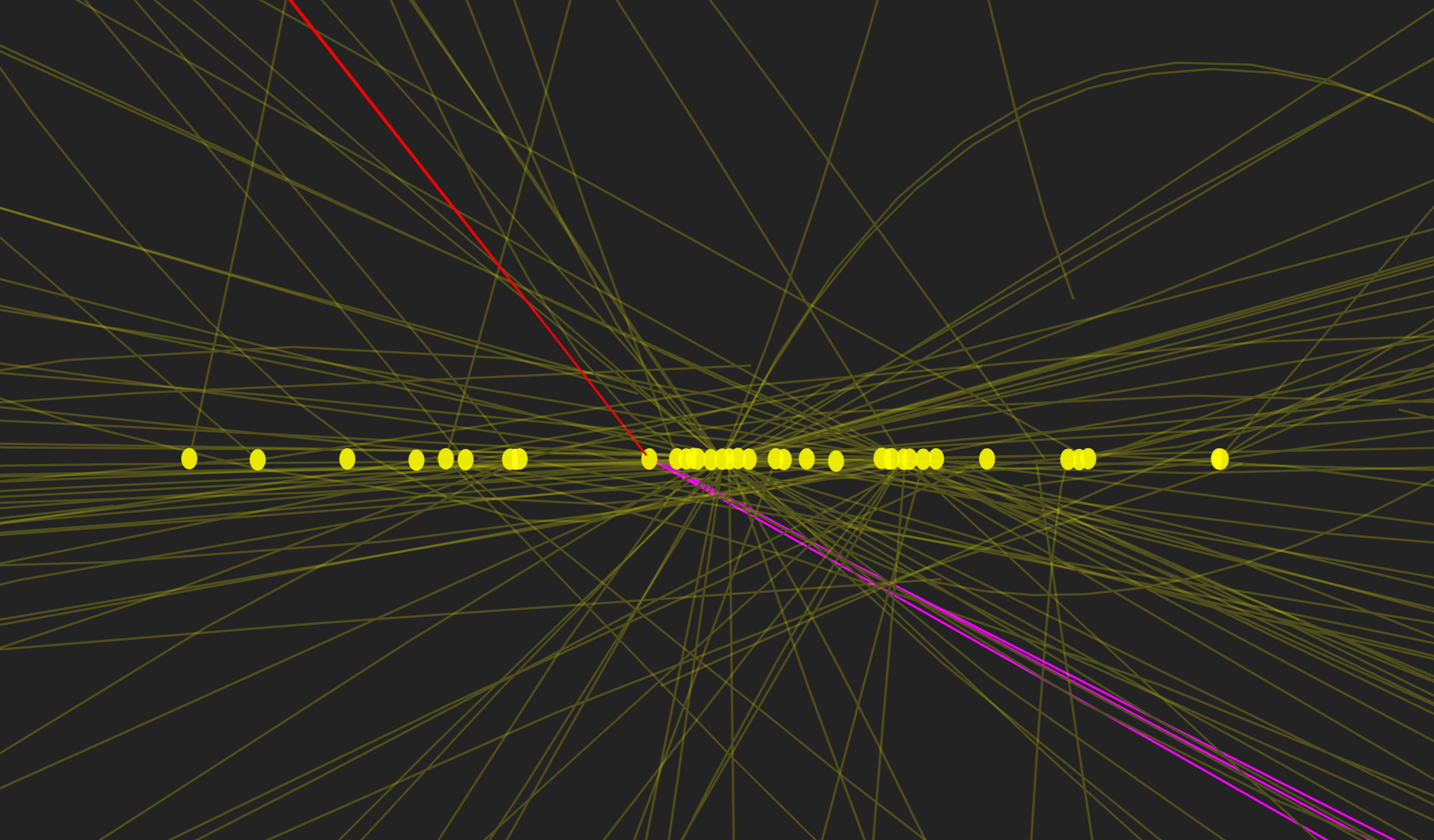
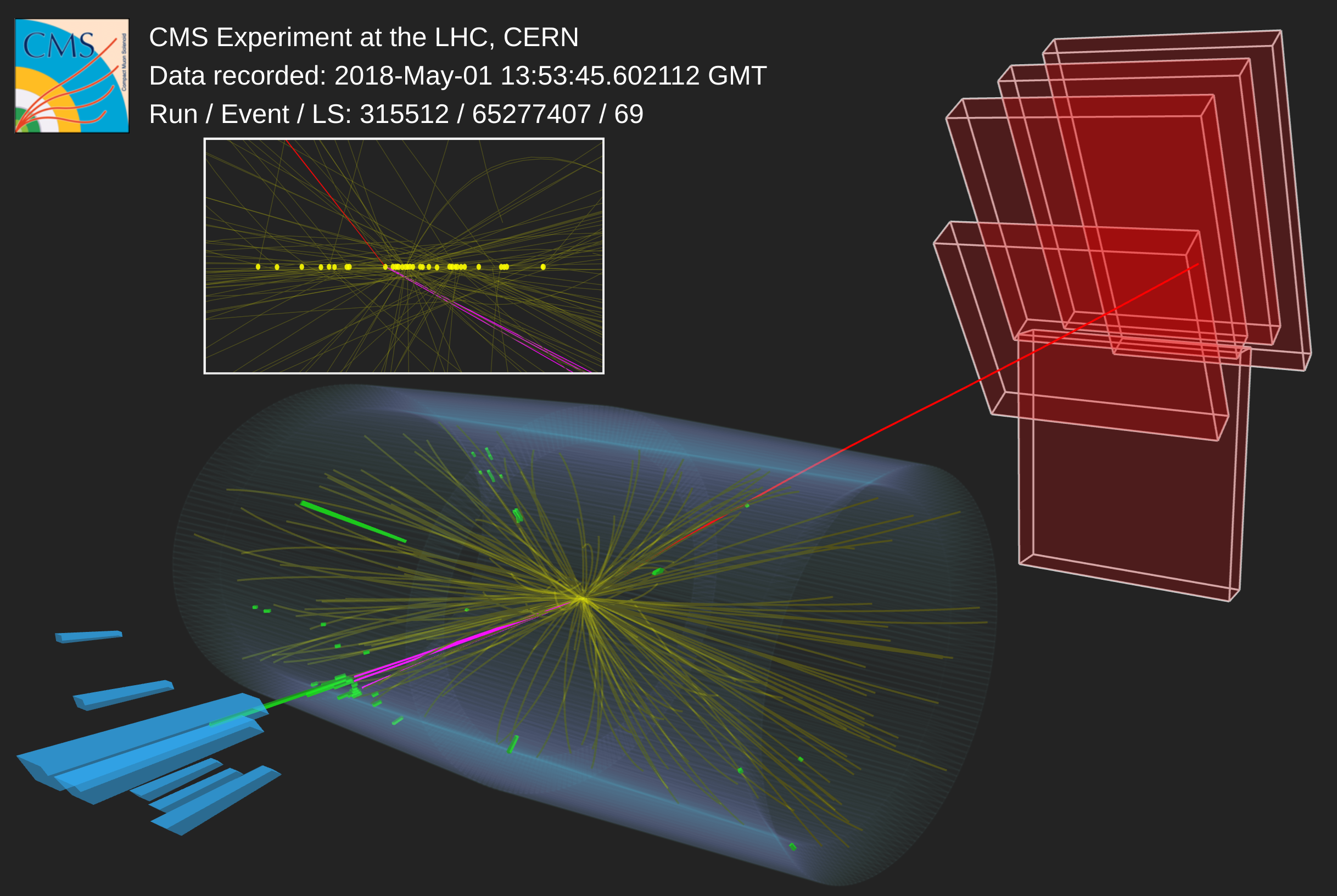
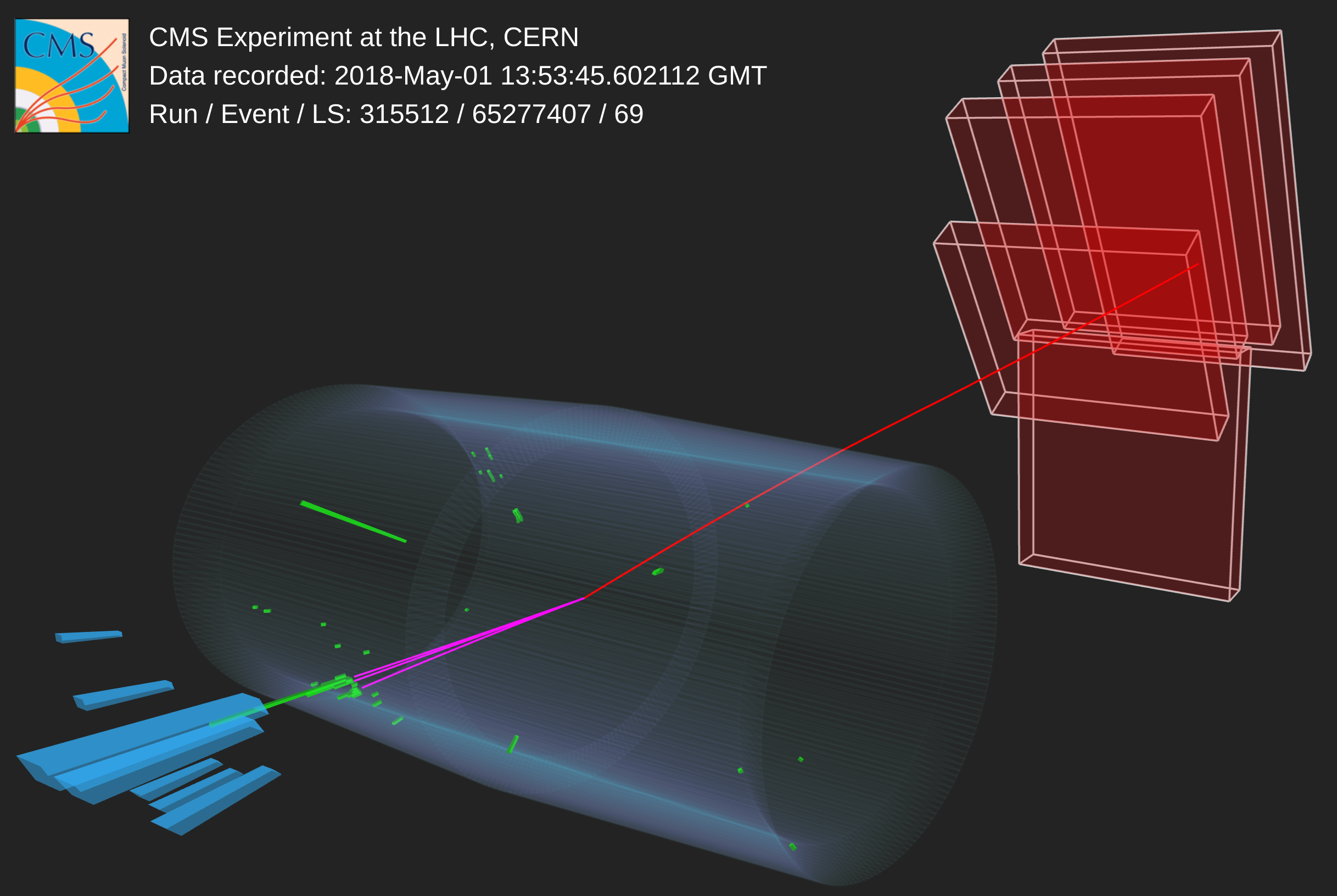
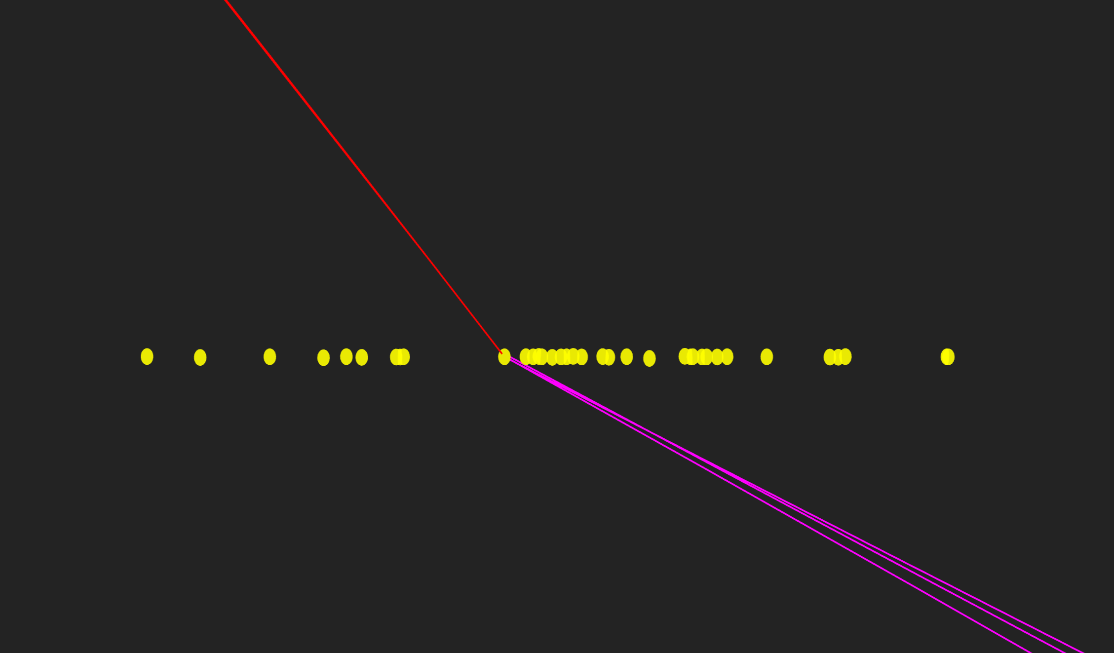
Candidate $\gamma\gamma \to \tau\tau$ event measured in proton-proton collisions by CMS. The event is reconstructed as having a leptonic $\tau$ decay, $\tau \to \mu\nu\nu$, with the μ track indicated in red, and a hadronic $\tau$ decay, $\tau \to \pi\pi\pi\nu$, with the 3 charged pions indicated by the yellow tracks and by the energy deposits in the ECAL (green) and HCAL (cyan). Find this 3-dimensional interactive version with all tracks here. |
png |
Additional Figure 47:
Candidate $\gamma\gamma \to \tau\tau$ event measured in proton-proton collisions by CMS. The event is reconstructed as having a leptonic $\tau$ decay, $\tau \to \mu\nu\nu$, with the μ track indicated in red, and a hadronic $\tau$ decay, $\tau \to \pi\pi\pi\nu$, with the 3 charged pions indicated by the yellow tracks and by the energy deposits in the ECAL (green) and HCAL (cyan). Find this 3-dimensional interactive version with all tracks here. |
png |
Additional Figure 48:
Candidate $\gamma\gamma \to \tau\tau$ event measured in proton-proton collisions by CMS. The event is reconstructed as having a leptonic $\tau$ decay, $\tau \to \mu\nu\nu$, with the μ track indicated in red, and a hadronic $\tau$ decay, $\tau \to \pi\pi\pi\nu$, with the 3 charged pions indicated by the yellow tracks and by the energy deposits in the ECAL (green) and HCAL (cyan). Find this 3-dimensional interactive version with all tracks here. |
png |
Additional Figure 49:
Candidate $\gamma\gamma \to \tau\tau$ event measured in proton-proton collisions by CMS. The event is reconstructed as having a leptonic $\tau$ decay, $\tau \to \mu\nu\nu$, with the μ track indicated in red, and a hadronic $\tau$ decay, $\tau \to \pi\pi\pi\nu$, with the 3 charged pions indicated by the yellow tracks and by the energy deposits in the ECAL (green) and HCAL (cyan). Find this 3-dimensional interactive version with all tracks here. |
png |
Additional Figure 50:
Candidate $\gamma\gamma \to \tau\tau$ event measured in proton-proton collisions by CMS. The event is reconstructed as having a leptonic $\tau$ decay, $\tau \to \mu\nu\nu$, with the μ track indicated in red, and a hadronic $\tau$ decay, $\tau \to \pi\pi\pi\nu$, with the 3 charged pions indicated by the yellow tracks and by the energy deposits in the ECAL (green) and HCAL (cyan). Find this 3-dimensional interactive version with all tracks here. |

png |
Additional Figure 51:
Candidate $\gamma\gamma \to \tau\tau$ event measured in proton-proton collisions by CMS. The event is reconstructed as having a leptonic $\tau$ decay, $\tau \to \mu\nu\nu$, with the μ track indicated in red, and a hadronic $\tau$ decay, $\tau \to \pi\pi\pi\nu$, with the 3 charged pions indicated by the yellow tracks and by the energy deposits in the ECAL (green) and HCAL (cyan). Find this 3-dimensional interactive version with all tracks here. |
| References | ||||
| 1 | V. M. Budnev, I. F. Ginzburg, G. V. Meledin, and V. G. Serbo | The process $ \mathrm{p}\mathrm{p}\to\mathrm{e}^+\mathrm{e}^- $ and the possibility of its calculation by means of quantum electrodynamics only | NPB 63 (1973) 519 | |
| 2 | STAR Collaboration | Production of $ \mathrm{e}^+\mathrm{e}^- $ pairs accompanied by nuclear dissociation in ultra-peripheral heavy ion collision | Phys. Rev. C 70 (2004) 031902 | nucl-ex/0404012 |
| 3 | CDF Collaboration | Observation of exclusive electron-positron production in hadron-hadron collisions | PRL 98 (2007) 112001 | hep-ex/0611040 |
| 4 | CDF Collaboration | Observation of exclusive charmonium production and $ \gamma\gamma \to \mu^+\mu^- $ in $ \mathrm{p}\overline{\mathrm{p}} $ collisions at $ \sqrt{s} = $ 1.96 TeV | PRL 102 (2009) 242001 | 0902.1271 |
| 5 | CDF Collaboration | Search for exclusive Z boson production and observation of high mass $ \mathrm{p}\bar{\mathrm{p}} \to \gamma \gamma \to \mathrm{p}\ell\ell\bar{\mathrm{p}} $ events in $ \mathrm{p}\bar{\mathrm{p}} $ collisions at $ \sqrt{s} = $ 1.96 TeV | PRL 102 (2009) 222002 | 0902.2816 |
| 6 | ATLAS Collaboration | Exclusive dimuon production in ultraperipheral Pb+Pb collisions at $ \sqrt{s_{\mathrm{NN}}} = $ 5.02 TeV with ATLAS | Phys. Rev. C 104 (2021) 024906 | 2011.12211 |
| 7 | CMS Collaboration | Search for exclusive or semi-exclusive photon pair production and observation of exclusive and semi-exclusive electron pair production in pp collisions at $ \sqrt{s}= $ 7 TeV | JHEP 11 (2012) 080 | CMS-FWD-11-004 1209.1666 |
| 8 | CMS Collaboration | Exclusive photon-photon production of muon pairs in proton-proton collisions at $ \sqrt{s}= $ 7 TeV | JHEP 01 (2012) 052 | CMS-FWD-10-005 1111.5536 |
| 9 | ATLAS Collaboration | Observation of the $ \gamma\gamma\to\tau\tau $ process in Pb+Pb collisions and constraints on the \ensuremath\tau-lepton anomalous magnetic moment with the ATLAS detector | PRL 131 (2023) 151802 | 2204.13478 |
| 10 | CMS Collaboration | Observation of $ \tau $ lepton pair production in ultraperipheral lead-lead collisions at $ \sqrt {\smash [b]{s_{_{\mathrm {NN}}}}} = $ 5.02 TeV | PRL 131 (2023) 151803 | CMS-HIN-21-009 2206.05192 |
| 11 | F. del Aguila, F. Cornet, and J. I. Illana | The possibility of using a large heavy-ion collider for measuring the electromagnetic properties of the tau lepton | PLB 271 (1991) 256 | |
| 12 | S. Atag and A. A. Billur | Possibility of determining $ \tau $ lepton electromagnetic moments in $ {\gamma\gamma \to \tau^{+}\tau^{-}} $ process at the CERN-LHC | JHEP 11 (2010) 060 | 1005.2841 |
| 13 | M. Dyndal, M. Klusek-Gawenda, M. Schott, and A. Szczurek | Anomalous electromagnetic moments of $ \tau $ lepton in $ \gamma \gamma \to \tau^+ \tau^- $ reaction in Pb+Pb collisions at the LHC | PLB 809 (2020) 135682 | 2002.05503 |
| 14 | L. Beresford and J. Liu | New physics and tau g$-$2 using LHC heavy ion collisions | PRD 102 (2020) 113008 | 1908.05180 |
| 15 | J. Schwinger | On quantum-electrodynamics and the magnetic moment of the electron | PR 73 (1948) 416 | |
| 16 | R. H. Parker et al. | Measurement of the fine-structure constant as a test of the standard model | Science 360 (2018) 191 | 1812.04130 |
| 17 | X. Fan, T. G. Myers, B. A. D. Sukra, and G. Gabrielse | Measurement of the electron magnetic moment | PRL 130 (2023) 071801 | 2209.13084 |
| 18 | Muon g$-$2 Collaboration | Measurement of the positive muon anomalous magnetic moment to 0.46 ppm | PRL 126 (2021) 141801 | 2104.03281 |
| 19 | Muon g$-$2 Collaboration | Measurement of the positive muon anomalous magnetic moment to 0.20 ppm | PRL 131 (2023) 161802 | 2308.06230 |
| 20 | T. Aoyama et al. | The anomalous magnetic moment of the muon in the standard model | Phys. Rept. 887 (2020) 1 | 2006.04822 |
| 21 | S. Eidelman and M. Passera | Theory of the tau lepton anomalous magnetic moment | Mod. Phys. Lett. A 22 (2007) 159 | hep-ph/0701260 |
| 22 | Y. Yamaguchi and N. Yamanaka | Large long-distance contributions to the electric dipole moments of charged leptons in the standard model | PRL 125 (2020) 241802 | 2003.08195 |
| 23 | A. Crivellin, M. Hoferichter, and J. M. Roney | Toward testing the magnetic moment of the tau at one part per million | PRD 106 (2022) 093007 | 2111.10378 |
| 24 | DELPHI Collaboration | Study of tau-pair production in photon-photon collisions at LEP and limits on the anomalous electromagnetic moments of the tau lepton | EPJC 35 (2004) 159 | hep-ex/0406010 |
| 25 | OPAL Collaboration | An upper limit on the anomalous magnetic moment of the tau lepton | PLB 431 (1998) 188 | hep-ex/9803020 |
| 26 | L3 Collaboration | Measurement of the anomalous magnetic and electric dipole moments of the tau lepton | PLB 434 (1998) 169 | |
| 27 | Belle Collaboration | An improved search for the electric dipole moment of the $ \tau $ lepton | JHEP 04 (2022) 110 | 2108.11543 |
| 28 | ARGUS Collaboration | A search for the electric dipole moment of the tau lepton | PLB 485 (2000) 37 | hep-ex/0004031 |
| 29 | CMS Collaboration | Study of exclusive two-photon production of $ \mathrm{W^+}\mathrm{W^-} $ in pp collisions at $ \sqrt{s} = $ 7 TeV and constraints on anomalous quartic gauge couplings | JHEP 07 (2013) 116 | CMS-FSQ-12-010 1305.5596 |
| 30 | CMS Collaboration | Evidence for exclusive $ \gamma\gamma \to \mathrm{W^+}\mathrm{W^-} $ production and constraints on anomalous quartic gauge couplings in pp collisions at $ \sqrt{s}= $ 7 and 8 TeV | JHEP 08 (2016) 119 | CMS-FSQ-13-008 1604.04464 |
| 31 | CMS and TOTEM Collaborations | Observation of proton-tagged, central (semi)exclusive production of high-mass lepton pairs in pp collisions at 13 TeV with the CMS-TOTEM precision proton spectrometer | JHEP 07 (2018) 153 | CMS-PPS-17-001 1803.04496 |
| 32 | ATLAS Collaboration | Measurement of exclusive $ \gamma\gamma\rightarrow \mathrm{W^+}\mathrm{W^-} $ production and search for exclusive Higgs boson production in pp collisions at $ \sqrt{s} = $ 8 TeV using the ATLAS detector | PRD 94 (2016) 032011 | 1607.03745 |
| 33 | ATLAS Collaboration | Observation of photon-induced $ \mathrm{W^+}\mathrm{W^-} $ production in pp collisions at $ \sqrt{s}= $ 13 TeV using the ATLAS detector | PLB 816 (2021) 136190 | 2010.04019 |
| 34 | CMS Collaboration | HEPData record for this analysis | link | |
| 35 | CMS Collaboration | The CMS experiment at the CERN LHC | JINST 3 (2008) S08004 | |
| 36 | CMS Collaboration | Performance of the CMS Level-1 trigger in proton-proton collisions at $ \sqrt{s} = $ 13 TeV | JINST 15 (2020) P10017 | CMS-TRG-17-001 2006.10165 |
| 37 | CMS Collaboration | The CMS trigger system | JINST 12 (2017) P01020 | CMS-TRG-12-001 1609.02366 |
| 38 | H.-S. Shao and D. d'Enterria | gamma-UPC: automated generation of exclusive photon-photon processes in ultraperipheral proton and nuclear collisions with varying form factors | JHEP 09 (2022) 248 | 2207.03012 |
| 39 | J. Alwall et al. | The automated computation of tree-level and next-to-leading order differential cross sections, and their matching to parton shower simulations | JHEP 07 (2014) 079 | 1405.0301 |
| 40 | J. Alwall et al. | MadGraph/MadEvent v4: the new web generation | JHEP 09 (2007) 028 | |
| 41 | R. Frederix and S. Frixione | Merging meets matching in MC@NLO | JHEP 12 (2012) 061 | 1209.6215 |
| 42 | H.-S. Shao and D. d'Enterria | Dimuon and ditau production in photon-photon collisions at next-to-leading order in QED | 2407.13610 | |
| 43 | L. A. Harland-Lang, M. Tasevsky, V. A. Khoze, and M. G. Ryskin | A new approach to modelling elastic and inelastic photon-initiated production at the LHC: SuperChic 4 | EPJC 80 (2020) 925 | 2007.12704 |
| 44 | I. Brivio, Y. Jiang, and M. Trott | The SMEFTsim package, theory and tools | JHEP 12 (2017) 070 | 1709.06492 |
| 45 | I. Brivio | SMEFTsim 3.0 \textemdash a practical guide | JHEP 04 (2021) 073 | 2012.11343 |
| 46 | P. Artoisenet, V. Lemaitre, F. Maltoni, and O. Mattelaer | Automation of the matrix element reweighting method | JHEP 12 (2010) 068 | 1007.3300 |
| 47 | P. Nason | A new method for combining NLO QCD with shower Monte Carlo algorithms | JHEP 11 (2004) 040 | hep-ph/0409146 |
| 48 | S. Frixione, P. Nason, and C. Oleari | Matching NLO QCD computations with parton shower simulations: the POWHEG method | JHEP 11 (2007) 070 | 0709.2092 |
| 49 | S. Alioli, P. Nason, C. Oleari, and E. Re | A general framework for implementing NLO calculations in shower Monte Carlo programs: the POWHEG BOX | JHEP 06 (2010) 043 | 1002.2581 |
| 50 | S. Alioli et al. | Jet pair production in POWHEG | JHEP 04 (2011) 081 | 1012.3380 |
| 51 | S. Alioli, P. Nason, C. Oleari, and E. Re | NLO Higgs boson production via gluon fusion matched with shower in POWHEG | JHEP 04 (2009) 002 | 0812.0578 |
| 52 | T. Sjöstrand et al. | An introduction to PYTHIA 8.2 | Comput. Phys. Commun. 191 (2015) 159 | 1410.3012 |
| 53 | CMS Collaboration | Extraction and validation of a new set of CMS PYTHIA8 tunes from underlying-event measurements | EPJC 80 (2020) 4 | CMS-GEN-17-001 1903.12179 |
| 54 | R. D. Ball et al. | Unbiased global determination of parton distributions and their uncertainties at NNLO and at LO | NPB 855 (2012) 153 | 1107.2652 |
| 55 | NNPDF Collaboration | Parton distributions with QED corrections | NPB 877 (2013) 290 | 1308.0598 |
| 56 | NNPDF Collaboration | Parton distributions from high-precision collider data | EPJC 77 (2017) 663 | 1706.00428 |
| 57 | GEANT4 Collaboration | GEANT 4 --- a simulation toolkit | NIM A 506 (2003) 250 | |
| 58 | CMS Collaboration | Particle-flow reconstruction and global event description with the CMS detector | JINST 12 (2017) P10003 | CMS-PRF-14-001 1706.04965 |
| 59 | CMS Collaboration | Electron and photon reconstruction and identification with the CMS experiment at the CERN LHC | JINST 16 (2021) P05014 | CMS-EGM-17-001 2012.06888 |
| 60 | CMS Collaboration | ECAL 2016 refined calibration and Run2 summary plots | CMS Detector Performance Note CMS-DP-2020-021, 2020 CDS |
|
| 61 | CMS Collaboration | Performance of the CMS muon detector and muon reconstruction with proton-proton collisions at $ \sqrt{s}= $ 13 TeV | JINST 13 (2018) P06015 | CMS-MUO-16-001 1804.04528 |
| 62 | CMS Collaboration | Performance of reconstruction and identification of $ \tau $ leptons decaying to hadrons and $ \nu_\tau $ in pp collisions at $ \sqrt{s}= $ 13 TeV | JINST 13 (2018) P10005 | CMS-TAU-16-003 1809.02816 |
| 63 | CMS Collaboration | Identification of hadronic tau lepton decays using a deep neural network | JINST 17 (2022) P07023 | CMS-TAU-20-001 2201.08458 |
| 64 | CMS Collaboration | Performance of missing transverse momentum reconstruction in proton-proton collisions at $ \sqrt{s} = $ 13 TeV using the CMS detector | JINST 14 (2019) P07004 | CMS-JME-17-001 1903.06078 |
| 65 | CMS Collaboration | Description and performance of track and primary-vertex reconstruction with the CMS tracker | JINST 9 (2014) P10009 | CMS-TRK-11-001 1405.6569 |
| 66 | Tracker Group of the CMS Collaboration | The CMS phase-1 pixel detector upgrade | JINST 16 (2021) P02027 | 2012.14304 |
| 67 | CMS Collaboration | Track impact parameter resolution for the full pseudo rapidity coverage in the 2017 dataset with the CMS phase-1 pixel detector | CMS Detector Performance Note CMS-DP-2020-049, 2020 CDS |
|
| 68 | CMS Collaboration | Performance of the CMS electromagnetic calorimeter in pp collisions at $ \sqrt{s} = $ 13 TeV | Submitted to JINST, 2024 | CMS-EGM-18-002 2403.15518 |
| 69 | CMS Collaboration | Precision luminosity measurement in proton-proton collisions at $ \sqrt{s} = $ 13 TeV in 2015 and 2016 at CMS | EPJC 81 (2021) 800 | CMS-LUM-17-003 2104.01927 |
| 70 | CMS Collaboration | CMS luminosity measurement for the 2017 data-taking period at $ \sqrt{s} = $ 13 TeV | CMS Physics Analysis Summary, 2018 link |
CMS-PAS-LUM-17-004 |
| 71 | CMS Collaboration | CMS luminosity measurement for the 2018 data-taking period at $ \sqrt{s} = $ 13 TeV | CMS Physics Analysis Summary, 2019 link |
CMS-PAS-LUM-18-002 |
| 72 | R. Gavin, Y. Li, F. Petriello, and S. Quackenbush | W physics at the LHC with FEWZ 2.1 | Comput. Phys. Commun. 184 (2013) 208 | 1201.5896 |
| 73 | R. Barlow and C. Beeston | Fitting using finite Monte Carlo samples | Comput. Phys. Commun. 77 (1993) 219 | |
| 74 | CMS Collaboration | Measurement of the inelastic proton-proton cross section at $ \sqrt{s}= $ 13 TeV | JHEP 07 (2018) 161 | CMS-FSQ-15-005 1802.02613 |
| 75 | CMS Collaboration | The CMS statistical analysis and combination tool: \textscCombine | Submitted to Comput. Softw. Big Sci, 2024 | CMS-CAT-23-001 2404.06614 |
| 76 | G. Cowan, K. Cranmer, E. Gross, and O. Vitells | Asymptotic formulae for likelihood-based tests of new physics | EPJC 71 (2011) 1554 | 1007.1727 |
|
|
Compact Muon Solenoid LHC, CERN |
|

|

|

|

|

|