Compact Muon Solenoid
LHC, CERN

Visit us: CMS Public Website, CMS Physics ; Contact us: CMS Publications Committee

CMS-PAS-TOP-20-006

Measurement of differential cross sections for the production of top quark pairs and of additional jets in pp collisions at $\sqrt{s}= $ 13 TeV

CMS Collaboration

March 2022

Abstract: Differential cross sections for top quark pair ($\mathrm{t\bar{t}}$) production are measured in proton-proton collisions at a centre-of-mass energy of 13 TeV using a sample of events containing two oppositely charged leptons. The data were recorded with the CMS detector at the LHC and correspond to an integrated luminosity of 138 fb$^{-1}$. Differential cross sections are measured as functions of kinematic observables of the $\mathrm{t\bar{t}}$ system, the top quark and antiquark and their decay products, and the number of additional jets in the event not originating from the $\mathrm{t\bar{t}}$ decay. These cross sections are measured as function of one, two, or three variables and are presented at the parton and particle levels. The measurements are compared to standard model predictions of Monte Carlo event generators with next-to-leading-order accuracy in quantum chromodynamics (QCD) at matrix-element level interfaced to parton showers. Some of the measurements are also confronted with predictions beyond next-to-leading-order precision in QCD. The nominal predictions from all calculations, neglecting theoretical uncertainties, do not describe well several of the measured cross sections, and the deviations are found to be largest for the multi-differential cross sections. (This document has been revised with respect to the version dated March 14th, 2022.)

Links: CDS record (PDF) ; CADI line (restricted) ; These preliminary results are superseded in this paper, Submitted to JHEP. The superseded preliminary plots can be found here.

Figures
png pdf	Figure 1: Example of a Feynman diagram for $\mathrm{t\bar{t}}$ plus additional jet production in pp collisions and subsequent dileptonic decay of the $\mathrm{t\bar{t}}$ system.
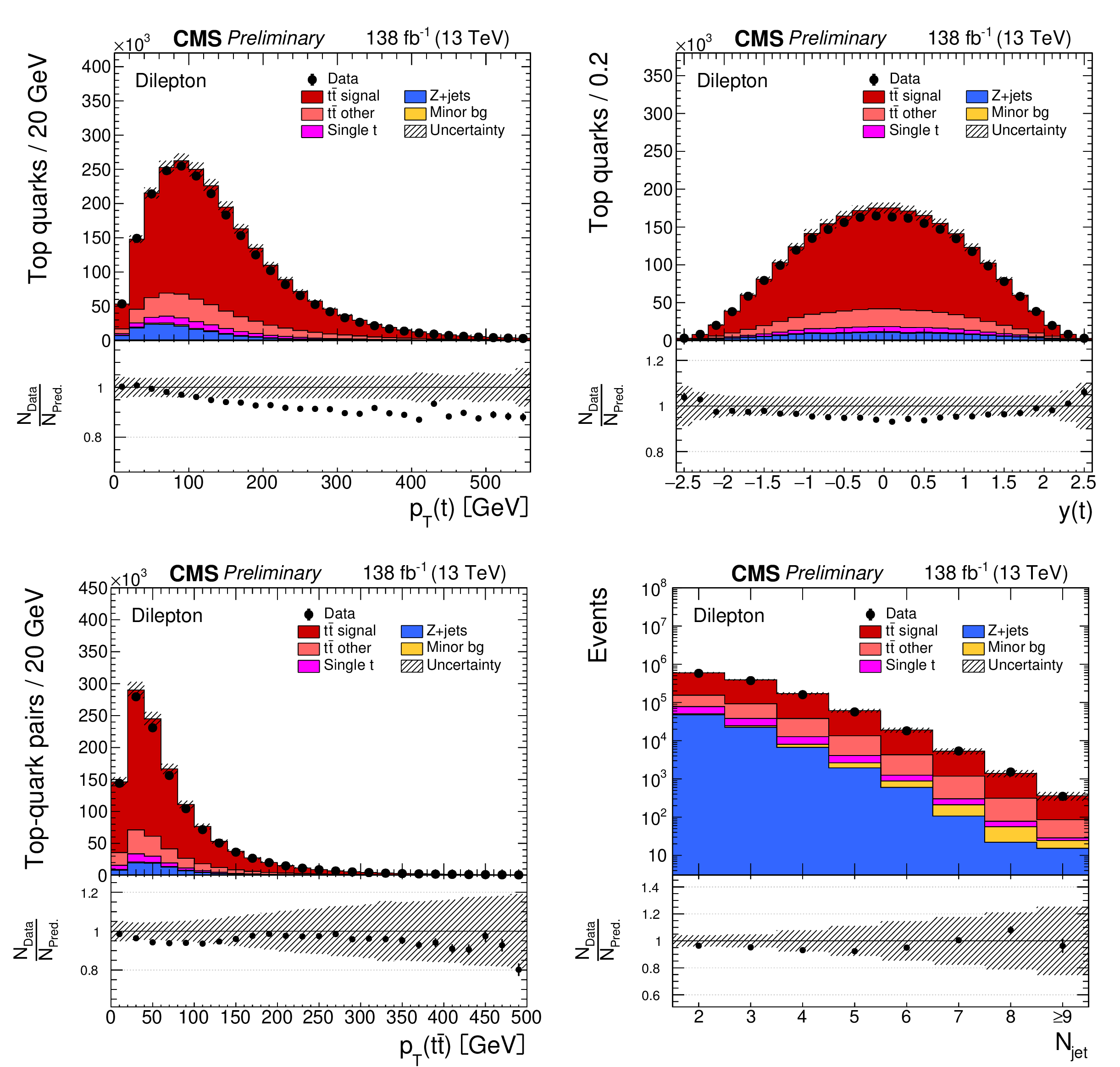
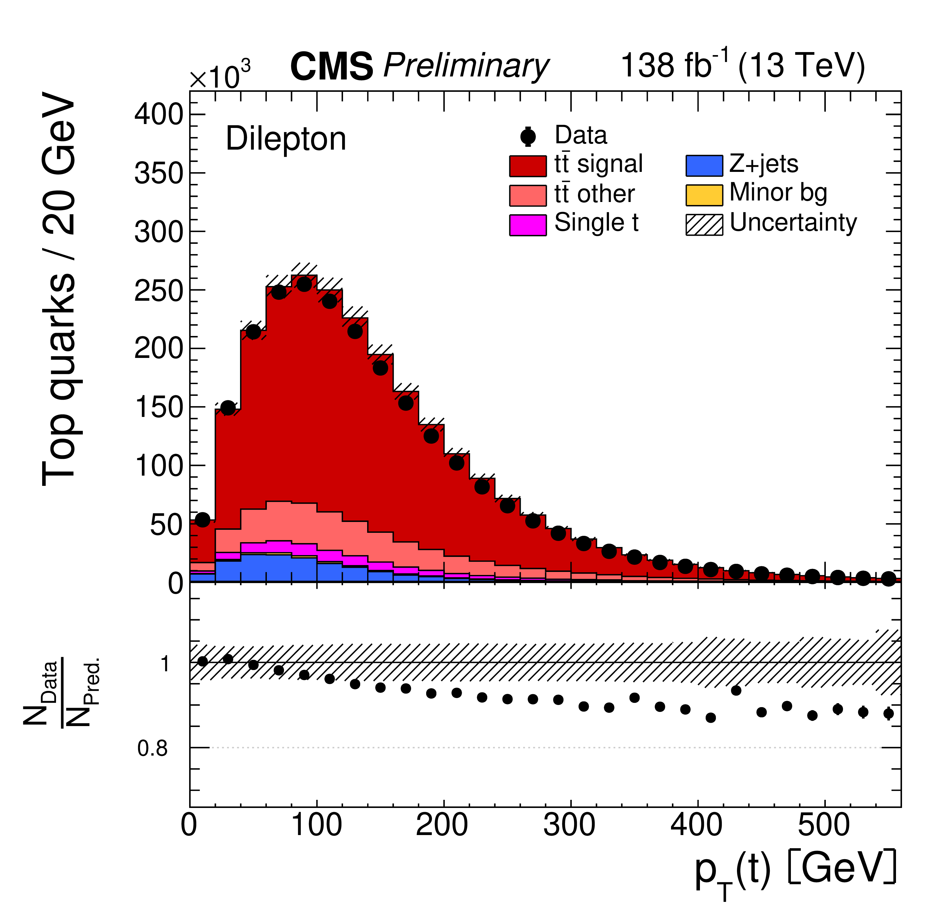
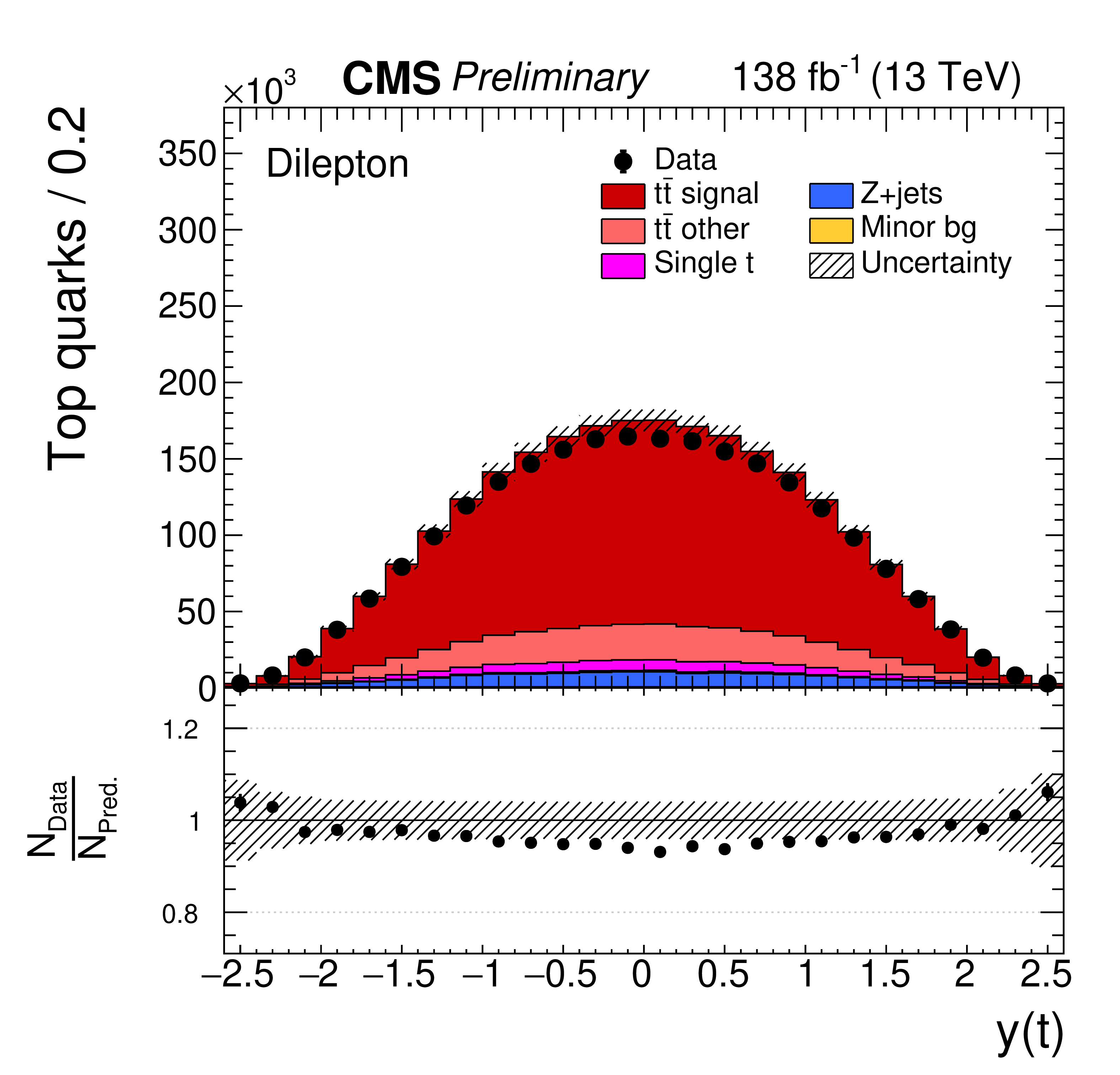
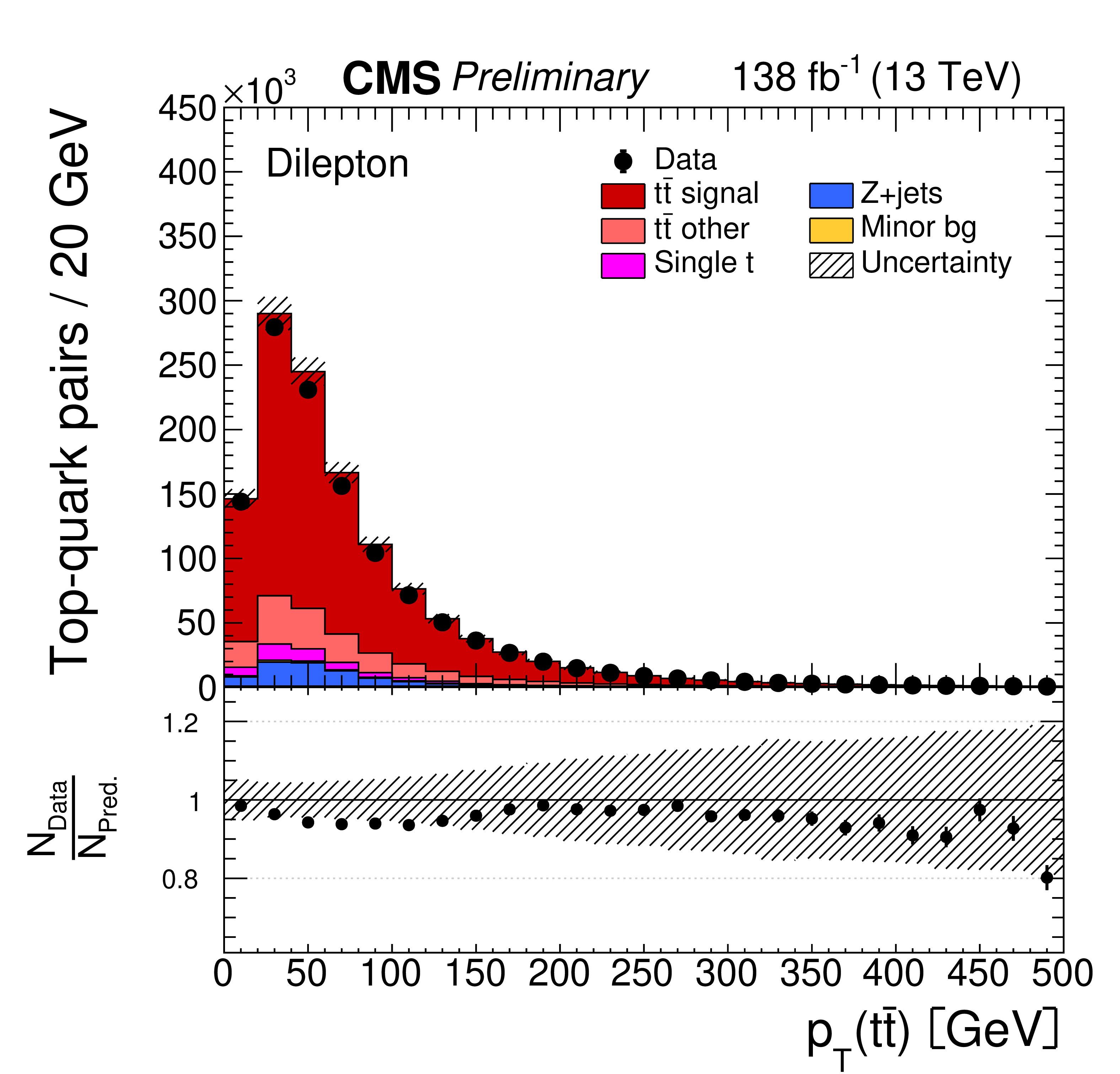
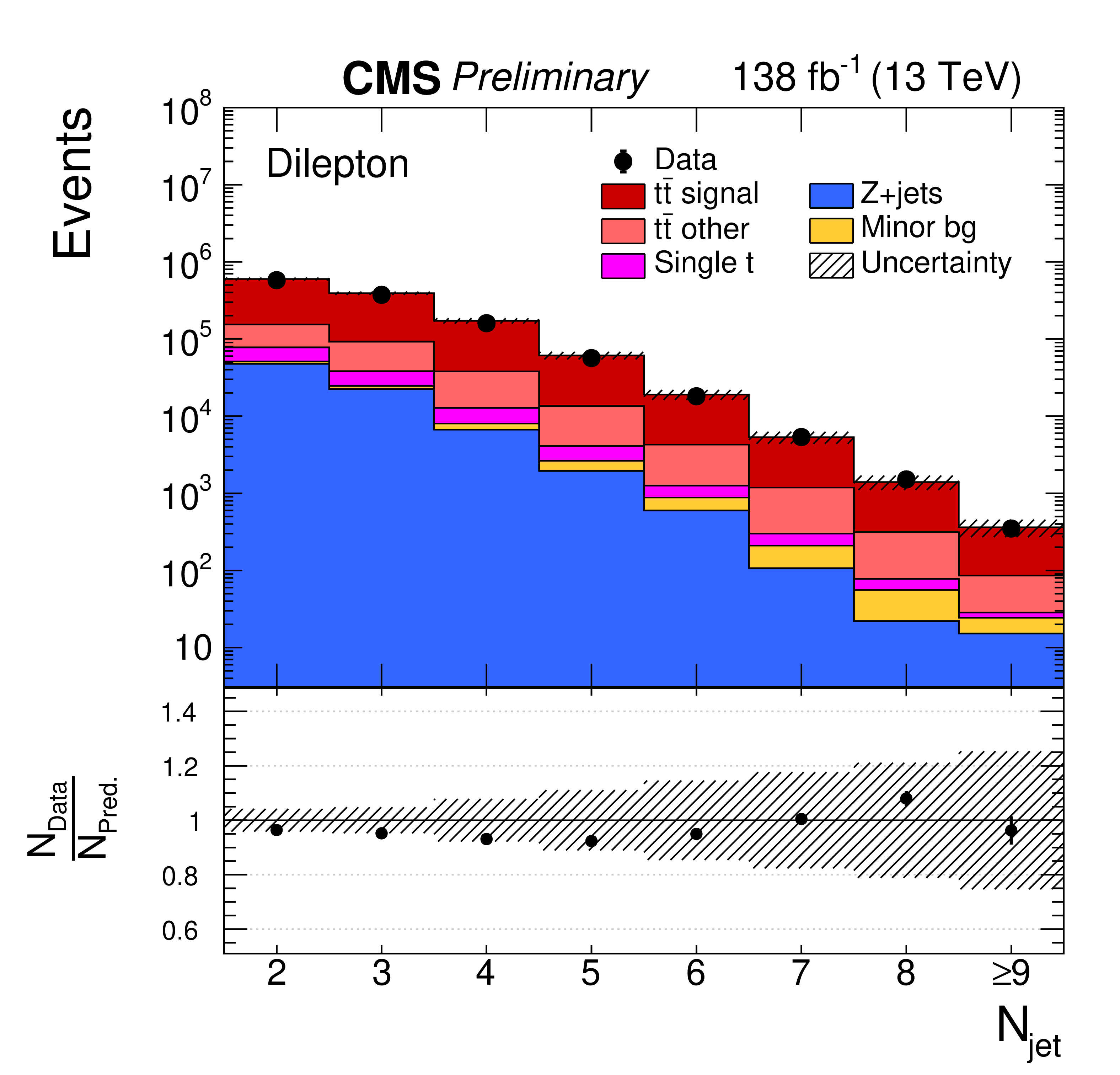
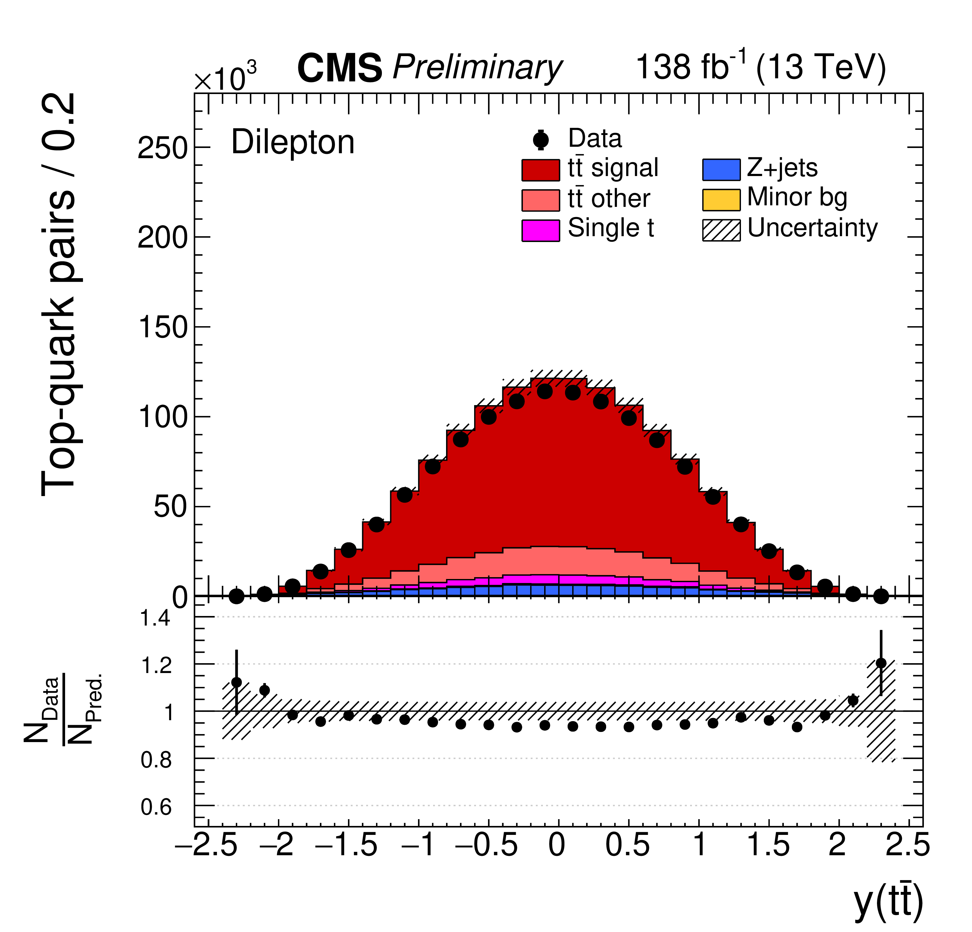
png pdf	Figure 2: Distributions of ${{p_{\mathrm {T}}} (\mathrm{t})}$ (upper left), ${y(\mathrm{t})}$ (upper right), ${{p_{\mathrm {T}}} ( \mathrm{t\bar{t}})}$ (middle left), and ${N_{\text {jet}}}$ (lower right) obtained in selected events with the full kinematic reconstruction. The data with vertical bars corresponding to their statistical uncertainties are plotted together with distributions of simulated signal and background processes. The hatched regions depict the shape uncertainties in the signal and backgrounds (as detailed in Section 7). The lower panel in each plot shows the ratio of the observed data event yields to those expected in the simulation.
png pdf	Figure 2-a: Distributions of ${{p_{\mathrm {T}}} (\mathrm{t})}$ (upper left), ${y(\mathrm{t})}$ (upper right), ${{p_{\mathrm {T}}} ( \mathrm{t\bar{t}})}$ (middle left), and ${N_{\text {jet}}}$ (lower right) obtained in selected events with the full kinematic reconstruction. The data with vertical bars corresponding to their statistical uncertainties are plotted together with distributions of simulated signal and background processes. The hatched regions depict the shape uncertainties in the signal and backgrounds (as detailed in Section 7). The lower panel in each plot shows the ratio of the observed data event yields to those expected in the simulation.
png pdf	Figure 2-b: Distributions of ${{p_{\mathrm {T}}} (\mathrm{t})}$ (upper left), ${y(\mathrm{t})}$ (upper right), ${{p_{\mathrm {T}}} ( \mathrm{t\bar{t}})}$ (middle left), and ${N_{\text {jet}}}$ (lower right) obtained in selected events with the full kinematic reconstruction. The data with vertical bars corresponding to their statistical uncertainties are plotted together with distributions of simulated signal and background processes. The hatched regions depict the shape uncertainties in the signal and backgrounds (as detailed in Section 7). The lower panel in each plot shows the ratio of the observed data event yields to those expected in the simulation.
png pdf	Figure 2-c: Distributions of ${{p_{\mathrm {T}}} (\mathrm{t})}$ (upper left), ${y(\mathrm{t})}$ (upper right), ${{p_{\mathrm {T}}} ( \mathrm{t\bar{t}})}$ (middle left), and ${N_{\text {jet}}}$ (lower right) obtained in selected events with the full kinematic reconstruction. The data with vertical bars corresponding to their statistical uncertainties are plotted together with distributions of simulated signal and background processes. The hatched regions depict the shape uncertainties in the signal and backgrounds (as detailed in Section 7). The lower panel in each plot shows the ratio of the observed data event yields to those expected in the simulation.
png pdf	Figure 2-d: Distributions of ${{p_{\mathrm {T}}} (\mathrm{t})}$ (upper left), ${y(\mathrm{t})}$ (upper right), ${{p_{\mathrm {T}}} ( \mathrm{t\bar{t}})}$ (middle left), and ${N_{\text {jet}}}$ (lower right) obtained in selected events with the full kinematic reconstruction. The data with vertical bars corresponding to their statistical uncertainties are plotted together with distributions of simulated signal and background processes. The hatched regions depict the shape uncertainties in the signal and backgrounds (as detailed in Section 7). The lower panel in each plot shows the ratio of the observed data event yields to those expected in the simulation.
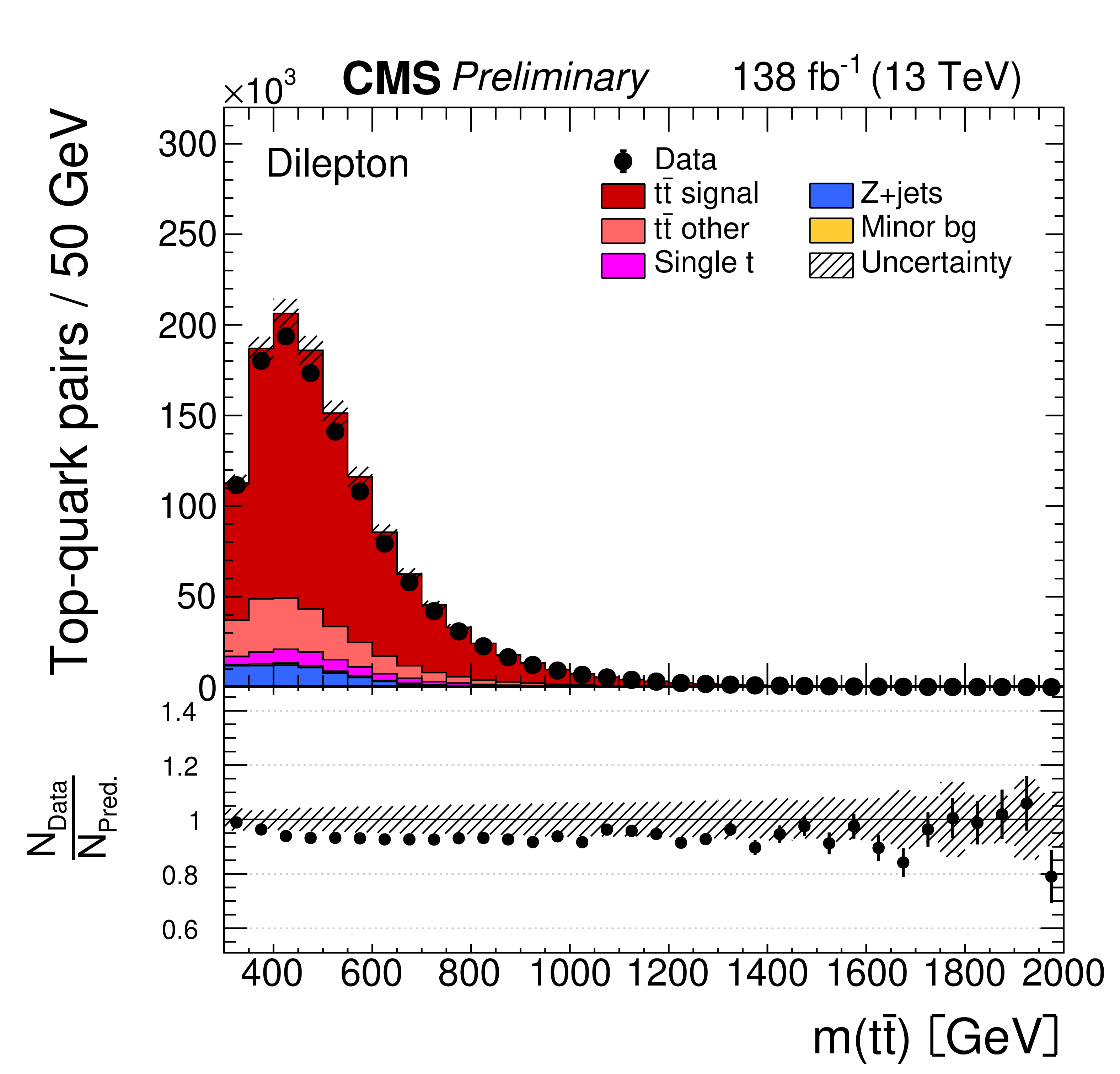
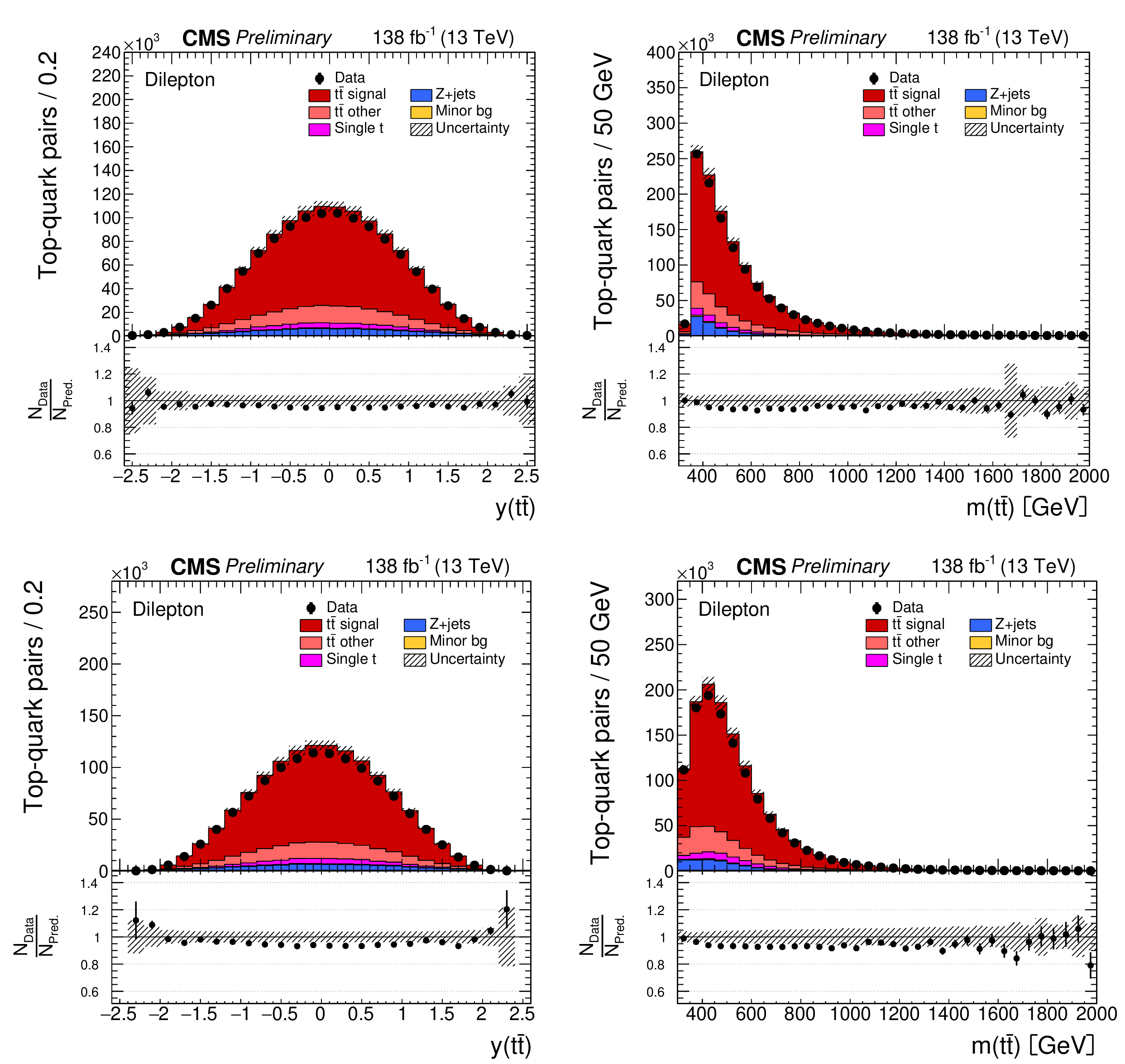
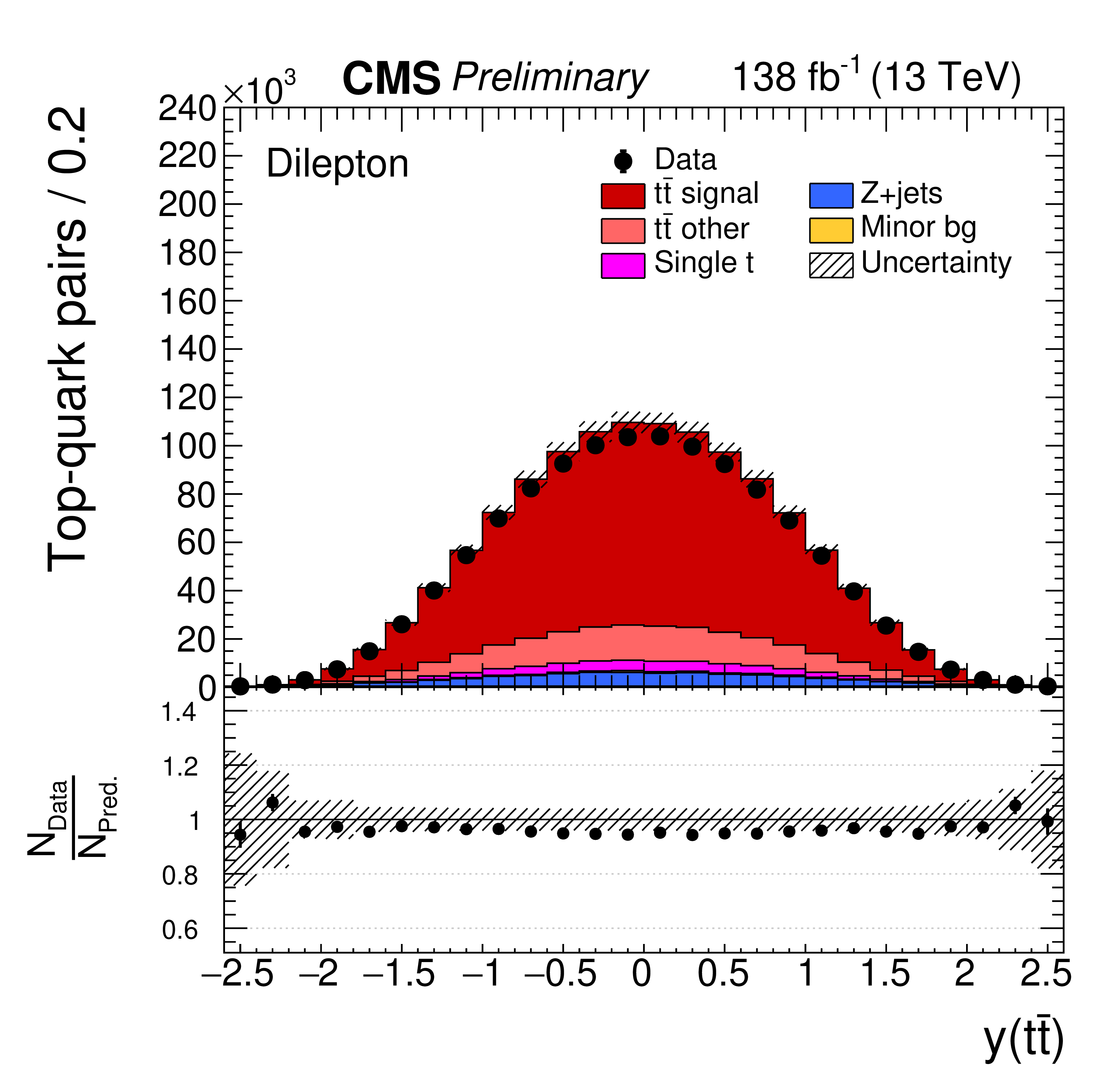
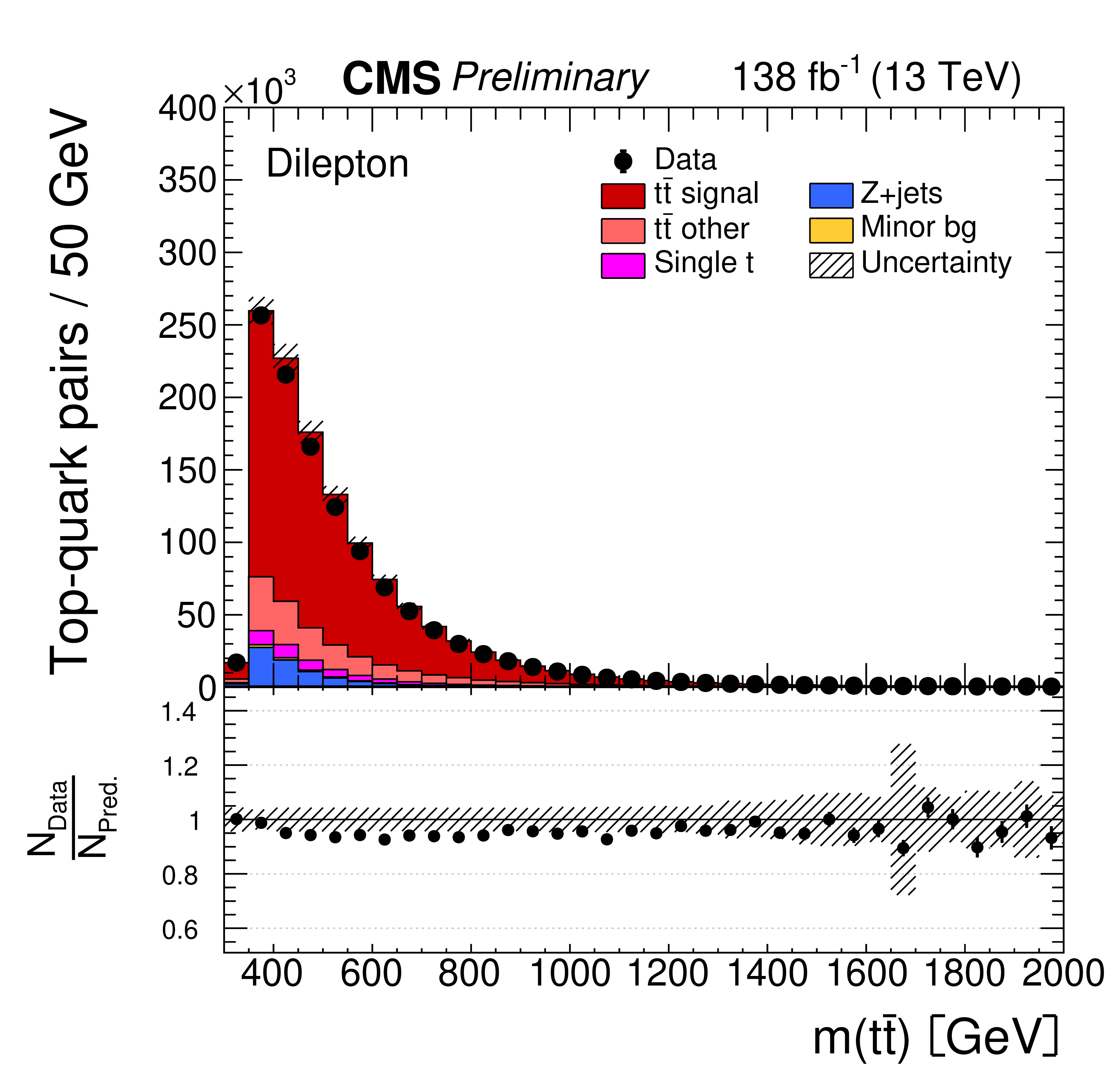
png pdf	Figure 3: Distributions of ${y( \mathrm{t\bar{t}})}$ (left) and ${m( \mathrm{t\bar{t}})}$ (right) obtained in selected events with the full (upper) and the loose kinematic reconstruction (lower). Further details can be found in the caption of Fig. 2.
png pdf	Figure 3-a: Distributions of ${y( \mathrm{t\bar{t}})}$ (left) and ${m( \mathrm{t\bar{t}})}$ (right) obtained in selected events with the full (upper) and the loose kinematic reconstruction (lower). Further details can be found in the caption of Fig. 2.
png pdf	Figure 3-b: Distributions of ${y( \mathrm{t\bar{t}})}$ (left) and ${m( \mathrm{t\bar{t}})}$ (right) obtained in selected events with the full (upper) and the loose kinematic reconstruction (lower). Further details can be found in the caption of Fig. 2.
png pdf	Figure 3-c: Distributions of ${y( \mathrm{t\bar{t}})}$ (left) and ${m( \mathrm{t\bar{t}})}$ (right) obtained in selected events with the full (upper) and the loose kinematic reconstruction (lower). Further details can be found in the caption of Fig. 2.
png pdf	Figure 3-d: Distributions of ${y( \mathrm{t\bar{t}})}$ (left) and ${m( \mathrm{t\bar{t}})}$ (right) obtained in selected events with the full (upper) and the loose kinematic reconstruction (lower). Further details can be found in the caption of Fig. 2.
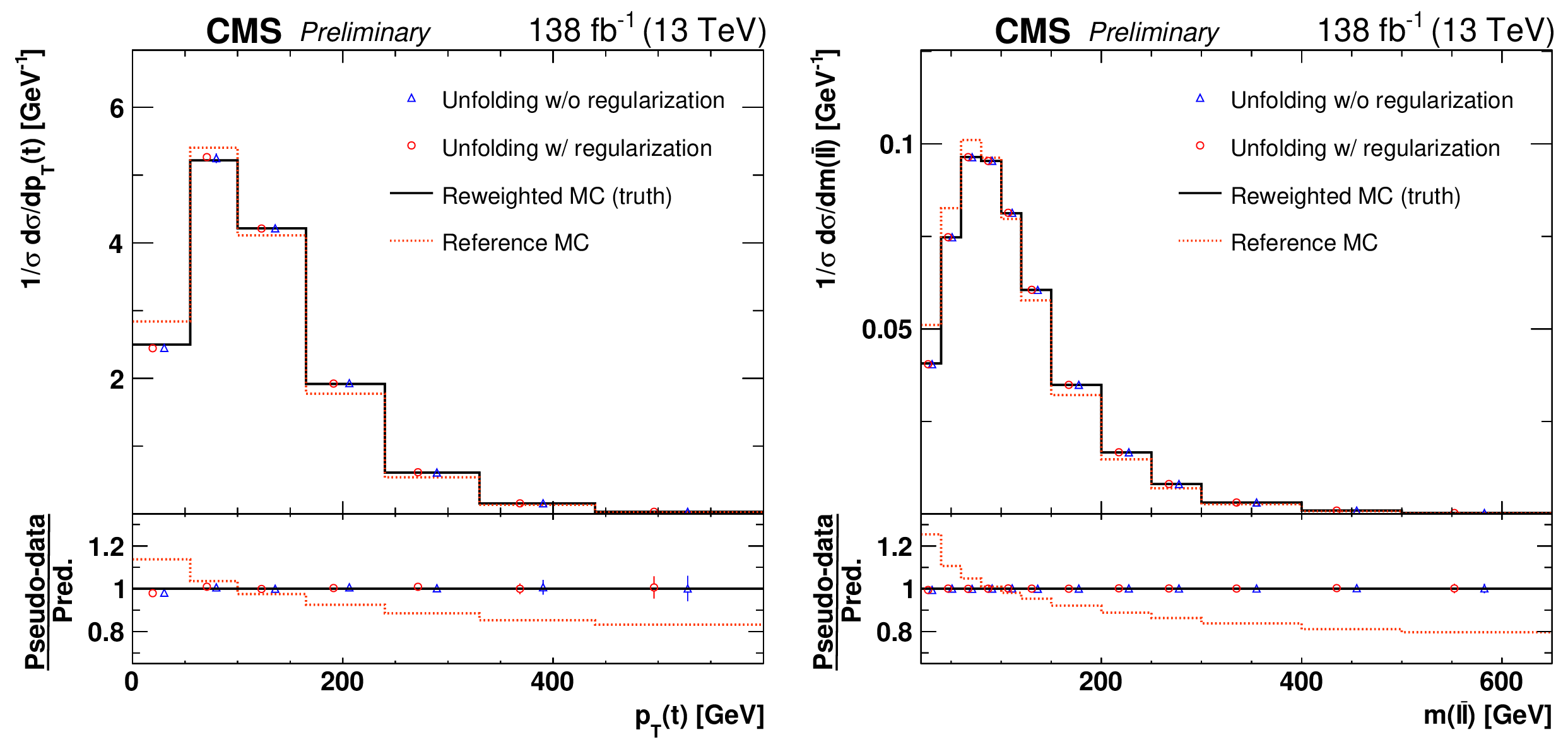
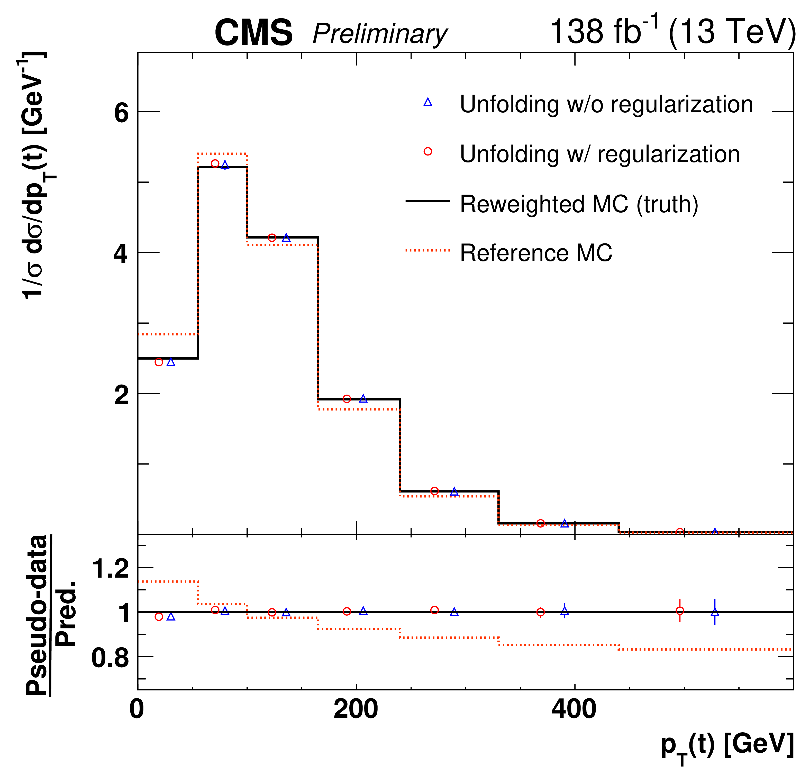
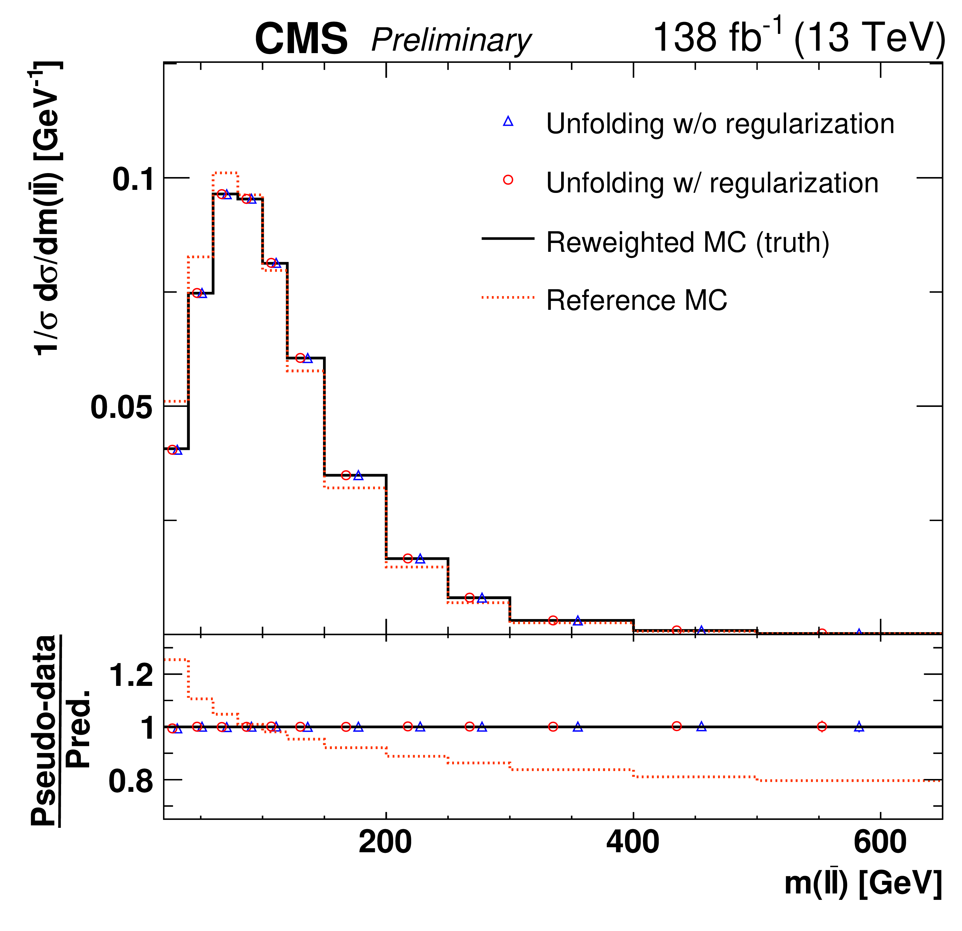
png pdf	Figure 4: Reweighting test for the extraction of the normalized differential cross sections as a function of ${{p_{\mathrm {T}}} (\mathrm{t})}$ (left) and ${m(\ell \overline {\ell})}$ (right). The former cross section is measured at parton level in the full phase space and the latter at particle level in a fiducial phase space. The nominal $\mathrm{t\bar{t}}$ signal MC spectra are shown as dotted histograms and the assumed true spectra, obtained from reweighting, as solid histograms. The unfolded spectra, using pseudo-data based on the true spectra but using the nominal spectra for the detector corrections and bias vector in the regularization, are presented as open circles. The unfolded spectra with the regularization switched off are also shown (open triangles). The statistical uncertainties in the unfolded cross sections are represented by a vertical bar on the corresponding points. The lower panel in each plot shows the ratios of the pseudo-data to the predicted spectra.
png pdf	Figure 4-a: Reweighting test for the extraction of the normalized differential cross sections as a function of ${{p_{\mathrm {T}}} (\mathrm{t})}$ (left) and ${m(\ell \overline {\ell})}$ (right). The former cross section is measured at parton level in the full phase space and the latter at particle level in a fiducial phase space. The nominal $\mathrm{t\bar{t}}$ signal MC spectra are shown as dotted histograms and the assumed true spectra, obtained from reweighting, as solid histograms. The unfolded spectra, using pseudo-data based on the true spectra but using the nominal spectra for the detector corrections and bias vector in the regularization, are presented as open circles. The unfolded spectra with the regularization switched off are also shown (open triangles). The statistical uncertainties in the unfolded cross sections are represented by a vertical bar on the corresponding points. The lower panel in each plot shows the ratios of the pseudo-data to the predicted spectra.
png pdf	Figure 4-b: Reweighting test for the extraction of the normalized differential cross sections as a function of ${{p_{\mathrm {T}}} (\mathrm{t})}$ (left) and ${m(\ell \overline {\ell})}$ (right). The former cross section is measured at parton level in the full phase space and the latter at particle level in a fiducial phase space. The nominal $\mathrm{t\bar{t}}$ signal MC spectra are shown as dotted histograms and the assumed true spectra, obtained from reweighting, as solid histograms. The unfolded spectra, using pseudo-data based on the true spectra but using the nominal spectra for the detector corrections and bias vector in the regularization, are presented as open circles. The unfolded spectra with the regularization switched off are also shown (open triangles). The statistical uncertainties in the unfolded cross sections are represented by a vertical bar on the corresponding points. The lower panel in each plot shows the ratios of the pseudo-data to the predicted spectra.
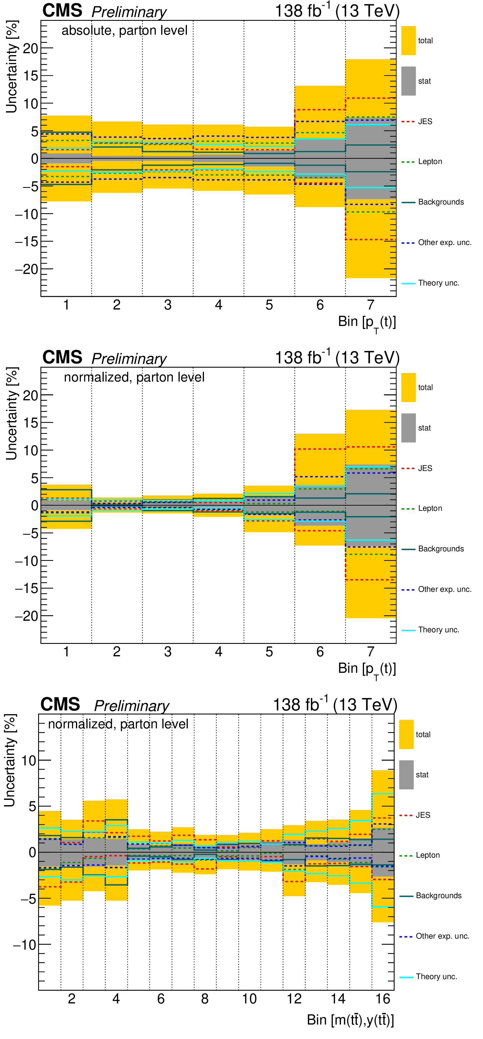
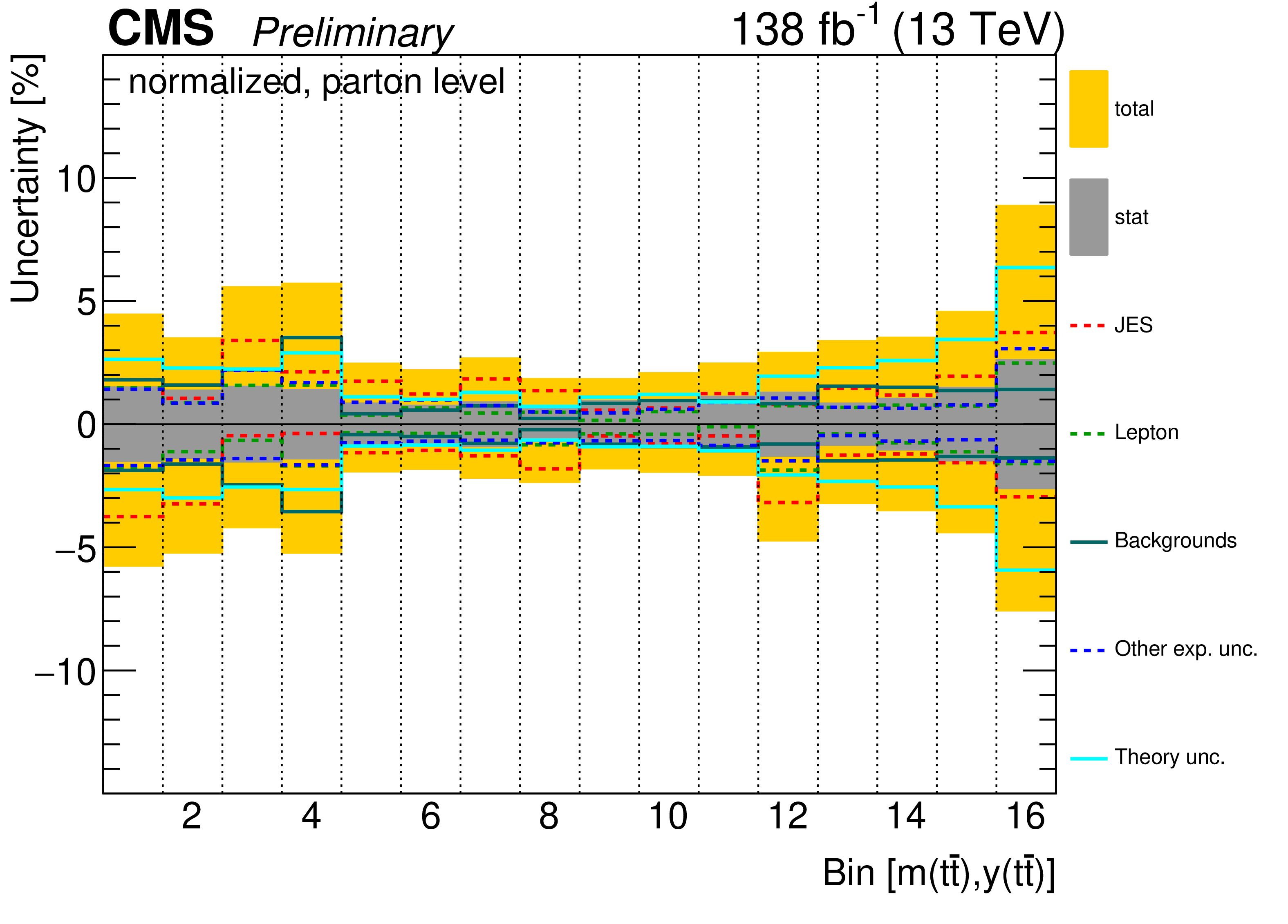
png pdf	Figure 5: The individual sources of systematic uncertainty in various parton-level measurements and their relative contributions to the overall uncertainty, separately for upward and downward variations. The statistical uncertainties and the total uncertainties (statistical and systematic uncertainties summed in quadrature) are shown as dark and light bands, respectively.
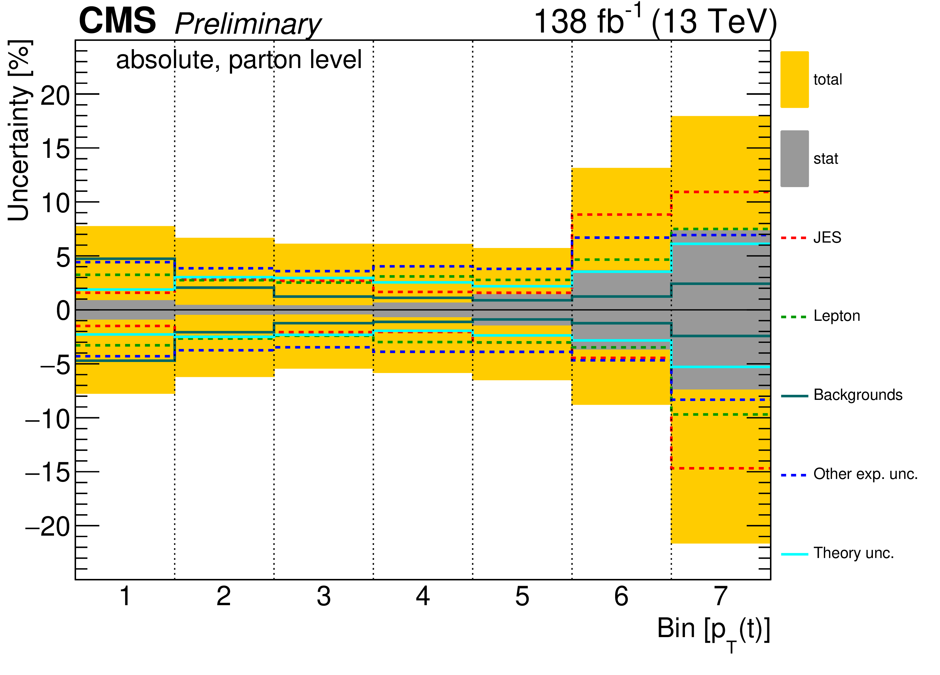
png pdf	Figure 5-a: The individual sources of systematic uncertainty in various parton-level measurements and their relative contributions to the overall uncertainty, separately for upward and downward variations. The statistical uncertainties and the total uncertainties (statistical and systematic uncertainties summed in quadrature) are shown as dark and light bands, respectively.
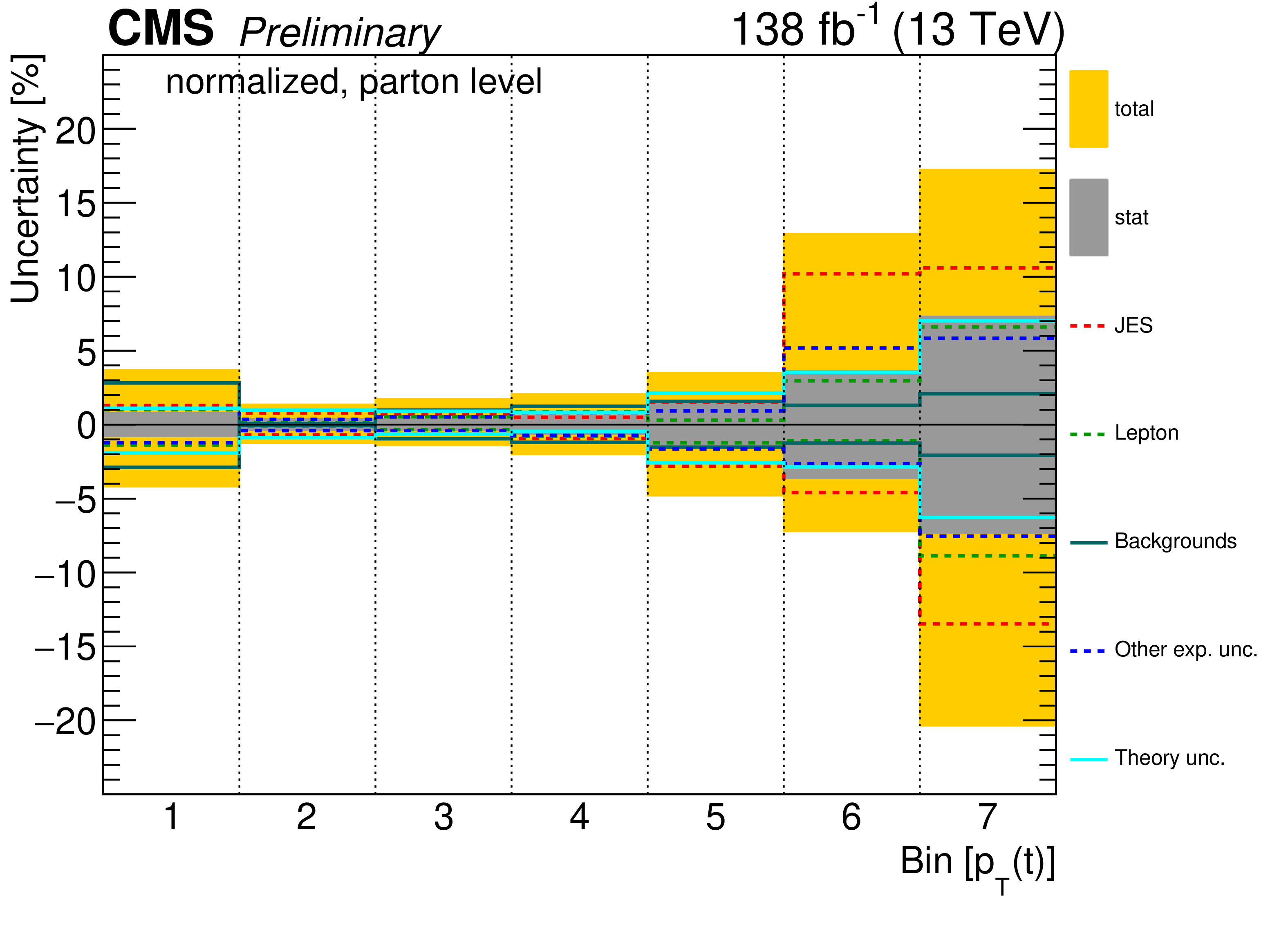
png pdf	Figure 5-b: The individual sources of systematic uncertainty in various parton-level measurements and their relative contributions to the overall uncertainty, separately for upward and downward variations. The statistical uncertainties and the total uncertainties (statistical and systematic uncertainties summed in quadrature) are shown as dark and light bands, respectively.
png pdf	Figure 5-c: The individual sources of systematic uncertainty in various parton-level measurements and their relative contributions to the overall uncertainty, separately for upward and downward variations. The statistical uncertainties and the total uncertainties (statistical and systematic uncertainties summed in quadrature) are shown as dark and light bands, respectively.
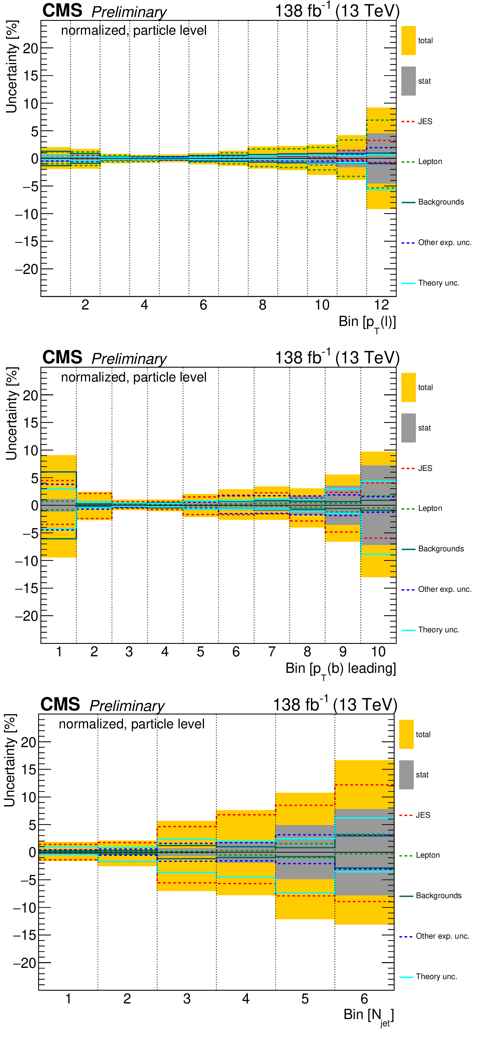
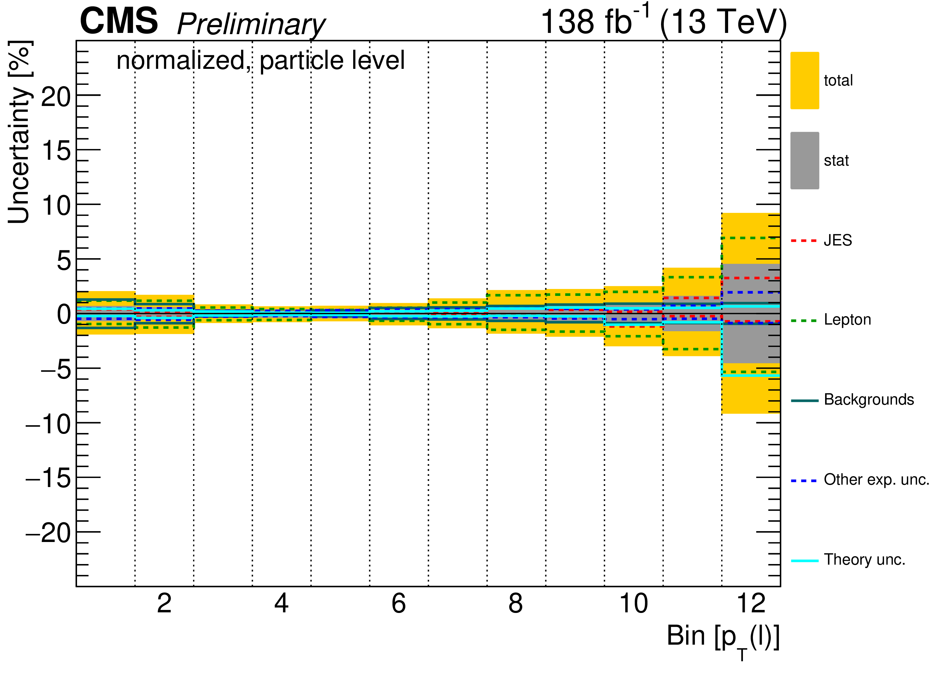
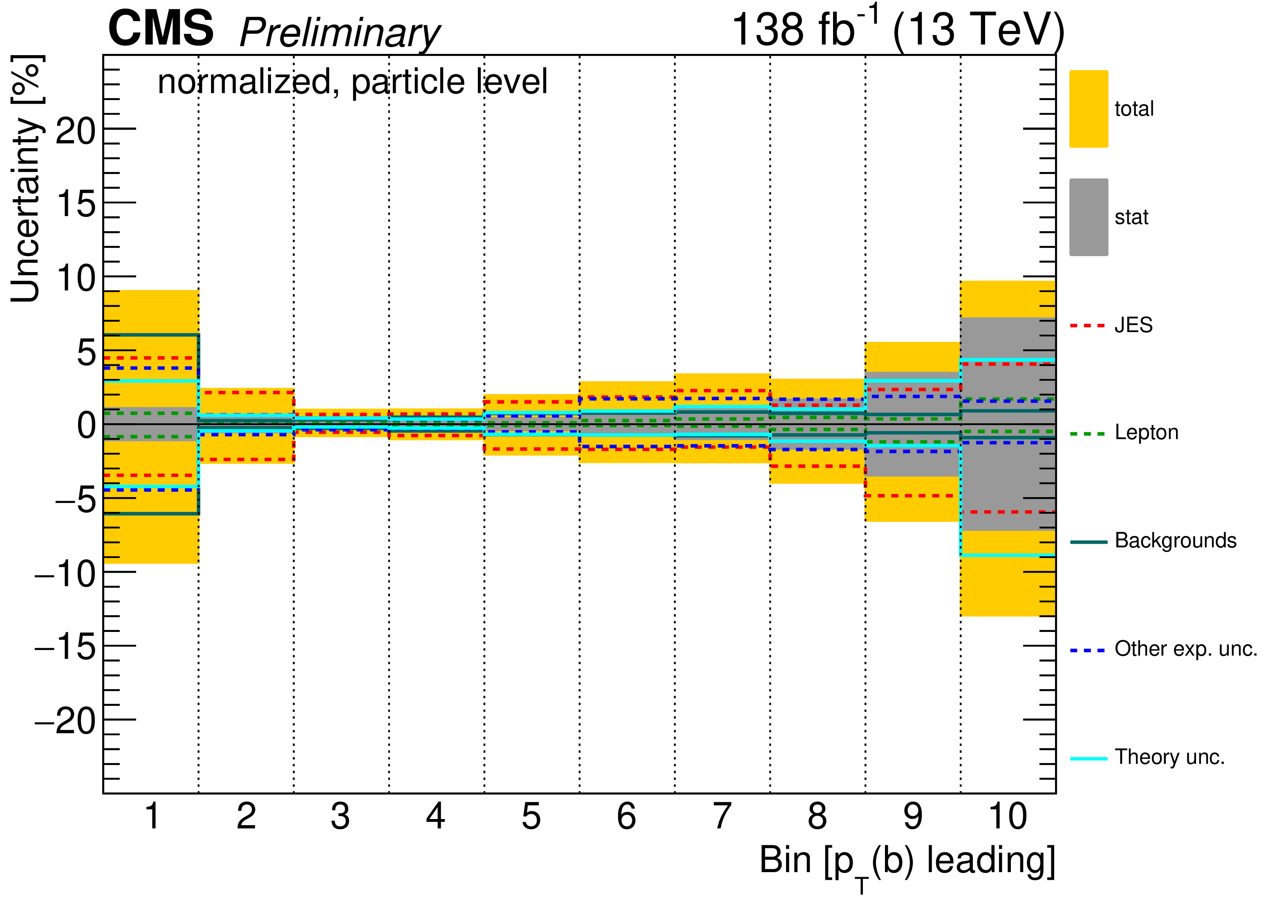
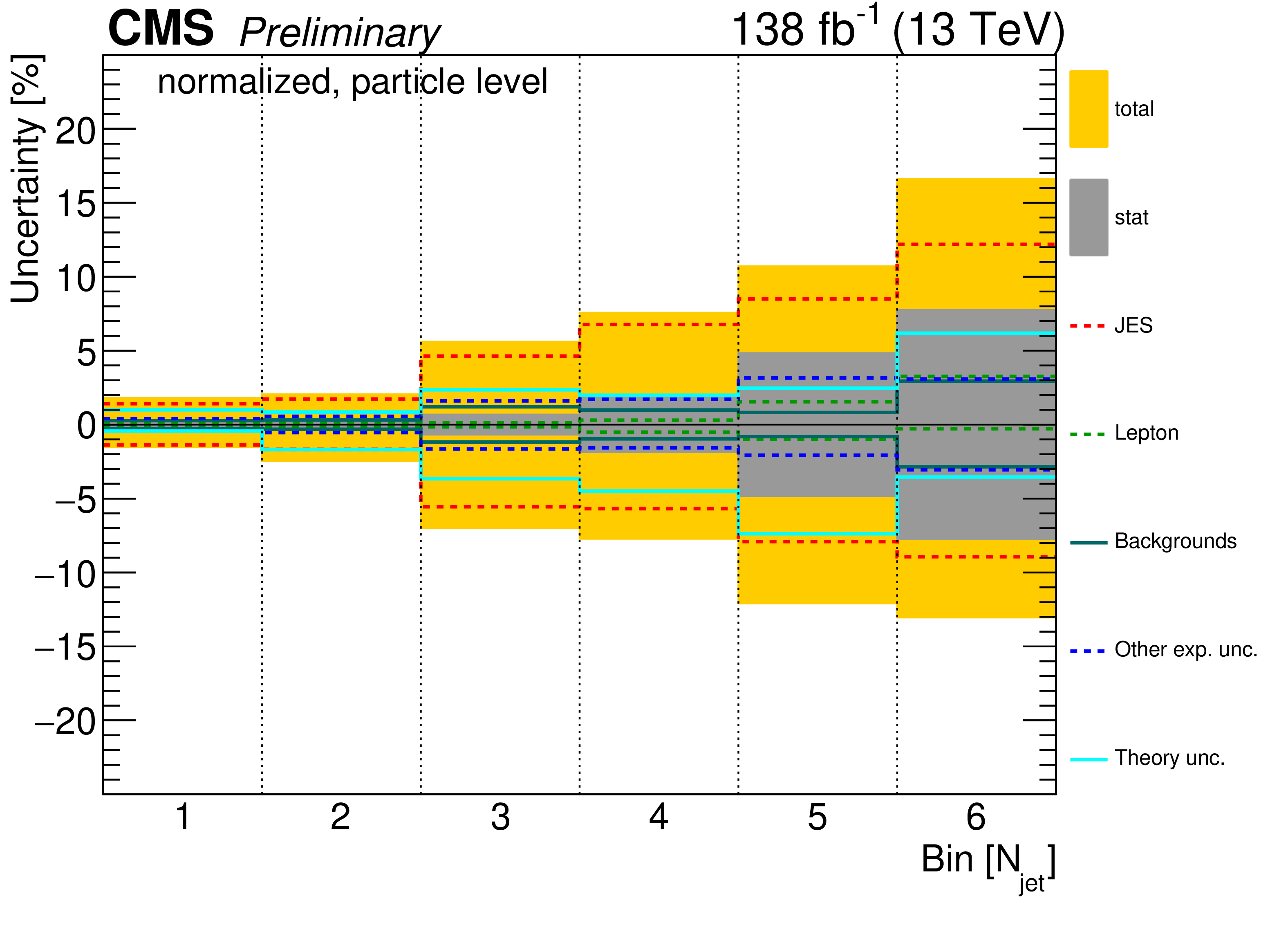
png pdf	Figure 6: The individual sources of systematic uncertainty in various particle-level measurements and their relative contributions to the overall uncertainty, separately for upward and downward variations. The statistical uncertainties and the total uncertainties (statistical and systematic uncertainties summed in quadrature) are shown as dark and light bands, respectively.
png pdf	Figure 6-a: The individual sources of systematic uncertainty in various particle-level measurements and their relative contributions to the overall uncertainty, separately for upward and downward variations. The statistical uncertainties and the total uncertainties (statistical and systematic uncertainties summed in quadrature) are shown as dark and light bands, respectively.
png pdf	Figure 6-b: The individual sources of systematic uncertainty in various particle-level measurements and their relative contributions to the overall uncertainty, separately for upward and downward variations. The statistical uncertainties and the total uncertainties (statistical and systematic uncertainties summed in quadrature) are shown as dark and light bands, respectively.
png pdf	Figure 6-c: The individual sources of systematic uncertainty in various particle-level measurements and their relative contributions to the overall uncertainty, separately for upward and downward variations. The statistical uncertainties and the total uncertainties (statistical and systematic uncertainties summed in quadrature) are shown as dark and light bands, respectively.
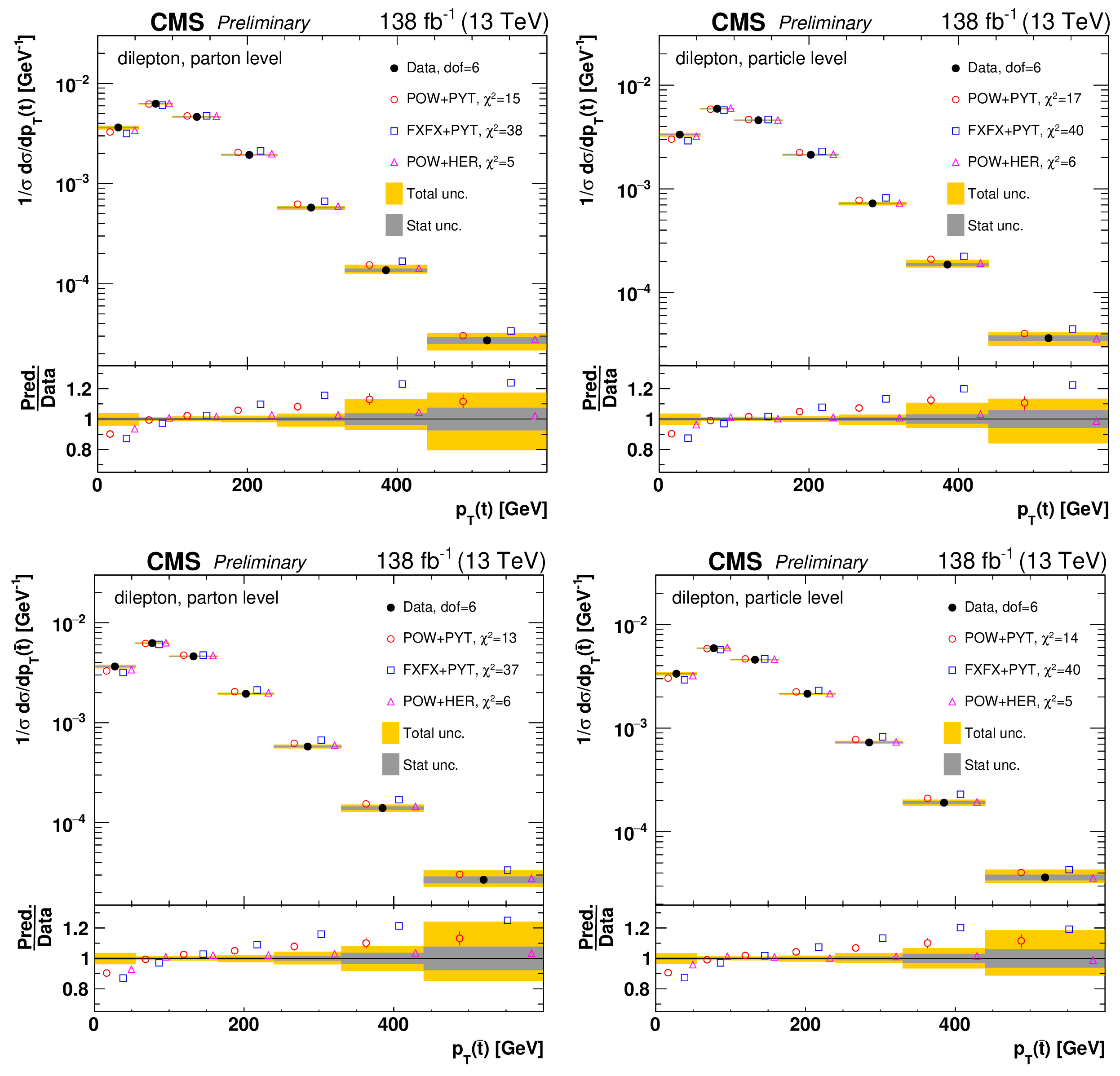
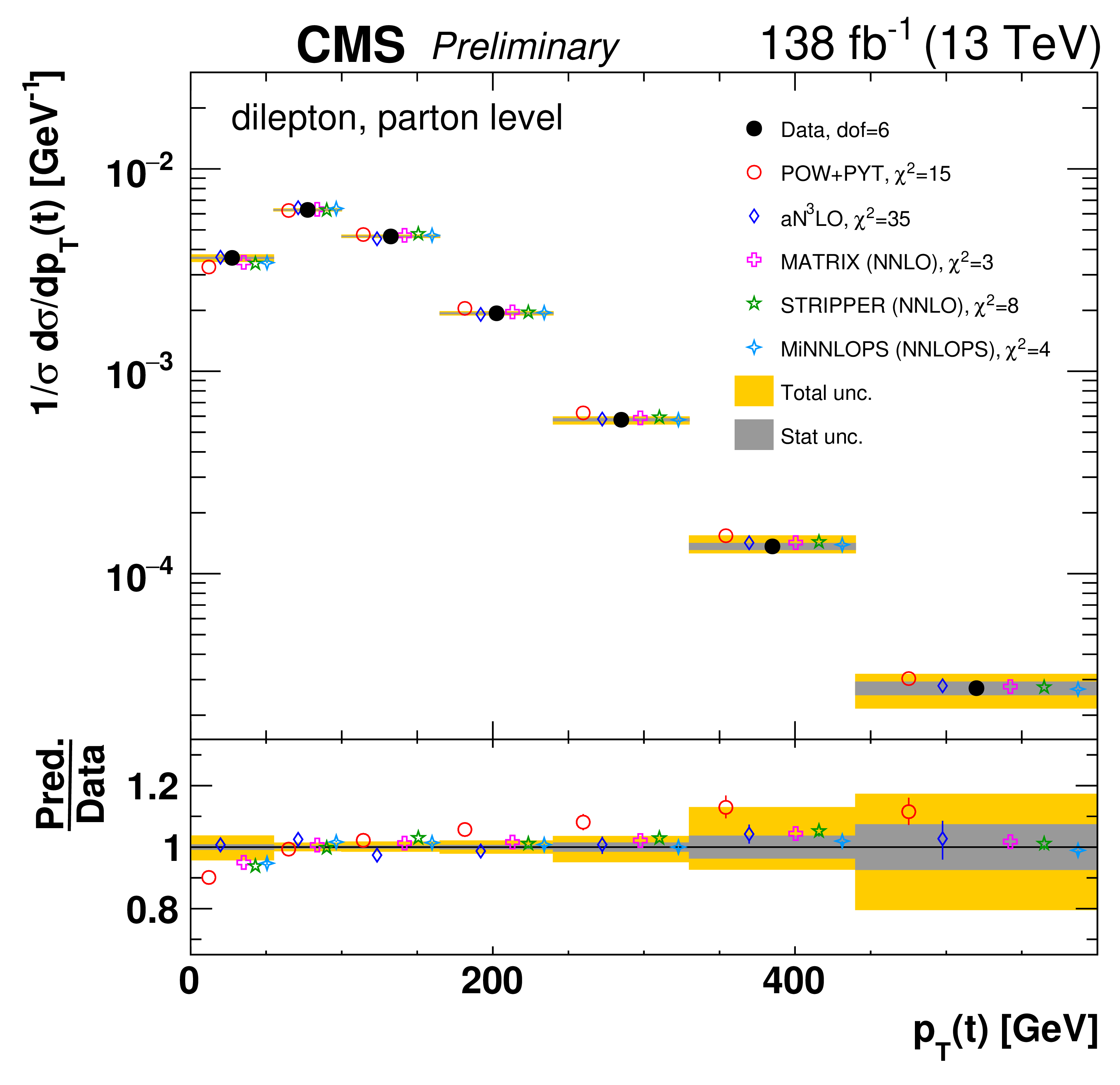
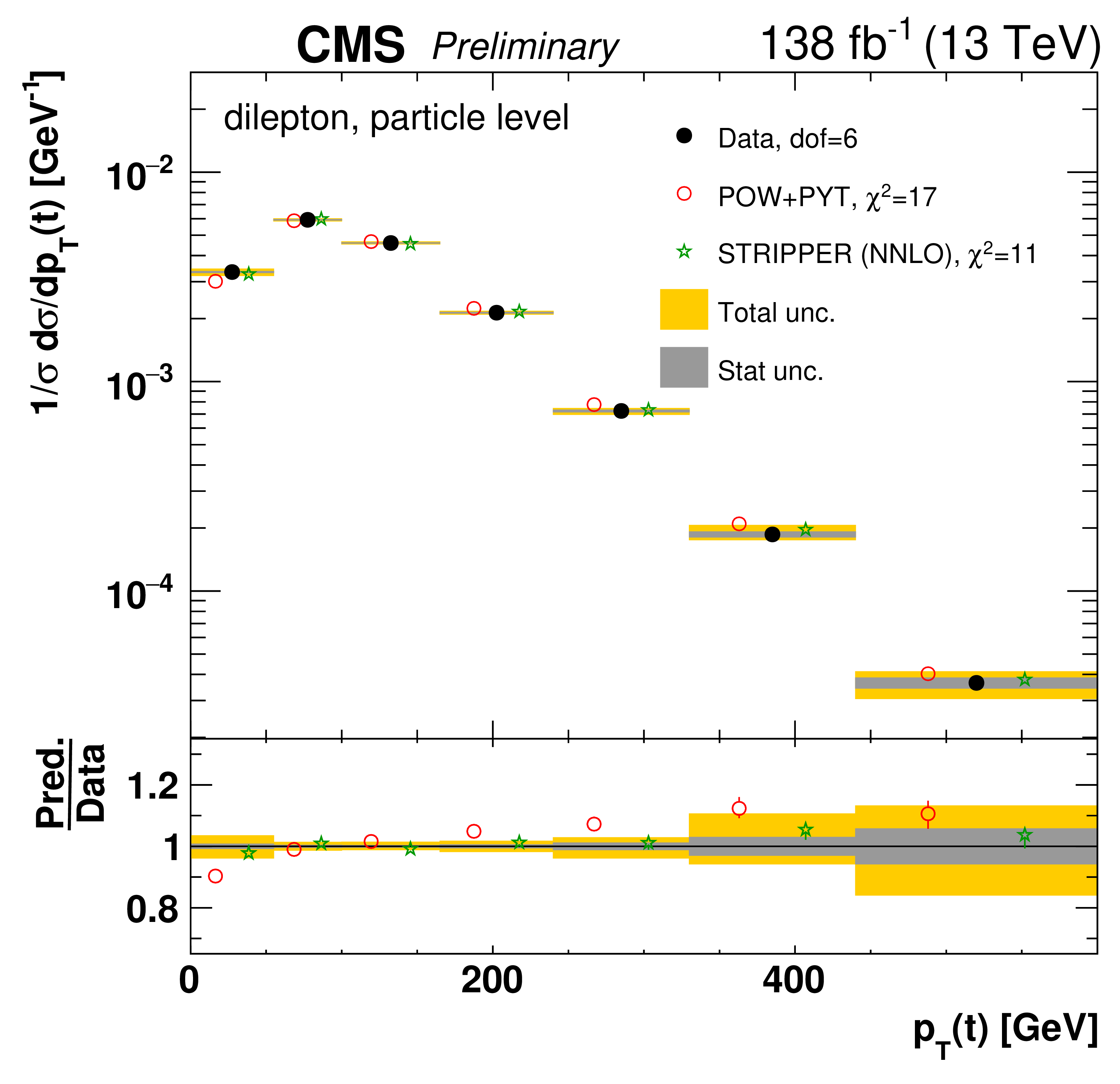
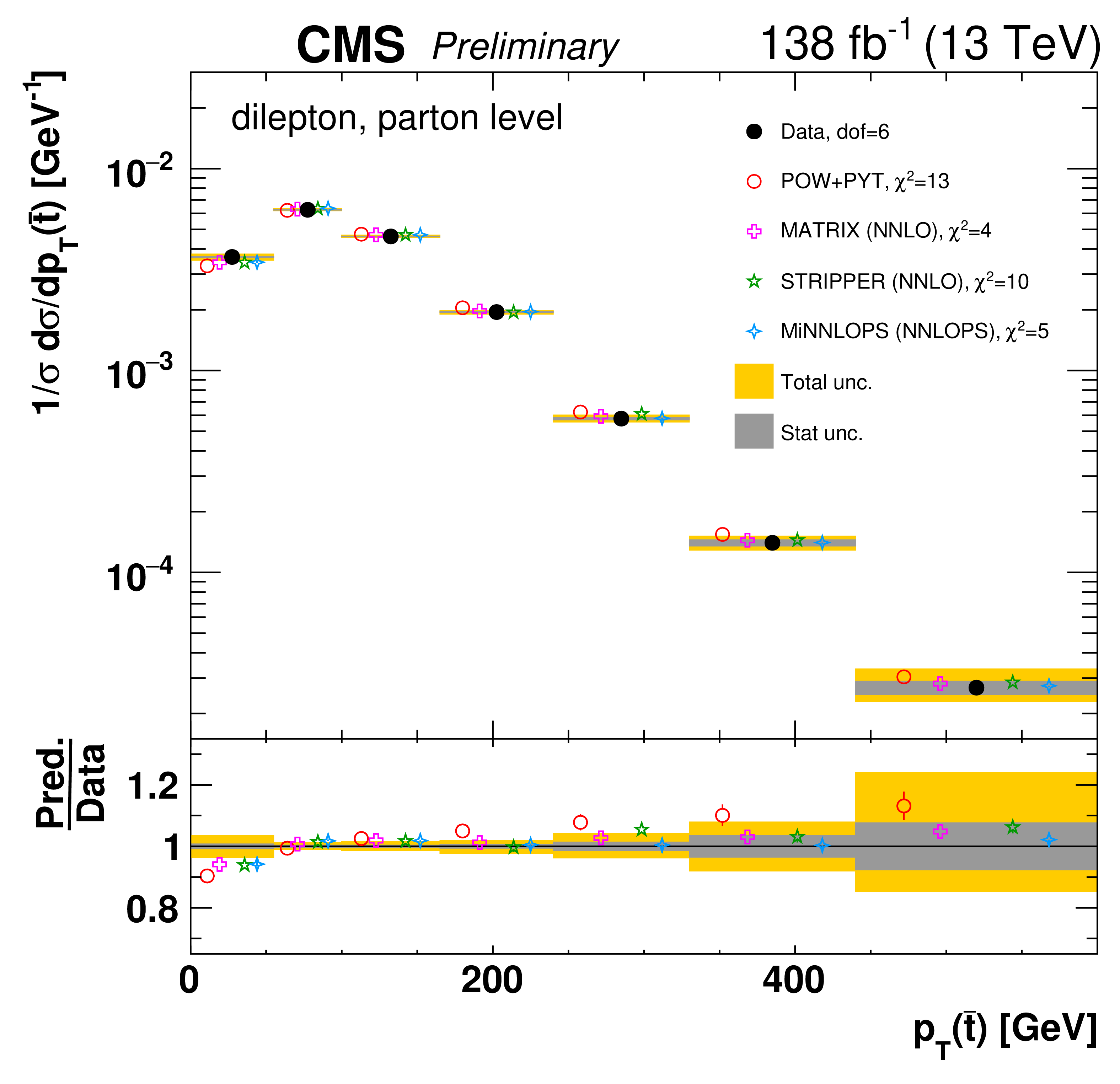
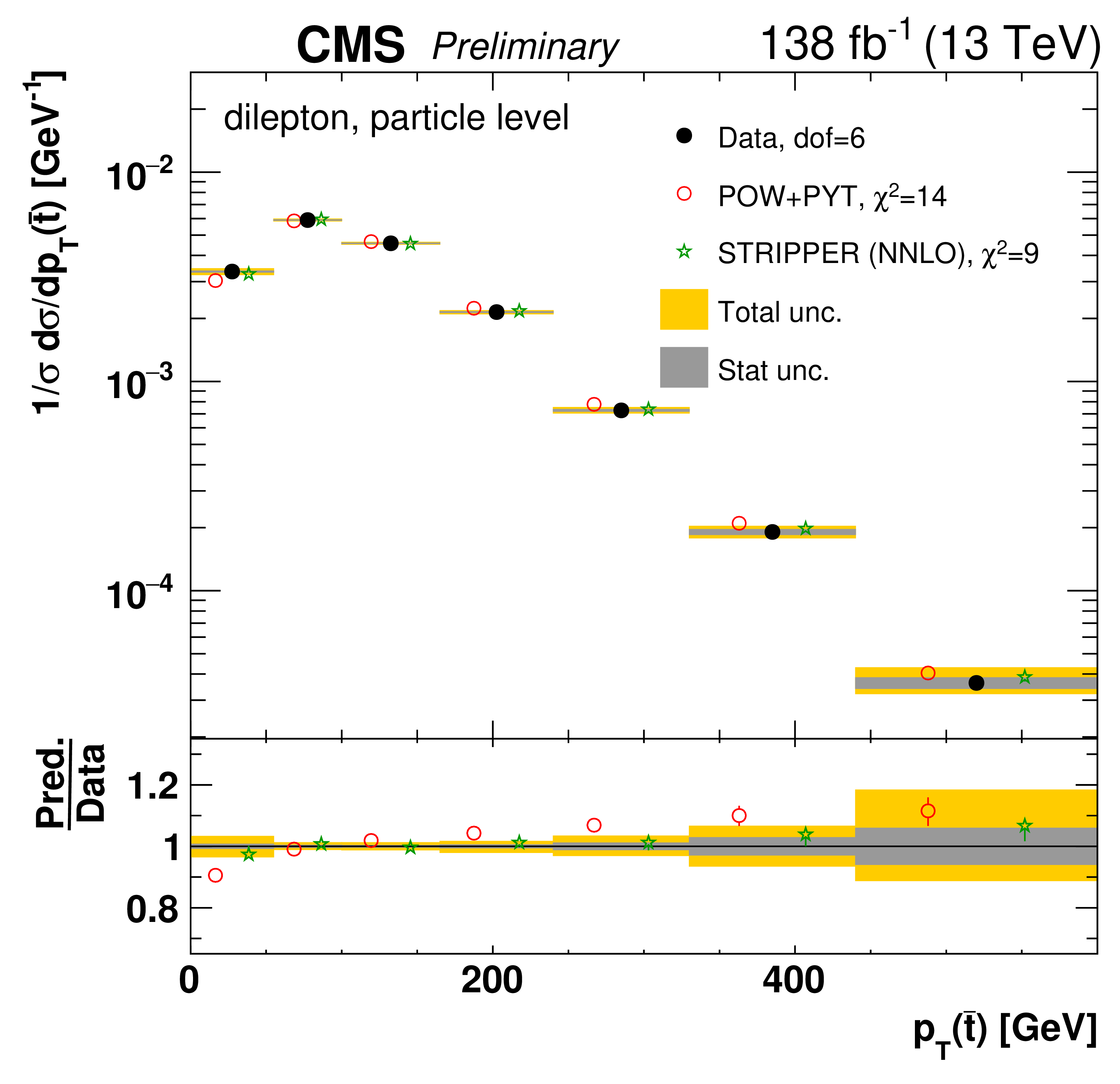
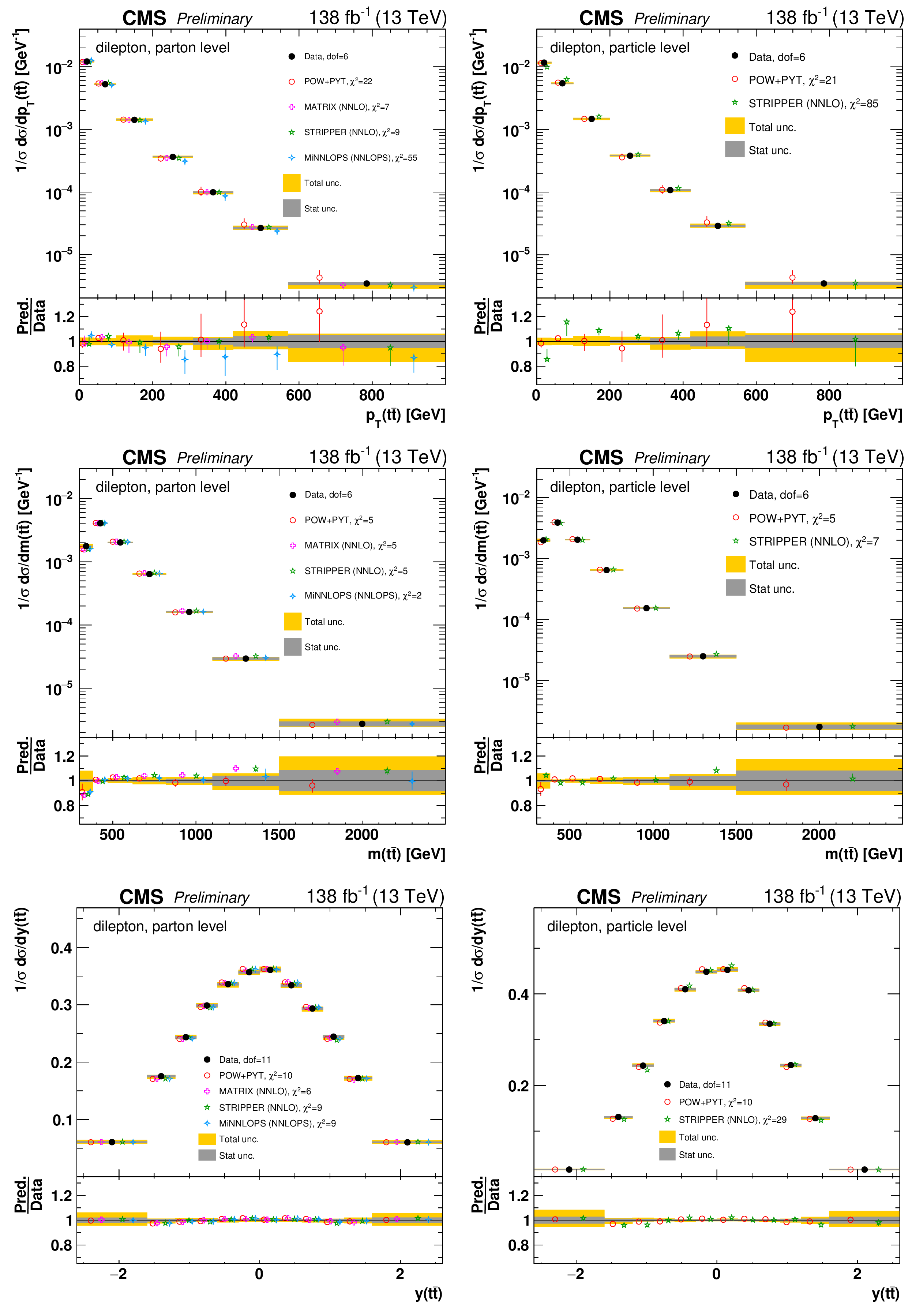
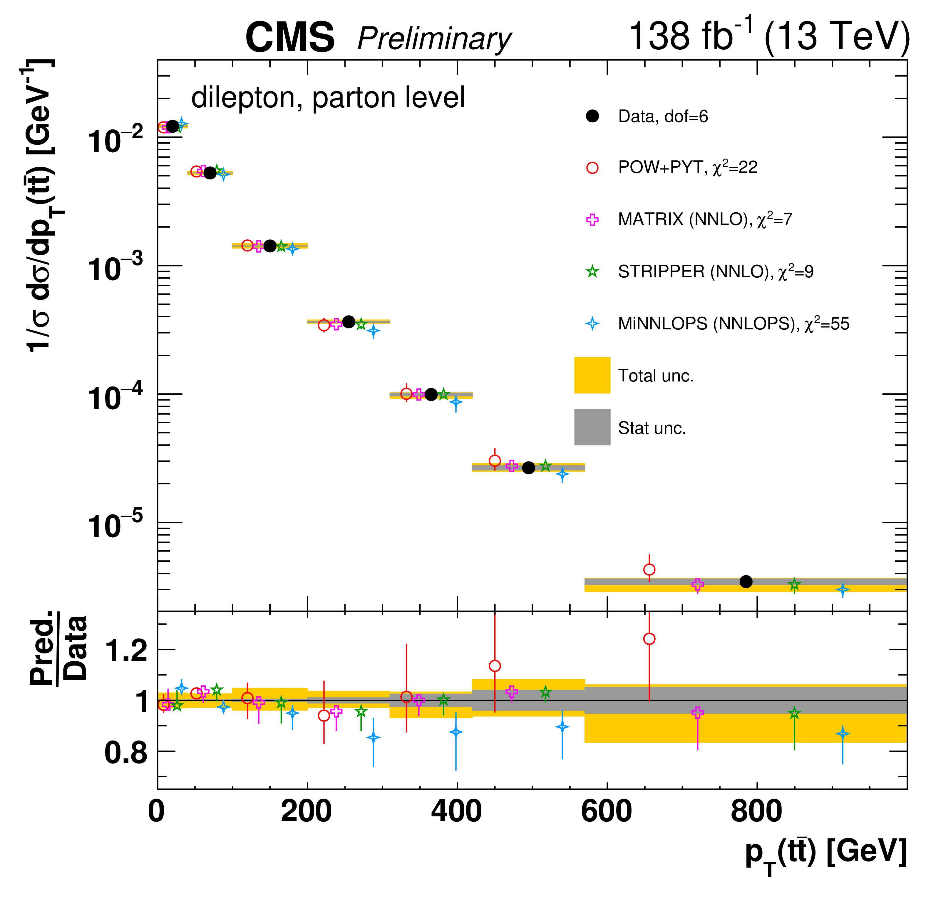
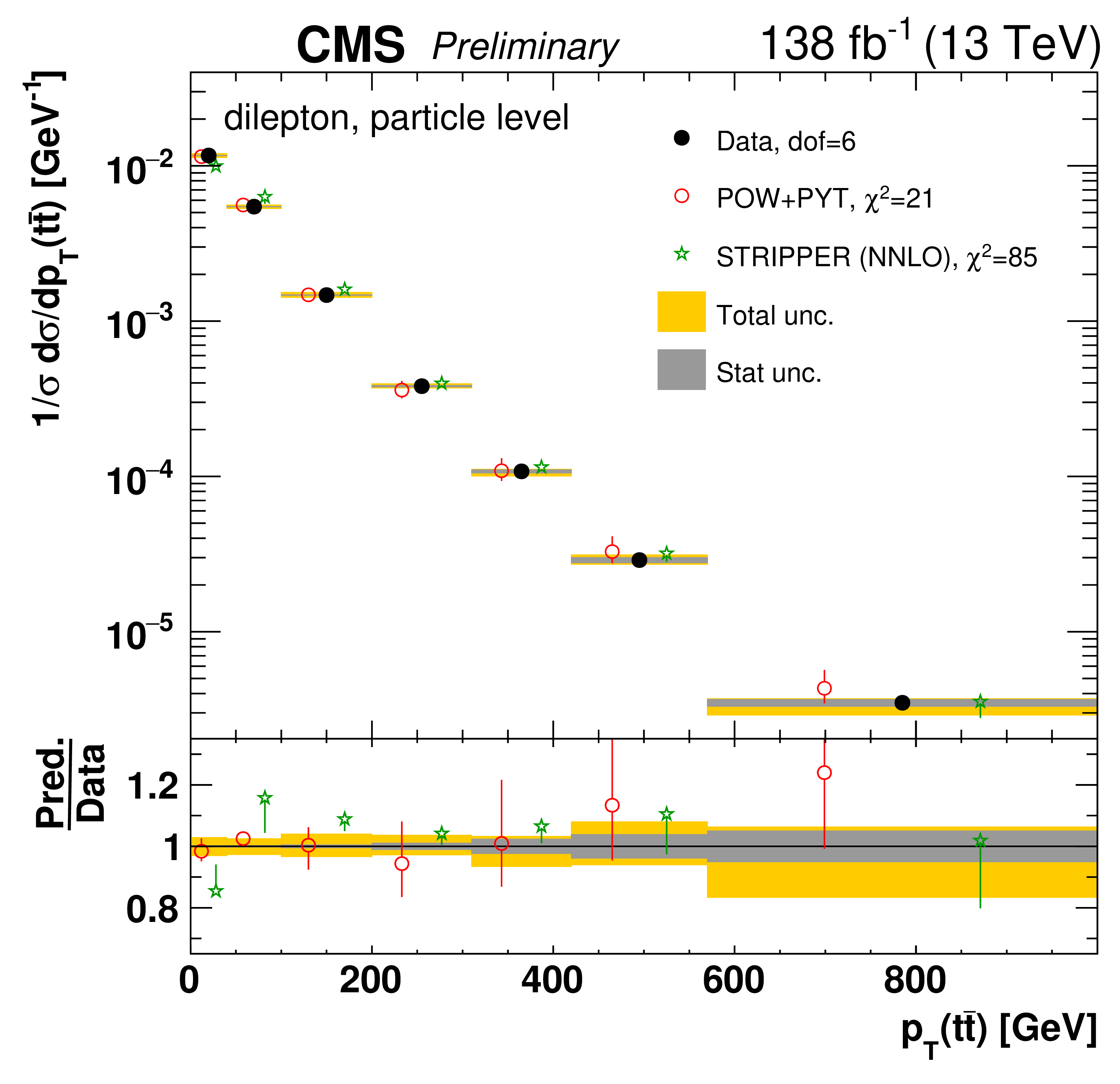
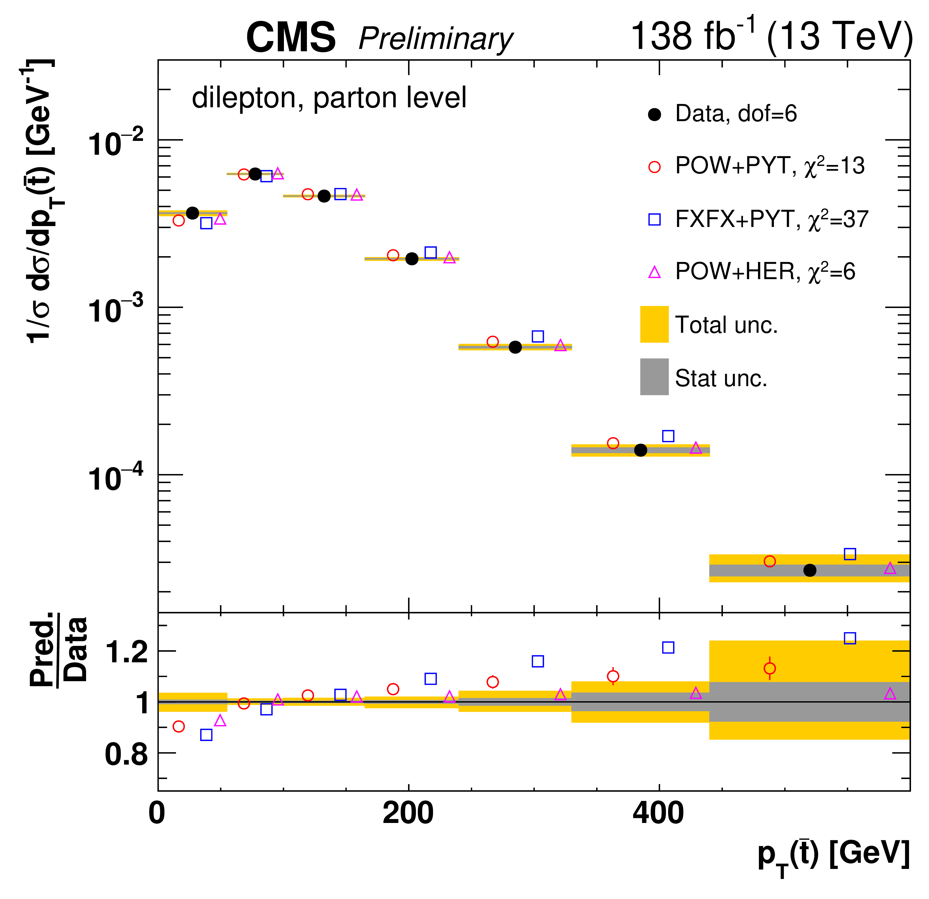
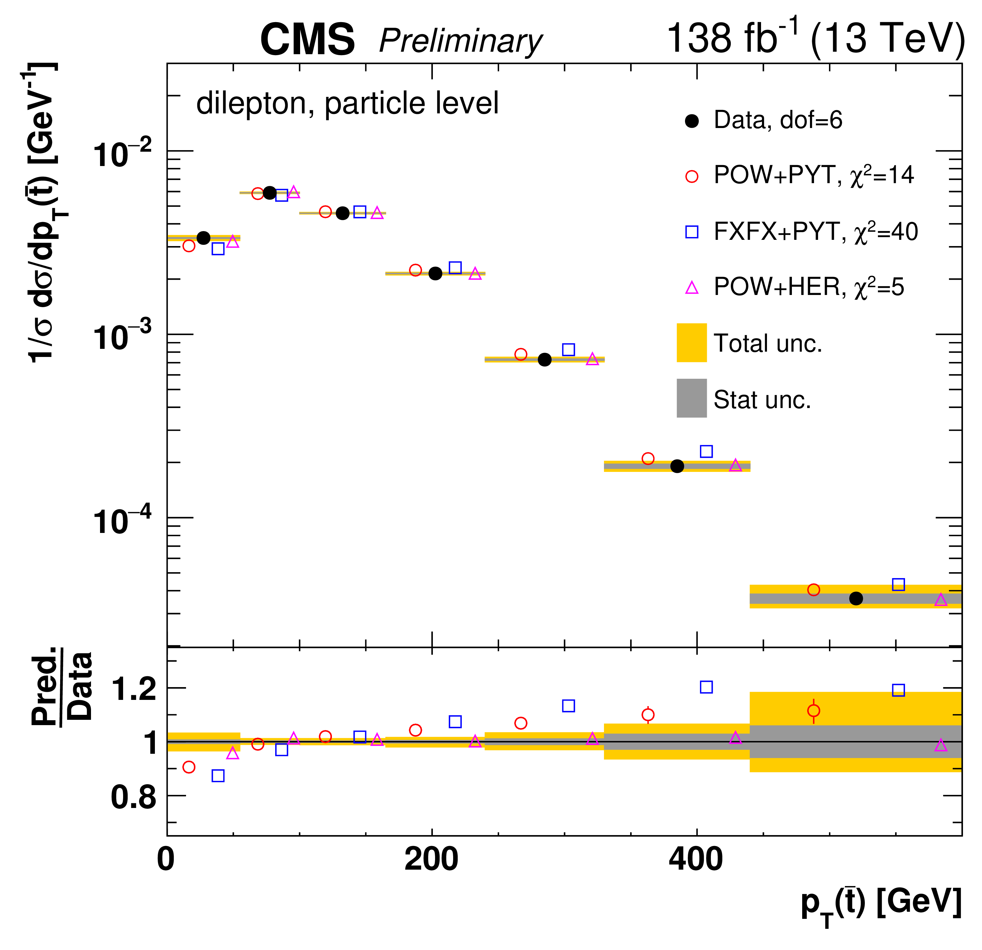
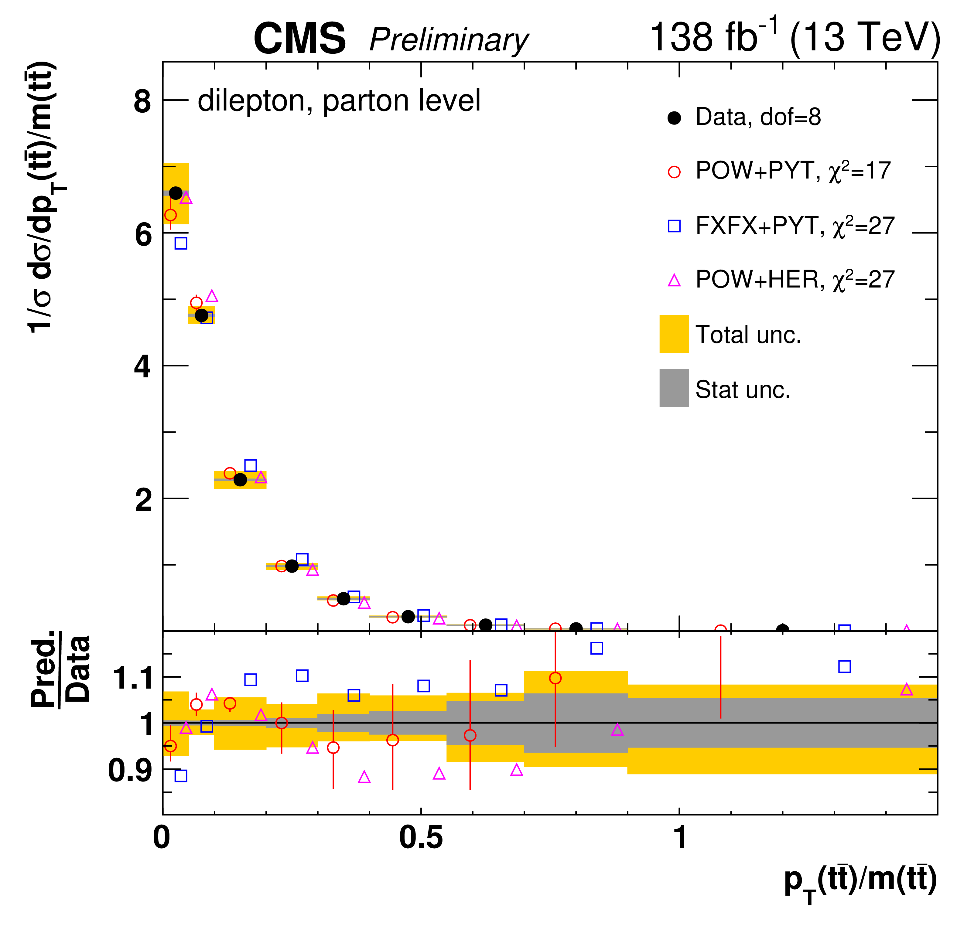
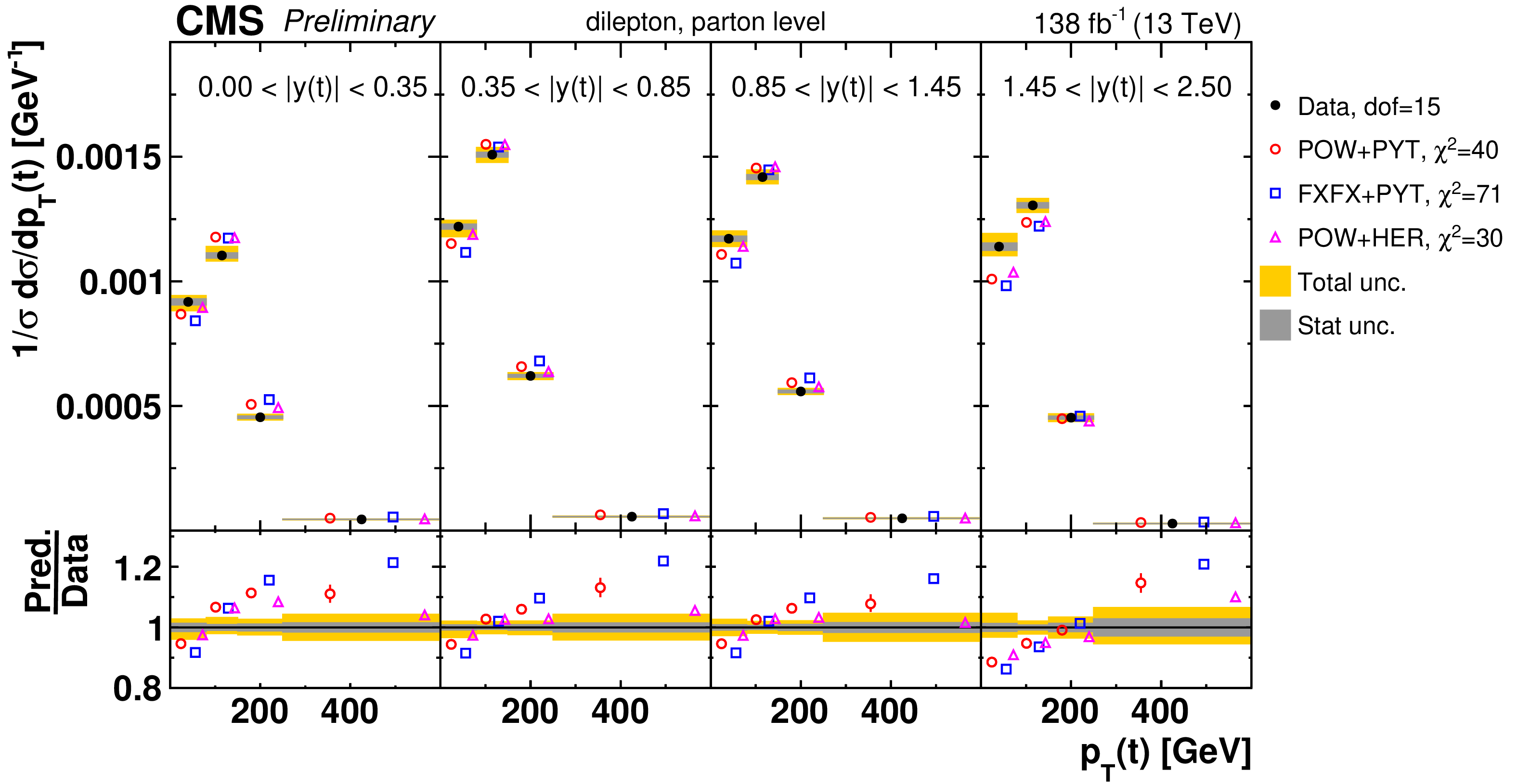
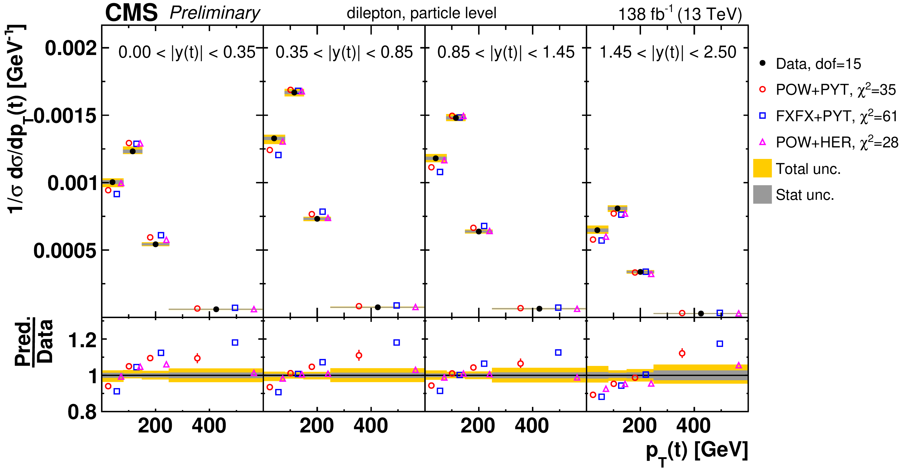
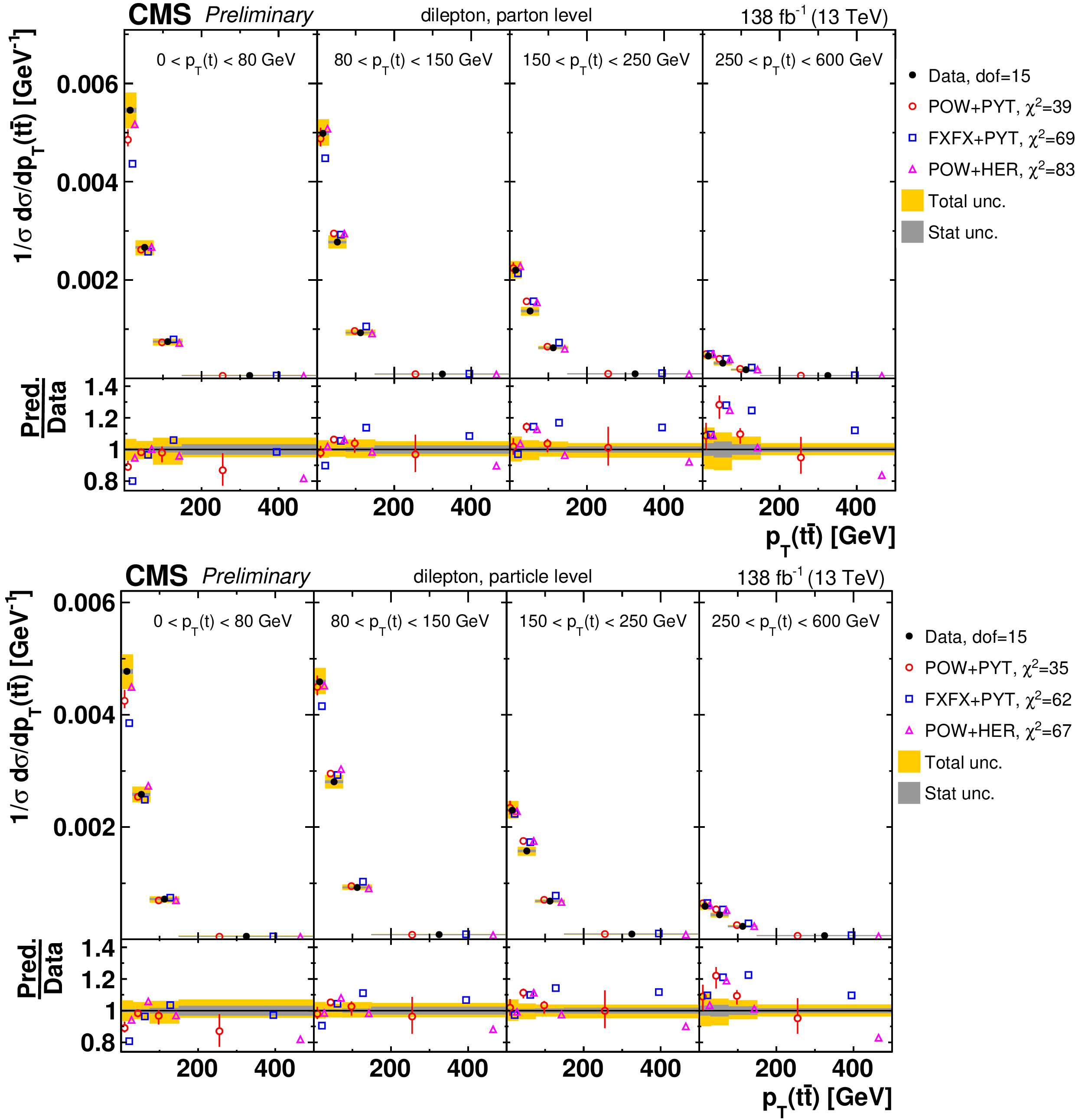
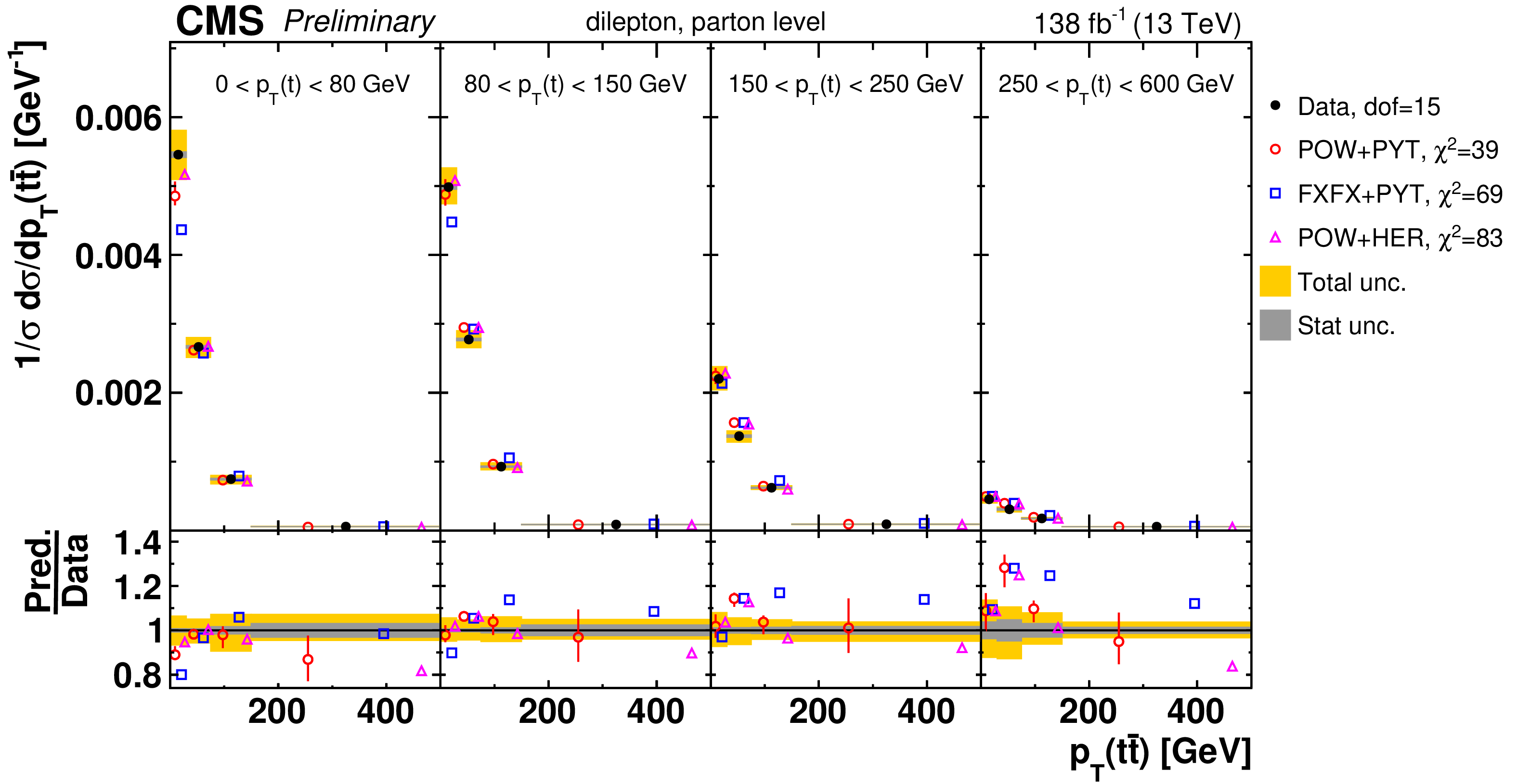
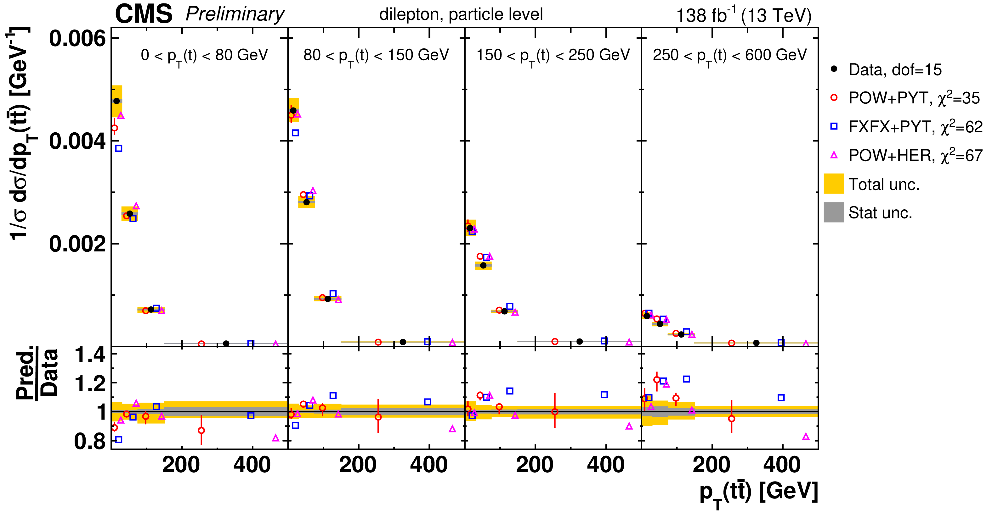
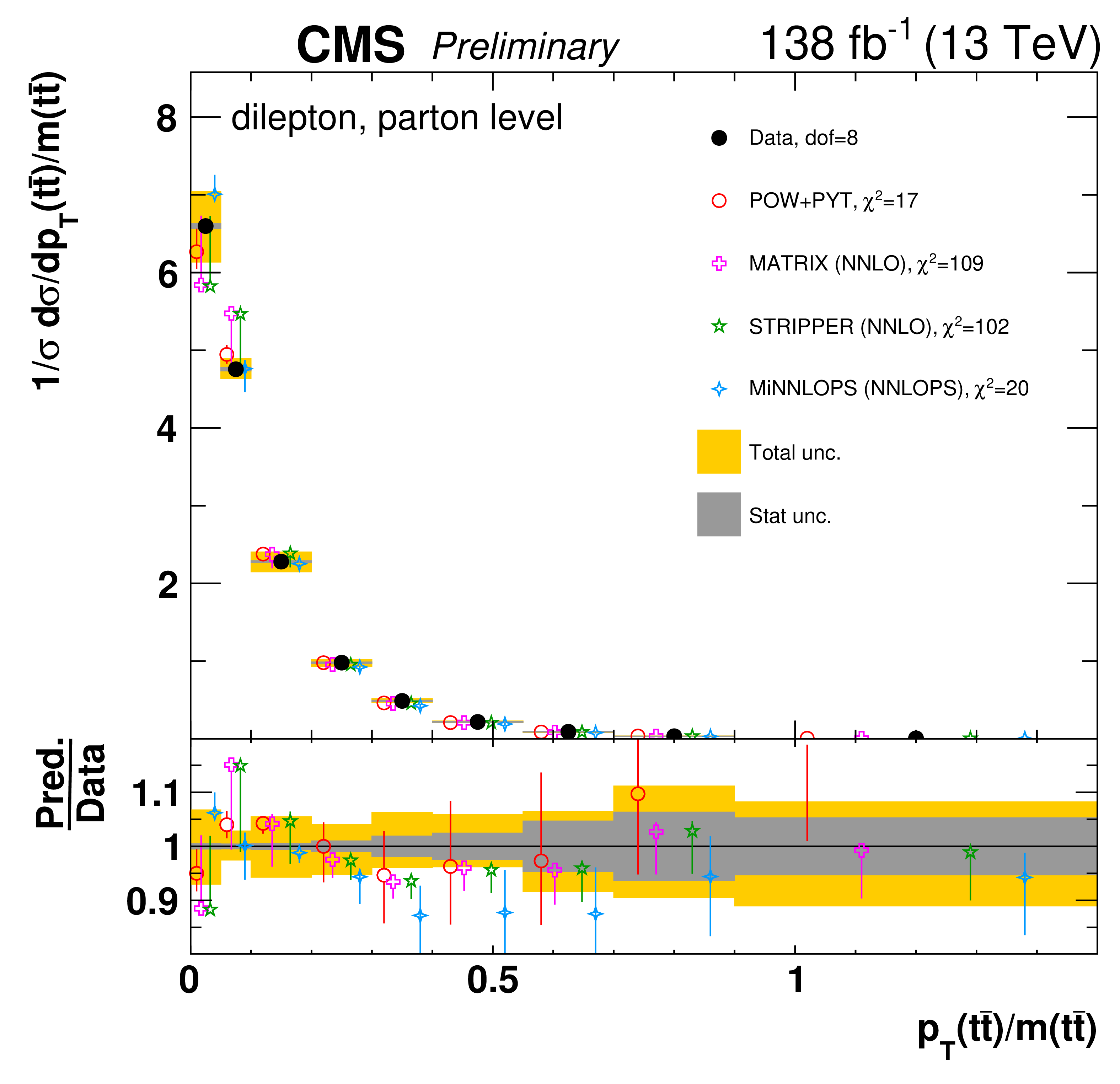
png pdf	Figure 7: Normalized differential $\mathrm{t\bar{t}}$ production cross sections as a function of ${{p_{\mathrm {T}}} (\mathrm{t})}$ (upper) and ${{p_{\mathrm {T}}} (\mathrm{\bar{t}})}$ (lower), measured at the parton level in the full phase space (left) and at the particle level in a fiducial phase space (right). The data are shown as filled circles with dark and light bands indicating the statistical and total uncertainties (statistical and systematic uncertainties summed in quadrature), respectively. The cross sections are compared to various MC predictions (other points). The estimated uncertainties in the POWHEG+PYTHIA-8 (`POW-PYT') simulation are represented by a vertical bar on the corresponding points. For each MC model, a value of ${\chi ^2}$ is reported that takes into account the measurement uncertainties. The lower panel in each plot shows the ratios of the predictions to the data.
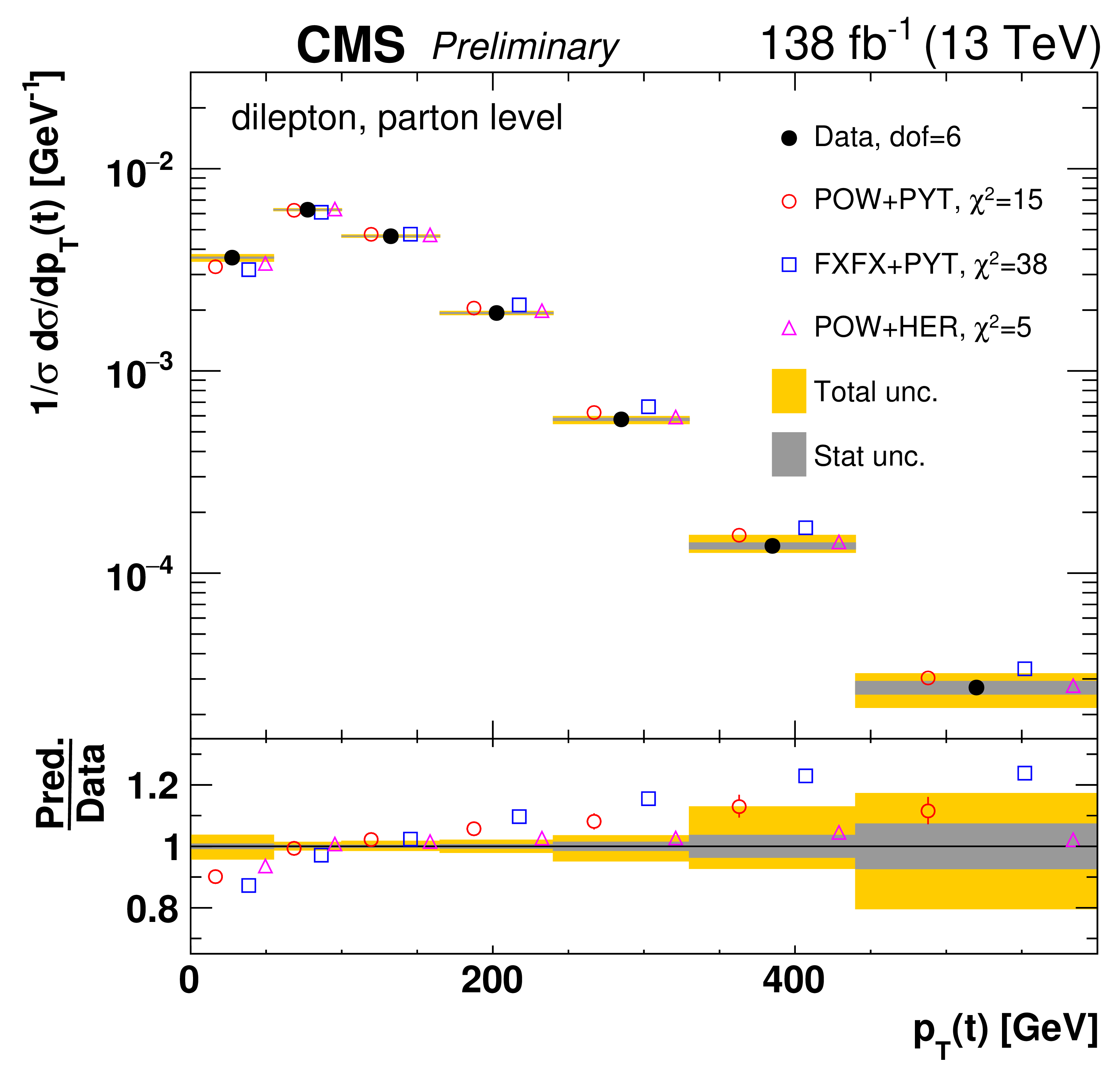
png pdf	Figure 7-a: Normalized differential $\mathrm{t\bar{t}}$ production cross sections as a function of ${{p_{\mathrm {T}}} (\mathrm{t})}$ (upper) and ${{p_{\mathrm {T}}} (\mathrm{\bar{t}})}$ (lower), measured at the parton level in the full phase space (left) and at the particle level in a fiducial phase space (right). The data are shown as filled circles with dark and light bands indicating the statistical and total uncertainties (statistical and systematic uncertainties summed in quadrature), respectively. The cross sections are compared to various MC predictions (other points). The estimated uncertainties in the POWHEG+PYTHIA-8 (`POW-PYT') simulation are represented by a vertical bar on the corresponding points. For each MC model, a value of ${\chi ^2}$ is reported that takes into account the measurement uncertainties. The lower panel in each plot shows the ratios of the predictions to the data.
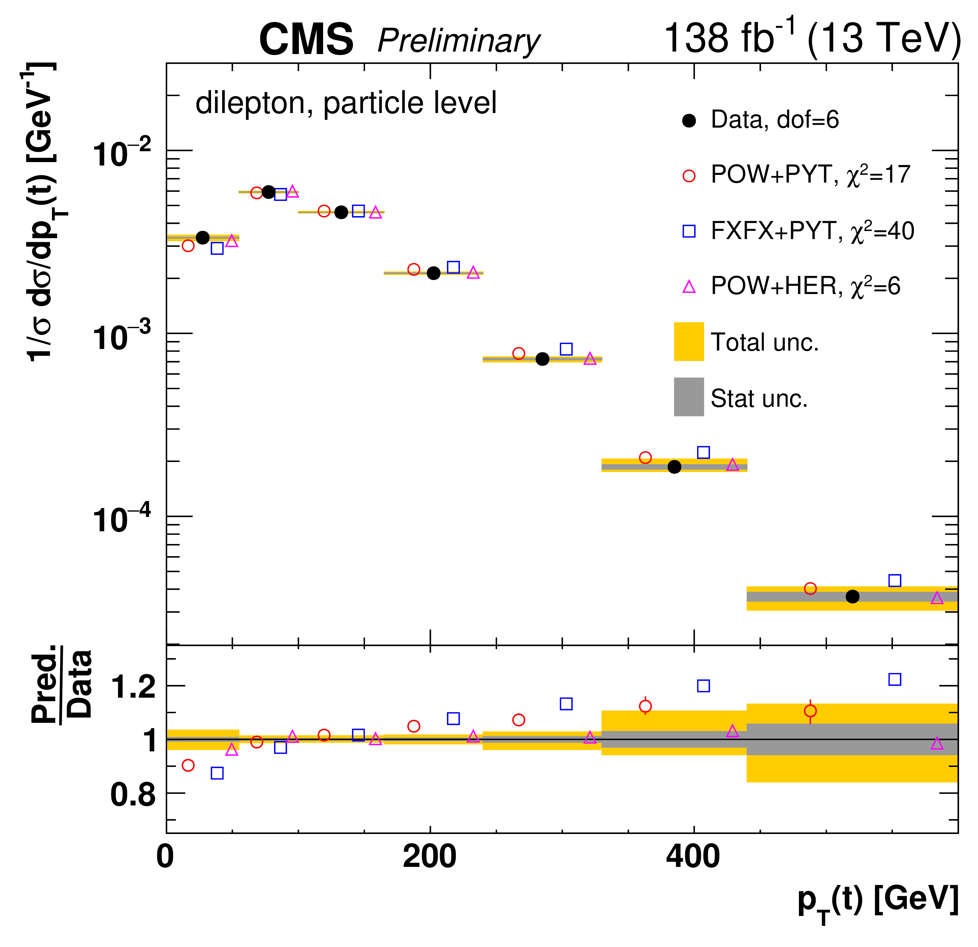
png pdf	Figure 7-b: Normalized differential $\mathrm{t\bar{t}}$ production cross sections as a function of ${{p_{\mathrm {T}}} (\mathrm{t})}$ (upper) and ${{p_{\mathrm {T}}} (\mathrm{\bar{t}})}$ (lower), measured at the parton level in the full phase space (left) and at the particle level in a fiducial phase space (right). The data are shown as filled circles with dark and light bands indicating the statistical and total uncertainties (statistical and systematic uncertainties summed in quadrature), respectively. The cross sections are compared to various MC predictions (other points). The estimated uncertainties in the POWHEG+PYTHIA-8 (`POW-PYT') simulation are represented by a vertical bar on the corresponding points. For each MC model, a value of ${\chi ^2}$ is reported that takes into account the measurement uncertainties. The lower panel in each plot shows the ratios of the predictions to the data.
png pdf	Figure 7-c: Normalized differential $\mathrm{t\bar{t}}$ production cross sections as a function of ${{p_{\mathrm {T}}} (\mathrm{t})}$ (upper) and ${{p_{\mathrm {T}}} (\mathrm{\bar{t}})}$ (lower), measured at the parton level in the full phase space (left) and at the particle level in a fiducial phase space (right). The data are shown as filled circles with dark and light bands indicating the statistical and total uncertainties (statistical and systematic uncertainties summed in quadrature), respectively. The cross sections are compared to various MC predictions (other points). The estimated uncertainties in the POWHEG+PYTHIA-8 (`POW-PYT') simulation are represented by a vertical bar on the corresponding points. For each MC model, a value of ${\chi ^2}$ is reported that takes into account the measurement uncertainties. The lower panel in each plot shows the ratios of the predictions to the data.
png pdf	Figure 7-d: Normalized differential $\mathrm{t\bar{t}}$ production cross sections as a function of ${{p_{\mathrm {T}}} (\mathrm{t})}$ (upper) and ${{p_{\mathrm {T}}} (\mathrm{\bar{t}})}$ (lower), measured at the parton level in the full phase space (left) and at the particle level in a fiducial phase space (right). The data are shown as filled circles with dark and light bands indicating the statistical and total uncertainties (statistical and systematic uncertainties summed in quadrature), respectively. The cross sections are compared to various MC predictions (other points). The estimated uncertainties in the POWHEG+PYTHIA-8 (`POW-PYT') simulation are represented by a vertical bar on the corresponding points. For each MC model, a value of ${\chi ^2}$ is reported that takes into account the measurement uncertainties. The lower panel in each plot shows the ratios of the predictions to the data.
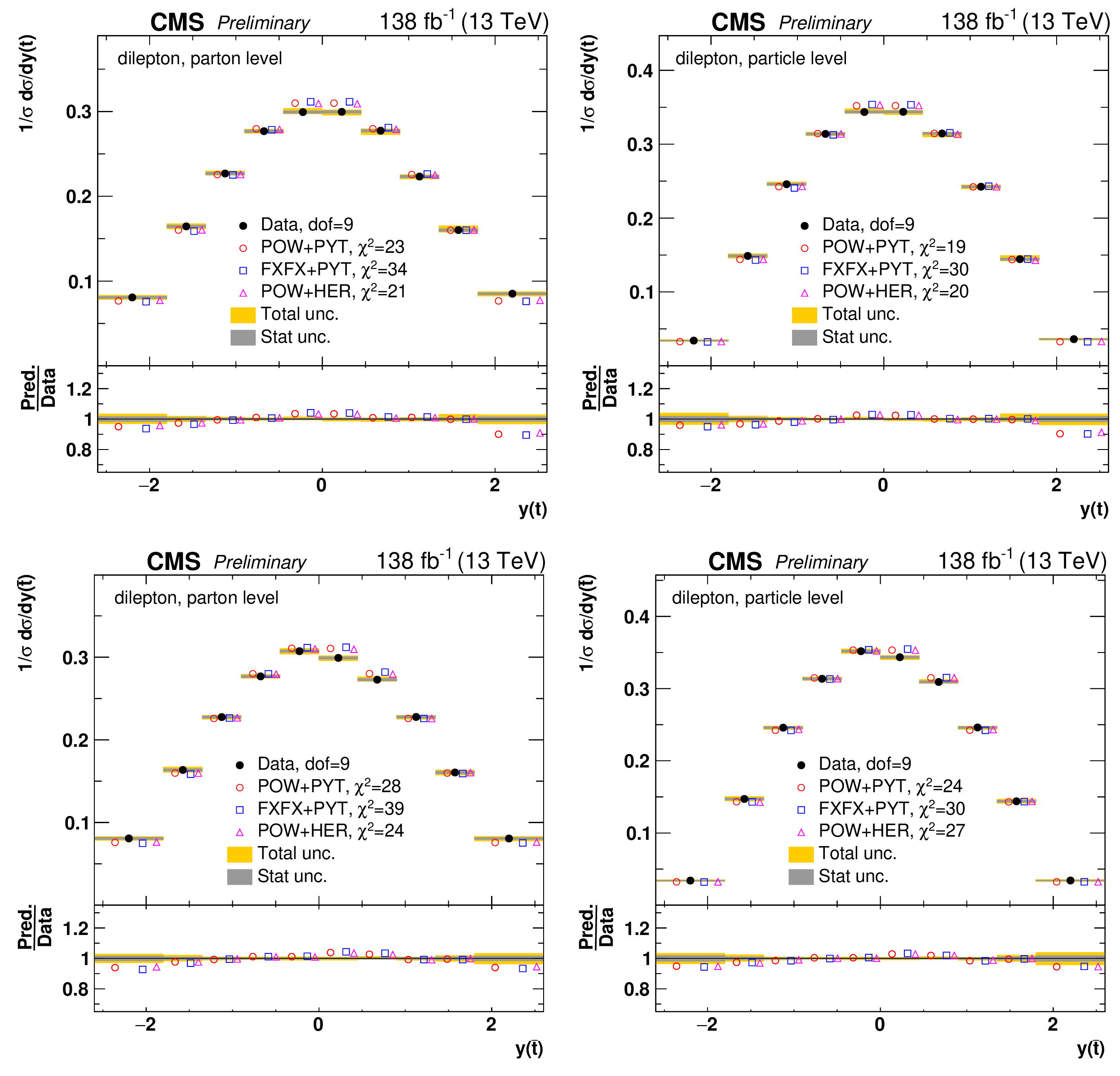
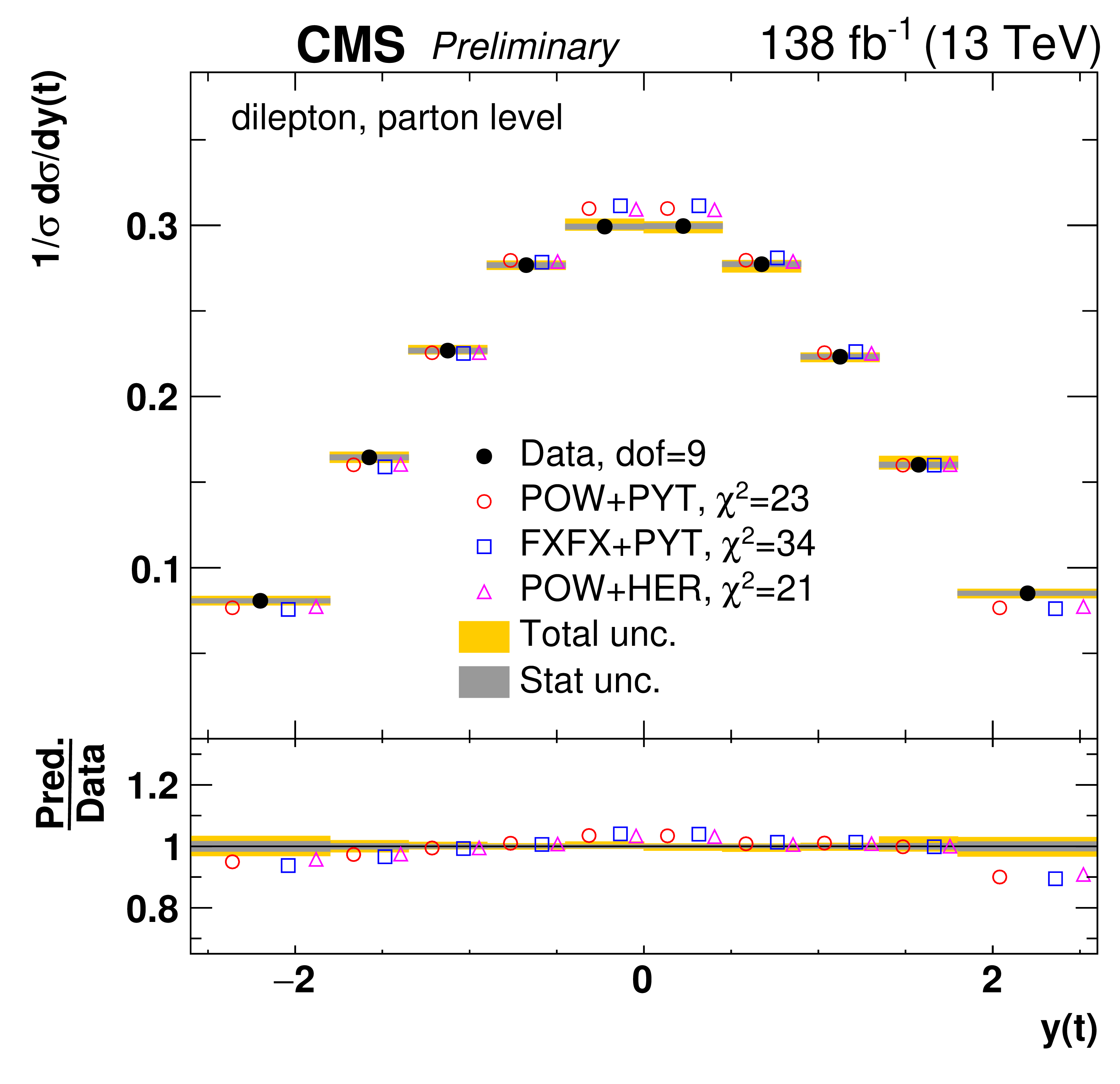
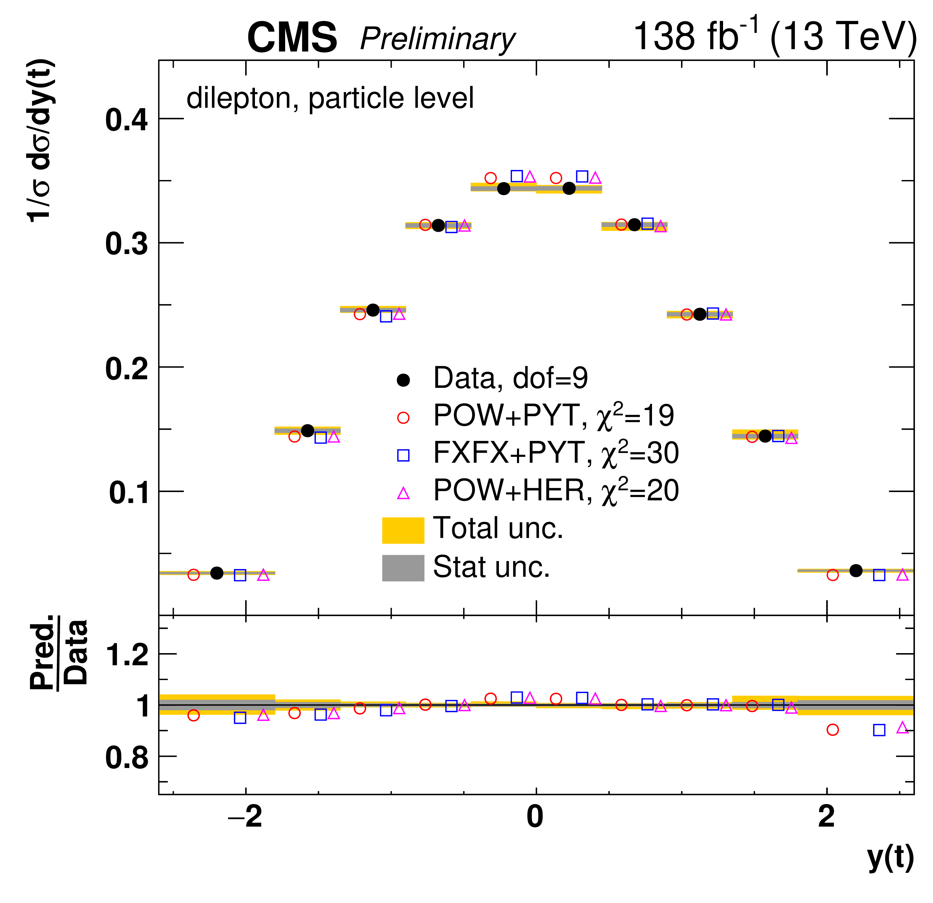
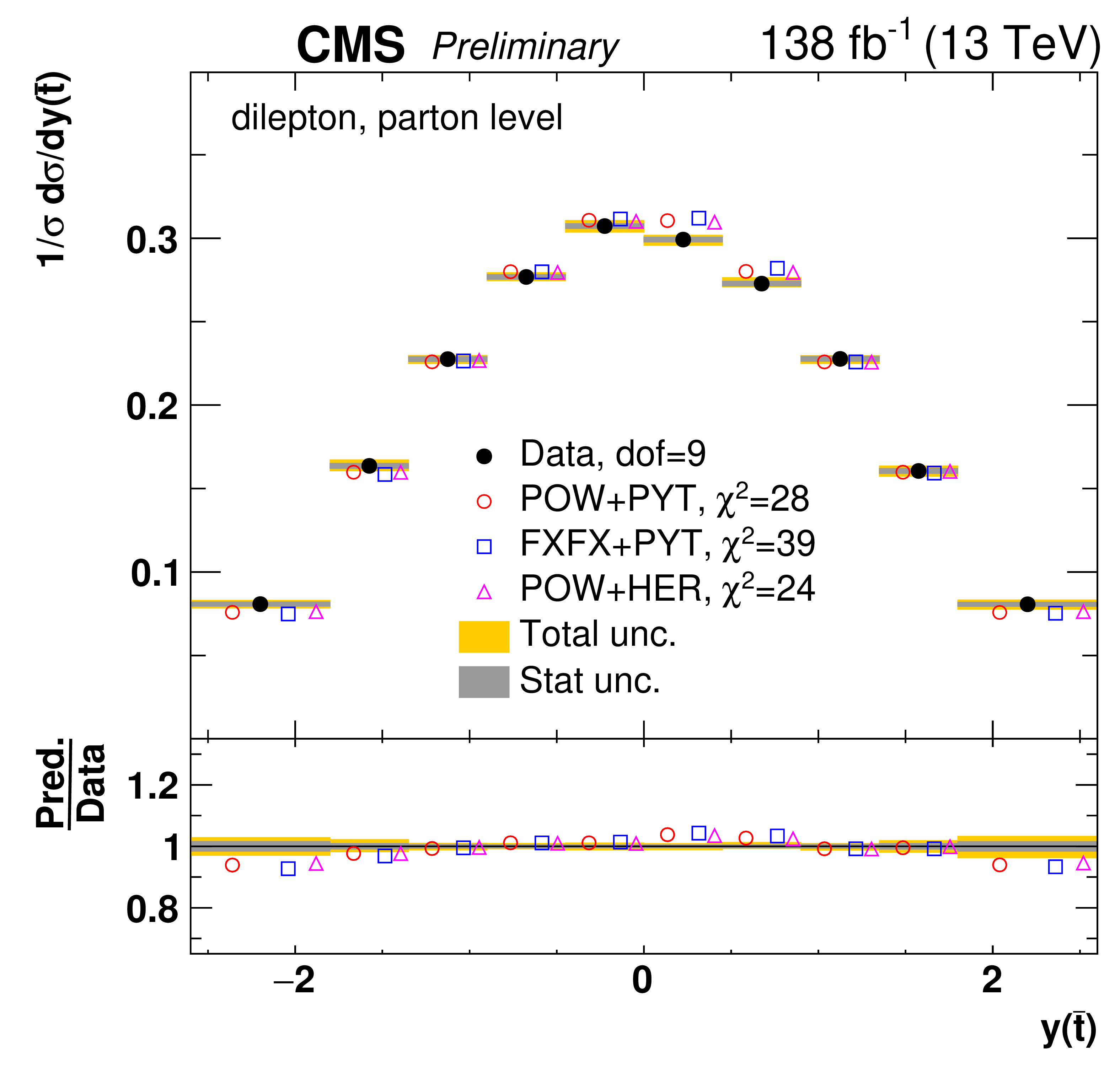
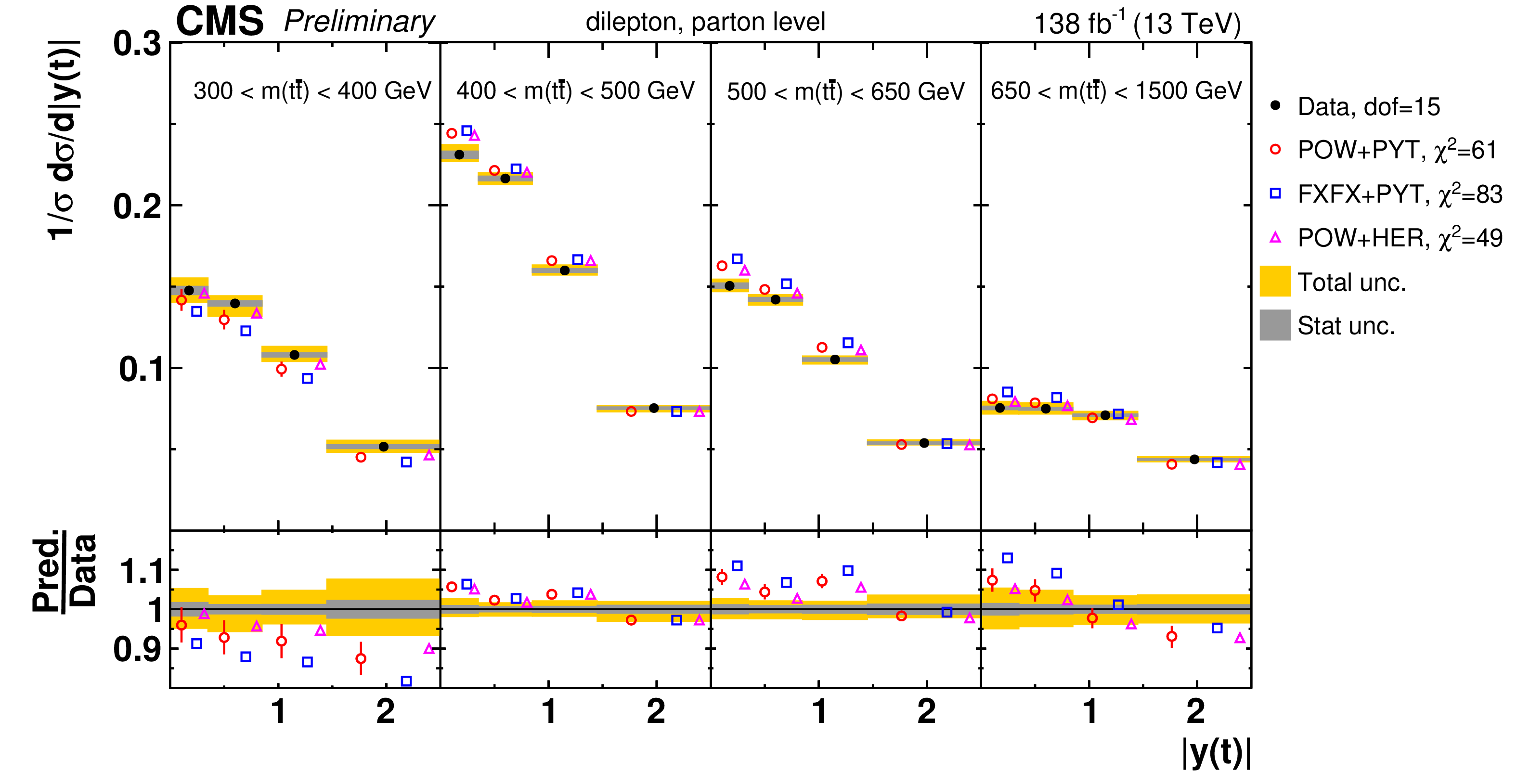
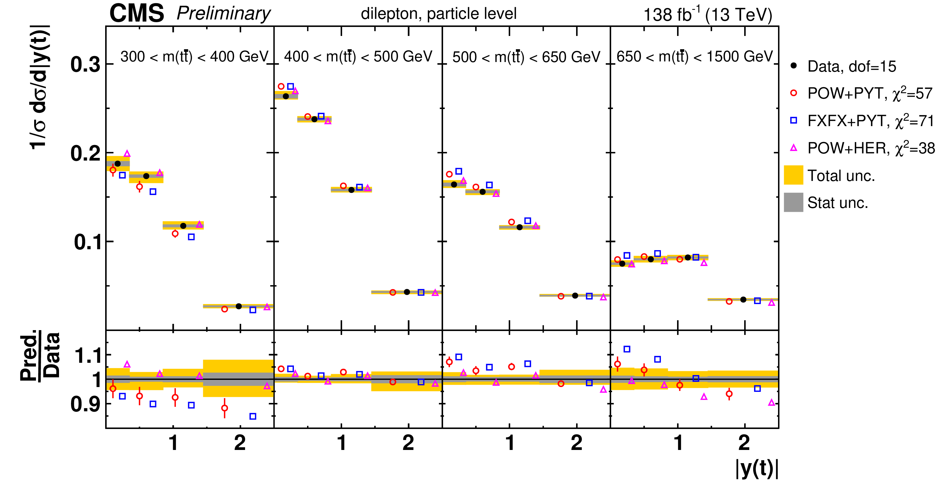
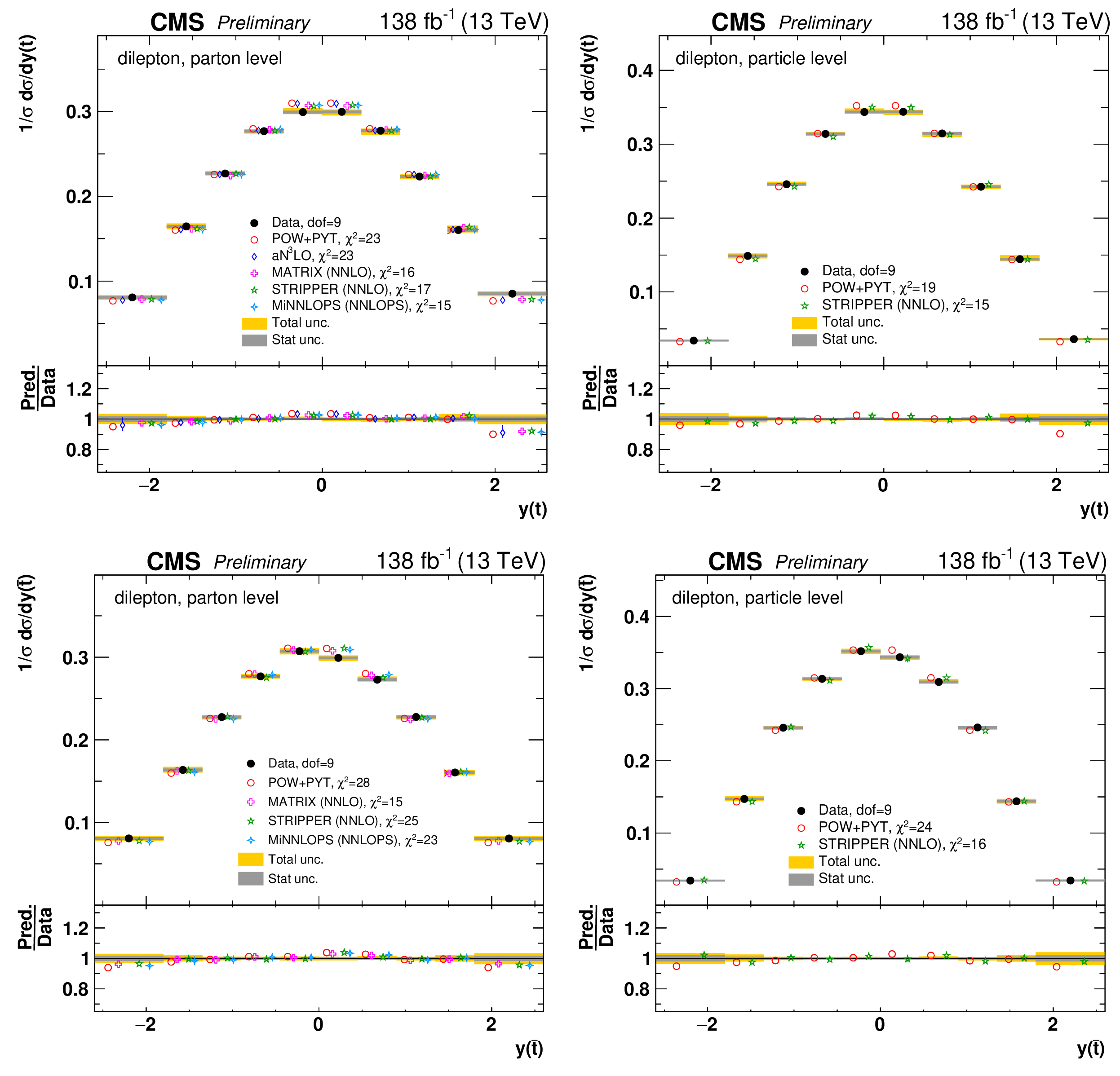
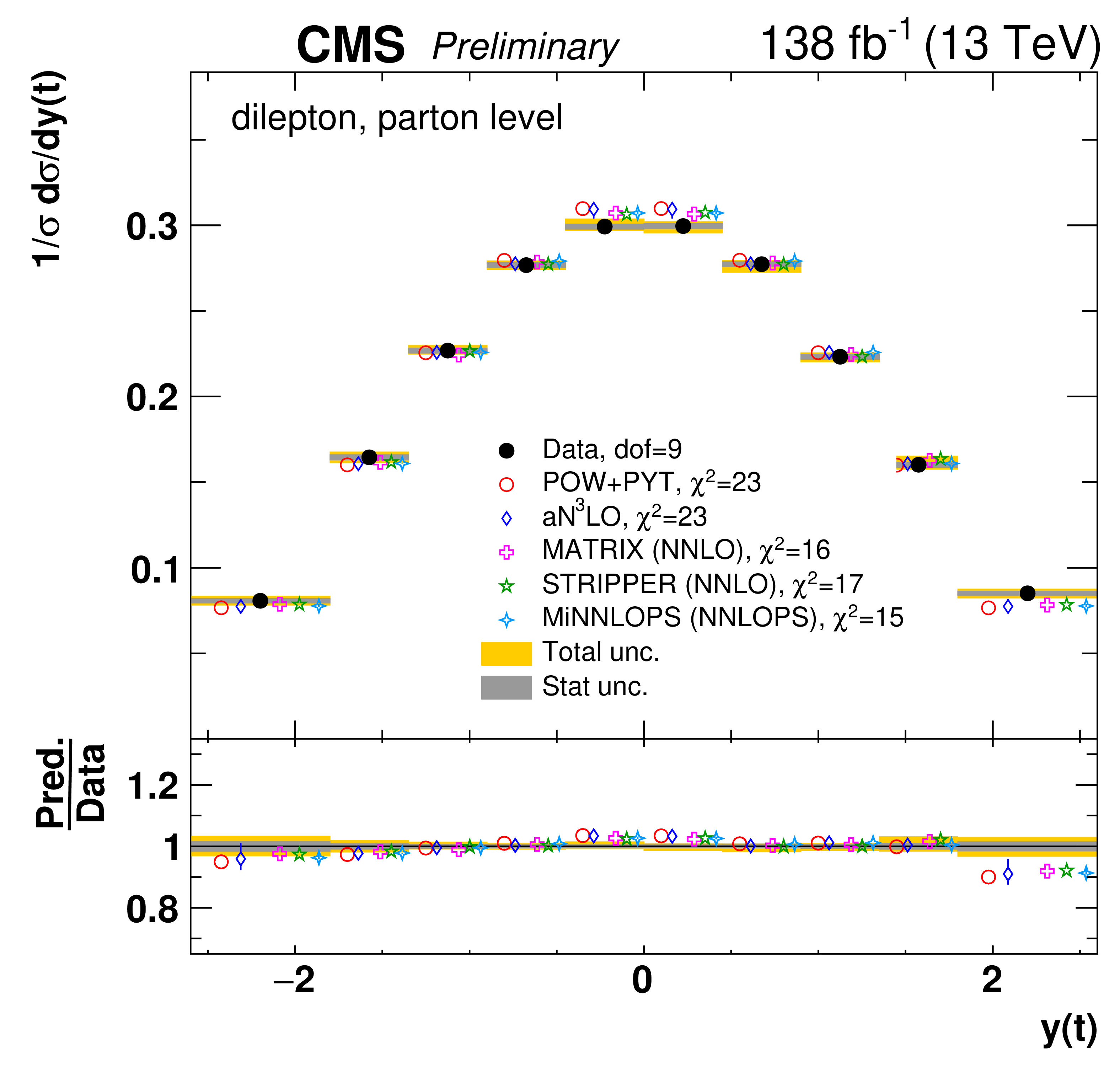
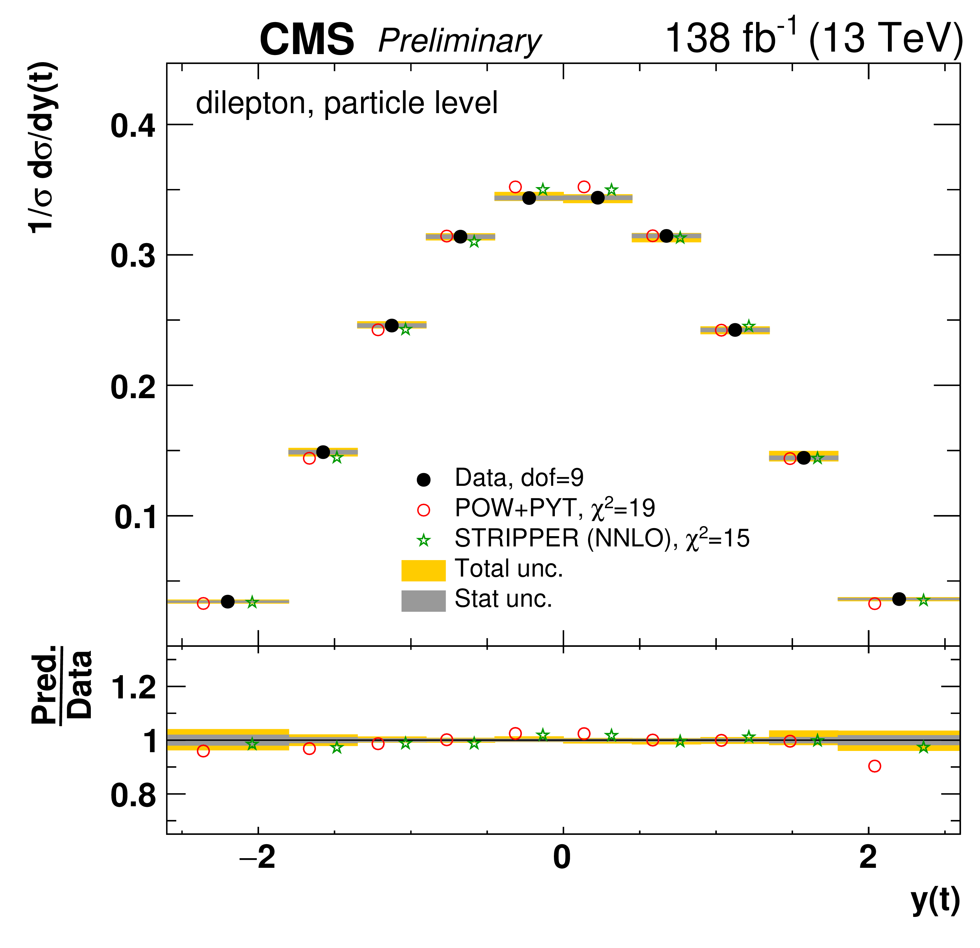
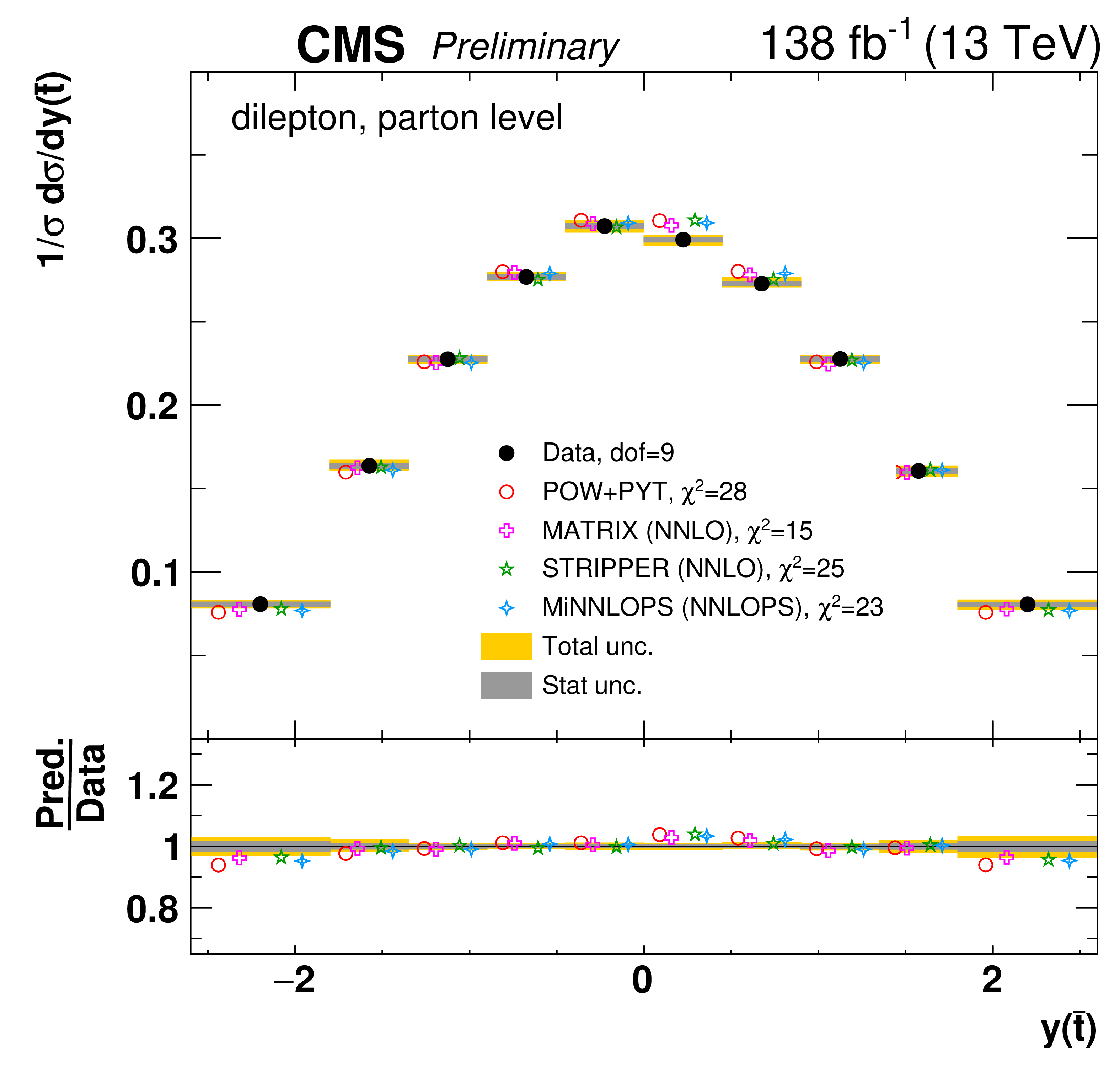
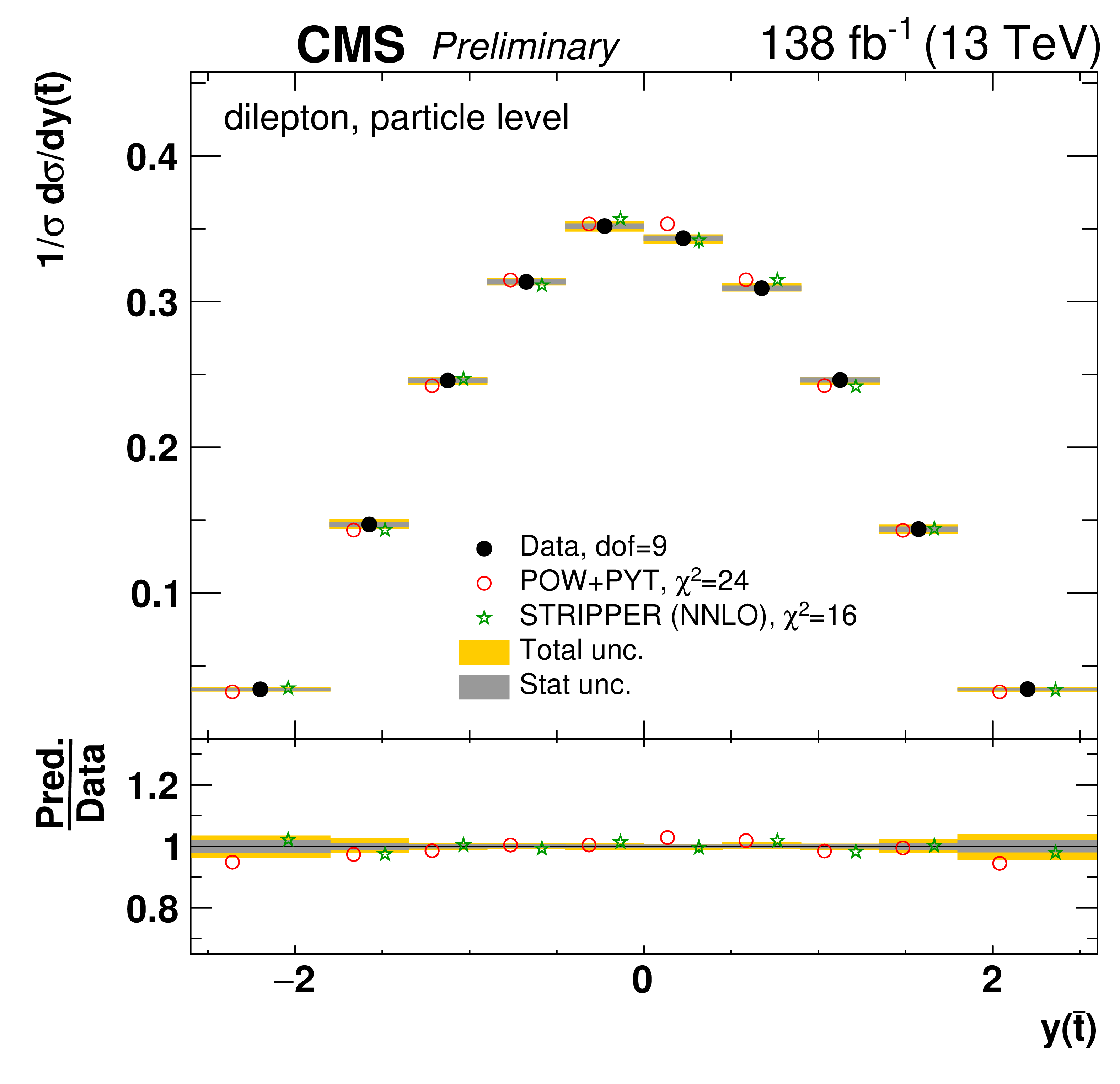
png pdf	Figure 8: Normalized differential $\mathrm{t\bar{t}}$ production cross sections as a function of ${y(\mathrm{t})}$ (upper) and ${y(\mathrm{\bar{t}})}$ (lower) are shown for data (filled circles) and various MC predictions (other points). Further details can be found in the caption of Fig. 7.
png pdf	Figure 8-a: Normalized differential $\mathrm{t\bar{t}}$ production cross sections as a function of ${y(\mathrm{t})}$ (upper) and ${y(\mathrm{\bar{t}})}$ (lower) are shown for data (filled circles) and various MC predictions (other points). Further details can be found in the caption of Fig. 7.
png pdf	Figure 8-b: Normalized differential $\mathrm{t\bar{t}}$ production cross sections as a function of ${y(\mathrm{t})}$ (upper) and ${y(\mathrm{\bar{t}})}$ (lower) are shown for data (filled circles) and various MC predictions (other points). Further details can be found in the caption of Fig. 7.
png pdf	Figure 8-c: Normalized differential $\mathrm{t\bar{t}}$ production cross sections as a function of ${y(\mathrm{t})}$ (upper) and ${y(\mathrm{\bar{t}})}$ (lower) are shown for data (filled circles) and various MC predictions (other points). Further details can be found in the caption of Fig. 7.
png pdf	Figure 8-d: Normalized differential $\mathrm{t\bar{t}}$ production cross sections as a function of ${y(\mathrm{t})}$ (upper) and ${y(\mathrm{\bar{t}})}$ (lower) are shown for data (filled circles) and various MC predictions (other points). Further details can be found in the caption of Fig. 7.
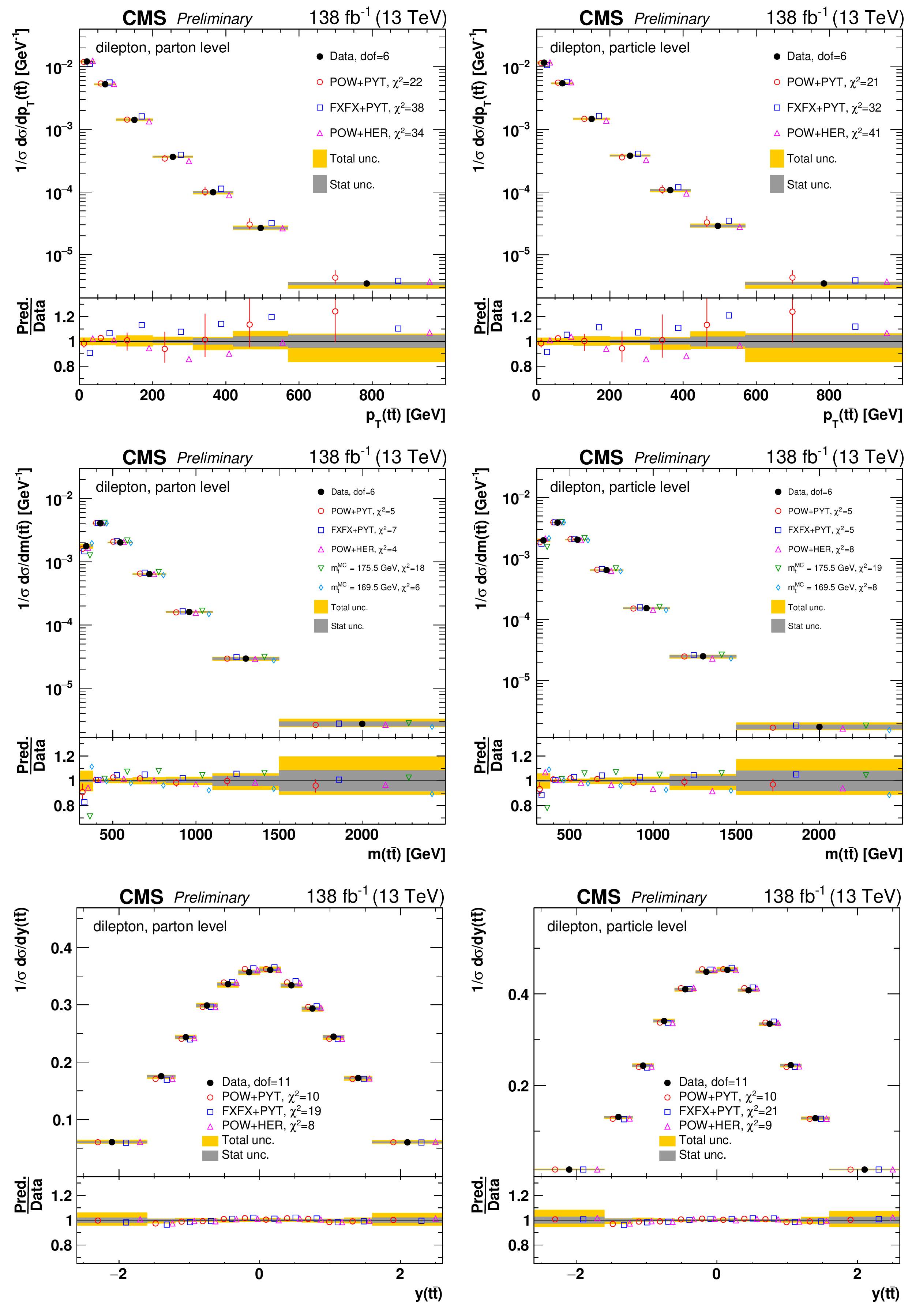
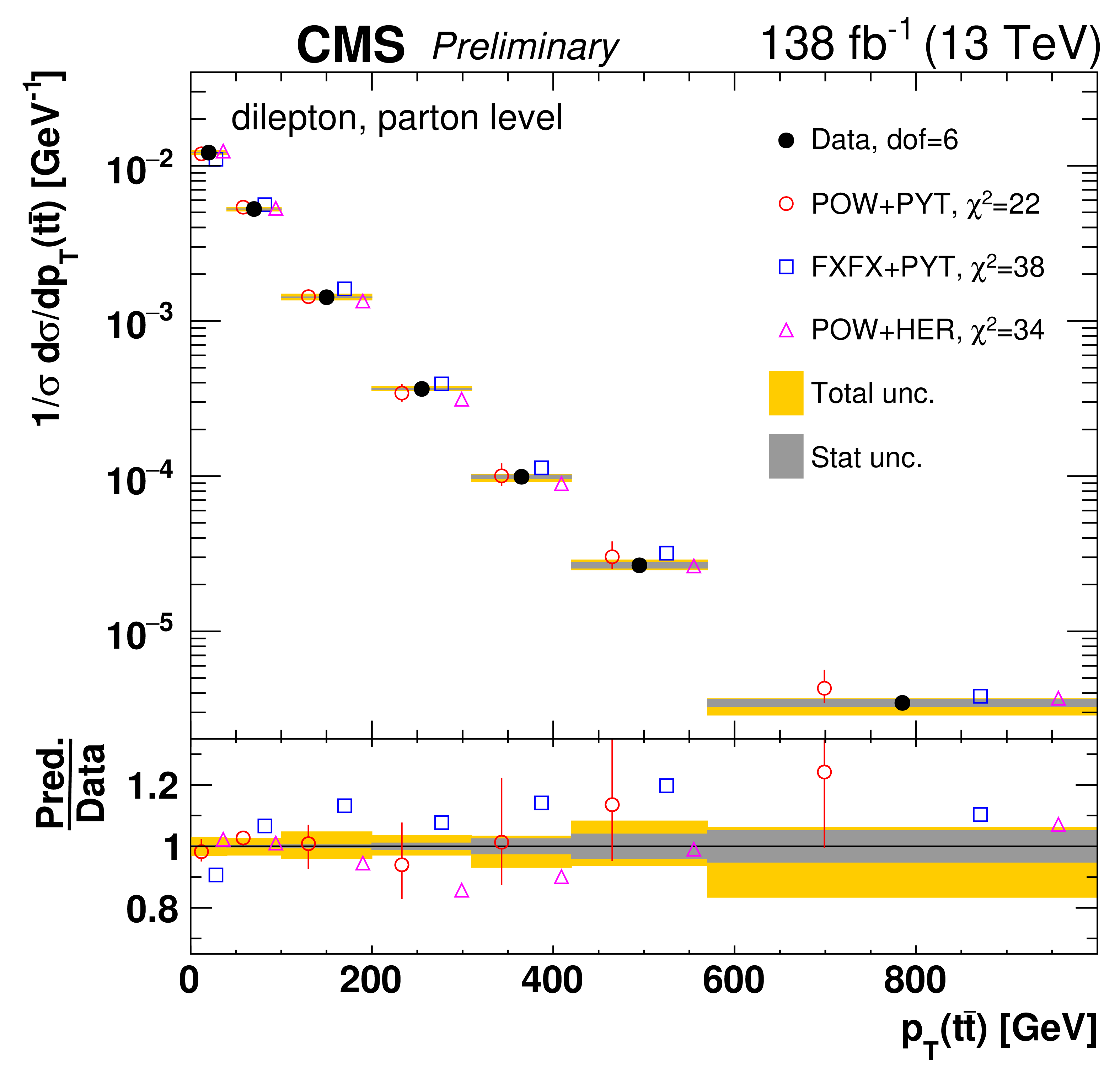
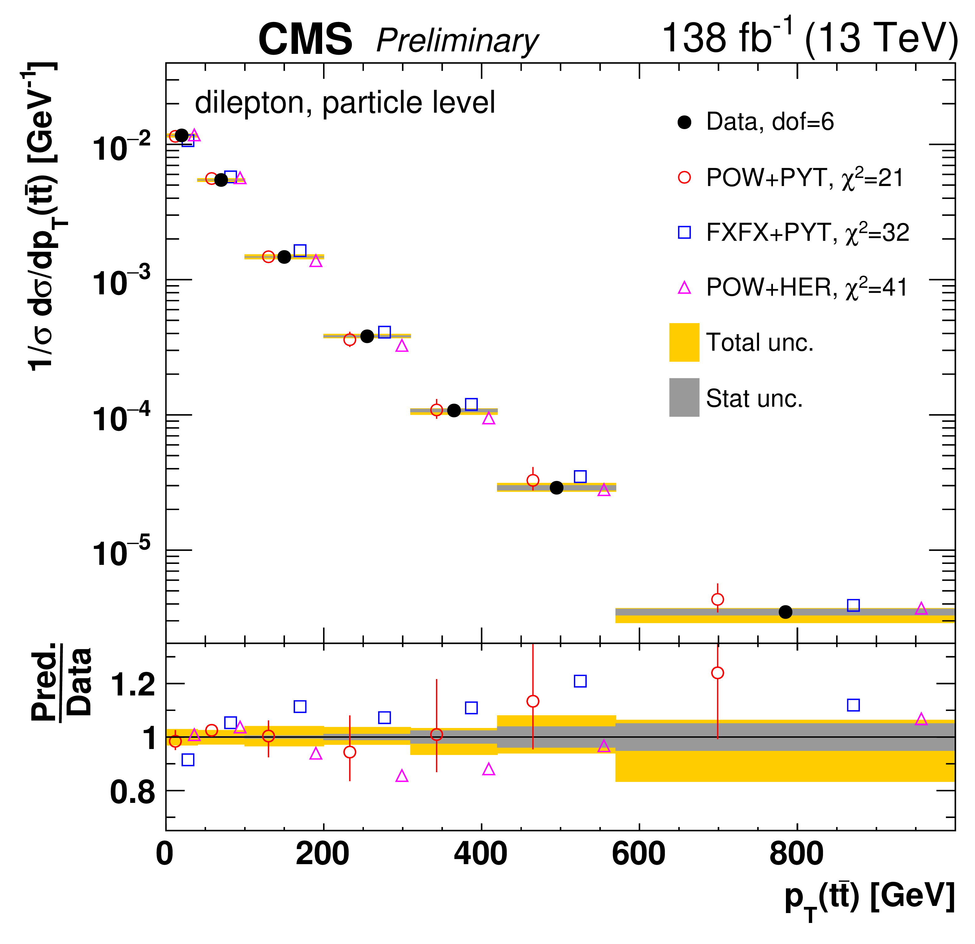
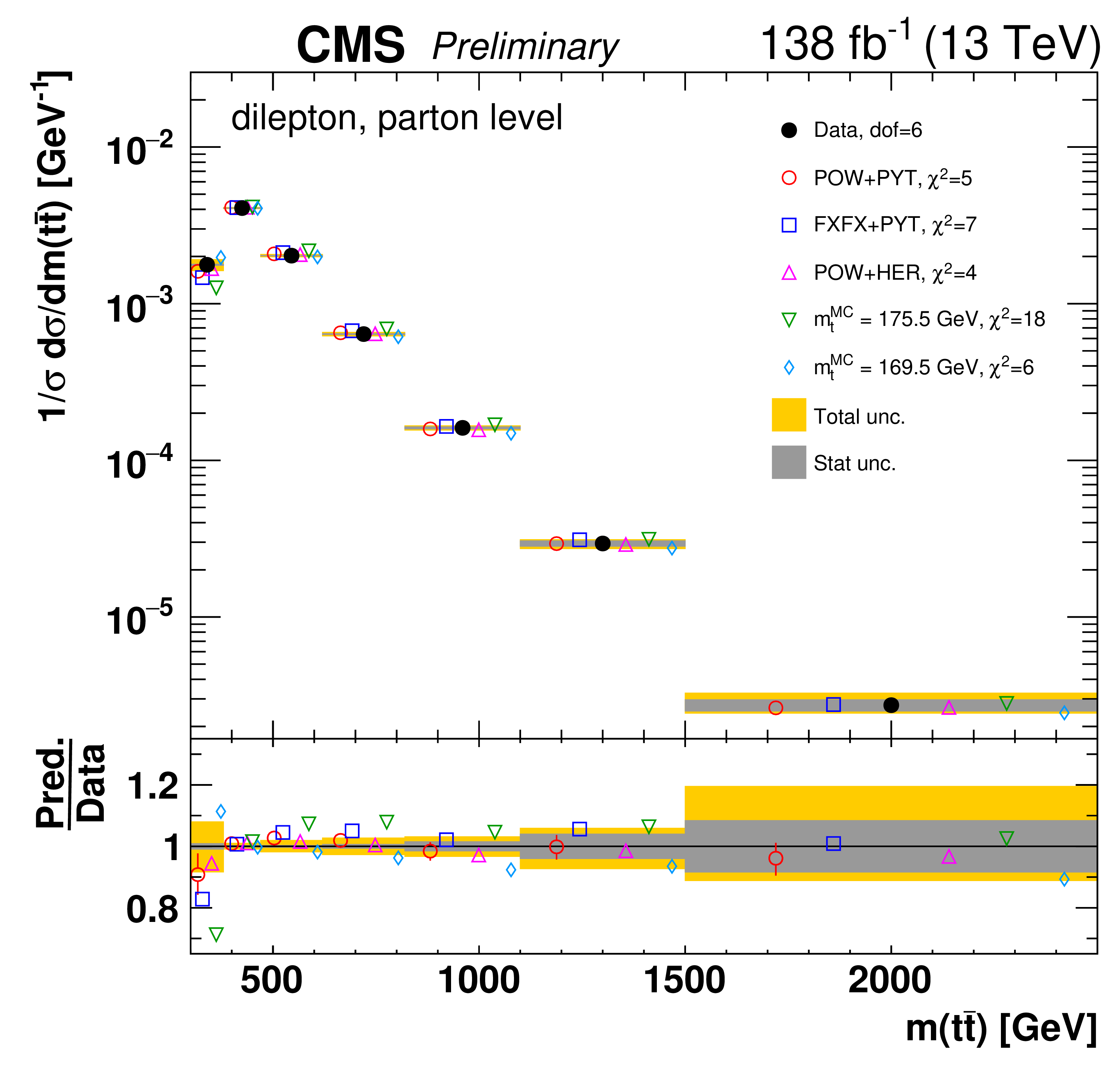
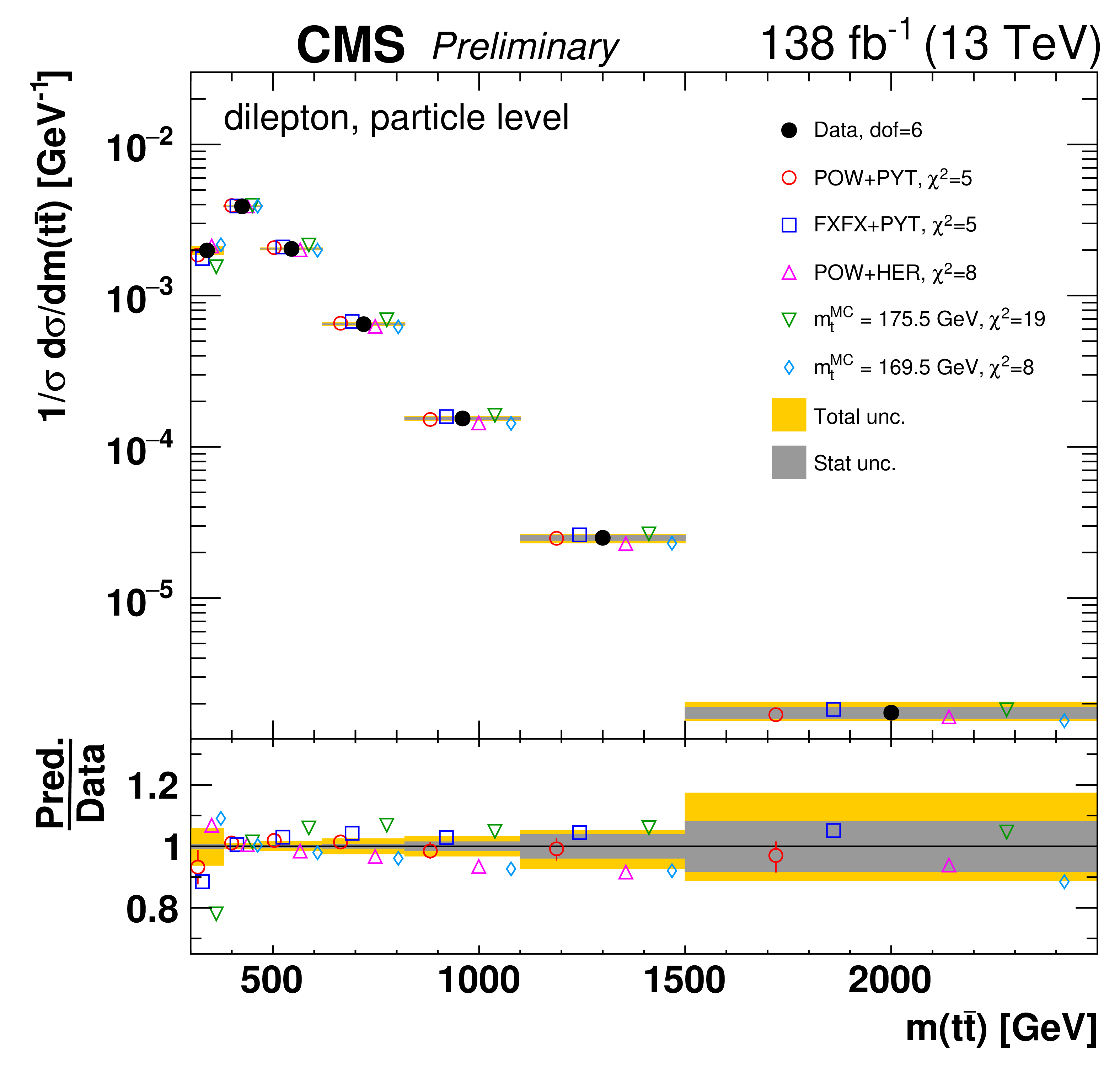
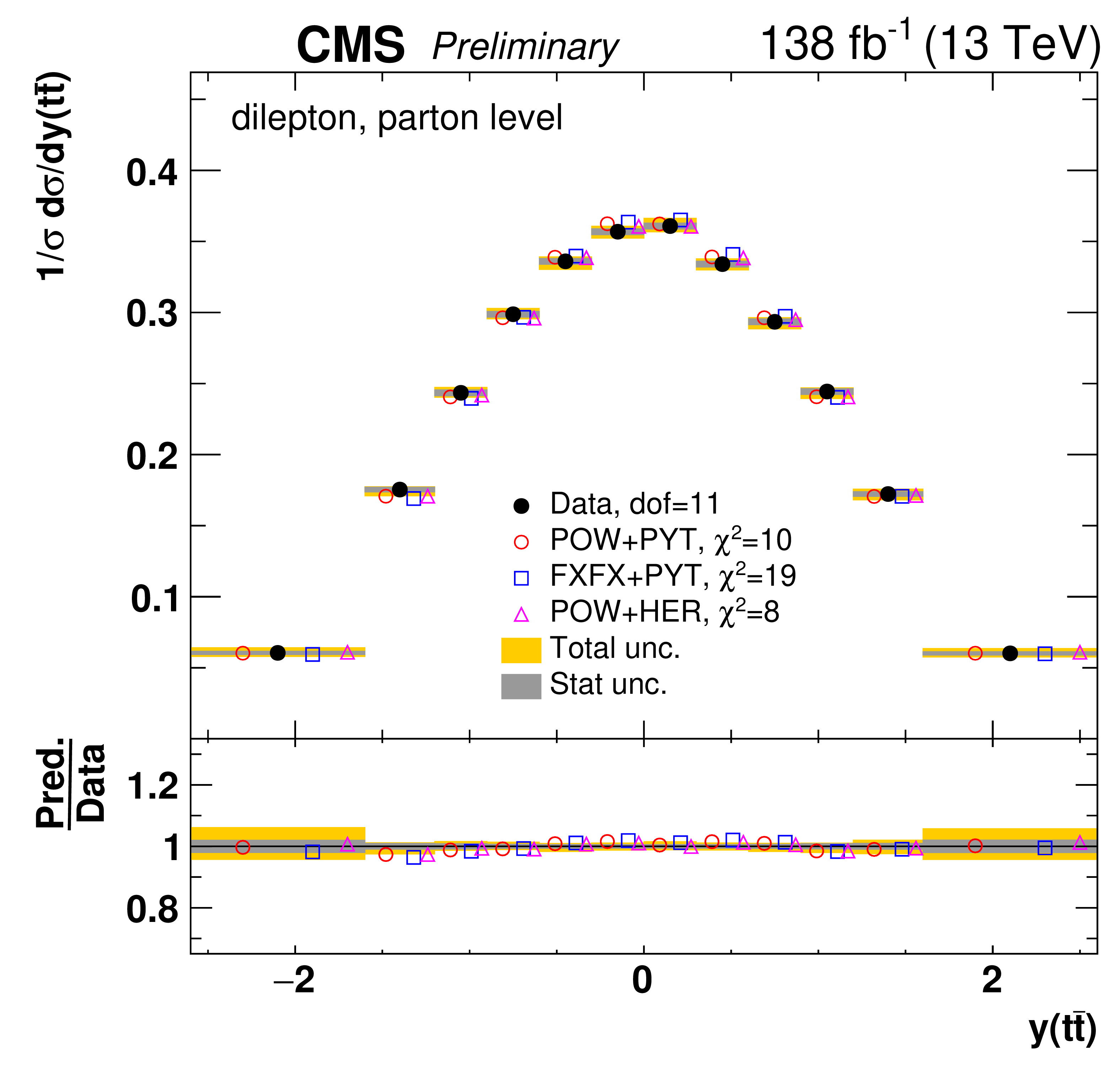
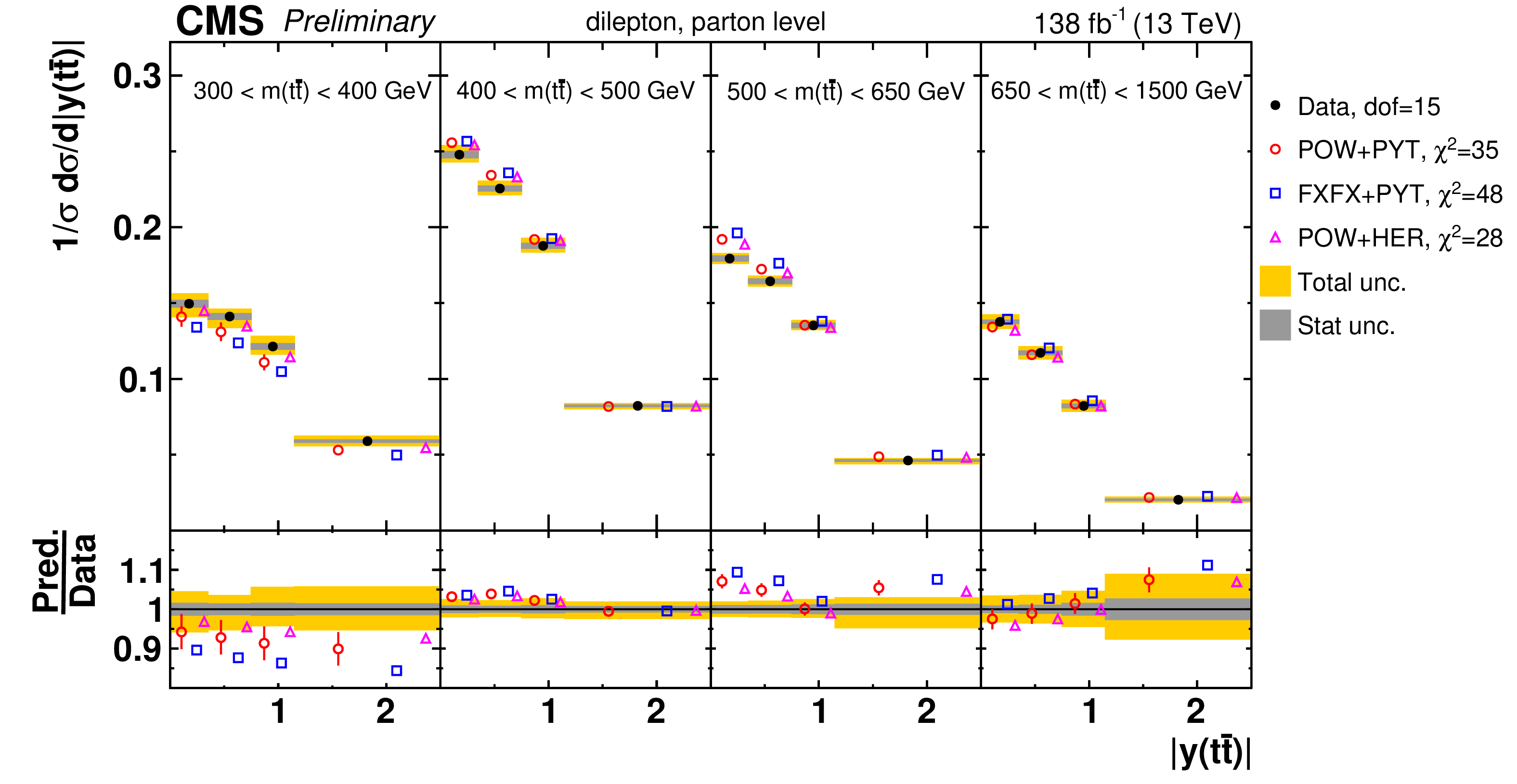
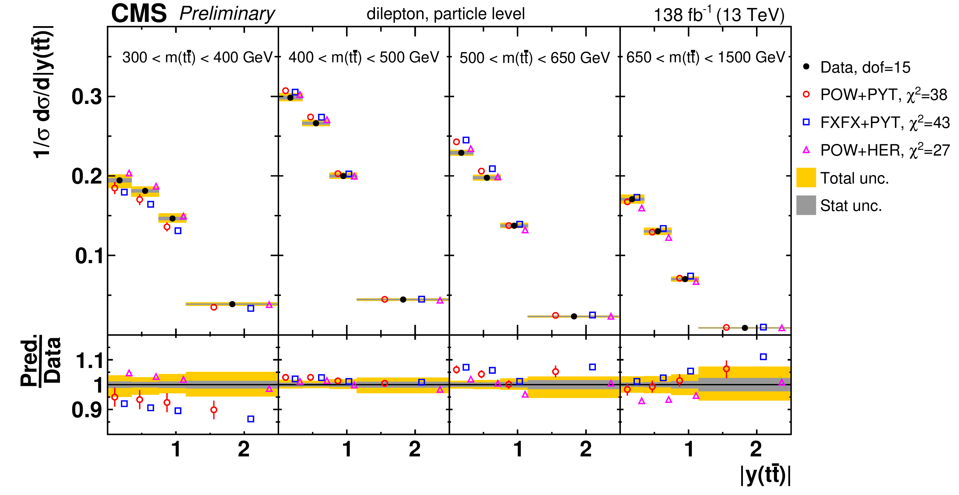
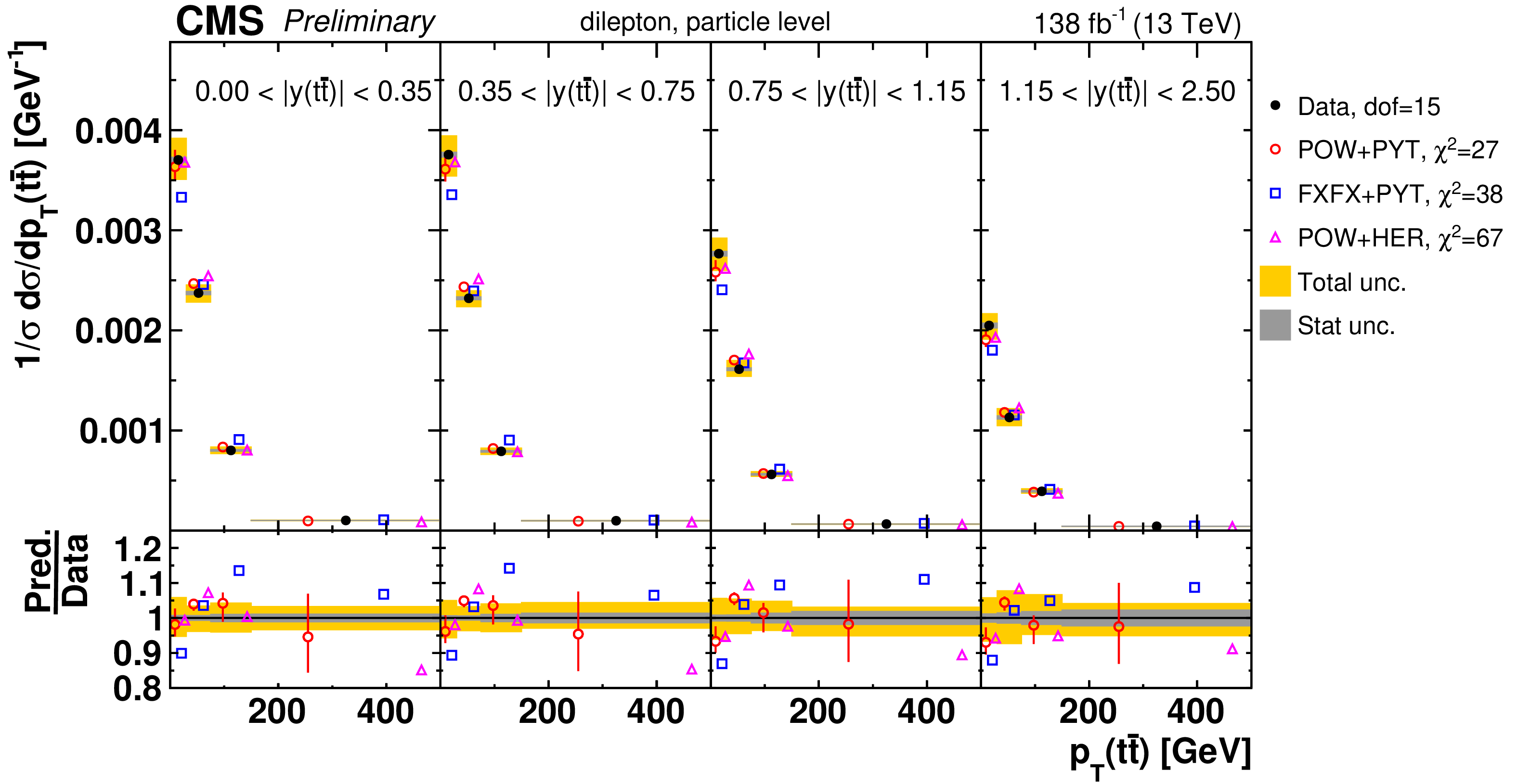
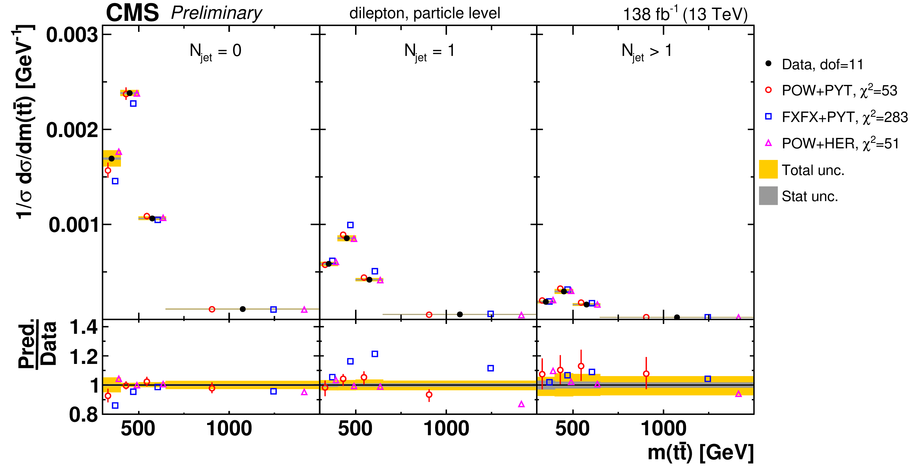
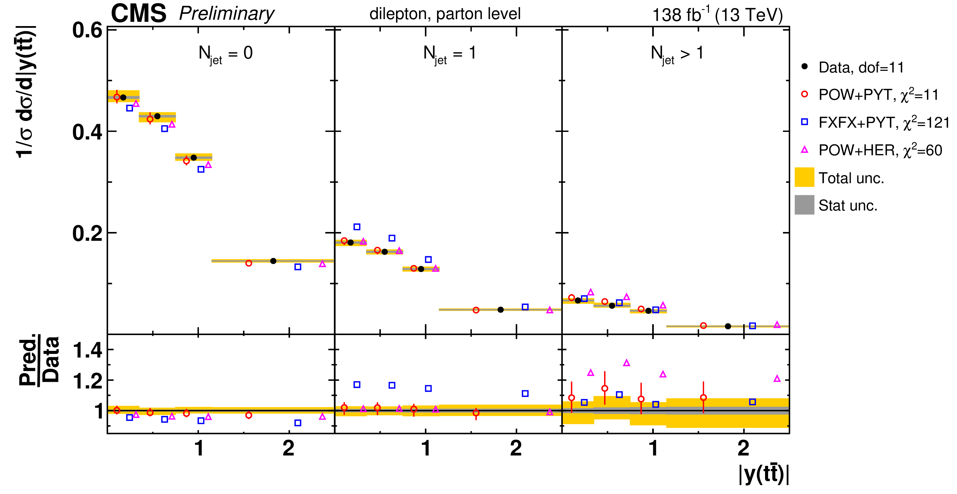
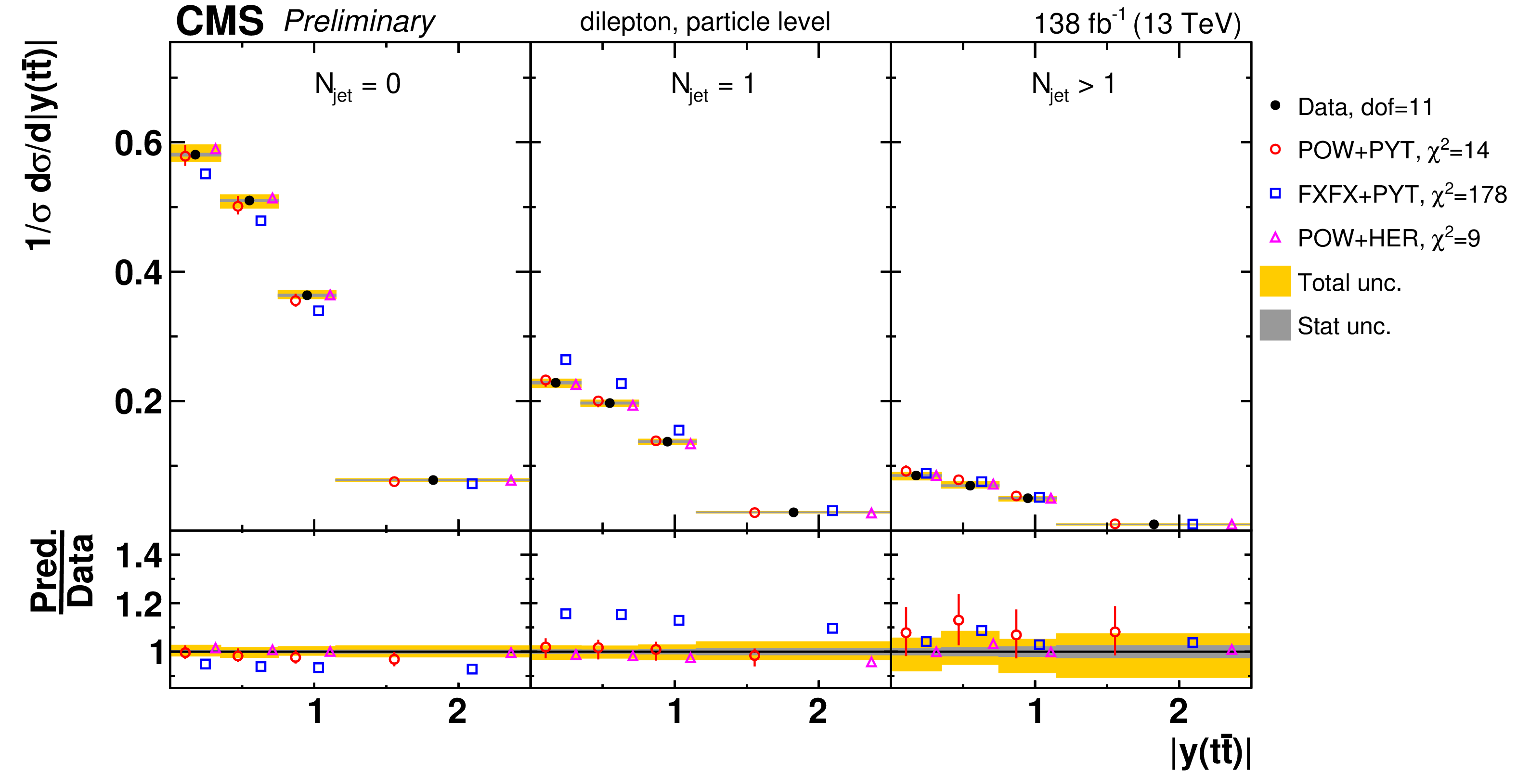
png pdf	Figure 9: Normalized differential $\mathrm{t\bar{t}}$ production cross sections as a function of ${{p_{\mathrm {T}}} ( \mathrm{t\bar{t}})}$ (upper), ${m( \mathrm{t\bar{t}})}$ (middle) and ${y( \mathrm{t\bar{t}})}$ (lower) are shown for data (filled circles) and various MC predictions (other points). The ${m( \mathrm{t\bar{t}})}$ distributions are also compared to POWHEG+PYTHIA-8 (`POW-PYT') simulations with different values of ${m_{\mathrm{t}}^{\text {MC}}}$. Further details can be found in the caption of Fig. 7.
png pdf	Figure 9-a: Normalized differential $\mathrm{t\bar{t}}$ production cross sections as a function of ${{p_{\mathrm {T}}} ( \mathrm{t\bar{t}})}$ (upper), ${m( \mathrm{t\bar{t}})}$ (middle) and ${y( \mathrm{t\bar{t}})}$ (lower) are shown for data (filled circles) and various MC predictions (other points). The ${m( \mathrm{t\bar{t}})}$ distributions are also compared to POWHEG+PYTHIA-8 (`POW-PYT') simulations with different values of ${m_{\mathrm{t}}^{\text {MC}}}$. Further details can be found in the caption of Fig. 7.
png pdf	Figure 9-b: Normalized differential $\mathrm{t\bar{t}}$ production cross sections as a function of ${{p_{\mathrm {T}}} ( \mathrm{t\bar{t}})}$ (upper), ${m( \mathrm{t\bar{t}})}$ (middle) and ${y( \mathrm{t\bar{t}})}$ (lower) are shown for data (filled circles) and various MC predictions (other points). The ${m( \mathrm{t\bar{t}})}$ distributions are also compared to POWHEG+PYTHIA-8 (`POW-PYT') simulations with different values of ${m_{\mathrm{t}}^{\text {MC}}}$. Further details can be found in the caption of Fig. 7.
png pdf	Figure 9-c: Normalized differential $\mathrm{t\bar{t}}$ production cross sections as a function of ${{p_{\mathrm {T}}} ( \mathrm{t\bar{t}})}$ (upper), ${m( \mathrm{t\bar{t}})}$ (middle) and ${y( \mathrm{t\bar{t}})}$ (lower) are shown for data (filled circles) and various MC predictions (other points). The ${m( \mathrm{t\bar{t}})}$ distributions are also compared to POWHEG+PYTHIA-8 (`POW-PYT') simulations with different values of ${m_{\mathrm{t}}^{\text {MC}}}$. Further details can be found in the caption of Fig. 7.
png pdf	Figure 9-d: Normalized differential $\mathrm{t\bar{t}}$ production cross sections as a function of ${{p_{\mathrm {T}}} ( \mathrm{t\bar{t}})}$ (upper), ${m( \mathrm{t\bar{t}})}$ (middle) and ${y( \mathrm{t\bar{t}})}$ (lower) are shown for data (filled circles) and various MC predictions (other points). The ${m( \mathrm{t\bar{t}})}$ distributions are also compared to POWHEG+PYTHIA-8 (`POW-PYT') simulations with different values of ${m_{\mathrm{t}}^{\text {MC}}}$. Further details can be found in the caption of Fig. 7.
png pdf	Figure 9-e: Normalized differential $\mathrm{t\bar{t}}$ production cross sections as a function of ${{p_{\mathrm {T}}} ( \mathrm{t\bar{t}})}$ (upper), ${m( \mathrm{t\bar{t}})}$ (middle) and ${y( \mathrm{t\bar{t}})}$ (lower) are shown for data (filled circles) and various MC predictions (other points). The ${m( \mathrm{t\bar{t}})}$ distributions are also compared to POWHEG+PYTHIA-8 (`POW-PYT') simulations with different values of ${m_{\mathrm{t}}^{\text {MC}}}$. Further details can be found in the caption of Fig. 7.
png pdf	Figure 9-f: Normalized differential $\mathrm{t\bar{t}}$ production cross sections as a function of ${{p_{\mathrm {T}}} ( \mathrm{t\bar{t}})}$ (upper), ${m( \mathrm{t\bar{t}})}$ (middle) and ${y( \mathrm{t\bar{t}})}$ (lower) are shown for data (filled circles) and various MC predictions (other points). The ${m( \mathrm{t\bar{t}})}$ distributions are also compared to POWHEG+PYTHIA-8 (`POW-PYT') simulations with different values of ${m_{\mathrm{t}}^{\text {MC}}}$. Further details can be found in the caption of Fig. 7.
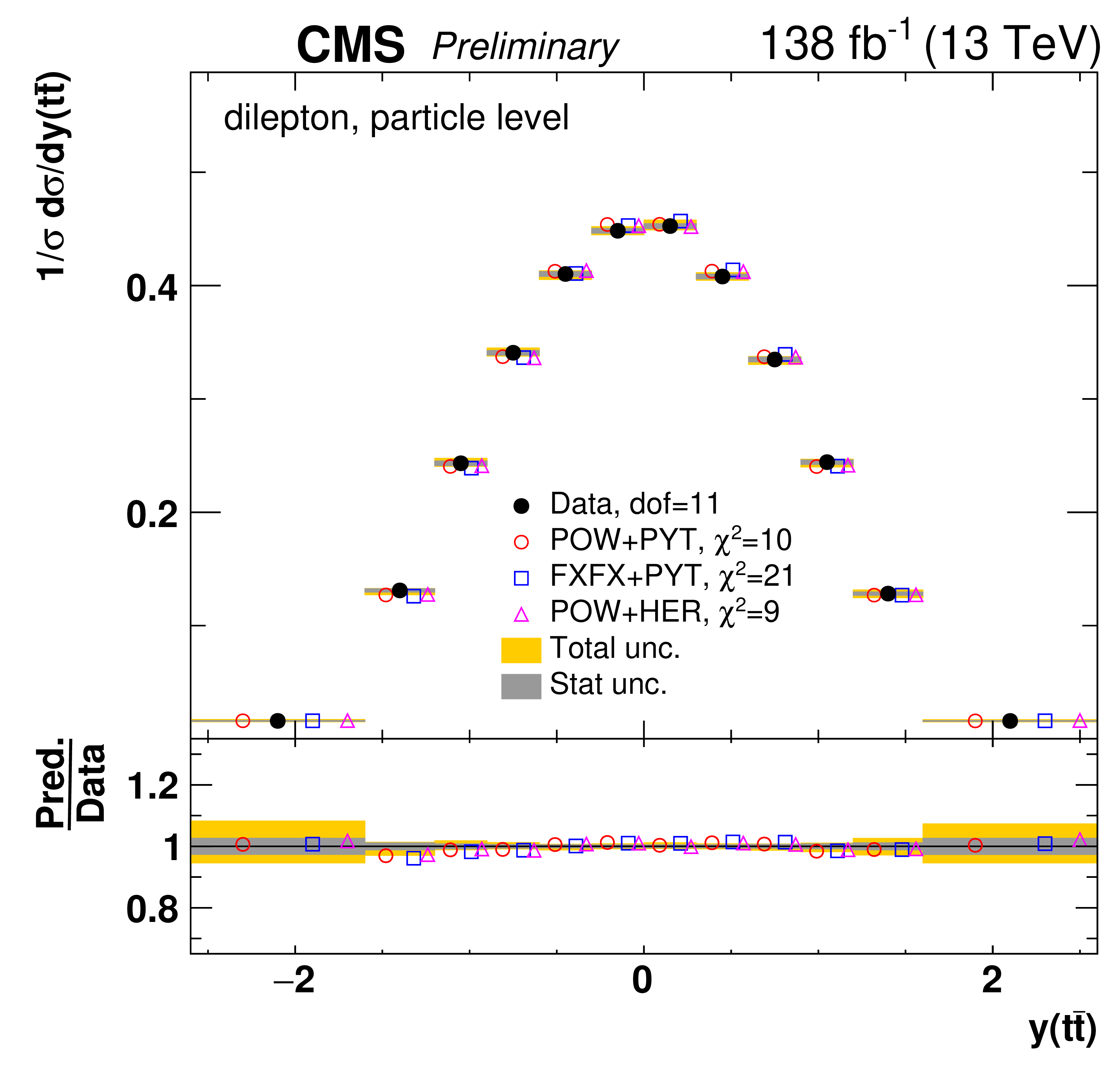
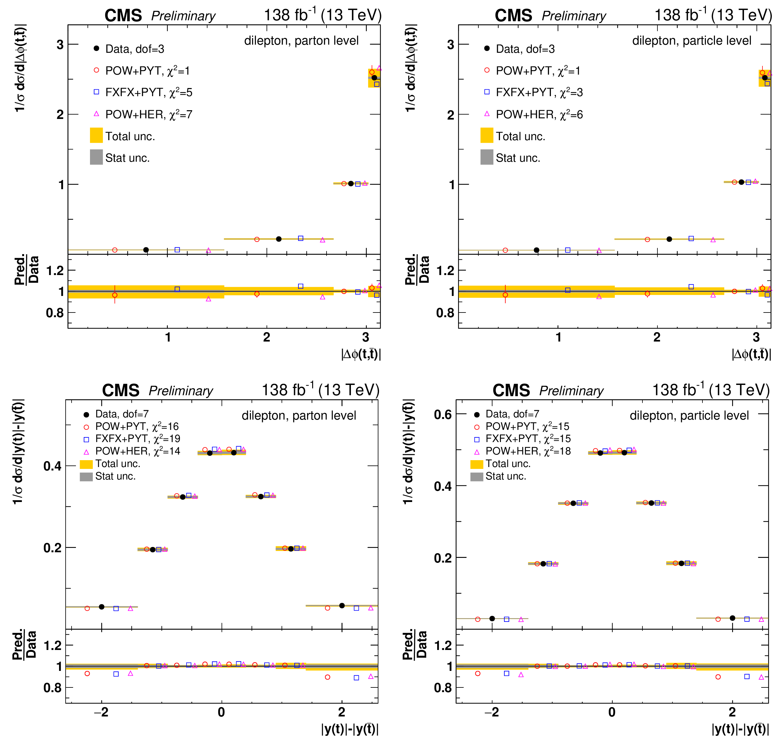
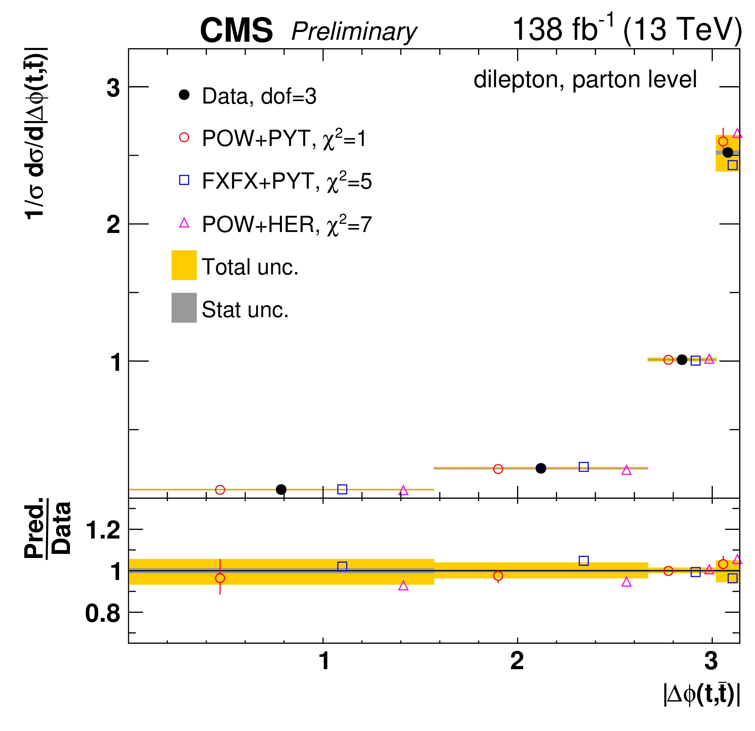
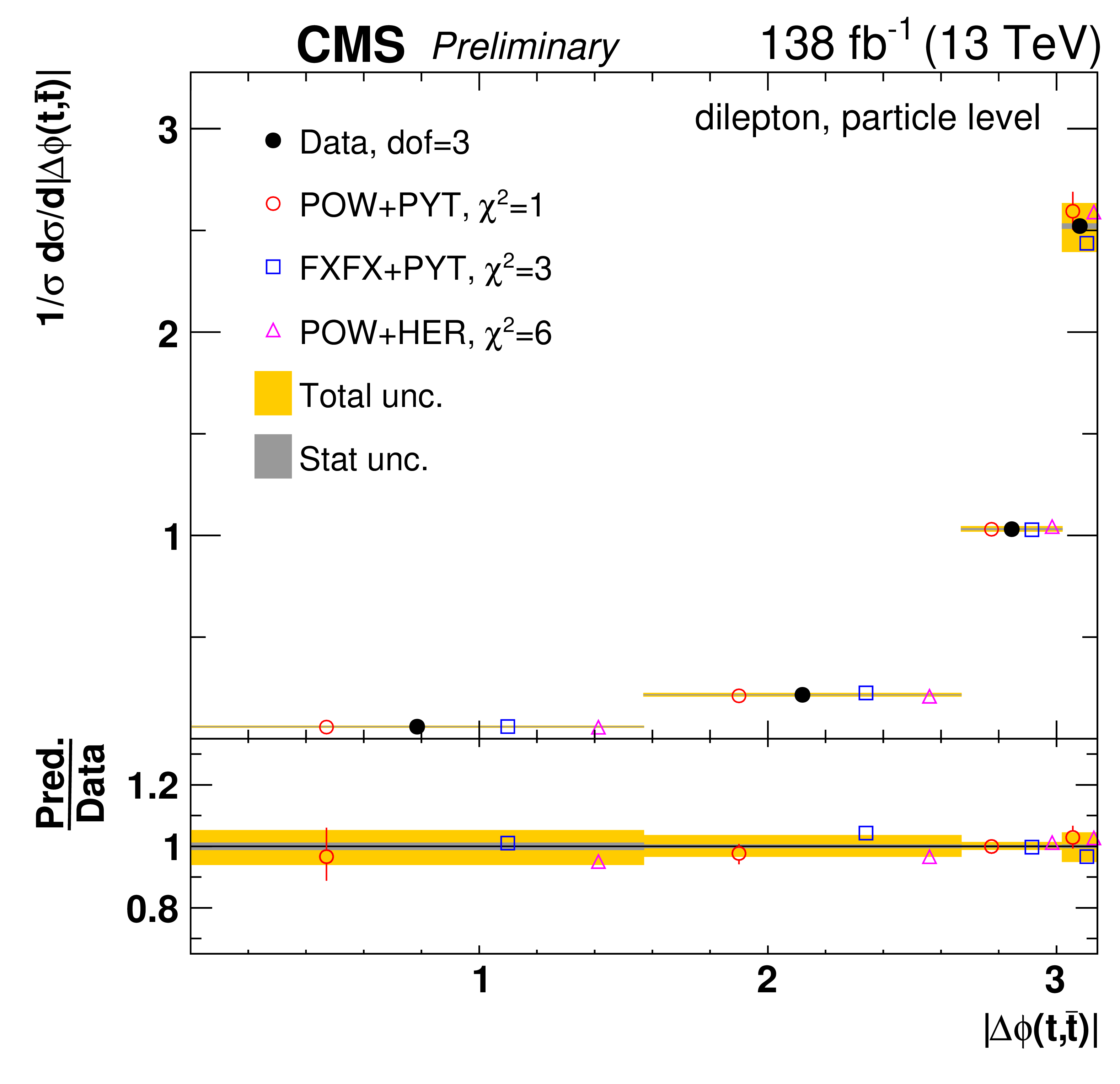
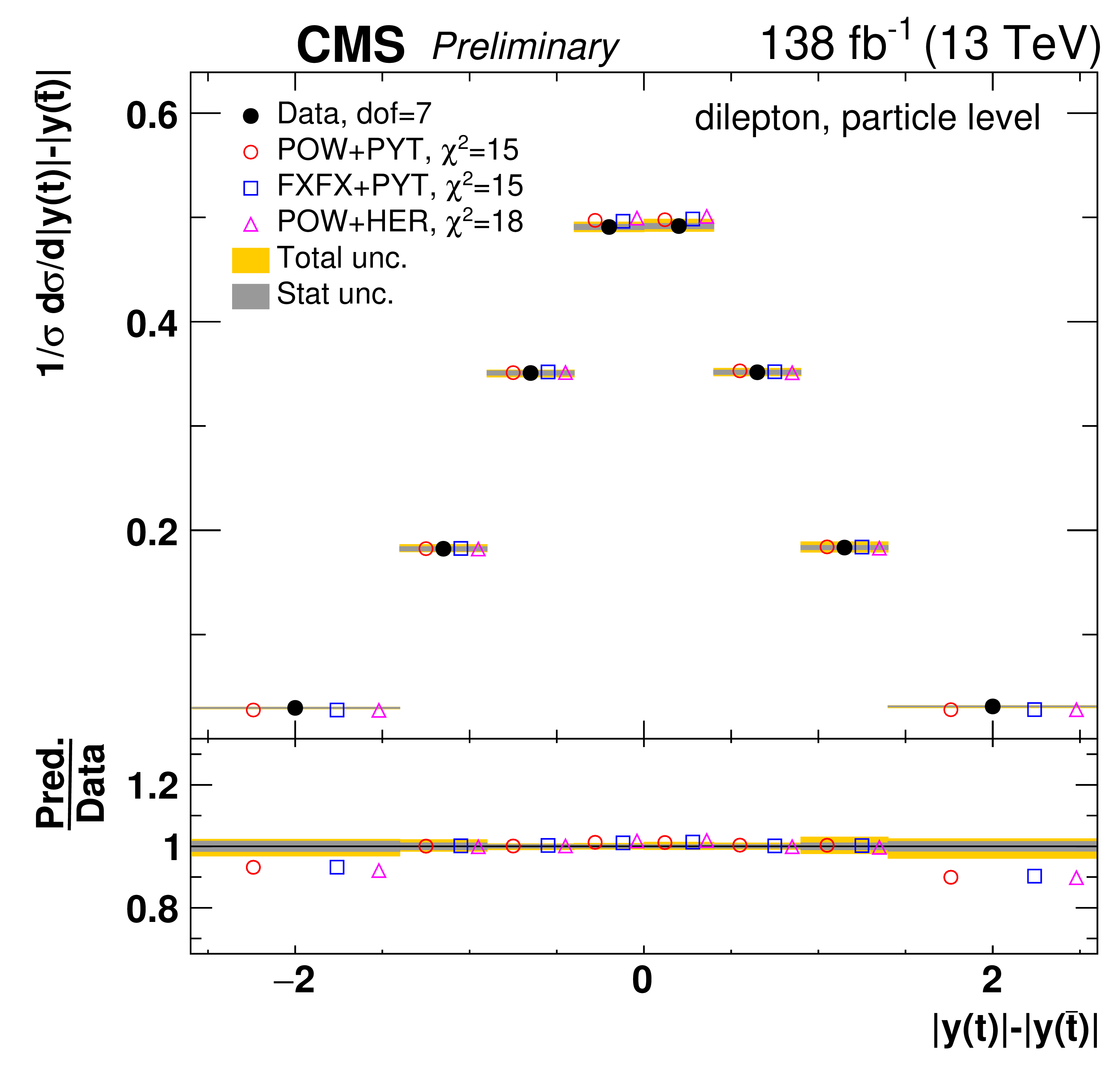
png pdf	Figure 10: Normalized differential $\mathrm{t\bar{t}}$ production cross sections as a function of ${|\Delta \phi (\mathrm{t},\mathrm{\bar{t}})|}$ (upper) and ${|y(\mathrm{t})|-|y(\mathrm{\bar{t}})|}$ (lower) are shown for data (filled circles) and various MC predictions (other points). Further details can be found in the caption of Fig. 7.
png pdf	Figure 10-a: Normalized differential $\mathrm{t\bar{t}}$ production cross sections as a function of ${|\Delta \phi (\mathrm{t},\mathrm{\bar{t}})|}$ (upper) and ${|y(\mathrm{t})|-|y(\mathrm{\bar{t}})|}$ (lower) are shown for data (filled circles) and various MC predictions (other points). Further details can be found in the caption of Fig. 7.
png pdf	Figure 10-b: Normalized differential $\mathrm{t\bar{t}}$ production cross sections as a function of ${|\Delta \phi (\mathrm{t},\mathrm{\bar{t}})|}$ (upper) and ${|y(\mathrm{t})|-|y(\mathrm{\bar{t}})|}$ (lower) are shown for data (filled circles) and various MC predictions (other points). Further details can be found in the caption of Fig. 7.
png pdf	Figure 10-c: Normalized differential $\mathrm{t\bar{t}}$ production cross sections as a function of ${|\Delta \phi (\mathrm{t},\mathrm{\bar{t}})|}$ (upper) and ${|y(\mathrm{t})|-|y(\mathrm{\bar{t}})|}$ (lower) are shown for data (filled circles) and various MC predictions (other points). Further details can be found in the caption of Fig. 7.
png pdf	Figure 10-d: Normalized differential $\mathrm{t\bar{t}}$ production cross sections as a function of ${|\Delta \phi (\mathrm{t},\mathrm{\bar{t}})|}$ (upper) and ${|y(\mathrm{t})|-|y(\mathrm{\bar{t}})|}$ (lower) are shown for data (filled circles) and various MC predictions (other points). Further details can be found in the caption of Fig. 7.
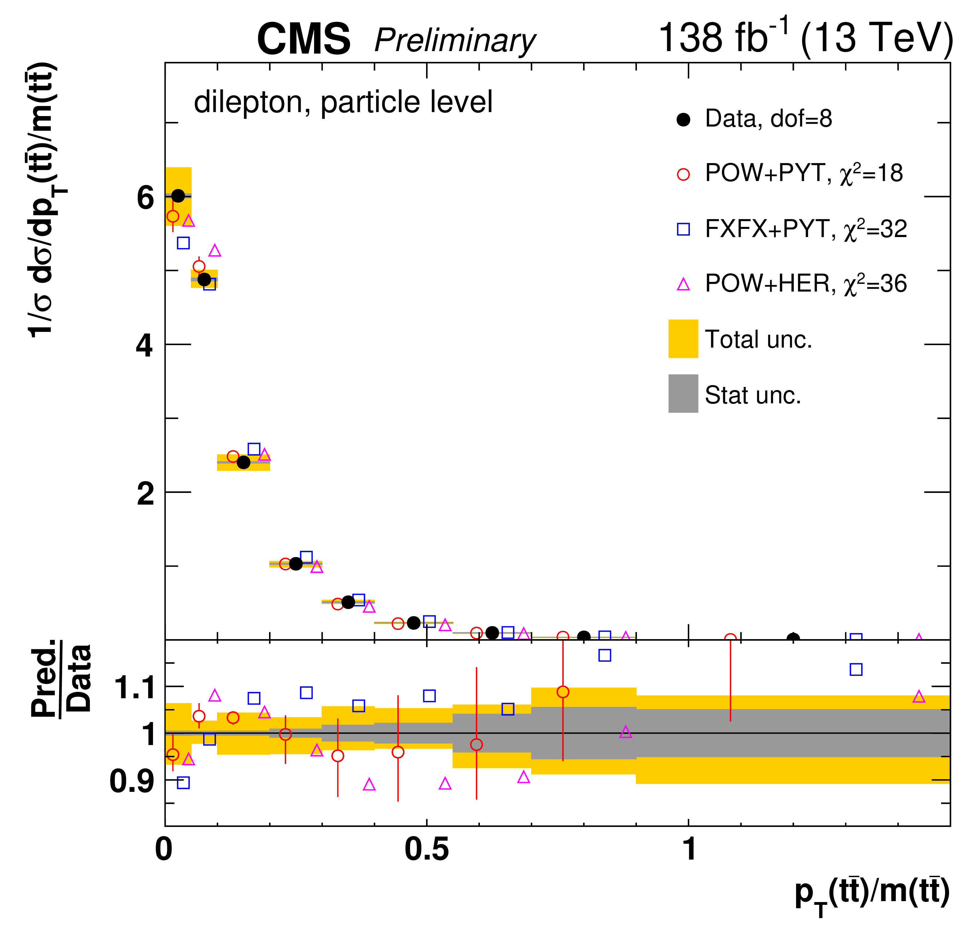
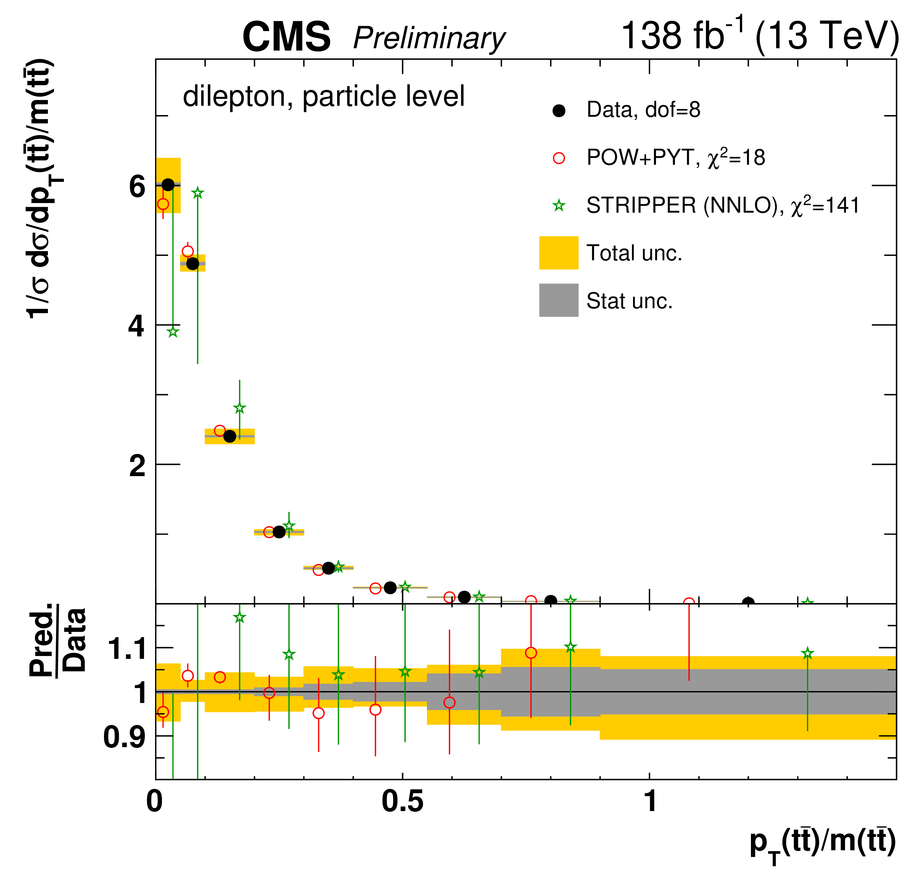
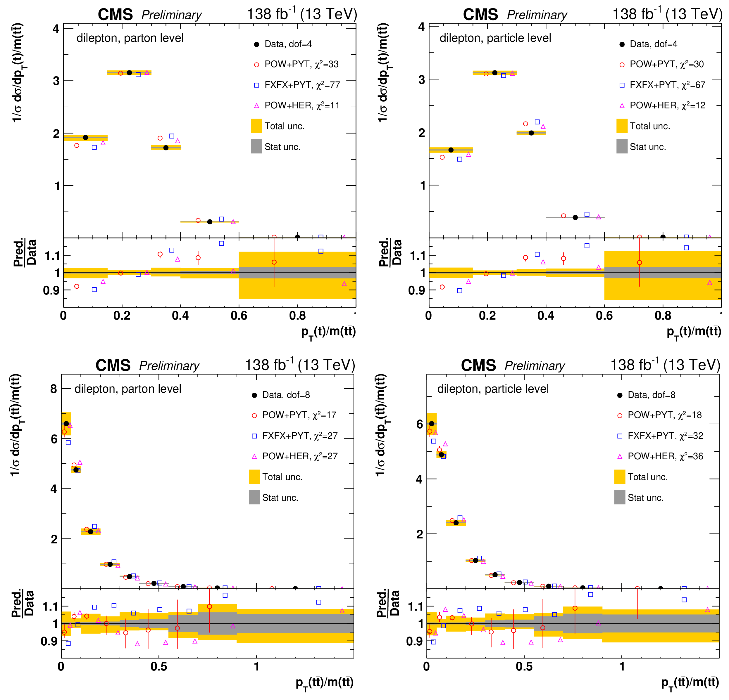
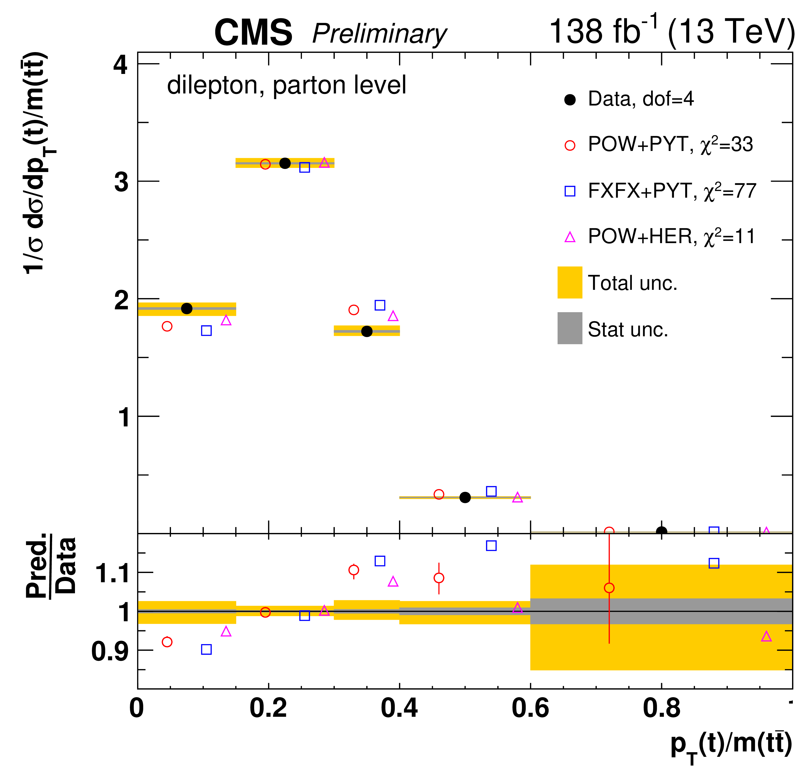
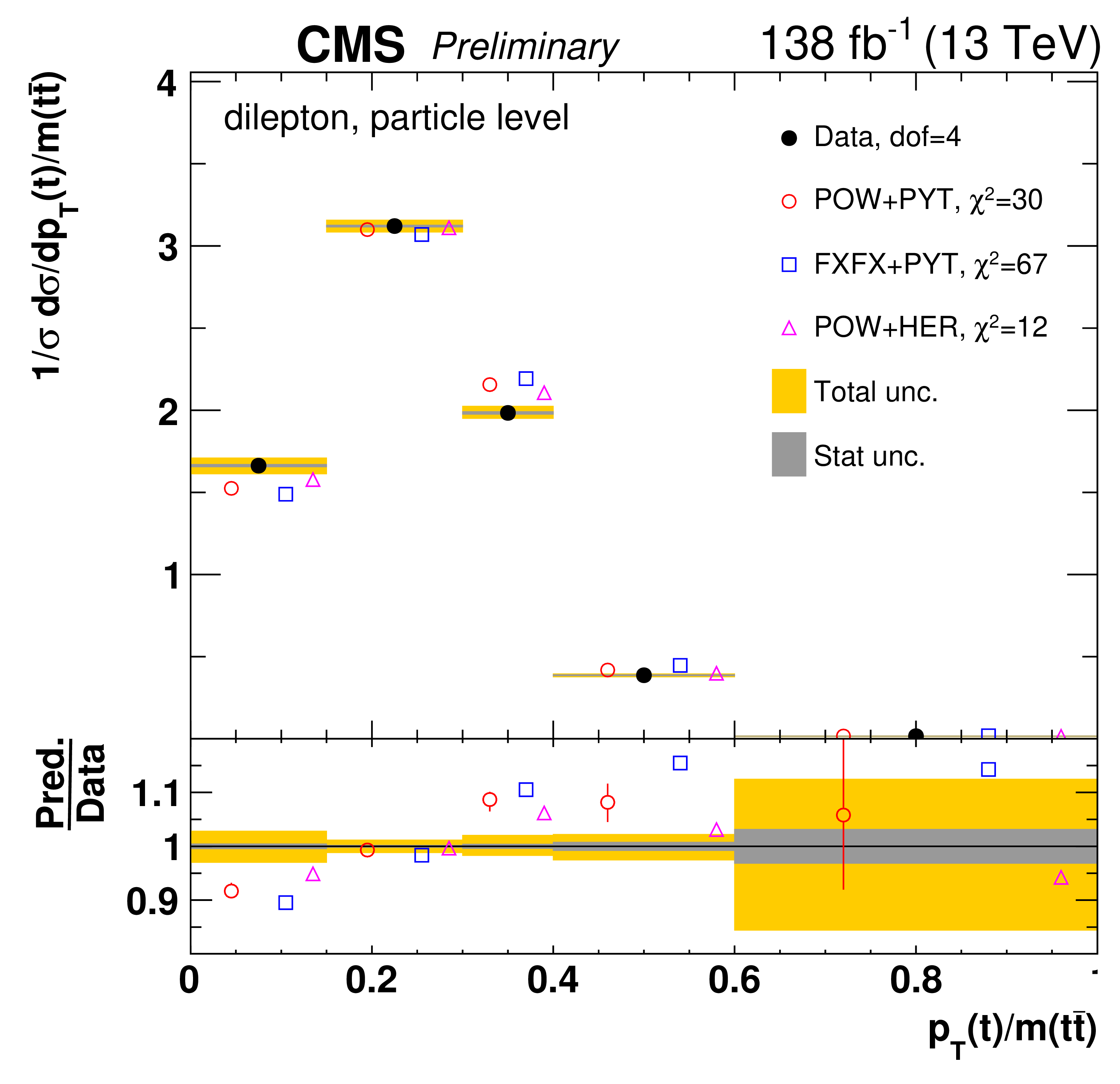
png pdf	Figure 11: Normalized differential $\mathrm{t\bar{t}}$ production cross sections as a function of $ {{p_{\mathrm {T}}} (\mathrm{t})} / {m( \mathrm{t\bar{t}})}$ (upper) and $ {{p_{\mathrm {T}}} ( \mathrm{t\bar{t}})} / {{m( \mathrm{t\bar{t}})}}$ (lower) are shown for data (filled circles) and various MC predictions (other points). Further details can be found in the caption of Fig. 7.
png pdf	Figure 11-a: Normalized differential $\mathrm{t\bar{t}}$ production cross sections as a function of $ {{p_{\mathrm {T}}} (\mathrm{t})} / {m( \mathrm{t\bar{t}})}$ (upper) and $ {{p_{\mathrm {T}}} ( \mathrm{t\bar{t}})} / {{m( \mathrm{t\bar{t}})}}$ (lower) are shown for data (filled circles) and various MC predictions (other points). Further details can be found in the caption of Fig. 7.
png pdf	Figure 11-b: Normalized differential $\mathrm{t\bar{t}}$ production cross sections as a function of $ {{p_{\mathrm {T}}} (\mathrm{t})} / {m( \mathrm{t\bar{t}})}$ (upper) and $ {{p_{\mathrm {T}}} ( \mathrm{t\bar{t}})} / {{m( \mathrm{t\bar{t}})}}$ (lower) are shown for data (filled circles) and various MC predictions (other points). Further details can be found in the caption of Fig. 7.
png pdf	Figure 11-c: Normalized differential $\mathrm{t\bar{t}}$ production cross sections as a function of $ {{p_{\mathrm {T}}} (\mathrm{t})} / {m( \mathrm{t\bar{t}})}$ (upper) and $ {{p_{\mathrm {T}}} ( \mathrm{t\bar{t}})} / {{m( \mathrm{t\bar{t}})}}$ (lower) are shown for data (filled circles) and various MC predictions (other points). Further details can be found in the caption of Fig. 7.
png pdf	Figure 11-d: Normalized differential $\mathrm{t\bar{t}}$ production cross sections as a function of $ {{p_{\mathrm {T}}} (\mathrm{t})} / {m( \mathrm{t\bar{t}})}$ (upper) and $ {{p_{\mathrm {T}}} ( \mathrm{t\bar{t}})} / {{m( \mathrm{t\bar{t}})}}$ (lower) are shown for data (filled circles) and various MC predictions (other points). Further details can be found in the caption of Fig. 7.
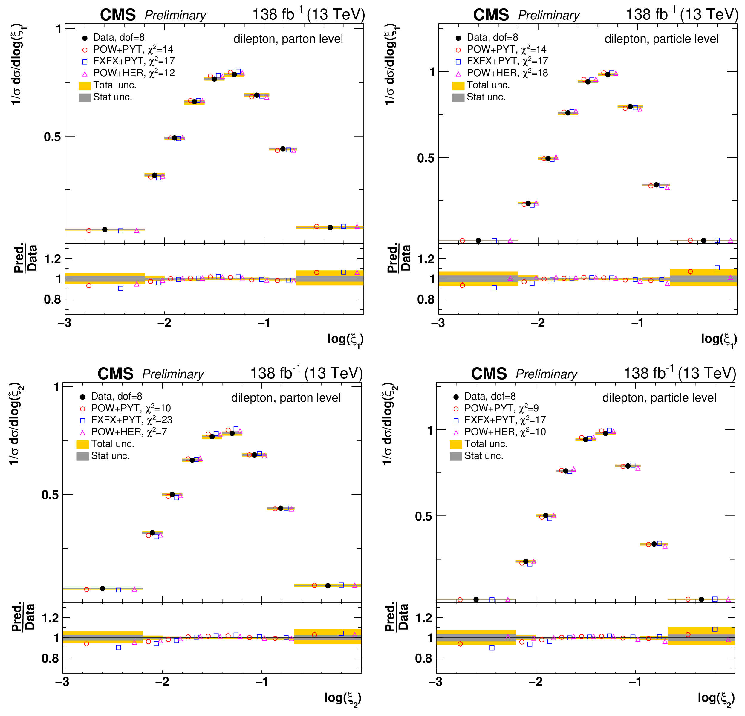
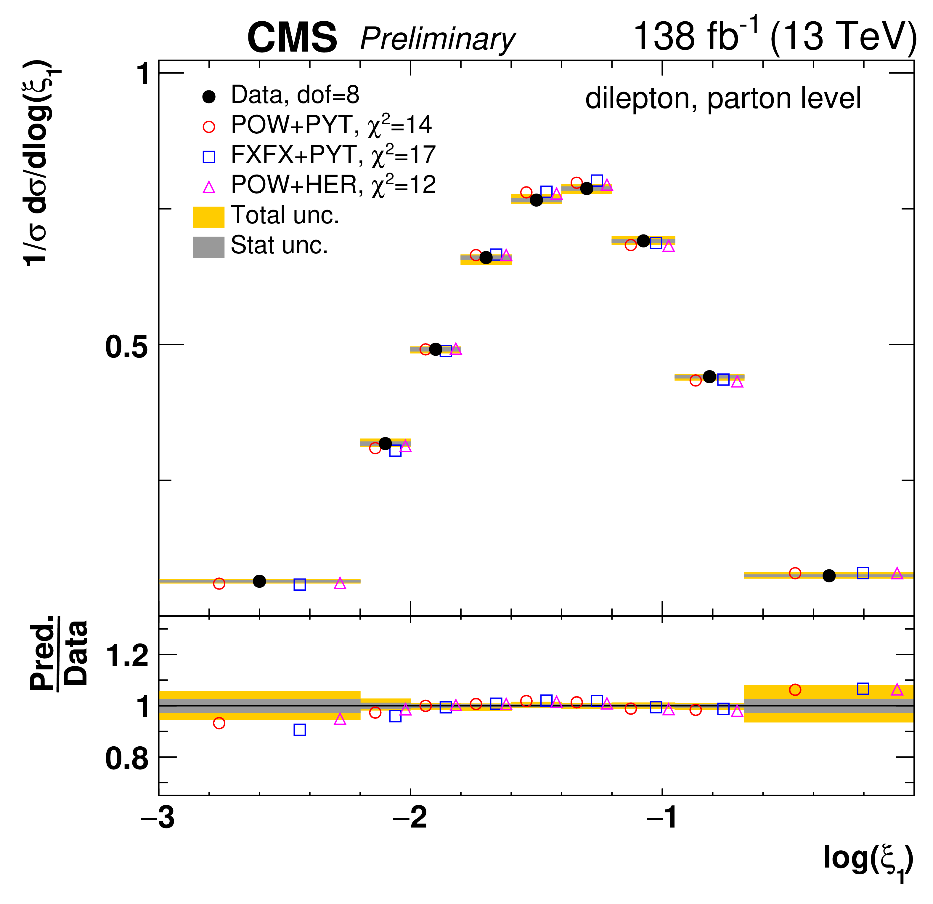
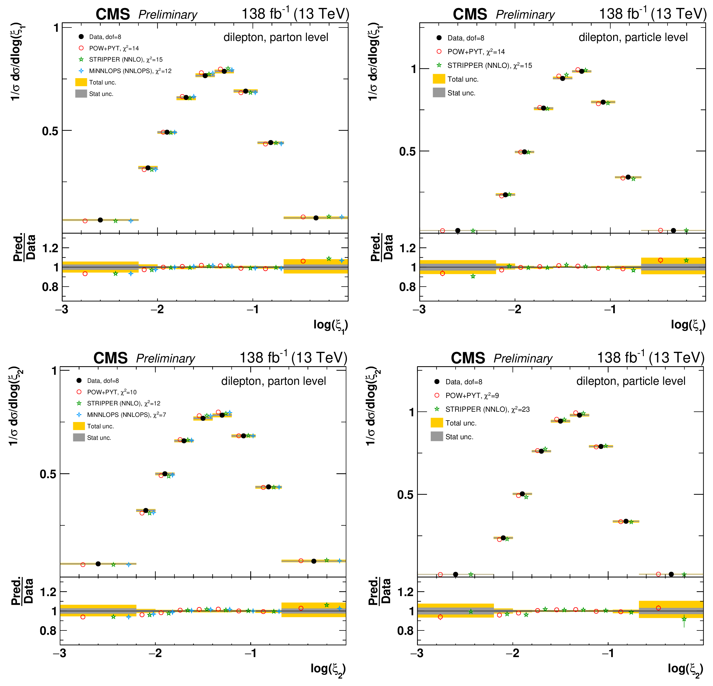
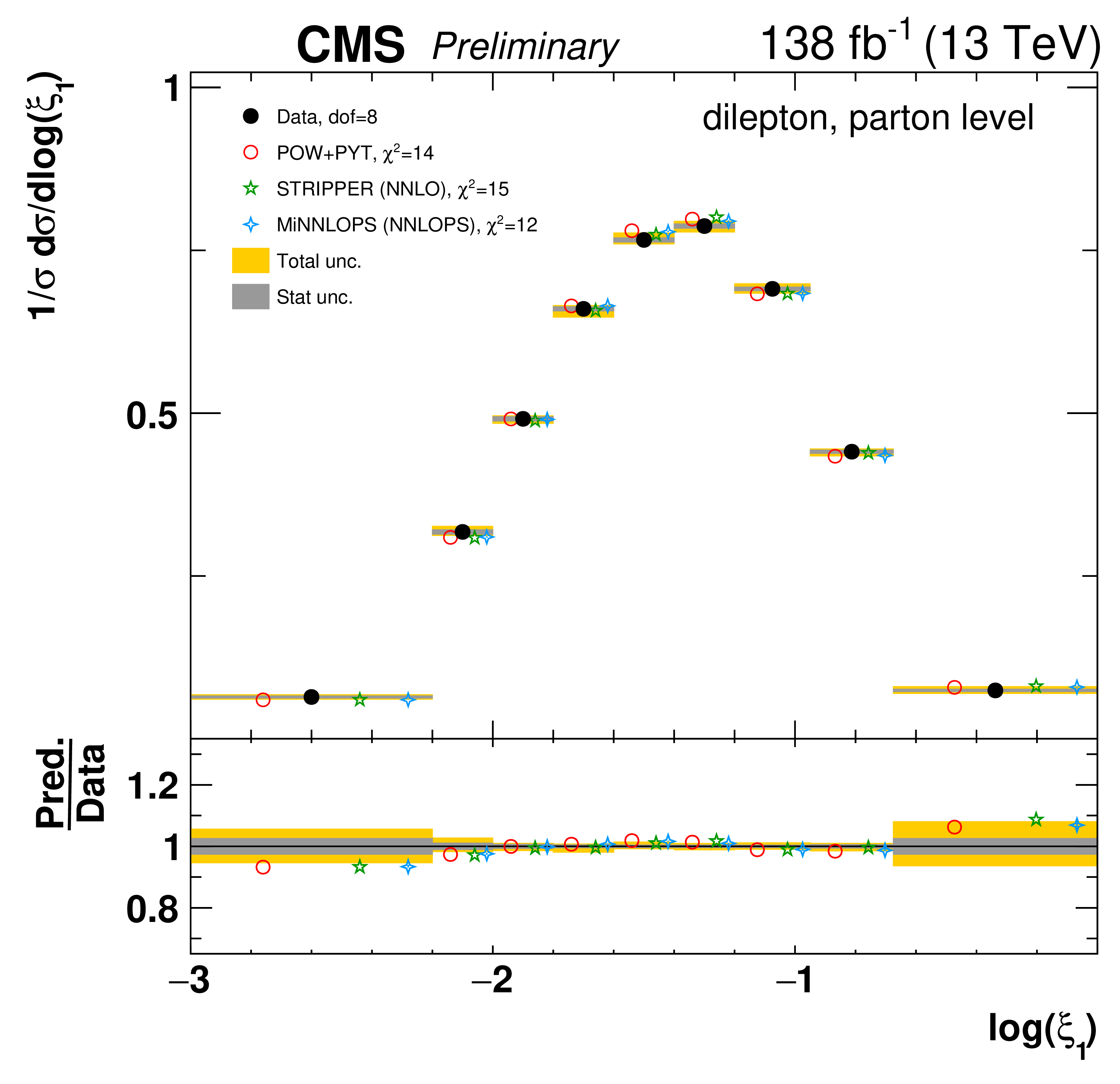
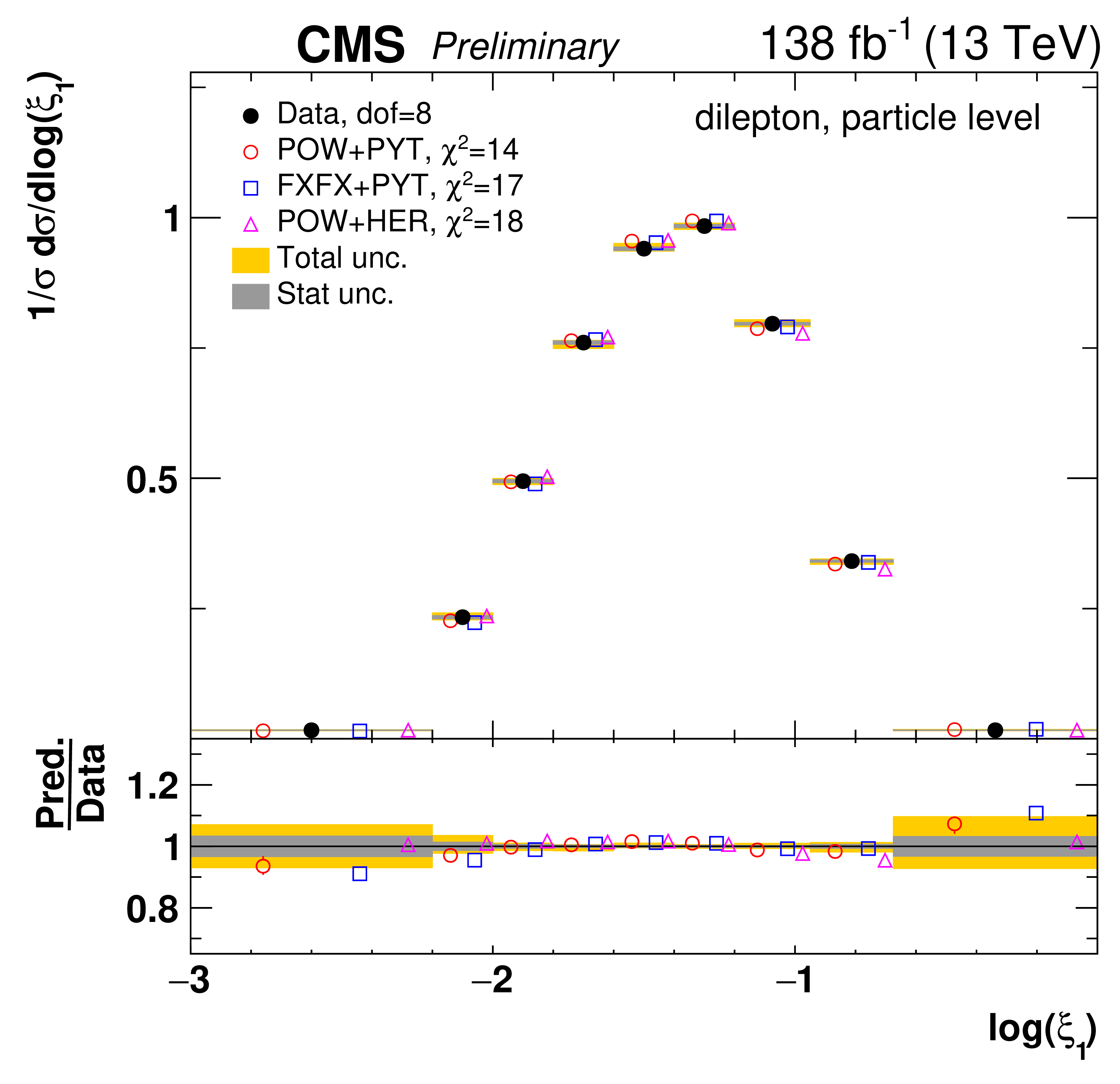
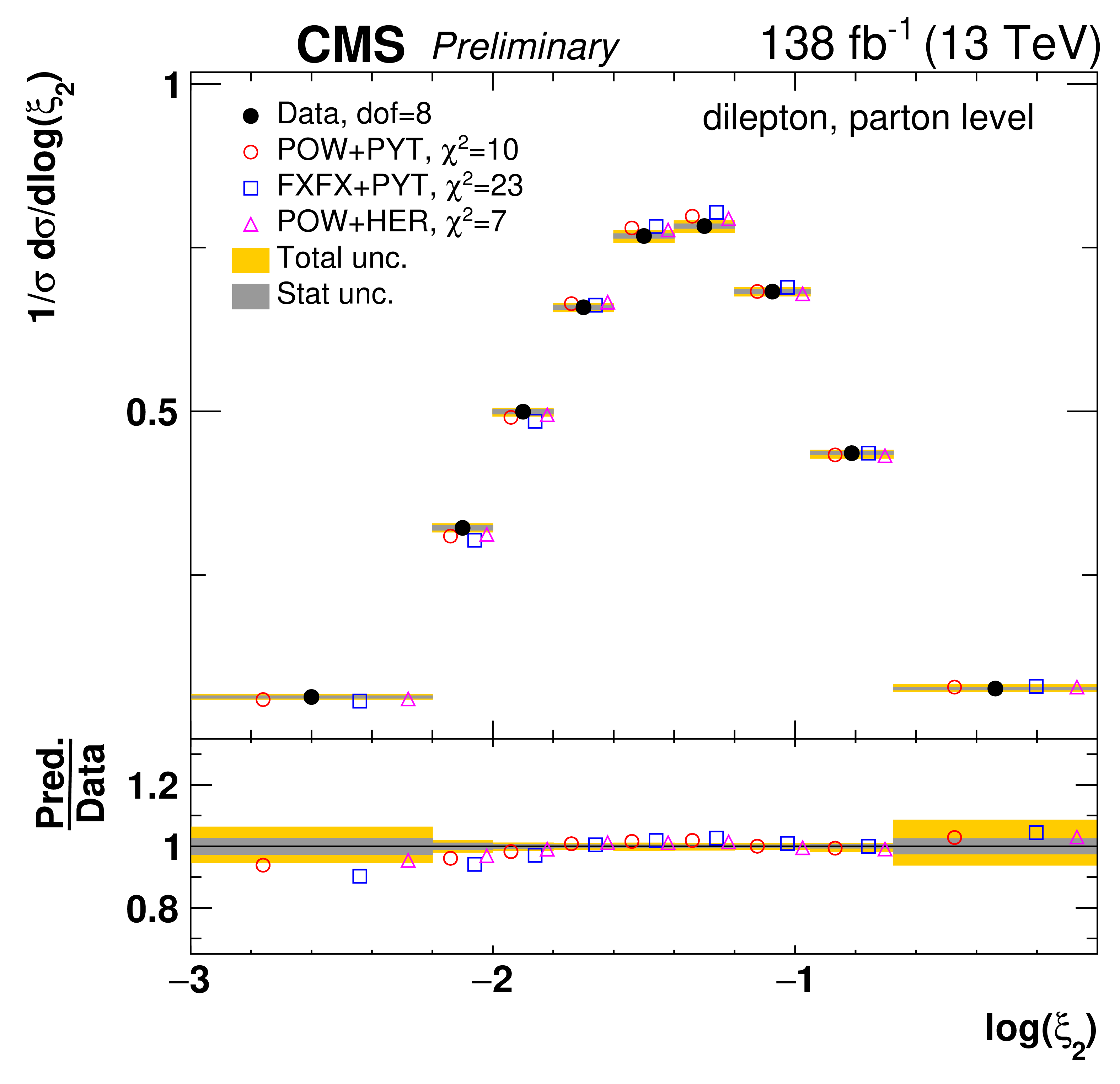
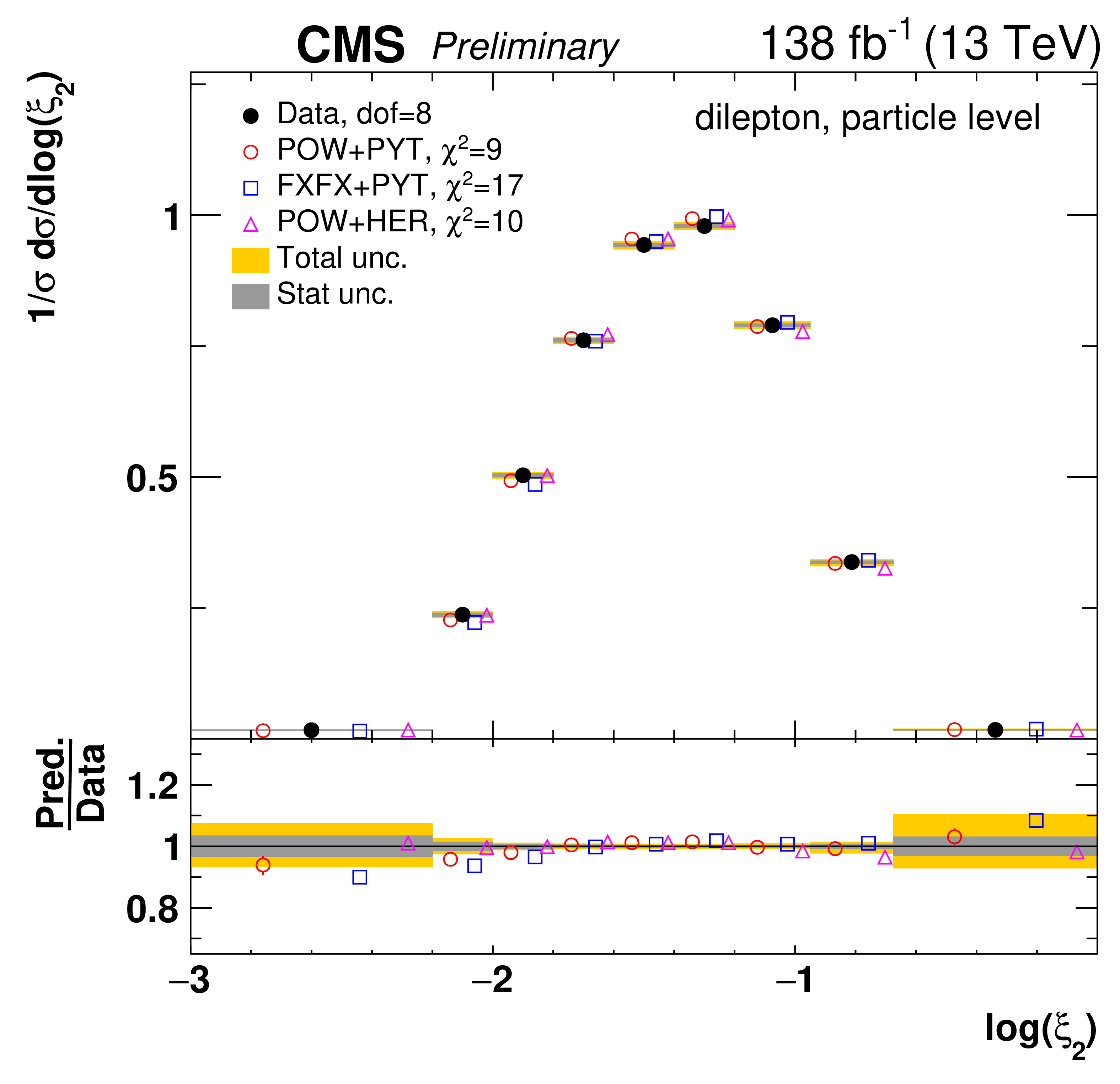
png pdf	Figure 12: Normalized differential $\mathrm{t\bar{t}}$ production cross sections as a function of ${\log(\xi _{1})}$ (upper) and ${\log(\xi _{2})}$ (lower) are shown for data (filled circles) and various MC predictions (other points). Further details can be found in the caption of Fig. 7.
png pdf	Figure 12-a: Normalized differential $\mathrm{t\bar{t}}$ production cross sections as a function of ${\log(\xi _{1})}$ (upper) and ${\log(\xi _{2})}$ (lower) are shown for data (filled circles) and various MC predictions (other points). Further details can be found in the caption of Fig. 7.
png pdf	Figure 12-b: Normalized differential $\mathrm{t\bar{t}}$ production cross sections as a function of ${\log(\xi _{1})}$ (upper) and ${\log(\xi _{2})}$ (lower) are shown for data (filled circles) and various MC predictions (other points). Further details can be found in the caption of Fig. 7.
png pdf	Figure 12-c: Normalized differential $\mathrm{t\bar{t}}$ production cross sections as a function of ${\log(\xi _{1})}$ (upper) and ${\log(\xi _{2})}$ (lower) are shown for data (filled circles) and various MC predictions (other points). Further details can be found in the caption of Fig. 7.
png pdf	Figure 12-d: Normalized differential $\mathrm{t\bar{t}}$ production cross sections as a function of ${\log(\xi _{1})}$ (upper) and ${\log(\xi _{2})}$ (lower) are shown for data (filled circles) and various MC predictions (other points). Further details can be found in the caption of Fig. 7.
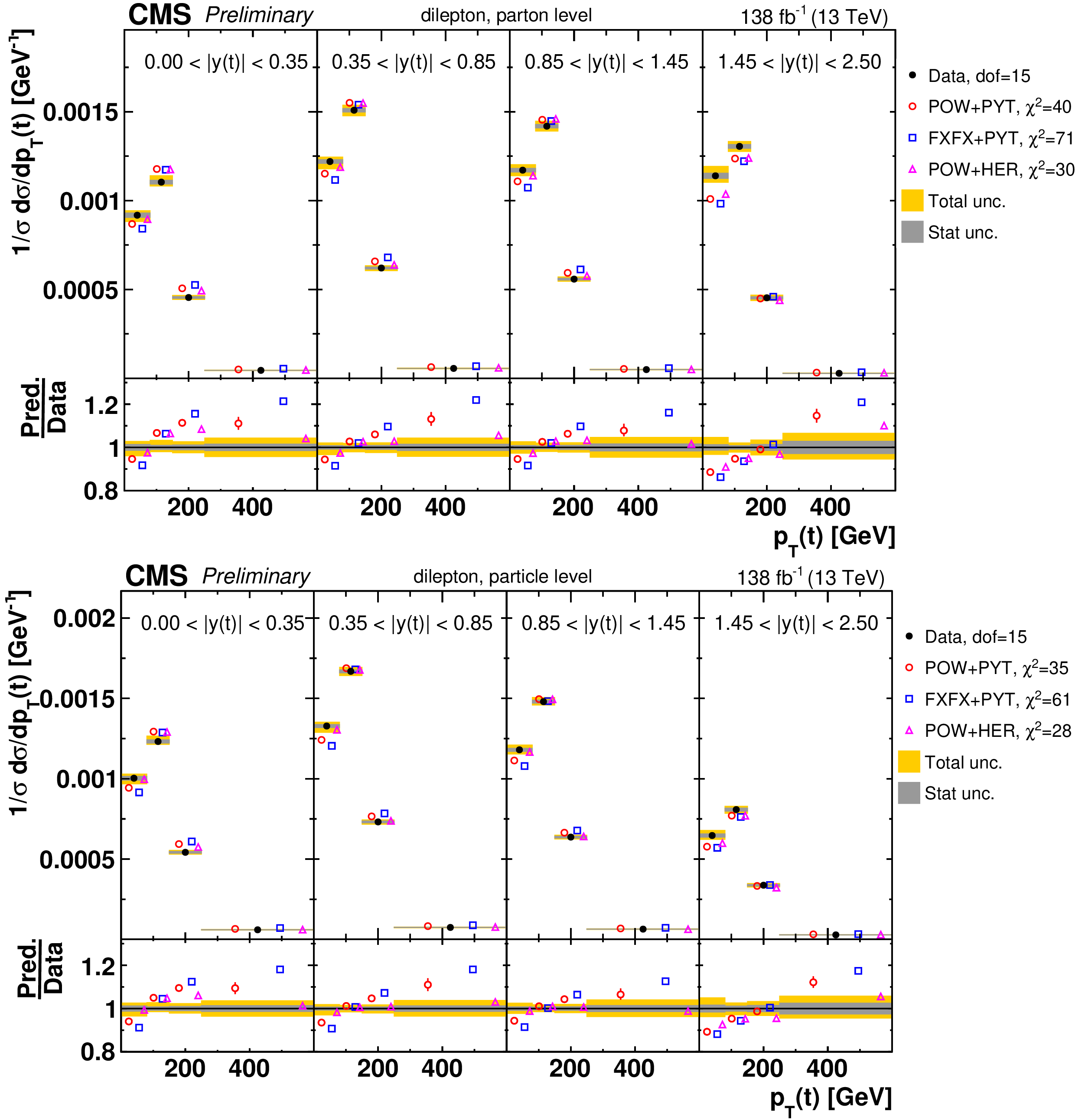
png pdf	Figure 13: Normalized $[ {|y(\mathrm{t})|},\,{{p_{\mathrm {T}}} (\mathrm{t})} ]$ cross sections measured at the parton level in the full phase space (upper) and at the particle level in a fiducial phase space (lower). The data are shown as filled circles with dark and light bands indicating the statistical and total uncertainties (statistical and systematic uncertainties summed in quadrature), respectively. The cross sections are compared to various MC predictions (other points). The estimated uncertainties in the POWHEG+PYTHIA-8 (`POW-PYT') simulation are represented by a vertical bar on the corresponding points. For each MC model, a value of ${\chi ^2}$ is reported that takes into account the measurement uncertainties. The lower panel in each plot shows the ratios of the predictions to the data.
png pdf	Figure 13-a: Normalized $[ {|y(\mathrm{t})|},\,{{p_{\mathrm {T}}} (\mathrm{t})} ]$ cross sections measured at the parton level in the full phase space (upper) and at the particle level in a fiducial phase space (lower). The data are shown as filled circles with dark and light bands indicating the statistical and total uncertainties (statistical and systematic uncertainties summed in quadrature), respectively. The cross sections are compared to various MC predictions (other points). The estimated uncertainties in the POWHEG+PYTHIA-8 (`POW-PYT') simulation are represented by a vertical bar on the corresponding points. For each MC model, a value of ${\chi ^2}$ is reported that takes into account the measurement uncertainties. The lower panel in each plot shows the ratios of the predictions to the data.
png pdf	Figure 13-b: Normalized $[ {|y(\mathrm{t})|},\,{{p_{\mathrm {T}}} (\mathrm{t})} ]$ cross sections measured at the parton level in the full phase space (upper) and at the particle level in a fiducial phase space (lower). The data are shown as filled circles with dark and light bands indicating the statistical and total uncertainties (statistical and systematic uncertainties summed in quadrature), respectively. The cross sections are compared to various MC predictions (other points). The estimated uncertainties in the POWHEG+PYTHIA-8 (`POW-PYT') simulation are represented by a vertical bar on the corresponding points. For each MC model, a value of ${\chi ^2}$ is reported that takes into account the measurement uncertainties. The lower panel in each plot shows the ratios of the predictions to the data.
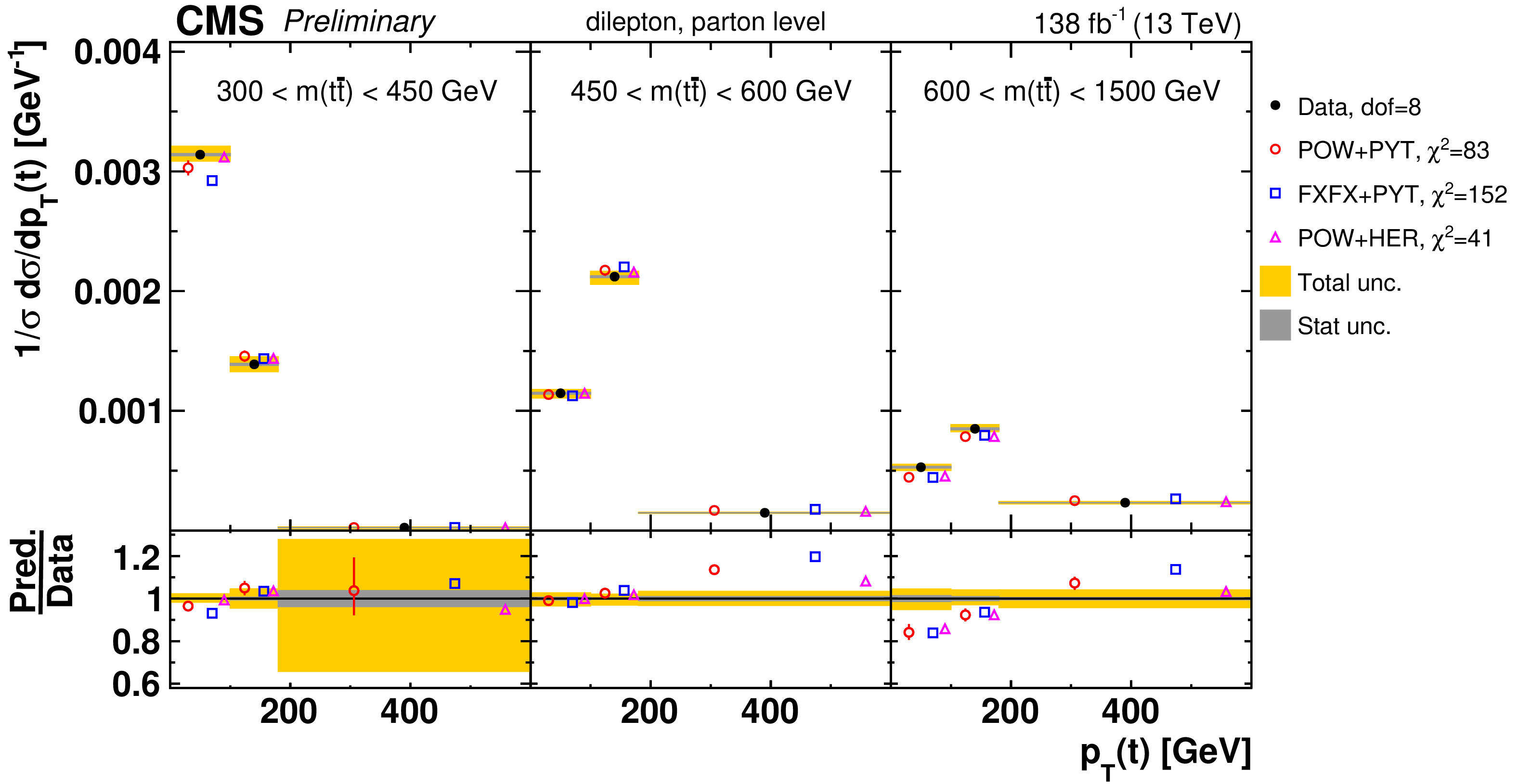
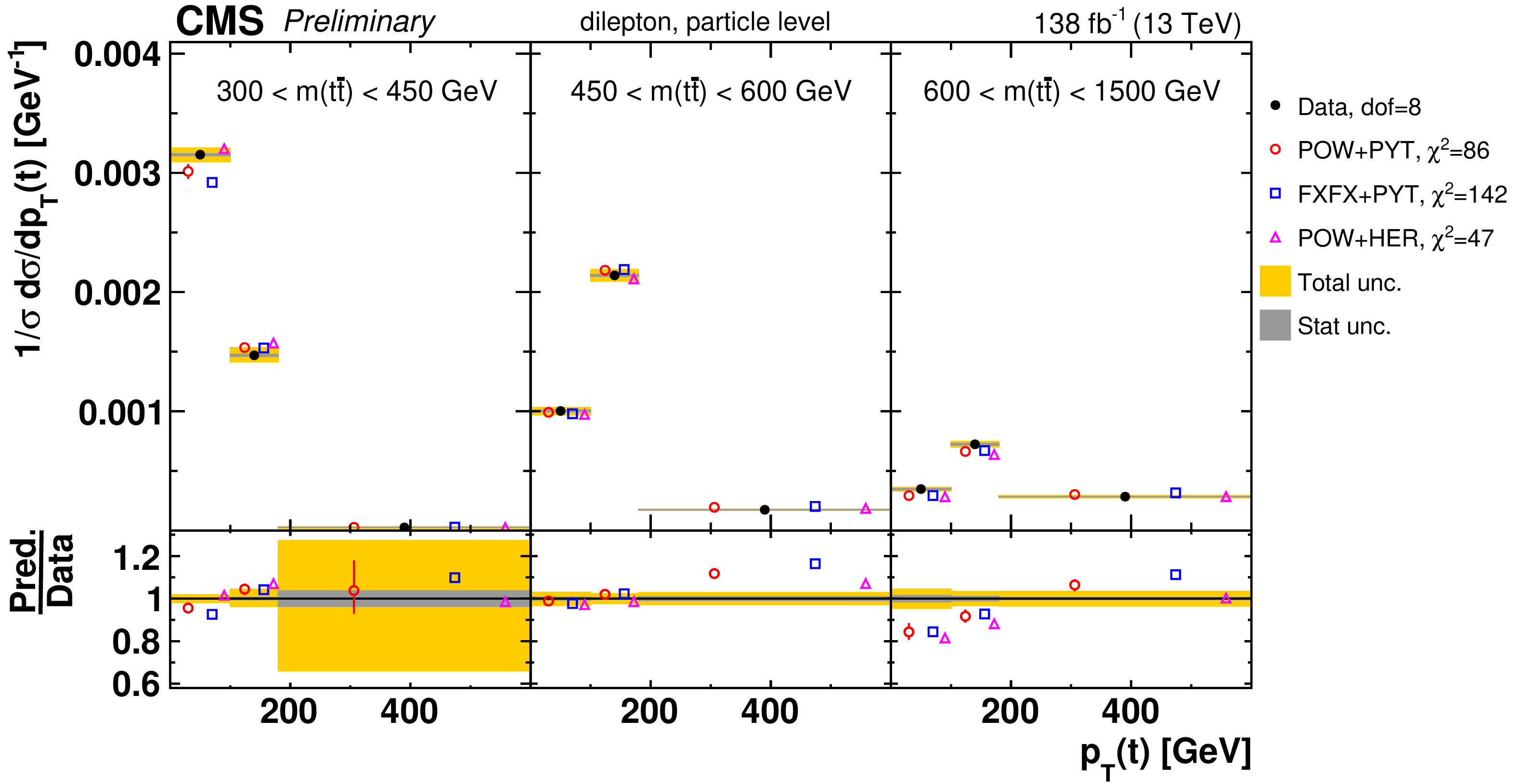
png pdf	Figure 14: Normalized $[ {m( \mathrm{t\bar{t}})},\,{{p_{\mathrm {T}}} (\mathrm{t})} ]$ cross sections are shown for data (filled circles) and various MC predictions (other points). Further details can be found in the caption of Fig. 13.
png pdf	Figure 14-a: Normalized $[ {m( \mathrm{t\bar{t}})},\,{{p_{\mathrm {T}}} (\mathrm{t})} ]$ cross sections are shown for data (filled circles) and various MC predictions (other points). Further details can be found in the caption of Fig. 13.
png pdf	Figure 14-b: Normalized $[ {m( \mathrm{t\bar{t}})},\,{{p_{\mathrm {T}}} (\mathrm{t})} ]$ cross sections are shown for data (filled circles) and various MC predictions (other points). Further details can be found in the caption of Fig. 13.
png pdf	Figure 15: Normalized $[ {{p_{\mathrm {T}}} (\mathrm{t})},\,{{p_{\mathrm {T}}} ( \mathrm{t\bar{t}})} ]$ cross sections are shown for data (filled circles) and various MC predictions (other points). Further details can be found in the caption of Fig. 13.
png pdf	Figure 15-a: Normalized $[ {{p_{\mathrm {T}}} (\mathrm{t})},\,{{p_{\mathrm {T}}} ( \mathrm{t\bar{t}})} ]$ cross sections are shown for data (filled circles) and various MC predictions (other points). Further details can be found in the caption of Fig. 13.
png pdf	Figure 15-b: Normalized $[ {{p_{\mathrm {T}}} (\mathrm{t})},\,{{p_{\mathrm {T}}} ( \mathrm{t\bar{t}})} ]$ cross sections are shown for data (filled circles) and various MC predictions (other points). Further details can be found in the caption of Fig. 13.
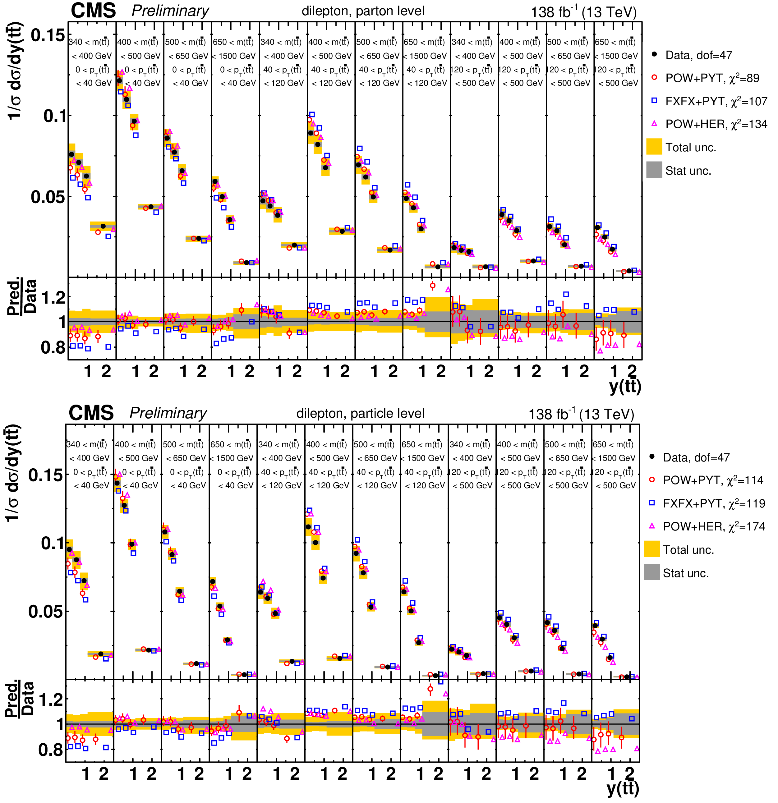
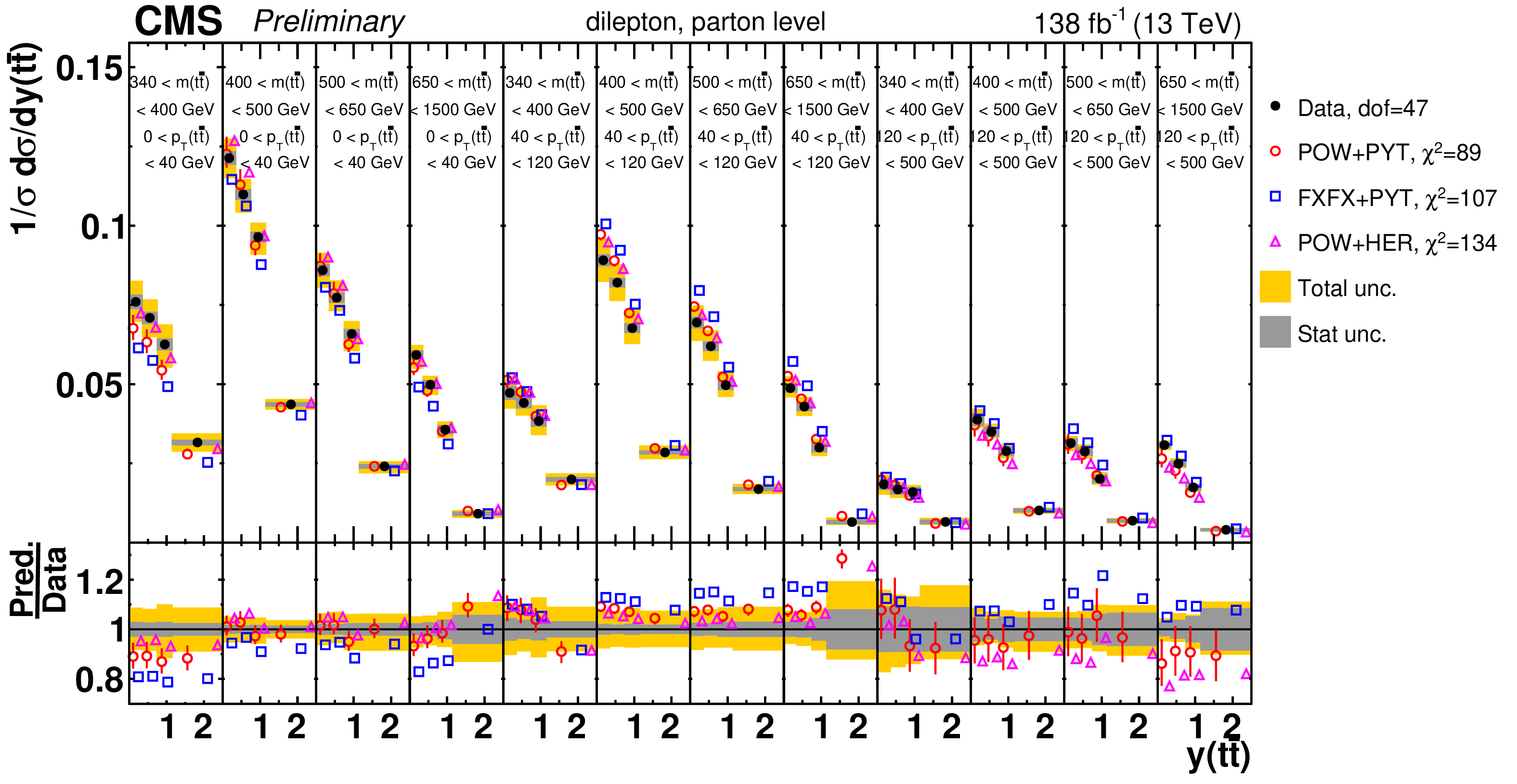
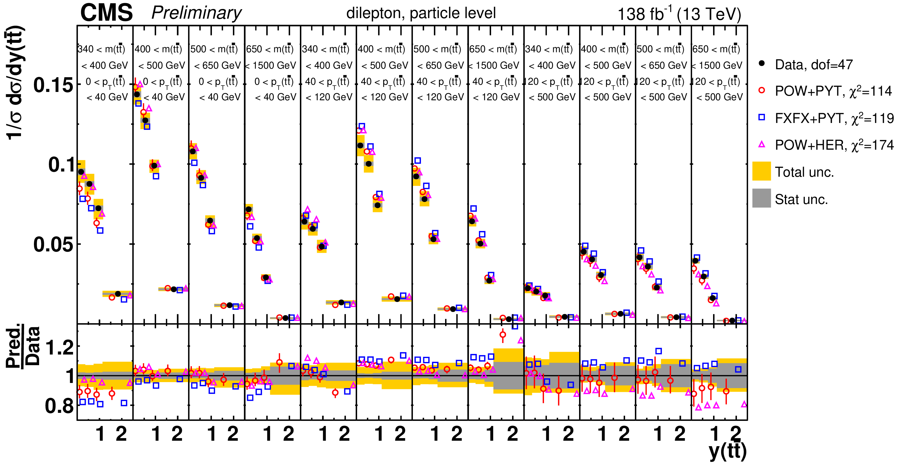
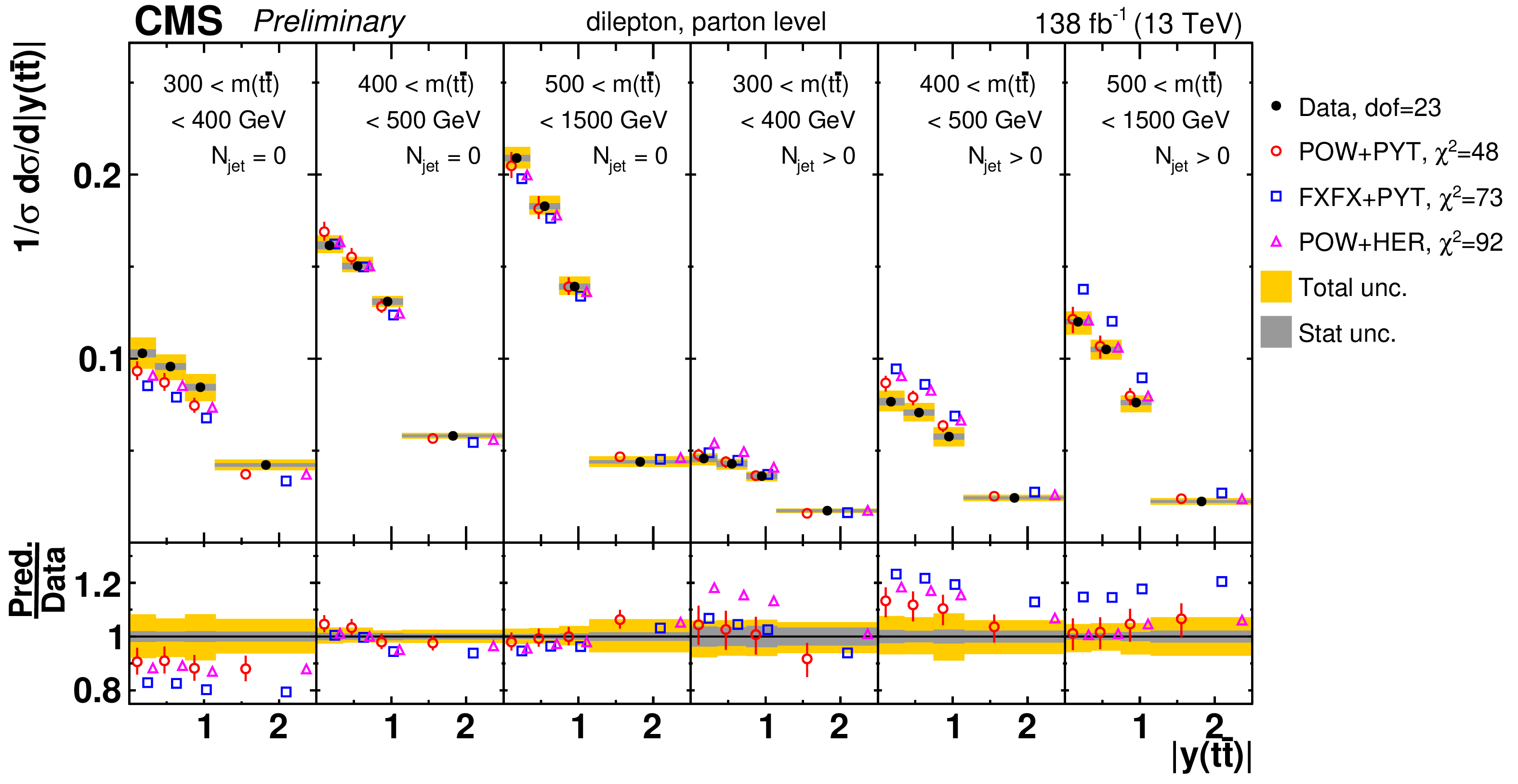
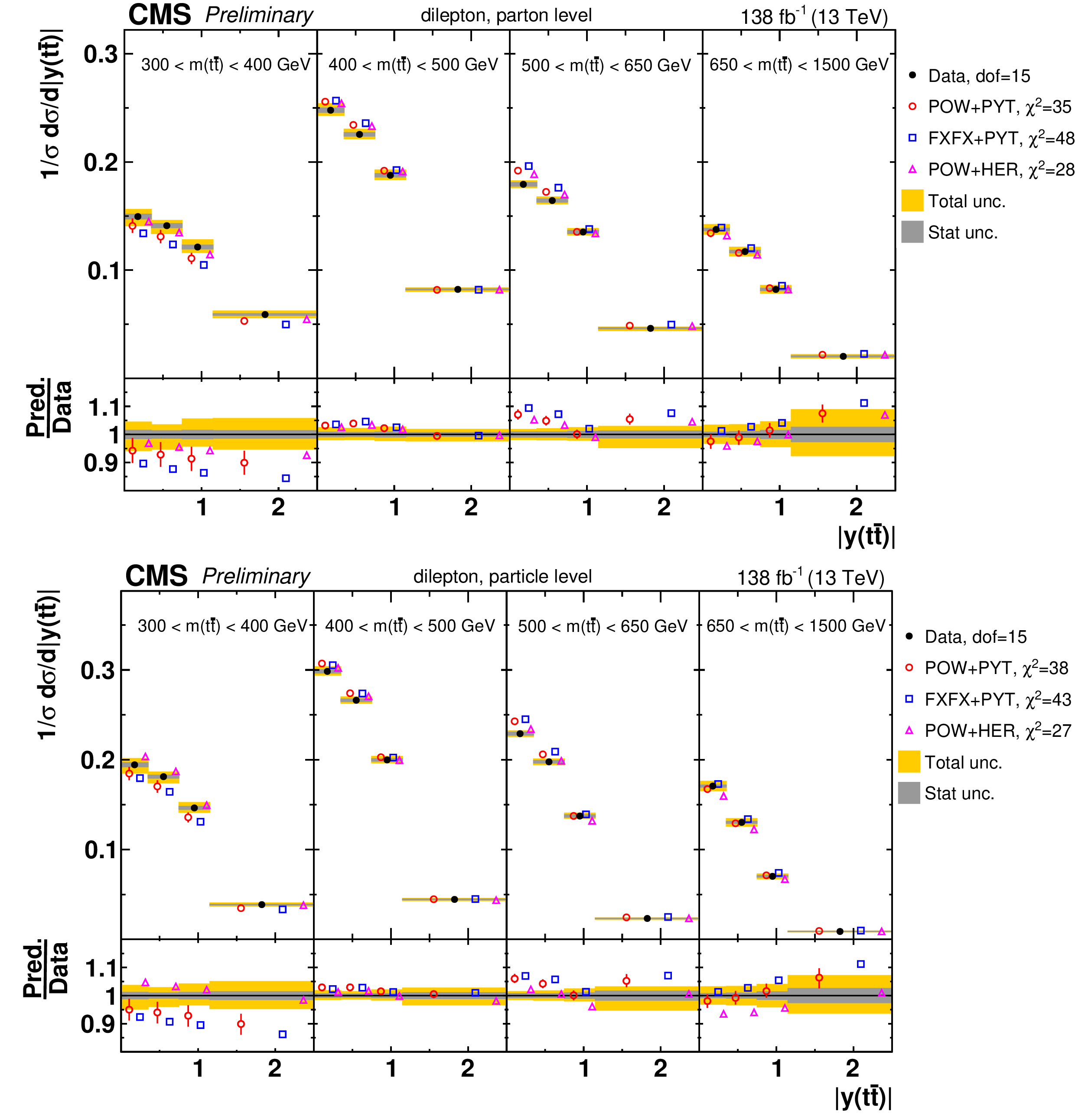
png pdf	Figure 16: Normalized $[ {m( \mathrm{t\bar{t}})},\,{|y( \mathrm{t\bar{t}})|} ]$ cross sections are shown for data (filled circles) and various MC predictions (other points). Further details can be found in the caption of Fig. 13.
png pdf	Figure 16-a: Normalized $[ {m( \mathrm{t\bar{t}})},\,{|y( \mathrm{t\bar{t}})|} ]$ cross sections are shown for data (filled circles) and various MC predictions (other points). Further details can be found in the caption of Fig. 13.
png pdf	Figure 16-b: Normalized $[ {m( \mathrm{t\bar{t}})},\,{|y( \mathrm{t\bar{t}})|} ]$ cross sections are shown for data (filled circles) and various MC predictions (other points). Further details can be found in the caption of Fig. 13.
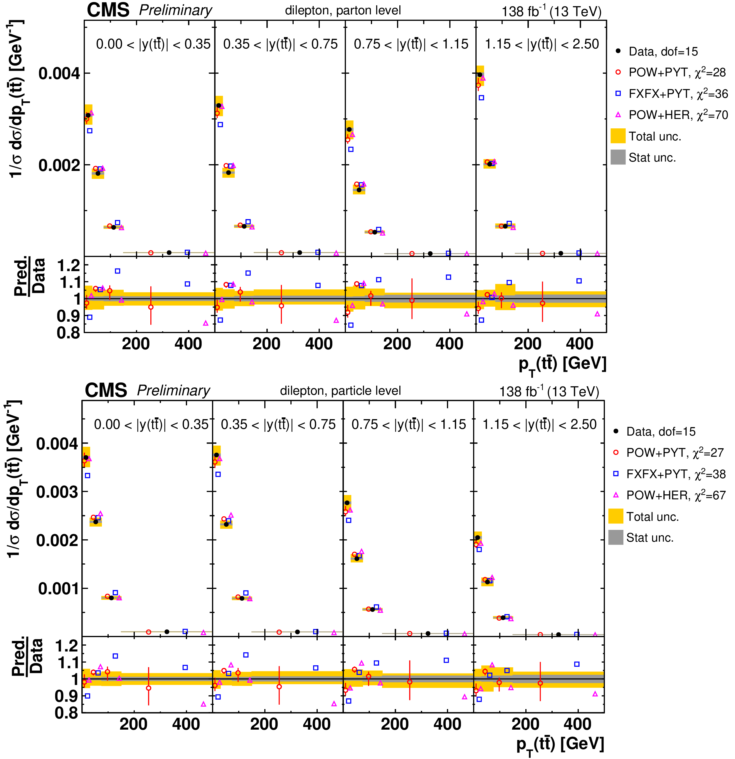
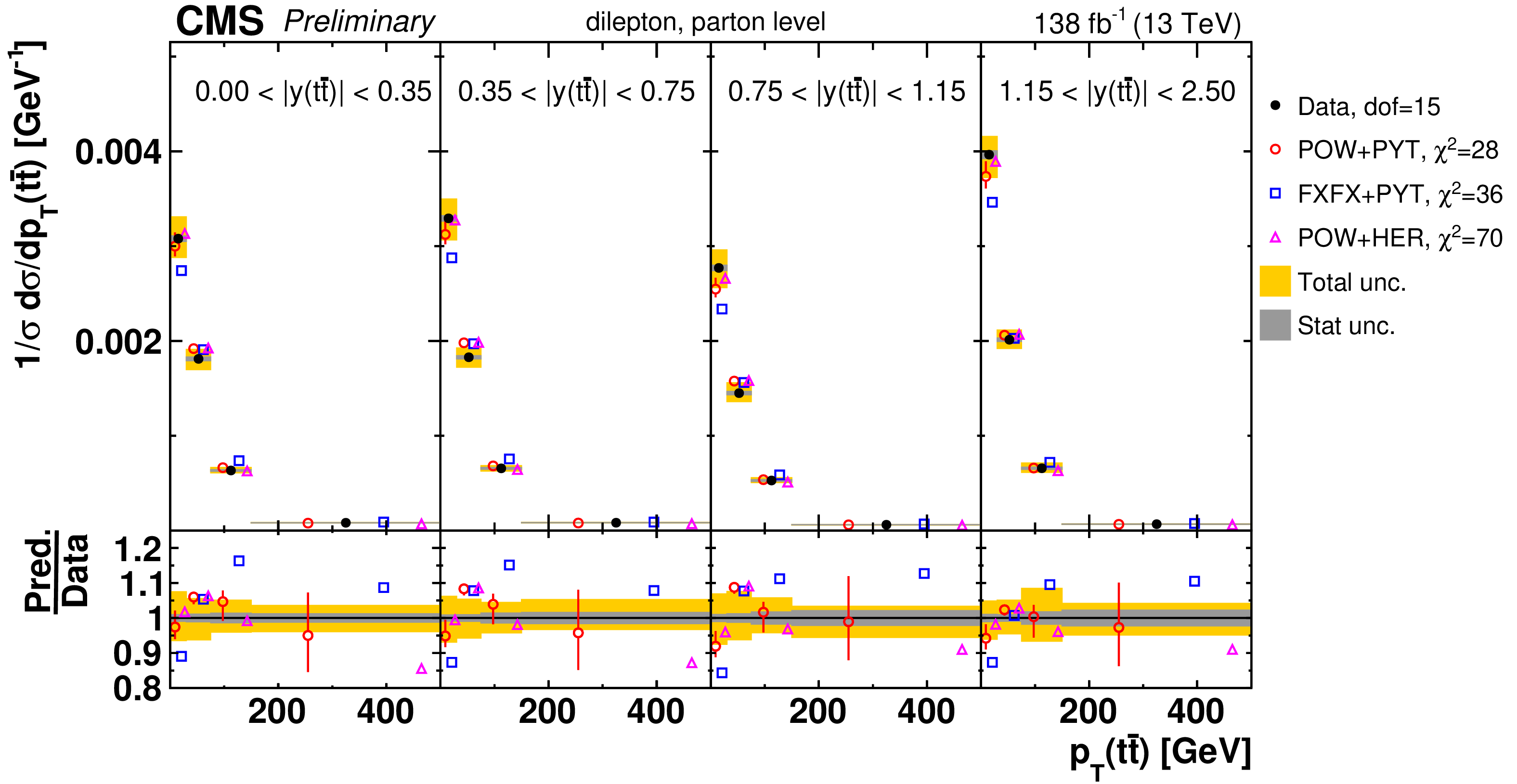
png pdf	Figure 17: Normalized $[ {|y( \mathrm{t\bar{t}})|},\,{{p_{\mathrm {T}}} ( \mathrm{t\bar{t}})} ]$ cross sections are shown for data (filled circles) and various MC predictions (other points). Further details can be found in the caption of Fig. 13.
png pdf	Figure 17-a: Normalized $[ {|y( \mathrm{t\bar{t}})|},\,{{p_{\mathrm {T}}} ( \mathrm{t\bar{t}})} ]$ cross sections are shown for data (filled circles) and various MC predictions (other points). Further details can be found in the caption of Fig. 13.
png pdf	Figure 17-b: Normalized $[ {|y( \mathrm{t\bar{t}})|},\,{{p_{\mathrm {T}}} ( \mathrm{t\bar{t}})} ]$ cross sections are shown for data (filled circles) and various MC predictions (other points). Further details can be found in the caption of Fig. 13.
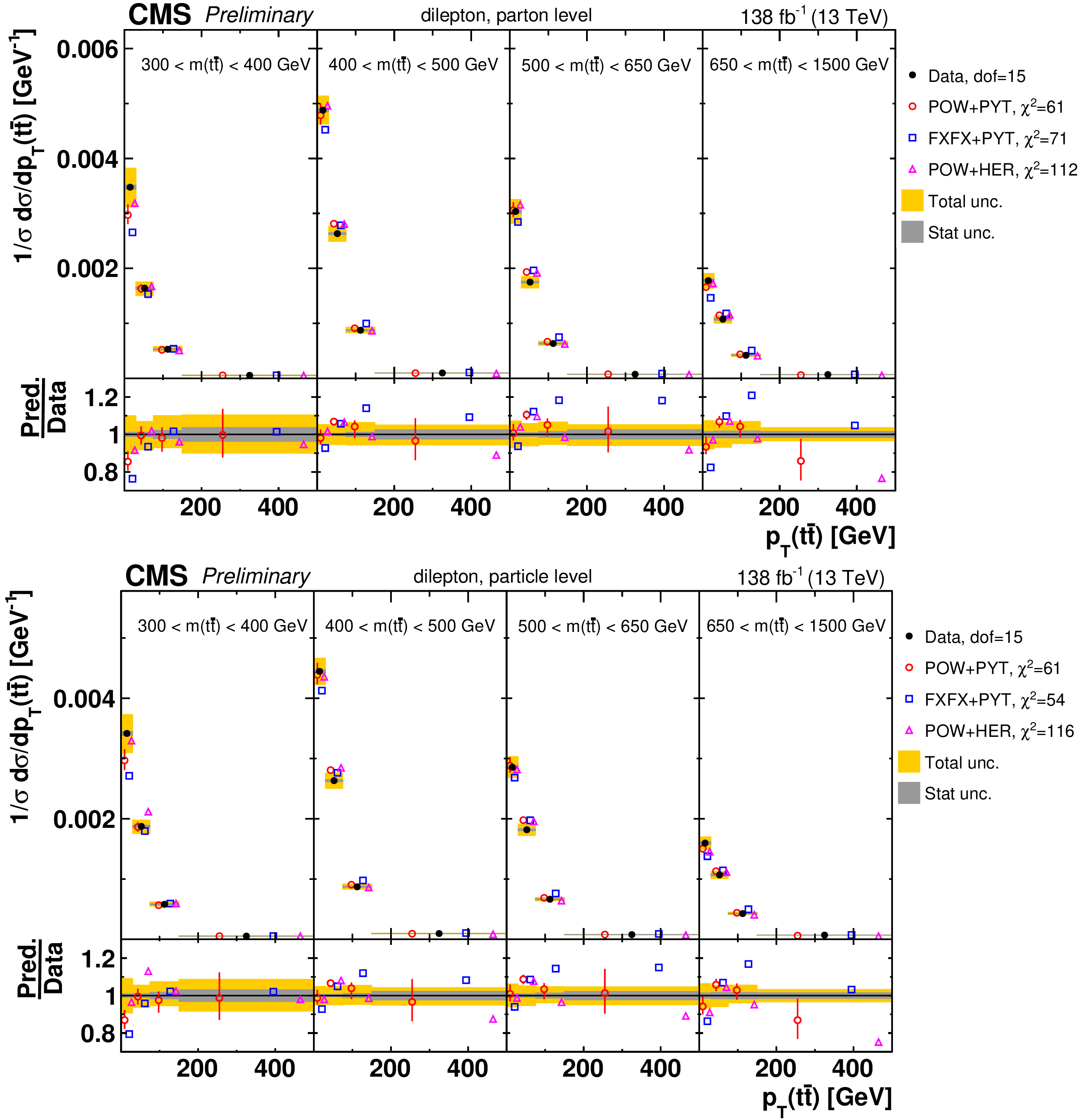
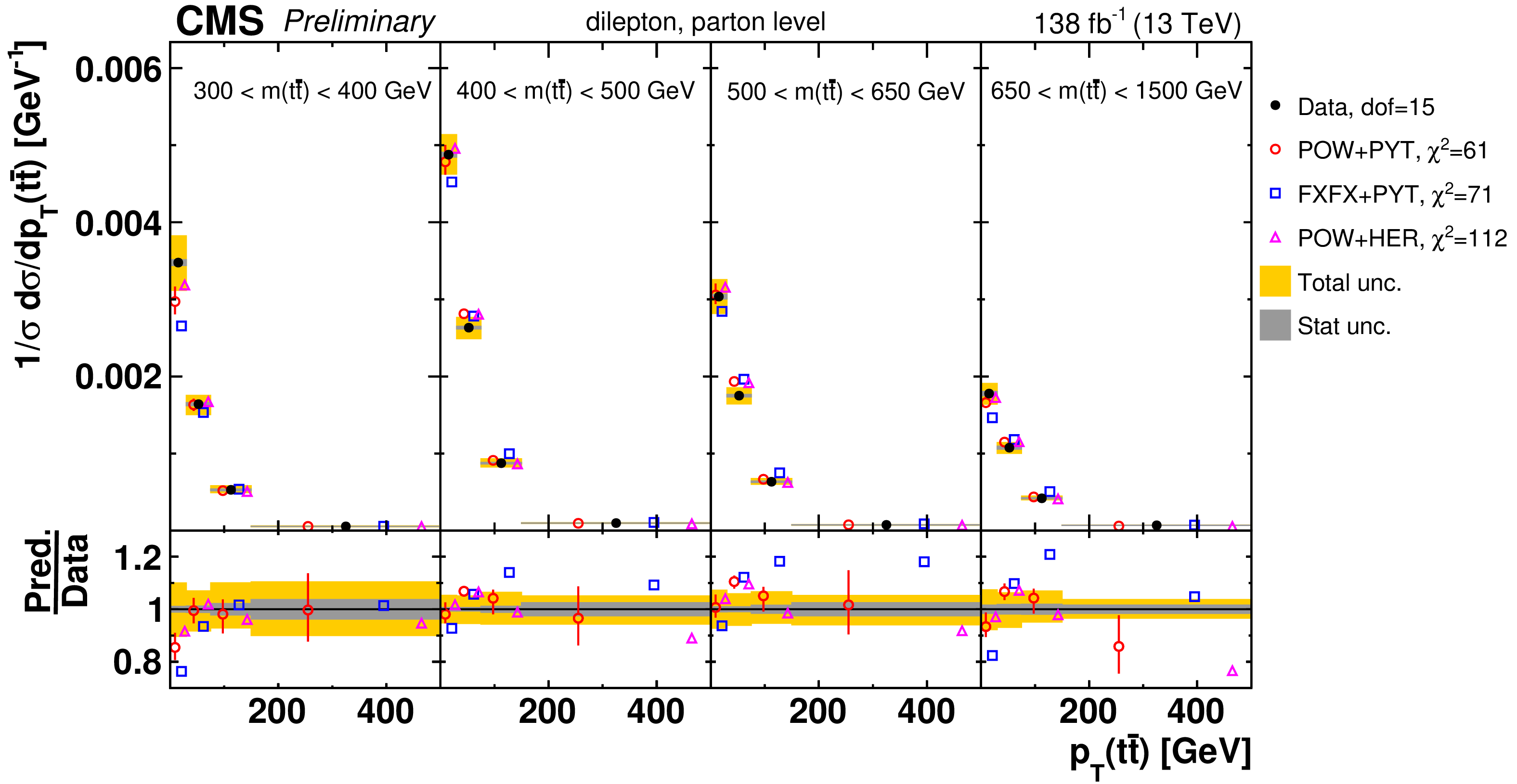
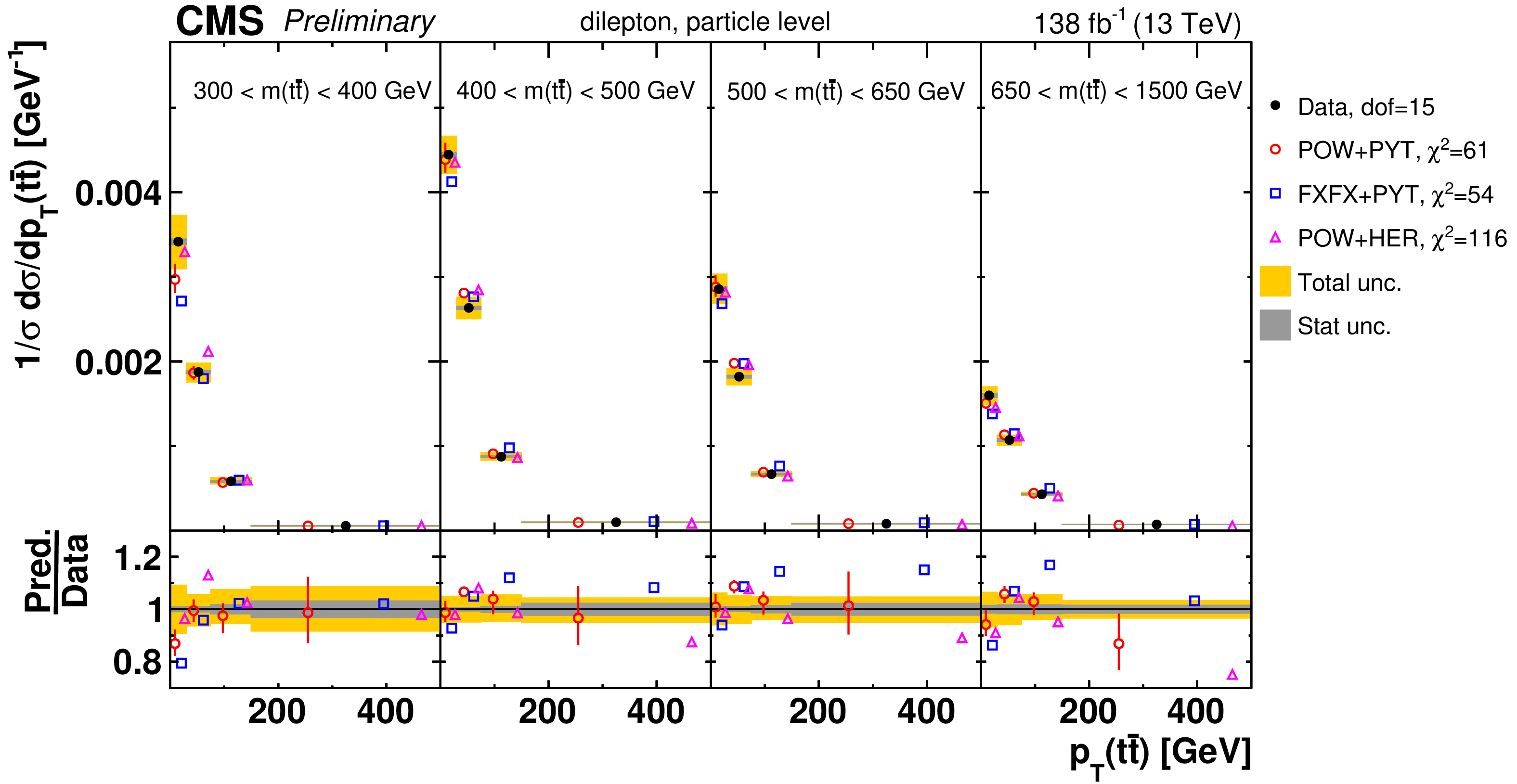
png pdf	Figure 18: Normalized $[ {m( \mathrm{t\bar{t}})},\,{{p_{\mathrm {T}}} ( \mathrm{t\bar{t}})} ]$ cross sections are shown for data (filled circles) and various MC predictions (other points). Further details can be found in the caption of Fig. 13.
png pdf	Figure 18-a: Normalized $[ {m( \mathrm{t\bar{t}})},\,{{p_{\mathrm {T}}} ( \mathrm{t\bar{t}})} ]$ cross sections are shown for data (filled circles) and various MC predictions (other points). Further details can be found in the caption of Fig. 13.
png pdf	Figure 18-b: Normalized $[ {m( \mathrm{t\bar{t}})},\,{{p_{\mathrm {T}}} ( \mathrm{t\bar{t}})} ]$ cross sections are shown for data (filled circles) and various MC predictions (other points). Further details can be found in the caption of Fig. 13.
png pdf	Figure 19: Normalized $[ {{p_{\mathrm {T}}} ( \mathrm{t\bar{t}})},\,{m( \mathrm{t\bar{t}})},\,{y( \mathrm{t\bar{t}})} ]$ cross sections are shown for data (filled circles) and various MC predictions (other points). Further details can be found in the caption of Fig. 13.
png pdf	Figure 19-a: Normalized $[ {{p_{\mathrm {T}}} ( \mathrm{t\bar{t}})},\,{m( \mathrm{t\bar{t}})},\,{y( \mathrm{t\bar{t}})} ]$ cross sections are shown for data (filled circles) and various MC predictions (other points). Further details can be found in the caption of Fig. 13.
png pdf	Figure 19-b: Normalized $[ {{p_{\mathrm {T}}} ( \mathrm{t\bar{t}})},\,{m( \mathrm{t\bar{t}})},\,{y( \mathrm{t\bar{t}})} ]$ cross sections are shown for data (filled circles) and various MC predictions (other points). Further details can be found in the caption of Fig. 13.
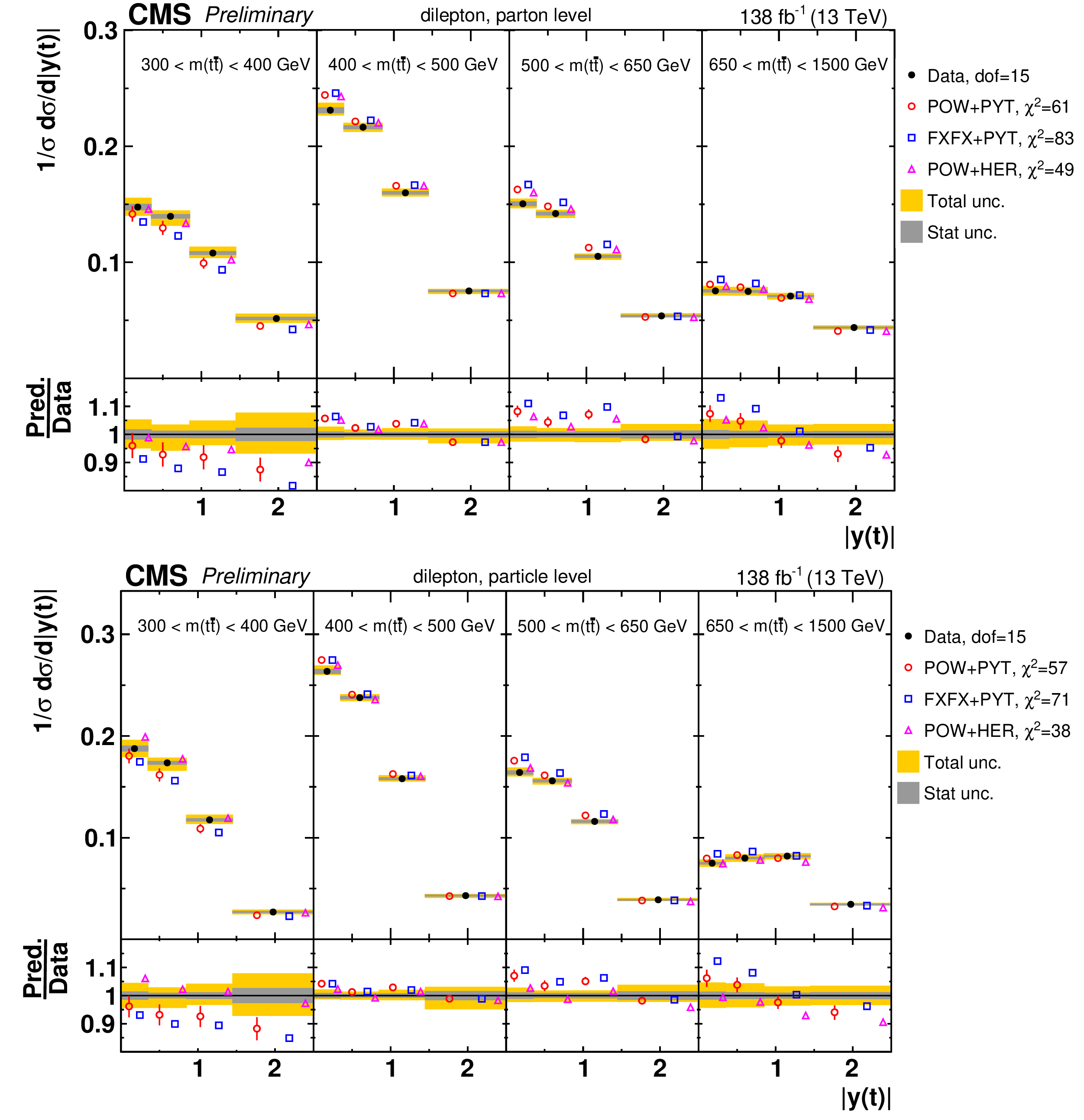
png pdf	Figure 20: Normalized $[ {m( \mathrm{t\bar{t}})},\,{|y(\mathrm{t})|} ]$ cross sections are shown for data (filled circles) and various MC predictions (other points). Further details can be found in the caption of Fig. 13.
png pdf	Figure 20-a: Normalized $[ {m( \mathrm{t\bar{t}})},\,{|y(\mathrm{t})|} ]$ cross sections are shown for data (filled circles) and various MC predictions (other points). Further details can be found in the caption of Fig. 13.
png pdf	Figure 20-b: Normalized $[ {m( \mathrm{t\bar{t}})},\,{|y(\mathrm{t})|} ]$ cross sections are shown for data (filled circles) and various MC predictions (other points). Further details can be found in the caption of Fig. 13.
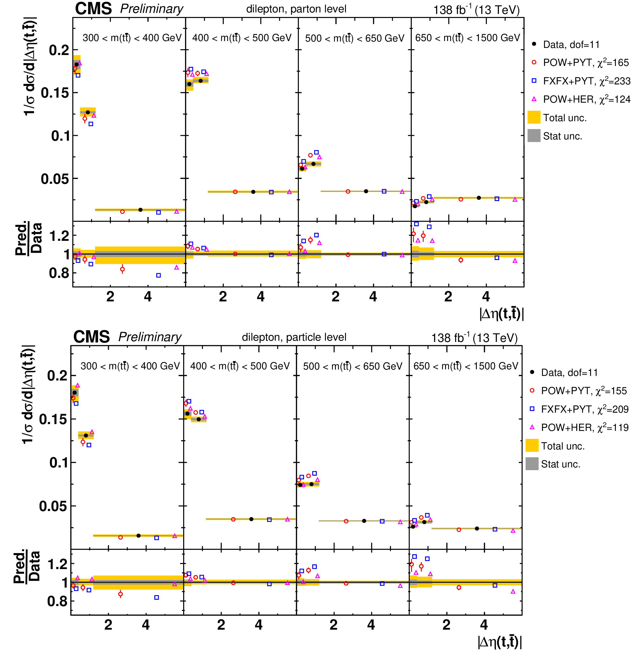
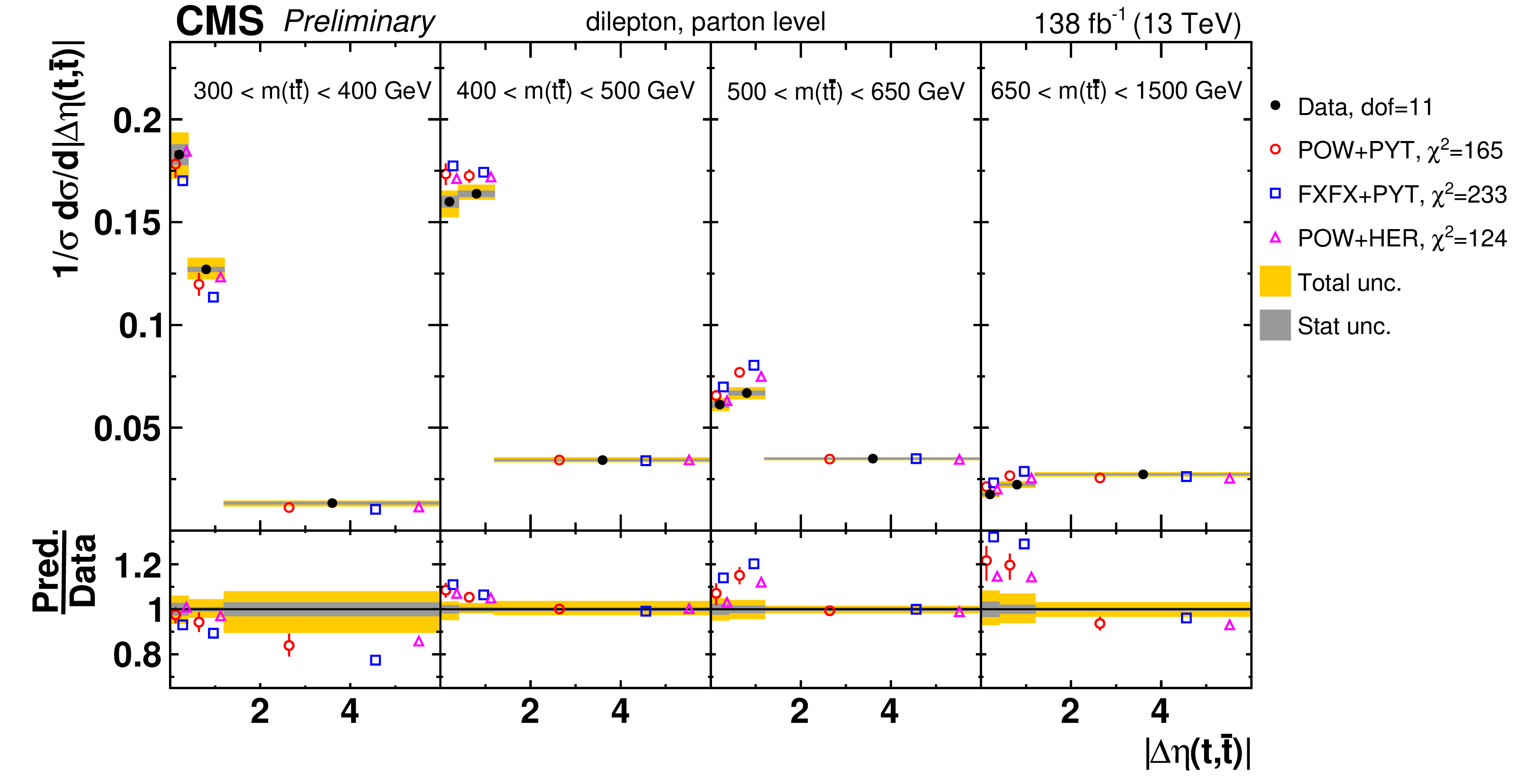
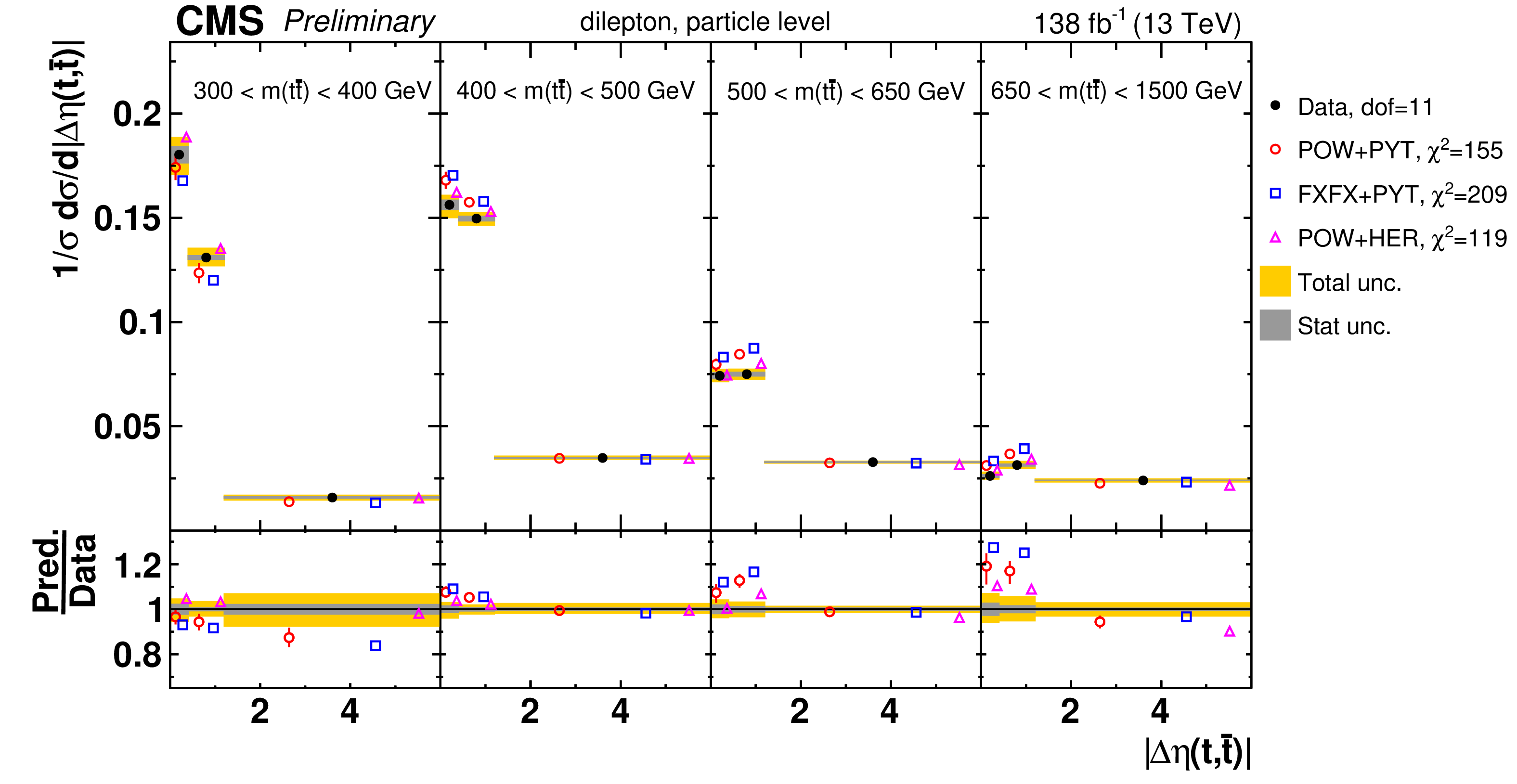
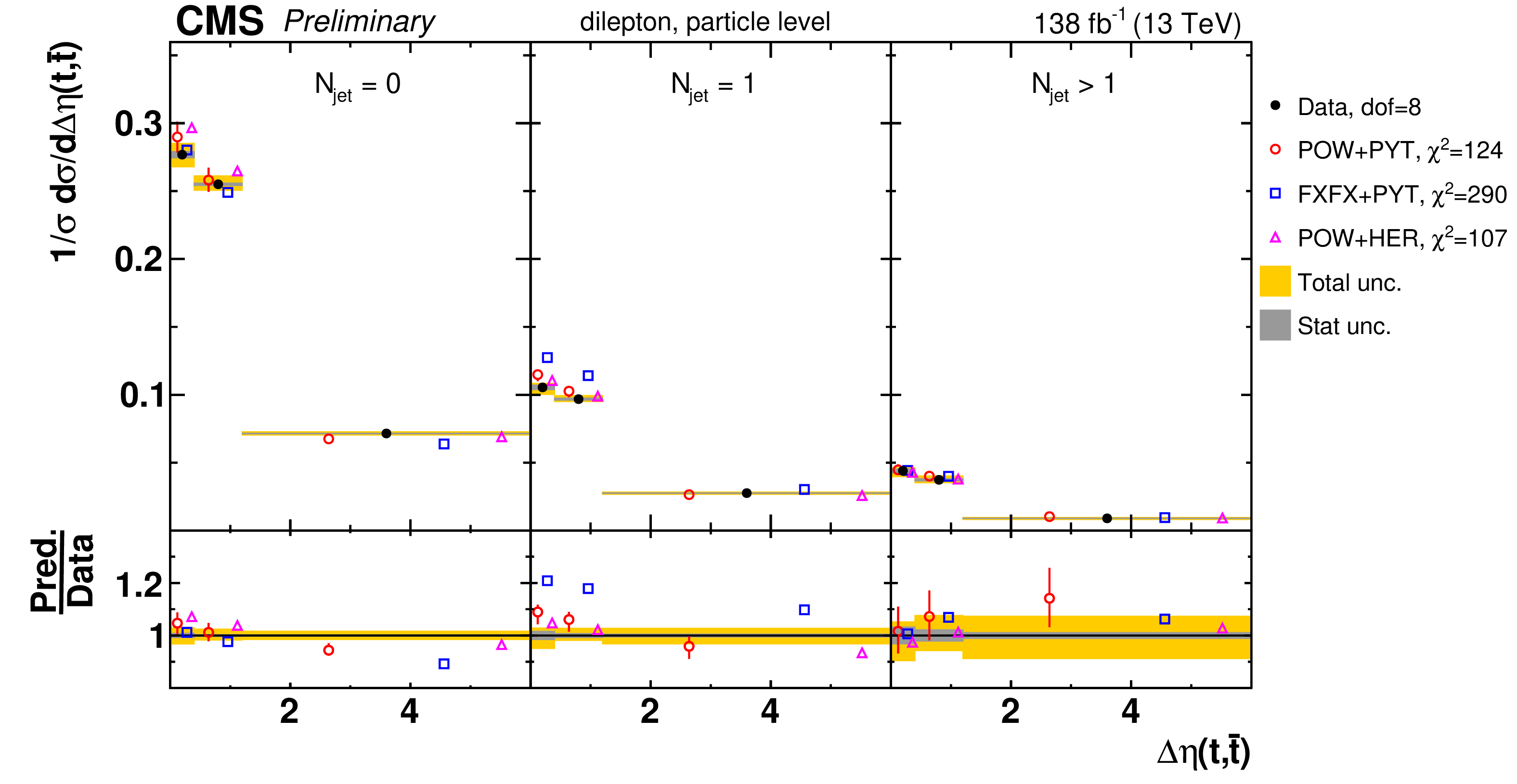
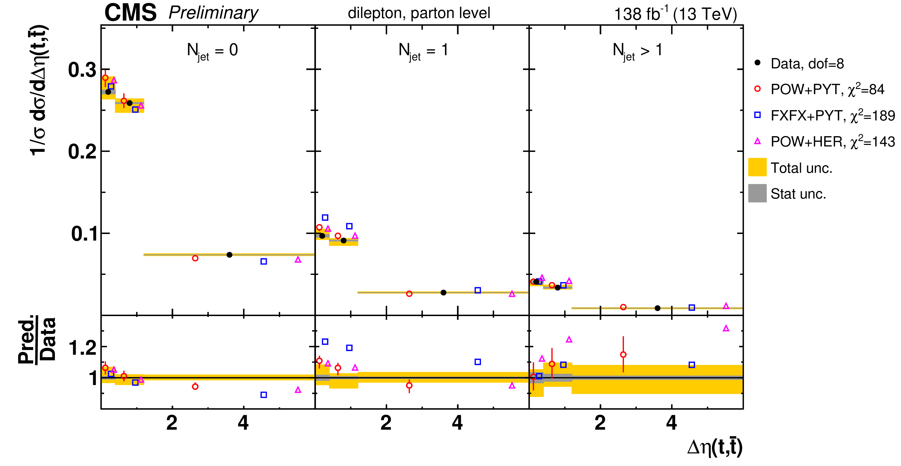
png pdf	Figure 21: Normalized $[ {m( \mathrm{t\bar{t}})},\,{|\Delta \eta (\mathrm{t},\mathrm{\bar{t}})|} ]$ cross sections are shown for data (filled circles) and various MC predictions (other points). Further details can be found in the caption of Fig. 13.
png pdf	Figure 21-a: Normalized $[ {m( \mathrm{t\bar{t}})},\,{|\Delta \eta (\mathrm{t},\mathrm{\bar{t}})|} ]$ cross sections are shown for data (filled circles) and various MC predictions (other points). Further details can be found in the caption of Fig. 13.
png pdf	Figure 21-b: Normalized $[ {m( \mathrm{t\bar{t}})},\,{|\Delta \eta (\mathrm{t},\mathrm{\bar{t}})|} ]$ cross sections are shown for data (filled circles) and various MC predictions (other points). Further details can be found in the caption of Fig. 13.
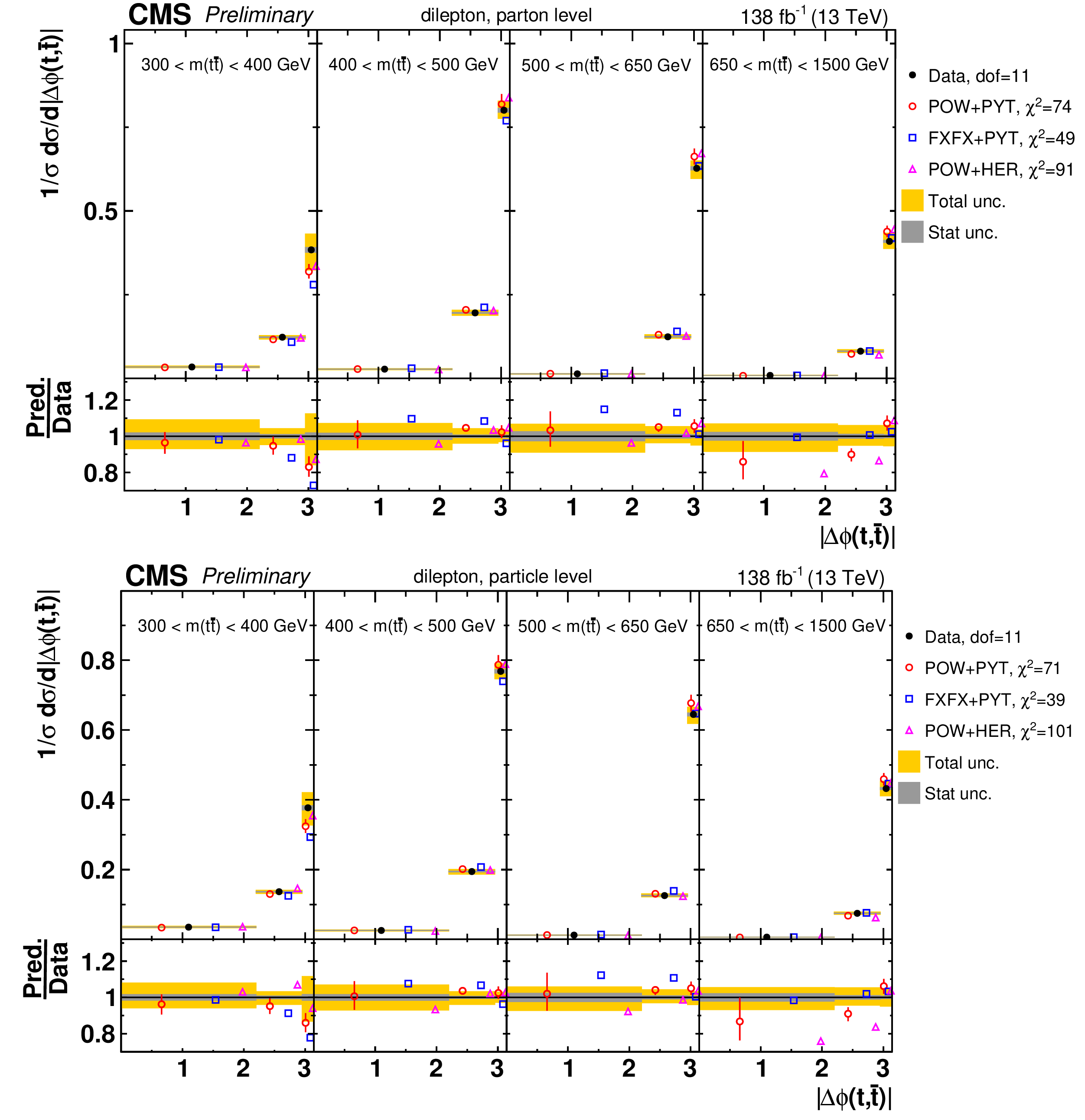
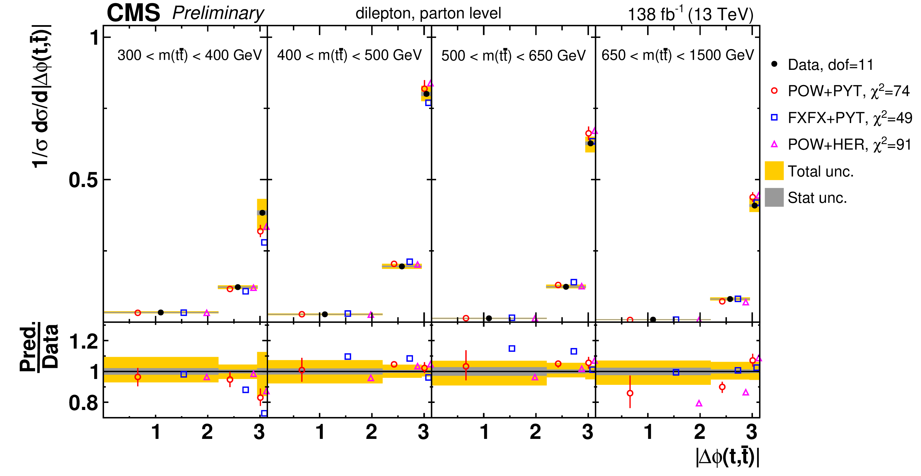
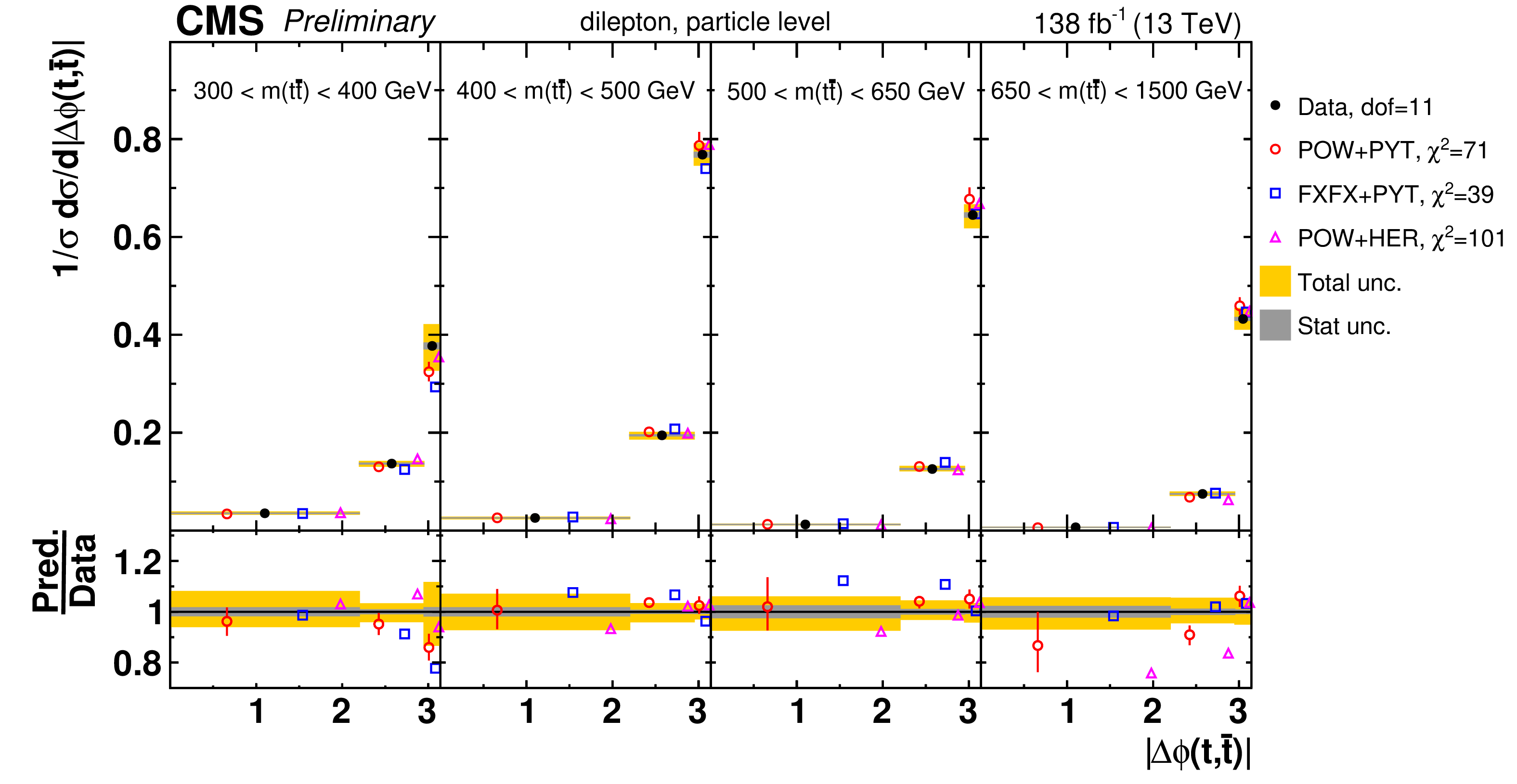
png pdf	Figure 22: Normalized $[ {m( \mathrm{t\bar{t}})},\,{|\Delta \phi (\mathrm{t},\mathrm{\bar{t}})|} ]$ cross sections are shown for data (filled circles) and various MC predictions (other points). Further details can be found in the caption of Fig. 13.
png pdf	Figure 22-a: Normalized $[ {m( \mathrm{t\bar{t}})},\,{|\Delta \phi (\mathrm{t},\mathrm{\bar{t}})|} ]$ cross sections are shown for data (filled circles) and various MC predictions (other points). Further details can be found in the caption of Fig. 13.
png pdf	Figure 22-b: Normalized $[ {m( \mathrm{t\bar{t}})},\,{|\Delta \phi (\mathrm{t},\mathrm{\bar{t}})|} ]$ cross sections are shown for data (filled circles) and various MC predictions (other points). Further details can be found in the caption of Fig. 13.
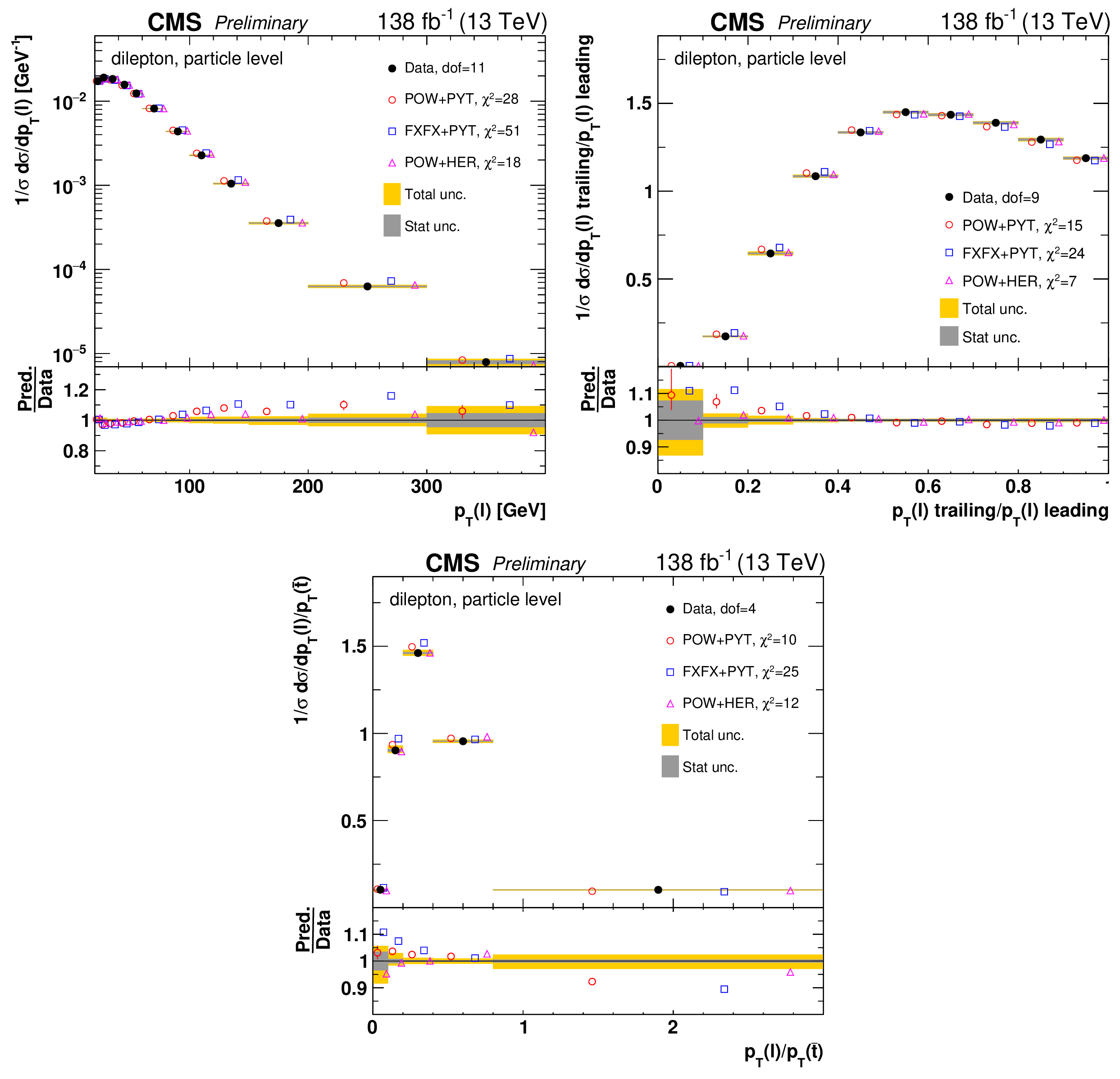
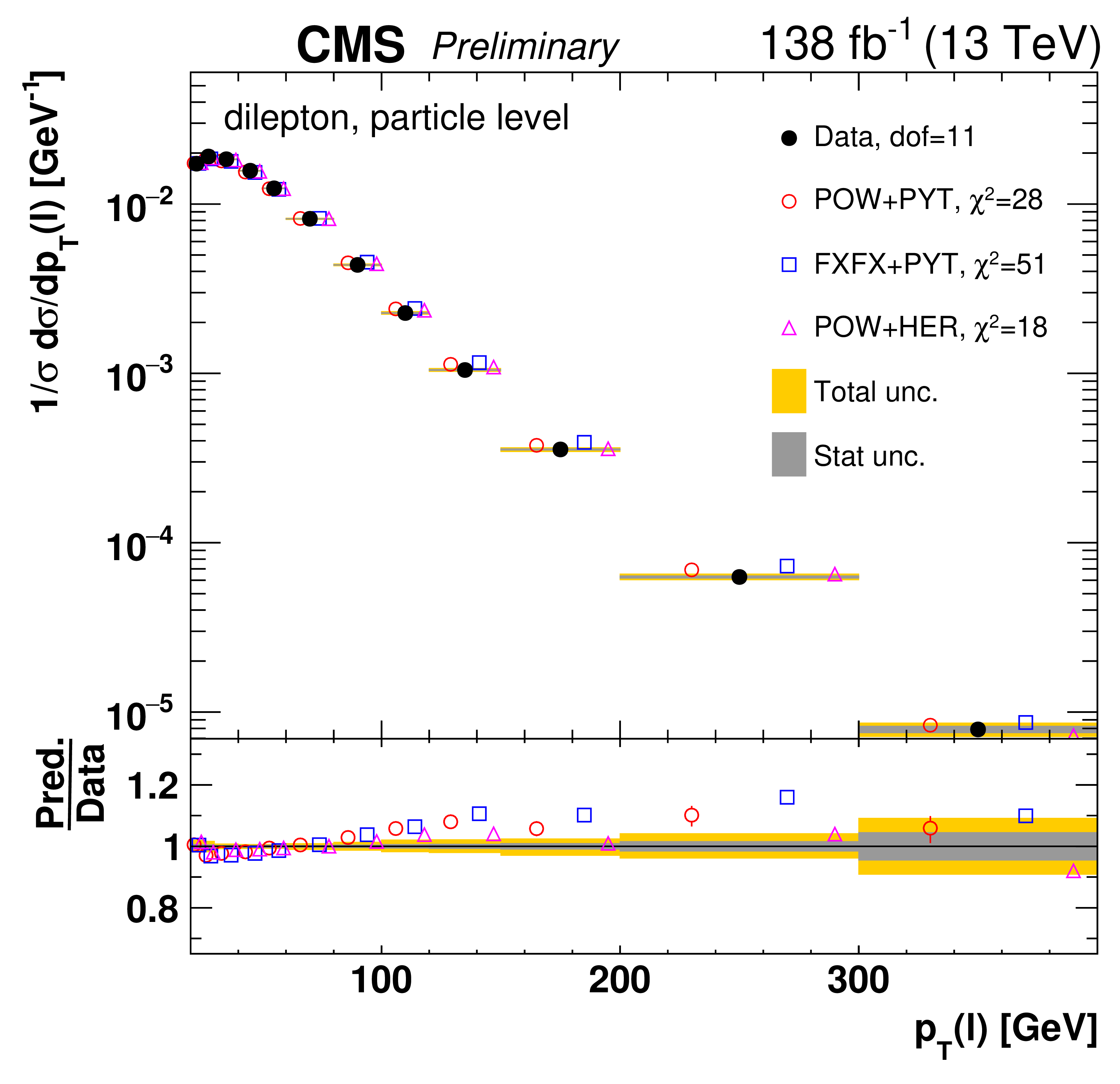
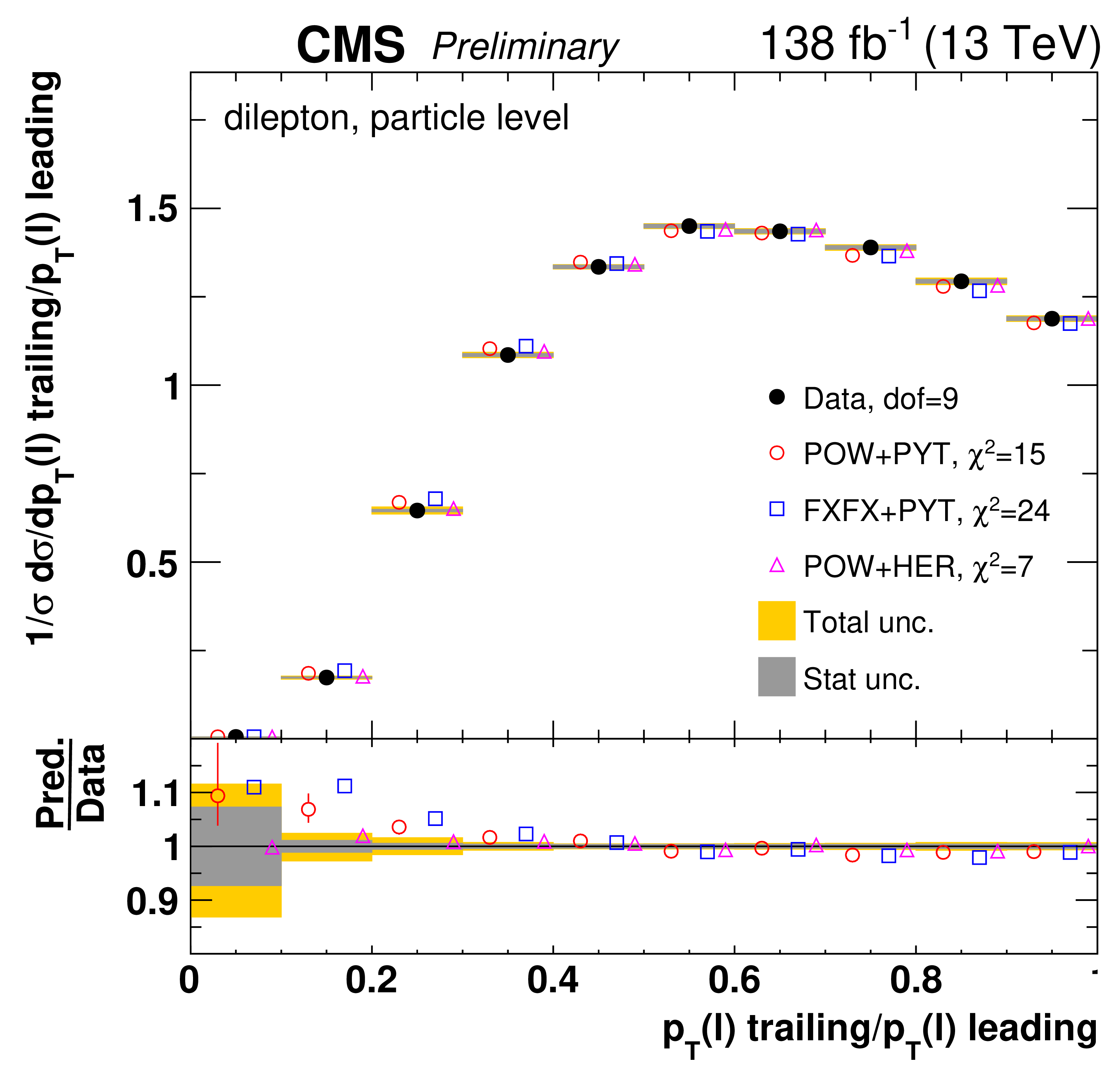
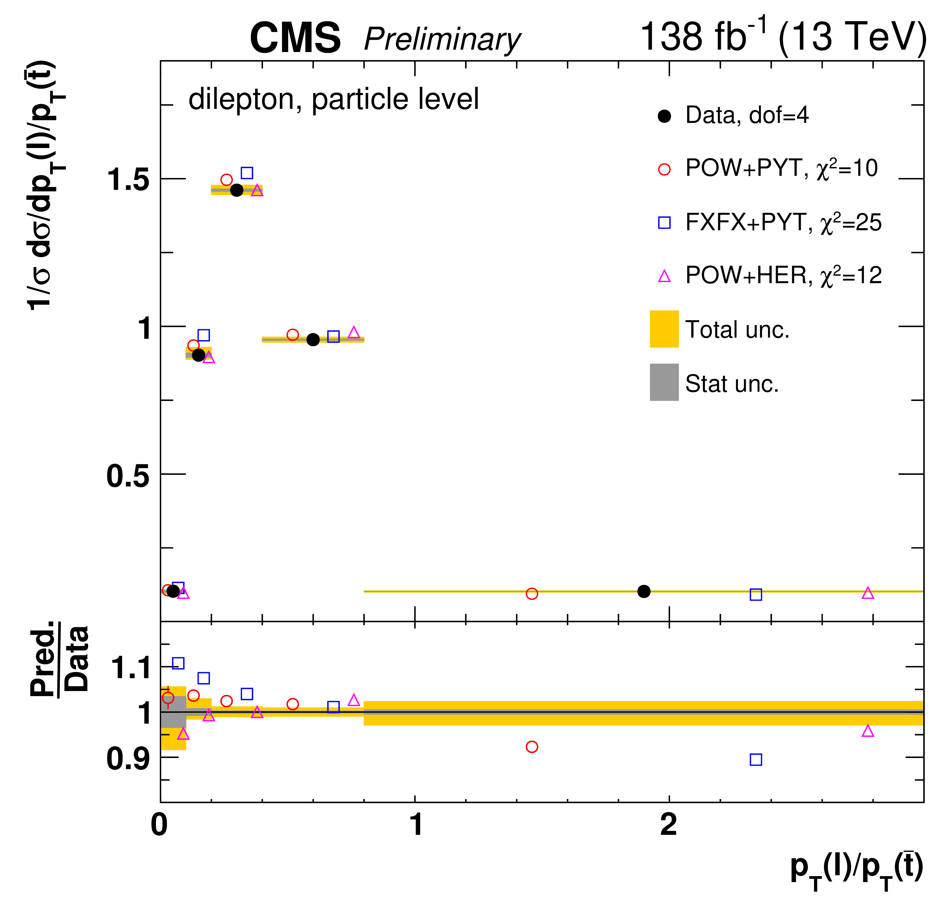
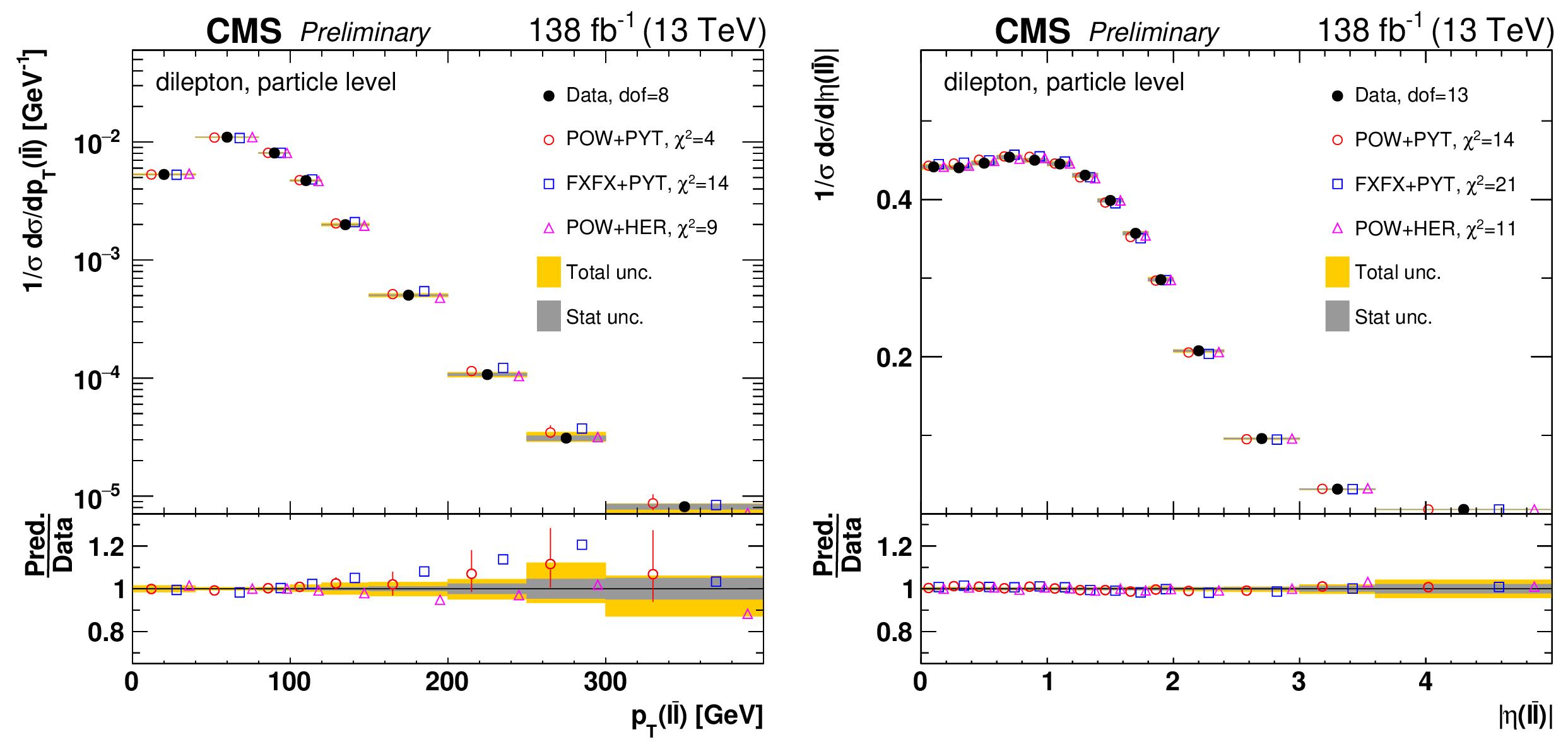
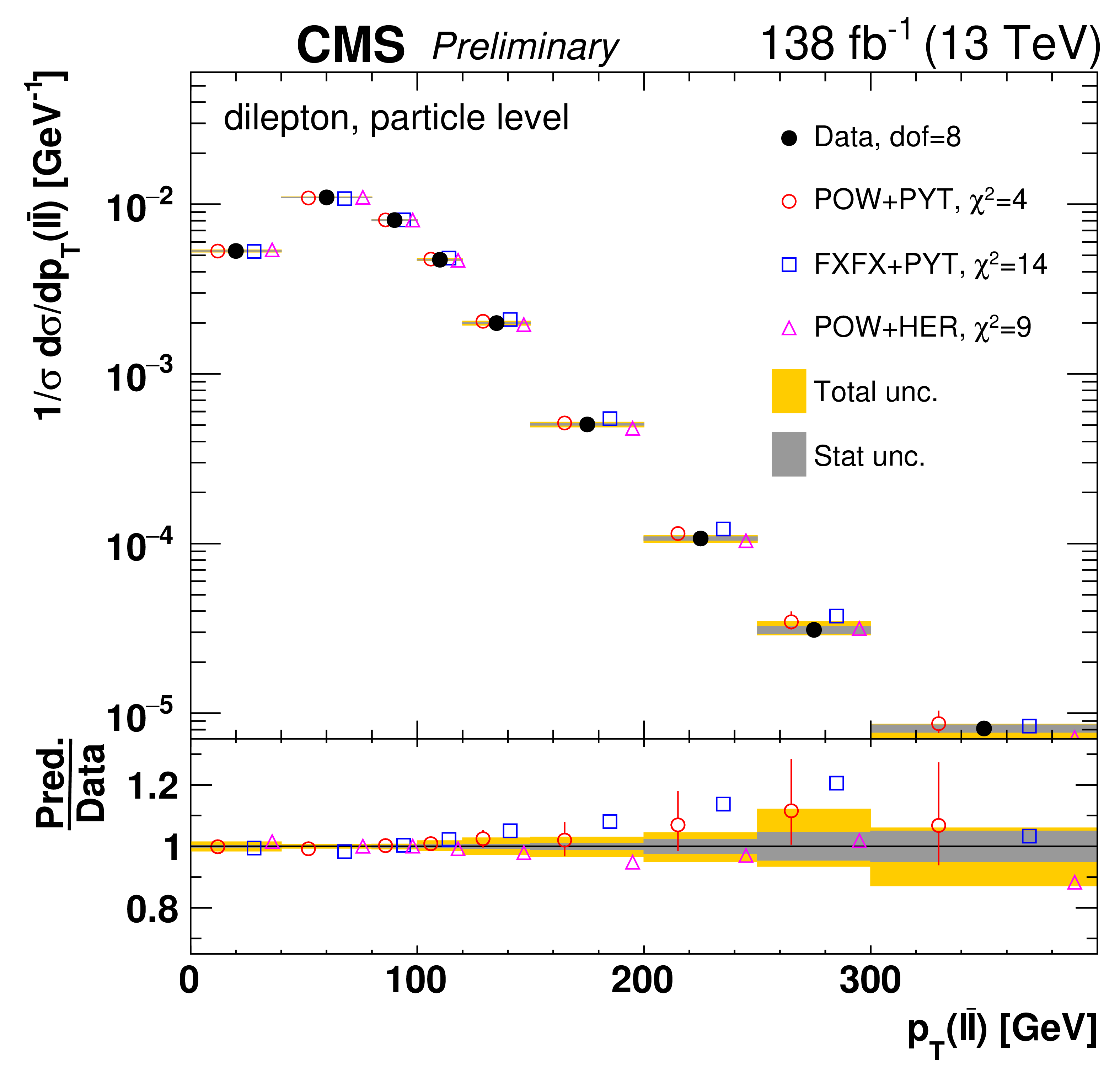
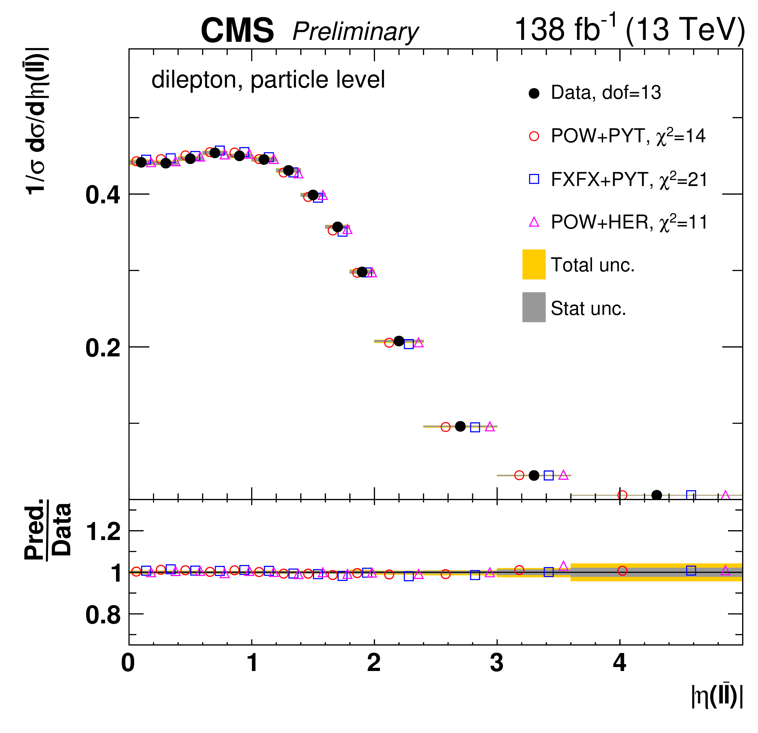
png pdf	Figure 23: Normalized differential $\mathrm{t\bar{t}}$ production cross sections as a function of ${p_{\mathrm {T}}}$ of the lepton (upper left), of the ratio of the trailing and leading lepton ${p_{\mathrm {T}}}$ (upper right), and of the ratio of lepton and top antiquark ${p_{\mathrm {T}}}$ (lower middle), measured at the particle level in a fiducial phase space. The data are shown as filled circles with dark and light bands indicating the statistical and total uncertainties (statistical and systematic uncertainties summed in quadrature), respectively. The estimated uncertainties in the POWHEG+PYTHIA-8 (`POW-PYT') simulation are represented by a vertical bar on the corresponding points. The cross sections are compared to various MC predictions (other points). For each MC model, a value of ${\chi ^2}$ is reported that takes into account the measurement uncertainties. The lower panel in each plot shows the ratios of the predictions to the data.
png pdf	Figure 23-a: Normalized differential $\mathrm{t\bar{t}}$ production cross sections as a function of ${p_{\mathrm {T}}}$ of the lepton (upper left), of the ratio of the trailing and leading lepton ${p_{\mathrm {T}}}$ (upper right), and of the ratio of lepton and top antiquark ${p_{\mathrm {T}}}$ (lower middle), measured at the particle level in a fiducial phase space. The data are shown as filled circles with dark and light bands indicating the statistical and total uncertainties (statistical and systematic uncertainties summed in quadrature), respectively. The estimated uncertainties in the POWHEG+PYTHIA-8 (`POW-PYT') simulation are represented by a vertical bar on the corresponding points. The cross sections are compared to various MC predictions (other points). For each MC model, a value of ${\chi ^2}$ is reported that takes into account the measurement uncertainties. The lower panel in each plot shows the ratios of the predictions to the data.
png pdf	Figure 23-b: Normalized differential $\mathrm{t\bar{t}}$ production cross sections as a function of ${p_{\mathrm {T}}}$ of the lepton (upper left), of the ratio of the trailing and leading lepton ${p_{\mathrm {T}}}$ (upper right), and of the ratio of lepton and top antiquark ${p_{\mathrm {T}}}$ (lower middle), measured at the particle level in a fiducial phase space. The data are shown as filled circles with dark and light bands indicating the statistical and total uncertainties (statistical and systematic uncertainties summed in quadrature), respectively. The estimated uncertainties in the POWHEG+PYTHIA-8 (`POW-PYT') simulation are represented by a vertical bar on the corresponding points. The cross sections are compared to various MC predictions (other points). For each MC model, a value of ${\chi ^2}$ is reported that takes into account the measurement uncertainties. The lower panel in each plot shows the ratios of the predictions to the data.
png pdf	Figure 23-c: Normalized differential $\mathrm{t\bar{t}}$ production cross sections as a function of ${p_{\mathrm {T}}}$ of the lepton (upper left), of the ratio of the trailing and leading lepton ${p_{\mathrm {T}}}$ (upper right), and of the ratio of lepton and top antiquark ${p_{\mathrm {T}}}$ (lower middle), measured at the particle level in a fiducial phase space. The data are shown as filled circles with dark and light bands indicating the statistical and total uncertainties (statistical and systematic uncertainties summed in quadrature), respectively. The estimated uncertainties in the POWHEG+PYTHIA-8 (`POW-PYT') simulation are represented by a vertical bar on the corresponding points. The cross sections are compared to various MC predictions (other points). For each MC model, a value of ${\chi ^2}$ is reported that takes into account the measurement uncertainties. The lower panel in each plot shows the ratios of the predictions to the data.
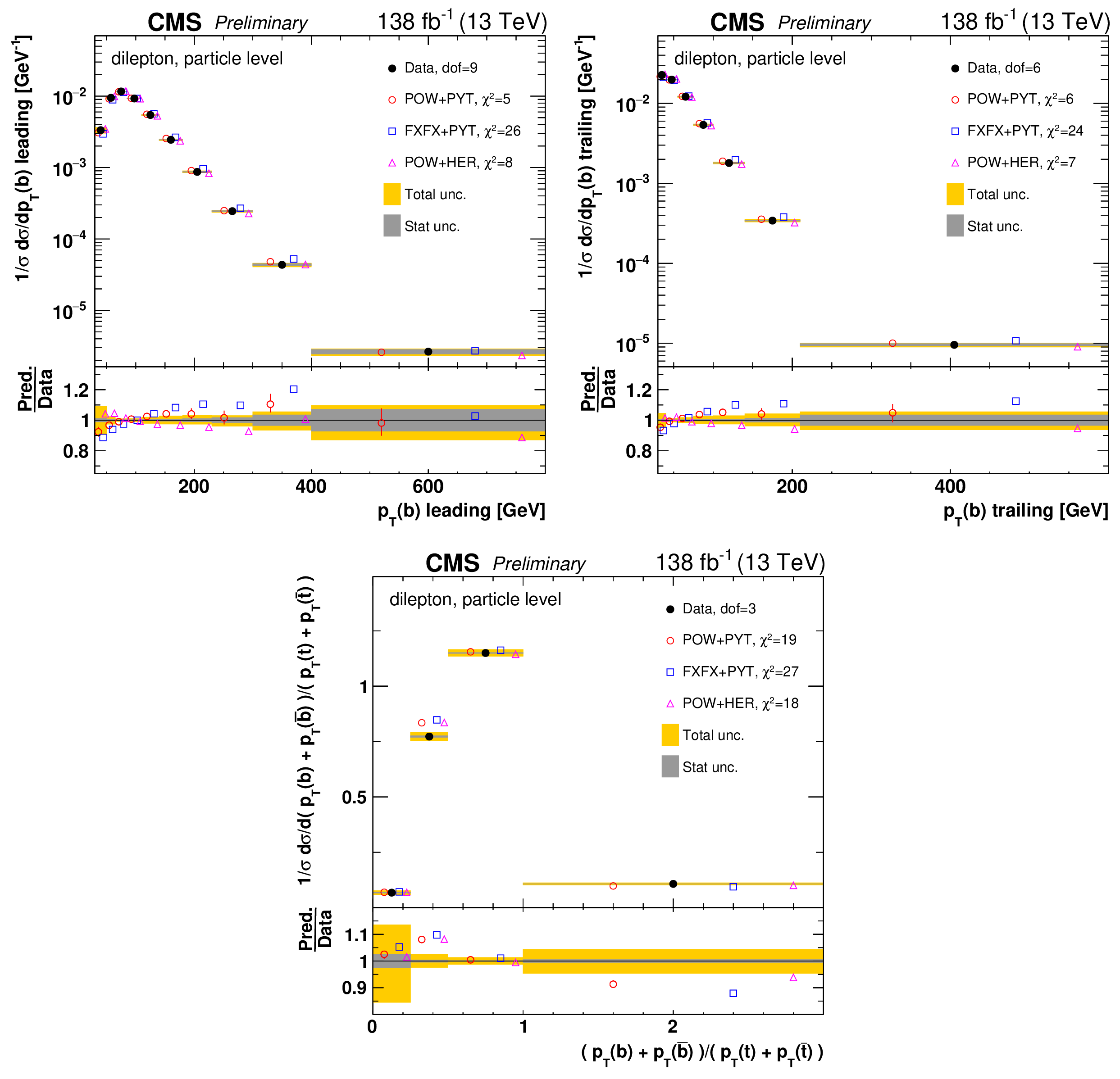
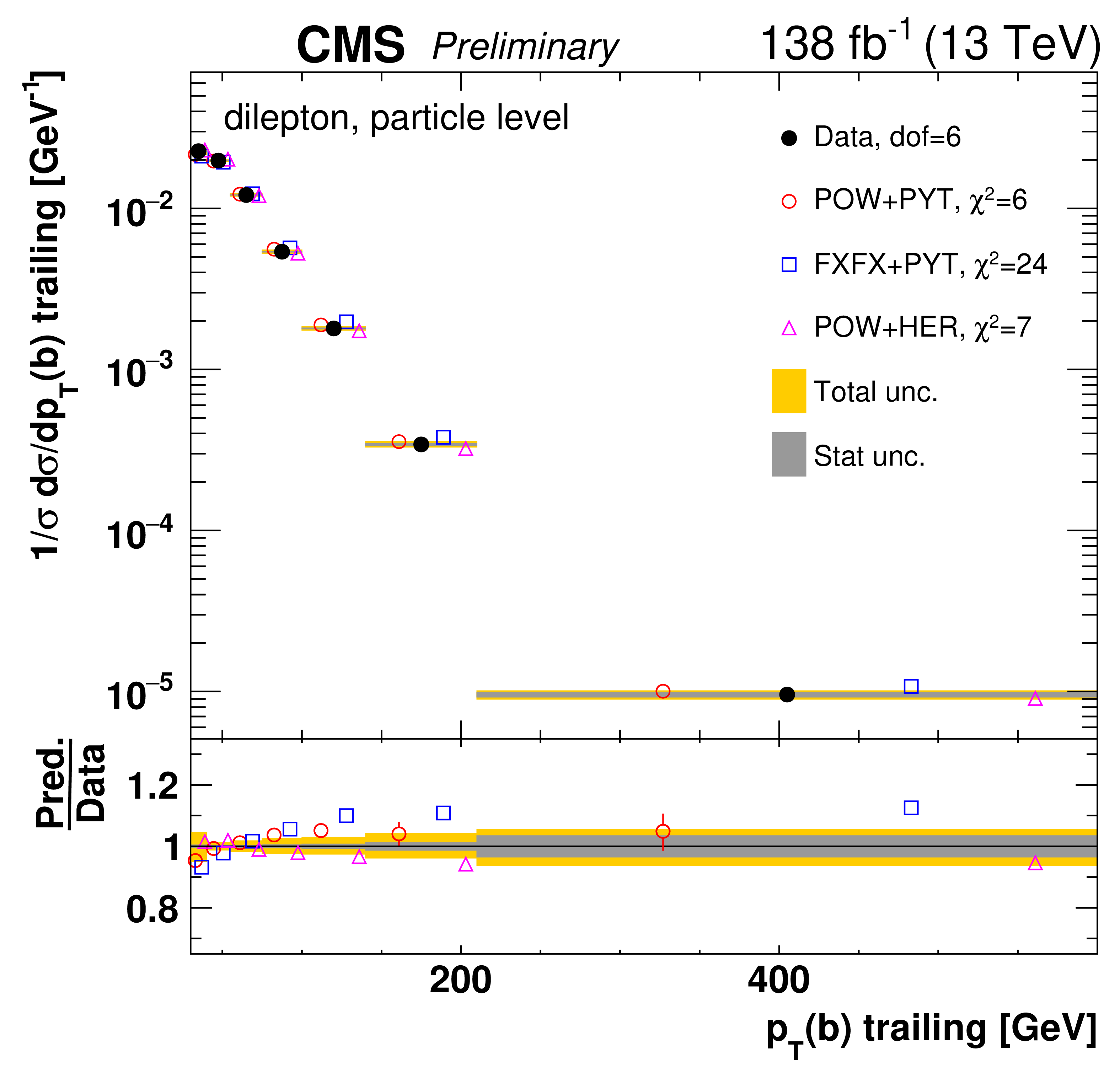
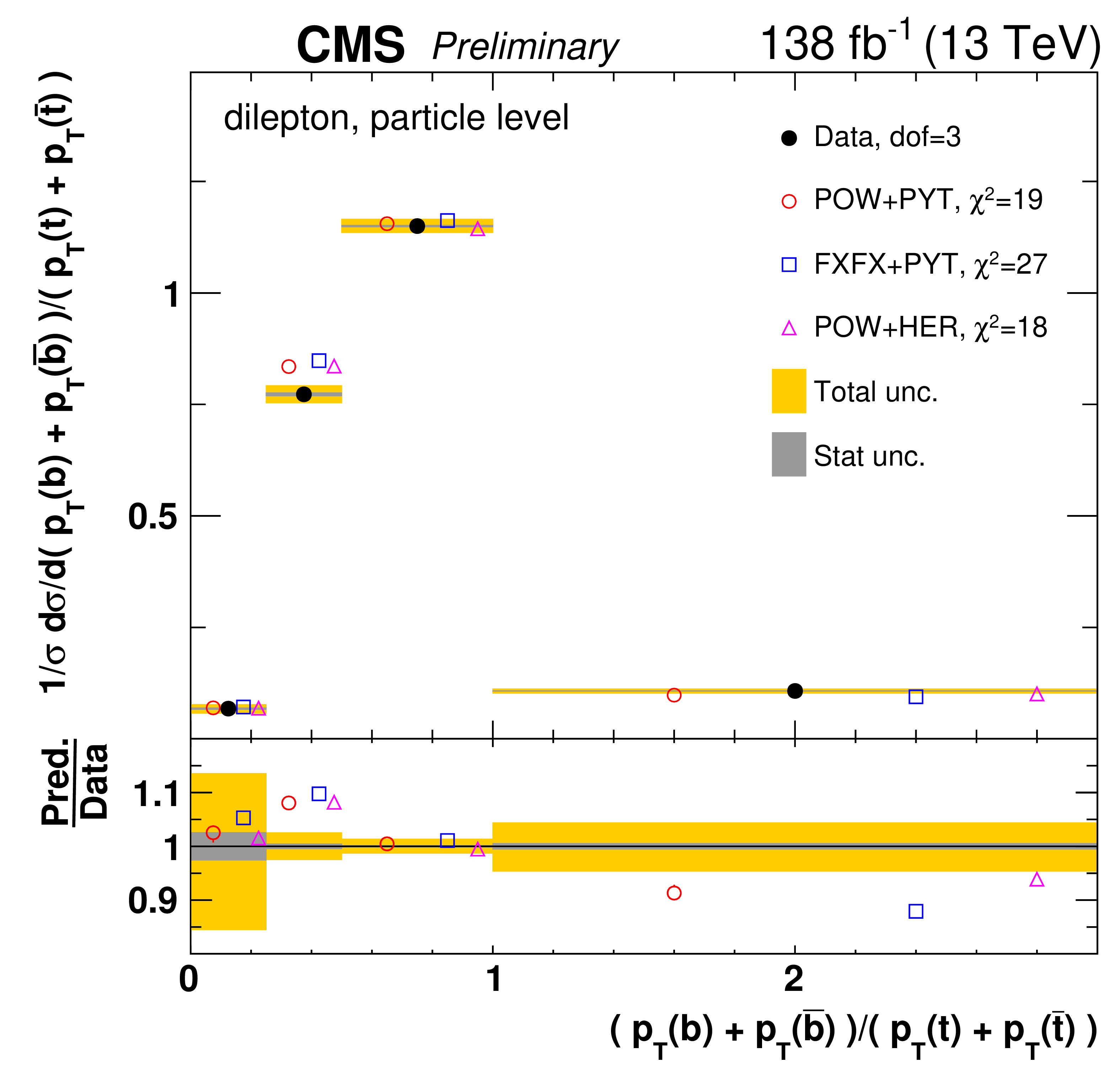
png pdf	Figure 24: Normalized differential $\mathrm{t\bar{t}}$ production cross sections as a function of the ${p_{\mathrm {T}}}$ of the leading (upper left) and trailing (upper right) b jet, and $( {{p_{\mathrm {T}}}}(\rm {b})+ {{p_{\mathrm {T}}}}(\mathrm{b\bar{b}}))/( {{p_{\mathrm {T}}}}(\rm {t})+ {{p_{\mathrm {T}}}}(\mathrm{\bar{t}}))$ (lower). Further details can be found in the caption of Fig. 23.
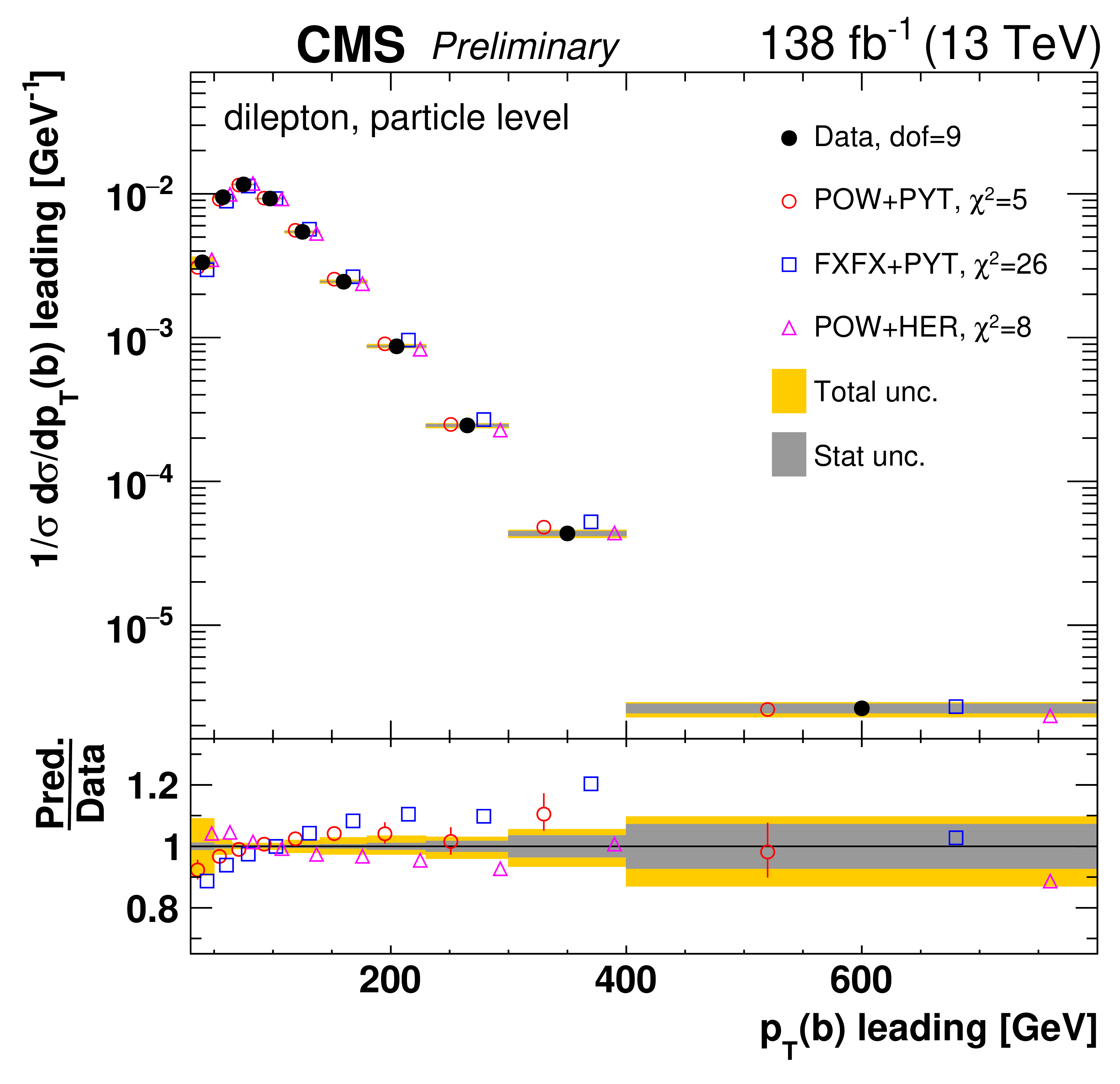
png pdf	Figure 24-a: Normalized differential $\mathrm{t\bar{t}}$ production cross sections as a function of the ${p_{\mathrm {T}}}$ of the leading (upper left) and trailing (upper right) b jet, and $( {{p_{\mathrm {T}}}}(\rm {b})+ {{p_{\mathrm {T}}}}(\mathrm{b\bar{b}}))/( {{p_{\mathrm {T}}}}(\rm {t})+ {{p_{\mathrm {T}}}}(\mathrm{\bar{t}}))$ (lower). Further details can be found in the caption of Fig. 23.
png pdf	Figure 24-b: Normalized differential $\mathrm{t\bar{t}}$ production cross sections as a function of the ${p_{\mathrm {T}}}$ of the leading (upper left) and trailing (upper right) b jet, and $( {{p_{\mathrm {T}}}}(\rm {b})+ {{p_{\mathrm {T}}}}(\mathrm{b\bar{b}}))/( {{p_{\mathrm {T}}}}(\rm {t})+ {{p_{\mathrm {T}}}}(\mathrm{\bar{t}}))$ (lower). Further details can be found in the caption of Fig. 23.
png pdf	Figure 24-c: Normalized differential $\mathrm{t\bar{t}}$ production cross sections as a function of the ${p_{\mathrm {T}}}$ of the leading (upper left) and trailing (upper right) b jet, and $( {{p_{\mathrm {T}}}}(\rm {b})+ {{p_{\mathrm {T}}}}(\mathrm{b\bar{b}}))/( {{p_{\mathrm {T}}}}(\rm {t})+ {{p_{\mathrm {T}}}}(\mathrm{\bar{t}}))$ (lower). Further details can be found in the caption of Fig. 23.
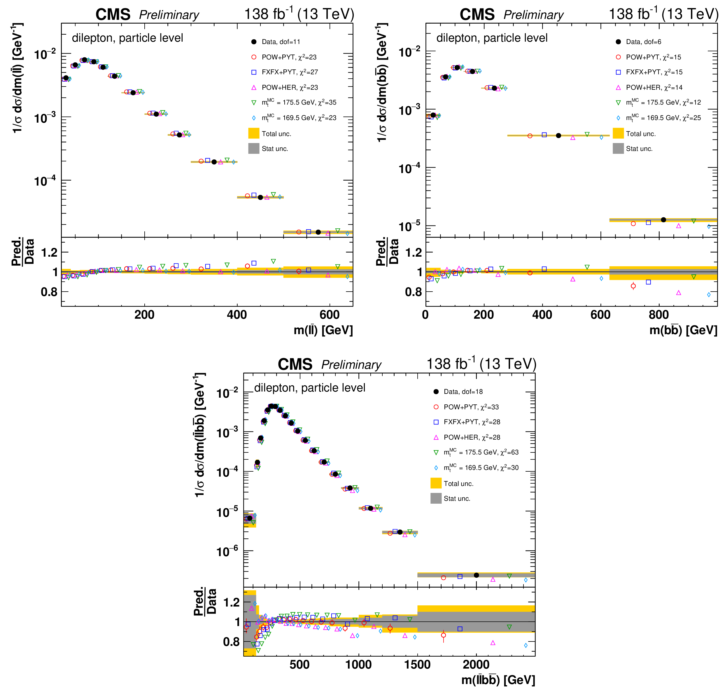
png pdf	Figure 25: Normalized differential $\mathrm{t\bar{t}}$ production cross sections as a function of ${m(\ell \overline {\ell})}$ (upper left), ${m(\mathrm{b} \mathrm{\bar{b}})}$ (upper right), and ${m(\ell \overline {\ell}\mathrm{b} \mathrm{\bar{b}})}$ (lower) are shown for data (filled circles) and various MC predictions (other points). The distributions are also compared to POWHEG+PYTHIA-8 (`POW-PYT') simulations with different values of ${m_{\mathrm{t}}^{\text {MC}}}$. Further details can be found in the caption of Fig. 23.
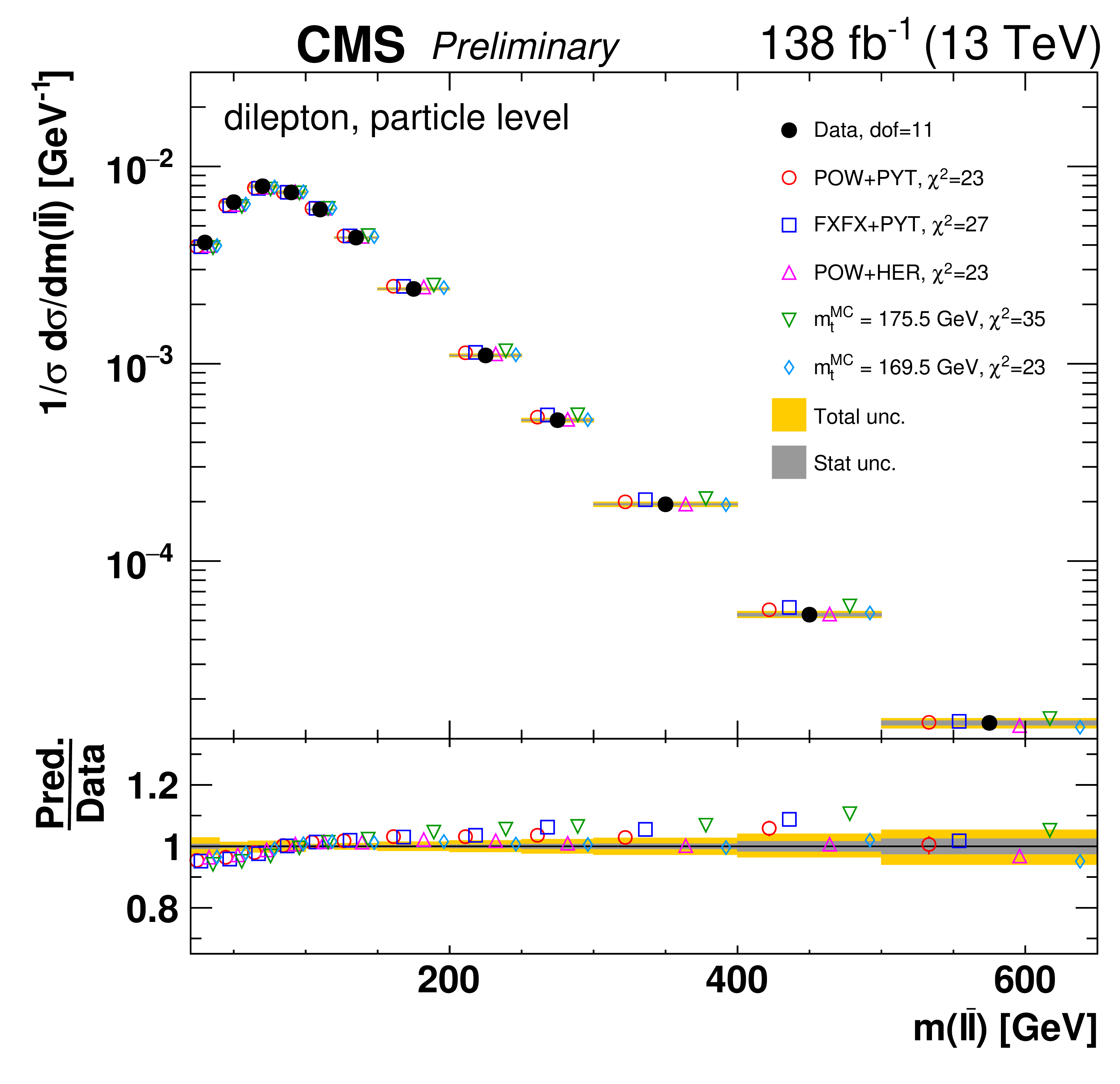
png pdf	Figure 25-a: Normalized differential $\mathrm{t\bar{t}}$ production cross sections as a function of ${m(\ell \overline {\ell})}$ (upper left), ${m(\mathrm{b} \mathrm{\bar{b}})}$ (upper right), and ${m(\ell \overline {\ell}\mathrm{b} \mathrm{\bar{b}})}$ (lower) are shown for data (filled circles) and various MC predictions (other points). The distributions are also compared to POWHEG+PYTHIA-8 (`POW-PYT') simulations with different values of ${m_{\mathrm{t}}^{\text {MC}}}$. Further details can be found in the caption of Fig. 23.
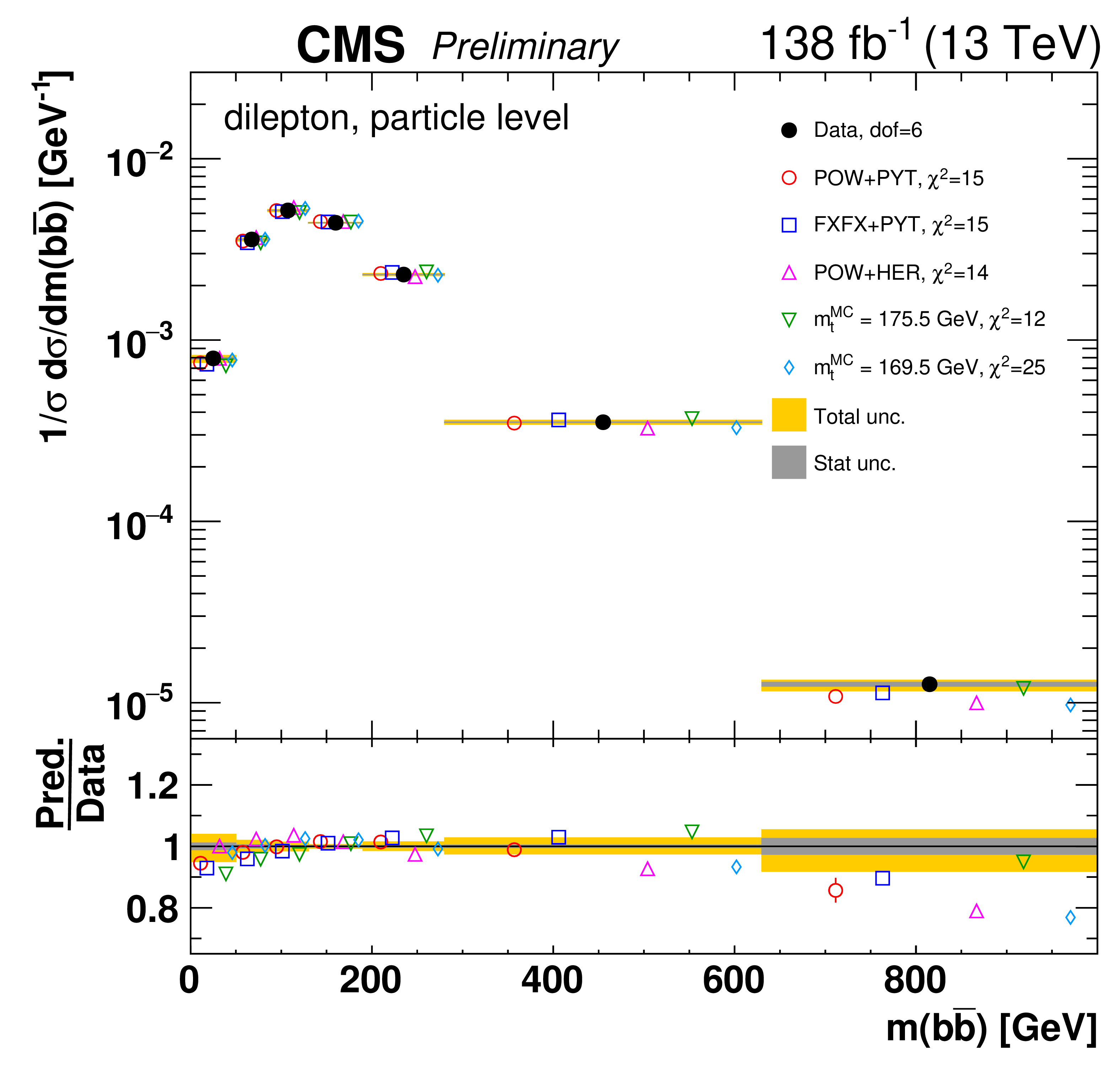
png pdf	Figure 25-b: Normalized differential $\mathrm{t\bar{t}}$ production cross sections as a function of ${m(\ell \overline {\ell})}$ (upper left), ${m(\mathrm{b} \mathrm{\bar{b}})}$ (upper right), and ${m(\ell \overline {\ell}\mathrm{b} \mathrm{\bar{b}})}$ (lower) are shown for data (filled circles) and various MC predictions (other points). The distributions are also compared to POWHEG+PYTHIA-8 (`POW-PYT') simulations with different values of ${m_{\mathrm{t}}^{\text {MC}}}$. Further details can be found in the caption of Fig. 23.
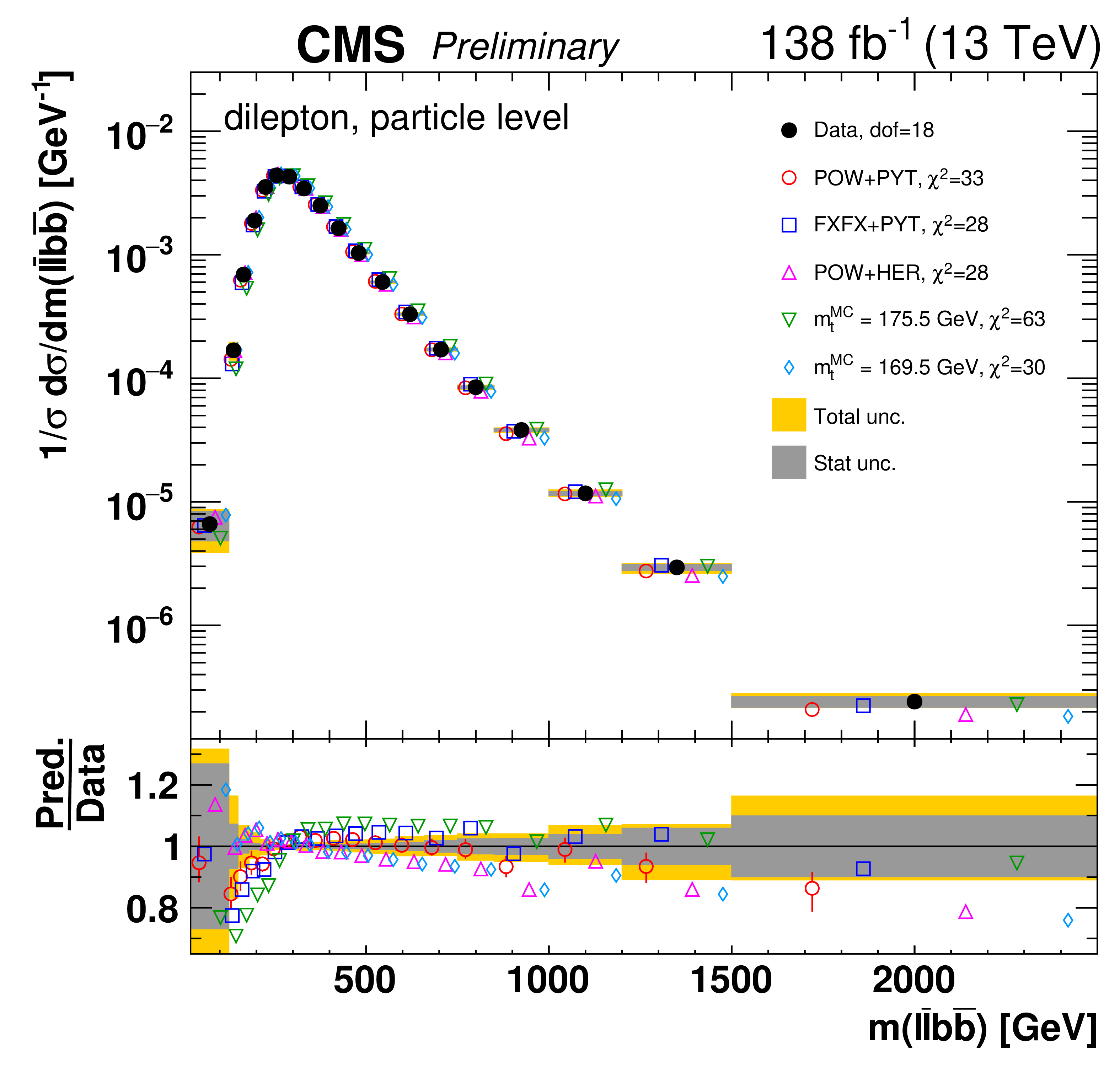
png pdf	Figure 25-c: Normalized differential $\mathrm{t\bar{t}}$ production cross sections as a function of ${m(\ell \overline {\ell})}$ (upper left), ${m(\mathrm{b} \mathrm{\bar{b}})}$ (upper right), and ${m(\ell \overline {\ell}\mathrm{b} \mathrm{\bar{b}})}$ (lower) are shown for data (filled circles) and various MC predictions (other points). The distributions are also compared to POWHEG+PYTHIA-8 (`POW-PYT') simulations with different values of ${m_{\mathrm{t}}^{\text {MC}}}$. Further details can be found in the caption of Fig. 23.
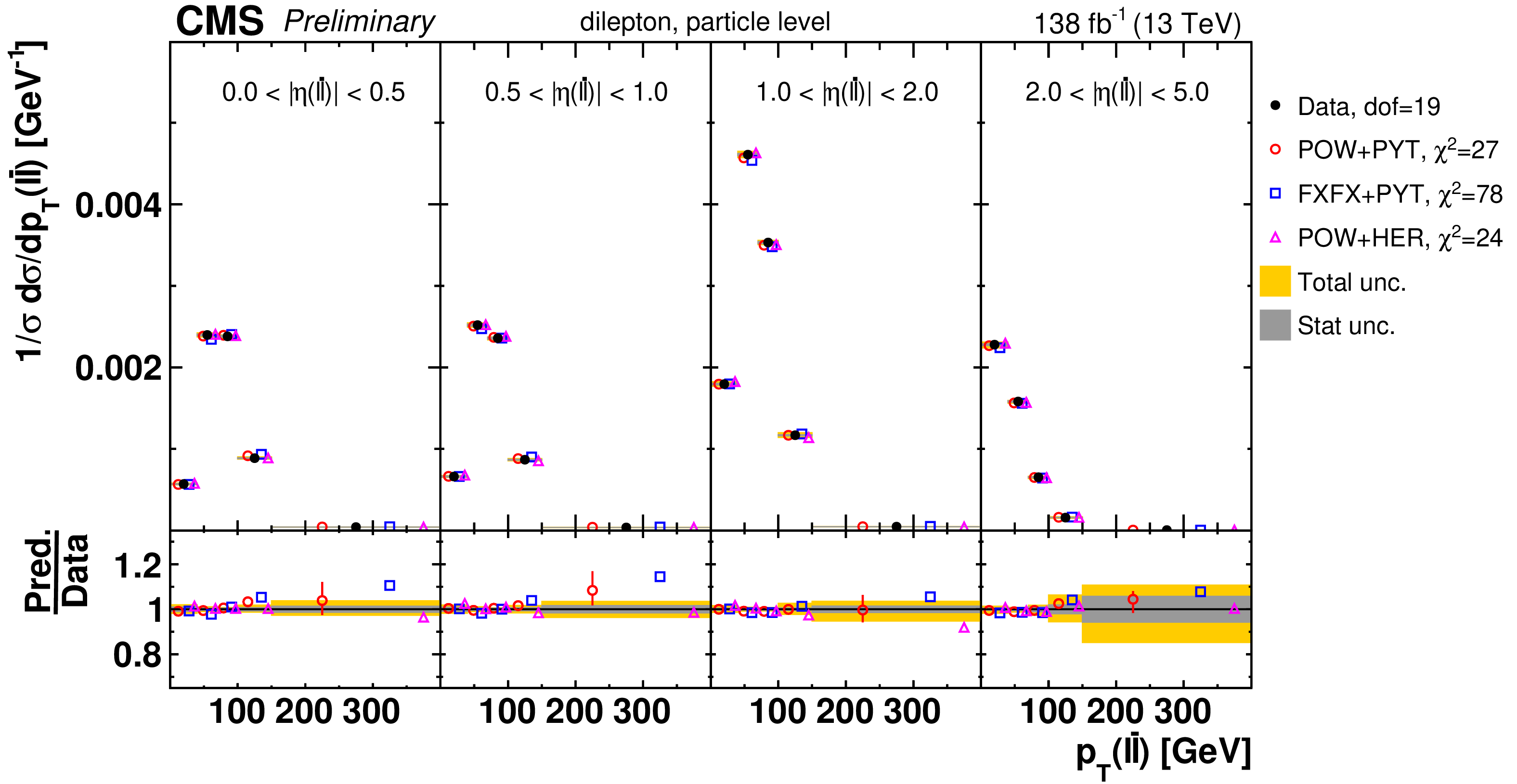
png pdf	Figure 26: Normalized differential $\mathrm{t\bar{t}}$ production cross sections as a function of ${{p_{\mathrm {T}}} (\ell \overline {\ell})}$ (left) and ${|\eta (\ell \overline {\ell})|}$ (right) are shown for data (filled circles) and various MC predictions (other points). Further details can be found in the caption of Fig. 23.
png pdf	Figure 26-a: Normalized differential $\mathrm{t\bar{t}}$ production cross sections as a function of ${{p_{\mathrm {T}}} (\ell \overline {\ell})}$ (left) and ${|\eta (\ell \overline {\ell})|}$ (right) are shown for data (filled circles) and various MC predictions (other points). Further details can be found in the caption of Fig. 23.
png pdf	Figure 26-b: Normalized differential $\mathrm{t\bar{t}}$ production cross sections as a function of ${{p_{\mathrm {T}}} (\ell \overline {\ell})}$ (left) and ${|\eta (\ell \overline {\ell})|}$ (right) are shown for data (filled circles) and various MC predictions (other points). Further details can be found in the caption of Fig. 23.
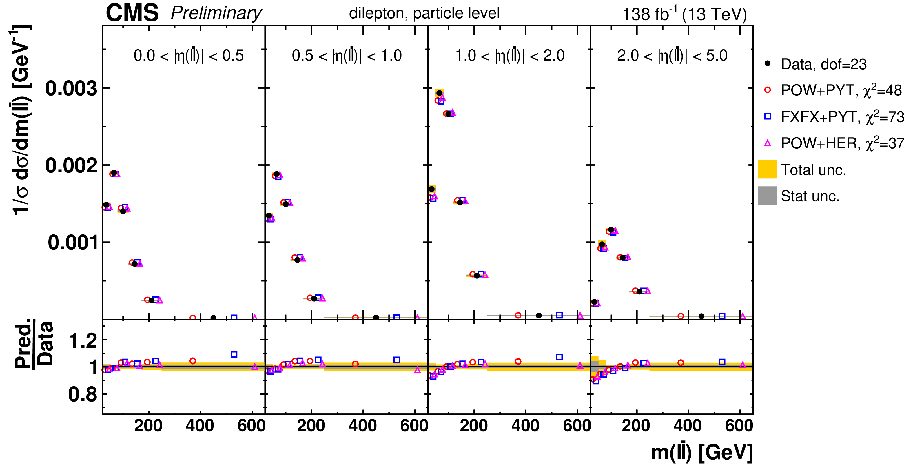
png pdf	Figure 27: Normalized $[ {|\eta (\ell \overline {\ell})|},\,{m(\ell \overline {\ell})} ]$ cross sections are shown for data (filled circles) and various MC predictions (other points). Further details can be found in the caption of Fig. 23.
png pdf	Figure 28: Normalized $[ {|\eta (\ell \overline {\ell})|},\,{{p_{\mathrm {T}}} (\ell \overline {\ell})} ]$ cross sections are shown for data (filled circles) and various MC predictions (other points). Further details can be found in the caption of Fig. 23.
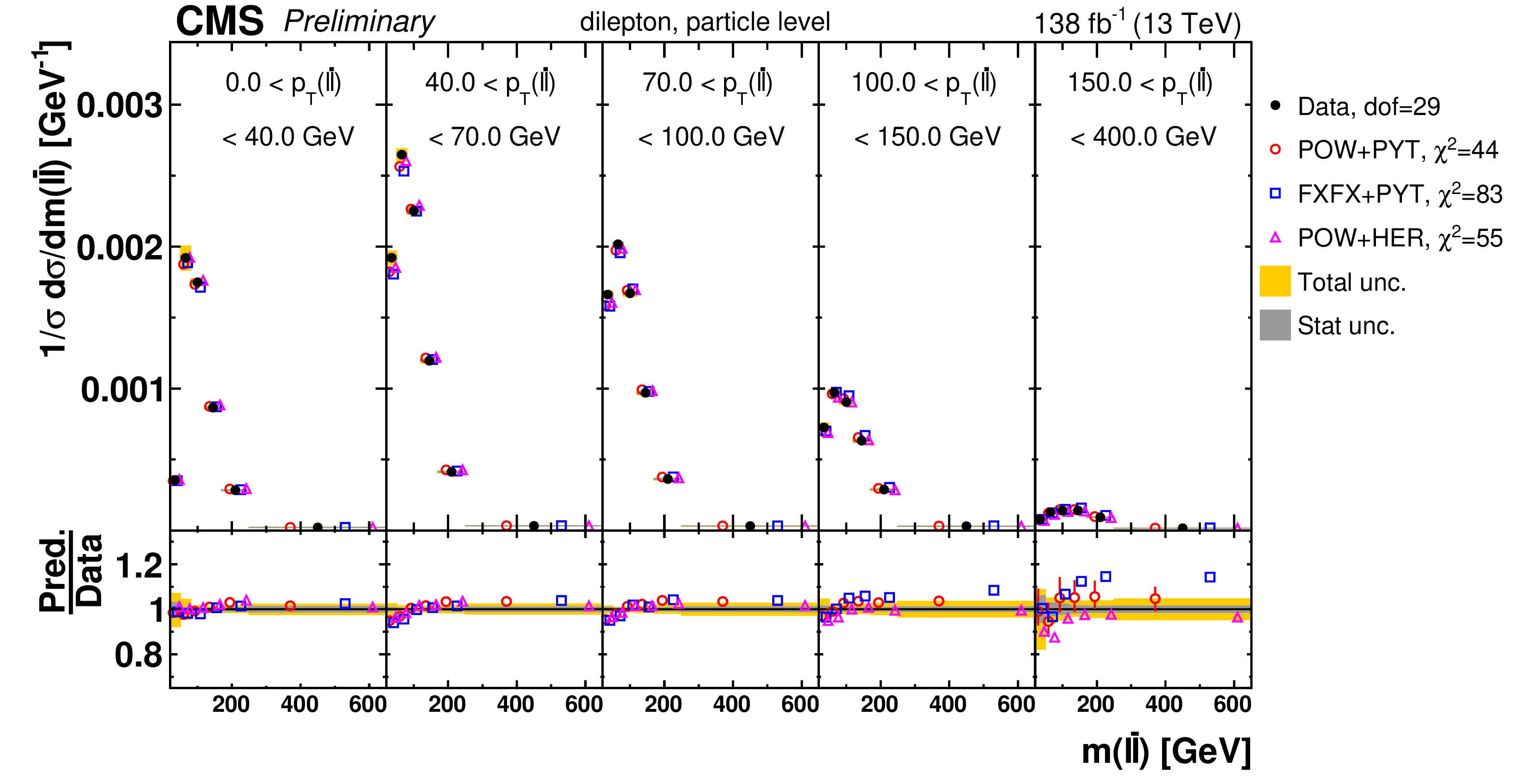
png pdf	Figure 29: Normalized $[ {{p_{\mathrm {T}}} (\ell \overline {\ell})},\,{m(\ell \overline {\ell})} ]$ cross sections are shown for data (filled circles) and various MC predictions (other points). Further details can be found in the caption of Fig. 23.
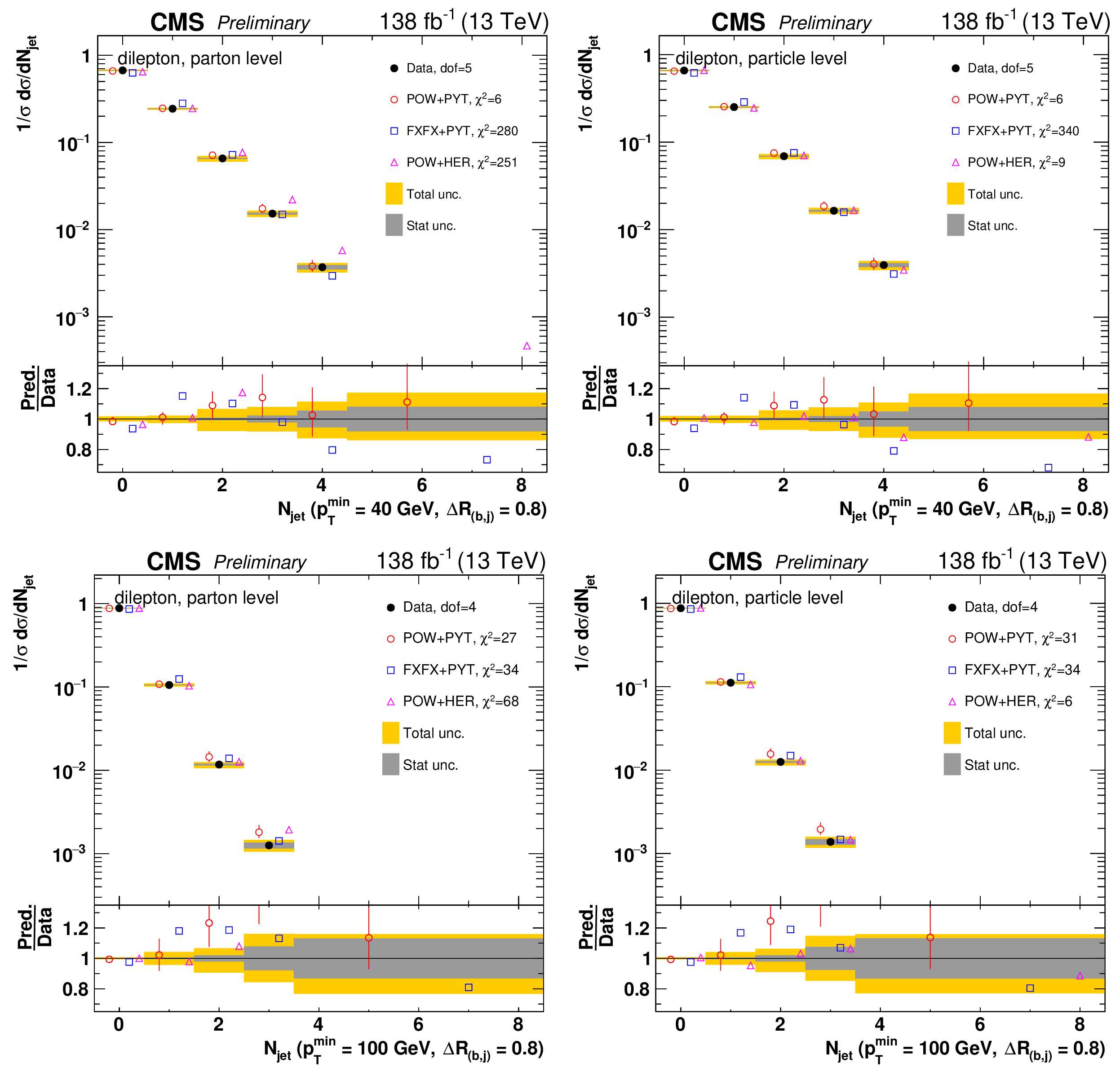
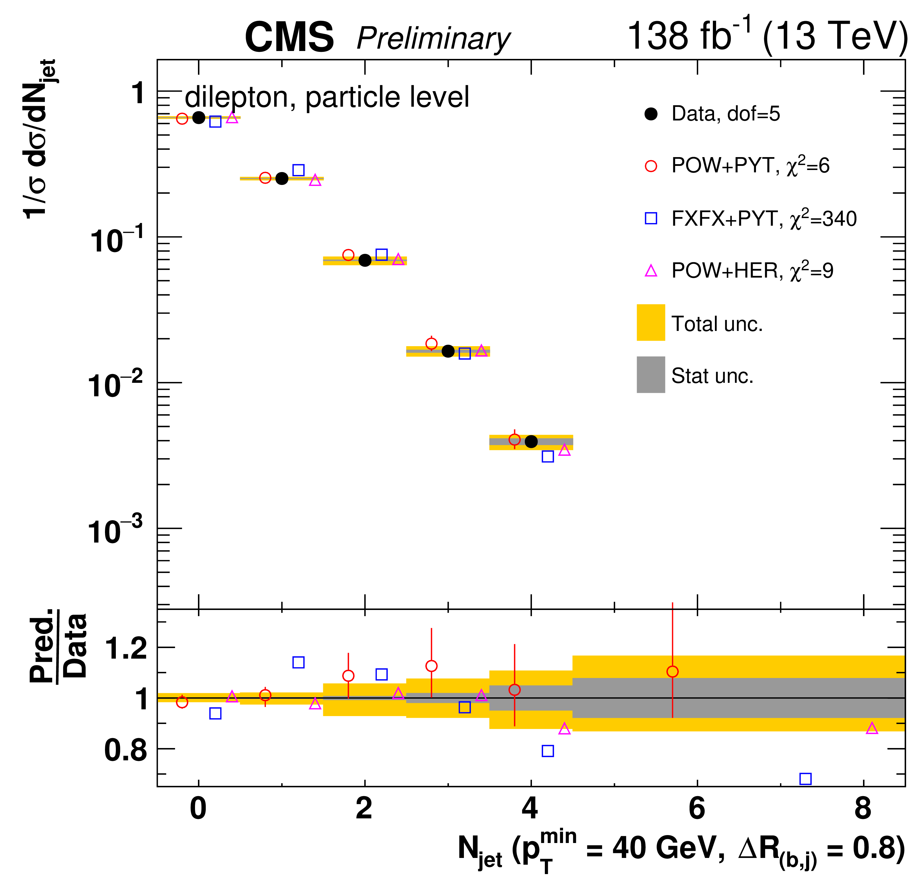
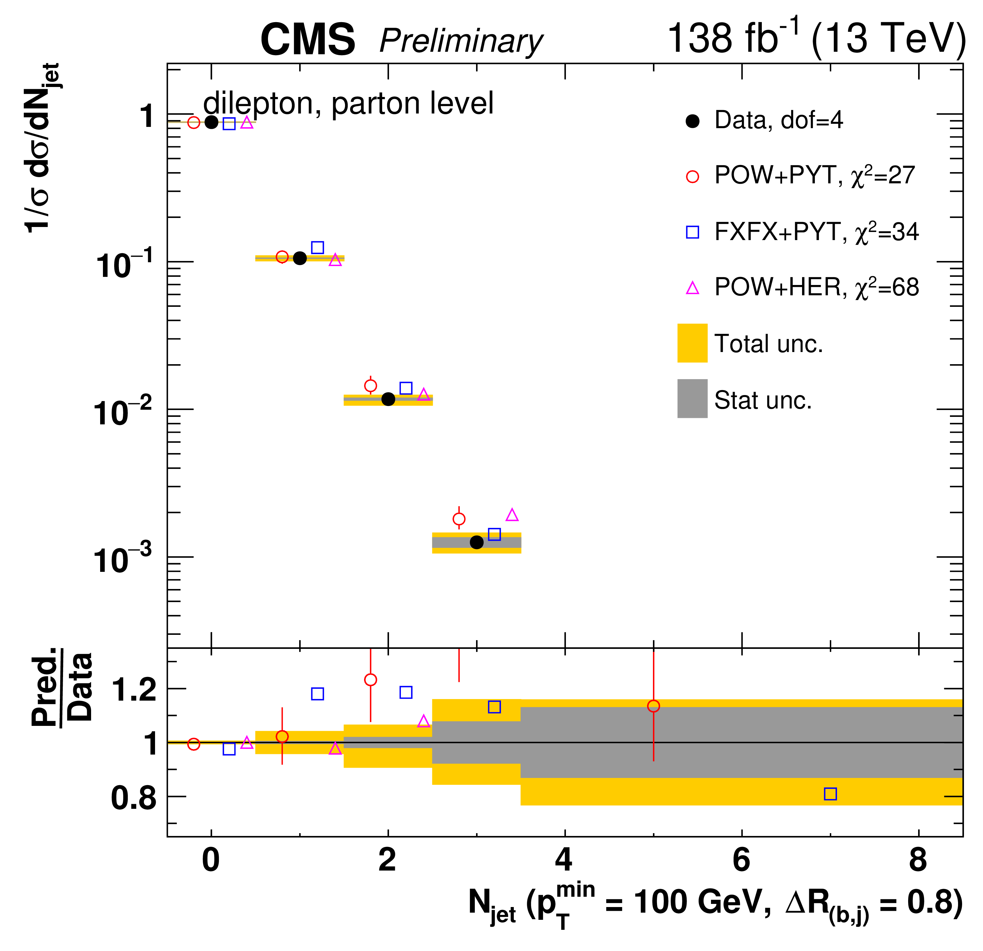
png pdf	Figure 30: Normalized differential $\mathrm{t\bar{t}}$ production cross sections as a function of ${N_{\text {jet}}}$, for a minimum jet ${p_{\mathrm {T}}}$ of 40 GeV (upper) and and 100 GeV (lower), measured at the parton level in the full phase space (left) and at the particle level in a fiducial phase space (right). The data are shown as filled circles with dark and light bands indicating the statistical and total uncertainties (statistical and systematic uncertainties summed in quadrature), respectively. The cross sections are compared to various MC predictions (other points). The estimated uncertainties in the POWHEG+PYTHIA-8 (`POW-PYT') simulation are represented by a vertical bar on the corresponding points. For each MC model, a value of ${\chi ^2}$ is reported that takes into account the measurement uncertainties. The lower panel in each plot shows the ratios of the predictions to the data.
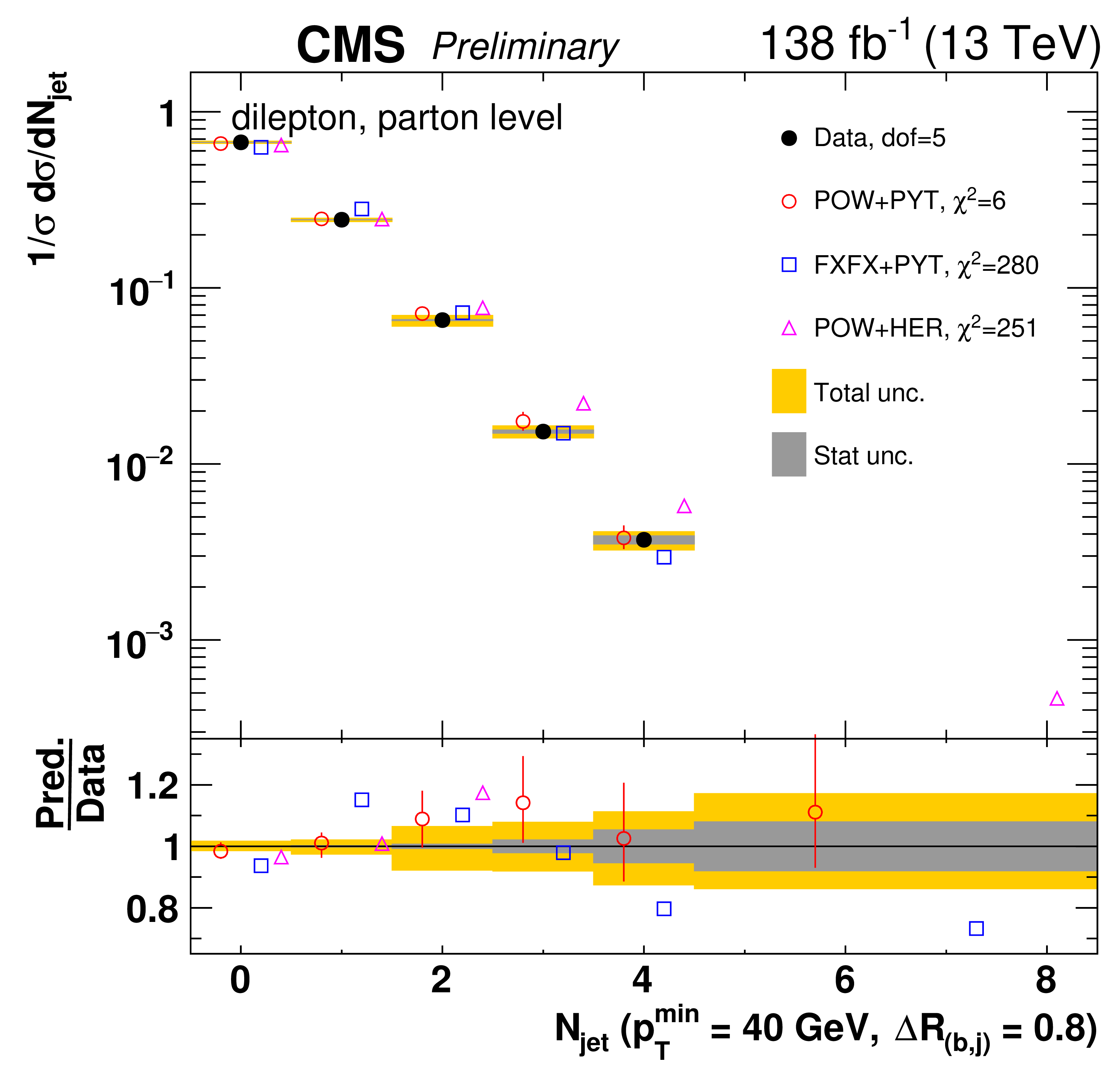
png pdf	Figure 30-a: Normalized differential $\mathrm{t\bar{t}}$ production cross sections as a function of ${N_{\text {jet}}}$, for a minimum jet ${p_{\mathrm {T}}}$ of 40 GeV (upper) and and 100 GeV (lower), measured at the parton level in the full phase space (left) and at the particle level in a fiducial phase space (right). The data are shown as filled circles with dark and light bands indicating the statistical and total uncertainties (statistical and systematic uncertainties summed in quadrature), respectively. The cross sections are compared to various MC predictions (other points). The estimated uncertainties in the POWHEG+PYTHIA-8 (`POW-PYT') simulation are represented by a vertical bar on the corresponding points. For each MC model, a value of ${\chi ^2}$ is reported that takes into account the measurement uncertainties. The lower panel in each plot shows the ratios of the predictions to the data.
png pdf	Figure 30-b: Normalized differential $\mathrm{t\bar{t}}$ production cross sections as a function of ${N_{\text {jet}}}$, for a minimum jet ${p_{\mathrm {T}}}$ of 40 GeV (upper) and and 100 GeV (lower), measured at the parton level in the full phase space (left) and at the particle level in a fiducial phase space (right). The data are shown as filled circles with dark and light bands indicating the statistical and total uncertainties (statistical and systematic uncertainties summed in quadrature), respectively. The cross sections are compared to various MC predictions (other points). The estimated uncertainties in the POWHEG+PYTHIA-8 (`POW-PYT') simulation are represented by a vertical bar on the corresponding points. For each MC model, a value of ${\chi ^2}$ is reported that takes into account the measurement uncertainties. The lower panel in each plot shows the ratios of the predictions to the data.
png pdf	Figure 30-c: Normalized differential $\mathrm{t\bar{t}}$ production cross sections as a function of ${N_{\text {jet}}}$, for a minimum jet ${p_{\mathrm {T}}}$ of 40 GeV (upper) and and 100 GeV (lower), measured at the parton level in the full phase space (left) and at the particle level in a fiducial phase space (right). The data are shown as filled circles with dark and light bands indicating the statistical and total uncertainties (statistical and systematic uncertainties summed in quadrature), respectively. The cross sections are compared to various MC predictions (other points). The estimated uncertainties in the POWHEG+PYTHIA-8 (`POW-PYT') simulation are represented by a vertical bar on the corresponding points. For each MC model, a value of ${\chi ^2}$ is reported that takes into account the measurement uncertainties. The lower panel in each plot shows the ratios of the predictions to the data.
png pdf	Figure 30-d: Normalized differential $\mathrm{t\bar{t}}$ production cross sections as a function of ${N_{\text {jet}}}$, for a minimum jet ${p_{\mathrm {T}}}$ of 40 GeV (upper) and and 100 GeV (lower), measured at the parton level in the full phase space (left) and at the particle level in a fiducial phase space (right). The data are shown as filled circles with dark and light bands indicating the statistical and total uncertainties (statistical and systematic uncertainties summed in quadrature), respectively. The cross sections are compared to various MC predictions (other points). The estimated uncertainties in the POWHEG+PYTHIA-8 (`POW-PYT') simulation are represented by a vertical bar on the corresponding points. For each MC model, a value of ${\chi ^2}$ is reported that takes into account the measurement uncertainties. The lower panel in each plot shows the ratios of the predictions to the data.
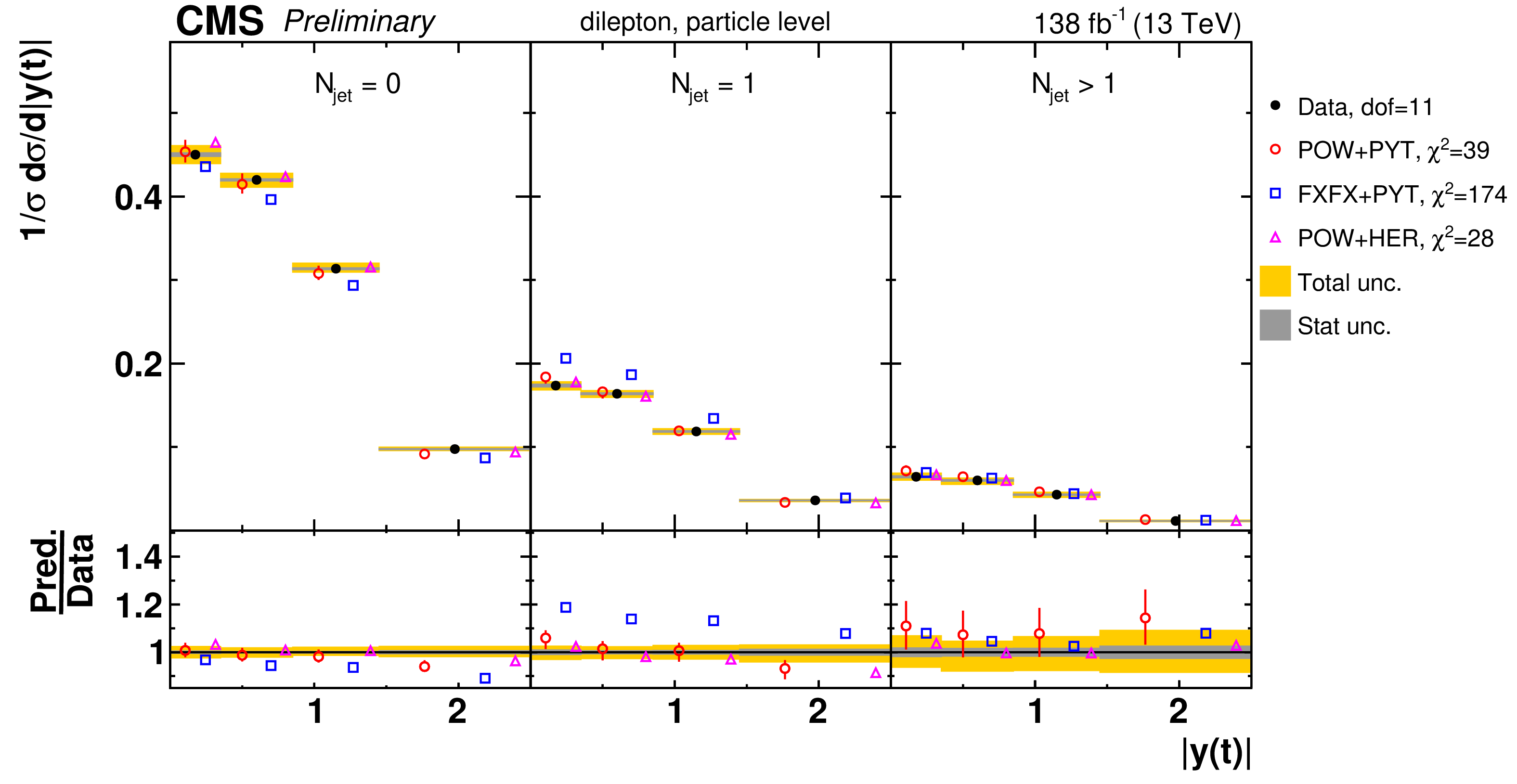
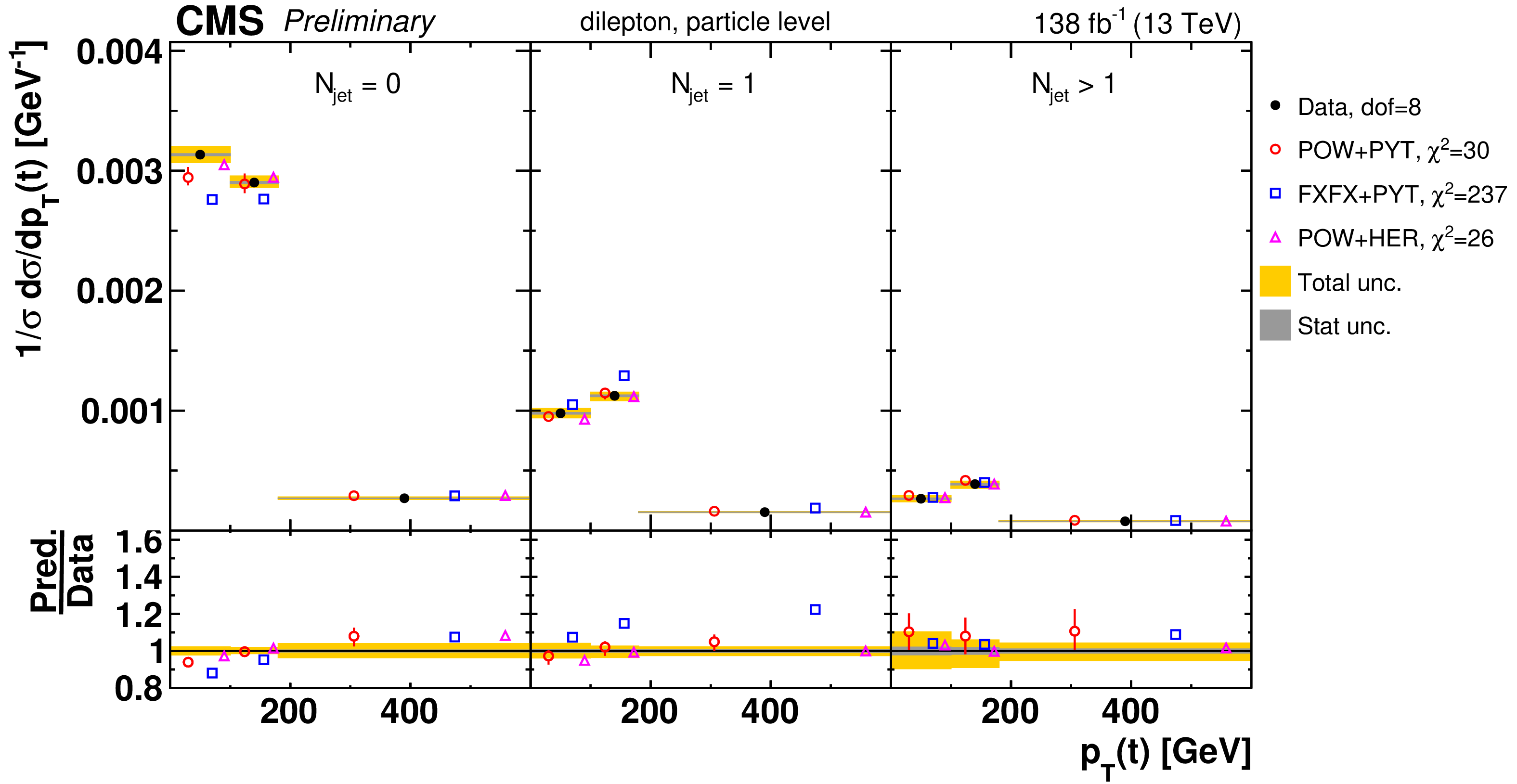
png pdf	Figure 31-a: Normalized $[ {N_{\text {jet}}},\,{{p_{\mathrm {T}}} (\mathrm{t})} ]$ cross sections measured at the parton level in the full phase space (upper) and at the particle level in a fiducial phase space (lower). The data are shown as filled circles with dark and light bands indicating the statistical and total uncertainties (statistical and systematic uncertainties summed in quadrature), respectively. The cross sections are compared to various MC predictions (other points). The estimated uncertainties in the POWHEG+PYTHIA-8 (`POW-PYT') simulation are represented by a vertical bar on the corresponding points. For each MC model, a value of ${\chi ^2}$ is reported that takes into account the measurement uncertainties. The lower panel in each plot shows the ratios of the predictions to the data.
png pdf	Figure 31-b: Normalized $[ {N_{\text {jet}}},\,{{p_{\mathrm {T}}} (\mathrm{t})} ]$ cross sections measured at the parton level in the full phase space (upper) and at the particle level in a fiducial phase space (lower). The data are shown as filled circles with dark and light bands indicating the statistical and total uncertainties (statistical and systematic uncertainties summed in quadrature), respectively. The cross sections are compared to various MC predictions (other points). The estimated uncertainties in the POWHEG+PYTHIA-8 (`POW-PYT') simulation are represented by a vertical bar on the corresponding points. For each MC model, a value of ${\chi ^2}$ is reported that takes into account the measurement uncertainties. The lower panel in each plot shows the ratios of the predictions to the data.
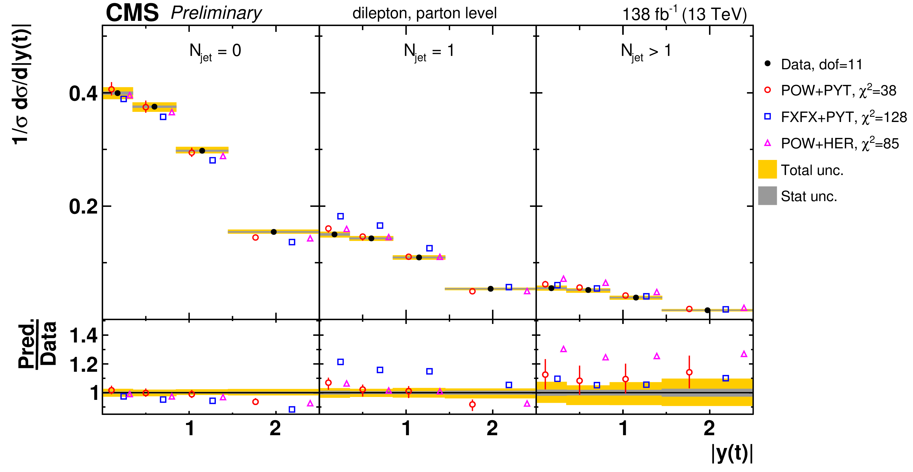
png pdf	Figure 32-a: Normalized $[ {N_{\text {jet}}},\,{|y(\mathrm{t})|} ]$ cross sections are shown for data (filled circles) and various MC predictions (other points). Further details can be found in the caption of Fig. 31.
png pdf	Figure 32-b: Normalized $[ {N_{\text {jet}}},\,{|y(\mathrm{t})|} ]$ cross sections are shown for data (filled circles) and various MC predictions (other points). Further details can be found in the caption of Fig. 31.
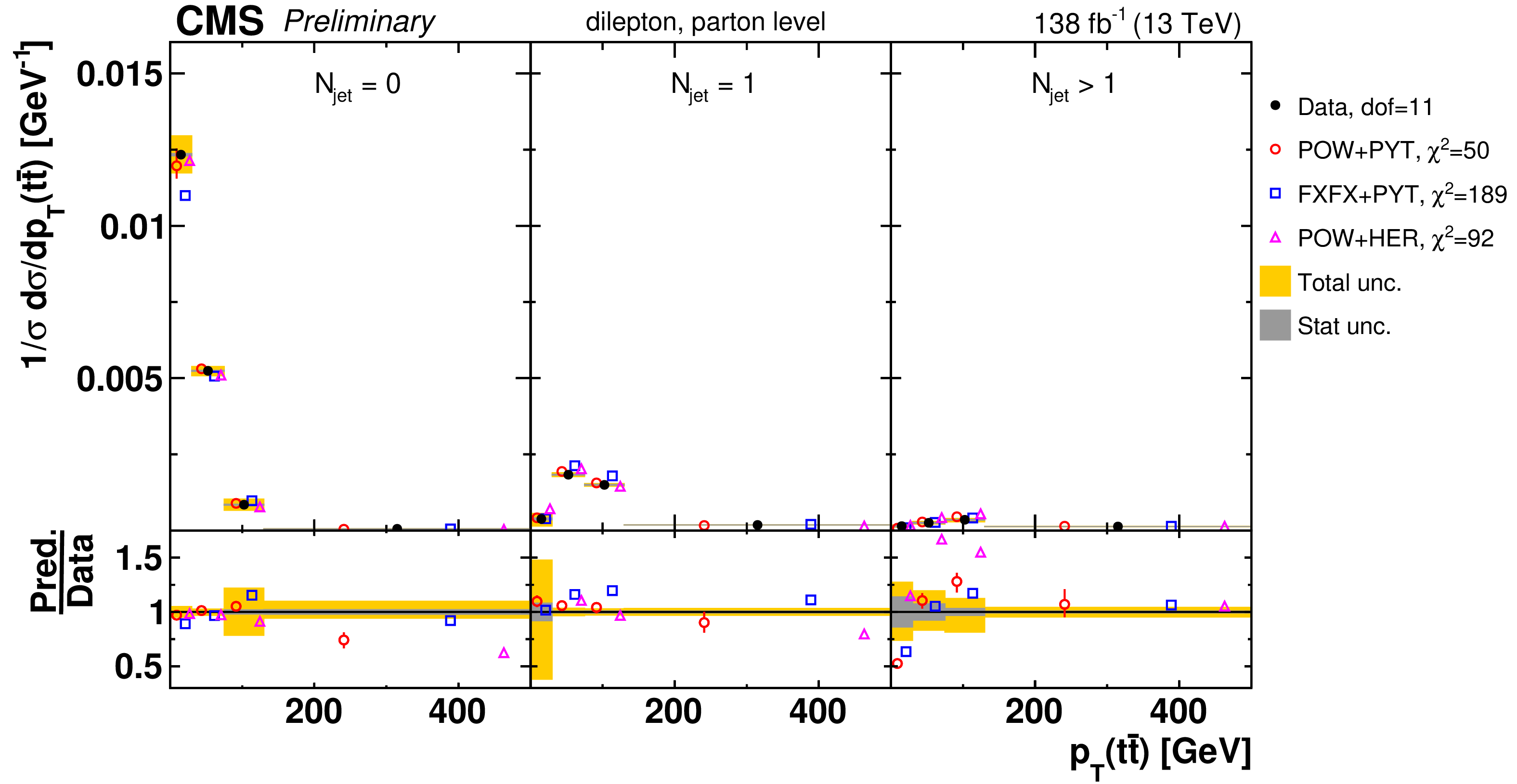
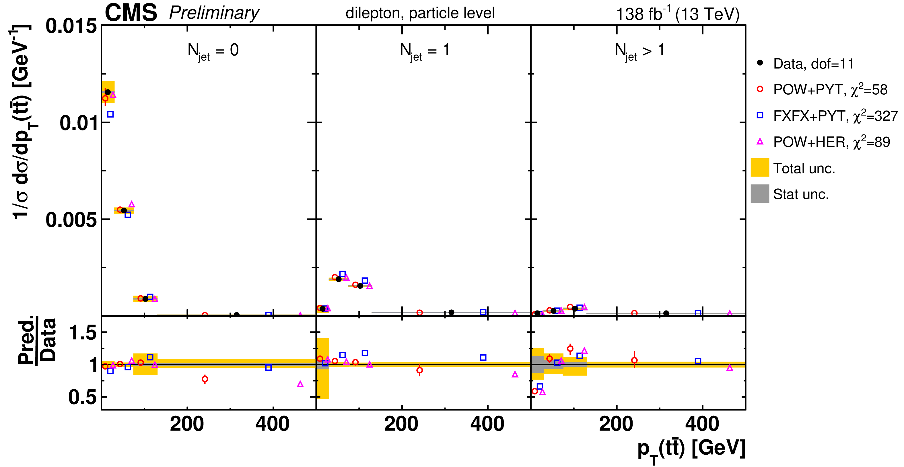
png pdf	Figure 33-a: Normalized $[ {N_{\text {jet}}},\,{{p_{\mathrm {T}}} ( \mathrm{t\bar{t}})} ]$ cross sections are shown for data (filled circles) and various MC predictions (other points). Further details can be found in the caption of Fig. 31.
png pdf	Figure 33-b: Normalized $[ {N_{\text {jet}}},\,{{p_{\mathrm {T}}} ( \mathrm{t\bar{t}})} ]$ cross sections are shown for data (filled circles) and various MC predictions (other points). Further details can be found in the caption of Fig. 31.
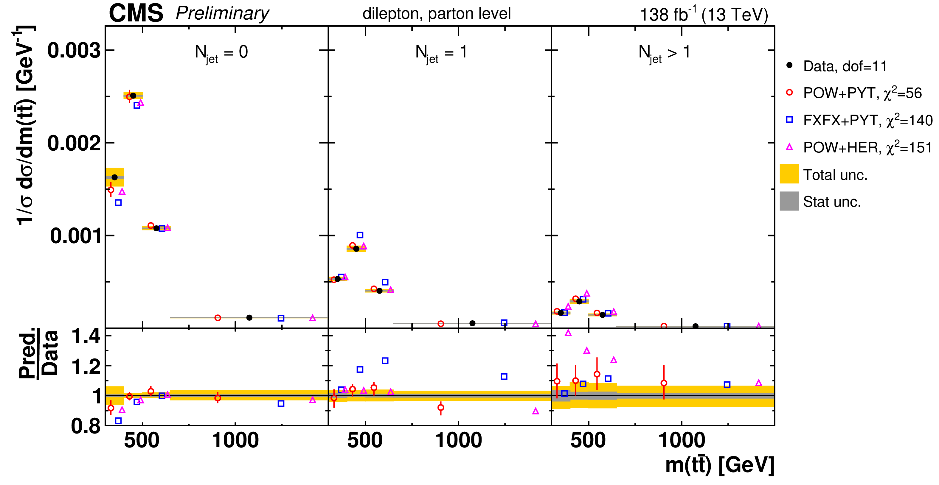
png pdf	Figure 34-a: Normalized $[ {N_{\text {jet}}},\,{m( \mathrm{t\bar{t}})} ]$ cross sections are shown for data (filled circles) and various MC predictions (other points). Further details can be found in the caption of Fig. 31.
png pdf	Figure 34-b: Normalized $[ {N_{\text {jet}}},\,{m( \mathrm{t\bar{t}})} ]$ cross sections are shown for data (filled circles) and various MC predictions (other points). Further details can be found in the caption of Fig. 31.
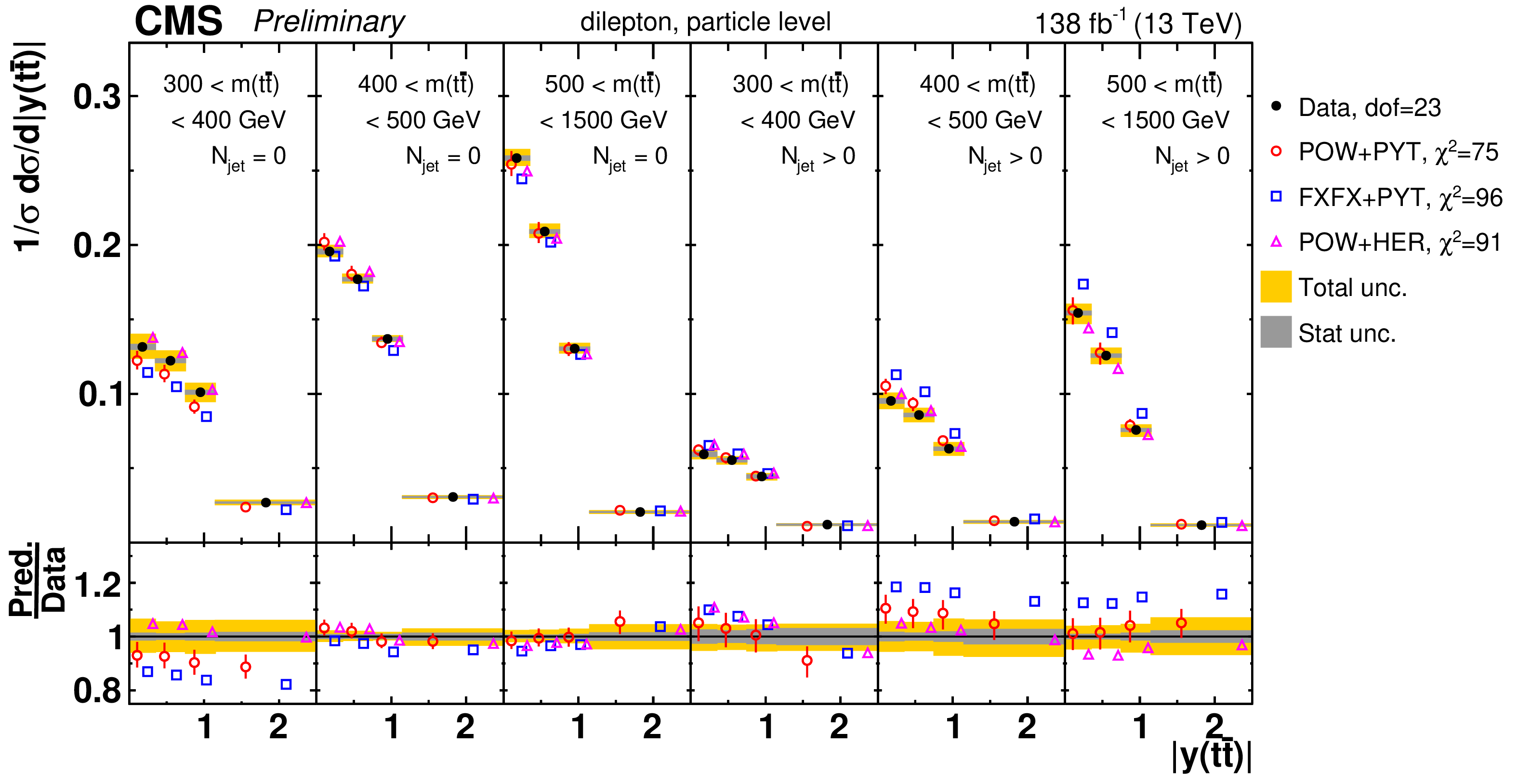
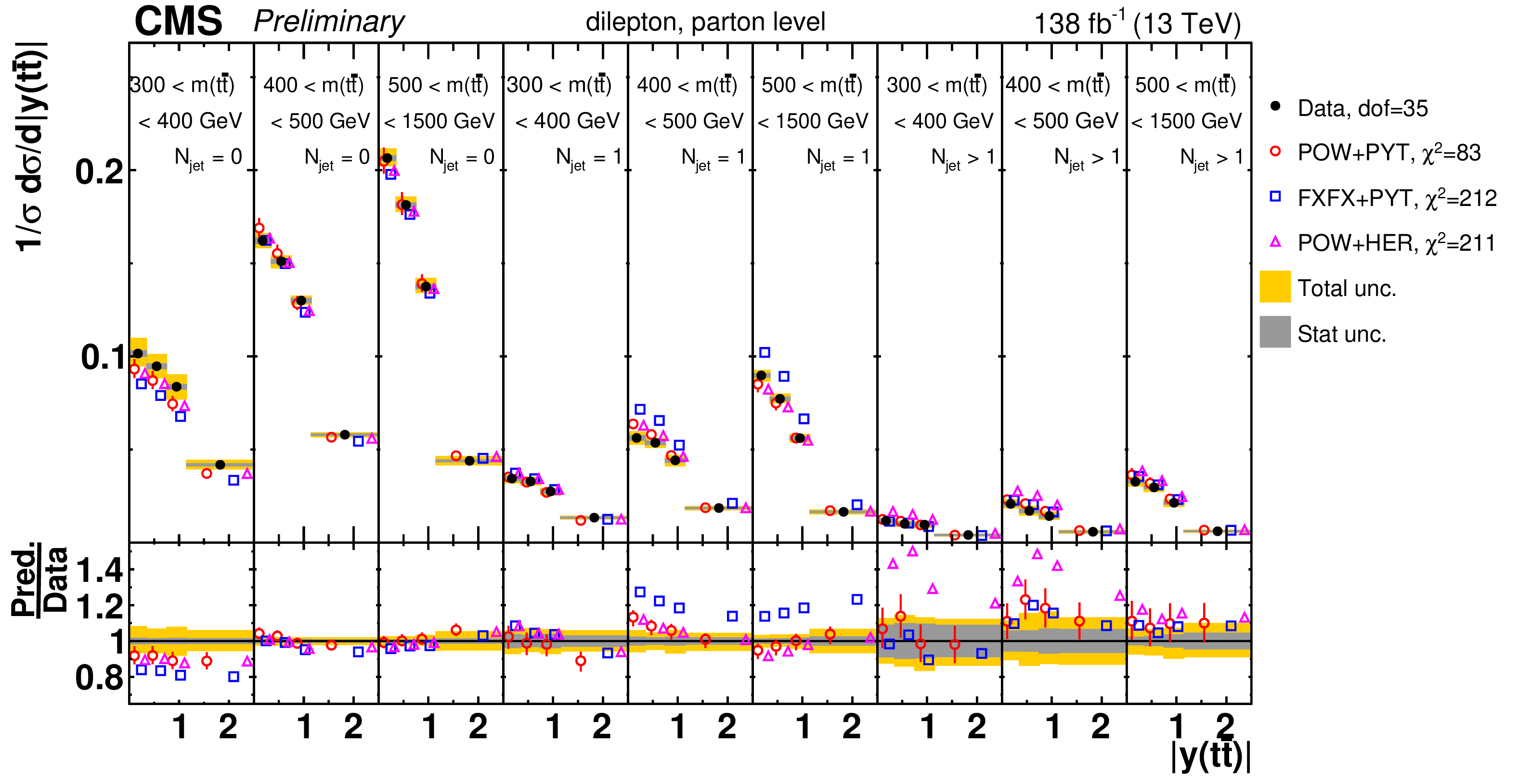
png pdf	Figure 35-a: Normalized $[ {N_{\text {jet}}},\,{|y( \mathrm{t\bar{t}})|} ]$ cross sections are shown for data (filled circles) and various MC predictions (other points). Further details can be found in the caption of Fig. 31.
png pdf	Figure 35-b: Normalized $[ {N_{\text {jet}}},\,{|y( \mathrm{t\bar{t}})|} ]$ cross sections are shown for data (filled circles) and various MC predictions (other points). Further details can be found in the caption of Fig. 31.
png pdf	Figure 36-a: Normalized $[ {N_{\text {jet}}},\,{\Delta \eta (\mathrm{t},\mathrm{\bar{t}})} ]$ cross sections are shown for data (filled circles) and various MC predictions (other points). Further details can be found in the caption of Fig. 31.
png pdf	Figure 36-b: Normalized $[ {N_{\text {jet}}},\,{\Delta \eta (\mathrm{t},\mathrm{\bar{t}})} ]$ cross sections are shown for data (filled circles) and various MC predictions (other points). Further details can be found in the caption of Fig. 31.
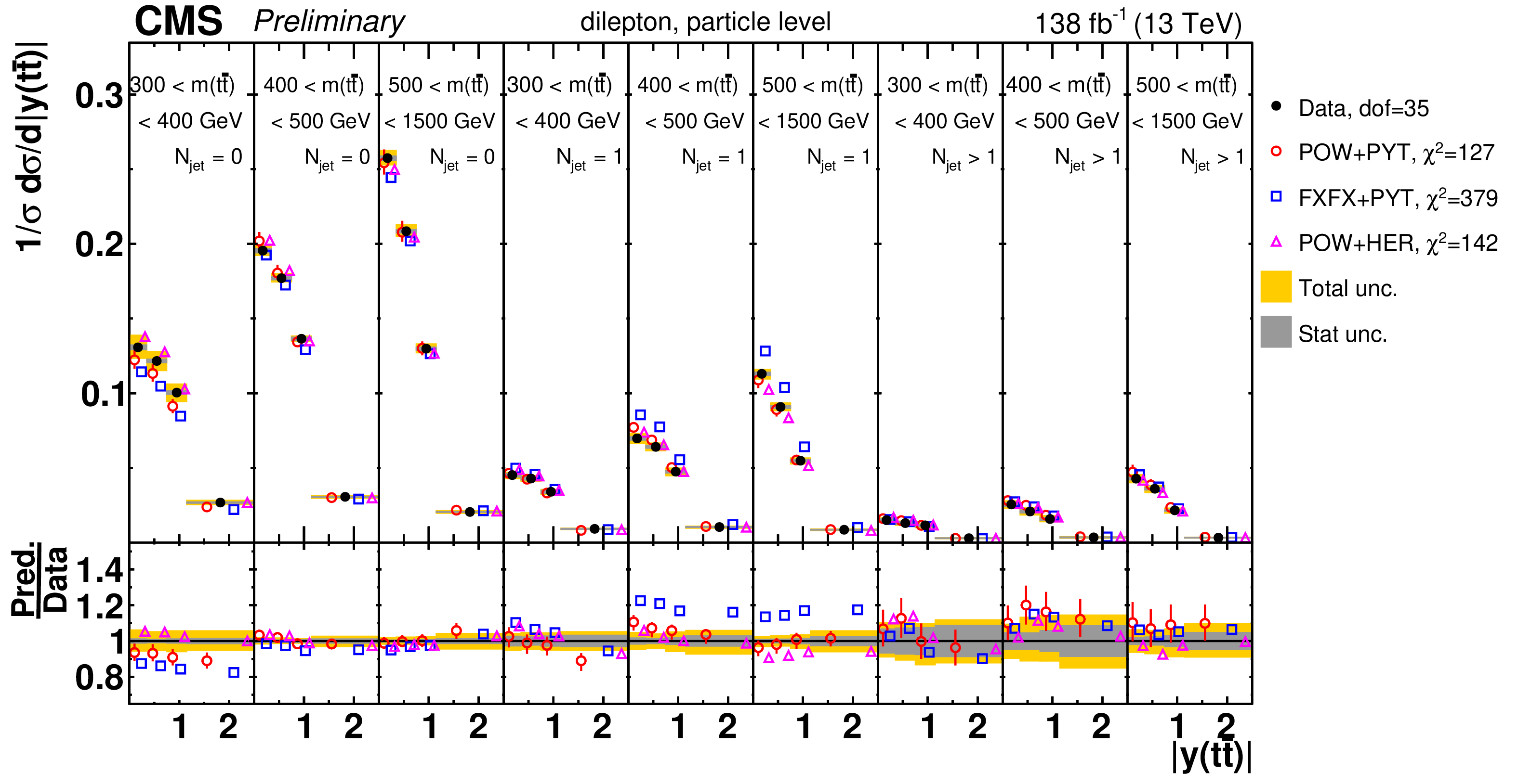
png pdf	Figure 37-a: Normalized $[N^{0,1+}_{\text {jet}},\, {m( \mathrm{t\bar{t}})},\,{|y( \mathrm{t\bar{t}})|} ]$ cross sections are shown for data (filled circles) and various MC predictions (other points). Further details can be found in the caption of Fig. 31.
png pdf	Figure 37-b: Normalized $[N^{0,1+}_{\text {jet}},\, {m( \mathrm{t\bar{t}})},\,{|y( \mathrm{t\bar{t}})|} ]$ cross sections are shown for data (filled circles) and various MC predictions (other points). Further details can be found in the caption of Fig. 31.
png pdf	Figure 38-a: Normalized $[N^{0,1,2+}_{\text {jet}},\, {m( \mathrm{t\bar{t}})},\,{|y( \mathrm{t\bar{t}})|} ]$ cross sections are shown for data (filled circles) and various MC predictions (other points). Further details can be found in the caption of Fig. 31.
png pdf	Figure 38-b: Normalized $[N^{0,1,2+}_{\text {jet}},\, {m( \mathrm{t\bar{t}})},\,{|y( \mathrm{t\bar{t}})|} ]$ cross sections are shown for data (filled circles) and various MC predictions (other points). Further details can be found in the caption of Fig. 31.
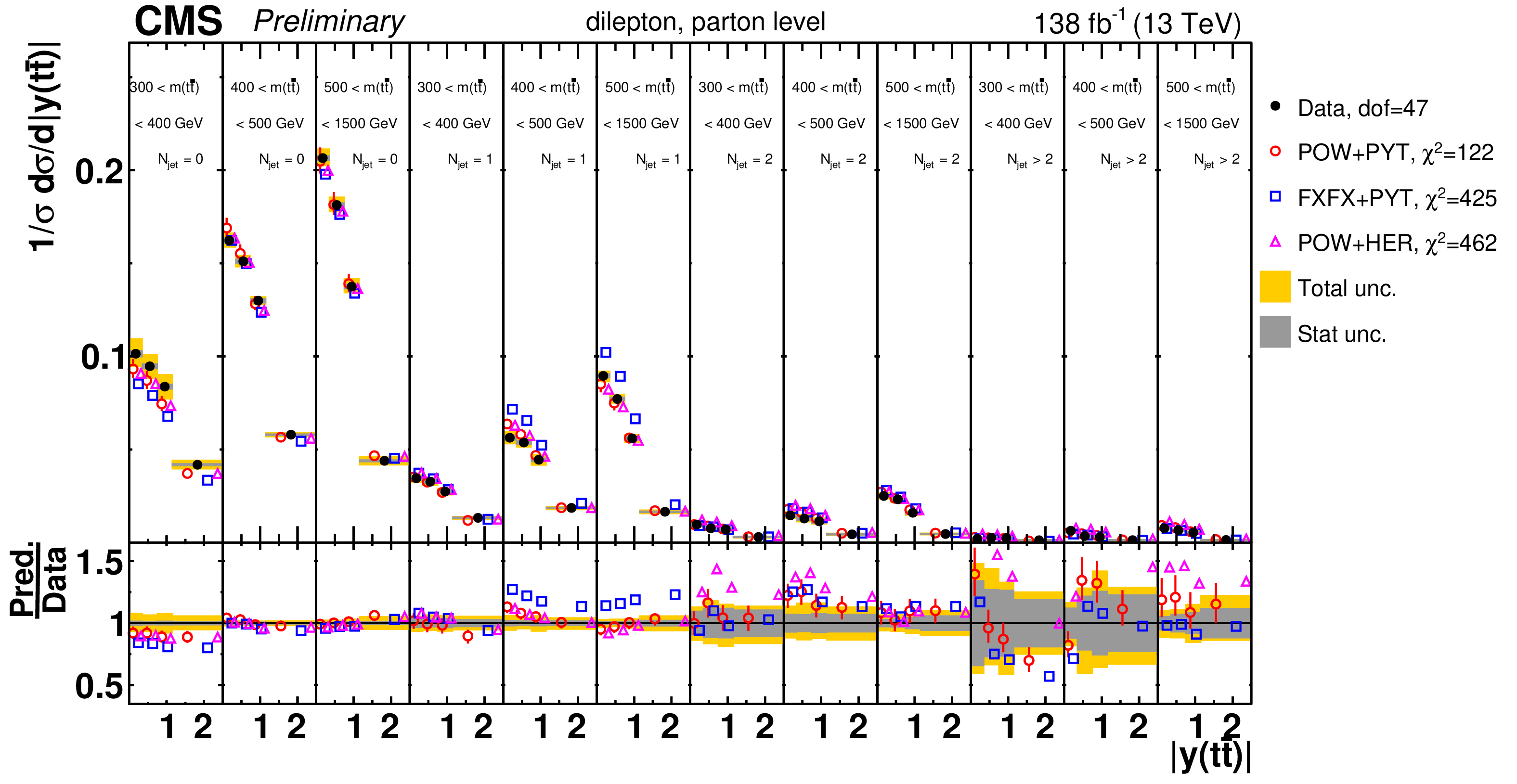
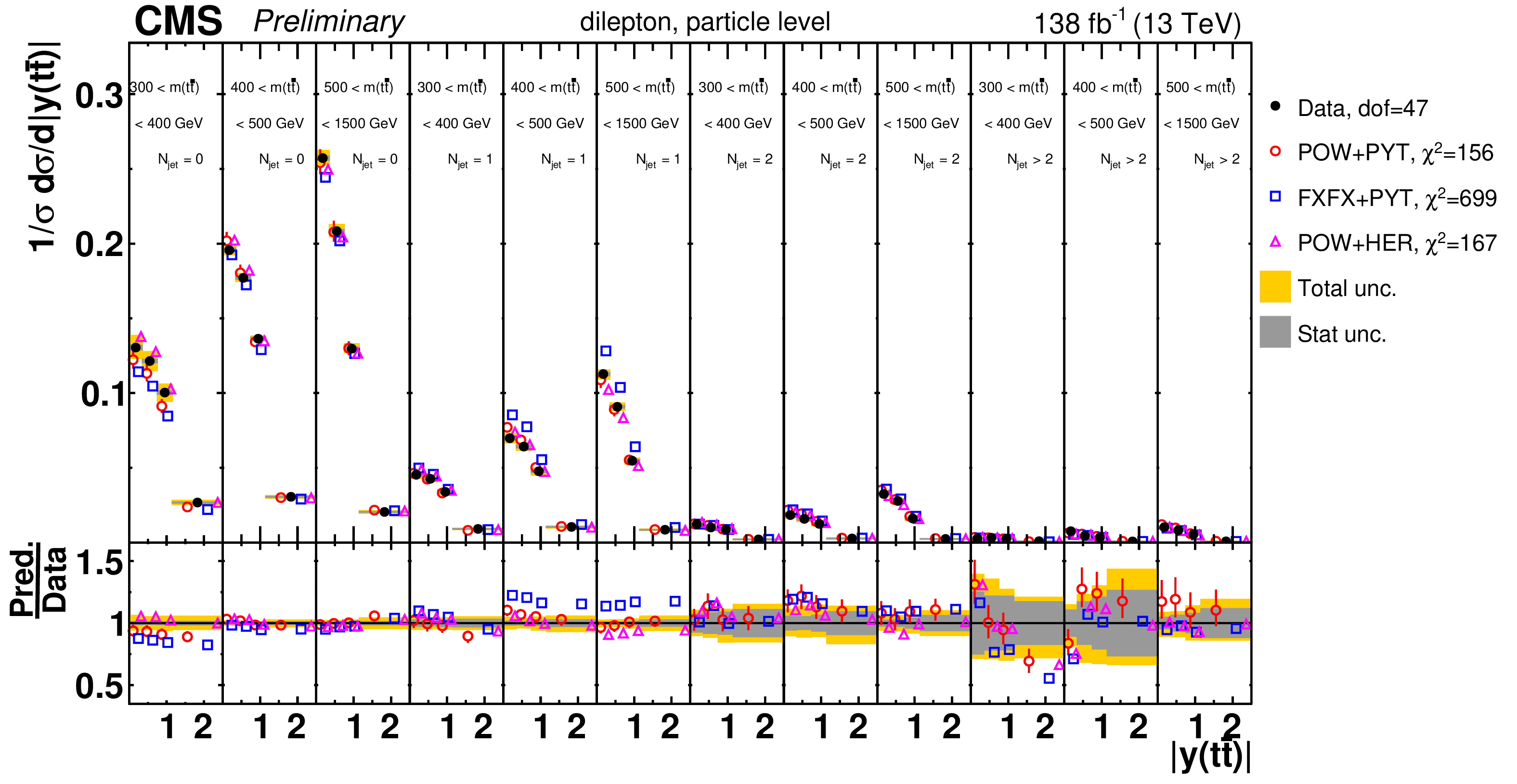
png pdf	Figure 39-a: Normalized $[N^{0,1,2,3+}_{\text {jet}},\, {m( \mathrm{t\bar{t}})},\,{|y( \mathrm{t\bar{t}})|} ]$ cross sections are shown for data (filled circles) and various MC predictions (other points). Further details can be found in the caption of Fig. 31.
png pdf	Figure 39-b: Normalized $[N^{0,1,2,3+}_{\text {jet}},\, {m( \mathrm{t\bar{t}})},\,{|y( \mathrm{t\bar{t}})|} ]$ cross sections are shown for data (filled circles) and various MC predictions (other points). Further details can be found in the caption of Fig. 31.
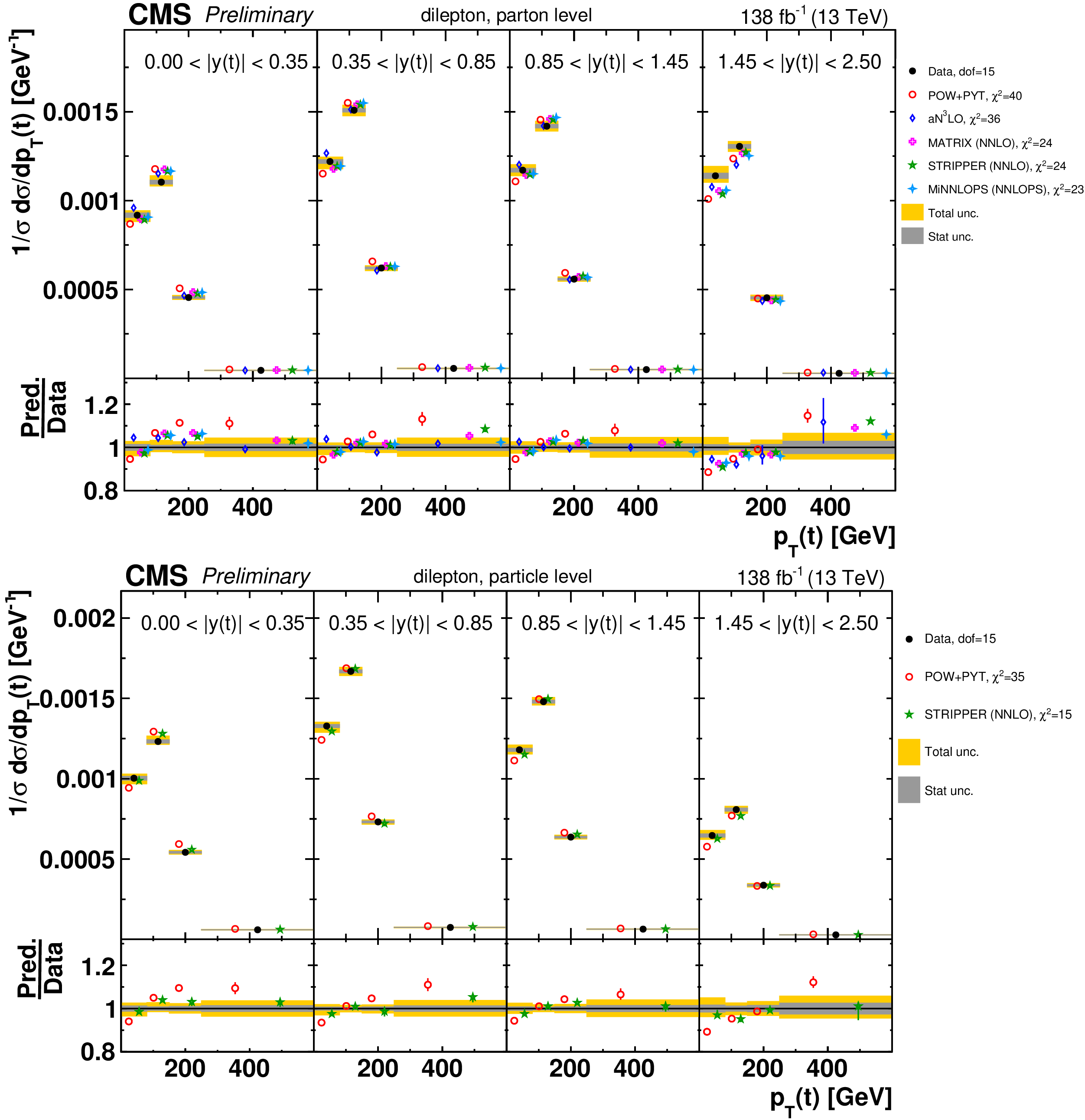
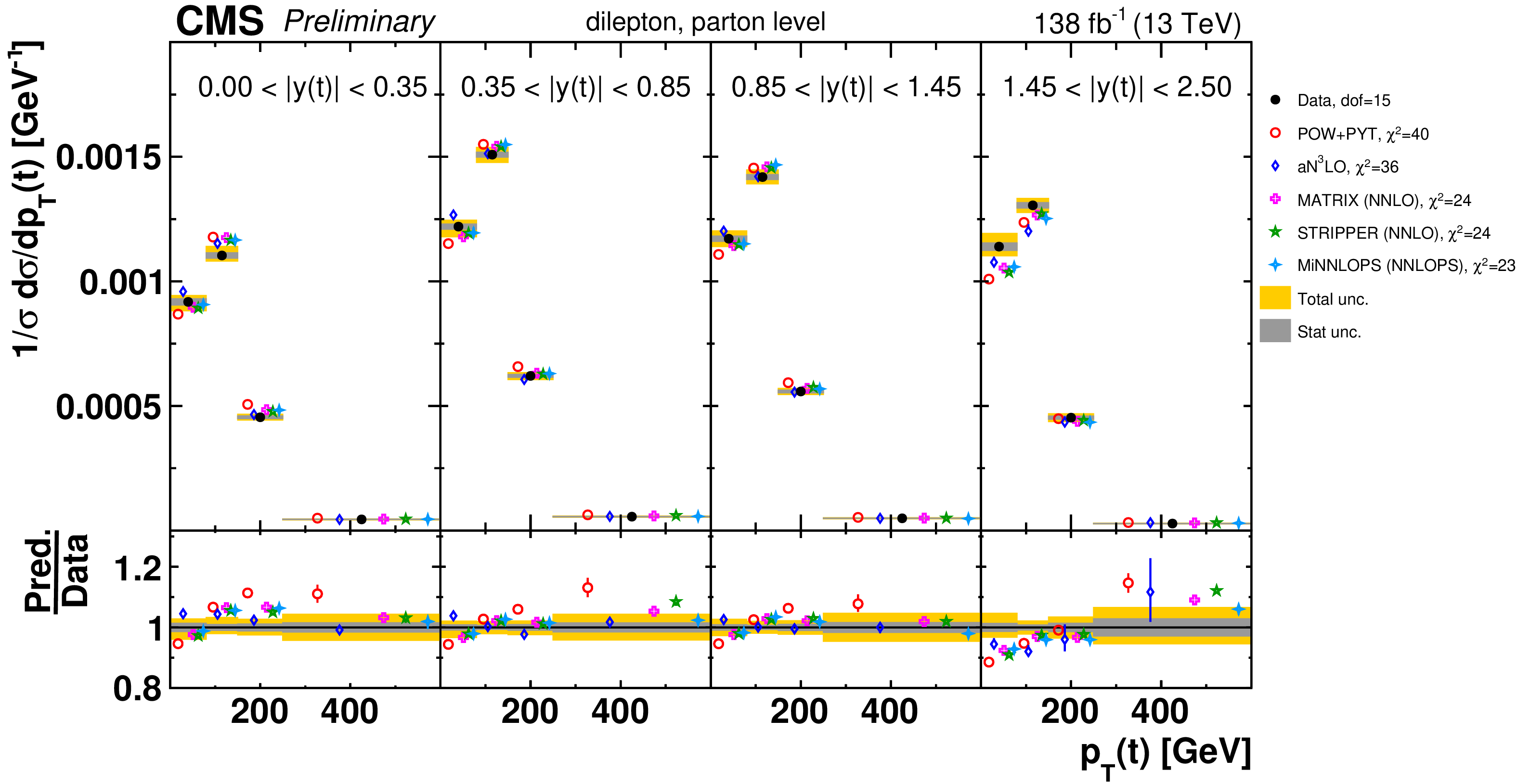
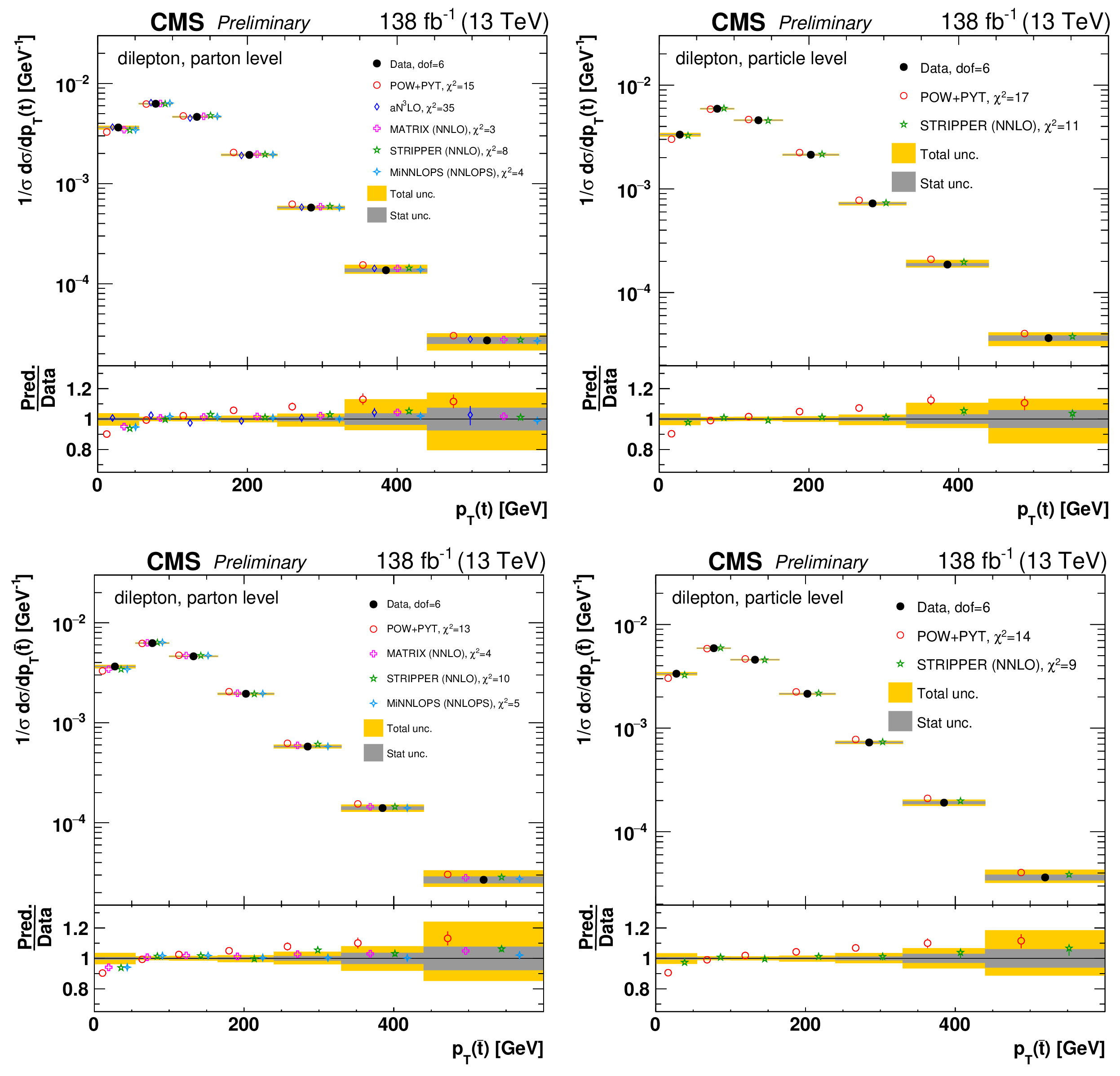
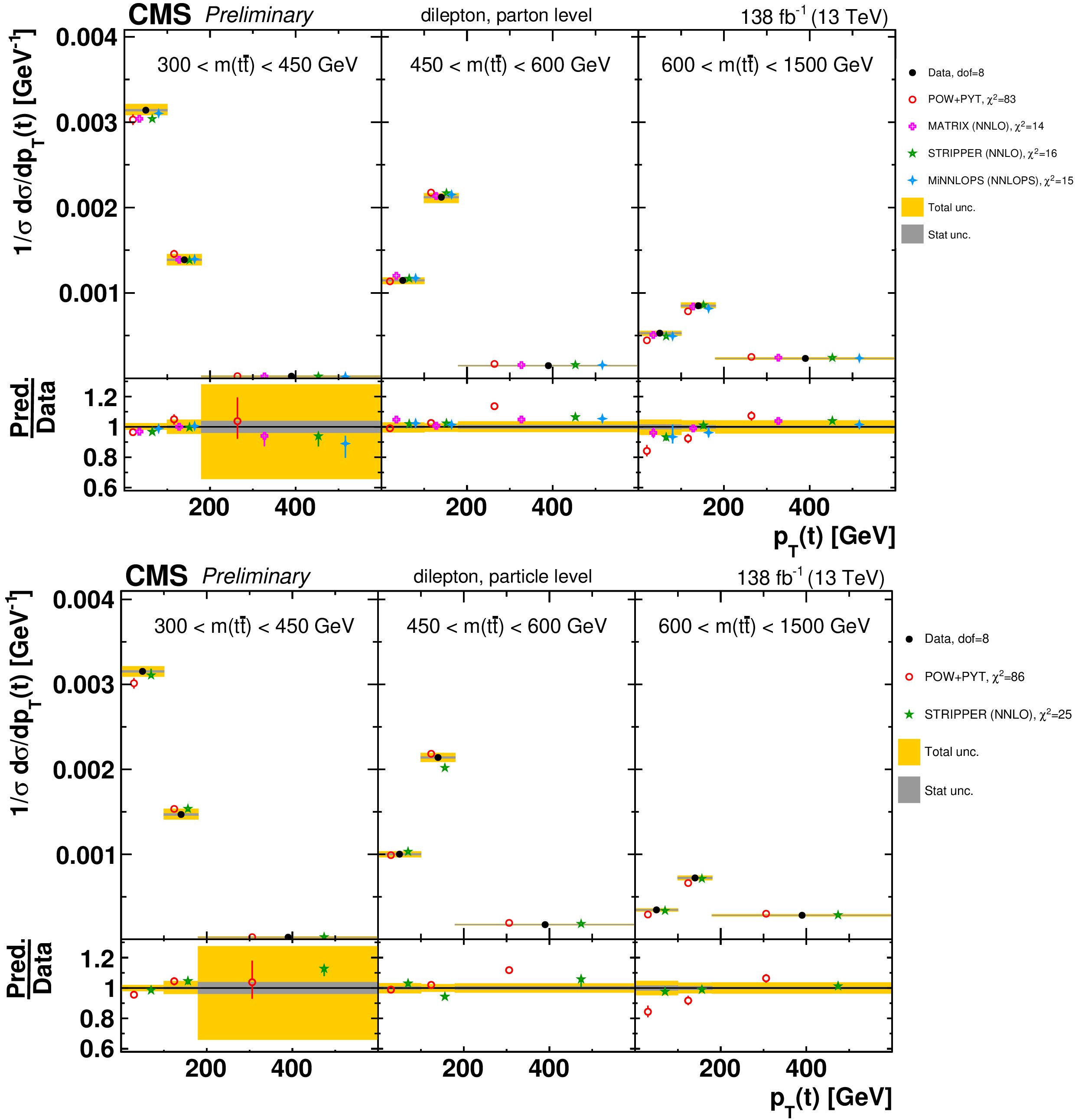
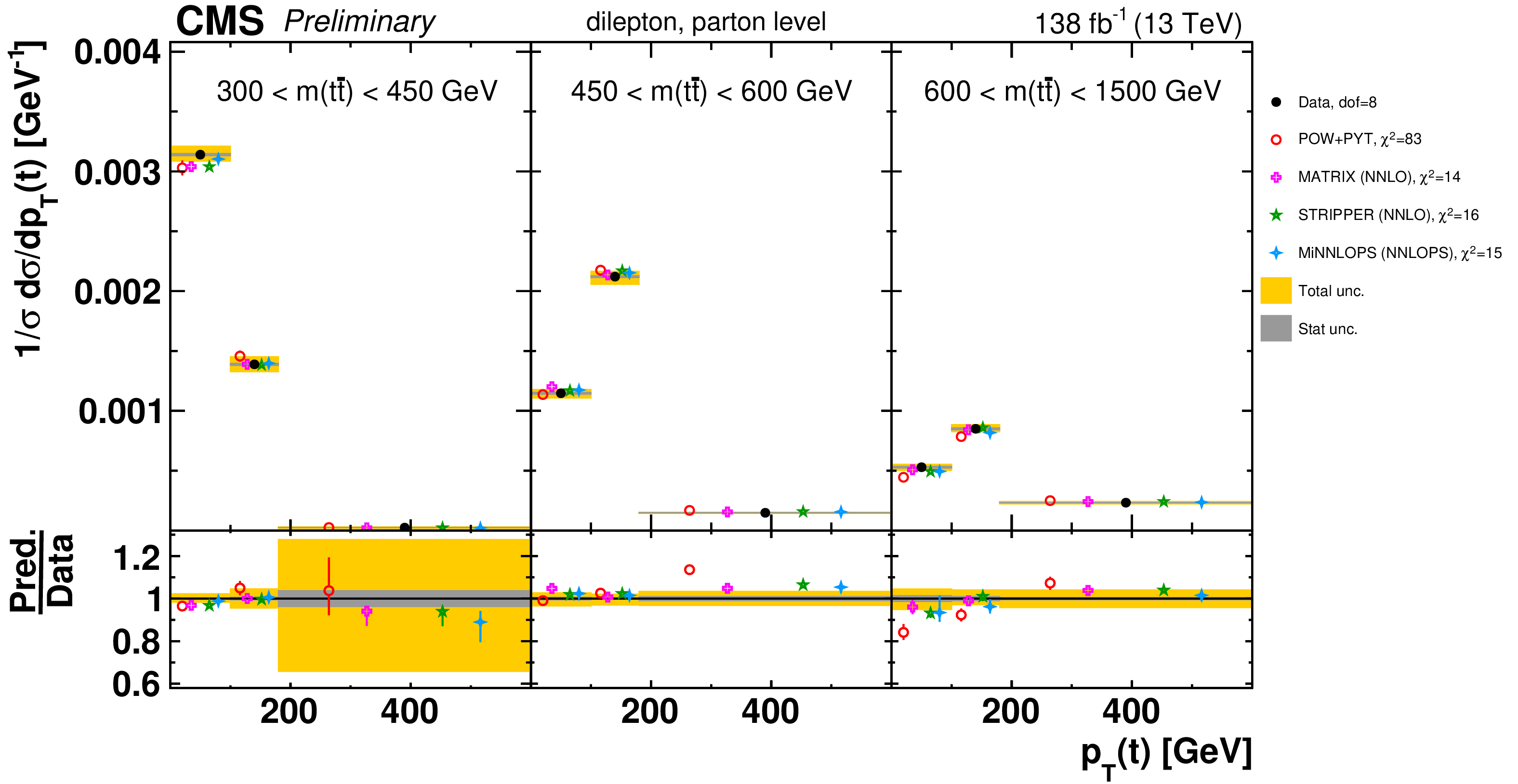
png pdf	Figure 40: Normalized differential $\mathrm{t\bar{t}}$ production cross sections as a function of ${{p_{\mathrm {T}}} (\mathrm{t})}$ (upper) and ${{p_{\mathrm {T}}} (\mathrm{\bar{t}})}$ (lower), measured at the parton level in the full phase space (left) and at the particle level in a fiducial phase space (right). The data are shown as filled circles with dark and light bands indicating the statistical and total uncertainties (statistical and systematic uncertainties summed in quadrature), respectively. The cross sections are compared to predictions from the POWHEG+PYTHIA-8 (`POW-PYT', open circles) simulation and various theoretical predictions with beyond-NLO precision (other points). The estimated uncertainties in the predictions are represented by a vertical bar on the corresponding points. For each model, a value of ${\chi ^2}$ is reported that takes into account the measurement uncertainties. The lower panel in each plot shows the ratios of the predictions to the data.
png pdf	Figure 40-a: Normalized differential $\mathrm{t\bar{t}}$ production cross sections as a function of ${{p_{\mathrm {T}}} (\mathrm{t})}$ (upper) and ${{p_{\mathrm {T}}} (\mathrm{\bar{t}})}$ (lower), measured at the parton level in the full phase space (left) and at the particle level in a fiducial phase space (right). The data are shown as filled circles with dark and light bands indicating the statistical and total uncertainties (statistical and systematic uncertainties summed in quadrature), respectively. The cross sections are compared to predictions from the POWHEG+PYTHIA-8 (`POW-PYT', open circles) simulation and various theoretical predictions with beyond-NLO precision (other points). The estimated uncertainties in the predictions are represented by a vertical bar on the corresponding points. For each model, a value of ${\chi ^2}$ is reported that takes into account the measurement uncertainties. The lower panel in each plot shows the ratios of the predictions to the data.
png pdf	Figure 40-b: Normalized differential $\mathrm{t\bar{t}}$ production cross sections as a function of ${{p_{\mathrm {T}}} (\mathrm{t})}$ (upper) and ${{p_{\mathrm {T}}} (\mathrm{\bar{t}})}$ (lower), measured at the parton level in the full phase space (left) and at the particle level in a fiducial phase space (right). The data are shown as filled circles with dark and light bands indicating the statistical and total uncertainties (statistical and systematic uncertainties summed in quadrature), respectively. The cross sections are compared to predictions from the POWHEG+PYTHIA-8 (`POW-PYT', open circles) simulation and various theoretical predictions with beyond-NLO precision (other points). The estimated uncertainties in the predictions are represented by a vertical bar on the corresponding points. For each model, a value of ${\chi ^2}$ is reported that takes into account the measurement uncertainties. The lower panel in each plot shows the ratios of the predictions to the data.
png pdf	Figure 40-c: Normalized differential $\mathrm{t\bar{t}}$ production cross sections as a function of ${{p_{\mathrm {T}}} (\mathrm{t})}$ (upper) and ${{p_{\mathrm {T}}} (\mathrm{\bar{t}})}$ (lower), measured at the parton level in the full phase space (left) and at the particle level in a fiducial phase space (right). The data are shown as filled circles with dark and light bands indicating the statistical and total uncertainties (statistical and systematic uncertainties summed in quadrature), respectively. The cross sections are compared to predictions from the POWHEG+PYTHIA-8 (`POW-PYT', open circles) simulation and various theoretical predictions with beyond-NLO precision (other points). The estimated uncertainties in the predictions are represented by a vertical bar on the corresponding points. For each model, a value of ${\chi ^2}$ is reported that takes into account the measurement uncertainties. The lower panel in each plot shows the ratios of the predictions to the data.
png pdf	Figure 40-d: Normalized differential $\mathrm{t\bar{t}}$ production cross sections as a function of ${{p_{\mathrm {T}}} (\mathrm{t})}$ (upper) and ${{p_{\mathrm {T}}} (\mathrm{\bar{t}})}$ (lower), measured at the parton level in the full phase space (left) and at the particle level in a fiducial phase space (right). The data are shown as filled circles with dark and light bands indicating the statistical and total uncertainties (statistical and systematic uncertainties summed in quadrature), respectively. The cross sections are compared to predictions from the POWHEG+PYTHIA-8 (`POW-PYT', open circles) simulation and various theoretical predictions with beyond-NLO precision (other points). The estimated uncertainties in the predictions are represented by a vertical bar on the corresponding points. For each model, a value of ${\chi ^2}$ is reported that takes into account the measurement uncertainties. The lower panel in each plot shows the ratios of the predictions to the data.
png pdf	Figure 41: Normalized differential $\mathrm{t\bar{t}}$ production cross sections as a function of ${y(\mathrm{t})}$ (upper) and ${y(\mathrm{\bar{t}})}$ (lower) are shown for data (filled circles), POWHEG+PYTHIA-8 (`POW-PYT', open circles) simulation, and various theoretical predictions with beyond-NLO precision (other points). Further details can be found in the caption of Fig. 40.
png pdf	Figure 41-a: Normalized differential $\mathrm{t\bar{t}}$ production cross sections as a function of ${y(\mathrm{t})}$ (upper) and ${y(\mathrm{\bar{t}})}$ (lower) are shown for data (filled circles), POWHEG+PYTHIA-8 (`POW-PYT', open circles) simulation, and various theoretical predictions with beyond-NLO precision (other points). Further details can be found in the caption of Fig. 40.
png pdf	Figure 41-b: Normalized differential $\mathrm{t\bar{t}}$ production cross sections as a function of ${y(\mathrm{t})}$ (upper) and ${y(\mathrm{\bar{t}})}$ (lower) are shown for data (filled circles), POWHEG+PYTHIA-8 (`POW-PYT', open circles) simulation, and various theoretical predictions with beyond-NLO precision (other points). Further details can be found in the caption of Fig. 40.
png pdf	Figure 41-c: Normalized differential $\mathrm{t\bar{t}}$ production cross sections as a function of ${y(\mathrm{t})}$ (upper) and ${y(\mathrm{\bar{t}})}$ (lower) are shown for data (filled circles), POWHEG+PYTHIA-8 (`POW-PYT', open circles) simulation, and various theoretical predictions with beyond-NLO precision (other points). Further details can be found in the caption of Fig. 40.
png pdf	Figure 41-d: Normalized differential $\mathrm{t\bar{t}}$ production cross sections as a function of ${y(\mathrm{t})}$ (upper) and ${y(\mathrm{\bar{t}})}$ (lower) are shown for data (filled circles), POWHEG+PYTHIA-8 (`POW-PYT', open circles) simulation, and various theoretical predictions with beyond-NLO precision (other points). Further details can be found in the caption of Fig. 40.
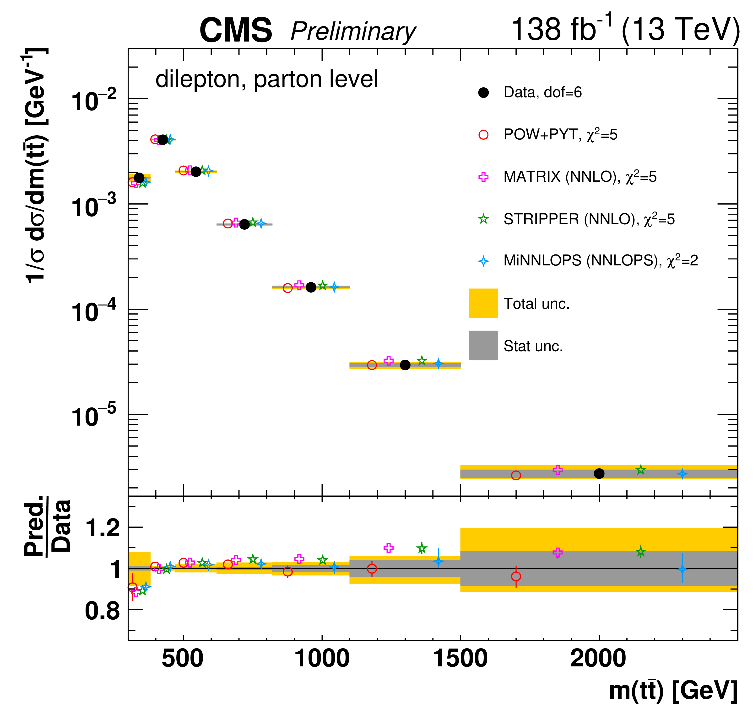
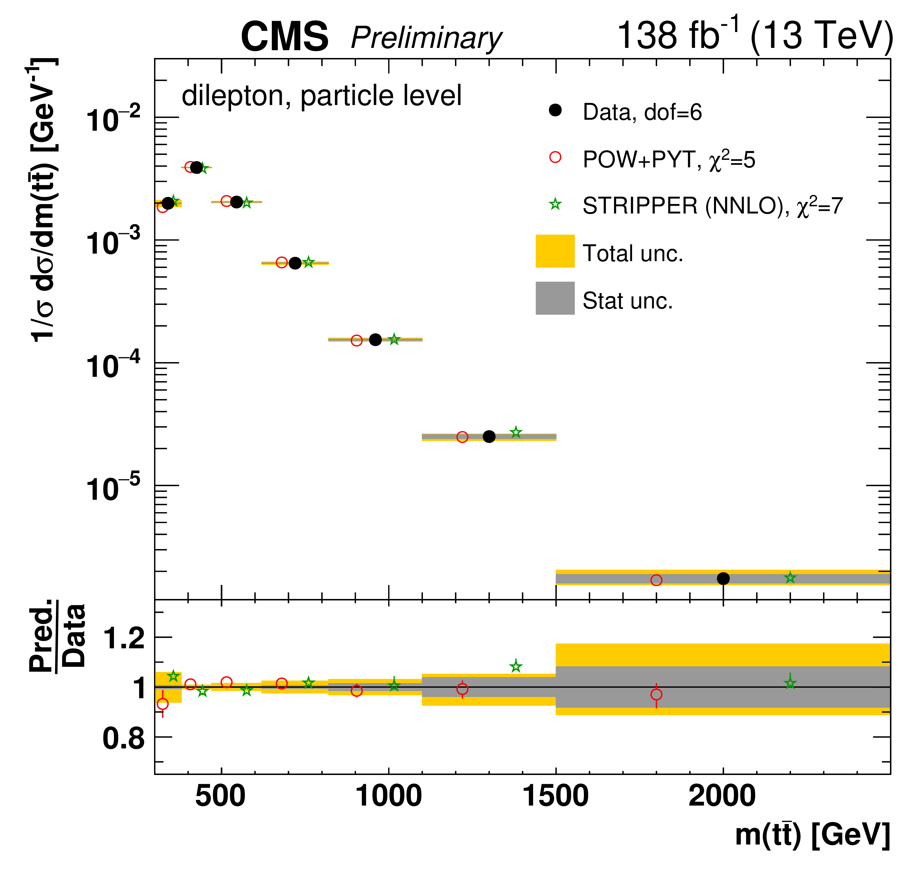
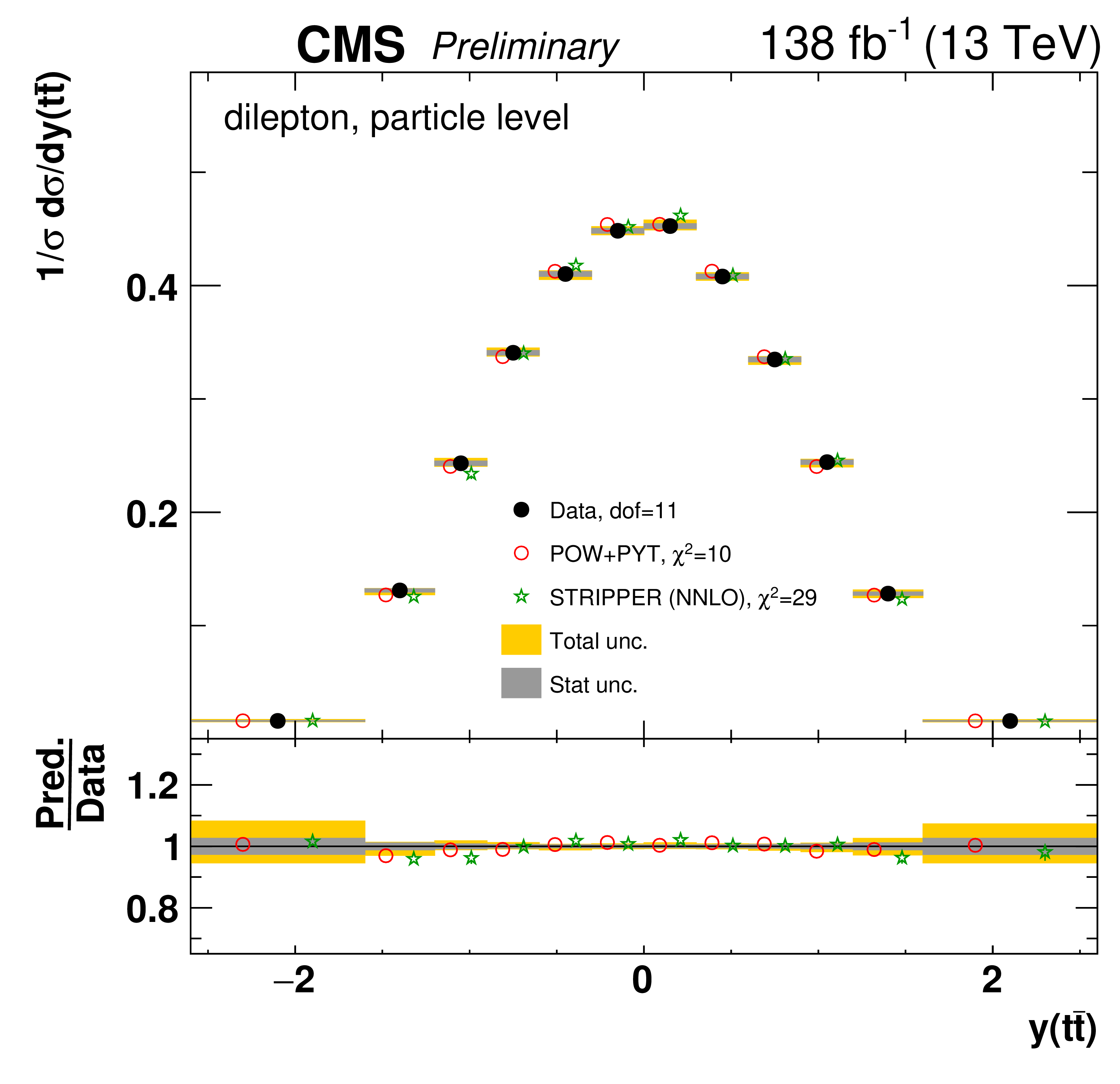
png pdf	Figure 42: Normalized differential $\mathrm{t\bar{t}}$ production cross sections as a function of ${{p_{\mathrm {T}}} ( \mathrm{t\bar{t}})}$ (upper), ${m( \mathrm{t\bar{t}})}$ (middle), and ${y( \mathrm{t\bar{t}})}$ (lower) are shown for data (filled circles), POWHEG+PYTHIA-8 (`POW-PYT', open circles) simulation, and various theoretical predictions with beyond-NLO precision (other points). Further details can be found in the caption of Fig. 40.
png pdf	Figure 42-a: Normalized differential $\mathrm{t\bar{t}}$ production cross sections as a function of ${{p_{\mathrm {T}}} ( \mathrm{t\bar{t}})}$ (upper), ${m( \mathrm{t\bar{t}})}$ (middle), and ${y( \mathrm{t\bar{t}})}$ (lower) are shown for data (filled circles), POWHEG+PYTHIA-8 (`POW-PYT', open circles) simulation, and various theoretical predictions with beyond-NLO precision (other points). Further details can be found in the caption of Fig. 40.
png pdf	Figure 42-b: Normalized differential $\mathrm{t\bar{t}}$ production cross sections as a function of ${{p_{\mathrm {T}}} ( \mathrm{t\bar{t}})}$ (upper), ${m( \mathrm{t\bar{t}})}$ (middle), and ${y( \mathrm{t\bar{t}})}$ (lower) are shown for data (filled circles), POWHEG+PYTHIA-8 (`POW-PYT', open circles) simulation, and various theoretical predictions with beyond-NLO precision (other points). Further details can be found in the caption of Fig. 40.
png pdf	Figure 42-c: Normalized differential $\mathrm{t\bar{t}}$ production cross sections as a function of ${{p_{\mathrm {T}}} ( \mathrm{t\bar{t}})}$ (upper), ${m( \mathrm{t\bar{t}})}$ (middle), and ${y( \mathrm{t\bar{t}})}$ (lower) are shown for data (filled circles), POWHEG+PYTHIA-8 (`POW-PYT', open circles) simulation, and various theoretical predictions with beyond-NLO precision (other points). Further details can be found in the caption of Fig. 40.
png pdf	Figure 42-d: Normalized differential $\mathrm{t\bar{t}}$ production cross sections as a function of ${{p_{\mathrm {T}}} ( \mathrm{t\bar{t}})}$ (upper), ${m( \mathrm{t\bar{t}})}$ (middle), and ${y( \mathrm{t\bar{t}})}$ (lower) are shown for data (filled circles), POWHEG+PYTHIA-8 (`POW-PYT', open circles) simulation, and various theoretical predictions with beyond-NLO precision (other points). Further details can be found in the caption of Fig. 40.
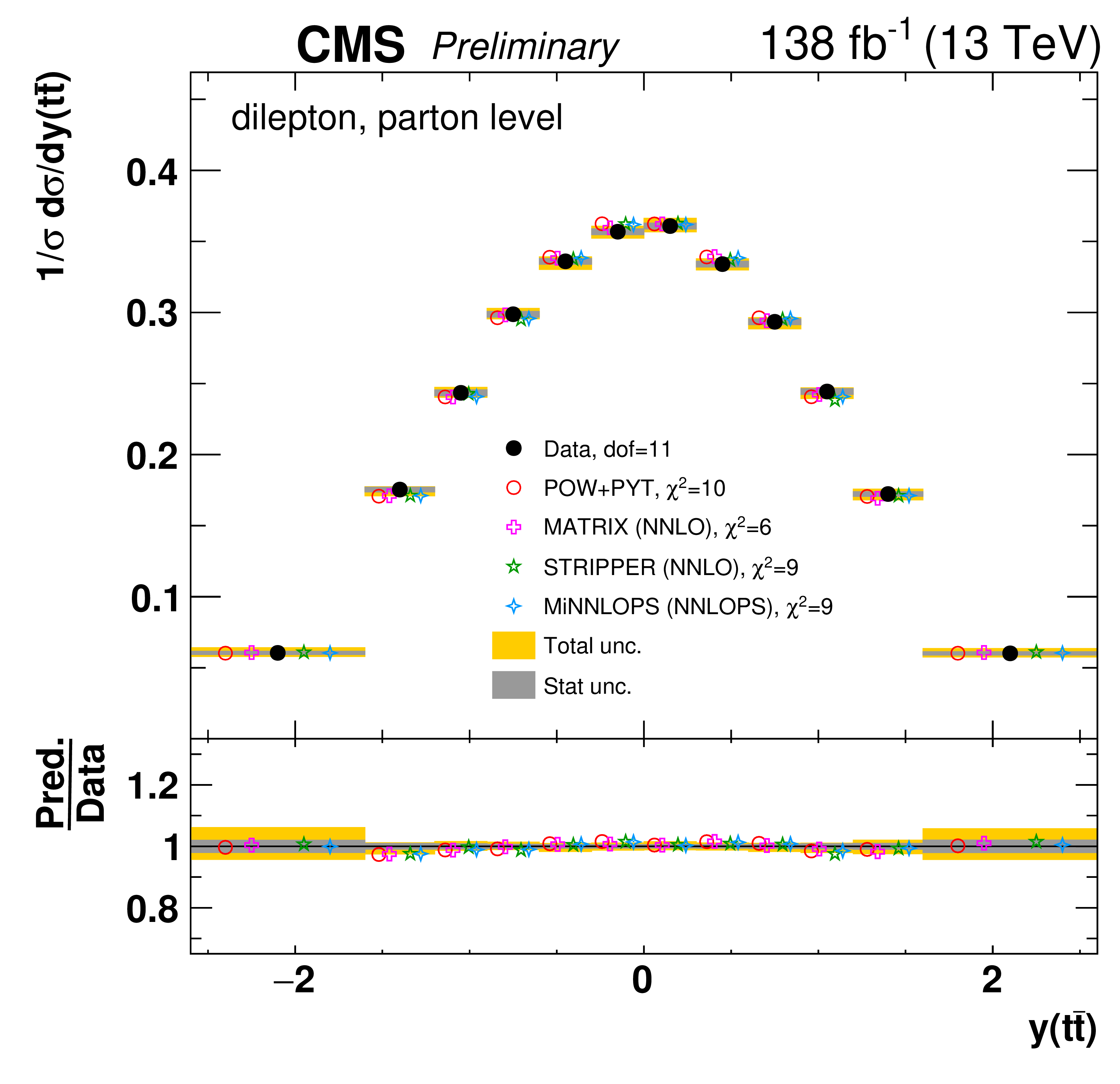
png pdf	Figure 42-e: Normalized differential $\mathrm{t\bar{t}}$ production cross sections as a function of ${{p_{\mathrm {T}}} ( \mathrm{t\bar{t}})}$ (upper), ${m( \mathrm{t\bar{t}})}$ (middle), and ${y( \mathrm{t\bar{t}})}$ (lower) are shown for data (filled circles), POWHEG+PYTHIA-8 (`POW-PYT', open circles) simulation, and various theoretical predictions with beyond-NLO precision (other points). Further details can be found in the caption of Fig. 40.
png pdf	Figure 42-f: Normalized differential $\mathrm{t\bar{t}}$ production cross sections as a function of ${{p_{\mathrm {T}}} ( \mathrm{t\bar{t}})}$ (upper), ${m( \mathrm{t\bar{t}})}$ (middle), and ${y( \mathrm{t\bar{t}})}$ (lower) are shown for data (filled circles), POWHEG+PYTHIA-8 (`POW-PYT', open circles) simulation, and various theoretical predictions with beyond-NLO precision (other points). Further details can be found in the caption of Fig. 40.
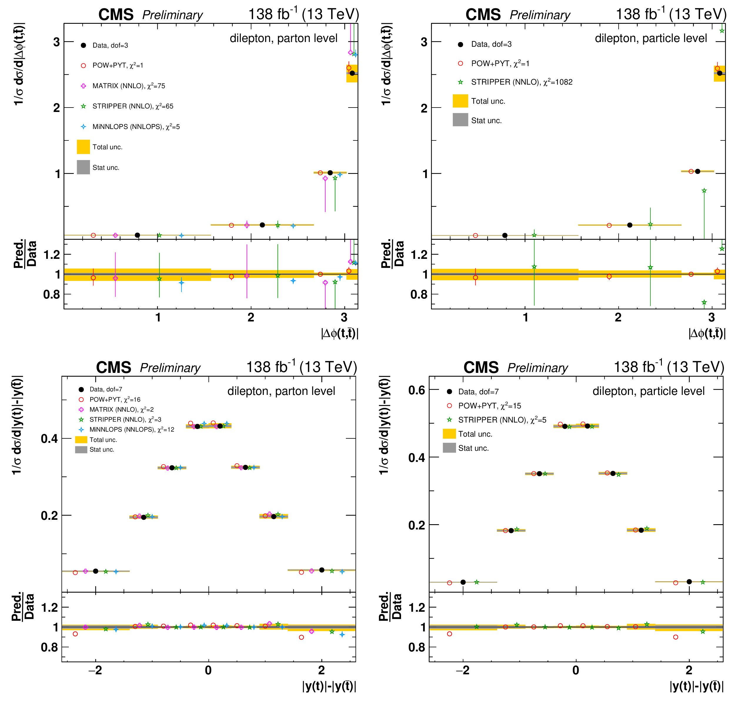
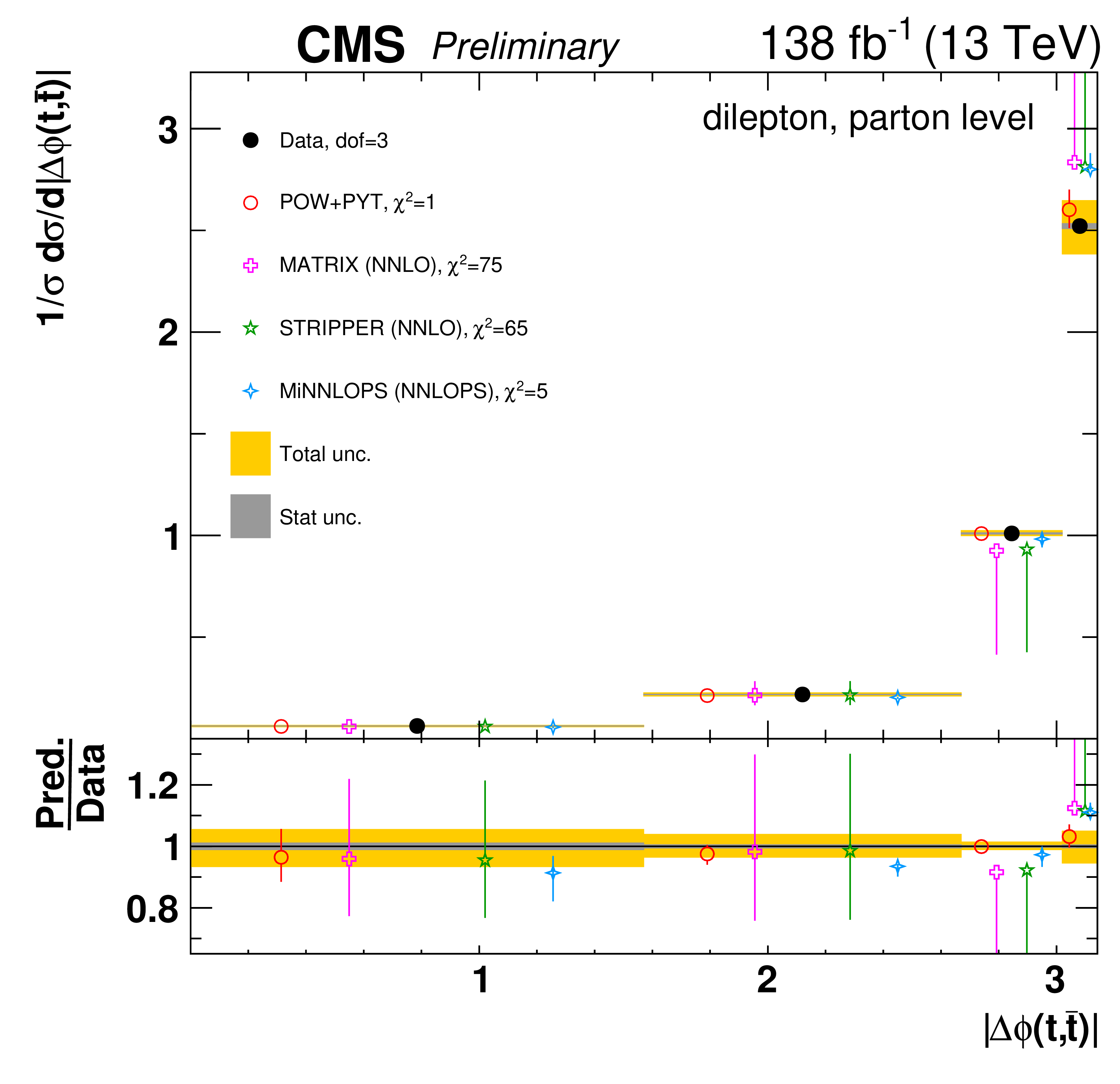
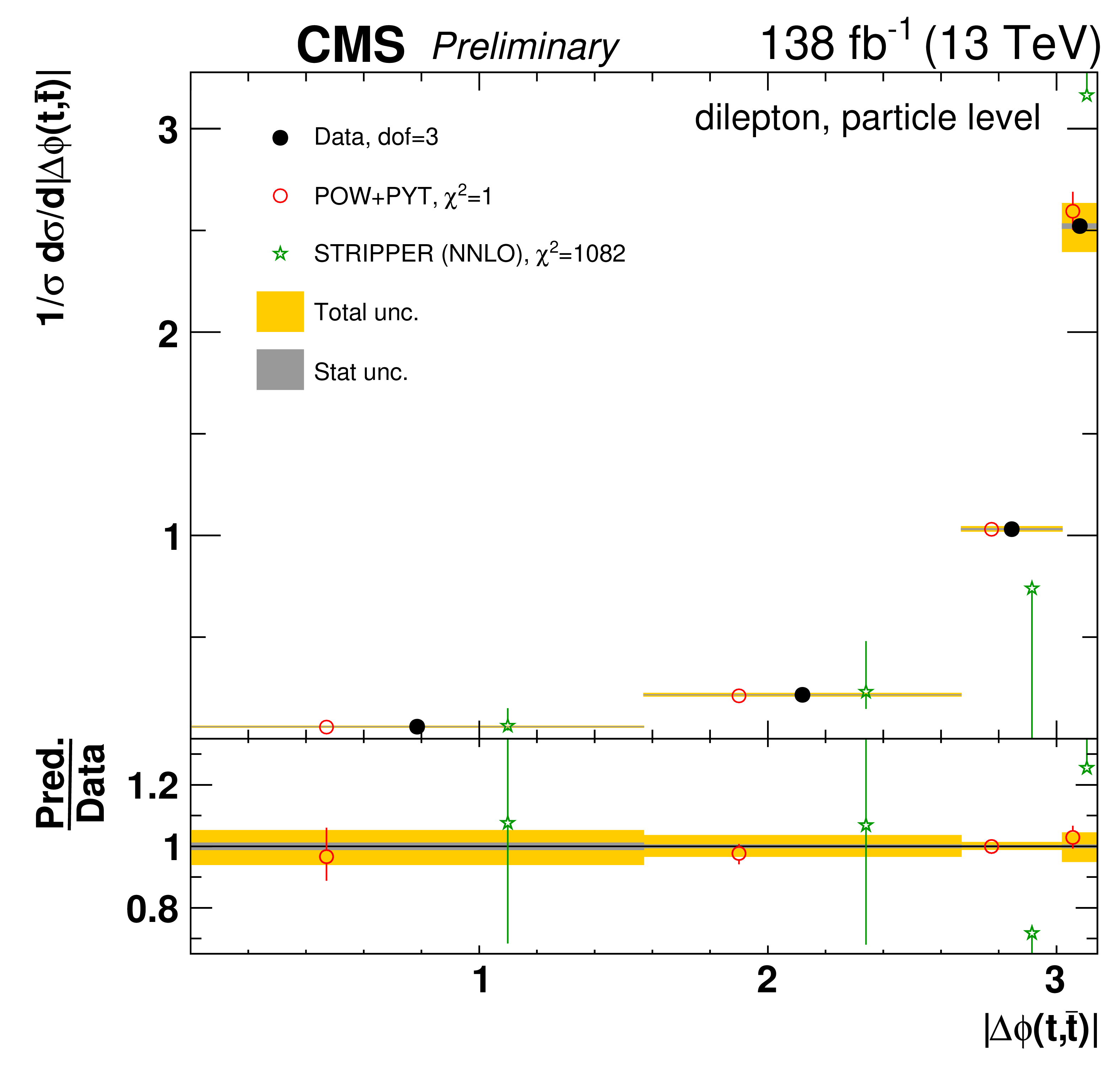
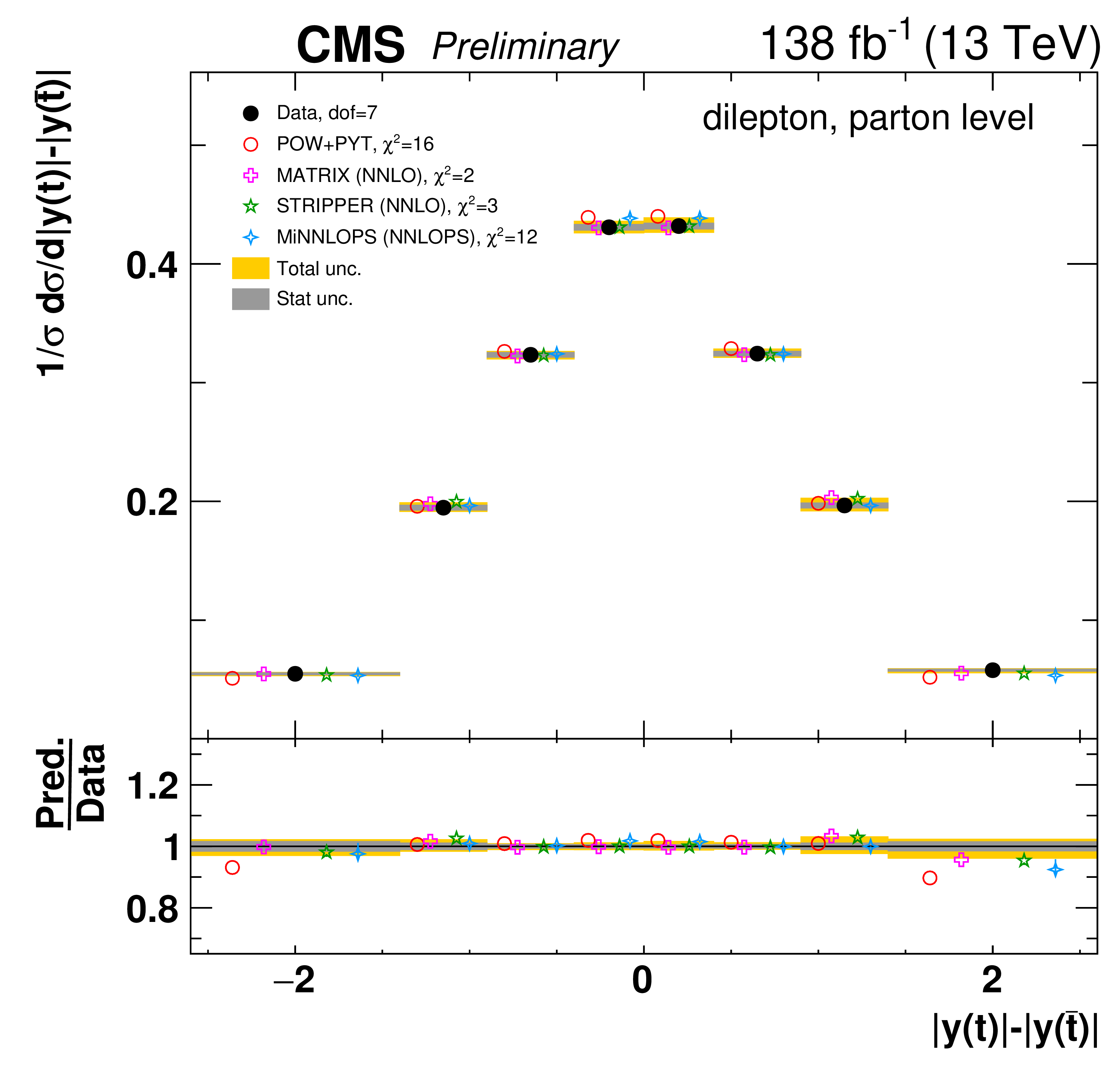
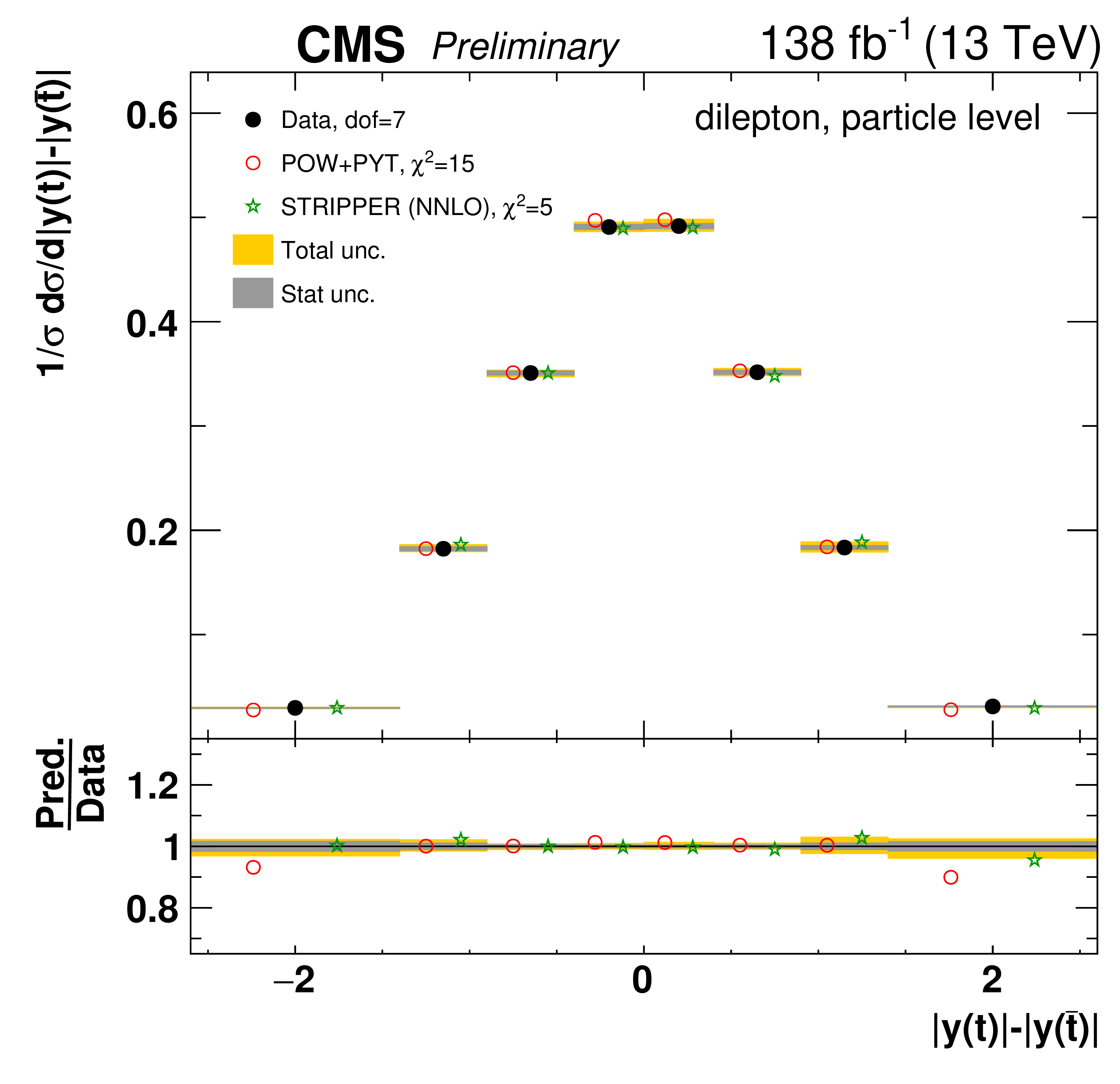
png pdf	Figure 43: Normalized differential $\mathrm{t\bar{t}}$ production cross sections as a function of ${|\Delta \phi (\mathrm{t},\mathrm{\bar{t}})|}$ (upper) and ${|y(\mathrm{t})|-|y(\mathrm{\bar{t}})|}$ (lower) are shown for data (filled circles), POWHEG+PYTHIA-8 (`POW-PYT', open circles) simulation, and various theoretical predictions with beyond-NLO precision (other points). Further details can be found in the caption of Fig. 40.
png pdf	Figure 43-a: Normalized differential $\mathrm{t\bar{t}}$ production cross sections as a function of ${|\Delta \phi (\mathrm{t},\mathrm{\bar{t}})|}$ (upper) and ${|y(\mathrm{t})|-|y(\mathrm{\bar{t}})|}$ (lower) are shown for data (filled circles), POWHEG+PYTHIA-8 (`POW-PYT', open circles) simulation, and various theoretical predictions with beyond-NLO precision (other points). Further details can be found in the caption of Fig. 40.
png pdf	Figure 43-b: Normalized differential $\mathrm{t\bar{t}}$ production cross sections as a function of ${|\Delta \phi (\mathrm{t},\mathrm{\bar{t}})|}$ (upper) and ${|y(\mathrm{t})|-|y(\mathrm{\bar{t}})|}$ (lower) are shown for data (filled circles), POWHEG+PYTHIA-8 (`POW-PYT', open circles) simulation, and various theoretical predictions with beyond-NLO precision (other points). Further details can be found in the caption of Fig. 40.
png pdf	Figure 43-c: Normalized differential $\mathrm{t\bar{t}}$ production cross sections as a function of ${|\Delta \phi (\mathrm{t},\mathrm{\bar{t}})|}$ (upper) and ${|y(\mathrm{t})|-|y(\mathrm{\bar{t}})|}$ (lower) are shown for data (filled circles), POWHEG+PYTHIA-8 (`POW-PYT', open circles) simulation, and various theoretical predictions with beyond-NLO precision (other points). Further details can be found in the caption of Fig. 40.
png pdf	Figure 43-d: Normalized differential $\mathrm{t\bar{t}}$ production cross sections as a function of ${|\Delta \phi (\mathrm{t},\mathrm{\bar{t}})|}$ (upper) and ${|y(\mathrm{t})|-|y(\mathrm{\bar{t}})|}$ (lower) are shown for data (filled circles), POWHEG+PYTHIA-8 (`POW-PYT', open circles) simulation, and various theoretical predictions with beyond-NLO precision (other points). Further details can be found in the caption of Fig. 40.
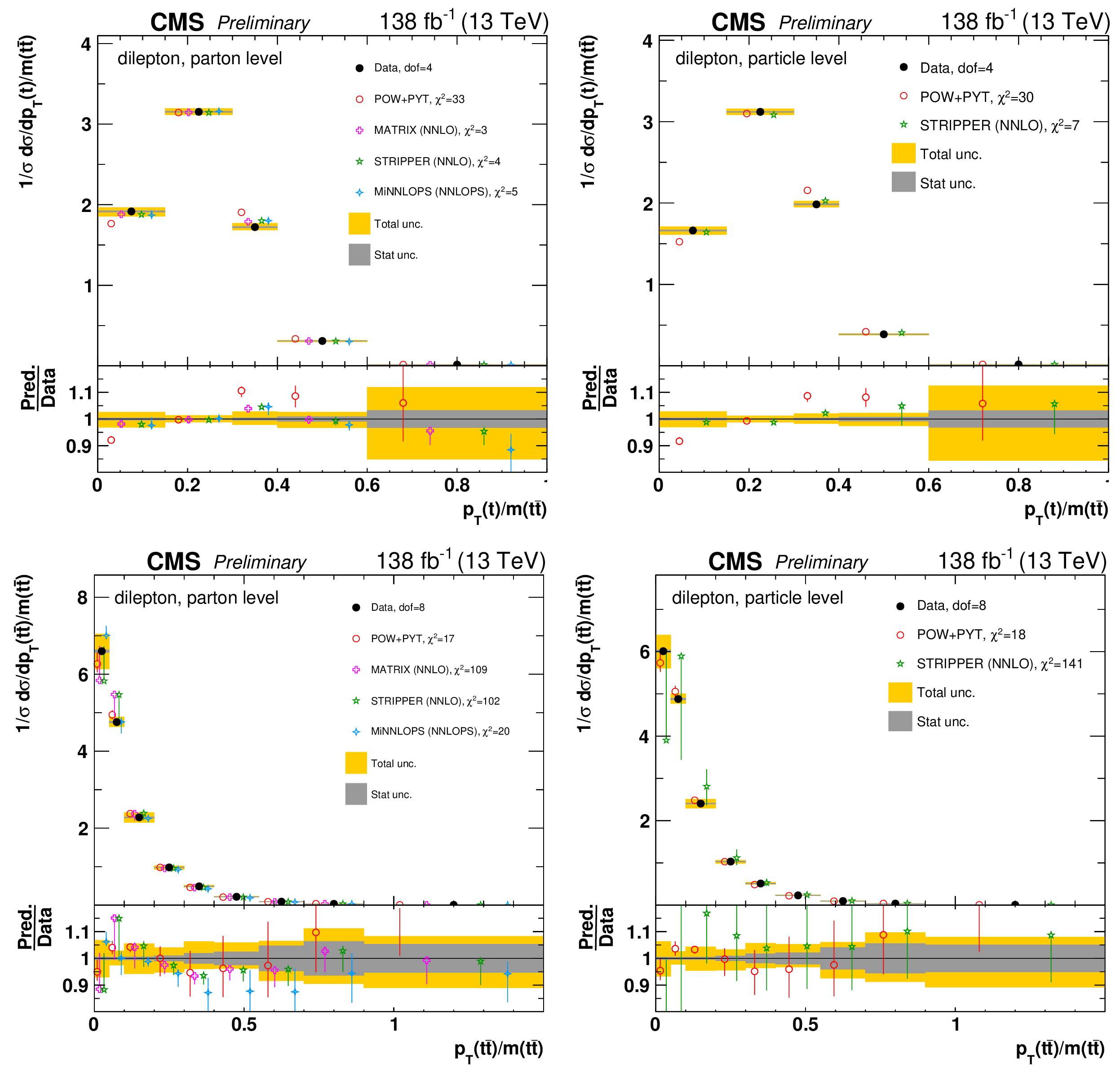
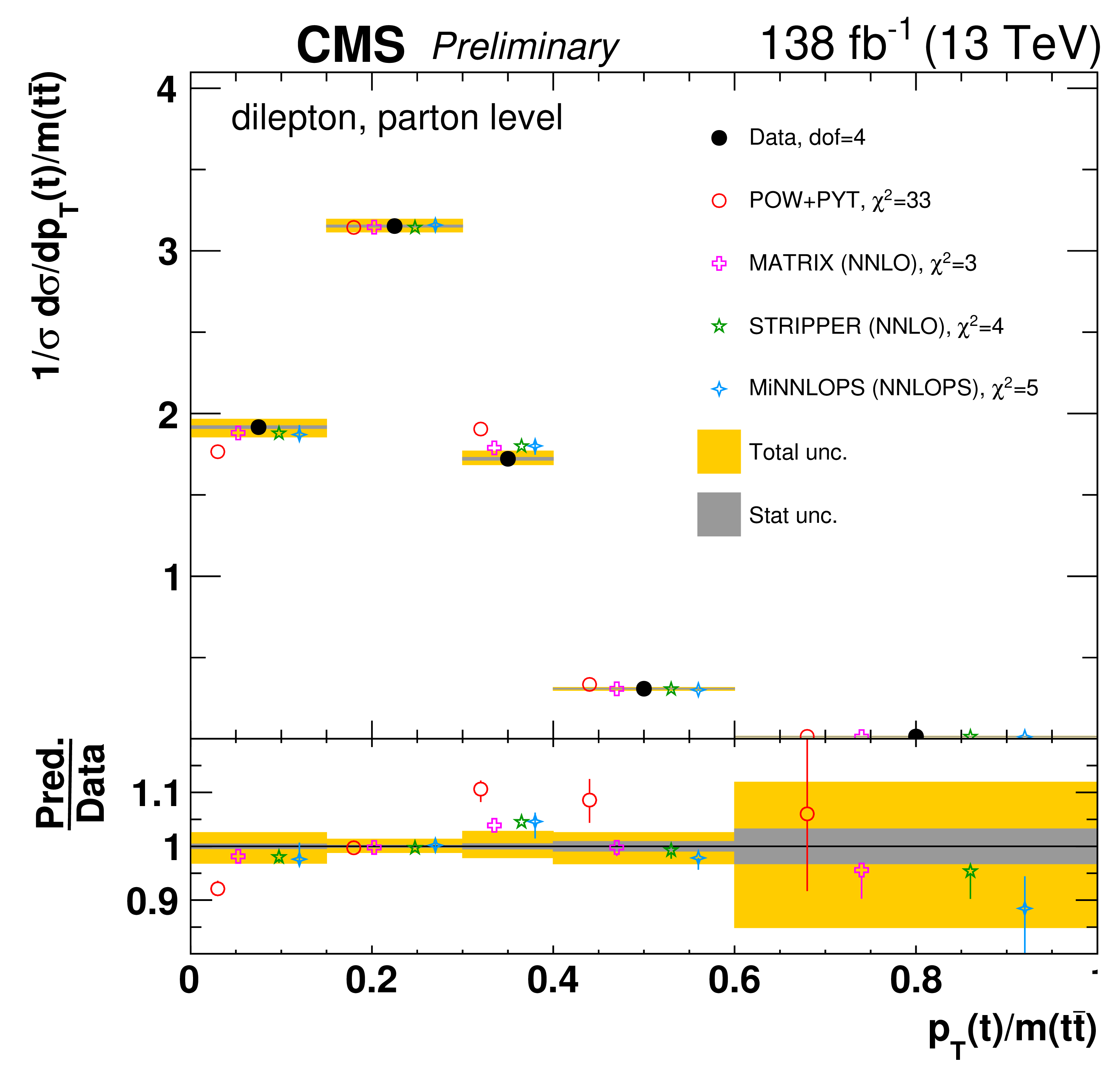
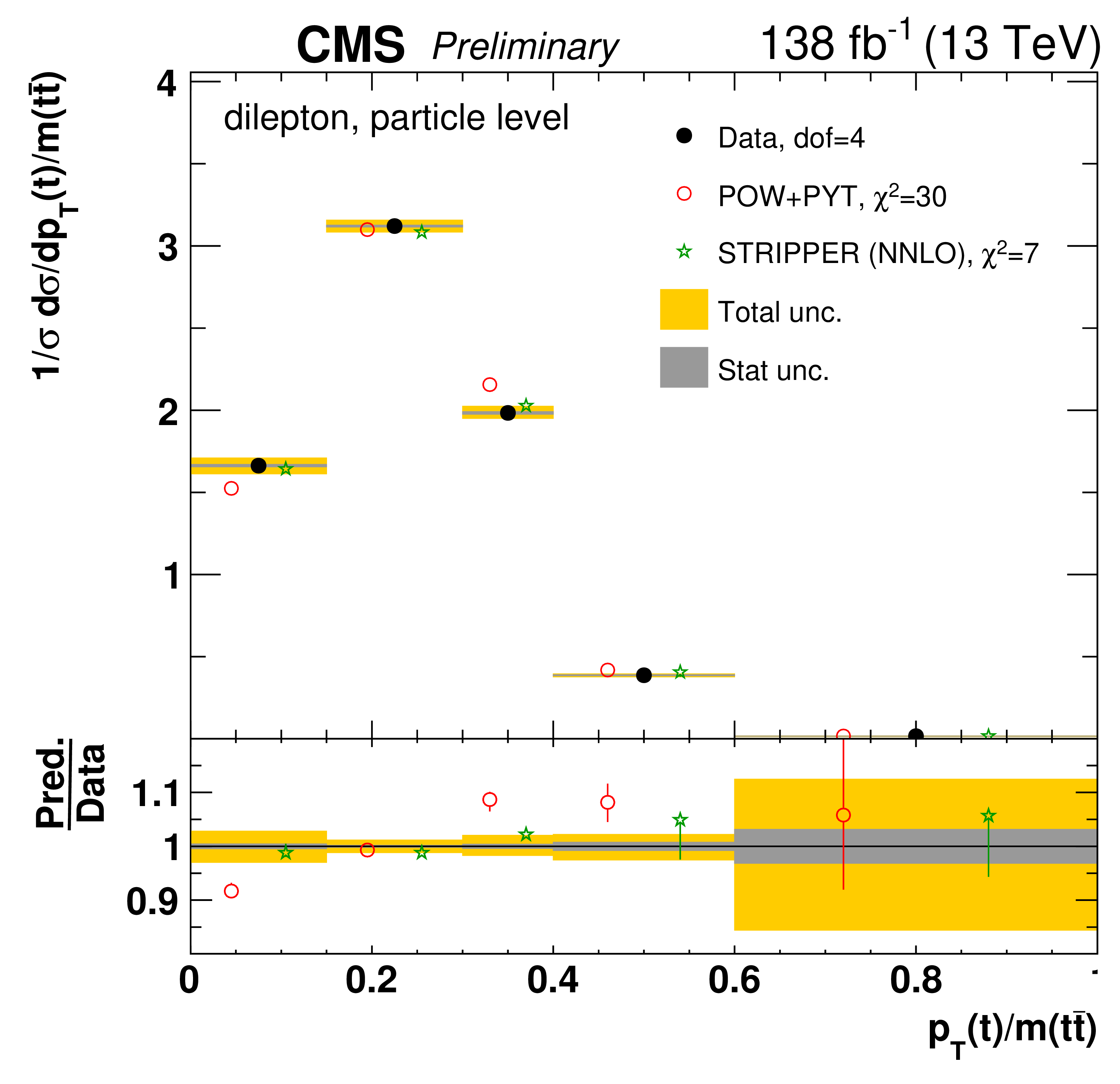
png pdf	Figure 44: Normalized differential $\mathrm{t\bar{t}}$ production cross sections as a function of $ {{p_{\mathrm {T}}} (\mathrm{t})} / {m( \mathrm{t\bar{t}})}$ (upper) and $ {{p_{\mathrm {T}}} ( \mathrm{t\bar{t}})} / {{m( \mathrm{t\bar{t}})}}$ (lower) are shown for data (filled circles), POWHEG+PYTHIA-8 (`POW-PYT', open circles) simulation, and various theoretical predictions with beyond-NLO precision (other points). Further details can be found in the caption of Fig. 40.
png pdf	Figure 44-a: Normalized differential $\mathrm{t\bar{t}}$ production cross sections as a function of $ {{p_{\mathrm {T}}} (\mathrm{t})} / {m( \mathrm{t\bar{t}})}$ (upper) and $ {{p_{\mathrm {T}}} ( \mathrm{t\bar{t}})} / {{m( \mathrm{t\bar{t}})}}$ (lower) are shown for data (filled circles), POWHEG+PYTHIA-8 (`POW-PYT', open circles) simulation, and various theoretical predictions with beyond-NLO precision (other points). Further details can be found in the caption of Fig. 40.
png pdf	Figure 44-b: Normalized differential $\mathrm{t\bar{t}}$ production cross sections as a function of $ {{p_{\mathrm {T}}} (\mathrm{t})} / {m( \mathrm{t\bar{t}})}$ (upper) and $ {{p_{\mathrm {T}}} ( \mathrm{t\bar{t}})} / {{m( \mathrm{t\bar{t}})}}$ (lower) are shown for data (filled circles), POWHEG+PYTHIA-8 (`POW-PYT', open circles) simulation, and various theoretical predictions with beyond-NLO precision (other points). Further details can be found in the caption of Fig. 40.
png pdf	Figure 44-c: Normalized differential $\mathrm{t\bar{t}}$ production cross sections as a function of $ {{p_{\mathrm {T}}} (\mathrm{t})} / {m( \mathrm{t\bar{t}})}$ (upper) and $ {{p_{\mathrm {T}}} ( \mathrm{t\bar{t}})} / {{m( \mathrm{t\bar{t}})}}$ (lower) are shown for data (filled circles), POWHEG+PYTHIA-8 (`POW-PYT', open circles) simulation, and various theoretical predictions with beyond-NLO precision (other points). Further details can be found in the caption of Fig. 40.
png pdf	Figure 44-d: Normalized differential $\mathrm{t\bar{t}}$ production cross sections as a function of $ {{p_{\mathrm {T}}} (\mathrm{t})} / {m( \mathrm{t\bar{t}})}$ (upper) and $ {{p_{\mathrm {T}}} ( \mathrm{t\bar{t}})} / {{m( \mathrm{t\bar{t}})}}$ (lower) are shown for data (filled circles), POWHEG+PYTHIA-8 (`POW-PYT', open circles) simulation, and various theoretical predictions with beyond-NLO precision (other points). Further details can be found in the caption of Fig. 40.
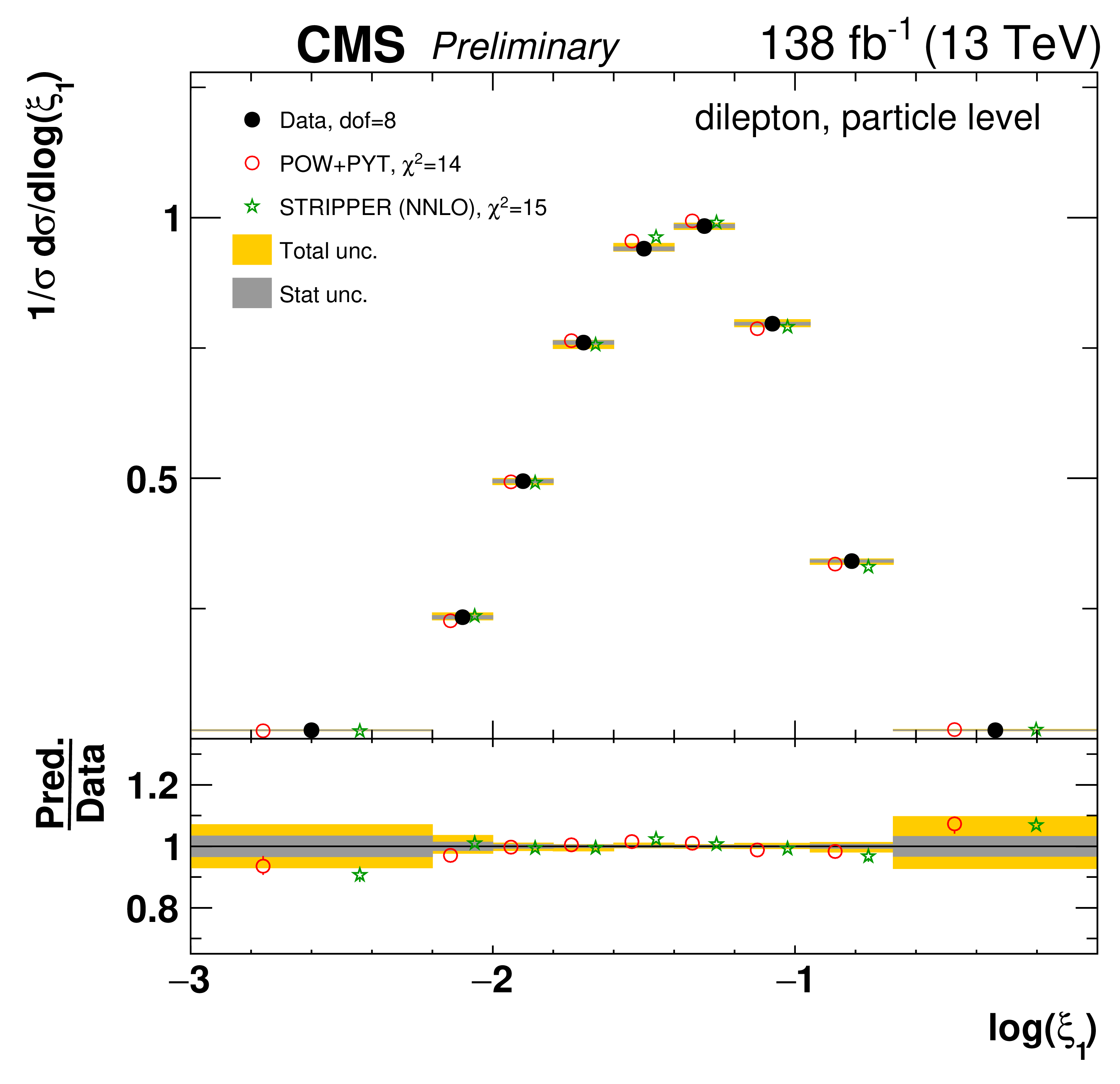
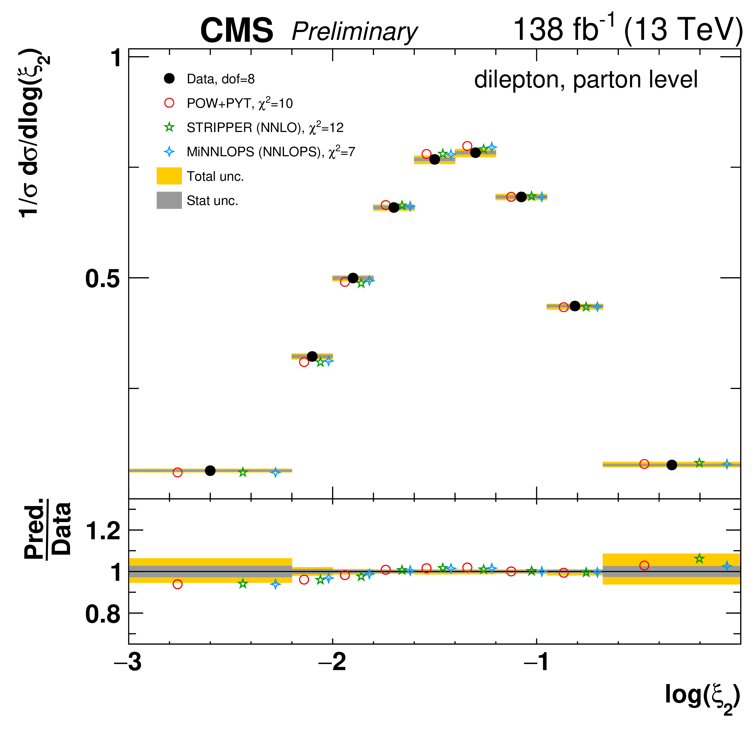
png pdf	Figure 45: Normalized differential $\mathrm{t\bar{t}}$ production cross sections as a function of ${\log(\xi _{1})}$ (upper) and ${\log(\xi _{2})}$ (lower) are shown for data (filled circles), POWHEG+PYTHIA-8 (`POW-PYT', open circles) simulation, and Stripper NNLO calculation (stars). Further details can be found in the caption of Fig. 40.
png pdf	Figure 45-a: Normalized differential $\mathrm{t\bar{t}}$ production cross sections as a function of ${\log(\xi _{1})}$ (upper) and ${\log(\xi _{2})}$ (lower) are shown for data (filled circles), POWHEG+PYTHIA-8 (`POW-PYT', open circles) simulation, and Stripper NNLO calculation (stars). Further details can be found in the caption of Fig. 40.
png pdf	Figure 45-b: Normalized differential $\mathrm{t\bar{t}}$ production cross sections as a function of ${\log(\xi _{1})}$ (upper) and ${\log(\xi _{2})}$ (lower) are shown for data (filled circles), POWHEG+PYTHIA-8 (`POW-PYT', open circles) simulation, and Stripper NNLO calculation (stars). Further details can be found in the caption of Fig. 40.
png pdf	Figure 45-c: Normalized differential $\mathrm{t\bar{t}}$ production cross sections as a function of ${\log(\xi _{1})}$ (upper) and ${\log(\xi _{2})}$ (lower) are shown for data (filled circles), POWHEG+PYTHIA-8 (`POW-PYT', open circles) simulation, and Stripper NNLO calculation (stars). Further details can be found in the caption of Fig. 40.
png pdf	Figure 45-d: Normalized differential $\mathrm{t\bar{t}}$ production cross sections as a function of ${\log(\xi _{1})}$ (upper) and ${\log(\xi _{2})}$ (lower) are shown for data (filled circles), POWHEG+PYTHIA-8 (`POW-PYT', open circles) simulation, and Stripper NNLO calculation (stars). Further details can be found in the caption of Fig. 40.
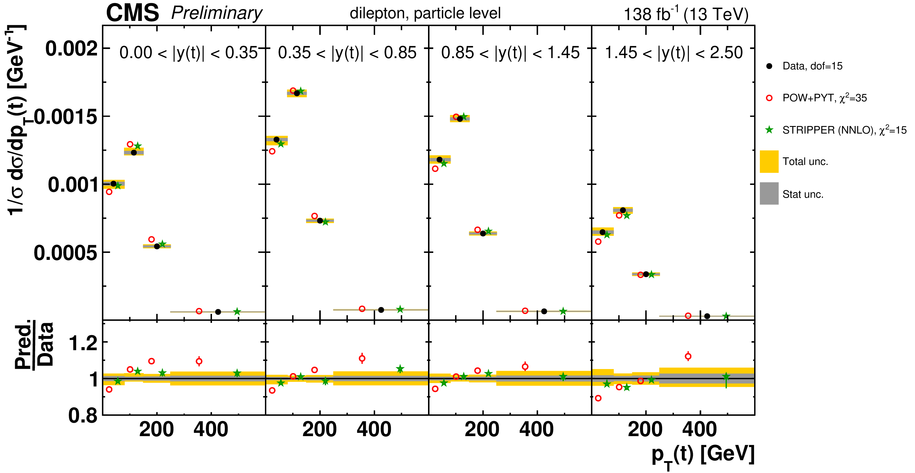
png pdf	Figure 46: Normalized $[ {|y(\mathrm{t})|},\,{{p_{\mathrm {T}}} (\mathrm{t})} ]$ cross sections measured at the parton level in the full phase space (upper) and at the particle level in a fiducial phase space (lower). The data are shown as filled circles with dark and light bands indicating the statistical and total uncertainties (statistical and systematic uncertainties summed in quadrature), respectively. The cross sections are compared to predictions from the POWHEG+PYTHIA-8 (`POW-PYT', open circles) simulation and various theoretical predictions with beyond-NLO precision (other points). The estimated uncertainties in the predictions are represented by a vertical bar on the corresponding points. For each model, a value of ${\chi ^2}$ is reported that takes into account the measurement uncertainties. The lower panel in each plot shows the ratios of the predictions to the data.
png pdf	Figure 46-a: Normalized $[ {|y(\mathrm{t})|},\,{{p_{\mathrm {T}}} (\mathrm{t})} ]$ cross sections measured at the parton level in the full phase space (upper) and at the particle level in a fiducial phase space (lower). The data are shown as filled circles with dark and light bands indicating the statistical and total uncertainties (statistical and systematic uncertainties summed in quadrature), respectively. The cross sections are compared to predictions from the POWHEG+PYTHIA-8 (`POW-PYT', open circles) simulation and various theoretical predictions with beyond-NLO precision (other points). The estimated uncertainties in the predictions are represented by a vertical bar on the corresponding points. For each model, a value of ${\chi ^2}$ is reported that takes into account the measurement uncertainties. The lower panel in each plot shows the ratios of the predictions to the data.
png pdf	Figure 46-b: Normalized $[ {|y(\mathrm{t})|},\,{{p_{\mathrm {T}}} (\mathrm{t})} ]$ cross sections measured at the parton level in the full phase space (upper) and at the particle level in a fiducial phase space (lower). The data are shown as filled circles with dark and light bands indicating the statistical and total uncertainties (statistical and systematic uncertainties summed in quadrature), respectively. The cross sections are compared to predictions from the POWHEG+PYTHIA-8 (`POW-PYT', open circles) simulation and various theoretical predictions with beyond-NLO precision (other points). The estimated uncertainties in the predictions are represented by a vertical bar on the corresponding points. For each model, a value of ${\chi ^2}$ is reported that takes into account the measurement uncertainties. The lower panel in each plot shows the ratios of the predictions to the data.
png pdf	Figure 47: Normalized $[ {m( \mathrm{t\bar{t}})},\,{{p_{\mathrm {T}}} (\mathrm{t})} ]$ cross sections are shown for data (filled circles), POWHEG+PYTHIA-8 (`POW-PYT', open circles) simulation, and various theoretical predictions with beyond-NLO precision (other points). Further details can be found in the caption of Fig. 46.
png pdf	Figure 47-a: Normalized $[ {m( \mathrm{t\bar{t}})},\,{{p_{\mathrm {T}}} (\mathrm{t})} ]$ cross sections are shown for data (filled circles), POWHEG+PYTHIA-8 (`POW-PYT', open circles) simulation, and various theoretical predictions with beyond-NLO precision (other points). Further details can be found in the caption of Fig. 46.
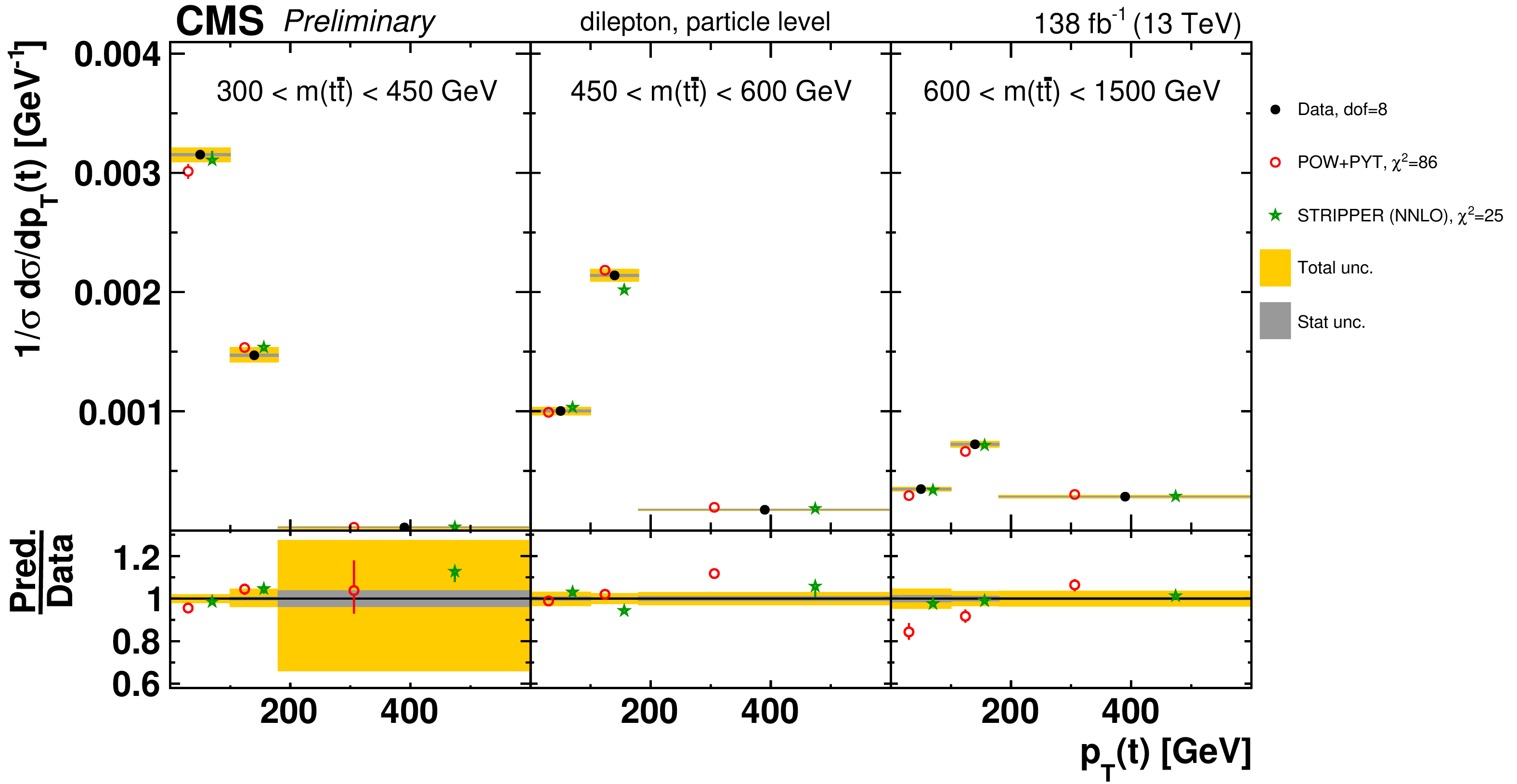
png pdf	Figure 47-b: Normalized $[ {m( \mathrm{t\bar{t}})},\,{{p_{\mathrm {T}}} (\mathrm{t})} ]$ cross sections are shown for data (filled circles), POWHEG+PYTHIA-8 (`POW-PYT', open circles) simulation, and various theoretical predictions with beyond-NLO precision (other points). Further details can be found in the caption of Fig. 46.
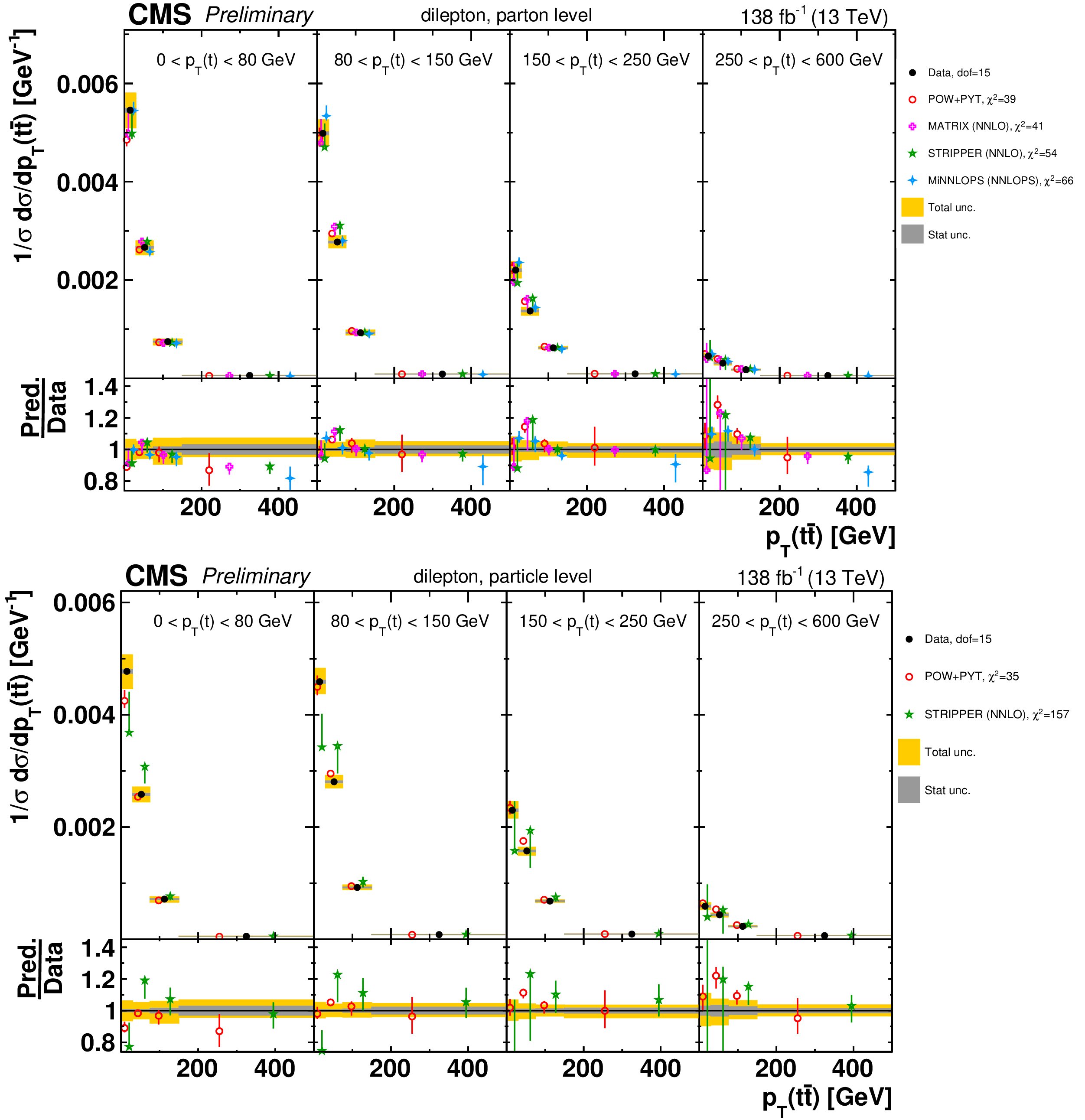
png pdf	Figure 48: Normalized $[ {{p_{\mathrm {T}}} (\mathrm{t})},\,{{p_{\mathrm {T}}} ( \mathrm{t\bar{t}})} ]$ cross sections are shown for data (filled circles), POWHEG+PYTHIA-8 (`POW-PYT', open circles) simulation, and various theoretical predictions with beyond-NLO precision (other points). Further details can be found in the caption of Fig. 46.
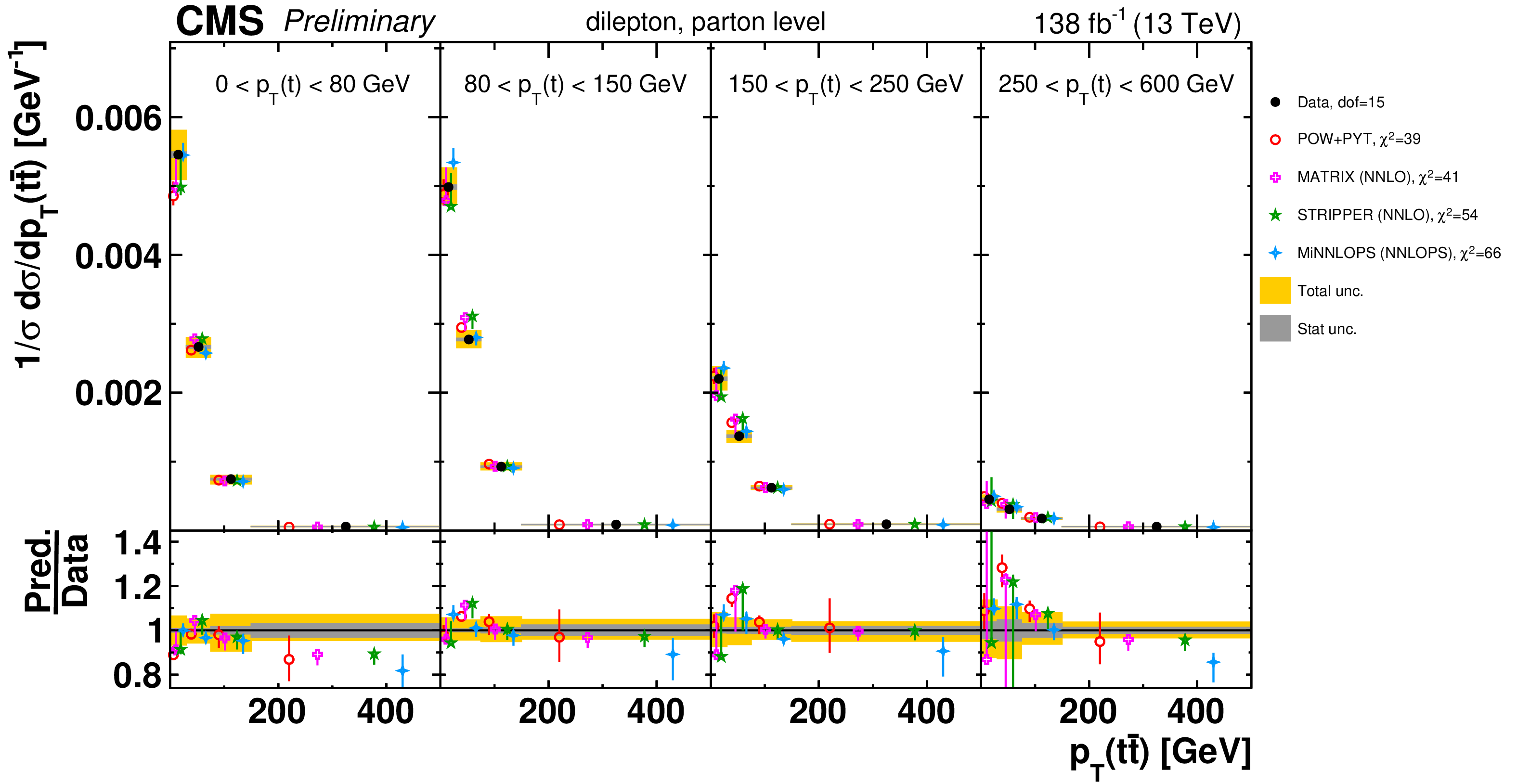
png pdf	Figure 48-a: Normalized $[ {{p_{\mathrm {T}}} (\mathrm{t})},\,{{p_{\mathrm {T}}} ( \mathrm{t\bar{t}})} ]$ cross sections are shown for data (filled circles), POWHEG+PYTHIA-8 (`POW-PYT', open circles) simulation, and various theoretical predictions with beyond-NLO precision (other points). Further details can be found in the caption of Fig. 46.
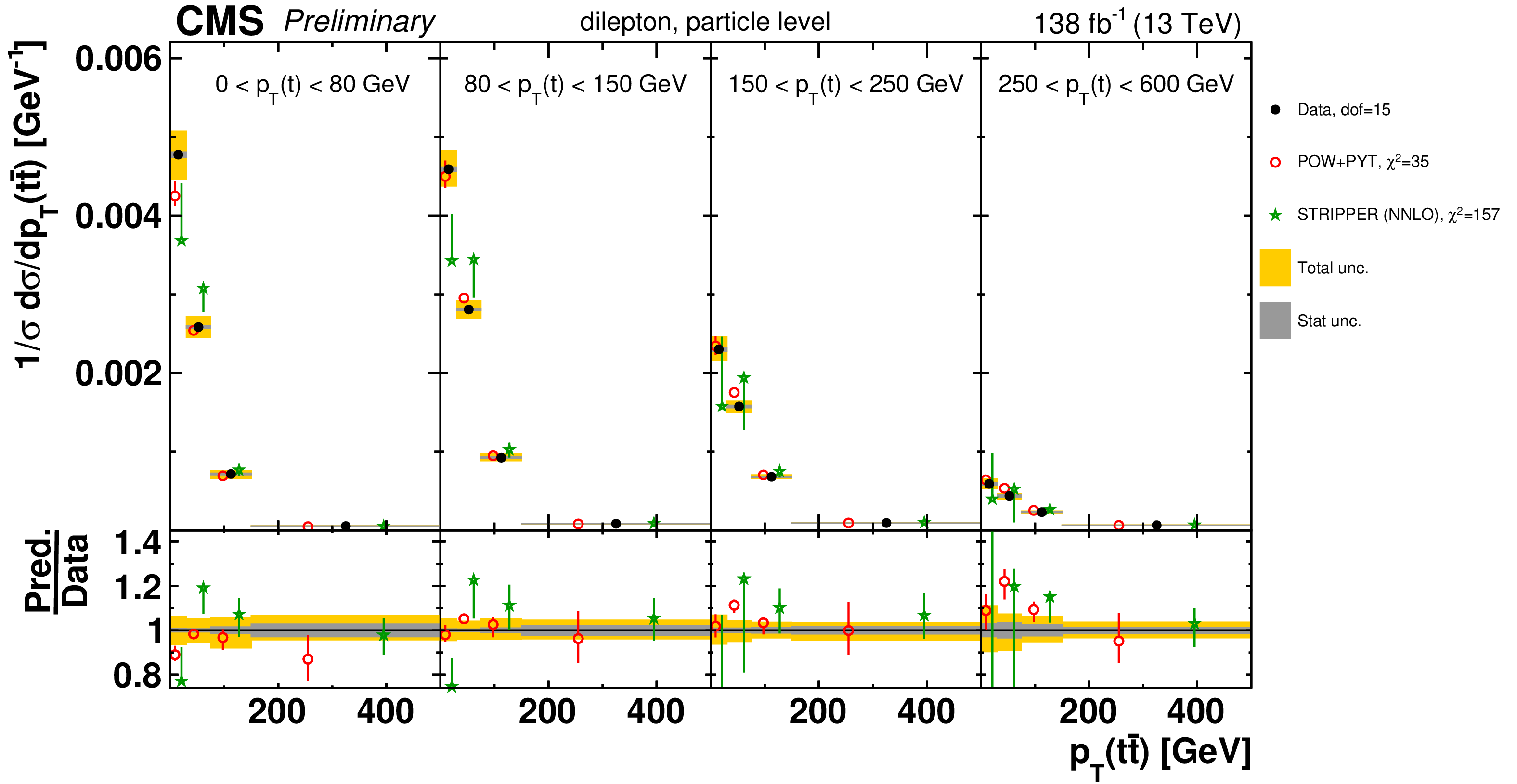
png pdf	Figure 48-b: Normalized $[ {{p_{\mathrm {T}}} (\mathrm{t})},\,{{p_{\mathrm {T}}} ( \mathrm{t\bar{t}})} ]$ cross sections are shown for data (filled circles), POWHEG+PYTHIA-8 (`POW-PYT', open circles) simulation, and various theoretical predictions with beyond-NLO precision (other points). Further details can be found in the caption of Fig. 46.
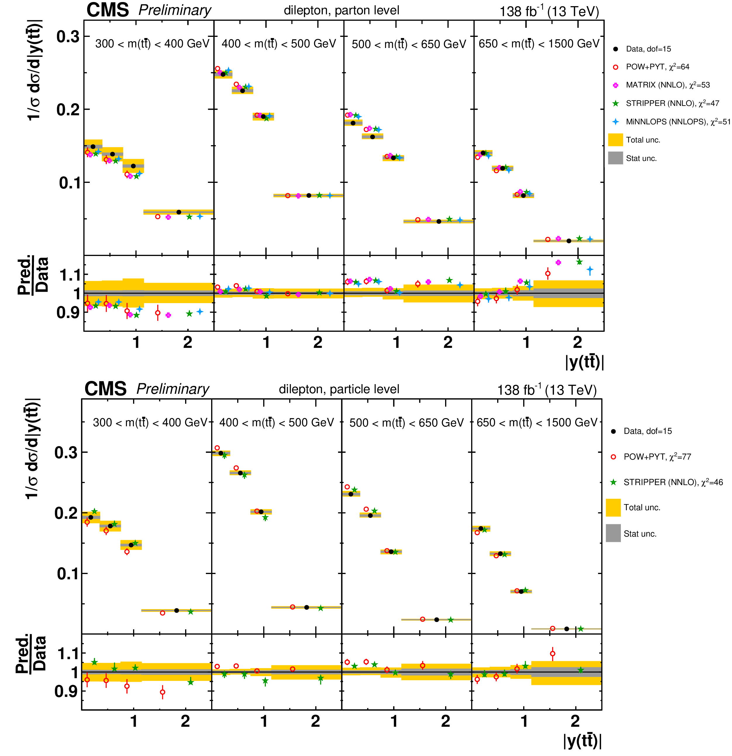
png pdf	Figure 49: Normalized $[ {m( \mathrm{t\bar{t}})},\,{|y( \mathrm{t\bar{t}})|} ]$ cross sections are shown for data (filled circles), POWHEG+PYTHIA-8 (`POW-PYT', open circles) simulation, and various theoretical predictions with beyond-NLO precision (other points). Further details can be found in the caption of Fig. 46.
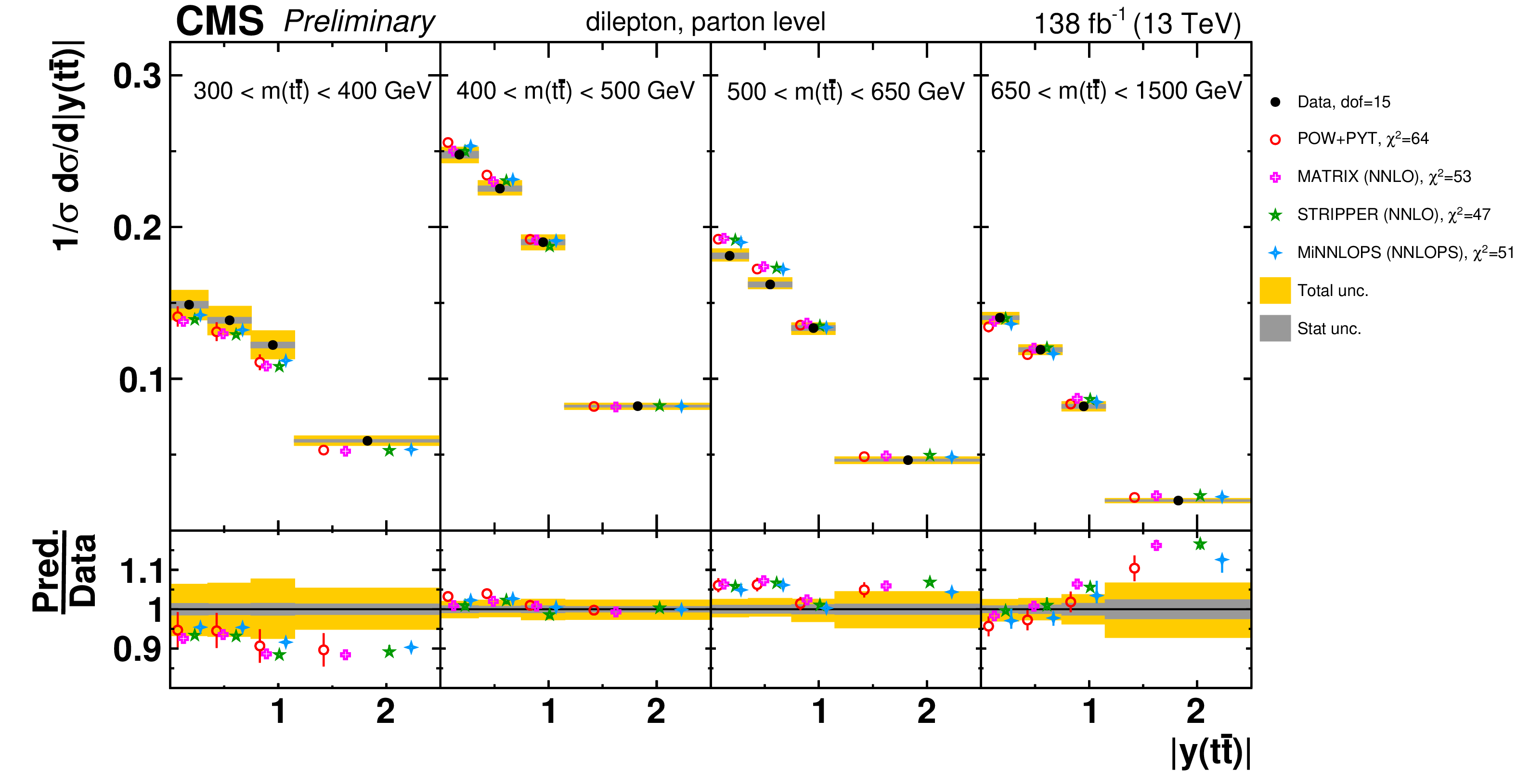
png pdf	Figure 49-a: Normalized $[ {m( \mathrm{t\bar{t}})},\,{|y( \mathrm{t\bar{t}})|} ]$ cross sections are shown for data (filled circles), POWHEG+PYTHIA-8 (`POW-PYT', open circles) simulation, and various theoretical predictions with beyond-NLO precision (other points). Further details can be found in the caption of Fig. 46.
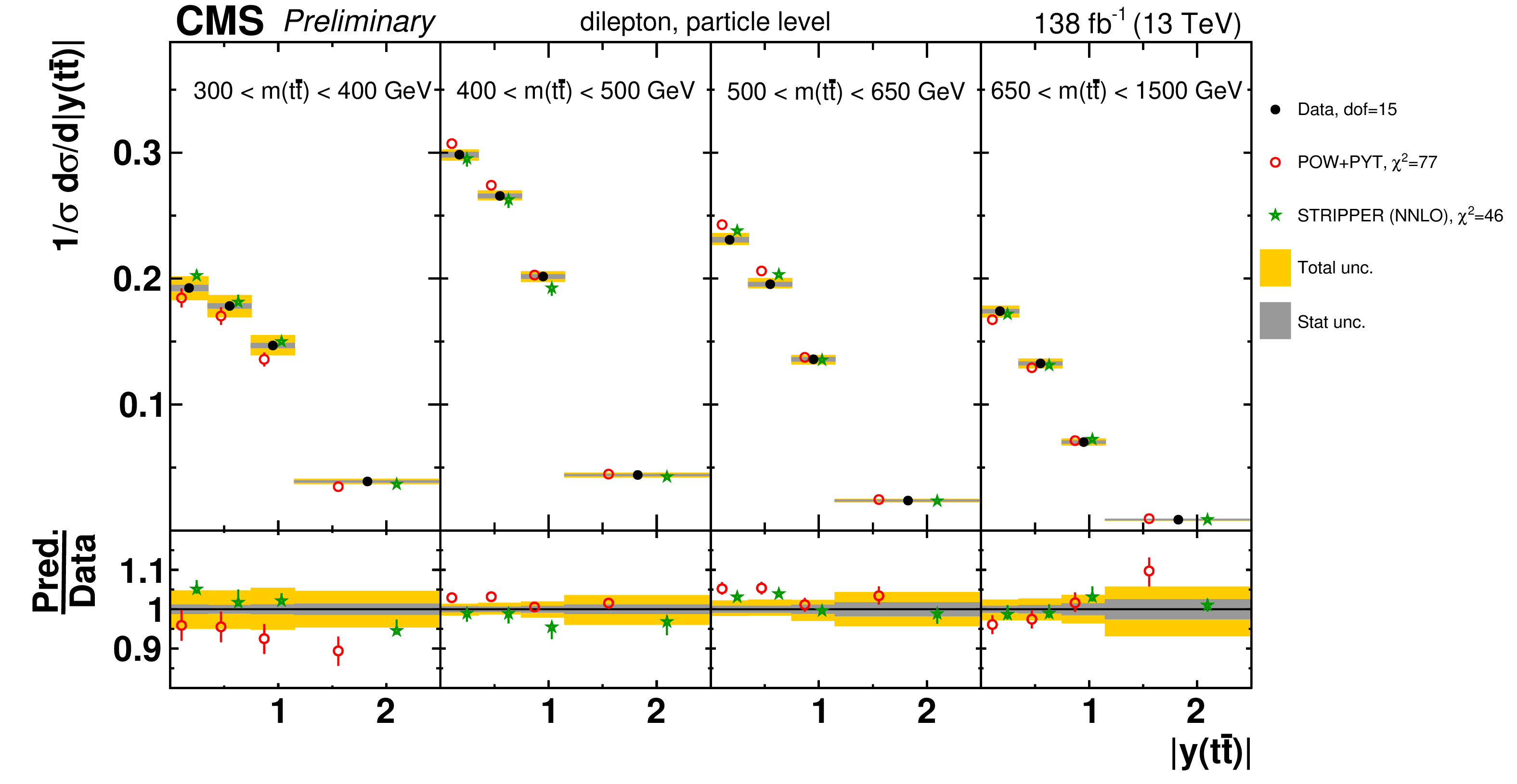
png pdf	Figure 49-b: Normalized $[ {m( \mathrm{t\bar{t}})},\,{|y( \mathrm{t\bar{t}})|} ]$ cross sections are shown for data (filled circles), POWHEG+PYTHIA-8 (`POW-PYT', open circles) simulation, and various theoretical predictions with beyond-NLO precision (other points). Further details can be found in the caption of Fig. 46.
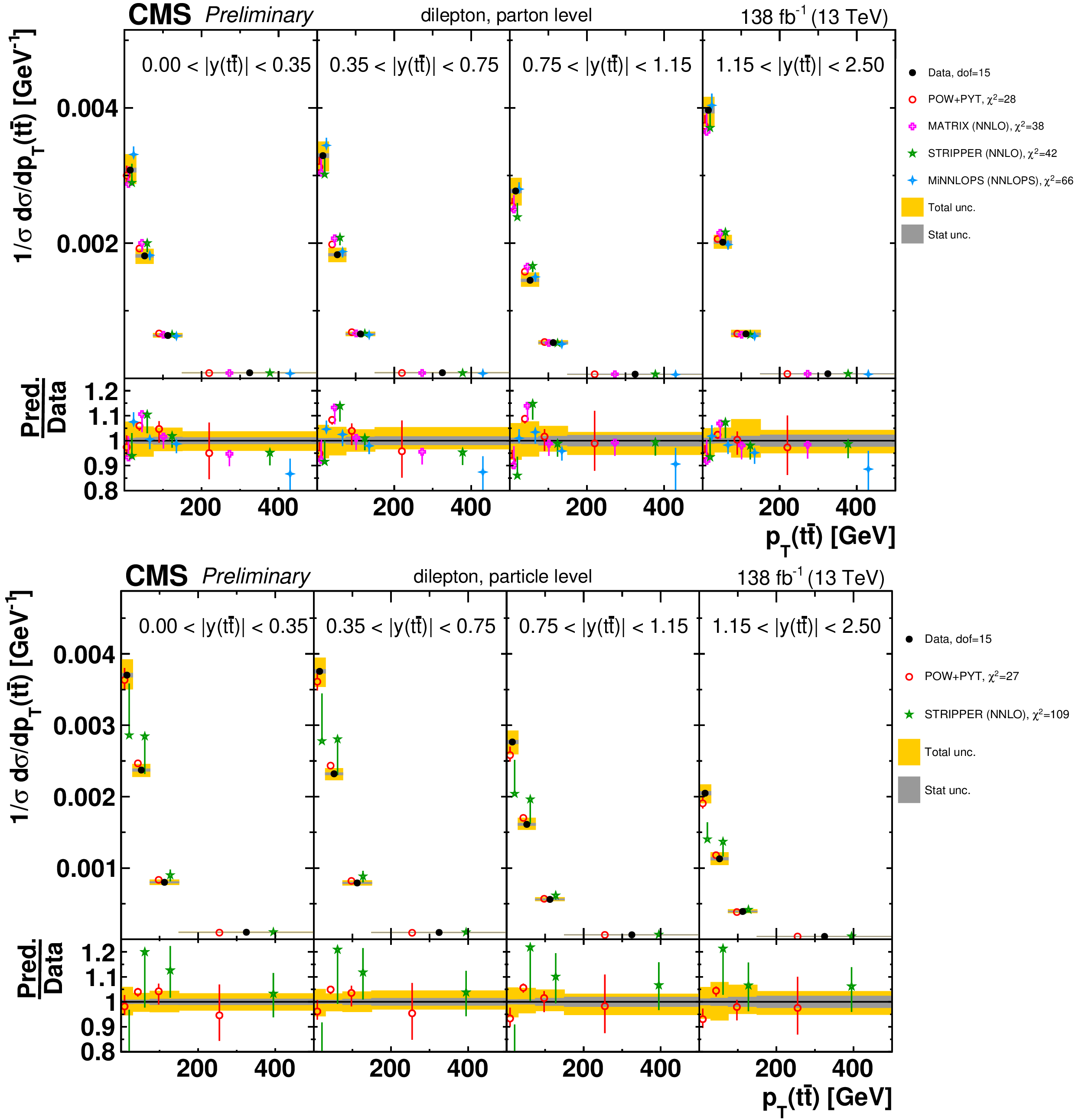
png pdf	Figure 50: Normalized $[ {|y( \mathrm{t\bar{t}})|},\,{{p_{\mathrm {T}}} ( \mathrm{t\bar{t}})} ]$ cross sections are shown for data (filled circles), POWHEG+PYTHIA-8 (`POW-PYT', open circles) simulation, and various theoretical predictions with beyond-NLO precision (other points). Further details can be found in the caption of Fig. 46.
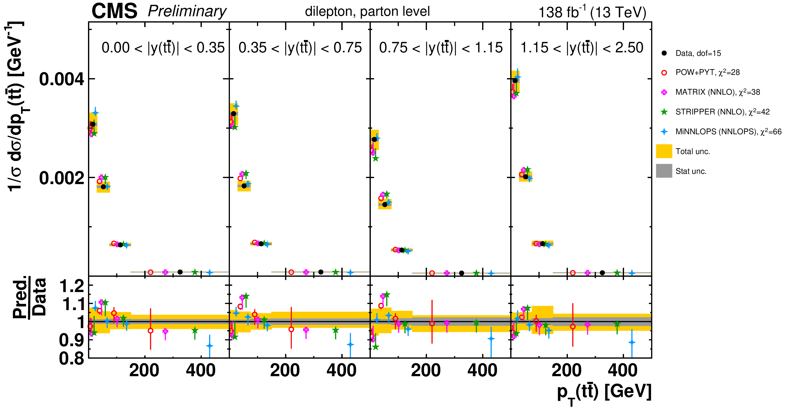
png pdf	Figure 50-a: Normalized $[ {|y( \mathrm{t\bar{t}})|},\,{{p_{\mathrm {T}}} ( \mathrm{t\bar{t}})} ]$ cross sections are shown for data (filled circles), POWHEG+PYTHIA-8 (`POW-PYT', open circles) simulation, and various theoretical predictions with beyond-NLO precision (other points). Further details can be found in the caption of Fig. 46.
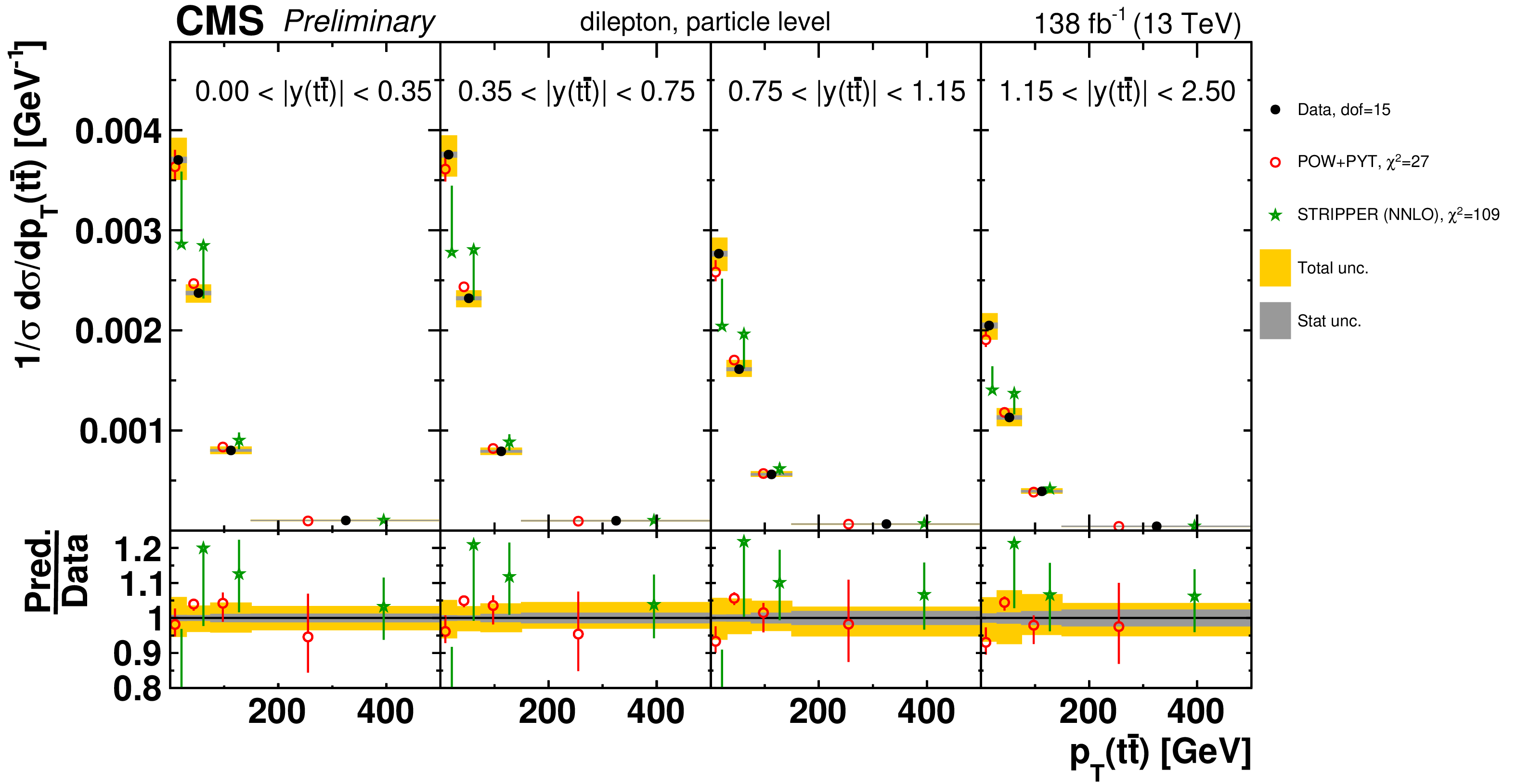
png pdf	Figure 50-b: Normalized $[ {|y( \mathrm{t\bar{t}})|},\,{{p_{\mathrm {T}}} ( \mathrm{t\bar{t}})} ]$ cross sections are shown for data (filled circles), POWHEG+PYTHIA-8 (`POW-PYT', open circles) simulation, and various theoretical predictions with beyond-NLO precision (other points). Further details can be found in the caption of Fig. 46.
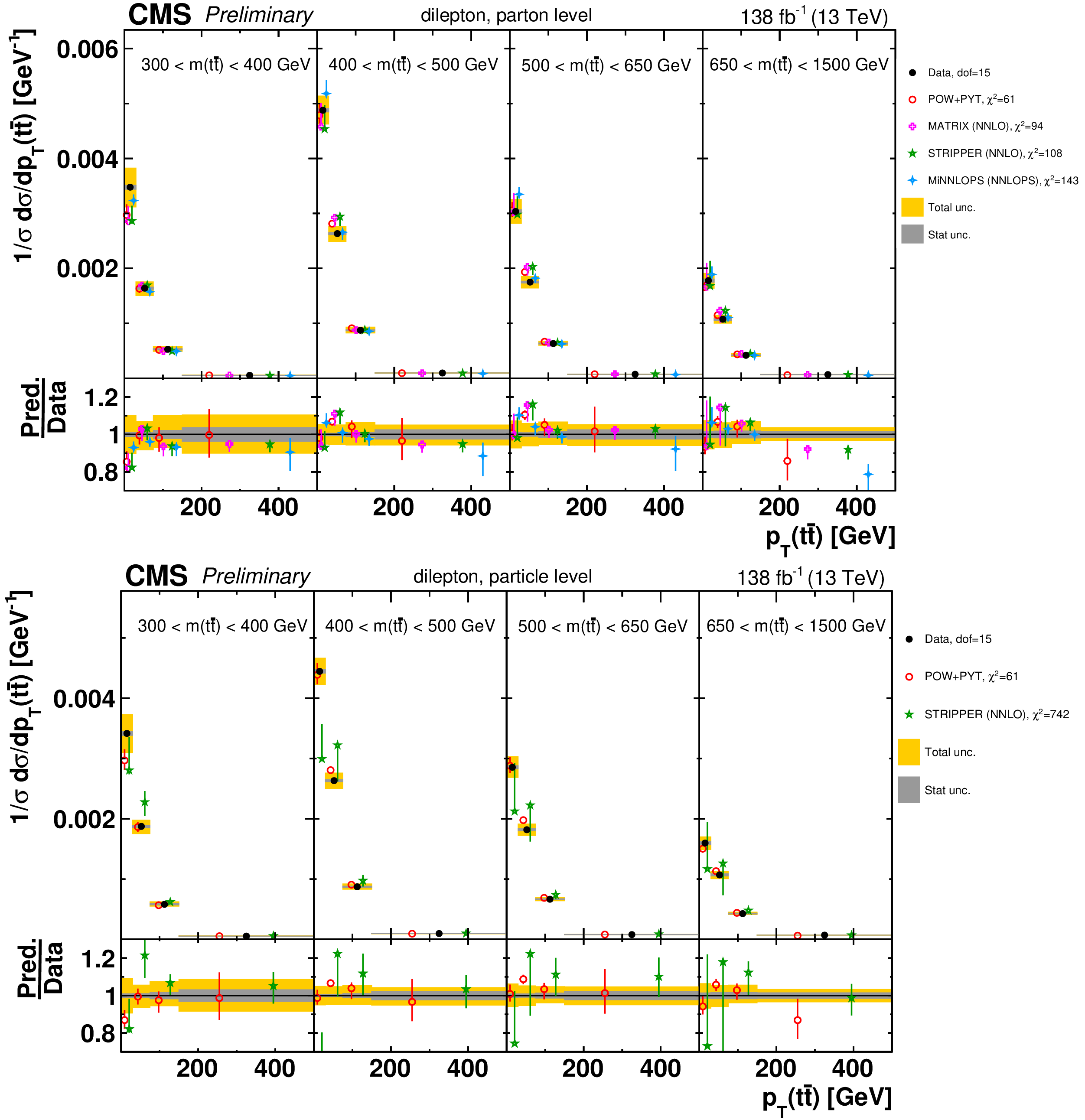
png pdf	Figure 51: Normalized $[ {m( \mathrm{t\bar{t}})},\,{{p_{\mathrm {T}}} ( \mathrm{t\bar{t}})} ]$ cross sections are shown for data (filled circles), POWHEG+PYTHIA-8 (`POW-PYT', open circles) simulation, and various theoretical predictions with beyond-NLO precision (other points). Further details can be found in the caption of Fig. 46.
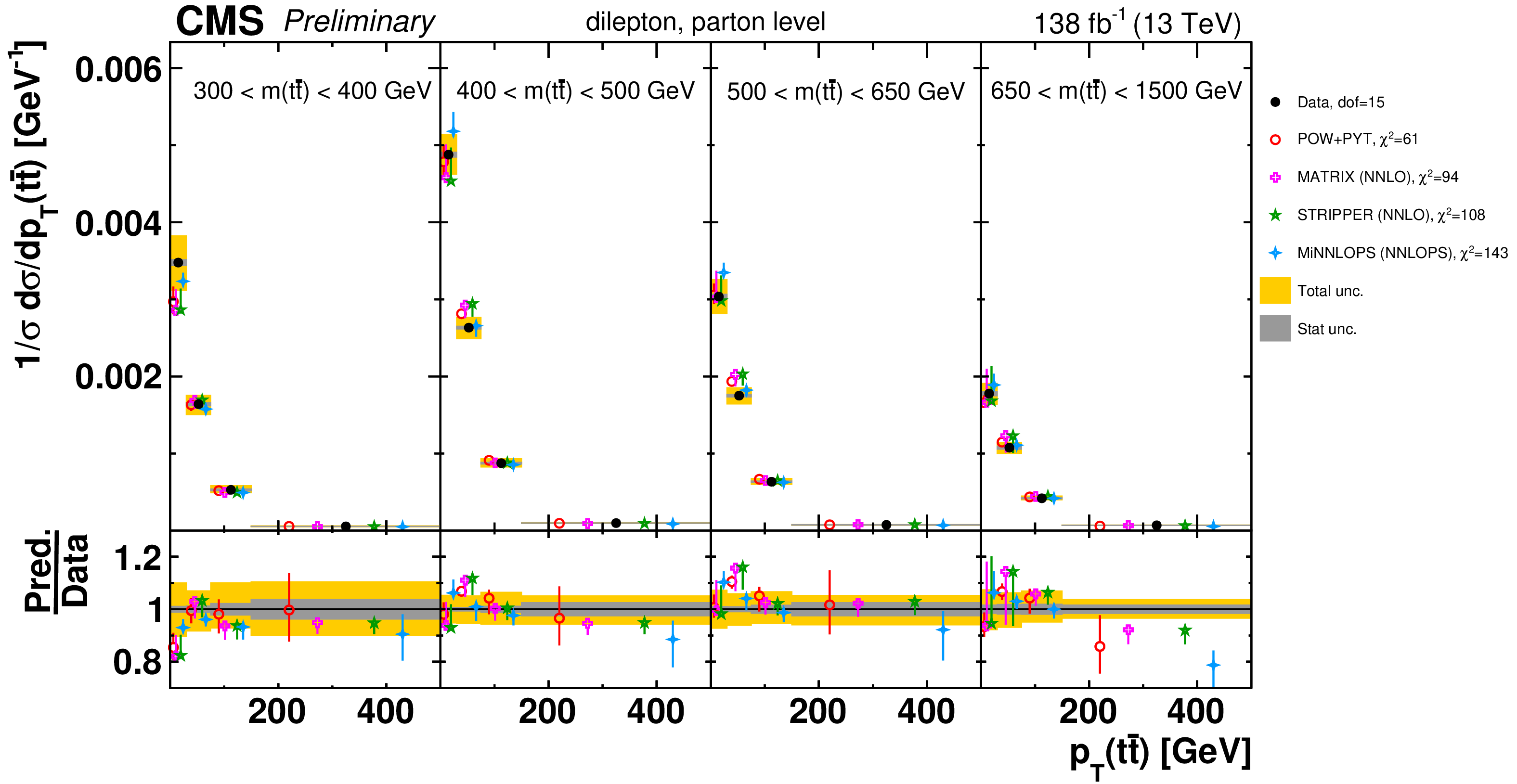
png pdf	Figure 51-a: Normalized $[ {m( \mathrm{t\bar{t}})},\,{{p_{\mathrm {T}}} ( \mathrm{t\bar{t}})} ]$ cross sections are shown for data (filled circles), POWHEG+PYTHIA-8 (`POW-PYT', open circles) simulation, and various theoretical predictions with beyond-NLO precision (other points). Further details can be found in the caption of Fig. 46.
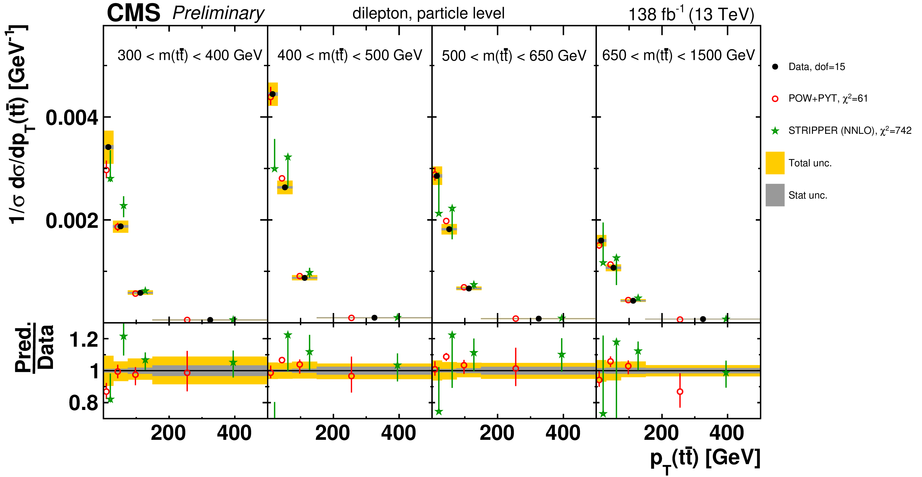
png pdf	Figure 51-b: Normalized $[ {m( \mathrm{t\bar{t}})},\,{{p_{\mathrm {T}}} ( \mathrm{t\bar{t}})} ]$ cross sections are shown for data (filled circles), POWHEG+PYTHIA-8 (`POW-PYT', open circles) simulation, and various theoretical predictions with beyond-NLO precision (other points). Further details can be found in the caption of Fig. 46.
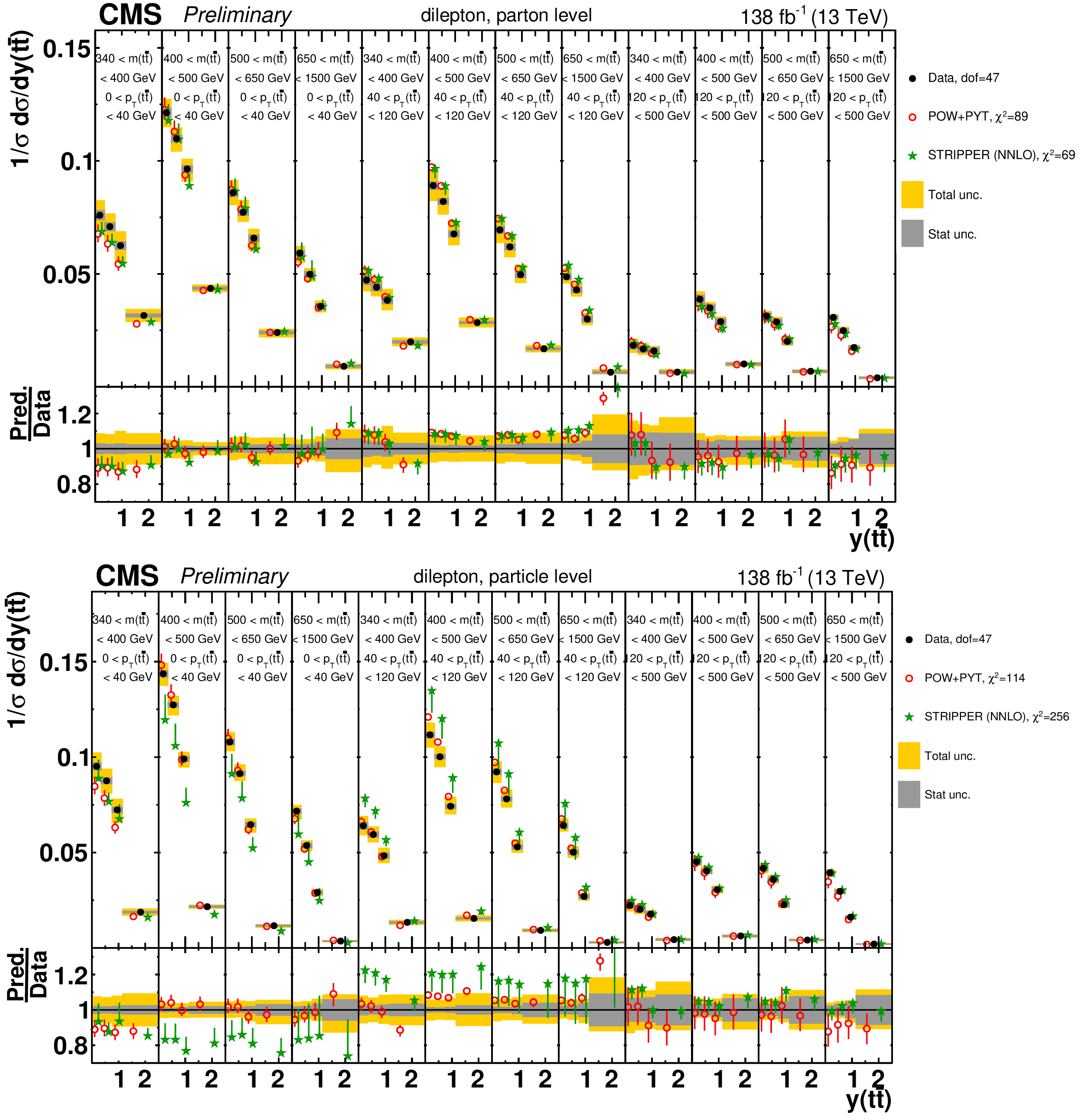
png pdf	Figure 52: Normalized $[ {{p_{\mathrm {T}}} ( \mathrm{t\bar{t}})},\,{m( \mathrm{t\bar{t}})},\,{y( \mathrm{t\bar{t}})} ]$ cross sections are shown for data (filled circles), POWHEG+PYTHIA-8 (`POW-PYT', open circles) simulation, and Stripper NNLO calculation (stars). Further details can be found in the caption of Fig. 46.
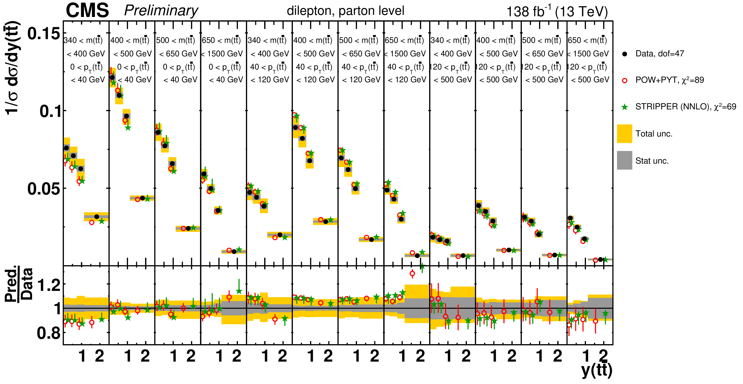
png pdf	Figure 52-a: Normalized $[ {{p_{\mathrm {T}}} ( \mathrm{t\bar{t}})},\,{m( \mathrm{t\bar{t}})},\,{y( \mathrm{t\bar{t}})} ]$ cross sections are shown for data (filled circles), POWHEG+PYTHIA-8 (`POW-PYT', open circles) simulation, and Stripper NNLO calculation (stars). Further details can be found in the caption of Fig. 46.
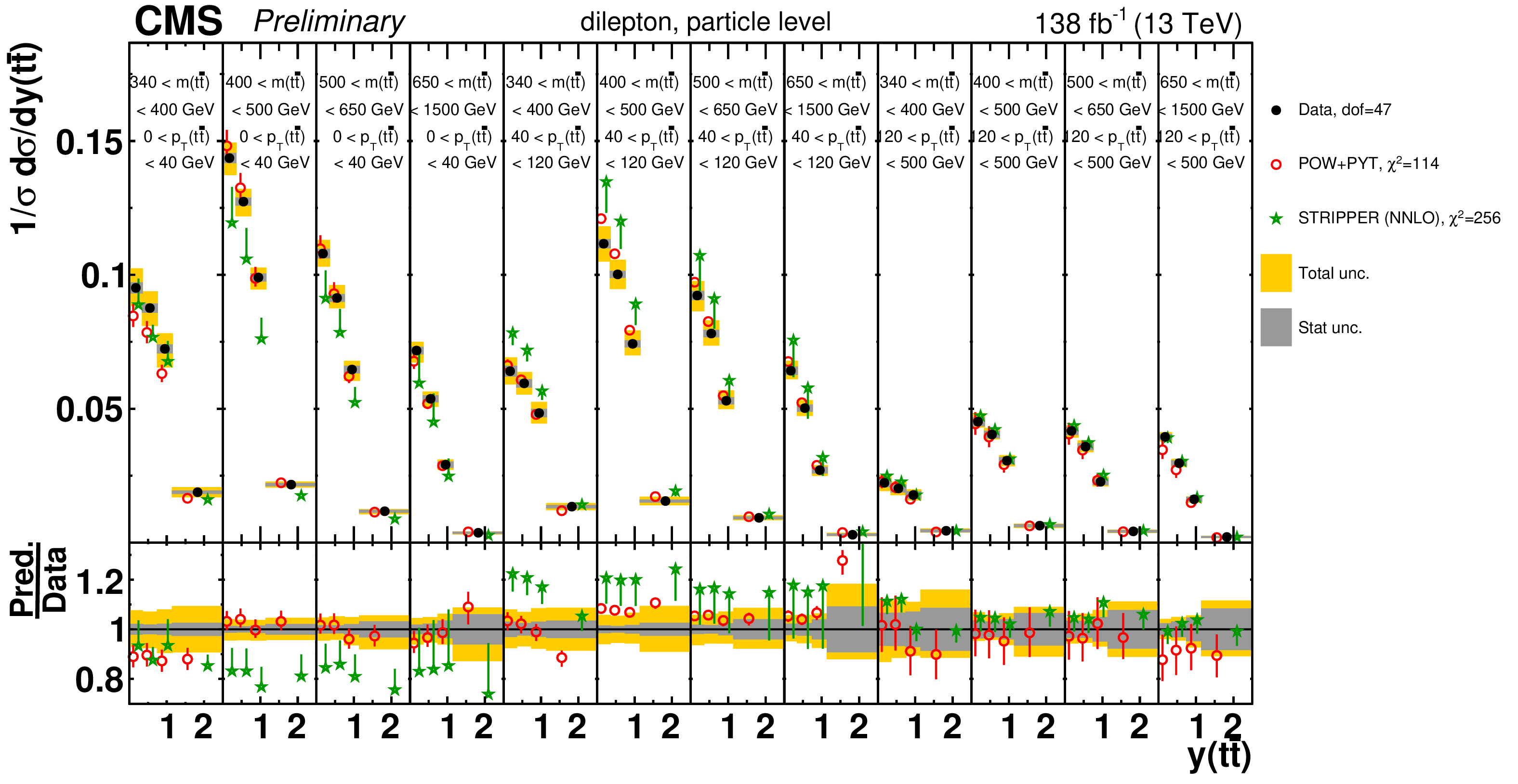
png pdf	Figure 52-b: Normalized $[ {{p_{\mathrm {T}}} ( \mathrm{t\bar{t}})},\,{m( \mathrm{t\bar{t}})},\,{y( \mathrm{t\bar{t}})} ]$ cross sections are shown for data (filled circles), POWHEG+PYTHIA-8 (`POW-PYT', open circles) simulation, and Stripper NNLO calculation (stars). Further details can be found in the caption of Fig. 46.
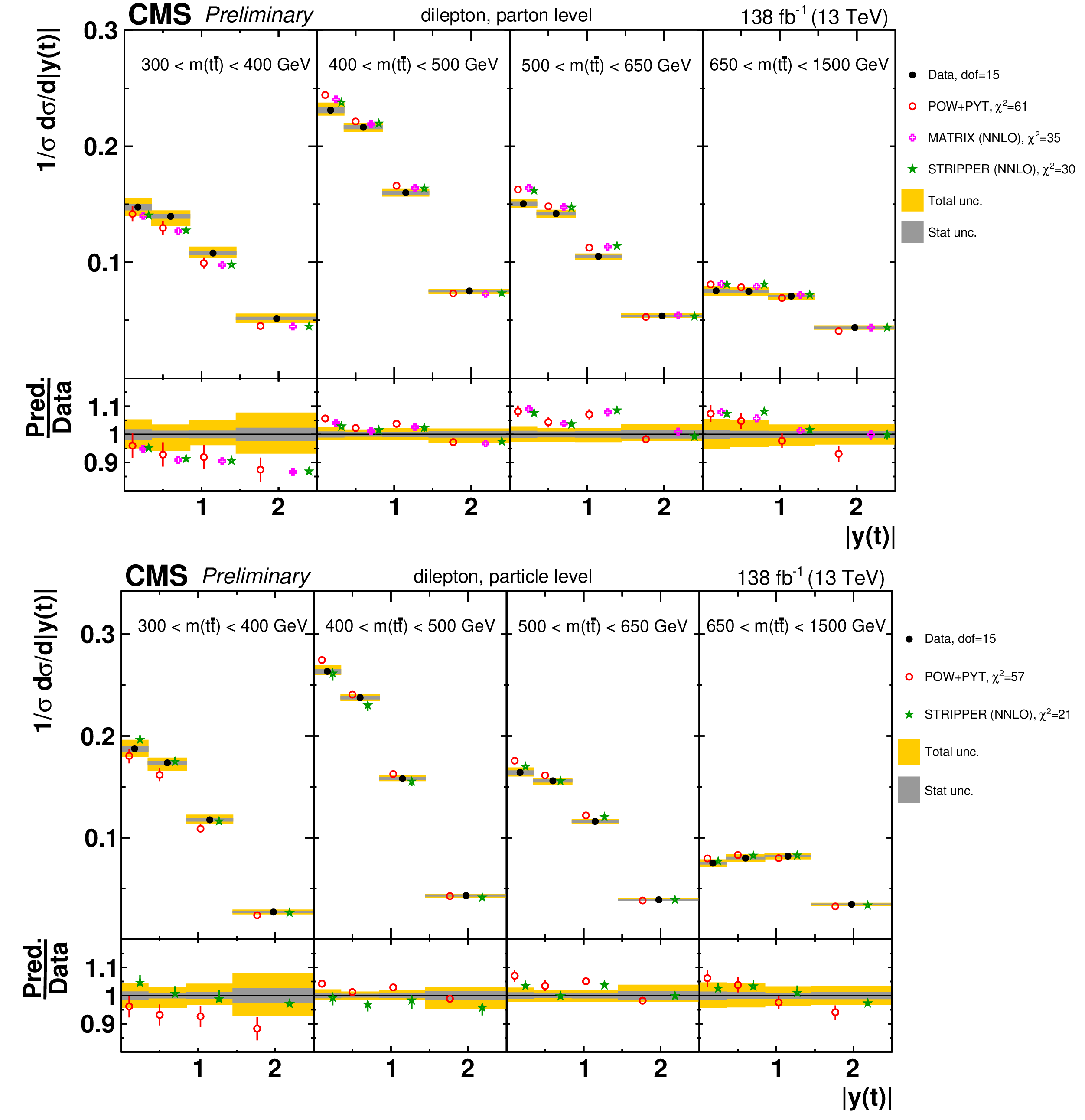
png pdf	Figure 53: Normalized $[ {m( \mathrm{t\bar{t}})},\,{|y(\mathrm{t})|} ]$ cross sections are shown for data (filled circles), POWHEG+PYTHIA-8 (`POW-PYT', open circles) simulation, and various theoretical predictions with beyond-NLO precision (other points). Further details can be found in the caption of Fig. 46.
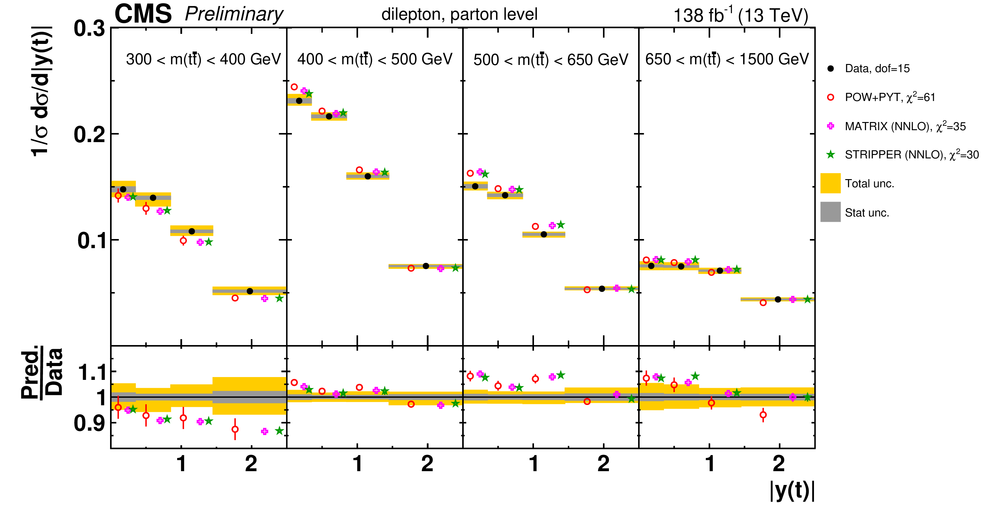
png pdf	Figure 53-a: Normalized $[ {m( \mathrm{t\bar{t}})},\,{|y(\mathrm{t})|} ]$ cross sections are shown for data (filled circles), POWHEG+PYTHIA-8 (`POW-PYT', open circles) simulation, and various theoretical predictions with beyond-NLO precision (other points). Further details can be found in the caption of Fig. 46.
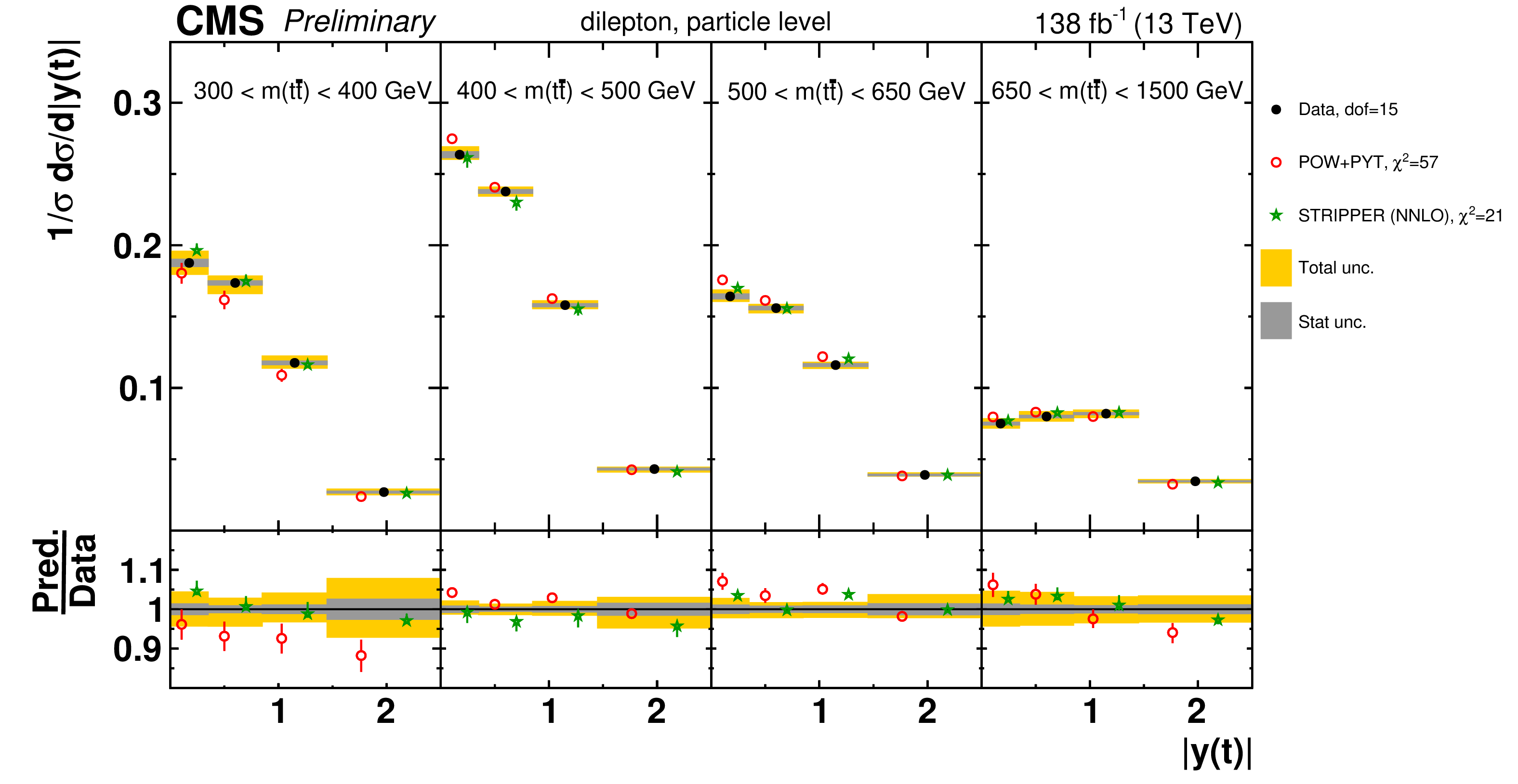
png pdf	Figure 53-b: Normalized $[ {m( \mathrm{t\bar{t}})},\,{|y(\mathrm{t})|} ]$ cross sections are shown for data (filled circles), POWHEG+PYTHIA-8 (`POW-PYT', open circles) simulation, and various theoretical predictions with beyond-NLO precision (other points). Further details can be found in the caption of Fig. 46.
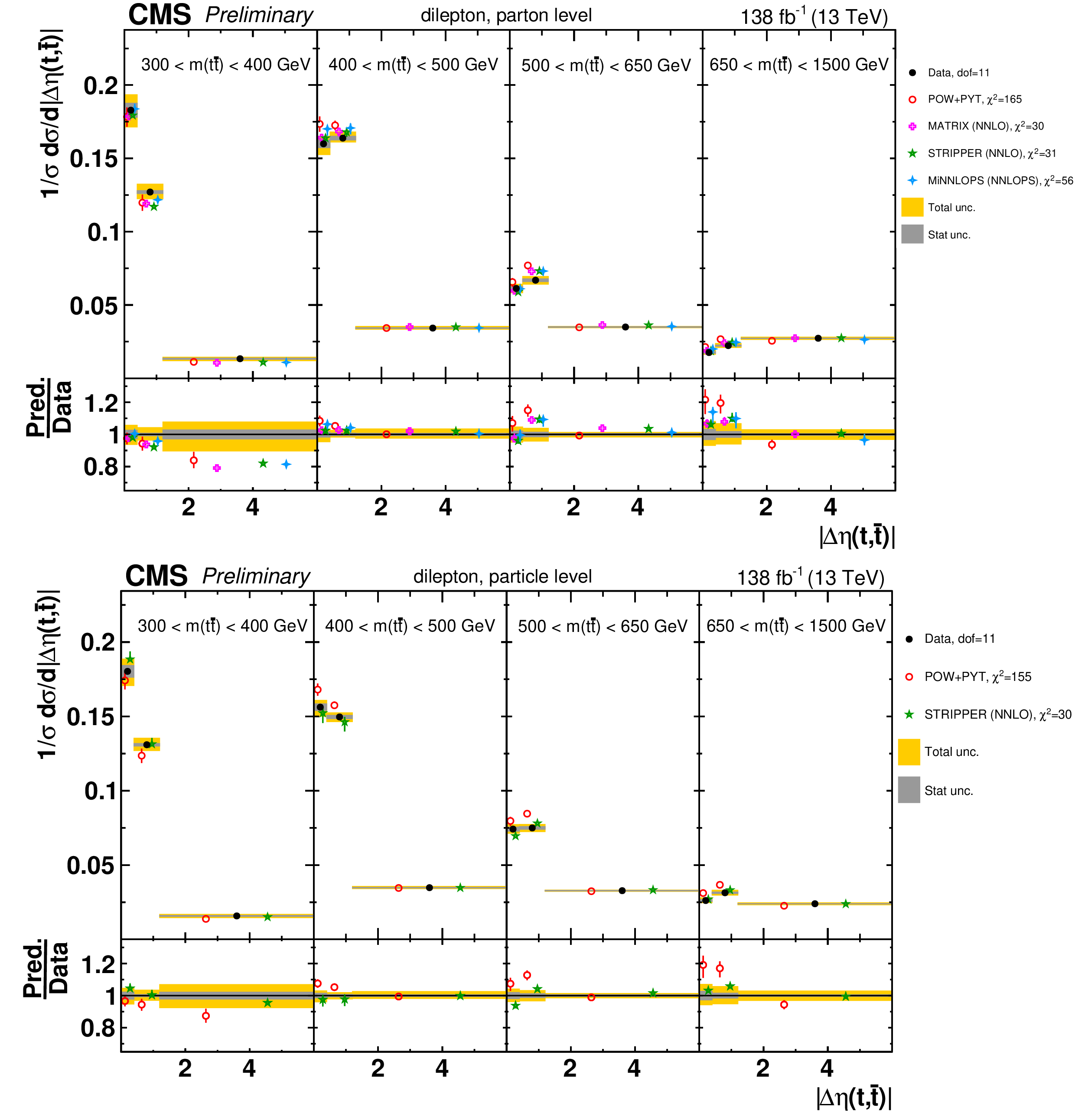
png pdf	Figure 54: Normalized $[ {m( \mathrm{t\bar{t}})},\,{|\Delta \eta (\mathrm{t},\mathrm{\bar{t}})|} ]$ cross sections are shown for data (filled circles), POWHEG+PYTHIA-8 (`POW-PYT', open circles) simulation, and various theoretical predictions with beyond-NLO precision (other points). Further details can be found in the caption of Fig. 46.
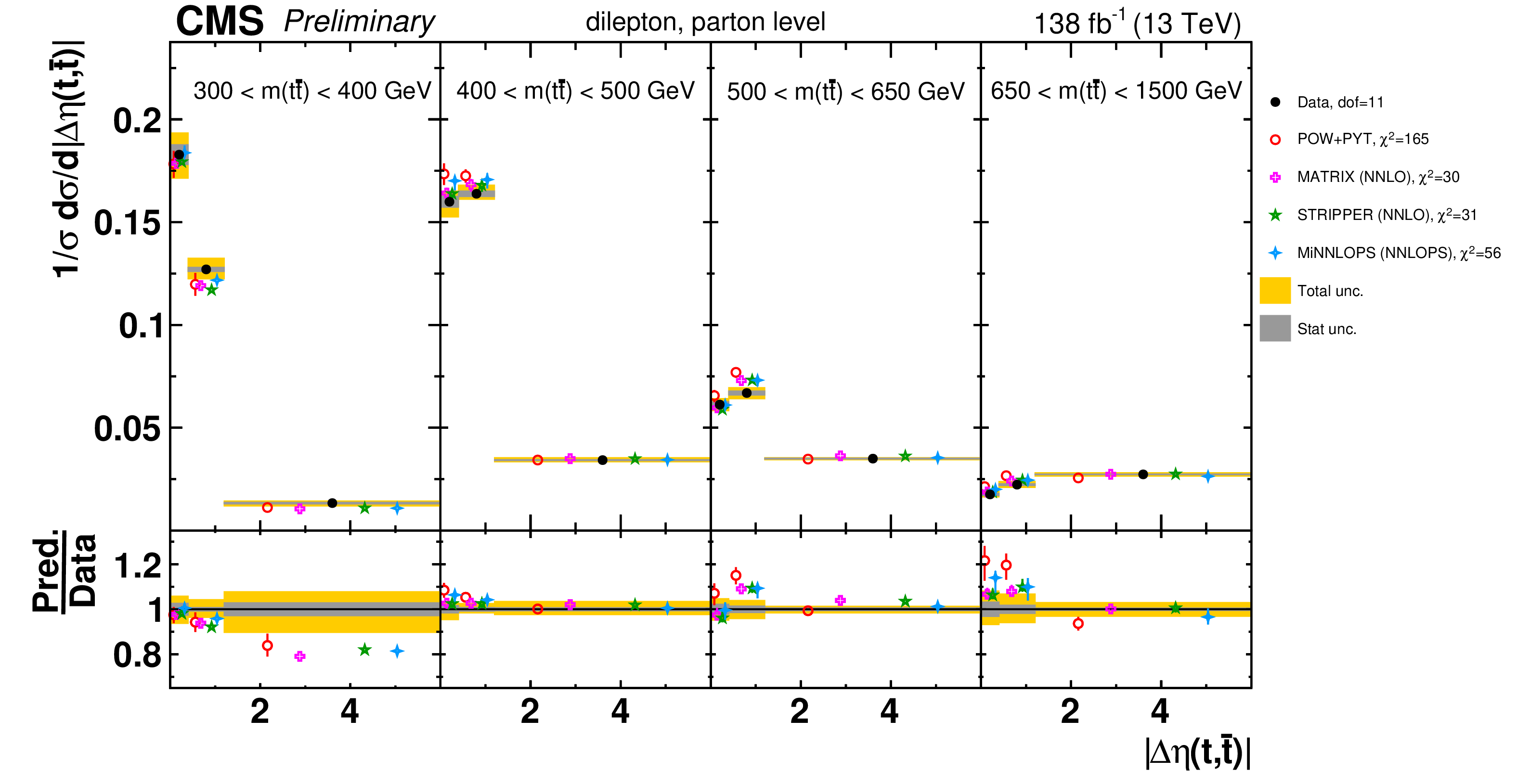
png pdf	Figure 54-a: Normalized $[ {m( \mathrm{t\bar{t}})},\,{|\Delta \eta (\mathrm{t},\mathrm{\bar{t}})|} ]$ cross sections are shown for data (filled circles), POWHEG+PYTHIA-8 (`POW-PYT', open circles) simulation, and various theoretical predictions with beyond-NLO precision (other points). Further details can be found in the caption of Fig. 46.
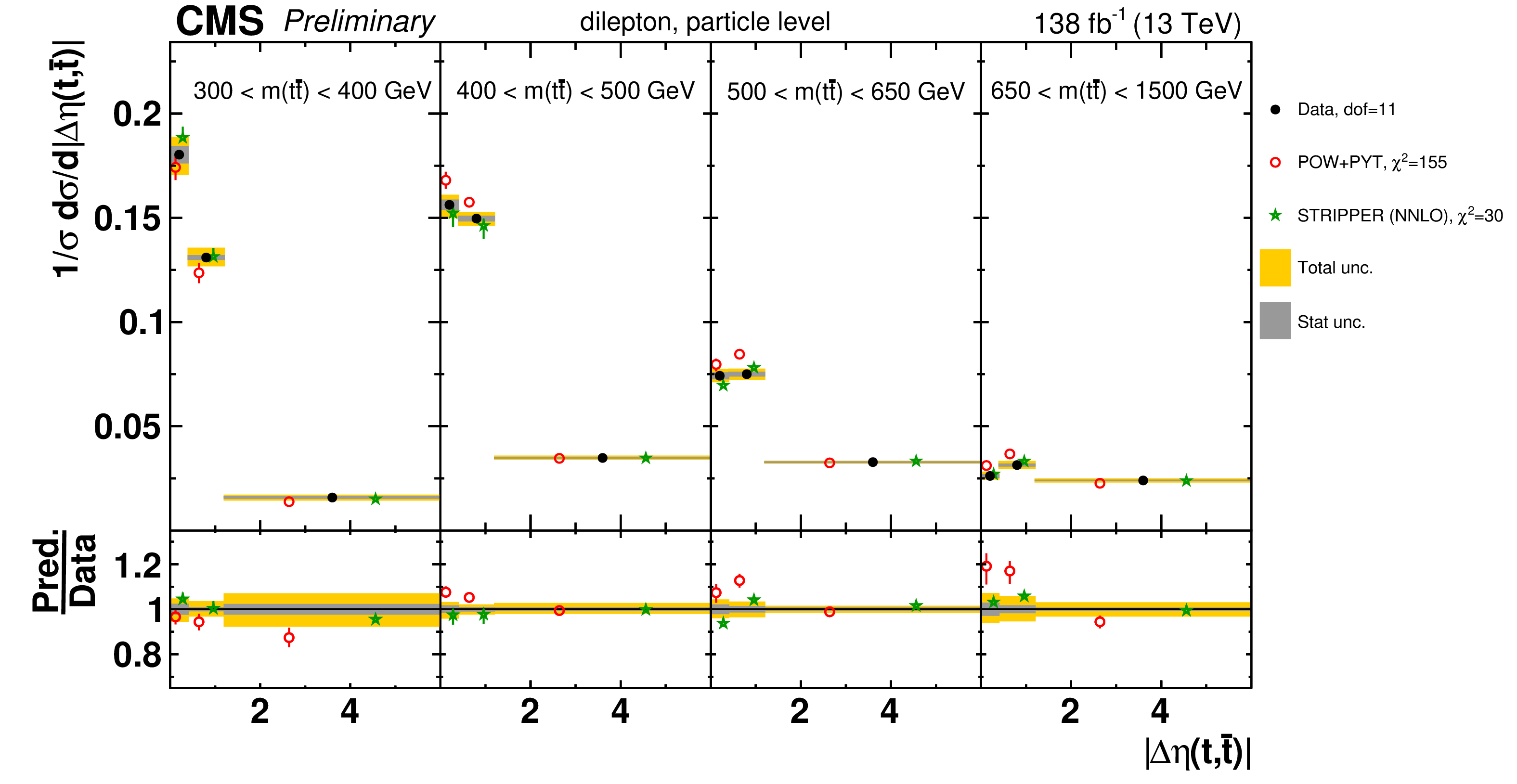
png pdf	Figure 54-b: Normalized $[ {m( \mathrm{t\bar{t}})},\,{|\Delta \eta (\mathrm{t},\mathrm{\bar{t}})|} ]$ cross sections are shown for data (filled circles), POWHEG+PYTHIA-8 (`POW-PYT', open circles) simulation, and various theoretical predictions with beyond-NLO precision (other points). Further details can be found in the caption of Fig. 46.
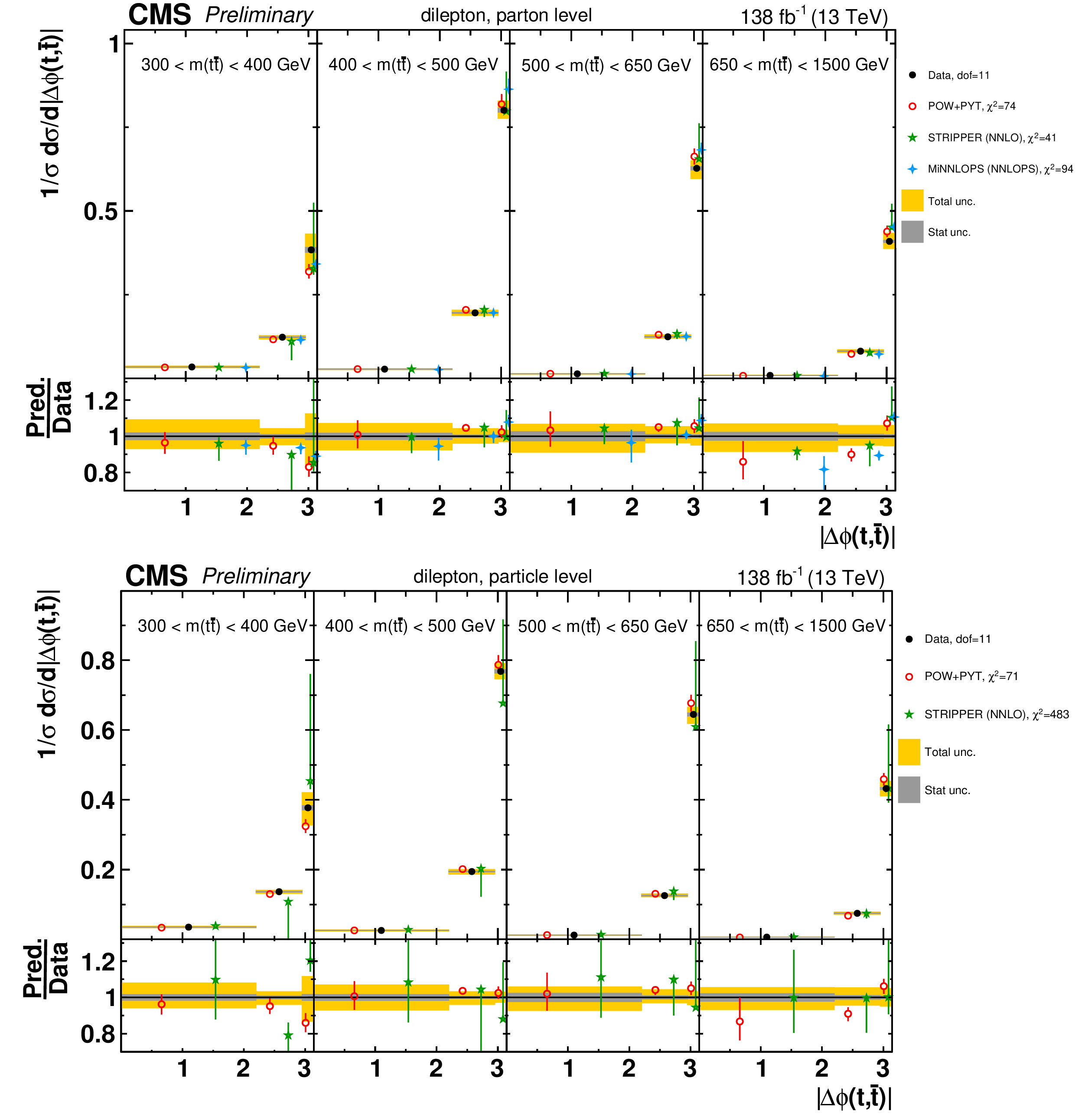
png pdf	Figure 55: Normalized $[ {m( \mathrm{t\bar{t}})},\,{|\Delta \phi (\mathrm{t},\mathrm{\bar{t}})|} ]$ cross sections are shown for data (filled circles), POWHEG+PYTHIA-8 (`POW-PYT', open circles) simulation, and various theoretical predictions with beyond-NLO precision (other points). Further details can be found in the caption of Fig. 46.
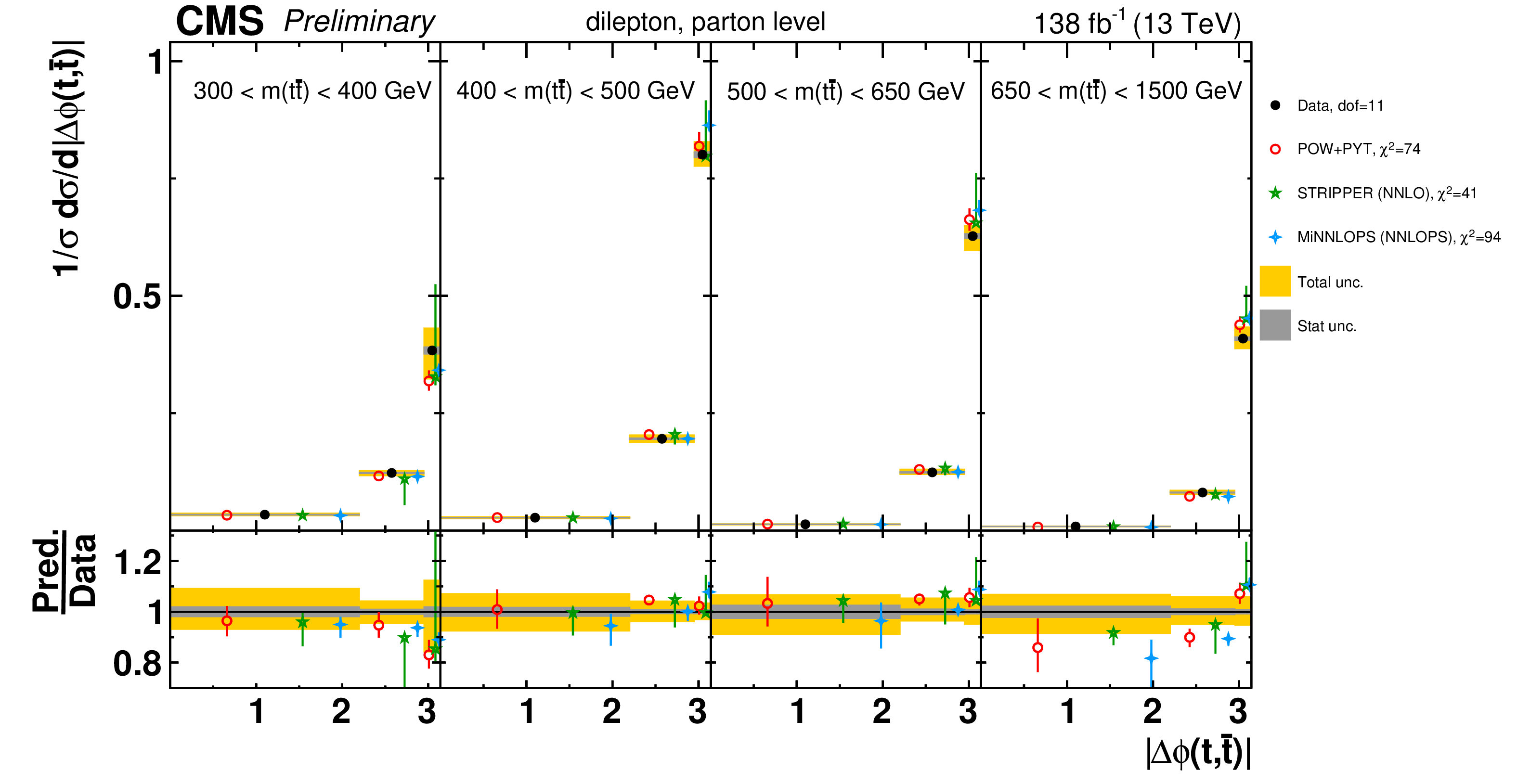
png pdf	Figure 55-a: Normalized $[ {m( \mathrm{t\bar{t}})},\,{|\Delta \phi (\mathrm{t},\mathrm{\bar{t}})|} ]$ cross sections are shown for data (filled circles), POWHEG+PYTHIA-8 (`POW-PYT', open circles) simulation, and various theoretical predictions with beyond-NLO precision (other points). Further details can be found in the caption of Fig. 46.
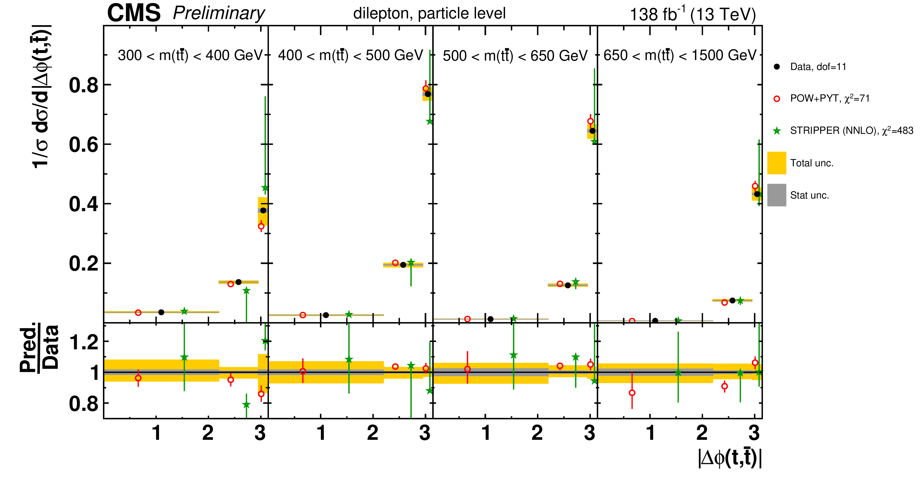
png pdf	Figure 55-b: Normalized $[ {m( \mathrm{t\bar{t}})},\,{|\Delta \phi (\mathrm{t},\mathrm{\bar{t}})|} ]$ cross sections are shown for data (filled circles), POWHEG+PYTHIA-8 (`POW-PYT', open circles) simulation, and various theoretical predictions with beyond-NLO precision (other points). Further details can be found in the caption of Fig. 46.
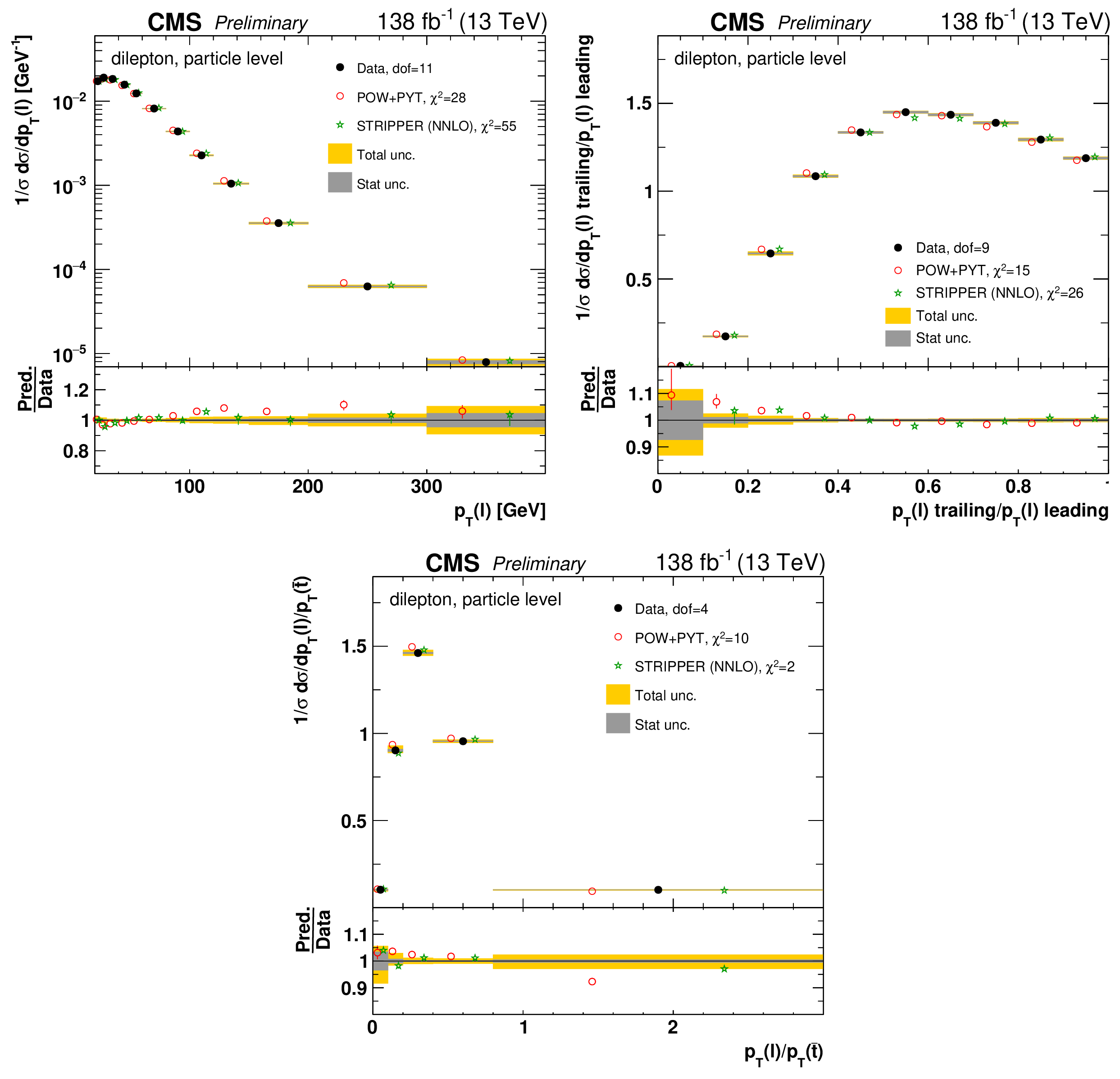
png pdf	Figure 56: Normalized differential $\mathrm{t\bar{t}}$ production cross sections as a function of ${p_{\mathrm {T}}}$ of the lepton (upper left), of the ratio of the trailing and leading lepton ${p_{\mathrm {T}}}$ (upper right), and of the ratio of lepton and top antiquark ${p_{\mathrm {T}}}$ (lower middle), measured at the particle level in a fiducial phase space. The data are shown as filled circles with dark and light bands indicating the statistical and total uncertainties (statistical and systematic uncertainties summed in quadrature), respectively. The cross sections are compared to predictions from the POWHEG+PYTHIA-8 (`POW-PYT', open circles) simulation and Stripper NNLO calculation (stars). The estimated uncertainties in the predictions are represented by a vertical bar on the corresponding points. For each model, a value of ${\chi ^2}$ is reported that takes into account the measurement uncertainties. The lower panel in each plot shows the ratios of the predictions to the data.
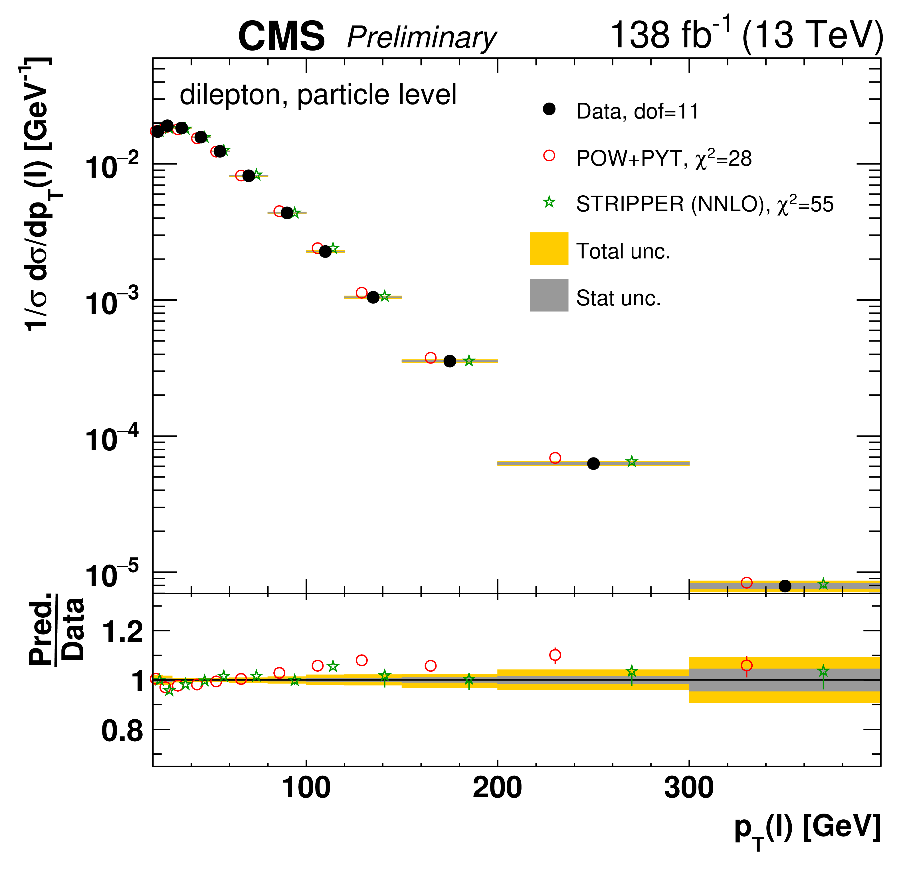
png pdf	Figure 56-a: Normalized differential $\mathrm{t\bar{t}}$ production cross sections as a function of ${p_{\mathrm {T}}}$ of the lepton (upper left), of the ratio of the trailing and leading lepton ${p_{\mathrm {T}}}$ (upper right), and of the ratio of lepton and top antiquark ${p_{\mathrm {T}}}$ (lower middle), measured at the particle level in a fiducial phase space. The data are shown as filled circles with dark and light bands indicating the statistical and total uncertainties (statistical and systematic uncertainties summed in quadrature), respectively. The cross sections are compared to predictions from the POWHEG+PYTHIA-8 (`POW-PYT', open circles) simulation and Stripper NNLO calculation (stars). The estimated uncertainties in the predictions are represented by a vertical bar on the corresponding points. For each model, a value of ${\chi ^2}$ is reported that takes into account the measurement uncertainties. The lower panel in each plot shows the ratios of the predictions to the data.
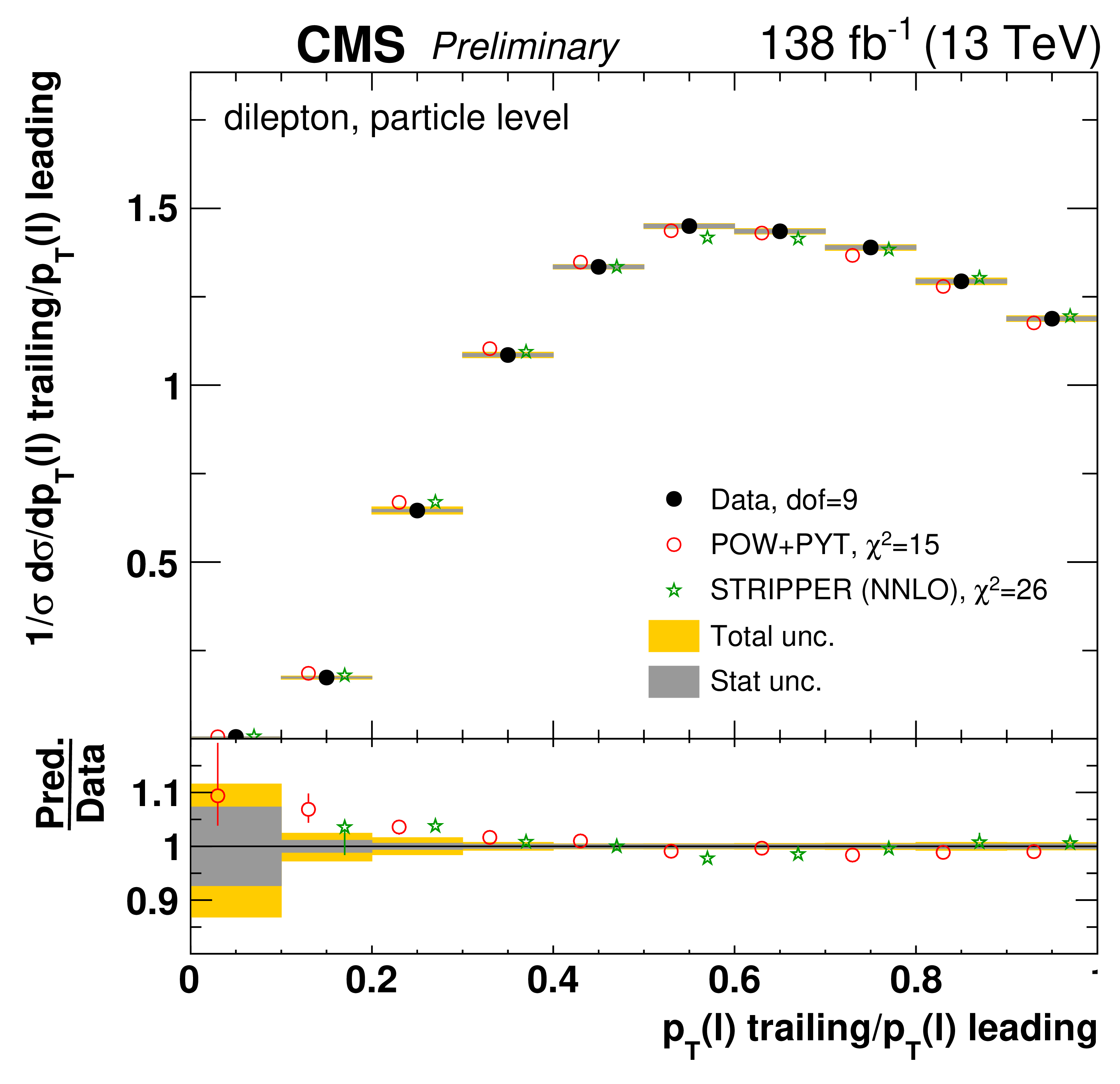
png pdf	Figure 56-b: Normalized differential $\mathrm{t\bar{t}}$ production cross sections as a function of ${p_{\mathrm {T}}}$ of the lepton (upper left), of the ratio of the trailing and leading lepton ${p_{\mathrm {T}}}$ (upper right), and of the ratio of lepton and top antiquark ${p_{\mathrm {T}}}$ (lower middle), measured at the particle level in a fiducial phase space. The data are shown as filled circles with dark and light bands indicating the statistical and total uncertainties (statistical and systematic uncertainties summed in quadrature), respectively. The cross sections are compared to predictions from the POWHEG+PYTHIA-8 (`POW-PYT', open circles) simulation and Stripper NNLO calculation (stars). The estimated uncertainties in the predictions are represented by a vertical bar on the corresponding points. For each model, a value of ${\chi ^2}$ is reported that takes into account the measurement uncertainties. The lower panel in each plot shows the ratios of the predictions to the data.
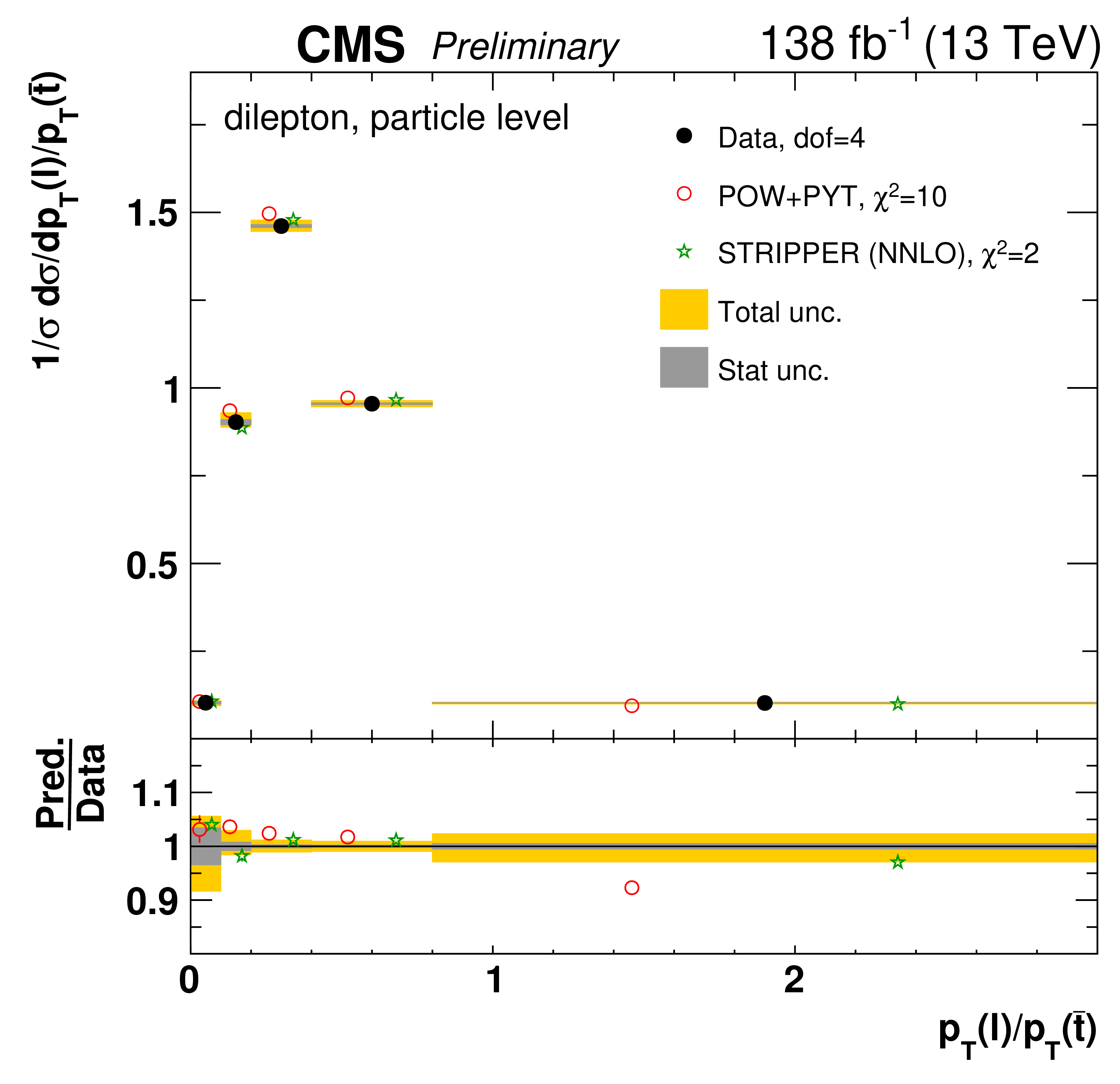
png pdf	Figure 56-c: Normalized differential $\mathrm{t\bar{t}}$ production cross sections as a function of ${p_{\mathrm {T}}}$ of the lepton (upper left), of the ratio of the trailing and leading lepton ${p_{\mathrm {T}}}$ (upper right), and of the ratio of lepton and top antiquark ${p_{\mathrm {T}}}$ (lower middle), measured at the particle level in a fiducial phase space. The data are shown as filled circles with dark and light bands indicating the statistical and total uncertainties (statistical and systematic uncertainties summed in quadrature), respectively. The cross sections are compared to predictions from the POWHEG+PYTHIA-8 (`POW-PYT', open circles) simulation and Stripper NNLO calculation (stars). The estimated uncertainties in the predictions are represented by a vertical bar on the corresponding points. For each model, a value of ${\chi ^2}$ is reported that takes into account the measurement uncertainties. The lower panel in each plot shows the ratios of the predictions to the data.
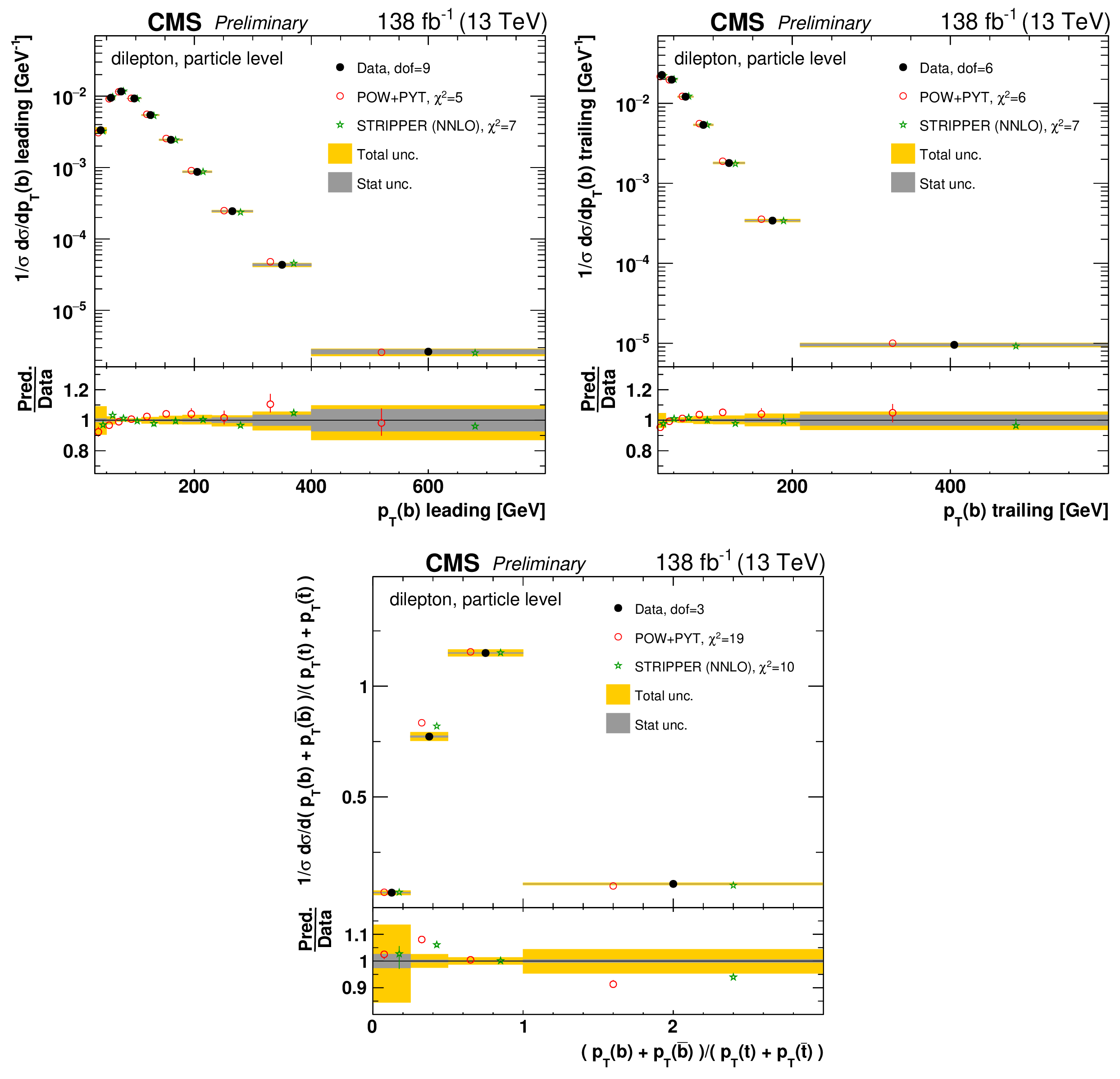
png pdf	Figure 57: Normalized differential $\mathrm{t\bar{t}}$ production cross sections as a function of the ${p_{\mathrm {T}}}$ of the leading (upper left) and trailing (upper right) b jet, and $( {{p_{\mathrm {T}}}}(\rm {b})+ {{p_{\mathrm {T}}}}(\mathrm{b\bar{b}}))/( {{p_{\mathrm {T}}}}(\rm {t})+ {{p_{\mathrm {T}}}}(\mathrm{\bar{t}}))$ (lower) are shown for data (filled circles), POWHEG+PYTHIA-8 (`POW-PYT', open circles) simulation, and Stripper NNLO calculation (stars). Further details can be found in the caption of Fig. 56.
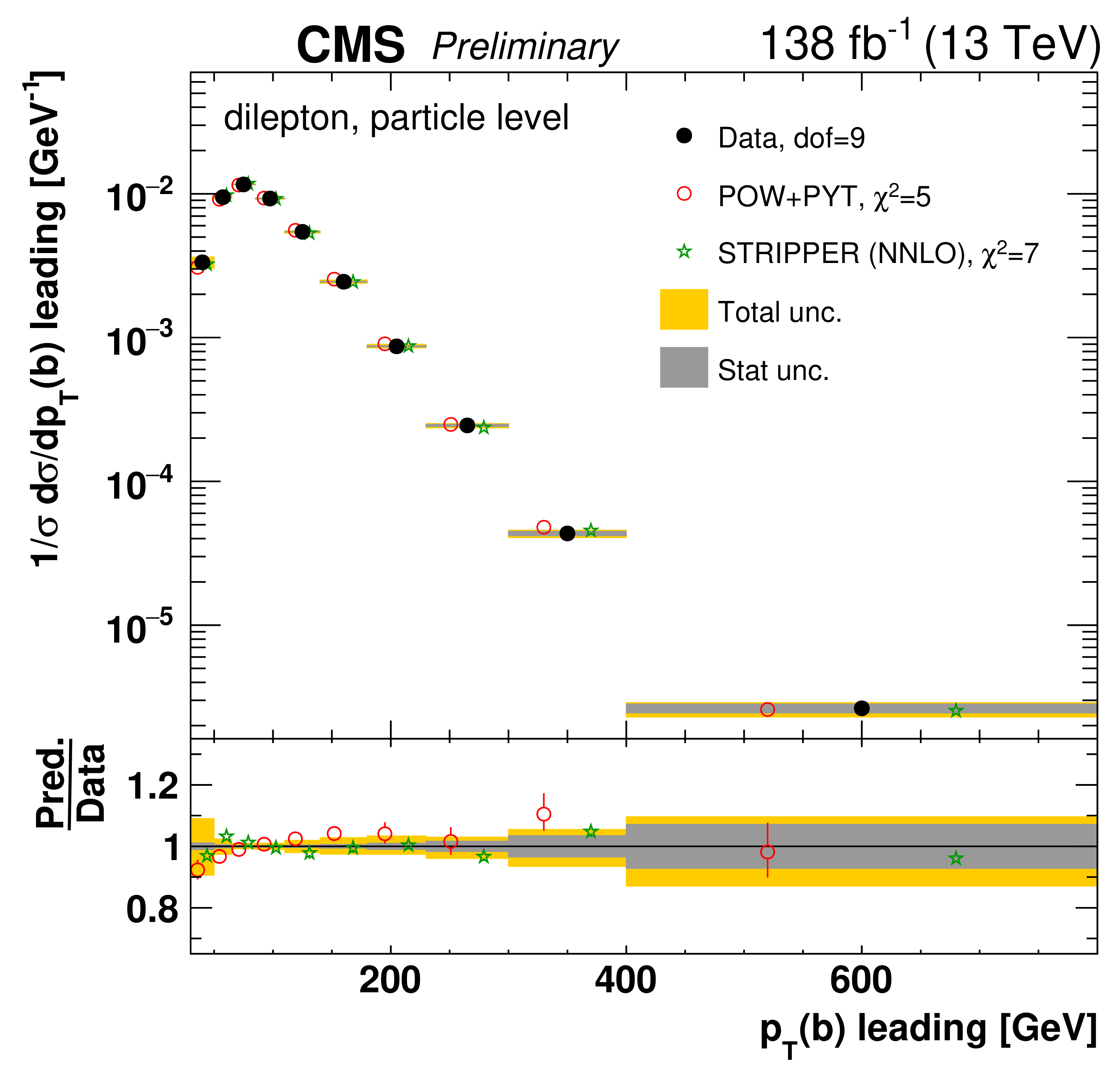
png pdf	Figure 57-a: Normalized differential $\mathrm{t\bar{t}}$ production cross sections as a function of the ${p_{\mathrm {T}}}$ of the leading (upper left) and trailing (upper right) b jet, and $( {{p_{\mathrm {T}}}}(\rm {b})+ {{p_{\mathrm {T}}}}(\mathrm{b\bar{b}}))/( {{p_{\mathrm {T}}}}(\rm {t})+ {{p_{\mathrm {T}}}}(\mathrm{\bar{t}}))$ (lower) are shown for data (filled circles), POWHEG+PYTHIA-8 (`POW-PYT', open circles) simulation, and Stripper NNLO calculation (stars). Further details can be found in the caption of Fig. 56.
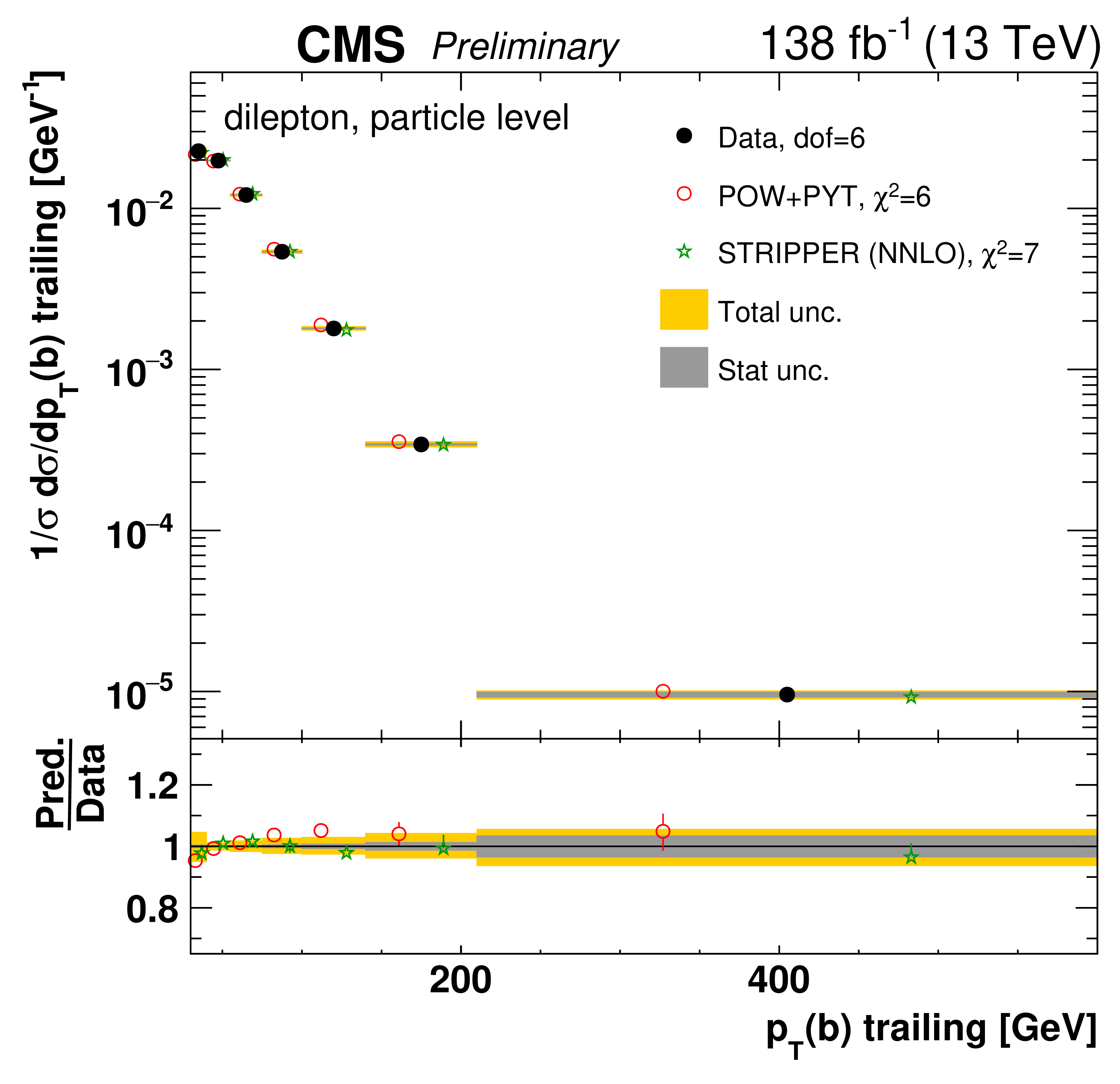
png pdf	Figure 57-b: Normalized differential $\mathrm{t\bar{t}}$ production cross sections as a function of the ${p_{\mathrm {T}}}$ of the leading (upper left) and trailing (upper right) b jet, and $( {{p_{\mathrm {T}}}}(\rm {b})+ {{p_{\mathrm {T}}}}(\mathrm{b\bar{b}}))/( {{p_{\mathrm {T}}}}(\rm {t})+ {{p_{\mathrm {T}}}}(\mathrm{\bar{t}}))$ (lower) are shown for data (filled circles), POWHEG+PYTHIA-8 (`POW-PYT', open circles) simulation, and Stripper NNLO calculation (stars). Further details can be found in the caption of Fig. 56.
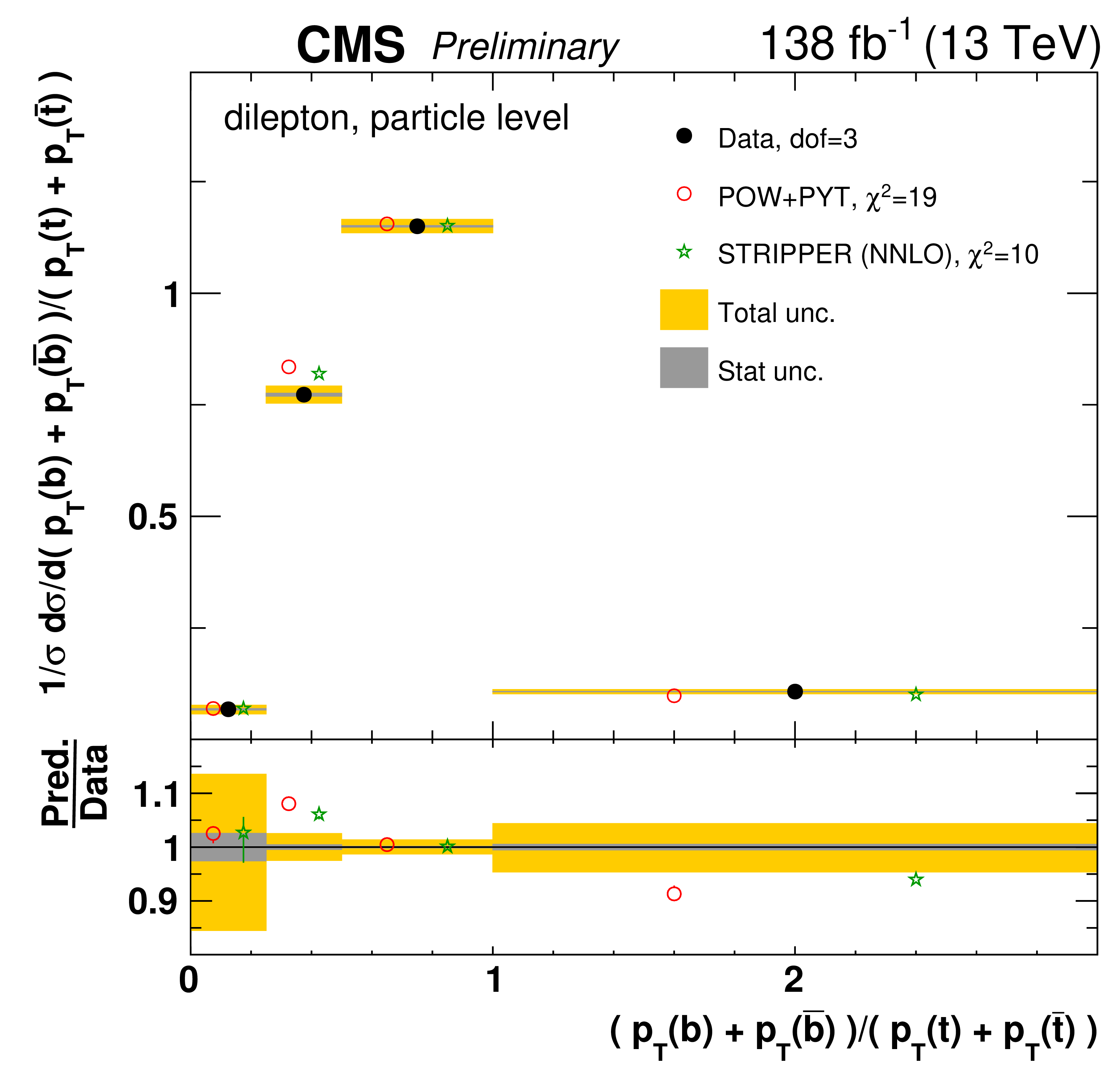
png pdf	Figure 57-c: Normalized differential $\mathrm{t\bar{t}}$ production cross sections as a function of the ${p_{\mathrm {T}}}$ of the leading (upper left) and trailing (upper right) b jet, and $( {{p_{\mathrm {T}}}}(\rm {b})+ {{p_{\mathrm {T}}}}(\mathrm{b\bar{b}}))/( {{p_{\mathrm {T}}}}(\rm {t})+ {{p_{\mathrm {T}}}}(\mathrm{\bar{t}}))$ (lower) are shown for data (filled circles), POWHEG+PYTHIA-8 (`POW-PYT', open circles) simulation, and Stripper NNLO calculation (stars). Further details can be found in the caption of Fig. 56.
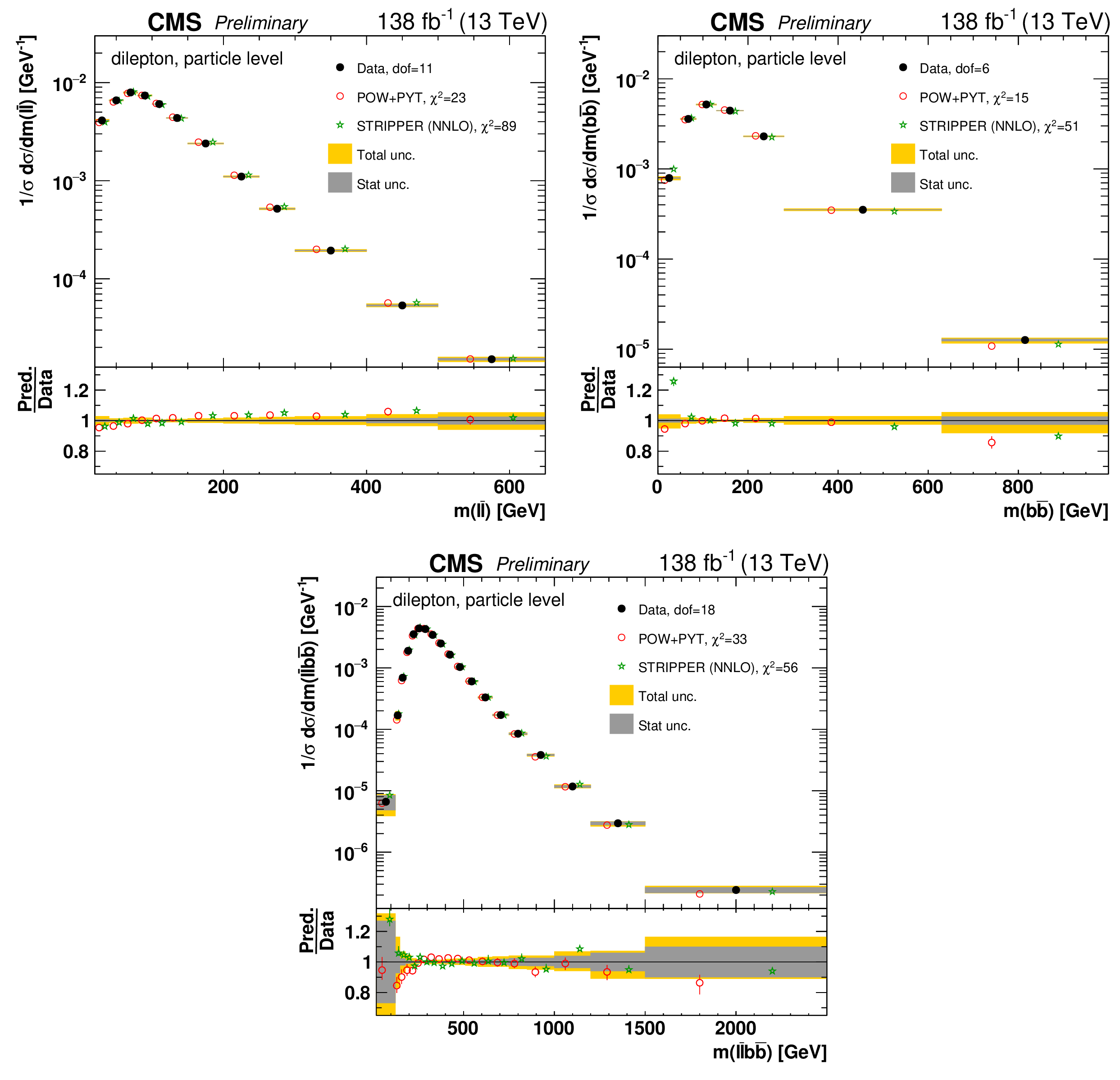
png pdf	Figure 58: Normalized differential $\mathrm{t\bar{t}}$ production cross sections as a function of ${m(\ell \overline {\ell})}$ (upper left), ${m(\mathrm{b} \mathrm{\bar{b}})}$ (upper right), and ${m(\ell \overline {\ell}\mathrm{b} \mathrm{\bar{b}})}$ (lower) are shown for data (filled circles), POWHEG+PYTHIA-8 (`POW-PYT', open circles) simulation, and Stripper NNLO calculation (stars). Further details can be found in the caption of Fig. 56.
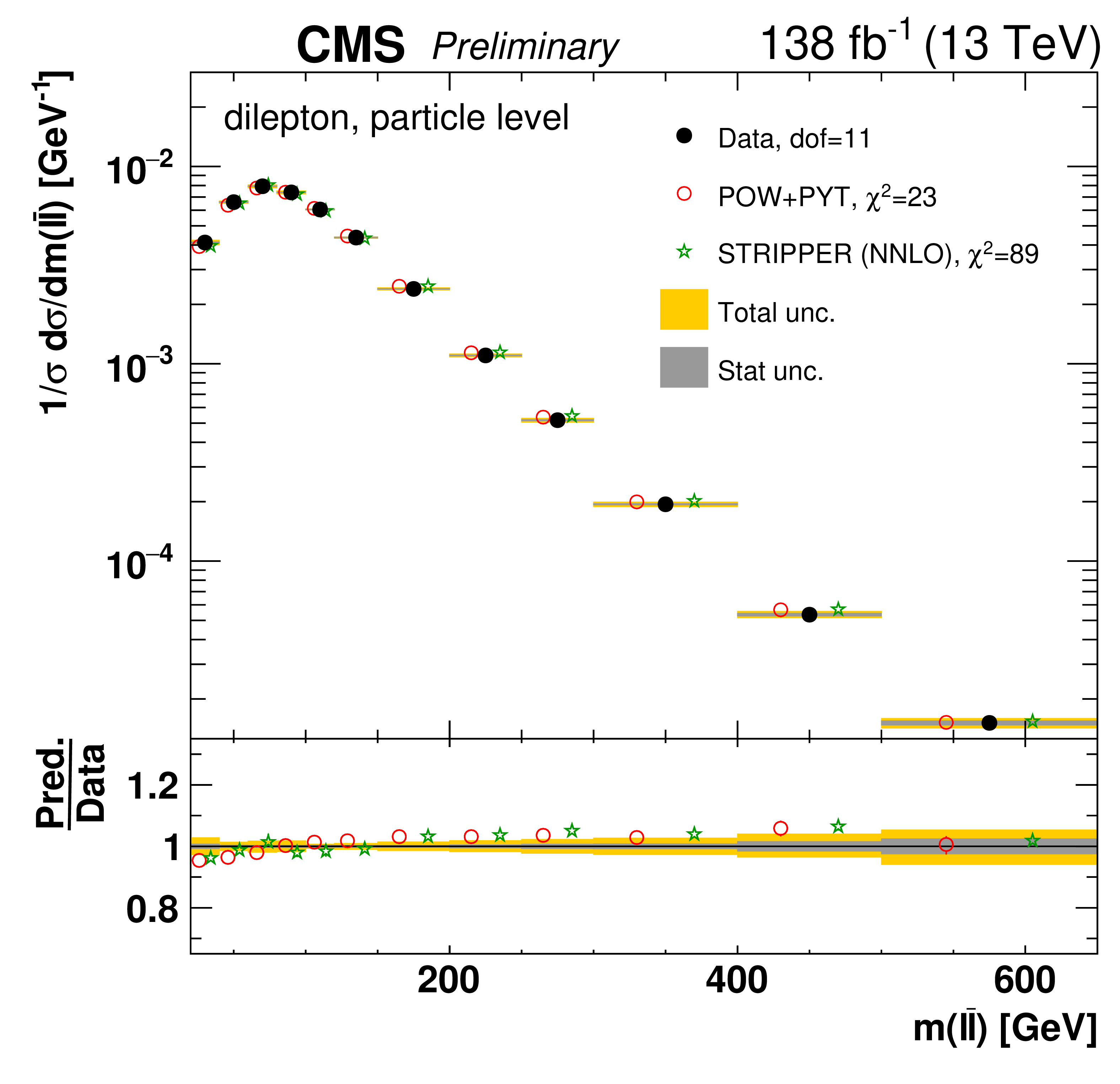
png pdf	Figure 58-a: Normalized differential $\mathrm{t\bar{t}}$ production cross sections as a function of ${m(\ell \overline {\ell})}$ (upper left), ${m(\mathrm{b} \mathrm{\bar{b}})}$ (upper right), and ${m(\ell \overline {\ell}\mathrm{b} \mathrm{\bar{b}})}$ (lower) are shown for data (filled circles), POWHEG+PYTHIA-8 (`POW-PYT', open circles) simulation, and Stripper NNLO calculation (stars). Further details can be found in the caption of Fig. 56.
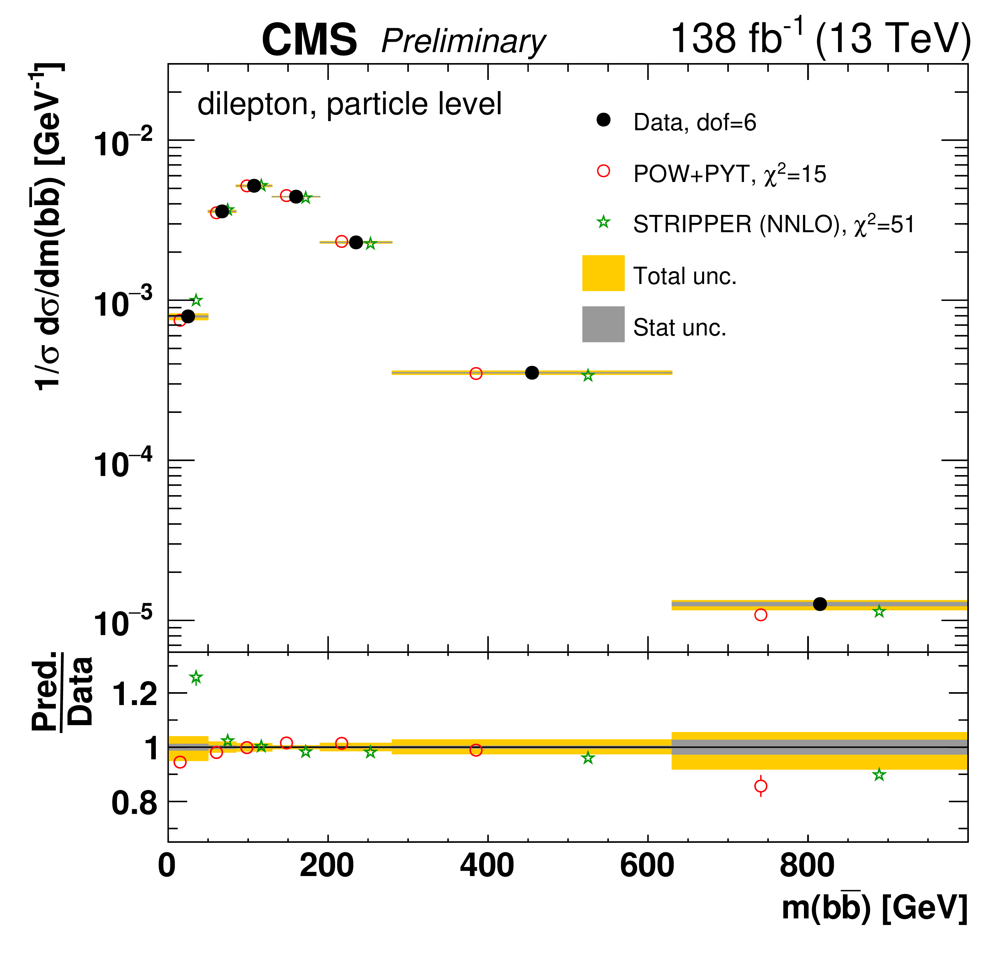
png pdf	Figure 58-b: Normalized differential $\mathrm{t\bar{t}}$ production cross sections as a function of ${m(\ell \overline {\ell})}$ (upper left), ${m(\mathrm{b} \mathrm{\bar{b}})}$ (upper right), and ${m(\ell \overline {\ell}\mathrm{b} \mathrm{\bar{b}})}$ (lower) are shown for data (filled circles), POWHEG+PYTHIA-8 (`POW-PYT', open circles) simulation, and Stripper NNLO calculation (stars). Further details can be found in the caption of Fig. 56.
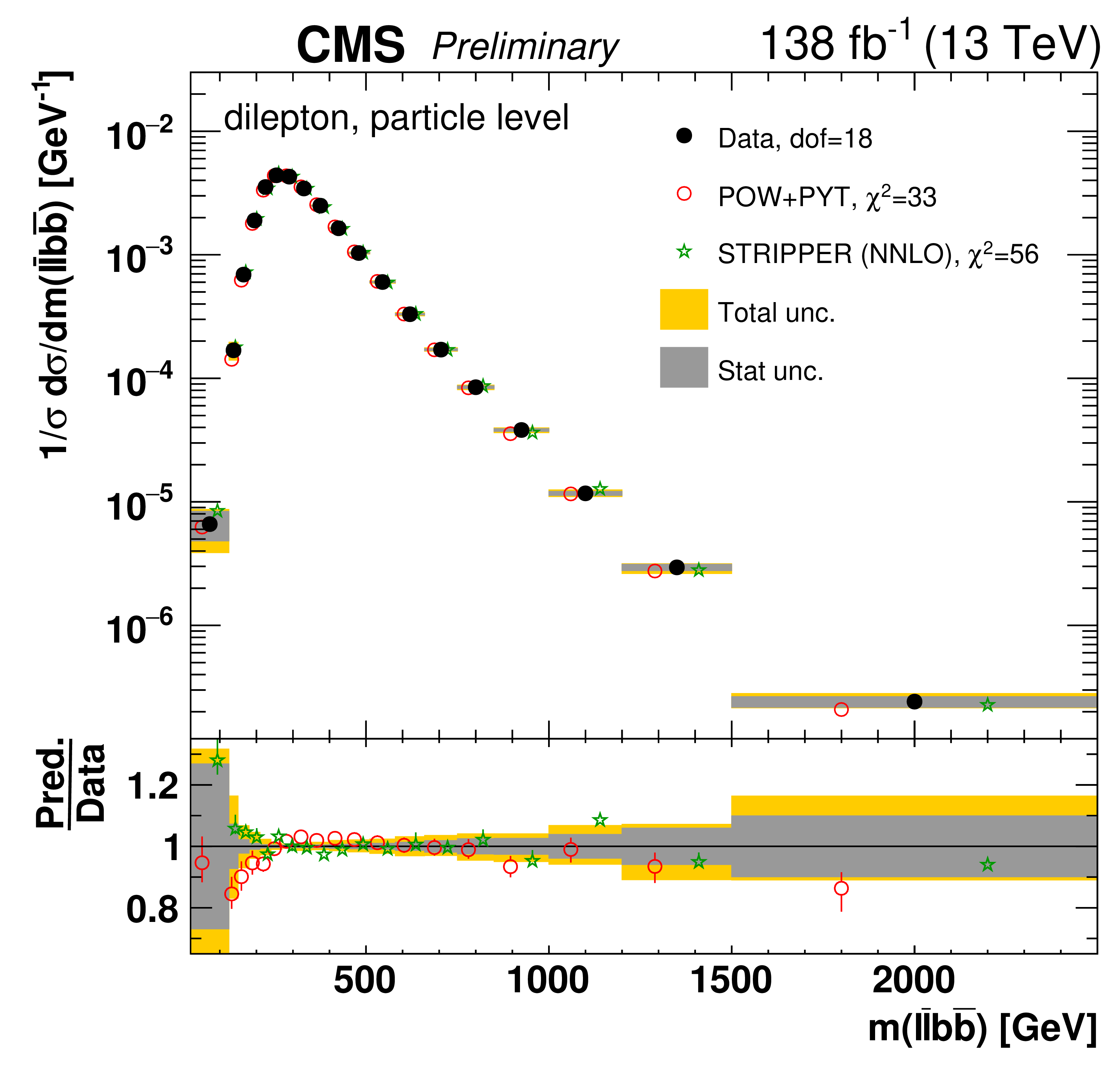
png pdf	Figure 58-c: Normalized differential $\mathrm{t\bar{t}}$ production cross sections as a function of ${m(\ell \overline {\ell})}$ (upper left), ${m(\mathrm{b} \mathrm{\bar{b}})}$ (upper right), and ${m(\ell \overline {\ell}\mathrm{b} \mathrm{\bar{b}})}$ (lower) are shown for data (filled circles), POWHEG+PYTHIA-8 (`POW-PYT', open circles) simulation, and Stripper NNLO calculation (stars). Further details can be found in the caption of Fig. 56.
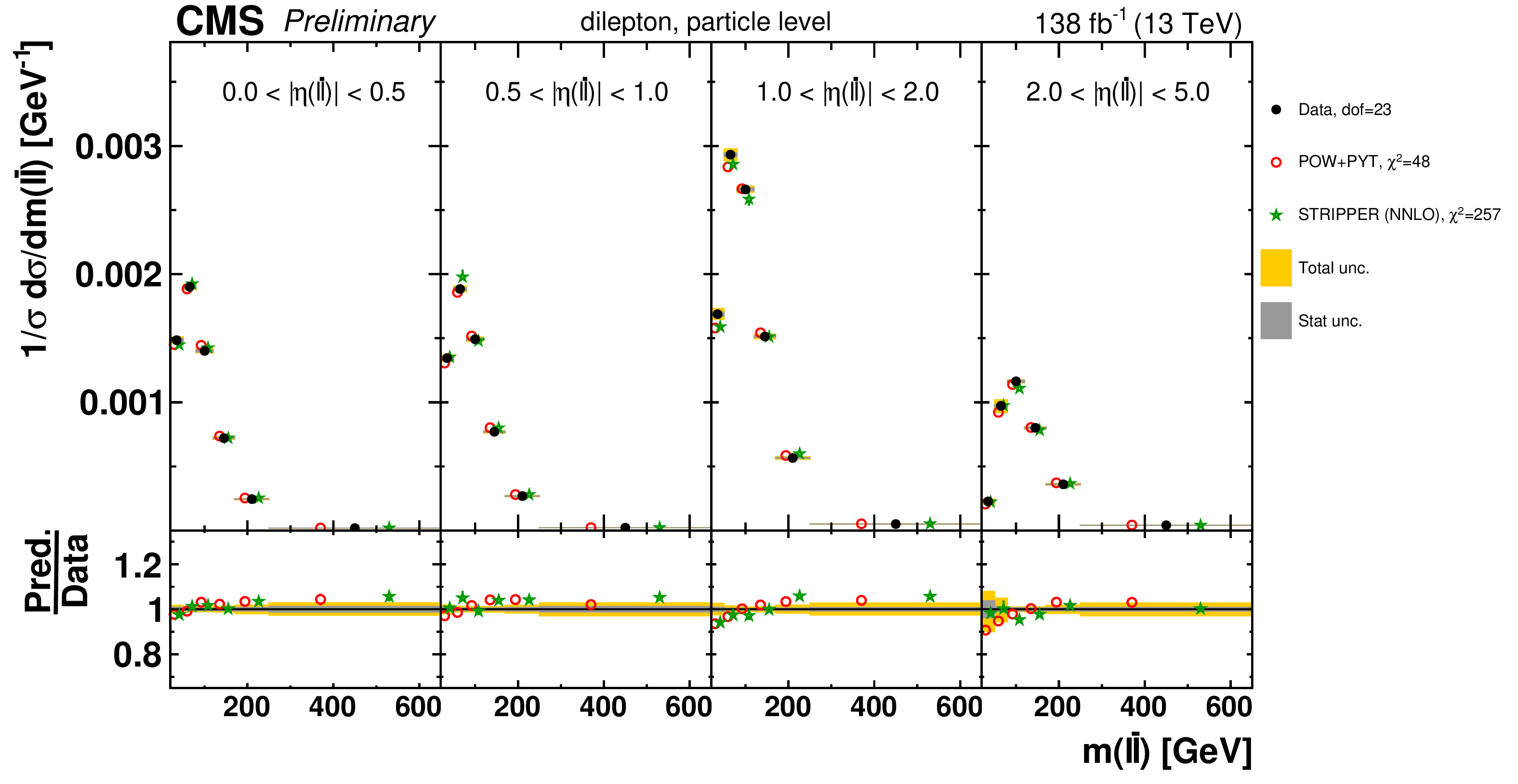
png pdf	Figure 59: Normalized $[ {|\eta (\ell \overline {\ell})|},\,{m(\ell \overline {\ell})} ]$ cross sections are shown for data (filled circles), POWHEG+PYTHIA-8 (`POW-PYT', open circles) simulation, and Stripper NNLO calculation (stars). Further details can be found in the caption of Fig. 56.
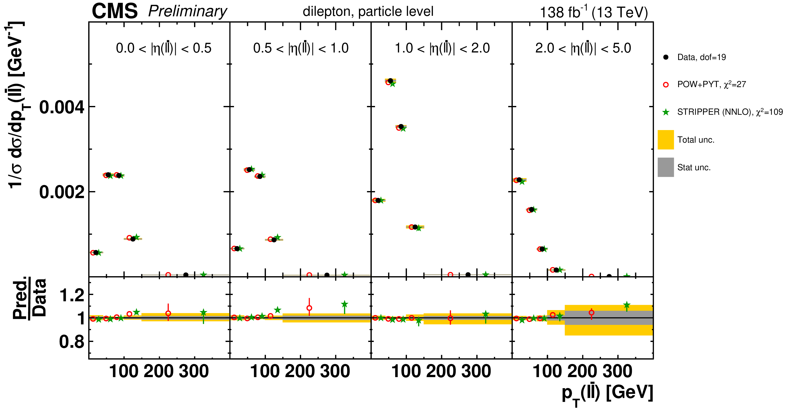
png pdf	Figure 60: Normalized $[ {|\eta (\ell \overline {\ell})|},\,{{p_{\mathrm {T}}} (\ell \overline {\ell})} ]$ cross sections are shown for data (filled circles), POWHEG+PYTHIA-8 (`POW-PYT', open circles) simulation, and Stripper NNLO calculation (stars). Further details can be found in the caption of Fig. 56.
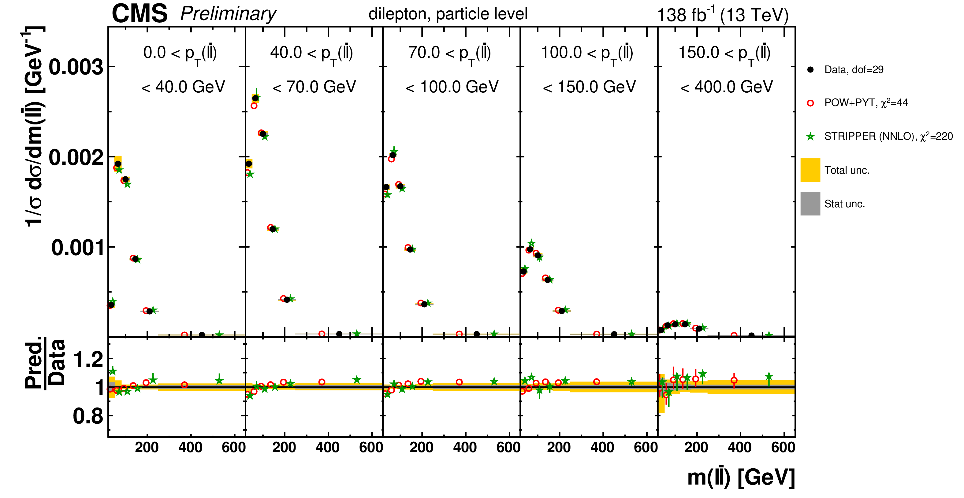
png pdf	Figure 61: Normalized $[ {{p_{\mathrm {T}}} (\ell \overline {\ell})},\,{m(\ell \overline {\ell})} ]$ cross sections are shown for data (filled circles), POWHEG+PYTHIA-8 (`POW-PYT', open circles) simulation, and Stripper NNLO calculation (stars). Further details can be found in the caption of Fig. 56.
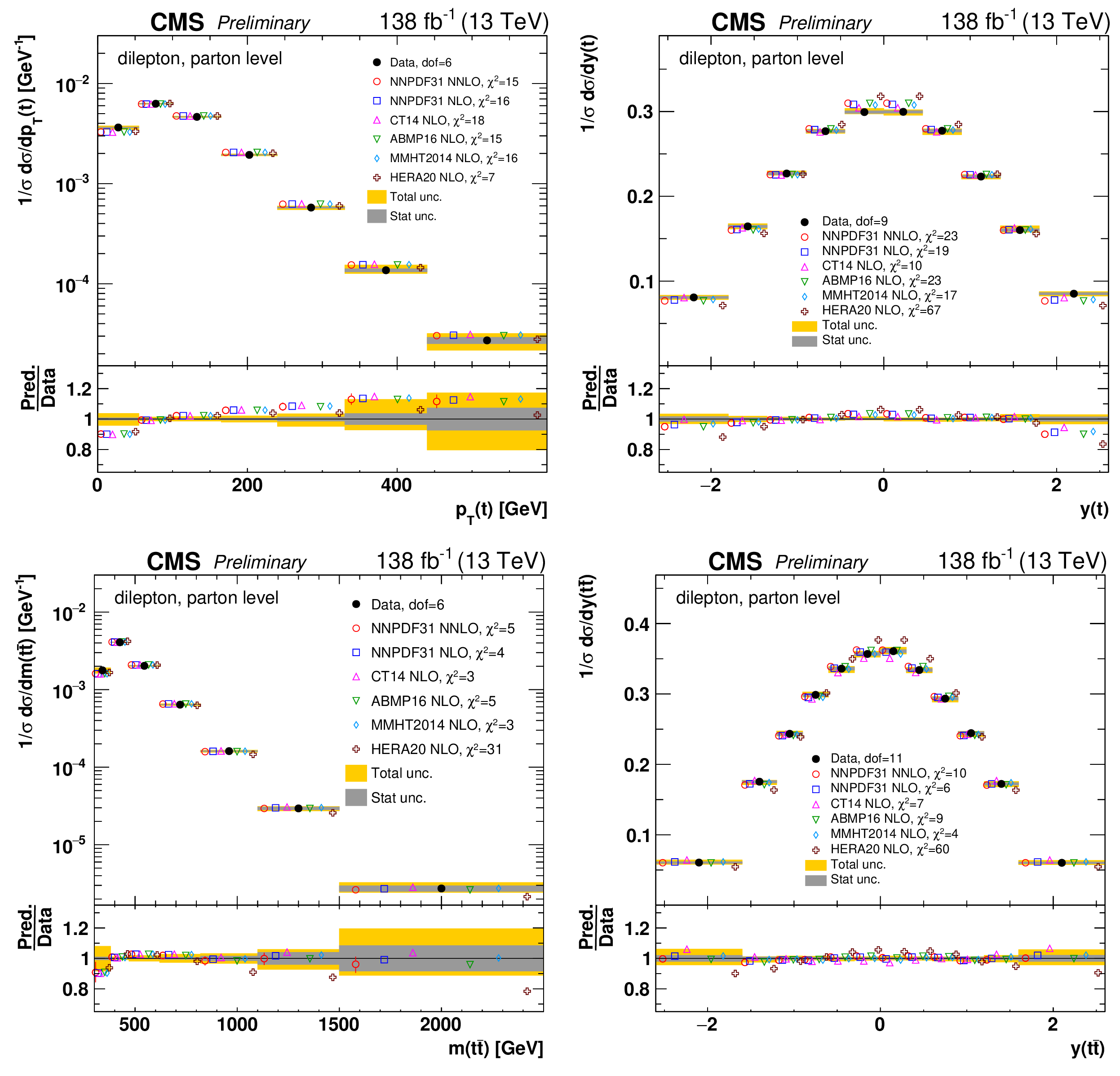
png pdf	Figure 62: Normalized differential $\mathrm{t\bar{t}}$ production cross sections as a function of ${{p_{\mathrm {T}}} (\mathrm{t})}$ (upper left), ${y(\mathrm{t})}$ (upper right), ${m( \mathrm{t\bar{t}})}$ (bottom left), and ${y( \mathrm{t\bar{t}})}$ (bottom right), measured at the parton level in the full phase space. The data are shown as filled circles with dark and light bands indicating the statistical and total uncertainties (statistical and systematic uncertainties summed in quadrature), respectively. The cross sections are compared to predictions from the POWHEG+PYTHIA-8 (`POW-PYT') simulation with various PDF sets. The nominal prediction (open circles) uses the PDF set NNPDF3.1 at NNLO accuracy, assuming a top quark mass value of 172.5 GeV and $\alpha _s = 0.118$. The alternative PDF sets (other points) constitute NNPDF3.1, CT14, ABMP16, MMHT2014, and HERAPDF2.0 at NLO accuracy and assume the same values for the top quark mass and $\alpha _s$ as the nominal NNPDF3.1 NNLO PDF set. The estimated uncertainties in the nominal prediction are represented by a vertical bar on the corresponding points. For each PDF set, a value of ${\chi ^2}$ is reported that takes into account the measurement uncertainties. The lower panel in each plot shows the ratios of the predictions to the data.
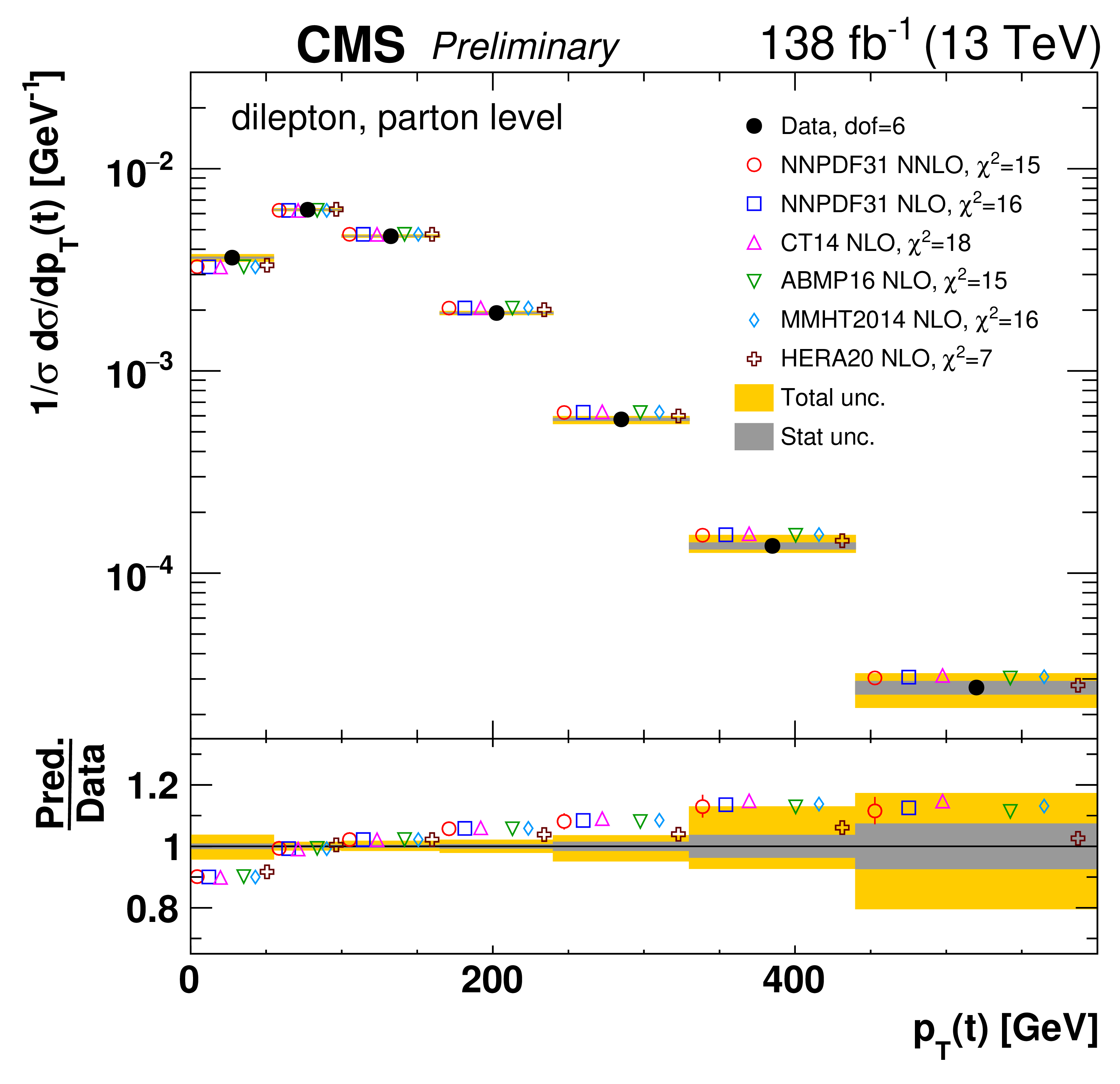
png pdf	Figure 62-a: Normalized differential $\mathrm{t\bar{t}}$ production cross sections as a function of ${{p_{\mathrm {T}}} (\mathrm{t})}$ (upper left), ${y(\mathrm{t})}$ (upper right), ${m( \mathrm{t\bar{t}})}$ (bottom left), and ${y( \mathrm{t\bar{t}})}$ (bottom right), measured at the parton level in the full phase space. The data are shown as filled circles with dark and light bands indicating the statistical and total uncertainties (statistical and systematic uncertainties summed in quadrature), respectively. The cross sections are compared to predictions from the POWHEG+PYTHIA-8 (`POW-PYT') simulation with various PDF sets. The nominal prediction (open circles) uses the PDF set NNPDF3.1 at NNLO accuracy, assuming a top quark mass value of 172.5 GeV and $\alpha _s = 0.118$. The alternative PDF sets (other points) constitute NNPDF3.1, CT14, ABMP16, MMHT2014, and HERAPDF2.0 at NLO accuracy and assume the same values for the top quark mass and $\alpha _s$ as the nominal NNPDF3.1 NNLO PDF set. The estimated uncertainties in the nominal prediction are represented by a vertical bar on the corresponding points. For each PDF set, a value of ${\chi ^2}$ is reported that takes into account the measurement uncertainties. The lower panel in each plot shows the ratios of the predictions to the data.
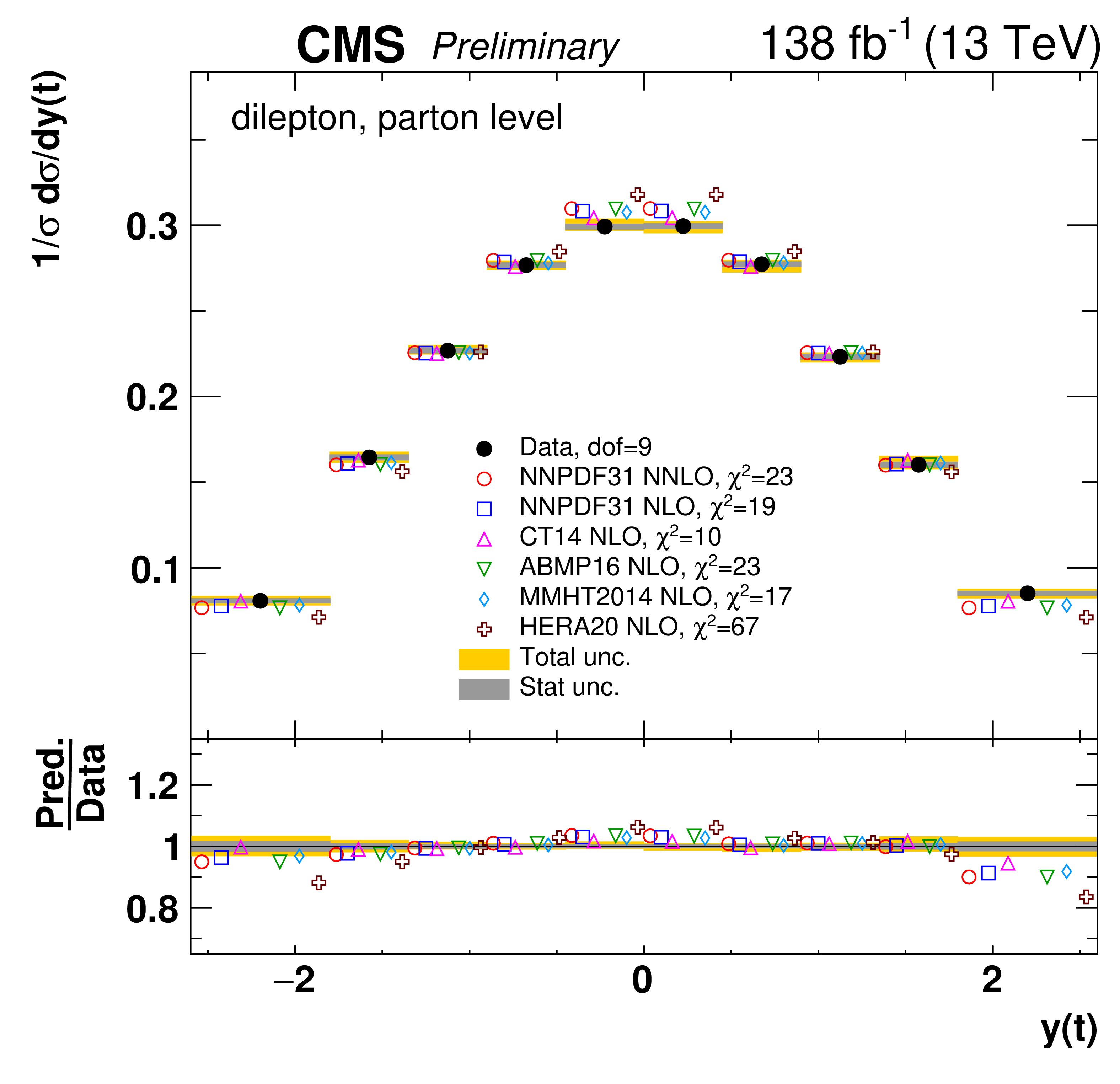
png pdf	Figure 62-b: Normalized differential $\mathrm{t\bar{t}}$ production cross sections as a function of ${{p_{\mathrm {T}}} (\mathrm{t})}$ (upper left), ${y(\mathrm{t})}$ (upper right), ${m( \mathrm{t\bar{t}})}$ (bottom left), and ${y( \mathrm{t\bar{t}})}$ (bottom right), measured at the parton level in the full phase space. The data are shown as filled circles with dark and light bands indicating the statistical and total uncertainties (statistical and systematic uncertainties summed in quadrature), respectively. The cross sections are compared to predictions from the POWHEG+PYTHIA-8 (`POW-PYT') simulation with various PDF sets. The nominal prediction (open circles) uses the PDF set NNPDF3.1 at NNLO accuracy, assuming a top quark mass value of 172.5 GeV and $\alpha _s = 0.118$. The alternative PDF sets (other points) constitute NNPDF3.1, CT14, ABMP16, MMHT2014, and HERAPDF2.0 at NLO accuracy and assume the same values for the top quark mass and $\alpha _s$ as the nominal NNPDF3.1 NNLO PDF set. The estimated uncertainties in the nominal prediction are represented by a vertical bar on the corresponding points. For each PDF set, a value of ${\chi ^2}$ is reported that takes into account the measurement uncertainties. The lower panel in each plot shows the ratios of the predictions to the data.
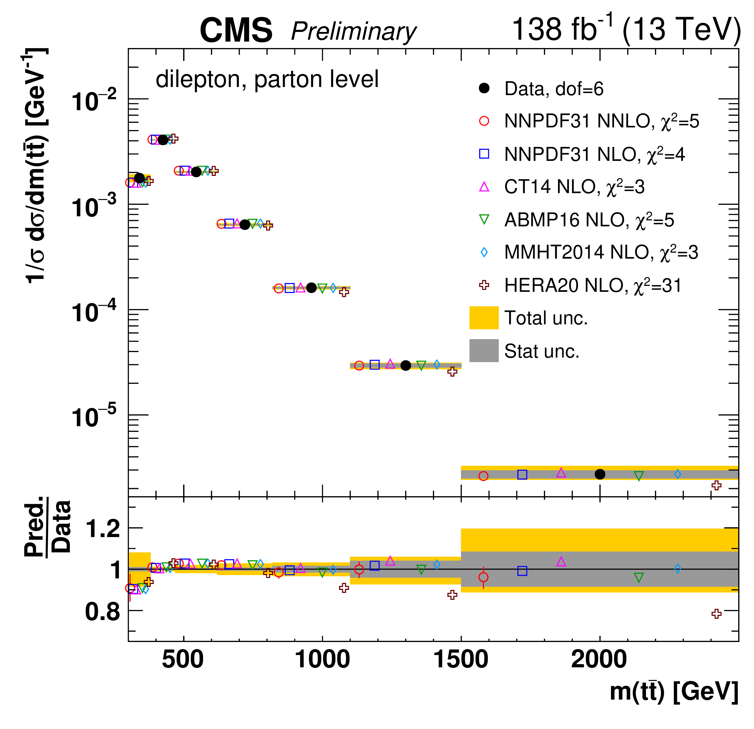
png pdf	Figure 62-c: Normalized differential $\mathrm{t\bar{t}}$ production cross sections as a function of ${{p_{\mathrm {T}}} (\mathrm{t})}$ (upper left), ${y(\mathrm{t})}$ (upper right), ${m( \mathrm{t\bar{t}})}$ (bottom left), and ${y( \mathrm{t\bar{t}})}$ (bottom right), measured at the parton level in the full phase space. The data are shown as filled circles with dark and light bands indicating the statistical and total uncertainties (statistical and systematic uncertainties summed in quadrature), respectively. The cross sections are compared to predictions from the POWHEG+PYTHIA-8 (`POW-PYT') simulation with various PDF sets. The nominal prediction (open circles) uses the PDF set NNPDF3.1 at NNLO accuracy, assuming a top quark mass value of 172.5 GeV and $\alpha _s = 0.118$. The alternative PDF sets (other points) constitute NNPDF3.1, CT14, ABMP16, MMHT2014, and HERAPDF2.0 at NLO accuracy and assume the same values for the top quark mass and $\alpha _s$ as the nominal NNPDF3.1 NNLO PDF set. The estimated uncertainties in the nominal prediction are represented by a vertical bar on the corresponding points. For each PDF set, a value of ${\chi ^2}$ is reported that takes into account the measurement uncertainties. The lower panel in each plot shows the ratios of the predictions to the data.
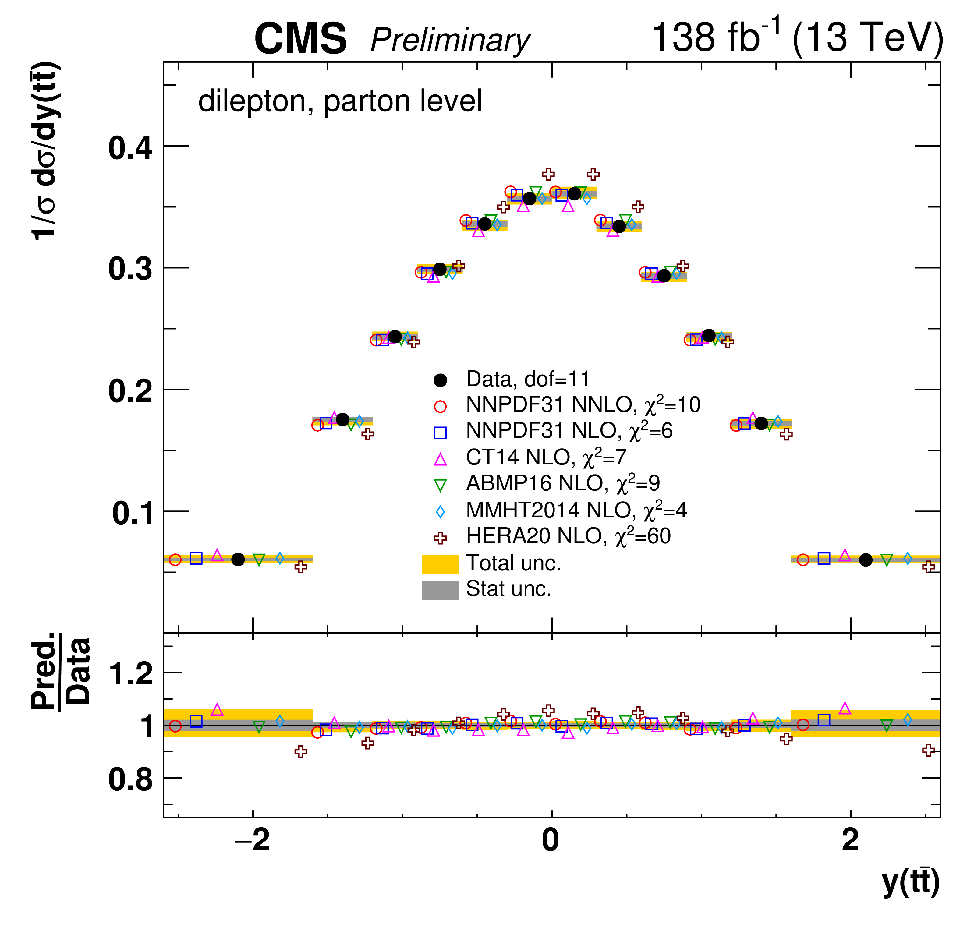
png pdf	Figure 62-d: Normalized differential $\mathrm{t\bar{t}}$ production cross sections as a function of ${{p_{\mathrm {T}}} (\mathrm{t})}$ (upper left), ${y(\mathrm{t})}$ (upper right), ${m( \mathrm{t\bar{t}})}$ (bottom left), and ${y( \mathrm{t\bar{t}})}$ (bottom right), measured at the parton level in the full phase space. The data are shown as filled circles with dark and light bands indicating the statistical and total uncertainties (statistical and systematic uncertainties summed in quadrature), respectively. The cross sections are compared to predictions from the POWHEG+PYTHIA-8 (`POW-PYT') simulation with various PDF sets. The nominal prediction (open circles) uses the PDF set NNPDF3.1 at NNLO accuracy, assuming a top quark mass value of 172.5 GeV and $\alpha _s = 0.118$. The alternative PDF sets (other points) constitute NNPDF3.1, CT14, ABMP16, MMHT2014, and HERAPDF2.0 at NLO accuracy and assume the same values for the top quark mass and $\alpha _s$ as the nominal NNPDF3.1 NNLO PDF set. The estimated uncertainties in the nominal prediction are represented by a vertical bar on the corresponding points. For each PDF set, a value of ${\chi ^2}$ is reported that takes into account the measurement uncertainties. The lower panel in each plot shows the ratios of the predictions to the data.
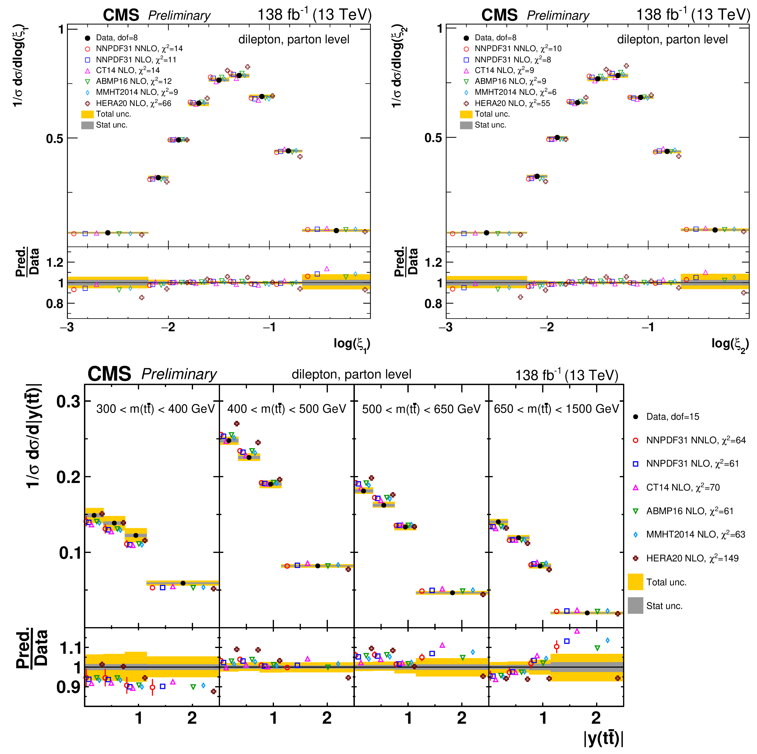
png pdf	Figure 63: Normalized ${\log(\xi _{1})}$ (upper left), ${\log(\xi _{2})}$ (upper right), and $[ {m( \mathrm{t\bar{t}})},\,{|y( \mathrm{t\bar{t}})|} ]$ (bottom) cross sections are shown for data (filled circles) and predictions from the POWHEG+PYTHIA-8 (`POW-PYT') simulation with various PDF sets (other points). Further details can be found in the caption of Fig. 62.
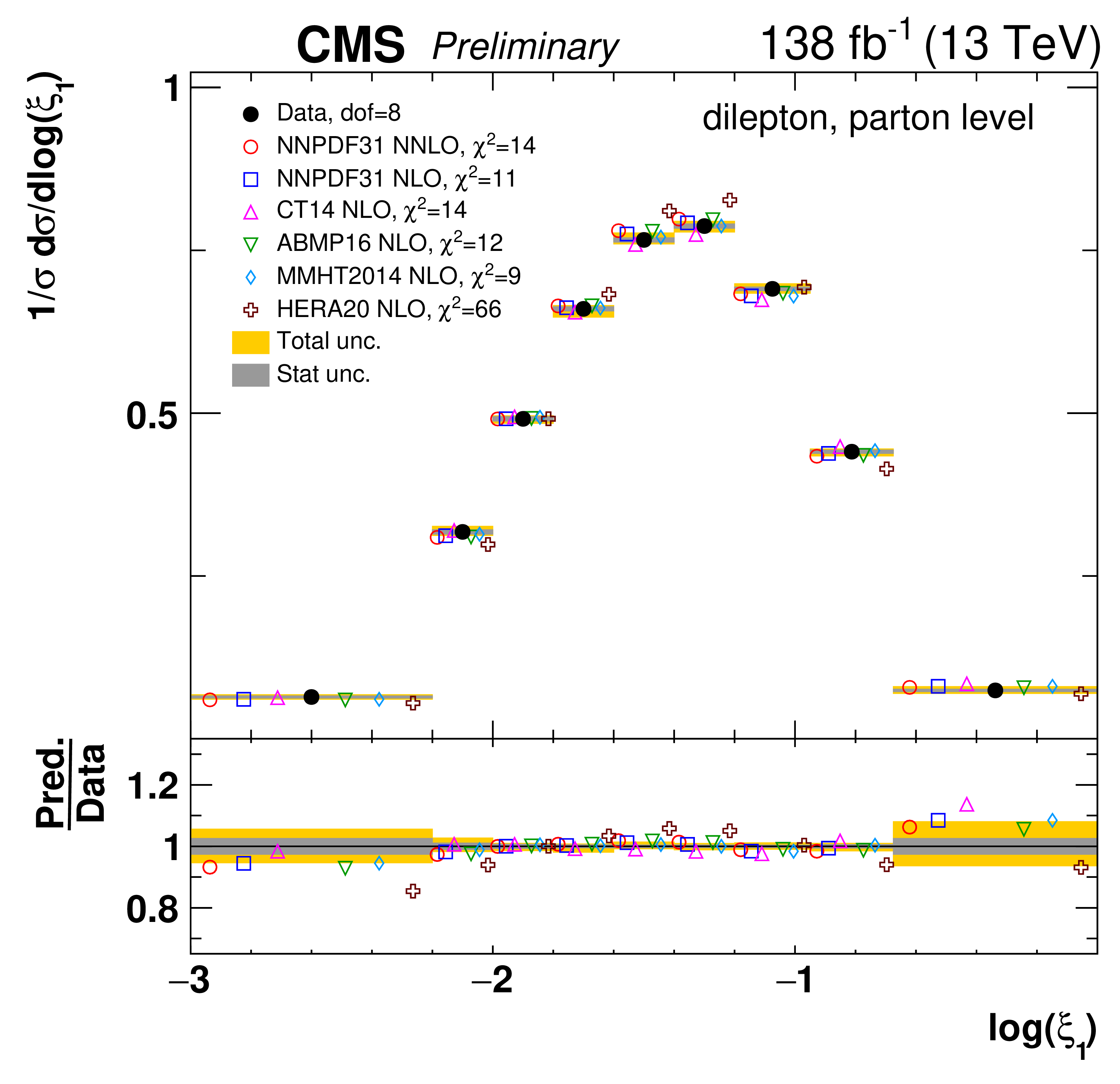
png pdf	Figure 63-a: Normalized ${\log(\xi _{1})}$ (upper left), ${\log(\xi _{2})}$ (upper right), and $[ {m( \mathrm{t\bar{t}})},\,{|y( \mathrm{t\bar{t}})|} ]$ (bottom) cross sections are shown for data (filled circles) and predictions from the POWHEG+PYTHIA-8 (`POW-PYT') simulation with various PDF sets (other points). Further details can be found in the caption of Fig. 62.
png pdf	Figure 63-b: Normalized ${\log(\xi _{1})}$ (upper left), ${\log(\xi _{2})}$ (upper right), and $[ {m( \mathrm{t\bar{t}})},\,{|y( \mathrm{t\bar{t}})|} ]$ (bottom) cross sections are shown for data (filled circles) and predictions from the POWHEG+PYTHIA-8 (`POW-PYT') simulation with various PDF sets (other points). Further details can be found in the caption of Fig. 62.
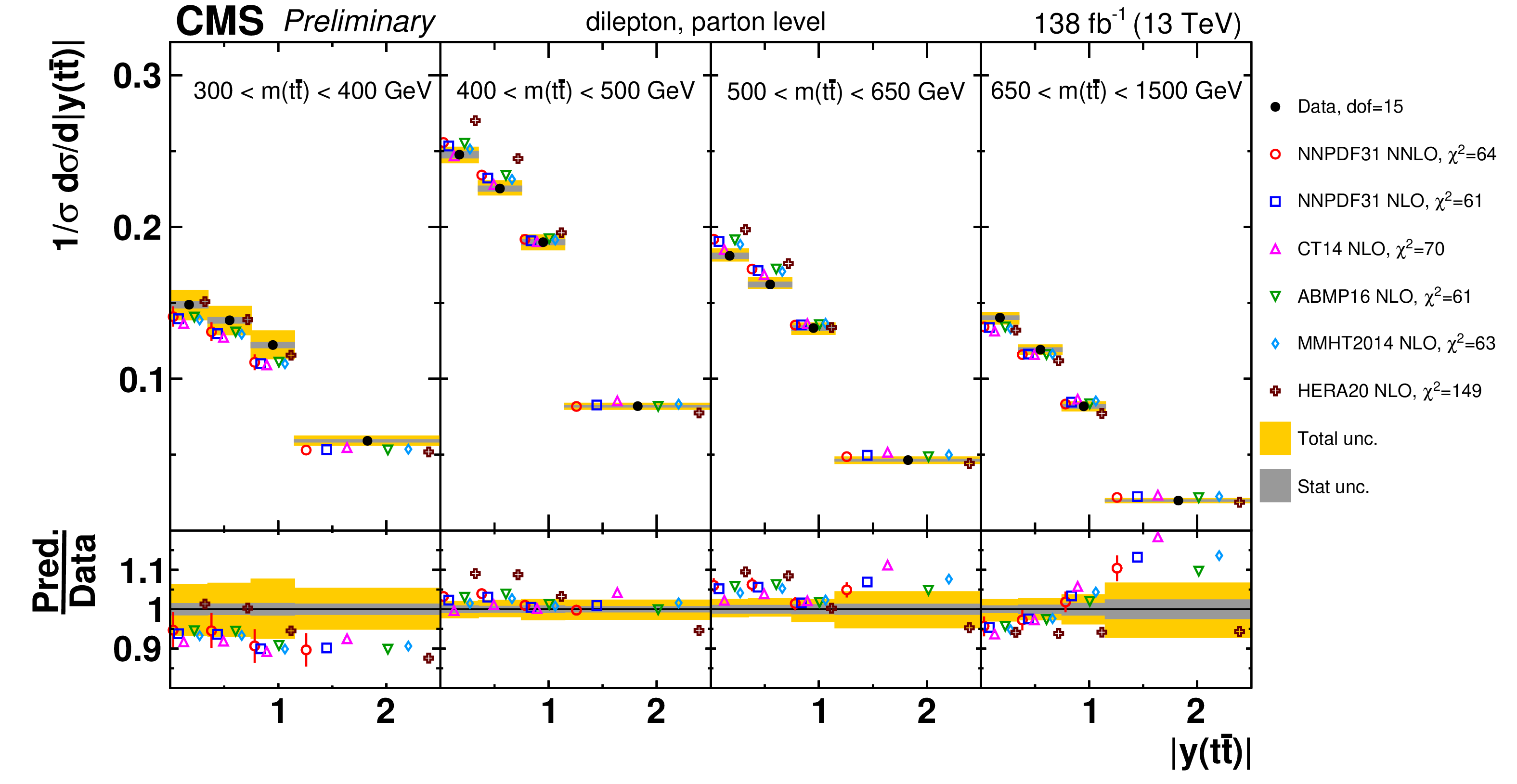
png pdf	Figure 63-c: Normalized ${\log(\xi _{1})}$ (upper left), ${\log(\xi _{2})}$ (upper right), and $[ {m( \mathrm{t\bar{t}})},\,{|y( \mathrm{t\bar{t}})|} ]$ (bottom) cross sections are shown for data (filled circles) and predictions from the POWHEG+PYTHIA-8 (`POW-PYT') simulation with various PDF sets (other points). Further details can be found in the caption of Fig. 62.
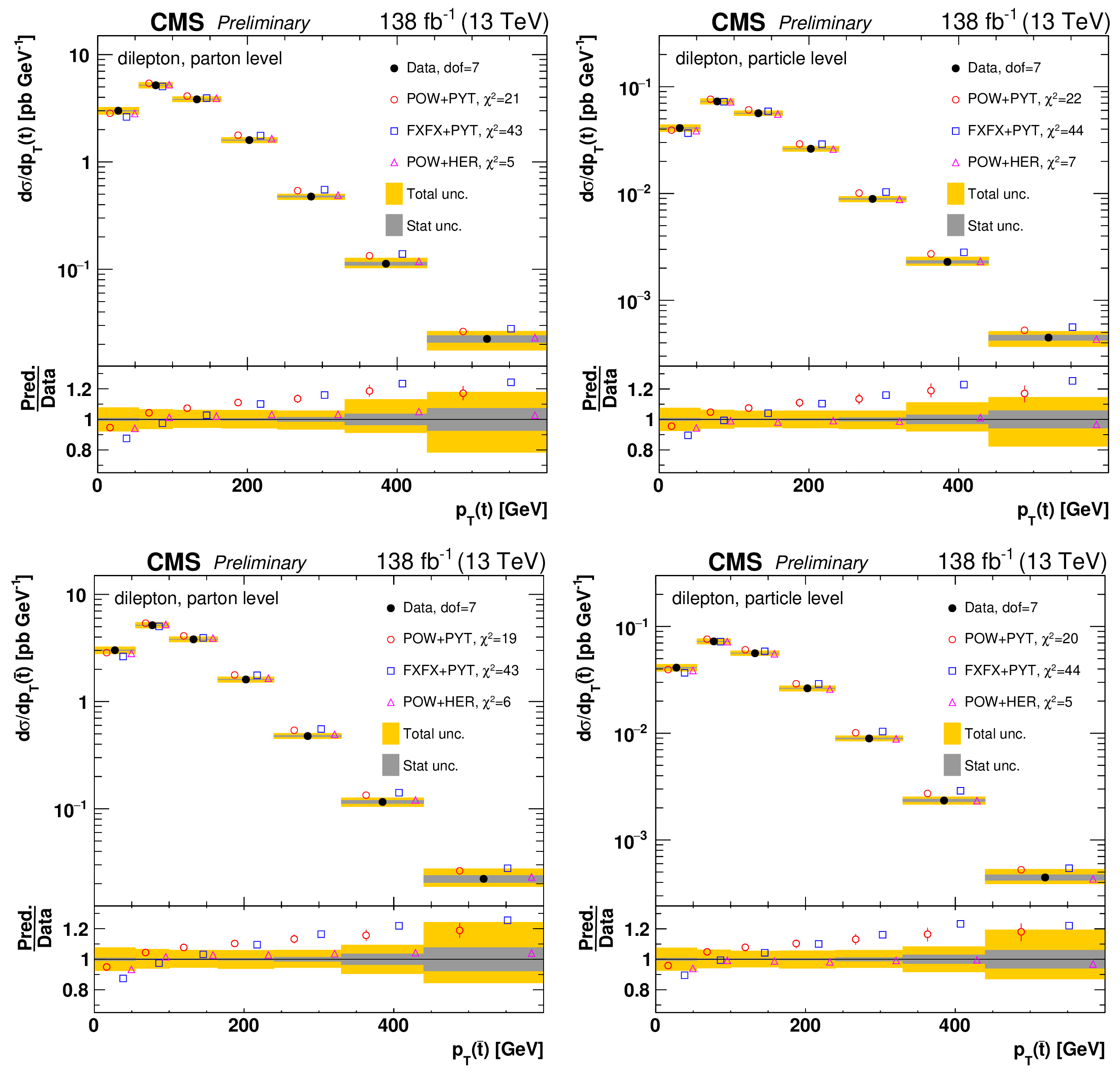
png pdf	Figure 64: Absolute differential $\mathrm{t\bar{t}}$ production cross sections as a function of ${{p_{\mathrm {T}}} (\mathrm{t})}$ (upper) and ${{p_{\mathrm {T}}} (\mathrm{\bar{t}})}$ (lower), measured at the parton level in the full phase space (left) and at the particle level in a fiducial phase space (right). The data are shown as filled circles with dark and light bands indicating the statistical and total uncertainties (statistical and systematic uncertainties summed in quadrature), respectively. The cross sections are compared to various MC predictions (other points). The estimated uncertainties in the POWHEG+PYTHIA-8 (`POW-PYT') simulation are represented by a vertical bar on the corresponding points. For each MC model, a value of ${\chi ^2}$ is reported that takes into account the measurement uncertainties. The lower panel in each plot shows the ratios of the predictions to the data.
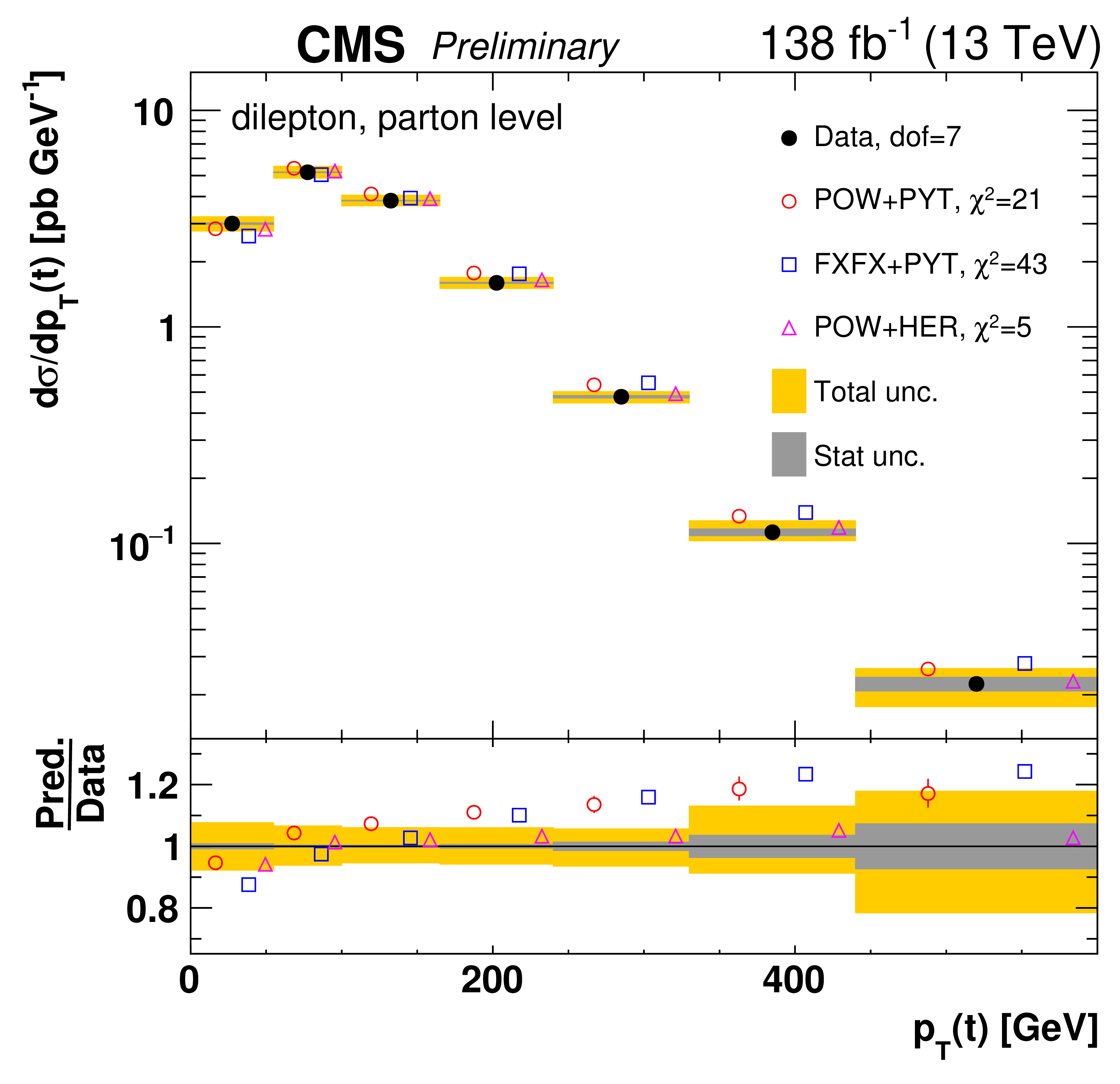
png pdf	Figure 64-a: Absolute differential $\mathrm{t\bar{t}}$ production cross sections as a function of ${{p_{\mathrm {T}}} (\mathrm{t})}$ (upper) and ${{p_{\mathrm {T}}} (\mathrm{\bar{t}})}$ (lower), measured at the parton level in the full phase space (left) and at the particle level in a fiducial phase space (right). The data are shown as filled circles with dark and light bands indicating the statistical and total uncertainties (statistical and systematic uncertainties summed in quadrature), respectively. The cross sections are compared to various MC predictions (other points). The estimated uncertainties in the POWHEG+PYTHIA-8 (`POW-PYT') simulation are represented by a vertical bar on the corresponding points. For each MC model, a value of ${\chi ^2}$ is reported that takes into account the measurement uncertainties. The lower panel in each plot shows the ratios of the predictions to the data.
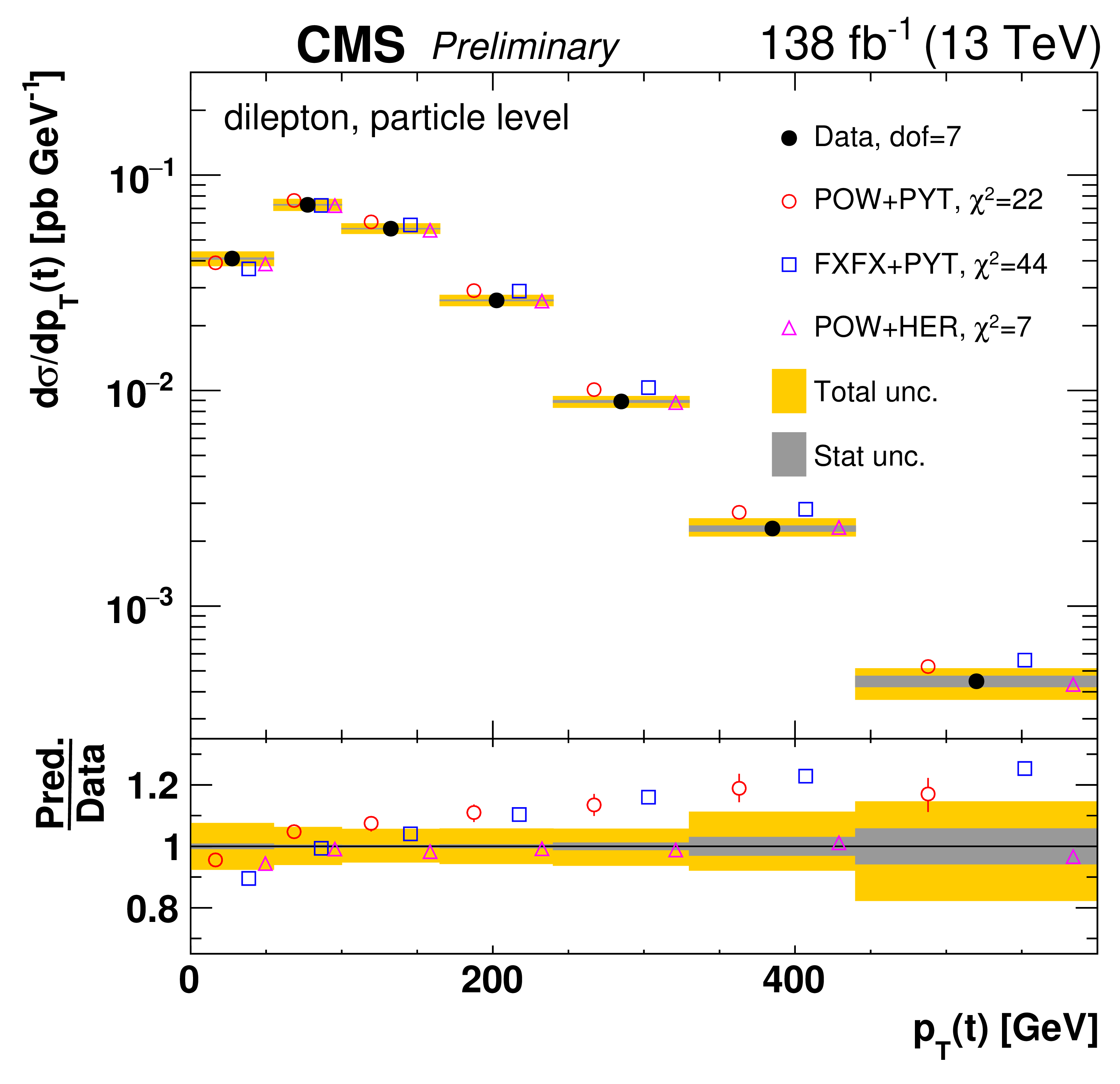
png pdf	Figure 64-b: Absolute differential $\mathrm{t\bar{t}}$ production cross sections as a function of ${{p_{\mathrm {T}}} (\mathrm{t})}$ (upper) and ${{p_{\mathrm {T}}} (\mathrm{\bar{t}})}$ (lower), measured at the parton level in the full phase space (left) and at the particle level in a fiducial phase space (right). The data are shown as filled circles with dark and light bands indicating the statistical and total uncertainties (statistical and systematic uncertainties summed in quadrature), respectively. The cross sections are compared to various MC predictions (other points). The estimated uncertainties in the POWHEG+PYTHIA-8 (`POW-PYT') simulation are represented by a vertical bar on the corresponding points. For each MC model, a value of ${\chi ^2}$ is reported that takes into account the measurement uncertainties. The lower panel in each plot shows the ratios of the predictions to the data.
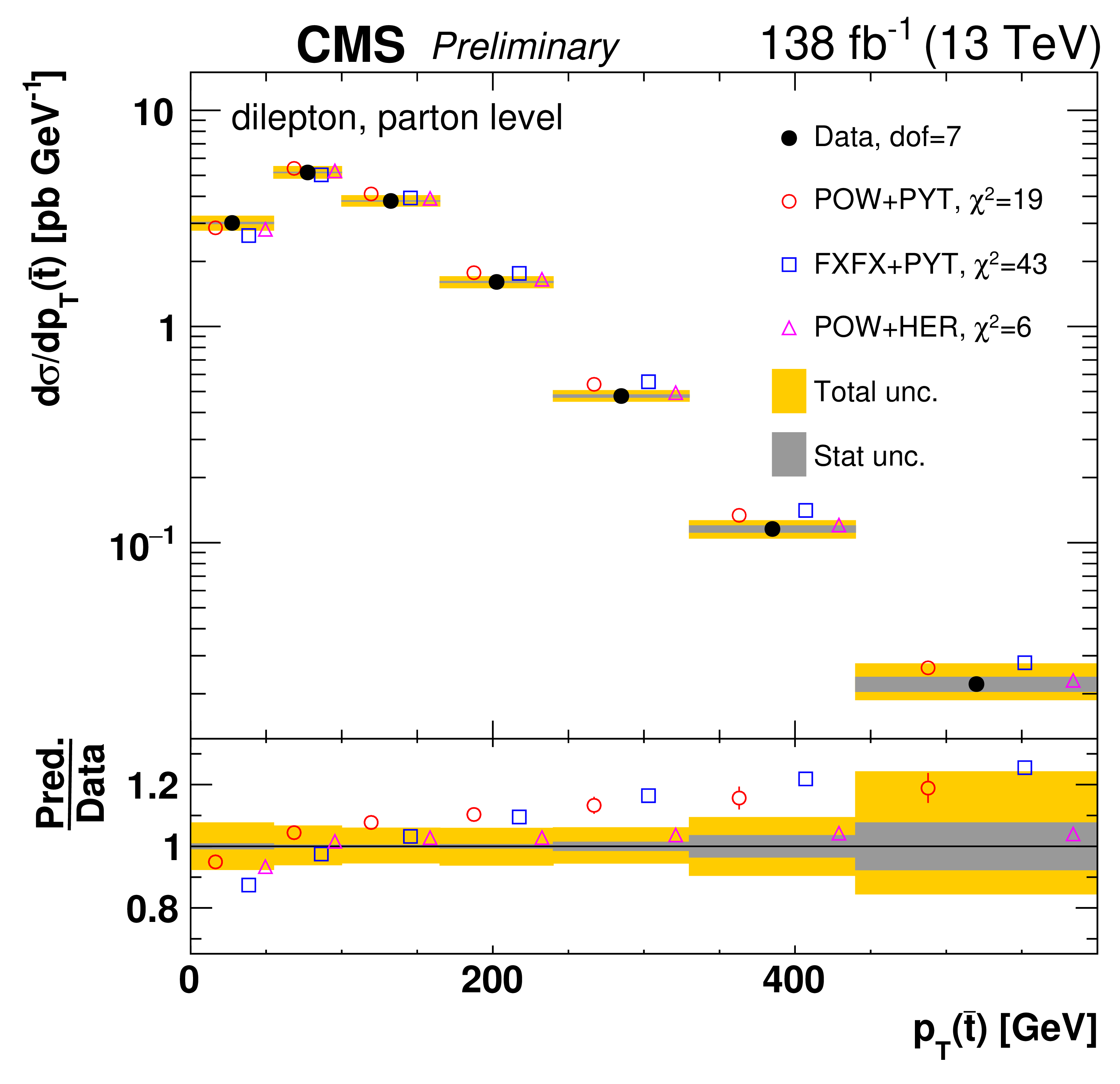
png pdf	Figure 64-c: Absolute differential $\mathrm{t\bar{t}}$ production cross sections as a function of ${{p_{\mathrm {T}}} (\mathrm{t})}$ (upper) and ${{p_{\mathrm {T}}} (\mathrm{\bar{t}})}$ (lower), measured at the parton level in the full phase space (left) and at the particle level in a fiducial phase space (right). The data are shown as filled circles with dark and light bands indicating the statistical and total uncertainties (statistical and systematic uncertainties summed in quadrature), respectively. The cross sections are compared to various MC predictions (other points). The estimated uncertainties in the POWHEG+PYTHIA-8 (`POW-PYT') simulation are represented by a vertical bar on the corresponding points. For each MC model, a value of ${\chi ^2}$ is reported that takes into account the measurement uncertainties. The lower panel in each plot shows the ratios of the predictions to the data.
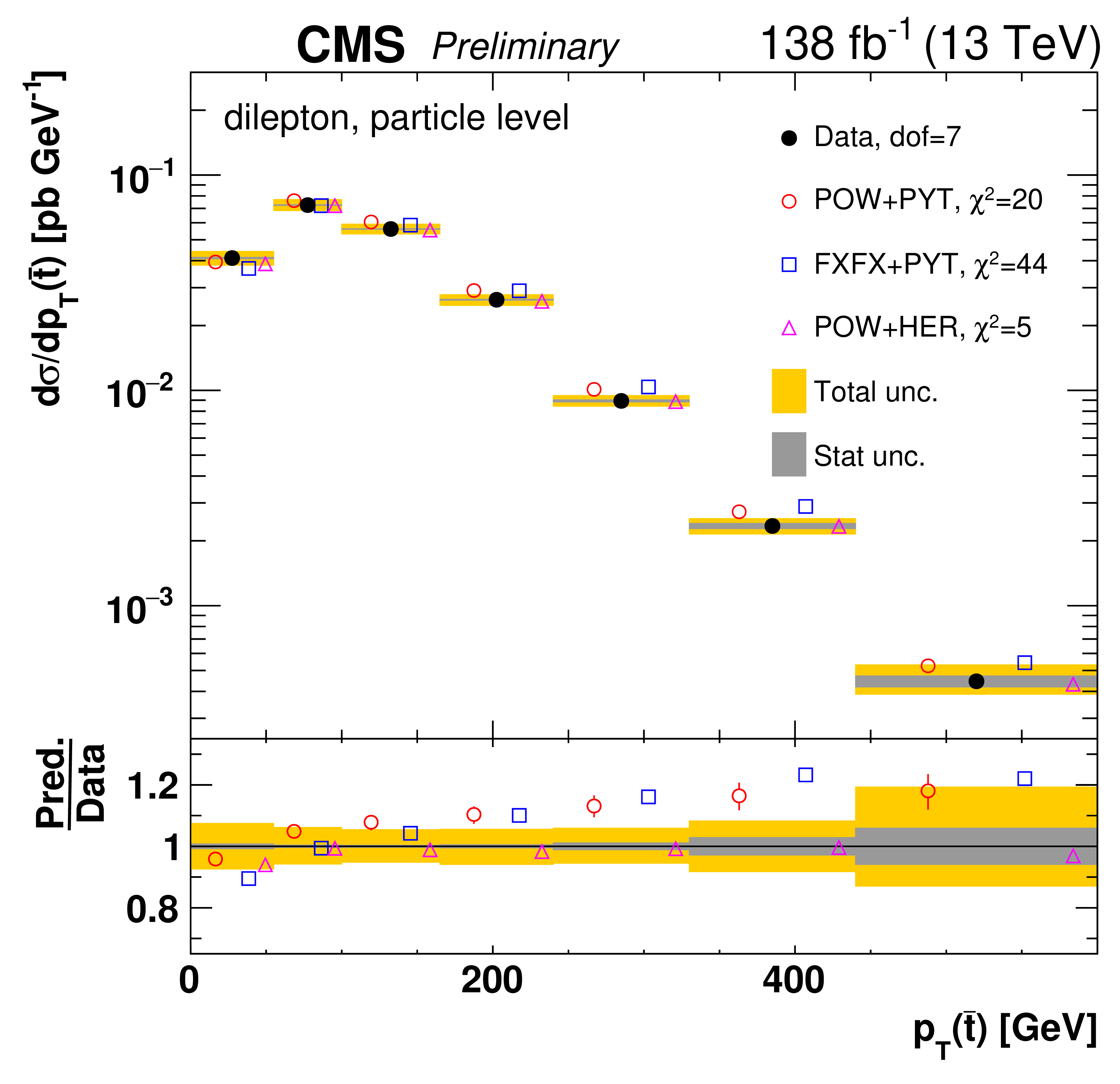
png pdf	Figure 64-d: Absolute differential $\mathrm{t\bar{t}}$ production cross sections as a function of ${{p_{\mathrm {T}}} (\mathrm{t})}$ (upper) and ${{p_{\mathrm {T}}} (\mathrm{\bar{t}})}$ (lower), measured at the parton level in the full phase space (left) and at the particle level in a fiducial phase space (right). The data are shown as filled circles with dark and light bands indicating the statistical and total uncertainties (statistical and systematic uncertainties summed in quadrature), respectively. The cross sections are compared to various MC predictions (other points). The estimated uncertainties in the POWHEG+PYTHIA-8 (`POW-PYT') simulation are represented by a vertical bar on the corresponding points. For each MC model, a value of ${\chi ^2}$ is reported that takes into account the measurement uncertainties. The lower panel in each plot shows the ratios of the predictions to the data.
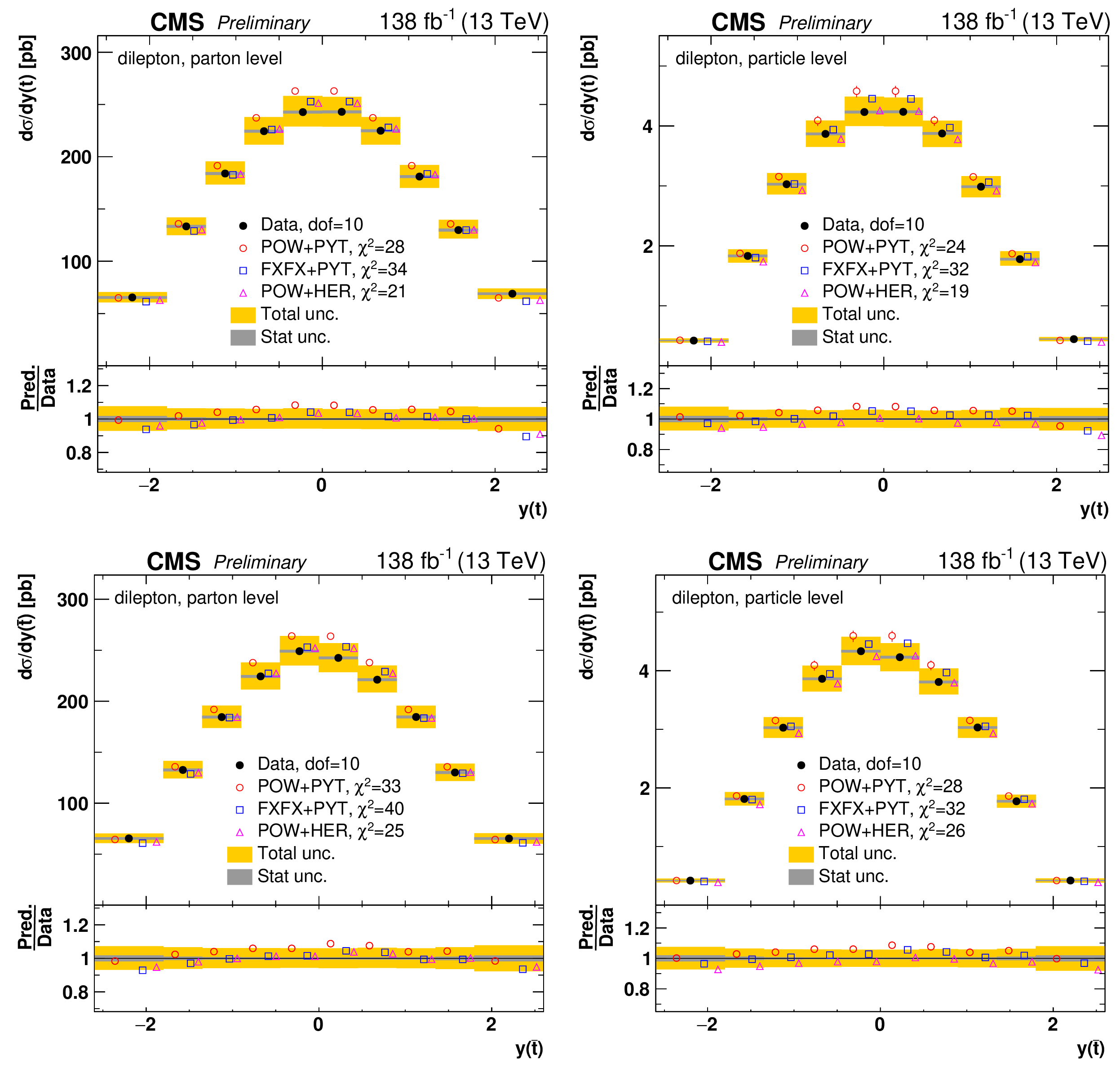
png pdf	Figure 65: Absolute differential $\mathrm{t\bar{t}}$ production cross sections as a function of ${y(\mathrm{t})}$ (upper) and ${y(\mathrm{\bar{t}})}$ (lower) are shown for data (filled circles) and various MC predictions (other points). Further details can be found in the caption of Fig. 64.
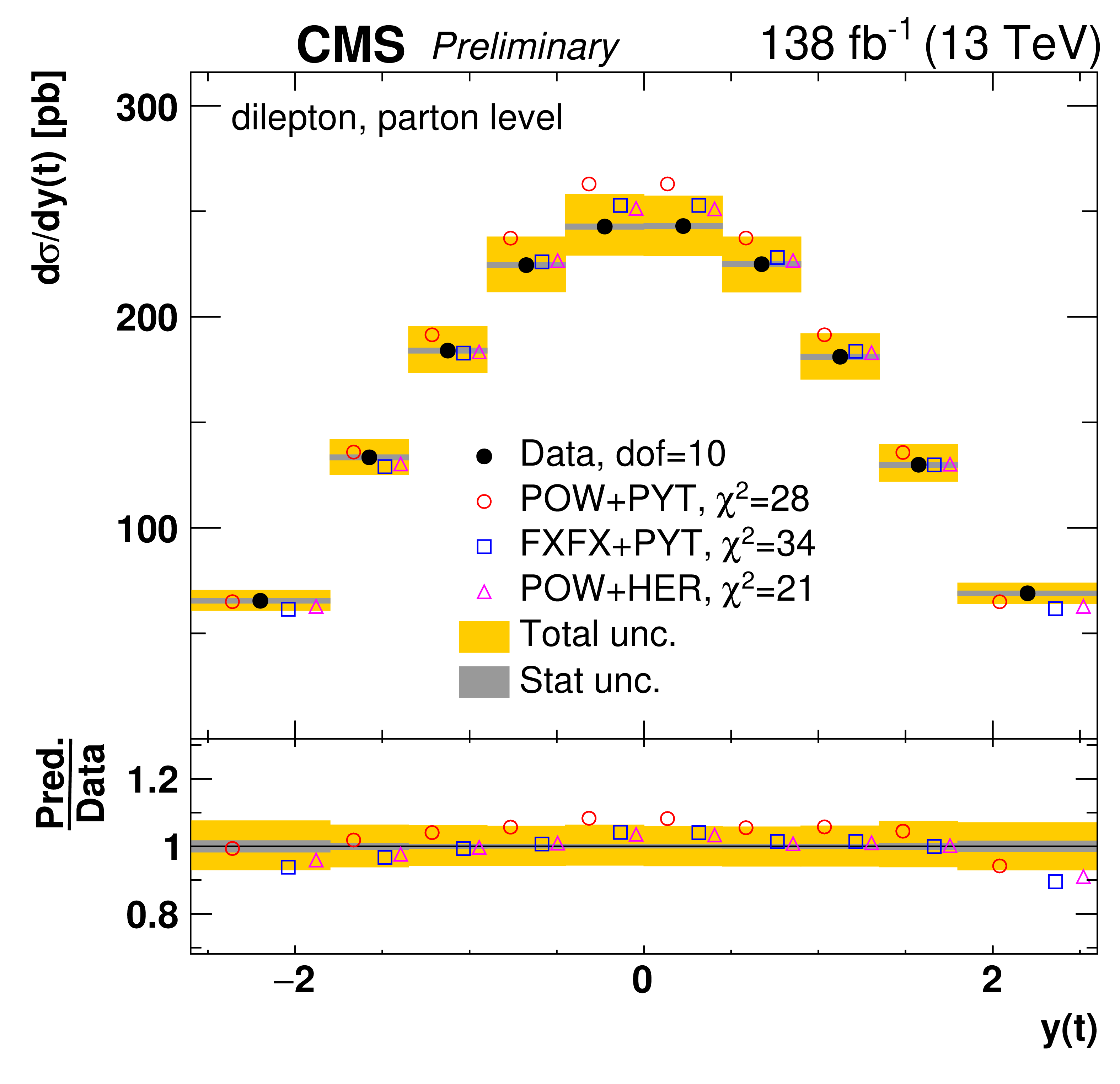
png pdf	Figure 65-a: Absolute differential $\mathrm{t\bar{t}}$ production cross sections as a function of ${y(\mathrm{t})}$ (upper) and ${y(\mathrm{\bar{t}})}$ (lower) are shown for data (filled circles) and various MC predictions (other points). Further details can be found in the caption of Fig. 64.
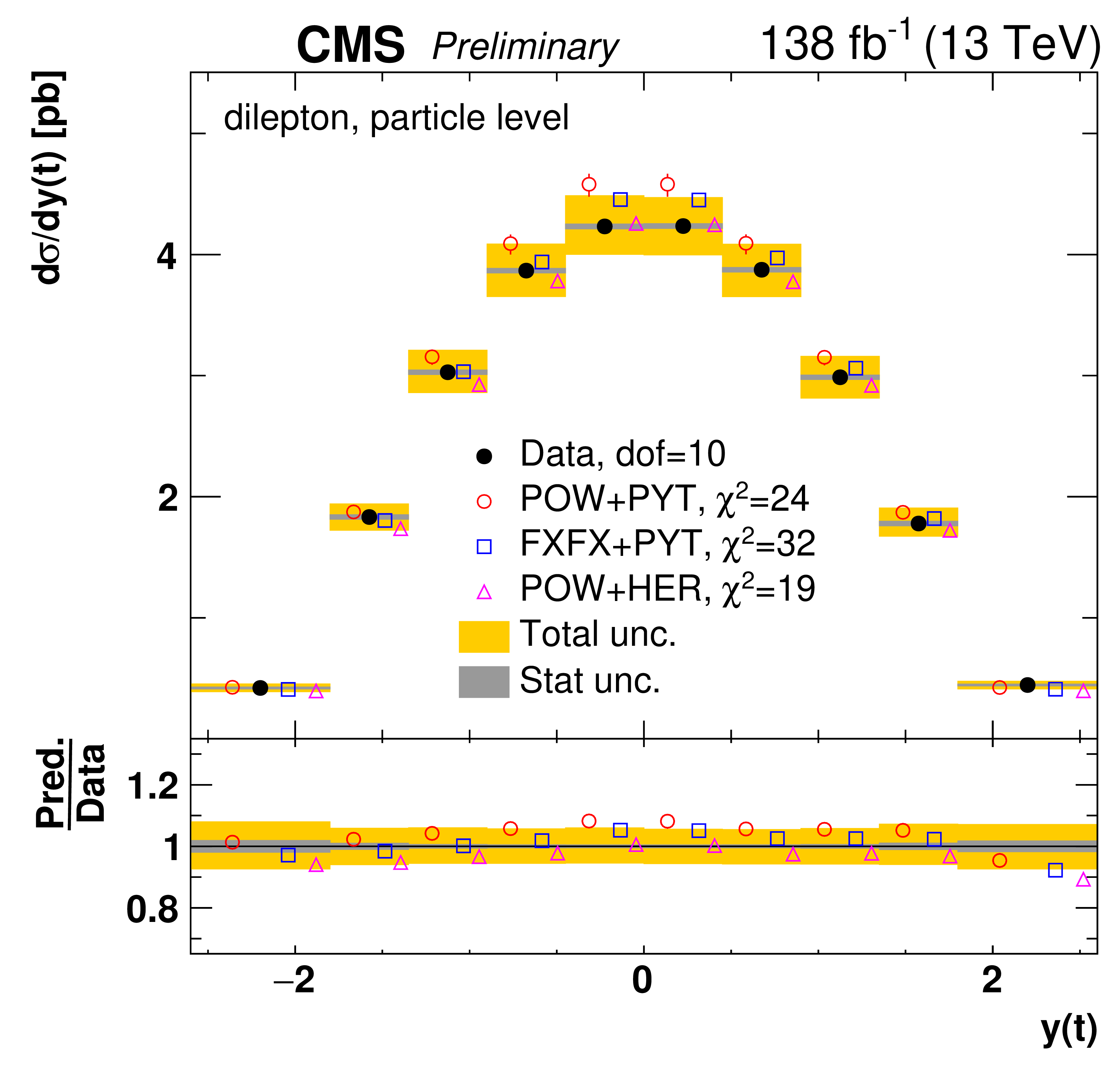
png pdf	Figure 65-b: Absolute differential $\mathrm{t\bar{t}}$ production cross sections as a function of ${y(\mathrm{t})}$ (upper) and ${y(\mathrm{\bar{t}})}$ (lower) are shown for data (filled circles) and various MC predictions (other points). Further details can be found in the caption of Fig. 64.
png pdf	Figure 65-c: Absolute differential $\mathrm{t\bar{t}}$ production cross sections as a function of ${y(\mathrm{t})}$ (upper) and ${y(\mathrm{\bar{t}})}$ (lower) are shown for data (filled circles) and various MC predictions (other points). Further details can be found in the caption of Fig. 64.
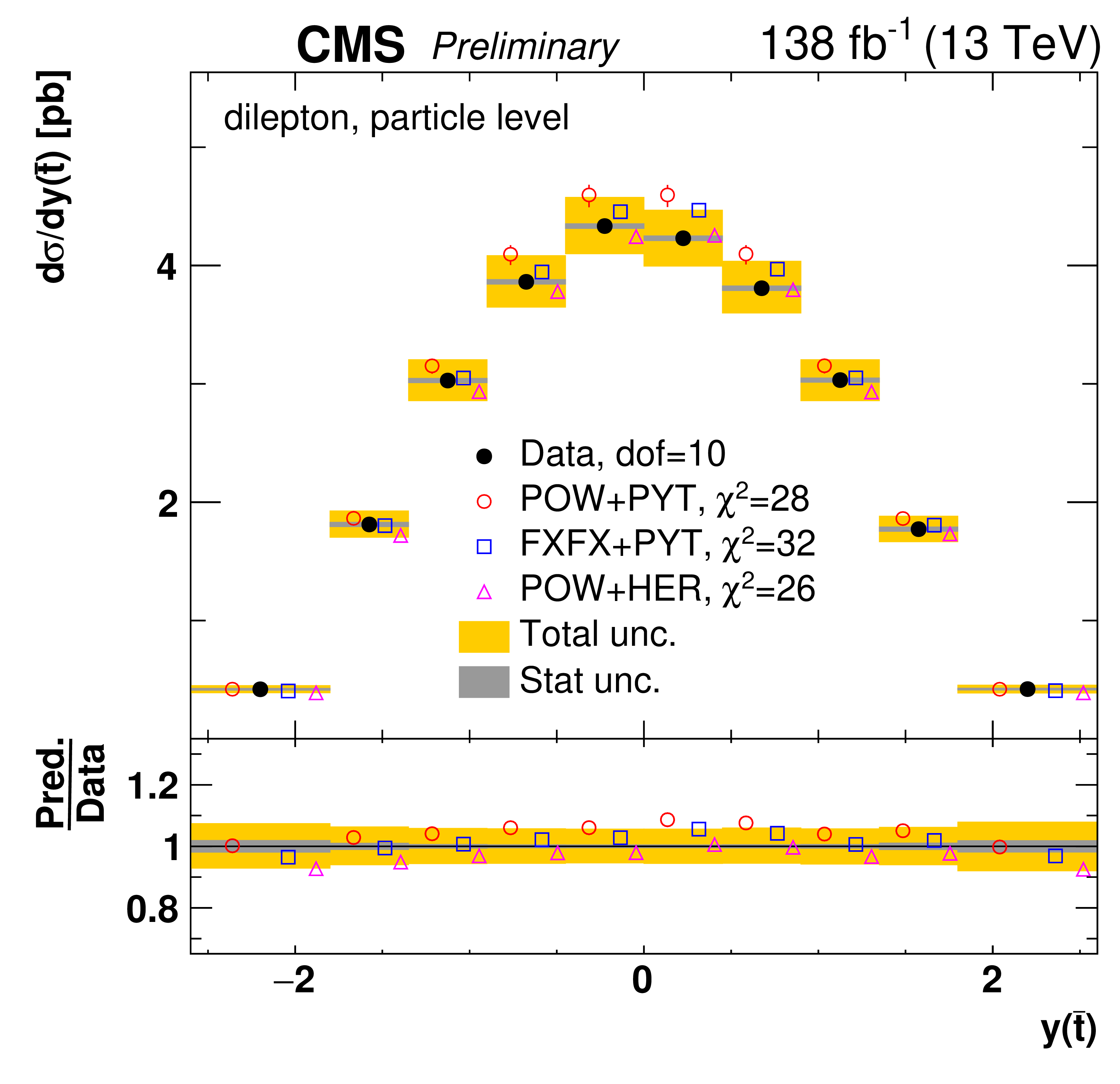
png pdf	Figure 65-d: Absolute differential $\mathrm{t\bar{t}}$ production cross sections as a function of ${y(\mathrm{t})}$ (upper) and ${y(\mathrm{\bar{t}})}$ (lower) are shown for data (filled circles) and various MC predictions (other points). Further details can be found in the caption of Fig. 64.
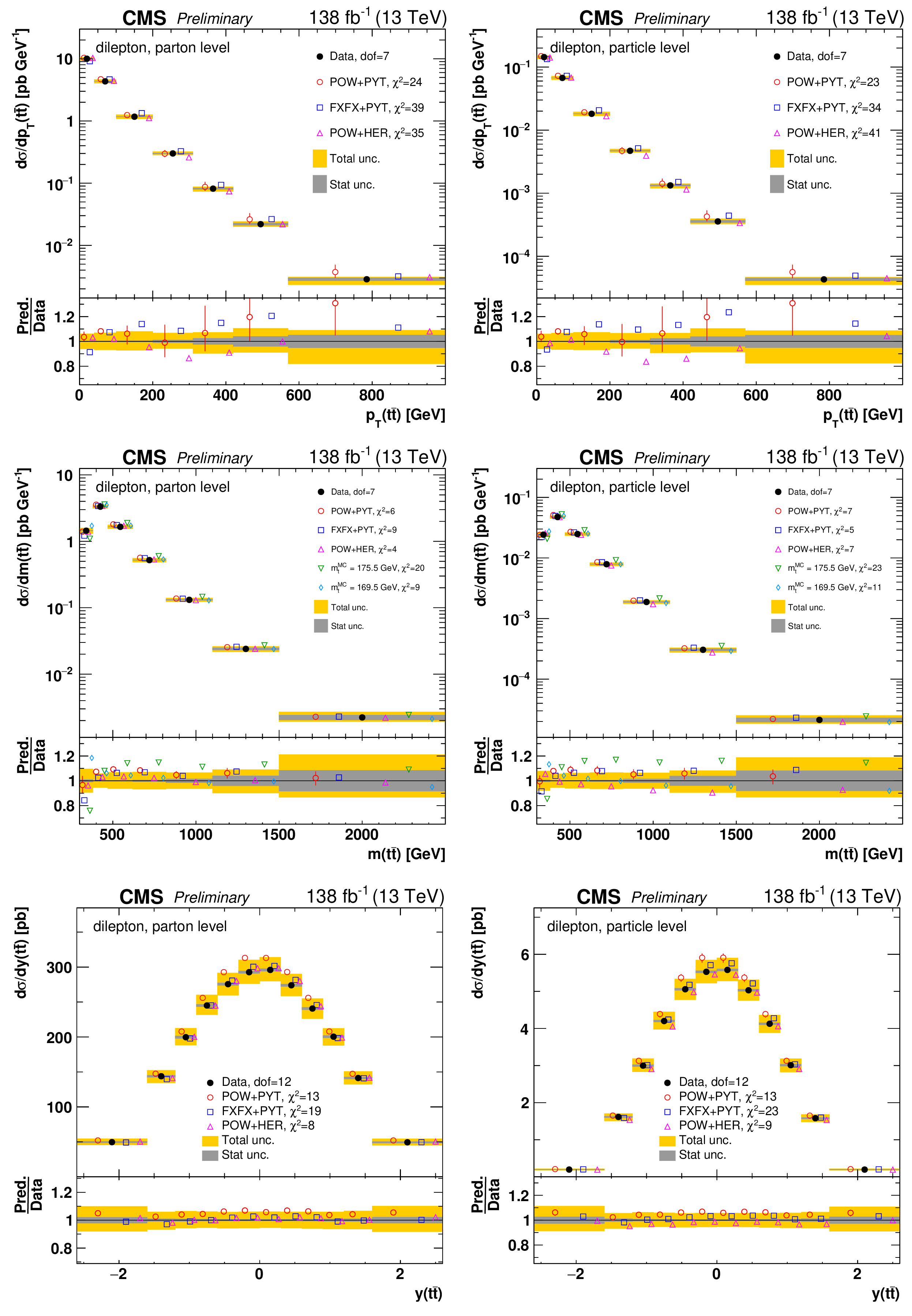
png pdf	Figure 66: Absolute differential $\mathrm{t\bar{t}}$ production cross sections as a function of ${{p_{\mathrm {T}}} ( \mathrm{t\bar{t}})}$ (upper), ${m( \mathrm{t\bar{t}})}$ (middle) and ${y( \mathrm{t\bar{t}})}$ (lower) are shown for data (filled circles) and various MC predictions (other points). Further details can be found in the caption of Fig. 7.
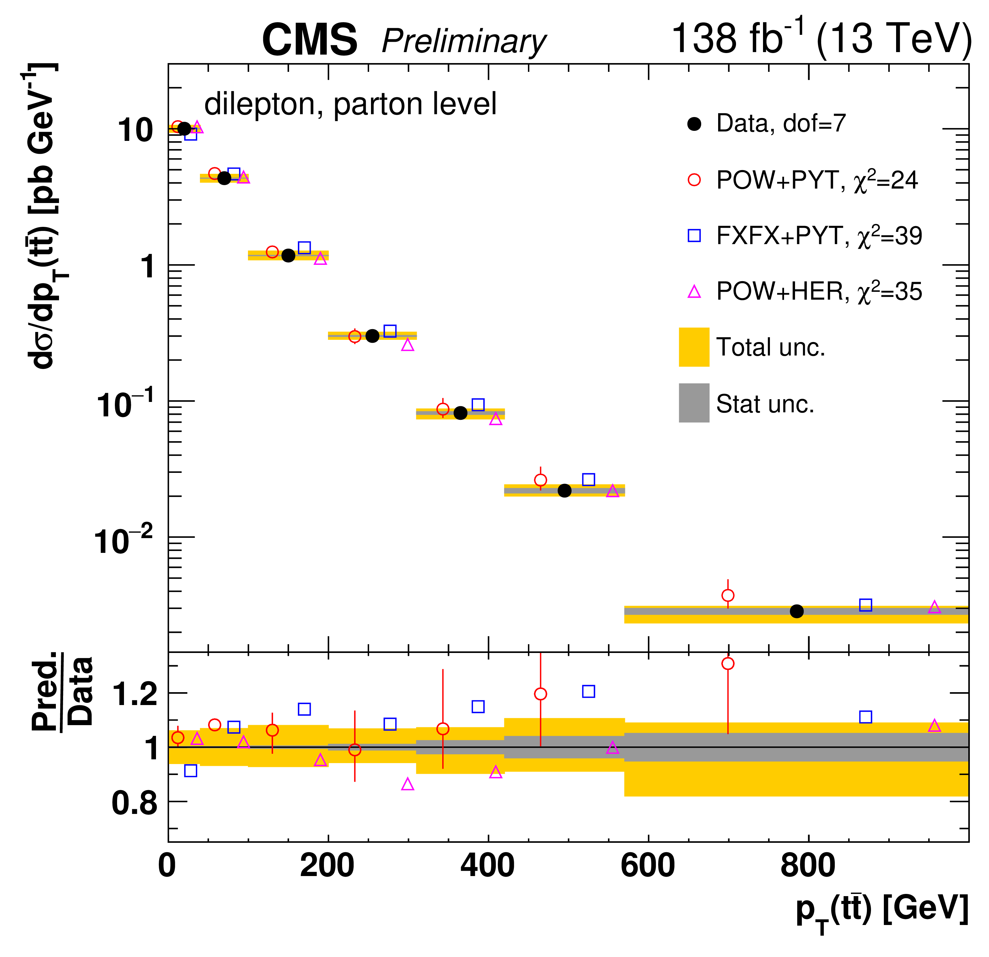
png pdf	Figure 66-a: Absolute differential $\mathrm{t\bar{t}}$ production cross sections as a function of ${{p_{\mathrm {T}}} ( \mathrm{t\bar{t}})}$ (upper), ${m( \mathrm{t\bar{t}})}$ (middle) and ${y( \mathrm{t\bar{t}})}$ (lower) are shown for data (filled circles) and various MC predictions (other points). Further details can be found in the caption of Fig. 7.
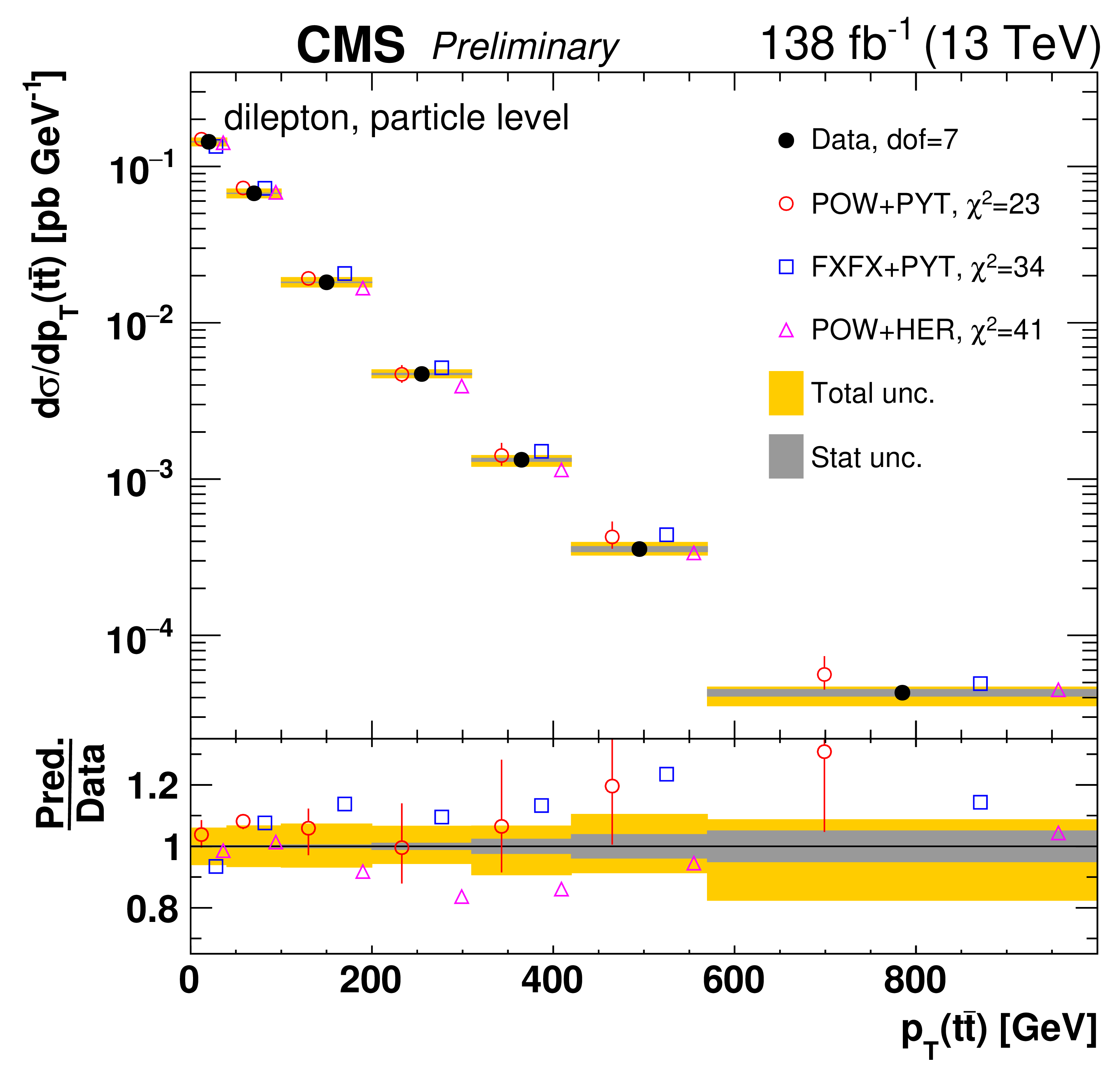
png pdf	Figure 66-b: Absolute differential $\mathrm{t\bar{t}}$ production cross sections as a function of ${{p_{\mathrm {T}}} ( \mathrm{t\bar{t}})}$ (upper), ${m( \mathrm{t\bar{t}})}$ (middle) and ${y( \mathrm{t\bar{t}})}$ (lower) are shown for data (filled circles) and various MC predictions (other points). Further details can be found in the caption of Fig. 7.
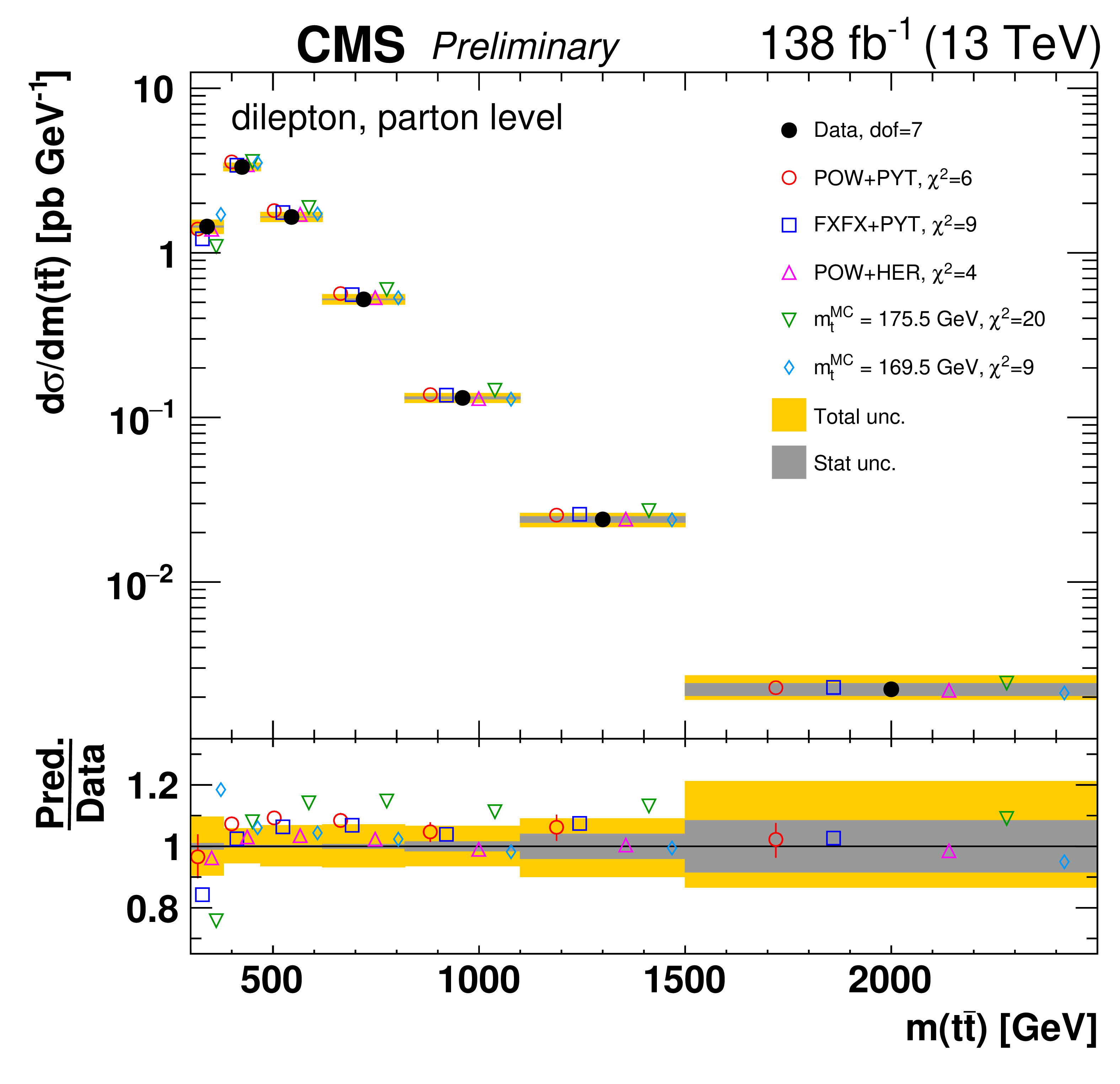
png pdf	Figure 66-c: Absolute differential $\mathrm{t\bar{t}}$ production cross sections as a function of ${{p_{\mathrm {T}}} ( \mathrm{t\bar{t}})}$ (upper), ${m( \mathrm{t\bar{t}})}$ (middle) and ${y( \mathrm{t\bar{t}})}$ (lower) are shown for data (filled circles) and various MC predictions (other points). Further details can be found in the caption of Fig. 7.
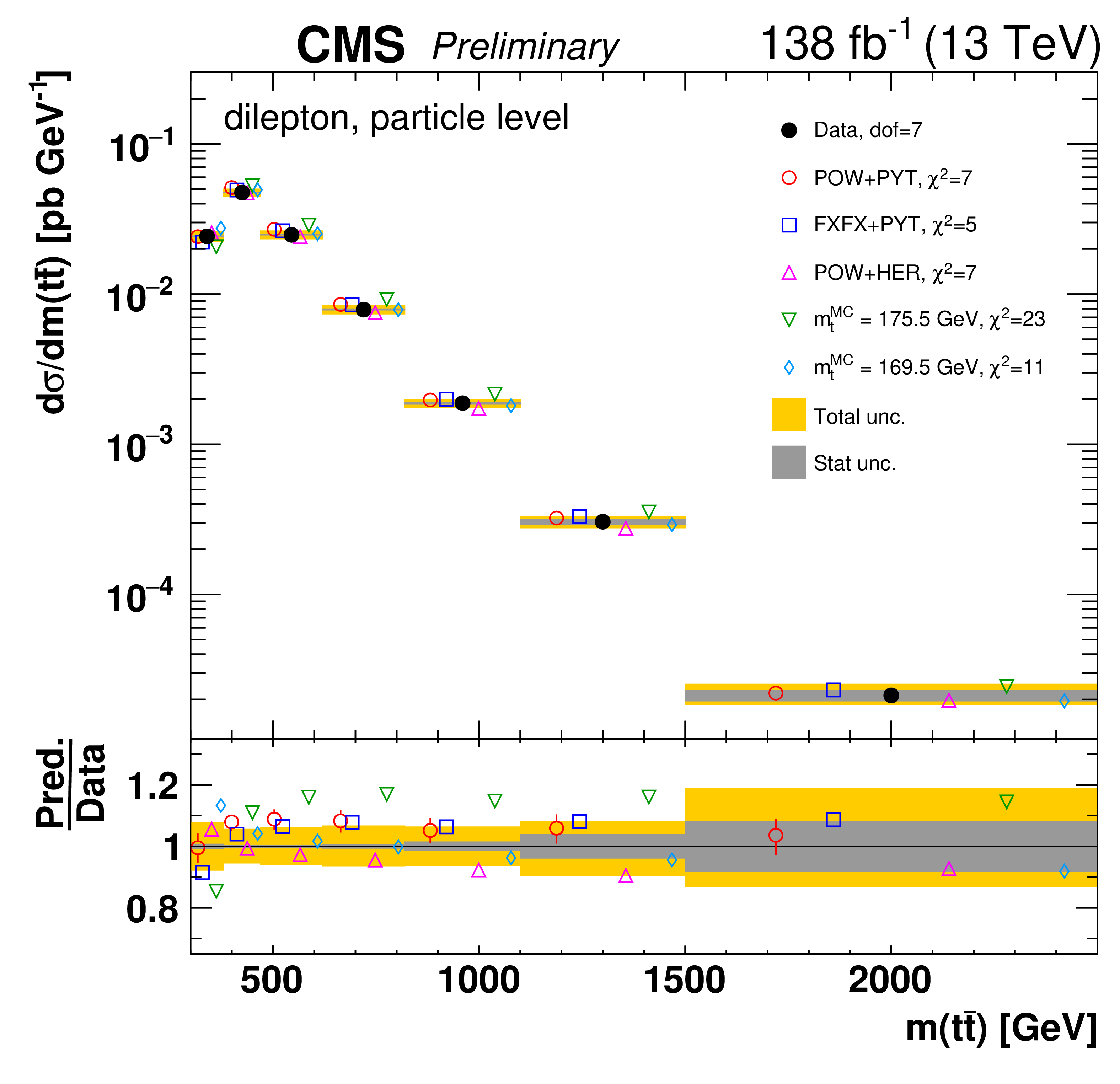
png pdf	Figure 66-d: Absolute differential $\mathrm{t\bar{t}}$ production cross sections as a function of ${{p_{\mathrm {T}}} ( \mathrm{t\bar{t}})}$ (upper), ${m( \mathrm{t\bar{t}})}$ (middle) and ${y( \mathrm{t\bar{t}})}$ (lower) are shown for data (filled circles) and various MC predictions (other points). Further details can be found in the caption of Fig. 7.
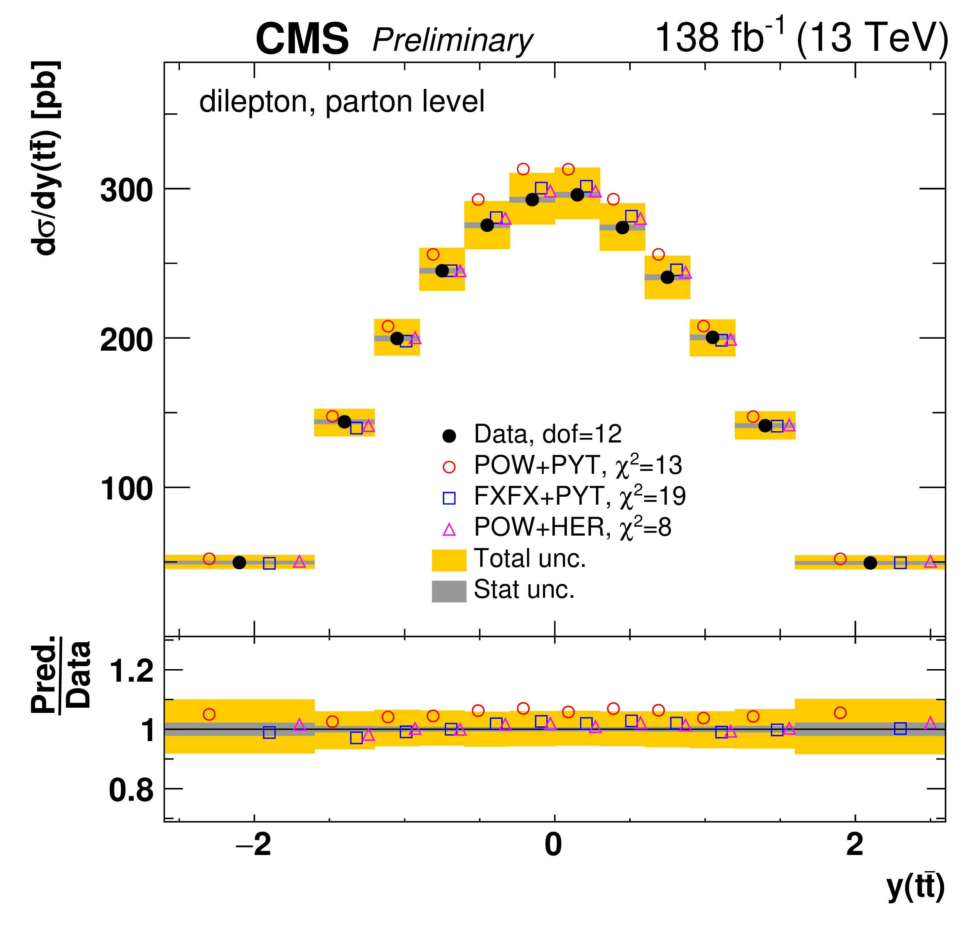
png pdf	Figure 66-e: Absolute differential $\mathrm{t\bar{t}}$ production cross sections as a function of ${{p_{\mathrm {T}}} ( \mathrm{t\bar{t}})}$ (upper), ${m( \mathrm{t\bar{t}})}$ (middle) and ${y( \mathrm{t\bar{t}})}$ (lower) are shown for data (filled circles) and various MC predictions (other points). Further details can be found in the caption of Fig. 7.
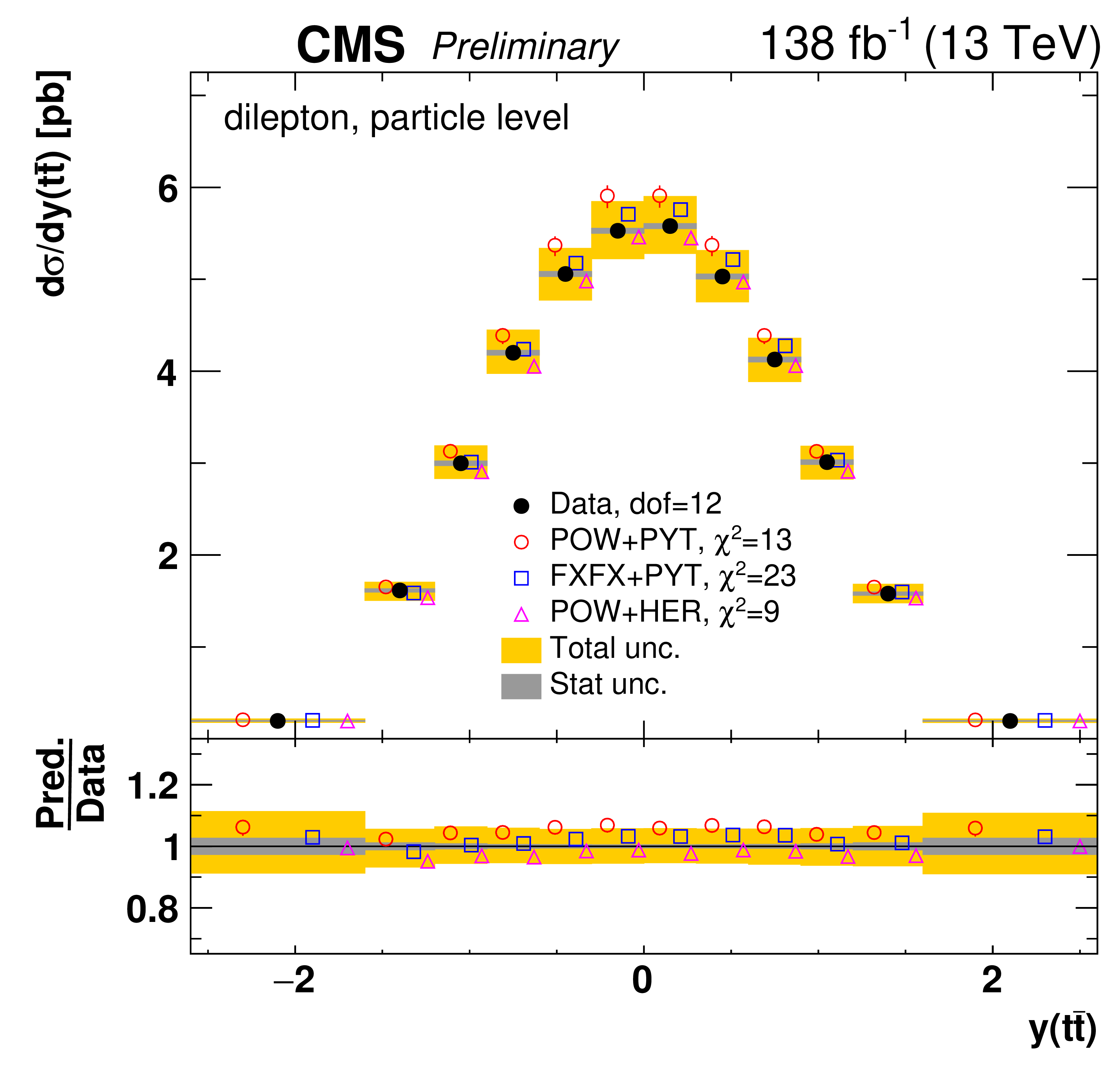
png pdf	Figure 66-f: Absolute differential $\mathrm{t\bar{t}}$ production cross sections as a function of ${{p_{\mathrm {T}}} ( \mathrm{t\bar{t}})}$ (upper), ${m( \mathrm{t\bar{t}})}$ (middle) and ${y( \mathrm{t\bar{t}})}$ (lower) are shown for data (filled circles) and various MC predictions (other points). Further details can be found in the caption of Fig. 7.
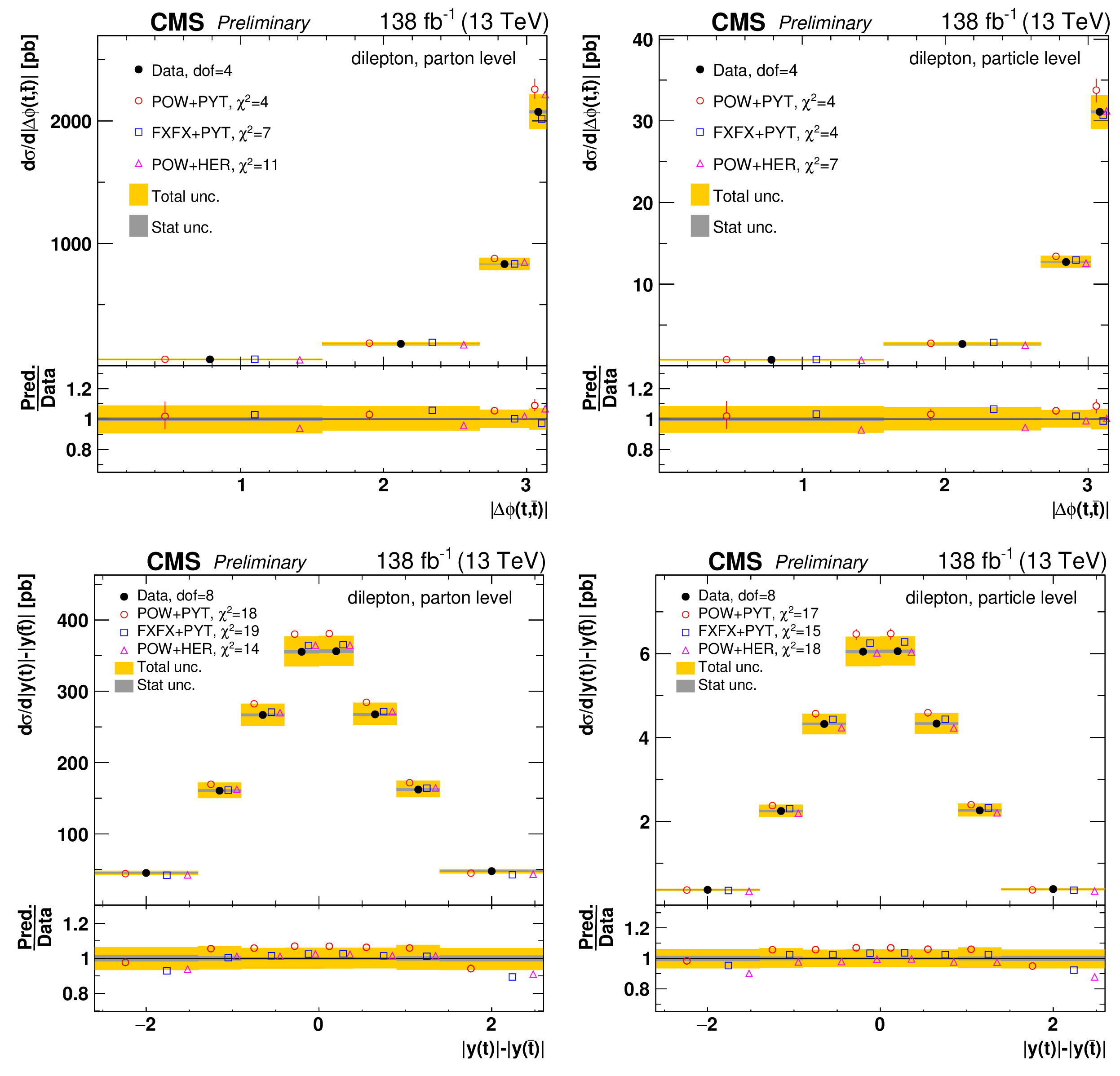
png pdf	Figure 67: Absolute differential $\mathrm{t\bar{t}}$ production cross sections as a function of ${|\Delta \phi (\mathrm{t},\mathrm{\bar{t}})|}$ (upper) and ${|y(\mathrm{t})|-|y(\mathrm{\bar{t}})|}$ (lower) are shown for the data (filled circles) and various MC predictions (other points). Further details can be found in the caption of Fig. 64.
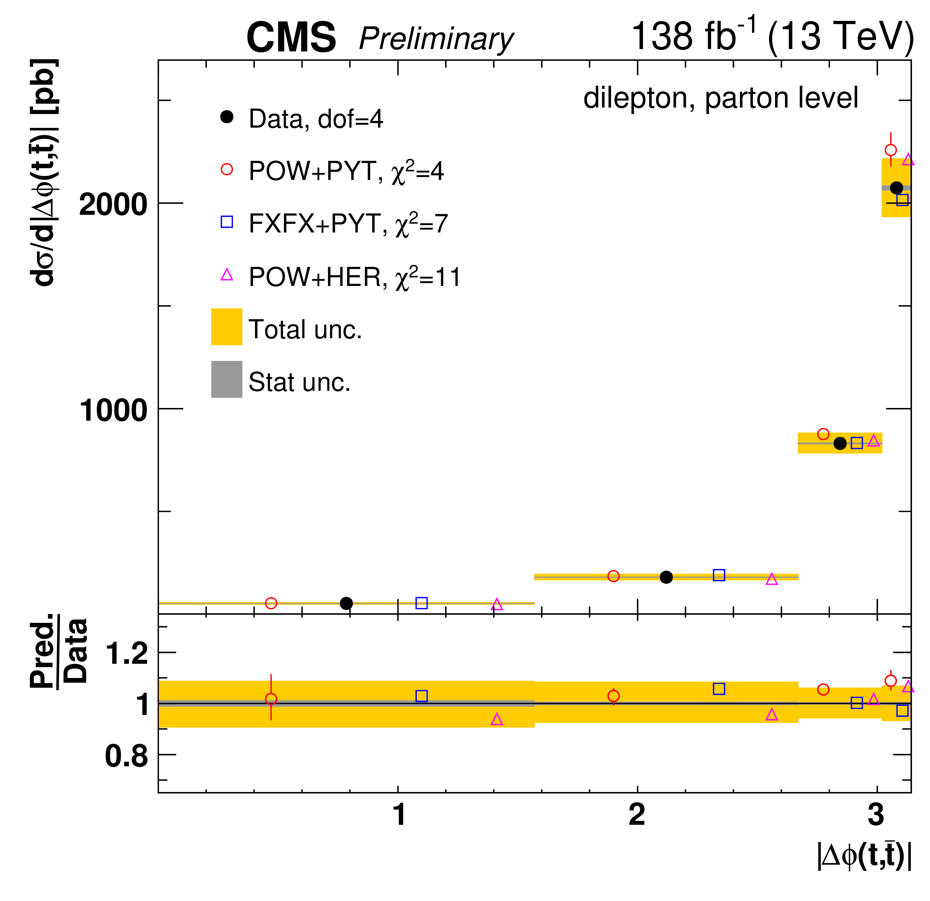
png pdf	Figure 67-a: Absolute differential $\mathrm{t\bar{t}}$ production cross sections as a function of ${|\Delta \phi (\mathrm{t},\mathrm{\bar{t}})|}$ (upper) and ${|y(\mathrm{t})|-|y(\mathrm{\bar{t}})|}$ (lower) are shown for the data (filled circles) and various MC predictions (other points). Further details can be found in the caption of Fig. 64.
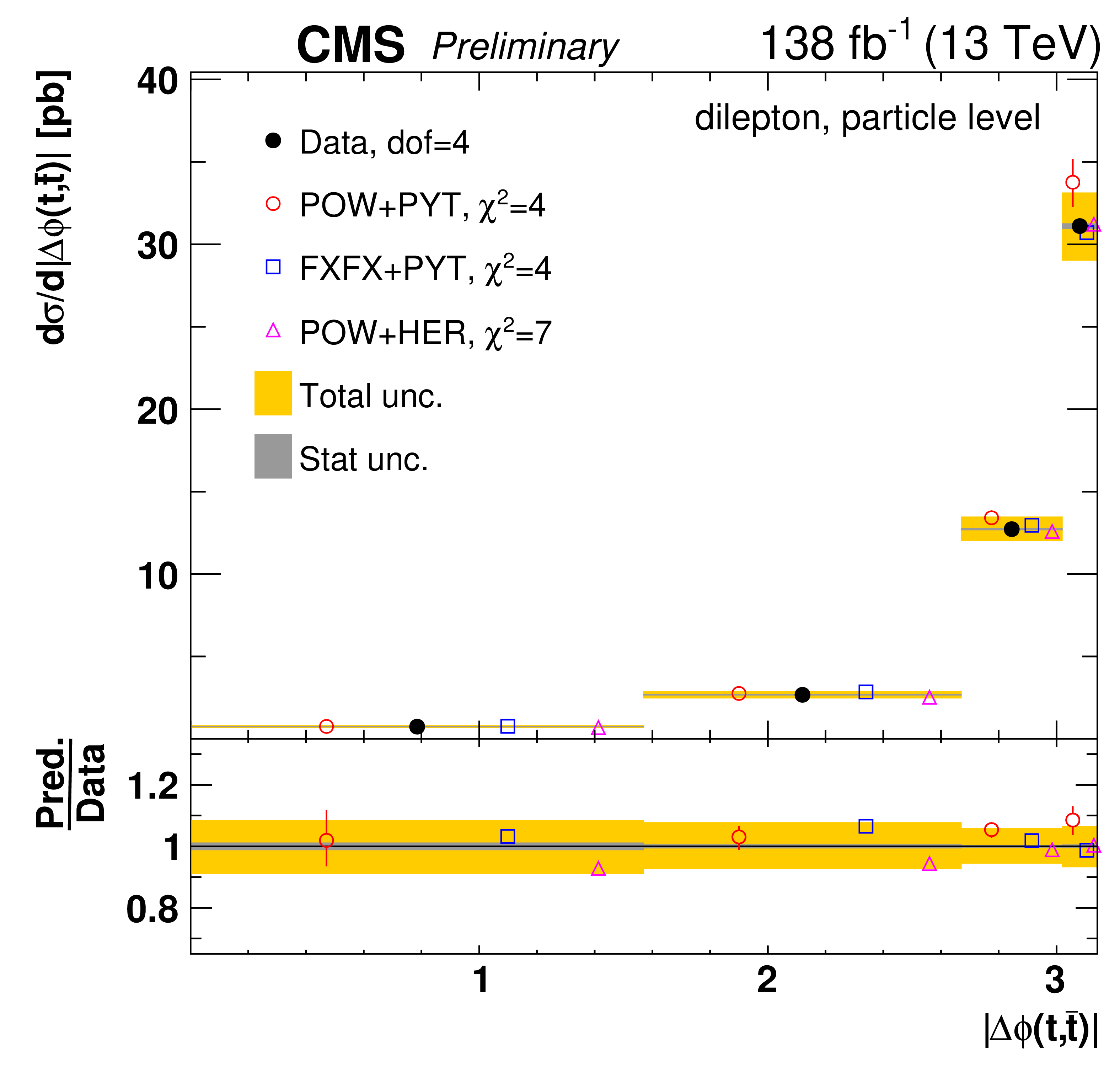
png pdf	Figure 67-b: Absolute differential $\mathrm{t\bar{t}}$ production cross sections as a function of ${|\Delta \phi (\mathrm{t},\mathrm{\bar{t}})|}$ (upper) and ${|y(\mathrm{t})|-|y(\mathrm{\bar{t}})|}$ (lower) are shown for the data (filled circles) and various MC predictions (other points). Further details can be found in the caption of Fig. 64.
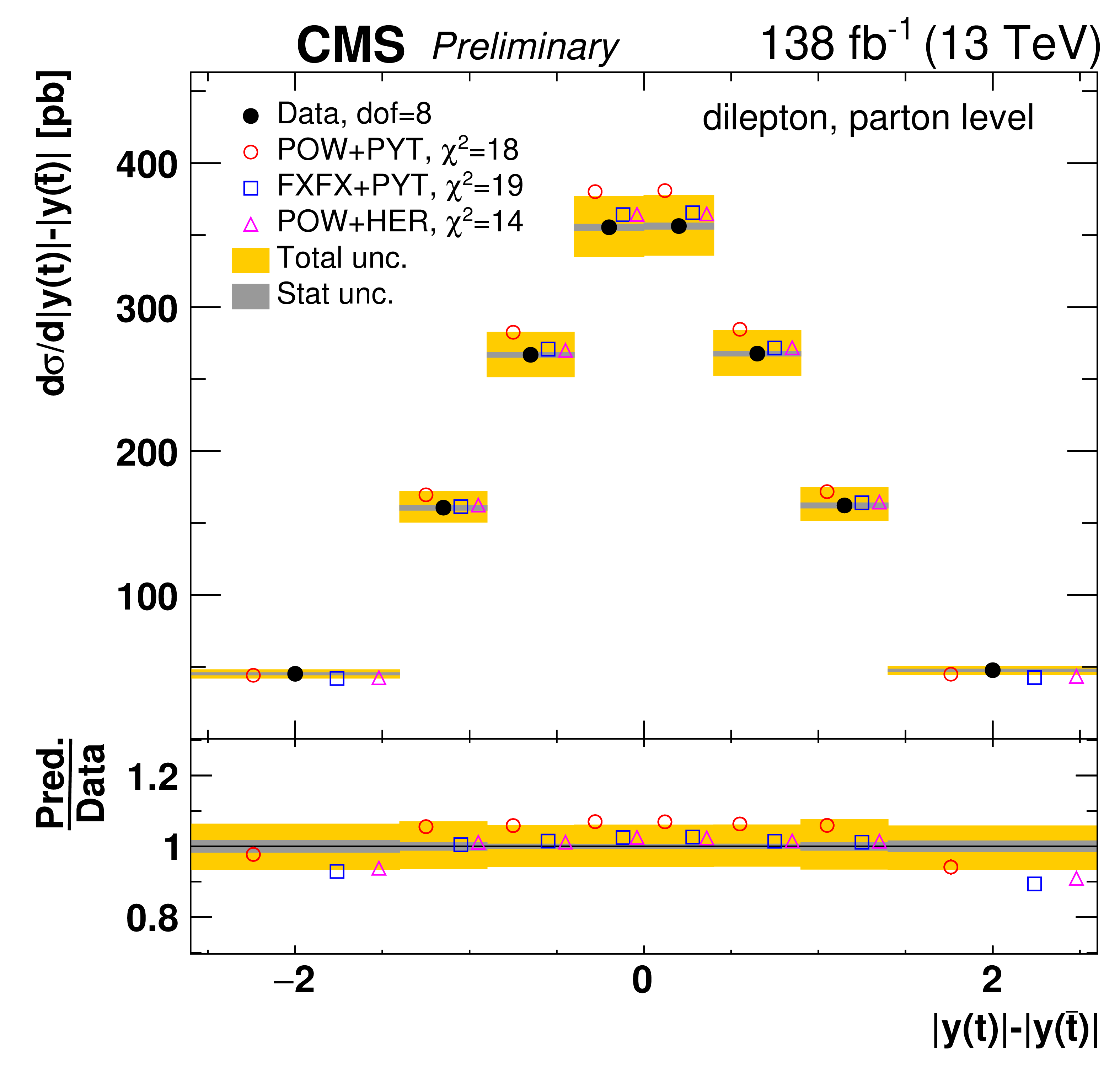
png pdf	Figure 67-c: Absolute differential $\mathrm{t\bar{t}}$ production cross sections as a function of ${|\Delta \phi (\mathrm{t},\mathrm{\bar{t}})|}$ (upper) and ${|y(\mathrm{t})|-|y(\mathrm{\bar{t}})|}$ (lower) are shown for the data (filled circles) and various MC predictions (other points). Further details can be found in the caption of Fig. 64.
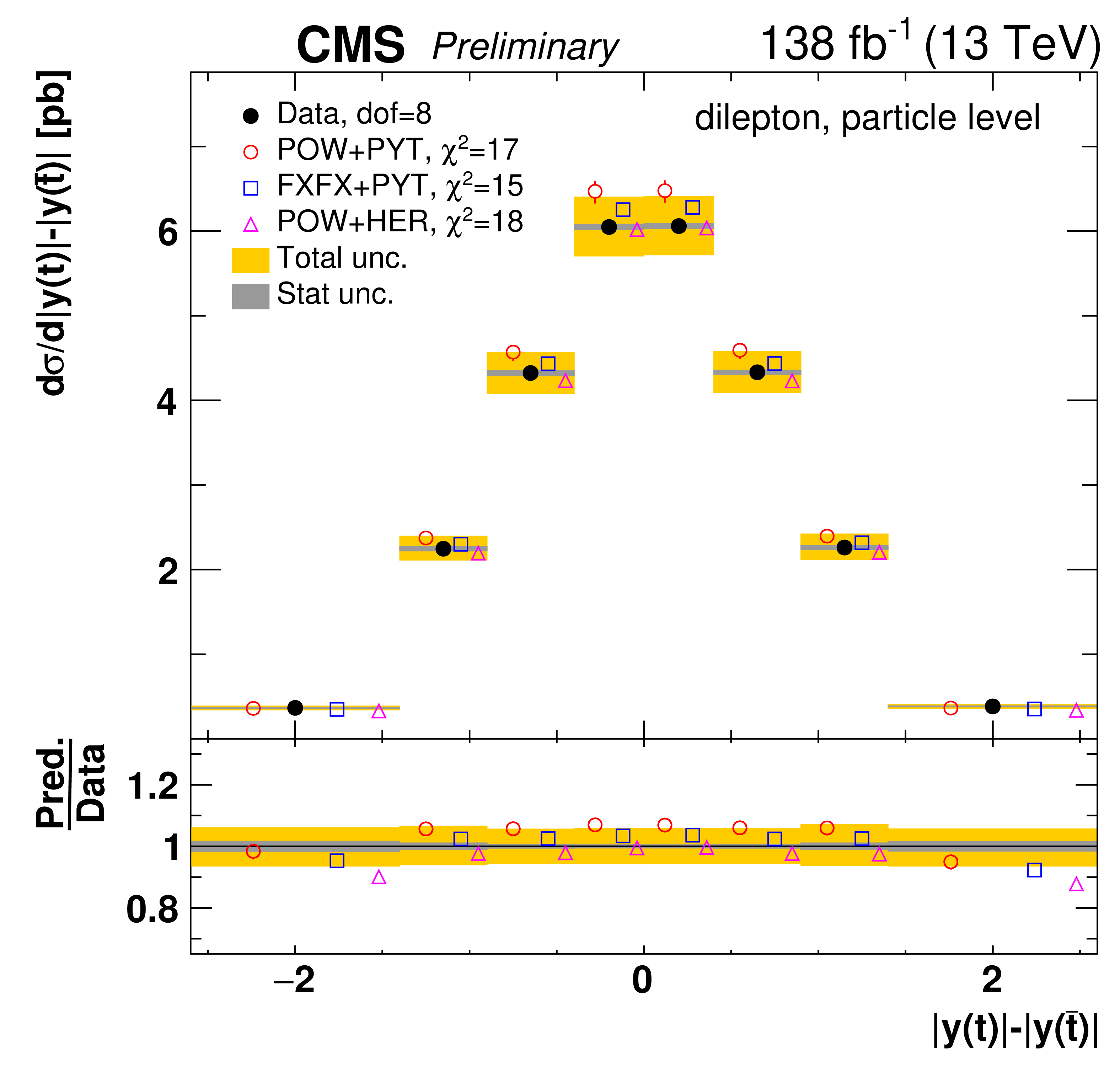
png pdf	Figure 67-d: Absolute differential $\mathrm{t\bar{t}}$ production cross sections as a function of ${|\Delta \phi (\mathrm{t},\mathrm{\bar{t}})|}$ (upper) and ${|y(\mathrm{t})|-|y(\mathrm{\bar{t}})|}$ (lower) are shown for the data (filled circles) and various MC predictions (other points). Further details can be found in the caption of Fig. 64.
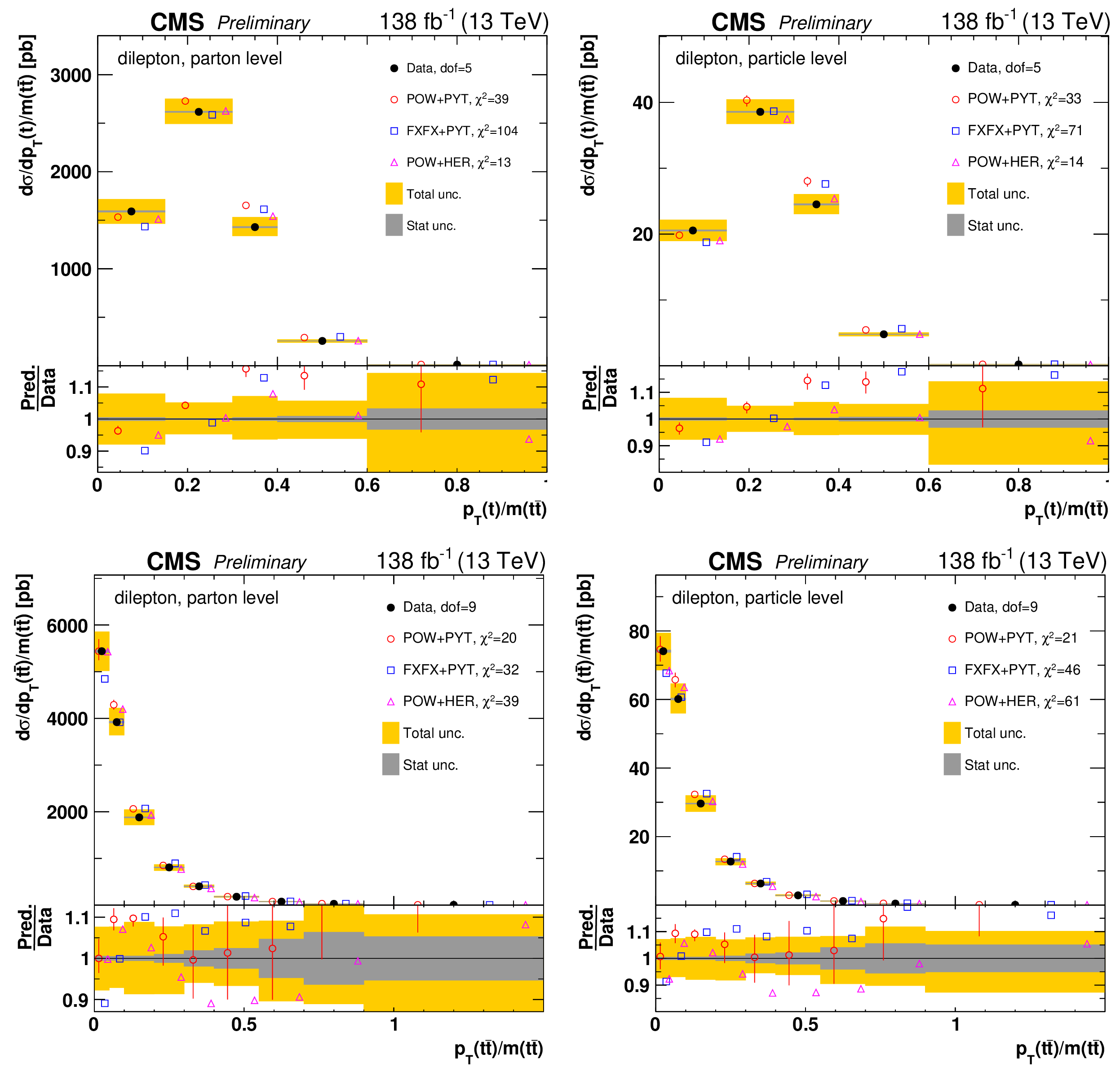
png pdf	Figure 68: Absolute differential $\mathrm{t\bar{t}}$ production cross sections as a function of $ {{p_{\mathrm {T}}} (\mathrm{t})} / {m( \mathrm{t\bar{t}})}$ (upper) and $ {{p_{\mathrm {T}}} ( \mathrm{t\bar{t}})} / {{m( \mathrm{t\bar{t}})}}$ (lower) are shown for the data (filled circles) and various MC predictions (other points). Further details can be found in the caption of Fig. 64.
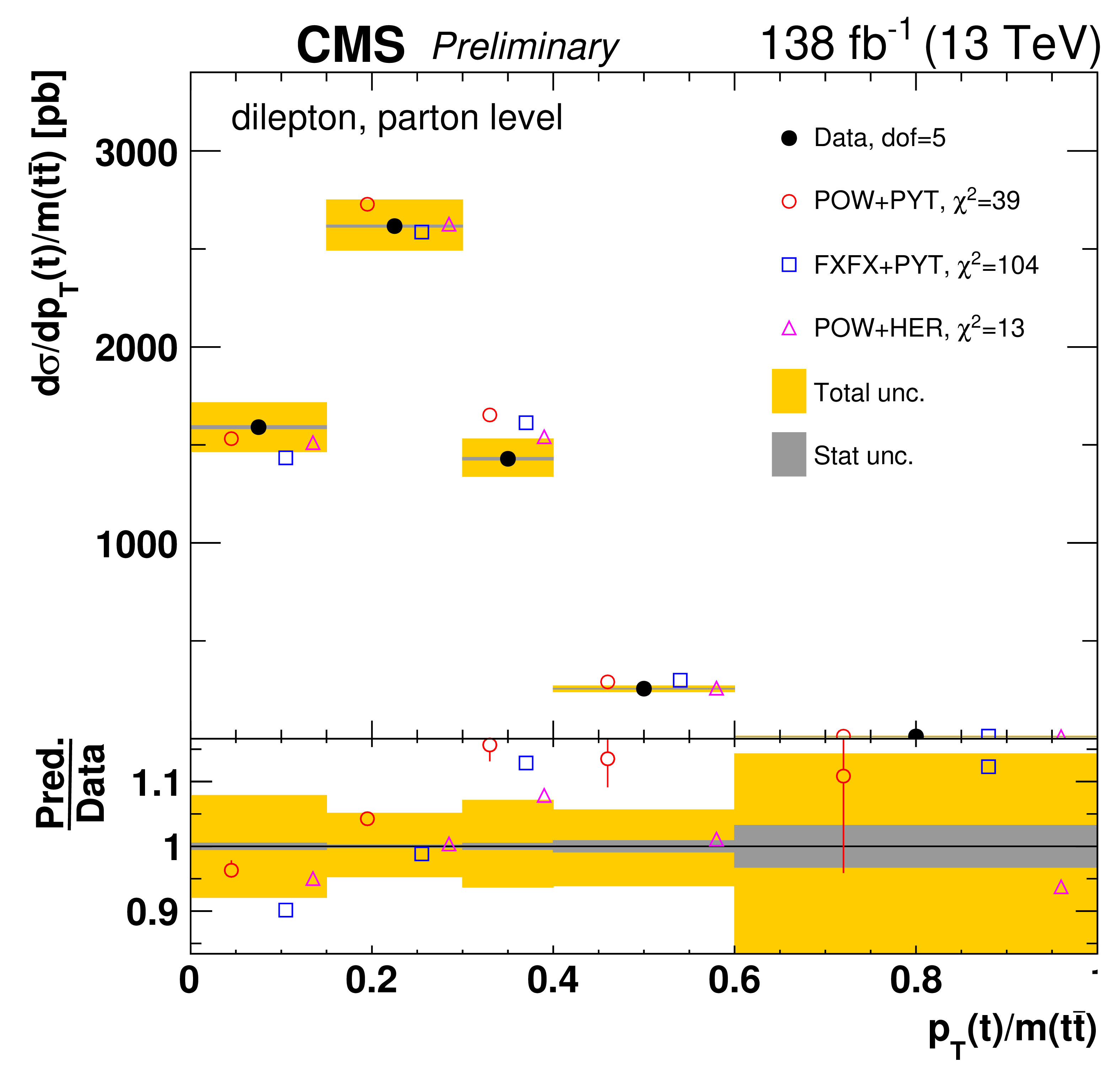
png pdf	Figure 68-a: Absolute differential $\mathrm{t\bar{t}}$ production cross sections as a function of $ {{p_{\mathrm {T}}} (\mathrm{t})} / {m( \mathrm{t\bar{t}})}$ (upper) and $ {{p_{\mathrm {T}}} ( \mathrm{t\bar{t}})} / {{m( \mathrm{t\bar{t}})}}$ (lower) are shown for the data (filled circles) and various MC predictions (other points). Further details can be found in the caption of Fig. 64.
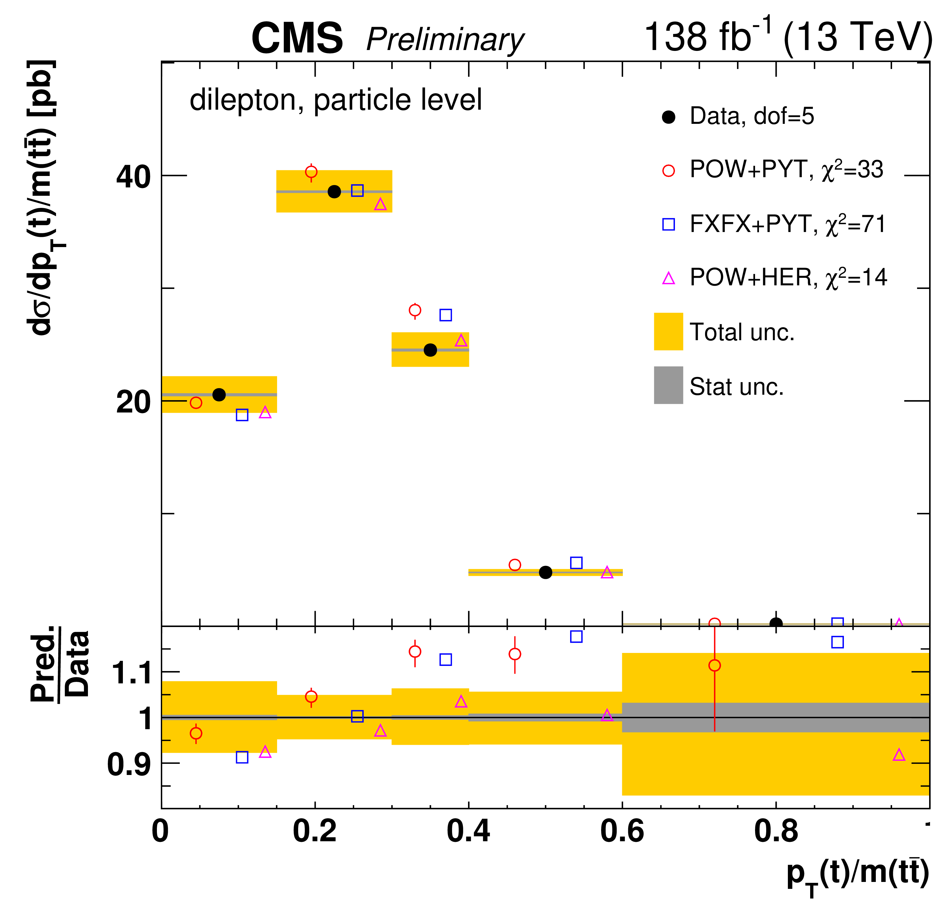
png pdf	Figure 68-b: Absolute differential $\mathrm{t\bar{t}}$ production cross sections as a function of $ {{p_{\mathrm {T}}} (\mathrm{t})} / {m( \mathrm{t\bar{t}})}$ (upper) and $ {{p_{\mathrm {T}}} ( \mathrm{t\bar{t}})} / {{m( \mathrm{t\bar{t}})}}$ (lower) are shown for the data (filled circles) and various MC predictions (other points). Further details can be found in the caption of Fig. 64.
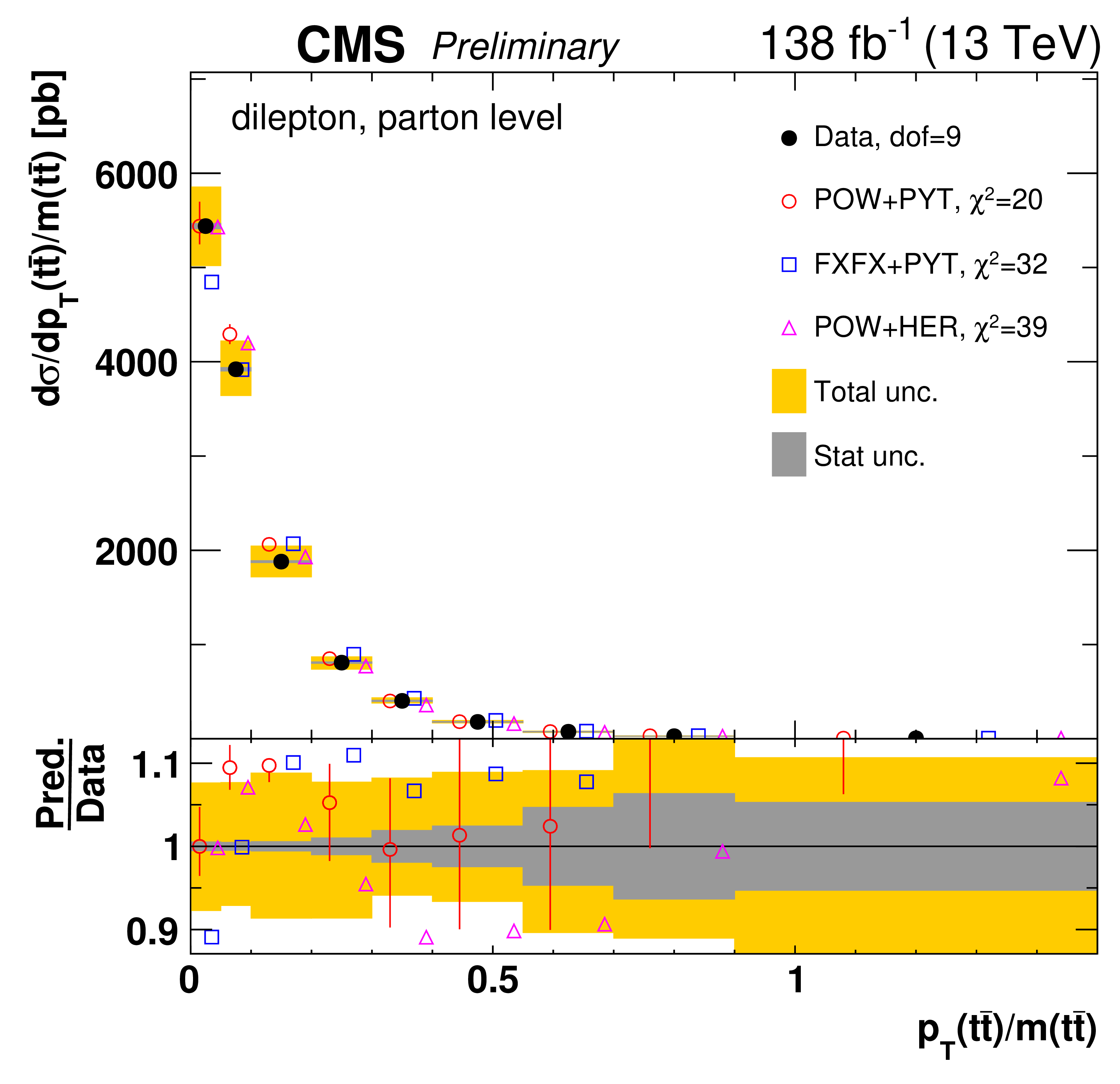
png pdf	Figure 68-c: Absolute differential $\mathrm{t\bar{t}}$ production cross sections as a function of $ {{p_{\mathrm {T}}} (\mathrm{t})} / {m( \mathrm{t\bar{t}})}$ (upper) and $ {{p_{\mathrm {T}}} ( \mathrm{t\bar{t}})} / {{m( \mathrm{t\bar{t}})}}$ (lower) are shown for the data (filled circles) and various MC predictions (other points). Further details can be found in the caption of Fig. 64.
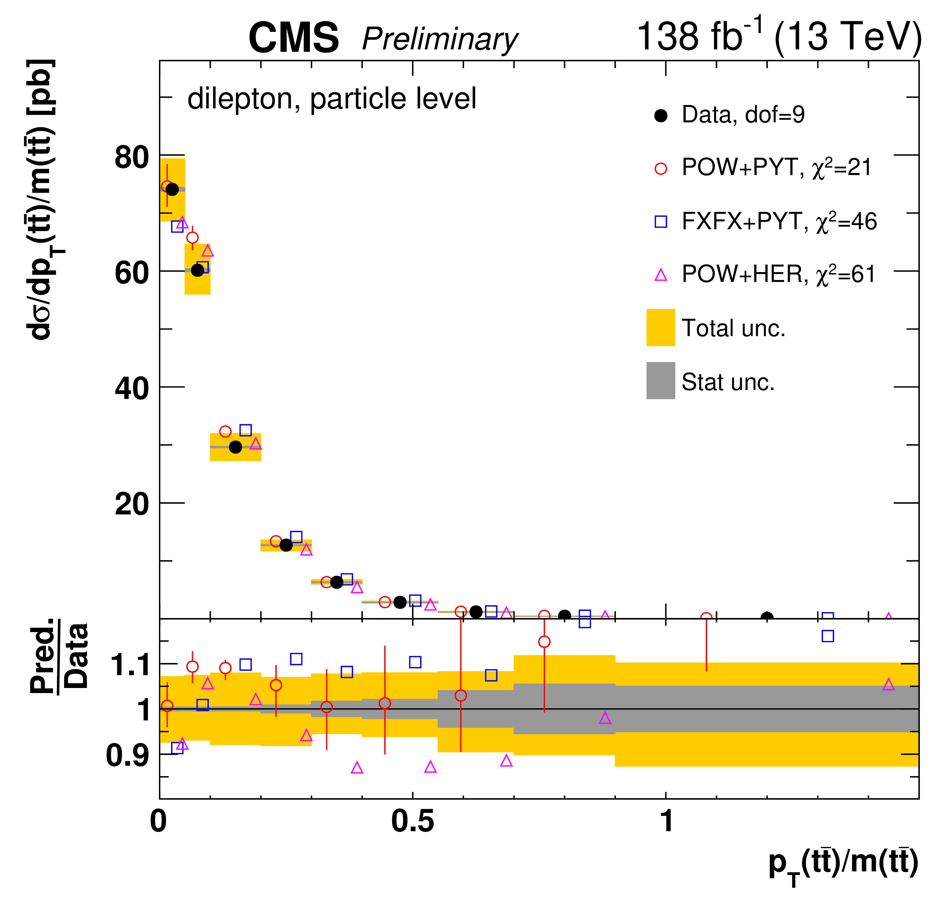
png pdf	Figure 68-d: Absolute differential $\mathrm{t\bar{t}}$ production cross sections as a function of $ {{p_{\mathrm {T}}} (\mathrm{t})} / {m( \mathrm{t\bar{t}})}$ (upper) and $ {{p_{\mathrm {T}}} ( \mathrm{t\bar{t}})} / {{m( \mathrm{t\bar{t}})}}$ (lower) are shown for the data (filled circles) and various MC predictions (other points). Further details can be found in the caption of Fig. 64.
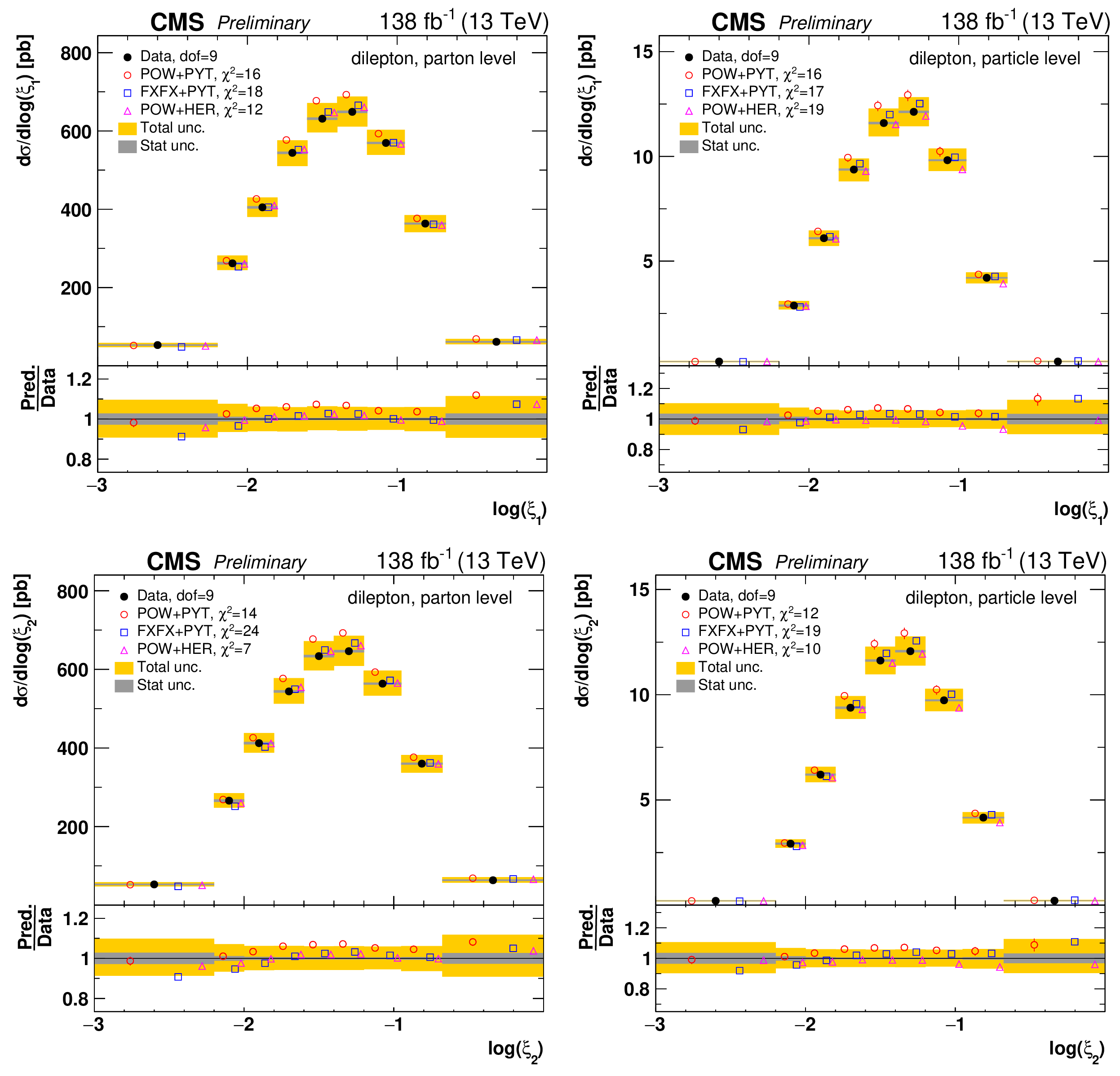
png pdf	Figure 69: Absolute differential $\mathrm{t\bar{t}}$ production cross sections as a function of ${\log(\xi _{1})}$ (upper) and ${\log(\xi _{2})}$ (lower) are shown for the data (filled circles) and various MC predictions (other points). Further details can be found in the caption of Fig. 64.
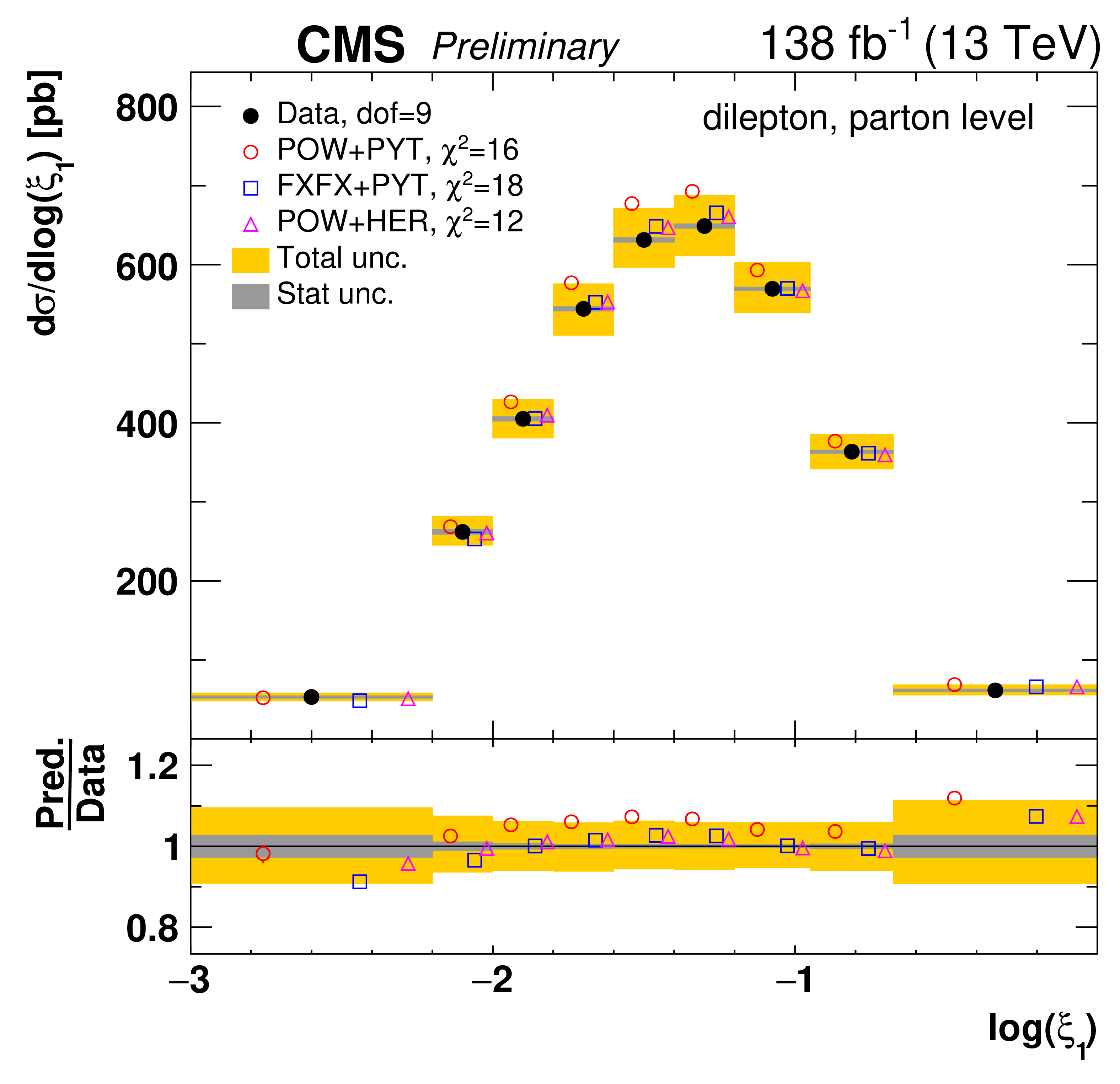
png pdf	Figure 69-a: Absolute differential $\mathrm{t\bar{t}}$ production cross sections as a function of ${\log(\xi _{1})}$ (upper) and ${\log(\xi _{2})}$ (lower) are shown for the data (filled circles) and various MC predictions (other points). Further details can be found in the caption of Fig. 64.
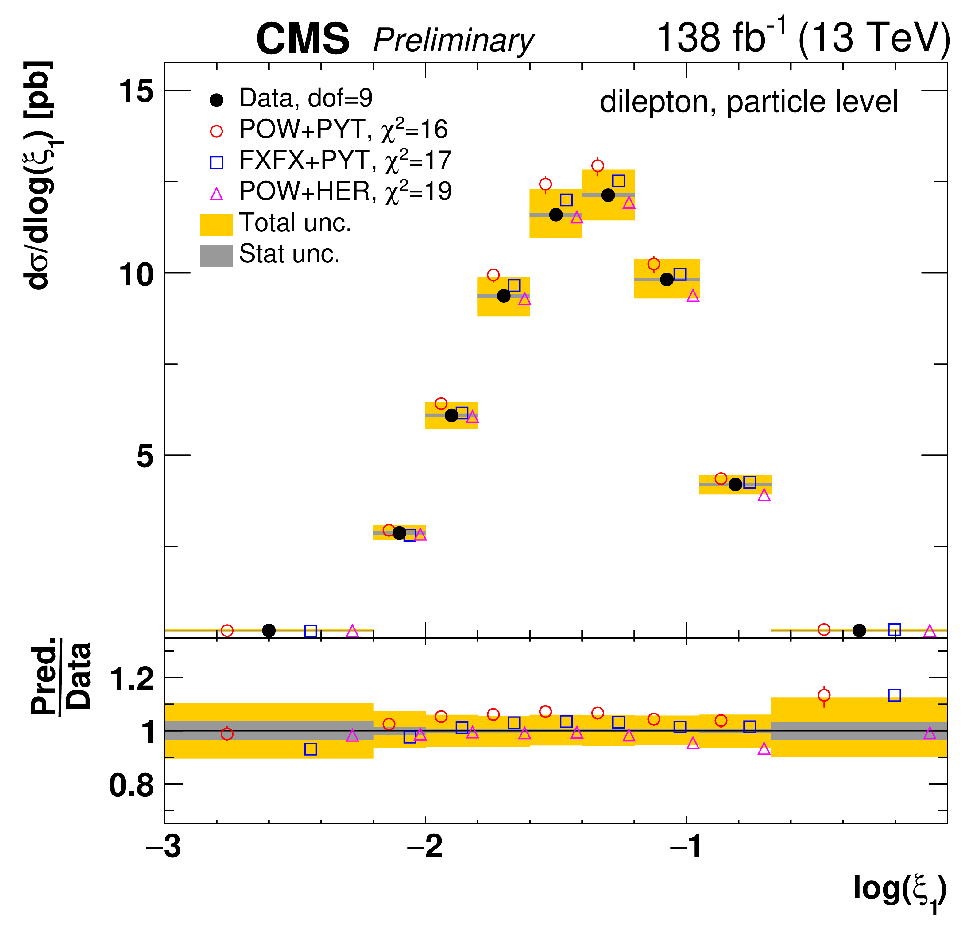
png pdf	Figure 69-b: Absolute differential $\mathrm{t\bar{t}}$ production cross sections as a function of ${\log(\xi _{1})}$ (upper) and ${\log(\xi _{2})}$ (lower) are shown for the data (filled circles) and various MC predictions (other points). Further details can be found in the caption of Fig. 64.
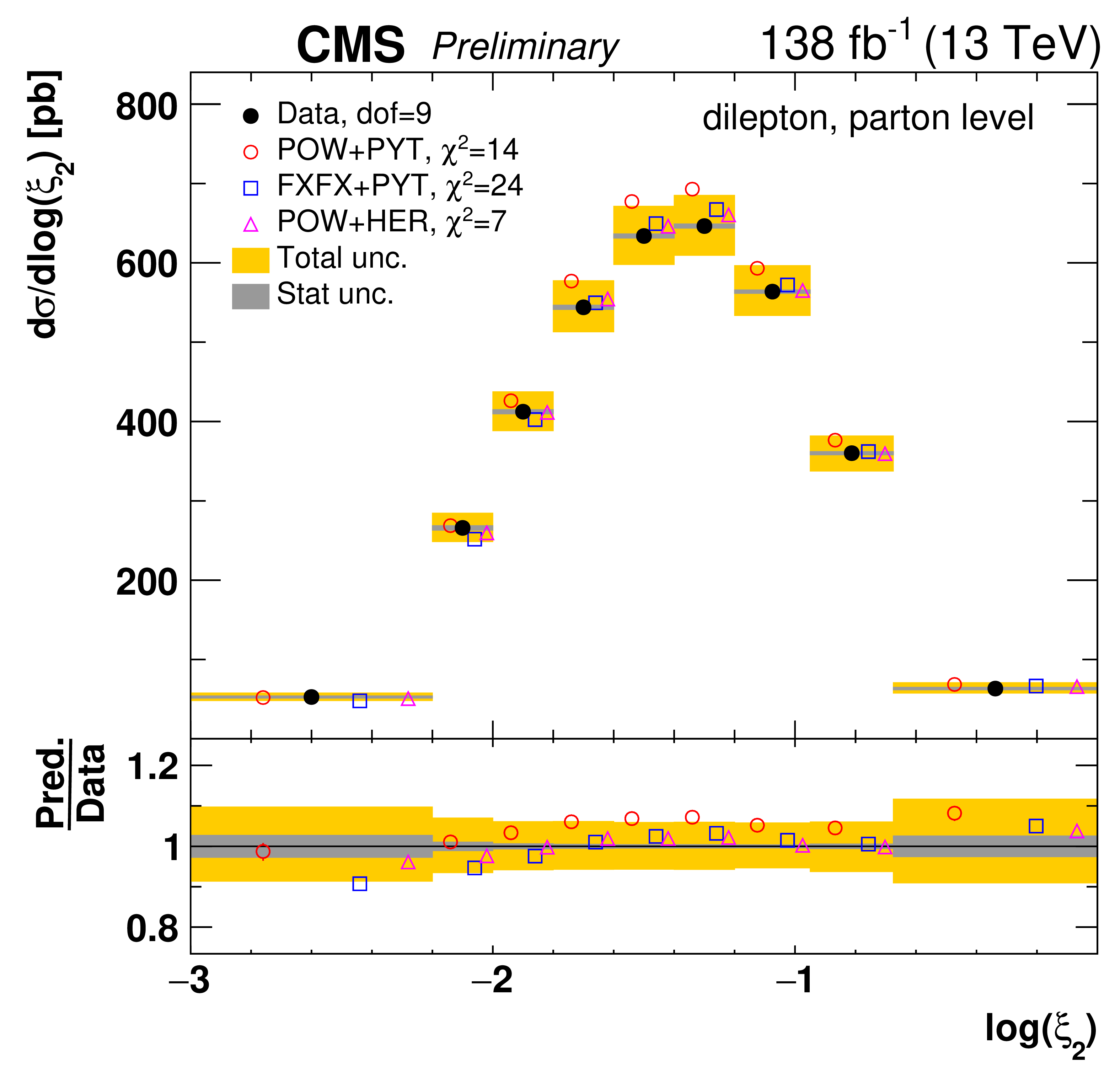
png pdf	Figure 69-c: Absolute differential $\mathrm{t\bar{t}}$ production cross sections as a function of ${\log(\xi _{1})}$ (upper) and ${\log(\xi _{2})}$ (lower) are shown for the data (filled circles) and various MC predictions (other points). Further details can be found in the caption of Fig. 64.
png pdf	Figure 69-d: Absolute differential $\mathrm{t\bar{t}}$ production cross sections as a function of ${\log(\xi _{1})}$ (upper) and ${\log(\xi _{2})}$ (lower) are shown for the data (filled circles) and various MC predictions (other points). Further details can be found in the caption of Fig. 64.
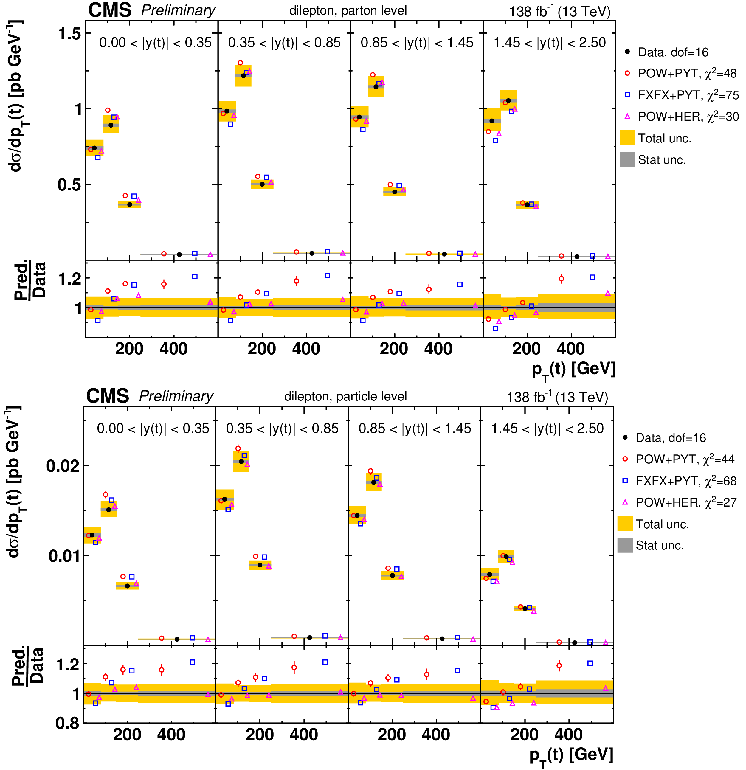
png pdf	Figure 70: Absolute $[ {|y(\mathrm{t})|},\,{{p_{\mathrm {T}}} (\mathrm{t})} ]$ cross sections measured at the parton level in the full phase space (upper) and at the particle level in a fiducial phase space (lower). The data are shown as filled circles with dark and light bands indicating the statistical and total uncertainties (statistical and systematic uncertainties summed in quadrature), respectively. The cross sections are compared to various MC predictions (other points). The estimated uncertainties in the POWHEG+PYTHIA-8 (`POW-PYT') simulation are represented by a vertical bar on the corresponding points. For each MC model, a value of ${\chi ^2}$ is reported that takes into account the measurement uncertainties. The lower panel in each plot shows the ratios of the predictions to the data.
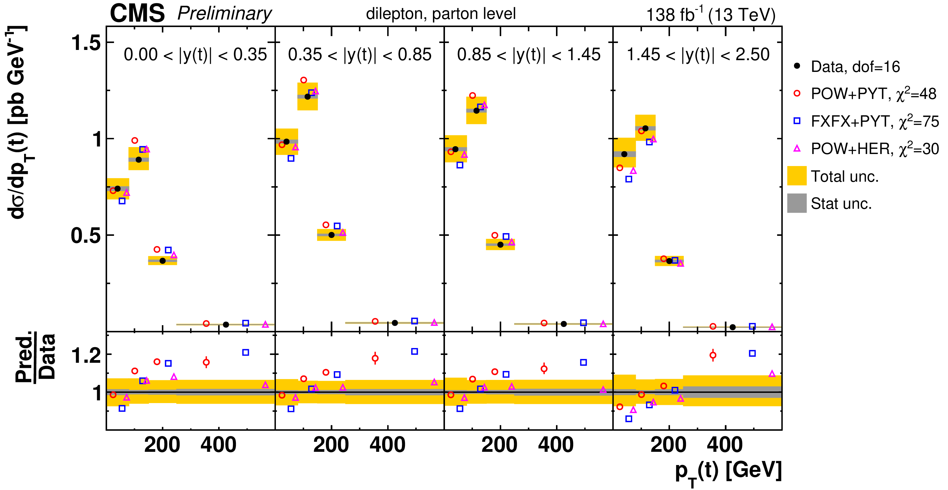
png pdf	Figure 70-a: Absolute $[ {|y(\mathrm{t})|},\,{{p_{\mathrm {T}}} (\mathrm{t})} ]$ cross sections measured at the parton level in the full phase space (upper) and at the particle level in a fiducial phase space (lower). The data are shown as filled circles with dark and light bands indicating the statistical and total uncertainties (statistical and systematic uncertainties summed in quadrature), respectively. The cross sections are compared to various MC predictions (other points). The estimated uncertainties in the POWHEG+PYTHIA-8 (`POW-PYT') simulation are represented by a vertical bar on the corresponding points. For each MC model, a value of ${\chi ^2}$ is reported that takes into account the measurement uncertainties. The lower panel in each plot shows the ratios of the predictions to the data.
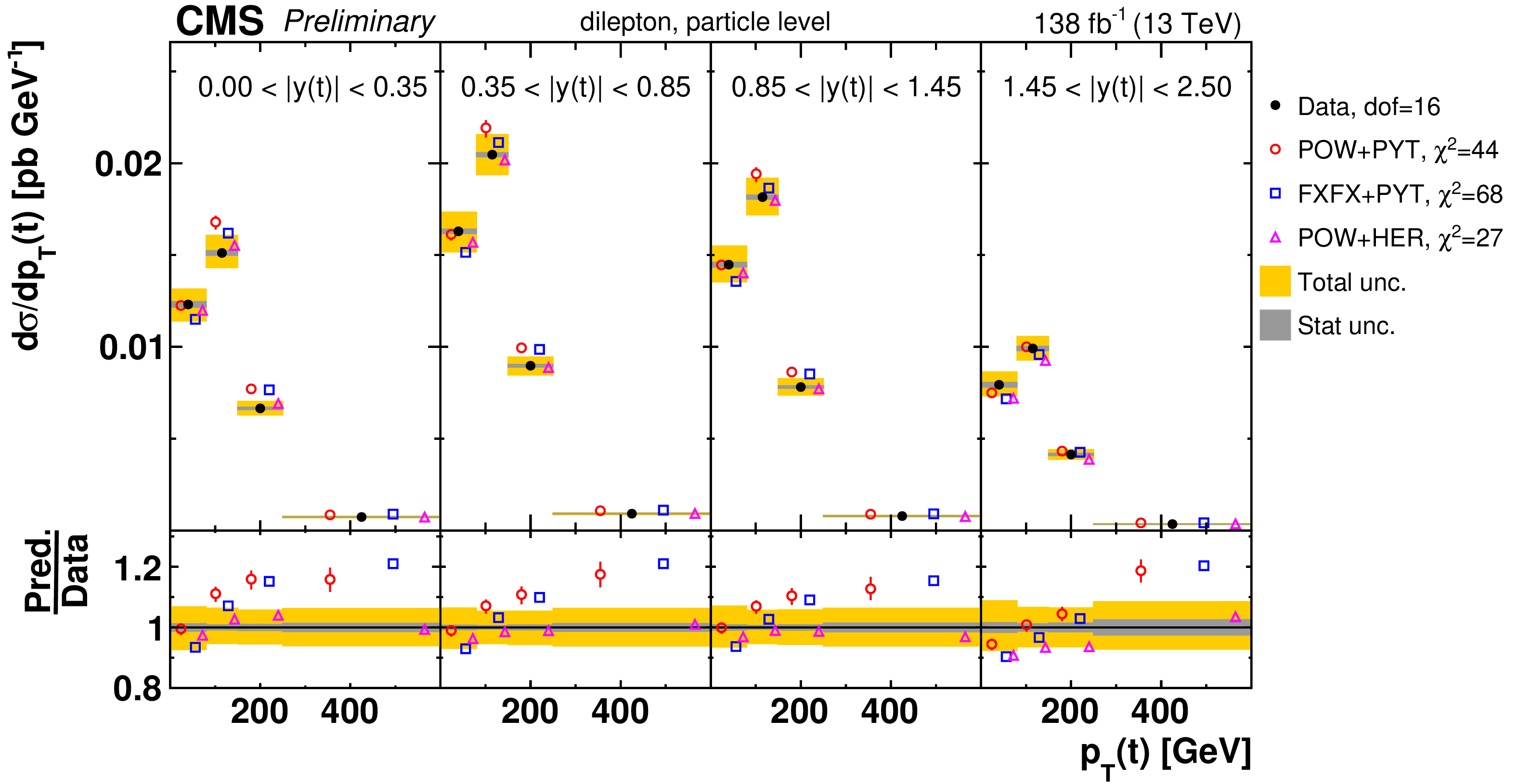
png pdf	Figure 70-b: Absolute $[ {|y(\mathrm{t})|},\,{{p_{\mathrm {T}}} (\mathrm{t})} ]$ cross sections measured at the parton level in the full phase space (upper) and at the particle level in a fiducial phase space (lower). The data are shown as filled circles with dark and light bands indicating the statistical and total uncertainties (statistical and systematic uncertainties summed in quadrature), respectively. The cross sections are compared to various MC predictions (other points). The estimated uncertainties in the POWHEG+PYTHIA-8 (`POW-PYT') simulation are represented by a vertical bar on the corresponding points. For each MC model, a value of ${\chi ^2}$ is reported that takes into account the measurement uncertainties. The lower panel in each plot shows the ratios of the predictions to the data.
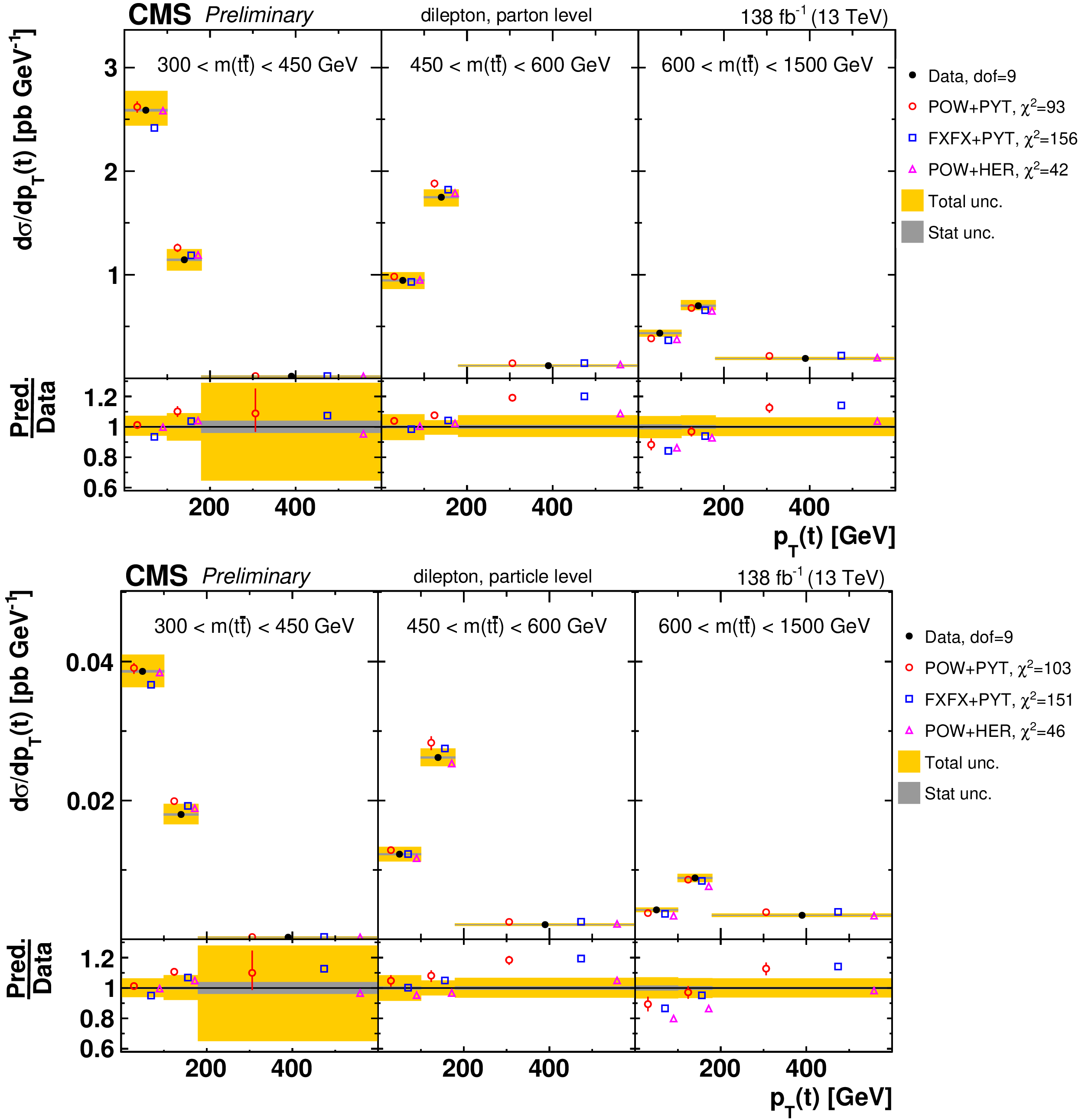
png pdf	Figure 71: Absolute $[ {m( \mathrm{t\bar{t}})},\,{{p_{\mathrm {T}}} (\mathrm{t})} ]$ cross sections are shown for data (filled circles) and various MC predictions (other points). Further details can be found in the caption of Fig. 70.
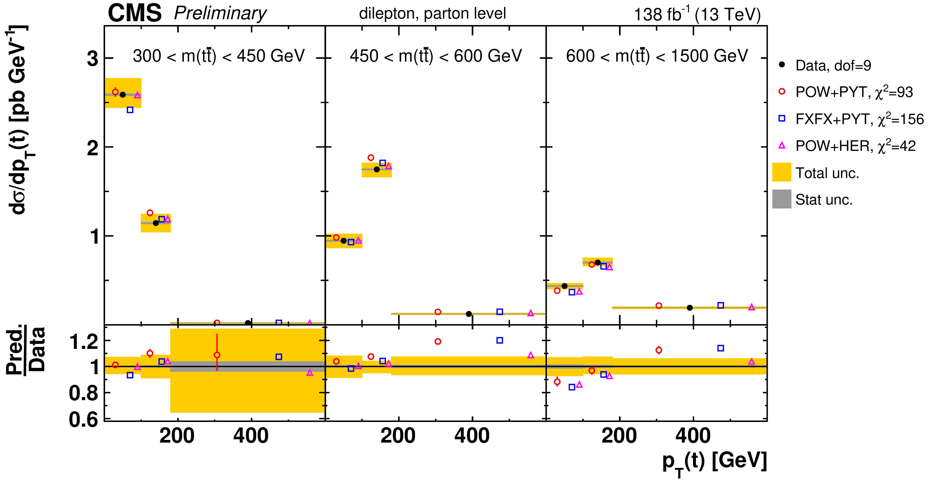
png pdf	Figure 71-a: Absolute $[ {m( \mathrm{t\bar{t}})},\,{{p_{\mathrm {T}}} (\mathrm{t})} ]$ cross sections are shown for data (filled circles) and various MC predictions (other points). Further details can be found in the caption of Fig. 70.
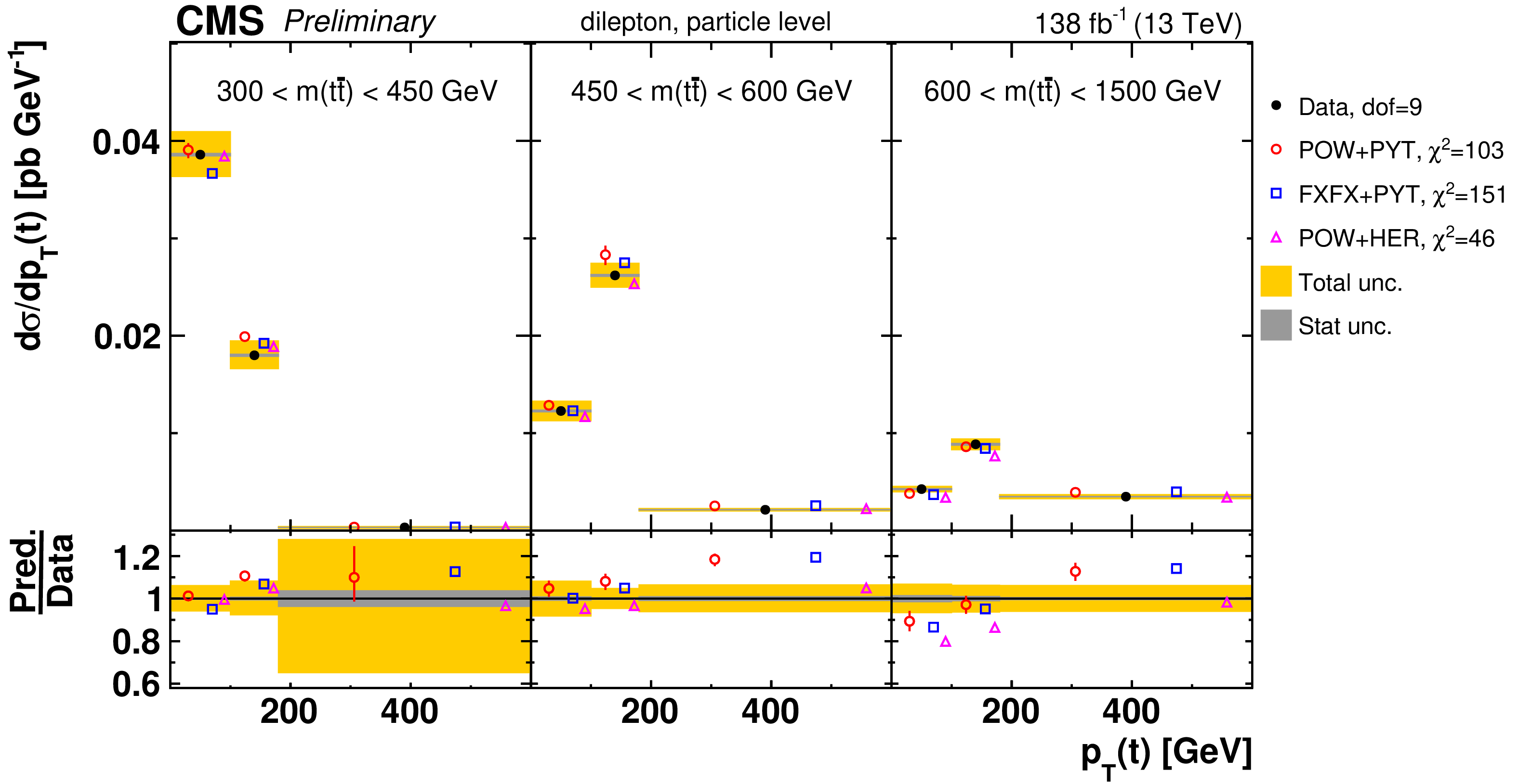
png pdf	Figure 71-b: Absolute $[ {m( \mathrm{t\bar{t}})},\,{{p_{\mathrm {T}}} (\mathrm{t})} ]$ cross sections are shown for data (filled circles) and various MC predictions (other points). Further details can be found in the caption of Fig. 70.
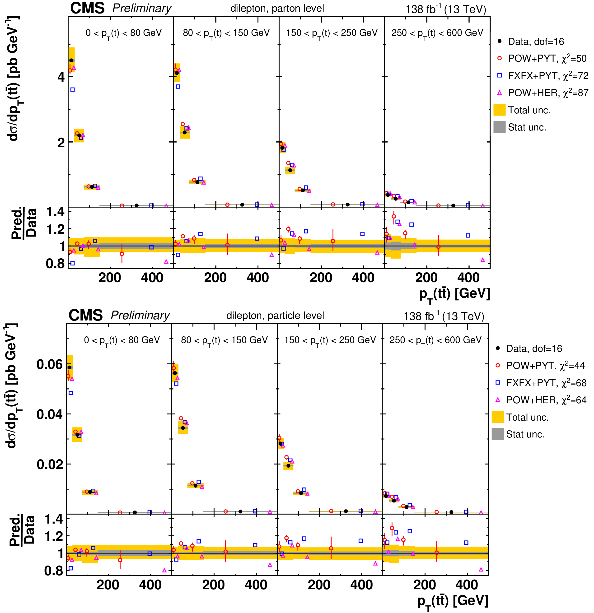
png pdf	Figure 72: Absolute $[ {{p_{\mathrm {T}}} (\mathrm{t})},\,{{p_{\mathrm {T}}} ( \mathrm{t\bar{t}})} ]$ cross sections are shown for data (filled circles) and various MC predictions (other points). Further details can be found in the caption of Fig. 70.
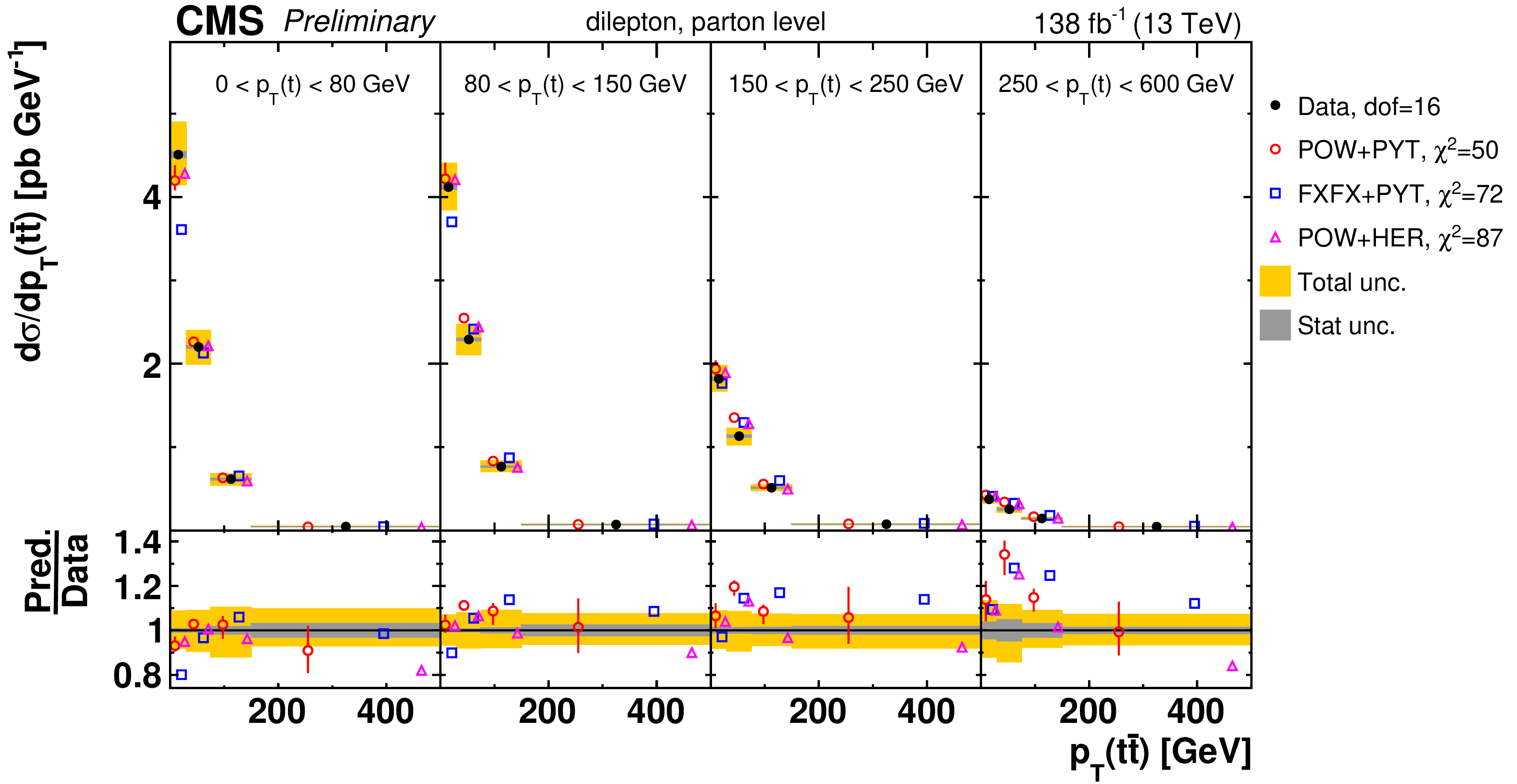
png pdf	Figure 72-a: Absolute $[ {{p_{\mathrm {T}}} (\mathrm{t})},\,{{p_{\mathrm {T}}} ( \mathrm{t\bar{t}})} ]$ cross sections are shown for data (filled circles) and various MC predictions (other points). Further details can be found in the caption of Fig. 70.
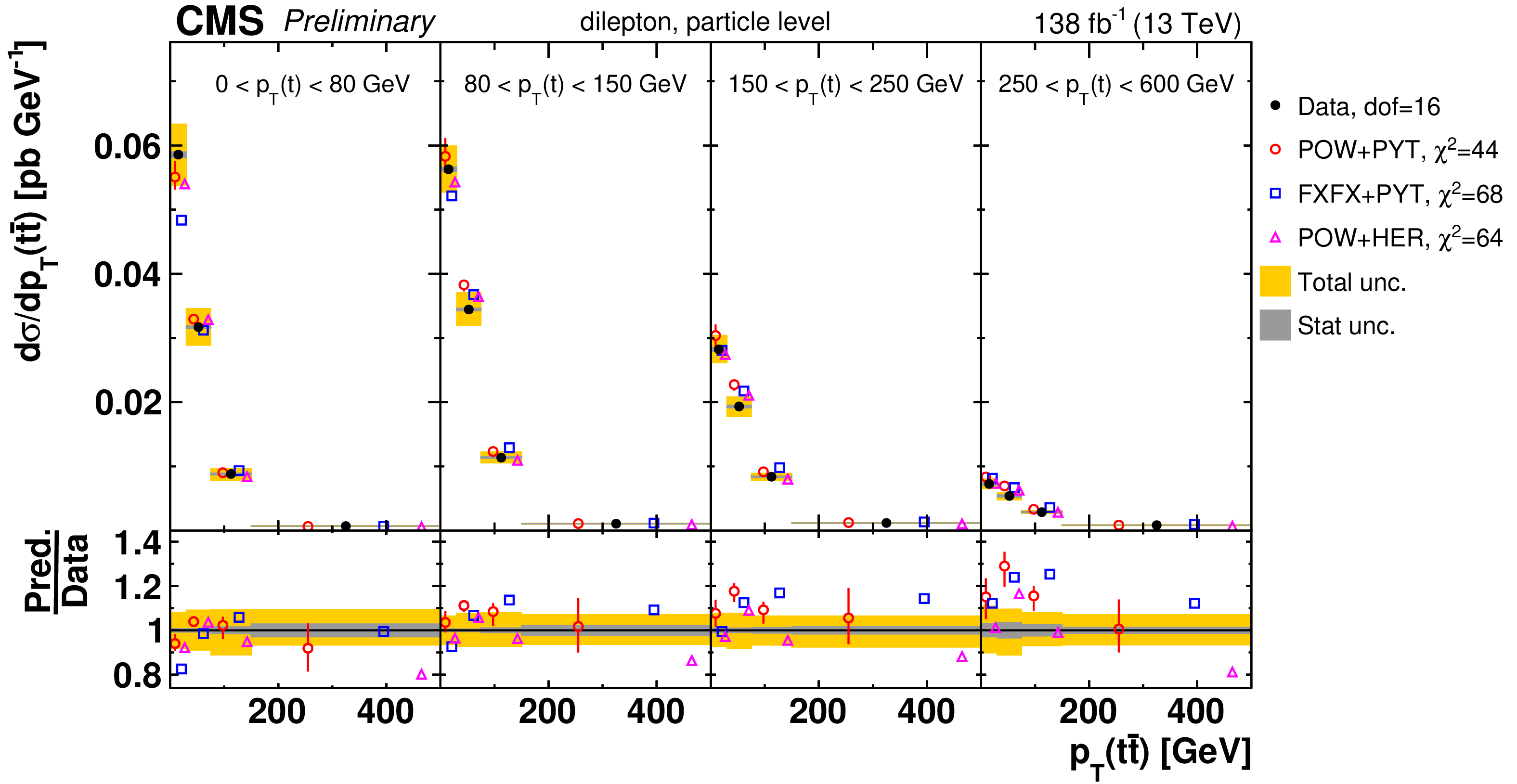
png pdf	Figure 72-b: Absolute $[ {{p_{\mathrm {T}}} (\mathrm{t})},\,{{p_{\mathrm {T}}} ( \mathrm{t\bar{t}})} ]$ cross sections are shown for data (filled circles) and various MC predictions (other points). Further details can be found in the caption of Fig. 70.
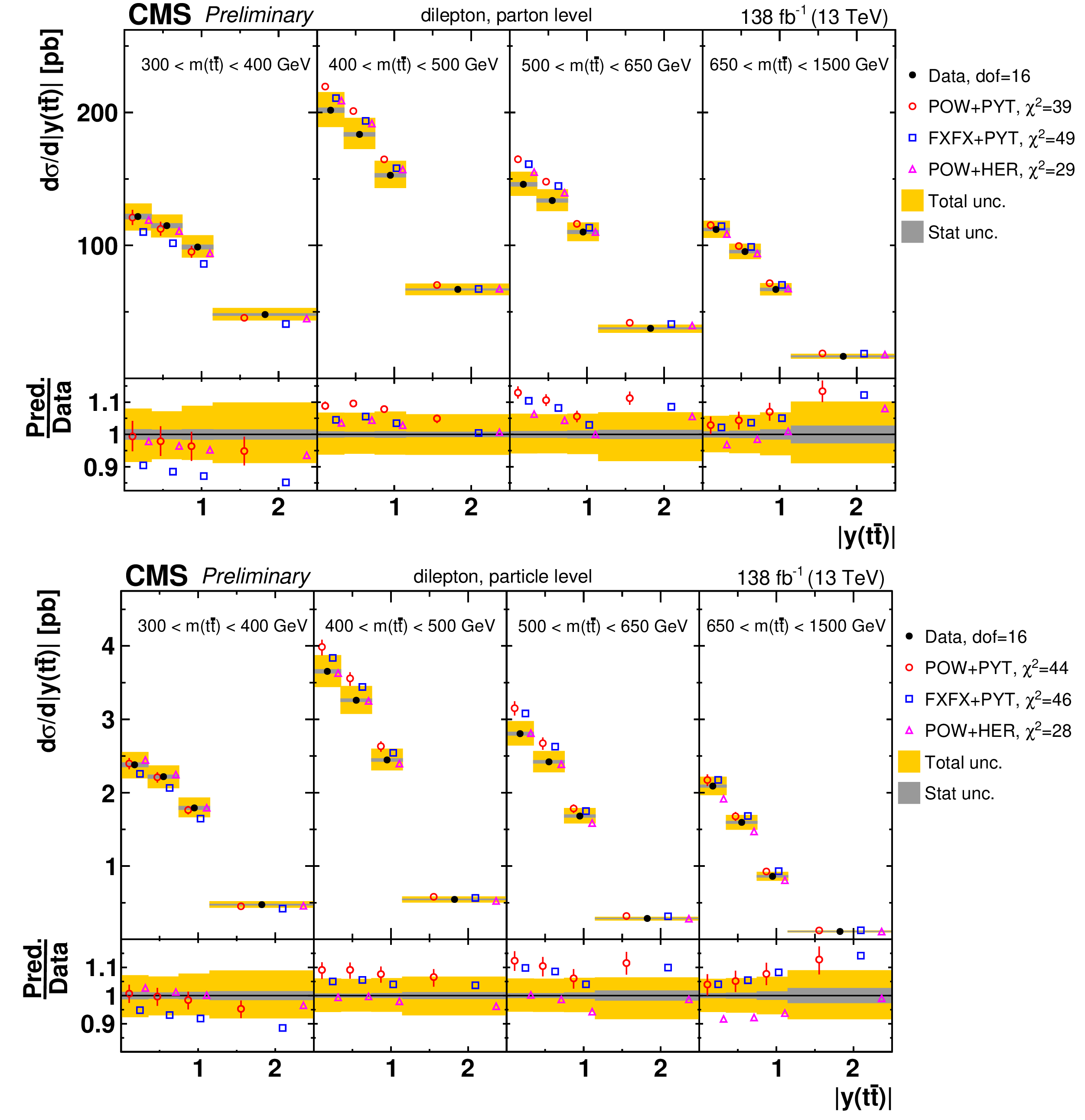
png pdf	Figure 73: Absolute $[ {m( \mathrm{t\bar{t}})},\,{|y( \mathrm{t\bar{t}})|} ]$ cross sections are shown for data (filled circles) and various MC predictions (other points). Further details can be found in the caption of Fig. 70.
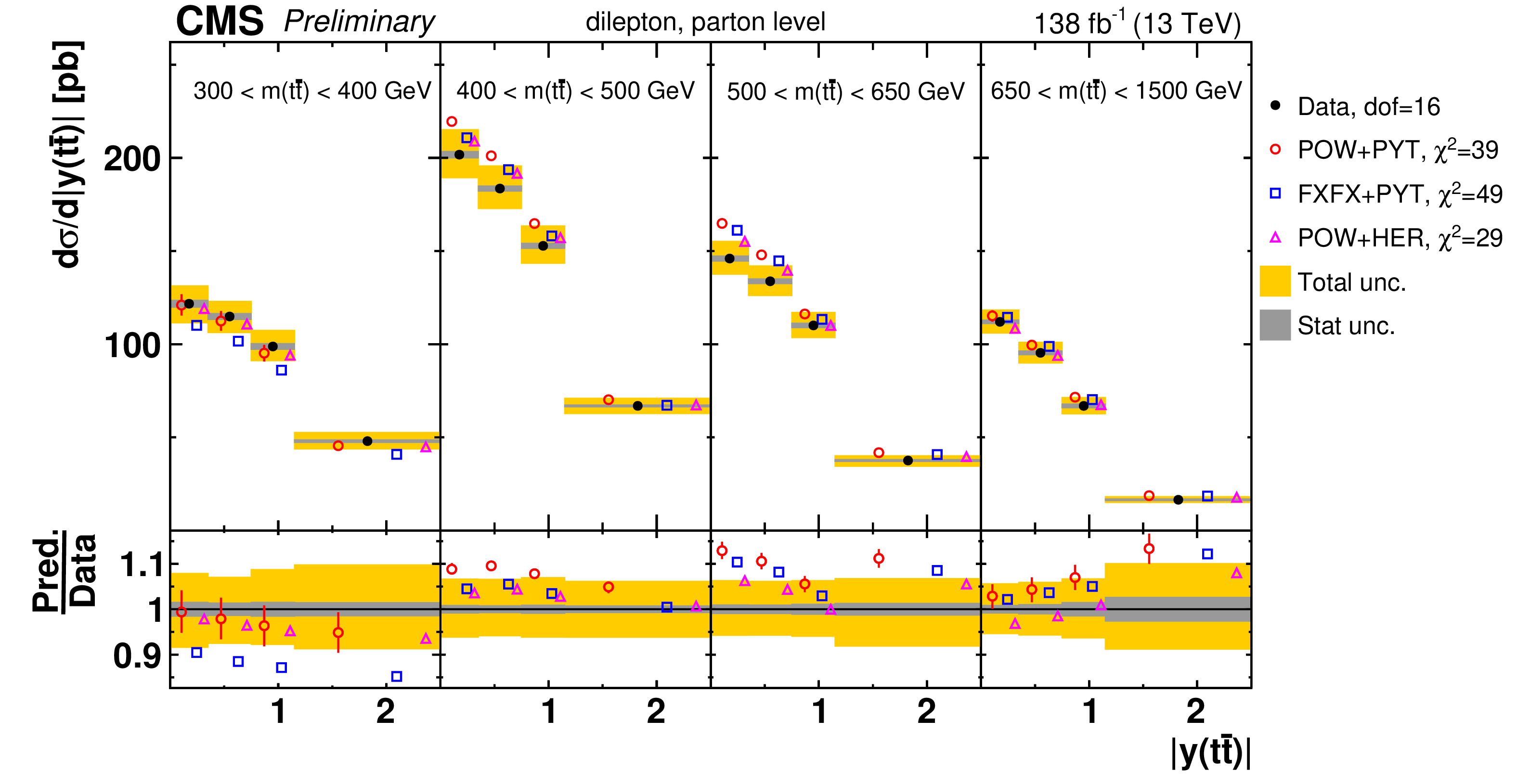
png pdf	Figure 73-a: Absolute $[ {m( \mathrm{t\bar{t}})},\,{|y( \mathrm{t\bar{t}})|} ]$ cross sections are shown for data (filled circles) and various MC predictions (other points). Further details can be found in the caption of Fig. 70.
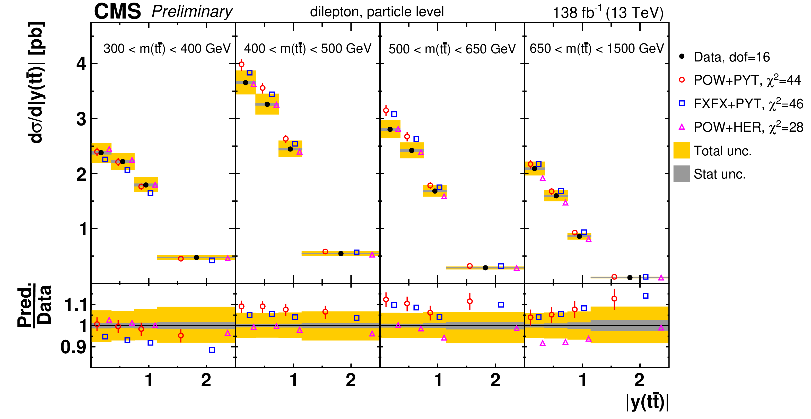
png pdf	Figure 73-b: Absolute $[ {m( \mathrm{t\bar{t}})},\,{|y( \mathrm{t\bar{t}})|} ]$ cross sections are shown for data (filled circles) and various MC predictions (other points). Further details can be found in the caption of Fig. 70.
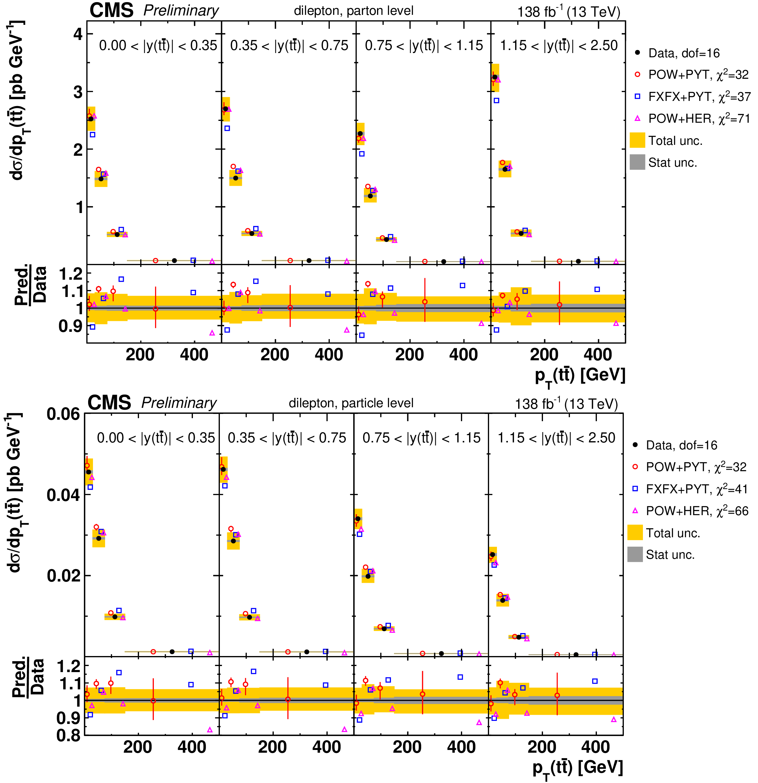
png pdf	Figure 74: Absolute $[ {|y( \mathrm{t\bar{t}})|},\,{{p_{\mathrm {T}}} ( \mathrm{t\bar{t}})} ]$ cross sections are shown for data (filled circles) and various MC predictions (other points). Further details can be found in the caption of Fig. 70.
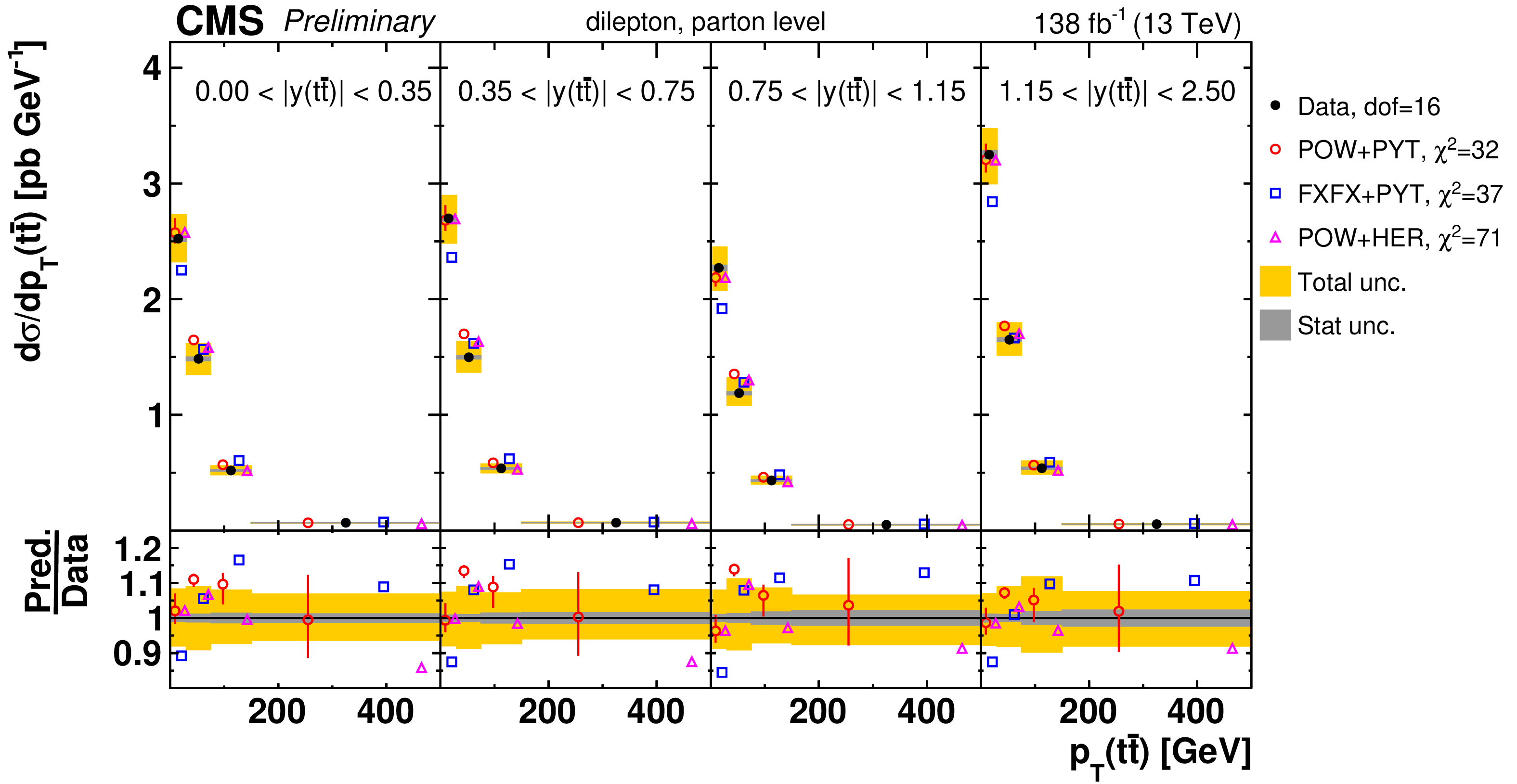
png pdf	Figure 74-a: Absolute $[ {|y( \mathrm{t\bar{t}})|},\,{{p_{\mathrm {T}}} ( \mathrm{t\bar{t}})} ]$ cross sections are shown for data (filled circles) and various MC predictions (other points). Further details can be found in the caption of Fig. 70.
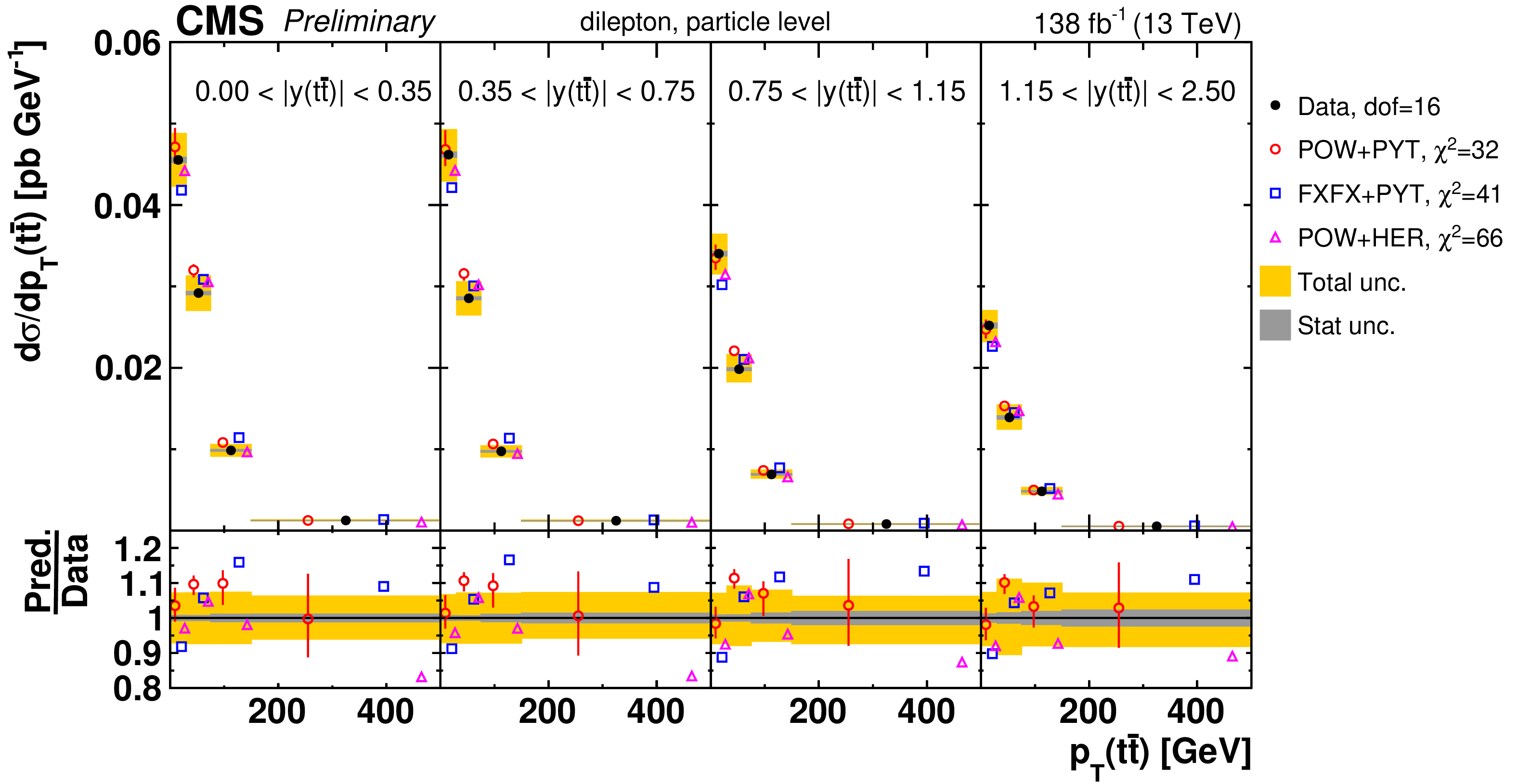
png pdf	Figure 74-b: Absolute $[ {|y( \mathrm{t\bar{t}})|},\,{{p_{\mathrm {T}}} ( \mathrm{t\bar{t}})} ]$ cross sections are shown for data (filled circles) and various MC predictions (other points). Further details can be found in the caption of Fig. 70.
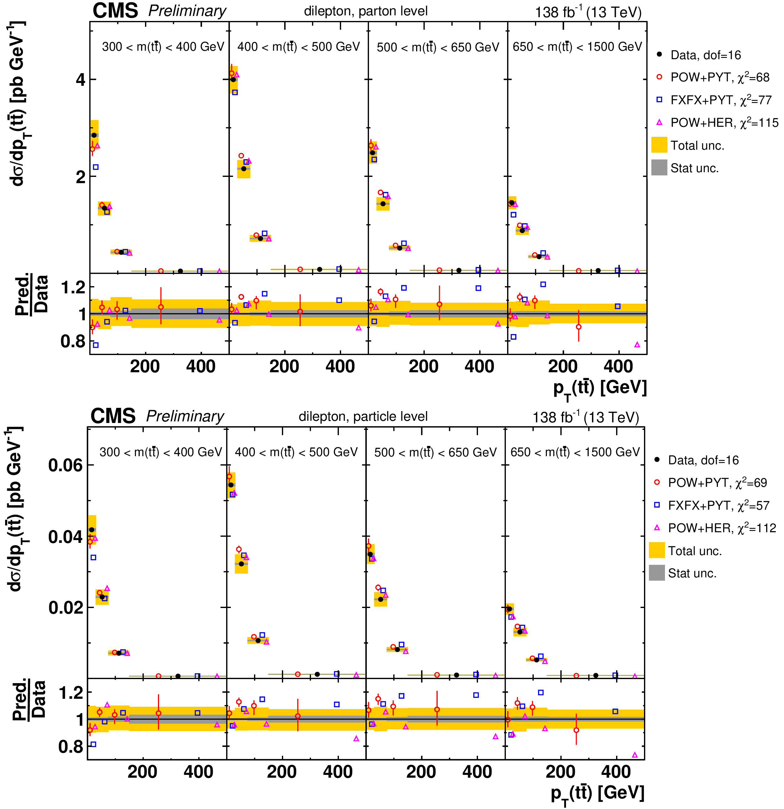
png pdf	Figure 75: Absolute $[ {m( \mathrm{t\bar{t}})},\,{{p_{\mathrm {T}}} ( \mathrm{t\bar{t}})} ]$ cross sections are shown for data (filled circles) and various MC predictions (other points). Further details can be found in the caption of Fig. 70.
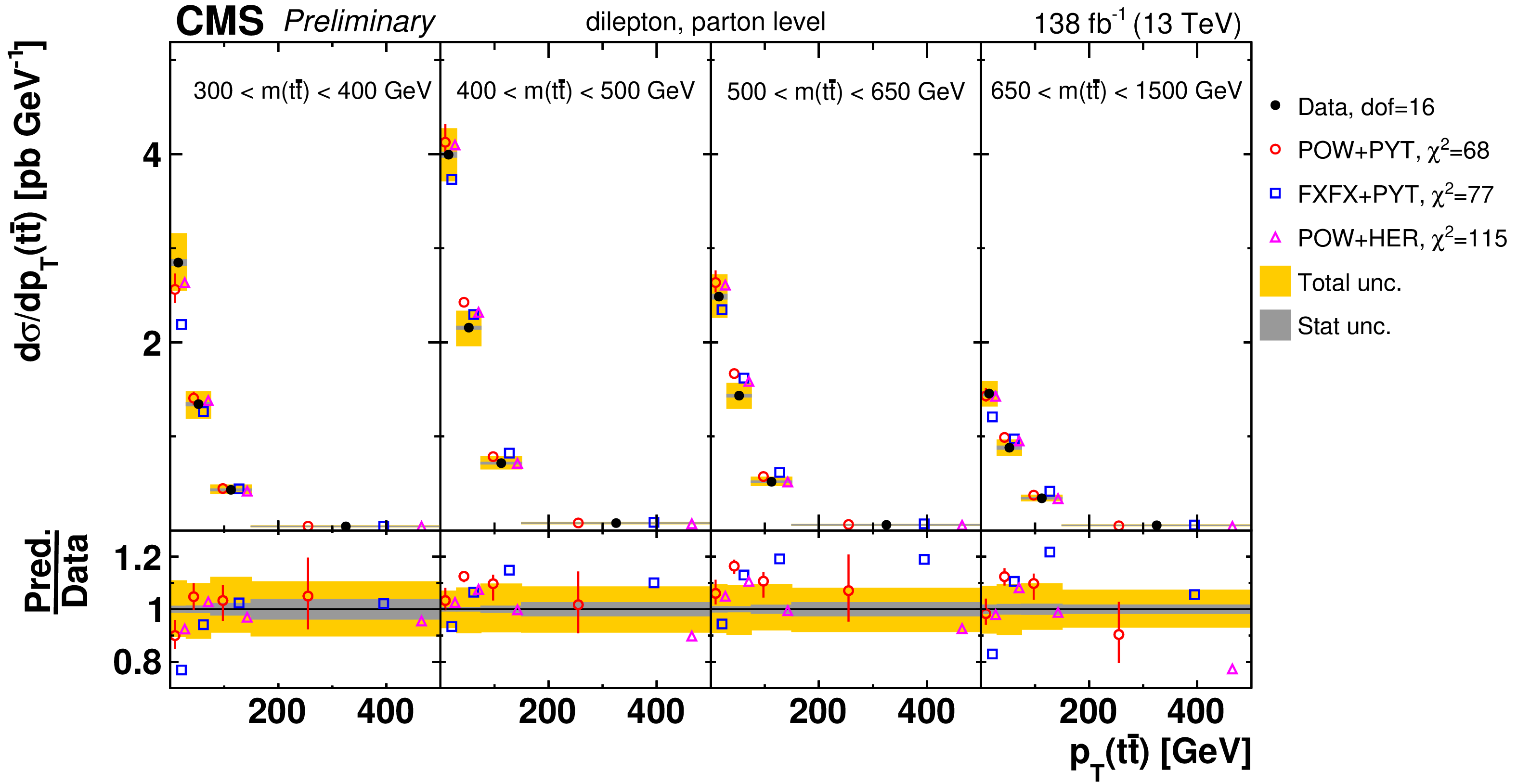
png pdf	Figure 75-a: Absolute $[ {m( \mathrm{t\bar{t}})},\,{{p_{\mathrm {T}}} ( \mathrm{t\bar{t}})} ]$ cross sections are shown for data (filled circles) and various MC predictions (other points). Further details can be found in the caption of Fig. 70.
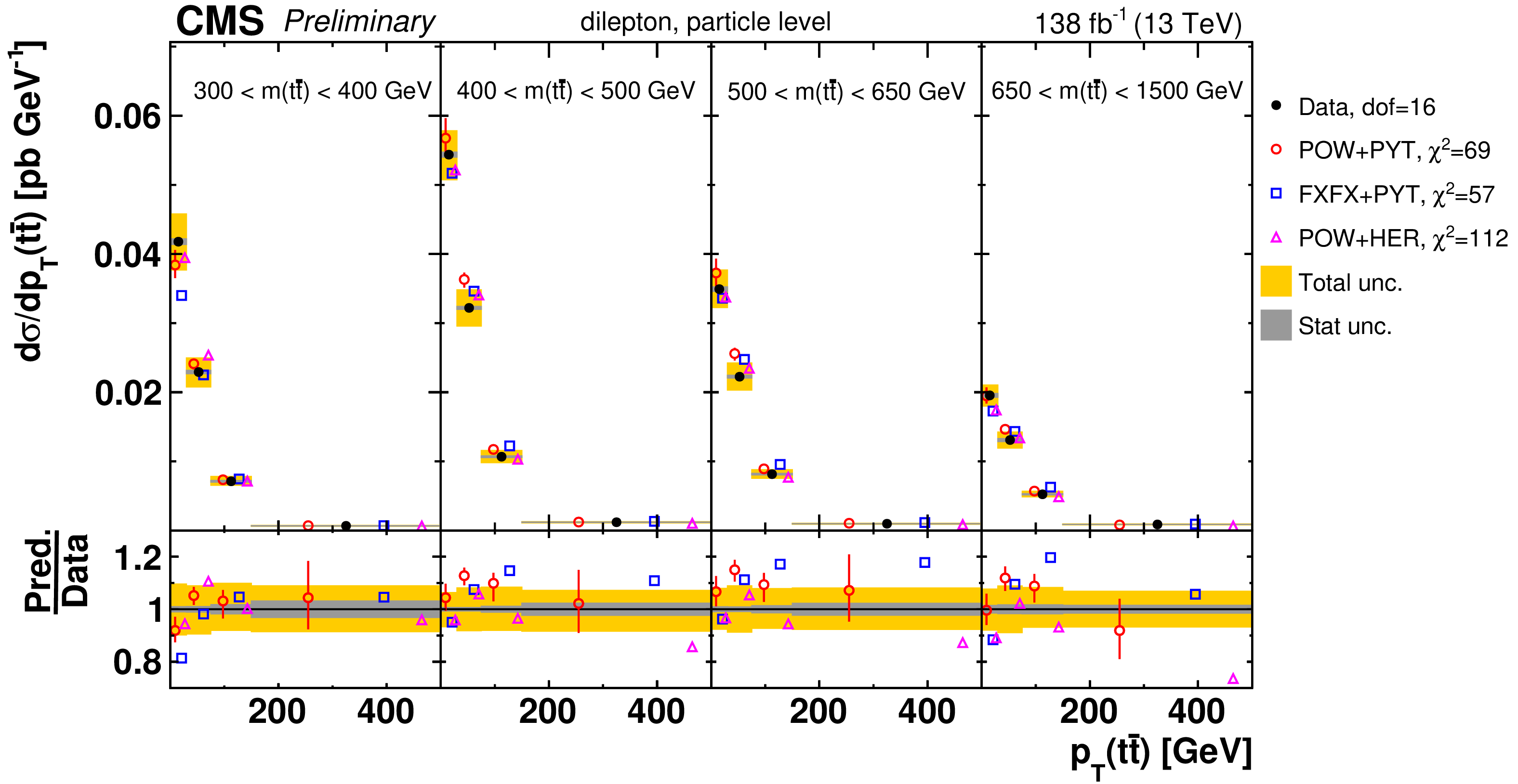
png pdf	Figure 75-b: Absolute $[ {m( \mathrm{t\bar{t}})},\,{{p_{\mathrm {T}}} ( \mathrm{t\bar{t}})} ]$ cross sections are shown for data (filled circles) and various MC predictions (other points). Further details can be found in the caption of Fig. 70.
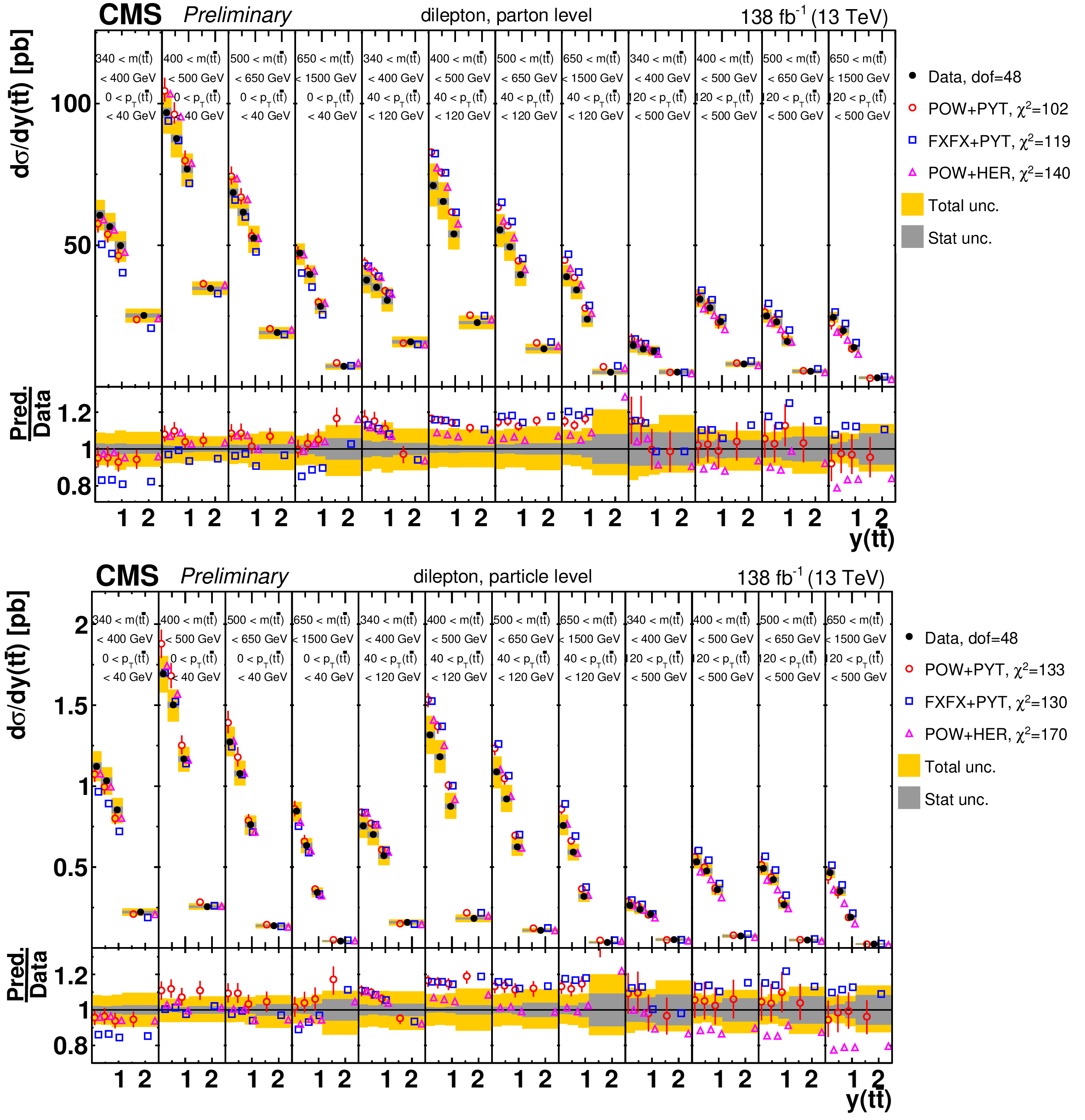
png pdf	Figure 76: Absolute $[ {{p_{\mathrm {T}}} ( \mathrm{t\bar{t}})},\,{m( \mathrm{t\bar{t}})},\,{y( \mathrm{t\bar{t}})} ]$ cross sections are shown for data (filled circles) and various MC predictions (other points). Further details can be found in the caption of Fig. 70.
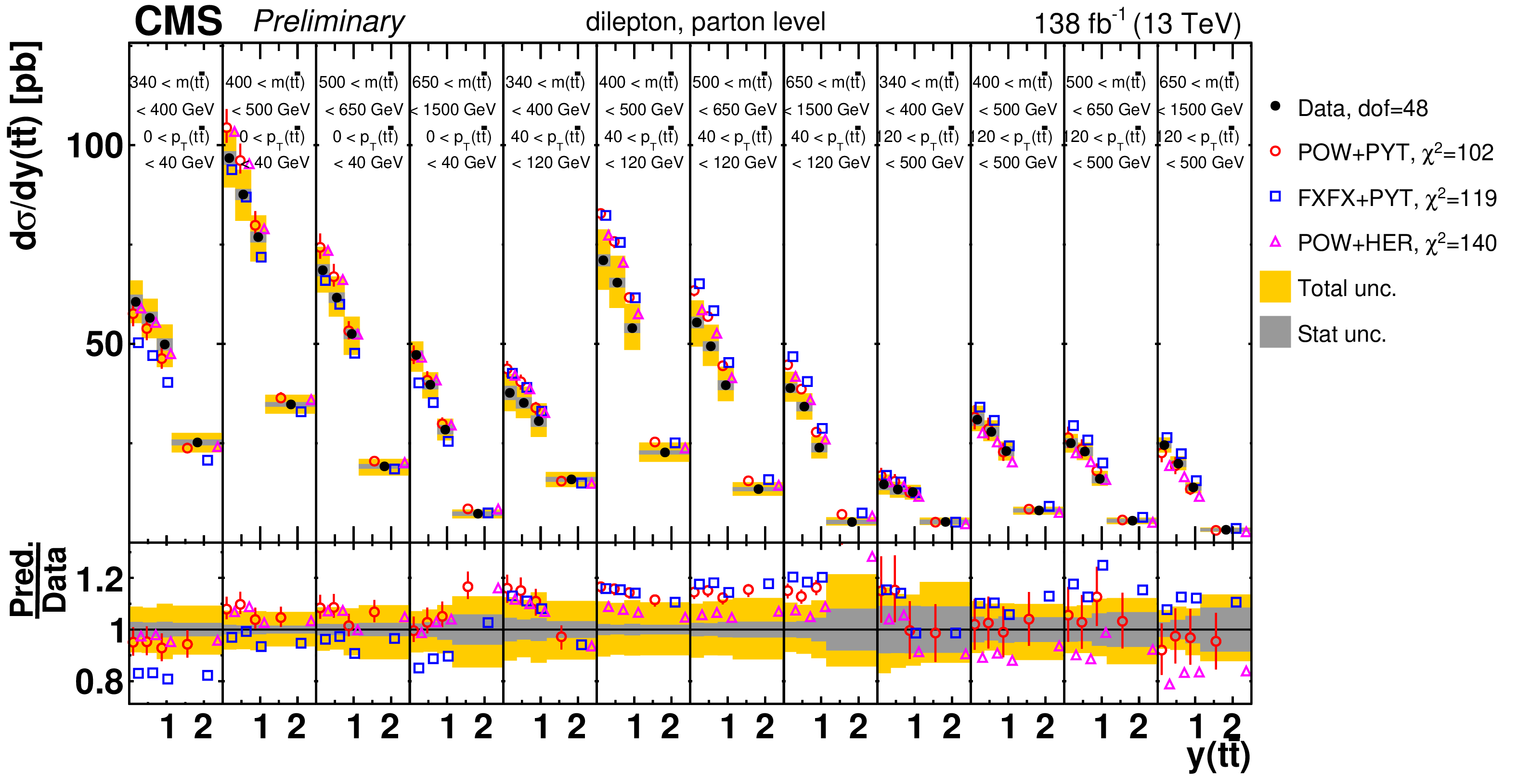
png pdf	Figure 76-a: Absolute $[ {{p_{\mathrm {T}}} ( \mathrm{t\bar{t}})},\,{m( \mathrm{t\bar{t}})},\,{y( \mathrm{t\bar{t}})} ]$ cross sections are shown for data (filled circles) and various MC predictions (other points). Further details can be found in the caption of Fig. 70.
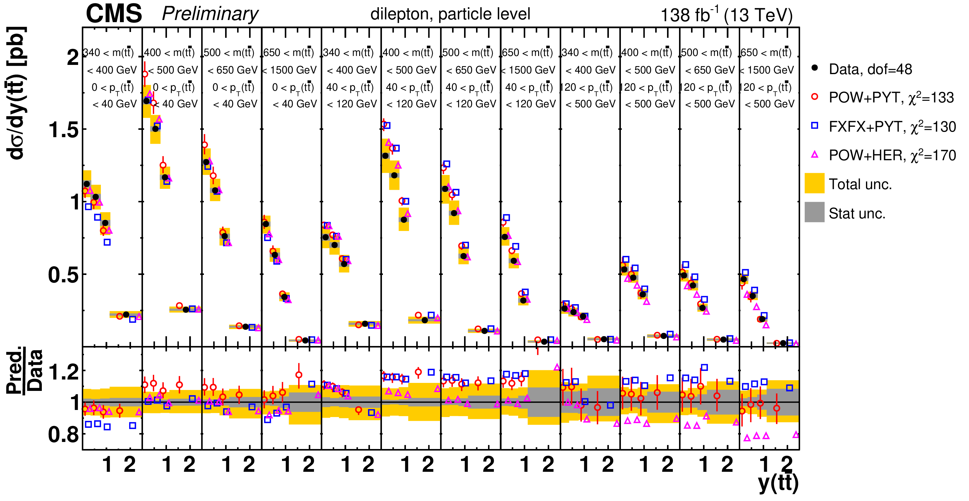
png pdf	Figure 76-b: Absolute $[ {{p_{\mathrm {T}}} ( \mathrm{t\bar{t}})},\,{m( \mathrm{t\bar{t}})},\,{y( \mathrm{t\bar{t}})} ]$ cross sections are shown for data (filled circles) and various MC predictions (other points). Further details can be found in the caption of Fig. 70.
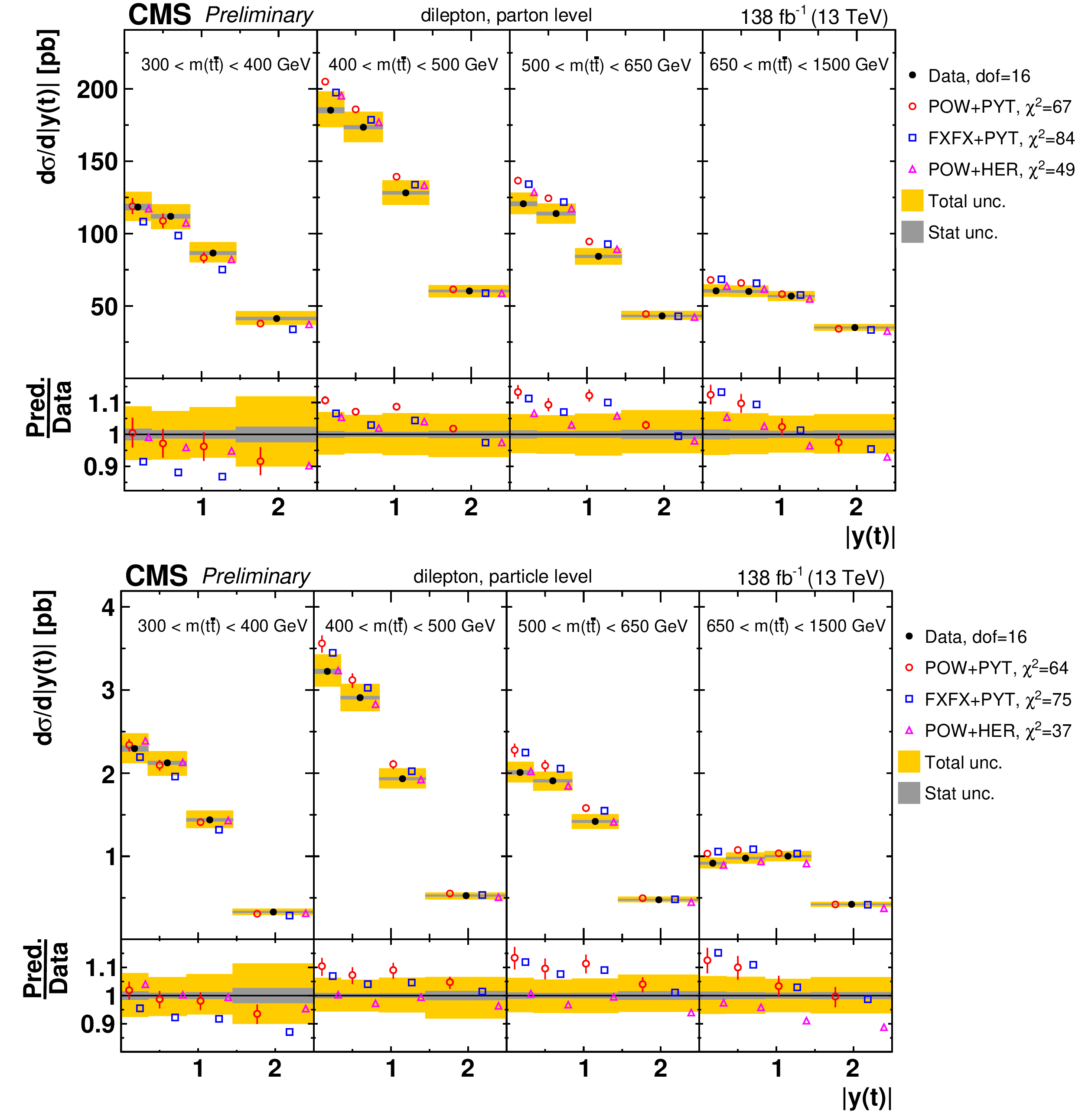
png pdf	Figure 77: Absolute $[ {m( \mathrm{t\bar{t}})},\,{|y(\mathrm{t})|} ]$ cross sections are shown for data (filled circles) and various MC predictions (other points). Further details can be found in the caption of Fig. 70.
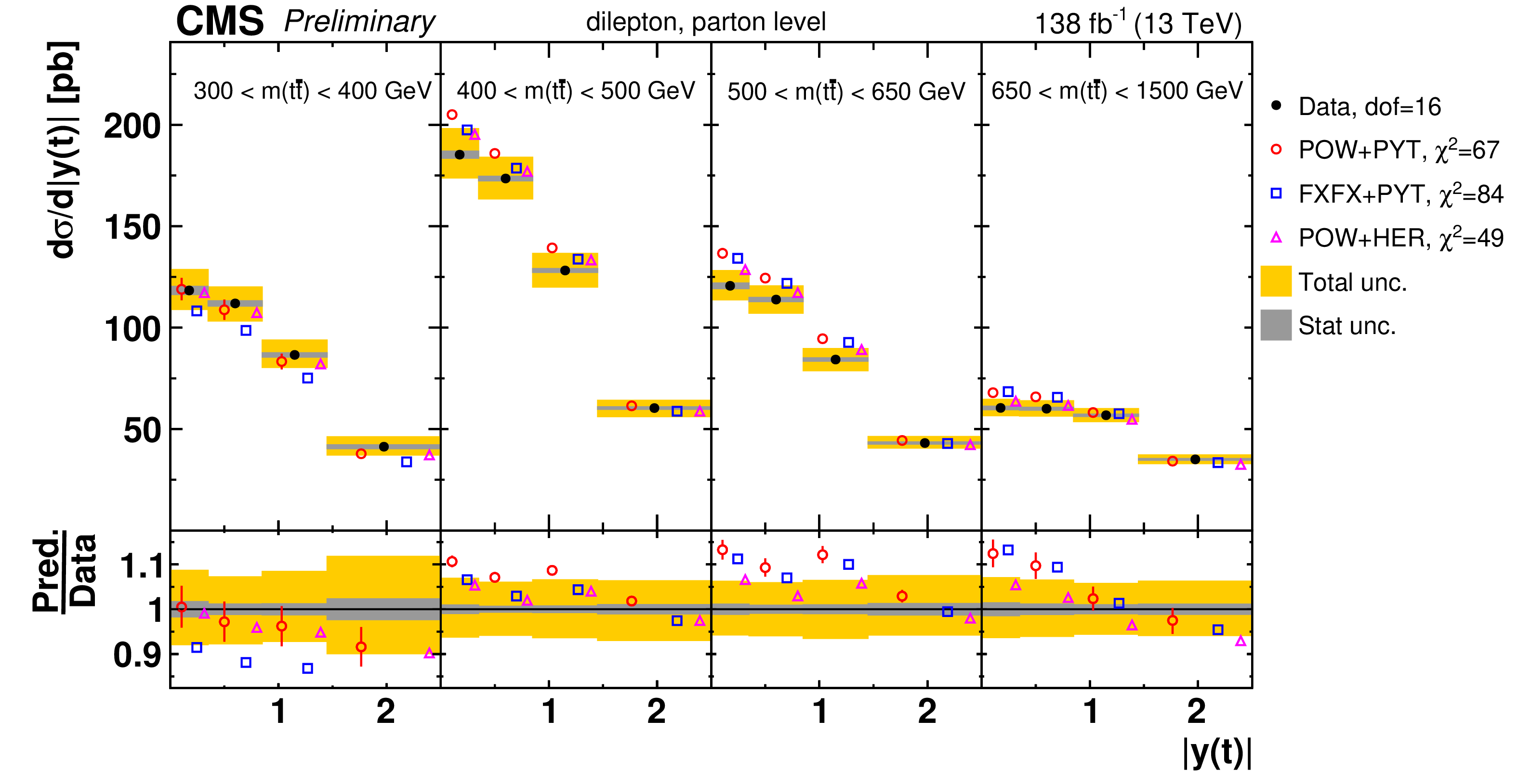
png pdf	Figure 77-a: Absolute $[ {m( \mathrm{t\bar{t}})},\,{|y(\mathrm{t})|} ]$ cross sections are shown for data (filled circles) and various MC predictions (other points). Further details can be found in the caption of Fig. 70.
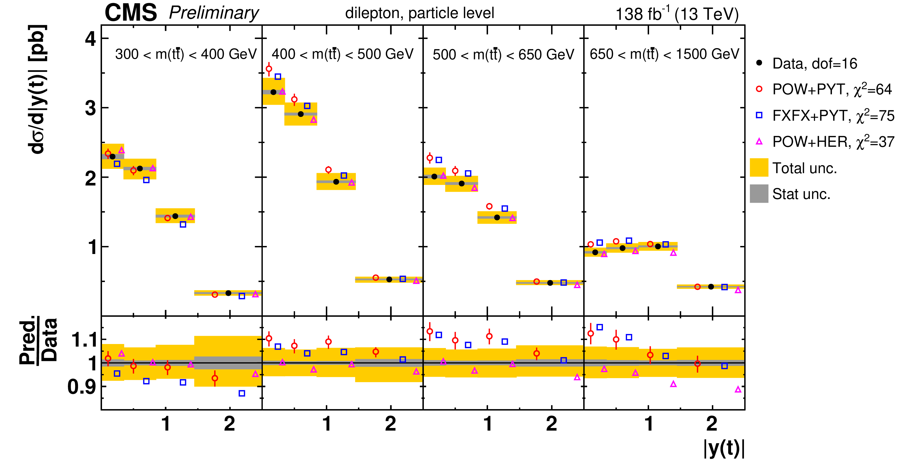
png pdf	Figure 77-b: Absolute $[ {m( \mathrm{t\bar{t}})},\,{|y(\mathrm{t})|} ]$ cross sections are shown for data (filled circles) and various MC predictions (other points). Further details can be found in the caption of Fig. 70.
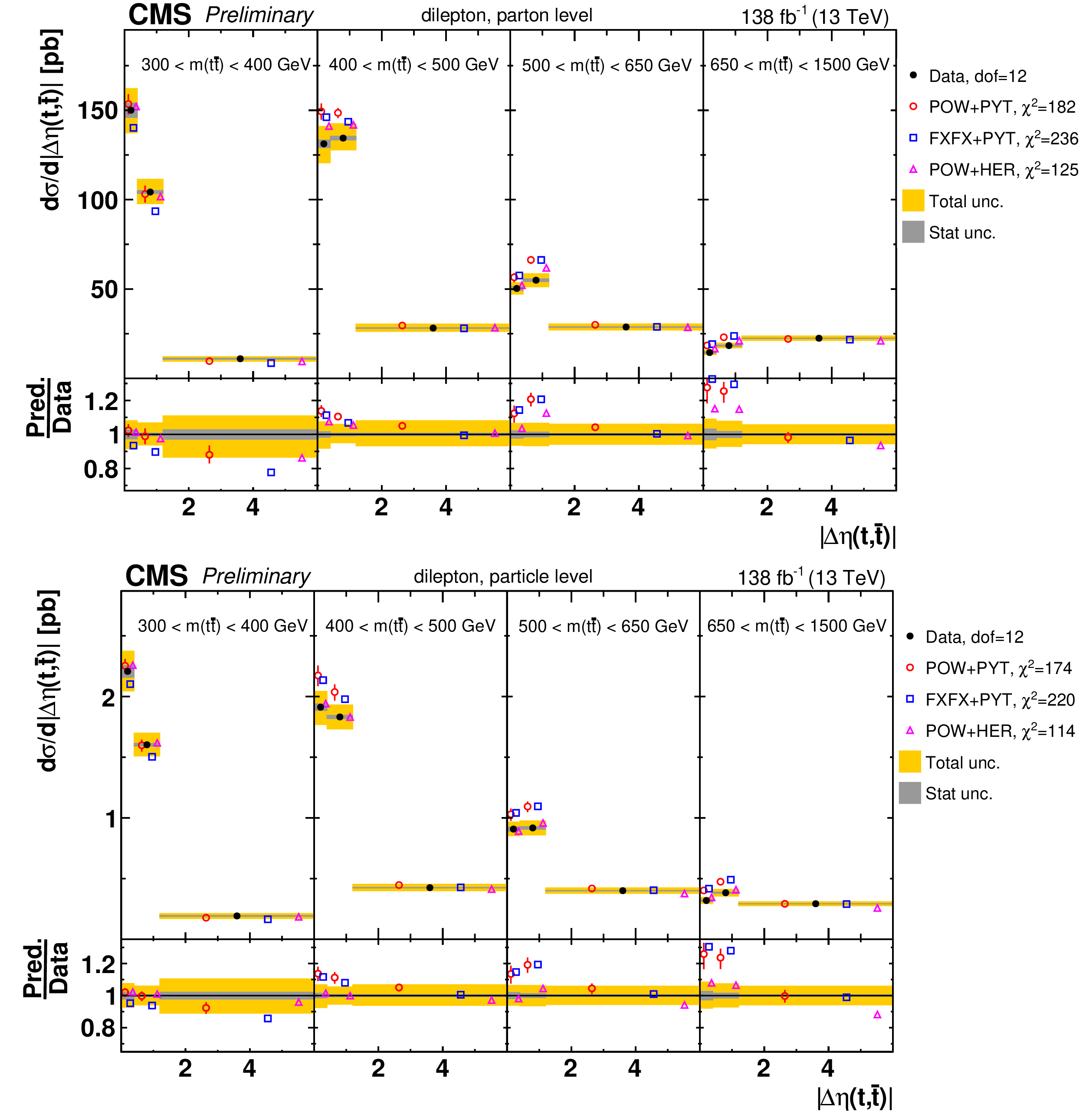
png pdf	Figure 78: Absolute $[ {m( \mathrm{t\bar{t}})},\,{|\Delta \eta (\mathrm{t},\mathrm{\bar{t}})|} ]$ cross sections are shown for data (filled circles) and various MC predictions (other points). Further details can be found in the caption of Fig. 70.
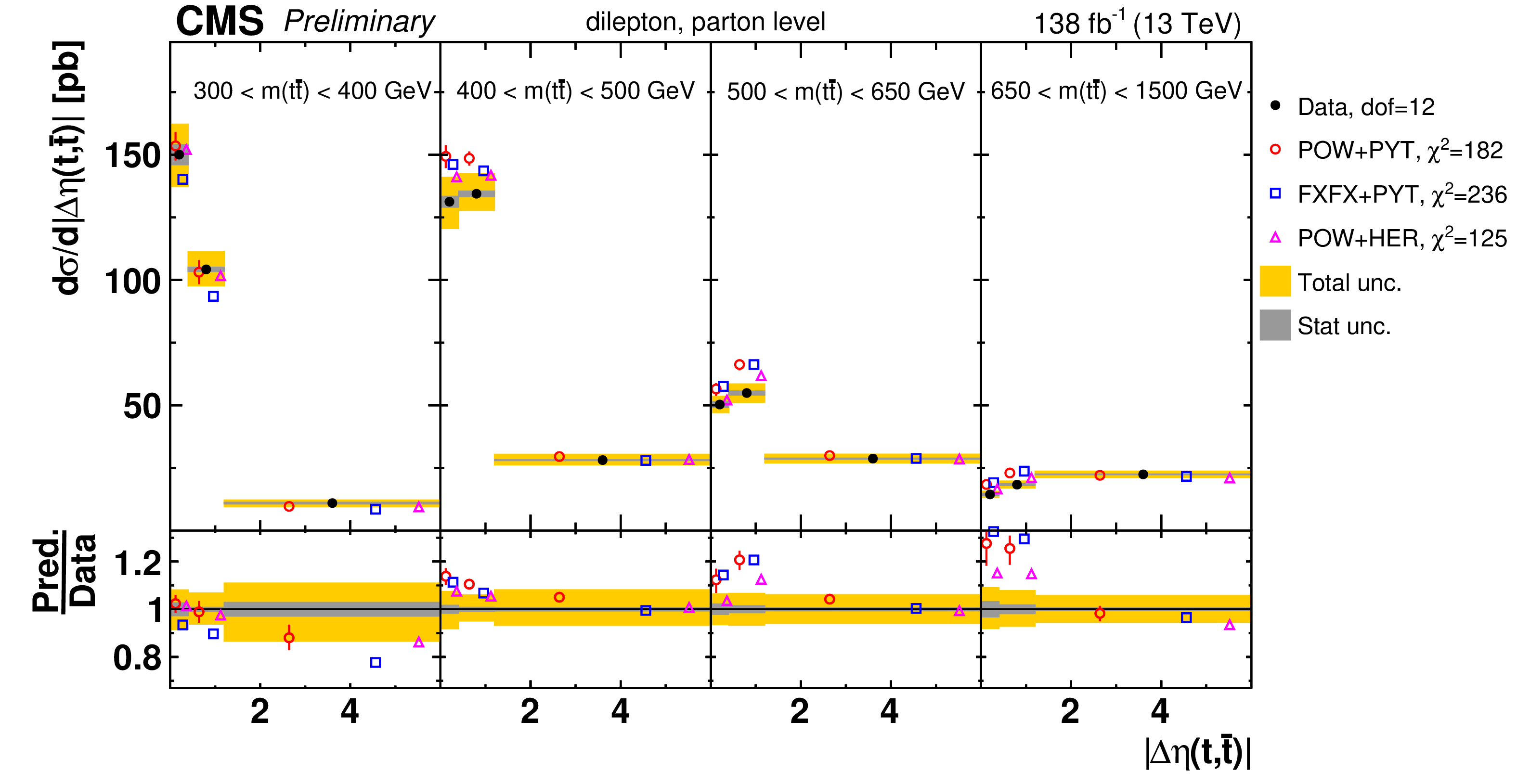
png pdf	Figure 78-a: Absolute $[ {m( \mathrm{t\bar{t}})},\,{|\Delta \eta (\mathrm{t},\mathrm{\bar{t}})|} ]$ cross sections are shown for data (filled circles) and various MC predictions (other points). Further details can be found in the caption of Fig. 70.
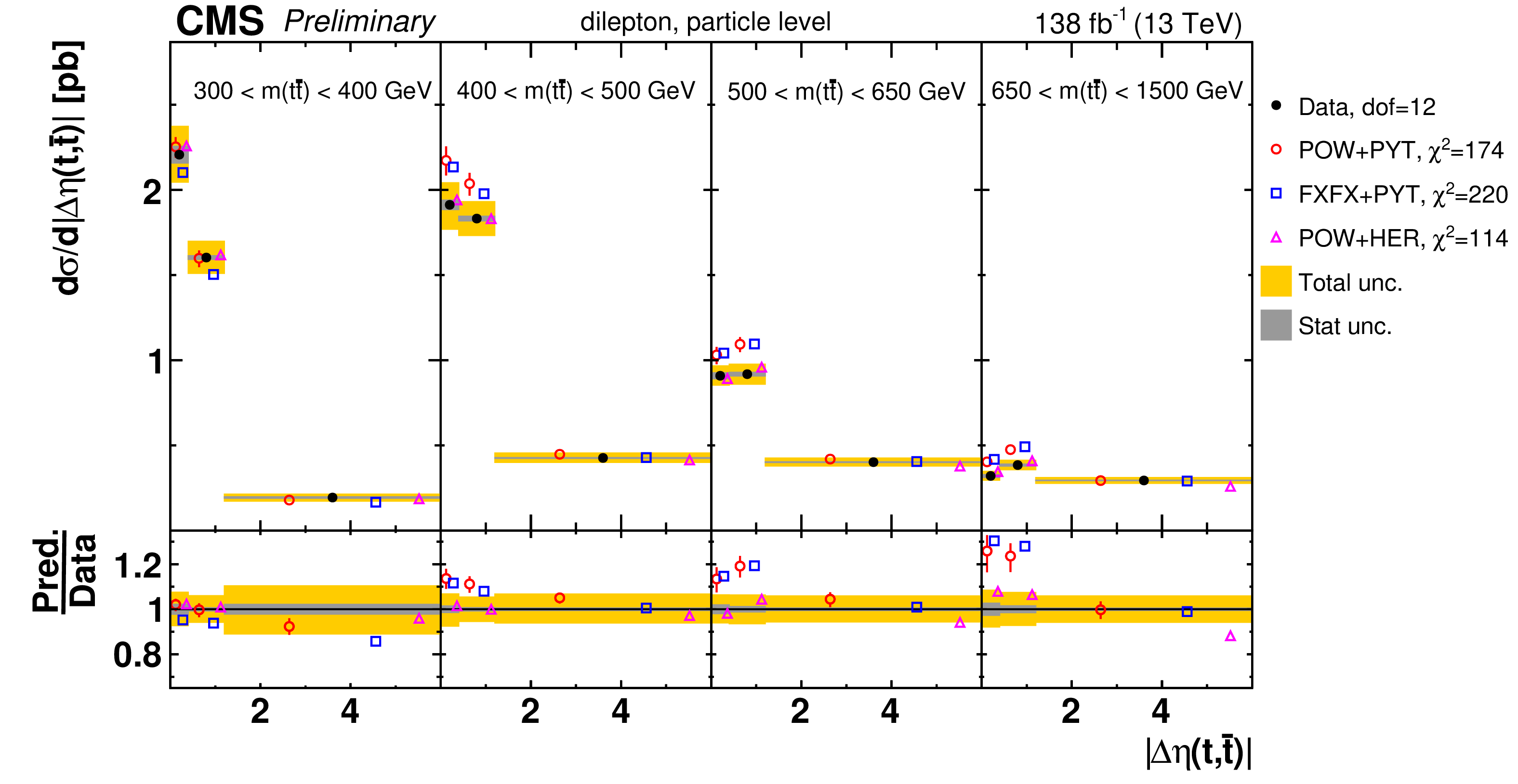
png pdf	Figure 78-b: Absolute $[ {m( \mathrm{t\bar{t}})},\,{|\Delta \eta (\mathrm{t},\mathrm{\bar{t}})|} ]$ cross sections are shown for data (filled circles) and various MC predictions (other points). Further details can be found in the caption of Fig. 70.
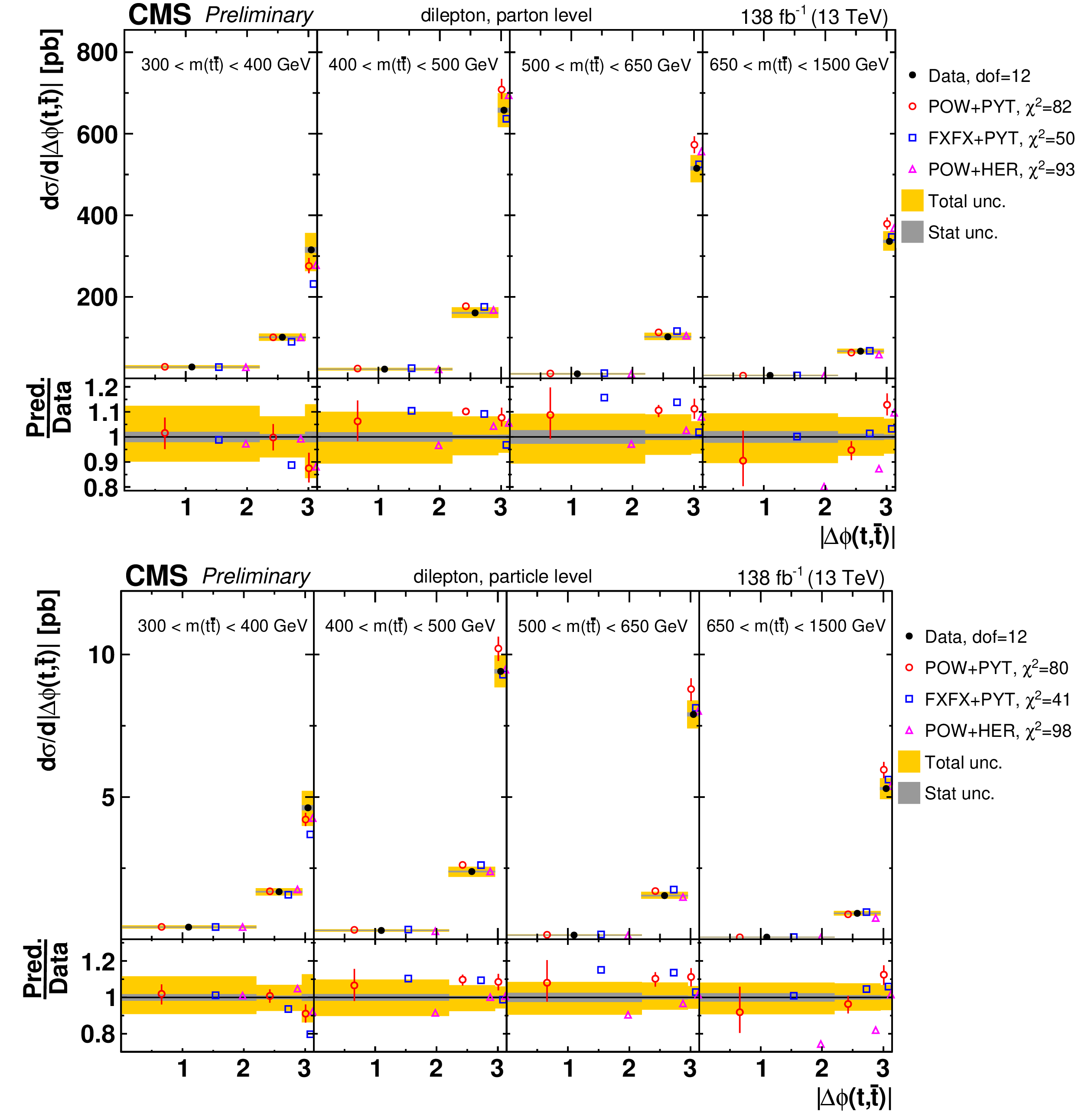
png pdf	Figure 79: Absolute $[ {m( \mathrm{t\bar{t}})},\,{|\Delta \phi (\mathrm{t},\mathrm{\bar{t}})|} ]$ cross sections are shown for data (filled circles) and various MC predictions (other points). Further details can be found in the caption of Fig. 70.
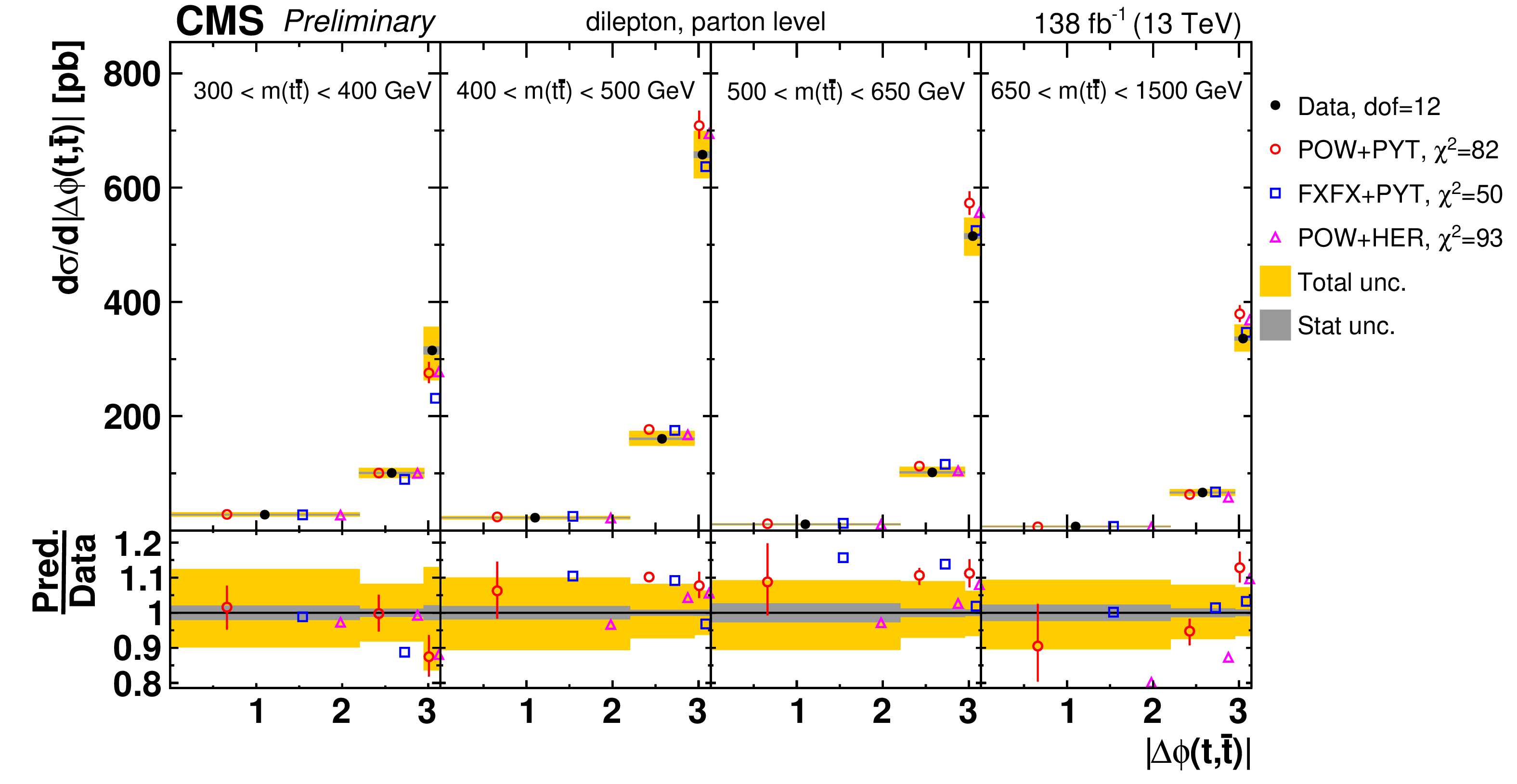
png pdf	Figure 79-a: Absolute $[ {m( \mathrm{t\bar{t}})},\,{|\Delta \phi (\mathrm{t},\mathrm{\bar{t}})|} ]$ cross sections are shown for data (filled circles) and various MC predictions (other points). Further details can be found in the caption of Fig. 70.
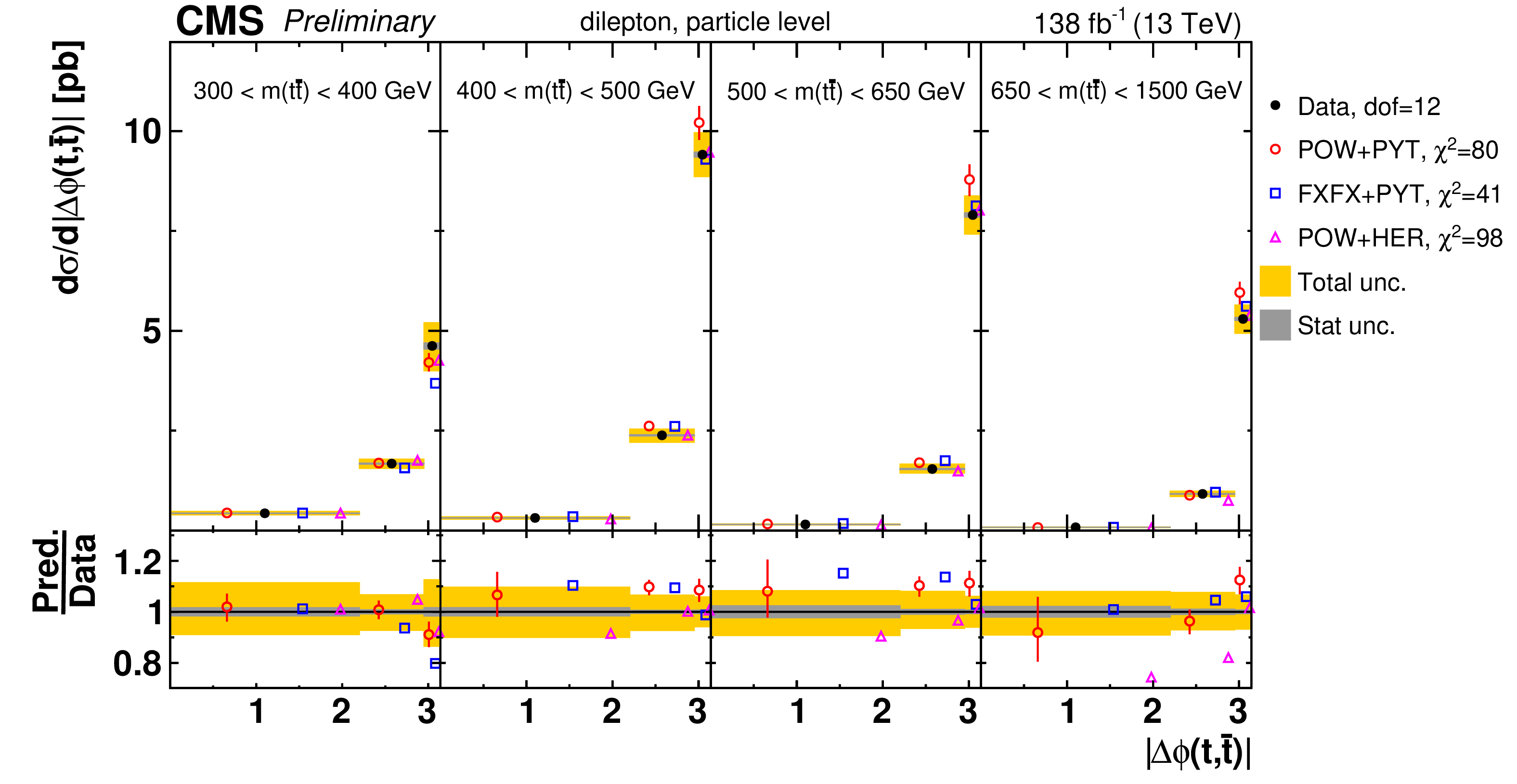
png pdf	Figure 79-b: Absolute $[ {m( \mathrm{t\bar{t}})},\,{|\Delta \phi (\mathrm{t},\mathrm{\bar{t}})|} ]$ cross sections are shown for data (filled circles) and various MC predictions (other points). Further details can be found in the caption of Fig. 70.
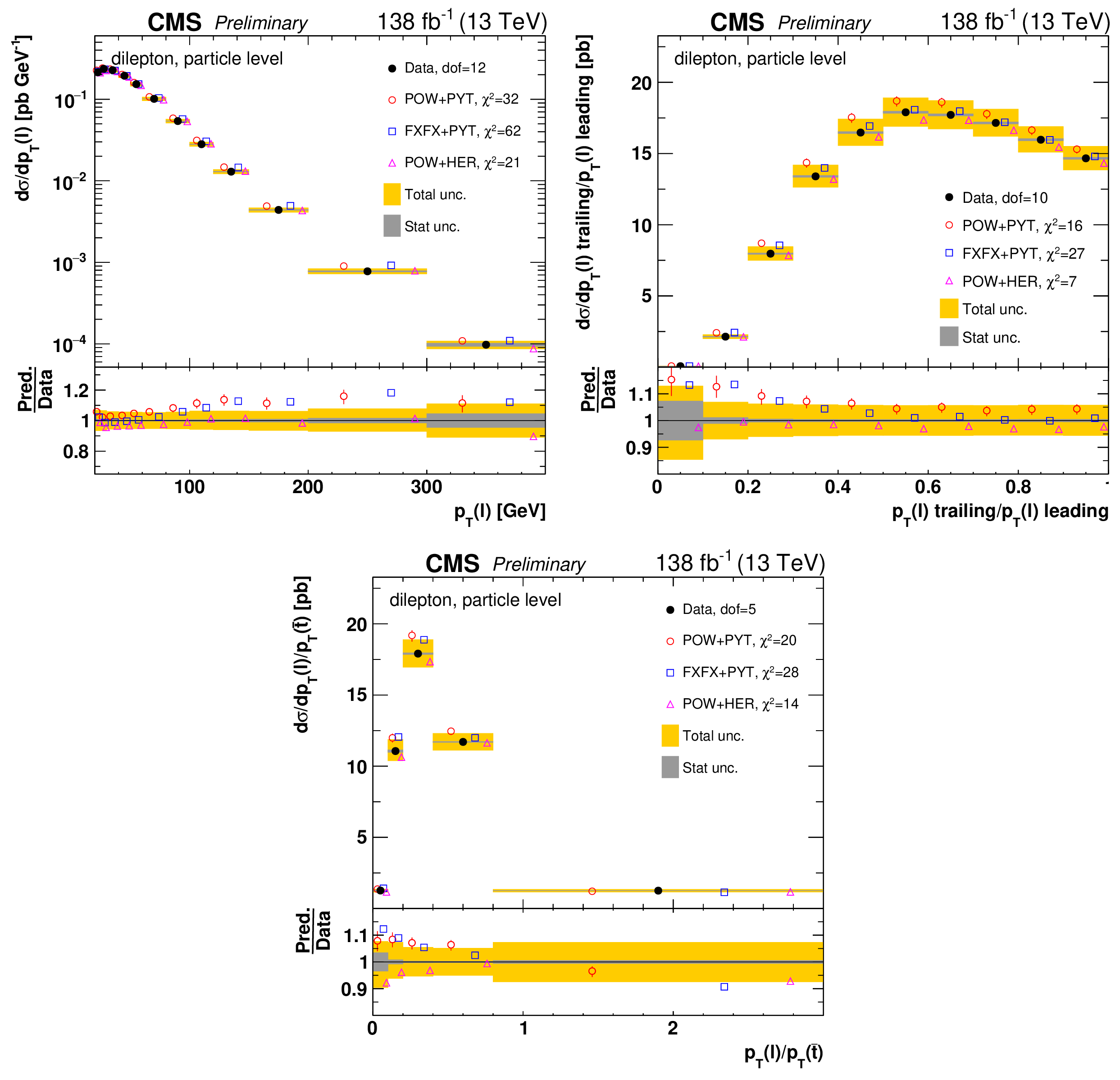
png pdf	Figure 80: Absolute differential $\mathrm{t\bar{t}}$ production cross sections as a function of ${p_{\mathrm {T}}}$ of the lepton (upper left), of the ratio of the trailing and leading lepton ${p_{\mathrm {T}}}$ (upper right), and of the ratio of lepton and top antiquark ${p_{\mathrm {T}}}$ (lower middle), measured at the particle level in a fiducial phase space. The data are shown as filled circles with dark and light bands indicating the statistical and total uncertainties (statistical and systematic uncertainties summed in quadrature), respectively. The cross sections are compared to various MC predictions (other points). The estimated uncertainties in the POWHEG+PYTHIA-8 (`POW-PYT') simulation are represented by a vertical bar on the corresponding points. For each MC model, a value of ${\chi ^2}$ is reported that takes into account the measurement uncertainties. The lower panel in each plot shows the ratios of the predictions to the data.
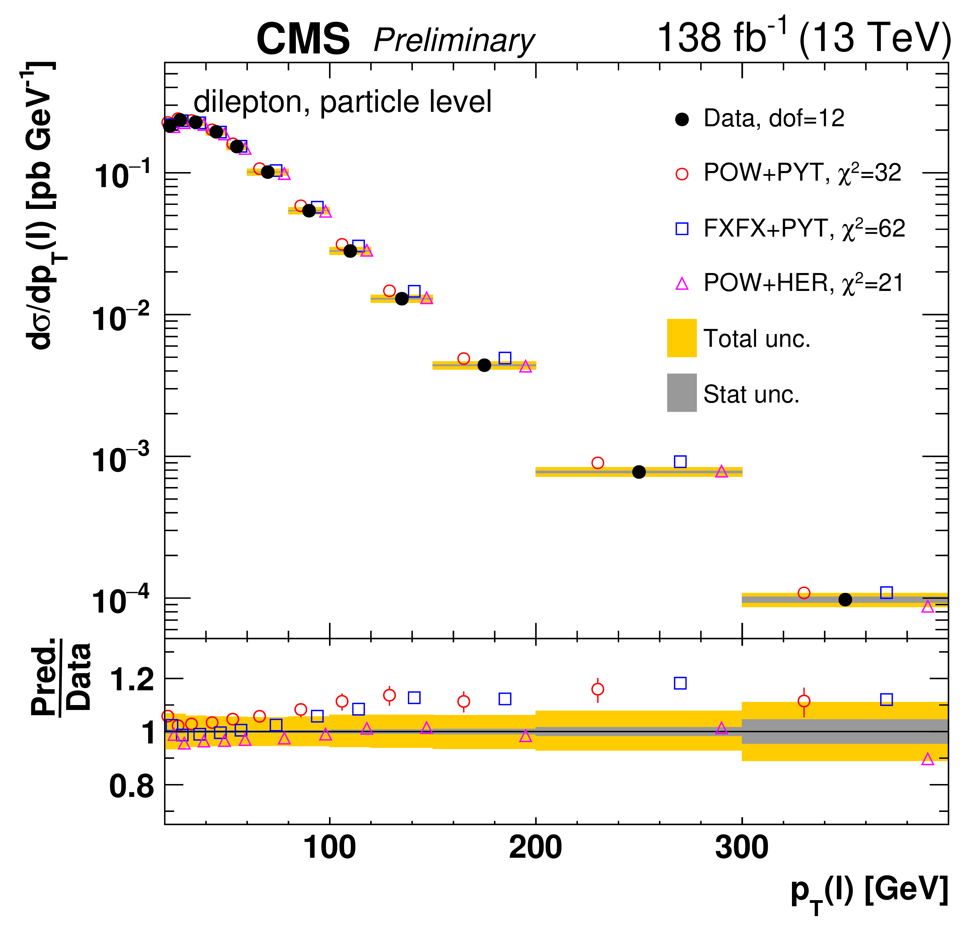
png pdf	Figure 80-a: Absolute differential $\mathrm{t\bar{t}}$ production cross sections as a function of ${p_{\mathrm {T}}}$ of the lepton (upper left), of the ratio of the trailing and leading lepton ${p_{\mathrm {T}}}$ (upper right), and of the ratio of lepton and top antiquark ${p_{\mathrm {T}}}$ (lower middle), measured at the particle level in a fiducial phase space. The data are shown as filled circles with dark and light bands indicating the statistical and total uncertainties (statistical and systematic uncertainties summed in quadrature), respectively. The cross sections are compared to various MC predictions (other points). The estimated uncertainties in the POWHEG+PYTHIA-8 (`POW-PYT') simulation are represented by a vertical bar on the corresponding points. For each MC model, a value of ${\chi ^2}$ is reported that takes into account the measurement uncertainties. The lower panel in each plot shows the ratios of the predictions to the data.
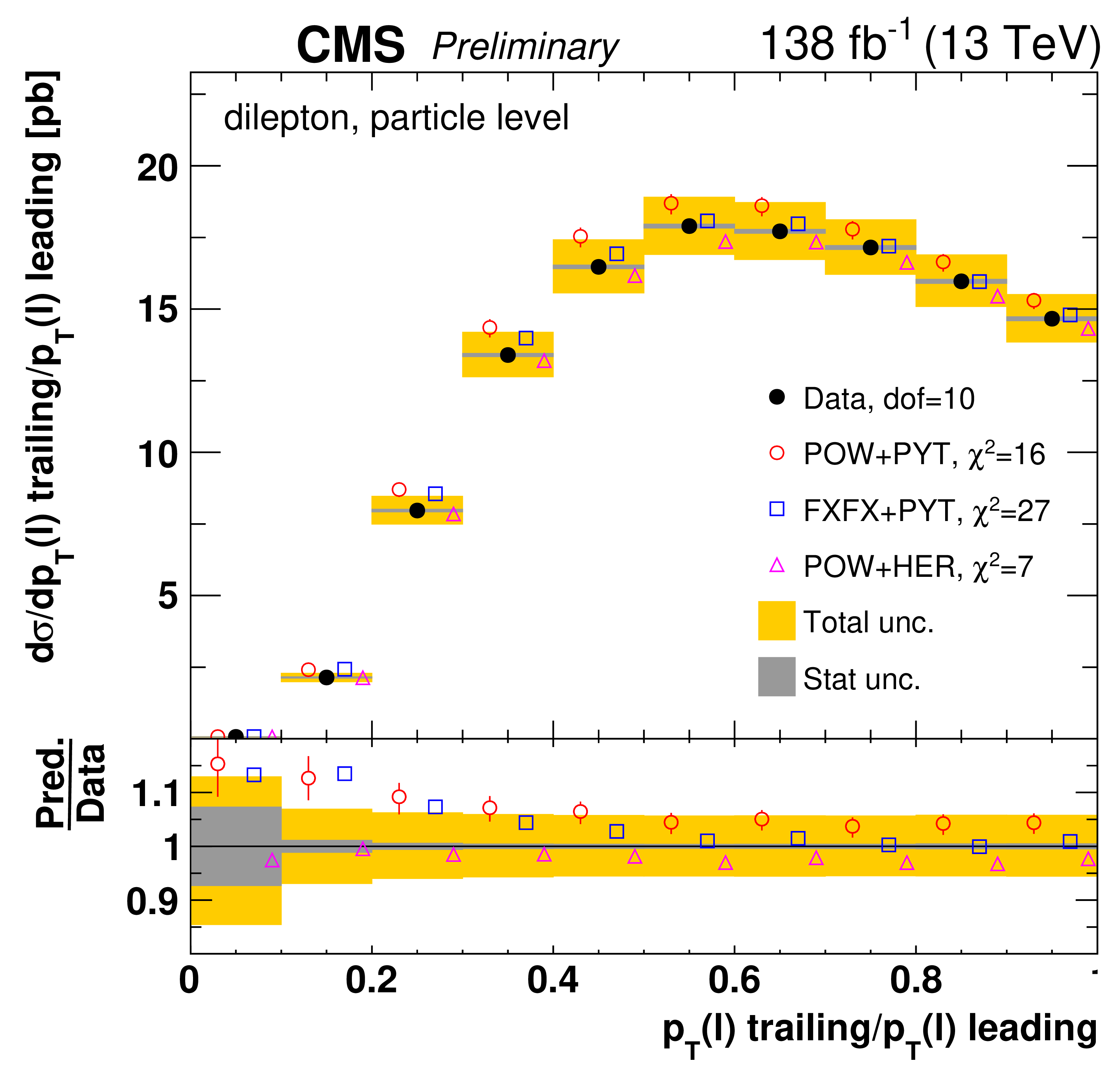
png pdf	Figure 80-b: Absolute differential $\mathrm{t\bar{t}}$ production cross sections as a function of ${p_{\mathrm {T}}}$ of the lepton (upper left), of the ratio of the trailing and leading lepton ${p_{\mathrm {T}}}$ (upper right), and of the ratio of lepton and top antiquark ${p_{\mathrm {T}}}$ (lower middle), measured at the particle level in a fiducial phase space. The data are shown as filled circles with dark and light bands indicating the statistical and total uncertainties (statistical and systematic uncertainties summed in quadrature), respectively. The cross sections are compared to various MC predictions (other points). The estimated uncertainties in the POWHEG+PYTHIA-8 (`POW-PYT') simulation are represented by a vertical bar on the corresponding points. For each MC model, a value of ${\chi ^2}$ is reported that takes into account the measurement uncertainties. The lower panel in each plot shows the ratios of the predictions to the data.
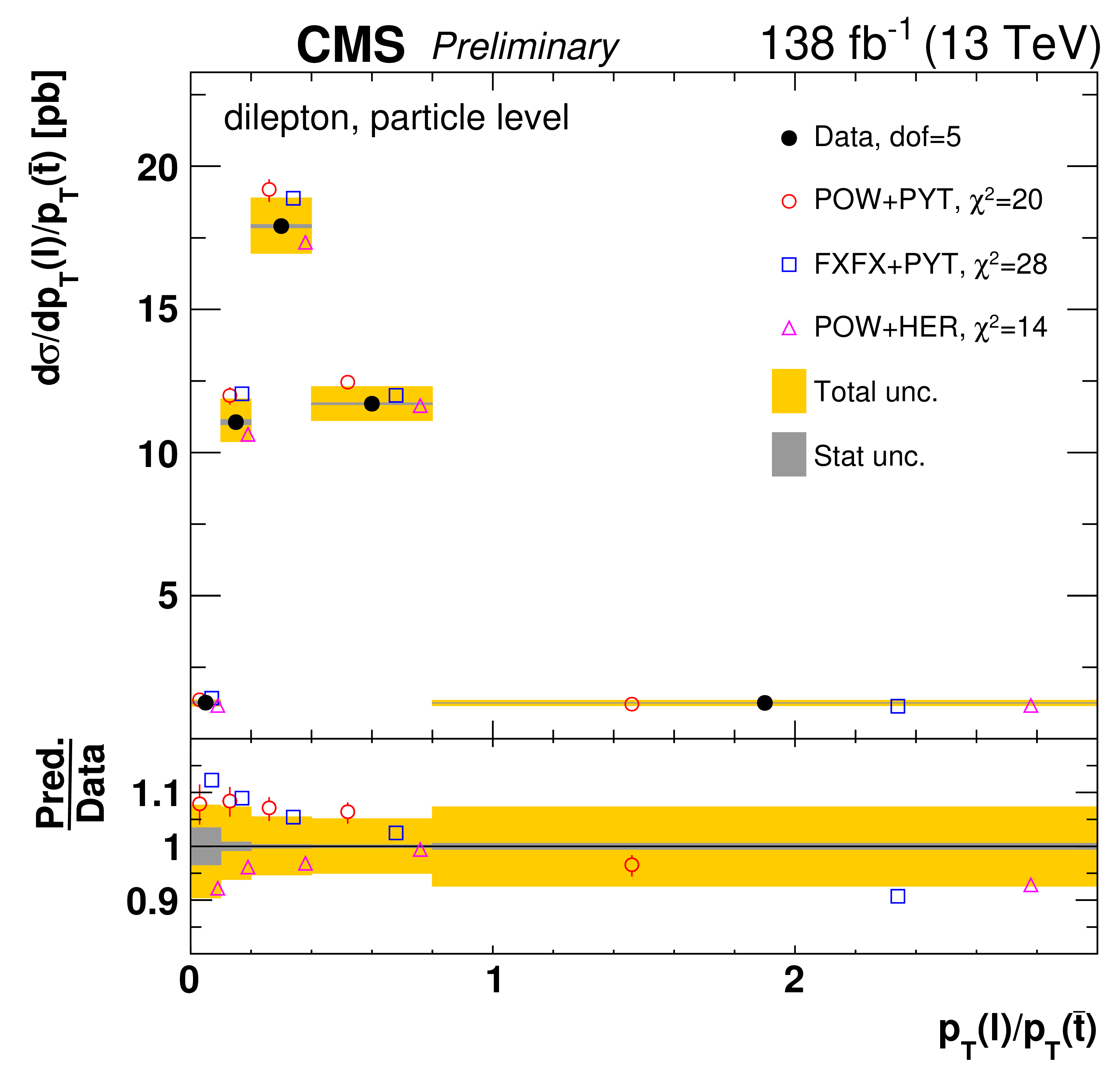
png pdf	Figure 80-c: Absolute differential $\mathrm{t\bar{t}}$ production cross sections as a function of ${p_{\mathrm {T}}}$ of the lepton (upper left), of the ratio of the trailing and leading lepton ${p_{\mathrm {T}}}$ (upper right), and of the ratio of lepton and top antiquark ${p_{\mathrm {T}}}$ (lower middle), measured at the particle level in a fiducial phase space. The data are shown as filled circles with dark and light bands indicating the statistical and total uncertainties (statistical and systematic uncertainties summed in quadrature), respectively. The cross sections are compared to various MC predictions (other points). The estimated uncertainties in the POWHEG+PYTHIA-8 (`POW-PYT') simulation are represented by a vertical bar on the corresponding points. For each MC model, a value of ${\chi ^2}$ is reported that takes into account the measurement uncertainties. The lower panel in each plot shows the ratios of the predictions to the data.
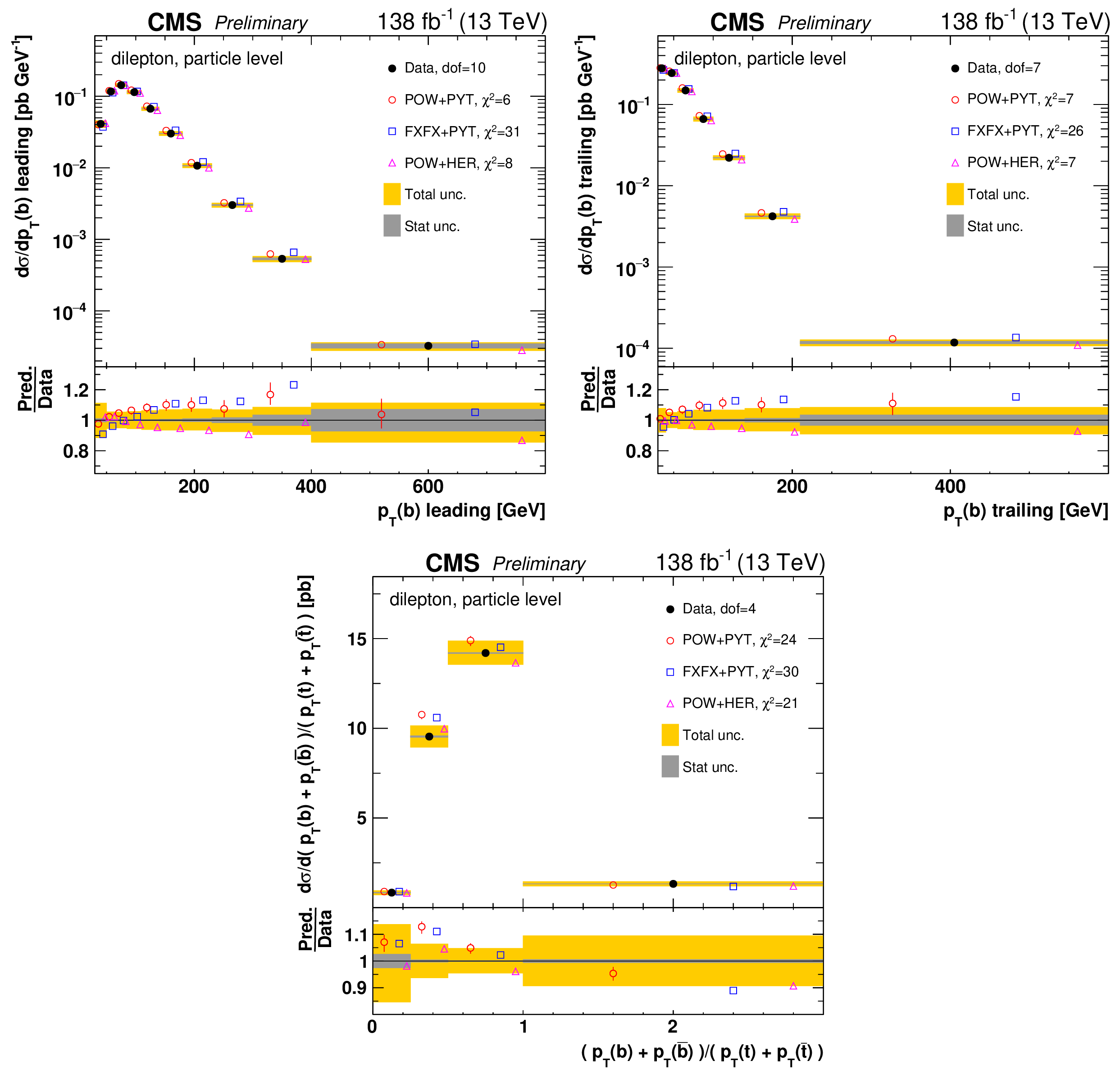
png pdf	Figure 81: Absolute differential $\mathrm{t\bar{t}}$ production cross sections as a function of the ${p_{\mathrm {T}}}$ of the leading (upper left) and trailing (upper right) b jet, and $( {{p_{\mathrm {T}}}}(\rm {b})+ {{p_{\mathrm {T}}}}(\mathrm{b\bar{b}}))/( {{p_{\mathrm {T}}}}(\rm {t})+ {{p_{\mathrm {T}}}}(\mathrm{\bar{t}}))$ (lower). Further details can be found in the caption of Fig. 80.
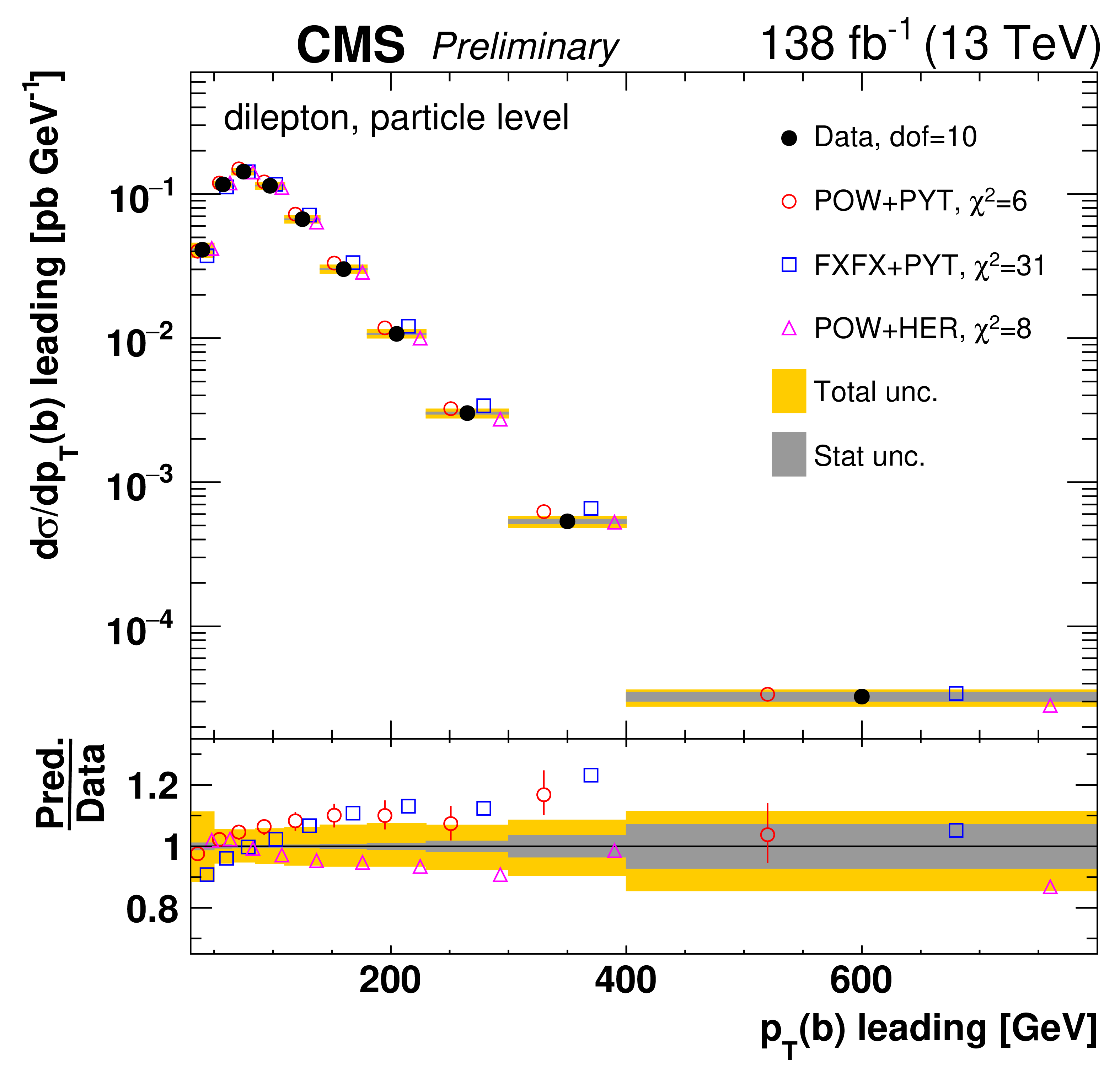
png pdf	Figure 81-a: Absolute differential $\mathrm{t\bar{t}}$ production cross sections as a function of the ${p_{\mathrm {T}}}$ of the leading (upper left) and trailing (upper right) b jet, and $( {{p_{\mathrm {T}}}}(\rm {b})+ {{p_{\mathrm {T}}}}(\mathrm{b\bar{b}}))/( {{p_{\mathrm {T}}}}(\rm {t})+ {{p_{\mathrm {T}}}}(\mathrm{\bar{t}}))$ (lower). Further details can be found in the caption of Fig. 80.
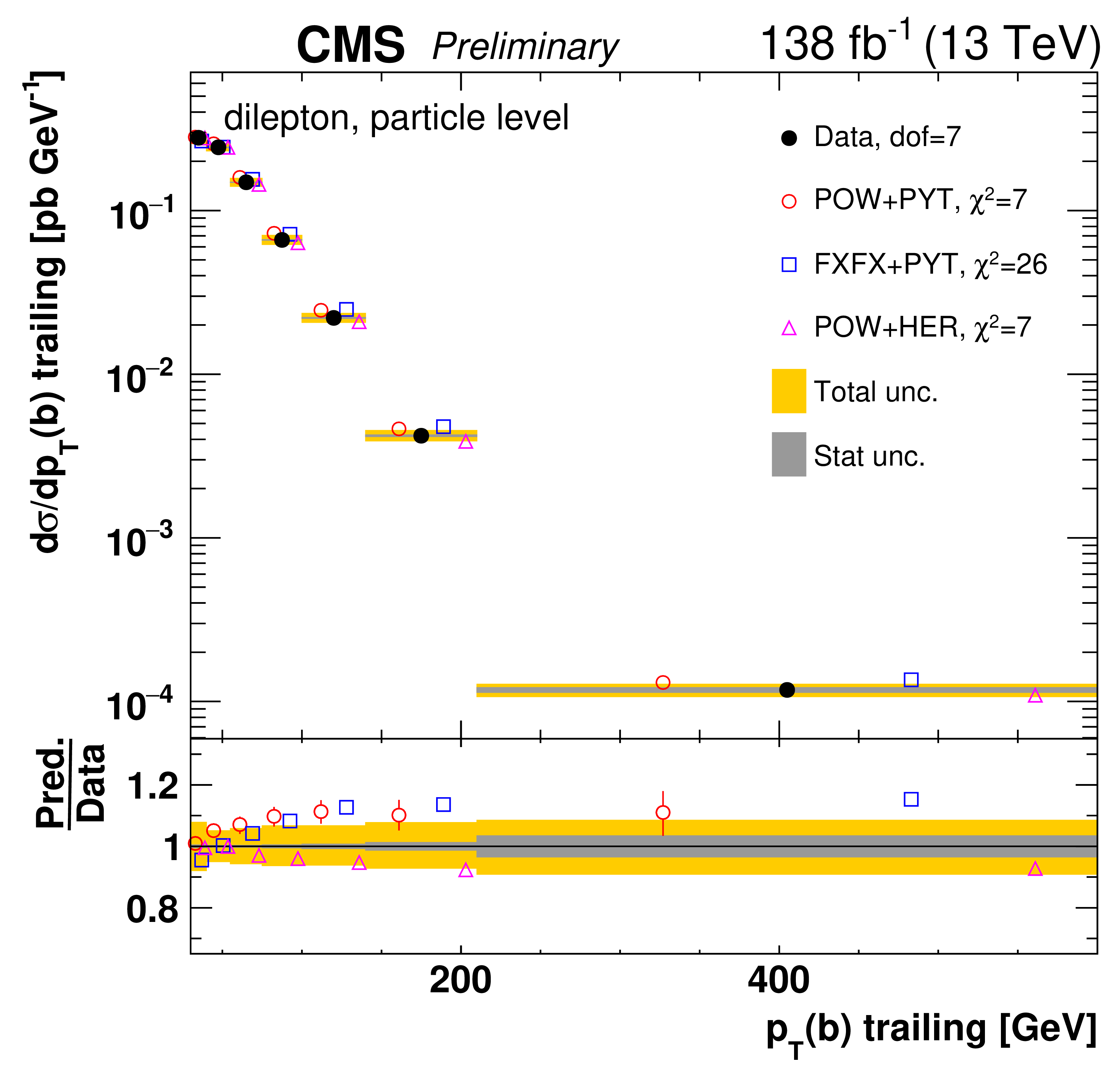
png pdf	Figure 81-b: Absolute differential $\mathrm{t\bar{t}}$ production cross sections as a function of the ${p_{\mathrm {T}}}$ of the leading (upper left) and trailing (upper right) b jet, and $( {{p_{\mathrm {T}}}}(\rm {b})+ {{p_{\mathrm {T}}}}(\mathrm{b\bar{b}}))/( {{p_{\mathrm {T}}}}(\rm {t})+ {{p_{\mathrm {T}}}}(\mathrm{\bar{t}}))$ (lower). Further details can be found in the caption of Fig. 80.
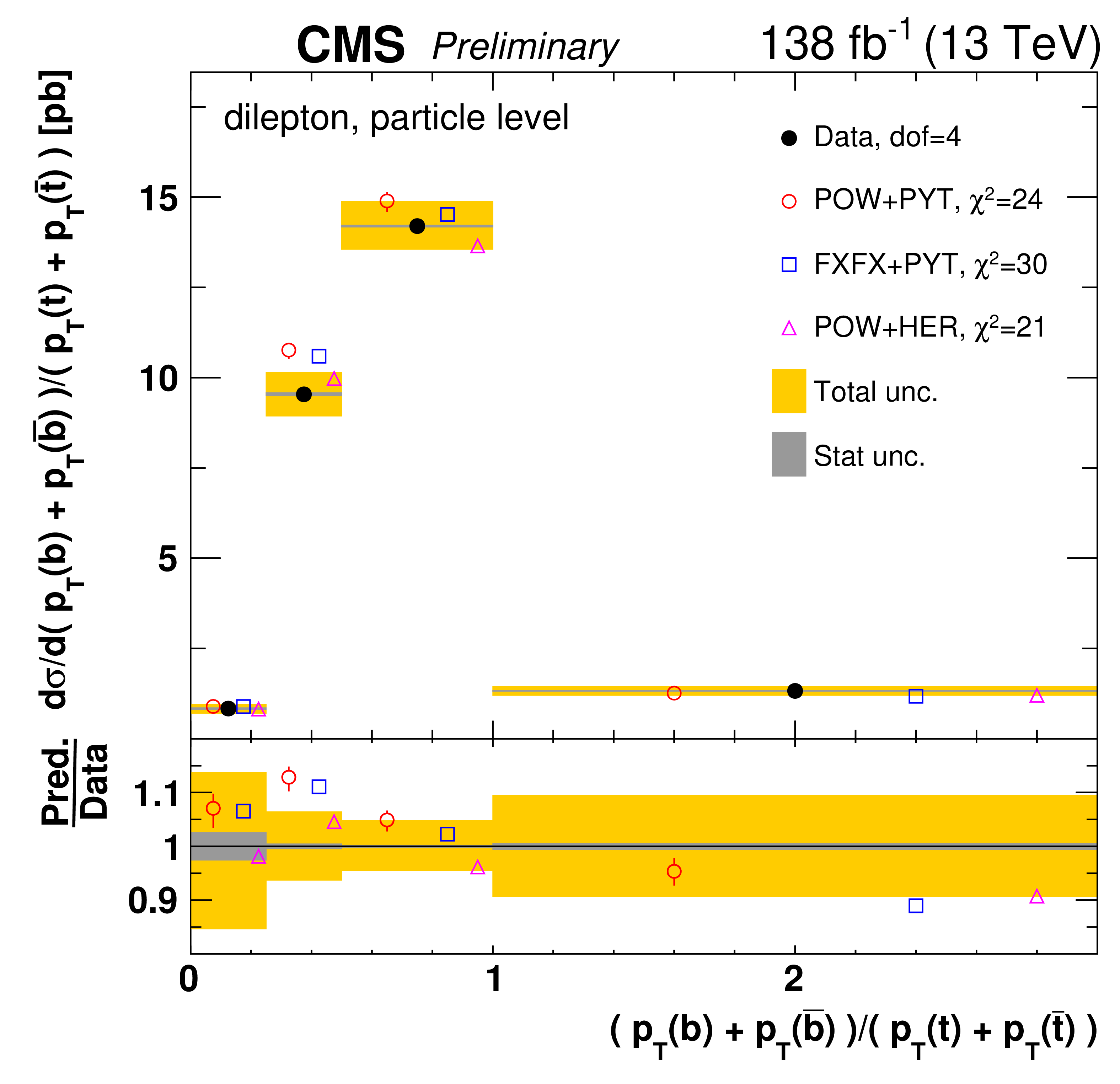
png pdf	Figure 81-c: Absolute differential $\mathrm{t\bar{t}}$ production cross sections as a function of the ${p_{\mathrm {T}}}$ of the leading (upper left) and trailing (upper right) b jet, and $( {{p_{\mathrm {T}}}}(\rm {b})+ {{p_{\mathrm {T}}}}(\mathrm{b\bar{b}}))/( {{p_{\mathrm {T}}}}(\rm {t})+ {{p_{\mathrm {T}}}}(\mathrm{\bar{t}}))$ (lower). Further details can be found in the caption of Fig. 80.
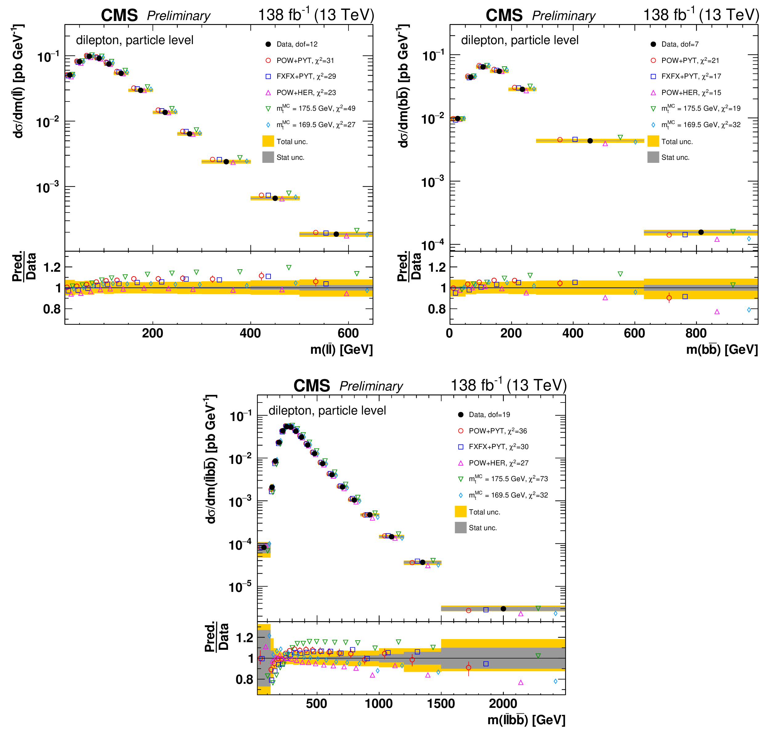
png pdf	Figure 82: Absolute differential $\mathrm{t\bar{t}}$ production cross sections as a function of ${m(\ell \overline {\ell})}$ (upper left), ${m(\mathrm{b} \mathrm{\bar{b}})}$ (upper right) and ${m(\ell \overline {\ell}\mathrm{b} \mathrm{\bar{b}})}$ (lower) are shown for data (filled circles) and various MC predictions (other points). Further details can be found in the caption of Fig. 80.
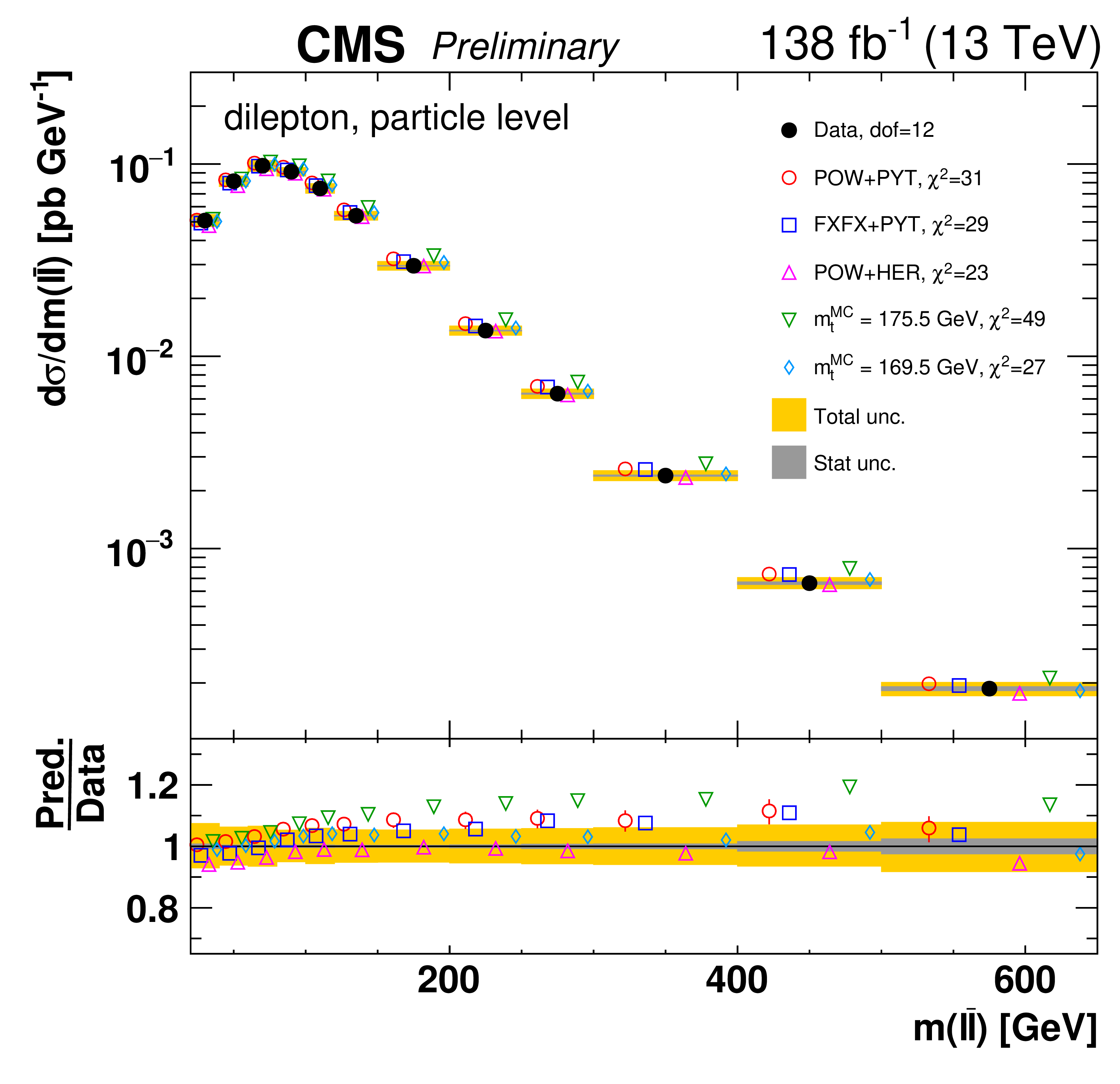
png pdf	Figure 82-a: Absolute differential $\mathrm{t\bar{t}}$ production cross sections as a function of ${m(\ell \overline {\ell})}$ (upper left), ${m(\mathrm{b} \mathrm{\bar{b}})}$ (upper right) and ${m(\ell \overline {\ell}\mathrm{b} \mathrm{\bar{b}})}$ (lower) are shown for data (filled circles) and various MC predictions (other points). Further details can be found in the caption of Fig. 80.
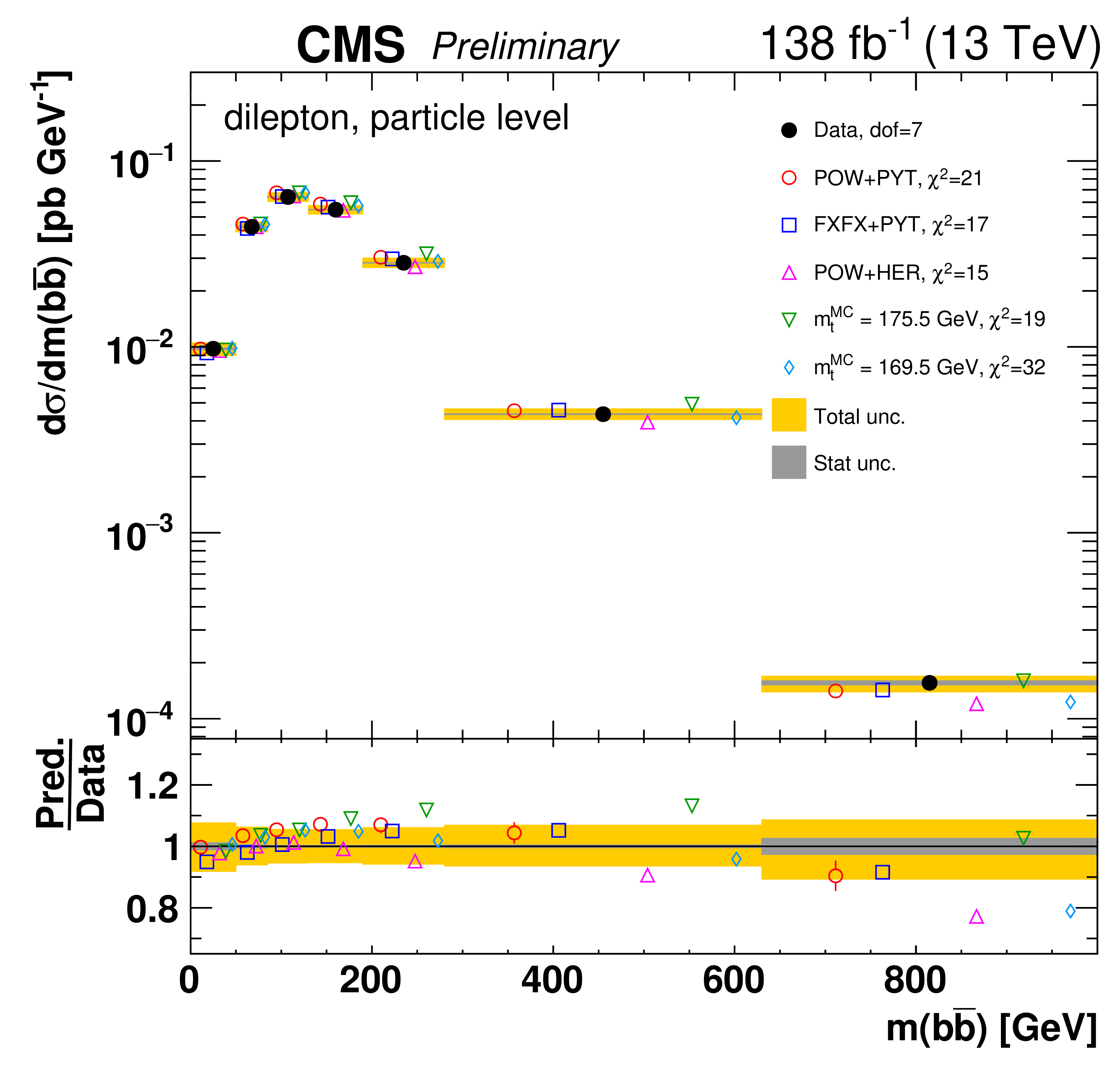
png pdf	Figure 82-b: Absolute differential $\mathrm{t\bar{t}}$ production cross sections as a function of ${m(\ell \overline {\ell})}$ (upper left), ${m(\mathrm{b} \mathrm{\bar{b}})}$ (upper right) and ${m(\ell \overline {\ell}\mathrm{b} \mathrm{\bar{b}})}$ (lower) are shown for data (filled circles) and various MC predictions (other points). Further details can be found in the caption of Fig. 80.
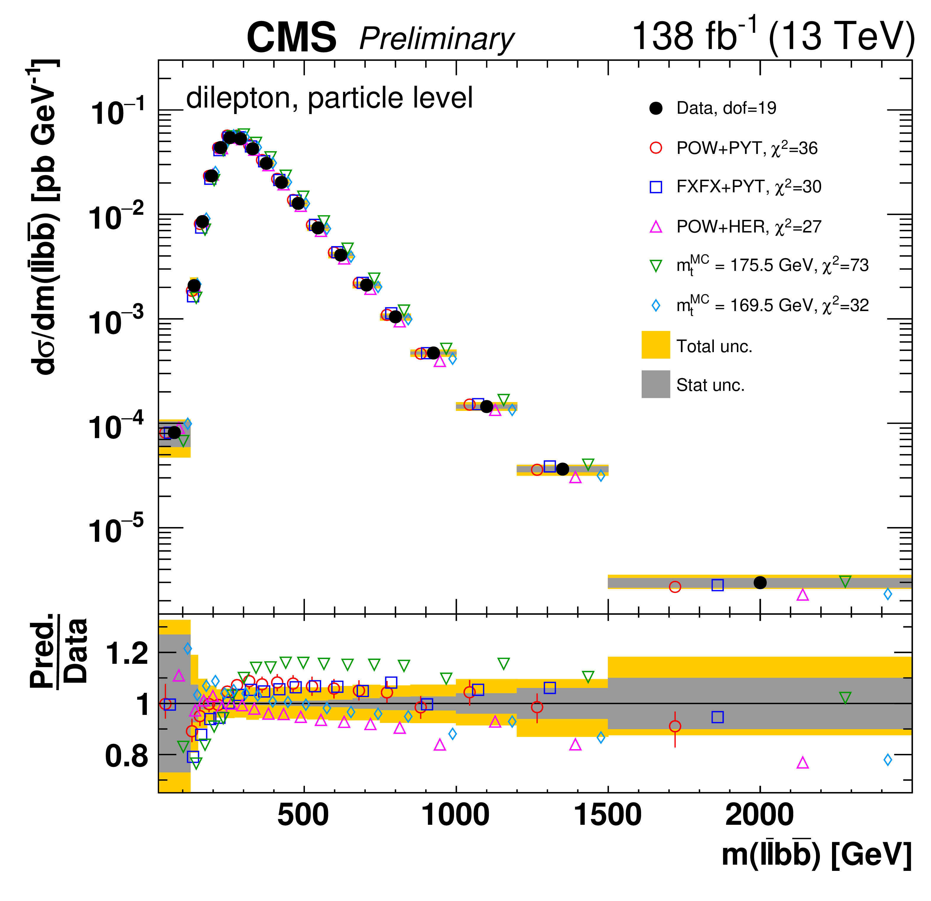
png pdf	Figure 82-c: Absolute differential $\mathrm{t\bar{t}}$ production cross sections as a function of ${m(\ell \overline {\ell})}$ (upper left), ${m(\mathrm{b} \mathrm{\bar{b}})}$ (upper right) and ${m(\ell \overline {\ell}\mathrm{b} \mathrm{\bar{b}})}$ (lower) are shown for data (filled circles) and various MC predictions (other points). Further details can be found in the caption of Fig. 80.
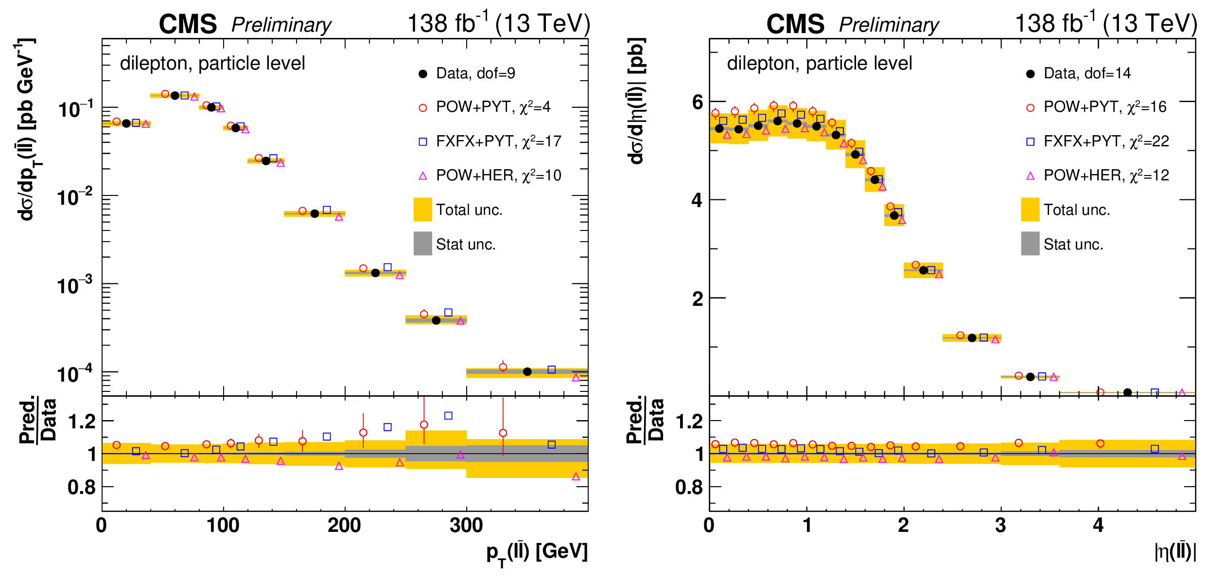
png pdf	Figure 83: Absolute differential $\mathrm{t\bar{t}}$ production cross sections as a function of ${{p_{\mathrm {T}}} (\ell \overline {\ell})}$ (left) and ${|\eta (\ell \overline {\ell})|}$ (right) are shown for data (filled circles) and various MC predictions (other points). Further details can be found in the caption of Fig. 23.
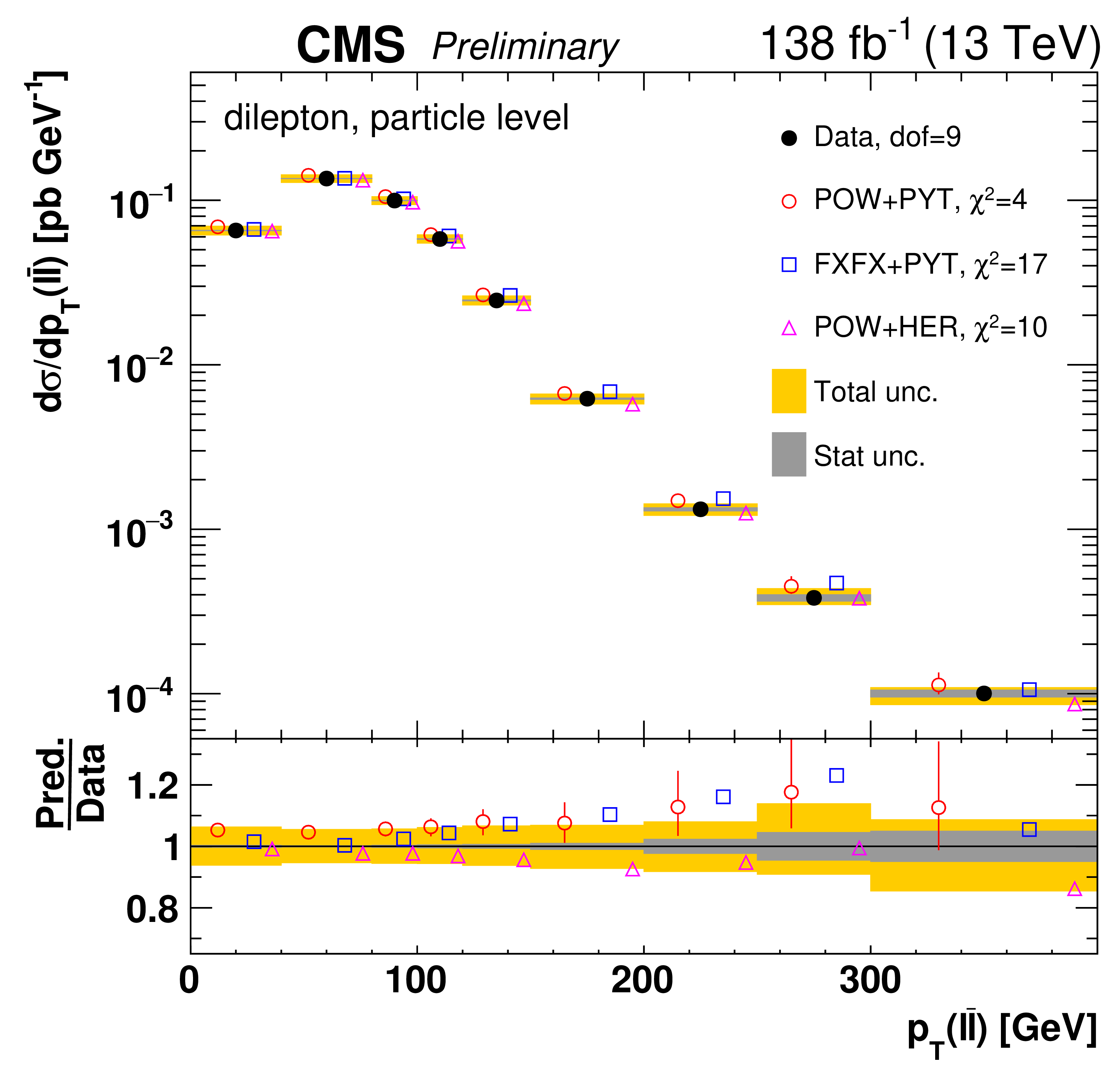
png pdf	Figure 83-a: Absolute differential $\mathrm{t\bar{t}}$ production cross sections as a function of ${{p_{\mathrm {T}}} (\ell \overline {\ell})}$ (left) and ${|\eta (\ell \overline {\ell})|}$ (right) are shown for data (filled circles) and various MC predictions (other points). Further details can be found in the caption of Fig. 23.
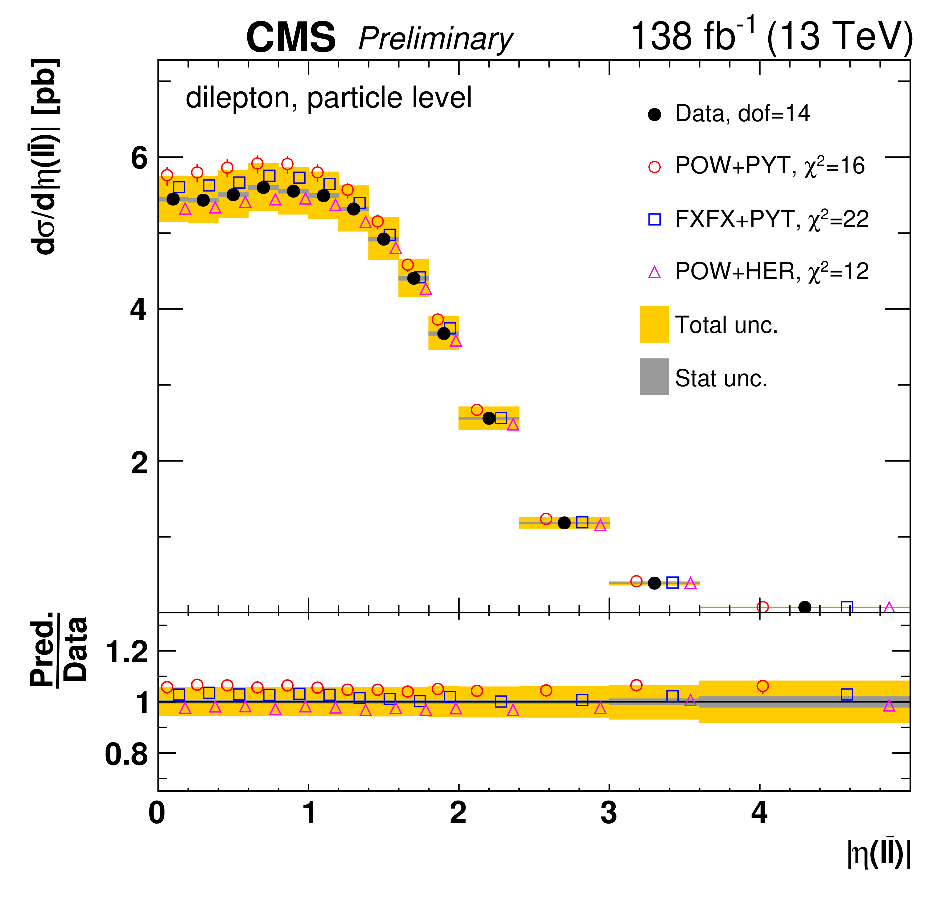
png pdf	Figure 83-b: Absolute differential $\mathrm{t\bar{t}}$ production cross sections as a function of ${{p_{\mathrm {T}}} (\ell \overline {\ell})}$ (left) and ${|\eta (\ell \overline {\ell})|}$ (right) are shown for data (filled circles) and various MC predictions (other points). Further details can be found in the caption of Fig. 23.
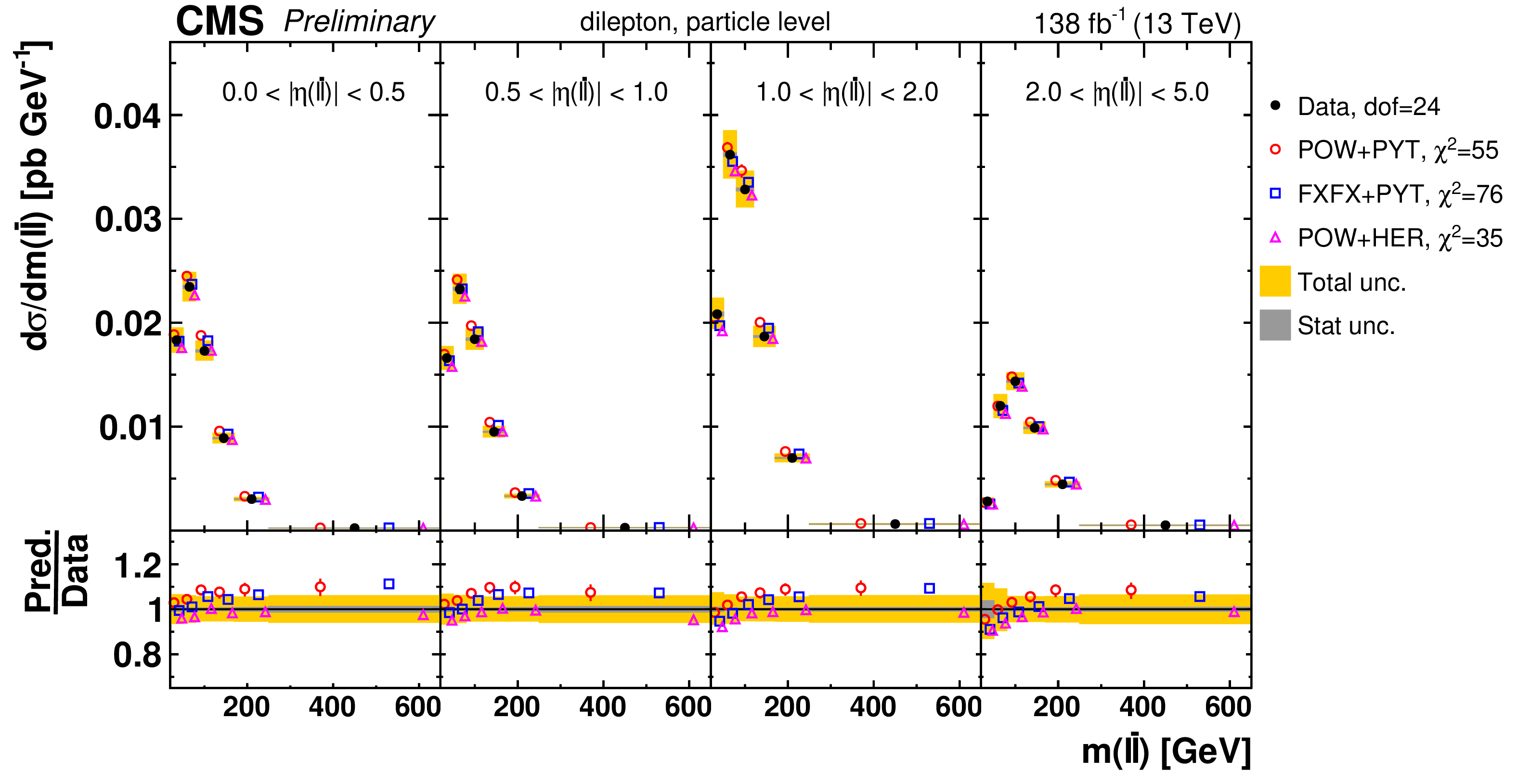
png pdf	Figure 84: Absolute $[ {|\eta (\ell \overline {\ell})|},\,{m(\ell \overline {\ell})} ]$ cross sections are shown for data (filled circles) and various MC predictions (other points). Further details can be found in the caption of Fig. 80.
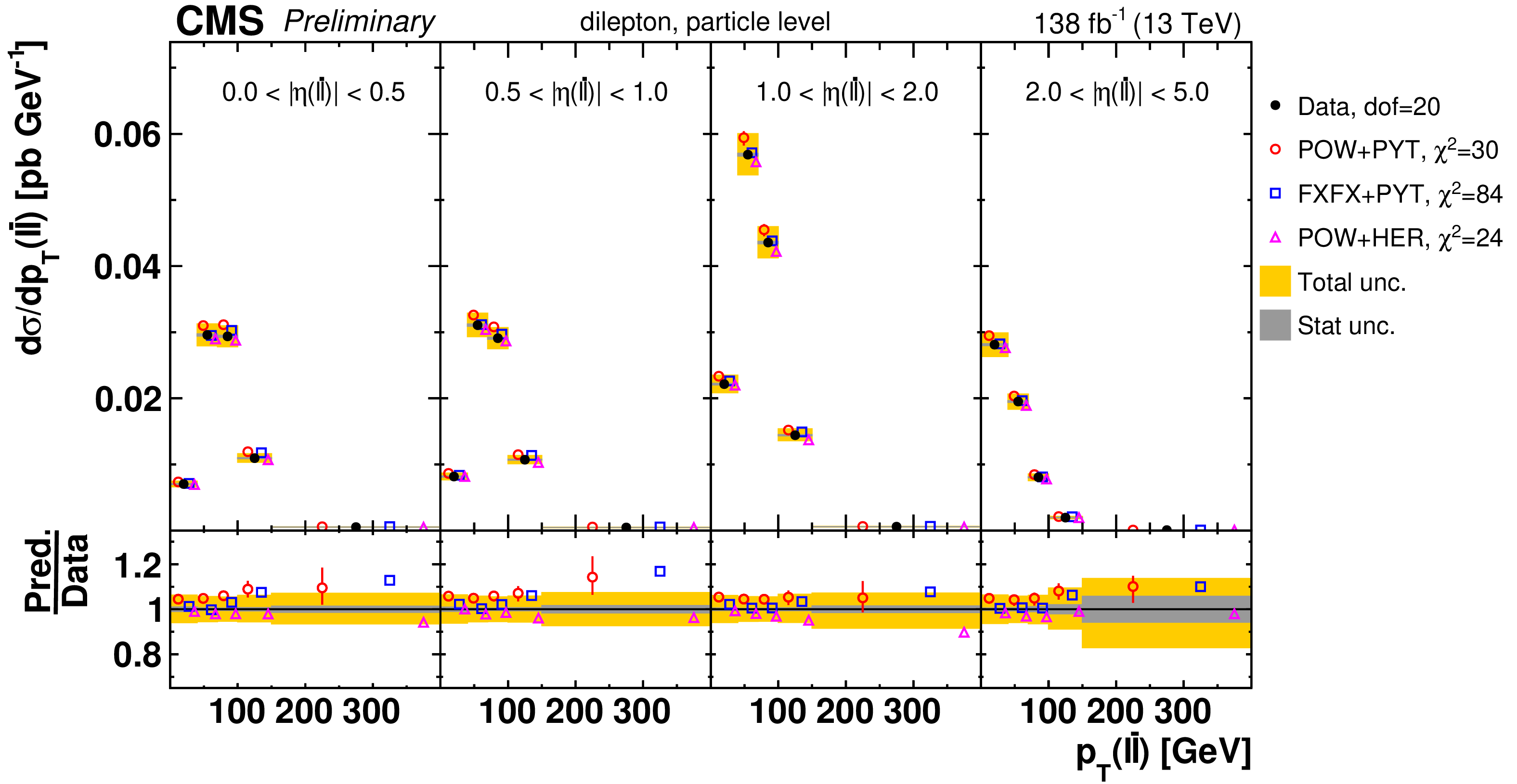
png pdf	Figure 85: Absolute $[ {|\eta (\ell \overline {\ell})|},\,{{p_{\mathrm {T}}} (\ell \overline {\ell})} ]$ cross sections are shown for data (filled circles) and various MC predictions (other points). Further details can be found in the caption of Fig. 80.
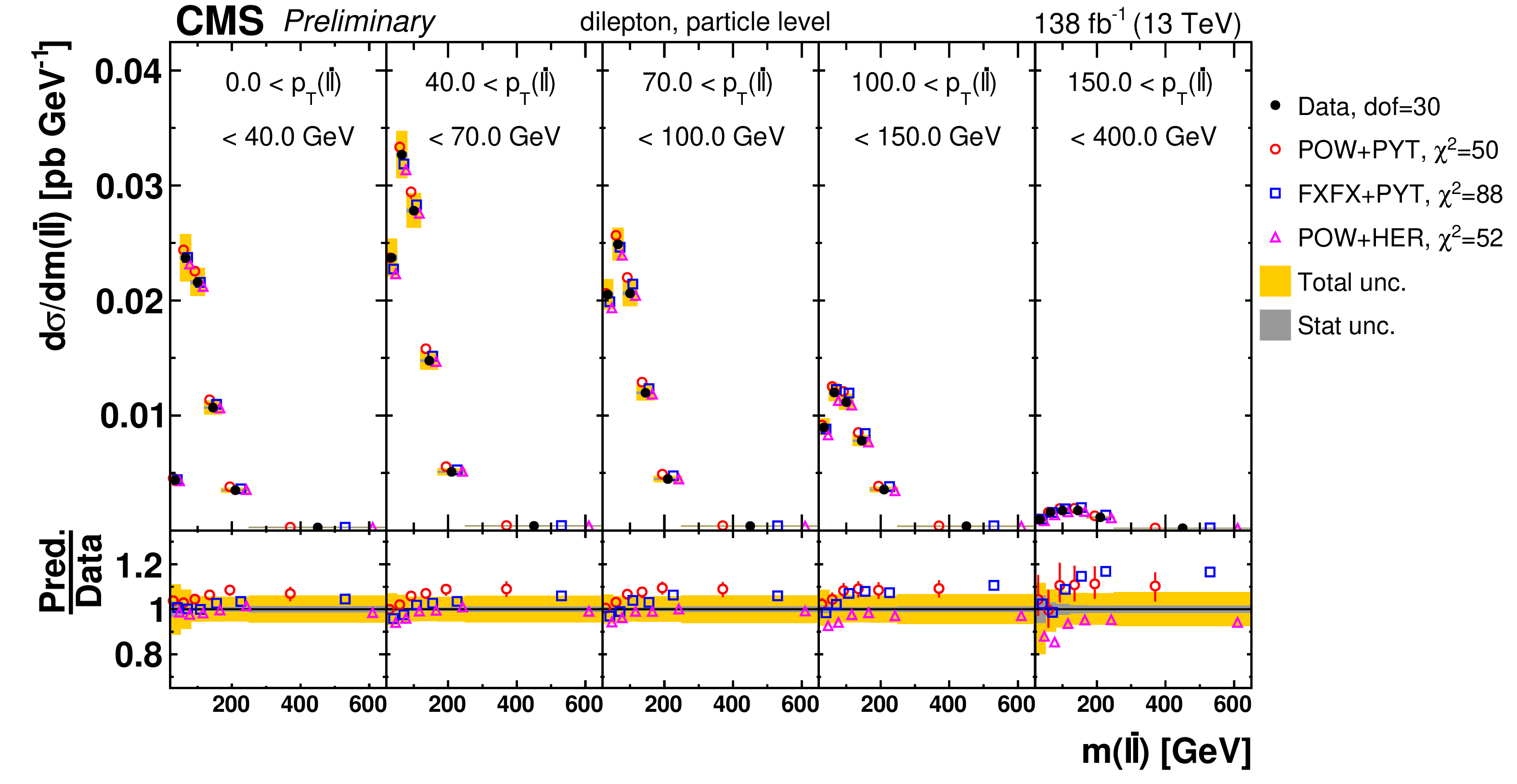
png pdf	Figure 86: Absolute $[ {{p_{\mathrm {T}}} (\ell \overline {\ell})},\,{m(\ell \overline {\ell})} ]$ cross sections are shown for data (filled circles) and various MC predictions (other points). Further details can be found in the caption of Fig. 80.
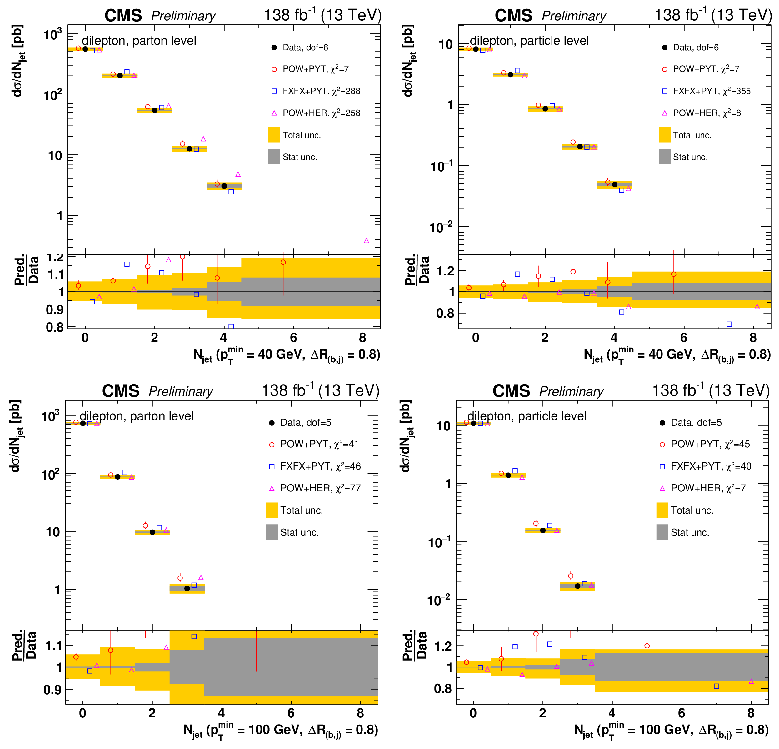
png pdf	Figure 87: Absolute differential $\mathrm{t\bar{t}}$ production cross sections as a function of ${N_{\text {jet}}}$, for a minimum jet ${p_{\mathrm {T}}}$ of 40 GeV (upper) and and 100 GeV (lower), measured at the parton level in the full phase space (left) and at the particle level in a fiducial phase space (right). The data are shown as filled circles with dark and light bands indicating the statistical and total uncertainties (statistical and systematic uncertainties summed in quadrature), respectively. The cross sections are compared to various MC predictions (other points). The estimated uncertainties in the POWHEG+PYTHIA-8 (`POW-PYT') simulation are represented by a vertical bar on the corresponding points. For each MC model, a value of ${\chi ^2}$ is reported that takes into account the measurement uncertainties. The lower panel in each plot shows the ratios of the predictions to the data.
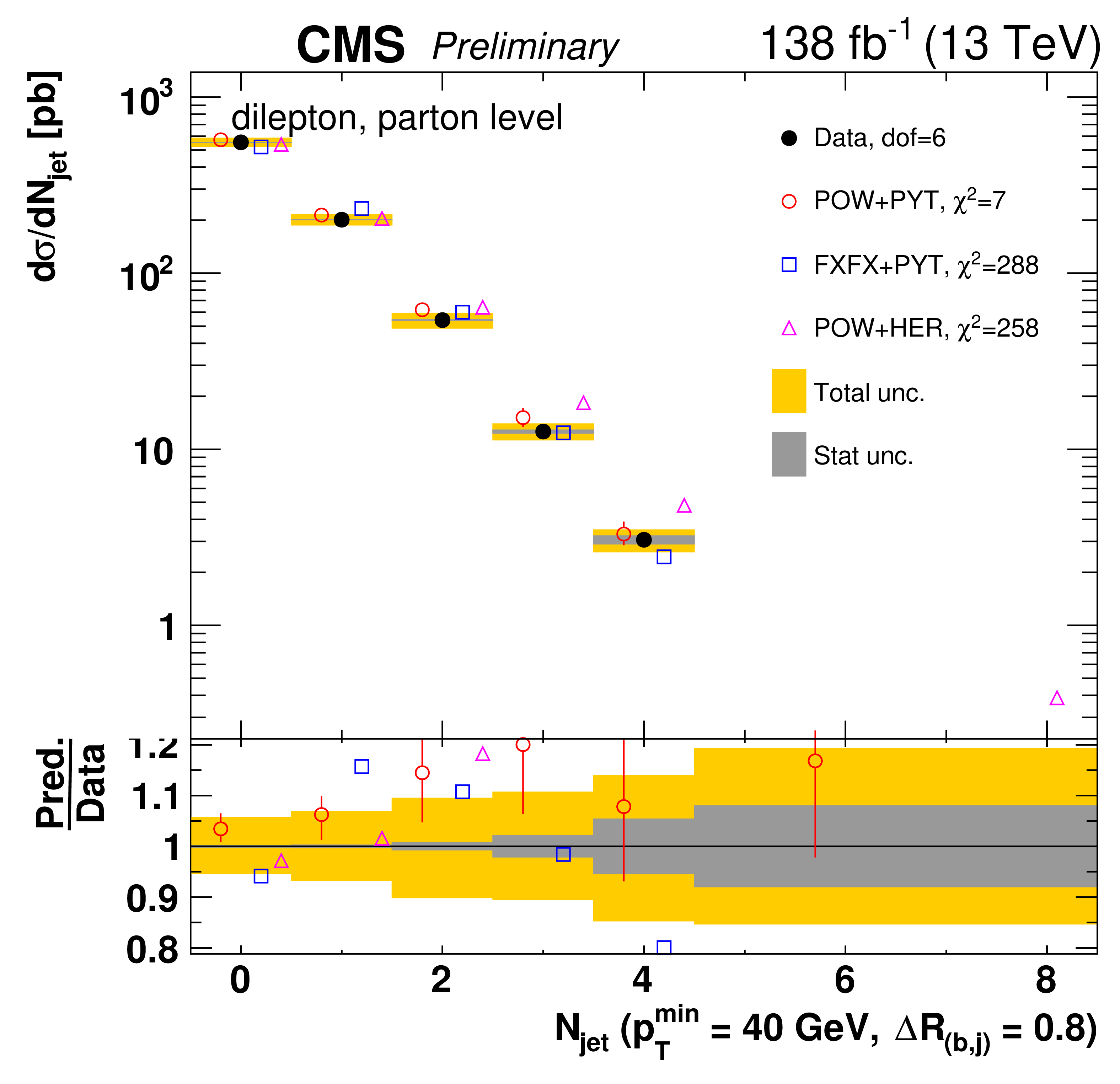
png pdf	Figure 87-a: Absolute differential $\mathrm{t\bar{t}}$ production cross sections as a function of ${N_{\text {jet}}}$, for a minimum jet ${p_{\mathrm {T}}}$ of 40 GeV (upper) and and 100 GeV (lower), measured at the parton level in the full phase space (left) and at the particle level in a fiducial phase space (right). The data are shown as filled circles with dark and light bands indicating the statistical and total uncertainties (statistical and systematic uncertainties summed in quadrature), respectively. The cross sections are compared to various MC predictions (other points). The estimated uncertainties in the POWHEG+PYTHIA-8 (`POW-PYT') simulation are represented by a vertical bar on the corresponding points. For each MC model, a value of ${\chi ^2}$ is reported that takes into account the measurement uncertainties. The lower panel in each plot shows the ratios of the predictions to the data.
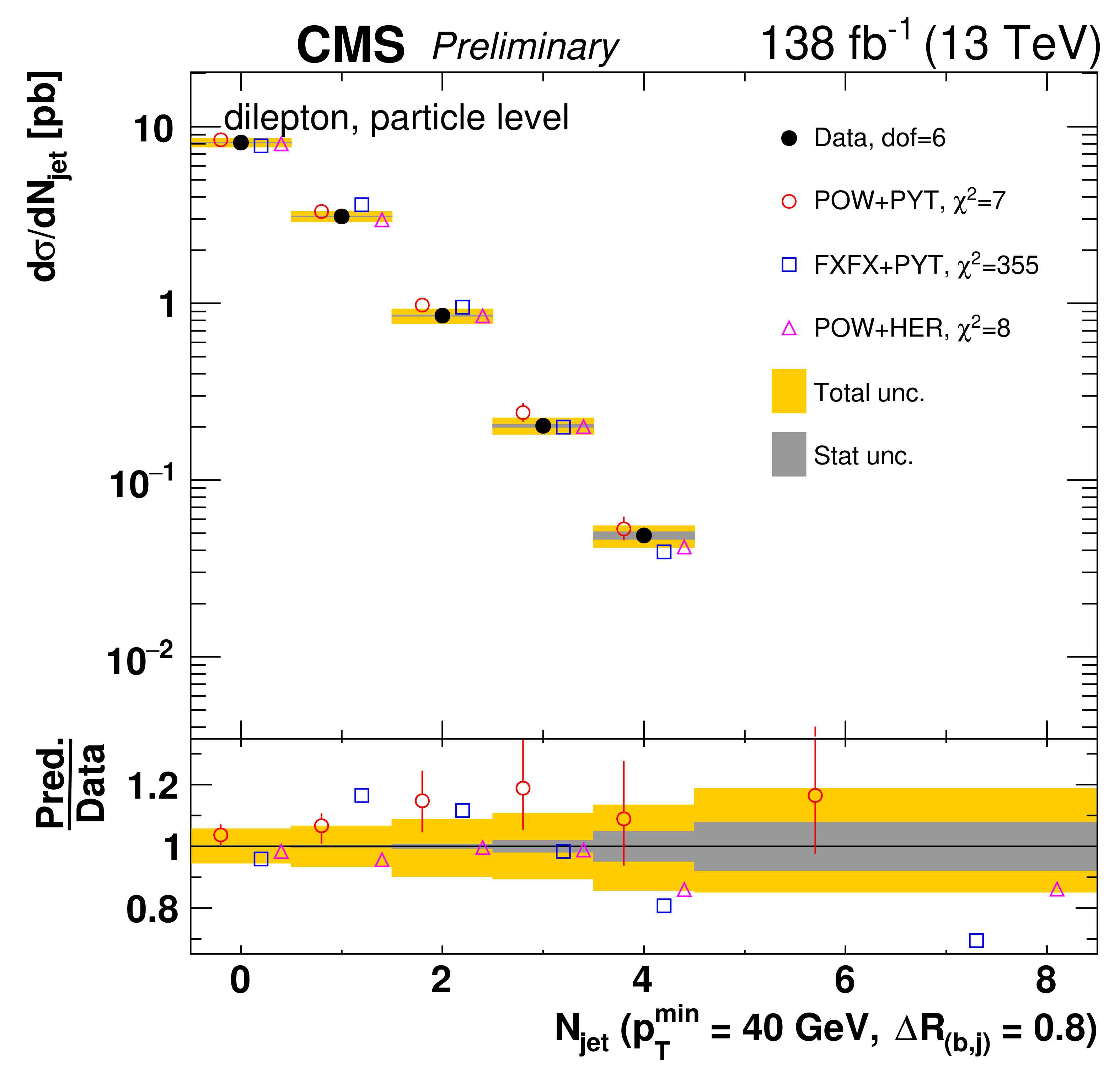
png pdf	Figure 87-b: Absolute differential $\mathrm{t\bar{t}}$ production cross sections as a function of ${N_{\text {jet}}}$, for a minimum jet ${p_{\mathrm {T}}}$ of 40 GeV (upper) and and 100 GeV (lower), measured at the parton level in the full phase space (left) and at the particle level in a fiducial phase space (right). The data are shown as filled circles with dark and light bands indicating the statistical and total uncertainties (statistical and systematic uncertainties summed in quadrature), respectively. The cross sections are compared to various MC predictions (other points). The estimated uncertainties in the POWHEG+PYTHIA-8 (`POW-PYT') simulation are represented by a vertical bar on the corresponding points. For each MC model, a value of ${\chi ^2}$ is reported that takes into account the measurement uncertainties. The lower panel in each plot shows the ratios of the predictions to the data.
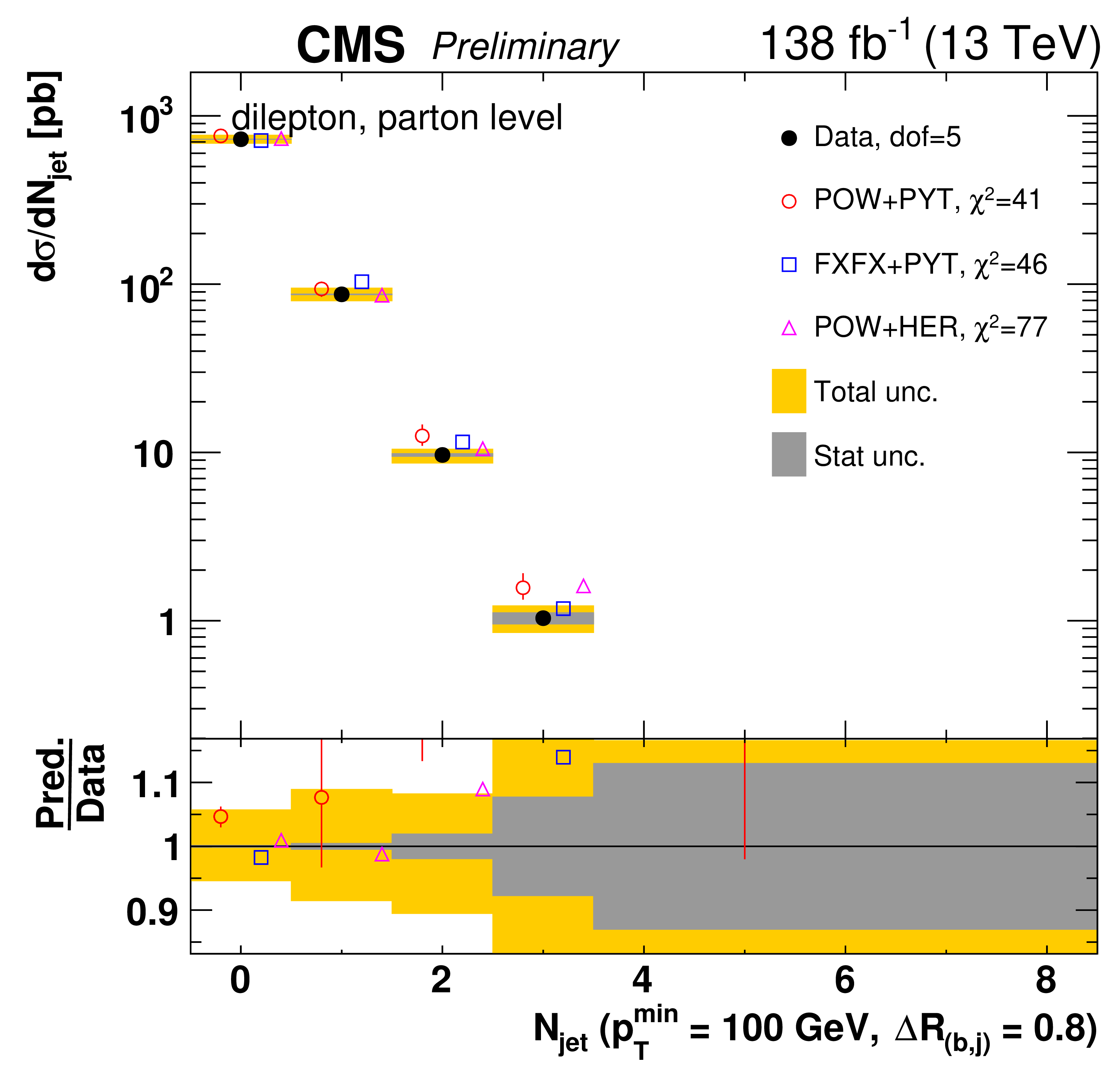
png pdf	Figure 87-c: Absolute differential $\mathrm{t\bar{t}}$ production cross sections as a function of ${N_{\text {jet}}}$, for a minimum jet ${p_{\mathrm {T}}}$ of 40 GeV (upper) and and 100 GeV (lower), measured at the parton level in the full phase space (left) and at the particle level in a fiducial phase space (right). The data are shown as filled circles with dark and light bands indicating the statistical and total uncertainties (statistical and systematic uncertainties summed in quadrature), respectively. The cross sections are compared to various MC predictions (other points). The estimated uncertainties in the POWHEG+PYTHIA-8 (`POW-PYT') simulation are represented by a vertical bar on the corresponding points. For each MC model, a value of ${\chi ^2}$ is reported that takes into account the measurement uncertainties. The lower panel in each plot shows the ratios of the predictions to the data.
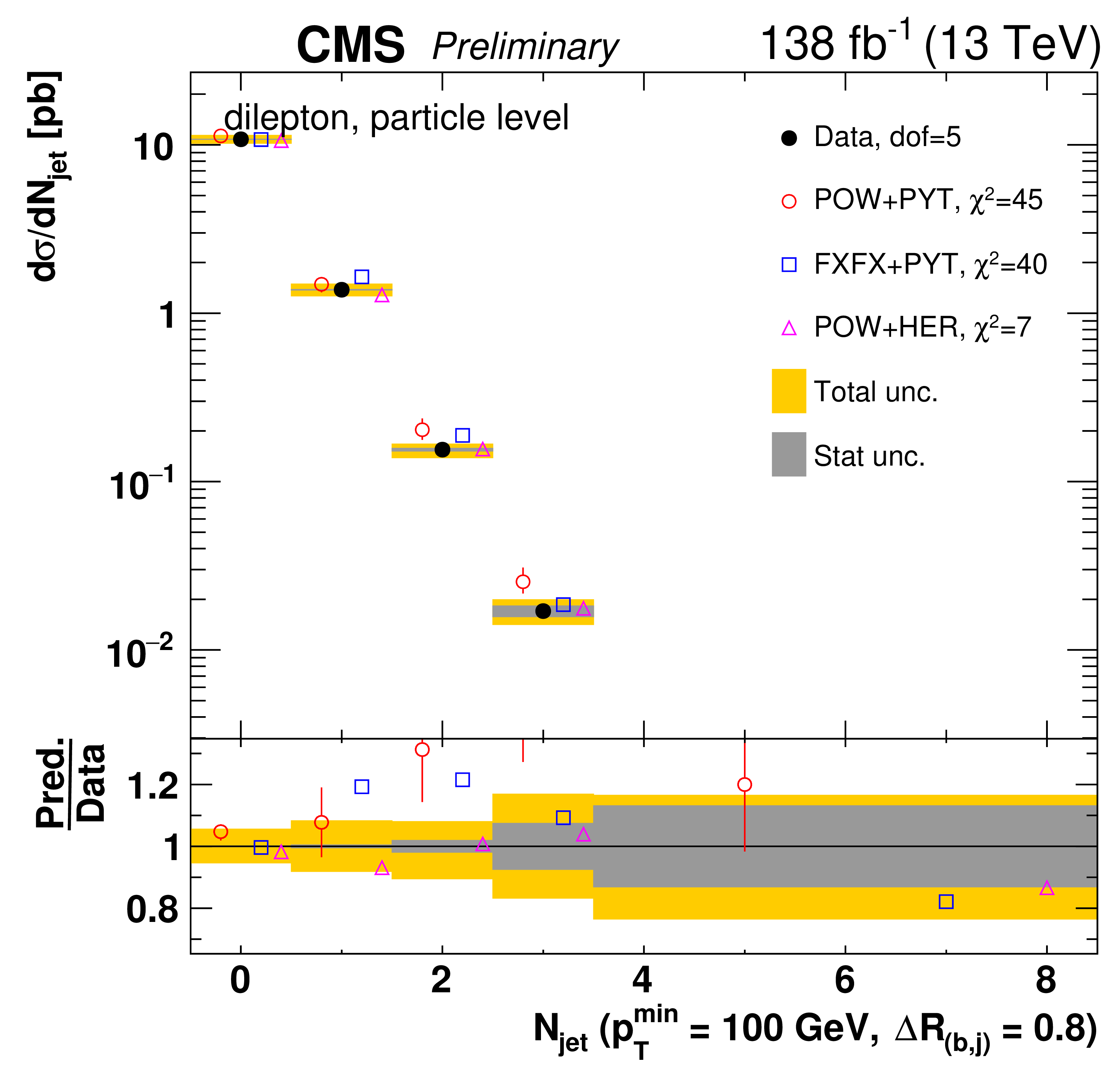
png pdf	Figure 87-d: Absolute differential $\mathrm{t\bar{t}}$ production cross sections as a function of ${N_{\text {jet}}}$, for a minimum jet ${p_{\mathrm {T}}}$ of 40 GeV (upper) and and 100 GeV (lower), measured at the parton level in the full phase space (left) and at the particle level in a fiducial phase space (right). The data are shown as filled circles with dark and light bands indicating the statistical and total uncertainties (statistical and systematic uncertainties summed in quadrature), respectively. The cross sections are compared to various MC predictions (other points). The estimated uncertainties in the POWHEG+PYTHIA-8 (`POW-PYT') simulation are represented by a vertical bar on the corresponding points. For each MC model, a value of ${\chi ^2}$ is reported that takes into account the measurement uncertainties. The lower panel in each plot shows the ratios of the predictions to the data.
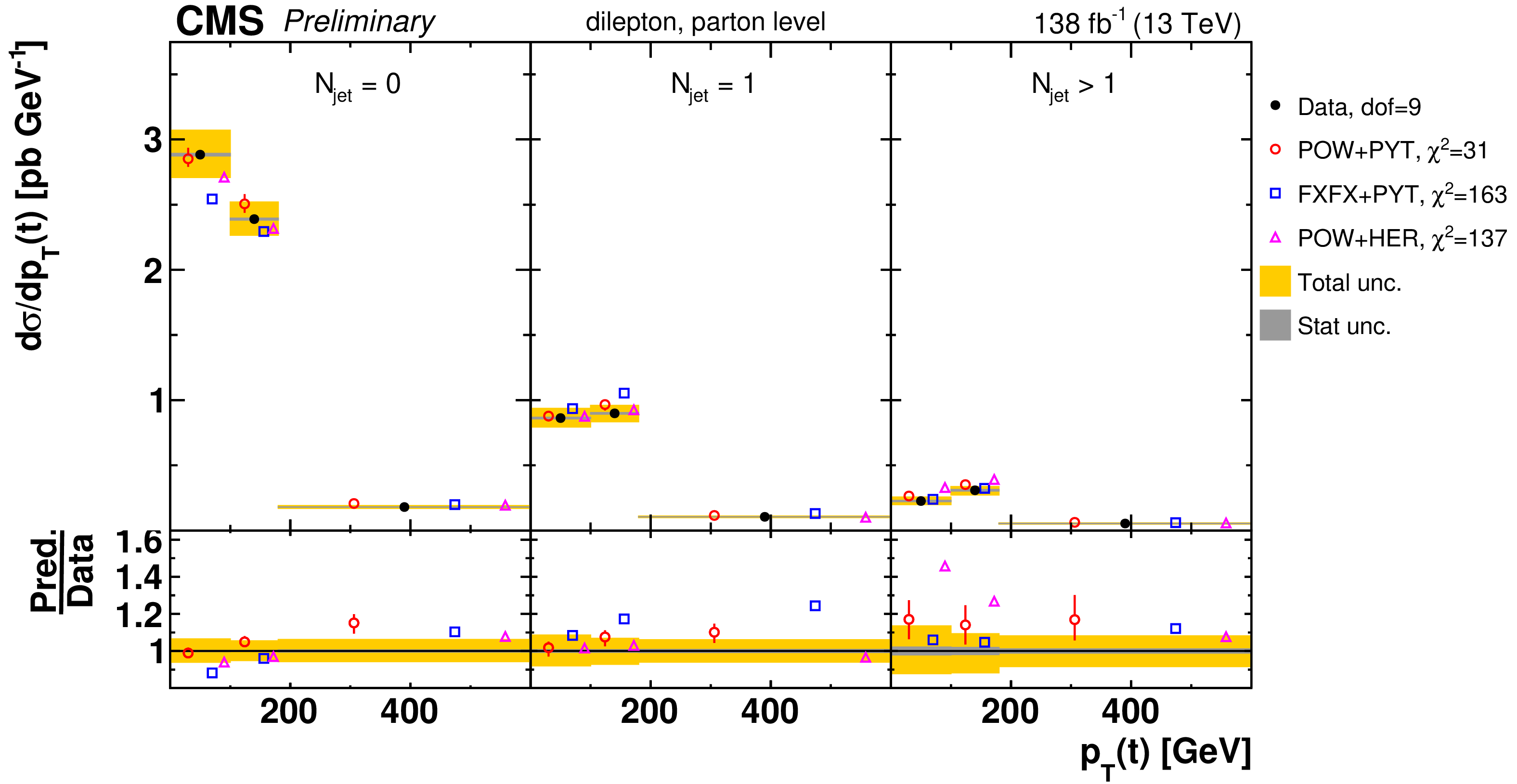
png pdf	Figure 88-a: Absolute $[ {N_{\text {jet}}},\,{{p_{\mathrm {T}}} (\mathrm{t})} ]$ cross sections measured at the parton level in the full phase space (upper) and at the particle level in a fiducial phase space (lower). The data are shown as filled circles with dark and light bands indicating the statistical and total (sum in quadrature of statistical and systematic) uncertainties, respectively. The cross sections are compared to various MC predictions (other points). The estimated uncertainties in the POWHEG+PYTHIA-8 (`POW-PYT') simulation are represented by a vertical bar on the corresponding points. For each MC model, a value of ${\chi ^2}$ is reported that takes into account the measurement uncertainties. The lower panel in each plot shows the ratios of the predictions to the data.
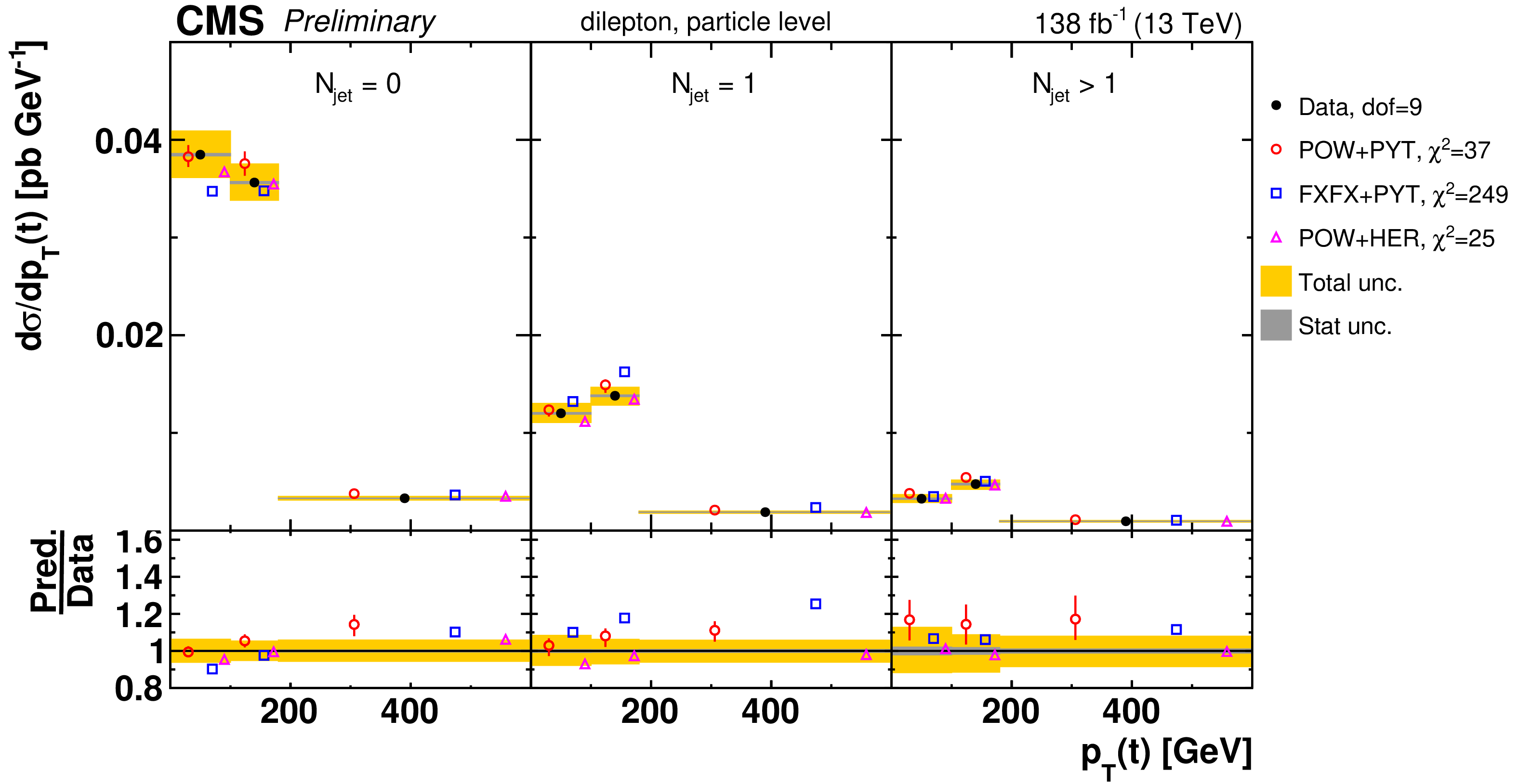
png pdf	Figure 88-b: Absolute $[ {N_{\text {jet}}},\,{{p_{\mathrm {T}}} (\mathrm{t})} ]$ cross sections measured at the parton level in the full phase space (upper) and at the particle level in a fiducial phase space (lower). The data are shown as filled circles with dark and light bands indicating the statistical and total (sum in quadrature of statistical and systematic) uncertainties, respectively. The cross sections are compared to various MC predictions (other points). The estimated uncertainties in the POWHEG+PYTHIA-8 (`POW-PYT') simulation are represented by a vertical bar on the corresponding points. For each MC model, a value of ${\chi ^2}$ is reported that takes into account the measurement uncertainties. The lower panel in each plot shows the ratios of the predictions to the data.
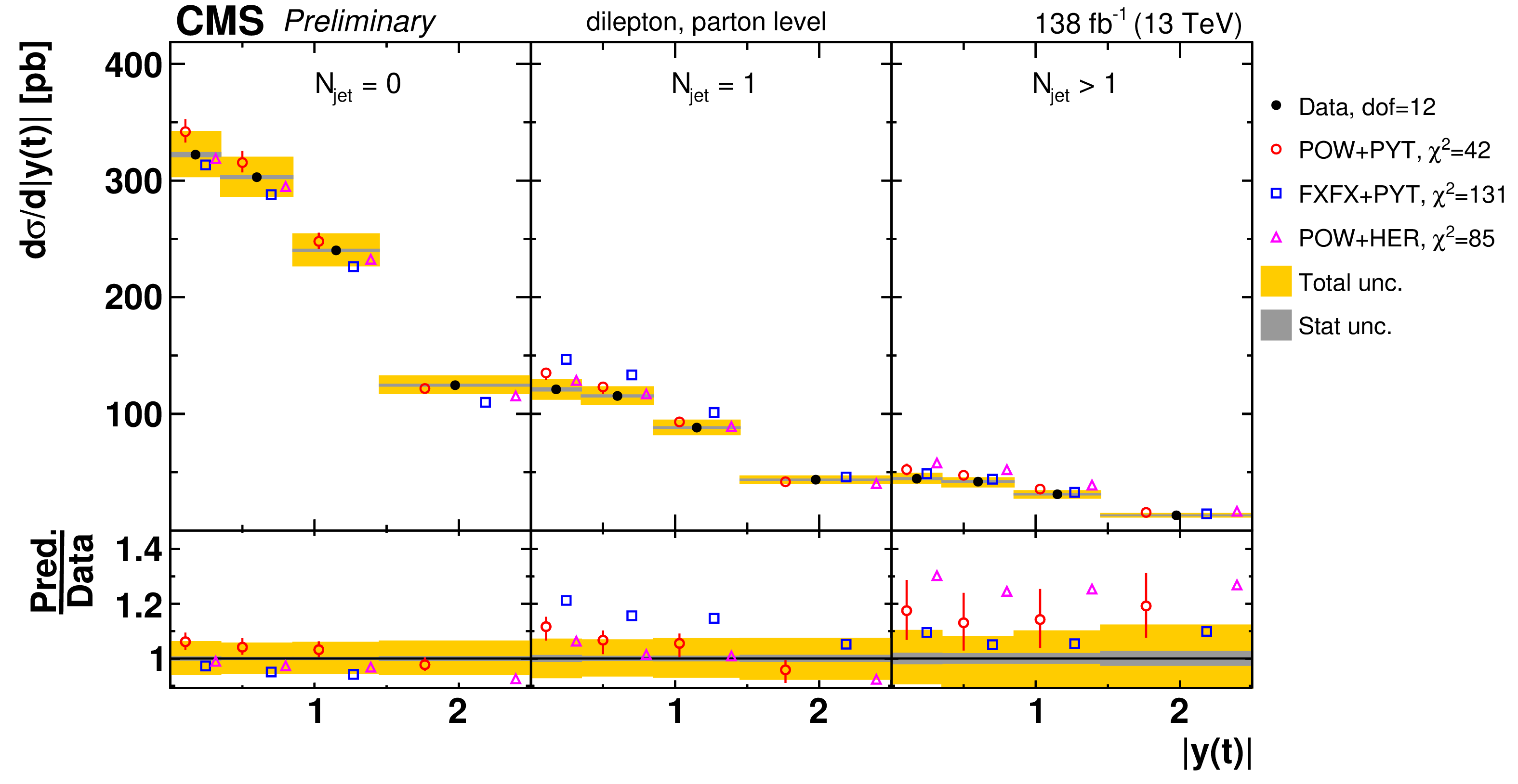
png pdf	Figure 89-a: Absolute $[ {N_{\text {jet}}},\,{|y(\mathrm{t})|} ]$ cross sections are shown for data (filled circles) and various MC predictions (other points). Further details can be found in the caption of Fig. 88.
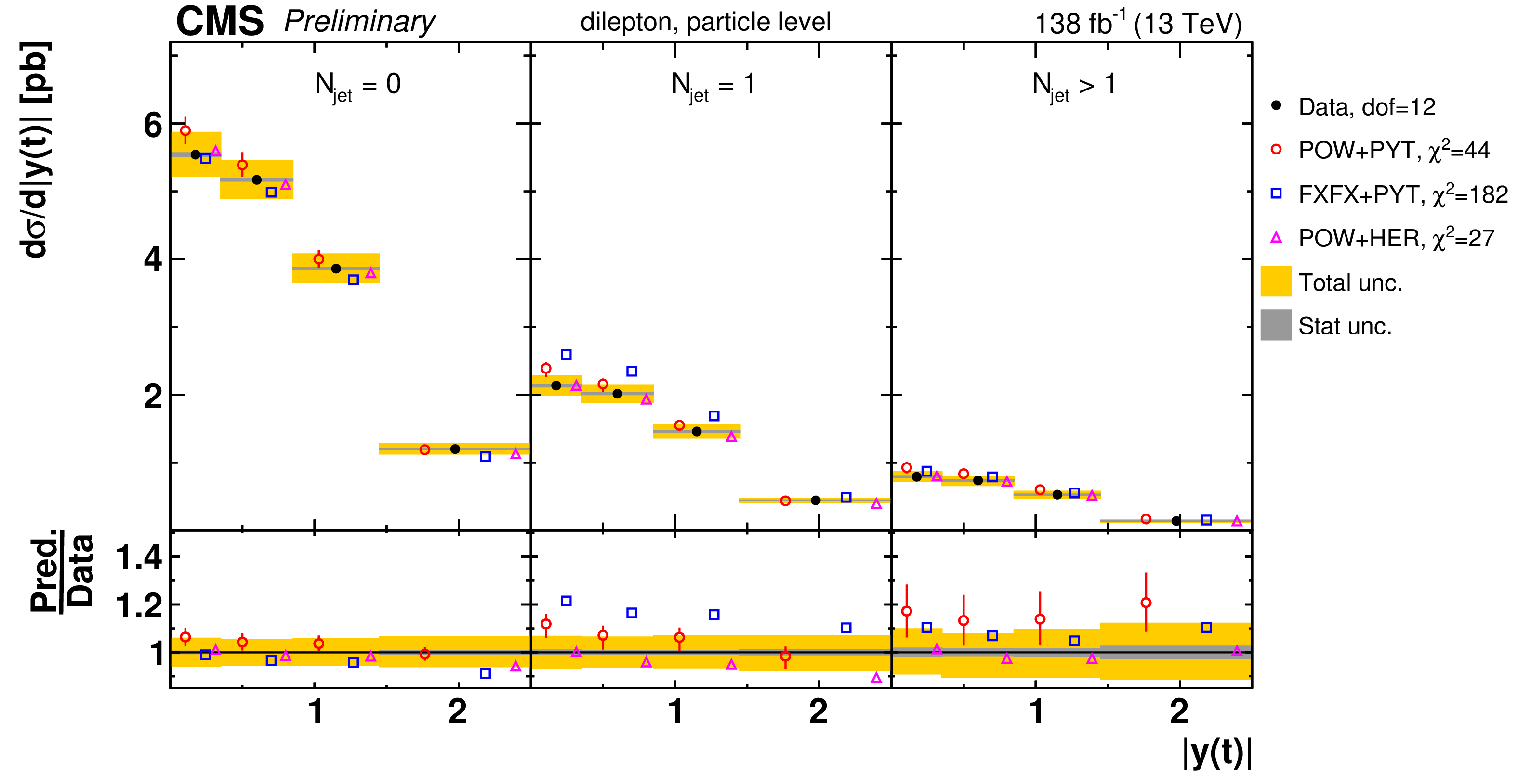
png pdf	Figure 89-b: Absolute $[ {N_{\text {jet}}},\,{|y(\mathrm{t})|} ]$ cross sections are shown for data (filled circles) and various MC predictions (other points). Further details can be found in the caption of Fig. 88.
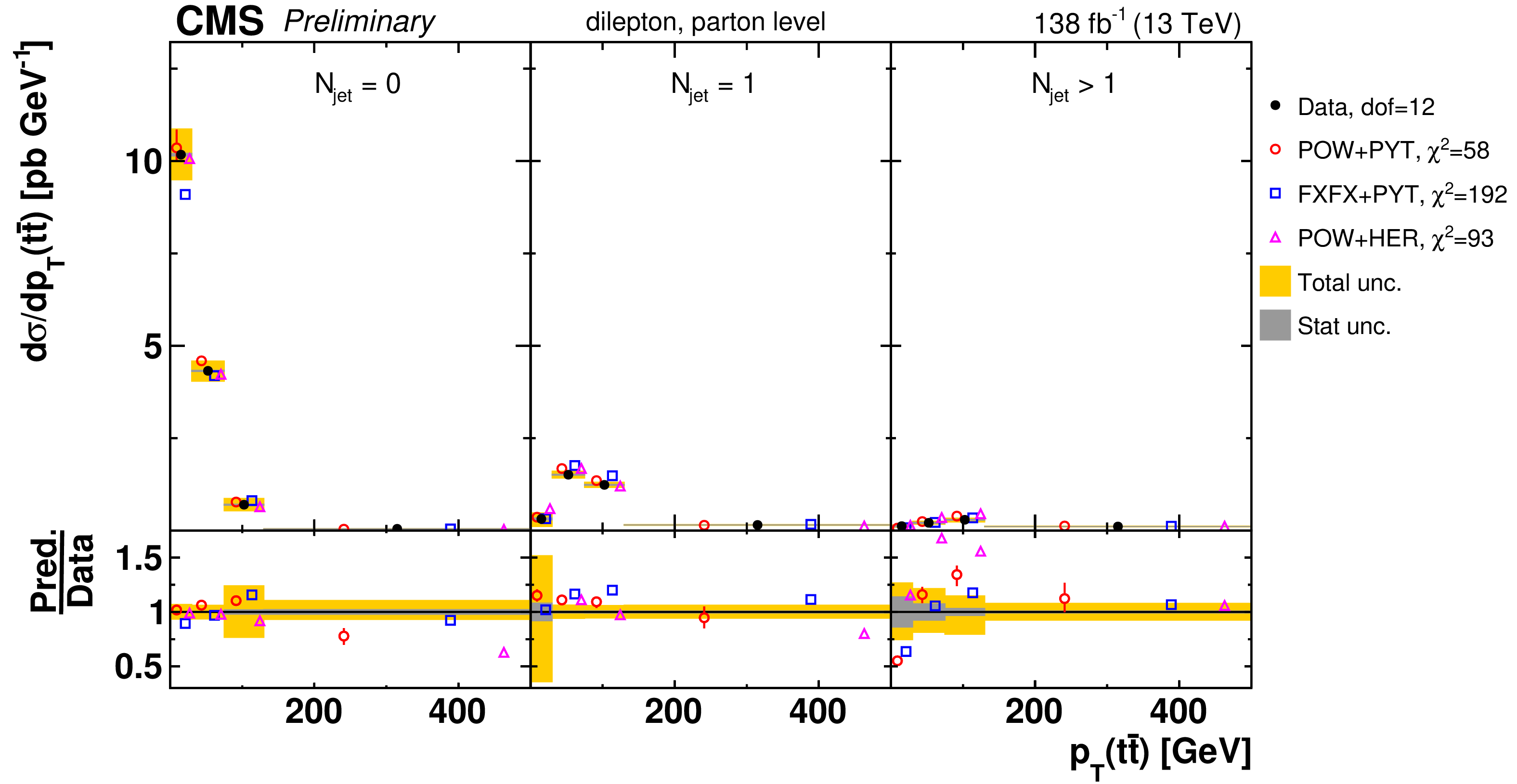
png pdf	Figure 90-a: Absolute $[ {N_{\text {jet}}},\,{{p_{\mathrm {T}}} ( \mathrm{t\bar{t}})} ]$ cross sections are shown for data (filled circles) and various MC predictions (other points). Further details can be found in the caption of Fig. 88.
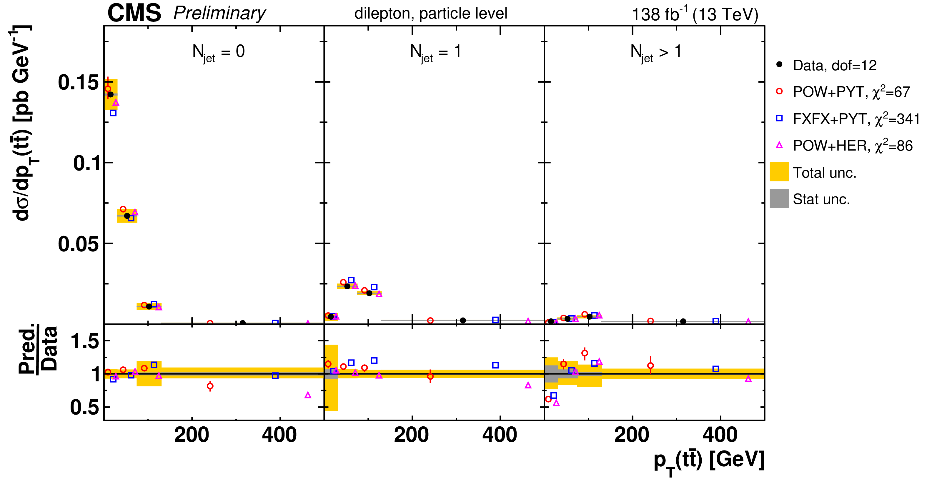
png pdf	Figure 90-b: Absolute $[ {N_{\text {jet}}},\,{{p_{\mathrm {T}}} ( \mathrm{t\bar{t}})} ]$ cross sections are shown for data (filled circles) and various MC predictions (other points). Further details can be found in the caption of Fig. 88.
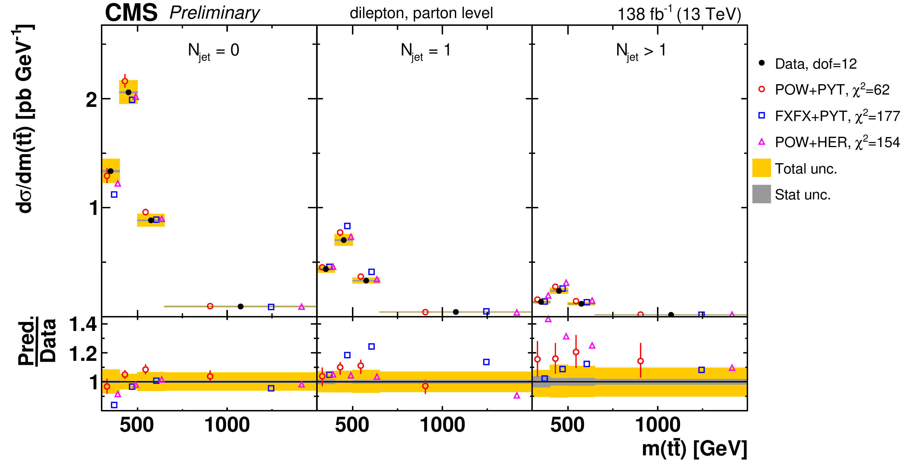
png pdf	Figure 91-a: Absolute $[ {N_{\text {jet}}},\,{m( \mathrm{t\bar{t}})} ]$ cross sections are shown for data (filled circles) and various MC predictions (other points). Further details can be found in the caption of Fig. 88.
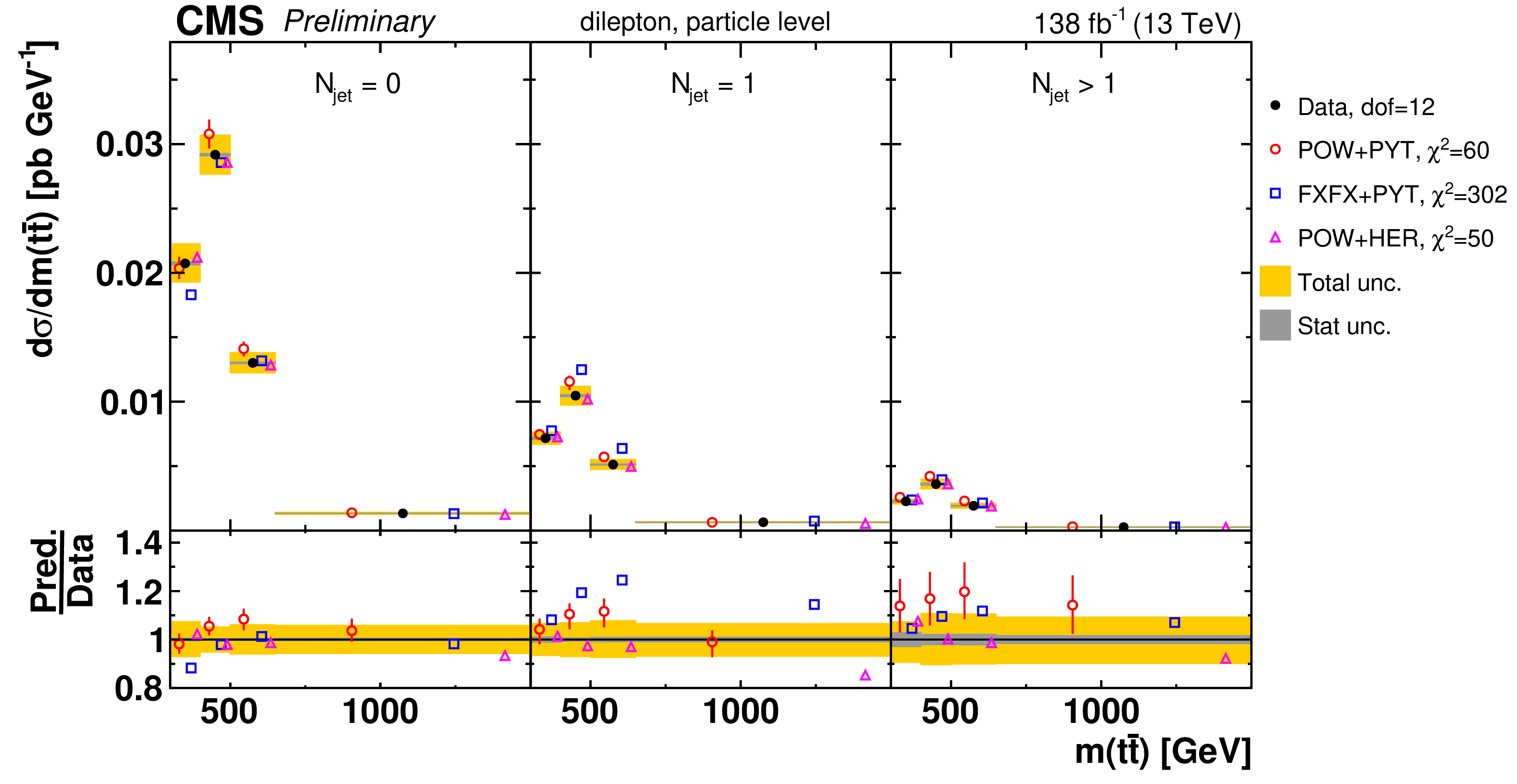
png pdf	Figure 91-b: Absolute $[ {N_{\text {jet}}},\,{m( \mathrm{t\bar{t}})} ]$ cross sections are shown for data (filled circles) and various MC predictions (other points). Further details can be found in the caption of Fig. 88.
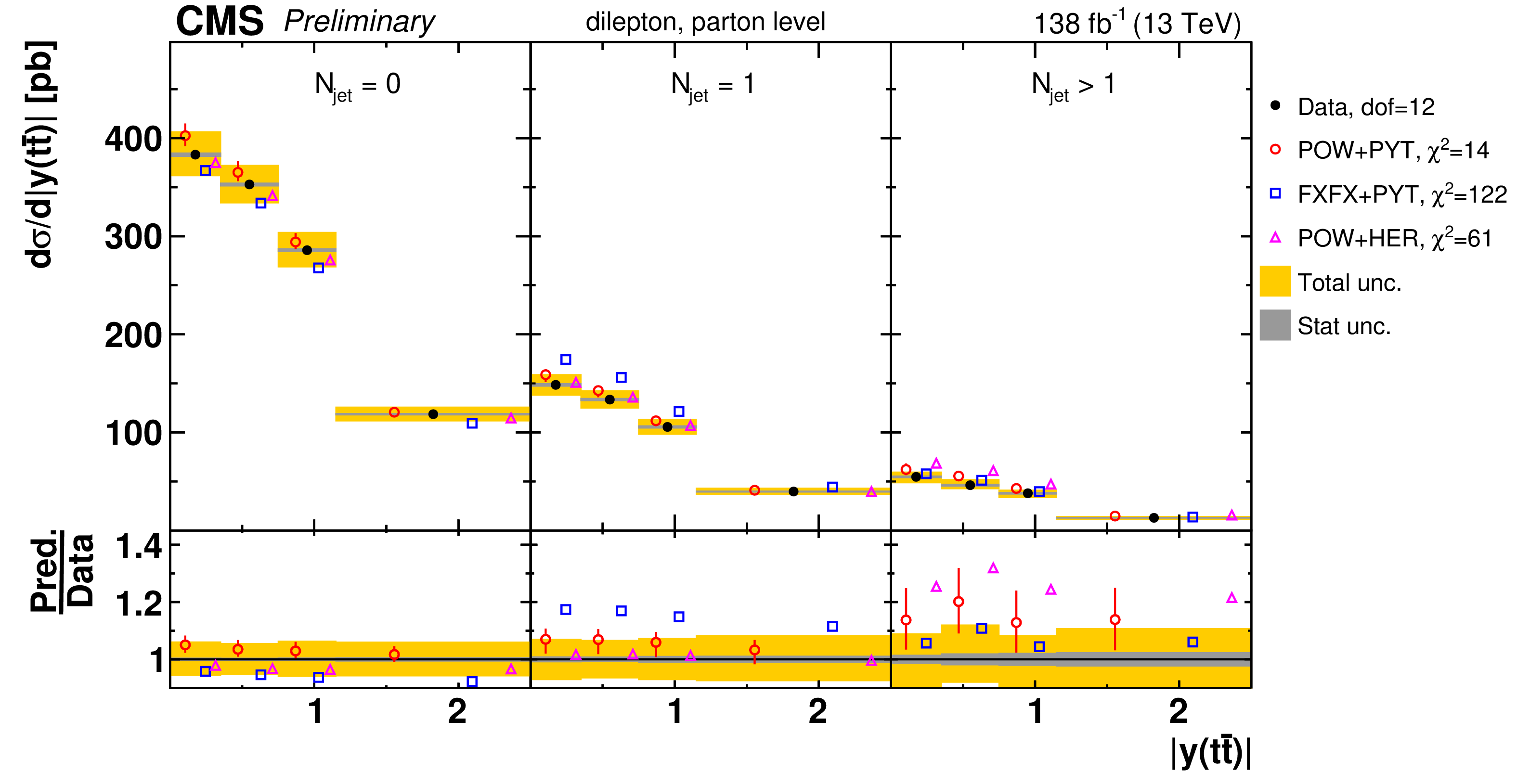
png pdf	Figure 92-a: Absolute $[ {N_{\text {jet}}},\,{|y( \mathrm{t\bar{t}})|} ]$ cross sections are shown for data (filled circles) and various MC predictions (other points). Further details can be found in the caption of Fig. 88.
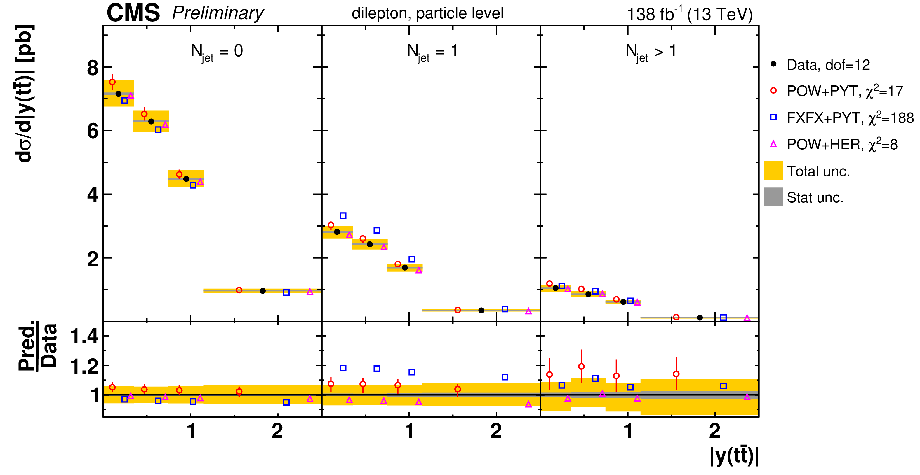
png pdf	Figure 92-b: Absolute $[ {N_{\text {jet}}},\,{|y( \mathrm{t\bar{t}})|} ]$ cross sections are shown for data (filled circles) and various MC predictions (other points). Further details can be found in the caption of Fig. 88.
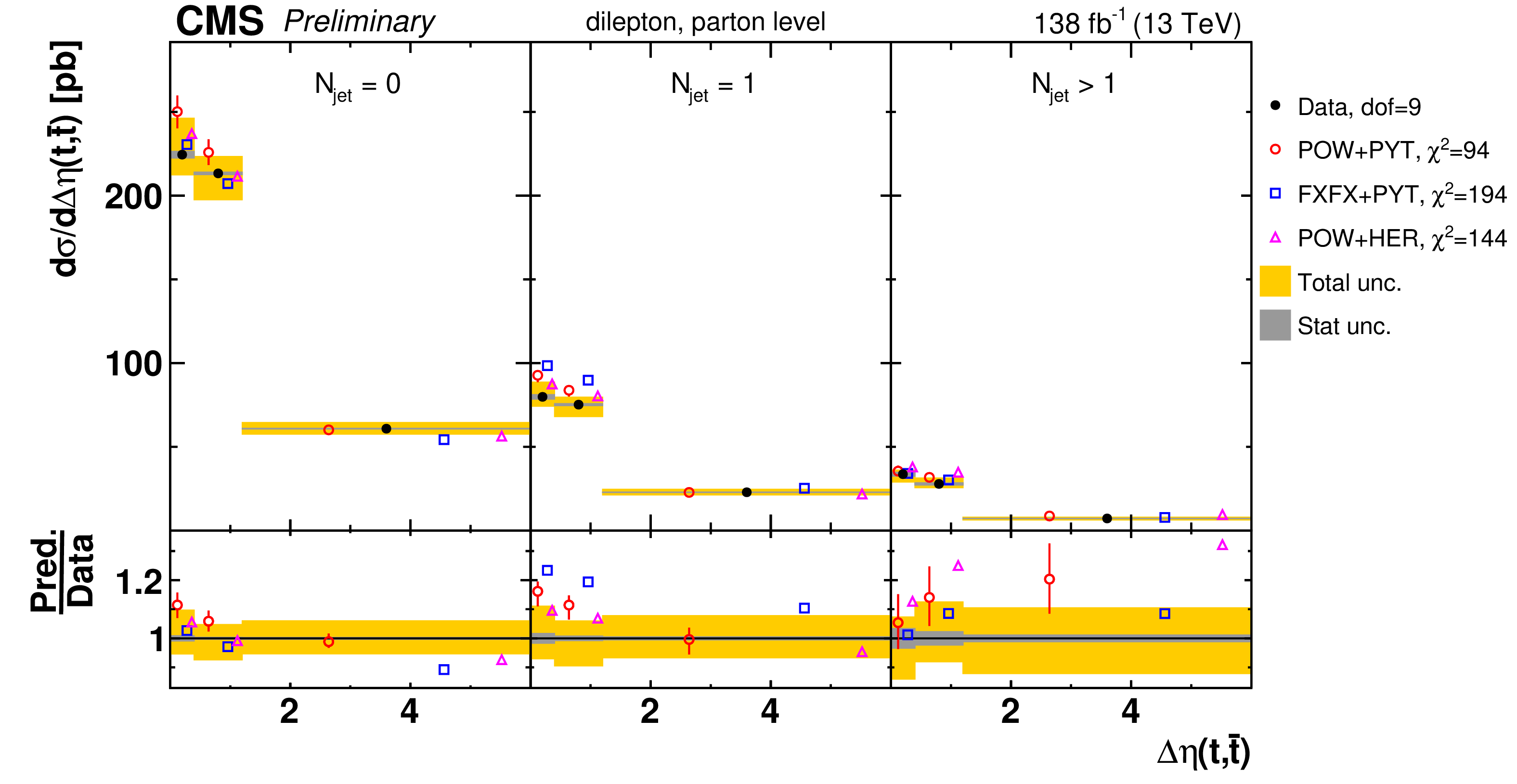
png pdf	Figure 93-a: Absolute $[ {N_{\text {jet}}},\,{\Delta \eta (\mathrm{t},\mathrm{\bar{t}})} ]$ cross sections are shown for data (filled circles) and various MC predictions (other points). Further details can be found in the caption of Fig. 88.
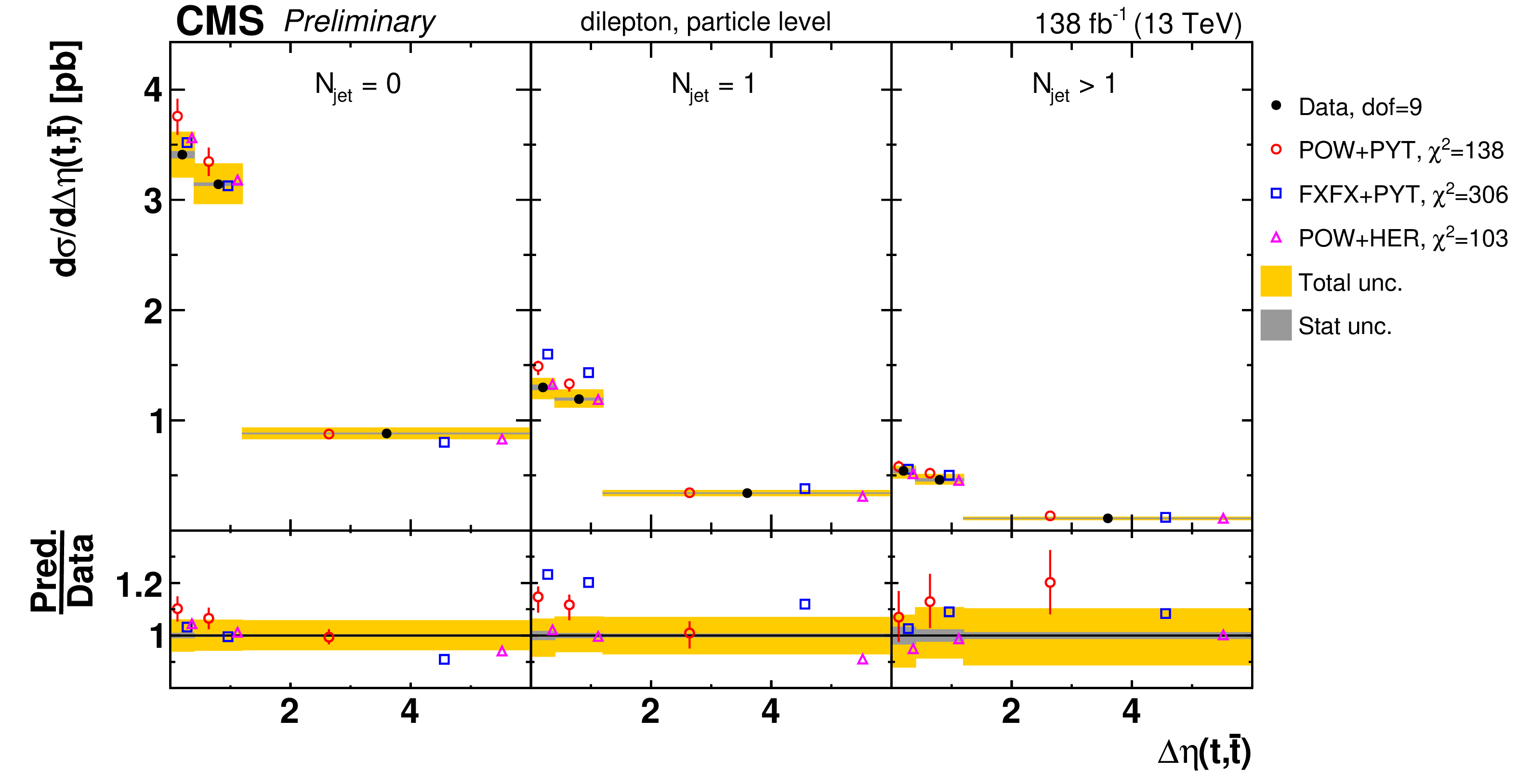
png pdf	Figure 93-b: Absolute $[ {N_{\text {jet}}},\,{\Delta \eta (\mathrm{t},\mathrm{\bar{t}})} ]$ cross sections are shown for data (filled circles) and various MC predictions (other points). Further details can be found in the caption of Fig. 88.
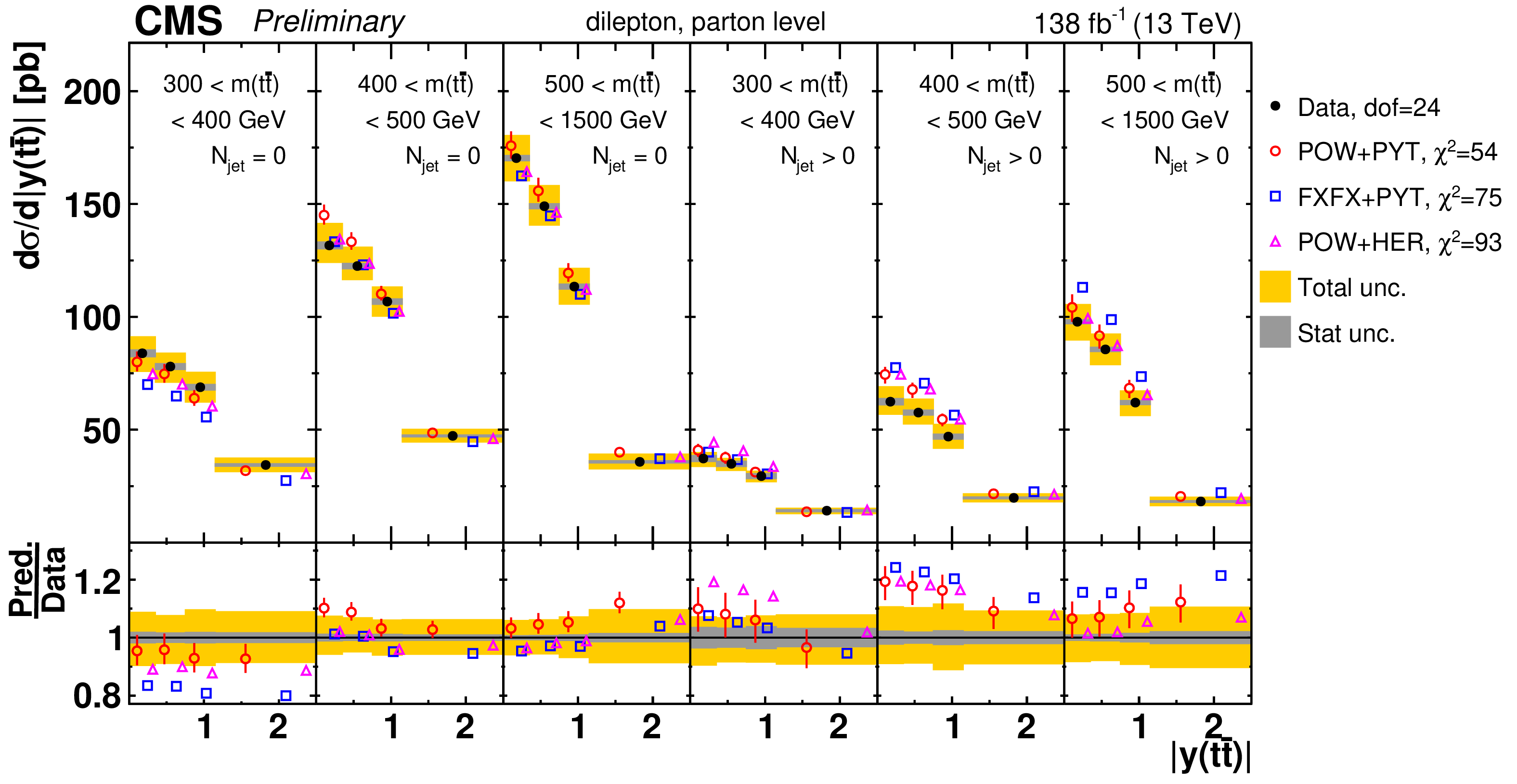
png pdf	Figure 94-a: Absolute $[N^{0,1+}_{\text {jet}},\, {m( \mathrm{t\bar{t}})},\,{|y( \mathrm{t\bar{t}})|} ]$ cross sections are shown for data (filled circles) and various MC predictions (other points). Further details can be found in the caption of Fig. 88.
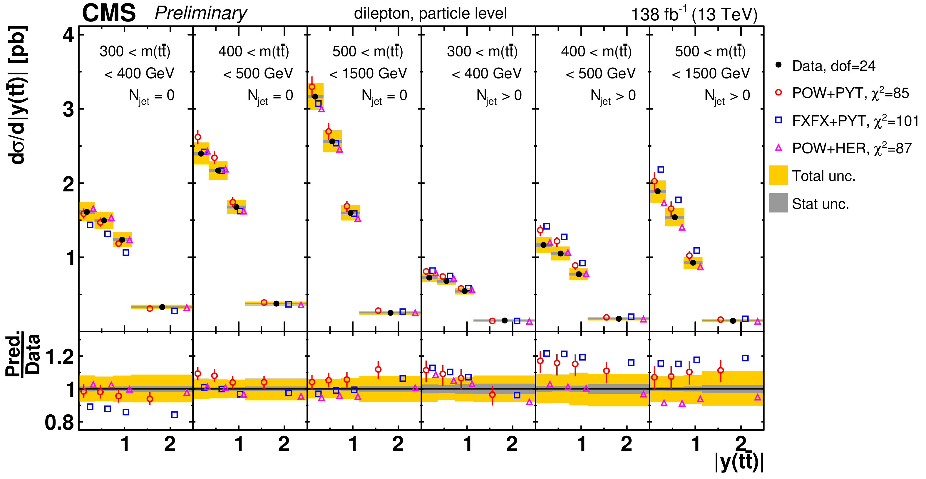
png pdf	Figure 94-b: Absolute $[N^{0,1+}_{\text {jet}},\, {m( \mathrm{t\bar{t}})},\,{|y( \mathrm{t\bar{t}})|} ]$ cross sections are shown for data (filled circles) and various MC predictions (other points). Further details can be found in the caption of Fig. 88.
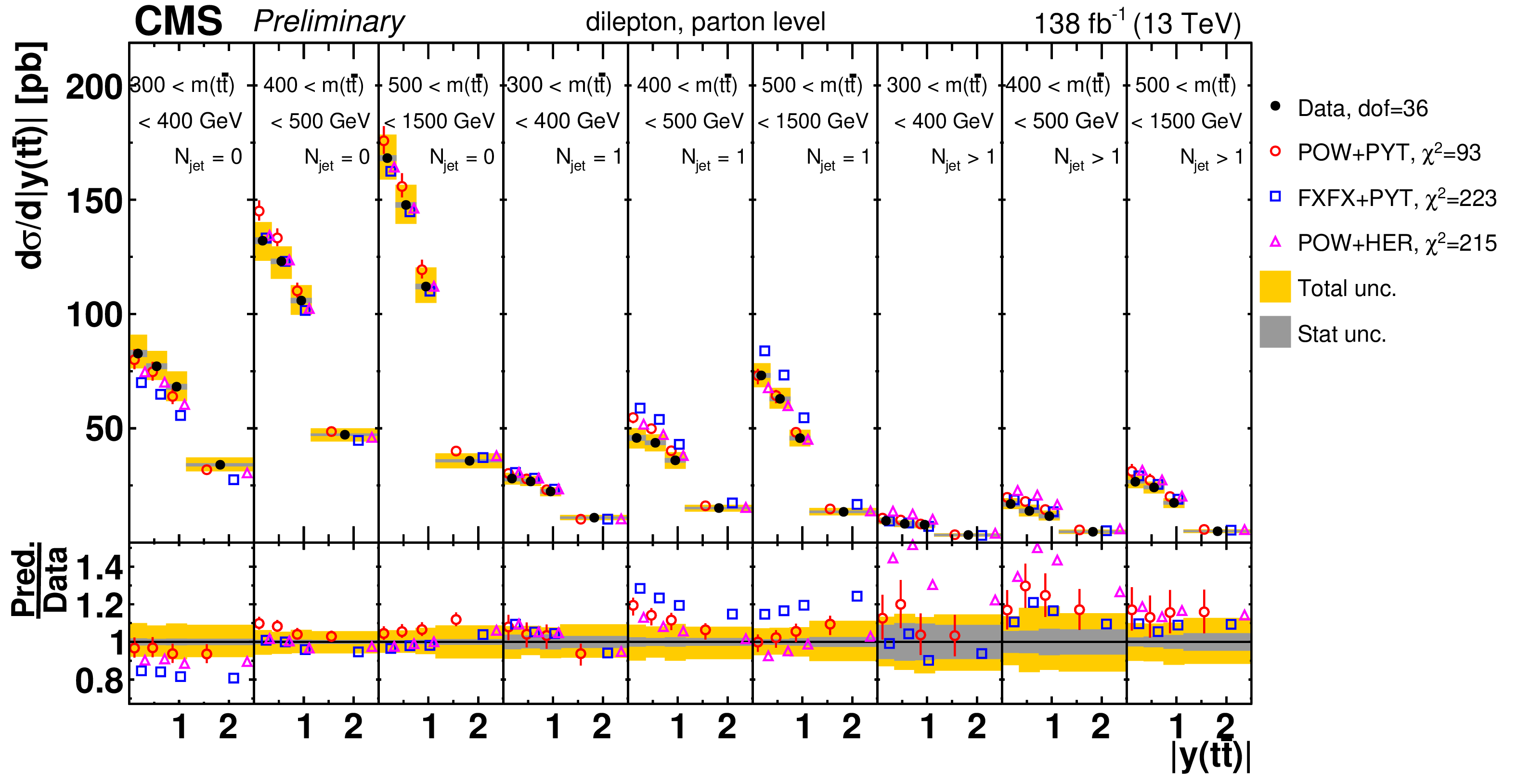
png pdf	Figure 95-a: Absolute $[N^{0,1,2+}_{\text {jet}},\, {m( \mathrm{t\bar{t}})},\,{|y( \mathrm{t\bar{t}})|} ]$ cross sections are shown for data (filled circles) and various MC predictions (other points). Further details can be found in the caption of Fig. 88.
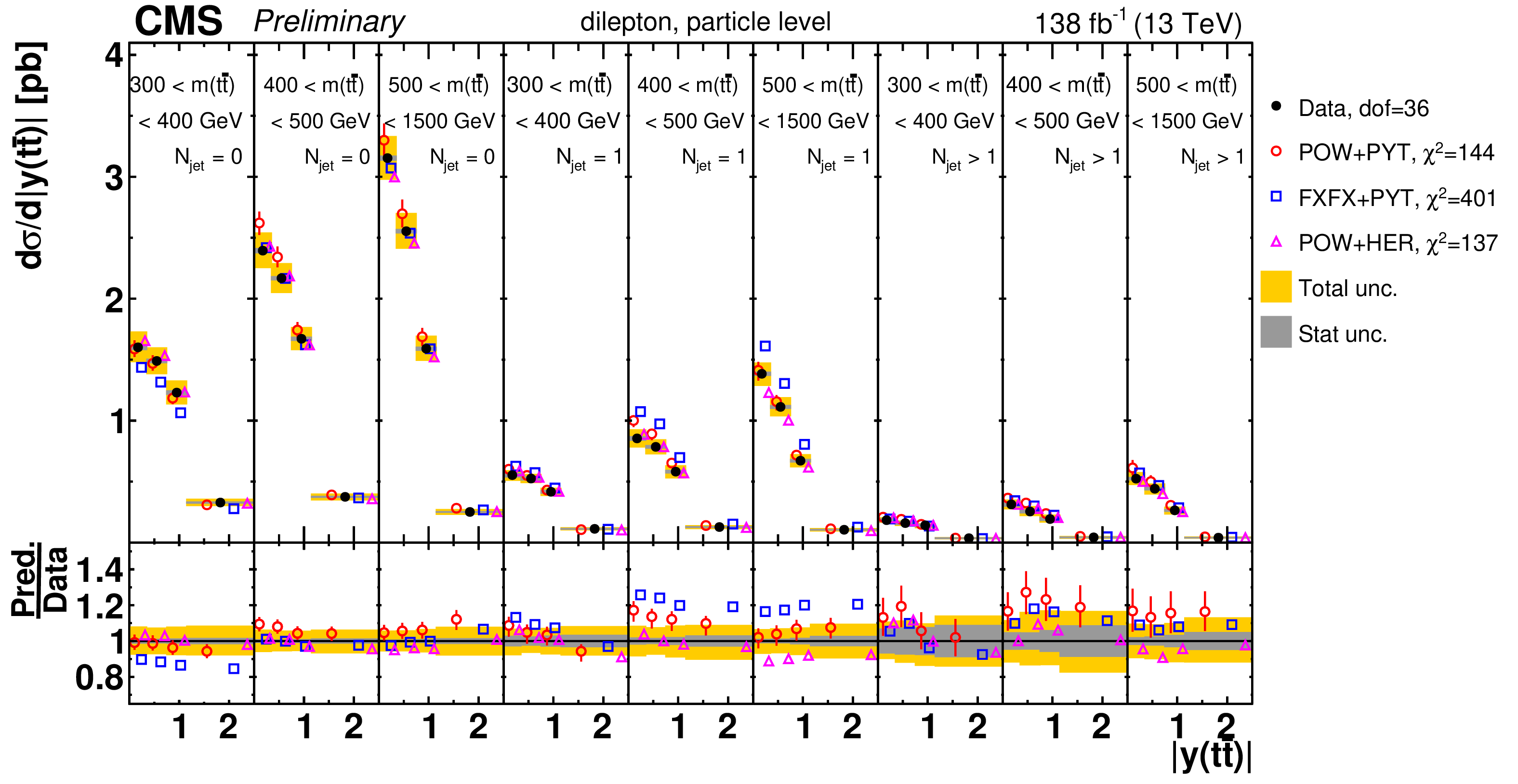
png pdf	Figure 95-b: Absolute $[N^{0,1,2+}_{\text {jet}},\, {m( \mathrm{t\bar{t}})},\,{|y( \mathrm{t\bar{t}})|} ]$ cross sections are shown for data (filled circles) and various MC predictions (other points). Further details can be found in the caption of Fig. 88.
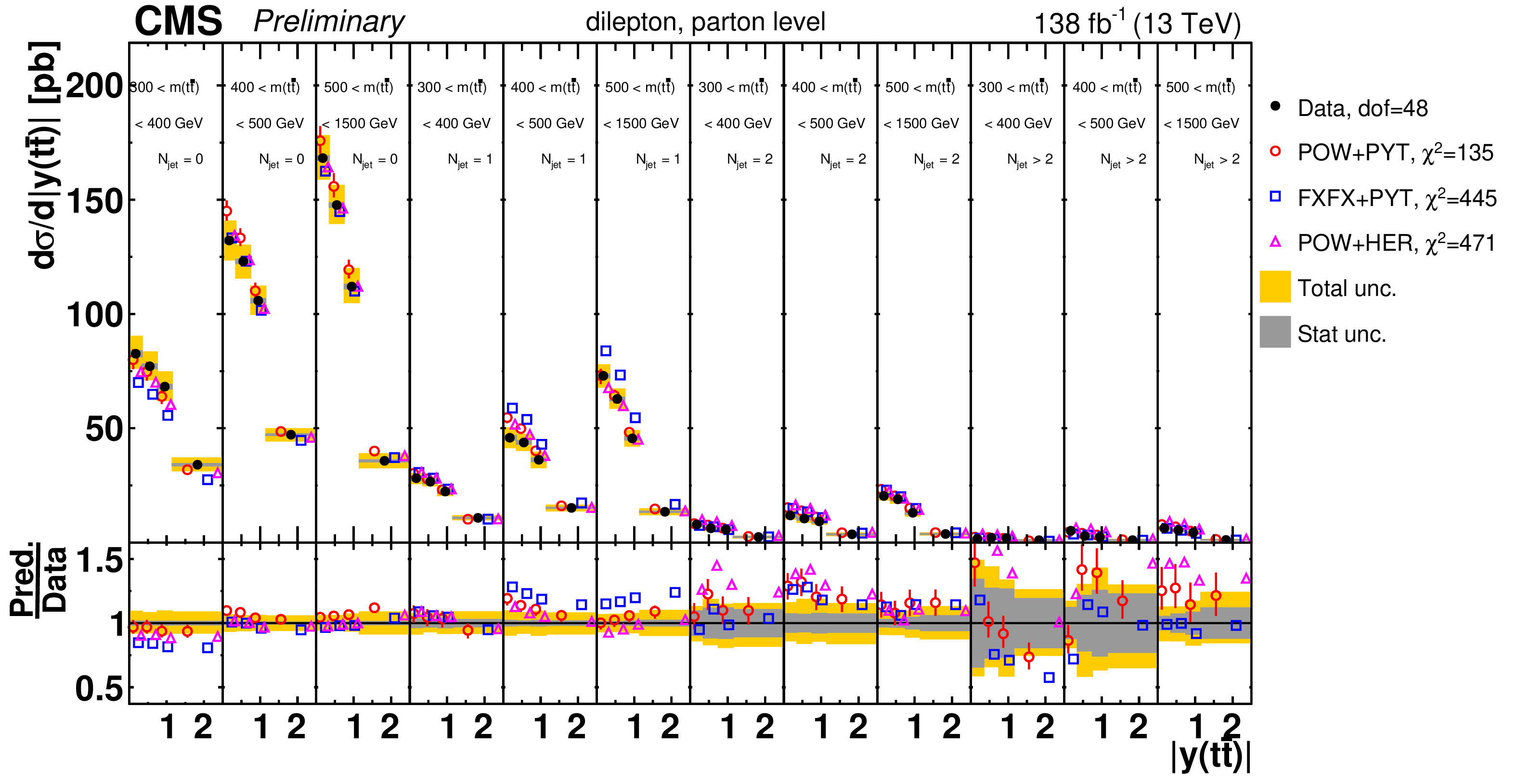
png pdf	Figure 96-a: Absolute $[N^{0,1,2,3+}_{\text {jet}},\, {m( \mathrm{t\bar{t}})},\,{|y( \mathrm{t\bar{t}})|} ]$ cross sections are shown for data (filled circles) and various MC predictions (other points). Further details can be found in the caption of Fig. 88.
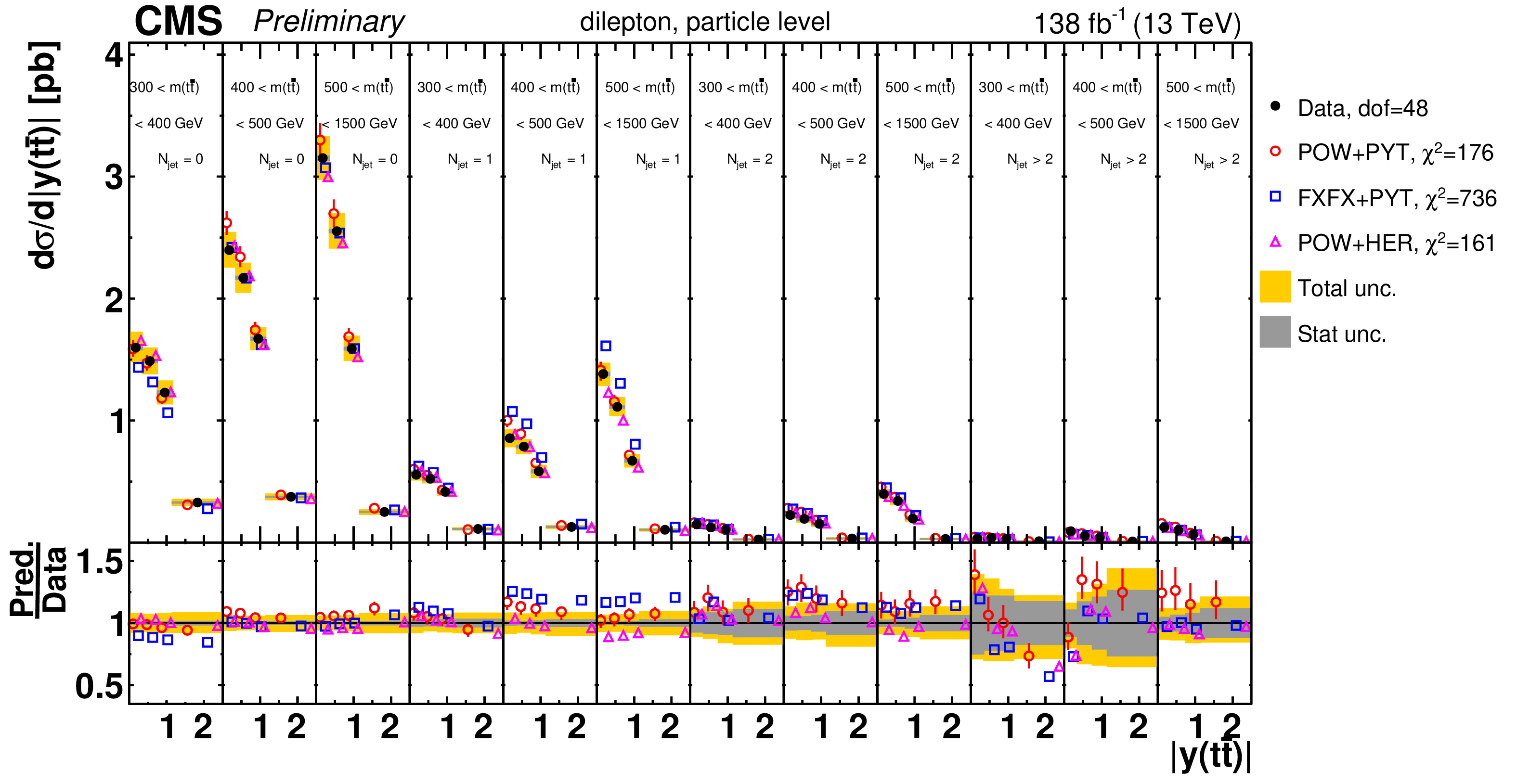
png pdf	Figure 96-b: Absolute $[N^{0,1,2,3+}_{\text {jet}},\, {m( \mathrm{t\bar{t}})},\,{|y( \mathrm{t\bar{t}})|} ]$ cross sections are shown for data (filled circles) and various MC predictions (other points). Further details can be found in the caption of Fig. 88.
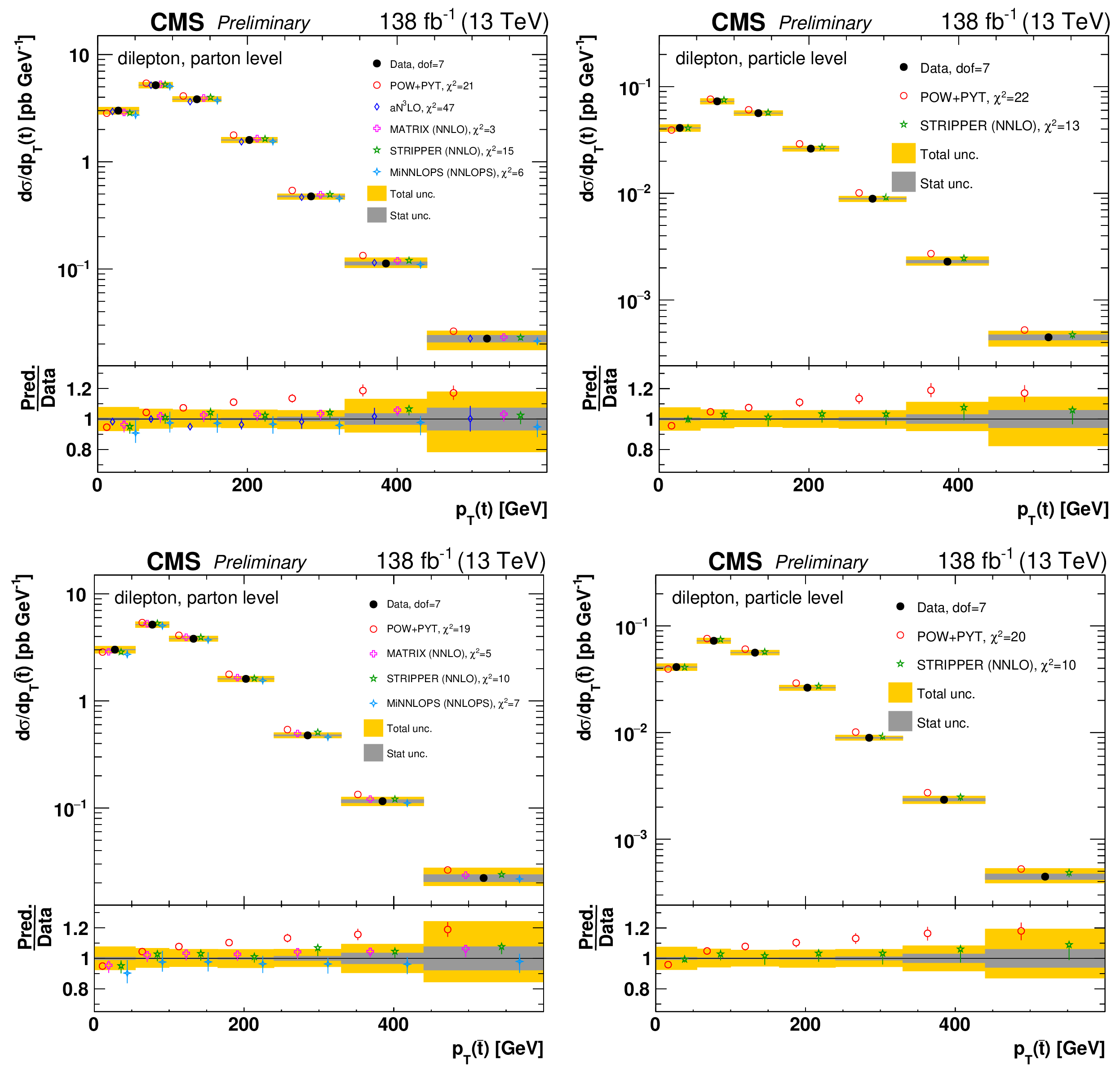
png pdf	Figure 97: Absolute differential $\mathrm{t\bar{t}}$ production cross sections as a function of ${{p_{\mathrm {T}}} (\mathrm{t})}$ (upper) and ${{p_{\mathrm {T}}} (\mathrm{\bar{t}})}$ (lower), measured at the parton level in the full phase space (left) and at the particle level in a fiducial phase space (right). The data are shown as filled circles with dark and light bands indicating the statistical and total uncertainties (statistical and systematic uncertainties summed in quadrature), respectively. The cross sections are compared to predictions from the POWHEG+PYTHIA-8 (`POW-PYT', open circles) simulation and various theoretical predictions with beyond-NLO precision (other points). The estimated uncertainties in the predictions are represented by a vertical bar on the corresponding points. For each model, a value of ${\chi ^2}$ is reported that takes into account the measurement uncertainties. The lower panel in each plot shows the ratios of the predictions to the data.
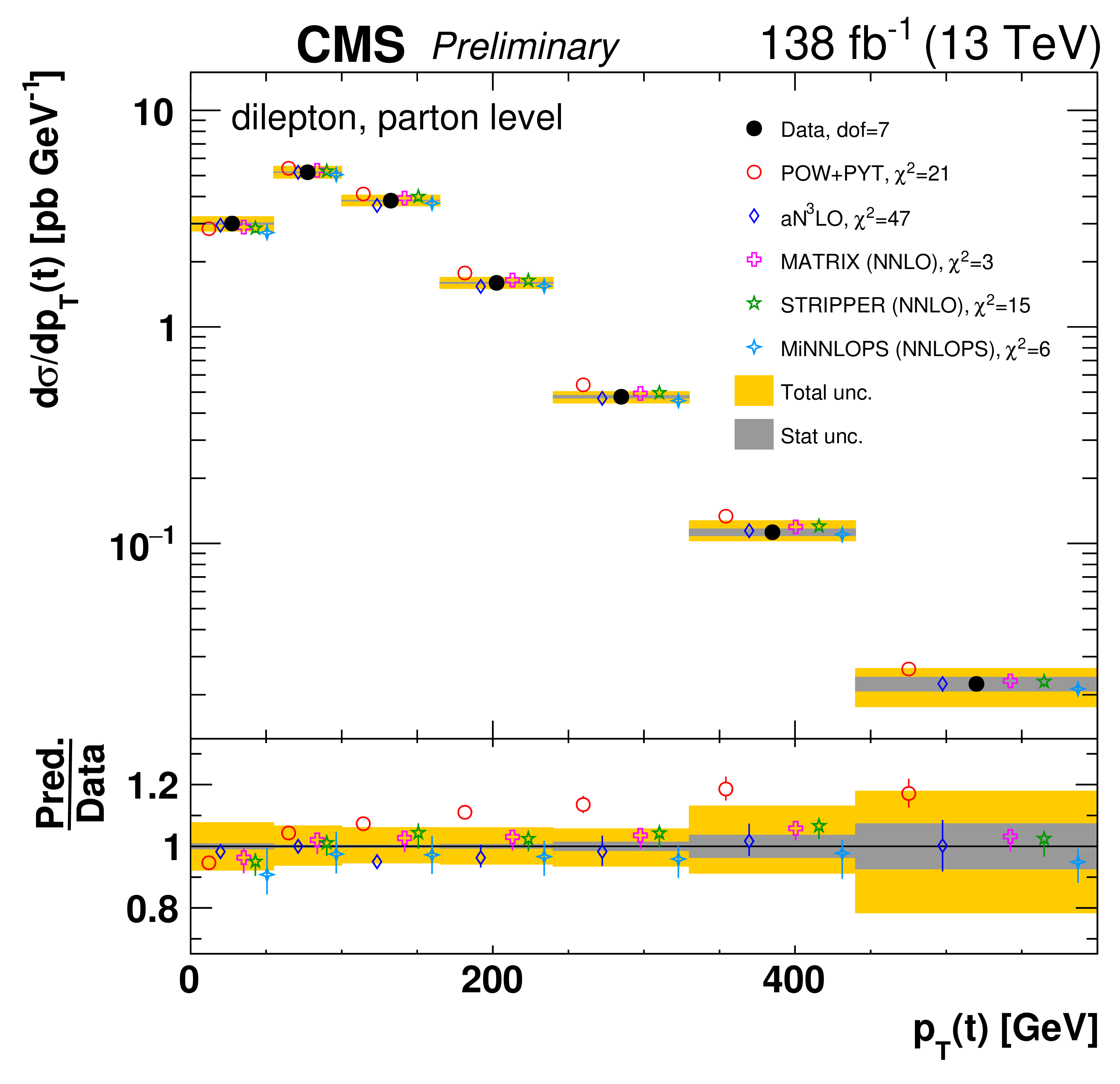
png pdf	Figure 97-a: Absolute differential $\mathrm{t\bar{t}}$ production cross sections as a function of ${{p_{\mathrm {T}}} (\mathrm{t})}$ (upper) and ${{p_{\mathrm {T}}} (\mathrm{\bar{t}})}$ (lower), measured at the parton level in the full phase space (left) and at the particle level in a fiducial phase space (right). The data are shown as filled circles with dark and light bands indicating the statistical and total uncertainties (statistical and systematic uncertainties summed in quadrature), respectively. The cross sections are compared to predictions from the POWHEG+PYTHIA-8 (`POW-PYT', open circles) simulation and various theoretical predictions with beyond-NLO precision (other points). The estimated uncertainties in the predictions are represented by a vertical bar on the corresponding points. For each model, a value of ${\chi ^2}$ is reported that takes into account the measurement uncertainties. The lower panel in each plot shows the ratios of the predictions to the data.
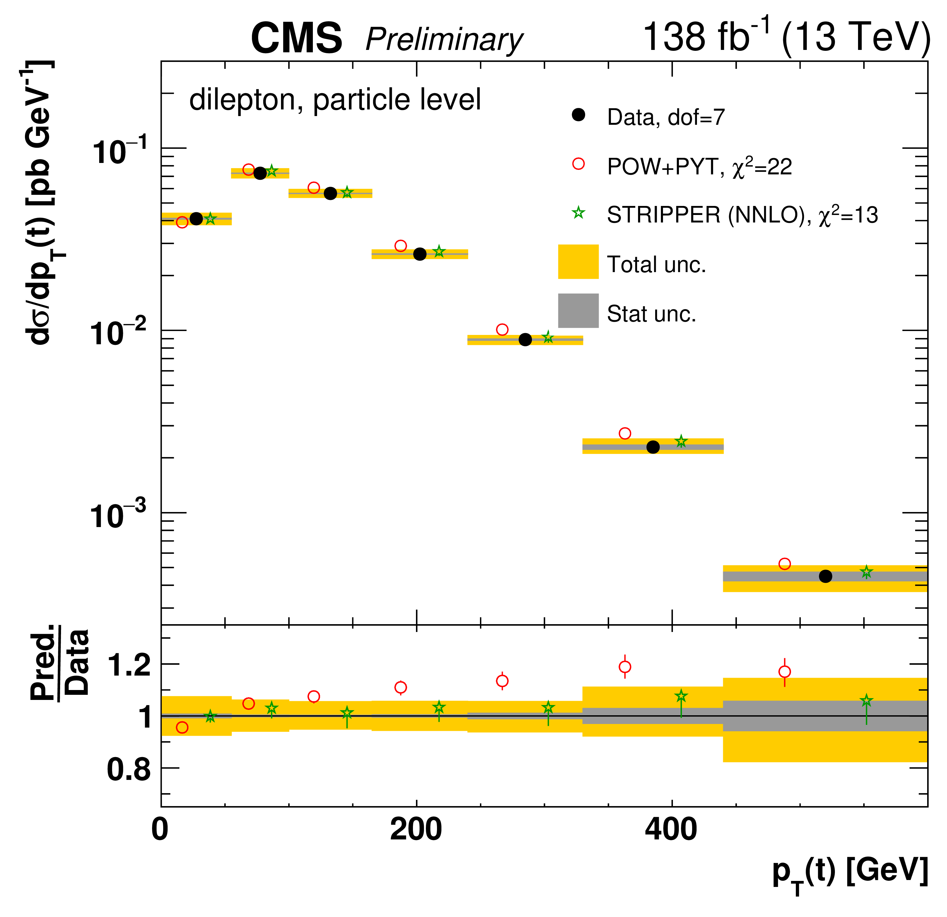
png pdf	Figure 97-b: Absolute differential $\mathrm{t\bar{t}}$ production cross sections as a function of ${{p_{\mathrm {T}}} (\mathrm{t})}$ (upper) and ${{p_{\mathrm {T}}} (\mathrm{\bar{t}})}$ (lower), measured at the parton level in the full phase space (left) and at the particle level in a fiducial phase space (right). The data are shown as filled circles with dark and light bands indicating the statistical and total uncertainties (statistical and systematic uncertainties summed in quadrature), respectively. The cross sections are compared to predictions from the POWHEG+PYTHIA-8 (`POW-PYT', open circles) simulation and various theoretical predictions with beyond-NLO precision (other points). The estimated uncertainties in the predictions are represented by a vertical bar on the corresponding points. For each model, a value of ${\chi ^2}$ is reported that takes into account the measurement uncertainties. The lower panel in each plot shows the ratios of the predictions to the data.
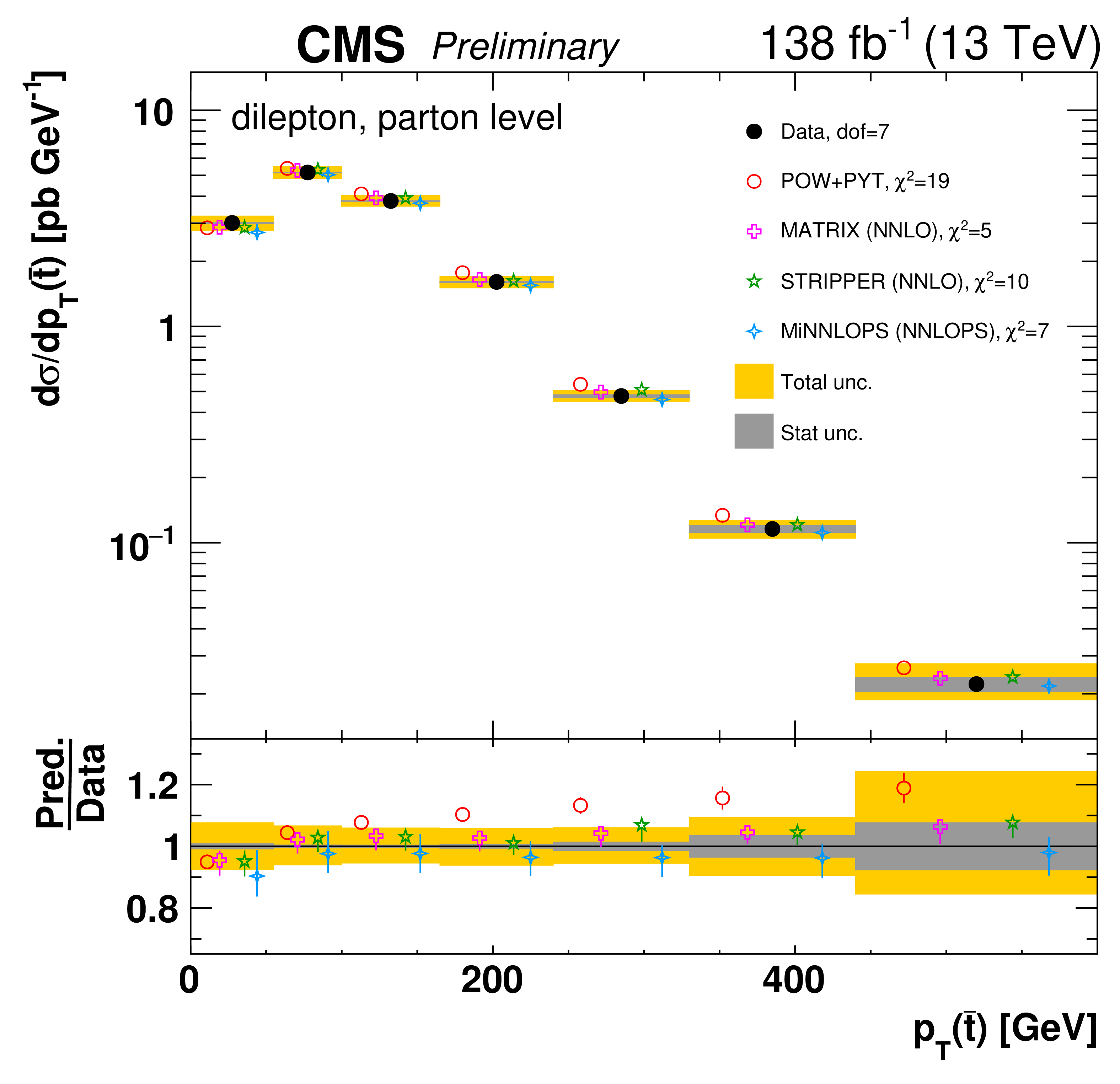
png pdf	Figure 97-c: Absolute differential $\mathrm{t\bar{t}}$ production cross sections as a function of ${{p_{\mathrm {T}}} (\mathrm{t})}$ (upper) and ${{p_{\mathrm {T}}} (\mathrm{\bar{t}})}$ (lower), measured at the parton level in the full phase space (left) and at the particle level in a fiducial phase space (right). The data are shown as filled circles with dark and light bands indicating the statistical and total uncertainties (statistical and systematic uncertainties summed in quadrature), respectively. The cross sections are compared to predictions from the POWHEG+PYTHIA-8 (`POW-PYT', open circles) simulation and various theoretical predictions with beyond-NLO precision (other points). The estimated uncertainties in the predictions are represented by a vertical bar on the corresponding points. For each model, a value of ${\chi ^2}$ is reported that takes into account the measurement uncertainties. The lower panel in each plot shows the ratios of the predictions to the data.
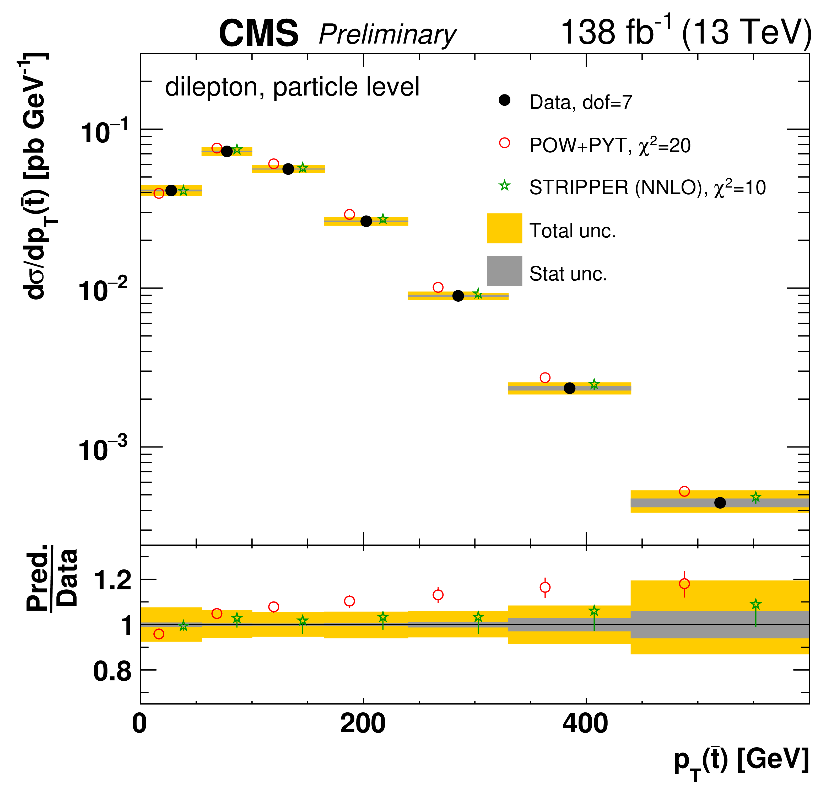
png pdf	Figure 97-d: Absolute differential $\mathrm{t\bar{t}}$ production cross sections as a function of ${{p_{\mathrm {T}}} (\mathrm{t})}$ (upper) and ${{p_{\mathrm {T}}} (\mathrm{\bar{t}})}$ (lower), measured at the parton level in the full phase space (left) and at the particle level in a fiducial phase space (right). The data are shown as filled circles with dark and light bands indicating the statistical and total uncertainties (statistical and systematic uncertainties summed in quadrature), respectively. The cross sections are compared to predictions from the POWHEG+PYTHIA-8 (`POW-PYT', open circles) simulation and various theoretical predictions with beyond-NLO precision (other points). The estimated uncertainties in the predictions are represented by a vertical bar on the corresponding points. For each model, a value of ${\chi ^2}$ is reported that takes into account the measurement uncertainties. The lower panel in each plot shows the ratios of the predictions to the data.
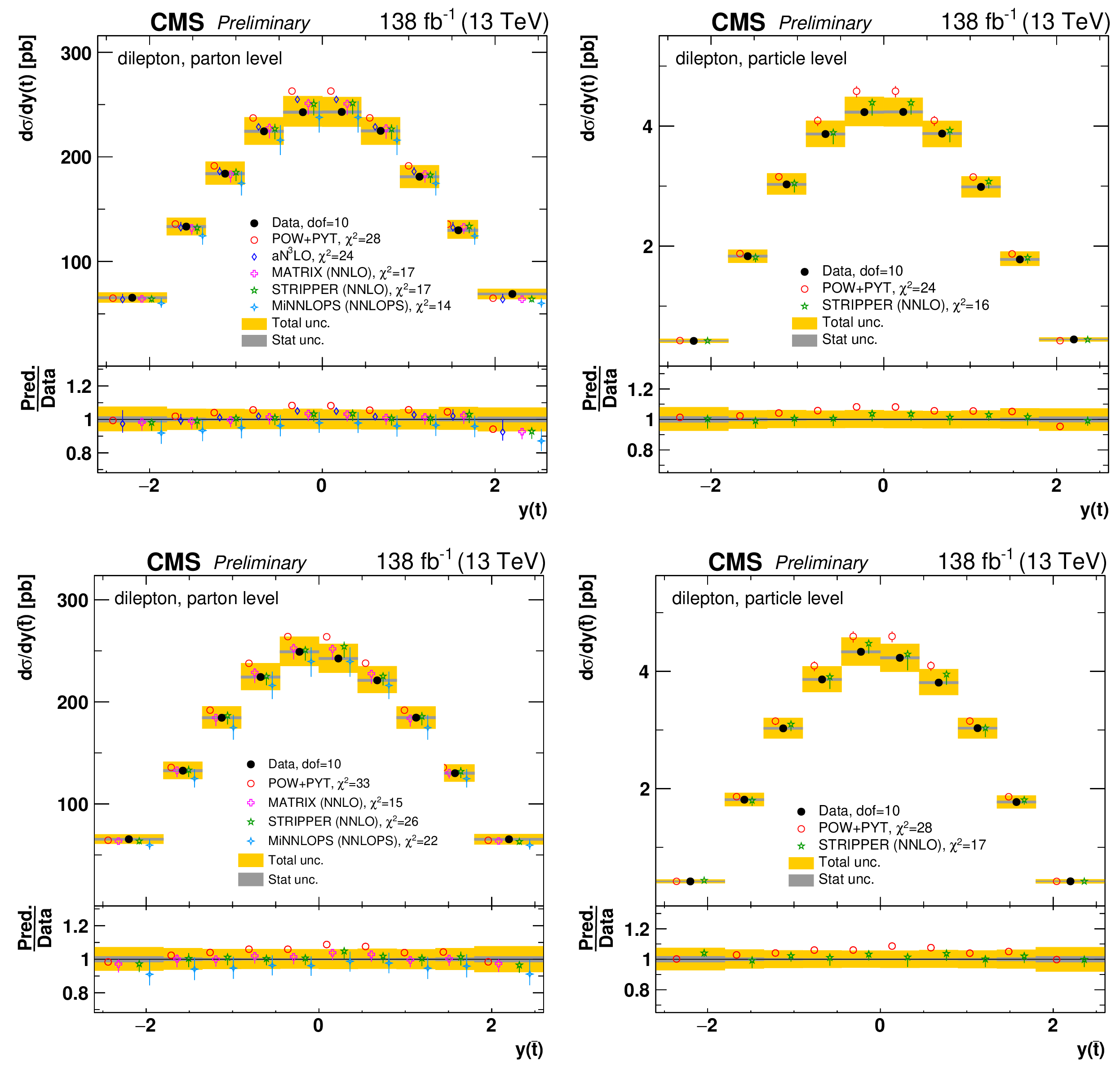
png pdf	Figure 98: Absolute differential $\mathrm{t\bar{t}}$ production cross sections as a function of ${y(\mathrm{t})}$ (upper) and ${y(\mathrm{\bar{t}})}$ (lower) are shown for data (filled circles), POWHEG+PYTHIA-8 (`POW-PYT', open circles) simulation, and various theoretical predictions with beyond-NLO precision (other points). Further details can be found in the caption of Fig. 97.
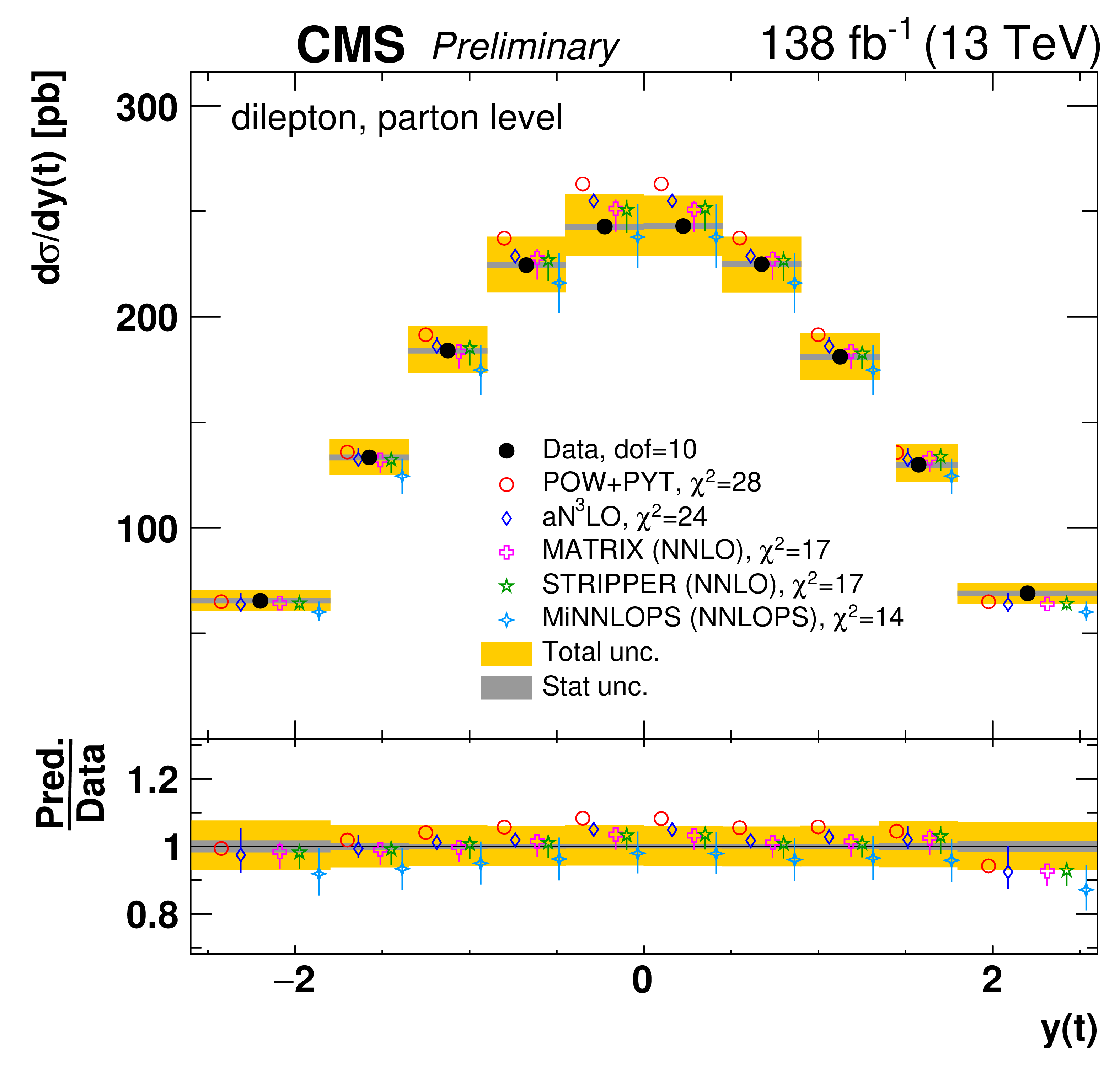
png pdf	Figure 98-a: Absolute differential $\mathrm{t\bar{t}}$ production cross sections as a function of ${y(\mathrm{t})}$ (upper) and ${y(\mathrm{\bar{t}})}$ (lower) are shown for data (filled circles), POWHEG+PYTHIA-8 (`POW-PYT', open circles) simulation, and various theoretical predictions with beyond-NLO precision (other points). Further details can be found in the caption of Fig. 97.
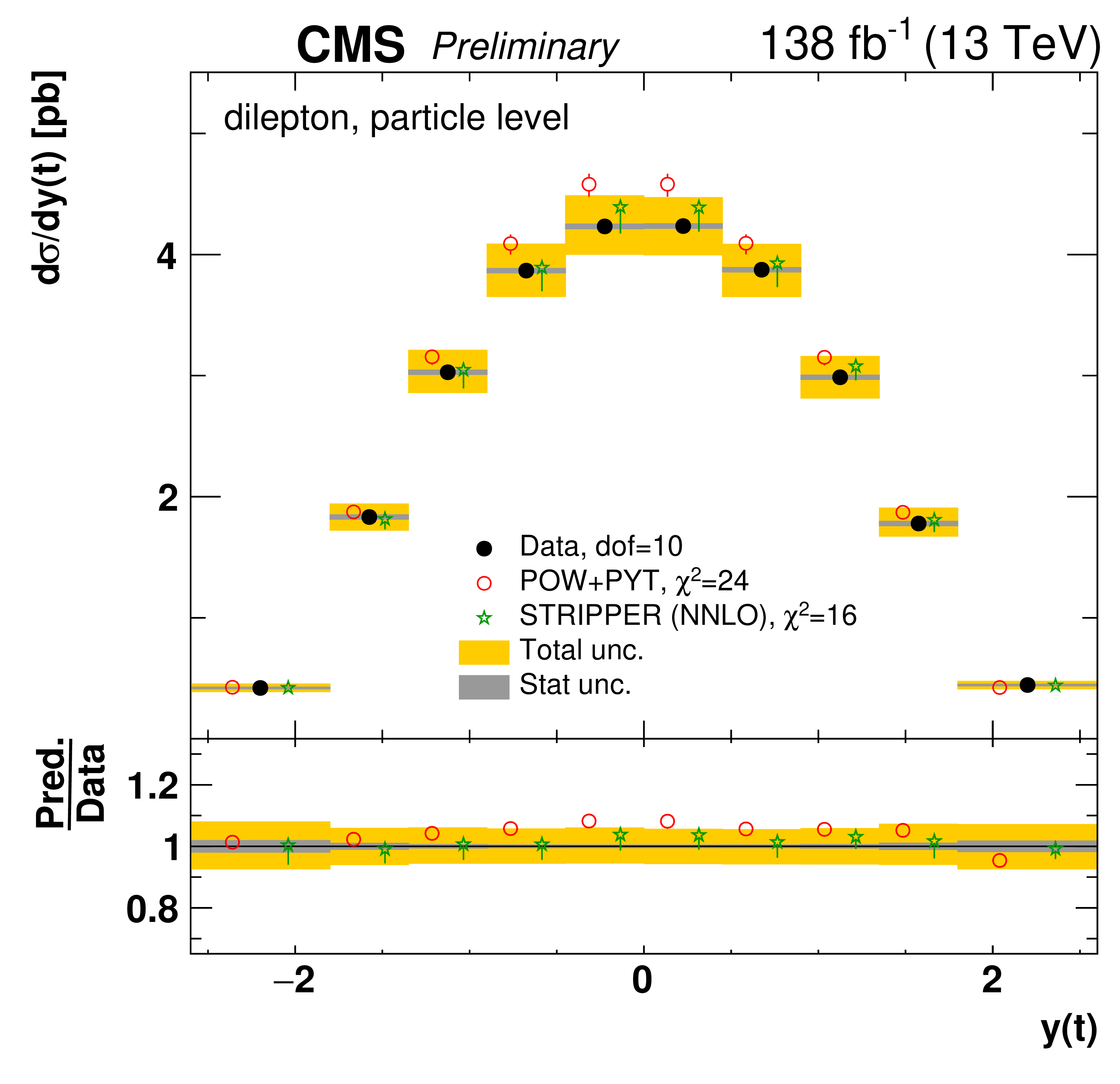
png pdf	Figure 98-b: Absolute differential $\mathrm{t\bar{t}}$ production cross sections as a function of ${y(\mathrm{t})}$ (upper) and ${y(\mathrm{\bar{t}})}$ (lower) are shown for data (filled circles), POWHEG+PYTHIA-8 (`POW-PYT', open circles) simulation, and various theoretical predictions with beyond-NLO precision (other points). Further details can be found in the caption of Fig. 97.
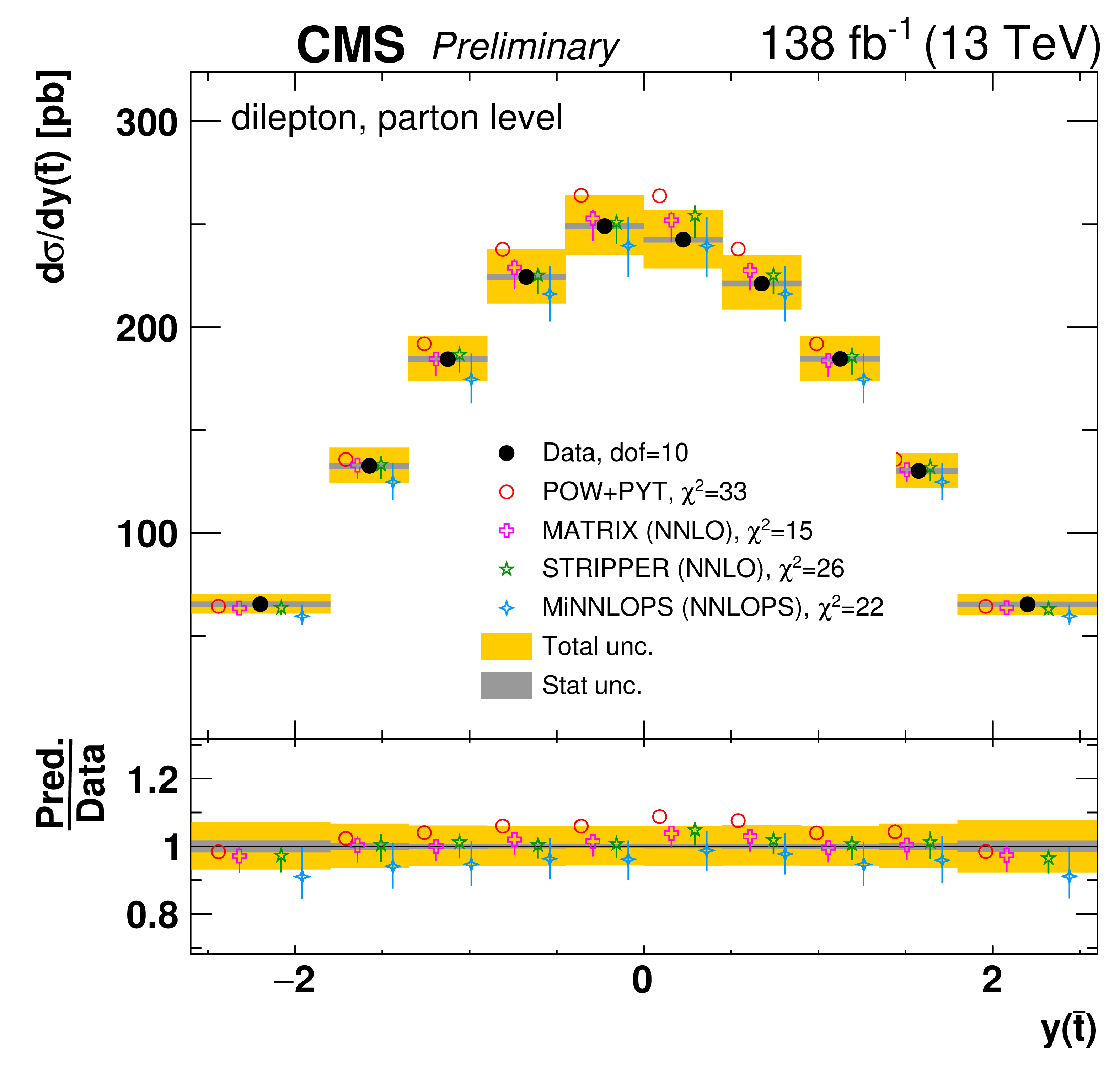
png pdf	Figure 98-c: Absolute differential $\mathrm{t\bar{t}}$ production cross sections as a function of ${y(\mathrm{t})}$ (upper) and ${y(\mathrm{\bar{t}})}$ (lower) are shown for data (filled circles), POWHEG+PYTHIA-8 (`POW-PYT', open circles) simulation, and various theoretical predictions with beyond-NLO precision (other points). Further details can be found in the caption of Fig. 97.
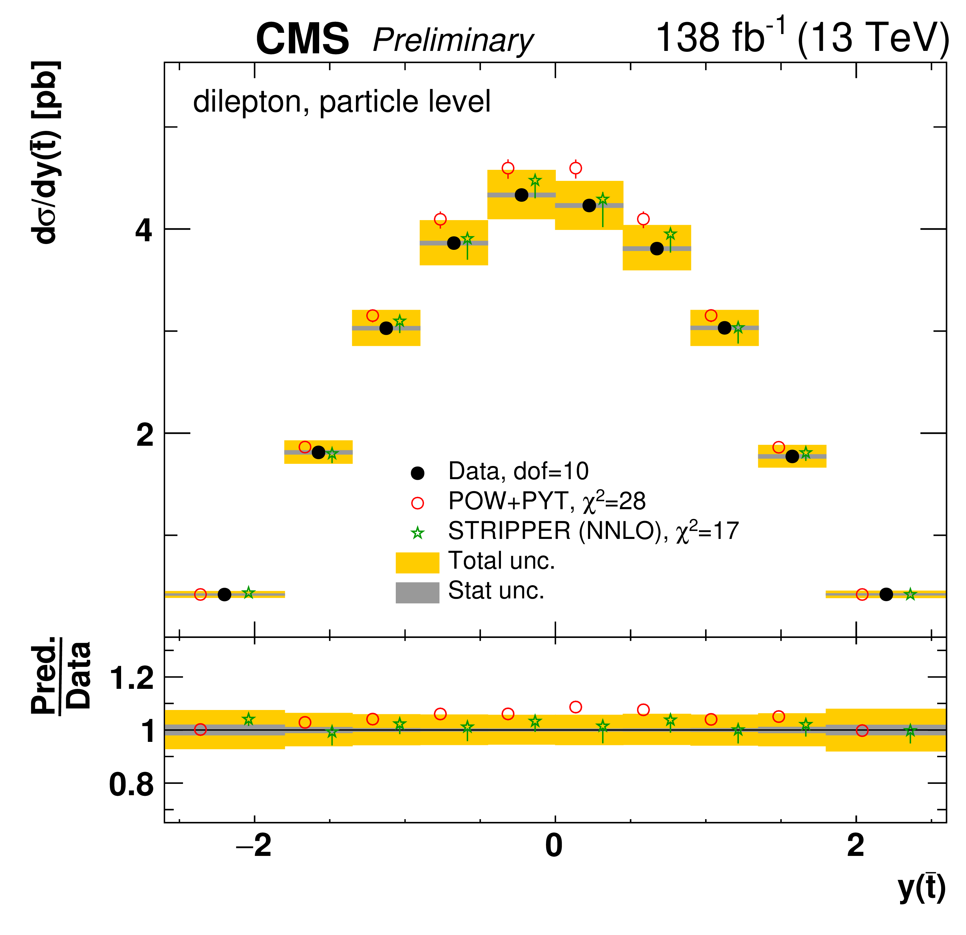
png pdf	Figure 98-d: Absolute differential $\mathrm{t\bar{t}}$ production cross sections as a function of ${y(\mathrm{t})}$ (upper) and ${y(\mathrm{\bar{t}})}$ (lower) are shown for data (filled circles), POWHEG+PYTHIA-8 (`POW-PYT', open circles) simulation, and various theoretical predictions with beyond-NLO precision (other points). Further details can be found in the caption of Fig. 97.
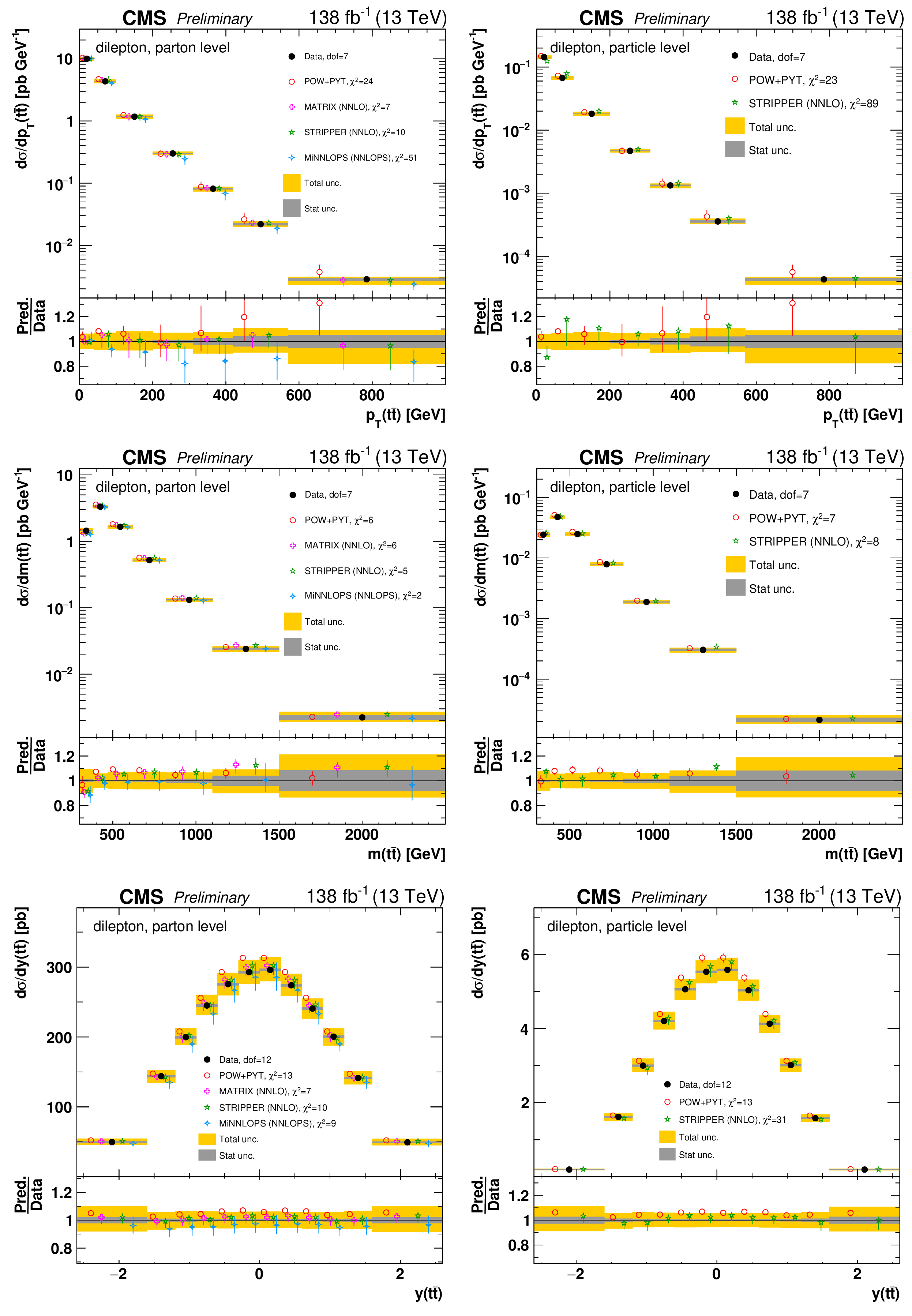
png pdf	Figure 99: Absolute differential $\mathrm{t\bar{t}}$ production cross sections as a function of ${{p_{\mathrm {T}}} ( \mathrm{t\bar{t}})}$ (upper), ${m( \mathrm{t\bar{t}})}$ (middle), and ${y( \mathrm{t\bar{t}})}$ (lower) are shown for data (filled circles), POWHEG+PYTHIA-8 (`POW-PYT', open circles) simulation, and various theoretical predictions with beyond-NLO precision (other points). Further details can be found in the caption of Fig. 97.
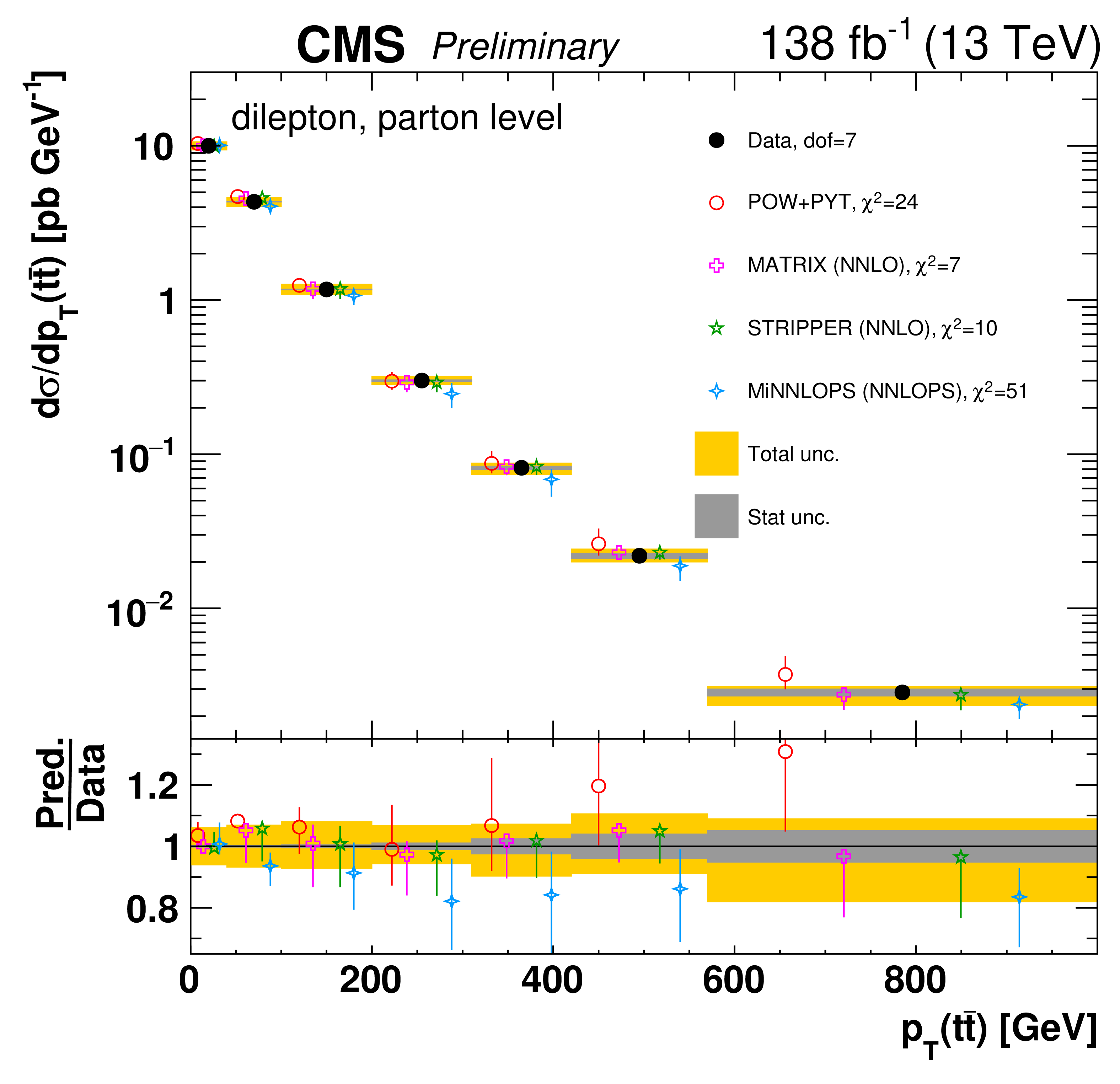
png pdf	Figure 99-a: Absolute differential $\mathrm{t\bar{t}}$ production cross sections as a function of ${{p_{\mathrm {T}}} ( \mathrm{t\bar{t}})}$ (upper), ${m( \mathrm{t\bar{t}})}$ (middle), and ${y( \mathrm{t\bar{t}})}$ (lower) are shown for data (filled circles), POWHEG+PYTHIA-8 (`POW-PYT', open circles) simulation, and various theoretical predictions with beyond-NLO precision (other points). Further details can be found in the caption of Fig. 97.
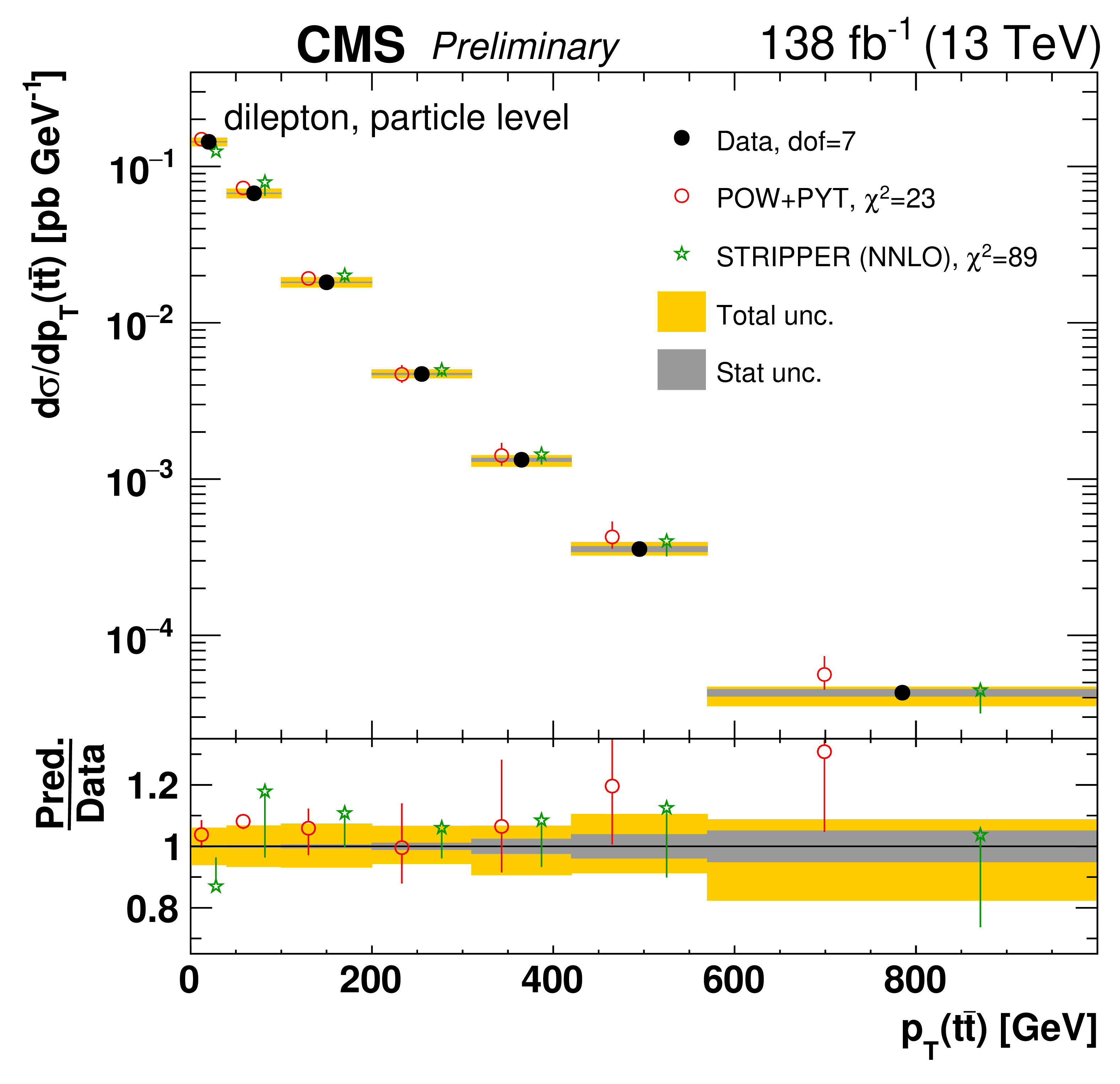
png pdf	Figure 99-b: Absolute differential $\mathrm{t\bar{t}}$ production cross sections as a function of ${{p_{\mathrm {T}}} ( \mathrm{t\bar{t}})}$ (upper), ${m( \mathrm{t\bar{t}})}$ (middle), and ${y( \mathrm{t\bar{t}})}$ (lower) are shown for data (filled circles), POWHEG+PYTHIA-8 (`POW-PYT', open circles) simulation, and various theoretical predictions with beyond-NLO precision (other points). Further details can be found in the caption of Fig. 97.
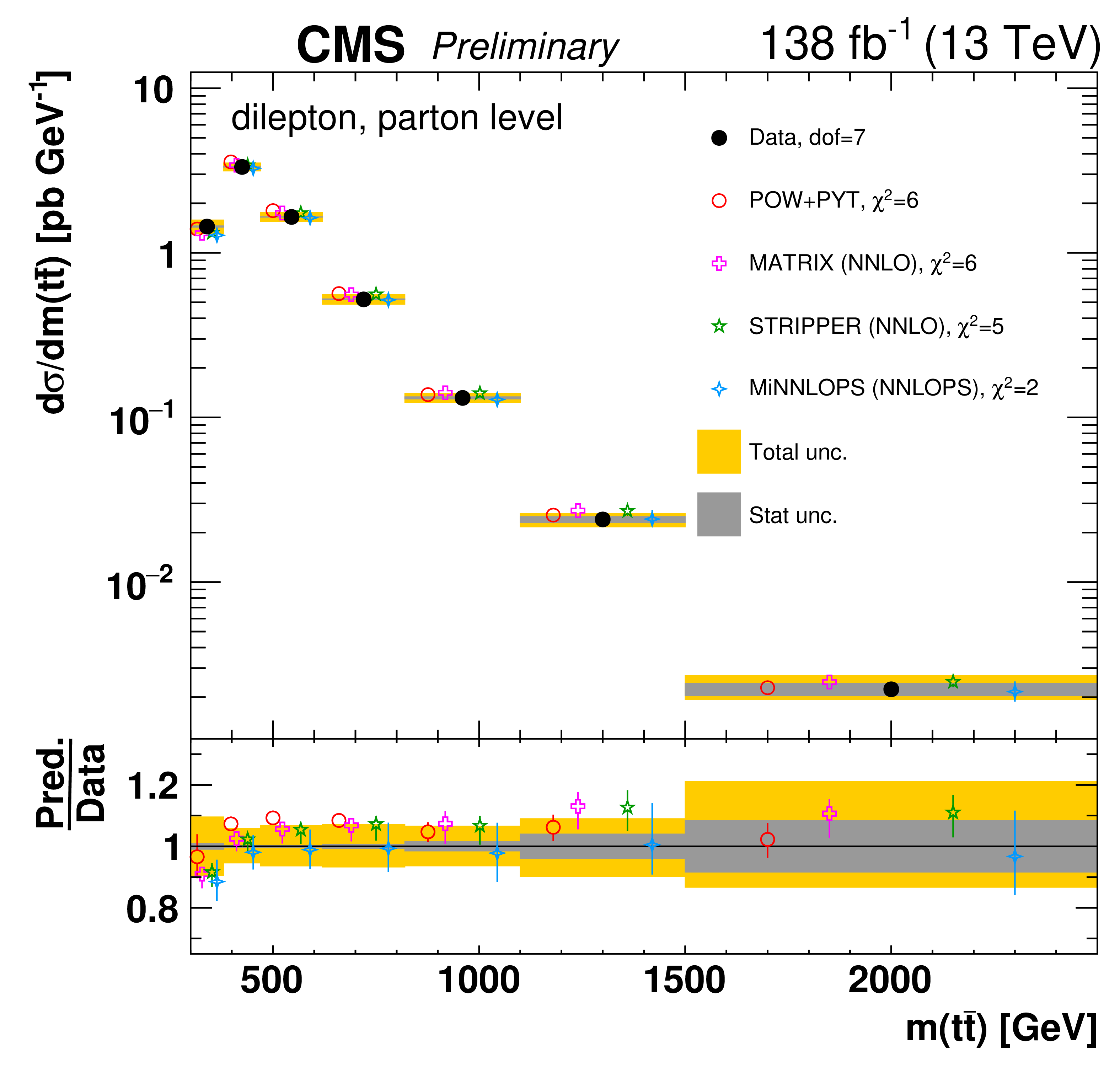
png pdf	Figure 99-c: Absolute differential $\mathrm{t\bar{t}}$ production cross sections as a function of ${{p_{\mathrm {T}}} ( \mathrm{t\bar{t}})}$ (upper), ${m( \mathrm{t\bar{t}})}$ (middle), and ${y( \mathrm{t\bar{t}})}$ (lower) are shown for data (filled circles), POWHEG+PYTHIA-8 (`POW-PYT', open circles) simulation, and various theoretical predictions with beyond-NLO precision (other points). Further details can be found in the caption of Fig. 97.
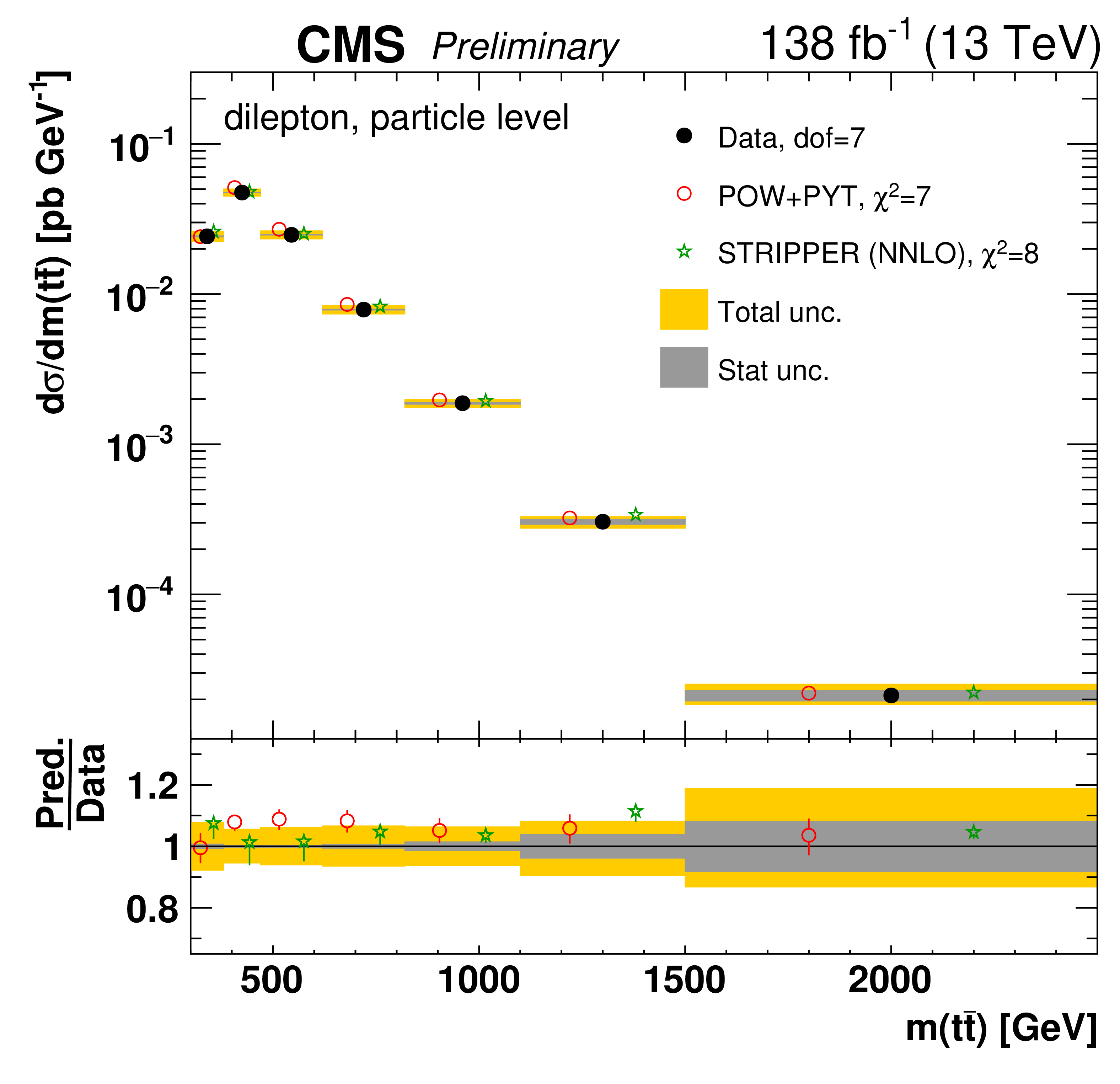
png pdf	Figure 99-d: Absolute differential $\mathrm{t\bar{t}}$ production cross sections as a function of ${{p_{\mathrm {T}}} ( \mathrm{t\bar{t}})}$ (upper), ${m( \mathrm{t\bar{t}})}$ (middle), and ${y( \mathrm{t\bar{t}})}$ (lower) are shown for data (filled circles), POWHEG+PYTHIA-8 (`POW-PYT', open circles) simulation, and various theoretical predictions with beyond-NLO precision (other points). Further details can be found in the caption of Fig. 97.
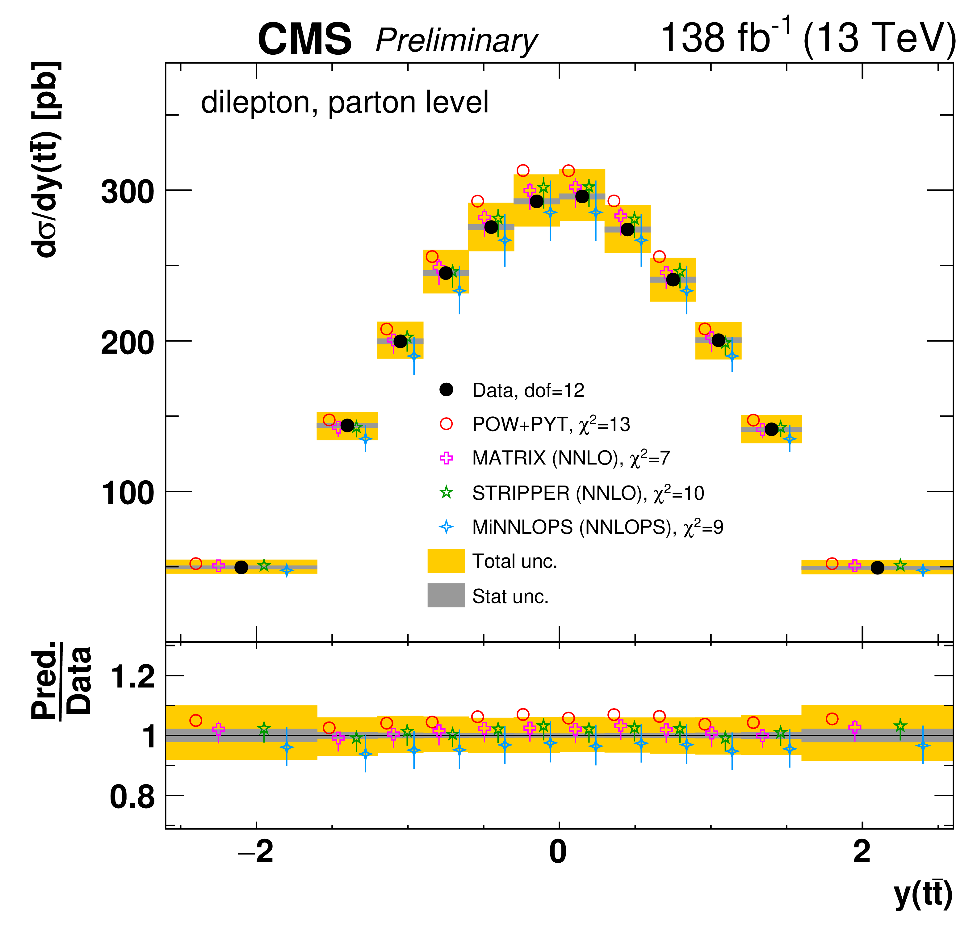
png pdf	Figure 99-e: Absolute differential $\mathrm{t\bar{t}}$ production cross sections as a function of ${{p_{\mathrm {T}}} ( \mathrm{t\bar{t}})}$ (upper), ${m( \mathrm{t\bar{t}})}$ (middle), and ${y( \mathrm{t\bar{t}})}$ (lower) are shown for data (filled circles), POWHEG+PYTHIA-8 (`POW-PYT', open circles) simulation, and various theoretical predictions with beyond-NLO precision (other points). Further details can be found in the caption of Fig. 97.
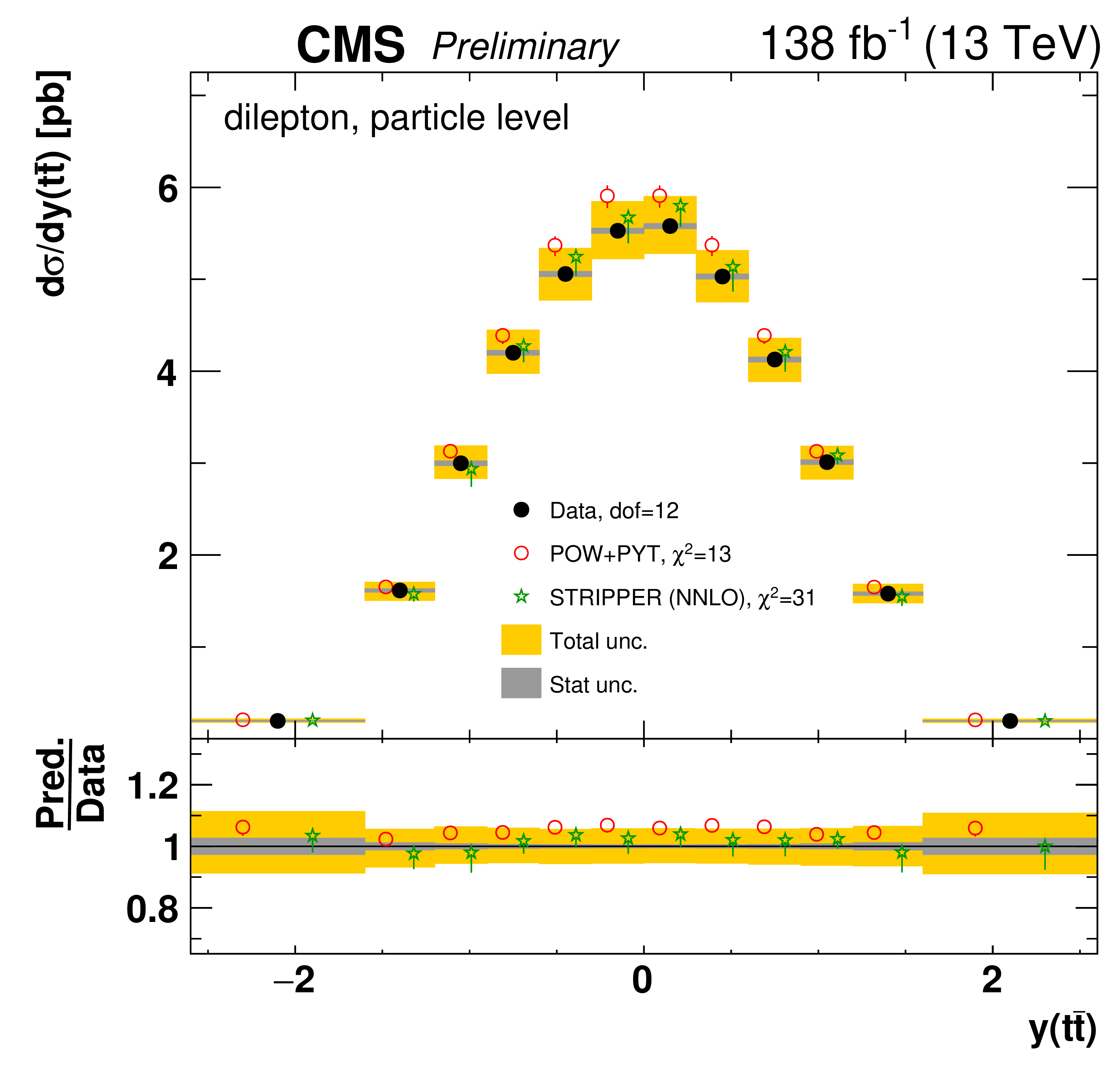
png pdf	Figure 99-f: Absolute differential $\mathrm{t\bar{t}}$ production cross sections as a function of ${{p_{\mathrm {T}}} ( \mathrm{t\bar{t}})}$ (upper), ${m( \mathrm{t\bar{t}})}$ (middle), and ${y( \mathrm{t\bar{t}})}$ (lower) are shown for data (filled circles), POWHEG+PYTHIA-8 (`POW-PYT', open circles) simulation, and various theoretical predictions with beyond-NLO precision (other points). Further details can be found in the caption of Fig. 97.
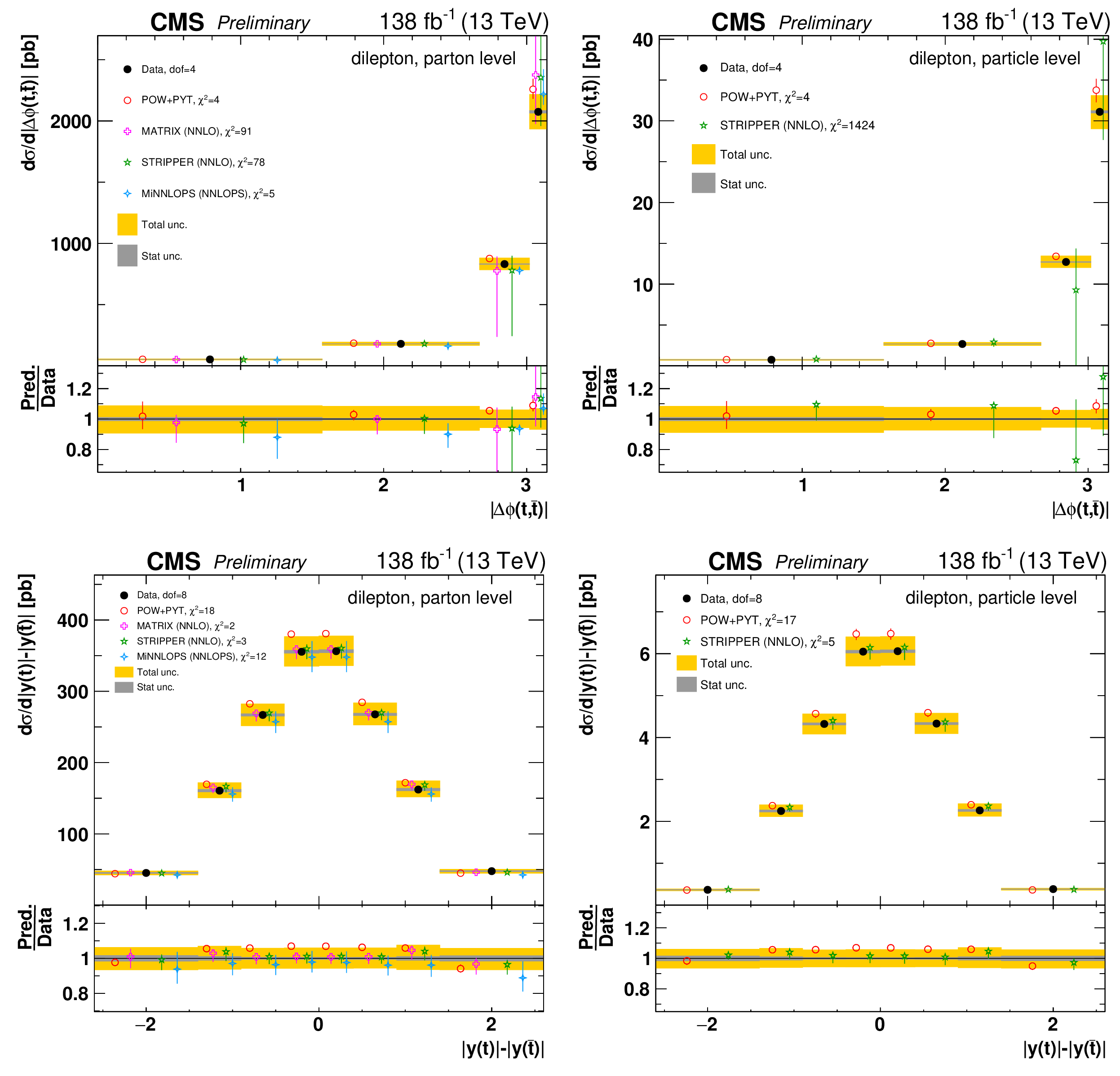
png pdf	Figure 100: Absolute differential $\mathrm{t\bar{t}}$ production cross sections as a function of ${|\Delta \phi (\mathrm{t},\mathrm{\bar{t}})|}$ (upper) and ${|y(\mathrm{t})|-|y(\mathrm{\bar{t}})|}$ (lower) are shown for data (filled circles), POWHEG+PYTHIA-8 (`POW-PYT', open circles) simulation, and various theoretical predictions with beyond-NLO precision (other points). Further details can be found in the caption of Fig. 97.
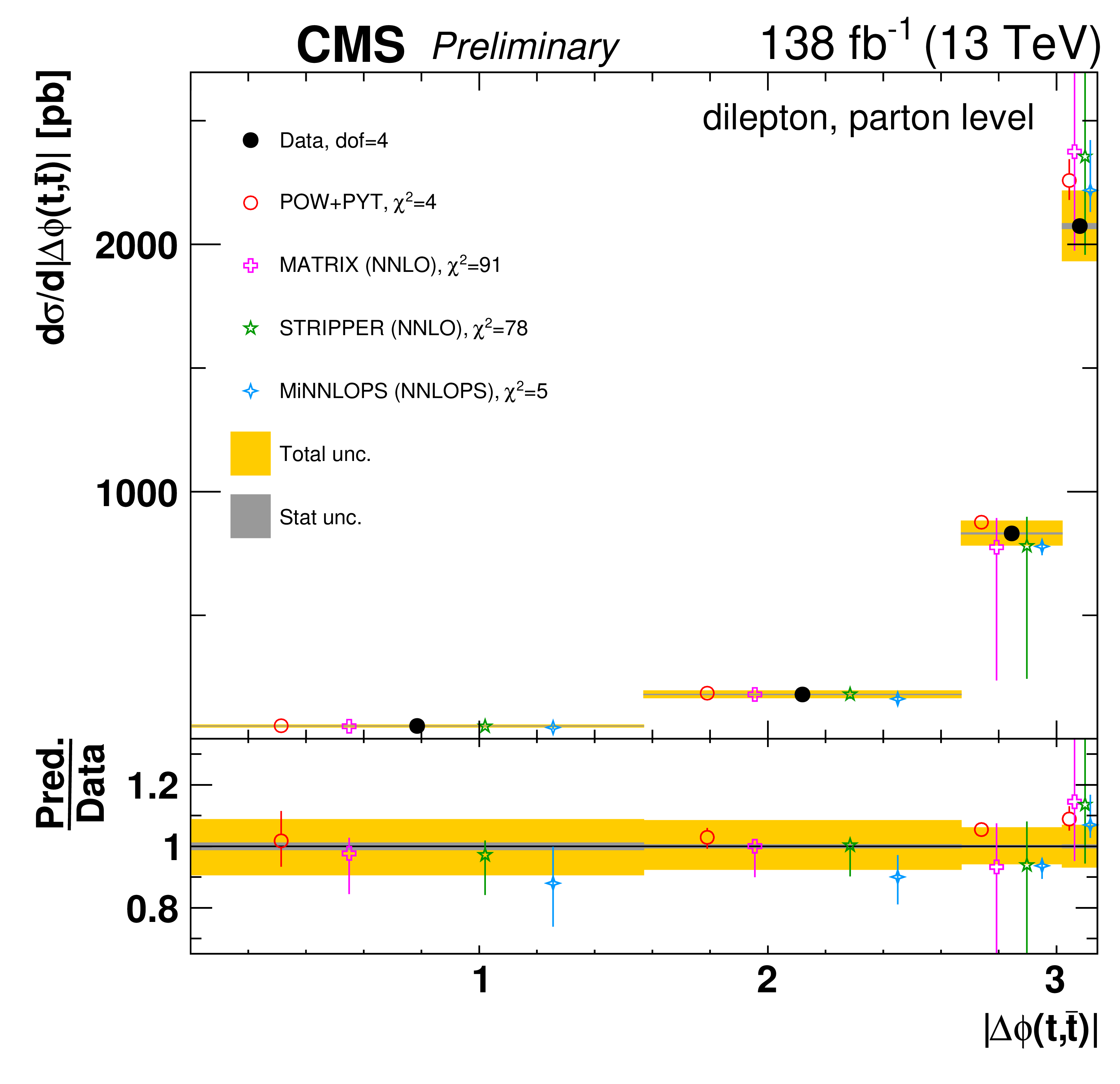
png pdf	Figure 100-a: Absolute differential $\mathrm{t\bar{t}}$ production cross sections as a function of ${|\Delta \phi (\mathrm{t},\mathrm{\bar{t}})|}$ (upper) and ${|y(\mathrm{t})|-|y(\mathrm{\bar{t}})|}$ (lower) are shown for data (filled circles), POWHEG+PYTHIA-8 (`POW-PYT', open circles) simulation, and various theoretical predictions with beyond-NLO precision (other points). Further details can be found in the caption of Fig. 97.
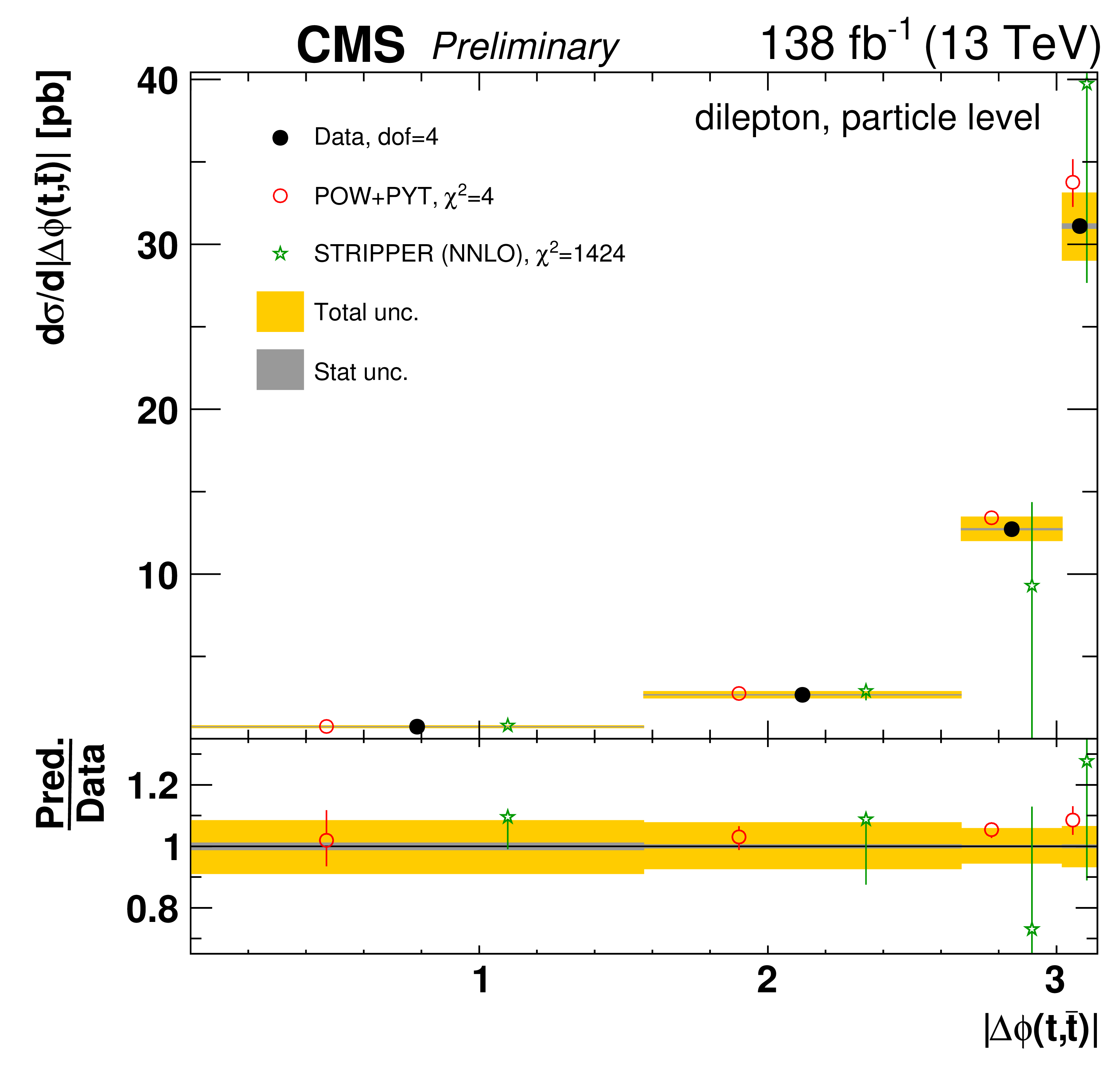
png pdf	Figure 100-b: Absolute differential $\mathrm{t\bar{t}}$ production cross sections as a function of ${|\Delta \phi (\mathrm{t},\mathrm{\bar{t}})|}$ (upper) and ${|y(\mathrm{t})|-|y(\mathrm{\bar{t}})|}$ (lower) are shown for data (filled circles), POWHEG+PYTHIA-8 (`POW-PYT', open circles) simulation, and various theoretical predictions with beyond-NLO precision (other points). Further details can be found in the caption of Fig. 97.
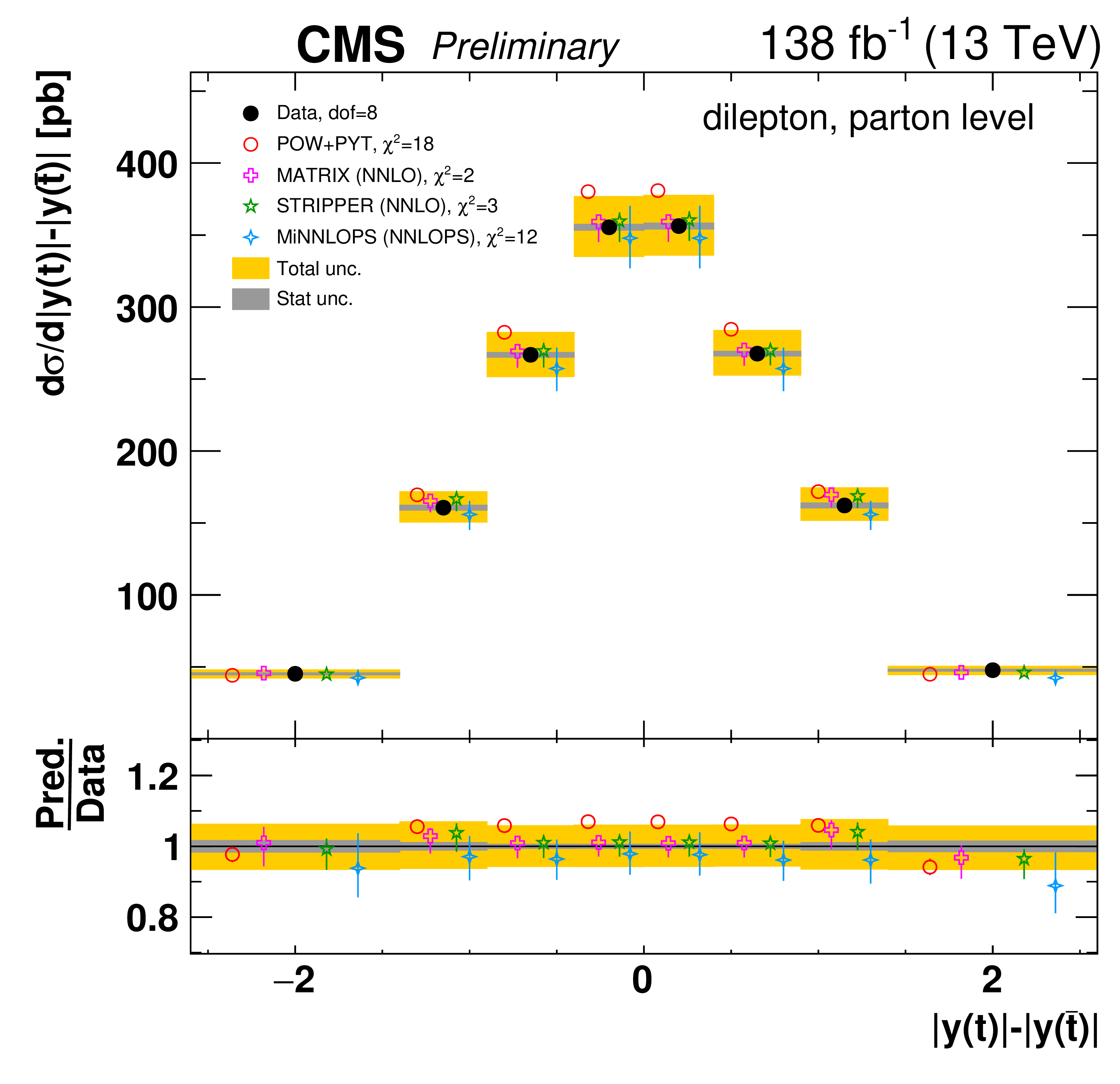
png pdf	Figure 100-c: Absolute differential $\mathrm{t\bar{t}}$ production cross sections as a function of ${|\Delta \phi (\mathrm{t},\mathrm{\bar{t}})|}$ (upper) and ${|y(\mathrm{t})|-|y(\mathrm{\bar{t}})|}$ (lower) are shown for data (filled circles), POWHEG+PYTHIA-8 (`POW-PYT', open circles) simulation, and various theoretical predictions with beyond-NLO precision (other points). Further details can be found in the caption of Fig. 97.
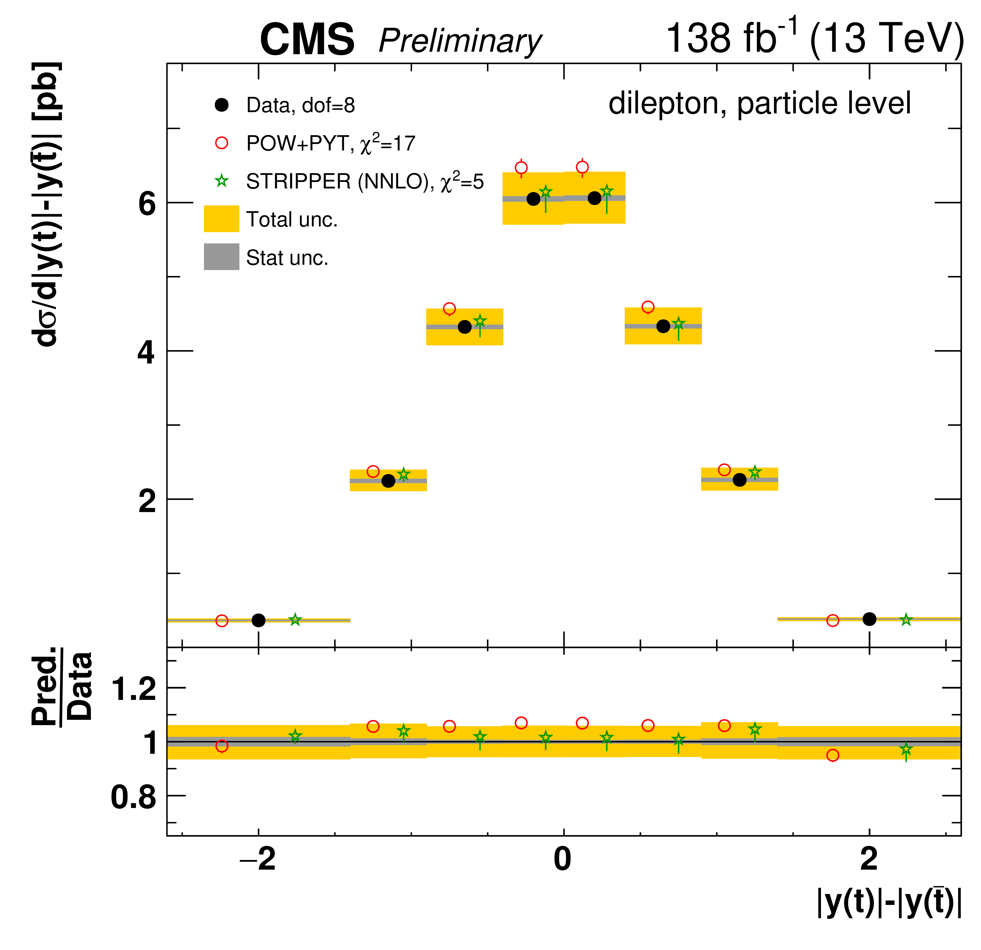
png pdf	Figure 100-d: Absolute differential $\mathrm{t\bar{t}}$ production cross sections as a function of ${|\Delta \phi (\mathrm{t},\mathrm{\bar{t}})|}$ (upper) and ${|y(\mathrm{t})|-|y(\mathrm{\bar{t}})|}$ (lower) are shown for data (filled circles), POWHEG+PYTHIA-8 (`POW-PYT', open circles) simulation, and various theoretical predictions with beyond-NLO precision (other points). Further details can be found in the caption of Fig. 97.
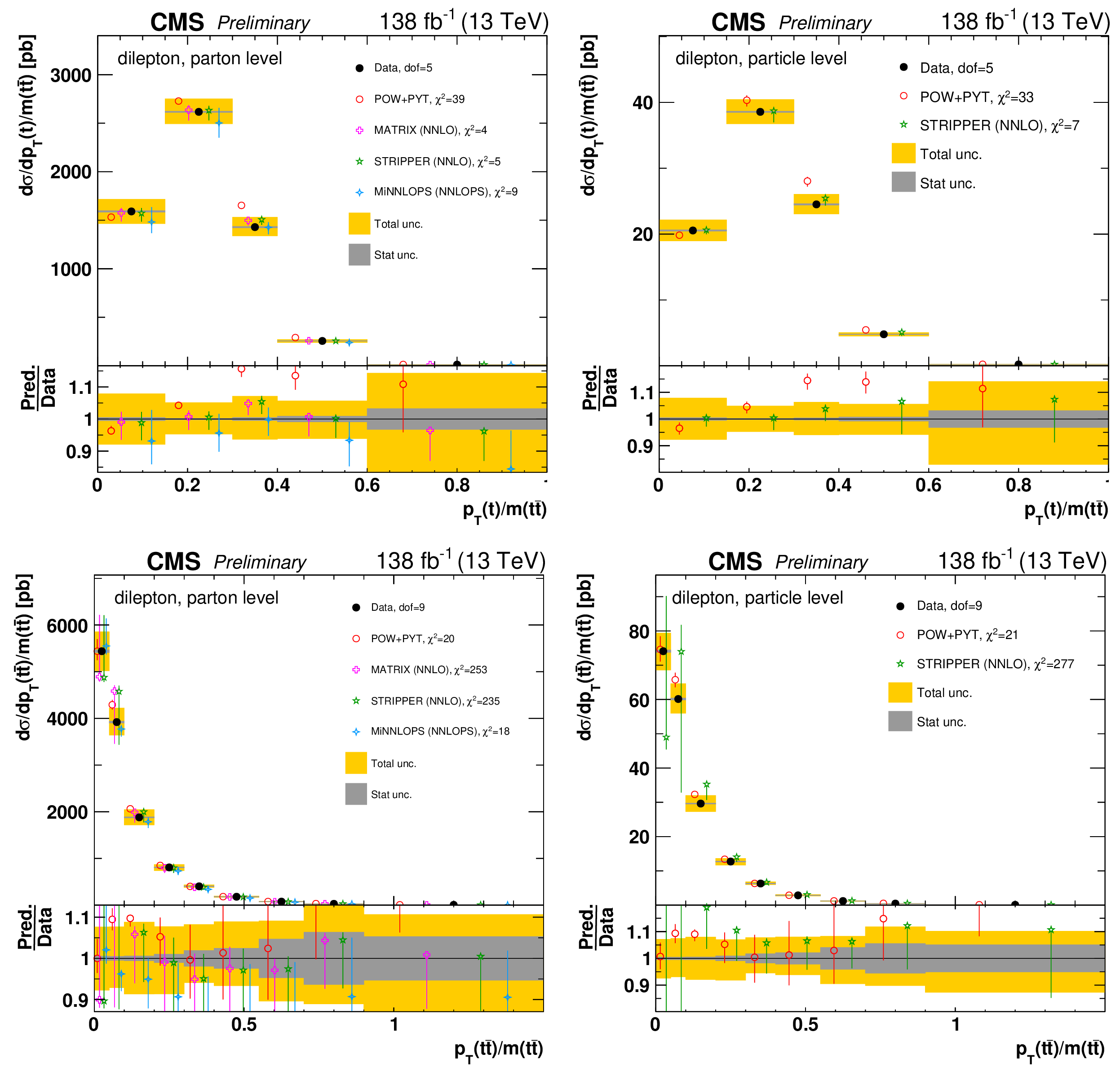
png pdf	Figure 101: Absolute differential $\mathrm{t\bar{t}}$ production cross sections as a function of $ {{p_{\mathrm {T}}} (\mathrm{t})} / {m( \mathrm{t\bar{t}})}$ (upper) and $ {{p_{\mathrm {T}}} ( \mathrm{t\bar{t}})} / {{m( \mathrm{t\bar{t}})}}$ (lower) are shown for data (filled circles), POWHEG+PYTHIA-8 (`POW-PYT', open circles) simulation, and various theoretical predictions with beyond-NLO precision (other points). Further details can be found in the caption of Fig. 97.
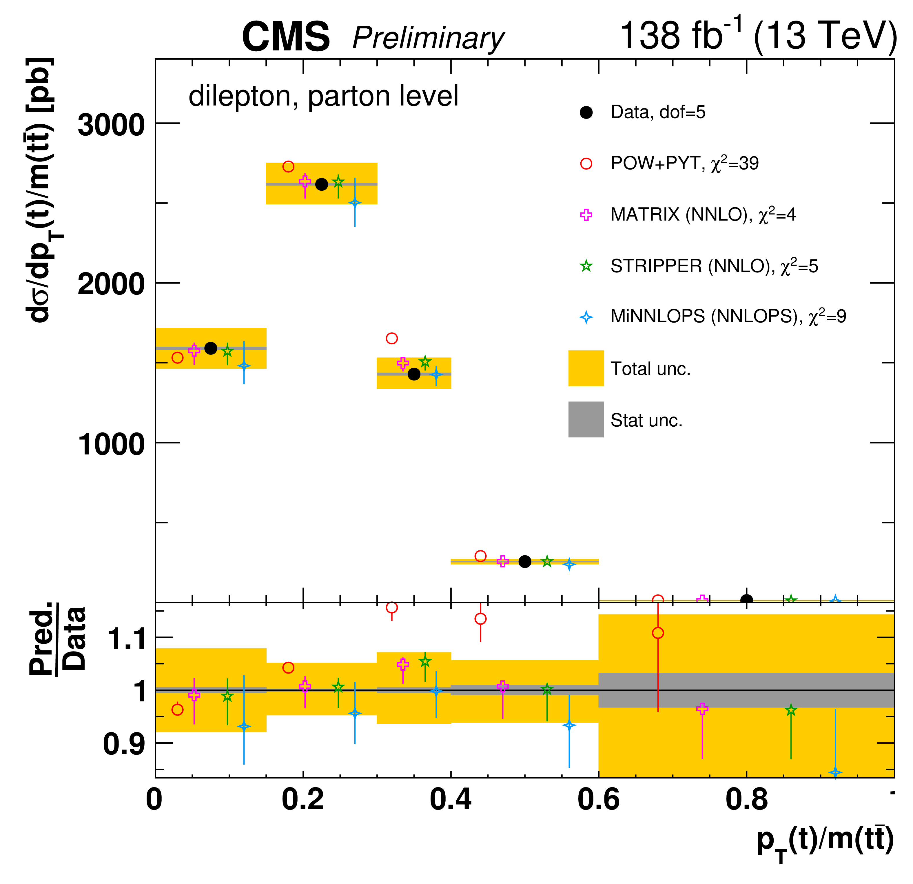
png pdf	Figure 101-a: Absolute differential $\mathrm{t\bar{t}}$ production cross sections as a function of $ {{p_{\mathrm {T}}} (\mathrm{t})} / {m( \mathrm{t\bar{t}})}$ (upper) and $ {{p_{\mathrm {T}}} ( \mathrm{t\bar{t}})} / {{m( \mathrm{t\bar{t}})}}$ (lower) are shown for data (filled circles), POWHEG+PYTHIA-8 (`POW-PYT', open circles) simulation, and various theoretical predictions with beyond-NLO precision (other points). Further details can be found in the caption of Fig. 97.
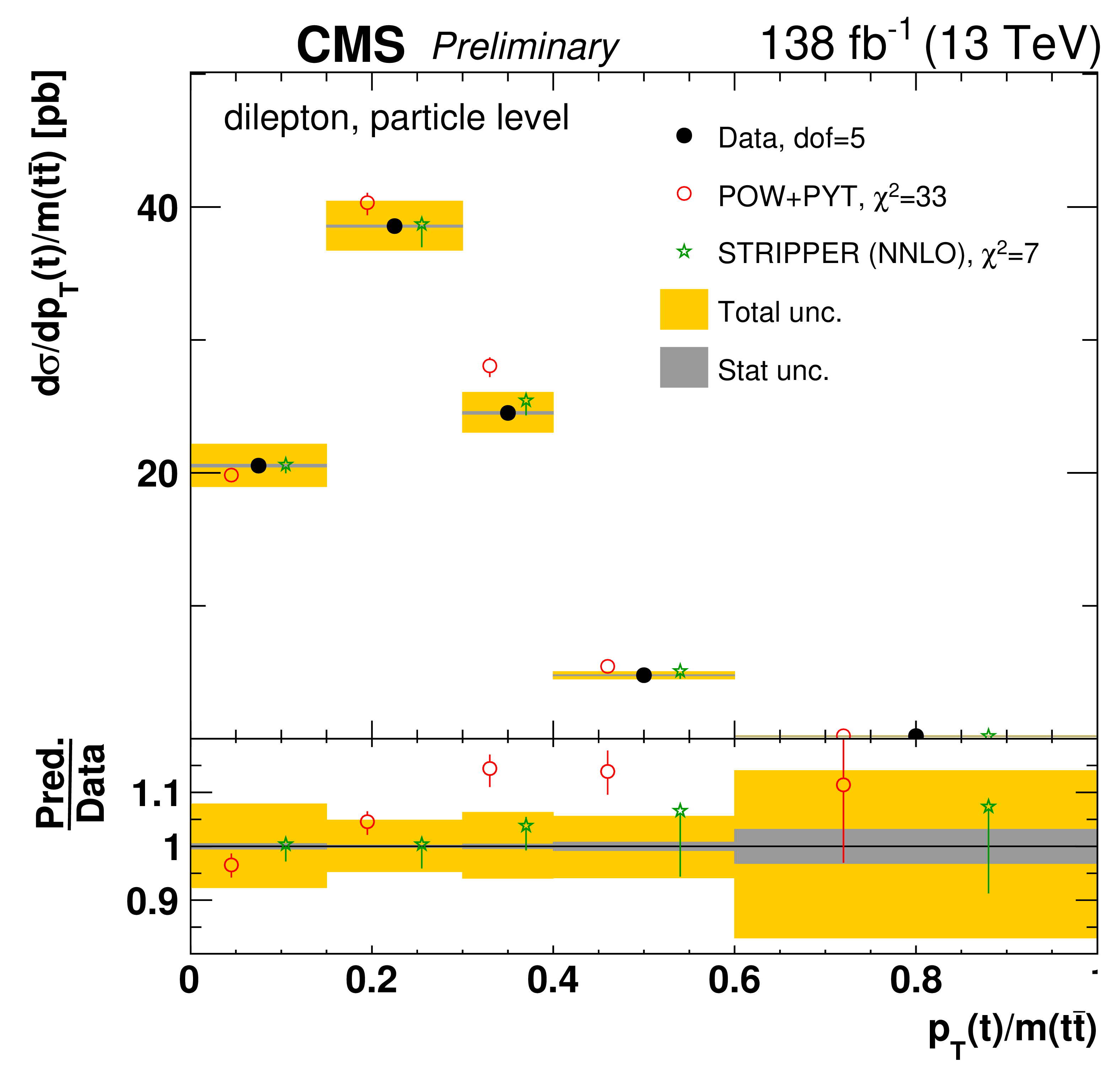
png pdf	Figure 101-b: Absolute differential $\mathrm{t\bar{t}}$ production cross sections as a function of $ {{p_{\mathrm {T}}} (\mathrm{t})} / {m( \mathrm{t\bar{t}})}$ (upper) and $ {{p_{\mathrm {T}}} ( \mathrm{t\bar{t}})} / {{m( \mathrm{t\bar{t}})}}$ (lower) are shown for data (filled circles), POWHEG+PYTHIA-8 (`POW-PYT', open circles) simulation, and various theoretical predictions with beyond-NLO precision (other points). Further details can be found in the caption of Fig. 97.
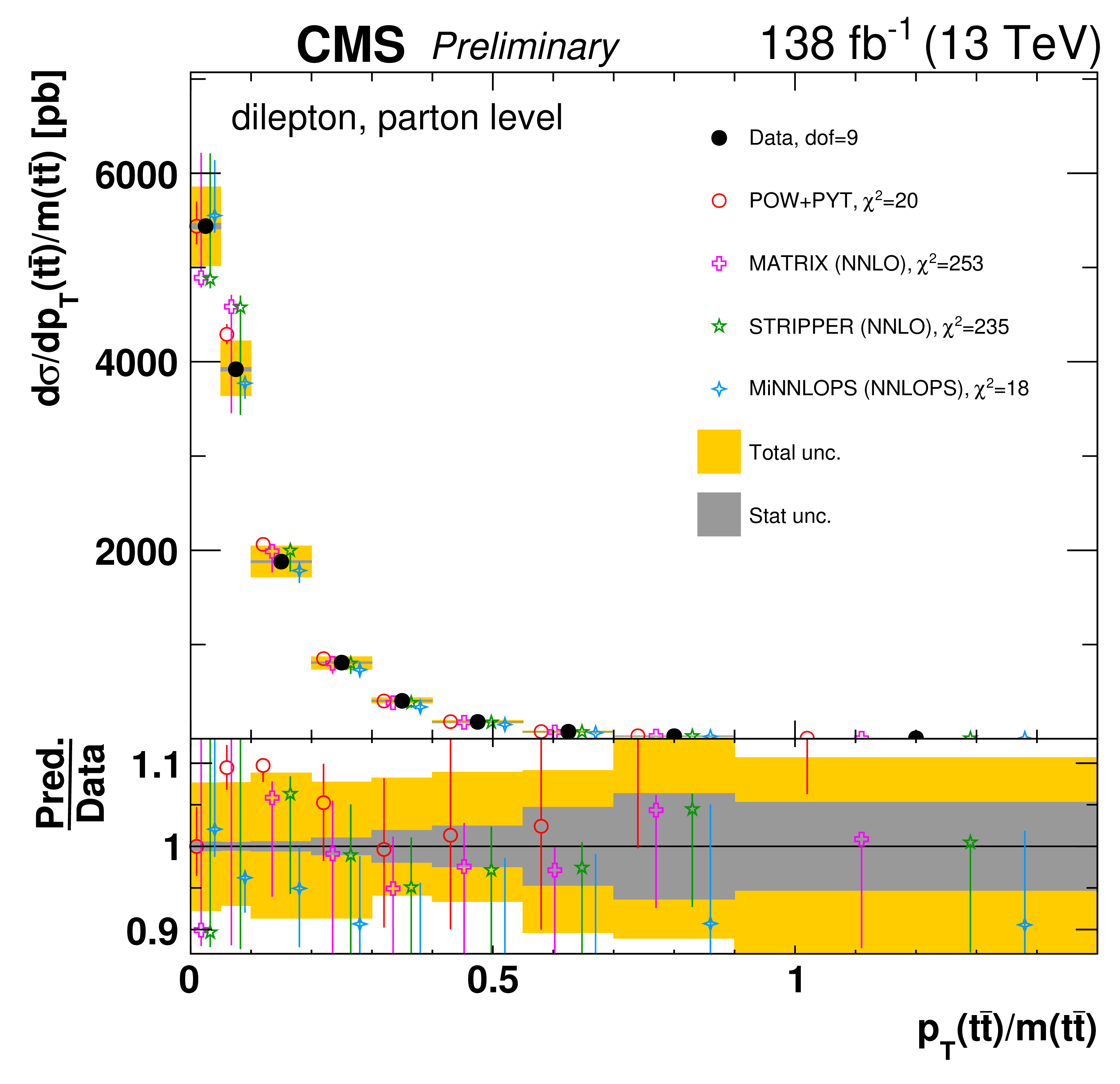
png pdf	Figure 101-c: Absolute differential $\mathrm{t\bar{t}}$ production cross sections as a function of $ {{p_{\mathrm {T}}} (\mathrm{t})} / {m( \mathrm{t\bar{t}})}$ (upper) and $ {{p_{\mathrm {T}}} ( \mathrm{t\bar{t}})} / {{m( \mathrm{t\bar{t}})}}$ (lower) are shown for data (filled circles), POWHEG+PYTHIA-8 (`POW-PYT', open circles) simulation, and various theoretical predictions with beyond-NLO precision (other points). Further details can be found in the caption of Fig. 97.
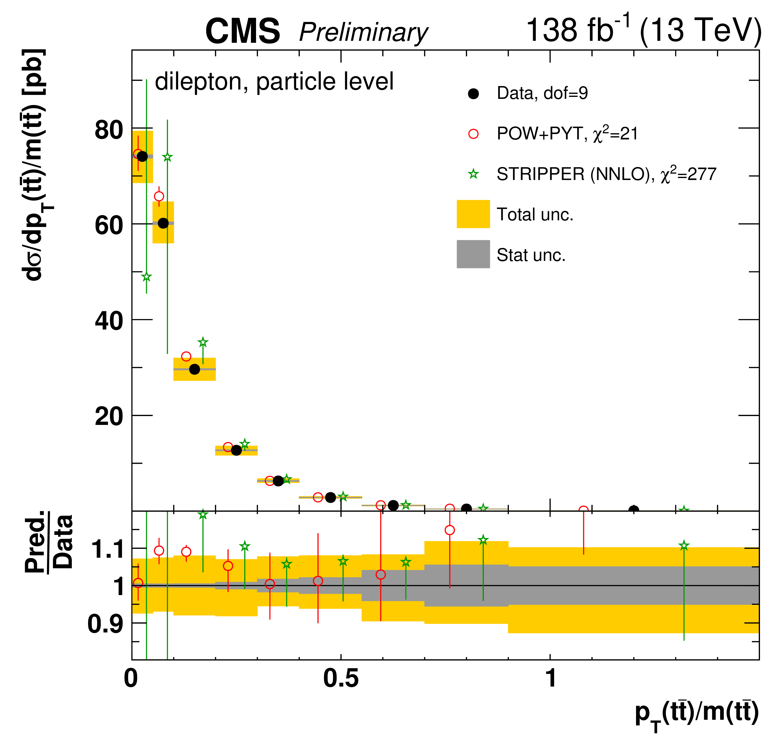
png pdf	Figure 101-d: Absolute differential $\mathrm{t\bar{t}}$ production cross sections as a function of $ {{p_{\mathrm {T}}} (\mathrm{t})} / {m( \mathrm{t\bar{t}})}$ (upper) and $ {{p_{\mathrm {T}}} ( \mathrm{t\bar{t}})} / {{m( \mathrm{t\bar{t}})}}$ (lower) are shown for data (filled circles), POWHEG+PYTHIA-8 (`POW-PYT', open circles) simulation, and various theoretical predictions with beyond-NLO precision (other points). Further details can be found in the caption of Fig. 97.
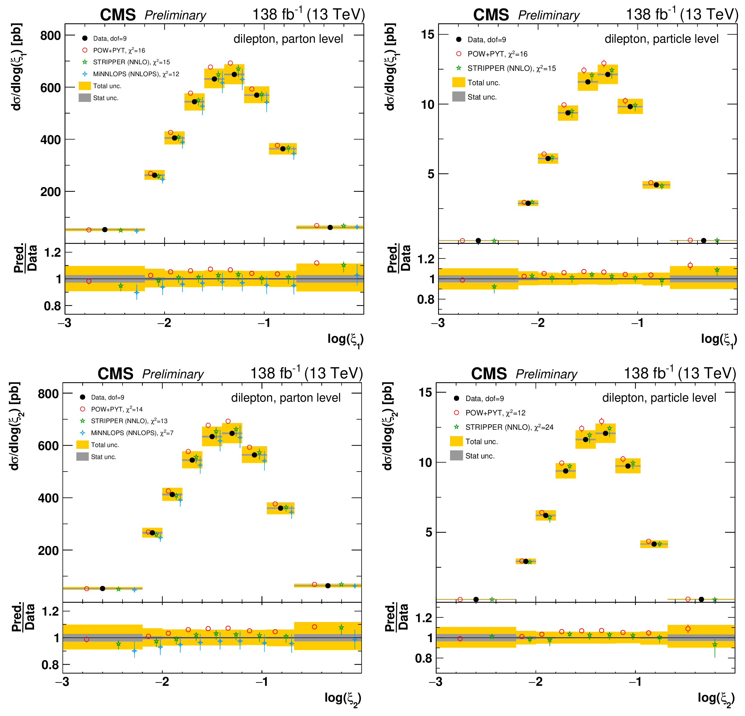
png pdf	Figure 102: Absolute differential $\mathrm{t\bar{t}}$ production cross sections as a function of ${\log(\xi _{1})}$ (upper) and ${\log(\xi _{2})}$ (lower) are shown for data (filled circles), POWHEG+PYTHIA-8 (`POW-PYT', open circles) simulation, and Stripper NNLO calculation (stars). Further details can be found in the caption of Fig. 97.
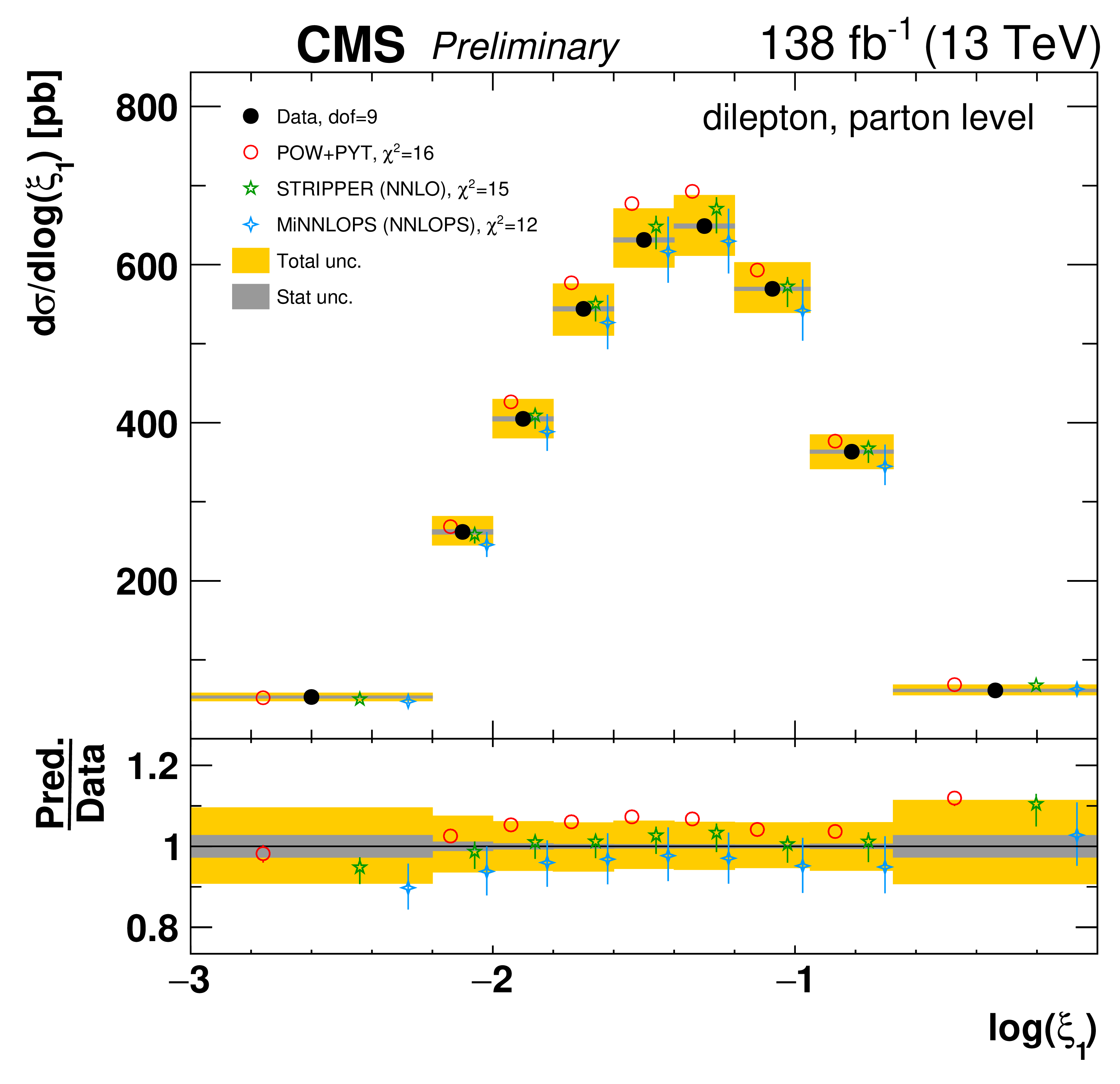
png pdf	Figure 102-a: Absolute differential $\mathrm{t\bar{t}}$ production cross sections as a function of ${\log(\xi _{1})}$ (upper) and ${\log(\xi _{2})}$ (lower) are shown for data (filled circles), POWHEG+PYTHIA-8 (`POW-PYT', open circles) simulation, and Stripper NNLO calculation (stars). Further details can be found in the caption of Fig. 97.
png pdf	Figure 102-b: Absolute differential $\mathrm{t\bar{t}}$ production cross sections as a function of ${\log(\xi _{1})}$ (upper) and ${\log(\xi _{2})}$ (lower) are shown for data (filled circles), POWHEG+PYTHIA-8 (`POW-PYT', open circles) simulation, and Stripper NNLO calculation (stars). Further details can be found in the caption of Fig. 97.
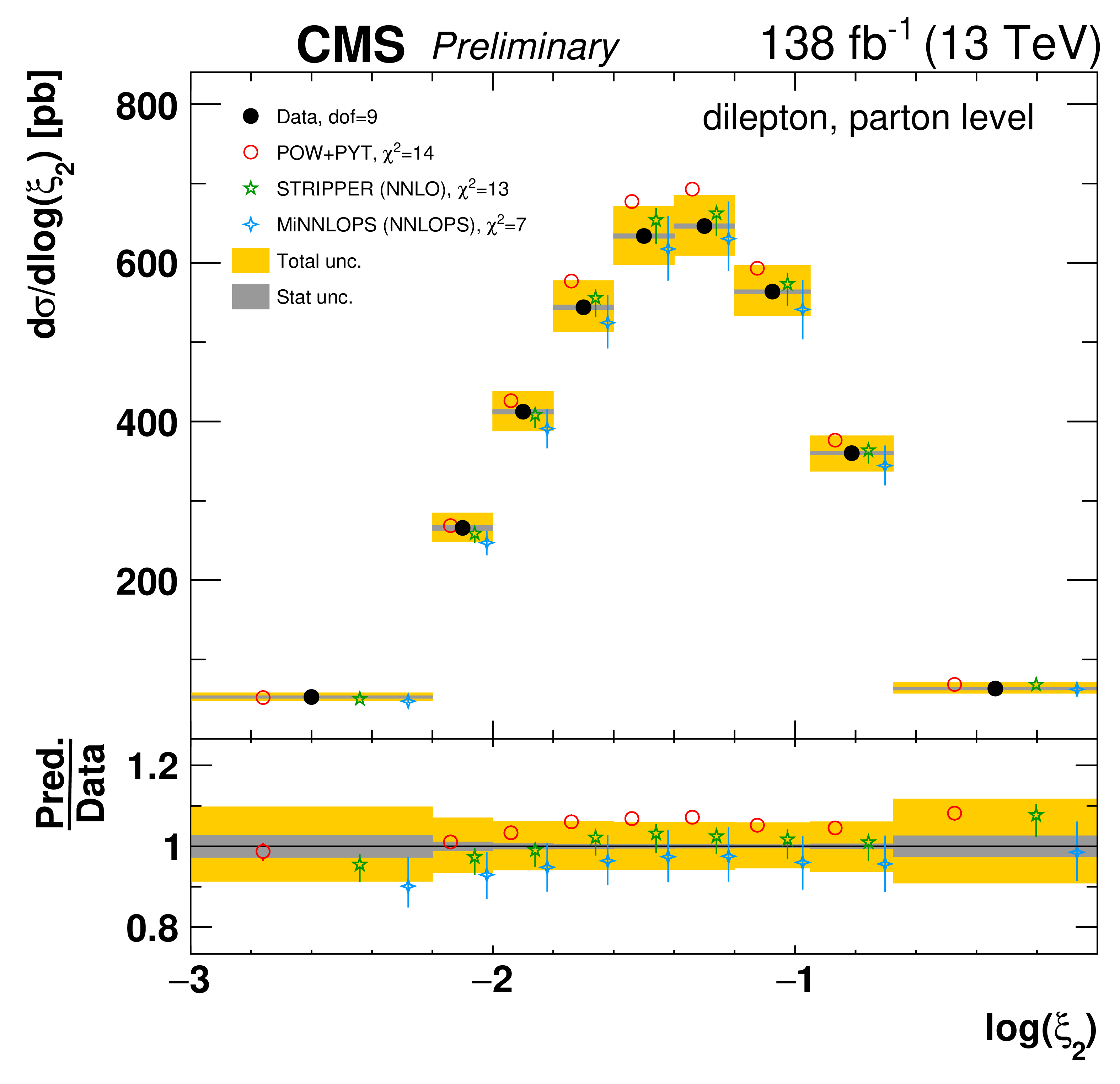
png pdf	Figure 102-c: Absolute differential $\mathrm{t\bar{t}}$ production cross sections as a function of ${\log(\xi _{1})}$ (upper) and ${\log(\xi _{2})}$ (lower) are shown for data (filled circles), POWHEG+PYTHIA-8 (`POW-PYT', open circles) simulation, and Stripper NNLO calculation (stars). Further details can be found in the caption of Fig. 97.
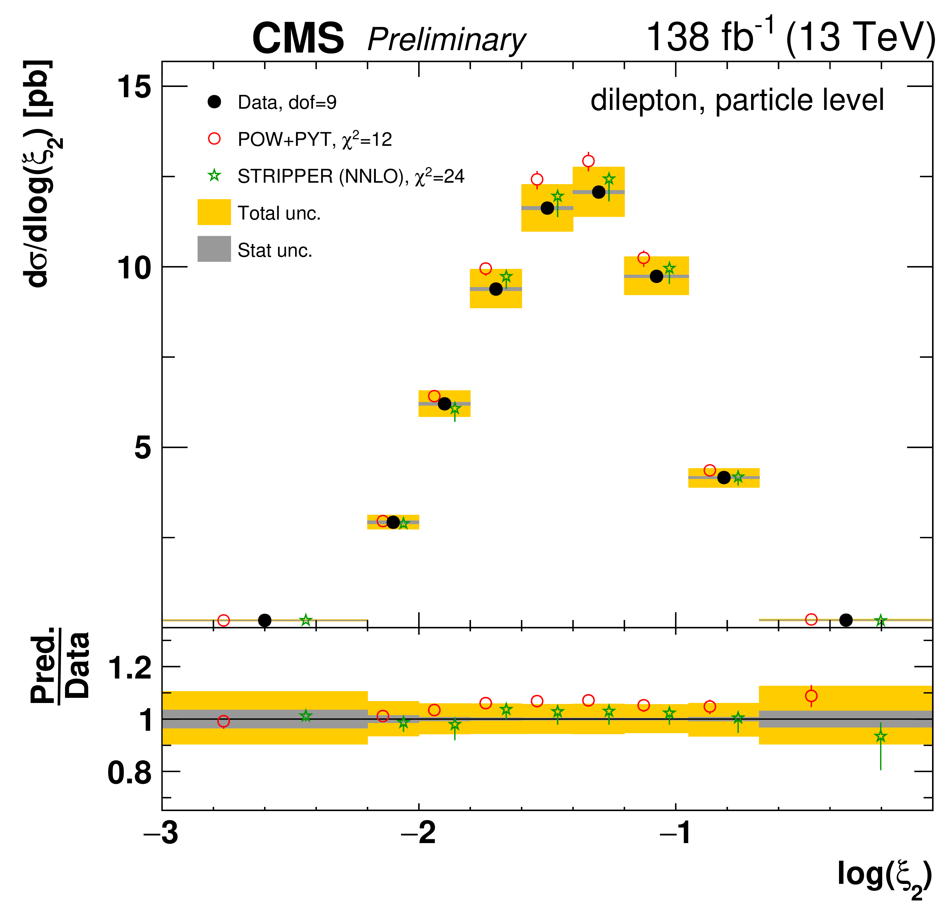
png pdf	Figure 102-d: Absolute differential $\mathrm{t\bar{t}}$ production cross sections as a function of ${\log(\xi _{1})}$ (upper) and ${\log(\xi _{2})}$ (lower) are shown for data (filled circles), POWHEG+PYTHIA-8 (`POW-PYT', open circles) simulation, and Stripper NNLO calculation (stars). Further details can be found in the caption of Fig. 97.
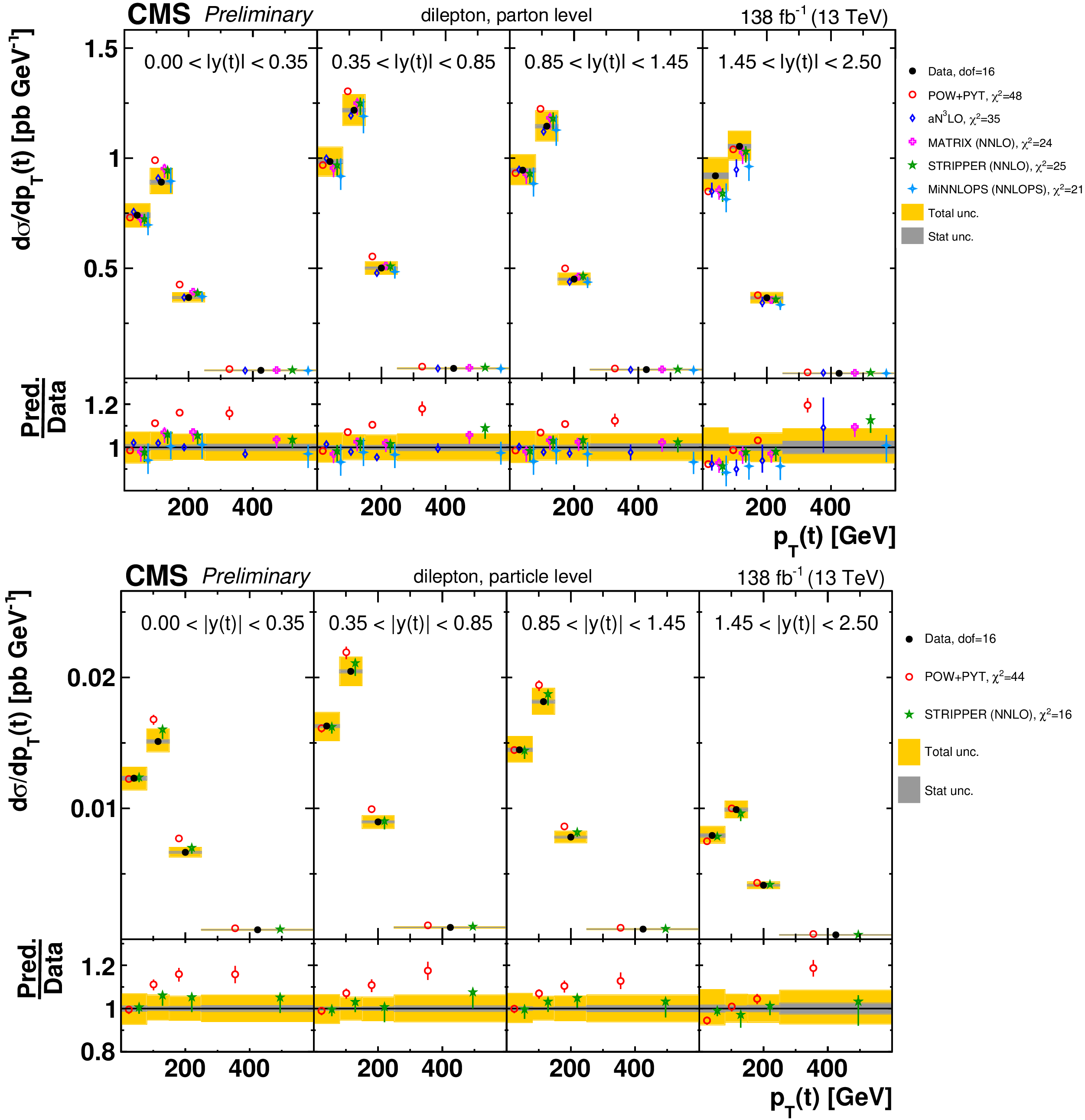
png pdf	Figure 103: Absolute $[ {|y(\mathrm{t})|},\,{{p_{\mathrm {T}}} (\mathrm{t})} ]$ cross sections measured at the parton level in the full phase space (upper) and at the particle level in a fiducial phase space (lower). The data are shown as filled circles with dark and light bands indicating the statistical and total uncertainties (statistical and systematic uncertainties summed in quadrature), respectively. The cross sections are compared to predictions from the POWHEG+PYTHIA-8 (`POW-PYT', open circles) simulation and various theoretical predictions with beyond-NLO precision (other points). The estimated uncertainties in the predictions are represented by a vertical bar on the corresponding points. For each model, a value of ${\chi ^2}$ is reported that takes into account the measurement uncertainties. The lower panel in each plot shows the ratios of the predictions to the data.
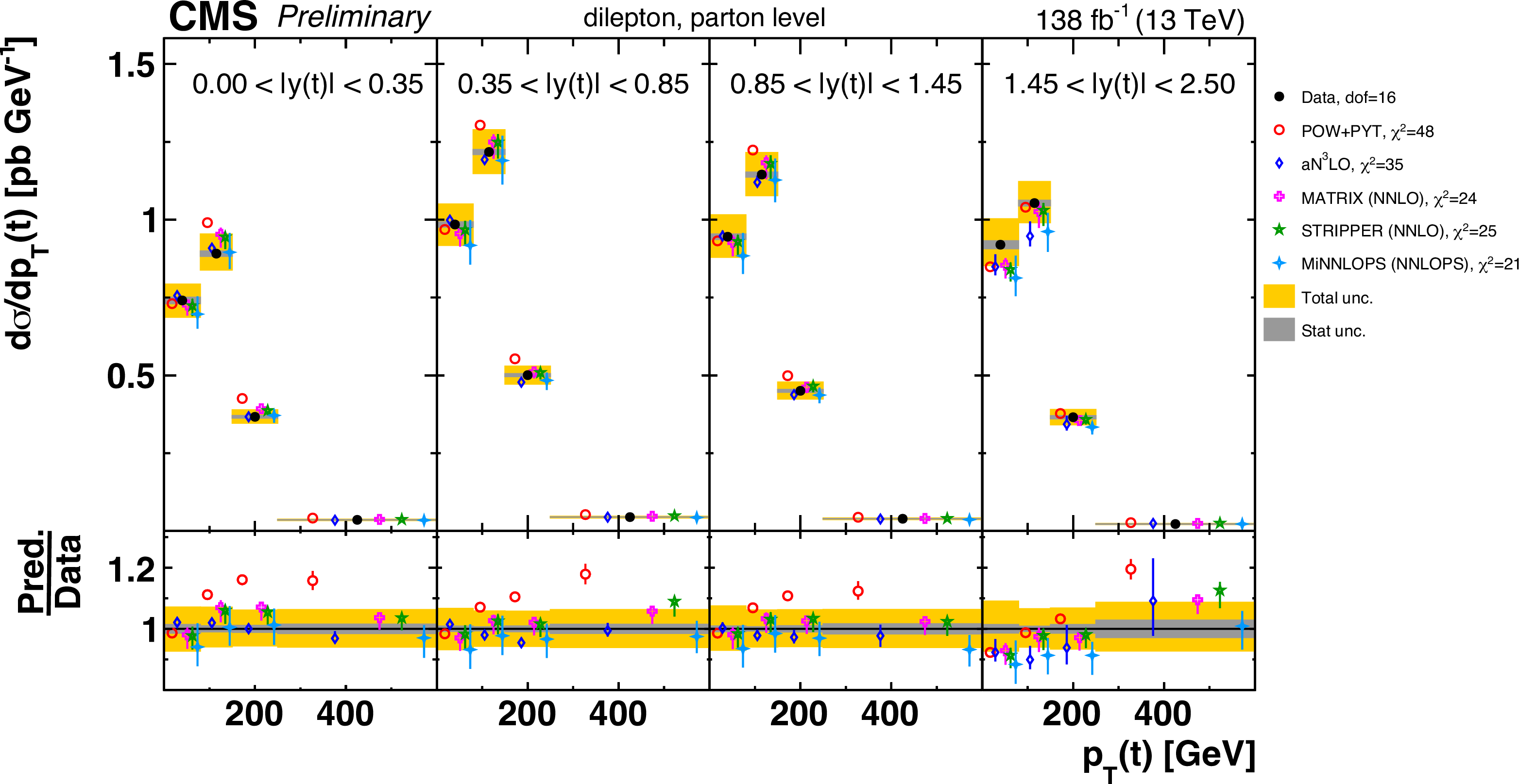
png pdf	Figure 103-a: Absolute $[ {|y(\mathrm{t})|},\,{{p_{\mathrm {T}}} (\mathrm{t})} ]$ cross sections measured at the parton level in the full phase space (upper) and at the particle level in a fiducial phase space (lower). The data are shown as filled circles with dark and light bands indicating the statistical and total uncertainties (statistical and systematic uncertainties summed in quadrature), respectively. The cross sections are compared to predictions from the POWHEG+PYTHIA-8 (`POW-PYT', open circles) simulation and various theoretical predictions with beyond-NLO precision (other points). The estimated uncertainties in the predictions are represented by a vertical bar on the corresponding points. For each model, a value of ${\chi ^2}$ is reported that takes into account the measurement uncertainties. The lower panel in each plot shows the ratios of the predictions to the data.
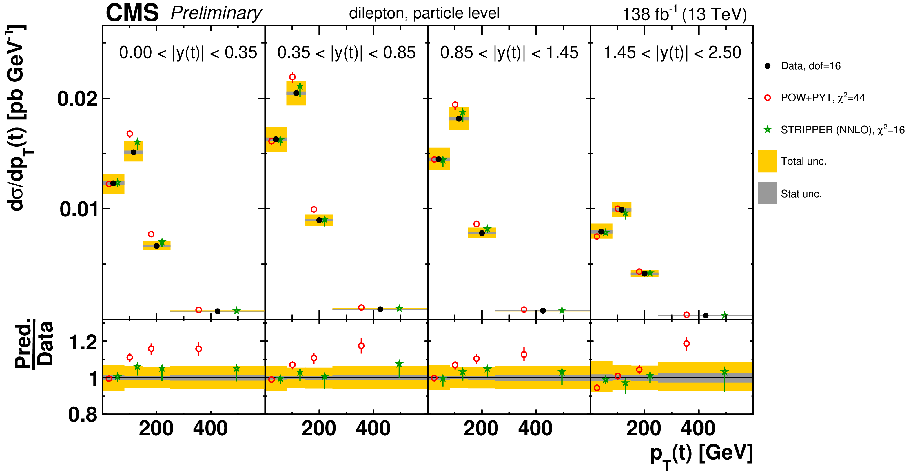
png pdf	Figure 103-b: Absolute $[ {|y(\mathrm{t})|},\,{{p_{\mathrm {T}}} (\mathrm{t})} ]$ cross sections measured at the parton level in the full phase space (upper) and at the particle level in a fiducial phase space (lower). The data are shown as filled circles with dark and light bands indicating the statistical and total uncertainties (statistical and systematic uncertainties summed in quadrature), respectively. The cross sections are compared to predictions from the POWHEG+PYTHIA-8 (`POW-PYT', open circles) simulation and various theoretical predictions with beyond-NLO precision (other points). The estimated uncertainties in the predictions are represented by a vertical bar on the corresponding points. For each model, a value of ${\chi ^2}$ is reported that takes into account the measurement uncertainties. The lower panel in each plot shows the ratios of the predictions to the data.
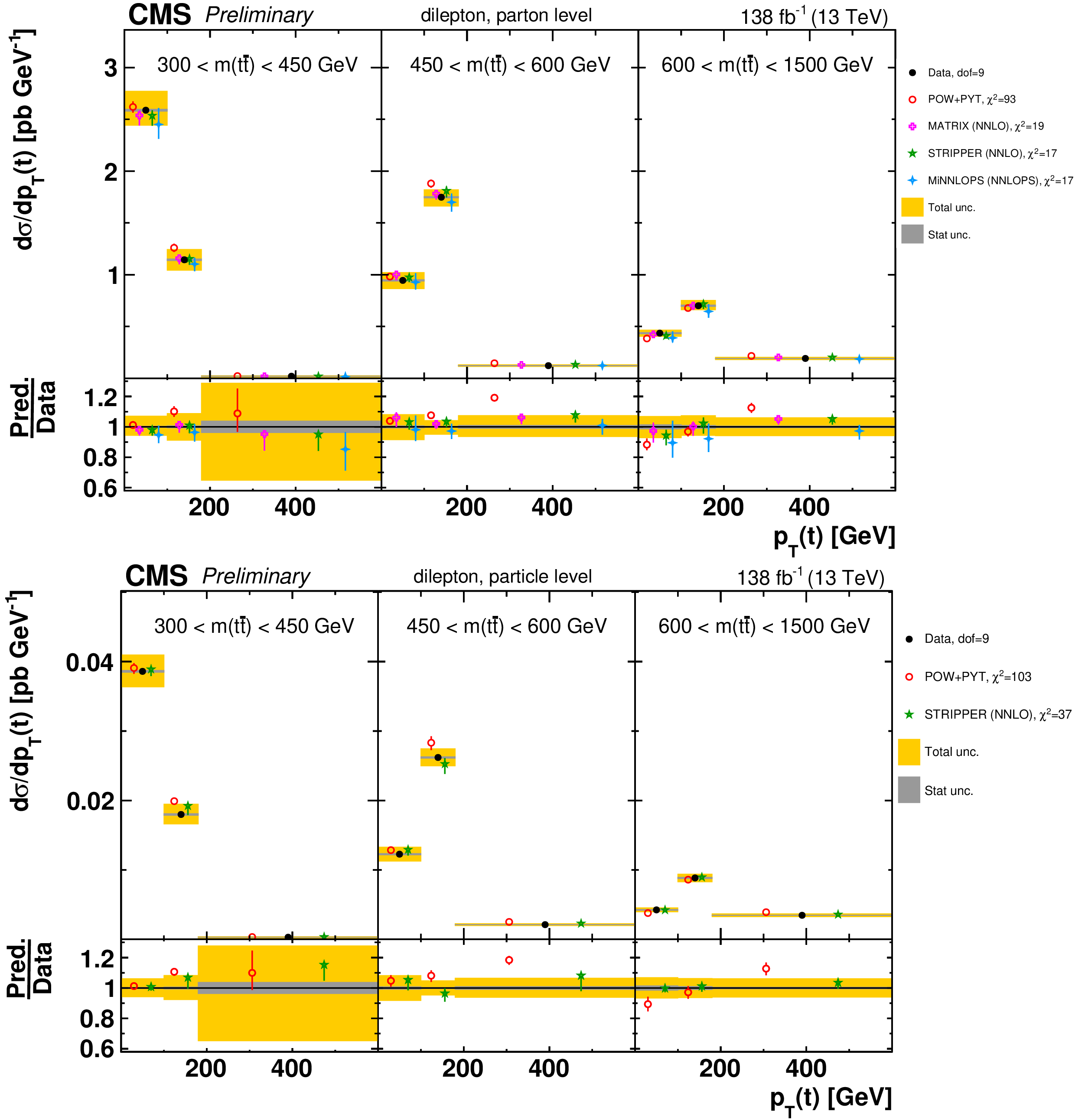
png pdf	Figure 104: Absolute $[ {m( \mathrm{t\bar{t}})},\,{{p_{\mathrm {T}}} (\mathrm{t})} ]$ cross sections are shown for data (filled circles), POWHEG+PYTHIA-8 (`POW-PYT', open circles) simulation, and various theoretical predictions with beyond-NLO precision (other points). Further details can be found in the caption of Fig. 103.
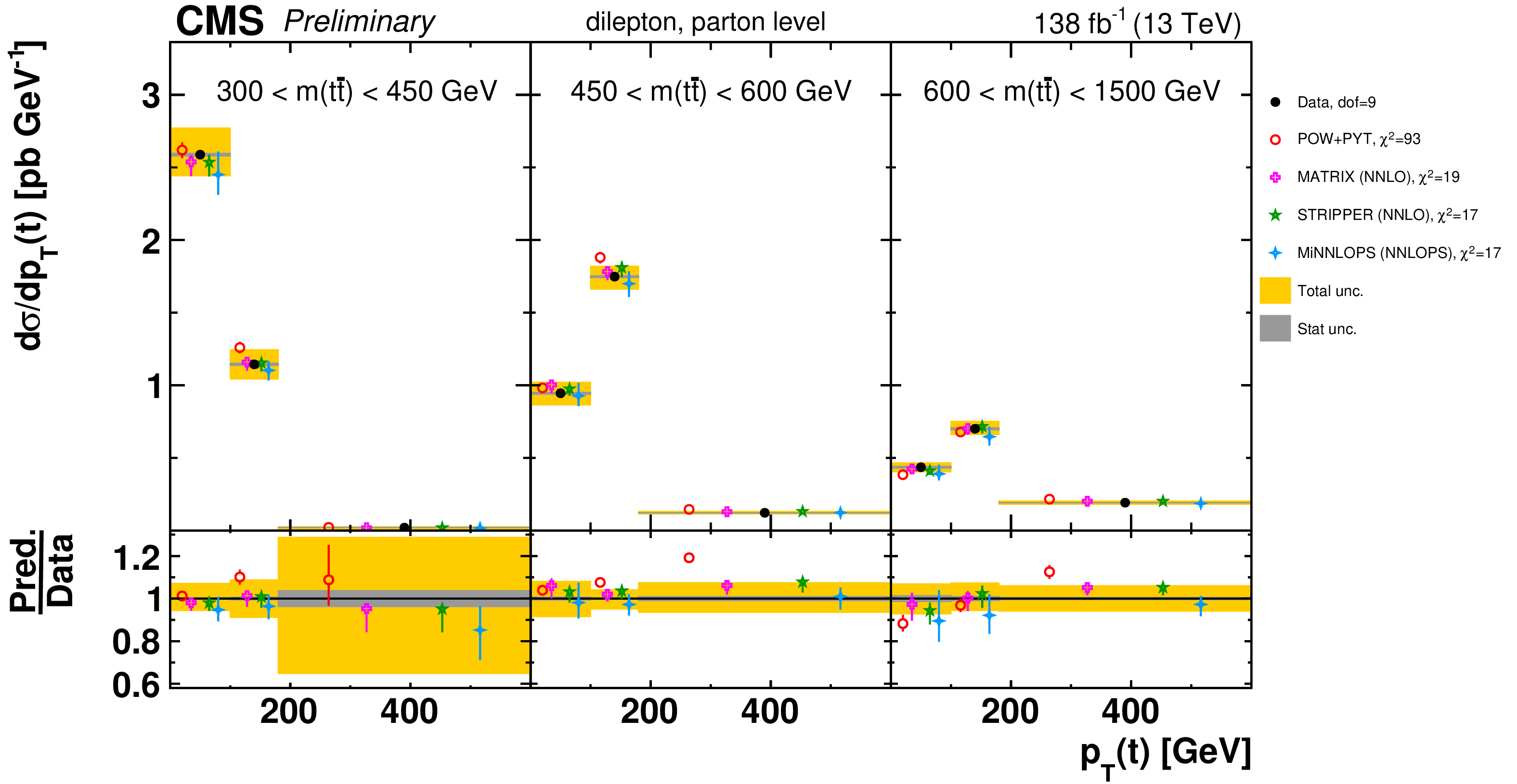
png pdf	Figure 104-a: Absolute $[ {m( \mathrm{t\bar{t}})},\,{{p_{\mathrm {T}}} (\mathrm{t})} ]$ cross sections are shown for data (filled circles), POWHEG+PYTHIA-8 (`POW-PYT', open circles) simulation, and various theoretical predictions with beyond-NLO precision (other points). Further details can be found in the caption of Fig. 103.
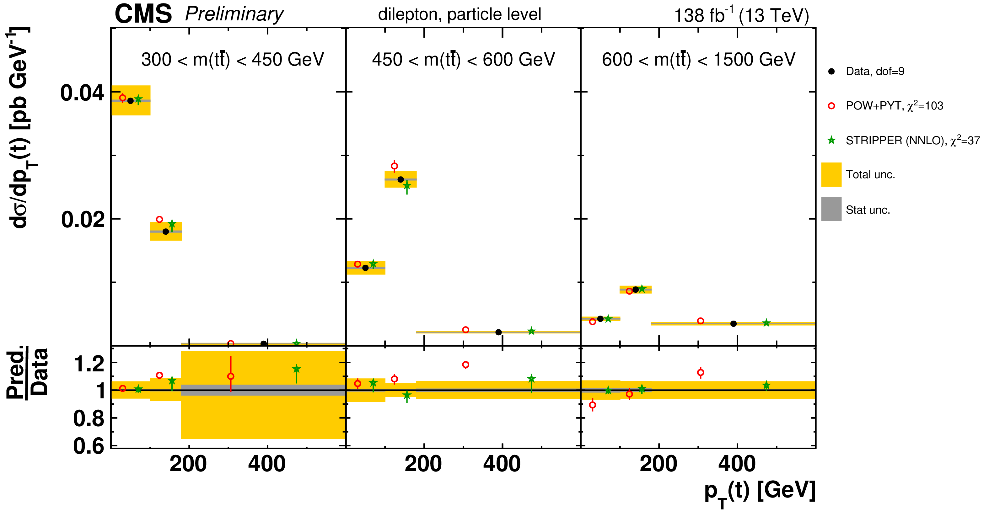
png pdf	Figure 104-b: Absolute $[ {m( \mathrm{t\bar{t}})},\,{{p_{\mathrm {T}}} (\mathrm{t})} ]$ cross sections are shown for data (filled circles), POWHEG+PYTHIA-8 (`POW-PYT', open circles) simulation, and various theoretical predictions with beyond-NLO precision (other points). Further details can be found in the caption of Fig. 103.
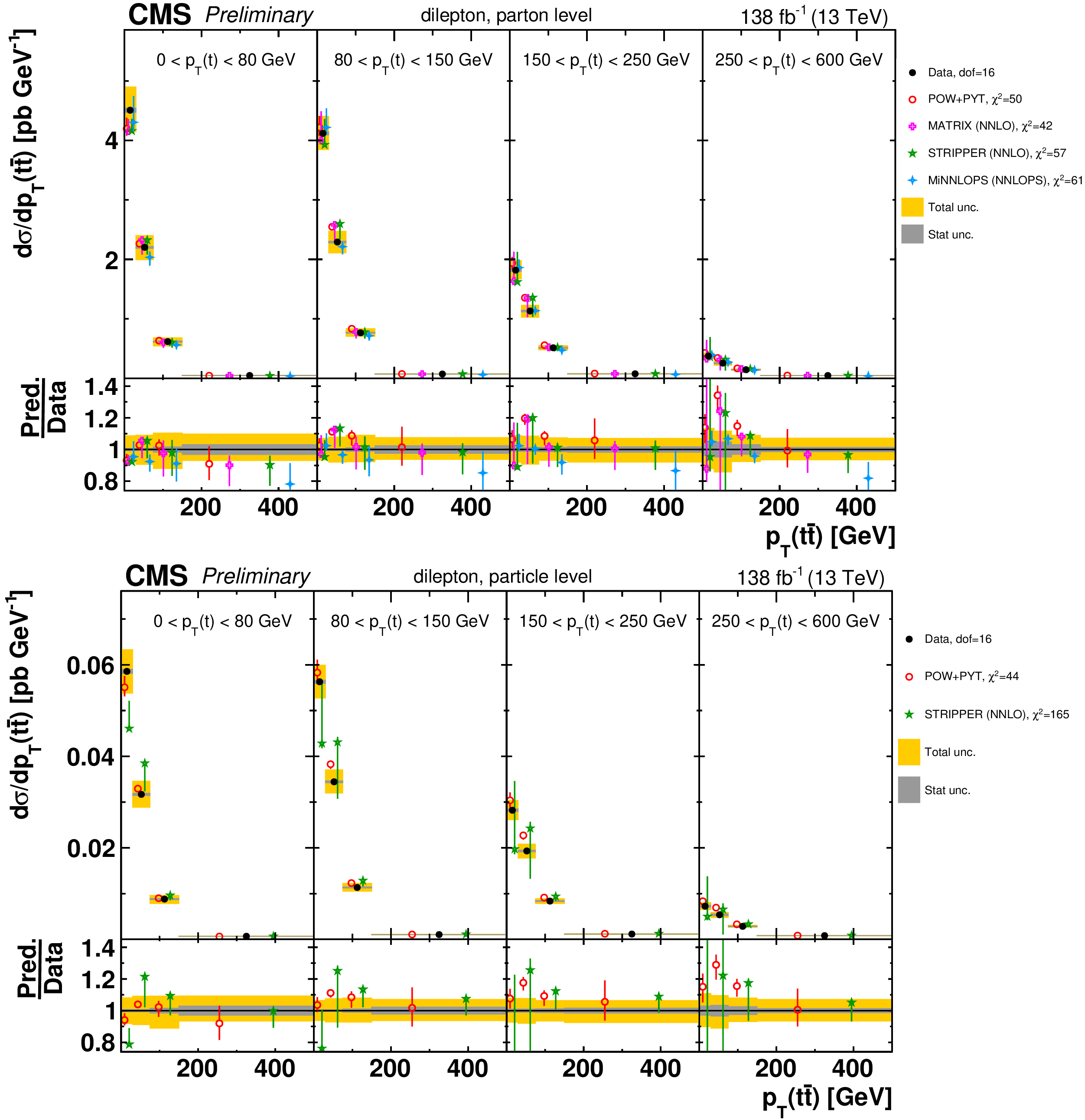
png pdf	Figure 105: Absolute $[ {{p_{\mathrm {T}}} (\mathrm{t})},\,{{p_{\mathrm {T}}} ( \mathrm{t\bar{t}})} ]$ cross sections are shown for data (filled circles), POWHEG+PYTHIA-8 (`POW-PYT', open circles) simulation, and various theoretical predictions with beyond-NLO precision (other points). Further details can be found in the caption of Fig. 103.
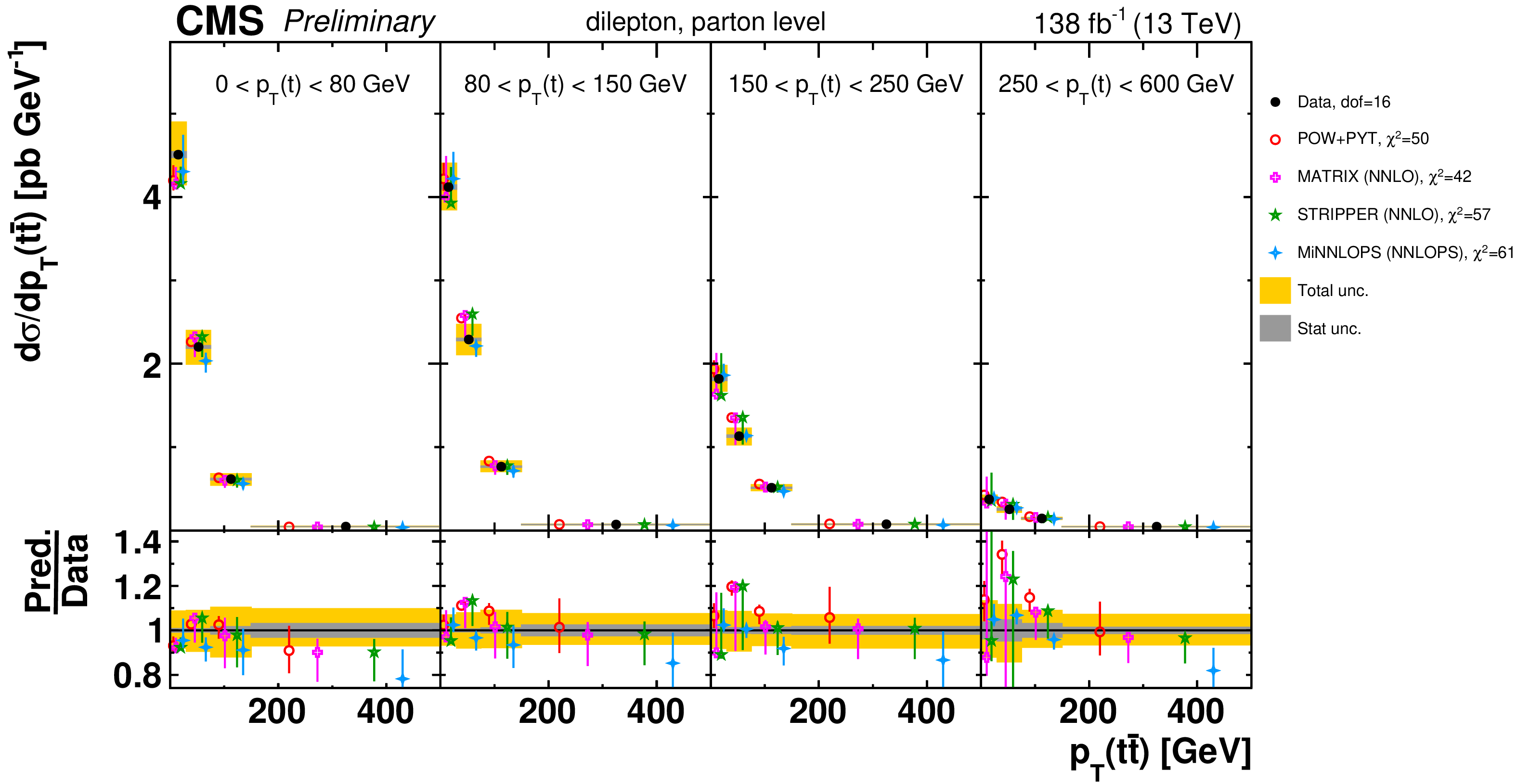
png pdf	Figure 105-a: Absolute $[ {{p_{\mathrm {T}}} (\mathrm{t})},\,{{p_{\mathrm {T}}} ( \mathrm{t\bar{t}})} ]$ cross sections are shown for data (filled circles), POWHEG+PYTHIA-8 (`POW-PYT', open circles) simulation, and various theoretical predictions with beyond-NLO precision (other points). Further details can be found in the caption of Fig. 103.
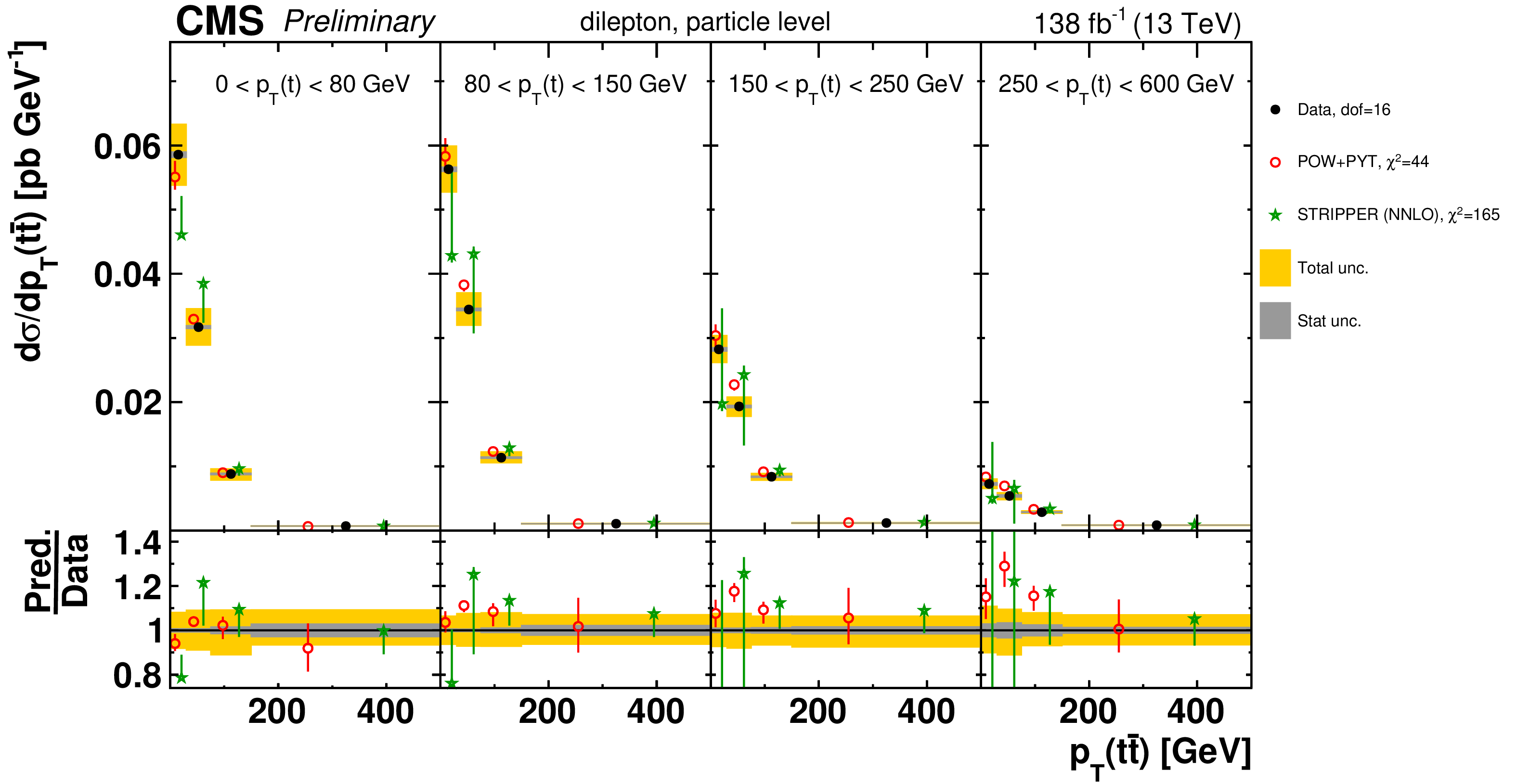
png pdf	Figure 105-b: Absolute $[ {{p_{\mathrm {T}}} (\mathrm{t})},\,{{p_{\mathrm {T}}} ( \mathrm{t\bar{t}})} ]$ cross sections are shown for data (filled circles), POWHEG+PYTHIA-8 (`POW-PYT', open circles) simulation, and various theoretical predictions with beyond-NLO precision (other points). Further details can be found in the caption of Fig. 103.
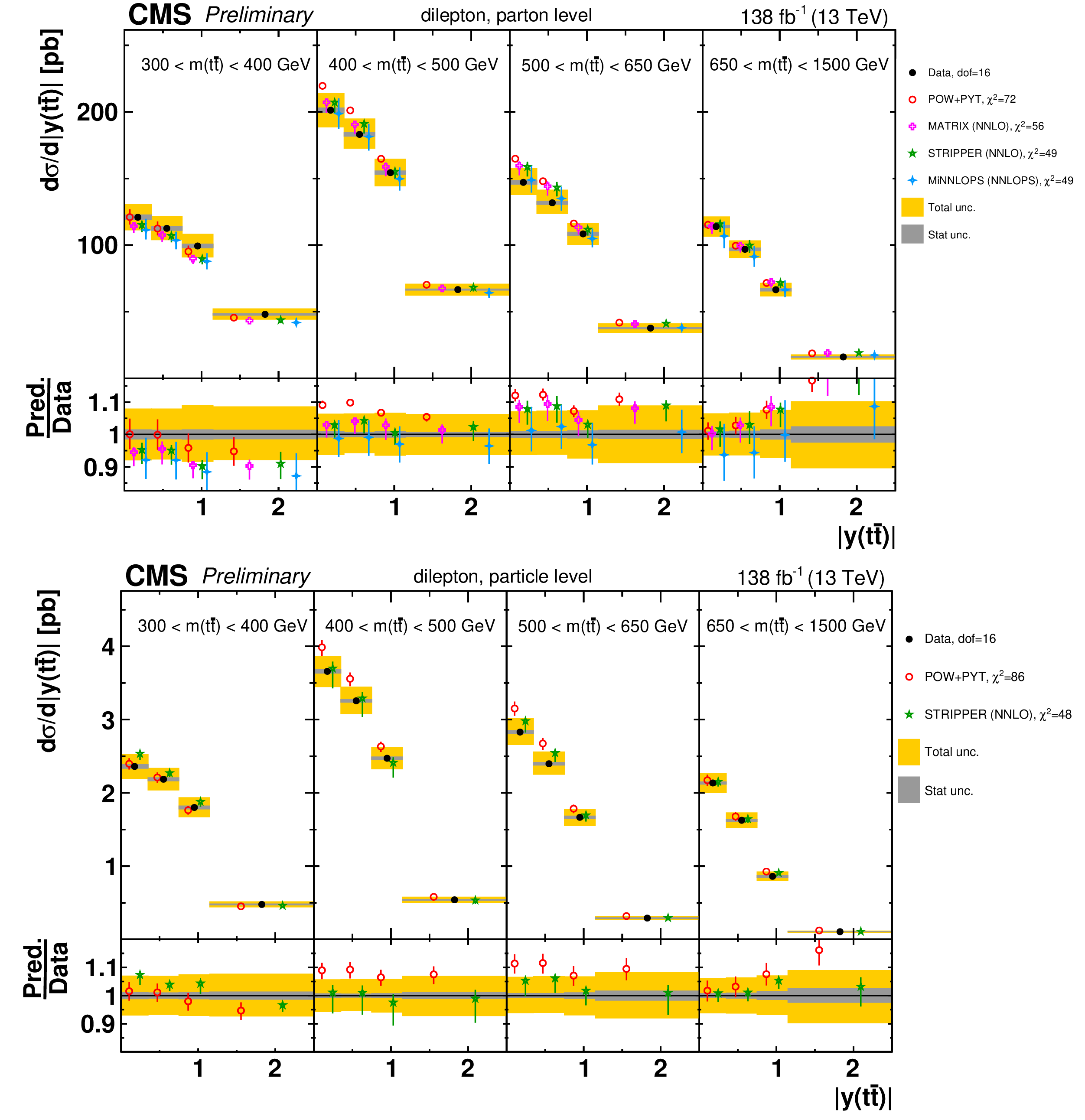
png pdf	Figure 106: Absolute $[ {m( \mathrm{t\bar{t}})},\,{|y( \mathrm{t\bar{t}})|} ]$ cross sections are shown for data (filled circles), POWHEG+PYTHIA-8 (`POW-PYT', open circles) simulation, and various theoretical predictions with beyond-NLO precision (other points). Further details can be found in the caption of Fig. 103.
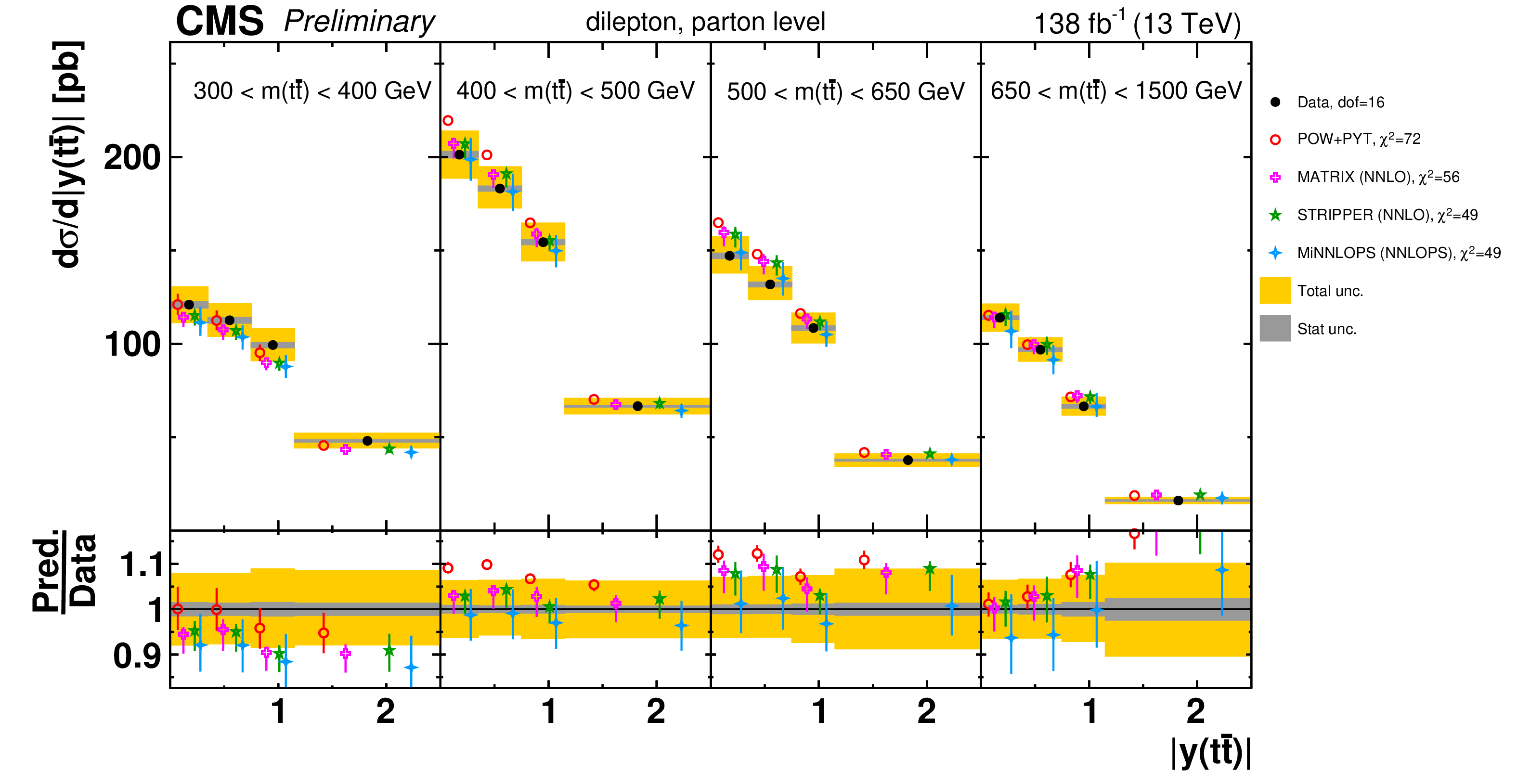
png pdf	Figure 106-a: Absolute $[ {m( \mathrm{t\bar{t}})},\,{|y( \mathrm{t\bar{t}})|} ]$ cross sections are shown for data (filled circles), POWHEG+PYTHIA-8 (`POW-PYT', open circles) simulation, and various theoretical predictions with beyond-NLO precision (other points). Further details can be found in the caption of Fig. 103.
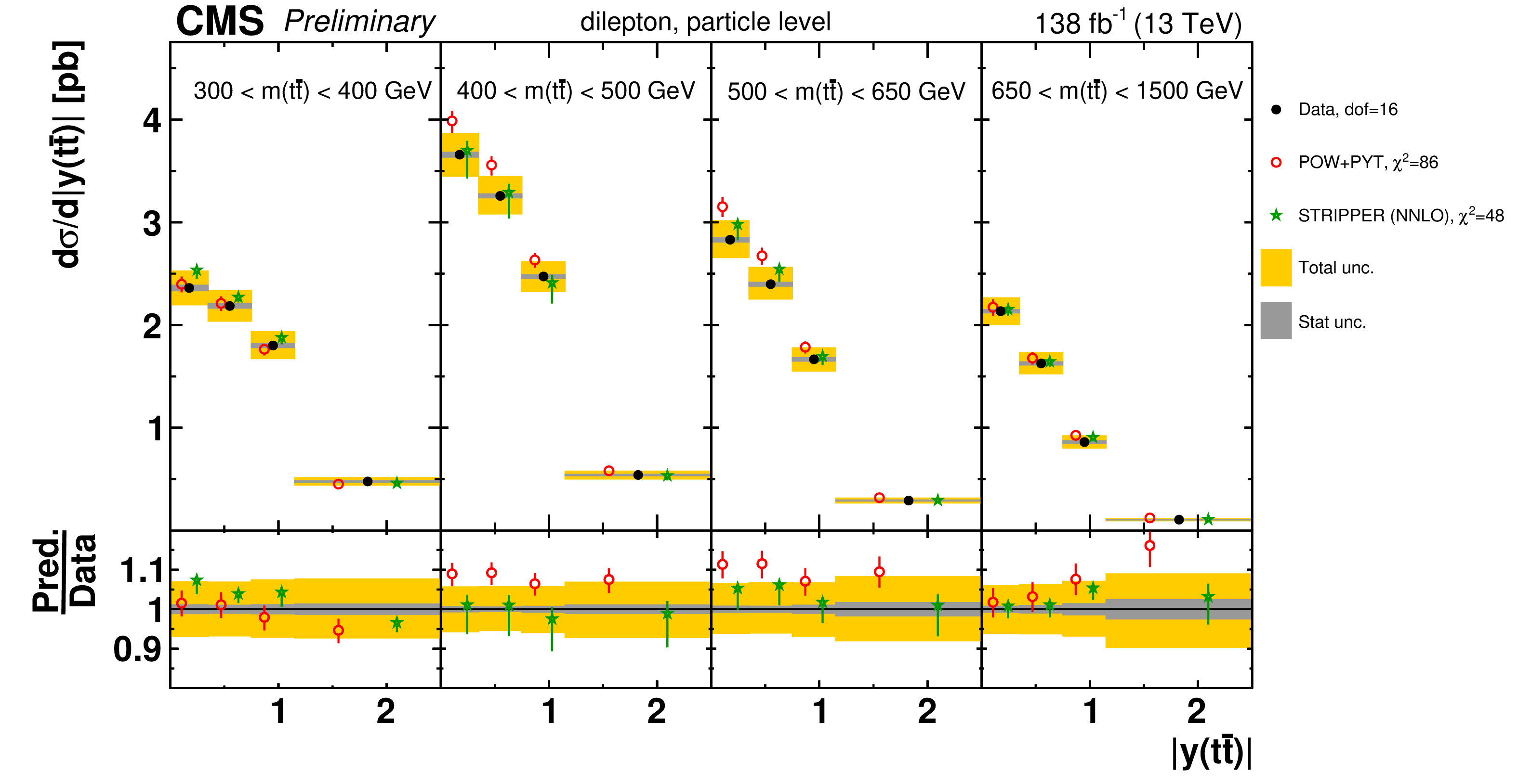
png pdf	Figure 106-b: Absolute $[ {m( \mathrm{t\bar{t}})},\,{|y( \mathrm{t\bar{t}})|} ]$ cross sections are shown for data (filled circles), POWHEG+PYTHIA-8 (`POW-PYT', open circles) simulation, and various theoretical predictions with beyond-NLO precision (other points). Further details can be found in the caption of Fig. 103.
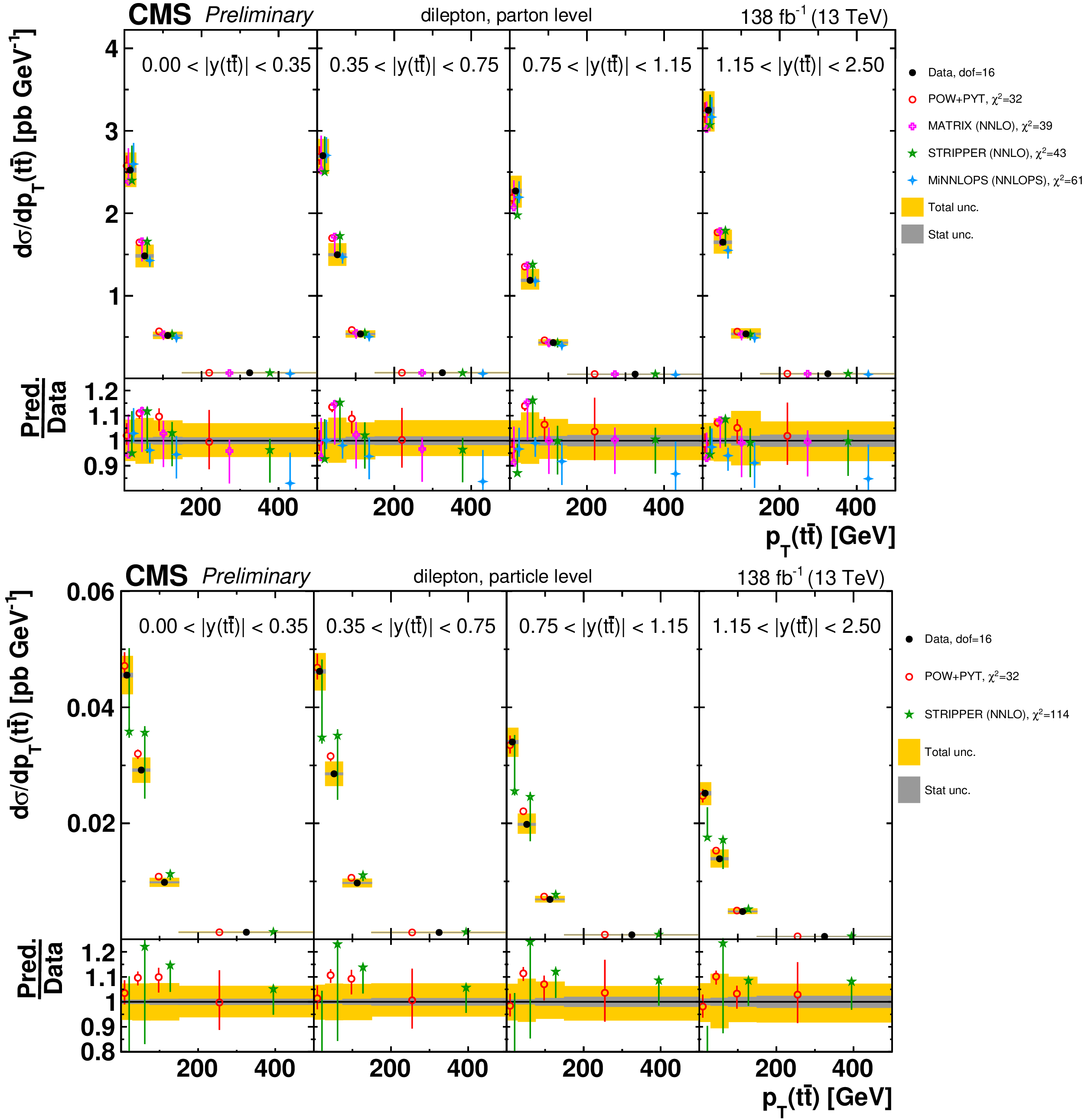
png pdf	Figure 107: Absolute $[ {|y( \mathrm{t\bar{t}})|},\,{{p_{\mathrm {T}}} ( \mathrm{t\bar{t}})} ]$ cross sections are shown for data (filled circles), POWHEG+PYTHIA-8 (`POW-PYT', open circles) simulation, and various theoretical predictions with beyond-NLO precision (other points). Further details can be found in the caption of Fig. 103.
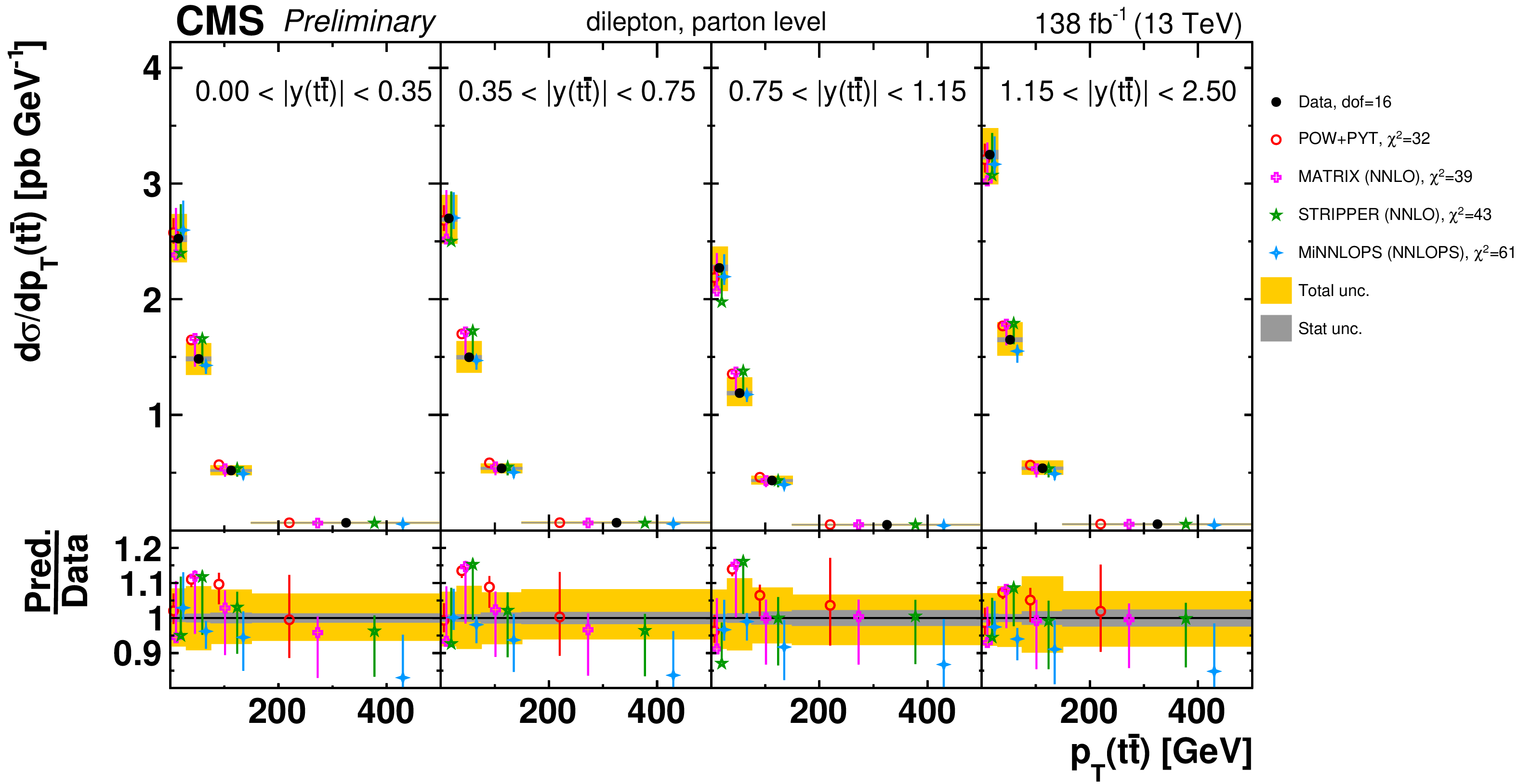
png pdf	Figure 107-a: Absolute $[ {|y( \mathrm{t\bar{t}})|},\,{{p_{\mathrm {T}}} ( \mathrm{t\bar{t}})} ]$ cross sections are shown for data (filled circles), POWHEG+PYTHIA-8 (`POW-PYT', open circles) simulation, and various theoretical predictions with beyond-NLO precision (other points). Further details can be found in the caption of Fig. 103.
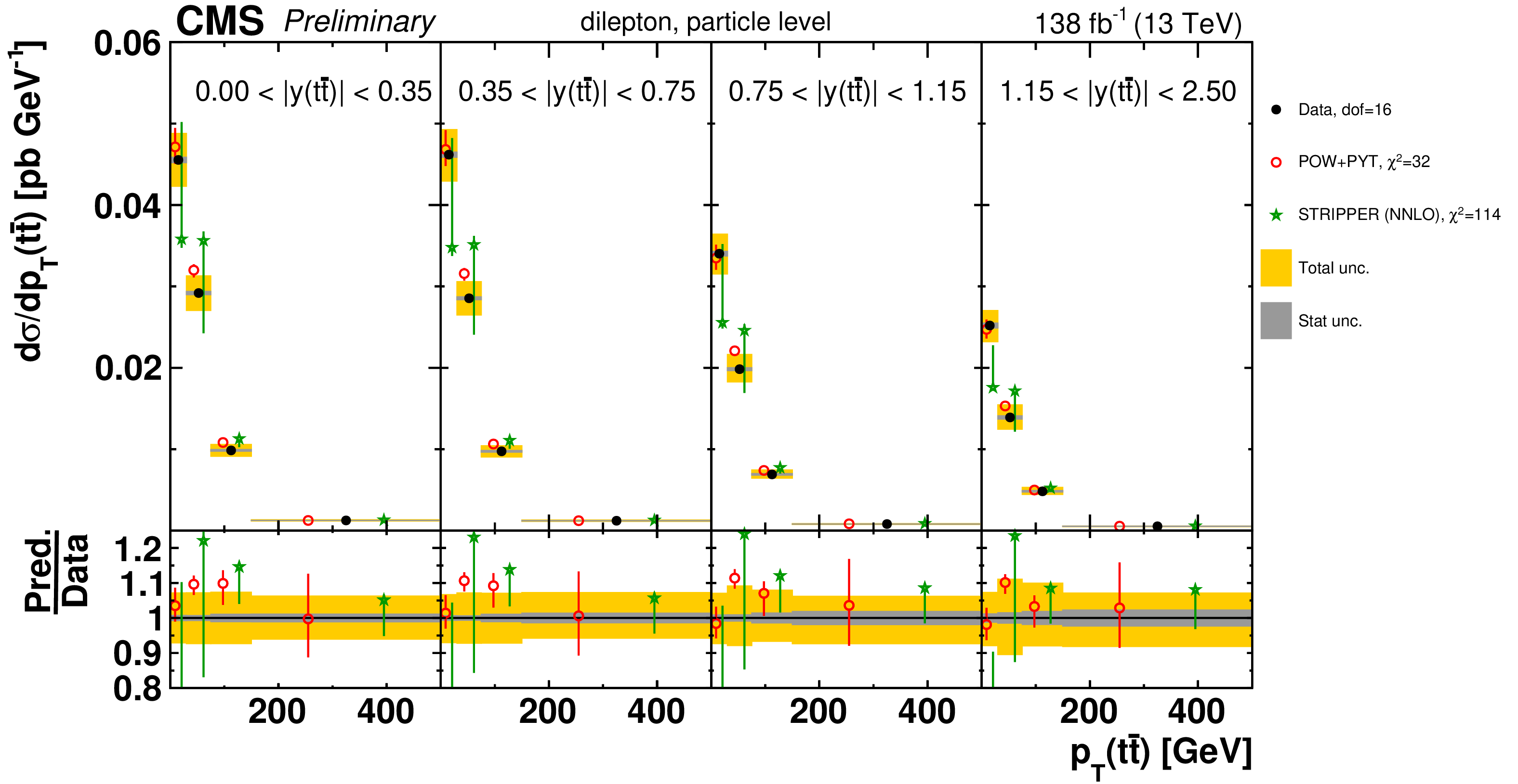
png pdf	Figure 107-b: Absolute $[ {|y( \mathrm{t\bar{t}})|},\,{{p_{\mathrm {T}}} ( \mathrm{t\bar{t}})} ]$ cross sections are shown for data (filled circles), POWHEG+PYTHIA-8 (`POW-PYT', open circles) simulation, and various theoretical predictions with beyond-NLO precision (other points). Further details can be found in the caption of Fig. 103.
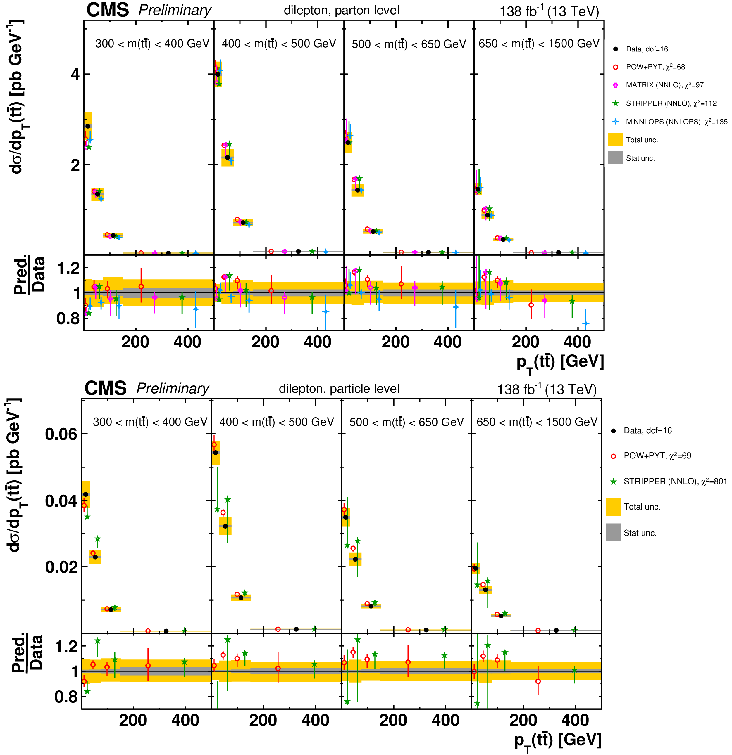
png pdf	Figure 108: Absolute $[ {m( \mathrm{t\bar{t}})},\,{{p_{\mathrm {T}}} ( \mathrm{t\bar{t}})} ]$ cross sections are shown for data (filled circles), POWHEG+PYTHIA-8 (`POW-PYT', open circles) simulation, and various theoretical predictions with beyond-NLO precision (other points). Further details can be found in the caption of Fig. 103.
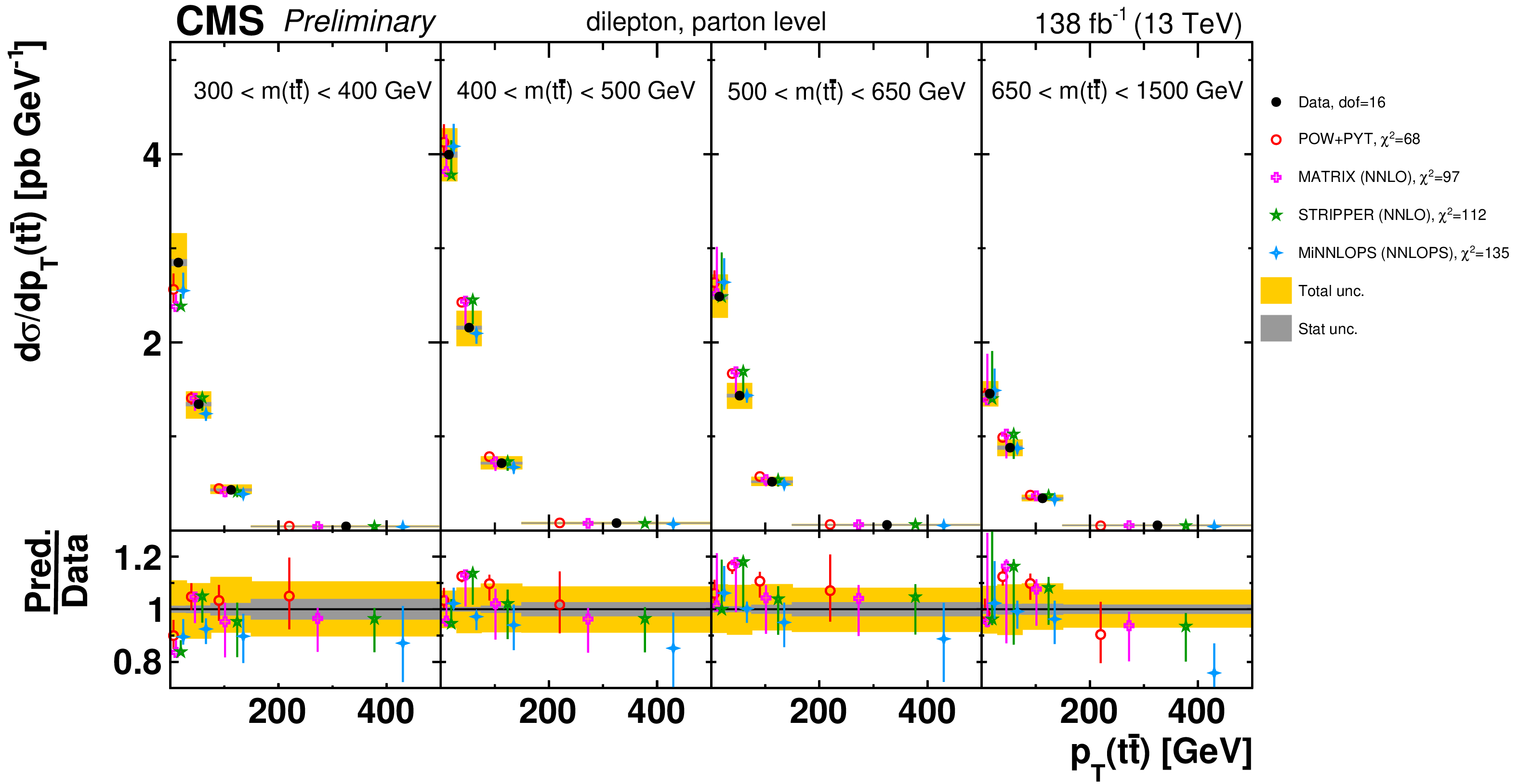
png pdf	Figure 108-a: Absolute $[ {m( \mathrm{t\bar{t}})},\,{{p_{\mathrm {T}}} ( \mathrm{t\bar{t}})} ]$ cross sections are shown for data (filled circles), POWHEG+PYTHIA-8 (`POW-PYT', open circles) simulation, and various theoretical predictions with beyond-NLO precision (other points). Further details can be found in the caption of Fig. 103.
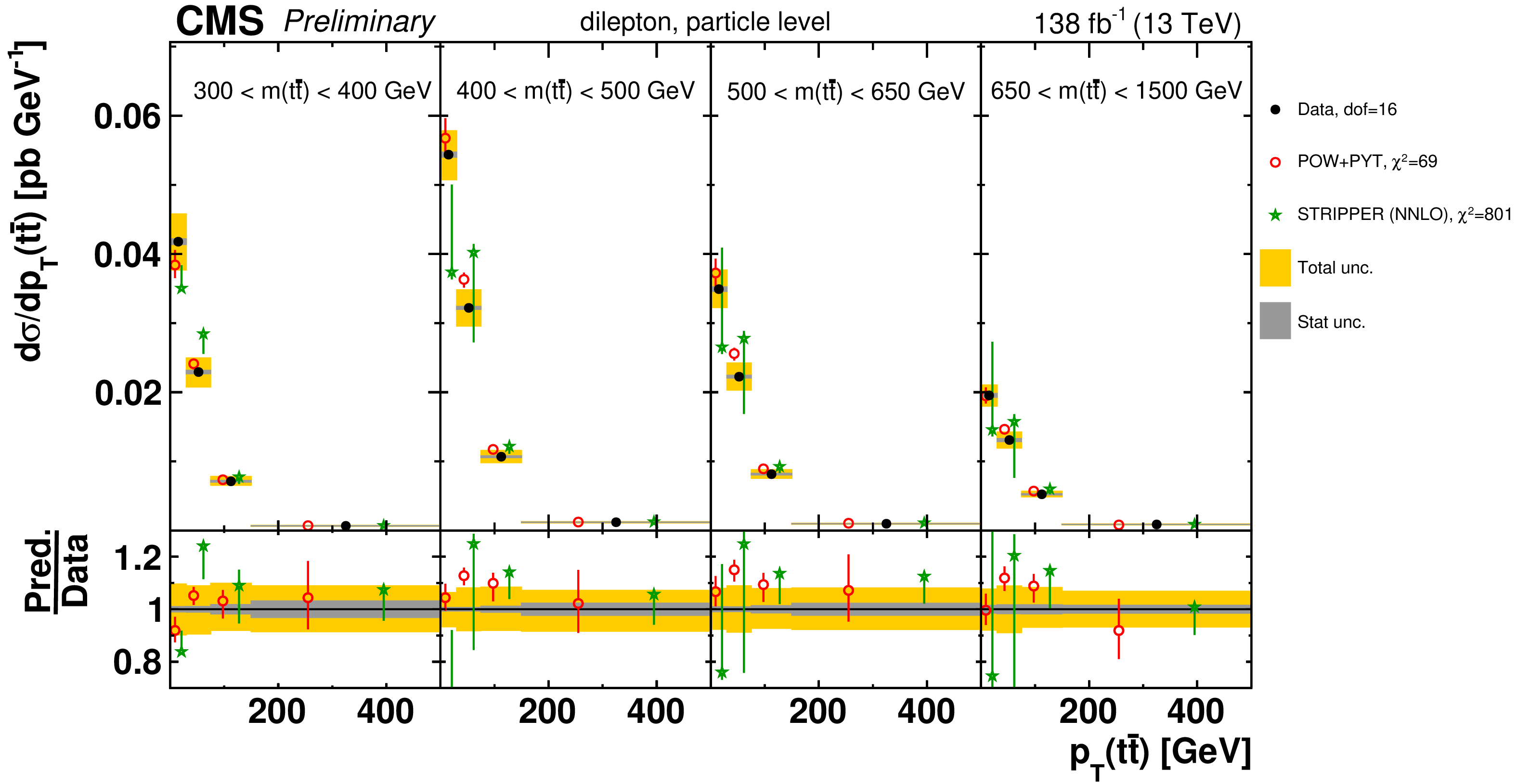
png pdf	Figure 108-b: Absolute $[ {m( \mathrm{t\bar{t}})},\,{{p_{\mathrm {T}}} ( \mathrm{t\bar{t}})} ]$ cross sections are shown for data (filled circles), POWHEG+PYTHIA-8 (`POW-PYT', open circles) simulation, and various theoretical predictions with beyond-NLO precision (other points). Further details can be found in the caption of Fig. 103.
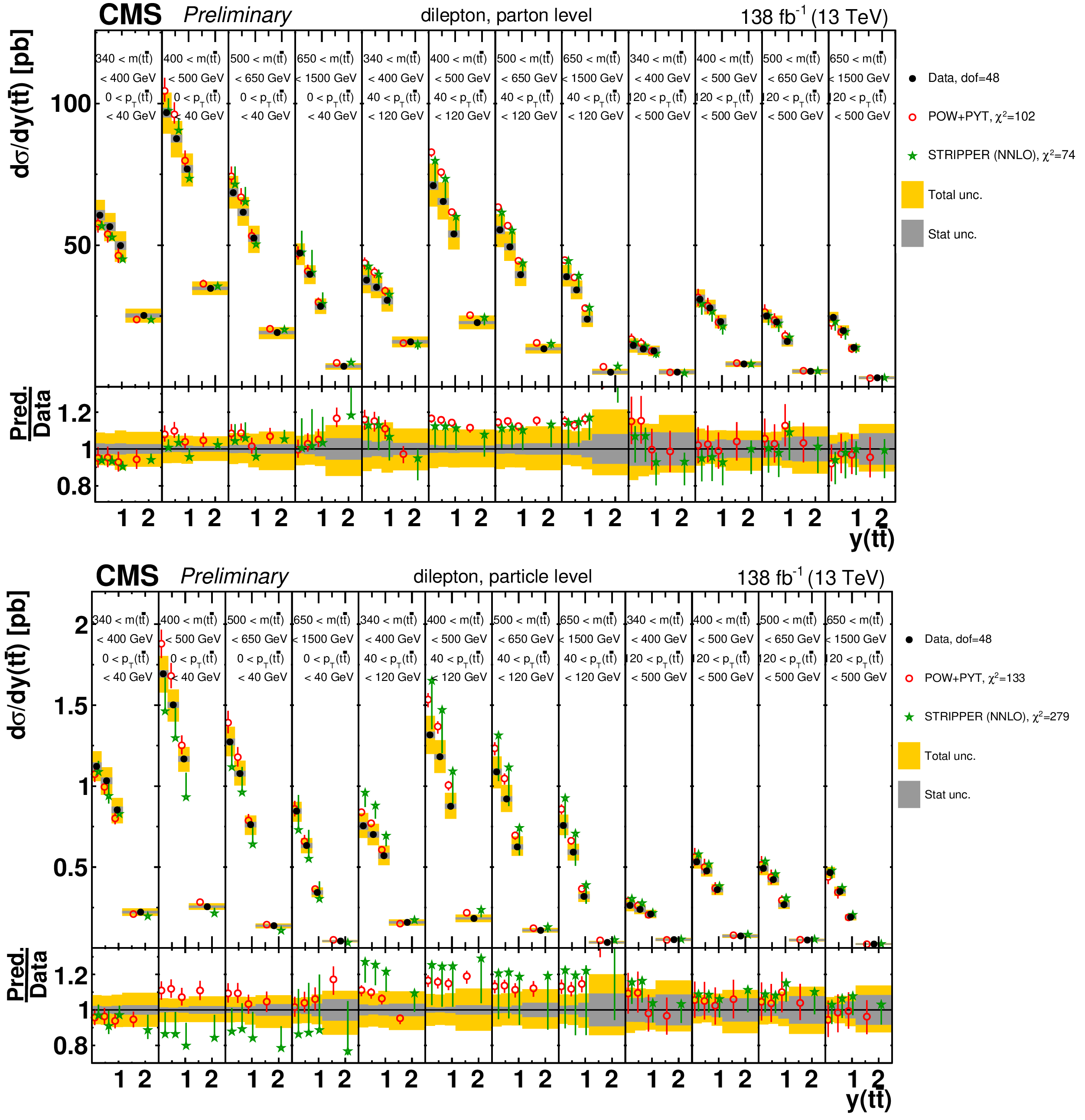
png pdf	Figure 109: Absolute $[ {{p_{\mathrm {T}}} ( \mathrm{t\bar{t}})},\,{m( \mathrm{t\bar{t}})},\,{y( \mathrm{t\bar{t}})} ]$ cross sections are shown for data (filled circles), POWHEG+PYTHIA-8 (`POW-PYT', open circles) simulation, and StripperOnly NNLO calculation (stars). Further details can be found in the caption of Fig. 103.
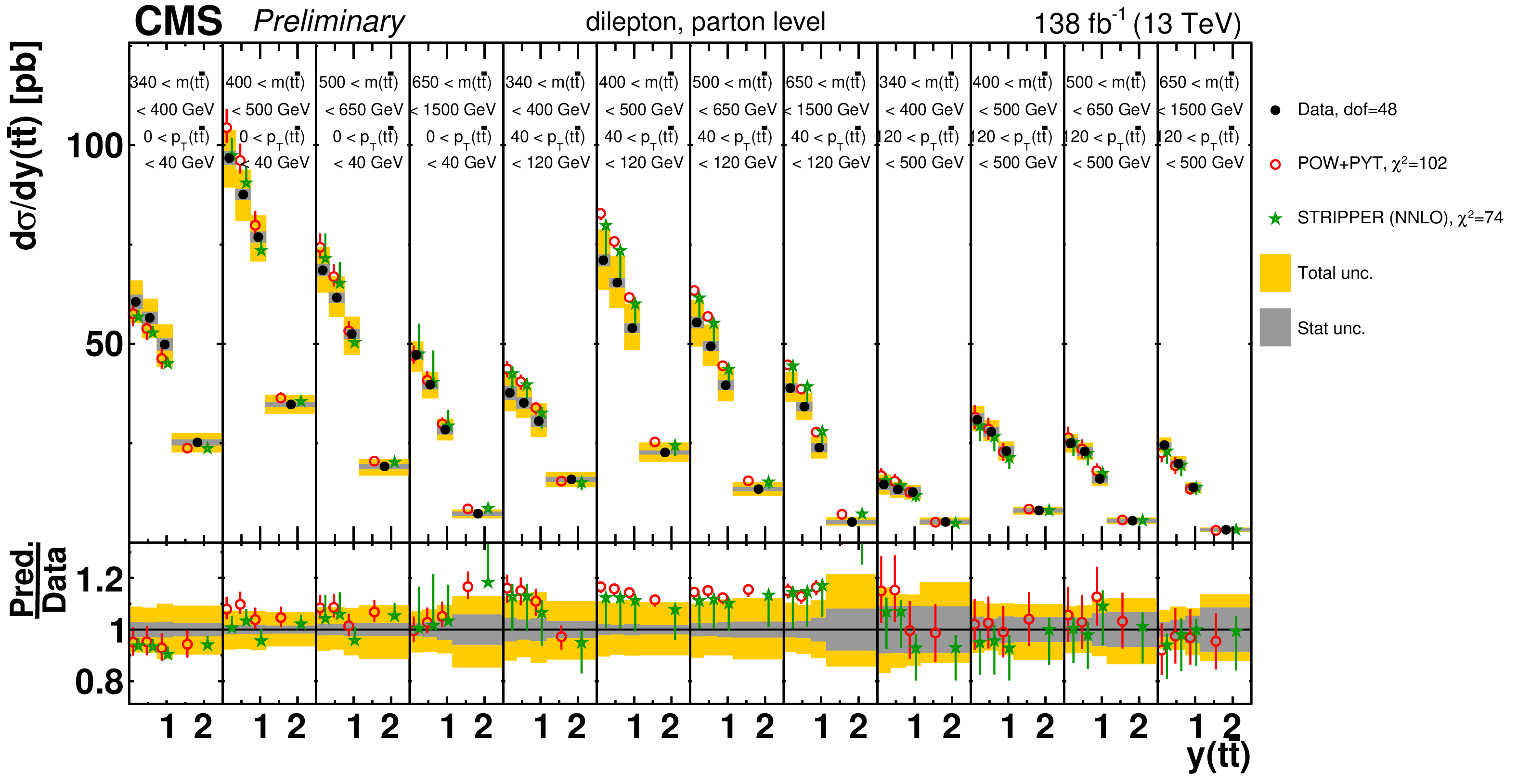
png pdf	Figure 109-a: Absolute $[ {{p_{\mathrm {T}}} ( \mathrm{t\bar{t}})},\,{m( \mathrm{t\bar{t}})},\,{y( \mathrm{t\bar{t}})} ]$ cross sections are shown for data (filled circles), POWHEG+PYTHIA-8 (`POW-PYT', open circles) simulation, and StripperOnly NNLO calculation (stars). Further details can be found in the caption of Fig. 103.
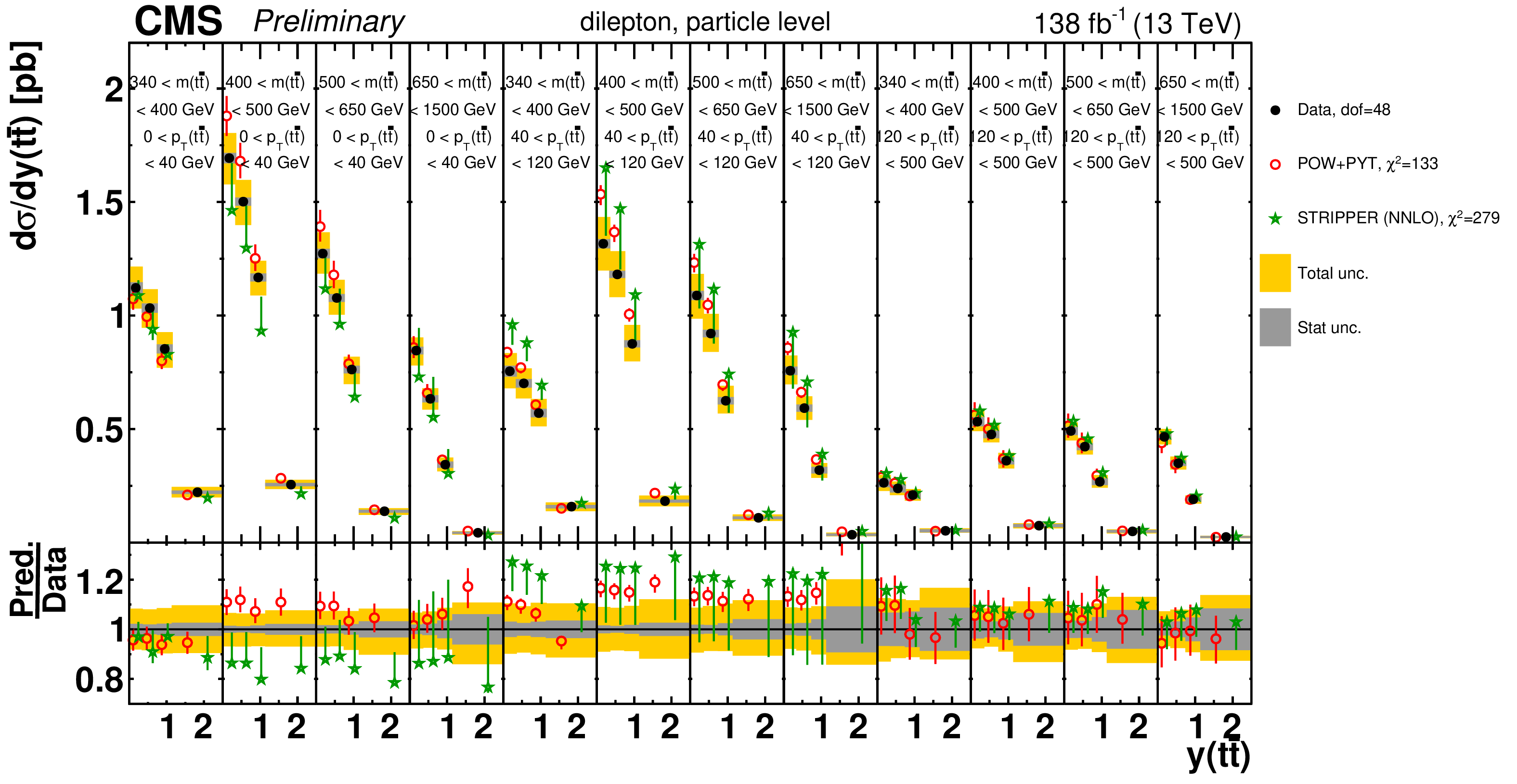
png pdf	Figure 109-b: Absolute $[ {{p_{\mathrm {T}}} ( \mathrm{t\bar{t}})},\,{m( \mathrm{t\bar{t}})},\,{y( \mathrm{t\bar{t}})} ]$ cross sections are shown for data (filled circles), POWHEG+PYTHIA-8 (`POW-PYT', open circles) simulation, and StripperOnly NNLO calculation (stars). Further details can be found in the caption of Fig. 103.
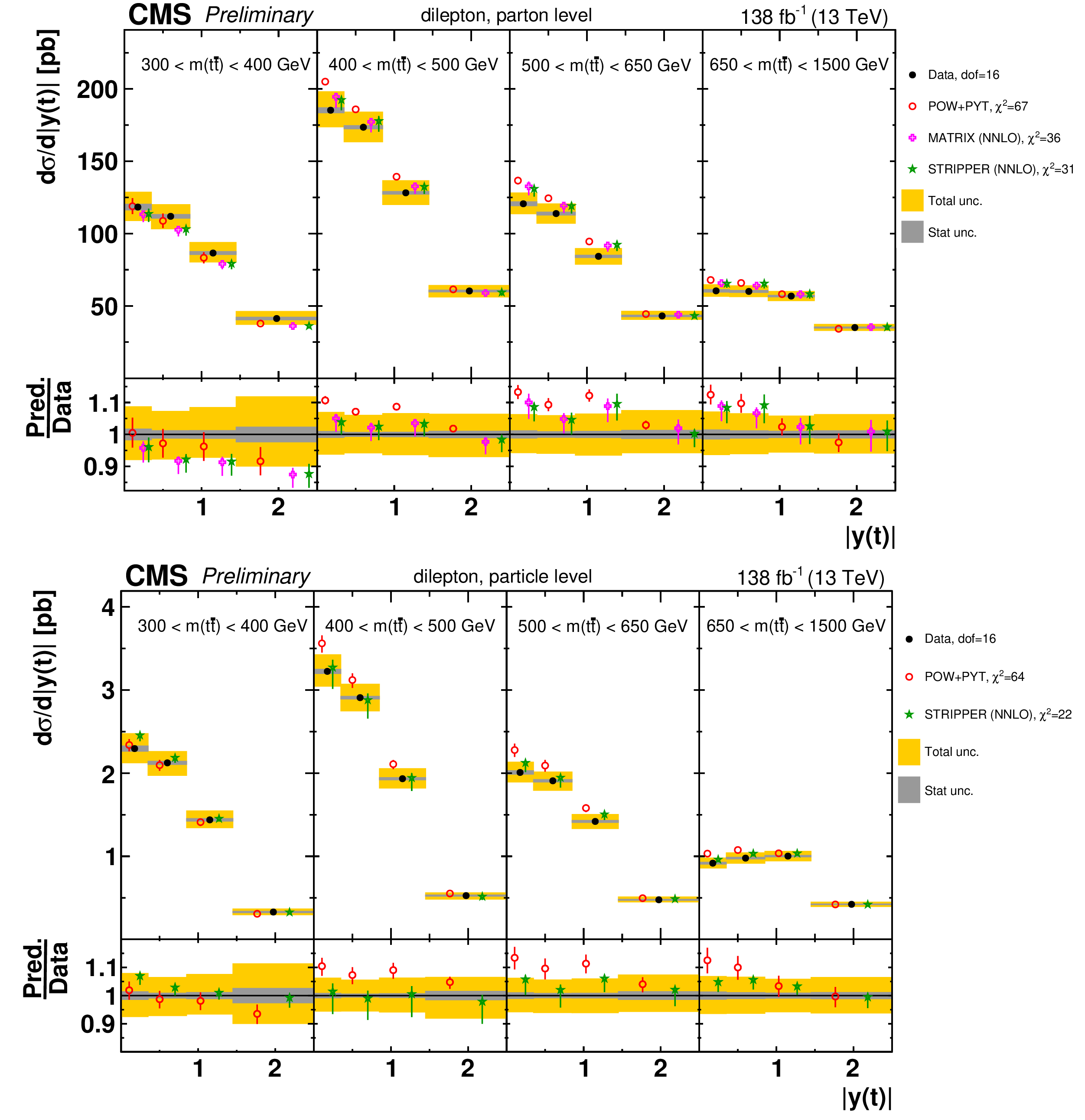
png pdf	Figure 110: Absolute $[ {m( \mathrm{t\bar{t}})},\,{|y(\mathrm{t})|} ]$ cross sections are shown for data (filled circles), POWHEG+PYTHIA-8 (`POW-PYT', open circles) simulation, and various theoretical predictions with beyond-NLO precision (other points). Further details can be found in the caption of Fig. 103.
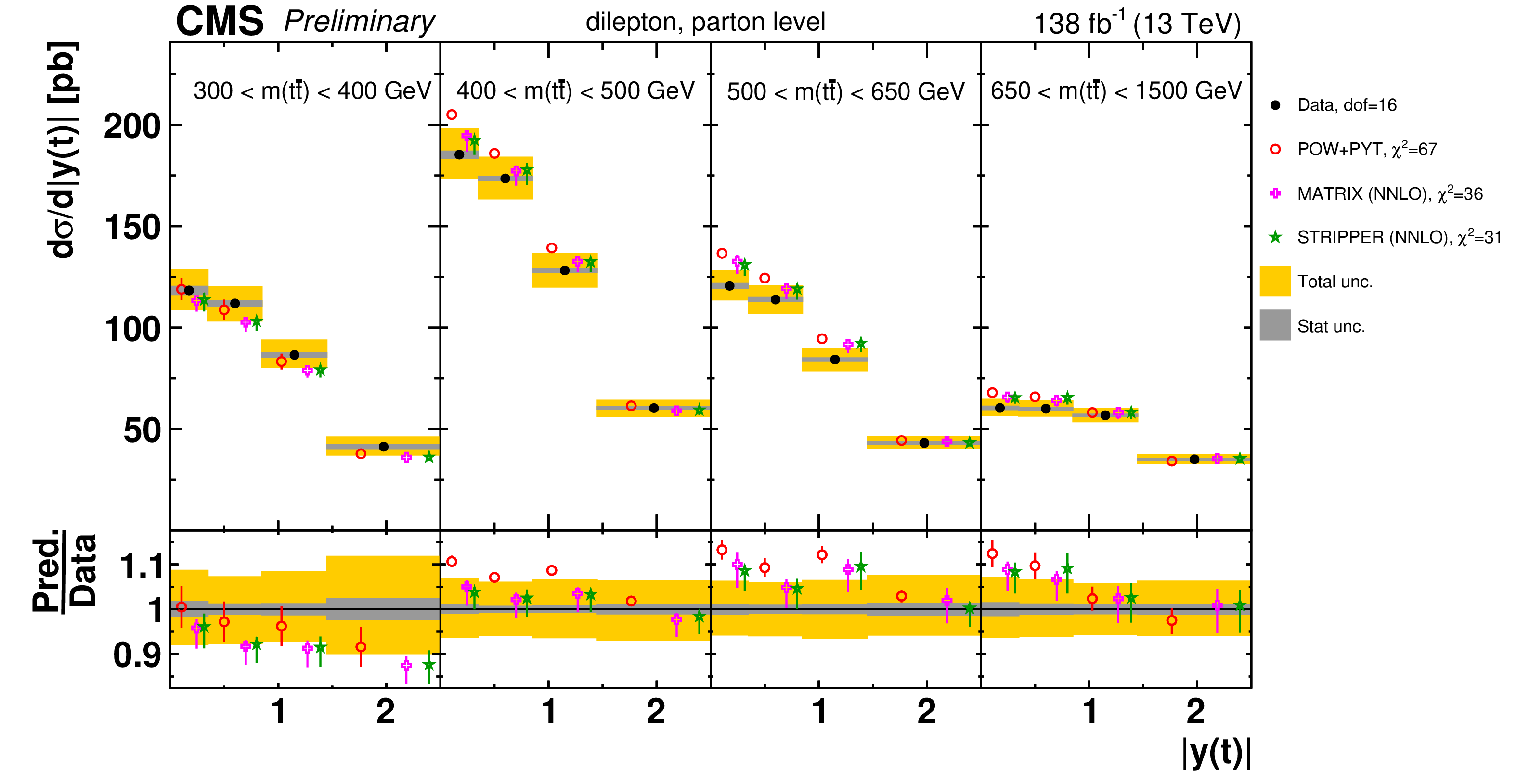
png pdf	Figure 110-a: Absolute $[ {m( \mathrm{t\bar{t}})},\,{|y(\mathrm{t})|} ]$ cross sections are shown for data (filled circles), POWHEG+PYTHIA-8 (`POW-PYT', open circles) simulation, and various theoretical predictions with beyond-NLO precision (other points). Further details can be found in the caption of Fig. 103.
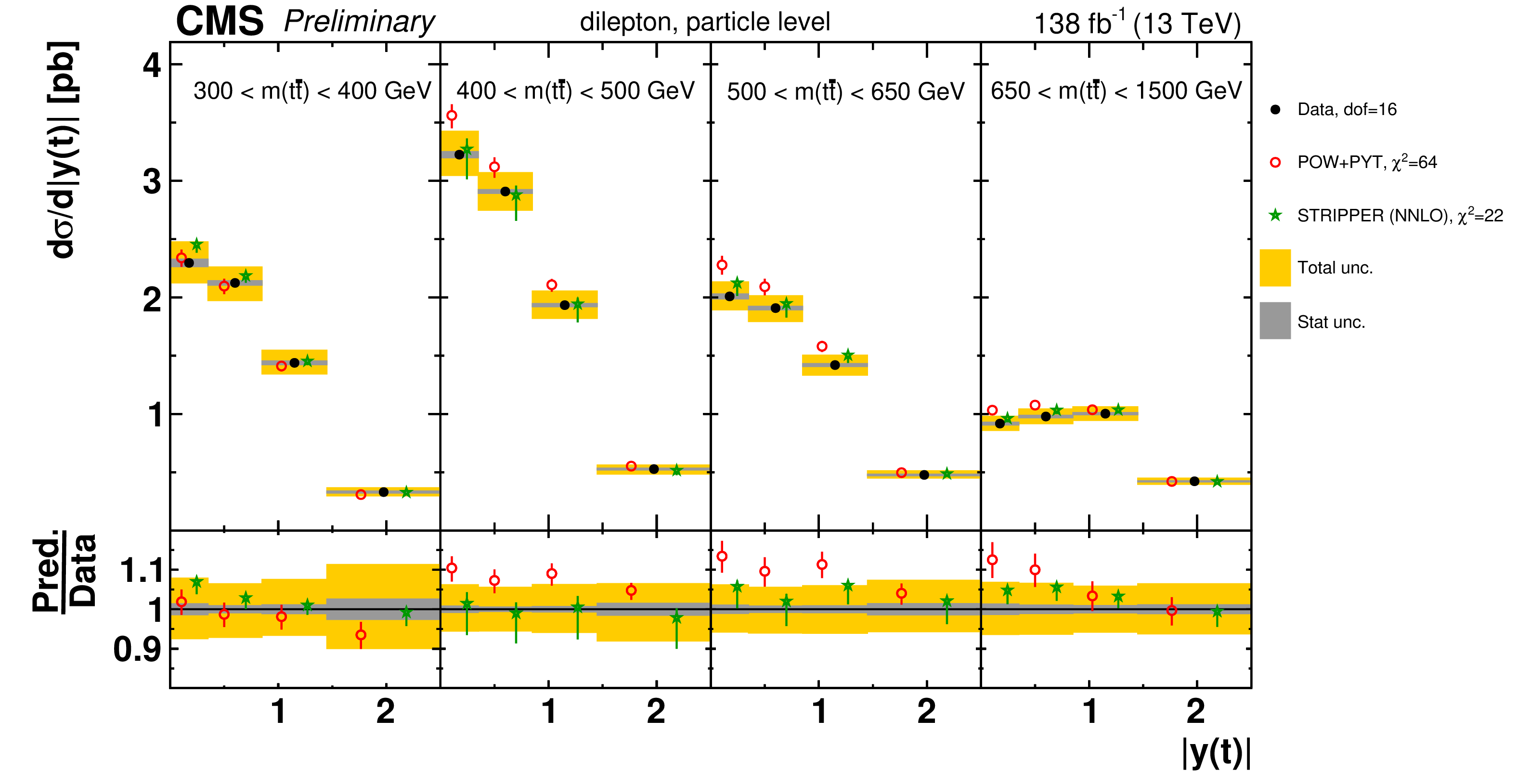
png pdf	Figure 110-b: Absolute $[ {m( \mathrm{t\bar{t}})},\,{|y(\mathrm{t})|} ]$ cross sections are shown for data (filled circles), POWHEG+PYTHIA-8 (`POW-PYT', open circles) simulation, and various theoretical predictions with beyond-NLO precision (other points). Further details can be found in the caption of Fig. 103.
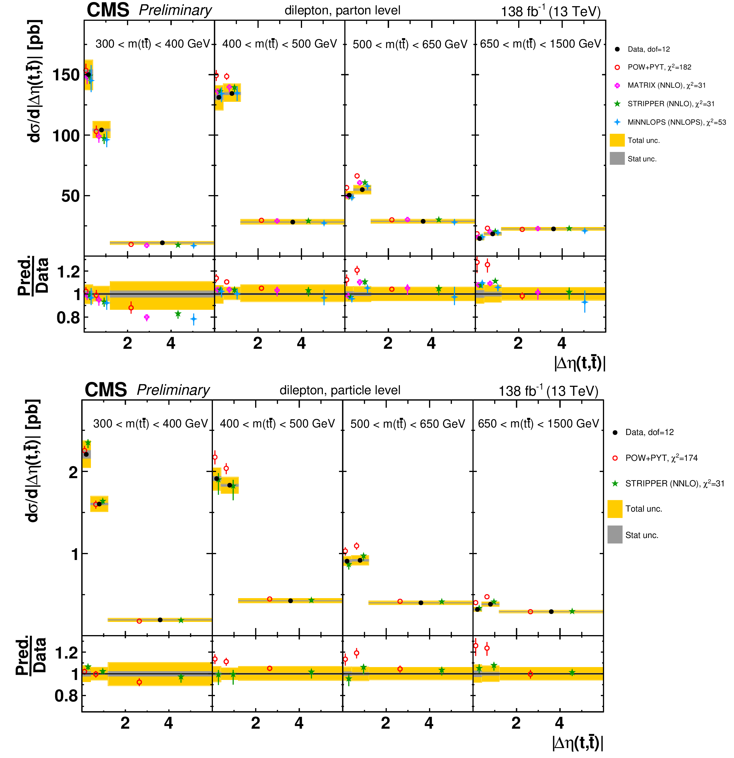
png pdf	Figure 111: Absolute $[ {m( \mathrm{t\bar{t}})},\,{|\Delta \eta (\mathrm{t},\mathrm{\bar{t}})|} ]$ cross sections are shown for data (filled circles), POWHEG+PYTHIA-8 (`POW-PYT', open circles) simulation, and various theoretical predictions with beyond-NLO precision (other points). Further details can be found in the caption of Fig. 103.
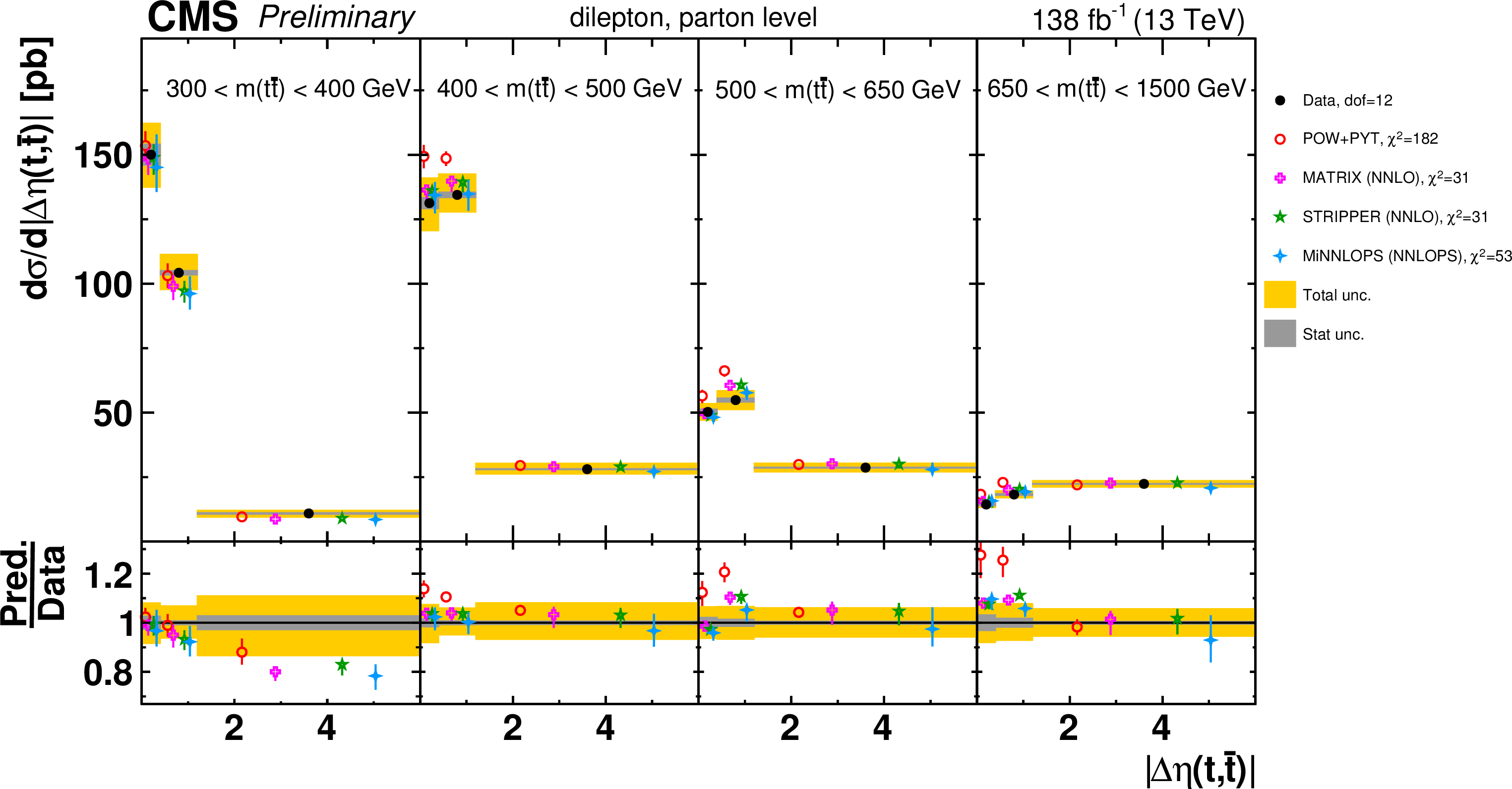
png pdf	Figure 111-a: Absolute $[ {m( \mathrm{t\bar{t}})},\,{|\Delta \eta (\mathrm{t},\mathrm{\bar{t}})|} ]$ cross sections are shown for data (filled circles), POWHEG+PYTHIA-8 (`POW-PYT', open circles) simulation, and various theoretical predictions with beyond-NLO precision (other points). Further details can be found in the caption of Fig. 103.
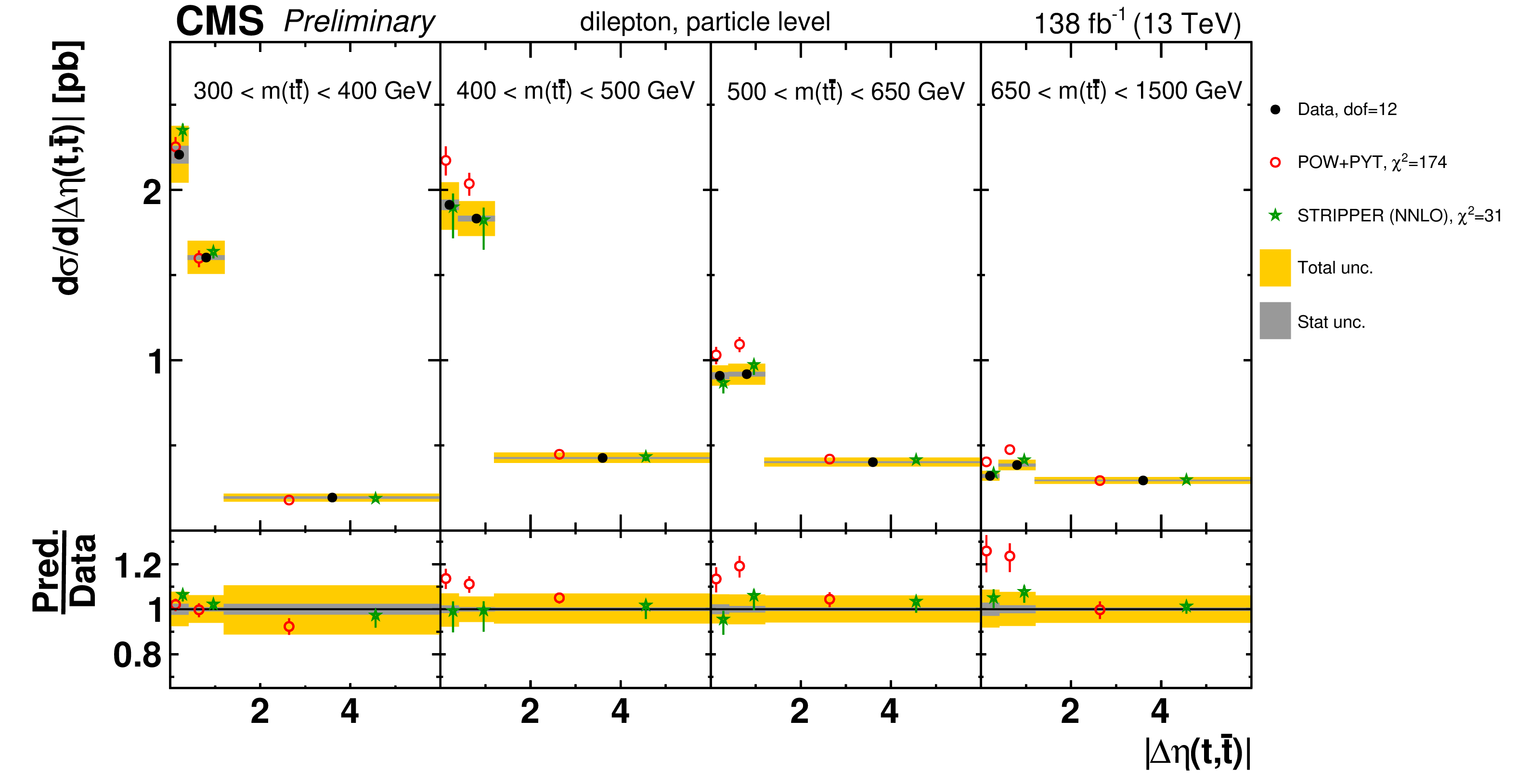
png pdf	Figure 111-b: Absolute $[ {m( \mathrm{t\bar{t}})},\,{|\Delta \eta (\mathrm{t},\mathrm{\bar{t}})|} ]$ cross sections are shown for data (filled circles), POWHEG+PYTHIA-8 (`POW-PYT', open circles) simulation, and various theoretical predictions with beyond-NLO precision (other points). Further details can be found in the caption of Fig. 103.
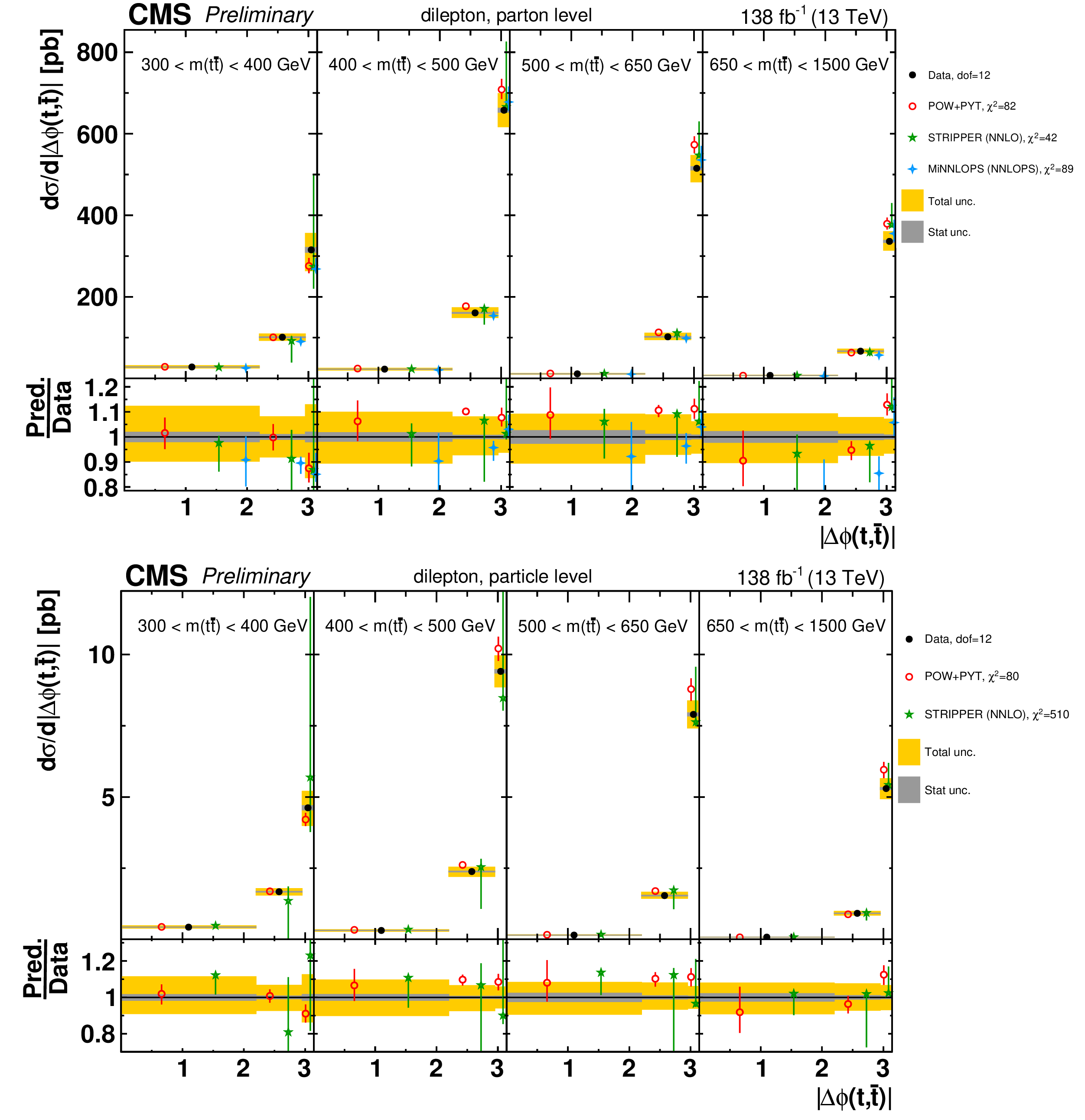
png pdf	Figure 112: Absolute $[ {m( \mathrm{t\bar{t}})},\,{|\Delta \phi (\mathrm{t},\mathrm{\bar{t}})|} ]$ cross sections are shown for data (filled circles), POWHEG+PYTHIA-8 (`POW-PYT', open circles) simulation, and various theoretical predictions with beyond-NLO precision (other points). Further details can be found in the caption of Fig. 103.
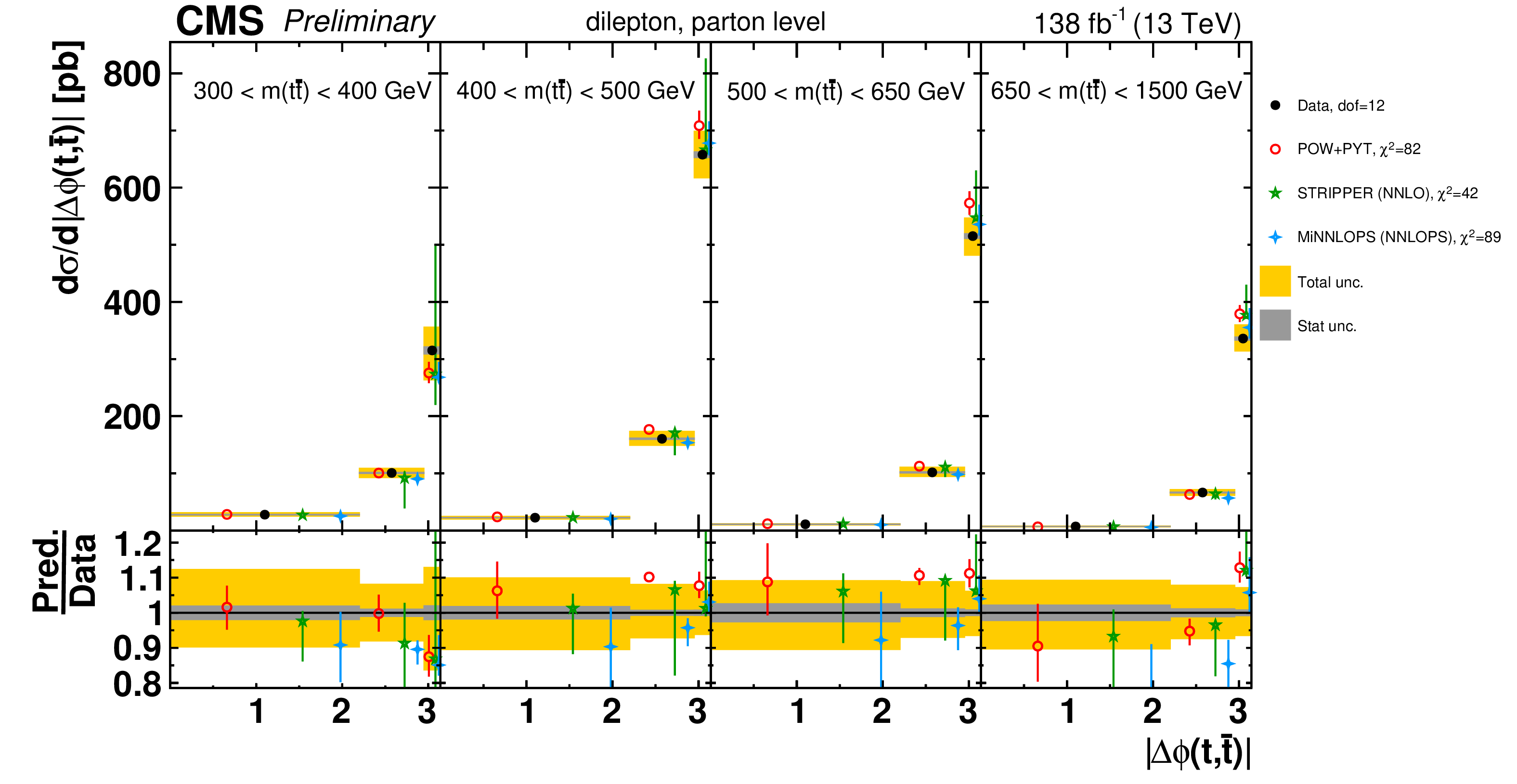
png pdf	Figure 112-a: Absolute $[ {m( \mathrm{t\bar{t}})},\,{|\Delta \phi (\mathrm{t},\mathrm{\bar{t}})|} ]$ cross sections are shown for data (filled circles), POWHEG+PYTHIA-8 (`POW-PYT', open circles) simulation, and various theoretical predictions with beyond-NLO precision (other points). Further details can be found in the caption of Fig. 103.
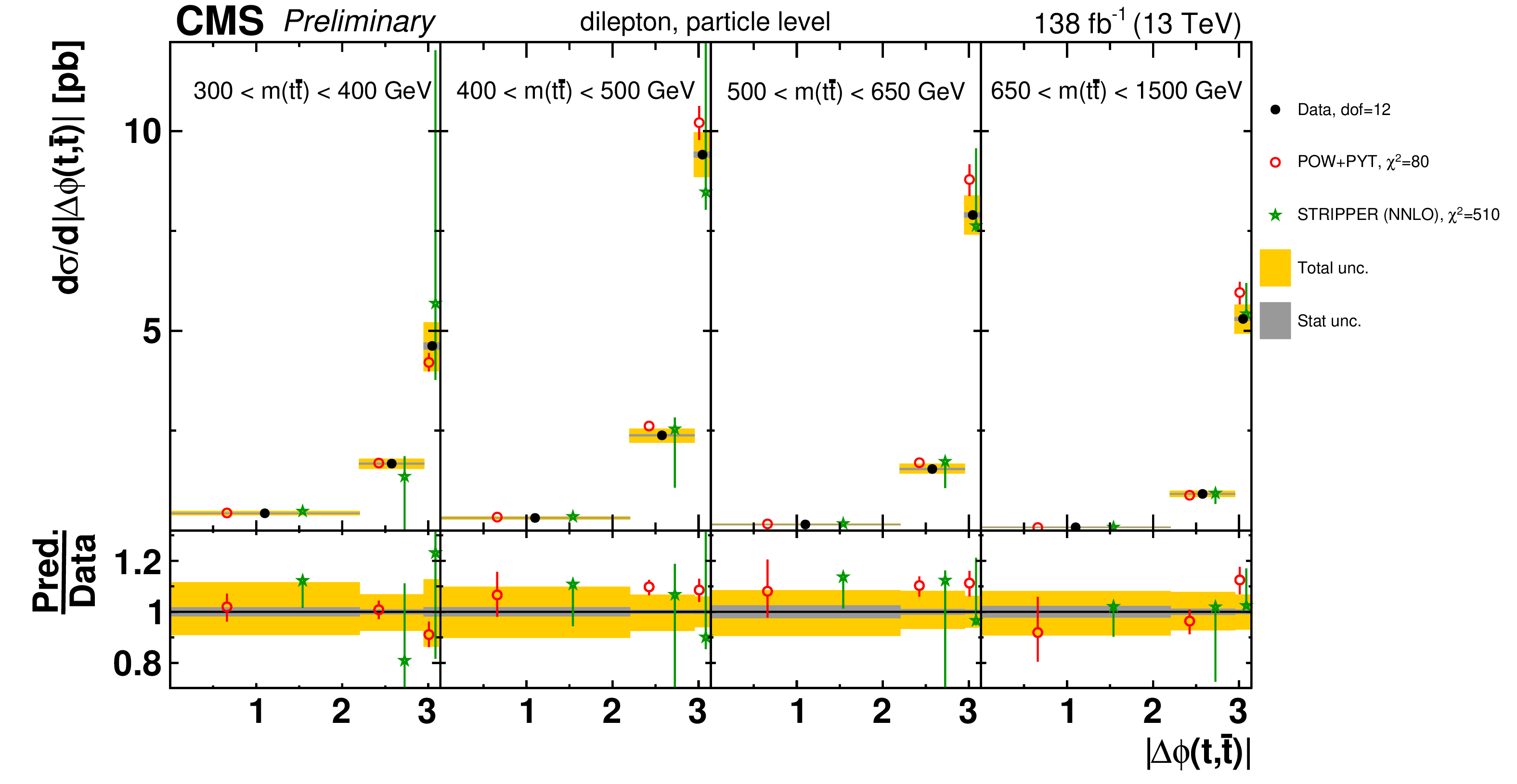
png pdf	Figure 112-b: Absolute $[ {m( \mathrm{t\bar{t}})},\,{|\Delta \phi (\mathrm{t},\mathrm{\bar{t}})|} ]$ cross sections are shown for data (filled circles), POWHEG+PYTHIA-8 (`POW-PYT', open circles) simulation, and various theoretical predictions with beyond-NLO precision (other points). Further details can be found in the caption of Fig. 103.
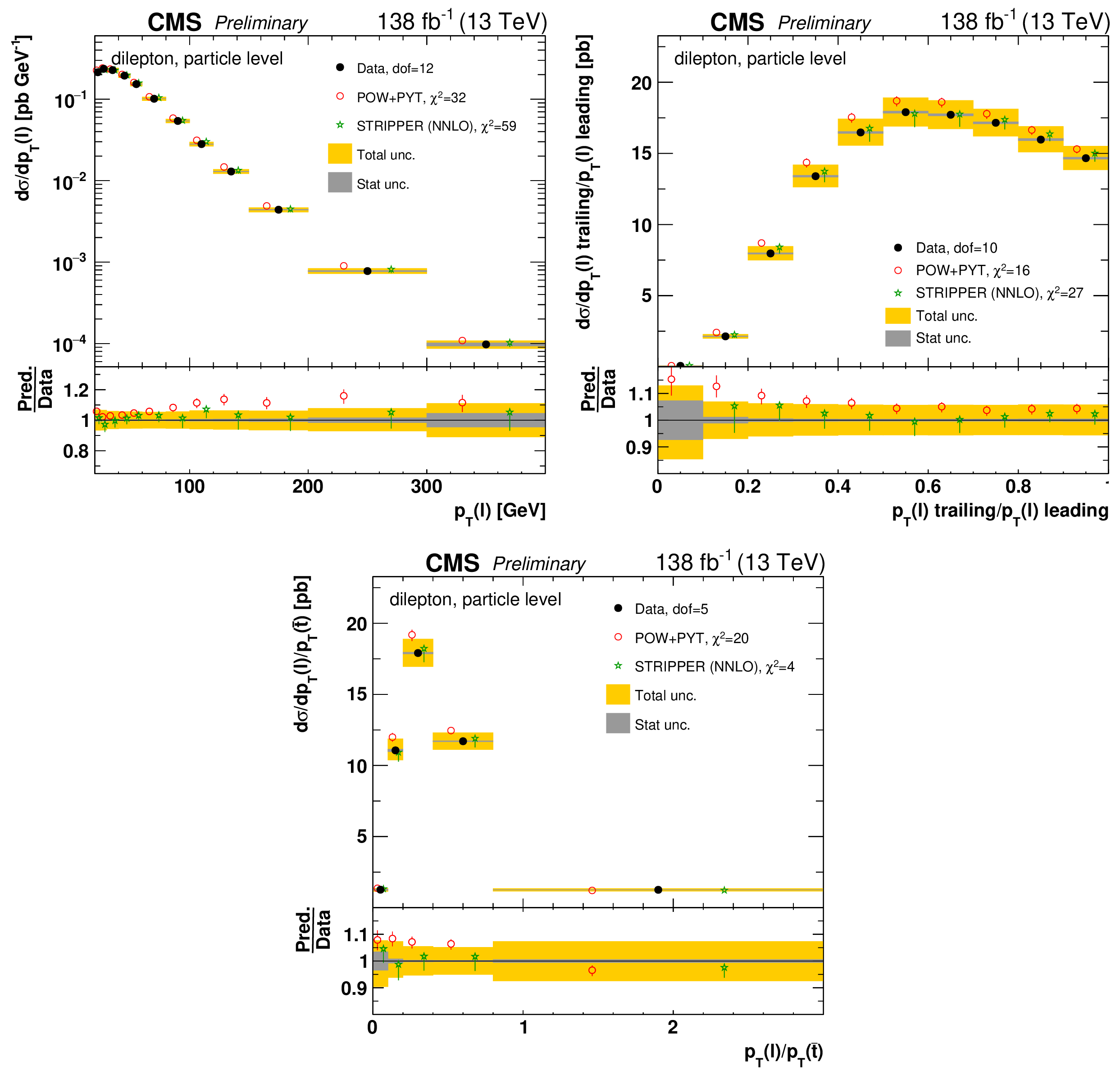
png pdf	Figure 113: Absolute differential $\mathrm{t\bar{t}}$ production cross sections as a function of ${p_{\mathrm {T}}}$ of the lepton (upper left), of the ratio of the trailing and leading lepton ${p_{\mathrm {T}}}$ (upper right), and of the ratio of lepton and top antiquark ${p_{\mathrm {T}}}$ (lower middle), measured at the particle level in a fiducial phase space. The data are shown as filled circles with dark and light bands indicating the statistical and total uncertainties (statistical and systematic uncertainties summed in quadrature), respectively. The cross sections are compared to predictions from the POWHEG+PYTHIA-8 (`POW-PYT', open circles) simulation and Stripper NNLO calculation (stars). The estimated uncertainties in the predictions are represented by a vertical bar on the corresponding points. For each model, a value of ${\chi ^2}$ is reported that takes into account the measurement uncertainties. The lower panel in each plot shows the ratios of the predictions to the data.
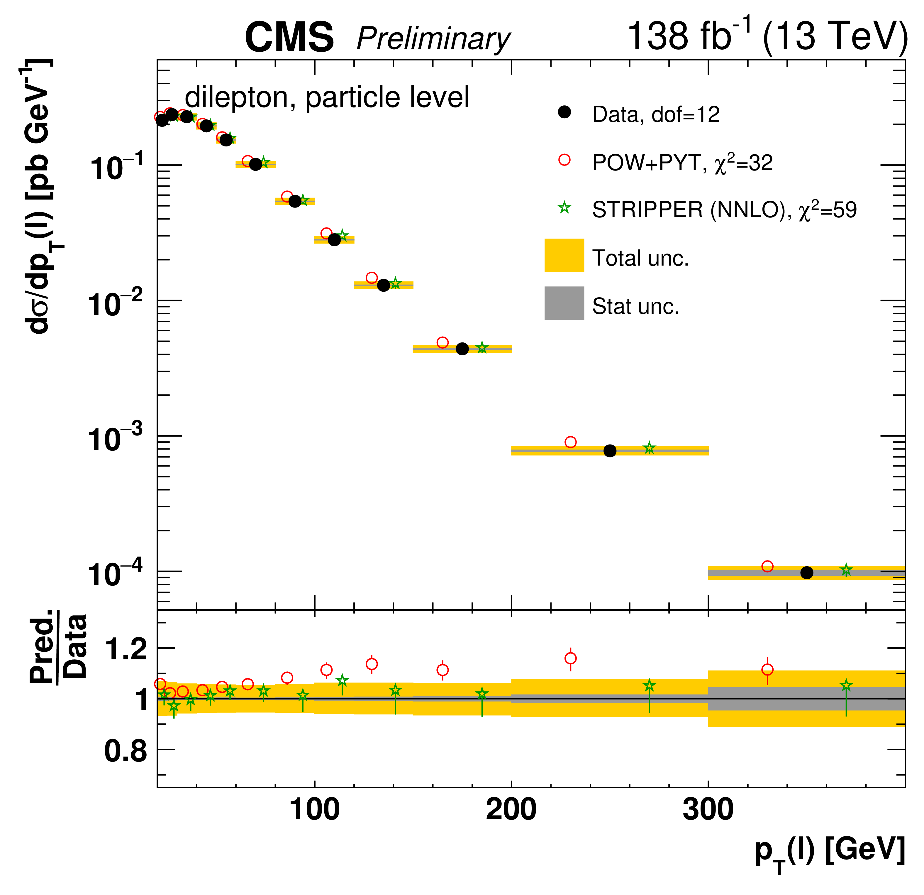
png pdf	Figure 113-a: Absolute differential $\mathrm{t\bar{t}}$ production cross sections as a function of ${p_{\mathrm {T}}}$ of the lepton (upper left), of the ratio of the trailing and leading lepton ${p_{\mathrm {T}}}$ (upper right), and of the ratio of lepton and top antiquark ${p_{\mathrm {T}}}$ (lower middle), measured at the particle level in a fiducial phase space. The data are shown as filled circles with dark and light bands indicating the statistical and total uncertainties (statistical and systematic uncertainties summed in quadrature), respectively. The cross sections are compared to predictions from the POWHEG+PYTHIA-8 (`POW-PYT', open circles) simulation and Stripper NNLO calculation (stars). The estimated uncertainties in the predictions are represented by a vertical bar on the corresponding points. For each model, a value of ${\chi ^2}$ is reported that takes into account the measurement uncertainties. The lower panel in each plot shows the ratios of the predictions to the data.
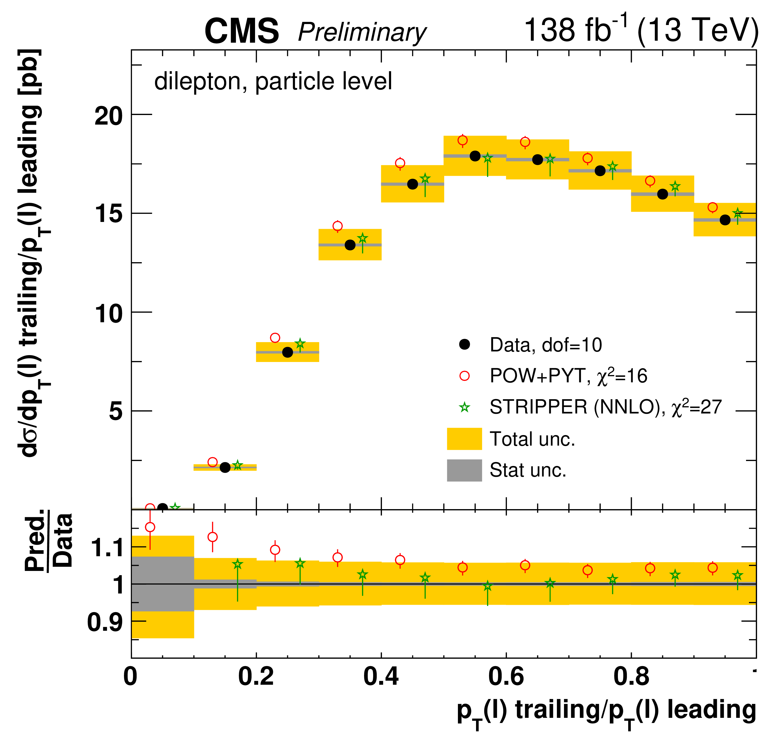
png pdf	Figure 113-b: Absolute differential $\mathrm{t\bar{t}}$ production cross sections as a function of ${p_{\mathrm {T}}}$ of the lepton (upper left), of the ratio of the trailing and leading lepton ${p_{\mathrm {T}}}$ (upper right), and of the ratio of lepton and top antiquark ${p_{\mathrm {T}}}$ (lower middle), measured at the particle level in a fiducial phase space. The data are shown as filled circles with dark and light bands indicating the statistical and total uncertainties (statistical and systematic uncertainties summed in quadrature), respectively. The cross sections are compared to predictions from the POWHEG+PYTHIA-8 (`POW-PYT', open circles) simulation and Stripper NNLO calculation (stars). The estimated uncertainties in the predictions are represented by a vertical bar on the corresponding points. For each model, a value of ${\chi ^2}$ is reported that takes into account the measurement uncertainties. The lower panel in each plot shows the ratios of the predictions to the data.
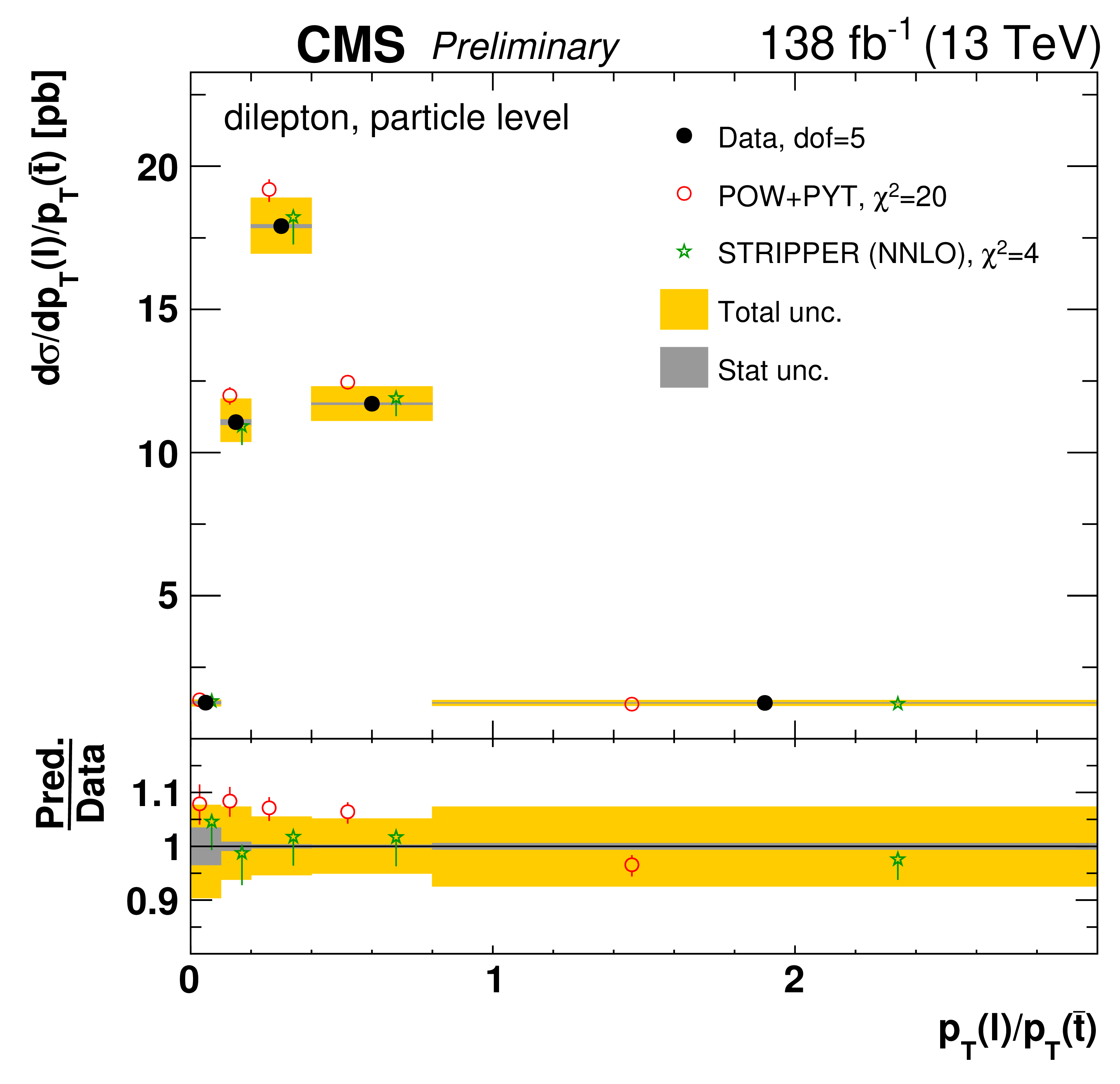
png pdf	Figure 113-c: Absolute differential $\mathrm{t\bar{t}}$ production cross sections as a function of ${p_{\mathrm {T}}}$ of the lepton (upper left), of the ratio of the trailing and leading lepton ${p_{\mathrm {T}}}$ (upper right), and of the ratio of lepton and top antiquark ${p_{\mathrm {T}}}$ (lower middle), measured at the particle level in a fiducial phase space. The data are shown as filled circles with dark and light bands indicating the statistical and total uncertainties (statistical and systematic uncertainties summed in quadrature), respectively. The cross sections are compared to predictions from the POWHEG+PYTHIA-8 (`POW-PYT', open circles) simulation and Stripper NNLO calculation (stars). The estimated uncertainties in the predictions are represented by a vertical bar on the corresponding points. For each model, a value of ${\chi ^2}$ is reported that takes into account the measurement uncertainties. The lower panel in each plot shows the ratios of the predictions to the data.
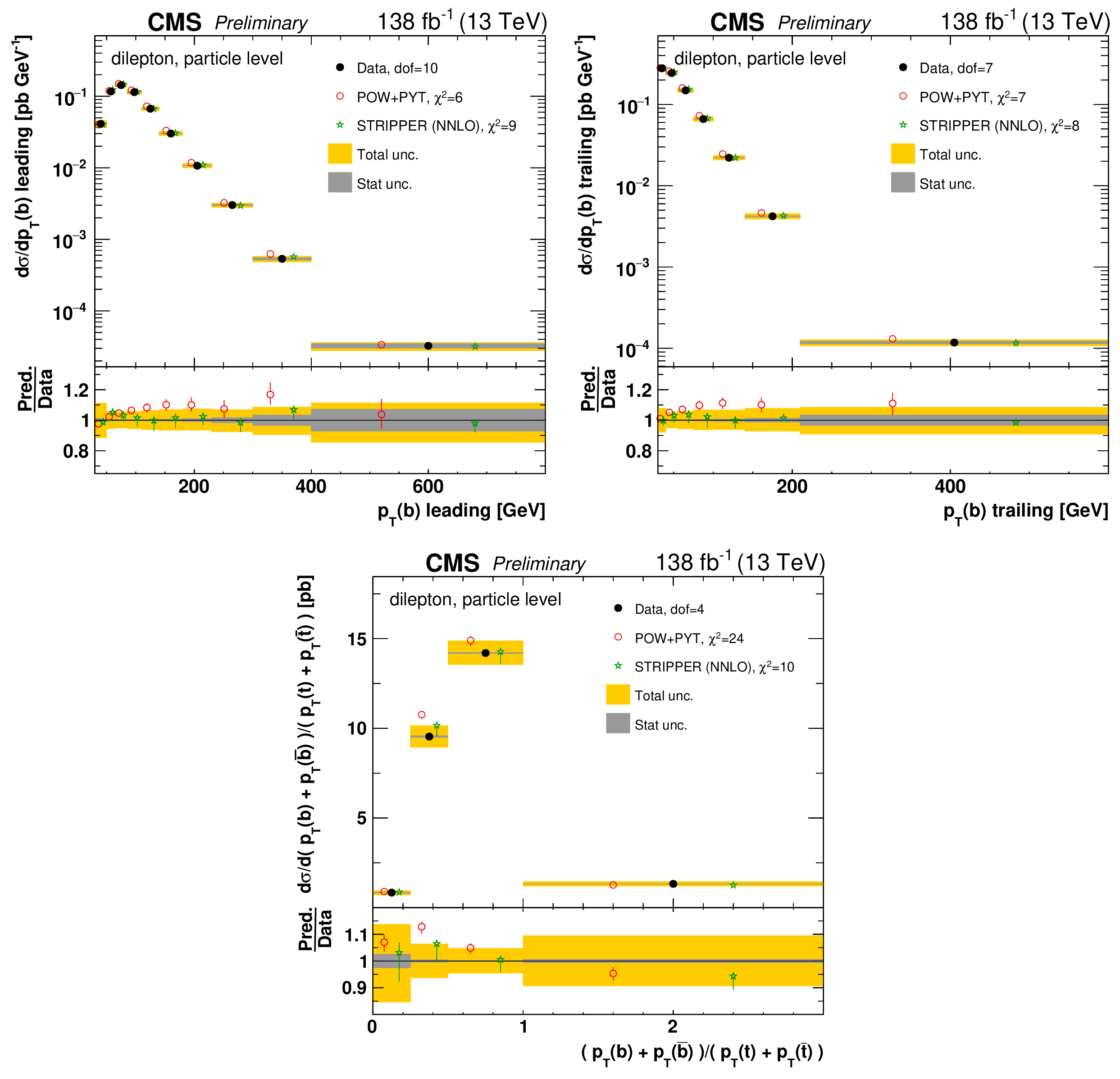
png pdf	Figure 114: Absolute differential $\mathrm{t\bar{t}}$ production cross sections as a function of the ${p_{\mathrm {T}}}$ of the leading (upper left) and trailing (upper right) b jet, and $( {{p_{\mathrm {T}}}}(\rm {b})+ {{p_{\mathrm {T}}}}(\mathrm{b\bar{b}}))/( {{p_{\mathrm {T}}}}(\rm {t})+ {{p_{\mathrm {T}}}}(\mathrm{\bar{t}}))$ (lower) are shown for data (filled circles), POWHEG+PYTHIA-8 (`POW-PYT', open circles) simulation, and Stripper NNLO calculation (stars). Further details can be found in the caption of Fig. 113.
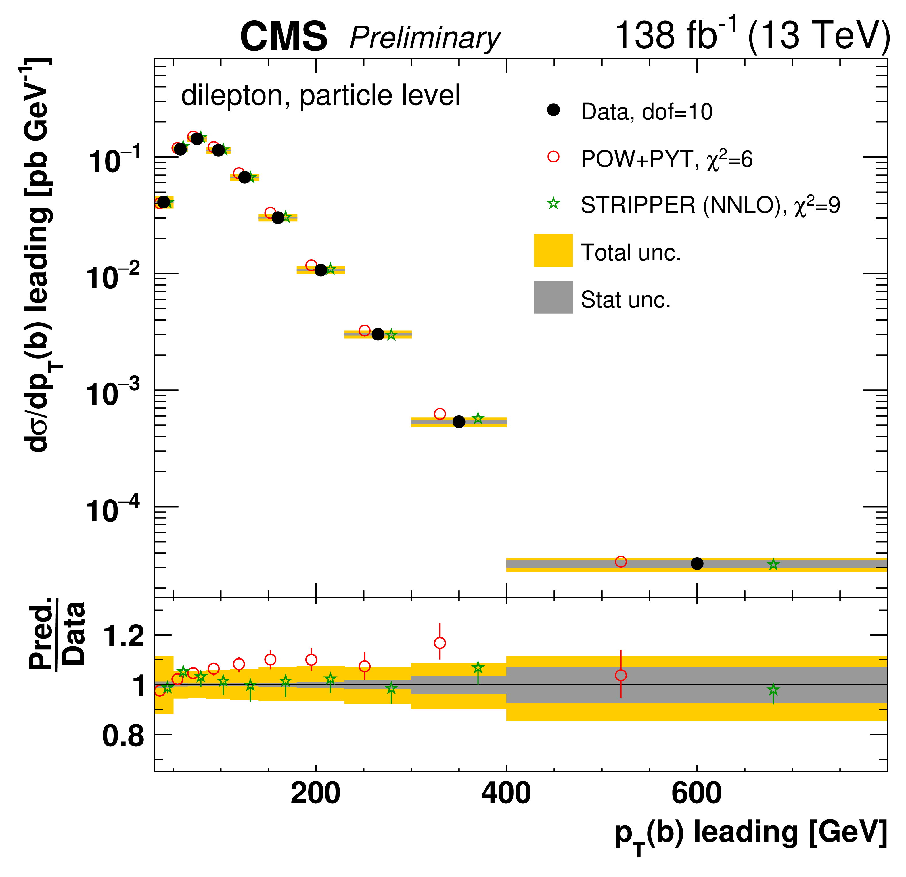
png pdf	Figure 114-a: Absolute differential $\mathrm{t\bar{t}}$ production cross sections as a function of the ${p_{\mathrm {T}}}$ of the leading (upper left) and trailing (upper right) b jet, and $( {{p_{\mathrm {T}}}}(\rm {b})+ {{p_{\mathrm {T}}}}(\mathrm{b\bar{b}}))/( {{p_{\mathrm {T}}}}(\rm {t})+ {{p_{\mathrm {T}}}}(\mathrm{\bar{t}}))$ (lower) are shown for data (filled circles), POWHEG+PYTHIA-8 (`POW-PYT', open circles) simulation, and Stripper NNLO calculation (stars). Further details can be found in the caption of Fig. 113.
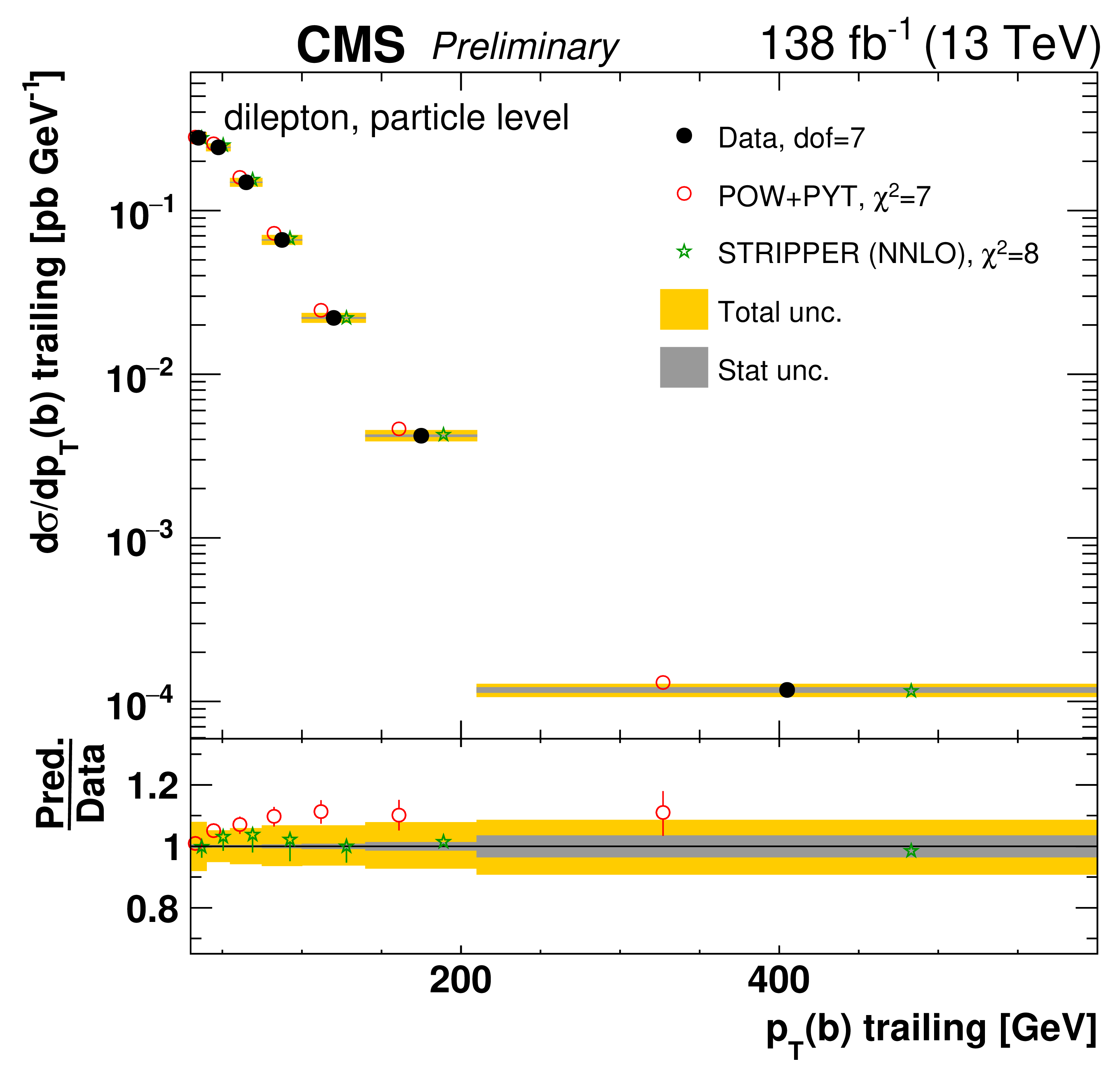
png pdf	Figure 114-b: Absolute differential $\mathrm{t\bar{t}}$ production cross sections as a function of the ${p_{\mathrm {T}}}$ of the leading (upper left) and trailing (upper right) b jet, and $( {{p_{\mathrm {T}}}}(\rm {b})+ {{p_{\mathrm {T}}}}(\mathrm{b\bar{b}}))/( {{p_{\mathrm {T}}}}(\rm {t})+ {{p_{\mathrm {T}}}}(\mathrm{\bar{t}}))$ (lower) are shown for data (filled circles), POWHEG+PYTHIA-8 (`POW-PYT', open circles) simulation, and Stripper NNLO calculation (stars). Further details can be found in the caption of Fig. 113.
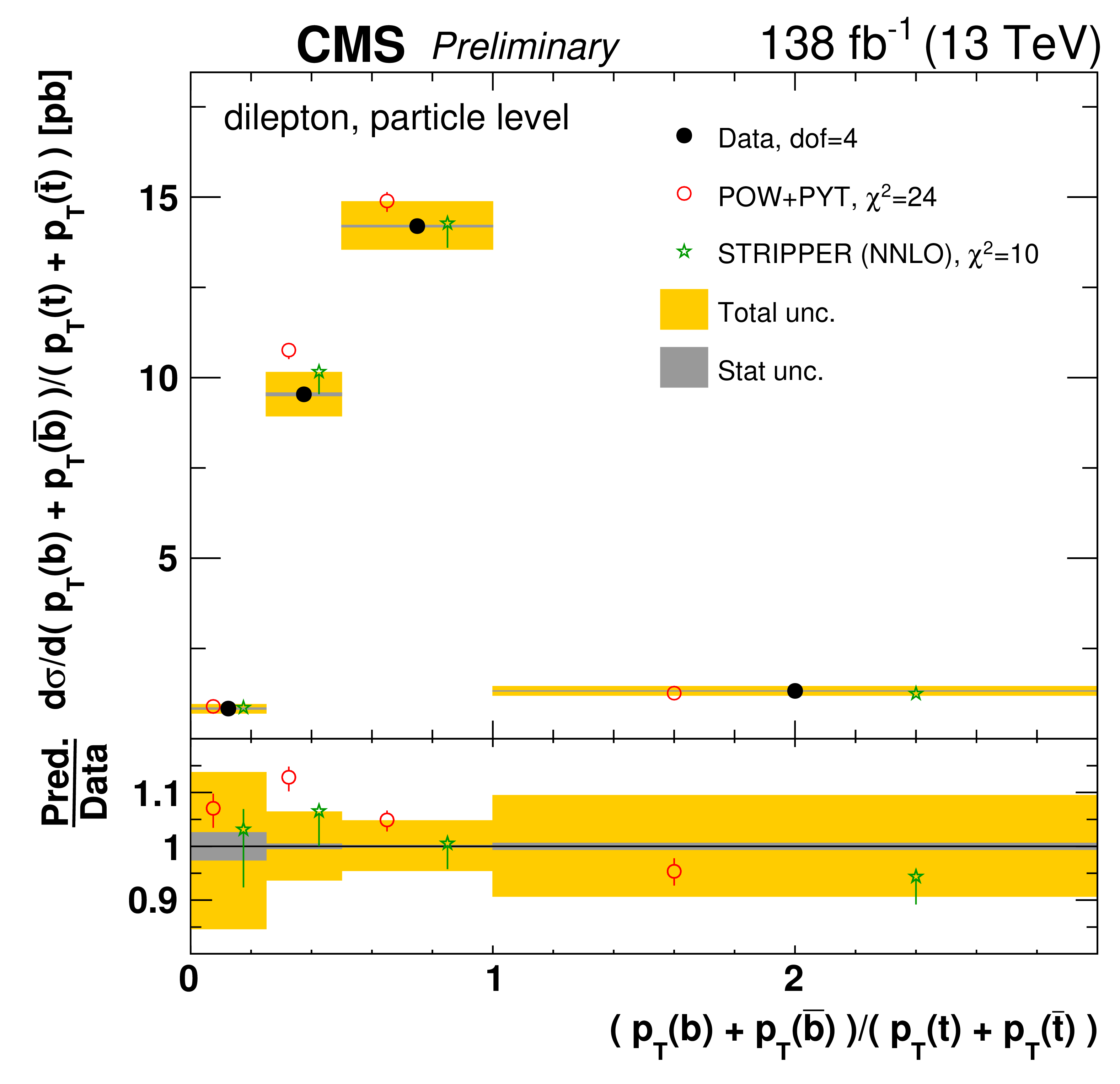
png pdf	Figure 114-c: Absolute differential $\mathrm{t\bar{t}}$ production cross sections as a function of the ${p_{\mathrm {T}}}$ of the leading (upper left) and trailing (upper right) b jet, and $( {{p_{\mathrm {T}}}}(\rm {b})+ {{p_{\mathrm {T}}}}(\mathrm{b\bar{b}}))/( {{p_{\mathrm {T}}}}(\rm {t})+ {{p_{\mathrm {T}}}}(\mathrm{\bar{t}}))$ (lower) are shown for data (filled circles), POWHEG+PYTHIA-8 (`POW-PYT', open circles) simulation, and Stripper NNLO calculation (stars). Further details can be found in the caption of Fig. 113.
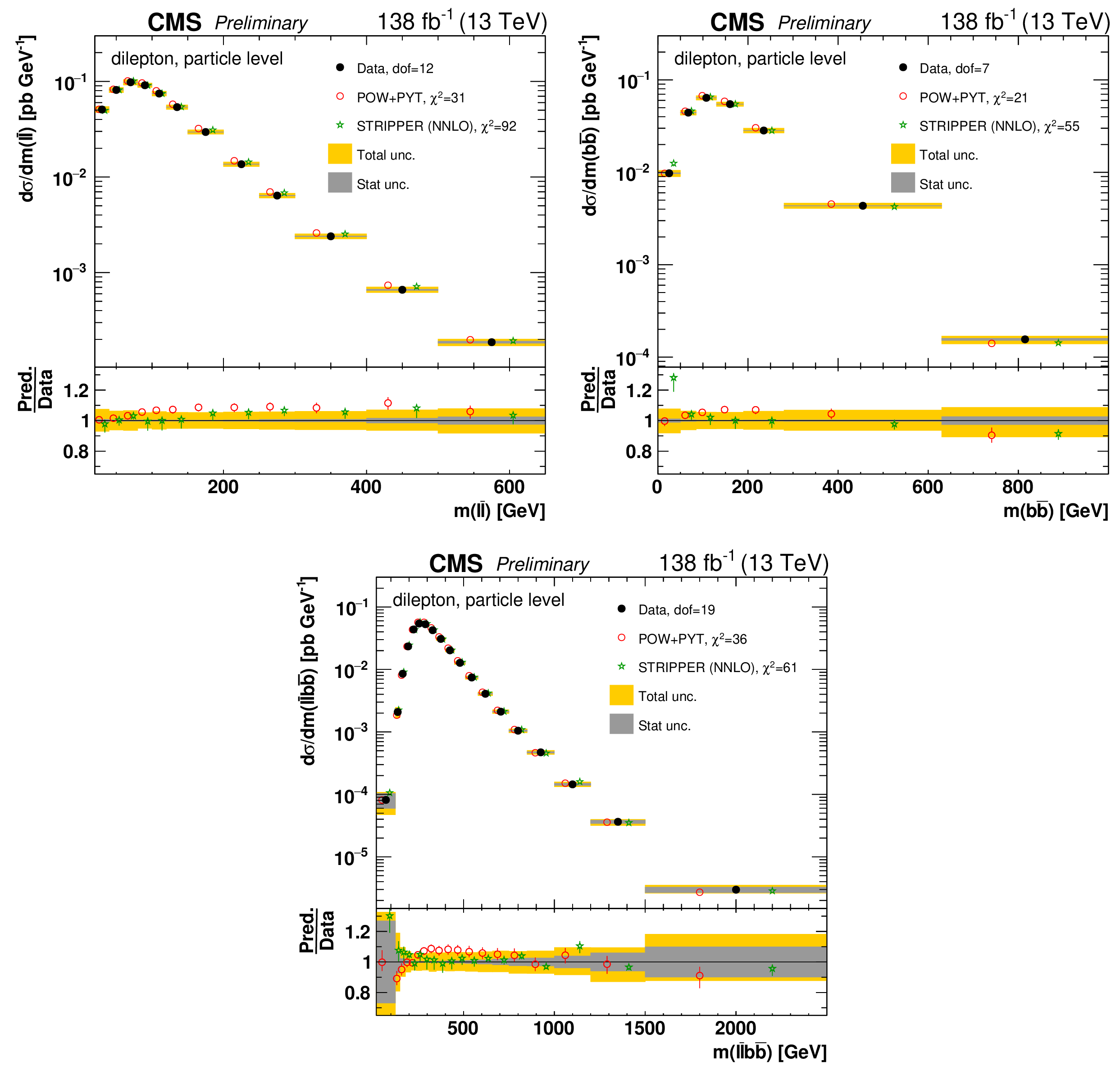
png pdf	Figure 115: Absolute differential $\mathrm{t\bar{t}}$ production cross sections as a function of ${m(\ell \overline {\ell})}$ (upper left), ${m(\mathrm{b} \mathrm{\bar{b}})}$ (upper right), and ${m(\ell \overline {\ell}\mathrm{b} \mathrm{\bar{b}})}$ (lower) are shown for data (filled circles), POWHEG+PYTHIA-8 (`POW-PYT', open circles) simulation, and Stripper NNLO calculation (stars). Further details can be found in the caption of Fig. 113.
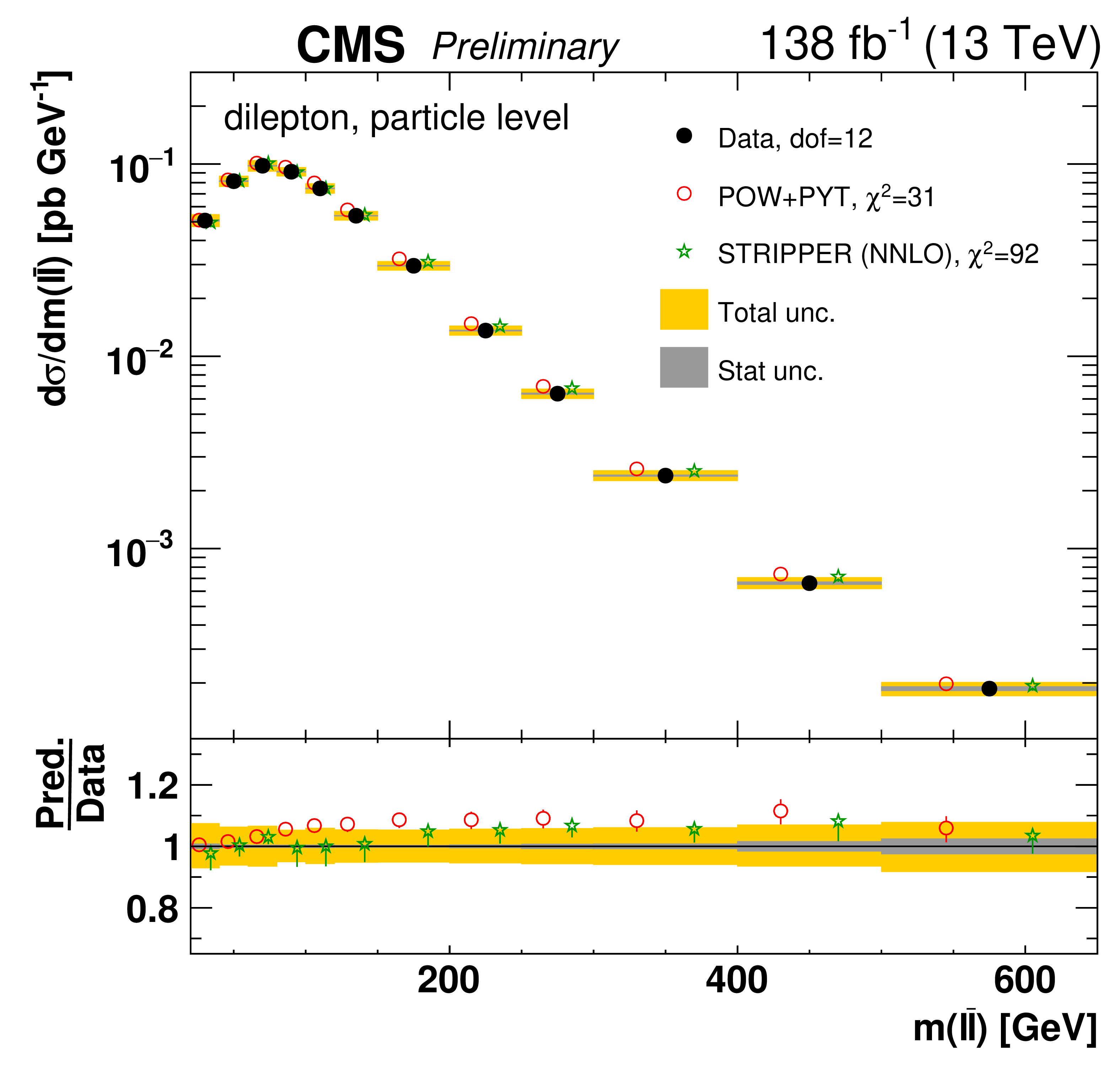
png pdf	Figure 115-a: Absolute differential $\mathrm{t\bar{t}}$ production cross sections as a function of ${m(\ell \overline {\ell})}$ (upper left), ${m(\mathrm{b} \mathrm{\bar{b}})}$ (upper right), and ${m(\ell \overline {\ell}\mathrm{b} \mathrm{\bar{b}})}$ (lower) are shown for data (filled circles), POWHEG+PYTHIA-8 (`POW-PYT', open circles) simulation, and Stripper NNLO calculation (stars). Further details can be found in the caption of Fig. 113.
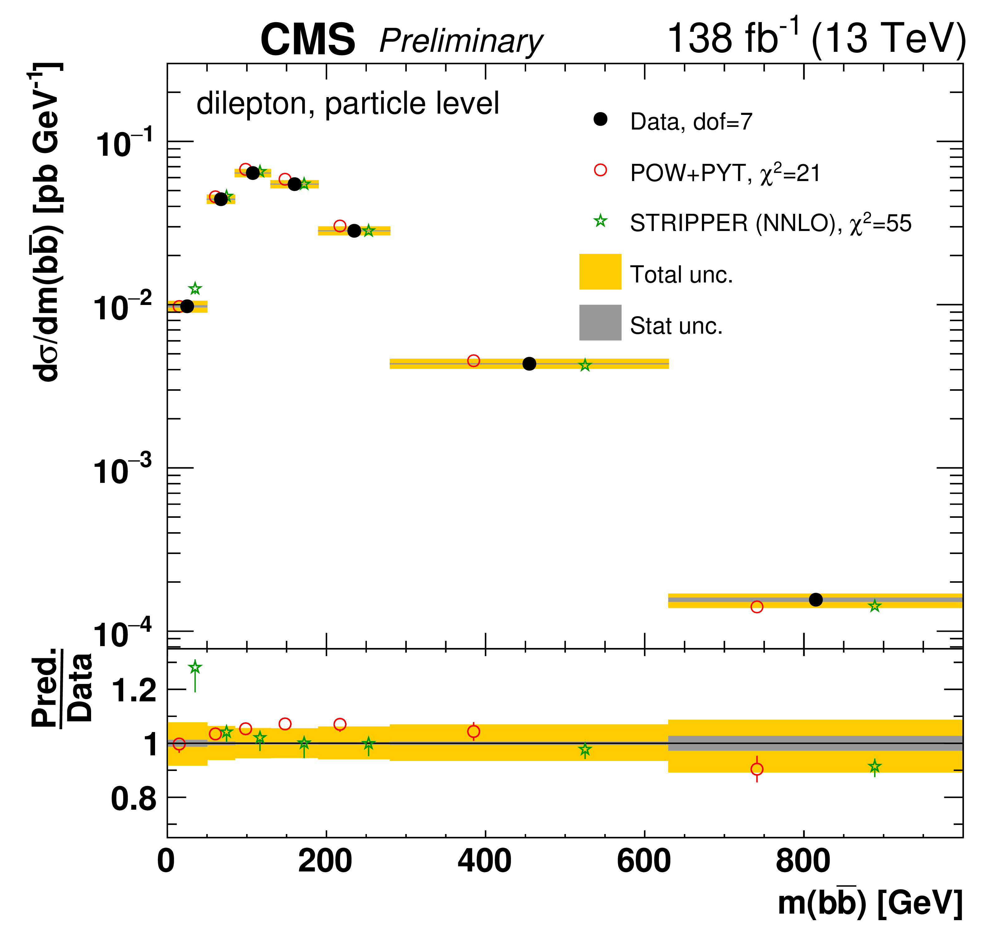
png pdf	Figure 115-b: Absolute differential $\mathrm{t\bar{t}}$ production cross sections as a function of ${m(\ell \overline {\ell})}$ (upper left), ${m(\mathrm{b} \mathrm{\bar{b}})}$ (upper right), and ${m(\ell \overline {\ell}\mathrm{b} \mathrm{\bar{b}})}$ (lower) are shown for data (filled circles), POWHEG+PYTHIA-8 (`POW-PYT', open circles) simulation, and Stripper NNLO calculation (stars). Further details can be found in the caption of Fig. 113.
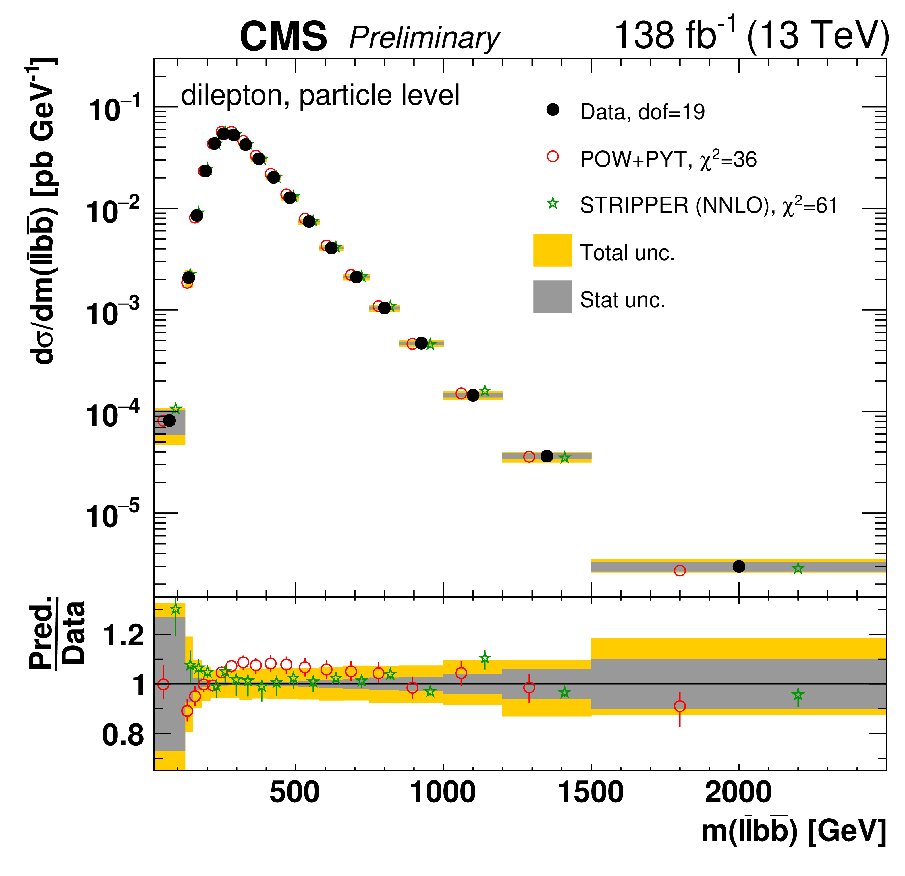
png pdf	Figure 115-c: Absolute differential $\mathrm{t\bar{t}}$ production cross sections as a function of ${m(\ell \overline {\ell})}$ (upper left), ${m(\mathrm{b} \mathrm{\bar{b}})}$ (upper right), and ${m(\ell \overline {\ell}\mathrm{b} \mathrm{\bar{b}})}$ (lower) are shown for data (filled circles), POWHEG+PYTHIA-8 (`POW-PYT', open circles) simulation, and Stripper NNLO calculation (stars). Further details can be found in the caption of Fig. 113.
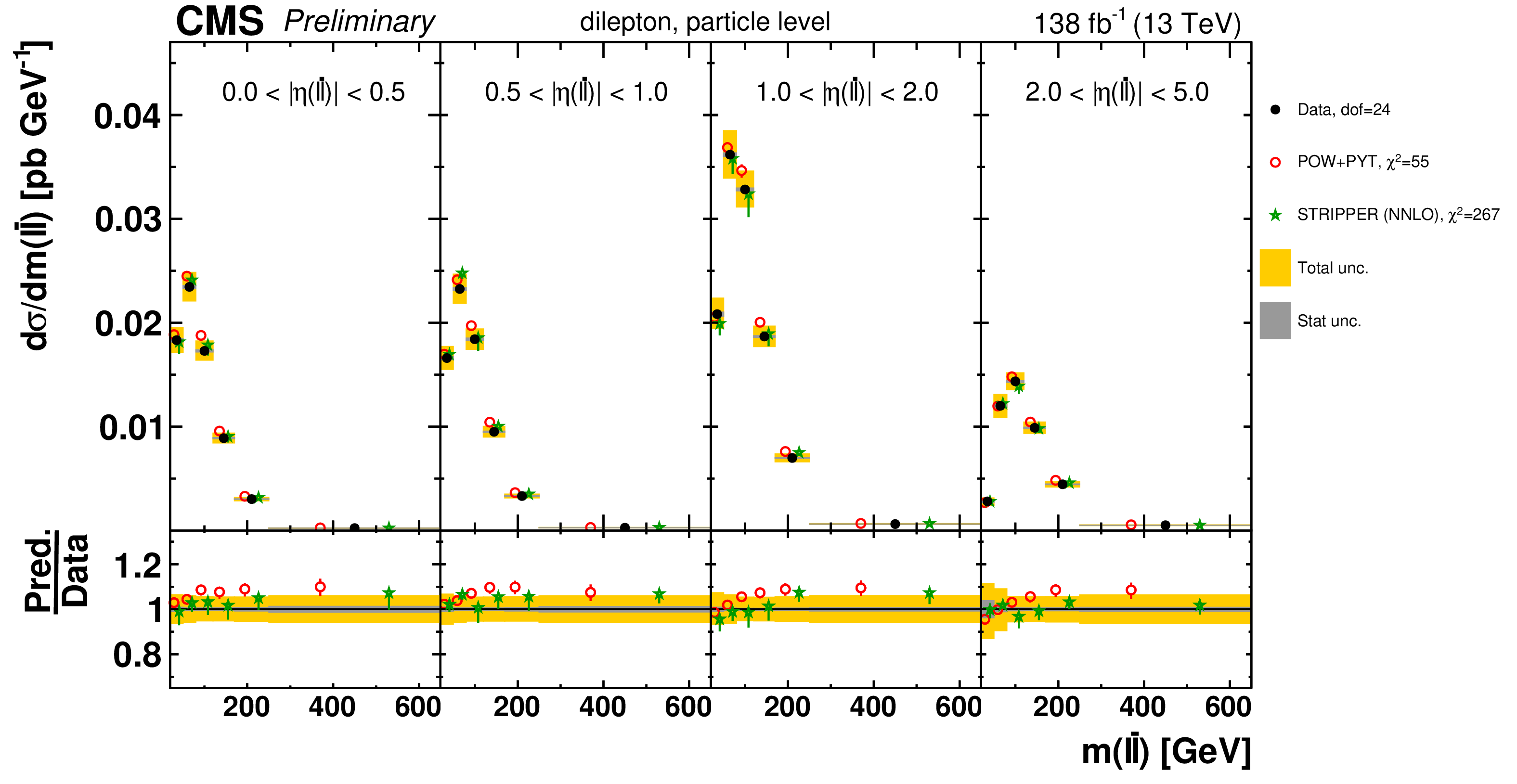
png pdf	Figure 116: Absolute $[ {|\eta (\ell \overline {\ell})|},\,{m(\ell \overline {\ell})} ]$ cross sections are shown for data (filled circles), POWHEG+PYTHIA-8 (`POW-PYT', open circles) simulation, and Stripper NNLO calculation (stars). Further details can be found in the caption of Fig. 113.
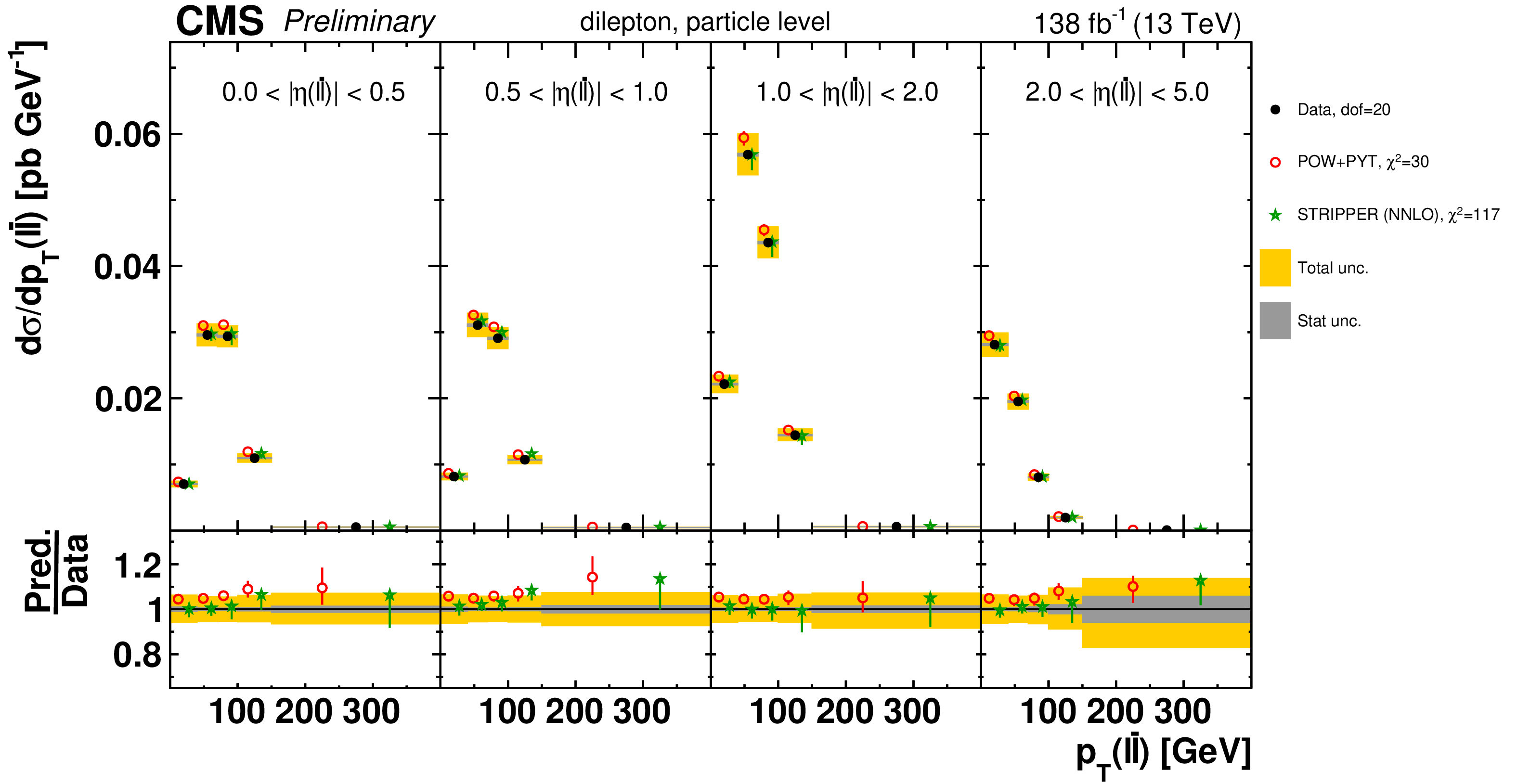
png pdf	Figure 117: Absolute $[ {|\eta (\ell \overline {\ell})|},\,{{p_{\mathrm {T}}} (\ell \overline {\ell})} ]$ cross sections are shown for data (filled circles), POWHEG+PYTHIA-8 (`POW-PYT', open circles) simulation, and Stripper NNLO calculation (stars). Further details can be found in the caption of Fig. 113.
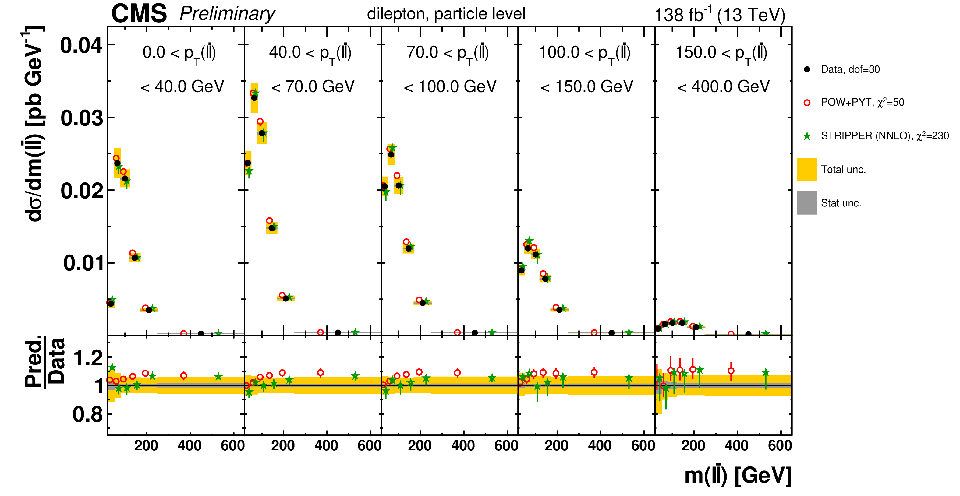
png pdf	Figure 118: Absolute $[ {{p_{\mathrm {T}}} (\ell \overline {\ell})},\,{m(\ell \overline {\ell})} ]$ cross sections are shown for data (filled circles), POWHEG+PYTHIA-8 (`POW-PYT', open circles) simulation, and Stripper NNLO calculation (stars). Further details can be found in the caption of Fig. 113.

Tables
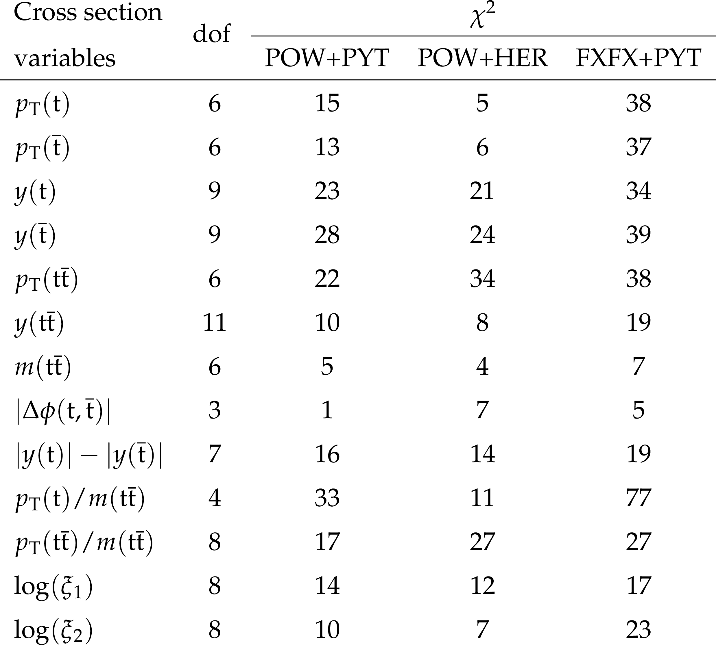
png pdf	Table 1: The ${\chi ^2}$ values and dof of the measured normalized single-differential cross sections for $\mathrm{t\bar{t}}$ and top quark kinematic observables at parton level, with respect to the predictions of various MC generators. Measurement uncertainties are taken into account in the calculation of ${\chi ^2}$, though the theoretical uncertainties in the predictions are not.
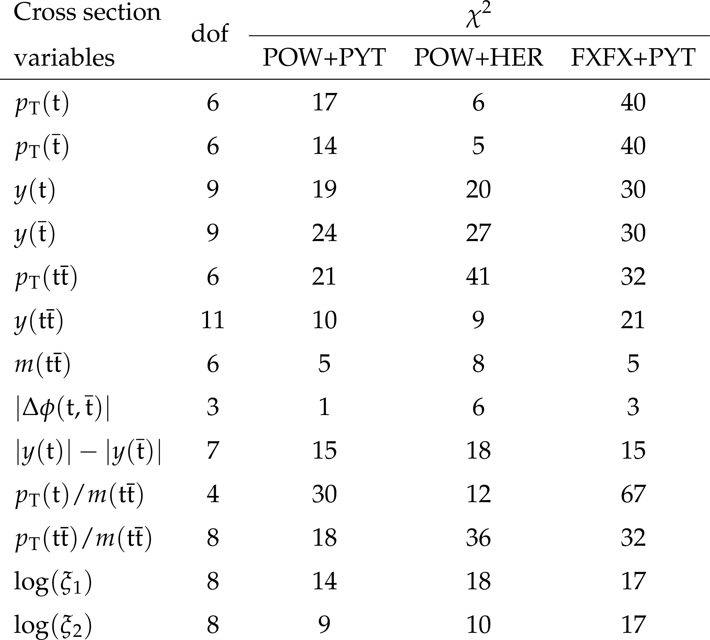
png pdf	Table 2: The ${\chi ^2}$ values and dof of the measured normalized single-differential cross sections for $\mathrm{t\bar{t}}$ and top quark kinematic observables at particle level, with respect to the predictions of various MC generators. Measurement uncertainties are taken into account in the calculation of ${\chi ^2}$, though the theoretical uncertainties in the predictions are not.
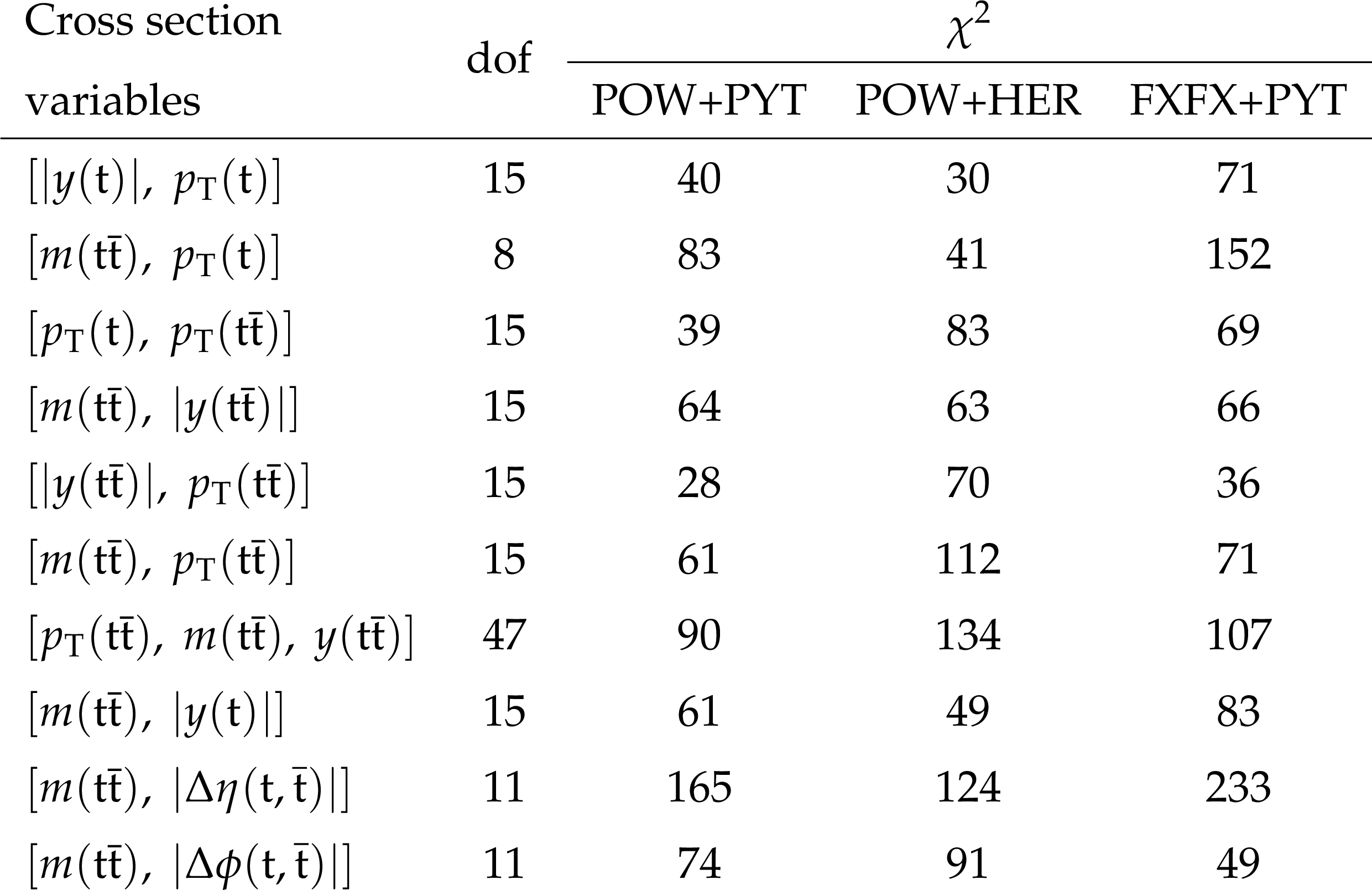
png pdf	Table 3: The ${\chi ^2}$ values and dof of the measured normalized multi-differential cross sections for $\mathrm{t\bar{t}}$ and top quark kinematic observables at parton level, with respect to the predictions of various MC generators. Measurement uncertainties are taken into account in the calculation of ${\chi ^2}$, though the theoretical uncertainties in the predictions are not.
png pdf	Table 4: The ${\chi ^2}$ values and dof of the measured normalized multi-differential cross sections for $\mathrm{t\bar{t}}$ and top quark kinematic observables at particle level, with respect to the predictions of various MC generators. Measurement uncertainties are taken into account in the calculation of ${\chi ^2}$, though the theoretical uncertainties in the predictions are not.
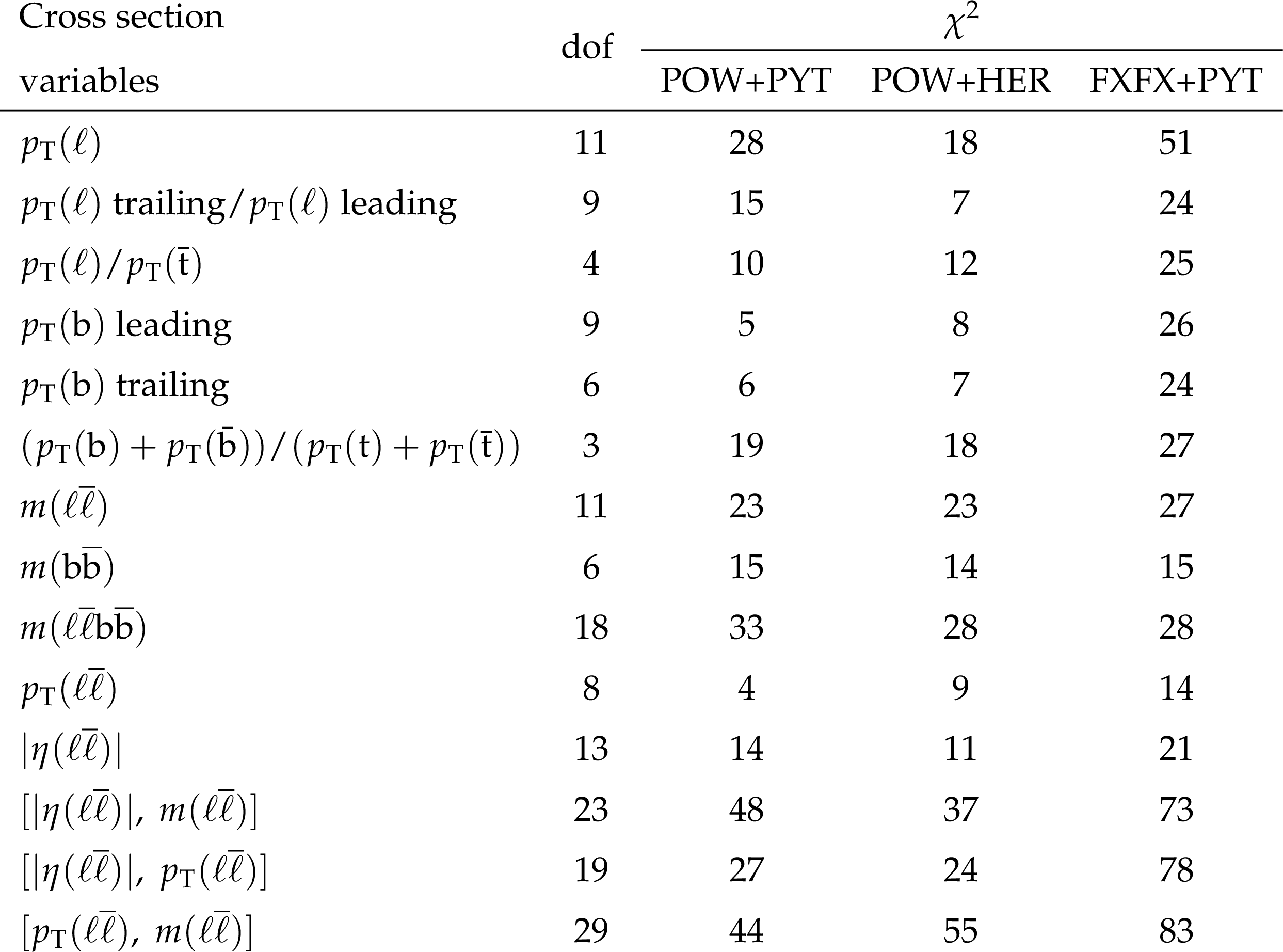
png pdf	Table 5: The ${\chi ^2}$ values and dof of the measured normalized differential cross sections for lepton and b-jet kinematic observables at particle level, with respect to the predictions of various MC generators. Measurement uncertainties are taken into account in the calculation of ${\chi ^2}$, though the theoretical uncertainties in the predictions are not.
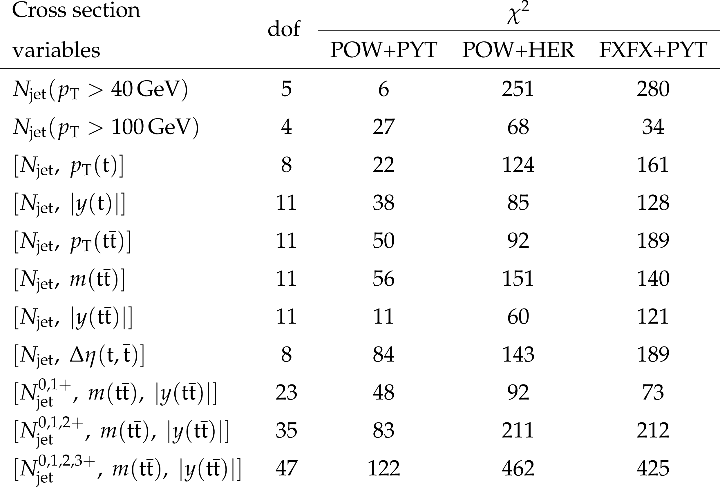
png pdf	Table 6: The ${\chi ^2}$ values and dof of the measured normalized differential cross sections as a function of the additional-jet multiplicity in the events, at the parton level of the top quark and antiquark, with respect to the predictions of various MC generators. Measurement uncertainties are taken into account in the calculation of ${\chi ^2}$, though the theoretical uncertainties in the predictions are not.
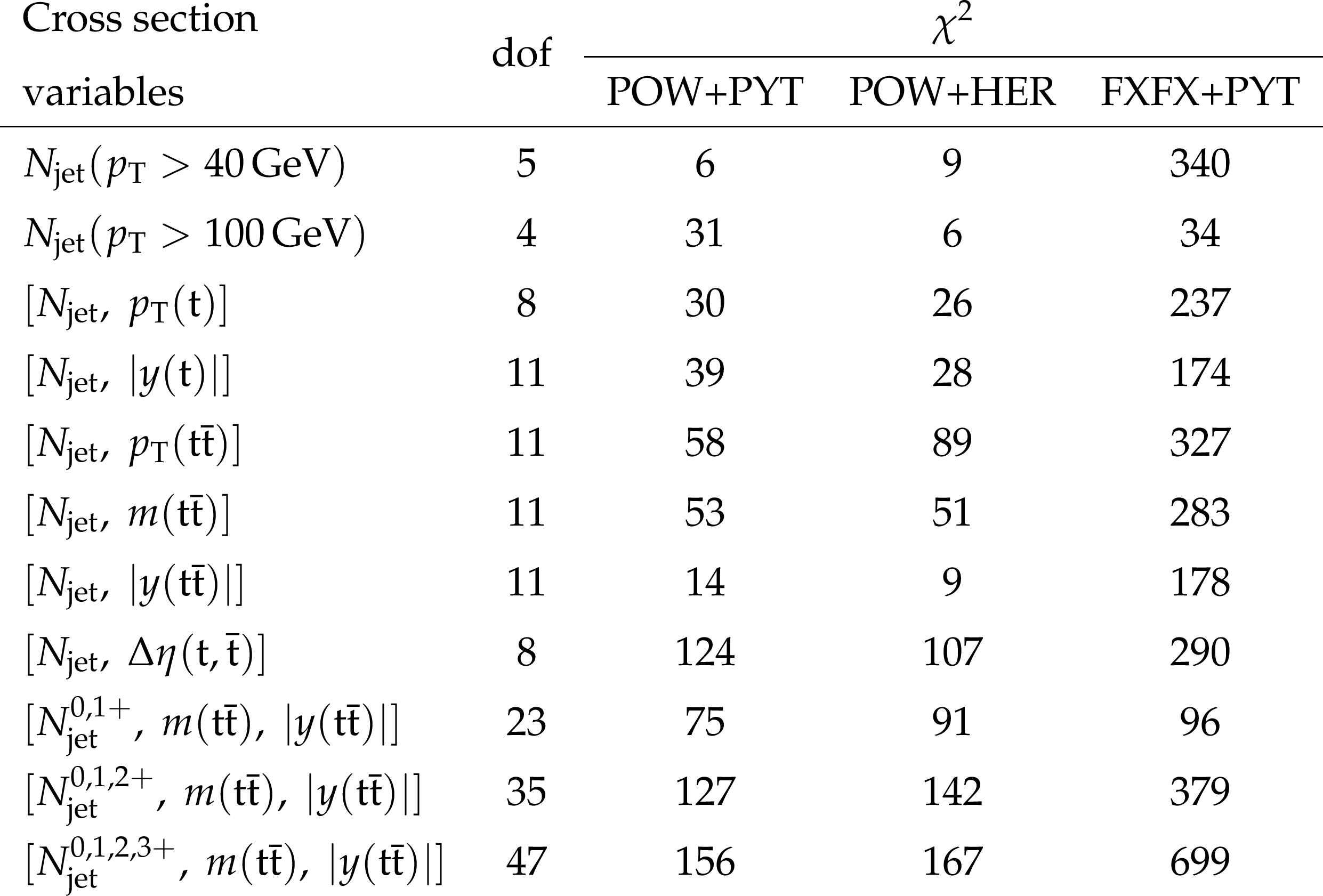
png pdf	Table 7: The ${\chi ^2}$ values and dof of the measured normalized differential cross sections as a function of the additional-jet multiplicity in the events, at the particle level of the top quark and antiquark, with respect to the predictions of various MC generators. Measurement uncertainties are taken into account in the calculation of ${\chi ^2}$, though the theoretical uncertainties in the predictions are not.
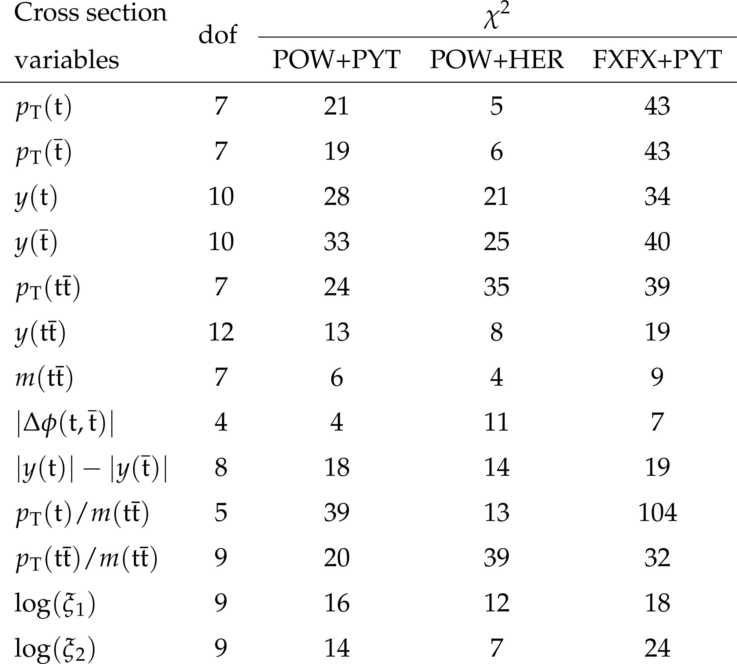
png pdf	Table 8: The ${\chi ^2}$ values and dof of the measured absolute single-differential cross sections for $\mathrm{t\bar{t}}$ and top quark kinematic observables at parton level, with respect to the predictions of various MC generators. Measurement uncertainties are taken into account in the calculation of ${\chi ^2}$, though the theoretical uncertainties in the predictions are not.
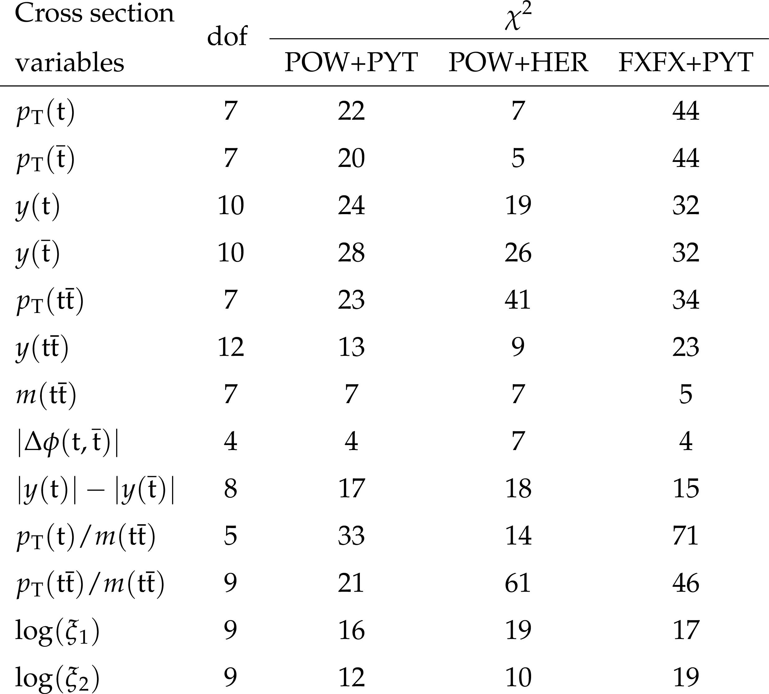
png pdf	Table 9: The ${\chi ^2}$ values and dof of the measured absolute single-differential cross sections for $\mathrm{t\bar{t}}$ and top quark kinematic observables at particle level, with respect to the predictions of various MC generators. Measurement uncertainties are taken into account in the calculation of ${\chi ^2}$, though the uncertainties in the predictions are not.
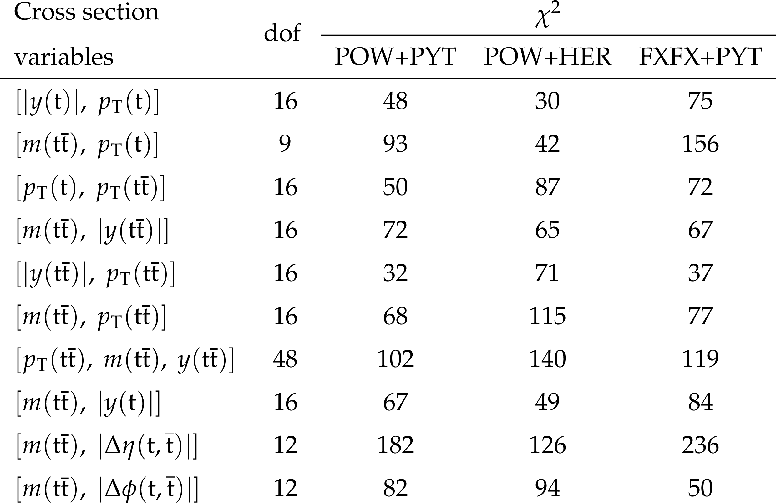
png pdf	Table 10: The ${\chi ^2}$ values and dof of the measured absolute multi-differential cross sections for $\mathrm{t\bar{t}}$ and top quark kinematic observables at parton level, with respect to the predictions of various MC generators. Measurement uncertainties are taken into account in the calculation of ${\chi ^2}$, though the theoretical uncertainties in the predictions are not.
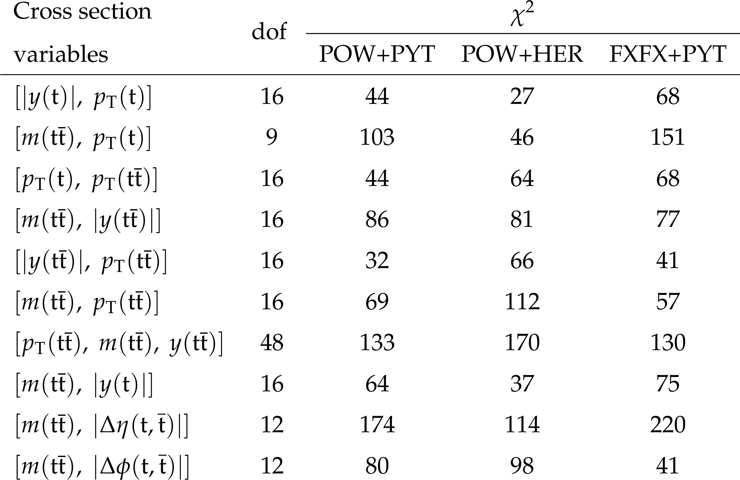
png pdf	Table 11: The ${\chi ^2}$ values and dof of the measured absolute multi-differential cross sections for $\mathrm{t\bar{t}}$ and top quark kinematic observables at particle level, with respect to the predictions of various MC generators. Measurement uncertainties are taken into account in the calculation of ${\chi ^2}$, though the theoretical uncertainties in the predictions are not.
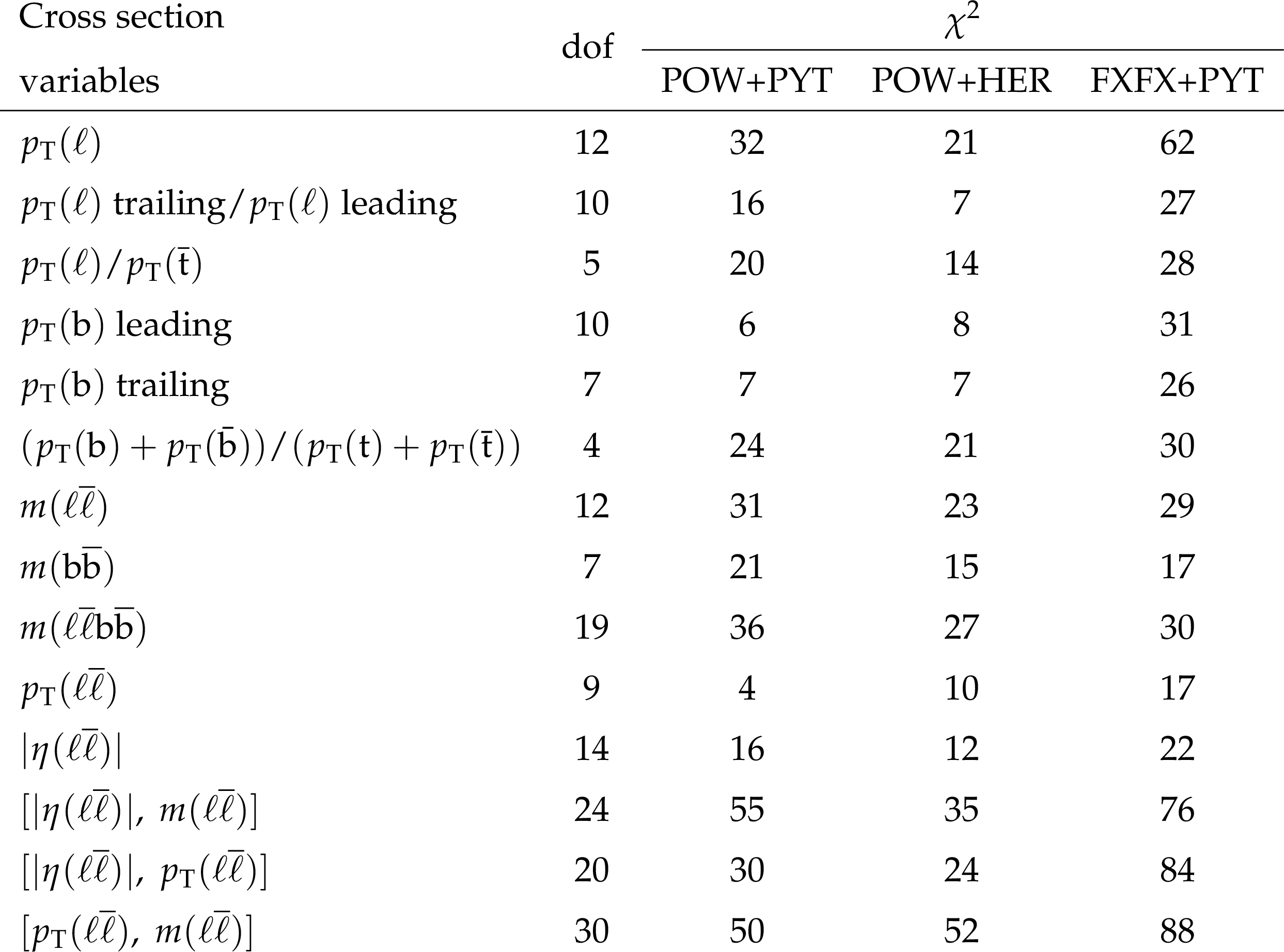
png pdf	Table 12: The ${\chi ^2}$ values and dof of the measured absolute differential cross sections for lepton and b-jet kinematic observables at particle level, with respect to the predictions of various MC generators. Measurement uncertainties are taken into account in the calculation of ${\chi ^2}$, though the theoretical uncertainties in the predictions are not.
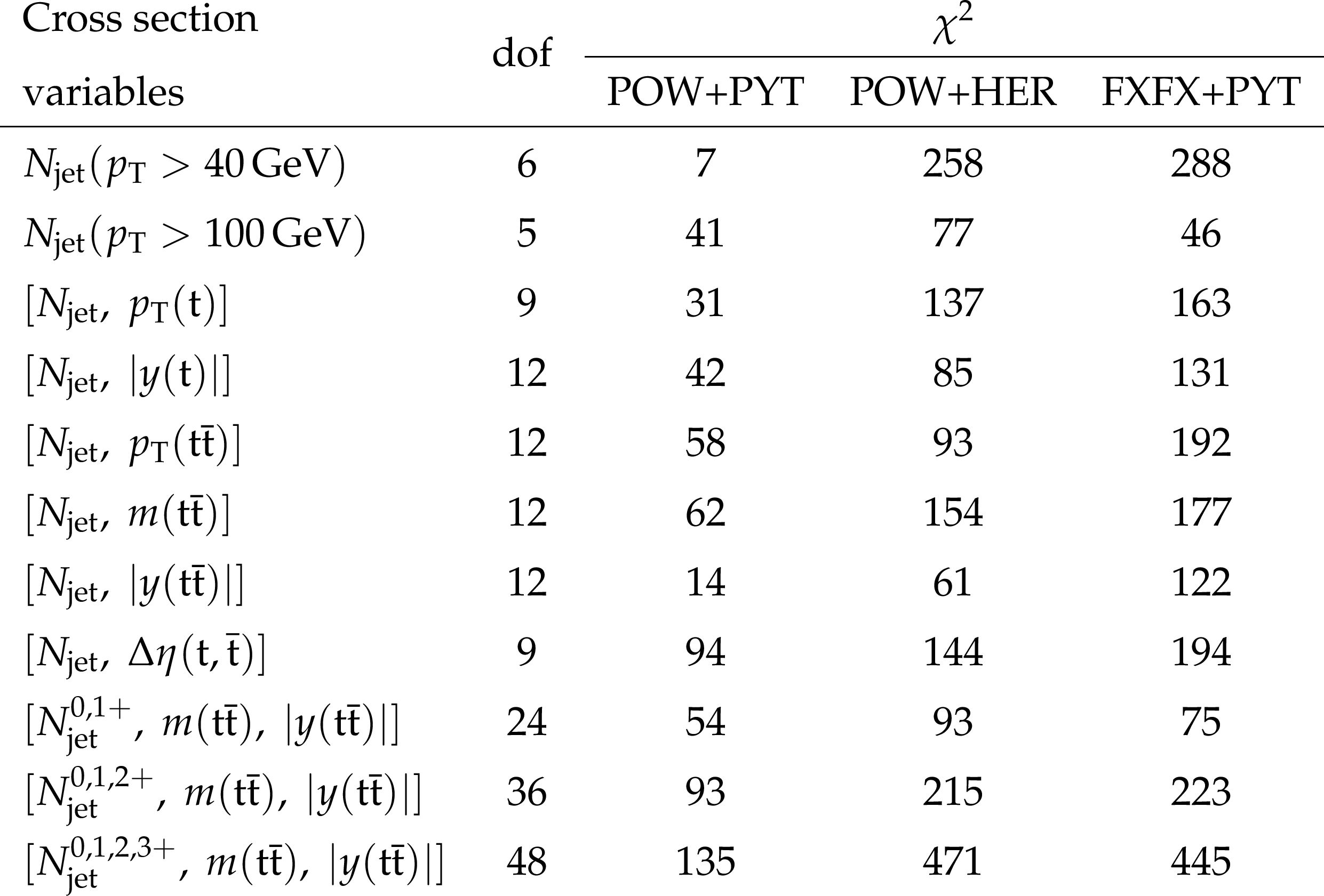
png pdf	Table 13: The ${\chi ^2}$ values and dof of the measured absolute differential cross sections as a function of the additional-jet multiplicity in the events, at the parton level of the top quark and antiquark, with respect to the predictions of various MC generators. Measurement uncertainties are taken into account in the calculation of ${\chi ^2}$, though the theoretical uncertainties in the predictions are not.
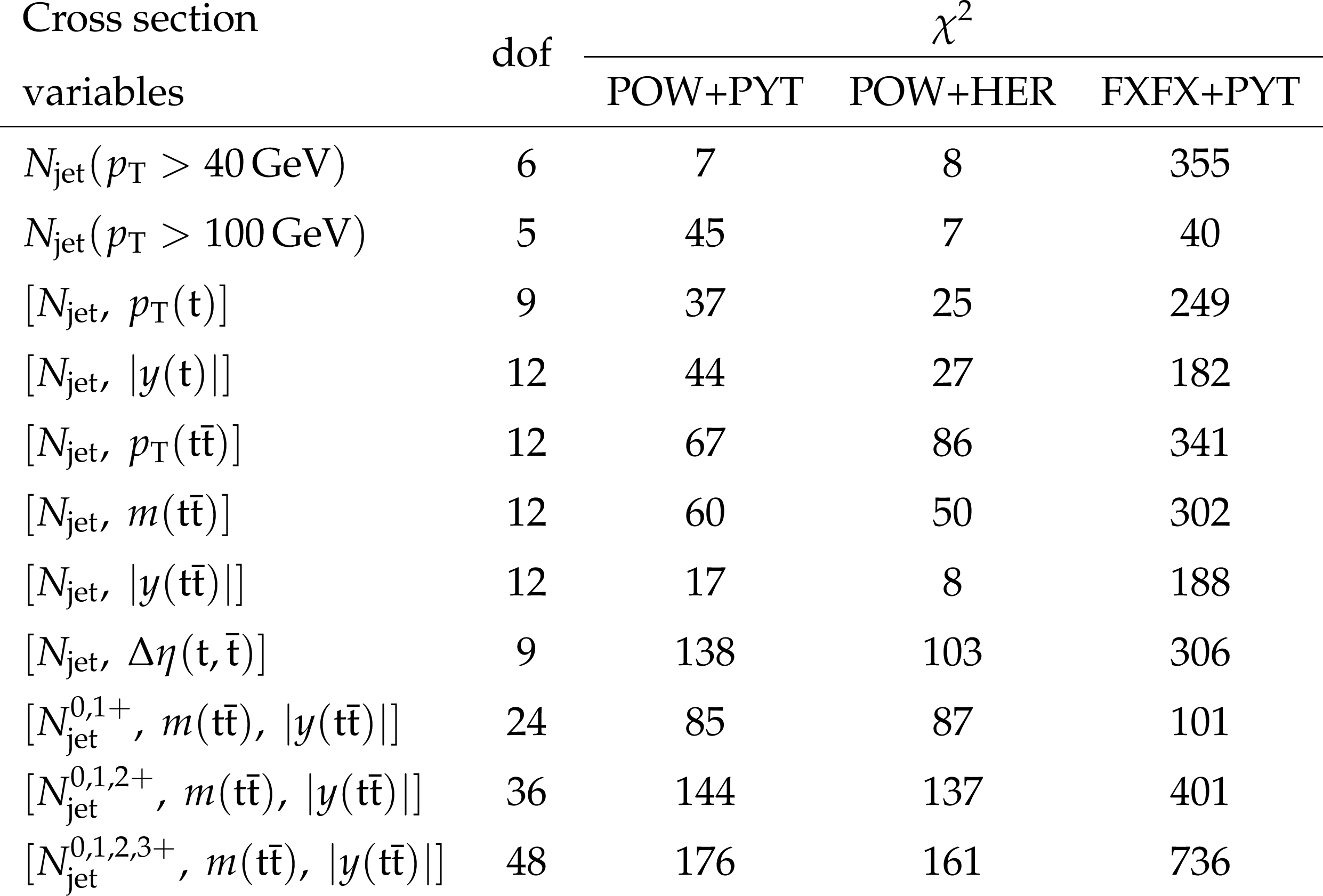
png pdf	Table 14: The ${\chi ^2}$ values and dof of the measured absolute differential cross sections as a function of the additional-jet multiplicity in the events, at the particle level of the top quark and antiquark, with respect to the predictions of various MC generators. Measurement uncertainties are taken into account in the calculation of ${\chi ^2}$, though the theoretical uncertainties in the predictions are not.

Summary

A measurement of differential $\mathrm{t\bar{t}}$ production cross sections in pp collisions at $\sqrt{s} = $ 13 TeV was presented, performed with events containing two oppositely charged leptons (electrons or muons). The data used in this analysis were recorded in the years 2016 through 2018 with the CMS detector at the LHC and correspond to an integrated luminosity of 138 fb$^{-1}$. Differential cross sections are measured as functions of kinematical observables of the $\mathrm{t\bar{t}}$ system, the top quark and antiquark and their decay products, and the total number of additional jets in the event not originating from the $\mathrm{t\bar{t}}$ decay. The measurements are performed as function of one observable, or simultaneously as functions of two or three kinematic variables. The differential cross sections are defined both with particle-level objects in a fiducial phase space close to that of the detector acceptance and with parton-level top quarks in the full phase space. Overall, both the statistical and the systematic uncertainties in the measurements are improved by a factor of about $2$ compared to the previous analyses [29,30] that are based on the 2016 data only. Predictions of several NLO Monte Carlo event generators that differ in the hard matrix element, parton shower, and hadronization models, were compared to the data. The predictions of these MC models, without taking theoretical uncertainties into account, generally fail to describe a large fraction of the measured cross sections. The calculations predict the top quark and antiquark to have harder transverse momentum and more-central rapidity distributions than observed in the data. The invariant mass and rapidity distributions of the $\mathrm{t\bar{t}}$ system are reasonably well described by the models overall. For the $\mathrm{t\bar{t}}$ transverse momentum spectrum, the predictions exhibit larger differences and none of them provides a good description of the data. Double- and triple-differential cross sections show enhanced model-to-data discrepancies, for instance the effect of a harder ${{p_{\mathrm {T}}} (\mathrm{t})}$ spectrum in the models is pronounced at high ${m( \mathrm{t\bar{t}})}$. Cross sections as functions of kinematic observables of the leptons and b jets originating from the decay of the top quark and antiquark are measured with high precision. Overall, the observed trends for these objects follow those for the top quarks and antiquarks, with the models predicting harder transverse momentum spectra than seen in the data. For the leptons, this effect is somewhat enhanced and also the dilepton invariant mass spectrum is harder in the models than in the data. The distribution of the multiplicity of additional jets in the $\mathrm{t\bar{t}}$ events shows clear differences between the models that are resolved by the data. The studies of the $\mathrm{t\bar{t}}$ and top quark and antiquark kinematical distributions as a function of the jet multiplicity show multiplicity-dependent shape differences between data and models. There is an indication that the trend of harder ${{p_{\mathrm {T}}} (\mathrm{t})}$ distributions in the models is localized at small jet multiplicities. Selected kinematic spectra were also compared to a variety of predictions beyond NLO precision. For observables of the top quark and the $\mathrm{t\bar{t}}$ systems, these predictions provide descriptions of the data that are of similar or improved quality, compared to the MC models, except for kinematic spectra where the theory scale uncertainties are large. For observables of the leptons and b jets, the tested NNLO model provides a data description quality that is on average comparable but not better than that of the NLO MC models. Comparing several kinematic distributions of the top quark and the $\mathrm{t\bar{t}}$ system to NLO MC models using different PDF sets, the data clearly provide some power for discriminating between some of the tested sets.

References
1	CMS Collaboration	Search for $ \mathrm{t\bar{t}} $ resonances in highly boosted lepton+jets and fully hadronic final states in proton-proton collisions at $ \sqrt{s}= $ 13 TeV	JHEP 07 (2017) 001	CMS-B2G-16-015 1704.03366
2	CMS Collaboration	Search for resonant $ \mathrm{t\bar{t}} $ production in proton-proton collisions at $ \sqrt{s}= $ 13 TeV	JHEP 04 (2019) 031	CMS-B2G-17-017 1810.05905
3	CMS Collaboration	Search for heavy Higgs bosons decaying to a top quark pair in proton-proton collisions at $ \sqrt{s} = $ 13 TeV	JHEP 04 (2020) 171	CMS-HIG-17-027 1908.01115
4	CMS Collaboration	Search for the pair production of light top squarks in the e$ \mu $ final state in proton-proton collisions at $ \sqrt{s} = $ 13 TeV	JHEP 03 (2019) 101	CMS-SUS-18-003 1901.01288
5	CMS Collaboration	Search for top squark pair production using dilepton final states in $ pp $ collision data collected at $ \sqrt{s}= $ 13 TeV	EPJC 81 (2021) 3	CMS-SUS-19-011 2008.05936
6	N. Kidonakis	NNNLO soft-gluon corrections for the top-quark $ {p_{\mathrm{T}}} $ and rapidity distributions	PRD 91 (2015) 031501	1411.2633
7	M. Czakon, D. Heymes, and A. Mitov	High-precision differential predictions for top-quark pairs at the LHC	PRL 116 (2016) 082003	1511.00549
8	M. Czakon et al.	Top-pair production at the LHC through NNLO QCD and NLO EW	JHEP 10 (2017) 186	1705.04105
9	M. Czakon et al.	Resummation for (boosted) top-quark pair production at NNLO+NNLL' in QCD	JHEP 05 (2018) 149	1803.07623
10	S. Catani et al.	Top-quark pair production at the LHC: Fully differential QCD predictions at NNLO	JHEP 07 (2019) 100	1906.06535
11	M. Czakon, A. Mitov, and R. Poncelet	NNLO QCD corrections to leptonic observables in top-quark pair production and decay	JHEP 05 (2021) 212	2008.11133
12	ATLAS Collaboration	Measurements of top quark pair relative differential cross sections with ATLAS in $ pp $ collisions at $ \sqrt{s} = $ 7 TeV	EPJC 73 (2013) 2261	1207.5644
13	CMS Collaboration	Measurement of differential top-quark pair production cross sections in $ pp $ collisions at $ \sqrt{s} = $ 7 TeV	EPJC 73 (2013) 2339	CMS-TOP-11-013 1211.2220
14	ATLAS Collaboration	Measurements of normalized differential cross sections for $ \mathrm{t\bar{t}} $ production in $ pp $ collisions at $ \sqrt{s} = $ 7 TeV using the ATLAS detector	PRD 90 (2014) 072004	1407.0371
15	ATLAS Collaboration	Differential top-antitop cross section measurements as a function of observables constructed from final-state particles using $ pp $ collisions at $ \sqrt{s}= $ 7 TeV in the ATLAS detector	JHEP 06 (2015) 100	1502.05923
16	ATLAS Collaboration	Measurement of top quark pair differential cross sections in the dilepton channel in $ pp $ collisions at $ \sqrt{s} = $ 7 and 8 TeV with ATLAS	PRD 94 (2016) 092003	1607.07281
17	CMS Collaboration	Measurement of the differential cross section for top quark pair production in $ pp $ collisions at $ \sqrt{s} = $ 8 TeV	EPJC 75 (2015) 542	CMS-TOP-12-028 1505.04480
18	ATLAS Collaboration	Measurements of top-quark pair differential cross sections in the lepton+jets channel in $ pp $ collisions at $ \sqrt{s}= $ 8 TeV using the ATLAS detector	EPJC 76 (2016) 538	1511.04716
19	ATLAS Collaboration	Measurement of the differential cross section of highly boosted top quarks as a function of their transverse momentum in $ \sqrt{s} = $ 8 TeV proton-proton collisions using the ATLAS detector	PRD 93 (2016) 032009	1510.03818
20	CMS Collaboration	Measurement of the $ \mathrm{t\bar{t}} $ production cross section in the all-jets final state in $ pp $ collisions at $ \sqrt{s}= $ 8 TeV	EPJC 76 (2016) 128	CMS-TOP-14-018 1509.06076
21	CMS Collaboration	Measurement of the integrated and differential $ \mathrm{t\bar{t}} $ production cross sections for high-$ {p_{\mathrm{T}}} $ top quarks in $ pp $ collisions at $ \sqrt{s} = $ 8 TeV	PRD 94 (2016) 072002	CMS-TOP-14-012 1605.00116
22	CMS Collaboration	Measurement of double-differential cross sections for top quark pair production in $ pp $ collisions at $ \sqrt{s} = $ 8 TeV and impact on parton distribution functions	EPJC 77 (2017) 459	CMS-TOP-14-013 1703.01630
23	ATLAS Collaboration	Measurement of the top-quark mass in $ \mathrm{t\bar{t}}+1 $-jet events collected with the ATLAS detector in $ pp $ collisions at $ \sqrt{s}= $ 8 TeV	JHEP 11 (2019) 150	1905.02302
24	CMS Collaboration	Measurement of differential cross sections for top quark pair production using the lepton+jets final state in proton-proton collisions at 13 TeV	PRD 95 (2017) 092001	CMS-TOP-16-008 1610.04191
25	ATLAS Collaboration	Measurement of jet activity produced in top-quark events with an electron, a muon and two b-tagged jets in the final state in $ pp $ collisions at $ \sqrt{s}= $ 13 TeV with the ATLAS detector	EPJC 77 (2017) 220	1610.09978
26	ATLAS Collaboration	Measurements of top-quark pair differential cross sections in the e$ \mu $ channel in $ pp $ collisions at $ \sqrt{s} = $ 13 TeV using the ATLAS detector	EPJC 77 (2017) 292	1612.05220
27	CMS Collaboration	Measurement of normalized differential $ \mathrm{t\bar{t}} $ cross sections in the dilepton channel from $ pp $ collisions at $ \sqrt{s}= $ 13 TeV	JHEP 04 (2018) 060	CMS-TOP-16-007 1708.07638
28	CMS Collaboration	Measurement of differential cross sections for the production of top quark pairs and of additional jets in lepton+jets events from $ pp $ collisions at $ \sqrt{s} = $ 13 TeV	PRD 97 (2018) 112003	CMS-TOP-17-002 1803.08856
29	CMS Collaboration	Measurements of $ \mathrm{t\bar{t}} $ differential cross sections in proton-proton collisions at $ \sqrt{s}= $ 13 TeV using events containing two leptons	JHEP 02 (2019) 149	CMS-TOP-17-014 1811.06625
30	CMS Collaboration	Measurement of $ \mathrm{t\bar{t}} $ normalised multi-differential cross sections in $ pp $ collisions at $ \sqrt s= $ 13 TeV, and simultaneous determination of the strong coupling strength, top quark pole mass, and parton distribution functions	EPJC 80 (2020) 658	CMS-TOP-18-004 1904.05237
31	ATLAS Collaboration	Measurements of top-quark pair differential and double-differential cross sections in the $ \ell $+jets channel with $ pp $ collisions at $ \sqrt{s}= $ 13 TeV using the ATLAS detector	EPJC 79 (2019) 1028	1908.07305
32	ATLAS Collaboration	Measurement of the $ \mathrm{t\bar{t}} $ production cross section and lepton differential distributions in e$ \mu $ dilepton events from $ pp $ collisions at $ \sqrt{s}= $ 13 TeV with the ATLAS detector	EPJC 80 (2020) 528	1910.08819
33	ATLAS Collaboration	Measurements of top-quark pair single- and double-differential cross sections in the all-hadronic channel in $ pp $ collisions at $ \sqrt{s}=13 \mbox{TeV} $ using the ATLAS detector	JHEP 01 (2021) 033	2006.09274
34	CMS Collaboration	Measurement of differential $ \mathrm{t\bar{t}} $ production cross sections in the full kinematic range using lepton+jets events from proton-proton collisions at $ \sqrt{s}= $ 13 TeV	PRD 104 (2021) 092013	CMS-TOP-20-001 2108.02803
35	S. Frixione, P. Nason, and C. Oleari	Matching NLO QCD computations with parton shower simulations: the POWHEG method	JHEP 11 (2007) 070	0709.2092
36	E. Re	Single-top Wt-channel production matched with parton showers using the POWHEG method	EPJC 71 (2011) 1547	1009.2450
37	J. Alwall et al.	The automated computation of tree-level and next-to-leading order differential cross sections, and their matching to parton shower simulations	JHEP 07 (2014) 079	1405.0301
38	T. Sjostrand, S. Mrenna, and P. Z. Skands	PYTHIA 6.4 physics and manual	JHEP 05 (2006) 026	hep-ph/0603175
39	T. Sjostrand et al.	An introduction to PYTHIA 8.2	CPC 191 (2015) 159	1410.3012
40	J. Bellm et al.	Herwig 7.0/Herwig++ 3.0 release note	EPJC 76 (2016) 196	1512.01178
41	NNPDF Collaboration	Unbiased global determination of parton distributions and their uncertainties at NNLO and LO	NPB 855 (2012) 153	1107.2652
42	NNPDF Collaboration	Parton distributions from high-precision collider data	EPJC 77 (2017) 663	1706.00428
43	S. Frixione, P. Nason, and G. Ridolfi	A positive-weight next-to-leading-order Monte Carlo for heavy flavour hadroproduction	JHEP 09 (2007) 126	0707.3088
44	S. Alioli, P. Nason, C. Oleari, and E. Re	A general framework for implementing NLO calculations in shower Monte Carlo programs: the POWHEG BOX	JHEP 06 (2010) 043	1002.2581
45	CMS Collaboration	Extraction and validation of a new set of CMS PYTHIA8 tunes from underlying-event measurements	EPJC 80 (2020) 4	CMS-GEN-17-001 1903.12179
46	R. Frederix and S. Frixione	Merging meets matching in MC@NLO	JHEP 12 (2012) 061	1209.6215
47	P. Artoisenet, R. Frederix, O. Mattelaer, and R. Rietkerk	Automatic spin-entangled decays of heavy resonances in Monte Carlo simulations	JHEP 03 (2013) 015	1212.3460
48	CMS Collaboration	Development and validation of HERWIG 7 tunes from CMS underlying-event measurements	EPJC 81 (2021) 312	CMS-GEN-19-001 2011.03422
49	S. Alioli, P. Nason, C. Oleari, and E. Re	NLO single-top production matched with shower in POWHEG : $s$- and $ t $-channel contributions	JHEP 09 (2009) 111	0907.4076
50	CMS Collaboration	Investigations of the impact of the parton shower tuning in PYTHIA in the modelling of $ \mathrm{t\bar{t}} $ at $ \sqrt{s}= $ 8 and 13 TeV	CMS-PAS-TOP-16-021	CMS-PAS-TOP-16-021
51	CMS Collaboration	Event generator tunes obtained from underlying event and multiparton scattering measurements	EPJC 76 (2016) 155	CMS-GEN-14-001 1512.00815
52	P. Skands, S. Carrazza, and J. Rojo	Tuning PYTHIA 8.1: the Monash 2013 Tune	EPJC 74 (2014) 3024	1404.5630
53	M. L. Mangano, M. Moretti, F. Piccinini, and M. Treccani	Matching matrix elements and shower evolution for top-quark production in hadronic collisions	JHEP 01 (2007) 013	hep-ex/0611129
54	S. Mrenna and P. Richardson	Matching matrix elements and parton showers with HERWIG and PYTHIA	JHEP 05 (2004) 040	hep-ph/0312274
55	P. Kant et al.	HatHor for single top-quark production: Updated predictions and uncertainty estimates for single top-quark production in hadronic collisions	CPC 191 (2015) 74	1406.4403
56	N. Kidonakis	Two-loop soft anomalous dimensions for single top quark associated production with $ {\mathrm{W}^-} $ or $ {\mathrm{H}^-} $	PRD 82 (2010) 054018	hep-ph/1005.4451
57	Y. Li and F. Petriello	Combining QCD and electroweak corrections to dilepton production in $ FEWZ $	PRD 86 (2012) 094034	1208.5967
58	J. M. Campbell, R. K. Ellis, and C. Williams	Vector boson pair production at the LHC	JHEP 07 (2011) 018	1105.0020
59	M. Czakon and A. Mitov	Top++: a program for the calculation of the top-pair cross section at hadron colliders	CPC 185 (2014) 2930	1112.5675
60	M. Cacciari et al.	Top-pair production at hadron colliders with next-to-next-to-leading logarithmic soft-gluon resummation	PLB 710 (2012) 612	1111.5869
61	P. Barnreuther, M. Czakon, and A. Mitov	Percent level precision physics at the Tevatron: first genuine NNLO QCD corrections to $ q\bar{q}\rightarrow \mathrm{t\bar{t}} +x $	PRL 109 (2012) 132001	1204.5201
62	M. Czakon and A. Mitov	NNLO corrections to top-pair production at hadron colliders: the all-fermionic scattering channels	JHEP 12 (2012) 054	1207.0236
63	M. Czakon and A. Mitov	NNLO corrections to top-pair production at hadron colliders: the quark-gluon reaction	JHEP 01 (2013) 080	1210.6832
64	M. Beneke, P. Falgari, S. Klein, and C. Schwinn	Hadronic top-quark pair production with NNLL threshold resummation	NPB 855 (2012) 695	1109.1536
65	M. Czakon, P. Fiedler, and A. Mitov	Total top-quark pair-production cross section at hadron colliders through $ o({\alpha_s}^4) $	PRL 110 (2013) 252004	1303.6254
66	GEANT4 Collaboration	GEANT4---a simulation toolkit	NIMA 506 (2003) 250
67	ATLAS Collaboration	Measurement of the inelastic proton-proton cross section at $ \sqrt{s} = $ 13 TeV with the ATLAS detector at the LHC	PRL 117 (2016) 182002	1606.02625
68	CMS Collaboration	Particle-flow reconstruction and global event description with the CMS detector	JINST 12 (2017) P10003	CMS-PRF-14-001 1706.04965
69	M. Cacciari, G. P. Salam, and G. Soyez	The anti-$ {k_{\mathrm{T}}} $ jet clustering algorithm	JHEP 04 (2008) 063	0802.1189
70	M. Cacciari, G. P. Salam, and G. Soyez	FastJet user manual	EPJC 72 (2012) 1896	1111.6097
71	CMS Collaboration	Performance of electron reconstruction and selection with the CMS detector in proton-proton collisions at $ \sqrt{s} = $ 8 TeV	JINST 10 (2015) P06005	CMS-EGM-13-001 1502.02701
72	CMS Collaboration	Performance of the CMS muon detector and muon reconstruction with proton-proton collisions at $ \sqrt{s} = $ 13 TeV	JINST 13 (2018) P06015	CMS-MUO-16-001 1804.04528
73	CMS Collaboration	Jet energy scale and resolution in the CMS experiment in $ pp $ collisions at 8 TeV	JINST 12 (2017) P02014	CMS-JME-13-004 1607.03663
74	CMS Collaboration	Identification of heavy-flavour jets with the CMS detector in $ pp $ collisions at 13 TeV	JINST 13 (2018) P05011	CMS-BTV-16-002 1712.07158
75	CMS Collaboration	A Deep Neural Network for simultaneous estimation of b jet energy and resolution	Comput. Softw. Big Sci. 4 (2020) 10	CMS-HIG-18-027 1912.06046
76	CMS Collaboration	Performance of missing transverse momentum reconstruction in proton-proton collisions at $ \sqrt{s} = $ 13 TeV using the CMS detector	JINST 14 (2019) P07004	CMS-JME-17-001 1903.06078
77	D. Bertolini, P. Harris, M. Low, and N. Tran	Pileup per particle identification	JHEP 10 (2014) 59	1407.6013
78	R. J. Barlow and C. Beeston	Fitting using finite Monte Carlo samples	CPC 77 (1993) 219
79	I. Antcheva et al.	ROOT: A C++ framework for petabyte data storage, statistical analysis and visualization	CPC 182 (2011) 1384
80	S. Schmitt	TUnfold: an algorithm for correcting migration effects in high energy physics	JINST 7 (2012) T10003	1205.6201
81	A. N. Tikhonov	Solution of incorrectly formulated problems and the regularization method	Sov. Math. Dokl. 4 (1963) 1035
82	S. Schmitt	Data unfolding methods in high energy physics	EPJWeb Conf. 137 (2017) 11008	1611.01927
83	CMS Collaboration	Object definitions for top quark analyses at the particle level	CDS
84	M. Cacciari, G. P. Salam, and G. Soyez	The catchment area of jets	JHEP 04 (2008) 005	0802.1188
85	CMS Collaboration	Precision luminosity measurement in proton-proton collisions at $ \sqrt{s} = $ 13 TeV in 2015 and 2016 at CMS	EPJC 81 (2021) 800	CMS-LUM-17-003 2104.01927
86	CMS Collaboration	CMS Luminosity measurement for the 2017 data-taking period	CMS-PAS-LUM-17-004	CMS-PAS-LUM-17-004
87	CMS Collaboration	CMS Luminosity measurement for the 2018 data-taking period	CMS-PAS-LUM-18-002	CMS-PAS-LUM-18-002
88	CMS Collaboration	Measurement of the Drell-Yan cross section in $ pp $ collisions at $ \sqrt{s}= $ 7 TeV	JHEP 10 (2011) 007	CMS-EWK-10-007 1108.0566
89	CMS Collaboration	Measurement of the top quark pair production cross section in proton-proton collisions at $ \sqrt{s} = $ 13 TeV	PRL 116 (2016) 052002	CMS-TOP-15-003 1510.05302
90	S. Argyropoulos and T. Sjostrand	Effects of color reconnection on $ \mathrm{t\bar{t}} $ final states at the LHC	JHEP 11 (2014) 043	1407.6653
91	J. R. Christiansen and P. Z. Skands	String formation beyond leading colour	JHEP 08 (2015) 003	1505.01681
92	Particle Data Group, P. A. Zyla et al.	Review of particle physics	Prog. Theor. Exp. Phys. 2020 (2020) 083C01
93	M. Diehl	Theory uncertainties	in Data analysis in high energy physics: A practical guide to statistical methods, O. Behnke, K. Kr\"oninger, T. Sch\"orner-Sadenius, and G. Schott, eds., p. 297 2013
94	M. Grazzini, S. Kallweit, and M. Wiesemann	Fully differential NNLO computations with MATRIX	EPJC 78 (2018) 537	1711.06631
95	S. Catani et al.	Top-quark pair hadroproduction at next-to-next-to-leading order in QCD	PRD 99 (2019) 051501	1901.04005
96	F. Buccioni et al.	OpenLoops 2	EPJC 79 (2019) 866	1907.13071
97	F. Cascioli, P. Maierhofer, and S. Pozzorini	Scattering amplitudes with Open Loops	PRL 108 (2012) 111601	1111.5206
98	A. Denner, S. Dittmaier, and L. Hofer	Collier: a fortran-based Complex One-Loop LIbrary in Extended Regularizations	CPC 212 (2017) 220	1604.06792
99	S. Catani et al.	Vector boson production at hadron colliders: hard-collinear coefficients at the NNLO	EPJC 72 (2012) 2195	1209.0158
100	S. Catani and M. Grazzini	An NNLO subtraction formalism in hadron collisions and its application to Higgs boson production at the LHC	PRL 98 (2007) 222002	hep-ph/0703012
101	M. Czakon	A novel subtraction scheme for double-real radiation at NNLO	PLB 693 (2010) 259	1005.0274
102	M. Czakon and D. Heymes	Four-dimensional formulation of the sector-improved residue subtraction scheme	NPB 890 (2014) 152	1408.2500
103	M. Czakon	Double-real radiation in hadronic top quark pair production as a proof of a certain concept	NPB 849 (2011) 250	1101.0642
104	P. F. Monni et al.	MiNNLO$ _{PS} $: a new method to match NNLO QCD to parton showers	JHEP 05 (2020) 143	1908.06987
105	P. F. Monni, E. Re, and M. Wiesemann	MiNNLO$ _{\text {PS}} $: optimizing $ 2\rightarrow 1 $ hadronic processes	EPJC 80 (2020) 1075	2006.04133
106	J. Mazzitelli et al.	Top-pair production at the LHC with MiNNLO$ _{\rm PS} $	Prepared for submission to JHEP	2112.12135
107	K. Hamilton, P. Nason, and G. Zanderighi	MINLO: Multi-Scale Improved NLO	JHEP 10 (2012) 155	1206.3572
108	K. Hamilton, P. Nason, C. Oleari, and G. Zanderighi	Merging H/W/Z + 0 and 1 jet at NLO with no merging scale: a path to parton shower + NNLO matching	JHEP 05 (2013) 082	1212.4504
109	S. Dulat et al.	New parton distribution functions from a global analysis of quantum chromodynamics	PRD 93 (2016) 033006	1506.07443
110	S. Alekhin, J. Blumlein, and S. Moch	NLO PDFs from the ABMP16 fit	EPJC 78 (2018) 477	1803.07537
111	L. A. Harland-Lang, A. D. Martin, P. Motylinski, and R. S. Thorne	Parton distributions in the LHC era: MMHT 2014 PDFs	EPJC 75 (2015) 204	1412.3989
112	H1 and ZEUS Collaborations	Combination of measurements of inclusive deep inelastic $ {e^{\pm}p} $ scattering cross sections and QCD analysis of HERA data	EPJC 75 (2015) 580	1506.06042
113	J. Butterworth et al.	PDF4LHC recommendations for LHC Run II	JPG 43 (2016) 023001	1510.03865
114	A. Accardi et al.	A critical appraisal and evaluation of modern PDFs	EPJC 76 (2016) 471	1603.08906

Compact Muon Solenoid LHC, CERN

© Copyright CERN 2018 for the benefit of the CMS Collaboration