

Compact Muon Solenoid
LHC, CERN
| CMS-PAS-HIG-17-034 | ||
| Constraints on anomalous HVV couplings in the production of Higgs bosons decaying to tau lepton pairs | ||
| CMS Collaboration | ||
| November 2018 | ||
| Abstract: A study of anomalous HVV interactions of the Higgs boson and its $CP$ properties is presented. The study uses Higgs boson candidates produced in vector boson fusion, WH and ZH processes and subsequently decaying to a pair of tau leptons. The data were recorded by the CMS experiment at the LHC at a center-of-mass energy of 13 TeV and correspond to an integrated luminosity of 35.9 fb$^{-1}$. A matrix element technique is employed for optimal analysis of four types of anomalous interactions. Constraints are further improved by combination of the H$\to\tau\tau$ and H$\to 4\ell$ decay channels resulting in the most stringent constraints on anomalous Higgs boson couplings to date: $f_{a3}\cos(\phi_{a3})= (0.00 \pm 0.27 )\times10^{-3}$, $f_{a2}\cos(\phi_{a2})=(0.08^{+1.04}_{-0.21})\times10^{-3}$, $f_{\lambda 1}\cos(\phi_{\lambda 1})=(0.00^{+0.53}_{-0.09})\times10^{-3}$, and $f_{\lambda 1}^{Z\gamma}\cos(\phi_{\lambda 1}^{Z\gamma})=(0.0^{+1.1}_{-1.3})\times10^{-3}$. These results are consistent with expectations of the standard model. | ||
|
Links:
CDS record (PDF) ;
CADI line (restricted) ;
These preliminary results are superseded in this paper, PRD 100 (2019) 112002. The superseded preliminary plots can be found here. |
||
| Figures & Tables | Summary | Additional Figures | References | CMS Publications |
|---|
| Figures | |
png pdf |
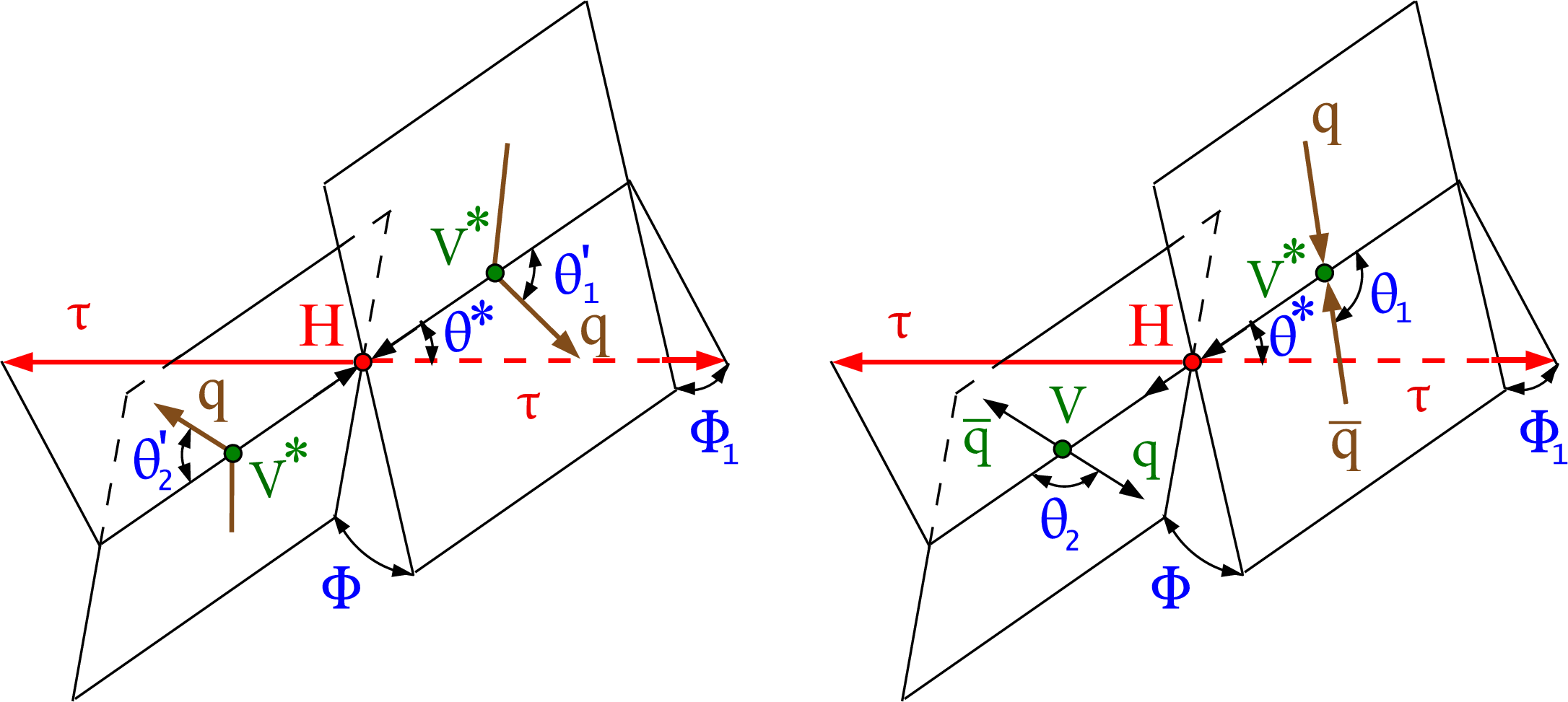
Figure 1:
Illustrations of $ {\mathrm {H}} $ production in strong $q{q^\prime}\to gg(q{q^\prime})\to {\mathrm {H}} (q{q^\prime})\to \tau \tau (q{q^\prime})$ or weak vector boson fusion $q{q^\prime}\to V^*V^*(q{q^\prime})\to {\mathrm {H}} (q{q^\prime})\to \tau \tau (q{q^\prime})$ (left) and $q\bar{q}^\prime \to V^*\to \mathrm {V} {\mathrm {H}} \to q\bar{q}^\prime \tau \tau $ (right). The decay $ {\mathrm {H}} \to \tau \tau $ is shown without further illustrating the $\tau $ decay chain. Angles and invariant masses fully characterize the orientation of the production and two-body decay chain and are defined in suitable rest frames [37,42]. |
png pdf |
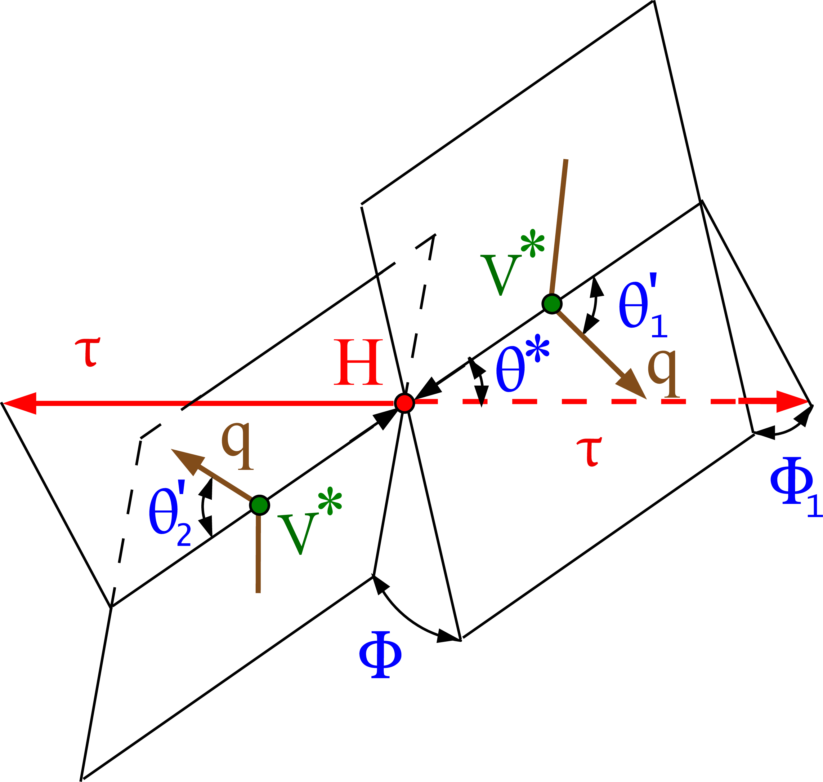
Figure 1-a:
Illustrations of $ {\mathrm {H}} $ production in strong $q{q^\prime}\to gg(q{q^\prime})\to {\mathrm {H}} (q{q^\prime})\to \tau \tau (q{q^\prime})$ or weak vector boson fusion $q{q^\prime}\to V^*V^*(q{q^\prime})\to {\mathrm {H}} (q{q^\prime})\to \tau \tau (q{q^\prime})$ (left) and $q\bar{q}^\prime \to V^*\to \mathrm {V} {\mathrm {H}} \to q\bar{q}^\prime \tau \tau $ (right). The decay $ {\mathrm {H}} \to \tau \tau $ is shown without further illustrating the $\tau $ decay chain. Angles and invariant masses fully characterize the orientation of the production and two-body decay chain and are defined in suitable rest frames [37,42]. |
png pdf |
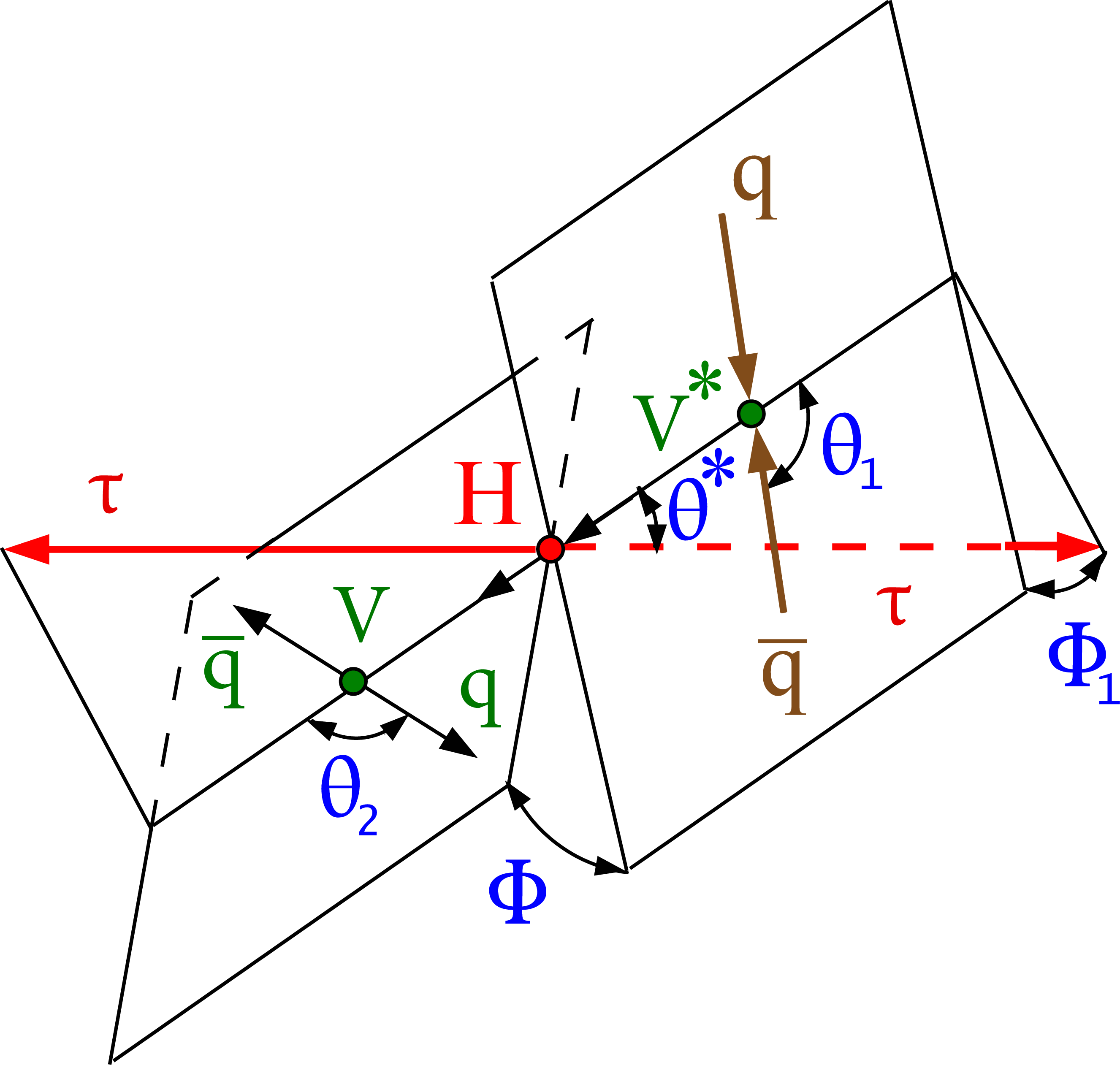
Figure 1-b:
Illustrations of $ {\mathrm {H}} $ production in strong $q{q^\prime}\to gg(q{q^\prime})\to {\mathrm {H}} (q{q^\prime})\to \tau \tau (q{q^\prime})$ or weak vector boson fusion $q{q^\prime}\to V^*V^*(q{q^\prime})\to {\mathrm {H}} (q{q^\prime})\to \tau \tau (q{q^\prime})$ (left) and $q\bar{q}^\prime \to V^*\to \mathrm {V} {\mathrm {H}} \to q\bar{q}^\prime \tau \tau $ (right). The decay $ {\mathrm {H}} \to \tau \tau $ is shown without further illustrating the $\tau $ decay chain. Angles and invariant masses fully characterize the orientation of the production and two-body decay chain and are defined in suitable rest frames [37,42]. |
png pdf |
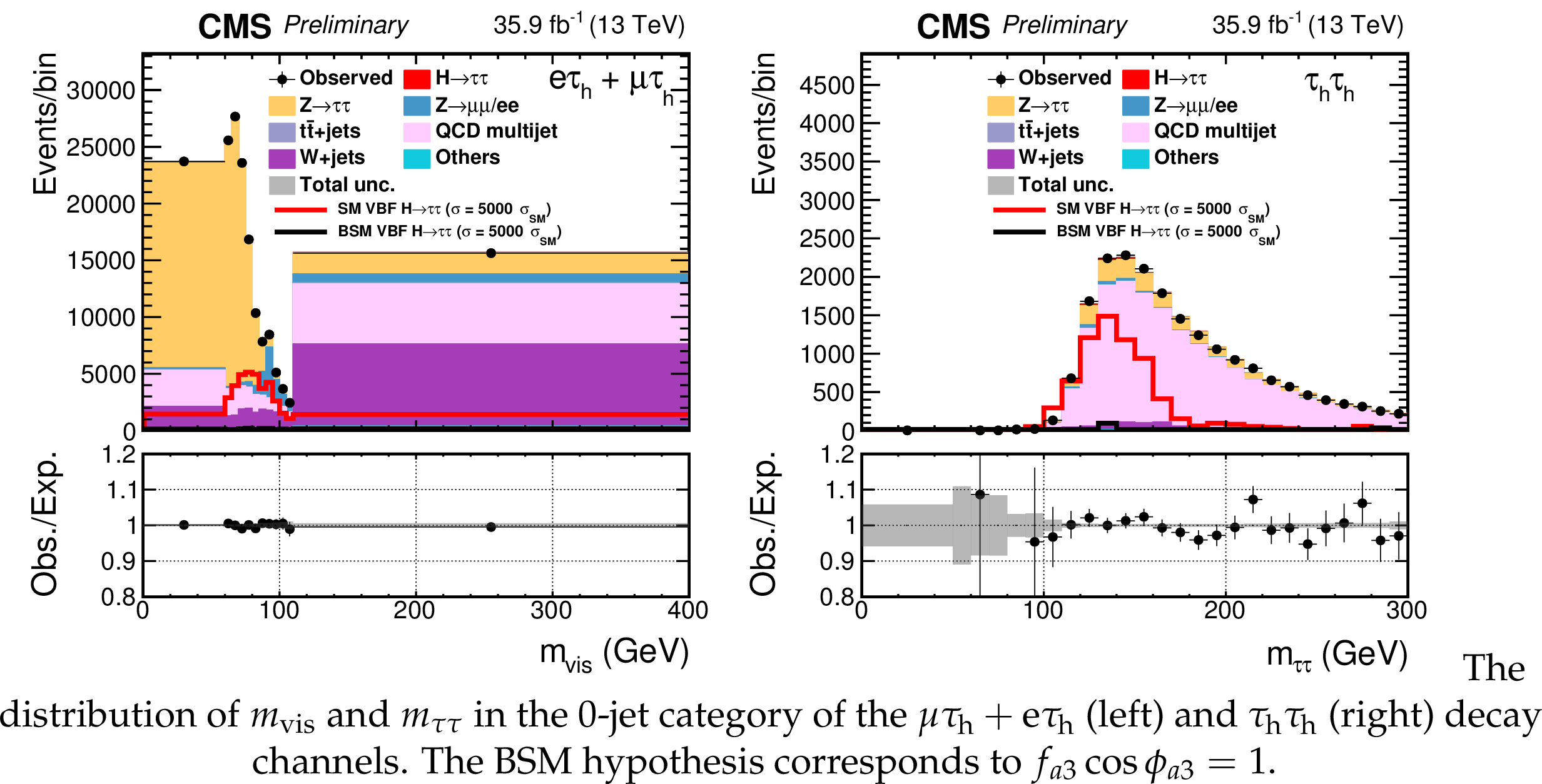
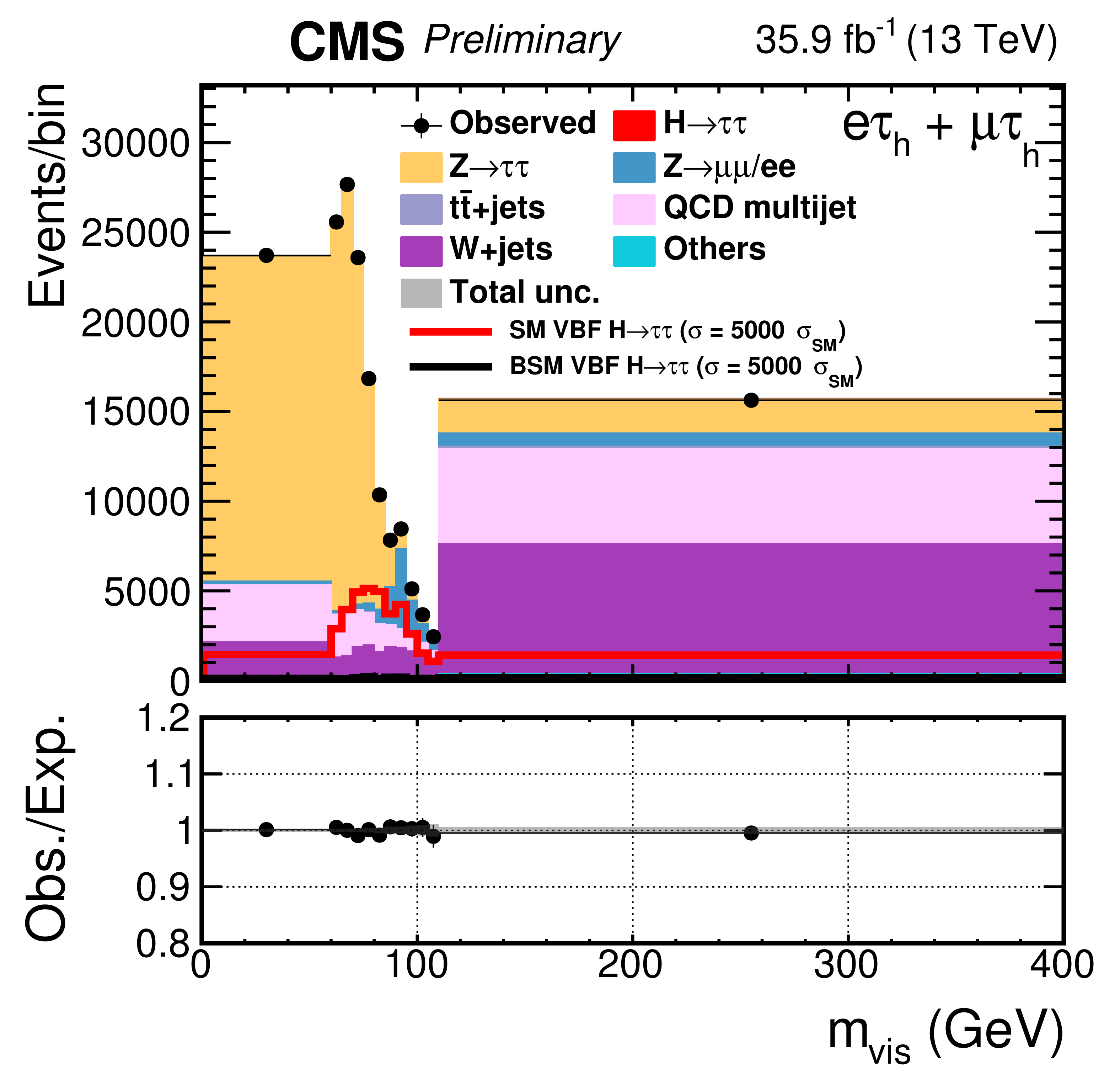
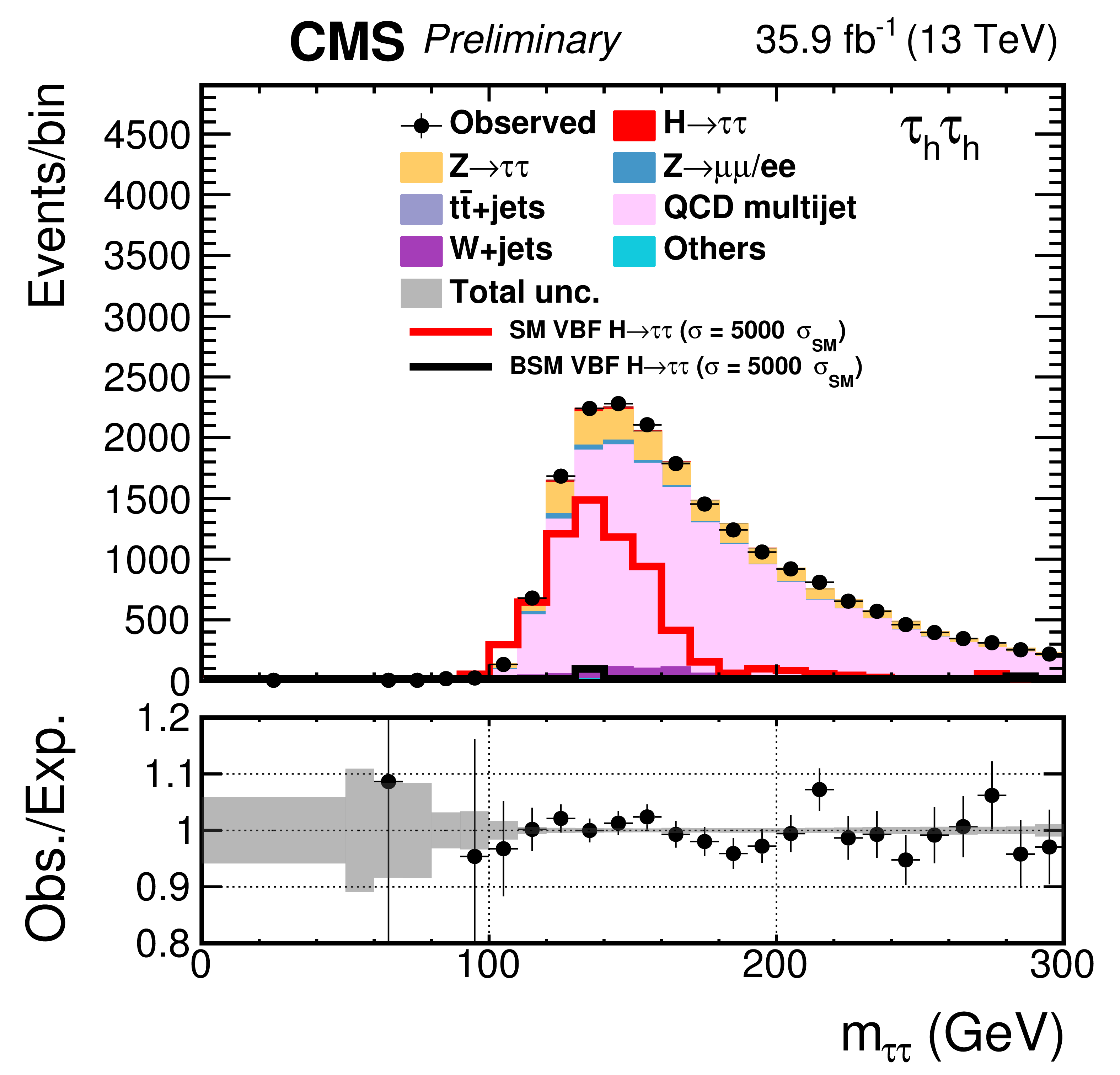
Figure 2:
The distribution of $ {m_\text {vis}} $ and $ {m_{{\tau} {\tau}}} $ in the 0-jet category of the $\mu {{\tau} _\mathrm {h}} + {\mathrm {e}} {{\tau} _\mathrm {h}} $ (left) and $ {{\tau} _\mathrm {h}} {{\tau} _\mathrm {h}} $ (right) decay channels. The BSM hypothesis corresponds to $f_{a3}\cos\phi _{a3}=1$. |
png pdf |
Figure 2-a:
The distribution of $ {m_\text {vis}} $ and $ {m_{{\tau} {\tau}}} $ in the 0-jet category of the $\mu {{\tau} _\mathrm {h}} + {\mathrm {e}} {{\tau} _\mathrm {h}} $ (left) and $ {{\tau} _\mathrm {h}} {{\tau} _\mathrm {h}} $ (right) decay channels. The BSM hypothesis corresponds to $f_{a3}\cos\phi _{a3}=1$. |
png pdf |
Figure 2-b:
The distribution of $ {m_\text {vis}} $ and $ {m_{{\tau} {\tau}}} $ in the 0-jet category of the $\mu {{\tau} _\mathrm {h}} + {\mathrm {e}} {{\tau} _\mathrm {h}} $ (left) and $ {{\tau} _\mathrm {h}} {{\tau} _\mathrm {h}} $ (right) decay channels. The BSM hypothesis corresponds to $f_{a3}\cos\phi _{a3}=1$. |
png pdf |
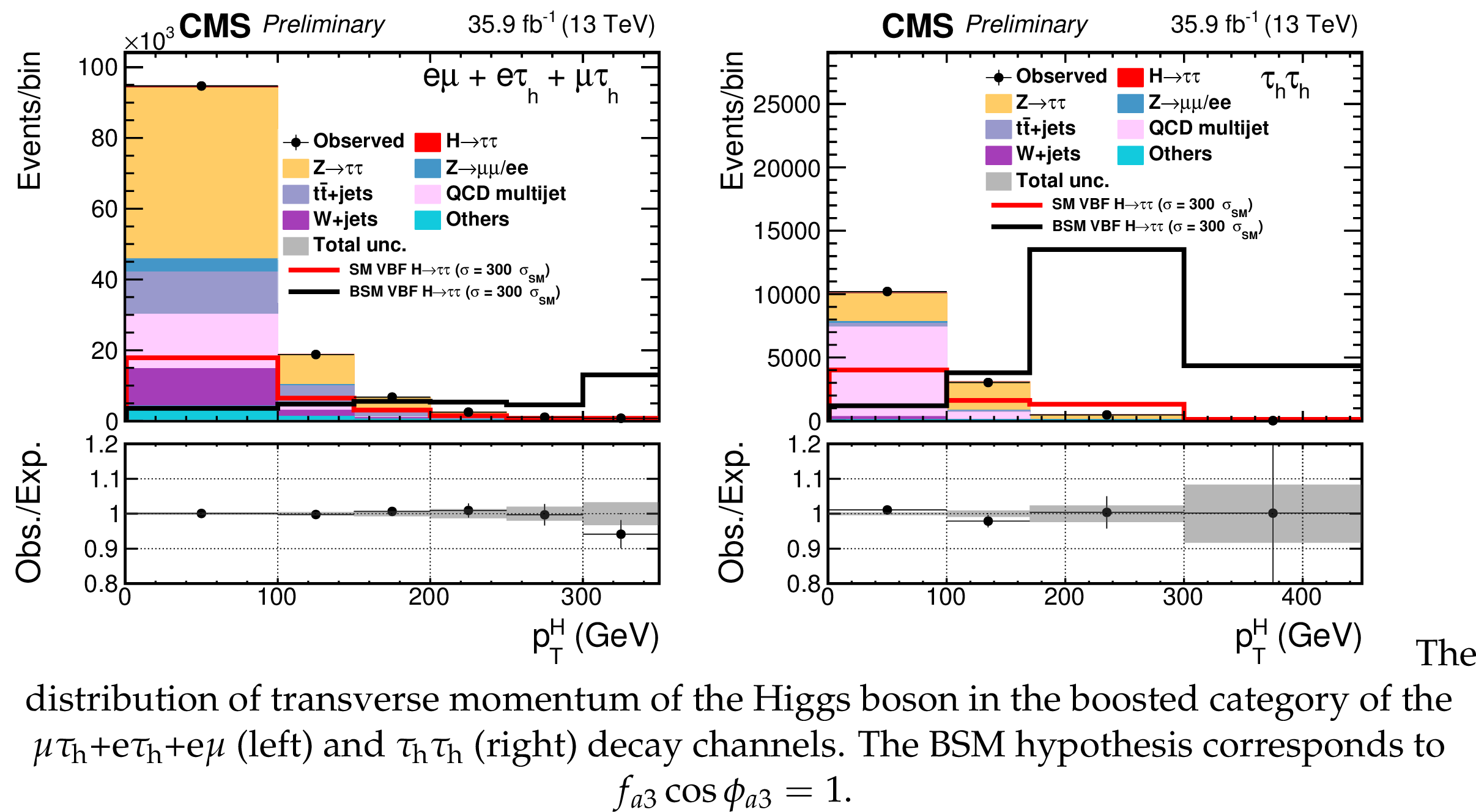
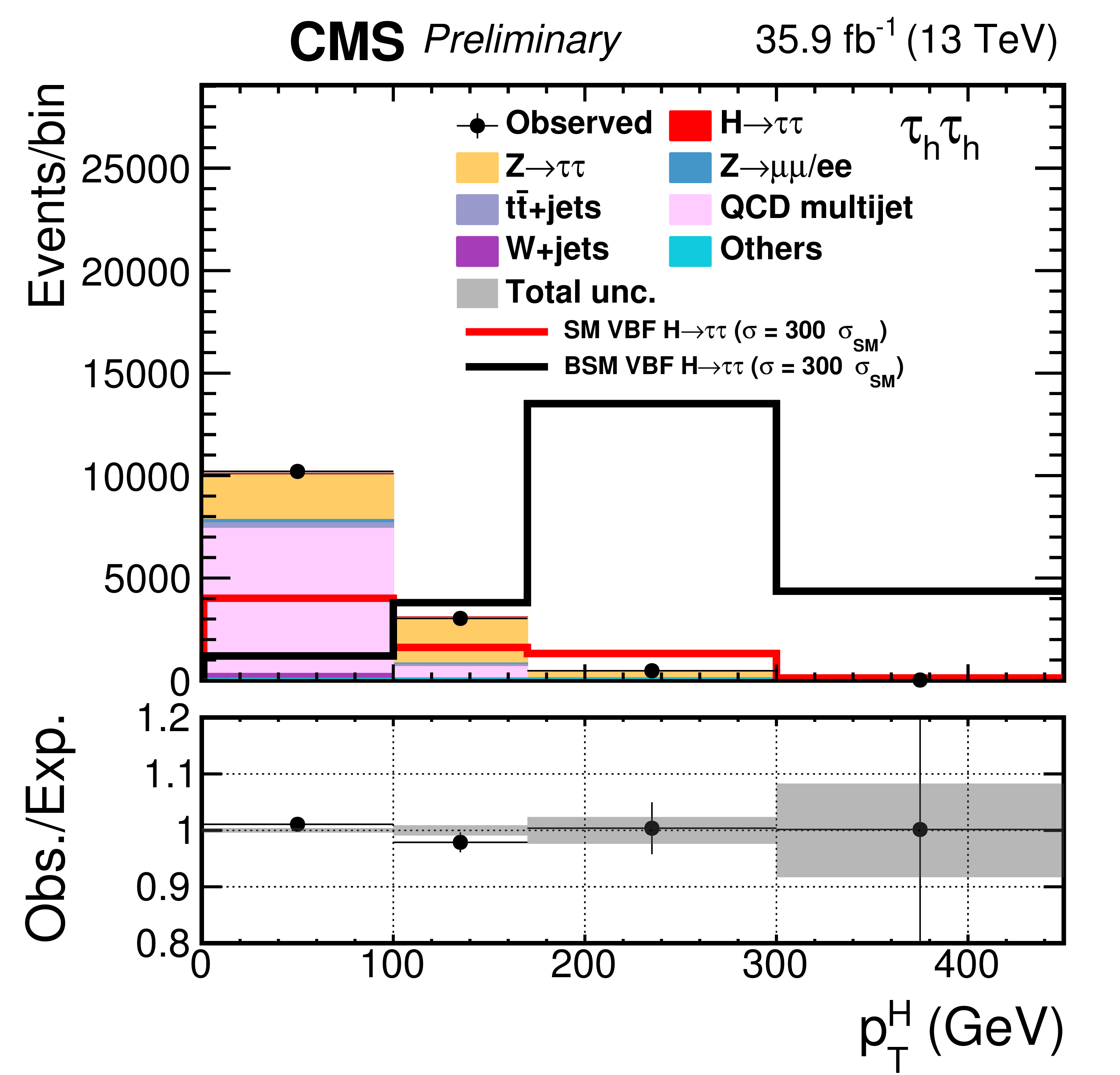
Figure 3:
The distribution of transverse momentum of the Higgs boson in the boosted category of the $\mu {{\tau} _\mathrm {h}} $+$ {\mathrm {e}} {{\tau} _\mathrm {h}} $+$ {\mathrm {e}} {{\mu}}$ (left) and $ {{\tau} _\mathrm {h}} {{\tau} _\mathrm {h}} $ (right) decay channels. The BSM hypothesis corresponds to $f_{a3}\cos\phi _{a3}=1$. |

png pdf |
Figure 3-a:
The distribution of transverse momentum of the Higgs boson in the boosted category of the $\mu {{\tau} _\mathrm {h}} $+$ {\mathrm {e}} {{\tau} _\mathrm {h}} $+$ {\mathrm {e}} {{\mu}}$ (left) and $ {{\tau} _\mathrm {h}} {{\tau} _\mathrm {h}} $ (right) decay channels. The BSM hypothesis corresponds to $f_{a3}\cos\phi _{a3}=1$. |
png pdf |
Figure 3-b:
The distribution of transverse momentum of the Higgs boson in the boosted category of the $\mu {{\tau} _\mathrm {h}} $+$ {\mathrm {e}} {{\tau} _\mathrm {h}} $+$ {\mathrm {e}} {{\mu}}$ (left) and $ {{\tau} _\mathrm {h}} {{\tau} _\mathrm {h}} $ (right) decay channels. The BSM hypothesis corresponds to $f_{a3}\cos\phi _{a3}=1$. |
png pdf |
Figure 4:
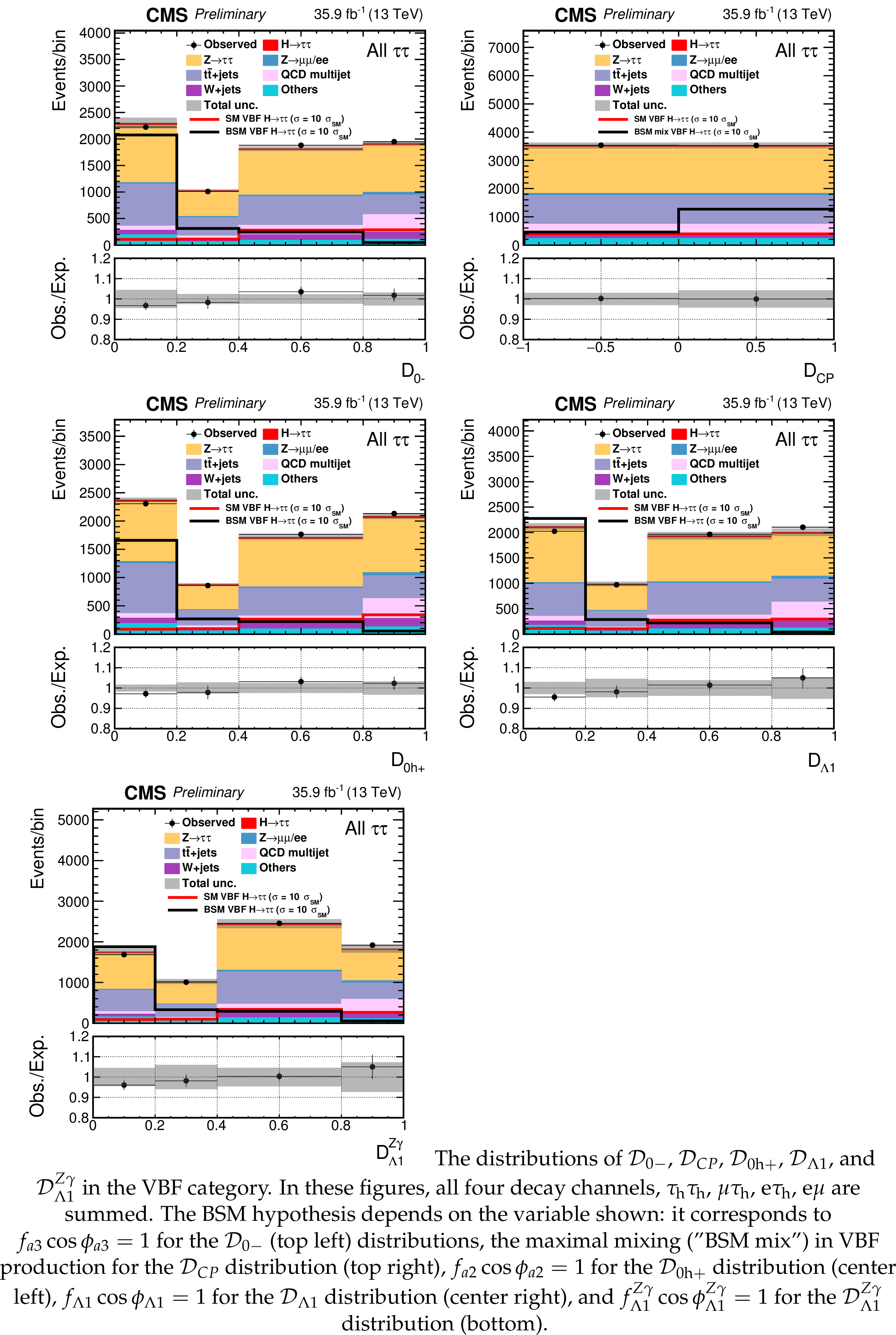
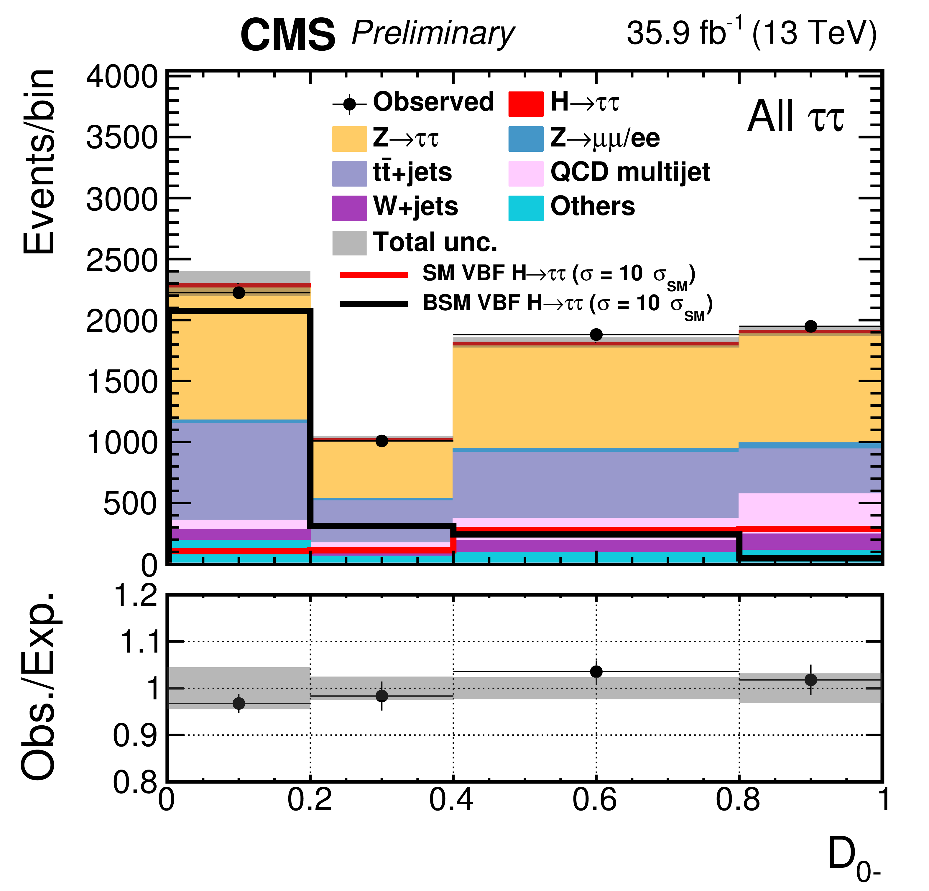
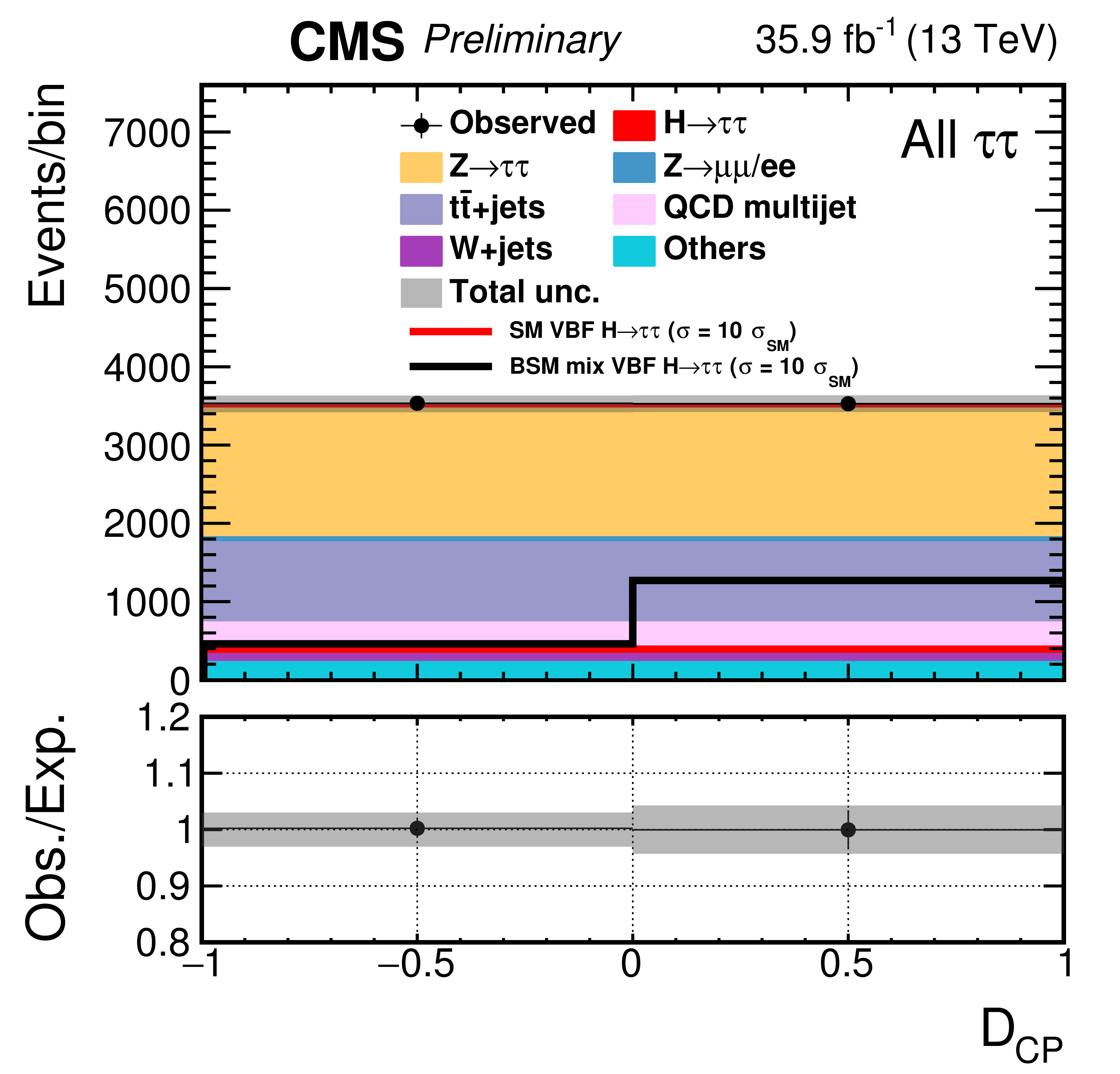
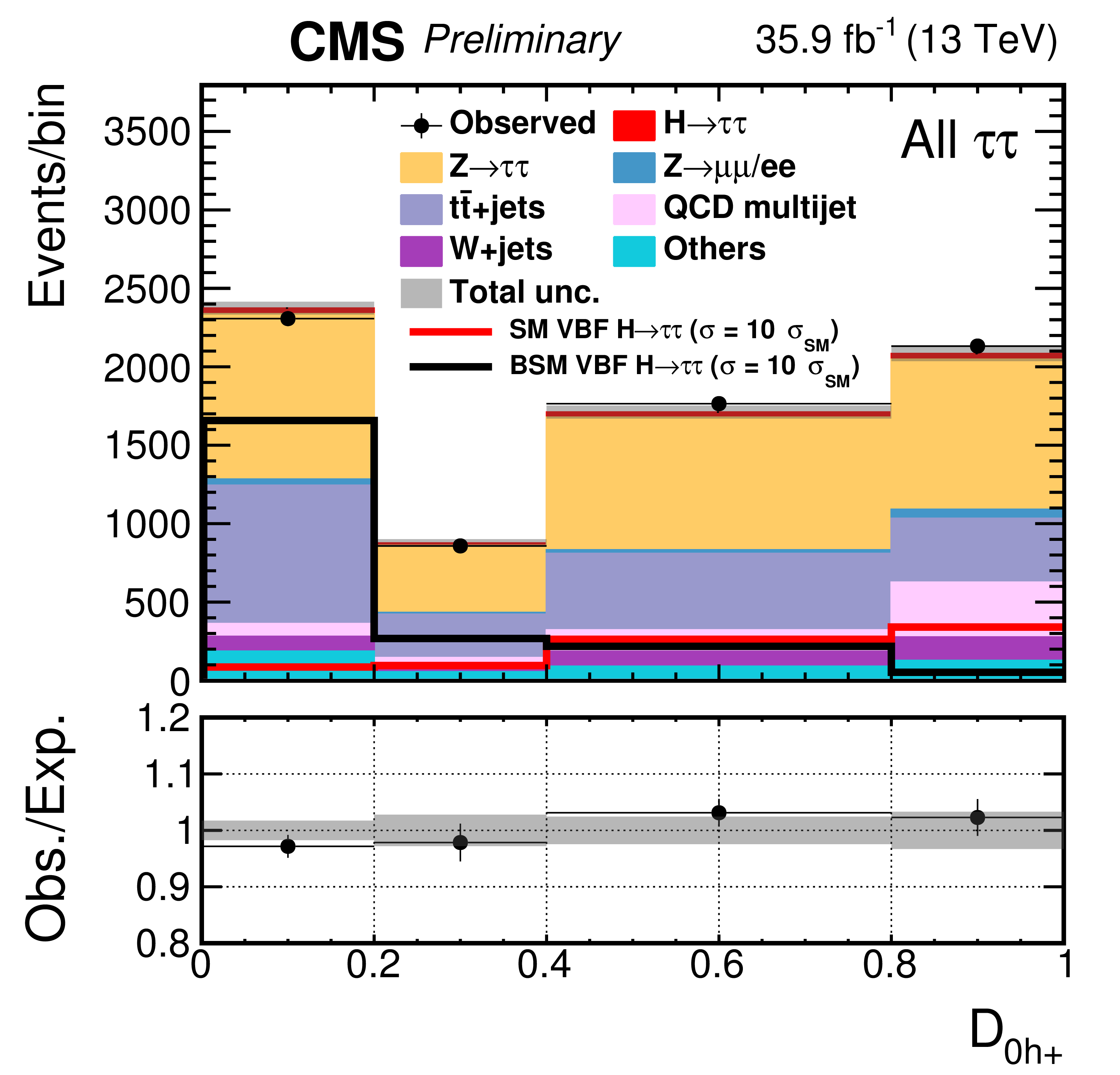
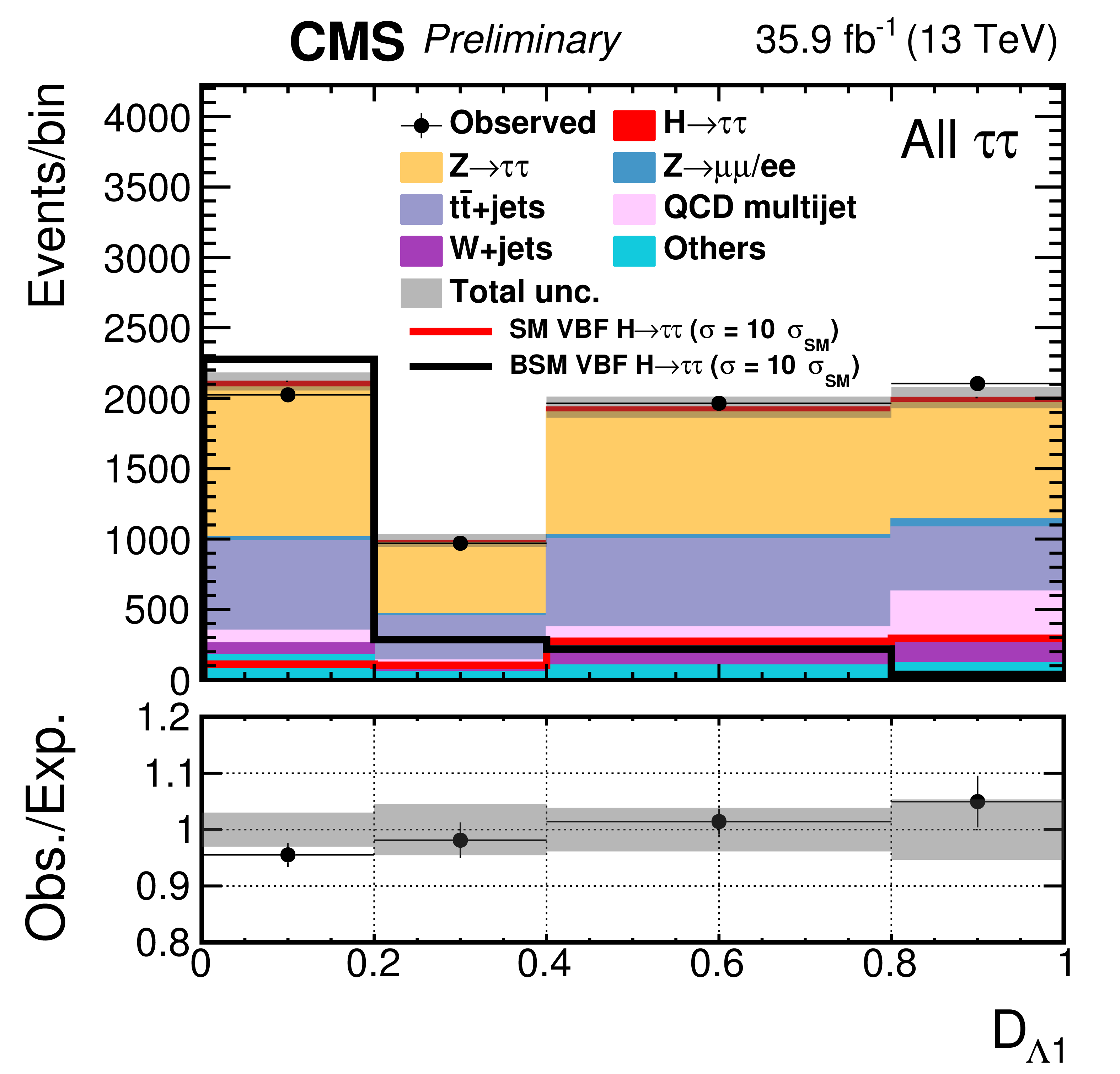
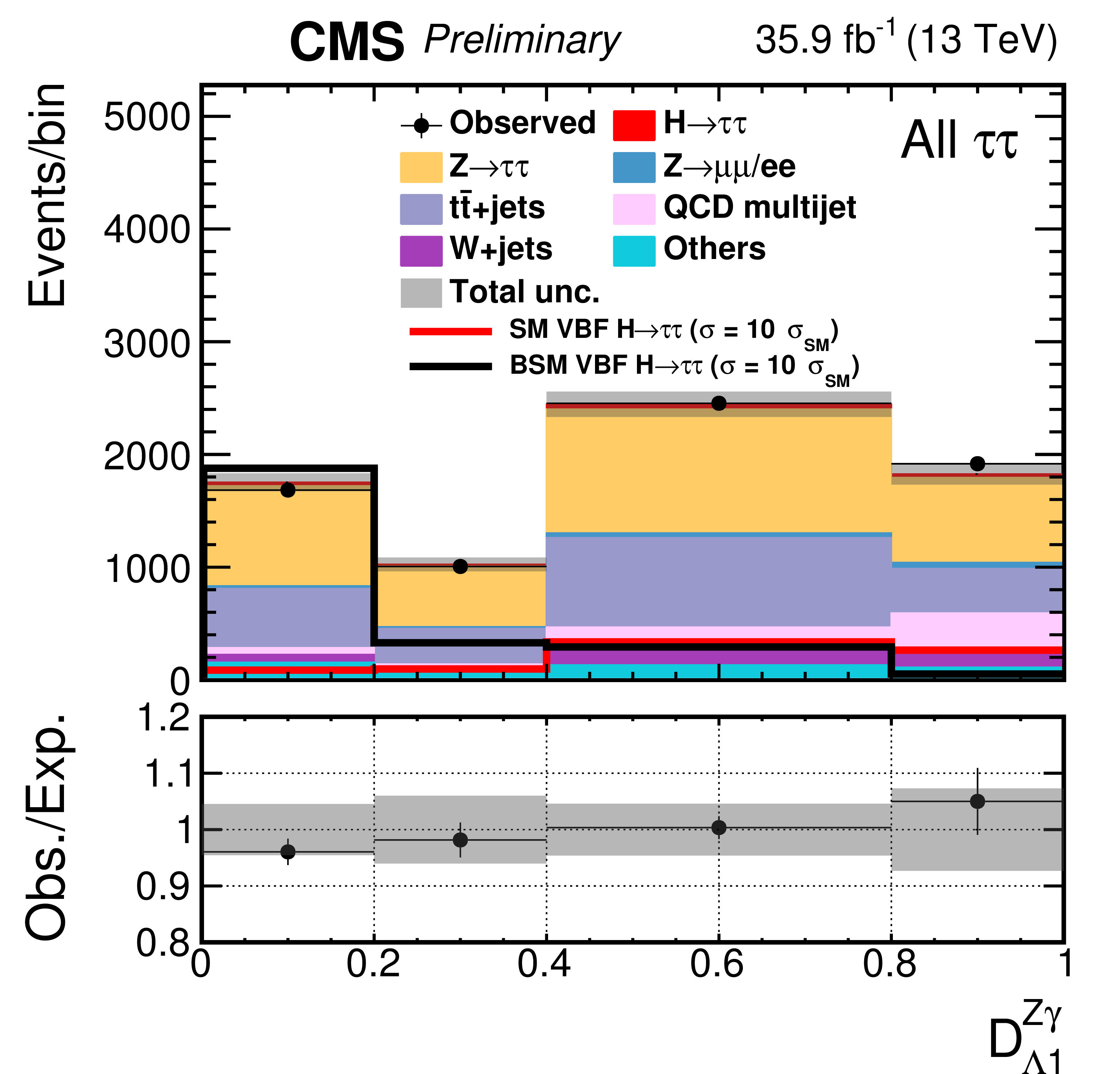
The distributions of $\mathcal {D}_\mathrm {0-}$, $\mathcal {D}_{CP}$, $\mathcal {D}_{\rm 0h+}$, $\mathcal {D}_{\lambda 1}$, and $\mathcal {D}_{\lambda 1}^{Z\gamma}$ in the VBF category. In these figures, all four decay channels, $ {{\tau} _\mathrm {h}} {{\tau} _\mathrm {h}} $, $\mu {{\tau} _\mathrm {h}} $, $ {\mathrm {e}} {{\tau} _\mathrm {h}} $, $ {\mathrm {e}} {{\mu}}$ are summed. The BSM hypothesis depends on the variable shown: it corresponds to $f_{a3}\cos\phi _{a3}=1$ for the $\mathcal {D}_\mathrm {0-}$ (top left) distributions, the maximal mixing ("BSM mix") in VBF production for the $\mathcal {D}_{CP}$ distribution (top right), $f_{a2}\cos\phi _{a2}=1$ for the $\mathcal {D}_{\rm 0h+}$ distribution (center left), $f_{\lambda 1}\cos\phi _{\lambda 1}=1$ for the $\mathcal {D}_{\lambda 1}$ distribution (center right), and $f_{\lambda 1}^{Z\gamma}\cos\phi _{\lambda 1}^{Z\gamma}=1$ for the $\mathcal {D}_{\lambda 1}^{Z\gamma}$ distribution (bottom). |
png pdf |
Figure 4-a:
The distributions of $\mathcal {D}_\mathrm {0-}$, $\mathcal {D}_{CP}$, $\mathcal {D}_{\rm 0h+}$, $\mathcal {D}_{\lambda 1}$, and $\mathcal {D}_{\lambda 1}^{Z\gamma}$ in the VBF category. In these figures, all four decay channels, $ {{\tau} _\mathrm {h}} {{\tau} _\mathrm {h}} $, $\mu {{\tau} _\mathrm {h}} $, $ {\mathrm {e}} {{\tau} _\mathrm {h}} $, $ {\mathrm {e}} {{\mu}}$ are summed. The BSM hypothesis depends on the variable shown: it corresponds to $f_{a3}\cos\phi _{a3}=1$ for the $\mathcal {D}_\mathrm {0-}$ (top left) distributions, the maximal mixing ("BSM mix") in VBF production for the $\mathcal {D}_{CP}$ distribution (top right), $f_{a2}\cos\phi _{a2}=1$ for the $\mathcal {D}_{\rm 0h+}$ distribution (center left), $f_{\lambda 1}\cos\phi _{\lambda 1}=1$ for the $\mathcal {D}_{\lambda 1}$ distribution (center right), and $f_{\lambda 1}^{Z\gamma}\cos\phi _{\lambda 1}^{Z\gamma}=1$ for the $\mathcal {D}_{\lambda 1}^{Z\gamma}$ distribution (bottom). |
png pdf |
Figure 4-b:
The distributions of $\mathcal {D}_\mathrm {0-}$, $\mathcal {D}_{CP}$, $\mathcal {D}_{\rm 0h+}$, $\mathcal {D}_{\lambda 1}$, and $\mathcal {D}_{\lambda 1}^{Z\gamma}$ in the VBF category. In these figures, all four decay channels, $ {{\tau} _\mathrm {h}} {{\tau} _\mathrm {h}} $, $\mu {{\tau} _\mathrm {h}} $, $ {\mathrm {e}} {{\tau} _\mathrm {h}} $, $ {\mathrm {e}} {{\mu}}$ are summed. The BSM hypothesis depends on the variable shown: it corresponds to $f_{a3}\cos\phi _{a3}=1$ for the $\mathcal {D}_\mathrm {0-}$ (top left) distributions, the maximal mixing ("BSM mix") in VBF production for the $\mathcal {D}_{CP}$ distribution (top right), $f_{a2}\cos\phi _{a2}=1$ for the $\mathcal {D}_{\rm 0h+}$ distribution (center left), $f_{\lambda 1}\cos\phi _{\lambda 1}=1$ for the $\mathcal {D}_{\lambda 1}$ distribution (center right), and $f_{\lambda 1}^{Z\gamma}\cos\phi _{\lambda 1}^{Z\gamma}=1$ for the $\mathcal {D}_{\lambda 1}^{Z\gamma}$ distribution (bottom). |
png pdf |
Figure 4-c:
The distributions of $\mathcal {D}_\mathrm {0-}$, $\mathcal {D}_{CP}$, $\mathcal {D}_{\rm 0h+}$, $\mathcal {D}_{\lambda 1}$, and $\mathcal {D}_{\lambda 1}^{Z\gamma}$ in the VBF category. In these figures, all four decay channels, $ {{\tau} _\mathrm {h}} {{\tau} _\mathrm {h}} $, $\mu {{\tau} _\mathrm {h}} $, $ {\mathrm {e}} {{\tau} _\mathrm {h}} $, $ {\mathrm {e}} {{\mu}}$ are summed. The BSM hypothesis depends on the variable shown: it corresponds to $f_{a3}\cos\phi _{a3}=1$ for the $\mathcal {D}_\mathrm {0-}$ (top left) distributions, the maximal mixing ("BSM mix") in VBF production for the $\mathcal {D}_{CP}$ distribution (top right), $f_{a2}\cos\phi _{a2}=1$ for the $\mathcal {D}_{\rm 0h+}$ distribution (center left), $f_{\lambda 1}\cos\phi _{\lambda 1}=1$ for the $\mathcal {D}_{\lambda 1}$ distribution (center right), and $f_{\lambda 1}^{Z\gamma}\cos\phi _{\lambda 1}^{Z\gamma}=1$ for the $\mathcal {D}_{\lambda 1}^{Z\gamma}$ distribution (bottom). |
png pdf |
Figure 4-d:
The distributions of $\mathcal {D}_\mathrm {0-}$, $\mathcal {D}_{CP}$, $\mathcal {D}_{\rm 0h+}$, $\mathcal {D}_{\lambda 1}$, and $\mathcal {D}_{\lambda 1}^{Z\gamma}$ in the VBF category. In these figures, all four decay channels, $ {{\tau} _\mathrm {h}} {{\tau} _\mathrm {h}} $, $\mu {{\tau} _\mathrm {h}} $, $ {\mathrm {e}} {{\tau} _\mathrm {h}} $, $ {\mathrm {e}} {{\mu}}$ are summed. The BSM hypothesis depends on the variable shown: it corresponds to $f_{a3}\cos\phi _{a3}=1$ for the $\mathcal {D}_\mathrm {0-}$ (top left) distributions, the maximal mixing ("BSM mix") in VBF production for the $\mathcal {D}_{CP}$ distribution (top right), $f_{a2}\cos\phi _{a2}=1$ for the $\mathcal {D}_{\rm 0h+}$ distribution (center left), $f_{\lambda 1}\cos\phi _{\lambda 1}=1$ for the $\mathcal {D}_{\lambda 1}$ distribution (center right), and $f_{\lambda 1}^{Z\gamma}\cos\phi _{\lambda 1}^{Z\gamma}=1$ for the $\mathcal {D}_{\lambda 1}^{Z\gamma}$ distribution (bottom). |
png pdf |
Figure 4-e:
The distributions of $\mathcal {D}_\mathrm {0-}$, $\mathcal {D}_{CP}$, $\mathcal {D}_{\rm 0h+}$, $\mathcal {D}_{\lambda 1}$, and $\mathcal {D}_{\lambda 1}^{Z\gamma}$ in the VBF category. In these figures, all four decay channels, $ {{\tau} _\mathrm {h}} {{\tau} _\mathrm {h}} $, $\mu {{\tau} _\mathrm {h}} $, $ {\mathrm {e}} {{\tau} _\mathrm {h}} $, $ {\mathrm {e}} {{\mu}}$ are summed. The BSM hypothesis depends on the variable shown: it corresponds to $f_{a3}\cos\phi _{a3}=1$ for the $\mathcal {D}_\mathrm {0-}$ (top left) distributions, the maximal mixing ("BSM mix") in VBF production for the $\mathcal {D}_{CP}$ distribution (top right), $f_{a2}\cos\phi _{a2}=1$ for the $\mathcal {D}_{\rm 0h+}$ distribution (center left), $f_{\lambda 1}\cos\phi _{\lambda 1}=1$ for the $\mathcal {D}_{\lambda 1}$ distribution (center right), and $f_{\lambda 1}^{Z\gamma}\cos\phi _{\lambda 1}^{Z\gamma}=1$ for the $\mathcal {D}_{\lambda 1}^{Z\gamma}$ distribution (bottom). |
png pdf |
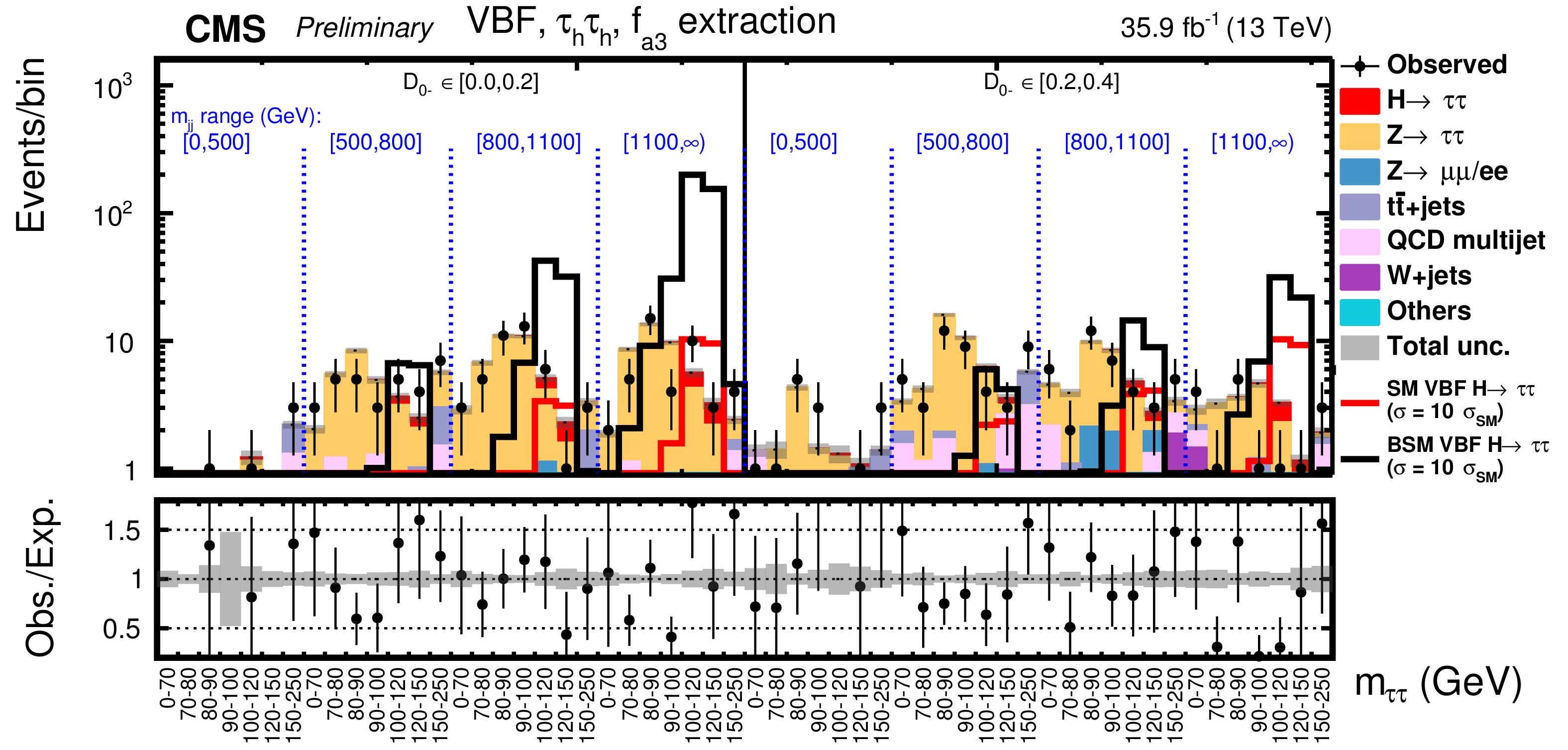
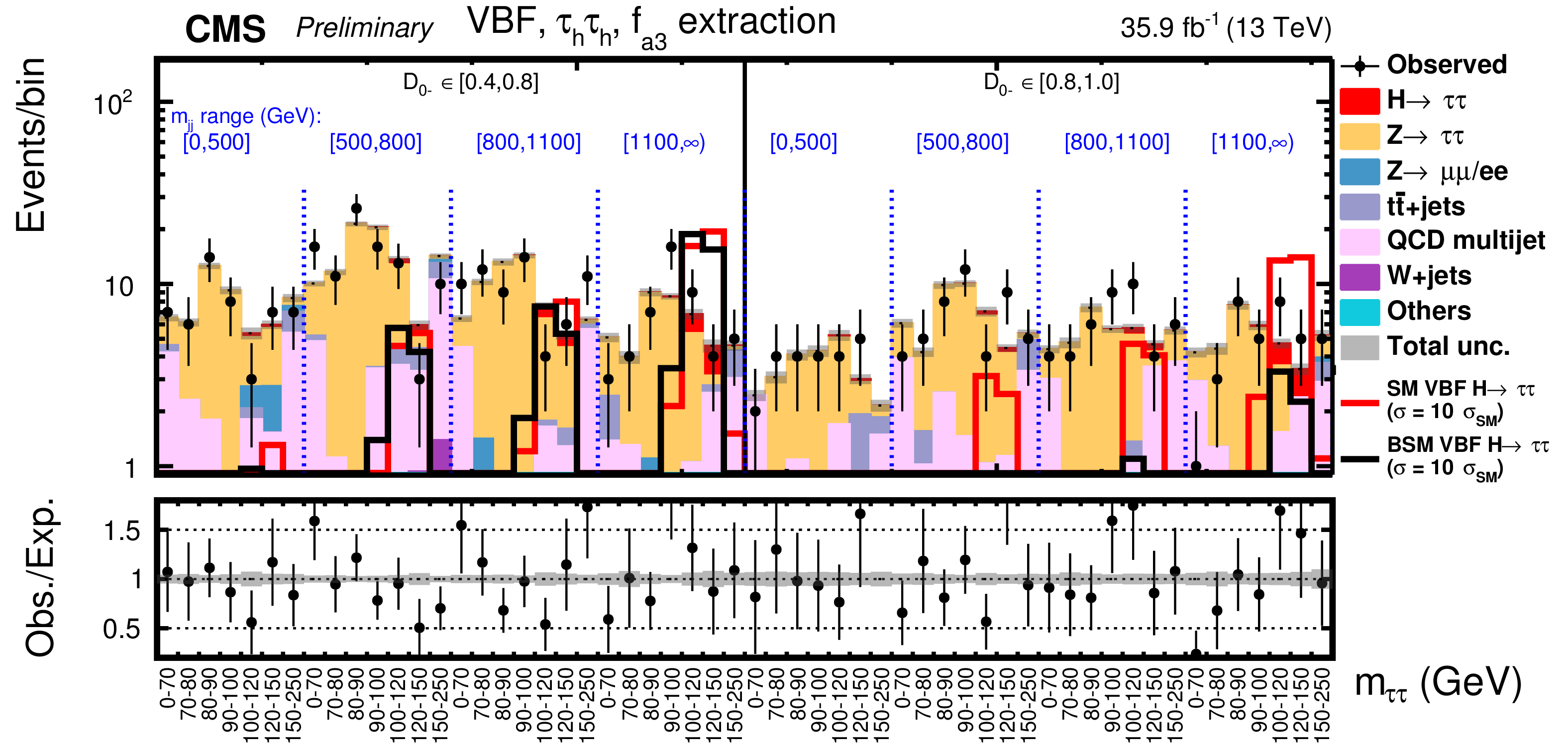
Figure 5:
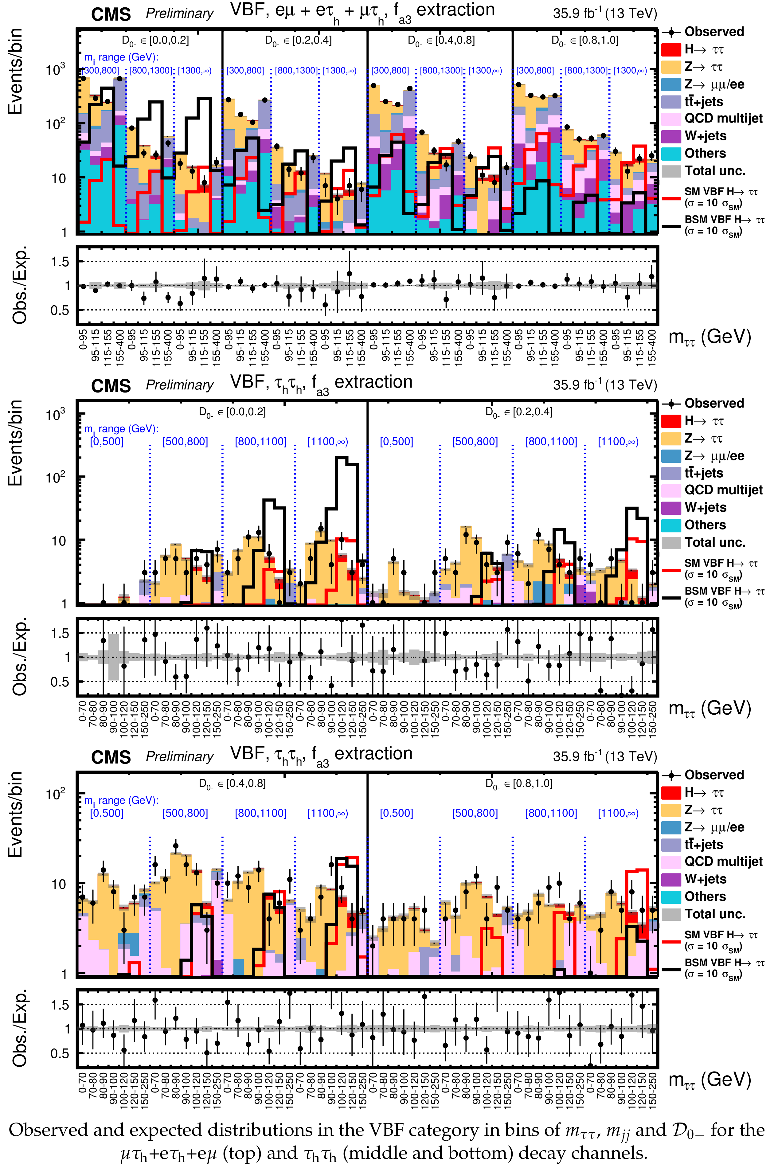
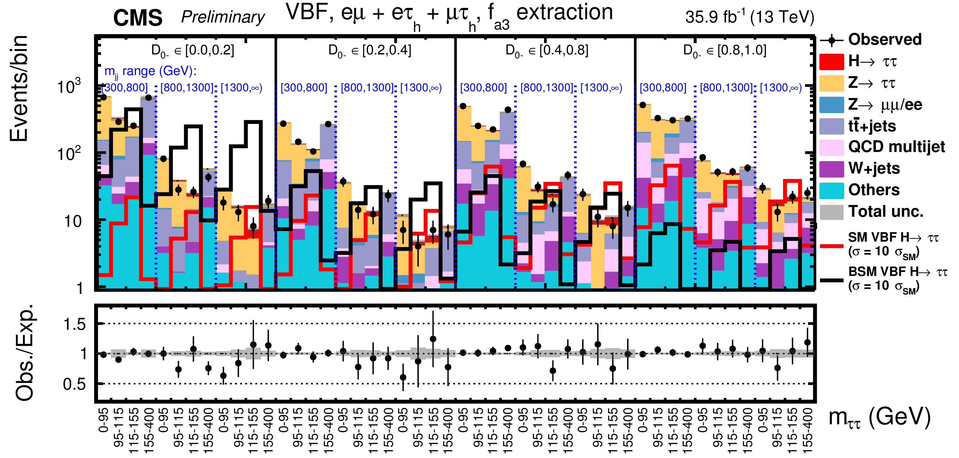
Observed and expected distributions in the VBF category in bins of $m_{\tau \tau}$, $m_{jj}$ and $\mathcal {D}_\mathrm {0-}$ for the $\mu {{\tau} _\mathrm {h}} $+$ {\mathrm {e}} {{\tau} _\mathrm {h}} $+$ {\mathrm {e}} {{\mu}}$ (top) and $ {{\tau} _\mathrm {h}} {{\tau} _\mathrm {h}} $ (middle and bottom) decay channels. |
png pdf |
Figure 5-a:
Observed and expected distributions in the VBF category in bins of $m_{\tau \tau}$, $m_{jj}$ and $\mathcal {D}_\mathrm {0-}$ for the $\mu {{\tau} _\mathrm {h}} $+$ {\mathrm {e}} {{\tau} _\mathrm {h}} $+$ {\mathrm {e}} {{\mu}}$ (top) and $ {{\tau} _\mathrm {h}} {{\tau} _\mathrm {h}} $ (middle and bottom) decay channels. |
png pdf |
Figure 5-b:
Observed and expected distributions in the VBF category in bins of $m_{\tau \tau}$, $m_{jj}$ and $\mathcal {D}_\mathrm {0-}$ for the $\mu {{\tau} _\mathrm {h}} $+$ {\mathrm {e}} {{\tau} _\mathrm {h}} $+$ {\mathrm {e}} {{\mu}}$ (top) and $ {{\tau} _\mathrm {h}} {{\tau} _\mathrm {h}} $ (middle and bottom) decay channels. |
png pdf |
Figure 5-c:
Observed and expected distributions in the VBF category in bins of $m_{\tau \tau}$, $m_{jj}$ and $\mathcal {D}_\mathrm {0-}$ for the $\mu {{\tau} _\mathrm {h}} $+$ {\mathrm {e}} {{\tau} _\mathrm {h}} $+$ {\mathrm {e}} {{\mu}}$ (top) and $ {{\tau} _\mathrm {h}} {{\tau} _\mathrm {h}} $ (middle and bottom) decay channels. |
png pdf |
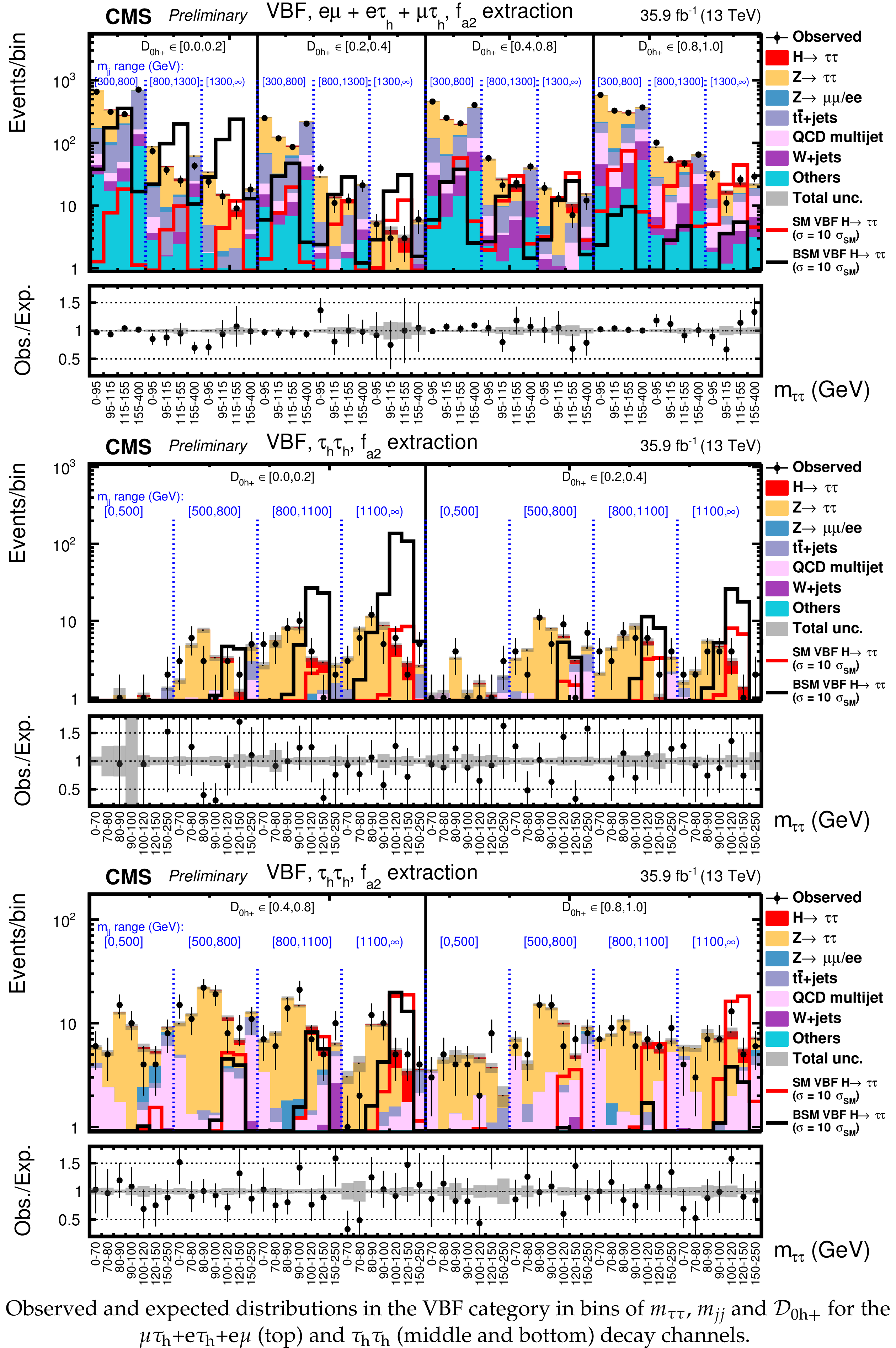
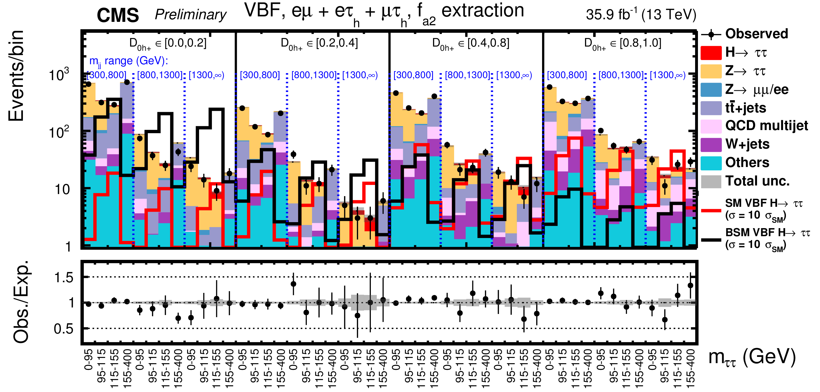
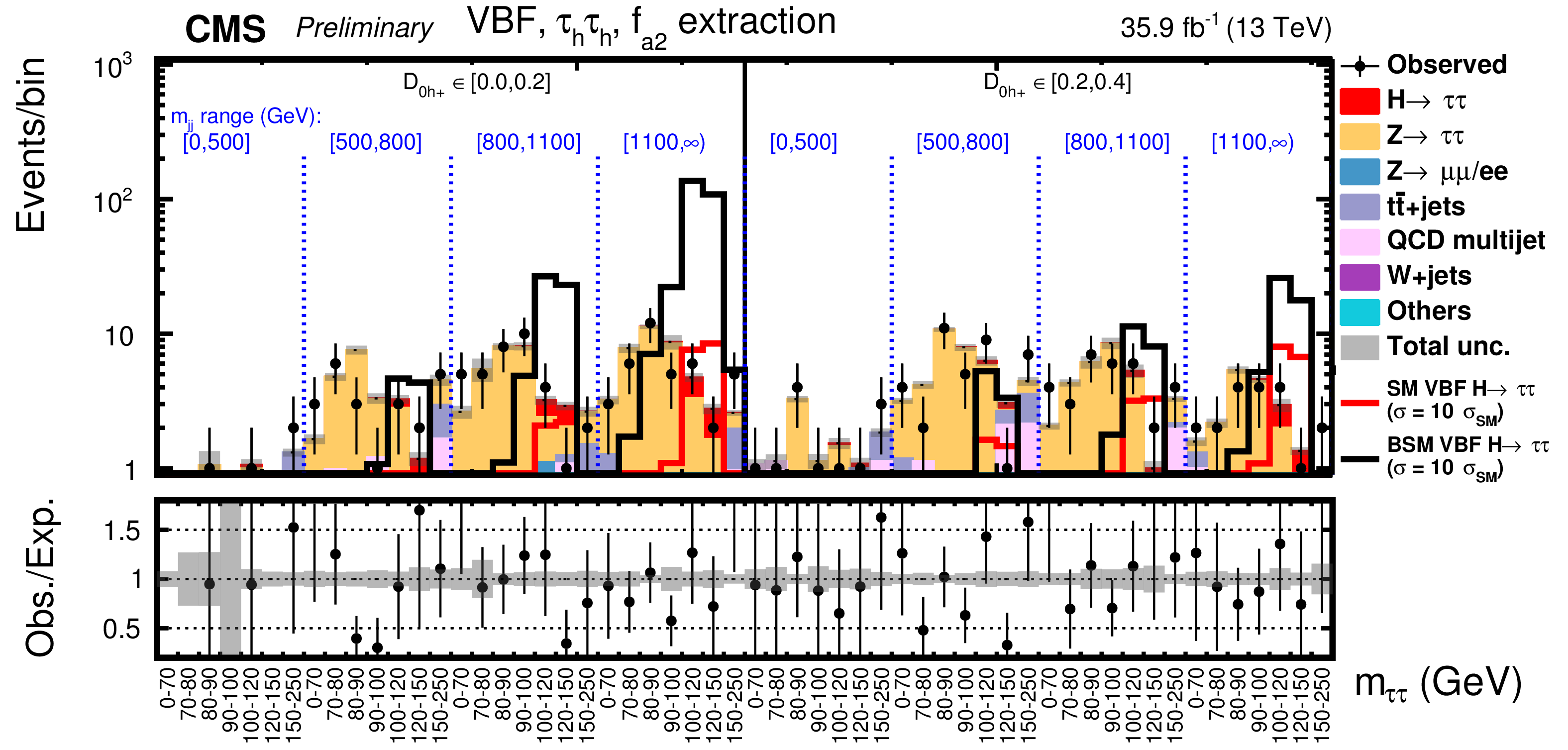
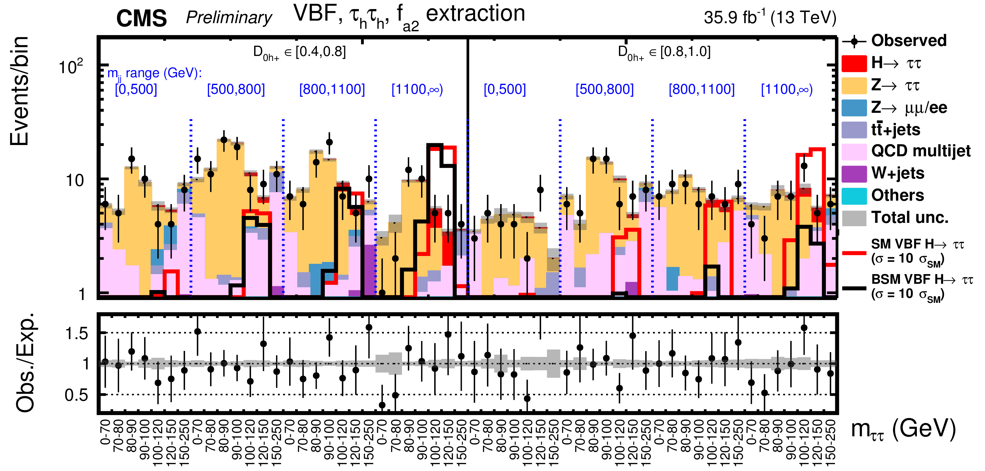
Figure 6:
Observed and expected distributions in the VBF category in bins of $m_{\tau \tau}$, $m_{jj}$ and $\mathcal {D}_{\rm 0h+}$ for the $\mu {{\tau} _\mathrm {h}} $+$ {\mathrm {e}} {{\tau} _\mathrm {h}} $+$ {\mathrm {e}} {{\mu}}$ (top) and $ {{\tau} _\mathrm {h}} {{\tau} _\mathrm {h}} $ (middle and bottom) decay channels. |
png pdf |
Figure 6-a:
Observed and expected distributions in the VBF category in bins of $m_{\tau \tau}$, $m_{jj}$ and $\mathcal {D}_{\rm 0h+}$ for the $\mu {{\tau} _\mathrm {h}} $+$ {\mathrm {e}} {{\tau} _\mathrm {h}} $+$ {\mathrm {e}} {{\mu}}$ (top) and $ {{\tau} _\mathrm {h}} {{\tau} _\mathrm {h}} $ (middle and bottom) decay channels. |
png pdf |
Figure 6-b:
Observed and expected distributions in the VBF category in bins of $m_{\tau \tau}$, $m_{jj}$ and $\mathcal {D}_{\rm 0h+}$ for the $\mu {{\tau} _\mathrm {h}} $+$ {\mathrm {e}} {{\tau} _\mathrm {h}} $+$ {\mathrm {e}} {{\mu}}$ (top) and $ {{\tau} _\mathrm {h}} {{\tau} _\mathrm {h}} $ (middle and bottom) decay channels. |
png pdf |
Figure 6-c:
Observed and expected distributions in the VBF category in bins of $m_{\tau \tau}$, $m_{jj}$ and $\mathcal {D}_{\rm 0h+}$ for the $\mu {{\tau} _\mathrm {h}} $+$ {\mathrm {e}} {{\tau} _\mathrm {h}} $+$ {\mathrm {e}} {{\mu}}$ (top) and $ {{\tau} _\mathrm {h}} {{\tau} _\mathrm {h}} $ (middle and bottom) decay channels. |
png pdf |
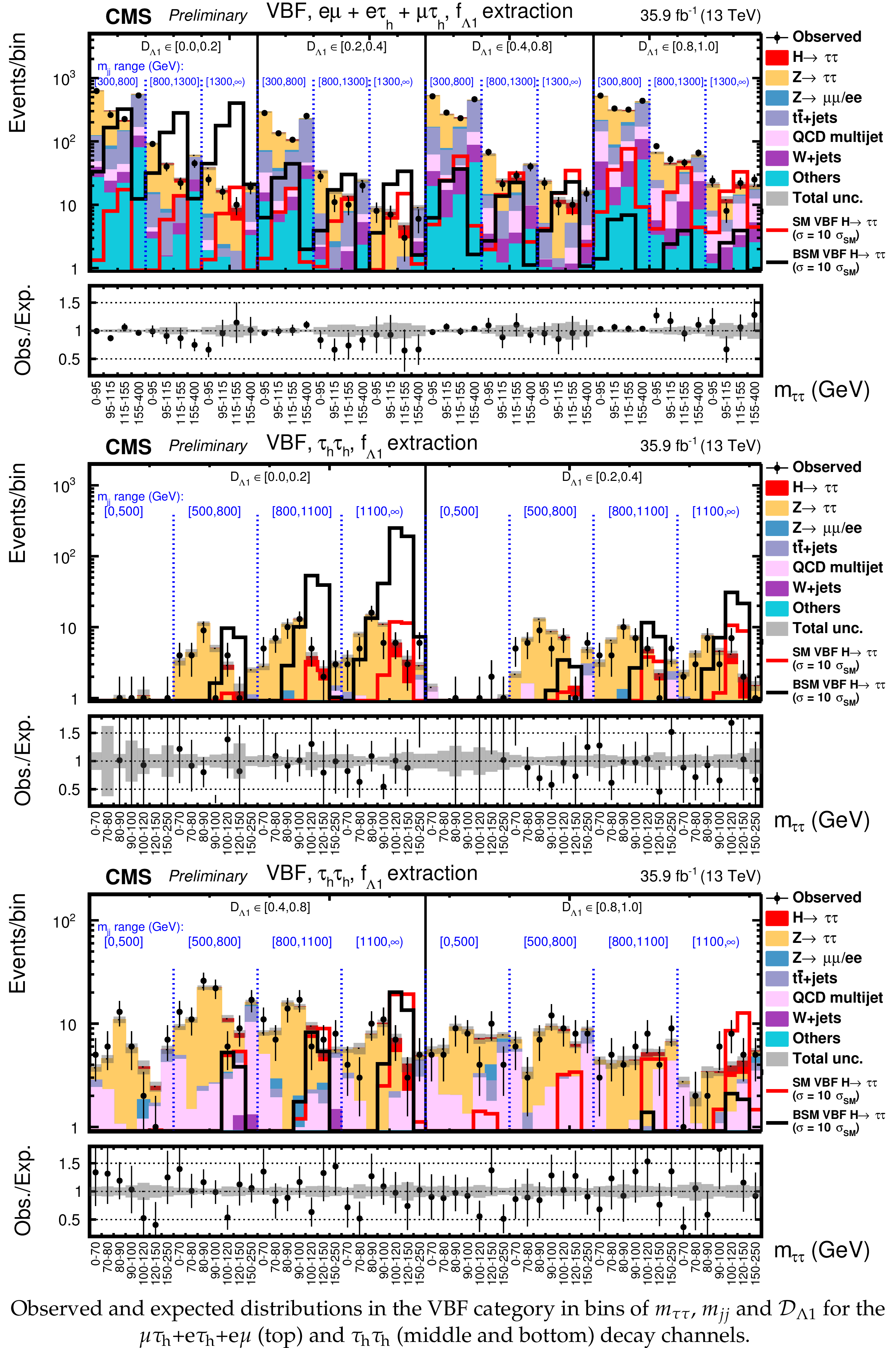
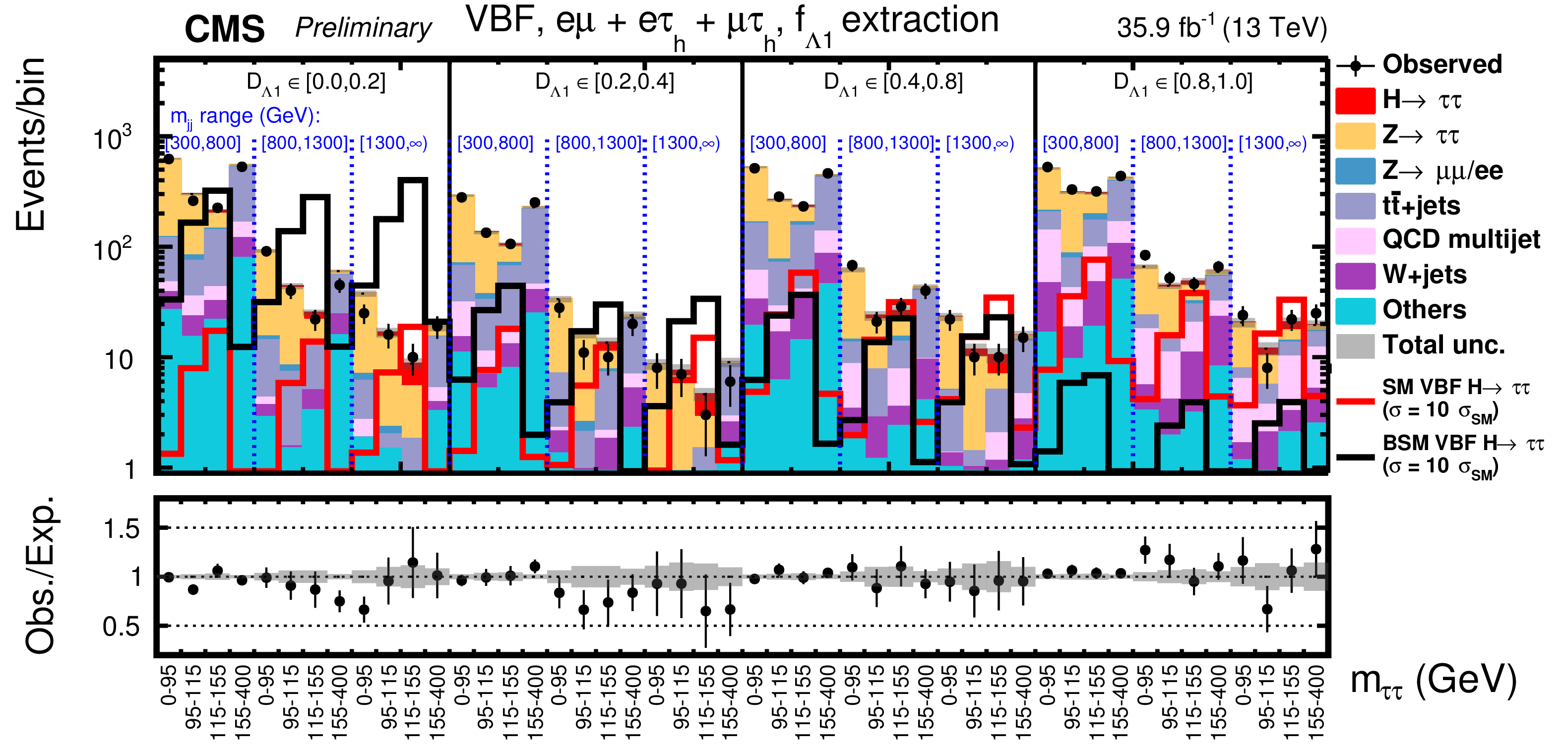
Figure 7:
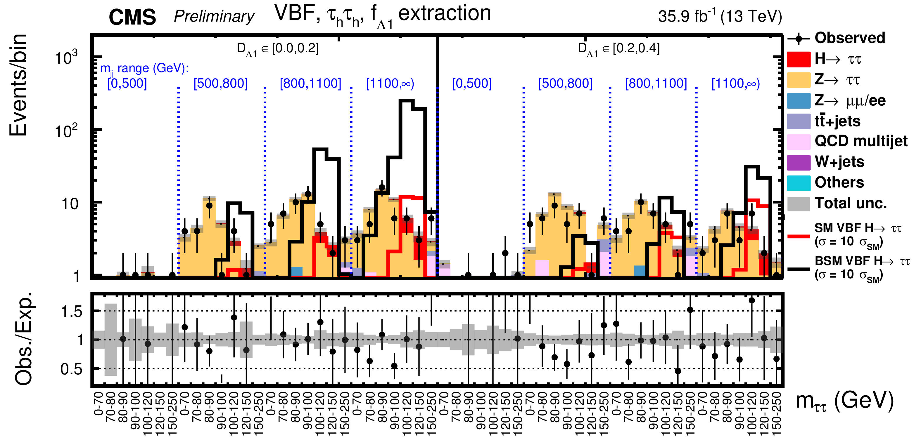
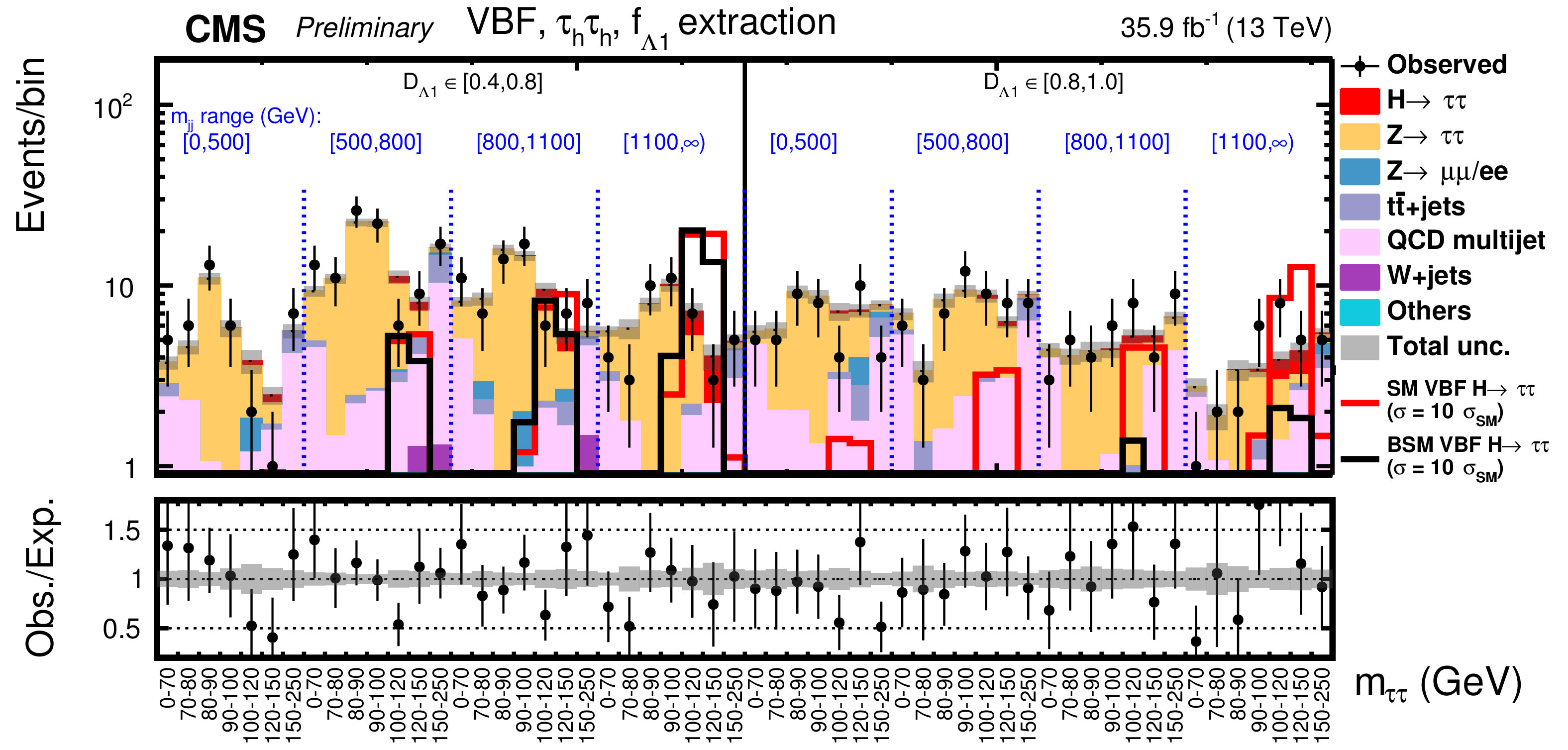
Observed and expected distributions in the VBF category in bins of $m_{\tau \tau}$, $m_{jj}$ and $\mathcal {D}_{\lambda 1}$ for the $\mu {{\tau} _\mathrm {h}} $+$ {\mathrm {e}} {{\tau} _\mathrm {h}} $+$ {\mathrm {e}} {{\mu}}$ (top) and $ {{\tau} _\mathrm {h}} {{\tau} _\mathrm {h}} $ (middle and bottom) decay channels. |
png pdf |
Figure 7-a:
Observed and expected distributions in the VBF category in bins of $m_{\tau \tau}$, $m_{jj}$ and $\mathcal {D}_{\lambda 1}$ for the $\mu {{\tau} _\mathrm {h}} $+$ {\mathrm {e}} {{\tau} _\mathrm {h}} $+$ {\mathrm {e}} {{\mu}}$ (top) and $ {{\tau} _\mathrm {h}} {{\tau} _\mathrm {h}} $ (middle and bottom) decay channels. |
png pdf |
Figure 7-b:
Observed and expected distributions in the VBF category in bins of $m_{\tau \tau}$, $m_{jj}$ and $\mathcal {D}_{\lambda 1}$ for the $\mu {{\tau} _\mathrm {h}} $+$ {\mathrm {e}} {{\tau} _\mathrm {h}} $+$ {\mathrm {e}} {{\mu}}$ (top) and $ {{\tau} _\mathrm {h}} {{\tau} _\mathrm {h}} $ (middle and bottom) decay channels. |
png pdf |
Figure 7-c:
Observed and expected distributions in the VBF category in bins of $m_{\tau \tau}$, $m_{jj}$ and $\mathcal {D}_{\lambda 1}$ for the $\mu {{\tau} _\mathrm {h}} $+$ {\mathrm {e}} {{\tau} _\mathrm {h}} $+$ {\mathrm {e}} {{\mu}}$ (top) and $ {{\tau} _\mathrm {h}} {{\tau} _\mathrm {h}} $ (middle and bottom) decay channels. |

png pdf |
Figure 8:
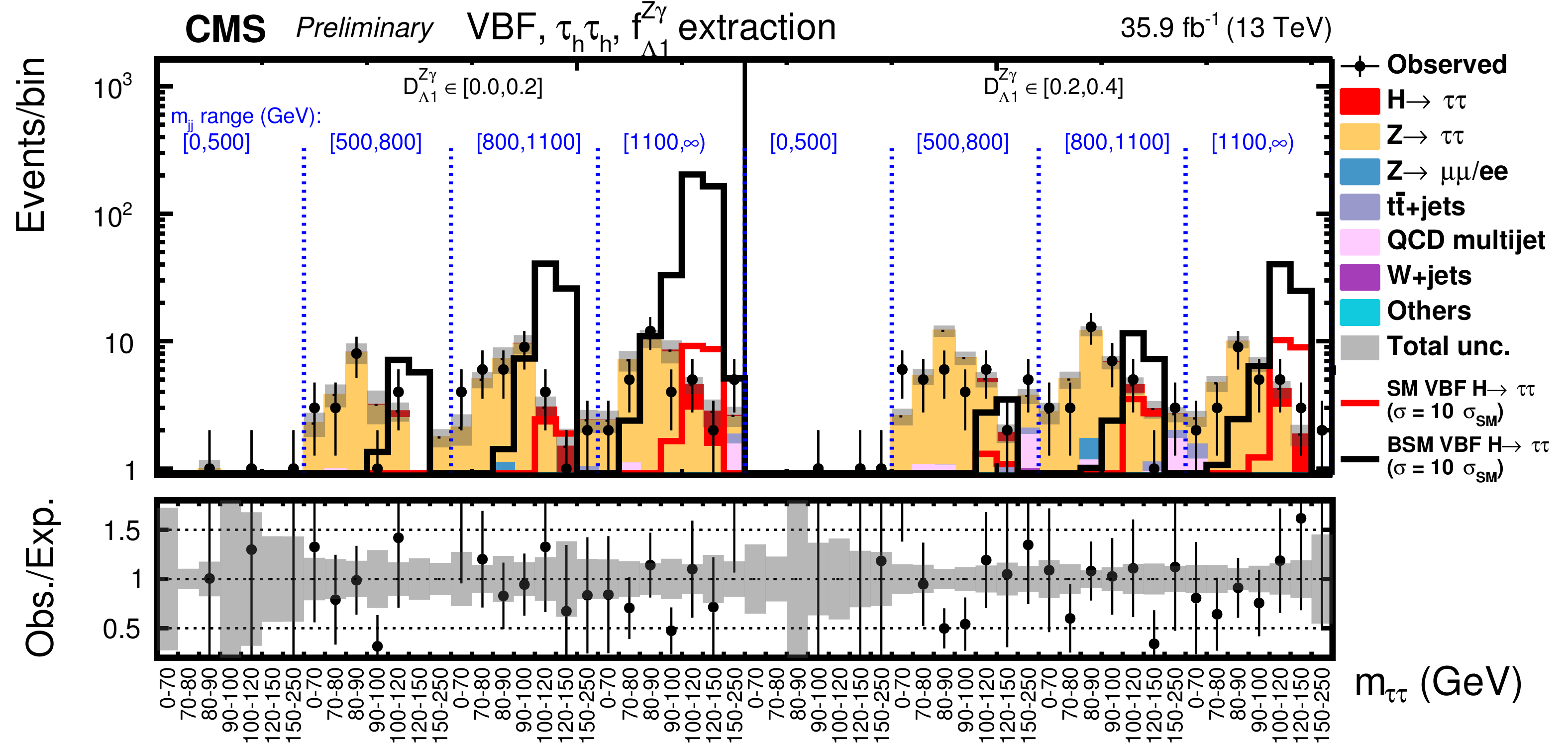
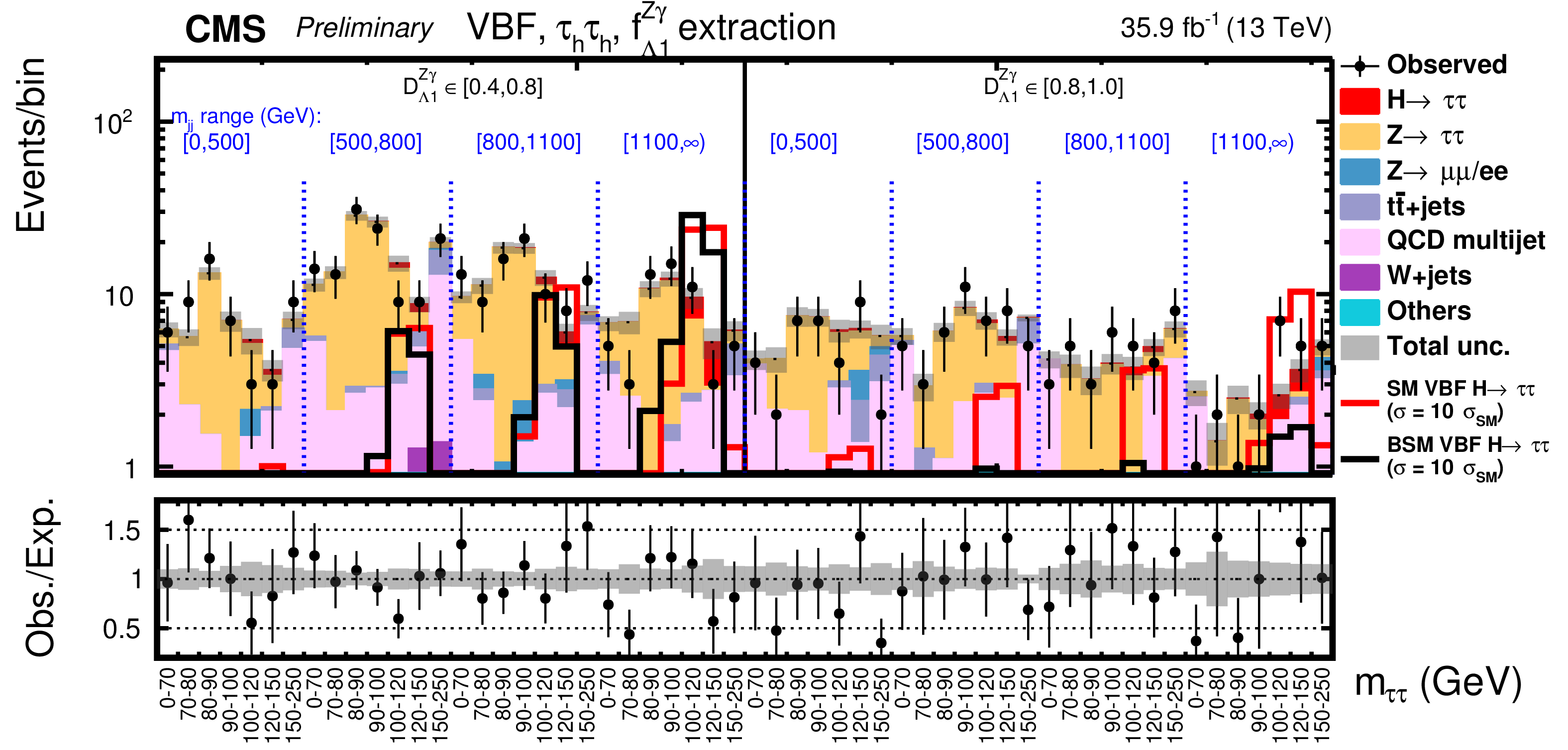
Observed and expected distributions in the VBF category in bins of $m_{\tau \tau}$, $m_{jj}$ and $\mathcal {D}_{\lambda 1}^{Z\gamma}$ for the $\mu {{\tau} _\mathrm {h}} $+$ {\mathrm {e}} {{\tau} _\mathrm {h}} $+$ {\mathrm {e}} {{\mu}}$ (top) and $ {{\tau} _\mathrm {h}} {{\tau} _\mathrm {h}} $ (middle and bottom) decay channels. |

png pdf |
Figure 8-a:
Observed and expected distributions in the VBF category in bins of $m_{\tau \tau}$, $m_{jj}$ and $\mathcal {D}_{\lambda 1}^{Z\gamma}$ for the $\mu {{\tau} _\mathrm {h}} $+$ {\mathrm {e}} {{\tau} _\mathrm {h}} $+$ {\mathrm {e}} {{\mu}}$ (top) and $ {{\tau} _\mathrm {h}} {{\tau} _\mathrm {h}} $ (middle and bottom) decay channels. |
png pdf |
Figure 8-b:
Observed and expected distributions in the VBF category in bins of $m_{\tau \tau}$, $m_{jj}$ and $\mathcal {D}_{\lambda 1}^{Z\gamma}$ for the $\mu {{\tau} _\mathrm {h}} $+$ {\mathrm {e}} {{\tau} _\mathrm {h}} $+$ {\mathrm {e}} {{\mu}}$ (top) and $ {{\tau} _\mathrm {h}} {{\tau} _\mathrm {h}} $ (middle and bottom) decay channels. |
png pdf |
Figure 8-c:
Observed and expected distributions in the VBF category in bins of $m_{\tau \tau}$, $m_{jj}$ and $\mathcal {D}_{\lambda 1}^{Z\gamma}$ for the $\mu {{\tau} _\mathrm {h}} $+$ {\mathrm {e}} {{\tau} _\mathrm {h}} $+$ {\mathrm {e}} {{\mu}}$ (top) and $ {{\tau} _\mathrm {h}} {{\tau} _\mathrm {h}} $ (middle and bottom) decay channels. |
png pdf |
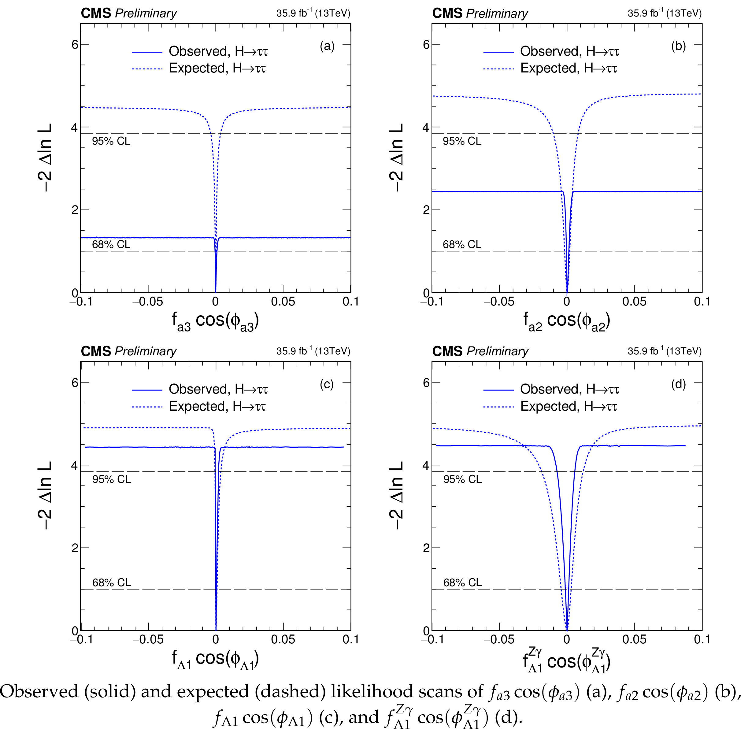
Figure 9:
Observed (solid) and expected (dashed) likelihood scans of $f_{a3}\cos(\phi _{a3})$ (a), $f_{a2}\cos(\phi _{a2})$ (b), $f_{\lambda 1}\cos(\phi _{\lambda 1})$ (c), and $f_{\lambda 1}^{Z\gamma}\cos(\phi _{\lambda 1}^{Z\gamma})$ (d). |
png pdf |
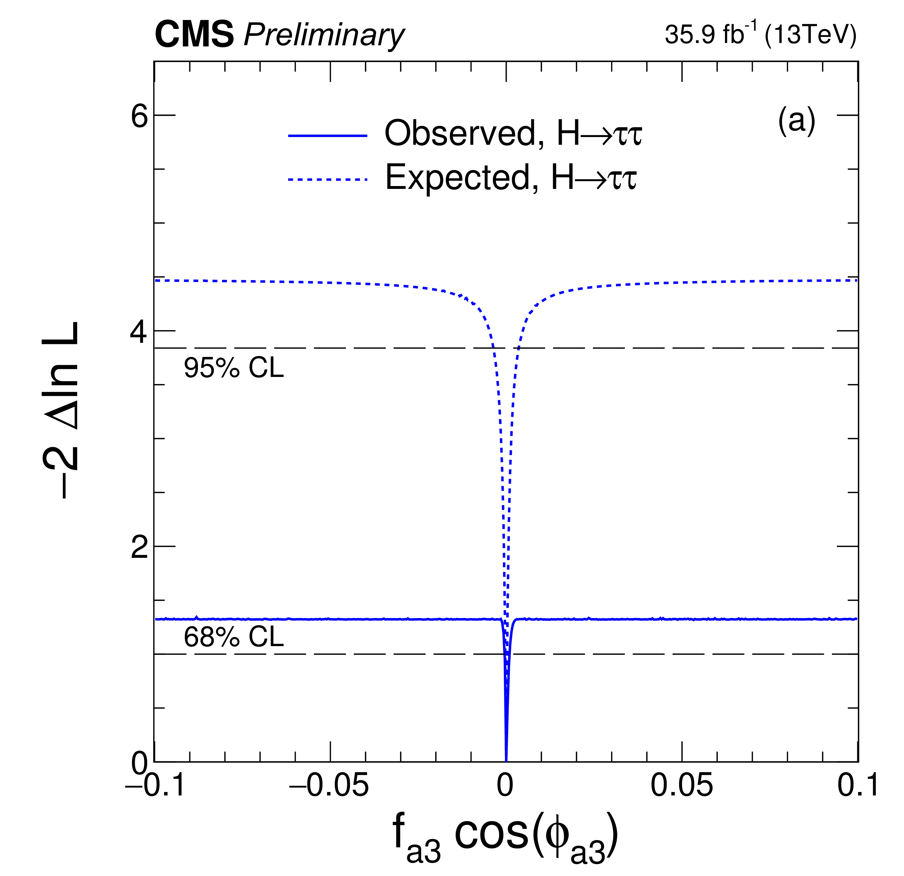
Figure 9-a:
Observed (solid) and expected (dashed) likelihood scans of $f_{a3}\cos(\phi _{a3})$ (a), $f_{a2}\cos(\phi _{a2})$ (b), $f_{\lambda 1}\cos(\phi _{\lambda 1})$ (c), and $f_{\lambda 1}^{Z\gamma}\cos(\phi _{\lambda 1}^{Z\gamma})$ (d). |
png pdf |
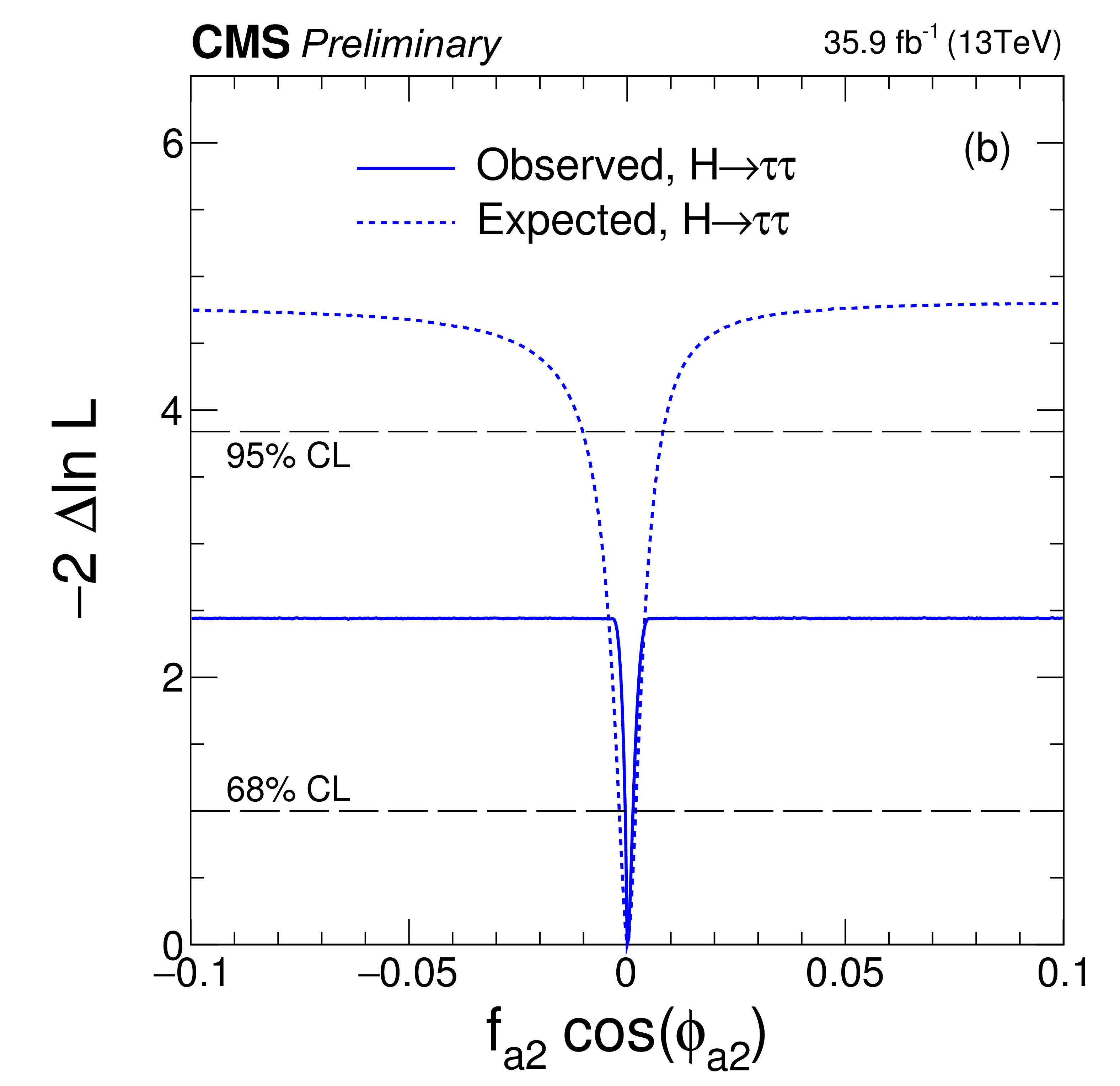
Figure 9-b:
Observed (solid) and expected (dashed) likelihood scans of $f_{a3}\cos(\phi _{a3})$ (a), $f_{a2}\cos(\phi _{a2})$ (b), $f_{\lambda 1}\cos(\phi _{\lambda 1})$ (c), and $f_{\lambda 1}^{Z\gamma}\cos(\phi _{\lambda 1}^{Z\gamma})$ (d). |
png pdf |
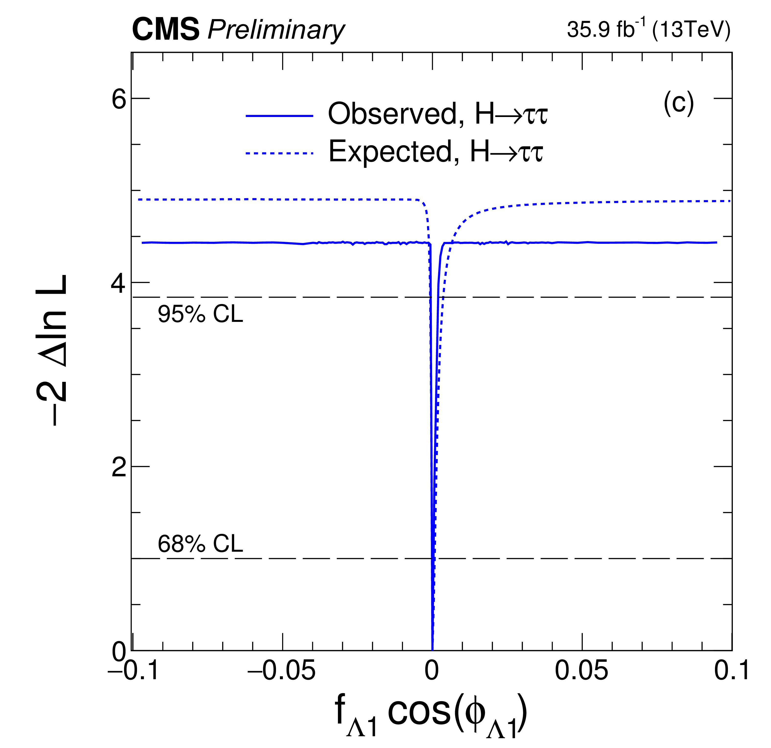
Figure 9-c:
Observed (solid) and expected (dashed) likelihood scans of $f_{a3}\cos(\phi _{a3})$ (a), $f_{a2}\cos(\phi _{a2})$ (b), $f_{\lambda 1}\cos(\phi _{\lambda 1})$ (c), and $f_{\lambda 1}^{Z\gamma}\cos(\phi _{\lambda 1}^{Z\gamma})$ (d). |
png pdf |
Figure 9-d:
Observed (solid) and expected (dashed) likelihood scans of $f_{a3}\cos(\phi _{a3})$ (a), $f_{a2}\cos(\phi _{a2})$ (b), $f_{\lambda 1}\cos(\phi _{\lambda 1})$ (c), and $f_{\lambda 1}^{Z\gamma}\cos(\phi _{\lambda 1}^{Z\gamma})$ (d). |
png pdf |
Figure 10:
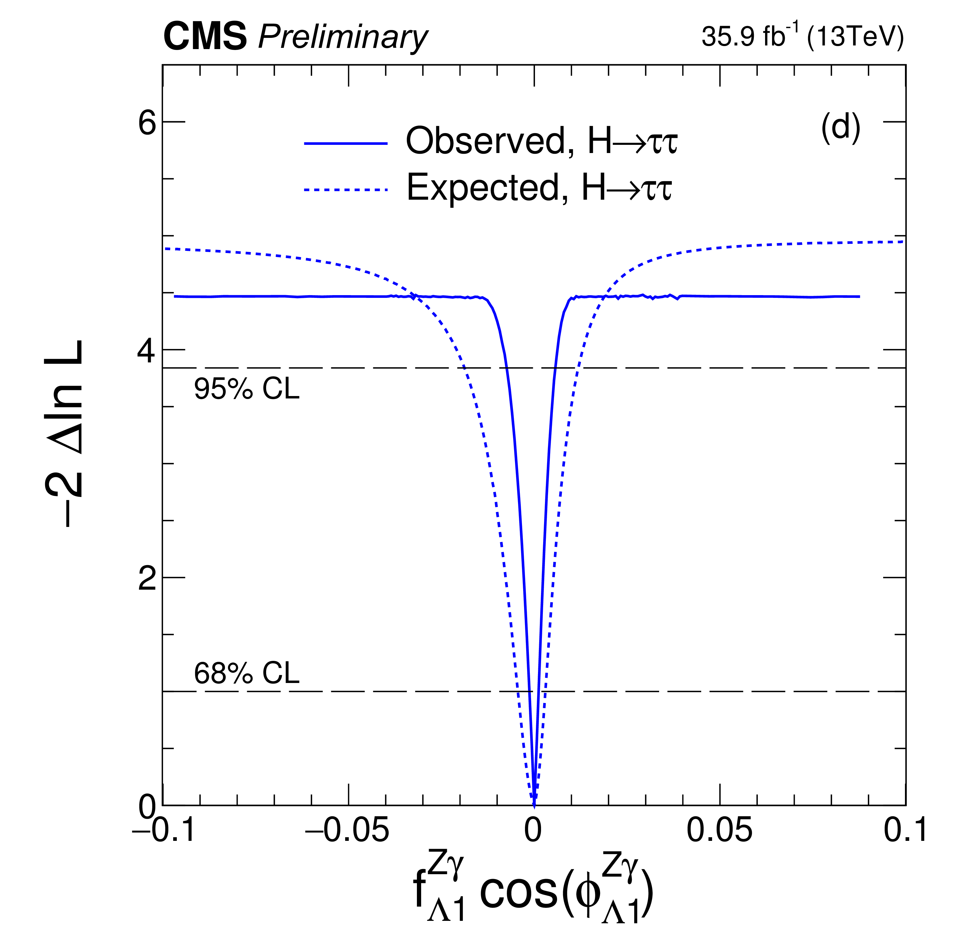
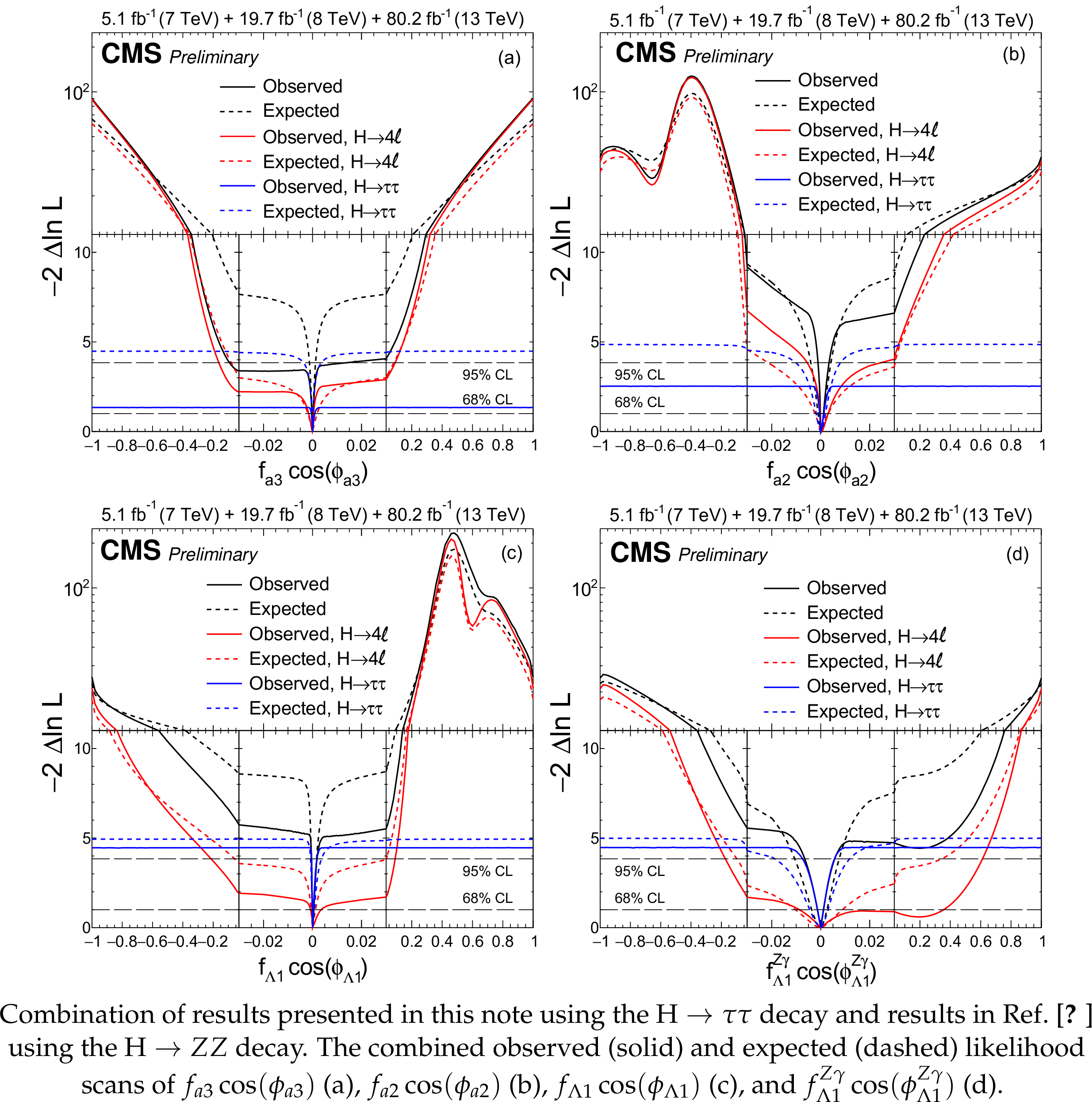
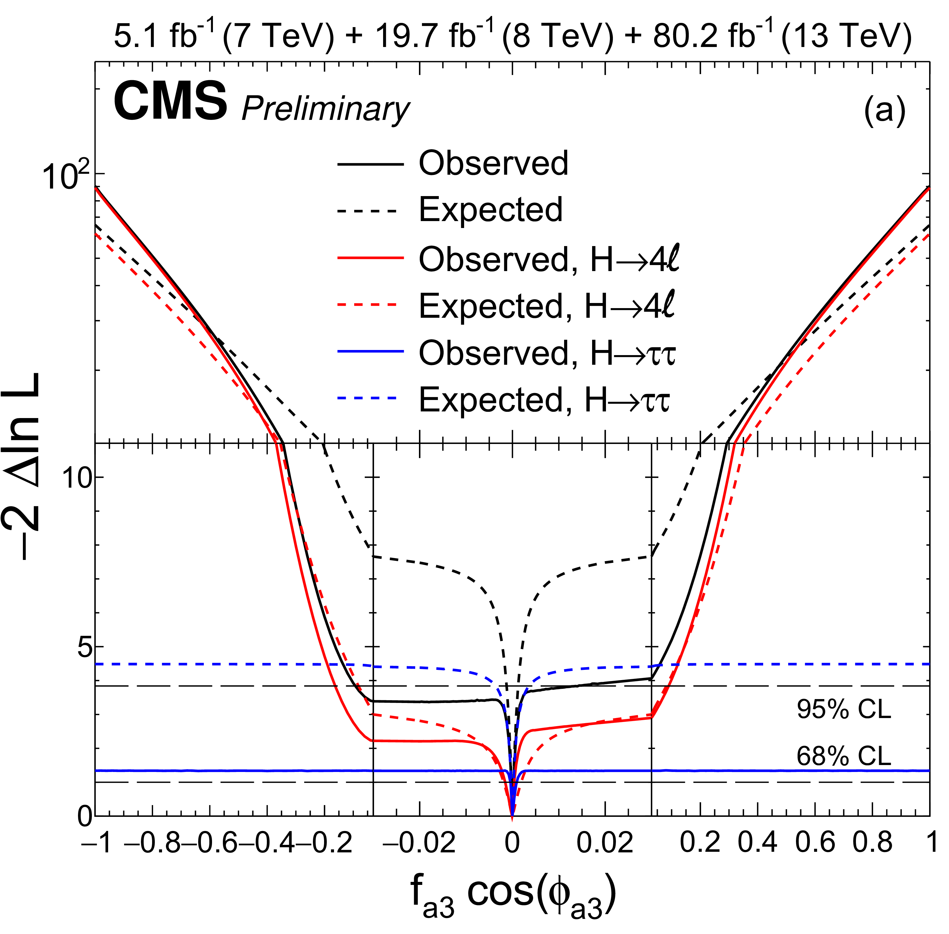
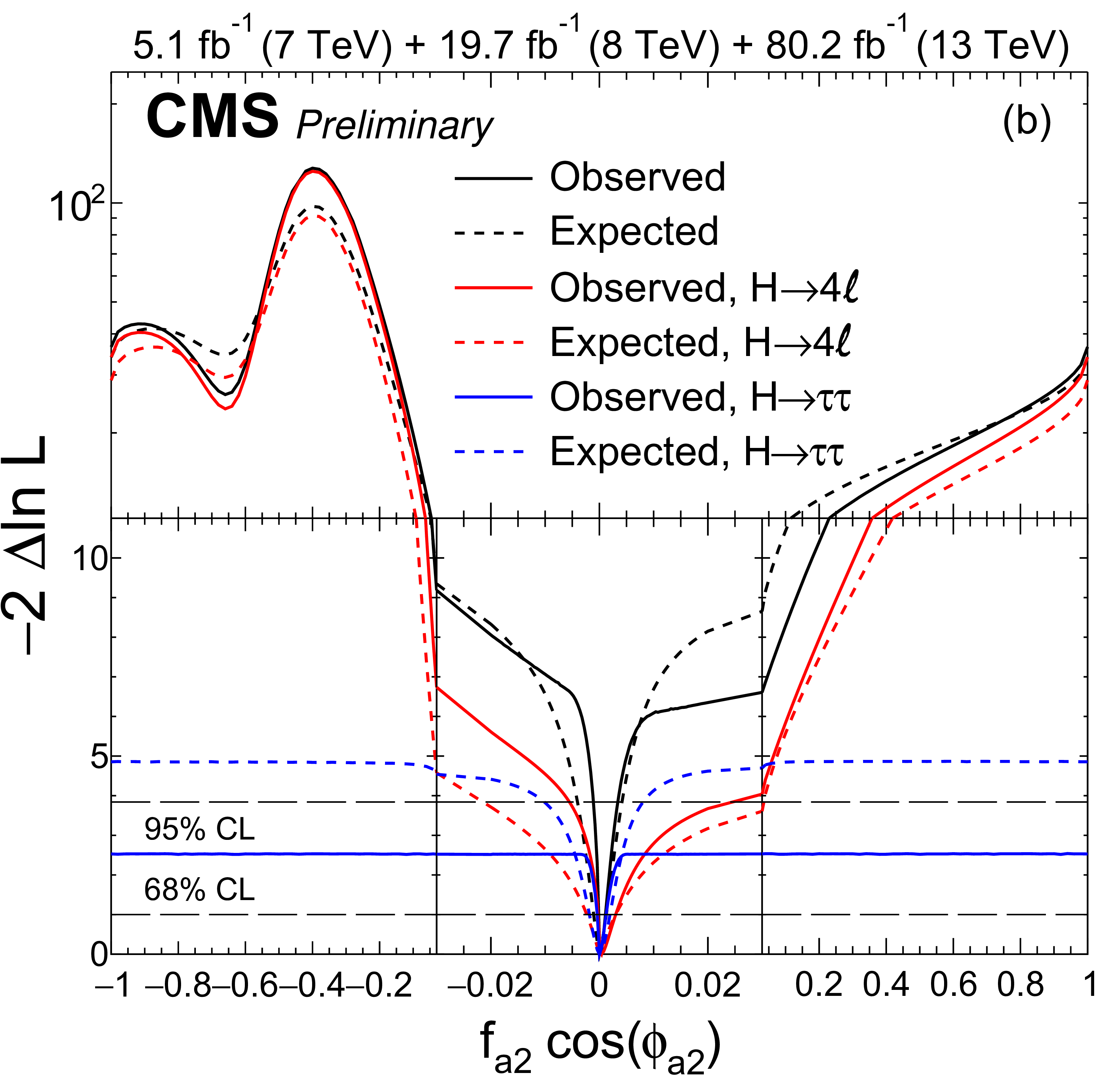
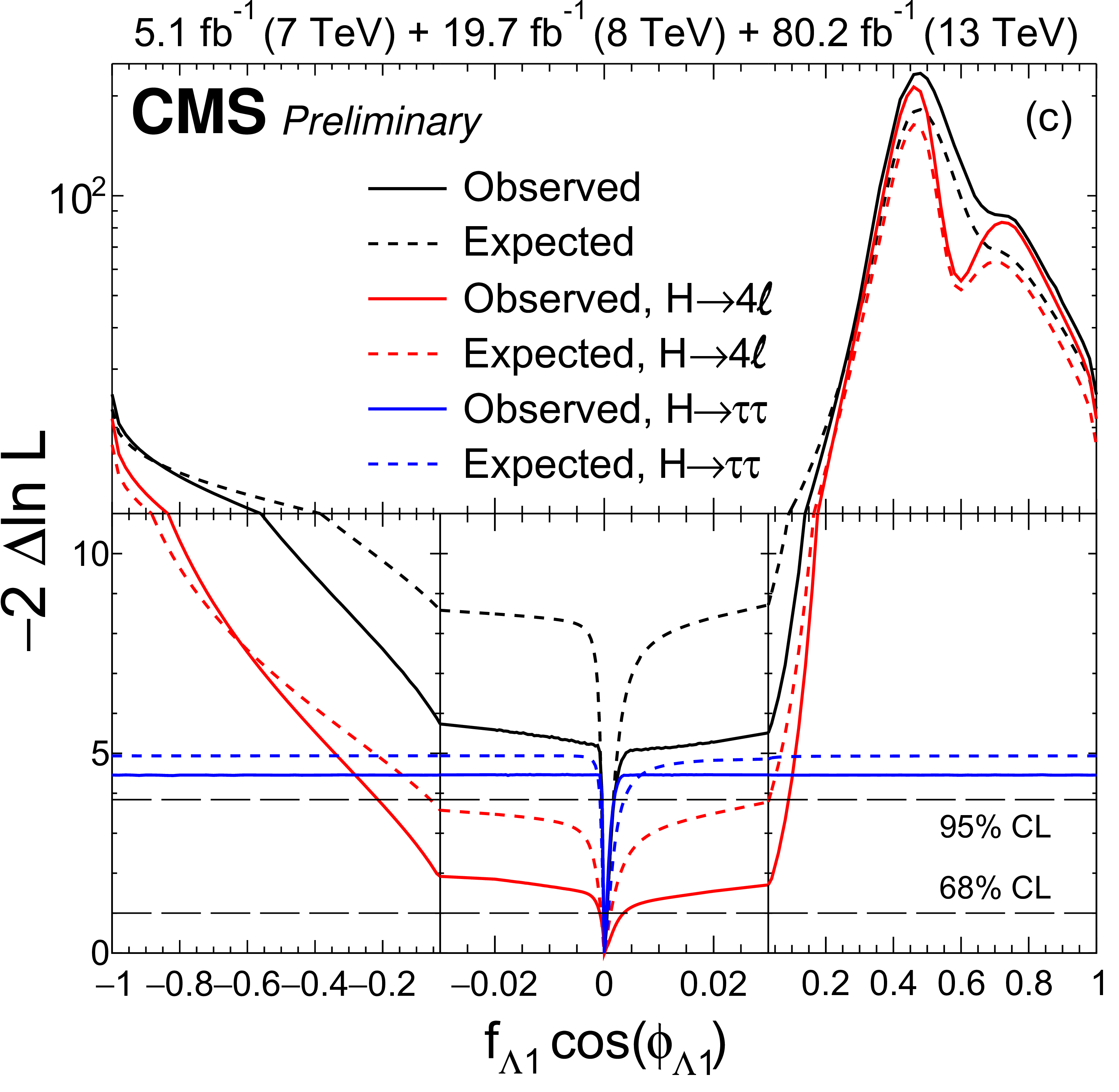
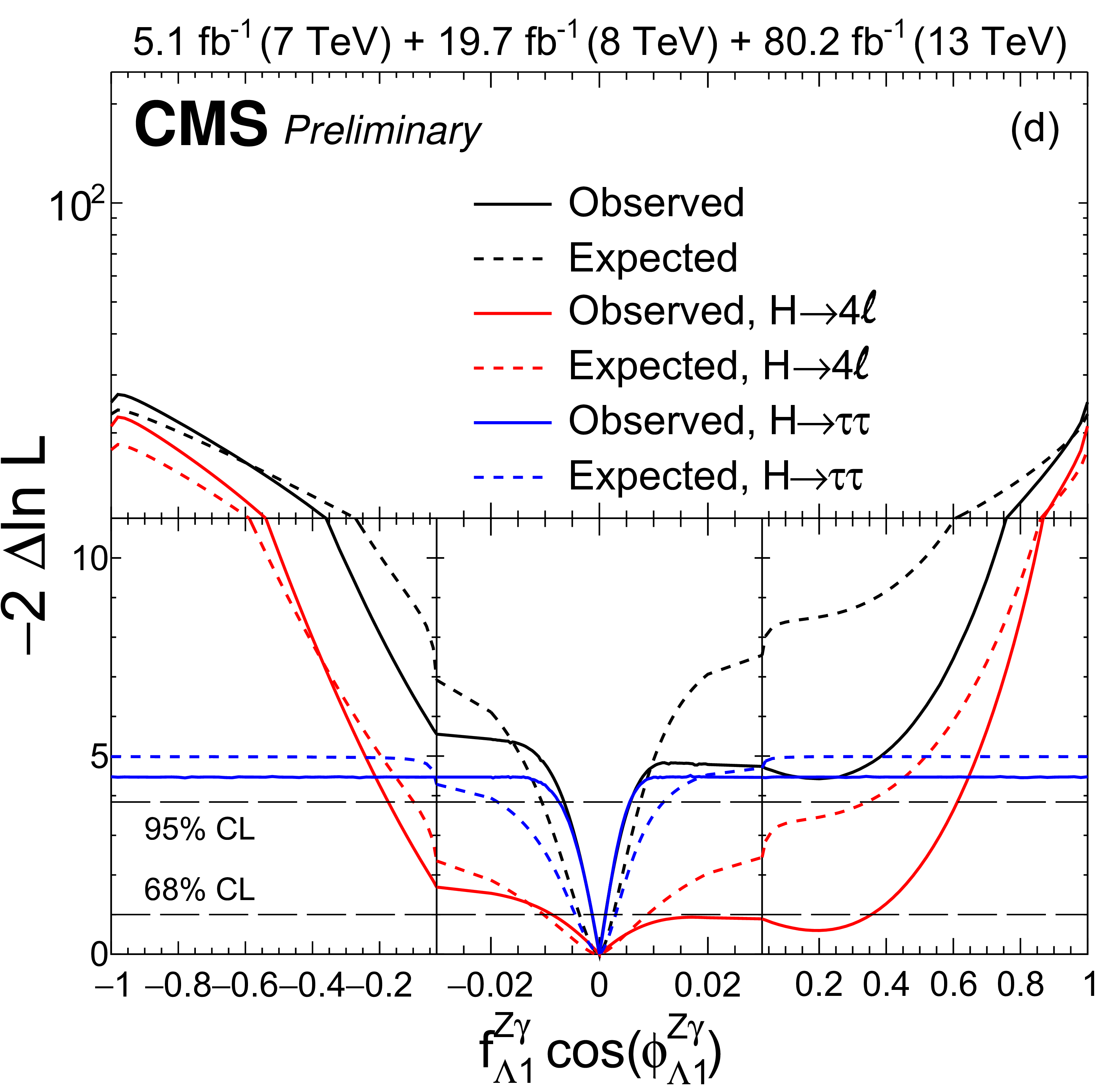
Combination of results presented in this note using the $ {\mathrm {H}} \to \tau \tau $ decay and results in Ref. [14] using the $ {\mathrm {H}} \to ZZ$ decay. The combined observed (solid) and expected (dashed) likelihood scans of $f_{a3}\cos(\phi _{a3})$ (a), $f_{a2}\cos(\phi _{a2})$ (b), $f_{\lambda 1}\cos(\phi _{\lambda 1})$ (c), and $f_{\lambda 1}^{Z\gamma}\cos(\phi _{\lambda 1}^{Z\gamma})$ (d). |
png pdf |
Figure 10-a:
Combination of results presented in this note using the $ {\mathrm {H}} \to \tau \tau $ decay and results in Ref. [14] using the $ {\mathrm {H}} \to ZZ$ decay. The combined observed (solid) and expected (dashed) likelihood scans of $f_{a3}\cos(\phi _{a3})$ (a), $f_{a2}\cos(\phi _{a2})$ (b), $f_{\lambda 1}\cos(\phi _{\lambda 1})$ (c), and $f_{\lambda 1}^{Z\gamma}\cos(\phi _{\lambda 1}^{Z\gamma})$ (d). |
png pdf |
Figure 10-b:
Combination of results presented in this note using the $ {\mathrm {H}} \to \tau \tau $ decay and results in Ref. [14] using the $ {\mathrm {H}} \to ZZ$ decay. The combined observed (solid) and expected (dashed) likelihood scans of $f_{a3}\cos(\phi _{a3})$ (a), $f_{a2}\cos(\phi _{a2})$ (b), $f_{\lambda 1}\cos(\phi _{\lambda 1})$ (c), and $f_{\lambda 1}^{Z\gamma}\cos(\phi _{\lambda 1}^{Z\gamma})$ (d). |
png pdf |
Figure 10-c:
Combination of results presented in this note using the $ {\mathrm {H}} \to \tau \tau $ decay and results in Ref. [14] using the $ {\mathrm {H}} \to ZZ$ decay. The combined observed (solid) and expected (dashed) likelihood scans of $f_{a3}\cos(\phi _{a3})$ (a), $f_{a2}\cos(\phi _{a2})$ (b), $f_{\lambda 1}\cos(\phi _{\lambda 1})$ (c), and $f_{\lambda 1}^{Z\gamma}\cos(\phi _{\lambda 1}^{Z\gamma})$ (d). |
png pdf |
Figure 10-d:
Combination of results presented in this note using the $ {\mathrm {H}} \to \tau \tau $ decay and results in Ref. [14] using the $ {\mathrm {H}} \to ZZ$ decay. The combined observed (solid) and expected (dashed) likelihood scans of $f_{a3}\cos(\phi _{a3})$ (a), $f_{a2}\cos(\phi _{a2})$ (b), $f_{\lambda 1}\cos(\phi _{\lambda 1})$ (c), and $f_{\lambda 1}^{Z\gamma}\cos(\phi _{\lambda 1}^{Z\gamma})$ (d). |
| Tables | |
png pdf |
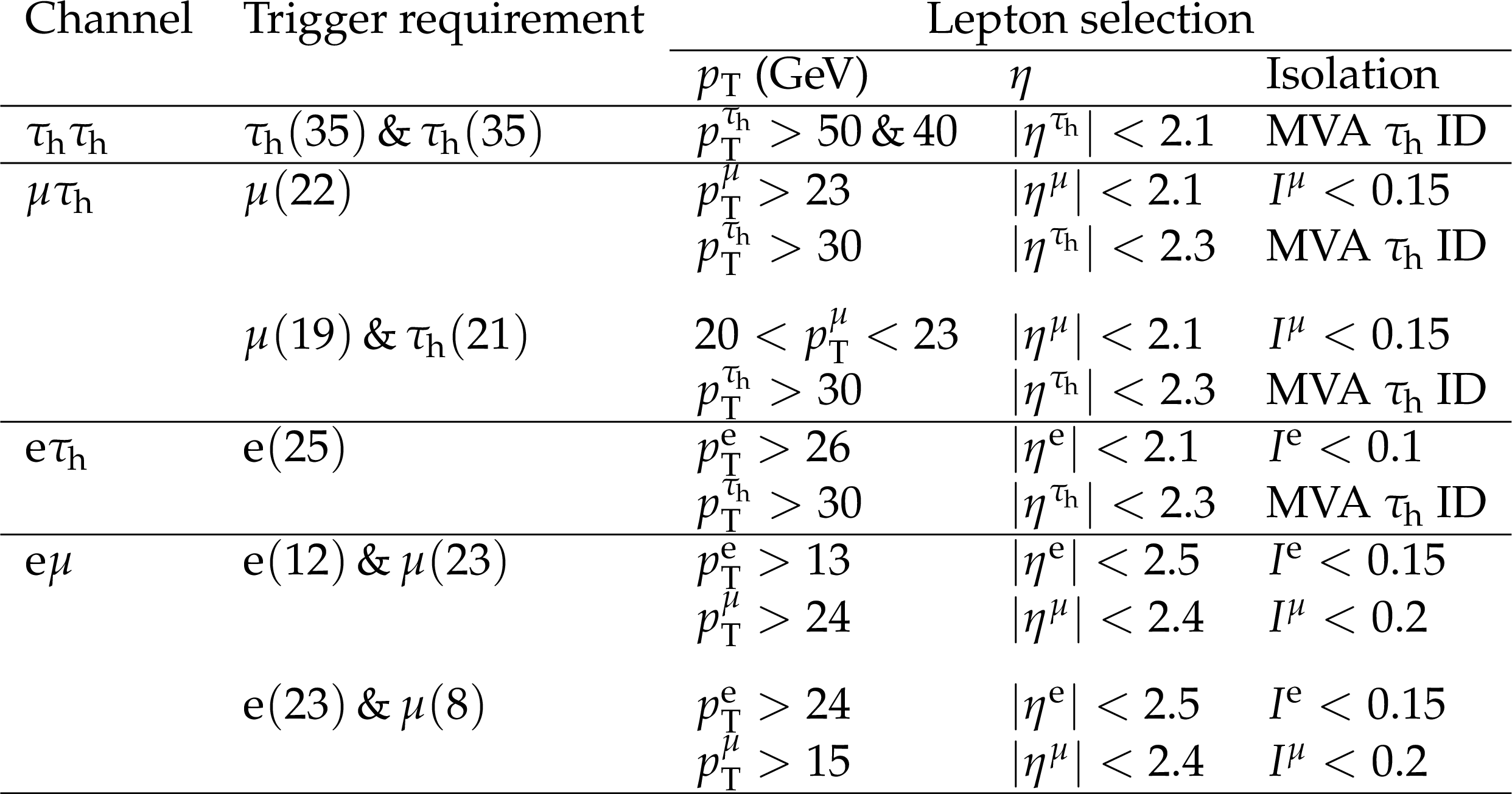
Table 1:
Kinematic selection criteria for the four decay channels. For the trigger threshold requirements, the numbers indicate the approximate trigger thresholds in GeV. The lepton selection criteria include transverse momentum threshold, pseudo-rapidity range as well as isolation criteria. |
png pdf |
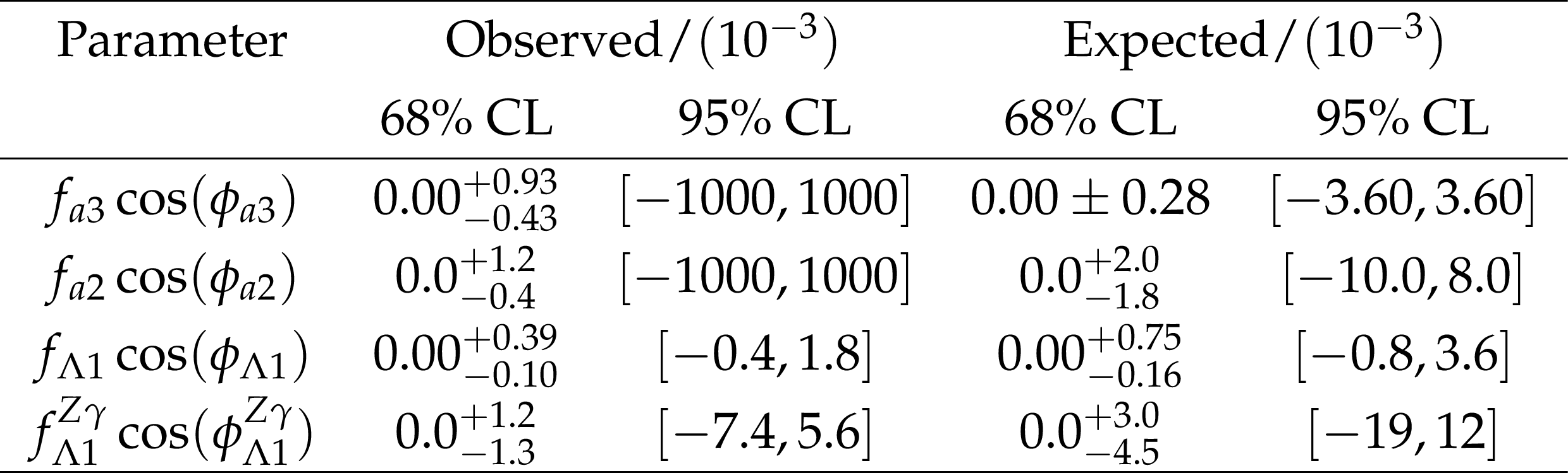
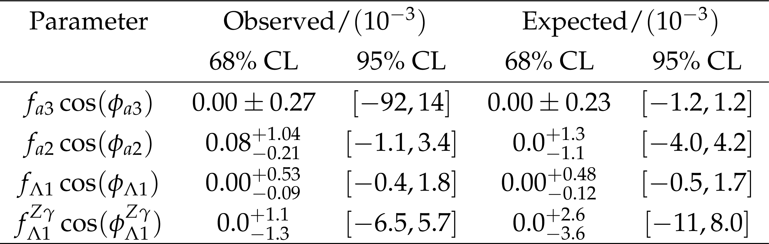
Table 2:
Summary of allowed 68% CL (central values with uncertainties) and 95% CL (in square brackets) intervals on anomalous coupling parameters using the $ {\mathrm {H}} \to \tau \tau $ decay. |
png pdf |
Table 3:
Summary of allowed 68% CL (central values with uncertainties) and 95% CL (in square brackets) intervals on anomalous coupling parameters using combination of the $ {\mathrm {H}} \to \tau \tau $ and $ {\mathrm {H}} \to 4\ell $ [14] decay channels. |
| Summary |
| A study of anomalous HVV interactions of the Higgs boson, including CP violation, has been presented, using its associated production with two quark jets in vector boson fusion and VH with subsequent decay to a pair of tau leptons. Constraints on the CP-violating parameter $f_{a3}$ and on the CP-conserving parameters $f_{a2}$, $f_{\lambda 1}$, and $f_{\lambda 1}^{Z\gamma}$ are set using matrix element techniques. The observed and expected limits on parameters are summarized in Table 2. The 68% CL constraints are generally tighter than those from previous measurements using either production or decay information. Further constraints are obtained in the combination of the $\mathrm{H}\to\tau\tau$ and $\mathrm{H}\to 4\ell$ decay channels and are summarized in Table 3. This results in the most stringent constraints on anomalous Higgs boson couplings: $f_{a3}\cos(\phi_{a3})=(0.00 \pm 0.27 )\times10^{-3}$, $f_{a2}\cos(\phi_{a2})=(0.08^{+1.04}_{-0.21})\times10^{-3}$, $f_{\lambda 1}\cos(\phi_{\lambda 1})=(0.00^{+0.53}_{-0.09})\times10^{-3}$, and $f_{\lambda 1}^{Z\gamma}\cos(\phi_{\lambda 1}^{Z\gamma})=(0.0^{+1.1}_{-1.3})\times10^{-3}$. The results are consistent with expectations for the standard model Higgs boson. |
| Additional Figures | |
png pdf |
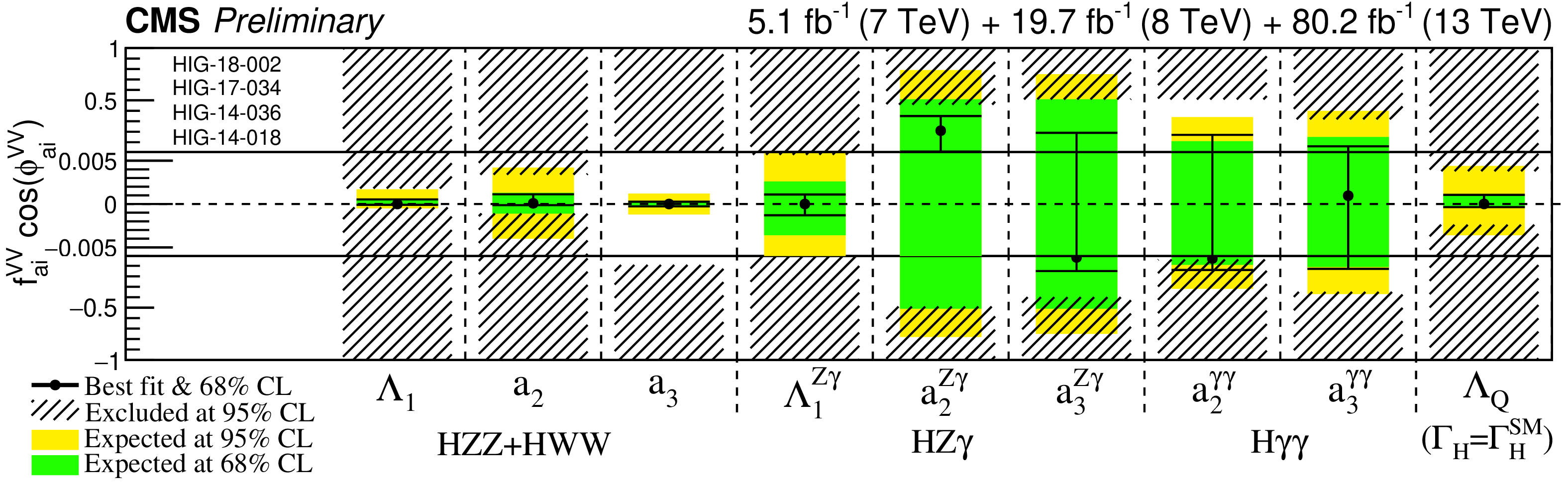
Additional Figure 1:
Summary of confidence level intervals of anomalous coupling parameters in $ {\mathrm {H}} \mathrm {V} \mathrm {V} $ interactions under the assumption that all the coupling ratios are real ($\phi _{ai}^{\mathrm {V} \mathrm {V}}=$ 0 or $\pi $). The $ {\mathrm {H}} {\mathrm {Z}} {\mathrm {Z}} + {\mathrm {H}} {\mathrm {W}} {\mathrm {W}}$ coupling limits assume that $a_{i}^{{\mathrm {Z}} {\mathrm {Z}}}=a_{i}^{{\mathrm {W}} {\mathrm {W}}}$. The expected 68% and 95% CL regions are shown as green and yellow bands. The observed intervals for 68% CL are shown as points with error bars, and the hatched areas indicate the excluded regions at 95% CL. The limits on $f_{a2,3}^{{\mathrm {Z}} \gamma,\gamma \gamma}$ are from Ref. [10], and the limits on $f_{\Lambda Q}$ are from Ref. [11]. |
| References | ||||
| 1 | S. L. Glashow | Partial-symmetries of weak interactions | NP 22 (1961) 579 | |
| 2 | F. Englert and R. Brout | Broken Symmetry and the Mass of Gauge Vector Mesons | PRL 13 (1964) 321 | |
| 3 | P. W. Higgs | Broken symmetries, massless particles and gauge fields | PL12 (1964) 132 | |
| 4 | P. W. Higgs | Broken symmetries and the masses of gauge bosons | PRL 13 (1964) 508 | |
| 5 | G. S. Guralnik, C. R. Hagen, and T. W. B. Kibble | Global conservation laws and massless particles | PRL 13 (1964) 585 | |
| 6 | S. Weinberg | A model of leptons | PRL 19 (1967) 1264 | |
| 7 | A. Salam | Weak and electromagnetic interactions | in Elementary particle physics: relativistic groups and analyticity, N. Svartholm, ed., p. 367 Almqvist \& Wiksell, Stockholm, 1968 Proceedings of the eighth Nobel symposium | |
| 8 | CMS Collaboration | On the mass and spin-parity of the Higgs boson candidate via its decays to Z boson pairs | PRL 110 (2013) 081803 | CMS-HIG-12-041 1212.6639 |
| 9 | CMS Collaboration | Measurement of the properties of a Higgs boson in the four-lepton final state | PRD 89 (2014) 092007 | CMS-HIG-13-002 1312.5353 |
| 10 | CMS Collaboration | Constraints on the spin-parity and anomalous HVV couplings of the Higgs boson in proton collisions at 7 and 8 TeV | PRD 92 (2015) 012004 | CMS-HIG-14-018 1411.3441 |
| 11 | CMS Collaboration | Limits on the Higgs boson lifetime and width from its decay to four charged leptons | PRD 92 (2015) 072010 | CMS-HIG-14-036 1507.06656 |
| 12 | CMS Collaboration | Combined search for anomalous pseudoscalar HVV couplings in VH(H $ \to \text{b}\bar{\text{b}} $) production and H $ \to $ VV decay | PLB 759 (2016) 672 | CMS-HIG-14-035 1602.04305 |
| 13 | CMS Collaboration | Constraints on anomalous Higgs boson couplings using production and decay information in the four-lepton final state | PLB775 (2017) 1 | CMS-HIG-17-011 1707.00541 |
| 14 | CMS Collaboration | Measurements of Higgs boson width and anomalous HVV couplings from on-shell and off-shell production in the four-lepton final state | CDS | |
| 15 | ATLAS Collaboration | Evidence for the spin-0 nature of the Higgs boson using ATLAS data | PLB 726 (2013) 120 | 1307.1432 |
| 16 | ATLAS Collaboration | Study of the spin and parity of the Higgs boson in diboson decays with the ATLAS detector | EPJC 75 (2015) 476 | 1506.05669 |
| 17 | ATLAS Collaboration | Test of CP invariance in vector-boson fusion production of the Higgs boson using the Optimal Observable method in the ditau decay channel with the ATLAS detector | EPJC 76 (2016) 658 | 1602.04516 |
| 18 | ATLAS Collaboration | Measurement of inclusive and differential cross sections in the $ H \rightarrow ZZ^* \rightarrow 4\ell $ decay channel in $ pp $ collisions at $ \sqrt{s}= $ 13 TeV with the ATLAS detector | JHEP 10 (2017) 132 | 1708.02810 |
| 19 | ATLAS Collaboration | Measurement of the Higgs boson coupling properties in the $ H\rightarrow ZZ^{*} \rightarrow 4\ell $ decay channel at $ \sqrt{s} = $ 13 TeV with the ATLAS detector | JHEP 03 (2018) 095 | 1712.02304 |
| 20 | ATLAS Collaboration | Measurements of Higgs boson properties in the diphoton decay channel with 36 fb$ ^{-1} $ of $ pp $ collision data at $ \sqrt{s} = $ 13 TeV with the ATLAS detector | PRD98 (2018) 052005 | 1802.04146 |
| 21 | CMS Collaboration | Observation of the Higgs boson decay to a pair of $ \tau $ leptons with the CMS detector | Submitted to PLB | CMS-HIG-16-043 1708.00373 |
| 22 | CMS Collaboration | The CMS experiment at the CERN LHC | JINST 3 (2008) S08004 | CMS-00-001 |
| 23 | CMS Collaboration | Particle-flow reconstruction and global event description with the cms detector | JINST 12 (2017) P10003 | CMS-PRF-14-001 1706.04965 |
| 24 | CMS Collaboration | Performance of the CMS muon detector and muon reconstruction with proton-proton collisons at $ \sqrt{s} = $ ~13 TeV | JINST 13 (2018) P06015 | CMS-MUO-16-001 1804.04528 |
| 25 | CMS Collaboration | Performance of electron reconstruction and selection with the CMS detector in proton-proton collisions at $ \sqrt{s} = $ 8 TeV | JINST 10 (2015) P06005 | CMS-EGM-13-001 1502.02701 |
| 26 | M. Cacciari, G. P. Salam, and G. Soyez | FastJet user manual | EPJC 72 (2012) 1896 | 1111.6097 |
| 27 | M. Cacciari, G. P. Salam | Dispelling the $ N^{3} $ myth for the $ k_t $ jet-finder | PLB 641 (2006) 57 | hep-ph/0512210 |
| 28 | CMS Collaboration | Reconstruction and identification of $ \tau $ lepton decays to hadrons and $ \nu_\tau $ at CMS | JINST 11 (2016) P01019 | CMS-TAU-14-001 1510.07488 |
| 29 | CMS Collaboration | Performance of reconstruction and identification of $ \tau $ leptons decaying to hardons and $ \nu_{\tau} $ in pp collisions at $ \sqrt{s} = $ 13 TeV | CMS-TAU-16-003 1809.02816 |
|
| 30 | H. Voss, A. Hocker, J. Stelzer, and F. Tegenfeldt | TMVA, the toolkit for multivariate data analysis with ROOT | in XI Int. Workshop on Advanced Computing and Analysis Techniques in Physics Research 2007 | physics/0703039 |
| 31 | CMS Collaboration | Performance of missing transverse momentum in pp collisions at $ \sqrt{s} = $ 13 TeV using the CMS detector | CDS | |
| 32 | L. Bianchini, J. Conway, E. K. Friis, and C. Veelken | Reconstruction of the Higgs mass in $ H \to \tau\tau $ Events by Dynamical Likelihood techniques | J. Phys. Conf. Ser. 513 (2014) 022035 | |
| 33 | T. Plehn, D. L. Rainwater, and D. Zeppenfeld | Determining the structure of Higgs couplings at the LHC | PRL 88 (2002) 051801 | hep-ph/0105325 |
| 34 | V. Hankele, G. Klamke, D. Zeppenfeld, and T. Figy | Anomalous Higgs boson couplings in vector boson fusion at the CERN LHC | PRD 74 (2006) 095001 | hep-ph/0609075 |
| 35 | E. Accomando et al. | Workshop on CP Studies and Non-Standard Higgs Physics | hep-ph/0608079 | |
| 36 | K. Hagiwara, Q. Li, and K. Mawatari | Jet angular correlation in vector-boson fusion processes at hadron colliders | JHEP 07 (2009) 101 | 0905.4314 |
| 37 | Y. Gao et al. | Spin determination of single-produced resonances at hadron colliders | PRD 81 (2010) 075022 | 1001.3396 |
| 38 | A. De R\' ujula et al. | Higgs look-alikes at the LHC | PRD 82 (2010) 013003 | 1001.5300 |
| 39 | S. Bolognesi et al. | Spin and parity of a single-produced resonance at the LHC | PRD 86 (2012) 095031 | 1208.4018 |
| 40 | J. Ellis, D. S. Hwang, V. Sanz, and T. You | A fast track towards the `Higgs' spin and parity | JHEP 11 (2012) 134 | 1208.6002 |
| 41 | P. Artoisenet et al. | A framework for Higgs characterisation | JHEP 11 (2013) 043 | 1306.6464 |
| 42 | I. Anderson et al. | Constraining anomalous HVV interactions at proton and lepton colliders | PRD 89 (2014) 035007 | 1309.4819 |
| 43 | M. J. Dolan, P. Harris, M. Jankowiak, and M. Spannowsky | Constraining $ CP $-violating Higgs Sectors at the LHC using gluon fusion | PRD90 (2014) 073008 | 1406.3322 |
| 44 | A. Greljo, G. Isidori, J. M. Lindert, and D. Marzocca | Pseudo-observables in electroweak Higgs production | EPJC 76 (2016) 158 | 1512.06135 |
| 45 | A. V. Gritsan, R. Rontsch, M. Schulze, and M. Xiao | Constraining anomalous Higgs boson couplings to the heavy flavor fermions using matrix element techniques | PRD 94 (2016) 055023 | 1606.03107 |
| 46 | S. Frixione, P. Nason, and C. Oleari | Matching NLO QCD computations with Parton Shower simulations: the POWHEG method | JHEP 11 (2007) 070 | 0709.2092 |
| 47 | E. Bagnaschi, G. Degrassi, P. Slavich, and A. Vicini | Higgs production via gluon fusion in the POWHEG approach in the SM and in the MSSM | JHEP 02 (2012) 088 | 1111.2854 |
| 48 | P. Nason and C. Oleari | NLO Higgs boson production via vector-boson fusion matched with shower in POWHEG | JHEP 02 (2010) 037 | 0911.5299 |
| 49 | G. Luisoni, P. Nason, C. Oleari, and F. Tramontano | $ HW^{\pm} $/HZ + 0 and 1 jet at NLO with the POWHEG BOX interfaced to GoSam and their merging within MiNLO | JHEP 10 (2013) 083 | 1306.2542 |
| 50 | T. Sjostrand et al. | An introduction to PYTHIA 8.2 | CPC 191 (2015) 159 | 1410.3012 |
| 51 | NNPDF Collaboration | Unbiased global determination of parton distributions and their uncertainties at NNLO and at LO | NPB 855 (2012) 153 | 1107.2652 |
| 52 | GEANT4 Collaboration | GEANT4---a simulation toolkit | NIMA 506 (2003) 250 | |
| 53 | CMS Collaboration | Observation of a new boson at a mass of 125 GeV with the CMS experiment at the LHC | PLB 716 (2012) 30 | CMS-HIG-12-028 1207.7235 |
| 54 | S. S. Wilks | The large-sample distribution of the likelihood ratio for testing composite hypotheses | Ann. Math. Stat. 9 (1938) 60 | |
|
|
Compact Muon Solenoid LHC, CERN |
|

|

|

|

|

|