

Compact Muon Solenoid
LHC, CERN
| CMS-PAS-EXO-19-016 | ||
| Search for a third-generation leptoquark coupling to a $\tau$ lepton and a b quark through single, pair and nonresonant production at $\sqrt{s}= $ 13 TeV | ||
| CMS Collaboration | ||
| July 2022 | ||
| Abstract: A search is presented for a third-generation leptoquark (LQ) coupling to a $\tau$ lepton and a b quark. Events with $\tau$ leptons plus at least one jet originating from a b quark are considered, targeting the single and pair production of the LQ as well as nonresonant production via $t$-channel LQ exchange. The search is based on proton-proton collision data at a center-of-mass energy of $\sqrt{s}= $ 13 TeV recorded with the CMS detector, corresponding to an integrated luminosity of 137 fb$^{-1}$. Upper limits are set on the LQ production cross section in the LQ mass range 0.5-2.3 TeV. Lower limits at 95% confidence level on the LQ mass are set in the 1.22-1.96 TeV range and for a coupling strength less than 2.5, depending on the LQ model. Upper limits are also set on the coupling strength of such LQs as a function of their mass. For a representative LQ mass of 2 TeV and a coupling strength of 2.5, an excess with a significance of 3.4 standard deviations above the standard model expectation is observed in the data. Consequently, the observed upper limits on the LQ production cross section are about three times larger than expected for this benchmark. | ||
|
Links:
CDS record (PDF) ;
CADI line (restricted) ;
These preliminary results are superseded in this paper, Submitted to JHEP. The superseded preliminary plots can be found here. |
||
| Figures & Tables | Summary | Additional Figures | References | CMS Publications |
|---|
| Figures | |

png pdf |
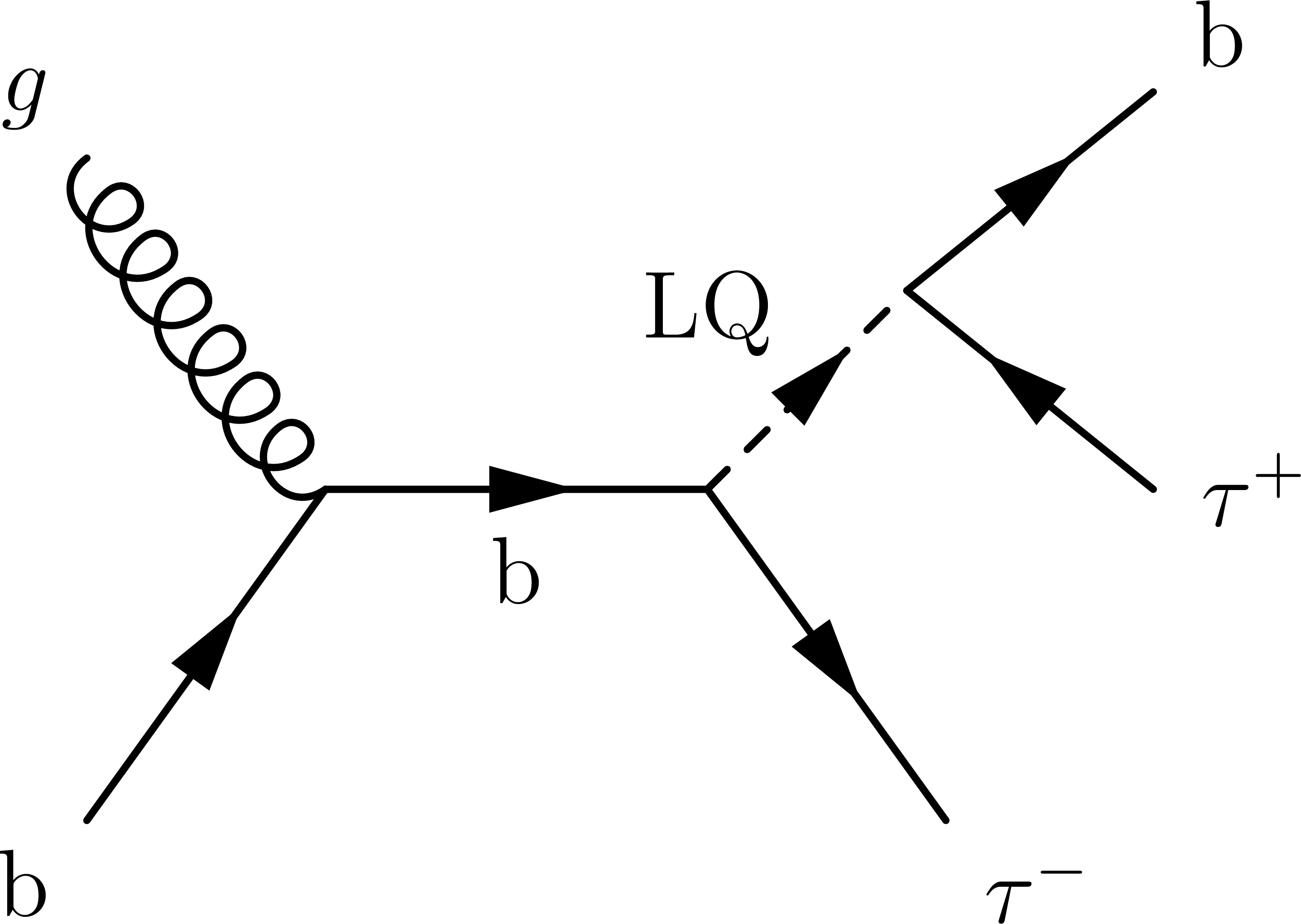
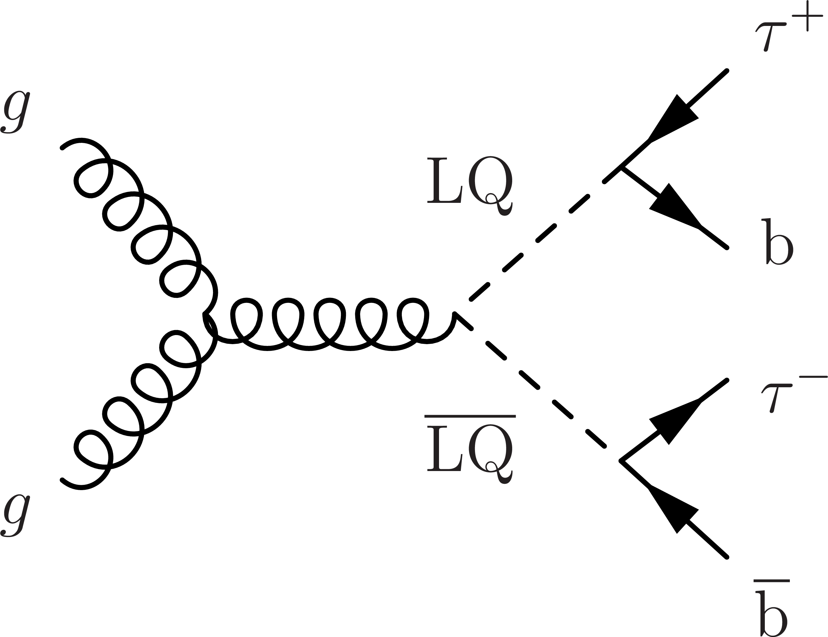
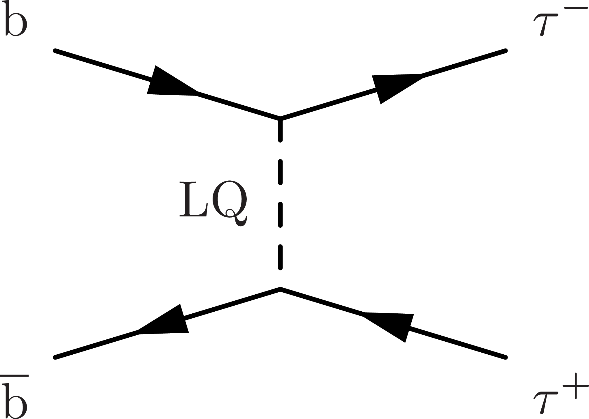
Figure 1:
Dominant Feynman diagrams of the signal at LO: single (left) and pair LQ production (center), as well as nonresonant production of two $\tau$ leptons via $t$-channel LQ exchange (right). |
png pdf |
Figure 1-a:
Dominant Feynman diagram of single LQ production at LO. |
png pdf |
Figure 1-b:
Dominant Feynman diagram of pair LQ production at LO. |
png pdf |
Figure 1-c:
Dominant Feynman diagram of nonresonant production of two $\tau$ leptons via $t$-channel LQ exchange at LO. |
png pdf |
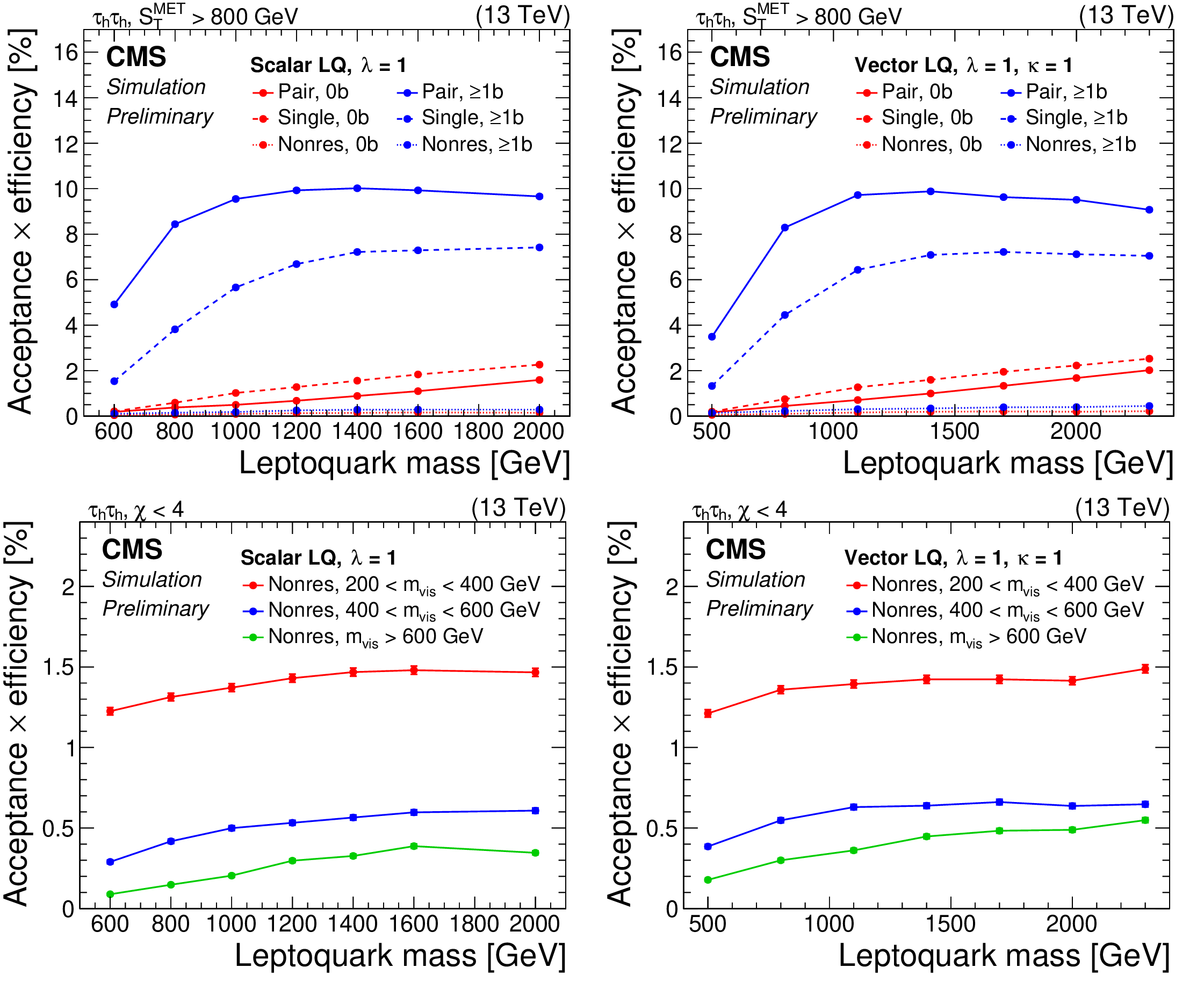
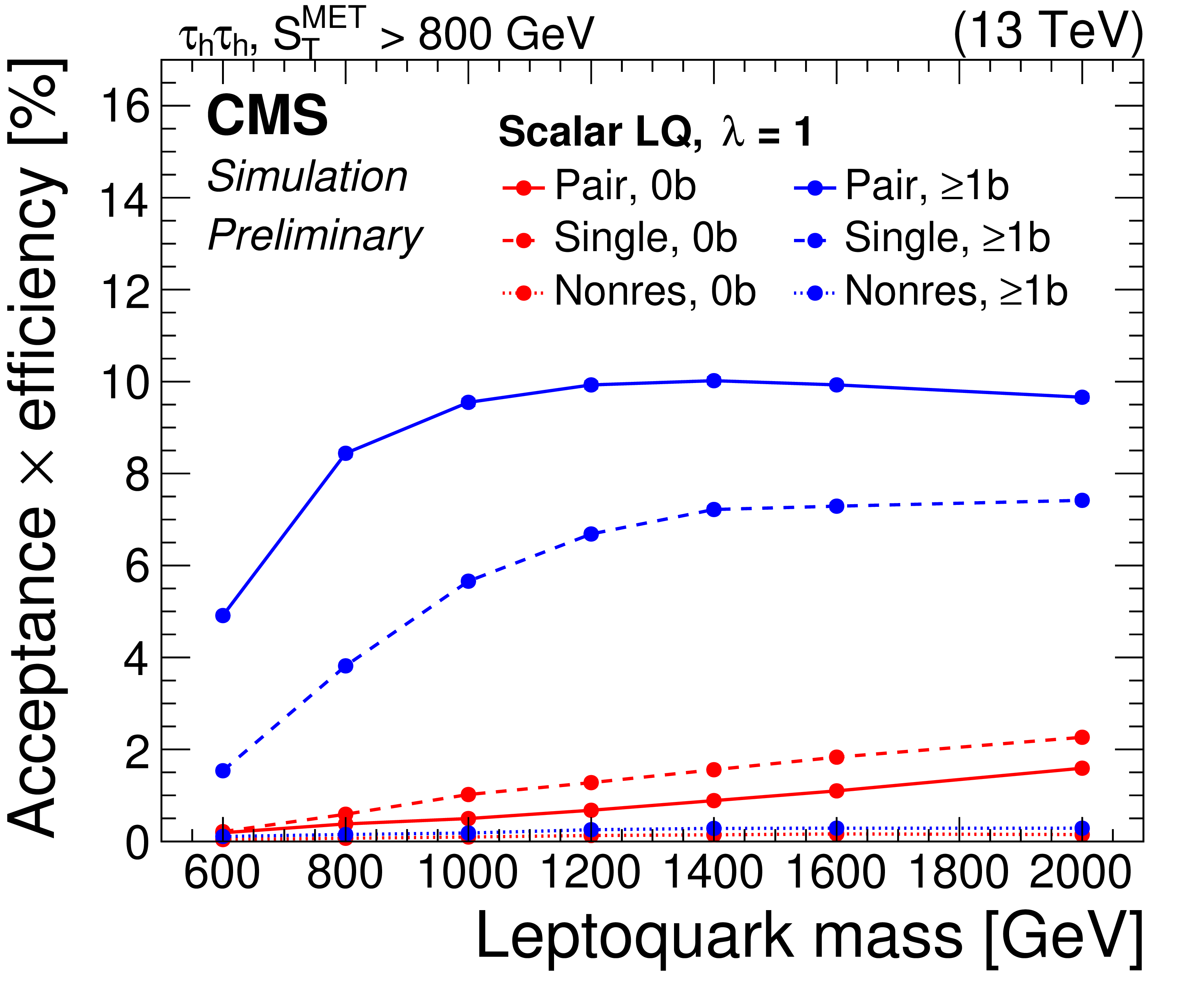
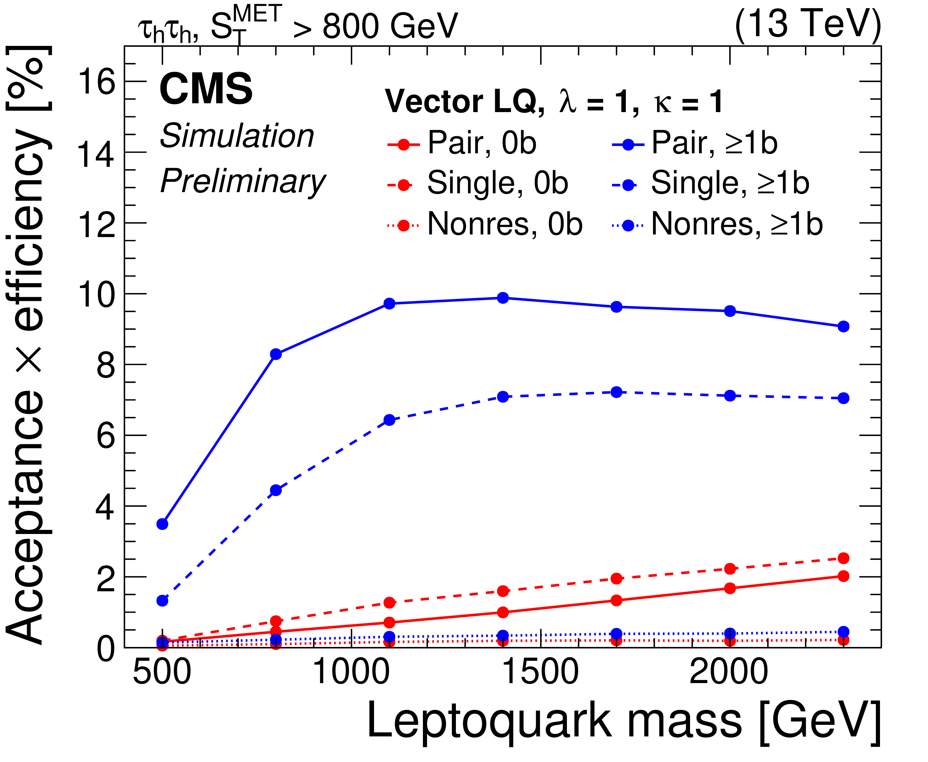
Figure 2:
The product of acceptance and efficiency for a vector LQ signal in the ${{\tau_{\mathrm{h}}\tau_{\mathrm{h}}}} $ (left) and $\mu\tau_{\mathrm{h}} $ (right) channels of the 0b and $\geq $1b (top), and the 0j categories (bottom) are shown. Vertical bars indicate the statistical uncertainty in the efficiency. |
png pdf |
Figure 2-a:
The product of acceptance and efficiency for a vector LQ signal in the ${{\tau_{\mathrm{h}}\tau_{\mathrm{h}}}} $ channel of the 0b and $\geq $1b category is shown. Vertical bars indicate the statistical uncertainty in the efficiency. |
png pdf |
Figure 2-b:
The product of acceptance and efficiency for a vector LQ signal in the $\mu\tau_{\mathrm{h}} $ channel of the 0b and $\geq $1b category is shown. Vertical bars indicate the statistical uncertainty in the efficiency. |
png pdf |
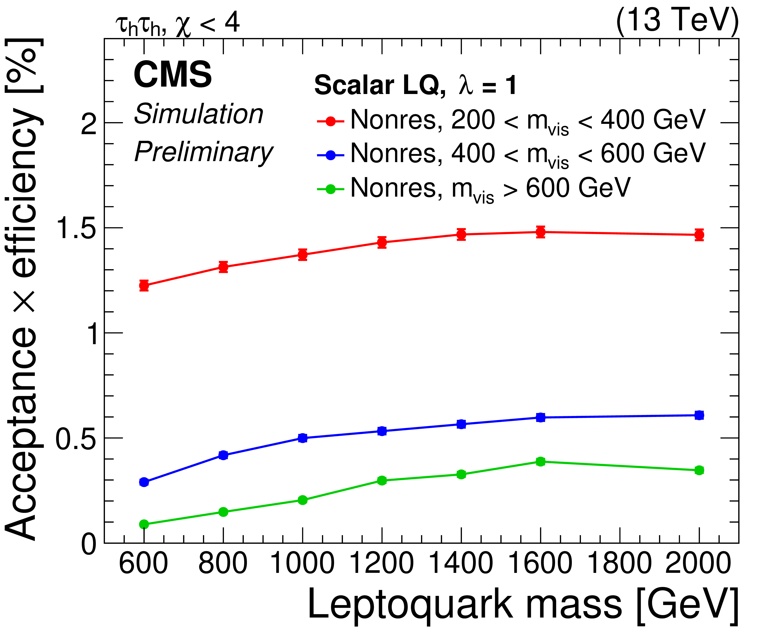
Figure 2-c:
The product of acceptance and efficiency for a vector LQ signal in the ${{\tau_{\mathrm{h}}\tau_{\mathrm{h}}}} $ channel of the 0j category is shown. Vertical bars indicate the statistical uncertainty in the efficiency. |

png pdf |
Figure 2-d:
The product of acceptance and efficiency for a vector LQ signal in the $\mu\tau_{\mathrm{h}} $ channel of the 0j category is shown. Vertical bars indicate the statistical uncertainty in the efficiency. |
png pdf |
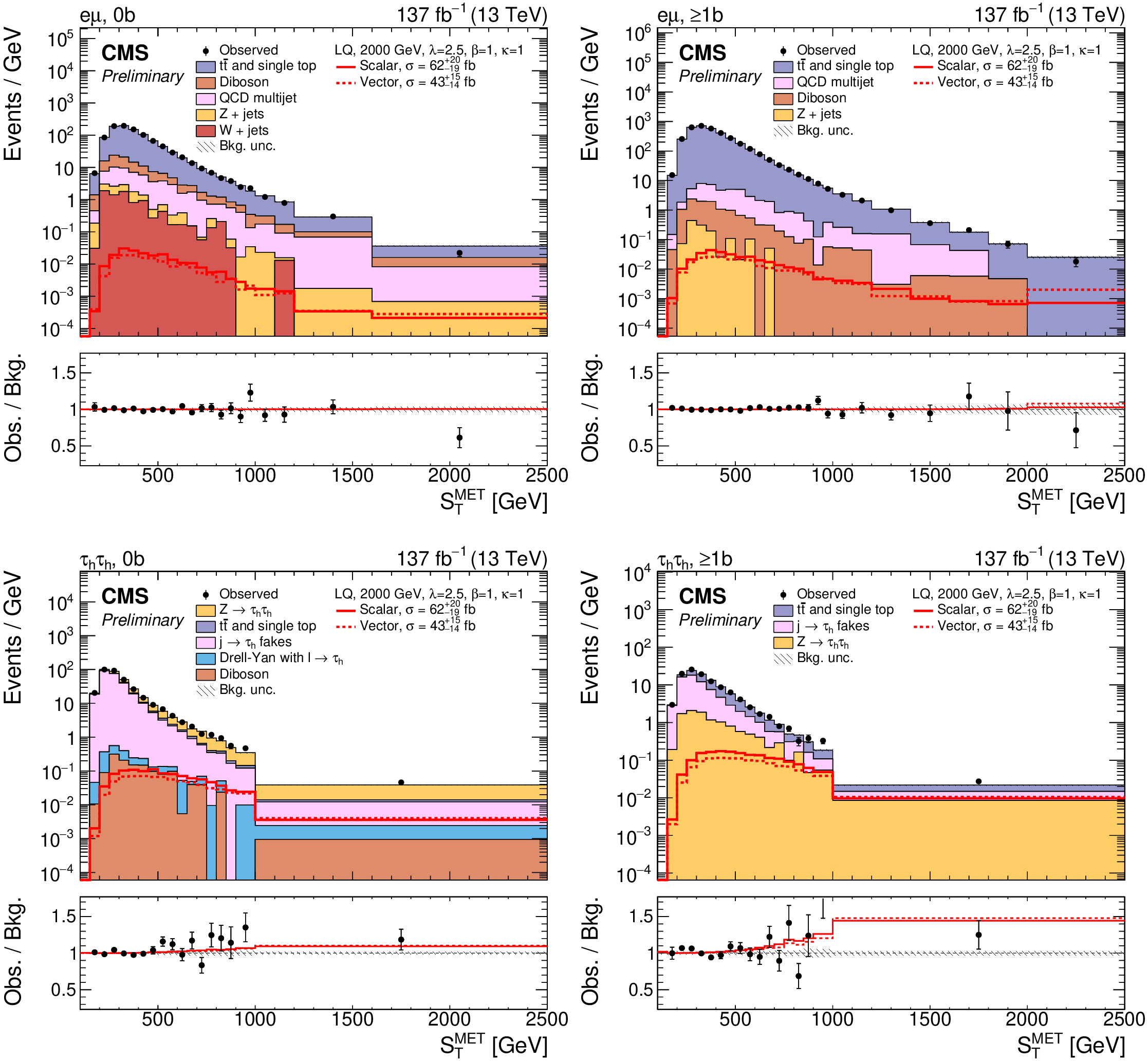
Figure 3:
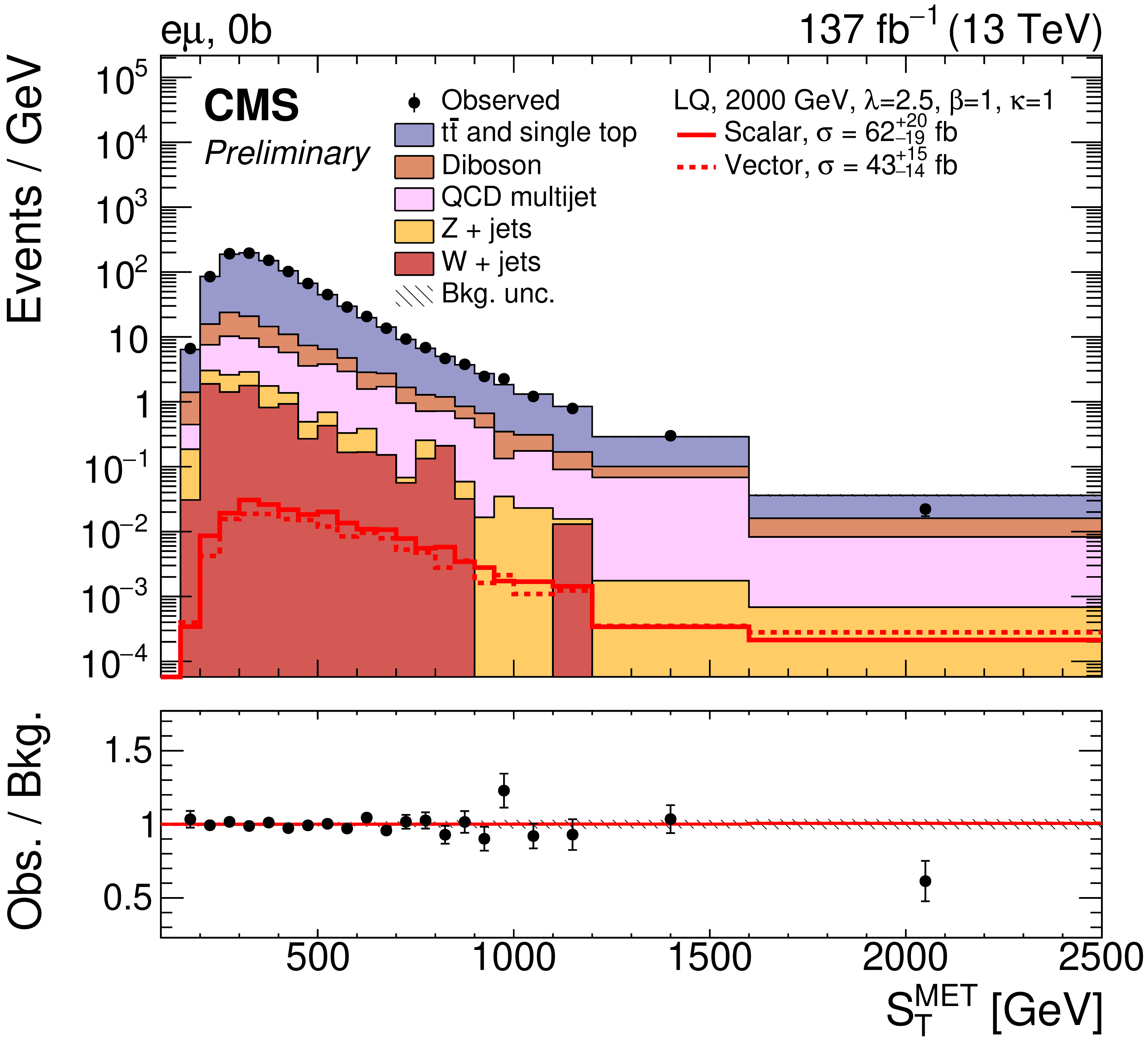
Postfit distributions of ${{S_\mathrm {T}^\text {MET}}} $ for the combined 2016-2018 dataset after a simultaneous fit of the scalar LQ signal to the data in each data-taking period. The last bin includes the overflow. The e$\mu$ (top) and ${{\tau_{\mathrm{h}}\tau_{\mathrm{h}}}} $ (bottom) channels in the 0b (left) and $\geq $1b (right) category are shown. The fitted signal distributions for the total scalar (solid red) and vector LQ model (dashed red) with a mass of 2000 GeV and a coupling strength of $\lambda = $ 2.5 are overlaid to illustrate the sensitivity. They include the single and pair LQ production, as well as the nonresonant production of a $\tau $ lepton pair. The lower panel shows the ratio between the observed data and background from the S+B fit (black). The hatched uncertainty bands include the total postfit uncertainties in the background. |
png pdf |
Figure 3-a:
Postfit distribution of ${{S_\mathrm {T}^\text {MET}}} $ for the e$\mu$ channel in the 0b category, for the combined 2016-2018 dataset after a simultaneous fit of the scalar LQ signal to the data in each data-taking period. The last bin includes the overflow. The fitted signal distributions for the total scalar (solid red) and vector LQ model (dashed red) with a mass of 2000 GeV and a coupling strength of $\lambda = $ 2.5 are overlaid to illustrate the sensitivity. They include the single and pair LQ production, as well as the nonresonant production of a $\tau $ lepton pair. The lower panel shows the ratio between the observed data and background from the S+B fit (black). The hatched uncertainty bands include the total postfit uncertainties in the background. |
png pdf |
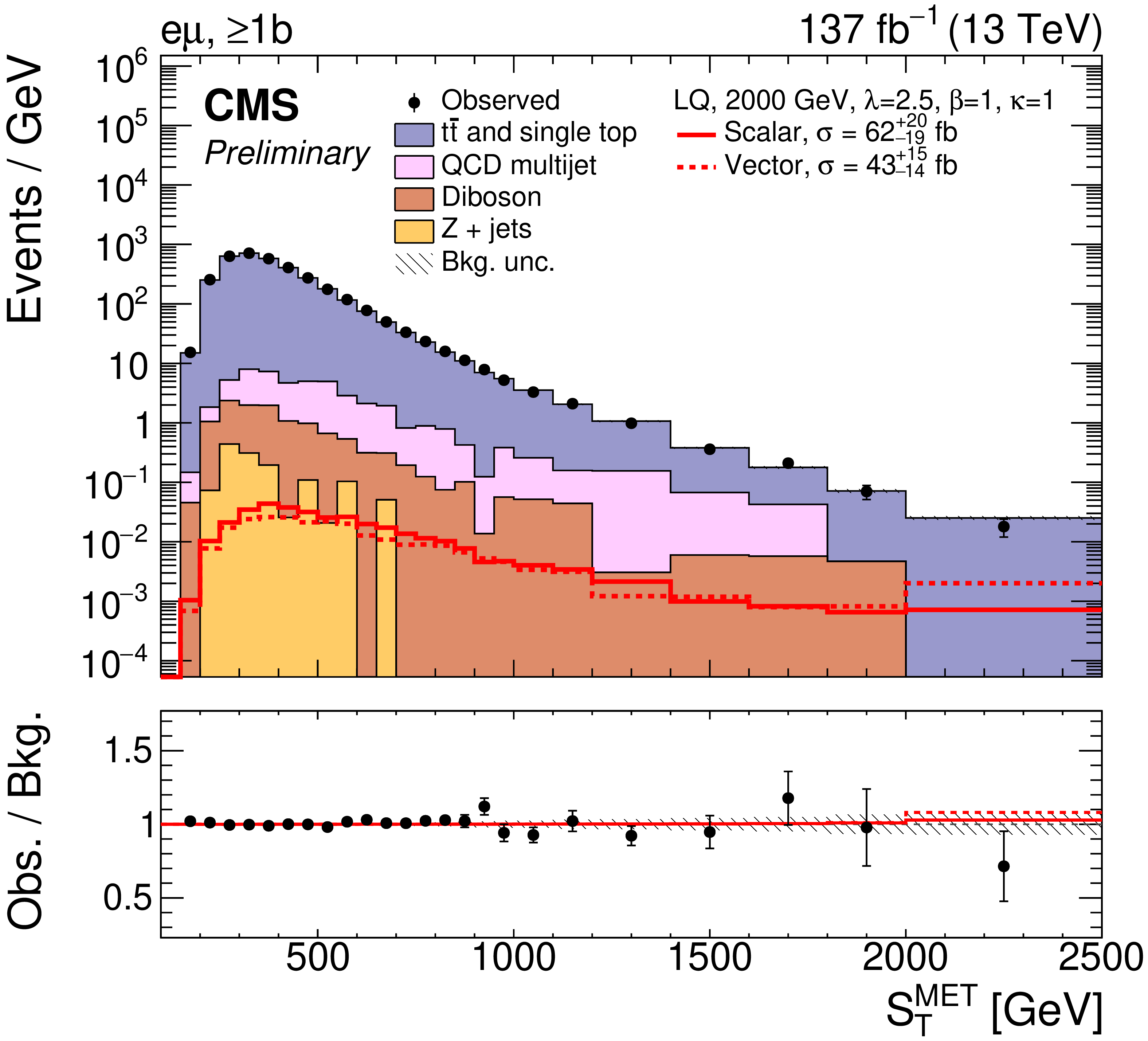
Figure 3-b:
Postfit distribution of ${{S_\mathrm {T}^\text {MET}}} $ for the e$\mu$ channel in the $\geq $1b category, for the combined 2016-2018 dataset after a simultaneous fit of the scalar LQ signal to the data in each data-taking period. The last bin includes the overflow. The fitted signal distributions for the total scalar (solid red) and vector LQ model (dashed red) with a mass of 2000 GeV and a coupling strength of $\lambda = $ 2.5 are overlaid to illustrate the sensitivity. They include the single and pair LQ production, as well as the nonresonant production of a $\tau $ lepton pair. The lower panel shows the ratio between the observed data and background from the S+B fit (black). The hatched uncertainty bands include the total postfit uncertainties in the background. |
png pdf |
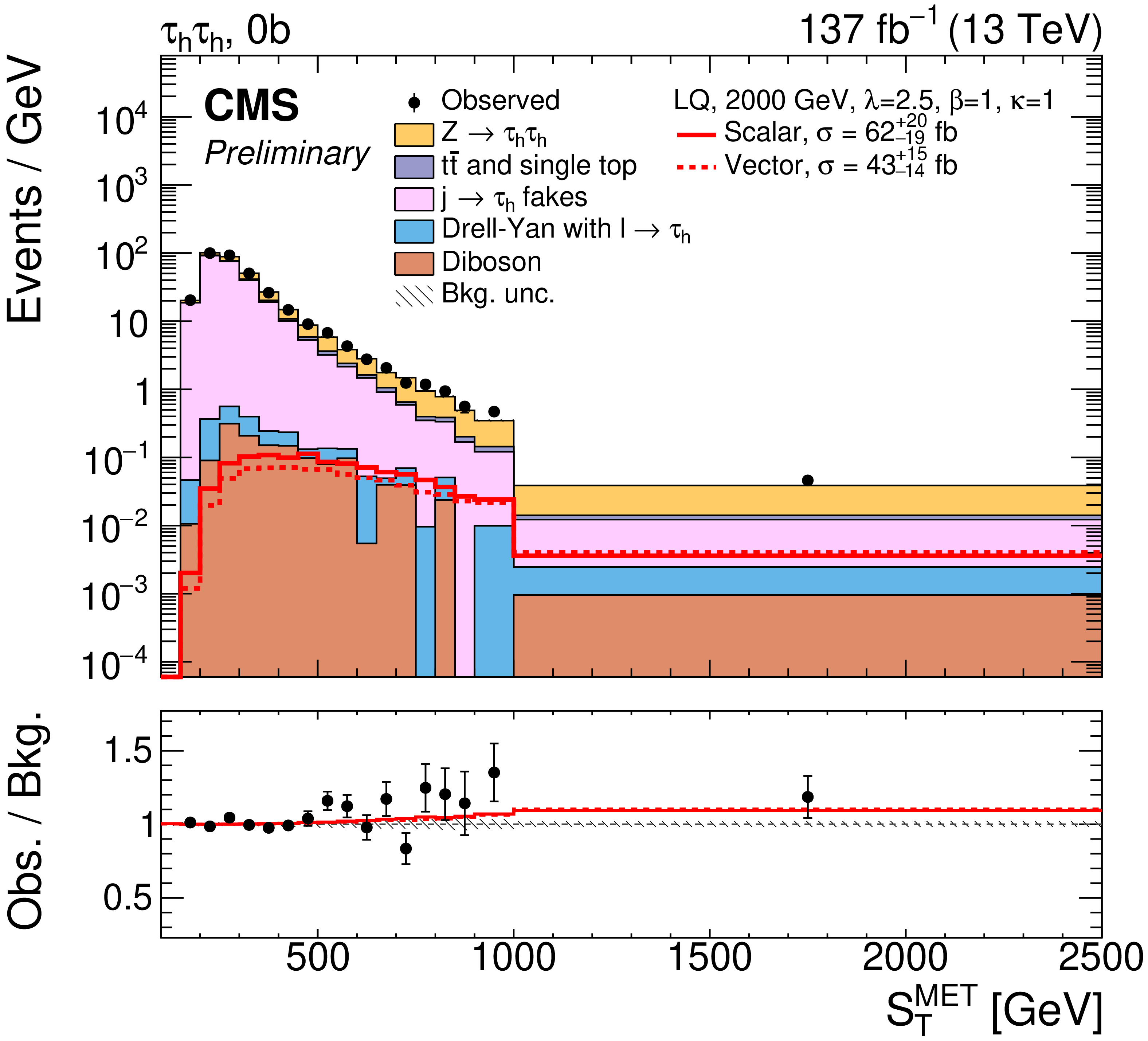
Figure 3-c:
Postfit distribution of ${{S_\mathrm {T}^\text {MET}}} $ for the ${{\tau_{\mathrm{h}}\tau_{\mathrm{h}}}} $ channel in the 0b category, for the combined 2016-2018 dataset after a simultaneous fit of the scalar LQ signal to the data in each data-taking period. The last bin includes the overflow. The fitted signal distributions for the total scalar (solid red) and vector LQ model (dashed red) with a mass of 2000 GeV and a coupling strength of $\lambda = $ 2.5 are overlaid to illustrate the sensitivity. They include the single and pair LQ production, as well as the nonresonant production of a $\tau $ lepton pair. The lower panel shows the ratio between the observed data and background from the S+B fit (black). The hatched uncertainty bands include the total postfit uncertainties in the background. |
png pdf |
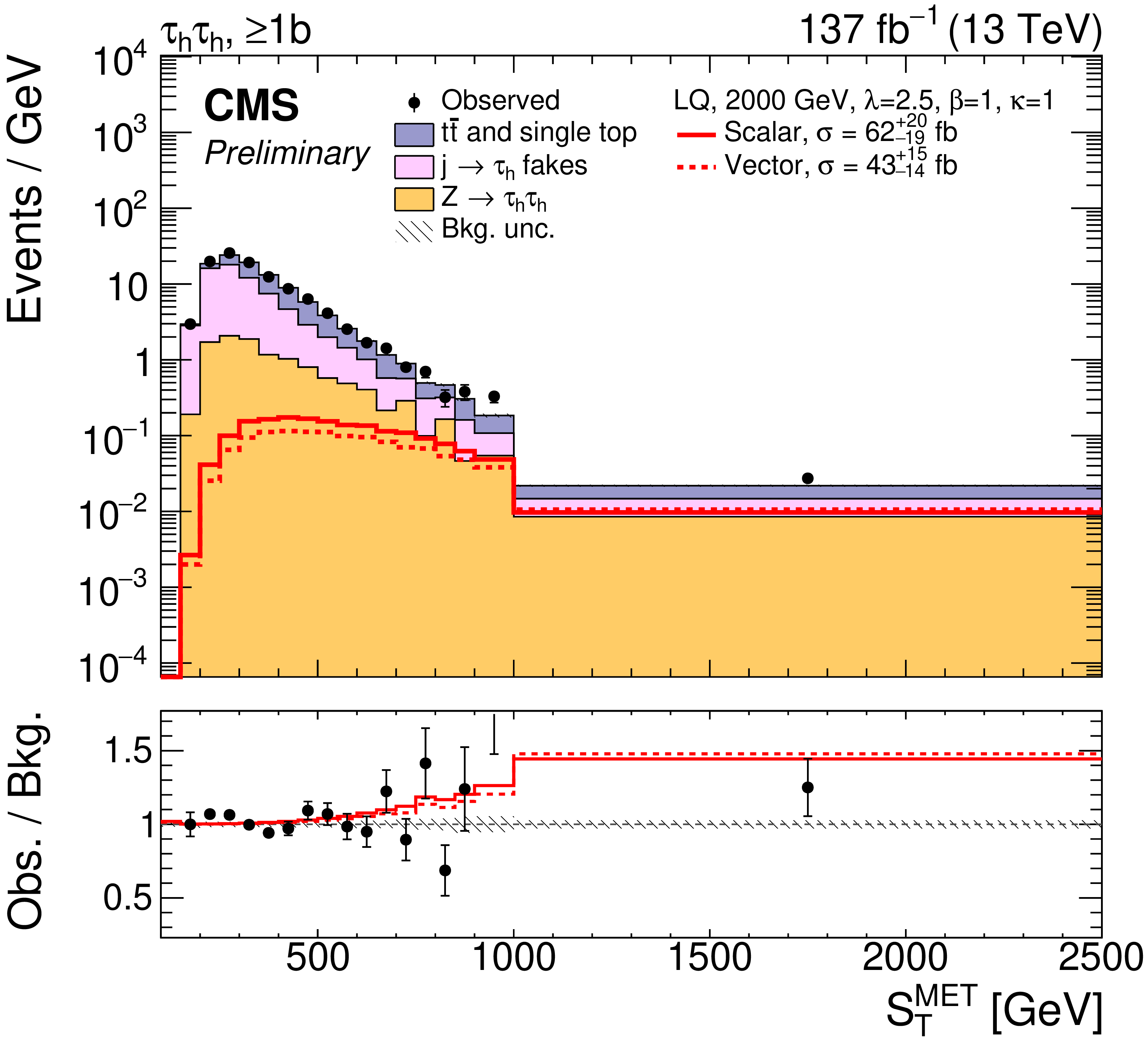
Figure 3-d:
Postfit distribution of ${{S_\mathrm {T}^\text {MET}}} $ for the ${{\tau_{\mathrm{h}}\tau_{\mathrm{h}}}} $ channel in the $\geq $1b category, for the combined 2016-2018 dataset after a simultaneous fit of the scalar LQ signal to the data in each data-taking period. The last bin includes the overflow. The fitted signal distributions for the total scalar (solid red) and vector LQ model (dashed red) with a mass of 2000 GeV and a coupling strength of $\lambda = $ 2.5 are overlaid to illustrate the sensitivity. They include the single and pair LQ production, as well as the nonresonant production of a $\tau $ lepton pair. The lower panel shows the ratio between the observed data and background from the S+B fit (black). The hatched uncertainty bands include the total postfit uncertainties in the background. |
png pdf |
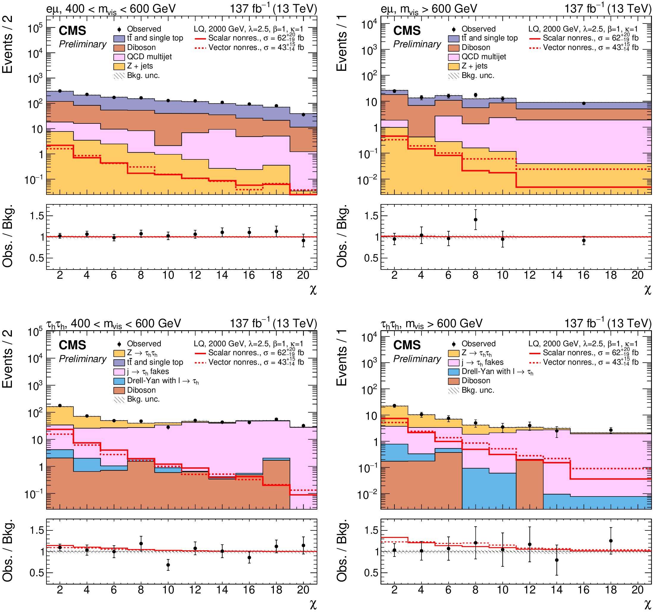
Figure 4:
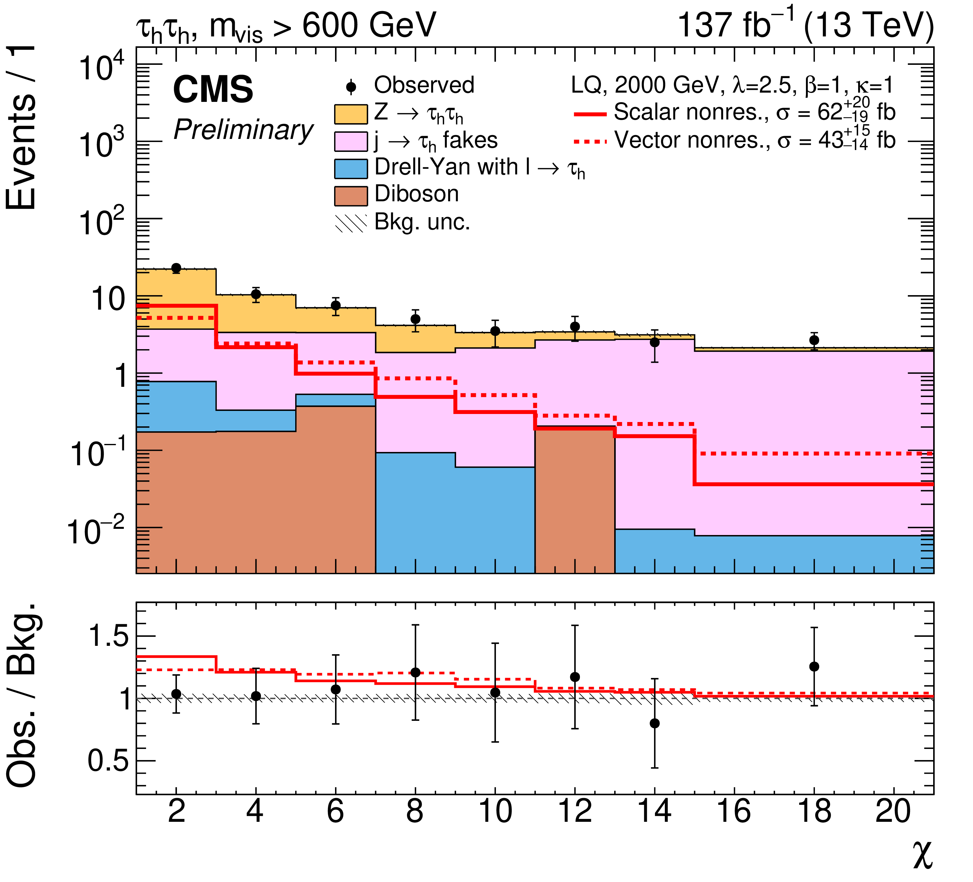
Postfit distributions of $\chi $ for the combined 2016-2018 dataset after a simultaneous fit of the scalar LQ signal to the data in each data-taking period. The e$\mu$ (top) and ${{\tau_{\mathrm{h}}\tau_{\mathrm{h}}}} $ (bottom) channels in the 400 GeV $ < {{m_\text {vis}}} < $ 600 GeV (left) and ${{m_\text {vis}}} > $ 600 GeV (right) category are shown. The fitted nonresonant signal for the scalar (solid red) and vector LQ model (dashed red) with a mass of 2000 GeV and a coupling strength of $\lambda = $ 2.5 are overlaid to illustrate the sensitivity. The lower panel shows the ratio between the observed data and background from the S+B fit (black). The hatched uncertainty bands include the total postfit uncertainties in the background. |
png pdf |
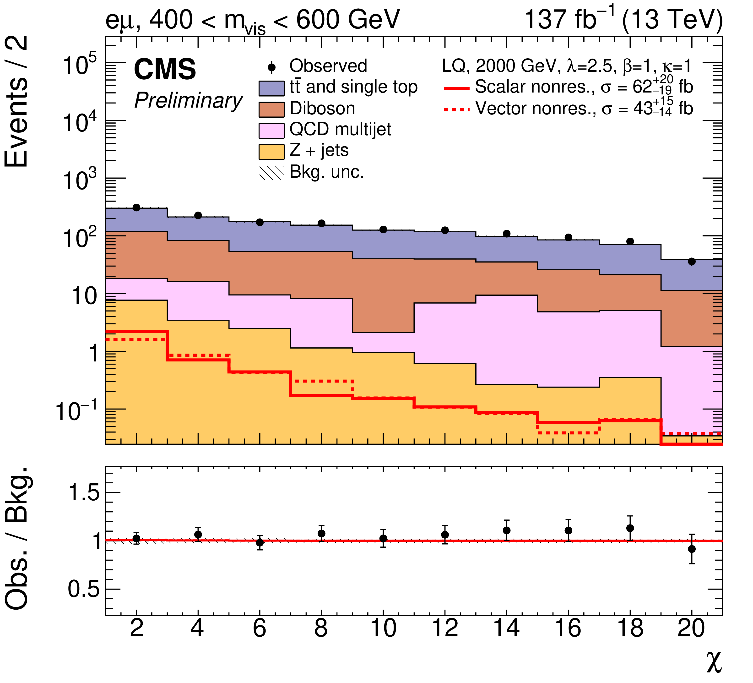
Figure 4-a:
Postfit distributions of $\chi $ for the e$\mu$ channel in the 400 GeV $ < {{m_\text {vis}}} < $ 600 GeV category, for the combined 2016-2018 dataset after a simultaneous fit of the scalar LQ signal to the data in each data-taking period. The fitted nonresonant signal for the scalar (solid red) and vector LQ model (dashed red) with a mass of 2000 GeV and a coupling strength of $\lambda = $ 2.5 are overlaid to illustrate the sensitivity. The lower panel shows the ratio between the observed data and background from the S+B fit (black). The hatched uncertainty bands include the total postfit uncertainties in the background. |
png pdf |
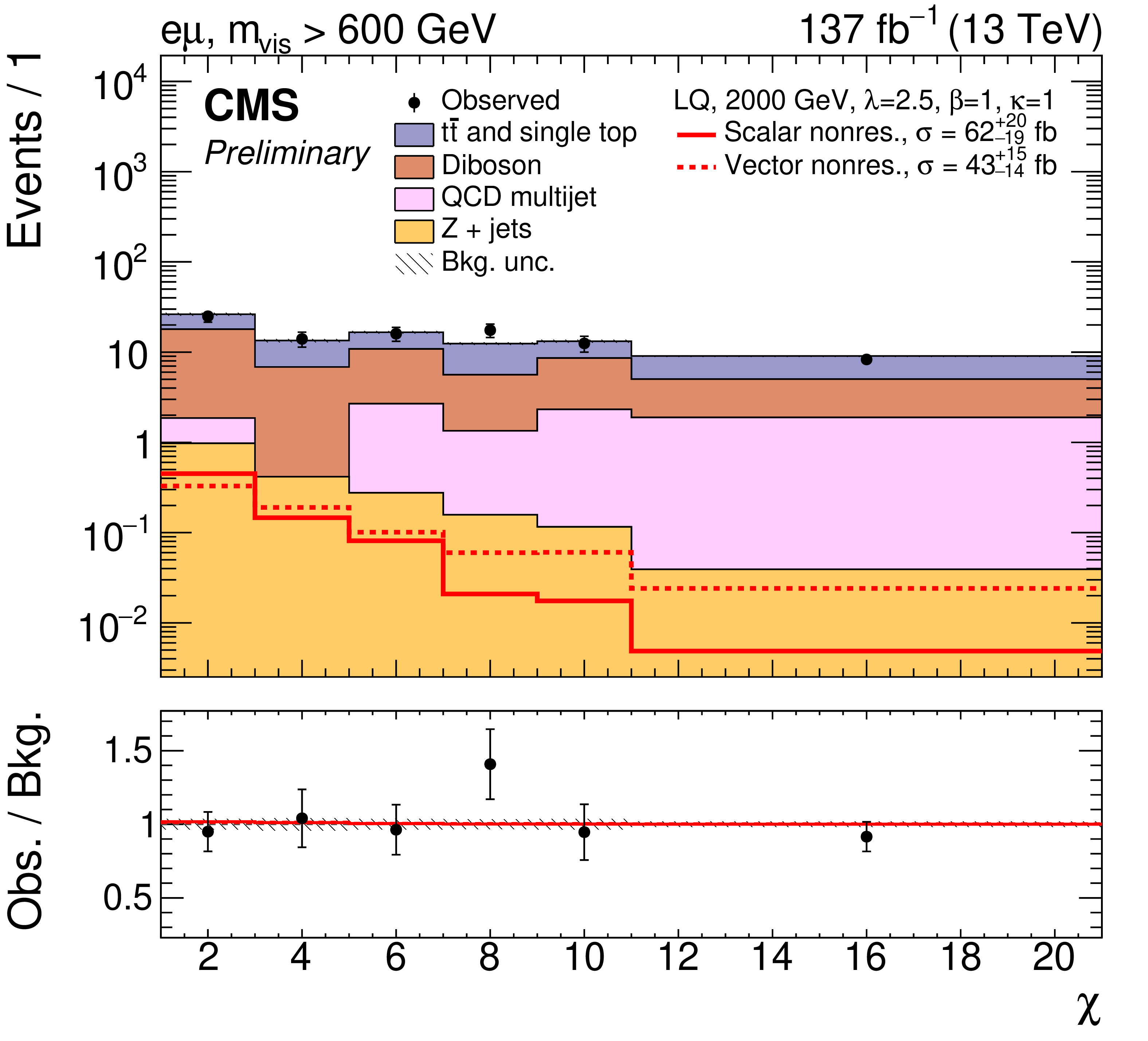
Figure 4-b:
Postfit distributions of $\chi $ for the e$\mu$ channel in the ${{m_\text {vis}}} > $ 600 GeV category, for the combined 2016-2018 dataset after a simultaneous fit of the scalar LQ signal to the data in each data-taking period. The fitted nonresonant signal for the scalar (solid red) and vector LQ model (dashed red) with a mass of 2000 GeV and a coupling strength of $\lambda = $ 2.5 are overlaid to illustrate the sensitivity. The lower panel shows the ratio between the observed data and background from the S+B fit (black). The hatched uncertainty bands include the total postfit uncertainties in the background. |
png pdf |
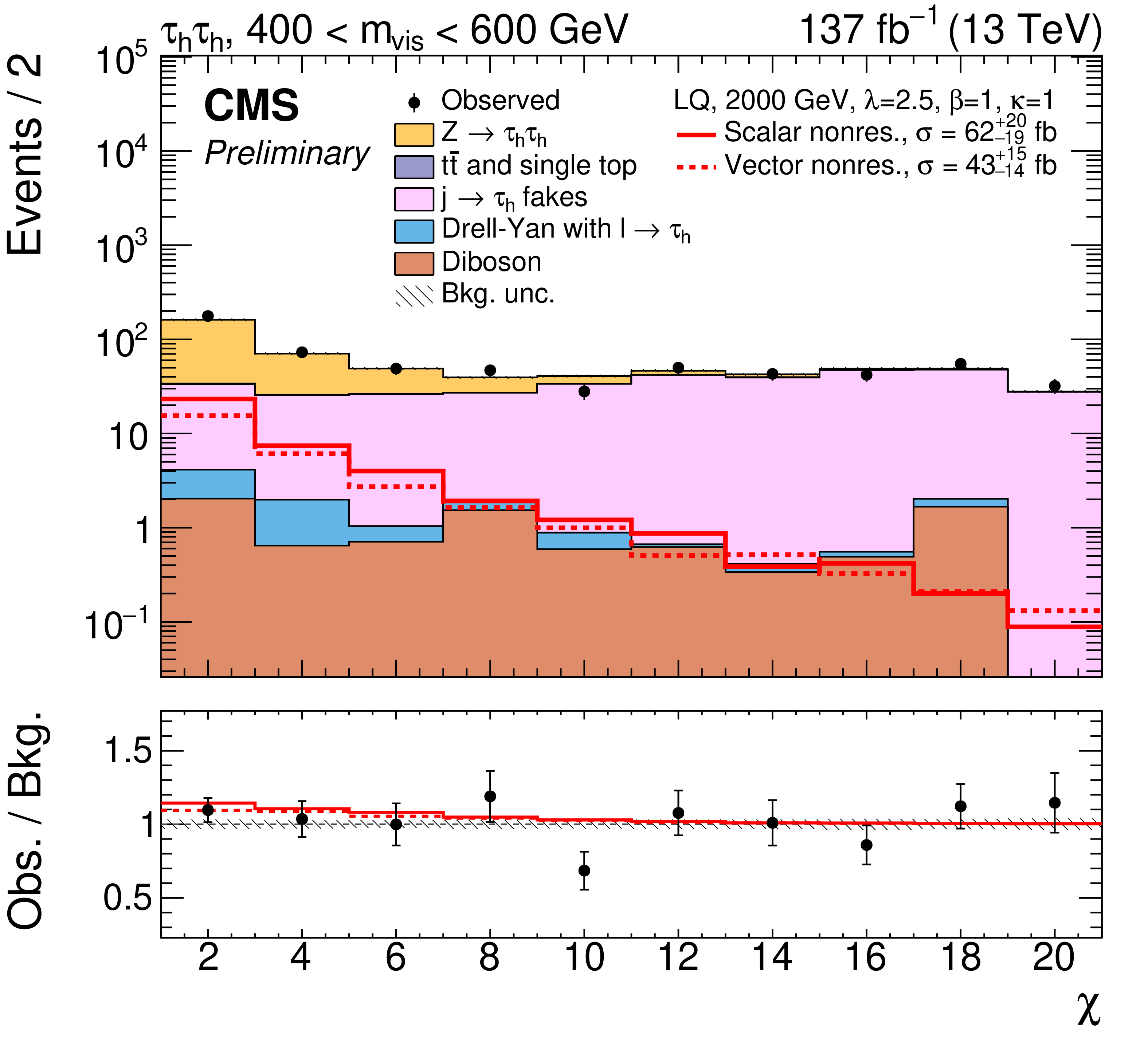
Figure 4-c:
Postfit distributions of $\chi $ for the ${{\tau_{\mathrm{h}}\tau_{\mathrm{h}}}} $ channel in the 400 GeV $ < {{m_\text {vis}}} < $ 600 GeV category, for the combined 2016-2018 dataset after a simultaneous fit of the scalar LQ signal to the data in each data-taking period. The fitted nonresonant signal for the scalar (solid red) and vector LQ model (dashed red) with a mass of 2000 GeV and a coupling strength of $\lambda = $ 2.5 are overlaid to illustrate the sensitivity. The lower panel shows the ratio between the observed data and background from the S+B fit (black). The hatched uncertainty bands include the total postfit uncertainties in the background. |
png pdf |
Figure 4-d:
Postfit distributions of $\chi $ for the ${{\tau_{\mathrm{h}}\tau_{\mathrm{h}}}} $ channel in the ${{m_\text {vis}}} > $ 600 GeV category, for the combined 2016-2018 dataset after a simultaneous fit of the scalar LQ signal to the data in each data-taking period. The fitted nonresonant signal for the scalar (solid red) and vector LQ model (dashed red) with a mass of 2000 GeV and a coupling strength of $\lambda = $ 2.5 are overlaid to illustrate the sensitivity. The lower panel shows the ratio between the observed data and background from the S+B fit (black). The hatched uncertainty bands include the total postfit uncertainties in the background. |

png pdf |
Figure 5:
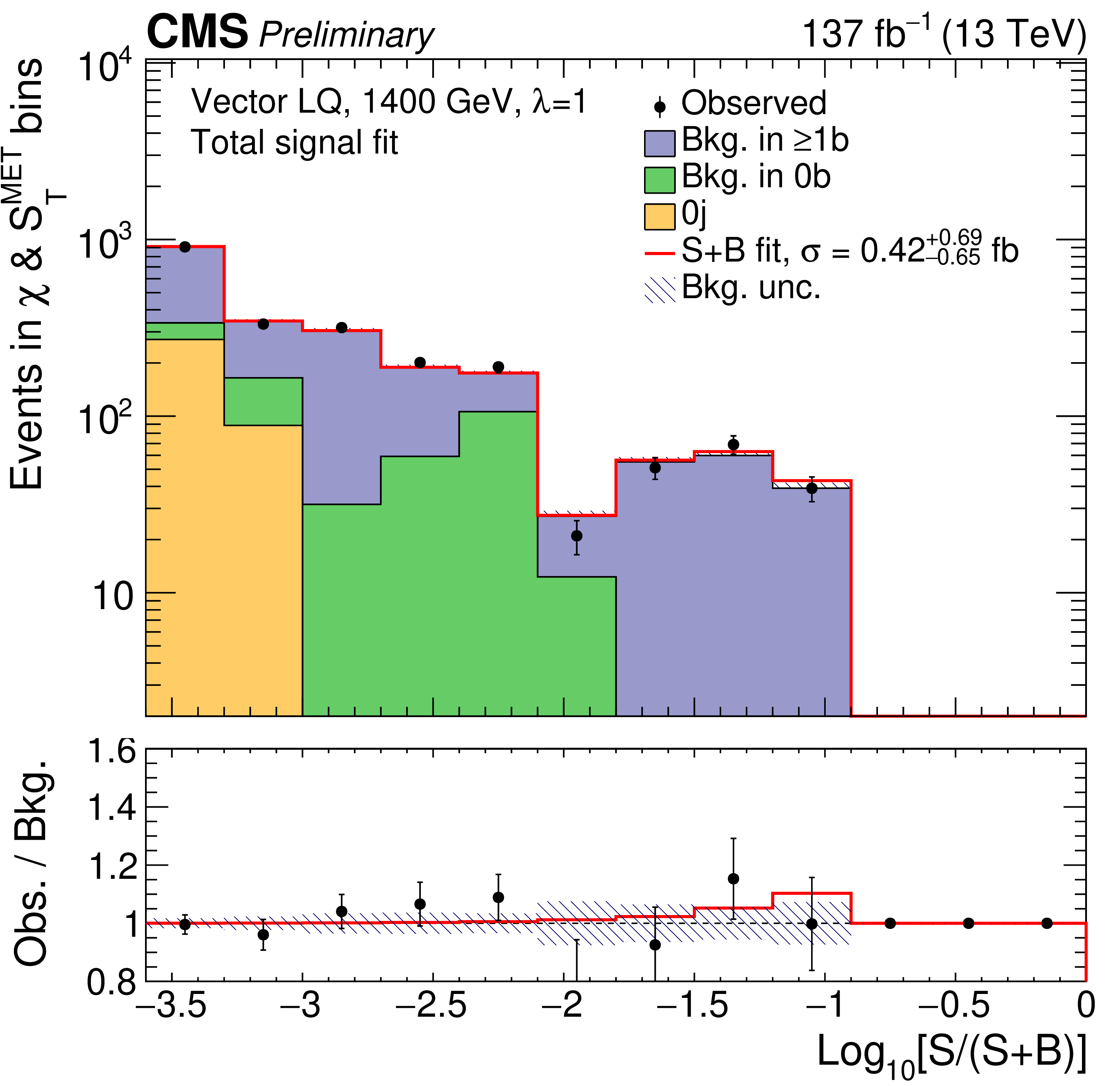
Histograms of ${{\log_{10}[S(S{+}B)]}}$ counting events in all bins, assuming a vector LQ with ${{m_{{{\mathrm {LQ}}}}}} = $ 1400 GeV and $\lambda = $ 1.0 (left), or ${{m_{{{\mathrm {LQ}}}}}} = $ 2000 GeV and $\lambda = $ 2.5 (right). The ${{\log_{10}[S(S{+}B)]}}$ is computed per bin of the postfit $\chi $ and ${{S_\mathrm {T}^\text {MET}}} $ distributions, using an S+B fit model. The total LQ signal strength (single, pair and nonresonant) is fitted simultaneously. The lower panel shows the ratio of the observed data to the expected background from the S+B fit. The expected background is grouped by jet categories in stacked histograms. |
png pdf |
Figure 5-a:
Histograms of ${{\log_{10}[S(S{+}B)]}}$ counting events in all bins, assuming a vector LQ with ${{m_{{{\mathrm {LQ}}}}}} = $ 1400 GeV and $\lambda = $ 1.0. The ${{\log_{10}[S(S{+}B)]}}$ is computed per bin of the postfit $\chi $ and ${{S_\mathrm {T}^\text {MET}}} $ distributions, using an S+B fit model. The total LQ signal strength (single, pair and nonresonant) is fitted simultaneously. The lower panel shows the ratio of the observed data to the expected background from the S+B fit. The expected background is grouped by jet categories in stacked histograms. |

png pdf |
Figure 5-b:
Histograms of ${{\log_{10}[S(S{+}B)]}}$ counting events in all bins, assuming a vector LQ with ${{m_{{{\mathrm {LQ}}}}}} = $ 2000 GeV and $\lambda = $ 2.5. The ${{\log_{10}[S(S{+}B)]}}$ is computed per bin of the postfit $\chi $ and ${{S_\mathrm {T}^\text {MET}}} $ distributions, using an S+B fit model. The total LQ signal strength (single, pair and nonresonant) is fitted simultaneously. The lower panel shows the ratio of the observed data to the expected background from the S+B fit. The expected background is grouped by jet categories in stacked histograms. |
png pdf |
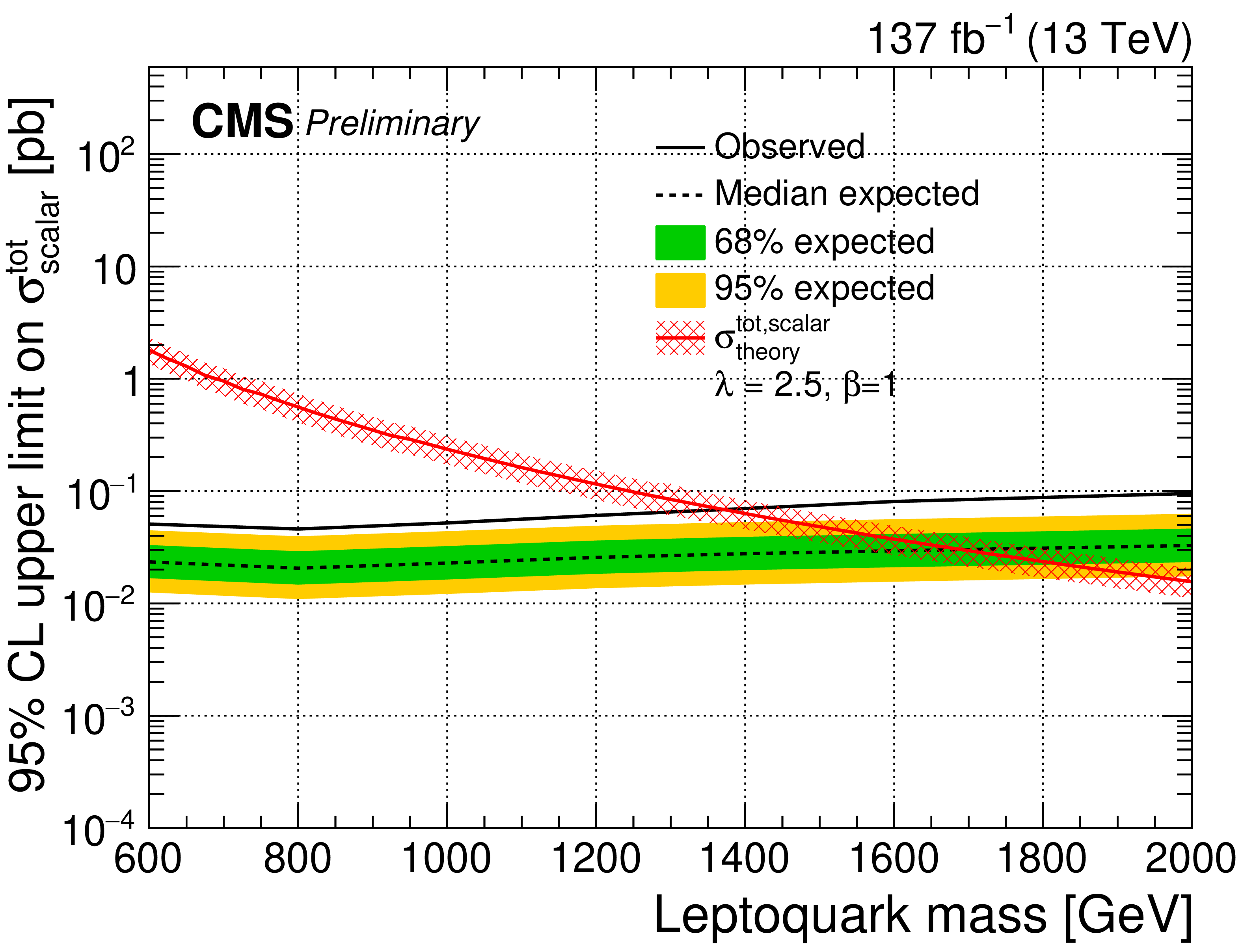
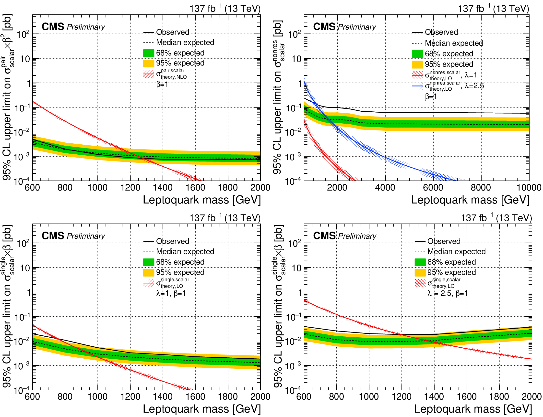
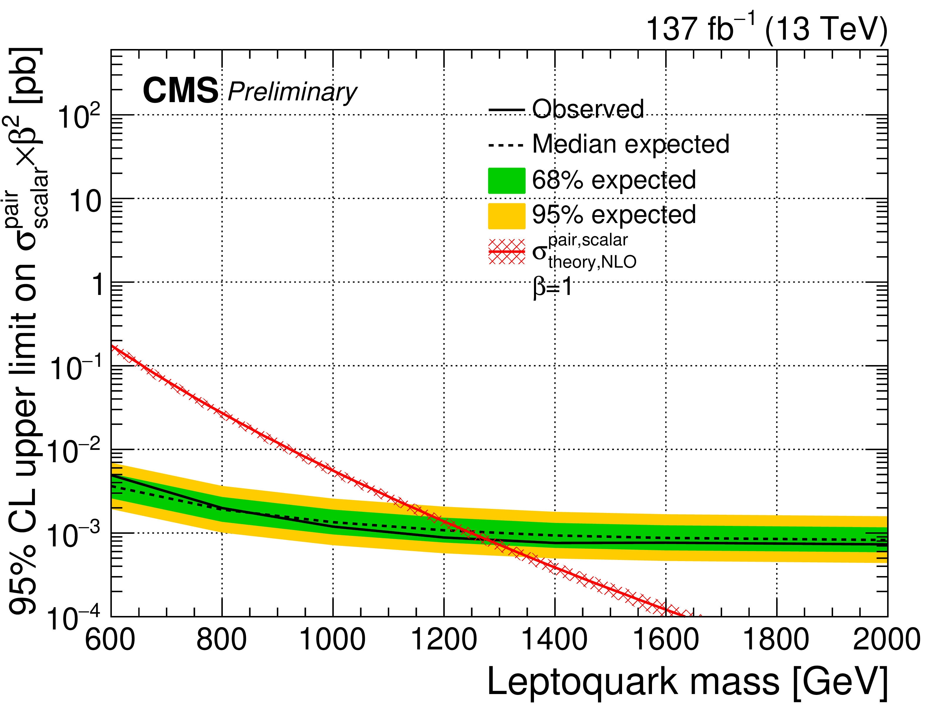
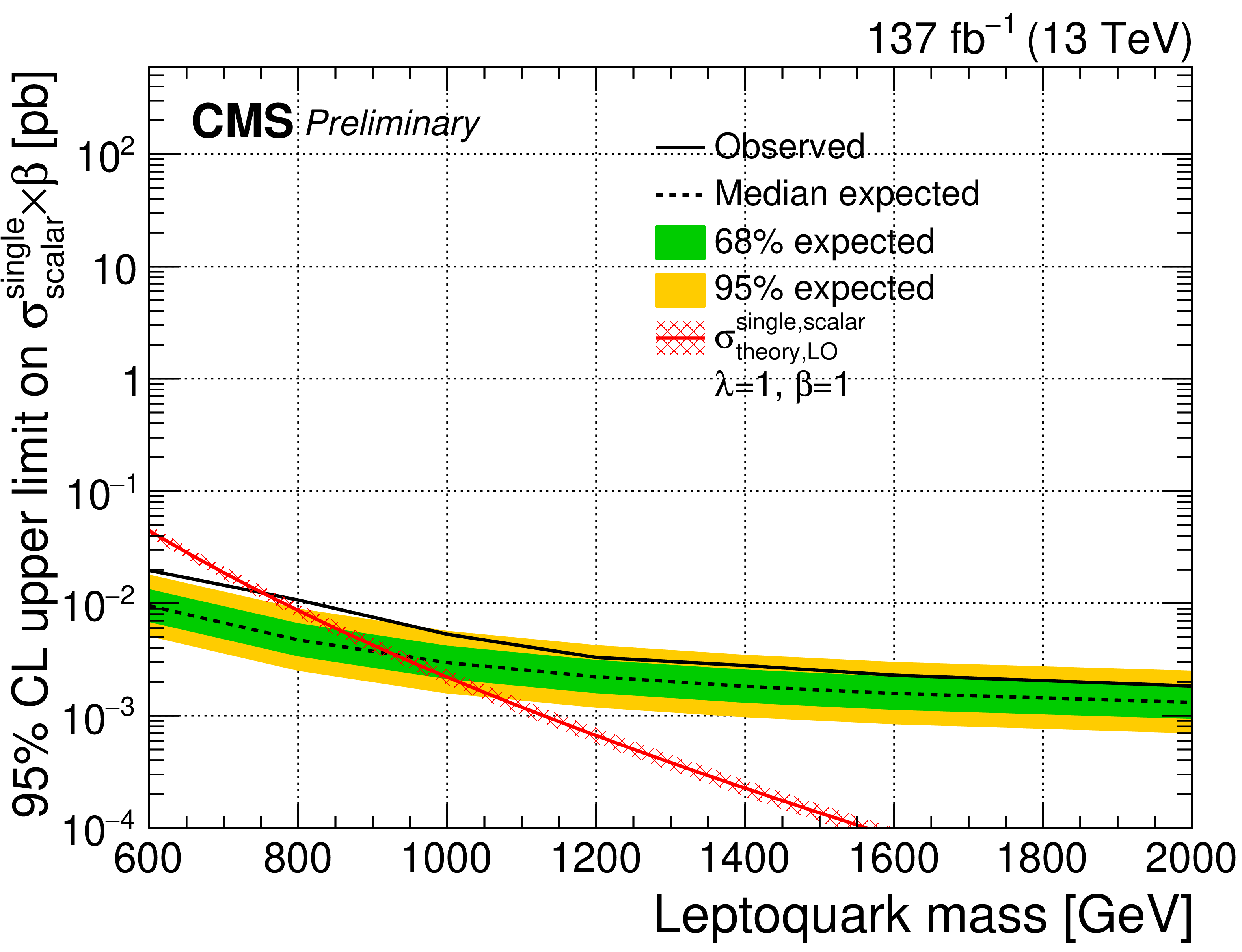
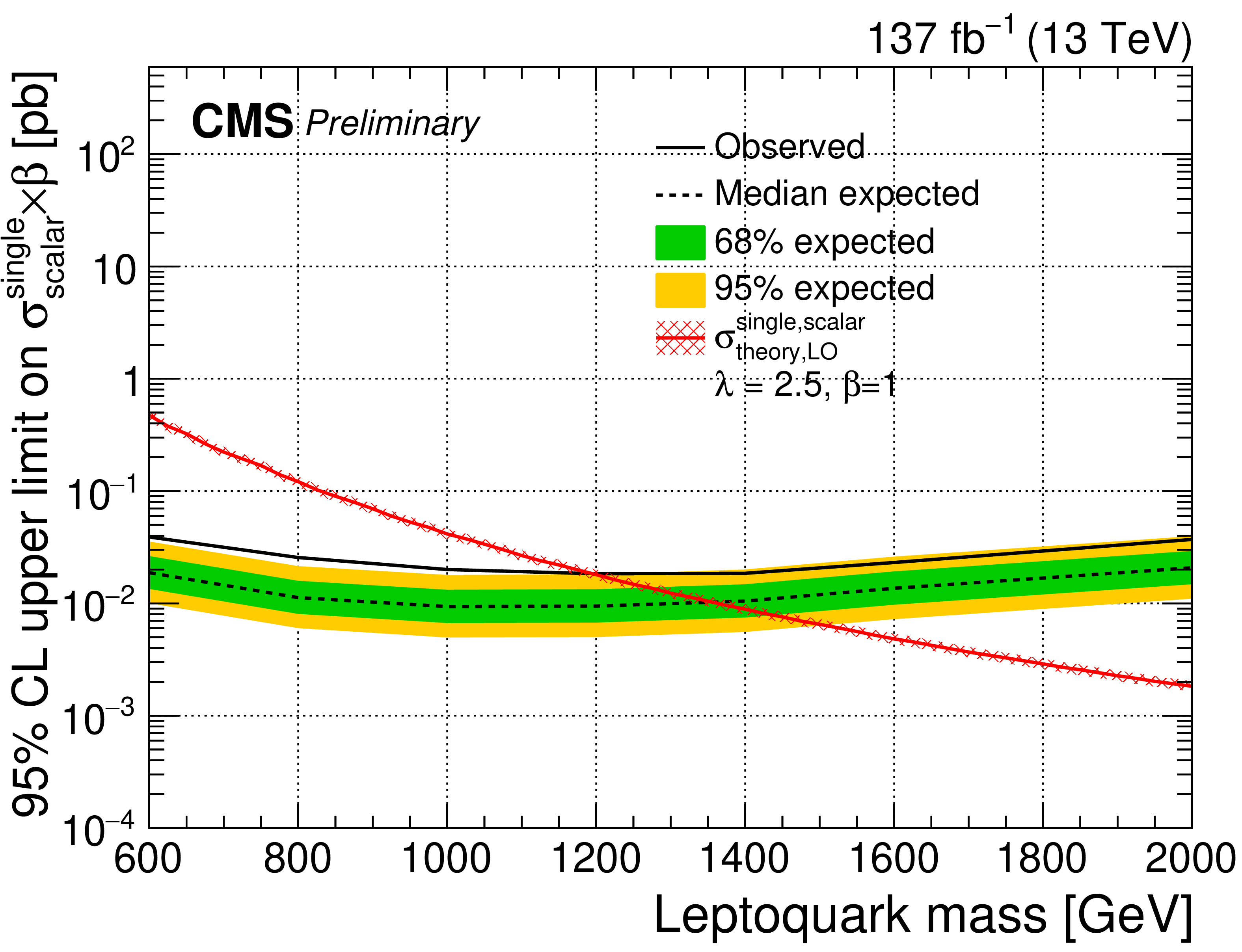
Figure 6:
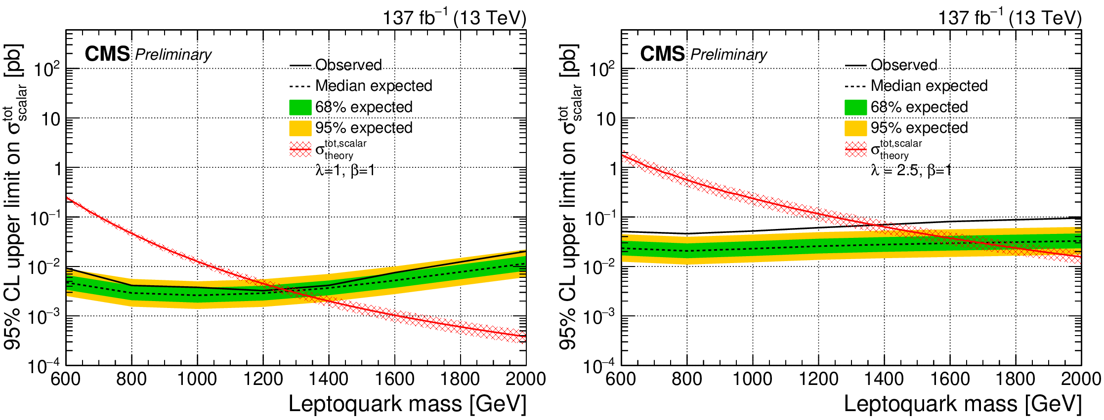
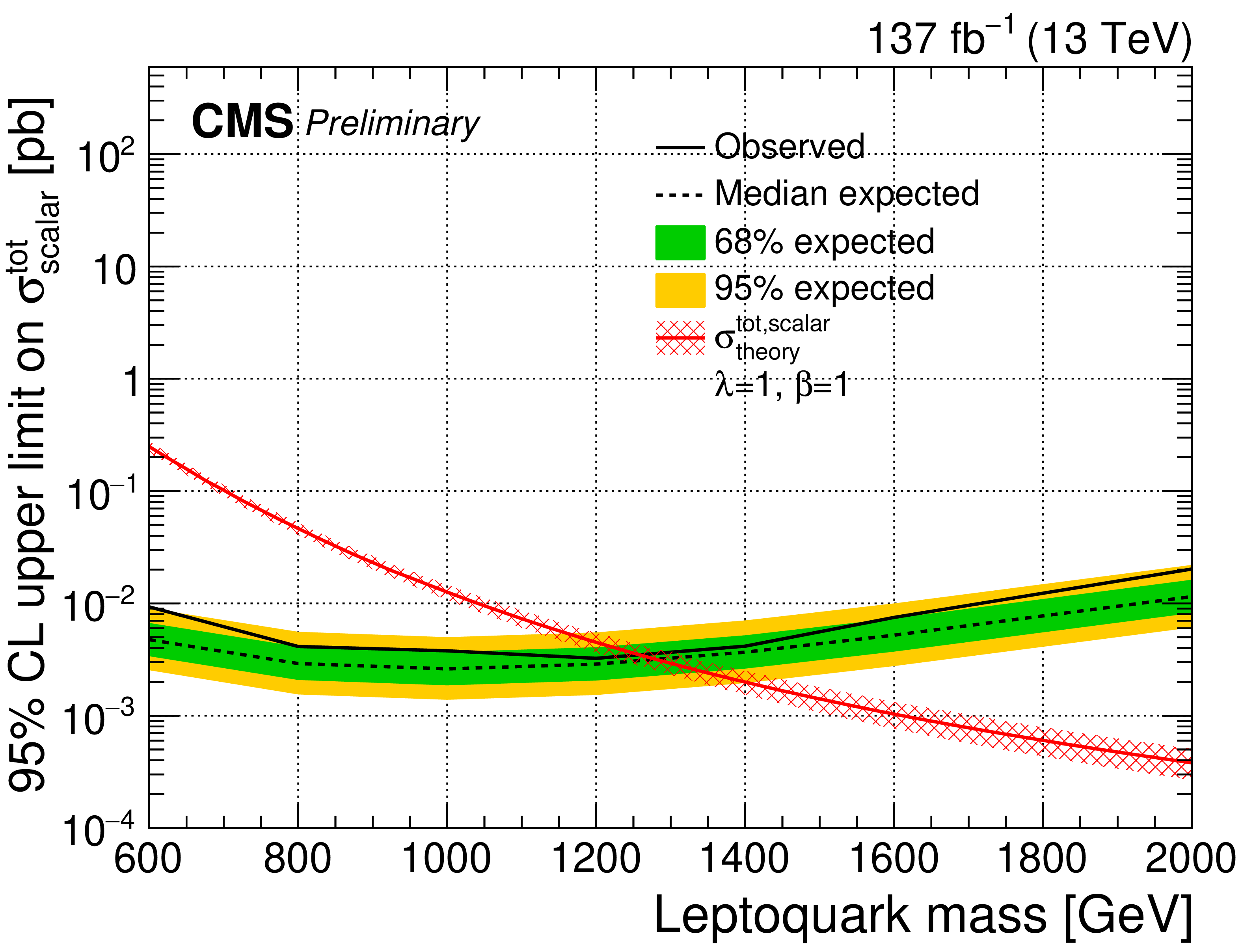
The observed and expected upper limit on the total cross section of a scalar LQ signal with $\lambda =$ 1 (left) and 2.5 (right) at 95% CL. The inner (green) band and the outer (yellow) band indicate the regions containing 68 and 95%, respectively, of the distribution of limits expected under the background-only hypothesis. |
png pdf |
Figure 6-a:
The observed and expected upper limit on the total cross section of a scalar LQ signal with $\lambda =$ 1 at 95% CL. The inner (green) band and the outer (yellow) band indicate the regions containing 68 and 95%, respectively, of the distribution of limits expected under the background-only hypothesis. |
png pdf |
Figure 6-b:
The observed and expected upper limit on the total cross section of a scalar LQ signal with $\lambda =$ 2.5 at 95% CL. The inner (green) band and the outer (yellow) band indicate the regions containing 68 and 95%, respectively, of the distribution of limits expected under the background-only hypothesis. |
png pdf |
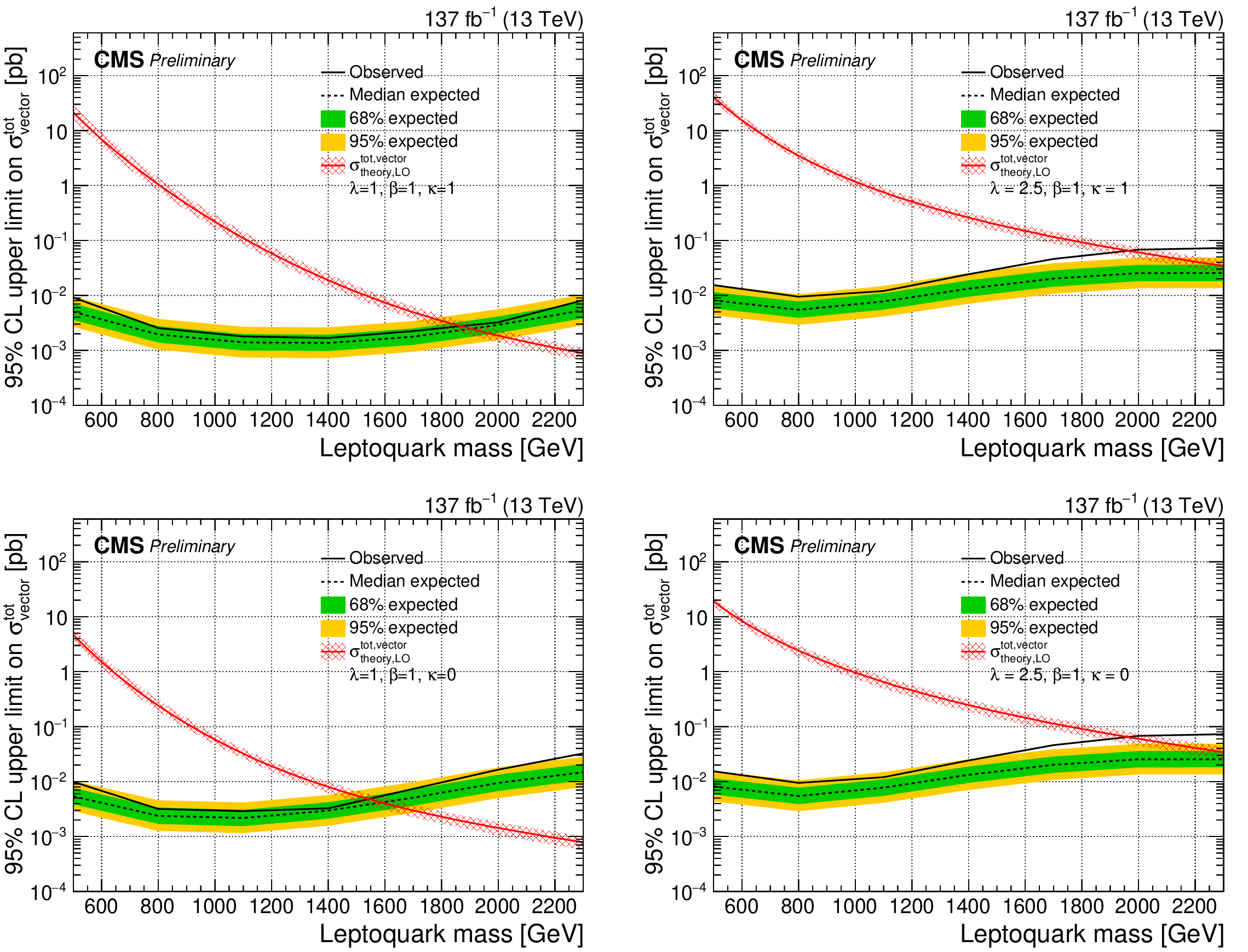
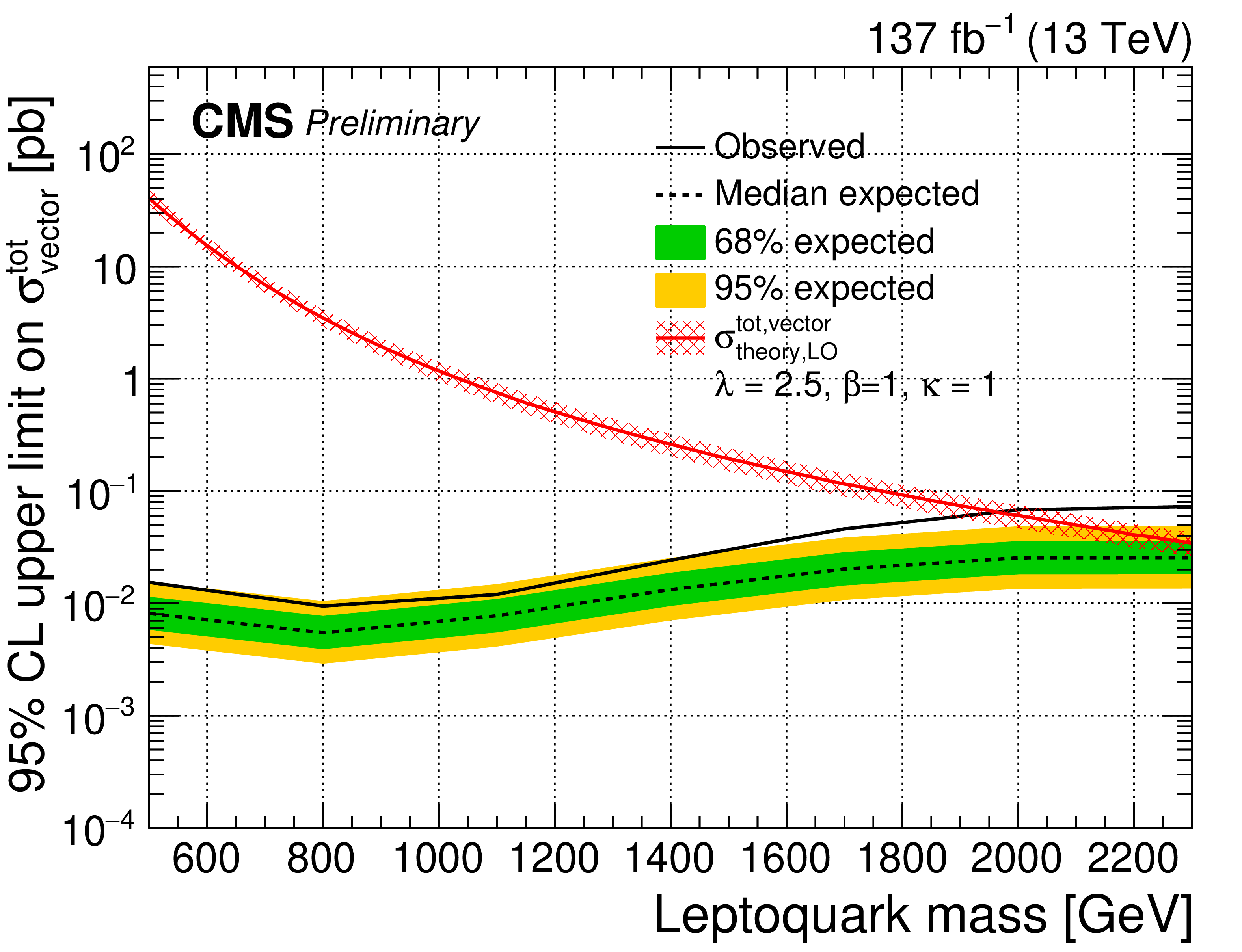
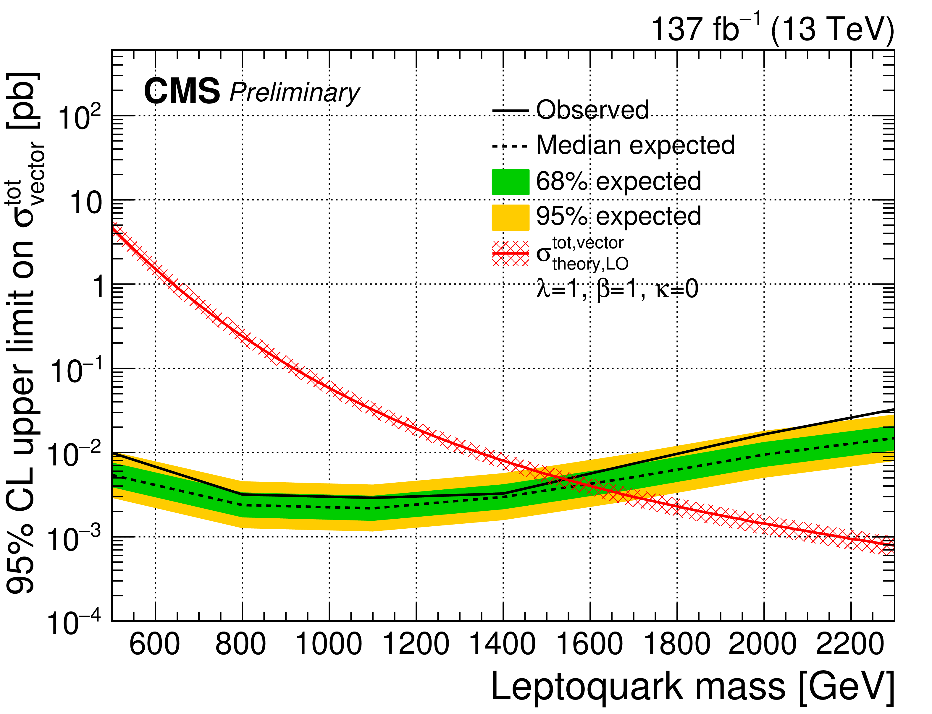
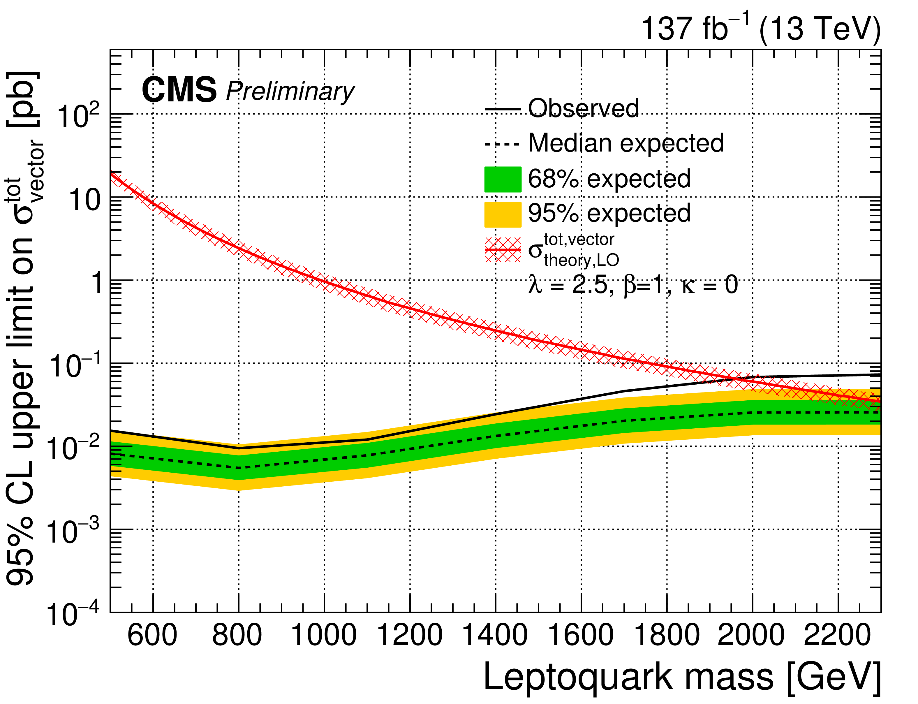
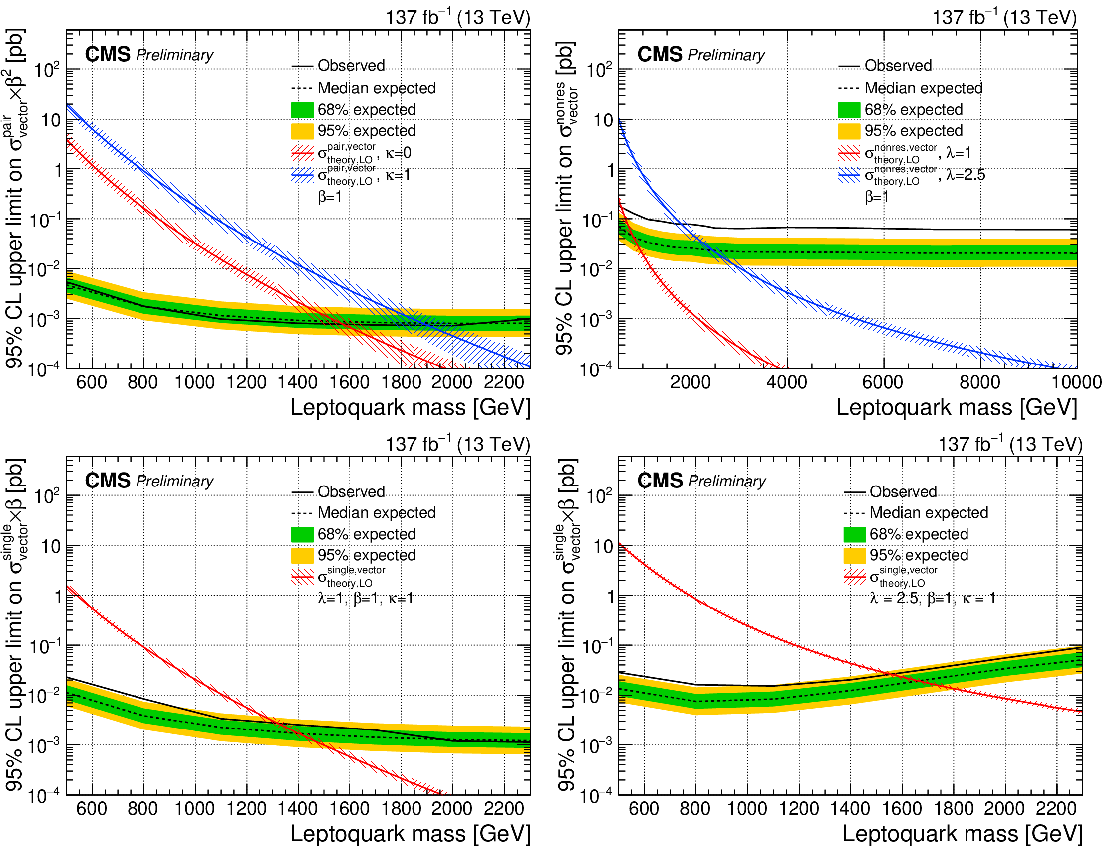
Figure 7:
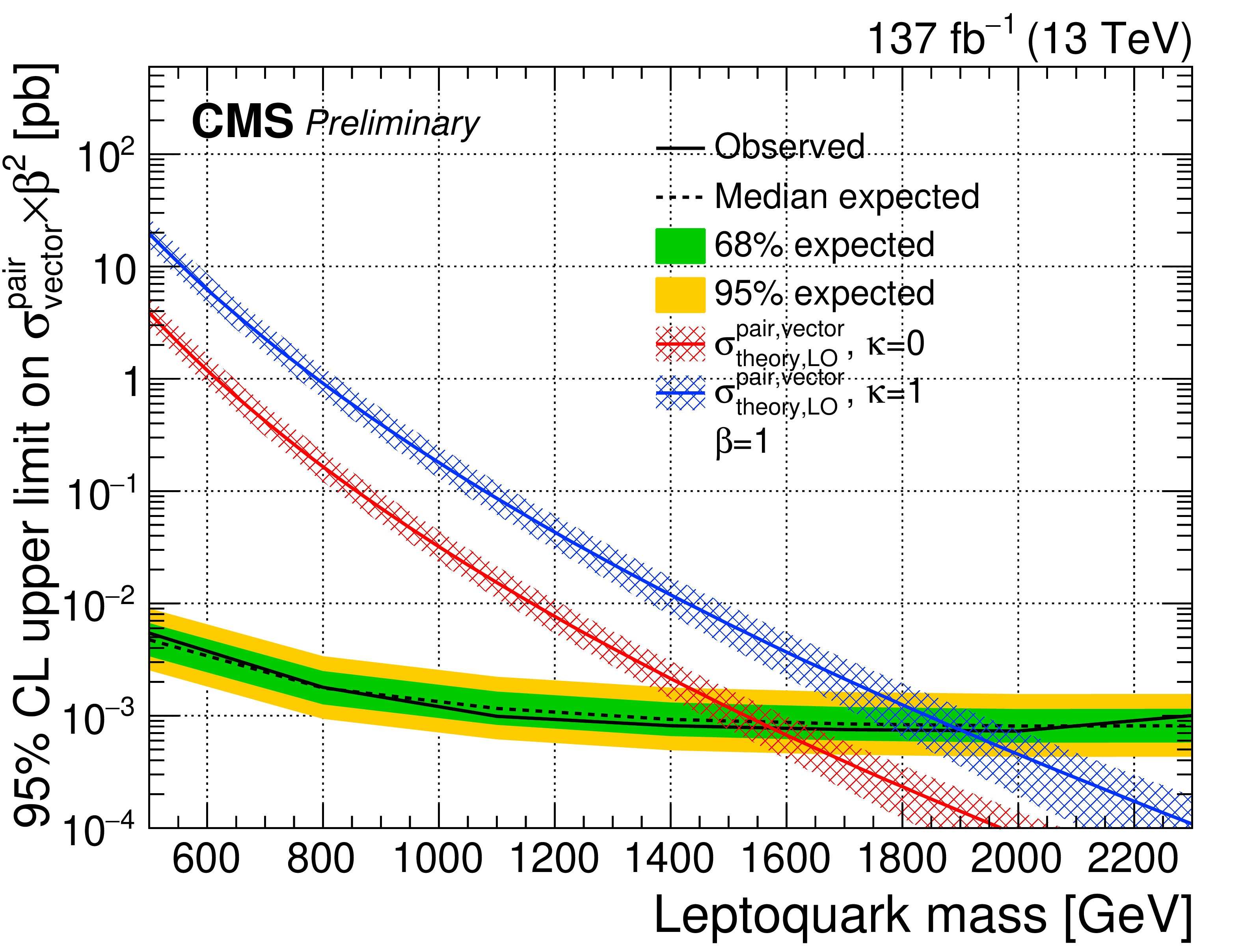
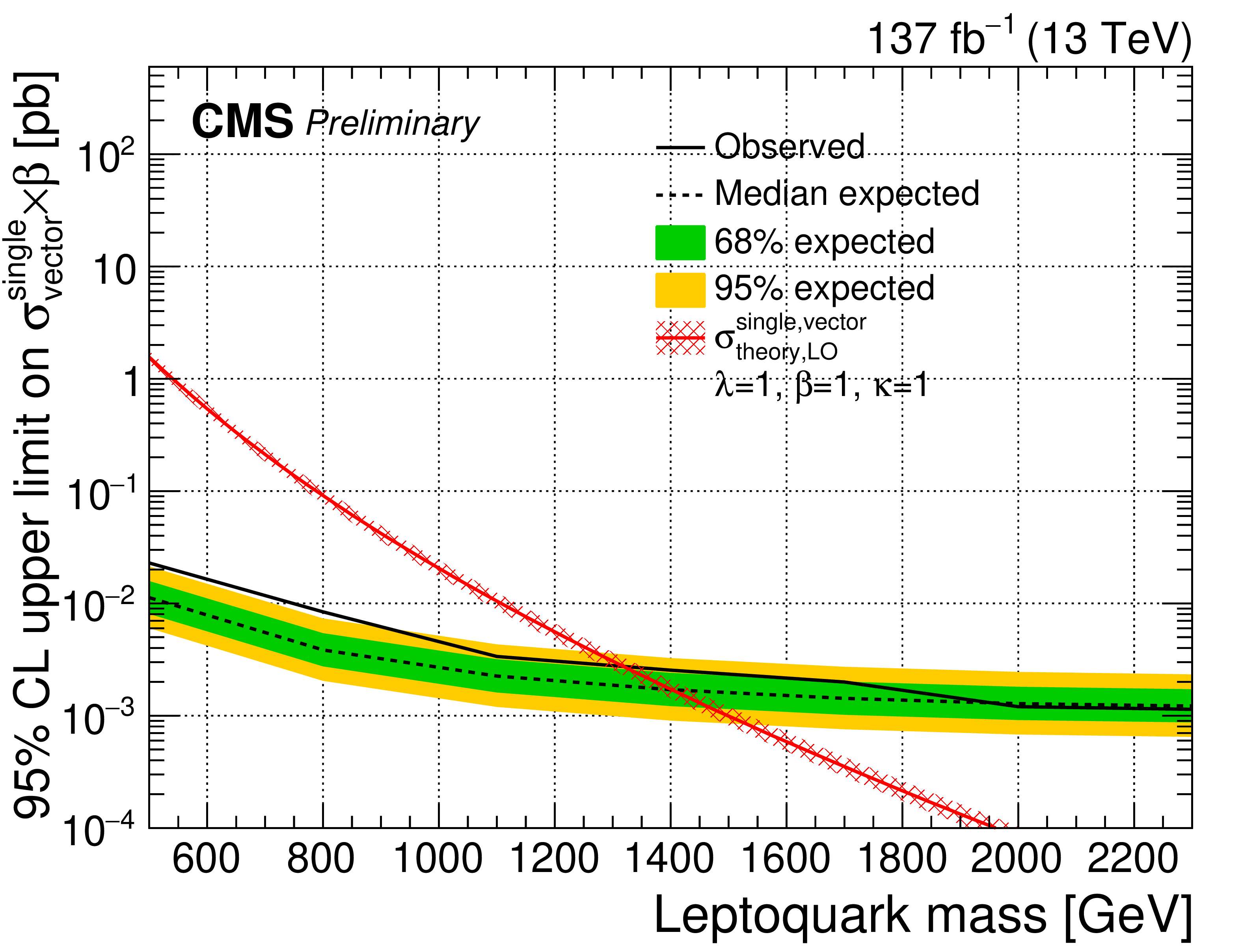
The observed and expected upper limit on the total cross section of a vector LQ signal with $\lambda =$ 1 (left) and 2.5 (right) at 95% CL. The top (bottom) row assumes a nonminimal coupling of $\kappa =$ 1 (0). The inner (green) band and the outer (yellow) band indicate the regions containing 68 and 95%, respectively, of the distribution of limits expected under the background-only hypothesis. |

png pdf |
Figure 7-a:
The observed and expected upper limit on the total cross section of a vector LQ signal with $\lambda =$ 1 at 95% CL, assuming a nonminimal coupling of $\kappa =$ 1. The inner (green) band and the outer (yellow) band indicate the regions containing 68 and 95%, respectively, of the distribution of limits expected under the background-only hypothesis. |
png pdf |
Figure 7-b:
The observed and expected upper limit on the total cross section of a vector LQ signal with $\lambda =$ 2.5 at 95% CL, assuming a nonminimal coupling of $\kappa =$ 1. The inner (green) band and the outer (yellow) band indicate the regions containing 68 and 95%, respectively, of the distribution of limits expected under the background-only hypothesis. |
png pdf |
Figure 7-c:
The observed and expected upper limit on the total cross section of a vector LQ signal with $\lambda =$ 1 at 95% CL, assuming a nonminimal coupling of $\kappa =$ 0. The inner (green) band and the outer (yellow) band indicate the regions containing 68 and 95%, respectively, of the distribution of limits expected under the background-only hypothesis. |
png pdf |
Figure 7-d:
The observed and expected upper limit on the total cross section of a vector LQ signal with $\lambda =$ 2.5 at 95% CL, assuming a nonminimal coupling of $\kappa =$ 0. The inner (green) band and the outer (yellow) band indicate the regions containing 68 and 95%, respectively, of the distribution of limits expected under the background-only hypothesis. |
png pdf |
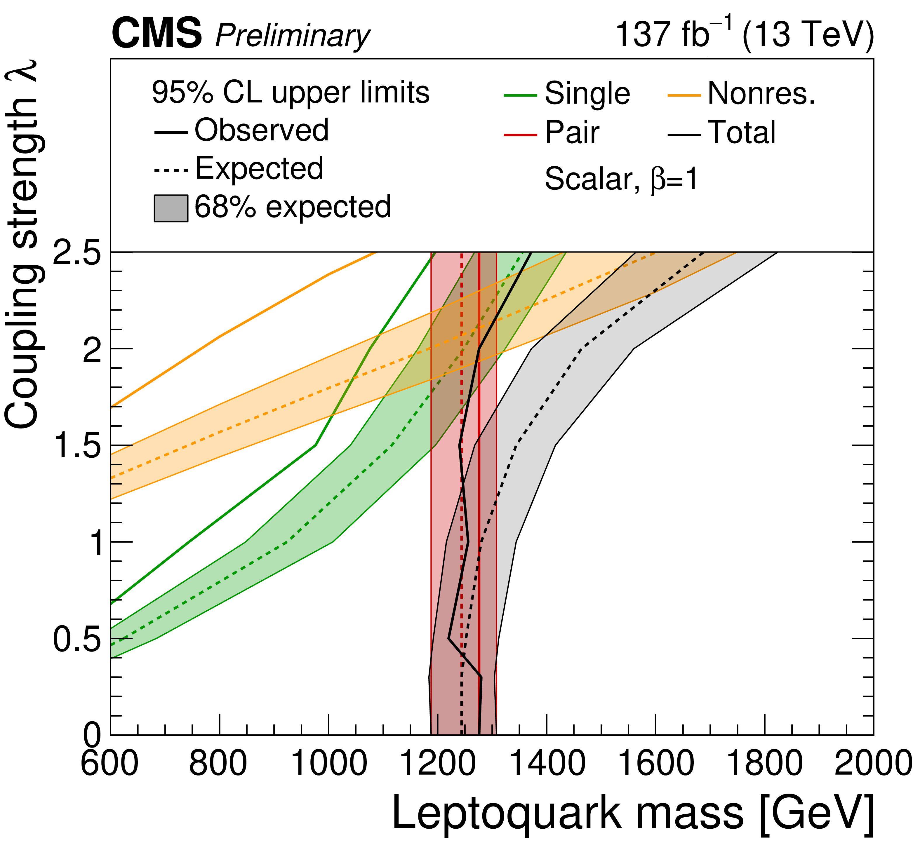
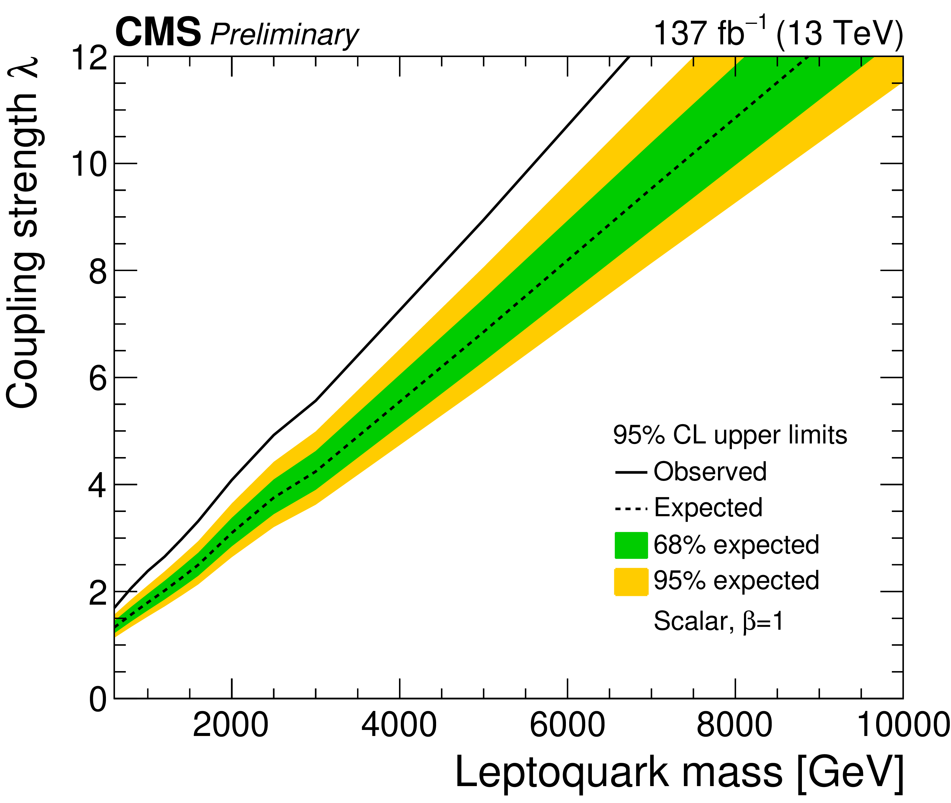
Figure 8:
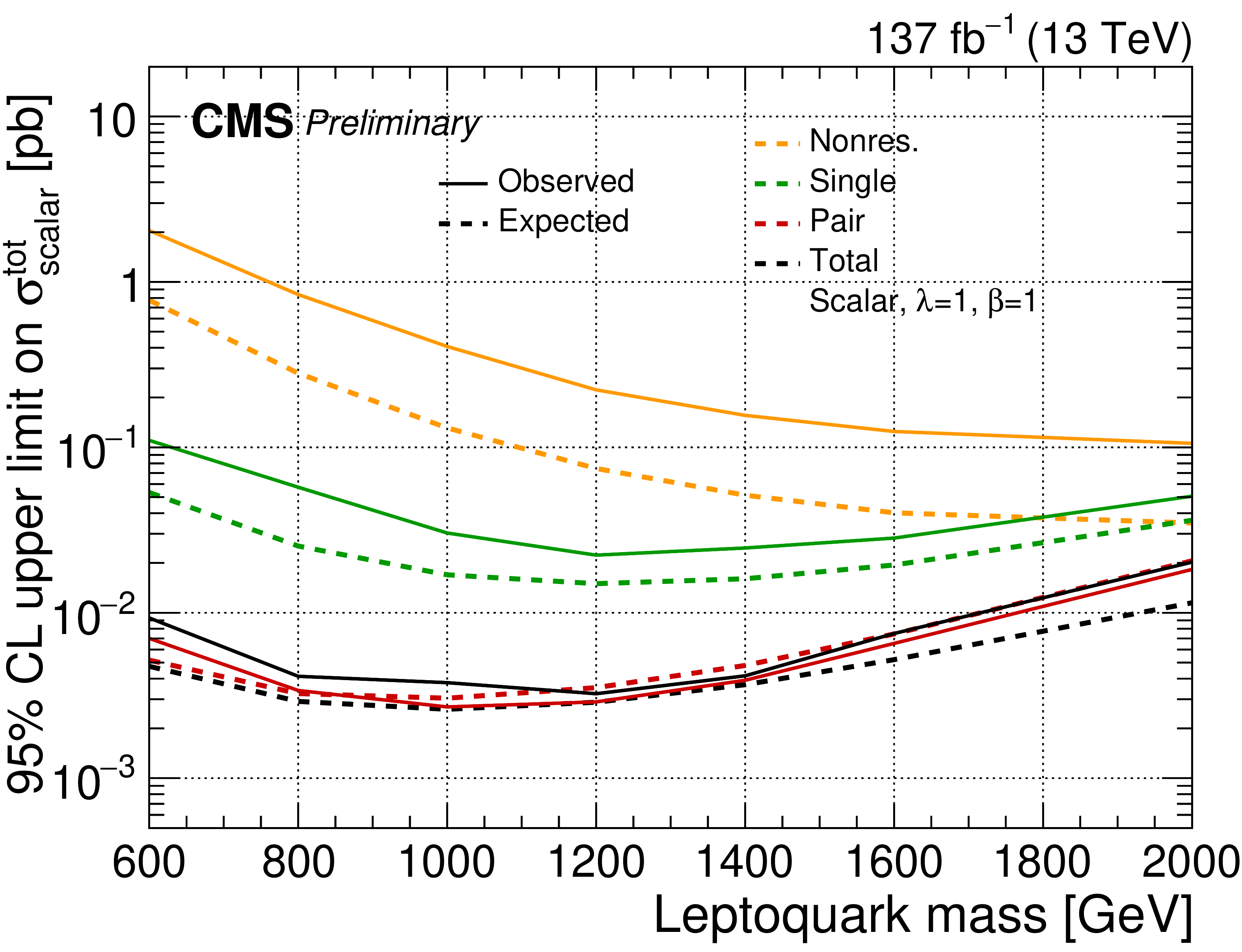
The observed and expected upper limit at 95% CL on the coupling strength $\lambda $ of a scalar LQ. All years and all channels in each category are combined. The limits derived for the single (green), pair (red), nonresonant (orange) and total LQ production (black) are shown. The hatched bands around the expected limit lines correspond to the regions containing 68% of the distribution of limits expected under the background-only hypothesis. |
png pdf |
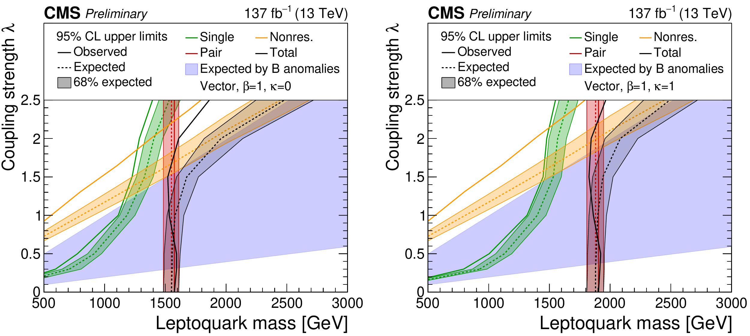
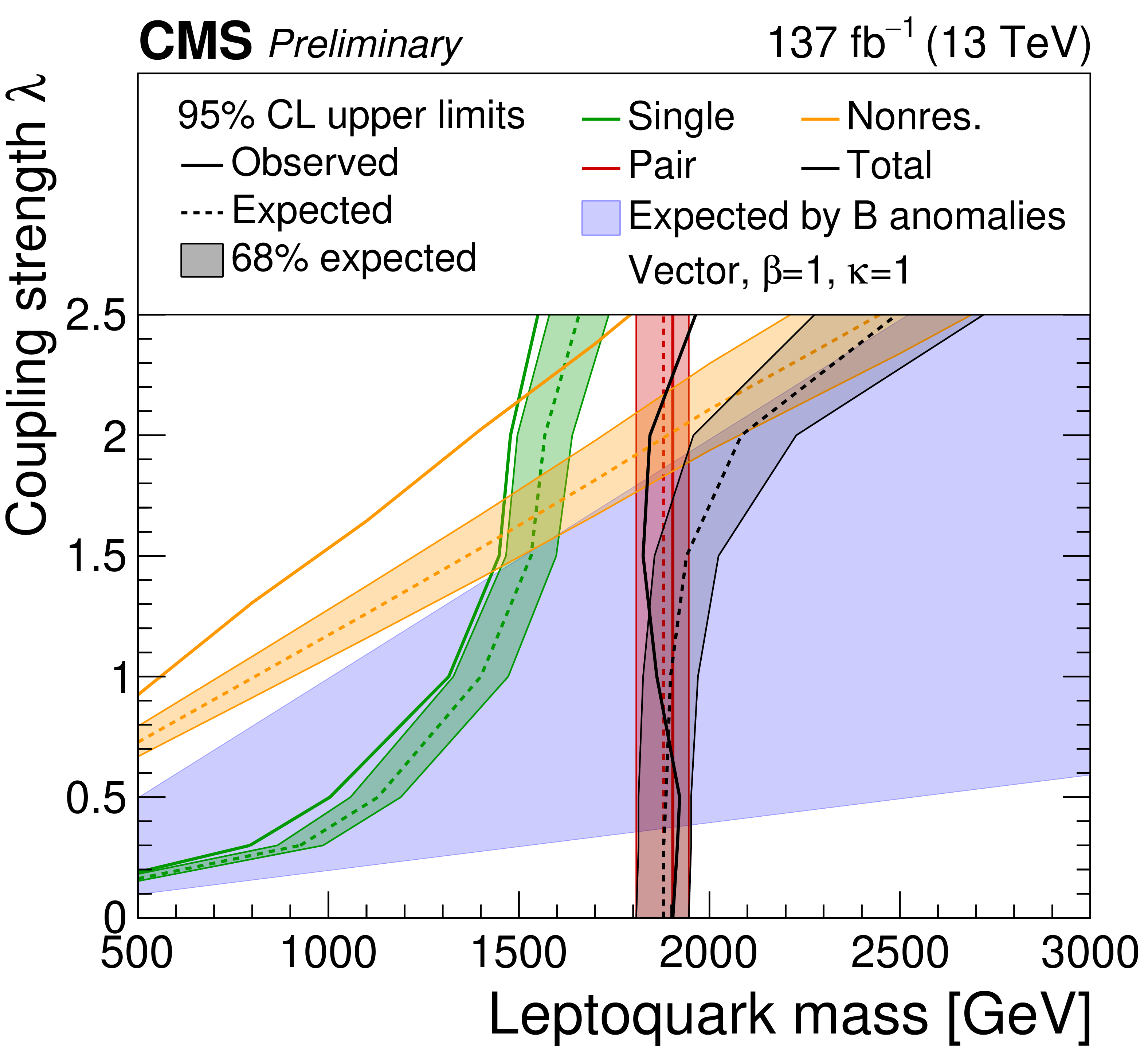
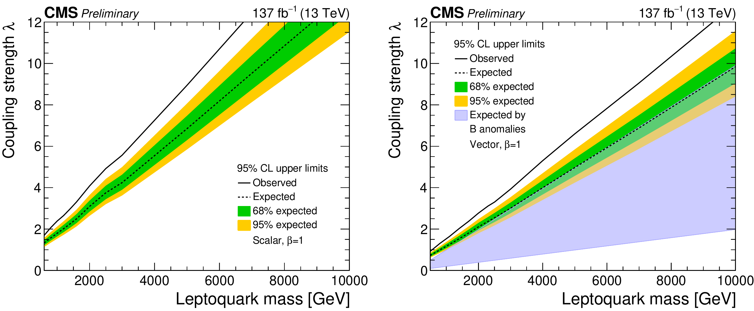
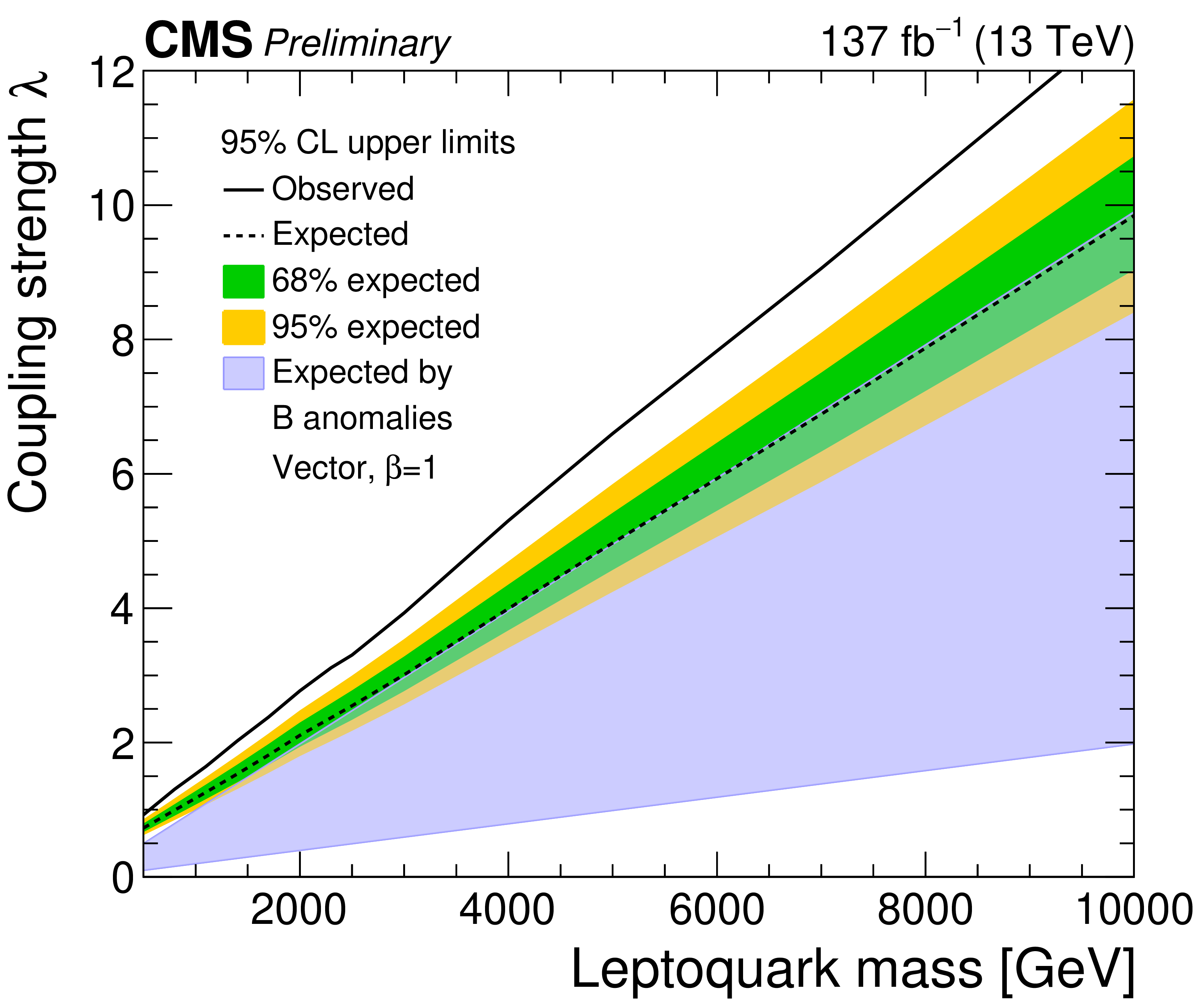
Figure 9:
The observed and expected upper limit at 95% CL on the coupling strength $\lambda $ of a vector LQ model with $\kappa =$ 0 (left) and $\kappa =$ 1 (right). All years and all channels in each category are combined. The limits derived for the single (green), pair (red), nonresonant (orange) and total LQ production (black) are shown. The hatched bands around the expected limit lines correspond to the regions containing 68% of the distribution of limits expected under the background-only hypothesis. The region with blue shading shows the parameter space preferred by one of the models proposed to explain anomalies observed in B physics. |
png pdf |
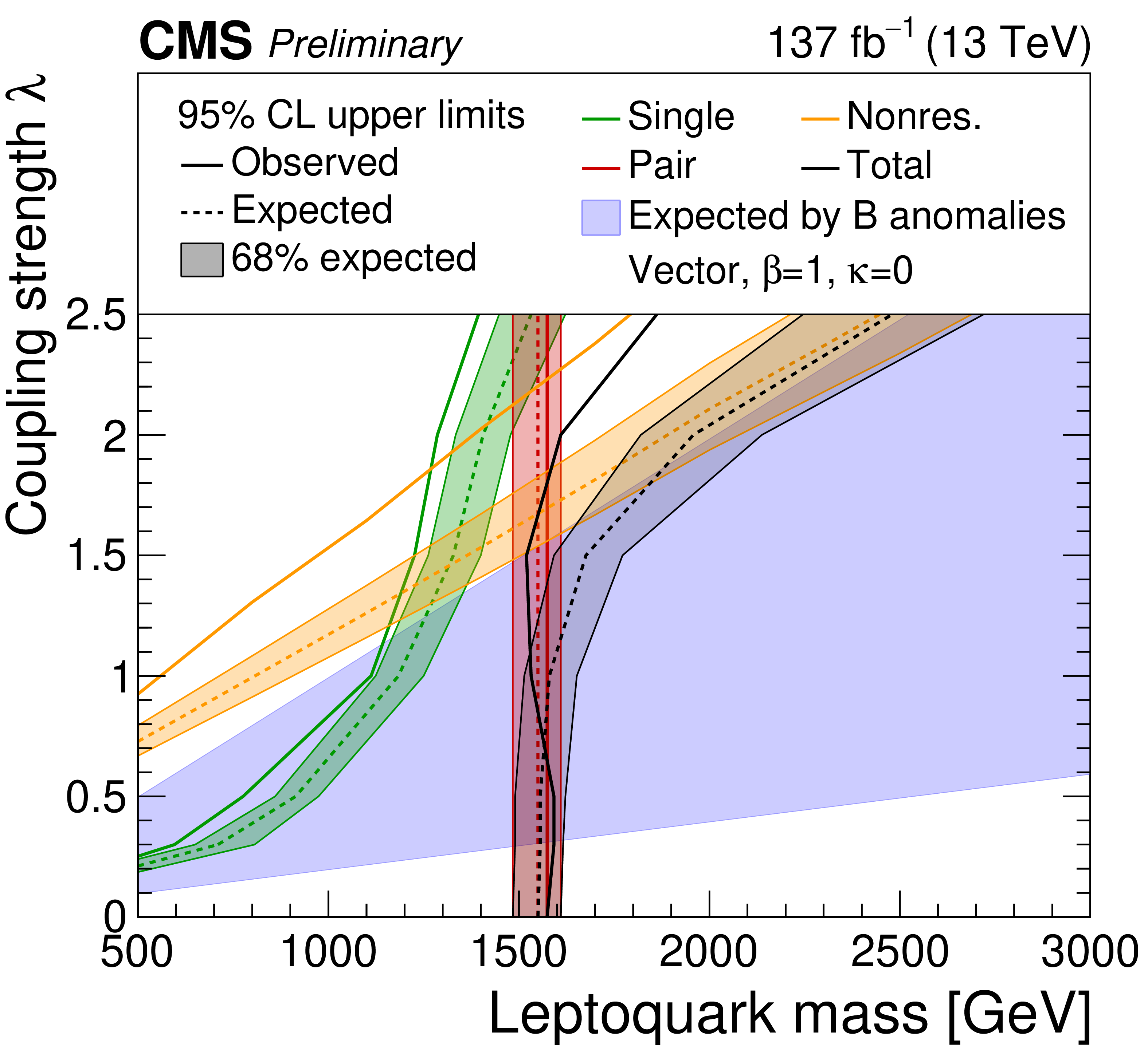
Figure 9-a:
The observed and expected upper limit at 95% CL on the coupling strength $\lambda $ of a vector LQ model with $\kappa =$ 0. All years and all channels in each category are combined. The limits derived for the single (green), pair (red), nonresonant (orange) and total LQ production (black) are shown. The hatched bands around the expected limit lines correspond to the regions containing 68% of the distribution of limits expected under the background-only hypothesis. The region with blue shading shows the parameter space preferred by one of the models proposed to explain anomalies observed in B physics. |
png pdf |
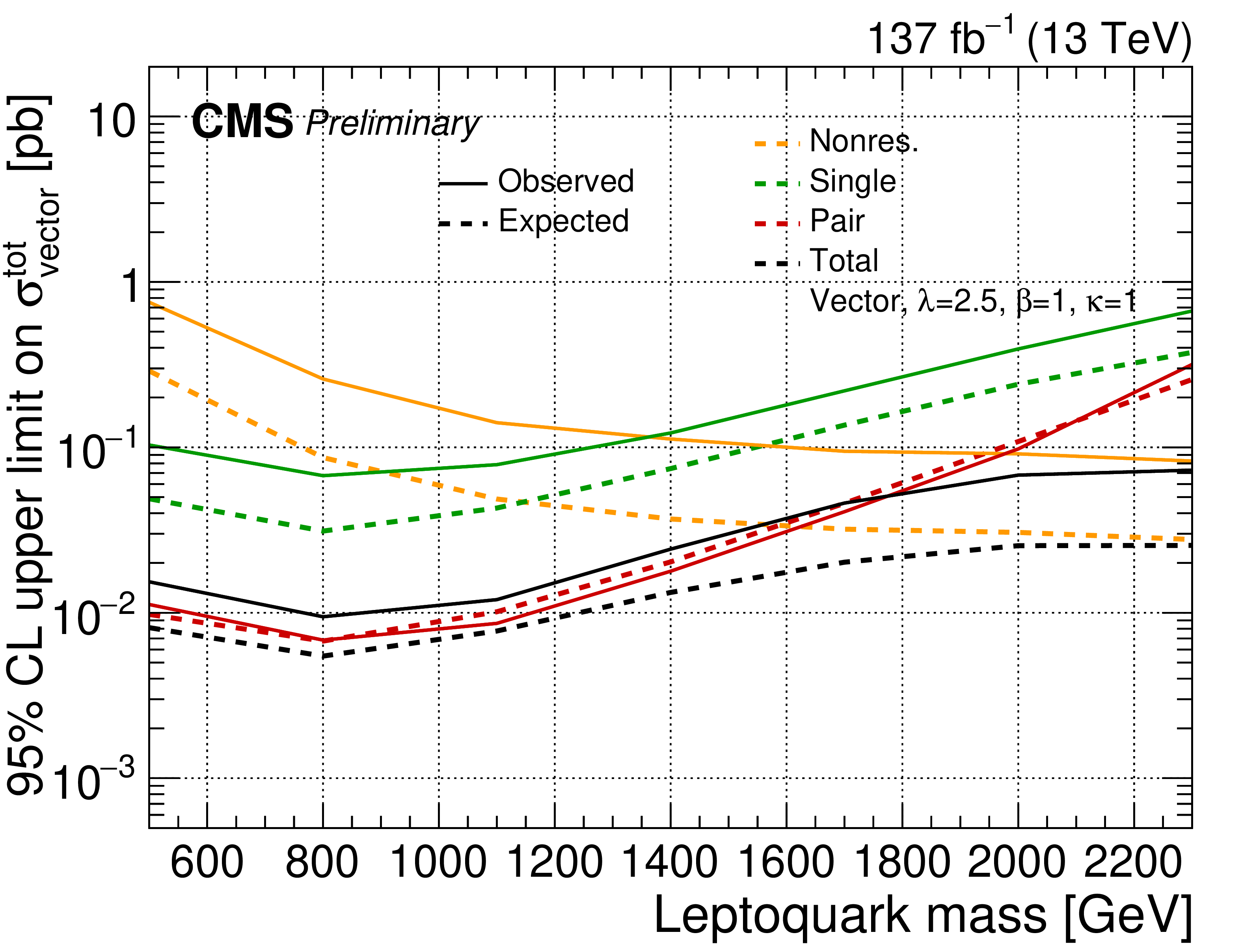
Figure 9-b:
The observed and expected upper limit at 95% CL on the coupling strength $\lambda $ of a vector LQ model with $\kappa =$ 1. All years and all channels in each category are combined. The limits derived for the single (green), pair (red), nonresonant (orange) and total LQ production (black) are shown. The hatched bands around the expected limit lines correspond to the regions containing 68% of the distribution of limits expected under the background-only hypothesis. The region with blue shading shows the parameter space preferred by one of the models proposed to explain anomalies observed in B physics. |
| Tables | |
png pdf |
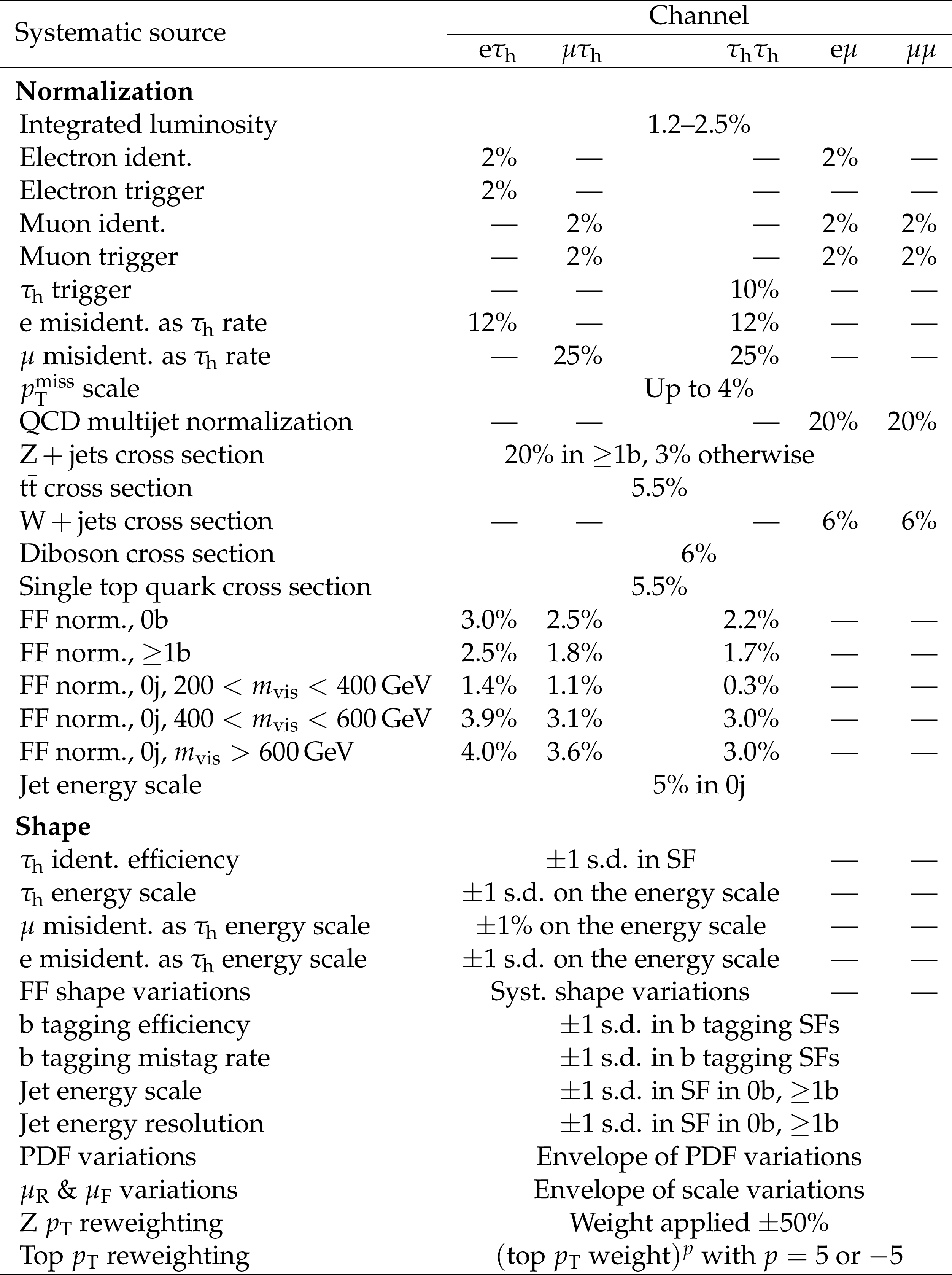
Table 1:
The sources of uncertainty considered, categorized as to whether they affect the normalization or shape of the distributions. "s.d.'' refers to the standard deviation of the input variable. |
png pdf |
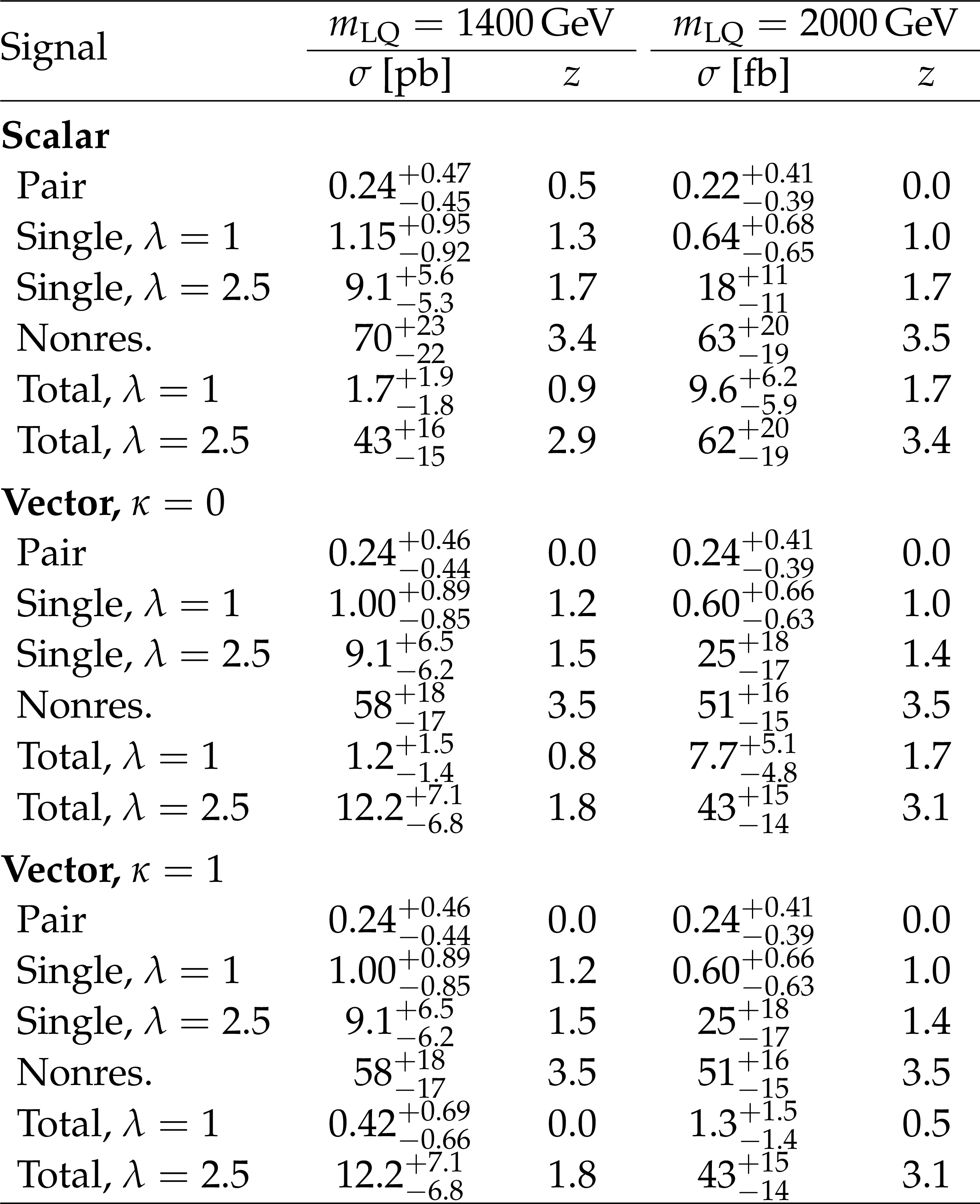
Table 2:
Best-fit LQ cross sections $\sigma $ for various masses and coupling strengths $\lambda $, and the corresponding significance $z$ (given in standard deviations) for different production modes individually, as well as their combination. |
| Summary |
|
This note has reported a search for a third-generation leptoquark (LQ) decaying to a $\tau$ lepton and a b quark. Events with $\tau$ leptons and one jet originating from a b quark were considered, targeting the single and pair production of the LQ, as well as the nonresonant production with the LQ in the $t$ channel. The search used proton-proton collision data at a center-of-mass energy of 13 TeV recorded with the CMS detector corresponding to an integrated luminosity of 137 fb$^{-1}$. Upper limits have been set on the third-generation scalar LQ production cross section as a function of the LQ mass, and results were compared with theoretical predictions to obtain lower limits on the LQ mass. At 95% confidence level, third-generation LQ decaying to a $\tau$ lepton and a b quark with unit coupling are excluded for masses below 1.25 TeV for a scalar model, and below 1.53 (1.86) GeV for a vector model with non-minimal coupling $\kappa=$ 0 (1), while at $\lambda=$ 2.5 the lower limits are 1.37 TeV for a scalar model, and 1.86 (1.96) GeV for a vector model with $\kappa=$ 0 (1). Upper limits are also set on the coupling strength of such LQs as a function of their mass. The observed data agree with the standard model expectation within 2 standard deviations below a coupling strength of $\lambda=$ 1.5. For a representative LQ mass of 2 TeV and a coupling strength of 2.5, an excess with a significance of 3.4 standard deviations above the standard model expectation is observed in the data. Consequently, the observed upper limits on the LQ production cross section are about three times larger than expected for this benchmark. |
| Additional Figures | |
png pdf |
Additional Figure 1:
The expected upper limit on the cross section of a scalar LQ signal at 95% CL. Shown are pair (top left), nonresonant (top right), and single production with $\lambda =$ 1 (bottom left) and $\lambda =$ 2.5 (bottom right). The inner (green) band and the outer (yellow) band indicate the regions containing 68 and 95%, respectively, of the distribution of limits expected under the background-only hypothesis. |
png pdf |
Additional Figure 1-a:
The expected upper limit on the cross section of a scalar LQ signal at 95% CL. Shown is pair production. The inner (green) band and the outer (yellow) band indicate the regions containing 68 and 95%, respectively, of the distribution of limits expected under the background-only hypothesis. |

png pdf |
Additional Figure 1-b:
The expected upper limit on the cross section of a scalar LQ signal at 95% CL. Shown is nonresonant production. The inner (green) band and the outer (yellow) band indicate the regions containing 68 and 95%, respectively, of the distribution of limits expected under the background-only hypothesis. |
png pdf |
Additional Figure 1-c:
The expected upper limit on the cross section of a scalar LQ signal at 95% CL. Shown is single production with $\lambda =$ 1. The inner (green) band and the outer (yellow) band indicate the regions containing 68 and 95%, respectively, of the distribution of limits expected under the background-only hypothesis. |
png pdf |
Additional Figure 1-d:
The expected upper limit on the cross section of a scalar LQ signal at 95% CL. Shown is single production with $\lambda =$ 2.5. The inner (green) band and the outer (yellow) band indicate the regions containing 68 and 95%, respectively, of the distribution of limits expected under the background-only hypothesis. |
png pdf |
Additional Figure 2:
The expected upper limit on the cross section of a vector LQ signal with $\kappa =$ 1 at 95% CL. Shown are pair (top left), nonresonant (top right), and single production with $\lambda =$ 1 (bottom left) and $\lambda =$ 2.5 (bottom right). The inner (green) band and the outer (yellow) band indicate the regions containing 68 and 95%, respectively, of the distribution of limits expected under the background-only hypothesis. |
png pdf |
Additional Figure 2-a:
The expected upper limit on the cross section of a vector LQ signal with $\kappa =$ 1 at 95% CL. Shown is pair production. The inner (green) band and the outer (yellow) band indicate the regions containing 68 and 95%, respectively, of the distribution of limits expected under the background-only hypothesis. |
png pdf |
Additional Figure 2-b:
The expected upper limit on the cross section of a vector LQ signal with $\kappa =$ 1 at 95% CL. Shown is nonresonant production. The inner (green) band and the outer (yellow) band indicate the regions containing 68 and 95%, respectively, of the distribution of limits expected under the background-only hypothesis. |
png pdf |
Additional Figure 2-c:
The expected upper limit on the cross section of a vector LQ signal with $\kappa =$ 1 at 95% CL. Shown is single production with $\lambda =$ 1. The inner (green) band and the outer (yellow) band indicate the regions containing 68 and 95%, respectively, of the distribution of limits expected under the background-only hypothesis. |

png pdf |
Additional Figure 2-d:
The expected upper limit on the cross section of a vector LQ signal with $\kappa =$ 1 at 95% CL. Shown is single production with $\lambda =$ 2.5. The inner (green) band and the outer (yellow) band indicate the regions containing 68 and 95%, respectively, of the distribution of limits expected under the background-only hypothesis. |
png pdf |
Additional Figure 3:
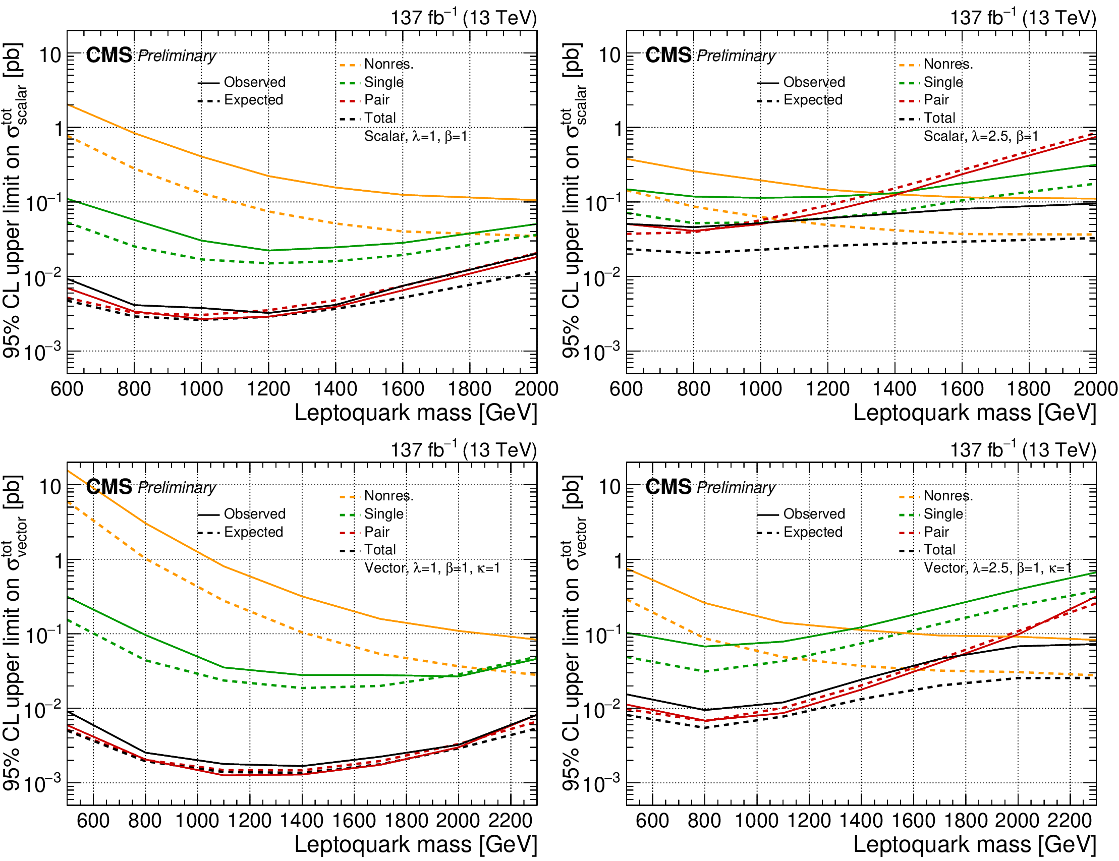
The expected upper limit on the total LQ production cross section at 95% CL comparing each production mode as a separate signal to illustrate their respective sensitivity and contribution to the total sensitivity: single (green), pair (red), nonresonant (orange) and total LQ production (black). All years and all channels in each category are combined. Shown are the scalar (top) and vector LQ model (bottom, $\kappa =$ 1) for $\lambda =$ 1 (left) and $\lambda =$ 2.5 (right). |
png pdf |
Additional Figure 3-a:
The expected upper limit on the total LQ production cross section at 95% CL comparing each production mode as a separate signal to illustrate their respective sensitivity and contribution to the total sensitivity: single (green), pair (red), nonresonant (orange) and total LQ production (black). All years and all channels in each category are combined. Shown is the scalar LQ model for $\lambda =$ 1. |

png pdf |
Additional Figure 3-b:
The expected upper limit on the total LQ production cross section at 95% CL comparing each production mode as a separate signal to illustrate their respective sensitivity and contribution to the total sensitivity: single (green), pair (red), nonresonant (orange) and total LQ production (black). All years and all channels in each category are combined. Shown is the scalar LQ model for $\lambda =$ 2.5. |

png pdf |
Additional Figure 3-c:
The expected upper limit on the total LQ production cross section at 95% CL comparing each production mode as a separate signal to illustrate their respective sensitivity and contribution to the total sensitivity: single (green), pair (red), nonresonant (orange) and total LQ production (black). All years and all channels in each category are combined. Shown is the vector LQ model ($\kappa =$ 1) for $\lambda =$ 1. |
png pdf |
Additional Figure 3-d:
The expected upper limit on the total LQ production cross section at 95% CL comparing each production mode as a separate signal to illustrate their respective sensitivity and contribution to the total sensitivity: single (green), pair (red), nonresonant (orange) and total LQ production (black). All years and all channels in each category are combined. Shown is the vector LQ model ($\kappa =$ 1) for $\lambda =$ 2.5. |
png pdf |
Additional Figure 4:
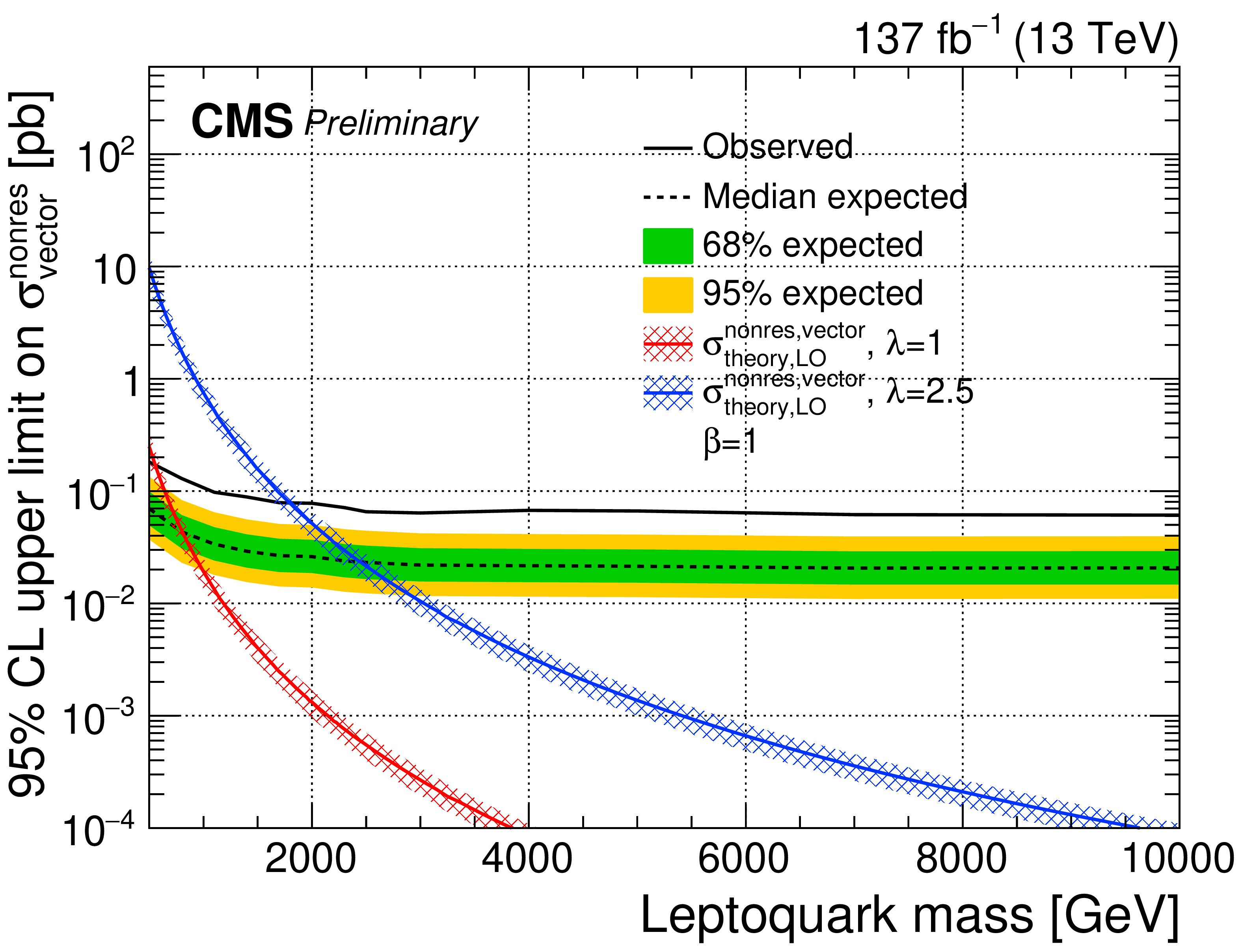
The observed and expected upper limit at 95% CL on the coupling strength $\lambda $ of a scalar (left) and vector LQ model (right) determined from a nonresonant LQ signal only. The inner (green) band and the outer (yellow) band indicate the regions containing 68 and 95%, respectively, of the distribution of limits expected under the background-only hypothesis. The region with blue shading shows the parameter space preferred by one of the models proposed to explain anomalies observed in B physics. |
png pdf |
Additional Figure 4-a:
The observed and expected upper limit at 95% CL on the coupling strength $\lambda $ of a scalar LQ model determined from a nonresonant LQ signal only. The inner (green) band and the outer (yellow) band indicate the regions containing 68 and 95%, respectively, of the distribution of limits expected under the background-only hypothesis. The region with blue shading shows the parameter space preferred by one of the models proposed to explain anomalies observed in B physics. |
png pdf |
Additional Figure 4-b:
The observed and expected upper limit at 95% CL on the coupling strength $\lambda $ of a vector LQ model determined from a nonresonant LQ signal only. The inner (green) band and the outer (yellow) band indicate the regions containing 68 and 95%, respectively, of the distribution of limits expected under the background-only hypothesis. The region with blue shading shows the parameter space preferred by one of the models proposed to explain anomalies observed in B physics. |
| References | ||||
| 1 | CMS Collaboration | Observation of a new boson at a mass of 125 GeV with the CMS experiment at the LHC | PLB 716 (2012) 30 | CMS-HIG-12-028 1207.7235 |
| 2 | ATLAS Collaboration | Observation of a new particle in the search for the Standard Model Higgs boson with the ATLAS detector at the LHC | PLB 716 (2012) 1 | 1207.7214 |
| 3 | CMS Collaboration | Observation of a new boson with mass near 125 GeV in pp collisions at $ \sqrt{s} = $ 7 and 8 TeV | JHEP 06 (2013) 081 | CMS-HIG-12-036 1303.4571 |
| 4 | BaBar Collaboration | Evidence for an excess of $ \bar{B} \to D^{(*)} \tau^-\bar{\nu}_\tau $ decays | PRL 109 (2012) 101802 | 1205.5442 |
| 5 | BaBar Collaboration | Measurement of an excess of $ \bar{B} \to D^{(*)}\tau^- \bar{\nu}_\tau $ decays and implications for charged Higgs bosons | PRD 88 (2013) 072012 | 1303.0571 |
| 6 | Belle Collaboration | Observation of $ B^0 \to D^{*-} \tau^+ \nu_\tau $ decay at Belle | PRL 99 (2007) 191807 | 0706.4429 |
| 7 | Belle Collaboration | Observation of $ B^+ \to \bar{D}^{*0} \tau^+ \nu_\tau $ and evidence for $ B^+ \to \bar{D}^0 \tau^+ \nu_\tau $ at Belle | PRD 82 (2010) 072005 | 1005.2302 |
| 8 | Belle Collaboration | Measurement of the branching ratio of $ \bar{B} \to D^{(\ast)} \tau^- \bar{\nu}_\tau $ relative to $ \bar{B} \to D^{(\ast)} \ell^- \bar{\nu}_\ell $ decays with hadronic tagging at Belle | PRD 92 (2015) 072014 | 1507.03233 |
| 9 | Belle Collaboration | Measurement of the branching ratio of $ \bar{B}^0 \rightarrow D^{*+} \tau^- \bar{\nu}_{\tau} $ relative to $ \bar{B}^0 \rightarrow D^{*+} \ell^- \bar{\nu}_{\ell} $ decays with a semileptonic tagging method | PRD 94 (2016) 072007 | 1607.07923 |
| 10 | Belle Collaboration | Measurement of the $ \tau $ lepton polarization and $ R(D^*) $ in the decay $ \bar{B} \to D^* \tau^- \bar{\nu}_\tau $ | PRL 118 (2017) 211801 | 1612.00529 |
| 11 | Belle Collaboration | Measurement of the $ \tau $ lepton polarization and $ R(D^*) $ in the decay $ \bar{B} \rightarrow D^* \tau^- \bar{\nu}_\tau $ with one-prong hadronic $ \tau $ decays at Belle | PRD 97 (2018) 012004 | 1709.00129 |
| 12 | LHCb Collaboration | Measurement of the ratio of branching fractions $ \mathcal{B}(\bar{B}^0 \to D^{*+}\tau^{-}\bar{\nu}_{\tau})/\mathcal{B}(\bar{B}^0 \to D^{*+}\mu^{-}\bar{\nu}_{\mu}) $ | PRL 115 (2015) 111803 | 1506.08614 |
| 13 | LHCb Collaboration | Measurement of the ratio of the $ B^0 \to D^{*-} \tau^+ \nu_{\tau} $ and $ B^0 \to D^{*-} \mu^+ \nu_{\mu} $ branching fractions using three-prong $ \tau $-lepton decays | PRL 120 (2018), no. 17, 171802 | 1708.08856 |
| 14 | LHCb Collaboration | Test of Lepton Flavor Universality by the measurement of the $ B^0 \to D^{*-} \tau^+ \nu_{\tau} $ branching fraction using three-prong $ \tau $ decays | PRD 97 (2018), no. 7, 072013 | 1711.02505 |
| 15 | B. Dumont, K. Nishiwaki, and R. Watanabe | LHC constraints and prospects for $ S_1 $ scalar leptoquark explaining the $ \bar B \to D^{(*)} \tau \bar\nu $ anomaly | PRD 94 (2016) 034001 | 1603.05248 |
| 16 | H. Georgi and S. L. Glashow | Unity of all elementary particle forces | PRL 32 (1974) 438 | |
| 17 | J. C. Pati and A. Salam | Unified lepton-hadron symmetry and a gauge theory of the basic interactions | PRD 8 (1973) 1240 | |
| 18 | J. C. Pati and A. Salam | Lepton number as the fourth color | PRD 10 (1974) 275 | |
| 19 | H. Murayama and T. Yanagida | A viable SU(5) GUT with light leptoquark bosons | MPLA 7 (1992) 147 | |
| 20 | H. Fritzsch and P. Minkowski | Unified interactions of leptons and hadrons | Annals Phys. 93 (1975) 193 | |
| 21 | G. Senjanovic and A. Sokorac | Light leptoquarks in SO(10) | Z. Phys. C 20 (1983) 255 | |
| 22 | P. H. Frampton and B.-H. Lee | SU(15) grand unification | PRL 64 (1990) 619 | |
| 23 | P. H. Frampton and T. W. Kephart | Higgs sector and proton decay in SU(15) grand unification | PRD 42 (1990) 3892 | |
| 24 | S. Dimopoulos and L. Susskind | Mass without scalars | NPB 155 (1979) 237 | |
| 25 | S. Dimopoulos | Technicolored signatures | NPB 168 (1980) 69 | |
| 26 | E. Farhi and L. Susskind | Technicolor | PR 74 (1981) 277 | |
| 27 | B. Schrempp and F. Schrempp | Light leptoquarks | PLB 153 (1985) 101 | |
| 28 | M. Tanaka and R. Watanabe | New physics in the weak interaction of $ \bar B \to D^{(*)}\tau\bar\nu $ | PRD 87 (2013) 034028 | 1212.1878 |
| 29 | Y. Sakaki, M. Tanaka, A. Tayduganov, and R. Watanabe | Testing leptoquark models in $ \bar B \to D^{(*)} \tau \bar\nu $ | PRD 88 (2013) 094012 | 1309.0301 |
| 30 | I. Doršner, S. Fajfer, N. Košnik, and I. Nišandžić | Minimally flavored colored scalar in $ \bar B \to D^{(*)} \tau \bar \nu $ and the mass matrices constraints | JHEP 11 (2013) 084 | 1306.6493 |
| 31 | B. Gripaios, M. Nardecchia, and S. A. Renner | Composite leptoquarks and anomalies in B-meson decays | JHEP 05 (2015) 006 | 1412.1791 |
| 32 | M. Bauer and M. Neubert | Minimal leptoquark explanation for the $ R_{D^{(*)}} $, $ R_K $ , and $ (g-2)_\mu $ anomalies | PRL 116 (2016) 141802 | 1511.01900 |
| 33 | R. Barbieri, G. Isidori, A. Pattori, and F. Senia | Anomalies in B-decays and U(2) flavour symmetry | EPJC 76 (2016), no. 2, 67 | 1512.01560 |
| 34 | I. Doršner et al. | Physics of leptoquarks in precision experiments and at particle colliders | PR 641 (2016) 1 | 1603.04993 |
| 35 | D. Bečirević and O. Sumensari | A leptoquark model to accommodate $ R_K^\mathrm{exp} < R_K^\mathrm{SM} $ and $ R_{K^\ast}^\mathrm{exp} < R_{K^\ast}^\mathrm{SM} $ | JHEP 08 (2017) 104 | 1704.05835 |
| 36 | D. Buttazzo, A. Greljo, G. Isidori, and D. Marzocca | B-physics anomalies: a guide to combined explanations | JHEP 11 (2017) 044 | 1706.07808 |
| 37 | E. Coluccio Leskow, G. DAmbrosio, A. Crivellin, and D. Muller | $ (g-2)_\mu $, lepton flavor violation, and Z decays with leptoquarks: Correlations and future prospects | PRD 95 (2017) 055018 | 1612.06858 |
| 38 | A. Crivellin, D. Muller, and T. Ota | Simultaneous explanation of $ R(D^{(*)}) $ and $ \mathrm{b}\to\mathrm{s}\mu^{+}\mu^{-} $: the last scalar leptoquarks standing | JHEP 09 (2017) 040 | 1703.09226 |
| 39 | G. Hiller and I. Nišandžić | $ R_K $ and $ R_{K^{\ast}} $ beyond the standard model | PRD 96 (2017) 035003 | 1704.05444 |
| 40 | I. Doršner, S. Fajfer, D. A. Faroughy, and N. Košnik | The role of the S$_3 $ GUT leptoquark in flavor universality and collider searches | JHEP 10 (2017) 188 | 1706.07779 |
| 41 | L. Di Luzio, A. Greljo, and M. Nardecchia | Gauge leptoquark as the origin of B-physics anomalies | PRD 96 (2017), no. 11, 115011 | 1708.08450 |
| 42 | L. Calibbi, A. Crivellin, and T. Li | Model of vector leptoquarks in view of the B-physics anomalies | PRD 98 (2018), no. 11, 115002 | 1709.00692 |
| 43 | M. Bordone, C. Cornella, J. Fuentes-Mart\'in, and G. Isidori | A three-site gauge model for flavor hierarchies and flavor anomalies | PLB 779 (2018) 317 | 1712.01368 |
| 44 | G. Hiller, D. Loose, and I. Nišandžić | Flavorful leptoquarks at hadron colliders | PRD 97 (2018) 075004 | 1801.09399 |
| 45 | D. Bečirević et al. | Scalar leptoquarks from grand unified theories to accommodate the B-physics anomalies | PRD 98 (2018), no. 5, 055003 | 1806.05689 |
| 46 | L. Di Luzio et al. | Maximal Flavour Violation: a Cabibbo mechanism for leptoquarks | JHEP 11 (2018) 081 | 1808.00942 |
| 47 | R. Barbieri and A. Tesi | B-decay anomalies in Pati-Salam SU(4) | EPJC 78 (2018), no. 3, 193 | 1712.06844 |
| 48 | D. Marzocca | Addressing the B-physics anomalies in a fundamental Composite Higgs Model | JHEP 07 (2018) 121 | 1803.10972 |
| 49 | A. Angelescu, D. Becirevic, D. A. Faroughy, and O. Sumensari | Closing the window on single leptoquark solutions to the B-physics anomalies | JHEP 10 (2018) 183 | 1808.08179 |
| 50 | M. J. Baker, J. Fuentes-Mart\'in, G. Isidori, and M. Konig | High-$ p_T $ signatures in vector-leptoquark models | EPJC 79 (2019), no. 4, 334 | 1901.10480 |
| 51 | C. Cornella, J. Fuentes-Mart\'in, and G. Isidori | Revisiting the vector leptoquark explanation of the B-physics anomalies | JHEP 07 (2019) 168 | 1903.11517 |
| 52 | C. Cornella et al. | Reading the footprints of the B-meson flavor anomalies | JHEP 08 (2021) 050 | 2103.16558 |
| 53 | G. Isidori, D. Lancierini, P. Owen, and N. Serra | On the significance of new physics in $ b \rightarrow s \ell^{+} \ell^{-} $ decays | PLB 822 (2021) 136644 | 2104.05631 |
| 54 | LHCb Collaboration | Differential branching fractions and isospin asymmetries of $ B \to K^{(*)} \mu^+ \mu^- $ decays | JHEP 06 (2014) 133 | 1403.8044 |
| 55 | LHCb Collaboration | Measurements of the S-wave fraction in $ B^{0}\rightarrow K^{+}\pi^{-}\mu^{+}\mu^{-} $ decays and the $ B^{0}\rightarrow K^{\ast}(892)^{0}\mu^{+}\mu^{-} $ differential branching fraction | JHEP 11 (2016) 047 | 1606.04731 |
| 56 | LHCb Collaboration | Angular analysis and differential branching fraction of the decay $ B^0_s\to\phi\mu^+\mu^- $ | JHEP 09 (2015) 179 | 1506.08777 |
| 57 | LHCb Collaboration | Angular analysis of the $ B^{0} \to K^{*0} \mu^{+} \mu^{-} $ decay using 3 fb$ ^{-1} $ of integrated luminosity | JHEP 02 (2016) 104 | 1512.04442 |
| 58 | LHCb Collaboration | Test of lepton universality using $ B^{+}\rightarrow K^{+}\ell^{+}\ell^{-} $ decays | PRL 113 (2014) 151601 | 1406.6482 |
| 59 | LHCb Collaboration | Test of lepton universality with $ B^{0} \rightarrow K^{*0}\ell^{+}\ell^{-} $ decays | JHEP 08 (2017) 055 | 1705.05802 |
| 60 | LHCb Collaboration | Search for lepton-universality violation in $ B^+\to K^+\ell^+\ell^- $ decays | PRL 122 (2019), no. 19, 191801 | 1903.09252 |
| 61 | LHCb Collaboration | Test of lepton universality in beauty-quark decays | NP 18 (2022), no. 3, 277 | 2103.11769 |
| 62 | LHCb Collaboration | Tests of lepton universality using $ B^0\to K^0_S \ell^+ \ell^- $ and $ B^+\to K^{*+} \ell^+ \ell^- $ decays | PRL 128 (2022), no. 19, 191802 | 2110.09501 |
| 63 | Belle Collaboration | Lepton-flavor-dependent angular analysis of $ B\to K^\ast \ell^+\ell^- $ | PRL 118 (2017) 111801 | 1612.05014 |
| 64 | I. Doršner and A. Greljo | Leptoquark toolbox for precision collider studies | JHEP 05 (2018) 126 | 1801.07641 |
| 65 | D. A. Faroughy, A. Greljo, and J. F. Kamenik | Confronting lepton flavor universality violation in B decays with high-$ p_T $ tau lepton searches at LHC | PLB 764 (2017) 126 | 1609.07138 |
| 66 | M. Schmaltz and Y.-M. Zhong | The leptoquark Hunter's guide: large coupling | JHEP 01 (2019) 132 | 1810.10017 |
| 67 | ATLAS Collaboration | Search for new phenomena in $ pp $ collisions in final states with tau leptons, b-jets, and missing transverse momentum with the ATLAS detector | PRD 104 (2021), no. 11, 112005 | 2108.07665 |
| 68 | CMS Collaboration | Search for a singly produced third-generation scalar leptoquark decaying to a $ \tau $ lepton and a bottom quark in proton-proton collisions at $ \sqrt{s} = $ 13 TeV | JHEP 07 (2018) 115 | CMS-EXO-17-029 1806.03472 |
| 69 | CMS Collaboration | Search for singly and pair-produced leptoquarks coupling to third-generation fermions in proton-proton collisions at $ \sqrt{s} = $ 13 TeV | PLB 819 (2021) 136446 | CMS-EXO-19-015 2012.04178 |
| 70 | CMS Collaboration | Searches for physics beyond the standard model with the $ M_\mathrm{T2} $ variable in hadronic final states with and without disappearing tracks in proton-proton collisions at $ \sqrt{s}= $ 13 TeV | EPJC 80 (2020), no. 1, 3 | CMS-SUS-19-005 1909.03460 |
| 71 | ATLAS Collaboration | Search for pair production of third-generation scalar leptoquarks decaying into a top quark and a $ \tau $-lepton in $ pp $ collisions at $ \sqrt{s} = $ 13 TeV with the ATLAS detector | JHEP 06 (2021) 179 | 2101.11582 |
| 72 | CMS Collaboration | The CMS trigger system | JINST 12 (2017) P01020 | CMS-TRG-12-001 1609.02366 |
| 73 | CMS Collaboration | The CMS experiment at the CERN LHC | JINST 3 (2008) S08004 | CMS-00-001 1510.07488 |
| 74 | J. Alwall et al. | The automated computation of tree-level and next-to-leading order differential cross sections, and their matching to parton shower simulations | JHEP 07 (2014) 079 | 1405.0301 |
| 75 | J. Alwall et al. | Comparative study of various algorithms for the merging of parton showers and matrix elements in hadronic collisions | EPJC 53 (2008) 473 | 0706.2569 |
| 76 | R. Frederix and S. Frixione | Merging meets matching in MC@NLO | JHEP 12 (2012) 061 | 1209.6215 |
| 77 | P. Nason | A new method for combining NLO QCD with shower Monte Carlo algorithms | JHEP 11 (2004) 040 | hep-ph/0409146 |
| 78 | S. Frixione, P. Nason, and C. Oleari | Matching NLO QCD computations with parton shower simulations: the POWHEG method | JHEP 11 (2007) 070 | 0709.2092 |
| 79 | S. Alioli, P. Nason, C. Oleari, and E. Re | A general framework for implementing NLO calculations in shower Monte Carlo programs: the POWHEG BOX | JHEP 06 (2010) 043 | 1002.2581 |
| 80 | S. Frixione, P. Nason, and G. Ridolfi | A positive-weight next-to-leading-order Monte Carlo for heavy flavour hadroproduction | JHEP 09 (2007) 126 | 0707.3088 |
| 81 | J. M. Campbell, R. K. Ellis, P. Nason, and E. Re | Top-pair production and decay at NLO matched with parton showers | JHEP 04 (2015) 114 | 1412.1828 |
| 82 | S. Alioli, P. Nason, C. Oleari, and E. Re | NLO single-top production matched with shower in POWHEG: $ s $- and $ t $-channel contributions | JHEP 09 (2009) 111 | 0907.4076 |
| 83 | E. Re | Single-top Wt-channel production matched with parton showers using the POWHEG method | EPJC 71 (2011) 1547 | 1009.2450 |
| 84 | Y. Li and F. Petriello | Combining QCD and electroweak corrections to production in FEWZ | PRD 86 (2012) 094034 | 1208.5967 |
| 85 | M. Czakon and A. Mitov | Top++: A program for the calculation of the top-pair cross-section at hadron colliders | CPC 185 (2014) 2930 | 1112.5675 |
| 86 | P. Kant et al. | HatHor for single top-quark production: Updated predictions and uncertainty estimates for single top-quark production in hadronic collisions | CPC 191 (2015) 74 | 1406.4403 |
| 87 | CMS Collaboration | Event generator tunes obtained from underlying event and multiparton scattering measurements | EPJC 76 (2016) 155 | CMS-GEN-14-001 1512.00815 |
| 88 | CMS Collaboration | Extraction and validation of a new set of CMS PYTHIA8 tunes from underlying-event measurements | EPJC 80 (2020) 4 | CMS-GEN-17-001 1903.12179 |
| 89 | CMS Collaboration | Investigations of the impact of the parton shower tuning in Pythia 8 in the modelling of $ \mathrm{t\overline{t}} $ at $ \sqrt{s}= $ 8 and 13 TeV | CMS-PAS-TOP-16-021 | CMS-PAS-TOP-16-021 |
| 90 | R. D. Ball et al. | Parton distributions for the LHC Run II | JHEP 15 (2015) 40 | 1410.8849 |
| 91 | GEANT4 Collaboration | GEANT4 --- a simulation toolkit | NIMA 506 (2003) 250 | |
| 92 | F. Maltoni and T. Stelzer | Madevent: Automatic event generation with madgraph | JHEP 02 (2003) 027 | hep-ph/0208156 |
| 93 | T. Sjostrand et al. | An introduction to PYTHIA 8.2 | CPC 191 (2015) 159 | 1410.3012 |
| 94 | C. Borschensky, B. Fuks, A. Kulesza, and D. Schwartlander | Scalar leptoquark pair production at hadron colliders | PRD 101 (2020), no. 11, 115017 | 2002.08971 |
| 95 | CMS Collaboration | Particle-flow reconstruction and global event description with the CMS detector | JINST 12 (2017) P10003 | CMS-PRF-14-001 1706.04965 |
| 96 | CMS Collaboration | Technical proposal for the Phase-II upgrade of the Compact Muon Solenoid | CMS-PAS-TDR-15-002 | CMS-PAS-TDR-15-002 |
| 97 | H. Voss, A. Hocker, J. Stelzer, and F. Tegenfeldt | TMVA, the toolkit for multivariate data analysis with ROOT | in XI Int. Workshop on Advanced Computing and Analysis Techniques in Physics Research 2007 PoS ACAT:040 | physics/0703039 |
| 98 | CMS Collaboration | Performance of electron reconstruction and selection with the CMS detector in proton-proton collisions at $ \sqrt{s} = $ 8 TeV | JINST 10 (2015) P06005 | CMS-EGM-13-001 1502.02701 |
| 99 | CMS Collaboration | Performance of the CMS muon detector and muon reconstruction with proton-proton collisions at $ \sqrt{s}= $ 13 TeV | JINST 13 (2018) P06015 | CMS-MUO-16-001 1804.04528 |
| 100 | M. Cacciari, G. P. Salam, and G. Soyez | The $ \text{anti-k}_\text{t} $ jet clustering algorithm | JHEP 04 (2008) 063 | 0802.1189 |
| 101 | M. Cacciari and G. P. Salam | Dispelling the $ N^{3} $ myth for the $ {k_{\mathrm{T}}} $ jet-finder | PLB 641 (2006) 57 | hep-ph/0512210 |
| 102 | M. Cacciari, G. P. Salam, and G. Soyez | FastJet user manual | EPJC 72 (2012) 1896 | 1111.6097 |
| 103 | CMS Collaboration | Determination of jet energy calibration and transverse momentum resolution in CMS | JINST 6 (2011) P11002 | CMS-JME-10-011 1107.4277 |
| 104 | CMS Collaboration | Pileup jet identification | CMS-PAS-JME-13-005 | CMS-PAS-JME-13-005 |
| 105 | CMS Collaboration | Jet algorithms performance in 13 TeV data | CMS-PAS-JME-16-003 | CMS-PAS-JME-16-003 |
| 106 | D. Guest et al. | Jet Flavor Classification in High-Energy Physics with Deep Neural Networks | PRD 94 (2016), no. 11, 112002 | 1607.08633 |
| 107 | CMS Collaboration | Identification of heavy-flavour jets with the CMS detector in pp collisions at 13 TeV | JINST 13 (2018), no. 05, P05011 | CMS-BTV-16-002 1712.07158 |
| 108 | CMS Collaboration | Performance of reconstruction and identification of $ \tau $ leptons decaying to hadrons and $ \nu_\tau $ in pp collisions at $ \sqrt{s}= $ 13 TeV | JINST 13 (2018) P10005 | CMS-TAU-16-003 1809.02816 |
| 109 | CMS Collaboration | Identification of hadronic tau lepton decays using a deep neural network | JINST 17 (2022), no. 07, P07023 | CMS-TAU-20-001 2201.08458 |
| 110 | CMS Collaboration | Performance of missing energy reconstruction in 13 TeV pp collision data using the CMS detector | CMS-PAS-JME-16-004 | CMS-PAS-JME-16-004 |
| 111 | CMS Collaboration | Performance of missing transverse momentum in pp collisions at $ \sqrt{s}= $ 13 ~TeV using the CMS detector | CMS-PAS-JME-17-001 | CMS-PAS-JME-17-001 |
| 112 | CMS Collaboration | Search for additional neutral MSSM Higgs bosons in the $ \tau\tau $ final state in proton-proton collisions at $ \sqrt{s}= $ 13 TeV | JHEP 09 (2018) 007 | CMS-HIG-17-020 1803.06553 |
| 113 | CMS Collaboration | Measurement of the $ \mathrm{Z}\gamma^{*} \to \tau\tau $ cross section in pp collisions at $ \sqrt{s} = $ 13 TeV and validation of $ \tau $ lepton analysis techniques | Submitted to \it EPJC | CMS-HIG-15-007 1801.03535 |
| 114 | CMS Collaboration | Precision luminosity measurement in proton-proton collisions at $ \sqrt{s} = $ 13 TeV in 2015 and 2016 at CMS | EPJC 81 (2021) 800 | CMS-LUM-17-003 2104.01927 |
| 115 | CMS Collaboration | CMS luminosity measurement for the 2017 data-taking period at $ \sqrt{s} = $ 13 TeV | CMS-PAS-LUM-17-004 | CMS-PAS-LUM-17-004 |
| 116 | CMS Collaboration | CMS luminosity measurement for the 2018 data-taking period at $ \sqrt{s} = $ 13 TeV | CMS-PAS-LUM-18-002 | CMS-PAS-LUM-18-002 |
| 117 | CMS Collaboration | Observation of the Higgs boson decay to a pair of $ \tau $ leptons with the CMS detector | PLB 779 (2018) 283 | CMS-HIG-16-043 1708.00373 |
| 118 | CMS Collaboration | Performance of reconstruction and identification of tau leptons in their decays to hadrons and tau neutrino in LHC Run-2 | CMS-PAS-TAU-16-002 | CMS-PAS-TAU-16-002 |
| 119 | J. Butterworth et al. | PDF4LHC recommendations for LHC Run II | JPG 43 (2016) 023001 | 1510.03865 |
| 120 | R. J. Barlow and C. Beeston | Fitting using finite Monte Carlo samples | CPC 77 (1993) 219 | |
| 121 | J. S. Conway | Incorporating Nuisance Parameters in Likelihoods for Multisource Spectra | in PHYSTAT 2011, p. 115 2011 | 1103.0354 |
| 122 | ATLAS and CMS Collaborations | Procedure for the LHC Higgs boson search combination in summer 2011 | CMS-NOTE-2011-005 | |
| 123 | T. Junk | Confidence level computation for combining searches with small statistics | NIMA 434 (1999) 435 | hep-ex/9902006 |
| 124 | A. L. Read | Presentation of search results: The CL$ _\text{s} $ technique | JPG 28 (2002) 2693 | |
| 125 | G. Cowan, K. Cranmer, E. Gross, and O. Vitells | Asymptotic formulae for likelihood-based tests of new physics | EPJC 71 (2011) | 1007.1727 |
|
|
Compact Muon Solenoid LHC, CERN |
|

|

|

|

|

|