

Compact Muon Solenoid
LHC, CERN
| CMS-HIG-24-018 ; CERN-EP-2025-202 | ||
| Simultaneous probe of the charm and bottom quark Yukawa couplings using $ {\mathrm{t}\overline{\mathrm{t}}} \mathrm{H} $ events | ||
| CMS Collaboration | ||
| 27 September 2025 | ||
| Phys. Rev. Lett. 136 (2026) 011801 | ||
| Abstract: A search for the standard model Higgs boson decaying to a charm quark-antiquark pair, $ \mathrm{H}{\to}\mathrm{c}\overline{\mathrm{c}} $, produced in association with a top quark-antiquark pair ($ {\mathrm{t}\overline{\mathrm{t}}} \mathrm{H} $) is presented. The search is performed with data from proton-proton collisions at $ \sqrt{s}= $ 13 TeV, corresponding to an integrated luminosity of 138 fb$ ^{-1} $. Advanced machine learning techniques are employed for jet flavor identification and event classification. The Higgs boson decay to a bottom quark-antiquark pair is measured simultaneously and the observed $ {\mathrm{t}\overline{\mathrm{t}}} \mathrm{H}(\mathrm{H}{\to}\mathrm{b}\overline{\mathrm{b}}) $ event rate relative to the standard model expectation is 0.91$^{+0.26}_{-0.22}$. The observed (expected) upper limit on the product of production cross section and branching fraction $ \sigma({\mathrm{t}\overline{\mathrm{t}}} \mathrm{H})\mathcal{B}(\mathrm{H}{\to}\mathrm{c}\overline{\mathrm{c}}) $ is 0.11 (0.13$^{+0.06}_{-0.04}$) pb at 95% confidence level, corresponding to 7.8 (8.7$^{+4.0}_{-2.6}$) times the standard model prediction. When combined with the previous search for $ \mathrm{H}{\to}\mathrm{c}\overline{\mathrm{c}} $ via associated production with a W or Z boson, the observed (expected) 95% confidence interval on the Higgs-charm Yukawa coupling modifier, $ \kappa_{\mathrm{c}} $, is $ |\kappa_{\mathrm{c}}| < $ 3.5 (2.7), the most stringent constraint to date. | ||
| Links: e-print arXiv:2509.22535 [hep-ex] (PDF) ; CDS record ; inSPIRE record ; HepData record ; Physics Briefing ; CADI line (restricted) ; | ||
| Figures & Tables | Summary | Additional Figures | References | CMS Publications |
|---|
| Figures | |
png pdf |
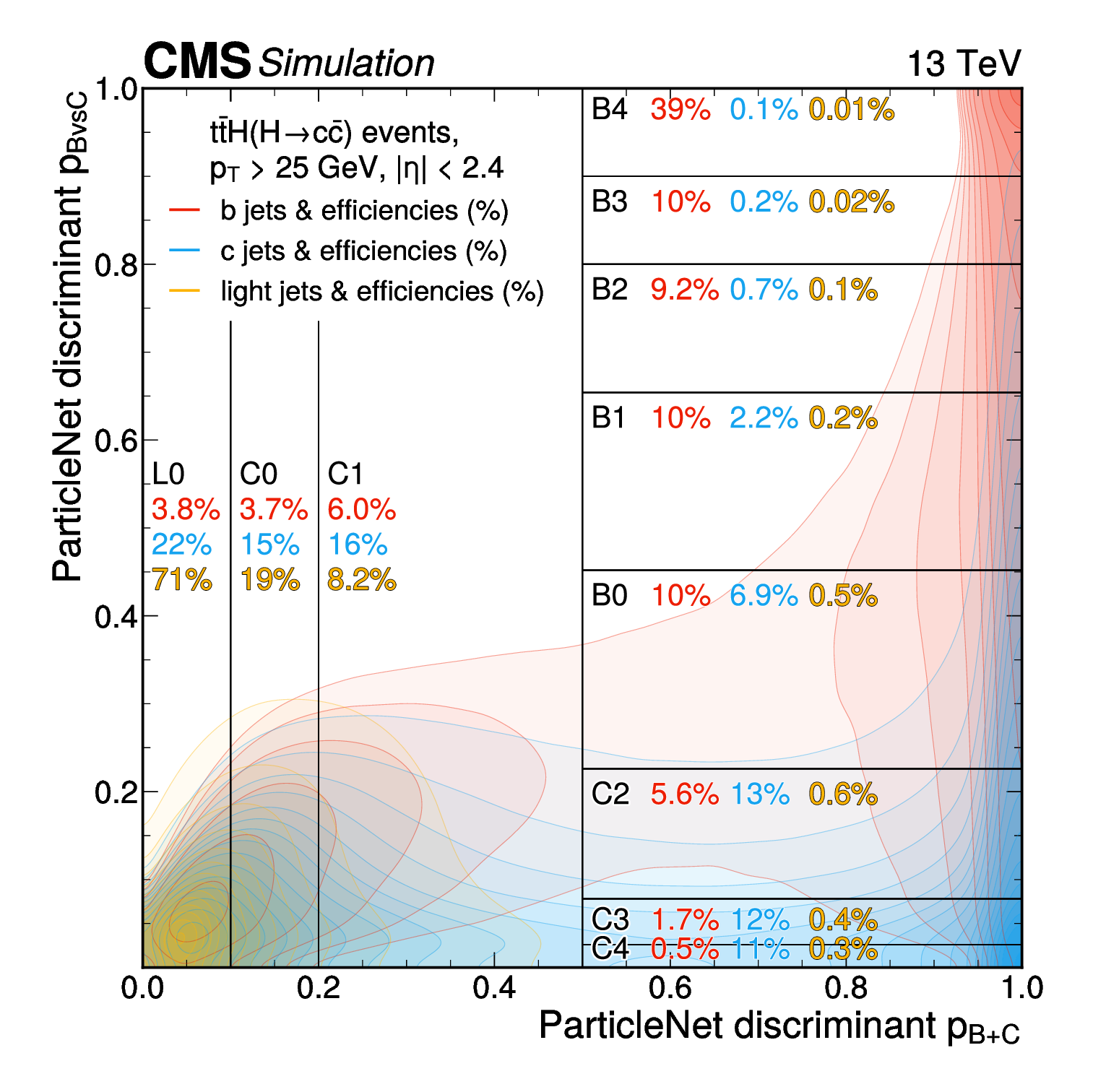
Figure 1:
Distribution of b, c, and light jets in the two-dimensional PARTICLENET discriminant plane. The vertical and horizontal lines correspond to the edges of the tagging categories. The numbers in each bin correspond to the tagging efficiencies for b (red), c (blue), and light (yellow) jets, evaluated on a sample of simulated $ {\mathrm{t}\overline{\mathrm{t}}} \mathrm{H}(\mathrm{H}{\to}\mathrm{c}\overline{\mathrm{c}}) $ events. The contour lines represent constant density values for each jet type in steps of 5%. |
png pdf |
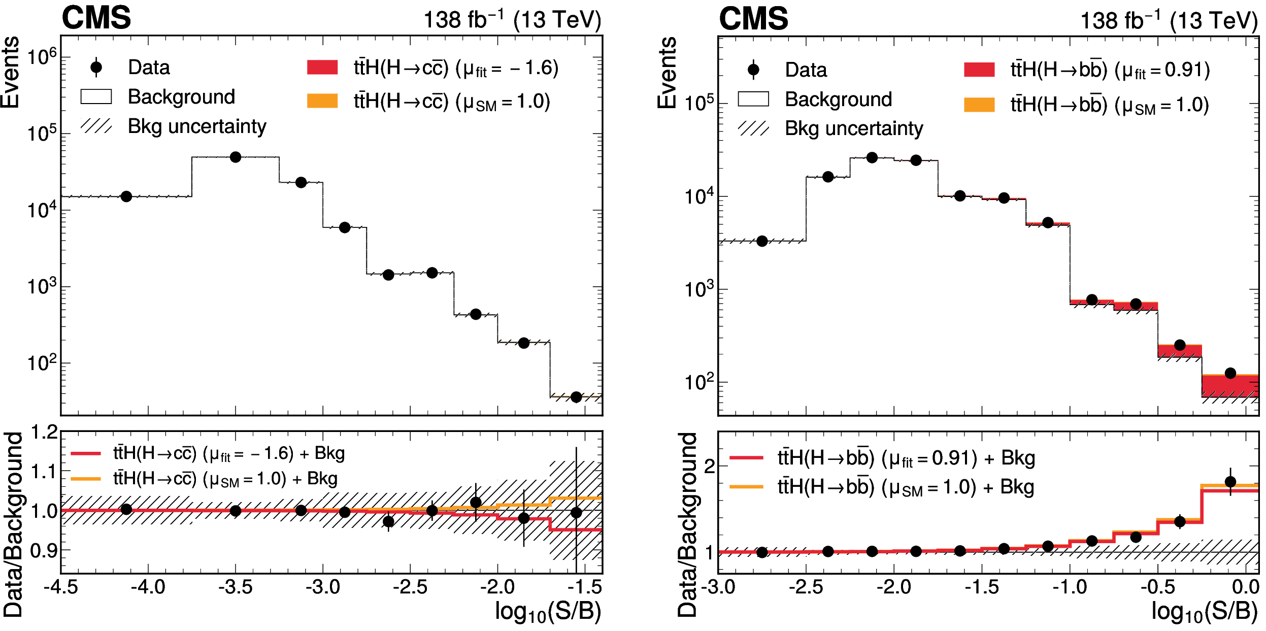
Figure 2:
Observed and expected event yields from all SRs and CRs as a function of $ \log_{10}(S/B) $, where $ S $ are the expected $ {\mathrm{t}\overline{\mathrm{t}}} \mathrm{H}(\mathrm{H}{\to}\mathrm{c}\overline{\mathrm{c}}) $ (left) and $ {\mathrm{t}\overline{\mathrm{t}}} \mathrm{H}(\mathrm{H}{\to}\mathrm{b}\overline{\mathrm{b}}) $ (right) yields, and $ B $ are the post-fit total background yields. Signal contributions are shown for the best fit signal strength (red) and for the SM prediction, $ \mu= $ 1 (orange). The lower panel shows the ratio of the data to the post-fit background predictions, compared to the signal-plus-background predictions. |
png pdf |
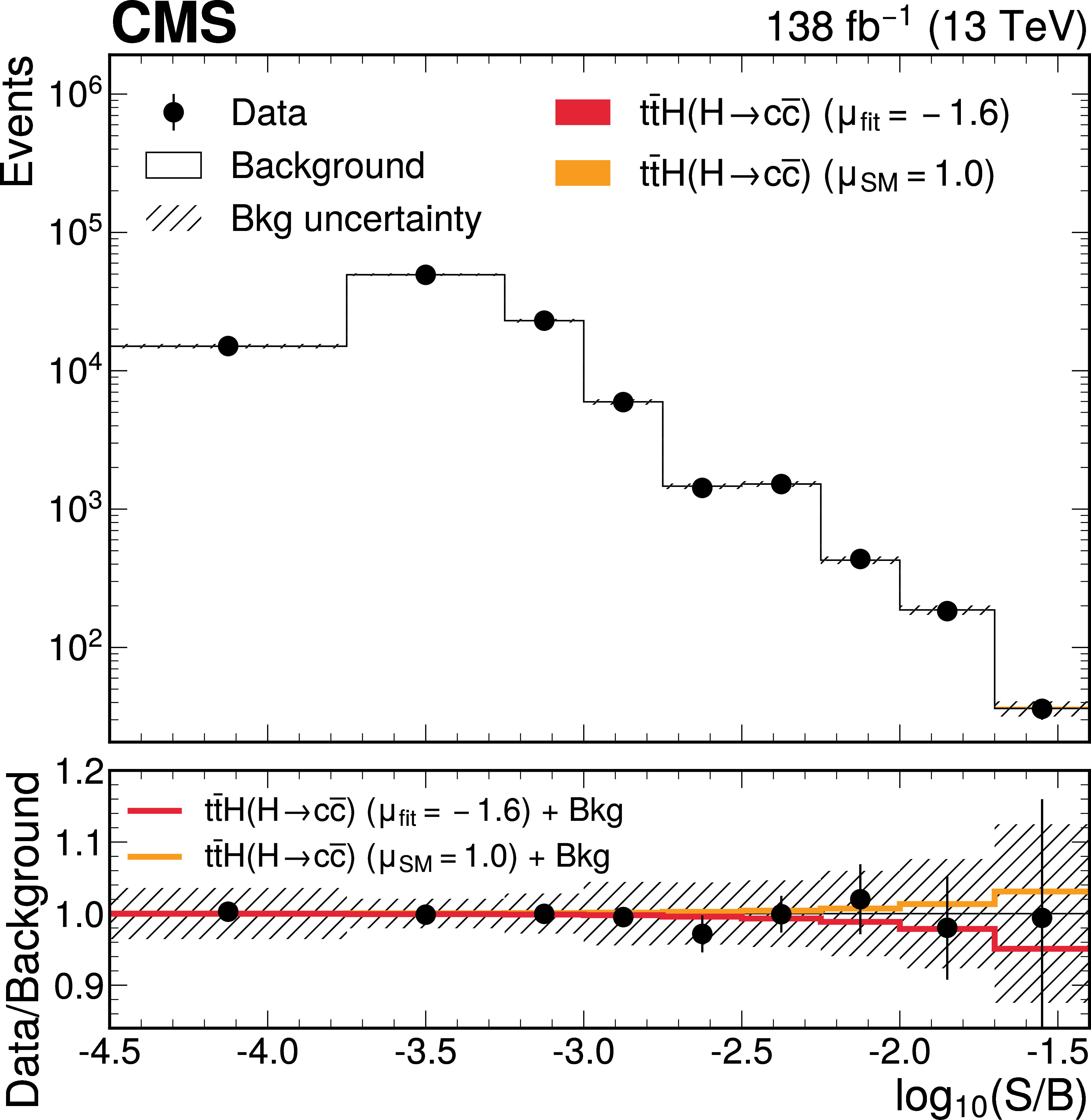
Figure 2-a:
Observed and expected event yields from all SRs and CRs as a function of $ \log_{10}(S/B) $, where $ S $ are the expected $ {\mathrm{t}\overline{\mathrm{t}}} \mathrm{H}(\mathrm{H}{\to}\mathrm{c}\overline{\mathrm{c}}) $ (left) and $ {\mathrm{t}\overline{\mathrm{t}}} \mathrm{H}(\mathrm{H}{\to}\mathrm{b}\overline{\mathrm{b}}) $ (right) yields, and $ B $ are the post-fit total background yields. Signal contributions are shown for the best fit signal strength (red) and for the SM prediction, $ \mu= $ 1 (orange). The lower panel shows the ratio of the data to the post-fit background predictions, compared to the signal-plus-background predictions. |
png pdf |
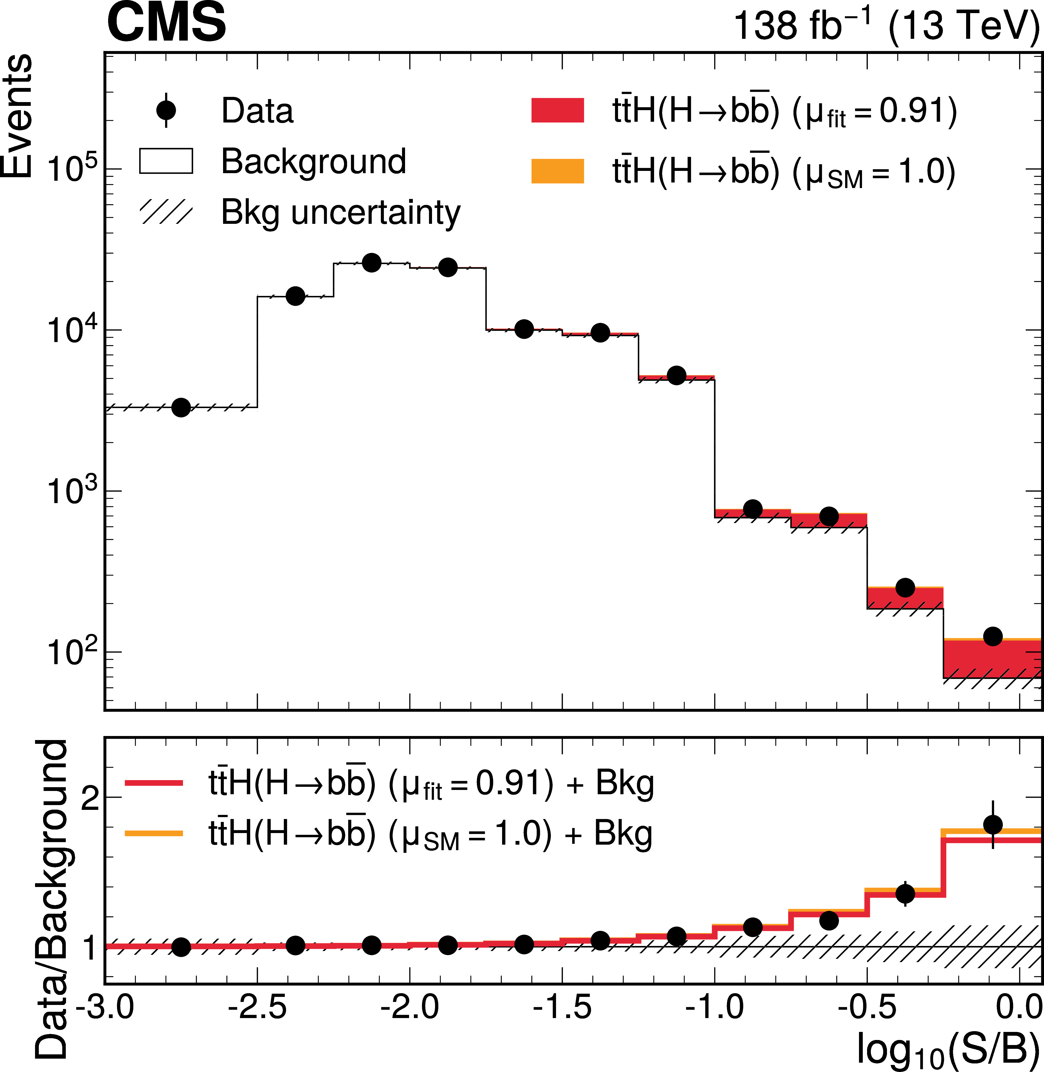
Figure 2-b:
Observed and expected event yields from all SRs and CRs as a function of $ \log_{10}(S/B) $, where $ S $ are the expected $ {\mathrm{t}\overline{\mathrm{t}}} \mathrm{H}(\mathrm{H}{\to}\mathrm{c}\overline{\mathrm{c}}) $ (left) and $ {\mathrm{t}\overline{\mathrm{t}}} \mathrm{H}(\mathrm{H}{\to}\mathrm{b}\overline{\mathrm{b}}) $ (right) yields, and $ B $ are the post-fit total background yields. Signal contributions are shown for the best fit signal strength (red) and for the SM prediction, $ \mu= $ 1 (orange). The lower panel shows the ratio of the data to the post-fit background predictions, compared to the signal-plus-background predictions. |
png pdf |
Figure 3:
The 95% CL upper limits on $ \mu_{{\mathrm{t}\overline{\mathrm{t}}} \mathrm{H}(\mathrm{H}{\to}\mathrm{c}\overline{\mathrm{c}})} $. The yellow and blue bands indicate the expected 68% and 95% CL regions, respectively, under the background-only hypothesis. The vertical red line indicates the SM value $ \mu_{{\mathrm{t}\overline{\mathrm{t}}} \mathrm{H}(\mathrm{H}{\to}\mathrm{c}\overline{\mathrm{c}})}= $ 1. |
png pdf |
Figure 4:
Constraints on the Higgs boson coupling modifiers $ \kappa_{\mathrm{c}} $ and $ \kappa_{\mathrm{b}} $. The 68% (95%) CL intervals are indicated by the dashed (solid) lines. The observed (expected) best fit values are shown by the orange (blue) markers. |
png pdf |
Figure 5:
Event categorization flowchart. |
png pdf |
Figure 6:
Distributions of the PART discriminants in data (points) and predicted signal and backgrounds (colored histograms) after the fit to data. The vertical bars on the points represent the statistical uncertainties in data. The hatched band represents the total uncertainty in the sum of the signal and background predictions. The lower panel shows the ratio of the data to the sum of the signal and background predictions. |
png pdf |
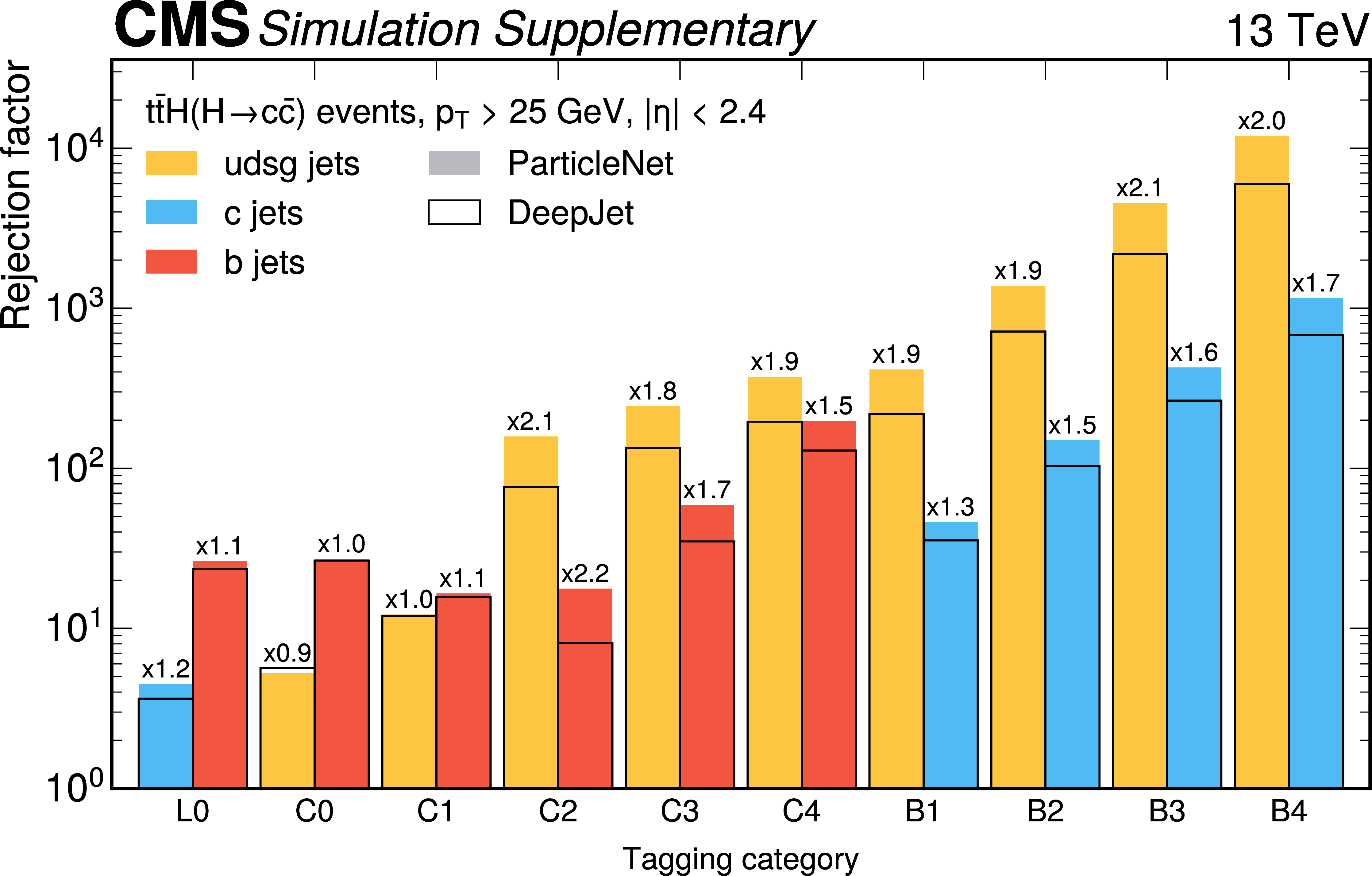
Figure B1:
Rejection factors for the subdominant jet flavors in each of the tagging bins. The filled bars represent the rejection factors achieved with the PARTICLENET tagger and the corresponding working point definitions. The black bars represent the rejection factors achieved with the DEEPJET tagger with working points mimicking the dominant flavor tagging efficiencies. Each bin is labeled with the relative improvement of the PARTICLENET tagger compared to the DEEPJET tagger. All rejection factors and tagging efficiencies are evaluated using simulated $ {\mathrm{t}\overline{\mathrm{t}}} \mathrm{H}(\mathrm{H}{\to}\mathrm{c}\overline{\mathrm{c}}) $ events with 2018 detector conditions. |
png pdf |
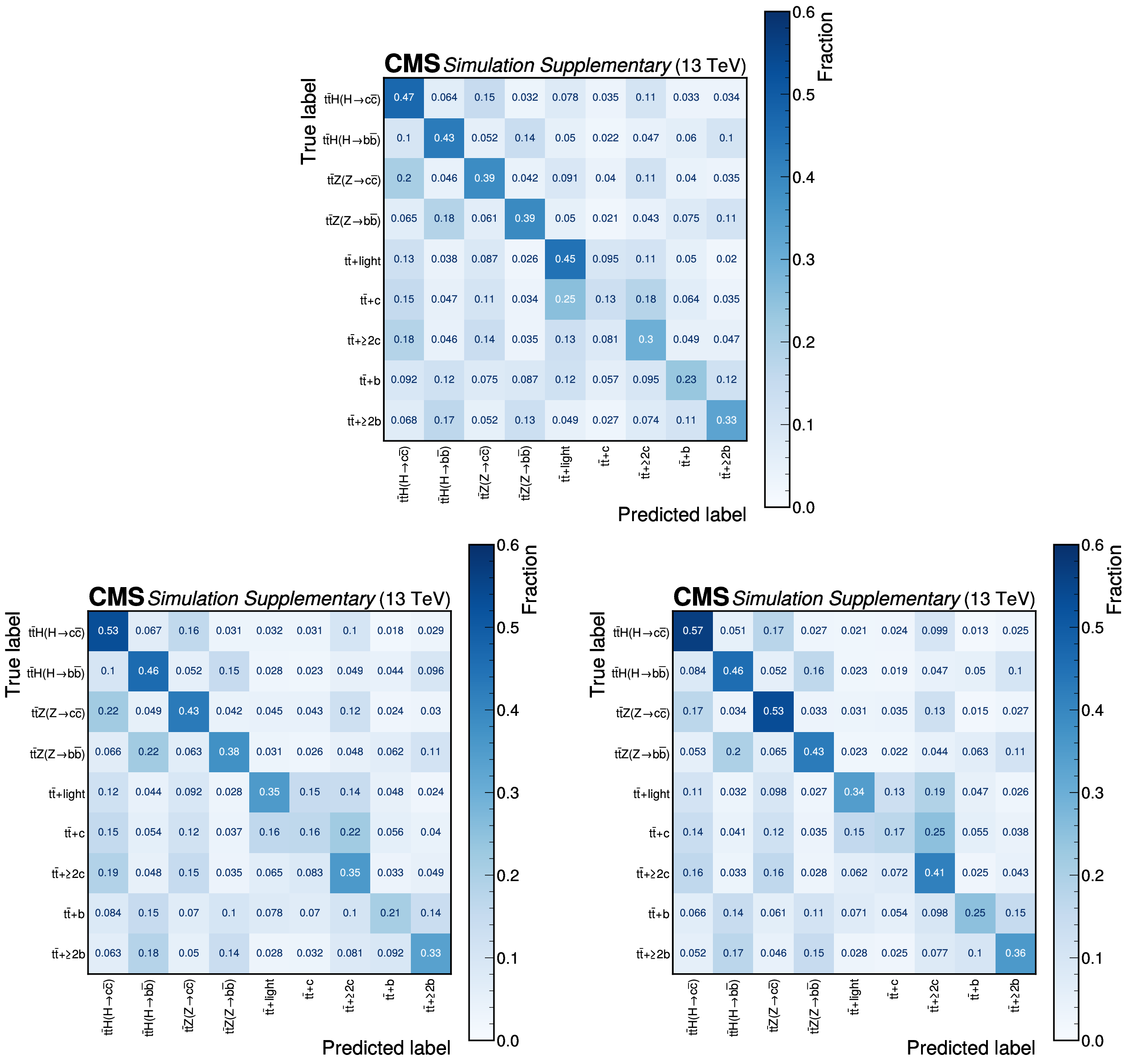
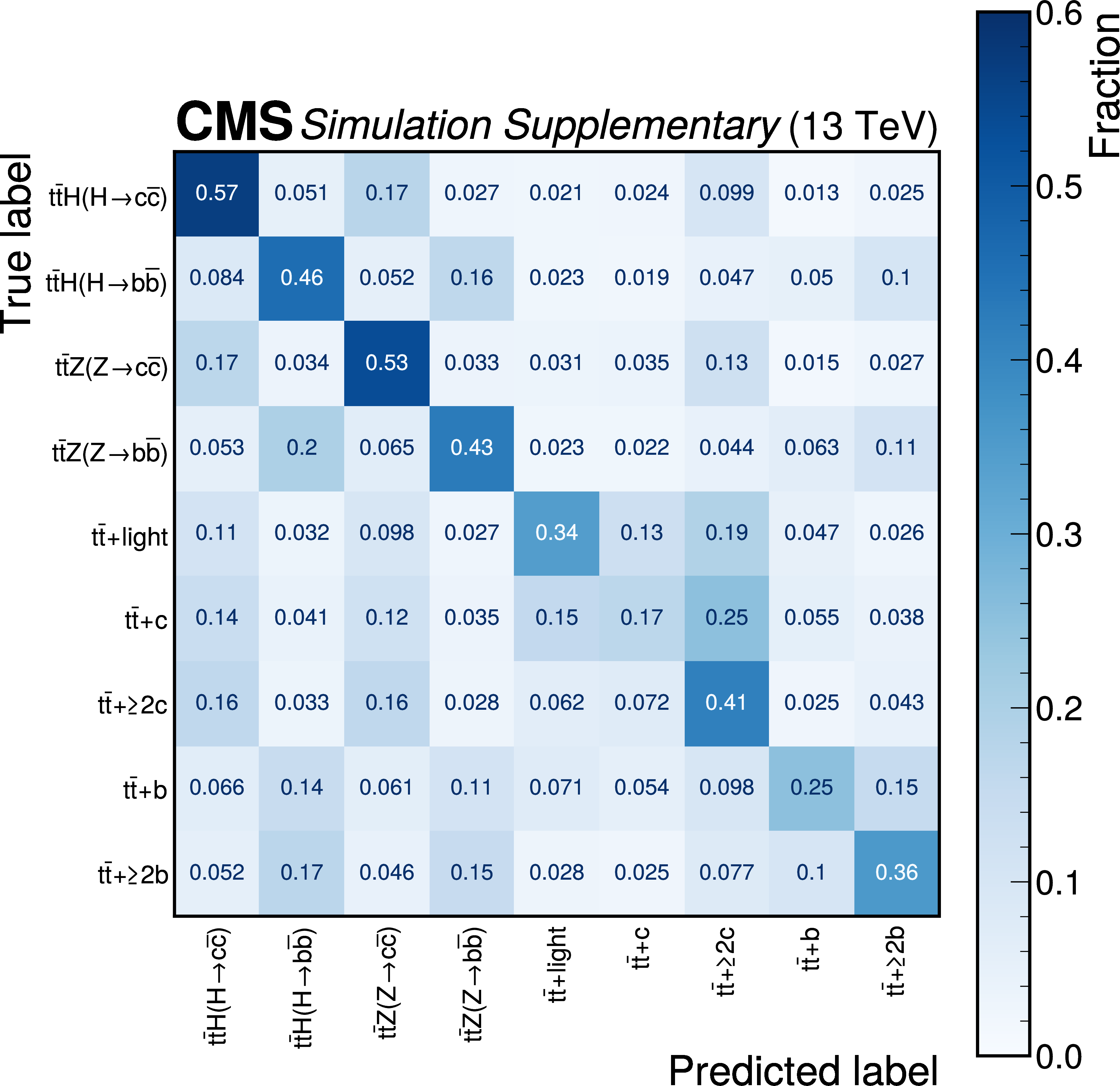
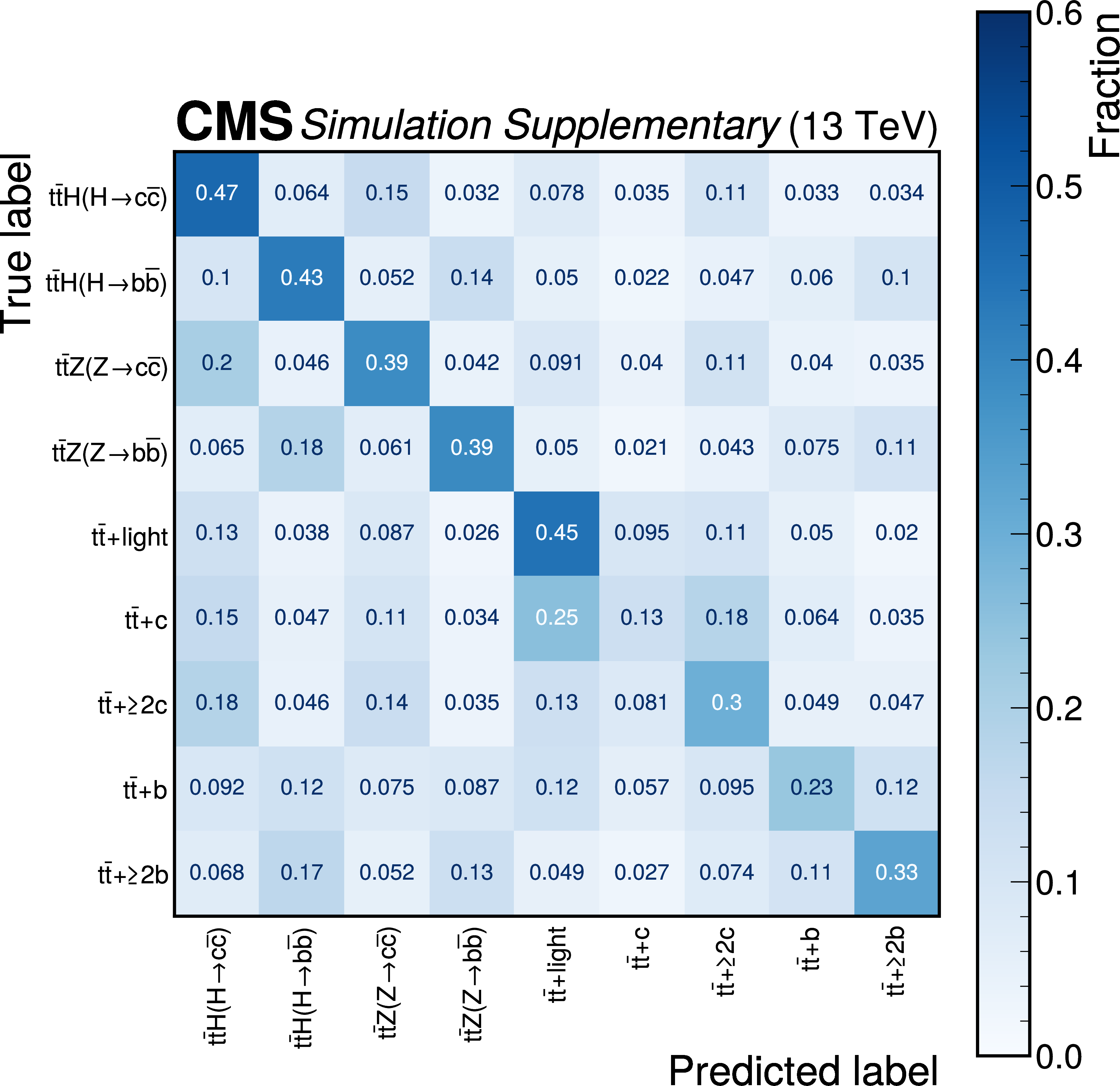
Figure B2:
Confusion matrices of the PART event classifier in the $ \text{0L} $ (upper), $ \text{1L} $ (lower left), and $ \text{2L} $ (lower right) channels after the baseline selection. For each event, the predicted label is the process with the highest output discriminant. The event yield fractions are normalized per true label such that each row sums up to unity. |

png pdf |
Figure B2-a:
Confusion matrices of the PART event classifier in the $ \text{0L} $ (upper), $ \text{1L} $ (lower left), and $ \text{2L} $ (lower right) channels after the baseline selection. For each event, the predicted label is the process with the highest output discriminant. The event yield fractions are normalized per true label such that each row sums up to unity. |

png pdf |
Figure B2-b:
Confusion matrices of the PART event classifier in the $ \text{0L} $ (upper), $ \text{1L} $ (lower left), and $ \text{2L} $ (lower right) channels after the baseline selection. For each event, the predicted label is the process with the highest output discriminant. The event yield fractions are normalized per true label such that each row sums up to unity. |
png pdf |
Figure B2-c:
Confusion matrices of the PART event classifier in the $ \text{0L} $ (upper), $ \text{1L} $ (lower left), and $ \text{2L} $ (lower right) channels after the baseline selection. For each event, the predicted label is the process with the highest output discriminant. The event yield fractions are normalized per true label such that each row sums up to unity. |
png pdf |
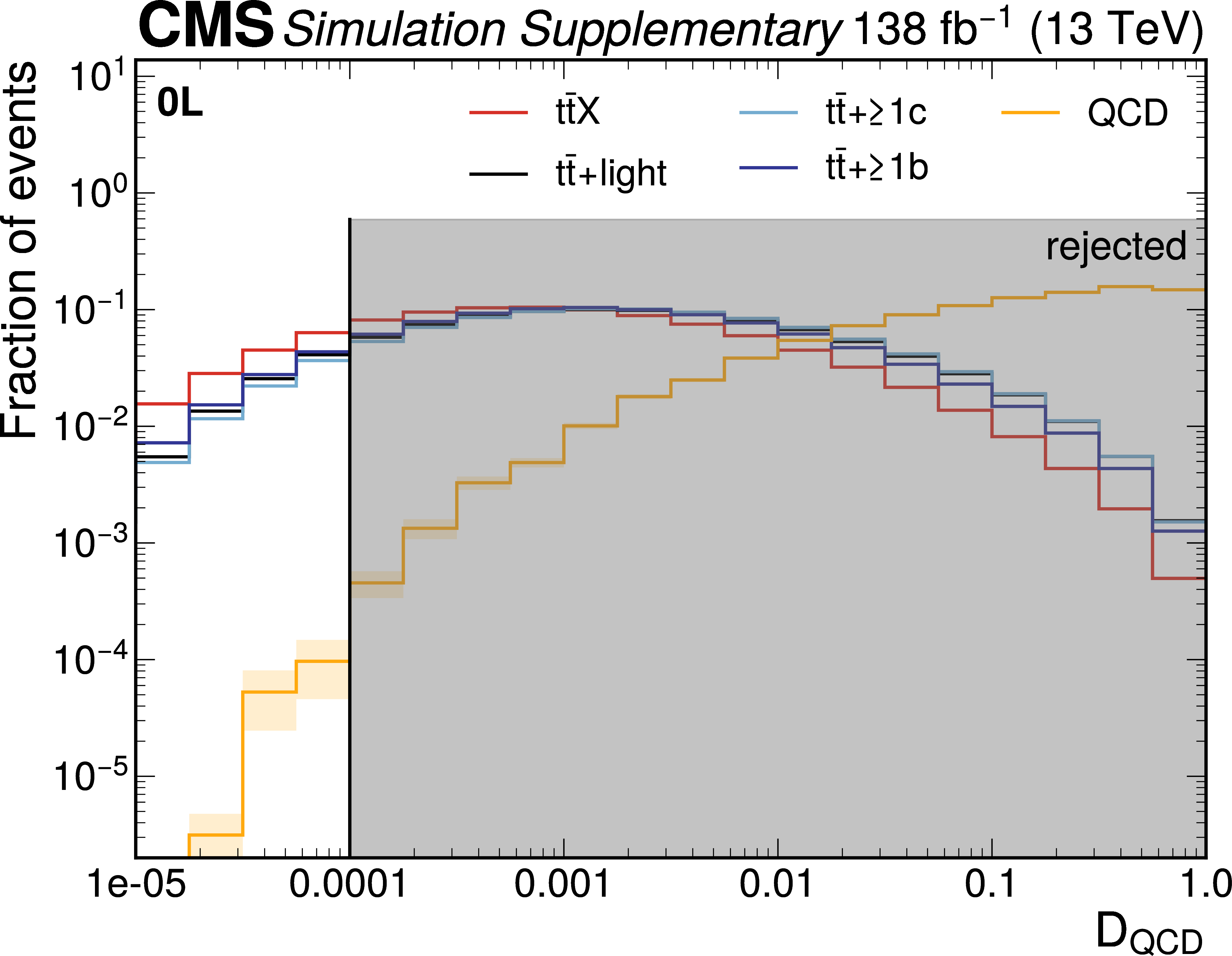
Figure B3:
Distribution of the PART $\mathcal{D}_ \text{QCD} $ discriminant used in the $ \text{0L} $ channel to remove the $ \text{QCD} $ background. The gray area indicates the region that is rejected in the analysis. The shaded band indicates the uncertainty in the $ \text{QCD} $ prediction due to limited size of simulated $ \text{QCD} $ multijet samples. All contributions are normalized to unity. |
png pdf |
Figure B4:
Distribution of the PART $\mathcal{D}_ {{\mathrm{t}\overline{\mathrm{t}}} {+}\text{light}} $ discriminant used to reduce the $ {{\mathrm{t}\overline{\mathrm{t}}} {+}\text{light}} $ background in the $ \text{2L} $ channel. The gray area indicates the region that is rejected in the analysis. All contributions are normalized to unity. The last bin includes the overflow. |
png pdf |
Figure B5:
Distribution of the PART $\mathcal{D}_{ {\mathrm{t}\overline{\mathrm{t}}} \mathrm{X} } $ discriminant used to define the different regions in the $ \text{1L} $ channel. The purple (yellow) area indicates the region that is used for the validation (analysis). The dashed line indicates the separation of SRs and CRs in the analysis. All contributions are normalized to unity. |
png pdf |
Figure B6:
Distributions of the PART discriminants in data (points) and predicted signal and backgrounds (colored histograms) after the maximum likelihood fit to data in the VR, defined by 0.4 $ < \score{{\mathrm{t}\overline{\mathrm{t}}} \mathrm{X}} < $ 0.6. The vertical bars on the points represent the statistical uncertainties in data. The hatched band represents the total uncertainty in the sum of the signal and background predictions. The lower panel shows the ratio of the data to the sum of the signal and background predictions. The ratio of the pre-fit expectation to the sum of the signal and background predictions after the fit is shown as a red line in the lower panel, including the pre-fit uncertainties as a shaded band. |
png pdf |
Figure B7:
Distributions of the PART discriminants in data (points) and predicted signal and backgrounds (colored histograms) after the maximum likelihood fit to data. The vertical bars on the points represent the statistical uncertainties in data. The hatched band represents the total uncertainty in the sum of the signal and background predictions. The lower panel shows the ratio of the data to the sum of the signal and background predictions. The ratio of the pre-fit expectation to the sum of the signal and background predictions after the fit is shown as a red line in the lower panel, including the pre-fit uncertainties as a shaded band. |
png pdf |
Figure B8:
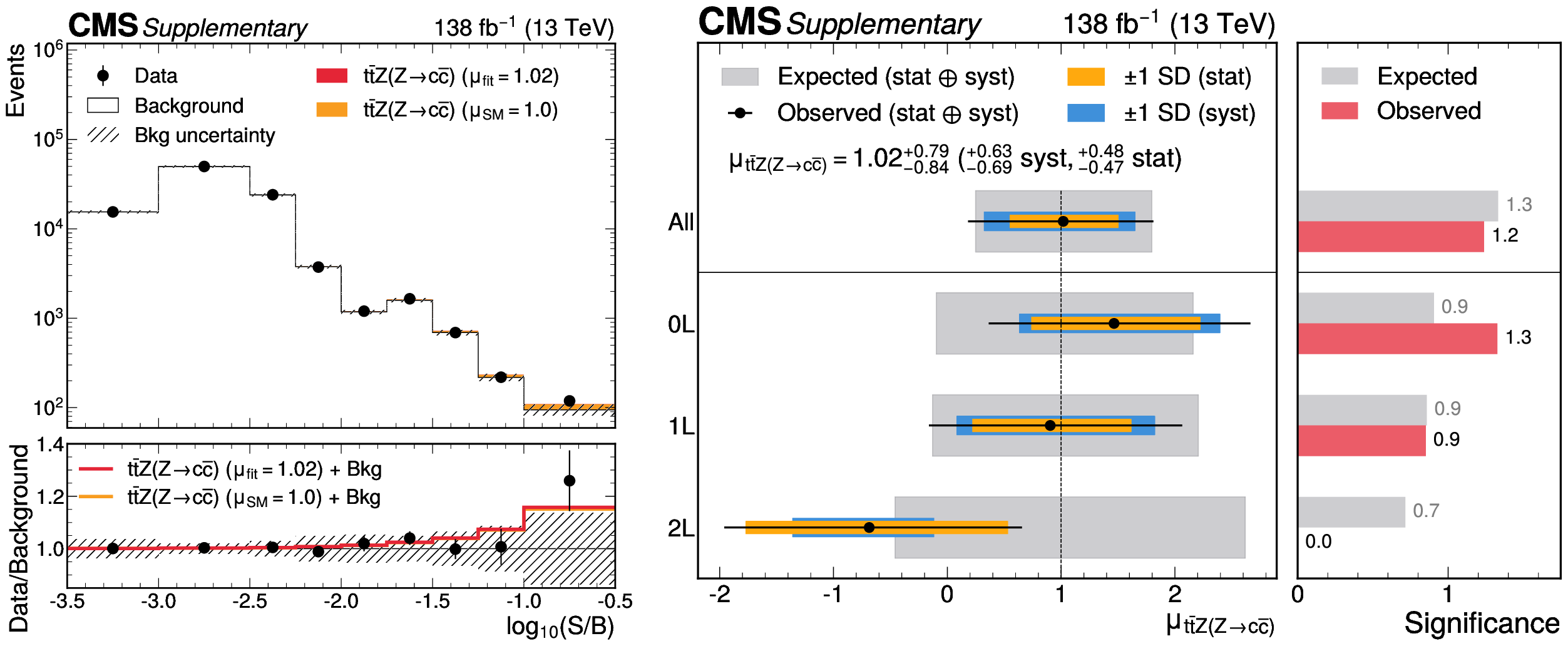
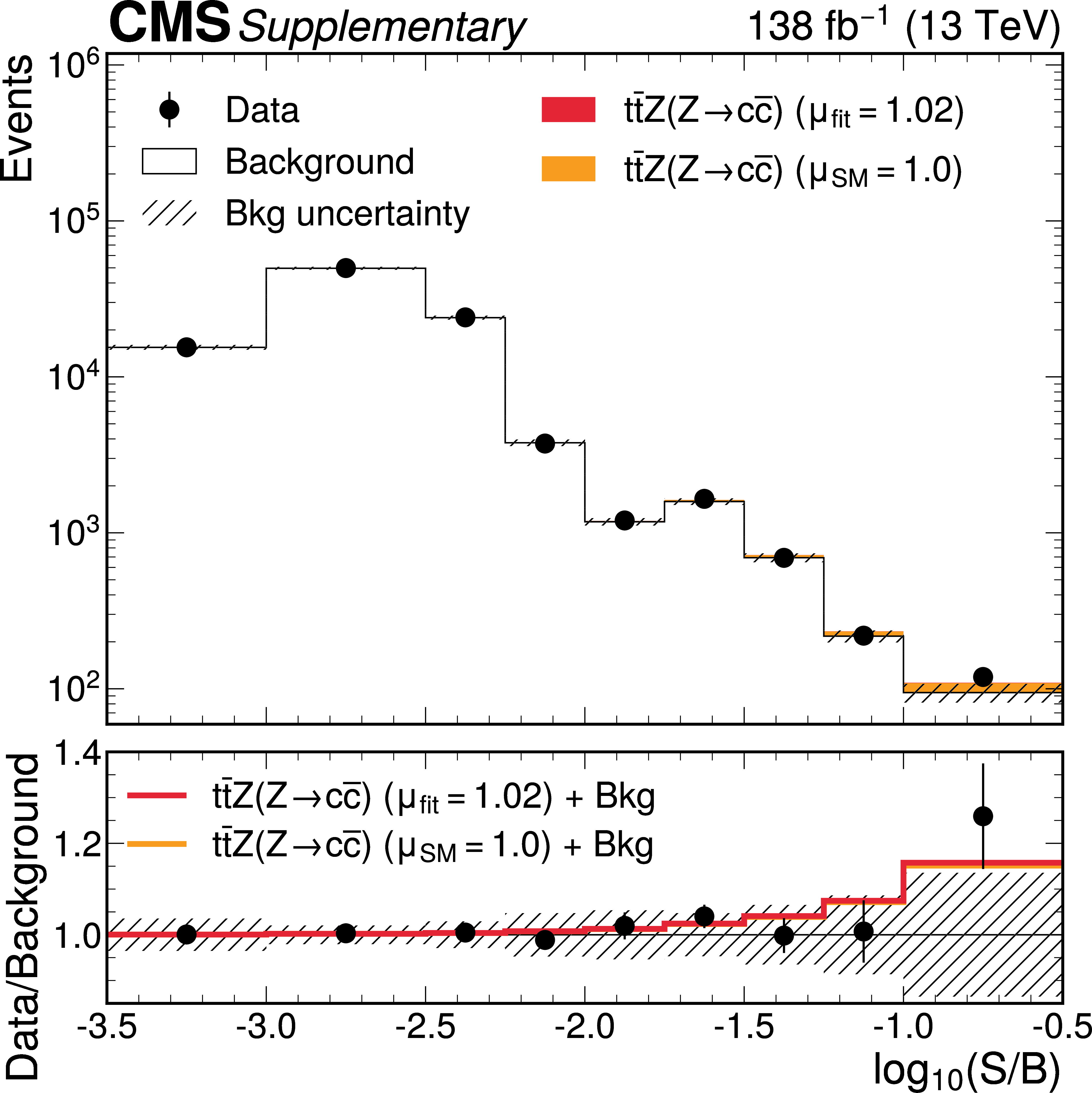
On the left, observed and expected event yields from all SRs and CRs as a function of $ \log_{10}(S/B) $, where $ S $ are the observed $ {\mathrm{t}\overline{\mathrm{t}}} \mathrm{Z}(\mathrm{Z}{\to}\mathrm{c}\overline{\mathrm{c}}) $ yields, and $ B $ are the total background yields in the combined fit to data. The signals are shown for the best fit signal strength (red), and the SM prediction, $ \mu= $ 1 (orange). The lower panel shows the ratio of the data to the post-fit background prediction, compared to the signal-plus-background predictions. On the right, fit results of $ \mu_{{\mathrm{t}\overline{\mathrm{t}}} \mathrm{Z}(\mathrm{Z}{\to}\mathrm{c}\overline{\mathrm{c}})} $ in the combination of channels (first row) and the channels individually (lower rows). The left panel shows the observed signal strength, compared to the expected results. The right panel shows the expected and observed significance. |
png pdf |
Figure B8-a:
On the left, observed and expected event yields from all SRs and CRs as a function of $ \log_{10}(S/B) $, where $ S $ are the observed $ {\mathrm{t}\overline{\mathrm{t}}} \mathrm{Z}(\mathrm{Z}{\to}\mathrm{c}\overline{\mathrm{c}}) $ yields, and $ B $ are the total background yields in the combined fit to data. The signals are shown for the best fit signal strength (red), and the SM prediction, $ \mu= $ 1 (orange). The lower panel shows the ratio of the data to the post-fit background prediction, compared to the signal-plus-background predictions. On the right, fit results of $ \mu_{{\mathrm{t}\overline{\mathrm{t}}} \mathrm{Z}(\mathrm{Z}{\to}\mathrm{c}\overline{\mathrm{c}})} $ in the combination of channels (first row) and the channels individually (lower rows). The left panel shows the observed signal strength, compared to the expected results. The right panel shows the expected and observed significance. |

png pdf |
Figure B8-b:
On the left, observed and expected event yields from all SRs and CRs as a function of $ \log_{10}(S/B) $, where $ S $ are the observed $ {\mathrm{t}\overline{\mathrm{t}}} \mathrm{Z}(\mathrm{Z}{\to}\mathrm{c}\overline{\mathrm{c}}) $ yields, and $ B $ are the total background yields in the combined fit to data. The signals are shown for the best fit signal strength (red), and the SM prediction, $ \mu= $ 1 (orange). The lower panel shows the ratio of the data to the post-fit background prediction, compared to the signal-plus-background predictions. On the right, fit results of $ \mu_{{\mathrm{t}\overline{\mathrm{t}}} \mathrm{Z}(\mathrm{Z}{\to}\mathrm{c}\overline{\mathrm{c}})} $ in the combination of channels (first row) and the channels individually (lower rows). The left panel shows the observed signal strength, compared to the expected results. The right panel shows the expected and observed significance. |
png pdf |
Figure B9:
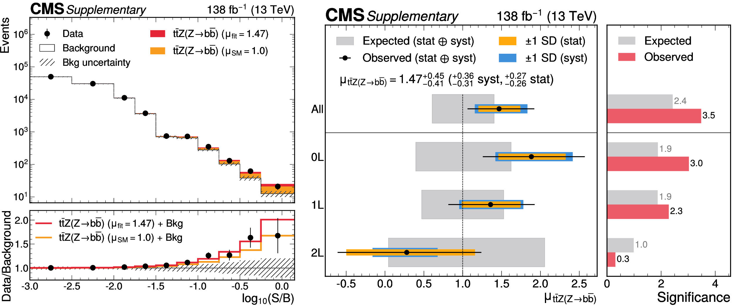
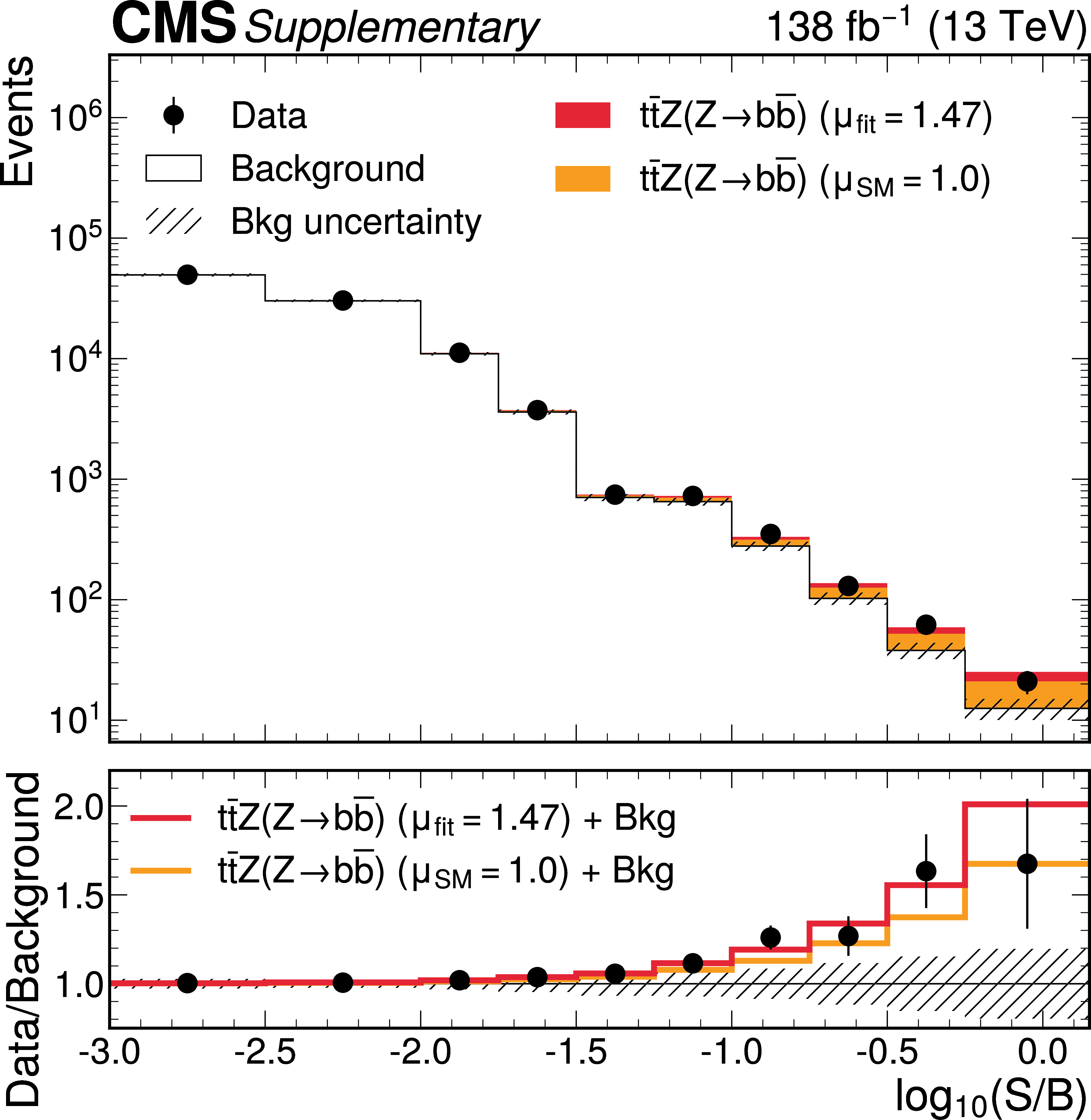
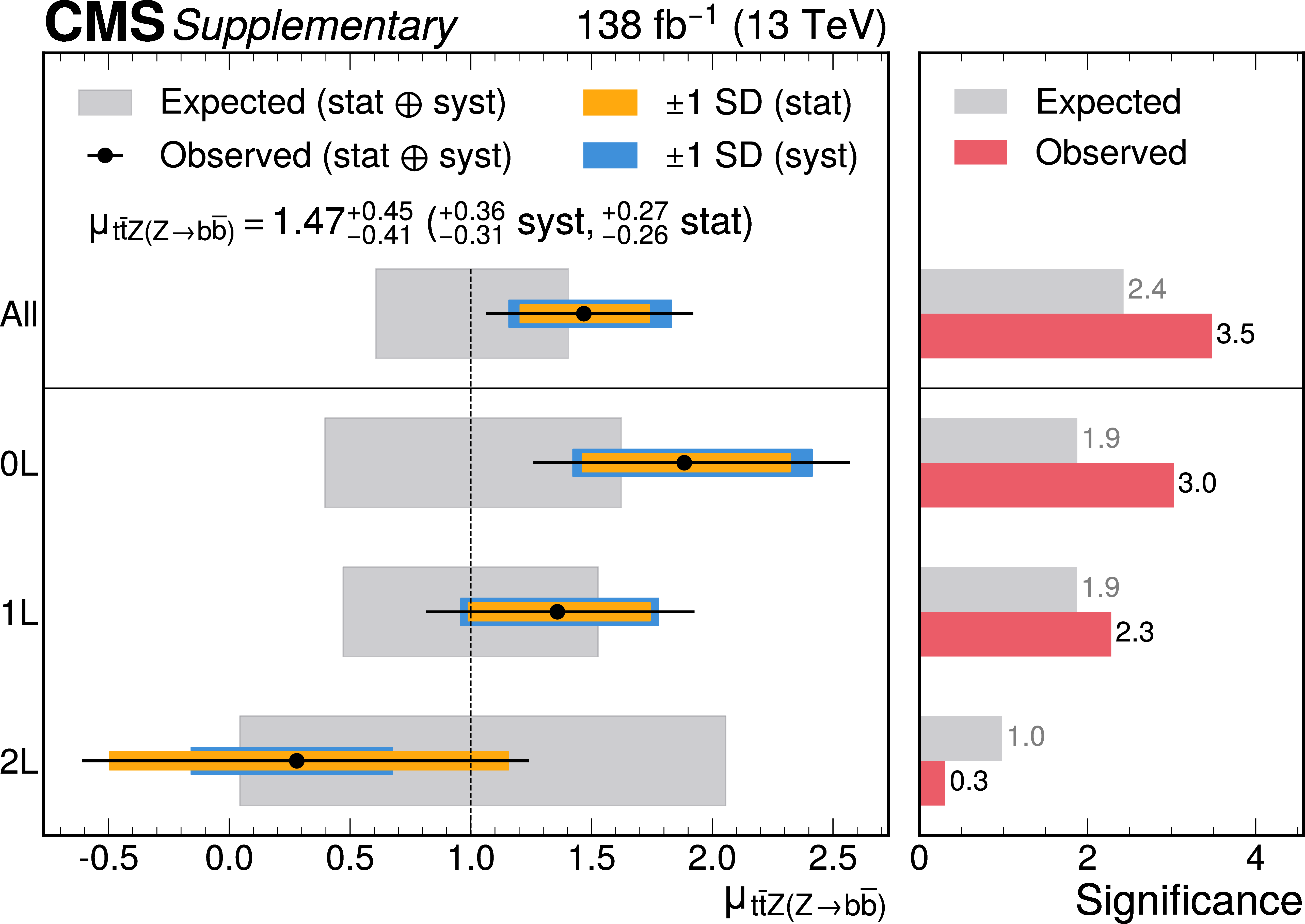
On the left, observed and expected event yields from all SRs and CRs as a function of $ \log_{10}(S/B) $, where $ S $ are the observed $ {\mathrm{t}\overline{\mathrm{t}}} \mathrm{Z}(\mathrm{Z}{\to}\mathrm{b}\overline{\mathrm{b}}) $ yields, and $ B $ are the total background yields in the combined fit to data. The signals are shown for the best fit signal strength (red), and the SM prediction, $ \mu = $ 1 (orange). The lower panel shows the ratio of the data to the post-fit background prediction, compared to the signal-plus-background predictions. On the right, fit results of $ \mu_{{\mathrm{t}\overline{\mathrm{t}}} \mathrm{Z}(\mathrm{Z}{\to}\mathrm{b}\overline{\mathrm{b}})} $ in the combination of channels (first row) and the channels individually (lower rows). The left panel shows the observed signal strength, compared to the expected results. The right panel shows the expected and observed significance. |
png pdf |
Figure B9-a:
On the left, observed and expected event yields from all SRs and CRs as a function of $ \log_{10}(S/B) $, where $ S $ are the observed $ {\mathrm{t}\overline{\mathrm{t}}} \mathrm{Z}(\mathrm{Z}{\to}\mathrm{b}\overline{\mathrm{b}}) $ yields, and $ B $ are the total background yields in the combined fit to data. The signals are shown for the best fit signal strength (red), and the SM prediction, $ \mu = $ 1 (orange). The lower panel shows the ratio of the data to the post-fit background prediction, compared to the signal-plus-background predictions. On the right, fit results of $ \mu_{{\mathrm{t}\overline{\mathrm{t}}} \mathrm{Z}(\mathrm{Z}{\to}\mathrm{b}\overline{\mathrm{b}})} $ in the combination of channels (first row) and the channels individually (lower rows). The left panel shows the observed signal strength, compared to the expected results. The right panel shows the expected and observed significance. |
png pdf |
Figure B9-b:
On the left, observed and expected event yields from all SRs and CRs as a function of $ \log_{10}(S/B) $, where $ S $ are the observed $ {\mathrm{t}\overline{\mathrm{t}}} \mathrm{Z}(\mathrm{Z}{\to}\mathrm{b}\overline{\mathrm{b}}) $ yields, and $ B $ are the total background yields in the combined fit to data. The signals are shown for the best fit signal strength (red), and the SM prediction, $ \mu = $ 1 (orange). The lower panel shows the ratio of the data to the post-fit background prediction, compared to the signal-plus-background predictions. On the right, fit results of $ \mu_{{\mathrm{t}\overline{\mathrm{t}}} \mathrm{Z}(\mathrm{Z}{\to}\mathrm{b}\overline{\mathrm{b}})} $ in the combination of channels (first row) and the channels individually (lower rows). The left panel shows the observed signal strength, compared to the expected results. The right panel shows the expected and observed significance. |
png pdf |
Figure B10:
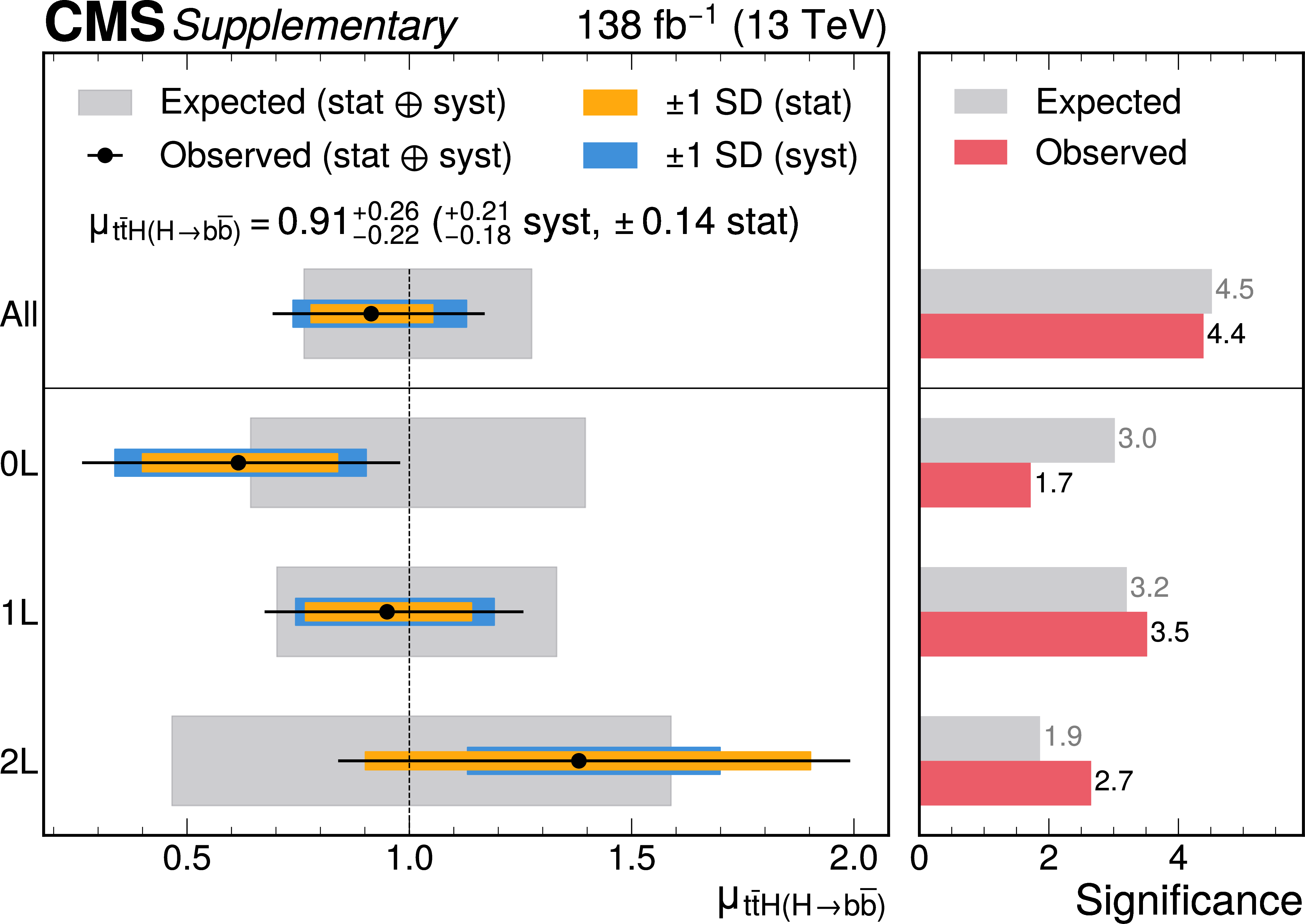
Fit results of $ \mu_{{\mathrm{t}\overline{\mathrm{t}}} \mathrm{H}(\mathrm{H}{\to}\mathrm{b}\overline{\mathrm{b}})} $. The left panel shows the observed signal strength, compared to the expected results. The right panel shows the expected and observed significance. |
png pdf |
Figure B11:
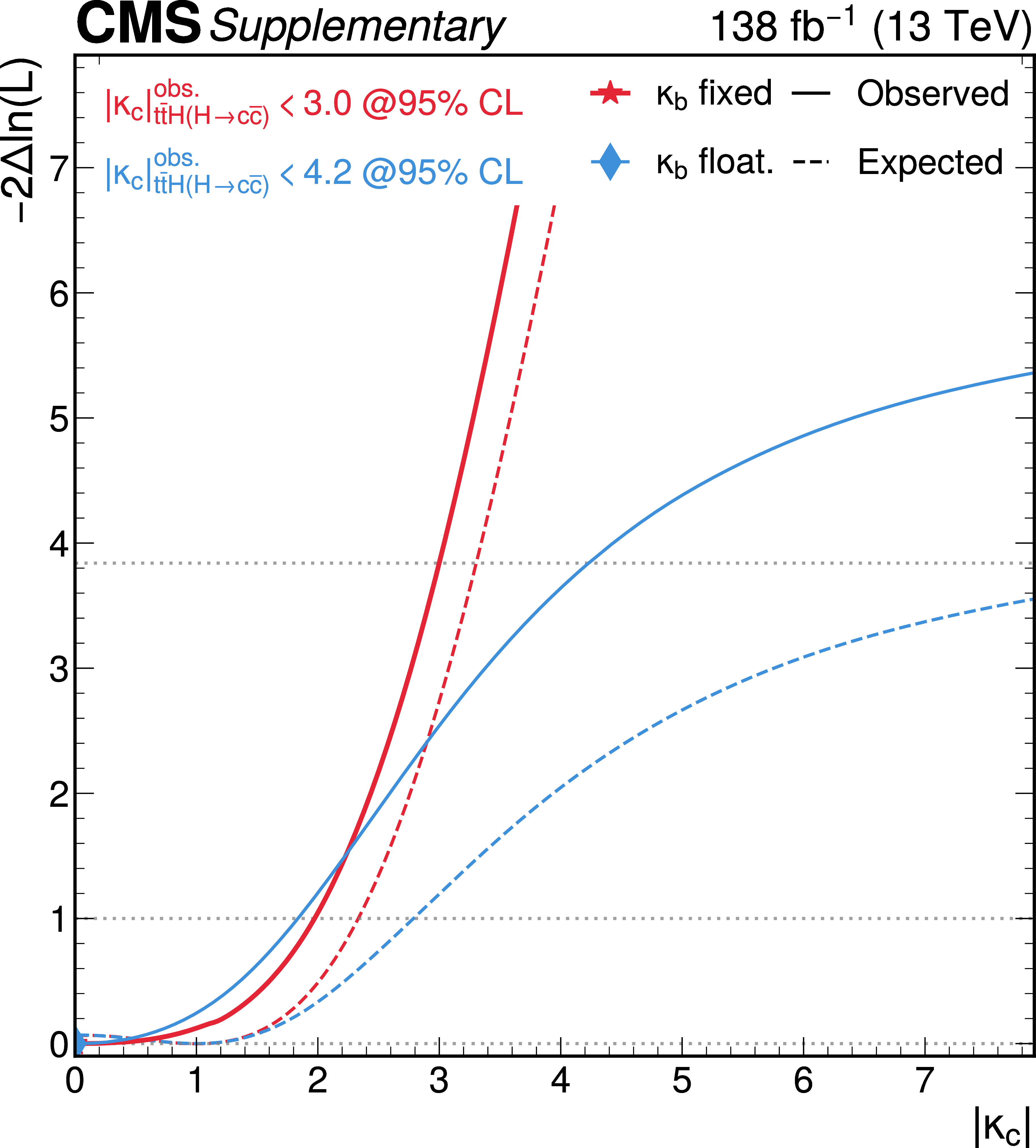
Likelihood scans of $ \kappa_{\mathrm{c}} $ with fixed $ \kappa_{\mathrm{b}}= $ 1 (red) and floating $ \kappa_{\mathrm{b}} $ (blue). The 68% and 95% CL intervals are indicated by the horizontal dotted lines. |
png pdf |
Figure B12:
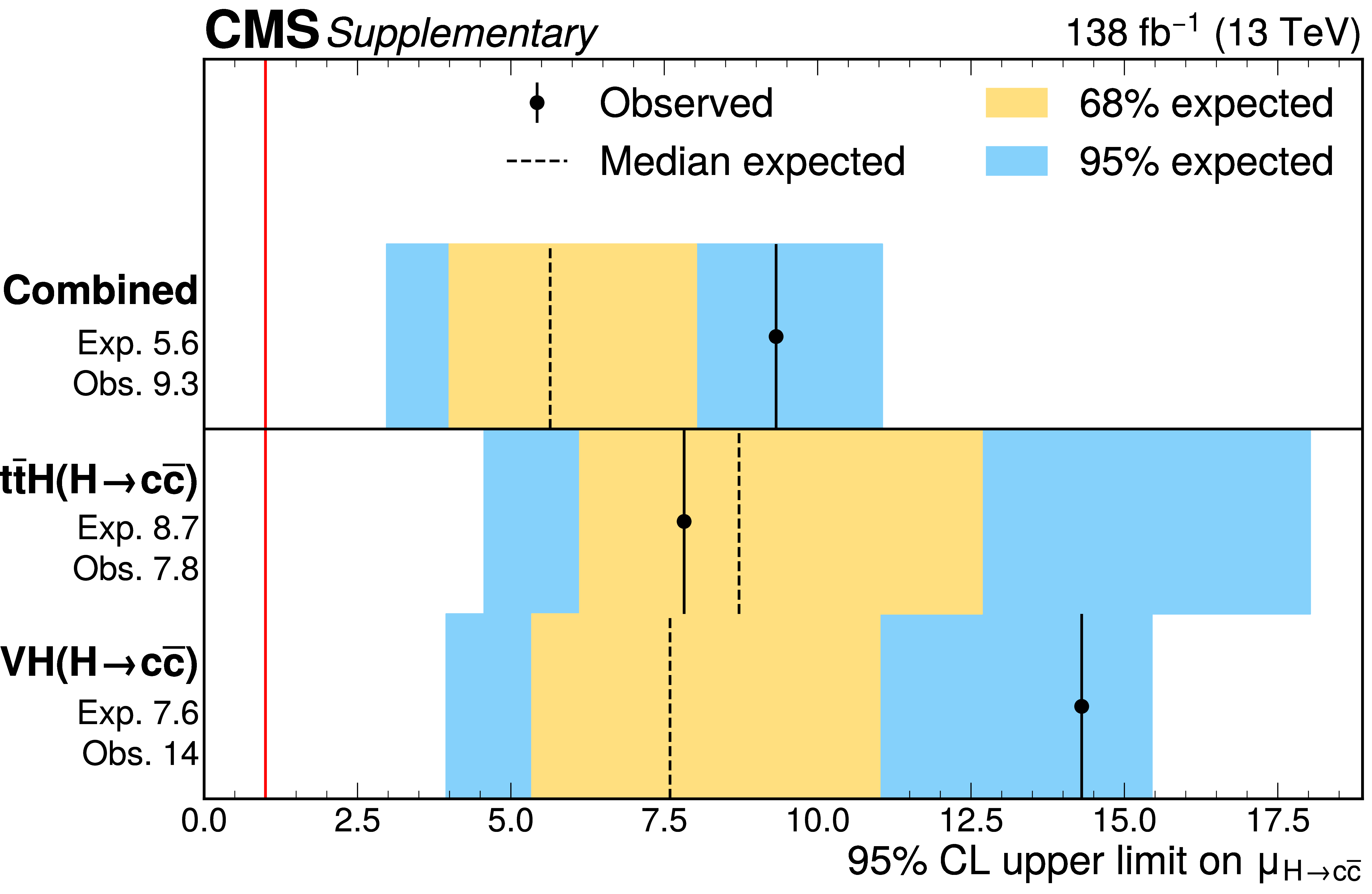
The 95% CL upper limits on $ \mu_{\mathrm{H}{\to}\mathrm{c}\overline{\mathrm{c}}} $. The blue and yellow bands indicate the expected 68% and 95% CL regions, respectively, under the background-only hypothesis. The vertical red line indicates the SM value $ \mu_{\mathrm{H}{\to}\mathrm{c}\overline{\mathrm{c}}}= $ 1. |
png pdf |
Figure B13:
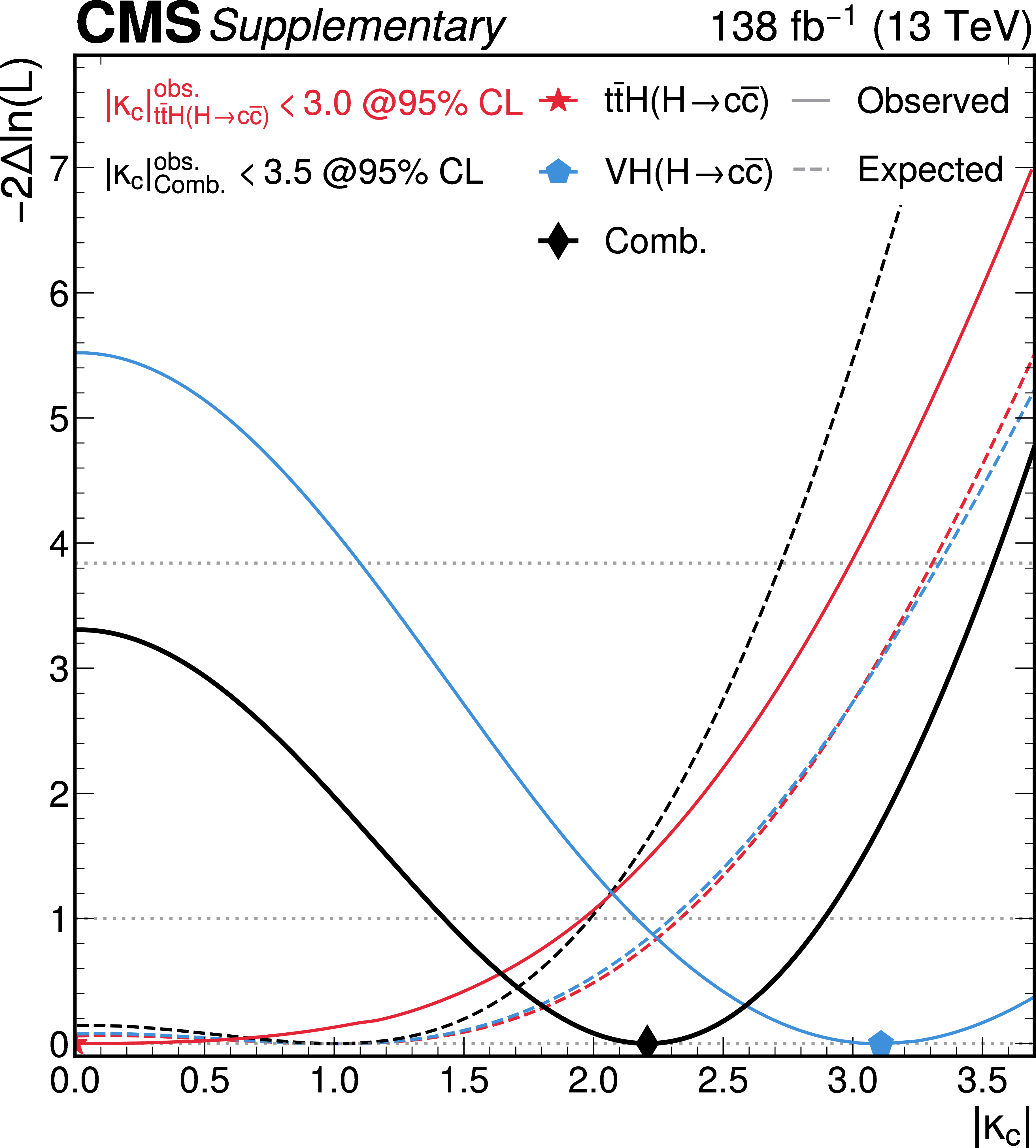
Likelihood scans of $ \kappa_{\mathrm{c}} $ with fixed $ \kappa_{\mathrm{b}}= $ 1 in the individual $ {\mathrm{t}\overline{\mathrm{t}}} \mathrm{H} $ (red) and VH (blue) channels and their combination (black). The 68% and 95% CL intervals are indicated by the horizontal dotted lines. |
png pdf |
Figure B14:
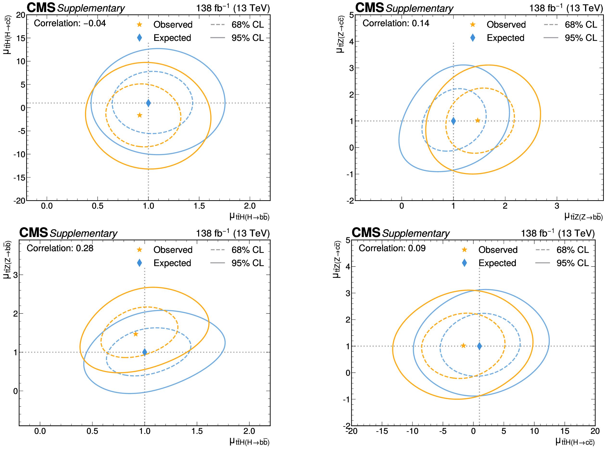
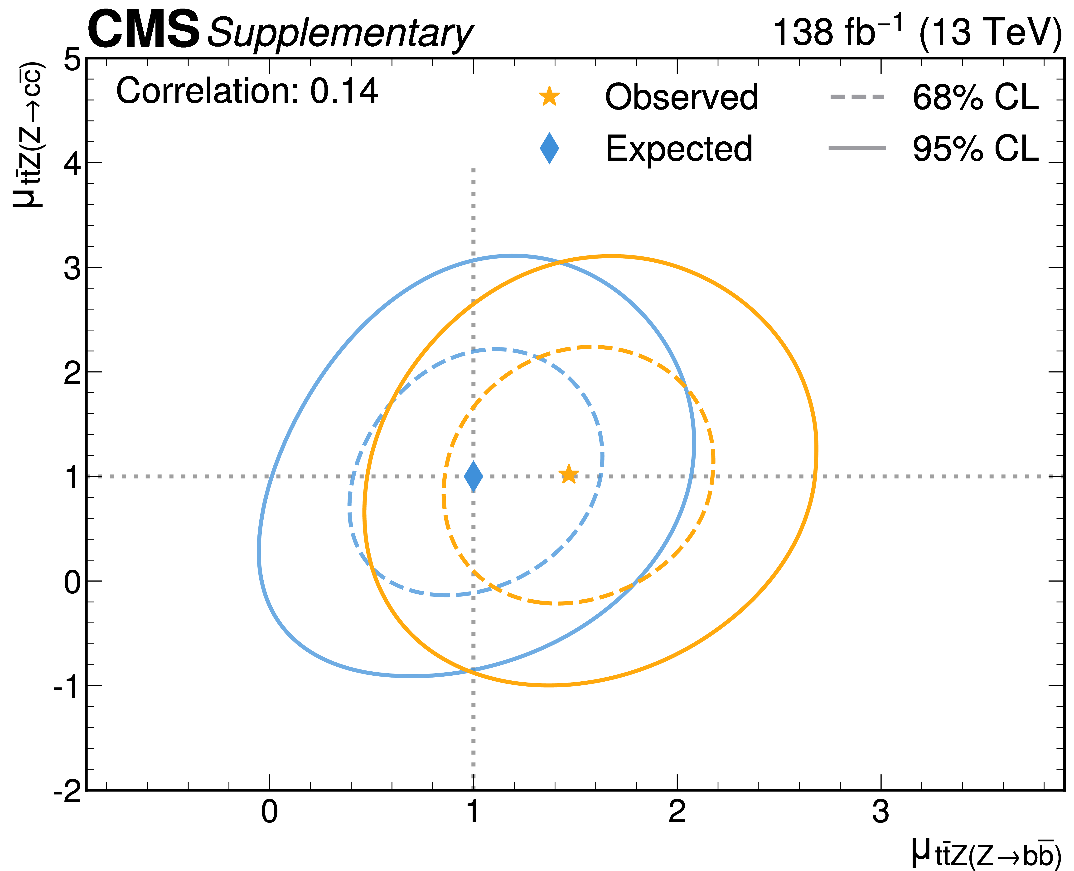
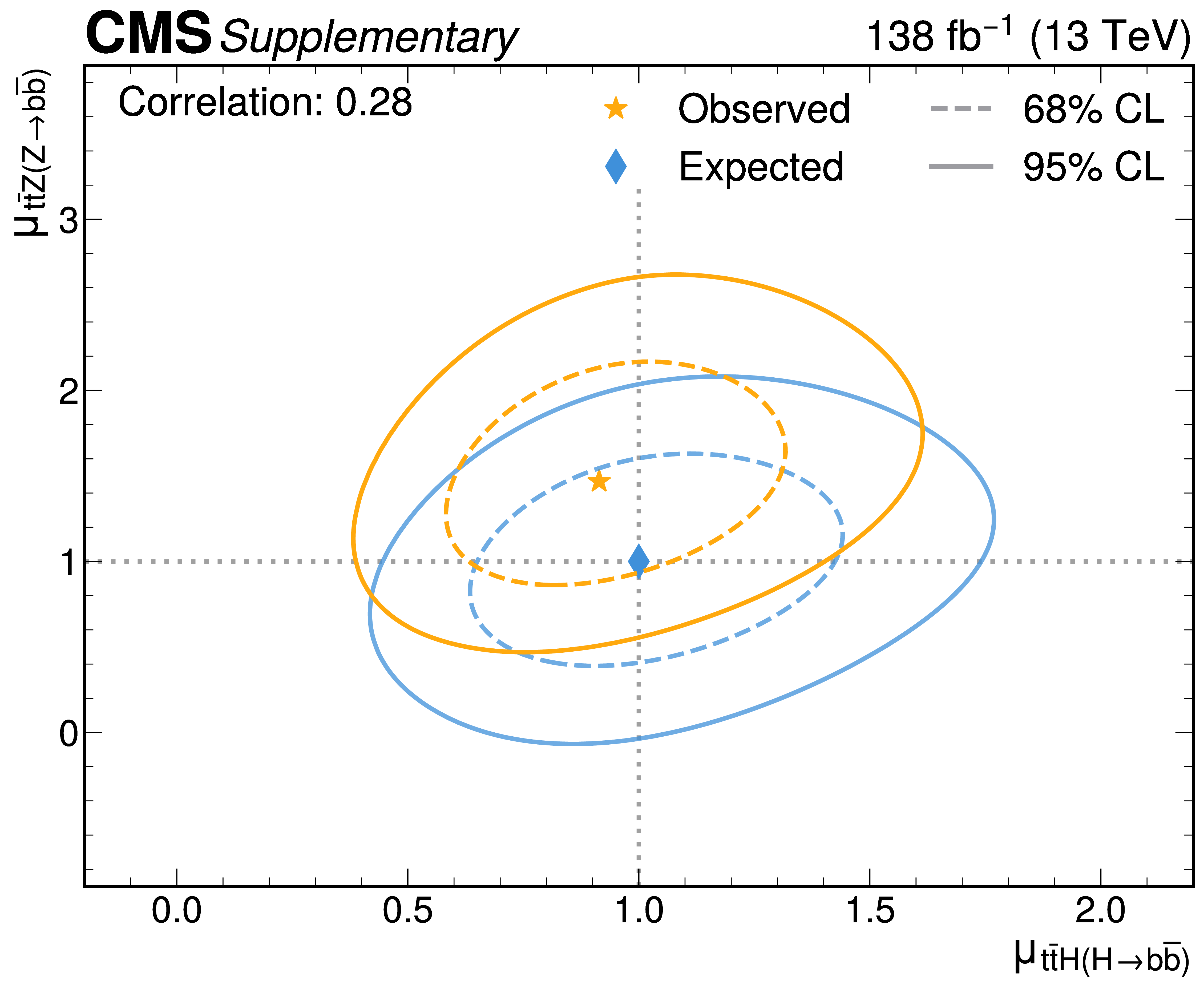
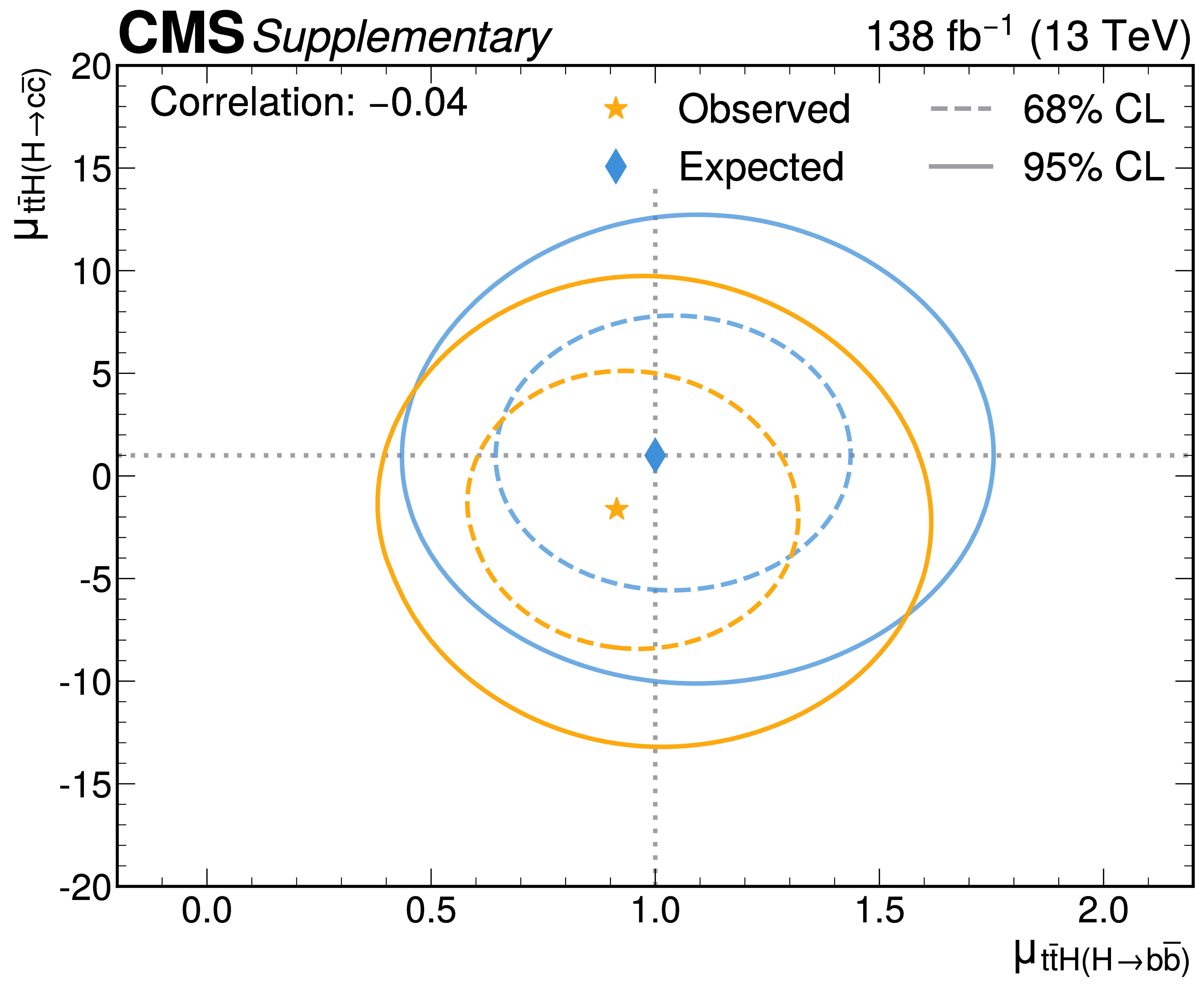
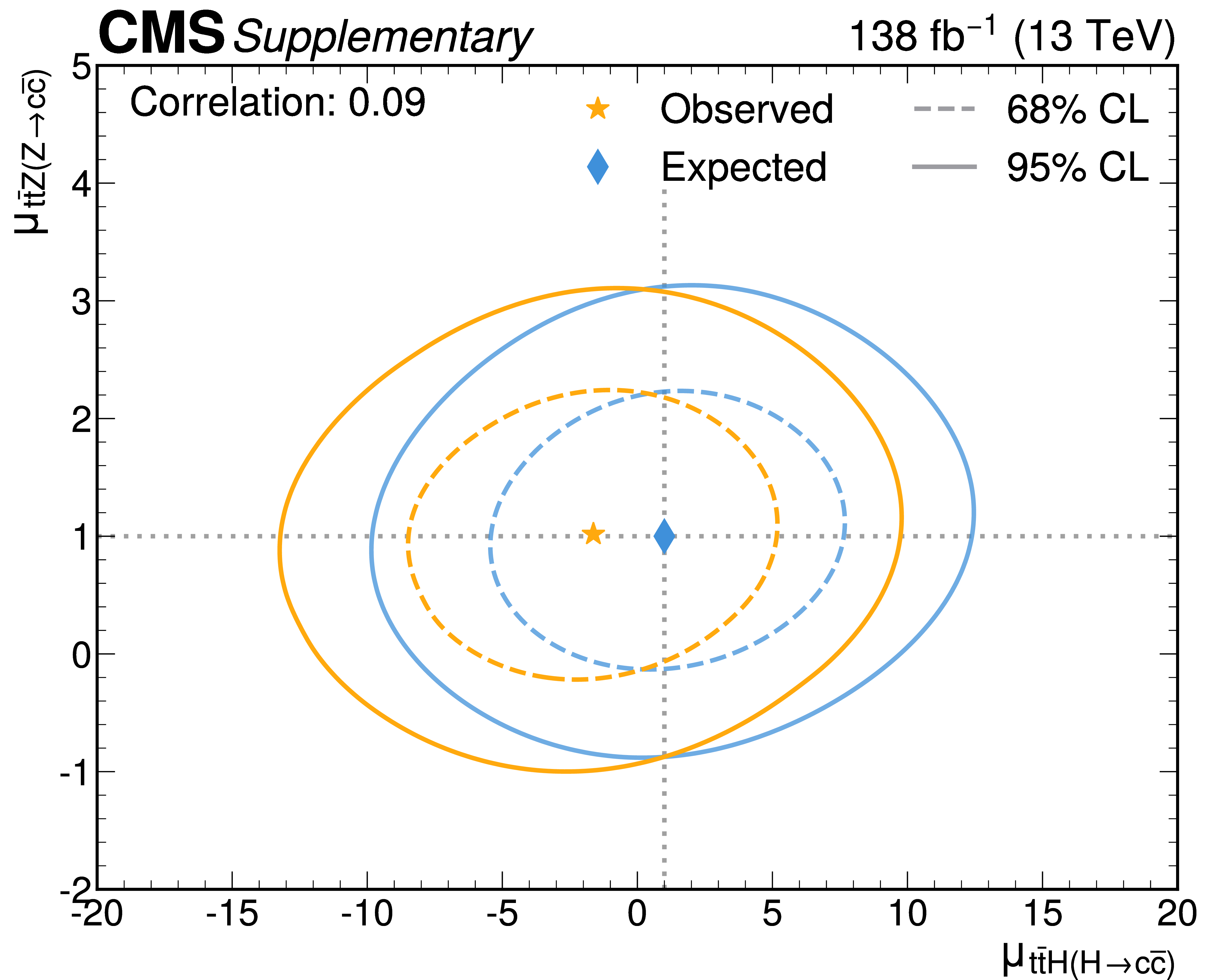
Likelihood scans for the simultaneous fit of $ \mu_{{\mathrm{t}\overline{\mathrm{t}}} \mathrm{H}(\mathrm{H}{\to}\mathrm{b}\overline{\mathrm{b}})} $ and $ \mu_{{\mathrm{t}\overline{\mathrm{t}}} \mathrm{H}(\mathrm{H}{\to}\mathrm{c}\overline{\mathrm{c}})} $ (upper left), $ \mu_{{\mathrm{t}\overline{\mathrm{t}}} \mathrm{Z}(\mathrm{Z}{\to}\mathrm{b}\overline{\mathrm{b}})} $ and $ \mu_{{\mathrm{t}\overline{\mathrm{t}}} \mathrm{Z}(\mathrm{Z}{\to}\mathrm{c}\overline{\mathrm{c}})} $ (upper right), $ \mu_{{\mathrm{t}\overline{\mathrm{t}}} \mathrm{H}(\mathrm{H}{\to}\mathrm{b}\overline{\mathrm{b}})} $ and $ \mu_{{\mathrm{t}\overline{\mathrm{t}}} \mathrm{Z}(\mathrm{Z}{\to}\mathrm{b}\overline{\mathrm{b}})} $ (lower left), and $ \mu_{{\mathrm{t}\overline{\mathrm{t}}} \mathrm{H}(\mathrm{H}{\to}\mathrm{c}\overline{\mathrm{c}})} $ and $ \mu_{{\mathrm{t}\overline{\mathrm{t}}} \mathrm{Z}(\mathrm{Z}{\to}\mathrm{c}\overline{\mathrm{c}})} $ (lower right). The 68% (95%) CL intervals are indicated by the dotted (solid) lines. The observed (expected) best fit values are shown by the orange (blue) markers. |

png pdf |
Figure B14-a:
Likelihood scans for the simultaneous fit of $ \mu_{{\mathrm{t}\overline{\mathrm{t}}} \mathrm{H}(\mathrm{H}{\to}\mathrm{b}\overline{\mathrm{b}})} $ and $ \mu_{{\mathrm{t}\overline{\mathrm{t}}} \mathrm{H}(\mathrm{H}{\to}\mathrm{c}\overline{\mathrm{c}})} $ (upper left), $ \mu_{{\mathrm{t}\overline{\mathrm{t}}} \mathrm{Z}(\mathrm{Z}{\to}\mathrm{b}\overline{\mathrm{b}})} $ and $ \mu_{{\mathrm{t}\overline{\mathrm{t}}} \mathrm{Z}(\mathrm{Z}{\to}\mathrm{c}\overline{\mathrm{c}})} $ (upper right), $ \mu_{{\mathrm{t}\overline{\mathrm{t}}} \mathrm{H}(\mathrm{H}{\to}\mathrm{b}\overline{\mathrm{b}})} $ and $ \mu_{{\mathrm{t}\overline{\mathrm{t}}} \mathrm{Z}(\mathrm{Z}{\to}\mathrm{b}\overline{\mathrm{b}})} $ (lower left), and $ \mu_{{\mathrm{t}\overline{\mathrm{t}}} \mathrm{H}(\mathrm{H}{\to}\mathrm{c}\overline{\mathrm{c}})} $ and $ \mu_{{\mathrm{t}\overline{\mathrm{t}}} \mathrm{Z}(\mathrm{Z}{\to}\mathrm{c}\overline{\mathrm{c}})} $ (lower right). The 68% (95%) CL intervals are indicated by the dotted (solid) lines. The observed (expected) best fit values are shown by the orange (blue) markers. |
png pdf |
Figure B14-b:
Likelihood scans for the simultaneous fit of $ \mu_{{\mathrm{t}\overline{\mathrm{t}}} \mathrm{H}(\mathrm{H}{\to}\mathrm{b}\overline{\mathrm{b}})} $ and $ \mu_{{\mathrm{t}\overline{\mathrm{t}}} \mathrm{H}(\mathrm{H}{\to}\mathrm{c}\overline{\mathrm{c}})} $ (upper left), $ \mu_{{\mathrm{t}\overline{\mathrm{t}}} \mathrm{Z}(\mathrm{Z}{\to}\mathrm{b}\overline{\mathrm{b}})} $ and $ \mu_{{\mathrm{t}\overline{\mathrm{t}}} \mathrm{Z}(\mathrm{Z}{\to}\mathrm{c}\overline{\mathrm{c}})} $ (upper right), $ \mu_{{\mathrm{t}\overline{\mathrm{t}}} \mathrm{H}(\mathrm{H}{\to}\mathrm{b}\overline{\mathrm{b}})} $ and $ \mu_{{\mathrm{t}\overline{\mathrm{t}}} \mathrm{Z}(\mathrm{Z}{\to}\mathrm{b}\overline{\mathrm{b}})} $ (lower left), and $ \mu_{{\mathrm{t}\overline{\mathrm{t}}} \mathrm{H}(\mathrm{H}{\to}\mathrm{c}\overline{\mathrm{c}})} $ and $ \mu_{{\mathrm{t}\overline{\mathrm{t}}} \mathrm{Z}(\mathrm{Z}{\to}\mathrm{c}\overline{\mathrm{c}})} $ (lower right). The 68% (95%) CL intervals are indicated by the dotted (solid) lines. The observed (expected) best fit values are shown by the orange (blue) markers. |
png pdf |
Figure B14-c:
Likelihood scans for the simultaneous fit of $ \mu_{{\mathrm{t}\overline{\mathrm{t}}} \mathrm{H}(\mathrm{H}{\to}\mathrm{b}\overline{\mathrm{b}})} $ and $ \mu_{{\mathrm{t}\overline{\mathrm{t}}} \mathrm{H}(\mathrm{H}{\to}\mathrm{c}\overline{\mathrm{c}})} $ (upper left), $ \mu_{{\mathrm{t}\overline{\mathrm{t}}} \mathrm{Z}(\mathrm{Z}{\to}\mathrm{b}\overline{\mathrm{b}})} $ and $ \mu_{{\mathrm{t}\overline{\mathrm{t}}} \mathrm{Z}(\mathrm{Z}{\to}\mathrm{c}\overline{\mathrm{c}})} $ (upper right), $ \mu_{{\mathrm{t}\overline{\mathrm{t}}} \mathrm{H}(\mathrm{H}{\to}\mathrm{b}\overline{\mathrm{b}})} $ and $ \mu_{{\mathrm{t}\overline{\mathrm{t}}} \mathrm{Z}(\mathrm{Z}{\to}\mathrm{b}\overline{\mathrm{b}})} $ (lower left), and $ \mu_{{\mathrm{t}\overline{\mathrm{t}}} \mathrm{H}(\mathrm{H}{\to}\mathrm{c}\overline{\mathrm{c}})} $ and $ \mu_{{\mathrm{t}\overline{\mathrm{t}}} \mathrm{Z}(\mathrm{Z}{\to}\mathrm{c}\overline{\mathrm{c}})} $ (lower right). The 68% (95%) CL intervals are indicated by the dotted (solid) lines. The observed (expected) best fit values are shown by the orange (blue) markers. |

png pdf |
Figure B14-d:
Likelihood scans for the simultaneous fit of $ \mu_{{\mathrm{t}\overline{\mathrm{t}}} \mathrm{H}(\mathrm{H}{\to}\mathrm{b}\overline{\mathrm{b}})} $ and $ \mu_{{\mathrm{t}\overline{\mathrm{t}}} \mathrm{H}(\mathrm{H}{\to}\mathrm{c}\overline{\mathrm{c}})} $ (upper left), $ \mu_{{\mathrm{t}\overline{\mathrm{t}}} \mathrm{Z}(\mathrm{Z}{\to}\mathrm{b}\overline{\mathrm{b}})} $ and $ \mu_{{\mathrm{t}\overline{\mathrm{t}}} \mathrm{Z}(\mathrm{Z}{\to}\mathrm{c}\overline{\mathrm{c}})} $ (upper right), $ \mu_{{\mathrm{t}\overline{\mathrm{t}}} \mathrm{H}(\mathrm{H}{\to}\mathrm{b}\overline{\mathrm{b}})} $ and $ \mu_{{\mathrm{t}\overline{\mathrm{t}}} \mathrm{Z}(\mathrm{Z}{\to}\mathrm{b}\overline{\mathrm{b}})} $ (lower left), and $ \mu_{{\mathrm{t}\overline{\mathrm{t}}} \mathrm{H}(\mathrm{H}{\to}\mathrm{c}\overline{\mathrm{c}})} $ and $ \mu_{{\mathrm{t}\overline{\mathrm{t}}} \mathrm{Z}(\mathrm{Z}{\to}\mathrm{c}\overline{\mathrm{c}})} $ (lower right). The 68% (95%) CL intervals are indicated by the dotted (solid) lines. The observed (expected) best fit values are shown by the orange (blue) markers. |
png pdf |
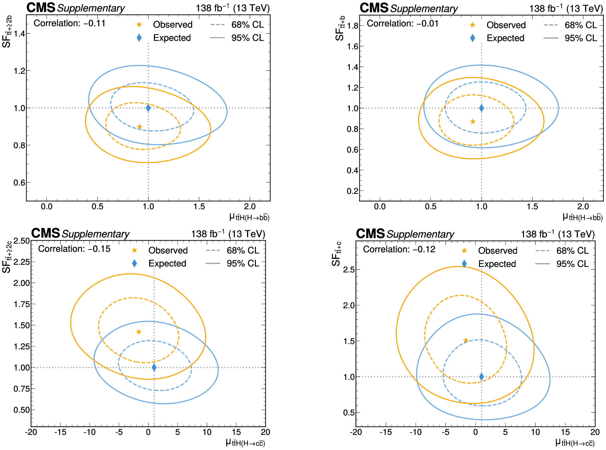
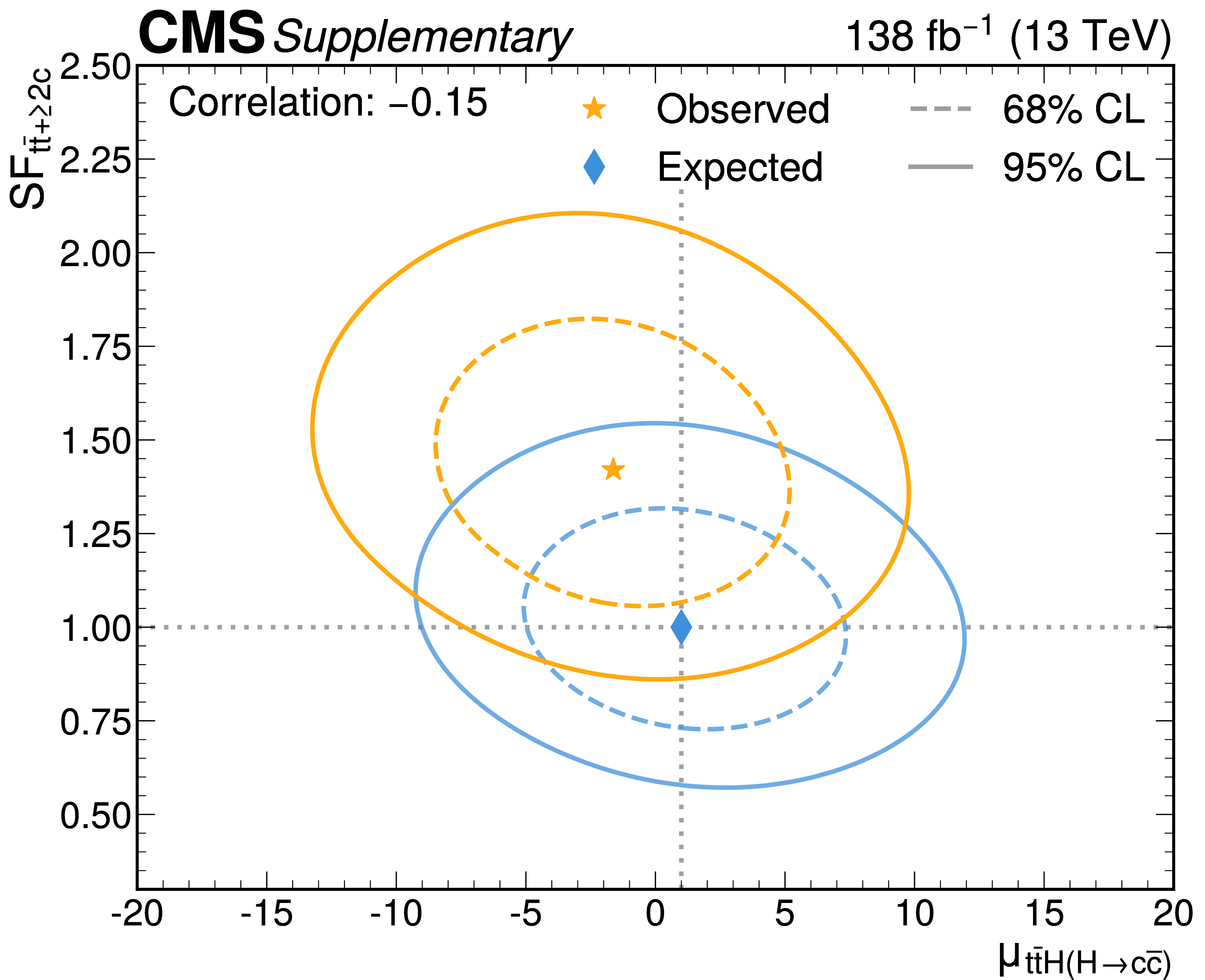
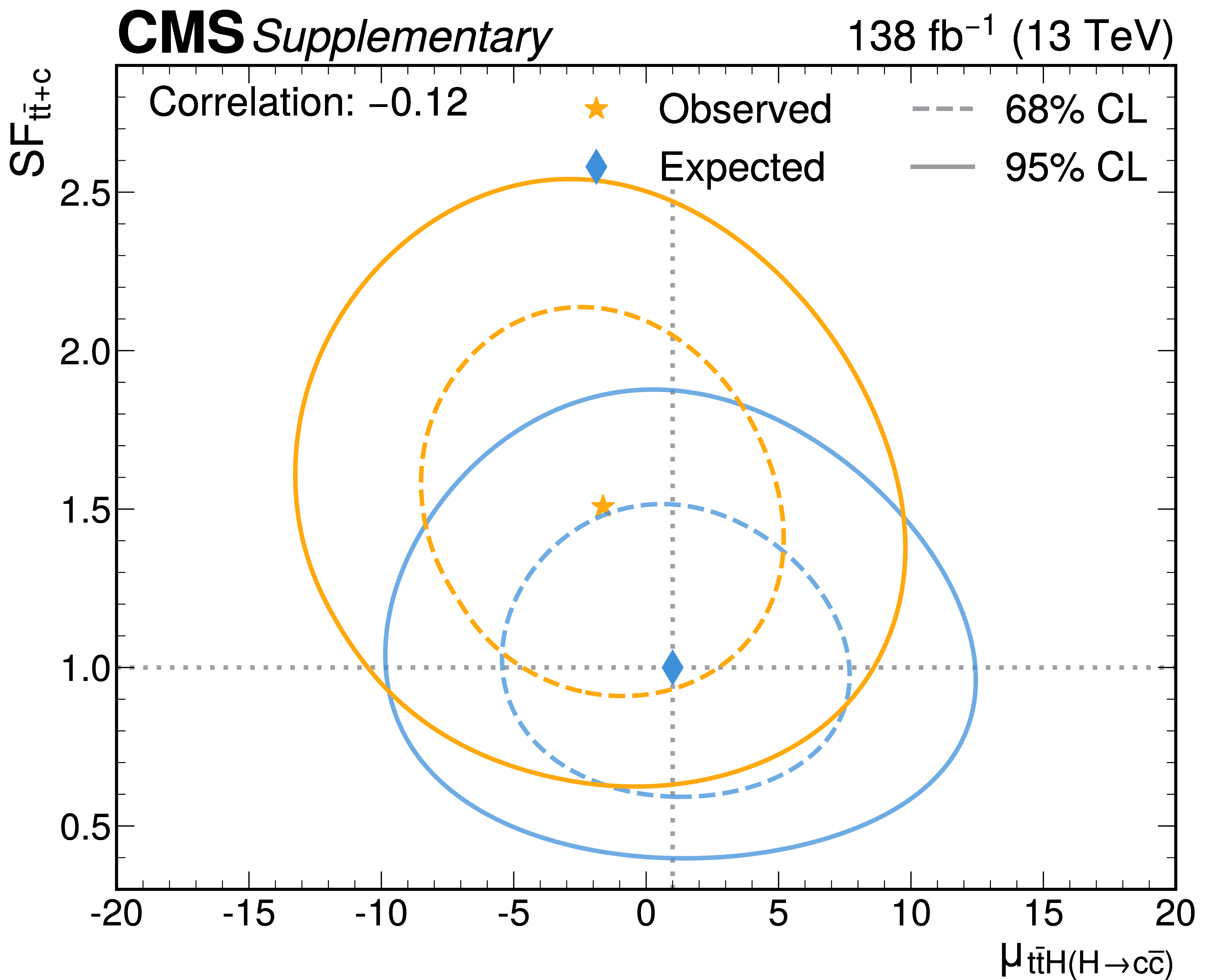
Figure B15:
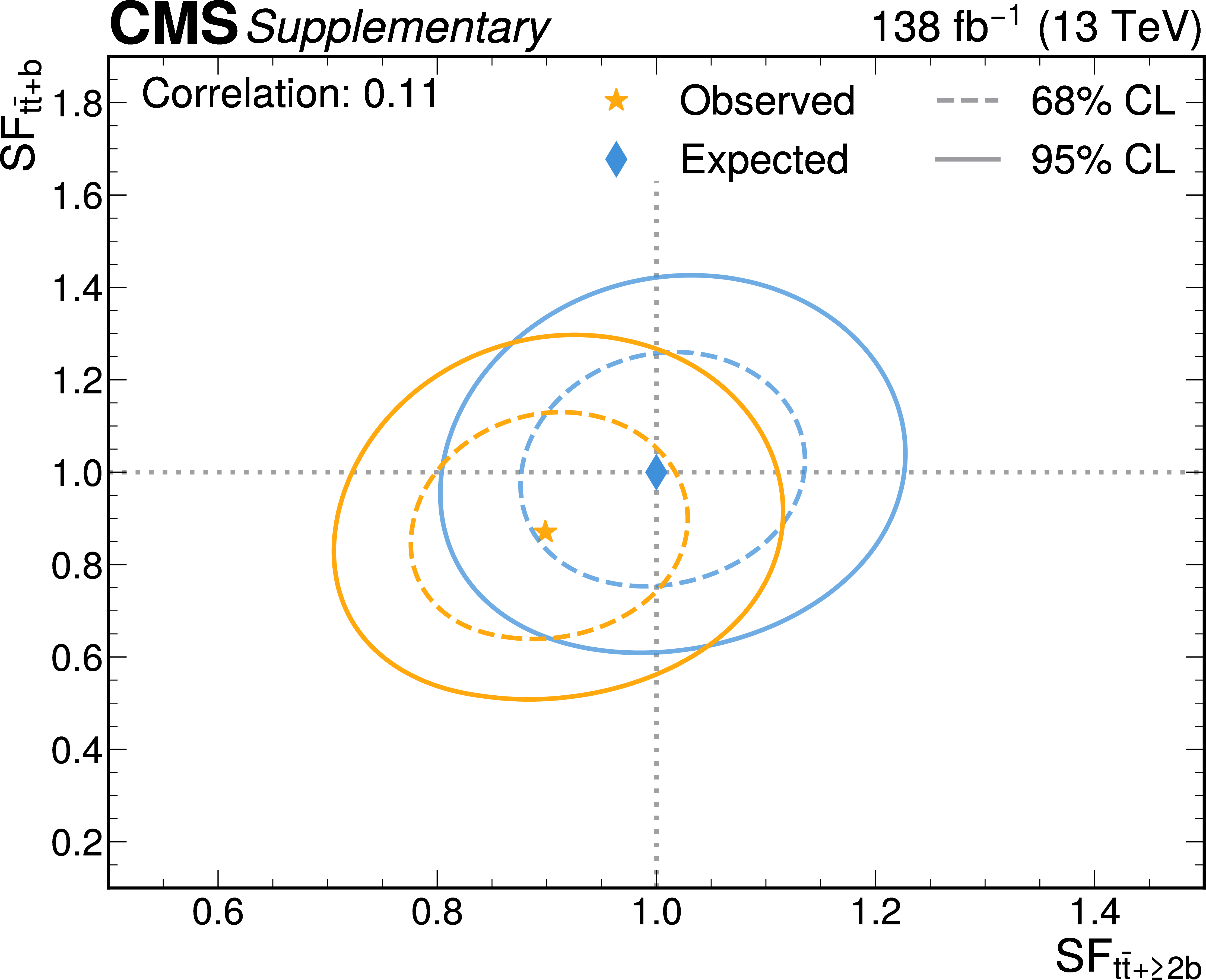
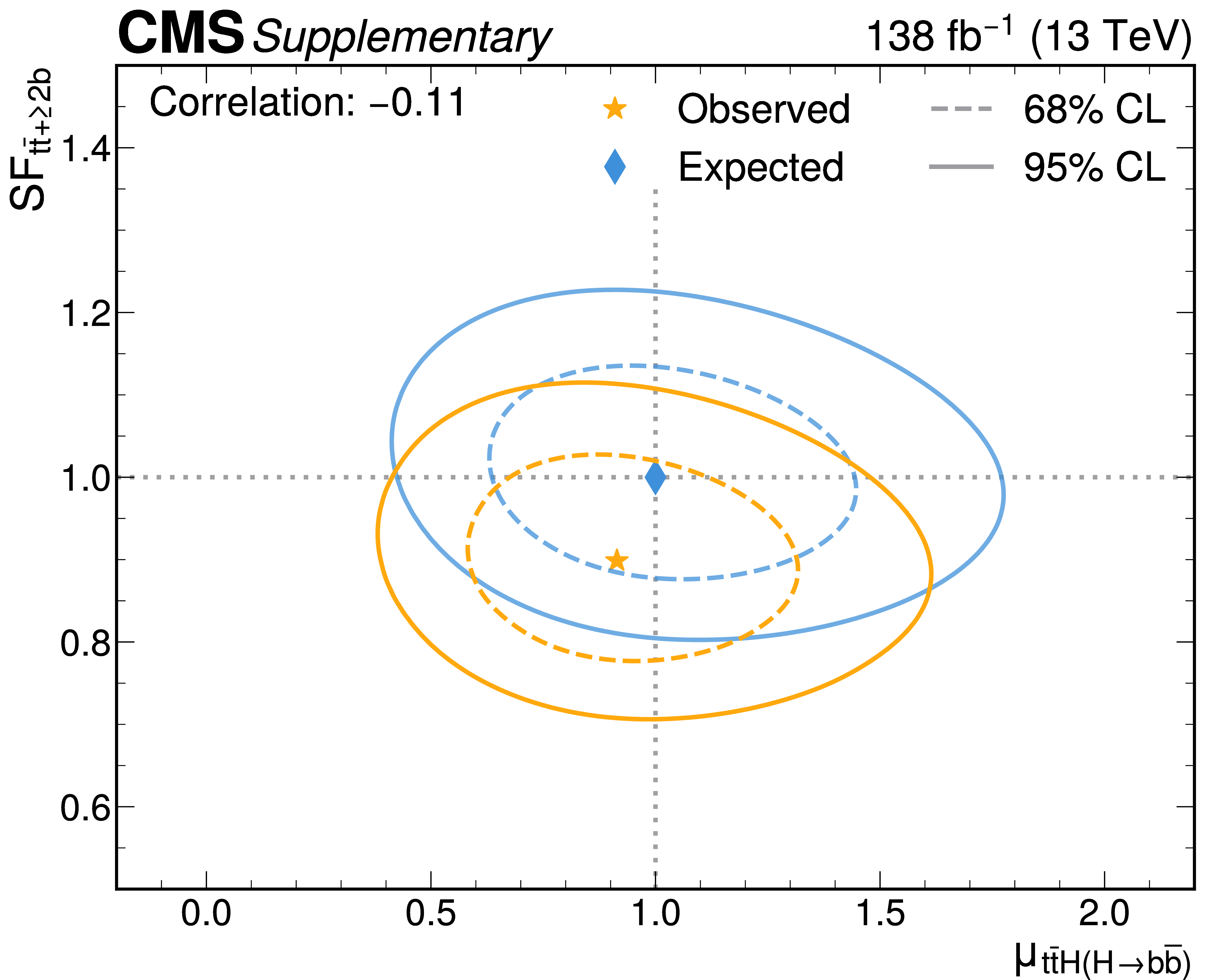
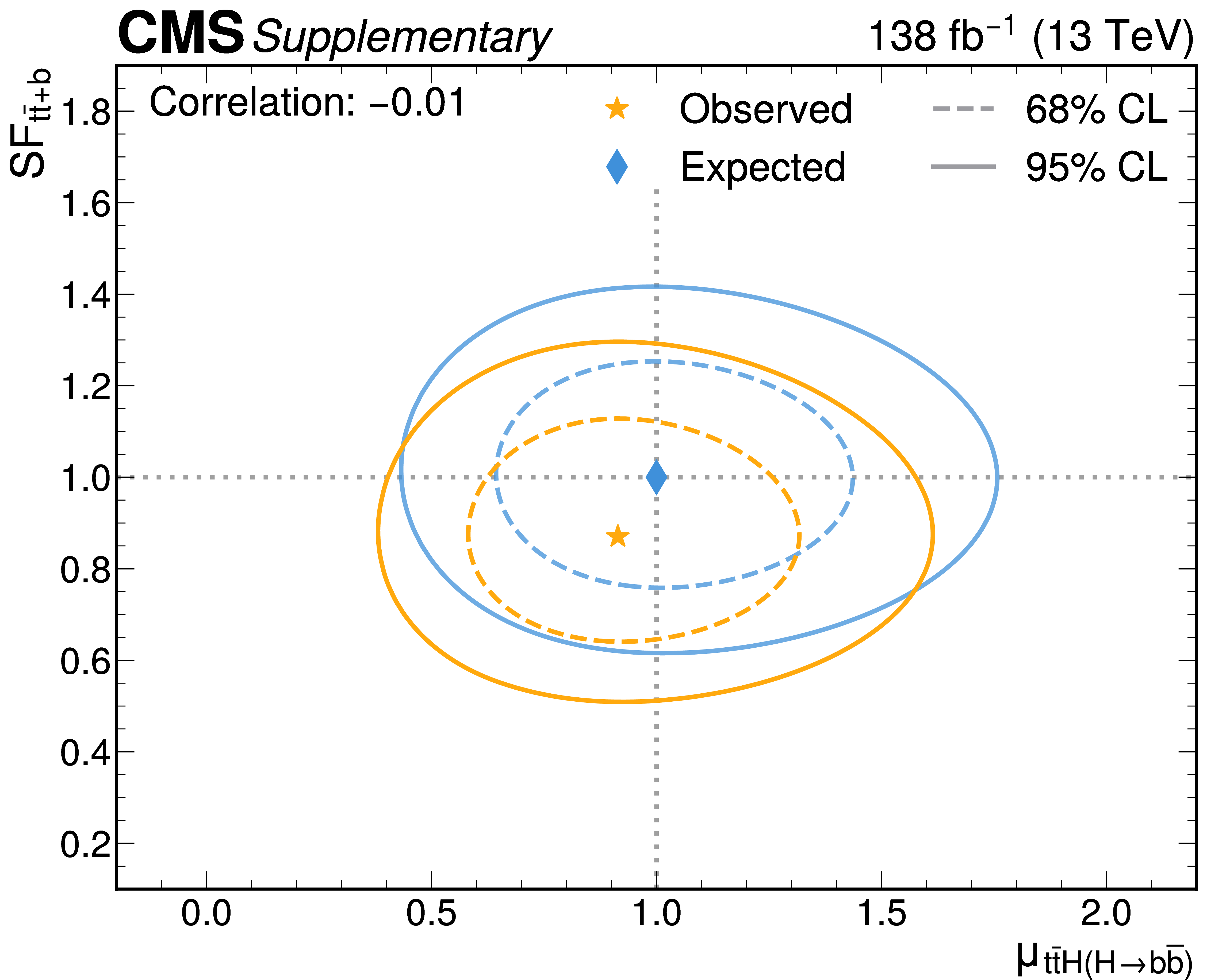
Likelihood scans for the simultaneous fit of $ \mu_{{\mathrm{t}\overline{\mathrm{t}}} \mathrm{H}(\mathrm{H}{\to}\mathrm{b}\overline{\mathrm{b}})} $ and the $ {\mathrm{t}\overline{\mathrm{t}}} {+}{\geq}2\mathrm{b} $ scale factor (upper left), $ \mu_{{\mathrm{t}\overline{\mathrm{t}}} \mathrm{H}(\mathrm{H}{\to}\mathrm{b}\overline{\mathrm{b}})} $ and the $ {\mathrm{t}\overline{\mathrm{t}}} {+}\mathrm{b} $ scale factor (upper right), $ \mu_{{\mathrm{t}\overline{\mathrm{t}}} \mathrm{H}(\mathrm{H}{\to}\mathrm{c}\overline{\mathrm{c}})} $ and the $ {\mathrm{t}\overline{\mathrm{t}}} {+}{\geq}2\mathrm{c} $ scale factor (lower left), and $ \mu_{{\mathrm{t}\overline{\mathrm{t}}} \mathrm{H}(\mathrm{H}{\to}\mathrm{c}\overline{\mathrm{c}})} $ and the $ {\mathrm{t}\overline{\mathrm{t}}} {+}\mathrm{c} $ scale factor (lower right). The 68% (95%) CL intervals are indicated by the dotted (solid) lines. The observed (expected) best fit values are shown by the orange (blue) markers. |

png pdf |
Figure B15-a:
Likelihood scans for the simultaneous fit of $ \mu_{{\mathrm{t}\overline{\mathrm{t}}} \mathrm{H}(\mathrm{H}{\to}\mathrm{b}\overline{\mathrm{b}})} $ and the $ {\mathrm{t}\overline{\mathrm{t}}} {+}{\geq}2\mathrm{b} $ scale factor (upper left), $ \mu_{{\mathrm{t}\overline{\mathrm{t}}} \mathrm{H}(\mathrm{H}{\to}\mathrm{b}\overline{\mathrm{b}})} $ and the $ {\mathrm{t}\overline{\mathrm{t}}} {+}\mathrm{b} $ scale factor (upper right), $ \mu_{{\mathrm{t}\overline{\mathrm{t}}} \mathrm{H}(\mathrm{H}{\to}\mathrm{c}\overline{\mathrm{c}})} $ and the $ {\mathrm{t}\overline{\mathrm{t}}} {+}{\geq}2\mathrm{c} $ scale factor (lower left), and $ \mu_{{\mathrm{t}\overline{\mathrm{t}}} \mathrm{H}(\mathrm{H}{\to}\mathrm{c}\overline{\mathrm{c}})} $ and the $ {\mathrm{t}\overline{\mathrm{t}}} {+}\mathrm{c} $ scale factor (lower right). The 68% (95%) CL intervals are indicated by the dotted (solid) lines. The observed (expected) best fit values are shown by the orange (blue) markers. |

png pdf |
Figure B15-b:
Likelihood scans for the simultaneous fit of $ \mu_{{\mathrm{t}\overline{\mathrm{t}}} \mathrm{H}(\mathrm{H}{\to}\mathrm{b}\overline{\mathrm{b}})} $ and the $ {\mathrm{t}\overline{\mathrm{t}}} {+}{\geq}2\mathrm{b} $ scale factor (upper left), $ \mu_{{\mathrm{t}\overline{\mathrm{t}}} \mathrm{H}(\mathrm{H}{\to}\mathrm{b}\overline{\mathrm{b}})} $ and the $ {\mathrm{t}\overline{\mathrm{t}}} {+}\mathrm{b} $ scale factor (upper right), $ \mu_{{\mathrm{t}\overline{\mathrm{t}}} \mathrm{H}(\mathrm{H}{\to}\mathrm{c}\overline{\mathrm{c}})} $ and the $ {\mathrm{t}\overline{\mathrm{t}}} {+}{\geq}2\mathrm{c} $ scale factor (lower left), and $ \mu_{{\mathrm{t}\overline{\mathrm{t}}} \mathrm{H}(\mathrm{H}{\to}\mathrm{c}\overline{\mathrm{c}})} $ and the $ {\mathrm{t}\overline{\mathrm{t}}} {+}\mathrm{c} $ scale factor (lower right). The 68% (95%) CL intervals are indicated by the dotted (solid) lines. The observed (expected) best fit values are shown by the orange (blue) markers. |
png pdf |
Figure B15-c:
Likelihood scans for the simultaneous fit of $ \mu_{{\mathrm{t}\overline{\mathrm{t}}} \mathrm{H}(\mathrm{H}{\to}\mathrm{b}\overline{\mathrm{b}})} $ and the $ {\mathrm{t}\overline{\mathrm{t}}} {+}{\geq}2\mathrm{b} $ scale factor (upper left), $ \mu_{{\mathrm{t}\overline{\mathrm{t}}} \mathrm{H}(\mathrm{H}{\to}\mathrm{b}\overline{\mathrm{b}})} $ and the $ {\mathrm{t}\overline{\mathrm{t}}} {+}\mathrm{b} $ scale factor (upper right), $ \mu_{{\mathrm{t}\overline{\mathrm{t}}} \mathrm{H}(\mathrm{H}{\to}\mathrm{c}\overline{\mathrm{c}})} $ and the $ {\mathrm{t}\overline{\mathrm{t}}} {+}{\geq}2\mathrm{c} $ scale factor (lower left), and $ \mu_{{\mathrm{t}\overline{\mathrm{t}}} \mathrm{H}(\mathrm{H}{\to}\mathrm{c}\overline{\mathrm{c}})} $ and the $ {\mathrm{t}\overline{\mathrm{t}}} {+}\mathrm{c} $ scale factor (lower right). The 68% (95%) CL intervals are indicated by the dotted (solid) lines. The observed (expected) best fit values are shown by the orange (blue) markers. |
png pdf |
Figure B15-d:
Likelihood scans for the simultaneous fit of $ \mu_{{\mathrm{t}\overline{\mathrm{t}}} \mathrm{H}(\mathrm{H}{\to}\mathrm{b}\overline{\mathrm{b}})} $ and the $ {\mathrm{t}\overline{\mathrm{t}}} {+}{\geq}2\mathrm{b} $ scale factor (upper left), $ \mu_{{\mathrm{t}\overline{\mathrm{t}}} \mathrm{H}(\mathrm{H}{\to}\mathrm{b}\overline{\mathrm{b}})} $ and the $ {\mathrm{t}\overline{\mathrm{t}}} {+}\mathrm{b} $ scale factor (upper right), $ \mu_{{\mathrm{t}\overline{\mathrm{t}}} \mathrm{H}(\mathrm{H}{\to}\mathrm{c}\overline{\mathrm{c}})} $ and the $ {\mathrm{t}\overline{\mathrm{t}}} {+}{\geq}2\mathrm{c} $ scale factor (lower left), and $ \mu_{{\mathrm{t}\overline{\mathrm{t}}} \mathrm{H}(\mathrm{H}{\to}\mathrm{c}\overline{\mathrm{c}})} $ and the $ {\mathrm{t}\overline{\mathrm{t}}} {+}\mathrm{c} $ scale factor (lower right). The 68% (95%) CL intervals are indicated by the dotted (solid) lines. The observed (expected) best fit values are shown by the orange (blue) markers. |
png pdf |
Figure B16:
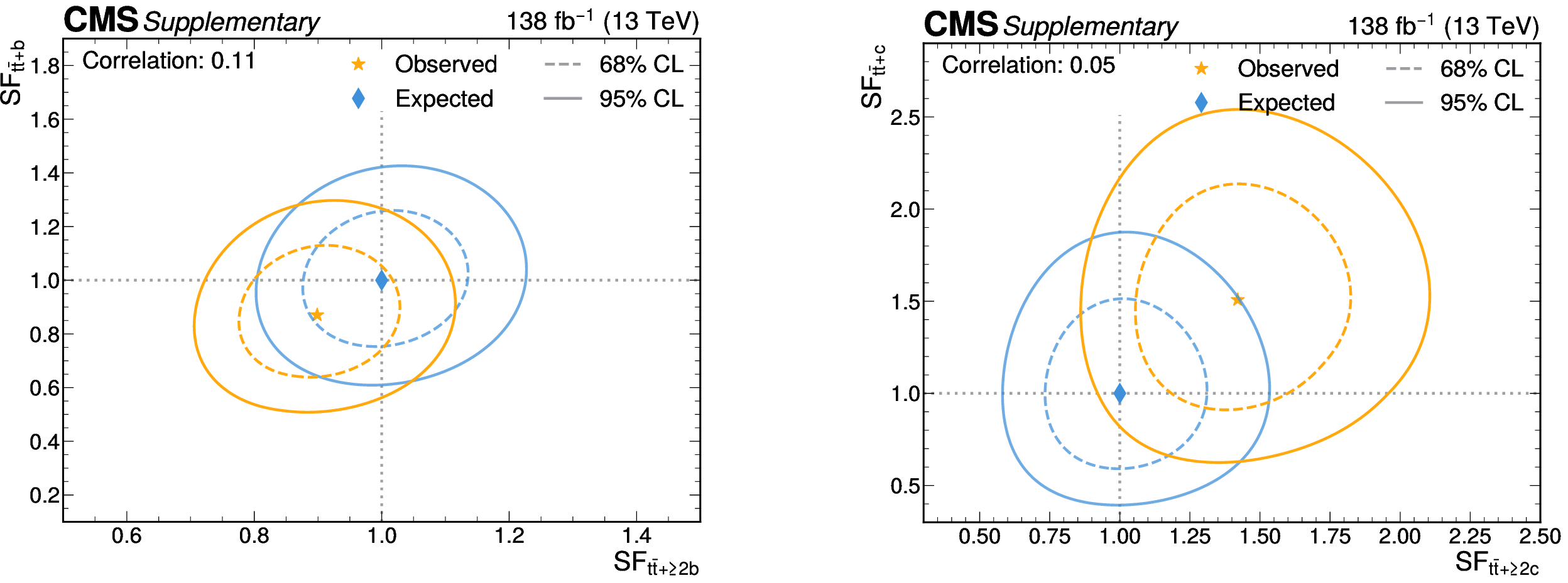
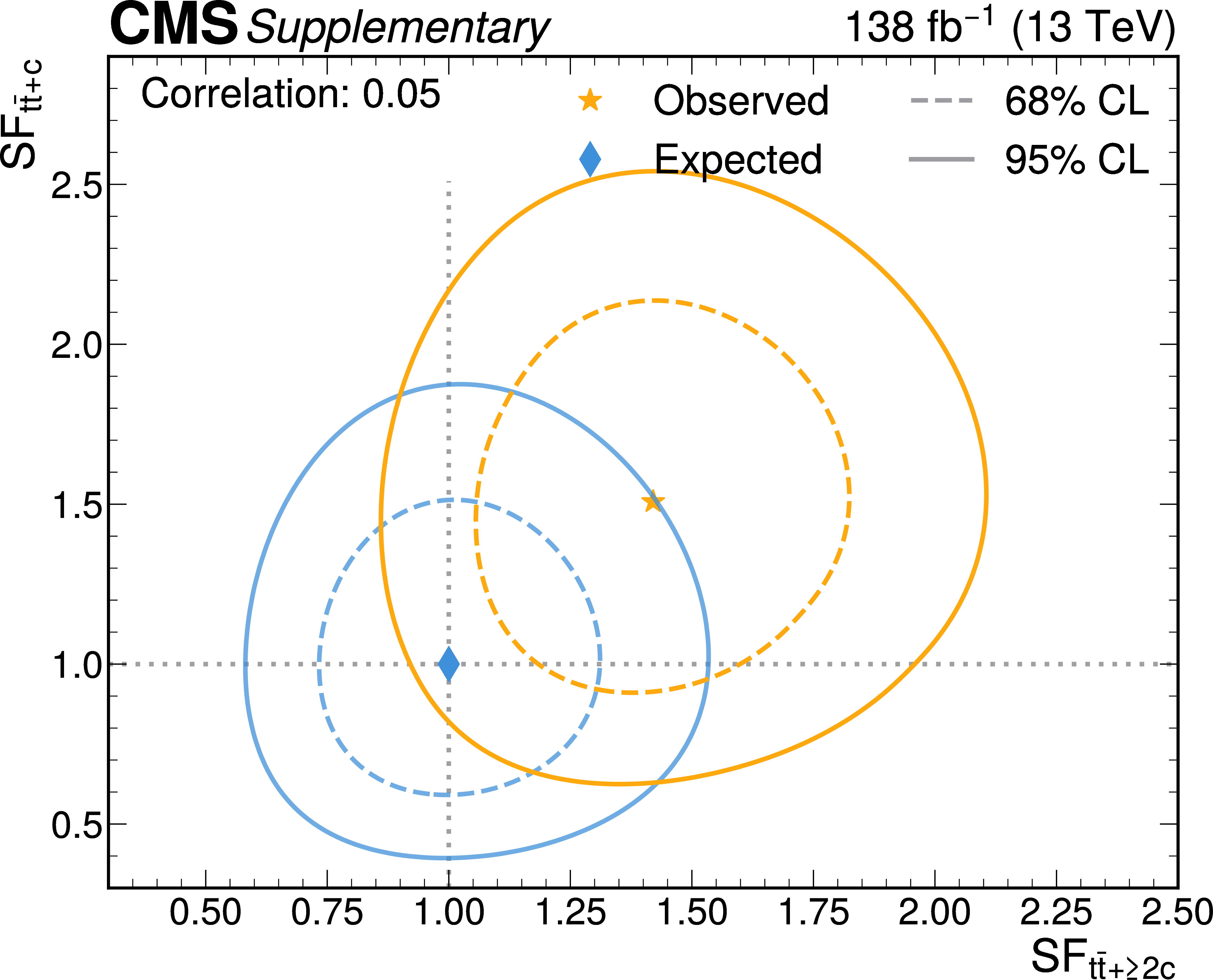
Likelihood scans for the simultaneous fit of the $ {\mathrm{t}\overline{\mathrm{t}}} {+}{\geq}2\mathrm{b} $ and $ {\mathrm{t}\overline{\mathrm{t}}} {+}\mathrm{b} $ scale factors (left), and of the $ {\mathrm{t}\overline{\mathrm{t}}} {+}{\geq}2\mathrm{c} $ and $ {\mathrm{t}\overline{\mathrm{t}}} {+}\mathrm{c} $ scale factors (right). The 68% (95%) CL intervals are indicated by the dotted (solid) lines. The observed (expected) best fit values are shown by the orange (blue) markers. |
png pdf |
Figure B16-a:
Likelihood scans for the simultaneous fit of the $ {\mathrm{t}\overline{\mathrm{t}}} {+}{\geq}2\mathrm{b} $ and $ {\mathrm{t}\overline{\mathrm{t}}} {+}\mathrm{b} $ scale factors (left), and of the $ {\mathrm{t}\overline{\mathrm{t}}} {+}{\geq}2\mathrm{c} $ and $ {\mathrm{t}\overline{\mathrm{t}}} {+}\mathrm{c} $ scale factors (right). The 68% (95%) CL intervals are indicated by the dotted (solid) lines. The observed (expected) best fit values are shown by the orange (blue) markers. |
png pdf |
Figure B16-b:
Likelihood scans for the simultaneous fit of the $ {\mathrm{t}\overline{\mathrm{t}}} {+}{\geq}2\mathrm{b} $ and $ {\mathrm{t}\overline{\mathrm{t}}} {+}\mathrm{b} $ scale factors (left), and of the $ {\mathrm{t}\overline{\mathrm{t}}} {+}{\geq}2\mathrm{c} $ and $ {\mathrm{t}\overline{\mathrm{t}}} {+}\mathrm{c} $ scale factors (right). The 68% (95%) CL intervals are indicated by the dotted (solid) lines. The observed (expected) best fit values are shown by the orange (blue) markers. |
| Tables | |
png pdf |
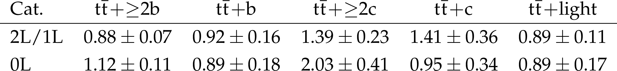
Table 1:
Best fit values of the $ {\mathrm{t}\overline{\mathrm{t}}} {+}\text{jets} $ background normalization factors for each analysis category (Cat.). |
png pdf |
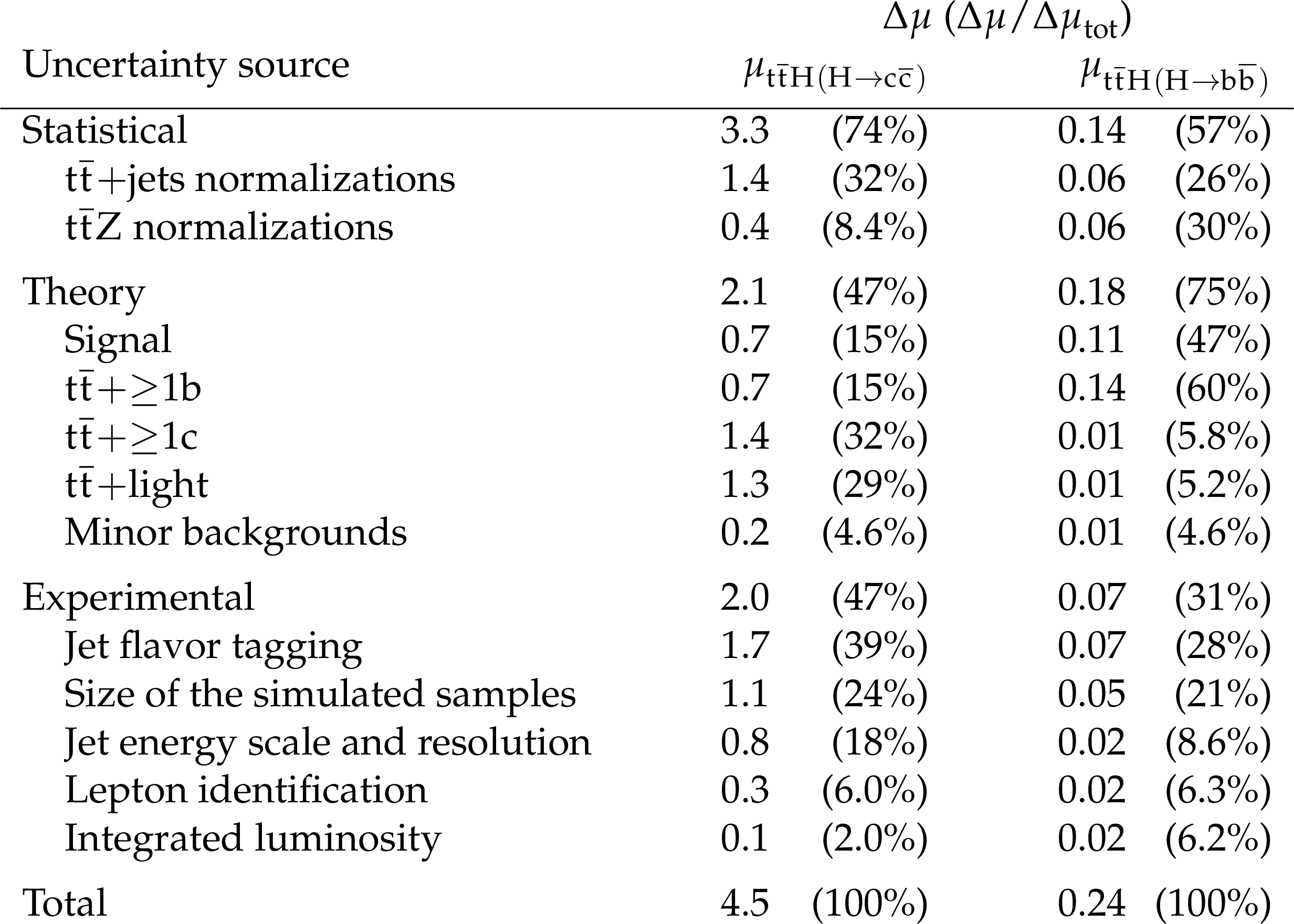
Table 2:
The absolute (relative) contributions to the total uncertainties, $ \Delta\mu $ ($ \Delta\mu/\Delta\mu_{\text{tot}} $). |
png pdf |
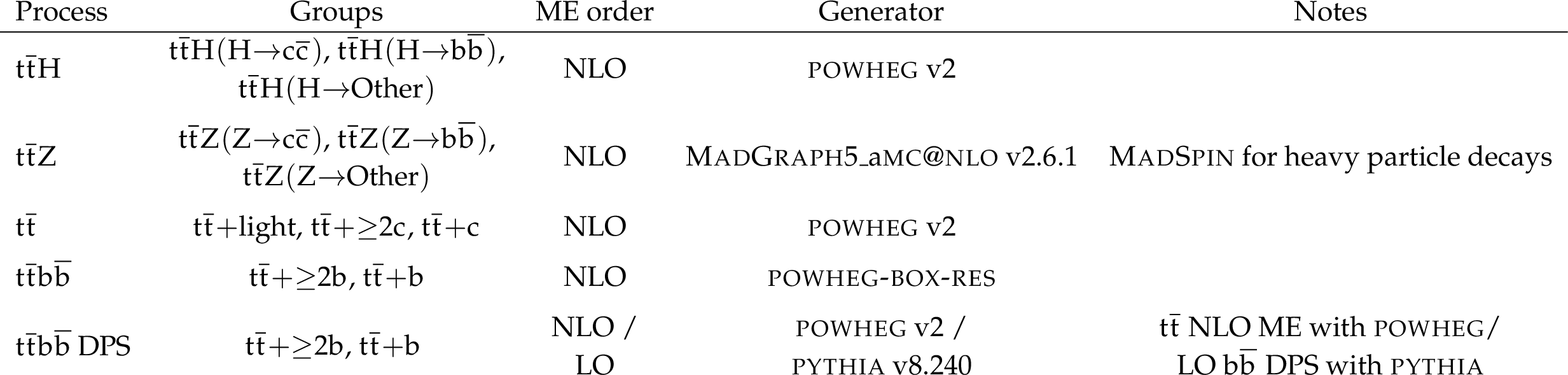
Table B1:
Generator settings for signal and major background samples. The ``Groups'' column refers to the grouping of processes in the maximum likelihood fits. Here, $ {\mathrm{t}\overline{\mathrm{t}}} \mathrm{H}(\mathrm{H}{\to}\text{Other}) $ and $ {\mathrm{t}\overline{\mathrm{t}}} \mathrm{Z}(\mathrm{Z}{\to}\text{Other}) $ refer to all Higgs boson and Z boson decay channels other than those to b and c quark pairs. |
png pdf |
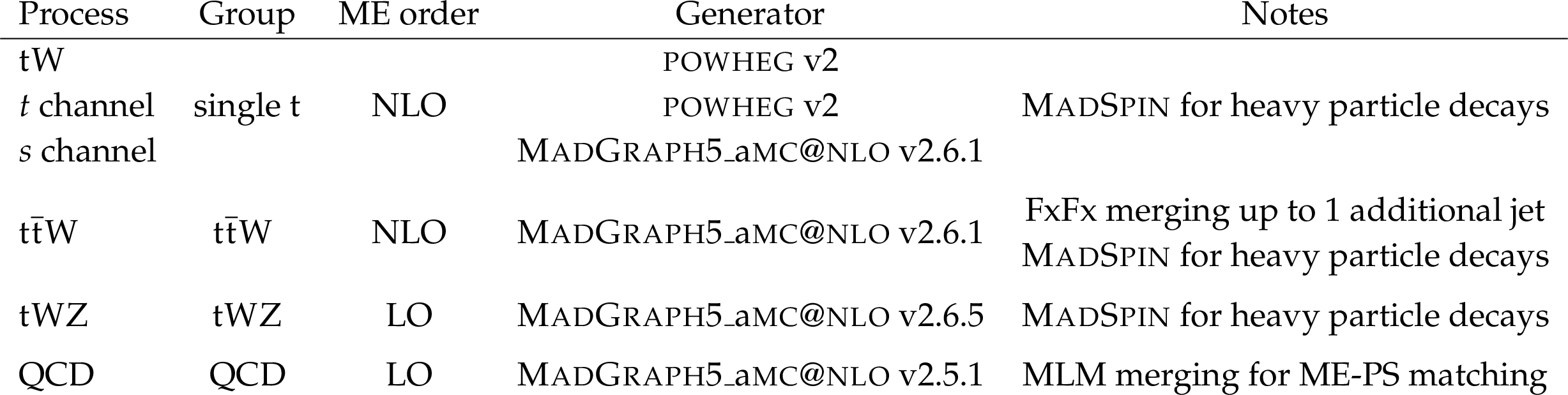
Table B2:
Generator settings for minor background samples. The ``Group'' column refers to the grouping of processes in the maximum likelihood fits. |
png pdf |
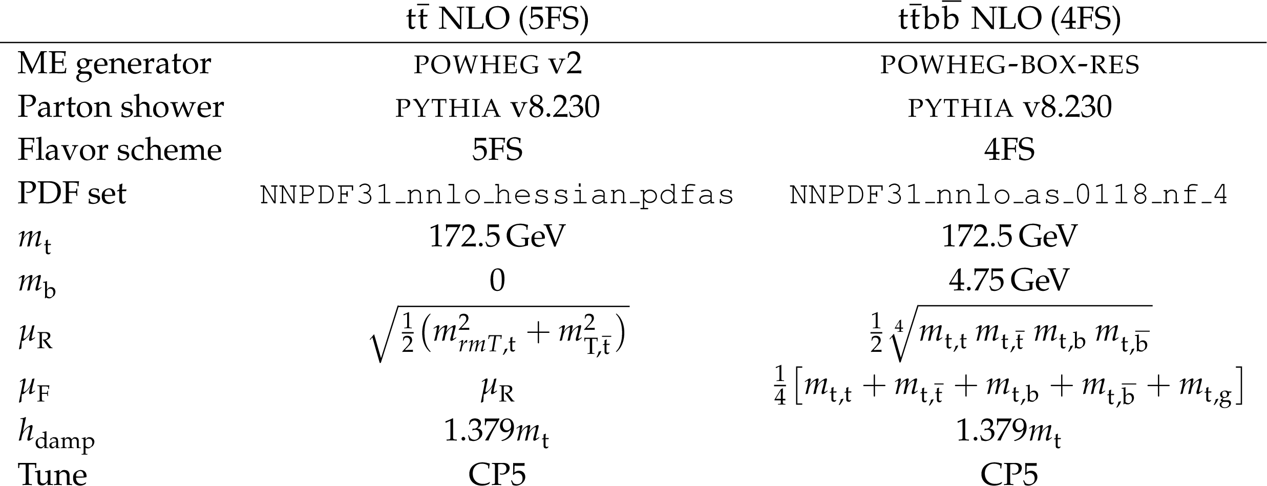
Table B3:
Summary of generator settings used for the $ {\mathrm{t}\overline{\mathrm{t}}} \mathrm{b}\overline{\mathrm{b}} $ and inclusive $ \mathrm{t} \overline{\mathrm{t}} $ samples. The transverse mass is defined as $ m_{\mathrm{T}}=\sqrt{\smash[b]{m^2 + p_{\mathrm{T}}^2}} $. |
png pdf |
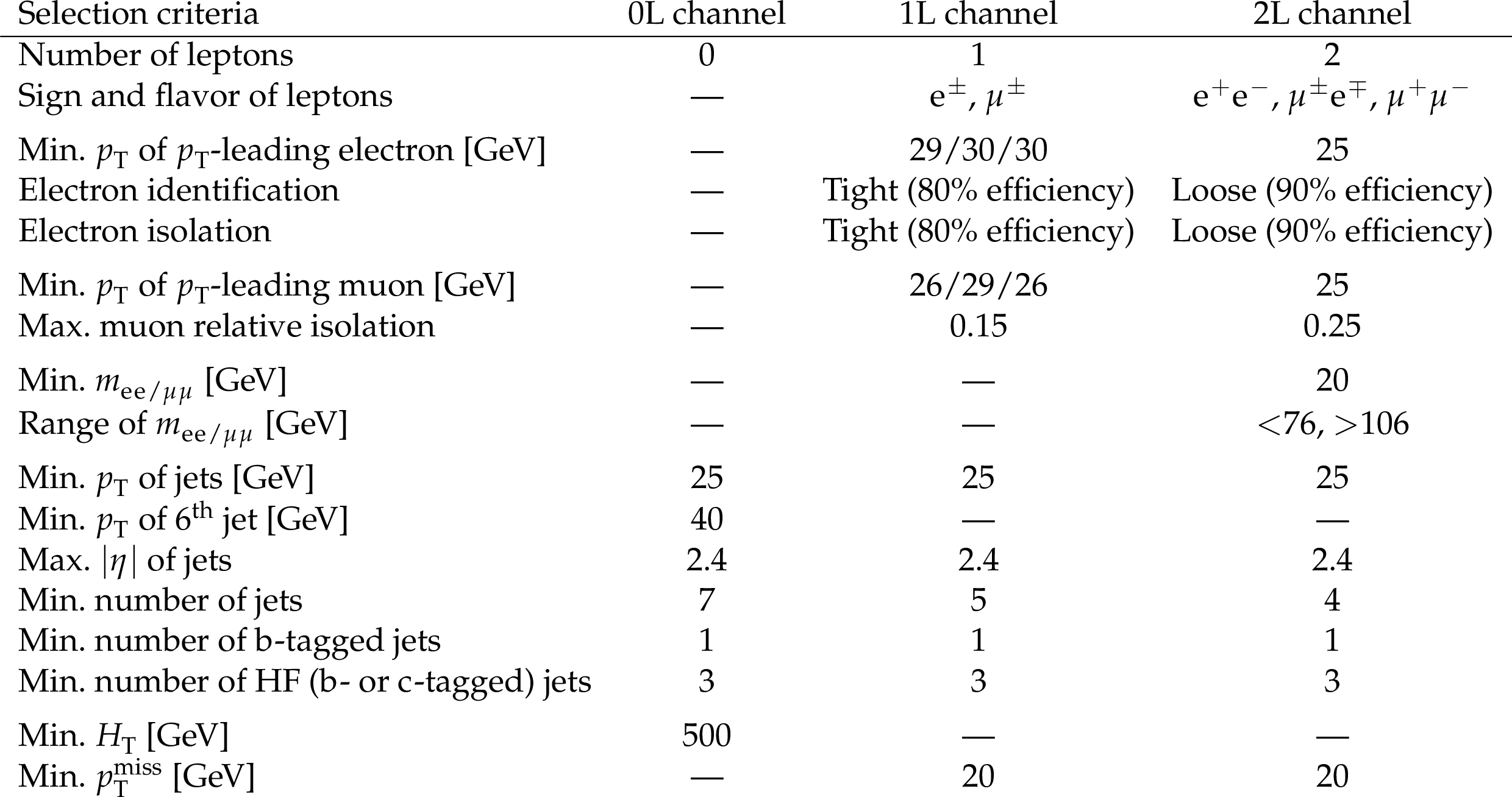
Table B4:
Baseline selection criteria in the $ \text{0L} $, $ \text{1L} $, and $ \text{2L} $ channels. Where the selection criteria differ per year, they are quoted as 2016/2017/2018. |
png pdf |
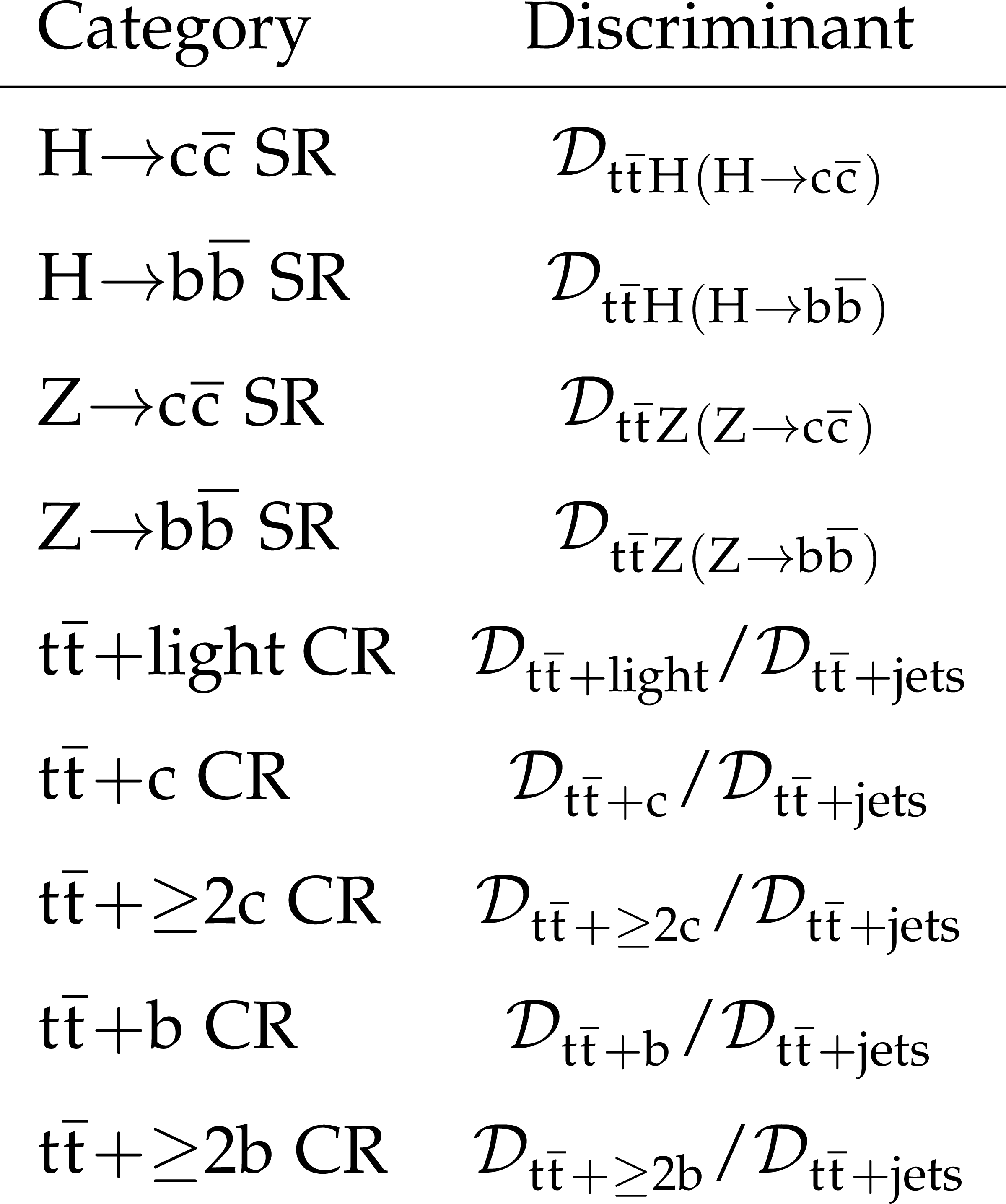
Table B5:
Definition of the PART event classifier discriminant for each category in the maximum likelihood fit. |
png pdf |
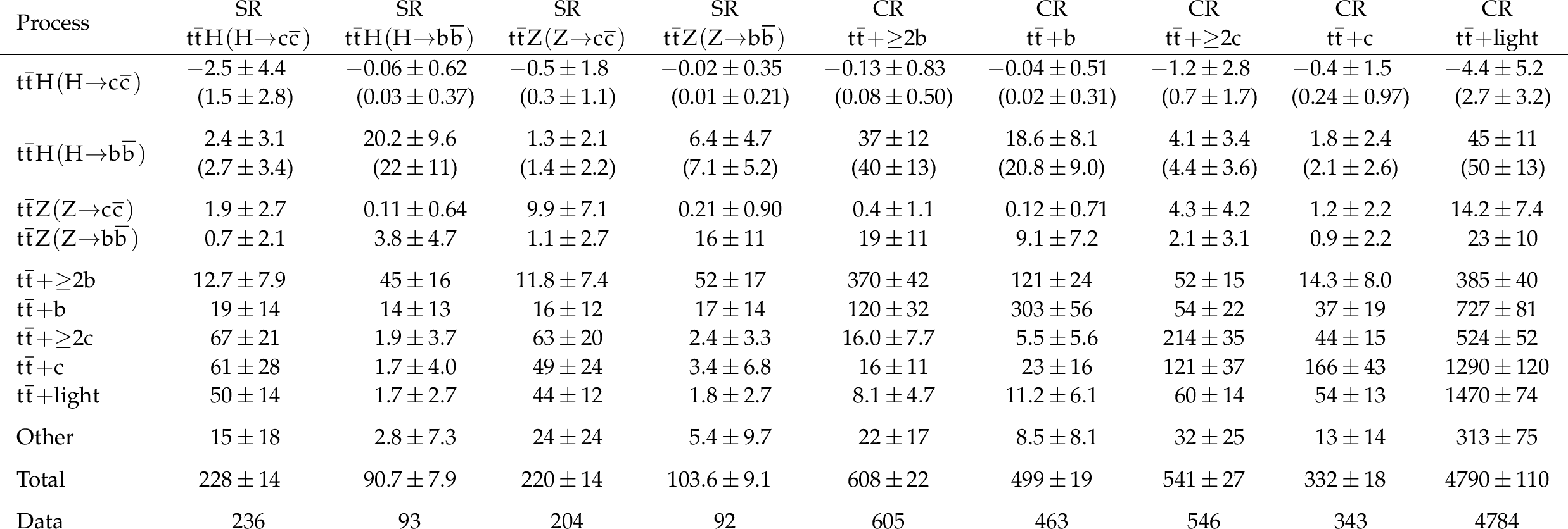
Table B6:
Event yields in the $ \text{2L} $ channel. Values in brackets correspond to the pre-fit expectations. |
png pdf |
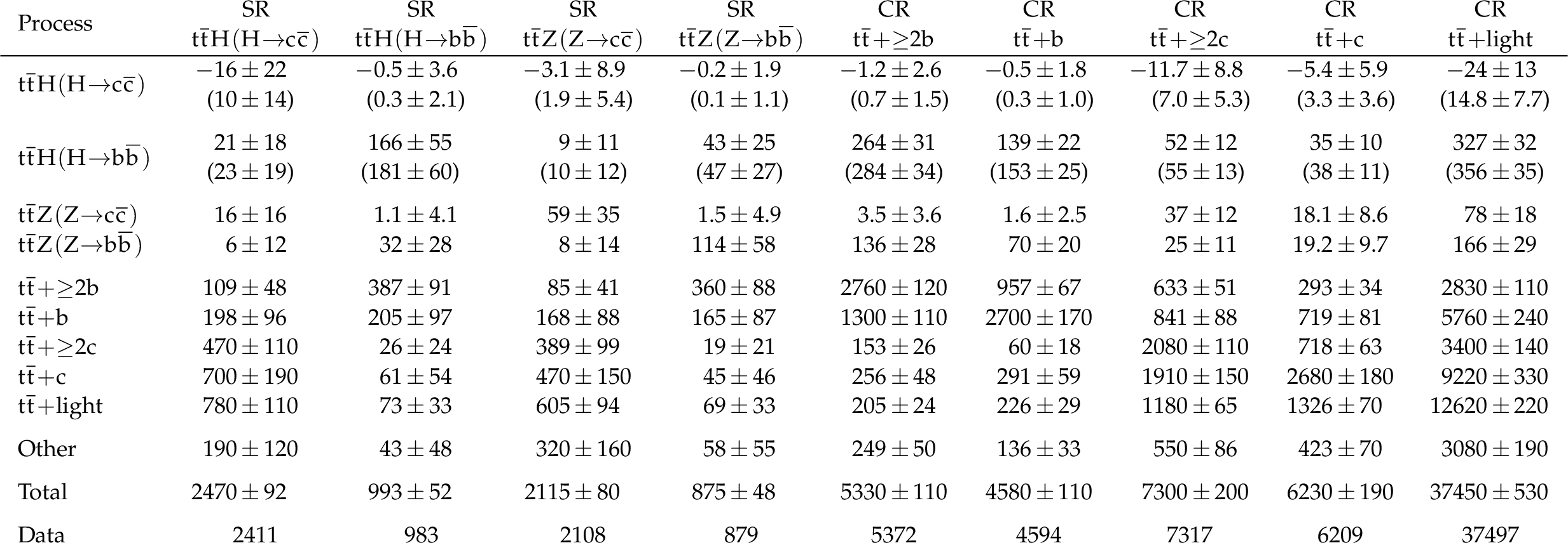
Table B7:
Event yields in the $ \text{1L} $ channel. Values in brackets correspond to the pre-fit expectations. |
png pdf |
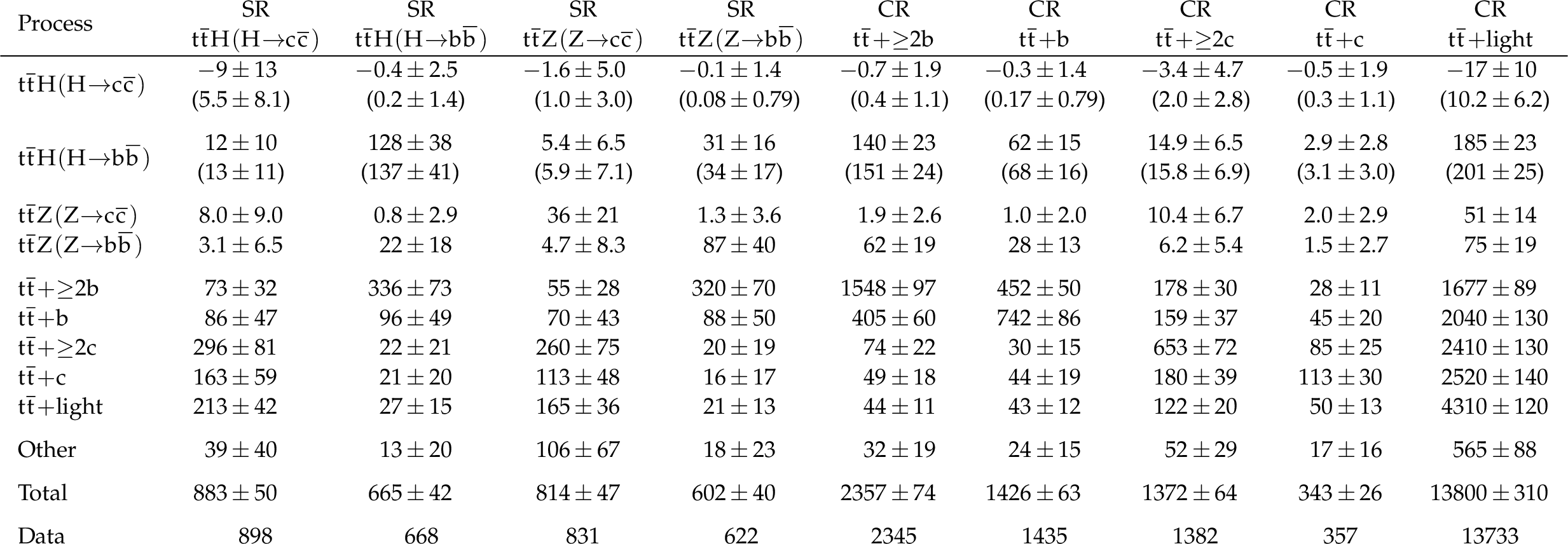
Table B8:
Event yields in the $ \text{0L} $ channel. Values in brackets correspond to the pre-fit expectations. |
png pdf |
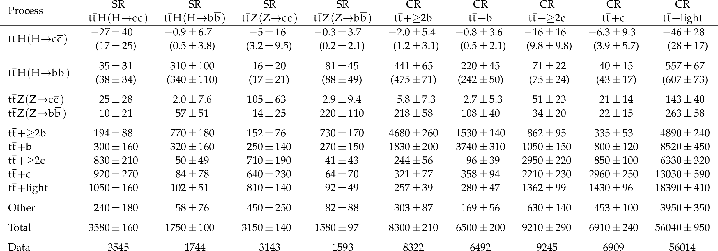
Table B9:
Event yields in the full analysis, separated in the SRs and CRs. Values in brackets correspond to the pre-fit expectations. |
png pdf |
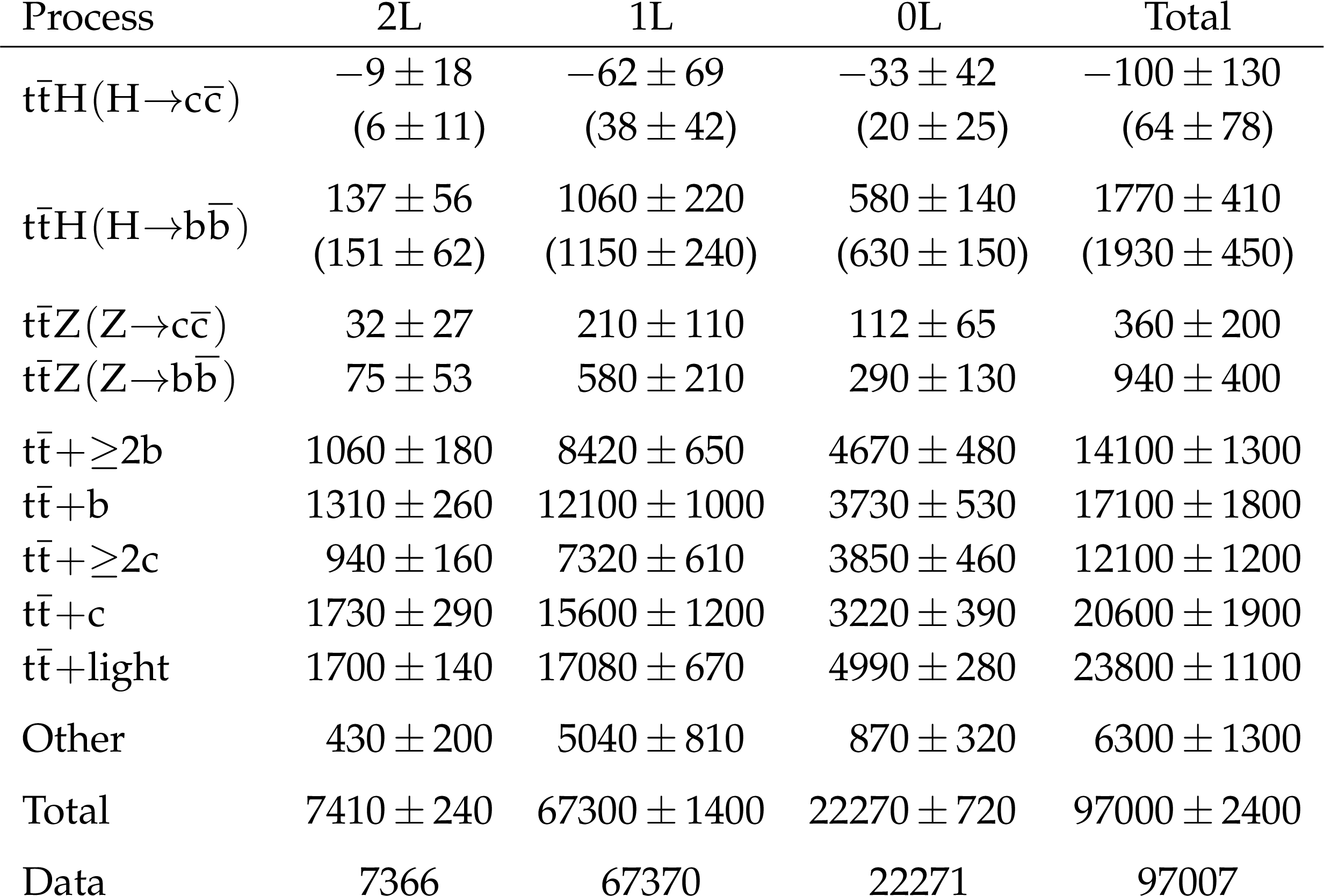
Table B10:
Event yields in the full analysis, separated per lepton channel. Values in brackets correspond to the pre-fit expectations. |
png pdf |
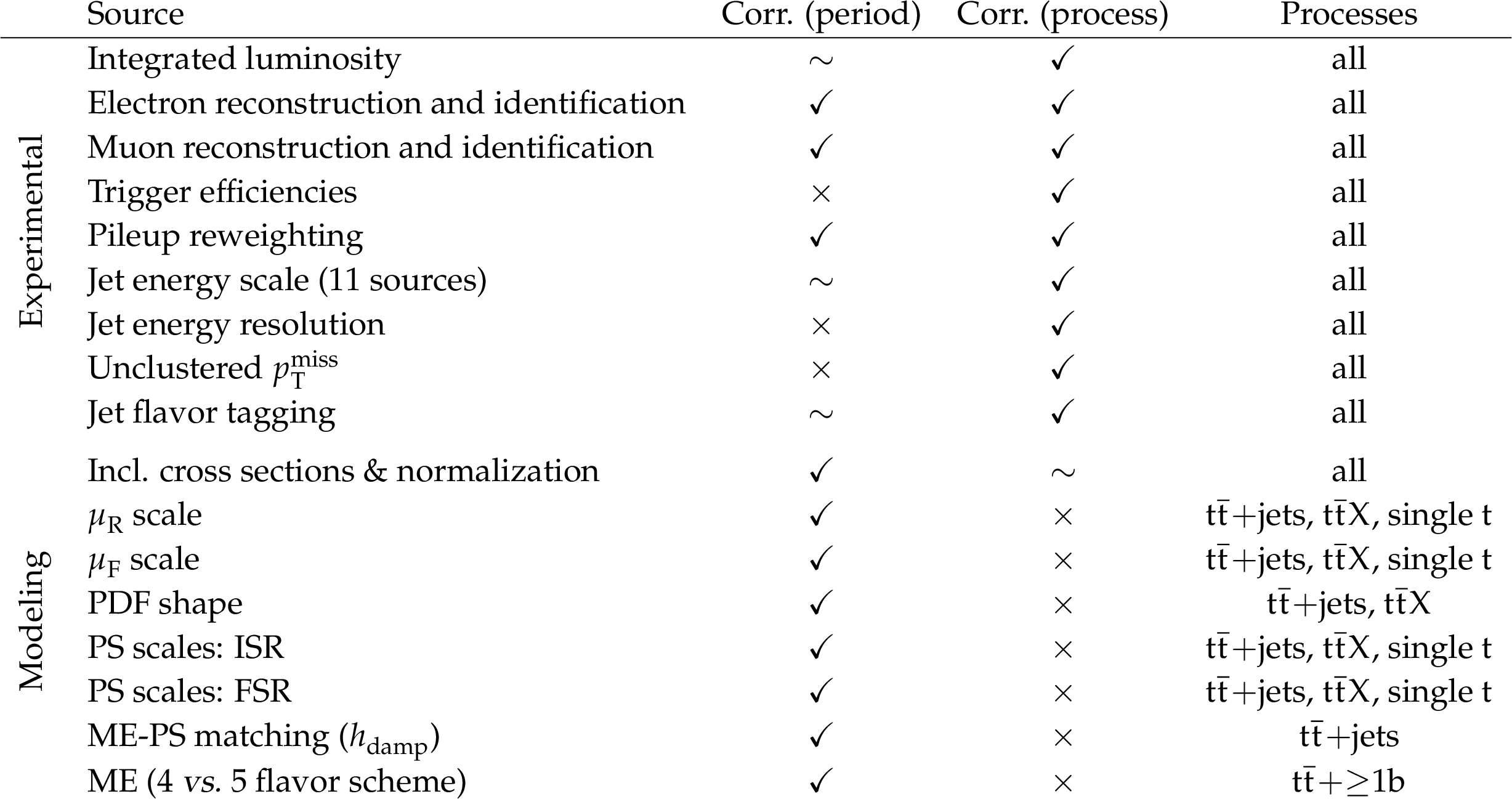
Table B11:
Summary of the systematic uncertainty sources in the measurement. The first column lists the source of the uncertainty. The second (third) column indicates the treatment of correlations of the uncertainties between different data-taking periods (processes), where $ \checkmark $ means fully correlated, $ \sim $ means partially correlated (i.e.,, contains sub-sources that are either fully correlated or uncorrelated), and $ \times $ means uncorrelated. The last column indicates whether the uncertainties are applied to all processes or only a subset. |
png pdf |
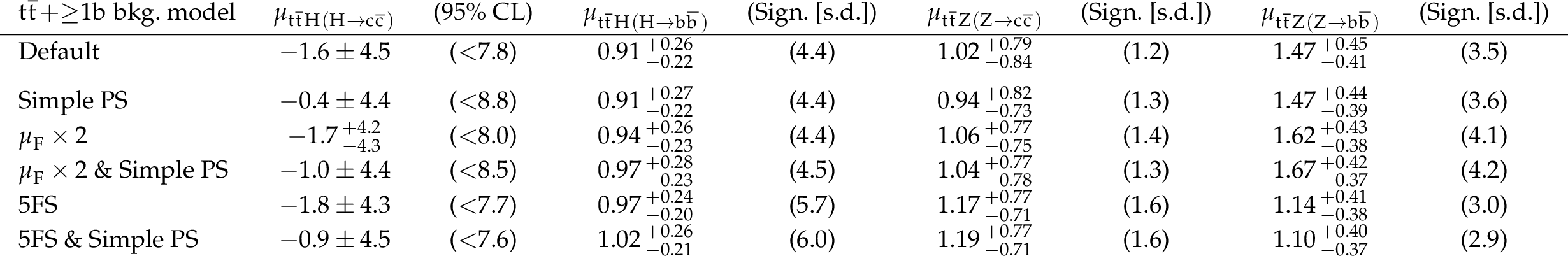
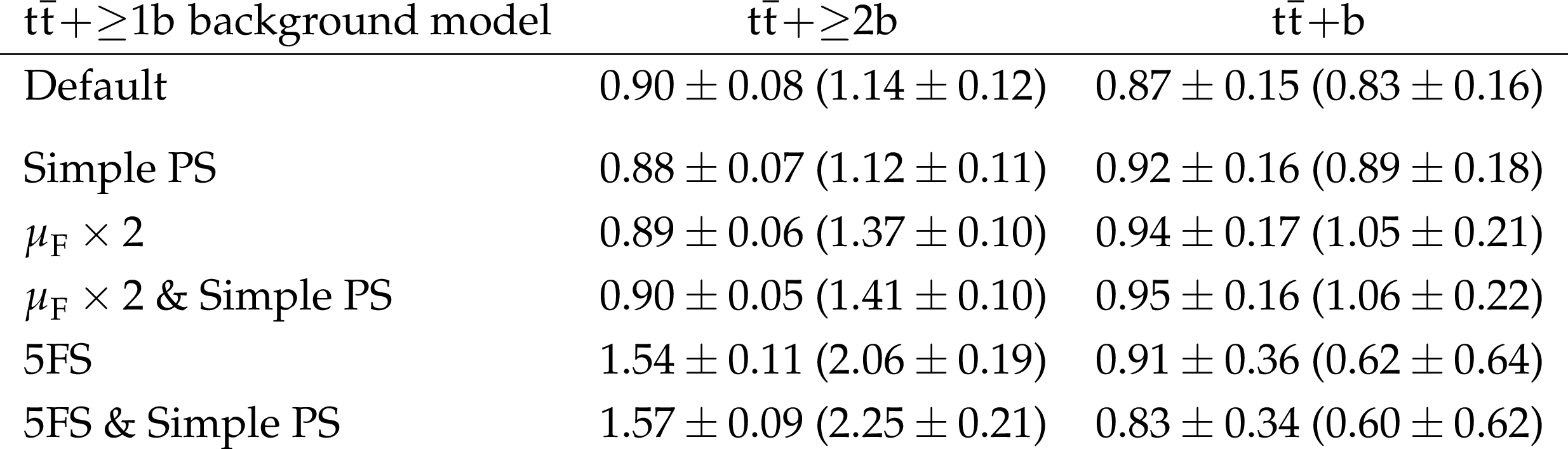
Table B12:
Observed signal strengths for $ {\mathrm{t}\overline{\mathrm{t}}} \mathrm{H}(\mathrm{H}{\to}\mathrm{c}\overline{\mathrm{c}}) $, $ {\mathrm{t}\overline{\mathrm{t}}} \mathrm{H}(\mathrm{H}{\to}\mathrm{b}\overline{\mathrm{b}}) $, $ {\mathrm{t}\overline{\mathrm{t}}} \mathrm{Z}(\mathrm{Z}{\to}\mathrm{c}\overline{\mathrm{c}}) $, and $ {\mathrm{t}\overline{\mathrm{t}}} \mathrm{Z}(\mathrm{Z}{\to}\mathrm{b}\overline{\mathrm{b}}) $ as obtained by the fits using alternative background models. In brackets are the observed upper limits for $ {\mathrm{t}\overline{\mathrm{t}}} \mathrm{H}(\mathrm{H}{\to}\mathrm{c}\overline{\mathrm{c}}) $ and the significance values for $ {\mathrm{t}\overline{\mathrm{t}}} \mathrm{H}(\mathrm{H}{\to}\mathrm{b}\overline{\mathrm{b}}) $, $ {\mathrm{t}\overline{\mathrm{t}}} \mathrm{Z}(\mathrm{Z}{\to}\mathrm{c}\overline{\mathrm{c}}) $, and $ {\mathrm{t}\overline{\mathrm{t}}} \mathrm{Z}(\mathrm{Z}{\to}\mathrm{b}\overline{\mathrm{b}}) $, respectively. |
png pdf |
Table B13:
Observed normalization scale factors for the background components as obtained by the fits using alternative background models. The background normalization scale factors are given for the $ \text{2L} $ & $ \text{1L} $ ($ \text{0L} $) channels. |
| Summary |
| In summary, a search for the SM Higgs boson decaying to a charm quark-antiquark pair via $ {\mathrm{t}\overline{\mathrm{t}}} \mathrm{H} $ production is presented, alongside a simultaneous measurement of the Higgs boson decay to a bottom quark-antiquark pair. Novel jet flavor identification tools and event classification techniques using advanced machine learning algorithms are developed for this analysis. The observed $ {\mathrm{t}\overline{\mathrm{t}}} \mathrm{H} $ signals relative to the SM predictions are $ \mu_{{\mathrm{t}\overline{\mathrm{t}}} \mathrm{H}(\mathrm{H}{\to}\mathrm{c}\overline{\mathrm{c}})}=- $1.6 $ \pm $ 4.5 and $ \mu_{{\mathrm{t}\overline{\mathrm{t}}} \mathrm{H}(\mathrm{H}{\to}\mathrm{b}\overline{\mathrm{b}})}=$ 0.91$^{+0.26}_{-0.22} $, with an observed (expected) significance of 4.4 (4.5) standard deviations for the $ {\mathrm{t}\overline{\mathrm{t}}} \mathrm{H}(\mathrm{H}{\to}\mathrm{b}\overline{\mathrm{b}}) $ process. The observed (expected) upper limit on $ \sigma({\mathrm{t}\overline{\mathrm{t}}} \mathrm{H})\mathcal{B}(\mathrm{H}{\to}\mathrm{c}\overline{\mathrm{c}}) $ is 0.11 (0.13$^{+0.06}_{-0.04}$) pb, corresponding to 7.8 (8.7$^{+4.0}_{-2.6}$) times the theoretical prediction for an SM Higgs boson mass of 125.38 GeV. When combined with the previous search for $ \mathrm{H}{\to}\mathrm{c}\overline{\mathrm{c}} $ via associated production with a W or Z boson, the observed (expected) 95% CL interval on the charm quark Yukawa coupling modifier, $ \kappa_{\mathrm{c}} $, is $ |\kappa_{\mathrm{c}}| < $ 3.5 (2.7). This represents the most stringent constraint on $ \kappa_{\mathrm{c}} $ to date. |
| Additional Figures | |
png pdf |
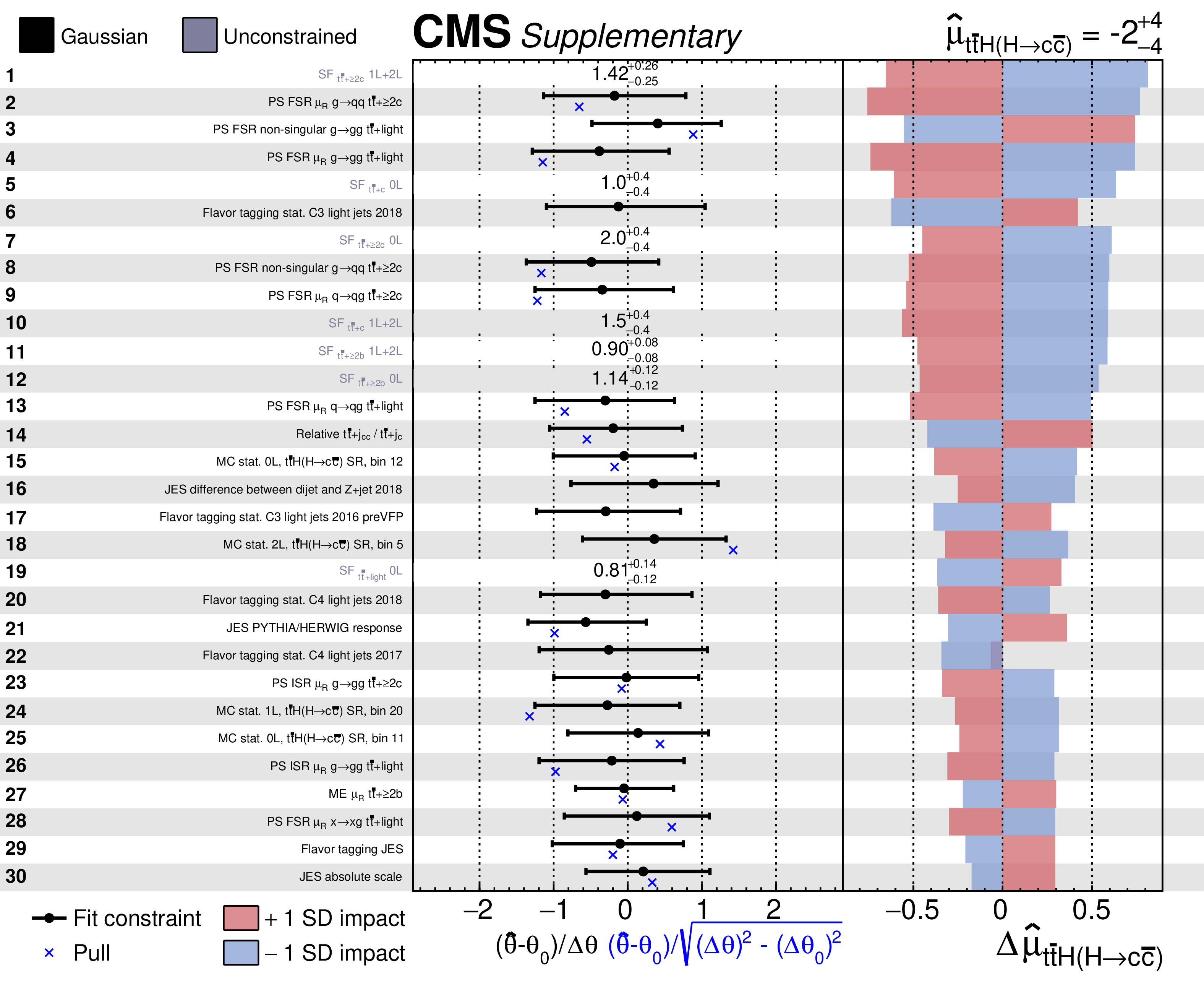
Additional Figure 1:
The nuisance-parameter uncertainties and impacts $ \Delta\hat{\mu}_{\mathrm{t}\overline{\mathrm{t}}\mathrm{H}(\mathrm{H}{\to}\mathrm{c}\overline{\mathrm{c}})} $ on the signal strength $ \mu_{\mathrm{t}\overline{\mathrm{t}}\mathrm{H}(\mathrm{H}{\to}\mathrm{c}\overline{\mathrm{c}})} $ from the fit to the data, ordered by their relative summed impact. Only the 30 highest ranked parameters are shown. Each row gives the name of the nuisance parameter, the difference in its maximum likelihood estimate ($ \hat{\theta} $, black points) with respect to its default value $ \theta_{0} $ relative to its uncertainty $ \Delta\theta $, and the impact with respect to the signal strength parameter $ \Delta\hat{\mu}_{\mathrm{t}\overline{\mathrm{t}}\mathrm{H}(\mathrm{H}{\to}\mathrm{c}\overline{\mathrm{c}})} $. The nuisance parameter constraints and impacts are calculated using the observed data set. The red and blue shaded boxes in each row represent the positive impact $ \Delta\hat{\mu}_{\mathrm{t}\overline{\mathrm{t}}\mathrm{H}(\mathrm{H}{\to}\mathrm{c}\overline{\mathrm{c}})}^{+} $ and negative impact $ \Delta\hat{\mu}_{\mathrm{t}\overline{\mathrm{t}}\mathrm{H}(\mathrm{H}{\to}\mathrm{c}\overline{\mathrm{c}})}^{-} $, respectively, for the observed data. The error bars on the fit constraint values indicate the ratio of $ \Delta^{+}\theta $ or $ \Delta^{-}\theta $, to their default values. The numerical values displayed in the figure give the value of $ \hat{\theta}^{+\Delta^{+}\theta}_{-\Delta^{-}\theta} $ for the nuisance parameters associated with the $ {\mathrm{t}\overline{\mathrm{t}}} {+}\text{jets} $ normalization, which do not have well-defined default uncertainty values. The blue points show the pull ($ (\hat{\theta}-\theta_{0})\sqrt{(\Delta\theta)^2-(\Delta\theta_0)^2} $) of the nuisance parameters. |
png pdf |
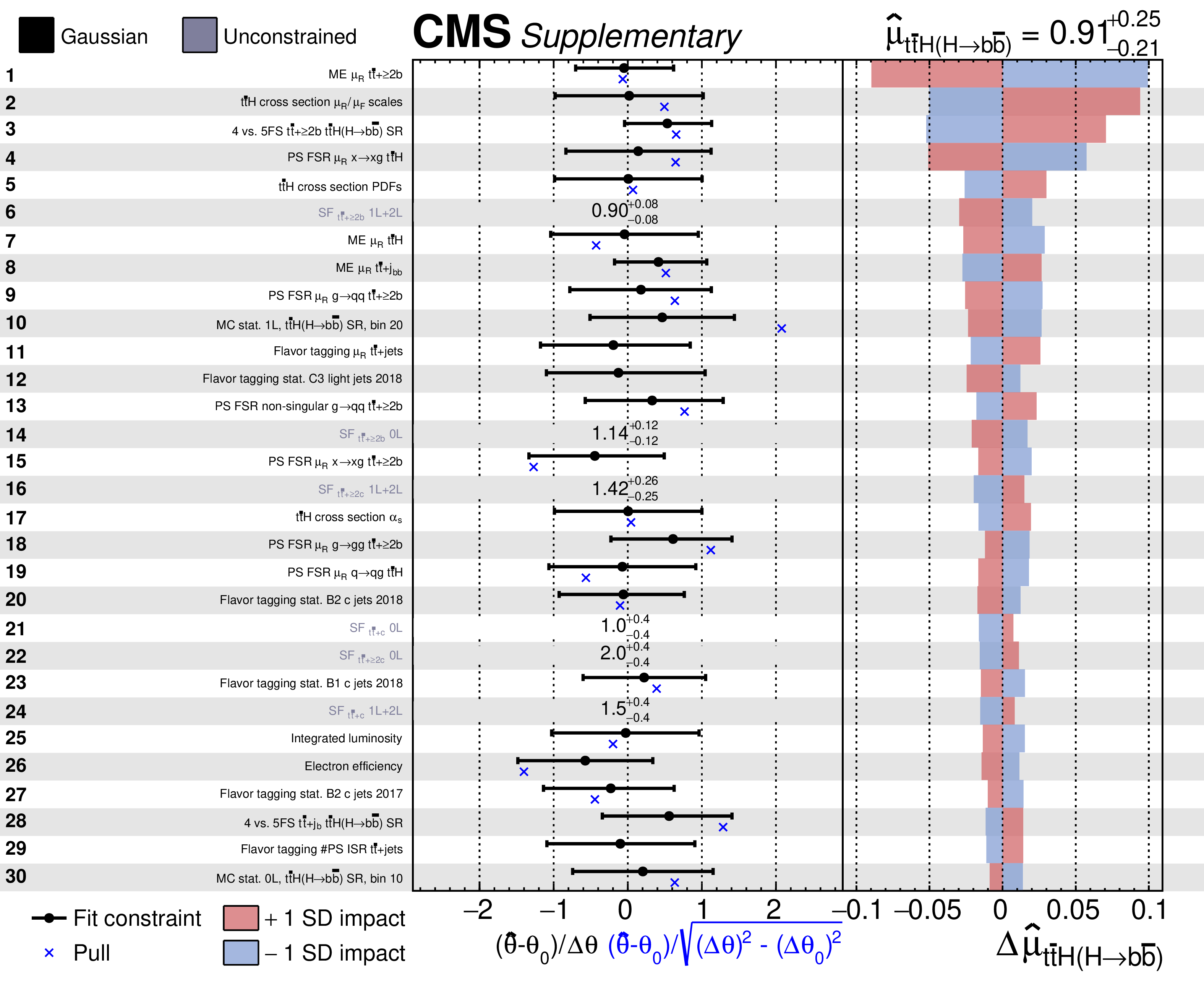
Additional Figure 2:
The nuisance-parameter uncertainties and impacts $ \Delta\hat{\mu}_{\mathrm{t}\overline{\mathrm{t}}\mathrm{H}(\mathrm{H}{\to}\mathrm{b}\overline{\mathrm{b}})} $ on the signal strength $ {\mu}_{\mathrm{t}\overline{\mathrm{t}}\mathrm{H}(\mathrm{H}{\to}\mathrm{b}\overline{\mathrm{b}})} $ from the fit to the data, ordered by their relative summed impact. Only the 30 highest ranked parameters are shown. Each row gives the name of the nuisance parameter, the difference in its maximum likelihood estimate ($ \hat{\theta} $, black points) with respect to its default value $ \theta_{0} $ relative to its uncertainty $ \Delta\theta $, and the impact with respect to the signal strength parameter $ \Delta\hat{\mu}_{\mathrm{t}\overline{\mathrm{t}}\mathrm{H}(\mathrm{H}{\to}\mathrm{b}\overline{\mathrm{b}})} $. The nuisance parameter constraints and impacts are calculated using the observed data set. The red and blue shaded boxes in each row represent the positive impact $ \Delta\hat{\mu}_{\mathrm{t}\overline{\mathrm{t}}\mathrm{H}(\mathrm{H}{\to}\mathrm{b}\overline{\mathrm{b}})}^{+} $ and negative impact $ \Delta\hat{\mu}_{\mathrm{t}\overline{\mathrm{t}}\mathrm{H}(\mathrm{H}{\to}\mathrm{b}\overline{\mathrm{b}})}^{-} $, respectively, for the observed data. The error bars on the fit constraint values indicate the ratio of $ \Delta^{+}\theta $ or $ \Delta^{-}\theta $, to their default values. The numerical values displayed in the figure give the value of $ \hat{\theta}^{+\Delta^{+}\theta}_{-\Delta^{-}\theta} $ for the nuisance parameters associated with the $ {\mathrm{t}\overline{\mathrm{t}}} {+}\text{jets} $ normalization, which do not have well-defined default uncertainty values. The blue points show the pull ($ (\hat{\theta}-\theta_{0})\sqrt{(\Delta\theta)^2-(\Delta\theta_0)^2} $) of the nuisance parameters. |
png pdf |
Additional Figure 2-a:
The nuisance-parameter uncertainties and impacts $ \Delta\hat{\mu}_{\mathrm{t}\overline{\mathrm{t}}\mathrm{H}(\mathrm{H}{\to}\mathrm{b}\overline{\mathrm{b}})} $ on the signal strength $ {\mu}_{\mathrm{t}\overline{\mathrm{t}}\mathrm{H}(\mathrm{H}{\to}\mathrm{b}\overline{\mathrm{b}})} $ from the fit to the data, ordered by their relative summed impact. Only the 30 highest ranked parameters are shown. Each row gives the name of the nuisance parameter, the difference in its maximum likelihood estimate ($ \hat{\theta} $, black points) with respect to its default value $ \theta_{0} $ relative to its uncertainty $ \Delta\theta $, and the impact with respect to the signal strength parameter $ \Delta\hat{\mu}_{\mathrm{t}\overline{\mathrm{t}}\mathrm{H}(\mathrm{H}{\to}\mathrm{b}\overline{\mathrm{b}})} $. The nuisance parameter constraints and impacts are calculated using the observed data set. The red and blue shaded boxes in each row represent the positive impact $ \Delta\hat{\mu}_{\mathrm{t}\overline{\mathrm{t}}\mathrm{H}(\mathrm{H}{\to}\mathrm{b}\overline{\mathrm{b}})}^{+} $ and negative impact $ \Delta\hat{\mu}_{\mathrm{t}\overline{\mathrm{t}}\mathrm{H}(\mathrm{H}{\to}\mathrm{b}\overline{\mathrm{b}})}^{-} $, respectively, for the observed data. The error bars on the fit constraint values indicate the ratio of $ \Delta^{+}\theta $ or $ \Delta^{-}\theta $, to their default values. The numerical values displayed in the figure give the value of $ \hat{\theta}^{+\Delta^{+}\theta}_{-\Delta^{-}\theta} $ for the nuisance parameters associated with the $ {\mathrm{t}\overline{\mathrm{t}}} {+}\text{jets} $ normalization, which do not have well-defined default uncertainty values. The blue points show the pull ($ (\hat{\theta}-\theta_{0})\sqrt{(\Delta\theta)^2-(\Delta\theta_0)^2} $) of the nuisance parameters. |
png pdf |
Additional Figure 2-b:
The nuisance-parameter uncertainties and impacts $ \Delta\hat{\mu}_{\mathrm{t}\overline{\mathrm{t}}\mathrm{H}(\mathrm{H}{\to}\mathrm{b}\overline{\mathrm{b}})} $ on the signal strength $ {\mu}_{\mathrm{t}\overline{\mathrm{t}}\mathrm{H}(\mathrm{H}{\to}\mathrm{b}\overline{\mathrm{b}})} $ from the fit to the data, ordered by their relative summed impact. Only the 30 highest ranked parameters are shown. Each row gives the name of the nuisance parameter, the difference in its maximum likelihood estimate ($ \hat{\theta} $, black points) with respect to its default value $ \theta_{0} $ relative to its uncertainty $ \Delta\theta $, and the impact with respect to the signal strength parameter $ \Delta\hat{\mu}_{\mathrm{t}\overline{\mathrm{t}}\mathrm{H}(\mathrm{H}{\to}\mathrm{b}\overline{\mathrm{b}})} $. The nuisance parameter constraints and impacts are calculated using the observed data set. The red and blue shaded boxes in each row represent the positive impact $ \Delta\hat{\mu}_{\mathrm{t}\overline{\mathrm{t}}\mathrm{H}(\mathrm{H}{\to}\mathrm{b}\overline{\mathrm{b}})}^{+} $ and negative impact $ \Delta\hat{\mu}_{\mathrm{t}\overline{\mathrm{t}}\mathrm{H}(\mathrm{H}{\to}\mathrm{b}\overline{\mathrm{b}})}^{-} $, respectively, for the observed data. The error bars on the fit constraint values indicate the ratio of $ \Delta^{+}\theta $ or $ \Delta^{-}\theta $, to their default values. The numerical values displayed in the figure give the value of $ \hat{\theta}^{+\Delta^{+}\theta}_{-\Delta^{-}\theta} $ for the nuisance parameters associated with the $ {\mathrm{t}\overline{\mathrm{t}}} {+}\text{jets} $ normalization, which do not have well-defined default uncertainty values. The blue points show the pull ($ (\hat{\theta}-\theta_{0})\sqrt{(\Delta\theta)^2-(\Delta\theta_0)^2} $) of the nuisance parameters. |

png pdf |
Additional Figure 2-c:
The nuisance-parameter uncertainties and impacts $ \Delta\hat{\mu}_{\mathrm{t}\overline{\mathrm{t}}\mathrm{H}(\mathrm{H}{\to}\mathrm{b}\overline{\mathrm{b}})} $ on the signal strength $ {\mu}_{\mathrm{t}\overline{\mathrm{t}}\mathrm{H}(\mathrm{H}{\to}\mathrm{b}\overline{\mathrm{b}})} $ from the fit to the data, ordered by their relative summed impact. Only the 30 highest ranked parameters are shown. Each row gives the name of the nuisance parameter, the difference in its maximum likelihood estimate ($ \hat{\theta} $, black points) with respect to its default value $ \theta_{0} $ relative to its uncertainty $ \Delta\theta $, and the impact with respect to the signal strength parameter $ \Delta\hat{\mu}_{\mathrm{t}\overline{\mathrm{t}}\mathrm{H}(\mathrm{H}{\to}\mathrm{b}\overline{\mathrm{b}})} $. The nuisance parameter constraints and impacts are calculated using the observed data set. The red and blue shaded boxes in each row represent the positive impact $ \Delta\hat{\mu}_{\mathrm{t}\overline{\mathrm{t}}\mathrm{H}(\mathrm{H}{\to}\mathrm{b}\overline{\mathrm{b}})}^{+} $ and negative impact $ \Delta\hat{\mu}_{\mathrm{t}\overline{\mathrm{t}}\mathrm{H}(\mathrm{H}{\to}\mathrm{b}\overline{\mathrm{b}})}^{-} $, respectively, for the observed data. The error bars on the fit constraint values indicate the ratio of $ \Delta^{+}\theta $ or $ \Delta^{-}\theta $, to their default values. The numerical values displayed in the figure give the value of $ \hat{\theta}^{+\Delta^{+}\theta}_{-\Delta^{-}\theta} $ for the nuisance parameters associated with the $ {\mathrm{t}\overline{\mathrm{t}}} {+}\text{jets} $ normalization, which do not have well-defined default uncertainty values. The blue points show the pull ($ (\hat{\theta}-\theta_{0})\sqrt{(\Delta\theta)^2-(\Delta\theta_0)^2} $) of the nuisance parameters. |
png pdf |
Additional Figure 3:
Distributions of the $ \mathrm{t}\overline{\mathrm{t}}\mathrm{H}(\mathrm{H}{\to}\mathrm{c}\overline{\mathrm{c}}) $ Particle Transformer discriminants in data (points) and predicted signal and backgrounds (colored histograms) after the fit to data. The vertical bars on the points represent the statistical uncertainties in data. The hatched band represents the total uncertainty in the sum of the signal and background predictions. The lower panel shows the ratio of the data to the sum of the signal and background predictions. |
png pdf |
Additional Figure 4:
Distributions of the $ \mathrm{t}\overline{\mathrm{t}}\mathrm{H}(\mathrm{H}{\to}\mathrm{b}\overline{\mathrm{b}}) $ Particle Transformer discriminants in data (points) and predicted signal and backgrounds (colored histograms) after the fit to data. The vertical bars on the points represent the statistical uncertainties in data. The hatched band represents the total uncertainty in the sum of the signal and background predictions. The lower panel shows the ratio of the data to the sum of the signal and background predictions. |
png pdf |
Additional Figure 5:
Distributions of the $ {\mathrm{t}\overline{\mathrm{t}}} \mathrm{Z}(\mathrm{Z}{\to}\mathrm{c}\overline{\mathrm{c}}) $ Particle Transformer discriminants in data (points) and predicted signal and backgrounds (colored histograms) after the fit to data. The vertical bars on the points represent the statistical uncertainties in data. The hatched band represents the total uncertainty in the sum of the signal and background predictions. The lower panel shows the ratio of the data to the sum of the signal and background predictions. |
png pdf |
Additional Figure 6:
Distributions of the $ {\mathrm{t}\overline{\mathrm{t}}} \mathrm{Z}(\mathrm{Z}{\to}\mathrm{b}\overline{\mathrm{b}}) $ Particle Transformer discriminants in data (points) and predicted signal and backgrounds (colored histograms) after the fit to data. The vertical bars on the points represent the statistical uncertainties in data. The hatched band represents the total uncertainty in the sum of the signal and background predictions. The lower panel shows the ratio of the data to the sum of the signal and background predictions. |
png pdf |
Additional Figure 7:
Distributions of the $ {\mathrm{t}\overline{\mathrm{t}}} {+}{\geq}2\mathrm{c} $ Particle Transformer discriminants in data (points) and predicted signal and backgrounds (colored histograms) after the fit to data. The vertical bars on the points represent the statistical uncertainties in data. The hatched band represents the total uncertainty in the sum of the signal and background predictions. The lower panel shows the ratio of the data to the sum of the signal and background predictions. |
png pdf |
Additional Figure 8:
Distributions of the $ {\mathrm{t}\overline{\mathrm{t}}} {+}\mathrm{c} $ Particle Transformer discriminants in data (points) and predicted signal and backgrounds (colored histograms) after the fit to data. The vertical bars on the points represent the statistical uncertainties in data. The hatched band represents the total uncertainty in the sum of the signal and background predictions. The lower panel shows the ratio of the data to the sum of the signal and background predictions. |

png pdf |
Additional Figure 8-a:
Distributions of the $ {\mathrm{t}\overline{\mathrm{t}}} {+}\mathrm{c} $ Particle Transformer discriminants in data (points) and predicted signal and backgrounds (colored histograms) after the fit to data. The vertical bars on the points represent the statistical uncertainties in data. The hatched band represents the total uncertainty in the sum of the signal and background predictions. The lower panel shows the ratio of the data to the sum of the signal and background predictions. |
png pdf |
Additional Figure 8-b:
Distributions of the $ {\mathrm{t}\overline{\mathrm{t}}} {+}\mathrm{c} $ Particle Transformer discriminants in data (points) and predicted signal and backgrounds (colored histograms) after the fit to data. The vertical bars on the points represent the statistical uncertainties in data. The hatched band represents the total uncertainty in the sum of the signal and background predictions. The lower panel shows the ratio of the data to the sum of the signal and background predictions. |
png pdf |
Additional Figure 9:
Distributions of the $ {\mathrm{t}\overline{\mathrm{t}}} {+}{\geq}2\mathrm{b} $ Particle Transformer discriminants in data (points) and predicted signal and backgrounds (colored histograms) after the fit to data. The vertical bars on the points represent the statistical uncertainties in data. The hatched band represents the total uncertainty in the sum of the signal and background predictions. The lower panel shows the ratio of the data to the sum of the signal and background predictions. |

png pdf |
Additional Figure 9-a:
Distributions of the $ {\mathrm{t}\overline{\mathrm{t}}} {+}{\geq}2\mathrm{b} $ Particle Transformer discriminants in data (points) and predicted signal and backgrounds (colored histograms) after the fit to data. The vertical bars on the points represent the statistical uncertainties in data. The hatched band represents the total uncertainty in the sum of the signal and background predictions. The lower panel shows the ratio of the data to the sum of the signal and background predictions. |

png pdf |
Additional Figure 9-b:
Distributions of the $ {\mathrm{t}\overline{\mathrm{t}}} {+}{\geq}2\mathrm{b} $ Particle Transformer discriminants in data (points) and predicted signal and backgrounds (colored histograms) after the fit to data. The vertical bars on the points represent the statistical uncertainties in data. The hatched band represents the total uncertainty in the sum of the signal and background predictions. The lower panel shows the ratio of the data to the sum of the signal and background predictions. |
png pdf |
Additional Figure 10:
Distributions of the $ {\mathrm{t}\overline{\mathrm{t}}} {+}\mathrm{b} $ Particle Transformer discriminants in data (points) and predicted signal and backgrounds (colored histograms) after the fit to data. The vertical bars on the points represent the statistical uncertainties in data. The hatched band represents the total uncertainty in the sum of the signal and background predictions. The lower panel shows the ratio of the data to the sum of the signal and background predictions. |
png pdf |
Additional Figure 11:
Distributions of the $ {\mathrm{t}\overline{\mathrm{t}}} {+}\text{light} $ Particle Transformer discriminants in data (points) and predicted signal and backgrounds (colored histograms) after the fit to data. The vertical bars on the points represent the statistical uncertainties in data. The hatched band represents the total uncertainty in the sum of the signal and background predictions. The lower panel shows the ratio of the data to the sum of the signal and background predictions. |
png pdf |
Additional Figure 12:
Distribution of b jets in the two-dimensional PARTICLENET discriminant plane. The vertical and horizontal lines correspond to the edges of the tagging categories. The numbers in each bin correspond to |
png pdf |
Additional Figure 13:
Distribution of c jets in the two-dimensional PARTICLENET discriminant plane. The vertical and horizontal lines correspond to the edges of the tagging categories. The numbers in each bin correspond to |
png pdf |
Additional Figure 14:
Distribution of light jets in the two-dimensional PARTICLENET discriminant plane. The vertical and horizontal lines correspond to the edges of the tagging categories. The numbers in each bin correspon |
png pdf |
Additional Figure 14-a:
Distribution of light jets in the two-dimensional PARTICLENET discriminant plane. The vertical and horizontal lines correspond to the edges of the tagging categories. The numbers in each bin correspon |

png pdf |
Additional Figure 14-b:
Distribution of light jets in the two-dimensional PARTICLENET discriminant plane. The vertical and horizontal lines correspond to the edges of the tagging categories. The numbers in each bin correspon |

png pdf |
Additional Figure 14-c:
Distribution of light jets in the two-dimensional PARTICLENET discriminant plane. The vertical and horizontal lines correspond to the edges of the tagging categories. The numbers in each bin correspon |
png pdf |
Additional Figure 14-d:
Distribution of light jets in the two-dimensional PARTICLENET discriminant plane. The vertical and horizontal lines correspond to the edges of the tagging categories. The numbers in each bin correspon |
png pdf |
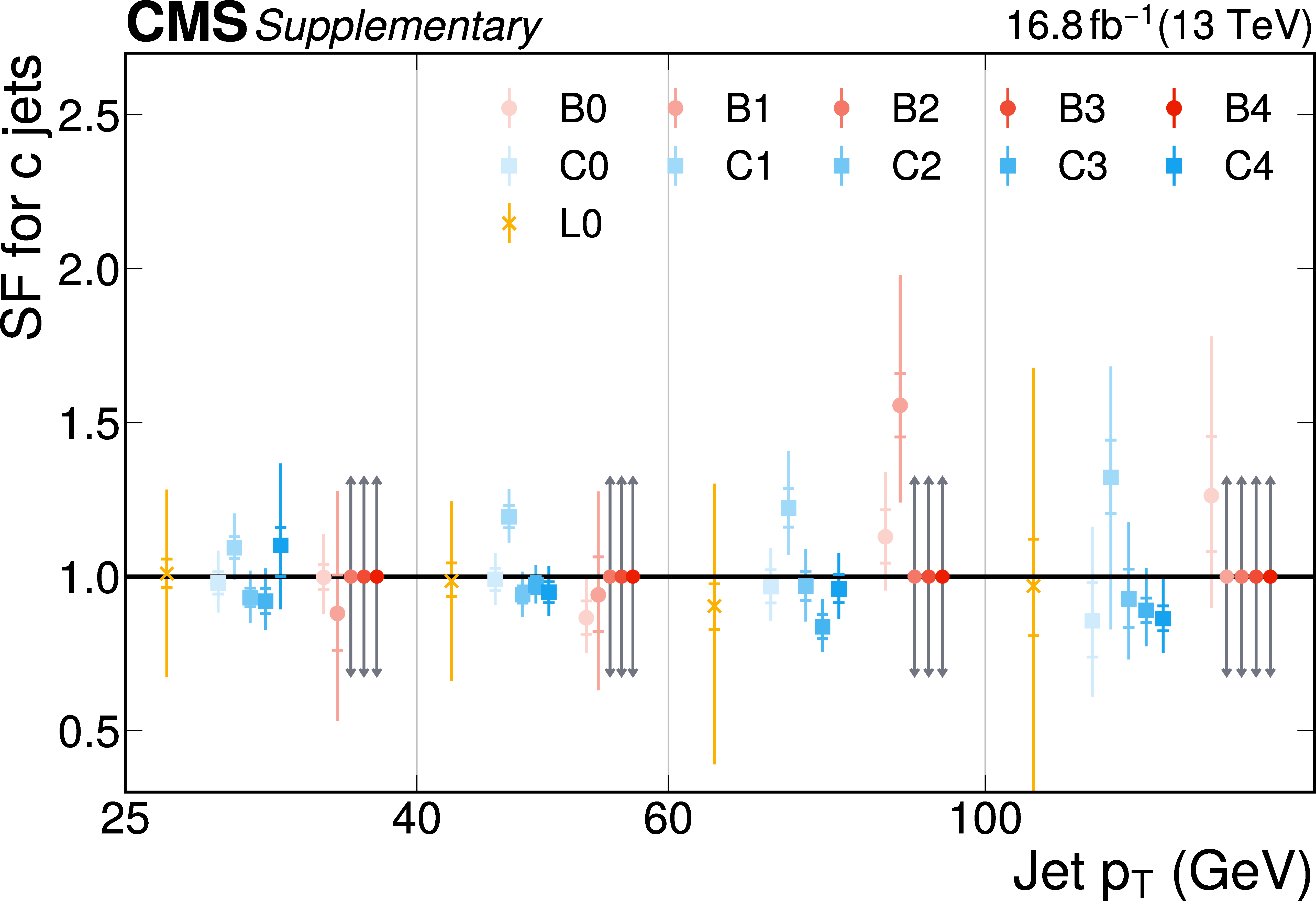
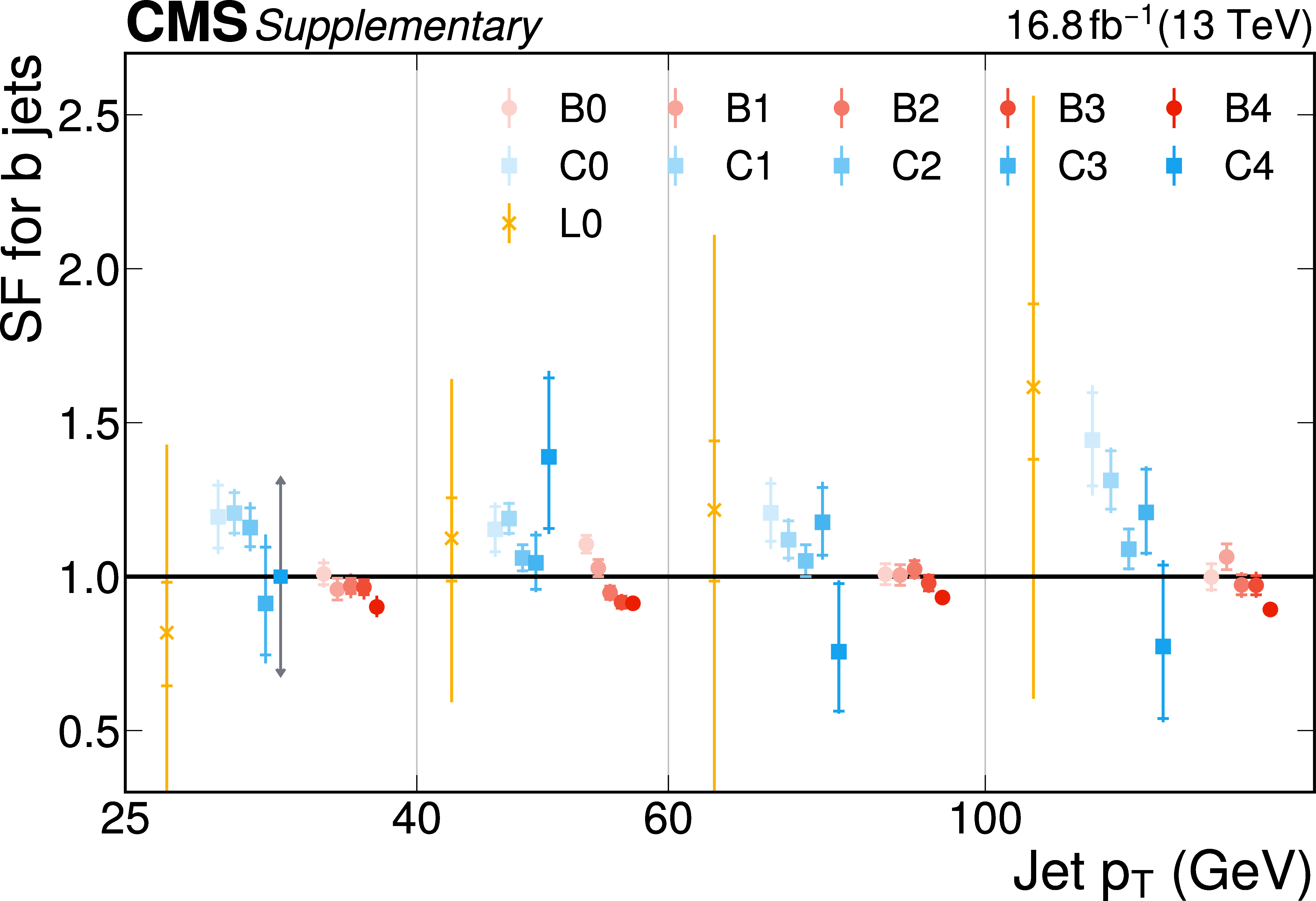
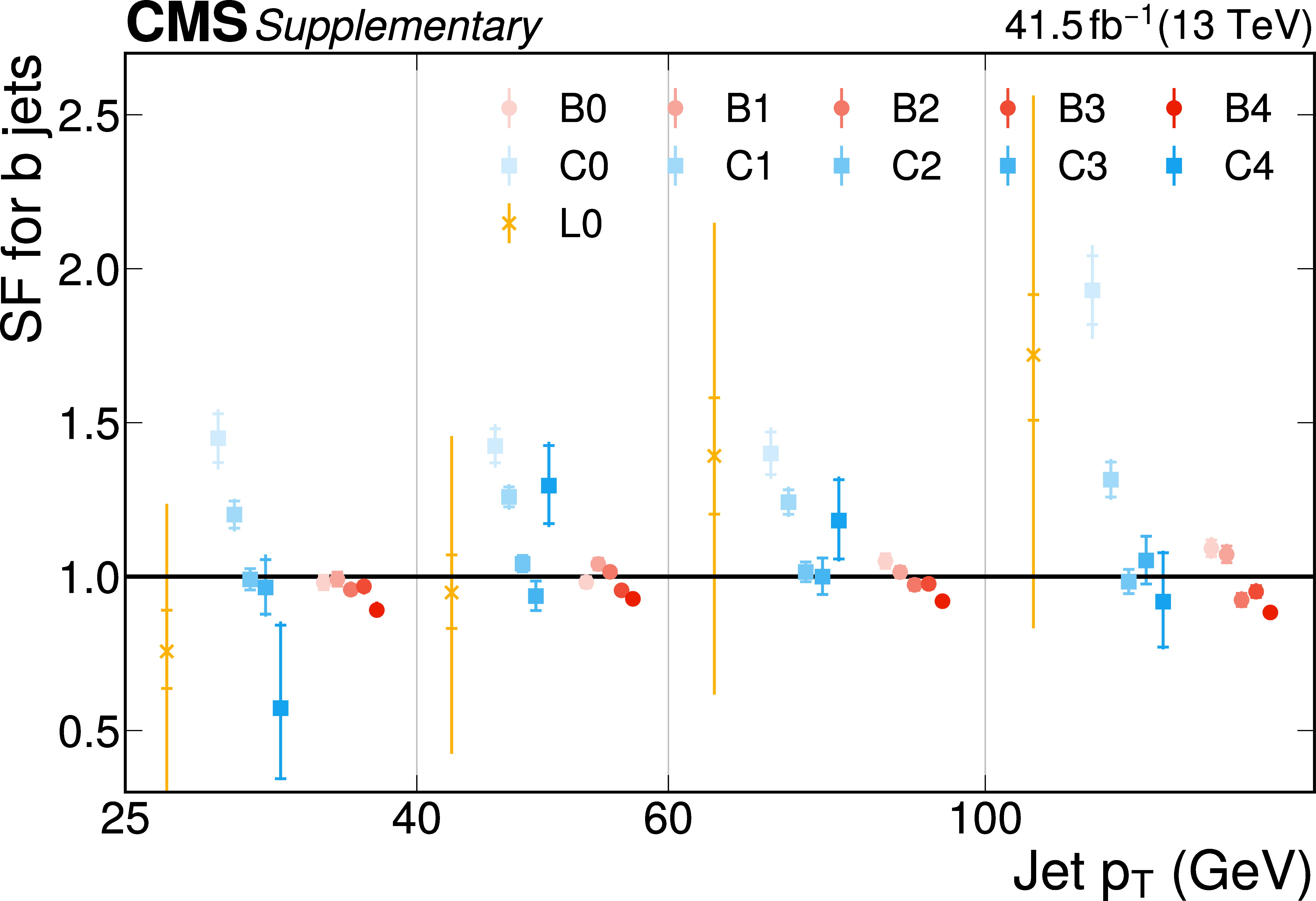
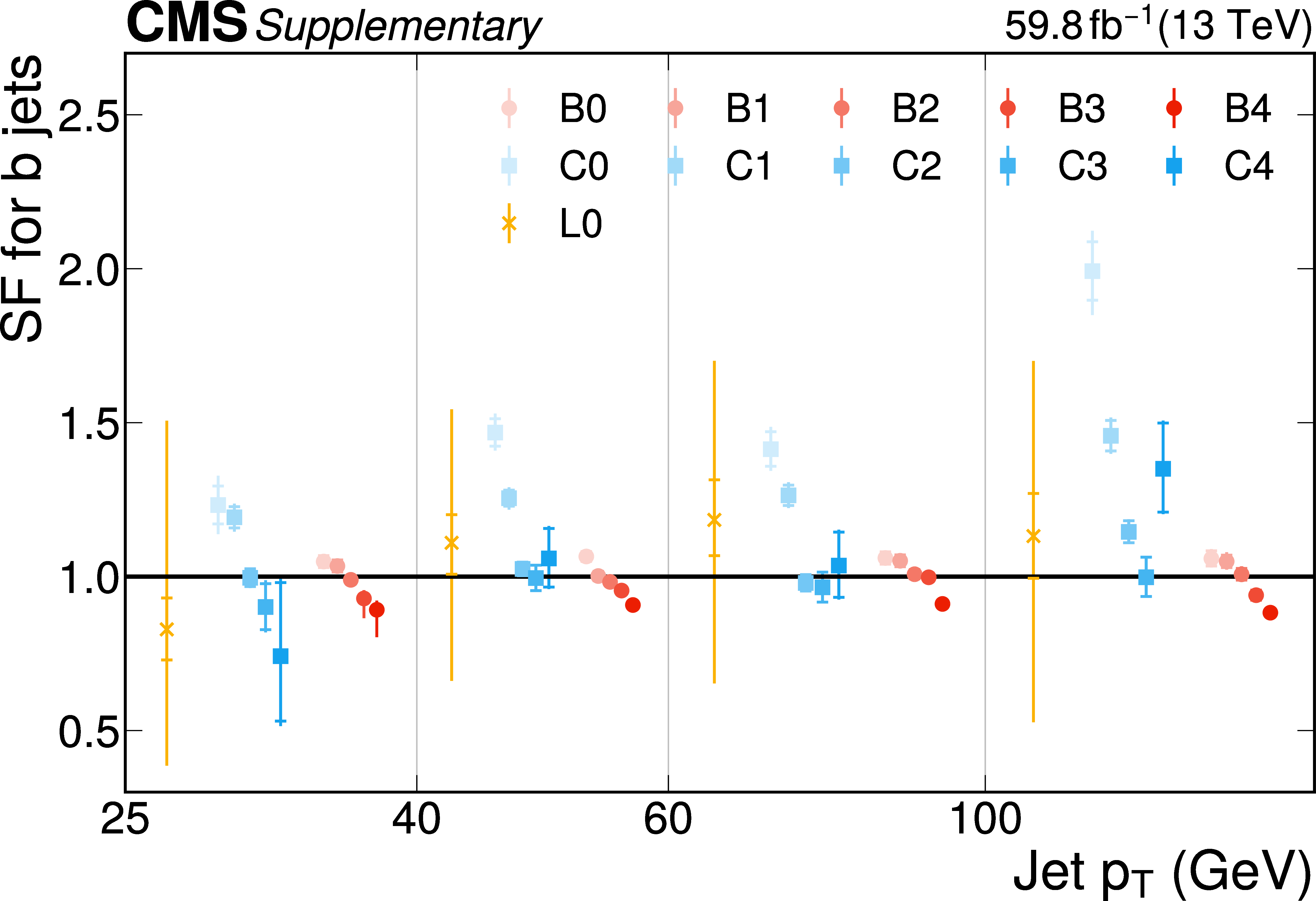
Additional Figure 15:
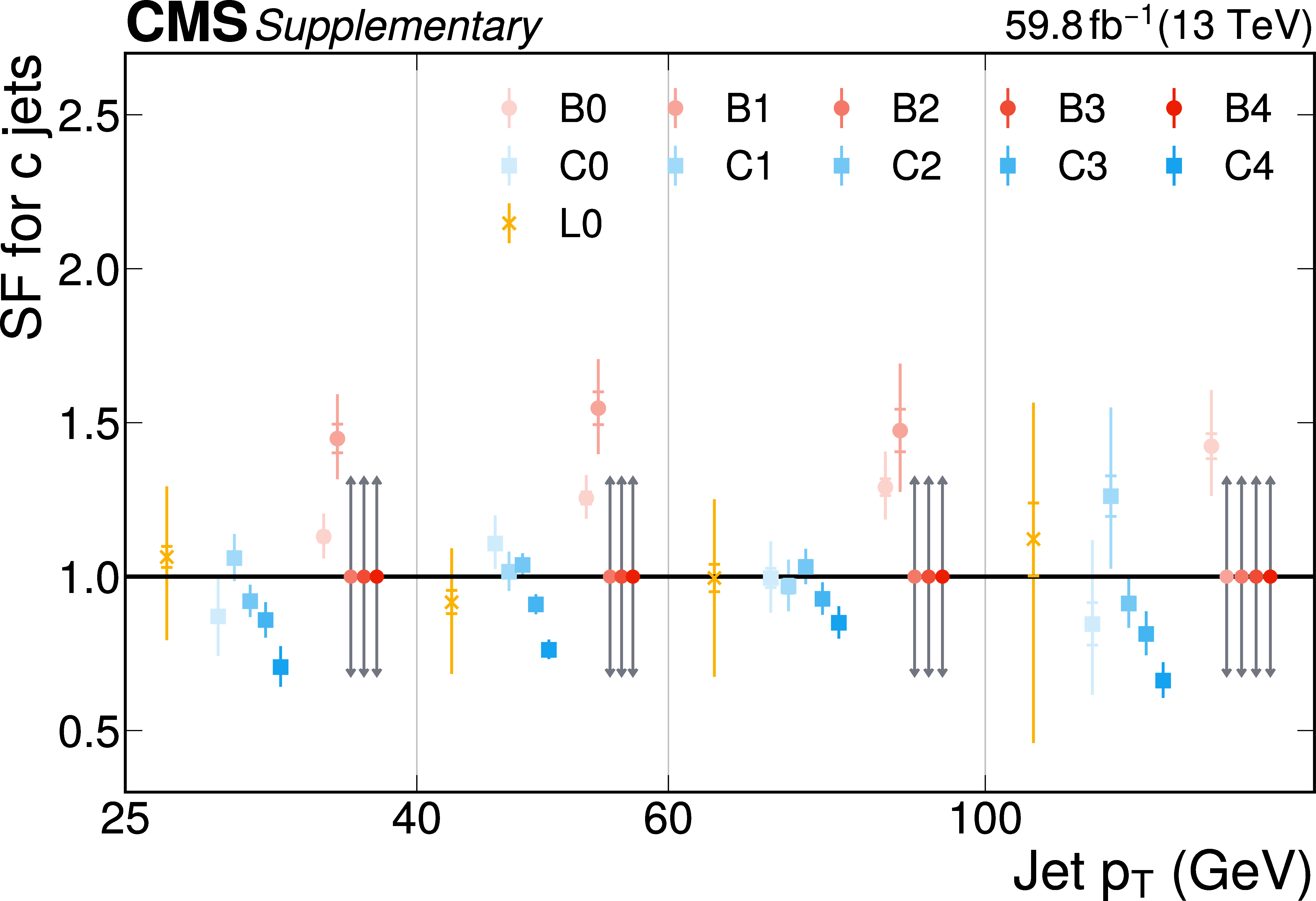
The PARTICLENET jet identification scale factors (SFs) for c jets as a function of the jet $ p_{\mathrm{T}} $ for the first part of the 2016 data-taking period. The individual colored points represent the SFs for each of the 11 tagging categories. The gray arrows indicate SFs of unity with an uncertainty covering the range $ [0.3, 3] $ as described in the text. |
png pdf |
Additional Figure 15-a:
The PARTICLENET jet identification scale factors (SFs) for c jets as a function of the jet $ p_{\mathrm{T}} $ for the first part of the 2016 data-taking period. The individual colored points represent the SFs for each of the 11 tagging categories. The gray arrows indicate SFs of unity with an uncertainty covering the range $ [0.3, 3] $ as described in the text. |
png pdf |
Additional Figure 15-b:
The PARTICLENET jet identification scale factors (SFs) for c jets as a function of the jet $ p_{\mathrm{T}} $ for the first part of the 2016 data-taking period. The individual colored points represent the SFs for each of the 11 tagging categories. The gray arrows indicate SFs of unity with an uncertainty covering the range $ [0.3, 3] $ as described in the text. |

png pdf |
Additional Figure 15-c:
The PARTICLENET jet identification scale factors (SFs) for c jets as a function of the jet $ p_{\mathrm{T}} $ for the first part of the 2016 data-taking period. The individual colored points represent the SFs for each of the 11 tagging categories. The gray arrows indicate SFs of unity with an uncertainty covering the range $ [0.3, 3] $ as described in the text. |

png pdf |
Additional Figure 15-d:
The PARTICLENET jet identification scale factors (SFs) for c jets as a function of the jet $ p_{\mathrm{T}} $ for the first part of the 2016 data-taking period. The individual colored points represent the SFs for each of the 11 tagging categories. The gray arrows indicate SFs of unity with an uncertainty covering the range $ [0.3, 3] $ as described in the text. |
png pdf |
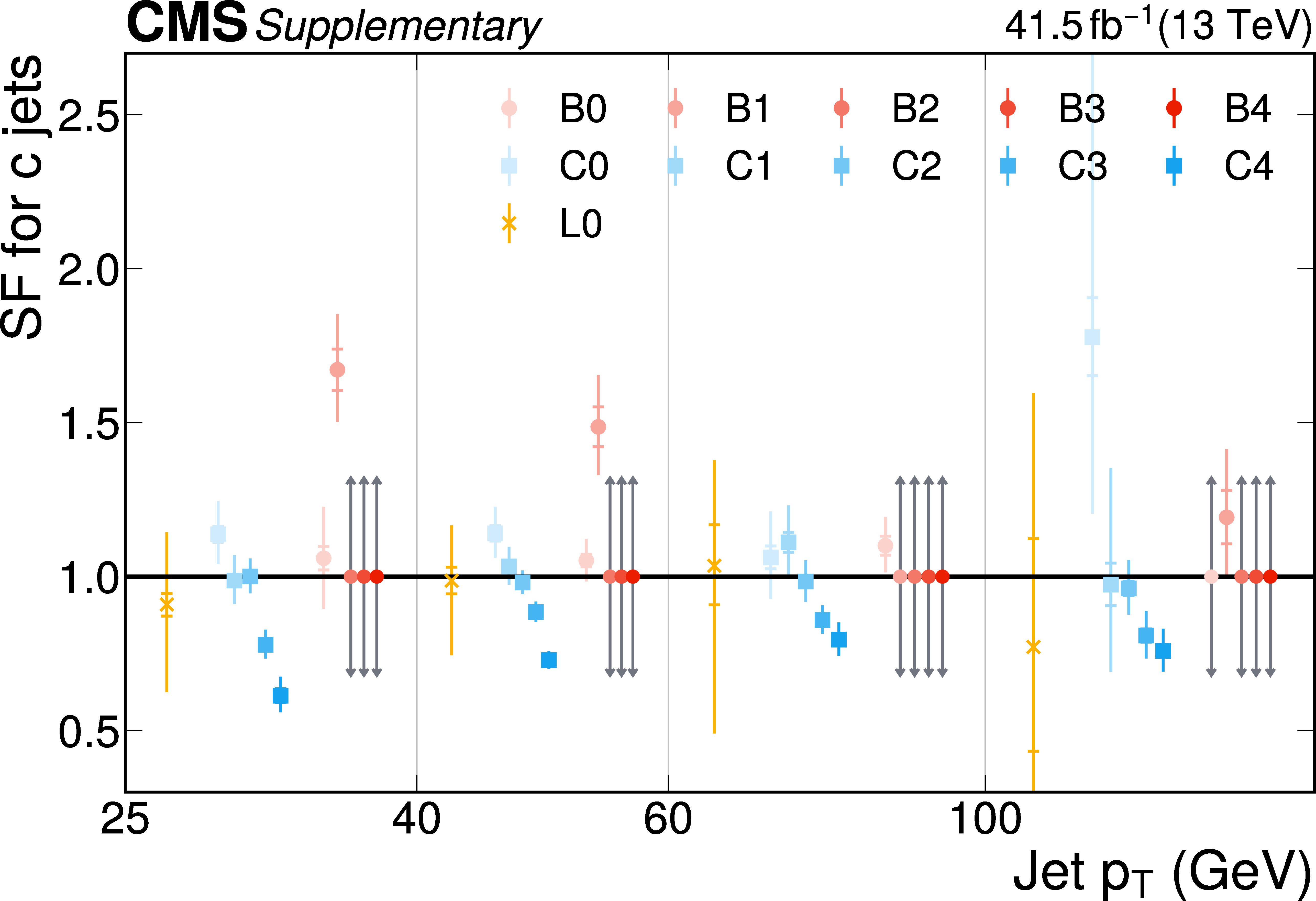
Additional Figure 16:
The PARTICLENET jet identification scale factors (SFs) for c jets as a function of the jet $ p_{\mathrm{T}} $ for the first part of the 2016 data-taking period. The individual colored points represent the SFs for each of the 11 tagging categories. The gray arrows indicate SFs of unity with an uncertainty covering the range $ [0.3, 3] $ as described in the text. |

png pdf |
Additional Figure 16-a:
The PARTICLENET jet identification scale factors (SFs) for c jets as a function of the jet $ p_{\mathrm{T}} $ for the first part of the 2016 data-taking period. The individual colored points represent the SFs for each of the 11 tagging categories. The gray arrows indicate SFs of unity with an uncertainty covering the range $ [0.3, 3] $ as described in the text. |

png pdf |
Additional Figure 16-b:
The PARTICLENET jet identification scale factors (SFs) for c jets as a function of the jet $ p_{\mathrm{T}} $ for the first part of the 2016 data-taking period. The individual colored points represent the SFs for each of the 11 tagging categories. The gray arrows indicate SFs of unity with an uncertainty covering the range $ [0.3, 3] $ as described in the text. |
png pdf |
Additional Figure 17:
The PARTICLENET jet identification scale factors (SFs) for c jets as a function of the jet $ p_{\mathrm{T}} $ for the first part of the 2016 data-taking period. The individual colored points represent the SFs for each of the 11 tagging categories. The gray arrows indicate SFs of unity with an uncertainty covering the range $ [0.3, 3] $ as described in the text. |
png pdf |
Additional Figure 18:
The PARTICLENET jet identification scale factors (SFs) for c jets as a function of the jet $ p_{\mathrm{T}} $ for the first part of the 2016 data-taking period. The individual colored points represent the SFs for each of the 11 tagging categories. The gray arrows indicate SFs of unity with an uncertainty covering the range $ [0.3, 3] $ as described in the text. |
png pdf |
Additional Figure 19:
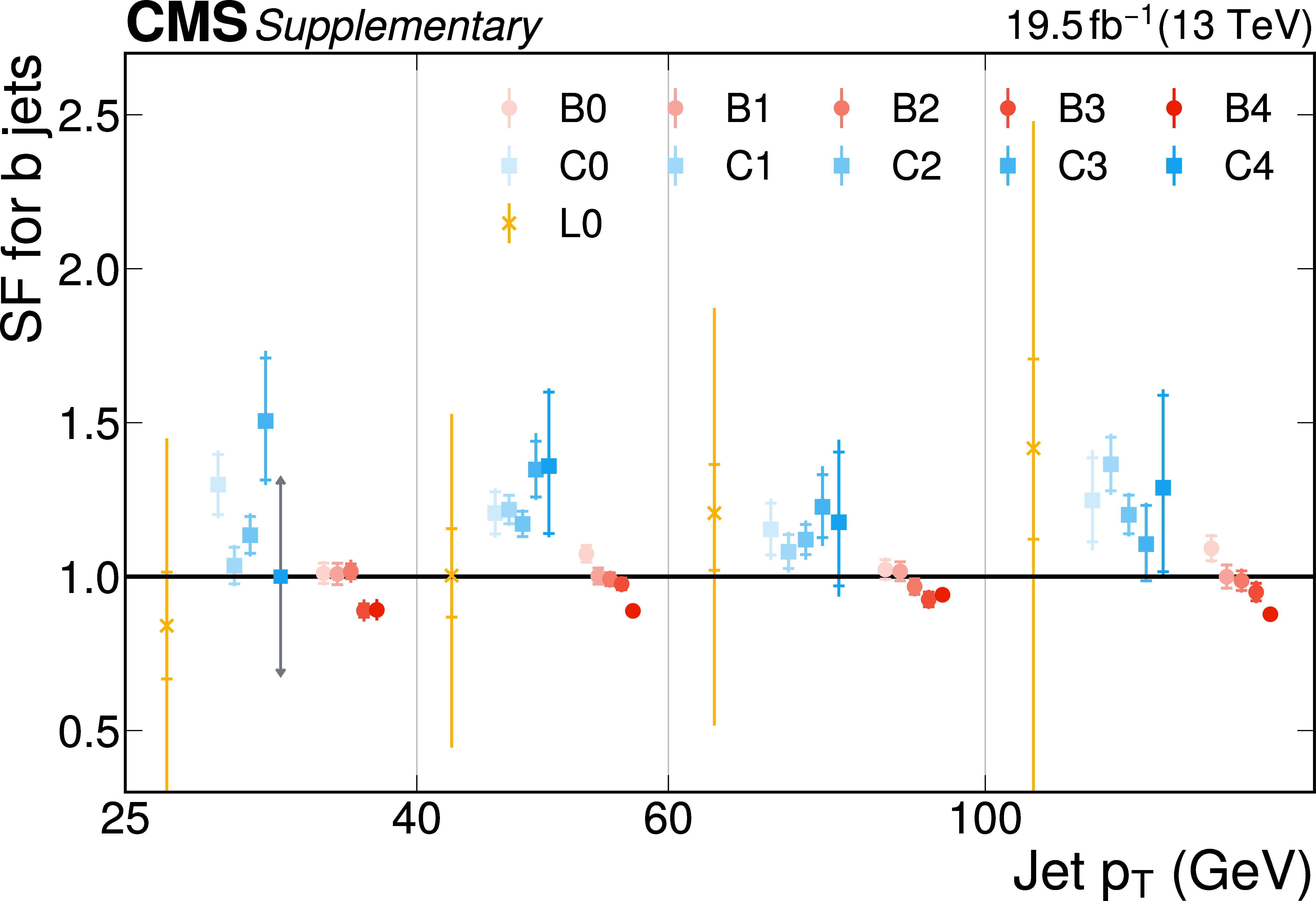
The PARTICLENET jet identification scale factors (SFs) for b jets as a function of the jet $ p_{\mathrm{T}} $ for the first part of the 2016 data-taking period. The individual colored points represent the SFs for each of the 11 tagging categories. The gray arrows indicate SFs of unity with an uncertainty covering the range $ [0.3, 3] $ as described in the text. |
png pdf |
Additional Figure 20:
The PARTICLENET jet identification scale factors (SFs) for b jets as a function of the jet $ p_{\mathrm{T}} $ for the first part of the 2016 data-taking period. The individual colored points represent the SFs for each of the 11 tagging categories. The gray arrows indicate SFs of unity with an uncertainty covering the range $ [0.3, 3] $ as described in the text. |

png pdf |
Additional Figure 21:
The PARTICLENET jet identification scale factors (SFs) for b jets as a function of the jet $ p_{\mathrm{T}} $ for the first part of the 2016 data-taking period. The individual colored points represent the SFs for each of the 11 tagging categories. The gray arrows indicate SFs of unity with an uncertainty covering the range $ [0.3, 3] $ as described in the text. |
png pdf |
Additional Figure 22:
The PARTICLENET jet identification scale factors (SFs) for b jets as a function of the jet $ p_{\mathrm{T}} $ for the first part of the 2016 data-taking period. The individual colored points represent the SFs for each of the 11 tagging categories. The gray arrows indicate SFs of unity with an uncertainty covering the range $ [0.3, 3] $ as described in the text. |
png pdf |
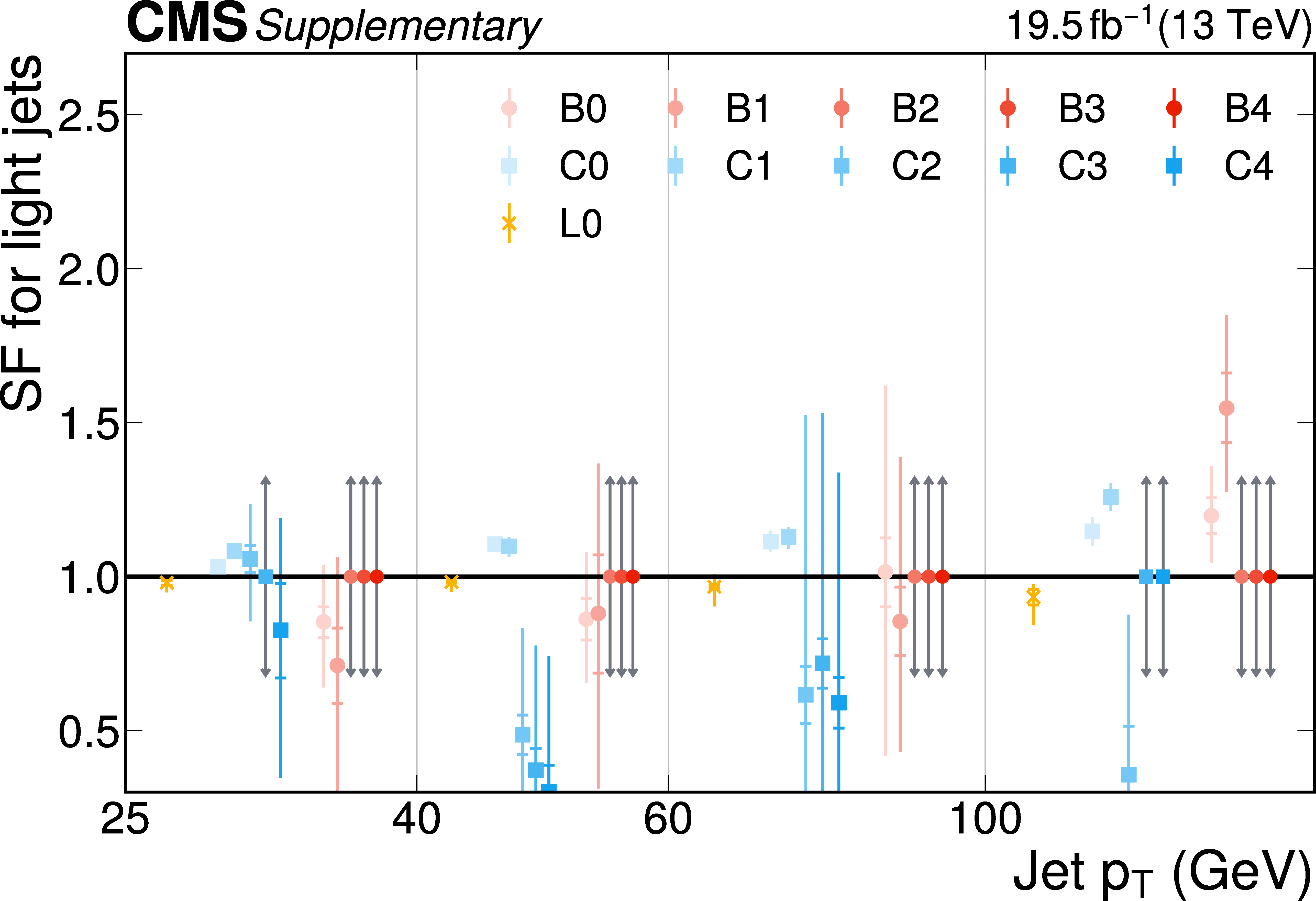
Additional Figure 23:
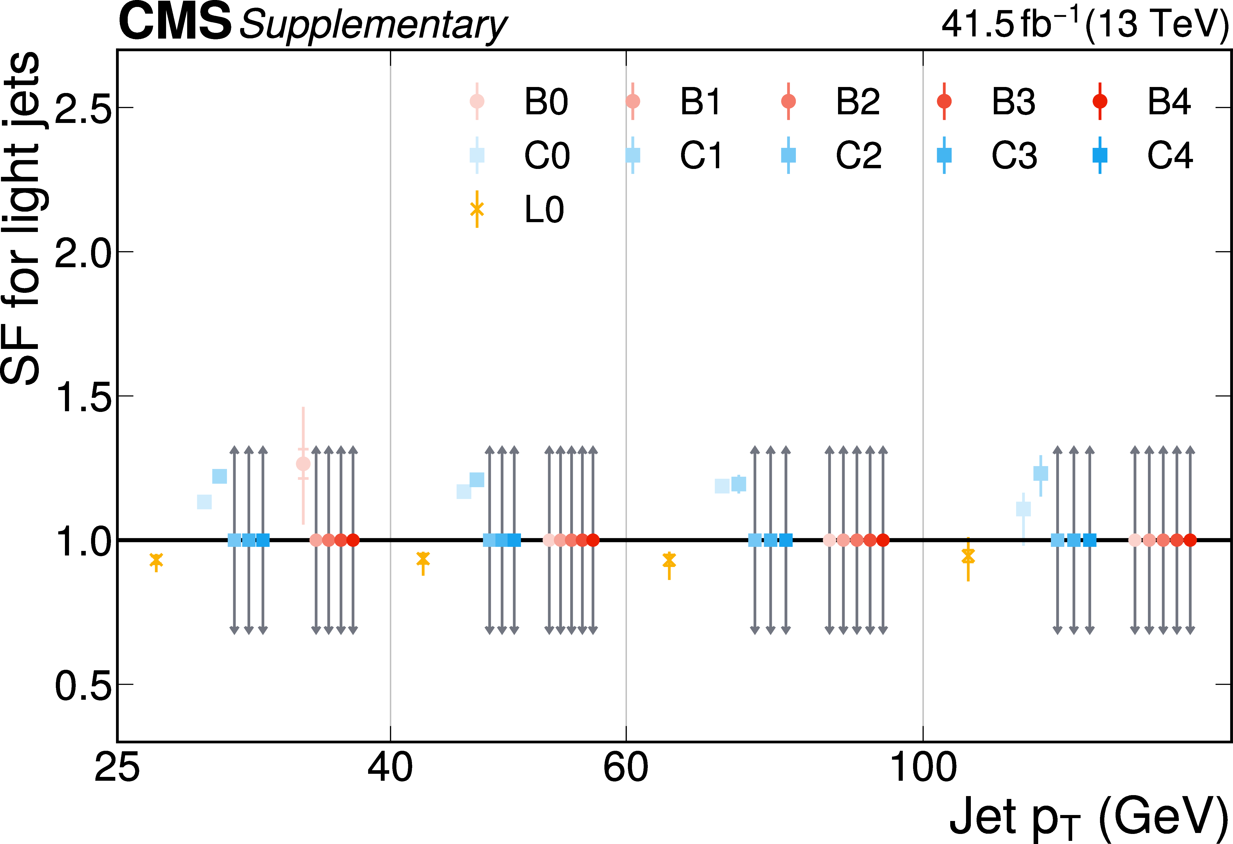
The PARTICLENET jet identification scale factors (SFs) for light jets as a function of the jet $ p_{\mathrm{T}} $ for the first part of the 2016 data-taking period. The individual colored points represent the SFs for each of the 11 tagging categories. The gray arrows indicate SFs of unity with an uncertainty covering the range $ [0.3, 3] $ as described in the text. |
png pdf |
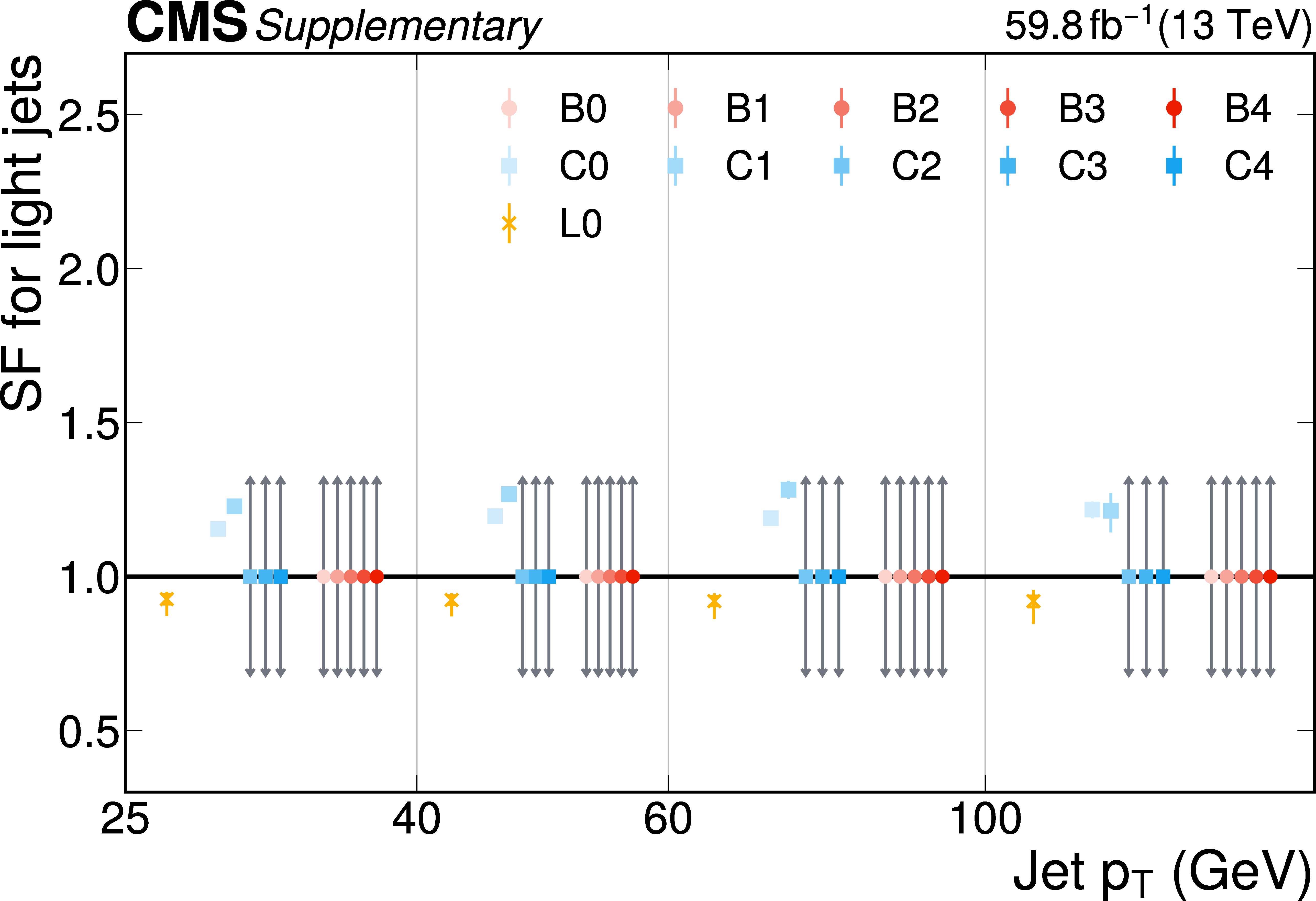
Additional Figure 24:
The PARTICLENET jet identification scale factors (SFs) for light jets as a function of the jet $ p_{\mathrm{T}} $ for the first part of the 2016 data-taking period. The individual colored points represent the SFs for each of the 11 tagging categories. The gray arrows indicate SFs of unity with an uncertainty covering the range $ [0.3, 3] $ as described in the text. |

png pdf |
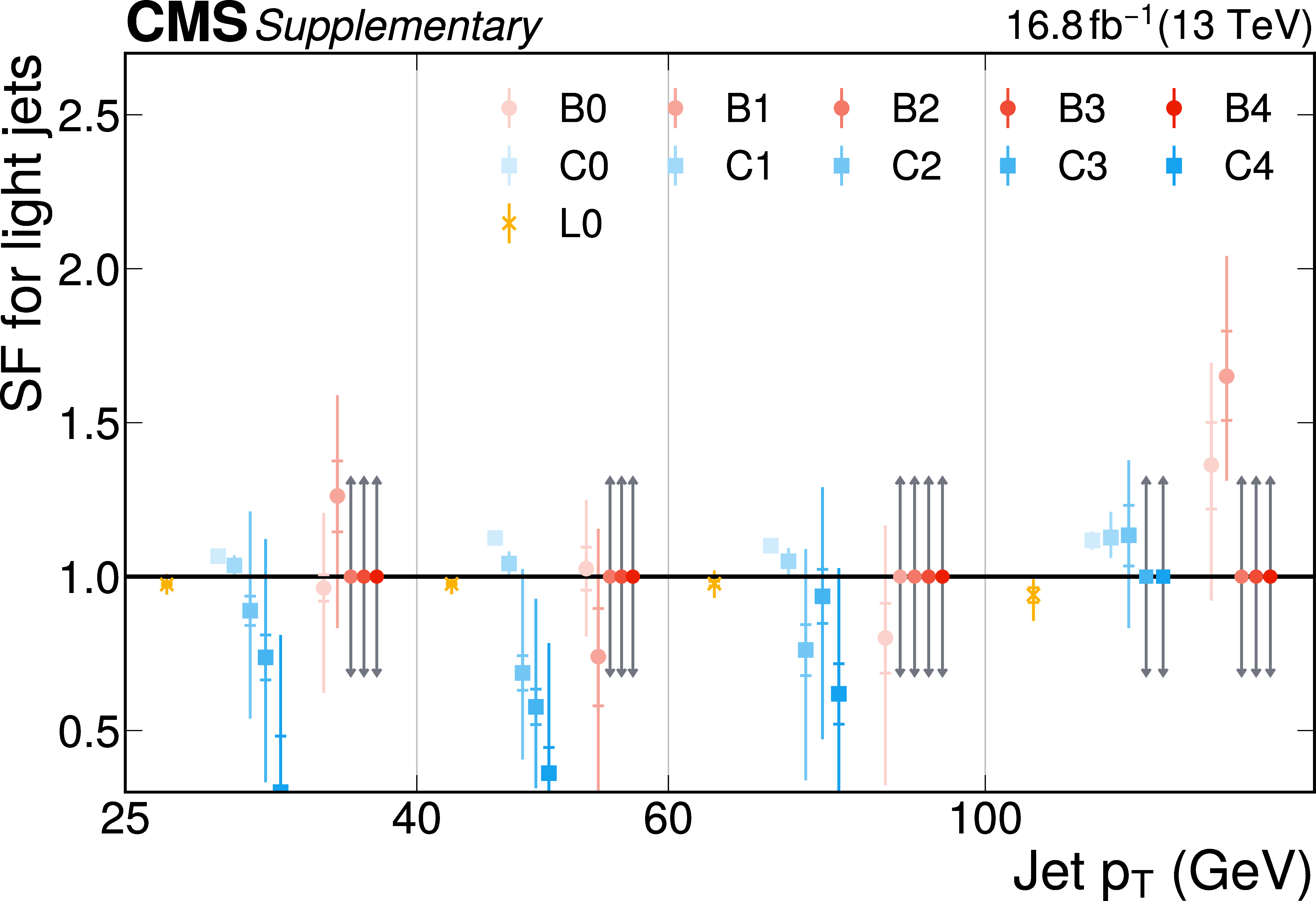
Additional Figure 25:
The PARTICLENET jet identification scale factors (SFs) for light jets as a function of the jet $ p_{\mathrm{T}} $ for the first part of the 2016 data-taking period. The individual colored points represent the SFs for each of the 11 tagging categories. The gray arrows indicate SFs of unity with an uncertainty covering the range $ [0.3, 3] $ as described in the text. |

png pdf |
Additional Figure 26:
The PARTICLENET jet identification scale factors (SFs) for light jets as a function of the jet $ p_{\mathrm{T}} $ for the first part of the 2016 data-taking period. The individual colored points represent the SFs for each of the 11 tagging categories. The gray arrows indicate SFs of unity with an uncertainty covering the range $ [0.3, 3] $ as described in the text. |
| References | ||||
| 1 | ATLAS Collaboration | Observation of a new particle in the search for the standard model Higgs boson with the ATLAS detector at the LHC | PLB 716 (2012) 1 | 1207.7214 |
| 2 | CMS Collaboration | Observation of a new boson at a mass of 125 GeV with the CMS experiment at the LHC | PLB 716 (2012) 30 | CMS-HIG-12-028 1207.7235 |
| 3 | CMS Collaboration | Observation of a new boson with mass near 125 GeV in $ {\mathrm{p}\mathrm{p}} $ collisions at $ \sqrt{s}= $ 7 and 8 TeV | JHEP 06 (2013) 081 | CMS-HIG-12-036 1303.4571 |
| 4 | CMS Collaboration | A measurement of the Higgs boson mass in the diphoton decay channel | PLB 805 (2020) 135425 | CMS-HIG-19-004 2002.06398 |
| 5 | ATLAS Collaboration | Measurement of Higgs boson production in the diphoton decay channel in $ {\mathrm{p}\mathrm{p}} $ collisions at center-of-mass energies of 7 and 8 TeV with the ATLAS detector | PRD 90 (2014) 112015 | 1408.7084 |
| 6 | CMS Collaboration | Observation of the diphoton decay of the Higgs boson and measurement of its properties | EPJC 74 (2014) 3076 | CMS-HIG-13-001 1407.0558 |
| 7 | ATLAS Collaboration | Measurements of Higgs boson production and couplings in the four-lepton channel in $ {\mathrm{p}\mathrm{p}} $ collisions at center-of-mass energies of 7 and 8 TeV with the ATLAS detector | PRD 91 (2015) 012006 | 1408.5191 |
| 8 | CMS Collaboration | Measurement of the properties of a Higgs boson in the four-lepton final state | PRD 89 (2014) 092007 | CMS-HIG-13-002 1312.5353 |
| 9 | ATLAS Collaboration | Observation and measurement of Higgs boson decays to $ {\mathrm{W}\mathrm{W}^\ast} $ with the ATLAS detector | PRD 92 (2015) 012006 | 1412.2641 |
| 10 | ATLAS Collaboration | Study of $ {(\mathrm{W}\!/\mathrm{Z})\mathrm{H}} $ production and Higgs boson couplings using $ {\mathrm{H}\to\mathrm{W}\mathrm{W}^\ast} $ decays with the ATLAS detector | JHEP 08 (2015) 137 | 1506.06641 |
| 11 | CMS Collaboration | Measurement of Higgs boson production and properties in the $ {\mathrm{W}\mathrm{W}} $ decay channel with leptonic final states | JHEP 01 (2014) 096 | CMS-HIG-13-023 1312.1129 |
| 12 | ATLAS Collaboration | Evidence for the Higgs-boson Yukawa coupling to tau leptons with the ATLAS detector | JHEP 04 (2015) 117 | 1501.04943 |
| 13 | CMS Collaboration | Evidence for the 125 GeV Higgs boson decaying to a pair of $ \tau $ leptons | JHEP 05 (2014) 104 | CMS-HIG-13-004 1401.5041 |
| 14 | CMS Collaboration | Observation of the Higgs boson decay to a pair of $ \tau $ leptons | PLB 779 (2018) 283 | CMS-HIG-16-043 1708.00373 |
| 15 | CMS Collaboration | Measurements of properties of the Higgs boson decaying to a W boson pair in $ {\mathrm{p}\mathrm{p}} $ collisions at $ \sqrt{s} = $ 13 TeV | PLB 791 (2019) 96 | CMS-HIG-16-042 1806.05246 |
| 16 | ATLAS Collaboration | Measurements of the Higgs boson production and decay rates and coupling strengths using $ {\mathrm{p}\mathrm{p}} $ collision data at $ \sqrt{s}= $ 7 and 8 TeV in the ATLAS experiment | EPJC 76 (2016) 6 | 1507.04548 |
| 17 | CMS Collaboration | Precise determination of the mass of the Higgs boson and tests of compatibility of its couplings with the standard model predictions using proton collisions at 7 and 8 TeV | EPJC 75 (2015) 212 | CMS-HIG-14-009 1412.8662 |
| 18 | CMS Collaboration | Study of the mass and spin-parity of the Higgs boson candidate via its decays to Z boson pairs | PRL 110 (2013) 081803 | CMS-HIG-12-041 1212.6639 |
| 19 | ATLAS Collaboration | Evidence for the spin-0 nature of the Higgs boson using ATLAS data | PLB 726 (2013) 120 | 1307.1432 |
| 20 | ATLAS and CMS Collaborations | Measurements of the Higgs boson production and decay rates and constraints on its couplings from a combined ATLAS and CMS analysis of the LHC $ {\mathrm{p}\mathrm{p}} $ collision data at $ \sqrt{s}= $ 7 and 8 TeV | JHEP 08 (2016) 045 | 1606.02266 |
| 21 | ATLAS and CMS Collaborations | Combined measurement of the Higgs boson mass in $ {\mathrm{p}\mathrm{p}} $ collisions at $ \sqrt{s}= $ 7 and 8 TeV with the ATLAS and CMS experiments | PRL 114 (2015) 191803 | 1503.07589 |
| 22 | CMS Collaboration | Measurements of properties of the Higgs boson decaying into the four-lepton final state in $ {\mathrm{p}\mathrm{p}} $ collisions at $ \sqrt{s} = $ 13 TeV | JHEP 11 (2017) 047 | CMS-HIG-16-041 1706.09936 |
| 23 | ATLAS Collaboration | Combined measurement of differential and total cross sections in the $ {\mathrm{H}\to\gamma\gamma} $ and the $ {\mathrm{H}\to\mathrm{Z}\mathrm{Z}^\ast\to4\ell} $ decay channels at $ \sqrt{s} = $ 13 TeV with the ATLAS detector | PLB 786 (2018) 114 | 1805.10197 |
| 24 | ATLAS Collaboration | Measurement of the Higgs boson mass in the $ {\mathrm{H}\to\mathrm{Z}\mathrm{Z}^\ast\to4\ell} $ and $ {\mathrm{H}\to\gamma\gamma} $ channels with $ \sqrt{s} = $ 13 TeV $ {\mathrm{p}\mathrm{p}} $ collisions using the ATLAS detector | PLB 784 (2018) 345 | 1806.00242 |
| 25 | CMS Collaboration | Search for the Higgs boson decaying to two muons in proton-proton collisions at $ \sqrt{s} = $ 13 TeV | PRL 122 (2019) 021801 | CMS-HIG-17-019 1807.06325 |
| 26 | ATLAS Collaboration | Measurements of $ {\mathrm{W}\mathrm{H}} $ and $ {\mathrm{Z}\mathrm{H}} $ production with Higgs boson decays into bottom quarks and direct constraints on the charm Yukawa coupling in 13 TeV $ {\mathrm{p}\mathrm{p}} $ collisions with the ATLAS detector | JHEP 04 (2025) 075 | 2410.19611 |
| 27 | CMS Collaboration | Search for Higgs boson decay to a charm quark-antiquark pair in proton-proton collisions at $ \sqrt{s} = $ 13 TeV | PRL 131 (2023) 061801 | CMS-HIG-21-008 2205.05550 |
| 28 | CMS Collaboration | Search for boosted Higgs boson decay to a charm quark-antiquark pair in proton-proton collisions at $ \sqrt{s} = $ 13 TeV | PRL 131 (2023) 041801 | CMS-HIG-21-012 2211.14181 |
| 29 | ATLAS and CMS Collaborations | Snowmass white paper contribution: Physics with the Phase-2 ATLAS and CMS detectors | CMS Physics Analysis Summary, ATL-PHYS-PUB-2022-018, 2022 CMS-PAS-FTR-22-001 |
|
| 30 | CMS Collaboration | Precision luminosity measurement in proton-proton collisions at $ \sqrt{s} = $ 13 TeV in 2015 and 2016 at CMS | EPJC 81 (2021) 800 | CMS-LUM-17-003 2104.01927 |
| 31 | CMS Collaboration | CMS luminosity measurement for the 2017 data-taking period at $ \sqrt{s} = $ 13 TeV | CMS Physics Analysis Summary, 2018 CMS-PAS-LUM-17-004 |
CMS-PAS-LUM-17-004 |
| 32 | CMS Collaboration | CMS luminosity measurement for the 2018 data-taking period at $ \sqrt{s} = $ 13 TeV | CMS Physics Analysis Summary, 2019 CMS-PAS-LUM-18-002 |
CMS-PAS-LUM-18-002 |
| 33 | H. Qu and L. Gouskos | Jet tagging via particle clouds | PRD 101 (2020) 056019 | 1902.08570 |
| 34 | H. Qu, C. Li, and S. Qian | Particle transformer for jet tagging | in Proc. 39th International Conference on Machine Learning (ICML ): Baltimore MD, USA, 2022 PMLR 162 (2022) 18281 |
2202.03772 |
| 35 | CMS Collaboration | The CMS experiment at the CERN LHC | JINST 3 (2008) S08004 | |
| 36 | CMS Collaboration | Development of the CMS detector for the CERN LHC Run 3 | JINST 19 (2024) P05064 | CMS-PRF-21-001 2309.05466 |
| 37 | CMS Collaboration | Performance of the CMS Level-1 trigger in proton-proton collisions at $ \sqrt{s} = $ 13 TeV | JINST 15 (2020) P10017 | CMS-TRG-17-001 2006.10165 |
| 38 | CMS Collaboration | The CMS trigger system | JINST 12 (2017) P01020 | CMS-TRG-12-001 1609.02366 |
| 39 | CMS Collaboration | Performance of the CMS high-level trigger during LHC Run 2 | JINST 19 (2024) P11021 | CMS-TRG-19-001 2410.17038 |
| 40 | CMS Collaboration | Electron and photon reconstruction and identification with the CMS experiment at the CERN LHC | JINST 16 (2021) P05014 | CMS-EGM-17-001 2012.06888 |
| 41 | CMS Collaboration | Performance of the CMS muon detector and muon reconstruction with proton-proton collisions at $ \sqrt{s} = $ 13 TeV | JINST 13 (2018) P06015 | CMS-MUO-16-001 1804.04528 |
| 42 | CMS Collaboration | Description and performance of track and primary-vertex reconstruction with the CMS tracker | JINST 9 (2014) P10009 | CMS-TRK-11-001 1405.6569 |
| 43 | CMS Collaboration | Particle-flow reconstruction and global event description with the CMS detector | JINST 12 (2017) P10003 | CMS-PRF-14-001 1706.04965 |
| 44 | M. Cacciari, G. P. Salam, and G. Soyez | The anti-$ k_{\mathrm{T}} $ jet clustering algorithm | JHEP 04 (2008) 063 | 0802.1189 |
| 45 | M. Cacciari, G. P. Salam, and G. Soyez | FASTJET user manual | EPJC 72 (2012) 1896 | 1111.6097 |
| 46 | CMS Collaboration | Jet energy scale and resolution in the CMS experiment in $ {\mathrm{p}\mathrm{p}} $ collisions at 8 TeV | JINST 12 (2017) P02014 | CMS-JME-13-004 1607.03663 |
| 47 | CMS Collaboration | Performance of missing transverse momentum reconstruction in proton-proton collisions at $ \sqrt{s} = $ 13 TeV using the CMS detector | JINST 14 (2019) P07004 | CMS-JME-17-001 1903.06078 |
| 48 | P. Nason | A new method for combining NLO QCD with shower Monte Carlo algorithms | JHEP 11 (2004) 040 | hep-ph/0409146 |
| 49 | S. Frixione, P. Nason, and C. Oleari | Matching NLO QCD computations with parton shower simulations: the POWHEG method | JHEP 11 (2007) 070 | 0709.2092 |
| 50 | S. Alioli, P. Nason, C. Oleari, and E. Re | A general framework for implementing NLO calculations in shower Monte Carlo programs: the POWHEG box | JHEP 06 (2010) 043 | 1002.2581 |
| 51 | CMS Collaboration | Identification of heavy-flavour jets with the CMS detector in $ {\mathrm{p}\mathrm{p}} $ collisions at 13 TeV | JINST 13 (2018) P05011 | CMS-BTV-16-002 1712.07158 |
| 52 | T. Ježo and P. Nason | On the treatment of resonances in next-to-leading order calculations matched to a parton shower | JHEP 12 (2015) 065 | 1509.09071 |
| 53 | T. Ježo, J. M. Lindert, N. Moretti, and S. Pozzorini | New NLOPS predictions for $ \mathrm{t} \overline{\mathrm{t}} $ +b-jet production at the LHC | EPJC 78 (2018) 502 | 1802.00426 |
| 54 | F. Buccioni et al. | OpenLoops 2 | EPJC 79 (2019) 866 | 1907.13071 |
| 55 | S. Frixione, G. Ridolfi, and P. Nason | A positive-weight next-to-leading-order Monte Carlo for heavy flavour hadroproduction | JHEP 09 (2007) 126 | 0707.3088 |
| 56 | CMS Collaboration | Inclusive and differential cross section measurements of $ {\mathrm{t}\overline{\mathrm{t}}} \mathrm{b}\overline{\mathrm{b}} $ production in the lepton+jets channel at $ \sqrt{s} = $ 13 TeV | JHEP 05 (2024) 042 | CMS-TOP-22-009 2309.14442 |
| 57 | ATLAS Collaboration | Measurement of $ \mathrm{t} \overline{\mathrm{t}} $ production in association with additional b-jets in the $ {\mathrm{e}\mu} $ final state in proton-proton collisions at $ \sqrt{s} = $ 13 TeV with the ATLAS detector | JHEP 01 (2025) 068 | 2407.13473 |
| 58 | CMS Collaboration | First measurement of the cross section for top quark pair production with additional charm jets using dileptonic final states in $ {\mathrm{p}\mathrm{p}} $ collisions at $ \sqrt{s} = $ 13 TeV | PLB 820 (2021) 136565 | CMS-TOP-20-003 2012.09225 |
| 59 | ATLAS Collaboration | Measurement of top-quark pair production in association with charm quarks in proton-proton collisions at $ \sqrt{s} = $ 13 TeV with the ATLAS detector | PLB 860 (2024) 139177 | 2409.11305 |
| 60 | E. Re | Single-top $ {\mathrm{W}\mathrm{t}} $-channel production matched with parton showers using the POWHEG method | EPJC 71 (2011) 1547 | 1009.2450 |
| 61 | R. Frederix, E. Re, and P. Torrielli | Single-top $ t $-channel hadroproduction in the four-flavors scheme with POWHEG and aMC@NLO | JHEP 09 (2012) 130 | 1207.5391 |
| 62 | S. Alioli, P. Nason, C. Oleari, and E. Re | NLO single-top production matched with shower in POWHEG: $ s $- and $ t $-channel contributions | JHEP 09 (2009) 111 | 0907.4076 |
| 63 | J. Alwall et al. | The automated computation of tree-level and next-to-leading order differential cross sections, and their matching to parton shower simulations | JHEP 07 (2014) 079 | 1405.0301 |
| 64 | M. Czakon and A. Mitov | top++: a program for the calculation of the top-pair cross-section at hadron colliders | Comput. Phys. Commun. 185 (2014) 2930 | 1112.5675 |
| 65 | N. Kidonakis | Top quark production | in Proc. Helmholtz International Summer School on Physics of Heavy Quarks and Hadrons (HQ 2013): Dubna, Russia, 2013 [DESY-PROC-2013-03] link |
1311.0283 |
| 66 | M. Czakon et al. | Top-pair production at the LHC through NNLO QCD and NLO EW | JHEP 10 (2017) 186 | 1705.04105 |
| 67 | R. Frederix and S. Frixione | Merging meets matching in MC@NLO | JHEP 12 (2012) 061 | 1209.6215 |
| 68 | J. Alwall et al. | Comparative study of various algorithms for the merging of parton showers and matrix elements in hadronic collisions | EPJC 53 (2008) 473 | 0706.2569 |
| 69 | NNPDF Collaboration | Parton distributions for the LHC run II | JHEP 04 (2015) 040 | 1410.8849 |
| 70 | T. Sjostrand et al. | An introduction to PYTHIA8.2 | Comput. Phys. Commun. 191 (2015) 159 | 1410.3012 |
| 71 | CMS Collaboration | Extraction and validation of a new set of CMS PYTHIA8 tunes from underlying-event measurements | EPJC 80 (2020) 4 | CMS-GEN-17-001 1903.12179 |
| 72 | GEANT4 Collaboration | GEANT 4---a simulation toolkit | NIM A 506 (2003) 250 | |
| 73 | CMS Collaboration | Supplemental Material: More details on simulated samples, jet flavor identification, baseline event selection, neural network event classifier, systematic uncertainties, validation of the background model, and additional results | URL will be inserted by publisher | |
| 74 | Y. Wang et al. | Dynamic graph CNN for learning on point clouds | ACM Trans. Graph. 38 (2018) 146 | 1801.07829 |
| 75 | E. Bols et al. | Jet flavour classification using DeepJet | JINST 15 (2020) P12012 | 2008.10519 |
| 76 | CMS Collaboration | The CMS statistical analysis and combination tool: combine | Comput. Softw. Big Sci. 8 (2024) 19 | CMS-CAT-23-001 2404.06614 |
| 77 | W. Verkerke and D. Kirkby | The RooFit toolkit for data modeling | in Proc. 13th International Conference on Computing in High Energy and Nuclear Physics (CHEP 2003): La Jolla CA, United States, 2003 [eConf C0303241 (2003) MOLT007] link |
physics/0306116 |
| 78 | L. Moneta et al. | The RooStats project | in Proc. 13th International Workshop on Advanced Computing and Analysis Techniques in Physics Research (ACAT 2010): Jaipur, India, 2010 [PoS (ACAT2010) 057] link |
1009.1003 |
| 79 | CMS Collaboration | Measurement of top quark pair production in association with a Z boson in proton-proton collisions at $ \sqrt{s} = $ 13 TeV | JHEP 03 (2020) 056 | CMS-TOP-18-009 1907.11270 |
| 80 | CMS Collaboration | Measurements of inclusive and differential cross sections for top quark production in association with a Z boson in proton-proton collisions at $ \sqrt{s} = $ 13 TeV | JHEP 02 (2025) 177 | CMS-TOP-23-004 2410.23475 |
| 81 | ATLAS Collaboration | Inclusive and differential cross-section measurements of $ {{\mathrm{t}\overline{\mathrm{t}}} \mathrm{Z}} $ production in $ {\mathrm{p}\mathrm{p}} $ collisions at $ \sqrt{s} = $ 13 TeV with the ATLAS detector, including EFT and spin-correlation interpretations | JHEP 07 (2024) 163 | 2312.04450 |
| 82 | ATLAS and CMS Collaborations, and LHC Higgs Combination Group | Procedure for the LHC Higgs boson search combination in Summer 2011 | Technical Report CMS-NOTE-2011-005, ATL-PHYS-PUB-2011-11, 2011 | |
| 83 | G. Cowan, K. Cranmer, E. Gross, and O. Vitells | Asymptotic formulae for likelihood-based tests of new physics | EPJC 71 (2011) 1554 | 1007.1727 |
| 84 | CMS Collaboration | Measurement of the $ {{\mathrm{t}\overline{\mathrm{t}}} \mathrm{H}} $ and $ {\mathrm{t}\mathrm{H}} $ production rates in the $ {\mathrm{H}\to\mathrm{b}\overline{\mathrm{b}}} $ decay channel using proton-proton collision data at $ \sqrt{s} = $ 13 TeV | JHEP 02 (2025) 097 | CMS-HIG-19-011 2407.10896 |
| 85 | T. Junk | Confidence level computation for combining searches with small statistics | NIM A 434 (1999) 435 | hep-ex/9902006 |
| 86 | A. L. Read | Presentation of search results: The $ \text{CL}_\text{s} $ technique | JPG 28 (2002) 2693 | |
| 87 | CMS Collaboration | HEPData record for this analysis | link | |
| 88 | LHC Higgs Cross Section Working Group, S. Heinemeyer et al. | Handbook of LHC Higgs cross sections: 3. Higgs properties | CERN Report CERN-2013-004, 2013 link |
1307.1347 |
| 89 | LHC Higgs Cross Section Working Group, D. de Florian et al. | Handbook of LHC Higgs cross sections: 4. Deciphering the nature of the Higgs sector | CERN Report CERN-2017-002-M, 2016 link |
1610.07922 |
| 90 | CMS Collaboration | CMS data availability statement | link | |
| 91 | ATLAS Collaboration | Study of the hard double-parton scattering contribution to inclusive four-lepton production in $ {\mathrm{p}\mathrm{p}} $ collisions at $ \sqrt{s}= $ 8 TeV with the ATLAS detector | PLB 790 (2019) 595 | 1811.11094 |
| 92 | P. Artoisenet, R. Frederix, O. Mattelaer, and R. Rietkerk | Automatic spin-entangled decays of heavy resonances in Monte Carlo simulations | JHEP 03 (2013) 015 | 1212.3460 |
| 93 | CMS Collaboration | Pileup mitigation at CMS in 13 TeV data | JINST 15 (2020) P09018 | CMS-JME-18-001 2003.00503 |
| 94 | A. Kulesza et al. | Associated top quark pair production with a heavy boson: differential cross sections at NLO+NNLL accuracy | EPJC 80 (2020) 428 | 2001.03031 |
| 95 | S. Mrenna and P. Skands | Automated parton-shower variations in PYTHIA8 | PRD 94 (2016) 074005 | 1605.08352 |
| 96 | CMS Collaboration | Reweighting simulated events using machine-learning techniques in the CMS experiment | EPJC 85 (2025) 495 | CMS-MLG-24-001 2411.03023 |
| 97 | CMS Collaboration | Evidence for $ {\mathrm{t}\mathrm{W}\mathrm{Z}} $ production in proton-proton collisions at $ \sqrt{s} = $ 13 TeV in multilepton final states | PLB 855 (2024) 138815 | CMS-TOP-22-008 2312.11668 |
| 98 | L. Buonocore et al. | Precise predictions for the associated production of a W boson with a top-antitop quark pair at the LHC | PRL 131 (2023) 231901 | 2306.16311 |
| 99 | ATLAS Collaboration | Measurement of the associated production of a top-antitop-quark pair and a Higgs boson decaying into a $ \mathrm{b}\overline{\mathrm{b}} $ pair in $ {\mathrm{p}\mathrm{p}} $ collisions at $ \sqrt{s} = $ 13 TeV using the ATLAS detector at the LHC | EPJC 85 (2025) 210 | 2407.10904 |
|
|
Compact Muon Solenoid LHC, CERN |
|

|

|

|

|

|