

Compact Muon Solenoid
LHC, CERN
| CMS-B2G-25-009 ; CERN-EP-2026-049 | ||
| Search for new particles decaying into top quark-antiquark pairs in proton-proton collisions at $ \sqrt{s}= $ 13 TeV | ||
| CMS Collaboration | ||
| 24 March 2026 | ||
| Submitted to the Journal of High Energy Physics | ||
| Abstract: A search for new particles decaying to top quark-antiquark pairs is performed using proton-proton collision data at a centre-of-mass energy of 13 TeV. The data set recorded with the CMS detector between 2016 and 2018 is used, corresponding to an integrated luminosity of 138 fb$ ^{-1} $. Final states with 0, 1, and 2 leptons are analyzed, covering all decay modes of the top quark-antiquark pairs. Heavy $ \mathrm{Z}^{'} $ bosons with relative widths of 1, 10, and 30% are excluded for masses in the ranges 0.4--4.8, 0.4--6.2, and 0.4--7.4 TeV, respectively. A Kaluza--Klein gluon in the Randall--Sundrum model and a dark-matter mediator are excluded for masses between 0.5--5.5 and 1.0--4.2 TeV, respectively. These results set the most stringent limits to date for the considered models in the $ \mathrm{t} \overline{\mathrm{t}} $ final state. In addition, in the two-Higgs-doublet models, upper limits are set on the coupling strength modifier for scalar and pseudoscalar Higgs bosons with relative widths of 2.5, 10, and 25% in the mass range of 0.5--1.0 TeV. | ||
| Links: e-print arXiv:2603.23454 [hep-ex] (PDF) ; CDS record ; inSPIRE record ; HepData record ; CADI line (restricted) ; | ||
| Figures | |
png pdf |
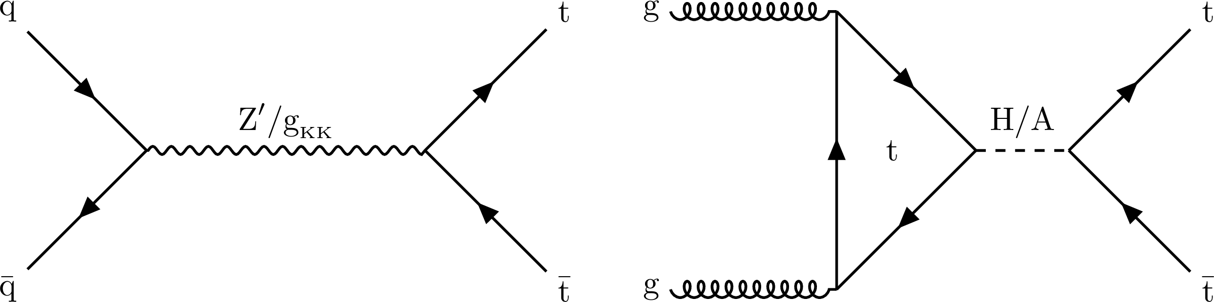
Figure 1:
Example Feynman diagrams at leading order for the production and decay of a spin-1 $ \mathrm{Z}^{'} /g_{KK}$ boson (left) and a scalar H or pseudoscalar $ \mathrm{A} $ resonance (right). |
png pdf |
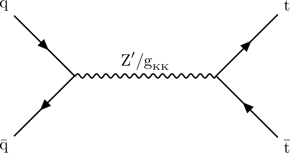
Figure 1-a:
Example Feynman diagrams at leading order for the production and decay of a spin-1 $ \mathrm{Z}^{'} /g_{KK}$ boson (left) and a scalar H or pseudoscalar $ \mathrm{A} $ resonance (right). |
png pdf |
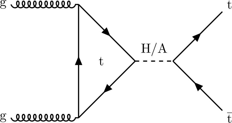
Figure 1-b:
Example Feynman diagrams at leading order for the production and decay of a spin-1 $ \mathrm{Z}^{'} /g_{KK}$ boson (left) and a scalar H or pseudoscalar $ \mathrm{A} $ resonance (right). |
png pdf |
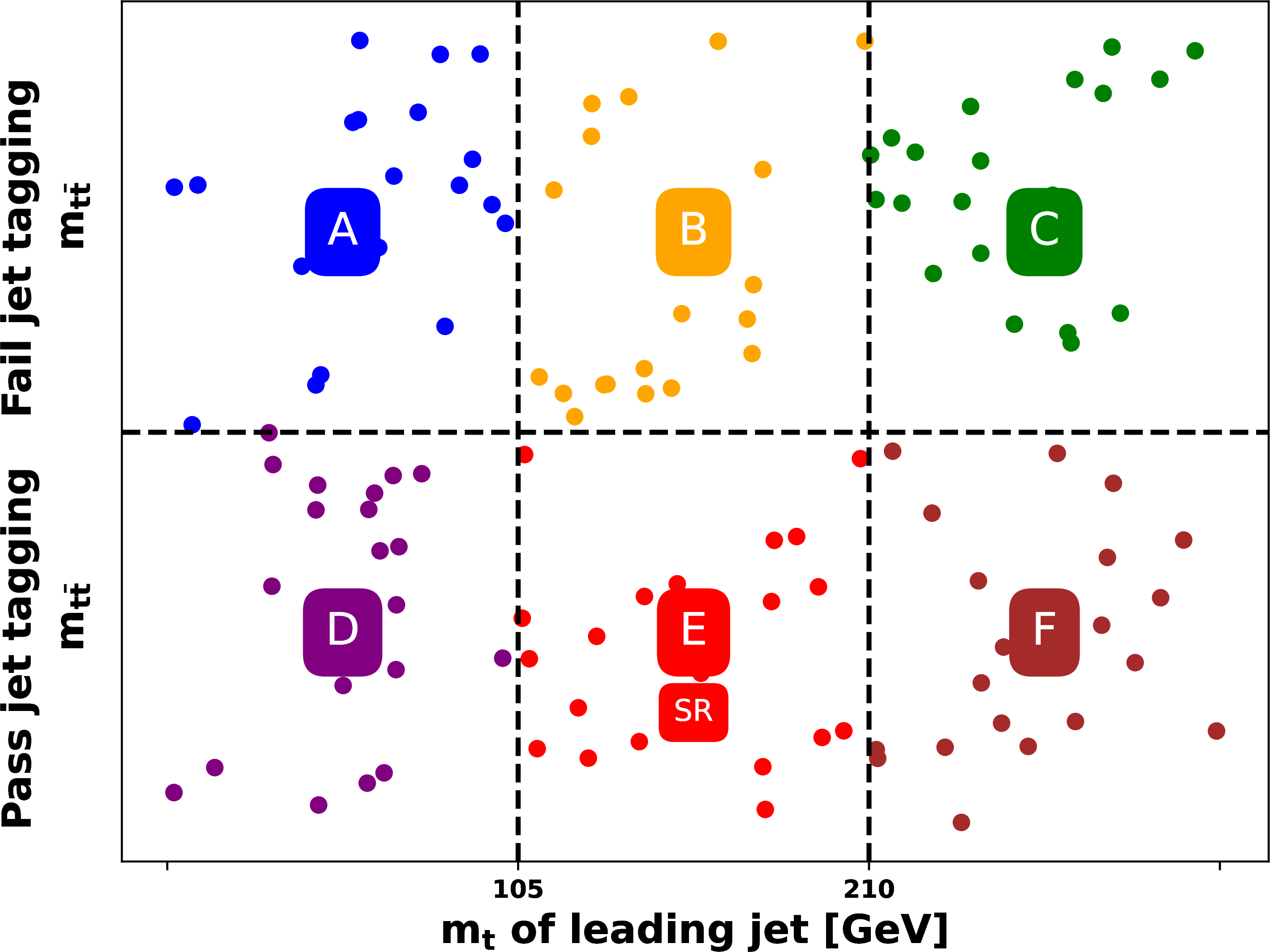
Figure 2:
Illustration of the background estimation method. The data set is binned in the leading jet mass $ m_{\mathrm{t}} $ and in the reconstructed $ \mathrm{t} \overline{\mathrm{t}} $ invariant mass $ m_{{\mathrm{t}\overline{\mathrm{t}}} } $. Disjoint regions are defined according to whether $ m_{\mathrm{t}} $ lies inside or outside the top quark mass window and whether the subleading jet passes or fails the $ \mathrm{t}\text{ tagging} $ requirement. A method based on control samples in data is used to estimate the QCD background in the signal region E from regions A, B, C, D, and F. The colored dotted points are shown for illustrative purposes only. |
png pdf |
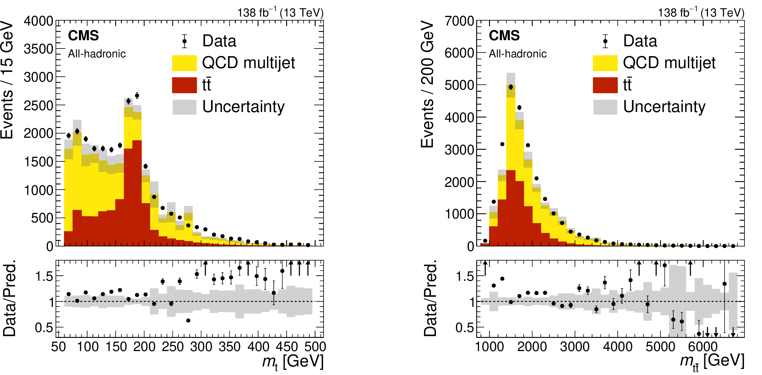
Figure 3:
Prefit data-to-simulation comparison of distributions in the all-hadronic channel for the mass of the leading $ \mathrm{t}\text{ tagged} $ jet (left) and the reconstructed $ \mathrm{t} \overline{\mathrm{t}} $ mass (right) in the central and forward categories combined, where both jets pass the $ \mathrm{t}\text{ tagging} $ requirement. The QCD background is taken from simulation for comparison, whereas in the analysis it is estimated from data. No cut on the $ m_{\mathrm{t}} $ variable is applied. |
png pdf |
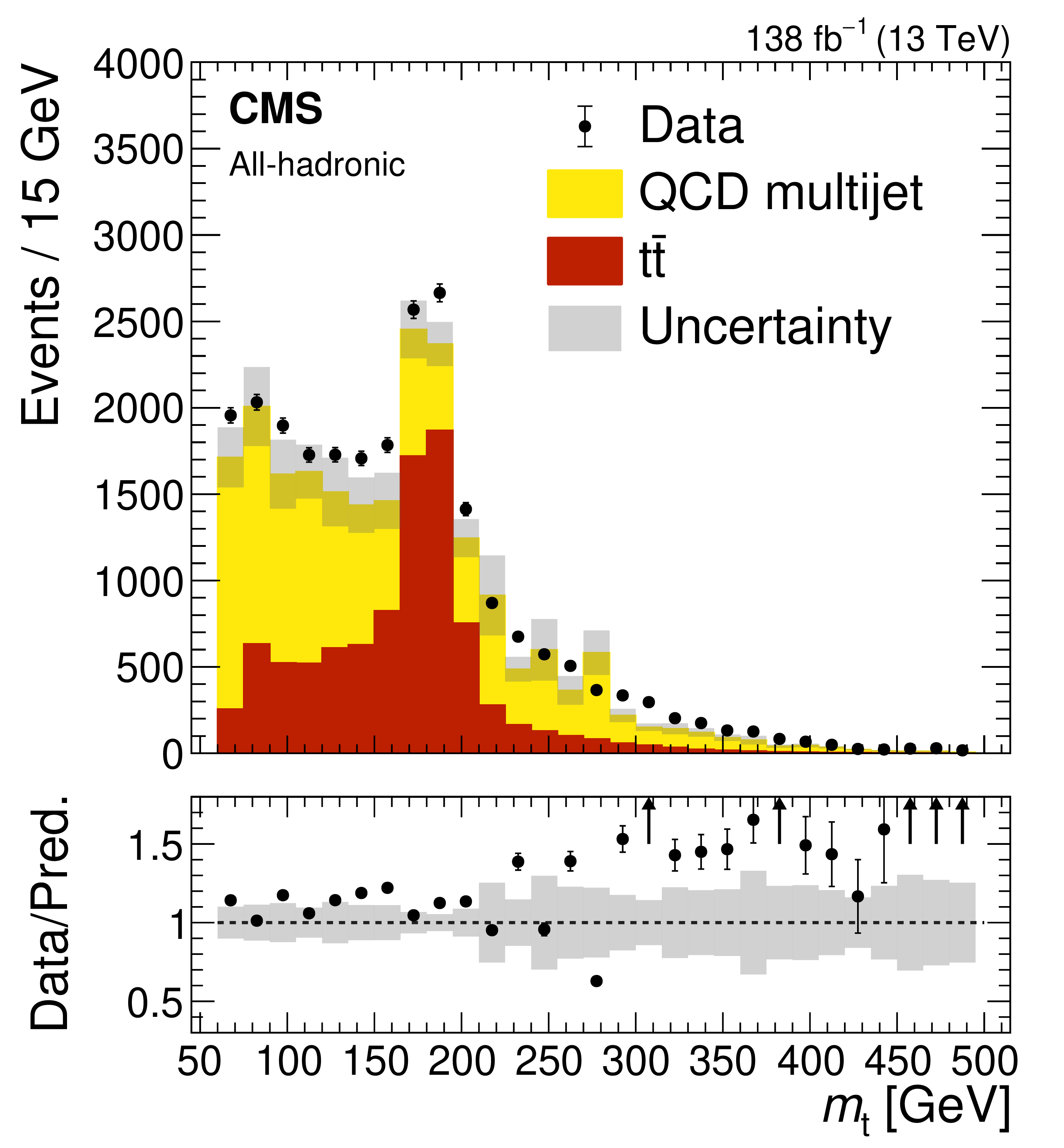
Figure 3-a:
Prefit data-to-simulation comparison of distributions in the all-hadronic channel for the mass of the leading $ \mathrm{t}\text{ tagged} $ jet (left) and the reconstructed $ \mathrm{t} \overline{\mathrm{t}} $ mass (right) in the central and forward categories combined, where both jets pass the $ \mathrm{t}\text{ tagging} $ requirement. The QCD background is taken from simulation for comparison, whereas in the analysis it is estimated from data. No cut on the $ m_{\mathrm{t}} $ variable is applied. |
png pdf |
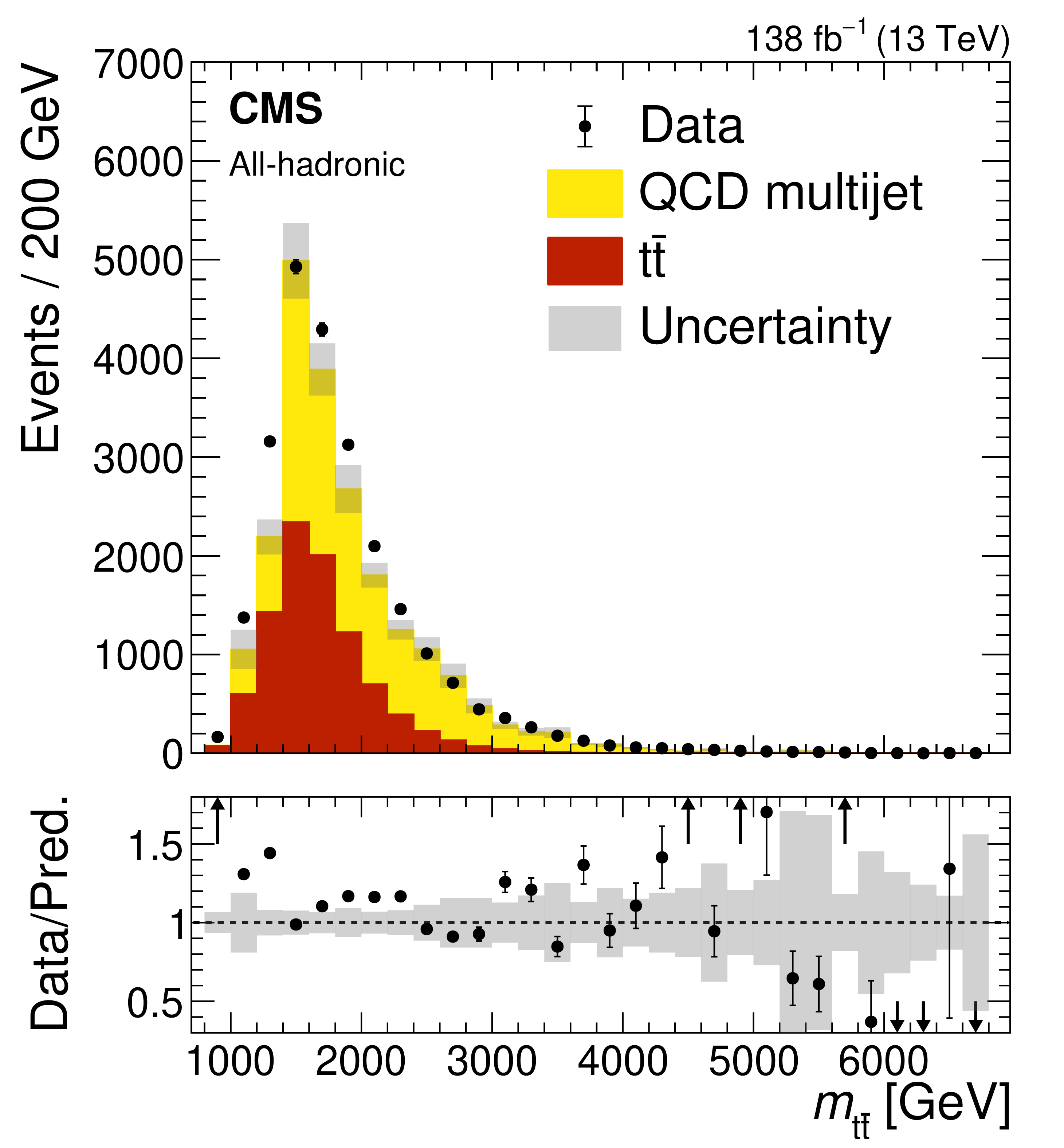
Figure 3-b:
Prefit data-to-simulation comparison of distributions in the all-hadronic channel for the mass of the leading $ \mathrm{t}\text{ tagged} $ jet (left) and the reconstructed $ \mathrm{t} \overline{\mathrm{t}} $ mass (right) in the central and forward categories combined, where both jets pass the $ \mathrm{t}\text{ tagging} $ requirement. The QCD background is taken from simulation for comparison, whereas in the analysis it is estimated from data. No cut on the $ m_{\mathrm{t}} $ variable is applied. |
png pdf |
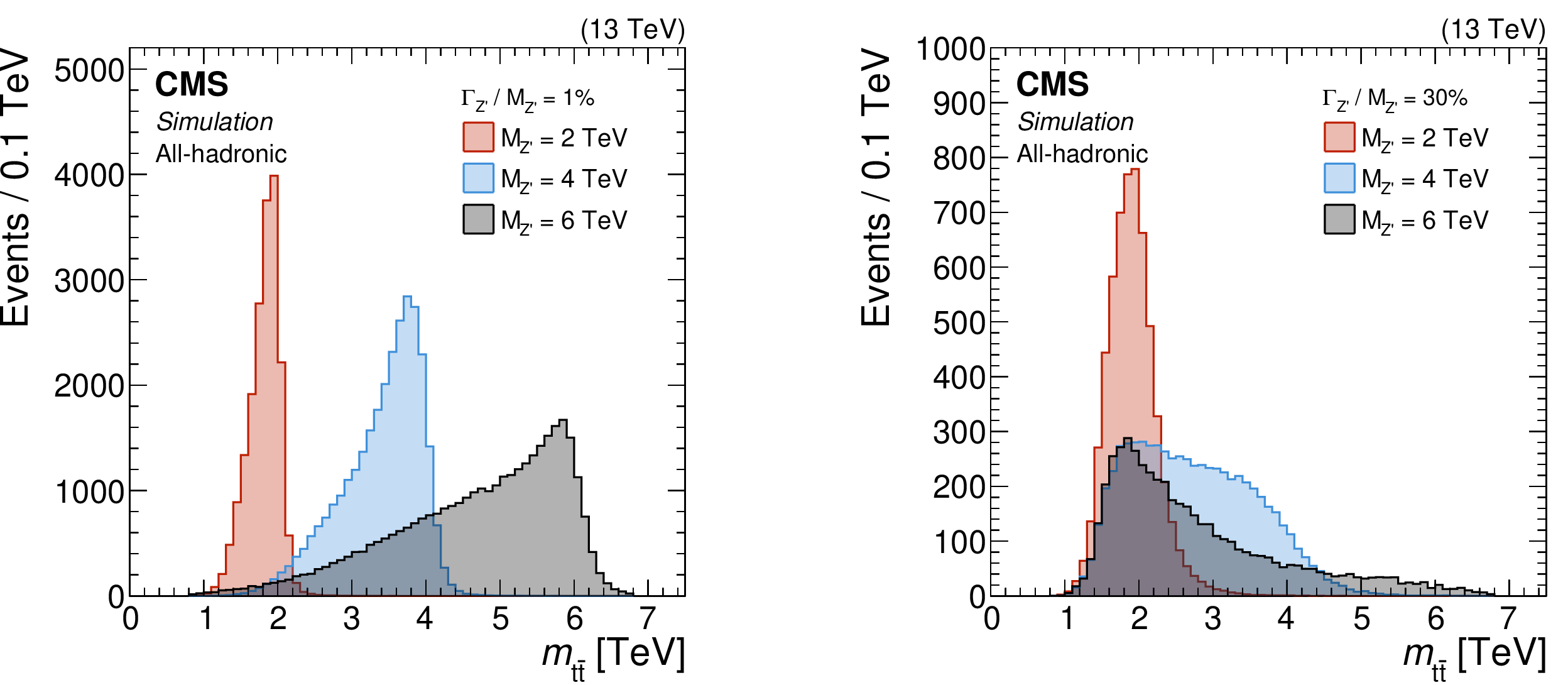
Figure 4:
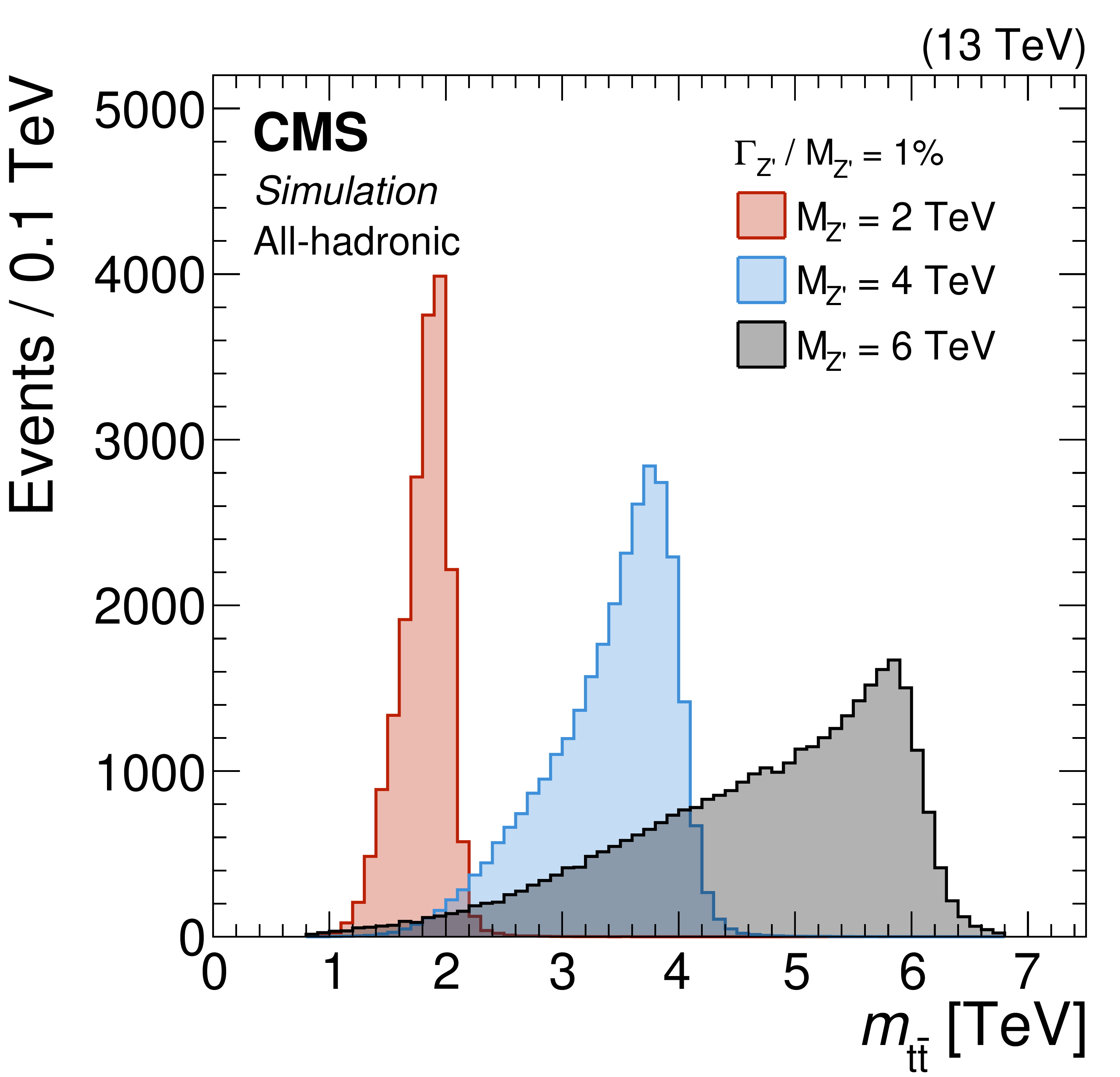
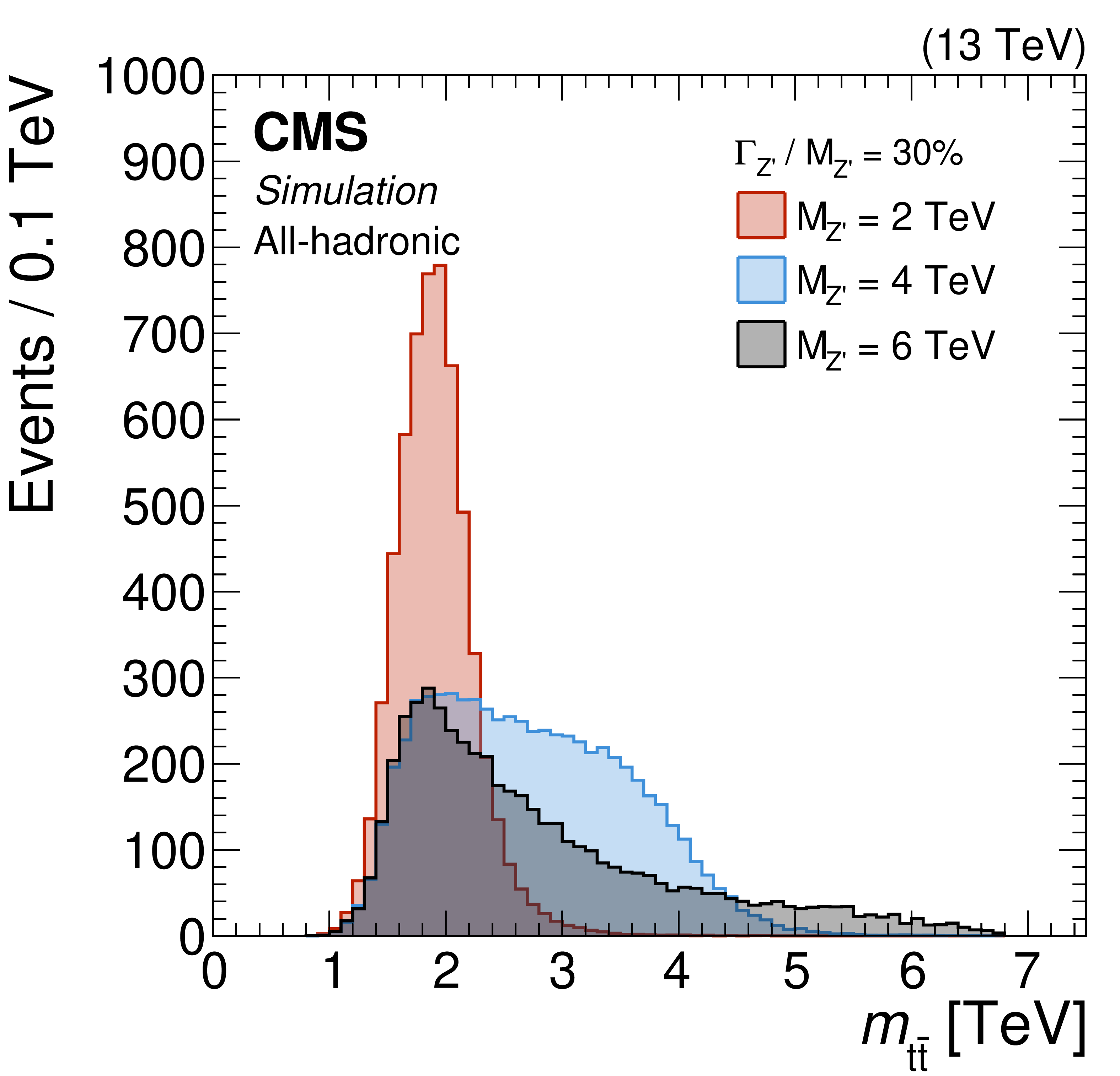
Reconstructed $ m_{{\mathrm{t}\overline{\mathrm{t}}} } $ distributions in simulation in the all-hadronic channel for $ \mathrm{Z}^{'} $ bosons with 1 and 30% relative widths, shown in the left and right panels, respectively. The signals correspond to $ \mathrm{Z}^{'} $ boson masses of 2, 4, and 6 TeV, where both jets pass the $ \mathrm{t}\text{ tagging} $ requirement. Signals are normalized to a cross section of 1\unitpb and an integrated luminosity of 138 fb$ ^{-1} $. No cut on the $ m_{\mathrm{t}} $ variable is applied. |
png pdf |
Figure 4-a:
Reconstructed $ m_{{\mathrm{t}\overline{\mathrm{t}}} } $ distributions in simulation in the all-hadronic channel for $ \mathrm{Z}^{'} $ bosons with 1 and 30% relative widths, shown in the left and right panels, respectively. The signals correspond to $ \mathrm{Z}^{'} $ boson masses of 2, 4, and 6 TeV, where both jets pass the $ \mathrm{t}\text{ tagging} $ requirement. Signals are normalized to a cross section of 1\unitpb and an integrated luminosity of 138 fb$ ^{-1} $. No cut on the $ m_{\mathrm{t}} $ variable is applied. |
png pdf |
Figure 4-b:
Reconstructed $ m_{{\mathrm{t}\overline{\mathrm{t}}} } $ distributions in simulation in the all-hadronic channel for $ \mathrm{Z}^{'} $ bosons with 1 and 30% relative widths, shown in the left and right panels, respectively. The signals correspond to $ \mathrm{Z}^{'} $ boson masses of 2, 4, and 6 TeV, where both jets pass the $ \mathrm{t}\text{ tagging} $ requirement. Signals are normalized to a cross section of 1\unitpb and an integrated luminosity of 138 fb$ ^{-1} $. No cut on the $ m_{\mathrm{t}} $ variable is applied. |
png pdf |
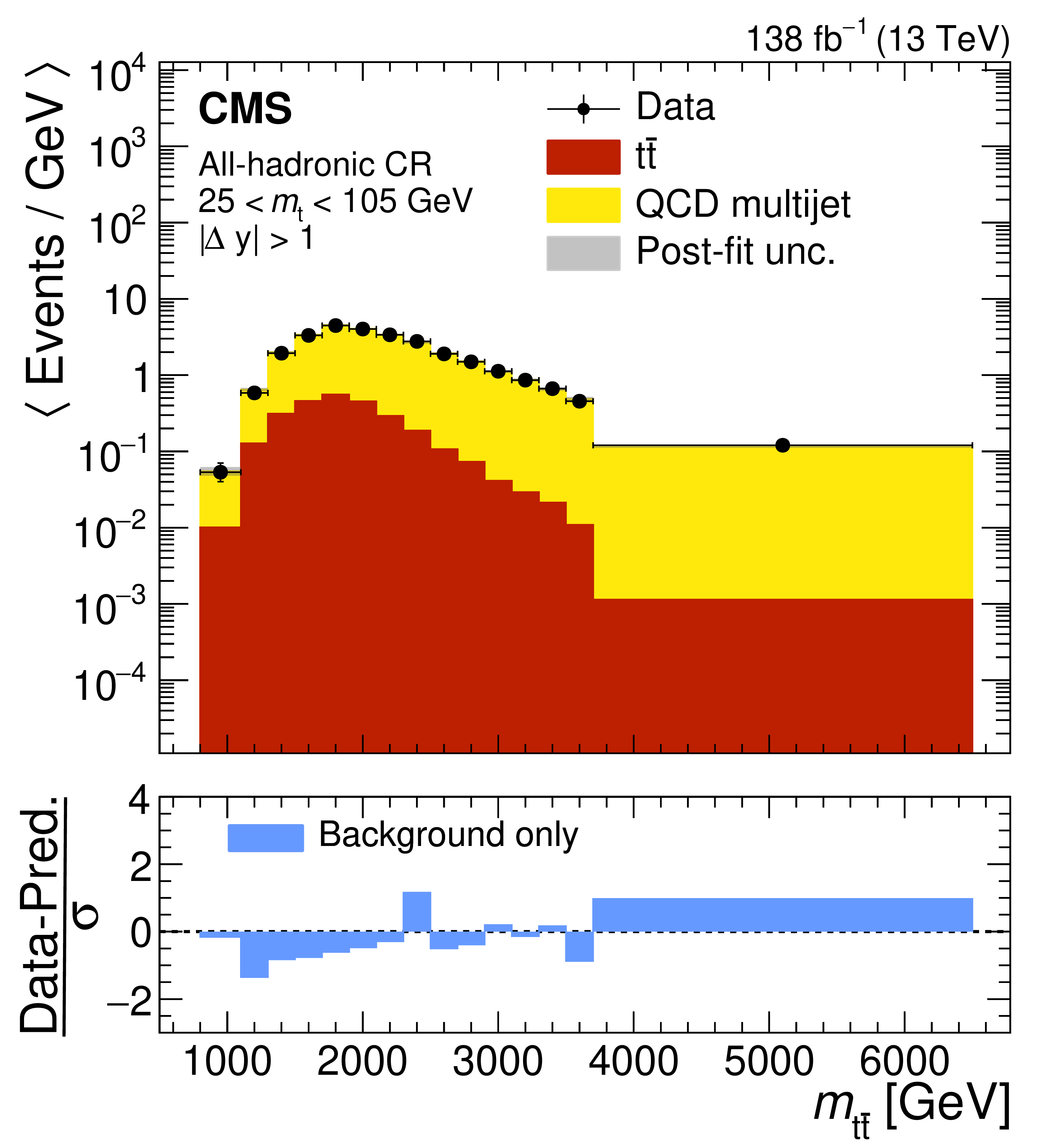
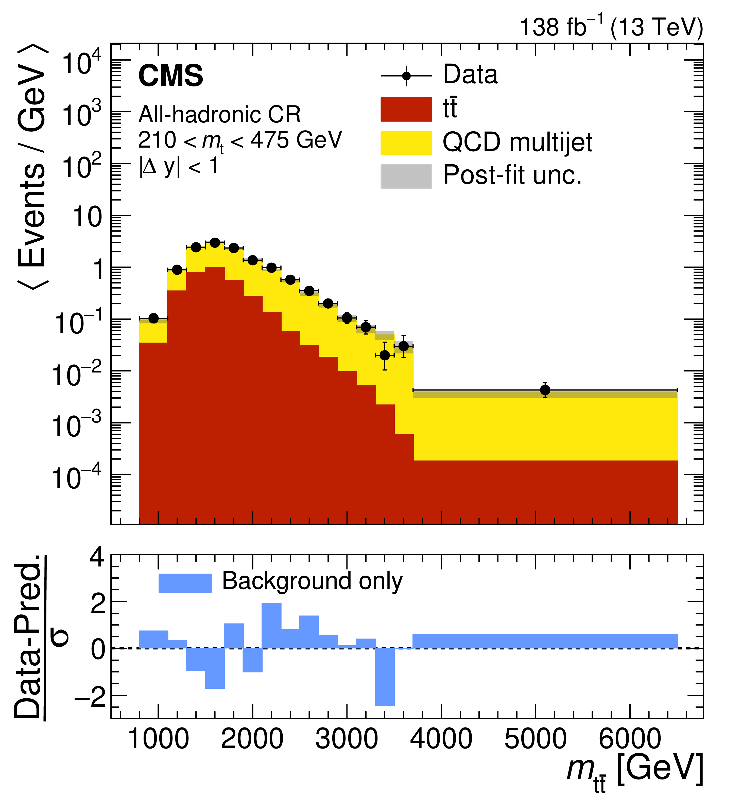
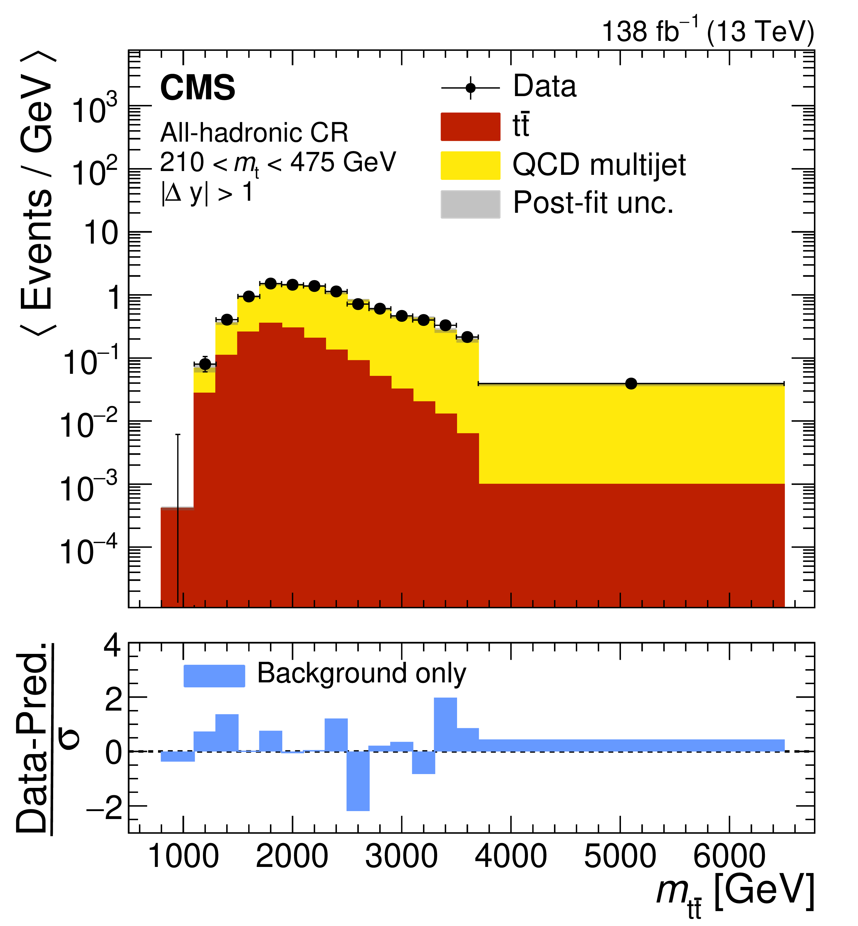
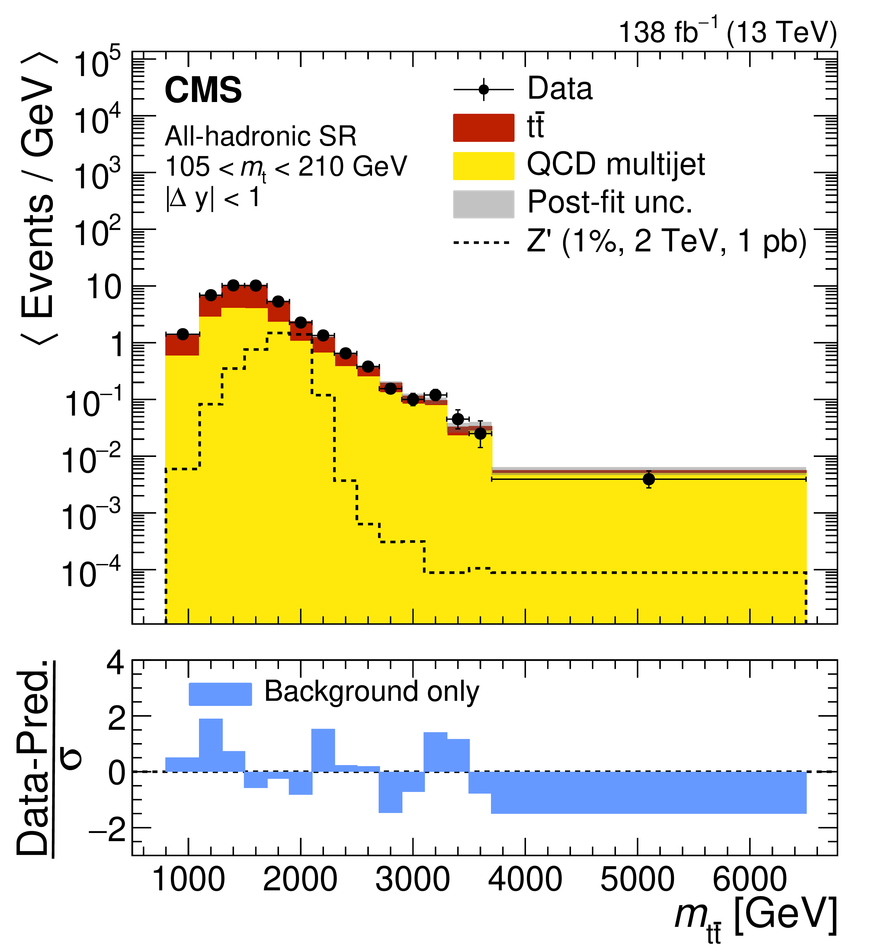
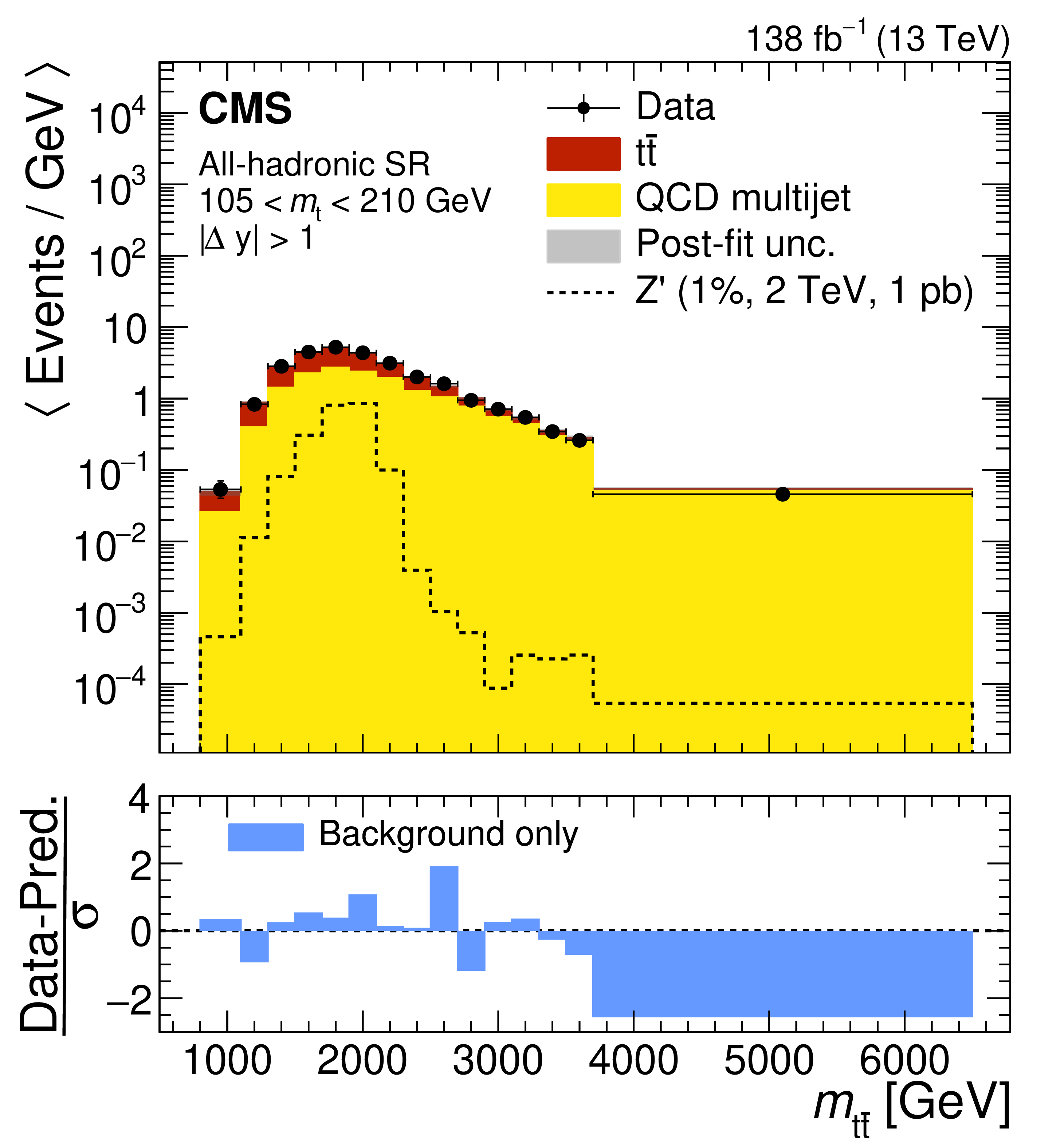
Figure 5:
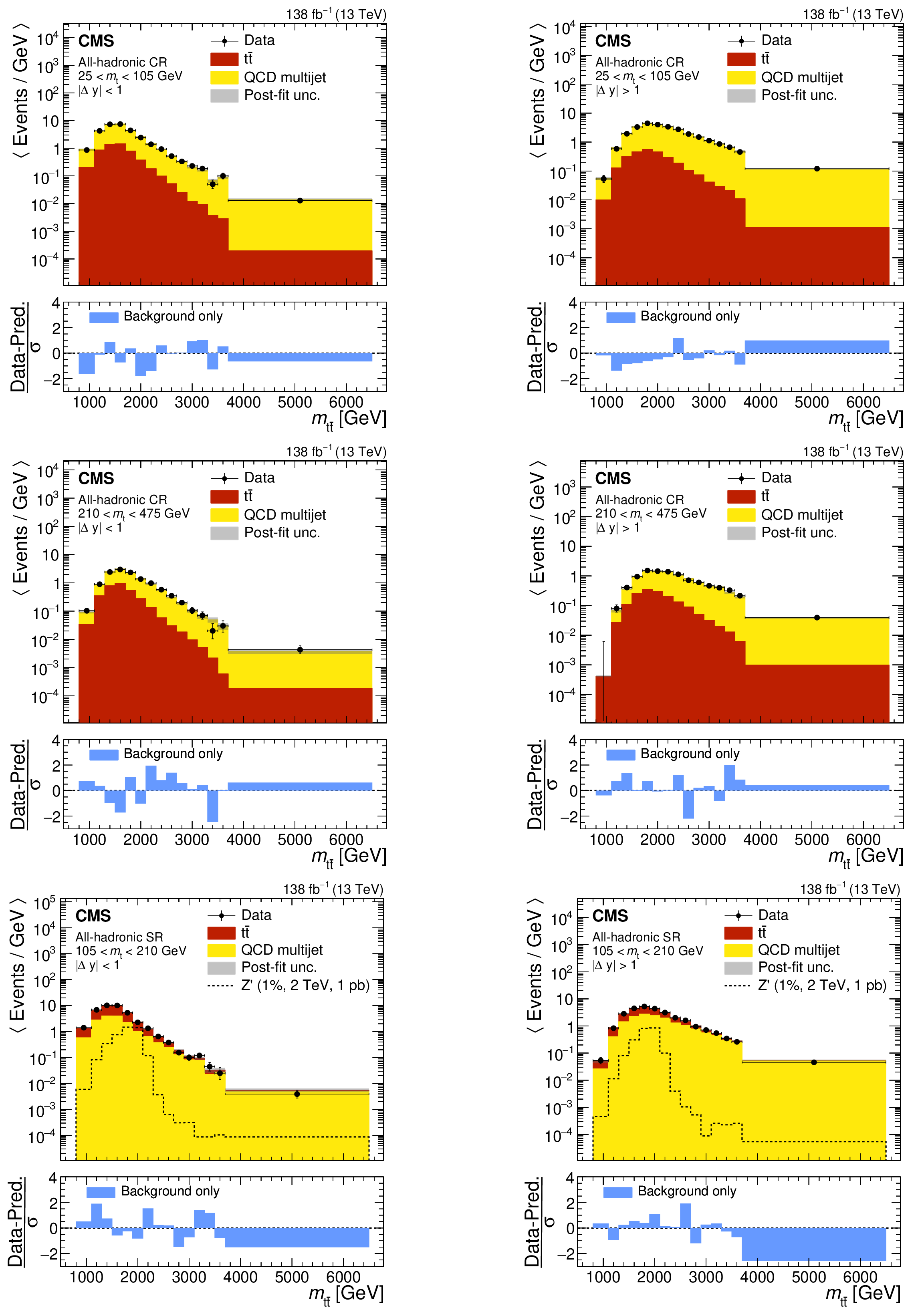
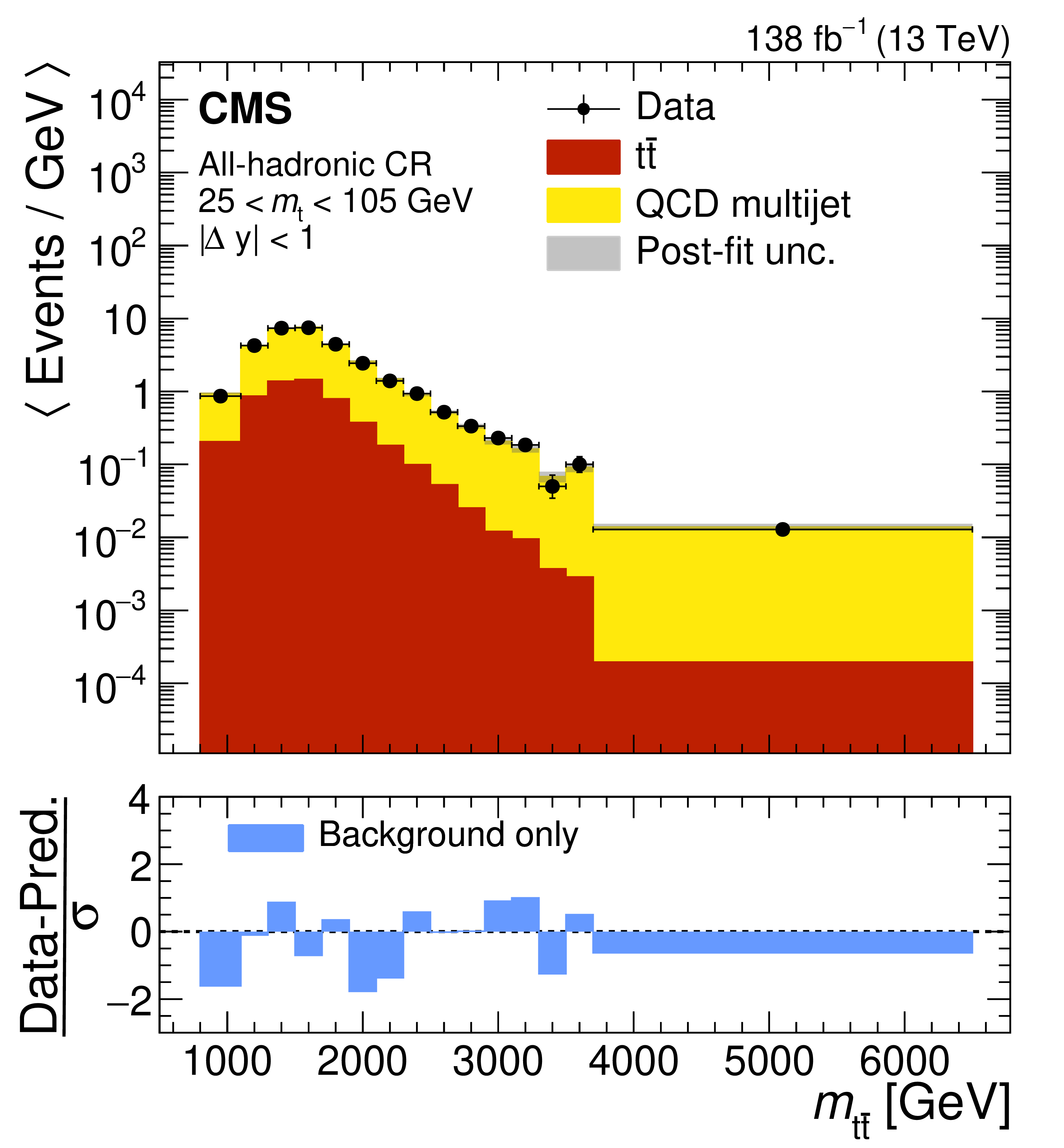
Postfit distributions in $ m_{{\mathrm{t}\overline{\mathrm{t}}} } $ for data and simulation for the central (left) and forward (right) categories for the all-hadronic channel, under the background-only hypothesis. Distributions are shown for the low-$ m_{\mathrm{t}} $ (upper) and high-$ m_{\mathrm{t}} $ (middle) sidebands, as well as the SR (lower). The horizontal bars on the data points indicate the bin width. For illustrative purposes, the $ \mathrm{Z}^{'} $ boson signal with a relative width of 1% and a mass of 2 TeV is normalized to a cross section of 1\unitpb and overlaid to the backgrounds in the signal regions. The lower panels show the pulls, defined as (Data - Prediction)$/\sigma $, where $ \sigma $ denotes the total postfit uncertainty in each bin, relative to the SM prediction. |
png pdf |
Figure 5-a:
Postfit distributions in $ m_{{\mathrm{t}\overline{\mathrm{t}}} } $ for data and simulation for the central (left) and forward (right) categories for the all-hadronic channel, under the background-only hypothesis. Distributions are shown for the low-$ m_{\mathrm{t}} $ (upper) and high-$ m_{\mathrm{t}} $ (middle) sidebands, as well as the SR (lower). The horizontal bars on the data points indicate the bin width. For illustrative purposes, the $ \mathrm{Z}^{'} $ boson signal with a relative width of 1% and a mass of 2 TeV is normalized to a cross section of 1\unitpb and overlaid to the backgrounds in the signal regions. The lower panels show the pulls, defined as (Data - Prediction)$/\sigma $, where $ \sigma $ denotes the total postfit uncertainty in each bin, relative to the SM prediction. |
png pdf |
Figure 5-b:
Postfit distributions in $ m_{{\mathrm{t}\overline{\mathrm{t}}} } $ for data and simulation for the central (left) and forward (right) categories for the all-hadronic channel, under the background-only hypothesis. Distributions are shown for the low-$ m_{\mathrm{t}} $ (upper) and high-$ m_{\mathrm{t}} $ (middle) sidebands, as well as the SR (lower). The horizontal bars on the data points indicate the bin width. For illustrative purposes, the $ \mathrm{Z}^{'} $ boson signal with a relative width of 1% and a mass of 2 TeV is normalized to a cross section of 1\unitpb and overlaid to the backgrounds in the signal regions. The lower panels show the pulls, defined as (Data - Prediction)$/\sigma $, where $ \sigma $ denotes the total postfit uncertainty in each bin, relative to the SM prediction. |
png pdf |
Figure 5-c:
Postfit distributions in $ m_{{\mathrm{t}\overline{\mathrm{t}}} } $ for data and simulation for the central (left) and forward (right) categories for the all-hadronic channel, under the background-only hypothesis. Distributions are shown for the low-$ m_{\mathrm{t}} $ (upper) and high-$ m_{\mathrm{t}} $ (middle) sidebands, as well as the SR (lower). The horizontal bars on the data points indicate the bin width. For illustrative purposes, the $ \mathrm{Z}^{'} $ boson signal with a relative width of 1% and a mass of 2 TeV is normalized to a cross section of 1\unitpb and overlaid to the backgrounds in the signal regions. The lower panels show the pulls, defined as (Data - Prediction)$/\sigma $, where $ \sigma $ denotes the total postfit uncertainty in each bin, relative to the SM prediction. |
png pdf |
Figure 5-d:
Postfit distributions in $ m_{{\mathrm{t}\overline{\mathrm{t}}} } $ for data and simulation for the central (left) and forward (right) categories for the all-hadronic channel, under the background-only hypothesis. Distributions are shown for the low-$ m_{\mathrm{t}} $ (upper) and high-$ m_{\mathrm{t}} $ (middle) sidebands, as well as the SR (lower). The horizontal bars on the data points indicate the bin width. For illustrative purposes, the $ \mathrm{Z}^{'} $ boson signal with a relative width of 1% and a mass of 2 TeV is normalized to a cross section of 1\unitpb and overlaid to the backgrounds in the signal regions. The lower panels show the pulls, defined as (Data - Prediction)$/\sigma $, where $ \sigma $ denotes the total postfit uncertainty in each bin, relative to the SM prediction. |
png pdf |
Figure 5-e:
Postfit distributions in $ m_{{\mathrm{t}\overline{\mathrm{t}}} } $ for data and simulation for the central (left) and forward (right) categories for the all-hadronic channel, under the background-only hypothesis. Distributions are shown for the low-$ m_{\mathrm{t}} $ (upper) and high-$ m_{\mathrm{t}} $ (middle) sidebands, as well as the SR (lower). The horizontal bars on the data points indicate the bin width. For illustrative purposes, the $ \mathrm{Z}^{'} $ boson signal with a relative width of 1% and a mass of 2 TeV is normalized to a cross section of 1\unitpb and overlaid to the backgrounds in the signal regions. The lower panels show the pulls, defined as (Data - Prediction)$/\sigma $, where $ \sigma $ denotes the total postfit uncertainty in each bin, relative to the SM prediction. |
png pdf |
Figure 5-f:
Postfit distributions in $ m_{{\mathrm{t}\overline{\mathrm{t}}} } $ for data and simulation for the central (left) and forward (right) categories for the all-hadronic channel, under the background-only hypothesis. Distributions are shown for the low-$ m_{\mathrm{t}} $ (upper) and high-$ m_{\mathrm{t}} $ (middle) sidebands, as well as the SR (lower). The horizontal bars on the data points indicate the bin width. For illustrative purposes, the $ \mathrm{Z}^{'} $ boson signal with a relative width of 1% and a mass of 2 TeV is normalized to a cross section of 1\unitpb and overlaid to the backgrounds in the signal regions. The lower panels show the pulls, defined as (Data - Prediction)$/\sigma $, where $ \sigma $ denotes the total postfit uncertainty in each bin, relative to the SM prediction. |
png pdf |
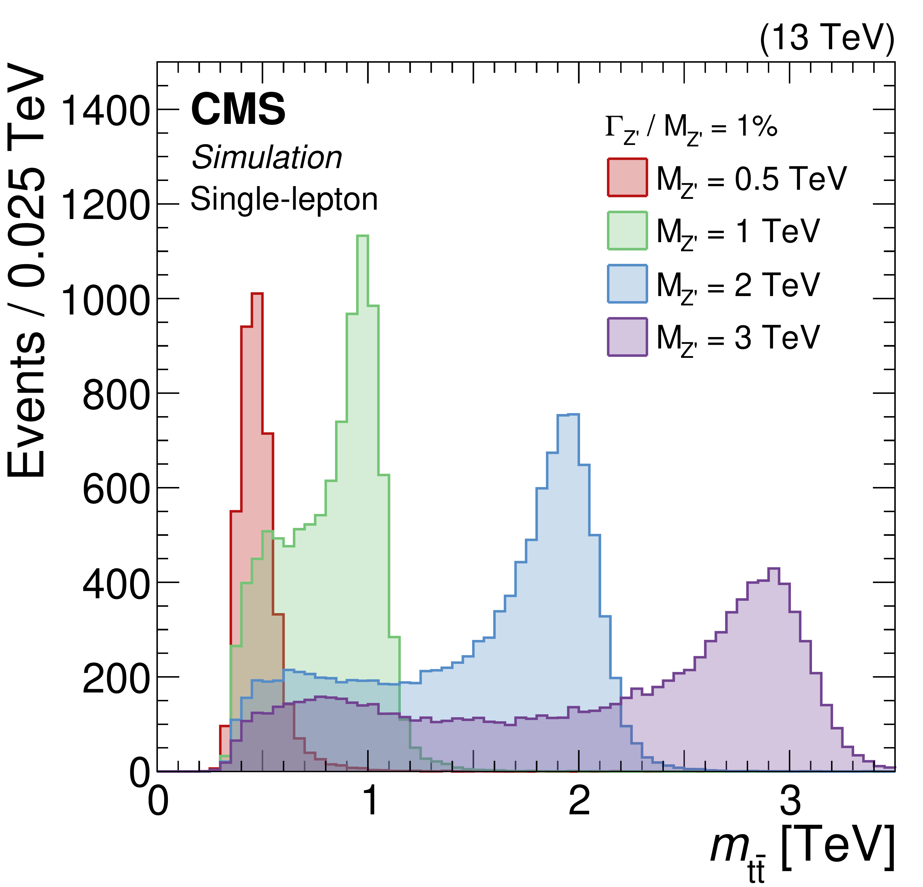
Figure 6:
Reconstructed invariant mass distribution in simulation in the single-lepton channel for $ \mathrm{Z}^{'} $ bosons with 1% relative width, for different mass hypotheses. Each distribution corresponds to a production cross section of 1 pb. |
png pdf |
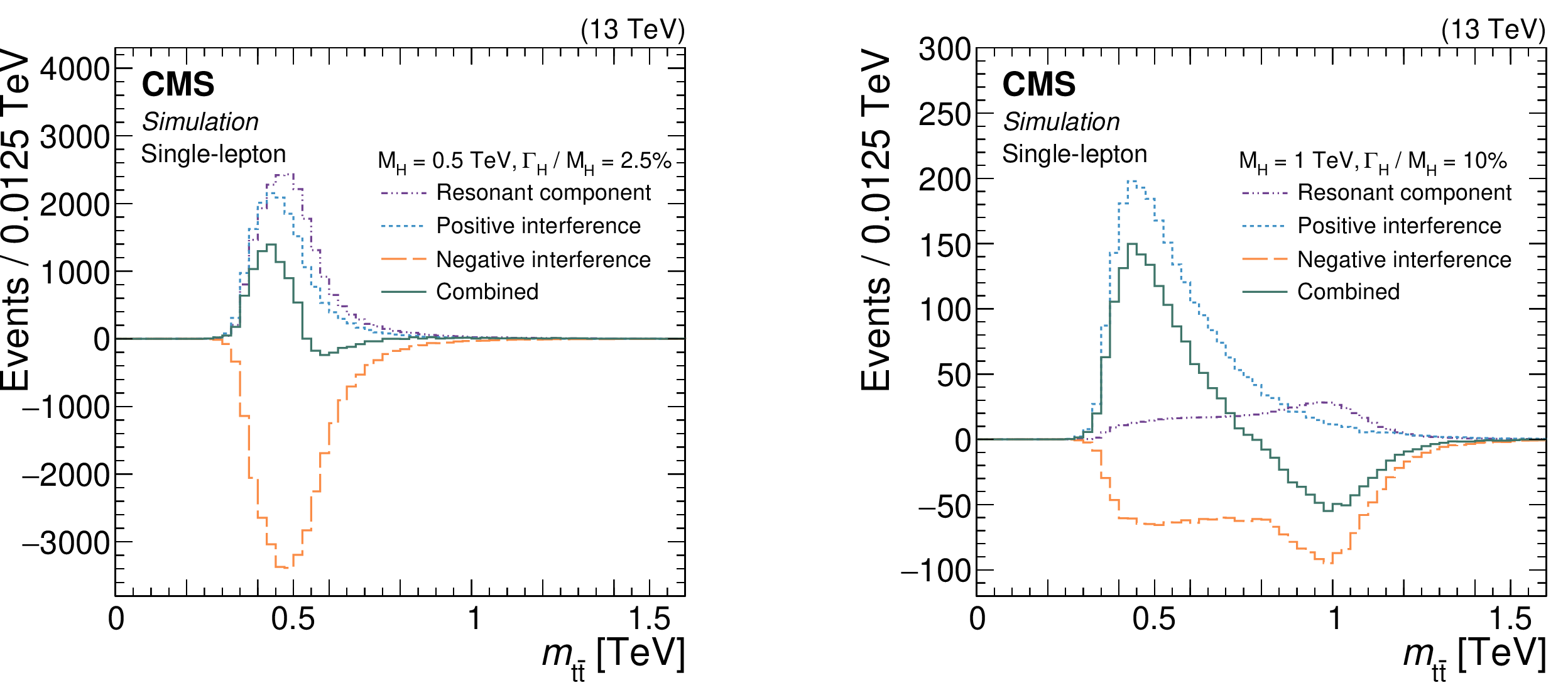
Figure 7:
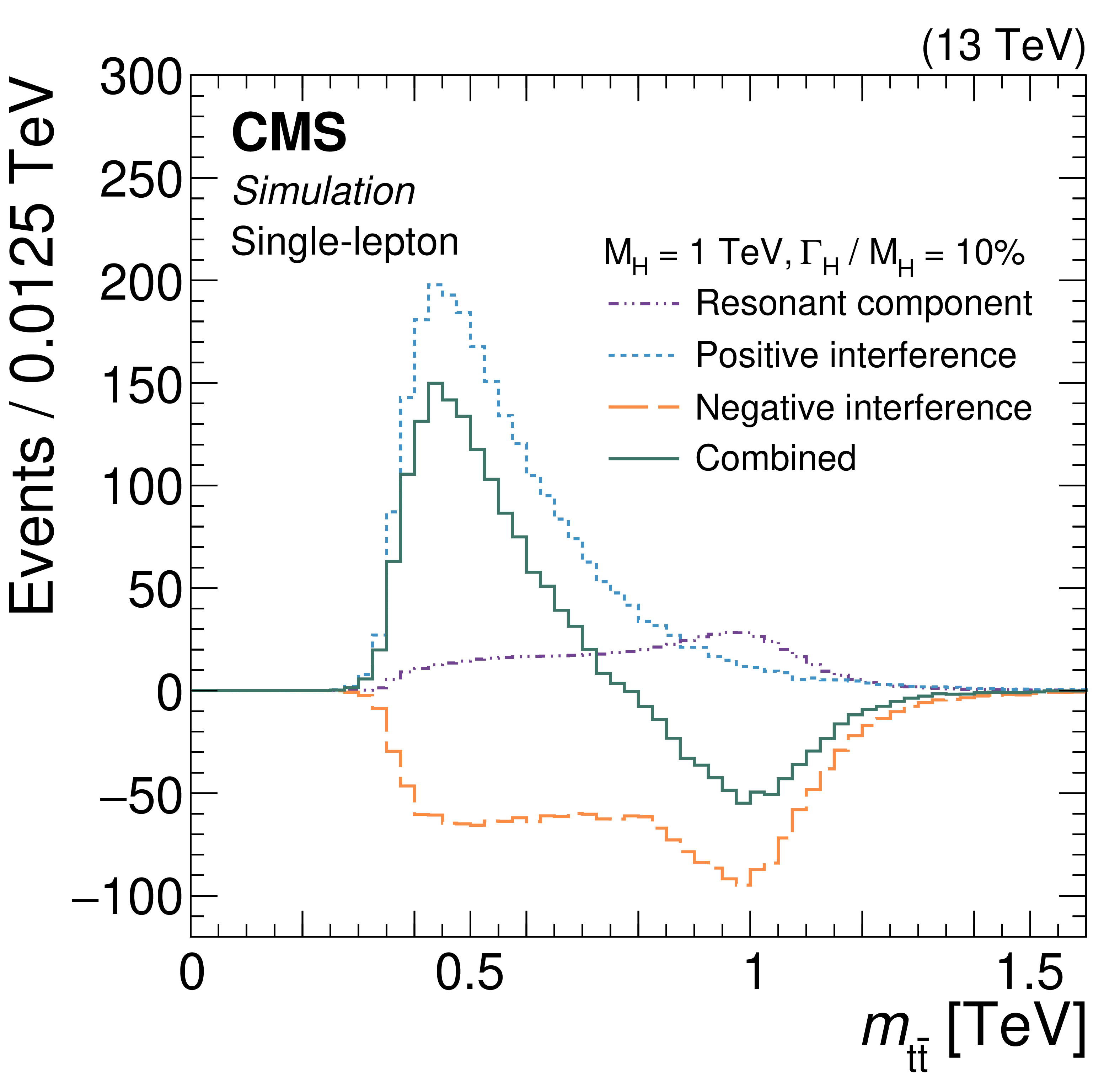
Different contributions to the $ m_{{\mathrm{t}\overline{\mathrm{t}}} } $ distribution in simulation in the single-lepton channel for scalar Higgs bosons with masses of 0.5 (left) and 1 TeV (right), and corresponding relative widths of 2.5 and 10%, respectively. Each distribution is normalized to the corresponding production cross section. |
png pdf |
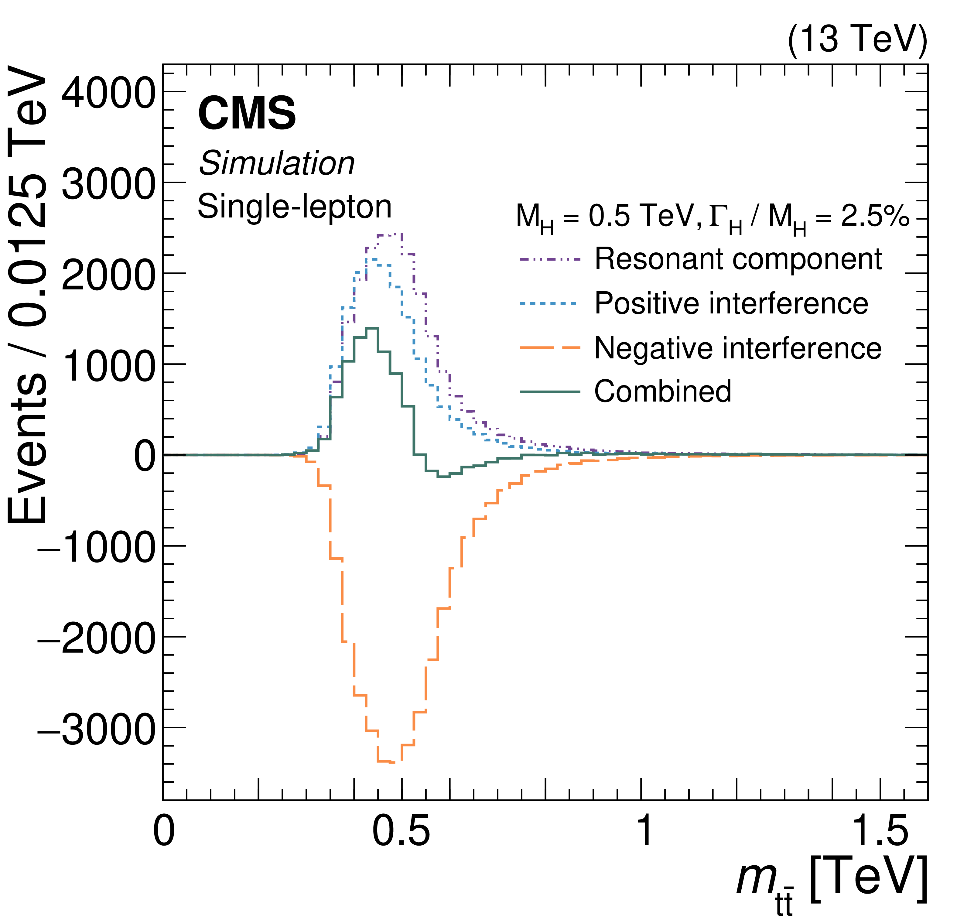
Figure 7-a:
Different contributions to the $ m_{{\mathrm{t}\overline{\mathrm{t}}} } $ distribution in simulation in the single-lepton channel for scalar Higgs bosons with masses of 0.5 (left) and 1 TeV (right), and corresponding relative widths of 2.5 and 10%, respectively. Each distribution is normalized to the corresponding production cross section. |
png pdf |
Figure 7-b:
Different contributions to the $ m_{{\mathrm{t}\overline{\mathrm{t}}} } $ distribution in simulation in the single-lepton channel for scalar Higgs bosons with masses of 0.5 (left) and 1 TeV (right), and corresponding relative widths of 2.5 and 10%, respectively. Each distribution is normalized to the corresponding production cross section. |
png pdf |
Figure 8:
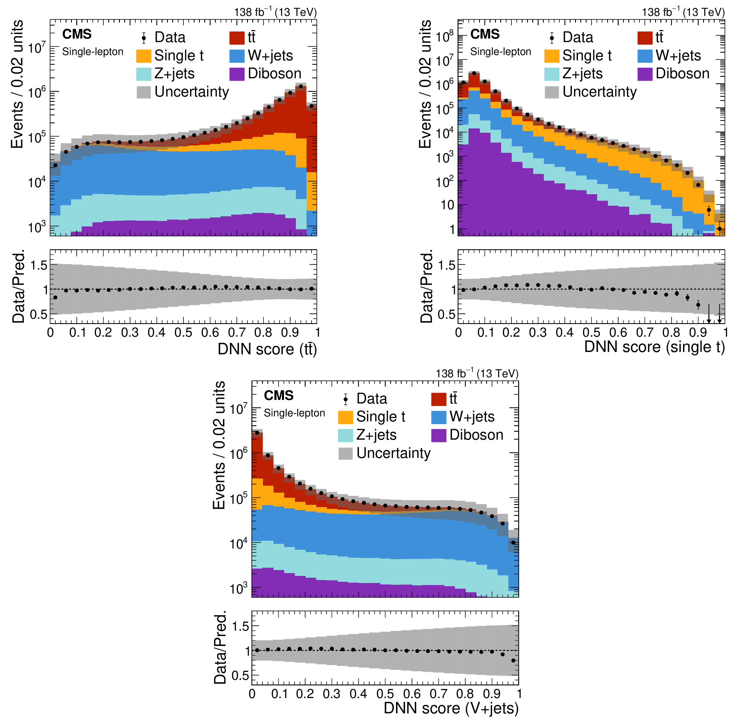
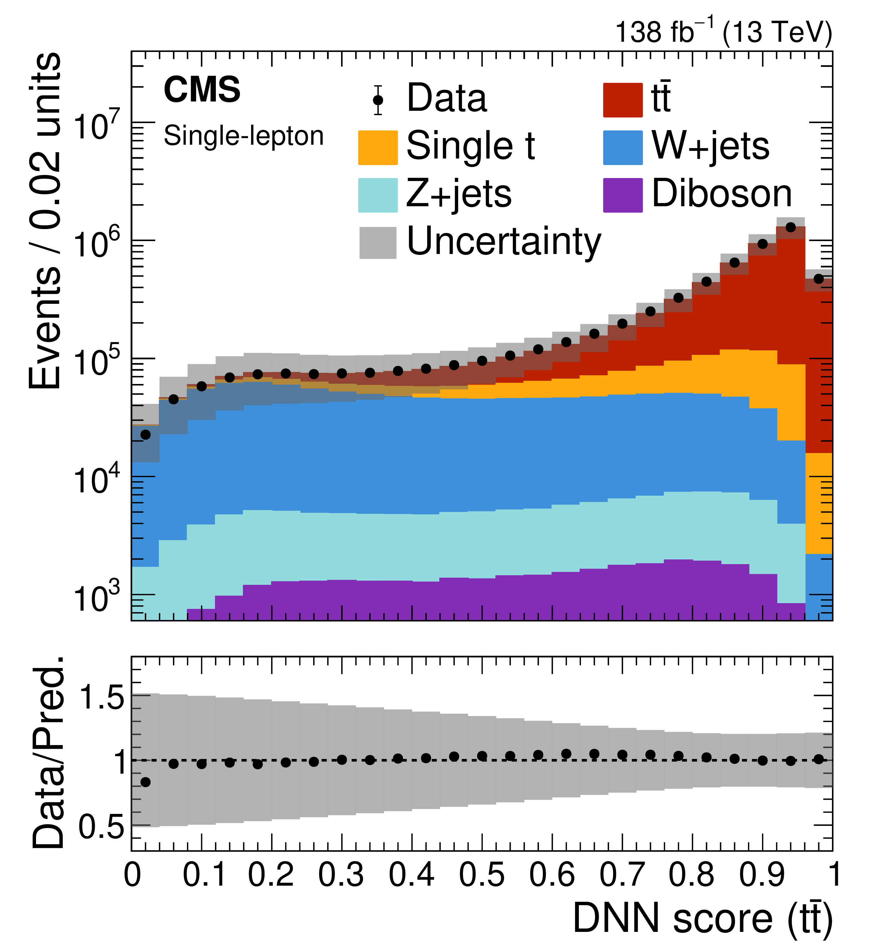
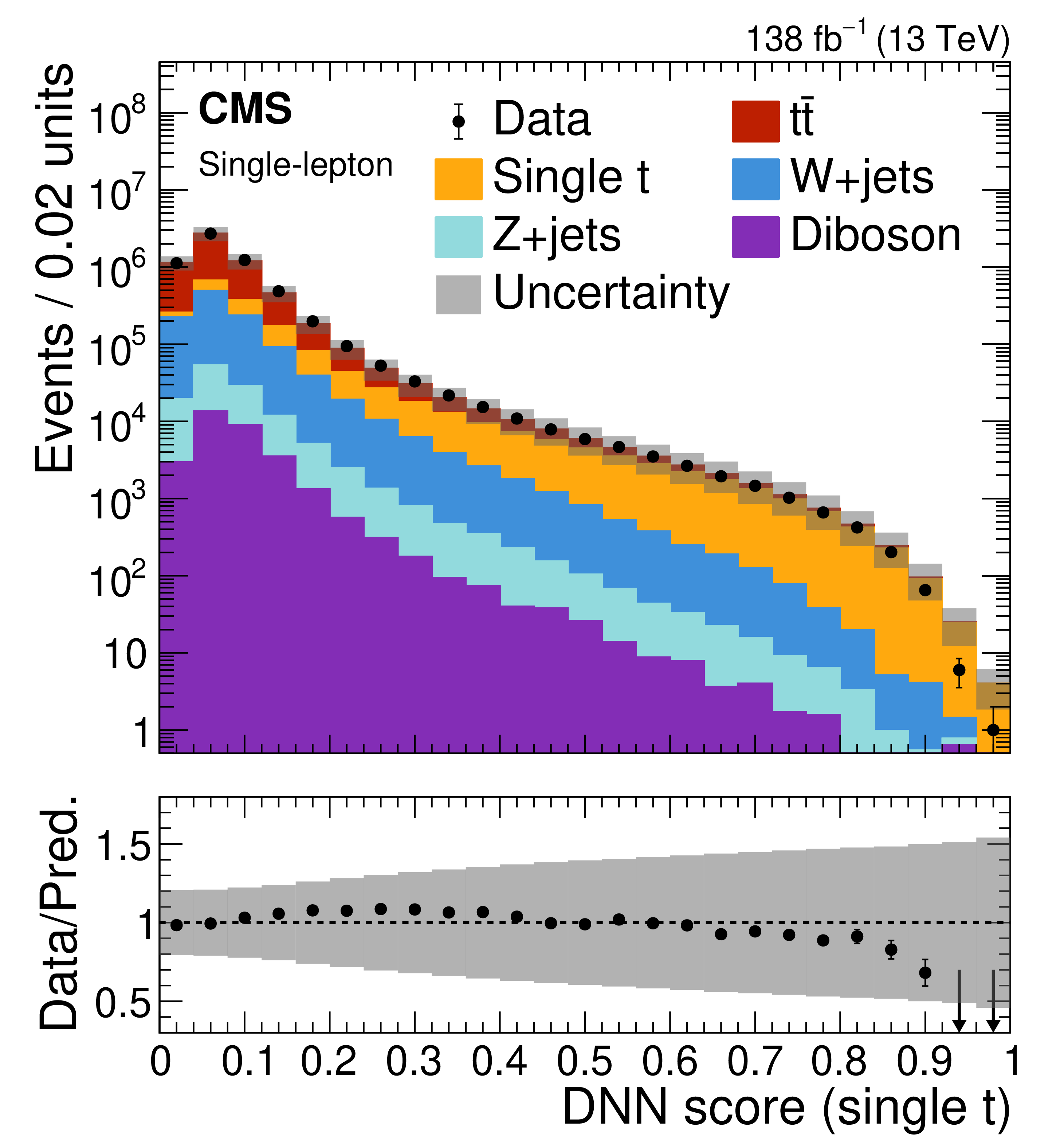
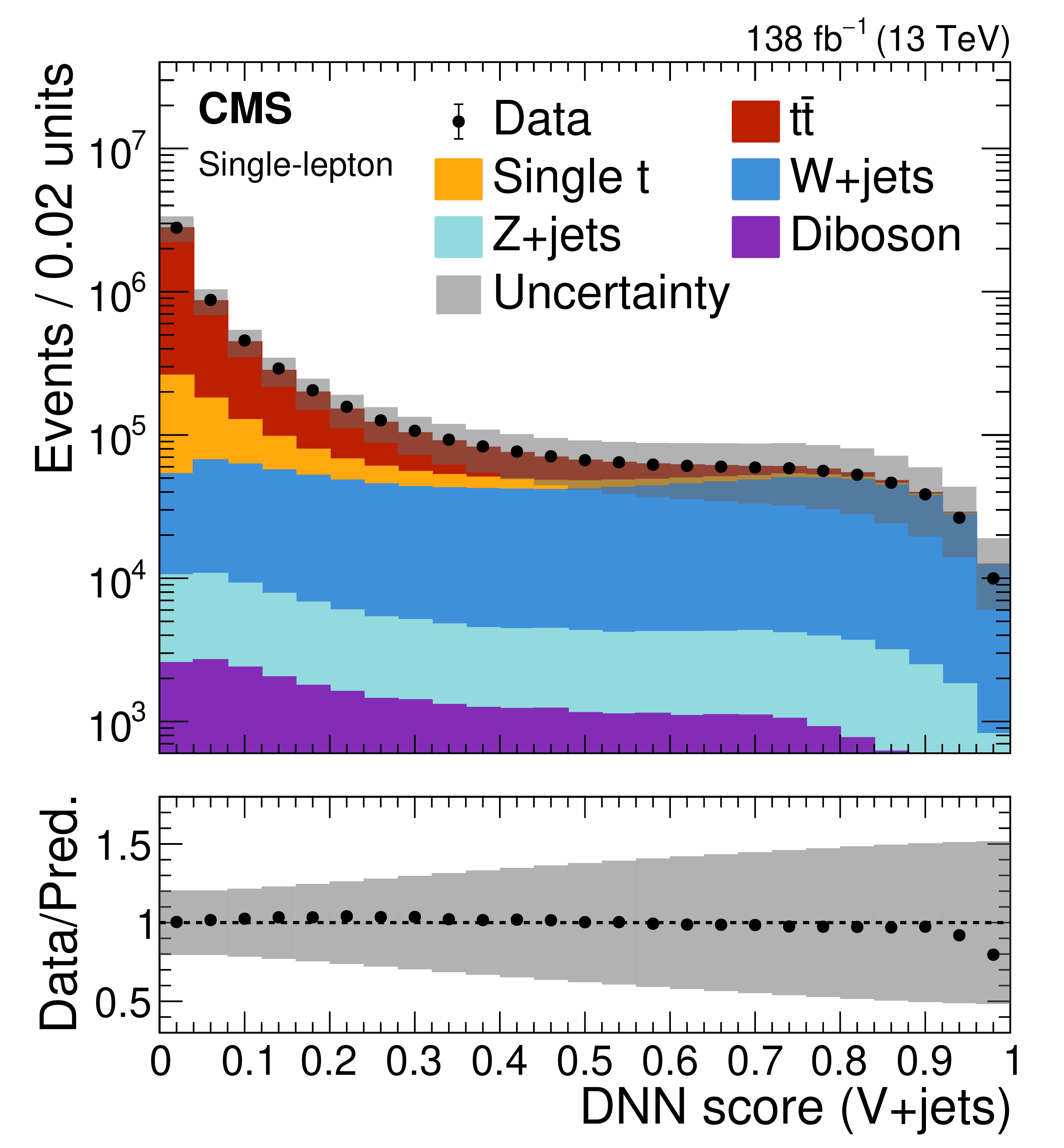
The DNN score distributions for the combined muon and electron channels in the single-lepton channel: $ \mathrm{t} \overline{\mathrm{t}} $ score (upper left), single t score (upper right), and V+jets score (lower). The lower panels show the ratio of the data to the total SM background prediction. The gray bands represent the uncertainty, computed by summing in quadrature the statistical uncertainty and the systematic uncertainties affecting the normalization of each process. These observables are not fitted to extract the final results; the uncertainties are the prefit values. |
png pdf |
Figure 8-a:
The DNN score distributions for the combined muon and electron channels in the single-lepton channel: $ \mathrm{t} \overline{\mathrm{t}} $ score (upper left), single t score (upper right), and V+jets score (lower). The lower panels show the ratio of the data to the total SM background prediction. The gray bands represent the uncertainty, computed by summing in quadrature the statistical uncertainty and the systematic uncertainties affecting the normalization of each process. These observables are not fitted to extract the final results; the uncertainties are the prefit values. |
png pdf |
Figure 8-b:
The DNN score distributions for the combined muon and electron channels in the single-lepton channel: $ \mathrm{t} \overline{\mathrm{t}} $ score (upper left), single t score (upper right), and V+jets score (lower). The lower panels show the ratio of the data to the total SM background prediction. The gray bands represent the uncertainty, computed by summing in quadrature the statistical uncertainty and the systematic uncertainties affecting the normalization of each process. These observables are not fitted to extract the final results; the uncertainties are the prefit values. |
png pdf |
Figure 8-c:
The DNN score distributions for the combined muon and electron channels in the single-lepton channel: $ \mathrm{t} \overline{\mathrm{t}} $ score (upper left), single t score (upper right), and V+jets score (lower). The lower panels show the ratio of the data to the total SM background prediction. The gray bands represent the uncertainty, computed by summing in quadrature the statistical uncertainty and the systematic uncertainties affecting the normalization of each process. These observables are not fitted to extract the final results; the uncertainties are the prefit values. |
png pdf |
Figure 9:
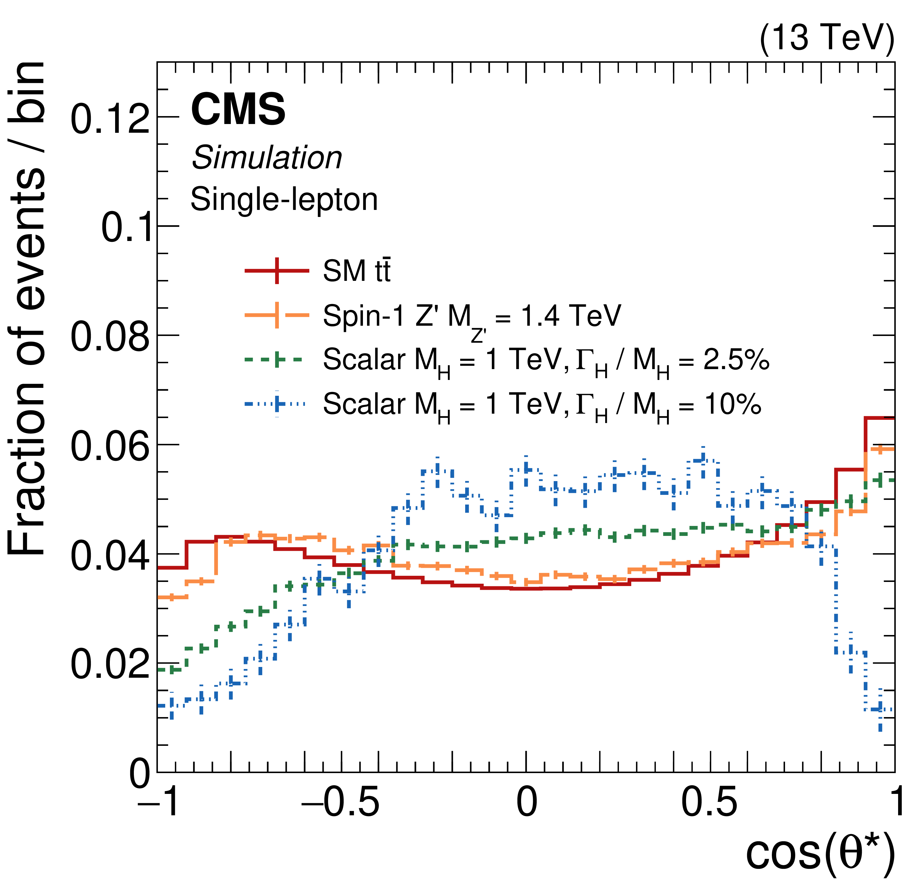
Distribution of $ \cos(\theta^\ast) $ for different processes in simulation in the single-lepton channel: SM $ \mathrm{t} \overline{\mathrm{t}} $ (solid red), $ \mathrm{Z}^{'} $ with $ m_{{\mathrm{t}\overline{\mathrm{t}}} }= $ 1.4 TeV (long-dashed orange), scalar H with $ m_{\mathrm{H}}= $ 1 TeV and 2.5% relative width (short-dashed green), and scalar H with $ m_{\mathrm{H}}= $ 1 TeV and 10% relative width (dash-dotted blue). All distributions are normalized to unit area. |
png pdf |
Figure 10:
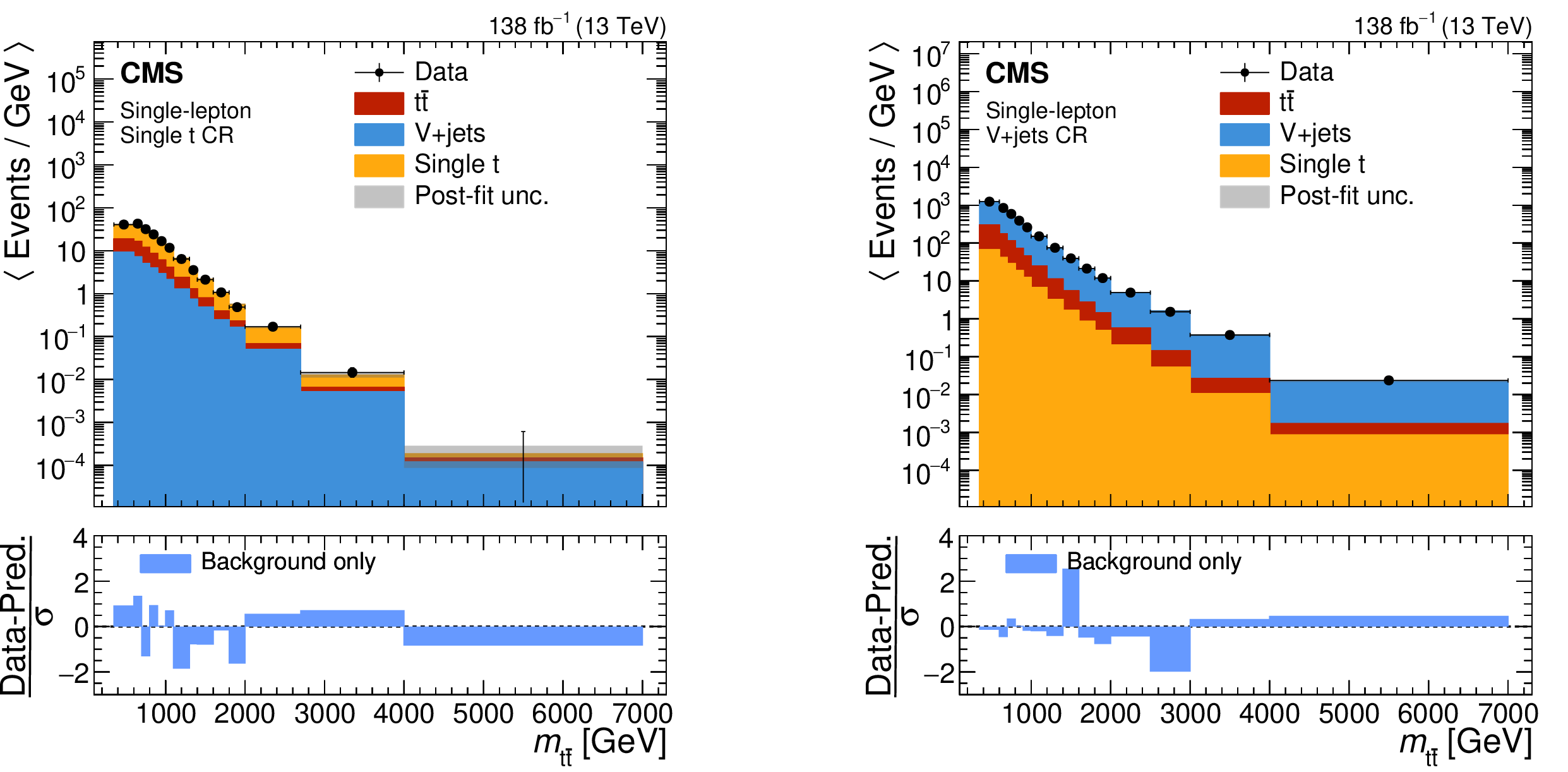
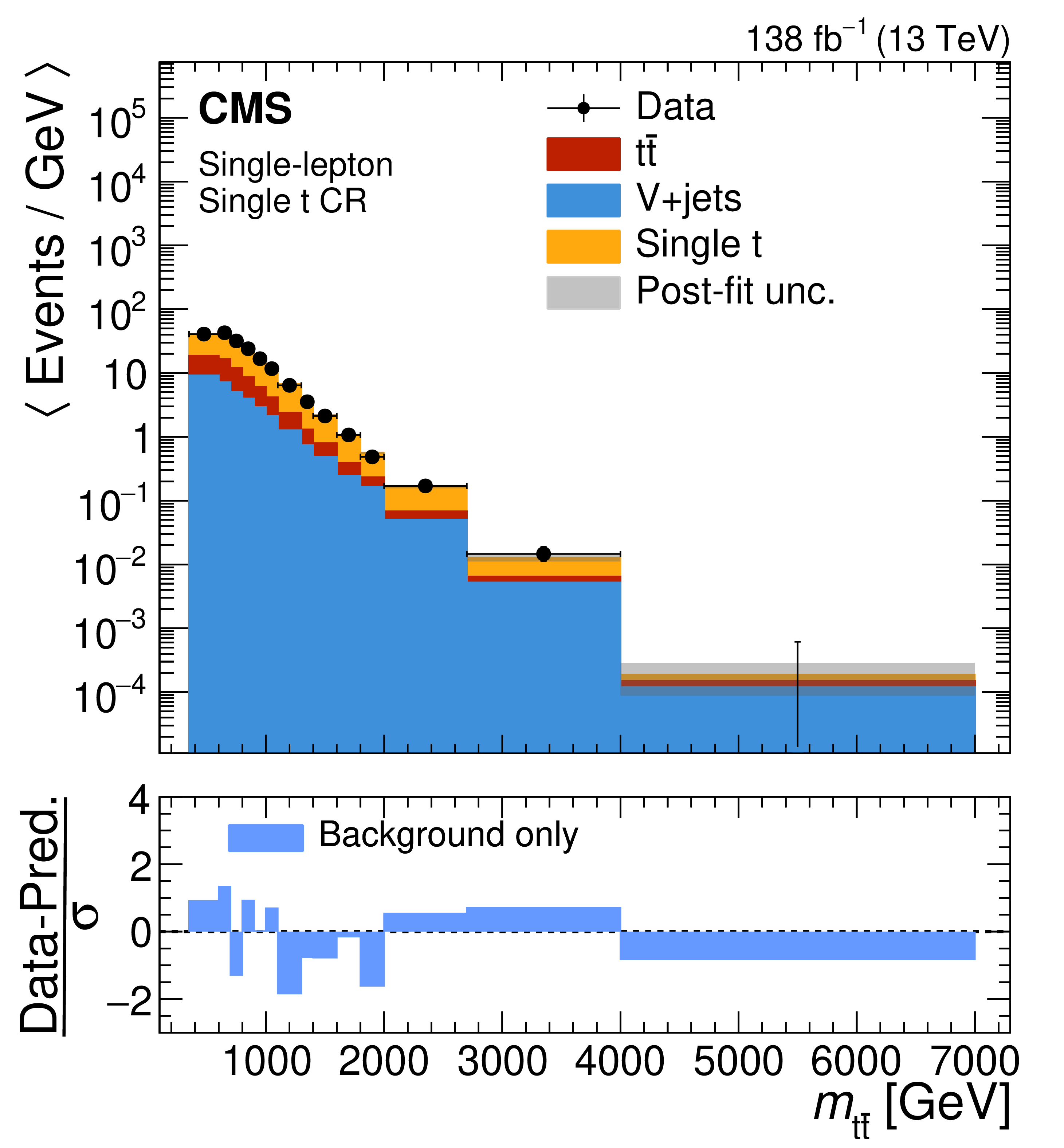
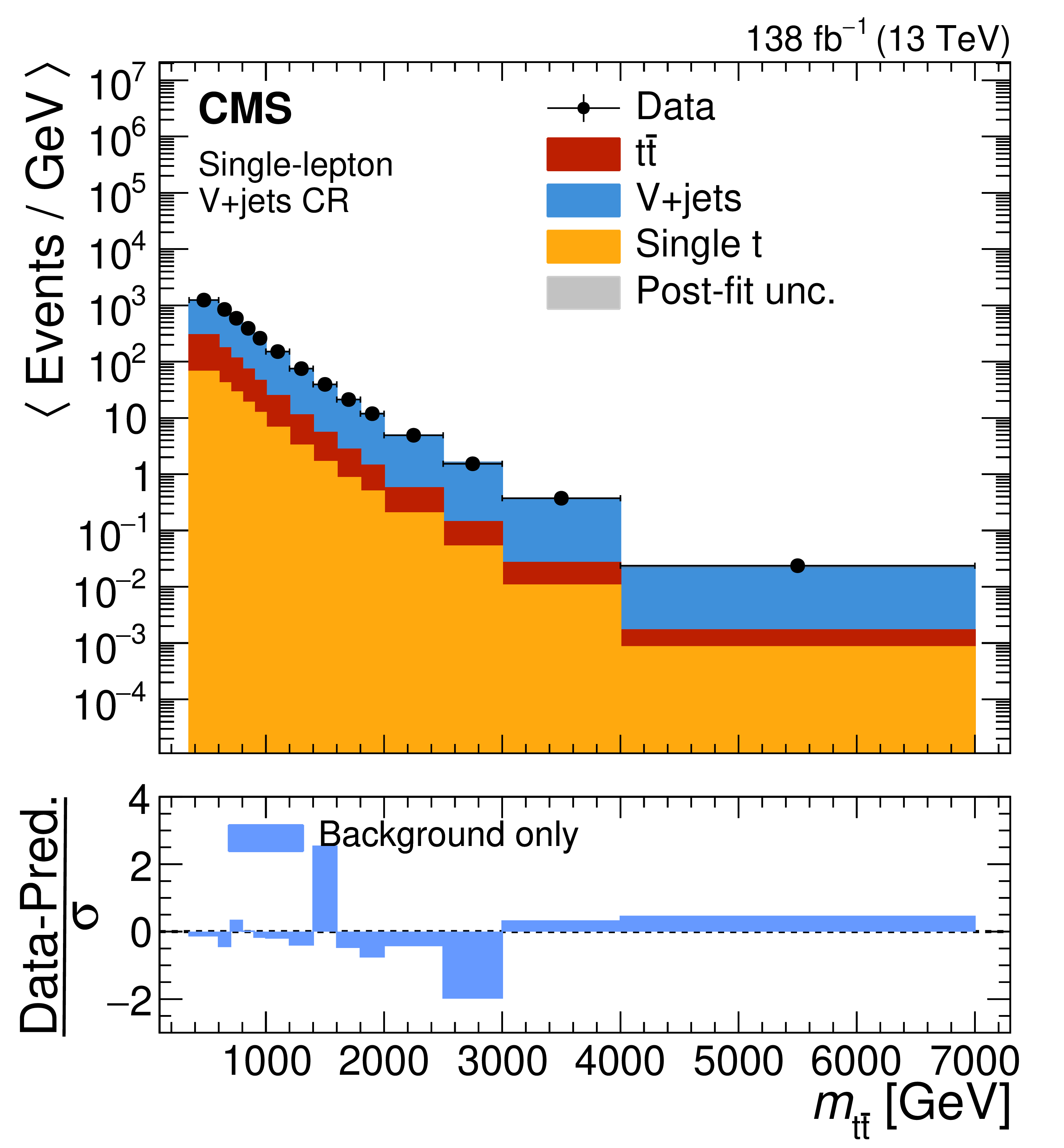
Postfit distributions in $ m_{{\mathrm{t}\overline{\mathrm{t}}} } $ in the single-lepton channel for data and simulation in the single t (left) and V+jets (right) CRs, under the background-only hypothesis. The horizontal bars on the data points indicate the bin width. The lower panels show the pulls, defined as (Data-Prediction)$/\sigma $, where $ \sigma $ denotes the total postfit uncertainty in each bin, relative to the SM prediction. |
png pdf |
Figure 10-a:
Postfit distributions in $ m_{{\mathrm{t}\overline{\mathrm{t}}} } $ in the single-lepton channel for data and simulation in the single t (left) and V+jets (right) CRs, under the background-only hypothesis. The horizontal bars on the data points indicate the bin width. The lower panels show the pulls, defined as (Data-Prediction)$/\sigma $, where $ \sigma $ denotes the total postfit uncertainty in each bin, relative to the SM prediction. |
png pdf |
Figure 10-b:
Postfit distributions in $ m_{{\mathrm{t}\overline{\mathrm{t}}} } $ in the single-lepton channel for data and simulation in the single t (left) and V+jets (right) CRs, under the background-only hypothesis. The horizontal bars on the data points indicate the bin width. The lower panels show the pulls, defined as (Data-Prediction)$/\sigma $, where $ \sigma $ denotes the total postfit uncertainty in each bin, relative to the SM prediction. |
png pdf |
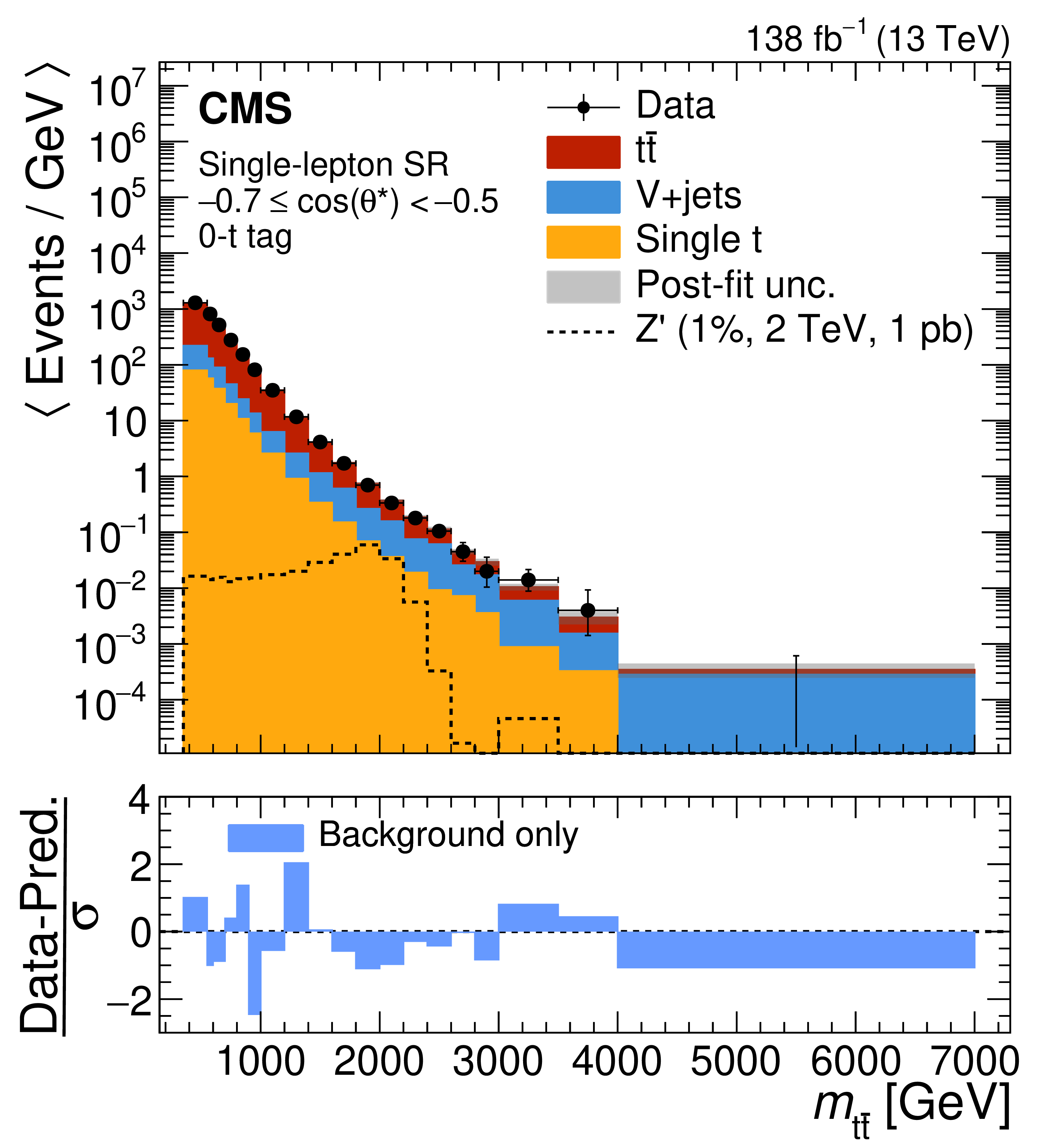
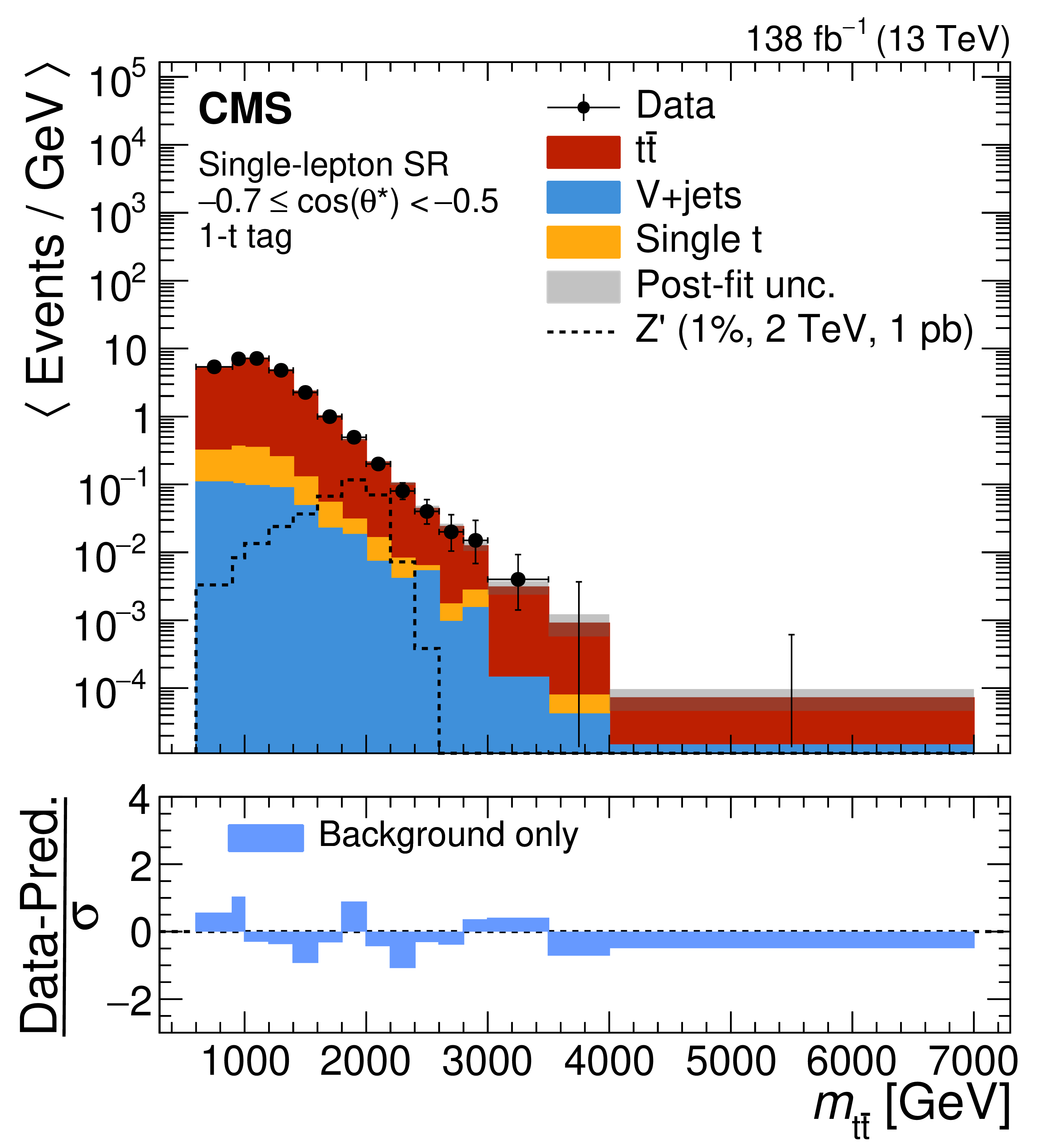
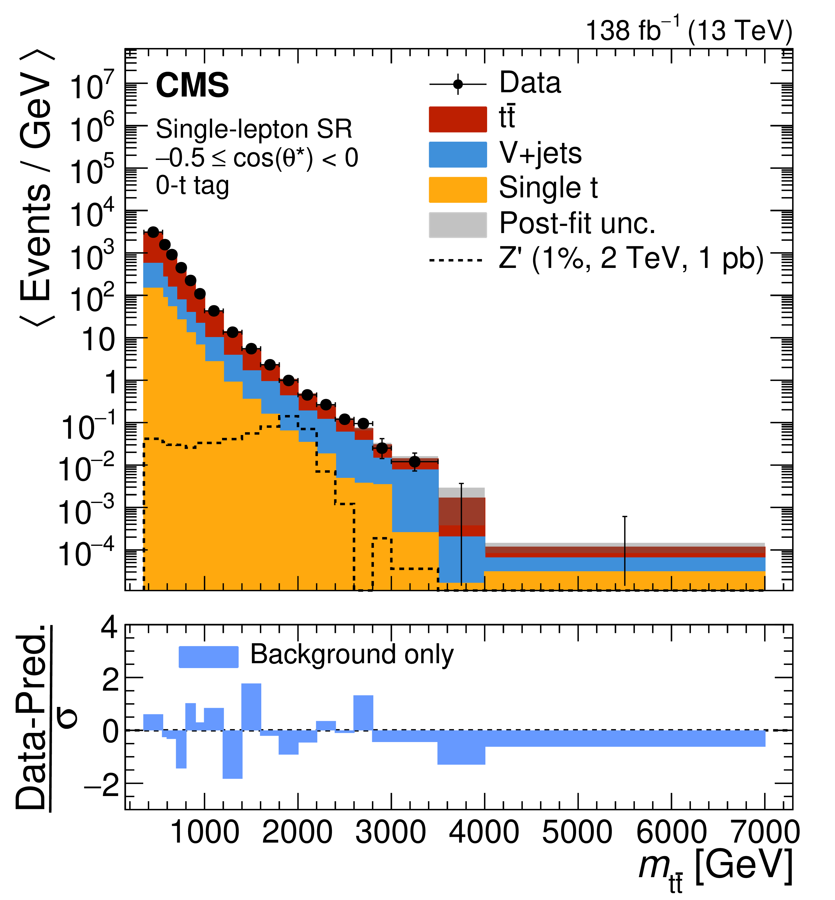
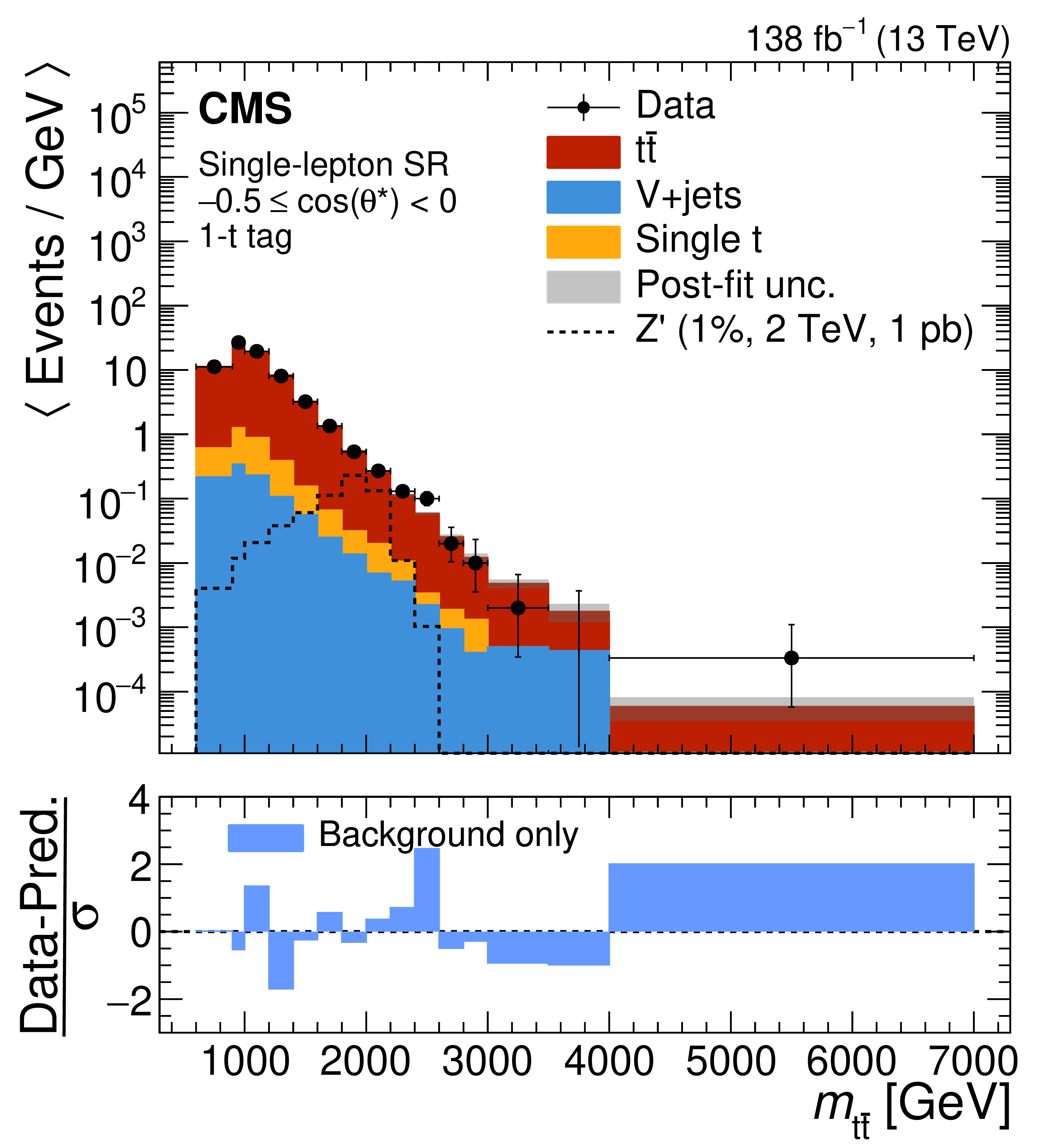
Figure 11:
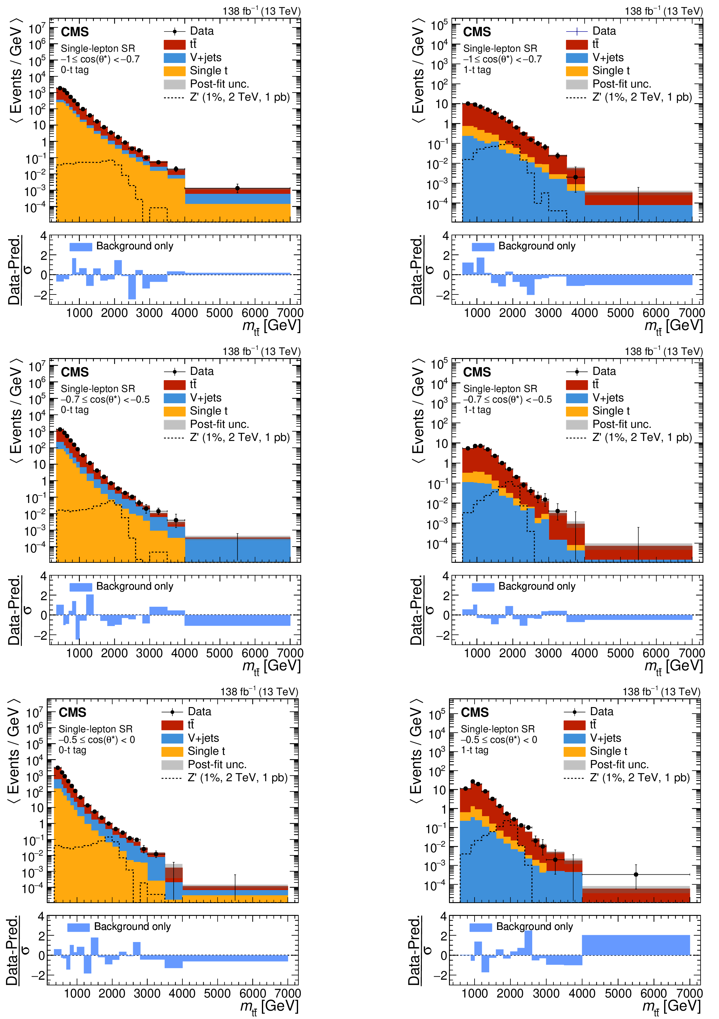
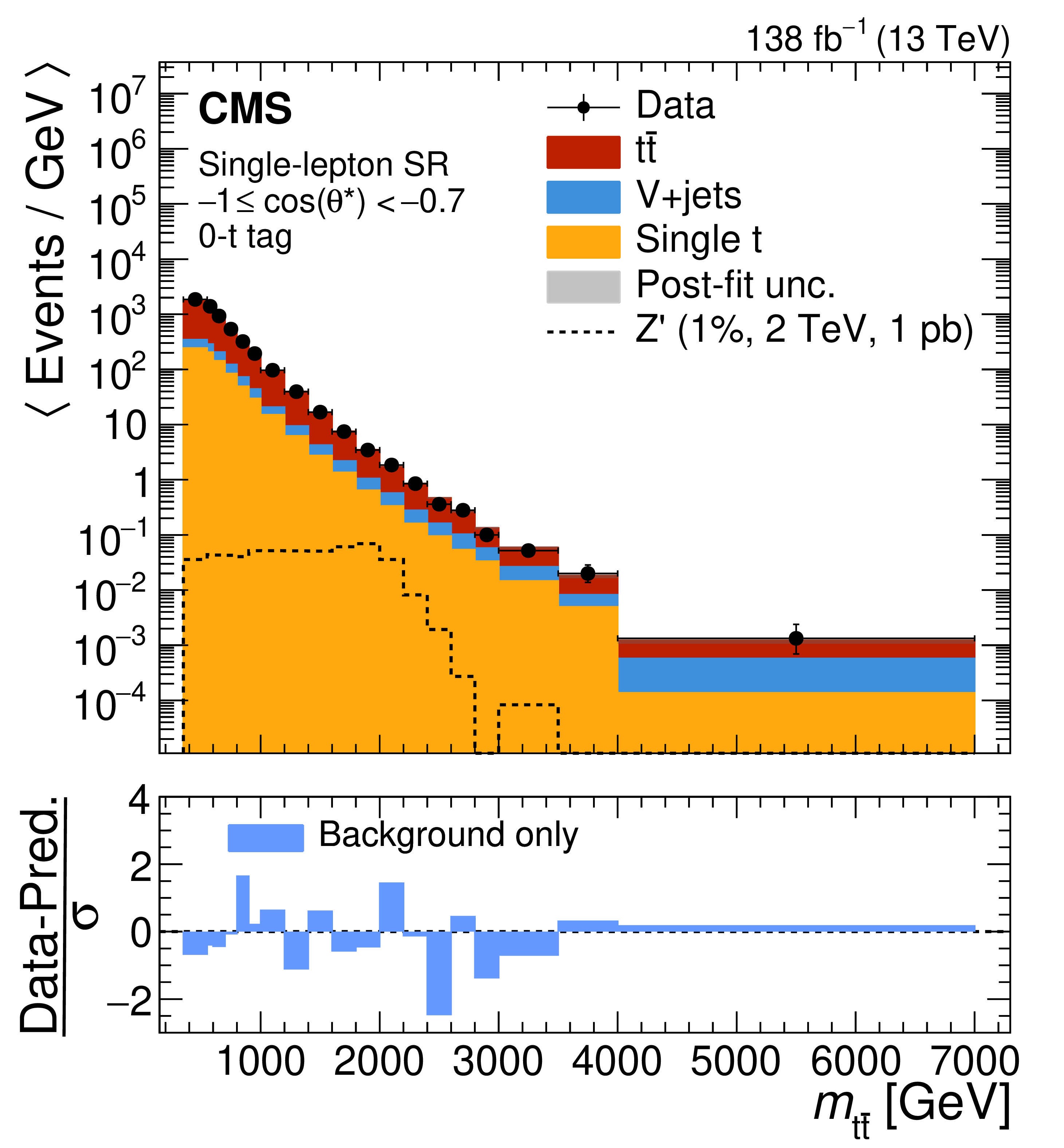
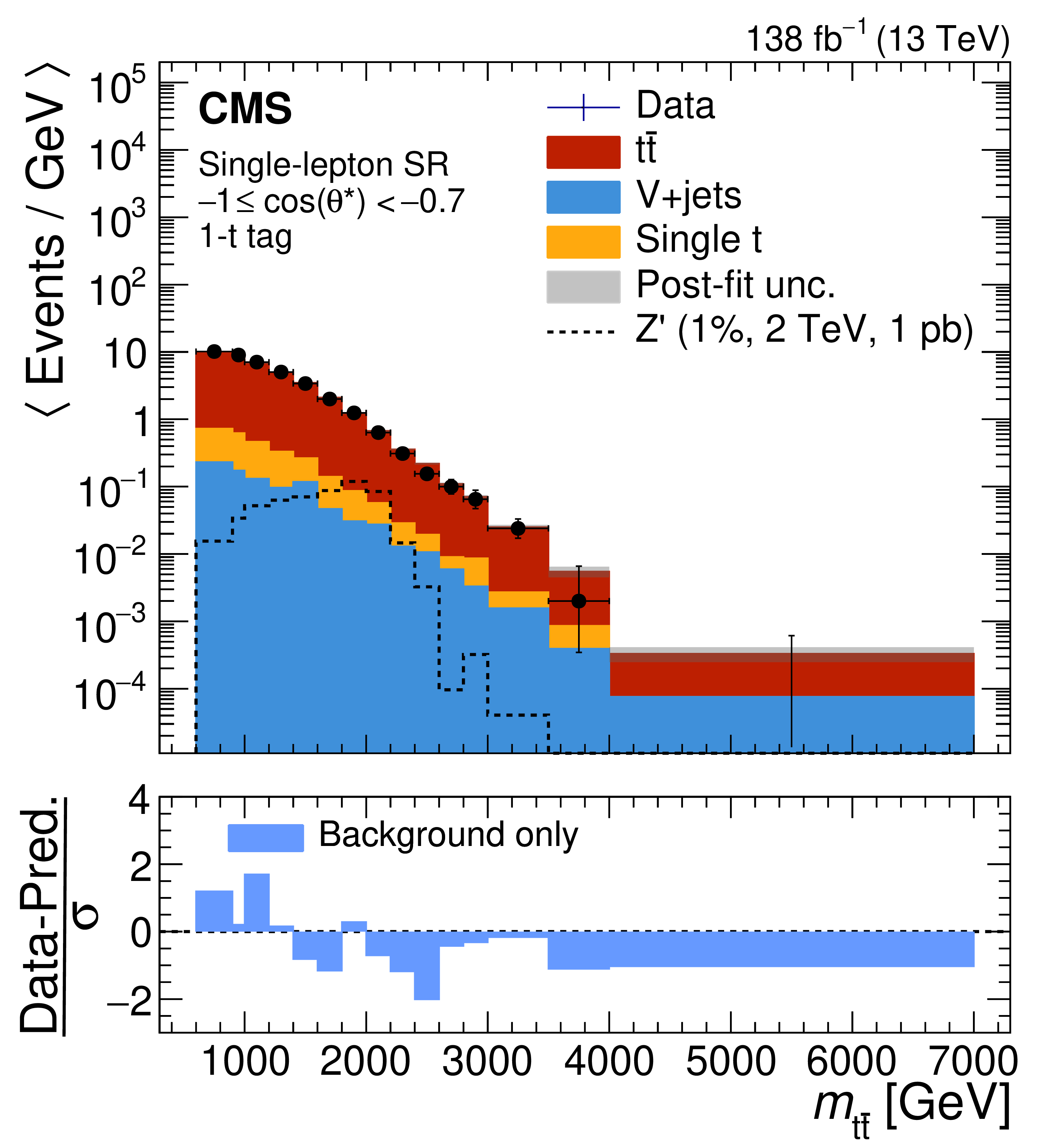
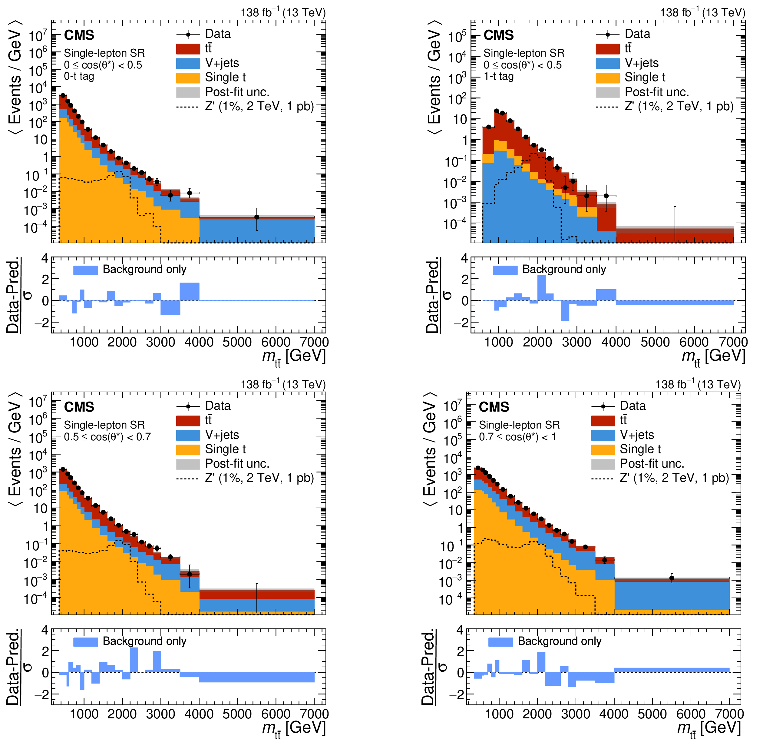
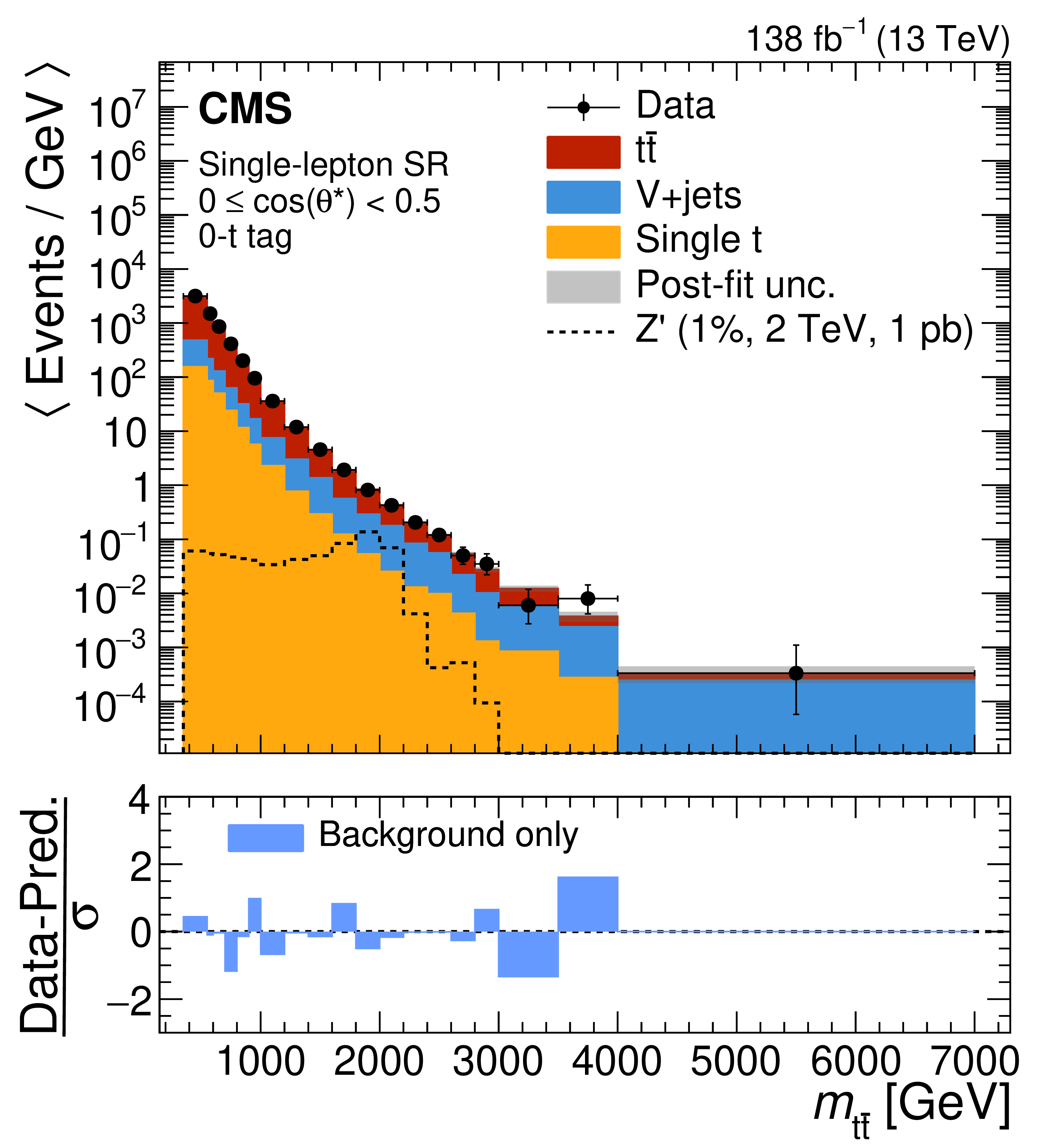
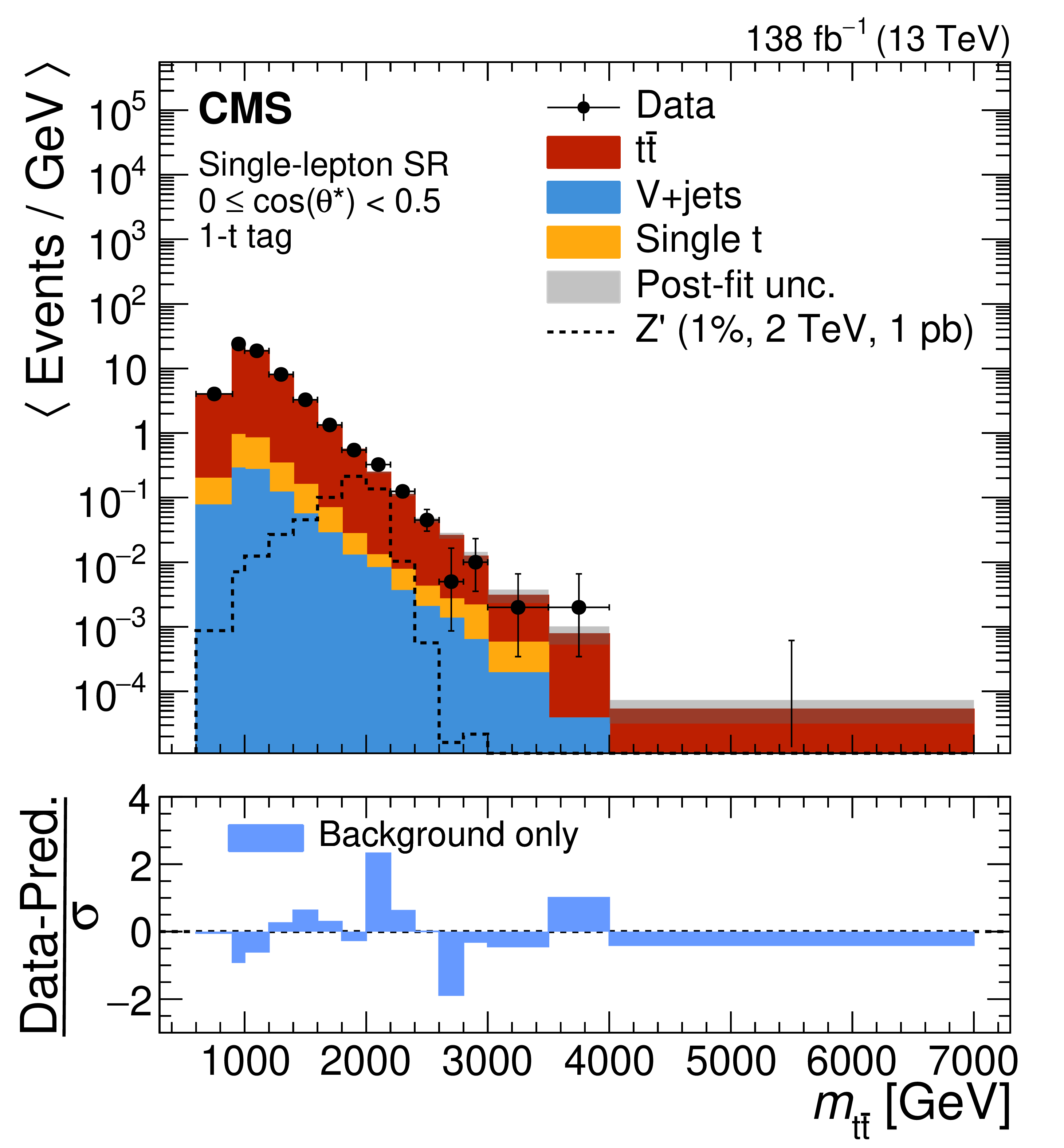
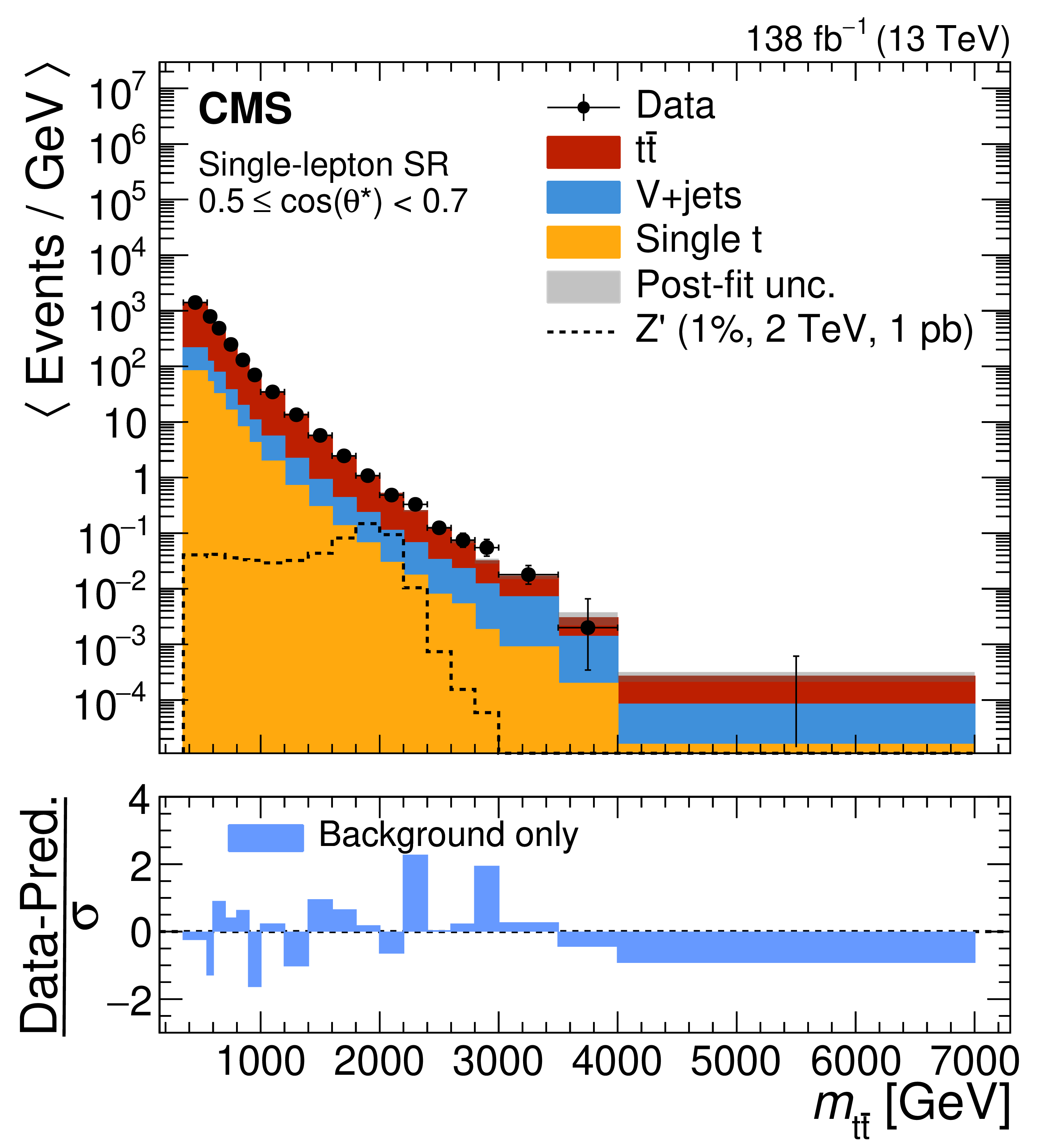
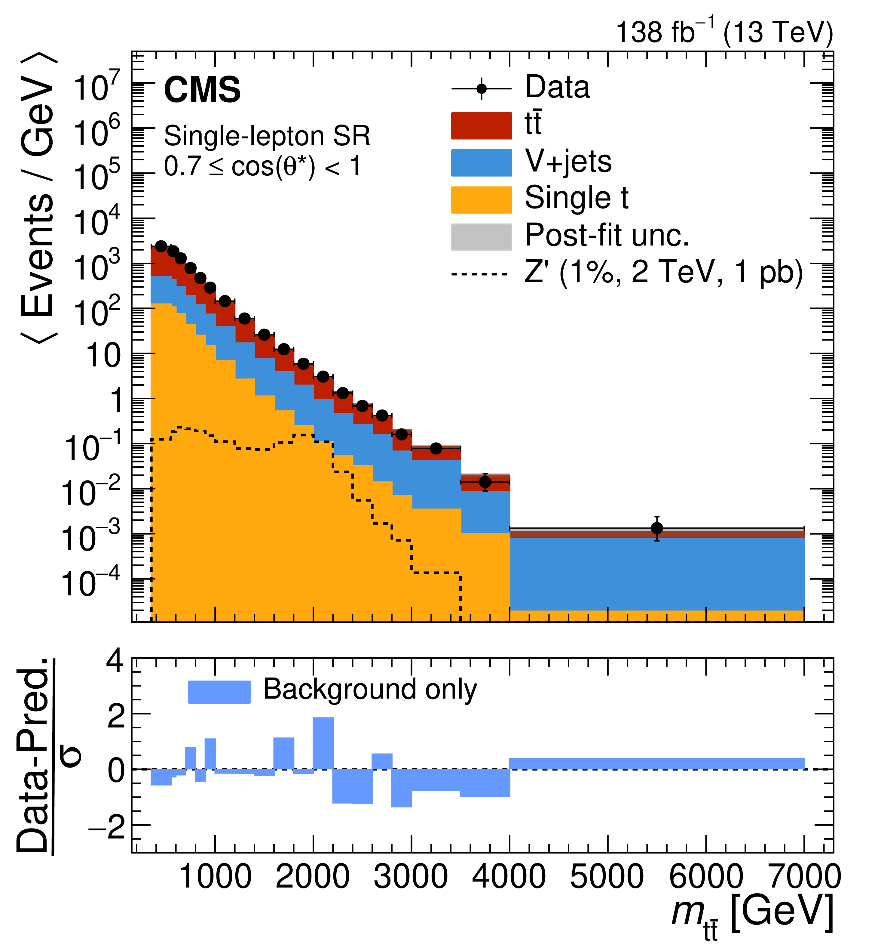
Postfit distributions in $ m_{{\mathrm{t}\overline{\mathrm{t}}} } $ in the single-lepton channel for data and simulation in the first three bins of $ \cos(\theta^\ast) $ in the $ \mathrm{t} \overline{\mathrm{t}} $ SR, shown for the resolved (0 t \text{tag}, left) and merged (1 t \text{tag}, right) categories, under the background-only hypothesis. The horizontal bars on the data points indicate the bin width. For illustrative purposes, the $ \mathrm{Z}^{'} $ boson signal with a relative width of 1% and a mass of 2 TeV is normalized to a cross section of 1\unitpb and overlaid to the backgrounds. The lower panels show the pulls, defined as ((Data-Prediction)$/\sigma $, where $ \sigma $ denotes the total postfit uncertainty in each bin, relative to the SM prediction. |
png pdf |
Figure 11-a:
Postfit distributions in $ m_{{\mathrm{t}\overline{\mathrm{t}}} } $ in the single-lepton channel for data and simulation in the first three bins of $ \cos(\theta^\ast) $ in the $ \mathrm{t} \overline{\mathrm{t}} $ SR, shown for the resolved (0 t \text{tag}, left) and merged (1 t \text{tag}, right) categories, under the background-only hypothesis. The horizontal bars on the data points indicate the bin width. For illustrative purposes, the $ \mathrm{Z}^{'} $ boson signal with a relative width of 1% and a mass of 2 TeV is normalized to a cross section of 1\unitpb and overlaid to the backgrounds. The lower panels show the pulls, defined as ((Data-Prediction)$/\sigma $, where $ \sigma $ denotes the total postfit uncertainty in each bin, relative to the SM prediction. |
png pdf |
Figure 11-b:
Postfit distributions in $ m_{{\mathrm{t}\overline{\mathrm{t}}} } $ in the single-lepton channel for data and simulation in the first three bins of $ \cos(\theta^\ast) $ in the $ \mathrm{t} \overline{\mathrm{t}} $ SR, shown for the resolved (0 t \text{tag}, left) and merged (1 t \text{tag}, right) categories, under the background-only hypothesis. The horizontal bars on the data points indicate the bin width. For illustrative purposes, the $ \mathrm{Z}^{'} $ boson signal with a relative width of 1% and a mass of 2 TeV is normalized to a cross section of 1\unitpb and overlaid to the backgrounds. The lower panels show the pulls, defined as ((Data-Prediction)$/\sigma $, where $ \sigma $ denotes the total postfit uncertainty in each bin, relative to the SM prediction. |
png pdf |
Figure 11-c:
Postfit distributions in $ m_{{\mathrm{t}\overline{\mathrm{t}}} } $ in the single-lepton channel for data and simulation in the first three bins of $ \cos(\theta^\ast) $ in the $ \mathrm{t} \overline{\mathrm{t}} $ SR, shown for the resolved (0 t \text{tag}, left) and merged (1 t \text{tag}, right) categories, under the background-only hypothesis. The horizontal bars on the data points indicate the bin width. For illustrative purposes, the $ \mathrm{Z}^{'} $ boson signal with a relative width of 1% and a mass of 2 TeV is normalized to a cross section of 1\unitpb and overlaid to the backgrounds. The lower panels show the pulls, defined as ((Data-Prediction)$/\sigma $, where $ \sigma $ denotes the total postfit uncertainty in each bin, relative to the SM prediction. |
png pdf |
Figure 11-d:
Postfit distributions in $ m_{{\mathrm{t}\overline{\mathrm{t}}} } $ in the single-lepton channel for data and simulation in the first three bins of $ \cos(\theta^\ast) $ in the $ \mathrm{t} \overline{\mathrm{t}} $ SR, shown for the resolved (0 t \text{tag}, left) and merged (1 t \text{tag}, right) categories, under the background-only hypothesis. The horizontal bars on the data points indicate the bin width. For illustrative purposes, the $ \mathrm{Z}^{'} $ boson signal with a relative width of 1% and a mass of 2 TeV is normalized to a cross section of 1\unitpb and overlaid to the backgrounds. The lower panels show the pulls, defined as ((Data-Prediction)$/\sigma $, where $ \sigma $ denotes the total postfit uncertainty in each bin, relative to the SM prediction. |
png pdf |
Figure 11-e:
Postfit distributions in $ m_{{\mathrm{t}\overline{\mathrm{t}}} } $ in the single-lepton channel for data and simulation in the first three bins of $ \cos(\theta^\ast) $ in the $ \mathrm{t} \overline{\mathrm{t}} $ SR, shown for the resolved (0 t \text{tag}, left) and merged (1 t \text{tag}, right) categories, under the background-only hypothesis. The horizontal bars on the data points indicate the bin width. For illustrative purposes, the $ \mathrm{Z}^{'} $ boson signal with a relative width of 1% and a mass of 2 TeV is normalized to a cross section of 1\unitpb and overlaid to the backgrounds. The lower panels show the pulls, defined as ((Data-Prediction)$/\sigma $, where $ \sigma $ denotes the total postfit uncertainty in each bin, relative to the SM prediction. |
png pdf |
Figure 11-f:
Postfit distributions in $ m_{{\mathrm{t}\overline{\mathrm{t}}} } $ in the single-lepton channel for data and simulation in the first three bins of $ \cos(\theta^\ast) $ in the $ \mathrm{t} \overline{\mathrm{t}} $ SR, shown for the resolved (0 t \text{tag}, left) and merged (1 t \text{tag}, right) categories, under the background-only hypothesis. The horizontal bars on the data points indicate the bin width. For illustrative purposes, the $ \mathrm{Z}^{'} $ boson signal with a relative width of 1% and a mass of 2 TeV is normalized to a cross section of 1\unitpb and overlaid to the backgrounds. The lower panels show the pulls, defined as ((Data-Prediction)$/\sigma $, where $ \sigma $ denotes the total postfit uncertainty in each bin, relative to the SM prediction. |
png pdf |
Figure 12:
Postfit distributions in $ m_{{\mathrm{t}\overline{\mathrm{t}}} } $ in the single-lepton channel for data and simulation in the last three bins of $ \cos(\theta^\ast) $ in the $ \mathrm{t} \overline{\mathrm{t}} $ SR, shown for the resolved (0 t \text{tag}, left) and merged (1 t \text{tag}, right) categories, under the background-only hypothesis. The horizontal bars on the data points indicate the bin width. In the last two $ \cos(\theta^\ast) $ bins (lower row) the resolved and merged categories are combined. For illustrative purposes, the $ \mathrm{Z}^{'} $ boson signal with a relative width of 1% and a mass of 2 TeV is normalized to a cross section of 1\unitpb and overlaid to the backgrounds. The lower panels show the pulls, defined as (Data-Prediction)/\sigma $, where $ \sigma $ denotes the total postfit uncertainty in each bin, relative to the SM prediction. |
png pdf |
Figure 12-a:
Postfit distributions in $ m_{{\mathrm{t}\overline{\mathrm{t}}} } $ in the single-lepton channel for data and simulation in the last three bins of $ \cos(\theta^\ast) $ in the $ \mathrm{t} \overline{\mathrm{t}} $ SR, shown for the resolved (0 t \text{tag}, left) and merged (1 t \text{tag}, right) categories, under the background-only hypothesis. The horizontal bars on the data points indicate the bin width. In the last two $ \cos(\theta^\ast) $ bins (lower row) the resolved and merged categories are combined. For illustrative purposes, the $ \mathrm{Z}^{'} $ boson signal with a relative width of 1% and a mass of 2 TeV is normalized to a cross section of 1\unitpb and overlaid to the backgrounds. The lower panels show the pulls, defined as (Data-Prediction)/\sigma $, where $ \sigma $ denotes the total postfit uncertainty in each bin, relative to the SM prediction. |
png pdf |
Figure 12-b:
Postfit distributions in $ m_{{\mathrm{t}\overline{\mathrm{t}}} } $ in the single-lepton channel for data and simulation in the last three bins of $ \cos(\theta^\ast) $ in the $ \mathrm{t} \overline{\mathrm{t}} $ SR, shown for the resolved (0 t \text{tag}, left) and merged (1 t \text{tag}, right) categories, under the background-only hypothesis. The horizontal bars on the data points indicate the bin width. In the last two $ \cos(\theta^\ast) $ bins (lower row) the resolved and merged categories are combined. For illustrative purposes, the $ \mathrm{Z}^{'} $ boson signal with a relative width of 1% and a mass of 2 TeV is normalized to a cross section of 1\unitpb and overlaid to the backgrounds. The lower panels show the pulls, defined as (Data-Prediction)/\sigma $, where $ \sigma $ denotes the total postfit uncertainty in each bin, relative to the SM prediction. |
png pdf |
Figure 12-c:
Postfit distributions in $ m_{{\mathrm{t}\overline{\mathrm{t}}} } $ in the single-lepton channel for data and simulation in the last three bins of $ \cos(\theta^\ast) $ in the $ \mathrm{t} \overline{\mathrm{t}} $ SR, shown for the resolved (0 t \text{tag}, left) and merged (1 t \text{tag}, right) categories, under the background-only hypothesis. The horizontal bars on the data points indicate the bin width. In the last two $ \cos(\theta^\ast) $ bins (lower row) the resolved and merged categories are combined. For illustrative purposes, the $ \mathrm{Z}^{'} $ boson signal with a relative width of 1% and a mass of 2 TeV is normalized to a cross section of 1\unitpb and overlaid to the backgrounds. The lower panels show the pulls, defined as (Data-Prediction)/\sigma $, where $ \sigma $ denotes the total postfit uncertainty in each bin, relative to the SM prediction. |
png pdf |
Figure 12-d:
Postfit distributions in $ m_{{\mathrm{t}\overline{\mathrm{t}}} } $ in the single-lepton channel for data and simulation in the last three bins of $ \cos(\theta^\ast) $ in the $ \mathrm{t} \overline{\mathrm{t}} $ SR, shown for the resolved (0 t \text{tag}, left) and merged (1 t \text{tag}, right) categories, under the background-only hypothesis. The horizontal bars on the data points indicate the bin width. In the last two $ \cos(\theta^\ast) $ bins (lower row) the resolved and merged categories are combined. For illustrative purposes, the $ \mathrm{Z}^{'} $ boson signal with a relative width of 1% and a mass of 2 TeV is normalized to a cross section of 1\unitpb and overlaid to the backgrounds. The lower panels show the pulls, defined as (Data-Prediction)/\sigma $, where $ \sigma $ denotes the total postfit uncertainty in each bin, relative to the SM prediction. |
png pdf |
Figure 13:
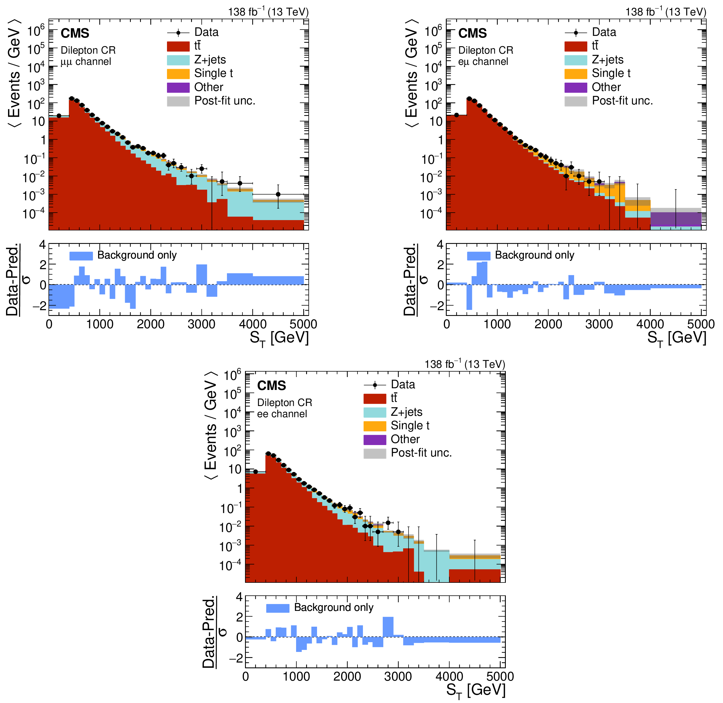
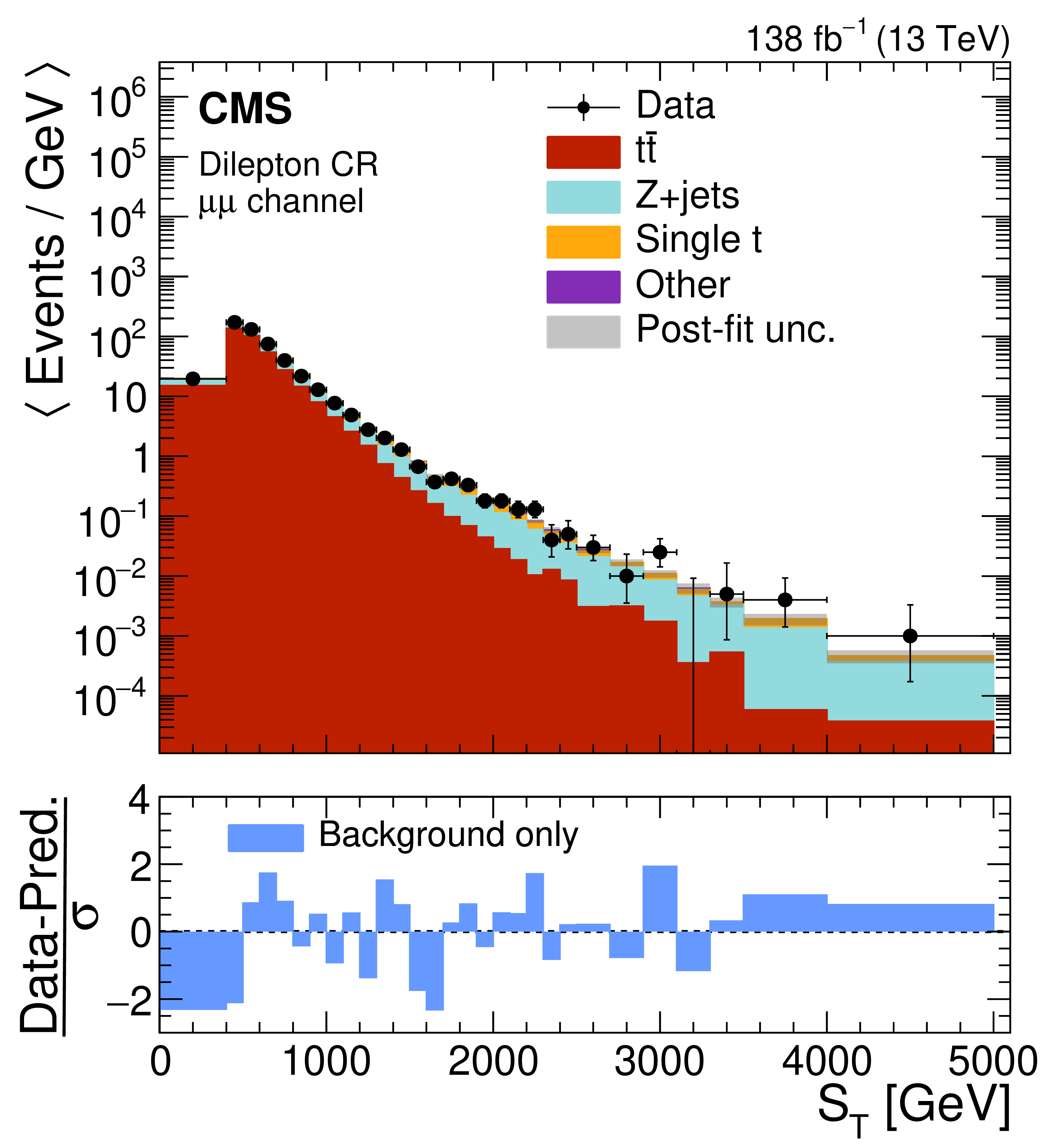
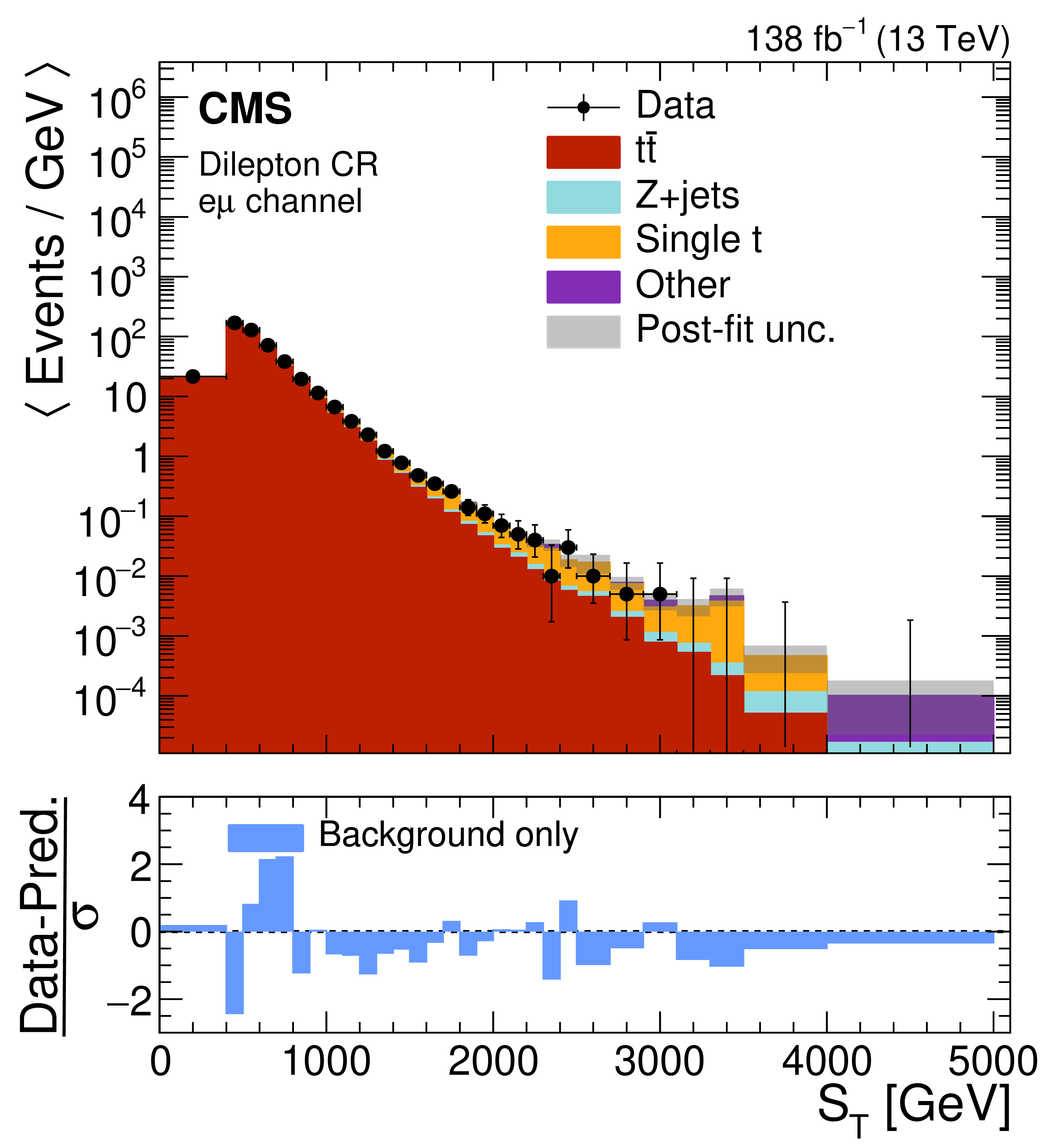
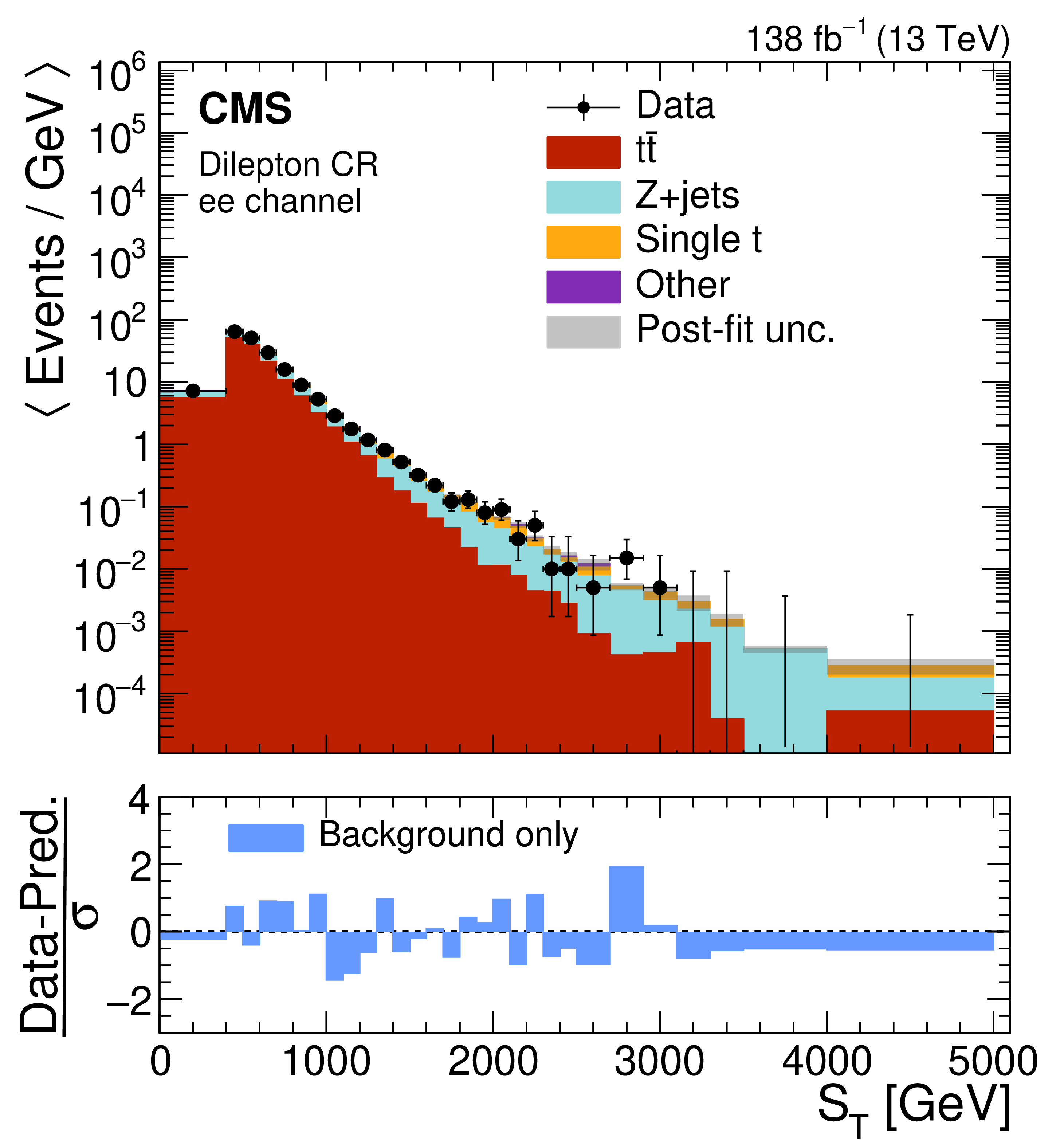
Postfit distributions in $ S_{\mathrm{T}} $ for data and simulation in the CR for the dilepton channel. Distributions are shown for the $ \mu\mu $ (upper left), $ \mathrm{e}\mu $ (upper right), and $ \mathrm{e}\mathrm{e} $ (lower) channels, under the background-only hypothesis. The horizontal bars on the data points indicate the bin width. The lower panels show the pulls, defined as (Data-Prediction)$/\sigma$, where $\sigma$ denotes the total postfit uncertainty in each bin, relative to the SM prediction. |
png pdf |
Figure 13-a:
Postfit distributions in $ S_{\mathrm{T}} $ for data and simulation in the CR for the dilepton channel. Distributions are shown for the $ \mu\mu $ (upper left), $ \mathrm{e}\mu $ (upper right), and $ \mathrm{e}\mathrm{e} $ (lower) channels, under the background-only hypothesis. The horizontal bars on the data points indicate the bin width. The lower panels show the pulls, defined as (Data-Prediction)$/\sigma$, where $\sigma$ denotes the total postfit uncertainty in each bin, relative to the SM prediction. |
png pdf |
Figure 13-b:
Postfit distributions in $ S_{\mathrm{T}} $ for data and simulation in the CR for the dilepton channel. Distributions are shown for the $ \mu\mu $ (upper left), $ \mathrm{e}\mu $ (upper right), and $ \mathrm{e}\mathrm{e} $ (lower) channels, under the background-only hypothesis. The horizontal bars on the data points indicate the bin width. The lower panels show the pulls, defined as (Data-Prediction)$/\sigma$, where $\sigma$ denotes the total postfit uncertainty in each bin, relative to the SM prediction. |
png pdf |
Figure 13-c:
Postfit distributions in $ S_{\mathrm{T}} $ for data and simulation in the CR for the dilepton channel. Distributions are shown for the $ \mu\mu $ (upper left), $ \mathrm{e}\mu $ (upper right), and $ \mathrm{e}\mathrm{e} $ (lower) channels, under the background-only hypothesis. The horizontal bars on the data points indicate the bin width. The lower panels show the pulls, defined as (Data-Prediction)$/\sigma$, where $\sigma$ denotes the total postfit uncertainty in each bin, relative to the SM prediction. |
png pdf |
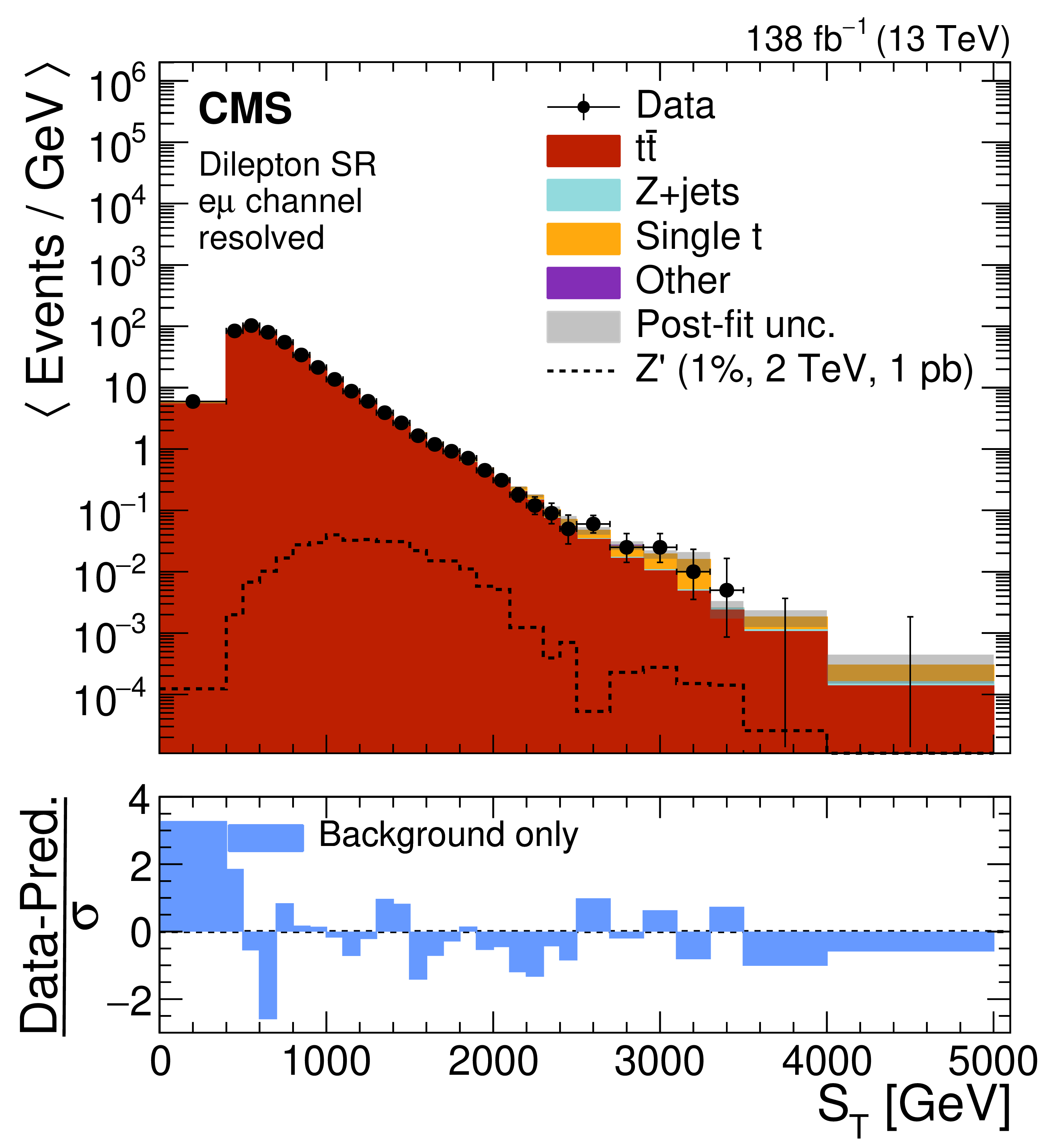
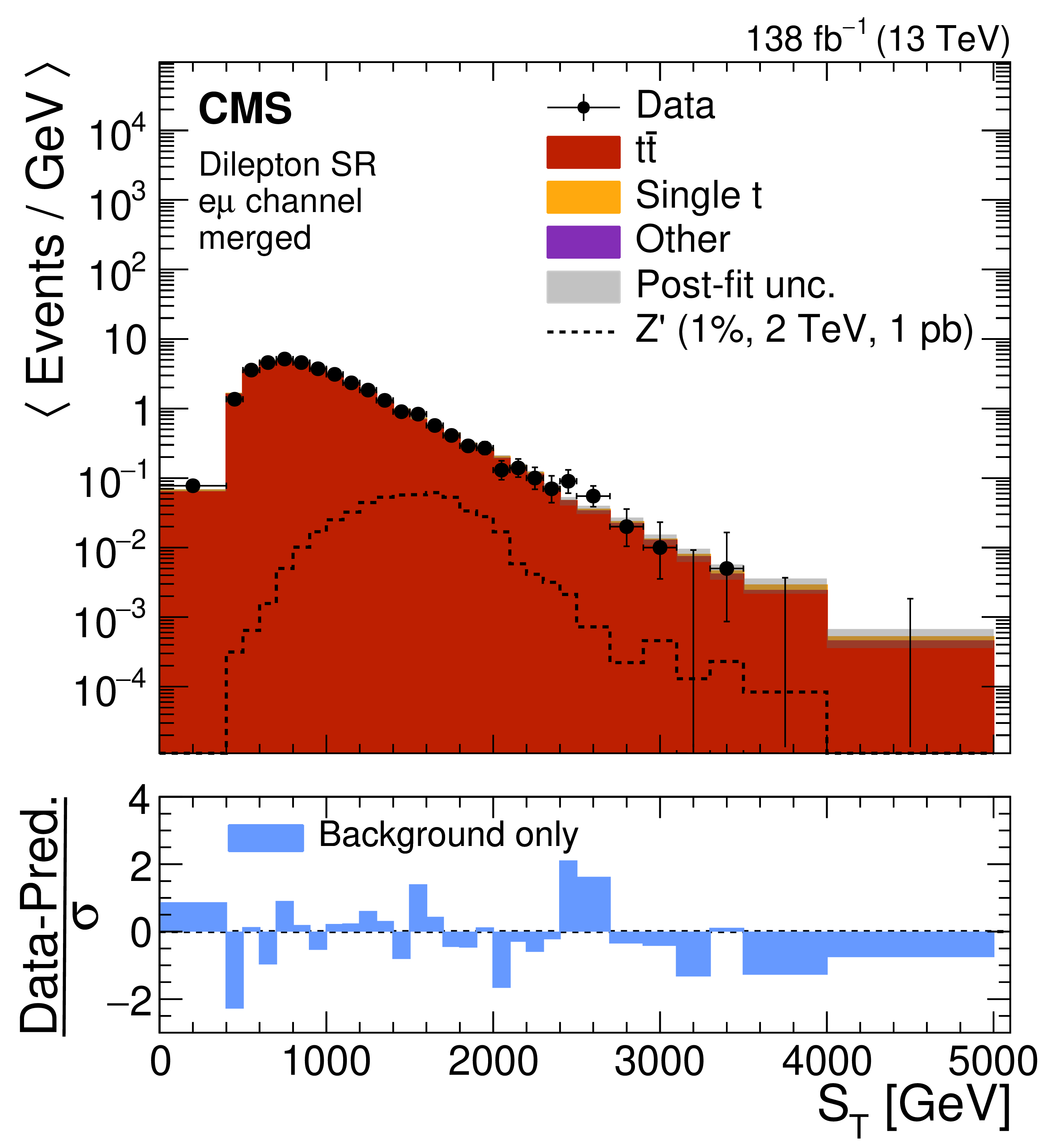
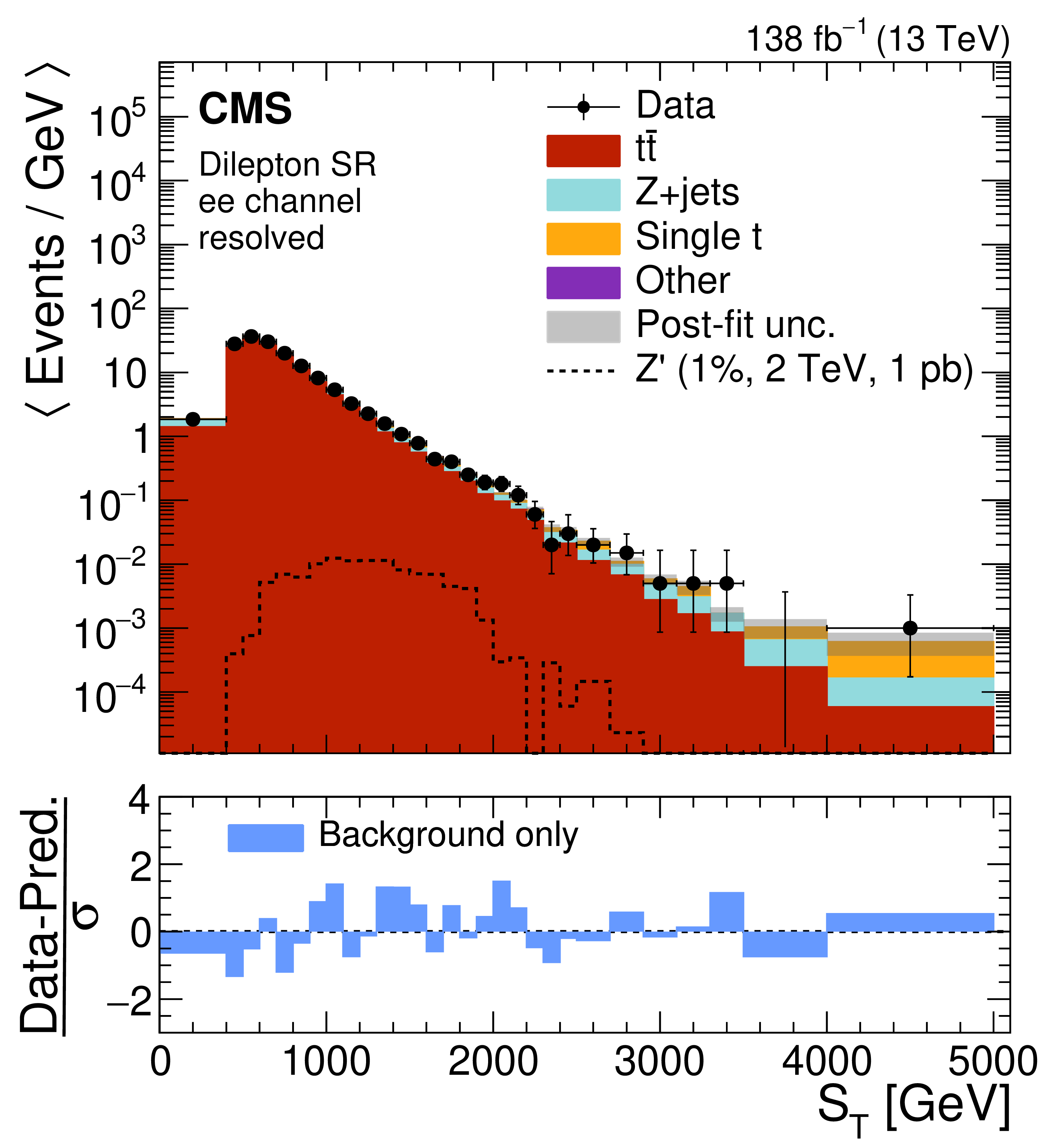
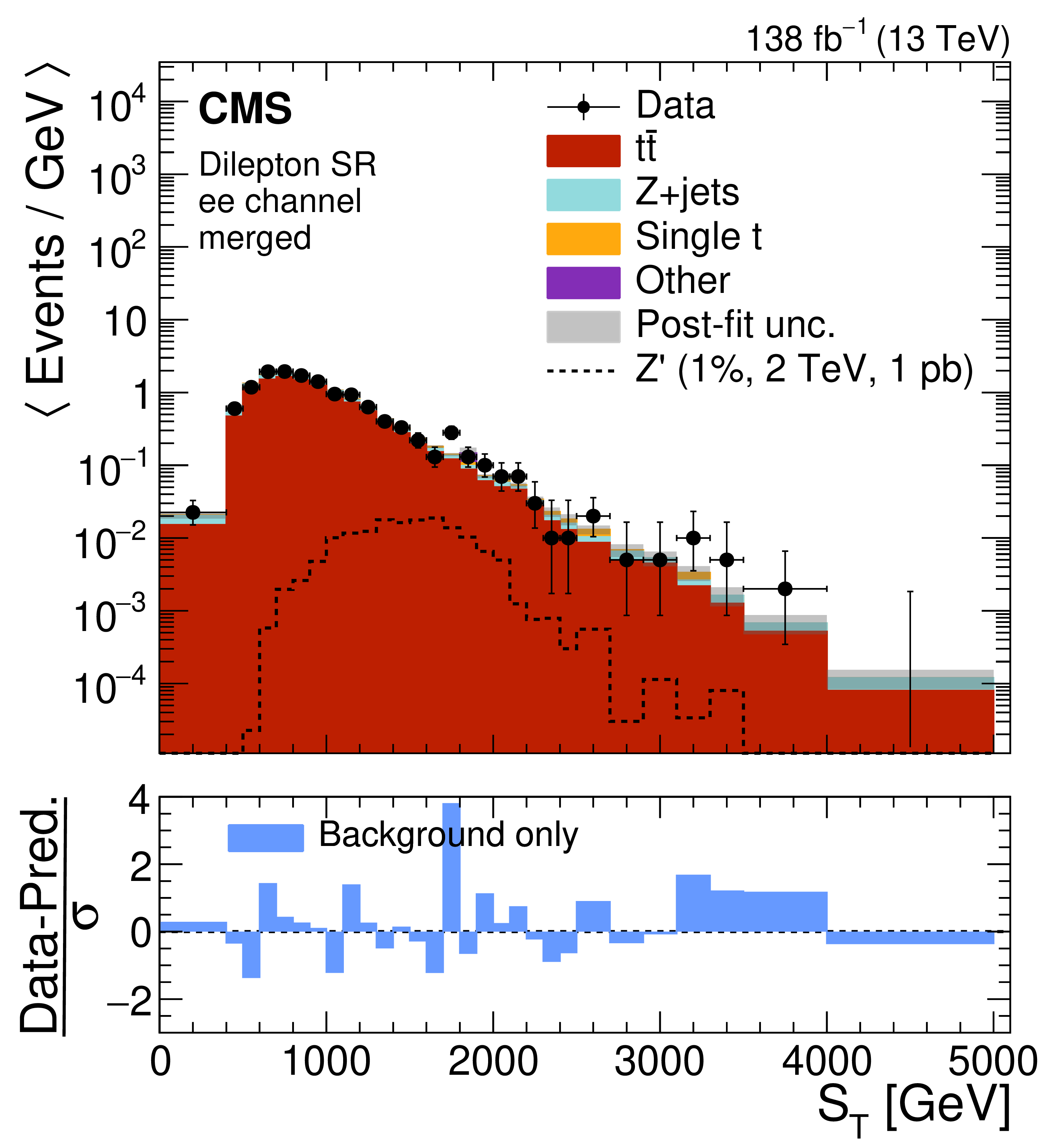
Figure 14:
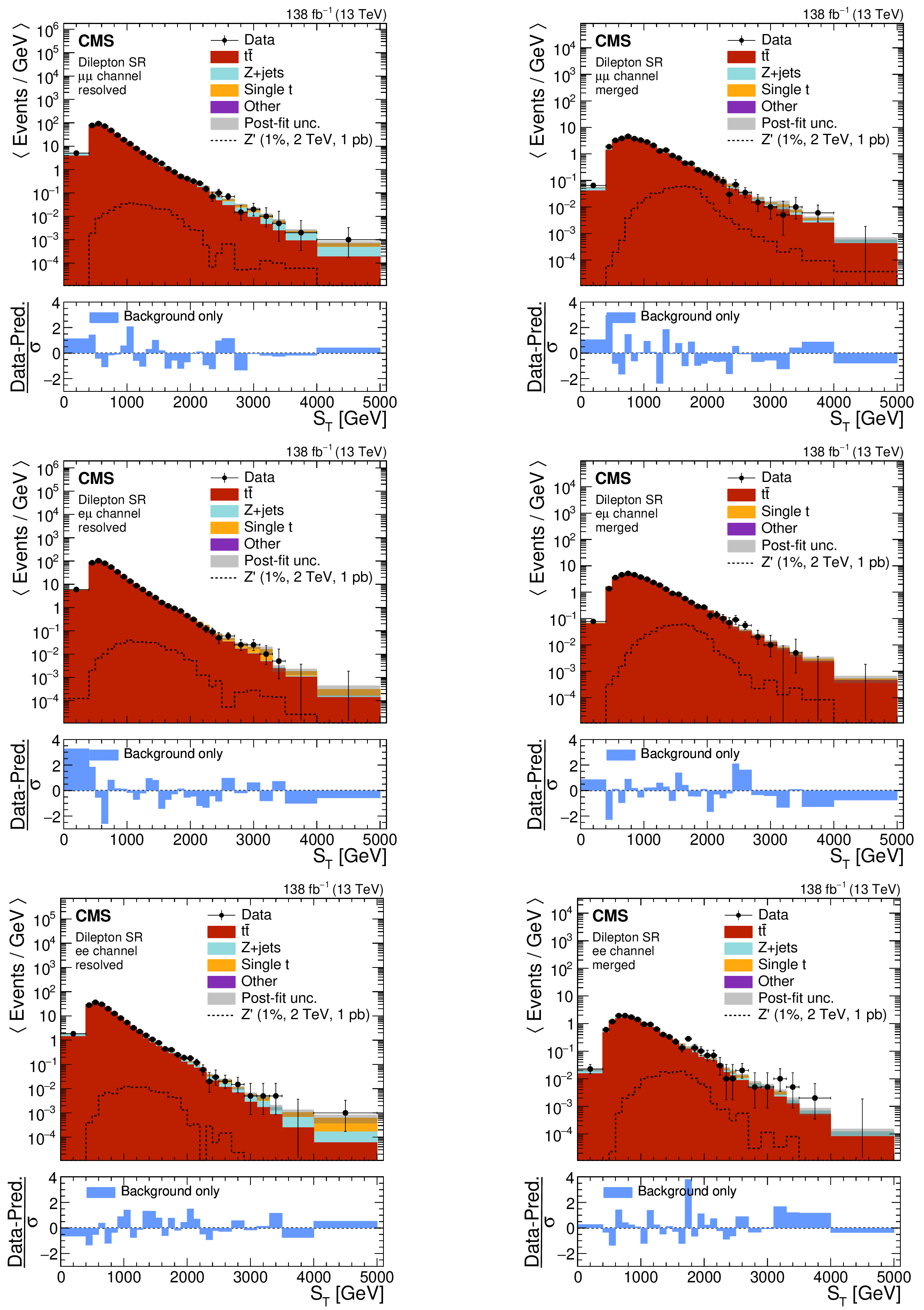
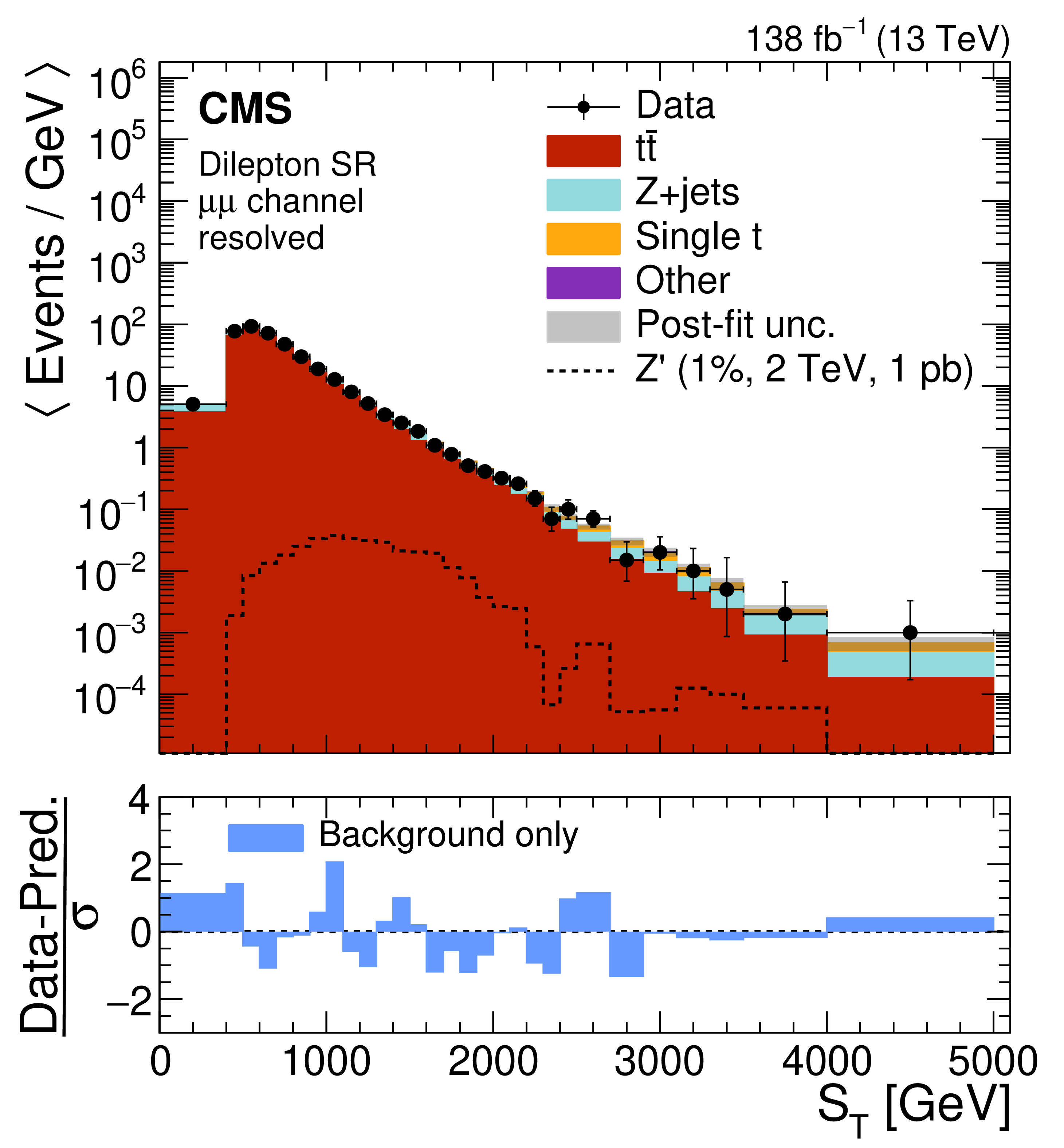
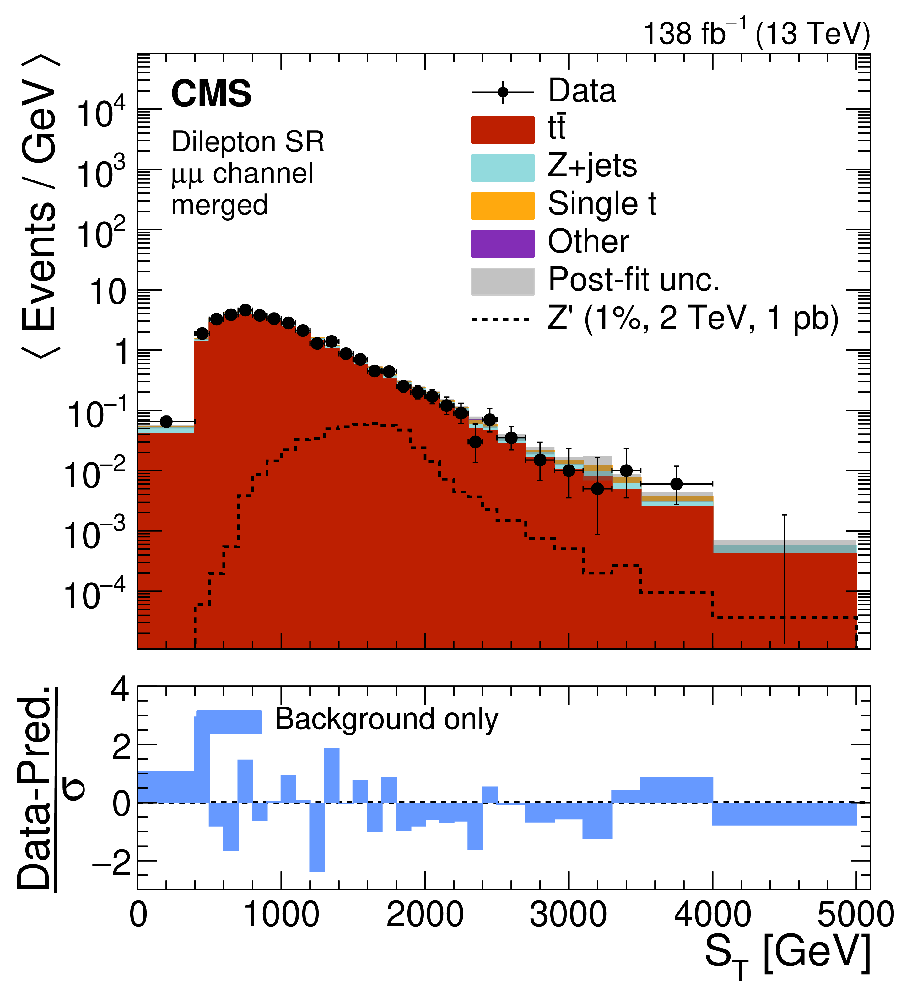
Postfit distributions in $ S_{\mathrm{T}} $ for data and simulation for the resolved (left) and merged (right) categories for the dilepton channel. Distributions are shown for the $ \mu\mu $ (upper), $ \mathrm{e}\mu $ (middle), and $ \mathrm{e}\mathrm{e} $ (lower) channels, under the background-only hypothesis. The horizontal bars on the data points indicate the bin width. For illustrative purposes, the $ \mathrm{Z}^{'} $ boson signal with a relative width of 1% and a mass of 2 TeV is normalized to a cross section of 1 pb and overlaid to the backgrounds. The lower panels show the pulls, defined as (Data-Prediction)$/\sigma$, where $ \sigma$ denotes the total postfit uncertainty in each bin, relative to the SM prediction. |
png pdf |
Figure 14-a:
Postfit distributions in $ S_{\mathrm{T}} $ for data and simulation for the resolved (left) and merged (right) categories for the dilepton channel. Distributions are shown for the $ \mu\mu $ (upper), $ \mathrm{e}\mu $ (middle), and $ \mathrm{e}\mathrm{e} $ (lower) channels, under the background-only hypothesis. The horizontal bars on the data points indicate the bin width. For illustrative purposes, the $ \mathrm{Z}^{'} $ boson signal with a relative width of 1% and a mass of 2 TeV is normalized to a cross section of 1 pb and overlaid to the backgrounds. The lower panels show the pulls, defined as (Data-Prediction)$/\sigma$, where $ \sigma$ denotes the total postfit uncertainty in each bin, relative to the SM prediction. |
png pdf |
Figure 14-b:
Postfit distributions in $ S_{\mathrm{T}} $ for data and simulation for the resolved (left) and merged (right) categories for the dilepton channel. Distributions are shown for the $ \mu\mu $ (upper), $ \mathrm{e}\mu $ (middle), and $ \mathrm{e}\mathrm{e} $ (lower) channels, under the background-only hypothesis. The horizontal bars on the data points indicate the bin width. For illustrative purposes, the $ \mathrm{Z}^{'} $ boson signal with a relative width of 1% and a mass of 2 TeV is normalized to a cross section of 1 pb and overlaid to the backgrounds. The lower panels show the pulls, defined as (Data-Prediction)$/\sigma$, where $ \sigma$ denotes the total postfit uncertainty in each bin, relative to the SM prediction. |
png pdf |
Figure 14-c:
Postfit distributions in $ S_{\mathrm{T}} $ for data and simulation for the resolved (left) and merged (right) categories for the dilepton channel. Distributions are shown for the $ \mu\mu $ (upper), $ \mathrm{e}\mu $ (middle), and $ \mathrm{e}\mathrm{e} $ (lower) channels, under the background-only hypothesis. The horizontal bars on the data points indicate the bin width. For illustrative purposes, the $ \mathrm{Z}^{'} $ boson signal with a relative width of 1% and a mass of 2 TeV is normalized to a cross section of 1 pb and overlaid to the backgrounds. The lower panels show the pulls, defined as (Data-Prediction)$/\sigma$, where $ \sigma$ denotes the total postfit uncertainty in each bin, relative to the SM prediction. |
png pdf |
Figure 14-d:
Postfit distributions in $ S_{\mathrm{T}} $ for data and simulation for the resolved (left) and merged (right) categories for the dilepton channel. Distributions are shown for the $ \mu\mu $ (upper), $ \mathrm{e}\mu $ (middle), and $ \mathrm{e}\mathrm{e} $ (lower) channels, under the background-only hypothesis. The horizontal bars on the data points indicate the bin width. For illustrative purposes, the $ \mathrm{Z}^{'} $ boson signal with a relative width of 1% and a mass of 2 TeV is normalized to a cross section of 1 pb and overlaid to the backgrounds. The lower panels show the pulls, defined as (Data-Prediction)$/\sigma$, where $ \sigma$ denotes the total postfit uncertainty in each bin, relative to the SM prediction. |
png pdf |
Figure 14-e:
Postfit distributions in $ S_{\mathrm{T}} $ for data and simulation for the resolved (left) and merged (right) categories for the dilepton channel. Distributions are shown for the $ \mu\mu $ (upper), $ \mathrm{e}\mu $ (middle), and $ \mathrm{e}\mathrm{e} $ (lower) channels, under the background-only hypothesis. The horizontal bars on the data points indicate the bin width. For illustrative purposes, the $ \mathrm{Z}^{'} $ boson signal with a relative width of 1% and a mass of 2 TeV is normalized to a cross section of 1 pb and overlaid to the backgrounds. The lower panels show the pulls, defined as (Data-Prediction)$/\sigma$, where $ \sigma$ denotes the total postfit uncertainty in each bin, relative to the SM prediction. |
png pdf |
Figure 14-f:
Postfit distributions in $ S_{\mathrm{T}} $ for data and simulation for the resolved (left) and merged (right) categories for the dilepton channel. Distributions are shown for the $ \mu\mu $ (upper), $ \mathrm{e}\mu $ (middle), and $ \mathrm{e}\mathrm{e} $ (lower) channels, under the background-only hypothesis. The horizontal bars on the data points indicate the bin width. For illustrative purposes, the $ \mathrm{Z}^{'} $ boson signal with a relative width of 1% and a mass of 2 TeV is normalized to a cross section of 1 pb and overlaid to the backgrounds. The lower panels show the pulls, defined as (Data-Prediction)$/\sigma$, where $ \sigma$ denotes the total postfit uncertainty in each bin, relative to the SM prediction. |
png pdf |
Figure 15:
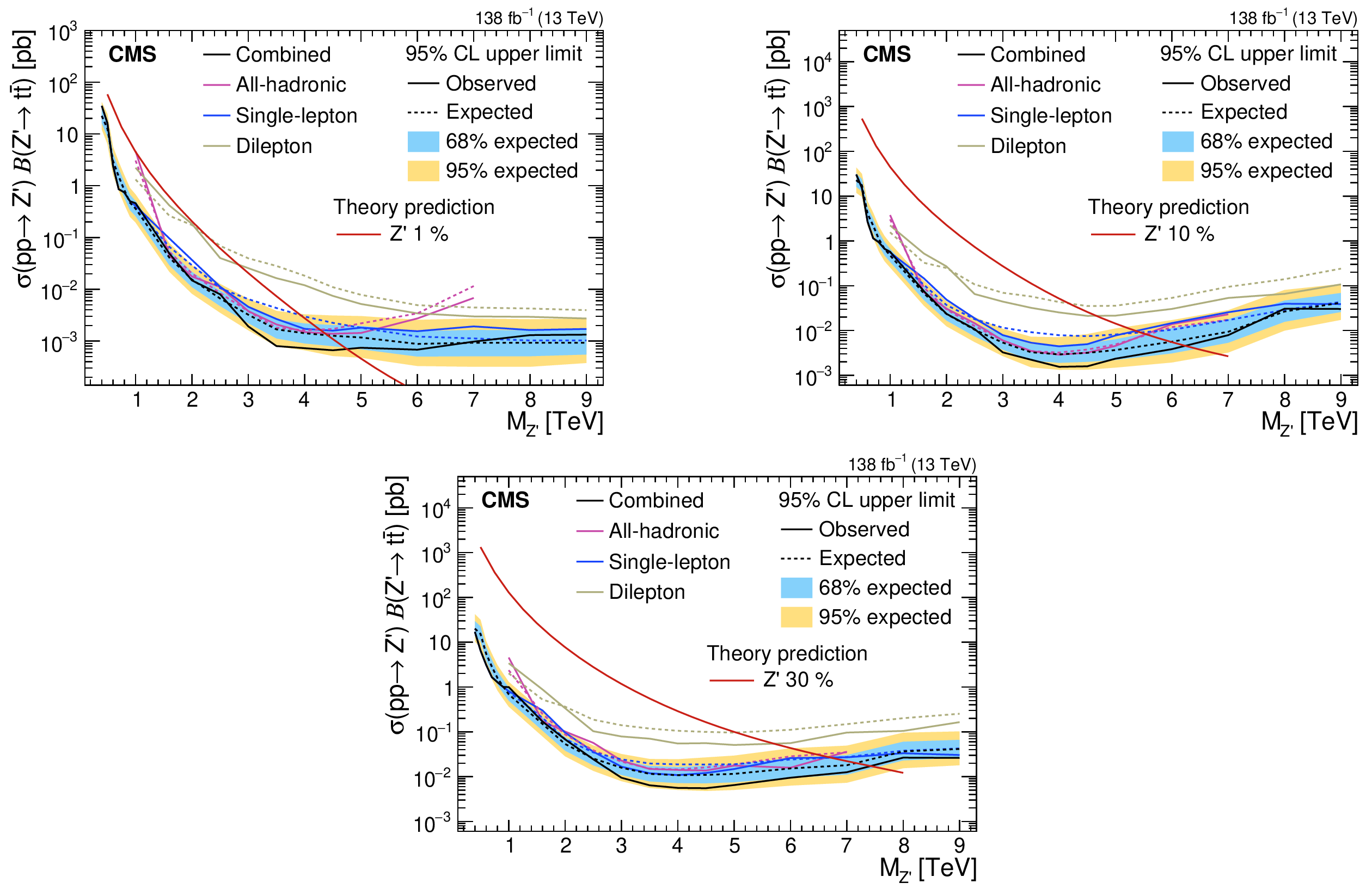
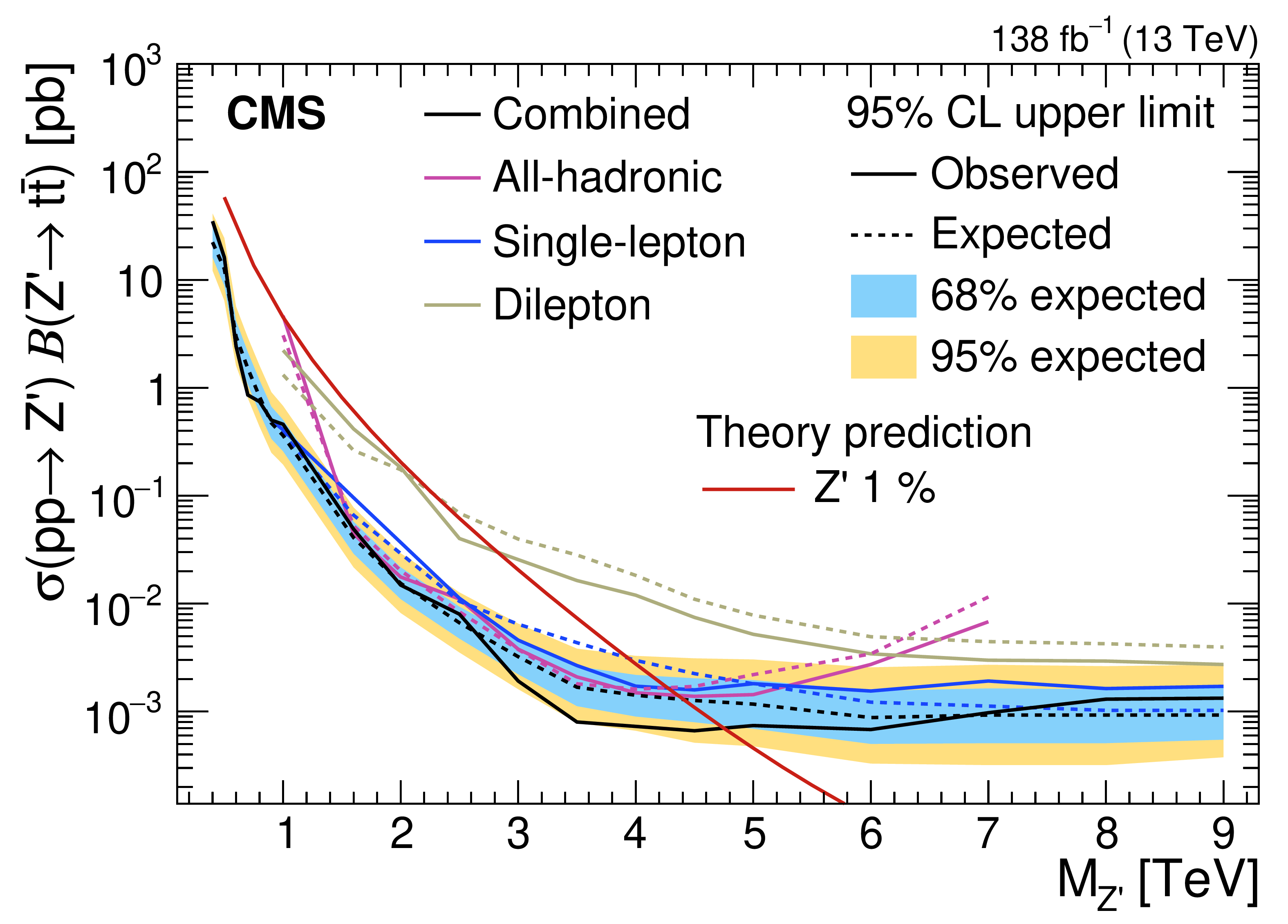
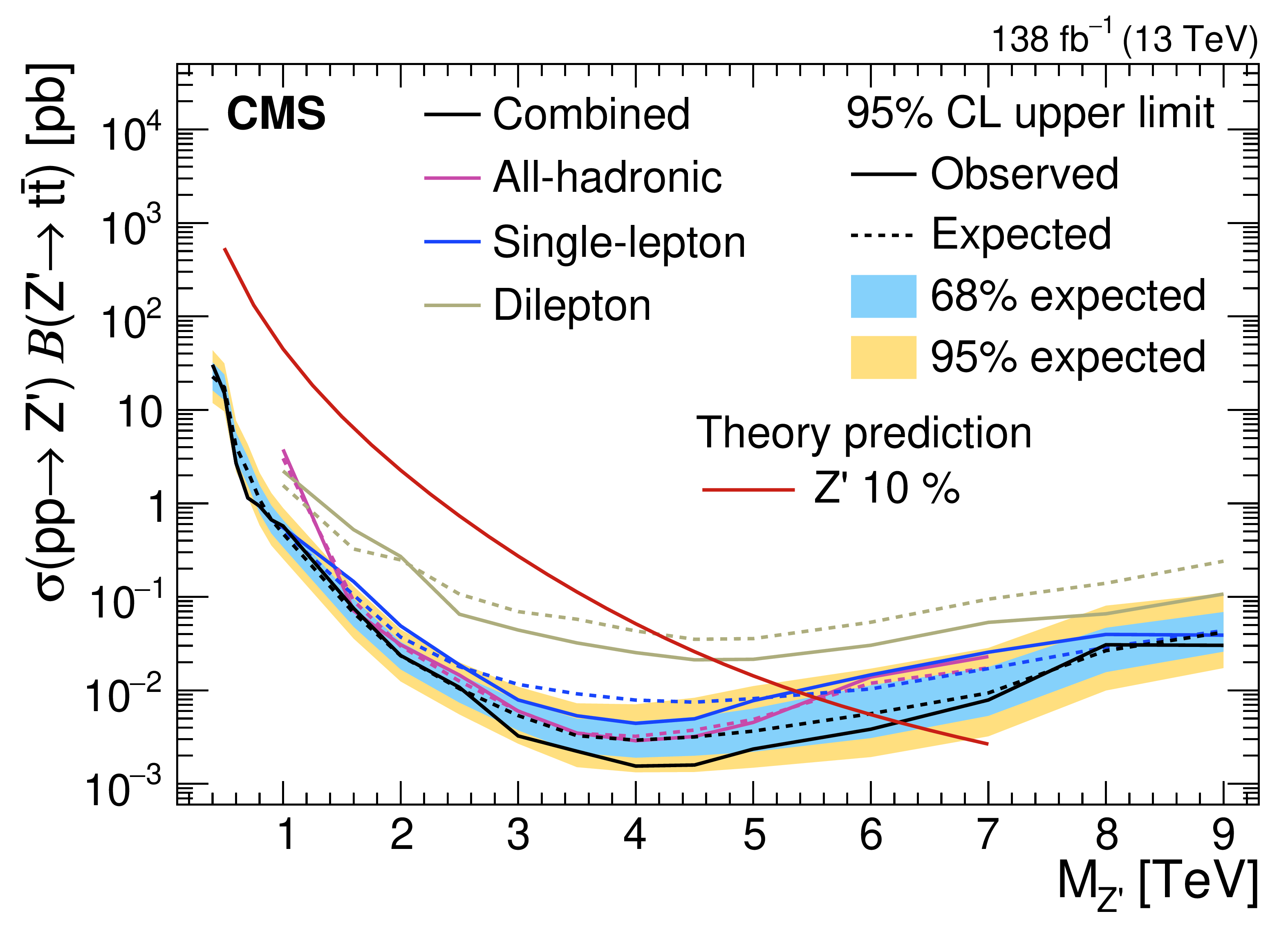
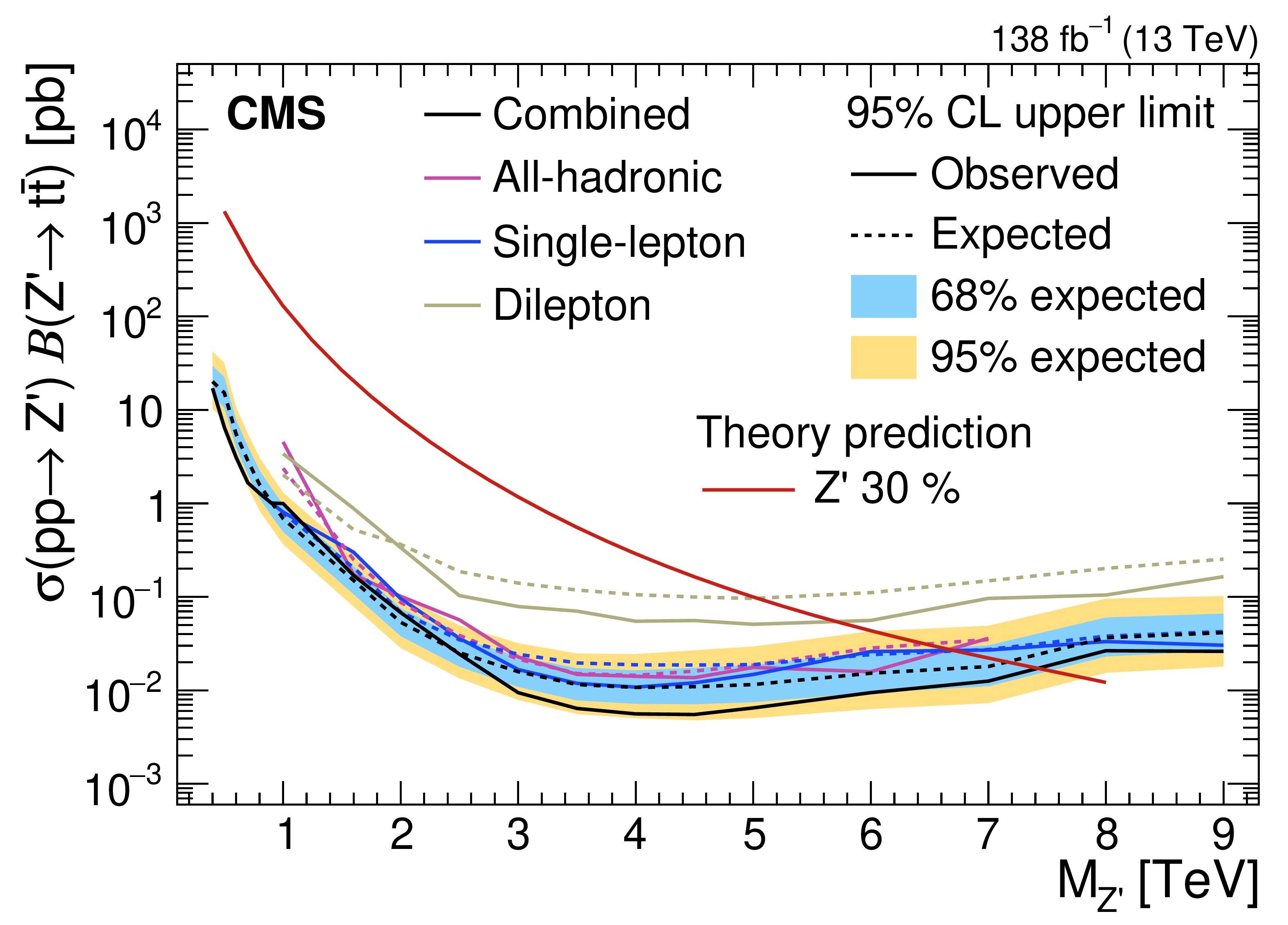
Expected and observed upper limits at 95% CL on the product of the production cross section and branching fraction as functions of the resonance mass. The limits are shown for $ \mathrm{Z}^{'} $ bosons with 1 (upper left), 10 (upper right), and 30% (lower) relative widths. In each panel we plot the expected combined upper limit on the signal strength times branching ratio (black dashed line) together with the 68 (light blue) and 95% (yellow) uncertainty bands, and the corresponding observed upper limit (black solid line). The expected (dashed lines) and observed (solid lines) limits from the single channels are overlaid: all-hadronic (purple), single-lepton (blue), and dilepton (light brown). The limits are compared with the respective theory predictions shown by the solid red curves. The rise in the limits seen at high mass for the $ \mathrm{Z}^{'} $ boson interpretation at 1% relative width (upper left) for the all-hadronic case arises from the limited number of events available to estimate the background. |
png pdf |
Figure 15-a:
Expected and observed upper limits at 95% CL on the product of the production cross section and branching fraction as functions of the resonance mass. The limits are shown for $ \mathrm{Z}^{'} $ bosons with 1 (upper left), 10 (upper right), and 30% (lower) relative widths. In each panel we plot the expected combined upper limit on the signal strength times branching ratio (black dashed line) together with the 68 (light blue) and 95% (yellow) uncertainty bands, and the corresponding observed upper limit (black solid line). The expected (dashed lines) and observed (solid lines) limits from the single channels are overlaid: all-hadronic (purple), single-lepton (blue), and dilepton (light brown). The limits are compared with the respective theory predictions shown by the solid red curves. The rise in the limits seen at high mass for the $ \mathrm{Z}^{'} $ boson interpretation at 1% relative width (upper left) for the all-hadronic case arises from the limited number of events available to estimate the background. |
png pdf |
Figure 15-b:
Expected and observed upper limits at 95% CL on the product of the production cross section and branching fraction as functions of the resonance mass. The limits are shown for $ \mathrm{Z}^{'} $ bosons with 1 (upper left), 10 (upper right), and 30% (lower) relative widths. In each panel we plot the expected combined upper limit on the signal strength times branching ratio (black dashed line) together with the 68 (light blue) and 95% (yellow) uncertainty bands, and the corresponding observed upper limit (black solid line). The expected (dashed lines) and observed (solid lines) limits from the single channels are overlaid: all-hadronic (purple), single-lepton (blue), and dilepton (light brown). The limits are compared with the respective theory predictions shown by the solid red curves. The rise in the limits seen at high mass for the $ \mathrm{Z}^{'} $ boson interpretation at 1% relative width (upper left) for the all-hadronic case arises from the limited number of events available to estimate the background. |
png pdf |
Figure 15-c:
Expected and observed upper limits at 95% CL on the product of the production cross section and branching fraction as functions of the resonance mass. The limits are shown for $ \mathrm{Z}^{'} $ bosons with 1 (upper left), 10 (upper right), and 30% (lower) relative widths. In each panel we plot the expected combined upper limit on the signal strength times branching ratio (black dashed line) together with the 68 (light blue) and 95% (yellow) uncertainty bands, and the corresponding observed upper limit (black solid line). The expected (dashed lines) and observed (solid lines) limits from the single channels are overlaid: all-hadronic (purple), single-lepton (blue), and dilepton (light brown). The limits are compared with the respective theory predictions shown by the solid red curves. The rise in the limits seen at high mass for the $ \mathrm{Z}^{'} $ boson interpretation at 1% relative width (upper left) for the all-hadronic case arises from the limited number of events available to estimate the background. |
png pdf |
Figure 16:
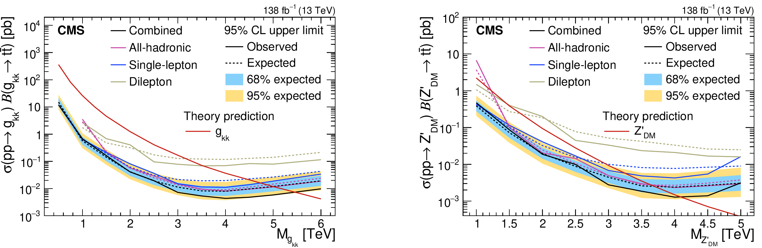
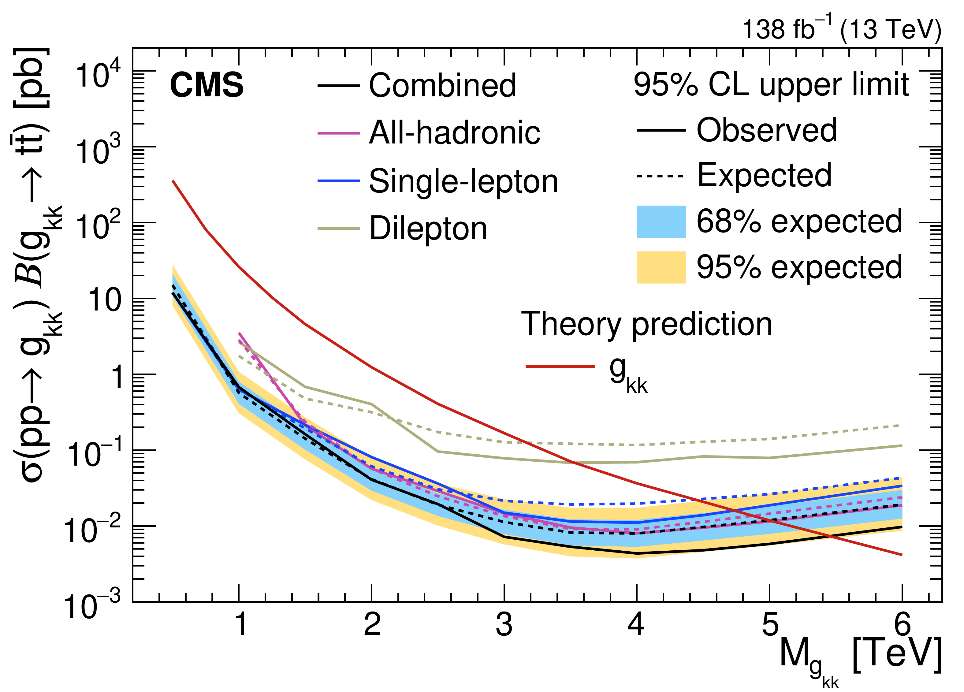
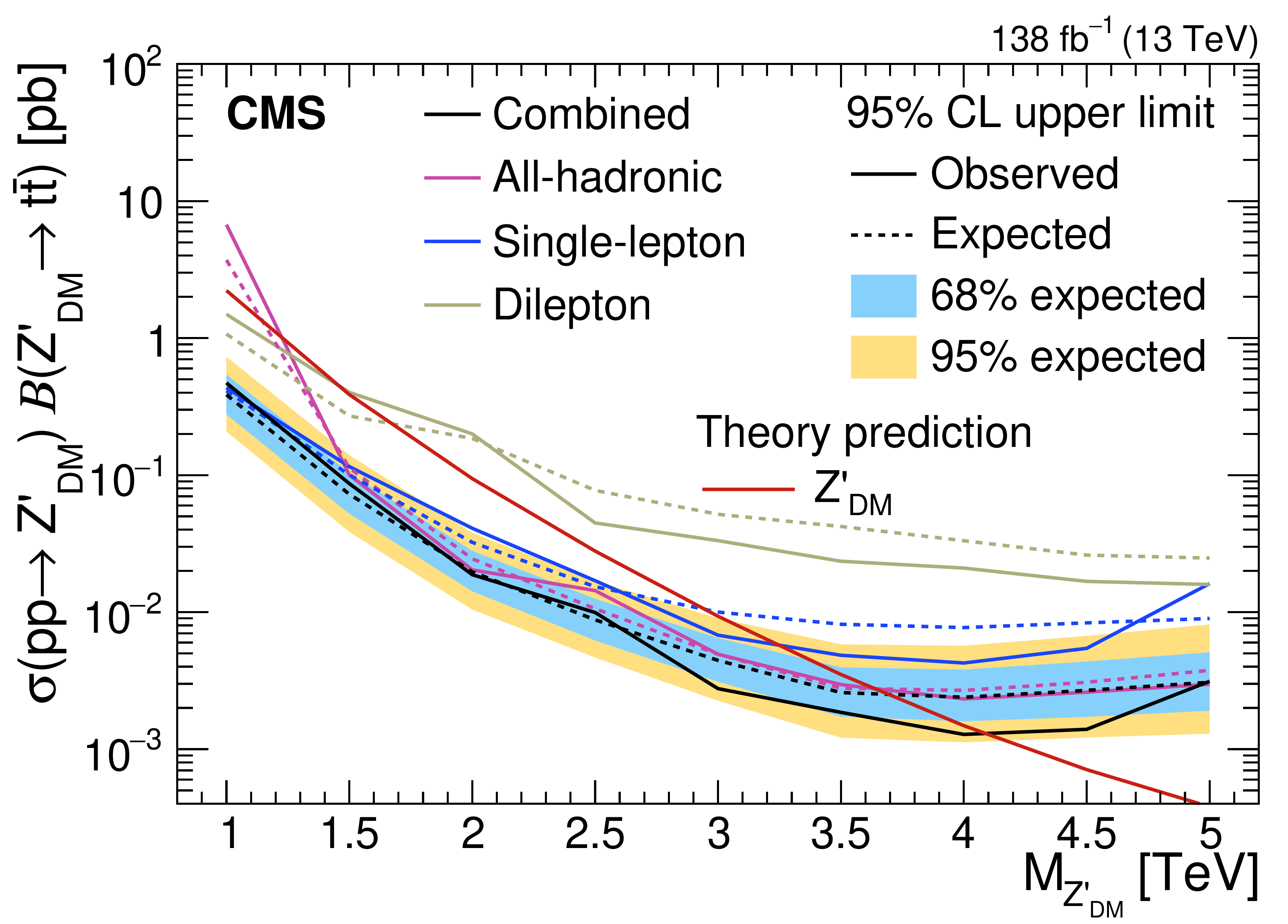
Expected and observed upper limits at 95% CL on the product of the production cross section and branching fraction as functions of the resonance mass. The limits are shown for the Kaluza--Klein gluon (left) and dark matter (right) scenarios. In each panel we plot the expected combined upper limit on the signal strength times branching fraction (black dashed line) together with the 68 (light blue) and 95% (yellow) uncertainty bands, and the corresponding observed upper limit (black solid line). The expected (dashed lines) and observed (solid lines) limits from the individual channels are overlaid: all-hadronic (purple), single-lepton (blue), and dilepton (light brown). The limits are compared with the respective theory predictions shown by the solid red curves. |
png pdf |
Figure 16-a:
Expected and observed upper limits at 95% CL on the product of the production cross section and branching fraction as functions of the resonance mass. The limits are shown for the Kaluza--Klein gluon (left) and dark matter (right) scenarios. In each panel we plot the expected combined upper limit on the signal strength times branching fraction (black dashed line) together with the 68 (light blue) and 95% (yellow) uncertainty bands, and the corresponding observed upper limit (black solid line). The expected (dashed lines) and observed (solid lines) limits from the individual channels are overlaid: all-hadronic (purple), single-lepton (blue), and dilepton (light brown). The limits are compared with the respective theory predictions shown by the solid red curves. |
png pdf |
Figure 16-b:
Expected and observed upper limits at 95% CL on the product of the production cross section and branching fraction as functions of the resonance mass. The limits are shown for the Kaluza--Klein gluon (left) and dark matter (right) scenarios. In each panel we plot the expected combined upper limit on the signal strength times branching fraction (black dashed line) together with the 68 (light blue) and 95% (yellow) uncertainty bands, and the corresponding observed upper limit (black solid line). The expected (dashed lines) and observed (solid lines) limits from the individual channels are overlaid: all-hadronic (purple), single-lepton (blue), and dilepton (light brown). The limits are compared with the respective theory predictions shown by the solid red curves. |
png pdf |
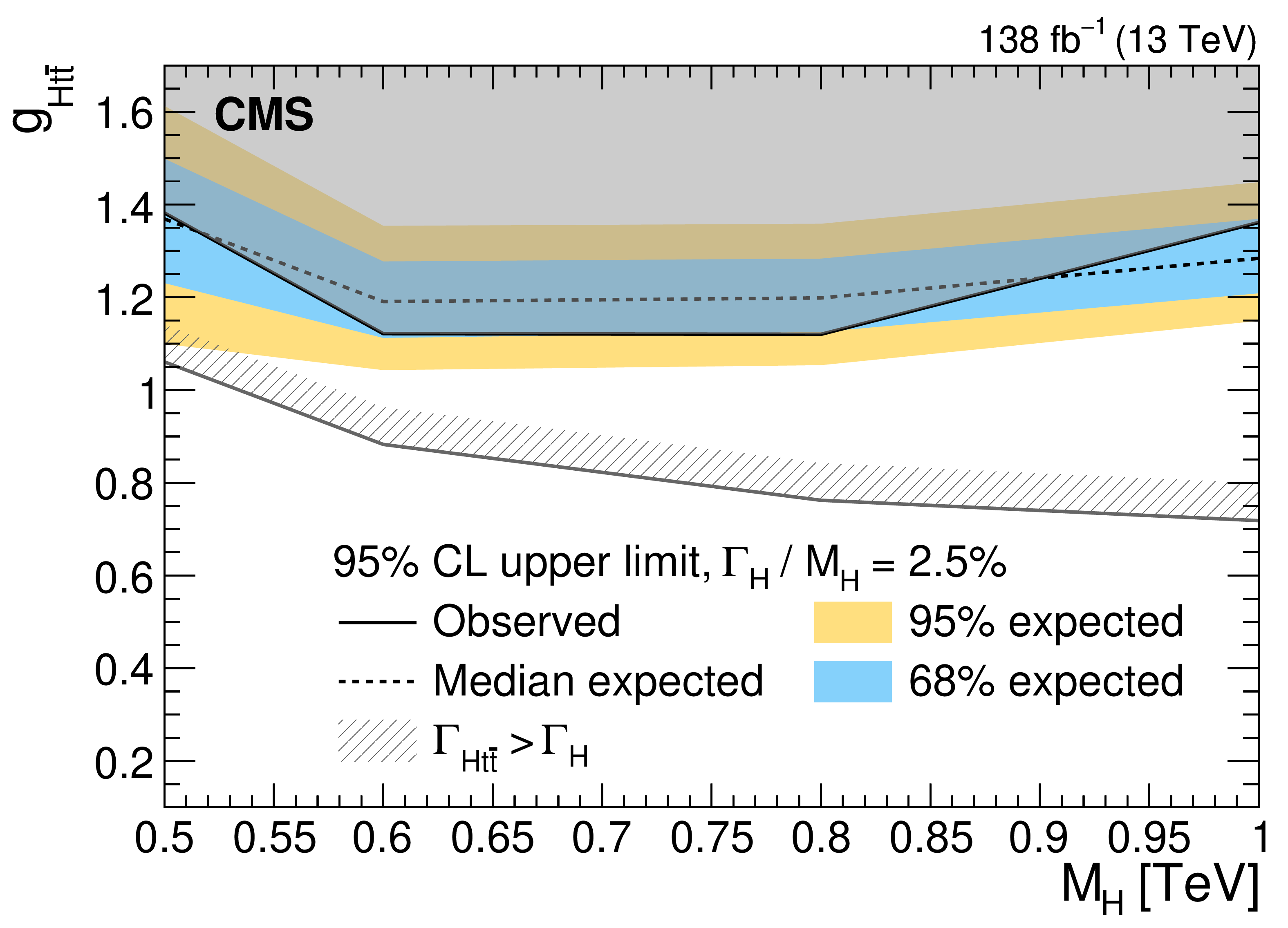
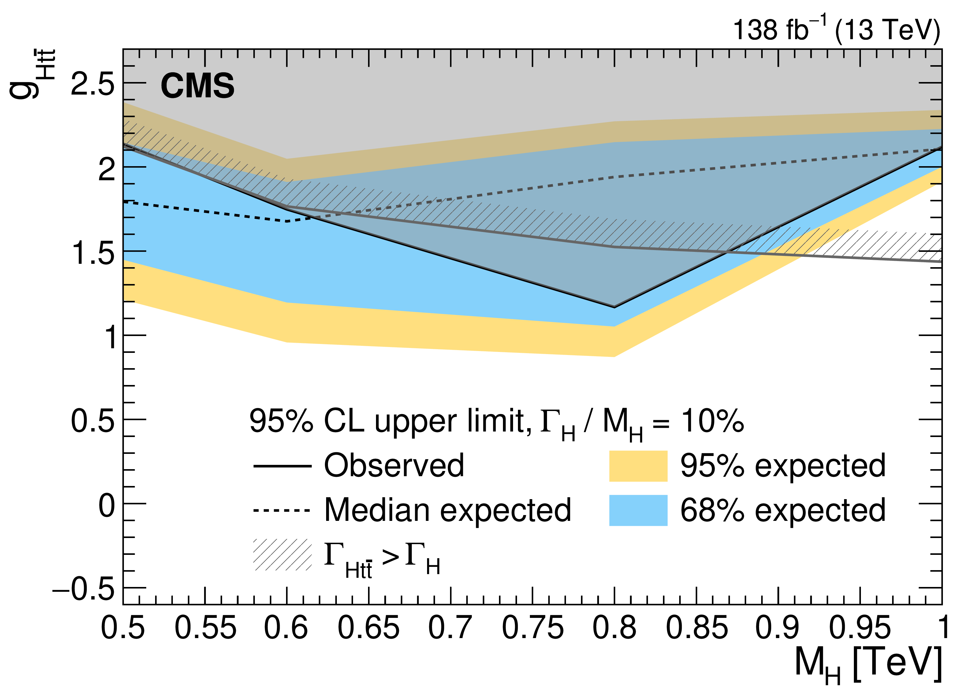
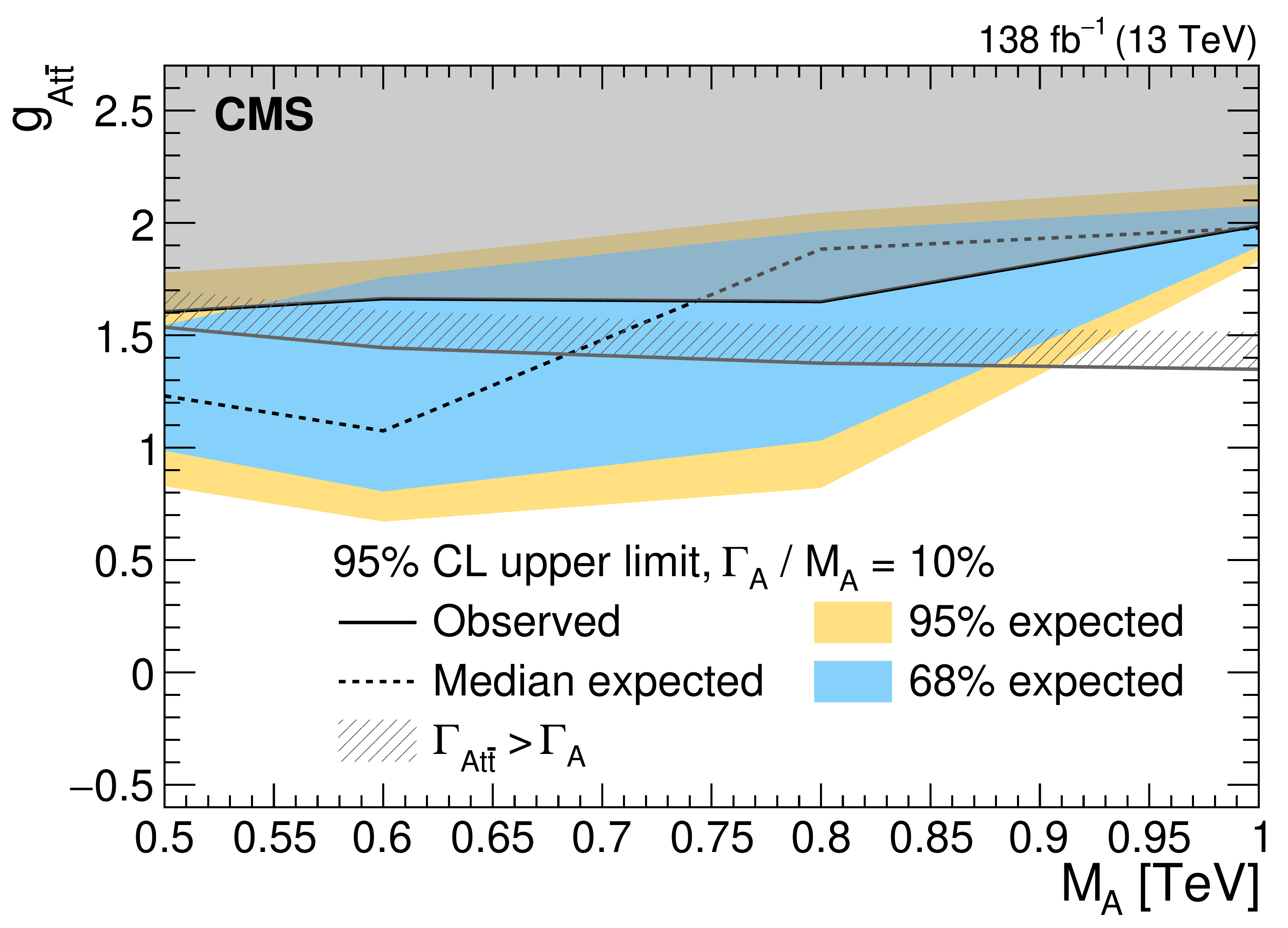
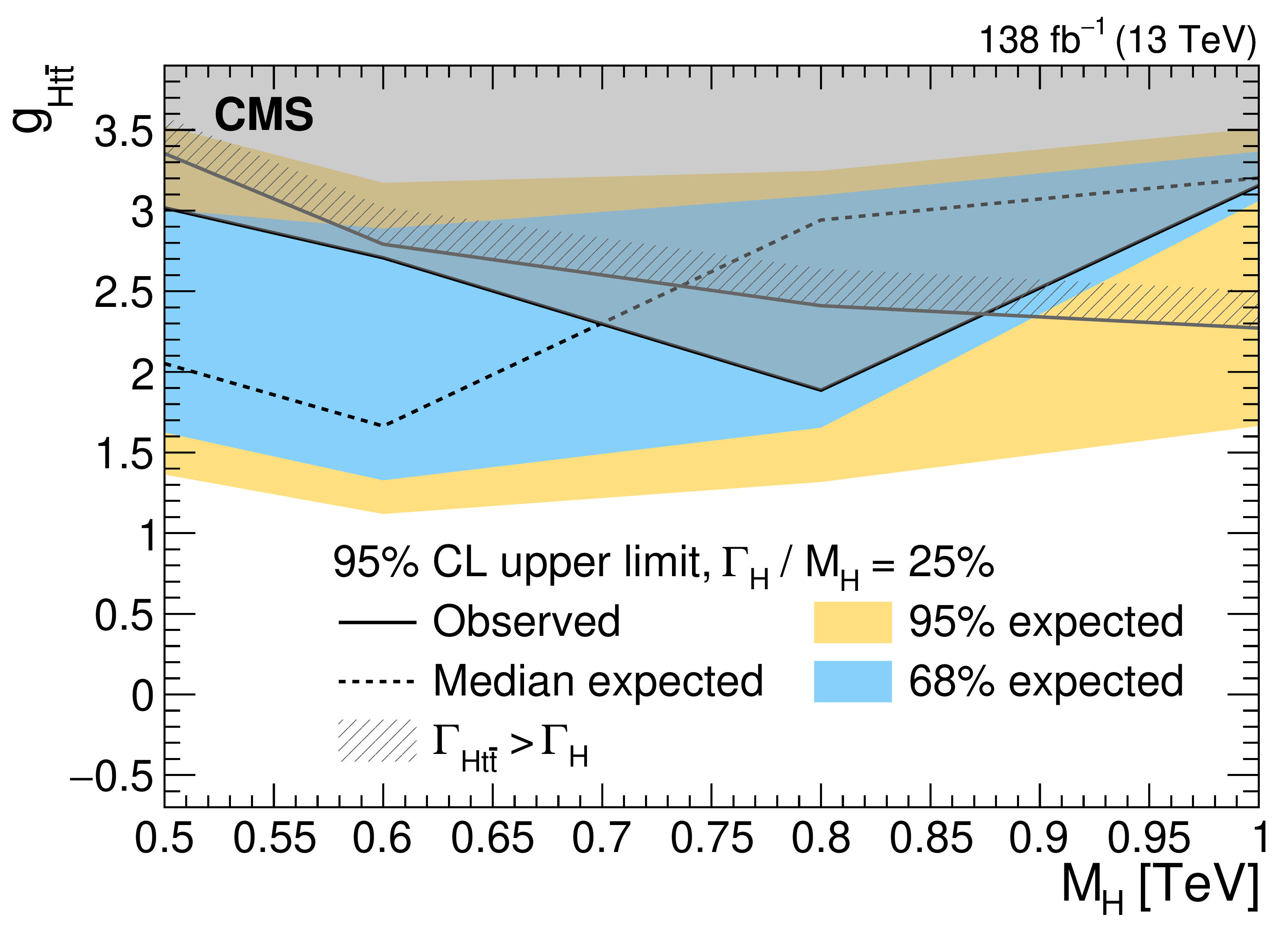
Figure 17:
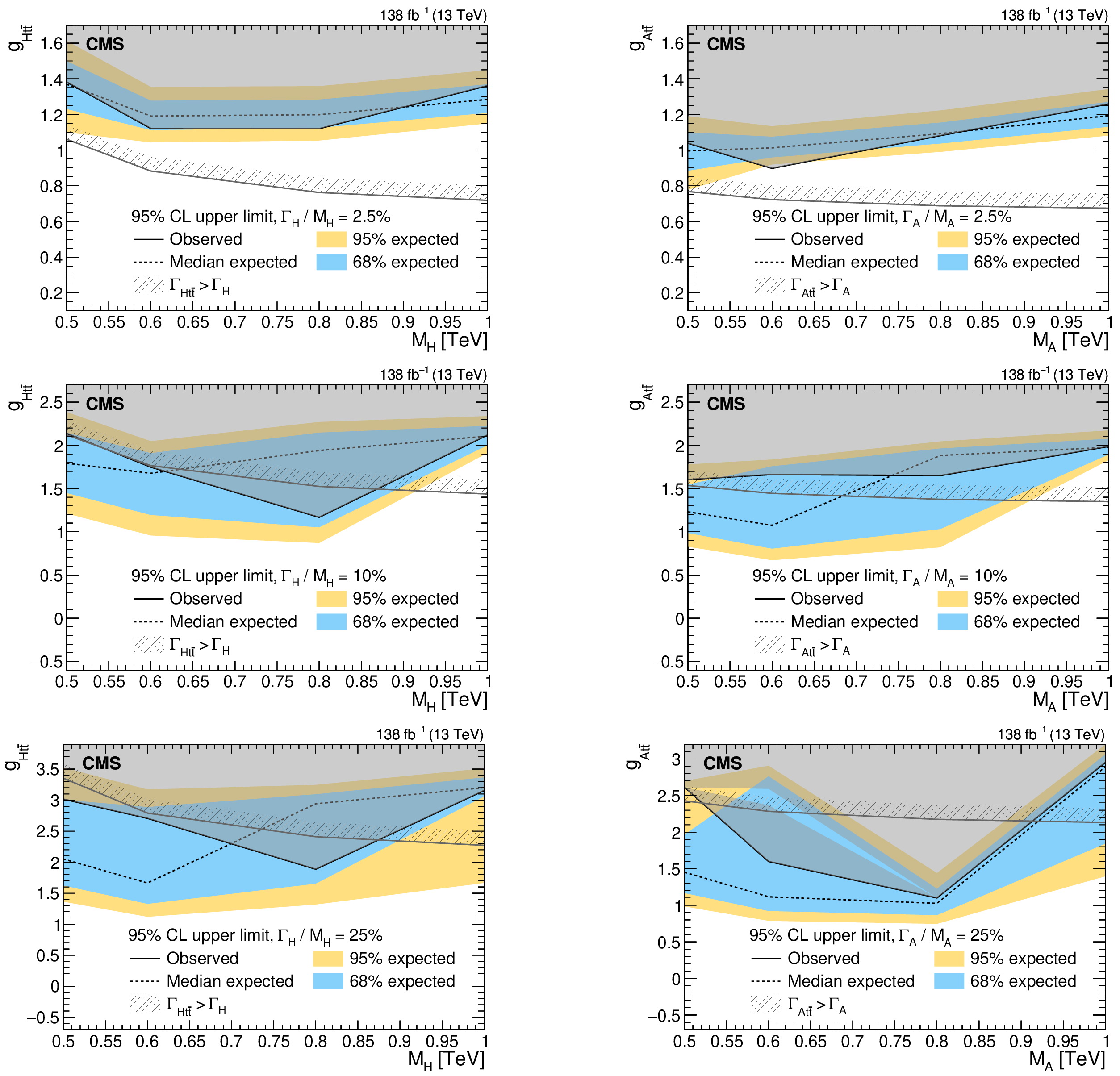
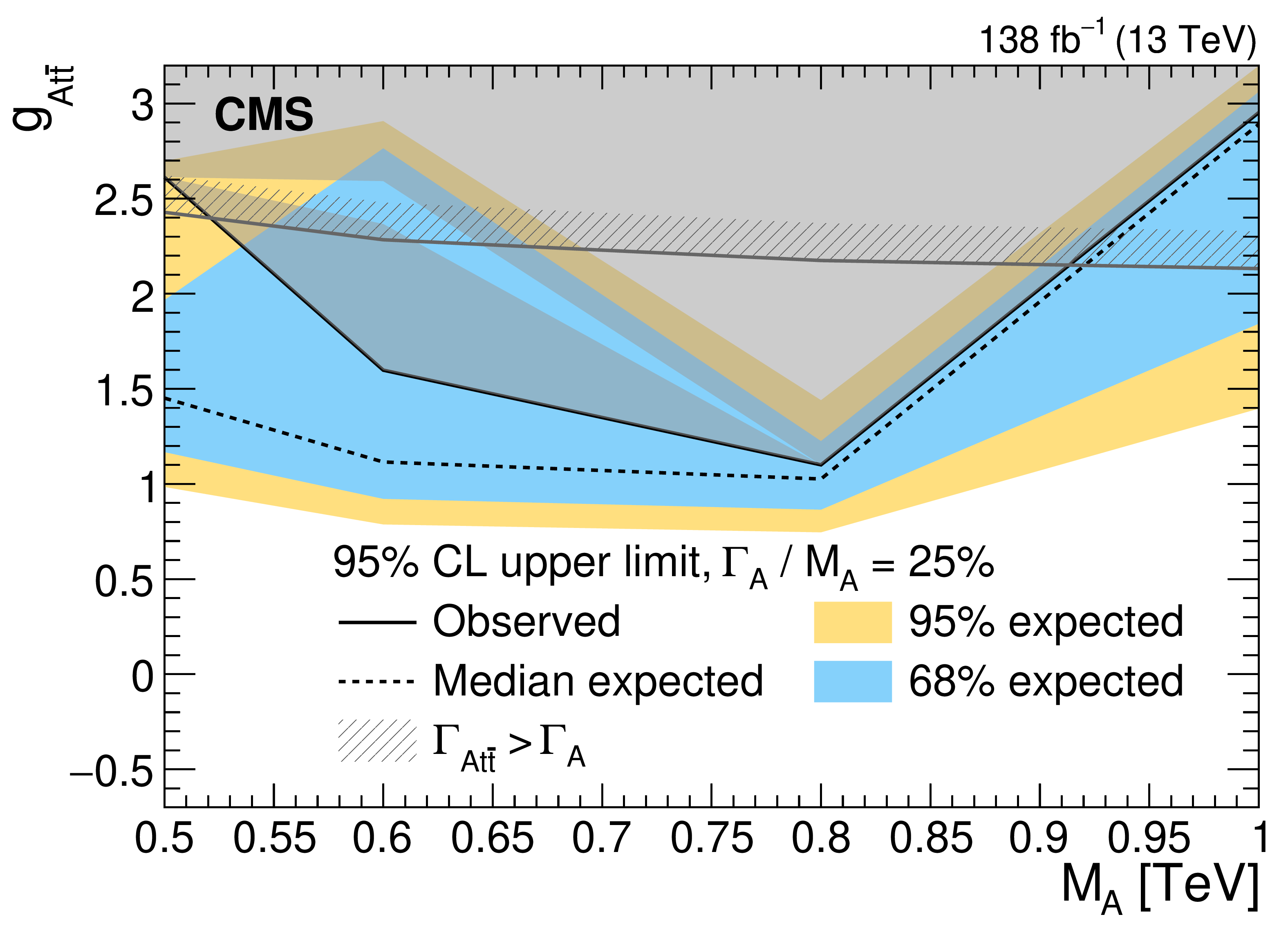
Expected and observed upper limits at 95% CL on the coupling strength modifier for scalar (H, left) and pseudoscalar ($ \mathrm{A} $, right) heavy Higgs bosons with relative widths of 2.5 (upper), 10 (middle), and 25% (lower), respectively. The solid gray shaded area denotes the parameter space excluded by this search. The discontinuity in the shape of the excluded region, observed for the 25% width pseudoscalar signals with masses below 0.8 TeV, arises from the behavior of the $ \text{CL}_\text{s} $ scan. The gray hatched area indicates the unphysical parameter space where the partial width $ \Gamma_{\Phi{\mathrm{t}\overline{\mathrm{t}}} } $ exceeds the total width $ \Gamma_{\Phi} $. |
png pdf |
Figure 17-a:
Expected and observed upper limits at 95% CL on the coupling strength modifier for scalar (H, left) and pseudoscalar ($ \mathrm{A} $, right) heavy Higgs bosons with relative widths of 2.5 (upper), 10 (middle), and 25% (lower), respectively. The solid gray shaded area denotes the parameter space excluded by this search. The discontinuity in the shape of the excluded region, observed for the 25% width pseudoscalar signals with masses below 0.8 TeV, arises from the behavior of the $ \text{CL}_\text{s} $ scan. The gray hatched area indicates the unphysical parameter space where the partial width $ \Gamma_{\Phi{\mathrm{t}\overline{\mathrm{t}}} } $ exceeds the total width $ \Gamma_{\Phi} $. |

png pdf |
Figure 17-b:
Expected and observed upper limits at 95% CL on the coupling strength modifier for scalar (H, left) and pseudoscalar ($ \mathrm{A} $, right) heavy Higgs bosons with relative widths of 2.5 (upper), 10 (middle), and 25% (lower), respectively. The solid gray shaded area denotes the parameter space excluded by this search. The discontinuity in the shape of the excluded region, observed for the 25% width pseudoscalar signals with masses below 0.8 TeV, arises from the behavior of the $ \text{CL}_\text{s} $ scan. The gray hatched area indicates the unphysical parameter space where the partial width $ \Gamma_{\Phi{\mathrm{t}\overline{\mathrm{t}}} } $ exceeds the total width $ \Gamma_{\Phi} $. |
png pdf |
Figure 17-c:
Expected and observed upper limits at 95% CL on the coupling strength modifier for scalar (H, left) and pseudoscalar ($ \mathrm{A} $, right) heavy Higgs bosons with relative widths of 2.5 (upper), 10 (middle), and 25% (lower), respectively. The solid gray shaded area denotes the parameter space excluded by this search. The discontinuity in the shape of the excluded region, observed for the 25% width pseudoscalar signals with masses below 0.8 TeV, arises from the behavior of the $ \text{CL}_\text{s} $ scan. The gray hatched area indicates the unphysical parameter space where the partial width $ \Gamma_{\Phi{\mathrm{t}\overline{\mathrm{t}}} } $ exceeds the total width $ \Gamma_{\Phi} $. |
png pdf |
Figure 17-d:
Expected and observed upper limits at 95% CL on the coupling strength modifier for scalar (H, left) and pseudoscalar ($ \mathrm{A} $, right) heavy Higgs bosons with relative widths of 2.5 (upper), 10 (middle), and 25% (lower), respectively. The solid gray shaded area denotes the parameter space excluded by this search. The discontinuity in the shape of the excluded region, observed for the 25% width pseudoscalar signals with masses below 0.8 TeV, arises from the behavior of the $ \text{CL}_\text{s} $ scan. The gray hatched area indicates the unphysical parameter space where the partial width $ \Gamma_{\Phi{\mathrm{t}\overline{\mathrm{t}}} } $ exceeds the total width $ \Gamma_{\Phi} $. |
png pdf |
Figure 17-e:
Expected and observed upper limits at 95% CL on the coupling strength modifier for scalar (H, left) and pseudoscalar ($ \mathrm{A} $, right) heavy Higgs bosons with relative widths of 2.5 (upper), 10 (middle), and 25% (lower), respectively. The solid gray shaded area denotes the parameter space excluded by this search. The discontinuity in the shape of the excluded region, observed for the 25% width pseudoscalar signals with masses below 0.8 TeV, arises from the behavior of the $ \text{CL}_\text{s} $ scan. The gray hatched area indicates the unphysical parameter space where the partial width $ \Gamma_{\Phi{\mathrm{t}\overline{\mathrm{t}}} } $ exceeds the total width $ \Gamma_{\Phi} $. |
png pdf |
Figure 17-f:
Expected and observed upper limits at 95% CL on the coupling strength modifier for scalar (H, left) and pseudoscalar ($ \mathrm{A} $, right) heavy Higgs bosons with relative widths of 2.5 (upper), 10 (middle), and 25% (lower), respectively. The solid gray shaded area denotes the parameter space excluded by this search. The discontinuity in the shape of the excluded region, observed for the 25% width pseudoscalar signals with masses below 0.8 TeV, arises from the behavior of the $ \text{CL}_\text{s} $ scan. The gray hatched area indicates the unphysical parameter space where the partial width $ \Gamma_{\Phi{\mathrm{t}\overline{\mathrm{t}}} } $ exceeds the total width $ \Gamma_{\Phi} $. |
| Tables | |
png pdf |
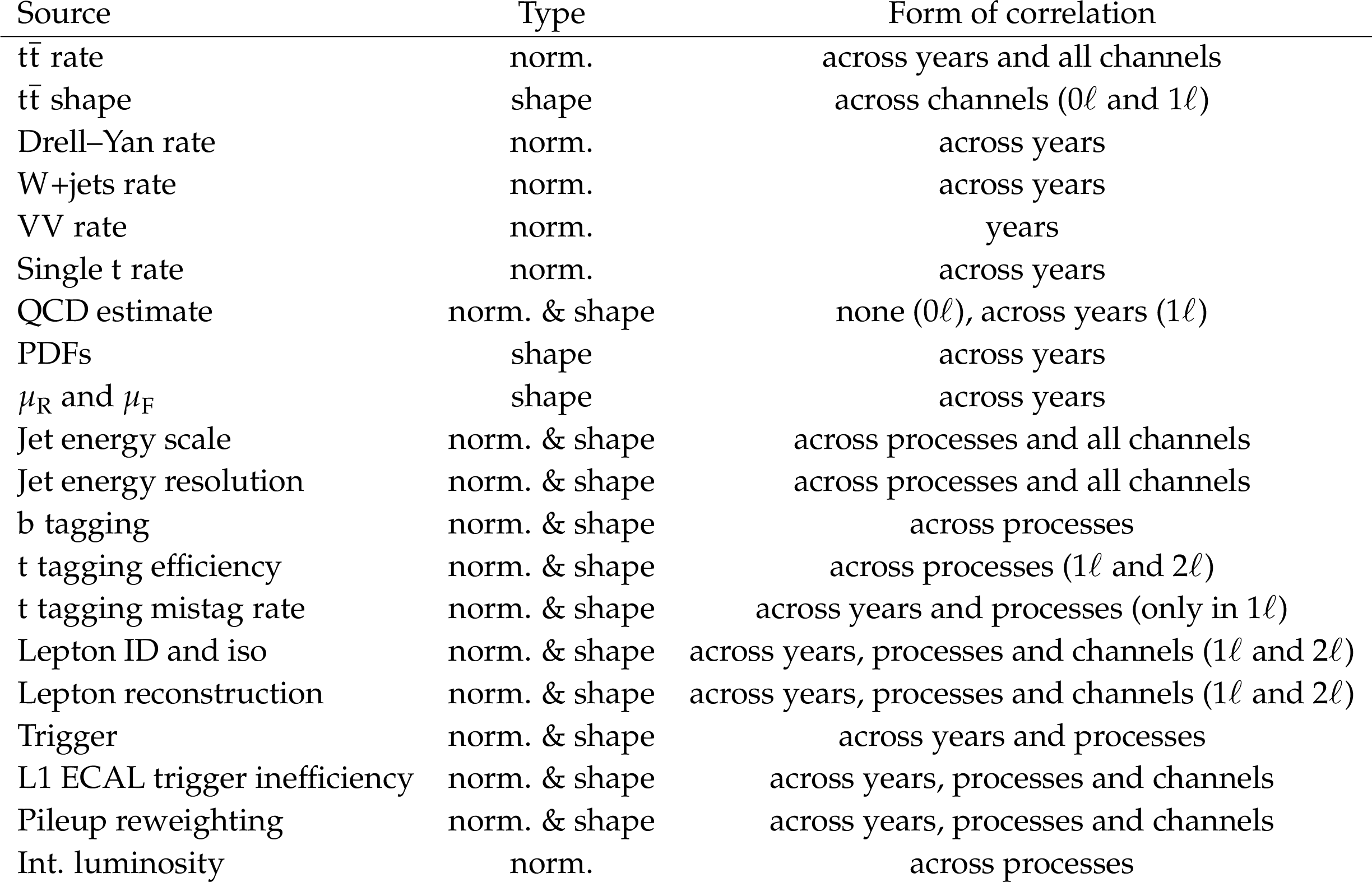
Table 1:
Sources of systematic uncertainties and correlations between them. The correlations take various forms: among data-taking years, among different processes (such as $ \mathrm{t} \overline{\mathrm{t}} $, single top quark production, etc), and/or channels (0\ell, 1\ell, and 2\ell). The $ \mathrm{Z}^{'} $ signal with a relative width of 1% and a mass of 2 TeV is used as a benchmark. The `` $ \mathrm{t} \overline{\mathrm{t}} $ rate'' row corresponds to the overall prior uncertainty in the $ \mathrm{t} \overline{\mathrm{t}} $ production cross section. The `` $ \mathrm{t} \overline{\mathrm{t}} $ shape'' row corresponds to differences in shapes between the NLO simulation and measured values of the $ \mathrm{t} \overline{\mathrm{t}} $ $ p_{\mathrm{T}} $ spectrum at large momentum due to destructive interference from higher-order terms that are not present in the simulation. |
png pdf |
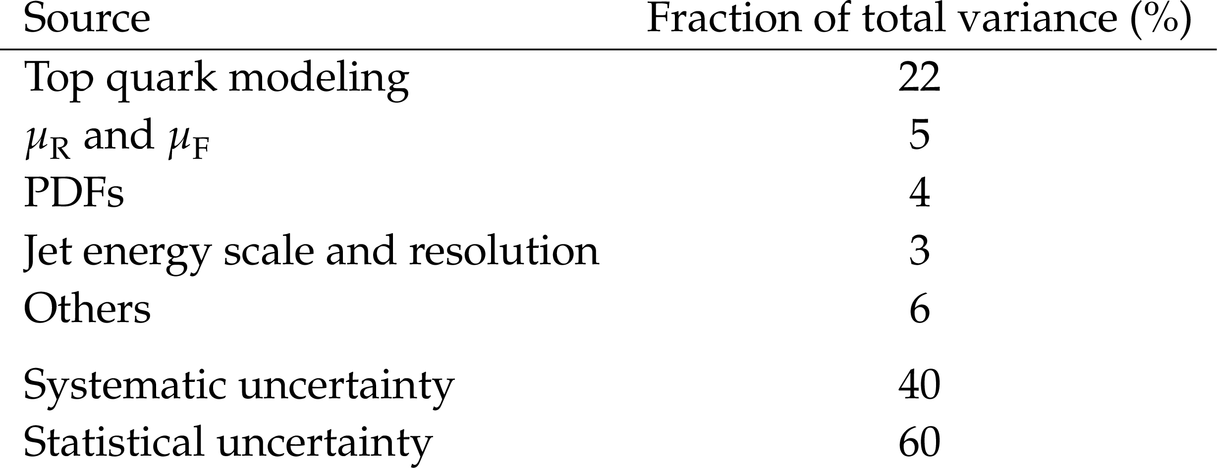
Table 2:
Relative contribution of the dominant sources of uncertainty to the total variance of the upper limits. The benchmark scenario corresponds to a $ \mathrm{Z}^{'} $ signal with a 1% relative width and a mass of 2 TeV. The top-quark modeling category includes nuisance parameters associated with the $ \mathrm{t} \overline{\mathrm{t}} $ production rate, $ \mathrm{t}\text{ tagging} $ efficiency, $ \mathrm{t}\text{ tagging} $ mistag rate, and modeling of the $ \mathrm{t} \overline{\mathrm{t}} $ transverse momentum spectrum. |
| Summary |
| A search for new particles decaying to a top quark-antiquark pair has been presented. The analysis uses 138 fb$ ^{-1} $ of data collected during 2016--2018 by the CMS experiment at a centre-of-mass energy of 13 TeV. The analysis performs a model-independent search and is sensitive both to the resolved and the merged regimes of the top quark hadronic decay. Upper limits at 95% confidence level are placed for different benchmark models. Heavy $ \mathrm{Z}^{'} $ bosons in the leptophobic topcolor model with relative widths of 1, 10, and 30% are excluded for mass ranges 0.4--4.8, 0.4--6.2, and 0.4--7.4 TeV, respectively. Additionally, Kaluza--Klein gluons in the Randall--Sundrum model and dark-matter mediators are excluded for masses between 0.5--5.5 and 1.0--4.2 TeV, respectively. These results set the most stringent limits to date for the considered models. Limits on the coupling strength modifier are set for scalar and pseudoscalar heavy Higgs bosons in two-Higgs-doublet models for 2.5, 10, and 25% relative widths in the mass range 0.5--1 TeV. |
| References | ||||
| 1 | J. L. Rosner | Prominent decay modes of a leptophobic $ \mathrm{Z}^{'} $ | PLB 387 (1996) 113 | hep-ph/9607207 |
| 2 | K. R. Lynch, S. Mrenna, M. Narain, and E. H. Simmons | Finding $ \mathrm{Z}^{'} $ bosons coupled preferentially to the third family at CERN LEP and the Fermilab Tevatron | PRD 63 (2001) 035006 | hep-ph/0007286 |
| 3 | M. Carena, A. Daleo, B. A. Dobrescu, and T. M. P. Tait | $ \mathrm{Z}^{'} $ gauge bosons at the Fermilab Tevatron | PRD 70 (2004) 093009 | hep-ph/0408098 |
| 4 | C. T. Hill | Topcolor: top quark condensation in a gauge extension of the standard model | PLB 266 (1991) 419 | |
| 5 | C. T. Hill and S. J. Parke | Top quark production: Sensitivity to new physics | PRD 49 (1994) 4454 | hep-ph/9312324 |
| 6 | C. T. Hill | Topcolor assisted technicolor | PLB 345 (1995) 483 | hep-ph/9411426 |
| 7 | R. M. Harris and S. Jain | Cross sections for leptophobic topcolor $ \mathrm{Z}^{'} $ decaying to top-antitop | EPJC 72 (2012) 2072 | 1112.4928 |
| 8 | P. H. Frampton and S. L. Glashow | Chiral color: An alternative to the standard model | PLB 190 (1987) 157 | |
| 9 | D. Choudhury, R. M. Godbole, R. K. Singh, and K. Wagh | Top production at the Tevatron/LHC and nonstandard, strongly interacting spin one particles | PLB 657 (2007) 69 | 0705.1499 |
| 10 | R. M. Godbole and D. Choudhury | Nonstandard, strongly interacting spin one $ \mathrm{t} \overline{\mathrm{t}} $ resonances | in the International Conference on High Energy Physics (ICHEP ): Philadelphia PA, USA, July 30--August 05,, 2008 Proc. 3 (2008) 4 |
0810.3635 |
| 11 | K. Agashe et al. | CERN LHC signals from warped extra dimensions | PRD 77 (2008) 015003 | hep-ph/0612015 |
| 12 | H. Davoudiasl, J. L. Hewett, and T. G. Rizzo | Phenomenology of the Randall--Sundrum gauge hierarchy model | PRL 84 (2000) 2080 | hep-ph/9909255 |
| 13 | L. Randall and R. Sundrum | A large mass hierarchy from a small extra dimension | PRL 83 (1999) 3370 | hep-ph/9905221 |
| 14 | L. Randall and R. Sundrum | An alternative to compactification | PRL 83 (1999) 4690 | hep-th/9906064 |
| 15 | ATLAS Collaboration | Search for $ \mathrm{t} \overline{\mathrm{t}} $ resonances in final states with exactly one or two leptons using 140 fb$ ^{-1} $ of $ {\mathrm{p}\mathrm{p}} $ collision data at $ \sqrt{s}= $ 13 TeV with the ATLAS experiment | Submitted to JHEP | 2512.17856 |
| 16 | CMS Collaboration | Search for resonant $ \mathrm{t} \overline{\mathrm{t}} $ production in proton-proton collisions at $ \sqrt{s}= $ 13 TeV | JHEP 04 (2019) 031 | 1810.05905 |
| 17 | CMS Collaboration | Observation of a pseudoscalar excess at the top quark pair production threshold | Rep. Prog. Phys. 88 (2025) 087801 | CMS-TOP-24-007 2503.22382 |
| 18 | CMS Collaboration | Search for heavy pseudoscalar and scalar bosons decaying to a top quark pair in proton-proton collisions at $ \sqrt{s}= $ 13 TeV | Rep. Prog. Phys. 88 (2025) 127801 | CMS-HIG-22-013 2507.05119 |
| 19 | CMS Collaboration | Identification of heavy, energetic, hadronically decaying particles using machine-learning techniques | JINST 15 (2020) P06005 | CMS-JME-18-002 2004.08262 |
| 20 | CMS Collaboration | HEPData record for this analysis | link | |
| 21 | V. D. Barger, W.-Y. Keung, and E. Ma | A gauge model with light W and Z bosons | PRD 22 (1980) 727 | |
| 22 | R. Contino, D. Pappadopulo, D. Marzocca, and R. Rattazzi | On the effect of resonances in composite Higgs phenomenology | JHEP 10 (2011) 081 | 1109.1570 |
| 23 | B. Bellazzini, C. Cs \'a ki, and J. Serra | Composite Higgses | EPJC 74 (2014) 2766 | 1401.2457 |
| 24 | A. Albert et al. | Recommendations of the LHC Dark Matter Working Group: Comparing LHC searches for dark matter mediators in visible and invisible decay channels and calculations of the thermal relic density | Phys. Dark Univ. 26 (2019) 100377 | 1703.05703 |
| 25 | R. Bonciani et al. | Electroweak top-quark pair production at the LHC with $ \mathrm{Z}^{'} $ bosons to NLO QCD in POWHEG | JHEP 02 (2016) 141 | 1511.08185 |
| 26 | T. D. Lee | A theory of spontaneous $ {T} $ violation | PRD 8 (1973) 1226 | |
| 27 | G. C. Branco et al. | Theory and phenomenology of two-Higgs-doublet models | Phys. Rept. 516 (2012) 1 | 1106.0034 |
| 28 | H. E. Haber and O. St \r a l | New LHC benchmarks for the $ {CP} $-conserving two-Higgs-doublet model | EPJC 75 (2015) 491 | 1507.04281 |
| 29 | F. Kling, J. M. No, and S. Su | Anatomy of exotic Higgs decays in 2HDM | JHEP 09 (2016) 093 | 1604.01406 |
| 30 | D. Dicus, A. Stange, and S. Willenbrock | Higgs decay to top quarks at hadron colliders | PLB 333 (1994) 126 | hep-ph/9404359 |
| 31 | CMS Collaboration | The CMS experiment at the CERN LHC | JINST 3 (2008) S08004 | |
| 32 | CMS Collaboration | Development of the CMS detector for the CERN LHC \mboxRun 3 | JINST 19 (2024) P05064 | CMS-PRF-21-001 2309.05466 |
| 33 | CMS Collaboration | Electron and photon reconstruction and identification with the CMS experiment at the CERN LHC | JINST 16 (2021) P05014 | CMS-EGM-17-001 2012.06888 |
| 34 | CMS Collaboration | Performance of the CMS muon detector and muon reconstruction with proton-proton collisions at $ \sqrt{s}= $ 13 TeV | JINST 13 (2018) P06015 | CMS-MUO-16-001 1804.04528 |
| 35 | CMS Collaboration | Description and performance of track and primary-vertex reconstruction with the CMS tracker | JINST 9 (2014) P10009 | CMS-TRK-11-001 1405.6569 |
| 36 | CMS Collaboration | Particle-flow reconstruction and global event description with the CMS detector | JINST 12 (2017) P10003 | CMS-PRF-14-001 1706.04965 |
| 37 | CMS Collaboration | Jet energy scale and resolution in the CMS experiment in $ {\mathrm{p}\mathrm{p}} $ collisions at 8 TeV | JINST 12 (2017) P02014 | CMS-JME-13-004 1607.03663 |
| 38 | CMS Collaboration | Performance of reconstruction and identification of $ \tau $ leptons decaying to hadrons and $ \nu_{\!\tau} $ in $ {\mathrm{p}\mathrm{p}} $ collisions at $ \sqrt{s}= $ 13 TeV | JINST 13 (2018) P10005 | CMS-TAU-16-003 1809.02816 |
| 39 | CMS Collaboration | Performance of missing transverse momentum reconstruction in proton-proton collisions at $ \sqrt{s}= $ 13 TeV using the CMS detector | JINST 14 (2019) P07004 | CMS-JME-17-001 1903.06078 |
| 40 | CMS Collaboration | Performance of the CMS Level-1 trigger in proton-proton collisions at $ \sqrt{s}= $ 13 TeV | JINST 15 (2020) P10017 | CMS-TRG-17-001 2006.10165 |
| 41 | CMS Collaboration | The CMS trigger system | JINST 12 (2017) P01020 | CMS-TRG-12-001 1609.02366 |
| 42 | CMS Collaboration | Performance of the CMS high-level trigger during LHC \mboxRun 2 | JINST 19 (2024) P11021 | CMS-TRG-19-001 2410.17038 |
| 43 | CMS Collaboration | Technical proposal for the Phase-II upgrade of the Compact Muon Solenoid | CMS Technical Proposal CERN-LHCC-2015-010, CMS-TDR-15-02, 2015 link |
|
| 44 | D. Bertolini, P. Harris, M. Low, and N. Tran | Pileup per particle identification | JHEP 10 (2014) 059 | 1407.6013 |
| 45 | CMS Collaboration | Pileup mitigation at CMS in 13 TeV data | JINST 15 (2020) P09018 | CMS-JME-18-001 2003.00503 |
| 46 | M. Cacciari, G. P. Salam, and G. Soyez | FASTJET user manual | EPJC 72 (2012) 1896 | 1111.6097 |
| 47 | M. Cacciari, G. P. Salam, and G. Soyez | The anti-$ k_{\mathrm{T}} $ jet clustering algorithm | JHEP 04 (2008) 063 | 0802.1189 |
| 48 | CMS Collaboration | Identification of heavy-flavour jets with the CMS detector in $ {\mathrm{p}\mathrm{p}} $ collisions at 13 TeV | JINST 13 (2018) P05011 | CMS-BTV-16-002 1712.07158 |
| 49 | E. Bols et al. | Jet flavour classification using DeepJet | JINST 15 (2020) P12012 | 2008.10519 |
| 50 | A. J. Larkoski, S. Marzani, G. Soyez, and J. Thaler | Soft drop | JHEP 05 (2014) 146 | 1402.2657 |
| 51 | M. Dasgupta, A. Fregoso, S. Marzani, and G. P. Salam | Towards an understanding of jet substructure | JHEP 09 (2013) 029 | 1307.0007 |
| 52 | Y. L. Dokshitzer, G. D. Leder, S. Moretti, and B. R. Webber | Better jet clustering algorithms | JHEP 08 (1997) 001 | hep-ph/9707323 |
| 53 | M. Wobisch and T. Wengler | Hadronization corrections to jet cross-sections in deep inelastic scattering | in Proc. Workshop on Monte Carlo Generators for HERA Physics: Hamburg, Germany, --30,, 1998 April 2 (1998) 270 |
hep-ph/9907280 |
| 54 | P. Nason | A new method for combining NLO QCD with shower Monte Carlo algorithms | JHEP 11 (2004) 040 | hep-ph/0409146 |
| 55 | S. Frixione, G. Ridolfi, and P. Nason | A positive-weight next-to-leading-order Monte Carlo for heavy flavour hadroproduction | JHEP 09 (2007) 126 | 0707.3088 |
| 56 | S. Frixione, P. Nason, and C. Oleari | Matching NLO QCD computations with parton shower simulations: the POWHEG method | JHEP 11 (2007) 070 | 0709.2092 |
| 57 | S. Alioli, P. Nason, C. Oleari, and E. Re | A general framework for implementing NLO calculations in shower Monte Carlo programs: the POWHEG box | JHEP 06 (2010) 043 | 1002.2581 |
| 58 | E. Re | Single-top $ {\mathrm{W}\mathrm{t}} $-channel production matched with parton showers using the POWHEG method | EPJC 71 (2011) 1547 | 1009.2450 |
| 59 | M. Czakon and A. Mitov | top++: a program for the calculation of the top-pair cross-section at hadron colliders | Comput. Phys. Commun. 185 (2014) 2930 | 1112.5675 |
| 60 | J. Alwall et al. | Comparative study of various algorithms for the merging of parton showers and matrix elements in hadronic collisions | EPJC 53 (2008) 473 | 0706.2569 |
| 61 | J. Alwall et al. | The automated computation of tree-level and next-to-leading order differential cross sections, and their matching to parton shower simulations | JHEP 07 (2014) 079 | 1405.0301 |
| 62 | J. M. Lindert et al. | Precise predictions for V+jets dark matter backgrounds | EPJC 77 (2017) 829 | 1705.04664 |
| 63 | T. Sjöstrand et al. | An introduction to PYTHIA8.2 | Comput. Phys. Commun. 191 (2015) 159 | 1410.3012 |
| 64 | N. Kidonakis | NNLL threshold resummation for top-pair and single-top production | Phys. Part. Nucl. 45 (2014) 714 | 1210.7813 |
| 65 | J. Gao et al. | Next-to-leading order QCD corrections to the heavy resonance production and decay into top quark pair at the LHC | PRD 82 (2010) 014020 | 1004.0876 |
| 66 | B. Hespel, F. Maltoni, and E. Vryonidou | Signal background interference effects in heavy scalar production and decay to a top-anti-top pair | JHEP 10 (2016) 016 | 1606.04149 |
| 67 | CMS Collaboration | Extraction and validation of a new set of CMS PYTHIA8 tunes from underlying-event measurements | EPJC 80 (2020) 4 | CMS-GEN-17-001 1903.12179 |
| 68 | NNPDF Collaboration | Parton distributions from high-precision collider data | EPJC 77 (2017) 663 | 1706.00428 |
| 69 | GEANT4 Collaboration | GEANT 4---a simulation toolkit | NIM A 506 (2003) 250 | |
| 70 | CMS Collaboration | Measurement of the inelastic proton-proton cross section at $ \sqrt{s}= $ 13 TeV | JHEP 07 (2018) 161 | CMS-FSQ-15-005 1802.02613 |
| 71 | R. A. Fisher | On the interpretation of $ \chi^2 $ from contingency tables, and the calculation of $ {P} $ | J. R. Stat. Soc. 85 (1922) 87 | |
| 72 | CMS Collaboration | Measurement of the $ \mathrm{t} \overline{\mathrm{t}} $ charge asymmetry in events with highly Lorentz-boosted top quarks in $ {\mathrm{p}\mathrm{p}} $ collisions at $ \sqrt{s}= $ 13 TeV | PLB 846 (2023) 137703 | CMS-TOP-21-014 2208.02751 |
| 73 | M. Carena and Z. Liu | Challenges and opportunities for heavy scalar searches in the $ \mathrm{t} \overline{\mathrm{t}} $ channel at the LHC | JHEP 11 (2016) 159 | 1608.07282 |
| 74 | A. Djouadi, J. Ellis, A. Popov, and J. Quevillon | Interference effects in $ \mathrm{t} \overline{\mathrm{t}} $ production at the LHC as a window on new physics | JHEP 03 (2019) 119 | 1901.03417 |
| 75 | F. Chollet et al. | keras | Software available from \urlhttps://keras.io, 2015 | |
| 76 | J. Thaler and K. Van Tilburg | Identifying boosted objects with $ {N} $-subjettiness | JHEP 03 (2011) 015 | 1011.2268 |
| 77 | J. Thaler and K. Van Tilburg | Maximizing boosted top identification by minimizing $ {N} $-subjettiness | JHEP 02 (2012) 093 | 1108.2701 |
| 78 | CMS Collaboration | Search for heavy Higgs bosons decaying to a top quark pair in proton-proton collisions at $ \sqrt{s}= $ 13 TeV | JHEP 04 (2020) 171 | CMS-HIG-17-027 1908.01115 |
| 79 | J. Butterworth et al. | PDF4LHC recommendations for LHC \mboxRun 2 | JPG 43 (2016) 023001 | 1510.03865 |
| 80 | CMS Collaboration | Precision luminosity measurement in proton-proton collisions at $ \sqrt{s}= $ 13 TeV in 2015 and 2016 at CMS | EPJC 81 (2021) 800 | CMS-LUM-17-003 2104.01927 |
| 81 | CMS Collaboration | CMS luminosity measurement for the 2017 data-taking period at $ \sqrt{s}= $ 13 TeV | CMS Physics Analysis Summary, 2018 CMS-PAS-LUM-17-004 |
CMS-PAS-LUM-17-004 |
| 82 | CMS Collaboration | CMS luminosity measurement for the 2018 data-taking period at $ \sqrt{s}= $ 13 TeV | CMS Physics Analysis Summary, 2019 CMS-PAS-LUM-18-002 |
CMS-PAS-LUM-18-002 |
| 83 | ATLAS and CMS Collaborations, and LHC Higgs Combination Group | Procedure for the LHC Higgs boson search combination in Summer 2011 | Technical Report CMS-NOTE-2011-005, ATL-PHYS-PUB-2011-11, 2011 | |
| 84 | T. Junk | Confidence level computation for combining searches with small statistics | NIM A 434 (1999) 435 | hep-ex/9902006 |
| 85 | A. L. Read | Presentation of search results: The $ \text{CL}_\text{s} $ technique | JPG 28 (2002) 2693 | |
| 86 | G. Cowan, K. Cranmer, E. Gross, and O. Vitells | Asymptotic formulae for likelihood-based tests of new physics | EPJC 71 (2011) 1554 | 1007.1727 |
| 87 | CMS Collaboration | The CMS statistical analysis and combination tool: combine | Comput. Softw. Big Sci. 8 (2024) 19 | CMS-CAT-23-001 2404.06614 |
| 88 | W. Verkerke and D. Kirkby | The RooFit toolkit for data modeling | in th International Conference on Computing in High Energy and Nuclear Physics (CHEP ): La Jolla CA, United States, March 24--28,.. [eConf C0303241 MOLT007], 2003 Proc. 1 (2003) 3 |
physics/0306116 |
| 89 | L. Moneta et al. | The RooStats project | in the International Workshop on Advanced Computing and Analysis Techniques in Physics Research (ACAT ): Jaipur, India, February 22--27,.. [PoS (ACAT) 057], 2010 Proc. 1 (2010) 3 |
1009.1003 |
|
|
Compact Muon Solenoid LHC, CERN |
|

|

|

|

|

|