

Compact Muon Solenoid
LHC, CERN
| CMS-PAS-BTV-25-002 | ||
| Performance of heavy-flavour jet identification in the CMS high-level trigger during LHC Run 3 | ||
| CMS Collaboration | ||
| 2026-05-14 | ||
| Abstract: The CMS trigger system plays a crucial role during data taking, reducing the large collision rate delivered by the Large Hadron Collider (LHC) to a few kHz for data storage and subsequent offline analysis. The system aims to maintain high selection efficiency for processes involving jets from heavy-flavour quarks (b and c), which constitute a distinctive signature in many physics analyses. To achieve this while maintaining a sustainable trigger output rate, dedicated jet flavour identification methods are developed and optimized for use in the CMS High Level Trigger (HLT). This note presents the design, commissioning, and performance of deep-learning-based jet identification algorithms deployed in the HLT during LHC Run 3, which delivered proton-proton collisions at $ \sqrt{s}= $ 13.6 TeV. The new algorithms enabled significant improvements in signal efficiency for a variety of key physics processes, including the non-resonant production of Higgs boson pairs decaying to four b quarks as well as Higgs boson production via both vector boson fusion and in association with a $ \mathrm{t\bar{t}} $ pair, in the $ \mathrm{H}\rightarrow\mathrm{b\bar{b}} $ and $ \mathrm{H}\rightarrow\mathrm{c\bar{c}} $ decay channels. | ||
| Links: CDS record (PDF) ; CADI line (restricted) ; | ||
| Figures | |
png pdf |
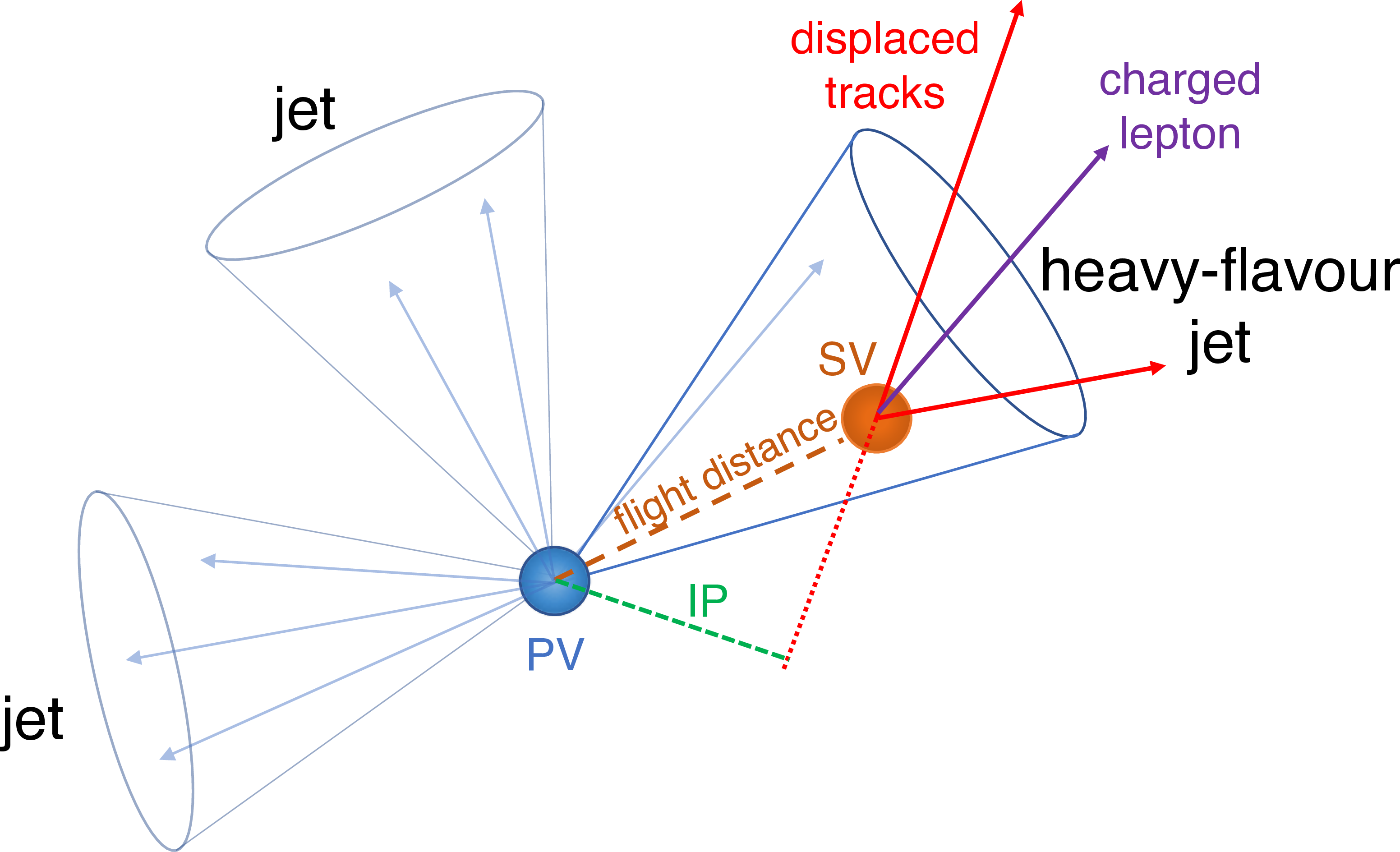
Figure 1:
Schematic diagram of a collision event with two light jets and one b jet. The finite and large lifetime of heavy-flavour hadrons (in particular b hadrons) leads to a displaced secondary vertex as well as tracks or leptons with large impact parameters. In contrast, light jets originate from the primary vertex and contain predominantly prompt tracks. Figure from Ref. [12]. |
png pdf |
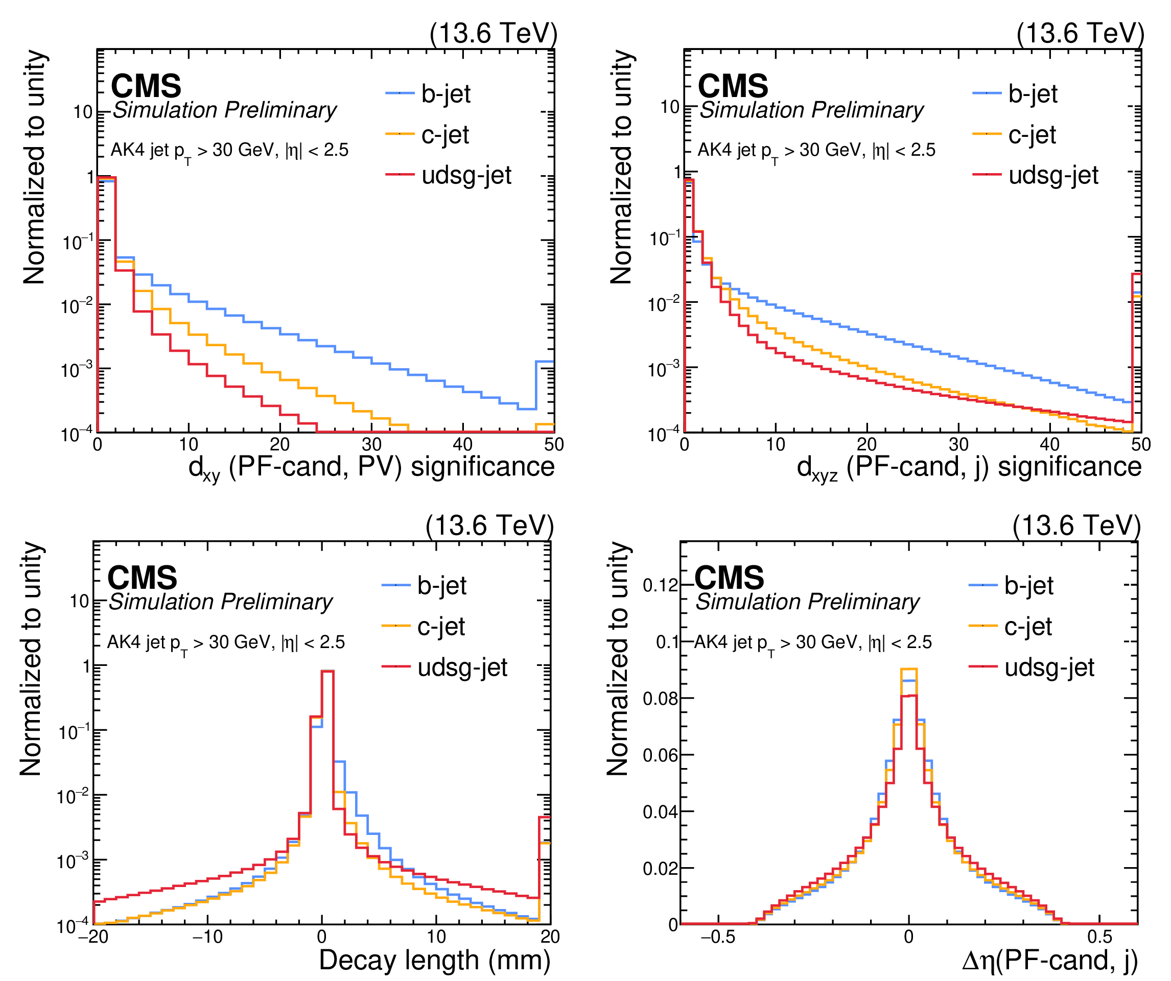
Figure 2:
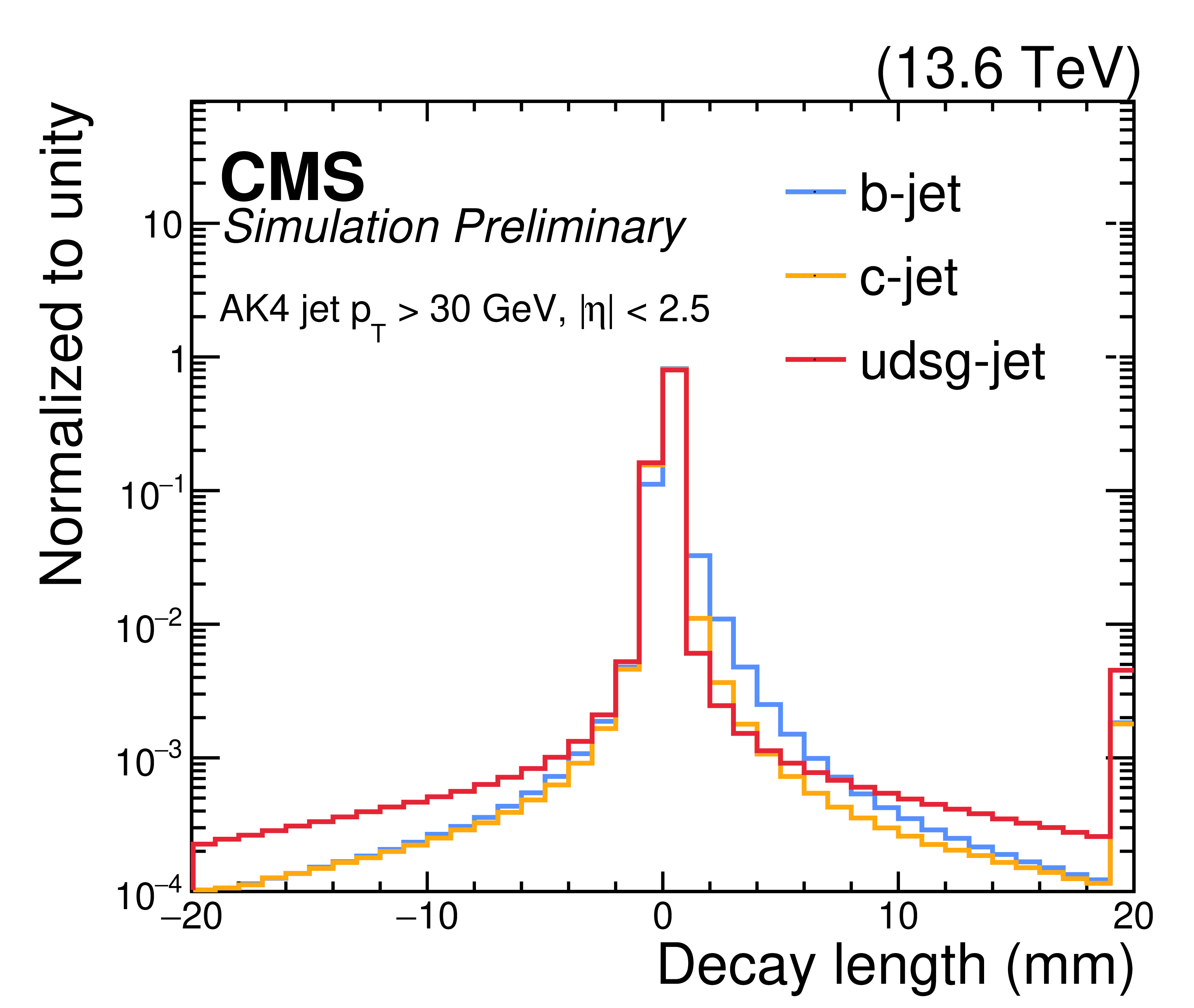
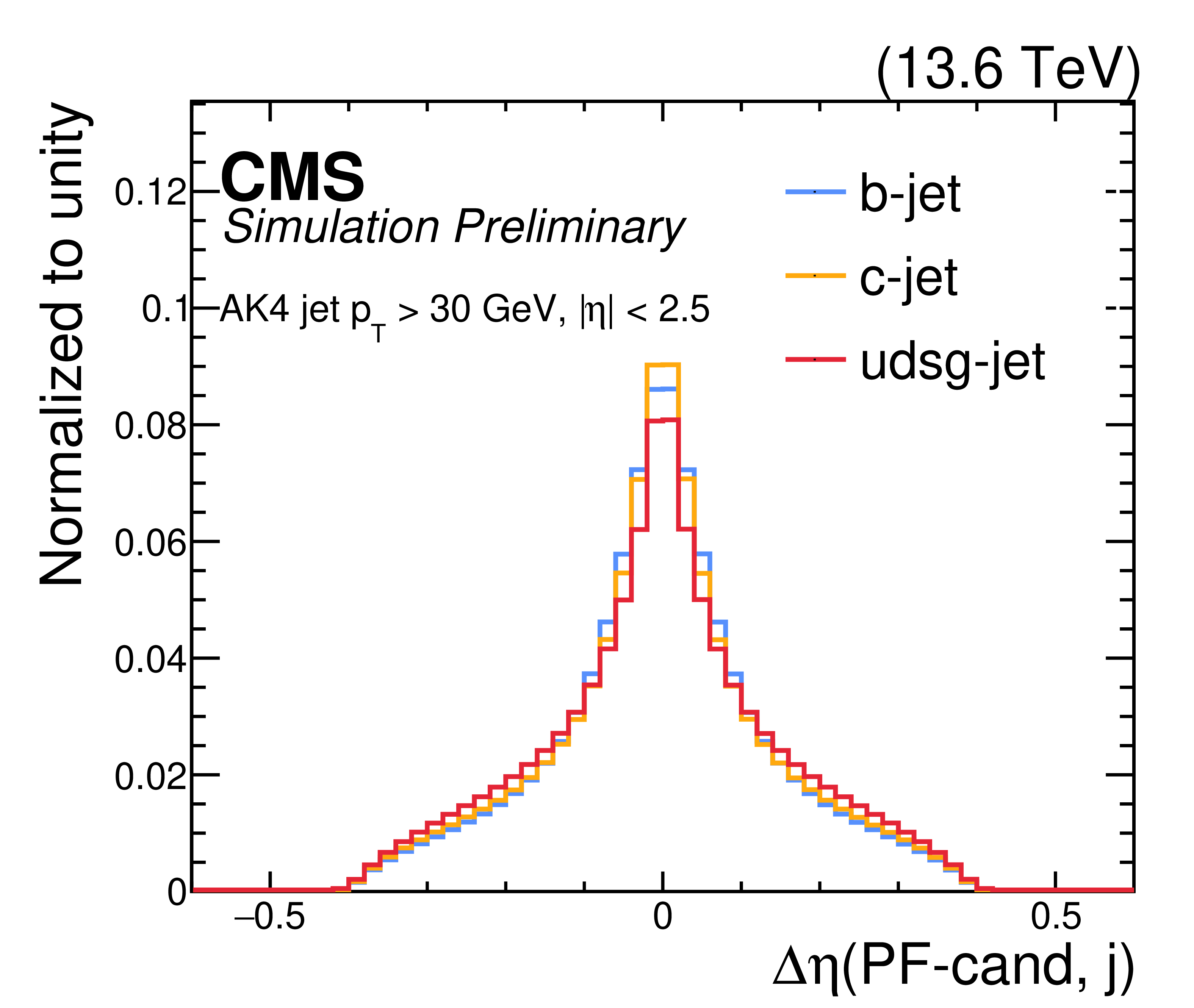
Distributions of PNET input variables related to PF candidates in b (blue), c (orange), and light (red) small-radius jets with $ p_{\mathrm{T}} > $ 30 GeV and $ {|\eta| < 2.5} $ from simulated $ \mathrm{t} \overline{\mathrm{t}} $ events. All distributions are normalized to unit area. Top: $ d_{xy} $ (left) and $ d_{xyz} $ (right) IP significances. Bottom: decay length with respect to the jet axis (left) and the $ \Delta\eta $ between the PF candidate and the jet axis (right). The first (last) bin includes underflow (overflow) entries. |
png pdf |
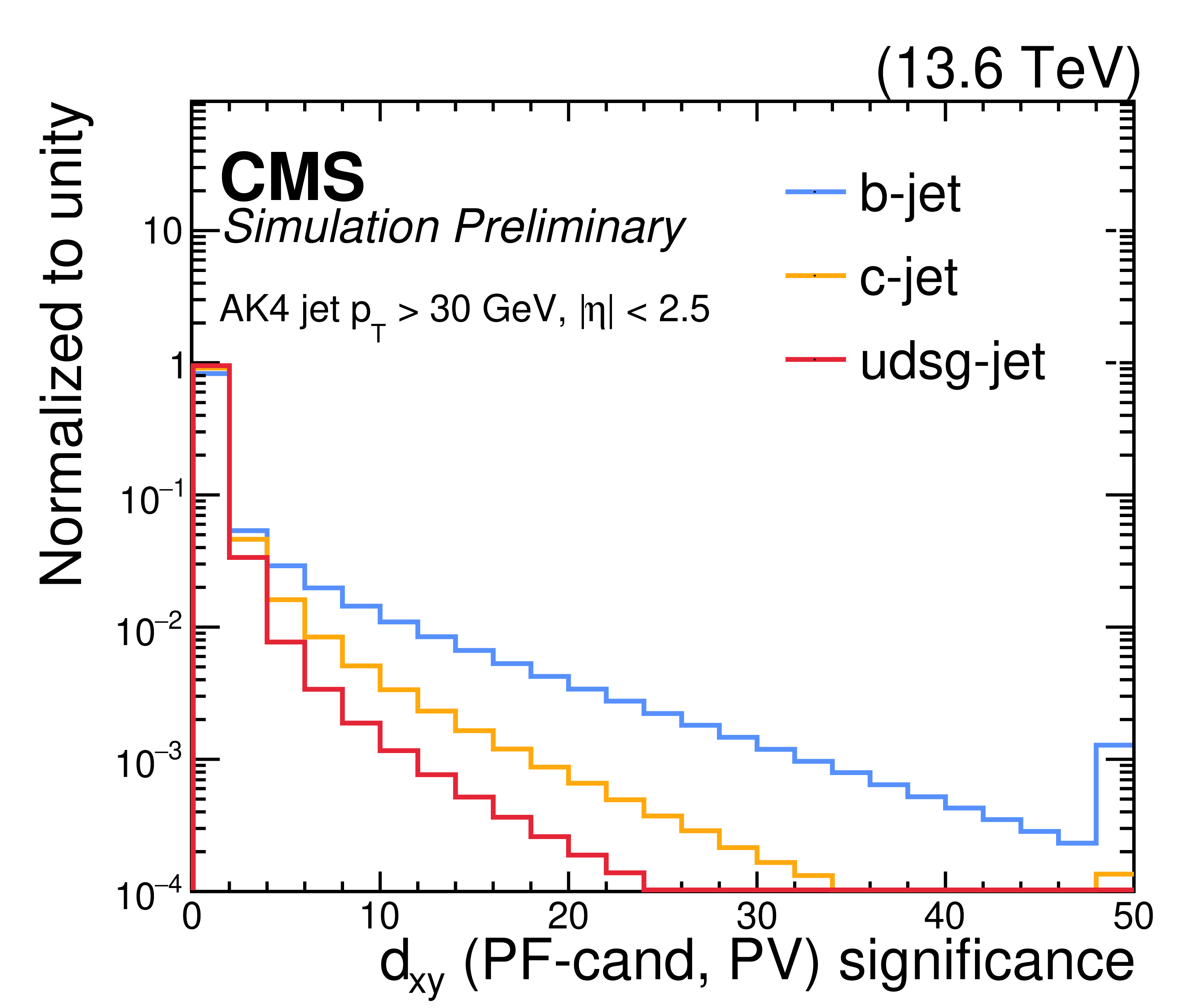
Figure 2-a:
Distributions of PNET input variables related to PF candidates in b (blue), c (orange), and light (red) small-radius jets with $ p_{\mathrm{T}} > $ 30 GeV and $ {|\eta| < 2.5} $ from simulated $ \mathrm{t} \overline{\mathrm{t}} $ events. All distributions are normalized to unit area. Top: $ d_{xy} $ (left) and $ d_{xyz} $ (right) IP significances. Bottom: decay length with respect to the jet axis (left) and the $ \Delta\eta $ between the PF candidate and the jet axis (right). The first (last) bin includes underflow (overflow) entries. |
png pdf |
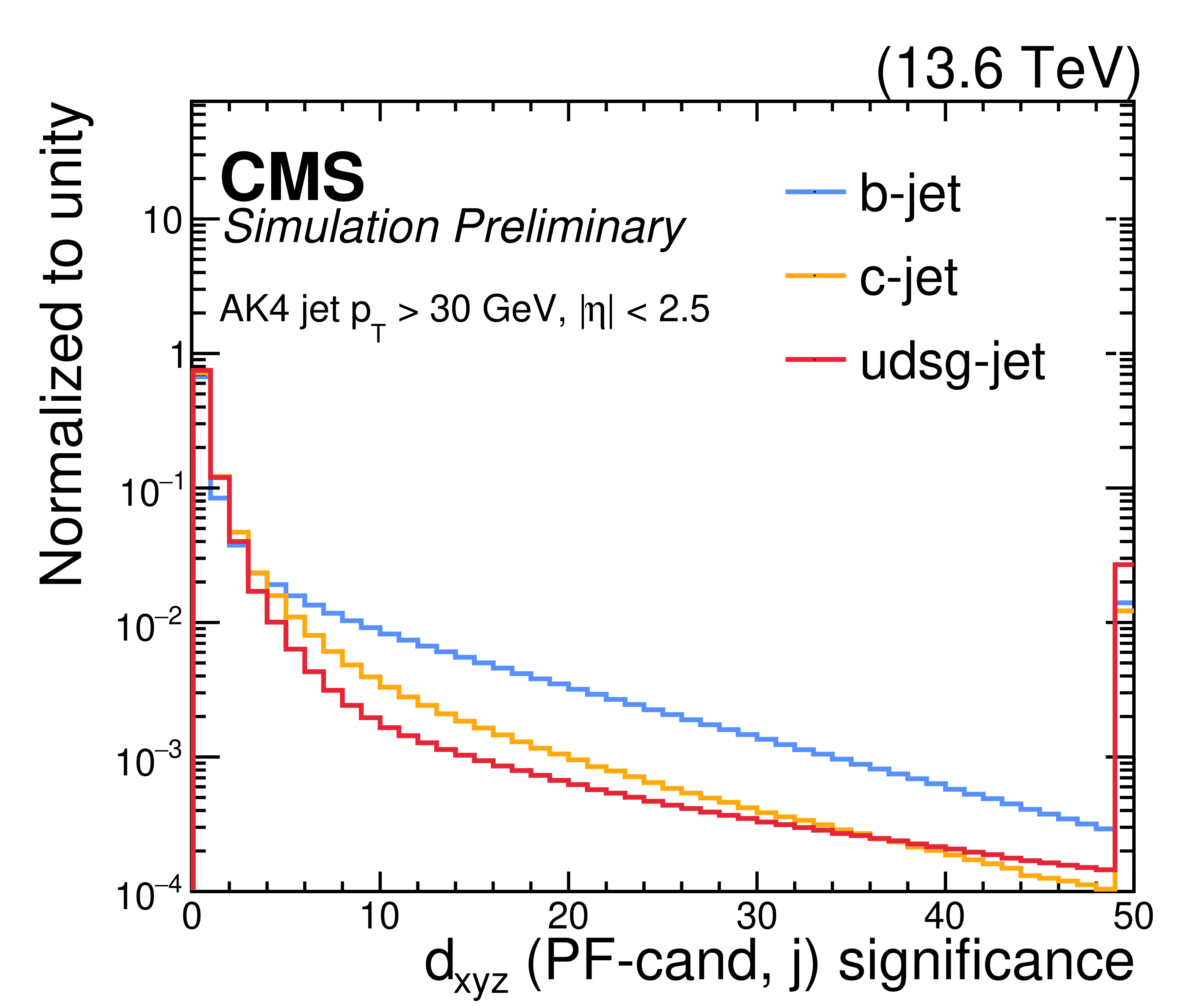
Figure 2-b:
Distributions of PNET input variables related to PF candidates in b (blue), c (orange), and light (red) small-radius jets with $ p_{\mathrm{T}} > $ 30 GeV and $ {|\eta| < 2.5} $ from simulated $ \mathrm{t} \overline{\mathrm{t}} $ events. All distributions are normalized to unit area. Top: $ d_{xy} $ (left) and $ d_{xyz} $ (right) IP significances. Bottom: decay length with respect to the jet axis (left) and the $ \Delta\eta $ between the PF candidate and the jet axis (right). The first (last) bin includes underflow (overflow) entries. |
png pdf |
Figure 2-c:
Distributions of PNET input variables related to PF candidates in b (blue), c (orange), and light (red) small-radius jets with $ p_{\mathrm{T}} > $ 30 GeV and $ {|\eta| < 2.5} $ from simulated $ \mathrm{t} \overline{\mathrm{t}} $ events. All distributions are normalized to unit area. Top: $ d_{xy} $ (left) and $ d_{xyz} $ (right) IP significances. Bottom: decay length with respect to the jet axis (left) and the $ \Delta\eta $ between the PF candidate and the jet axis (right). The first (last) bin includes underflow (overflow) entries. |
png pdf |
Figure 2-d:
Distributions of PNET input variables related to PF candidates in b (blue), c (orange), and light (red) small-radius jets with $ p_{\mathrm{T}} > $ 30 GeV and $ {|\eta| < 2.5} $ from simulated $ \mathrm{t} \overline{\mathrm{t}} $ events. All distributions are normalized to unit area. Top: $ d_{xy} $ (left) and $ d_{xyz} $ (right) IP significances. Bottom: decay length with respect to the jet axis (left) and the $ \Delta\eta $ between the PF candidate and the jet axis (right). The first (last) bin includes underflow (overflow) entries. |
png pdf |
Figure 3:
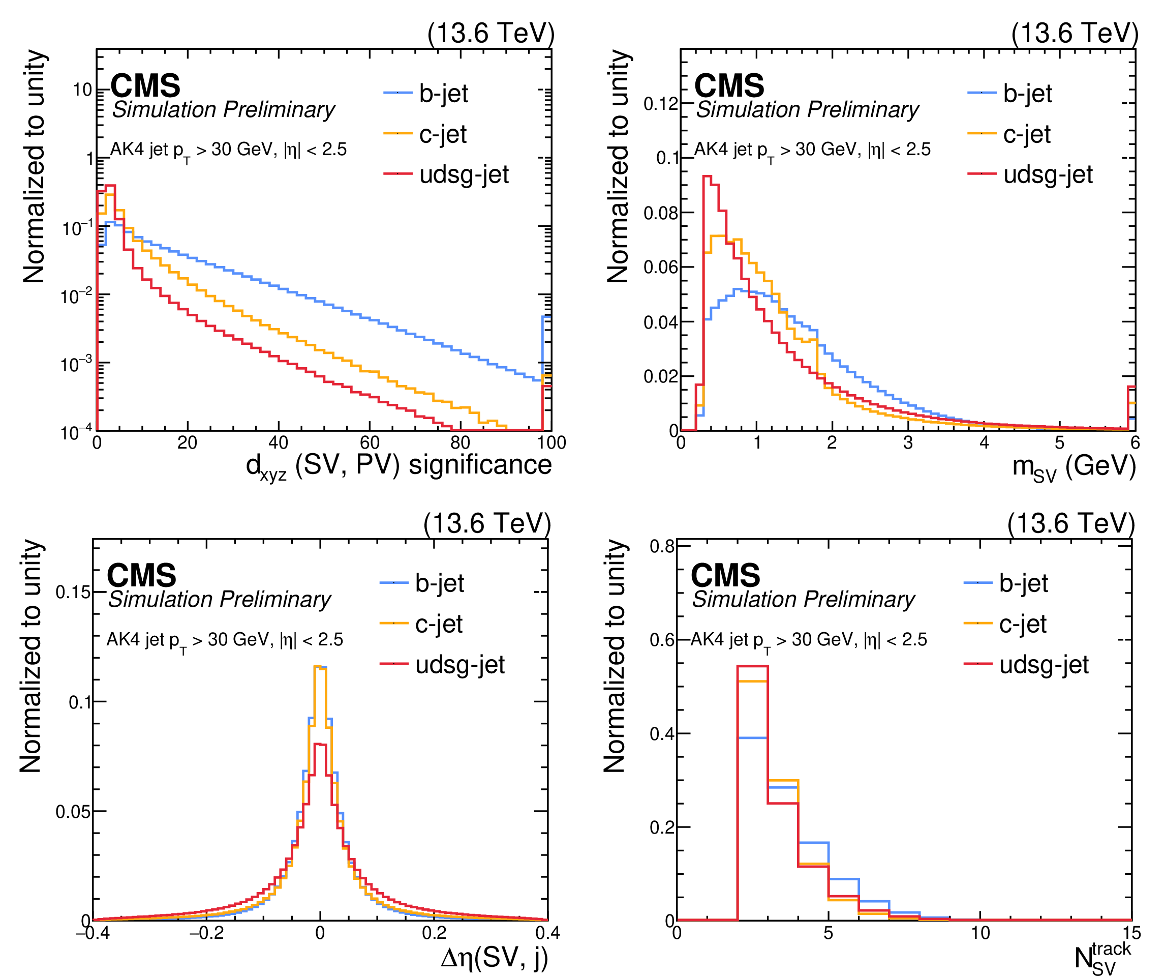
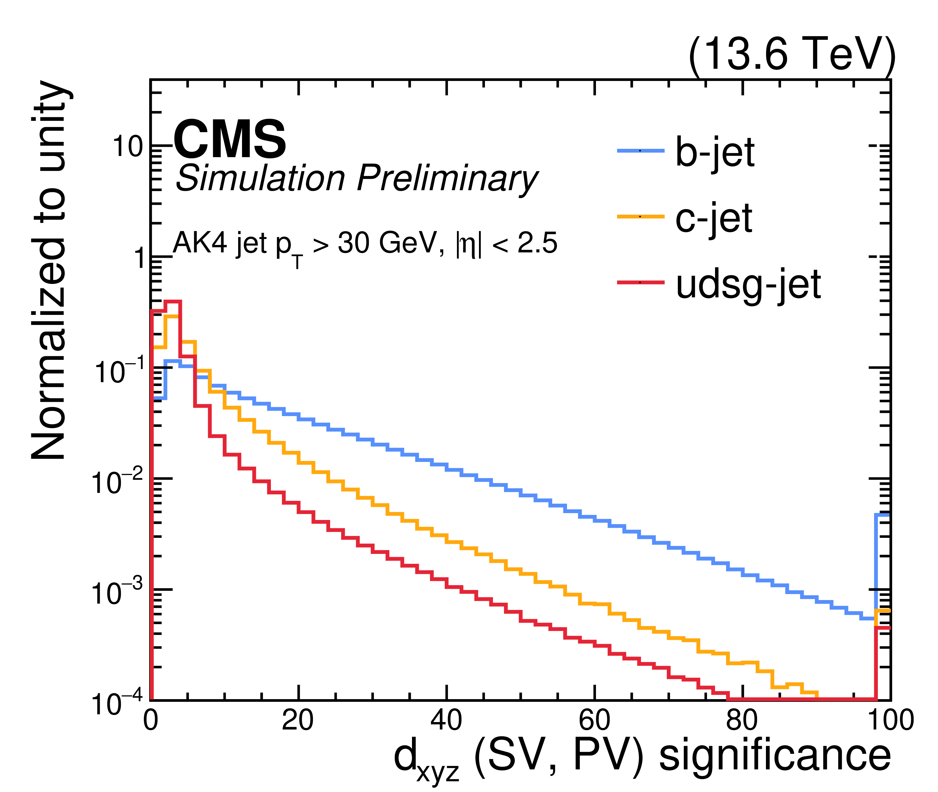
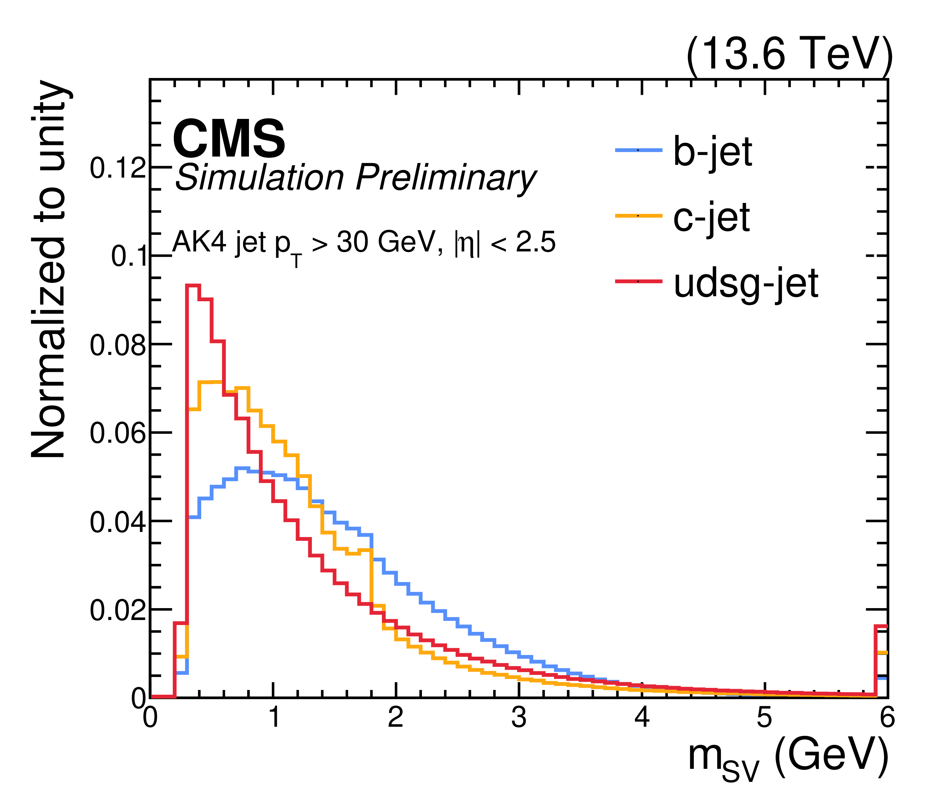
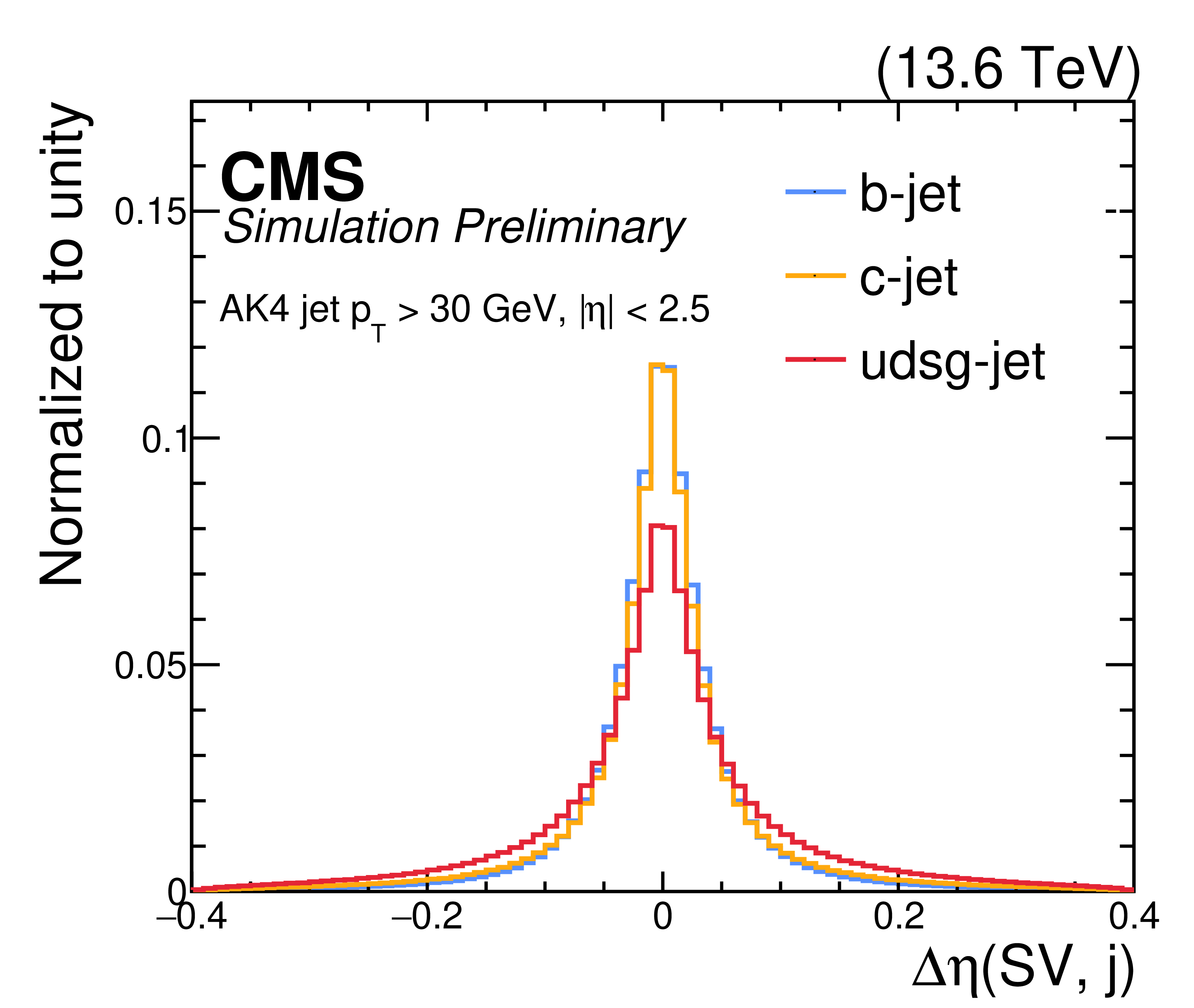
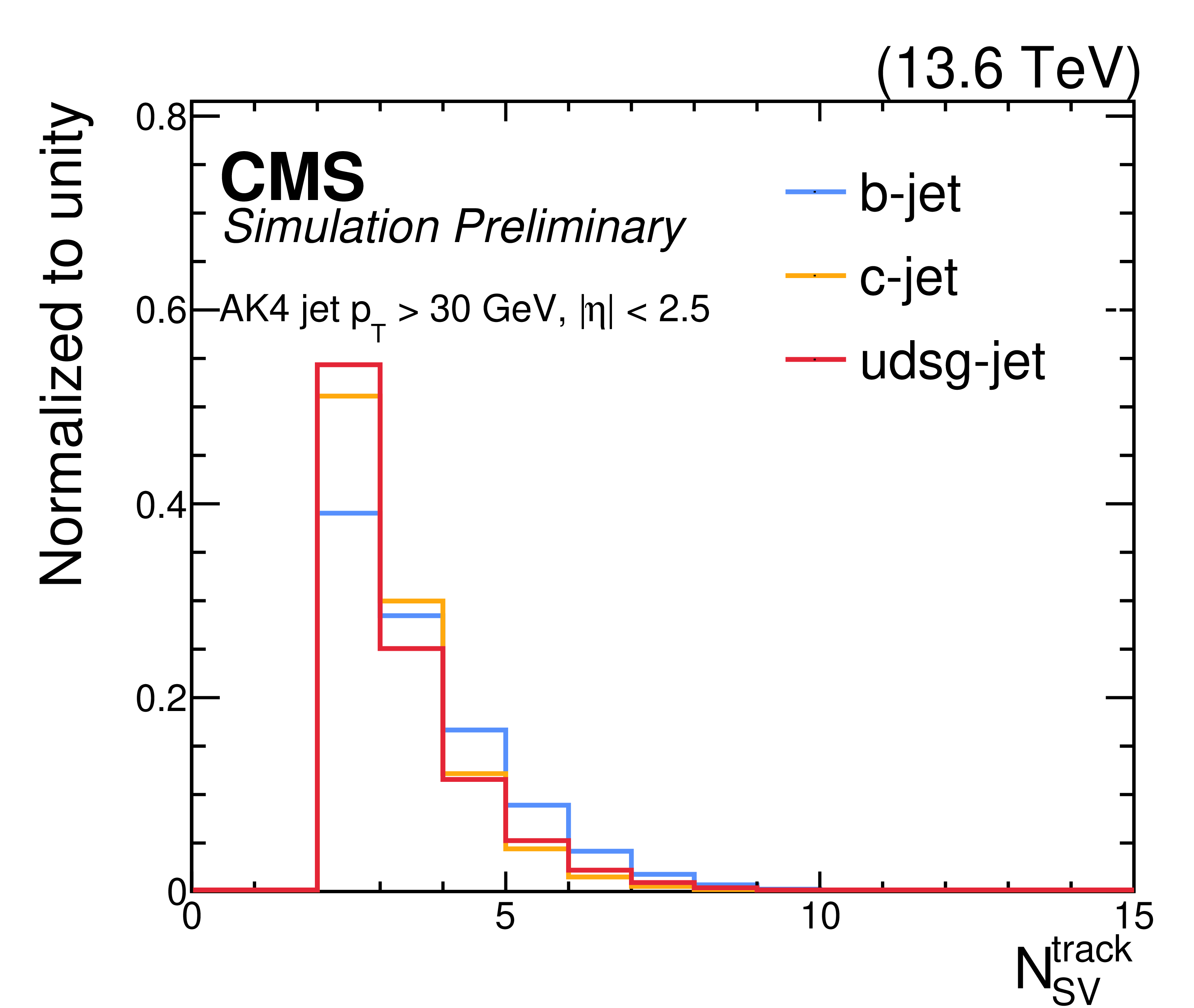
Distributions of PNET input variables related to SVs in b (blue), c (orange), and light (red) small-radius jets with $ p_{\mathrm{T}} > $ 30 GeV and $ {|\eta| < 2.5} $ from simulated $ \mathrm{t} \overline{\mathrm{t}} $ events. All distributions are normalized to unit area. Top: $ d_{xyz} $ significance (left) and SV invariant mass (right). Bottom: $ \Delta\eta $ between the SV and the jet axis (left) and the SV track multiplicity (right). The first (last) bin includes underflow (overflow) entries. |
png pdf |
Figure 3-a:
Distributions of PNET input variables related to SVs in b (blue), c (orange), and light (red) small-radius jets with $ p_{\mathrm{T}} > $ 30 GeV and $ {|\eta| < 2.5} $ from simulated $ \mathrm{t} \overline{\mathrm{t}} $ events. All distributions are normalized to unit area. Top: $ d_{xyz} $ significance (left) and SV invariant mass (right). Bottom: $ \Delta\eta $ between the SV and the jet axis (left) and the SV track multiplicity (right). The first (last) bin includes underflow (overflow) entries. |
png pdf |
Figure 3-b:
Distributions of PNET input variables related to SVs in b (blue), c (orange), and light (red) small-radius jets with $ p_{\mathrm{T}} > $ 30 GeV and $ {|\eta| < 2.5} $ from simulated $ \mathrm{t} \overline{\mathrm{t}} $ events. All distributions are normalized to unit area. Top: $ d_{xyz} $ significance (left) and SV invariant mass (right). Bottom: $ \Delta\eta $ between the SV and the jet axis (left) and the SV track multiplicity (right). The first (last) bin includes underflow (overflow) entries. |
png pdf |
Figure 3-c:
Distributions of PNET input variables related to SVs in b (blue), c (orange), and light (red) small-radius jets with $ p_{\mathrm{T}} > $ 30 GeV and $ {|\eta| < 2.5} $ from simulated $ \mathrm{t} \overline{\mathrm{t}} $ events. All distributions are normalized to unit area. Top: $ d_{xyz} $ significance (left) and SV invariant mass (right). Bottom: $ \Delta\eta $ between the SV and the jet axis (left) and the SV track multiplicity (right). The first (last) bin includes underflow (overflow) entries. |
png pdf |
Figure 3-d:
Distributions of PNET input variables related to SVs in b (blue), c (orange), and light (red) small-radius jets with $ p_{\mathrm{T}} > $ 30 GeV and $ {|\eta| < 2.5} $ from simulated $ \mathrm{t} \overline{\mathrm{t}} $ events. All distributions are normalized to unit area. Top: $ d_{xyz} $ significance (left) and SV invariant mass (right). Bottom: $ \Delta\eta $ between the SV and the jet axis (left) and the SV track multiplicity (right). The first (last) bin includes underflow (overflow) entries. |
png pdf |
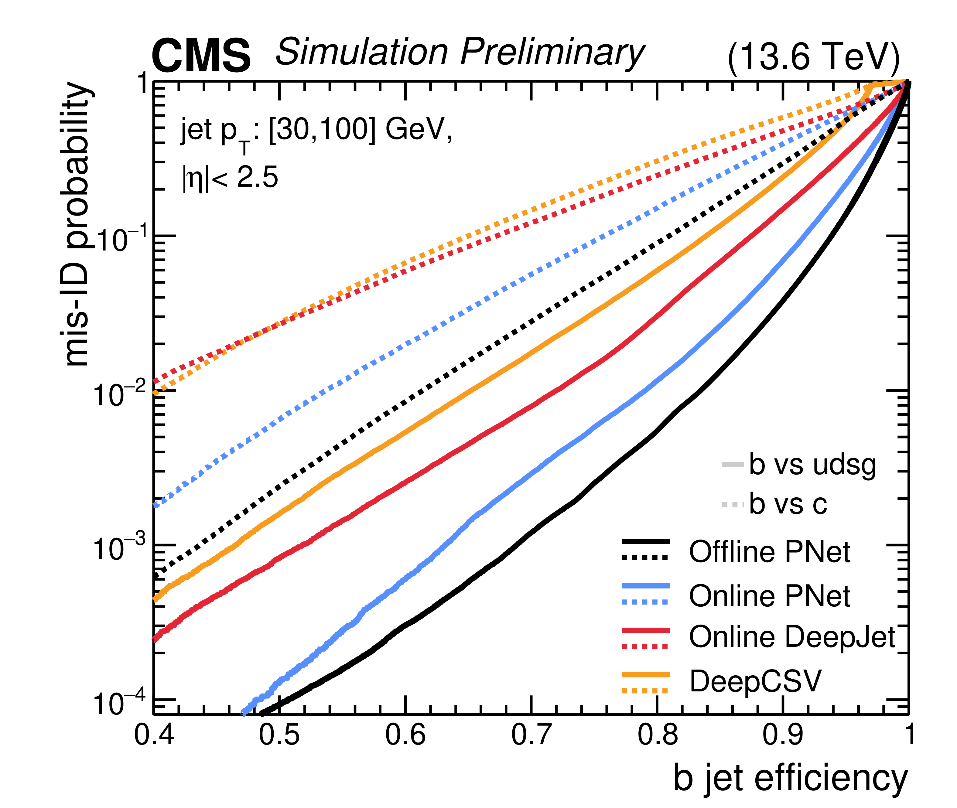
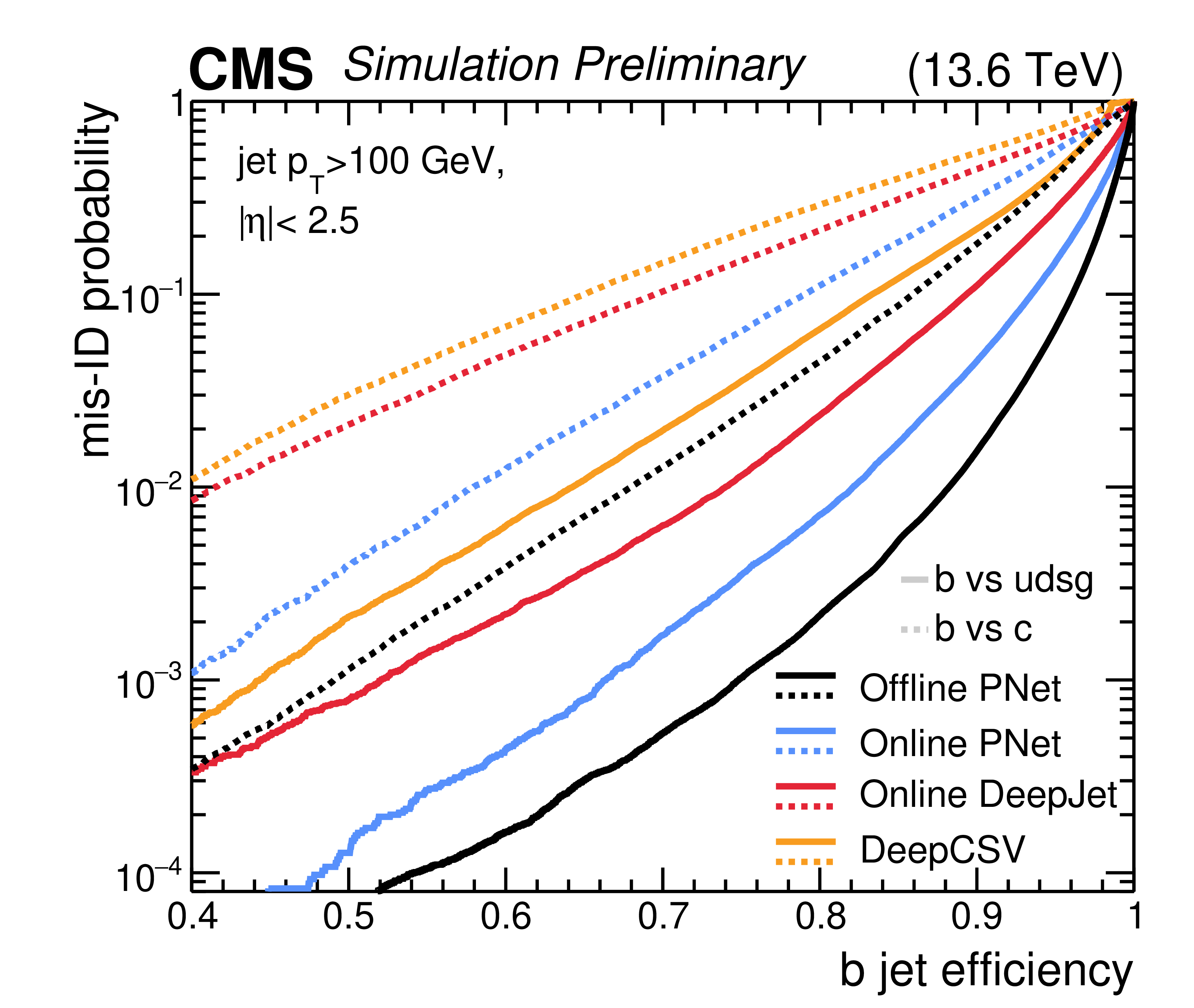
Figure 4:
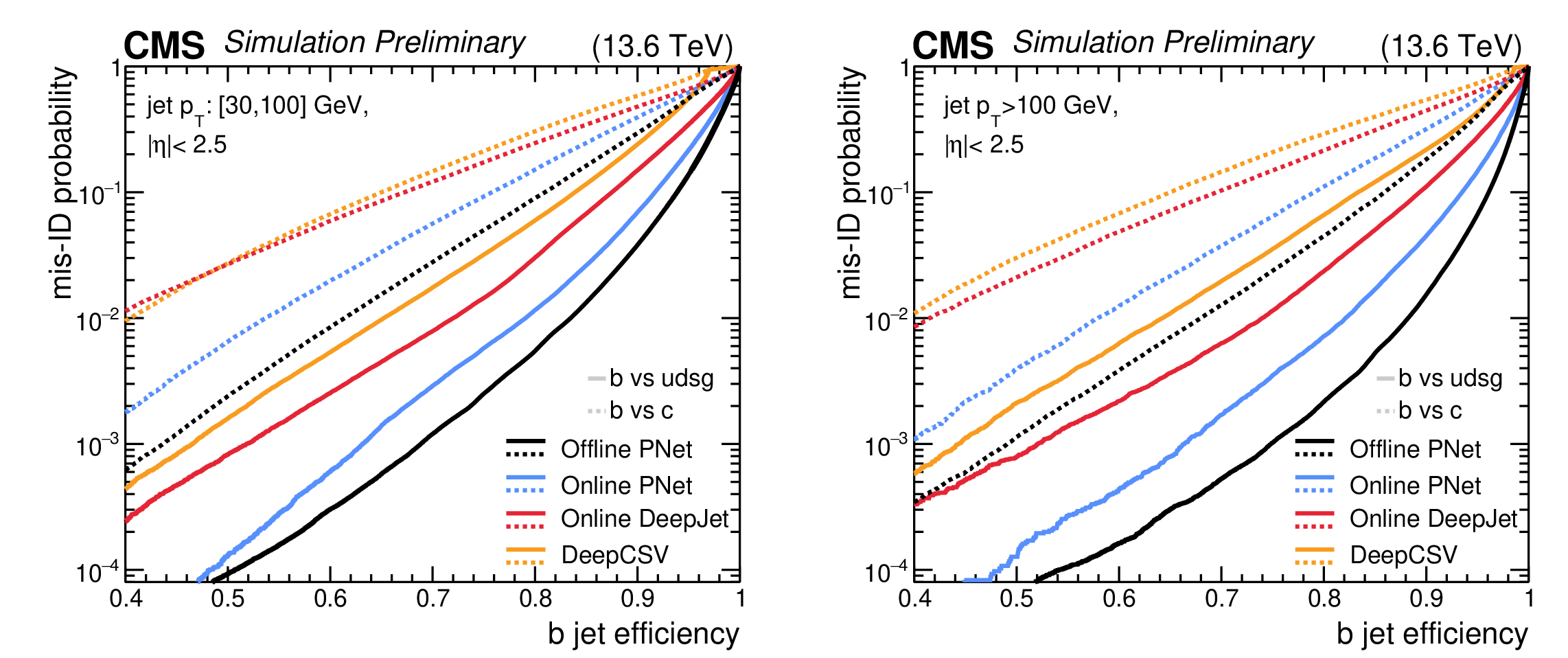
Misidentification probability for light jets (uds and gluon) (solid curves) and c (dashed curves) as a function of b jet identification efficiency for various jet-tagging algorithms applied to small-radius jets with $ {|\eta| < 2.5} $ and $ 30 < p_{\mathrm{T}} < $ 100 GeV (left) or $ p_{\mathrm{T}} > $ 100 GeV (right) from simulated $ \mathrm{t} \overline{\mathrm{t}} $ events. Results are shown for the PNET (blue) and DEEPJET (red) taggers trained for Run 3, and for the DEEPCSV (orange) discriminator used during Run 2. The performance of jet flavour taggers developed for the HLT can be compared with that obtained from the offline PNET algorithm (black) [65], evaluated on jets from the same selected events. |
png pdf |
Figure 4-a:
Misidentification probability for light jets (uds and gluon) (solid curves) and c (dashed curves) as a function of b jet identification efficiency for various jet-tagging algorithms applied to small-radius jets with $ {|\eta| < 2.5} $ and $ 30 < p_{\mathrm{T}} < $ 100 GeV (left) or $ p_{\mathrm{T}} > $ 100 GeV (right) from simulated $ \mathrm{t} \overline{\mathrm{t}} $ events. Results are shown for the PNET (blue) and DEEPJET (red) taggers trained for Run 3, and for the DEEPCSV (orange) discriminator used during Run 2. The performance of jet flavour taggers developed for the HLT can be compared with that obtained from the offline PNET algorithm (black) [65], evaluated on jets from the same selected events. |
png pdf |
Figure 4-b:
Misidentification probability for light jets (uds and gluon) (solid curves) and c (dashed curves) as a function of b jet identification efficiency for various jet-tagging algorithms applied to small-radius jets with $ {|\eta| < 2.5} $ and $ 30 < p_{\mathrm{T}} < $ 100 GeV (left) or $ p_{\mathrm{T}} > $ 100 GeV (right) from simulated $ \mathrm{t} \overline{\mathrm{t}} $ events. Results are shown for the PNET (blue) and DEEPJET (red) taggers trained for Run 3, and for the DEEPCSV (orange) discriminator used during Run 2. The performance of jet flavour taggers developed for the HLT can be compared with that obtained from the offline PNET algorithm (black) [65], evaluated on jets from the same selected events. |
png pdf |
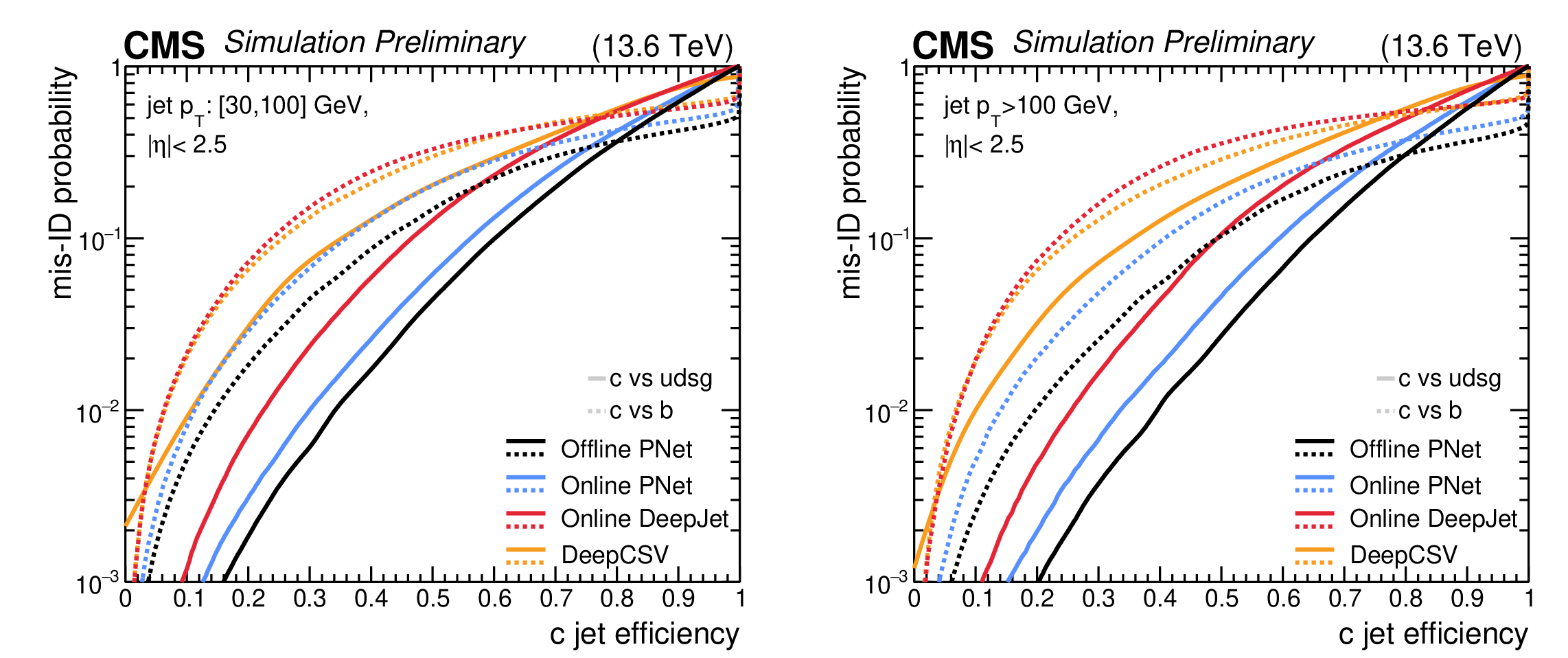
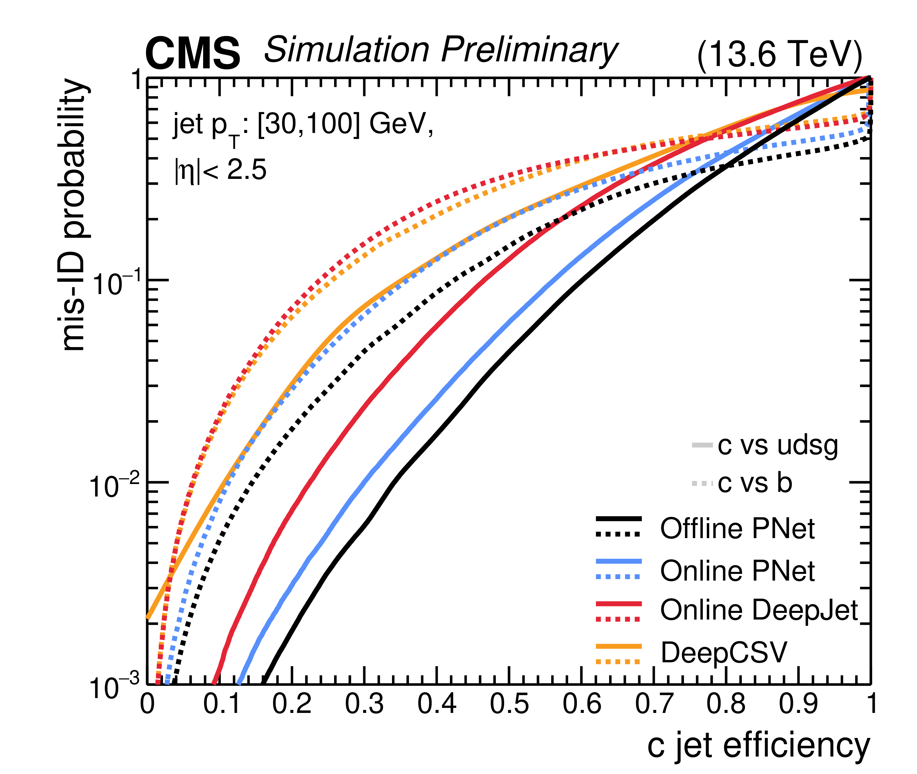
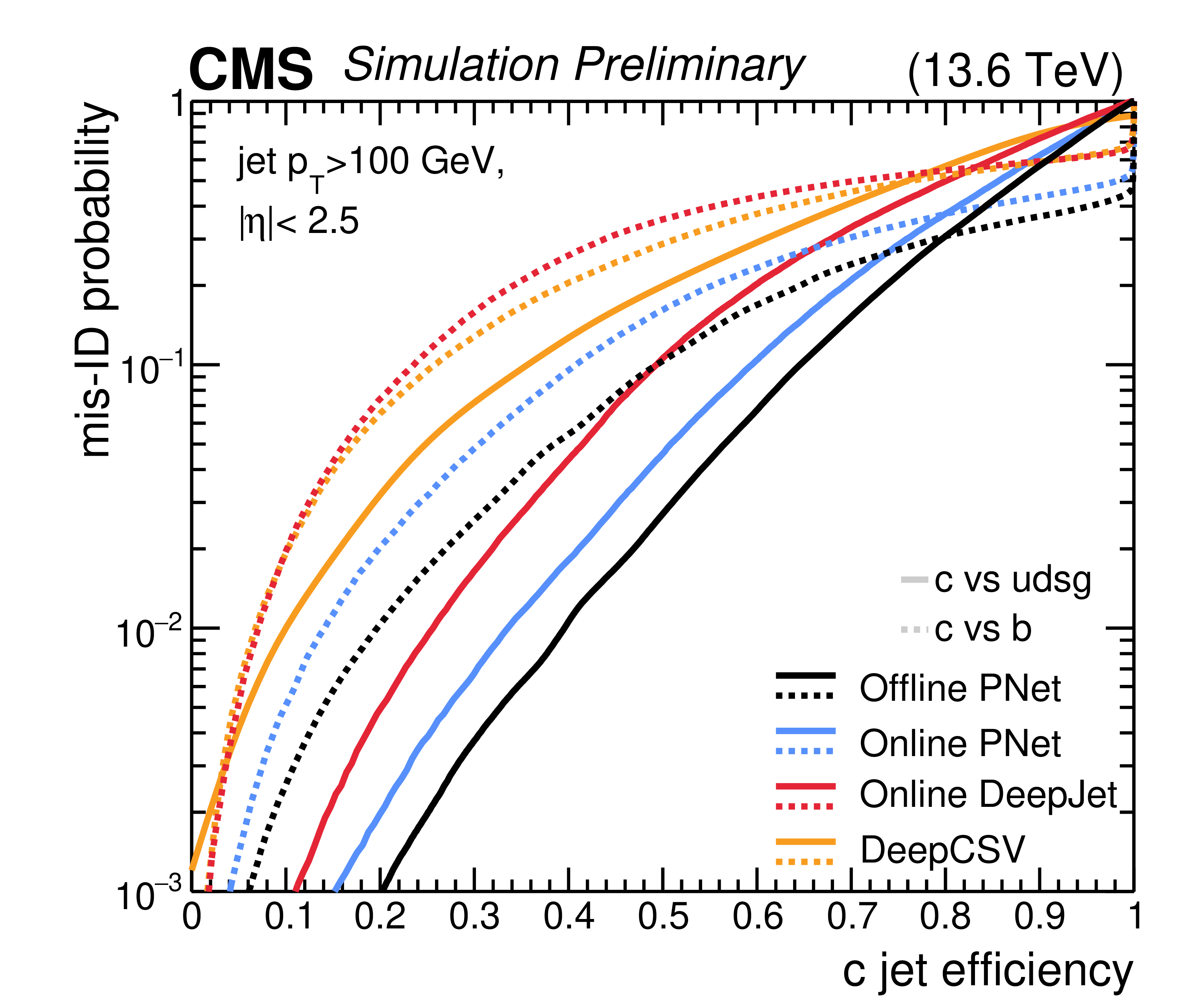
Figure 5:
Misidentification probability for light jets (uds and gluon) (solid curves) and b (dashed curves) as a function of c jet identification efficiency for various jet-tagging algorithms applied to small-radius jets with $ {|\eta| < 2.5} $ and $ 30 < p_{\mathrm{T}} < $ 100 GeV (left) or $ p_{\mathrm{T}} > $ 100 GeV (right) from simulated $ \mathrm{t} \overline{\mathrm{t}} $ events. Results are shown for the PNET (blue) and DEEPJET (red) taggers trained for Run 3, and for the DEEPCSV (orange) discriminator used during Run 2. The performance of jet flavour taggers developed for the HLT can be compared with that obtained from the offline PNET algorithm (black) [65], evaluated on jets from the same selected events. |
png pdf |
Figure 5-a:
Misidentification probability for light jets (uds and gluon) (solid curves) and b (dashed curves) as a function of c jet identification efficiency for various jet-tagging algorithms applied to small-radius jets with $ {|\eta| < 2.5} $ and $ 30 < p_{\mathrm{T}} < $ 100 GeV (left) or $ p_{\mathrm{T}} > $ 100 GeV (right) from simulated $ \mathrm{t} \overline{\mathrm{t}} $ events. Results are shown for the PNET (blue) and DEEPJET (red) taggers trained for Run 3, and for the DEEPCSV (orange) discriminator used during Run 2. The performance of jet flavour taggers developed for the HLT can be compared with that obtained from the offline PNET algorithm (black) [65], evaluated on jets from the same selected events. |
png pdf |
Figure 5-b:
Misidentification probability for light jets (uds and gluon) (solid curves) and b (dashed curves) as a function of c jet identification efficiency for various jet-tagging algorithms applied to small-radius jets with $ {|\eta| < 2.5} $ and $ 30 < p_{\mathrm{T}} < $ 100 GeV (left) or $ p_{\mathrm{T}} > $ 100 GeV (right) from simulated $ \mathrm{t} \overline{\mathrm{t}} $ events. Results are shown for the PNET (blue) and DEEPJET (red) taggers trained for Run 3, and for the DEEPCSV (orange) discriminator used during Run 2. The performance of jet flavour taggers developed for the HLT can be compared with that obtained from the offline PNET algorithm (black) [65], evaluated on jets from the same selected events. |
png pdf |
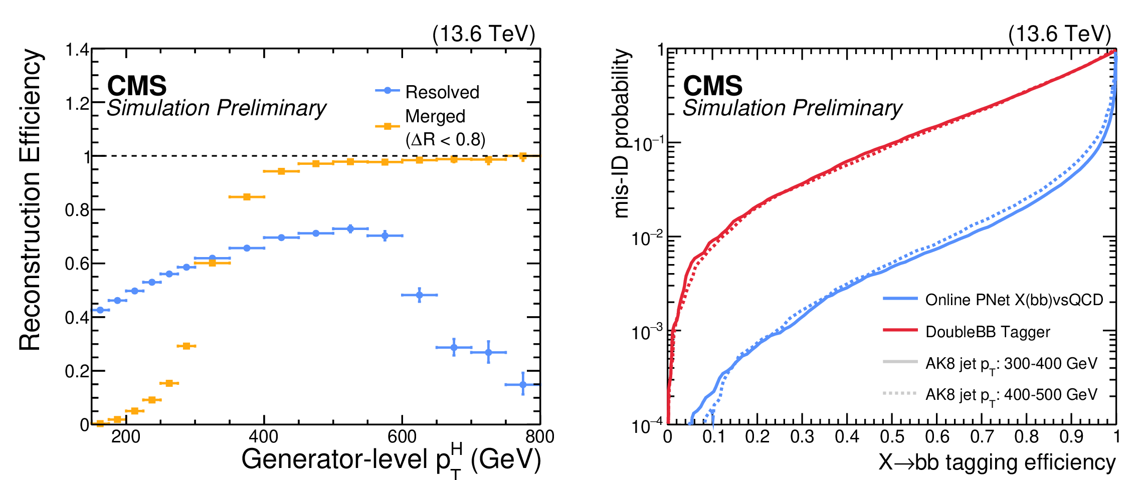
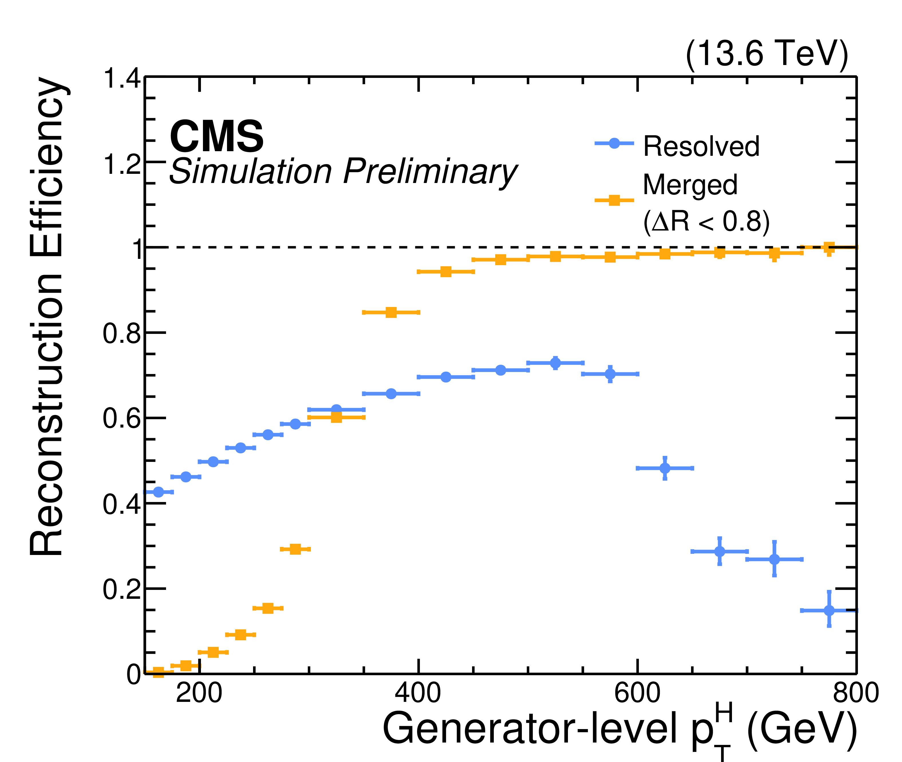
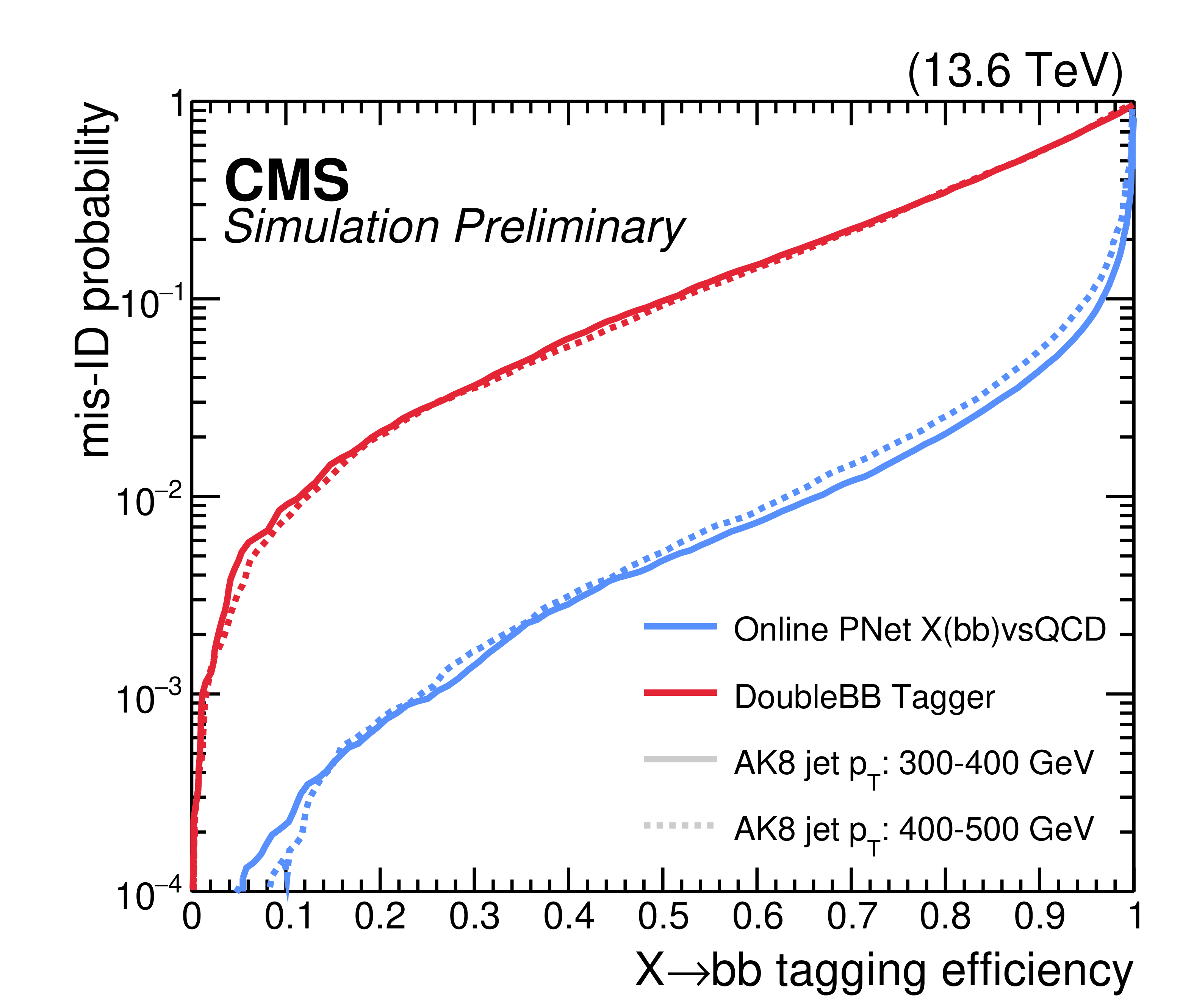
Figure 6:
Left: reconstruction efficiency of $ \mathrm{H} \to \mathrm{b}\overline{\mathrm{b}} $ candidates, as a function of the its generator-level $ p_{\mathrm{T}} $, as two small-radius jets (resolved approach) in azure or as a single larger-radius jet (merged approach) in orange. The $ \mathrm{H} \to \mathrm{b}\overline{\mathrm{b}} $ candidates are obtained from simulated $ \mathrm{H}\mathrm{H} \to 4\mathrm{b} $ events. Right: Misidentification probability for QCD jets versus the $ \text{X} \to \mathrm{b}\overline{\mathrm{b}} $ tagging efficiency for the PNET (blue) and DOUBLE-B (red) algorithms, applied to simulated jets reconstructed at the HLT with $ {|\eta| < 2.5} $, $ m_{\mathrm{SD}} > $ 40 GeV, and $ 300 < p_{\mathrm{T}} < $ 400 GeV (solid) or $ 400 < p_{\mathrm{T}} < $ 500 GeV (dashed). |
png pdf |
Figure 6-a:
Left: reconstruction efficiency of $ \mathrm{H} \to \mathrm{b}\overline{\mathrm{b}} $ candidates, as a function of the its generator-level $ p_{\mathrm{T}} $, as two small-radius jets (resolved approach) in azure or as a single larger-radius jet (merged approach) in orange. The $ \mathrm{H} \to \mathrm{b}\overline{\mathrm{b}} $ candidates are obtained from simulated $ \mathrm{H}\mathrm{H} \to 4\mathrm{b} $ events. Right: Misidentification probability for QCD jets versus the $ \text{X} \to \mathrm{b}\overline{\mathrm{b}} $ tagging efficiency for the PNET (blue) and DOUBLE-B (red) algorithms, applied to simulated jets reconstructed at the HLT with $ {|\eta| < 2.5} $, $ m_{\mathrm{SD}} > $ 40 GeV, and $ 300 < p_{\mathrm{T}} < $ 400 GeV (solid) or $ 400 < p_{\mathrm{T}} < $ 500 GeV (dashed). |
png pdf |
Figure 6-b:
Left: reconstruction efficiency of $ \mathrm{H} \to \mathrm{b}\overline{\mathrm{b}} $ candidates, as a function of the its generator-level $ p_{\mathrm{T}} $, as two small-radius jets (resolved approach) in azure or as a single larger-radius jet (merged approach) in orange. The $ \mathrm{H} \to \mathrm{b}\overline{\mathrm{b}} $ candidates are obtained from simulated $ \mathrm{H}\mathrm{H} \to 4\mathrm{b} $ events. Right: Misidentification probability for QCD jets versus the $ \text{X} \to \mathrm{b}\overline{\mathrm{b}} $ tagging efficiency for the PNET (blue) and DOUBLE-B (red) algorithms, applied to simulated jets reconstructed at the HLT with $ {|\eta| < 2.5} $, $ m_{\mathrm{SD}} > $ 40 GeV, and $ 300 < p_{\mathrm{T}} < $ 400 GeV (solid) or $ 400 < p_{\mathrm{T}} < $ 500 GeV (dashed). |
png pdf |
Figure 7:
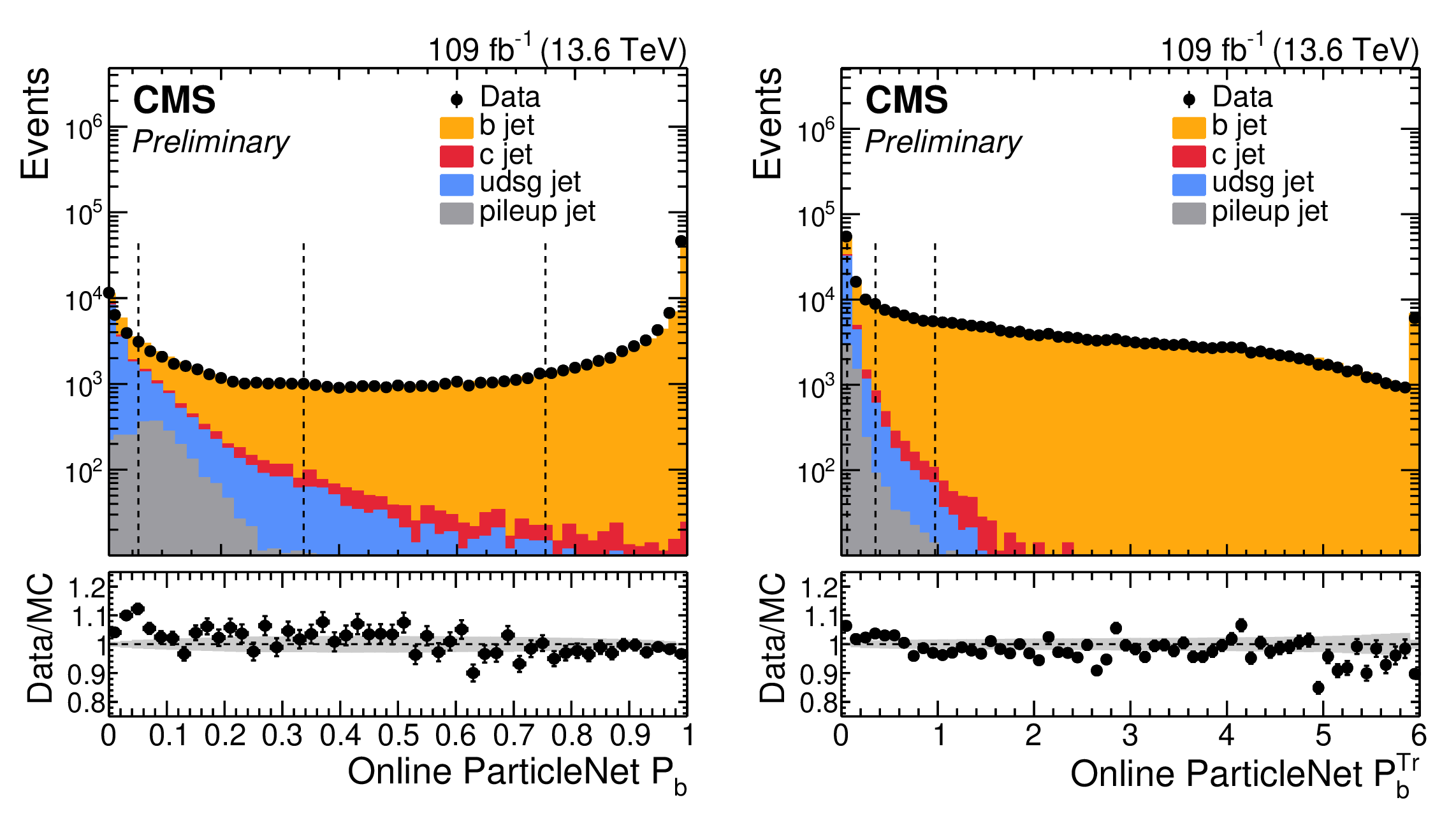
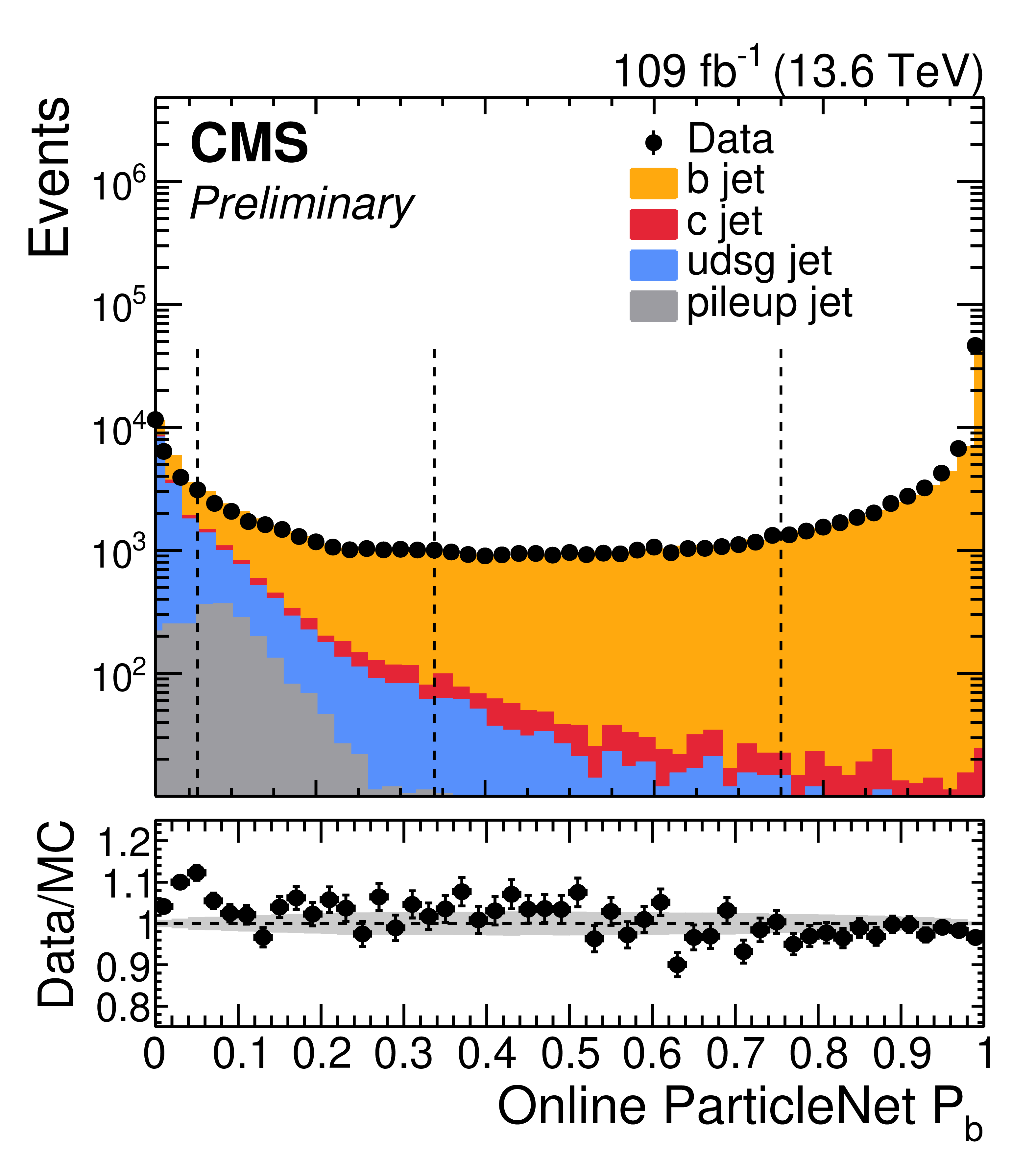
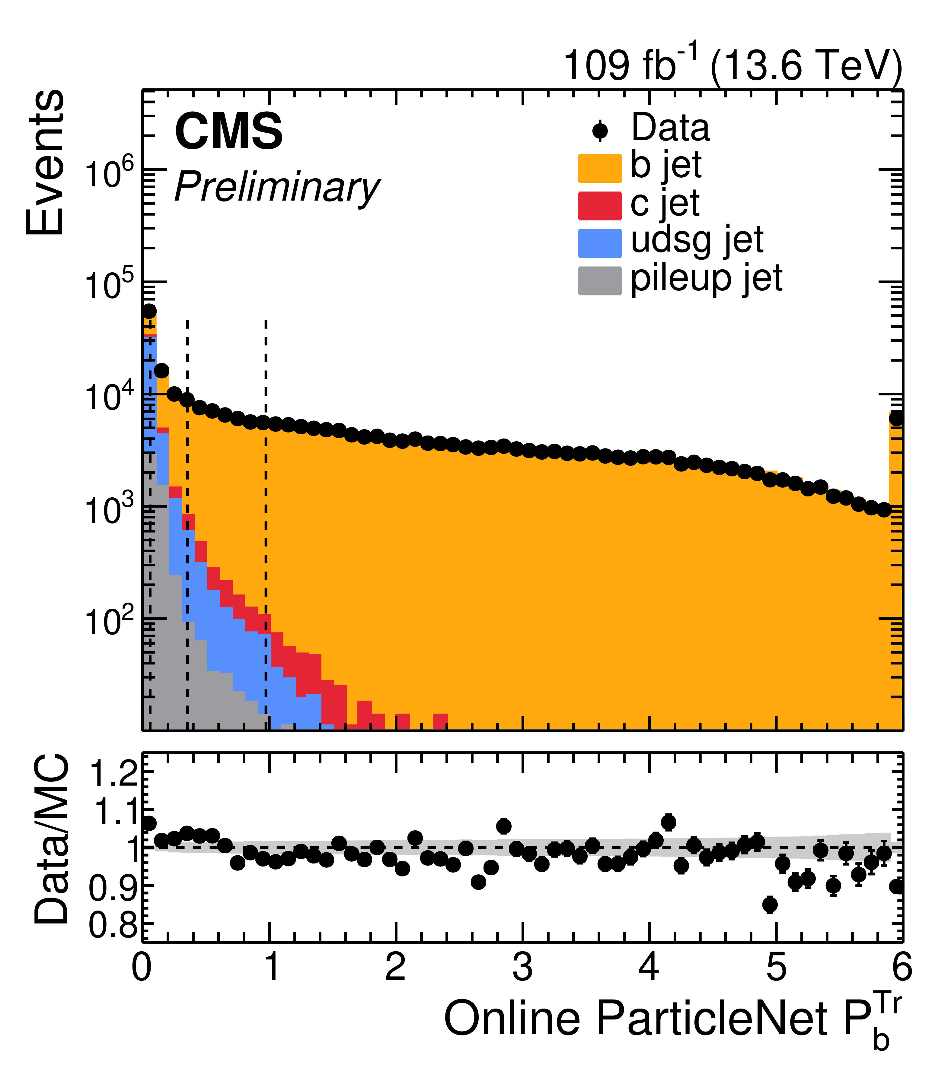
Left: distribution of the online PNET $\mathcal{P}_{\mathrm{b}}$ score for small-radius jets with $ p_{\mathrm{T}} > $ 25 GeV and $ {|\eta| < 2.5} $ in the $ {{\mathrm{t}\overline{\mathrm{t}}} (\mathrm{e}\mu)} $ region, shown for data (black points) and the MC prediction for SM processes. The simulated contribution is separated into exclusive jet-flavour categories: b (orange), c (red), and light-flavour quarks plus gluons (blue). Jets originating from pileup interactions are shown in gray. The lower panel displays the ratio of data to the MC prediction as a function of $ \mathcal{P}_{\mathrm{b}} $, while the grey error band displays the statistical uncertainty of the simulation. Right: distribution of the transformed b-tagging score ($ \mathcal{P}_{\mathrm{b}}^{\mathrm{Tr}} $), defined as $ \mathcal{P}_{\mathrm{b}}^{\mathrm{Tr}} = \tanh^{-1}(\mathcal{P}_{\mathrm{b}}) $. The black dashed vertical lines indicate, from left to right, the three b-tagging working points (L, M, and T) used in the efficiency studies. |
png pdf |
Figure 7-a:
Left: distribution of the online PNET $\mathcal{P}_{\mathrm{b}}$ score for small-radius jets with $ p_{\mathrm{T}} > $ 25 GeV and $ {|\eta| < 2.5} $ in the $ {{\mathrm{t}\overline{\mathrm{t}}} (\mathrm{e}\mu)} $ region, shown for data (black points) and the MC prediction for SM processes. The simulated contribution is separated into exclusive jet-flavour categories: b (orange), c (red), and light-flavour quarks plus gluons (blue). Jets originating from pileup interactions are shown in gray. The lower panel displays the ratio of data to the MC prediction as a function of $ \mathcal{P}_{\mathrm{b}} $, while the grey error band displays the statistical uncertainty of the simulation. Right: distribution of the transformed b-tagging score ($ \mathcal{P}_{\mathrm{b}}^{\mathrm{Tr}} $), defined as $ \mathcal{P}_{\mathrm{b}}^{\mathrm{Tr}} = \tanh^{-1}(\mathcal{P}_{\mathrm{b}}) $. The black dashed vertical lines indicate, from left to right, the three b-tagging working points (L, M, and T) used in the efficiency studies. |
png pdf |
Figure 7-b:
Left: distribution of the online PNET $\mathcal{P}_{\mathrm{b}}$ score for small-radius jets with $ p_{\mathrm{T}} > $ 25 GeV and $ {|\eta| < 2.5} $ in the $ {{\mathrm{t}\overline{\mathrm{t}}} (\mathrm{e}\mu)} $ region, shown for data (black points) and the MC prediction for SM processes. The simulated contribution is separated into exclusive jet-flavour categories: b (orange), c (red), and light-flavour quarks plus gluons (blue). Jets originating from pileup interactions are shown in gray. The lower panel displays the ratio of data to the MC prediction as a function of $ \mathcal{P}_{\mathrm{b}} $, while the grey error band displays the statistical uncertainty of the simulation. Right: distribution of the transformed b-tagging score ($ \mathcal{P}_{\mathrm{b}}^{\mathrm{Tr}} $), defined as $ \mathcal{P}_{\mathrm{b}}^{\mathrm{Tr}} = \tanh^{-1}(\mathcal{P}_{\mathrm{b}}) $. The black dashed vertical lines indicate, from left to right, the three b-tagging working points (L, M, and T) used in the efficiency studies. |
png pdf |
Figure 8:
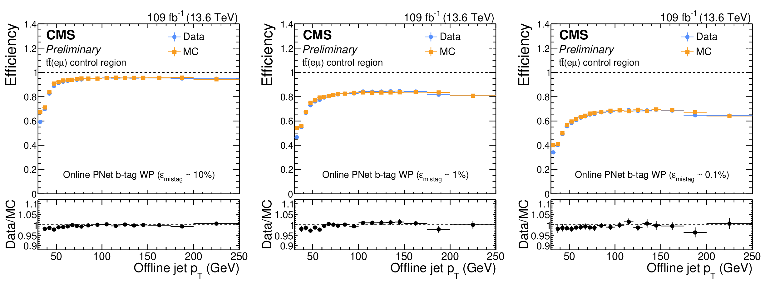
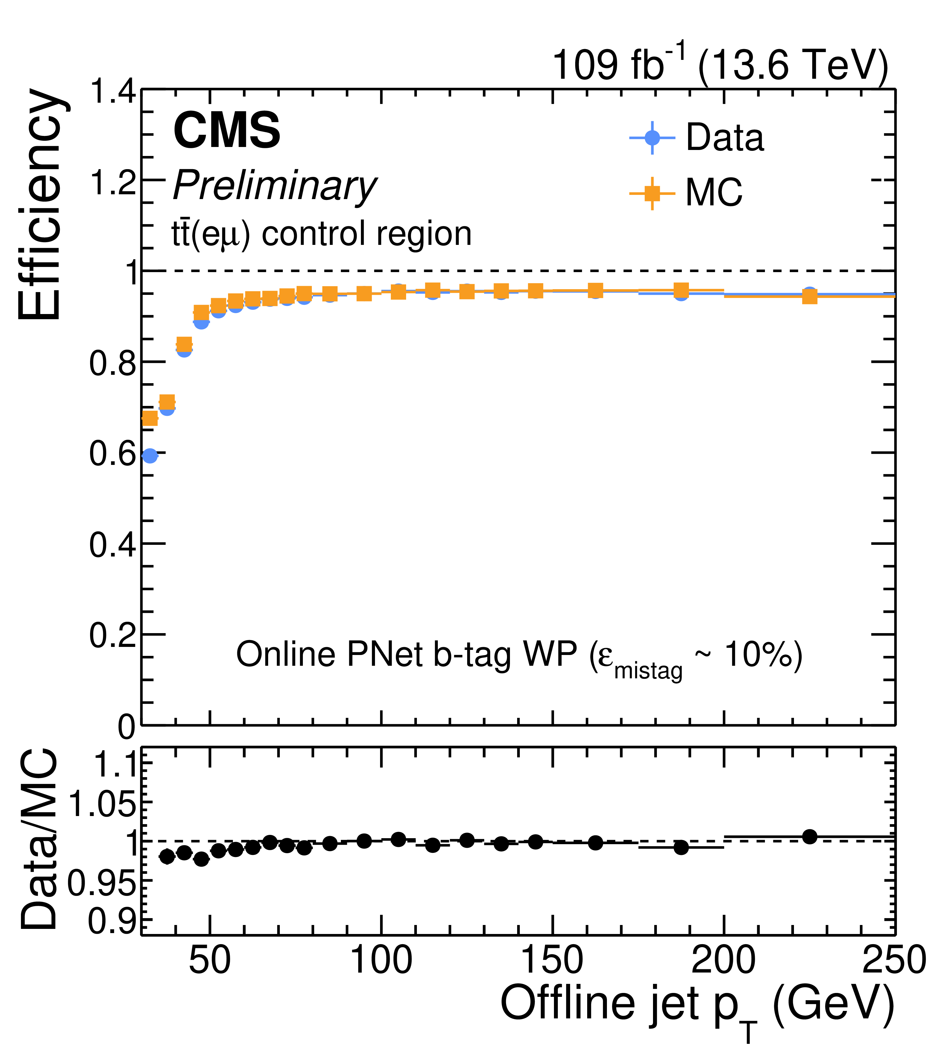
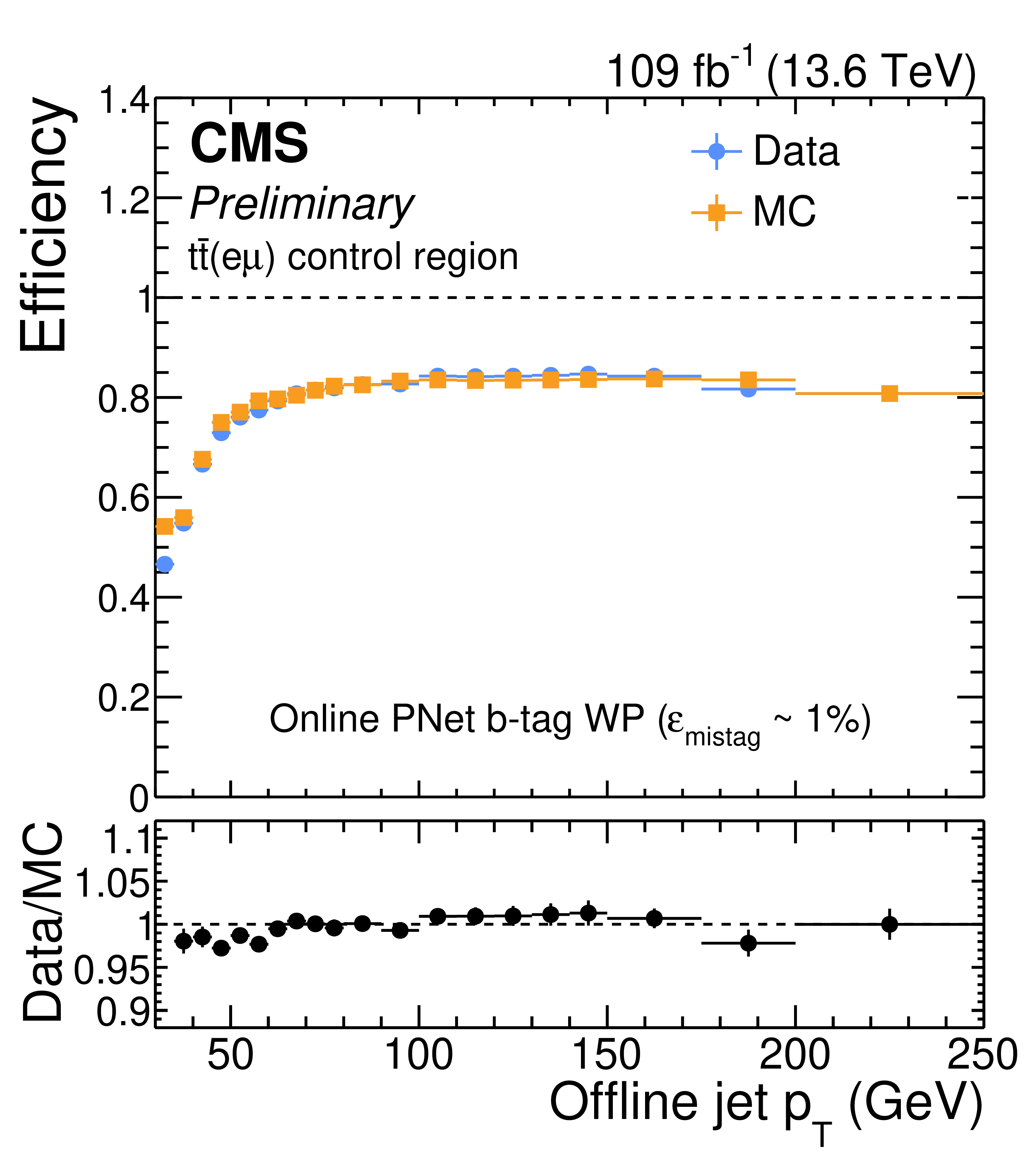
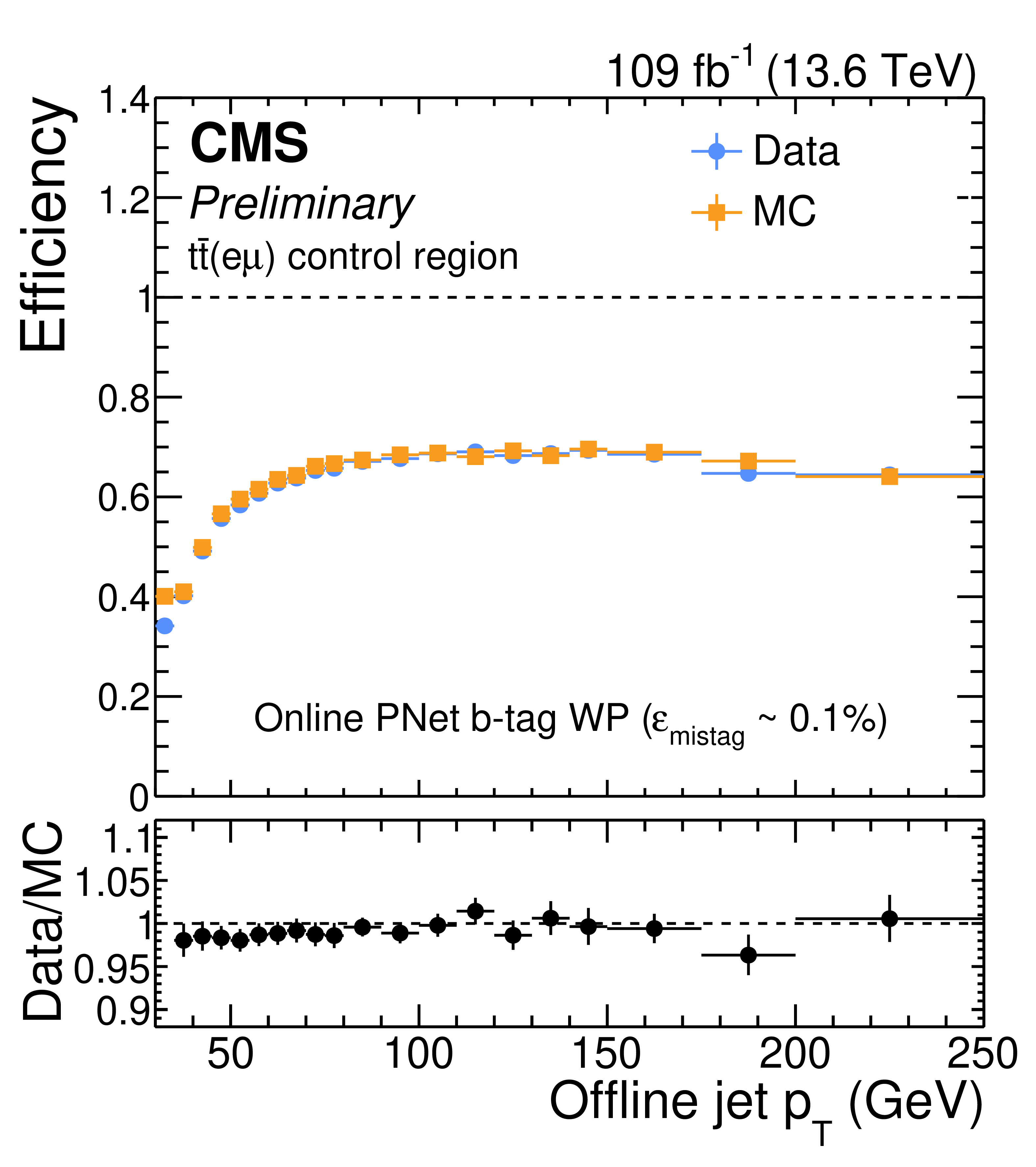
Efficiency of the online PNET b tagging algorithm as a function of the offline small-radius jet $ p_{\mathrm{T}} $ in the $ {\mathrm{t}\overline{\mathrm{t}}} (\mathrm{e}\mu) $ region, measured in data (blue) and simulation (orange). Results are shown for the loose (left), medium (middle), and tight (right) $ \mathcal{P}_{\mathrm{b}} $ working points (WP), corresponding to mistag rates ($ \varepsilon_{\mathrm{mistag}} $) of 10%, 1%, and 0.1%, respectively. |
png pdf |
Figure 8-a:
Efficiency of the online PNET b tagging algorithm as a function of the offline small-radius jet $ p_{\mathrm{T}} $ in the $ {\mathrm{t}\overline{\mathrm{t}}} (\mathrm{e}\mu) $ region, measured in data (blue) and simulation (orange). Results are shown for the loose (left), medium (middle), and tight (right) $ \mathcal{P}_{\mathrm{b}} $ working points (WP), corresponding to mistag rates ($ \varepsilon_{\mathrm{mistag}} $) of 10%, 1%, and 0.1%, respectively. |
png pdf |
Figure 8-b:
Efficiency of the online PNET b tagging algorithm as a function of the offline small-radius jet $ p_{\mathrm{T}} $ in the $ {\mathrm{t}\overline{\mathrm{t}}} (\mathrm{e}\mu) $ region, measured in data (blue) and simulation (orange). Results are shown for the loose (left), medium (middle), and tight (right) $ \mathcal{P}_{\mathrm{b}} $ working points (WP), corresponding to mistag rates ($ \varepsilon_{\mathrm{mistag}} $) of 10%, 1%, and 0.1%, respectively. |
png pdf |
Figure 8-c:
Efficiency of the online PNET b tagging algorithm as a function of the offline small-radius jet $ p_{\mathrm{T}} $ in the $ {\mathrm{t}\overline{\mathrm{t}}} (\mathrm{e}\mu) $ region, measured in data (blue) and simulation (orange). Results are shown for the loose (left), medium (middle), and tight (right) $ \mathcal{P}_{\mathrm{b}} $ working points (WP), corresponding to mistag rates ($ \varepsilon_{\mathrm{mistag}} $) of 10%, 1%, and 0.1%, respectively. |
png pdf |
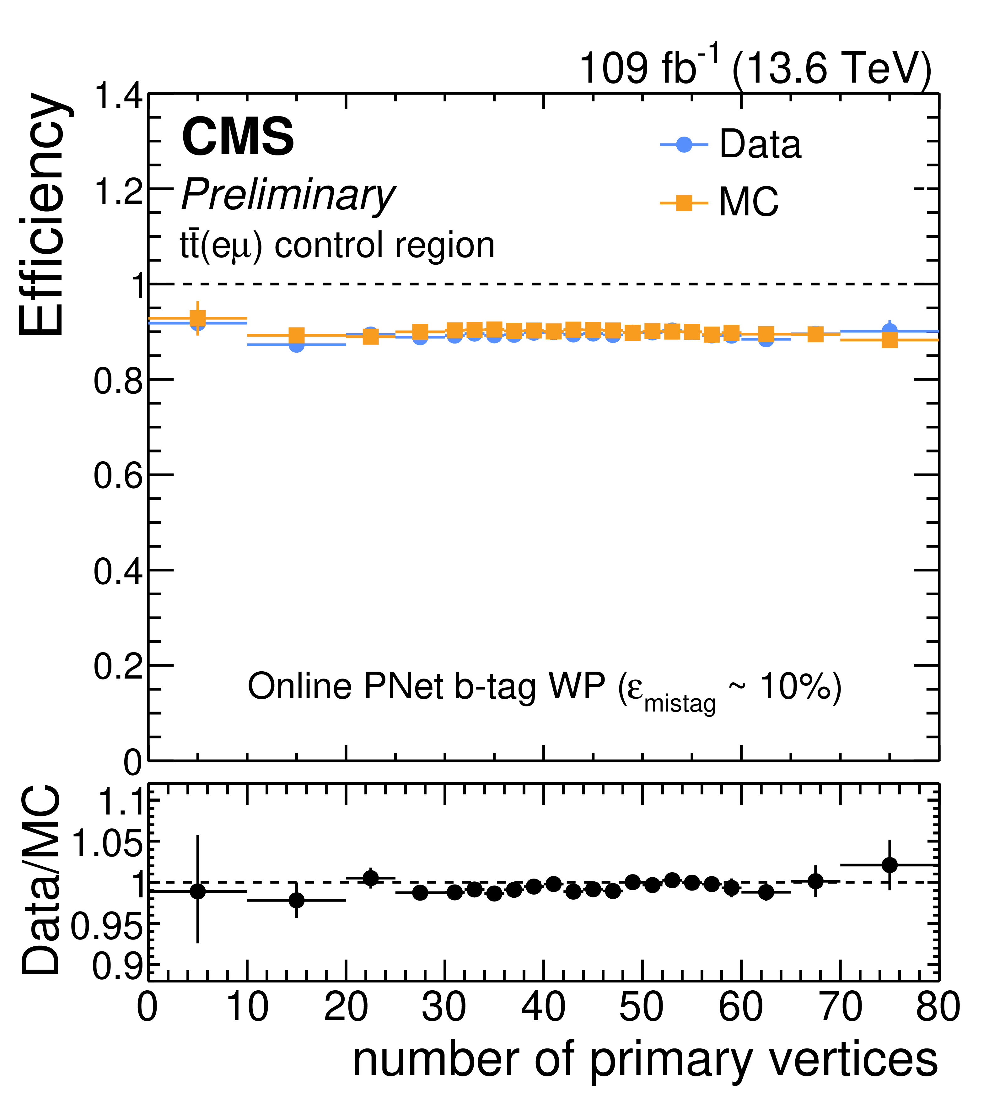
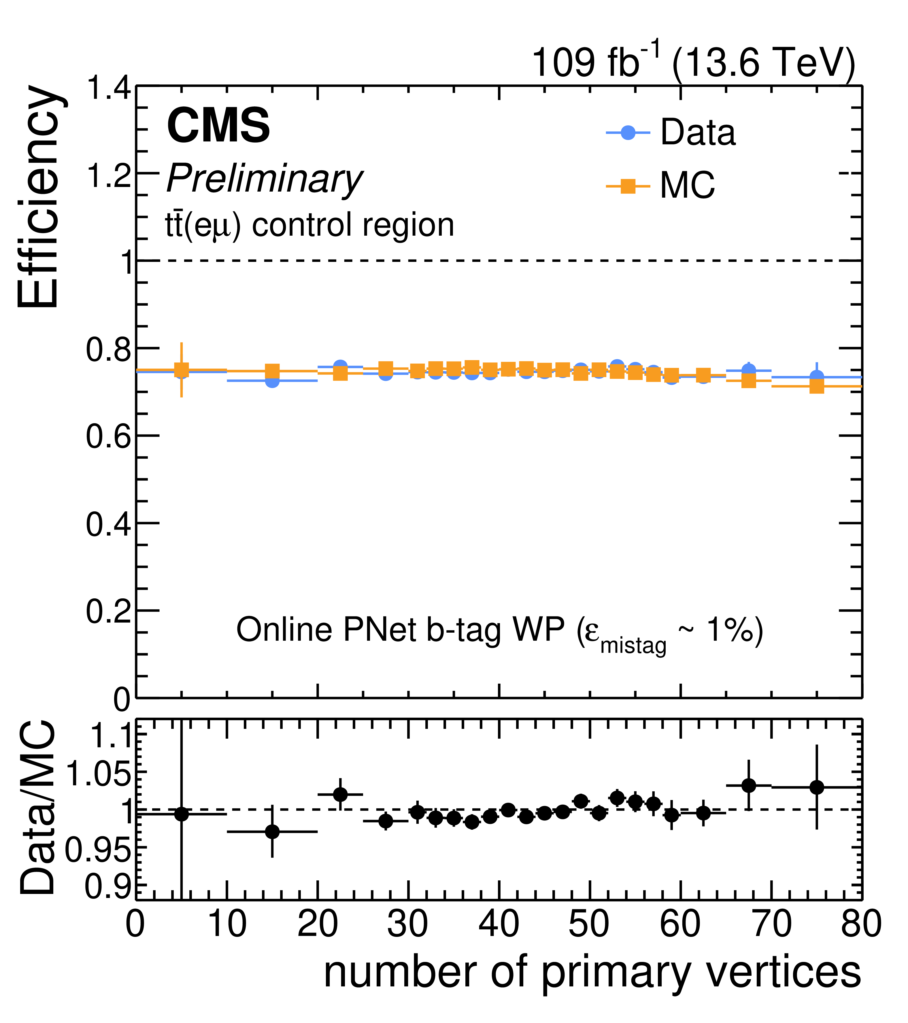
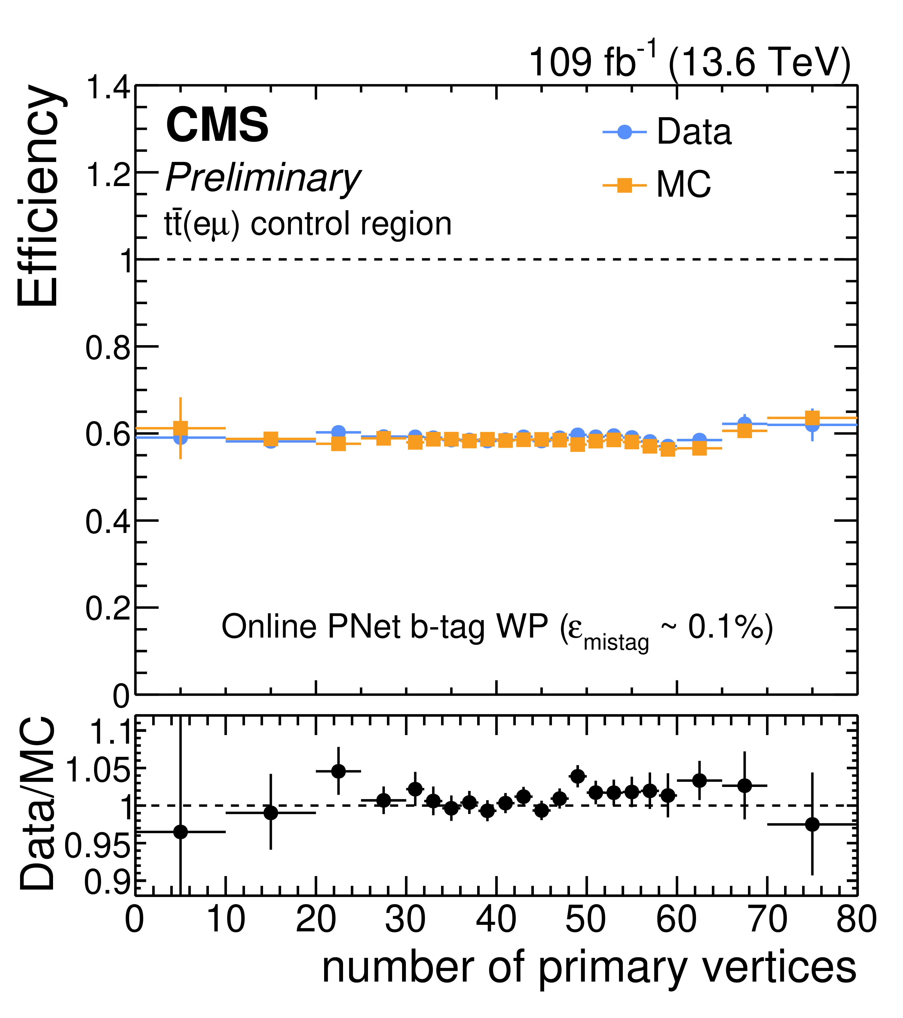
Figure 9:
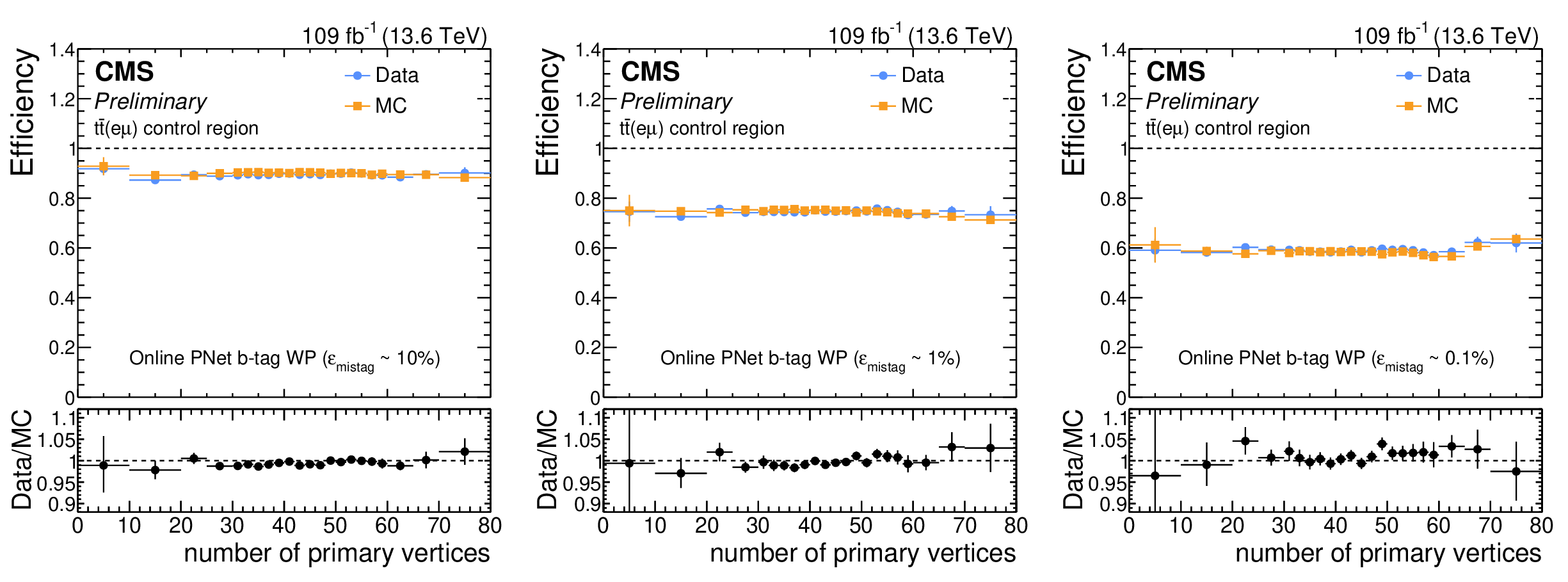
Efficiency of the online PNET b tagging algorithm as a function of the number of reconstructed primary vertices in the $ {\mathrm{t}\overline{\mathrm{t}}} (\mathrm{e}\mu) $ region, measured in data (blue) and simulation (orange). The panel definitions and styling follow Fig. 8. |
png pdf |
Figure 9-a:
Efficiency of the online PNET b tagging algorithm as a function of the number of reconstructed primary vertices in the $ {\mathrm{t}\overline{\mathrm{t}}} (\mathrm{e}\mu) $ region, measured in data (blue) and simulation (orange). The panel definitions and styling follow Fig. 8. |
png pdf |
Figure 9-b:
Efficiency of the online PNET b tagging algorithm as a function of the number of reconstructed primary vertices in the $ {\mathrm{t}\overline{\mathrm{t}}} (\mathrm{e}\mu) $ region, measured in data (blue) and simulation (orange). The panel definitions and styling follow Fig. 8. |
png pdf |
Figure 9-c:
Efficiency of the online PNET b tagging algorithm as a function of the number of reconstructed primary vertices in the $ {\mathrm{t}\overline{\mathrm{t}}} (\mathrm{e}\mu) $ region, measured in data (blue) and simulation (orange). The panel definitions and styling follow Fig. 8. |
png pdf |
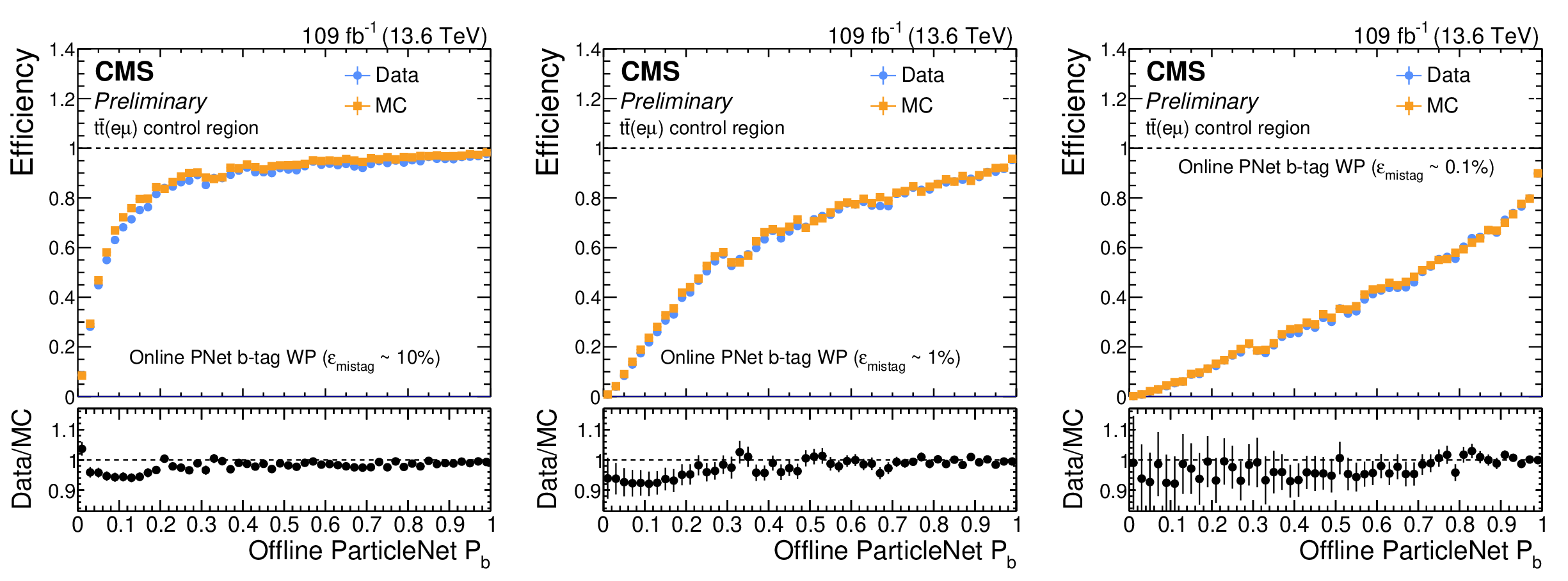
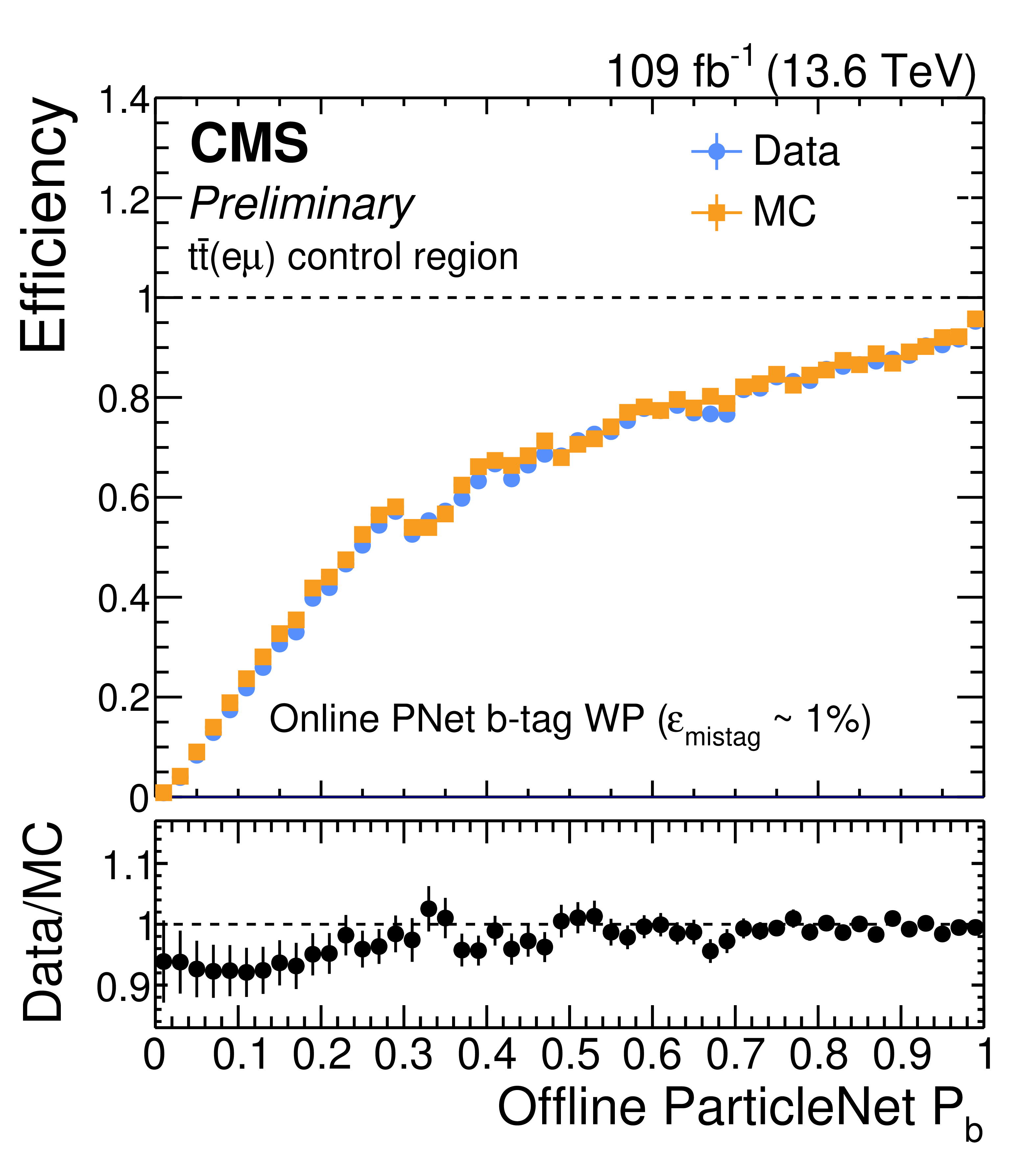
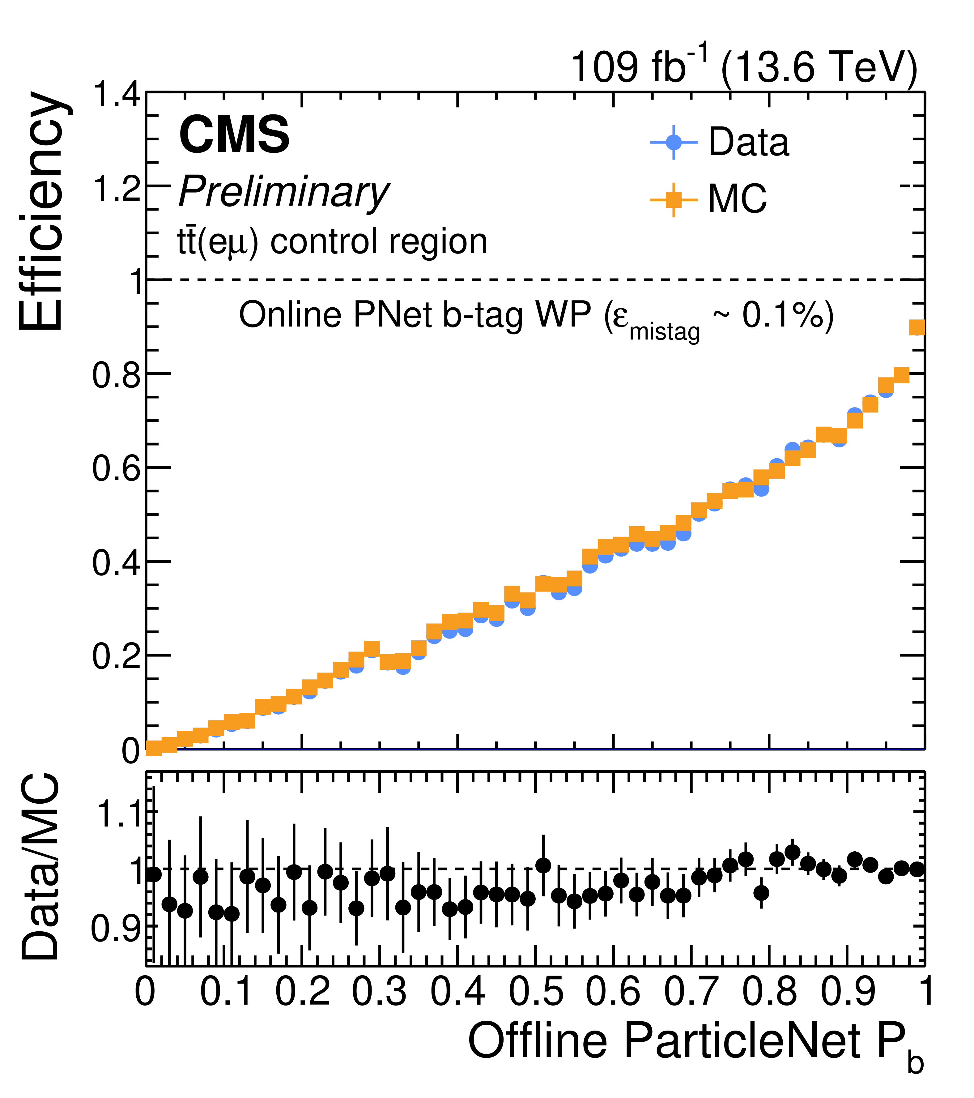
Figure 10:
Efficiency of the online PNET b tagging algorithm as a function of the offline PNET $ \mathcal{P}_{\mathrm{b}} $ score in the $ {\mathrm{t}\overline{\mathrm{t}}} (\mathrm{e}\mu) $ region, for data (blue) and simulation (orange). The panel definitions and styling follow Fig. 8. For this measurement, no requirements are applied to the offline $ \mathcal{P}_{\mathrm{b}} $ score. |

png pdf |
Figure 10-a:
Efficiency of the online PNET b tagging algorithm as a function of the offline PNET $ \mathcal{P}_{\mathrm{b}} $ score in the $ {\mathrm{t}\overline{\mathrm{t}}} (\mathrm{e}\mu) $ region, for data (blue) and simulation (orange). The panel definitions and styling follow Fig. 8. For this measurement, no requirements are applied to the offline $ \mathcal{P}_{\mathrm{b}} $ score. |
png pdf |
Figure 10-b:
Efficiency of the online PNET b tagging algorithm as a function of the offline PNET $ \mathcal{P}_{\mathrm{b}} $ score in the $ {\mathrm{t}\overline{\mathrm{t}}} (\mathrm{e}\mu) $ region, for data (blue) and simulation (orange). The panel definitions and styling follow Fig. 8. For this measurement, no requirements are applied to the offline $ \mathcal{P}_{\mathrm{b}} $ score. |
png pdf |
Figure 10-c:
Efficiency of the online PNET b tagging algorithm as a function of the offline PNET $ \mathcal{P}_{\mathrm{b}} $ score in the $ {\mathrm{t}\overline{\mathrm{t}}} (\mathrm{e}\mu) $ region, for data (blue) and simulation (orange). The panel definitions and styling follow Fig. 8. For this measurement, no requirements are applied to the offline $ \mathcal{P}_{\mathrm{b}} $ score. |
png pdf |
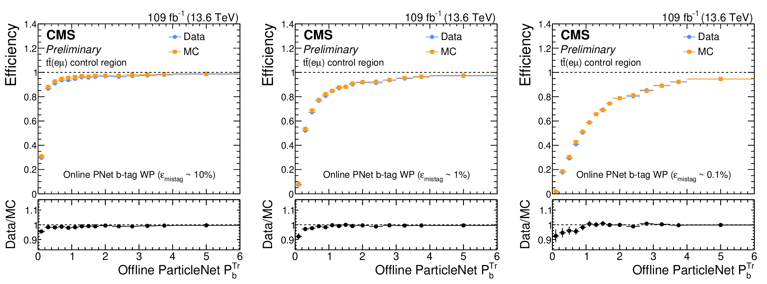
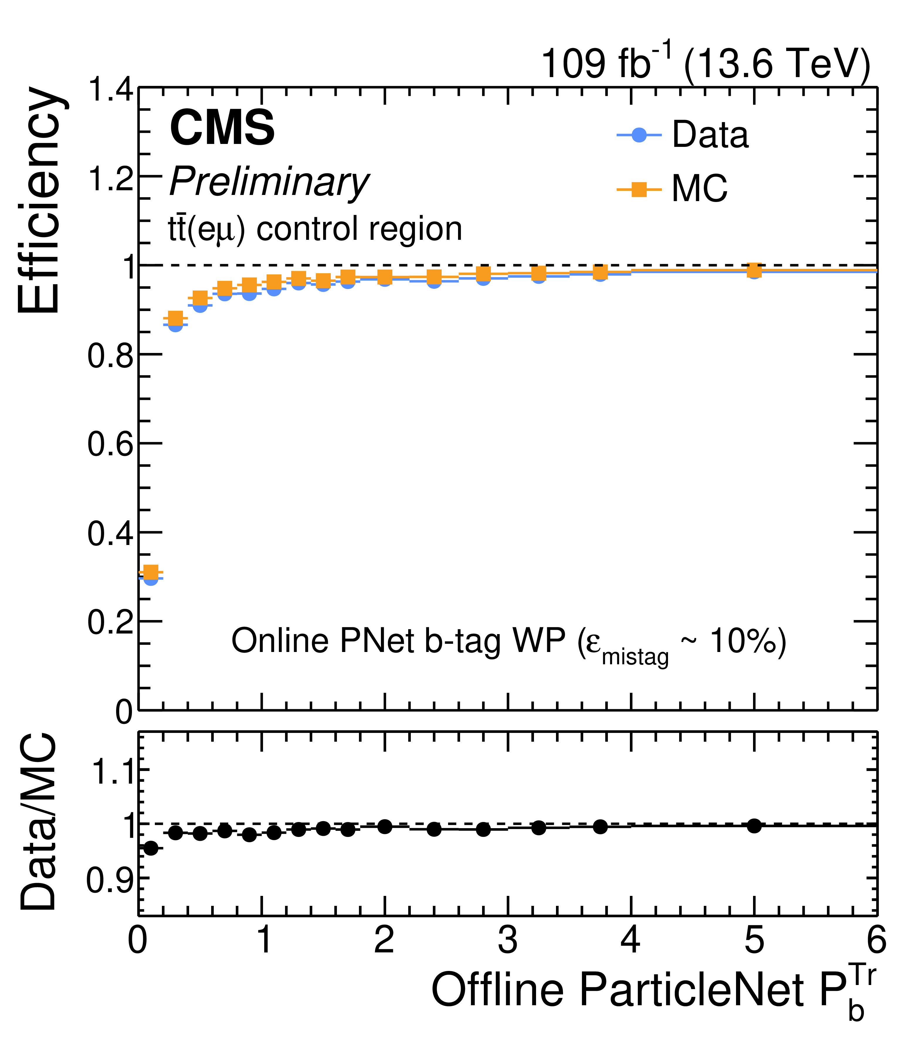
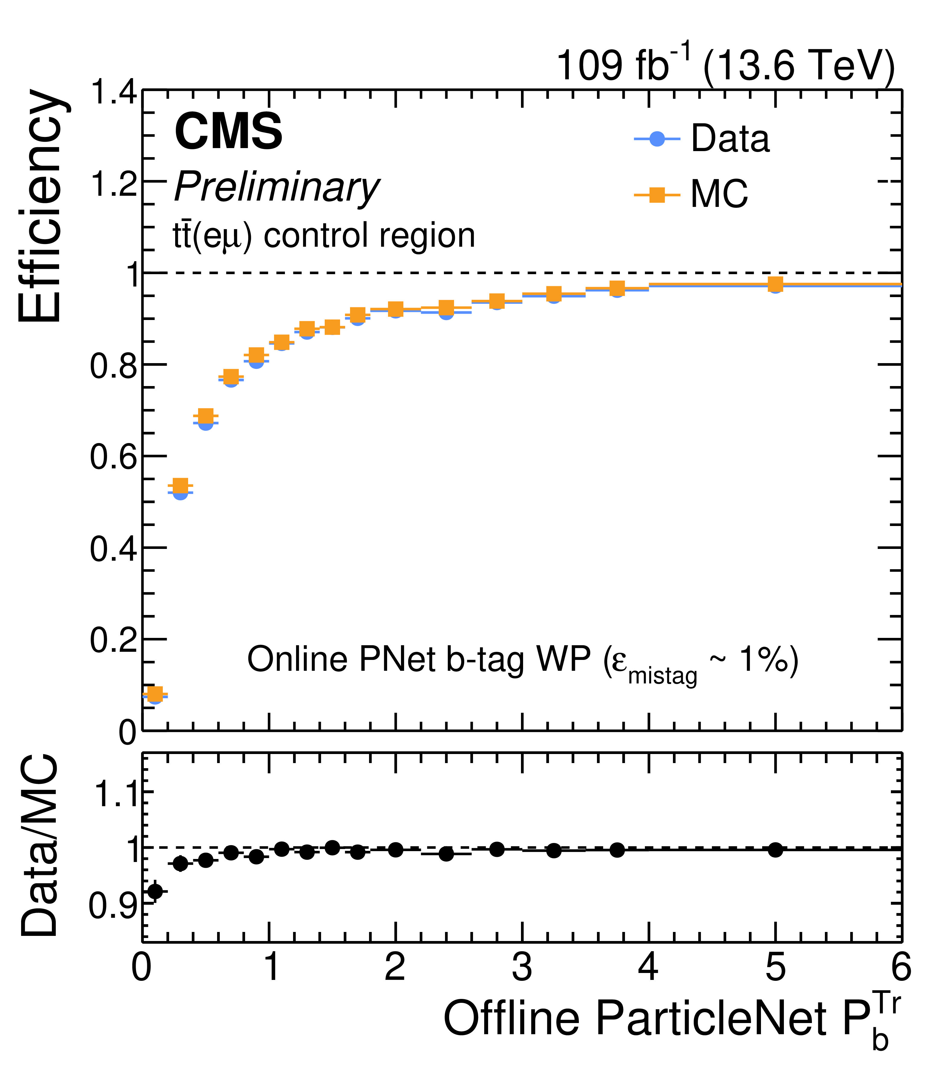
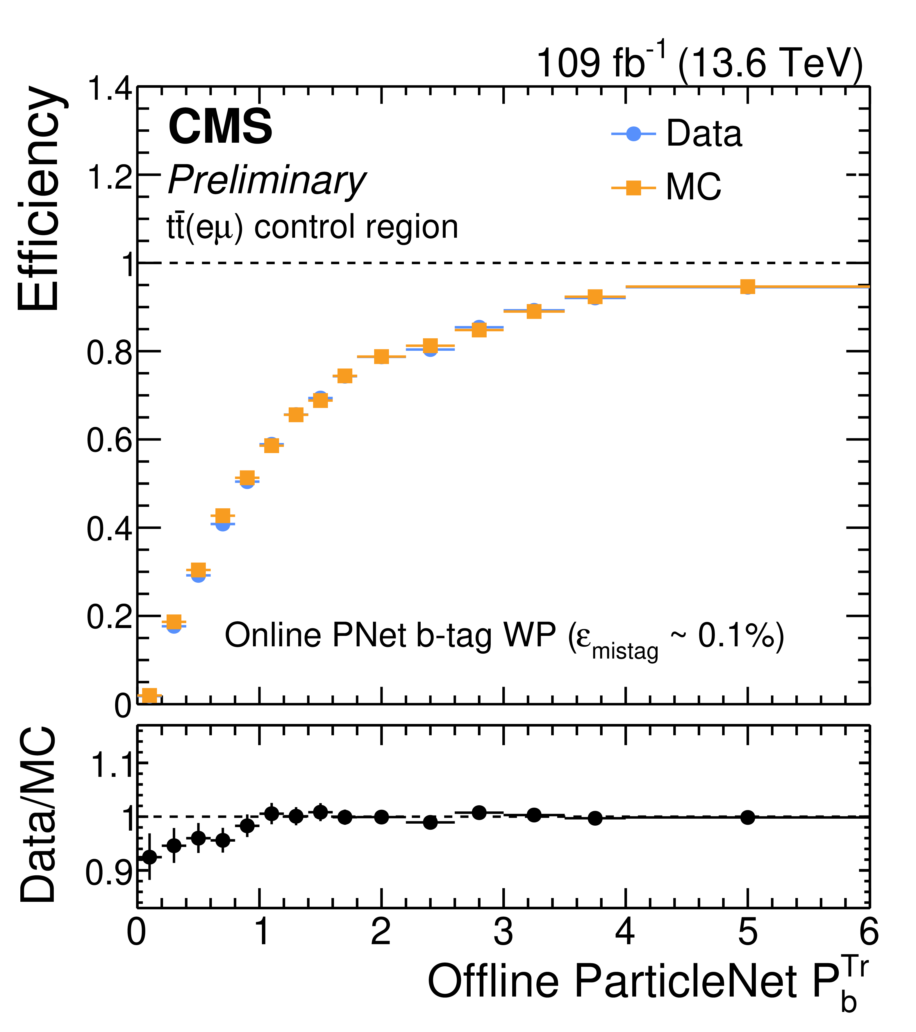
Figure 11:
Efficiency of the online PNET b tagging algorithm as a function of the offline PNET $ \mathcal{P}_{\mathrm{b}}^{Tr} $ score in the $ {\mathrm{t}\overline{\mathrm{t}}} (\mathrm{e}\mu) $ region, for data (blue) and simulation (orange). The panel definitions and styling follow Fig. 8. For this measurement, no requirements are applied to the offline $ \mathcal{P}_{\mathrm{b}} $ score. |
png pdf |
Figure 11-a:
Efficiency of the online PNET b tagging algorithm as a function of the offline PNET $ \mathcal{P}_{\mathrm{b}}^{Tr} $ score in the $ {\mathrm{t}\overline{\mathrm{t}}} (\mathrm{e}\mu) $ region, for data (blue) and simulation (orange). The panel definitions and styling follow Fig. 8. For this measurement, no requirements are applied to the offline $ \mathcal{P}_{\mathrm{b}} $ score. |
png pdf |
Figure 11-b:
Efficiency of the online PNET b tagging algorithm as a function of the offline PNET $ \mathcal{P}_{\mathrm{b}}^{Tr} $ score in the $ {\mathrm{t}\overline{\mathrm{t}}} (\mathrm{e}\mu) $ region, for data (blue) and simulation (orange). The panel definitions and styling follow Fig. 8. For this measurement, no requirements are applied to the offline $ \mathcal{P}_{\mathrm{b}} $ score. |
png pdf |
Figure 11-c:
Efficiency of the online PNET b tagging algorithm as a function of the offline PNET $ \mathcal{P}_{\mathrm{b}}^{Tr} $ score in the $ {\mathrm{t}\overline{\mathrm{t}}} (\mathrm{e}\mu) $ region, for data (blue) and simulation (orange). The panel definitions and styling follow Fig. 8. For this measurement, no requirements are applied to the offline $ \mathcal{P}_{\mathrm{b}} $ score. |
png pdf |
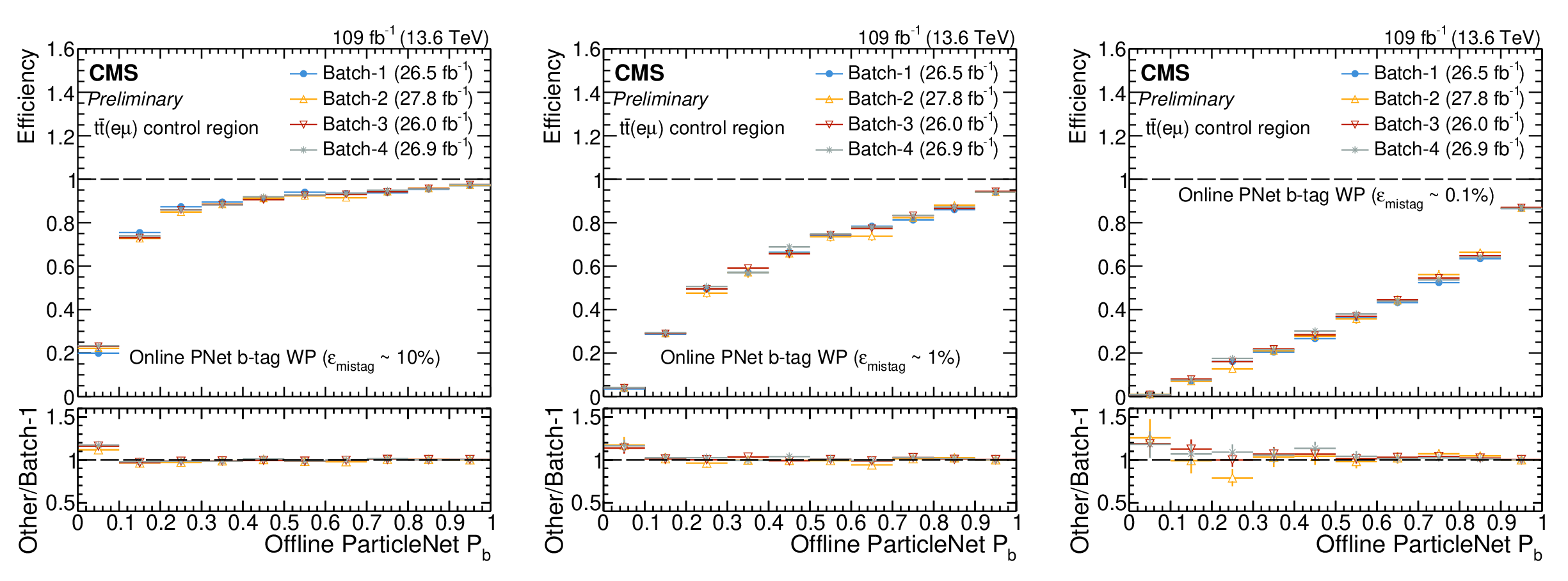
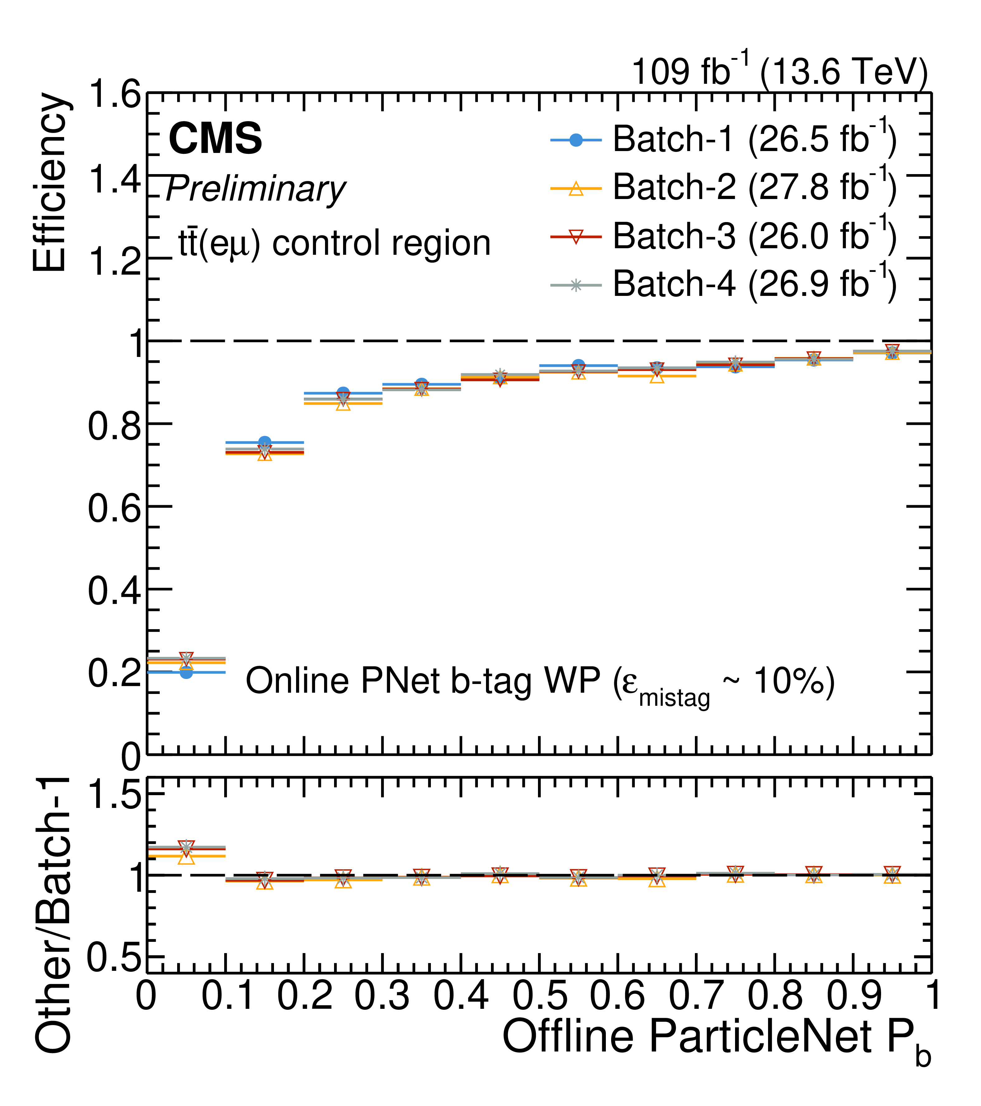
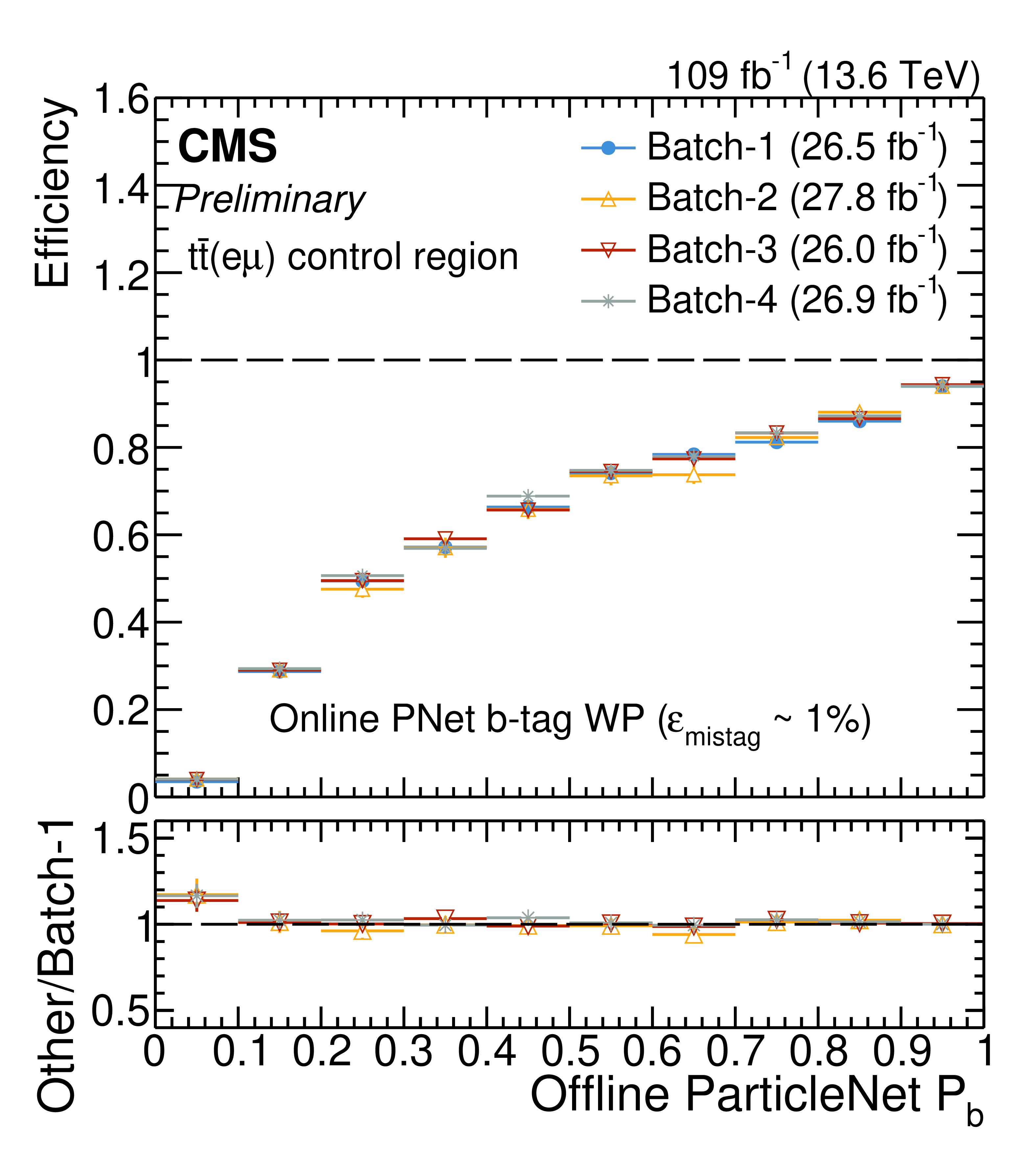
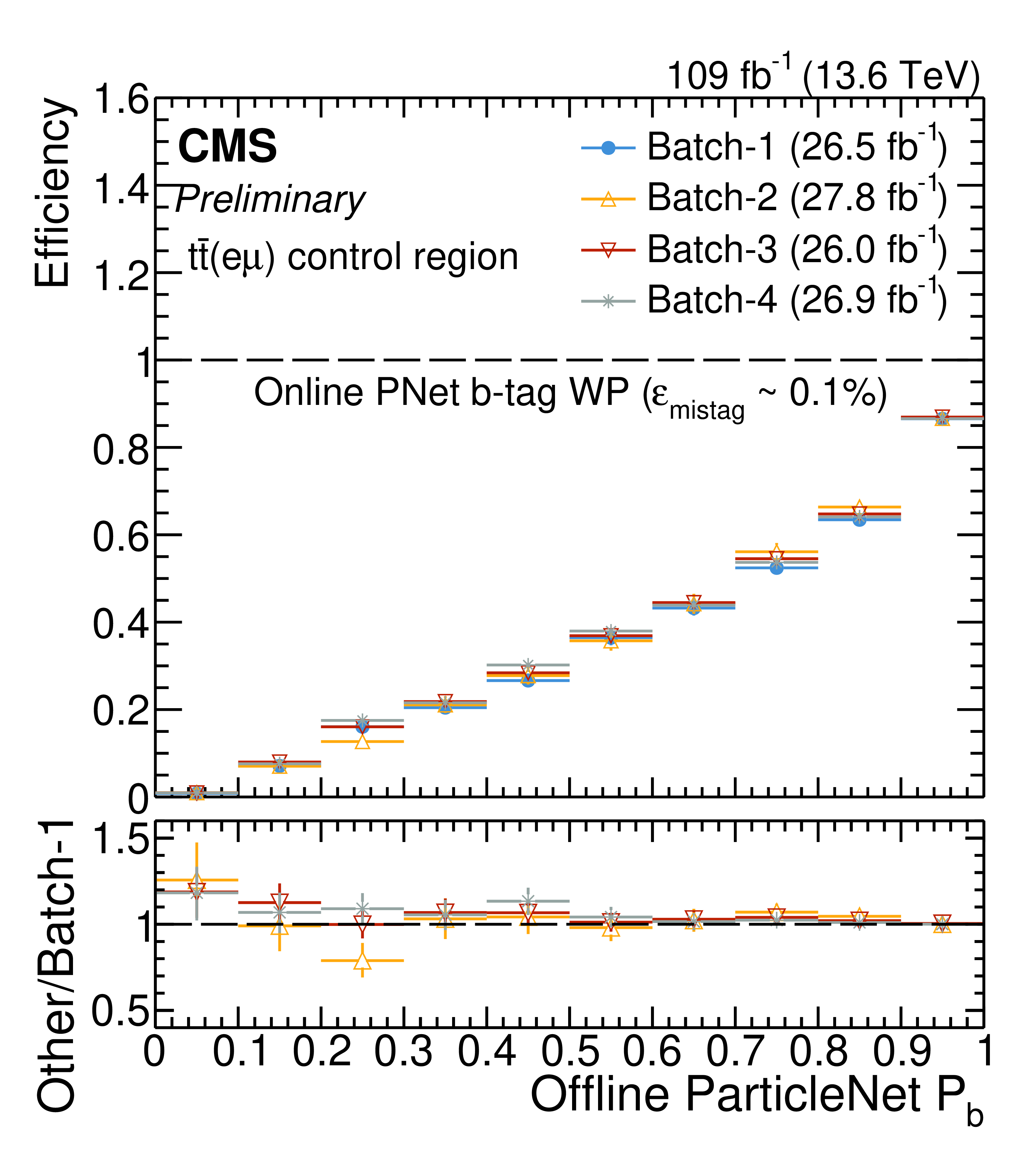
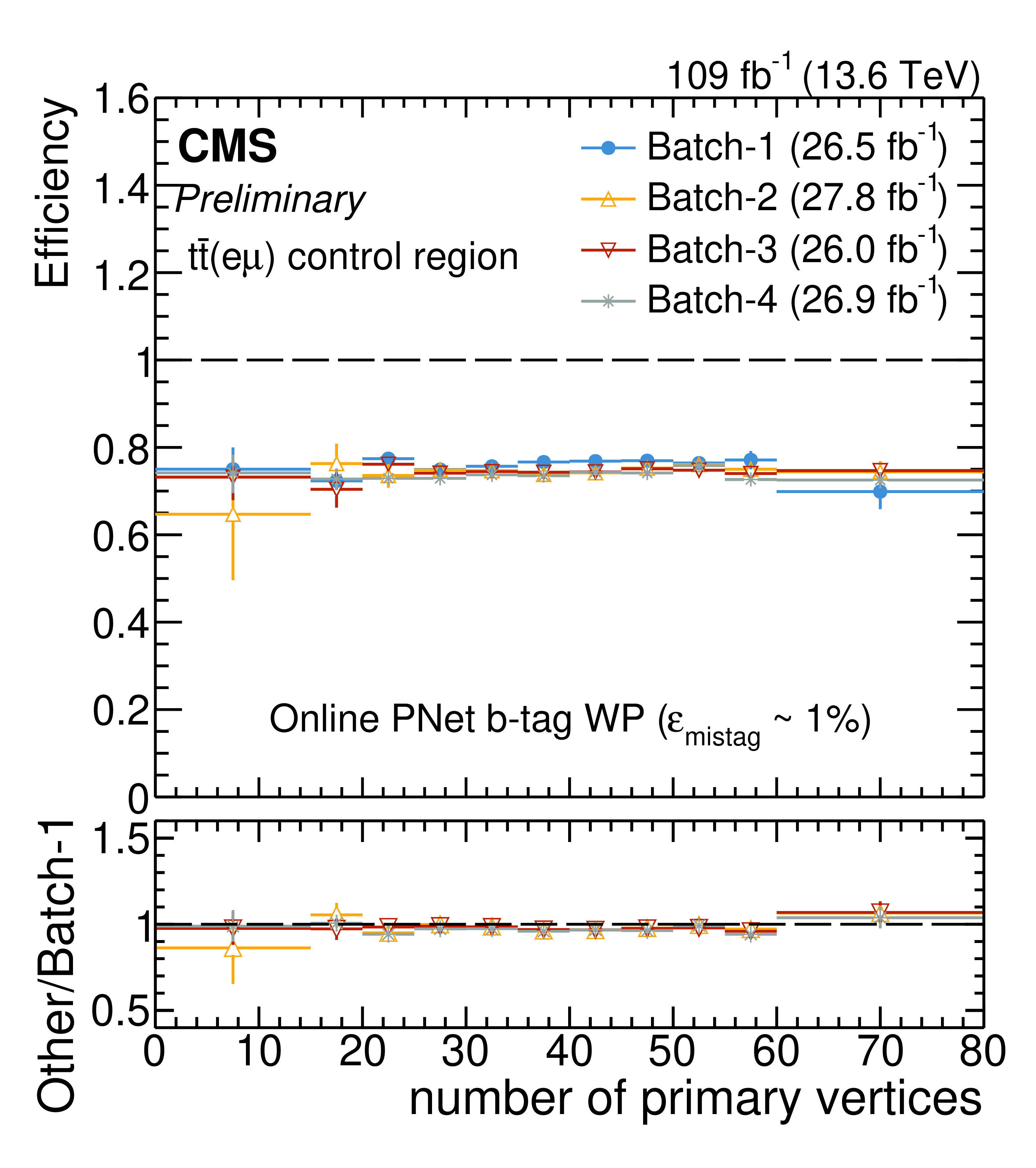
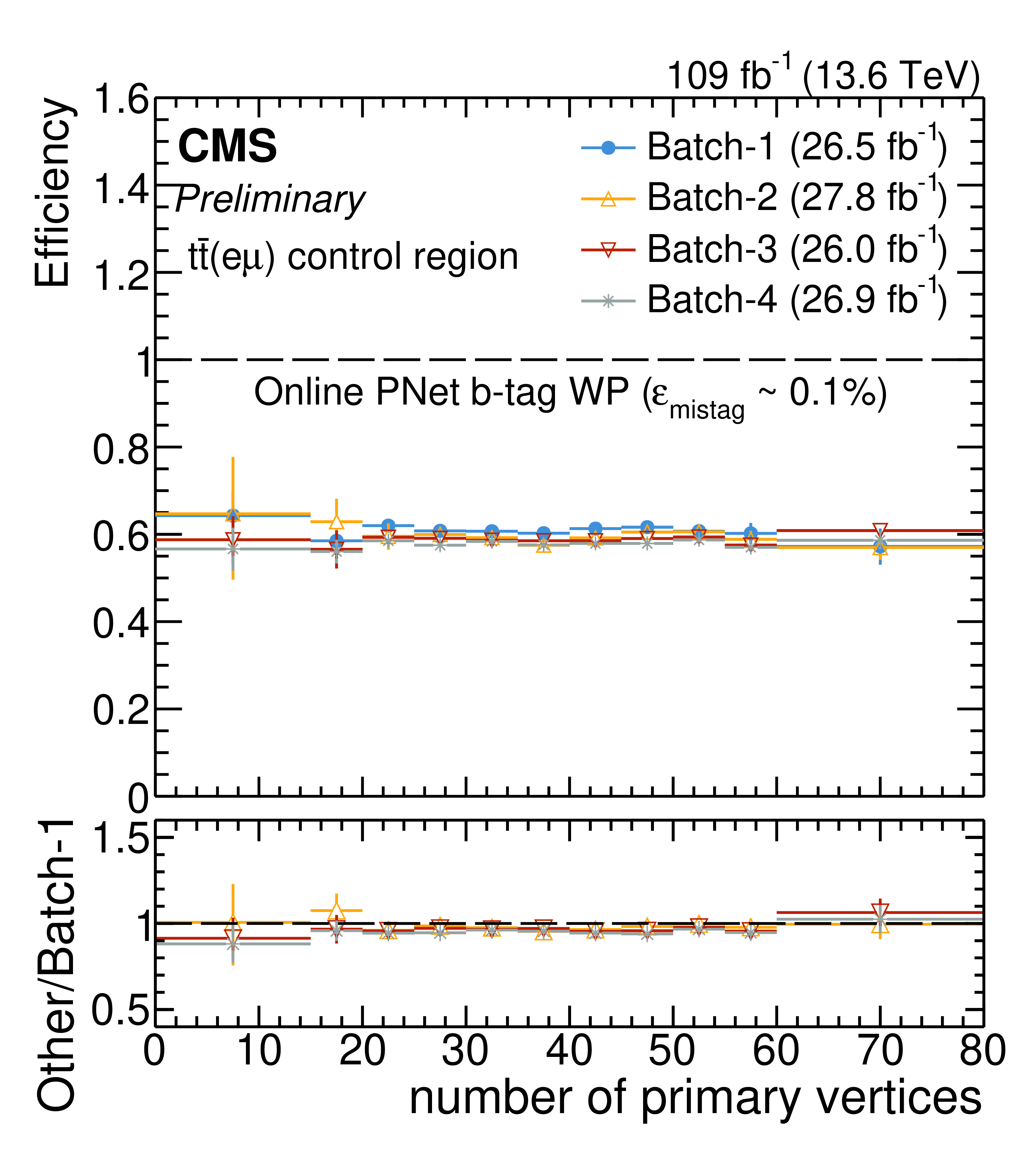
Figure 12:
Efficiency of the online PNET b tagging algorithm as a function of the offline PNET} $ \mathcal{P}_{\mathrm{b}} $ score in the $ {{\mathrm{t}\overline{\mathrm{t}}} (\mathrm{e}\mu)} $ region, measured in data for four consecutive time periods (batch-1 to batch-4) during 2024. The lower panel shows the ratio of efficiencies in batch-$ N $ ($ N=2,\ldots, $ 4) to batch-1. |
png pdf |
Figure 12-a:
Efficiency of the online PNET b tagging algorithm as a function of the offline PNET} $ \mathcal{P}_{\mathrm{b}} $ score in the $ {{\mathrm{t}\overline{\mathrm{t}}} (\mathrm{e}\mu)} $ region, measured in data for four consecutive time periods (batch-1 to batch-4) during 2024. The lower panel shows the ratio of efficiencies in batch-$ N $ ($ N=2,\ldots, $ 4) to batch-1. |
png pdf |
Figure 12-b:
Efficiency of the online PNET b tagging algorithm as a function of the offline PNET} $ \mathcal{P}_{\mathrm{b}} $ score in the $ {{\mathrm{t}\overline{\mathrm{t}}} (\mathrm{e}\mu)} $ region, measured in data for four consecutive time periods (batch-1 to batch-4) during 2024. The lower panel shows the ratio of efficiencies in batch-$ N $ ($ N=2,\ldots, $ 4) to batch-1. |
png pdf |
Figure 12-c:
Efficiency of the online PNET b tagging algorithm as a function of the offline PNET} $ \mathcal{P}_{\mathrm{b}} $ score in the $ {{\mathrm{t}\overline{\mathrm{t}}} (\mathrm{e}\mu)} $ region, measured in data for four consecutive time periods (batch-1 to batch-4) during 2024. The lower panel shows the ratio of efficiencies in batch-$ N $ ($ N=2,\ldots, $ 4) to batch-1. |
png pdf |
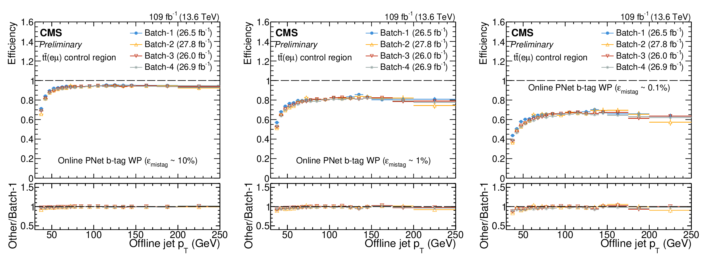
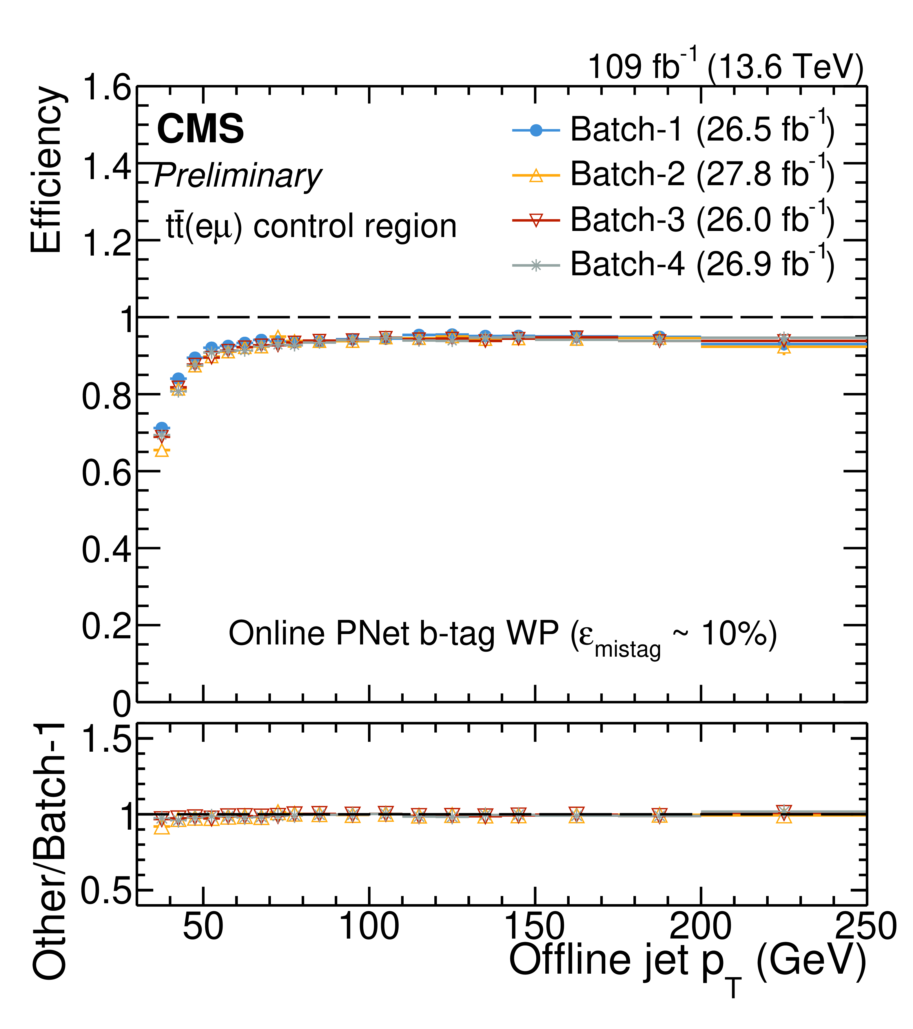
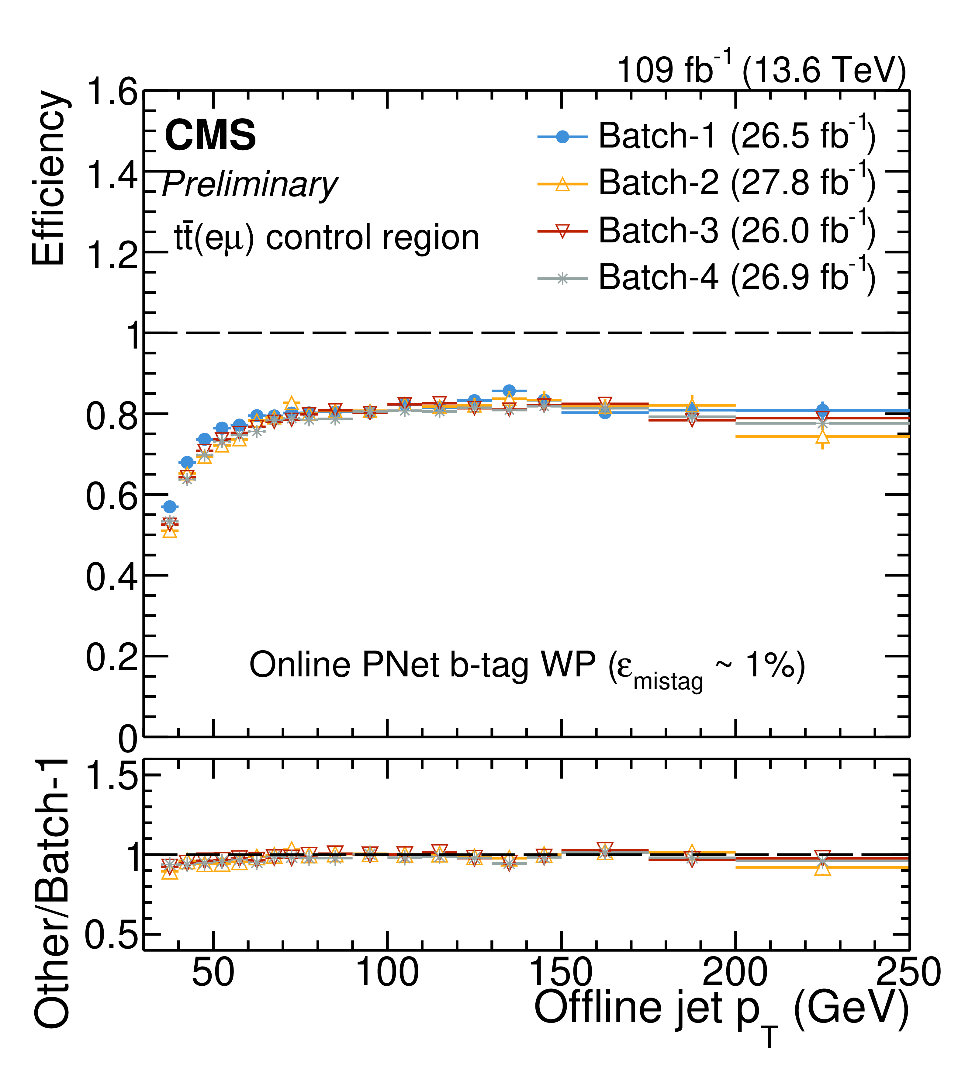
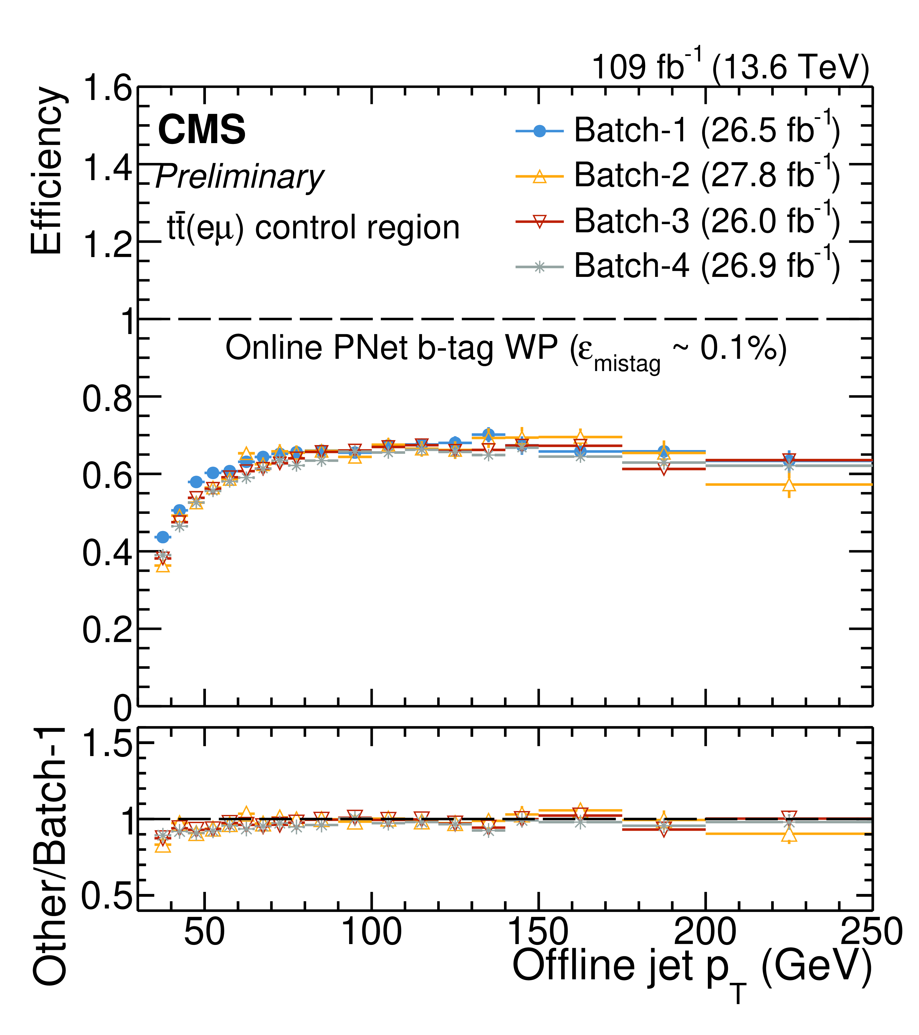
Figure 13:
Efficiency of the online PNET b tagging algorithm as a function of the offline jet $ p_{\mathrm{T}} $ in the $ {{\mathrm{t}\overline{\mathrm{t}}} (\mathrm{e}\mu)} $ region. The panel definition and ratios follow Fig. 12. |
png pdf |
Figure 13-a:
Efficiency of the online PNET b tagging algorithm as a function of the offline jet $ p_{\mathrm{T}} $ in the $ {{\mathrm{t}\overline{\mathrm{t}}} (\mathrm{e}\mu)} $ region. The panel definition and ratios follow Fig. 12. |
png pdf |
Figure 13-b:
Efficiency of the online PNET b tagging algorithm as a function of the offline jet $ p_{\mathrm{T}} $ in the $ {{\mathrm{t}\overline{\mathrm{t}}} (\mathrm{e}\mu)} $ region. The panel definition and ratios follow Fig. 12. |
png pdf |
Figure 13-c:
Efficiency of the online PNET b tagging algorithm as a function of the offline jet $ p_{\mathrm{T}} $ in the $ {{\mathrm{t}\overline{\mathrm{t}}} (\mathrm{e}\mu)} $ region. The panel definition and ratios follow Fig. 12. |
png pdf |
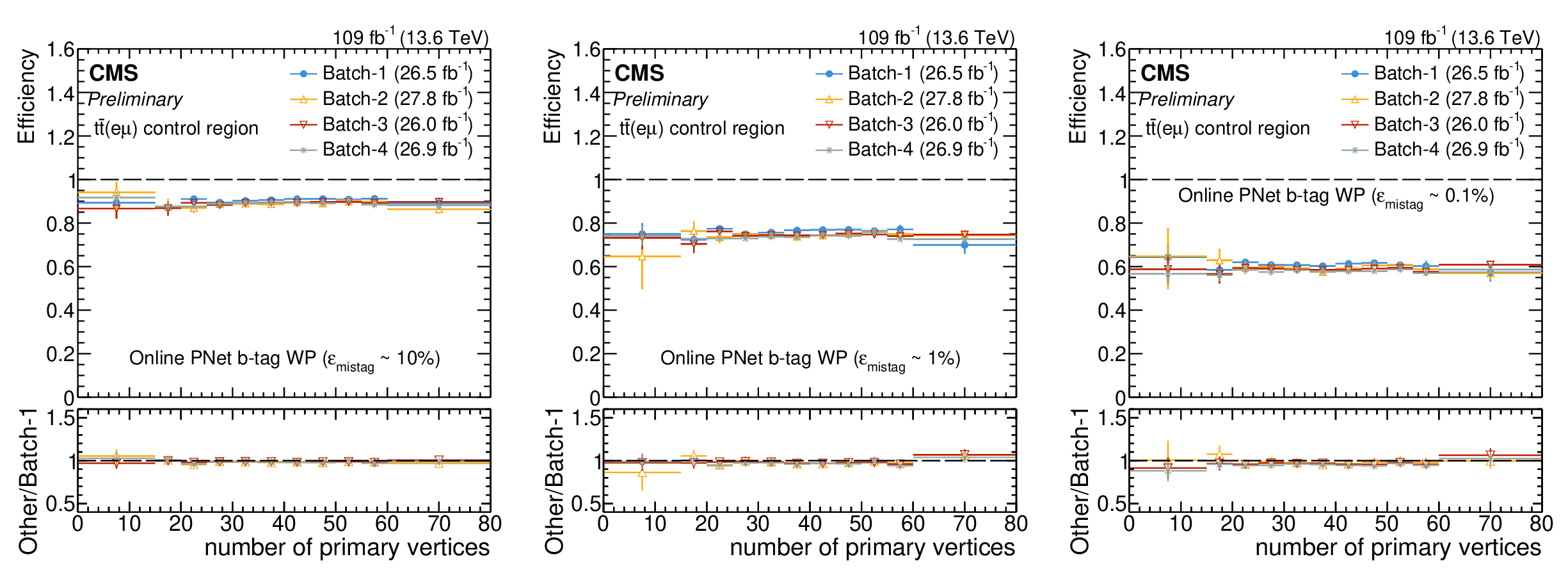
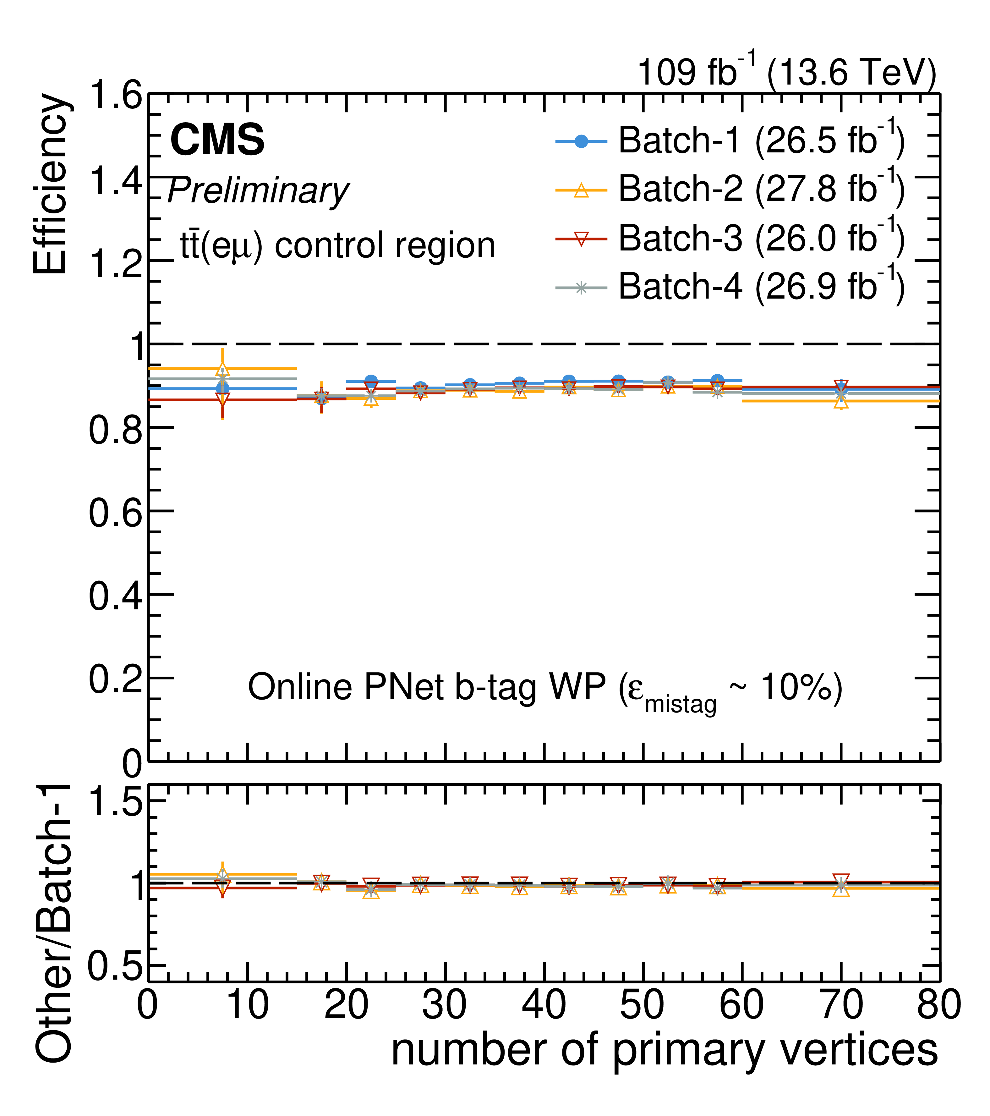
Figure 14:
Efficiency of the online PNET b tagging algorithm as a function of the number of reconstructed primary vertices in the $ {{\mathrm{t}\overline{\mathrm{t}}} (\mathrm{e}\mu)} $ region. The panel definition and ratios follow Fig. 12. |
png pdf |
Figure 14-a:
Efficiency of the online PNET b tagging algorithm as a function of the number of reconstructed primary vertices in the $ {{\mathrm{t}\overline{\mathrm{t}}} (\mathrm{e}\mu)} $ region. The panel definition and ratios follow Fig. 12. |
png pdf |
Figure 14-b:
Efficiency of the online PNET b tagging algorithm as a function of the number of reconstructed primary vertices in the $ {{\mathrm{t}\overline{\mathrm{t}}} (\mathrm{e}\mu)} $ region. The panel definition and ratios follow Fig. 12. |
png pdf |
Figure 14-c:
Efficiency of the online PNET b tagging algorithm as a function of the number of reconstructed primary vertices in the $ {{\mathrm{t}\overline{\mathrm{t}}} (\mathrm{e}\mu)} $ region. The panel definition and ratios follow Fig. 12. |
png pdf |
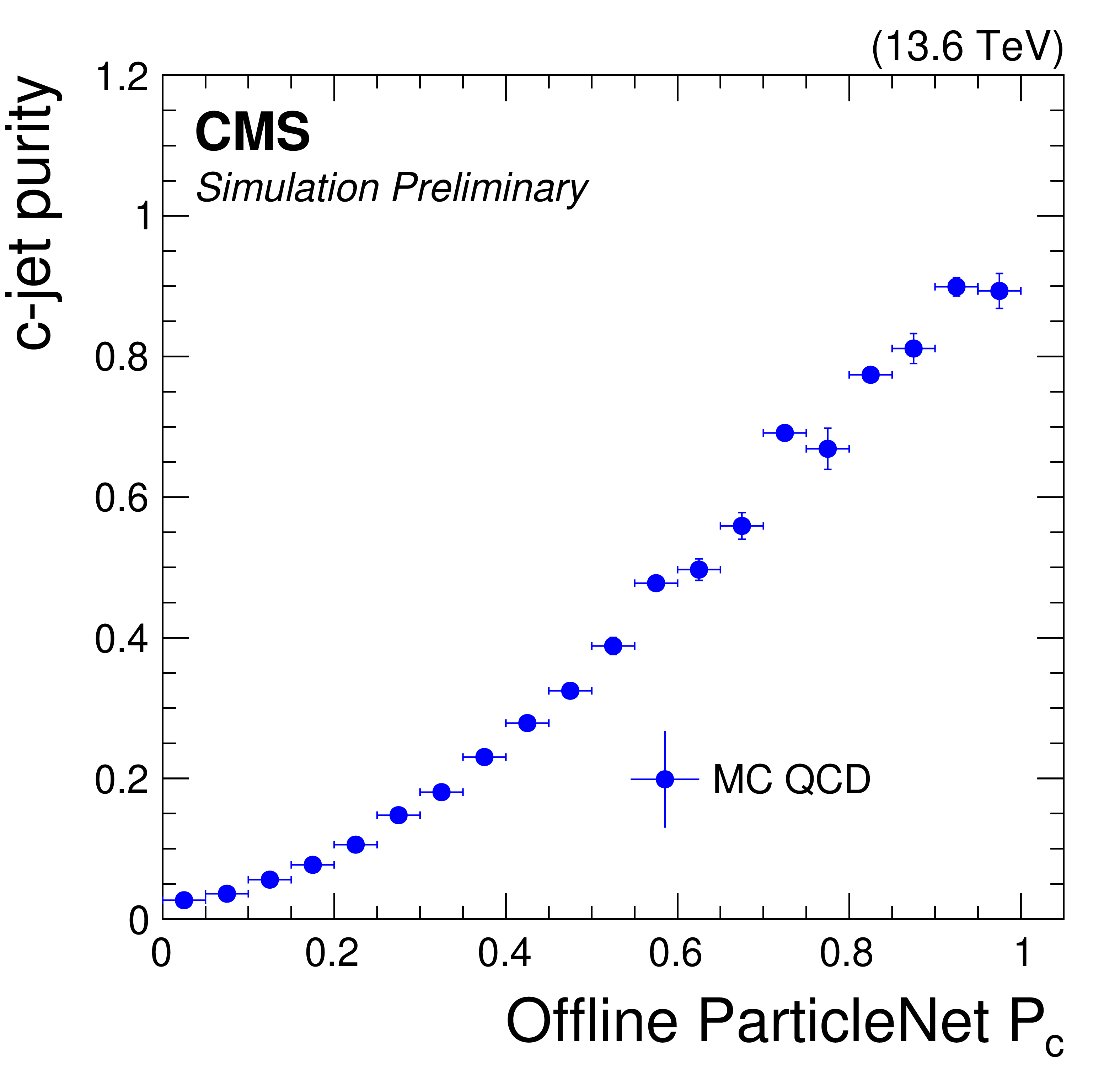
Figure 15:
Purity of the leading c-tagged jet as a function of the offline PNET $\mathcal{P}_{\mathrm{c}}$ score in simulated QCD multijet events. The purity is the fraction of jets matched to a charm quark. Selections correspond to the VBF $ \mathrm{H} \to \mathrm{c}\overline{\mathrm{c}} $ phase space described in the text. |
png pdf |
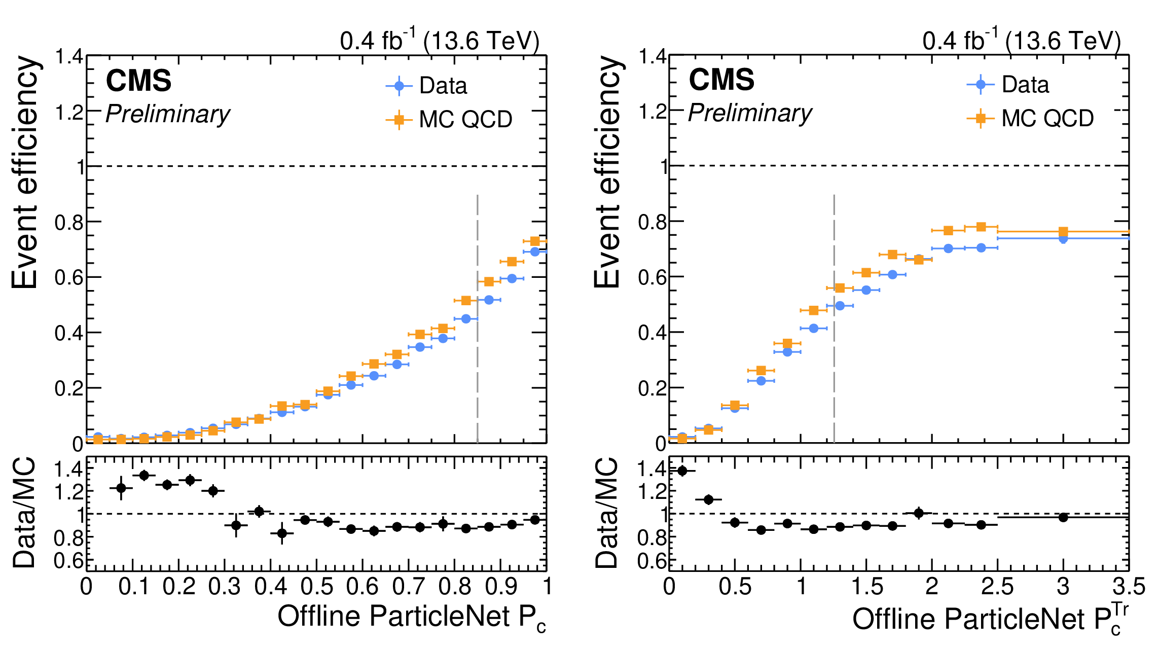
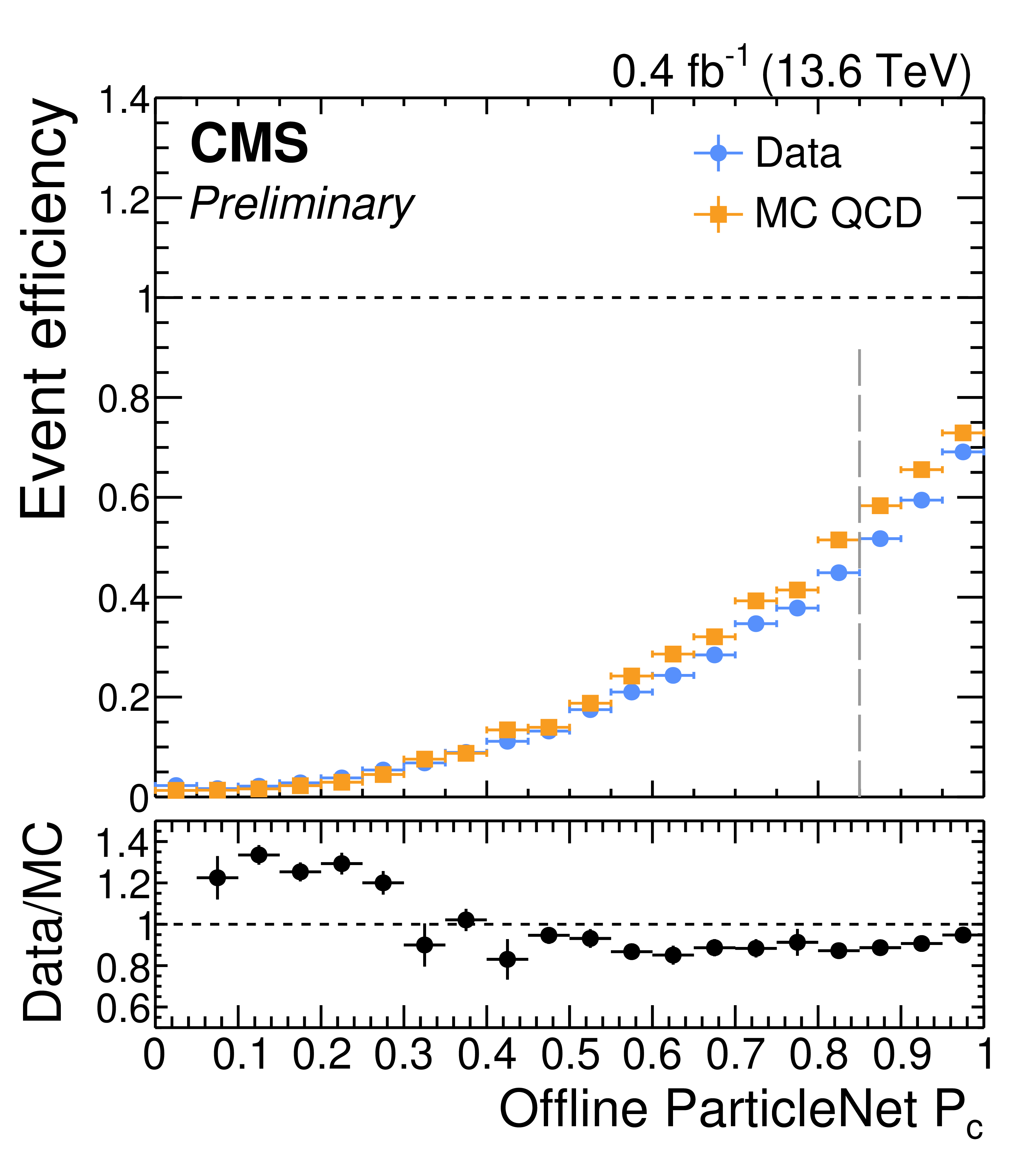
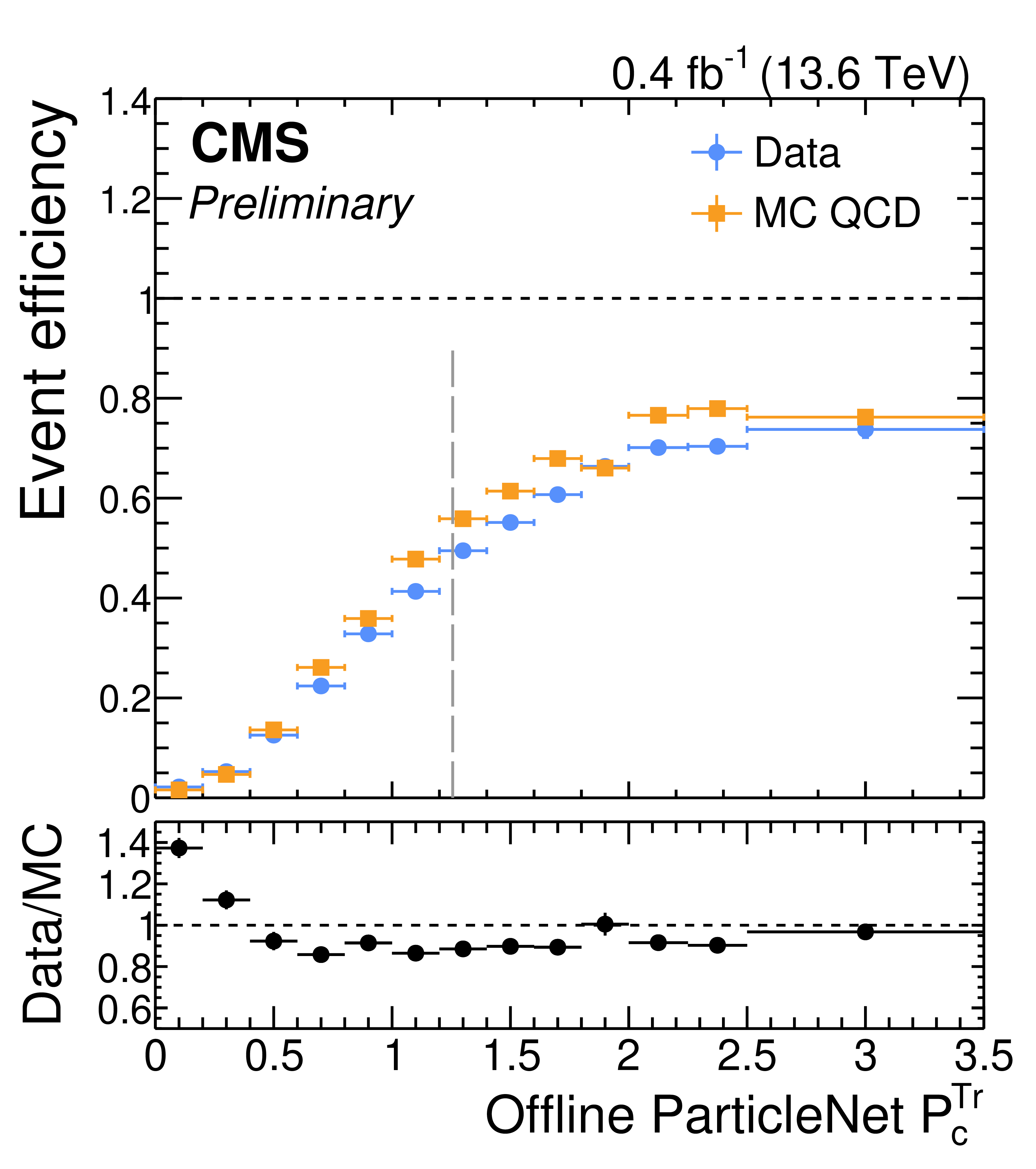
Figure 16:
Online PNET c tagging efficiency in the selected VBF-like QCD multijet events as a function of offline $ \mathcal{P}_{\mathrm{c}} $ (left) and $ \mathcal{P}_{\mathrm{c}}^{\mathrm{Tr}} $ (right) scores, as measured in data (blue) and simulation (orange) in a QCD-enriched region. Only the highest-$\mathcal{P}_{\mathrm{c}}$ small-radius jet in the event is considered. The vertical dashed line denotes the reference value $ \mathcal{P}_{\mathrm{c}}= $ 0.85, corresponding to a c tagging purity above 80%. |
png pdf |
Figure 16-a:
Online PNET c tagging efficiency in the selected VBF-like QCD multijet events as a function of offline $ \mathcal{P}_{\mathrm{c}} $ (left) and $ \mathcal{P}_{\mathrm{c}}^{\mathrm{Tr}} $ (right) scores, as measured in data (blue) and simulation (orange) in a QCD-enriched region. Only the highest-$\mathcal{P}_{\mathrm{c}}$ small-radius jet in the event is considered. The vertical dashed line denotes the reference value $ \mathcal{P}_{\mathrm{c}}= $ 0.85, corresponding to a c tagging purity above 80%. |
png pdf |
Figure 16-b:
Online PNET c tagging efficiency in the selected VBF-like QCD multijet events as a function of offline $ \mathcal{P}_{\mathrm{c}} $ (left) and $ \mathcal{P}_{\mathrm{c}}^{\mathrm{Tr}} $ (right) scores, as measured in data (blue) and simulation (orange) in a QCD-enriched region. Only the highest-$\mathcal{P}_{\mathrm{c}}$ small-radius jet in the event is considered. The vertical dashed line denotes the reference value $ \mathcal{P}_{\mathrm{c}}= $ 0.85, corresponding to a c tagging purity above 80%. |
png pdf |
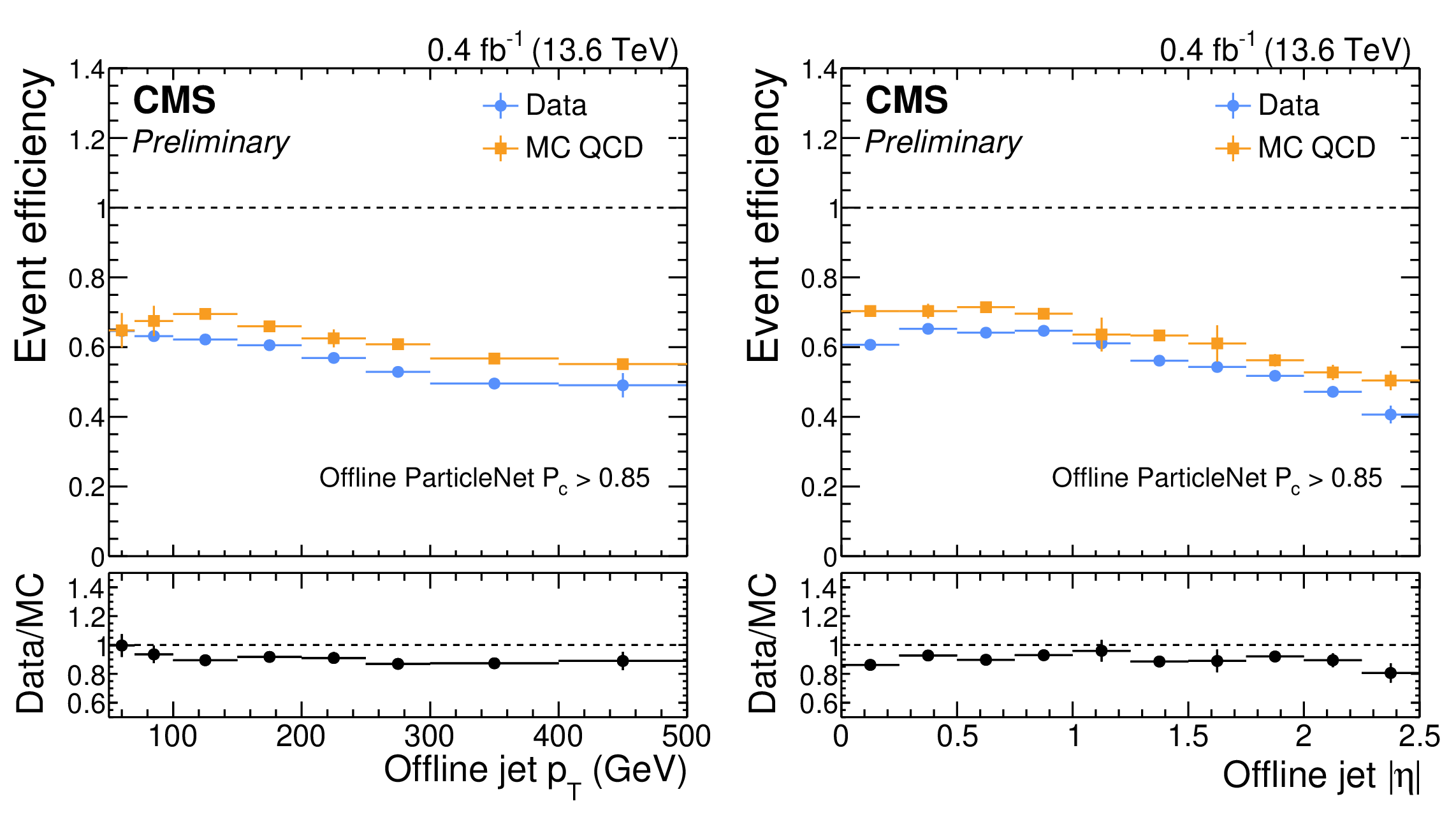
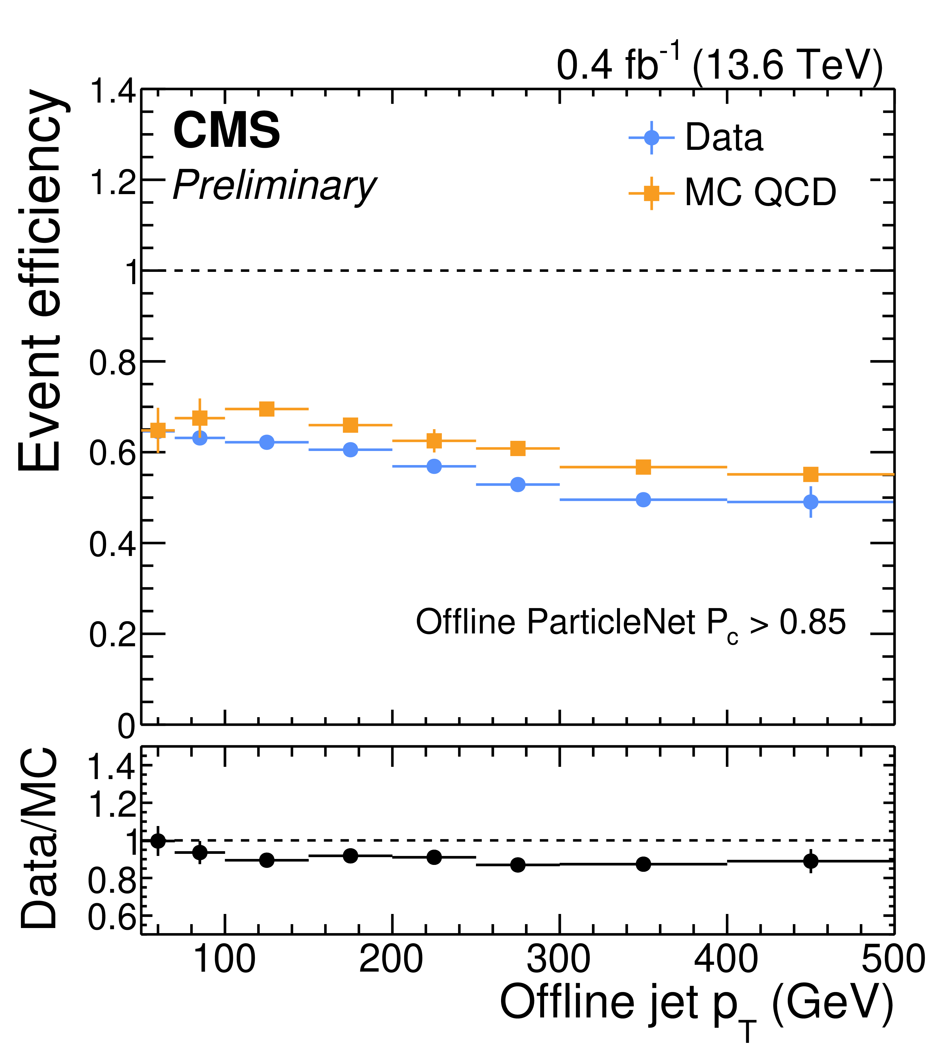
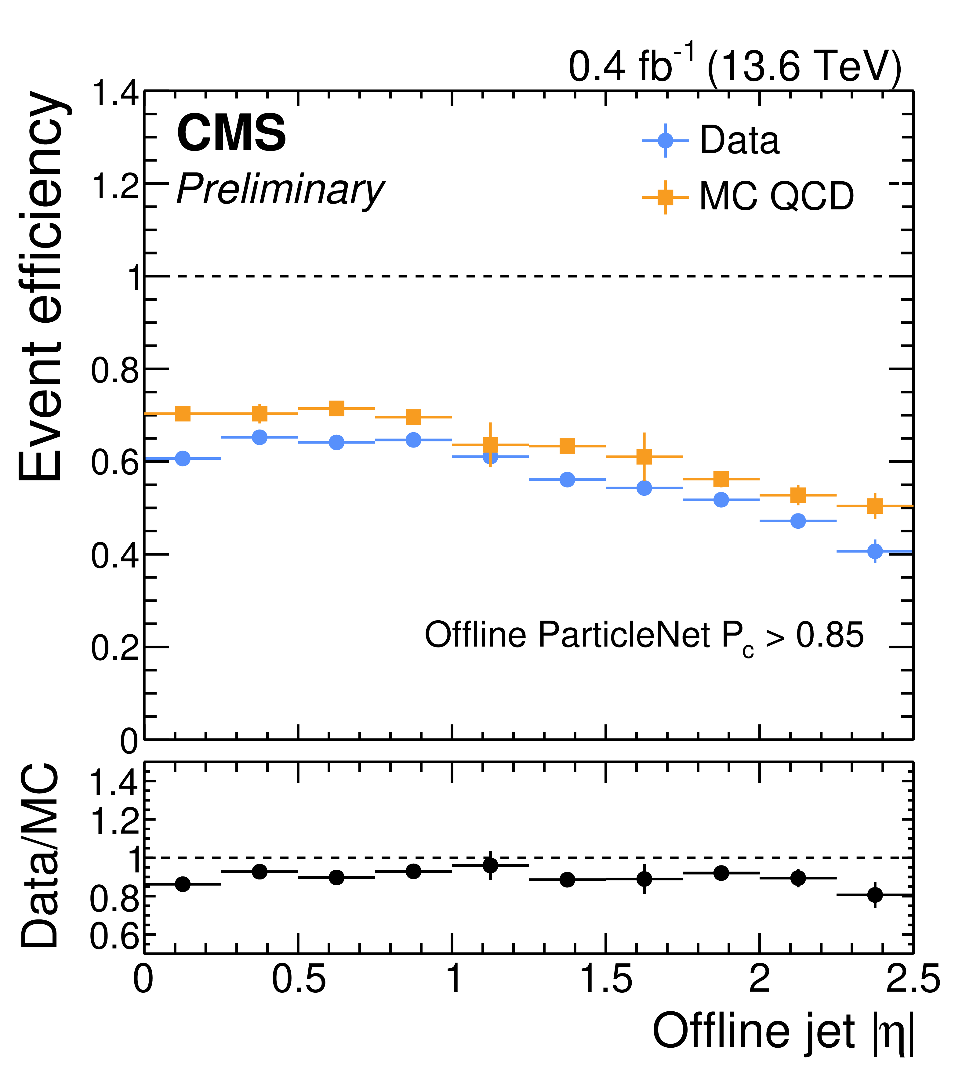
Figure 17:
Online PNET c tagging efficiency in the selected VBF-like QCD multijet events as a function of offline c-tagged jet $ p_{\mathrm{T}} $ (left) and $ \eta $ (right), as measured in data (blue) and simulation (orange) in a QCD-enriched region. |
png pdf |
Figure 17-a:
Online PNET c tagging efficiency in the selected VBF-like QCD multijet events as a function of offline c-tagged jet $ p_{\mathrm{T}} $ (left) and $ \eta $ (right), as measured in data (blue) and simulation (orange) in a QCD-enriched region. |
png pdf |
Figure 17-b:
Online PNET c tagging efficiency in the selected VBF-like QCD multijet events as a function of offline c-tagged jet $ p_{\mathrm{T}} $ (left) and $ \eta $ (right), as measured in data (blue) and simulation (orange) in a QCD-enriched region. |
png pdf |
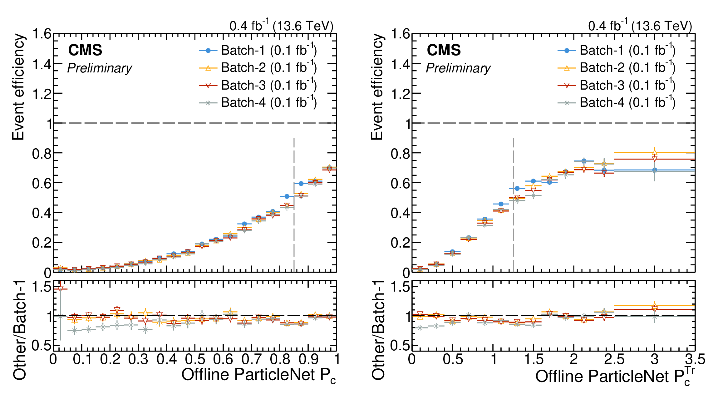
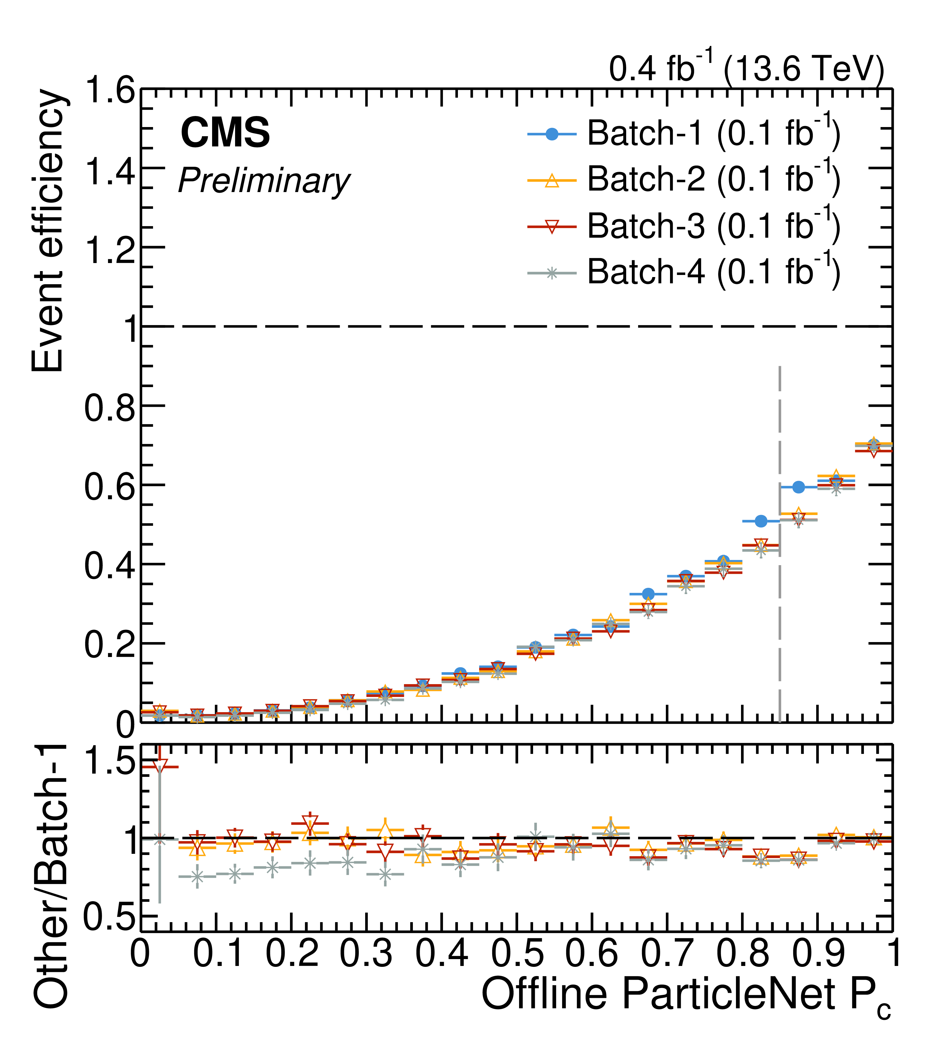
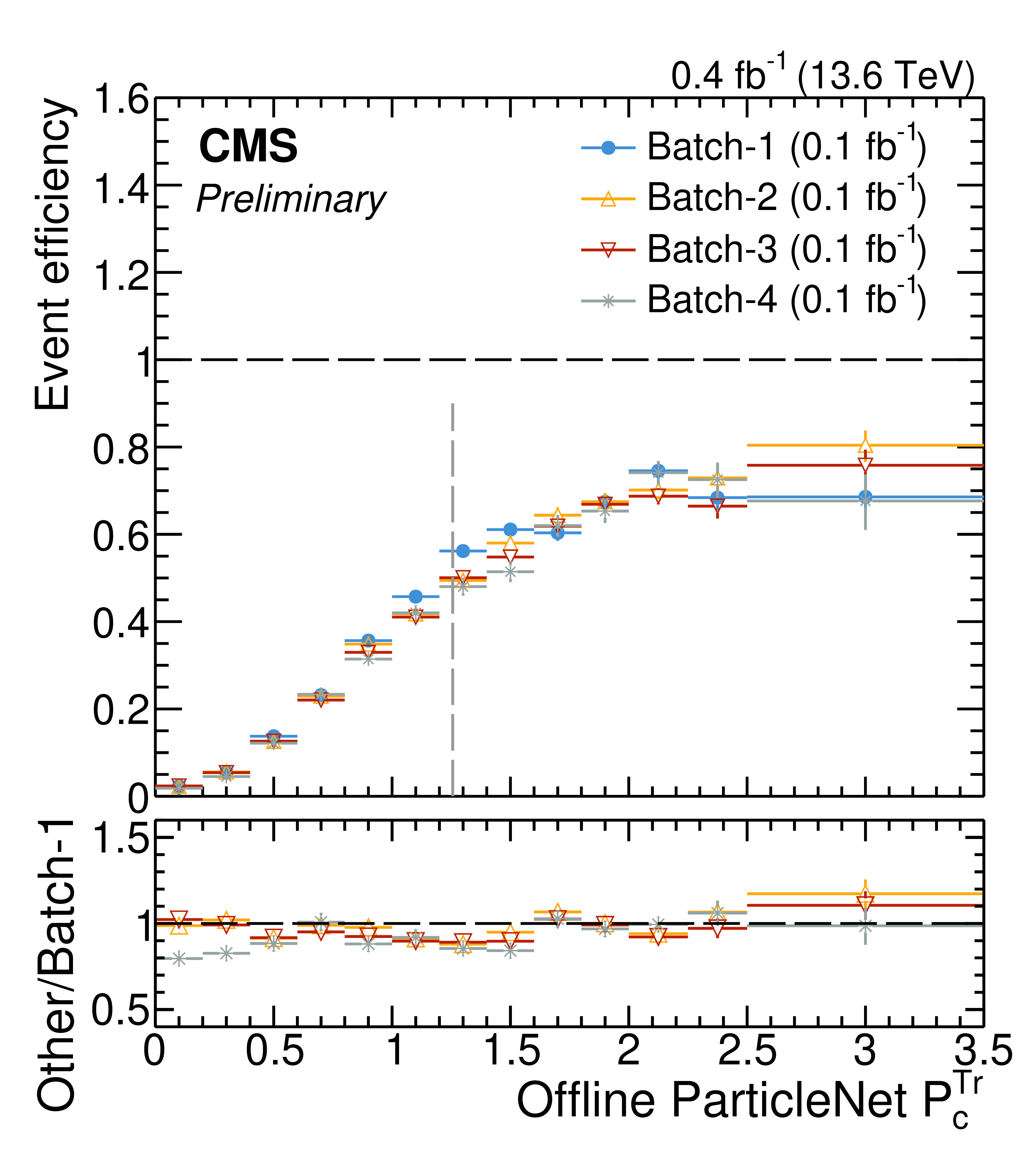
Figure 18:
Efficiency of the online PNET c-tagging algorithm in the selected VBF-like QCD multijet events as a function of the offline PNET $\mathcal{P}_{\mathrm{c}}$ (left) and $ \mathcal{P}_{\mathrm{c}}^{\mathrm{Tr}} $ (right) scores, measured in data for four consecutive time periods (batch-1 to batch-4) during 2024. The lower panels show the ratio of the efficiencies in batch-$ N $ ($ N=2,\ldots, $ 4) relative to batch-1. The vertical dashed line denotes the reference value $ \mathcal{P}_{\mathrm{c}}= $ 0.85, corresponding to a c tagging purity above 80%. |
png pdf |
Figure 18-a:
Efficiency of the online PNET c-tagging algorithm in the selected VBF-like QCD multijet events as a function of the offline PNET $\mathcal{P}_{\mathrm{c}}$ (left) and $ \mathcal{P}_{\mathrm{c}}^{\mathrm{Tr}} $ (right) scores, measured in data for four consecutive time periods (batch-1 to batch-4) during 2024. The lower panels show the ratio of the efficiencies in batch-$ N $ ($ N=2,\ldots, $ 4) relative to batch-1. The vertical dashed line denotes the reference value $ \mathcal{P}_{\mathrm{c}}= $ 0.85, corresponding to a c tagging purity above 80%. |
png pdf |
Figure 18-b:
Efficiency of the online PNET c-tagging algorithm in the selected VBF-like QCD multijet events as a function of the offline PNET $\mathcal{P}_{\mathrm{c}}$ (left) and $ \mathcal{P}_{\mathrm{c}}^{\mathrm{Tr}} $ (right) scores, measured in data for four consecutive time periods (batch-1 to batch-4) during 2024. The lower panels show the ratio of the efficiencies in batch-$ N $ ($ N=2,\ldots, $ 4) relative to batch-1. The vertical dashed line denotes the reference value $ \mathcal{P}_{\mathrm{c}}= $ 0.85, corresponding to a c tagging purity above 80%. |
png pdf |
Figure 19:
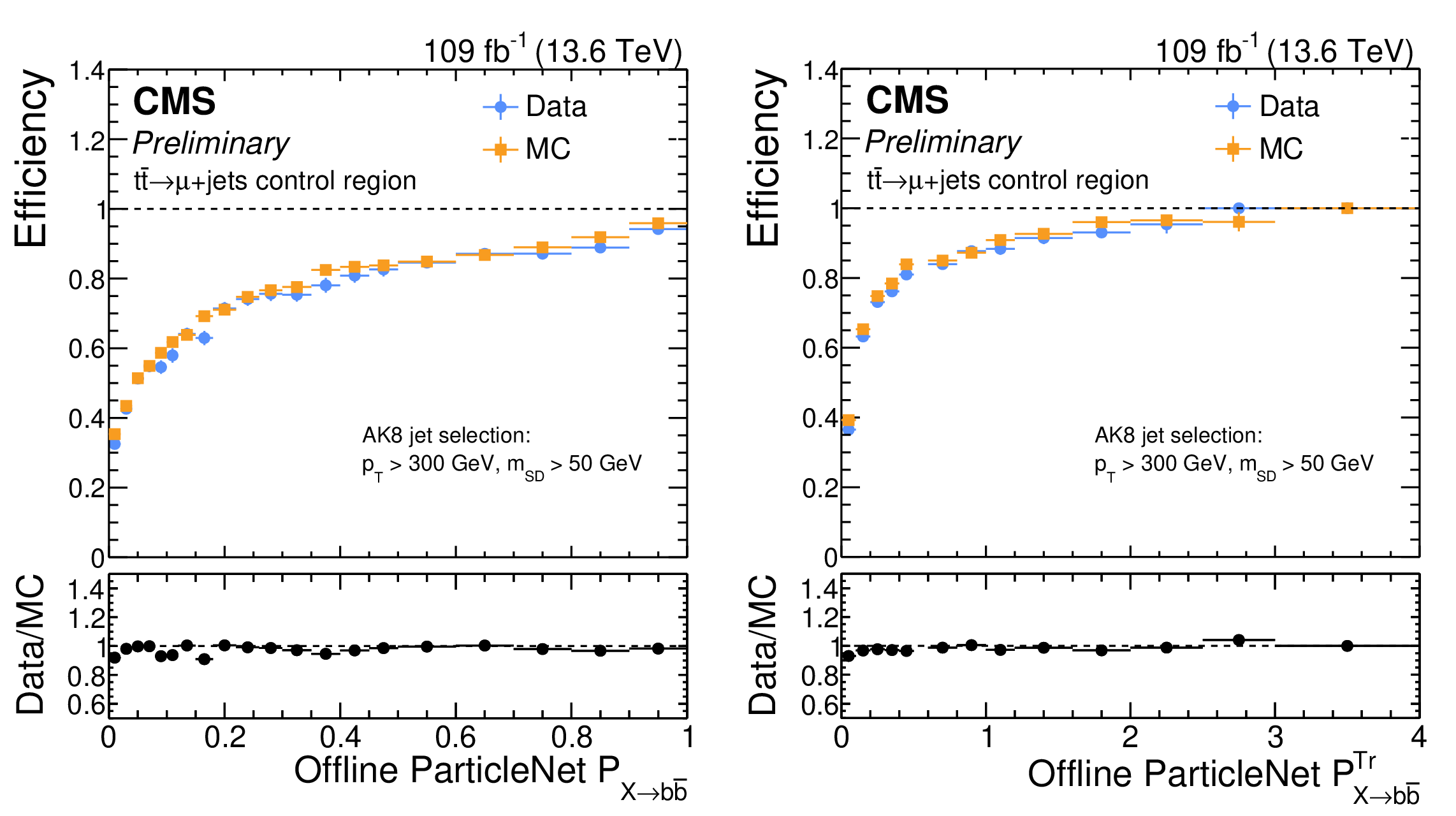
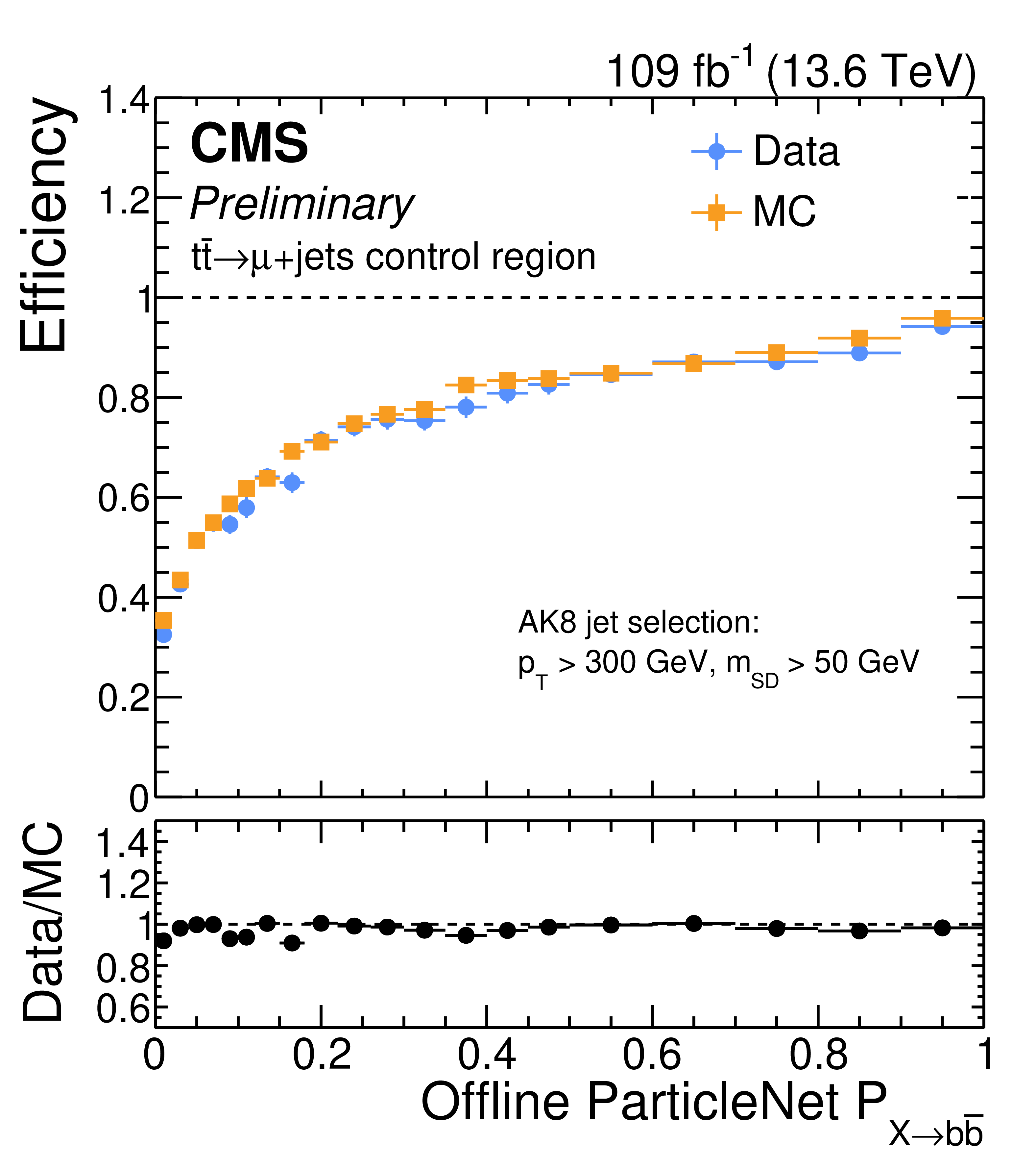
Online PNET $\mathrm{X\to\mathrm{b}\overline{\mathrm{b}}} $ tagging efficiency as a function of the offline $ \mathcal{P}_{\mathrm{X\to\mathrm{b}\overline{\mathrm{b}}}} $ (left) and $ \mathcal{P}_{\mathrm{X\to\mathrm{b}\overline{\mathrm{b}}}}^{\mathrm{Tr}} $ (right) scores for large-radius jets with $ p_{\mathrm{T}} > $ 300 GeV and $ m_{\mathrm{SD}} > $ 50 GeV in a semileptonic $ \mathrm{t} \overline{\mathrm{t}} $ -enriched region, measured in data (blue) and simulation (orange). |
png pdf |
Figure 19-a:
Online PNET $\mathrm{X\to\mathrm{b}\overline{\mathrm{b}}} $ tagging efficiency as a function of the offline $ \mathcal{P}_{\mathrm{X\to\mathrm{b}\overline{\mathrm{b}}}} $ (left) and $ \mathcal{P}_{\mathrm{X\to\mathrm{b}\overline{\mathrm{b}}}}^{\mathrm{Tr}} $ (right) scores for large-radius jets with $ p_{\mathrm{T}} > $ 300 GeV and $ m_{\mathrm{SD}} > $ 50 GeV in a semileptonic $ \mathrm{t} \overline{\mathrm{t}} $ -enriched region, measured in data (blue) and simulation (orange). |
png pdf |
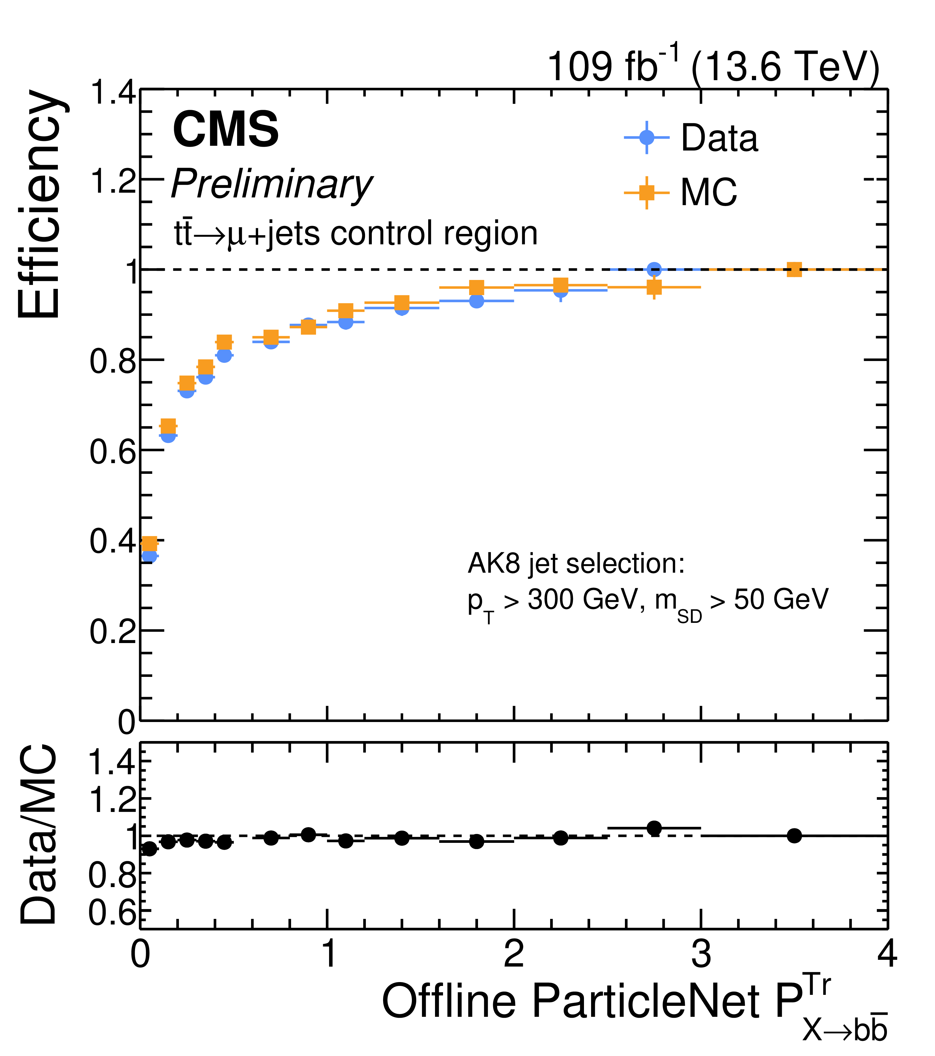
Figure 19-b:
Online PNET $\mathrm{X\to\mathrm{b}\overline{\mathrm{b}}} $ tagging efficiency as a function of the offline $ \mathcal{P}_{\mathrm{X\to\mathrm{b}\overline{\mathrm{b}}}} $ (left) and $ \mathcal{P}_{\mathrm{X\to\mathrm{b}\overline{\mathrm{b}}}}^{\mathrm{Tr}} $ (right) scores for large-radius jets with $ p_{\mathrm{T}} > $ 300 GeV and $ m_{\mathrm{SD}} > $ 50 GeV in a semileptonic $ \mathrm{t} \overline{\mathrm{t}} $ -enriched region, measured in data (blue) and simulation (orange). |
png pdf |
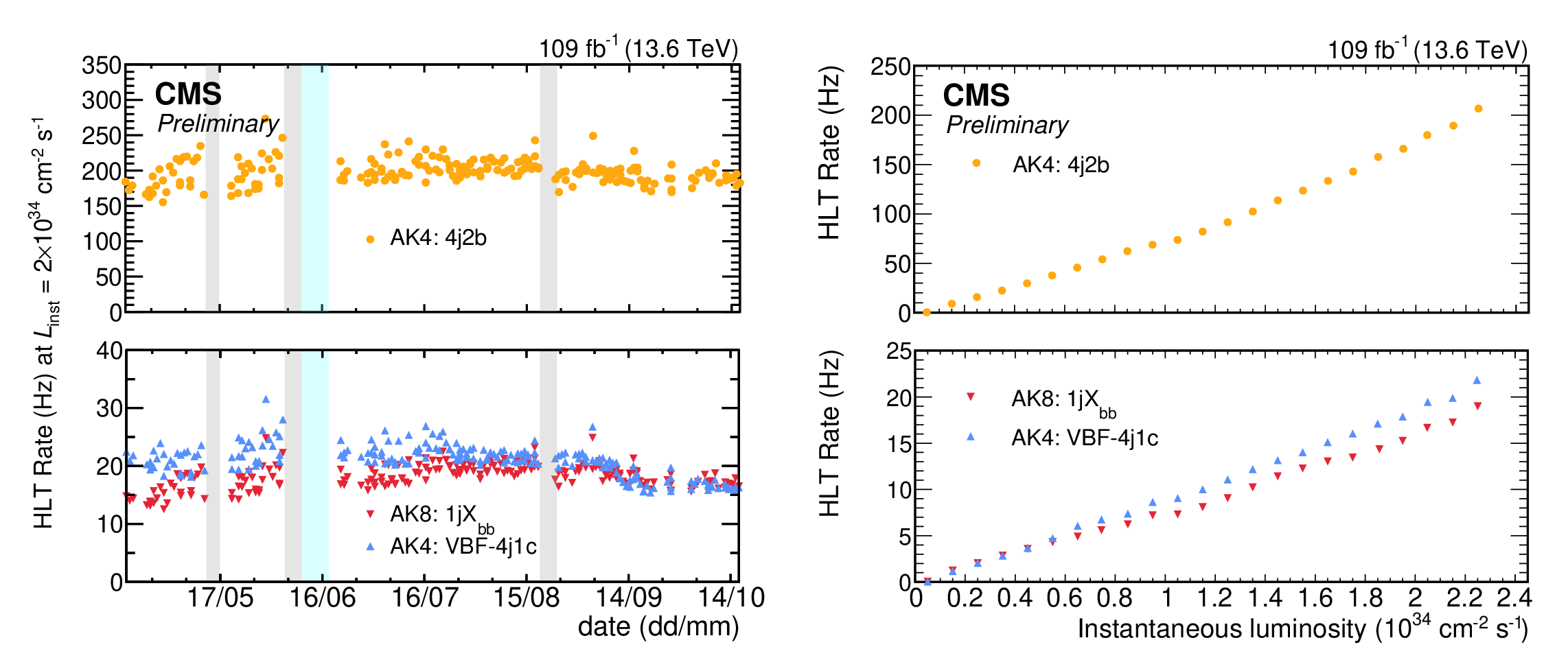
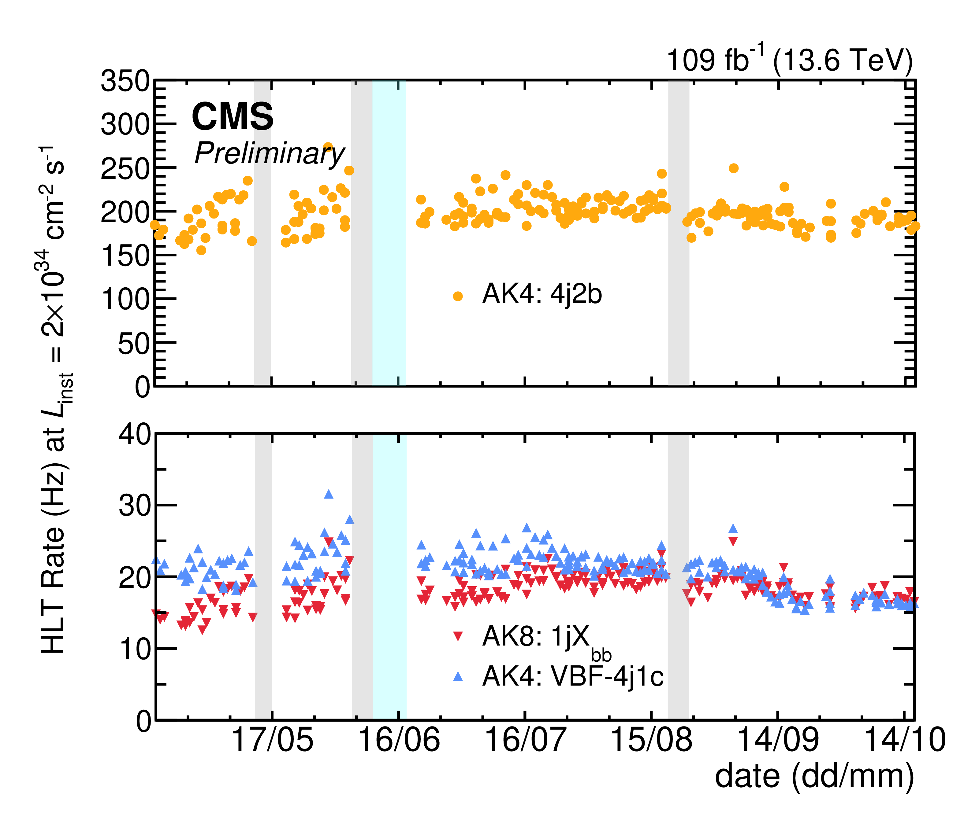
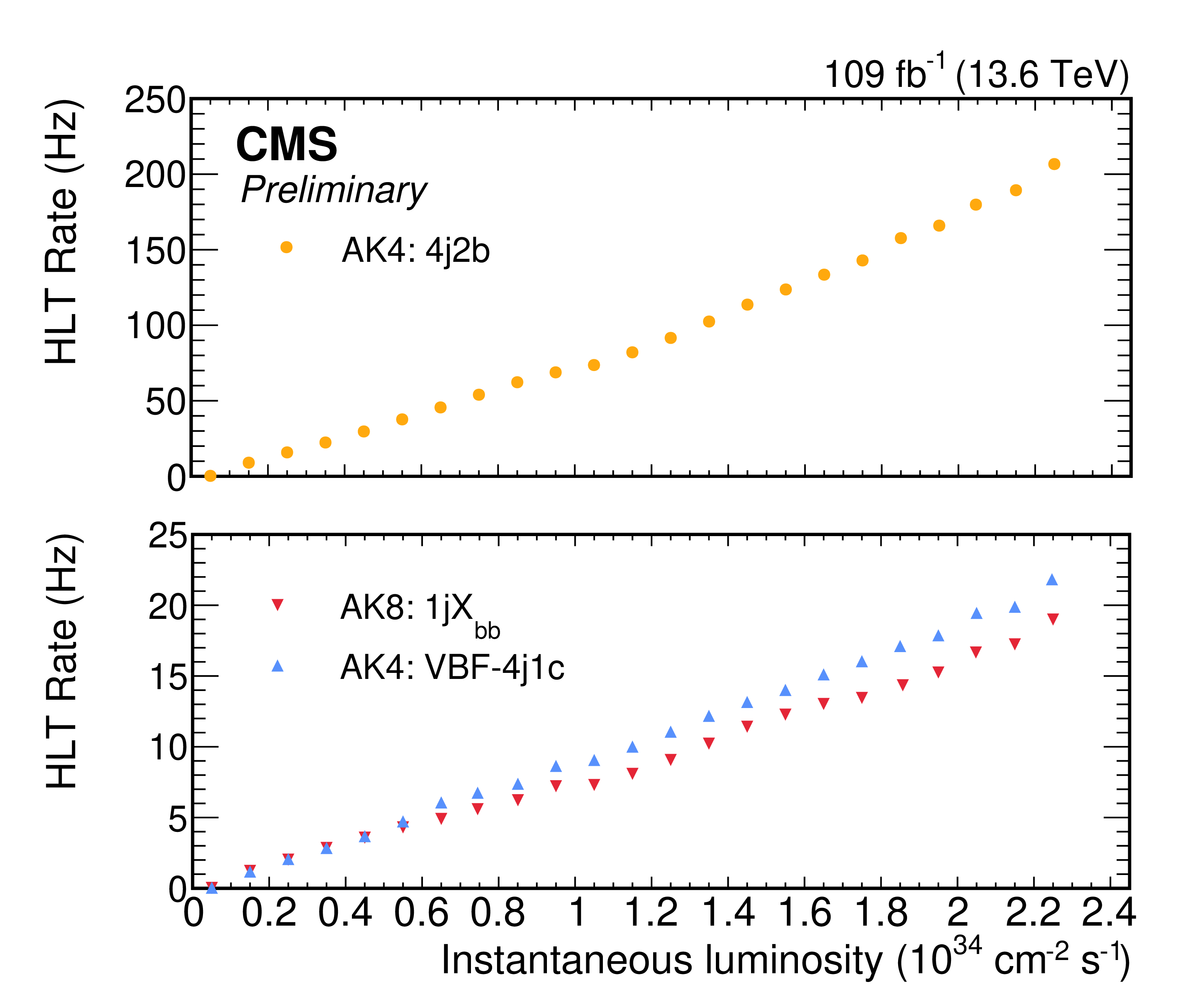
Figure 20:
Average output rates correspond to an instantaneous luminosity of $ \approx 2\times10^{34} \text{cm}^{-2} \text{s}^{-1} $ for the selected heavy-flavour triggers reported in Tab. 2 during 2024 as a function of time (left) and instantaneous luminosity (right). Only certified pp fills at $ \sqrt{s}= $ 13.6 TeV and with the highest number of colliding bunches are considered. |
png pdf |
Figure 20-a:
Average output rates correspond to an instantaneous luminosity of $ \approx 2\times10^{34} \text{cm}^{-2} \text{s}^{-1} $ for the selected heavy-flavour triggers reported in Tab. 2 during 2024 as a function of time (left) and instantaneous luminosity (right). Only certified pp fills at $ \sqrt{s}= $ 13.6 TeV and with the highest number of colliding bunches are considered. |
png pdf |
Figure 20-b:
Average output rates correspond to an instantaneous luminosity of $ \approx 2\times10^{34} \text{cm}^{-2} \text{s}^{-1} $ for the selected heavy-flavour triggers reported in Tab. 2 during 2024 as a function of time (left) and instantaneous luminosity (right). Only certified pp fills at $ \sqrt{s}= $ 13.6 TeV and with the highest number of colliding bunches are considered. |
png pdf |
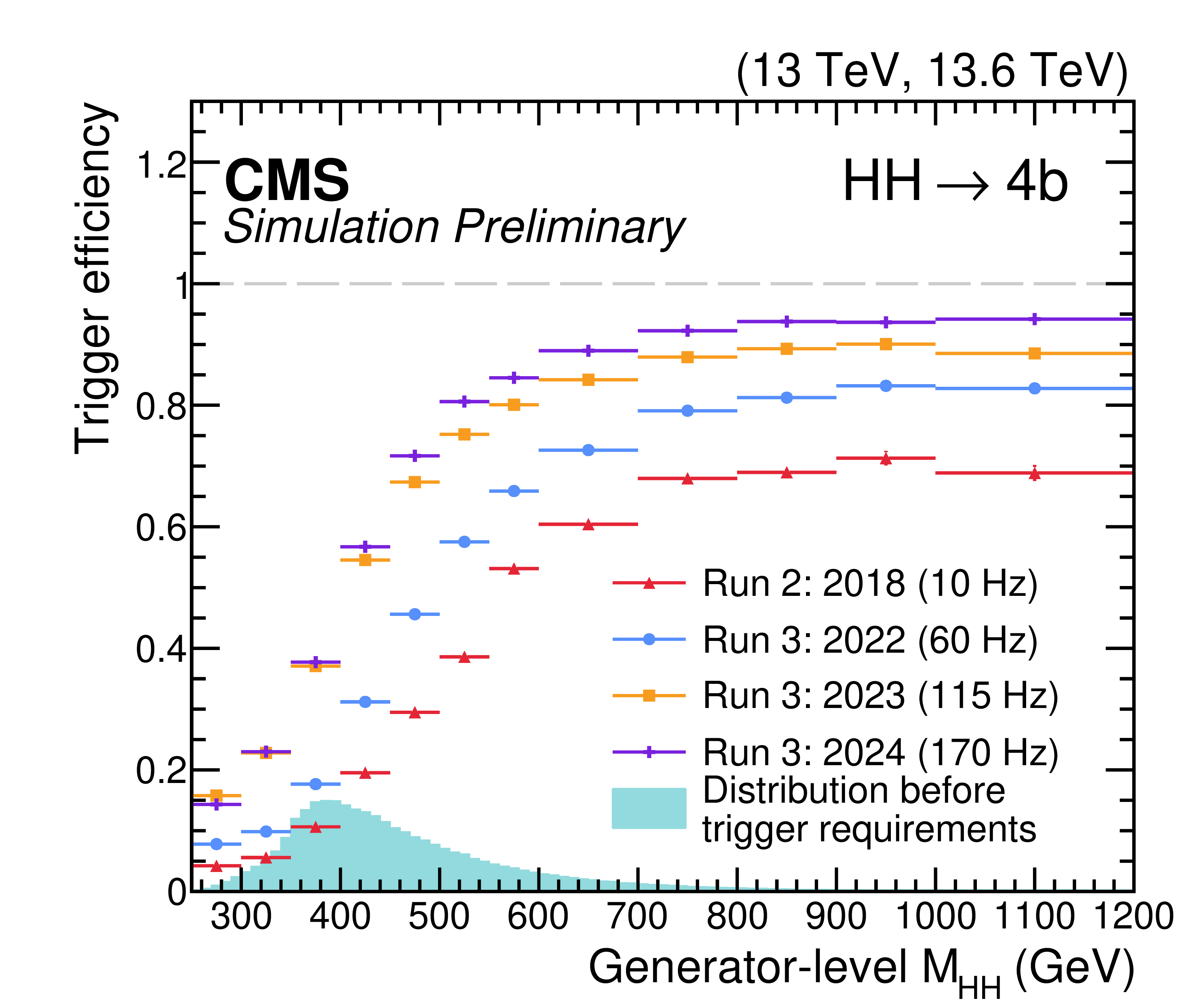
Figure 21:
Efficiency of the Run 3 \texttt4j2b trigger in simulated $ \mathrm{H}\mathrm{H} \to 4\mathrm{b} $ events for 2022 (azure), 2023 (orange), and 2024 (purple) configurations as a function of generator-level $ m_{\mathrm{H}\mathrm{H}} $. Four generator-level jets are required in the selected events with $ p_{\mathrm{T}} > $ 25 GeV and $ {|\eta| < 2.5} $. Results are compared to Run 2 triggers (red). The corresponding trigger rates are 10, 60, 115, and 170\unitHz for 2018, 2022, 2023, and 2024, respectively, at an instantaneous luminosity of $ \approx 2\times10^{34} \text{cm}^{-2} \text{s}^{-1} $. The increase in trigger rate across Run 3 configurations reflects the progressive relaxation and optimisation of the trigger selection in later years. The teal histogram shows the expected distribution of the simulated events at $ \sqrt{s}= $ 13.6 TeV before trigger requirements, scaled by an arbitrary factor for visibility. |
png pdf |
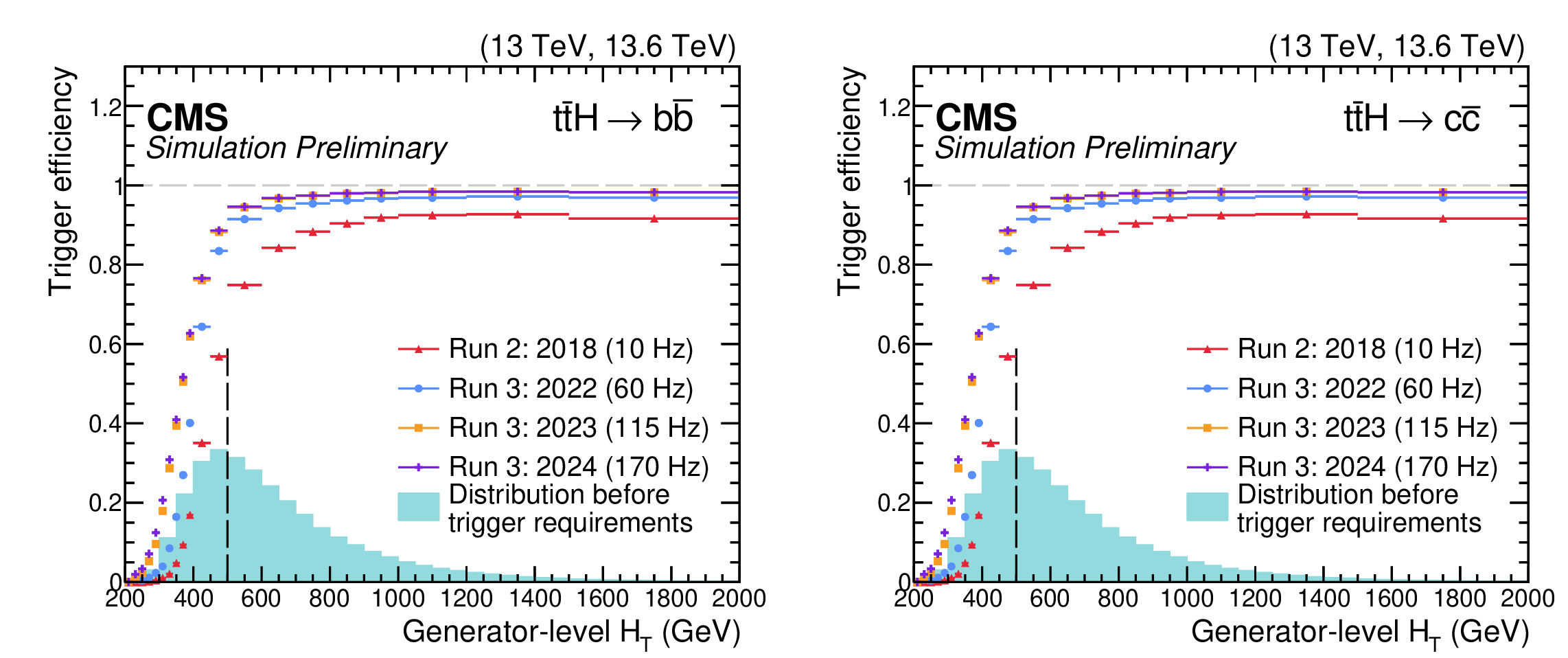
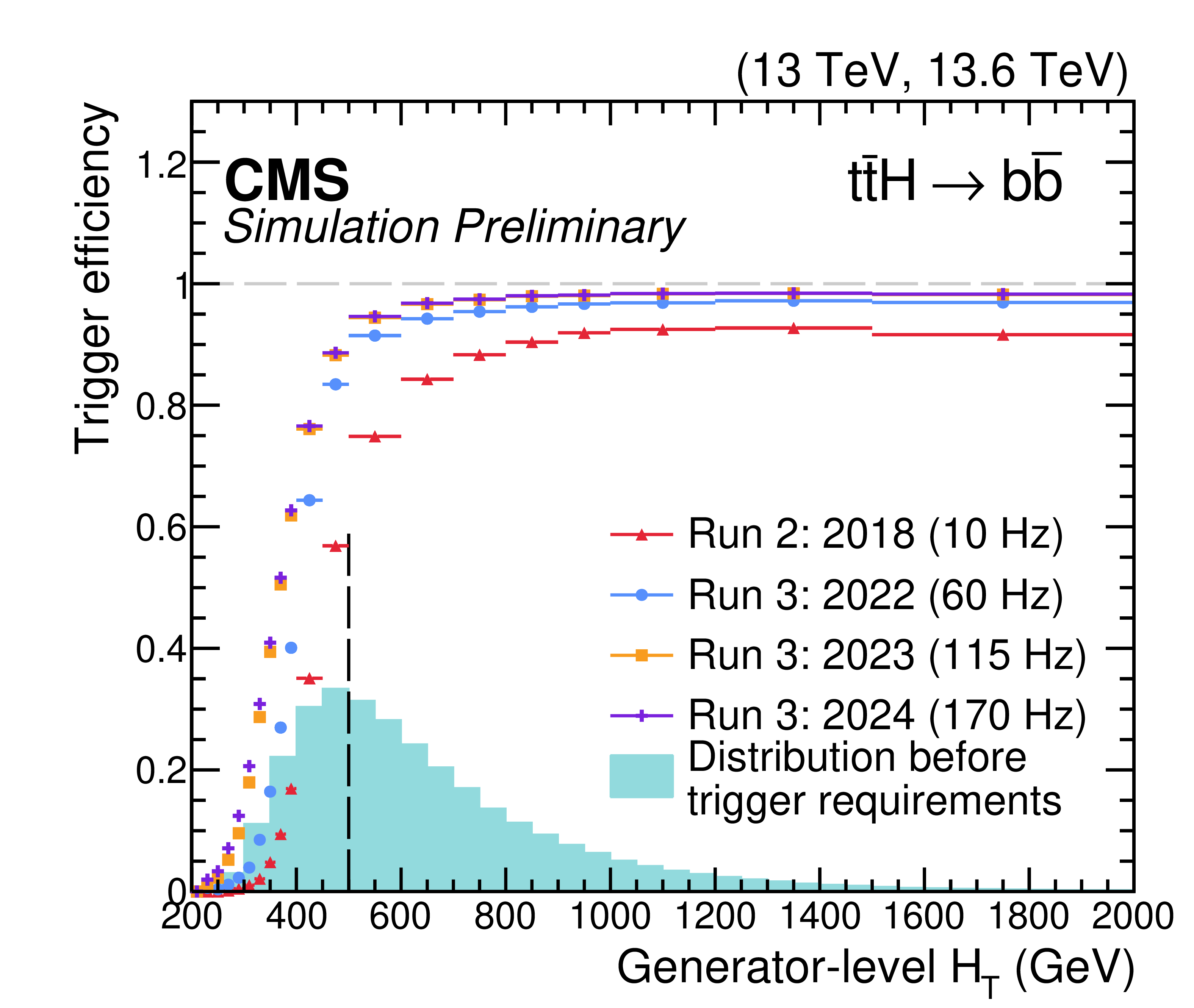
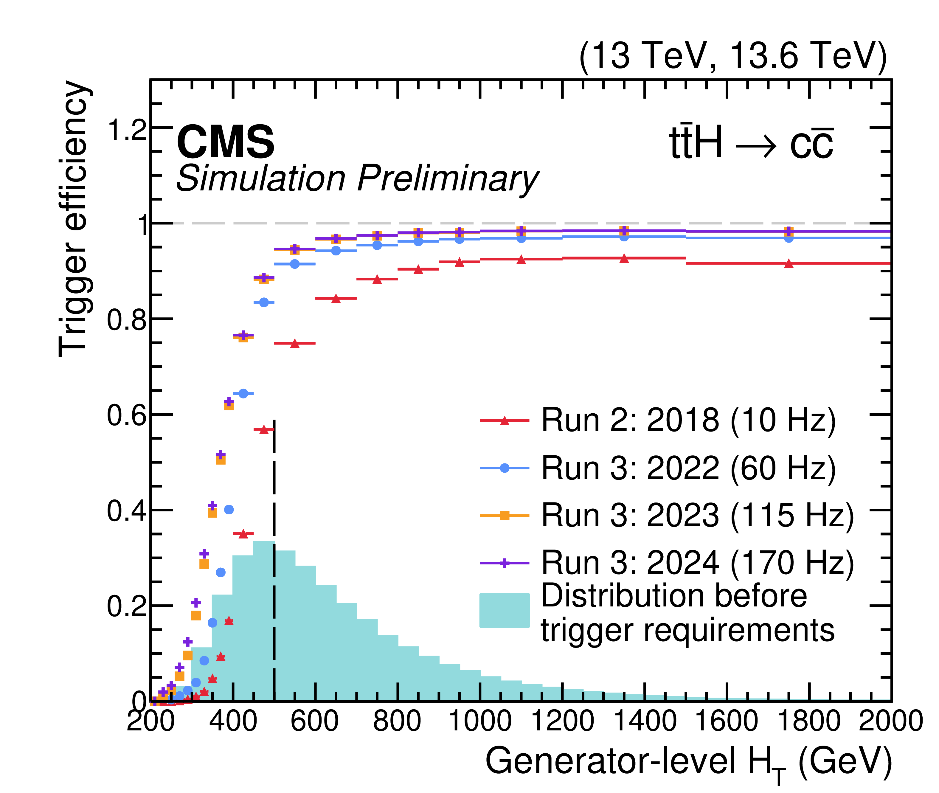
Figure 22:
Efficiency of the Run 3 \texttt4j2b trigger in simulated $ {\mathrm{t}\overline{\mathrm{t}}} \mathrm{H} \to \mathrm{b}\overline{\mathrm{b}} $ (left) and $ {\mathrm{t}\overline{\mathrm{t}}} \mathrm{H} \to \mathrm{c}\overline{\mathrm{c}} $ (right) events, shown for 2022 (azure), 2023 (orange), and 2024 (purple) configurations as a function of generator-level $ H_{\mathrm{T}} $. Six generator-level jets in the event are required to satisfy $ p_{\mathrm{T}} > $ 25 GeV and $ |\eta| < $ 2.5. Results are compared to Run 2 triggers (red). The dashed line at $ H_{\mathrm{T}}= $ 500 GeV indicates the Run 2 offline threshold. The corresponding trigger rates are 10, 60, 115, and 170\unitHz for 2018, 2022, 2023, and 2024, respectively, at an instantaneous luminosity of $ \approx 2\times10^{34} \text{cm}^{-2} \text{s}^{-1} $. The teal histogram shows the expected distribution of the simulated events at $ \sqrt{s}= $ 13.6 TeV before trigger requirements, scaled by an arbitrary factor for visibility. |
png pdf |
Figure 22-a:
Efficiency of the Run 3 \texttt4j2b trigger in simulated $ {\mathrm{t}\overline{\mathrm{t}}} \mathrm{H} \to \mathrm{b}\overline{\mathrm{b}} $ (left) and $ {\mathrm{t}\overline{\mathrm{t}}} \mathrm{H} \to \mathrm{c}\overline{\mathrm{c}} $ (right) events, shown for 2022 (azure), 2023 (orange), and 2024 (purple) configurations as a function of generator-level $ H_{\mathrm{T}} $. Six generator-level jets in the event are required to satisfy $ p_{\mathrm{T}} > $ 25 GeV and $ |\eta| < $ 2.5. Results are compared to Run 2 triggers (red). The dashed line at $ H_{\mathrm{T}}= $ 500 GeV indicates the Run 2 offline threshold. The corresponding trigger rates are 10, 60, 115, and 170\unitHz for 2018, 2022, 2023, and 2024, respectively, at an instantaneous luminosity of $ \approx 2\times10^{34} \text{cm}^{-2} \text{s}^{-1} $. The teal histogram shows the expected distribution of the simulated events at $ \sqrt{s}= $ 13.6 TeV before trigger requirements, scaled by an arbitrary factor for visibility. |
png pdf |
Figure 22-b:
Efficiency of the Run 3 \texttt4j2b trigger in simulated $ {\mathrm{t}\overline{\mathrm{t}}} \mathrm{H} \to \mathrm{b}\overline{\mathrm{b}} $ (left) and $ {\mathrm{t}\overline{\mathrm{t}}} \mathrm{H} \to \mathrm{c}\overline{\mathrm{c}} $ (right) events, shown for 2022 (azure), 2023 (orange), and 2024 (purple) configurations as a function of generator-level $ H_{\mathrm{T}} $. Six generator-level jets in the event are required to satisfy $ p_{\mathrm{T}} > $ 25 GeV and $ |\eta| < $ 2.5. Results are compared to Run 2 triggers (red). The dashed line at $ H_{\mathrm{T}}= $ 500 GeV indicates the Run 2 offline threshold. The corresponding trigger rates are 10, 60, 115, and 170\unitHz for 2018, 2022, 2023, and 2024, respectively, at an instantaneous luminosity of $ \approx 2\times10^{34} \text{cm}^{-2} \text{s}^{-1} $. The teal histogram shows the expected distribution of the simulated events at $ \sqrt{s}= $ 13.6 TeV before trigger requirements, scaled by an arbitrary factor for visibility. |
png pdf |
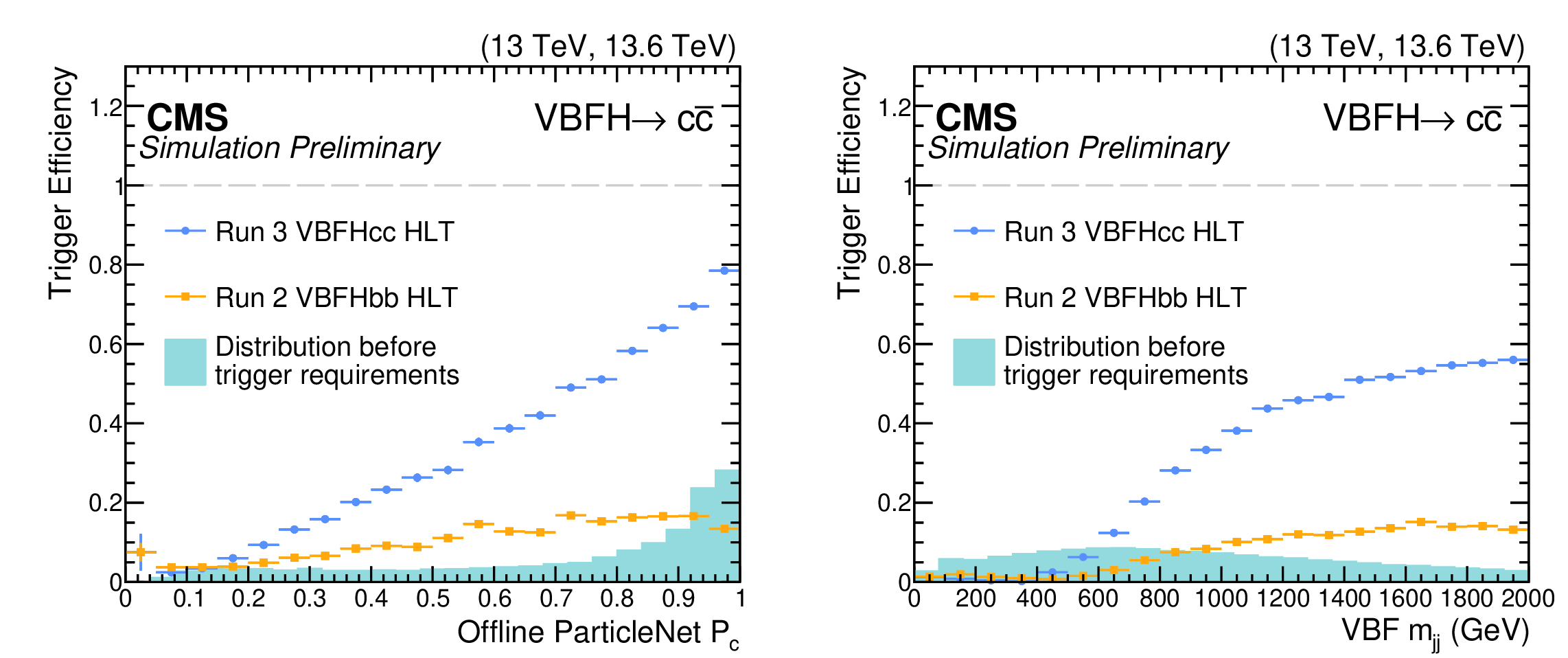
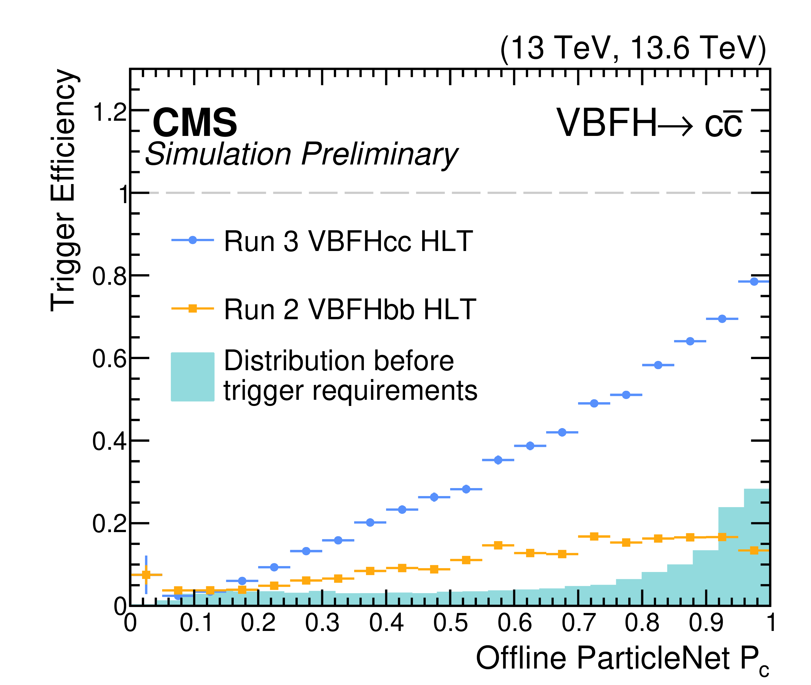
Figure 23:
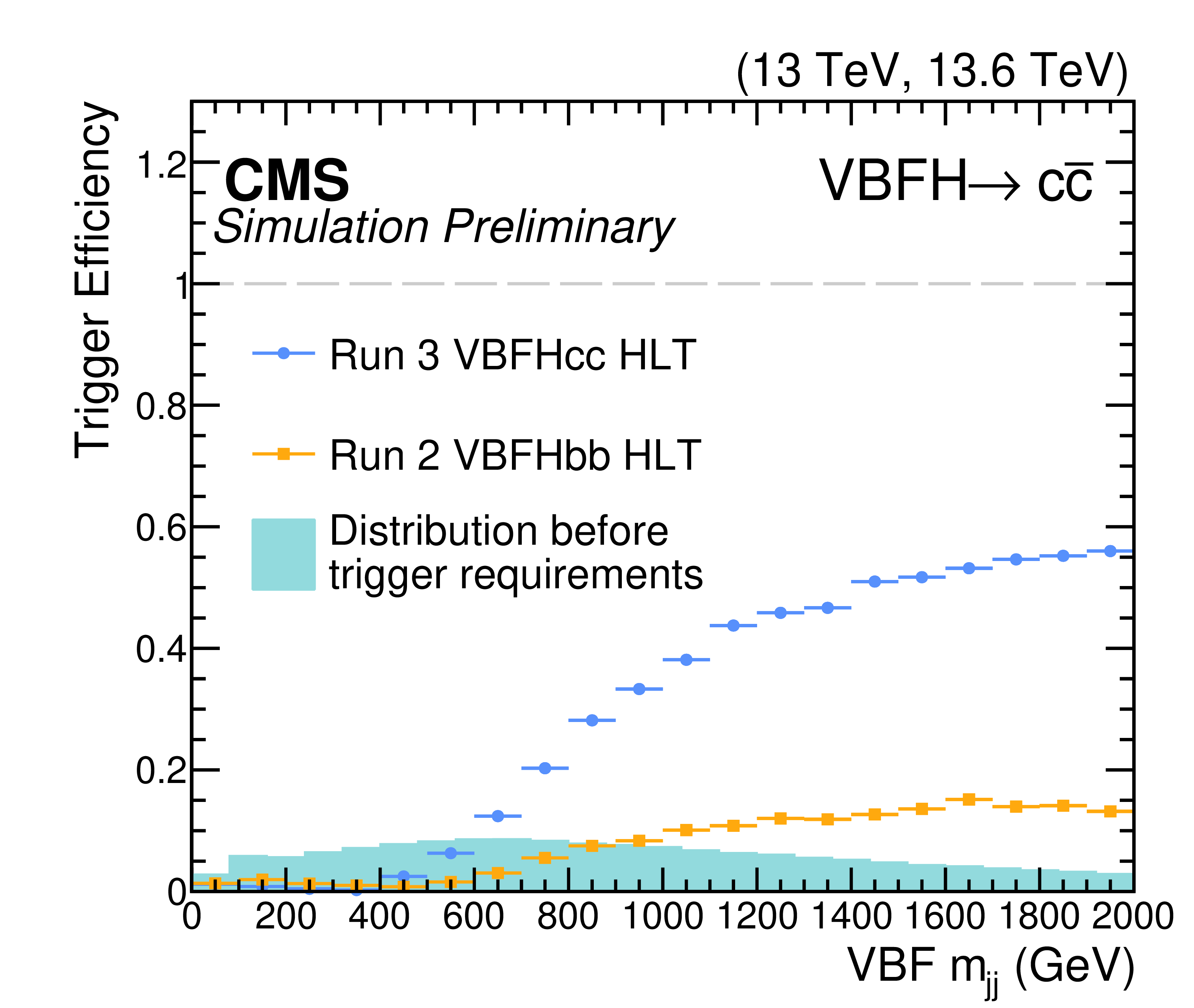
Efficiency of the \textttVBF-4j1c trigger (blue) in simulated VBF $ \mathrm{H} \to \mathrm{c}\overline{\mathrm{c}} $ events as a function of $ m_{\mathrm{jj}} $ (left) and the offline $ \mathcal{P}_{\mathrm{c}} $ score of the leading c-tagged jet (right). Events require at least four small-radius jets with $ {|\eta| < 4.7} $ and $ p_{\mathrm{T}} > $ 100, 88, 70, and 30 GeV. For the right, at least one jet pair must satisfy $ m_{\mathrm{jj}} > $ 500 GeV and $ {|\Delta\eta_{\mathrm{jj}}| > 4} $. Results are compared to the Run 2 VBF $ \mathrm{H} \to \mathrm{b}\overline{\mathrm{b}} $ triggers [4] (orange). An improvement exceeding a factor of two is observed at large $ m_{\mathrm{jj}} $ and high $ \mathcal{P}_{\mathrm{c}} $. The teal histogram shows the expected distribution of the simulated events at $ \sqrt{s}= $ 13.6 TeV before trigger requirements, scaled by an arbitrary factor for visibility. |
png pdf |
Figure 23-a:
Efficiency of the \textttVBF-4j1c trigger (blue) in simulated VBF $ \mathrm{H} \to \mathrm{c}\overline{\mathrm{c}} $ events as a function of $ m_{\mathrm{jj}} $ (left) and the offline $ \mathcal{P}_{\mathrm{c}} $ score of the leading c-tagged jet (right). Events require at least four small-radius jets with $ {|\eta| < 4.7} $ and $ p_{\mathrm{T}} > $ 100, 88, 70, and 30 GeV. For the right, at least one jet pair must satisfy $ m_{\mathrm{jj}} > $ 500 GeV and $ {|\Delta\eta_{\mathrm{jj}}| > 4} $. Results are compared to the Run 2 VBF $ \mathrm{H} \to \mathrm{b}\overline{\mathrm{b}} $ triggers [4] (orange). An improvement exceeding a factor of two is observed at large $ m_{\mathrm{jj}} $ and high $ \mathcal{P}_{\mathrm{c}} $. The teal histogram shows the expected distribution of the simulated events at $ \sqrt{s}= $ 13.6 TeV before trigger requirements, scaled by an arbitrary factor for visibility. |
png pdf |
Figure 23-b:
Efficiency of the \textttVBF-4j1c trigger (blue) in simulated VBF $ \mathrm{H} \to \mathrm{c}\overline{\mathrm{c}} $ events as a function of $ m_{\mathrm{jj}} $ (left) and the offline $ \mathcal{P}_{\mathrm{c}} $ score of the leading c-tagged jet (right). Events require at least four small-radius jets with $ {|\eta| < 4.7} $ and $ p_{\mathrm{T}} > $ 100, 88, 70, and 30 GeV. For the right, at least one jet pair must satisfy $ m_{\mathrm{jj}} > $ 500 GeV and $ {|\Delta\eta_{\mathrm{jj}}| > 4} $. Results are compared to the Run 2 VBF $ \mathrm{H} \to \mathrm{b}\overline{\mathrm{b}} $ triggers [4] (orange). An improvement exceeding a factor of two is observed at large $ m_{\mathrm{jj}} $ and high $ \mathcal{P}_{\mathrm{c}} $. The teal histogram shows the expected distribution of the simulated events at $ \sqrt{s}= $ 13.6 TeV before trigger requirements, scaled by an arbitrary factor for visibility. |
png pdf |
Figure 24:
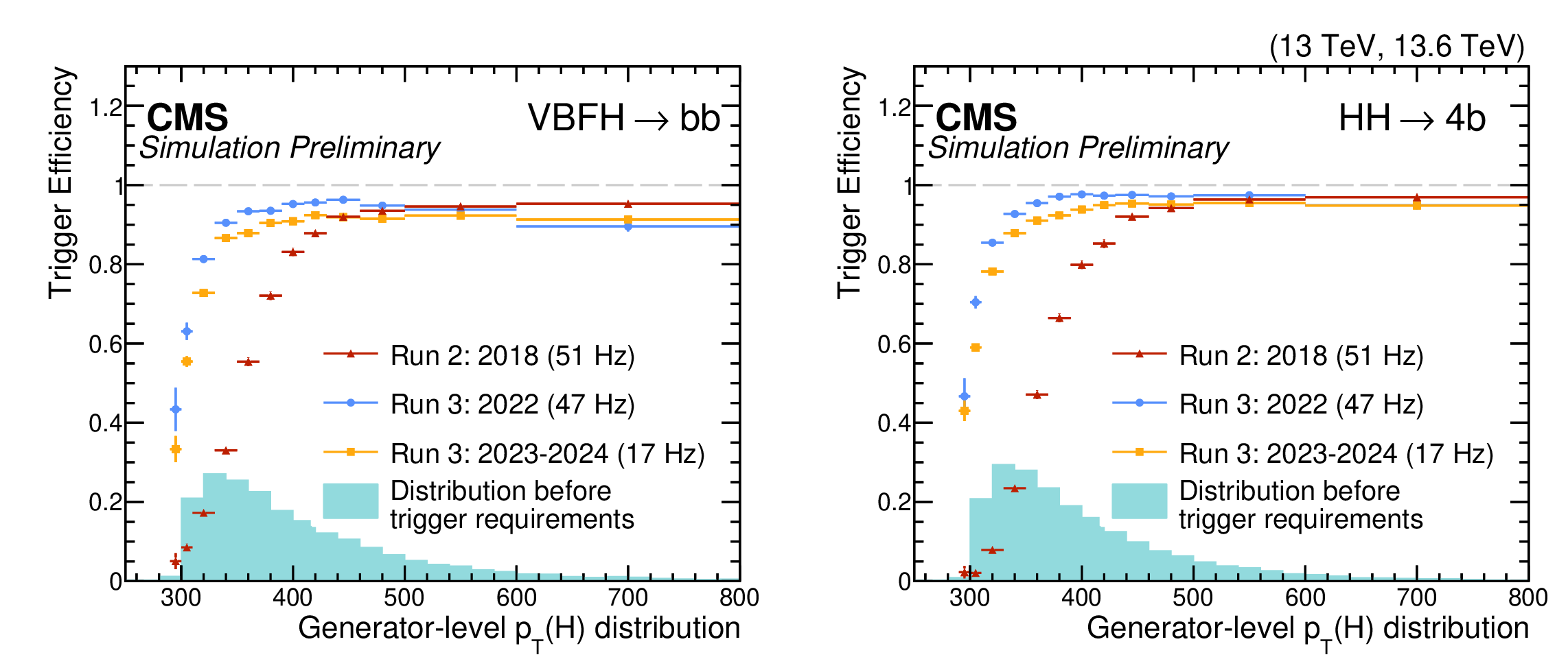
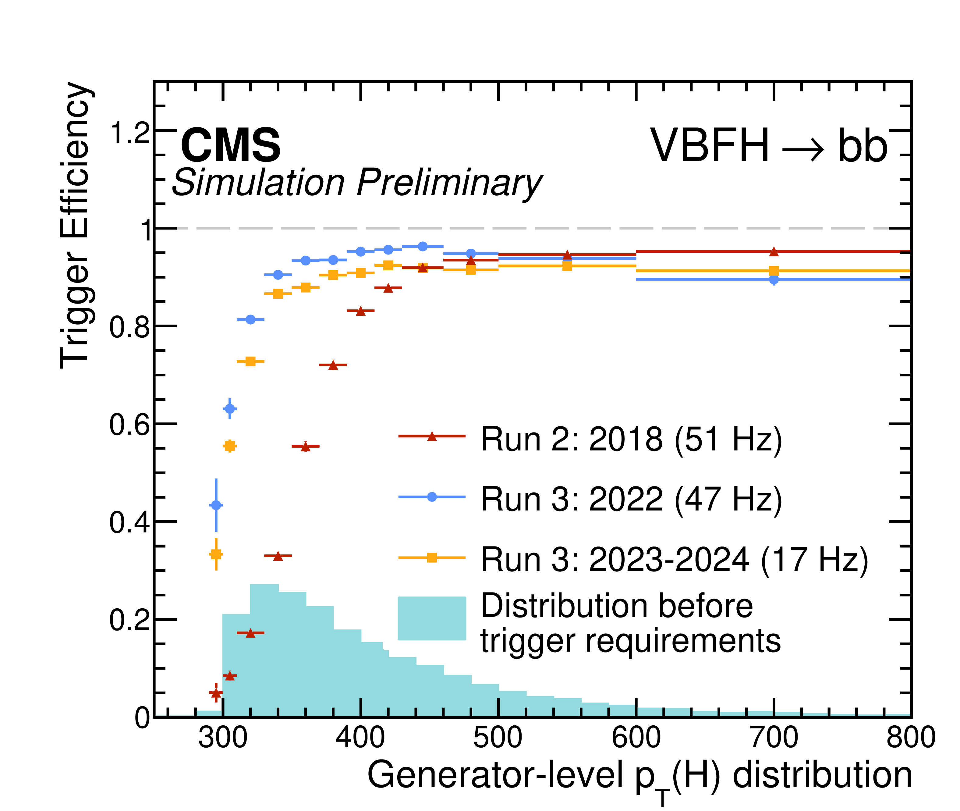
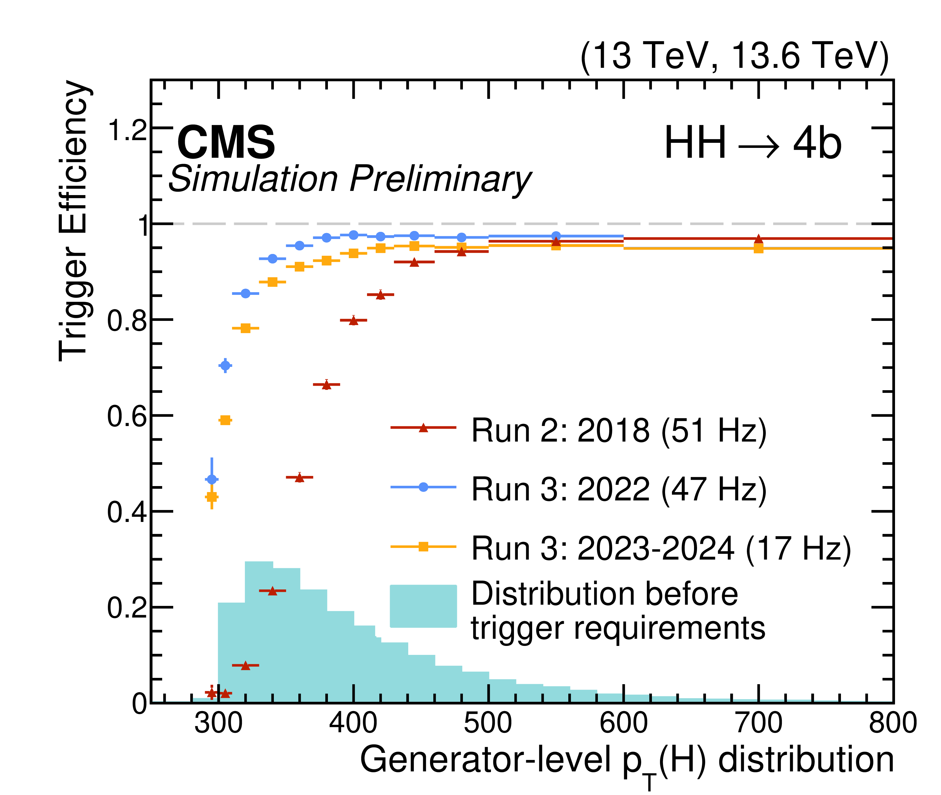
Efficiency of the Run 3 $ \text{X} \to \mathrm{b}\overline{\mathrm{b}} $ triggers in 2022 (azure) and 2023--24 (orange) in simulated VBF $ \mathrm{H} \to \mathrm{b}\overline{\mathrm{b}} $ (left) and $ \mathrm{H}\mathrm{H} \to 4\mathrm{b} $ (right) events as a function of the generator-level Higgs boson $ p_{\mathrm{T}} $. Only events in which at least one $ \mathrm{H} \to \mathrm{b}\overline{\mathrm{b}} $ candidates has $ {\Delta R(\mathrm{b},\overline{\mathrm{b}}) < 0.8} $ are considered. Results are compared to Run 2 (red). The corresponding trigger rates are 51, 47, and 17\unitHz for 2018, 2022, and 2023, respectively, at an instantaneous luminosity of $ \approx 2\times10^{34} \text{cm}^{-2} \text{s}^{-1} $. The teal histogram shows the expected distribution of the simulated events at $ \sqrt{s}= $ 13.6 TeV before trigger requirements, scaled by an arbitrary factor for visibility. |
png pdf |
Figure 24-a:
Efficiency of the Run 3 $ \text{X} \to \mathrm{b}\overline{\mathrm{b}} $ triggers in 2022 (azure) and 2023--24 (orange) in simulated VBF $ \mathrm{H} \to \mathrm{b}\overline{\mathrm{b}} $ (left) and $ \mathrm{H}\mathrm{H} \to 4\mathrm{b} $ (right) events as a function of the generator-level Higgs boson $ p_{\mathrm{T}} $. Only events in which at least one $ \mathrm{H} \to \mathrm{b}\overline{\mathrm{b}} $ candidates has $ {\Delta R(\mathrm{b},\overline{\mathrm{b}}) < 0.8} $ are considered. Results are compared to Run 2 (red). The corresponding trigger rates are 51, 47, and 17\unitHz for 2018, 2022, and 2023, respectively, at an instantaneous luminosity of $ \approx 2\times10^{34} \text{cm}^{-2} \text{s}^{-1} $. The teal histogram shows the expected distribution of the simulated events at $ \sqrt{s}= $ 13.6 TeV before trigger requirements, scaled by an arbitrary factor for visibility. |
png pdf |
Figure 24-b:
Efficiency of the Run 3 $ \text{X} \to \mathrm{b}\overline{\mathrm{b}} $ triggers in 2022 (azure) and 2023--24 (orange) in simulated VBF $ \mathrm{H} \to \mathrm{b}\overline{\mathrm{b}} $ (left) and $ \mathrm{H}\mathrm{H} \to 4\mathrm{b} $ (right) events as a function of the generator-level Higgs boson $ p_{\mathrm{T}} $. Only events in which at least one $ \mathrm{H} \to \mathrm{b}\overline{\mathrm{b}} $ candidates has $ {\Delta R(\mathrm{b},\overline{\mathrm{b}}) < 0.8} $ are considered. Results are compared to Run 2 (red). The corresponding trigger rates are 51, 47, and 17\unitHz for 2018, 2022, and 2023, respectively, at an instantaneous luminosity of $ \approx 2\times10^{34} \text{cm}^{-2} \text{s}^{-1} $. The teal histogram shows the expected distribution of the simulated events at $ \sqrt{s}= $ 13.6 TeV before trigger requirements, scaled by an arbitrary factor for visibility. |
| Tables | |
png pdf |
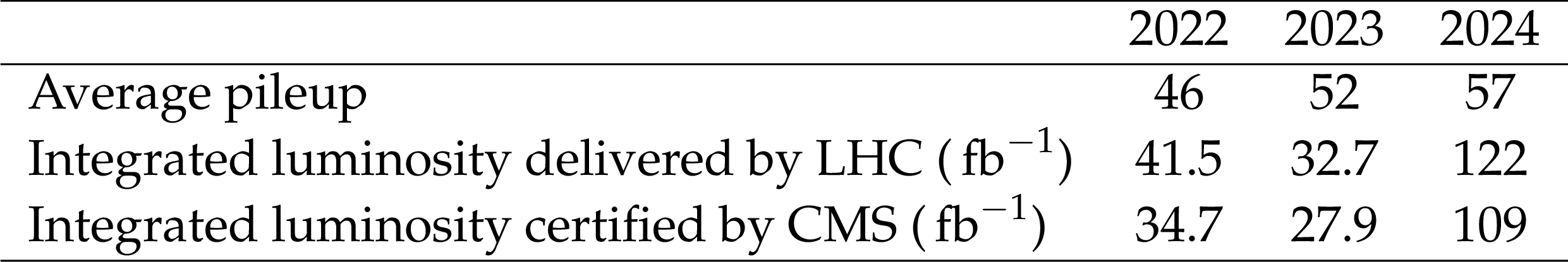
Table 1:
LHC operating parameters during the first three years of Run 3. Pileup is computed from physics fills with the nominal filling scheme, assuming a minimum-bias cross section of 80 \unitmb. The reported integrated luminosities correspond to both the LHC delivered and CMS-certified values for physics analyses. |
png pdf |
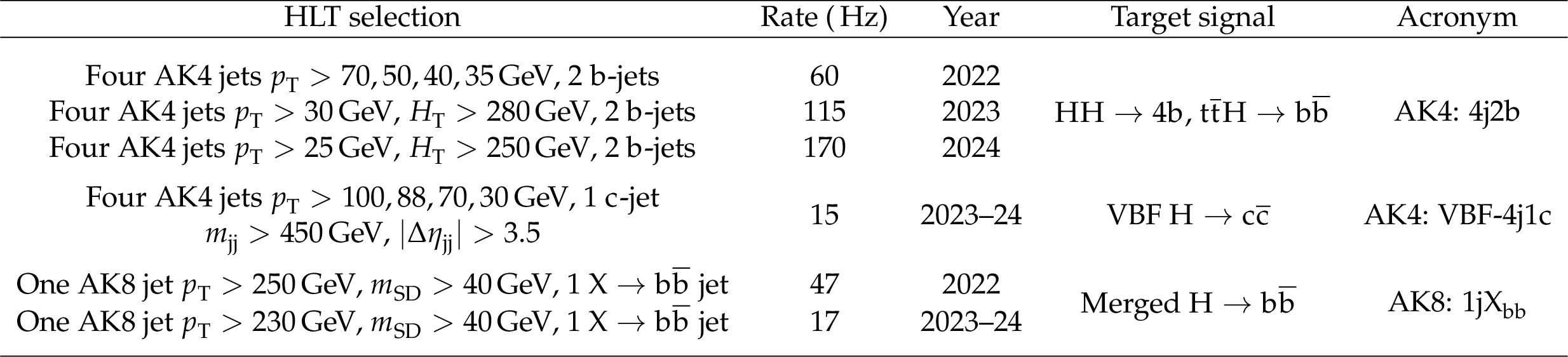
Table 2:
Summary of representative Run 3 HLT triggers using PNET-based heavy-flavour tagging. Here, AK4 and AK8 denote small- and large-radius jets, respectively. All triggers are seeded by common L1 $ H_{\mathrm{T}} $ requirements, $ H_{\mathrm{T}} > $ 360 GeV in 2022 to $ H_{\mathrm{T}} > $ 280 GeV in 2023--24, with AK8 triggers also accepting events with at least one jet with $ p_{\mathrm{T}} > $ 180 GeV and $ {|\eta| < 2.5} $. Rates correspond to at an instantaneous luminosity of $ \approx 2\times10^{34} \text{cm}^{-2} \text{s}^{-1} $. |
| Summary |
| The CMS trigger system plays a crucial role during data-taking, reducing the large collision rate delivered by the LHC to a few kHz for data storage and subsequent offline analysis. The system aims at maintaining high selection efficiency, notably for processes involving jets from heavy-flavour quarks which constitute a distinctive signature in many physics analyses. To achieve this while maintaining a sustainable trigger output rate, dedicated jet flavour identification methods are developed and optimized for use in the CMS HLT. This note presents the design, performance, and commissioning of trigger algorithms based on novel deep-learning-based jet identification techniques deployed at the HLT during the LHC Run 3. The new algorithms enable high signal selection efficiency at fixed trigger rate for a broad range of physics targets, including non-resonant production of Higgs boson pairs decaying to four b quarks, as well as Higgs boson production via vector boson fusion or in association with a $ \mathrm{t} \overline{\mathrm{t}} $ pair in the $ \mathrm{H} \to \mathrm{b}\overline{\mathrm{b}} $ and $ \mathrm{H} \to \mathrm{c}\overline{\mathrm{c}} $ decay channels. |
| References | ||||
| 1 | CMS Collaboration | The CMS Experiment at the CERN LHC | JINST 3 (2008) S08004 | |
| 2 | CMS Collaboration | Search for Higgs boson pair production in the four b quark final state in proton-proton collisions at $ \sqrt{s}= $ 13 TeV | PRL 129 (2022) 081802 | CMS-HIG-20-005 2202.09617 |
| 3 | CMS Collaboration | Search for nonresonant pair production of highly energetic Higgs bosons decaying to bottom quarks | PRL 131 (2023) 041803 | 2205.06667 |
| 4 | CMS Collaboration | Measurement of the Higgs boson production via vector boson fusion and its decay into bottom quarks in proton-proton collisions at $ \sqrt{s}= $ 13 TeV | JHEP 01 (2024) 173 | CMS-HIG-22-009 2308.01253 |
| 5 | CMS Collaboration | Measurement of boosted Higgs bosons produced via vector boson fusion or gluon fusion in the $ \mathrm{H} \to \mathrm{b}\overline{\mathrm{b}} $ decay mode using LHC proton-proton collision data at $ \sqrt{s}= $ 13 TeV | JHEP 12 (2024) 035 | CMS-HIG-21-020 2407.08012 |
| 6 | CMS Collaboration | Measurement of the $ {\mathrm{t}\overline{\mathrm{t}}} \mathrm{H} $ and tH production rates in the $ \mathrm{H} \to \mathrm{b}\overline{\mathrm{b}} $ decay channel using proton-proton collision data at $ \sqrt{s}= $ 13 TeV | JHEP 02 (2025) 097 | CMS-HIG-19-011 2407.10896 |
| 7 | CMS Collaboration | Simultaneous probe of the charm and bottom quark Yukawa couplings using $ {\mathrm{t}\overline{\mathrm{t}}} \mathrm{H} $ events | PRL 136 (2026) 011801 | CMS-HIG-24-018 2509.22535 |
| 8 | CMS Collaboration | Search for a massive resonance decaying to a pair of Higgs bosons in the four b quark final state in proton-proton collisions at $ \sqrt{s}= $ 13 TeV | PLB 781 (2018) 244 | 1710.04960 |
| 9 | CMS Collaboration | Searches for Higgs boson production through decays of heavy resonances | Phys. Rept. 1115 (2025) 368 | 2403.16926 |
| 10 | CMS Collaboration | Measurement of differential $ \mathrm{t\bar{t}} $ production cross sections using top quarks at large transverse momenta in $ pp $ collisions at $ \sqrt{s} = $ 13 TeV | PRD 103 (2021) 5 | CMS-TOP-18-013 2008.07860 |
| 11 | Particle Data Group Collaboration | Review of particle physics | PRD 110 (2024) 3 | |
| 12 | CMS Collaboration | Identification of heavy-flavour jets with the CMS detector in pp collisions at 13 TeV | JINST 13 (2018) 05 | CMS-BTV-16-002 1712.07158 |
| 13 | CMS Collaboration | Performance of the CMS high-level trigger during LHC Run 2 | JINST 19 (2024) P11021 | CMS-TRG-19-001 2410.17038 |
| 14 | H. Qu and L. Gouskos | ParticleNet: Jet Tagging via Particle Clouds | PRD 101 (2020) 056019 | 1902.08570 |
| 15 | CMS Collaboration | Development of the CMS detector for the CERN LHC Run 3 | JINST 19 (2024) P05064 | CMS-PRF-21-001 2309.05466 |
| 16 | CMS Collaboration | Performance of the CMS Level-1 trigger in proton-proton collisions at $ \sqrt{s}= $ 13 TeV | JINST 15 (2020) P10017 | CMS-TRG-17-001 2006.10165 |
| 17 | CMS Collaboration | The CMS trigger system | JINST 12 (2017) P01020 | CMS-TRG-12-001 1609.02366 |
| 18 | CMS Collaboration | Electron and photon reconstruction and identification with the CMS experiment at the CERN LHC | JINST 16 (2021) P05014 | CMS-EGM-17-001 2012.06888 |
| 19 | CMS Collaboration | Performance of the CMS muon detector and muon reconstruction with proton-proton collisions at $ \sqrt{s}= $ 13 TeV | JINST 13 (2018) P06015 | CMS-MUO-16-001 1804.04528 |
| 20 | CMS Collaboration | Description and performance of track and primary-vertex reconstruction with the CMS tracker | JINST 9 (2014) P10009 | CMS-TRK-11-001 1405.6569 |
| 21 | CMS Collaboration | Precision luminosity measurement in proton-proton collisions at $ \sqrt{s} = $ 13 TeV in 2015 and 2016 at CMS | EPJC 81 (2021) 800 | CMS-LUM-17-003 2104.01927 |
| 22 | J. Alwall et al. | The automated computation of tree-level and next-to-leading order differential cross sections, and their matching to parton shower simulations | JHEP 07 (2014) 079 | 1405.0301 |
| 23 | P. Nason | A New method for combining NLO QCD with shower Monte Carlo algorithms | JHEP 11 (2004) 040 | hep-ph/0409146 |
| 24 | S. Frixione, P. Nason, and C. Oleari | Matching NLO QCD computations with Parton Shower simulations: the POWHEG method | JHEP 11 (2007) 070 | 0709.2092 |
| 25 | S. Alioli, P. Nason, C. Oleari, and E. Re | A general framework for implementing NLO calculations in shower Monte Carlo programs: the POWHEG BOX | JHEP 06 (2010) 043 | 1002.2581 |
| 26 | T. Je \v z o et al. | An NLO+PS generator for $ t\bar{t} $ and $ \mathrm{t}\mathrm{W} $ production and decay including non-resonant and interference effects | EPJC 76 (2016) 691 | 1607.04538 |
| 27 | M. Czakon and A. Mitov | Top++: A program for the calculation of the top-pair cross-section at hadron colliders | Comput. Phys. Commun. 185 (2014) 2930 | 1112.5675 |
| 28 | M. Czakon et al. | Top-pair production at the LHC through NNLO QCD and NLO EW | JHEP 10 (2017) 186 | 1705.04105 |
| 29 | E. Bagnaschi, G. Degrassi, P. Slavich, and A. Vicini | Higgs production via gluon fusion in the POWHEG approach in the SM and in the MSSM | JHEP 02 (2012) 088 | 1111.2854 |
| 30 | P. Nason and C. Oleari | NLO Higgs boson production via vector-boson fusion matched with shower in POWHEG | JHEP 02 (2010) 037 | 0911.5299 |
| 31 | G. Luisoni, P. Nason, C. Oleari, and F. Tramontano | $ HW^{\pm} $/HZ + 0 and 1 jet at NLO with the POWHEG BOX interfaced to GoSam and their merging within MiNLO | JHEP 10 (2013) 083 | 1306.2542 |
| 32 | H. B. Hartanto, B. Jager, L. Reina, and D. Wackeroth | Higgs boson production in association with top quarks in the POWHEG BOX | PRD 91 (2015) 094003 | 1501.04498 |
| 33 | G. Heinrich et al. | NLO predictions for Higgs boson pair production with full top quark mass dependence matched to parton showers | JHEP 08 (2017) 088 | 1703.09252 |
| 34 | S. Jones and S. Kuttimalai | Parton shower and NLO-matching uncertainties in Higgs boson pair production | JHEP 02 (2018) 176 | 1711.03319 |
| 35 | G. Buchalla et al. | Higgs boson pair production in non-linear effective field theory with full $ m_\mathrm{t} $-dependence at NLO QCD | JHEP 09 (2018) 057 | 1806.05162 |
| 36 | G. Heinrich et al. | Probing the trilinear Higgs boson coupling in di-Higgs production at NLO QCD including parton shower effects | JHEP 06 (2019) 066 | 1903.08137 |
| 37 | G. Heinrich, S. P. Jones, M. Kerner, and L. Scyboz | A non-linear EFT description of $ \mathrm{g}\mathrm{g}\to\mathrm{H}\mathrm{H} $ at NLO interfaced to POWHEG | JHEP 10 (2020) 021 | 2006.16877 |
| 38 | J. Davies et al. | Double Higgs boson production at NLO: Combining the exact numerical result and high-energy expansion | JHEP 11 (2019) 024 | 1907.06408 |
| 39 | T. Sjöstrand et al. | An introduction to PYTHIA8.2 | Comput. Phys. Commun. 191 (2015) 159 | 1410.3012 |
| 40 | R. Frederix and S. Frixione | Merging meets matching in MC@NLO | JHEP 12 (2012) 061 | 1209.6215 |
| 41 | L. Randall and R. Sundrum | A Large mass hierarchy from a small extra dimension | PRL 83 (1999) 3370 | hep-ph/9905221 |
| 42 | L. Randall and R. Sundrum | An Alternative to compactification | PRL 83 (1999) 4690 | hep-th/9906064 |
| 43 | CMS Collaboration | Identification of highly Lorentz-boosted heavy particles using graph neural networks and new mass decorrelation techniques | CMS Detector Performance Note CMS-DP-2020-002, CERN, 2020 CDS |
|
| 44 | CMS Collaboration | Extraction and validation of a new set of CMS PYTHIA8 tunes from underlying-event measurements | EPJC 80 (2020) 4 | CMS-GEN-17-001 1903.12179 |
| 45 | NNPDF Collaboration | Parton distributions for the LHC Run II | JHEP 04 (2015) 040 | 1410.8849 |
| 46 | NNPDF Collaboration | Parton distributions from high-precision collider data | EPJC 77 (2017) 663 | 1706.00428 |
| 47 | GEANT4 Collaboration | GEANT 4---a simulation toolkit | NIM A 506 (2003) 250 | |
| 48 | CMS Collaboration | Particle-flow reconstruction and global event description with the CMS detector | JINST 12 (2017) P10003 | CMS-PRF-14-001 1706.04965 |
| 49 | M. Cacciari, G. P. Salam, and G. Soyez | The anti-$ k_{\mathrm{T}} $ jet clustering algorithm | JHEP 04 (2008) 063 | 0802.1189 |
| 50 | M. Cacciari, G. P. Salam, and G. Soyez | FastJet user manual | EPJC 72 (2012) 1896 | 1111.6097 |
| 51 | D. Bertolini, P. Harris, M. Low, and N. Tran | Pileup per particle identification | JHEP 10 (2014) 059 | 1407.6013 |
| 52 | CMS Collaboration | Pileup mitigation at CMS in 13 TeV data | JINST 15 (2020) 09 | CMS-JME-18-001 2003.00503 |
| 53 | CMS Collaboration | Jet energy scale and resolution in the CMS experiment in pp collisions at 8 TeV | JINST 12 (2017) P02014 | CMS-JME-13-004 1607.03663 |
| 54 | C. D. Jones and E. Sexton-Kennedy | Stitched Together: Transitioning CMS to a Hierarchical Threaded Framework | J. Phys. Conf. Ser. 513 (2014) 022034 | |
| 55 | C. D. Jones et al. | Using the cms threaded framework in a production environment | Journal of Physics: (dec, ) 07, 2015 Conference Series 66 (2015) 4 |
|
| 56 | D. Dagenhart | Concurrent conditions access across validity intervals in CMSSW | CMS Collaboration, in 24th International Conference on Computing in High Energy and Nuclear Physics. 2, 2020 | |
| 57 | R. Fr \"u hwirth | Application of kalman filtering to track and vertex fitting | Nuclear Instruments and Methods in Physics Research Section A: Accelerators, Spectrometers,, no. 2, 444--450, 1987 Detectors and Associated Equipment 262 (1987) |
|
| 58 | K. Rose | Deterministic annealing for clustering, compression, classification, regression, and related optimization problems | Proceedings of the IEEE 86 (1998) | |
| 59 | W. Waltenberger, R. Fr \"u hwirth, and P. Vanlaer | Adaptive vertex fitting | Journal of Physics G: Nuclear and Particle Physics 3 (2007) 4 | |
| 60 | A. Bocci et al. | Heterogeneous Reconstruction of Tracks and Primary Vertices With the CMS Pixel Tracker | Front. Big Data 3 (2020) 601728 | 2008.13461 |
| 61 | E. Bols et al. | Jet Flavour Classification Using DeepJet | JINST 15 (2020) 12 | 2008.10519 |
| 62 | M. Cacciari and E. Gardi | Heavy quark fragmentation | NPB 664 (2003) 299 | hep-ph/0301047 |
| 63 | M. Cacciari and G. P. Salam | Pileup subtraction using jet areas | PLB 659 (2008) 119 | 0707.1378 |
| 64 | CMS Collaboration | A new calibration method for charm jet identification validated with proton-proton collision events at $ \sqrt{s} = $ 13 TeV | JINST 17 (2022) P03014 | CMS-BTV-20-001 2111.03027 |
| 65 | CMS Collaboration | A unified approach for jet tagging in Run 3 at $ \sqrt{s} = $ 13.6 TeV in CMS | CMS Detector Performance Note CMS-DP-2024-066, CERN, 2024 CDS |
|
| 66 | CMS Collaboration | Measurements of the differential jet cross section as a function of the jet mass in dijet events from proton-proton collisions at $ \sqrt{s}= $ 13 TeV | JHEP 11 (2018) 113 | CMS-SMP-16-010 1807.05974 |
| 67 | A. J. Larkoski, S. Marzani, G. Soyez, and J. Thaler | Soft Drop | JHEP 05 (2014) 146 | 1402.2657 |
| 68 | CMS Collaboration | Performance of heavy-flavour jet identification in Lorentz-boosted topologies in proton-proton collisions at $ \sqrt{s}= $ 13 TeV | JINST 20 (2025) P11006 | CMS-BTV-22-001 2510.10228 |
| 69 | CMS Collaboration | Identification of heavy, energetic, hadronically decaying particles using machine-learning techniques | JINST 15 (2020) P06005 | CMS-JME-18-002 2004.08262 |
| 70 | CMS Collaboration | A portrait of the Higgs boson by the CMS experiment ten years after the discovery. | Nature 607 (2022) 60 | CMS-HIG-22-001 2207.00043 |
| 71 | ATLAS Collaboration | Combination of searches for Higgs boson pair production in pp collisions at $ \sqrt{s}= $ 13 TeV with the ATLAS detector | PRL 133 (2024) 101801 | 2406.09971 |
| 72 | CMS Collaboration | Enriching the physics program of the CMS experiment via data scouting and data parking | Phys. Rept. 1115 (2025) 678 | CMS-EXO-23-007 2403.16134 |
| 73 | CMS Collaboration | Evidence for Higgs boson decay to a pair of muons | JHEP 01 (2021) 148 | CMS-HIG-19-006 2009.04363 |
| 74 | CMS Collaboration | Search for Higgs boson decay to a charm quark-antiquark pair in proton-proton collisions at $ \sqrt{s}= $ 13 TeV | PRL 131 (2023) 061801 | CMS-HIG-21-008 2205.05550 |
| 75 | CMS Collaboration | Search for Higgs Boson and Observation of Z Boson through their Decay into a Charm Quark-Antiquark Pair in Boosted Topologies in Proton-Proton Collisions at s=13 TeV | PRL 131 (2023) 041801 | CMS-HIG-21-012 2211.14181 |
|
|
Compact Muon Solenoid LHC, CERN |
|

|

|

|

|

|