

Compact Muon Solenoid
LHC, CERN
| CMS-PAS-JME-18-002 | ||
| Machine learning-based identification of highly Lorentz-boosted hadronically decaying particles at the CMS experiment | ||
| CMS Collaboration | ||
| July 2019 | ||
| Abstract: In this note, machine learning (ML) based techniques are presented to identify and classify hadronic decays of highly Lorentz-boosted W/Z/H bosons and top quarks, to be used by the CMS Collaboration. The techniques presented include the Energy Correlation Functions tagger, the Boosted Event Shape Tagger, the ImageTop tagger, and the DeepAK8 tagger. Techniques without ML have also been evaluated and are included for comparison. An alternative approach for jet clustering and identification, the Heavy Resonance Tagger with Variable-R, has been also studied. The identification performance is studied in simulated events and directly compared among algorithms. The algorithms are also validated using 35.9 fb$^{-1}$ of proton-proton events collected at $\sqrt{s}= $ 13 TeV, and systematic uncertainties are assessed. The new techniques studied in this note provide significant performance improvements over non-ML techniques, reducing the background rate by up to a factor of $\sim$ 10 for the same signal efficiency. | ||
|
Links:
CDS record (PDF) ;
CADI line (restricted) ;
These preliminary results are superseded in this paper, JINST 15 (2020) P06005. The superseded preliminary plots can be found here. |
||
| Figures | |
png pdf |
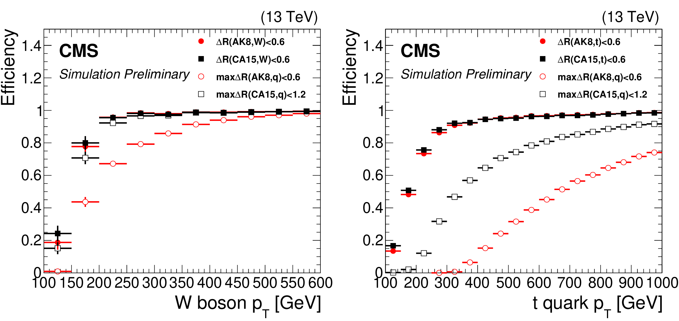
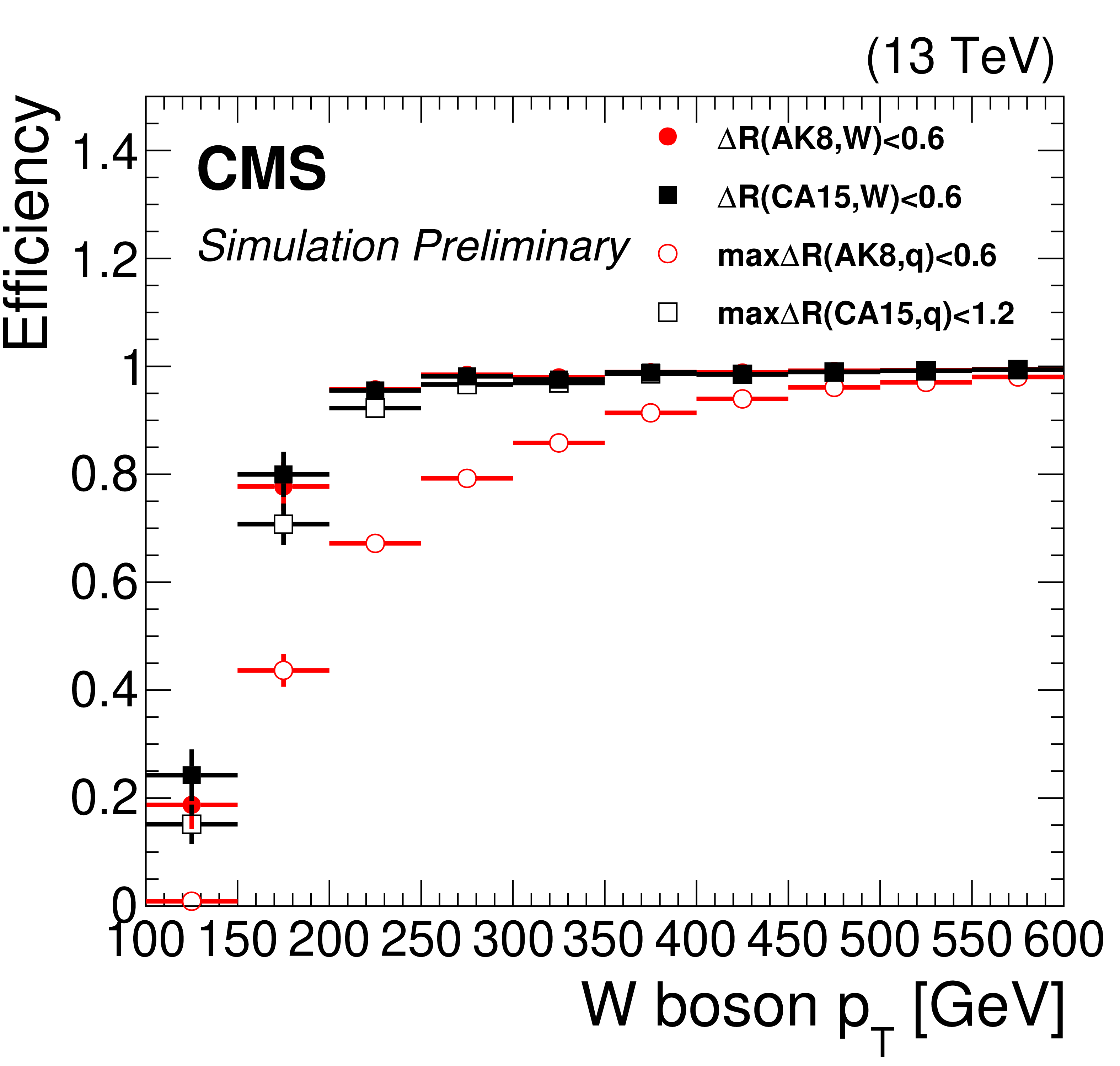
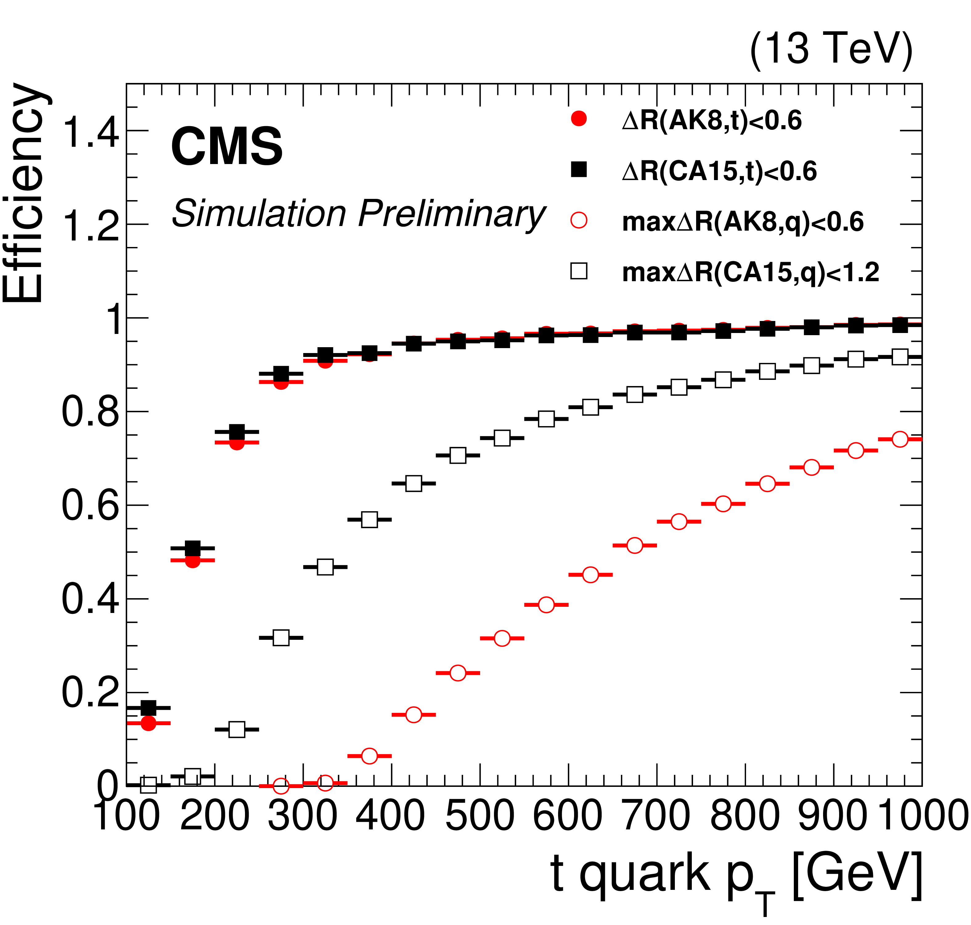
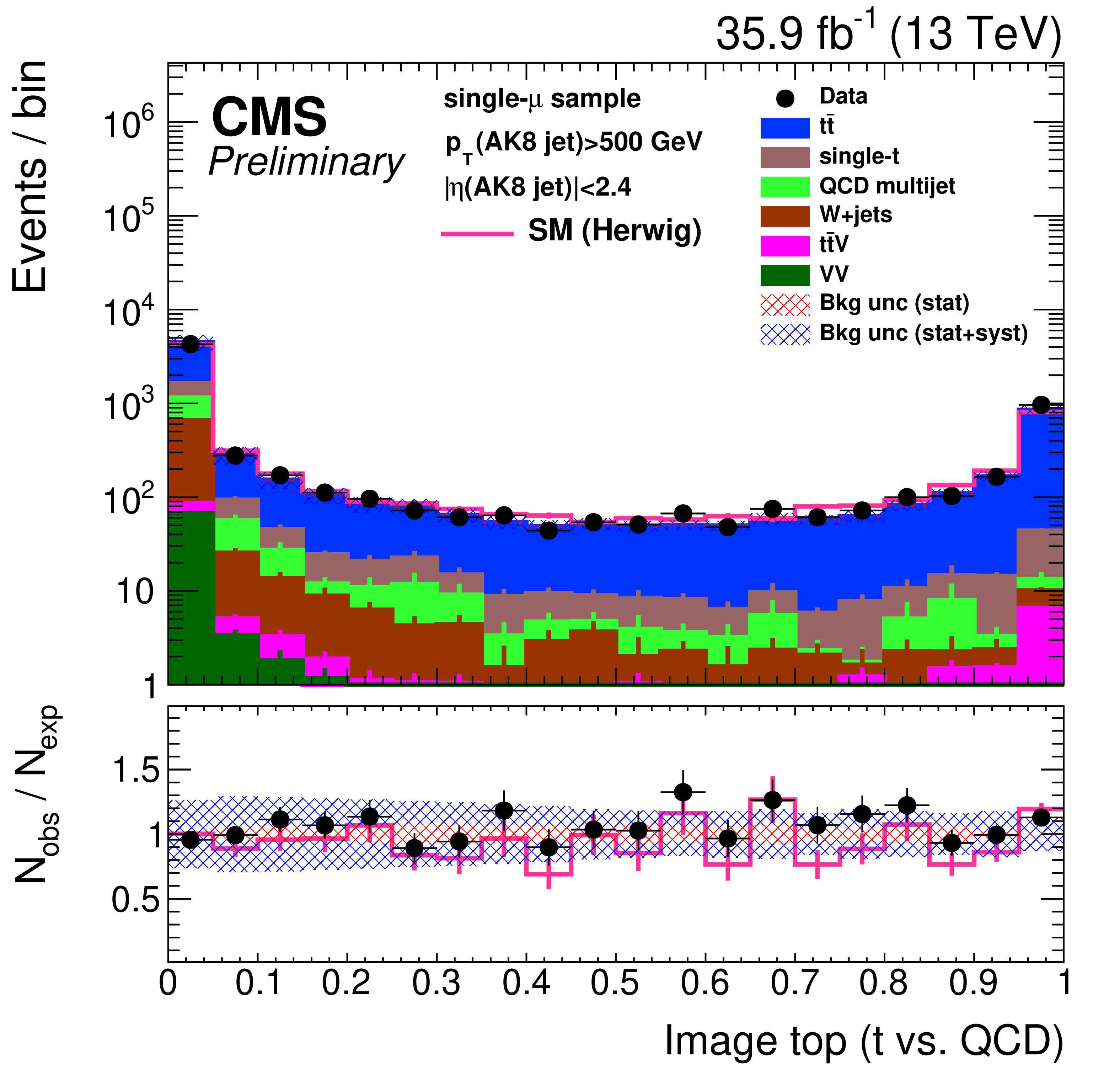
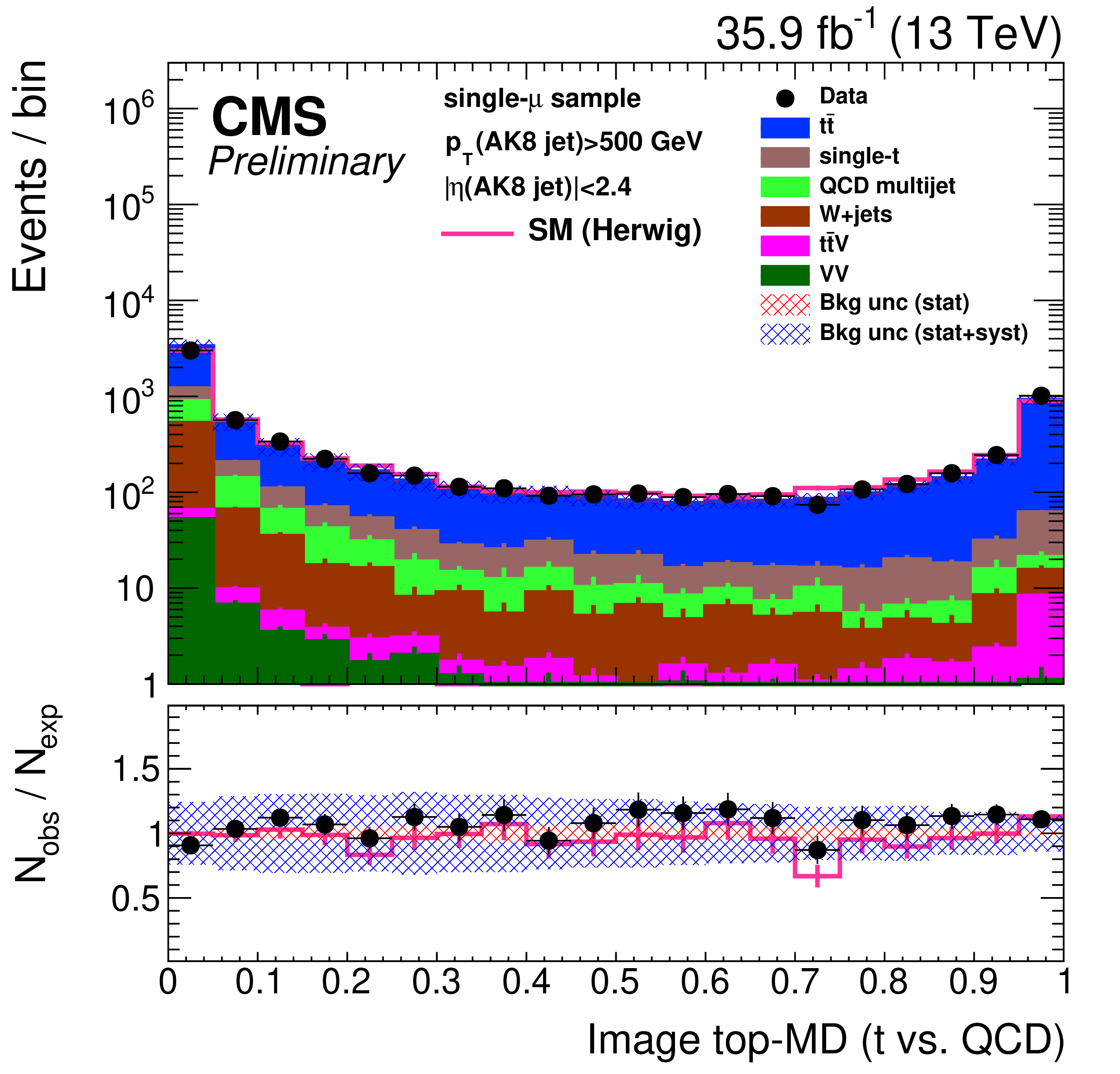
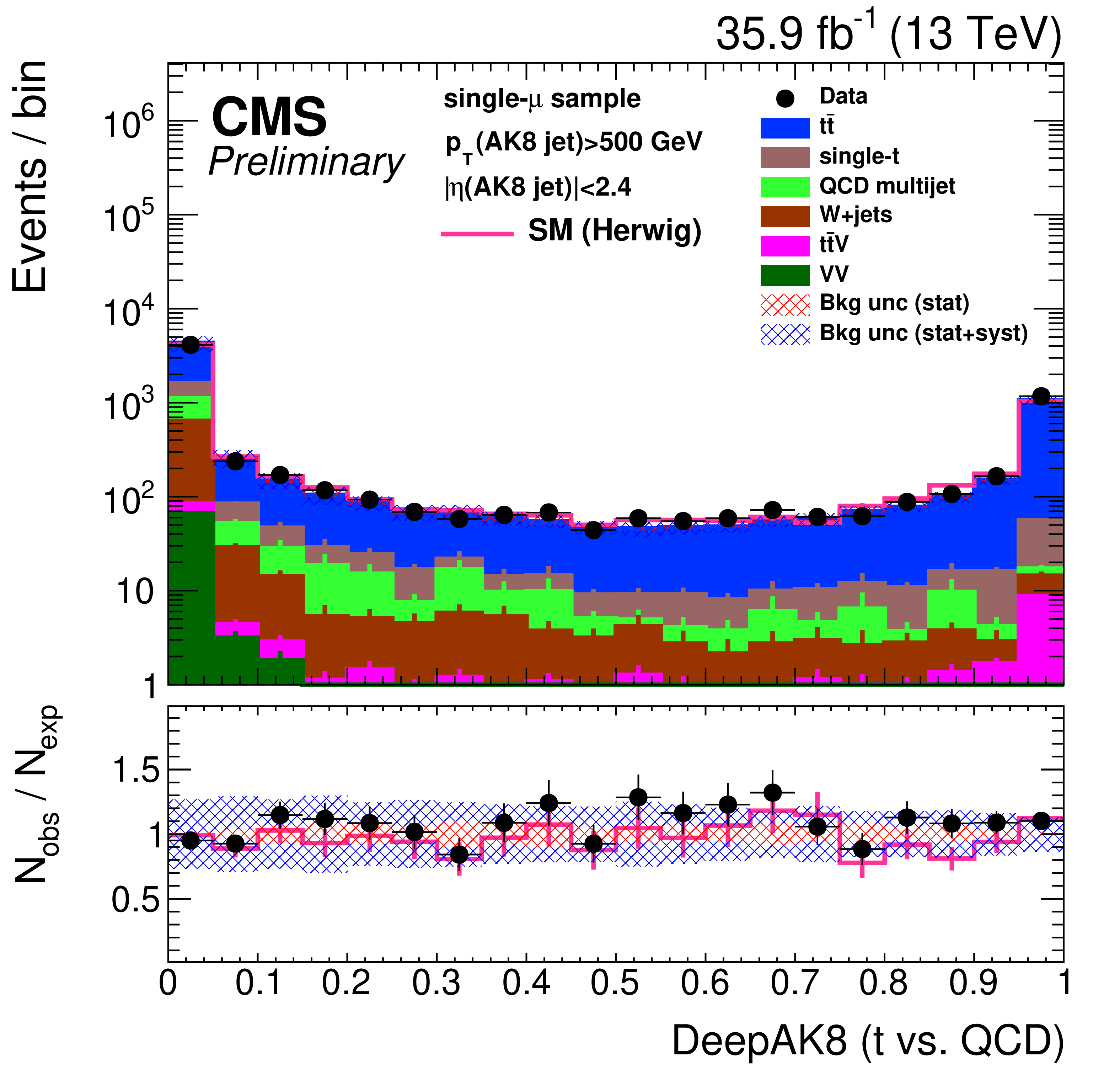
Figure 1:
Matching efficiency as a function of the ${p_{\mathrm {T}}}$ of the truth particle; hadronically decaying W bosons (left) and t quarks (right). This efficiency is defined as the fraction of the truth particles (t quarks or W bosons) that are within $\Delta R < $ 0.6 with an AK8 or CA15 jet with $ {p_{\mathrm {T}}} > $ 200 GeV and $|\eta | < $ 2.4. Superimposed is the merging efficiency as a function of the truth particle ${p_{\mathrm {T}}}$ when all decay products are within $\Delta R (\text {AK8}, \mathrm{q} _{i}) < $ 0.6 ($\Delta R (\text {CA15}, \mathrm{q} _{i}) < $ 1.2) with an AK8 (CA15) jet. |
png pdf |
Figure 1-a:
Matching efficiency as a function of the ${p_{\mathrm {T}}}$ of the truth particle; hadronically decaying W bosons (left) and t quarks (right). This efficiency is defined as the fraction of the truth particles (t quarks or W bosons) that are within $\Delta R < $ 0.6 with an AK8 or CA15 jet with $ {p_{\mathrm {T}}} > $ 200 GeV and $|\eta | < $ 2.4. Superimposed is the merging efficiency as a function of the truth particle ${p_{\mathrm {T}}}$ when all decay products are within $\Delta R (\text {AK8}, \mathrm{q} _{i}) < $ 0.6 ($\Delta R (\text {CA15}, \mathrm{q} _{i}) < $ 1.2) with an AK8 (CA15) jet. |
png pdf |
Figure 1-b:
Matching efficiency as a function of the ${p_{\mathrm {T}}}$ of the truth particle; hadronically decaying W bosons (left) and t quarks (right). This efficiency is defined as the fraction of the truth particles (t quarks or W bosons) that are within $\Delta R < $ 0.6 with an AK8 or CA15 jet with $ {p_{\mathrm {T}}} > $ 200 GeV and $|\eta | < $ 2.4. Superimposed is the merging efficiency as a function of the truth particle ${p_{\mathrm {T}}}$ when all decay products are within $\Delta R (\text {AK8}, \mathrm{q} _{i}) < $ 0.6 ($\Delta R (\text {CA15}, \mathrm{q} _{i}) < $ 1.2) with an AK8 (CA15) jet. |
png pdf |
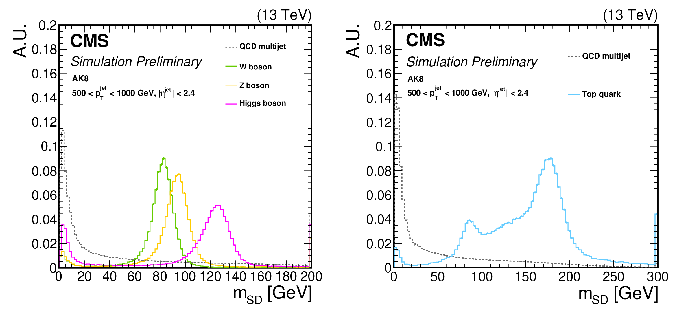
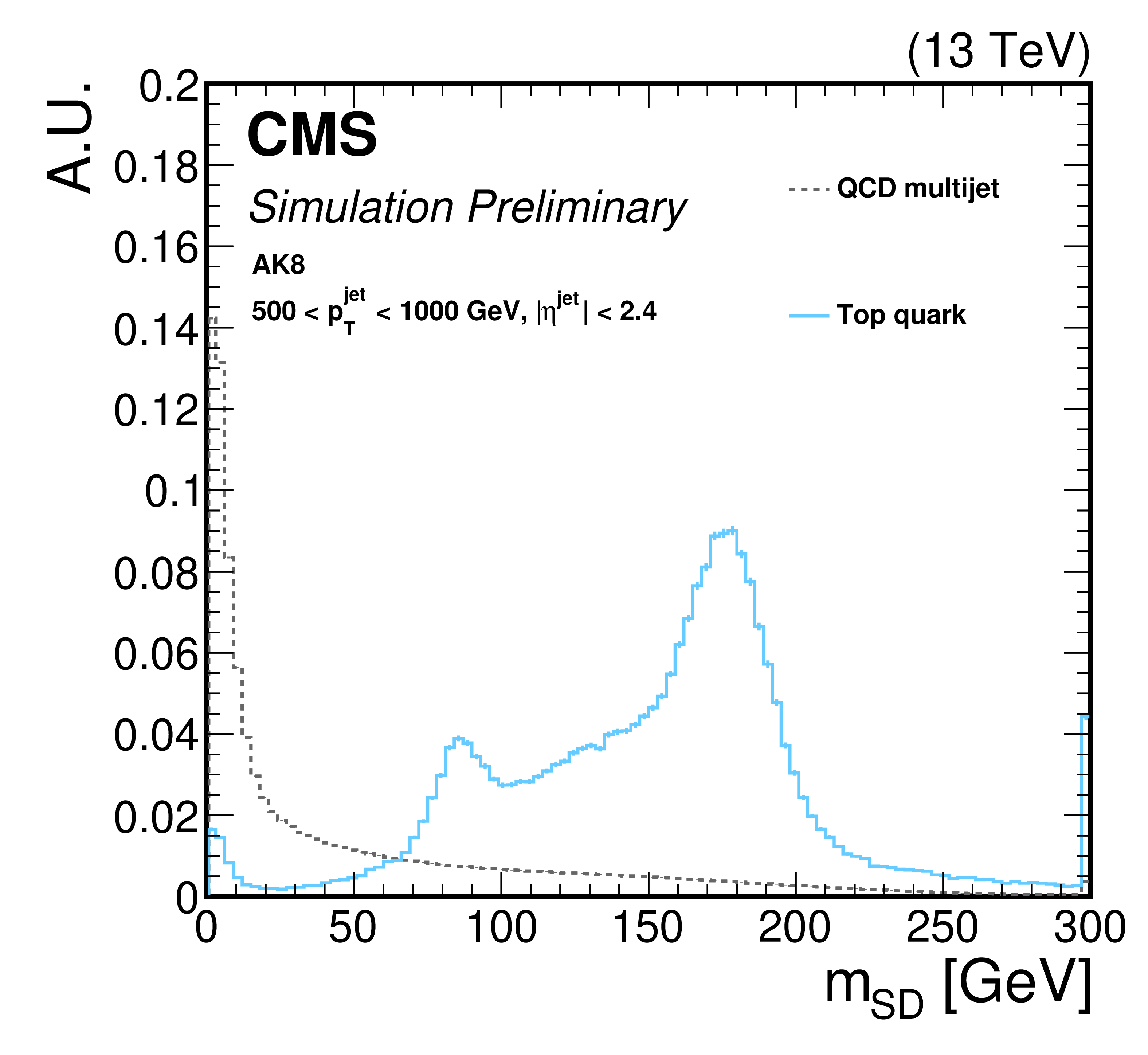
Figure 2:
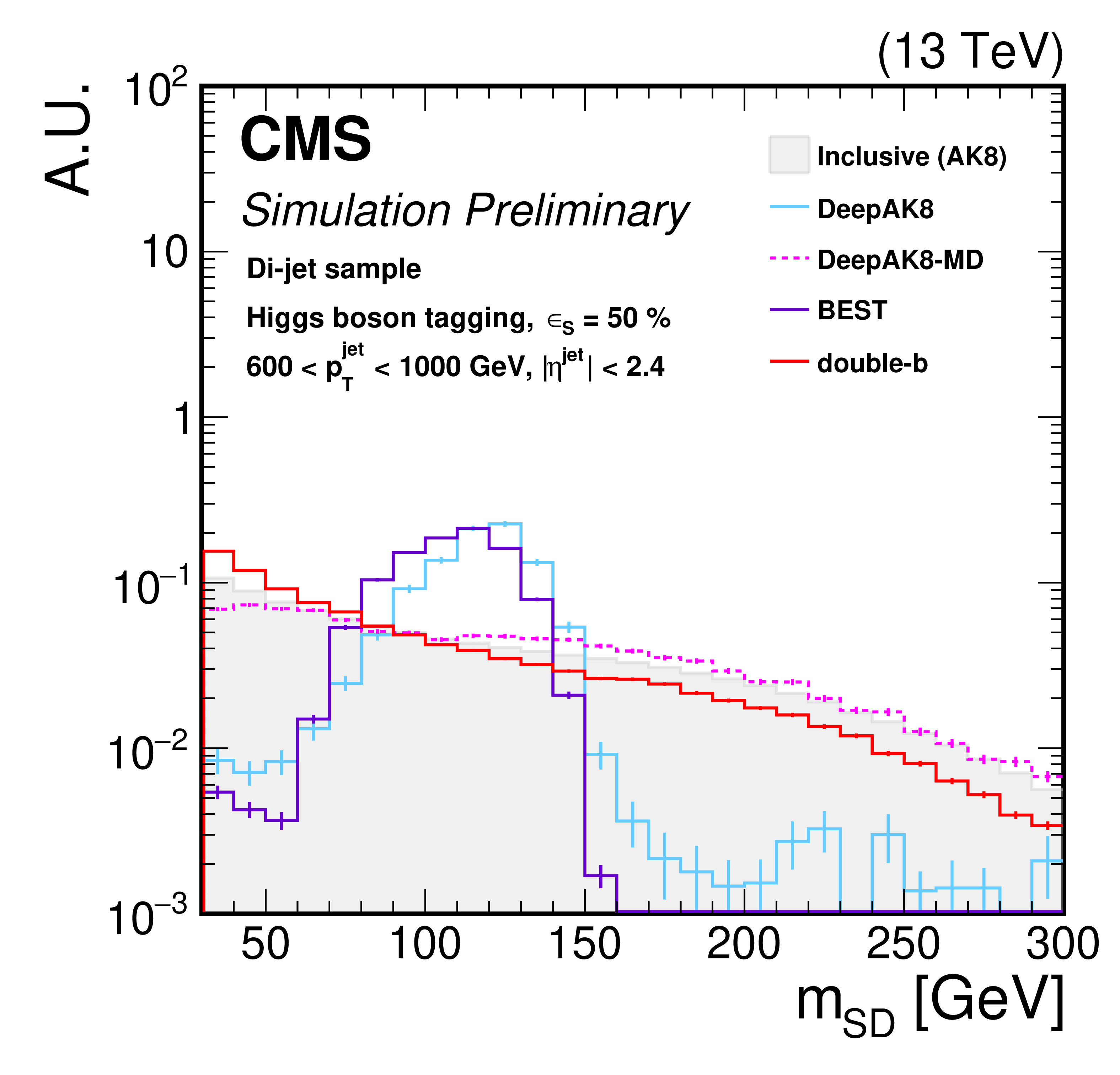
Comparison of the ${m_{\text {SD}}}$ shape in signal and background AK8 jets in simulation. The fiducial selection on the jets is displayed on the plots. Signal jets are defined as jets arising from hadronic decays of W/Z/H bosons (left) or t quarks (right), whereas background jets are obtained from the QCD multijet sample. |

png pdf |
Figure 2-a:
Comparison of the ${m_{\text {SD}}}$ shape in signal and background AK8 jets in simulation. The fiducial selection on the jets is displayed on the plots. Signal jets are defined as jets arising from hadronic decays of W/Z/H bosons (left) or t quarks (right), whereas background jets are obtained from the QCD multijet sample. |
png pdf |
Figure 2-b:
Comparison of the ${m_{\text {SD}}}$ shape in signal and background AK8 jets in simulation. The fiducial selection on the jets is displayed on the plots. Signal jets are defined as jets arising from hadronic decays of W/Z/H bosons (left) or t quarks (right), whereas background jets are obtained from the QCD multijet sample. |
png pdf |
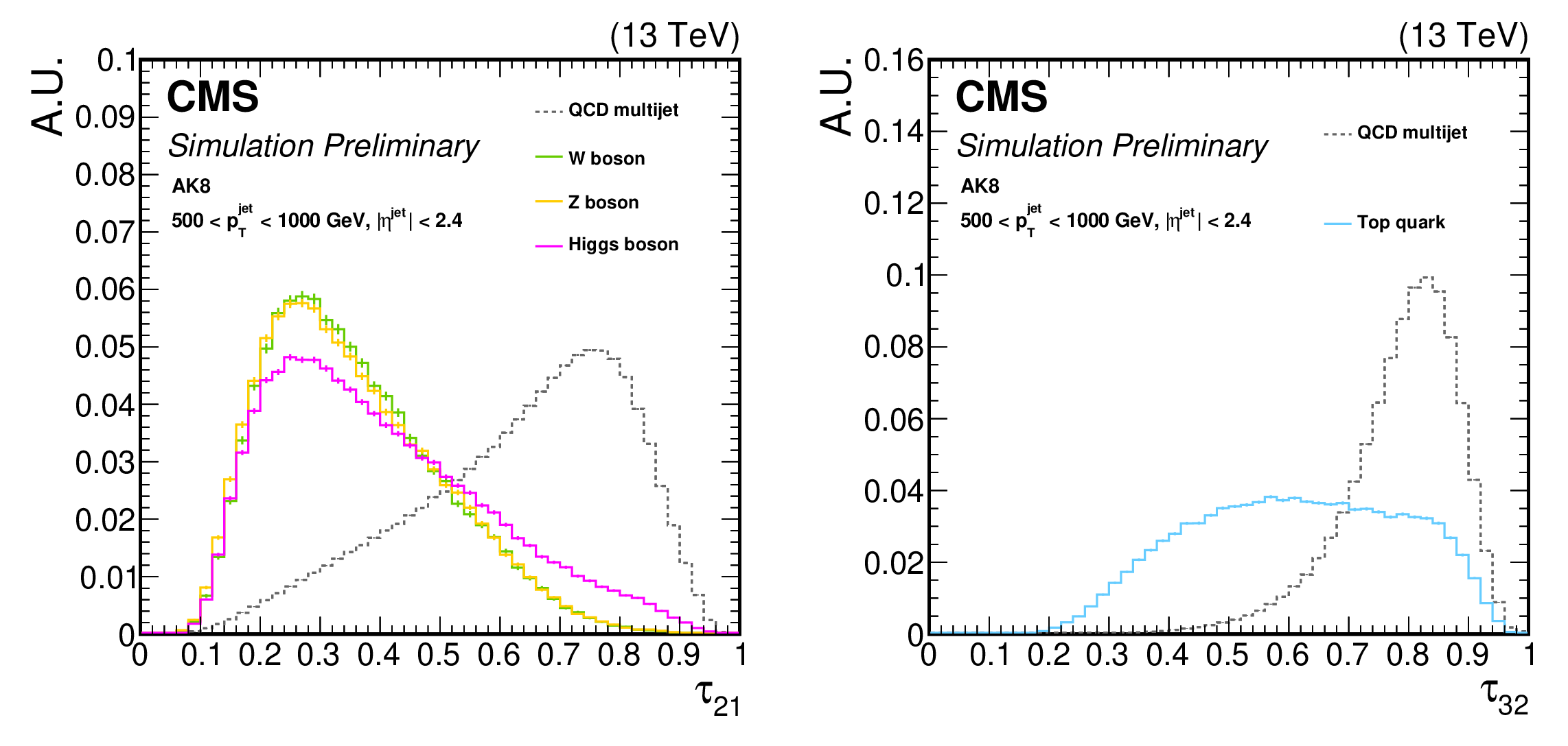
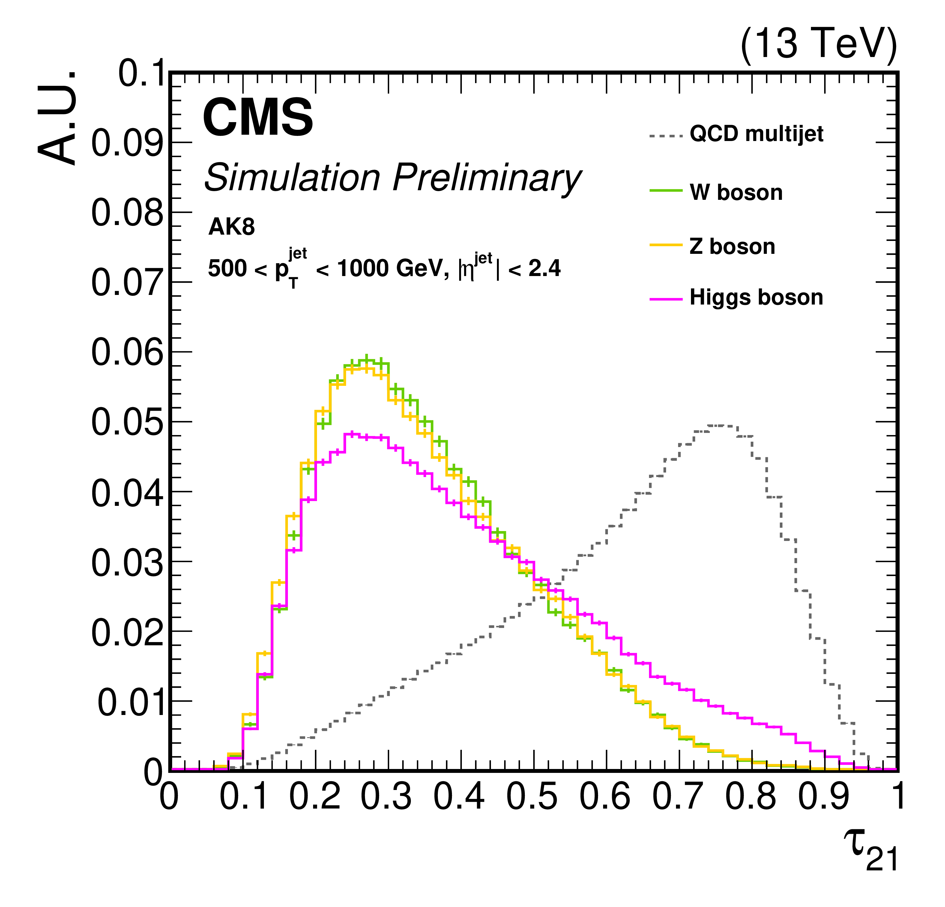
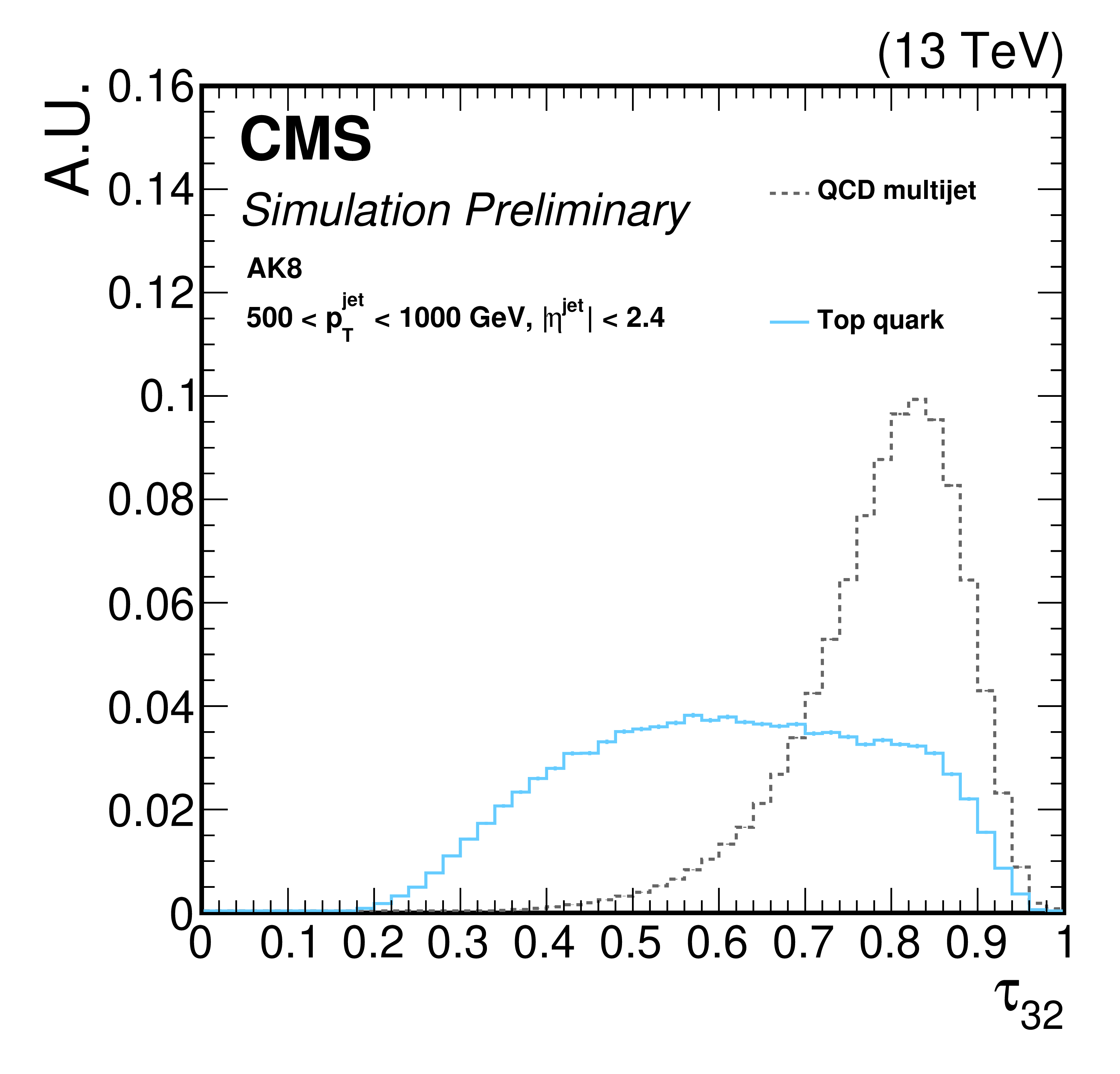
Figure 3:
Comparison of the ${\tau _{21}}$ (left) and ${\tau _{32}}$ (right) shape in signal and background AK8 jets. The fiducial selection on the jets is displayed on the plots. As signal jets we consider jets stemming from hadronic decays of W, Z or H bosons (left) or t quarks (right), whereas background jets are obtained from the QCD multijet sample. |
png pdf |
Figure 3-a:
Comparison of the ${\tau _{21}}$ (left) and ${\tau _{32}}$ (right) shape in signal and background AK8 jets. The fiducial selection on the jets is displayed on the plots. As signal jets we consider jets stemming from hadronic decays of W, Z or H bosons (left) or t quarks (right), whereas background jets are obtained from the QCD multijet sample. |
png pdf |
Figure 3-b:
Comparison of the ${\tau _{21}}$ (left) and ${\tau _{32}}$ (right) shape in signal and background AK8 jets. The fiducial selection on the jets is displayed on the plots. As signal jets we consider jets stemming from hadronic decays of W, Z or H bosons (left) or t quarks (right), whereas background jets are obtained from the QCD multijet sample. |
png pdf |
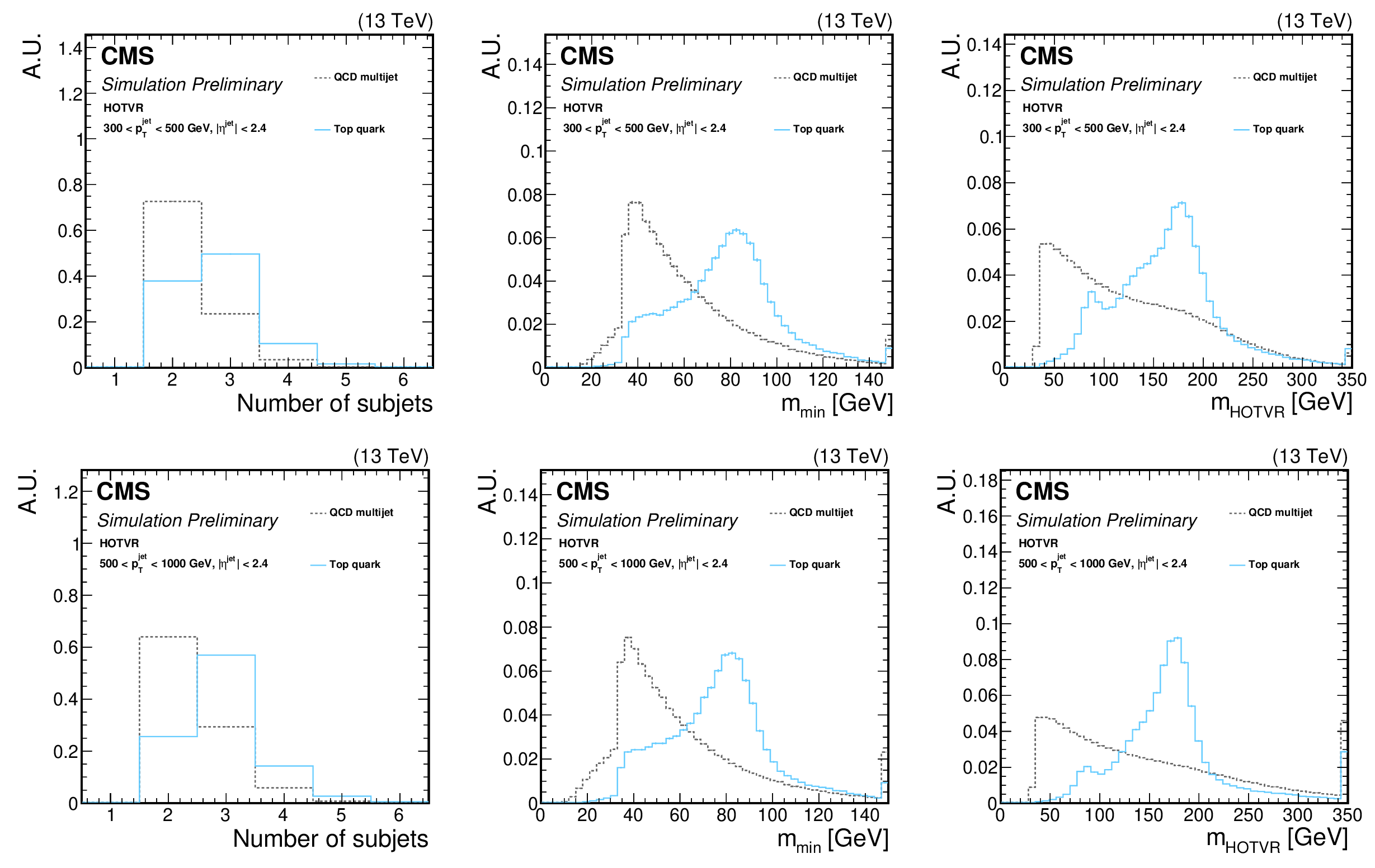
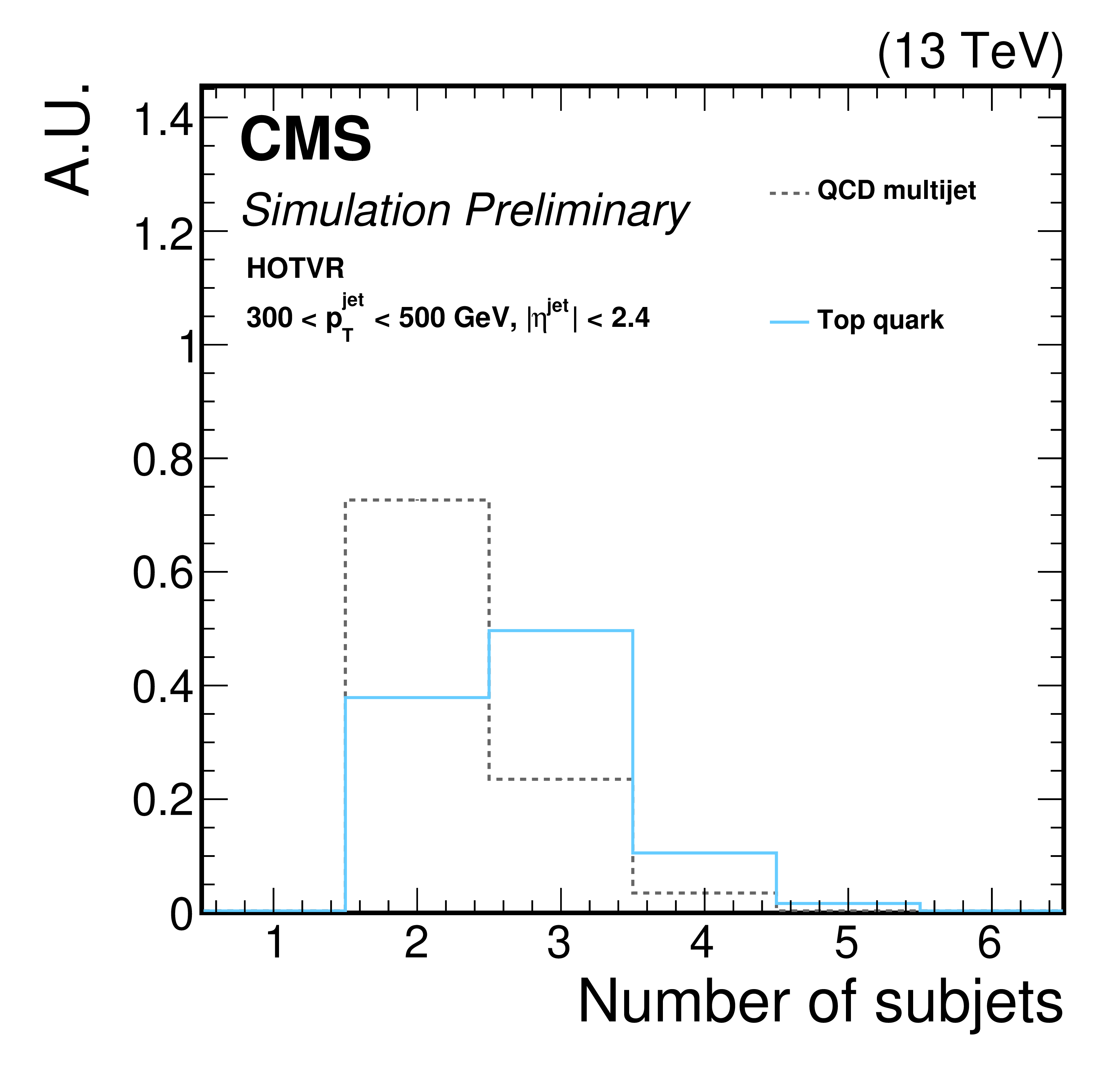
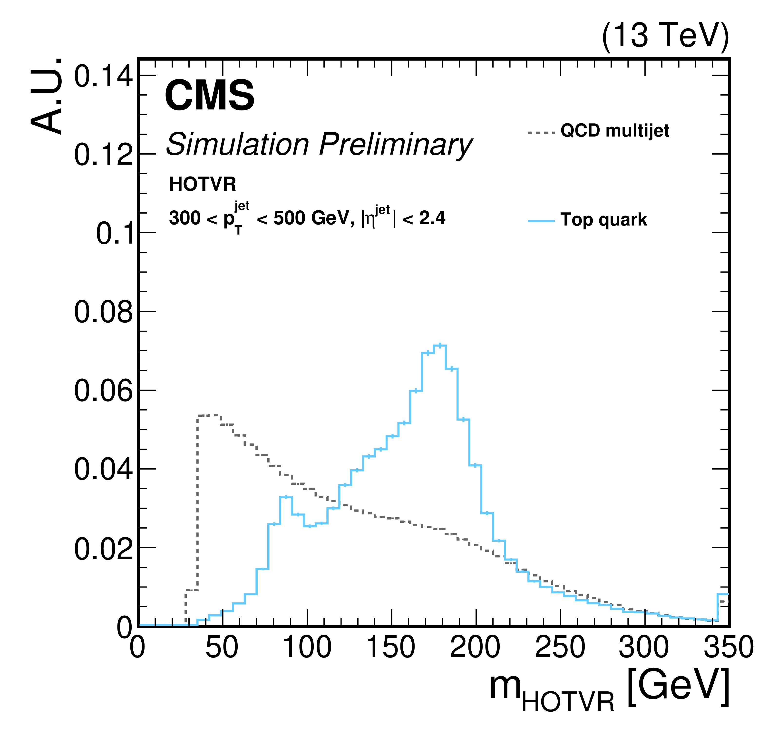
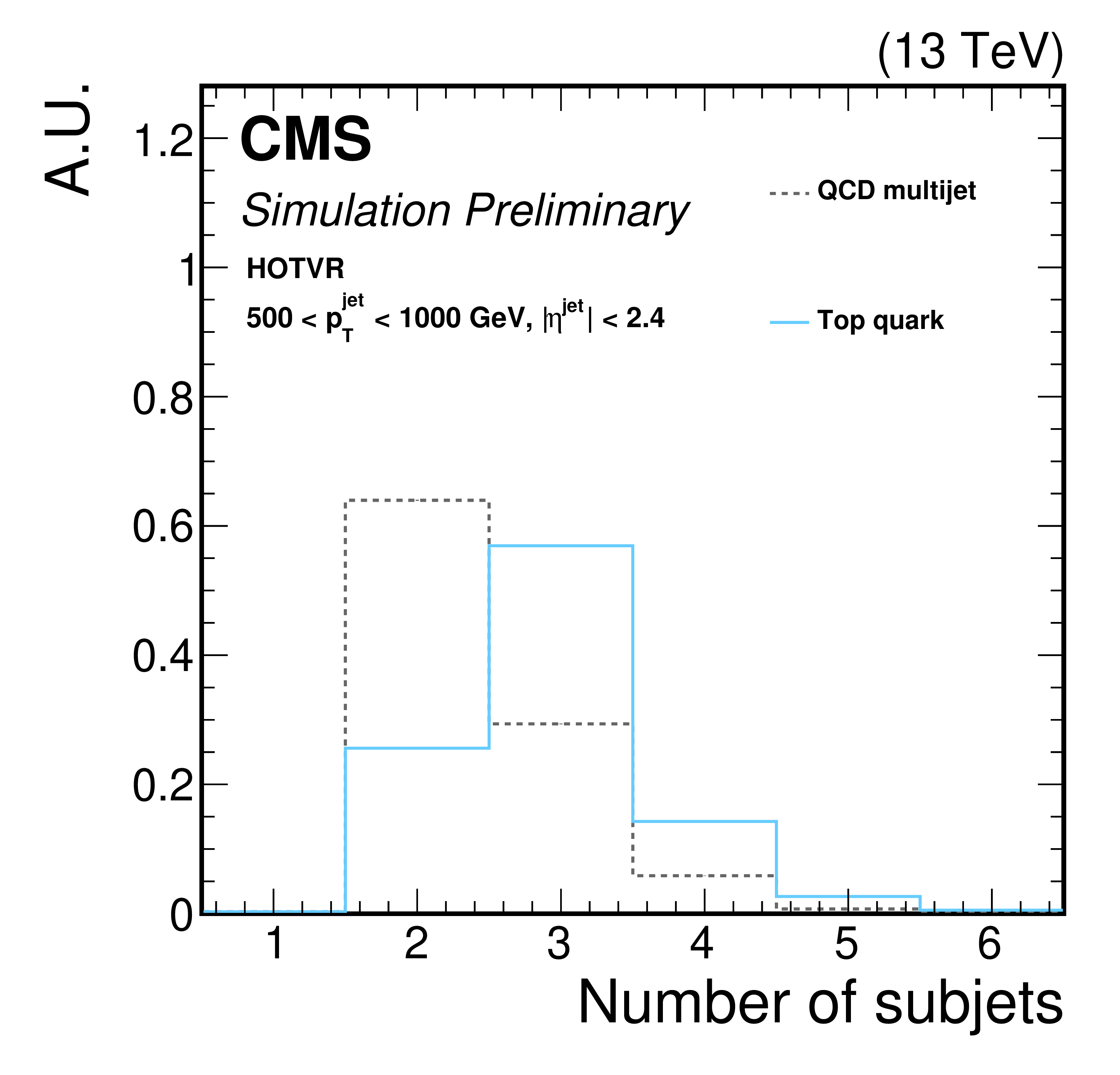
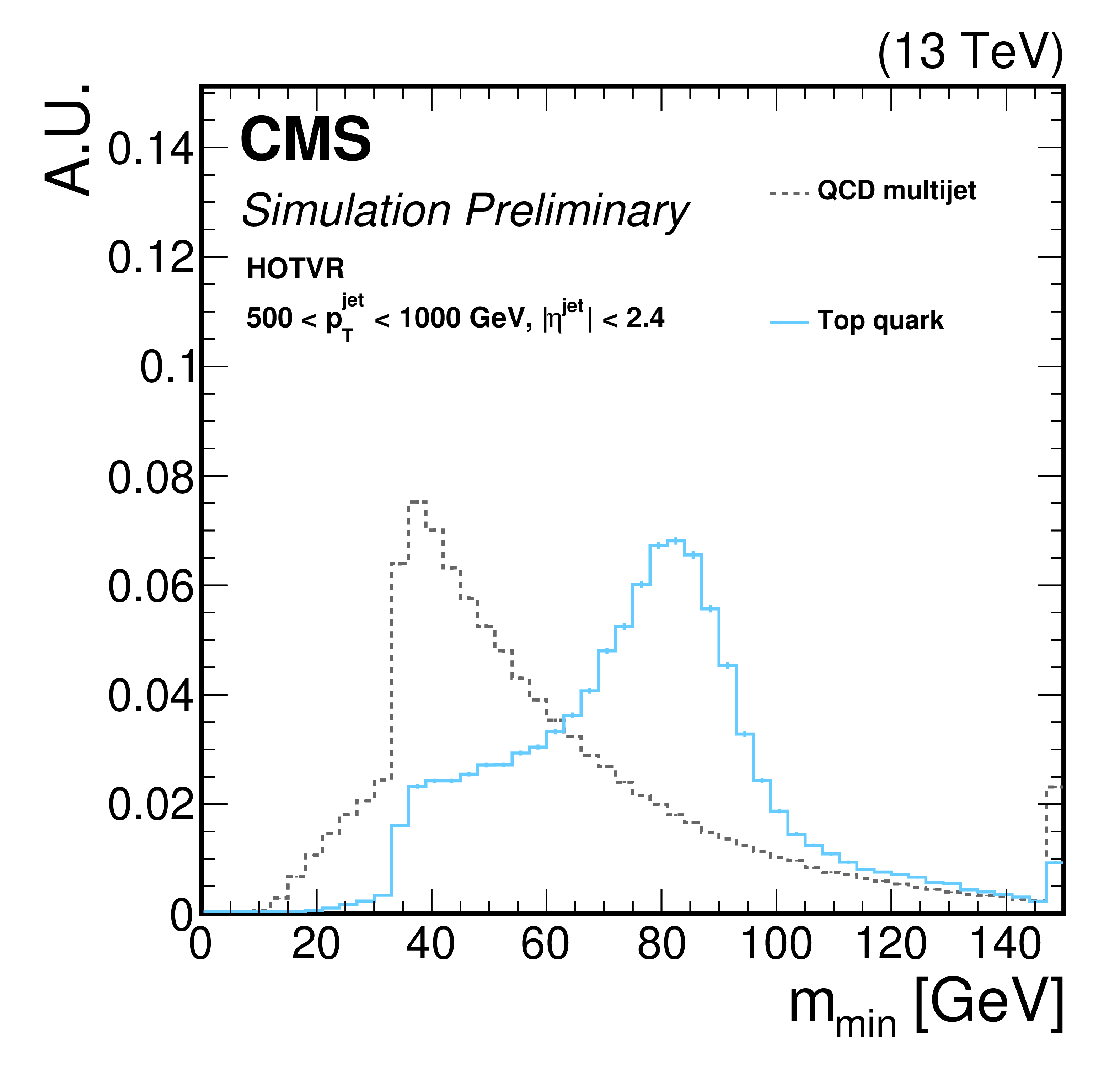
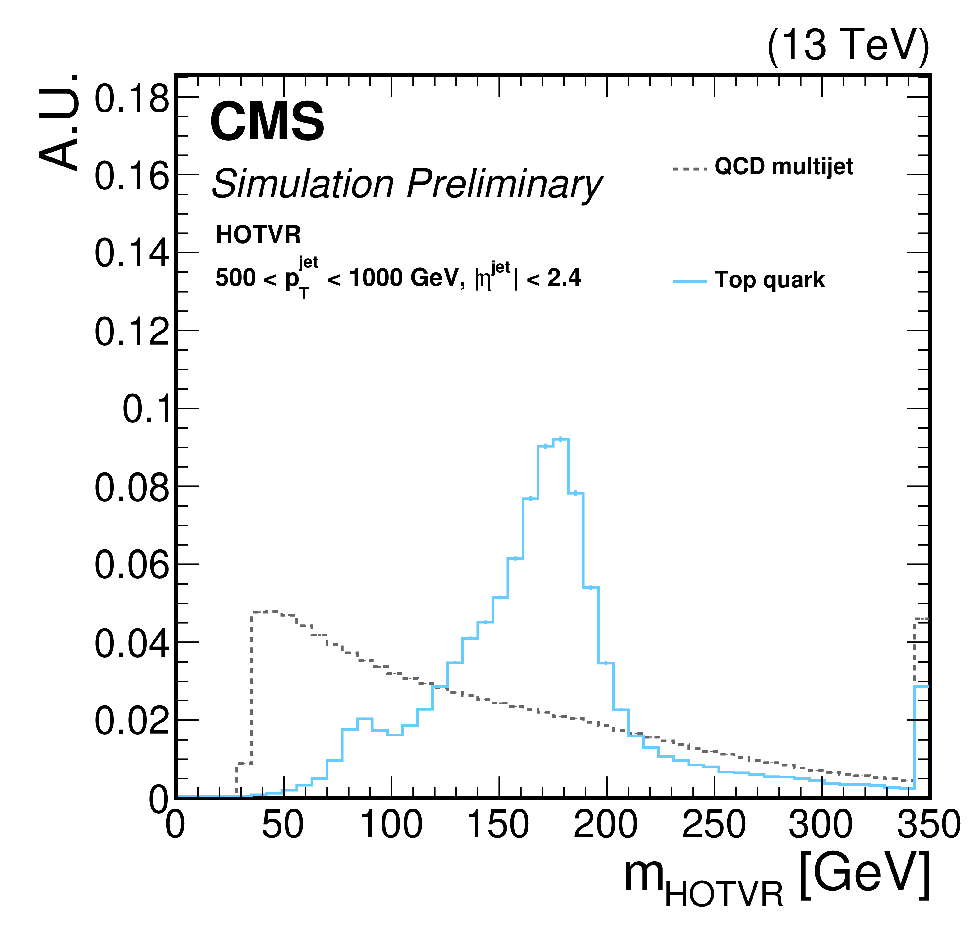
Figure 4:
Shape comparison of the main variables of the HOTVR algorithm for signal and background jets, in two different regions of the parton ${p_{\mathrm {T}}}$ as displayed on the plots. |
png pdf |
Figure 4-a:
Shape comparison of the main variables of the HOTVR algorithm for signal and background jets, in two different regions of the parton ${p_{\mathrm {T}}}$ as displayed on the plots. |

png pdf |
Figure 4-b:
Shape comparison of the main variables of the HOTVR algorithm for signal and background jets, in two different regions of the parton ${p_{\mathrm {T}}}$ as displayed on the plots. |
png pdf |
Figure 4-c:
Shape comparison of the main variables of the HOTVR algorithm for signal and background jets, in two different regions of the parton ${p_{\mathrm {T}}}$ as displayed on the plots. |
png pdf |
Figure 4-d:
Shape comparison of the main variables of the HOTVR algorithm for signal and background jets, in two different regions of the parton ${p_{\mathrm {T}}}$ as displayed on the plots. |
png pdf |
Figure 4-e:
Shape comparison of the main variables of the HOTVR algorithm for signal and background jets, in two different regions of the parton ${p_{\mathrm {T}}}$ as displayed on the plots. |
png pdf |
Figure 4-f:
Shape comparison of the main variables of the HOTVR algorithm for signal and background jets, in two different regions of the parton ${p_{\mathrm {T}}}$ as displayed on the plots. |
png pdf |
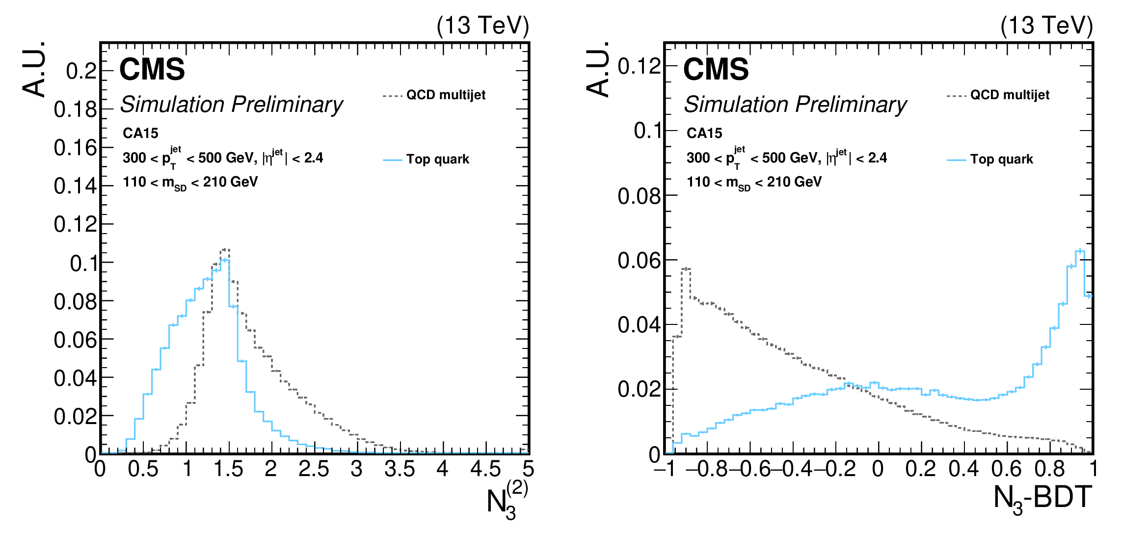
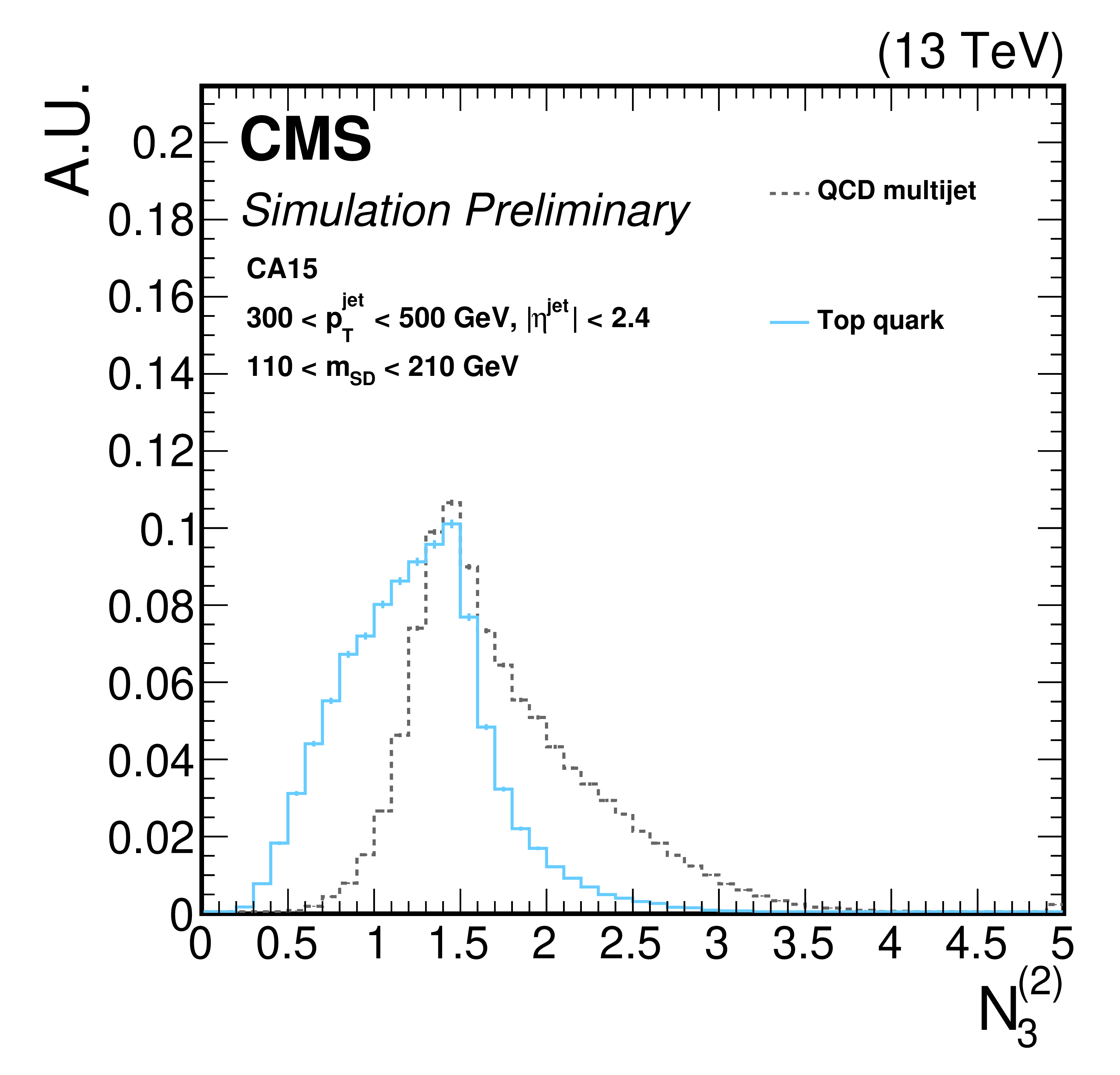
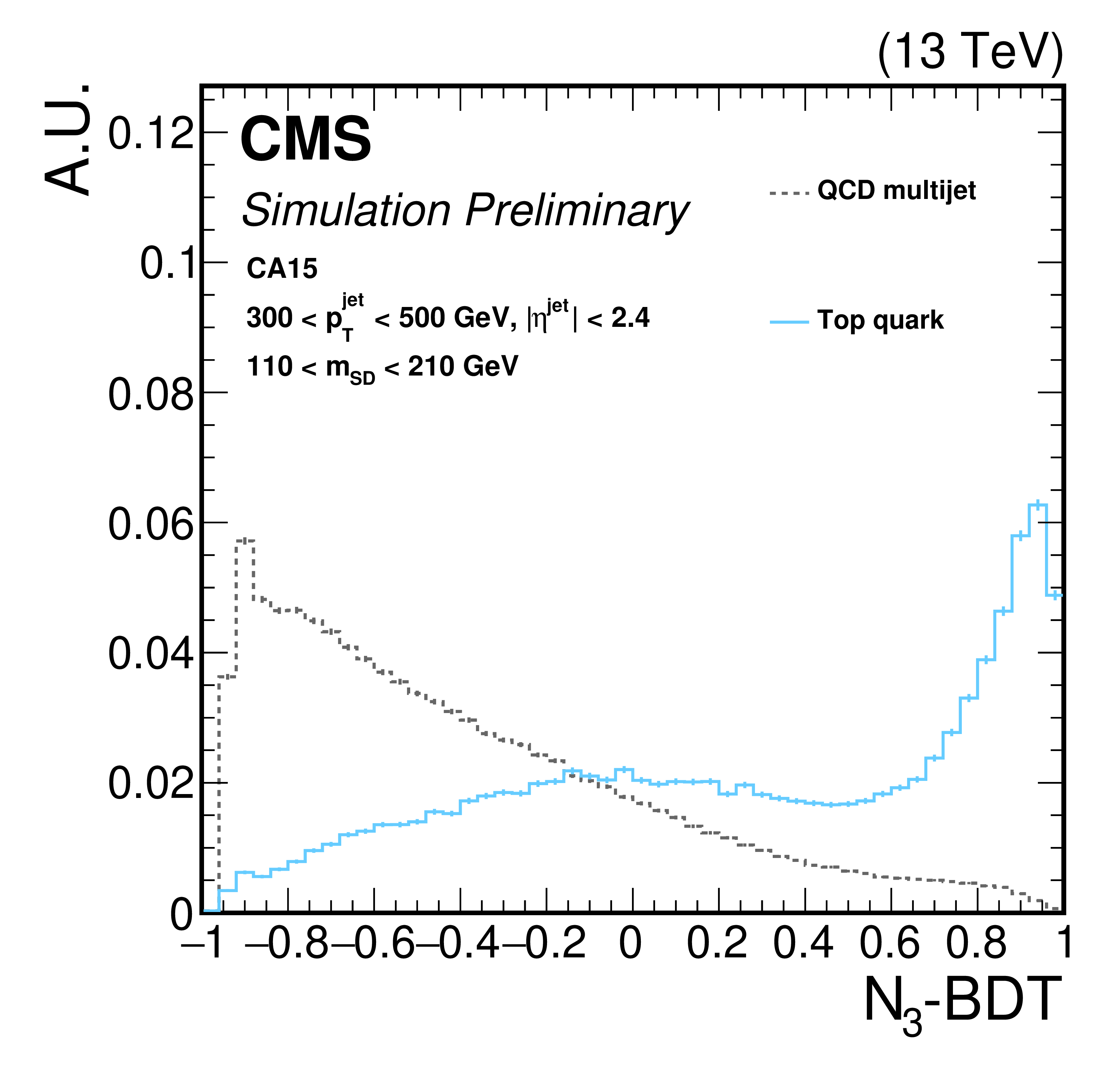
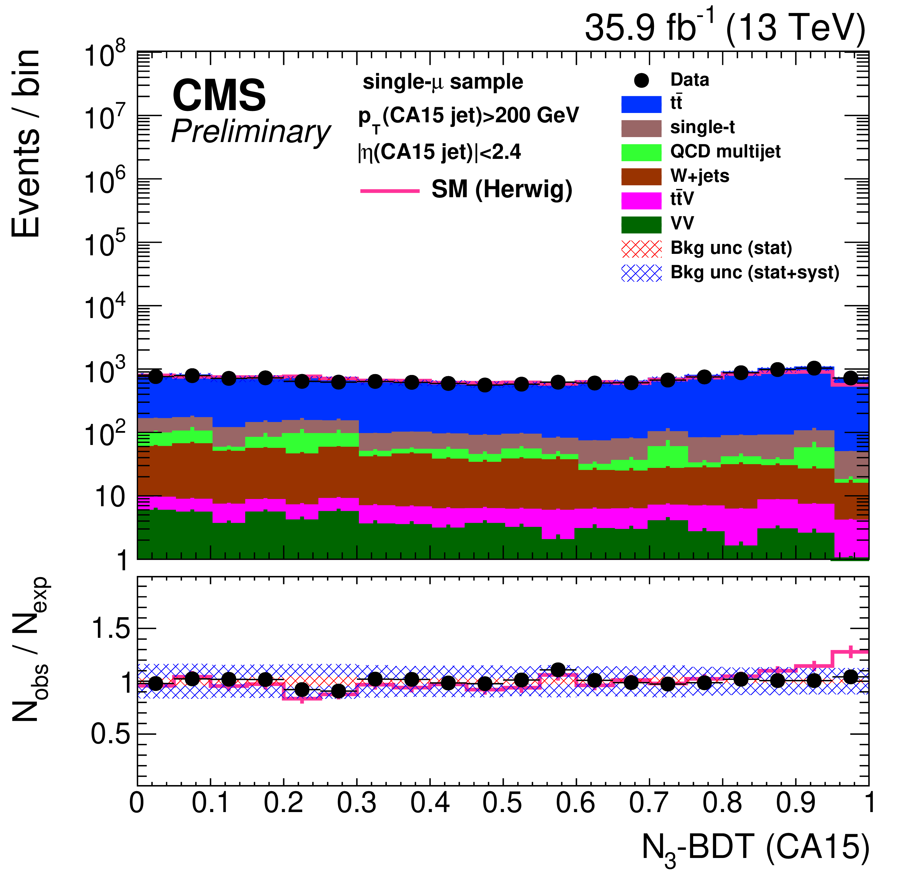
Figure 5:
Comparison of the distribution of $N_3^{(2)}$ (left) and the ${N_{3}-\text {BDT} (\text {CA}15)}$ discriminant (right) in t quarks jets (signal) and jet from QCD multijet processes (background). |
png pdf |
Figure 5-a:
Comparison of the distribution of $N_3^{(2)}$ (left) and the ${N_{3}-\text {BDT} (\text {CA}15)}$ discriminant (right) in t quarks jets (signal) and jet from QCD multijet processes (background). |
png pdf |
Figure 5-b:
Comparison of the distribution of $N_3^{(2)}$ (left) and the ${N_{3}-\text {BDT} (\text {CA}15)}$ discriminant (right) in t quarks jets (signal) and jet from QCD multijet processes (background). |
png pdf |
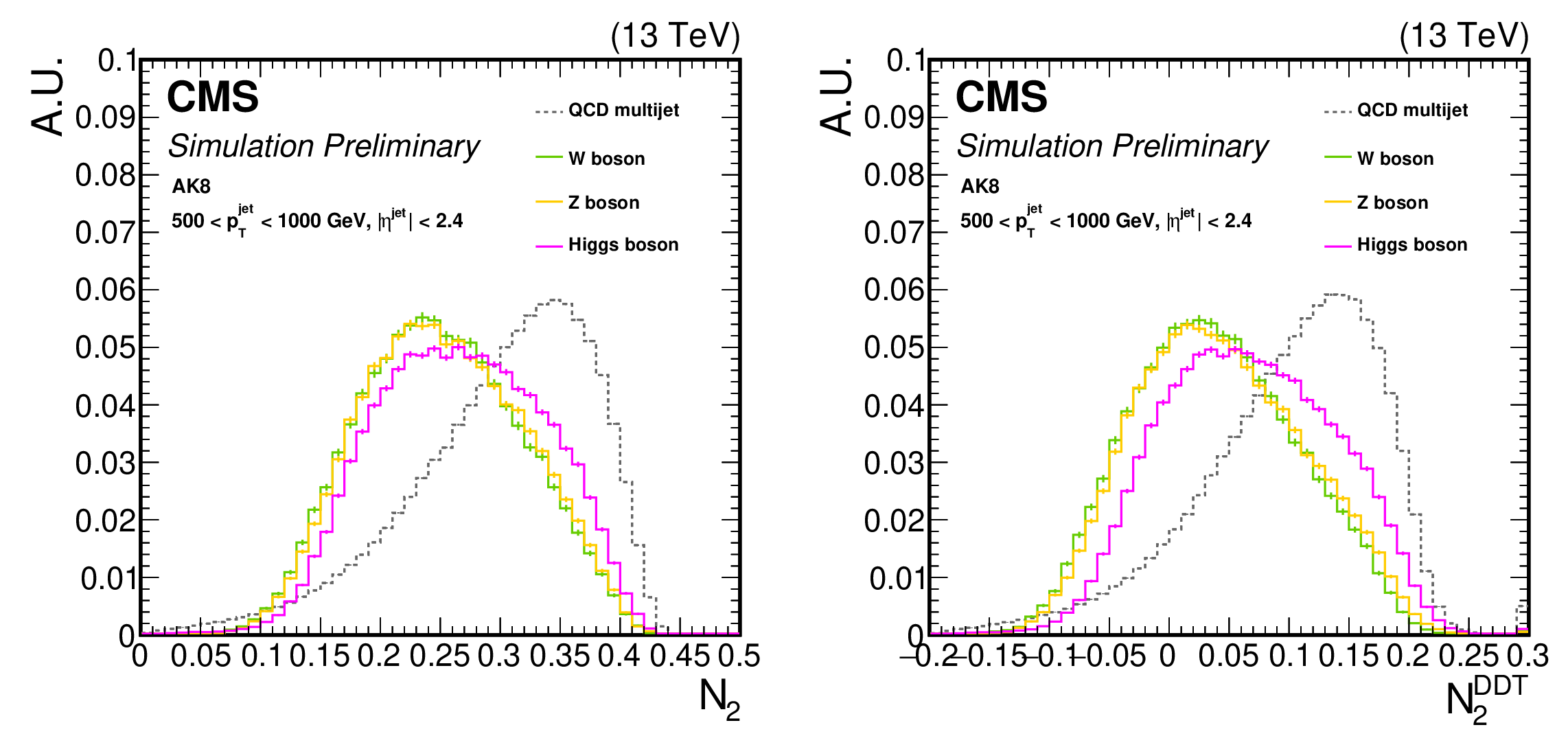
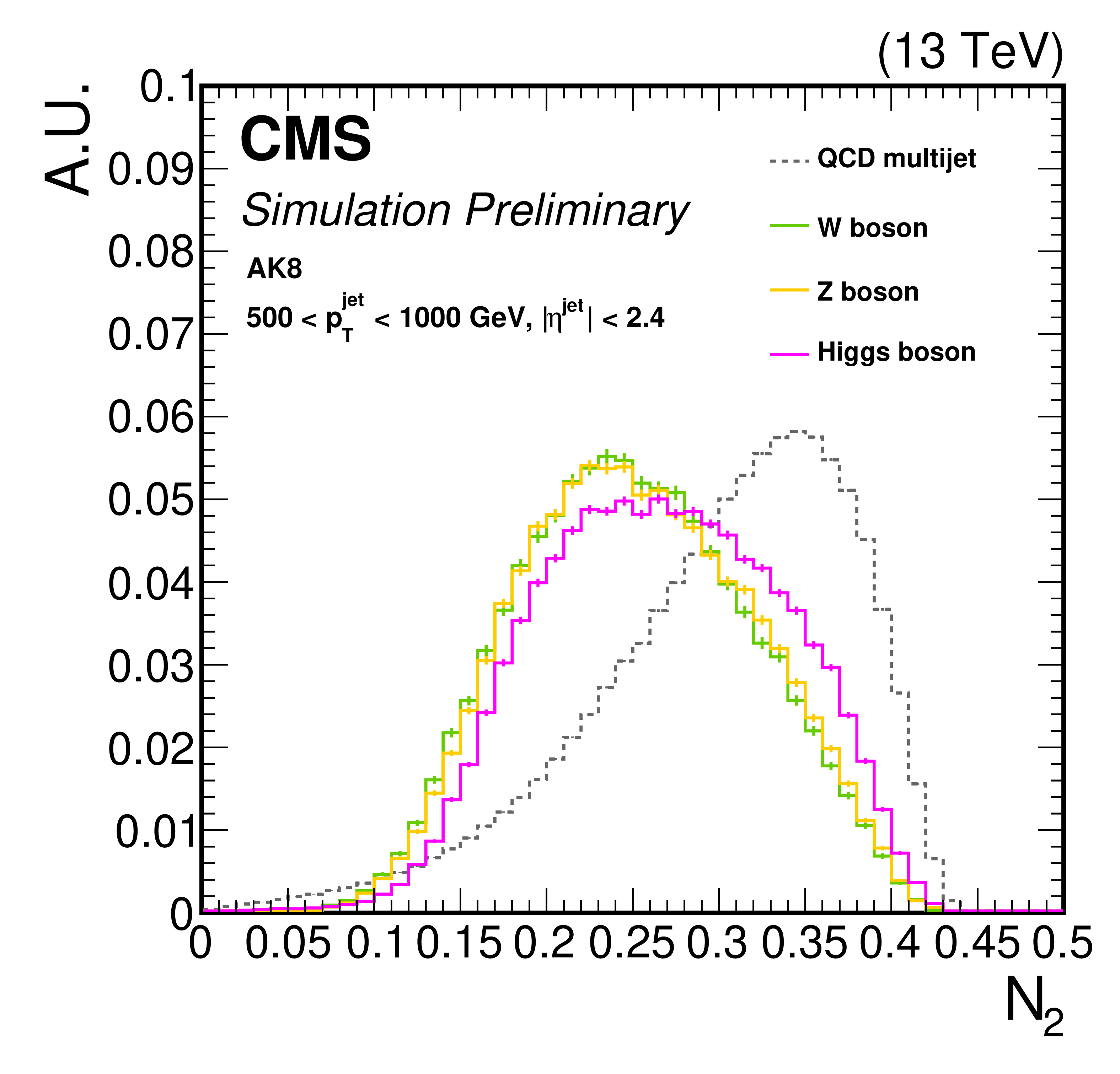
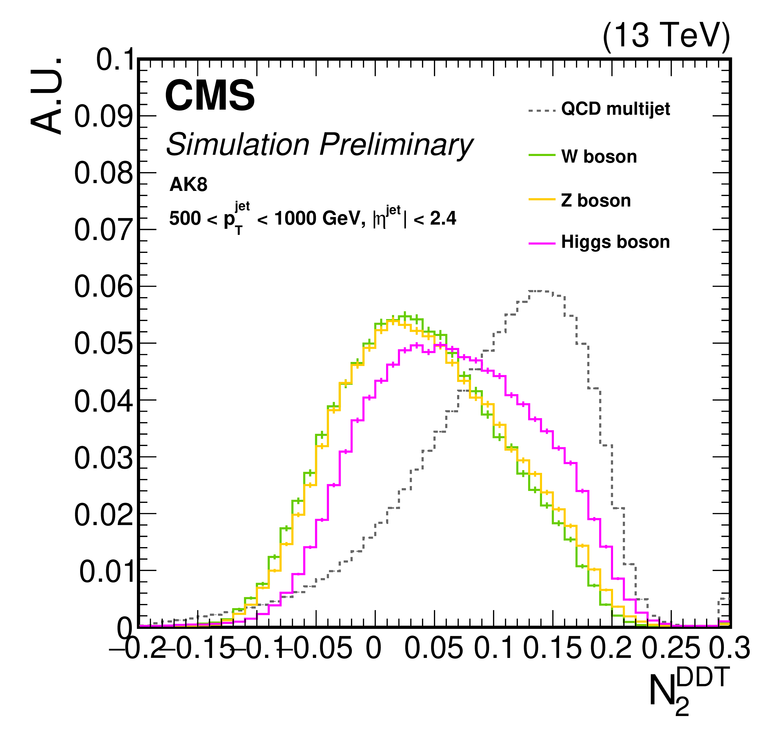
Figure 6:
Distributions of the ${m_\text {SD}+N_{2}}$ (left) and ${m_\text {SD}+N_{2}^{\text {DDT}}}$ (right) in signal and background jets. |
png pdf |
Figure 6-a:
Distributions of the ${m_\text {SD}+N_{2}}$ (left) and ${m_\text {SD}+N_{2}^{\text {DDT}}}$ (right) in signal and background jets. |
png pdf |
Figure 6-b:
Distributions of the ${m_\text {SD}+N_{2}}$ (left) and ${m_\text {SD}+N_{2}^{\text {DDT}}}$ (right) in signal and background jets. |
png pdf |
Figure 7:
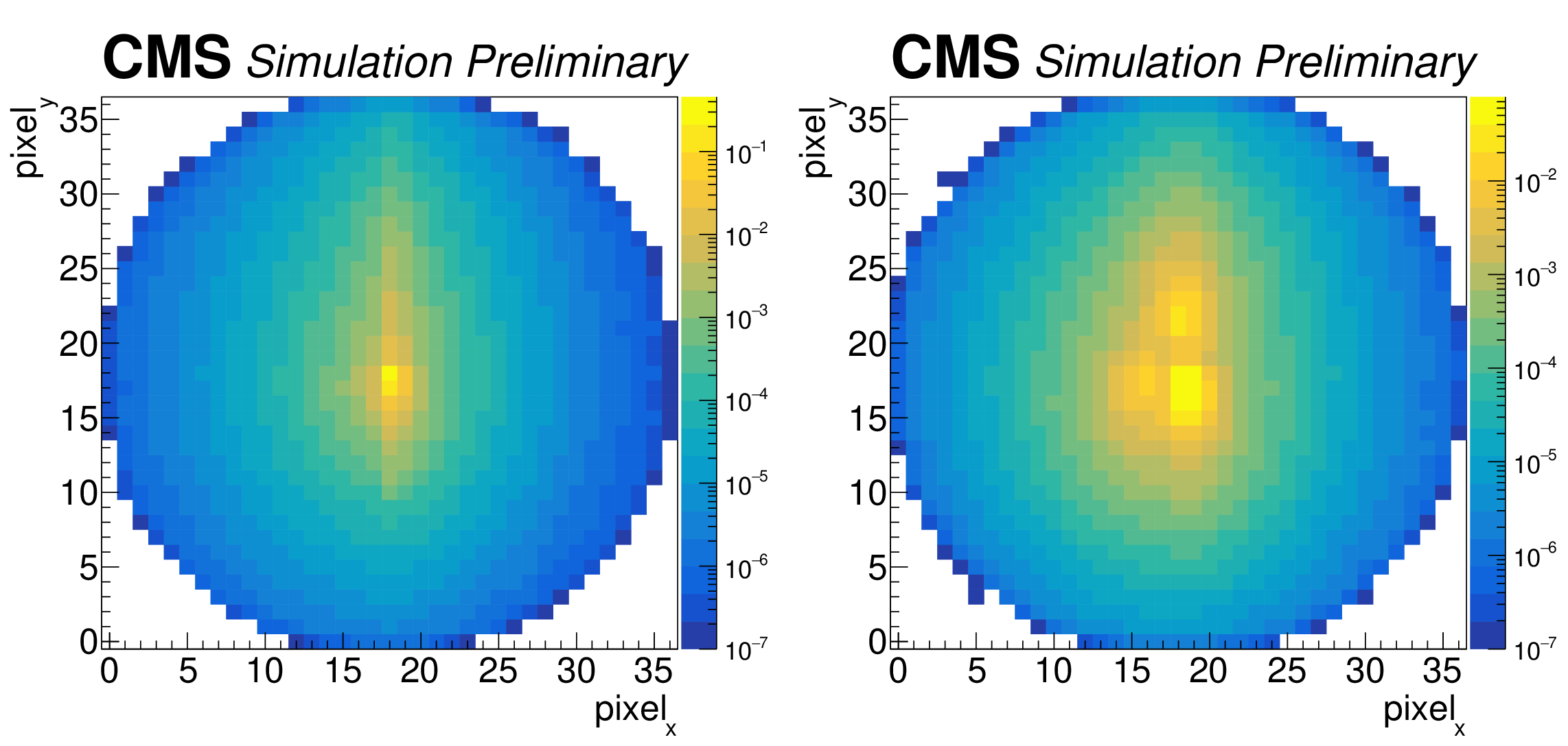
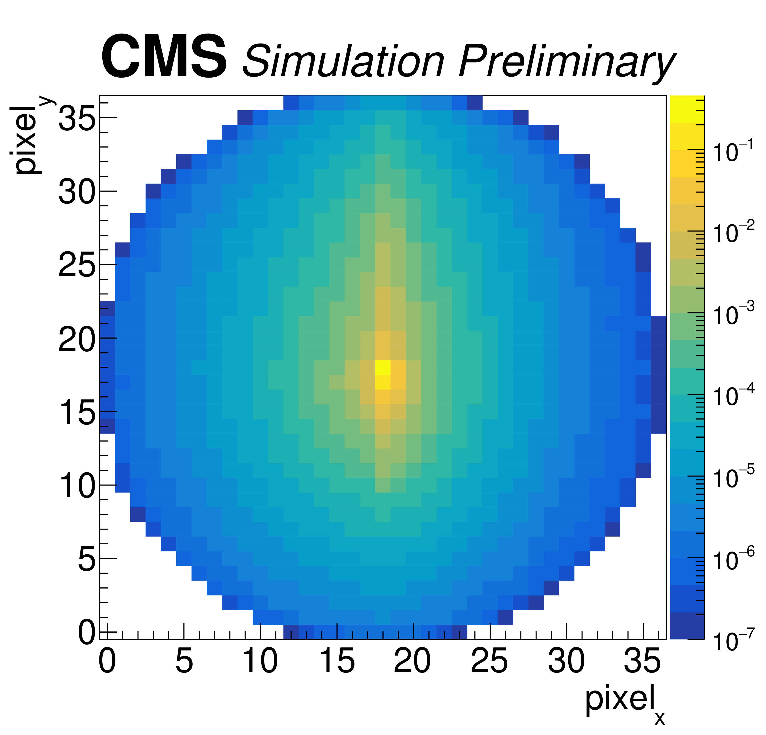
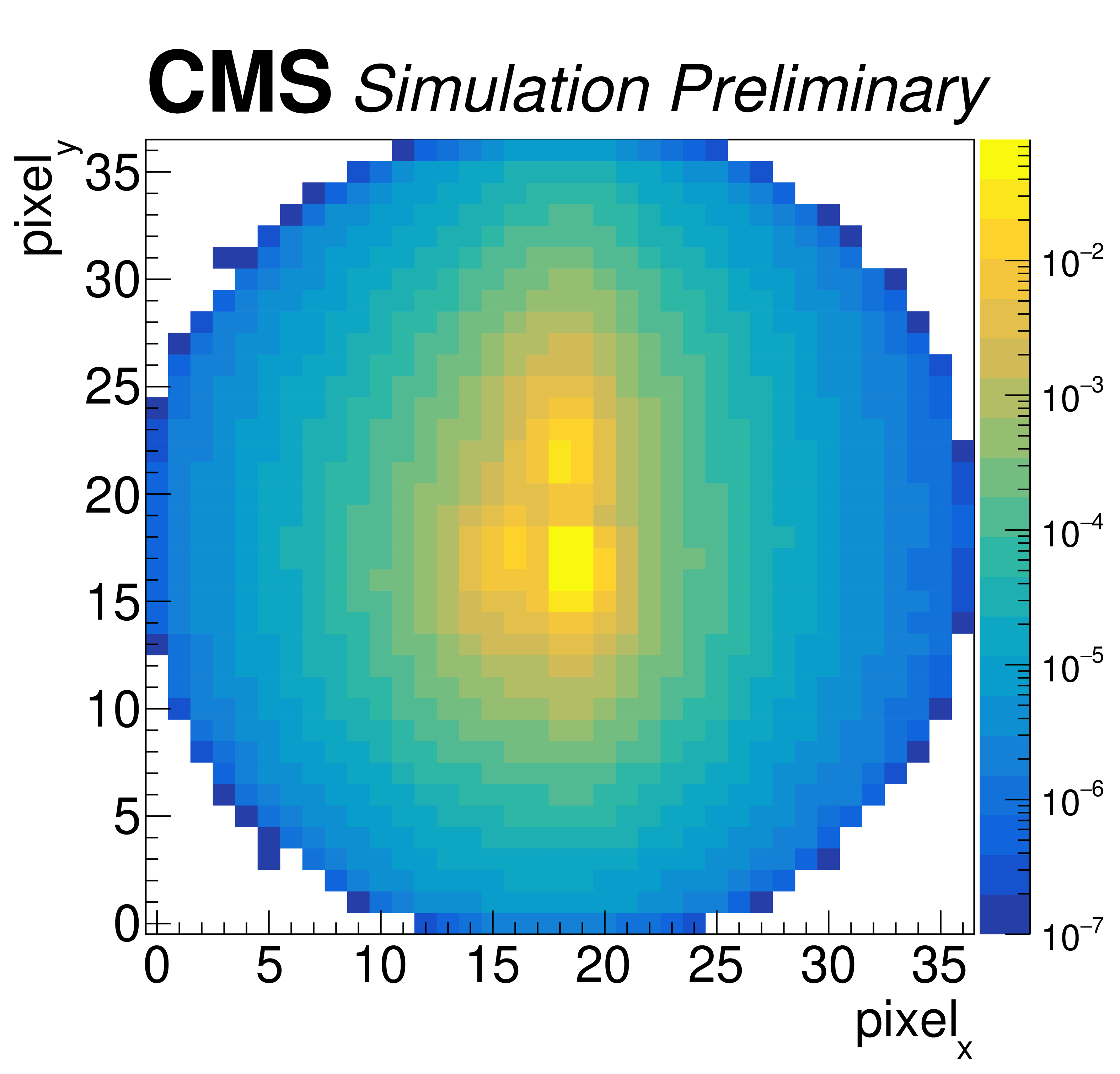
The pixelized greyscale images used in the ImageTop network for QCD (left) and top (right). The x and y axes are the pixel number, and roughly scale with $\Delta R$. The z axis is the intensity of the greyscale image in the given pixel, (particle flow candidate $ {p_{\mathrm {T}}} $) and has been normalized to unity. This figure shows an ensemble of overlaid images after the image post processing, where we can see clear differences between the top and QCD energy deposition patterns. |
png pdf |
Figure 7-a:
The pixelized greyscale images used in the ImageTop network for QCD (left) and top (right). The x and y axes are the pixel number, and roughly scale with $\Delta R$. The z axis is the intensity of the greyscale image in the given pixel, (particle flow candidate $ {p_{\mathrm {T}}} $) and has been normalized to unity. This figure shows an ensemble of overlaid images after the image post processing, where we can see clear differences between the top and QCD energy deposition patterns. |
png pdf |
Figure 7-b:
The pixelized greyscale images used in the ImageTop network for QCD (left) and top (right). The x and y axes are the pixel number, and roughly scale with $\Delta R$. The z axis is the intensity of the greyscale image in the given pixel, (particle flow candidate $ {p_{\mathrm {T}}} $) and has been normalized to unity. This figure shows an ensemble of overlaid images after the image post processing, where we can see clear differences between the top and QCD energy deposition patterns. |
png pdf |
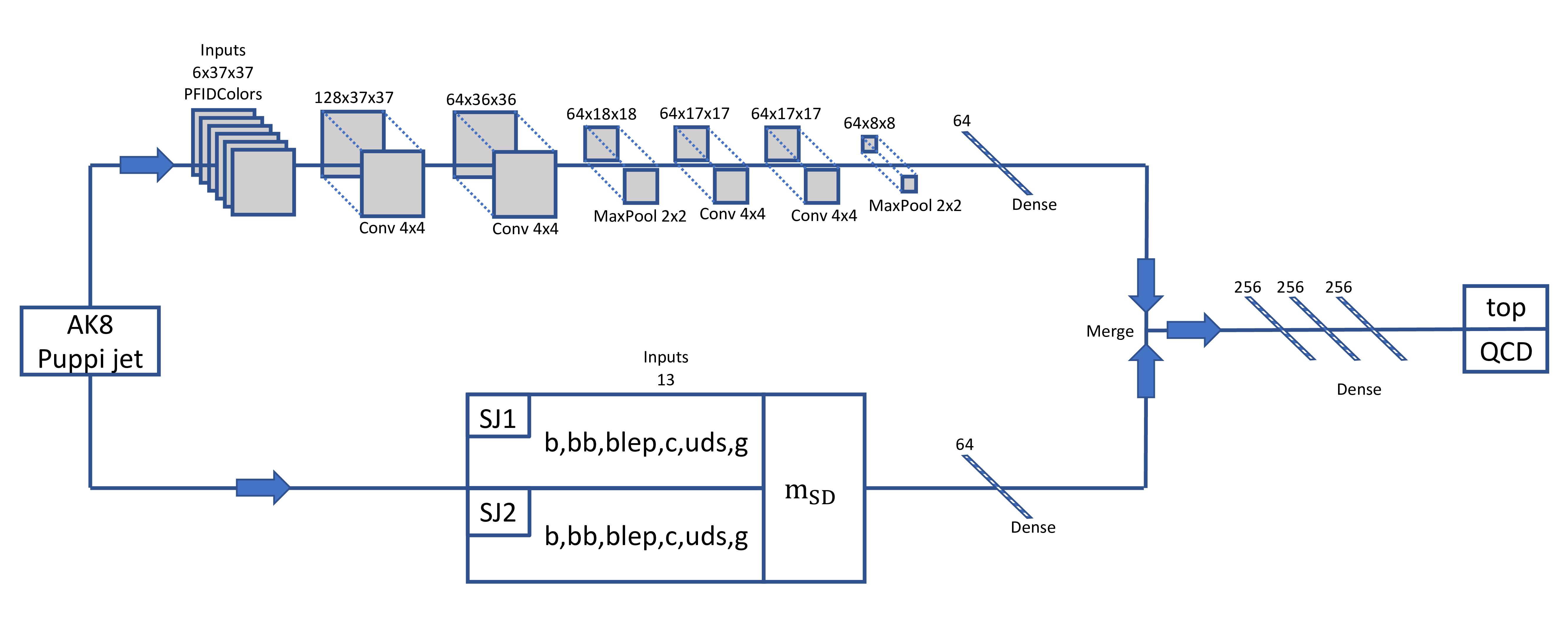
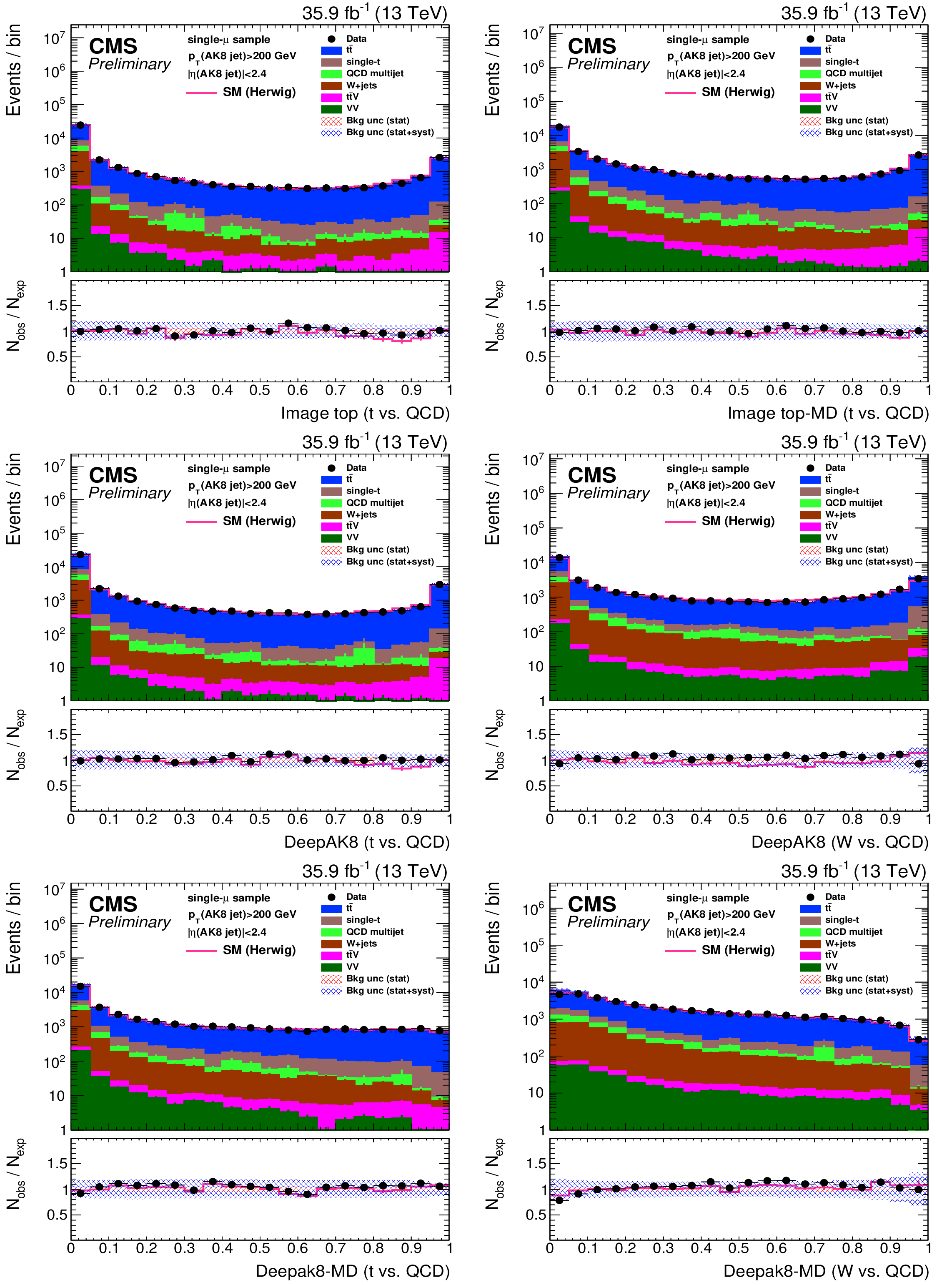
Figure 8:
The ImageTop network architecture. The NN inputs are the 37x37 pixelized PF candidate ${p_{\mathrm {T}}}$ map, which is split into colors based on the PF candidate flavor, as well as the DeepFlavour subjet b tags applied to both subjets. The pixelized images are sent through a two dimensional CNN, and the subjet b tags are inputs into a dense layer. The NN are merged before being input into three dense layers and finally the two node output which is used as the top tagging discriminator. |
png pdf |
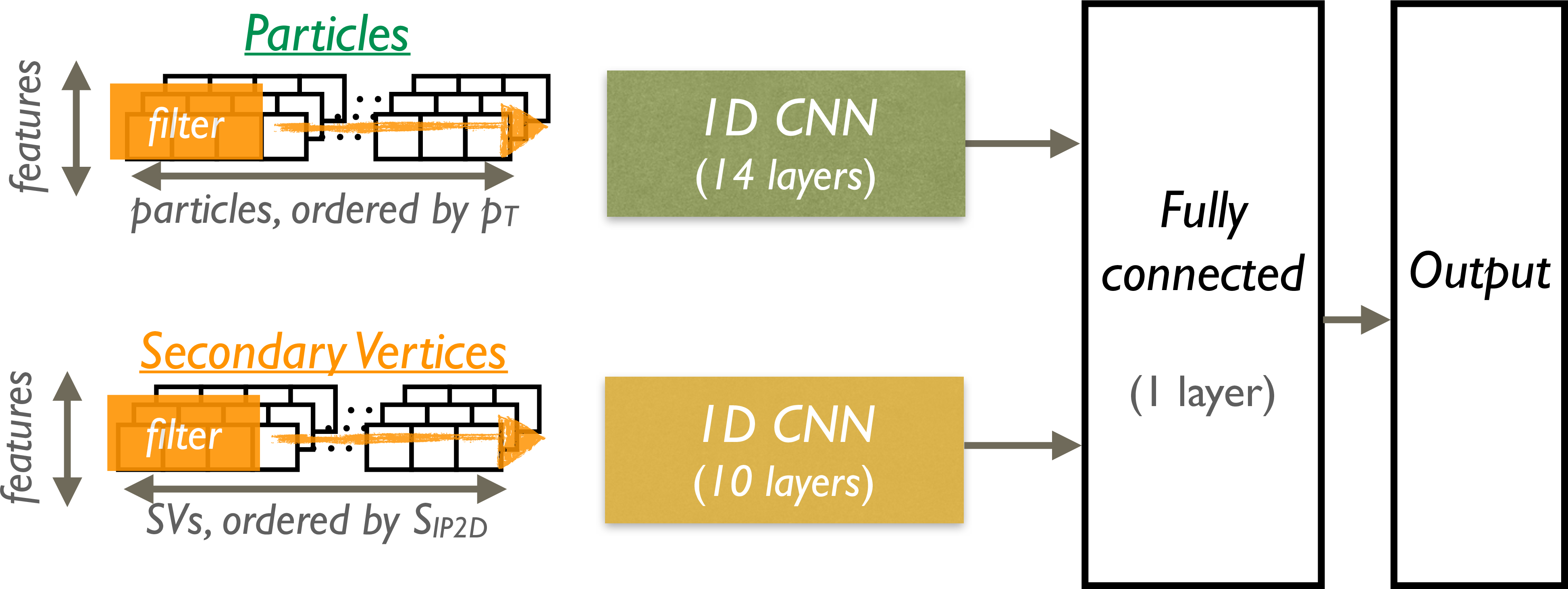
Figure 9:
The network architecture of DeepAK8. |
png pdf |
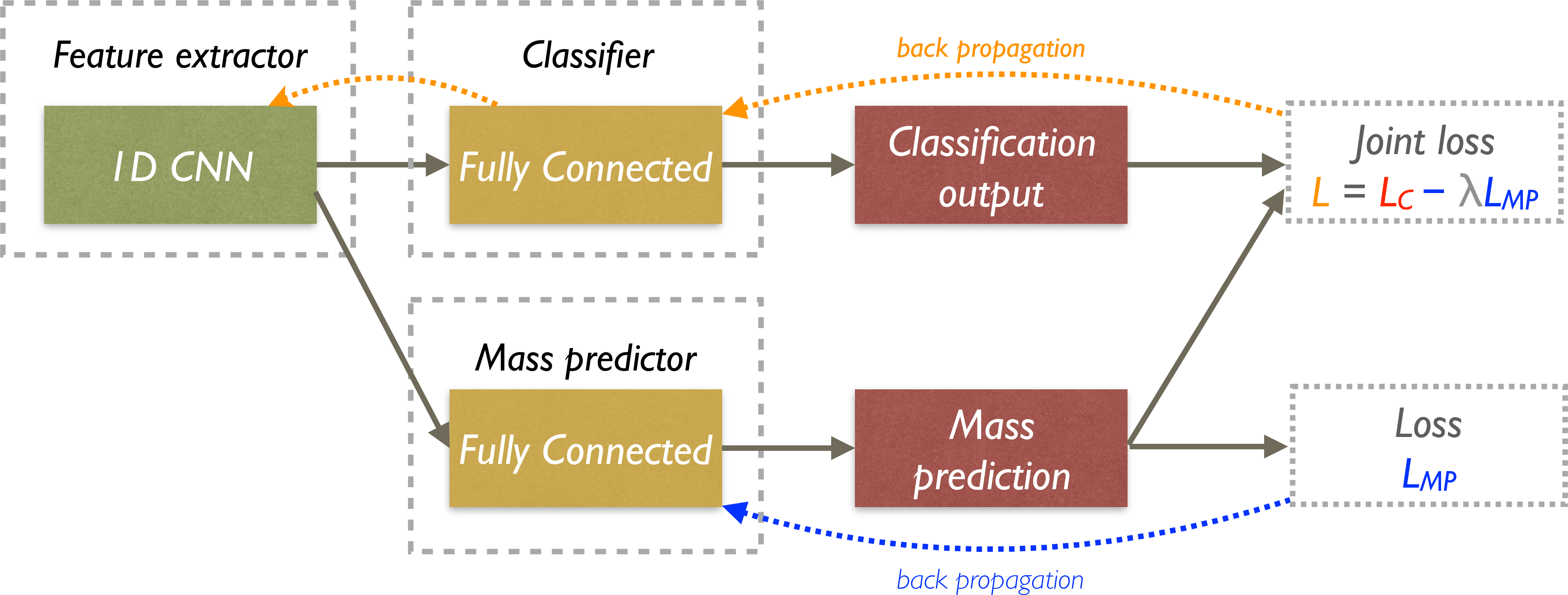
Figure 10:
The network architecture of DeepAK8-MD. |
png pdf |
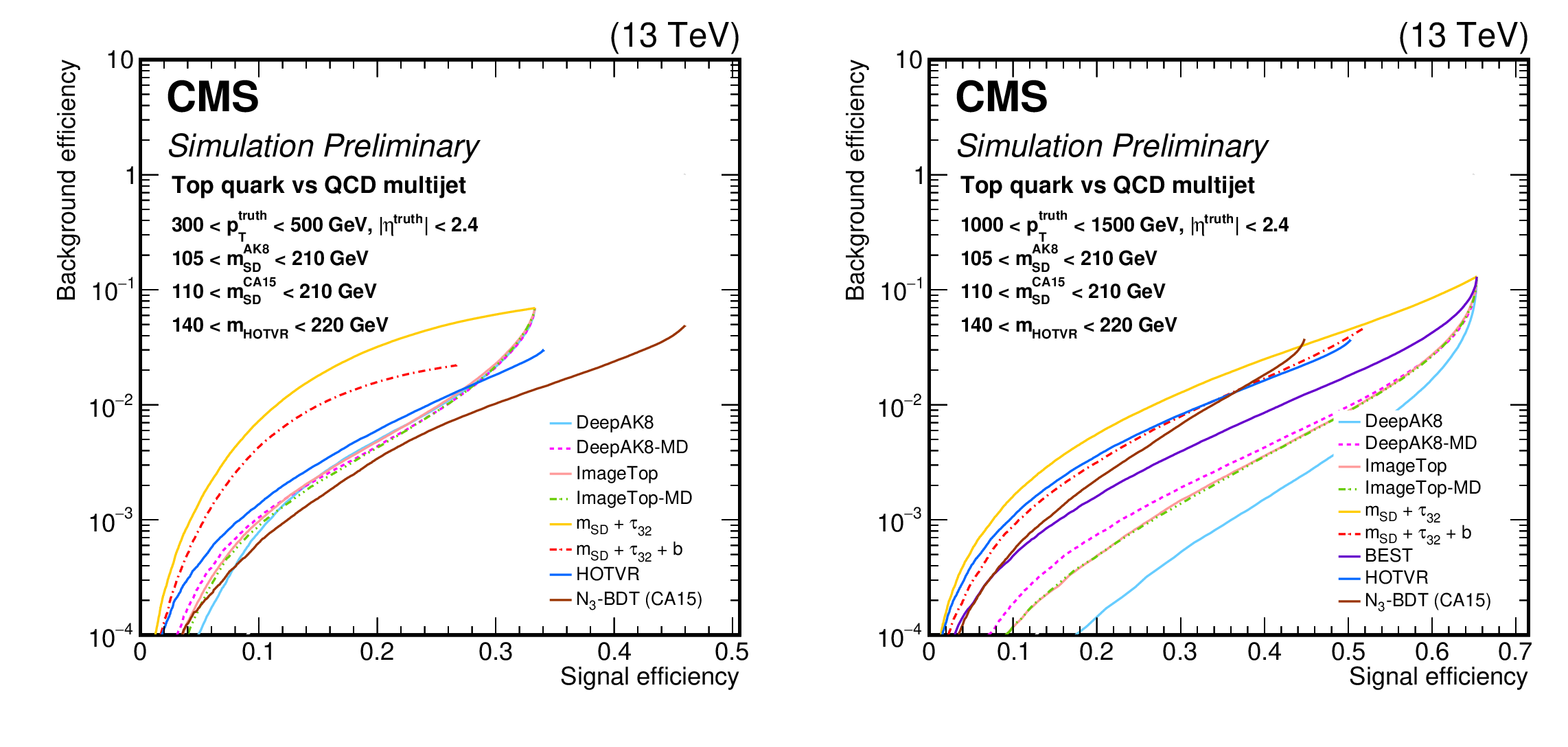
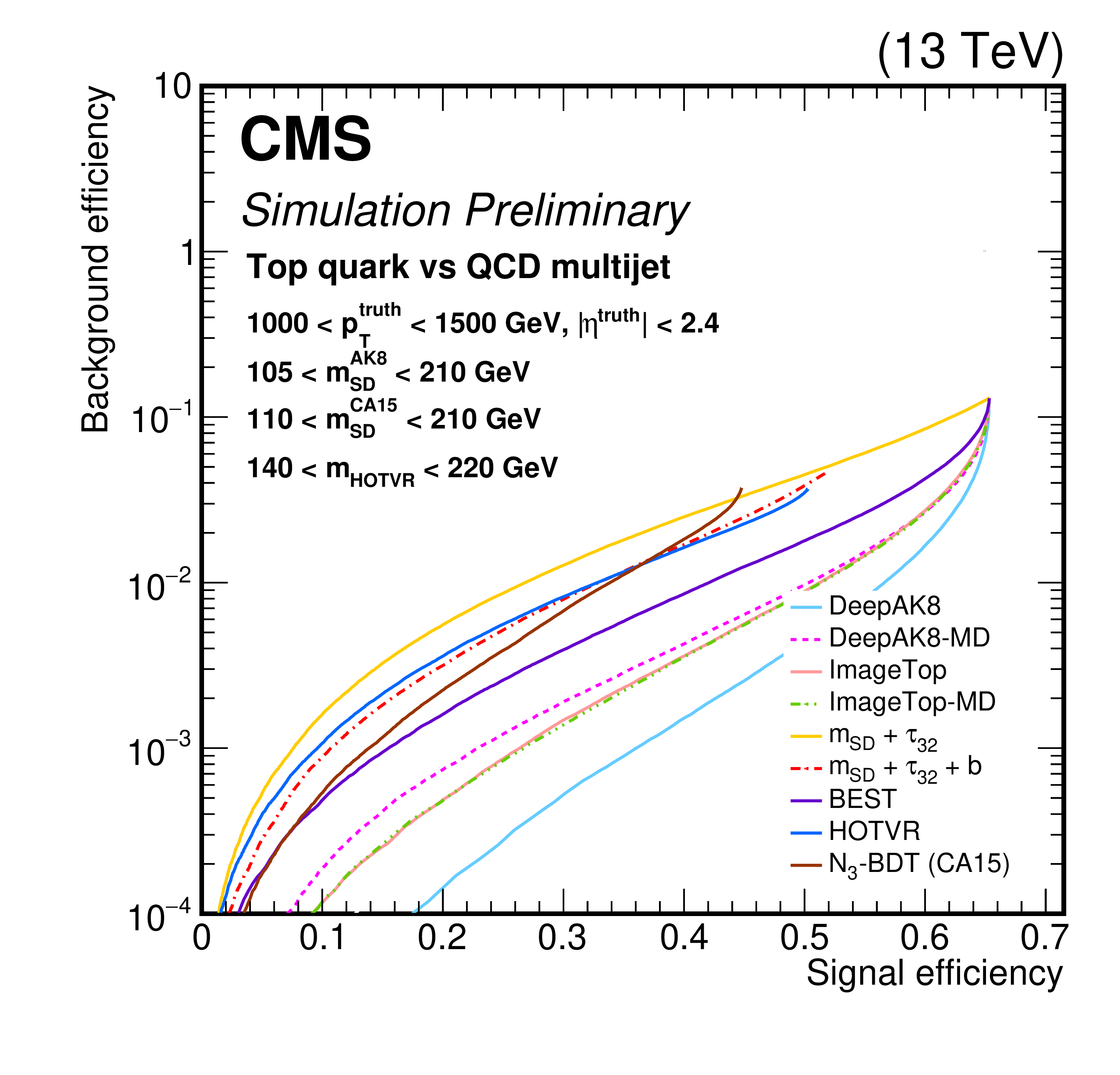
Figure 11:
Performance comparison of the hadronically decaying t quark identification algorithms in terms of receiver operating characteristic (ROC) curves in two regions based on the ${p_{\mathrm {T}}}$ of the truth particle; Left: 300 $ < {p_{\mathrm {T}}} < $ 500 GeV, and Right: 1000 $ < {p_{\mathrm {T}}} < $ 1500 GeV. Additional fiducial selection criteria applied to the jets are displayed on the plots. |
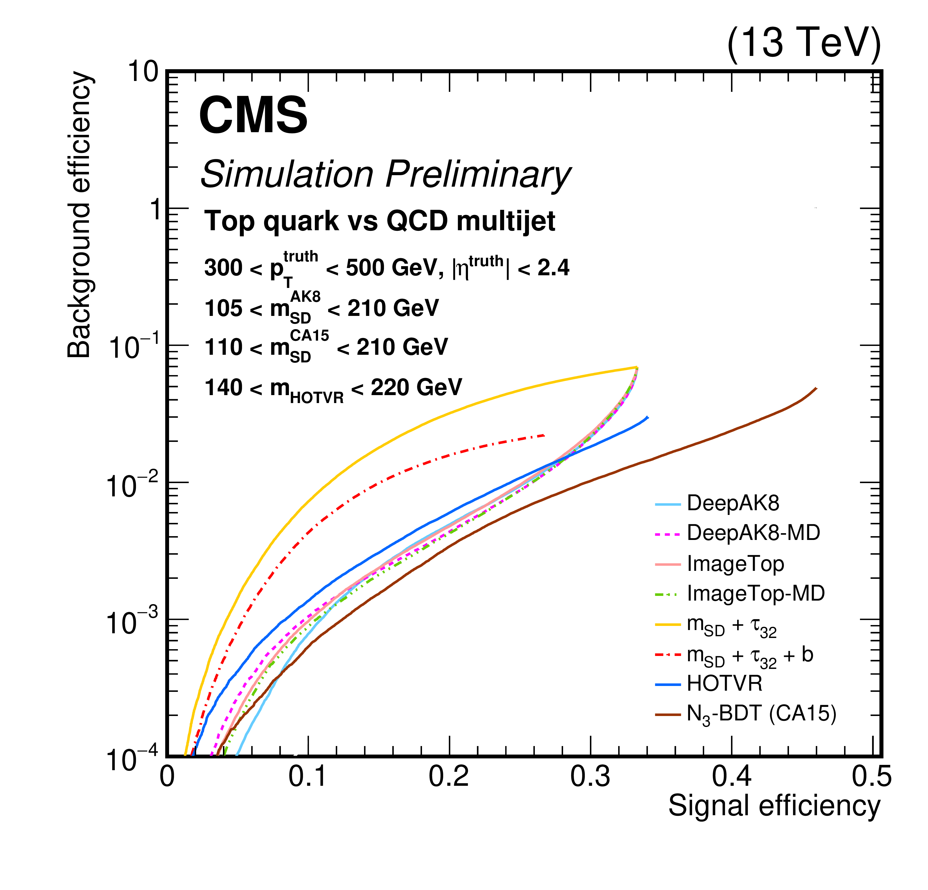
png pdf |
Figure 11-a:
Performance comparison of the hadronically decaying t quark identification algorithms in terms of receiver operating characteristic (ROC) curves in two regions based on the ${p_{\mathrm {T}}}$ of the truth particle; Left: 300 $ < {p_{\mathrm {T}}} < $ 500 GeV, and Right: 1000 $ < {p_{\mathrm {T}}} < $ 1500 GeV. Additional fiducial selection criteria applied to the jets are displayed on the plots. |
png pdf |
Figure 11-b:
Performance comparison of the hadronically decaying t quark identification algorithms in terms of receiver operating characteristic (ROC) curves in two regions based on the ${p_{\mathrm {T}}}$ of the truth particle; Left: 300 $ < {p_{\mathrm {T}}} < $ 500 GeV, and Right: 1000 $ < {p_{\mathrm {T}}} < $ 1500 GeV. Additional fiducial selection criteria applied to the jets are displayed on the plots. |
png pdf |
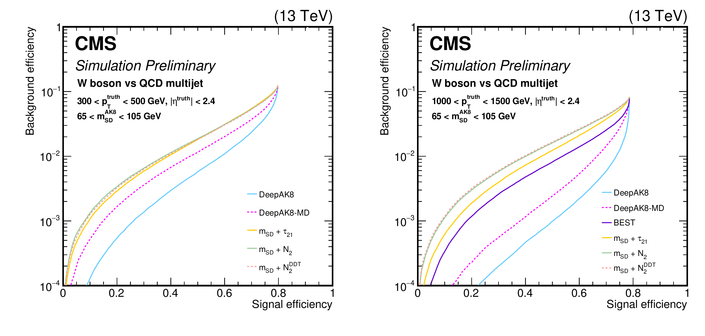
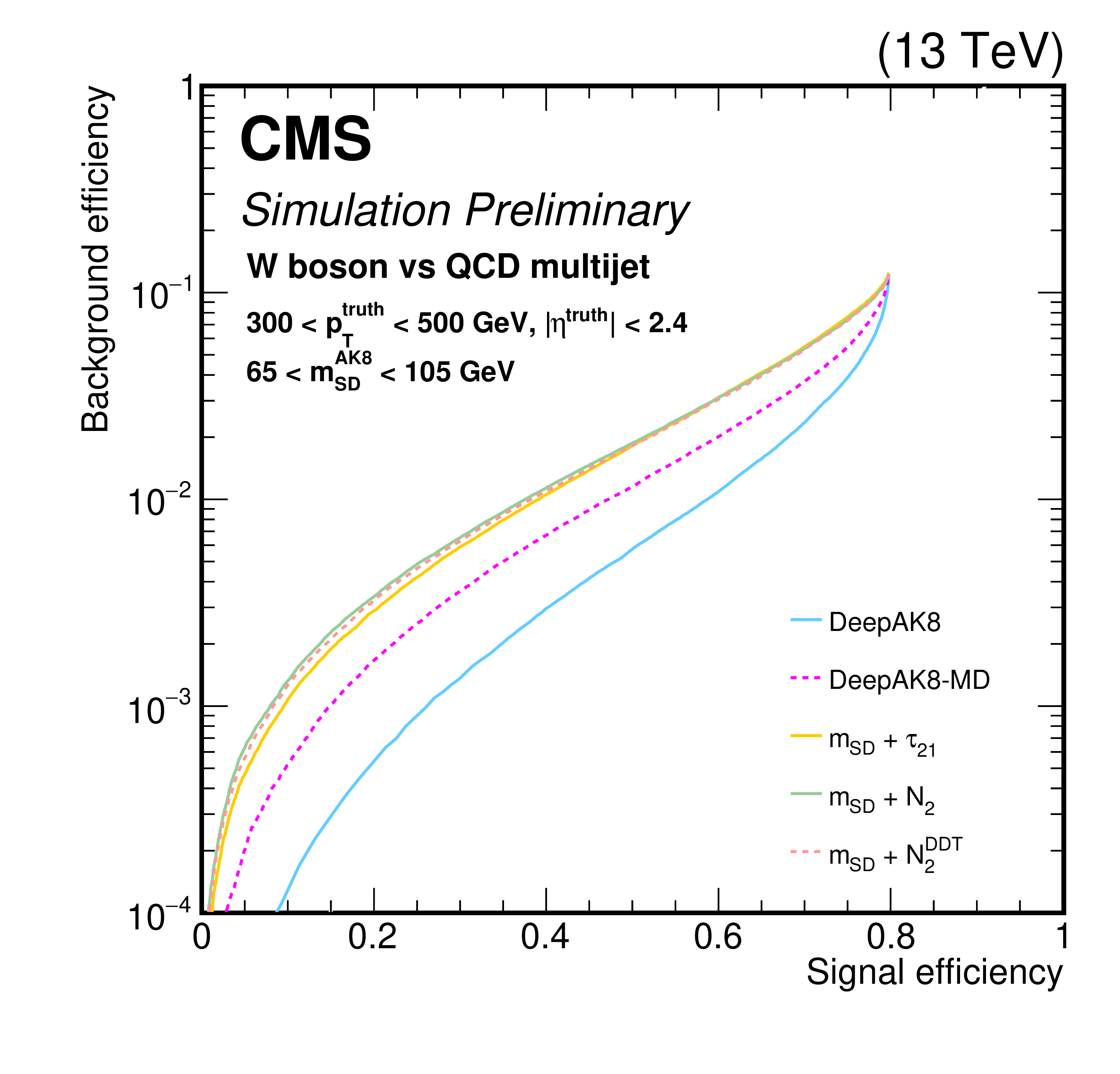
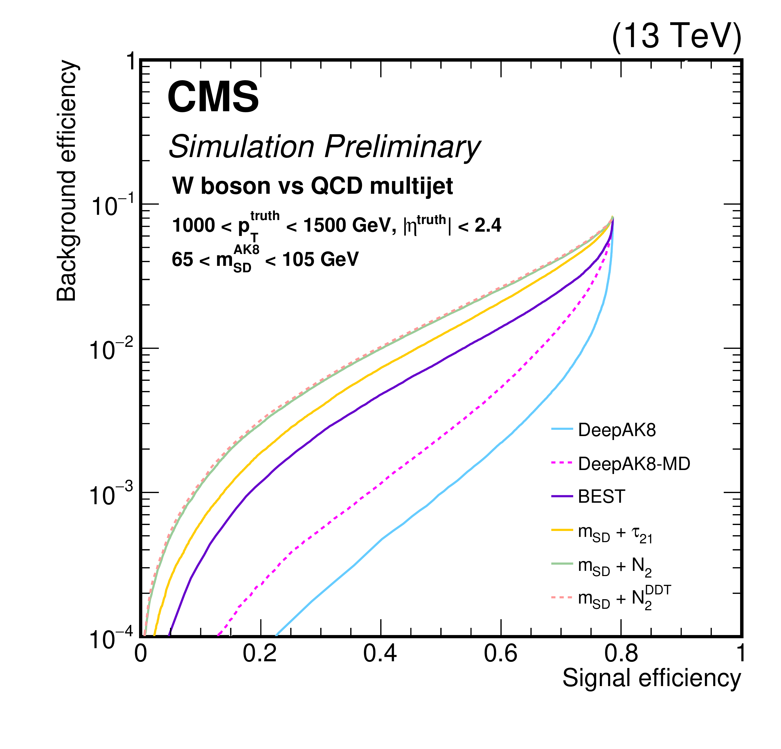
Figure 12:
Performance comparison of the hadronically decaying W boson identification algorithms in terms of receiver operating characteristic (ROC) curves in two regions based on the ${p_{\mathrm {T}}}$ of the truth particle; Left: 300 $ < {p_{\mathrm {T}}} < $ 500 GeV, and Right: 1000 $ < {p_{\mathrm {T}}} < $ 1500 GeV. Additional fiducial selection criteria applied to the jets are displayed on the plots. |
png pdf |
Figure 12-a:
Performance comparison of the hadronically decaying W boson identification algorithms in terms of receiver operating characteristic (ROC) curves in two regions based on the ${p_{\mathrm {T}}}$ of the truth particle; Left: 300 $ < {p_{\mathrm {T}}} < $ 500 GeV, and Right: 1000 $ < {p_{\mathrm {T}}} < $ 1500 GeV. Additional fiducial selection criteria applied to the jets are displayed on the plots. |
png pdf |
Figure 12-b:
Performance comparison of the hadronically decaying W boson identification algorithms in terms of receiver operating characteristic (ROC) curves in two regions based on the ${p_{\mathrm {T}}}$ of the truth particle; Left: 300 $ < {p_{\mathrm {T}}} < $ 500 GeV, and Right: 1000 $ < {p_{\mathrm {T}}} < $ 1500 GeV. Additional fiducial selection criteria applied to the jets are displayed on the plots. |
png pdf |
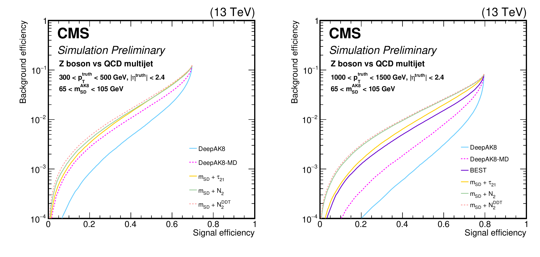
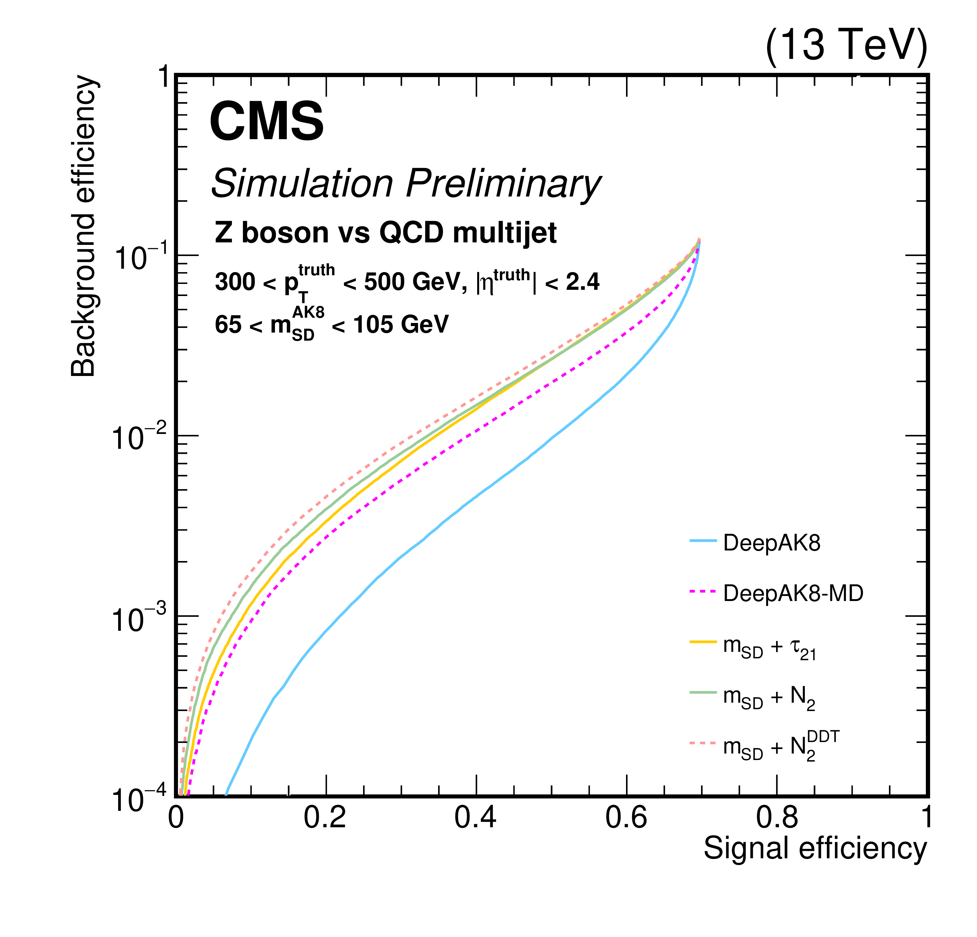
Figure 13:
Performance comparison of the hadronically decaying Z boson identification algorithms in terms of receiver operating characteristic (ROC) curves in two regions based on the ${p_{\mathrm {T}}}$ of the truth particle; Left: 300 $ < {p_{\mathrm {T}}} < $ 500 GeV, and Right: 1000 $ < {p_{\mathrm {T}}} < $ 1500 GeV. Additional fiducial selection criteria applied to the jets are displayed on the plots. |
png pdf |
Figure 13-a:
Performance comparison of the hadronically decaying Z boson identification algorithms in terms of receiver operating characteristic (ROC) curves in two regions based on the ${p_{\mathrm {T}}}$ of the truth particle; Left: 300 $ < {p_{\mathrm {T}}} < $ 500 GeV, and Right: 1000 $ < {p_{\mathrm {T}}} < $ 1500 GeV. Additional fiducial selection criteria applied to the jets are displayed on the plots. |

png pdf |
Figure 13-b:
Performance comparison of the hadronically decaying Z boson identification algorithms in terms of receiver operating characteristic (ROC) curves in two regions based on the ${p_{\mathrm {T}}}$ of the truth particle; Left: 300 $ < {p_{\mathrm {T}}} < $ 500 GeV, and Right: 1000 $ < {p_{\mathrm {T}}} < $ 1500 GeV. Additional fiducial selection criteria applied to the jets are displayed on the plots. |
png pdf |
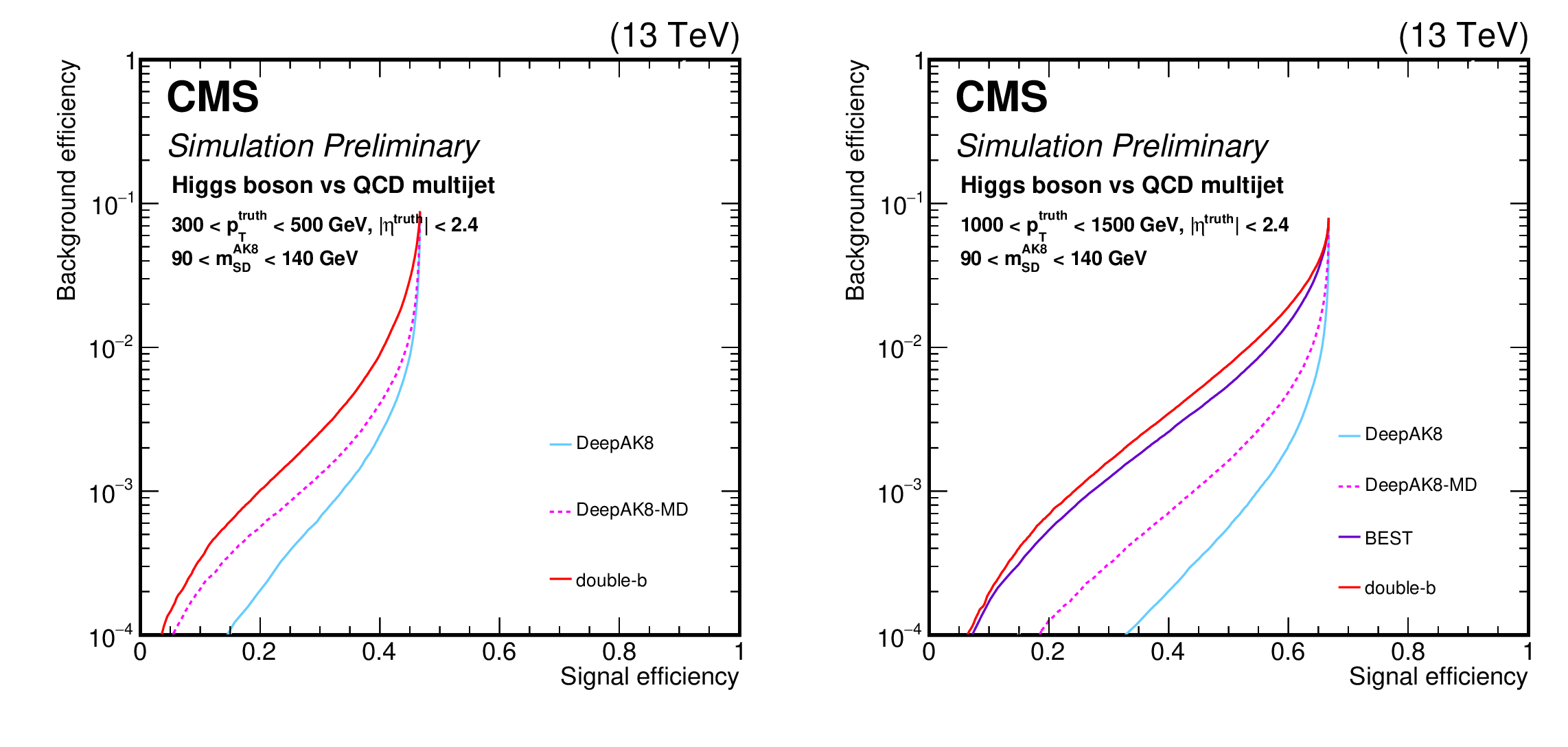
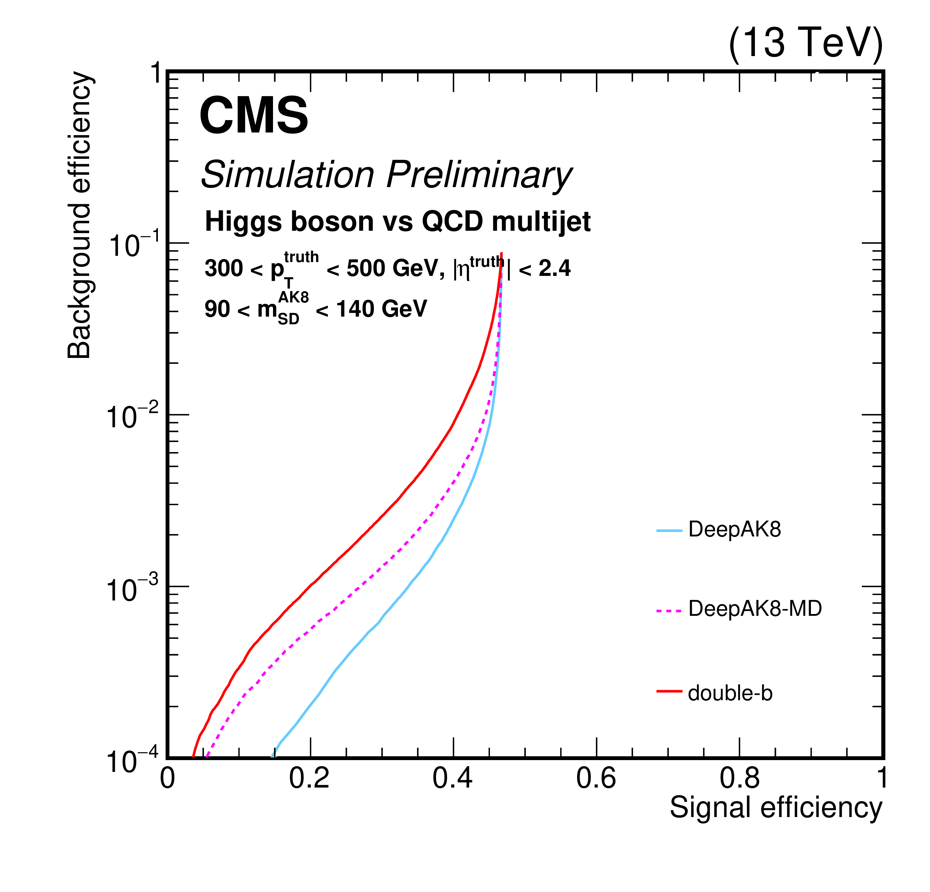
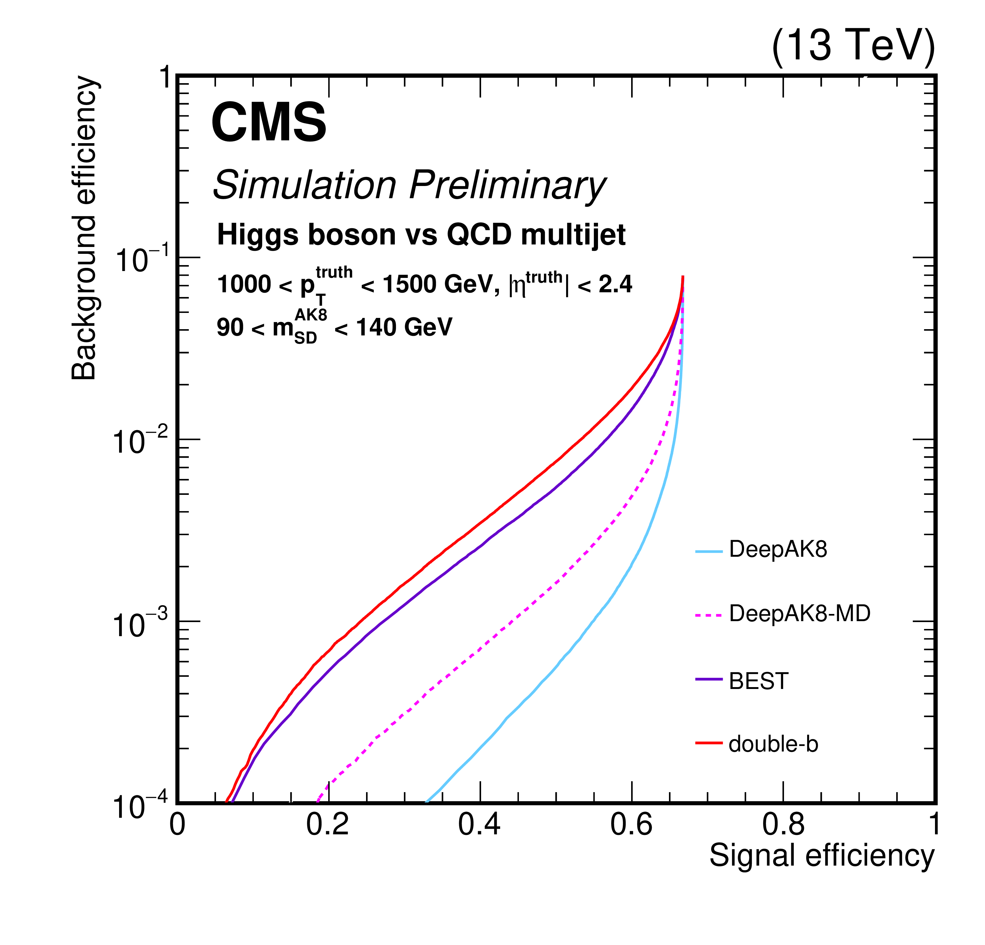
Figure 14:
Performance comparison of the hadronically decaying H boson identification algorithms in terms of receiver operating characteristic (ROC) curves in two regions based on the ${p_{\mathrm {T}}}$ of the truth particle; Left: 300 $ < {p_{\mathrm {T}}} < $ 500 GeV, and Right: 1000 $ < {p_{\mathrm {T}}} < $ 1500 GeV. The H boson is forced to decay in a pair of b quarks. Additional fiducial selection criteria applied to the jets are displayed on the plots. |
png pdf |
Figure 14-a:
Performance comparison of the hadronically decaying H boson identification algorithms in terms of receiver operating characteristic (ROC) curves in two regions based on the ${p_{\mathrm {T}}}$ of the truth particle; Left: 300 $ < {p_{\mathrm {T}}} < $ 500 GeV, and Right: 1000 $ < {p_{\mathrm {T}}} < $ 1500 GeV. The H boson is forced to decay in a pair of b quarks. Additional fiducial selection criteria applied to the jets are displayed on the plots. |
png pdf |
Figure 14-b:
Performance comparison of the hadronically decaying H boson identification algorithms in terms of receiver operating characteristic (ROC) curves in two regions based on the ${p_{\mathrm {T}}}$ of the truth particle; Left: 300 $ < {p_{\mathrm {T}}} < $ 500 GeV, and Right: 1000 $ < {p_{\mathrm {T}}} < $ 1500 GeV. The H boson is forced to decay in a pair of b quarks. Additional fiducial selection criteria applied to the jets are displayed on the plots. |
png pdf |
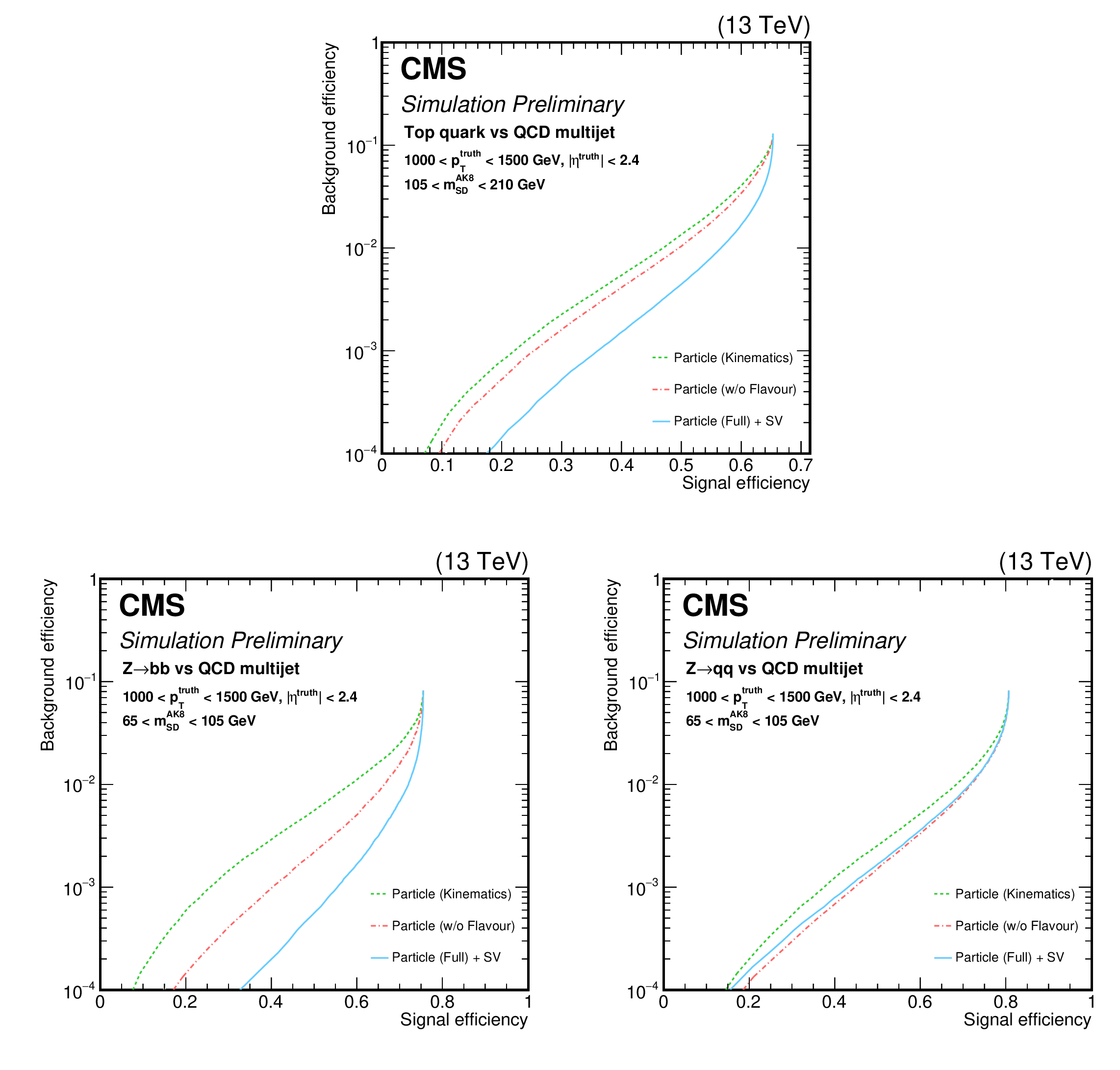
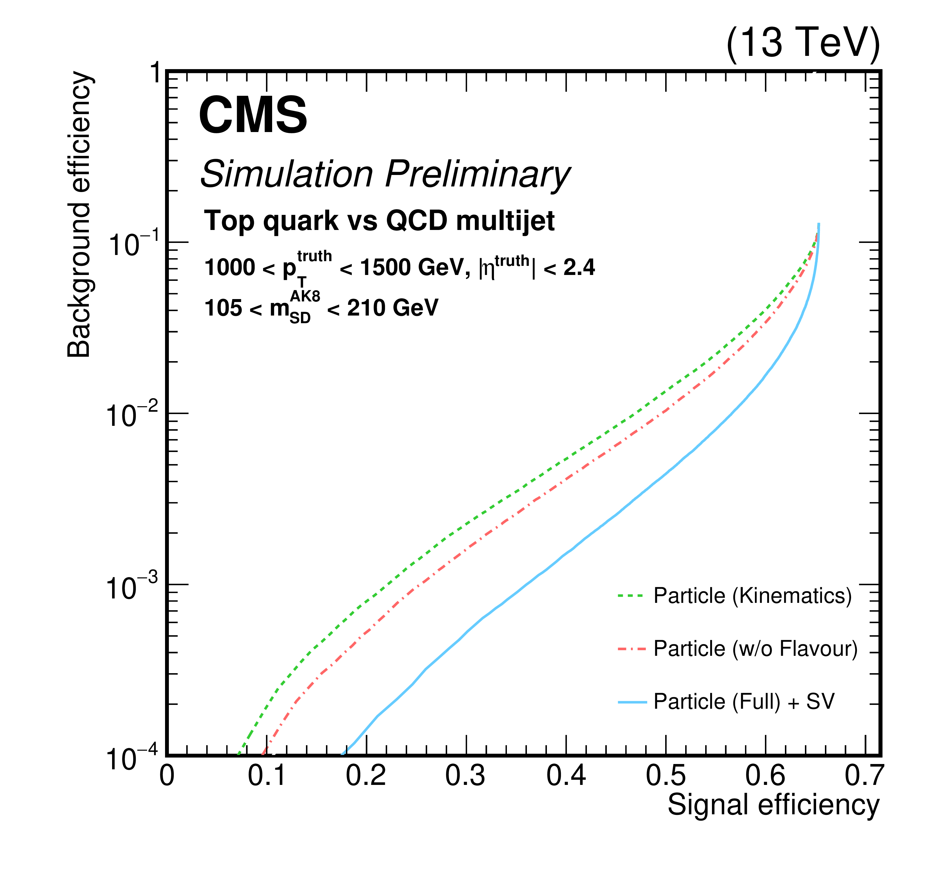
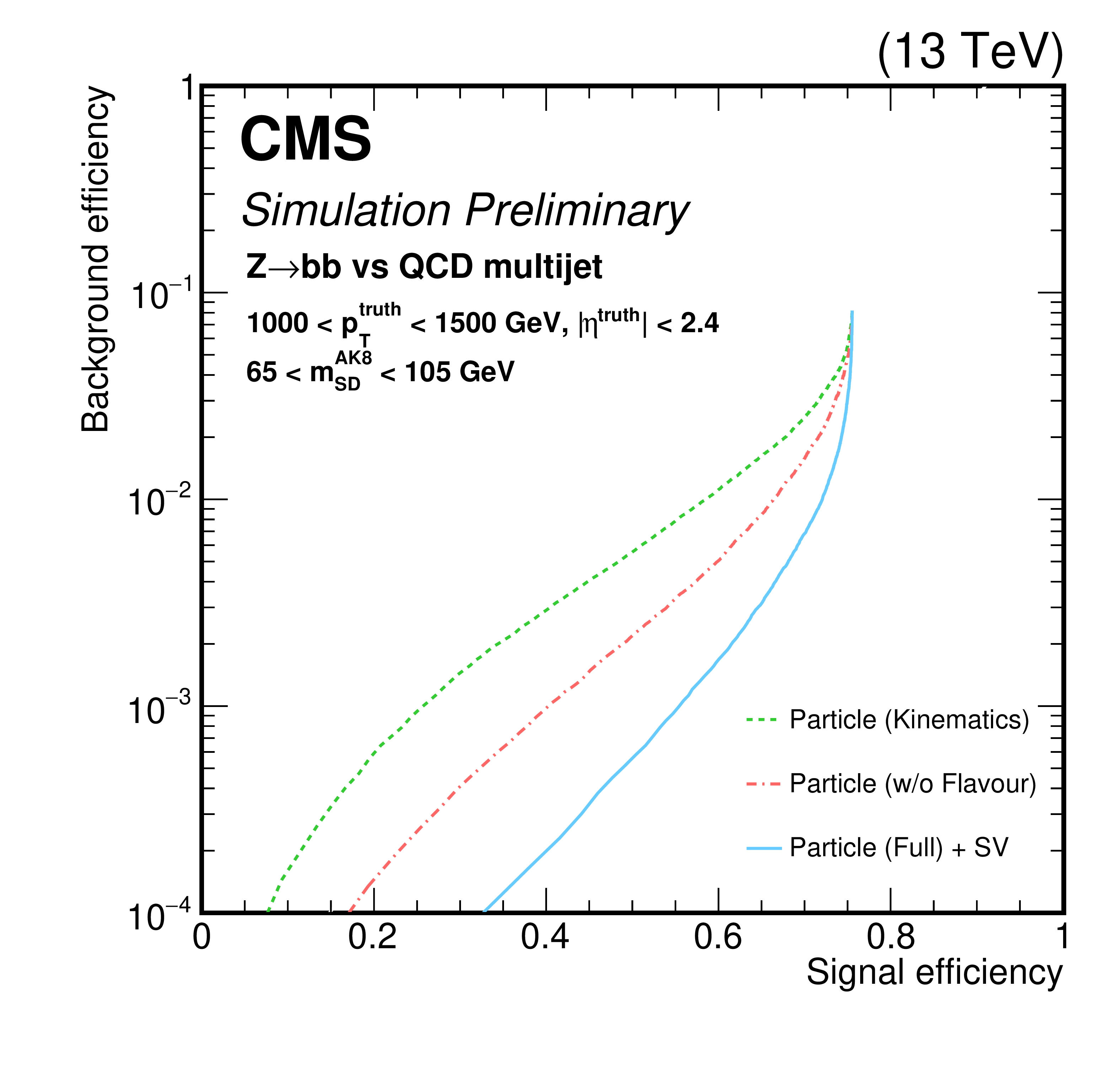
Figure 15:
Alternative versions of DeepAK8 trained using a subset of the input features. The details about each version are discussed in the text. The performances of the three versions of DeepAK8 are compared for t quark (upper) and Z (lower) identification. For the latter, the left plot corresponds Z bosons decaying to a pair of b quarks, and the right to a pair of light quarks. |
png pdf |
Figure 15-a:
Alternative versions of DeepAK8 trained using a subset of the input features. The details about each version are discussed in the text. The performances of the three versions of DeepAK8 are compared for t quark (upper) and Z (lower) identification. For the latter, the left plot corresponds Z bosons decaying to a pair of b quarks, and the right to a pair of light quarks. |
png pdf |
Figure 15-b:
Alternative versions of DeepAK8 trained using a subset of the input features. The details about each version are discussed in the text. The performances of the three versions of DeepAK8 are compared for t quark (upper) and Z (lower) identification. For the latter, the left plot corresponds Z bosons decaying to a pair of b quarks, and the right to a pair of light quarks. |
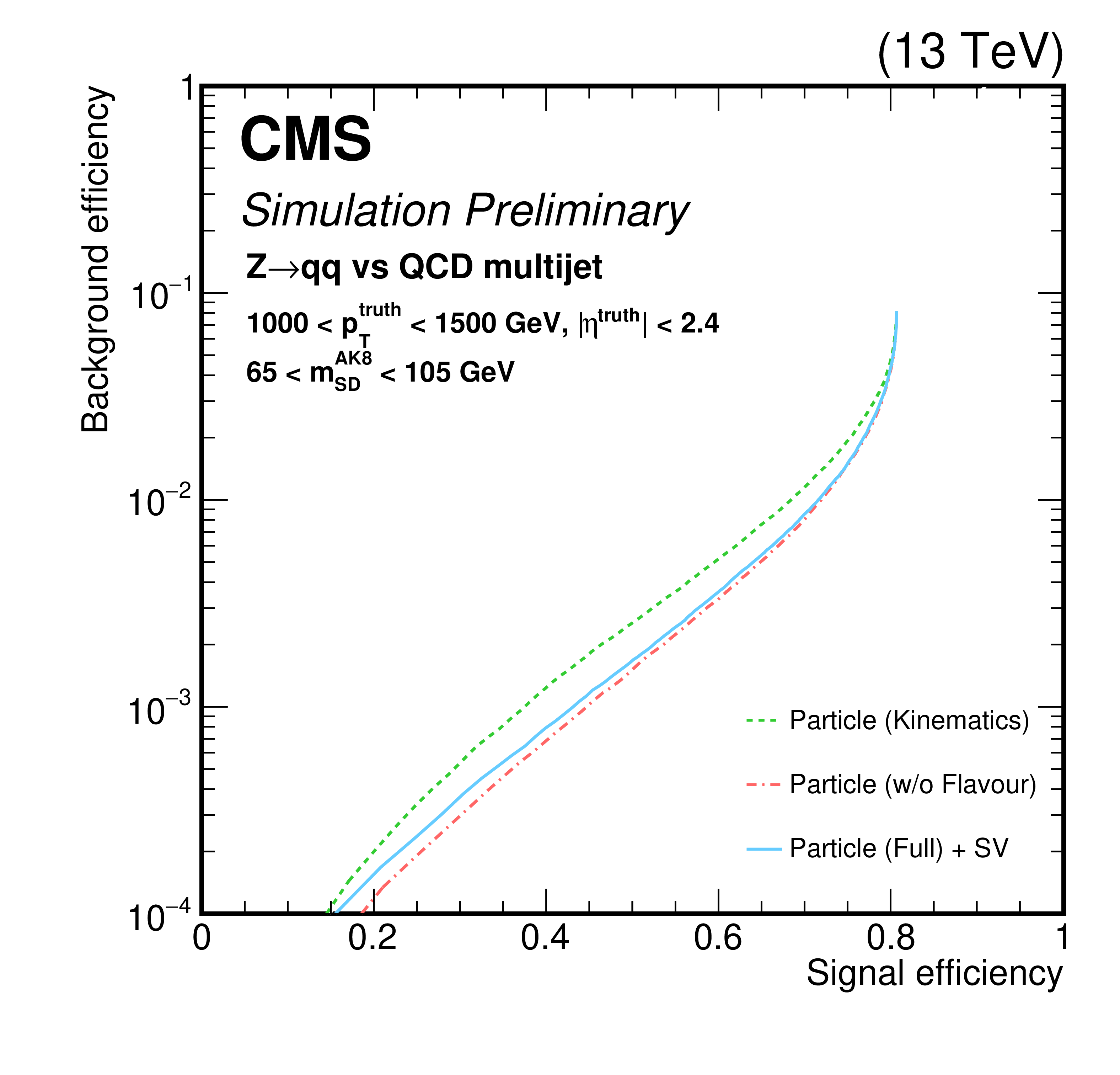
png pdf |
Figure 15-c:
Alternative versions of DeepAK8 trained using a subset of the input features. The details about each version are discussed in the text. The performances of the three versions of DeepAK8 are compared for t quark (upper) and Z (lower) identification. For the latter, the left plot corresponds Z bosons decaying to a pair of b quarks, and the right to a pair of light quarks. |
png pdf |
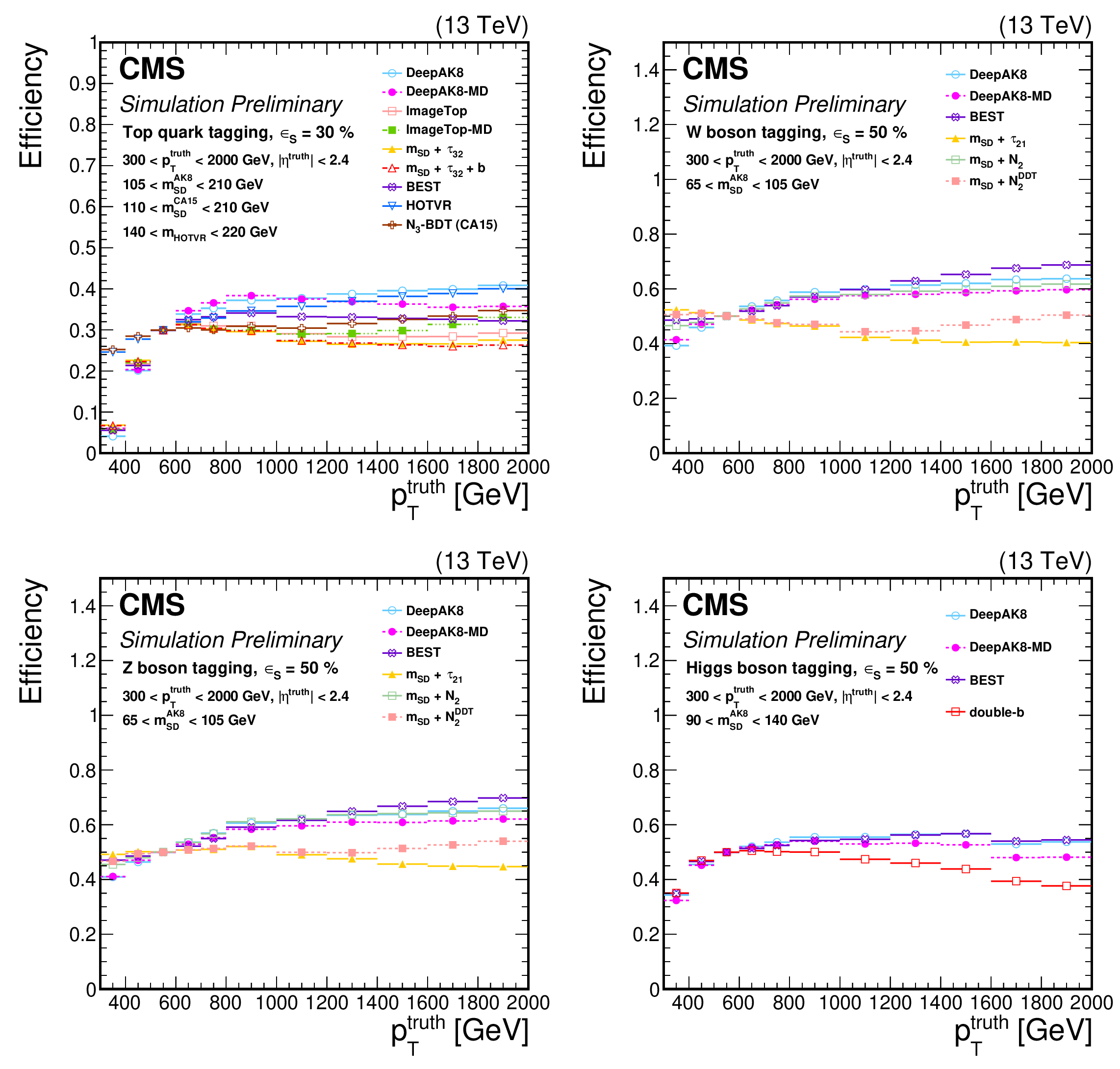
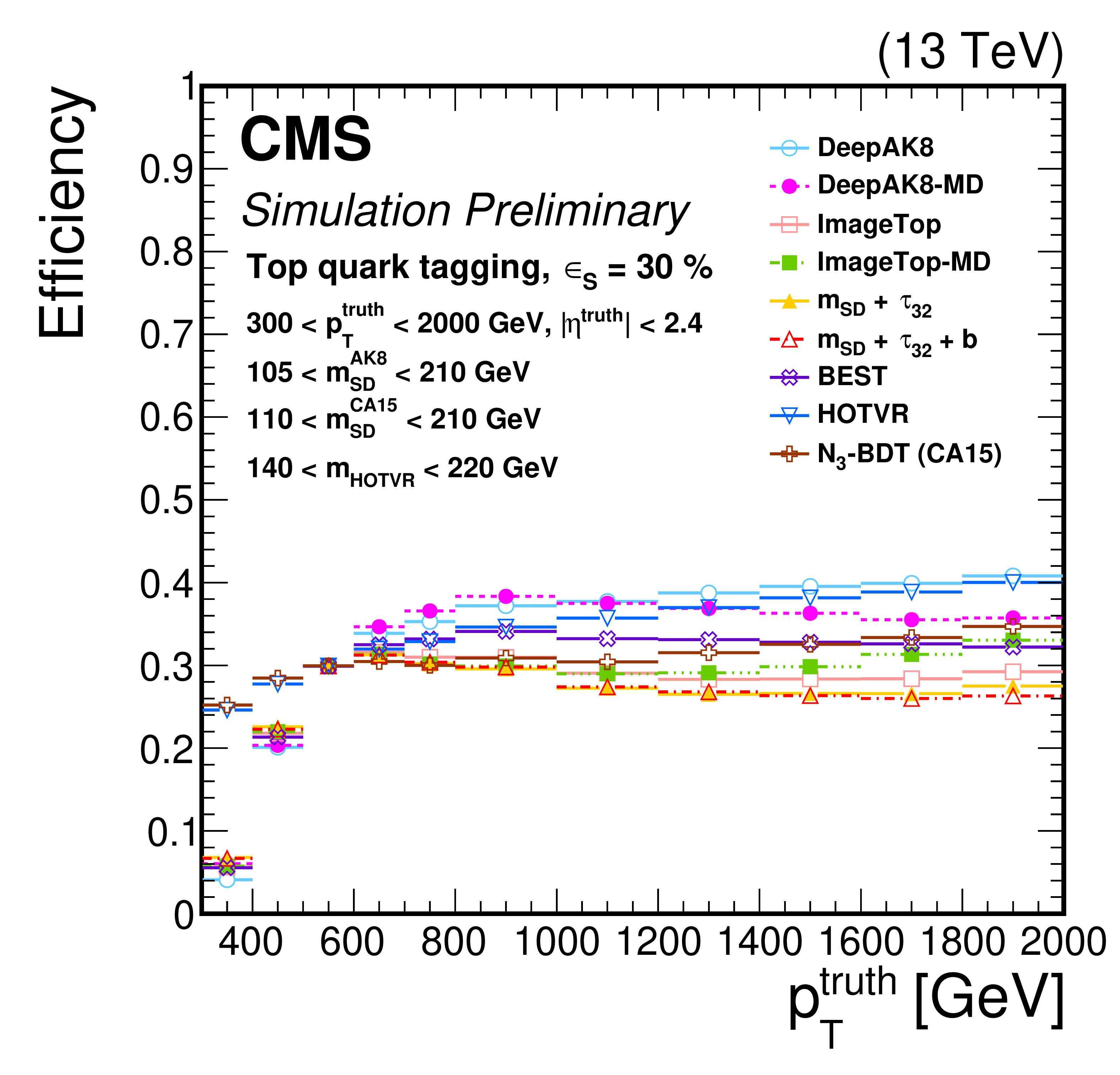
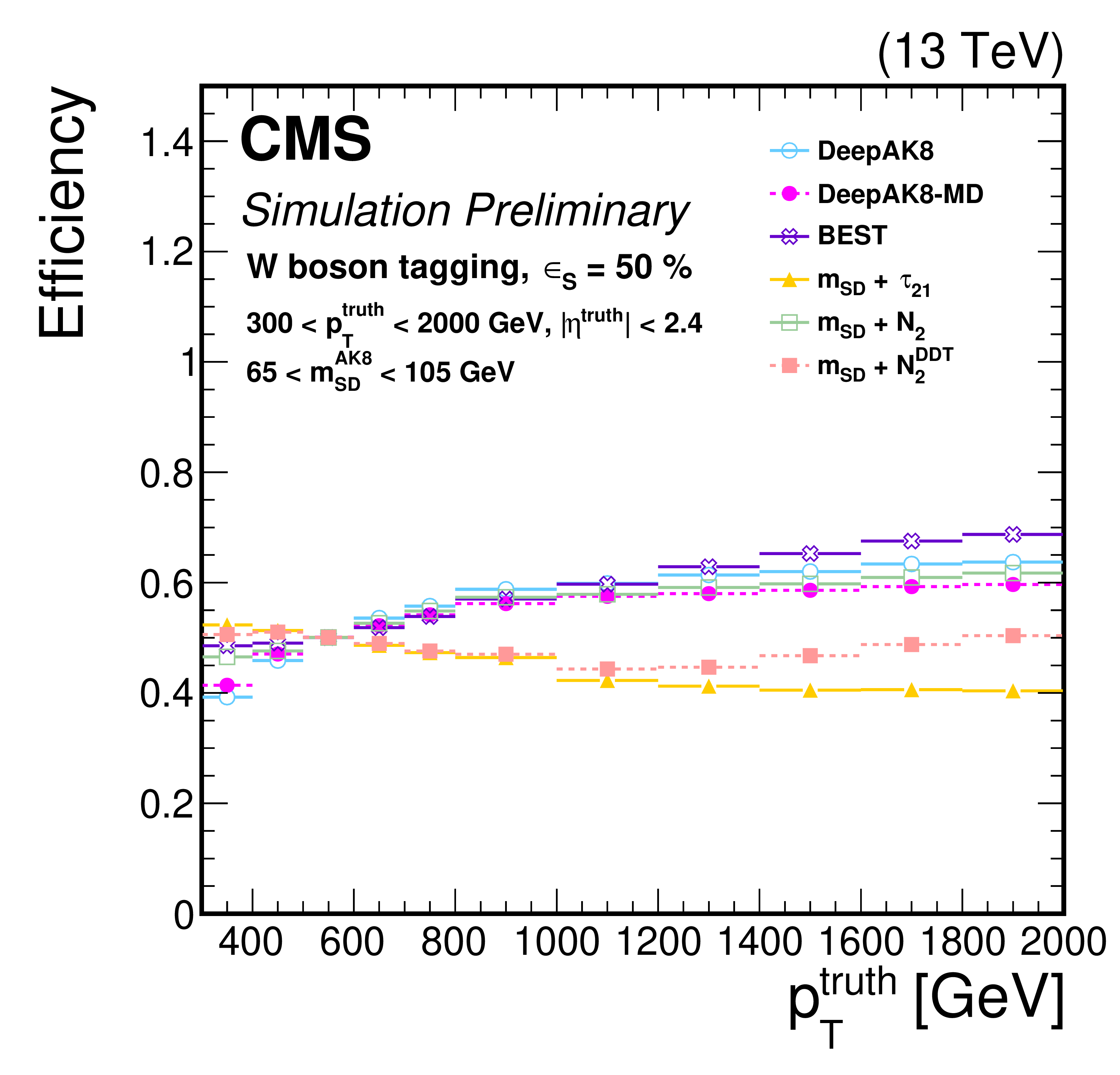
Figure 16:
The distribution of ${\epsilon _{S}}$\ as a function of the ${p_{\mathrm {T}}}$ of the truth particle for a working point corresponding to $ {\epsilon _{S}}= $ 30% (50%) for t quark (W, Z, and H boson) identification. Upper left: t quark, upper right: W boson, lower left: Z boson, lower right: H boson. The error bars represent the statistical uncertainty in each specific bin, due to the limited number of simulated events. Additional fiducial selection criteria applied to the jets are displayed on the plots. |
png pdf |
Figure 16-a:
The distribution of ${\epsilon _{S}}$\ as a function of the ${p_{\mathrm {T}}}$ of the truth particle for a working point corresponding to $ {\epsilon _{S}}= $ 30% (50%) for t quark (W, Z, and H boson) identification. Upper left: t quark, upper right: W boson, lower left: Z boson, lower right: H boson. The error bars represent the statistical uncertainty in each specific bin, due to the limited number of simulated events. Additional fiducial selection criteria applied to the jets are displayed on the plots. |
png pdf |
Figure 16-b:
The distribution of ${\epsilon _{S}}$\ as a function of the ${p_{\mathrm {T}}}$ of the truth particle for a working point corresponding to $ {\epsilon _{S}}= $ 30% (50%) for t quark (W, Z, and H boson) identification. Upper left: t quark, upper right: W boson, lower left: Z boson, lower right: H boson. The error bars represent the statistical uncertainty in each specific bin, due to the limited number of simulated events. Additional fiducial selection criteria applied to the jets are displayed on the plots. |
png pdf |
Figure 16-c:
The distribution of ${\epsilon _{S}}$\ as a function of the ${p_{\mathrm {T}}}$ of the truth particle for a working point corresponding to $ {\epsilon _{S}}= $ 30% (50%) for t quark (W, Z, and H boson) identification. Upper left: t quark, upper right: W boson, lower left: Z boson, lower right: H boson. The error bars represent the statistical uncertainty in each specific bin, due to the limited number of simulated events. Additional fiducial selection criteria applied to the jets are displayed on the plots. |
png pdf |
Figure 16-d:
The distribution of ${\epsilon _{S}}$\ as a function of the ${p_{\mathrm {T}}}$ of the truth particle for a working point corresponding to $ {\epsilon _{S}}= $ 30% (50%) for t quark (W, Z, and H boson) identification. Upper left: t quark, upper right: W boson, lower left: Z boson, lower right: H boson. The error bars represent the statistical uncertainty in each specific bin, due to the limited number of simulated events. Additional fiducial selection criteria applied to the jets are displayed on the plots. |
png pdf |
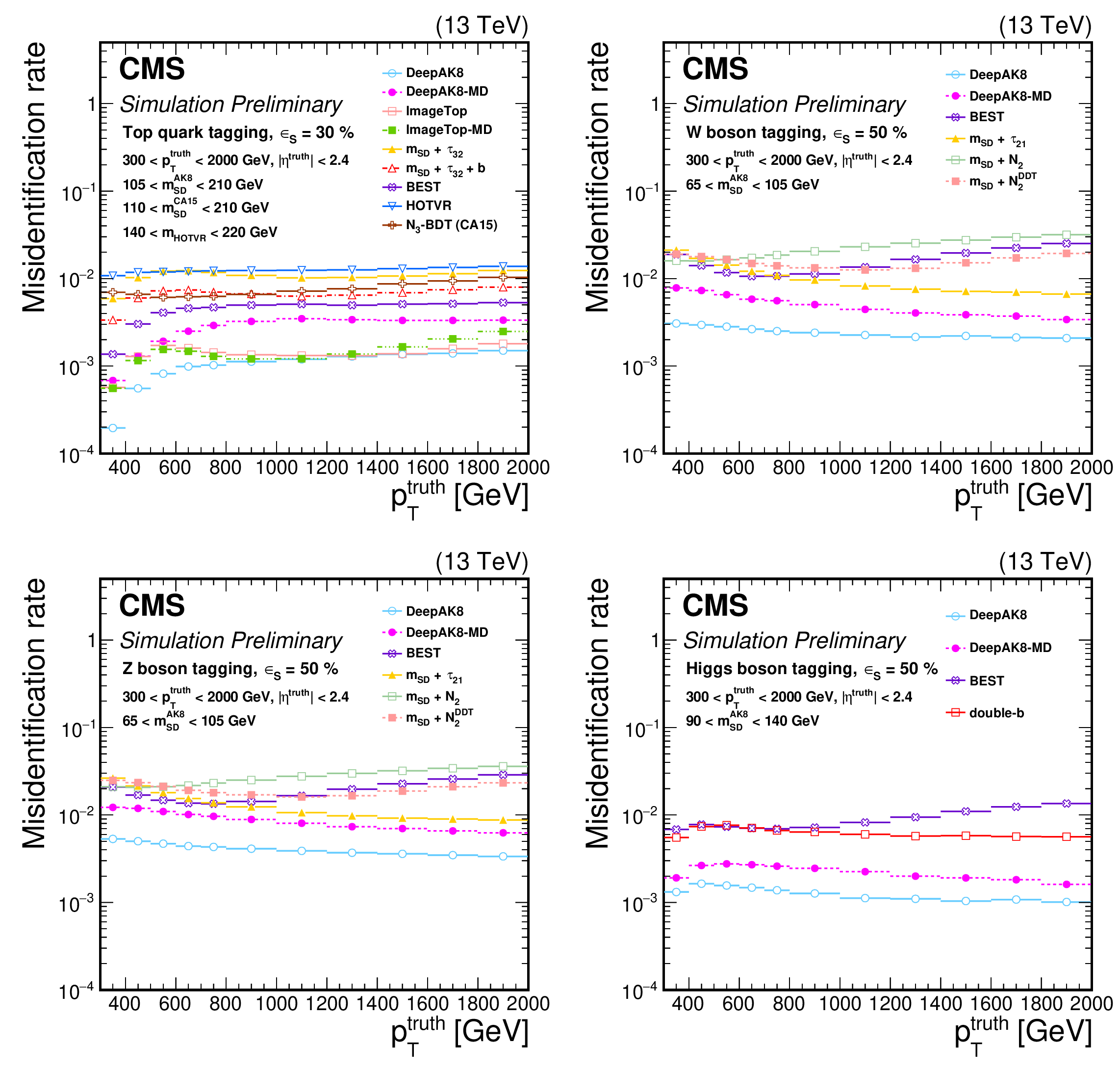
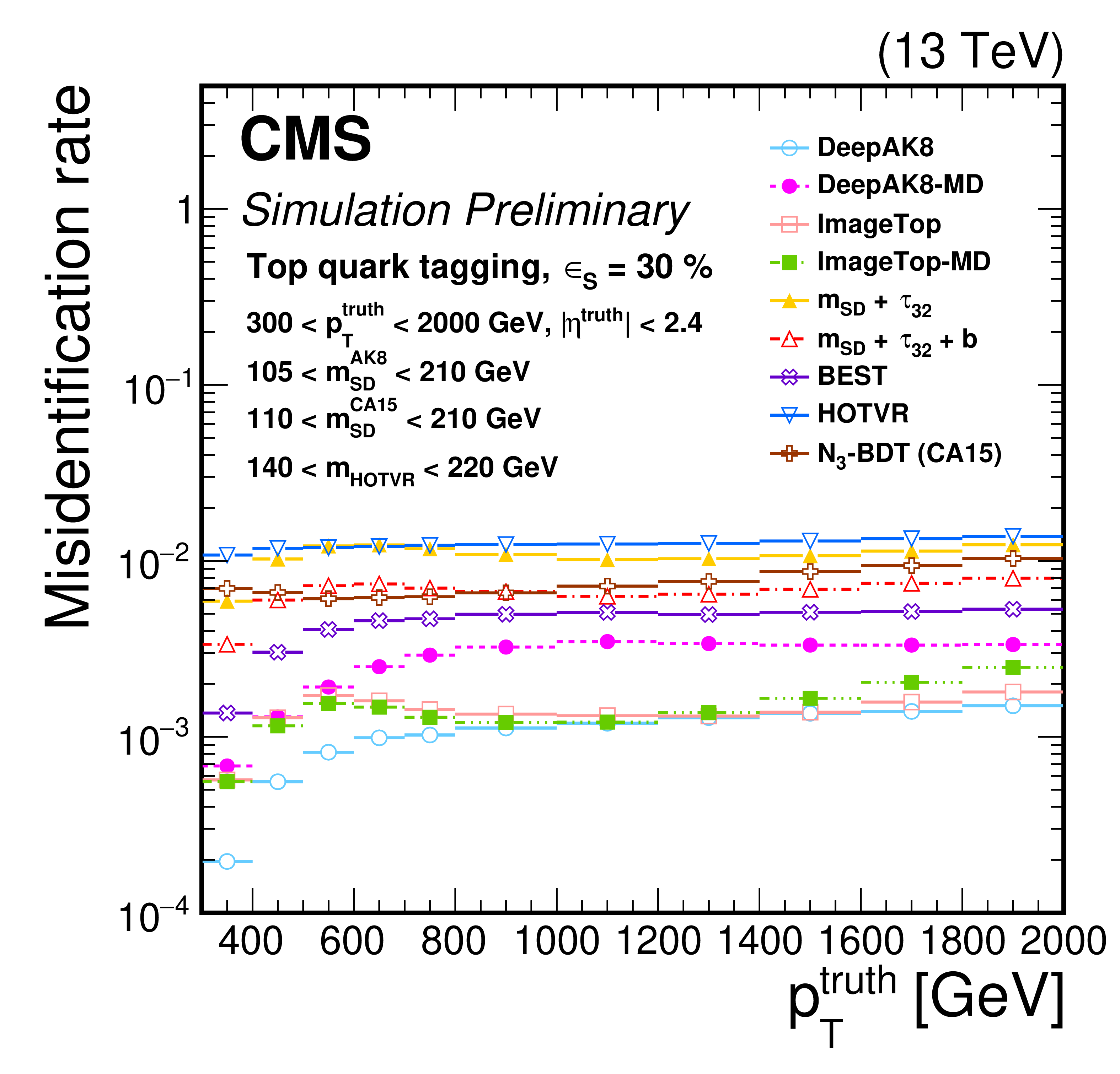
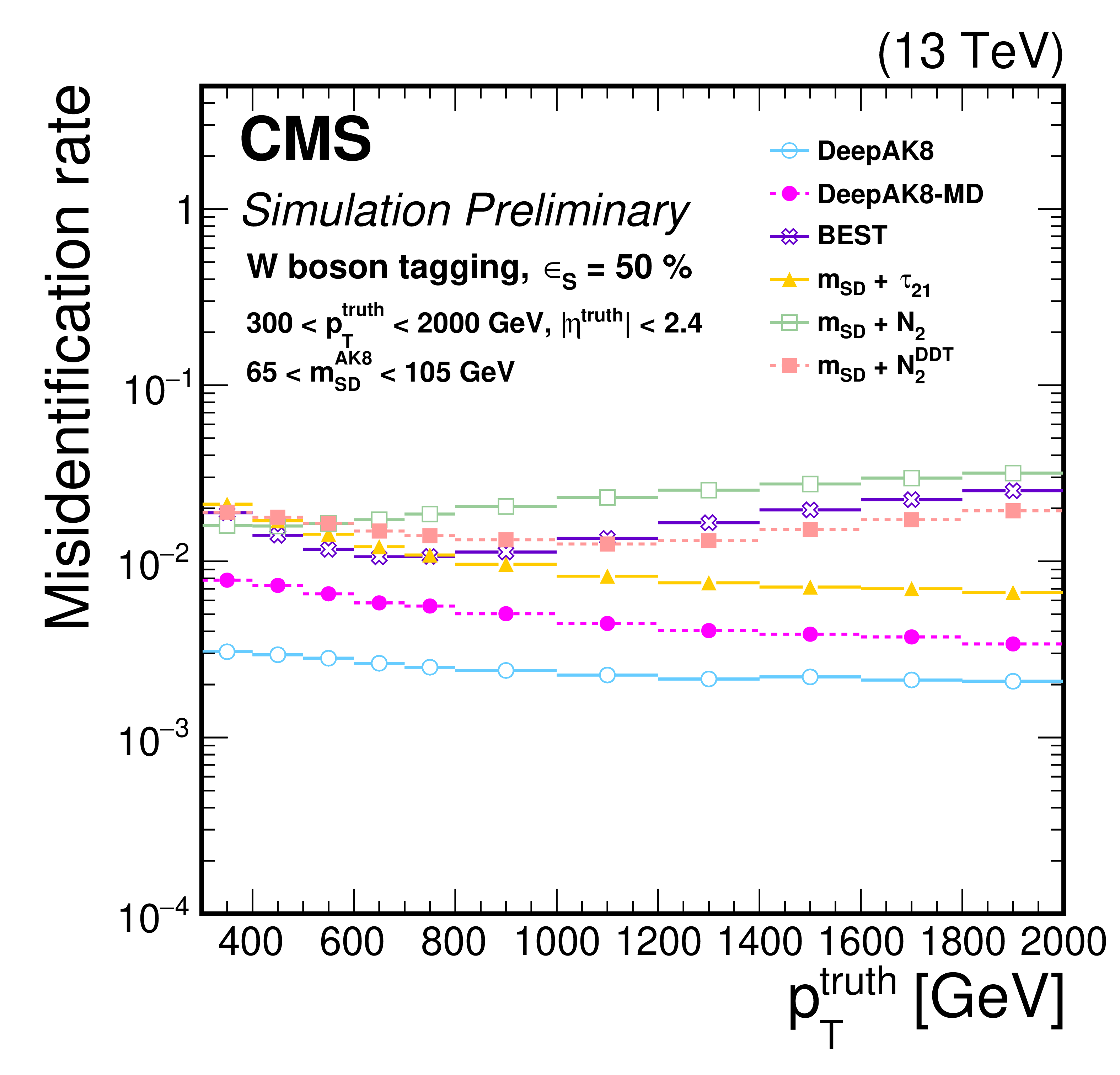
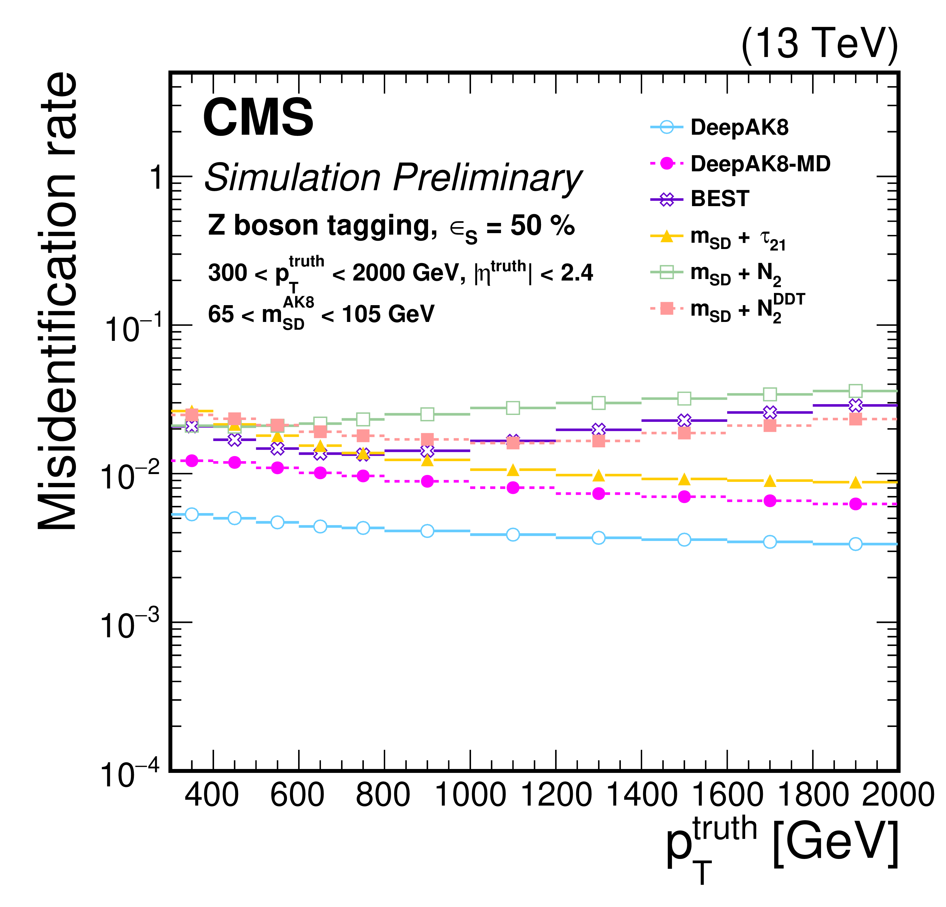
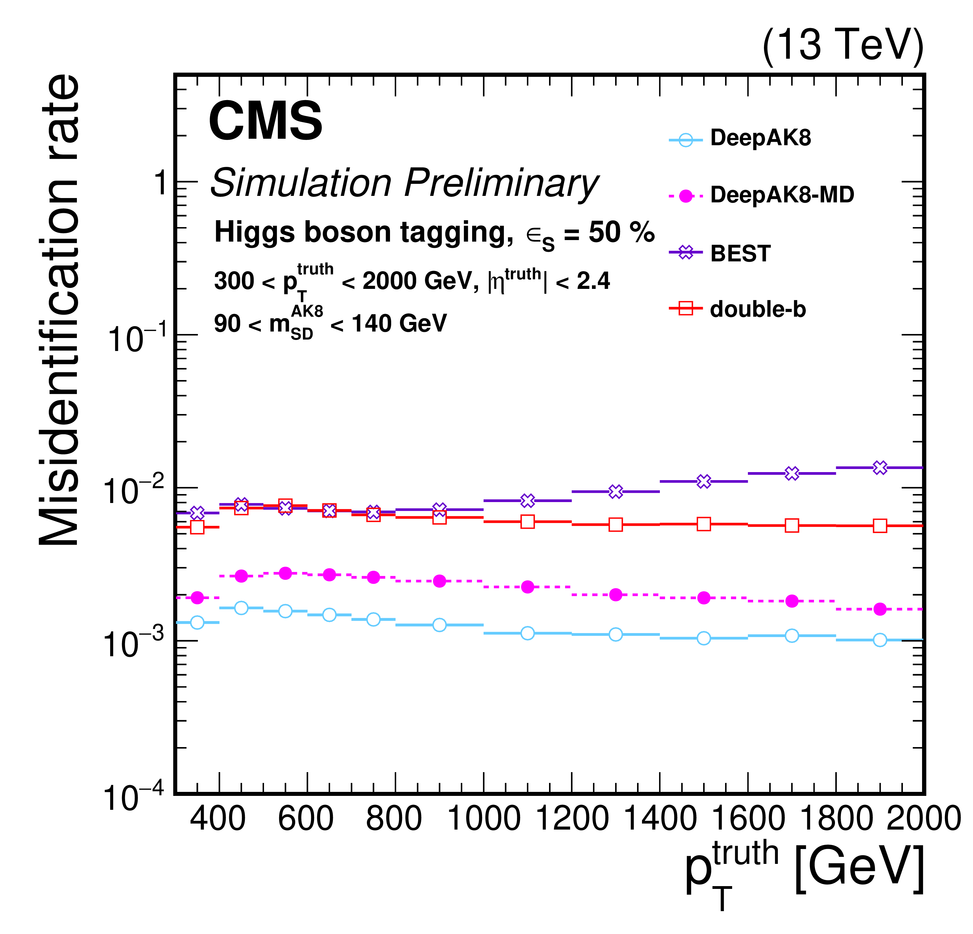
Figure 17:
The distribution of ${\epsilon _{B}}$ as a function of the ${p_{\mathrm {T}}}$ of the truth particle for a working point corresponding to $ {\epsilon _{S}}= $ 30% (50%) for t quark (W, Z, and H boson) identification. Upper left: t quark, upper right: W boson, lower left: Z boson, lower right: H boson. The error bars represent the statistical uncertainty in each specific bin, due to the limited number of simulated events. Additional fiducial selection criteria applied to the jets are displayed on the plots. |
png pdf |
Figure 17-a:
The distribution of ${\epsilon _{B}}$ as a function of the ${p_{\mathrm {T}}}$ of the truth particle for a working point corresponding to $ {\epsilon _{S}}= $ 30% (50%) for t quark (W, Z, and H boson) identification. Upper left: t quark, upper right: W boson, lower left: Z boson, lower right: H boson. The error bars represent the statistical uncertainty in each specific bin, due to the limited number of simulated events. Additional fiducial selection criteria applied to the jets are displayed on the plots. |
png pdf |
Figure 17-b:
The distribution of ${\epsilon _{B}}$ as a function of the ${p_{\mathrm {T}}}$ of the truth particle for a working point corresponding to $ {\epsilon _{S}}= $ 30% (50%) for t quark (W, Z, and H boson) identification. Upper left: t quark, upper right: W boson, lower left: Z boson, lower right: H boson. The error bars represent the statistical uncertainty in each specific bin, due to the limited number of simulated events. Additional fiducial selection criteria applied to the jets are displayed on the plots. |
png pdf |
Figure 17-c:
The distribution of ${\epsilon _{B}}$ as a function of the ${p_{\mathrm {T}}}$ of the truth particle for a working point corresponding to $ {\epsilon _{S}}= $ 30% (50%) for t quark (W, Z, and H boson) identification. Upper left: t quark, upper right: W boson, lower left: Z boson, lower right: H boson. The error bars represent the statistical uncertainty in each specific bin, due to the limited number of simulated events. Additional fiducial selection criteria applied to the jets are displayed on the plots. |
png pdf |
Figure 17-d:
The distribution of ${\epsilon _{B}}$ as a function of the ${p_{\mathrm {T}}}$ of the truth particle for a working point corresponding to $ {\epsilon _{S}}= $ 30% (50%) for t quark (W, Z, and H boson) identification. Upper left: t quark, upper right: W boson, lower left: Z boson, lower right: H boson. The error bars represent the statistical uncertainty in each specific bin, due to the limited number of simulated events. Additional fiducial selection criteria applied to the jets are displayed on the plots. |
png pdf |
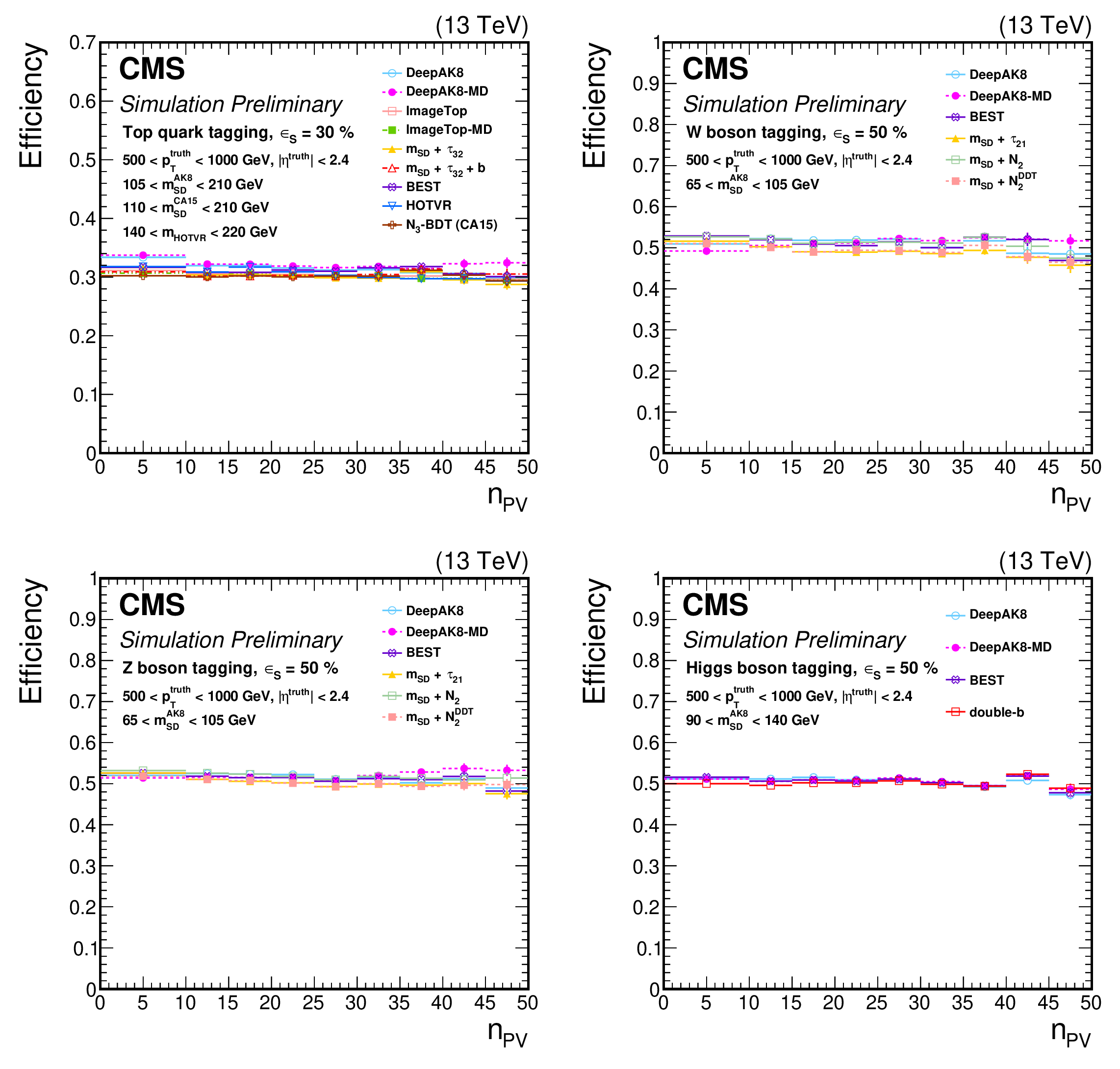
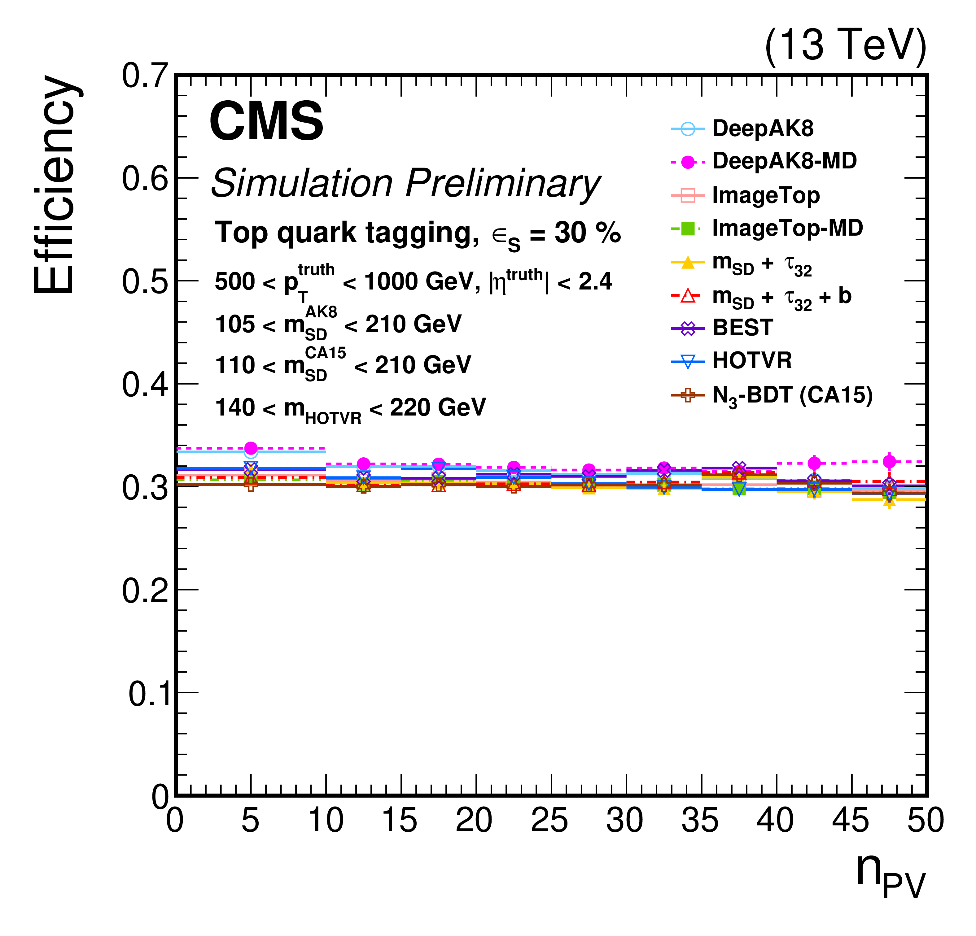
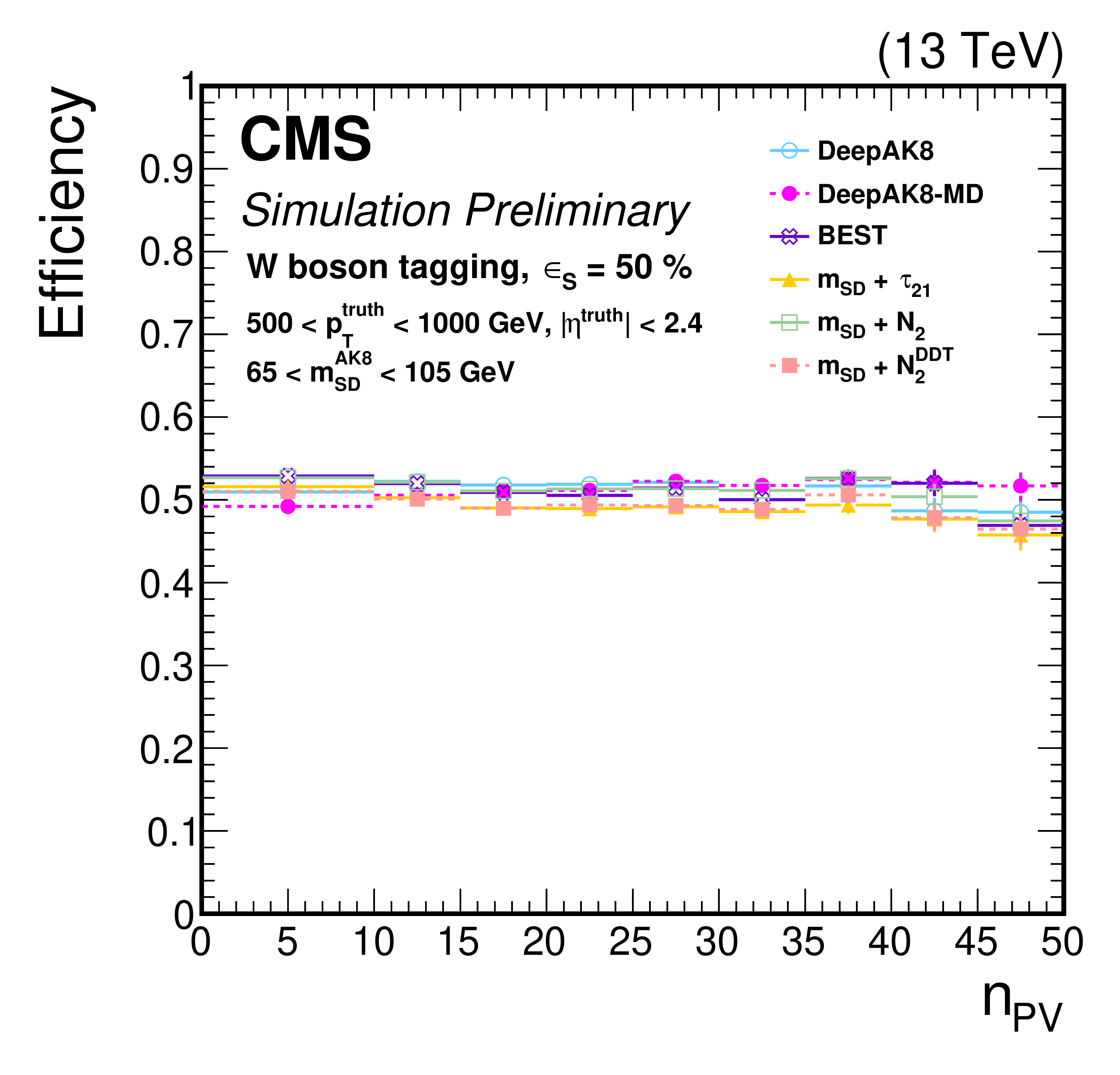
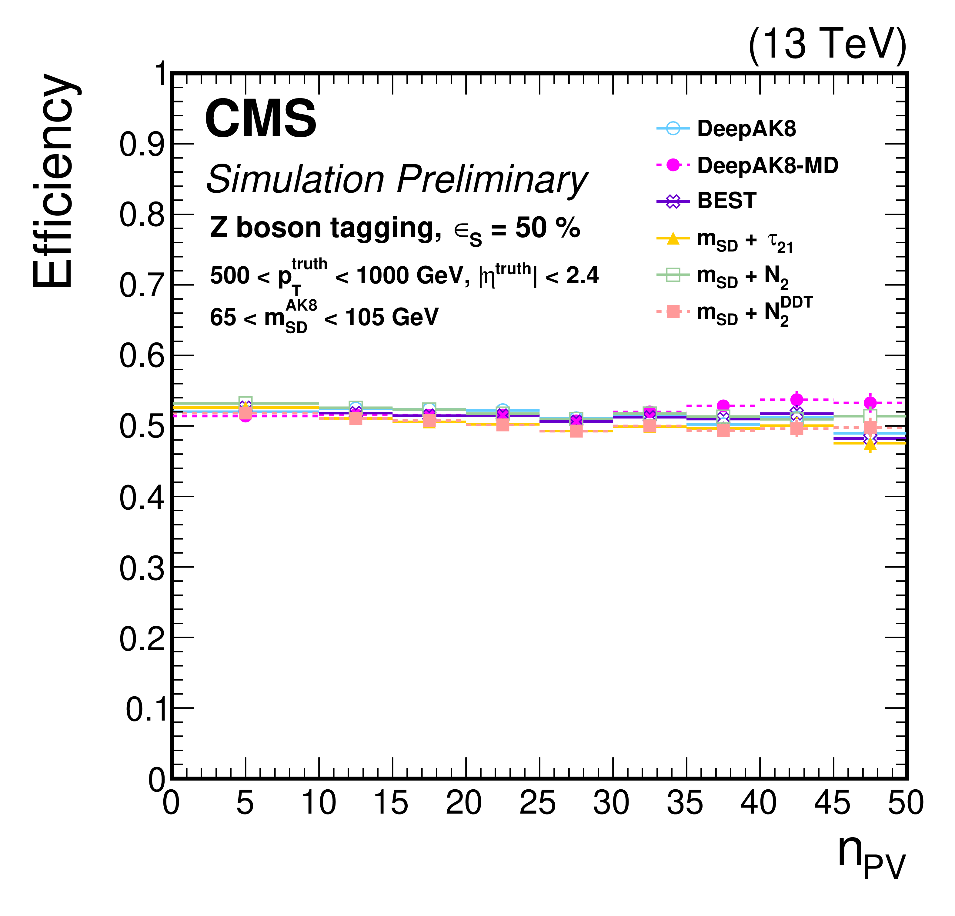
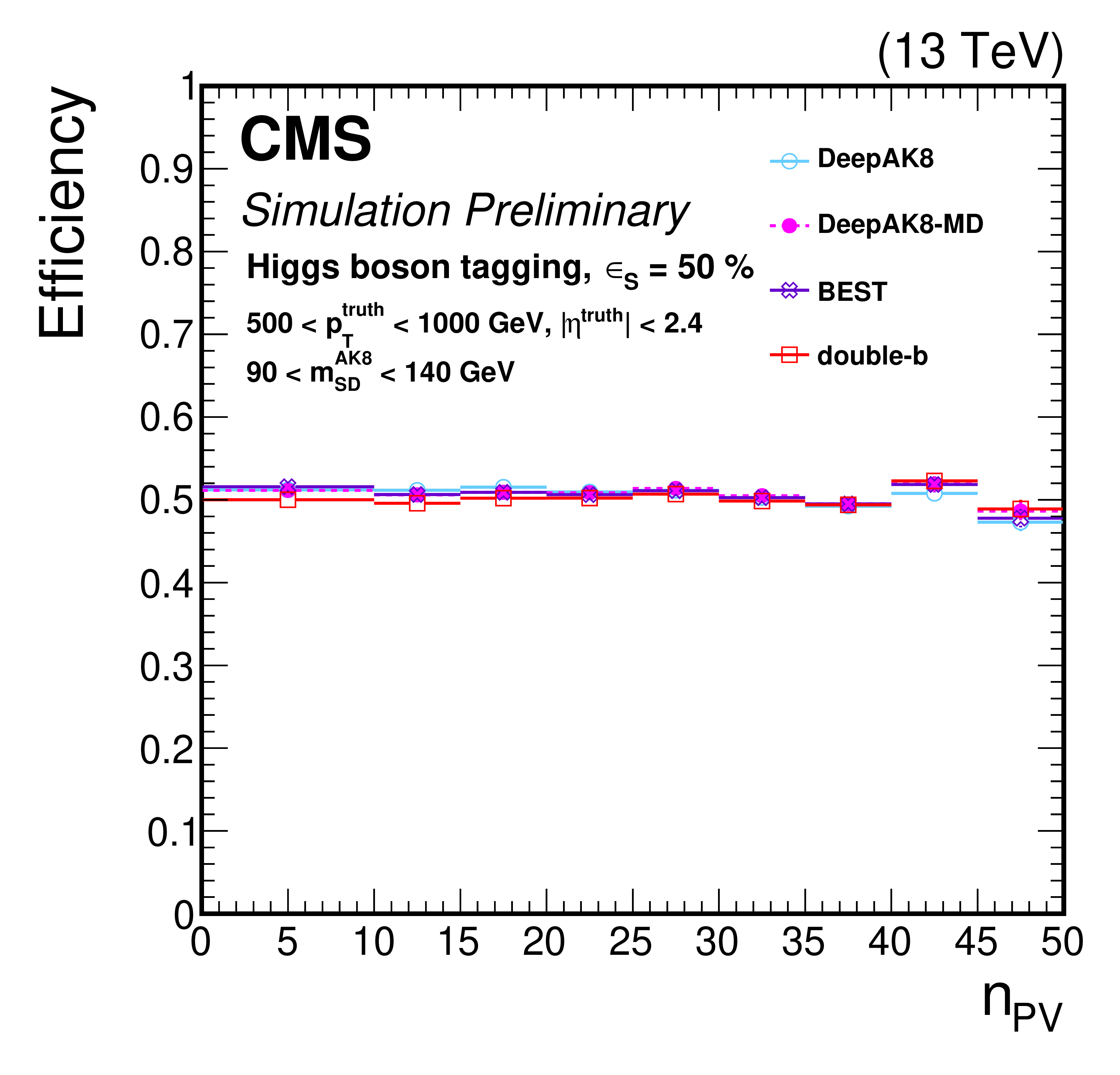
Figure 18:
The ${\epsilon _{S}}$ as a function of ${\text {N}_{\text {vtx}}}$ for truth particles with 500 $ < {p_{\mathrm {T}}} (\text {truth particle}) < $ 1000 GeV at a working point corresponding to $ {\epsilon _{S}}= $ 30% (50%) for t quark (W, Z, and H boson) identification. Upper left: t quark, upper right: W boson, lower left: Z boson, lower right: H boson. The error bars represent the statistical uncertainty in each specific bin, due to a limited number of simulated events. Additional fiducial selection criteria applied to the jets are displayed on the plots. |
png pdf |
Figure 18-a:
The ${\epsilon _{S}}$ as a function of ${\text {N}_{\text {vtx}}}$ for truth particles with 500 $ < {p_{\mathrm {T}}} (\text {truth particle}) < $ 1000 GeV at a working point corresponding to $ {\epsilon _{S}}= $ 30% (50%) for t quark (W, Z, and H boson) identification. Upper left: t quark, upper right: W boson, lower left: Z boson, lower right: H boson. The error bars represent the statistical uncertainty in each specific bin, due to a limited number of simulated events. Additional fiducial selection criteria applied to the jets are displayed on the plots. |
png pdf |
Figure 18-b:
The ${\epsilon _{S}}$ as a function of ${\text {N}_{\text {vtx}}}$ for truth particles with 500 $ < {p_{\mathrm {T}}} (\text {truth particle}) < $ 1000 GeV at a working point corresponding to $ {\epsilon _{S}}= $ 30% (50%) for t quark (W, Z, and H boson) identification. Upper left: t quark, upper right: W boson, lower left: Z boson, lower right: H boson. The error bars represent the statistical uncertainty in each specific bin, due to a limited number of simulated events. Additional fiducial selection criteria applied to the jets are displayed on the plots. |
png pdf |
Figure 18-c:
The ${\epsilon _{S}}$ as a function of ${\text {N}_{\text {vtx}}}$ for truth particles with 500 $ < {p_{\mathrm {T}}} (\text {truth particle}) < $ 1000 GeV at a working point corresponding to $ {\epsilon _{S}}= $ 30% (50%) for t quark (W, Z, and H boson) identification. Upper left: t quark, upper right: W boson, lower left: Z boson, lower right: H boson. The error bars represent the statistical uncertainty in each specific bin, due to a limited number of simulated events. Additional fiducial selection criteria applied to the jets are displayed on the plots. |
png pdf |
Figure 18-d:
The ${\epsilon _{S}}$ as a function of ${\text {N}_{\text {vtx}}}$ for truth particles with 500 $ < {p_{\mathrm {T}}} (\text {truth particle}) < $ 1000 GeV at a working point corresponding to $ {\epsilon _{S}}= $ 30% (50%) for t quark (W, Z, and H boson) identification. Upper left: t quark, upper right: W boson, lower left: Z boson, lower right: H boson. The error bars represent the statistical uncertainty in each specific bin, due to a limited number of simulated events. Additional fiducial selection criteria applied to the jets are displayed on the plots. |
png pdf |
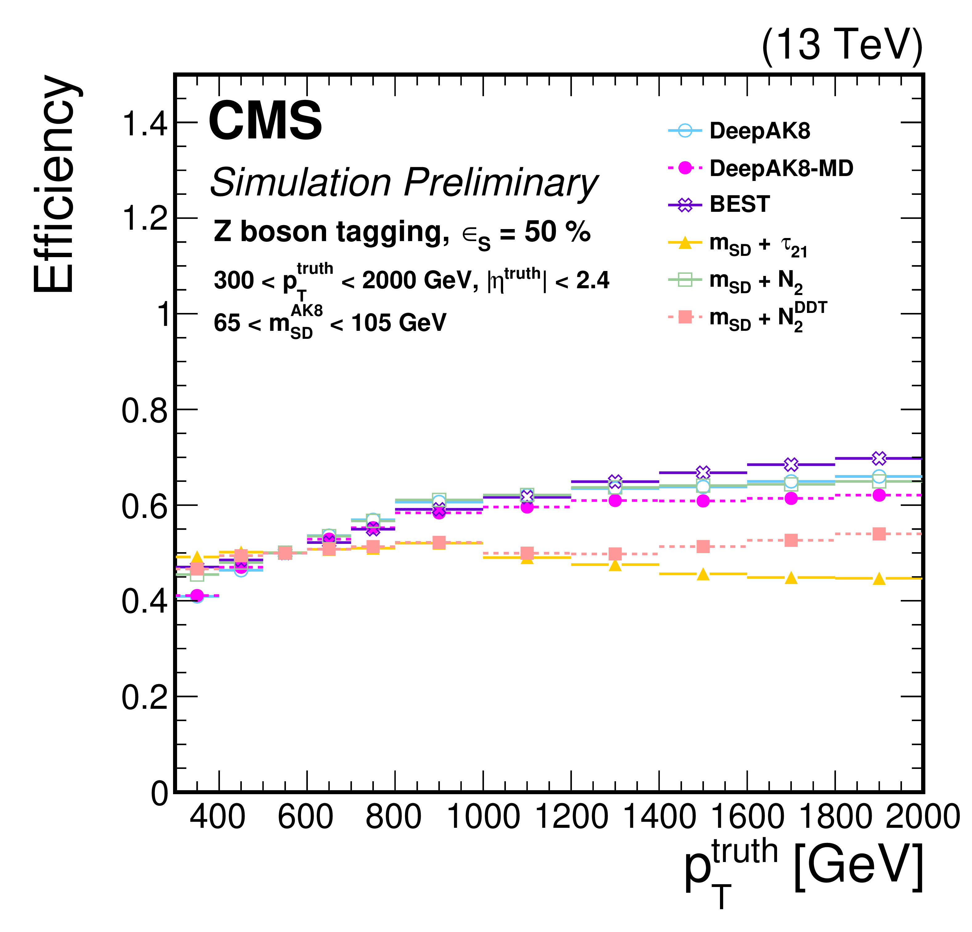
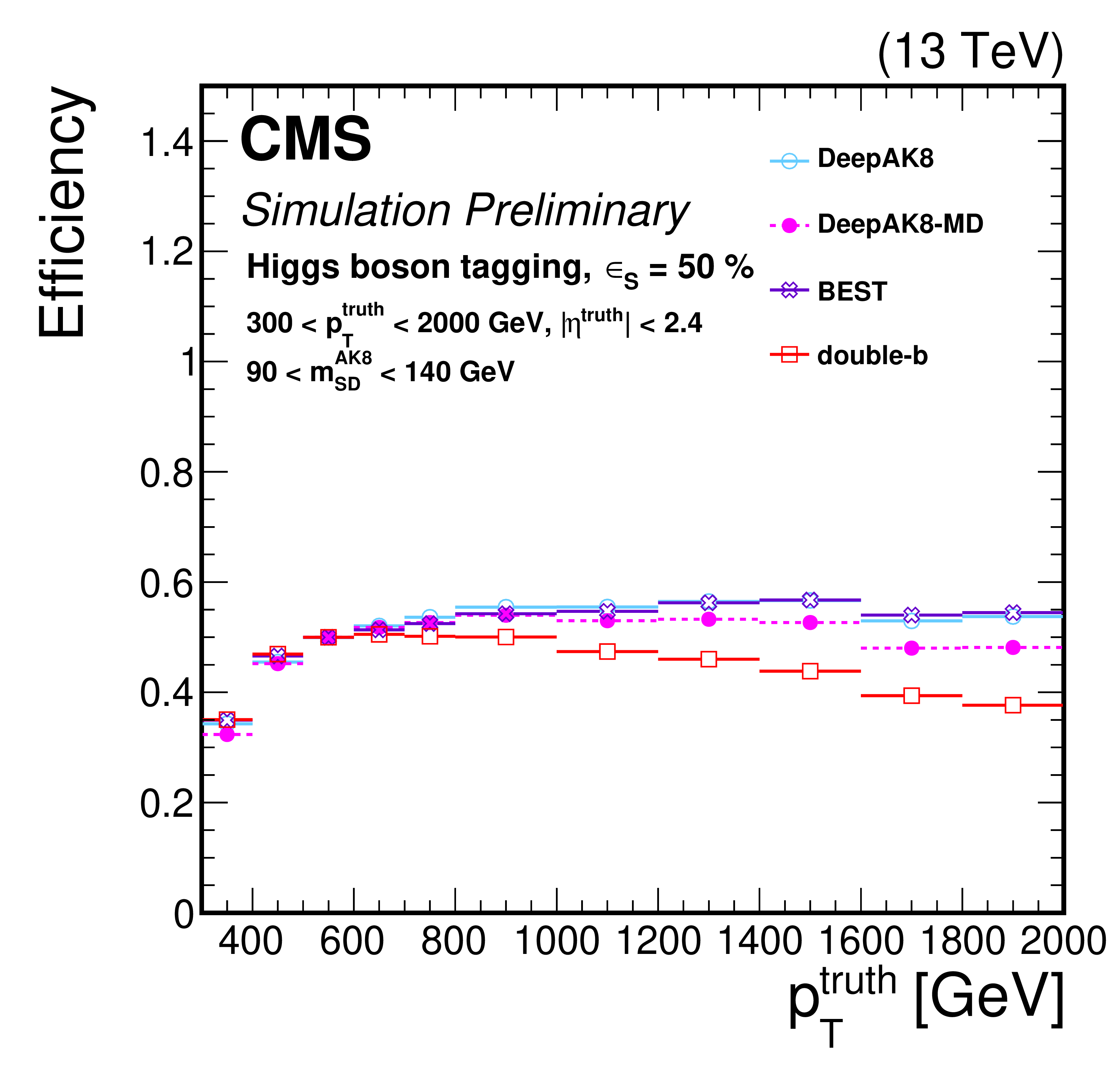
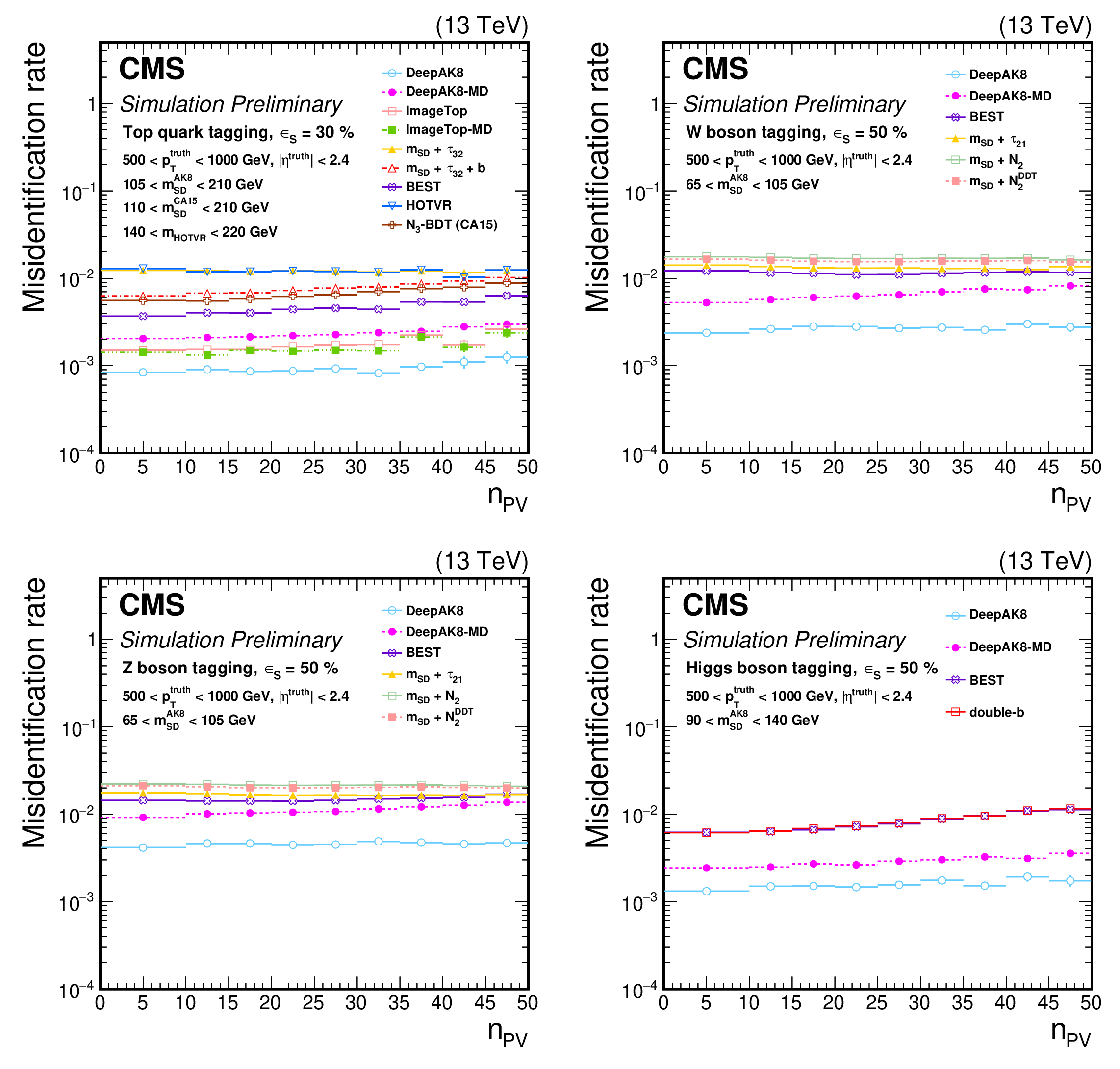
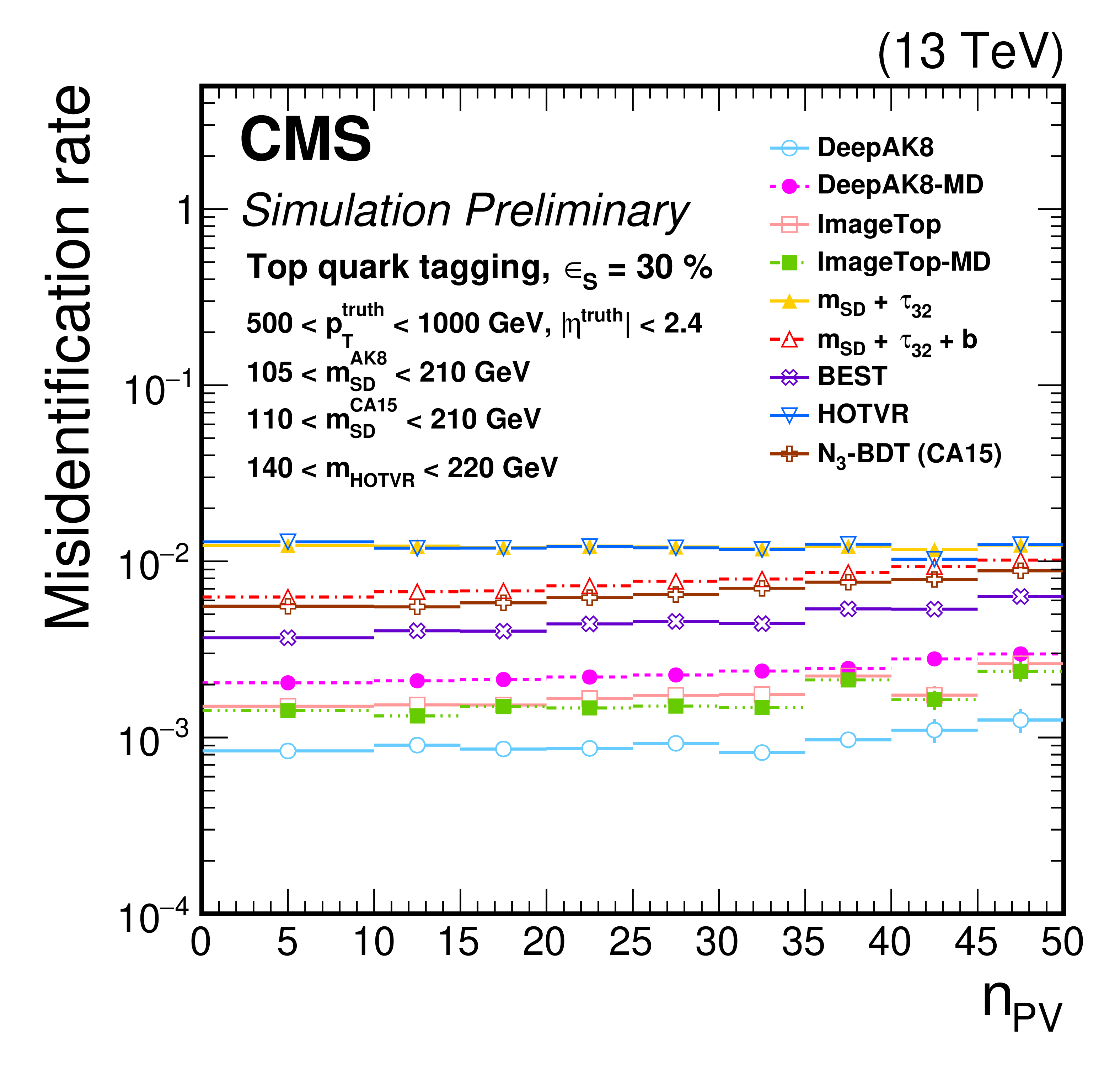
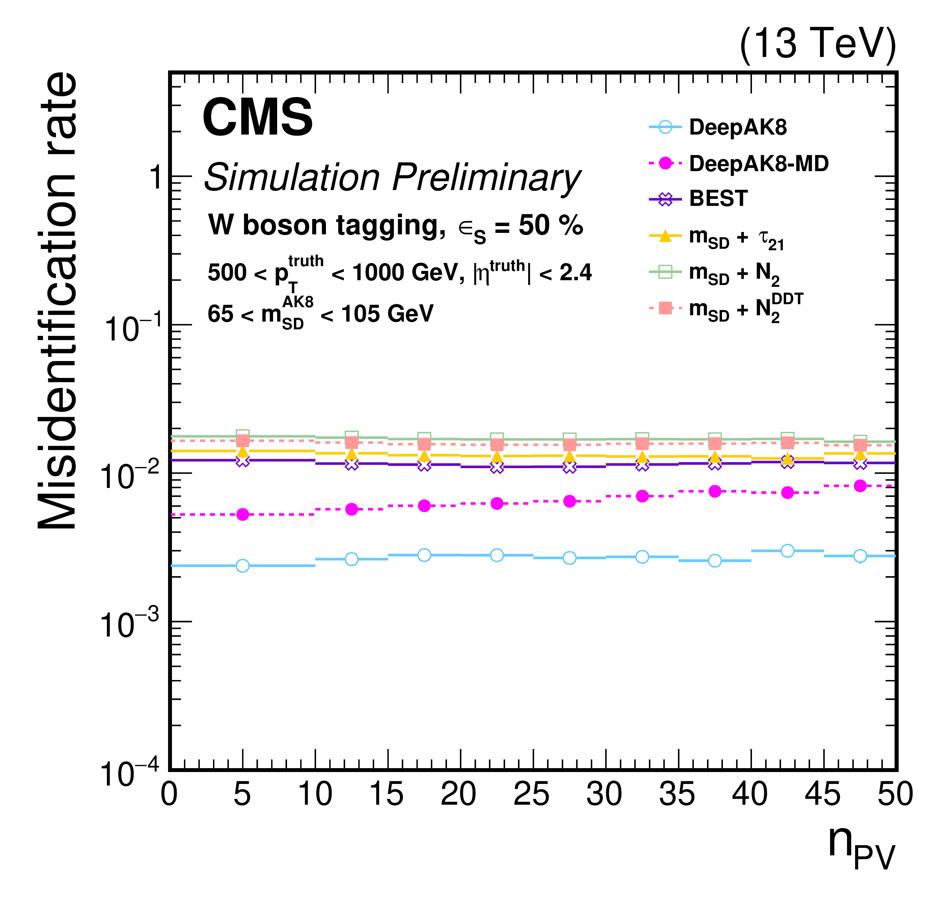
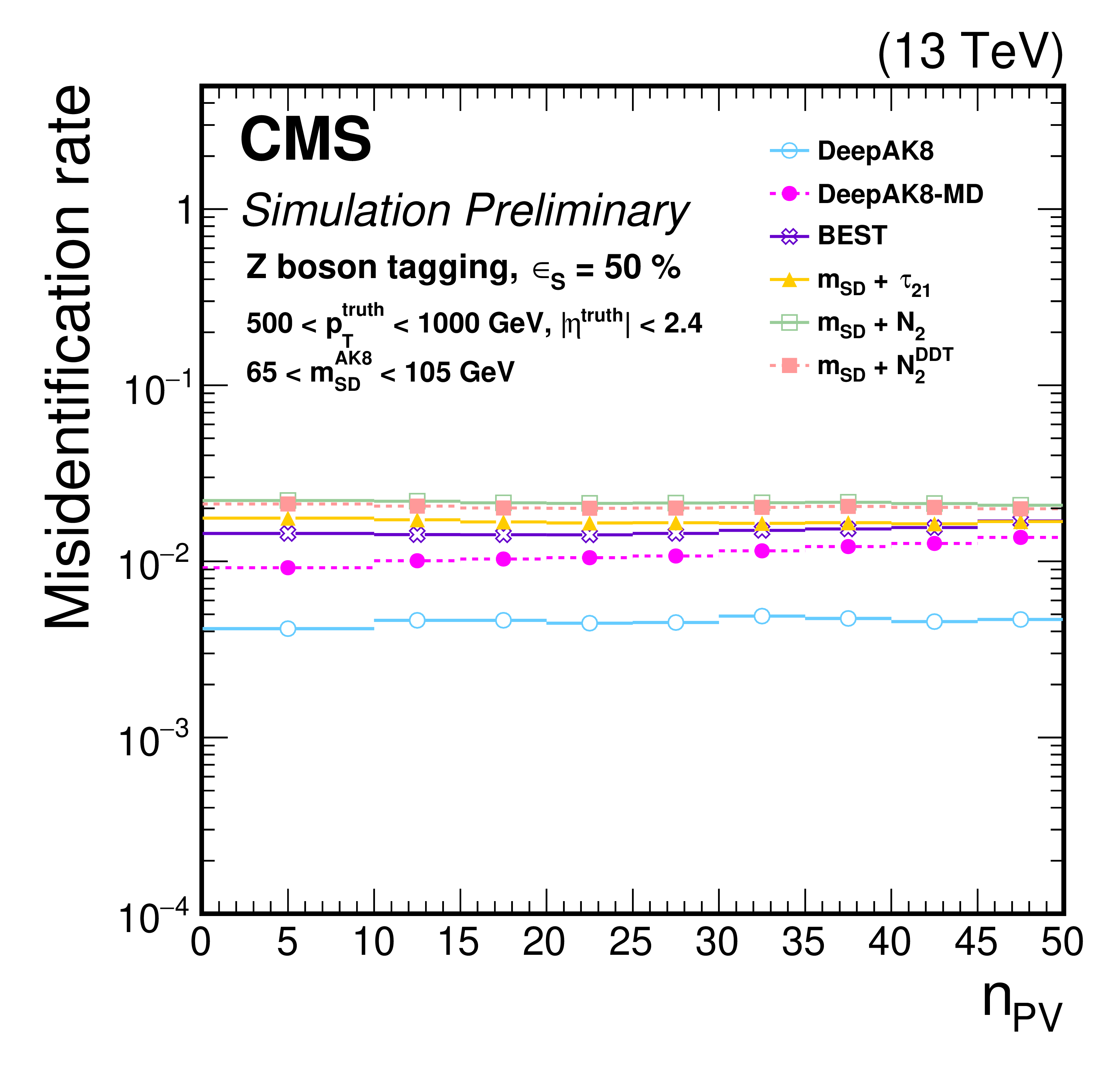
Figure 19:
The ${\epsilon _{B}}$ as a function of ${\text {N}_{\text {vtx}}}$ for truth particles with 500 $ < {p_{\mathrm {T}}} (\text {truth particle}) < $ 1000 GeV at a working point corresponding to $ {\epsilon _{S}}= $ 30% (50%) for t quark (W, Z, and H boson) identification. Upper left: t quark, upper right: W boson, lower left: Z boson, lower right: H boson. The error bars represent the statistical uncertainty in each specific bin, due to the limited number of simulated events. Additional fiducial selection criteria applied to the jets are displayed on the plots. |
png pdf |
Figure 19-a:
The ${\epsilon _{B}}$ as a function of ${\text {N}_{\text {vtx}}}$ for truth particles with 500 $ < {p_{\mathrm {T}}} (\text {truth particle}) < $ 1000 GeV at a working point corresponding to $ {\epsilon _{S}}= $ 30% (50%) for t quark (W, Z, and H boson) identification. Upper left: t quark, upper right: W boson, lower left: Z boson, lower right: H boson. The error bars represent the statistical uncertainty in each specific bin, due to the limited number of simulated events. Additional fiducial selection criteria applied to the jets are displayed on the plots. |
png pdf |
Figure 19-b:
The ${\epsilon _{B}}$ as a function of ${\text {N}_{\text {vtx}}}$ for truth particles with 500 $ < {p_{\mathrm {T}}} (\text {truth particle}) < $ 1000 GeV at a working point corresponding to $ {\epsilon _{S}}= $ 30% (50%) for t quark (W, Z, and H boson) identification. Upper left: t quark, upper right: W boson, lower left: Z boson, lower right: H boson. The error bars represent the statistical uncertainty in each specific bin, due to the limited number of simulated events. Additional fiducial selection criteria applied to the jets are displayed on the plots. |
png pdf |
Figure 19-c:
The ${\epsilon _{B}}$ as a function of ${\text {N}_{\text {vtx}}}$ for truth particles with 500 $ < {p_{\mathrm {T}}} (\text {truth particle}) < $ 1000 GeV at a working point corresponding to $ {\epsilon _{S}}= $ 30% (50%) for t quark (W, Z, and H boson) identification. Upper left: t quark, upper right: W boson, lower left: Z boson, lower right: H boson. The error bars represent the statistical uncertainty in each specific bin, due to the limited number of simulated events. Additional fiducial selection criteria applied to the jets are displayed on the plots. |

png pdf |
Figure 19-d:
The ${\epsilon _{B}}$ as a function of ${\text {N}_{\text {vtx}}}$ for truth particles with 500 $ < {p_{\mathrm {T}}} (\text {truth particle}) < $ 1000 GeV at a working point corresponding to $ {\epsilon _{S}}= $ 30% (50%) for t quark (W, Z, and H boson) identification. Upper left: t quark, upper right: W boson, lower left: Z boson, lower right: H boson. The error bars represent the statistical uncertainty in each specific bin, due to the limited number of simulated events. Additional fiducial selection criteria applied to the jets are displayed on the plots. |
png pdf |
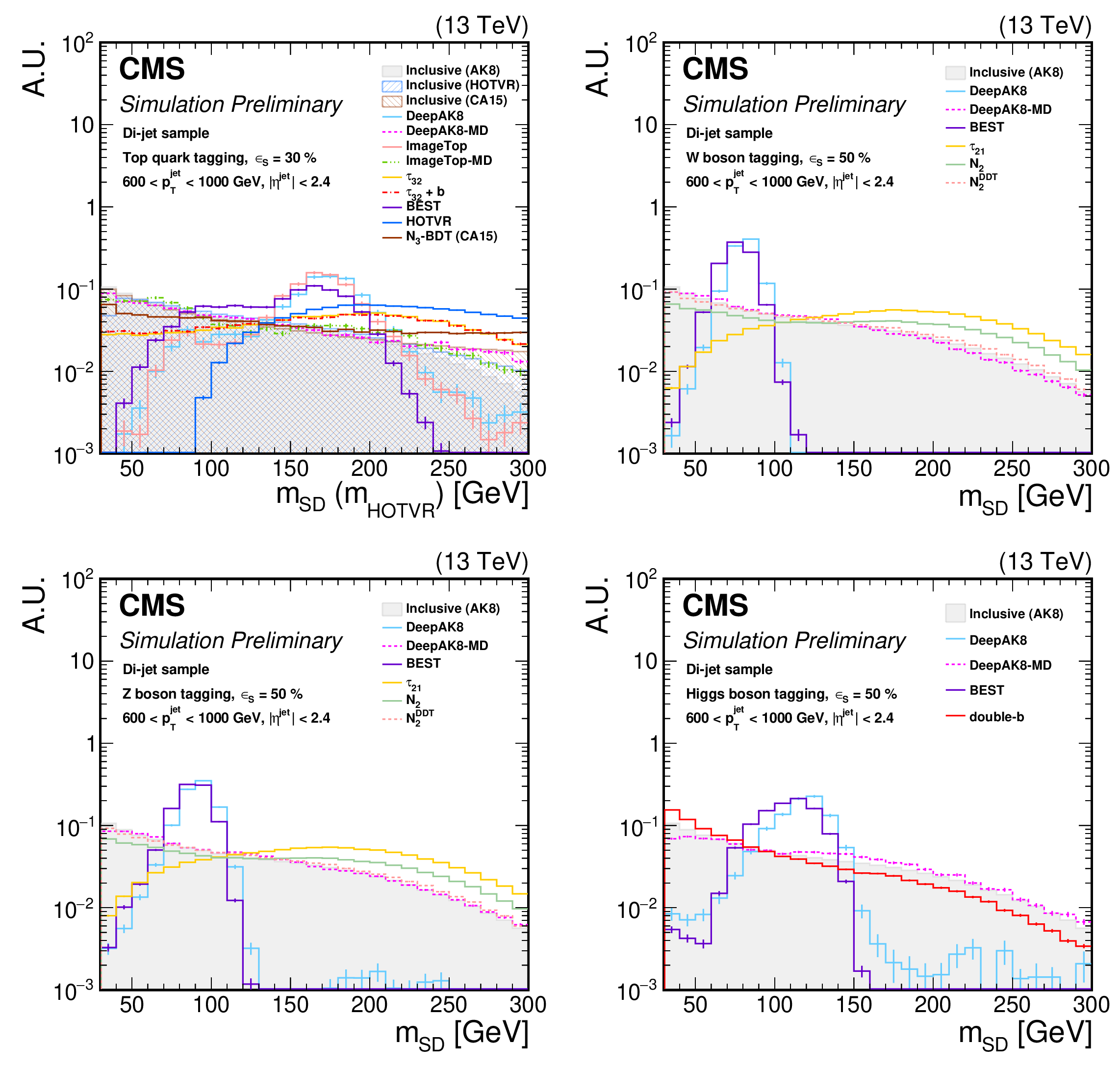
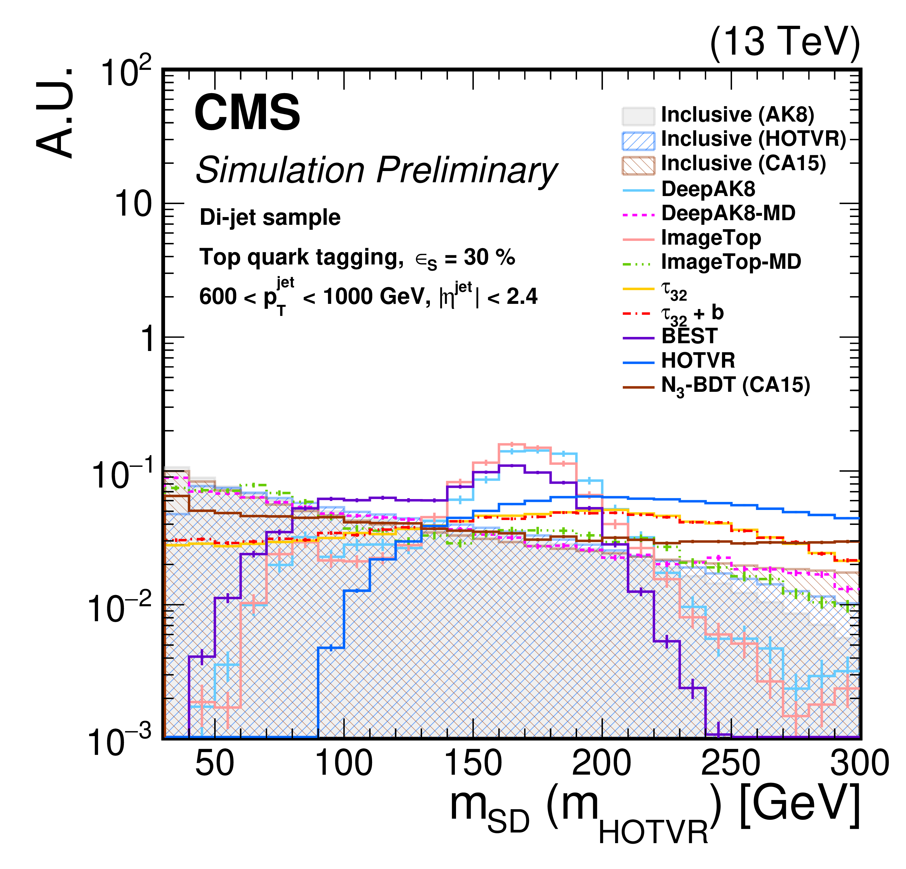
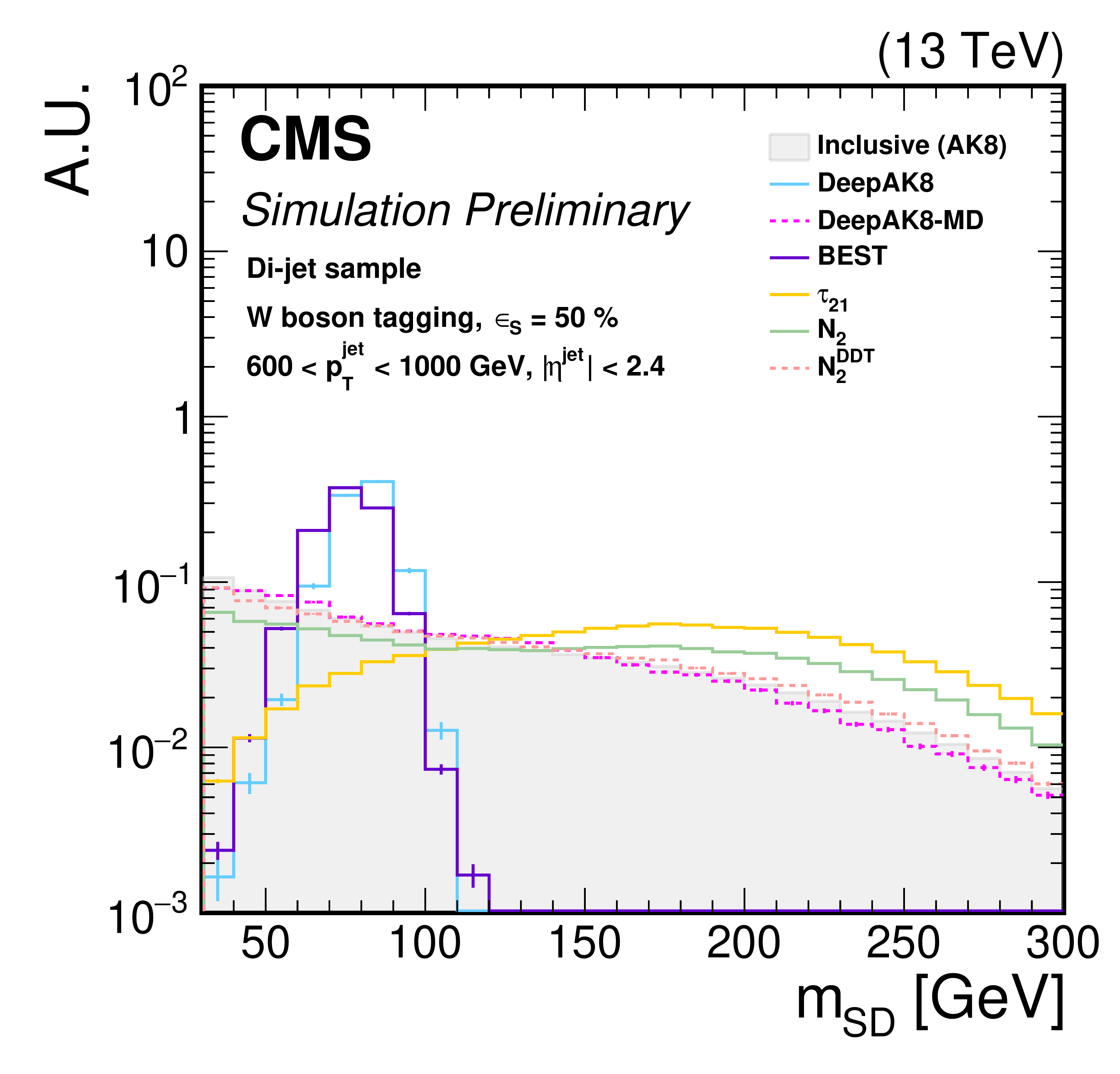
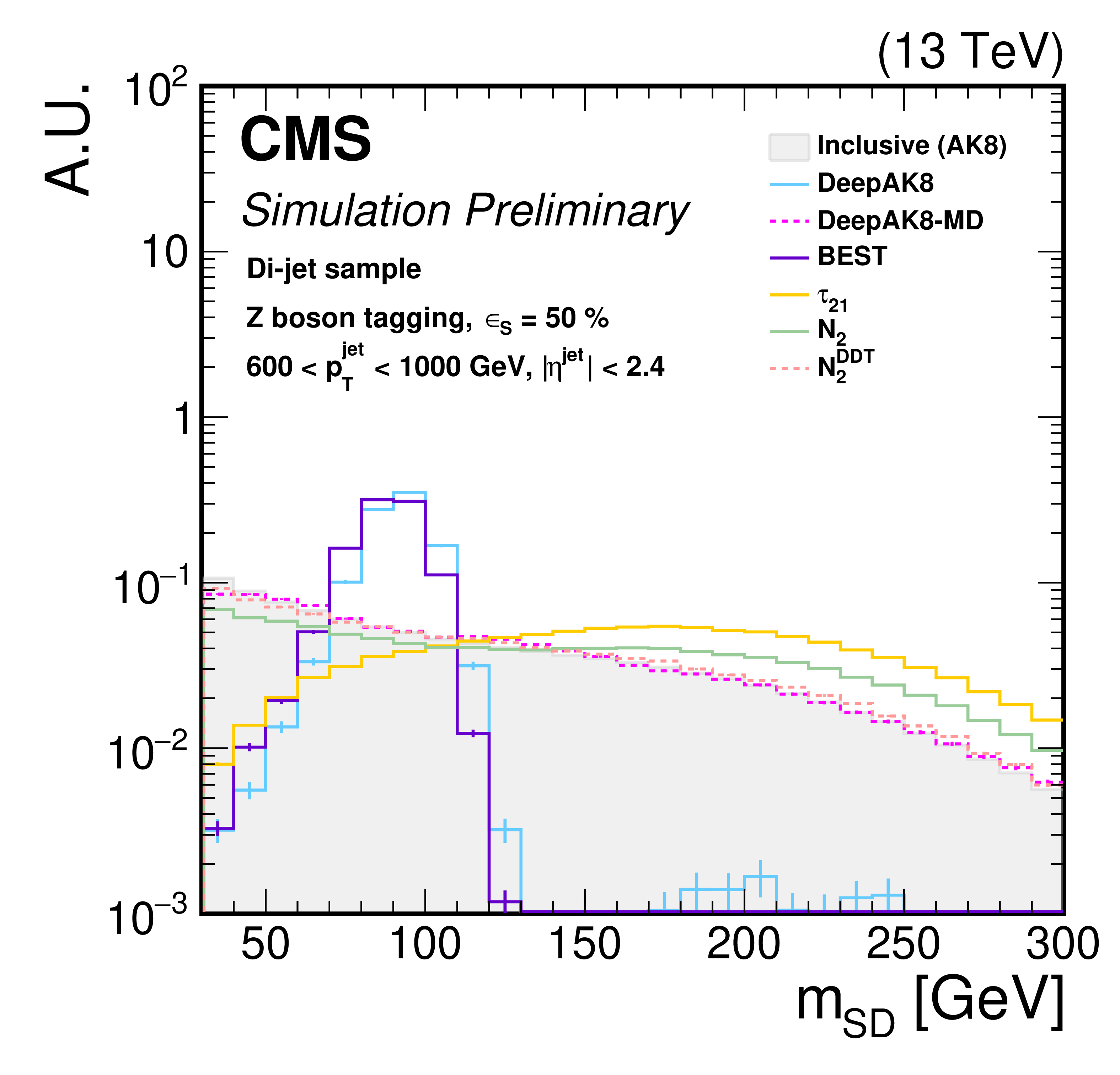
Figure 20:
The shape of the softdrop mass distribution for background jets with 600 $ < {p_{\mathrm {T}}} (\text {jet}) < $ 1000 GeV, inclusively and after selection by each algorithm. The working point chosen corresponds to $ {\epsilon _{S}}=$ 30% ($ {\epsilon _{S}}=$ 50%) for t quarks (W, Z, and H bosons). Upper left: t quark, upper right: W boson, lower left: Z boson, lower right: H boson. The error bars represent the statistical uncertainty in each specific bin, due to the limited number of simulated events. Additional fiducial selection criteria applied to the jets are displayed on the plots. |
png pdf |
Figure 20-a:
The shape of the softdrop mass distribution for background jets with 600 $ < {p_{\mathrm {T}}} (\text {jet}) < $ 1000 GeV, inclusively and after selection by each algorithm. The working point chosen corresponds to $ {\epsilon _{S}}=$ 30% ($ {\epsilon _{S}}=$ 50%) for t quarks (W, Z, and H bosons). Upper left: t quark, upper right: W boson, lower left: Z boson, lower right: H boson. The error bars represent the statistical uncertainty in each specific bin, due to the limited number of simulated events. Additional fiducial selection criteria applied to the jets are displayed on the plots. |
png pdf |
Figure 20-b:
The shape of the softdrop mass distribution for background jets with 600 $ < {p_{\mathrm {T}}} (\text {jet}) < $ 1000 GeV, inclusively and after selection by each algorithm. The working point chosen corresponds to $ {\epsilon _{S}}=$ 30% ($ {\epsilon _{S}}=$ 50%) for t quarks (W, Z, and H bosons). Upper left: t quark, upper right: W boson, lower left: Z boson, lower right: H boson. The error bars represent the statistical uncertainty in each specific bin, due to the limited number of simulated events. Additional fiducial selection criteria applied to the jets are displayed on the plots. |
png pdf |
Figure 20-c:
The shape of the softdrop mass distribution for background jets with 600 $ < {p_{\mathrm {T}}} (\text {jet}) < $ 1000 GeV, inclusively and after selection by each algorithm. The working point chosen corresponds to $ {\epsilon _{S}}=$ 30% ($ {\epsilon _{S}}=$ 50%) for t quarks (W, Z, and H bosons). Upper left: t quark, upper right: W boson, lower left: Z boson, lower right: H boson. The error bars represent the statistical uncertainty in each specific bin, due to the limited number of simulated events. Additional fiducial selection criteria applied to the jets are displayed on the plots. |
png pdf |
Figure 20-d:
The shape of the softdrop mass distribution for background jets with 600 $ < {p_{\mathrm {T}}} (\text {jet}) < $ 1000 GeV, inclusively and after selection by each algorithm. The working point chosen corresponds to $ {\epsilon _{S}}=$ 30% ($ {\epsilon _{S}}=$ 50%) for t quarks (W, Z, and H bosons). Upper left: t quark, upper right: W boson, lower left: Z boson, lower right: H boson. The error bars represent the statistical uncertainty in each specific bin, due to the limited number of simulated events. Additional fiducial selection criteria applied to the jets are displayed on the plots. |
png pdf |
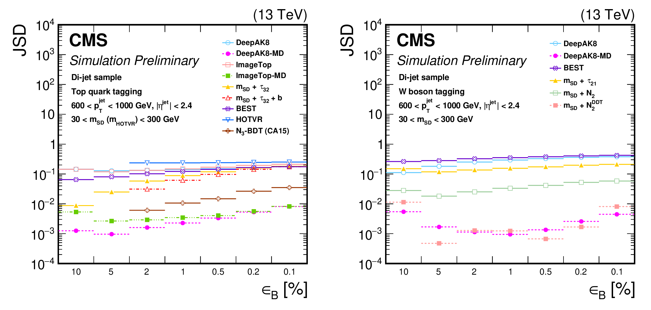
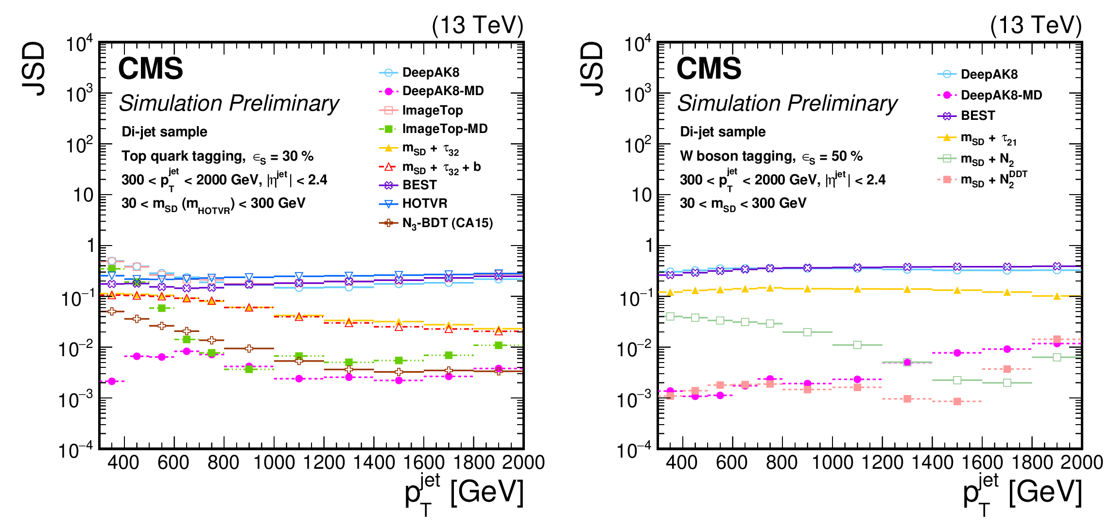
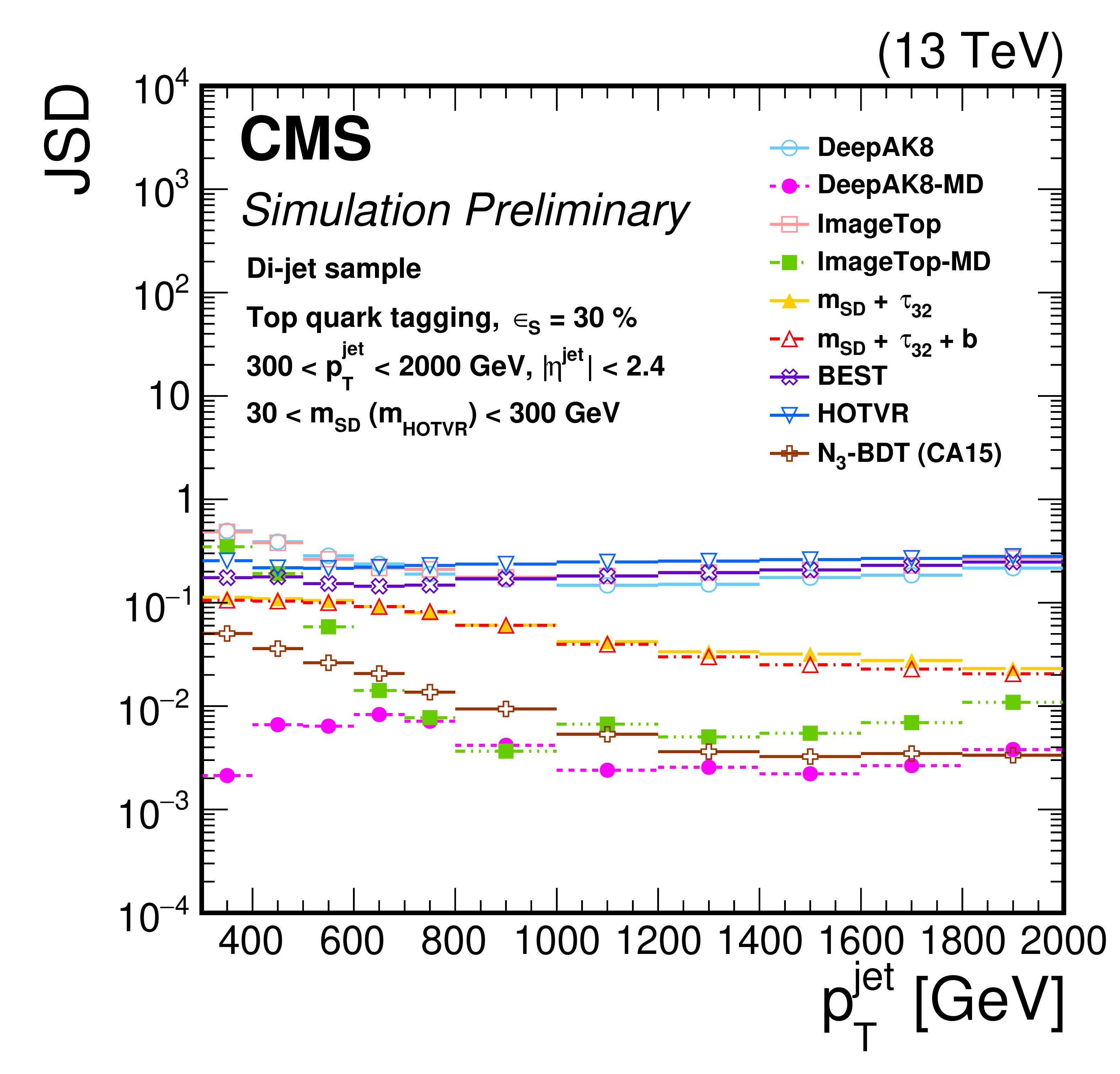
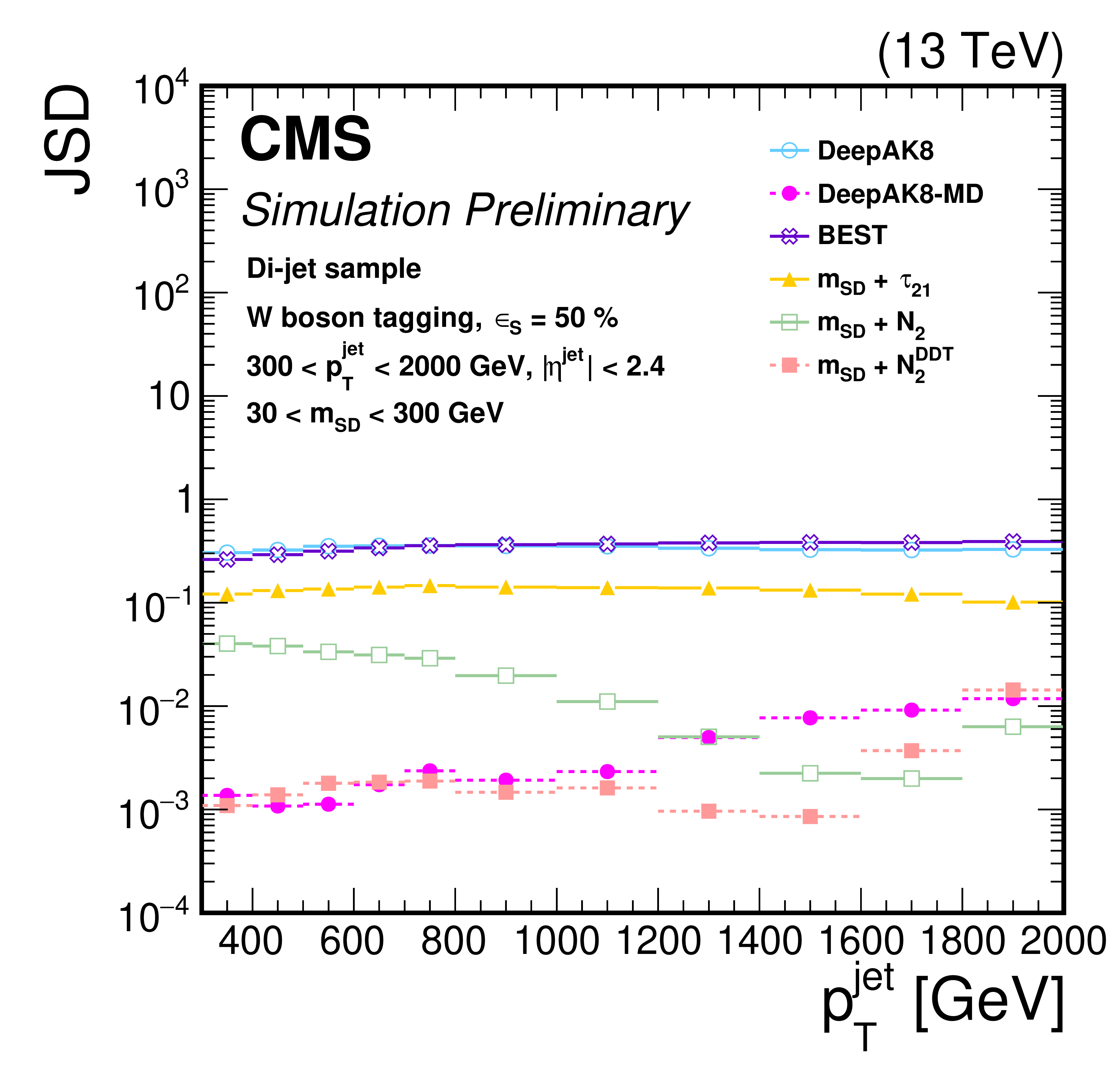
Figure 21:
The JSD as a function of successively tighter selections (expressed in terms of ${\epsilon _{B}}$) for the various t - (left) and W (right) tagging algorithms. Lower values of JSD indicate larger similarity of the $M { _{SD}}$ in QCD multijet events passing and failing the selection on the tagging algorithm. Additional fiducial selection criteria applied to the jets are displayed on the plots. |
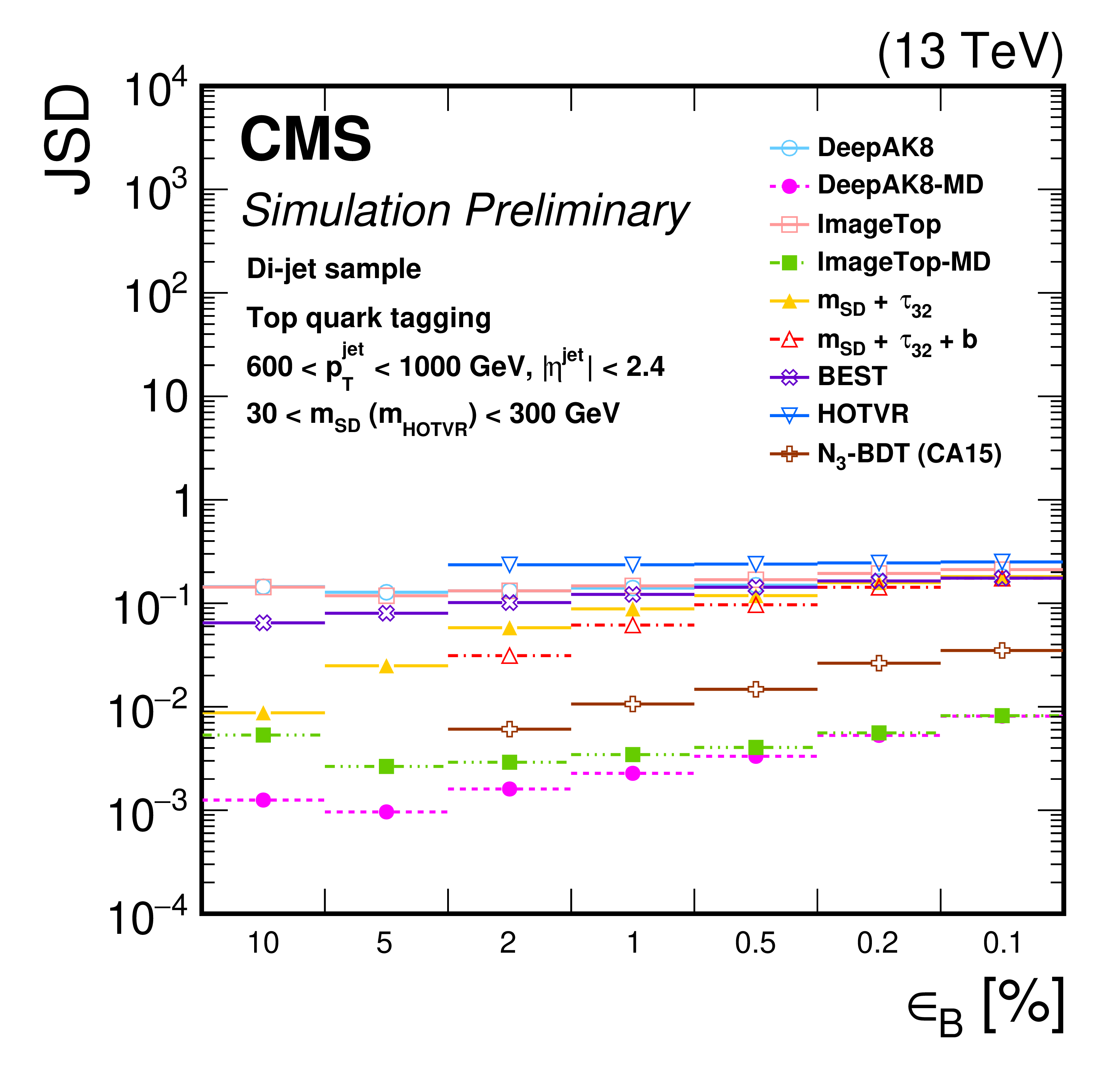
png pdf |
Figure 21-a:
The JSD as a function of successively tighter selections (expressed in terms of ${\epsilon _{B}}$) for the various t - (left) and W (right) tagging algorithms. Lower values of JSD indicate larger similarity of the $M { _{SD}}$ in QCD multijet events passing and failing the selection on the tagging algorithm. Additional fiducial selection criteria applied to the jets are displayed on the plots. |
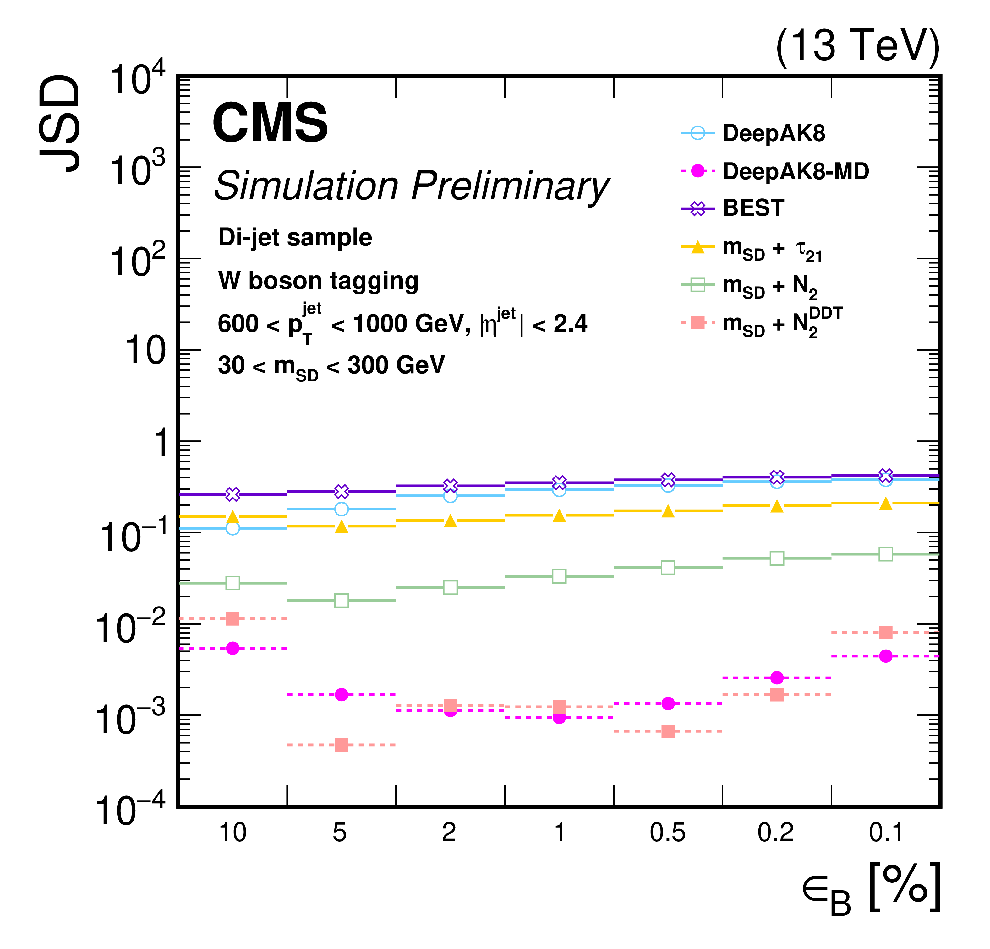
png pdf |
Figure 21-b:
The JSD as a function of successively tighter selections (expressed in terms of ${\epsilon _{B}}$) for the various t - (left) and W (right) tagging algorithms. Lower values of JSD indicate larger similarity of the $M { _{SD}}$ in QCD multijet events passing and failing the selection on the tagging algorithm. Additional fiducial selection criteria applied to the jets are displayed on the plots. |
png pdf |
Figure 22:
The JSD as a function of the jet ${p_{\mathrm {T}}}$ for the various t (left) and W (right) tagging algorithms. Lower values of JSD indicate larger similarity of the $M { _{SD}}$ in QCD multijet events passing and failing the selection on the tagging algorithm. Additional fiducial selection criteria applied to the jets are displayed on the plots. |
png pdf |
Figure 22-a:
The JSD as a function of the jet ${p_{\mathrm {T}}}$ for the various t (left) and W (right) tagging algorithms. Lower values of JSD indicate larger similarity of the $M { _{SD}}$ in QCD multijet events passing and failing the selection on the tagging algorithm. Additional fiducial selection criteria applied to the jets are displayed on the plots. |
png pdf |
Figure 22-b:
The JSD as a function of the jet ${p_{\mathrm {T}}}$ for the various t (left) and W (right) tagging algorithms. Lower values of JSD indicate larger similarity of the $M { _{SD}}$ in QCD multijet events passing and failing the selection on the tagging algorithm. Additional fiducial selection criteria applied to the jets are displayed on the plots. |

png pdf |
Figure 23:
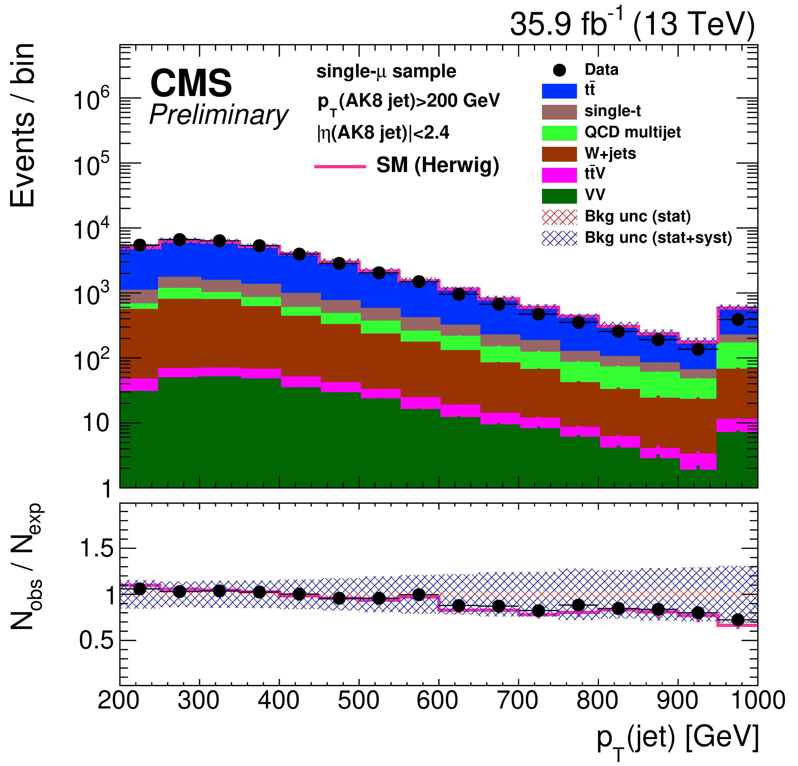
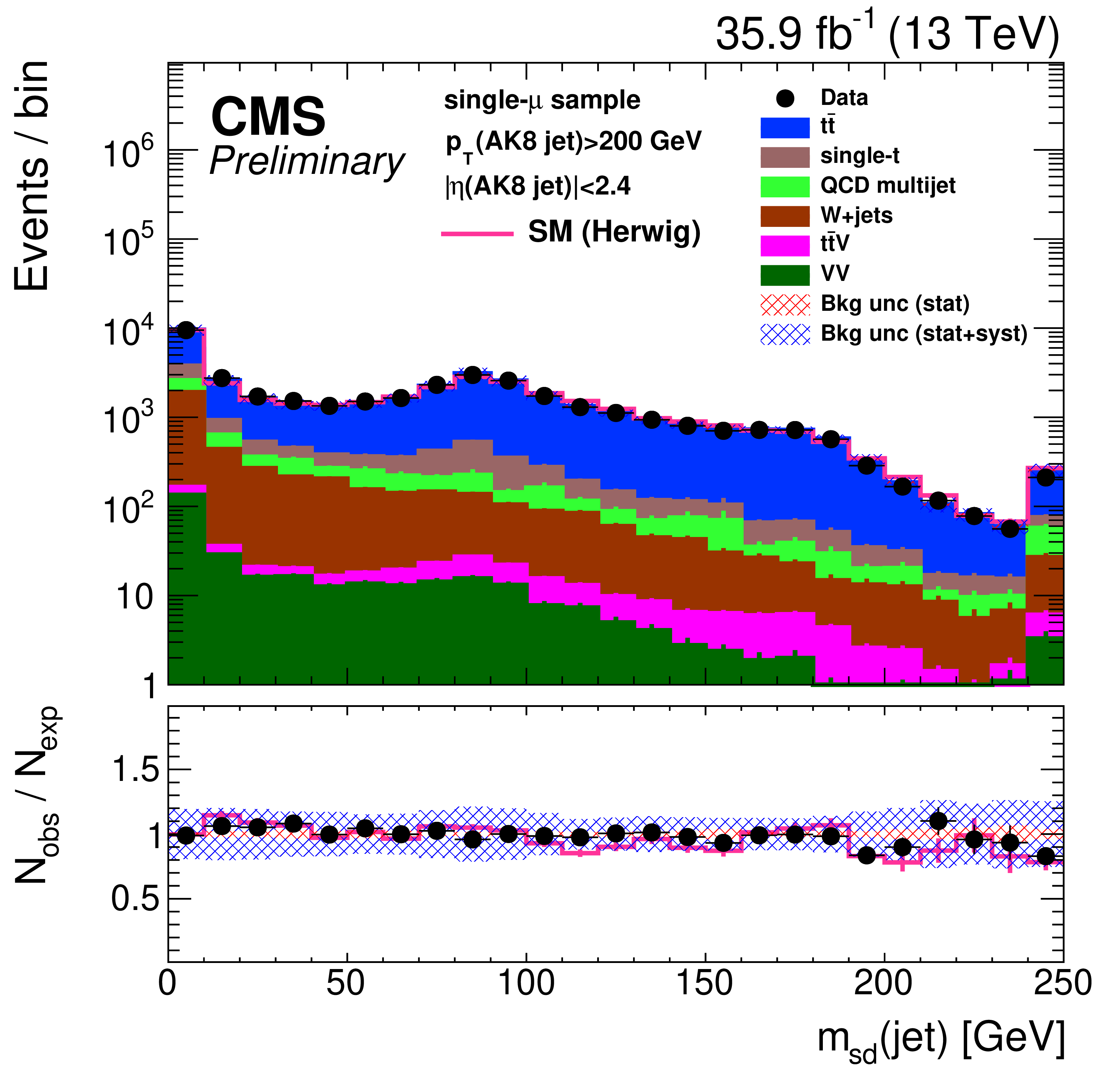
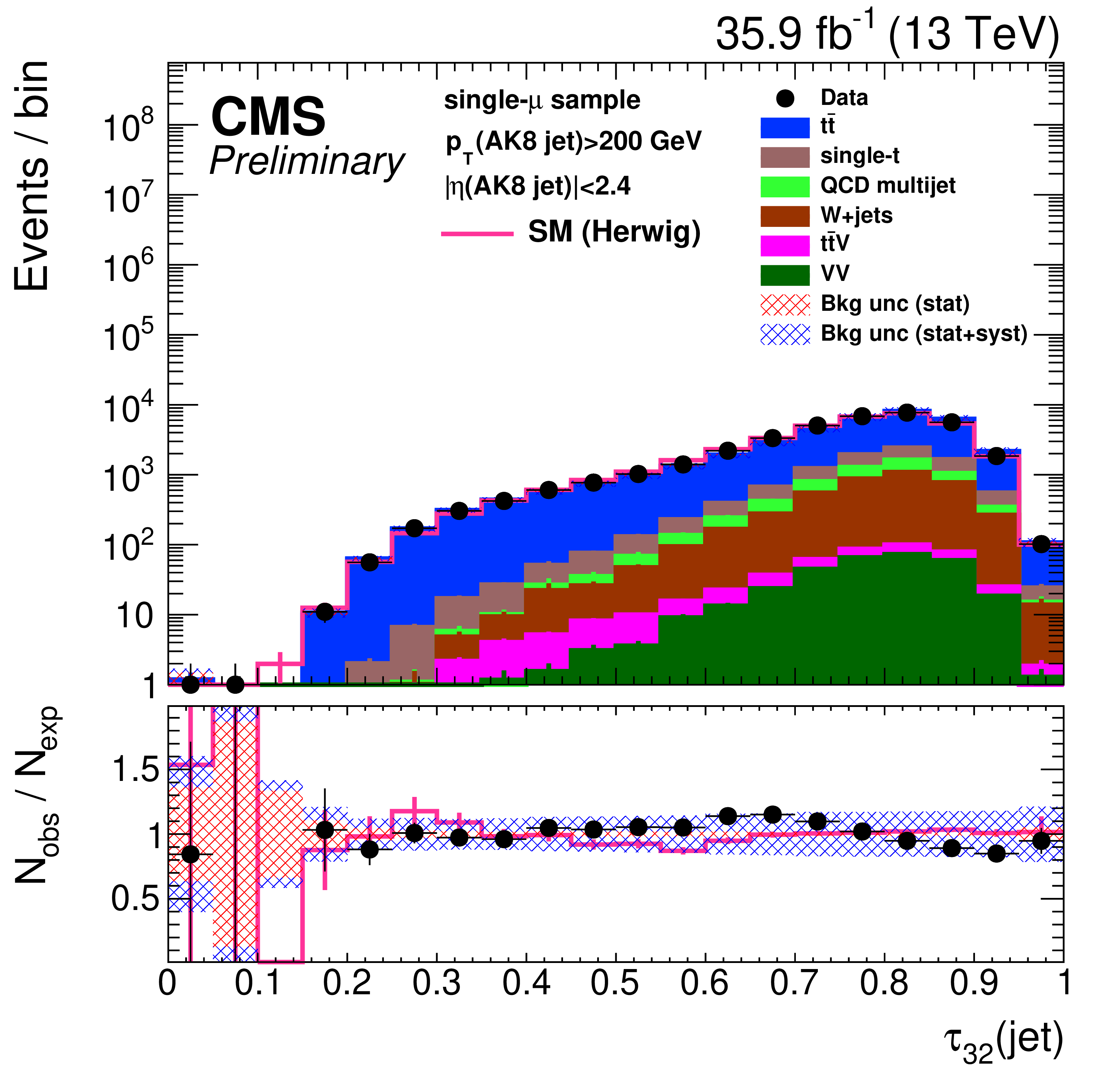
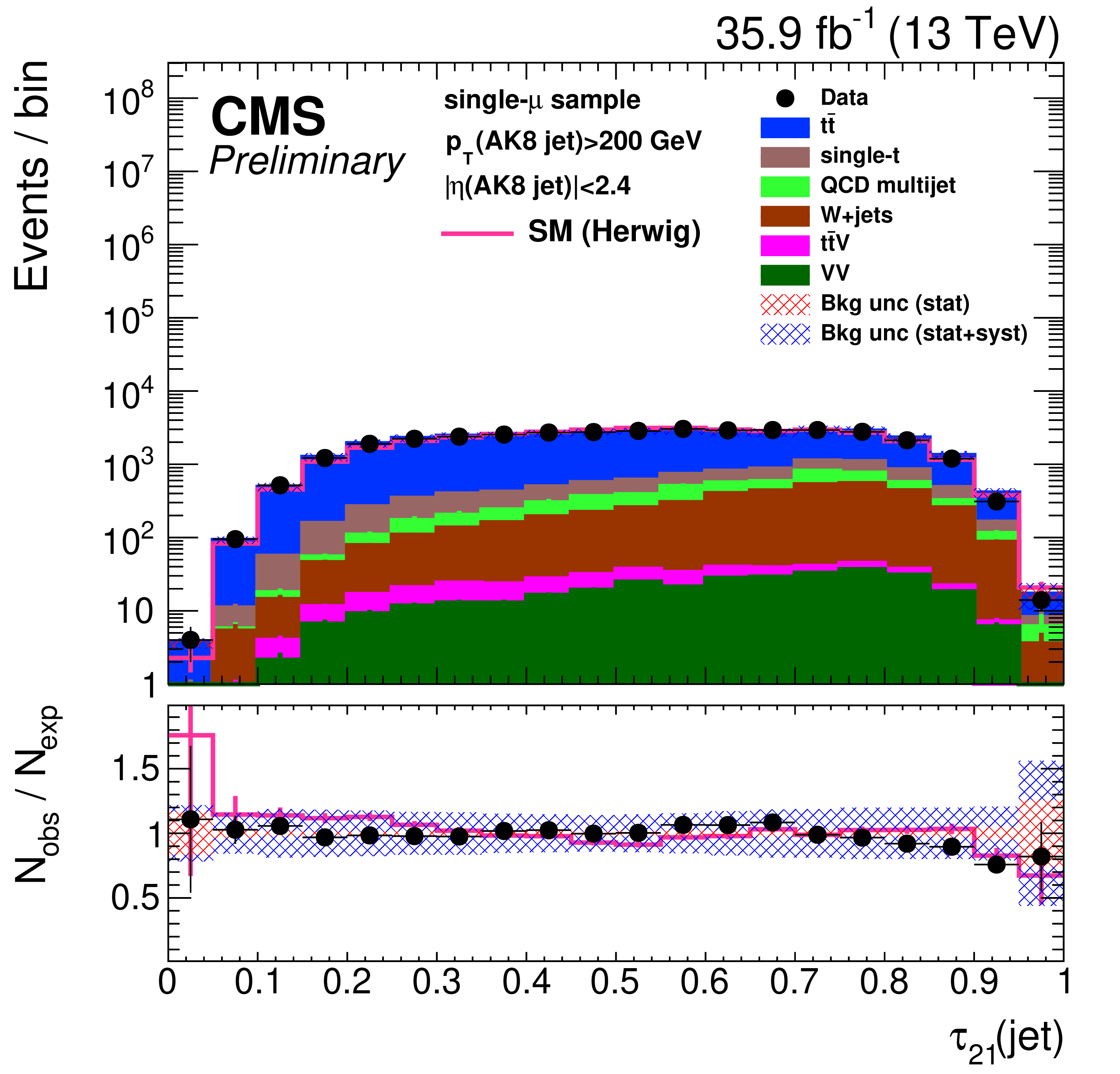
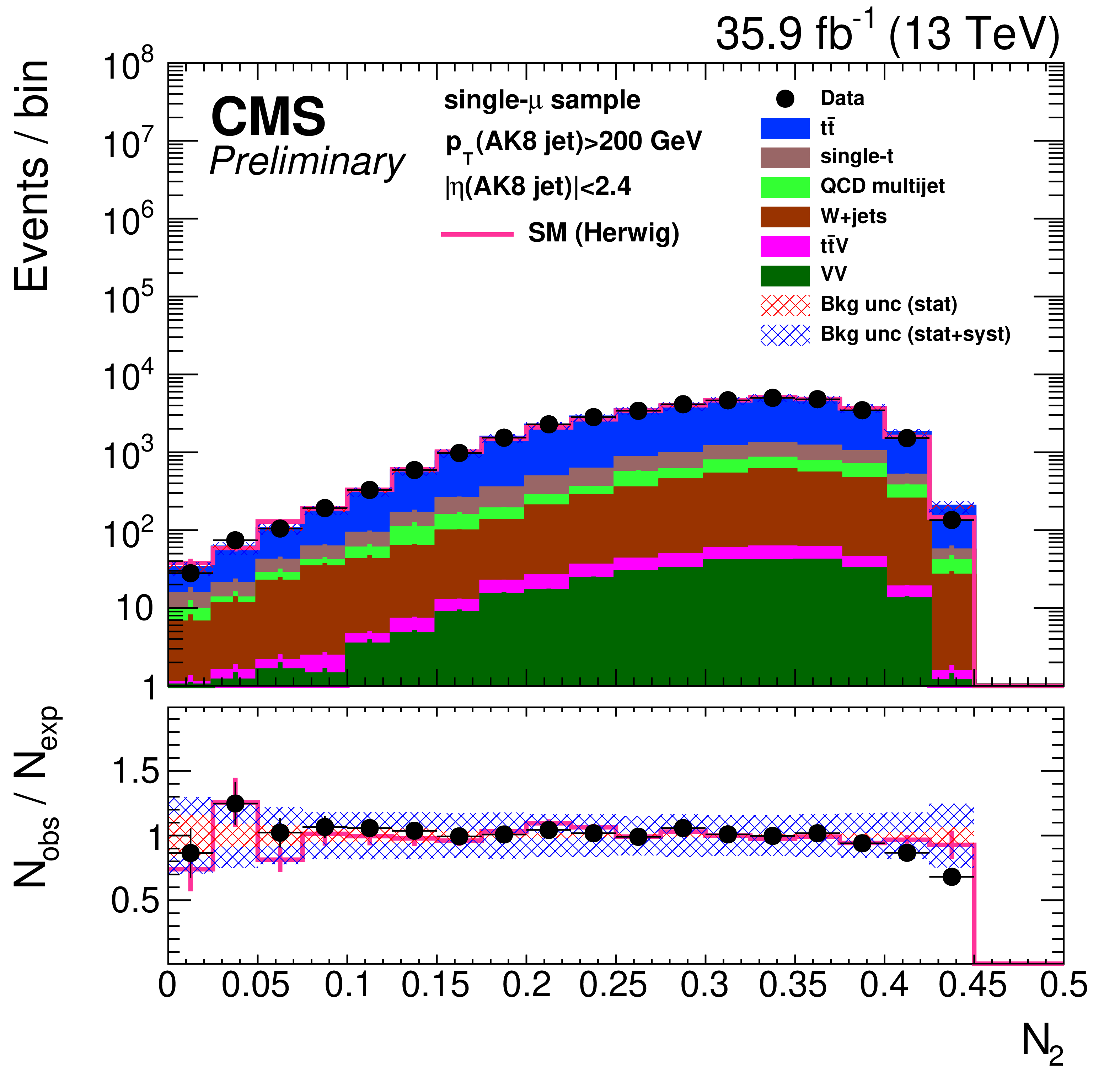
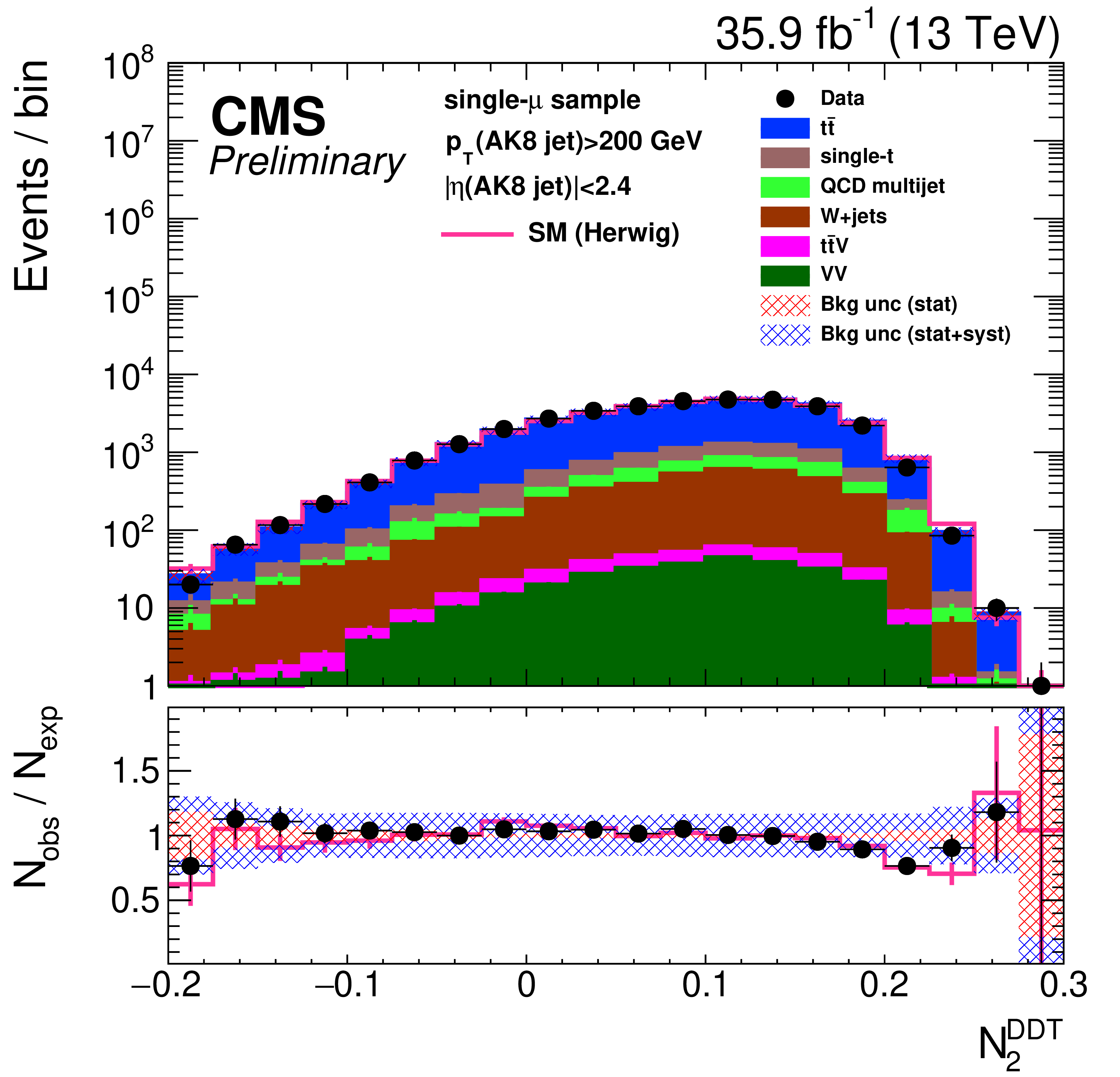
Distribution of the the jet ${p_{\mathrm {T}}}$ (upper-left), jet mass, ${m_{\text {SD}}}$ (upper-right), the N-subjetiness ratios, $ {\tau _{32}}$ (middle-left) and $ {\tau _{21}}$ (middle-right), and the $N_2$ (lower-left) and $N_2^{\text {DDT}}$ (lower-right) in data and simulation in the single-$\mu $ signal sample. The pink solid line corresponds to the simulation distribution obtained using the alternative ${\mathrm{t} \mathrm{\bar{t}}}$ sample. The background event yield is normalized to the total observed data yield. The lower panel shows the data to simulation ratio. The shaded blue (red) band corresponds to the total uncertainty (statistical uncertainty of the simulated samples), the pink line to the data to simulation ratio using the alternative ${\mathrm{t} \mathrm{\bar{t}}}$ sample, and the vertical lines correspond to the statistical uncertainty of the data. The distributions are weighted according to the top ${p_{\mathrm {T}}}$ reweighting procedure described in the text. |
png pdf |
Figure 23-a:
Distribution of the the jet ${p_{\mathrm {T}}}$ (upper-left), jet mass, ${m_{\text {SD}}}$ (upper-right), the N-subjetiness ratios, $ {\tau _{32}}$ (middle-left) and $ {\tau _{21}}$ (middle-right), and the $N_2$ (lower-left) and $N_2^{\text {DDT}}$ (lower-right) in data and simulation in the single-$\mu $ signal sample. The pink solid line corresponds to the simulation distribution obtained using the alternative ${\mathrm{t} \mathrm{\bar{t}}}$ sample. The background event yield is normalized to the total observed data yield. The lower panel shows the data to simulation ratio. The shaded blue (red) band corresponds to the total uncertainty (statistical uncertainty of the simulated samples), the pink line to the data to simulation ratio using the alternative ${\mathrm{t} \mathrm{\bar{t}}}$ sample, and the vertical lines correspond to the statistical uncertainty of the data. The distributions are weighted according to the top ${p_{\mathrm {T}}}$ reweighting procedure described in the text. |
png pdf |
Figure 23-b:
Distribution of the the jet ${p_{\mathrm {T}}}$ (upper-left), jet mass, ${m_{\text {SD}}}$ (upper-right), the N-subjetiness ratios, $ {\tau _{32}}$ (middle-left) and $ {\tau _{21}}$ (middle-right), and the $N_2$ (lower-left) and $N_2^{\text {DDT}}$ (lower-right) in data and simulation in the single-$\mu $ signal sample. The pink solid line corresponds to the simulation distribution obtained using the alternative ${\mathrm{t} \mathrm{\bar{t}}}$ sample. The background event yield is normalized to the total observed data yield. The lower panel shows the data to simulation ratio. The shaded blue (red) band corresponds to the total uncertainty (statistical uncertainty of the simulated samples), the pink line to the data to simulation ratio using the alternative ${\mathrm{t} \mathrm{\bar{t}}}$ sample, and the vertical lines correspond to the statistical uncertainty of the data. The distributions are weighted according to the top ${p_{\mathrm {T}}}$ reweighting procedure described in the text. |
png pdf |
Figure 23-c:
Distribution of the the jet ${p_{\mathrm {T}}}$ (upper-left), jet mass, ${m_{\text {SD}}}$ (upper-right), the N-subjetiness ratios, $ {\tau _{32}}$ (middle-left) and $ {\tau _{21}}$ (middle-right), and the $N_2$ (lower-left) and $N_2^{\text {DDT}}$ (lower-right) in data and simulation in the single-$\mu $ signal sample. The pink solid line corresponds to the simulation distribution obtained using the alternative ${\mathrm{t} \mathrm{\bar{t}}}$ sample. The background event yield is normalized to the total observed data yield. The lower panel shows the data to simulation ratio. The shaded blue (red) band corresponds to the total uncertainty (statistical uncertainty of the simulated samples), the pink line to the data to simulation ratio using the alternative ${\mathrm{t} \mathrm{\bar{t}}}$ sample, and the vertical lines correspond to the statistical uncertainty of the data. The distributions are weighted according to the top ${p_{\mathrm {T}}}$ reweighting procedure described in the text. |
png pdf |
Figure 23-d:
Distribution of the the jet ${p_{\mathrm {T}}}$ (upper-left), jet mass, ${m_{\text {SD}}}$ (upper-right), the N-subjetiness ratios, $ {\tau _{32}}$ (middle-left) and $ {\tau _{21}}$ (middle-right), and the $N_2$ (lower-left) and $N_2^{\text {DDT}}$ (lower-right) in data and simulation in the single-$\mu $ signal sample. The pink solid line corresponds to the simulation distribution obtained using the alternative ${\mathrm{t} \mathrm{\bar{t}}}$ sample. The background event yield is normalized to the total observed data yield. The lower panel shows the data to simulation ratio. The shaded blue (red) band corresponds to the total uncertainty (statistical uncertainty of the simulated samples), the pink line to the data to simulation ratio using the alternative ${\mathrm{t} \mathrm{\bar{t}}}$ sample, and the vertical lines correspond to the statistical uncertainty of the data. The distributions are weighted according to the top ${p_{\mathrm {T}}}$ reweighting procedure described in the text. |
png pdf |
Figure 23-e:
Distribution of the the jet ${p_{\mathrm {T}}}$ (upper-left), jet mass, ${m_{\text {SD}}}$ (upper-right), the N-subjetiness ratios, $ {\tau _{32}}$ (middle-left) and $ {\tau _{21}}$ (middle-right), and the $N_2$ (lower-left) and $N_2^{\text {DDT}}$ (lower-right) in data and simulation in the single-$\mu $ signal sample. The pink solid line corresponds to the simulation distribution obtained using the alternative ${\mathrm{t} \mathrm{\bar{t}}}$ sample. The background event yield is normalized to the total observed data yield. The lower panel shows the data to simulation ratio. The shaded blue (red) band corresponds to the total uncertainty (statistical uncertainty of the simulated samples), the pink line to the data to simulation ratio using the alternative ${\mathrm{t} \mathrm{\bar{t}}}$ sample, and the vertical lines correspond to the statistical uncertainty of the data. The distributions are weighted according to the top ${p_{\mathrm {T}}}$ reweighting procedure described in the text. |
png pdf |
Figure 23-f:
Distribution of the the jet ${p_{\mathrm {T}}}$ (upper-left), jet mass, ${m_{\text {SD}}}$ (upper-right), the N-subjetiness ratios, $ {\tau _{32}}$ (middle-left) and $ {\tau _{21}}$ (middle-right), and the $N_2$ (lower-left) and $N_2^{\text {DDT}}$ (lower-right) in data and simulation in the single-$\mu $ signal sample. The pink solid line corresponds to the simulation distribution obtained using the alternative ${\mathrm{t} \mathrm{\bar{t}}}$ sample. The background event yield is normalized to the total observed data yield. The lower panel shows the data to simulation ratio. The shaded blue (red) band corresponds to the total uncertainty (statistical uncertainty of the simulated samples), the pink line to the data to simulation ratio using the alternative ${\mathrm{t} \mathrm{\bar{t}}}$ sample, and the vertical lines correspond to the statistical uncertainty of the data. The distributions are weighted according to the top ${p_{\mathrm {T}}}$ reweighting procedure described in the text. |
png pdf |
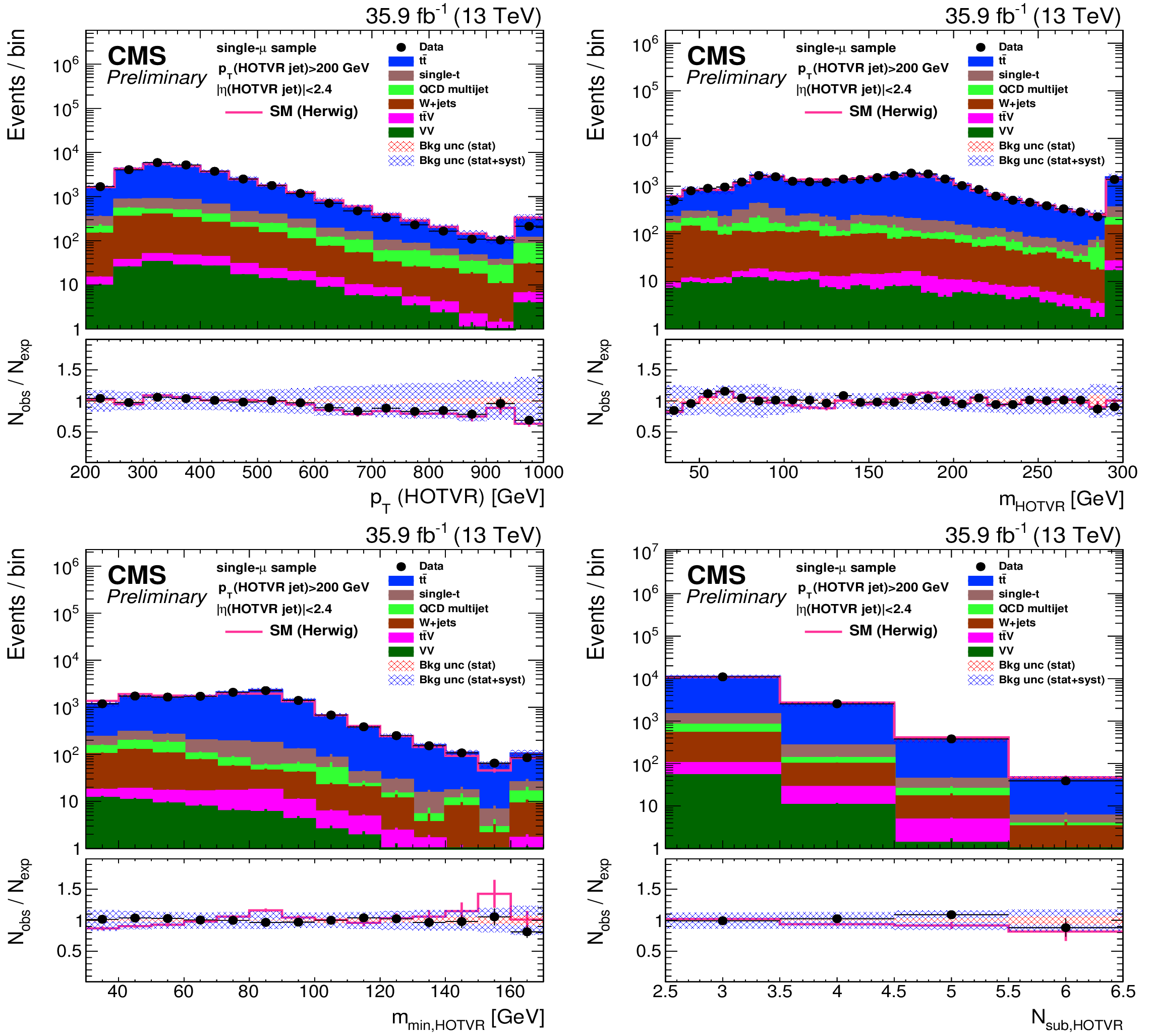
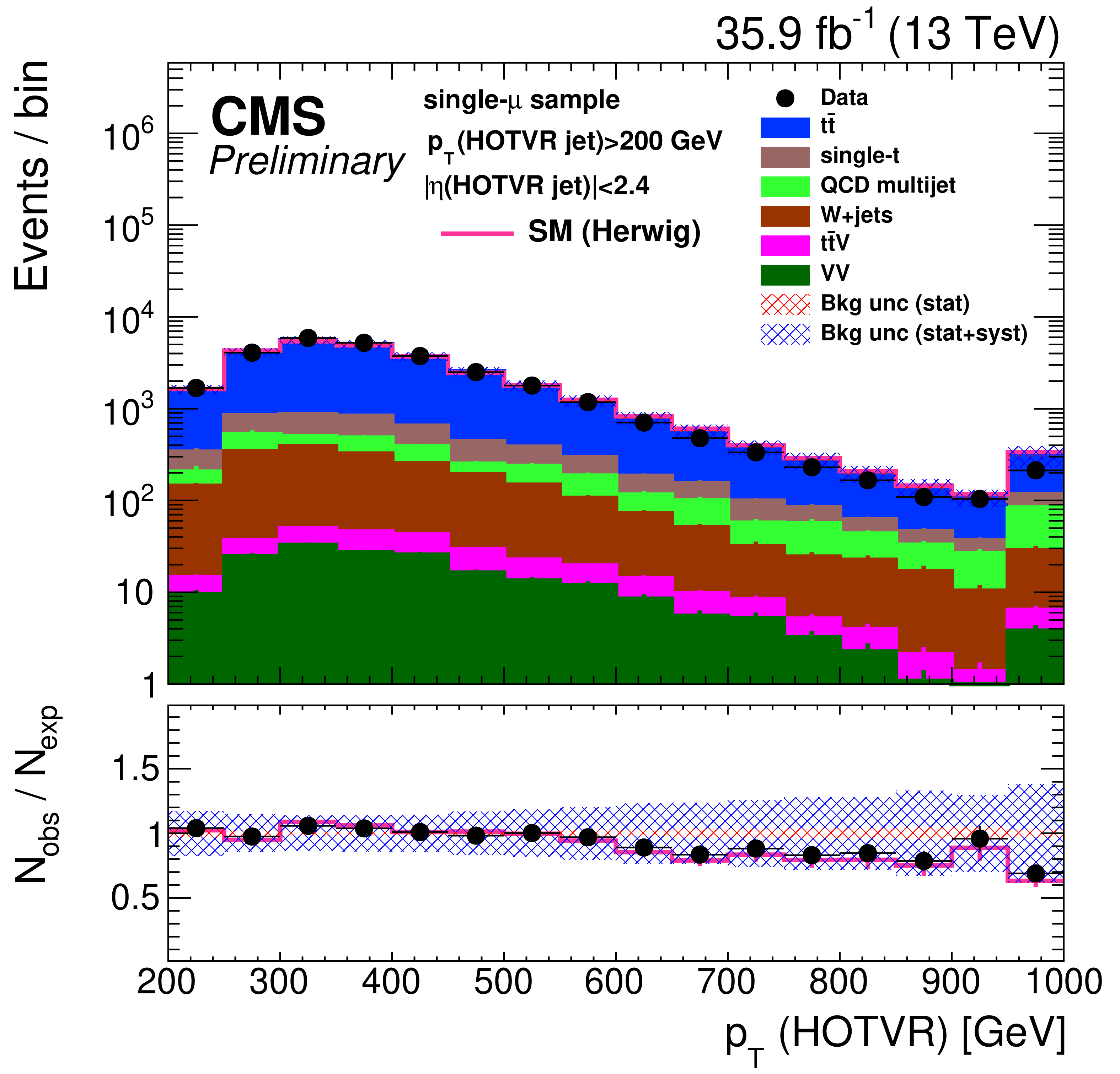
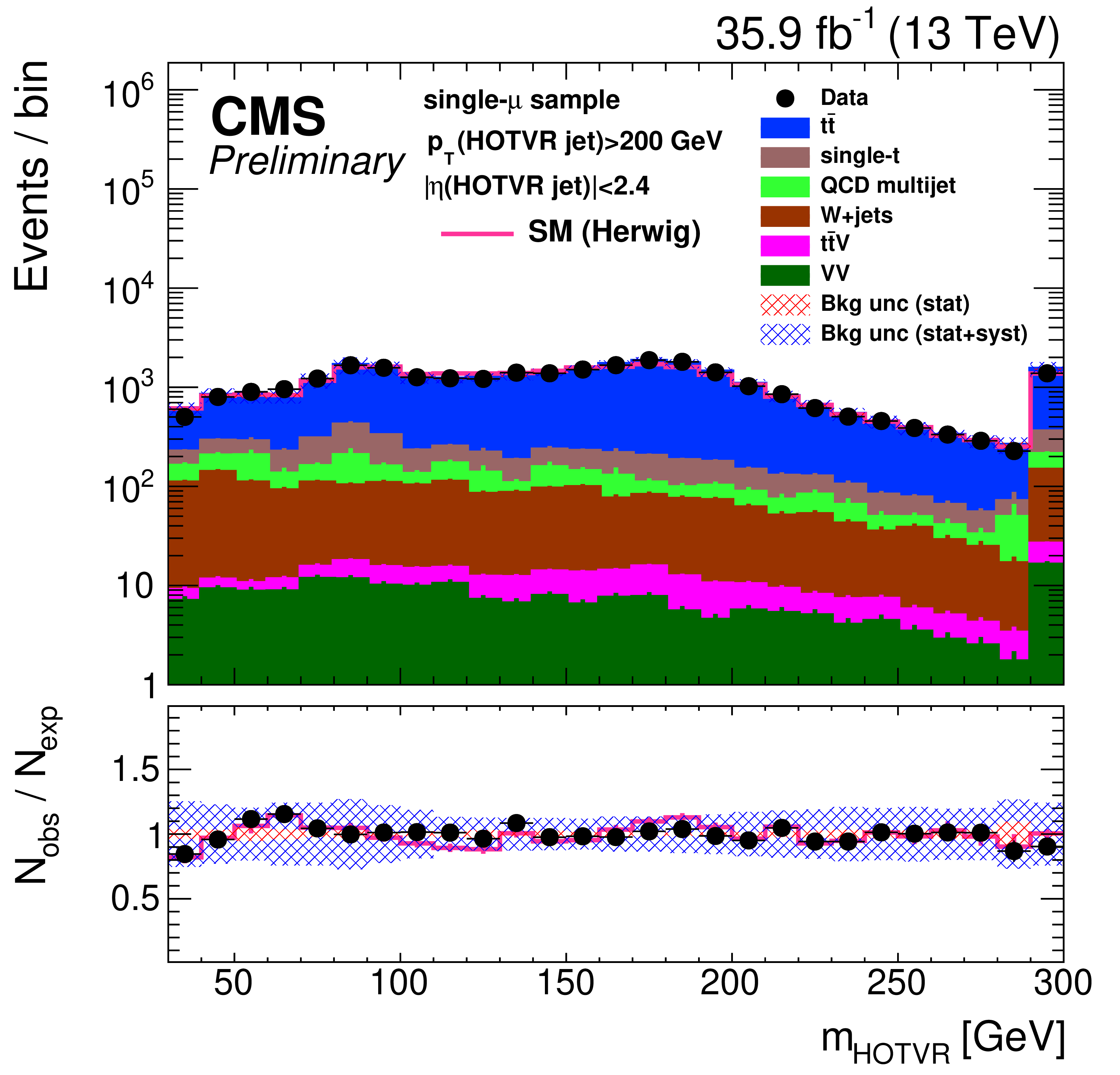
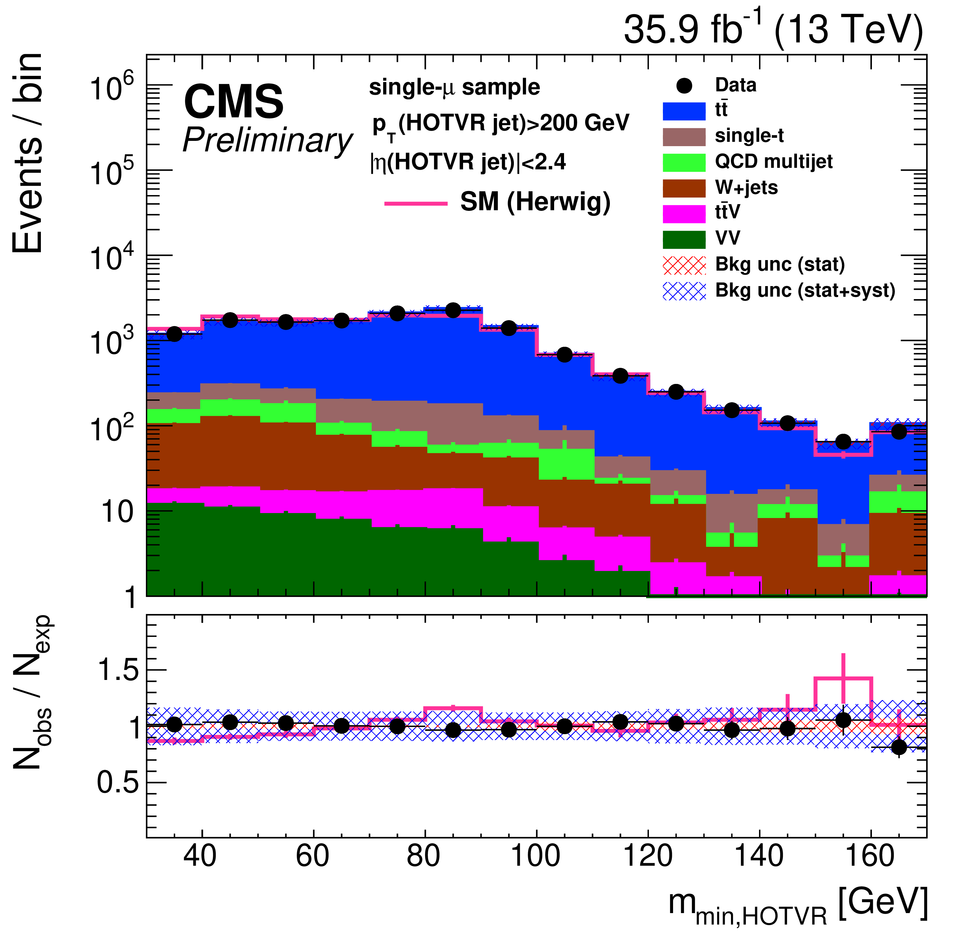
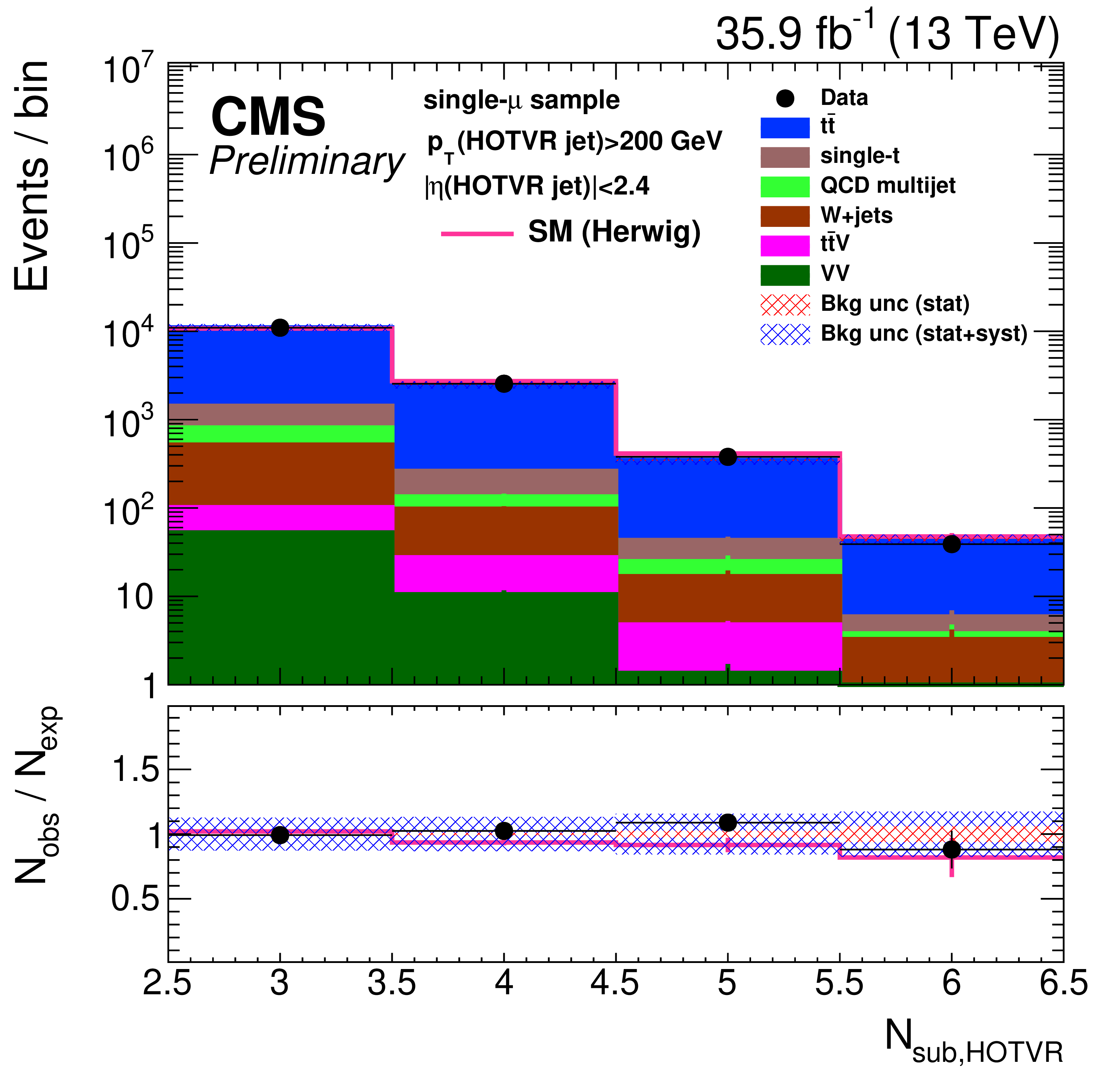
Figure 24:
Distribution of the main observables of the HOTVR algorithm, $p_{T}(\text {HOTVR jet})$ (upper-left), $m_{\text {HOTVR}}$ (upper-right), $m_{\text {min,HOTVR}}$ (lower-left), and $N_{\text {sub,HOTVR}}$ (lower-right) in data and simulation in the single-$\mu $ signal sample. The pink solid line corresponds to the simulation distribution obtained using the alternative ${\mathrm{t} \mathrm{\bar{t}}}$ sample. The background event yield is normalized to the total observed data yield. The lower panel shows the data to simulation ratio. The shaded blue (red) band corresponds to the total uncertainty (statistical uncertainty of the simulated samples), the pink line to the data to simulation ratio using the alternative ${\mathrm{t} \mathrm{\bar{t}}}$ sample, and the vertical lines correspond to the statistical uncertainty of the data. The distributions are weighted according to the top ${p_{\mathrm {T}}}$ reweighting procedure described in the text. |
png pdf |
Figure 24-a:
Distribution of the main observables of the HOTVR algorithm, $p_{T}(\text {HOTVR jet})$ (upper-left), $m_{\text {HOTVR}}$ (upper-right), $m_{\text {min,HOTVR}}$ (lower-left), and $N_{\text {sub,HOTVR}}$ (lower-right) in data and simulation in the single-$\mu $ signal sample. The pink solid line corresponds to the simulation distribution obtained using the alternative ${\mathrm{t} \mathrm{\bar{t}}}$ sample. The background event yield is normalized to the total observed data yield. The lower panel shows the data to simulation ratio. The shaded blue (red) band corresponds to the total uncertainty (statistical uncertainty of the simulated samples), the pink line to the data to simulation ratio using the alternative ${\mathrm{t} \mathrm{\bar{t}}}$ sample, and the vertical lines correspond to the statistical uncertainty of the data. The distributions are weighted according to the top ${p_{\mathrm {T}}}$ reweighting procedure described in the text. |
png pdf |
Figure 24-b:
Distribution of the main observables of the HOTVR algorithm, $p_{T}(\text {HOTVR jet})$ (upper-left), $m_{\text {HOTVR}}$ (upper-right), $m_{\text {min,HOTVR}}$ (lower-left), and $N_{\text {sub,HOTVR}}$ (lower-right) in data and simulation in the single-$\mu $ signal sample. The pink solid line corresponds to the simulation distribution obtained using the alternative ${\mathrm{t} \mathrm{\bar{t}}}$ sample. The background event yield is normalized to the total observed data yield. The lower panel shows the data to simulation ratio. The shaded blue (red) band corresponds to the total uncertainty (statistical uncertainty of the simulated samples), the pink line to the data to simulation ratio using the alternative ${\mathrm{t} \mathrm{\bar{t}}}$ sample, and the vertical lines correspond to the statistical uncertainty of the data. The distributions are weighted according to the top ${p_{\mathrm {T}}}$ reweighting procedure described in the text. |
png pdf |
Figure 24-c:
Distribution of the main observables of the HOTVR algorithm, $p_{T}(\text {HOTVR jet})$ (upper-left), $m_{\text {HOTVR}}$ (upper-right), $m_{\text {min,HOTVR}}$ (lower-left), and $N_{\text {sub,HOTVR}}$ (lower-right) in data and simulation in the single-$\mu $ signal sample. The pink solid line corresponds to the simulation distribution obtained using the alternative ${\mathrm{t} \mathrm{\bar{t}}}$ sample. The background event yield is normalized to the total observed data yield. The lower panel shows the data to simulation ratio. The shaded blue (red) band corresponds to the total uncertainty (statistical uncertainty of the simulated samples), the pink line to the data to simulation ratio using the alternative ${\mathrm{t} \mathrm{\bar{t}}}$ sample, and the vertical lines correspond to the statistical uncertainty of the data. The distributions are weighted according to the top ${p_{\mathrm {T}}}$ reweighting procedure described in the text. |
png pdf |
Figure 24-d:
Distribution of the main observables of the HOTVR algorithm, $p_{T}(\text {HOTVR jet})$ (upper-left), $m_{\text {HOTVR}}$ (upper-right), $m_{\text {min,HOTVR}}$ (lower-left), and $N_{\text {sub,HOTVR}}$ (lower-right) in data and simulation in the single-$\mu $ signal sample. The pink solid line corresponds to the simulation distribution obtained using the alternative ${\mathrm{t} \mathrm{\bar{t}}}$ sample. The background event yield is normalized to the total observed data yield. The lower panel shows the data to simulation ratio. The shaded blue (red) band corresponds to the total uncertainty (statistical uncertainty of the simulated samples), the pink line to the data to simulation ratio using the alternative ${\mathrm{t} \mathrm{\bar{t}}}$ sample, and the vertical lines correspond to the statistical uncertainty of the data. The distributions are weighted according to the top ${p_{\mathrm {T}}}$ reweighting procedure described in the text. |
png pdf |
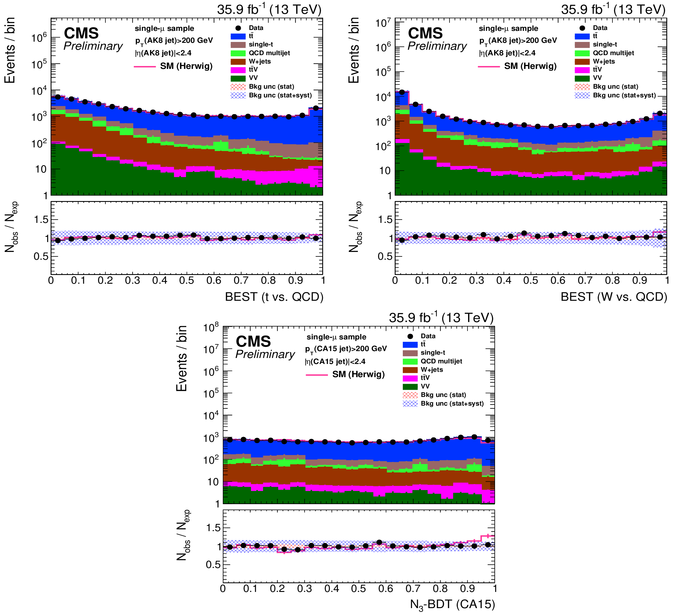
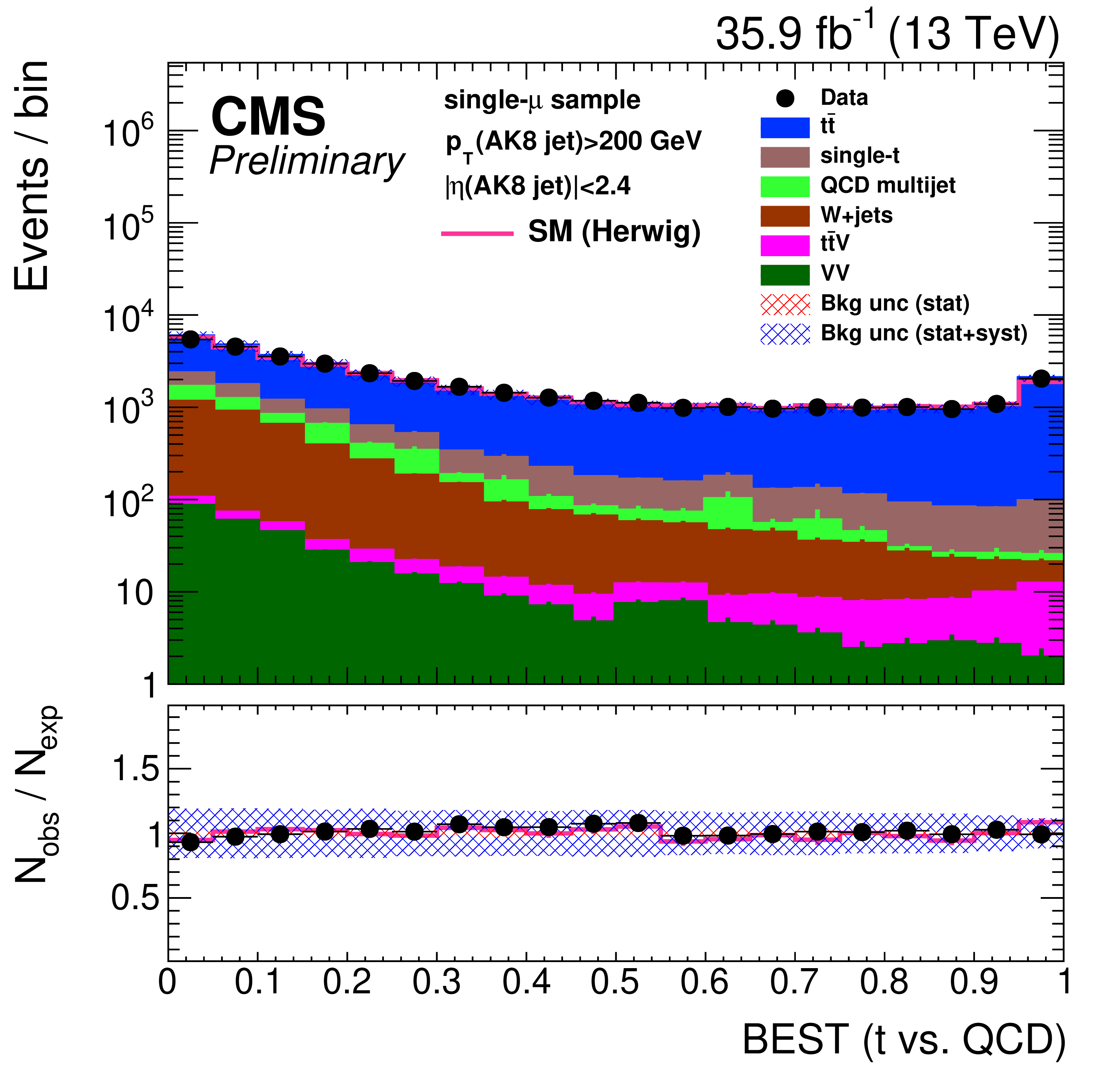
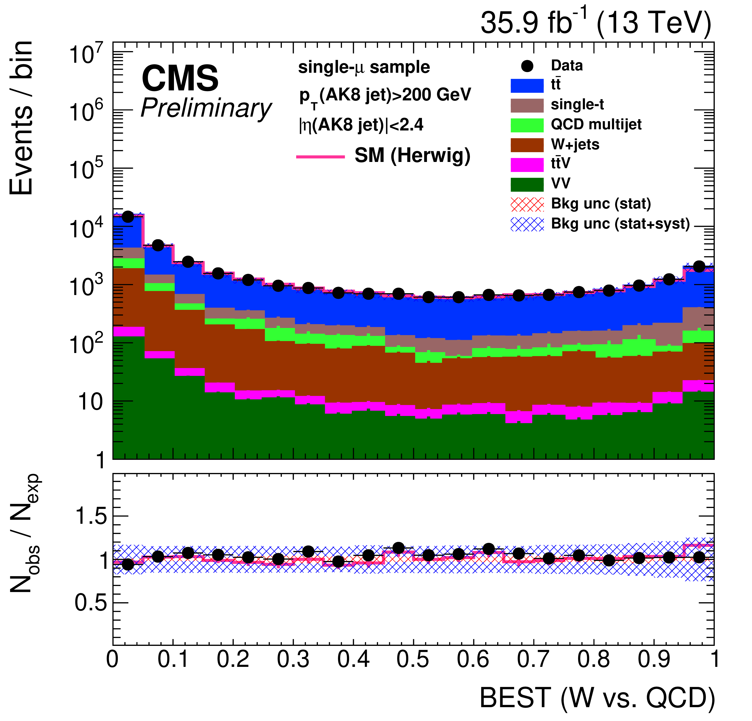
Figure 25:
Distribution of the t quark (upper-left) and W boson (upper-right) identification probabilities for the BEST algorithm, and the ${N_{3}-\text {BDT} (\text {CA}15)}$ discriminant, in data and simulation in the single-$\mu $ signal sample. The pink solid line corresponds to the simulation distribution obtained using the alternative ${\mathrm{t} \mathrm{\bar{t}}}$ sample. The background event yield is normalized to the total observed data yield. The lower panel shows the data to simulation ratio. The shaded blue (red) band corresponds to the total uncertainty (statistical uncertainty of the simulated samples), the pink line to the data to simulation ratio using the alternative ${\mathrm{t} \mathrm{\bar{t}}}$ sample, and the vertical lines correspond to the statistical uncertainty of the data. The distributions are weighted according to the top ${p_{\mathrm {T}}}$ reweighting procedure described in the text. |
png pdf |
Figure 25-a:
Distribution of the t quark (upper-left) and W boson (upper-right) identification probabilities for the BEST algorithm, and the ${N_{3}-\text {BDT} (\text {CA}15)}$ discriminant, in data and simulation in the single-$\mu $ signal sample. The pink solid line corresponds to the simulation distribution obtained using the alternative ${\mathrm{t} \mathrm{\bar{t}}}$ sample. The background event yield is normalized to the total observed data yield. The lower panel shows the data to simulation ratio. The shaded blue (red) band corresponds to the total uncertainty (statistical uncertainty of the simulated samples), the pink line to the data to simulation ratio using the alternative ${\mathrm{t} \mathrm{\bar{t}}}$ sample, and the vertical lines correspond to the statistical uncertainty of the data. The distributions are weighted according to the top ${p_{\mathrm {T}}}$ reweighting procedure described in the text. |
png pdf |
Figure 25-b:
Distribution of the t quark (upper-left) and W boson (upper-right) identification probabilities for the BEST algorithm, and the ${N_{3}-\text {BDT} (\text {CA}15)}$ discriminant, in data and simulation in the single-$\mu $ signal sample. The pink solid line corresponds to the simulation distribution obtained using the alternative ${\mathrm{t} \mathrm{\bar{t}}}$ sample. The background event yield is normalized to the total observed data yield. The lower panel shows the data to simulation ratio. The shaded blue (red) band corresponds to the total uncertainty (statistical uncertainty of the simulated samples), the pink line to the data to simulation ratio using the alternative ${\mathrm{t} \mathrm{\bar{t}}}$ sample, and the vertical lines correspond to the statistical uncertainty of the data. The distributions are weighted according to the top ${p_{\mathrm {T}}}$ reweighting procedure described in the text. |
png pdf |
Figure 25-c:
Distribution of the t quark (upper-left) and W boson (upper-right) identification probabilities for the BEST algorithm, and the ${N_{3}-\text {BDT} (\text {CA}15)}$ discriminant, in data and simulation in the single-$\mu $ signal sample. The pink solid line corresponds to the simulation distribution obtained using the alternative ${\mathrm{t} \mathrm{\bar{t}}}$ sample. The background event yield is normalized to the total observed data yield. The lower panel shows the data to simulation ratio. The shaded blue (red) band corresponds to the total uncertainty (statistical uncertainty of the simulated samples), the pink line to the data to simulation ratio using the alternative ${\mathrm{t} \mathrm{\bar{t}}}$ sample, and the vertical lines correspond to the statistical uncertainty of the data. The distributions are weighted according to the top ${p_{\mathrm {T}}}$ reweighting procedure described in the text. |
png pdf |
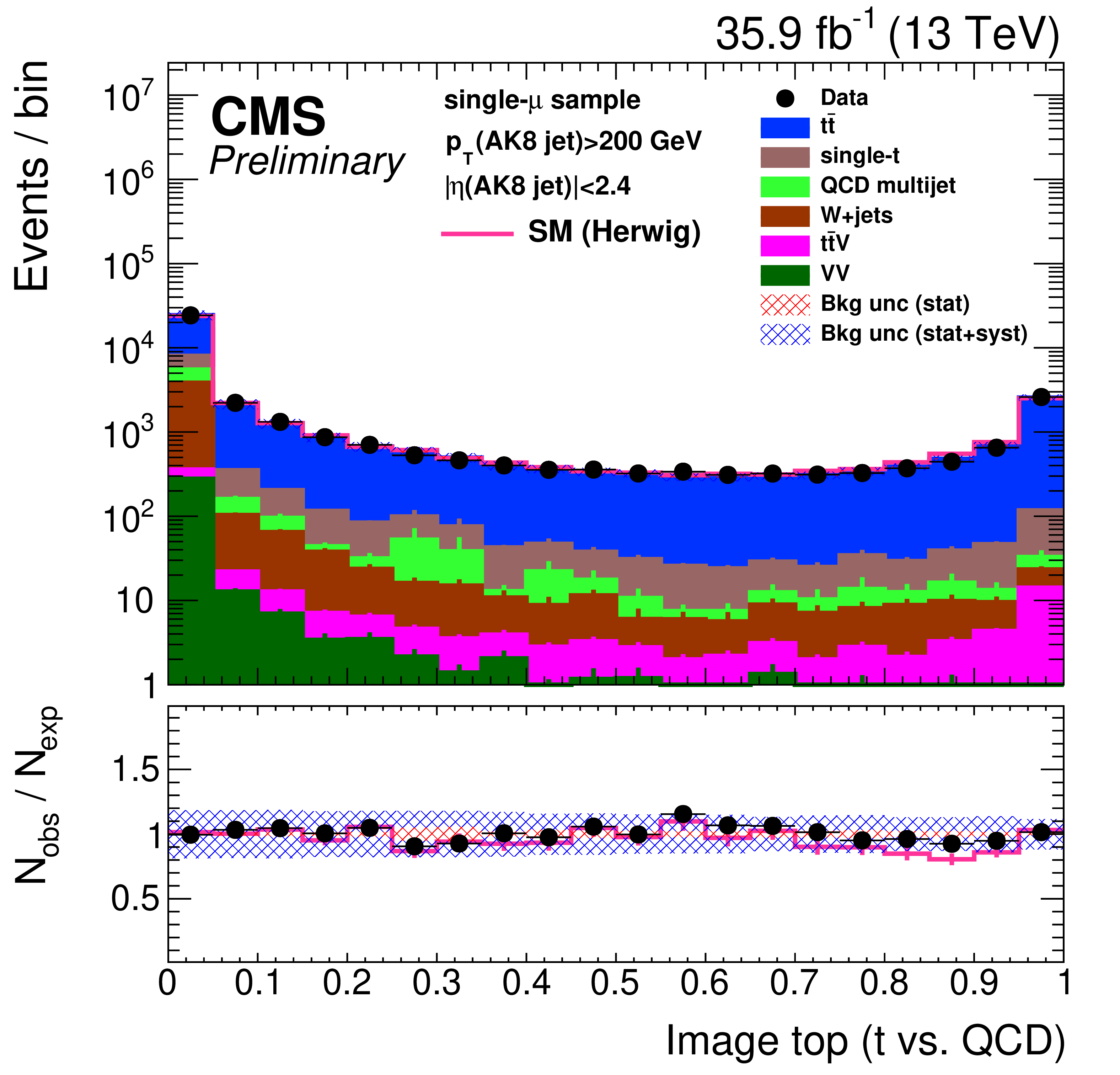
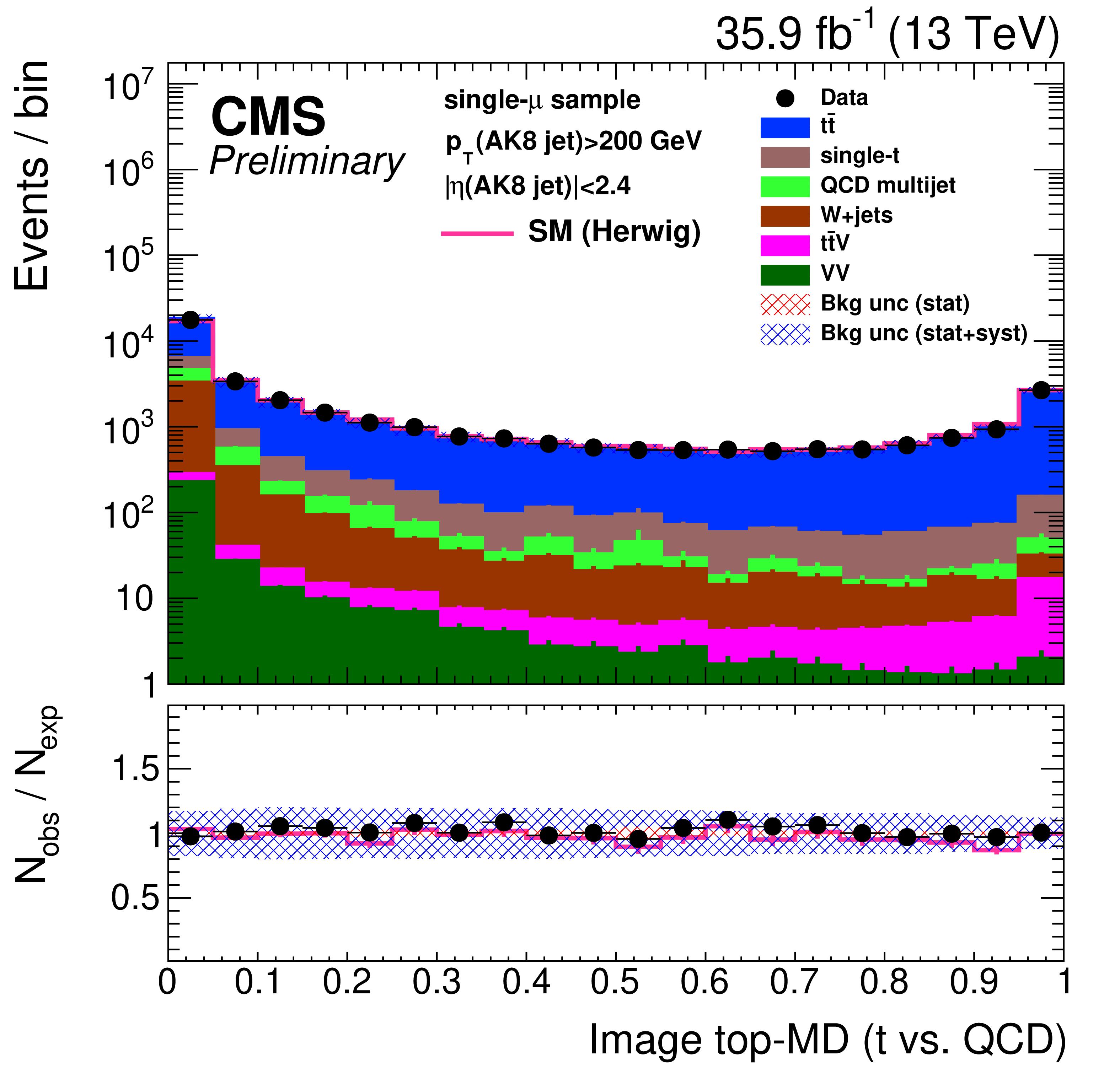
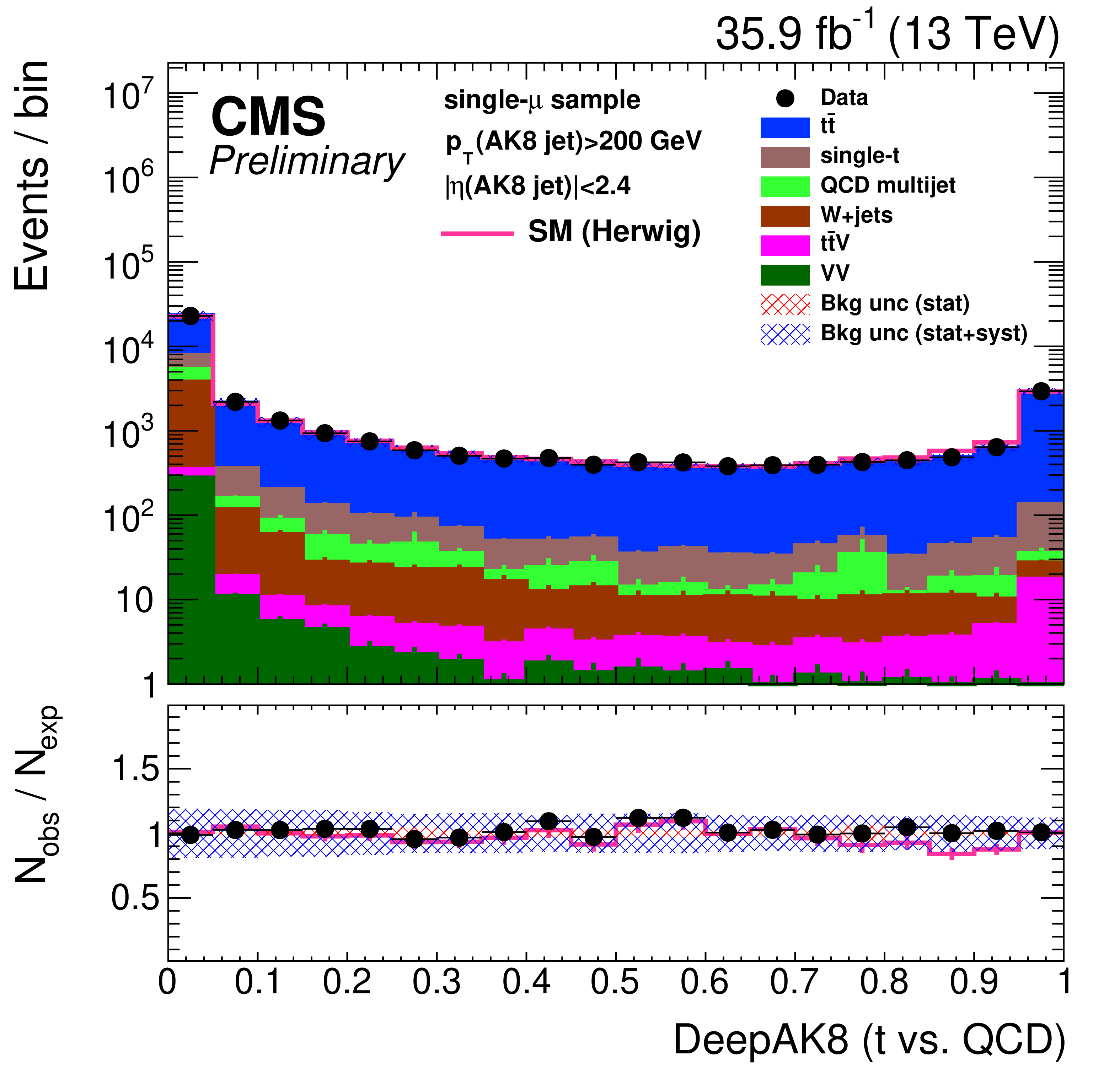
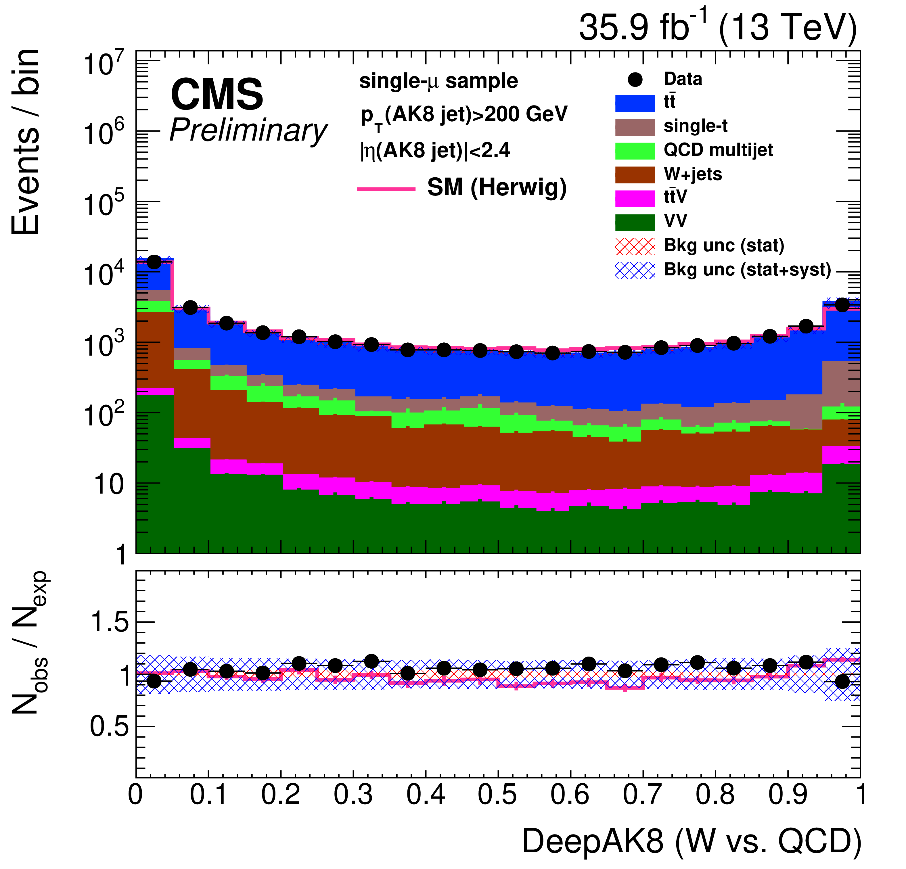
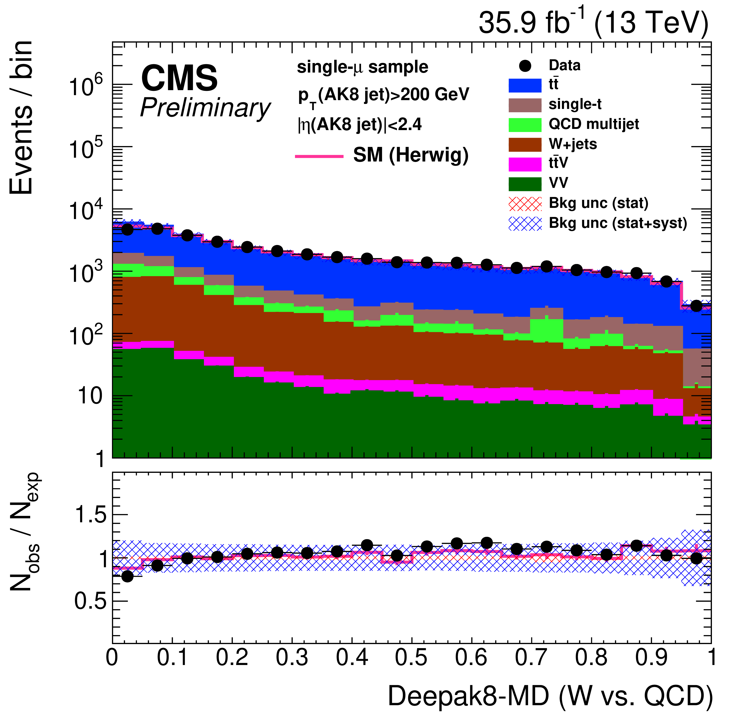
Figure 26:
Distribution of the ImageTop (upper-left) and ImageTop-MD (upper-right) discriminant in data and simulation in the single-$\mu $ sample. The plots in the middle row show the t quark (left) and W boson (right) identification probabilities in data and simulation for the DeepAK8 algorithm. The corresponding plots for DeepAK8-MD are displayed in the lower row. The pink solid line corresponds to the simulation distribution obtained using the alternative ${\mathrm{t} \mathrm{\bar{t}}}$ sample. The background event yield is normalized to the total observed data yield. The lower panel shows the data to simulation ratio. The shaded blue (red) band corresponds to the total uncertainty (statistical uncertainty of the simulated samples), the pink line to the data to simulation ratio using the alternative ${\mathrm{t} \mathrm{\bar{t}}}$ sample, and the vertical lines correspond to the statistical uncertainty of the data. The distributions are weighted according to the top ${p_{\mathrm {T}}}$ reweighting procedure described in the text. |
png pdf |
Figure 26-a:
Distribution of the ImageTop (upper-left) and ImageTop-MD (upper-right) discriminant in data and simulation in the single-$\mu $ sample. The plots in the middle row show the t quark (left) and W boson (right) identification probabilities in data and simulation for the DeepAK8 algorithm. The corresponding plots for DeepAK8-MD are displayed in the lower row. The pink solid line corresponds to the simulation distribution obtained using the alternative ${\mathrm{t} \mathrm{\bar{t}}}$ sample. The background event yield is normalized to the total observed data yield. The lower panel shows the data to simulation ratio. The shaded blue (red) band corresponds to the total uncertainty (statistical uncertainty of the simulated samples), the pink line to the data to simulation ratio using the alternative ${\mathrm{t} \mathrm{\bar{t}}}$ sample, and the vertical lines correspond to the statistical uncertainty of the data. The distributions are weighted according to the top ${p_{\mathrm {T}}}$ reweighting procedure described in the text. |
png pdf |
Figure 26-b:
Distribution of the ImageTop (upper-left) and ImageTop-MD (upper-right) discriminant in data and simulation in the single-$\mu $ sample. The plots in the middle row show the t quark (left) and W boson (right) identification probabilities in data and simulation for the DeepAK8 algorithm. The corresponding plots for DeepAK8-MD are displayed in the lower row. The pink solid line corresponds to the simulation distribution obtained using the alternative ${\mathrm{t} \mathrm{\bar{t}}}$ sample. The background event yield is normalized to the total observed data yield. The lower panel shows the data to simulation ratio. The shaded blue (red) band corresponds to the total uncertainty (statistical uncertainty of the simulated samples), the pink line to the data to simulation ratio using the alternative ${\mathrm{t} \mathrm{\bar{t}}}$ sample, and the vertical lines correspond to the statistical uncertainty of the data. The distributions are weighted according to the top ${p_{\mathrm {T}}}$ reweighting procedure described in the text. |
png pdf |
Figure 26-c:
Distribution of the ImageTop (upper-left) and ImageTop-MD (upper-right) discriminant in data and simulation in the single-$\mu $ sample. The plots in the middle row show the t quark (left) and W boson (right) identification probabilities in data and simulation for the DeepAK8 algorithm. The corresponding plots for DeepAK8-MD are displayed in the lower row. The pink solid line corresponds to the simulation distribution obtained using the alternative ${\mathrm{t} \mathrm{\bar{t}}}$ sample. The background event yield is normalized to the total observed data yield. The lower panel shows the data to simulation ratio. The shaded blue (red) band corresponds to the total uncertainty (statistical uncertainty of the simulated samples), the pink line to the data to simulation ratio using the alternative ${\mathrm{t} \mathrm{\bar{t}}}$ sample, and the vertical lines correspond to the statistical uncertainty of the data. The distributions are weighted according to the top ${p_{\mathrm {T}}}$ reweighting procedure described in the text. |
png pdf |
Figure 26-d:
Distribution of the ImageTop (upper-left) and ImageTop-MD (upper-right) discriminant in data and simulation in the single-$\mu $ sample. The plots in the middle row show the t quark (left) and W boson (right) identification probabilities in data and simulation for the DeepAK8 algorithm. The corresponding plots for DeepAK8-MD are displayed in the lower row. The pink solid line corresponds to the simulation distribution obtained using the alternative ${\mathrm{t} \mathrm{\bar{t}}}$ sample. The background event yield is normalized to the total observed data yield. The lower panel shows the data to simulation ratio. The shaded blue (red) band corresponds to the total uncertainty (statistical uncertainty of the simulated samples), the pink line to the data to simulation ratio using the alternative ${\mathrm{t} \mathrm{\bar{t}}}$ sample, and the vertical lines correspond to the statistical uncertainty of the data. The distributions are weighted according to the top ${p_{\mathrm {T}}}$ reweighting procedure described in the text. |

png pdf |
Figure 26-e:
Distribution of the ImageTop (upper-left) and ImageTop-MD (upper-right) discriminant in data and simulation in the single-$\mu $ sample. The plots in the middle row show the t quark (left) and W boson (right) identification probabilities in data and simulation for the DeepAK8 algorithm. The corresponding plots for DeepAK8-MD are displayed in the lower row. The pink solid line corresponds to the simulation distribution obtained using the alternative ${\mathrm{t} \mathrm{\bar{t}}}$ sample. The background event yield is normalized to the total observed data yield. The lower panel shows the data to simulation ratio. The shaded blue (red) band corresponds to the total uncertainty (statistical uncertainty of the simulated samples), the pink line to the data to simulation ratio using the alternative ${\mathrm{t} \mathrm{\bar{t}}}$ sample, and the vertical lines correspond to the statistical uncertainty of the data. The distributions are weighted according to the top ${p_{\mathrm {T}}}$ reweighting procedure described in the text. |
png pdf |
Figure 26-f:
Distribution of the ImageTop (upper-left) and ImageTop-MD (upper-right) discriminant in data and simulation in the single-$\mu $ sample. The plots in the middle row show the t quark (left) and W boson (right) identification probabilities in data and simulation for the DeepAK8 algorithm. The corresponding plots for DeepAK8-MD are displayed in the lower row. The pink solid line corresponds to the simulation distribution obtained using the alternative ${\mathrm{t} \mathrm{\bar{t}}}$ sample. The background event yield is normalized to the total observed data yield. The lower panel shows the data to simulation ratio. The shaded blue (red) band corresponds to the total uncertainty (statistical uncertainty of the simulated samples), the pink line to the data to simulation ratio using the alternative ${\mathrm{t} \mathrm{\bar{t}}}$ sample, and the vertical lines correspond to the statistical uncertainty of the data. The distributions are weighted according to the top ${p_{\mathrm {T}}}$ reweighting procedure described in the text. |
png pdf |
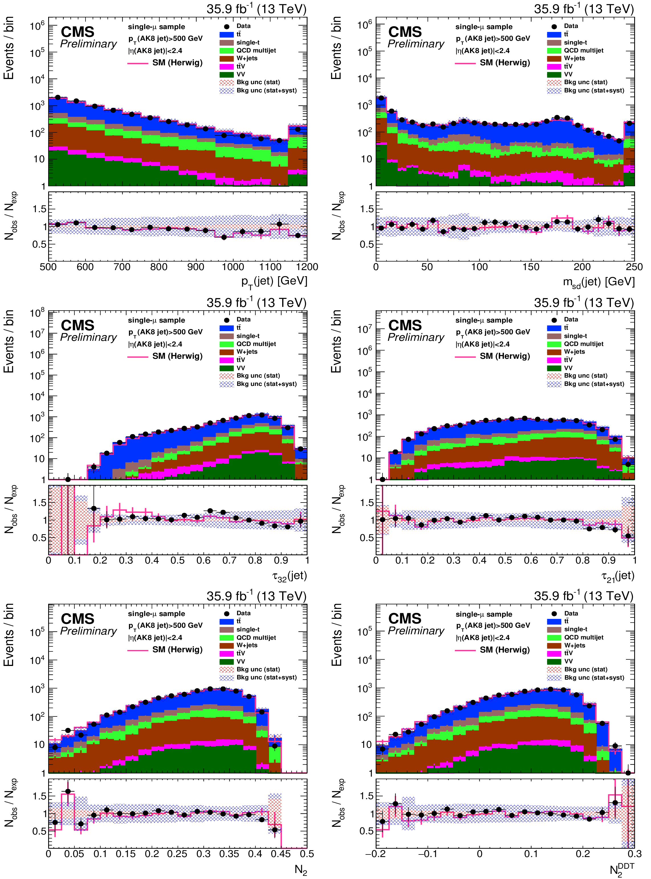
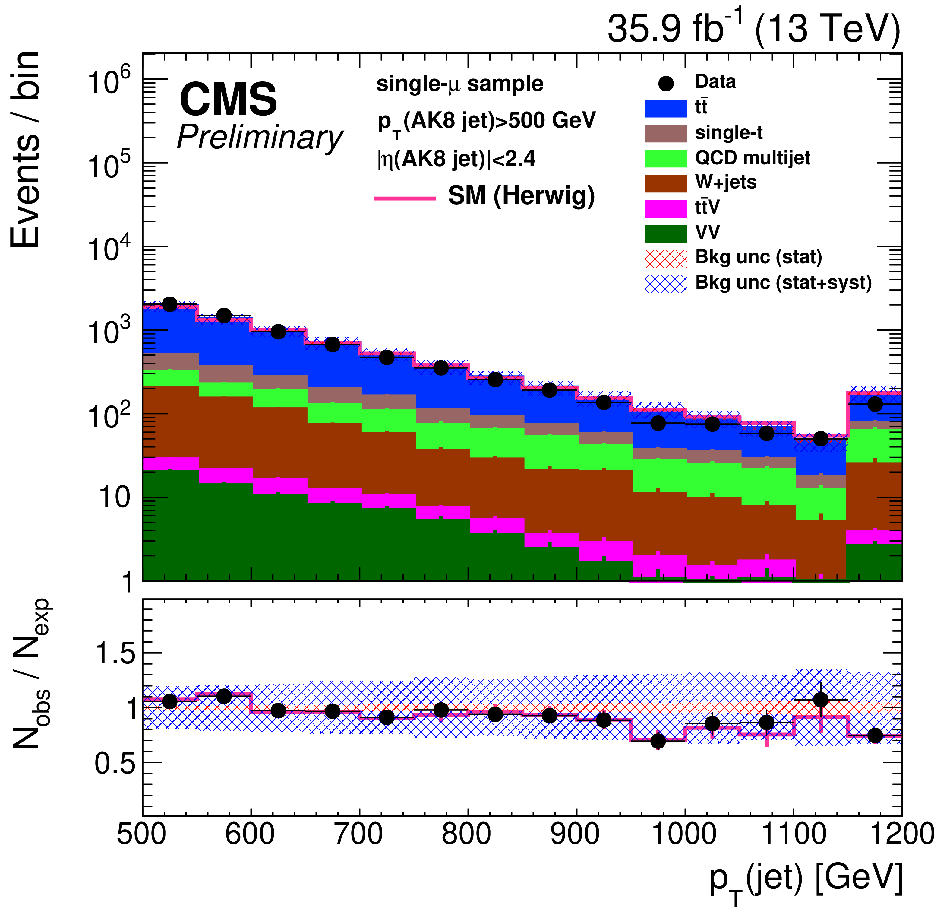
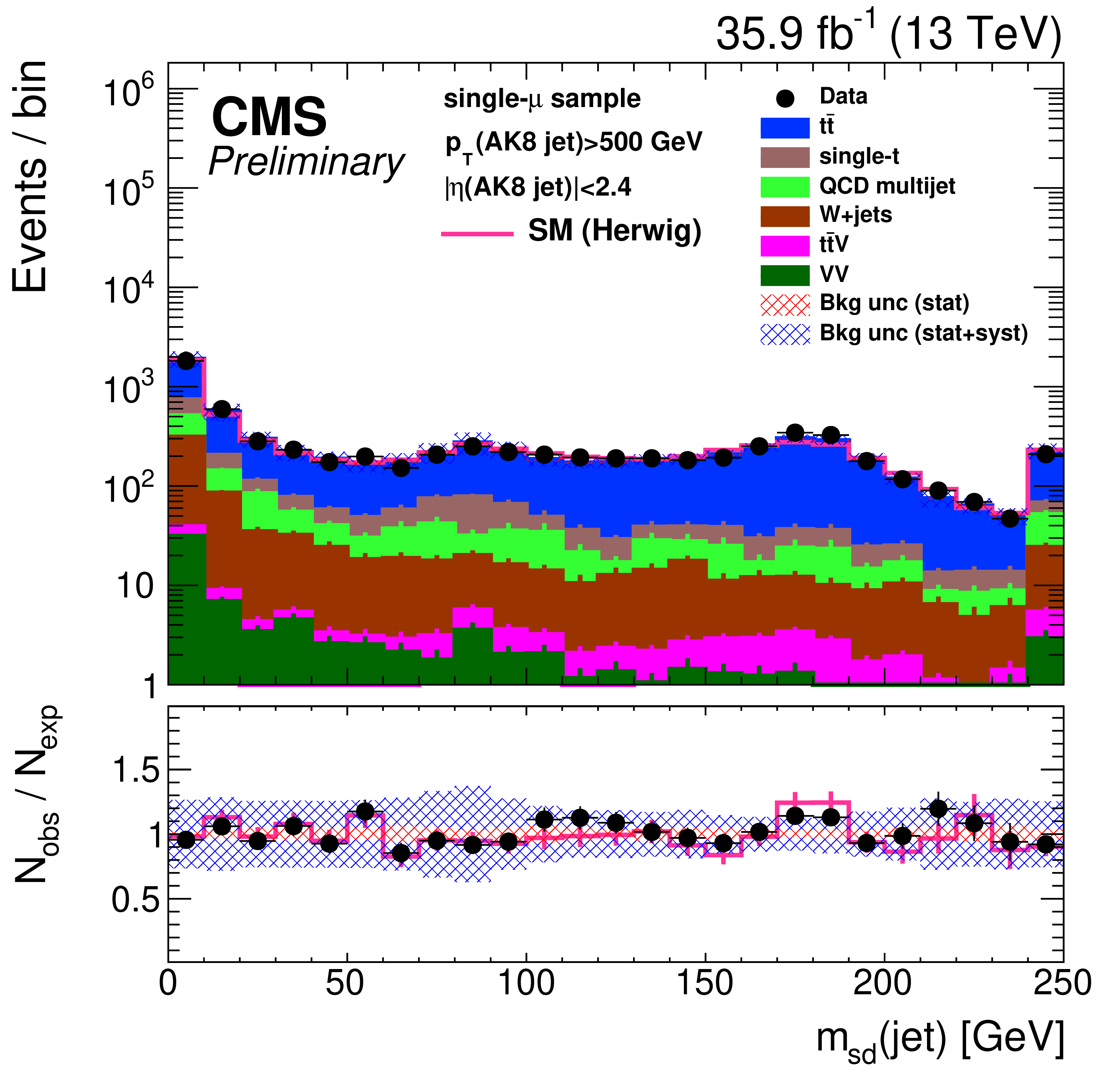
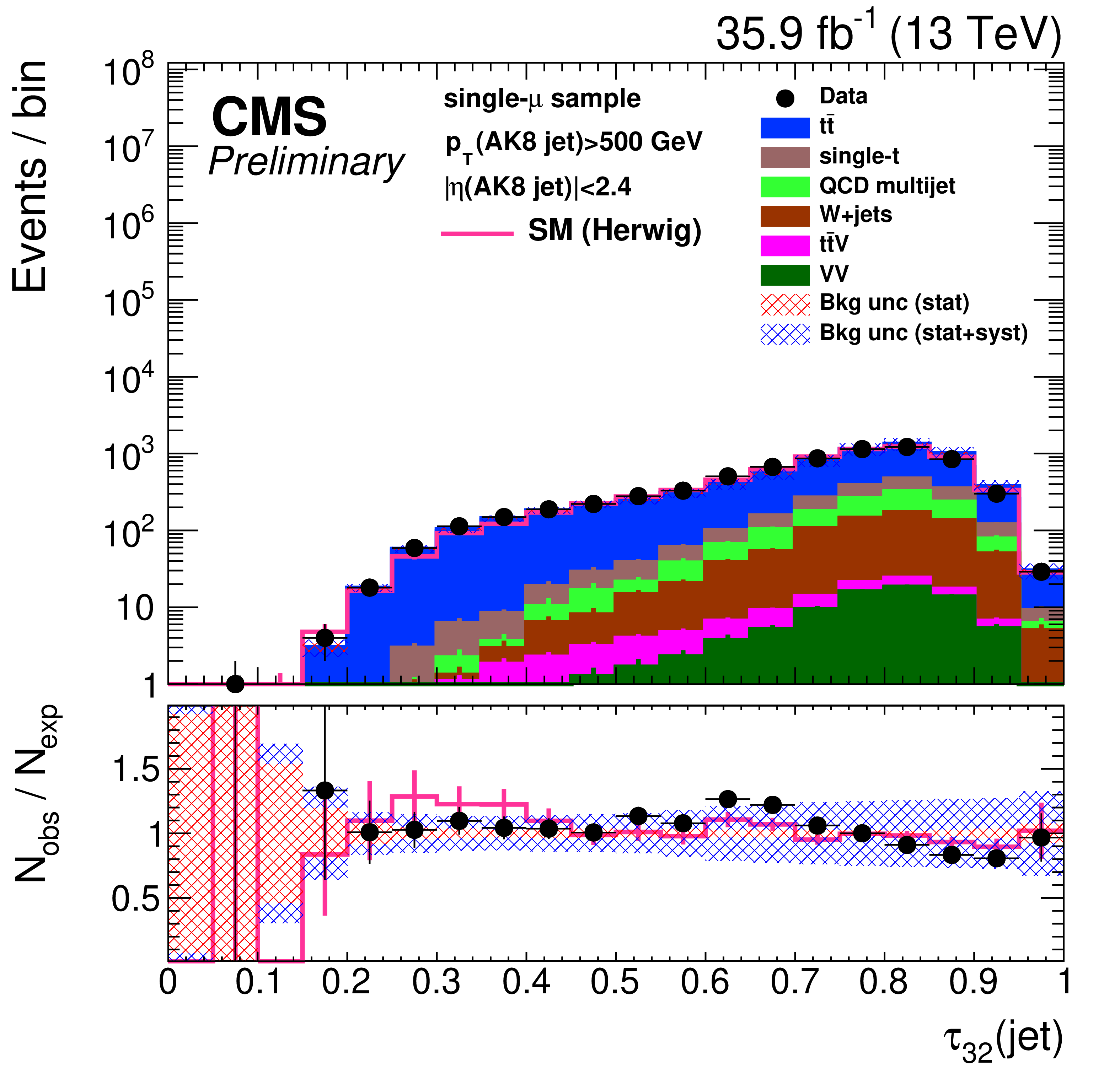
Figure 27:
Distribution of the jet ${p_{\mathrm {T}}}$ (upper-left), the jet mass, ${m_{\text {SD}}}$ (upper-right), the N-subjetiness ratios, $ {\tau _{32}}$ (middle-left) and $ {\tau _{21}}$ (middle-right), and the $N_2$ (lower-left) and $N_2^{\text {DDT}}$ (lower-right) in data and simulation in the single-$\mu $ signal sample, after applying a jet momentum cut $ {p_{\mathrm {T}}} > 500$ GeV. The pink solid line corresponds to the simulation distribution obtained using the alternative ${\mathrm{t} \mathrm{\bar{t}}}$ sample. The background event yield is normalized to the total observed data yield. The lower panel shows the data to simulation ratio. The shaded blue (red) band corresponds to the total uncertainty (statistical uncertainty of the simulated samples), the pink line to the data to simulation ratio using the alternative ${\mathrm{t} \mathrm{\bar{t}}}$ sample, and the vertical lines correspond to the statistical uncertainty of the data. The distributions are weighted according to the top ${p_{\mathrm {T}}}$ reweighting procedure described in the text. |
png pdf |
Figure 27-a:
Distribution of the jet ${p_{\mathrm {T}}}$ (upper-left), the jet mass, ${m_{\text {SD}}}$ (upper-right), the N-subjetiness ratios, $ {\tau _{32}}$ (middle-left) and $ {\tau _{21}}$ (middle-right), and the $N_2$ (lower-left) and $N_2^{\text {DDT}}$ (lower-right) in data and simulation in the single-$\mu $ signal sample, after applying a jet momentum cut $ {p_{\mathrm {T}}} > 500$ GeV. The pink solid line corresponds to the simulation distribution obtained using the alternative ${\mathrm{t} \mathrm{\bar{t}}}$ sample. The background event yield is normalized to the total observed data yield. The lower panel shows the data to simulation ratio. The shaded blue (red) band corresponds to the total uncertainty (statistical uncertainty of the simulated samples), the pink line to the data to simulation ratio using the alternative ${\mathrm{t} \mathrm{\bar{t}}}$ sample, and the vertical lines correspond to the statistical uncertainty of the data. The distributions are weighted according to the top ${p_{\mathrm {T}}}$ reweighting procedure described in the text. |
png pdf |
Figure 27-b:
Distribution of the jet ${p_{\mathrm {T}}}$ (upper-left), the jet mass, ${m_{\text {SD}}}$ (upper-right), the N-subjetiness ratios, $ {\tau _{32}}$ (middle-left) and $ {\tau _{21}}$ (middle-right), and the $N_2$ (lower-left) and $N_2^{\text {DDT}}$ (lower-right) in data and simulation in the single-$\mu $ signal sample, after applying a jet momentum cut $ {p_{\mathrm {T}}} > 500$ GeV. The pink solid line corresponds to the simulation distribution obtained using the alternative ${\mathrm{t} \mathrm{\bar{t}}}$ sample. The background event yield is normalized to the total observed data yield. The lower panel shows the data to simulation ratio. The shaded blue (red) band corresponds to the total uncertainty (statistical uncertainty of the simulated samples), the pink line to the data to simulation ratio using the alternative ${\mathrm{t} \mathrm{\bar{t}}}$ sample, and the vertical lines correspond to the statistical uncertainty of the data. The distributions are weighted according to the top ${p_{\mathrm {T}}}$ reweighting procedure described in the text. |
png pdf |
Figure 27-c:
Distribution of the jet ${p_{\mathrm {T}}}$ (upper-left), the jet mass, ${m_{\text {SD}}}$ (upper-right), the N-subjetiness ratios, $ {\tau _{32}}$ (middle-left) and $ {\tau _{21}}$ (middle-right), and the $N_2$ (lower-left) and $N_2^{\text {DDT}}$ (lower-right) in data and simulation in the single-$\mu $ signal sample, after applying a jet momentum cut $ {p_{\mathrm {T}}} > 500$ GeV. The pink solid line corresponds to the simulation distribution obtained using the alternative ${\mathrm{t} \mathrm{\bar{t}}}$ sample. The background event yield is normalized to the total observed data yield. The lower panel shows the data to simulation ratio. The shaded blue (red) band corresponds to the total uncertainty (statistical uncertainty of the simulated samples), the pink line to the data to simulation ratio using the alternative ${\mathrm{t} \mathrm{\bar{t}}}$ sample, and the vertical lines correspond to the statistical uncertainty of the data. The distributions are weighted according to the top ${p_{\mathrm {T}}}$ reweighting procedure described in the text. |
png pdf |
Figure 27-d:
Distribution of the jet ${p_{\mathrm {T}}}$ (upper-left), the jet mass, ${m_{\text {SD}}}$ (upper-right), the N-subjetiness ratios, $ {\tau _{32}}$ (middle-left) and $ {\tau _{21}}$ (middle-right), and the $N_2$ (lower-left) and $N_2^{\text {DDT}}$ (lower-right) in data and simulation in the single-$\mu $ signal sample, after applying a jet momentum cut $ {p_{\mathrm {T}}} > 500$ GeV. The pink solid line corresponds to the simulation distribution obtained using the alternative ${\mathrm{t} \mathrm{\bar{t}}}$ sample. The background event yield is normalized to the total observed data yield. The lower panel shows the data to simulation ratio. The shaded blue (red) band corresponds to the total uncertainty (statistical uncertainty of the simulated samples), the pink line to the data to simulation ratio using the alternative ${\mathrm{t} \mathrm{\bar{t}}}$ sample, and the vertical lines correspond to the statistical uncertainty of the data. The distributions are weighted according to the top ${p_{\mathrm {T}}}$ reweighting procedure described in the text. |
png pdf |
Figure 27-e:
Distribution of the jet ${p_{\mathrm {T}}}$ (upper-left), the jet mass, ${m_{\text {SD}}}$ (upper-right), the N-subjetiness ratios, $ {\tau _{32}}$ (middle-left) and $ {\tau _{21}}$ (middle-right), and the $N_2$ (lower-left) and $N_2^{\text {DDT}}$ (lower-right) in data and simulation in the single-$\mu $ signal sample, after applying a jet momentum cut $ {p_{\mathrm {T}}} > 500$ GeV. The pink solid line corresponds to the simulation distribution obtained using the alternative ${\mathrm{t} \mathrm{\bar{t}}}$ sample. The background event yield is normalized to the total observed data yield. The lower panel shows the data to simulation ratio. The shaded blue (red) band corresponds to the total uncertainty (statistical uncertainty of the simulated samples), the pink line to the data to simulation ratio using the alternative ${\mathrm{t} \mathrm{\bar{t}}}$ sample, and the vertical lines correspond to the statistical uncertainty of the data. The distributions are weighted according to the top ${p_{\mathrm {T}}}$ reweighting procedure described in the text. |
png pdf |
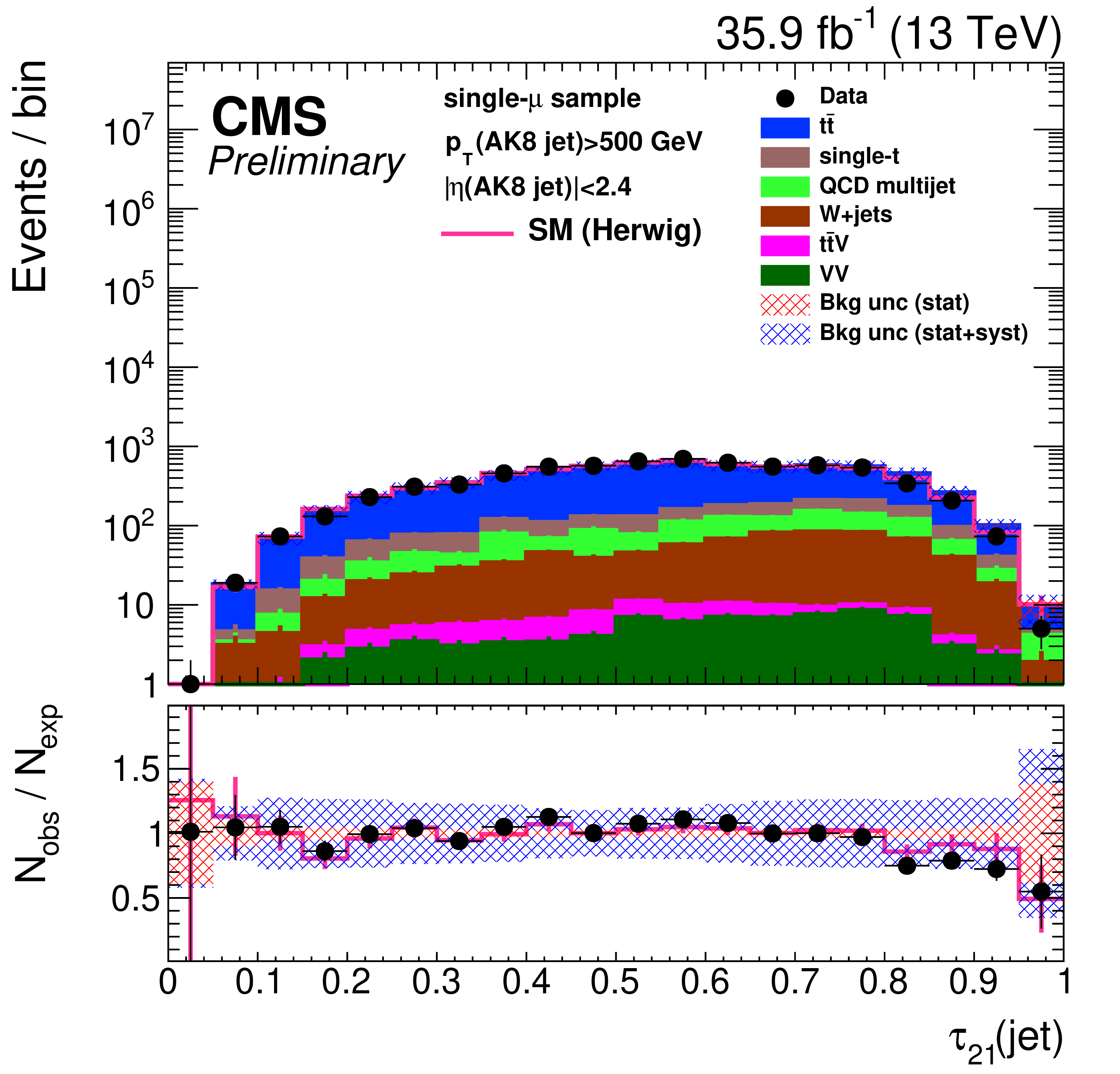
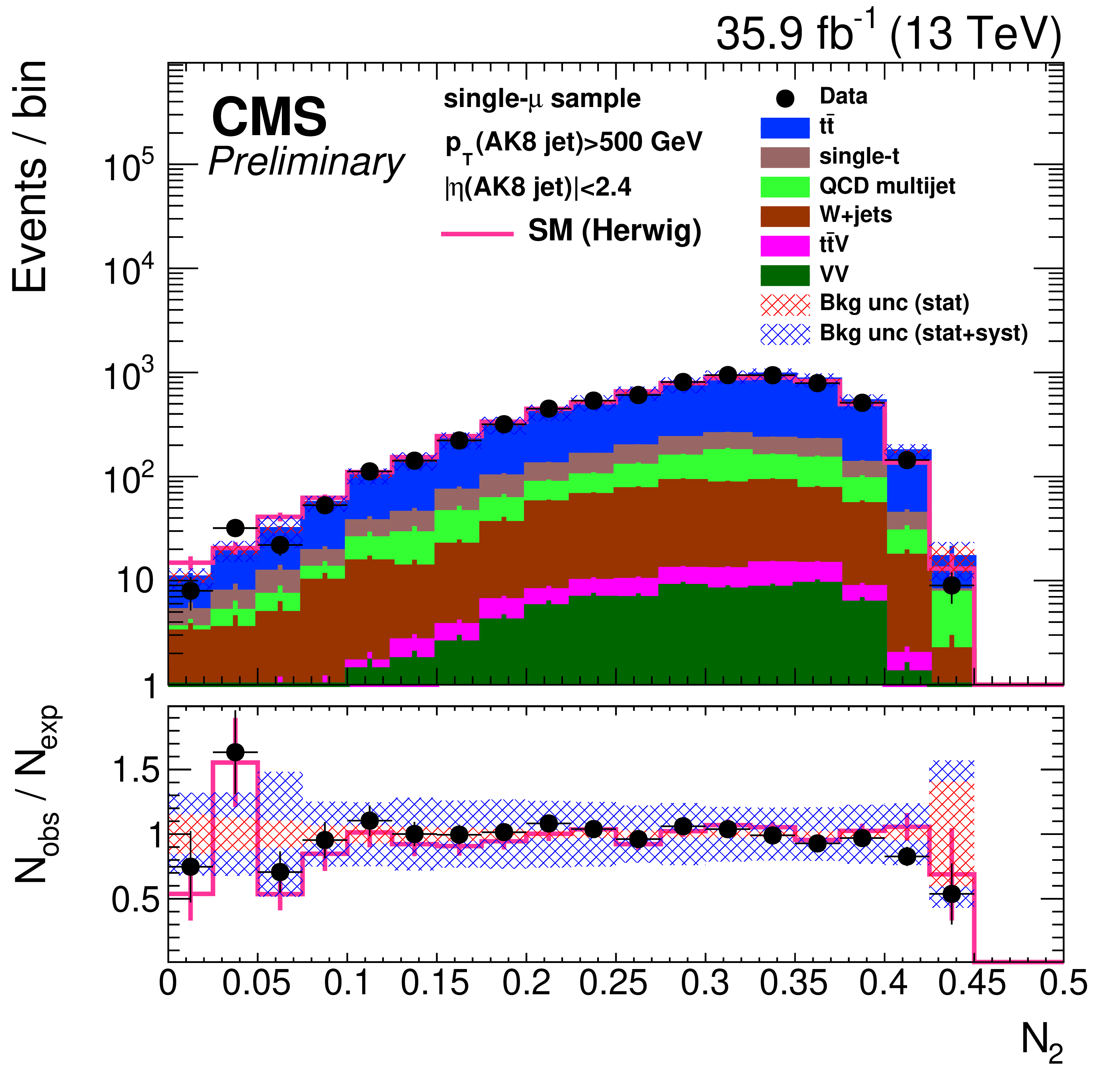
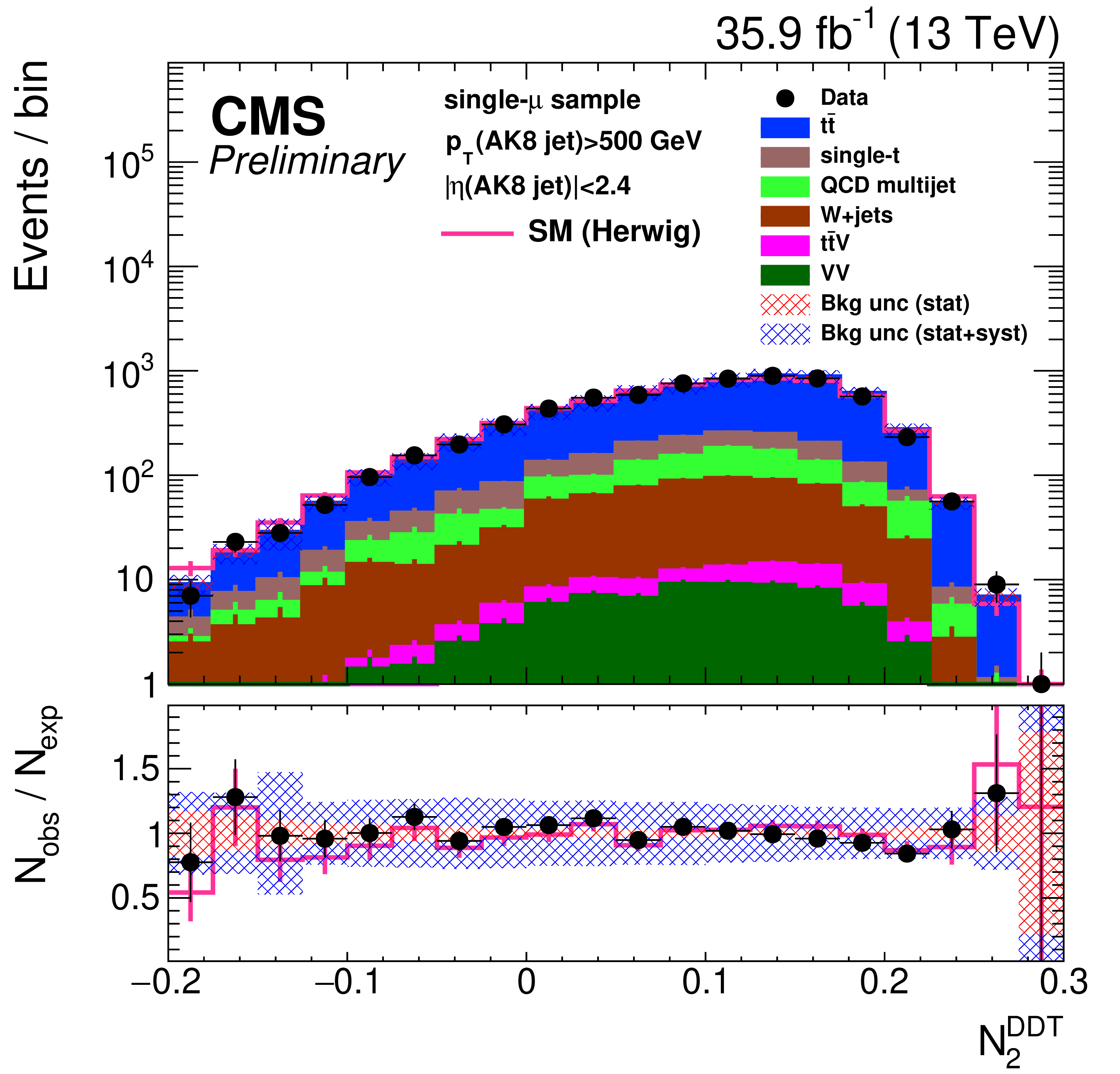
Figure 27-f:
Distribution of the jet ${p_{\mathrm {T}}}$ (upper-left), the jet mass, ${m_{\text {SD}}}$ (upper-right), the N-subjetiness ratios, $ {\tau _{32}}$ (middle-left) and $ {\tau _{21}}$ (middle-right), and the $N_2$ (lower-left) and $N_2^{\text {DDT}}$ (lower-right) in data and simulation in the single-$\mu $ signal sample, after applying a jet momentum cut $ {p_{\mathrm {T}}} > 500$ GeV. The pink solid line corresponds to the simulation distribution obtained using the alternative ${\mathrm{t} \mathrm{\bar{t}}}$ sample. The background event yield is normalized to the total observed data yield. The lower panel shows the data to simulation ratio. The shaded blue (red) band corresponds to the total uncertainty (statistical uncertainty of the simulated samples), the pink line to the data to simulation ratio using the alternative ${\mathrm{t} \mathrm{\bar{t}}}$ sample, and the vertical lines correspond to the statistical uncertainty of the data. The distributions are weighted according to the top ${p_{\mathrm {T}}}$ reweighting procedure described in the text. |
png pdf |
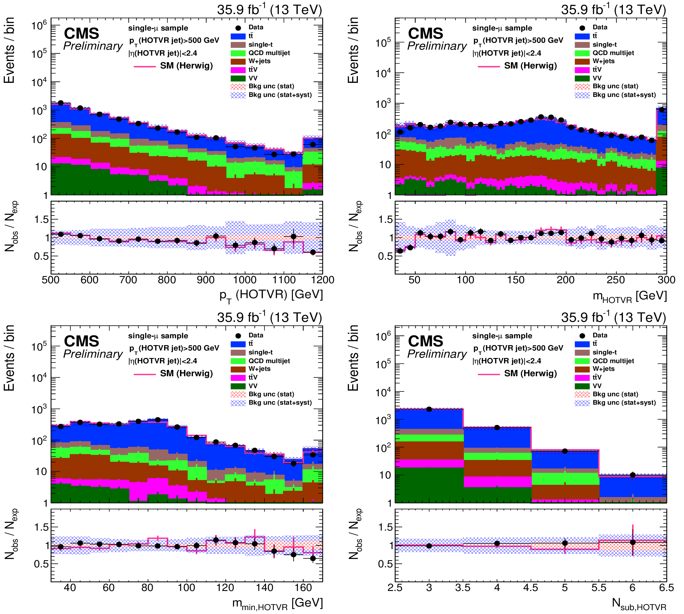
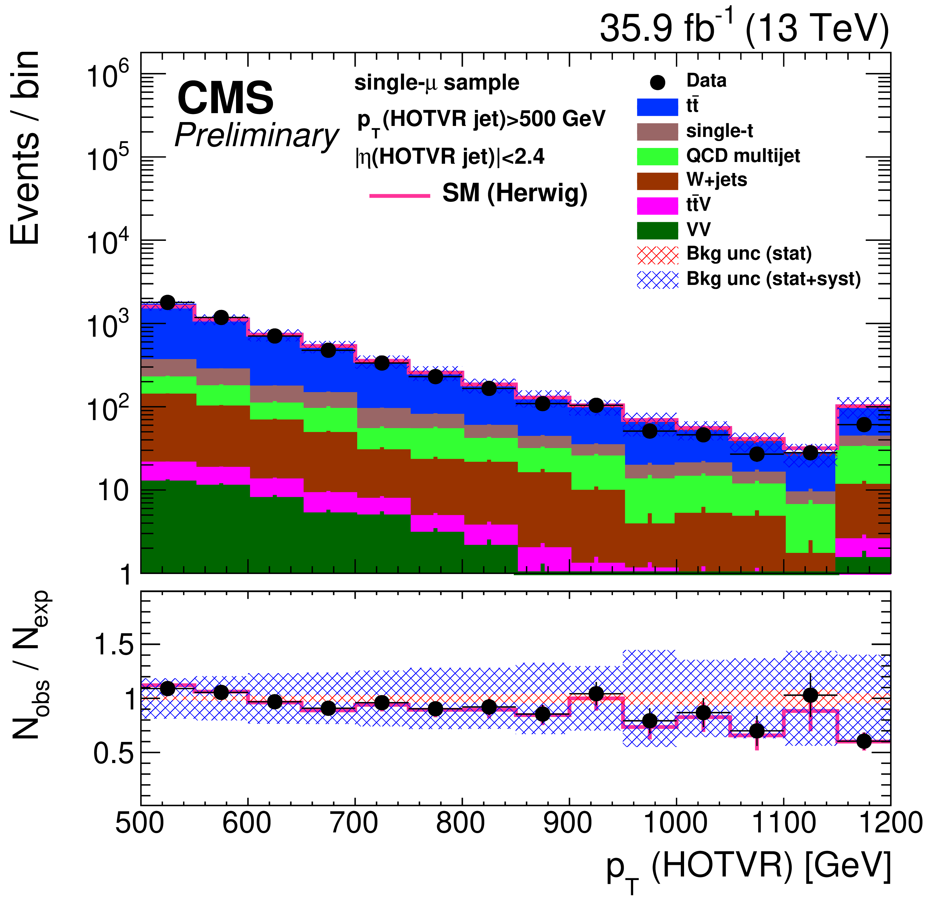
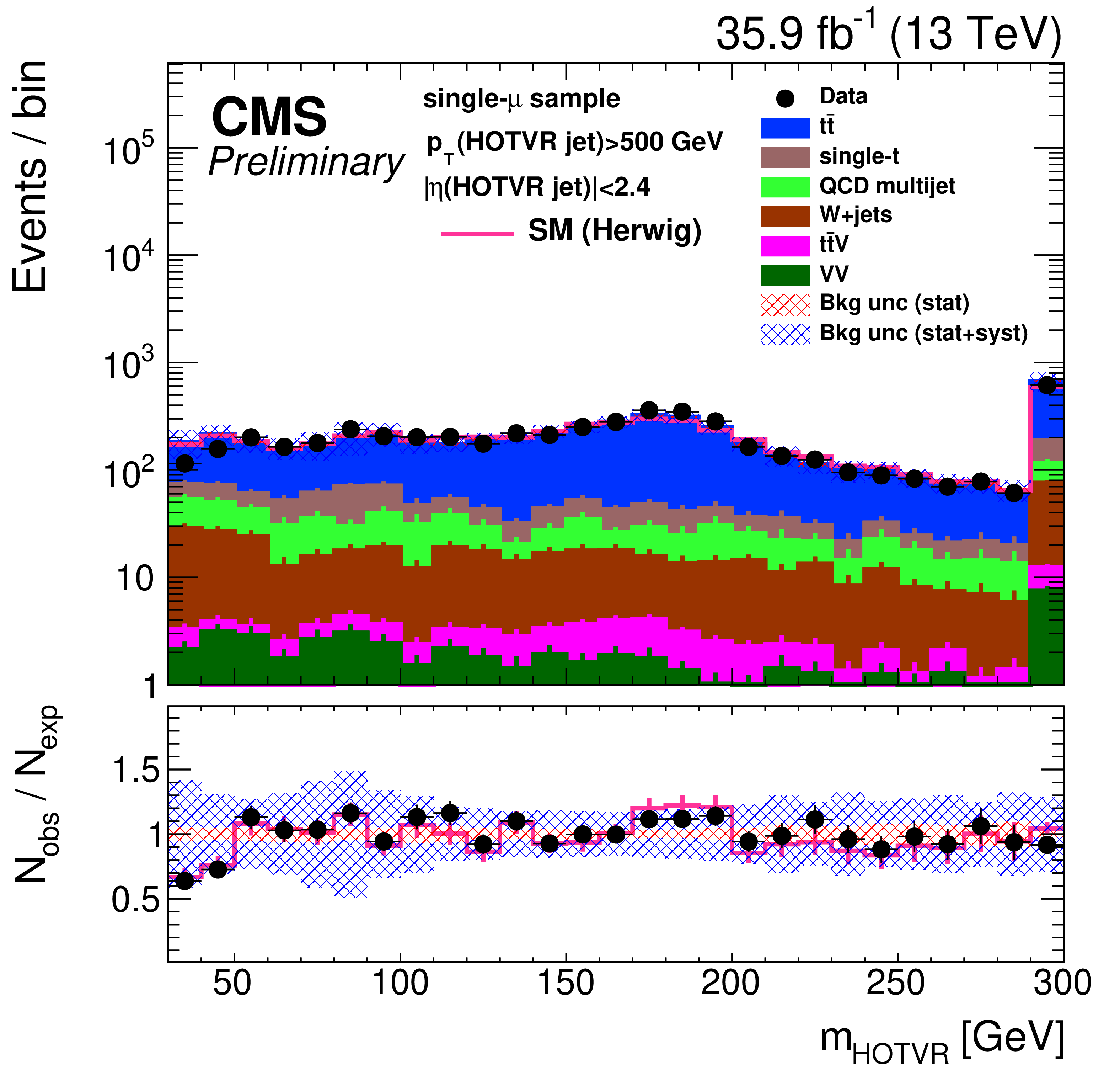
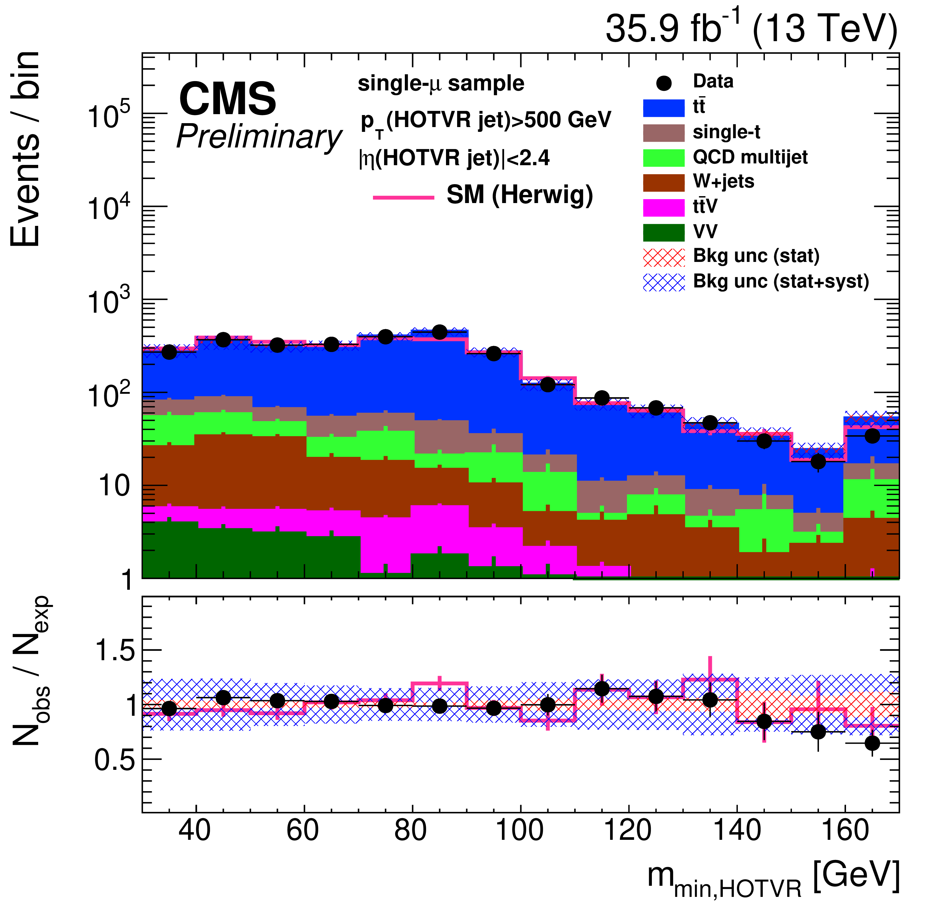
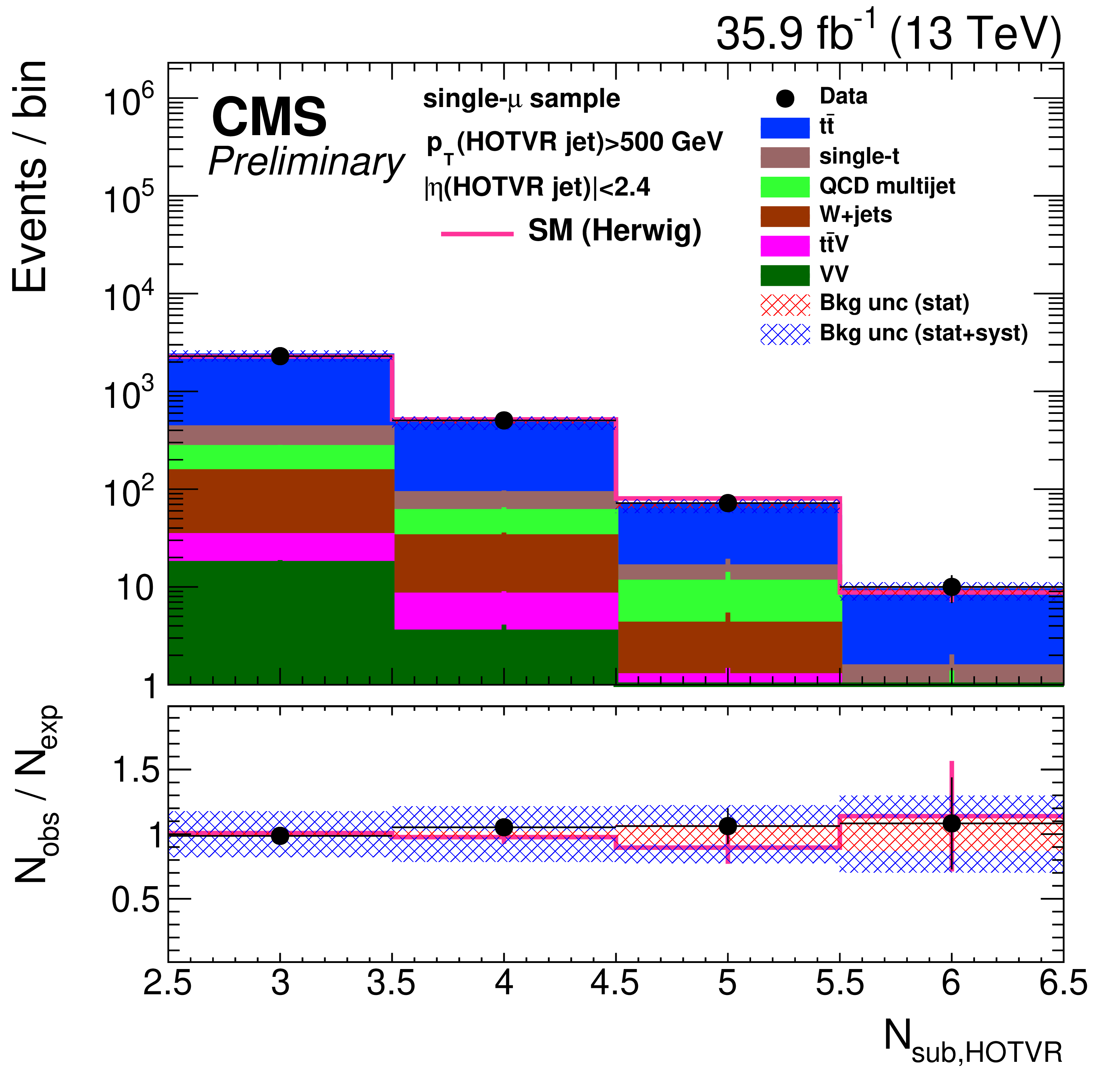
Figure 28:
Distribution of the main observables of the HOTVR algorithm, $p_{T}(\text {HOTVR jet})$ (upper-left), $m_{\text {HOTVR}}$ (upper-right), $m_{\text {min,HOTVR}}$ (lower-left) and $N_{\text {sub,HOTVR}}$ (lower-right) in data and simulation in the single-$\mu $ signal sample, after applying a jet momentum cut $ {p_{\mathrm {T}}} > 500$ GeV. The pink solid line corresponds to the simulation distribution obtained using the alternative ${\mathrm{t} \mathrm{\bar{t}}}$ sample. The background event yield is normalized to the total observed data yield. The lower panel shows the data to simulation ratio. The shaded blue (red) band corresponds to the total uncertainty (statistical uncertainty of the simulated samples), the pink line to the data to simulation ratio using the alternative ${\mathrm{t} \mathrm{\bar{t}}}$ sample, and the vertical lines correspond to the statistical uncertainty of the data. The distributions are weighted according to the top ${p_{\mathrm {T}}}$ reweighting procedure described in the text. |
png pdf |
Figure 28-a:
Distribution of the main observables of the HOTVR algorithm, $p_{T}(\text {HOTVR jet})$ (upper-left), $m_{\text {HOTVR}}$ (upper-right), $m_{\text {min,HOTVR}}$ (lower-left) and $N_{\text {sub,HOTVR}}$ (lower-right) in data and simulation in the single-$\mu $ signal sample, after applying a jet momentum cut $ {p_{\mathrm {T}}} > 500$ GeV. The pink solid line corresponds to the simulation distribution obtained using the alternative ${\mathrm{t} \mathrm{\bar{t}}}$ sample. The background event yield is normalized to the total observed data yield. The lower panel shows the data to simulation ratio. The shaded blue (red) band corresponds to the total uncertainty (statistical uncertainty of the simulated samples), the pink line to the data to simulation ratio using the alternative ${\mathrm{t} \mathrm{\bar{t}}}$ sample, and the vertical lines correspond to the statistical uncertainty of the data. The distributions are weighted according to the top ${p_{\mathrm {T}}}$ reweighting procedure described in the text. |
png pdf |
Figure 28-b:
Distribution of the main observables of the HOTVR algorithm, $p_{T}(\text {HOTVR jet})$ (upper-left), $m_{\text {HOTVR}}$ (upper-right), $m_{\text {min,HOTVR}}$ (lower-left) and $N_{\text {sub,HOTVR}}$ (lower-right) in data and simulation in the single-$\mu $ signal sample, after applying a jet momentum cut $ {p_{\mathrm {T}}} > 500$ GeV. The pink solid line corresponds to the simulation distribution obtained using the alternative ${\mathrm{t} \mathrm{\bar{t}}}$ sample. The background event yield is normalized to the total observed data yield. The lower panel shows the data to simulation ratio. The shaded blue (red) band corresponds to the total uncertainty (statistical uncertainty of the simulated samples), the pink line to the data to simulation ratio using the alternative ${\mathrm{t} \mathrm{\bar{t}}}$ sample, and the vertical lines correspond to the statistical uncertainty of the data. The distributions are weighted according to the top ${p_{\mathrm {T}}}$ reweighting procedure described in the text. |
png pdf |
Figure 28-c:
Distribution of the main observables of the HOTVR algorithm, $p_{T}(\text {HOTVR jet})$ (upper-left), $m_{\text {HOTVR}}$ (upper-right), $m_{\text {min,HOTVR}}$ (lower-left) and $N_{\text {sub,HOTVR}}$ (lower-right) in data and simulation in the single-$\mu $ signal sample, after applying a jet momentum cut $ {p_{\mathrm {T}}} > 500$ GeV. The pink solid line corresponds to the simulation distribution obtained using the alternative ${\mathrm{t} \mathrm{\bar{t}}}$ sample. The background event yield is normalized to the total observed data yield. The lower panel shows the data to simulation ratio. The shaded blue (red) band corresponds to the total uncertainty (statistical uncertainty of the simulated samples), the pink line to the data to simulation ratio using the alternative ${\mathrm{t} \mathrm{\bar{t}}}$ sample, and the vertical lines correspond to the statistical uncertainty of the data. The distributions are weighted according to the top ${p_{\mathrm {T}}}$ reweighting procedure described in the text. |
png pdf |
Figure 28-d:
Distribution of the main observables of the HOTVR algorithm, $p_{T}(\text {HOTVR jet})$ (upper-left), $m_{\text {HOTVR}}$ (upper-right), $m_{\text {min,HOTVR}}$ (lower-left) and $N_{\text {sub,HOTVR}}$ (lower-right) in data and simulation in the single-$\mu $ signal sample, after applying a jet momentum cut $ {p_{\mathrm {T}}} > 500$ GeV. The pink solid line corresponds to the simulation distribution obtained using the alternative ${\mathrm{t} \mathrm{\bar{t}}}$ sample. The background event yield is normalized to the total observed data yield. The lower panel shows the data to simulation ratio. The shaded blue (red) band corresponds to the total uncertainty (statistical uncertainty of the simulated samples), the pink line to the data to simulation ratio using the alternative ${\mathrm{t} \mathrm{\bar{t}}}$ sample, and the vertical lines correspond to the statistical uncertainty of the data. The distributions are weighted according to the top ${p_{\mathrm {T}}}$ reweighting procedure described in the text. |
png pdf |
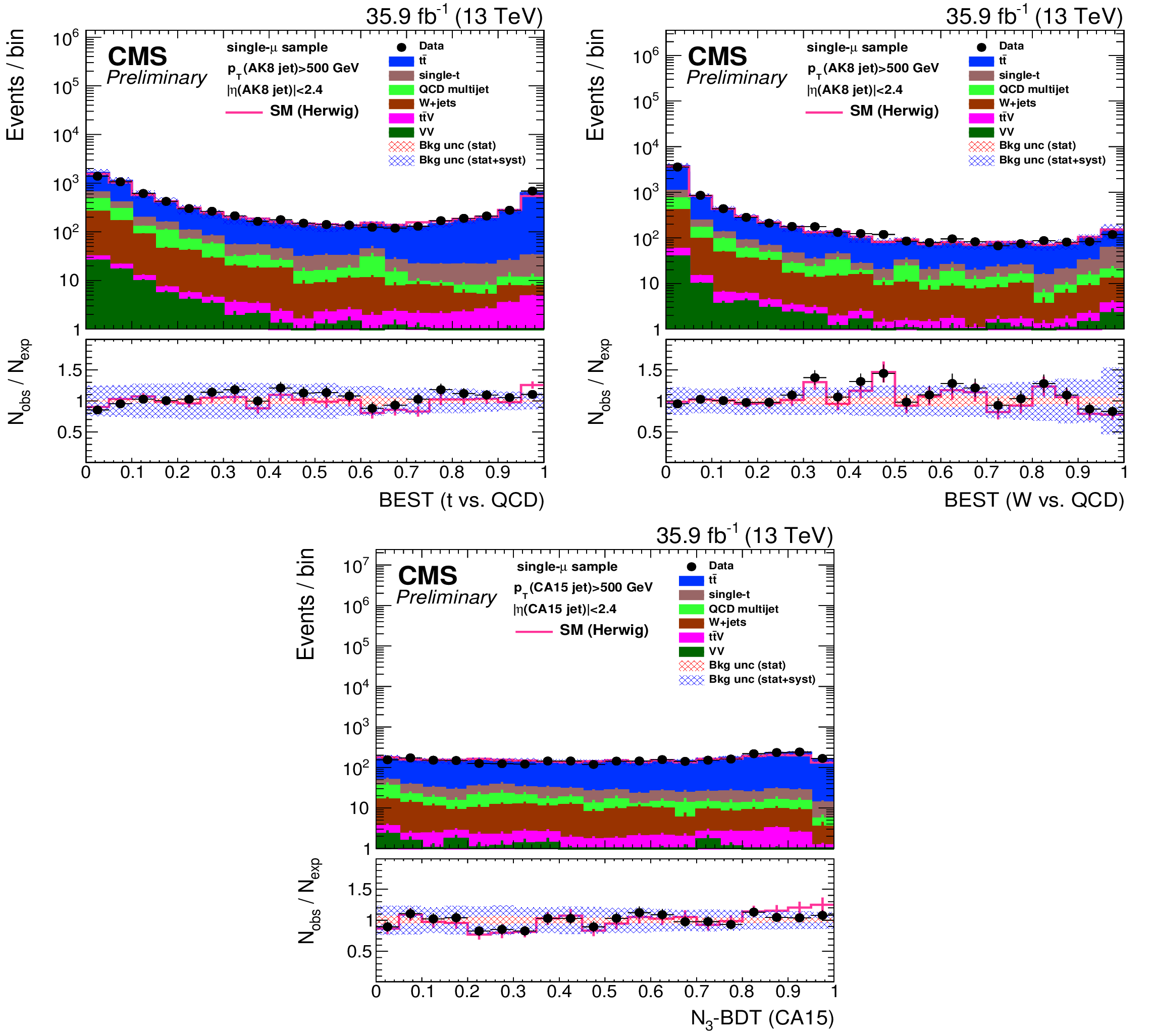
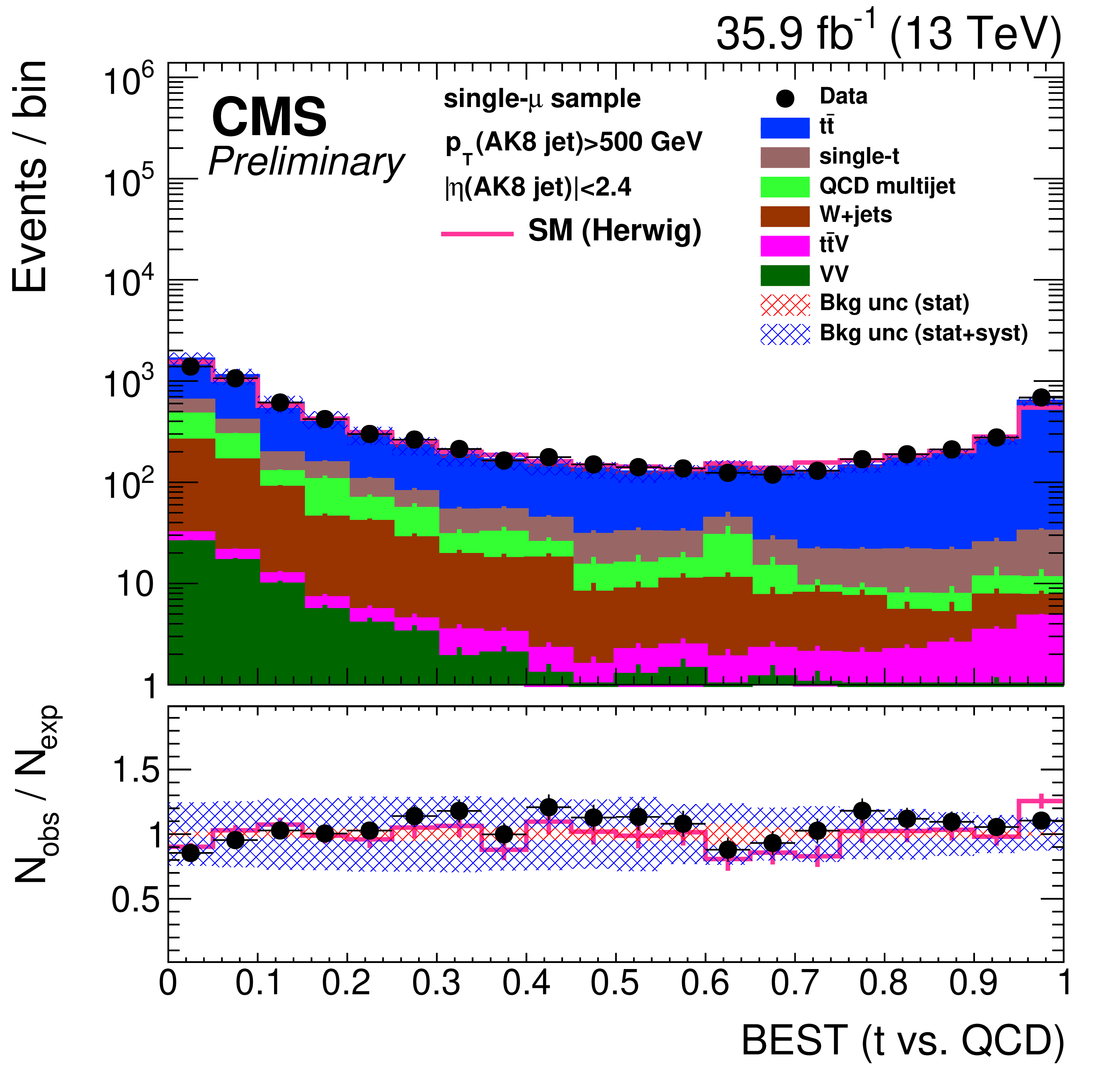
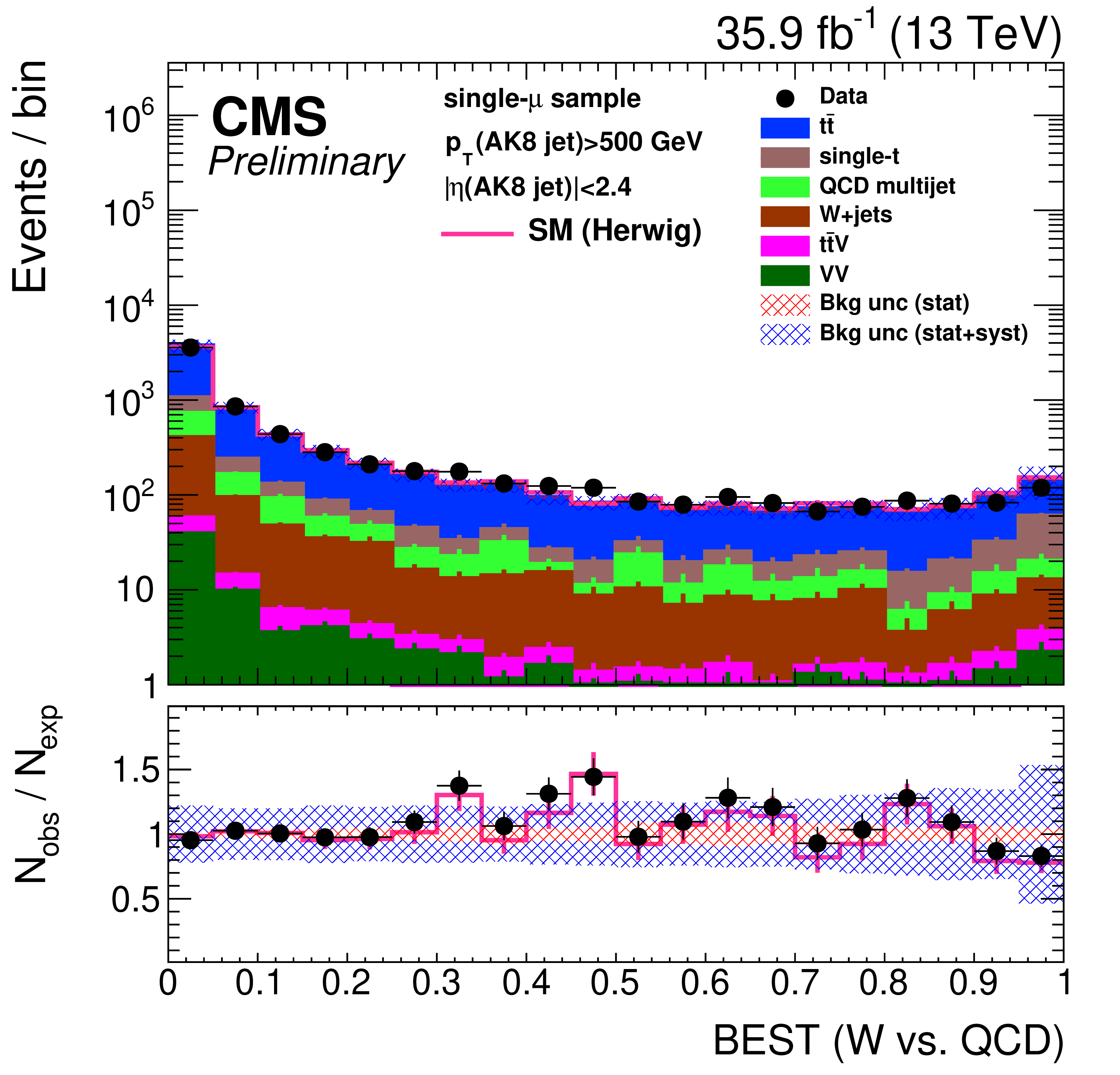
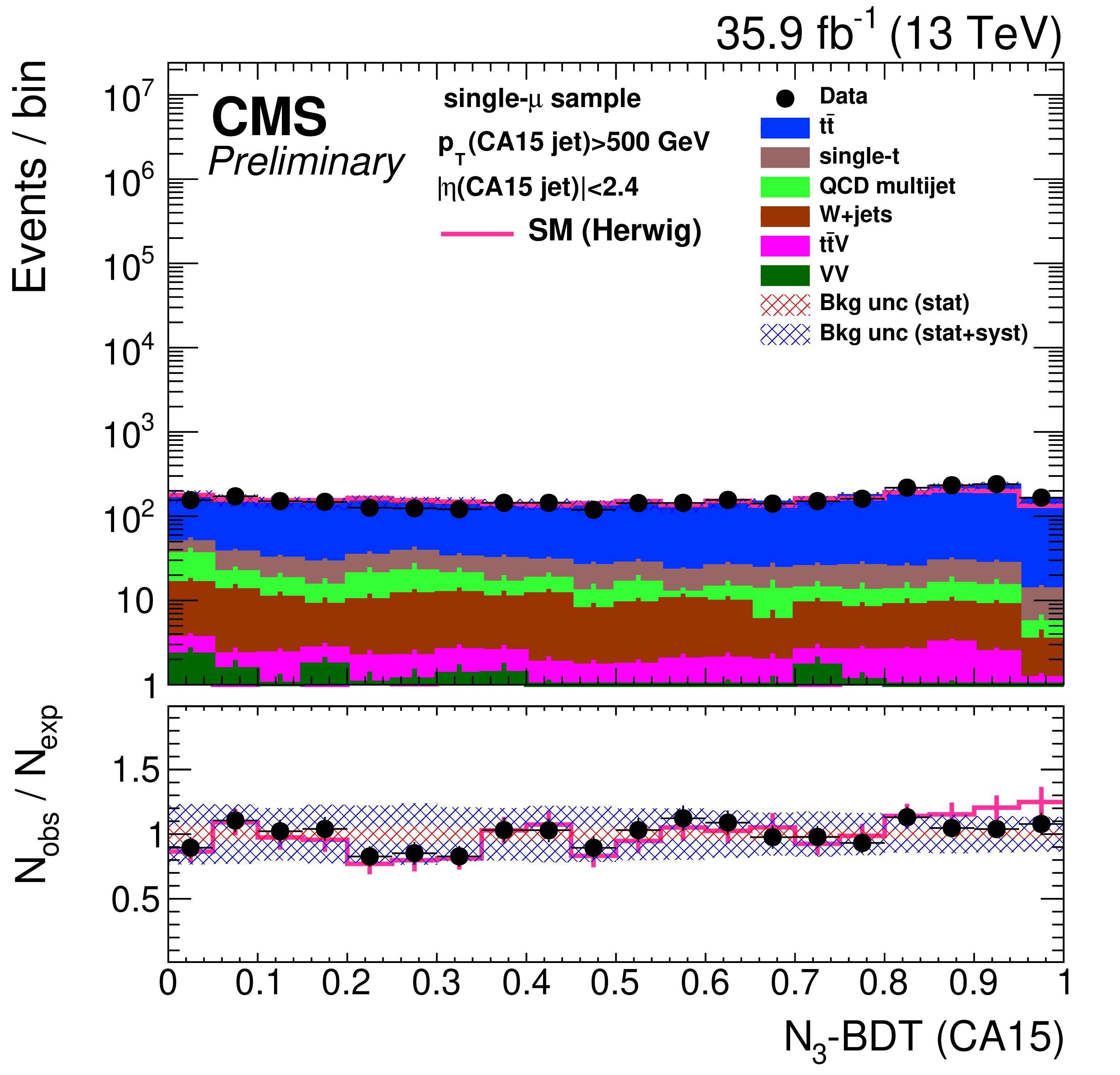
Figure 29:
Distribution of the t quark (upper-left) and W boson (upper-right) identification probabilities for the BEST algorithm, and the ${N_{3}-\text {BDT} (\text {CA}15)}$ discriminant, in data and simulation in the single-$\mu $ signal sample, after applying a jet momentum cut $ {p_{\mathrm {T}}} > 500$ GeV. The pink solid line corresponds to the simulation distribution obtained using the alternative ${\mathrm{t} \mathrm{\bar{t}}}$ sample. The background event yield is normalized to the total observed data yield. The lower panel shows the data to simulation ratio. The shaded blue (red) band corresponds to the total uncertainty (statistical uncertainty of the simulated samples), the pink line to the data to simulation ratio using the alternative ${\mathrm{t} \mathrm{\bar{t}}}$ sample, and the vertical lines correspond to the statistical uncertainty of the data. The distributions are weighted according to the top ${p_{\mathrm {T}}}$ reweighting procedure described in the text. |
png pdf |
Figure 29-a:
Distribution of the t quark (upper-left) and W boson (upper-right) identification probabilities for the BEST algorithm, and the ${N_{3}-\text {BDT} (\text {CA}15)}$ discriminant, in data and simulation in the single-$\mu $ signal sample, after applying a jet momentum cut $ {p_{\mathrm {T}}} > 500$ GeV. The pink solid line corresponds to the simulation distribution obtained using the alternative ${\mathrm{t} \mathrm{\bar{t}}}$ sample. The background event yield is normalized to the total observed data yield. The lower panel shows the data to simulation ratio. The shaded blue (red) band corresponds to the total uncertainty (statistical uncertainty of the simulated samples), the pink line to the data to simulation ratio using the alternative ${\mathrm{t} \mathrm{\bar{t}}}$ sample, and the vertical lines correspond to the statistical uncertainty of the data. The distributions are weighted according to the top ${p_{\mathrm {T}}}$ reweighting procedure described in the text. |
png pdf |
Figure 29-b:
Distribution of the t quark (upper-left) and W boson (upper-right) identification probabilities for the BEST algorithm, and the ${N_{3}-\text {BDT} (\text {CA}15)}$ discriminant, in data and simulation in the single-$\mu $ signal sample, after applying a jet momentum cut $ {p_{\mathrm {T}}} > 500$ GeV. The pink solid line corresponds to the simulation distribution obtained using the alternative ${\mathrm{t} \mathrm{\bar{t}}}$ sample. The background event yield is normalized to the total observed data yield. The lower panel shows the data to simulation ratio. The shaded blue (red) band corresponds to the total uncertainty (statistical uncertainty of the simulated samples), the pink line to the data to simulation ratio using the alternative ${\mathrm{t} \mathrm{\bar{t}}}$ sample, and the vertical lines correspond to the statistical uncertainty of the data. The distributions are weighted according to the top ${p_{\mathrm {T}}}$ reweighting procedure described in the text. |
png pdf |
Figure 29-c:
Distribution of the t quark (upper-left) and W boson (upper-right) identification probabilities for the BEST algorithm, and the ${N_{3}-\text {BDT} (\text {CA}15)}$ discriminant, in data and simulation in the single-$\mu $ signal sample, after applying a jet momentum cut $ {p_{\mathrm {T}}} > 500$ GeV. The pink solid line corresponds to the simulation distribution obtained using the alternative ${\mathrm{t} \mathrm{\bar{t}}}$ sample. The background event yield is normalized to the total observed data yield. The lower panel shows the data to simulation ratio. The shaded blue (red) band corresponds to the total uncertainty (statistical uncertainty of the simulated samples), the pink line to the data to simulation ratio using the alternative ${\mathrm{t} \mathrm{\bar{t}}}$ sample, and the vertical lines correspond to the statistical uncertainty of the data. The distributions are weighted according to the top ${p_{\mathrm {T}}}$ reweighting procedure described in the text. |
png pdf |
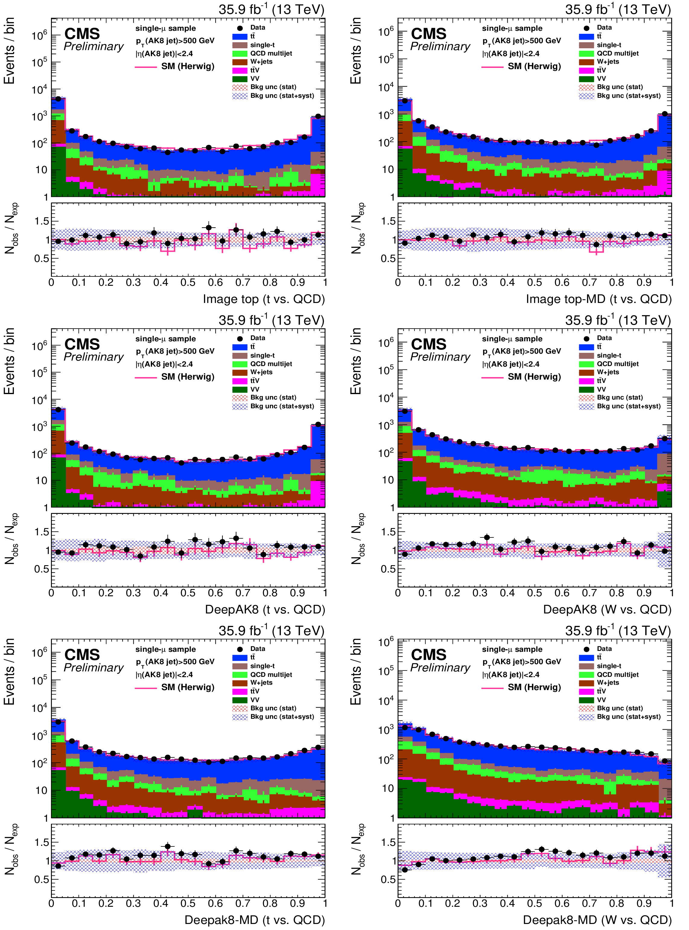
Figure 30:
Distribution of the ImageTop (upper left) and ImageTop-MD (upper-right) discriminant in data and simulation in the single-$\mu $ sample. The plots in the middle row show the t quark (left) and W boson (right) identification probabilities in data and simulation for the DeepAK8 algorithm, after applying a jet momentum cut $ {p_{\mathrm {T}}} > 500$ GeV. The corresponding plots for DeepAK8-MD are displayed in the lower row. The pink solid line corresponds to the simulation distribution obtained using the alternative ${\mathrm{t} \mathrm{\bar{t}}}$ sample. The background event yield is normalized to the total observed data yield. The lower panel shows the data to simulation ratio. The shaded blue (red) band corresponds to the total uncertainty (statistical uncertainty of the simulated samples), the pink line to the data to simulation ratio using the alternative ${\mathrm{t} \mathrm{\bar{t}}}$ sample, and the vertical lines correspond to the statistical uncertainty of the data. The distributions are weighted according to the top ${p_{\mathrm {T}}}$ reweighting procedure described in the text. |
png pdf |
Figure 30-a:
Distribution of the ImageTop (upper left) and ImageTop-MD (upper-right) discriminant in data and simulation in the single-$\mu $ sample. The plots in the middle row show the t quark (left) and W boson (right) identification probabilities in data and simulation for the DeepAK8 algorithm, after applying a jet momentum cut $ {p_{\mathrm {T}}} > 500$ GeV. The corresponding plots for DeepAK8-MD are displayed in the lower row. The pink solid line corresponds to the simulation distribution obtained using the alternative ${\mathrm{t} \mathrm{\bar{t}}}$ sample. The background event yield is normalized to the total observed data yield. The lower panel shows the data to simulation ratio. The shaded blue (red) band corresponds to the total uncertainty (statistical uncertainty of the simulated samples), the pink line to the data to simulation ratio using the alternative ${\mathrm{t} \mathrm{\bar{t}}}$ sample, and the vertical lines correspond to the statistical uncertainty of the data. The distributions are weighted according to the top ${p_{\mathrm {T}}}$ reweighting procedure described in the text. |
png pdf |
Figure 30-b:
Distribution of the ImageTop (upper left) and ImageTop-MD (upper-right) discriminant in data and simulation in the single-$\mu $ sample. The plots in the middle row show the t quark (left) and W boson (right) identification probabilities in data and simulation for the DeepAK8 algorithm, after applying a jet momentum cut $ {p_{\mathrm {T}}} > 500$ GeV. The corresponding plots for DeepAK8-MD are displayed in the lower row. The pink solid line corresponds to the simulation distribution obtained using the alternative ${\mathrm{t} \mathrm{\bar{t}}}$ sample. The background event yield is normalized to the total observed data yield. The lower panel shows the data to simulation ratio. The shaded blue (red) band corresponds to the total uncertainty (statistical uncertainty of the simulated samples), the pink line to the data to simulation ratio using the alternative ${\mathrm{t} \mathrm{\bar{t}}}$ sample, and the vertical lines correspond to the statistical uncertainty of the data. The distributions are weighted according to the top ${p_{\mathrm {T}}}$ reweighting procedure described in the text. |
png pdf |
Figure 30-c:
Distribution of the ImageTop (upper left) and ImageTop-MD (upper-right) discriminant in data and simulation in the single-$\mu $ sample. The plots in the middle row show the t quark (left) and W boson (right) identification probabilities in data and simulation for the DeepAK8 algorithm, after applying a jet momentum cut $ {p_{\mathrm {T}}} > 500$ GeV. The corresponding plots for DeepAK8-MD are displayed in the lower row. The pink solid line corresponds to the simulation distribution obtained using the alternative ${\mathrm{t} \mathrm{\bar{t}}}$ sample. The background event yield is normalized to the total observed data yield. The lower panel shows the data to simulation ratio. The shaded blue (red) band corresponds to the total uncertainty (statistical uncertainty of the simulated samples), the pink line to the data to simulation ratio using the alternative ${\mathrm{t} \mathrm{\bar{t}}}$ sample, and the vertical lines correspond to the statistical uncertainty of the data. The distributions are weighted according to the top ${p_{\mathrm {T}}}$ reweighting procedure described in the text. |
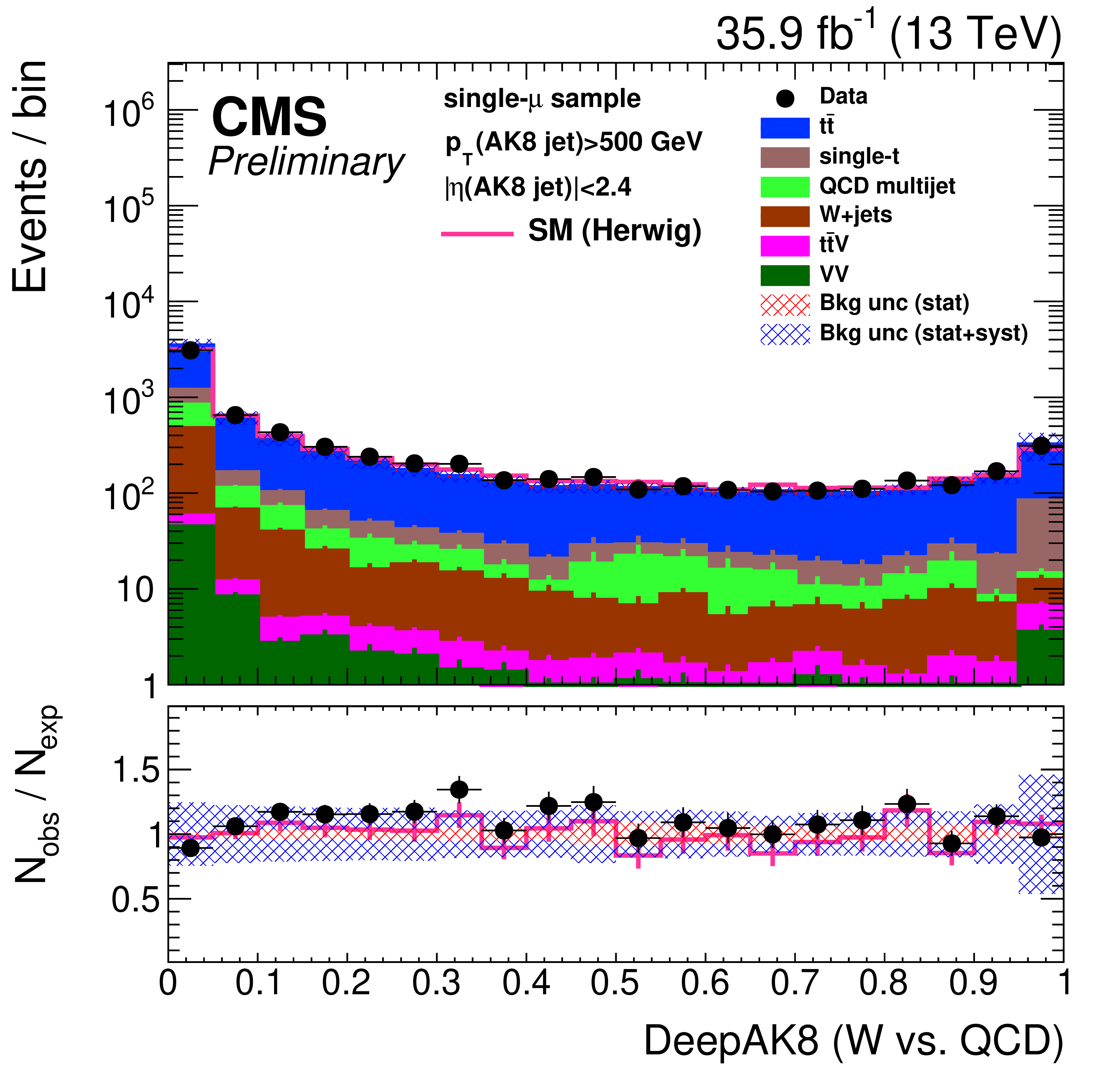
png pdf |
Figure 30-d:
Distribution of the ImageTop (upper left) and ImageTop-MD (upper-right) discriminant in data and simulation in the single-$\mu $ sample. The plots in the middle row show the t quark (left) and W boson (right) identification probabilities in data and simulation for the DeepAK8 algorithm, after applying a jet momentum cut $ {p_{\mathrm {T}}} > 500$ GeV. The corresponding plots for DeepAK8-MD are displayed in the lower row. The pink solid line corresponds to the simulation distribution obtained using the alternative ${\mathrm{t} \mathrm{\bar{t}}}$ sample. The background event yield is normalized to the total observed data yield. The lower panel shows the data to simulation ratio. The shaded blue (red) band corresponds to the total uncertainty (statistical uncertainty of the simulated samples), the pink line to the data to simulation ratio using the alternative ${\mathrm{t} \mathrm{\bar{t}}}$ sample, and the vertical lines correspond to the statistical uncertainty of the data. The distributions are weighted according to the top ${p_{\mathrm {T}}}$ reweighting procedure described in the text. |
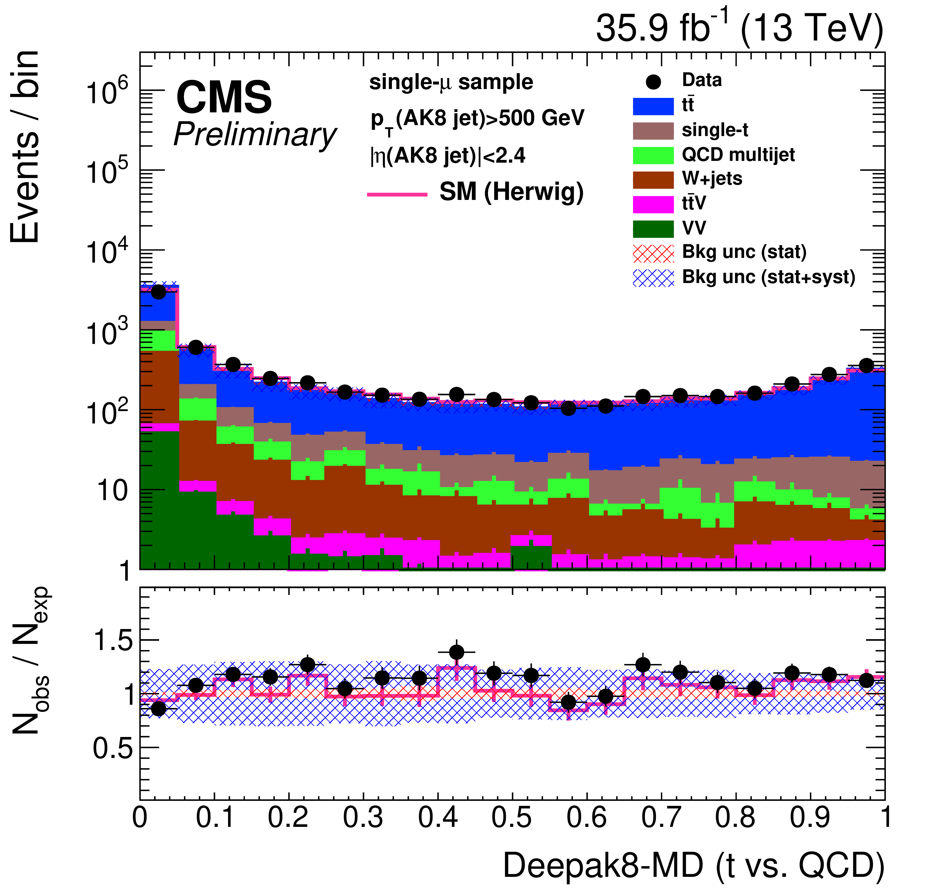
png pdf |
Figure 30-e:
Distribution of the ImageTop (upper left) and ImageTop-MD (upper-right) discriminant in data and simulation in the single-$\mu $ sample. The plots in the middle row show the t quark (left) and W boson (right) identification probabilities in data and simulation for the DeepAK8 algorithm, after applying a jet momentum cut $ {p_{\mathrm {T}}} > 500$ GeV. The corresponding plots for DeepAK8-MD are displayed in the lower row. The pink solid line corresponds to the simulation distribution obtained using the alternative ${\mathrm{t} \mathrm{\bar{t}}}$ sample. The background event yield is normalized to the total observed data yield. The lower panel shows the data to simulation ratio. The shaded blue (red) band corresponds to the total uncertainty (statistical uncertainty of the simulated samples), the pink line to the data to simulation ratio using the alternative ${\mathrm{t} \mathrm{\bar{t}}}$ sample, and the vertical lines correspond to the statistical uncertainty of the data. The distributions are weighted according to the top ${p_{\mathrm {T}}}$ reweighting procedure described in the text. |
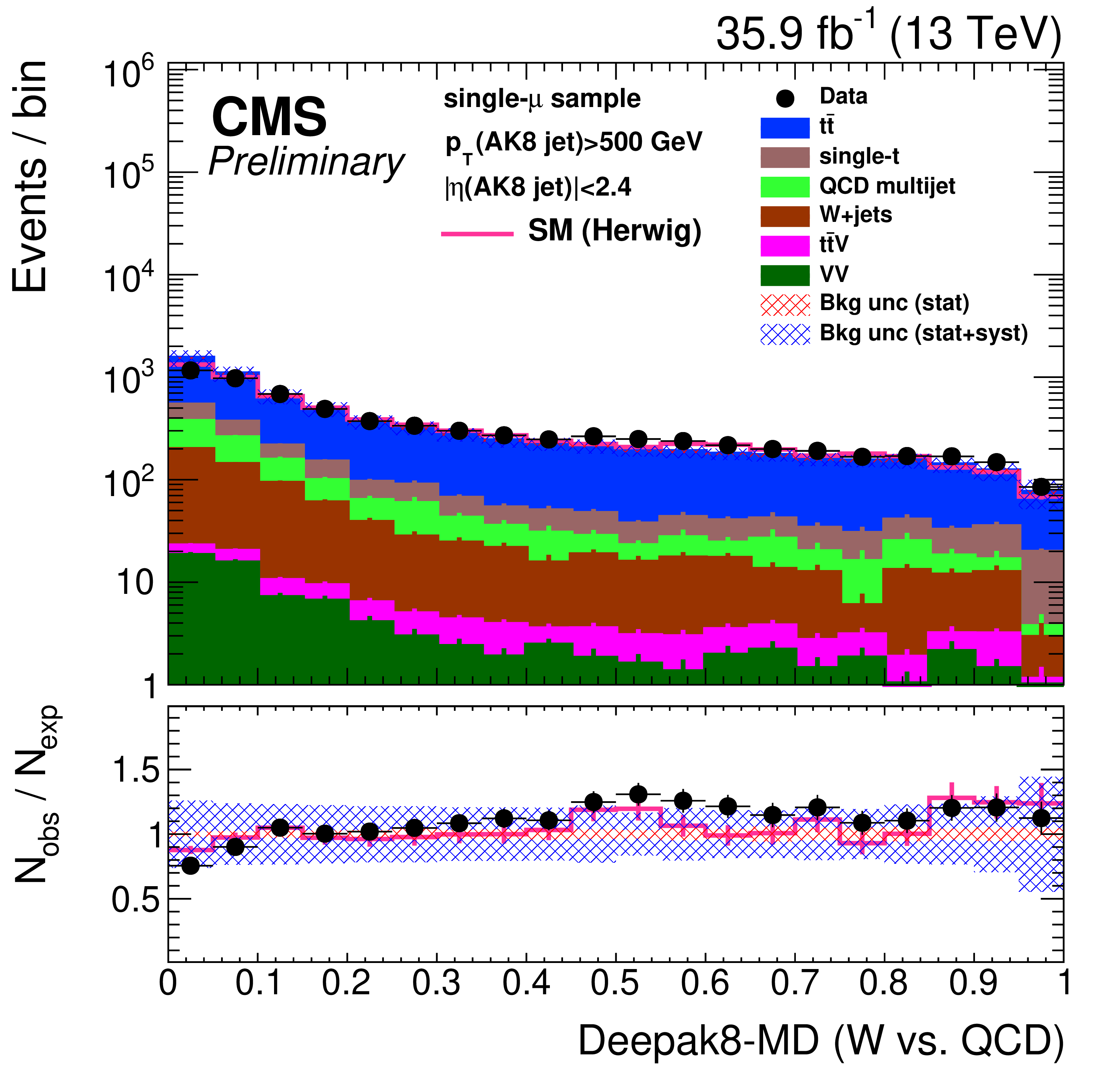
png pdf |
Figure 30-f:
Distribution of the ImageTop (upper left) and ImageTop-MD (upper-right) discriminant in data and simulation in the single-$\mu $ sample. The plots in the middle row show the t quark (left) and W boson (right) identification probabilities in data and simulation for the DeepAK8 algorithm, after applying a jet momentum cut $ {p_{\mathrm {T}}} > 500$ GeV. The corresponding plots for DeepAK8-MD are displayed in the lower row. The pink solid line corresponds to the simulation distribution obtained using the alternative ${\mathrm{t} \mathrm{\bar{t}}}$ sample. The background event yield is normalized to the total observed data yield. The lower panel shows the data to simulation ratio. The shaded blue (red) band corresponds to the total uncertainty (statistical uncertainty of the simulated samples), the pink line to the data to simulation ratio using the alternative ${\mathrm{t} \mathrm{\bar{t}}}$ sample, and the vertical lines correspond to the statistical uncertainty of the data. The distributions are weighted according to the top ${p_{\mathrm {T}}}$ reweighting procedure described in the text. |
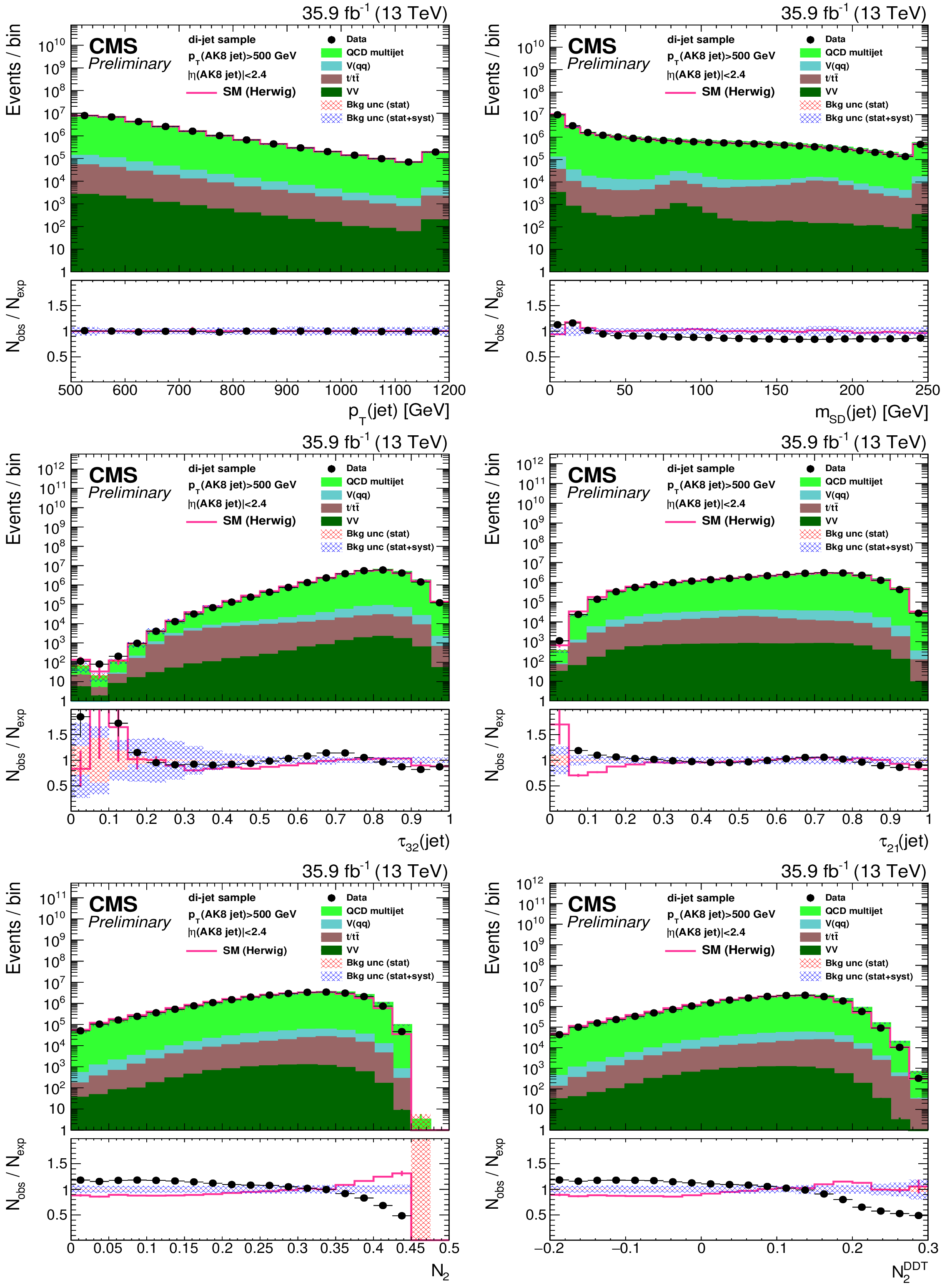
png pdf |
Figure 31:
Distribution of the jet ${p_{\mathrm {T}}}$ (upper-left), the jet mass, ${m_{\text {SD}}}$ (upper-right), the N-subjetiness ratios, $ {\tau _{32}}$ (middle-left) and $ {\tau _{21}}$ (middle-right), and the $N_2$ (lower-left) and $N_{2}^{\text {DDT}}$ (lower-right) in data and simulation in the di-jet sample. The pink solid line corresponds to the simulation distribution obtained using the alternative QCD multijet sample. The background event yield is normalized to the total observed data yield. The lower panel shows the data to simulation ratio. The shaded blue (red) band corresponds to the total uncertainty (statistical uncertainty of the simulated samples), the pink line to the data to simulation ratio using the alternative QCD multijet sample, and the vertical lines correspond to the statistical uncertainty of the data. The distributions are weighted so that the jet ${p_{\mathrm {T}}}$ distribution of the simulation matches the data. |
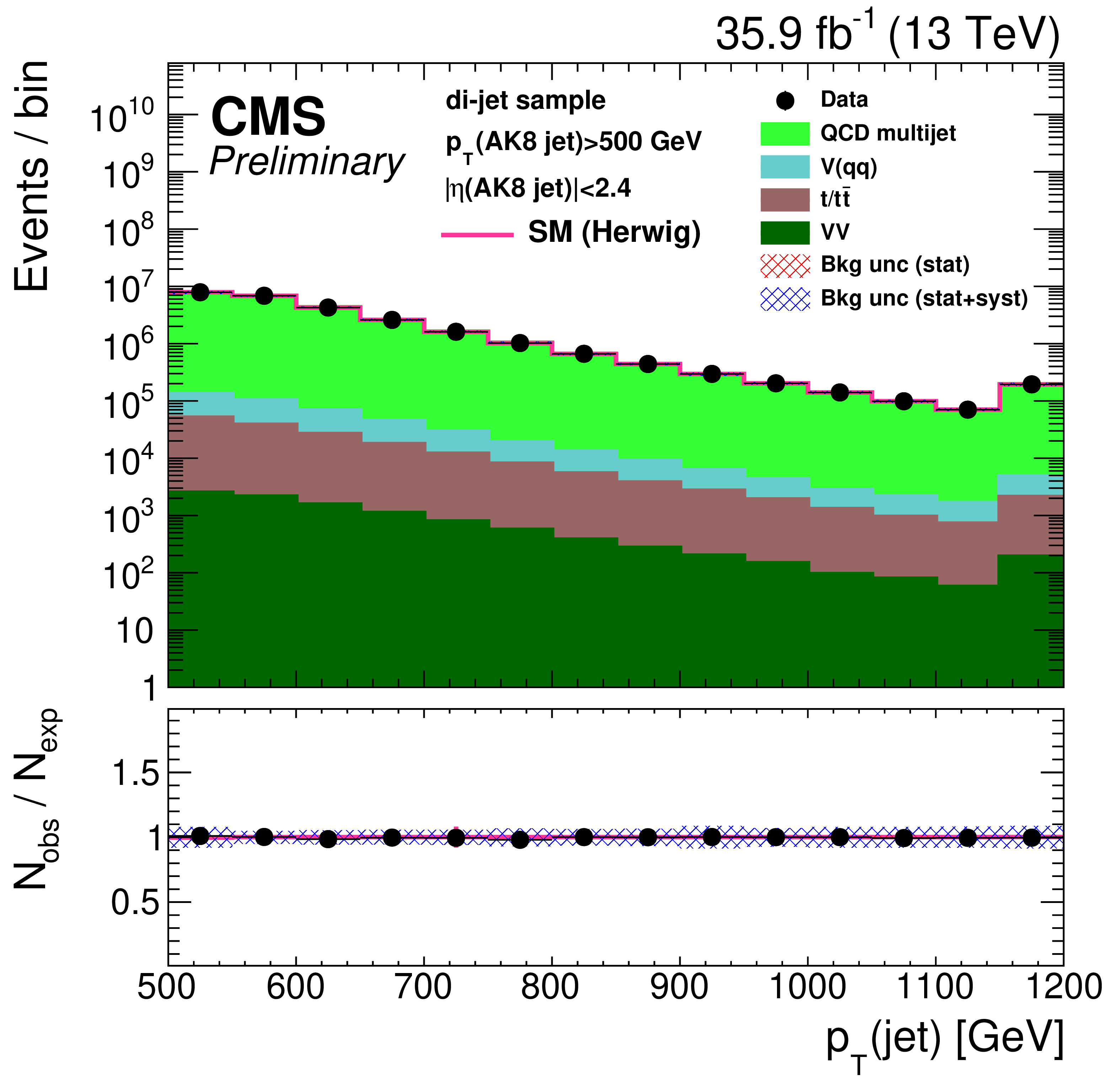
png pdf |
Figure 31-a:
Distribution of the jet ${p_{\mathrm {T}}}$ (upper-left), the jet mass, ${m_{\text {SD}}}$ (upper-right), the N-subjetiness ratios, $ {\tau _{32}}$ (middle-left) and $ {\tau _{21}}$ (middle-right), and the $N_2$ (lower-left) and $N_{2}^{\text {DDT}}$ (lower-right) in data and simulation in the di-jet sample. The pink solid line corresponds to the simulation distribution obtained using the alternative QCD multijet sample. The background event yield is normalized to the total observed data yield. The lower panel shows the data to simulation ratio. The shaded blue (red) band corresponds to the total uncertainty (statistical uncertainty of the simulated samples), the pink line to the data to simulation ratio using the alternative QCD multijet sample, and the vertical lines correspond to the statistical uncertainty of the data. The distributions are weighted so that the jet ${p_{\mathrm {T}}}$ distribution of the simulation matches the data. |

png pdf |
Figure 31-b:
Distribution of the jet ${p_{\mathrm {T}}}$ (upper-left), the jet mass, ${m_{\text {SD}}}$ (upper-right), the N-subjetiness ratios, $ {\tau _{32}}$ (middle-left) and $ {\tau _{21}}$ (middle-right), and the $N_2$ (lower-left) and $N_{2}^{\text {DDT}}$ (lower-right) in data and simulation in the di-jet sample. The pink solid line corresponds to the simulation distribution obtained using the alternative QCD multijet sample. The background event yield is normalized to the total observed data yield. The lower panel shows the data to simulation ratio. The shaded blue (red) band corresponds to the total uncertainty (statistical uncertainty of the simulated samples), the pink line to the data to simulation ratio using the alternative QCD multijet sample, and the vertical lines correspond to the statistical uncertainty of the data. The distributions are weighted so that the jet ${p_{\mathrm {T}}}$ distribution of the simulation matches the data. |
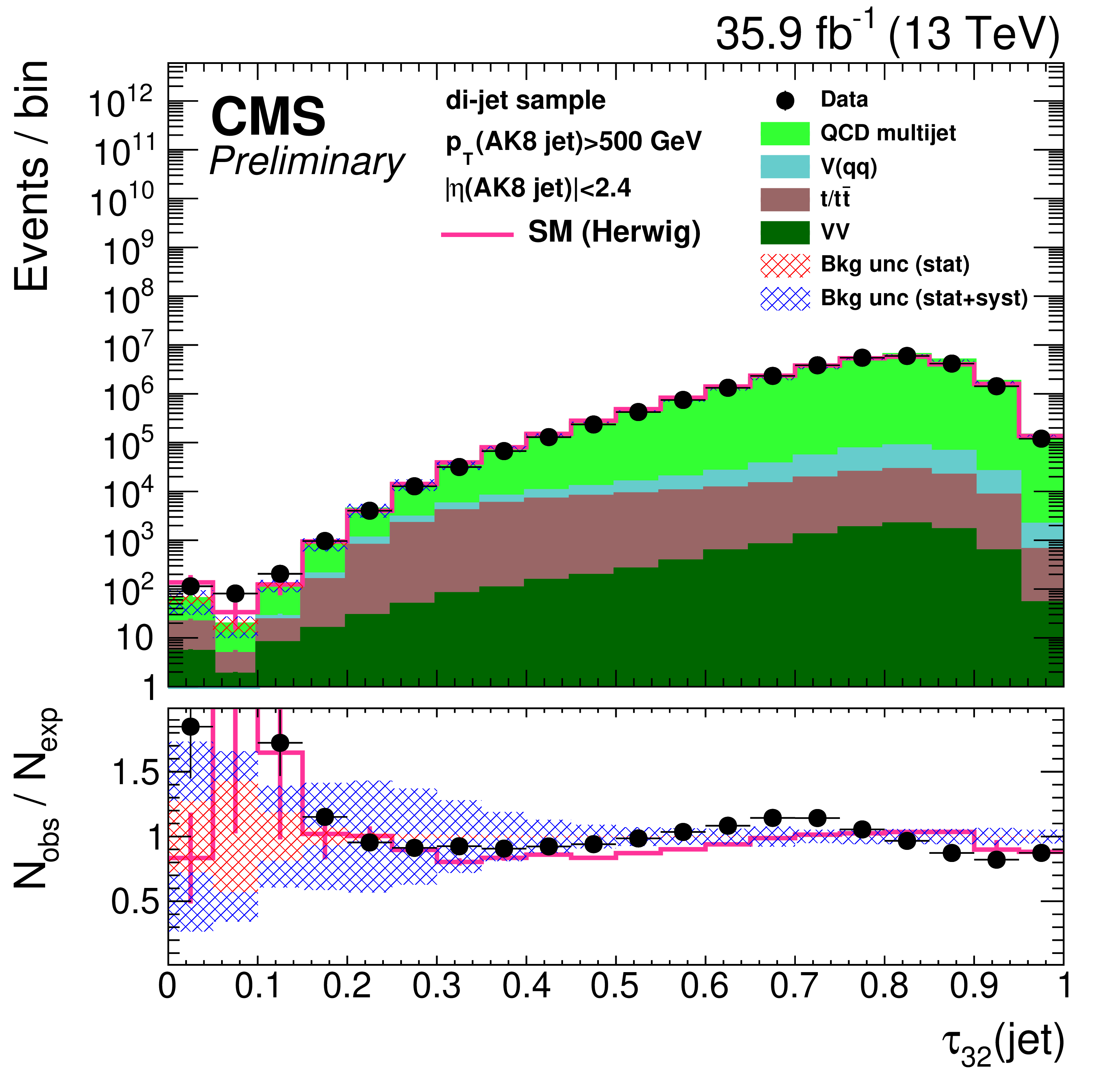
png pdf |
Figure 31-c:
Distribution of the jet ${p_{\mathrm {T}}}$ (upper-left), the jet mass, ${m_{\text {SD}}}$ (upper-right), the N-subjetiness ratios, $ {\tau _{32}}$ (middle-left) and $ {\tau _{21}}$ (middle-right), and the $N_2$ (lower-left) and $N_{2}^{\text {DDT}}$ (lower-right) in data and simulation in the di-jet sample. The pink solid line corresponds to the simulation distribution obtained using the alternative QCD multijet sample. The background event yield is normalized to the total observed data yield. The lower panel shows the data to simulation ratio. The shaded blue (red) band corresponds to the total uncertainty (statistical uncertainty of the simulated samples), the pink line to the data to simulation ratio using the alternative QCD multijet sample, and the vertical lines correspond to the statistical uncertainty of the data. The distributions are weighted so that the jet ${p_{\mathrm {T}}}$ distribution of the simulation matches the data. |
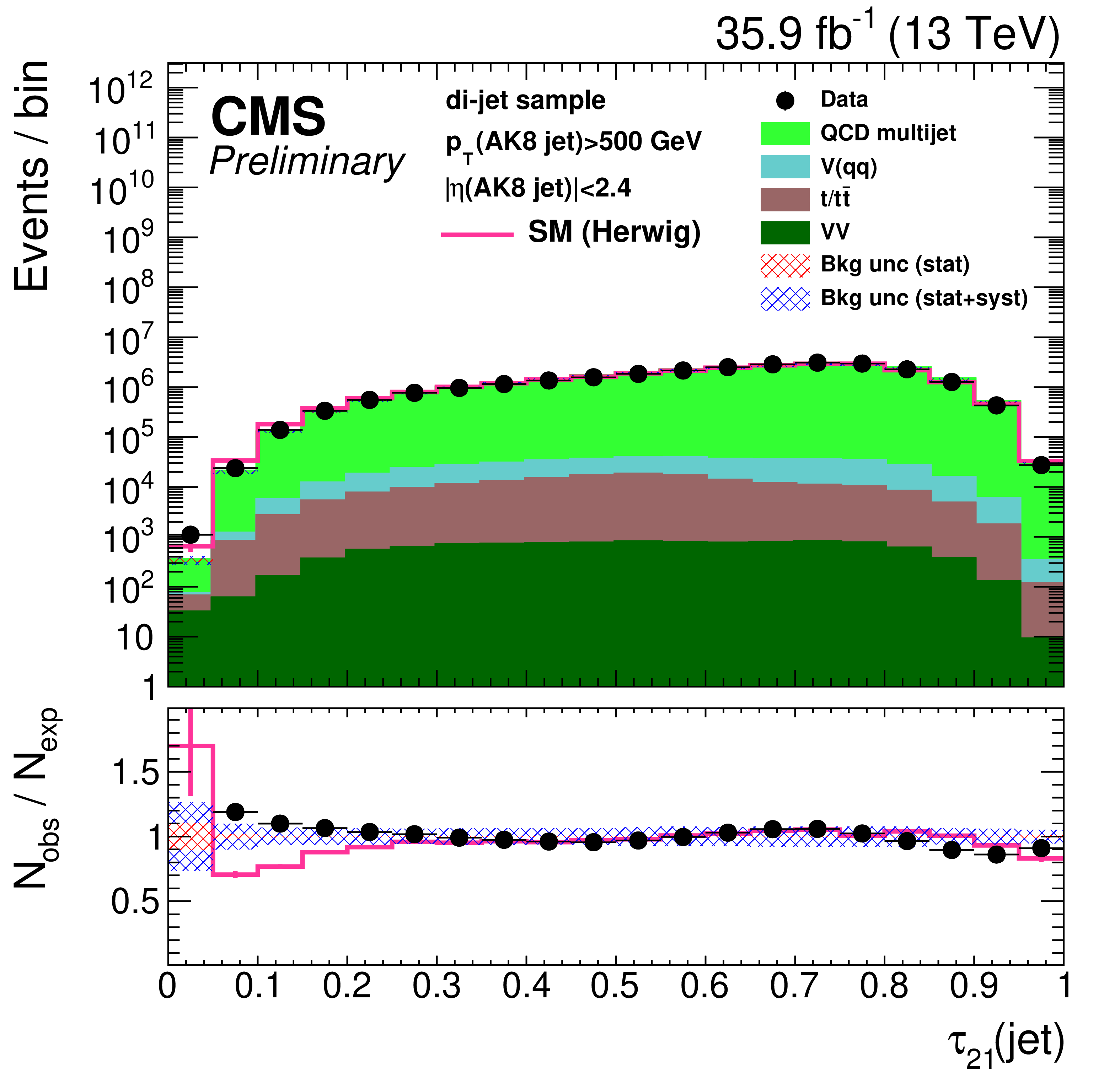
png pdf |
Figure 31-d:
Distribution of the jet ${p_{\mathrm {T}}}$ (upper-left), the jet mass, ${m_{\text {SD}}}$ (upper-right), the N-subjetiness ratios, $ {\tau _{32}}$ (middle-left) and $ {\tau _{21}}$ (middle-right), and the $N_2$ (lower-left) and $N_{2}^{\text {DDT}}$ (lower-right) in data and simulation in the di-jet sample. The pink solid line corresponds to the simulation distribution obtained using the alternative QCD multijet sample. The background event yield is normalized to the total observed data yield. The lower panel shows the data to simulation ratio. The shaded blue (red) band corresponds to the total uncertainty (statistical uncertainty of the simulated samples), the pink line to the data to simulation ratio using the alternative QCD multijet sample, and the vertical lines correspond to the statistical uncertainty of the data. The distributions are weighted so that the jet ${p_{\mathrm {T}}}$ distribution of the simulation matches the data. |
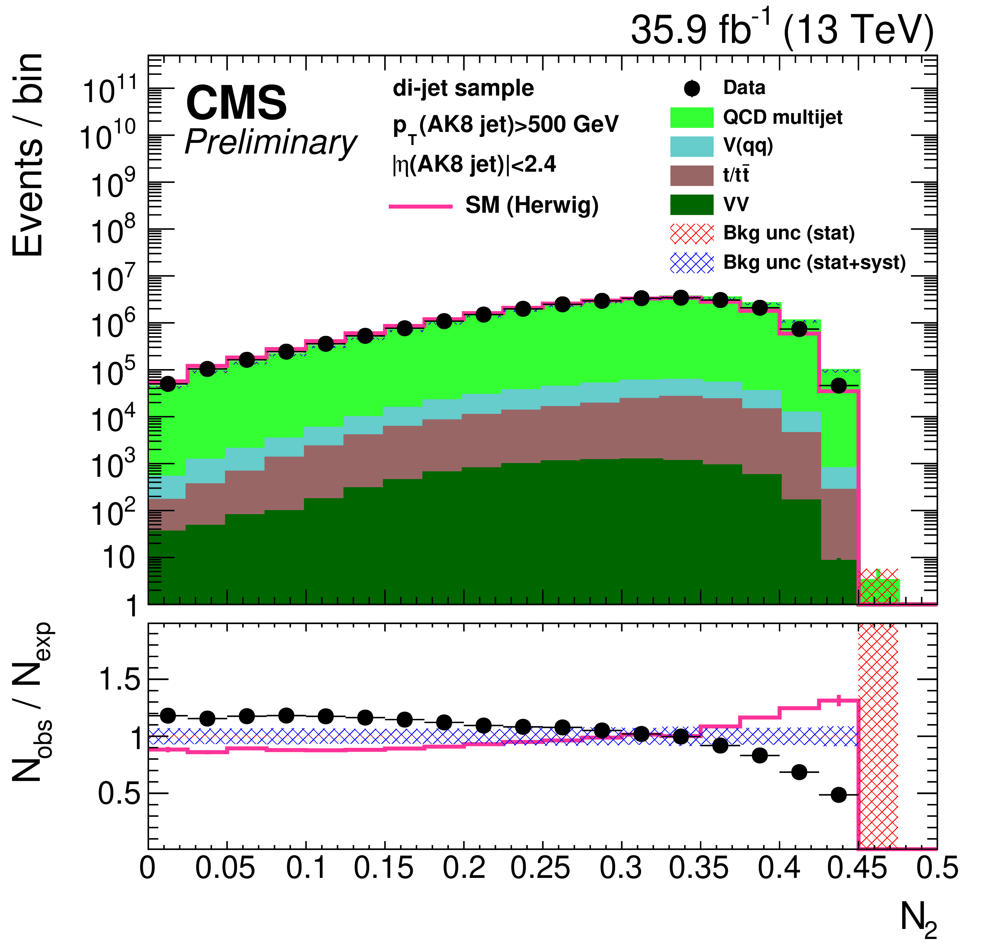
png pdf |
Figure 31-e:
Distribution of the jet ${p_{\mathrm {T}}}$ (upper-left), the jet mass, ${m_{\text {SD}}}$ (upper-right), the N-subjetiness ratios, $ {\tau _{32}}$ (middle-left) and $ {\tau _{21}}$ (middle-right), and the $N_2$ (lower-left) and $N_{2}^{\text {DDT}}$ (lower-right) in data and simulation in the di-jet sample. The pink solid line corresponds to the simulation distribution obtained using the alternative QCD multijet sample. The background event yield is normalized to the total observed data yield. The lower panel shows the data to simulation ratio. The shaded blue (red) band corresponds to the total uncertainty (statistical uncertainty of the simulated samples), the pink line to the data to simulation ratio using the alternative QCD multijet sample, and the vertical lines correspond to the statistical uncertainty of the data. The distributions are weighted so that the jet ${p_{\mathrm {T}}}$ distribution of the simulation matches the data. |
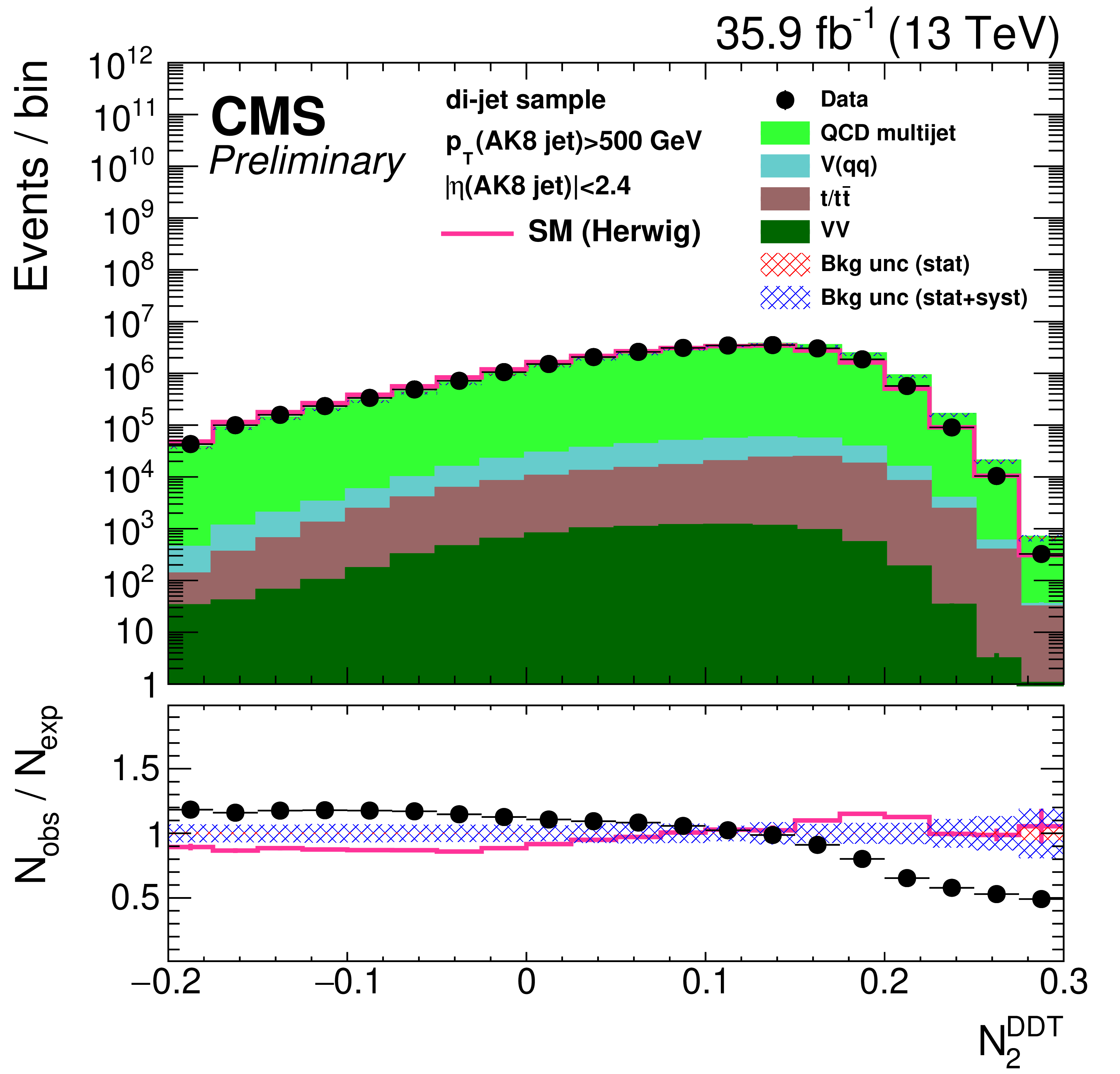
png pdf |
Figure 31-f:
Distribution of the jet ${p_{\mathrm {T}}}$ (upper-left), the jet mass, ${m_{\text {SD}}}$ (upper-right), the N-subjetiness ratios, $ {\tau _{32}}$ (middle-left) and $ {\tau _{21}}$ (middle-right), and the $N_2$ (lower-left) and $N_{2}^{\text {DDT}}$ (lower-right) in data and simulation in the di-jet sample. The pink solid line corresponds to the simulation distribution obtained using the alternative QCD multijet sample. The background event yield is normalized to the total observed data yield. The lower panel shows the data to simulation ratio. The shaded blue (red) band corresponds to the total uncertainty (statistical uncertainty of the simulated samples), the pink line to the data to simulation ratio using the alternative QCD multijet sample, and the vertical lines correspond to the statistical uncertainty of the data. The distributions are weighted so that the jet ${p_{\mathrm {T}}}$ distribution of the simulation matches the data. |
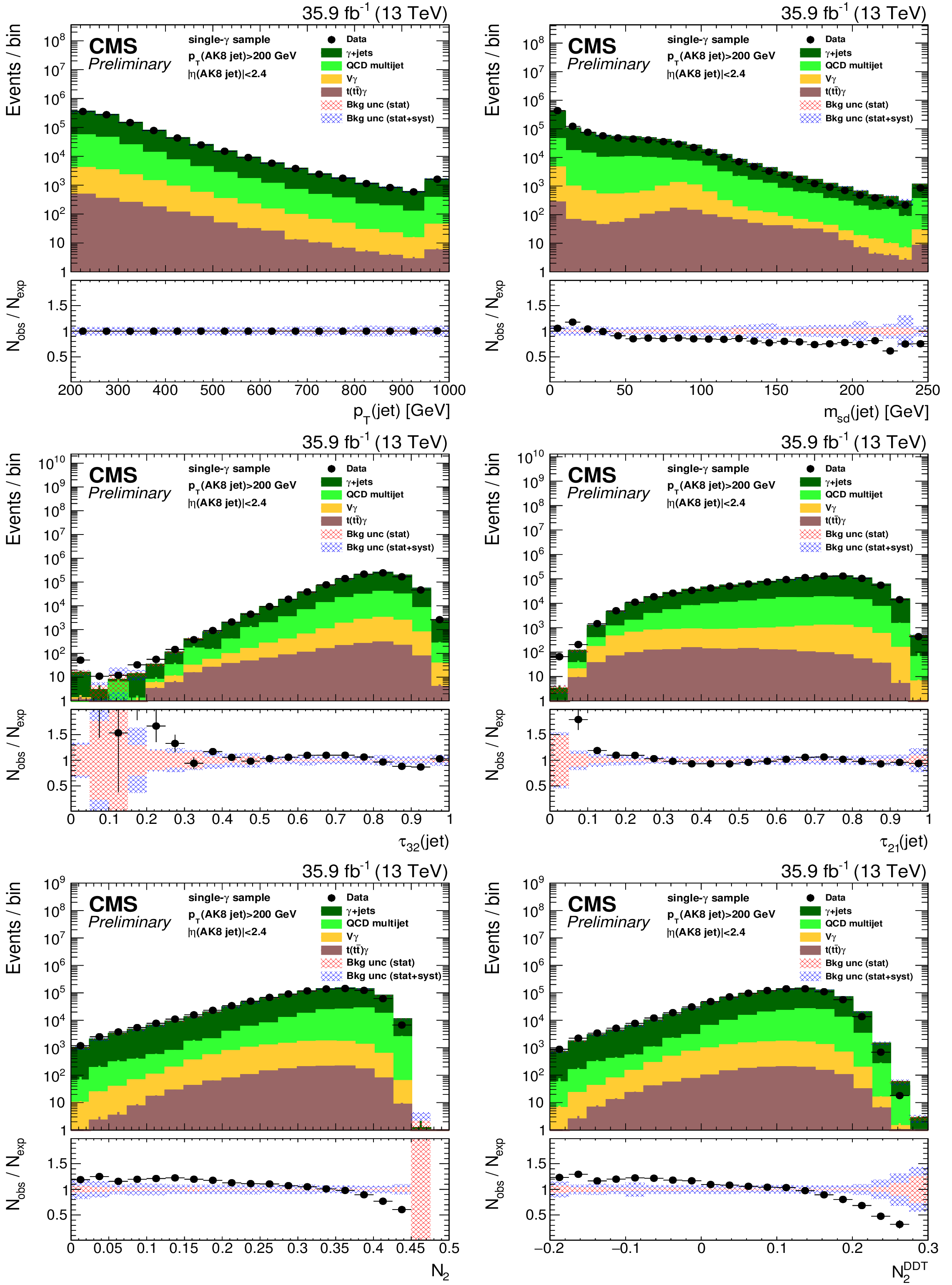
png pdf |
Figure 32:
Distribution of the jet ${p_{\mathrm {T}}}$ (upper-left), the jet mass, ${m_{\text {SD}}}$ (upper-right), the N-subjetiness ratios, $ {\tau _{32}}$ (middle-left) and $ {\tau _{21}}$ (middle-right), and the $N_2$ (lower-left) and $N_{2}^{\text {DDT}}$ (lower-right) in data and simulation in the single-$\gamma $ sample. The background event yield is normalized to the total observed data yield. The lower panel shows the data to simulation ratio. The shaded blue (red) band corresponds to the total uncertainty (statistical uncertainty of the simulated samples), and the vertical lines correspond to the statistical uncertainty of the data. The distributions are weighted so that the jet ${p_{\mathrm {T}}}$ distribution of the simulation matches the data. |
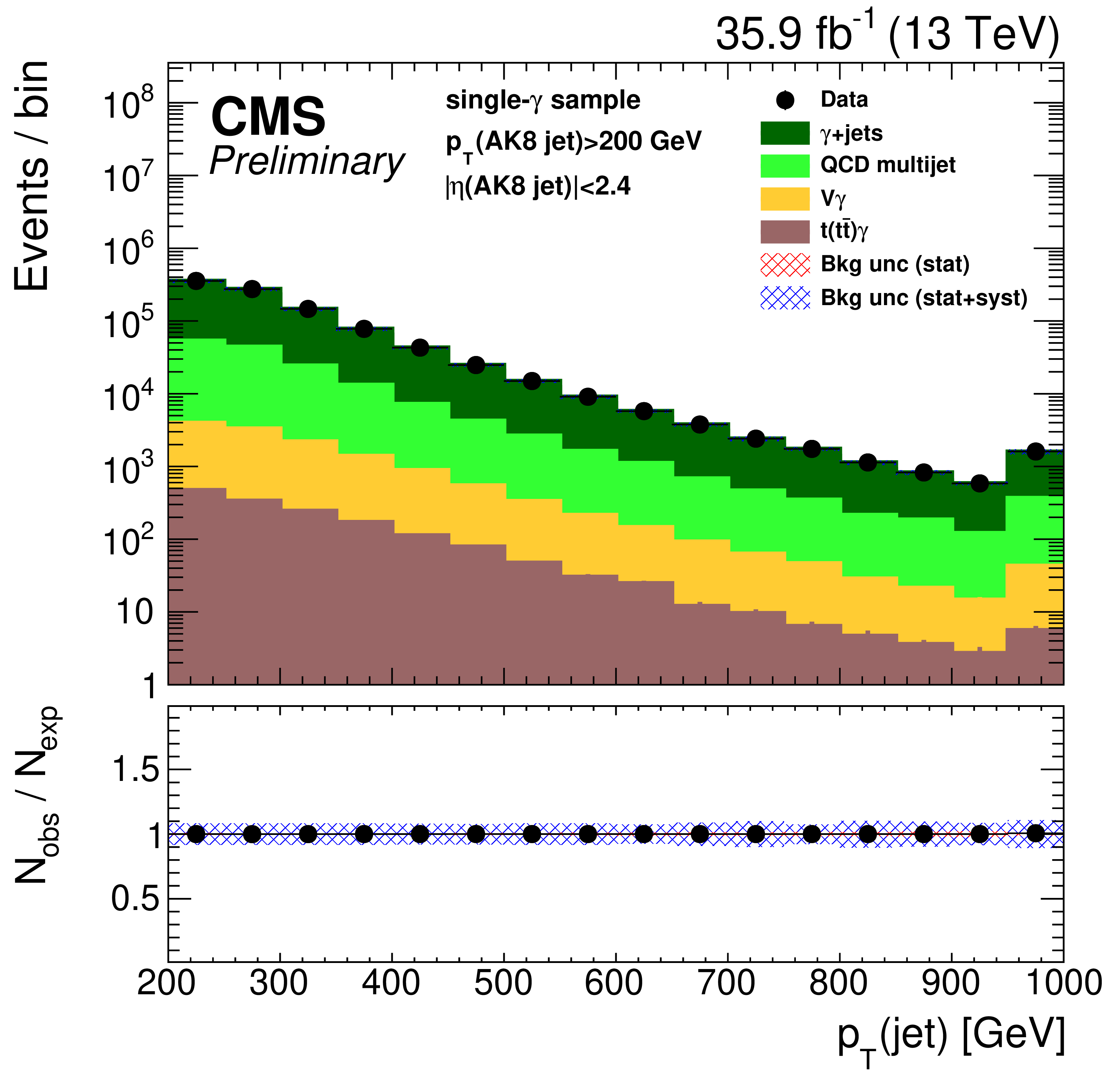
png pdf |
Figure 32-a:
Distribution of the jet ${p_{\mathrm {T}}}$ (upper-left), the jet mass, ${m_{\text {SD}}}$ (upper-right), the N-subjetiness ratios, $ {\tau _{32}}$ (middle-left) and $ {\tau _{21}}$ (middle-right), and the $N_2$ (lower-left) and $N_{2}^{\text {DDT}}$ (lower-right) in data and simulation in the single-$\gamma $ sample. The background event yield is normalized to the total observed data yield. The lower panel shows the data to simulation ratio. The shaded blue (red) band corresponds to the total uncertainty (statistical uncertainty of the simulated samples), and the vertical lines correspond to the statistical uncertainty of the data. The distributions are weighted so that the jet ${p_{\mathrm {T}}}$ distribution of the simulation matches the data. |
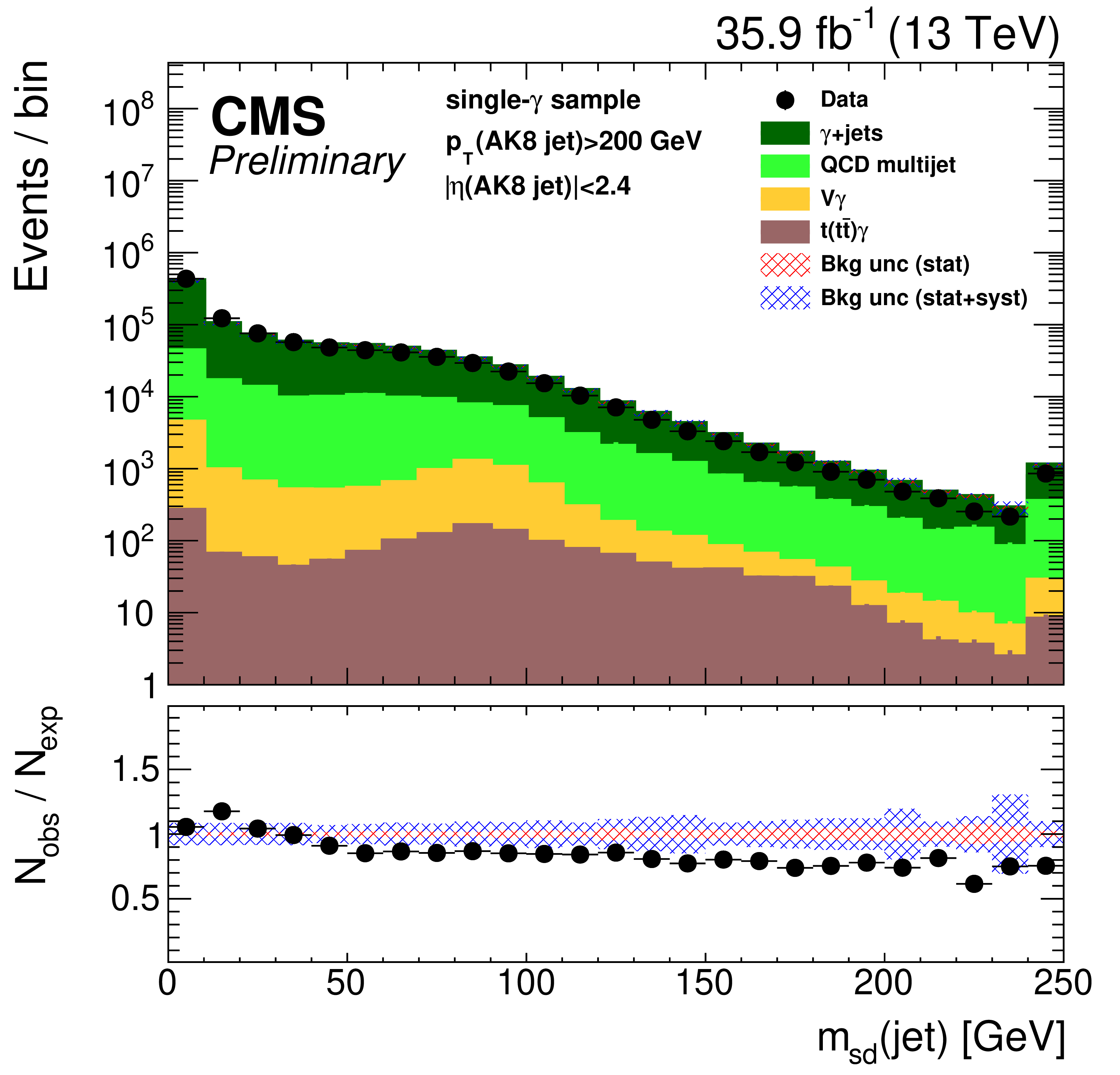
png pdf |
Figure 32-b:
Distribution of the jet ${p_{\mathrm {T}}}$ (upper-left), the jet mass, ${m_{\text {SD}}}$ (upper-right), the N-subjetiness ratios, $ {\tau _{32}}$ (middle-left) and $ {\tau _{21}}$ (middle-right), and the $N_2$ (lower-left) and $N_{2}^{\text {DDT}}$ (lower-right) in data and simulation in the single-$\gamma $ sample. The background event yield is normalized to the total observed data yield. The lower panel shows the data to simulation ratio. The shaded blue (red) band corresponds to the total uncertainty (statistical uncertainty of the simulated samples), and the vertical lines correspond to the statistical uncertainty of the data. The distributions are weighted so that the jet ${p_{\mathrm {T}}}$ distribution of the simulation matches the data. |
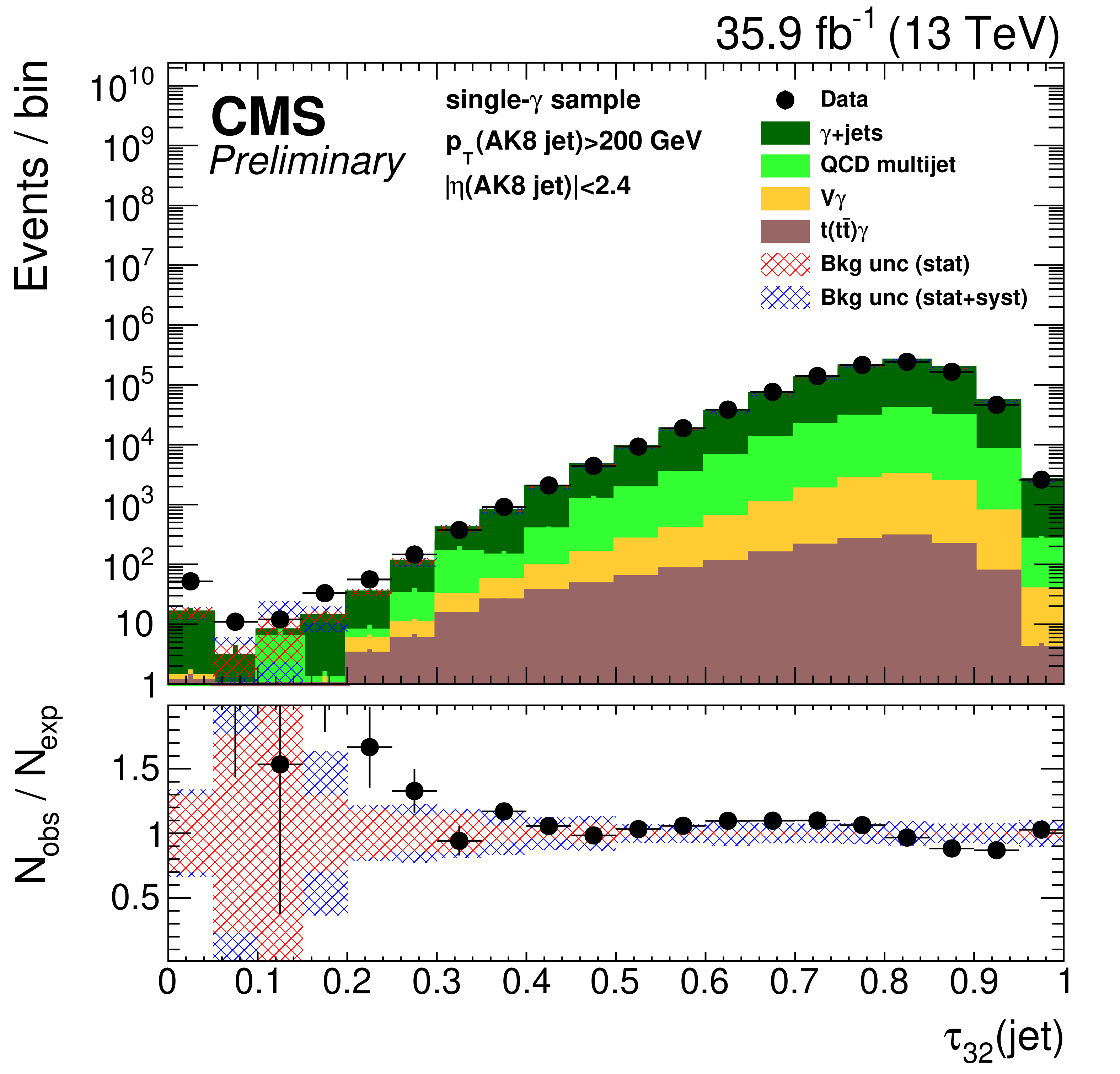
png pdf |
Figure 32-c:
Distribution of the jet ${p_{\mathrm {T}}}$ (upper-left), the jet mass, ${m_{\text {SD}}}$ (upper-right), the N-subjetiness ratios, $ {\tau _{32}}$ (middle-left) and $ {\tau _{21}}$ (middle-right), and the $N_2$ (lower-left) and $N_{2}^{\text {DDT}}$ (lower-right) in data and simulation in the single-$\gamma $ sample. The background event yield is normalized to the total observed data yield. The lower panel shows the data to simulation ratio. The shaded blue (red) band corresponds to the total uncertainty (statistical uncertainty of the simulated samples), and the vertical lines correspond to the statistical uncertainty of the data. The distributions are weighted so that the jet ${p_{\mathrm {T}}}$ distribution of the simulation matches the data. |

png pdf |
Figure 32-d:
Distribution of the jet ${p_{\mathrm {T}}}$ (upper-left), the jet mass, ${m_{\text {SD}}}$ (upper-right), the N-subjetiness ratios, $ {\tau _{32}}$ (middle-left) and $ {\tau _{21}}$ (middle-right), and the $N_2$ (lower-left) and $N_{2}^{\text {DDT}}$ (lower-right) in data and simulation in the single-$\gamma $ sample. The background event yield is normalized to the total observed data yield. The lower panel shows the data to simulation ratio. The shaded blue (red) band corresponds to the total uncertainty (statistical uncertainty of the simulated samples), and the vertical lines correspond to the statistical uncertainty of the data. The distributions are weighted so that the jet ${p_{\mathrm {T}}}$ distribution of the simulation matches the data. |
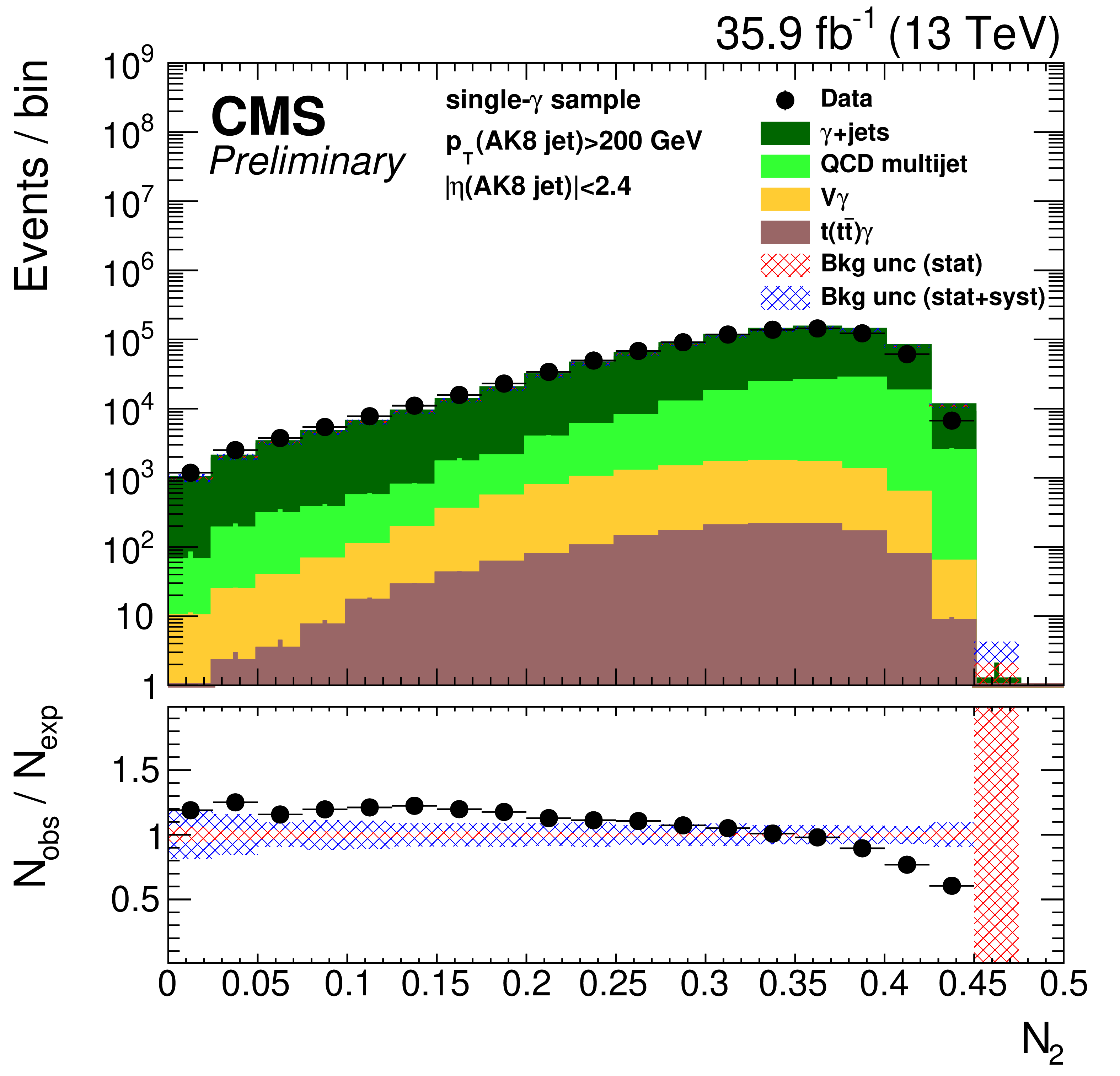
png pdf |
Figure 32-e:
Distribution of the jet ${p_{\mathrm {T}}}$ (upper-left), the jet mass, ${m_{\text {SD}}}$ (upper-right), the N-subjetiness ratios, $ {\tau _{32}}$ (middle-left) and $ {\tau _{21}}$ (middle-right), and the $N_2$ (lower-left) and $N_{2}^{\text {DDT}}$ (lower-right) in data and simulation in the single-$\gamma $ sample. The background event yield is normalized to the total observed data yield. The lower panel shows the data to simulation ratio. The shaded blue (red) band corresponds to the total uncertainty (statistical uncertainty of the simulated samples), and the vertical lines correspond to the statistical uncertainty of the data. The distributions are weighted so that the jet ${p_{\mathrm {T}}}$ distribution of the simulation matches the data. |
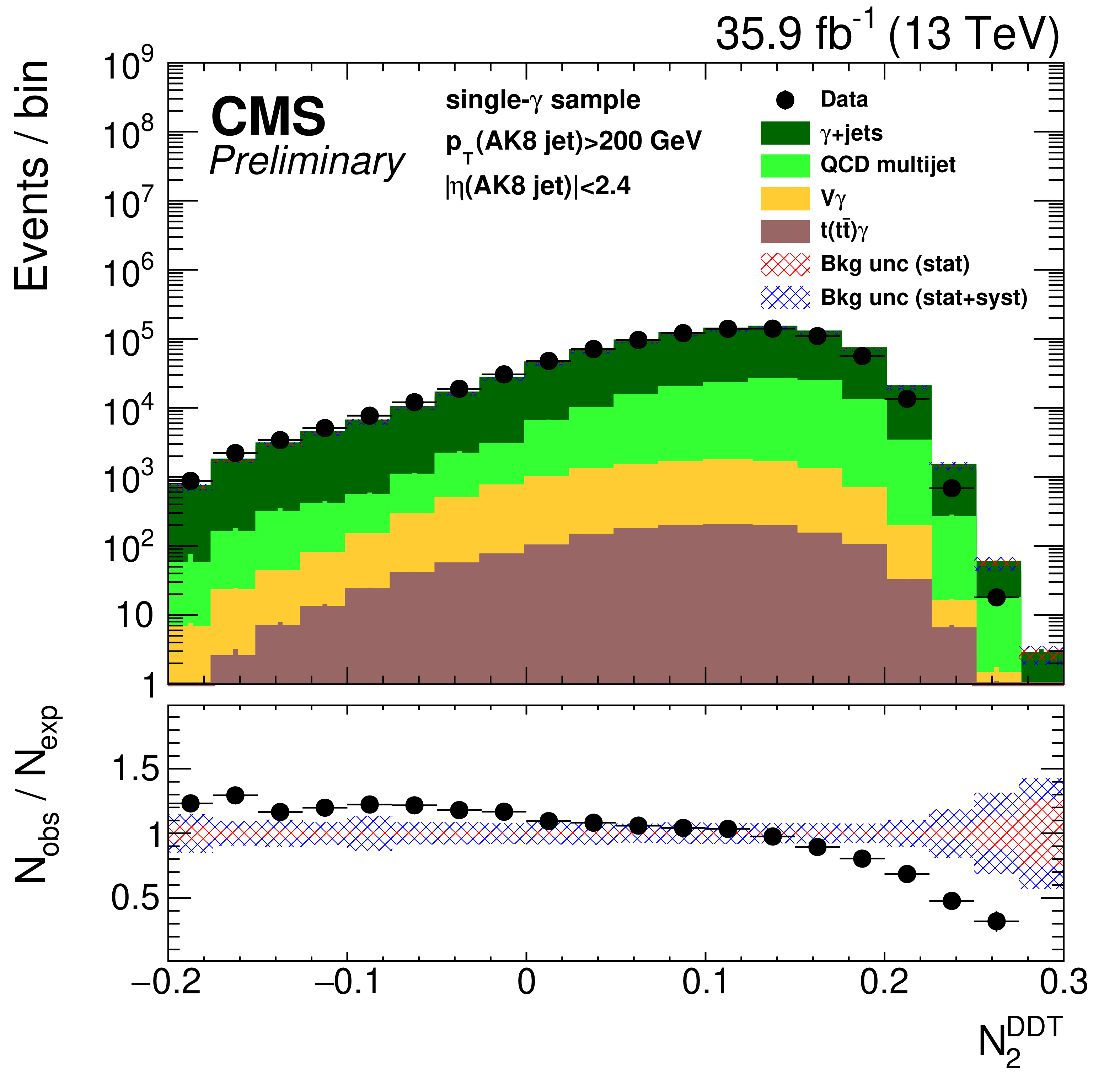
png pdf |
Figure 32-f:
Distribution of the jet ${p_{\mathrm {T}}}$ (upper-left), the jet mass, ${m_{\text {SD}}}$ (upper-right), the N-subjetiness ratios, $ {\tau _{32}}$ (middle-left) and $ {\tau _{21}}$ (middle-right), and the $N_2$ (lower-left) and $N_{2}^{\text {DDT}}$ (lower-right) in data and simulation in the single-$\gamma $ sample. The background event yield is normalized to the total observed data yield. The lower panel shows the data to simulation ratio. The shaded blue (red) band corresponds to the total uncertainty (statistical uncertainty of the simulated samples), and the vertical lines correspond to the statistical uncertainty of the data. The distributions are weighted so that the jet ${p_{\mathrm {T}}}$ distribution of the simulation matches the data. |
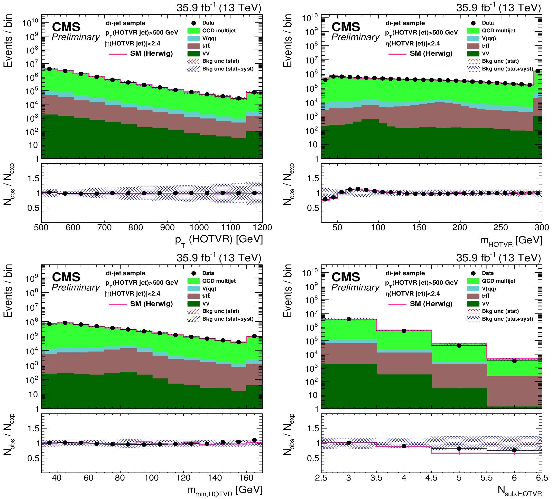
png pdf |
Figure 33:
Distribution of the main observables of the HOTVR algorithm, $p_{T}(\text {HOTVR jet})$ (upper-left), $m_{\text {HOTVR}}$ (upper-right), $m_{\text {min,HOTVR}}$ (lower-left) and $N_{\text {sub,HOTVR}}$ (lower-right) in data and simulation in the di-jet sample. The pink solid line corresponds to the simulation distribution obtained using the alternative QCD multijet sample. The background event yield is normalized to the total observed data yield. The lower panel shows the data to simulation ratio. The shaded blue (red) band corresponds to the total uncertainty (statistical uncertainty of the simulated samples), the pink line to the data to simulation ratio using the alternative QCD multijet sample, and the vertical lines correspond to the statistical uncertainty of the data. The distributions are weighted so that the jet ${p_{\mathrm {T}}}$ distribution of the simulation matches the data. |

png pdf |
Figure 33-a:
Distribution of the main observables of the HOTVR algorithm, $p_{T}(\text {HOTVR jet})$ (upper-left), $m_{\text {HOTVR}}$ (upper-right), $m_{\text {min,HOTVR}}$ (lower-left) and $N_{\text {sub,HOTVR}}$ (lower-right) in data and simulation in the di-jet sample. The pink solid line corresponds to the simulation distribution obtained using the alternative QCD multijet sample. The background event yield is normalized to the total observed data yield. The lower panel shows the data to simulation ratio. The shaded blue (red) band corresponds to the total uncertainty (statistical uncertainty of the simulated samples), the pink line to the data to simulation ratio using the alternative QCD multijet sample, and the vertical lines correspond to the statistical uncertainty of the data. The distributions are weighted so that the jet ${p_{\mathrm {T}}}$ distribution of the simulation matches the data. |
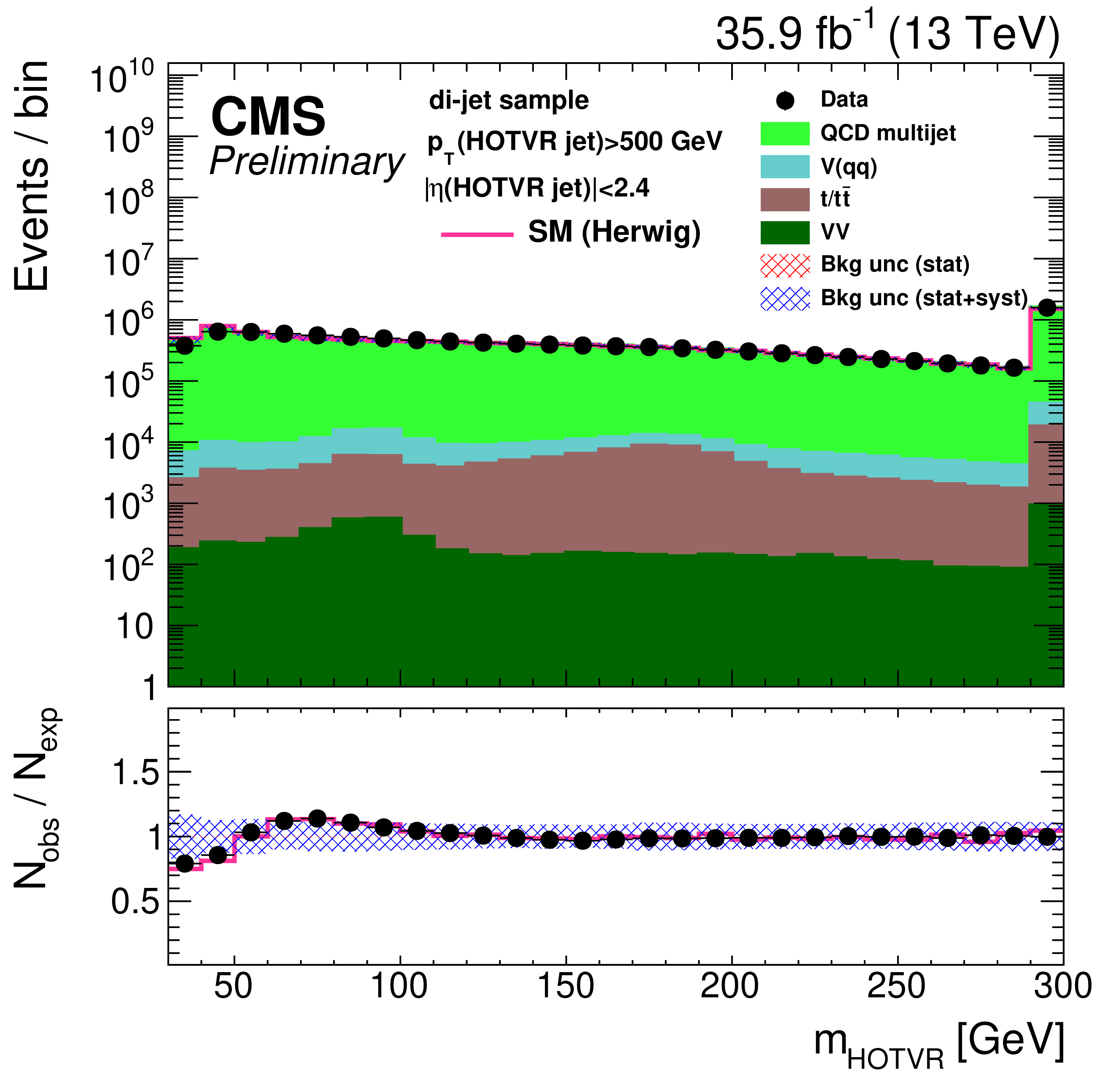
png pdf |
Figure 33-b:
Distribution of the main observables of the HOTVR algorithm, $p_{T}(\text {HOTVR jet})$ (upper-left), $m_{\text {HOTVR}}$ (upper-right), $m_{\text {min,HOTVR}}$ (lower-left) and $N_{\text {sub,HOTVR}}$ (lower-right) in data and simulation in the di-jet sample. The pink solid line corresponds to the simulation distribution obtained using the alternative QCD multijet sample. The background event yield is normalized to the total observed data yield. The lower panel shows the data to simulation ratio. The shaded blue (red) band corresponds to the total uncertainty (statistical uncertainty of the simulated samples), the pink line to the data to simulation ratio using the alternative QCD multijet sample, and the vertical lines correspond to the statistical uncertainty of the data. The distributions are weighted so that the jet ${p_{\mathrm {T}}}$ distribution of the simulation matches the data. |
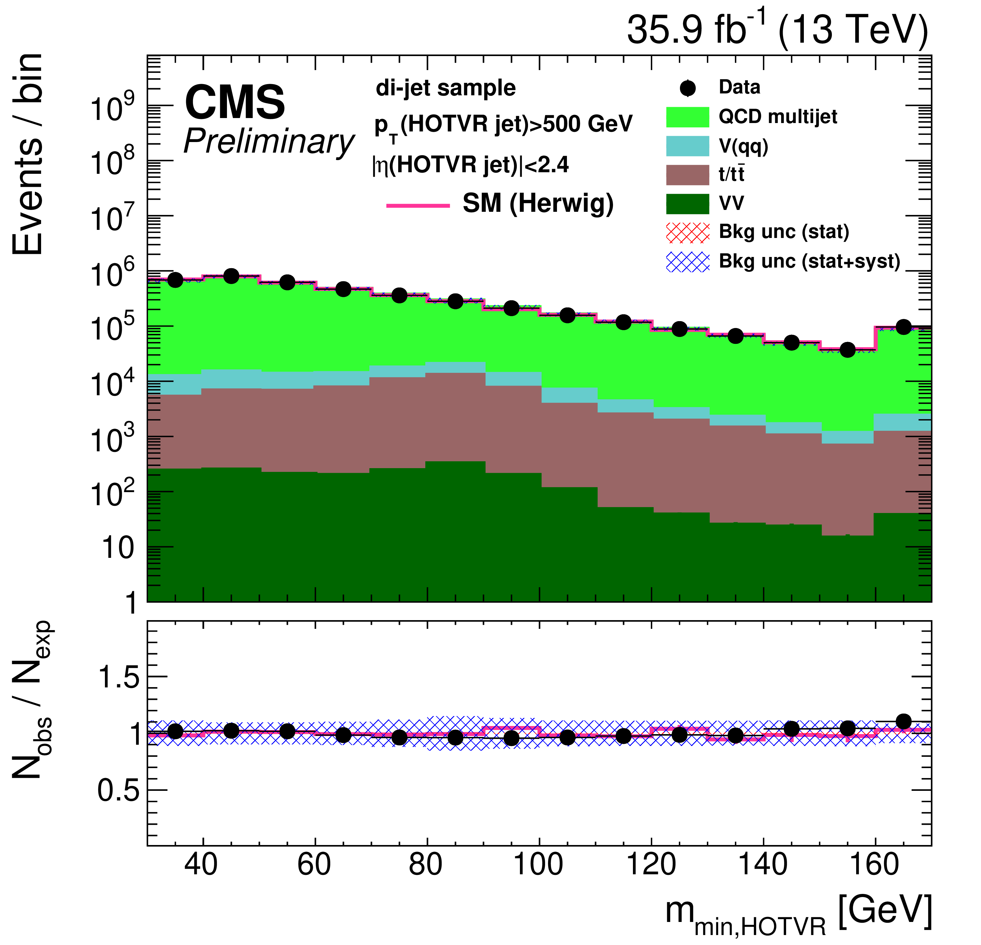
png pdf |
Figure 33-c:
Distribution of the main observables of the HOTVR algorithm, $p_{T}(\text {HOTVR jet})$ (upper-left), $m_{\text {HOTVR}}$ (upper-right), $m_{\text {min,HOTVR}}$ (lower-left) and $N_{\text {sub,HOTVR}}$ (lower-right) in data and simulation in the di-jet sample. The pink solid line corresponds to the simulation distribution obtained using the alternative QCD multijet sample. The background event yield is normalized to the total observed data yield. The lower panel shows the data to simulation ratio. The shaded blue (red) band corresponds to the total uncertainty (statistical uncertainty of the simulated samples), the pink line to the data to simulation ratio using the alternative QCD multijet sample, and the vertical lines correspond to the statistical uncertainty of the data. The distributions are weighted so that the jet ${p_{\mathrm {T}}}$ distribution of the simulation matches the data. |
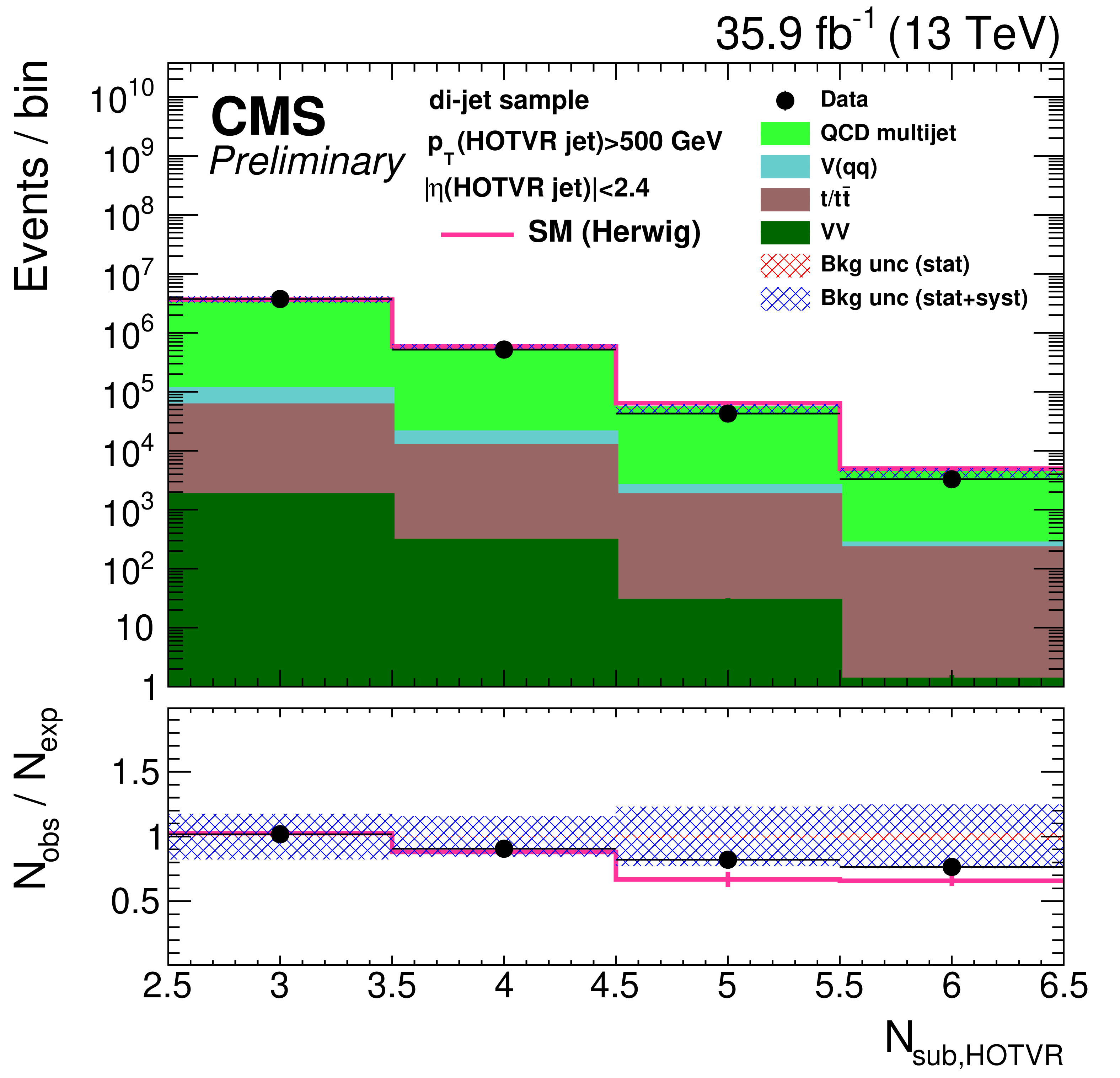
png pdf |
Figure 33-d:
Distribution of the main observables of the HOTVR algorithm, $p_{T}(\text {HOTVR jet})$ (upper-left), $m_{\text {HOTVR}}$ (upper-right), $m_{\text {min,HOTVR}}$ (lower-left) and $N_{\text {sub,HOTVR}}$ (lower-right) in data and simulation in the di-jet sample. The pink solid line corresponds to the simulation distribution obtained using the alternative QCD multijet sample. The background event yield is normalized to the total observed data yield. The lower panel shows the data to simulation ratio. The shaded blue (red) band corresponds to the total uncertainty (statistical uncertainty of the simulated samples), the pink line to the data to simulation ratio using the alternative QCD multijet sample, and the vertical lines correspond to the statistical uncertainty of the data. The distributions are weighted so that the jet ${p_{\mathrm {T}}}$ distribution of the simulation matches the data. |
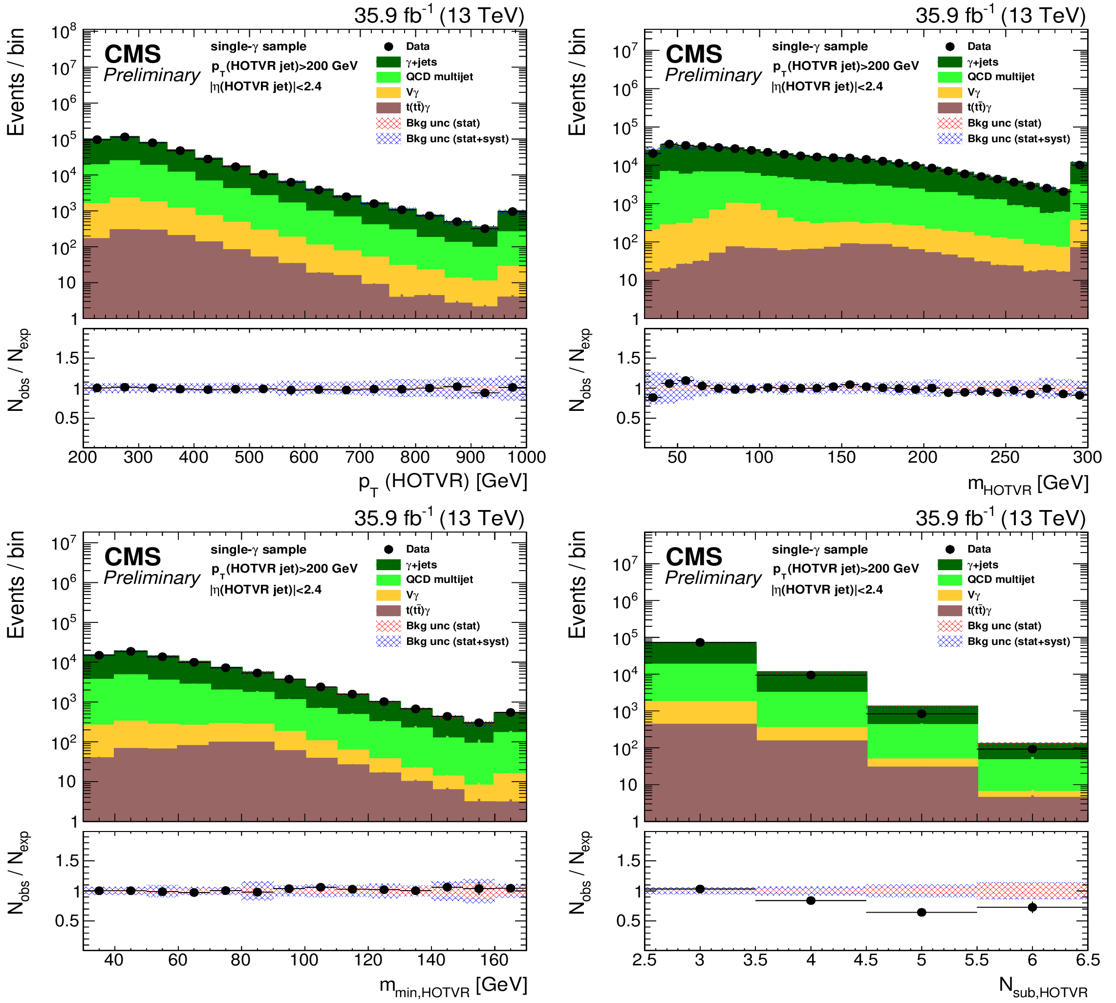
png pdf |
Figure 34:
Distribution of the main observables of the HOTVR algorithm, $p_{T}(\text {HOTVR jet})$ (upper-left), $m_{\text {HOTVR}}$ (upper-right), $m_{\text {min,HOTVR}}$ (lower-left) and $N_{\text {sub,HOTVR}}$ (lower-right) in data and simulation in the single-$\gamma $ sample. The background event yield is normalized to the total observed data yield. The lower panel shows the data to simulation ratio. The shaded blue (red) band corresponds to the total uncertainty (statistical uncertainty of the simulated samples), and the vertical lines correspond to the statistical uncertainty of the data. The distributions are weighted so that the jet ${p_{\mathrm {T}}}$ distribution of the simulation matches the data. |
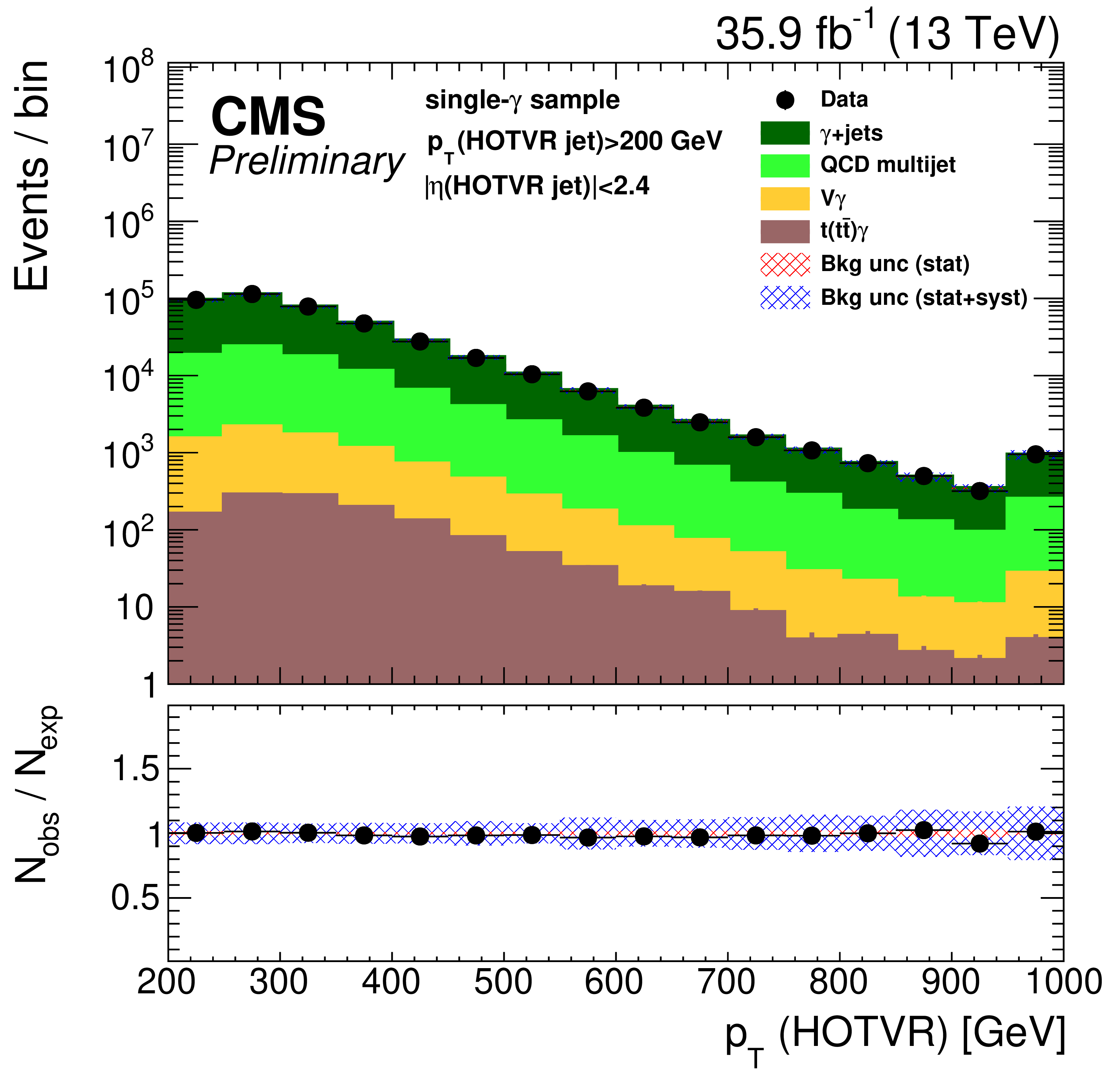
png pdf |
Figure 34-a:
Distribution of the main observables of the HOTVR algorithm, $p_{T}(\text {HOTVR jet})$ (upper-left), $m_{\text {HOTVR}}$ (upper-right), $m_{\text {min,HOTVR}}$ (lower-left) and $N_{\text {sub,HOTVR}}$ (lower-right) in data and simulation in the single-$\gamma $ sample. The background event yield is normalized to the total observed data yield. The lower panel shows the data to simulation ratio. The shaded blue (red) band corresponds to the total uncertainty (statistical uncertainty of the simulated samples), and the vertical lines correspond to the statistical uncertainty of the data. The distributions are weighted so that the jet ${p_{\mathrm {T}}}$ distribution of the simulation matches the data. |
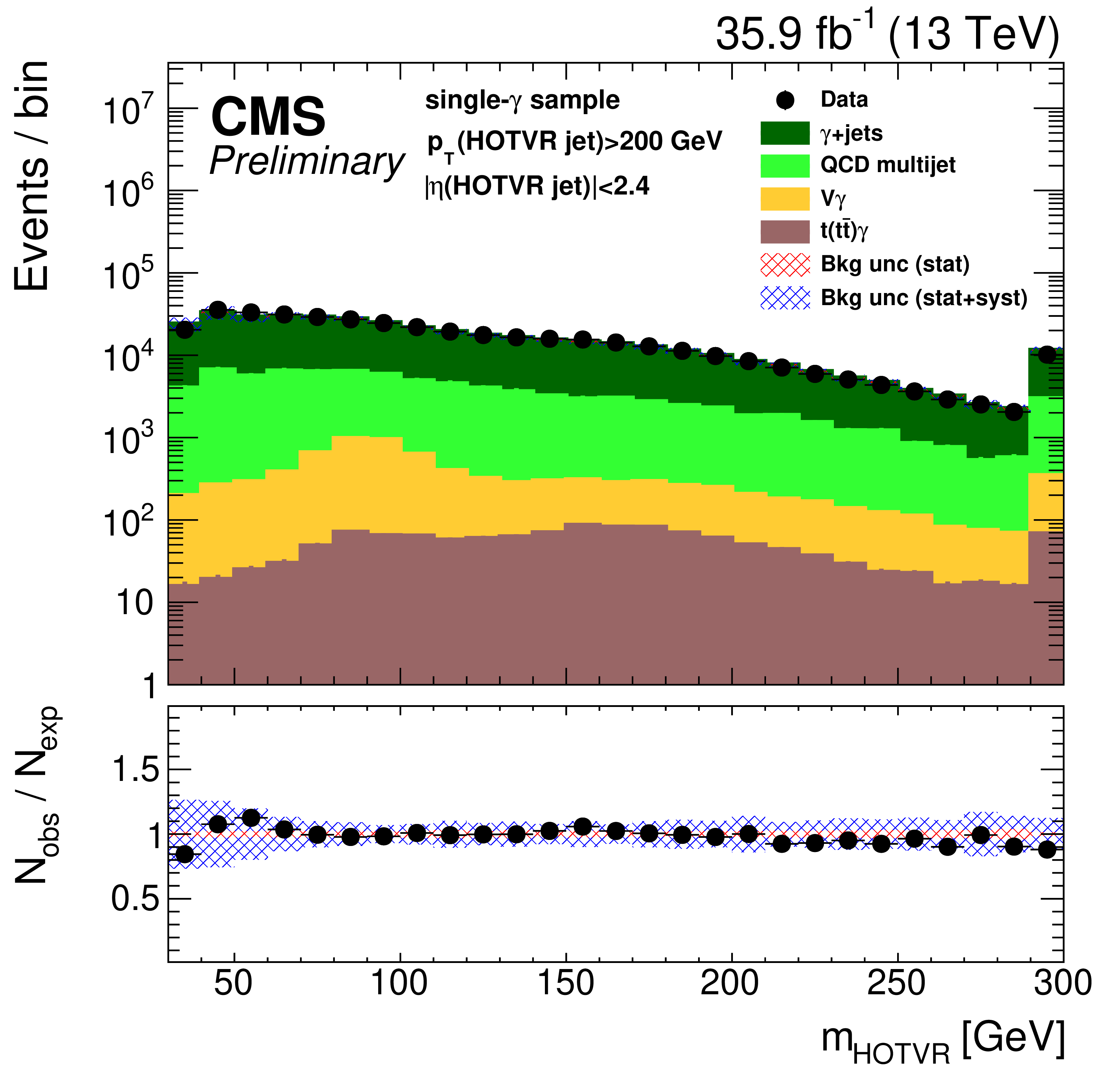
png pdf |
Figure 34-b:
Distribution of the main observables of the HOTVR algorithm, $p_{T}(\text {HOTVR jet})$ (upper-left), $m_{\text {HOTVR}}$ (upper-right), $m_{\text {min,HOTVR}}$ (lower-left) and $N_{\text {sub,HOTVR}}$ (lower-right) in data and simulation in the single-$\gamma $ sample. The background event yield is normalized to the total observed data yield. The lower panel shows the data to simulation ratio. The shaded blue (red) band corresponds to the total uncertainty (statistical uncertainty of the simulated samples), and the vertical lines correspond to the statistical uncertainty of the data. The distributions are weighted so that the jet ${p_{\mathrm {T}}}$ distribution of the simulation matches the data. |
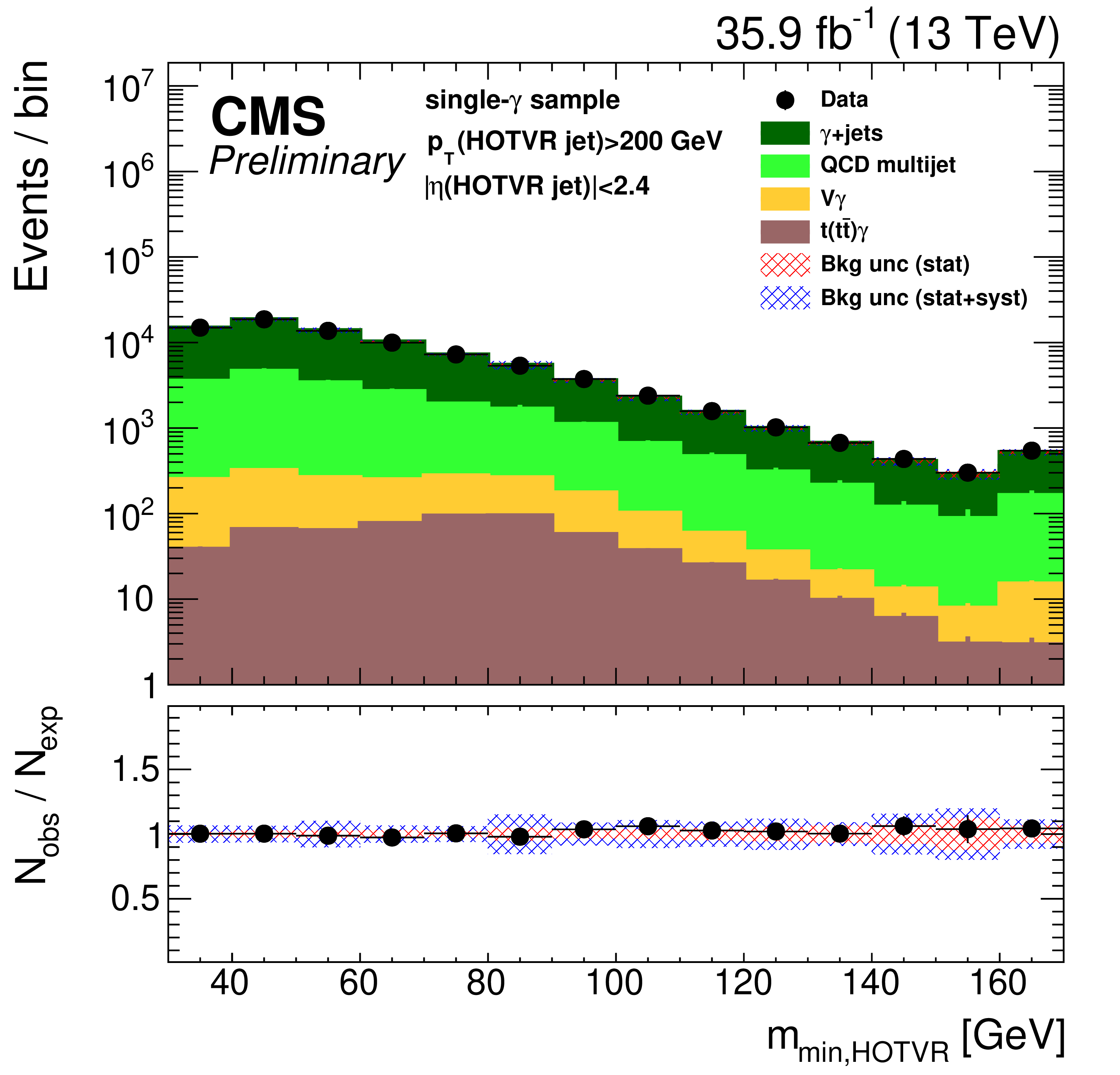
png pdf |
Figure 34-c:
Distribution of the main observables of the HOTVR algorithm, $p_{T}(\text {HOTVR jet})$ (upper-left), $m_{\text {HOTVR}}$ (upper-right), $m_{\text {min,HOTVR}}$ (lower-left) and $N_{\text {sub,HOTVR}}$ (lower-right) in data and simulation in the single-$\gamma $ sample. The background event yield is normalized to the total observed data yield. The lower panel shows the data to simulation ratio. The shaded blue (red) band corresponds to the total uncertainty (statistical uncertainty of the simulated samples), and the vertical lines correspond to the statistical uncertainty of the data. The distributions are weighted so that the jet ${p_{\mathrm {T}}}$ distribution of the simulation matches the data. |
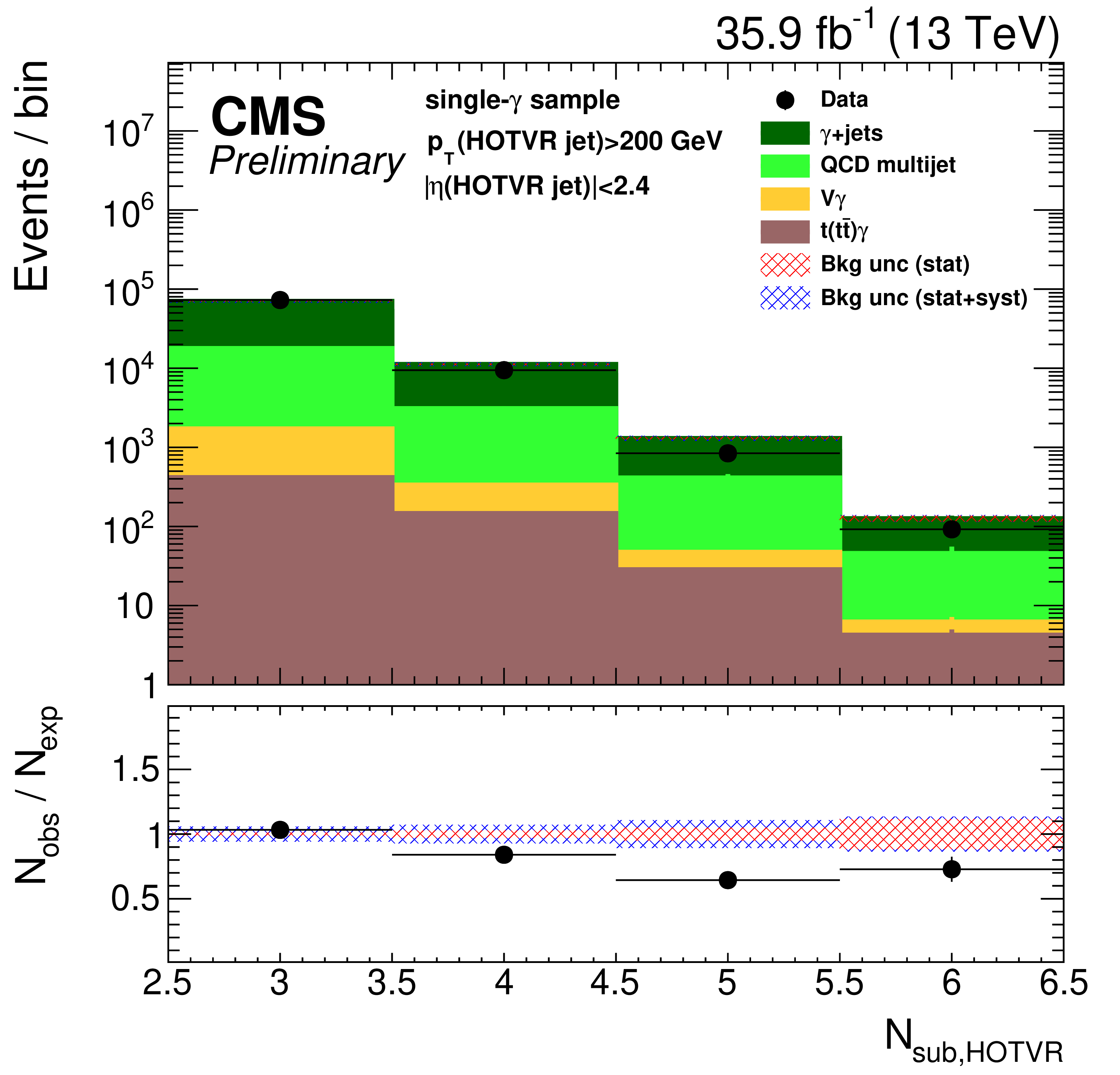
png pdf |
Figure 34-d:
Distribution of the main observables of the HOTVR algorithm, $p_{T}(\text {HOTVR jet})$ (upper-left), $m_{\text {HOTVR}}$ (upper-right), $m_{\text {min,HOTVR}}$ (lower-left) and $N_{\text {sub,HOTVR}}$ (lower-right) in data and simulation in the single-$\gamma $ sample. The background event yield is normalized to the total observed data yield. The lower panel shows the data to simulation ratio. The shaded blue (red) band corresponds to the total uncertainty (statistical uncertainty of the simulated samples), and the vertical lines correspond to the statistical uncertainty of the data. The distributions are weighted so that the jet ${p_{\mathrm {T}}}$ distribution of the simulation matches the data. |
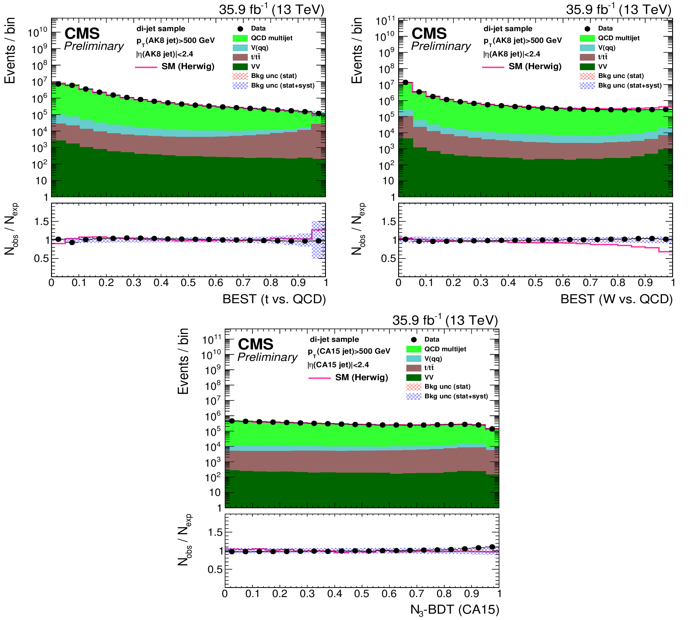
png pdf |
Figure 35:
Distribution of the t quark (upper left) and W boson (upper-right) identification probabilities for the BEST algorithm, and the ${N_{3}-\text {BDT} (\text {CA}15)}$ discriminant, in data and simulation in the di-jet sample. The background event yield is normalized to the total observed data yield. The pink solid line corresponds to the simulation distribution obtained using the alternative QCD multijet sample. The background event yield is normalized to the total observed data yield. The lower panel shows the data to simulation ratio. The shaded blue (red) band corresponds to the total uncertainty (statistical uncertainty of the simulated samples), the pink line to the data to simulation ratio using the alternative QCD multijet sample, and the vertical lines correspond to the statistical uncertainty of the data. The distributions are weighted so that the jet ${p_{\mathrm {T}}}$ distribution of the simulation matches the data. |
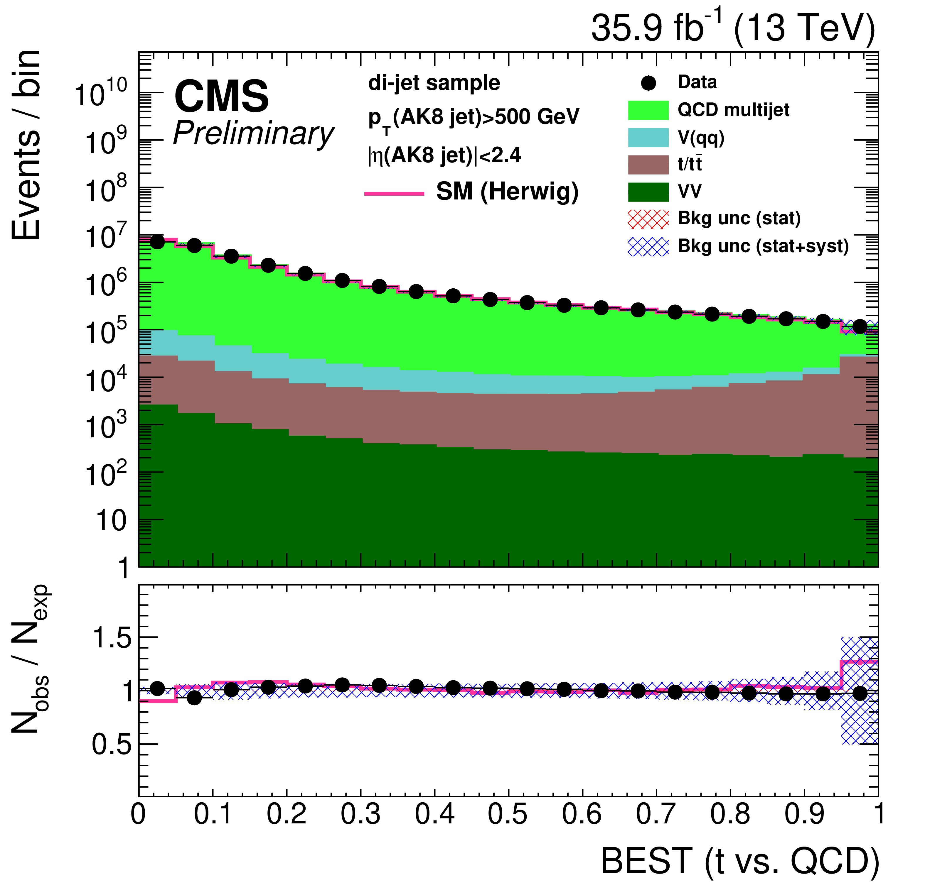
png pdf |
Figure 35-a:
Distribution of the t quark (upper left) and W boson (upper-right) identification probabilities for the BEST algorithm, and the ${N_{3}-\text {BDT} (\text {CA}15)}$ discriminant, in data and simulation in the di-jet sample. The background event yield is normalized to the total observed data yield. The pink solid line corresponds to the simulation distribution obtained using the alternative QCD multijet sample. The background event yield is normalized to the total observed data yield. The lower panel shows the data to simulation ratio. The shaded blue (red) band corresponds to the total uncertainty (statistical uncertainty of the simulated samples), the pink line to the data to simulation ratio using the alternative QCD multijet sample, and the vertical lines correspond to the statistical uncertainty of the data. The distributions are weighted so that the jet ${p_{\mathrm {T}}}$ distribution of the simulation matches the data. |
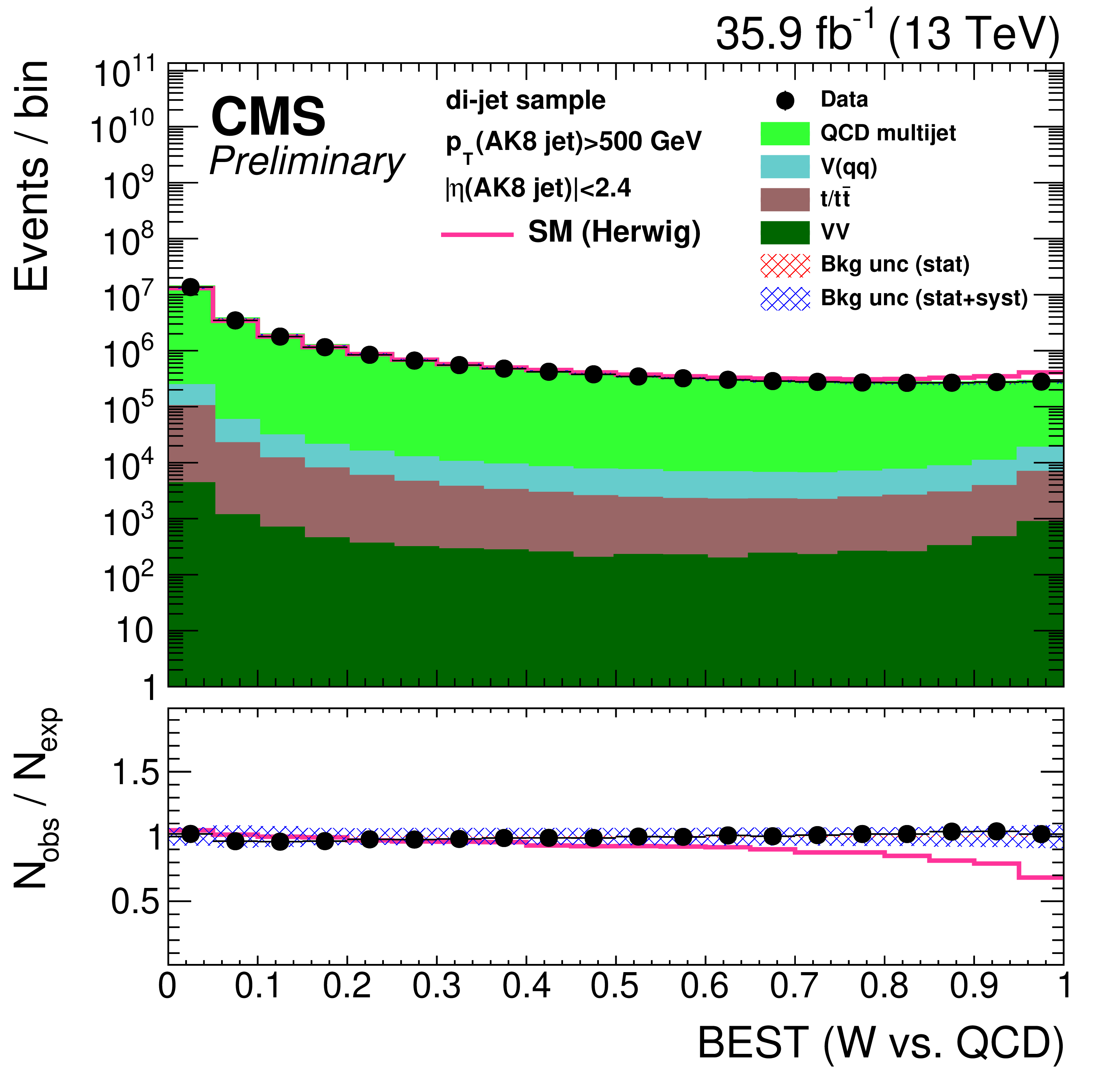
png pdf |
Figure 35-b:
Distribution of the t quark (upper left) and W boson (upper-right) identification probabilities for the BEST algorithm, and the ${N_{3}-\text {BDT} (\text {CA}15)}$ discriminant, in data and simulation in the di-jet sample. The background event yield is normalized to the total observed data yield. The pink solid line corresponds to the simulation distribution obtained using the alternative QCD multijet sample. The background event yield is normalized to the total observed data yield. The lower panel shows the data to simulation ratio. The shaded blue (red) band corresponds to the total uncertainty (statistical uncertainty of the simulated samples), the pink line to the data to simulation ratio using the alternative QCD multijet sample, and the vertical lines correspond to the statistical uncertainty of the data. The distributions are weighted so that the jet ${p_{\mathrm {T}}}$ distribution of the simulation matches the data. |

png pdf |
Figure 35-c:
Distribution of the t quark (upper left) and W boson (upper-right) identification probabilities for the BEST algorithm, and the ${N_{3}-\text {BDT} (\text {CA}15)}$ discriminant, in data and simulation in the di-jet sample. The background event yield is normalized to the total observed data yield. The pink solid line corresponds to the simulation distribution obtained using the alternative QCD multijet sample. The background event yield is normalized to the total observed data yield. The lower panel shows the data to simulation ratio. The shaded blue (red) band corresponds to the total uncertainty (statistical uncertainty of the simulated samples), the pink line to the data to simulation ratio using the alternative QCD multijet sample, and the vertical lines correspond to the statistical uncertainty of the data. The distributions are weighted so that the jet ${p_{\mathrm {T}}}$ distribution of the simulation matches the data. |
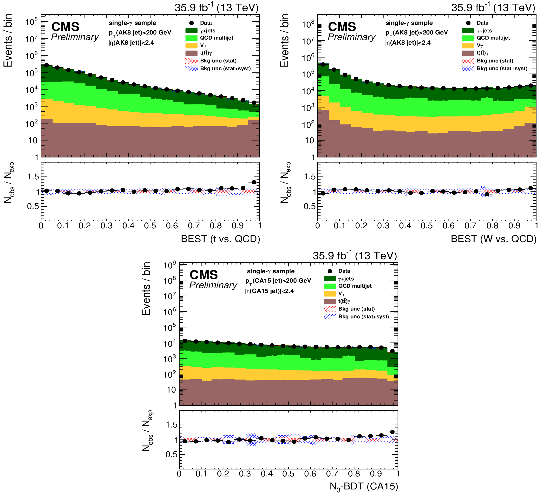
png pdf |
Figure 36:
Distribution of the t quark (upper left) and W boson (upper-right) identification probabilities for the BEST algorithm, and the ${N_{3}-\text {BDT} (\text {CA}15)}$ discriminant, in data and simulation in the single-$\gamma $ sample. The background event yield is normalized to the total observed data yield. The background event yield is normalized to the total observed data yield. The lower panel shows the data to simulation ratio. The shaded blue (red) band corresponds to the total uncertainty (statistical uncertainty of the simulated samples), and the vertical lines correspond to the statistical uncertainty of the data. The distributions are weighted so that the jet ${p_{\mathrm {T}}}$ distribution of the simulation matches the data. |
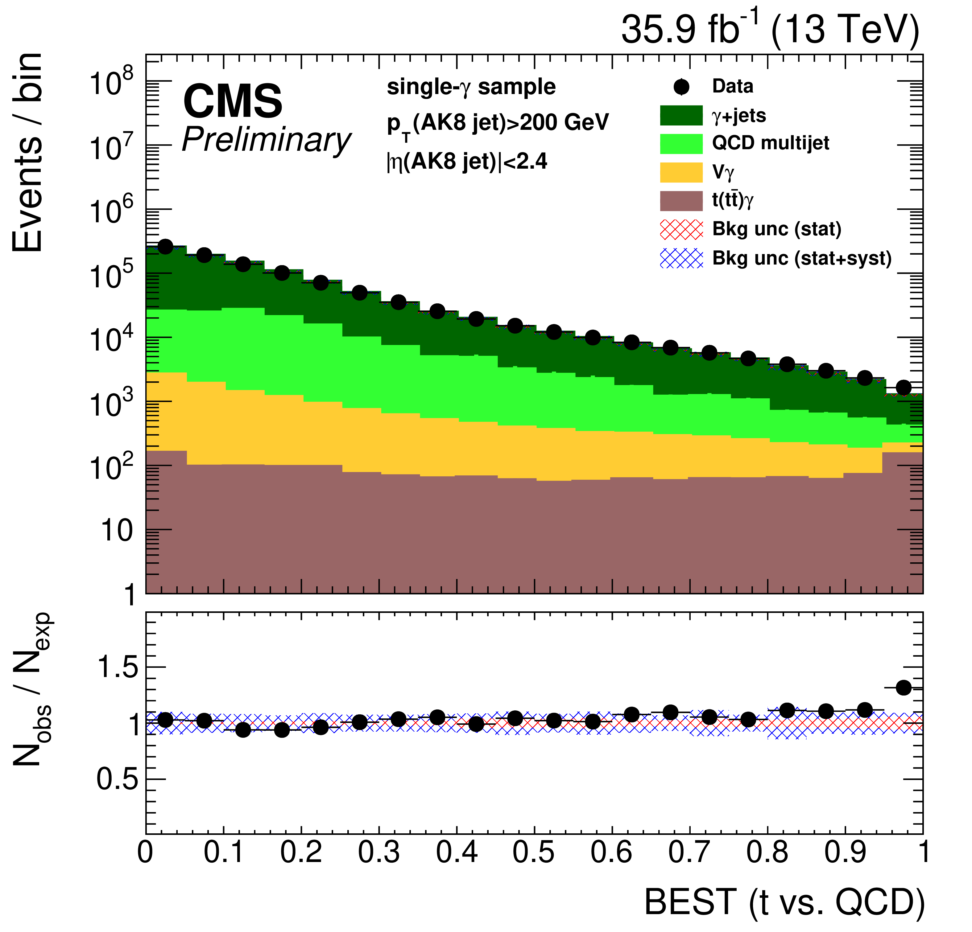
png pdf |
Figure 36-a:
Distribution of the t quark (upper left) and W boson (upper-right) identification probabilities for the BEST algorithm, and the ${N_{3}-\text {BDT} (\text {CA}15)}$ discriminant, in data and simulation in the single-$\gamma $ sample. The background event yield is normalized to the total observed data yield. The background event yield is normalized to the total observed data yield. The lower panel shows the data to simulation ratio. The shaded blue (red) band corresponds to the total uncertainty (statistical uncertainty of the simulated samples), and the vertical lines correspond to the statistical uncertainty of the data. The distributions are weighted so that the jet ${p_{\mathrm {T}}}$ distribution of the simulation matches the data. |
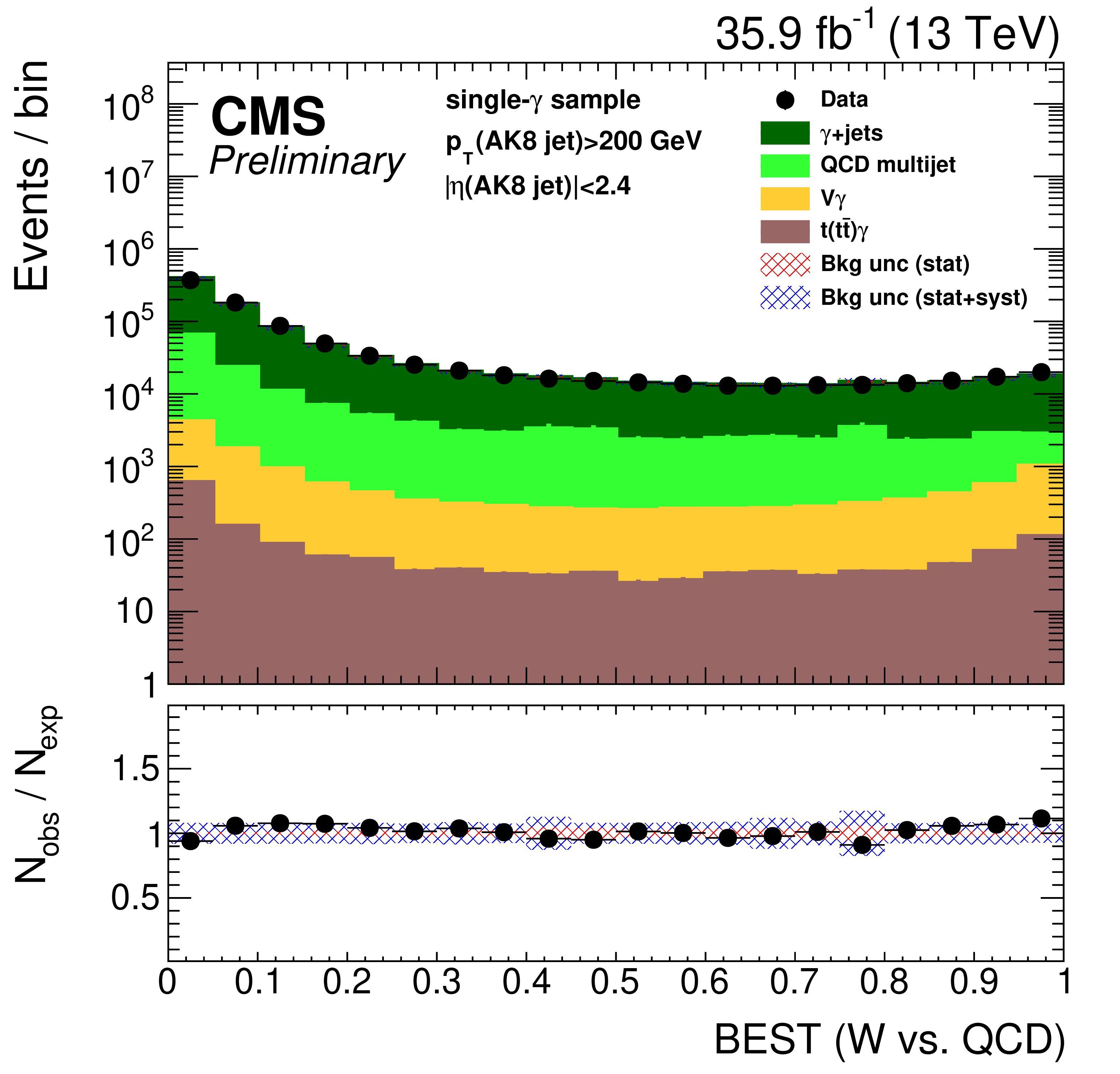
png pdf |
Figure 36-b:
Distribution of the t quark (upper left) and W boson (upper-right) identification probabilities for the BEST algorithm, and the ${N_{3}-\text {BDT} (\text {CA}15)}$ discriminant, in data and simulation in the single-$\gamma $ sample. The background event yield is normalized to the total observed data yield. The background event yield is normalized to the total observed data yield. The lower panel shows the data to simulation ratio. The shaded blue (red) band corresponds to the total uncertainty (statistical uncertainty of the simulated samples), and the vertical lines correspond to the statistical uncertainty of the data. The distributions are weighted so that the jet ${p_{\mathrm {T}}}$ distribution of the simulation matches the data. |
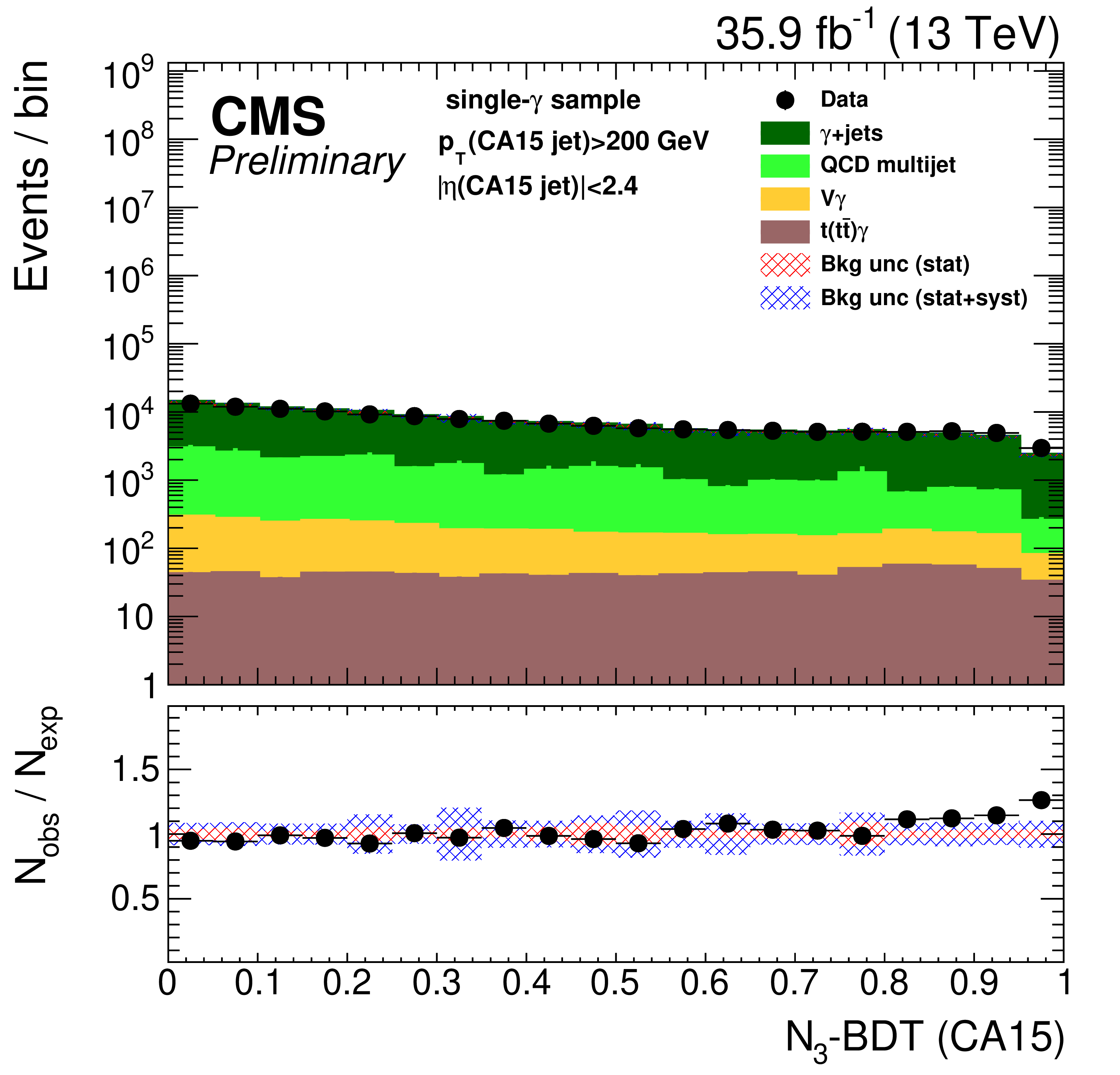
png pdf |
Figure 36-c:
Distribution of the t quark (upper left) and W boson (upper-right) identification probabilities for the BEST algorithm, and the ${N_{3}-\text {BDT} (\text {CA}15)}$ discriminant, in data and simulation in the single-$\gamma $ sample. The background event yield is normalized to the total observed data yield. The background event yield is normalized to the total observed data yield. The lower panel shows the data to simulation ratio. The shaded blue (red) band corresponds to the total uncertainty (statistical uncertainty of the simulated samples), and the vertical lines correspond to the statistical uncertainty of the data. The distributions are weighted so that the jet ${p_{\mathrm {T}}}$ distribution of the simulation matches the data. |
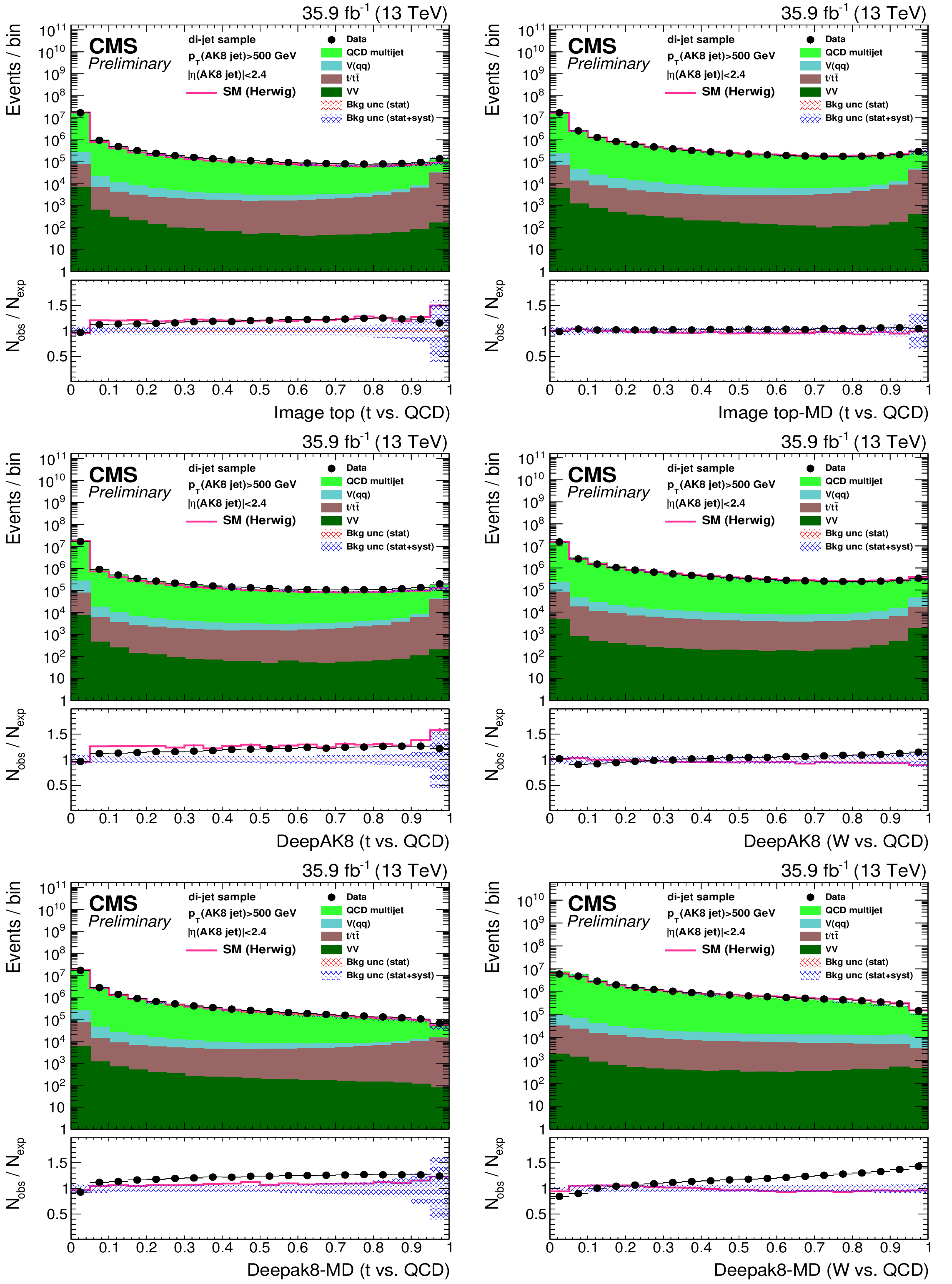
png pdf |
Figure 37:
Distribution of the ImageTop (upper-left) and ImageTop-MD (upper-right) discriminant in data and simulation in the di-jet sample. The plots in the middle row show the t quark (left) and W boson (right) identification probabilities in data and simulation for the DeepAK8 algorithm. The corresponding plots for DeepAK8-MD are displayed in the lower row. The pink solid line corresponds to the simulation distribution obtained using the alternative QCD multijet sample. The background event yield is normalized to the total observed data yield. The lower panel shows the data to simulation ratio. The shaded blue (red) band corresponds to the total uncertainty (statistical uncertainty of the simulated samples), the pink line to the data to simulation ratio using the alternative QCD multijet sample, and the vertical lines correspond to the statistical uncertainty of the data. The distributions are weighted so that the jet ${p_{\mathrm {T}}}$ distribution of the simulation matches the data. |
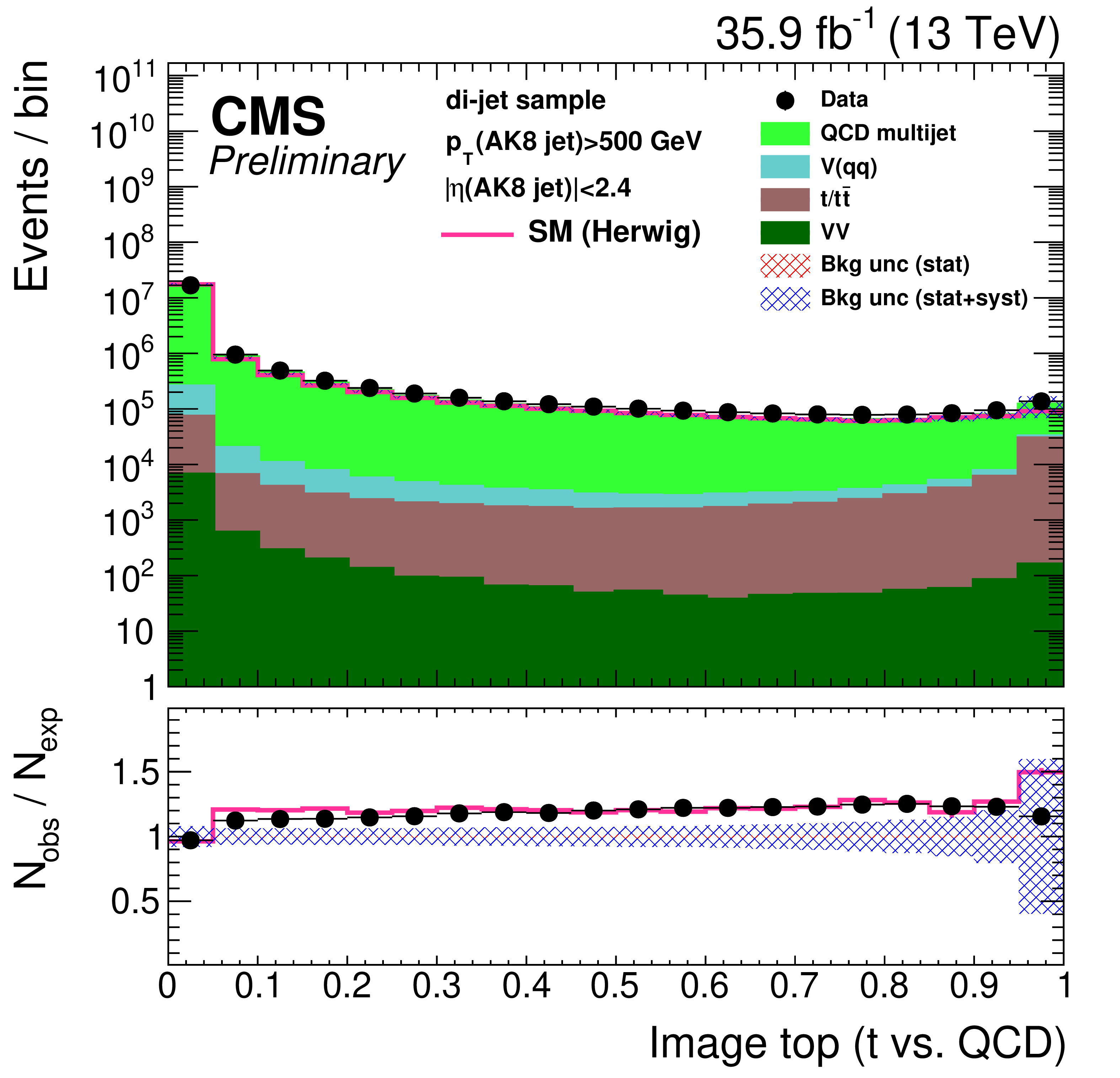
png pdf |
Figure 37-a:
Distribution of the ImageTop (upper-left) and ImageTop-MD (upper-right) discriminant in data and simulation in the di-jet sample. The plots in the middle row show the t quark (left) and W boson (right) identification probabilities in data and simulation for the DeepAK8 algorithm. The corresponding plots for DeepAK8-MD are displayed in the lower row. The pink solid line corresponds to the simulation distribution obtained using the alternative QCD multijet sample. The background event yield is normalized to the total observed data yield. The lower panel shows the data to simulation ratio. The shaded blue (red) band corresponds to the total uncertainty (statistical uncertainty of the simulated samples), the pink line to the data to simulation ratio using the alternative QCD multijet sample, and the vertical lines correspond to the statistical uncertainty of the data. The distributions are weighted so that the jet ${p_{\mathrm {T}}}$ distribution of the simulation matches the data. |
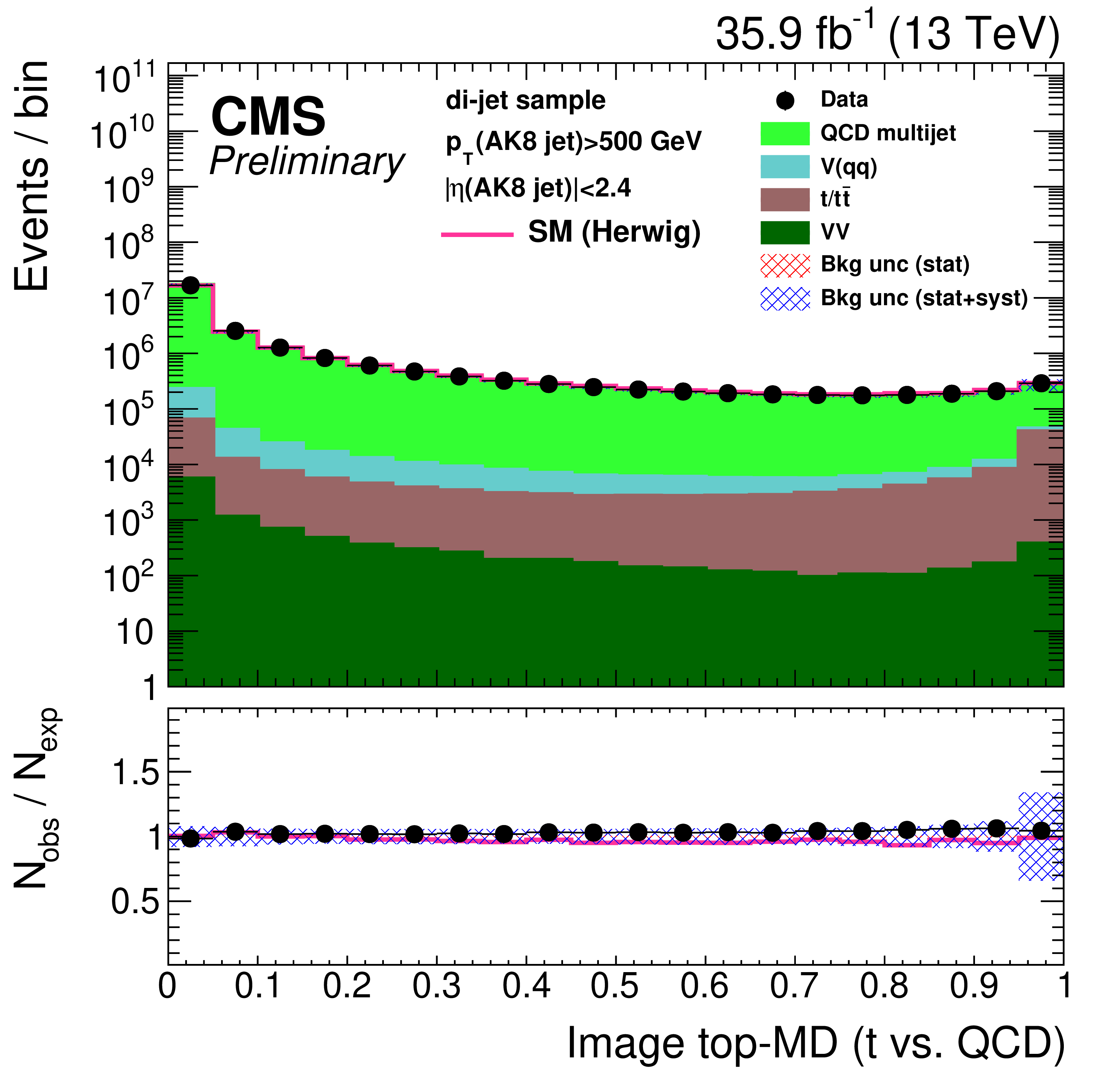
png pdf |
Figure 37-b:
Distribution of the ImageTop (upper-left) and ImageTop-MD (upper-right) discriminant in data and simulation in the di-jet sample. The plots in the middle row show the t quark (left) and W boson (right) identification probabilities in data and simulation for the DeepAK8 algorithm. The corresponding plots for DeepAK8-MD are displayed in the lower row. The pink solid line corresponds to the simulation distribution obtained using the alternative QCD multijet sample. The background event yield is normalized to the total observed data yield. The lower panel shows the data to simulation ratio. The shaded blue (red) band corresponds to the total uncertainty (statistical uncertainty of the simulated samples), the pink line to the data to simulation ratio using the alternative QCD multijet sample, and the vertical lines correspond to the statistical uncertainty of the data. The distributions are weighted so that the jet ${p_{\mathrm {T}}}$ distribution of the simulation matches the data. |
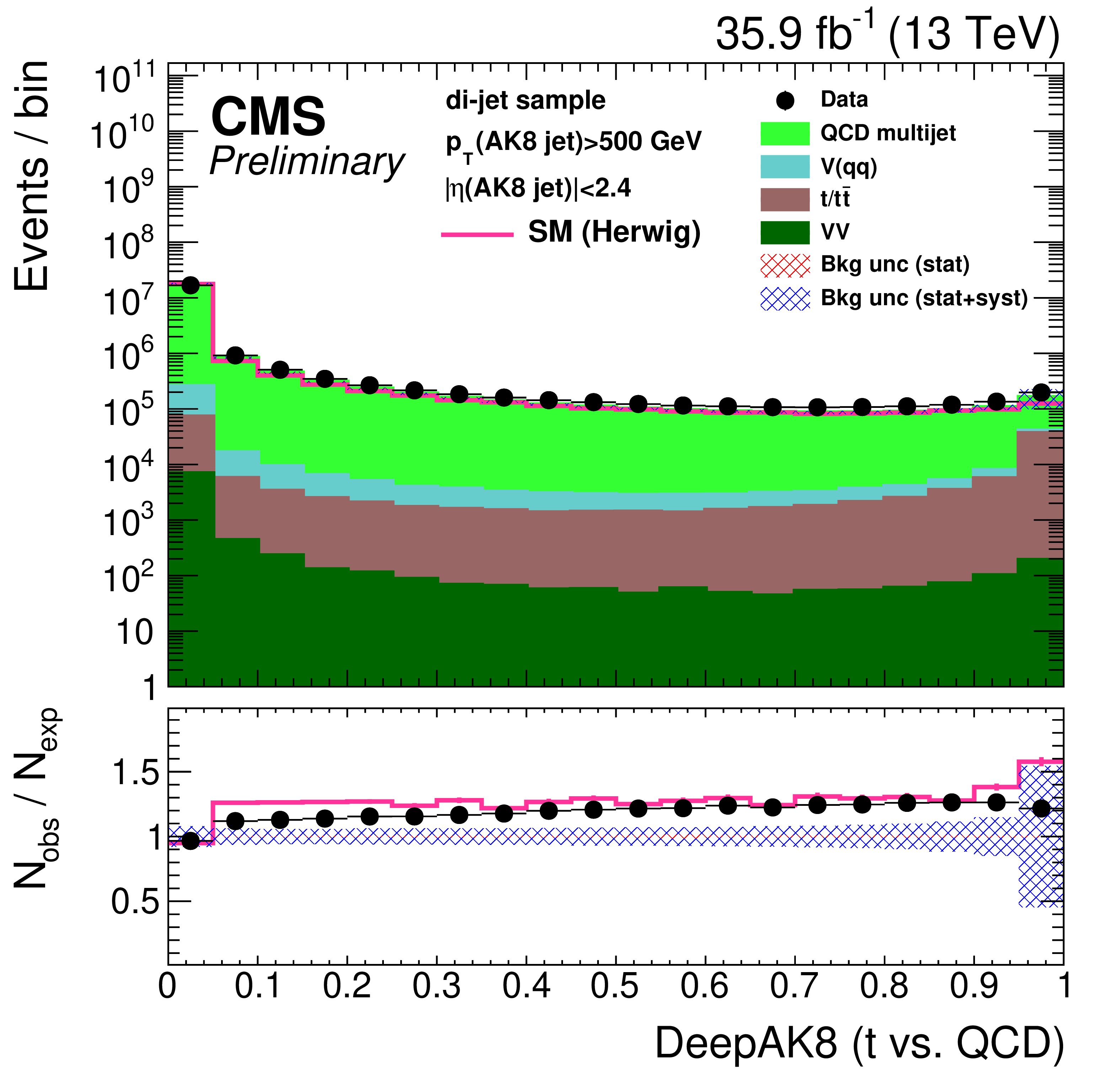
png pdf |
Figure 37-c:
Distribution of the ImageTop (upper-left) and ImageTop-MD (upper-right) discriminant in data and simulation in the di-jet sample. The plots in the middle row show the t quark (left) and W boson (right) identification probabilities in data and simulation for the DeepAK8 algorithm. The corresponding plots for DeepAK8-MD are displayed in the lower row. The pink solid line corresponds to the simulation distribution obtained using the alternative QCD multijet sample. The background event yield is normalized to the total observed data yield. The lower panel shows the data to simulation ratio. The shaded blue (red) band corresponds to the total uncertainty (statistical uncertainty of the simulated samples), the pink line to the data to simulation ratio using the alternative QCD multijet sample, and the vertical lines correspond to the statistical uncertainty of the data. The distributions are weighted so that the jet ${p_{\mathrm {T}}}$ distribution of the simulation matches the data. |
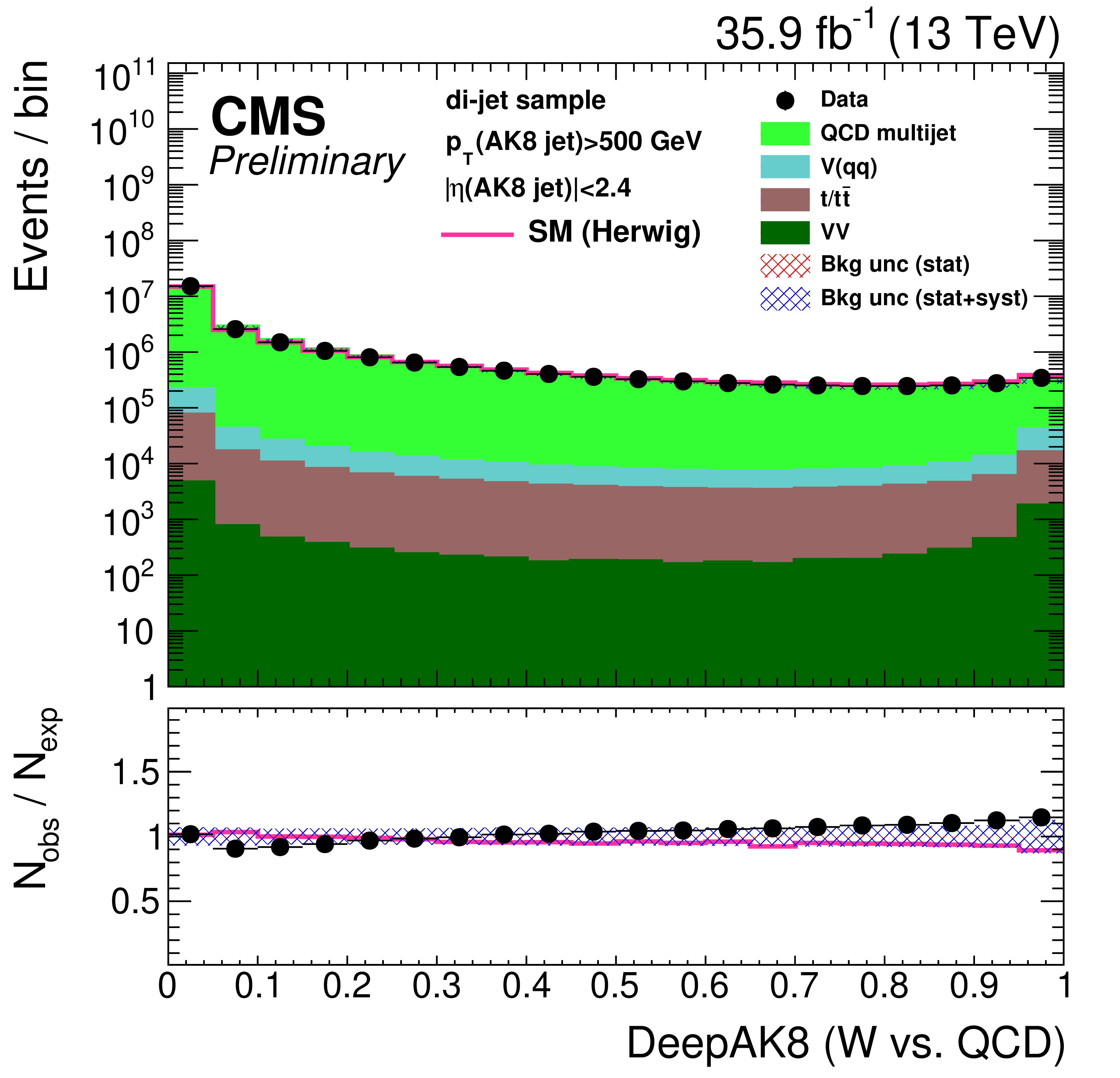
png pdf |
Figure 37-d:
Distribution of the ImageTop (upper-left) and ImageTop-MD (upper-right) discriminant in data and simulation in the di-jet sample. The plots in the middle row show the t quark (left) and W boson (right) identification probabilities in data and simulation for the DeepAK8 algorithm. The corresponding plots for DeepAK8-MD are displayed in the lower row. The pink solid line corresponds to the simulation distribution obtained using the alternative QCD multijet sample. The background event yield is normalized to the total observed data yield. The lower panel shows the data to simulation ratio. The shaded blue (red) band corresponds to the total uncertainty (statistical uncertainty of the simulated samples), the pink line to the data to simulation ratio using the alternative QCD multijet sample, and the vertical lines correspond to the statistical uncertainty of the data. The distributions are weighted so that the jet ${p_{\mathrm {T}}}$ distribution of the simulation matches the data. |
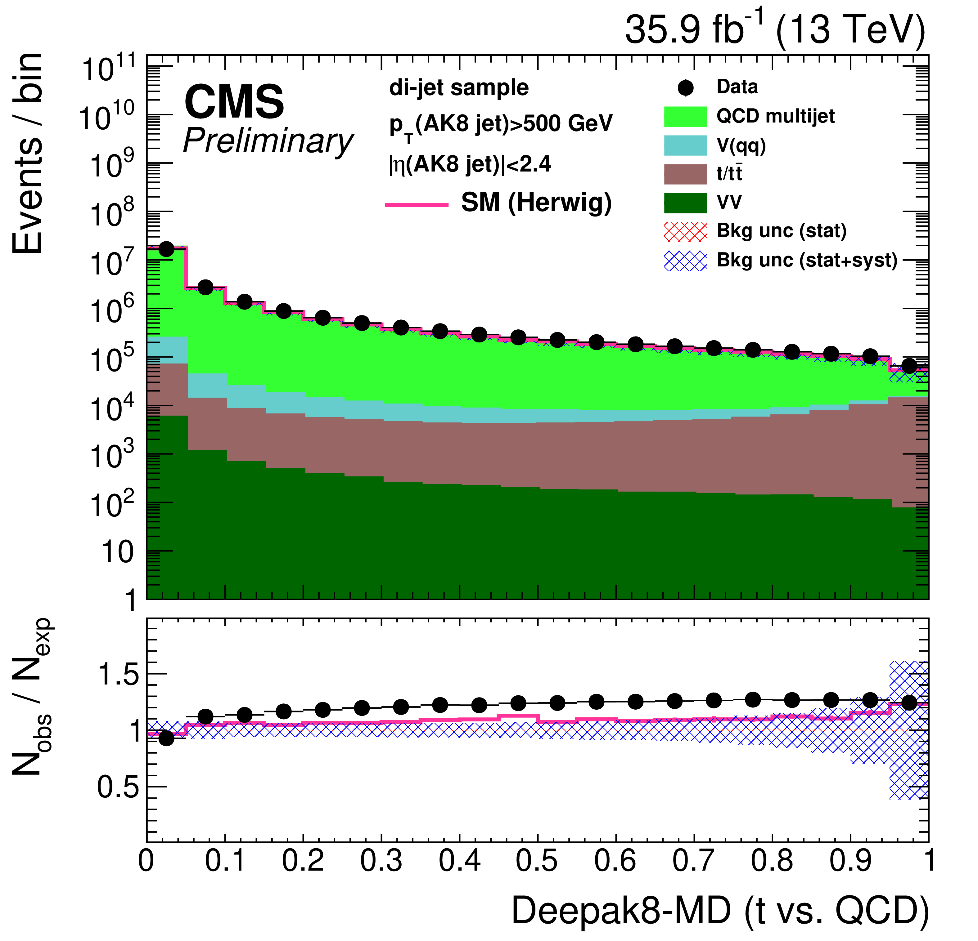
png pdf |
Figure 37-e:
Distribution of the ImageTop (upper-left) and ImageTop-MD (upper-right) discriminant in data and simulation in the di-jet sample. The plots in the middle row show the t quark (left) and W boson (right) identification probabilities in data and simulation for the DeepAK8 algorithm. The corresponding plots for DeepAK8-MD are displayed in the lower row. The pink solid line corresponds to the simulation distribution obtained using the alternative QCD multijet sample. The background event yield is normalized to the total observed data yield. The lower panel shows the data to simulation ratio. The shaded blue (red) band corresponds to the total uncertainty (statistical uncertainty of the simulated samples), the pink line to the data to simulation ratio using the alternative QCD multijet sample, and the vertical lines correspond to the statistical uncertainty of the data. The distributions are weighted so that the jet ${p_{\mathrm {T}}}$ distribution of the simulation matches the data. |

png pdf |
Figure 37-f:
Distribution of the ImageTop (upper-left) and ImageTop-MD (upper-right) discriminant in data and simulation in the di-jet sample. The plots in the middle row show the t quark (left) and W boson (right) identification probabilities in data and simulation for the DeepAK8 algorithm. The corresponding plots for DeepAK8-MD are displayed in the lower row. The pink solid line corresponds to the simulation distribution obtained using the alternative QCD multijet sample. The background event yield is normalized to the total observed data yield. The lower panel shows the data to simulation ratio. The shaded blue (red) band corresponds to the total uncertainty (statistical uncertainty of the simulated samples), the pink line to the data to simulation ratio using the alternative QCD multijet sample, and the vertical lines correspond to the statistical uncertainty of the data. The distributions are weighted so that the jet ${p_{\mathrm {T}}}$ distribution of the simulation matches the data. |
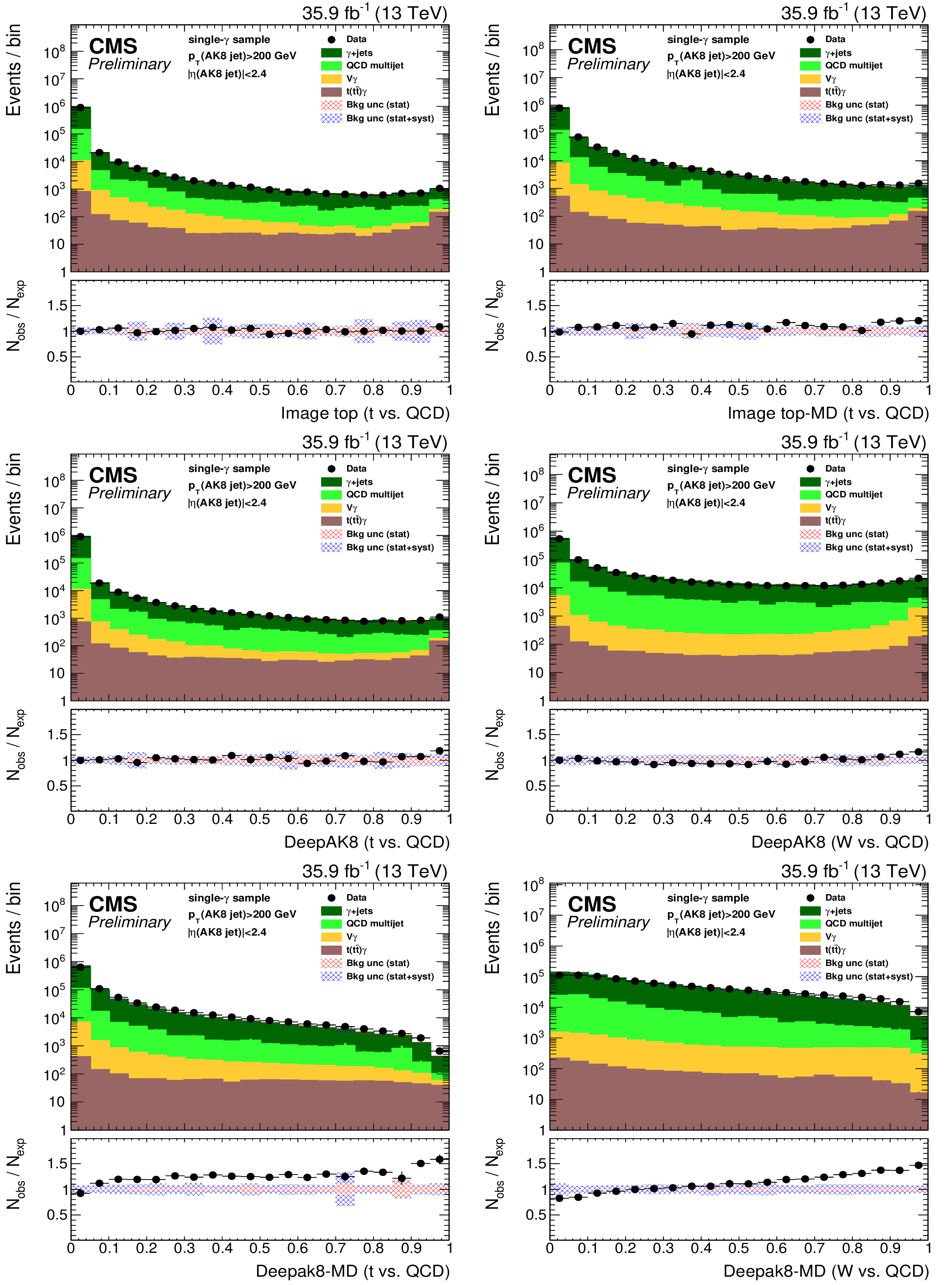
png pdf |
Figure 38:
Distribution of the ImageTop (upper-left) and ImageTop-MD (upper-right) discriminant in data and simulation in the single-$\gamma $ sample. The plots in the middle row show the t quark (left) and W boson (right) identification probabilities in data and simulation for the DeepAK8 algorithm. The corresponding plots for DeepAK8-MD are displayed in the lower row. The background event yield is normalized to the total observed data yield. The lower panel shows the data to simulation ratio. The shaded blue (red) band corresponds to the total uncertainty (statistical uncertainty of the simulated samples), and the vertical lines correspond to the statistical uncertainty of the data. The distributions are weighted so that the jet ${p_{\mathrm {T}}}$ distribution of the simulation matches the data. |
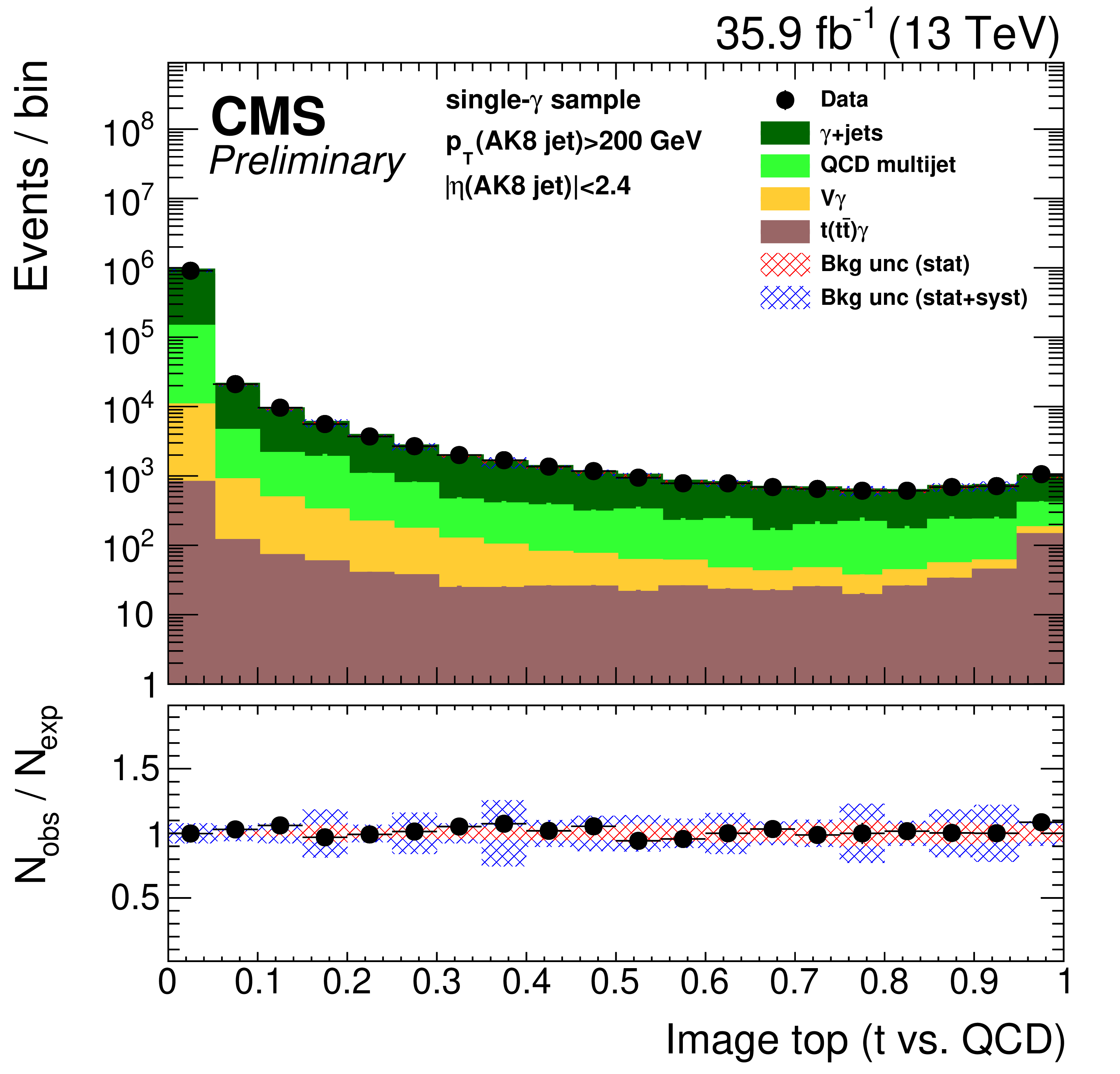
png pdf |
Figure 38-a:
Distribution of the ImageTop (upper-left) and ImageTop-MD (upper-right) discriminant in data and simulation in the single-$\gamma $ sample. The plots in the middle row show the t quark (left) and W boson (right) identification probabilities in data and simulation for the DeepAK8 algorithm. The corresponding plots for DeepAK8-MD are displayed in the lower row. The background event yield is normalized to the total observed data yield. The lower panel shows the data to simulation ratio. The shaded blue (red) band corresponds to the total uncertainty (statistical uncertainty of the simulated samples), and the vertical lines correspond to the statistical uncertainty of the data. The distributions are weighted so that the jet ${p_{\mathrm {T}}}$ distribution of the simulation matches the data. |
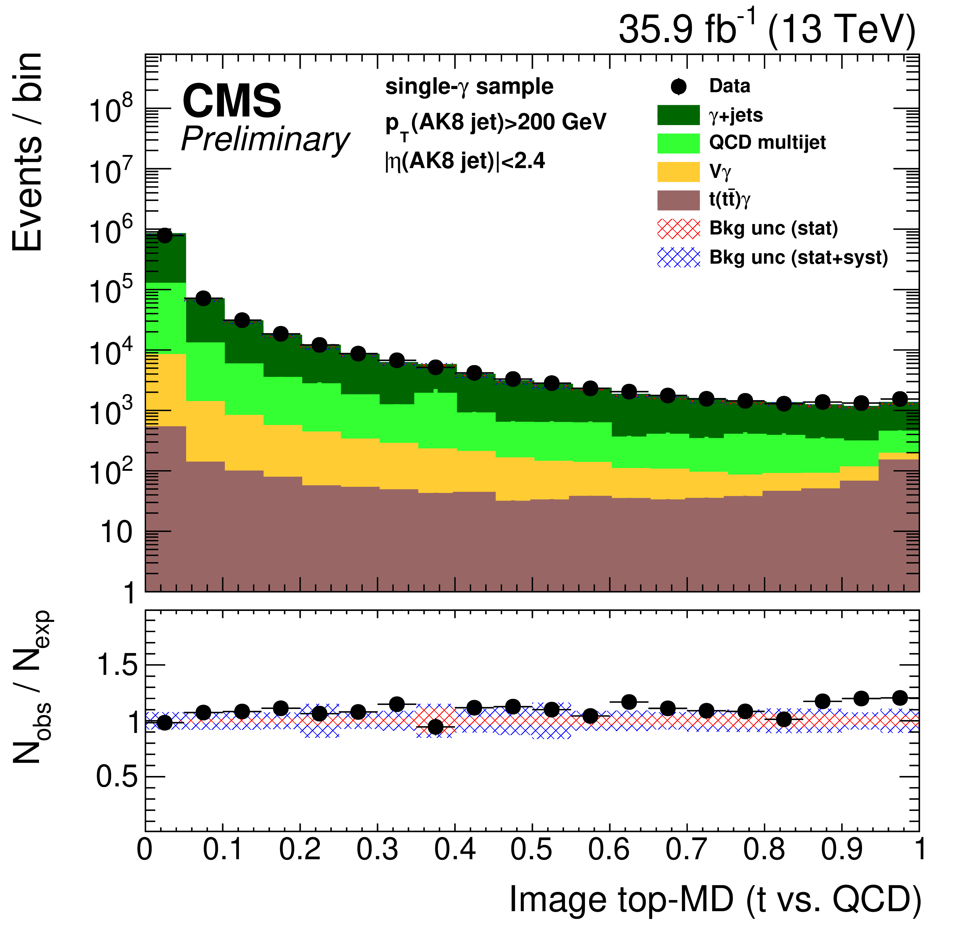
png pdf |
Figure 38-b:
Distribution of the ImageTop (upper-left) and ImageTop-MD (upper-right) discriminant in data and simulation in the single-$\gamma $ sample. The plots in the middle row show the t quark (left) and W boson (right) identification probabilities in data and simulation for the DeepAK8 algorithm. The corresponding plots for DeepAK8-MD are displayed in the lower row. The background event yield is normalized to the total observed data yield. The lower panel shows the data to simulation ratio. The shaded blue (red) band corresponds to the total uncertainty (statistical uncertainty of the simulated samples), and the vertical lines correspond to the statistical uncertainty of the data. The distributions are weighted so that the jet ${p_{\mathrm {T}}}$ distribution of the simulation matches the data. |
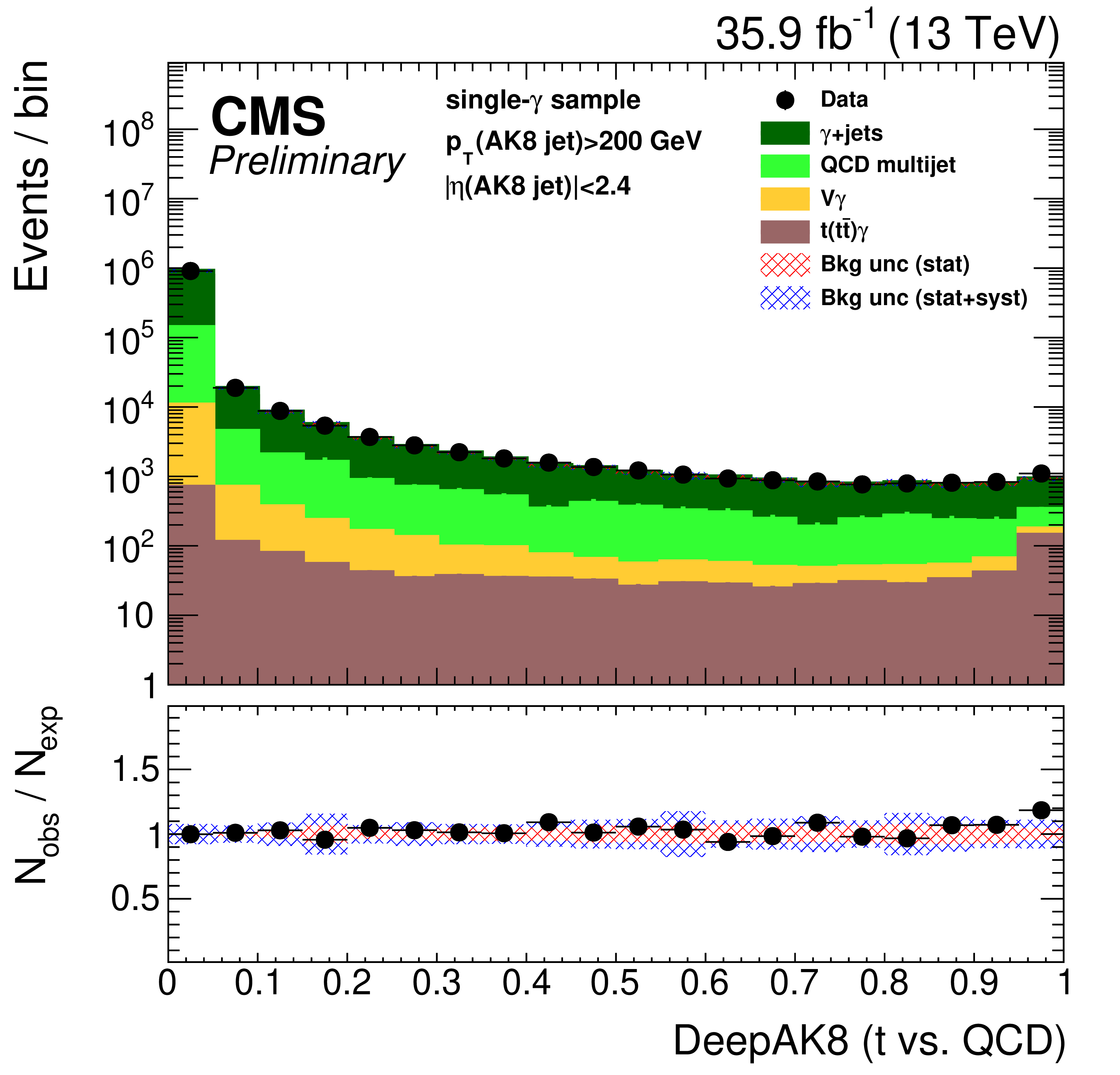
png pdf |
Figure 38-c:
Distribution of the ImageTop (upper-left) and ImageTop-MD (upper-right) discriminant in data and simulation in the single-$\gamma $ sample. The plots in the middle row show the t quark (left) and W boson (right) identification probabilities in data and simulation for the DeepAK8 algorithm. The corresponding plots for DeepAK8-MD are displayed in the lower row. The background event yield is normalized to the total observed data yield. The lower panel shows the data to simulation ratio. The shaded blue (red) band corresponds to the total uncertainty (statistical uncertainty of the simulated samples), and the vertical lines correspond to the statistical uncertainty of the data. The distributions are weighted so that the jet ${p_{\mathrm {T}}}$ distribution of the simulation matches the data. |
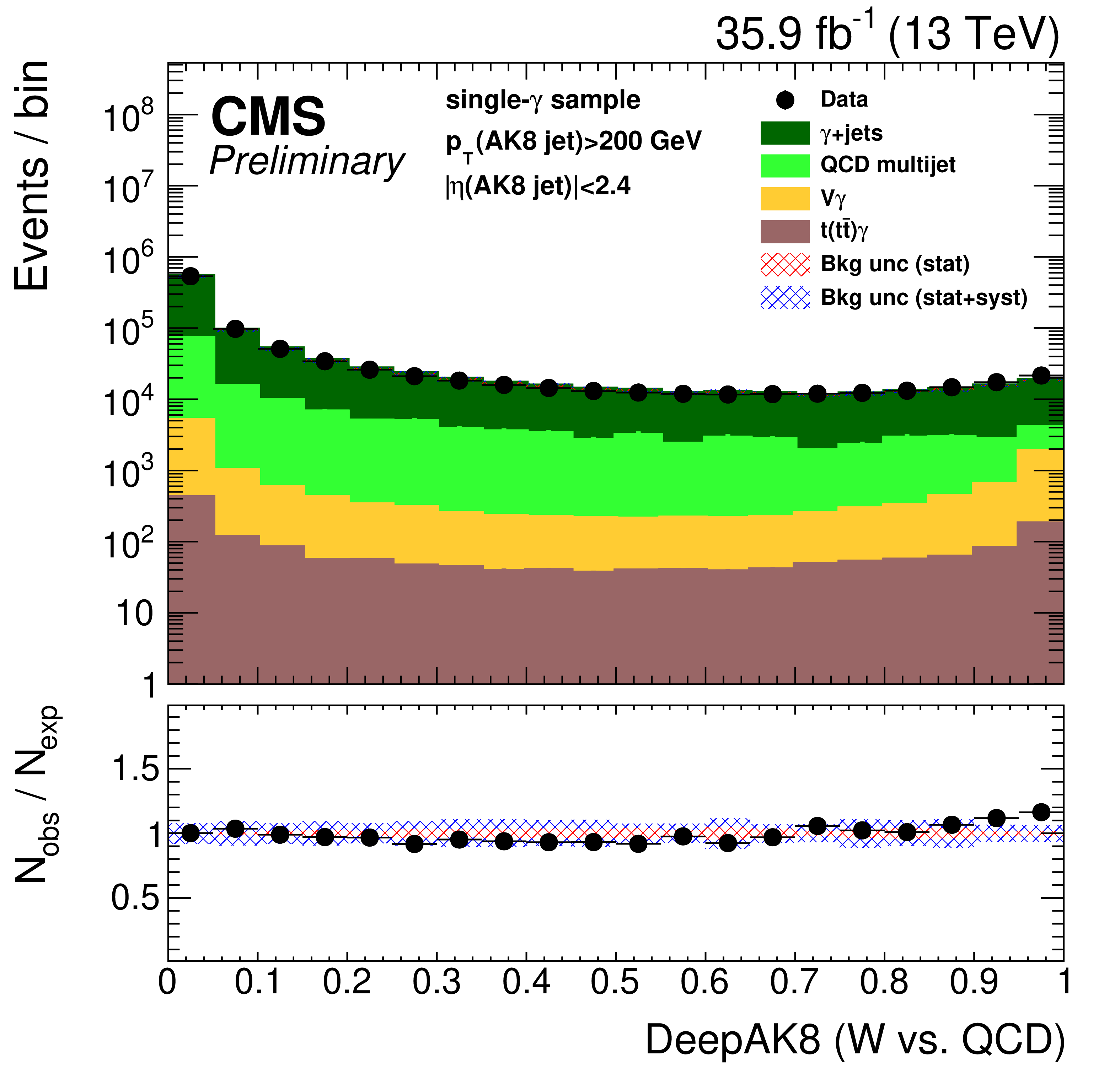
png pdf |
Figure 38-d:
Distribution of the ImageTop (upper-left) and ImageTop-MD (upper-right) discriminant in data and simulation in the single-$\gamma $ sample. The plots in the middle row show the t quark (left) and W boson (right) identification probabilities in data and simulation for the DeepAK8 algorithm. The corresponding plots for DeepAK8-MD are displayed in the lower row. The background event yield is normalized to the total observed data yield. The lower panel shows the data to simulation ratio. The shaded blue (red) band corresponds to the total uncertainty (statistical uncertainty of the simulated samples), and the vertical lines correspond to the statistical uncertainty of the data. The distributions are weighted so that the jet ${p_{\mathrm {T}}}$ distribution of the simulation matches the data. |
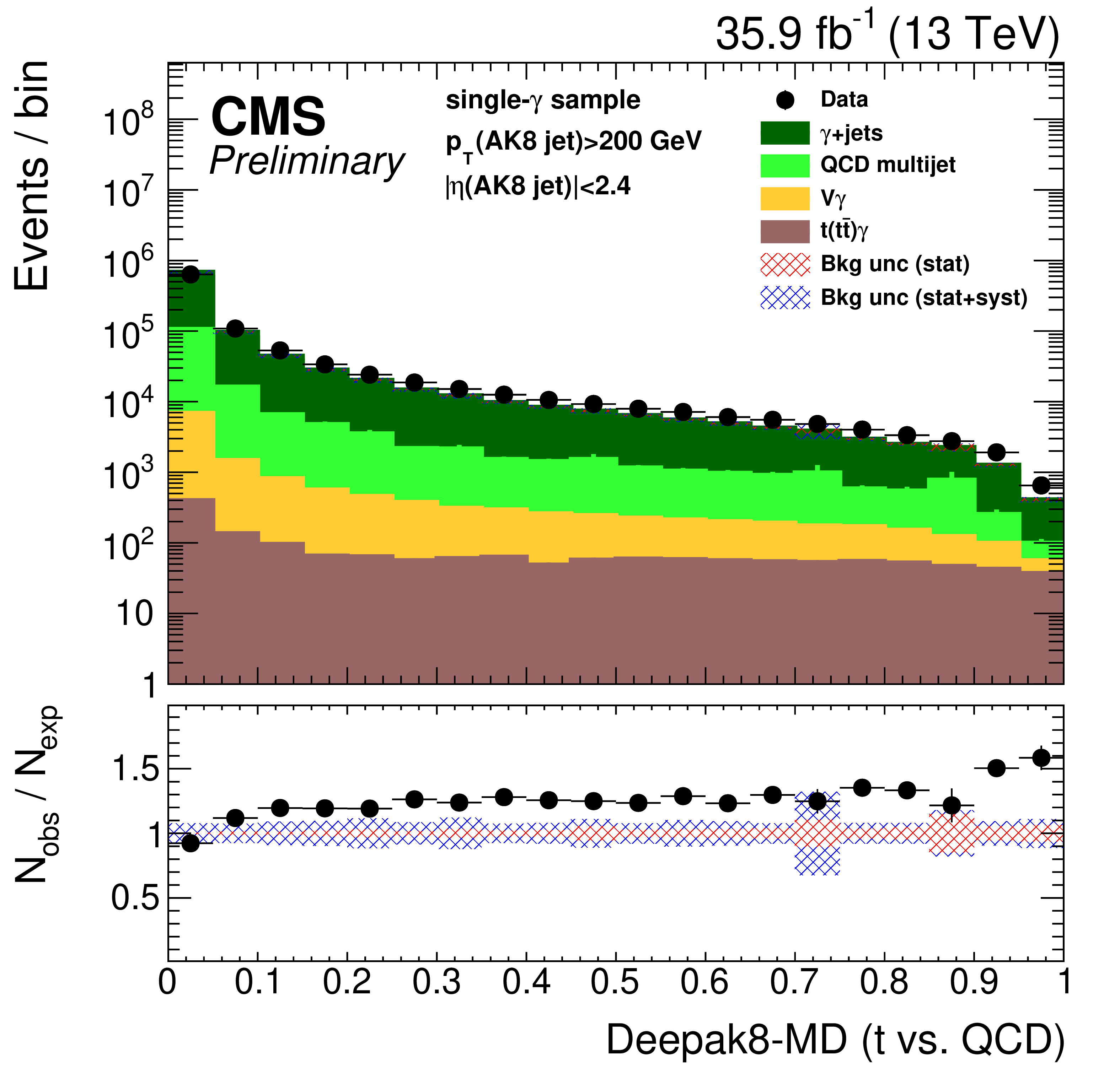
png pdf |
Figure 38-e:
Distribution of the ImageTop (upper-left) and ImageTop-MD (upper-right) discriminant in data and simulation in the single-$\gamma $ sample. The plots in the middle row show the t quark (left) and W boson (right) identification probabilities in data and simulation for the DeepAK8 algorithm. The corresponding plots for DeepAK8-MD are displayed in the lower row. The background event yield is normalized to the total observed data yield. The lower panel shows the data to simulation ratio. The shaded blue (red) band corresponds to the total uncertainty (statistical uncertainty of the simulated samples), and the vertical lines correspond to the statistical uncertainty of the data. The distributions are weighted so that the jet ${p_{\mathrm {T}}}$ distribution of the simulation matches the data. |
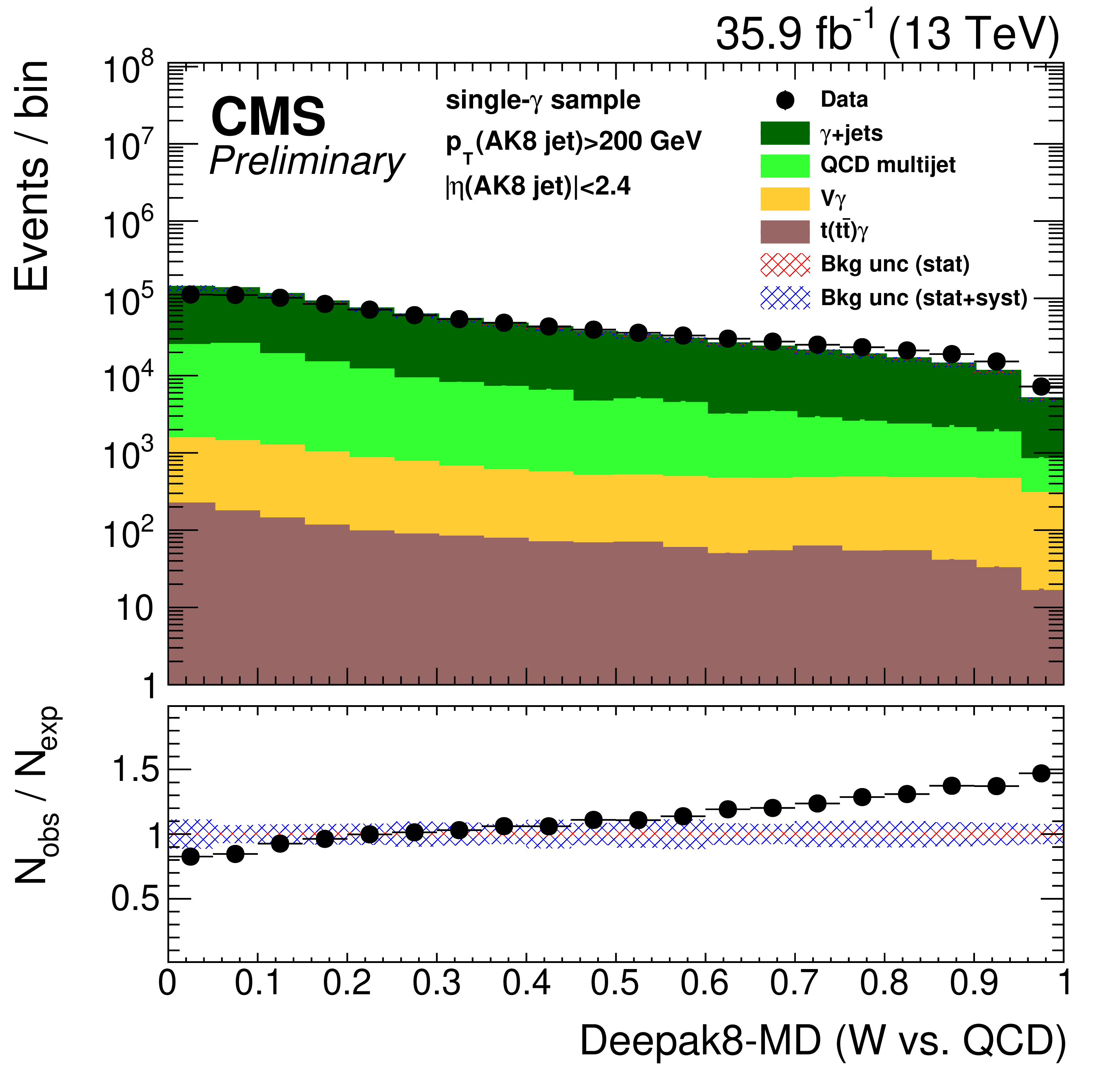
png pdf |
Figure 38-f:
Distribution of the ImageTop (upper-left) and ImageTop-MD (upper-right) discriminant in data and simulation in the single-$\gamma $ sample. The plots in the middle row show the t quark (left) and W boson (right) identification probabilities in data and simulation for the DeepAK8 algorithm. The corresponding plots for DeepAK8-MD are displayed in the lower row. The background event yield is normalized to the total observed data yield. The lower panel shows the data to simulation ratio. The shaded blue (red) band corresponds to the total uncertainty (statistical uncertainty of the simulated samples), and the vertical lines correspond to the statistical uncertainty of the data. The distributions are weighted so that the jet ${p_{\mathrm {T}}}$ distribution of the simulation matches the data. |
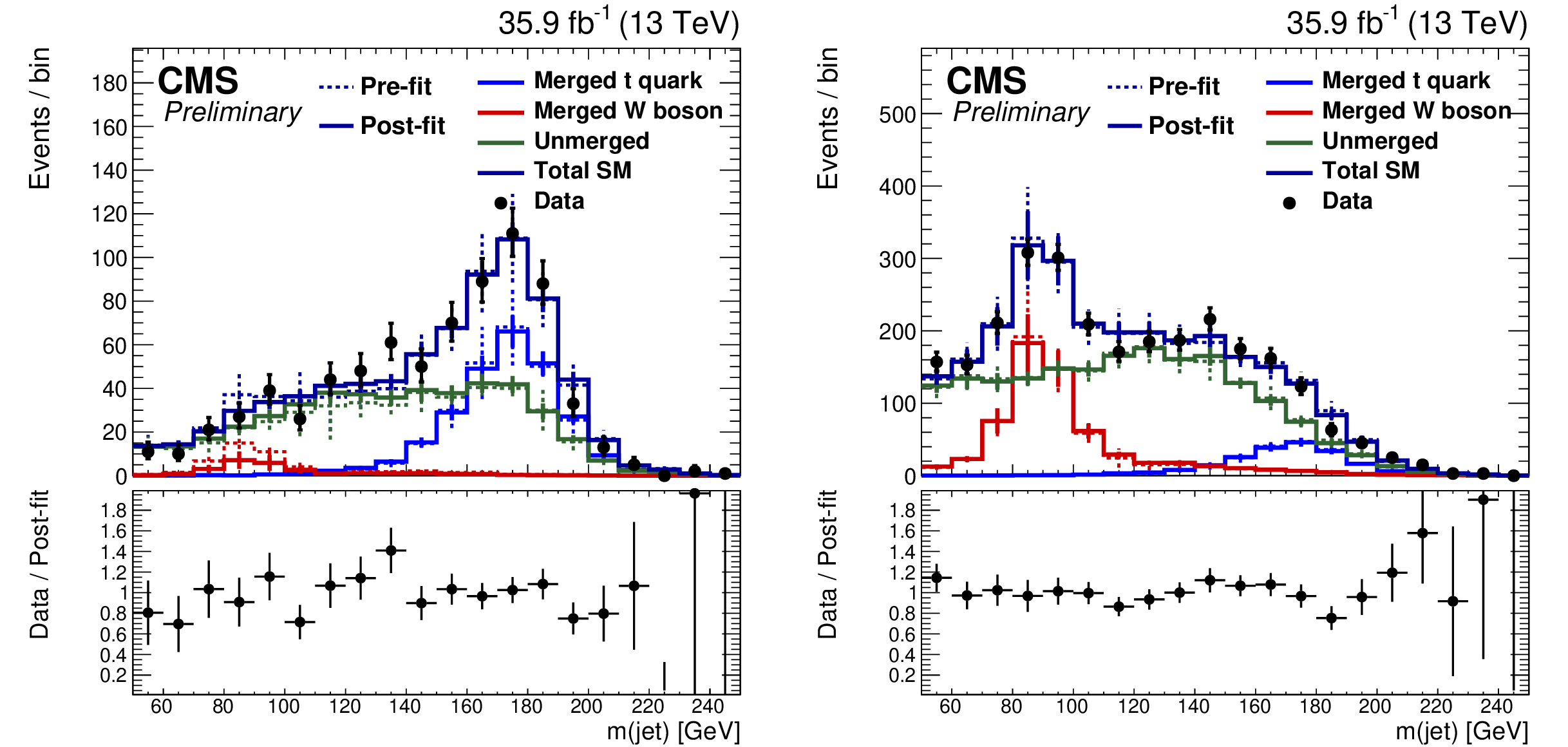
png pdf |
Figure 39:
The ${m_{\text {jet}}}$ distributions for data and simulation in the passing (left) and failing (right) categories for 400 $ < {p_{\mathrm {T}}} (\text {jet}) < $ 480 GeV. The solid lines correspond to the contribution of each category after performing the maximum likelihood fit as described in the text. The dashed lines are the expectation from simulation before the fit. The lower panel shows the data to simulation ratio. |
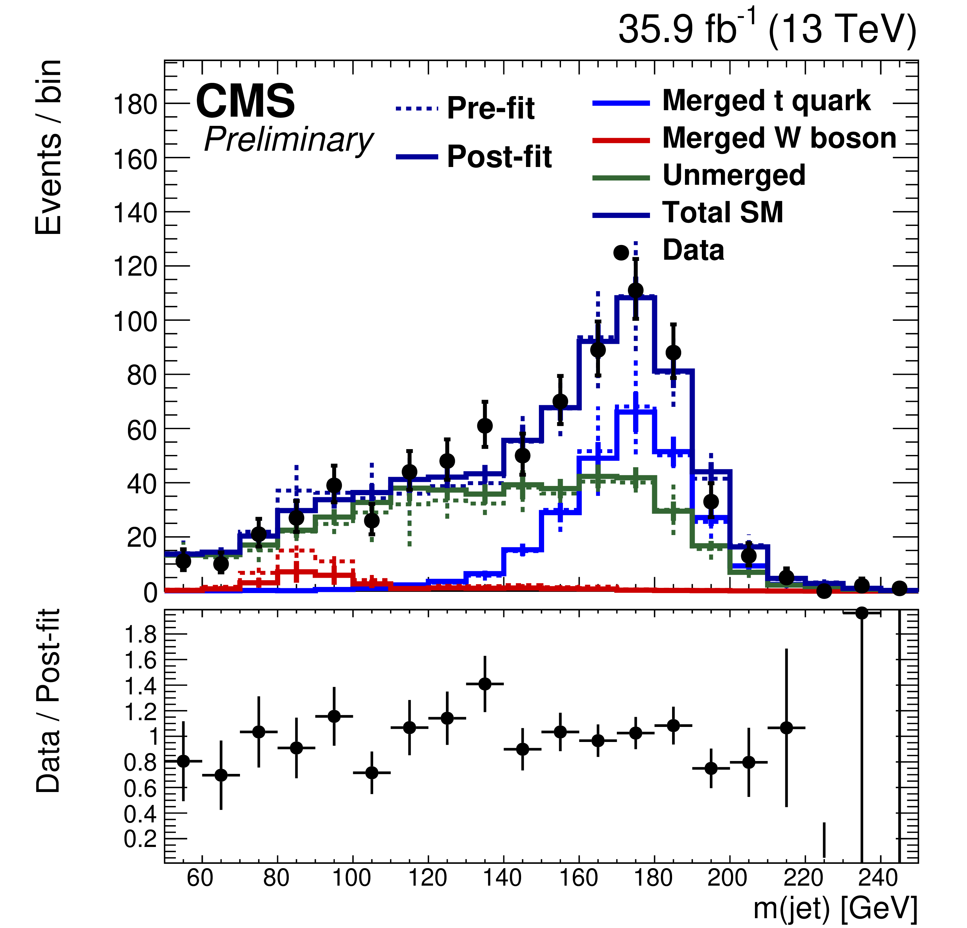
png pdf |
Figure 39-a:
The ${m_{\text {jet}}}$ distributions for data and simulation in the passing (left) and failing (right) categories for 400 $ < {p_{\mathrm {T}}} (\text {jet}) < $ 480 GeV. The solid lines correspond to the contribution of each category after performing the maximum likelihood fit as described in the text. The dashed lines are the expectation from simulation before the fit. The lower panel shows the data to simulation ratio. |
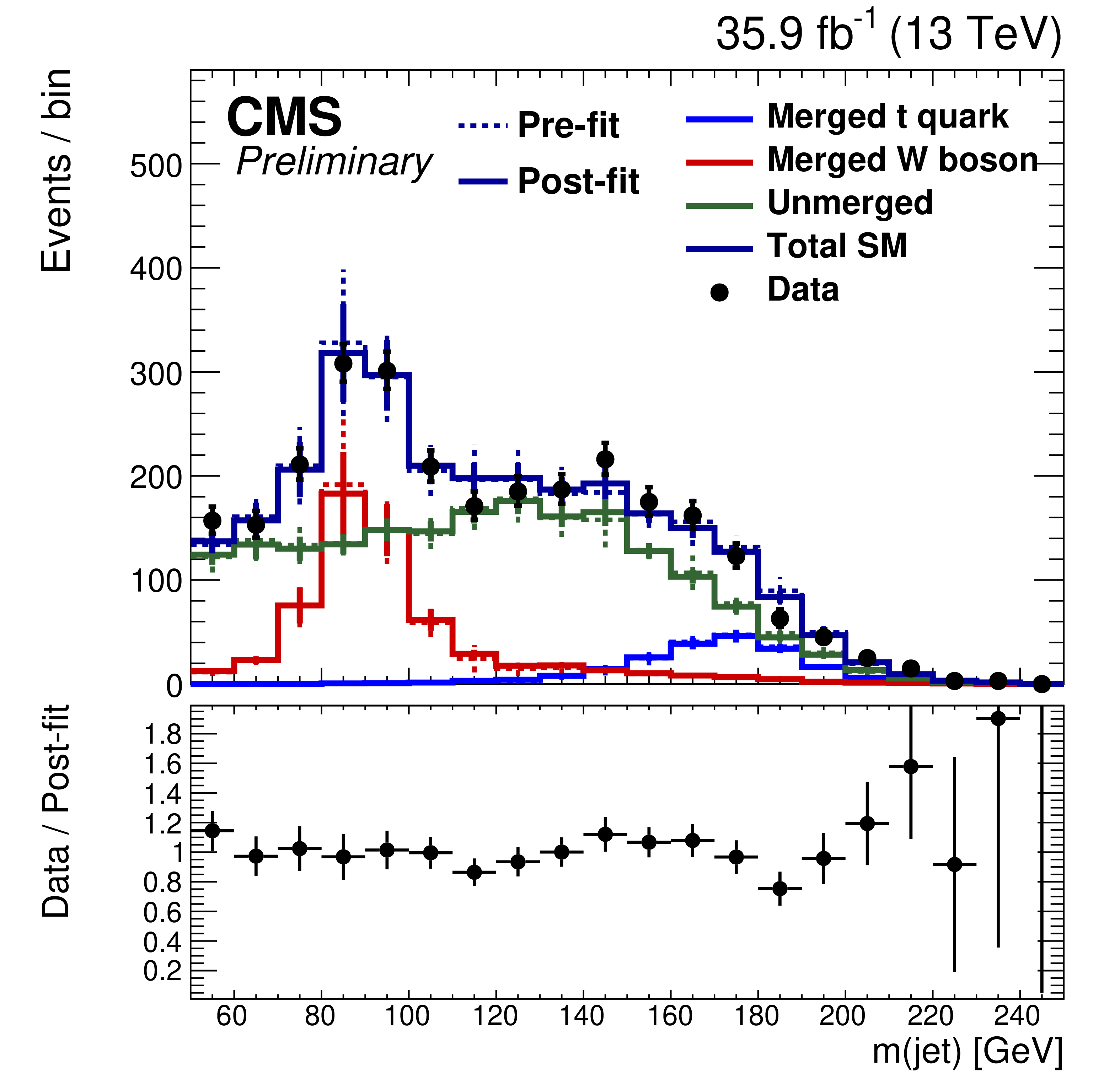
png pdf |
Figure 39-b:
The ${m_{\text {jet}}}$ distributions for data and simulation in the passing (left) and failing (right) categories for 400 $ < {p_{\mathrm {T}}} (\text {jet}) < $ 480 GeV. The solid lines correspond to the contribution of each category after performing the maximum likelihood fit as described in the text. The dashed lines are the expectation from simulation before the fit. The lower panel shows the data to simulation ratio. |
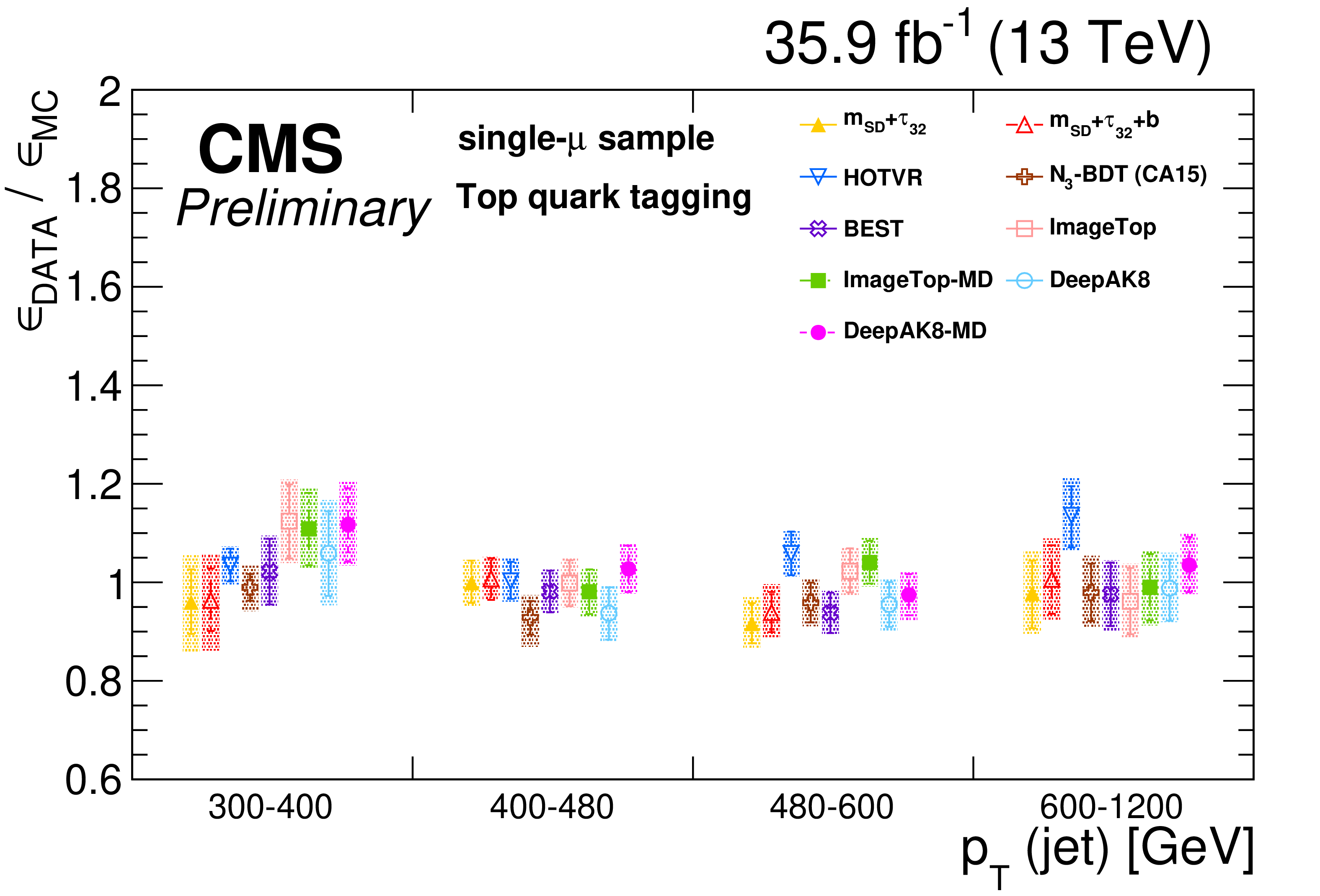
png pdf |
Figure 40:
Summary of the SFs measured for each of the t quark identification algorithms. The markers correspond to the SF value, the error bars to the statistical uncertainty on the SF measurement, and the band is the total uncertainty (statistical + systematic). |
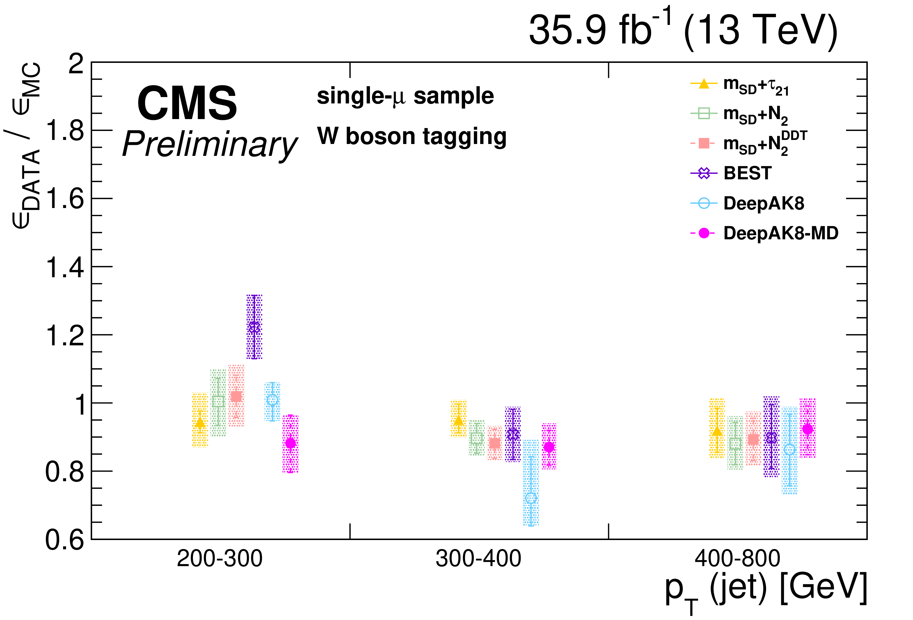
png pdf |
Figure 41:
Summary of the SF measured for each of the W boson identification algorithms. The markers correspond to the SF value, the error bars to the statistical uncertainty on the SF measurement, and the band is the total uncertainty (statistical + systematic). |
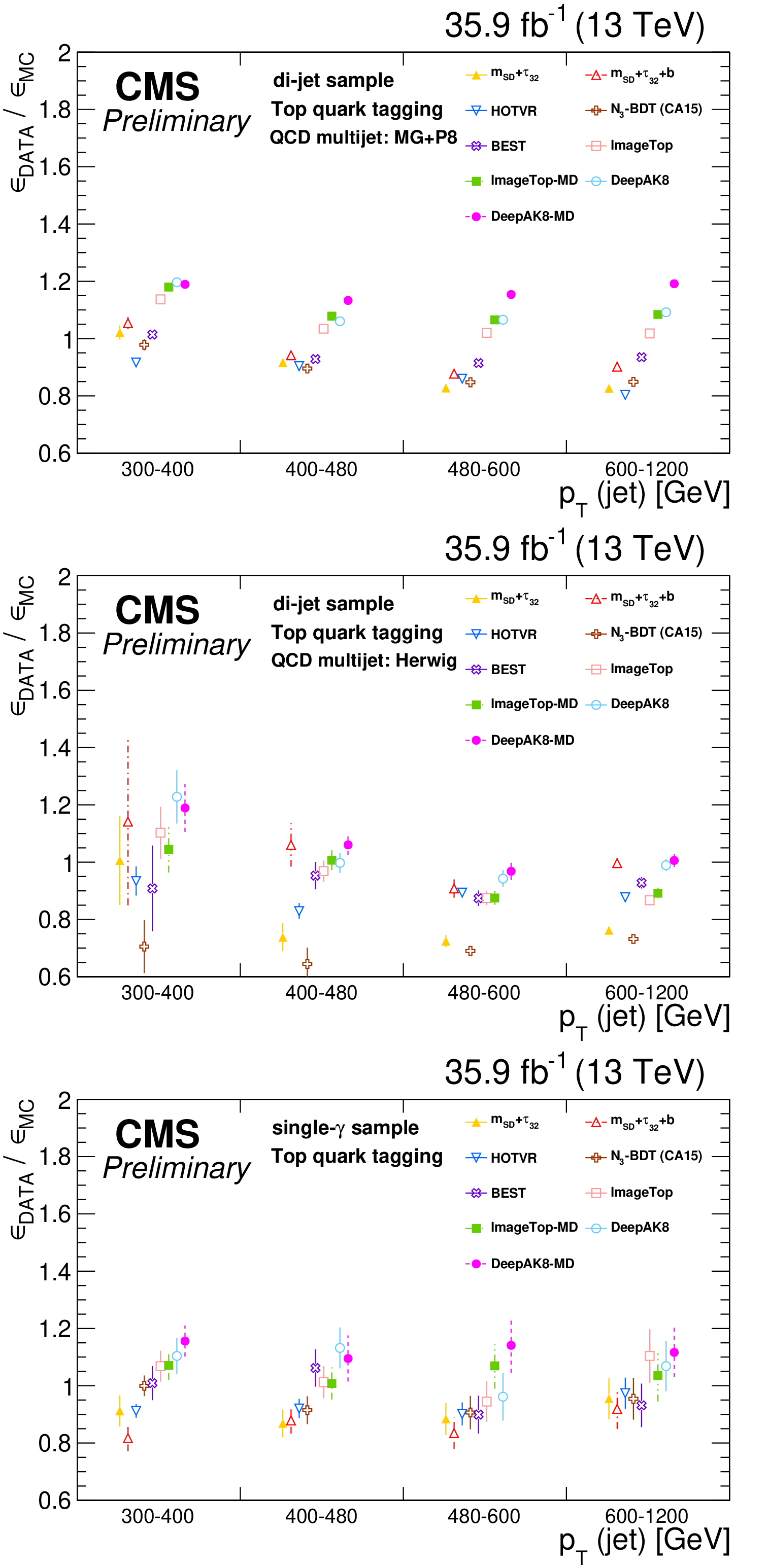
png pdf |
Figure 42:
The ratio of the misidentification rate of t quarks in data and simulation in the di-jet (upper and middle rows) and the single-$\gamma $ (lower row) samples. The QCD multijet process is simulated using MadGraph for the hard process and PYTHIA for parton showering (upper) and HERWIG++ for both (middle). |
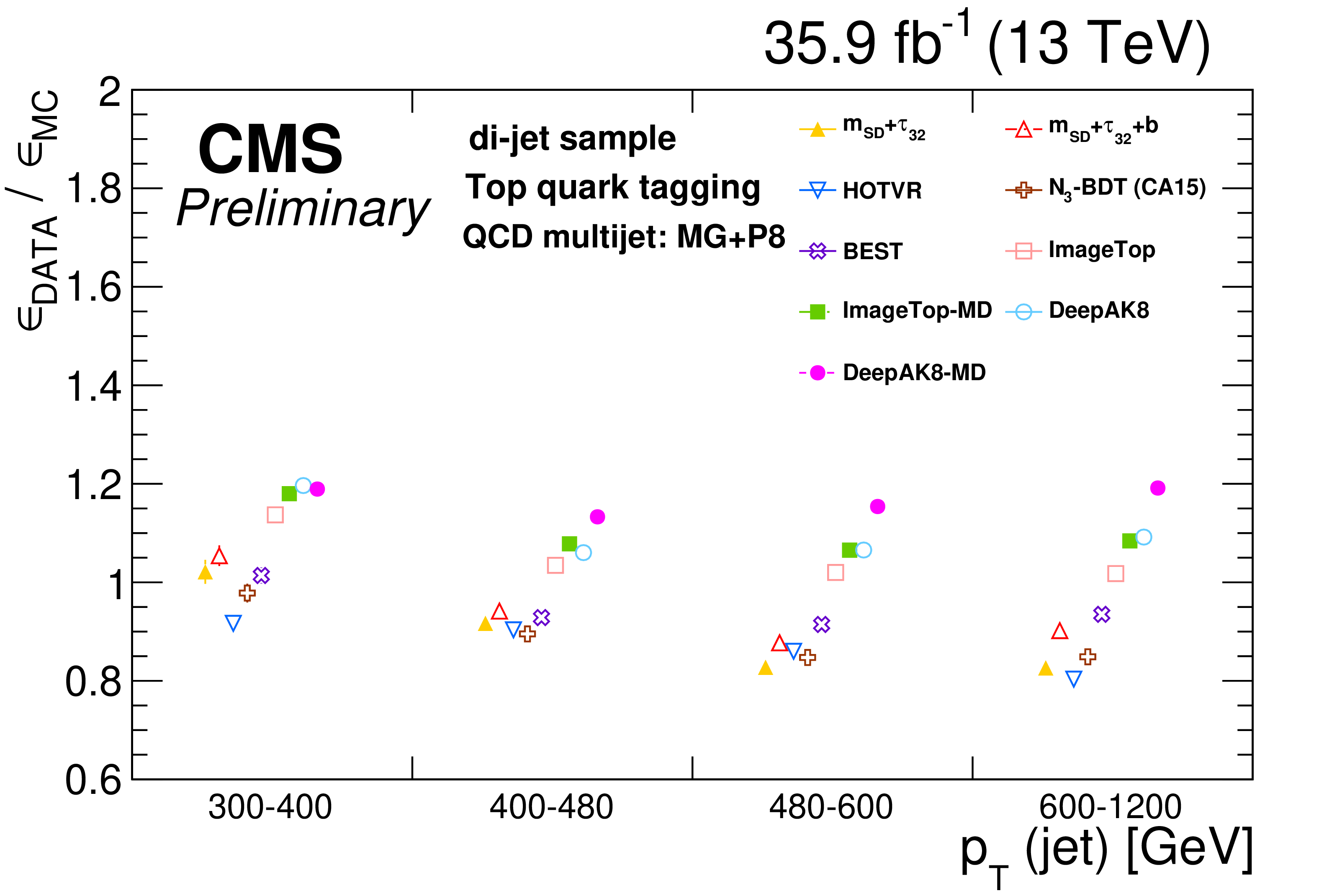
png pdf |
Figure 42-a:
The ratio of the misidentification rate of t quarks in data and simulation in the di-jet (upper and middle rows) and the single-$\gamma $ (lower row) samples. The QCD multijet process is simulated using MadGraph for the hard process and PYTHIA for parton showering (upper) and HERWIG++ for both (middle). |
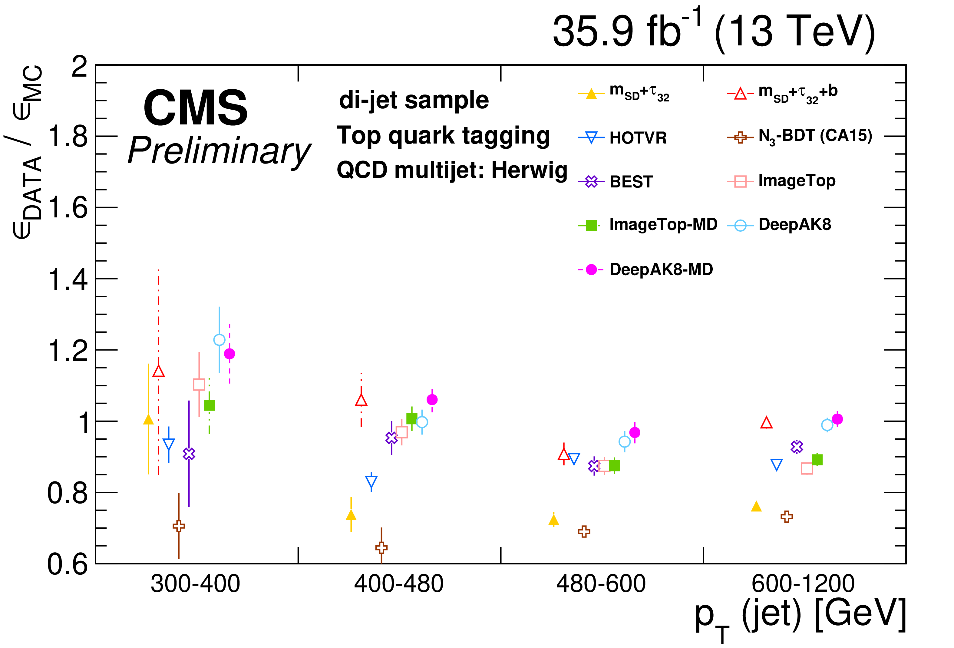
png pdf |
Figure 42-b:
The ratio of the misidentification rate of t quarks in data and simulation in the di-jet (upper and middle rows) and the single-$\gamma $ (lower row) samples. The QCD multijet process is simulated using MadGraph for the hard process and PYTHIA for parton showering (upper) and HERWIG++ for both (middle). |
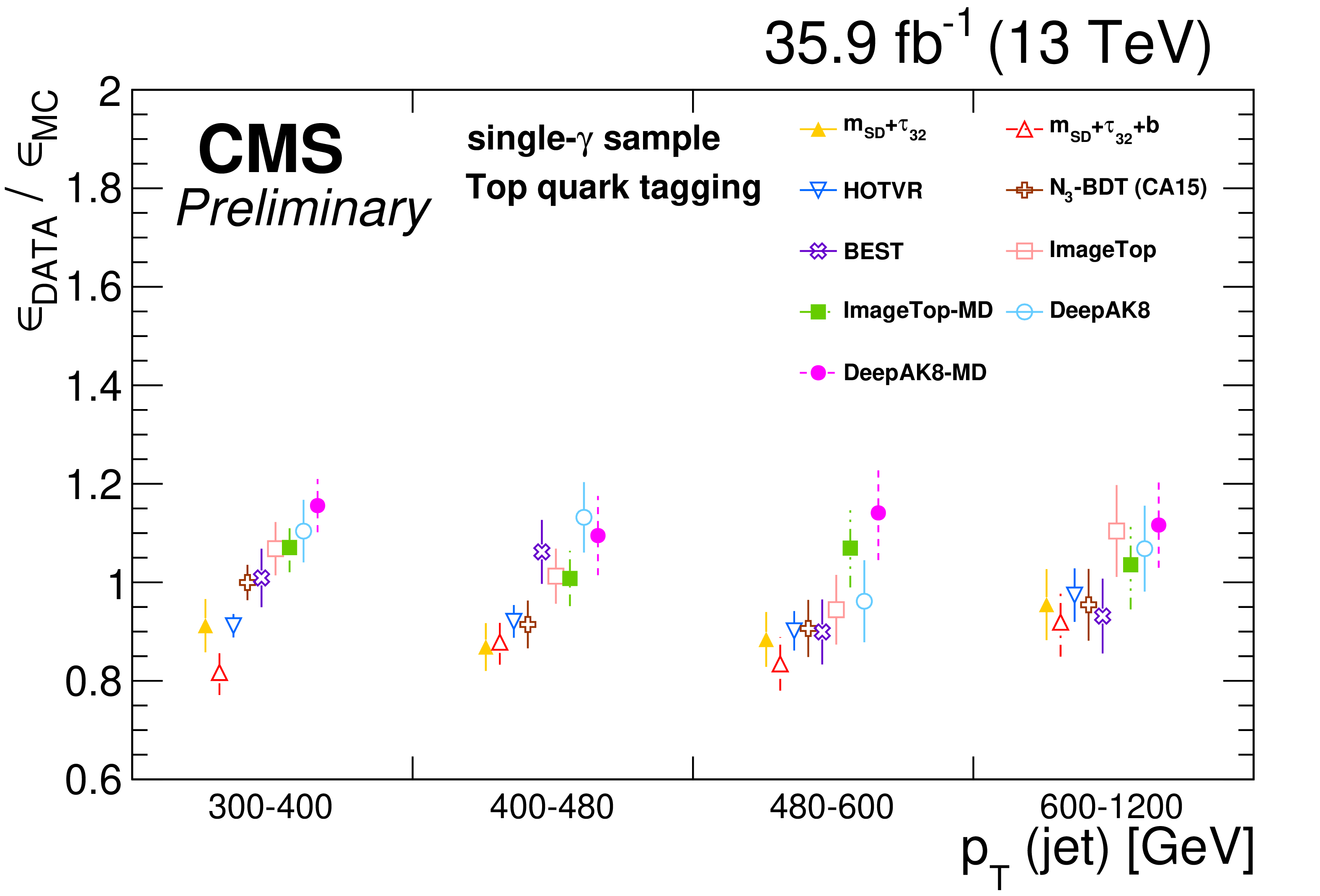
png pdf |
Figure 42-c:
The ratio of the misidentification rate of t quarks in data and simulation in the di-jet (upper and middle rows) and the single-$\gamma $ (lower row) samples. The QCD multijet process is simulated using MadGraph for the hard process and PYTHIA for parton showering (upper) and HERWIG++ for both (middle). |
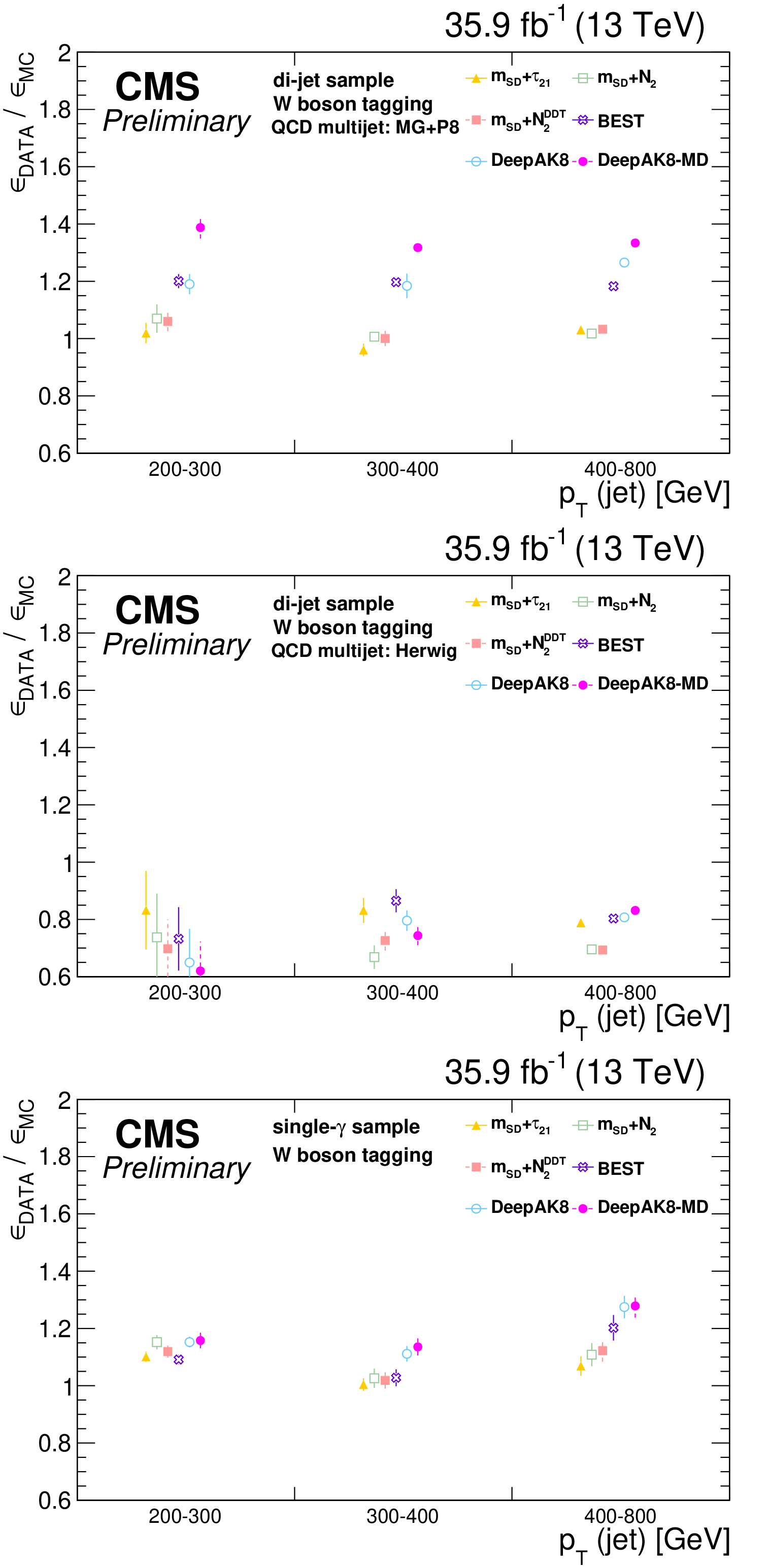
png pdf |
Figure 43:
The ratio of the misidentification rate of W bosons in data and simulation in the di-jet (upper and middle rows) and the single-$\gamma $ (lower row) samples. The QCD multijet process is simulated using MadGraph for the hard process and PYTHIA for parton showering (upper) and HERWIG++ for both (middle). |
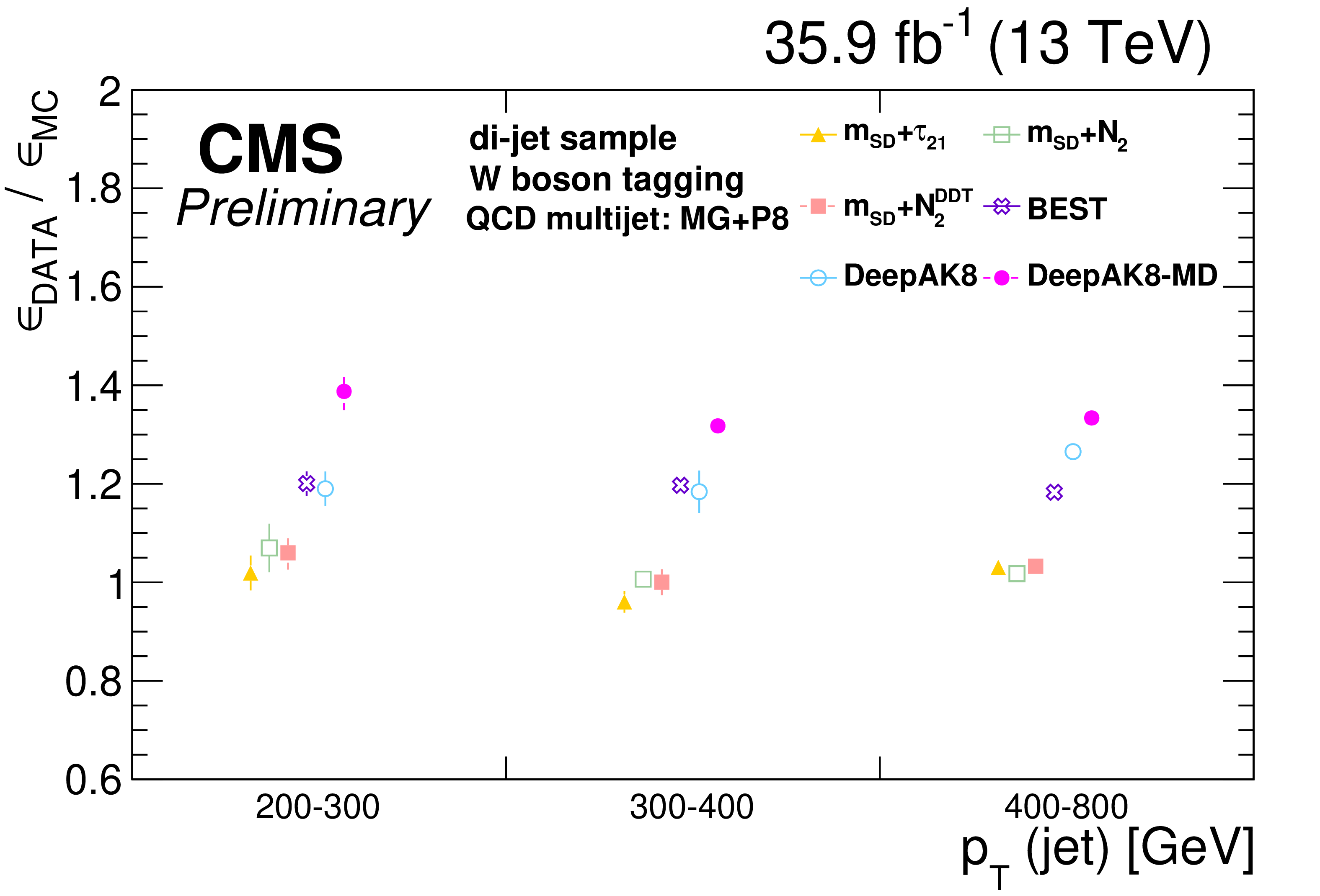
png pdf |
Figure 43-a:
The ratio of the misidentification rate of W bosons in data and simulation in the di-jet (upper and middle rows) and the single-$\gamma $ (lower row) samples. The QCD multijet process is simulated using MadGraph for the hard process and PYTHIA for parton showering (upper) and HERWIG++ for both (middle). |
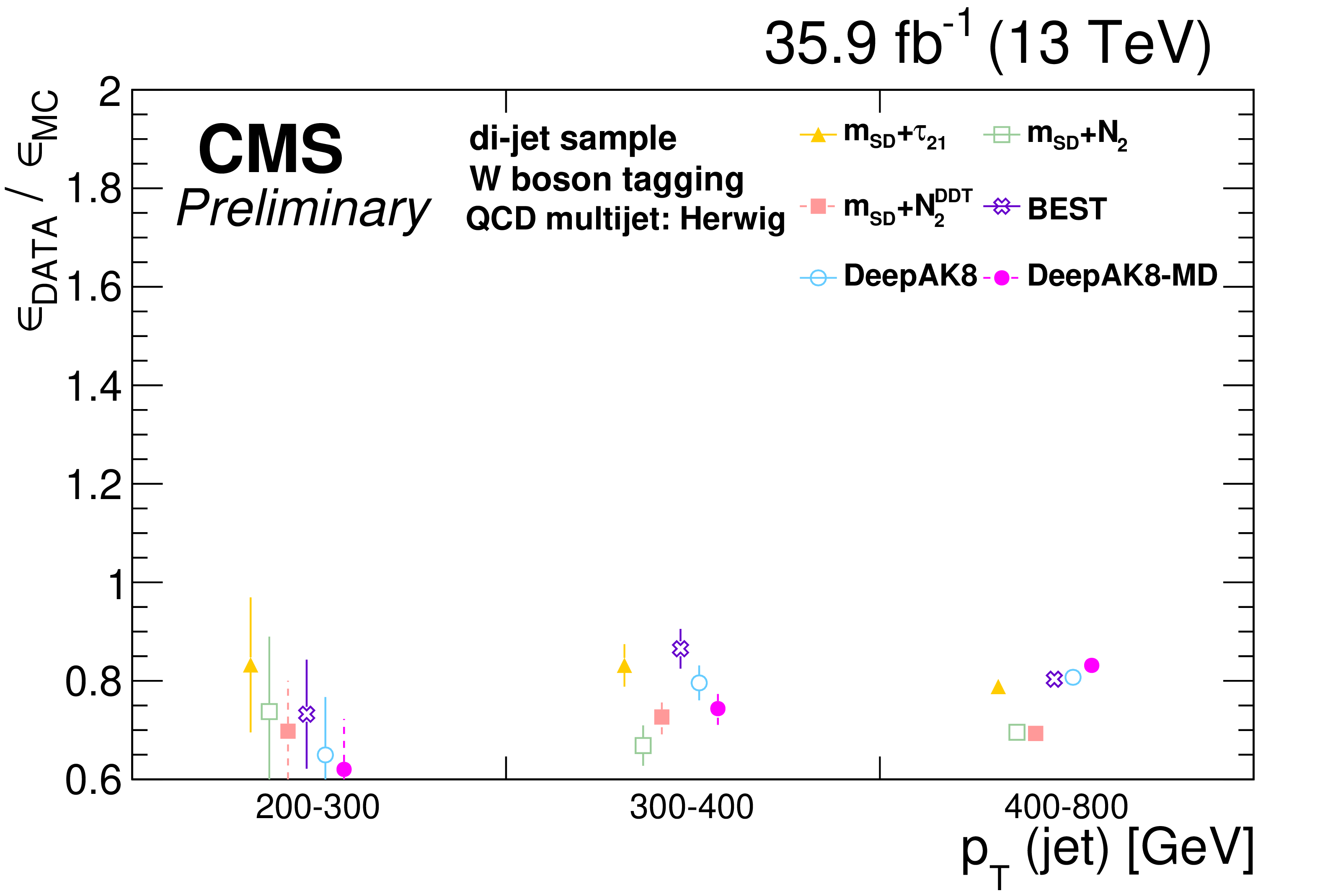
png pdf |
Figure 43-b:
The ratio of the misidentification rate of W bosons in data and simulation in the di-jet (upper and middle rows) and the single-$\gamma $ (lower row) samples. The QCD multijet process is simulated using MadGraph for the hard process and PYTHIA for parton showering (upper) and HERWIG++ for both (middle). |
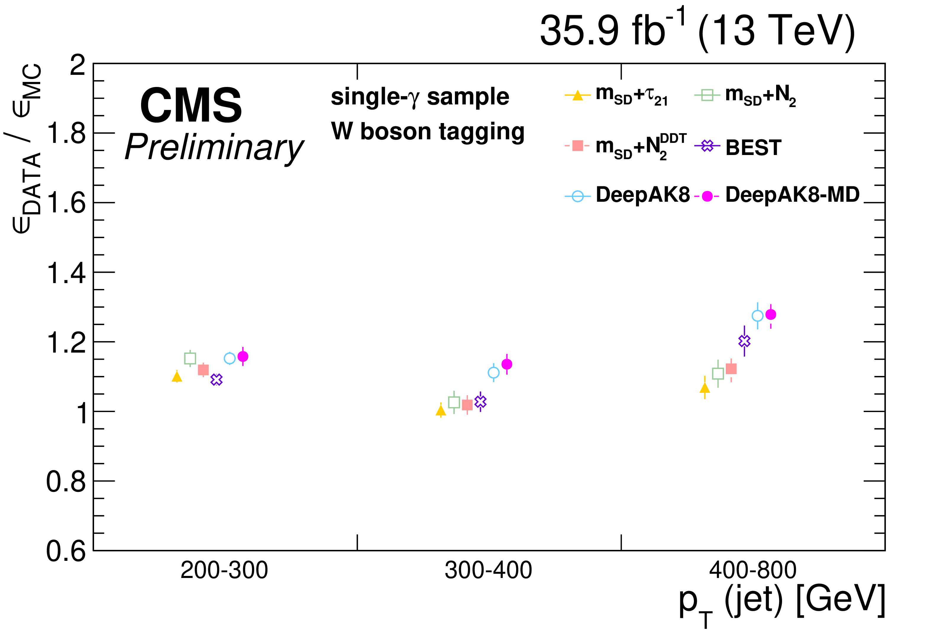
png pdf |
Figure 43-c:
The ratio of the misidentification rate of W bosons in data and simulation in the di-jet (upper and middle rows) and the single-$\gamma $ (lower row) samples. The QCD multijet process is simulated using MadGraph for the hard process and PYTHIA for parton showering (upper) and HERWIG++ for both (middle). |
| Tables | |
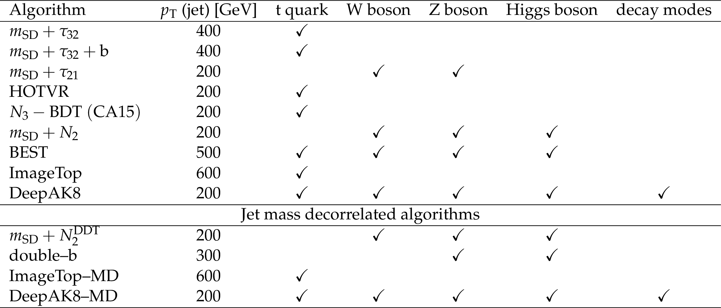
png pdf |
Table 1:
Summary of the CMS algorithms for the identification of hadronically decaying t quarks and W, Z and Higgs bosons. The column "$ {p_{\mathrm {T}}}$ (jet)'' indicates the jet ${p_{\mathrm {T}}}$ threshold to be used in each algorithm. |
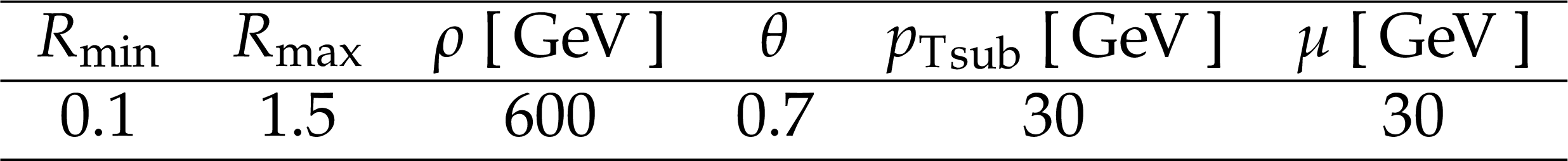
png pdf |
Table 2:
Summary of the HOTVR parameters. The $ {p_{\mathrm {T}}} _{\text {sub}}$ is the minimum ${p_{\mathrm {T}}}$ threshold of each subjet. |
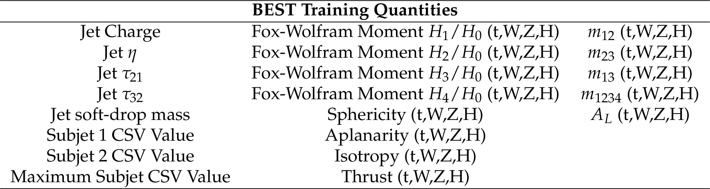
png pdf |
Table 3:
List of input quantities used for the training and evaluation of the BEST algorithm on AK8 jets. |
| Summary |
|
A review of the heavy object tagging methods recently developed in CMS has been presented. Tagging algorithms based on theory inspired higher-level observables, which were studied in LHC Run1, serve as a reference. New tagging approaches, such as the ECF tagger and the BEST algorithm, utilize multivariate methods (i.e., boosted decision trees or deep neural networks) on higher-level observables and result in enhanced performance. A novel set of tagging algorithms, ImageTop and DeepAK8, are developed based on candidate level information, allowing to explore more of the CMS potential. Lower-level information is processed using advanced machine learning methods. This approach results in significant performance improvement which in some cases leads to ${\sim} \mathcal{O}$(10) gain in background rejection for the same signal efficiency. Moreover, the BEST and DeepAK8 algorithms are developed to provide multi-class tagging capabilities, which can potentially enable new measurements and search approaches. Finally, dedicated versions of the algorithms which are only loosely correlated with the jet mass are developed. The performance of these new techniques has been directly compared in simulation in a jet transverse momentum range from 200 to 2000 GeV. The techniques have also been validated in collision data events, with scale factors extracted including systematic uncertainties. |
| References | ||||
| 1 | L. Evans and P. Bryant (editors) | LHC Machine | JINST 3 (2008) S08001 | |
| 2 | L. Asquith et al. | Jet Substructure at the Large Hadron Collider : Experimental Review | 1803.06991 | |
| 3 | A. J. Larkoski, I. Moult, and B. Nachman | Jet Substructure at the Large Hadron Collider: A Review of Recent Advances in Theory and Machine Learning | 1709.04464 | |
| 4 | CMS Collaboration | The CMS experiment at the CERN LHC | JINST 3 (2008) S08004 | CMS-00-001 |
| 5 | CMS Collaboration | Measurement of the integrated and differential $ t \bar t $ production cross sections for high-$ p_t $ top quarks in $ pp $ collisions at $ \sqrt s = $ 8 TeV | PRD 94 (2016) 072002 | CMS-TOP-14-012 1605.00116 |
| 6 | CMS Collaboration | Measurement of the jet mass in highly boosted $ {\mathrm{t}}\overline{\mathrm{t}} $ events from pp collisions at $ \sqrt{s}= $ 8 TeV | EPJC 77 (2017) 467 | CMS-TOP-15-015 1703.06330 |
| 7 | CMS Collaboration | Studies of Jet Mass in Dijet and W/Z + Jet Events | JHEP 05 (2013) 090 | CMS-SMP-12-019 1303.4811 |
| 8 | CMS Collaboration | Measurements of the differential jet cross section as a function of the jet mass in dijet events from proton-proton collisions at $ \sqrt{s}= $ 13 TeV | JHEP 11 (2018) 113 | CMS-SMP-16-010 1807.05974 |
| 9 | CMS Collaboration | Measurement of jet substructure observables in $ \mathrm{t\overline{t}} $ events from proton-proton collisions at $ \sqrt{s}= $ 13TeV | PRD 98 (2018) 092014 | CMS-TOP-17-013 1808.07340 |
| 10 | ATLAS Collaboration | Jet mass and substructure of inclusive jets in $ \sqrt{s}=7 TeV pp $ collisions with the ATLAS experiment | JHEP 05 (2012) 128 | 1203.4606 |
| 11 | ATLAS Collaboration | Measurement of the Soft-Drop Jet Mass in pp Collisions at $ \sqrt{s} = $ 13 TeV with the ATLAS Detector | PRL 121 (2018) 092001 | 1711.08341 |
| 12 | ATLAS Collaboration | Measurement of the cross-section of high transverse momentum vector bosons reconstructed as single jets and studies of jet substructure in $ pp $ collisions at $ {\sqrt{s}} = $ 7 TeV with the ATLAS detector | New J. Phys. 16 (2014) 113013 | 1407.0800 |
| 13 | ATLAS Collaboration | Measurements of $ t\bar{t} $ differential cross-sections of highly boosted top quarks decaying to all-hadronic final states in $ pp $ collisions at $ \sqrt{s}= $ 13 TeV using the ATLAS detector | PRD 98 (2018) 012003 | 1801.02052 |
| 14 | ATLAS Collaboration | Measurement of jet-substructure observables in top quark, $ W $ boson and light jet production in proton-proton collisions at $ \sqrt{s}= $ 13 TeV with the ATLAS detector | Submitted to: JHEP (2019) | 1903.02942 |
| 15 | J. Dolen et al. | Thinking outside the ROCs: Designing Decorrelated Taggers (DDT) for jet substructure | JHEP 05 (2016) 156 | 1603.00027 |
| 16 | CMS Collaboration | Boosted top jet tagging at cms | CMS-PAS-JME-13-007 | CMS-PAS-JME-13-007 |
| 17 | CMS Collaboration | Top tagging with new approaches | CMS-PAS-JME-15-002 | CMS-PAS-JME-15-002 |
| 18 | CMS Collaboration | Jet algorithms performance in 13 tev data | CMS-PAS-JME-16-003 | CMS-PAS-JME-16-003 |
| 19 | CMS Collaboration | Identification techniques for highly boosted W bosons that decay into hadrons | JHEP 12 (2014) 017 | CMS-JME-13-006 1410.4227 |
| 20 | CMS Collaboration | Identification of heavy-flavour jets with the CMS detector in pp collisions at 13 TeV | JINST 13 (2018) P05011 | CMS-BTV-16-002 1712.07158 |
| 21 | CMS Collaboration | The CMS experiment at the CERN LHC | JINST 3 (2008) S08004 | CMS-00-001 |
| 22 | CMS Collaboration | Performance of photon reconstruction and identification with the CMS detector in proton-proton collisions at $ \sqrt{s} = $ 8 TeV | JINST 10 (2015) P08010 | CMS-EGM-14-001 1502.02702 |
| 23 | CMS Collaboration | Performance of CMS muon reconstruction in $ pp $ collision events at $ \sqrt{s} = $ 7 TeV | JINST 7 (2012) P10002 | CMS-MUO-10-004 1206.4071 |
| 24 | CMS Collaboration | Description and performance of track and primary-vertex reconstruction with the CMS tracker | JINST 9 (2014) P10009 | CMS-TRK-11-001 1405.6569 |
| 25 | CMS Collaboration | The CMS trigger system | JINST 12 (2017) P01020 | CMS-TRG-12-001 1609.02366 |
| 26 | J. Alwall et al. | The automated computation of tree-level and next-to-leading order differential cross sections, and their matching to parton shower simulations | JHEP 07 (2014) 079 | 1405.0301 |
| 27 | T. Sjostrand, S. Mrenna, and P. Z. Skands | A Brief Introduction to PYTHIA 8.1 | CPC 178 (2008) 852 | 0710.3820 |
| 28 | P. Skands, S. Carrazza, and J. Rojo | Tuning PYTHIA 8.1: the Monash 2013 Tune | EPJC 74 (2014) 3024 | 1404.5630 |
| 29 | NNPDF Collaboration | Parton distributions for the LHC Run II | JHEP 04 (2015) 040 | 1410.8849 |
| 30 | P. Nason | A new method for combining NLO QCD with shower Monte Carlo algorithms | JHEP 11 (2004) 040 | hep-ph/0409146 |
| 31 | S. Frixione, P. Nason, and G. Ridolfi | A positive-weight next-to-leading-order Monte Carlo for heavy flavour hadroproduction | JHEP 09 (2007) 126 | 0707.3088 |
| 32 | S. Alioli, P. Nason, C. Oleari, and E. Re | A general framework for implementing NLO calculations in shower Monte Carlo programs: the POWHEG BOX | JHEP 06 (2010) 043 | 1002.2581 |
| 33 | R. Frederix and S. Frixione | Merging meets matching in MC@NLO | JHEP 12 (2012) 061 | 1209.6215 |
| 34 | J. Alwall et al. | Comparative study of various algorithms for the merging of parton showers and matrix elements in hadronic collisions | EPJC 53 (2008) 473 | 0706.2569 |
| 35 | M. Bahr et al. | Herwig++ Physics and Manual | EPJC58 (2008) 639--707 | 0803.0883 |
| 36 | J. Bellm et al. | Herwig++ 2.7 Release Note | 1310.6877 | |
| 37 | CMS Collaboration | Measurement of differential cross sections for top quark pair production using the $ \text{lepton}+\text{jets} $ final state in proton-proton collisions at 13 tev | PRD 95 (May, 2017) 092001 | |
| 38 | GEANT4 Collaboration | GEANT4--a simulation toolkit | NIMA 506 (2003) 250 | |
| 39 | CMS Collaboration | Particle-flow reconstruction and global event description with the CMS detector | JINST 12 (2017) P10003 | CMS-PRF-14-001 1706.04965 |
| 40 | M. Cacciari, G. P. Salam, and G. Soyez | The anti-$ k_t $ jet clustering algorithm | JHEP 04 (2008) 063 | 0802.1189 |
| 41 | M. Cacciari, G. P. Salam, and G. Soyez | FastJet user manual | EPJC 72 (2012) 1896 | 1111.6097 |
| 42 | CMS Collaboration | Performance of electron reconstruction and selection with the CMS detector in proton-proton collisions at $ \sqrt{s} = $ 8 TeV | JINST 10 (2015), no. 06, P06005 | CMS-EGM-13-001 1502.02701 |
| 43 | CMS Collaboration | Pileup removal algorithms | CMS-PAS-JME-14-001 | CMS-PAS-JME-14-001 |
| 44 | Y. L. Dokshitzer, G. D. Leder, S. Moretti, and B. R. Webber | Better jet clustering algorithms | JHEP 08 (1997) 001 | hep-ph/9707323 |
| 45 | M. Wobisch and T. Wengler | Hadronization corrections to jet cross-sections in deep inelastic scattering | in Proceedings of the Workshop on Monte Carlo Generators for HERA Physics, Hamburg, Germany, p. 270 1998 | hep-ph/9907280 |
| 46 | D. Bertolini, P. Harris, M. Low, and N. Tran | Pileup Per Particle Identification | JHEP 10 (2014) 059 | 1407.6013 |
| 47 | CMS Collaboration | Pile up mitigation at CMS in 13 TeV data | CMS-PAS-JME-18-001 | CMS-PAS-JME-18-001 |
| 48 | CMS Collaboration | Jet energy scale and resolution in the CMS experiment in pp collisions at 8 TeV | JINST 12 (2017) P02014 | CMS-JME-13-004 1607.03663 |
| 49 | CMS Collaboration | Identification of heavy-flavour jets with the CMS detector in pp collisions at 13 TeV | JINST 13 (2018) P05011 | CMS-BTV-16-002 1712.07158 |
| 50 | CMS Collaboration | Performance of missing transverse momentum reconstruction in proton-proton collisions at $ \sqrt{s} = $ 13 TeV using the CMS detector | Submitted to: JINST (2019) | CMS-JME-17-001 1903.06078 |
| 51 | CMS Collaboration | Searches for new physics using the $ t\bar{t} $ invariant mass distribution in pp collisions at $ \sqrt{s} = $ 8 TeV | PRL 111 (2013) 211804 | CMS-B2G-13-001 1309.2030 |
| 52 | CMS Collaboration | Search for resonant $ t \bar t $ production in proton-proton collisions at $ \sqrt s= $ 8 TeV | PRD 93 (2016) 012001 | CMS-B2G-13-008 1506.03062 |
| 53 | CMS Collaboration | Search for $ \mathrm{t}\overline{\mathrm{t}} $ resonances in highly boosted lepton+jets and fully hadronic final states in proton-proton collisions at $ \sqrt{s}= $ 13 TeV | JHEP 07 (2017) 001 | CMS-B2G-16-015 1704.03366 |
| 54 | CMS Collaboration | Search for resonant $ \mathrm{t}\overline{\mathrm{t}} $ production in proton-proton collisions at $ \sqrt{s}= $ 13 TeV | JHEP 04 (2019) 031 | CMS-B2G-17-017 1810.05905 |
| 55 | A. Butter et al. | The Machine Learning Landscape of Top Taggers | 1902.09914 | |
| 56 | M. Dasgupta, A. Fregoso, S. Marzani, and G. P. Salam | Towards an understanding of jet substructure | JHEP 09 (2013) 029 | 1307.0007 |
| 57 | A. J. Larkoski, S. Marzani, G. Soyez, and J. Thaler | Soft drop | JHEP 05 (2014) 146 | 1402.2657 |
| 58 | C. Frye, A. J. Larkoski, M. D. Schwartz, and K. Yan | Factorization for groomed jet substructure beyond the next-to-leading logarithm | JHEP 07 (2016) 064 | 1603.09338 |
| 59 | S. Marzani, L. Schunk, and G. Soyez | A study of jet mass distributions with grooming | JHEP 07 (2017) 132 | 1704.02210 |
| 60 | J. Thaler and K. Van Tilburg | Identifying boosted objects with $ N $-subjettiness | JHEP 03 (2011) 015 | 1011.2268 |
| 61 | J. Thaler and K. Van Tilburg | Maximizing boosted top identification by minimizing $ N $-subjettiness | JHEP 02 (2012) 093 | 1108.2701 |
| 62 | S. Catani, Y. L. Dokshitzer, M. H. Seymour, and B. R. Webber | Longitudinally invariant $ K_t $ clustering algorithms for hadron hadron collisions | NPB 406 (1993) 187--224 | |
| 63 | S. D. Ellis and D. E. Soper | Successive combination jet algorithm for hadron collisions | PRD 48 (1993) 3160--3166 | hep-ph/9305266 |
| 64 | CMS Collaboration | A multi-dimensional search for new heavy resonances decaying to boosted WW, WZ, or ZZ boson pairs in the dijet final state at 13 TeV | CMS-B2G-18-002 1906.05977 |
|
| 65 | CMS Collaboration | Search for heavy resonances that decay into a vector boson and a Higgs boson in hadronic final states at $ \sqrt{s} = $ 13 TeV | EPJC 77 (2017) 636 | CMS-B2G-17-002 1707.01303 |
| 66 | CMS Collaboration | Search for vector-like T and B quark pairs in final states with leptons at $ \sqrt{s} = $ 13 TeV | JHEP 08 (2018) 177 | CMS-B2G-17-011 1805.04758 |
| 67 | CMS Collaboration | Search for pair production of vector-like quarks in the fully hadronic final state | CMS-B2G-18-005 1906.11903 |
|
| 68 | CMS Collaboration | Search for a W$ ^\prime $ boson decaying to a vector-like quark and a top or bottom quark in the all-jets final state | JHEP 03 (2019) 127 | CMS-B2G-18-001 1811.07010 |
| 69 | T. Lapsien, R. Kogler, and J. Haller | A new tagger for hadronically decaying heavy particles at the lhc | The European Physical Journal C 76 (2016), no. 11, 600 | |
| 70 | I. Moult, L. Necib, and J. Thaler | New angles on energy correlation functions | Journal of High Energy Physics 2016 (2016), no. 12, 153 | |
| 71 | T. Plehn, G. P. Salam, and M. Spannowsky | Fat Jets for a Light Higgs | PRL 104 (2010) 111801 | 0910.5472 |
| 72 | T. Plehn, M. Spannowsky, M. Takeuchi, and D. Zerwas | Stop Reconstruction with Tagged Tops | JHEP 10 (2010) 078 | 1006.2833 |
| 73 | G. Kasieczka et al. | Resonance Searches with an Updated Top Tagger | JHEP 06 (2015) 203 | 1503.05921 |
| 74 | H. Voss, A. Hocker, J. Stelzer, and F. Tegenfeldt | TMVA, the toolkit for multivariate data analysis with ROOT | in XIth International Workshop on Advanced Computing and Analysis Techniques in Physics Research (ACAT), p. 40 2007 | physics/0703039 |
| 75 | CMS Collaboration | Search for dark matter in events with energetic, hadronically decaying top quarks and missing transverse momentum at $ \sqrt{s}= $ 13 TeV | JHEP 06 (2018) 027 | CMS-EXO-16-051 1801.08427 |
| 76 | CMS Collaboration | Search for low mass vector resonances decaying into quark-antiquark pairs in proton-proton collisions at $ \sqrt{s}= $ 13 TeV | JHEP 01 (2018) 097 | CMS-EXO-17-001 1710.00159 |
| 77 | CMS Collaboration | Inclusive search for a highly boosted Higgs boson decaying to a bottom quark-antiquark pair | PRL 120 (2018) 071802 | CMS-HIG-17-010 1709.05543 |
| 78 | CMS Collaboration | Identification of heavy-flavour jets with the CMS detector in pp collisions at 13 TeV | JINST 13 (2018) P05011 | CMS-BTV-16-002 1712.07158 |
| 79 | J. S. Conway, R. Bhaskar, R. D. Erbacher, and J. Pilot | Identification of high-momentum top quarks, higgs bosons, and w and z bosons using boosted event shapes | PRD 94 (Nov, 2016) 094027 | |
| 80 | G. C. Fox and S. Wolfram | Observables for the analysis of event shapes in $ {e}^{+}{e}^{{-}} $ annihilation and other processes | PRL 41 (1978) 1581 | |
| 81 | J. D. Bjorken and S. J. Brodsky | Statistical model for electron-positron annihilation into hadrons | PRD 1 (1970) 1416 | |
| 82 | E. Farhi | Quantum chromodynamics test for jets | PRL 39 (1977) 1587 | |
| 83 | F. Pedregosa et al. | Scikit-learn: Machine learning in Python | J. Mach. Learn. Res. 12 (2011) 2825--2830 | 1201.0490 |
| 84 | V. Nair and G. E. Hinton | Rectified linear units improve restricted boltzmann machines | in Proceedings of the 27th International Conference on International Conference on Machine Learning, ICML'10, pp. 807--814 Omnipress, USA | |
| 85 | D. P. Kingma and J. Ba | Adam: A method for stochastic optimization | 2014 \url http://arxiv.org/abs/1412.6980 | |
| 86 | S. Macaluso and D. Shih | Pulling Out All the Tops with Computer Vision and Deep Learning | JHEP 10 (2018) 121 | 1803.00107 |
| 87 | G. Kasieczka, T. Plehn, M. Russell, and T. Schell | Deep-learning Top Taggers or The End of QCD? | JHEP 05 (2017) 006 | 1701.08784 |
| 88 | M. D. Zeiler | ADADELTA: an adaptive learning rate method | CoRR abs/1212.5701 (2012) | 1212.5701 |
| 89 | CMS Collaboration | Performance of b tagging algorithms in proton-proton collisions at 13 TeV with phase 1 CMS detector | CDS | |
| 90 | K. He, X. Zhang, S. Ren, and J. Sun | Deep residual learning for image recognition | CoRR abs/1512.03385 (2015) | 1512.03385 |
| 91 | N. Srivastava et al. | Dropout: A simple way to prevent neural networks from overfitting | Journal of Machine Learning Research 15 (2014) 1929 | |
| 92 | T. Chen et al. | Mxnet: A flexible and efficient machine learning library for heterogeneous distributed systems | CoRR abs/1512.01274 (2015) | 1512.01274 |
| 93 | G. Louppe, M. Kagan, and K. Cranmer | Learning to pivot with adversarial networks | in Advances in Neural Information Processing Systems 30, I. Guyon et al., eds., p. 981 Curran Associates, Inc. | |
| 94 | CMS Collaboration | Search for production of Higgs boson pairs in the four b quark final state using large-area jets in proton-proton collisions at $ \sqrt{s}= $ 13 TeV | JHEP 01 (2019) 040 | CMS-B2G-17-019 1808.01473 |
| 95 | CMS Collaboration | Search for low-mass resonances decaying into bottom quark-antiquark pairs in proton-proton collisions at $ \sqrt{s} = $ 13 TeV | PRD 99 (2019) 012005 | CMS-EXO-17-024 1810.11822 |
| 96 | J. Lin | Lin jh.. divergence measures based on the shannon entropy. ieee trans inform theory 37: 145-151 | IEEE Transactions on Information Theory 37 (01, 1991) 145 | |
| 97 | S. Kullback and R. A. Leibler | On information and sufficiency | Ann. Math. Statist. 22 (1951), no. 1, 79--86 | |
| 98 | CMS Collaboration | Search for the standard model higgs boson decaying to charm quarks | CMS-PAS-HIG-18-031 | CMS-PAS-HIG-18-031 |
| 99 | CMS Collaboration | Measurement of the inelastic proton-proton cross section at $ \sqrt{s}= $ 13 TeV | JHEP 07 (2018) 161 | CMS-FSQ-15-005 1802.02613 |
| 100 | ATLAS Collaboration | Measurement of the Inelastic Proton-Proton Cross Section at $ \sqrt{s} = $ 13 TeV with the ATLAS Detector at the LHC | PRL 117 (2016), no. 18, 182002 | 1606.02625 |
|
|
Compact Muon Solenoid LHC, CERN |
|

|

|

|

|

|