

Compact Muon Solenoid
LHC, CERN
| CMS-PAS-JME-15-002 | ||
| Top Tagging with New Approaches | ||
| CMS Collaboration | ||
| May 2016 | ||
| Abstract: Methods for boosted hadronically decaying top quark identification (top tagging) are tested in view of the 13 TeV data-taking run of the LHC. In addition to evaluating the discrimination power of single observables, the gain from combining different substructure techniques is quantified. The interplay between different top tagging variables and b tagging is evaluated and the performance of selected observables for high transverse momentum jets is studied. Aditionally, a comparison of top tagging variables between data and simulation is performed, using collision events with a center-of-mass energy of 8 TeV. | ||
| Links: CDS record (PDF) ; inSPIRE record ; CADI line (restricted) ; | ||
| Figures | |
png pdf |
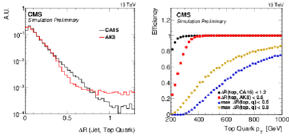
Figure 1:
Distance between reconstructed jet and closest generated top quark (left). Jet reconstruction efficiency (right) as function of the generated top quark $ {p_{\mathrm {T}}} $. The efficiency is defined as the fraction of top quarks for which a reconstructed jet with $ {p_{\mathrm {T}}} > $ 200 GeV can be found within $\Delta R < $ 1.2 ($\Delta R < $ 0.6) for CA15 (AK8) jets. Superimposed is the fraction of merged top quarks as function of $ {p_{\mathrm {T}}} $ for the two thresholds used: 0.8 (0.6) at low (high) boost. All distributions are made using hadronically decaying top quarks with $ {p_{\mathrm {T}}} > $ 200 GeV. |
png pdf |
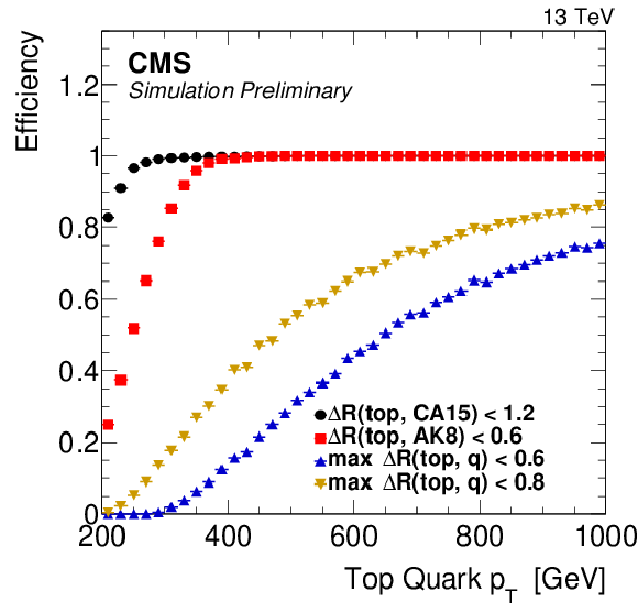
Figure 1)b:
Jet reconstruction efficiency as function of the generated top quark $ {p_{\mathrm {T}}} $. The efficiency is defined as the fraction of top quarks for which a reconstructed jet with $ {p_{\mathrm {T}}} > $ 200 GeV can be found within $\Delta R < $ 1.2 ($\Delta R < $ 0.6) for CA15 (AK8) jets. Superimposed is the fraction of merged top quarks as function of $ {p_{\mathrm {T}}} $ for the two thresholds used: 0.8 (0.6) at low (high) boost. All distributions are made using hadronically decaying top quarks with $ {p_{\mathrm {T}}} > $ 200 GeV. |
png pdf |
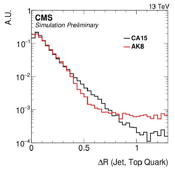
Figure 1-b:
Distance between reconstructed jet and closest generated top quark (left). Jet reconstruction efficiency (right) as function of the generated top quark $ {p_{\mathrm {T}}} $. The efficiency is defined as the fraction of top quarks for which a reconstructed jet with $ {p_{\mathrm {T}}} > $ 200 GeV can be found within $\Delta R < $ 1.2 ($\Delta R < $ 0.6) for CA15 (AK8) jets. Superimposed is the fraction of merged top quarks as function of $ {p_{\mathrm {T}}} $ for the two thresholds used: 0.8 (0.6) at low (high) boost. All distributions are made using hadronically decaying top quarks with $ {p_{\mathrm {T}}} > $ 200 GeV. |

png pdf |
Figure 2:
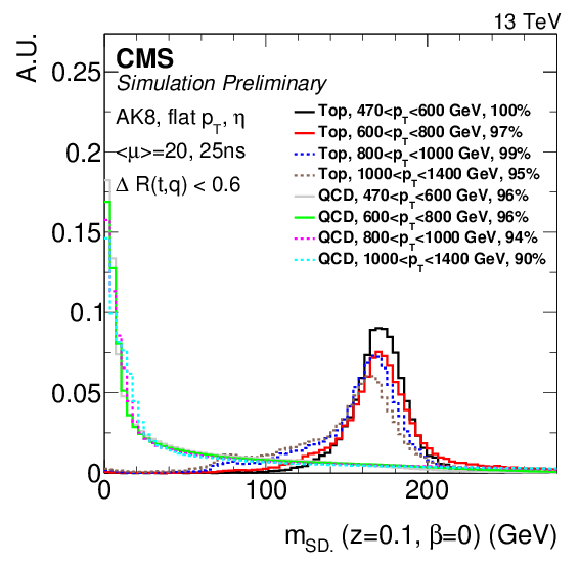
Distribution of pruned mass (top), softdrop ($z=$ 0.2, $\beta = $ 1) mass for low $ {p_{\mathrm {T}}} $ jets reconstructed using CA15 (center), and softdrop ($z=$ 0.1, $\beta =$ 0) mass (bottom) for high $ {p_{\mathrm {T}}} $ jets reconstructed using AK8. The softdrop mass distributions are shown for a fiducial selection without (left) and with (right) the merged-top requirement. The percentage in the legend indicates the fraction of entries shown in the plot with respect to the fiducial selection. Events correspond to an average number of $< \mu >$ pileup interactions and a bunch spacing of 25 ns. |

png pdf |
Figure 2-a:
Distribution of pruned mass for high $ {p_{\mathrm {T}}} $ jets reconstructed using AK8. The softdrop mass distributions are shown for a fiducial selection without the merged-top requirement. The percentage in the legend indicates the fraction of entries shown in the plot with respect to the fiducial selection. Events correspond to an average number of $< \mu >$ pileup interactions and a bunch spacing of 25 ns. |

png pdf |
Figure 2-b:
Distribution of pruned mass for high $ {p_{\mathrm {T}}} $ jets reconstructed using AK8. The softdrop mass distributions are shown for a fiducial selection with the merged-top requirement. The percentage in the legend indicates the fraction of entries shown in the plot with respect to the fiducial selection. Events correspond to an average number of $< \mu >$ pileup interactions and a bunch spacing of 25 ns. |
png pdf |
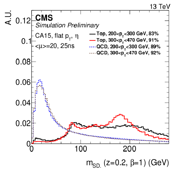
Figure 2-c:
Distribution of softdrop ($z=$ 0.2, $\beta = $ 1) mass for low $ {p_{\mathrm {T}}} $ jets reconstructed using CA15 for high $ {p_{\mathrm {T}}} $ jets reconstructed using AK8. The softdrop mass distributions are shown for a fiducial selection without the merged-top requirement. The percentage in the legend indicates the fraction of entries shown in the plot with respect to the fiducial selection. Events correspond to an average number of $< \mu >$ pileup interactions and a bunch spacing of 25 ns. |

png pdf |
Figure 2-d:
Distribution of softdrop ($z=$ 0.2, $\beta = $ 1) mass for low $ {p_{\mathrm {T}}} $ jets reconstructed using CA15 for high $ {p_{\mathrm {T}}} $ jets reconstructed using AK8. The softdrop mass distributions are shown for a fiducial selection with the merged-top requirement. The percentage in the legend indicates the fraction of entries shown in the plot with respect to the fiducial selection. Events correspond to an average number of $< \mu >$ pileup interactions and a bunch spacing of 25 ns. |

png pdf |
Figure 2-e:
Distribution of softdrop ($z=$ 0.1, $\beta =$ 0) mass for high $ {p_{\mathrm {T}}} $ jets reconstructed using AK8. The softdrop mass distributions are shown for a fiducial selection without the merged-top requirement. The percentage in the legend indicates the fraction of entries shown in the plot with respect to the fiducial selection. Events correspond to an average number of $< \mu >$ pileup interactions and a bunch spacing of 25 ns. |
png pdf |
Figure 2-f:
Distribution of softdrop ($z=$ 0.1, $\beta =$ 0) mass for high $ {p_{\mathrm {T}}} $ jets reconstructed using AK8. The softdrop mass distributions are shown for a fiducial selection with the merged-top requirement. The percentage in the legend indicates the fraction of entries shown in the plot with respect to the fiducial selection. Events correspond to an average number of $< \mu >$ pileup interactions and a bunch spacing of 25 ns. |

png pdf |
Figure 3:
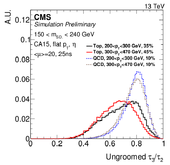
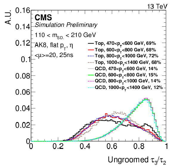
Distribution of ungroomed n-subjettiness (top) at low $ {p_{\mathrm {T}}} $ (left) and high $ {p_{\mathrm {T}}} $ (right). In addition, the softdrop n-subjettiness (bottom left) and the Qjet volatility (bottom right) are shown for low $ {p_{\mathrm {T}}} $ jets clustered using CA15 jets. All distributions are shown after selecting on the jet mass. The percentage in the legend indicates the fraction of entries shown in the plot with respect to the fiducial selection. Events correspond to an average number of $< \mu >$ pileup interactions and a bunch spacing of 25 ns. |
png pdf |
Figure 3-a:
Distribution of ungroomed n-subjettiness at low $ {p_{\mathrm {T}}} $. The distribution is shown after selecting on the jet mass. The percentage in the legend indicates the fraction of entries shown in the plot with respect to the fiducial selection. Events correspond to an average number of $< \mu >$ pileup interactions and a bunch spacing of 25 ns. |
png pdf |
Figure 3-b:
Distribution of ungroomed n-subjettiness at high $ {p_{\mathrm {T}}} $. The distribution is shown after selecting on the jet mass. The percentage in the legend indicates the fraction of entries shown in the plot with respect to the fiducial selection. Events correspond to an average number of $< \mu >$ pileup interactions and a bunch spacing of 25 ns. |

png pdf |
Figure 3-c:
The softdrop n-subjettiness is shown for low $ {p_{\mathrm {T}}} $ jets clustered using CA15 jets. The distribution is shown after selecting on the jet mass. The percentage in the legend indicates the fraction of entries shown in the plot with respect to the fiducial selection. Events correspond to an average number of $< \mu >$ pileup interactions and a bunch spacing of 25 ns. |

png pdf |
Figure 3-d:
The Qjet volatility is shown for low $ {p_{\mathrm {T}}} $ jets clustered using CA15 jets. The distribution is shown after selecting on the jet mass. The percentage in the legend indicates the fraction of entries shown in the plot with respect to the fiducial selection. Events correspond to an average number of $< \mu >$ pileup interactions and a bunch spacing of 25 ns. |

png pdf |
Figure 4:
Distribution of the HTT V2 candidate mass (top), $f_{Rec}$ (center) and $\Delta R_{opt}$ (bottom) for low $ {p_{\mathrm {T}}} $ jets (left) and high $ {p_{\mathrm {T}}} $ jets (right) reconstructed using CA15 jets. The percentage in the legend indicates the fraction of entries shown in the plot with respect to the fiducial selection. Events correspond to an average number of $< \mu >$ pileup interactions and a bunch spacing of 25 ns. |

png pdf |
Figure 4-a:
Distribution of the HTT V2 candidate mass for low $ {p_{\mathrm {T}}} $ jets reconstructed using CA15 jets. The percentage in the legend indicates the fraction of entries shown in the plot with respect to the fiducial selection. Events correspond to an average number of $< \mu >$ pileup interactions and a bunch spacing of 25 ns. |

png pdf |
Figure 4-b:
Distribution of the HTT V2 candidate mass for high $ {p_{\mathrm {T}}} $ jets reconstructed using CA15 jets. The percentage in the legend indicates the fraction of entries shown in the plot with respect to the fiducial selection. Events correspond to an average number of $< \mu >$ pileup interactions and a bunch spacing of 25 ns. |

png pdf |
Figure 4-c:
Distribution of $f_{Rec}$ for low $ {p_{\mathrm {T}}} $ jets reconstructed using CA15 jets. The percentage in the legend indicates the fraction of entries shown in the plot with respect to the fiducial selection. Events correspond to an average number of $< \mu >$ pileup interactions and a bunch spacing of 25 ns. |

png pdf |
Figure 4-d:
Distribution of $f_{Rec}$ for high $ {p_{\mathrm {T}}} $ jets reconstructed using CA15 jets. The percentage in the legend indicates the fraction of entries shown in the plot with respect to the fiducial selection. Events correspond to an average number of $< \mu >$ pileup interactions and a bunch spacing of 25 ns. |

png pdf |
Figure 4-e:
Distribution of $\Delta R_{opt}$ for low $ {p_{\mathrm {T}}} $ jets reconstructed using CA15 jets. The percentage in the legend indicates the fraction of entries shown in the plot with respect to the fiducial selection. Events correspond to an average number of $< \mu >$ pileup interactions and a bunch spacing of 25 ns. |

png pdf |
Figure 4-f:
Distribution of $\Delta R_{opt}$ for high $ {p_{\mathrm {T}}} $ jets reconstructed using CA15 jets. The percentage in the legend indicates the fraction of entries shown in the plot with respect to the fiducial selection. Events correspond to an average number of $< \mu >$ pileup interactions and a bunch spacing of 25 ns. |
png pdf |
Figure 5:
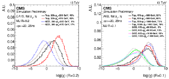
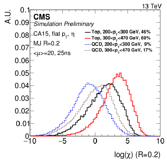
Distribution of the shower deconstruction discriminator for low (high) $ {p_{\mathrm {T}}} $ jets reconstructed using CA15 (AK8) on the left (right). For the low (high) $ {p_{\mathrm {T}}} $ jets a microjet distance parameter of 0.2 (0.1) is used. No selection on the jet mass is applied. The percentage in the legend indicates the fraction of entries shown in the plot with respect to the fiducial selection. Events correspond to an average number of $< \mu >$ pileup interactions and a bunch spacing of 25 ns. |
png pdf |
Figure 5-a:
Distribution of the shower deconstruction discriminator for low $ {p_{\mathrm {T}}} $ jets reconstructed using CA15. A microjet distance parameter of 0.2 is used. No selection on the jet mass is applied. The percentage in the legend indicates the fraction of entries shown in the plot with respect to the fiducial selection. Events correspond to an average number of $< \mu >$ pileup interactions and a bunch spacing of 25 ns. |

png pdf |
Figure 5-b:
Distribution of the shower deconstruction discriminator for high $ {p_{\mathrm {T}}} $ jets reconstructed using AK8. A microjet distance parameter of 0.1 is used. No selection on the jet mass is applied. The percentage in the legend indicates the fraction of entries shown in the plot with respect to the fiducial selection. Events correspond to an average number of $< \mu >$ pileup interactions and a bunch spacing of 25 ns. |
png pdf |
Figure 6:
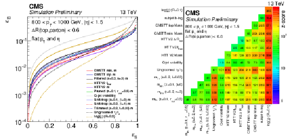
Single variable ROC curves (left) and $z$-score, defined as $1/\varepsilon _B$ at a signal efficiency of 30% (right) calculated per-parton for objects passing the fiducial selection criteria for a high $ {p_{\mathrm {T}}} $ sample. Each point on the ROC curve corresponds to a simple selection window using the tagging variable. The $z$-score is determined using a likelihood estimator for the diagonal and a BDT for the off-diagonal elements. |

png pdf |
Figure 6-a:
Single variable ROC curves calculated per-parton for objects passing the fiducial selection criteria for a high $ {p_{\mathrm {T}}} $ sample. Each point on the curve corresponds to a simple selection window using the tagging variable. |

png pdf |
Figure 6-b:
Single variable $z$-score, defined as $1/\varepsilon _B$ at a signal efficiency of 30%, calculated per-parton for objects passing the fiducial selection criteria for a high $ {p_{\mathrm {T}}} $ sample. The $z$-score is determined using a likelihood estimator for the diagonal and a BDT for the off-diagonal elements. |

png pdf |
Figure 7:
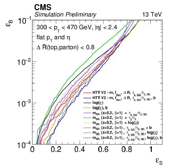
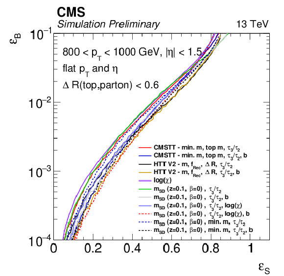
ROC curves for calculated per-parton for objects passing the fiducial selection criteria for merged top quarks at low boost (left) and high boost (right). Each point on the curve corresponds to a set of simple selection windows on the given variables. |
png pdf |
Figure 7-a:
ROC curves for calculated per-parton for objects passing the fiducial selection criteria for merged top quarks at low boost. Each point on the curve corresponds to a set of simple selection windows on the given variables. |
png pdf |
Figure 7-b:
ROC curves for calculated per-parton for objects passing the fiducial selection criteria for merged top quarks at high boost. Each point on the curve corresponds to a set of simple selection windows on the given variables. |

png pdf |
Figure 8:
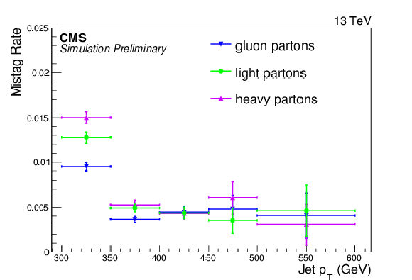
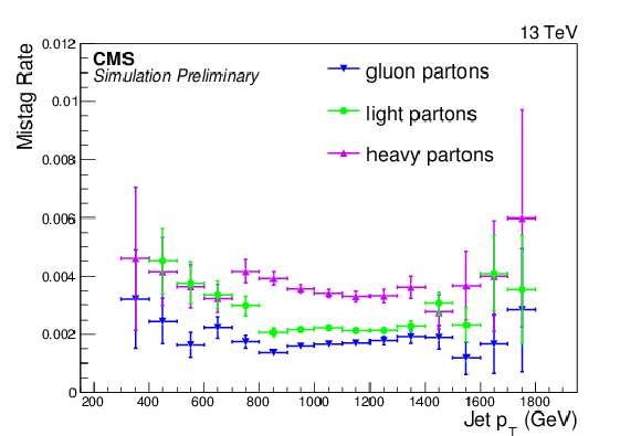
Comparisons of efficiencies for the low $ {p_{\mathrm {T}}} $ working points (left): softdrop ($z=$ 0.2, $\beta = $ 1) mass with 150 $ < m_{SD} < $ 240 GeV and ungroomed $\tau _3/\tau _2 < $ 0.58 and high $ {p_{\mathrm {T}}} $ working points (right): softdrop ($z=$ 0.1, $\beta = $ 0) mass with 110 $ < m_{SD} < $ 210 GeV and ungroomed $\tau _3/\tau _2 < $ 0.5. |
png pdf |
Figure 8-a:
Comparisons of efficiencies for the low $ {p_{\mathrm {T}}} $ working points: softdrop ($z=$ 0.2, $\beta = $ 1) mass with 150 $ < m_{SD}< $ 240 GeV and ungroomed $\tau _3/\tau _2 < $ 0.58. |
png pdf |
Figure 8-b:
Comparisons of efficiencies for the high $ {p_{\mathrm {T}}} $ working points: softdrop ($z=$ 0.1, $\beta = $ 0) mass with 110 $ < m_{SD} < $ 210 GeV and ungroomed $\tau _3/\tau _2 < $ 0.5. |
png pdf |
Figure 9:
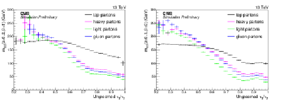
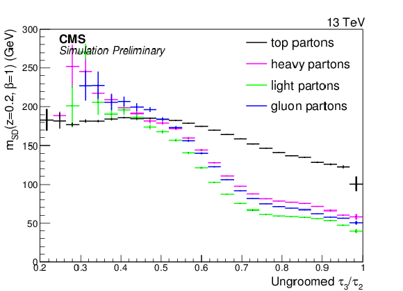
Profile plots showing the average values of $m_{SD}$ as a function of ungroomed $\tau _3/\tau _2$ for (left) CA15 jets and (right) AK8 jets. For CA15 (AK8) jets the softdrop parameters $z=$ 0.2, $\beta = $ 1 ($z=$ 0.1, $\beta = $ 0) are used. |
png pdf |
Figure 9-a:
Profile plots showing the average values of $m_{SD}$ as a function of ungroomed $\tau _3/\tau _2$ for CA15 jets. For CA15 jets the softdrop parameters $z=$ 0.2, $\beta = $ 1 are used. |

png pdf |
Figure 9-b:
Profile plots showing the average values of $m_{SD}$ as a function of ungroomed $\tau _3/\tau _2$ for AK8 jets. For AK8 jets the softdrop parameters $z=$ 0.1, $\beta = $ 0 are used. |
png pdf |
Figure 10:
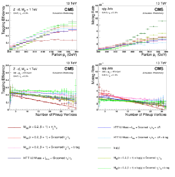
Top-tagging efficiency for the low $ {p_{\mathrm {T}}} $ working points listed in Table 3. The top plots show efficiency as a function of parton $ {p_{\mathrm {T}}} $, while the bottom ones show efficiency as a function of the number of pileup vertices. The plots in the first column are based on a Z'$\rightarrow t\bar{t}$ sample with $M_{\mathrm {Z'}} = $ 1 TeV, while those in the second column refer to QCD multijet production. The top right plot uses a flat parton ${p_{\mathrm {T}}}$ distribution whereas a $ {p_{\mathrm {T}}} = $ 300-470 GeV QCD background sample is used for the bottom right one. |
png pdf |
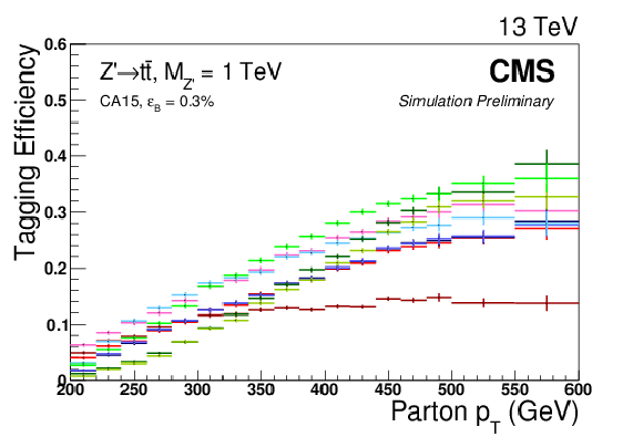
Figure 10-a:
Top-tagging efficiency for the low $ {p_{\mathrm {T}}} $ working points listed in Table 3. The top plots show efficiency as a function of parton $ {p_{\mathrm {T}}} $, while the bottom ones show efficiency as a function of the number of pileup vertices. The plots in the first column are based on a Z'$\rightarrow t\bar{t}$ sample with $M_{\mathrm {Z'}} = $ 1 TeV, while those in the second column refer to QCD multijet production. The top right plot uses a flat parton ${p_{\mathrm {T}}}$ distribution whereas a $ {p_{\mathrm {T}}} = $ 300-470 GeV QCD background sample is used for the bottom right one. |
png pdf |
Figure 10-b:
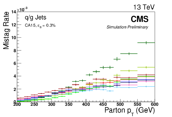
Top-tagging efficiency for the low $ {p_{\mathrm {T}}} $ working points listed in Table 3. The top plots show efficiency as a function of parton $ {p_{\mathrm {T}}} $, while the bottom ones show efficiency as a function of the number of pileup vertices. The plots in the first column are based on a Z'$\rightarrow t\bar{t}$ sample with $M_{\mathrm {Z'}} = $ 1 TeV, while those in the second column refer to QCD multijet production. The top right plot uses a flat parton ${p_{\mathrm {T}}}$ distribution whereas a $ {p_{\mathrm {T}}} = $ 300-470 GeV QCD background sample is used for the bottom right one. |

png pdf |
Figure 10-c:
Top-tagging efficiency for the low $ {p_{\mathrm {T}}} $ working points listed in Table 3. The top plots show efficiency as a function of parton $ {p_{\mathrm {T}}} $, while the bottom ones show efficiency as a function of the number of pileup vertices. The plots in the first column are based on a Z'$\rightarrow t\bar{t}$ sample with $M_{\mathrm {Z'}} = $ 1 TeV, while those in the second column refer to QCD multijet production. The top right plot uses a flat parton ${p_{\mathrm {T}}}$ distribution whereas a $ {p_{\mathrm {T}}} = $ 300-470 GeV QCD background sample is used for the bottom right one. |
png pdf |
Figure 10-d:
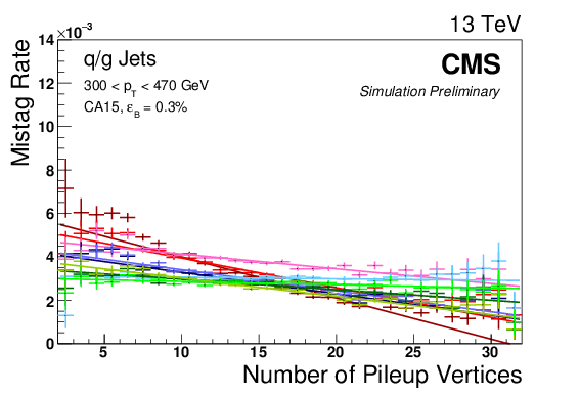
Top-tagging efficiency for the low $ {p_{\mathrm {T}}} $ working points listed in Table 3. The top plots show efficiency as a function of parton $ {p_{\mathrm {T}}} $, while the bottom ones show efficiency as a function of the number of pileup vertices. The plots in the first column are based on a Z'$\rightarrow t\bar{t}$ sample with $M_{\mathrm {Z'}} = $ 1 TeV, while those in the second column refer to QCD multijet production. The top right plot uses a flat parton ${p_{\mathrm {T}}}$ distribution whereas a $ {p_{\mathrm {T}}} = $ 300-470 GeV QCD background sample is used for the bottom right one. |

png pdf |
Figure 10-e:
Top-tagging efficiency for the low $ {p_{\mathrm {T}}} $ working points listed in Table 3. The top plots show efficiency as a function of parton $ {p_{\mathrm {T}}} $, while the bottom ones show efficiency as a function of the number of pileup vertices. The plots in the first column are based on a Z'$\rightarrow t\bar{t}$ sample with $M_{\mathrm {Z'}} = $ 1 TeV, while those in the second column refer to QCD multijet production. The top right plot uses a flat parton ${p_{\mathrm {T}}}$ distribution whereas a $ {p_{\mathrm {T}}} = $ 300-470 GeV QCD background sample is used for the bottom right one. |

png pdf |
Figure 10-f:
Top-tagging efficiency for the low $ {p_{\mathrm {T}}} $ working points listed in Table 3. The top plots show efficiency as a function of parton $ {p_{\mathrm {T}}} $, while the bottom ones show efficiency as a function of the number of pileup vertices. The plots in the first column are based on a Z'$\rightarrow t\bar{t}$ sample with $M_{\mathrm {Z'}} = $ 1 TeV, while those in the second column refer to QCD multijet production. The top right plot uses a flat parton ${p_{\mathrm {T}}}$ distribution whereas a $ {p_{\mathrm {T}}} = $ 300-470 GeV QCD background sample is used for the bottom right one. |
png pdf |
Figure 11:
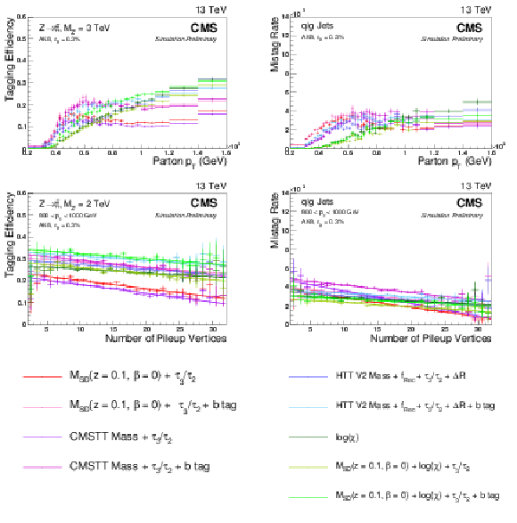
Top-tagging efficiency for the high $ {p_{\mathrm {T}}} $ working points listed in Table 2. The top plots show efficiency as a function of parton $ {p_{\mathrm {T}}} $, while the bottom ones show efficiency as a function of the number of pileup vertices. The plots in the first column are based on a Z'$\rightarrow t\bar{t}$ sample with $M_{\mathrm {Z'}} = $ 3 TeV or 2 TeV, while those in the second column refer to QCD multijet production. The top right plot uses a flat parton ${p_{\mathrm {T}}}$ distribution whereas a $ {p_{\mathrm {T}}} = $ 300-470 GeV QCD background sample is used for the bottom right one. |
png pdf |
Figure 11-a:
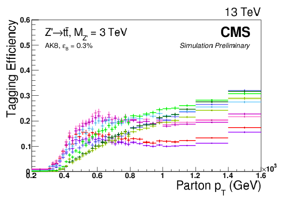
Top-tagging efficiency for the high $ {p_{\mathrm {T}}} $ working points listed in Table 2. The top plots show efficiency as a function of parton $ {p_{\mathrm {T}}} $, while the bottom ones show efficiency as a function of the number of pileup vertices. The plots in the first column are based on a Z'$\rightarrow t\bar{t}$ sample with $M_{\mathrm {Z'}} = $ 3 TeV or 2 TeV, while those in the second column refer to QCD multijet production. The top right plot uses a flat parton ${p_{\mathrm {T}}}$ distribution whereas a $ {p_{\mathrm {T}}} = $ 300-470 GeV QCD background sample is used for the bottom right one. |

png pdf |
Figure 11-b:
Top-tagging efficiency for the high $ {p_{\mathrm {T}}} $ working points listed in Table 2. The top plots show efficiency as a function of parton $ {p_{\mathrm {T}}} $, while the bottom ones show efficiency as a function of the number of pileup vertices. The plots in the first column are based on a Z'$\rightarrow t\bar{t}$ sample with $M_{\mathrm {Z'}} = $ 3 TeV or 2 TeV, while those in the second column refer to QCD multijet production. The top right plot uses a flat parton ${p_{\mathrm {T}}}$ distribution whereas a $ {p_{\mathrm {T}}} = $ 300-470 GeV QCD background sample is used for the bottom right one. |

png pdf |
Figure 11-c:
Top-tagging efficiency for the high $ {p_{\mathrm {T}}} $ working points listed in Table 2. The top plots show efficiency as a function of parton $ {p_{\mathrm {T}}} $, while the bottom ones show efficiency as a function of the number of pileup vertices. The plots in the first column are based on a Z'$\rightarrow t\bar{t}$ sample with $M_{\mathrm {Z'}} = $ 3 TeV or 2 TeV, while those in the second column refer to QCD multijet production. The top right plot uses a flat parton ${p_{\mathrm {T}}}$ distribution whereas a $ {p_{\mathrm {T}}} = $ 300-470 GeV QCD background sample is used for the bottom right one. |
png pdf |
Figure 11-d:
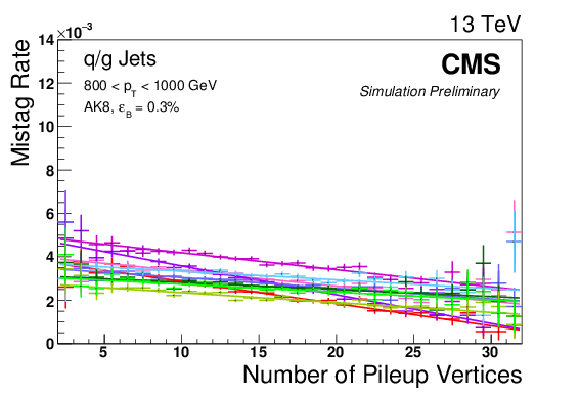
Top-tagging efficiency for the high $ {p_{\mathrm {T}}} $ working points listed in Table 2. The top plots show efficiency as a function of parton $ {p_{\mathrm {T}}} $, while the bottom ones show efficiency as a function of the number of pileup vertices. The plots in the first column are based on a Z'$\rightarrow t\bar{t}$ sample with $M_{\mathrm {Z'}} = $ 3 TeV or 2 TeV, while those in the second column refer to QCD multijet production. The top right plot uses a flat parton ${p_{\mathrm {T}}}$ distribution whereas a $ {p_{\mathrm {T}}} = $ 300-470 GeV QCD background sample is used for the bottom right one. |

png pdf |
Figure 11-e:
Top-tagging efficiency for the high $ {p_{\mathrm {T}}} $ working points listed in Table 2. The top plots show efficiency as a function of parton $ {p_{\mathrm {T}}} $, while the bottom ones show efficiency as a function of the number of pileup vertices. The plots in the first column are based on a Z'$\rightarrow t\bar{t}$ sample with $M_{\mathrm {Z'}} = $ 3 TeV or 2 TeV, while those in the second column refer to QCD multijet production. The top right plot uses a flat parton ${p_{\mathrm {T}}}$ distribution whereas a $ {p_{\mathrm {T}}} = $ 300-470 GeV QCD background sample is used for the bottom right one. |
png pdf |
Figure 11-f:
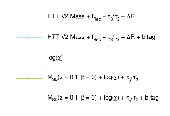
Top-tagging efficiency for the high $ {p_{\mathrm {T}}} $ working points listed in Table 2. The top plots show efficiency as a function of parton $ {p_{\mathrm {T}}} $, while the bottom ones show efficiency as a function of the number of pileup vertices. The plots in the first column are based on a Z'$\rightarrow t\bar{t}$ sample with $M_{\mathrm {Z'}} = $ 3 TeV or 2 TeV, while those in the second column refer to QCD multijet production. The top right plot uses a flat parton ${p_{\mathrm {T}}}$ distribution whereas a $ {p_{\mathrm {T}}} = $ 300-470 GeV QCD background sample is used for the bottom right one. |
png pdf |
Figure 12:
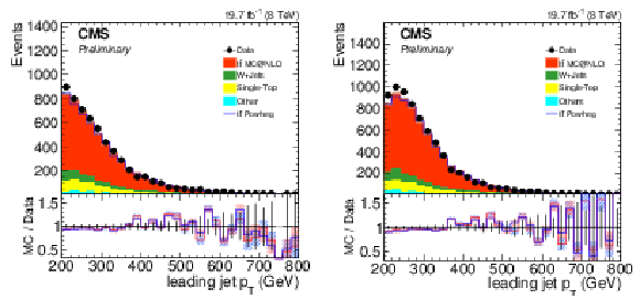
Distribution of $ {p_{\mathrm {T}}} $ for selected CA8 (left) and CA15 jets (right) after the signal selection. Only statistical uncertainties are shown. The ratio of simulation to data is shown at the bottom, where the ratio to POWHEG is reported in blue while the one to mc@nlo is shown in red. The hashed bands depict the statistical uncertainty of the simulated samples, whereas the vertical bars show the statistical uncertainties of data. |

png pdf |
Figure 12-a:
Distribution of $ {p_{\mathrm {T}}} $ for selected CA8 jets after the signal selection. Only statistical uncertainties are shown. The ratio of simulation to data is shown at the bottom, where the ratio to POWHEG is reported in blue while the one to mc@nlo is shown in red. The hashed bands depict the statistical uncertainty of the simulated samples, whereas the vertical bars show the statistical uncertainties of data. |
png pdf |
Figure 12-b:
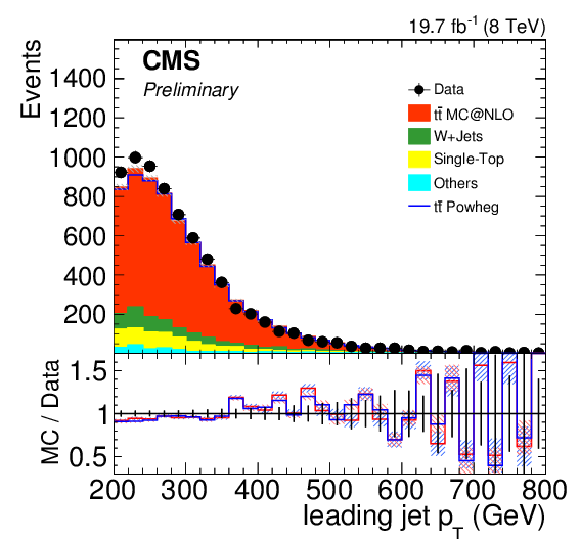
Distribution of $ {p_{\mathrm {T}}} $ for selected CA15 jets after the signal selection. Only statistical uncertainties are shown. The ratio of simulation to data is shown at the bottom, where the ratio to POWHEG is reported in blue while the one to mc@nlo is shown in red. The hashed bands depict the statistical uncertainty of the simulated samples, whereas the vertical bars show the statistical uncertainties of data. |
png pdf |
Figure 13:
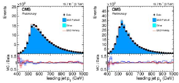
$ {p_{\mathrm {T}}} $ distribution for CA8 (left) and CA15 (right) jets after the background selection. Data is compared to simulated events by PYTHIA 8 and HERWIG++ . Only statistical uncertainties are shown. The ratio of simulation to data is shown at the bottom, where the ratio to PYTHIA 8 is reported in blue while the one to HERWIG++ is shown in red. The hashed bands depict the statistical uncertainty of the simulated samples, whereas the vertical bars show the statistical uncertainties of data. |

png pdf |
Figure 13-a:
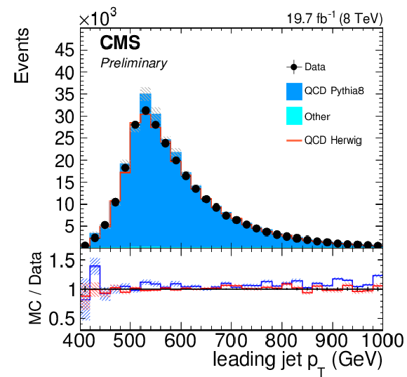
$ {p_{\mathrm {T}}} $ distribution for CA8 jets after the background selection. Data is compared to simulated events by PYTHIA 8 and HERWIG++ . Only statistical uncertainties are shown. The ratio of simulation to data is shown at the bottom, where the ratio to PYTHIA 8 is reported in blue while the one to HERWIG++ is shown in red. The hashed bands depict the statistical uncertainty of the simulated samples, whereas the vertical bars show the statistical uncertainties of data. |
png pdf |
Figure 13-b:
$ {p_{\mathrm {T}}} $ distribution for CA15 jets after the background selection. Data is compared to simulated events by PYTHIA 8 and HERWIG++ . Only statistical uncertainties are shown. The ratio of simulation to data is shown at the bottom, where the ratio to PYTHIA 8 is reported in blue while the one to HERWIG++ is shown in red. The hashed bands depict the statistical uncertainty of the simulated samples, whereas the vertical bars show the statistical uncertainties of data. |
png pdf |
Figure 14:
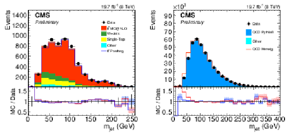
Jet mass for the signal selection (left) and the background one (right). Only statistical uncertainties are shown. The ratio of simulation to data is shown at the bottom of each panel. In the case of the signal (background) selection, the ratio to POWHEG (PYTHIA 8) is shown in blue while the one to mc@nlo (HERWIG++ ) is shown in red. The hashed bands depict the statistical uncertainty of the simulated samples, whereas the vertical bars show the statistical uncertainties of data. |

png pdf |
Figure 14-a:
Jet mass for the signal selection. Only statistical uncertainties are shown. The ratio of simulation to data is shown at the bottom of each panel. In the case of the signal (background) selection, the ratio to POWHEG (PYTHIA 8) is shown in blue while the one to mc@nlo (HERWIG++ ) is shown in red. The hashed bands depict the statistical uncertainty of the simulated samples, whereas the vertical bars show the statistical uncertainties of data. |

png pdf |
Figure 14-b:
Jet mass for the background selection. Only statistical uncertainties are shown. The ratio of simulation to data is shown at the bottom of each panel. In the case of the signal (background) selection, the ratio to POWHEG (PYTHIA 8) is shown in blue while the one to mc@nlo (HERWIG++ ) is shown in red. The hashed bands depict the statistical uncertainty of the simulated samples, whereas the vertical bars show the statistical uncertainties of data. |
png pdf |
Figure 15:
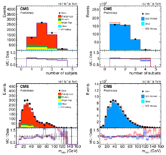
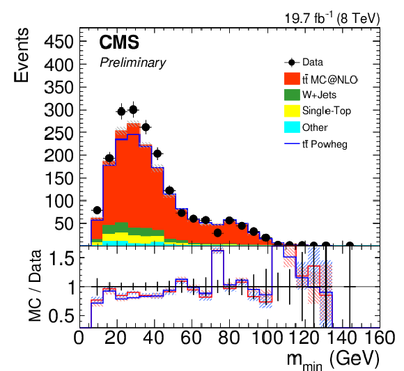
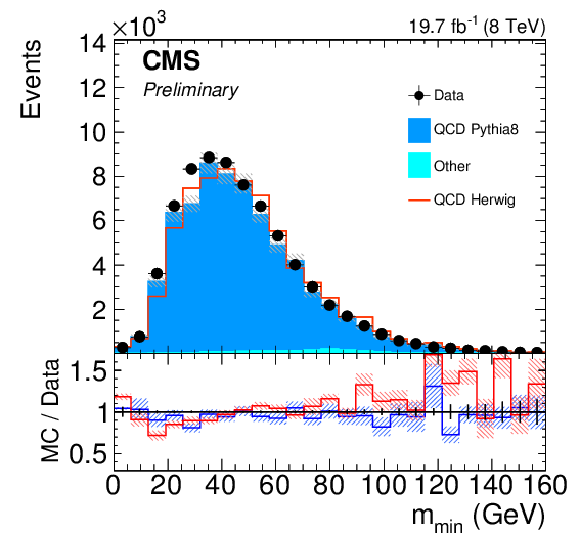
Distribution of the minimum pairwise mass (bottom) and the number of subjets found by the CMSTT (top) for the signal sample (left) and for the background one (right). Only statistical uncertainties are shown. The ratio of simulation to data is shown at the bottom of each panel. In the case of the signal (background) selection, the ratio to POWHEG (PYTHIA 8) is shown in blue while the one to mc@nlo (HERWIG++ ) is shown in red. The hashed bands depict the statistical uncertainty of the simulated samples, whereas the vertical bars show the statistical uncertainties of data. |

png pdf |
Figure 15-a:
Distribution of the number of subjets found by the CMSTT for the signal sample. Only statistical uncertainties are shown. The ratio of simulation to data is shown at the bottom of the panel. The ratio to POWHEG is shown in blue while the one to mc@nlo is shown in red. The hashed bands depict the statistical uncertainty of the simulated samples, whereas the vertical bars show the statistical uncertainties of data. |

png pdf |
Figure 15-b:
Distribution of the number of subjets found by the CMSTT for the background one sample. Only statistical uncertainties are shown. The ratio of simulation to data is shown at the bottom of the panel. The ratio to PYTHIA 8 is shown in blue while the one to HERWIG++ is shown in red. The hashed bands depict the statistical uncertainty of the simulated samples, whereas the vertical bars show the statistical uncertainties of data. |
png pdf |
Figure 15-c:
Distribution of the minimum pairwise mass for the signal sample. Only statistical uncertainties are shown. The ratio of simulation to data is shown at the bottom of the panel. The ratio to POWHEG is shown in blue while the one to mc@nlo is shown in red. The hashed bands depict the statistical uncertainty of the simulated samples, whereas the vertical bars show the statistical uncertainties of data. |
png pdf |
Figure 15-d:
Distribution of the minimum pairwise mass for the background sample. Only statistical uncertainties are shown. The ratio of simulation to data is shown at the bottom of the panel. The ratio to PYTHIA 8 is shown in blue while the one to HERWIG++ is shown in red. The hashed bands depict the statistical uncertainty of the simulated samples, whereas the vertical bars show the statistical uncertainties of data. |

png pdf |
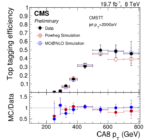
Figure 16:
Efficiency (left) and mistag rate (right) of the CMSTT as function of $ {p_{\mathrm {T}}} $. The error bars show the combined statistical and systematic uncertainties. At the bottom of each panel the ratio of simulation to data is shown. |
png pdf |
Figure 16-a:
Efficiency of the CMSTT as function of $ {p_{\mathrm {T}}} $. The error bars show the combined statistical and systematic uncertainties. At the bottom of each panel the ratio of simulation to data is shown. |

png pdf |
Figure 16-b:
Mistag rate of the CMSTT as function of $ {p_{\mathrm {T}}} $. The error bars show the combined statistical and systematic uncertainties. At the bottom of each panel the ratio of simulation to data is shown. |
png pdf |
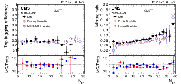
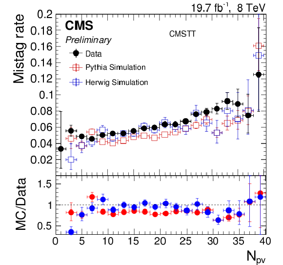
Figure 17:
Efficiency (left) and mistag rate (right) of the CMSTT as function of the number of reconstructed primary vertices. The error bars show the combined statistical and systematic uncertainties. At the bottom of each panel the ratio of simulation to data is shown. |

png pdf |
Figure 17-a:
Efficiency of the CMSTT as function of the number of reconstructed primary vertices. The error bars show the combined statistical and systematic uncertainties. At the bottom of each panel the ratio of simulation to data is shown. |
png pdf |
Figure 17-b:
Mistag rate of the CMSTT as function of the number of reconstructed primary vertices. The error bars show the combined statistical and systematic uncertainties. At the bottom of each panel the ratio of simulation to data is shown. |

png pdf |
Figure 18:
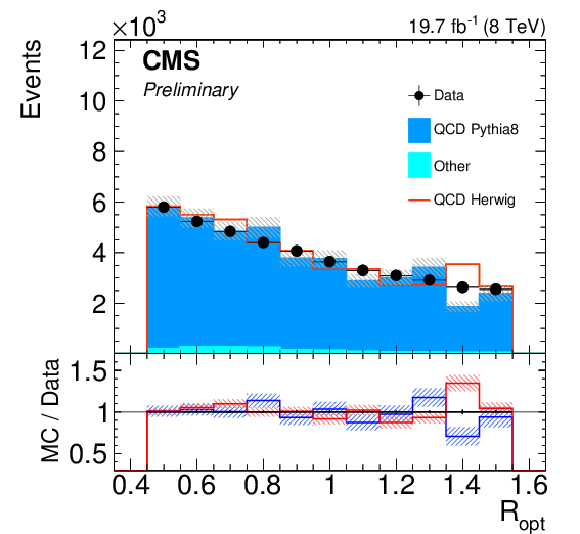
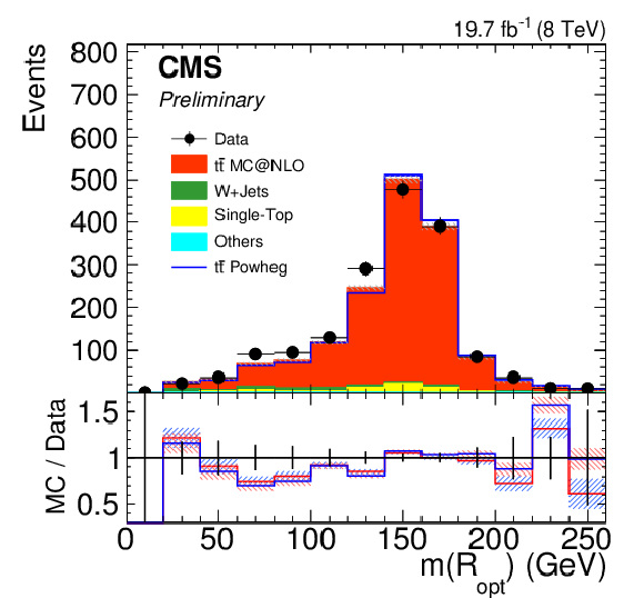
Distribution of the optimal radius $R_{\mathrm {opt}}$ (top) and the mass $m_{123}$ at the optimal radius $R_{\mathrm {opt}}$ (bottom) of the HTT v2 for the signal selection (left) and for the background one (right). Only statistical uncertainties are shown. The ratio of simulation to data is shown at the bottom of each panel. In the case of the signal (background) selection, the ratio to POWHEG (PYTHIA 8) is shown in blue while the one to mc@nlo (HERWIG++ ) is shown in red. The hashed bands depict the statistical uncertainty of the simulated samples, whereas the vertical bars show the statistical uncertainties of data. |

png pdf |
Figure 18-a:
Distribution of the optimal radius $R_{\mathrm {opt}}$ of the HTT v2 for the signal selection. Only statistical uncertainties are shown. The ratio of simulation to data is shown at the bottom of each panel. The ratio to POWHEG is shown in blue while the one to mc@nlo is shown in red. The hashed bands depict the statistical uncertainty of the simulated samples, whereas the vertical bars show the statistical uncertainties of data. |
png pdf |
Figure 18-b:
Distribution of the optimal radius $R_{\mathrm {opt}}$ of the HTT v2 for the background selection. Only statistical uncertainties are shown. The ratio of simulation to data is shown at the bottom of each panel. The ratio to PYTHIA 8 is shown in blue while the one to HERWIG++ is shown in red. The hashed bands depict the statistical uncertainty of the simulated samples, whereas the vertical bars show the statistical uncertainties of data. |
png pdf |
Figure 18-c:
Distribution of the mass $m_{123}$ at the optimal radius $R_{\mathrm {opt}}$ of the HTT v2 for the signal selection. Only statistical uncertainties are shown. The ratio of simulation to data is shown at the bottom of each panel. The ratio to POWHEG is shown in blue while the one to mc@nlo is shown in red. The hashed bands depict the statistical uncertainty of the simulated samples, whereas the vertical bars show the statistical uncertainties of data. |

png pdf |
Figure 18-d:
Distribution of the mass $m_{123}$ at the optimal radius $R_{\mathrm {opt}}$ of the HTT v2 for the background selection. Only statistical uncertainties are shown. The ratio of simulation to data is shown at the bottom of each panel. The ratio to PYTHIA 8 is shown in blue while the one to HERWIG++ is shown in red. The hashed bands depict the statistical uncertainty of the simulated samples, whereas the vertical bars show the statistical uncertainties of data. |
png pdf |
Figure 19:
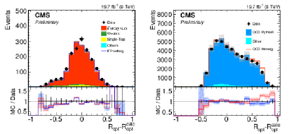
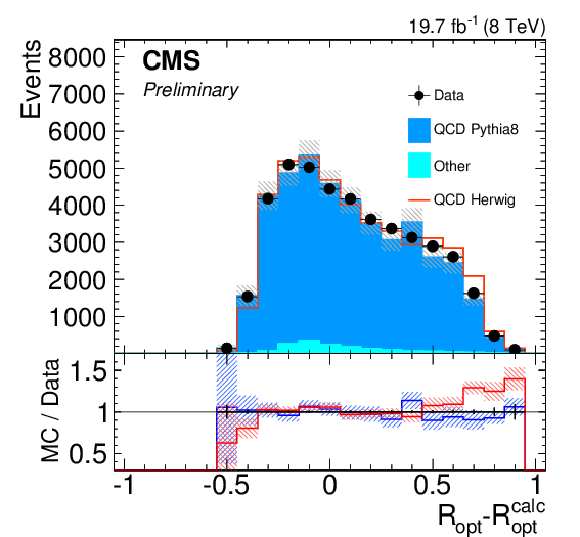
Distribution of the decision variable $R_{\mathrm {opt}}-R_{\mathrm {opt}}^{\mathrm {calc}}$ for the signal selection (left) and background one (right). Only statistical uncertainties are shown. The ratio of simulation to data is shown at the bottom of each panel. In the case of the signal (background) selection, the ratio to POWHEG (PYTHIA 8) is shown in blue and while the one to mc@nlo (HERWIG++ ) is shown in red. The hashed bands depict the statistical uncertainty of the simulated samples, whereas the vertical bars show the statistical uncertainties of data. |

png pdf |
Figure 19-a:
Distribution of the decision variable $R_{\mathrm {opt}}-R_{\mathrm {opt}}^{\mathrm {calc}}$ for the signal selection. Only statistical uncertainties are shown. The ratio of simulation to data is shown at the bottom of each panel. In the case of the signal selection, the ratio to POWHEG is shown in blue and while the one to mc@nlo is shown in red. The hashed bands depict the statistical uncertainty of the simulated samples, whereas the vertical bars show the statistical uncertainties of data. |
png pdf |
Figure 19-b:
Distribution of the decision variable $R_{\mathrm {opt}}-R_{\mathrm {opt}}^{\mathrm {calc}}$ for the background selection. Only statistical uncertainties are shown. The ratio of simulation to data is shown at the bottom of each panel. In the case of the background selection, the ratio to PYTHIA 8 is shown in blue and while the one to HERWIG++ is shown in red. The hashed bands depict the statistical uncertainty of the simulated samples, whereas the vertical bars show the statistical uncertainties of data. |
png pdf |
Figure 20:
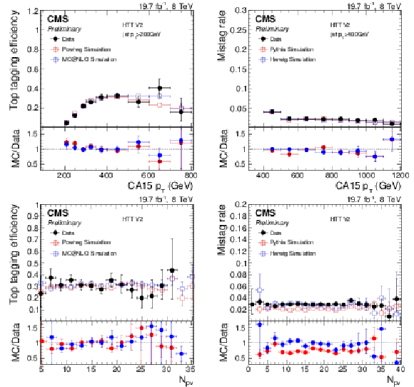
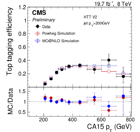
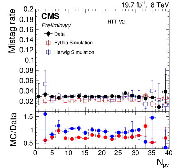
Efficiency (left) and mistag rate (right) of the HTT V2 as function of $ {p_{\mathrm {T}}} $ (top) and the number of reconstructed primary vertices (bottom). The error bars show the combined statistical and systematic uncertainties. At the bottom of each panel the ratio of simulation to data is shown. |
png pdf |
Figure 20-a:
Efficiency of the HTT V2 as function of $ {p_{\mathrm {T}}} $. The error bars show the combined statistical and systematic uncertainties. At the bottom of the panel the ratio of simulation to data is shown. |

png pdf |
Figure 20-b:
Mistag rate of the HTT V2 as function of $ {p_{\mathrm {T}}} $. The error bars show the combined statistical and systematic uncertainties. At the bottom of the panel the ratio of simulation to data is shown. |

png pdf |
Figure 20-c:
Efficiency of the number of reconstructed primary vertices. The error bars show the combined statistical and systematic uncertainties. At the bottom of the panel the ratio of simulation to data is shown. |
png pdf |
Figure 20-d:
Mistag rate of the number of reconstructed primary vertices. The error bars show the combined statistical and systematic uncertainties. At the bottom of the panel the ratio of simulation to data is shown. |
png pdf |
Figure 21:
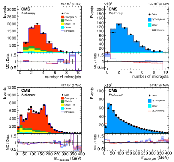
Distribution of the microjet multiplicity (top) and invariant mass of all microjets (bottom) for the signal sample (left) and background one (right). Only statistical uncertainties are shown. The ratio of simulation to data is shown at the bottom of each panel. In the case of the signal (background) selection, the ratio to POWHEG (PYTHIA 8) is shown in blue while the one to mc@nlo (HERWIG++ ) is shown in red. The hashed bands depict the statistical uncertainty of the simulated samples, whereas the vertical bars show the statistical uncertainties of data. |
png pdf |
Figure 21-a:
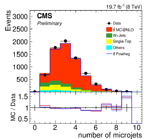
Distribution of the microjet multiplicity for the signal sample. Only statistical uncertainties are shown. The ratio of simulation to data is shown at the bottom of the panel. The ratio to POWHEG is shown in blue while the one to mc@nlo is shown in red. The hashed bands depict the statistical uncertainty of the simulated samples, whereas the vertical bars show the statistical uncertainties of data. |
png pdf |
Figure 21-b:
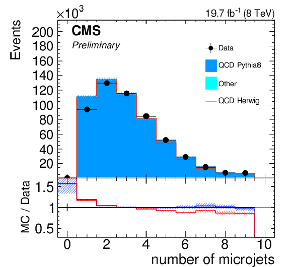
Distribution of the microjet multiplicity for the background sample. Only statistical uncertainties are shown. The ratio of simulation to data is shown at the bottom of the panel. The ratio to PYTHIA 8 is shown in blue while the one to HERWIG++ is shown in red. The hashed bands depict the statistical uncertainty of the simulated samples, whereas the vertical bars show the statistical uncertainties of data. |

png pdf |
Figure 21-c:
Distribution of the invariant mass of all microjets for the signal background sample. Only statistical uncertainties are shown. The ratio of simulation to data is shown at the bottom of the panel. The ratio to POWHEG is shown in blue while the one to mc@nlo is shown in red. The hashed bands depict the statistical uncertainty of the simulated samples, whereas the vertical bars show the statistical uncertainties of data. |

png pdf |
Figure 21-d:
Distribution of the invariant mass of all microjets for the signal background sample. Only statistical uncertainties are shown. The ratio of simulation to data is shown at the bottom of the panel. The ratio to PYTHIA 8 is shown in blue while the one to HERWIG++ is shown in red. The hashed bands depict the statistical uncertainty of the simulated samples, whereas the vertical bars show the statistical uncertainties of data. |
png pdf |
Figure 22:
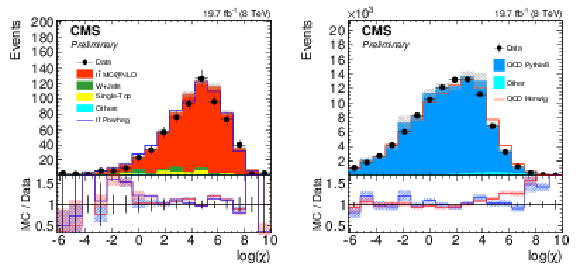
Distribution of the decision variable $\chi $ for jets with $ {p_{\mathrm {T}}} > $ 350 GeV for signal jets (left) and background ones (right). Only statistical uncertainties are shown. The ratio of simulation to data is shown at the bottom of each panel. In the case of the signal (background) selection, the ratio to POWHEG (PYTHIA 8) is shown in blue while the one to mc@nlo (HERWIG++ ) is shown in red. The hashed bands depict the statistical uncertainty of the simulated samples, whereas the vertical bars show the statistical uncertainties of data. |

png pdf |
Figure 22-a:
Distribution of the decision variable $\chi $ for jets with $ {p_{\mathrm {T}}} > $ 350 GeV for signal jets. Only statistical uncertainties are shown. The ratio of simulation to data is shown at the bottom of the panel. The ratio to POWHEG is shown in blue while the one to mc@nlo is shown in red. The hashed bands depict the statistical uncertainty of the simulated samples, whereas the vertical bars show the statistical uncertainties of data. |

png pdf |
Figure 22-b:
Distribution of the decision variable $\chi $ for jets with $ {p_{\mathrm {T}}} > $ 350 GeV for background jets. Only statistical uncertainties are shown. The ratio of simulation to data is shown at the bottom of the panel. The ratio to PYTHIA 8 is shown in blue while the one to HERWIG++ is shown in red. The hashed bands depict the statistical uncertainty of the simulated samples, whereas the vertical bars show the statistical uncertainties of data. |

png pdf |
Figure 23:
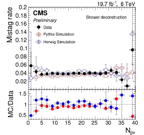
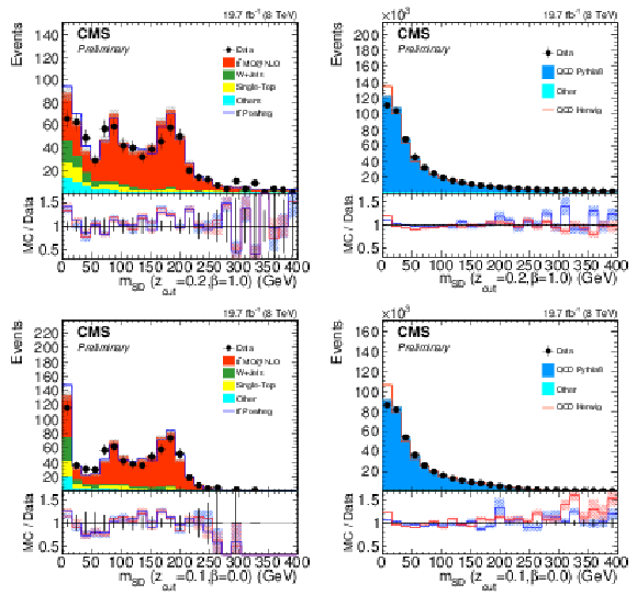
Efficiency (left) and mistag rate (right) of the shower deconstruction tagger requiring $\log (\chi )> $ 3.5 as function of $ {p_{\mathrm {T}}} $ (top) and the number of reconstructed primary vertices (bottom). The error bars show the combined statistical and systematic uncertainties. At the bottom of each panel the ratio of simulation to data is shown. |

png pdf |
Figure 23-a:
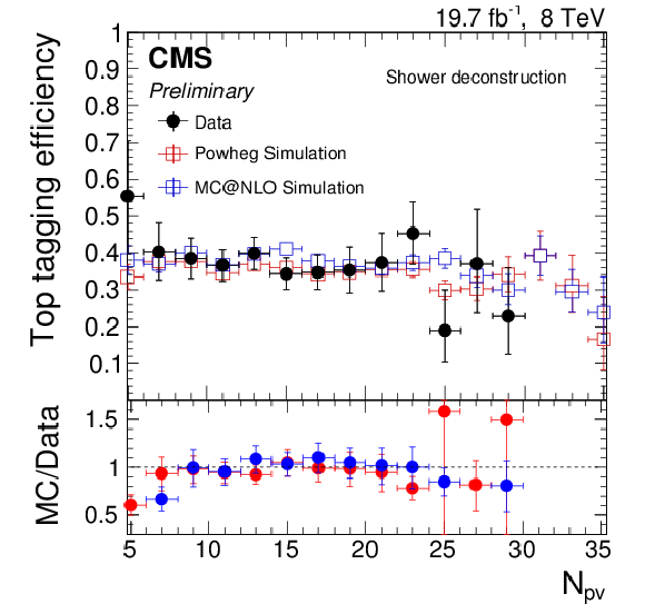
Mistag rate of the shower deconstruction tagger requiring $\log (\chi )> $ 3.5 as function of the number of reconstructed primary vertices. The error bars show the combined statistical and systematic uncertainties. At the bottom of the panel the ratio of simulation to data is shown. |
png pdf |
Figure 23-b:
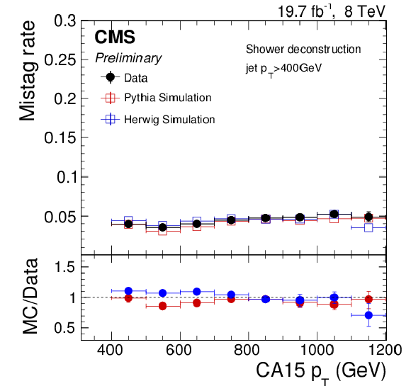
Mistag rate of the shower deconstruction tagger requiring $\log (\chi )> $ 3.5 as function of $ {p_{\mathrm {T}}} $. The error bars show the combined statistical and systematic uncertainties. At the bottom of the panel the ratio of simulation to data is shown. |
png pdf |
Figure 23-c:
Efficiency (left) and mistag rate (right) of the shower deconstruction tagger requiring $\log (\chi )> $ 3.5 as function of $ {p_{\mathrm {T}}} $ (top) and the number of reconstructed primary vertices (bottom). The error bars show the combined statistical and systematic uncertainties. At the bottom of each panel the ratio of simulation to data is shown. |
png pdf |
Figure 23-d:
Efficiency (left) and mistag rate (right) of the shower deconstruction tagger requiring $\log (\chi )> $ 3.5 as function of $ {p_{\mathrm {T}}} $ (top) and the number of reconstructed primary vertices (bottom). The error bars show the combined statistical and systematic uncertainties. At the bottom of each panel the ratio of simulation to data is shown. |
png pdf |
Figure 24:
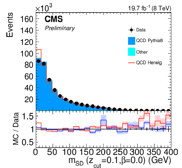
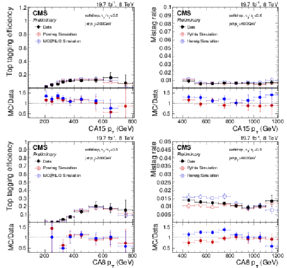
Distribution the jet mass after applying softdrop for the CA15 selection with $z_{\rm {cut}}=$ 0.2 and $\beta = $ 1 (top) and the CA8 selection with $z_{\rm {cut}}=$ 0.1 and $\beta = $ 0 (bottom) for signal jets (left) and background ones (right). Only statistical uncertainties are shown. The ratio of simulation to data is shown at the bottom of each panel. In the case of the signal (background) selection, the ratio to POWHEG (PYTHIA 8) is shown in blue while the one to mc@nlo (HERWIG++ ) is shown in red. The hashed bands depict the statistical uncertainty of the simulated samples, whereas the vertical bars show the statistical uncertainties of data. |

png pdf |
Figure 24-a:
Distribution the jet mass after applying softdrop for the CA15 selection with $z_{\rm {cut}}=$ 0.2 and $\beta = $ 1 for signal jets. Only statistical uncertainties are shown. The ratio of simulation to data is shown at the bottom of the panel. The ratio to POWHEG is shown in blue while the one to mc@nlo is shown in red. The hashed bands depict the statistical uncertainty of the simulated samples, whereas the vertical bars show the statistical uncertainties of data. |

png pdf |
Figure 24-b:
Distribution the jet mass after applying softdrop for the CA15 selection with $z_{\rm {cut}}=$ 0.2 and $\beta = $ 1 for background jets. Only statistical uncertainties are shown. The ratio of simulation to data is shown at the bottom of the panel. The ratio to PYTHIA 8 is shown in blue while the one to HERWIG++ is shown in red. The hashed bands depict the statistical uncertainty of the simulated samples, whereas the vertical bars show the statistical uncertainties of data. |

png pdf |
Figure 24-c:
Distribution the jet mass after applying softdrop for the CA8 selection with $z_{\rm {cut}}=$ 0.1 and $\beta = $ 0 for signal jets. Only statistical uncertainties are shown. The ratio of simulation to data is shown at the bottom of the panel. The ratio to POWHEG is shown in blue while the one to mc@nlo is shown in red. The hashed bands depict the statistical uncertainty of the simulated samples, whereas the vertical bars show the statistical uncertainties of data. |
png pdf |
Figure 24-d:
Distribution the jet mass after applying softdrop for the CA8 selection with $z_{\rm {cut}}=$ 0.1 and $\beta = $ 0 for background jets. Only statistical uncertainties are shown. The ratio of simulation to data is shown at the bottom of the panel. The ratio to PYTHIA 8 is shown in blue while the one to HERWIG++ is shown in red. The hashed bands depict the statistical uncertainty of the simulated samples, whereas the vertical bars show the statistical uncertainties of data. |
png pdf |
Figure 25:
Efficiency (left) and mistag rate (right) of the softdrop based tagging criteria as function of $ {p_{\mathrm {T}}} $, for CA15 jets, $z_{\rm {cut}}= $ 0.2 and $\beta = $ 1.0 (top) and CA8 jets, $z_{\rm {cut}}= $ 0.1 and $\beta = $ 0 (bottom). The error bars show the combined statistical and systematic uncertainties. At the bottom of each panel the ratio of simulation to data is shown. |
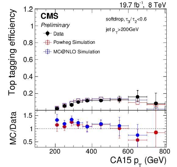
png pdf |
Figure 25-a:
Efficiency of the softdrop based tagging criteria as function of $ {p_{\mathrm {T}}} $, for CA15 jets, $z_{\rm {cut}}= $ 0.2 and $\beta = $ 1.0. The error bars show the combined statistical and systematic uncertainties. At the bottom of each panel the ratio of simulation to data is shown. |
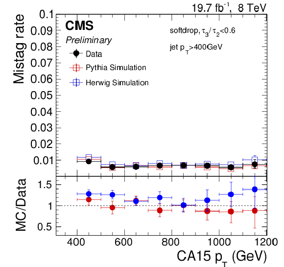
png pdf |
Figure 25-b:
Mistag rate of the softdrop based tagging criteria as function of $ {p_{\mathrm {T}}} $, for CA15 jets, $z_{\rm {cut}}= $ 0.2 and $\beta = $ 1.0. The error bars show the combined statistical and systematic uncertainties. At the bottom of each panel the ratio of simulation to data is shown. |

png pdf |
Figure 25-c:
Efficiency of the softdrop based tagging criteria as function of $ {p_{\mathrm {T}}} $, for CA8 jets, $z_{\rm {cut}}= $ 0.1 and $\beta = $ 0. The error bars show the combined statistical and systematic uncertainties. At the bottom of each panel the ratio of simulation to data is shown. |
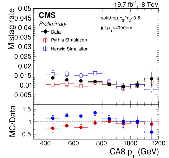
png pdf |
Figure 25-d:
Mistag rate of the softdrop based tagging criteria as function of $ {p_{\mathrm {T}}} $, for CA8 jets, $z_{\rm {cut}}= $ 0.1 and $\beta = $ 0. The error bars show the combined statistical and systematic uncertainties. At the bottom of each panel the ratio of simulation to data is shown. |
| Tables | |

png pdf |
Table 1:
Overview of signal and background samples and selection criteria used for studies of top-tagging performance. $R$ denotes the distance parameter used for jet reconstruction. Background samples are denoted by the $ {p_{\mathrm {T}}} $ bin whereas signal samples are denoted by the mass of the Z' resonance. For parton to jet matching, labeled $\Delta R (\textrm {p},\textrm {jet})$, where p stands for the top quark in the case of signal jets and light quarks, and partons from the hard scattering in the case of background ones. The merged top requirement (max ($\Delta R (\textrm {t},\textrm {q})$)) restricts the maximal distance between the top quark (t) and the three decay products (q). |

png pdf |
Table 2:
Summary of working points considered for studying their dependence on top quark $ {p_{\mathrm {T}}} $, $\eta $, and number of pileup vertices. The working points here are for the low-$ {p_{\mathrm {T}}} $ region, $R = $ 1.5 jets, and correspond to a background efficiency of 0.3%. The quantity $\chi _{2}$ refers to the shower deconstruction output using a microjet size of $R = $ 0.2. |

png pdf |
Table 3:
Summary of working points considered for studying their dependence on top quark $ {p_{\mathrm {T}}} $, $\eta $, and number of pileup vertices. The working points here are for the high-$ {p_{\mathrm {T}}} $ region, $R = $ 0.8 jets, and correspond to a background efficiency of 0.3%. The quantity $\chi _{1}$ refers to the shower deconstruction output using a microjet size of $R = $ 0.1. |

png pdf |
Table 4:
Sample composition after the signal selection including the statistical uncertainty. |
| Summary |
|
A review of top-tagging techniques aimed at Run II of the LHC is presented. By analyzing the performance with respect to generator truth-level, inside a fiducial region with flat jet transverse momentum and $\eta$ distributions, it is possible to disentangle kinematic correlations from the discriminating power of individual variables. Softdrop, pruning and HTT V2 algorithms provide a stable reconstructed mass as a function of top-quark $p_{\mathrm{T}}$. The HTT V2 method also supplies a stable $f_{Rec}$ discriminant. Shower deconstruction provides a single variable offering strong discrimination between signal and background jets. Improvements can be obtained after combination with a groomed mass variable. When multiple observables are considered to select top-jet candidates, a combination of the HTT V2 decision variables, the n-subjettiness, and b tagging; or alternatively a combination of shower deconstruction, the softdrop mass, the n-subjettiness, and b tagging offer superior performance. A simplified combination of the softdrop mass, the n-subjettiness, and b tagging only has at most 15% lower signal efficiency at the same background rejection, therefore it is recommended as the default technique. A set of different working points is tested for their stability with respect to $p_{\mathrm{T}}$, $\eta$, and the amount of pileup present in the event. In general, a turn-on behavior with a stable plateau at high $p_{\mathrm{T}}$ is observed, with the main exception of shower deconstruction where the efficiency and mistag rate rise linearly with $p_{\mathrm{T}}$. This can already be inferred from the one-dimensional distributions where a shift in the shower deconstruction discriminator with $p_{\mathrm{T}}$ is observed. A dependence of the expected background mistag rate on the parton flavor is observed, with bottom quarks showing the highest and gluons showing the lowest mistag rate. This is consistent with the different shapes of these variables in the two-dimensional n-subjettiness versus groomed mass plane. In order to measure top-tagging efficiencies in an analysis setting, we compare the simulations with data collected at a center-of-mass energy of 8 TeV. To measure the efficiency and mistag rate in data, two selections were designed to enrich a sample with semi-leptonic $\mathrm{ t \bar{t} }$ events and the other with di-jet ones. After reweighting the $p_{\mathrm{T}}$ distribution of the leading jet for the background selection, we examine the decision variables of the tagging algorithms using data events. Overall the agreement between simulation and data is good. The discriminating variables as well as the efficiencies and mistag rates are well modeled by MC and POWHEG for the signal and by HERWIGpp and PYTHIA 8 for the backgrounds. |
| References | ||||
| 1 | C. T. Hill | Topcolor: Top quark condensation in a gauge extension of the standard model | PLB266 (1991) 419--424 | |
| 2 | C. T. Hill | Topcolor assisted technicolor | PLB345 (1995) 483--489 | hep-ph/9411426 |
| 3 | R. M. Harris, C. T. Hill, and S. J. Parke | Cross-section for topcolor $ Z'_{\mathrm{t}} $ decaying to $ \mathrm{ t \bar{t} } $ | hep-ph/9911288 | |
| 4 | L. Randall and R. Sundrum | An Alternative to compactification | PRL 83 (1999) 4690--4693 | hep-th/9906064 |
| 5 | ATLAS Collaboration | A search for $ \mathrm{ t \bar{t} } $ resonances in lepton+jets events with highly boosted top quarks collected in $ pp $ collisions at $ \sqrt{s} = $ 7 TeV with the ATLAS detector | JHEP 1209 (2012) 041 | 1207.2409 |
| 6 | ATLAS Collaboration | A search for $ \mathrm{ t \bar{t} } $ resonances in the lepton plus jets final state with ATLAS using 14 fb$ ^{-1} $ of pp collisions at $ \sqrt{s}= $ 8 TeV | ATLAS-CONF-2013-052 | |
| 7 | ATLAS Collaboration | A search for $ \mathrm{ t \bar{t} } $ resonances using lepton-plus-jets events in proton-proton collisions at $ \sqrt{s}= $ 8 TeV with the ATLAS detector | JHEP 08 (2015) 148 | 1505.07018 |
| 8 | CMS Collaboration | Search for anomalous $ \mathrm{ t \bar{t} } $ production in the highly-boosted all-hadronic final state | JHEP 1209 (2012) 029 | CMS-EXO-11-006 1204.2488 |
| 9 | CMS Collaboration | Search for Anomalous Top Quark Pair Production in the Boosted All-Hadronic Final State using pp Collisions at $ \sqrt{s} = $ 8 TeV | CMS-PAS-B2G-12-005 | |
| 10 | J. M. Butterworth, A. R. Davison, M. Rubin, and G. P. Salam | Jet substructure as a new Higgs search channel at the LHC | PRL 100 (2008) 242001 | 0802.2470 |
| 11 | D. Krohn, J. Thaler, and L.-T. Wang | Jet Trimming | JHEP 1002 (2010) 084 | 0912.1342 |
| 12 | S. D. Ellis, C. K. Vermilion, and J. R. Walsh | Recombination Algorithms and Jet Substructure: Pruning as a Tool for Heavy Particle Searches | PRD81 (2010) 094023 | 0912.0033 |
| 13 | A. J. Larkoski, S. Marzani, G. Soyez, and J. Thaler | Soft Drop | JHEP 1405 (2014) 146 | 1402.2657 |
| 14 | S. D. Ellis et al. | Qjets: A Non-Deterministic Approach to Tree-Based Jet Substructure | PRL 108 (2012) 182003 | 1201.1914 |
| 15 | J. Thaler and K. Van Tilburg | Identifying Boosted Objects with N-subjettiness | JHEP 1103 (2011) 015 | 1011.2268 |
| 16 | S. Catani, Y. L. Dokshitzer, M. H. Seymour, and B. R. Webber | Longitudinally invariant $ K_t $ clustering algorithms for hadron hadron collisions | Nucl. Phys. B406 (1993) 187--224 | |
| 17 | D. E. Kaplan, K. Rehermann, M. D. Schwartz, and B. Tweedie | Top Tagging: A Method for Identifying Boosted Hadronically Decaying Top Quarks | PRL 101 (2008) 142001 | 0806.0848 |
| 18 | CMS Collaboration | A Cambridge-Aachen (C-A) based Jet Algorithm for boosted to-jet tagging | CDS | |
| 19 | T. Plehn, G. P. Salam, and M. Spannowsky | Fat Jets for a Light Higgs | PRL 104 (2010) 111801 | 0910.5472 |
| 20 | T. Plehn, M. Spannowsky, M. Takeuchi, and D. Zerwas | Stop Reconstruction with Tagged Tops | JHEP 1010 (2010) 078 | 1006.2833 |
| 21 | G. Kasieczka et al. | Resonance Searches with an Updated Top Tagger | 1503.05921 | |
| 22 | D. E. Soper and M. Spannowsky | Finding physics signals with shower deconstruction | PRD84 (2011) 074002 | 1102.3480 |
| 23 | D. E. Soper and M. Spannowsky | Finding top quarks with shower deconstruction | PRD87 (2013) 054012 | 1211.3140 |
| 24 | CMS Collaboration | Boosted Top Jet Tagging at CMS | CDS | |
| 25 | J. Alwall et al. | The automated computation of tree-level and next-to-leading order differential cross sections, and their matching to parton shower simulations | JHEP 07 (2014) 079 | 1405.0301 |
| 26 | T. Sjöstrand et al. | An Introduction to PYTHIA 8.2 | CPC 191 (2015) 159--177 | 1410.3012 |
| 27 | NNPDF Collaboration | Parton distributions for the LHC Run II | JHEP 04 (2015) 040 | 1410.8849 |
| 28 | R. D. Ball et al. | Parton distributions with LHC data | Nucl. Phys. B867 (2013) 244--289 | 1207.1303 |
| 29 | S. Frixione, P. Nason, and G. Ridolfi | A Positive-Weight Next-to-Leading-Order Monte Carlo for Heavy Flavour Hadroproduction | JHEP 09 (2007) 126 | 0707.3088 |
| 30 | P. Nason | A new method for combining NLO QCD with shower Monte Carlo algorithms | JHEP 11 (2004) 040 | hep-ph/0409146 |
| 31 | S. Frixione, P. Nason, and C. Oleari | Matching NLO QCD computations with Parton Shower simulations: the POWHEG method | JHEP 11 (2007) 070 | 0709.2092 |
| 32 | S. Alioli, P. Nason, C. Oleari, and E. Re | A general framework for implementing NLO calculations in shower Monte Carlo programs: the POWHEG BOX | JHEP 06 (2010) 043 | 1002.2581 |
| 33 | T. Sjostrand, S. Mrenna, and P. Skands | PYTHIA 6.4 physics and manual | JHEP 05 (2006) 026 | hep-ph/0603175 |
| 34 | S. Frixione and B. R. Webber | Matching NLO QCD computations and parton shower simulations | JHEP 06 (2002) 029 | hep-ph/0204244 |
| 35 | G. Corcella et al. | HERWIG 6: An Event generator for hadron emission reactions with interfering gluons (including supersymmetric processes) | JHEP 01 (2001) 010 | hep-ph/0011363 |
| 36 | M. L. Mangano, M. Moretti, F. Piccinini, and M. Treccani | Matching Matrix Elements and Shower Evolution for Top-Quark Production in Hadronic Collisions | JHEP 01 (2007) 013 | |
| 37 | T. Sjostrand, S. Mrenna, and P. Z. Skands | A Brief Introduction to PYTHIA 8.1 | CPC 178 (2008) 852--867 | 0710.3820 |
| 38 | M. Bahr et al. | Herwig++ Physics and Manual | EPJC58 (2008) 639--707 | 0803.0883 |
| 39 | P. M. Nadolsky et al. | Implications of CTEQ global analysis for collider observables | PRD78 (2008) 013004 | 0802.0007 |
| 40 | H.-L. Lai et al. | New parton distributions for collider physics | PRD82 (2010) 074024 | 1007.2241 |
| 41 | A. D. Martin, R. G. Roberts, W. J. Stirling, and R. S. Thorne | MRST2001: Partons and $ \alpha_s $ from precise deep inelastic scattering and Tevatron jet data | EPJC23 (2002) 73--87 | hep-ph/0110215 |
| 42 | CMS Collaboration | Particle-Flow Event Reconstruction in CMS and Performance for Jets, Taus, and MET | CDS | |
| 43 | CMS Collaboration | Jet performance in CMS | PoS EPS-HEP2013 (2013)433 | |
| 44 | Y. L. Dokshitzer, G. D. Leder, S. Moretti, and B. R. Webber | Better jet clustering algorithms | JHEP 08 (1997) 001 | hep-ph/9707323 |
| 45 | M. Cacciari, G. P. Salam, and G. Soyez | The anti-$ k_t $ jet clustering algorithm | JHEP 04 (2008) 063 | 0802.1189 |
| 46 | CMS Collaboration | V Tagging Observables and Correlations | CMS-PAS-JME-14-002 | CMS-PAS-JME-14-002 |
| 47 | CMS Collaboration | Performance of Electron Reconstruction and Selection with the CMS Detector in Proton-Proton Collisions at $ \sqrt{s} = $ 8 TeV | JINST 10 (2015), no. 06, P06005 | CMS-EGM-13-001 1502.02701 |
| 48 | CMS Collaboration | Performance of CMS muon reconstruction in $ pp $ collision events at $ \sqrt{s} = $ 7 TeV | JINST 7 (2012) P10002 | CMS-MUO-10-004 1206.4071 |
| 49 | CMS Collaboration | Pileup Jet Identification | CMS-PAS-JME-13-005 | CMS-PAS-JME-13-005 |
| 50 | CMS Collaboration | Performance of the CMS missing transverse momentum reconstruction in pp data at $ \sqrt{s} = $ 8 TeV | JINST 10 (2015), no. 02, P02006 | CMS-JME-13-003 1411.0511 |
| 51 | CMS Collaboration | Missing transverse energy performance of the CMS detector | JINST 6 (2011), no. 09, P09001 | |
| 52 | CMS Collaboration | Performance of b tagging at $ \sqrt{s}= $ 8 TeV in multijet, $ \rm{t}\overline{\rm t} $ and boosted topology events | CMS-PAS-BTV-13-001 | CMS-PAS-BTV-13-001 |
| 53 | A. Hoecker et al. | TMVA: Toolkit for Multivariate Data Analysis | PoS ACAT (2007) 040 | physics/0703039 |
| 54 | CMS Collaboration | Identification of b-quark jets with the CMS experiment | ||
| 55 | CMS Collaboration | Searches for new physics using the $ \mathrm{ t \bar{t} } $ invariant mass distribution in pp collisions at $ \sqrt{s} = $ 8 TeV | PRL 111 (2013), no. 21, 211804 | CMS-B2G-13-001 1309.2030 |
| 56 | CMS Collaboration | Search for Resonant $ \mathrm{ t \bar{t} } $ Production in Proton-Proton Collisions at $ \sqrt{s} = $ 8 TeV | CMS-B2G-13-008 1506.03062 |
|

|
Compact Muon Solenoid LHC, CERN |

|

|

|

|

|

|