Compact Muon Solenoid
LHC, CERN

Visit us: CMS Public Website, CMS Physics ; Contact us: CMS Publications Committee

CMS-PAS-HIG-24-010

Improved results on Higgs boson pair production in the 4b final state

CMS Collaboration

2025-10-29

Abstract: Measurements of Higgs boson pair (HH) production in the four bottom quark final state are presented using a data set of proton-proton (pp) collisions at $ \sqrt{s}= $ 13.6 TeV collected by the CMS experiment during 2022-2023 and corresponding to an integrated luminosity of 62 fb$ ^{-1} $. Events in which each Higgs boson decay is separately reconstructed as a pair of small-radius jets (resolved), as well as events in which each $ \mathrm{H}\to\mathrm{b}\bar{\mathrm{b}} $ decay is reconstructed as a single large-radius jet (merged) are analyzed exclusively. Benefiting from novel analysis techniques, the combination of resolved and merged channels gives an observed (expected) upper limit at 95% confidence level (CL) on the HH signal strength $ \mu_{\mathrm{HH}} $, defined as the observed HH production cross section divided by the standard model (SM) prediction, of 4.4 (4.4). Compared to previous LHC results, the expected limit with an equivalent integrated luminosity is improved by more than a factor two in the resolved topology and significantly improved in the merged topology as well. The allowed ranges at 95% CL for the Higgs trilinear self-coupling and quartic coupling between two Higgs bosons and two vector bosons, relative to the standard model expectation, are observed (expected, in absence of signal) to be $ [-3.3,9.7] $ ($ [-3.4,10.0] $) and $ [0.63,1.43] $ ($ [0.54,1.51] $), respectively. An updated analysis of the resolved topology using a 13 TeV pp collision data set corresponding to 138 fb$ ^{-1} $ and collected in 2016-2018, reports an observed (expected) 95% CL upper limit on $ \mu_{\mathrm{HH}} $ of 10.0 (5.9), an improvement of about 25% in the expected limit compared to the published results using the same data.

Links: CDS record (PDF) ; CADI line (restricted) ;

Figures
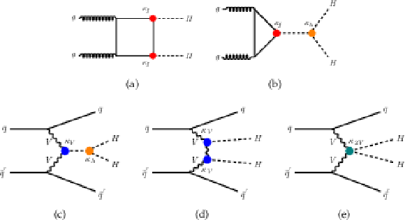
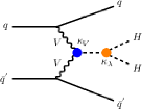
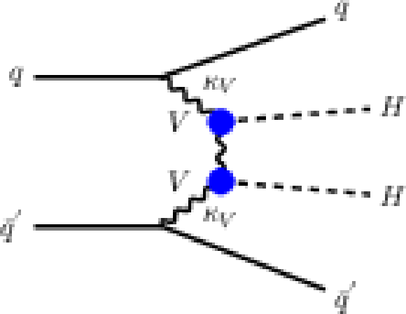
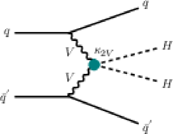
png pdf	Figure 1: Feynman diagrams that contribute to ggF and VBF HH production at leading order with coupling modifiers affecting the Higgs-to-fermion coupling $ \kappa_f $, to vector-boson coupling $ \kappa_{\text{V}} $, to two-vector-boson vertices $ \kappa_{\text{2V}} $ and self-coupling $ \kappa_{\lambda} $.
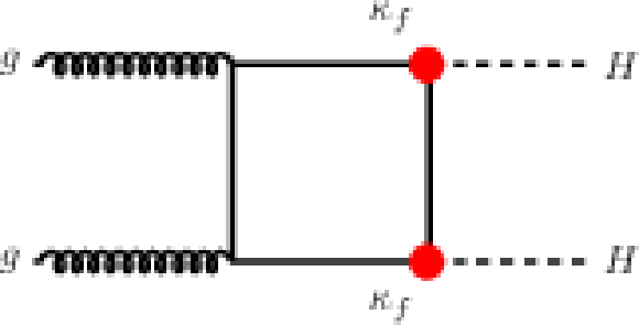
png pdf	Figure 1-a: Feynman diagrams that contribute to ggF and VBF HH production at leading order with coupling modifiers affecting the Higgs-to-fermion coupling $ \kappa_f $, to vector-boson coupling $ \kappa_{\text{V}} $, to two-vector-boson vertices $ \kappa_{\text{2V}} $ and self-coupling $ \kappa_{\lambda} $.
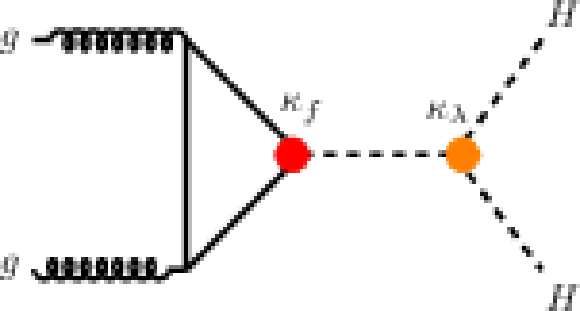
png pdf	Figure 1-b: Feynman diagrams that contribute to ggF and VBF HH production at leading order with coupling modifiers affecting the Higgs-to-fermion coupling $ \kappa_f $, to vector-boson coupling $ \kappa_{\text{V}} $, to two-vector-boson vertices $ \kappa_{\text{2V}} $ and self-coupling $ \kappa_{\lambda} $.
png pdf	Figure 1-c: Feynman diagrams that contribute to ggF and VBF HH production at leading order with coupling modifiers affecting the Higgs-to-fermion coupling $ \kappa_f $, to vector-boson coupling $ \kappa_{\text{V}} $, to two-vector-boson vertices $ \kappa_{\text{2V}} $ and self-coupling $ \kappa_{\lambda} $.
png pdf	Figure 1-d: Feynman diagrams that contribute to ggF and VBF HH production at leading order with coupling modifiers affecting the Higgs-to-fermion coupling $ \kappa_f $, to vector-boson coupling $ \kappa_{\text{V}} $, to two-vector-boson vertices $ \kappa_{\text{2V}} $ and self-coupling $ \kappa_{\lambda} $.
png pdf	Figure 1-e: Feynman diagrams that contribute to ggF and VBF HH production at leading order with coupling modifiers affecting the Higgs-to-fermion coupling $ \kappa_f $, to vector-boson coupling $ \kappa_{\text{V}} $, to two-vector-boson vertices $ \kappa_{\text{2V}} $ and self-coupling $ \kappa_{\lambda} $.
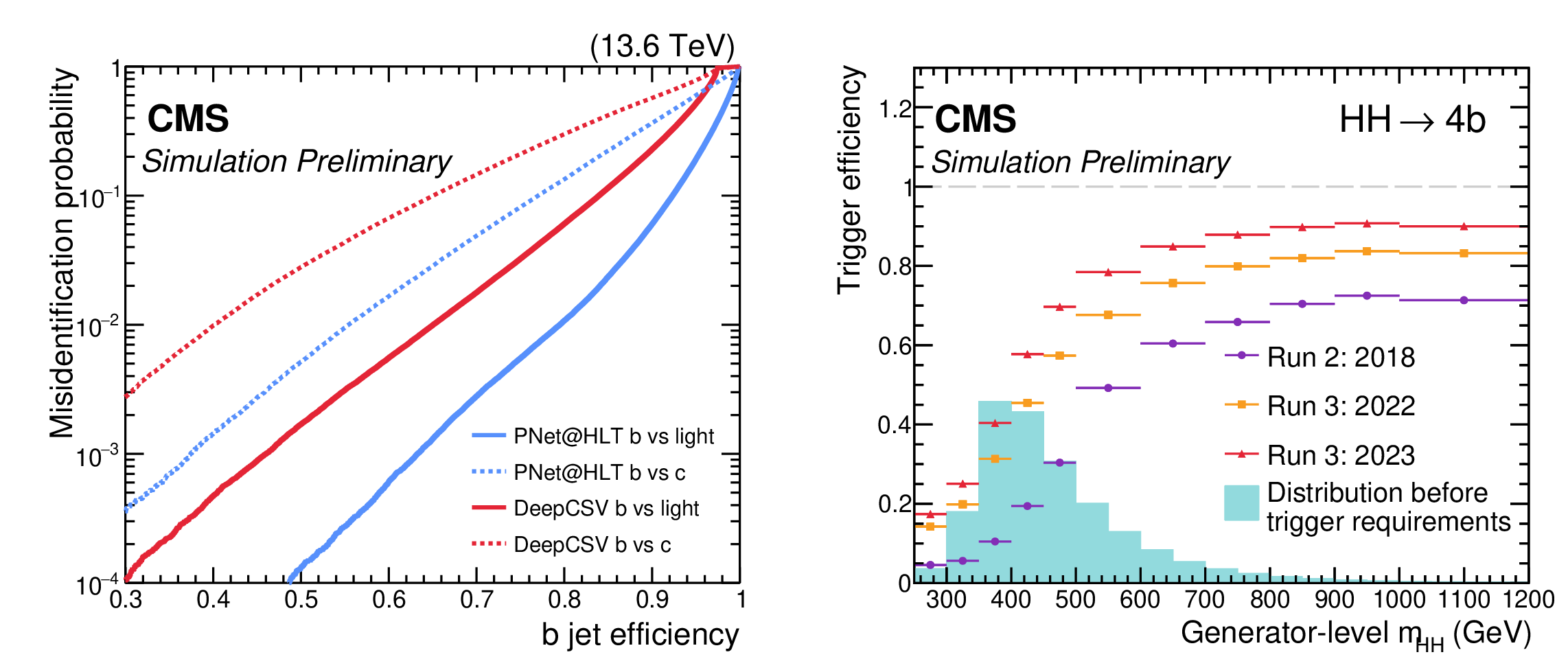
png pdf	Figure 2: Left: the b tagging performance of the Run 3 PNET@HLT algorithm (in blue) compared to the best-performing algorithm deployed at HLT in Run 2 (DEEPCSV, in red), as evaluated from $ \mathrm{t} \overline{\mathrm{t}} $ simulation on trigger-level AK4 jets with $ p_{\mathrm{T}} > $ 30 GeV and $ {|\eta| < 2.5} $. Right: efficiency of the triggers targeting the resolved $ \mathrm{H}\mathrm{H} \to 4\mathrm{b} $ topology as a function of the generator-level $ m_{\mathrm{H}\mathrm{H}} $ in simulated SM $ \mathrm{H}\mathrm{H} \to 4\mathrm{b} $ signal events in which the generator-level jets from the b quarks produced by $ \mathrm{H}\to \mathrm{b}\overline{\mathrm{b}} $ decays have $ p_{\mathrm{T}} $ larger than 25 GeV and $ {|\eta| < 2.5} $. The teal histogram shows the expected distribution for the SM $ \mathrm{g}\mathrm{g}\mathrm{H}\mathrm{H} $ signal prior to any trigger selections.
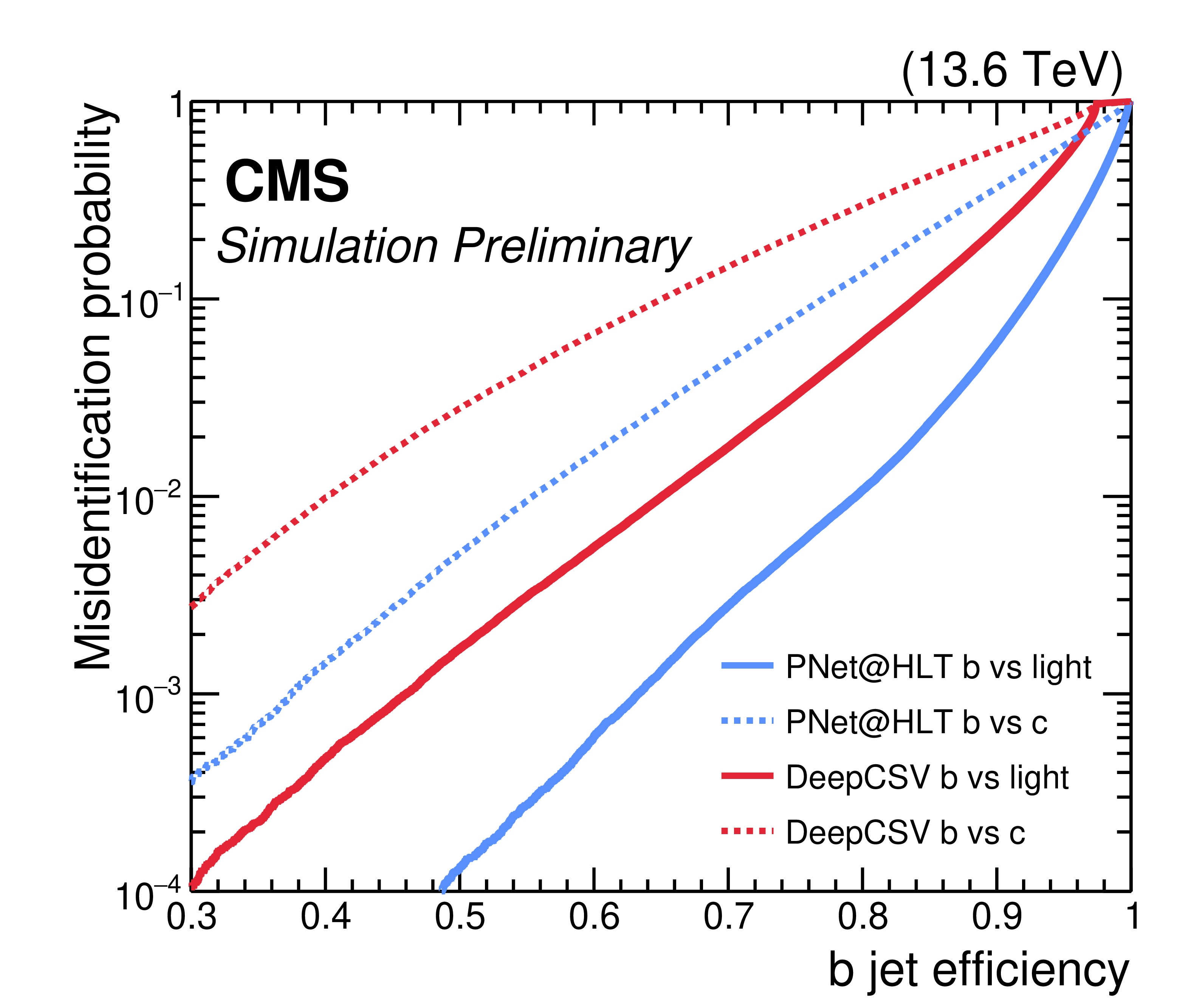
png pdf	Figure 2-a: Left: the b tagging performance of the Run 3 PNET@HLT algorithm (in blue) compared to the best-performing algorithm deployed at HLT in Run 2 (DEEPCSV, in red), as evaluated from $ \mathrm{t} \overline{\mathrm{t}} $ simulation on trigger-level AK4 jets with $ p_{\mathrm{T}} > $ 30 GeV and $ {|\eta| < 2.5} $. Right: efficiency of the triggers targeting the resolved $ \mathrm{H}\mathrm{H} \to 4\mathrm{b} $ topology as a function of the generator-level $ m_{\mathrm{H}\mathrm{H}} $ in simulated SM $ \mathrm{H}\mathrm{H} \to 4\mathrm{b} $ signal events in which the generator-level jets from the b quarks produced by $ \mathrm{H}\to \mathrm{b}\overline{\mathrm{b}} $ decays have $ p_{\mathrm{T}} $ larger than 25 GeV and $ {|\eta| < 2.5} $. The teal histogram shows the expected distribution for the SM $ \mathrm{g}\mathrm{g}\mathrm{H}\mathrm{H} $ signal prior to any trigger selections.
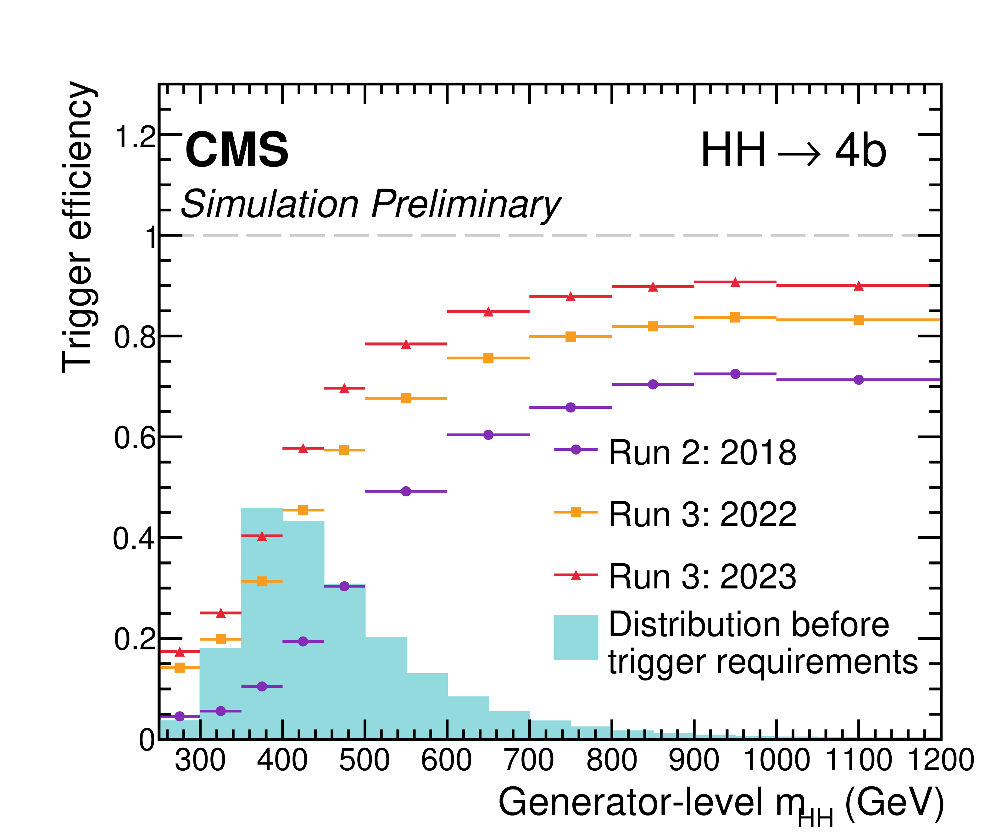
png pdf	Figure 2-b: Left: the b tagging performance of the Run 3 PNET@HLT algorithm (in blue) compared to the best-performing algorithm deployed at HLT in Run 2 (DEEPCSV, in red), as evaluated from $ \mathrm{t} \overline{\mathrm{t}} $ simulation on trigger-level AK4 jets with $ p_{\mathrm{T}} > $ 30 GeV and $ {|\eta| < 2.5} $. Right: efficiency of the triggers targeting the resolved $ \mathrm{H}\mathrm{H} \to 4\mathrm{b} $ topology as a function of the generator-level $ m_{\mathrm{H}\mathrm{H}} $ in simulated SM $ \mathrm{H}\mathrm{H} \to 4\mathrm{b} $ signal events in which the generator-level jets from the b quarks produced by $ \mathrm{H}\to \mathrm{b}\overline{\mathrm{b}} $ decays have $ p_{\mathrm{T}} $ larger than 25 GeV and $ {|\eta| < 2.5} $. The teal histogram shows the expected distribution for the SM $ \mathrm{g}\mathrm{g}\mathrm{H}\mathrm{H} $ signal prior to any trigger selections.
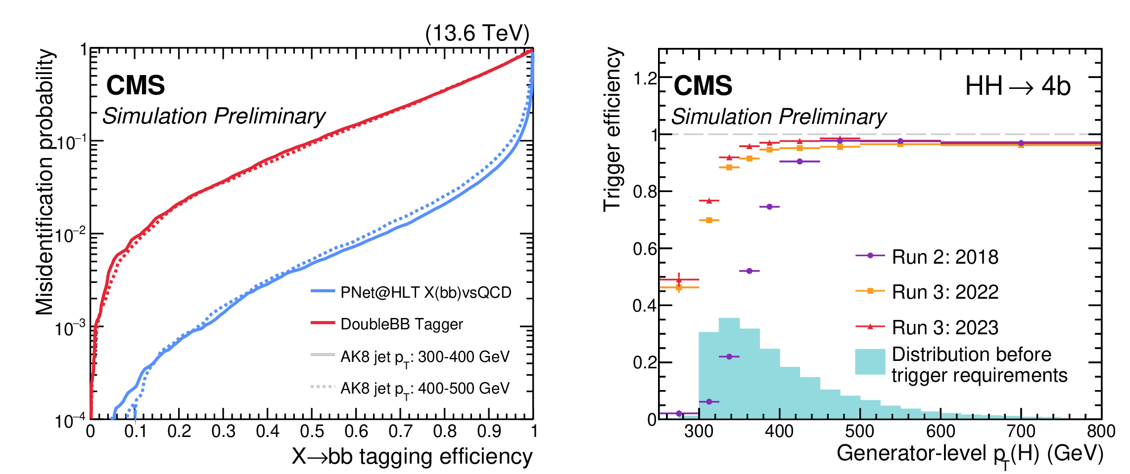
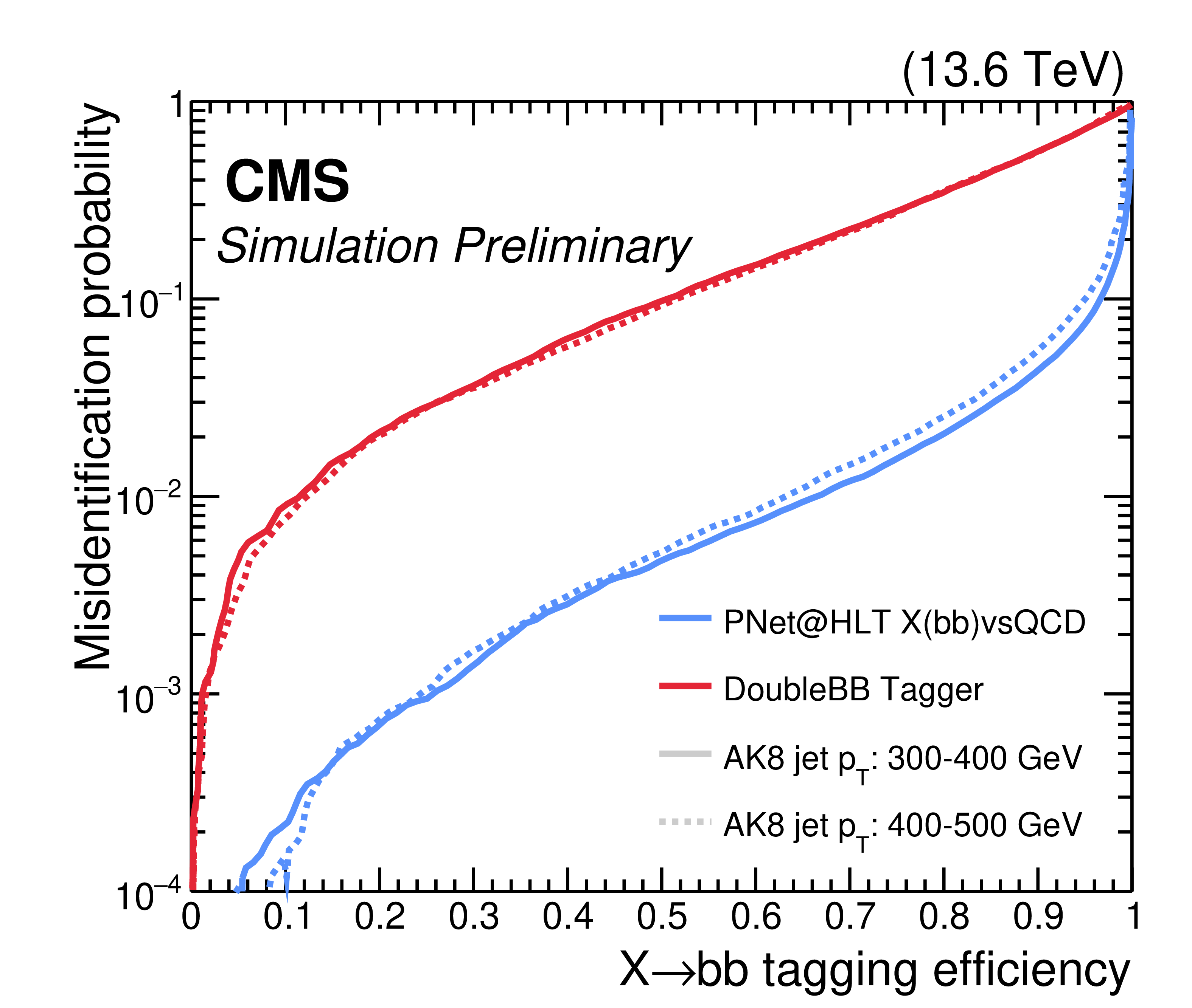
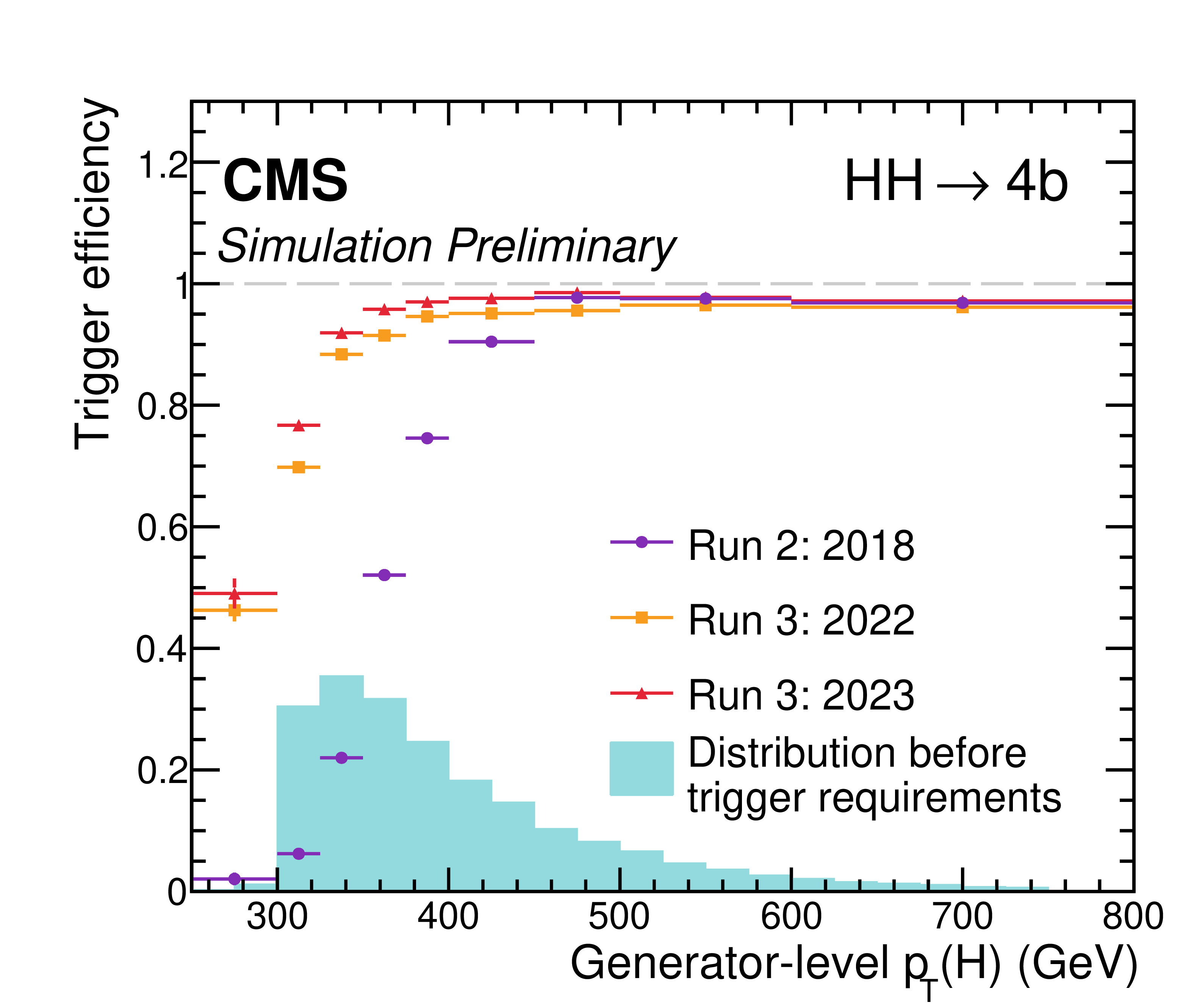
png pdf	Figure 3: Left: the $ \mathrm{b}\overline{\mathrm{b}} $ tagging performance of the PNET@HLT algorithm (in blue) compared to the highest-performing Run 2 algorithm (DOUBLEBB, in red), as evaluated on AK8 jets in the HLT from simulated $ \mathrm{H}\mathrm{H} \to 4\mathrm{b} $ and QCD multijet events with $ p_{\mathrm{T}} > $ 300 GeV and $ {|\eta| < 2.5} $. Right: efficiency of the logical or of the trigger paths developed for the merged topology, as a function of the generator-level leading H candidate $ p_{\mathrm{T}} $ in simulated SM $ \mathrm{H}\mathrm{H} \to 4\mathrm{b} $ events in which $ {\Delta R(\mathrm{b},\overline{\mathrm{b}}) < 0.8} $. The teal histogram shows the expected distribution for the SM $ \mathrm{g}\mathrm{g}\mathrm{H}\mathrm{H} $ signal prior to any selections.
png pdf	Figure 3-a: Left: the $ \mathrm{b}\overline{\mathrm{b}} $ tagging performance of the PNET@HLT algorithm (in blue) compared to the highest-performing Run 2 algorithm (DOUBLEBB, in red), as evaluated on AK8 jets in the HLT from simulated $ \mathrm{H}\mathrm{H} \to 4\mathrm{b} $ and QCD multijet events with $ p_{\mathrm{T}} > $ 300 GeV and $ {|\eta| < 2.5} $. Right: efficiency of the logical or of the trigger paths developed for the merged topology, as a function of the generator-level leading H candidate $ p_{\mathrm{T}} $ in simulated SM $ \mathrm{H}\mathrm{H} \to 4\mathrm{b} $ events in which $ {\Delta R(\mathrm{b},\overline{\mathrm{b}}) < 0.8} $. The teal histogram shows the expected distribution for the SM $ \mathrm{g}\mathrm{g}\mathrm{H}\mathrm{H} $ signal prior to any selections.
png pdf	Figure 3-b: Left: the $ \mathrm{b}\overline{\mathrm{b}} $ tagging performance of the PNET@HLT algorithm (in blue) compared to the highest-performing Run 2 algorithm (DOUBLEBB, in red), as evaluated on AK8 jets in the HLT from simulated $ \mathrm{H}\mathrm{H} \to 4\mathrm{b} $ and QCD multijet events with $ p_{\mathrm{T}} > $ 300 GeV and $ {|\eta| < 2.5} $. Right: efficiency of the logical or of the trigger paths developed for the merged topology, as a function of the generator-level leading H candidate $ p_{\mathrm{T}} $ in simulated SM $ \mathrm{H}\mathrm{H} \to 4\mathrm{b} $ events in which $ {\Delta R(\mathrm{b},\overline{\mathrm{b}}) < 0.8} $. The teal histogram shows the expected distribution for the SM $ \mathrm{g}\mathrm{g}\mathrm{H}\mathrm{H} $ signal prior to any selections.
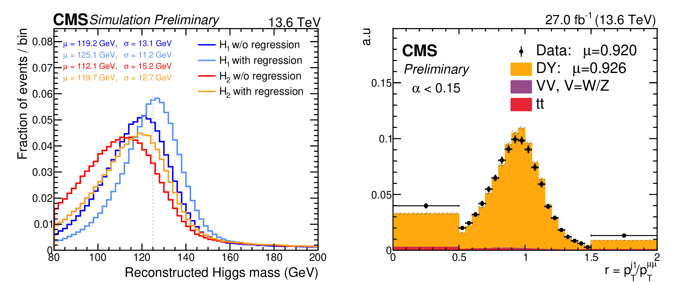
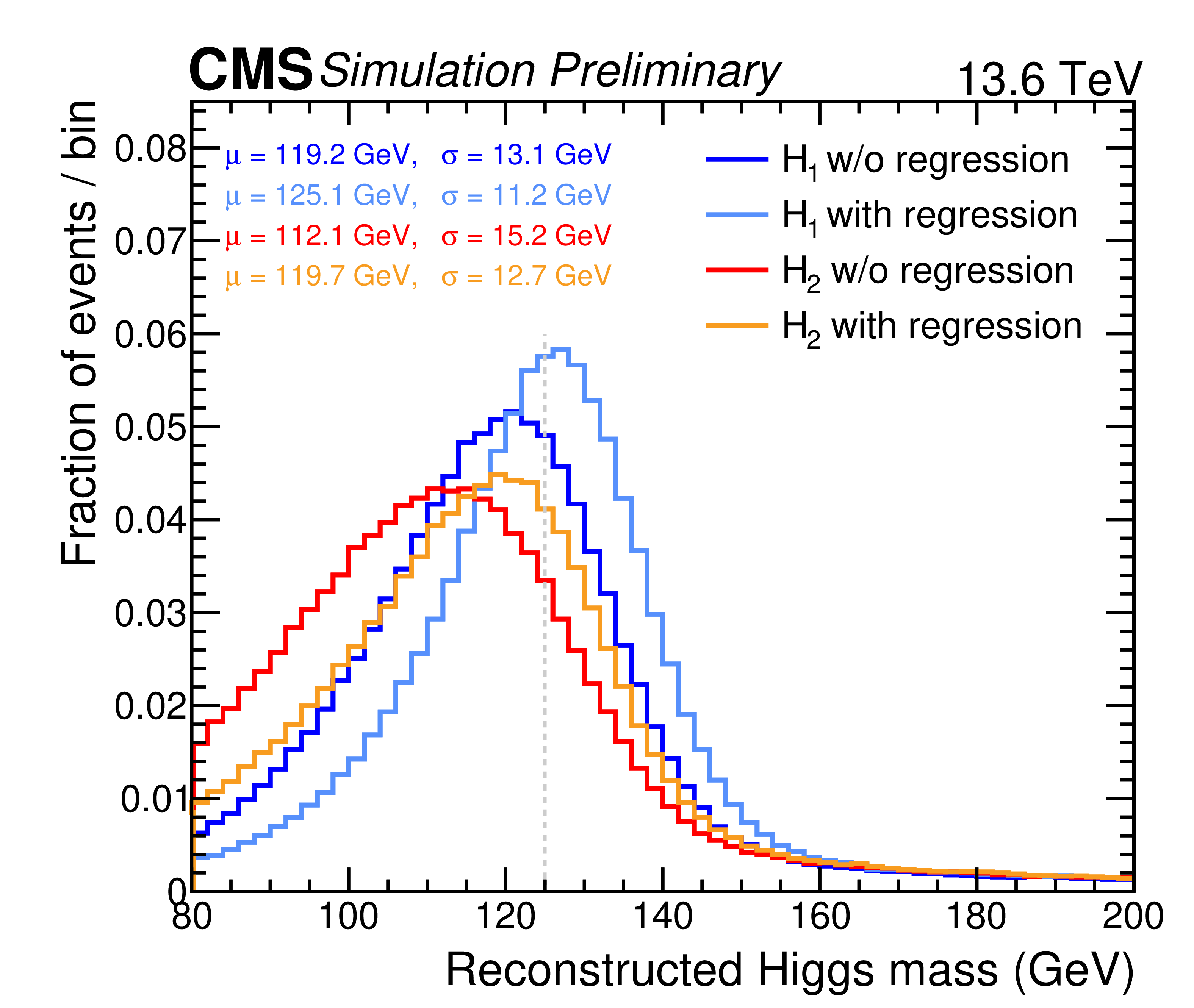
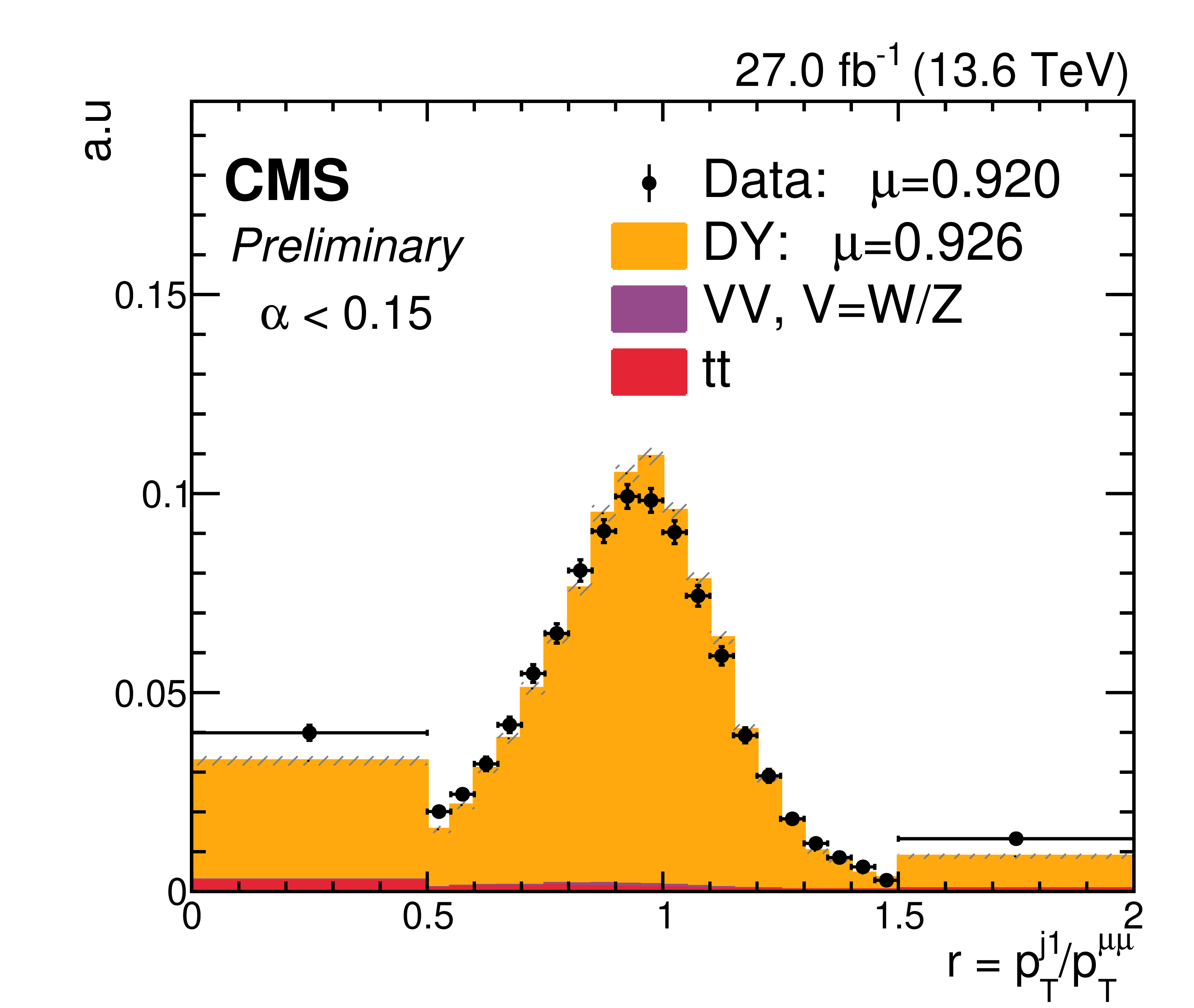
png pdf	Figure 4: Left: invariant mass distributions for the leading ($ m_{\mathrm{H}_1} $) and subleading ($ m_{\mathrm{H}_2} $) $ p_{\mathrm{T}} \mathrm{H} $ candidates in SM $ \mathrm{H}\mathrm{H} \to 4\mathrm{b} $ events obtained before and after the application of the PNET jet $ p_{\mathrm{T}} $ regression. Right: distribution of the $ p_{\mathrm{T}} $ balance, $ r=p_{\mathrm{T}}^{\mathrm{j_{1}}}/p_{\mathrm{T}}^{\mu\mu} $, in 2023 data and simulated events for the selected $ \mathrm{Z}(\mu\mu)+\mathrm{b}\text{-jet} $ region with $ \alpha=p_{\mathrm{T}}^{\mathrm{j_{2}}}/p_{\mathrm{T}}^{\mu\mu} < $ 0.15, obtained after applying the PNET jet $ p_{\mathrm{T}} $ regression. The $ \mu $ values quoted in the legend correspond to the mean of the distributions.
png pdf	Figure 4-a: Left: invariant mass distributions for the leading ($ m_{\mathrm{H}_1} $) and subleading ($ m_{\mathrm{H}_2} $) $ p_{\mathrm{T}} \mathrm{H} $ candidates in SM $ \mathrm{H}\mathrm{H} \to 4\mathrm{b} $ events obtained before and after the application of the PNET jet $ p_{\mathrm{T}} $ regression. Right: distribution of the $ p_{\mathrm{T}} $ balance, $ r=p_{\mathrm{T}}^{\mathrm{j_{1}}}/p_{\mathrm{T}}^{\mu\mu} $, in 2023 data and simulated events for the selected $ \mathrm{Z}(\mu\mu)+\mathrm{b}\text{-jet} $ region with $ \alpha=p_{\mathrm{T}}^{\mathrm{j_{2}}}/p_{\mathrm{T}}^{\mu\mu} < $ 0.15, obtained after applying the PNET jet $ p_{\mathrm{T}} $ regression. The $ \mu $ values quoted in the legend correspond to the mean of the distributions.
png pdf	Figure 4-b: Left: invariant mass distributions for the leading ($ m_{\mathrm{H}_1} $) and subleading ($ m_{\mathrm{H}_2} $) $ p_{\mathrm{T}} \mathrm{H} $ candidates in SM $ \mathrm{H}\mathrm{H} \to 4\mathrm{b} $ events obtained before and after the application of the PNET jet $ p_{\mathrm{T}} $ regression. Right: distribution of the $ p_{\mathrm{T}} $ balance, $ r=p_{\mathrm{T}}^{\mathrm{j_{1}}}/p_{\mathrm{T}}^{\mu\mu} $, in 2023 data and simulated events for the selected $ \mathrm{Z}(\mu\mu)+\mathrm{b}\text{-jet} $ region with $ \alpha=p_{\mathrm{T}}^{\mathrm{j_{2}}}/p_{\mathrm{T}}^{\mu\mu} < $ 0.15, obtained after applying the PNET jet $ p_{\mathrm{T}} $ regression. The $ \mu $ values quoted in the legend correspond to the mean of the distributions.
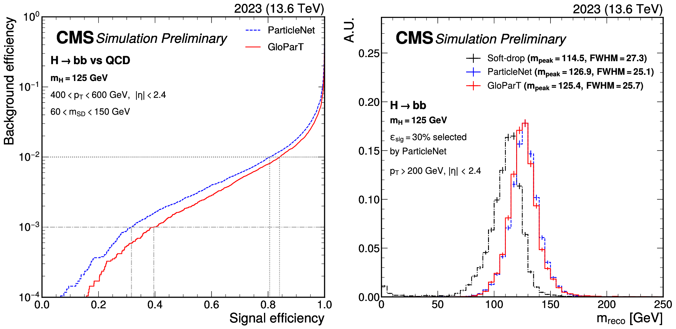
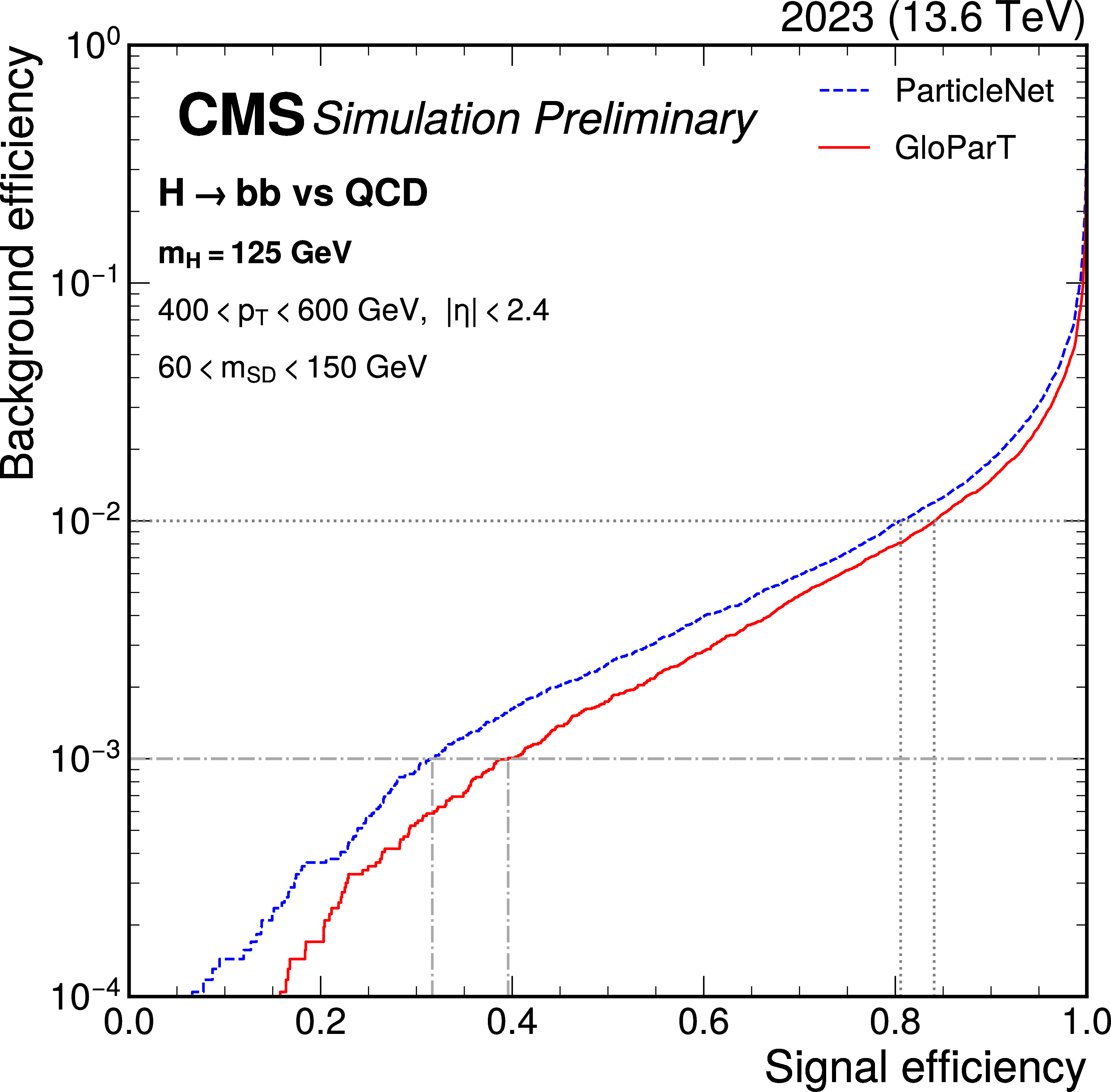
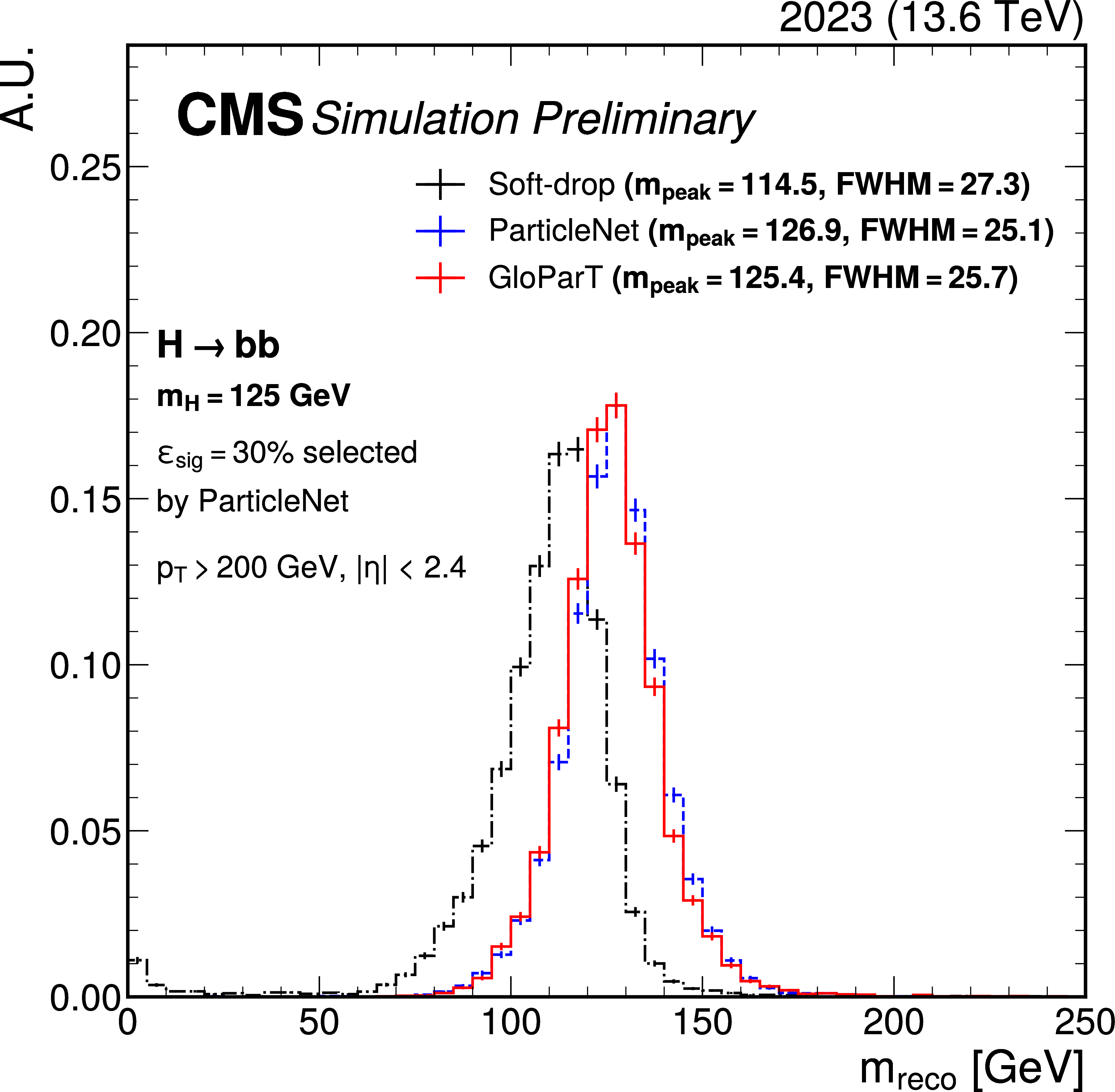
png pdf	Figure 5: The ROC curve for GLOPART and PNET for discriminating $ \mathrm{H}\to\mathrm{b}\overline{\mathrm{b}} $ from QCD jets with 400 $ < p_{\mathrm{T}} < $ 600 GeV, $ |\eta| < $ 2.4, and 60 $ < m_\text{SD} < $ 150 GeV (left). The mass regression performance for GLOPART and PNET for jets with $ p_{\mathrm{T}} > $ 200 GeV, $ |\eta| < $ 2.4, and satisfying a PNET selection corresponding to 30% signal efficiency (right). The conditions correspond to those during data collection in 2023.
png pdf	Figure 5-a: The ROC curve for GLOPART and PNET for discriminating $ \mathrm{H}\to\mathrm{b}\overline{\mathrm{b}} $ from QCD jets with 400 $ < p_{\mathrm{T}} < $ 600 GeV, $ |\eta| < $ 2.4, and 60 $ < m_\text{SD} < $ 150 GeV (left). The mass regression performance for GLOPART and PNET for jets with $ p_{\mathrm{T}} > $ 200 GeV, $ |\eta| < $ 2.4, and satisfying a PNET selection corresponding to 30% signal efficiency (right). The conditions correspond to those during data collection in 2023.
png pdf	Figure 5-b: The ROC curve for GLOPART and PNET for discriminating $ \mathrm{H}\to\mathrm{b}\overline{\mathrm{b}} $ from QCD jets with 400 $ < p_{\mathrm{T}} < $ 600 GeV, $ |\eta| < $ 2.4, and 60 $ < m_\text{SD} < $ 150 GeV (left). The mass regression performance for GLOPART and PNET for jets with $ p_{\mathrm{T}} > $ 200 GeV, $ |\eta| < $ 2.4, and satisfying a PNET selection corresponding to 30% signal efficiency (right). The conditions correspond to those during data collection in 2023.
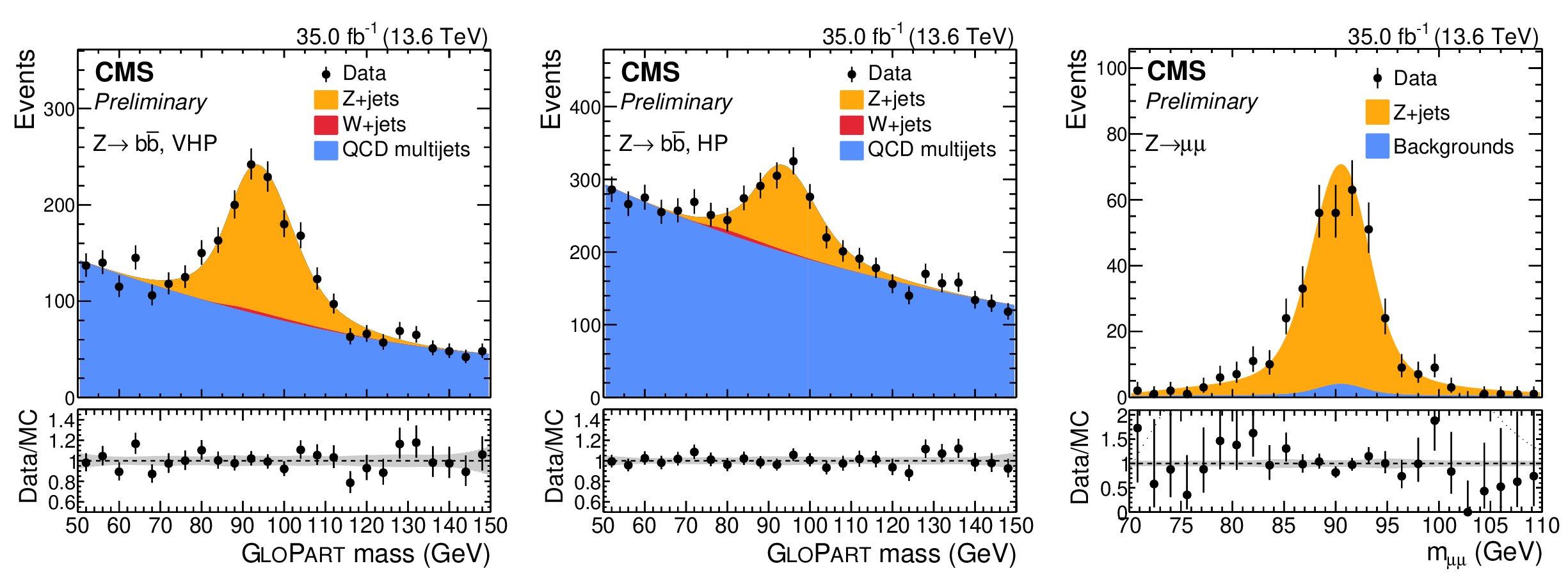
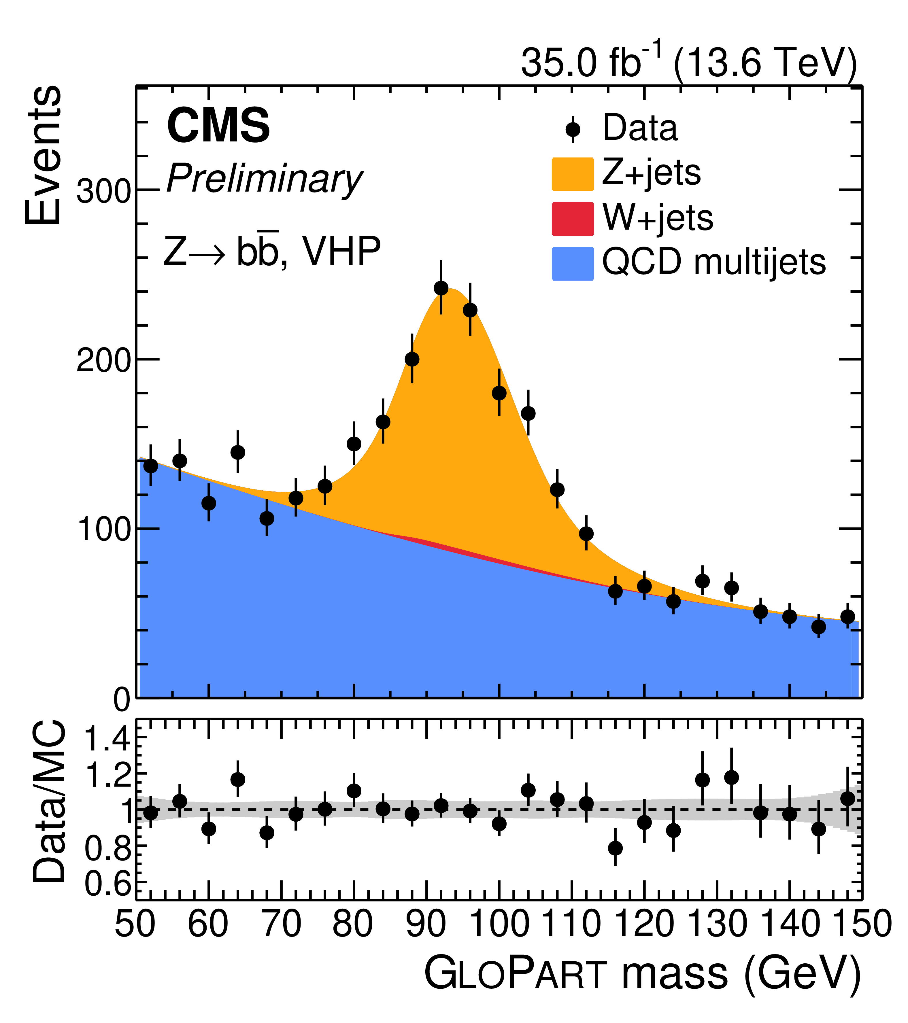
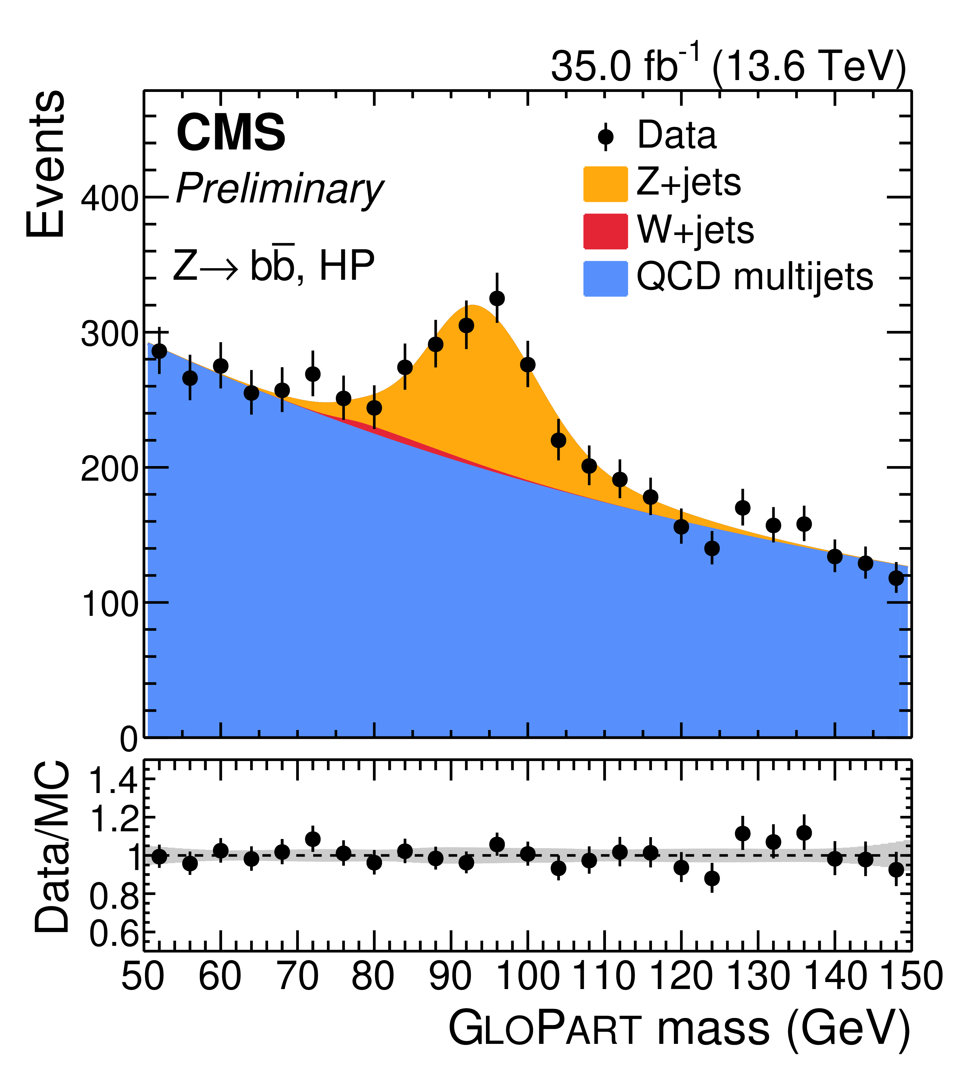
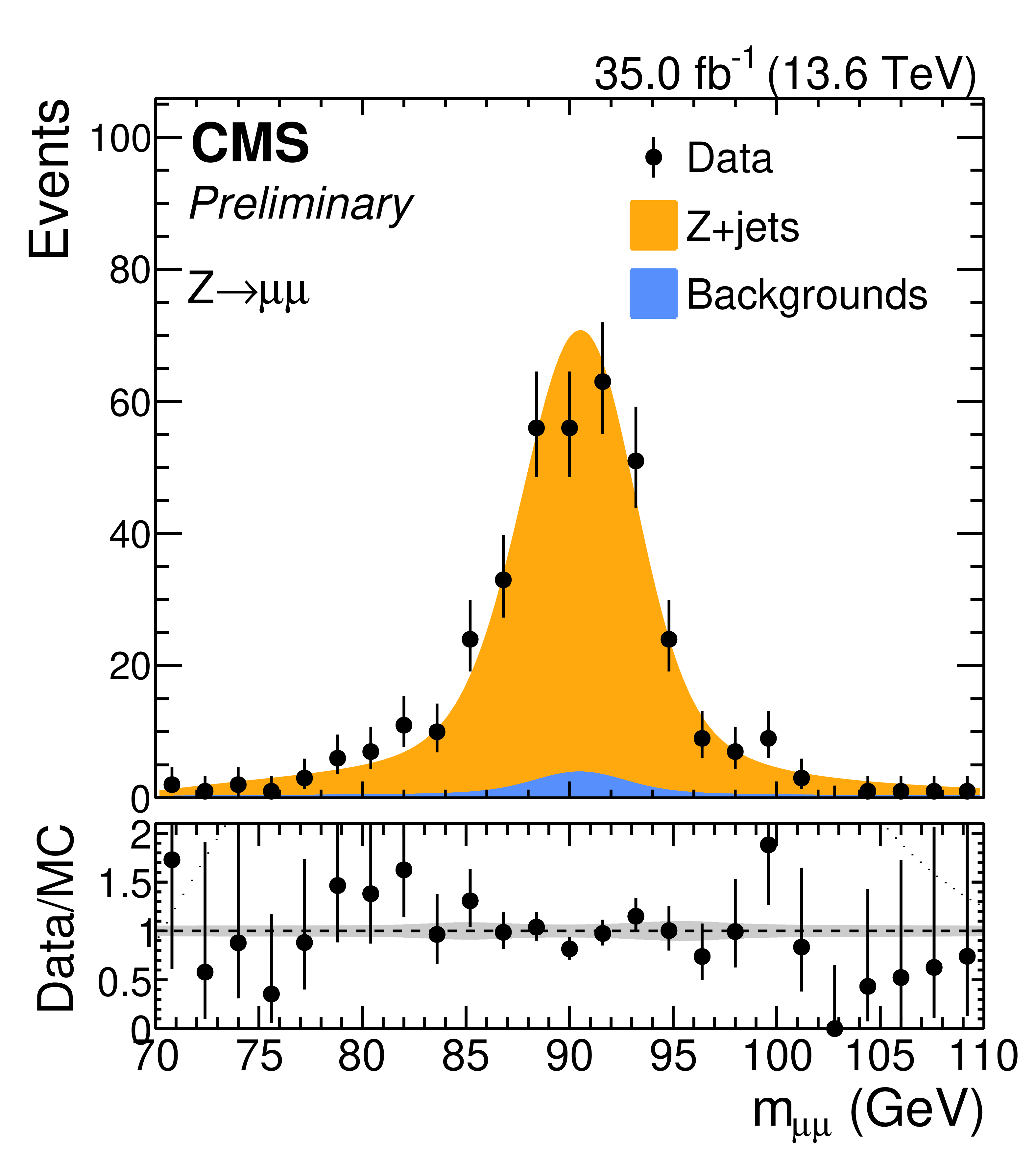
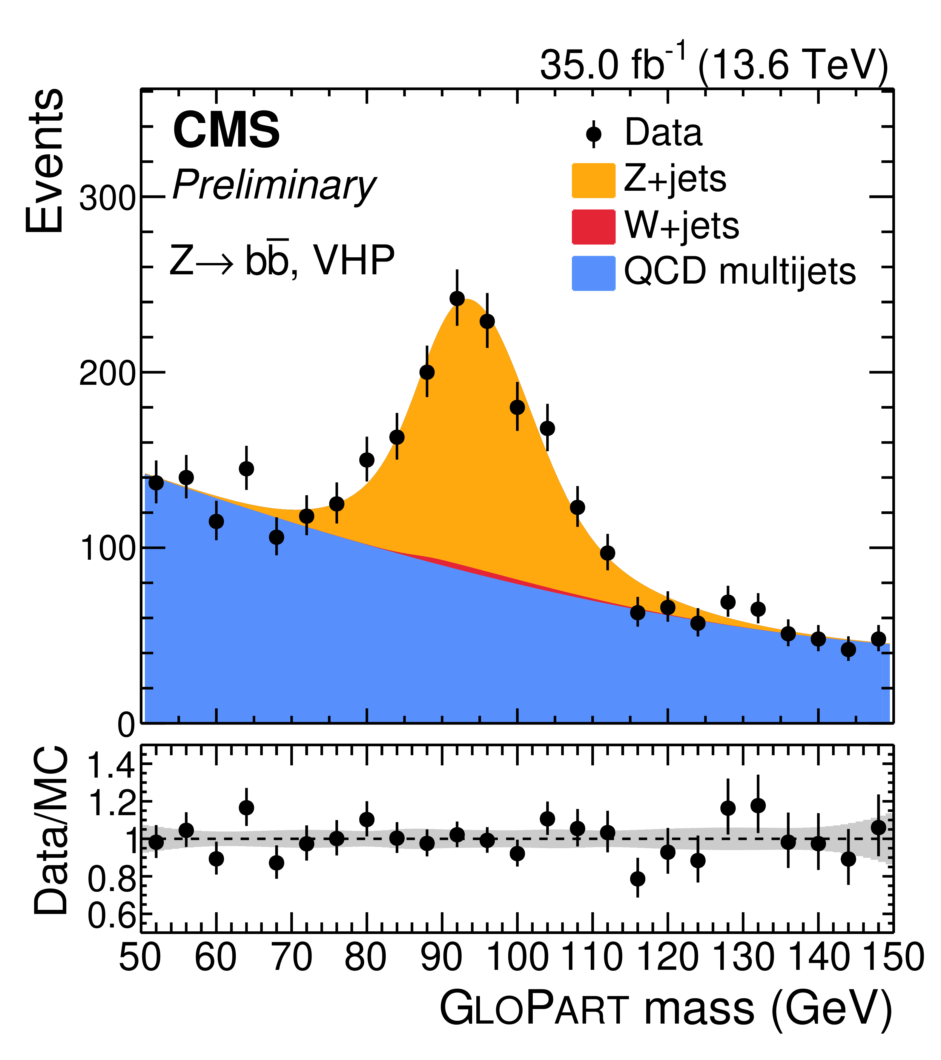
png pdf	Figure 6: Comparison between data and fit prediction from a simultaneous signal-plus-background fit to the GLOPART regressed jet mass distributions in $ \mathrm{Z} \to \mathrm{b}\overline{\mathrm{b}} $ VHP (left) and HP (middle) categories. Data corresponds to the full integrated luminosity collected by the CMS detector in 2022. The same comparison is performed for the $ m_{\mu\mu} $ distributions in the $ \mathrm{Z} \to \mu\mu $ region (right). Each process considered in the fit is modeled via a parametric function as described in the text.
png pdf	Figure 6-a: Comparison between data and fit prediction from a simultaneous signal-plus-background fit to the GLOPART regressed jet mass distributions in $ \mathrm{Z} \to \mathrm{b}\overline{\mathrm{b}} $ VHP (left) and HP (middle) categories. Data corresponds to the full integrated luminosity collected by the CMS detector in 2022. The same comparison is performed for the $ m_{\mu\mu} $ distributions in the $ \mathrm{Z} \to \mu\mu $ region (right). Each process considered in the fit is modeled via a parametric function as described in the text.
png pdf	Figure 6-b: Comparison between data and fit prediction from a simultaneous signal-plus-background fit to the GLOPART regressed jet mass distributions in $ \mathrm{Z} \to \mathrm{b}\overline{\mathrm{b}} $ VHP (left) and HP (middle) categories. Data corresponds to the full integrated luminosity collected by the CMS detector in 2022. The same comparison is performed for the $ m_{\mu\mu} $ distributions in the $ \mathrm{Z} \to \mu\mu $ region (right). Each process considered in the fit is modeled via a parametric function as described in the text.
png pdf	Figure 6-c: Comparison between data and fit prediction from a simultaneous signal-plus-background fit to the GLOPART regressed jet mass distributions in $ \mathrm{Z} \to \mathrm{b}\overline{\mathrm{b}} $ VHP (left) and HP (middle) categories. Data corresponds to the full integrated luminosity collected by the CMS detector in 2022. The same comparison is performed for the $ m_{\mu\mu} $ distributions in the $ \mathrm{Z} \to \mu\mu $ region (right). Each process considered in the fit is modeled via a parametric function as described in the text.
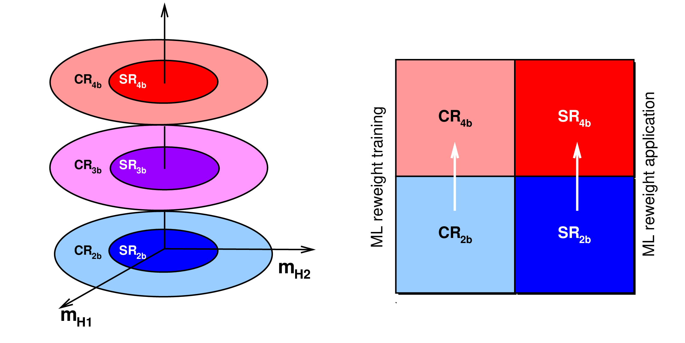
png pdf	Figure 7: Left: schematic diagram of the signal regions (dark shaded circles) and control regions (annular regions) in the $ m_{\mathrm{H}_1} $--$ m_{\mathrm{H}_2} $ mass plane as a function of $N_{\mathrm{b jet}}$. Right: schematic diagram showing the background estimation strategy, which applies a multidimensional reweighting of events from $ \mathrm{SR_{2\mathrm{b}}} $ to $ \mathrm{SR_{4\mathrm{b}}} $.
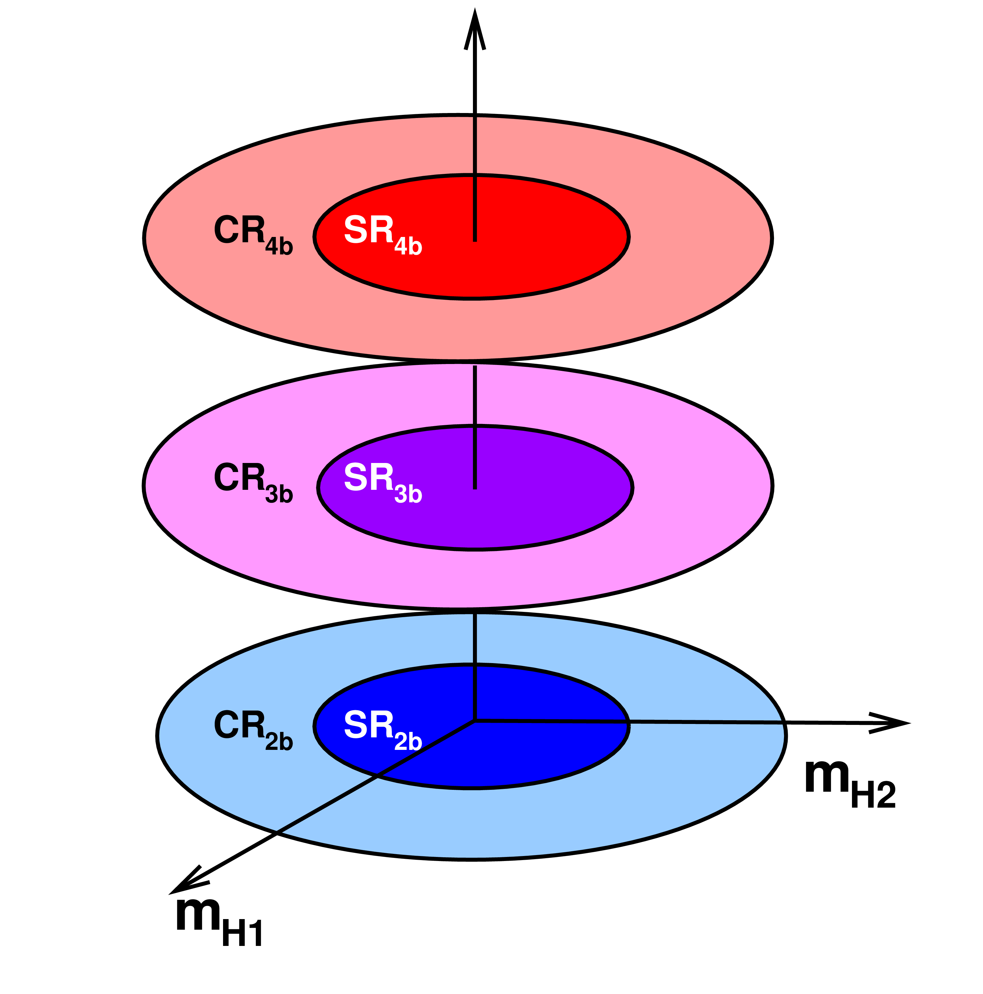
png pdf	Figure 7-a: Left: schematic diagram of the signal regions (dark shaded circles) and control regions (annular regions) in the $ m_{\mathrm{H}_1} $--$ m_{\mathrm{H}_2} $ mass plane as a function of $N_{\mathrm{b jet}}$. Right: schematic diagram showing the background estimation strategy, which applies a multidimensional reweighting of events from $ \mathrm{SR_{2\mathrm{b}}} $ to $ \mathrm{SR_{4\mathrm{b}}} $.
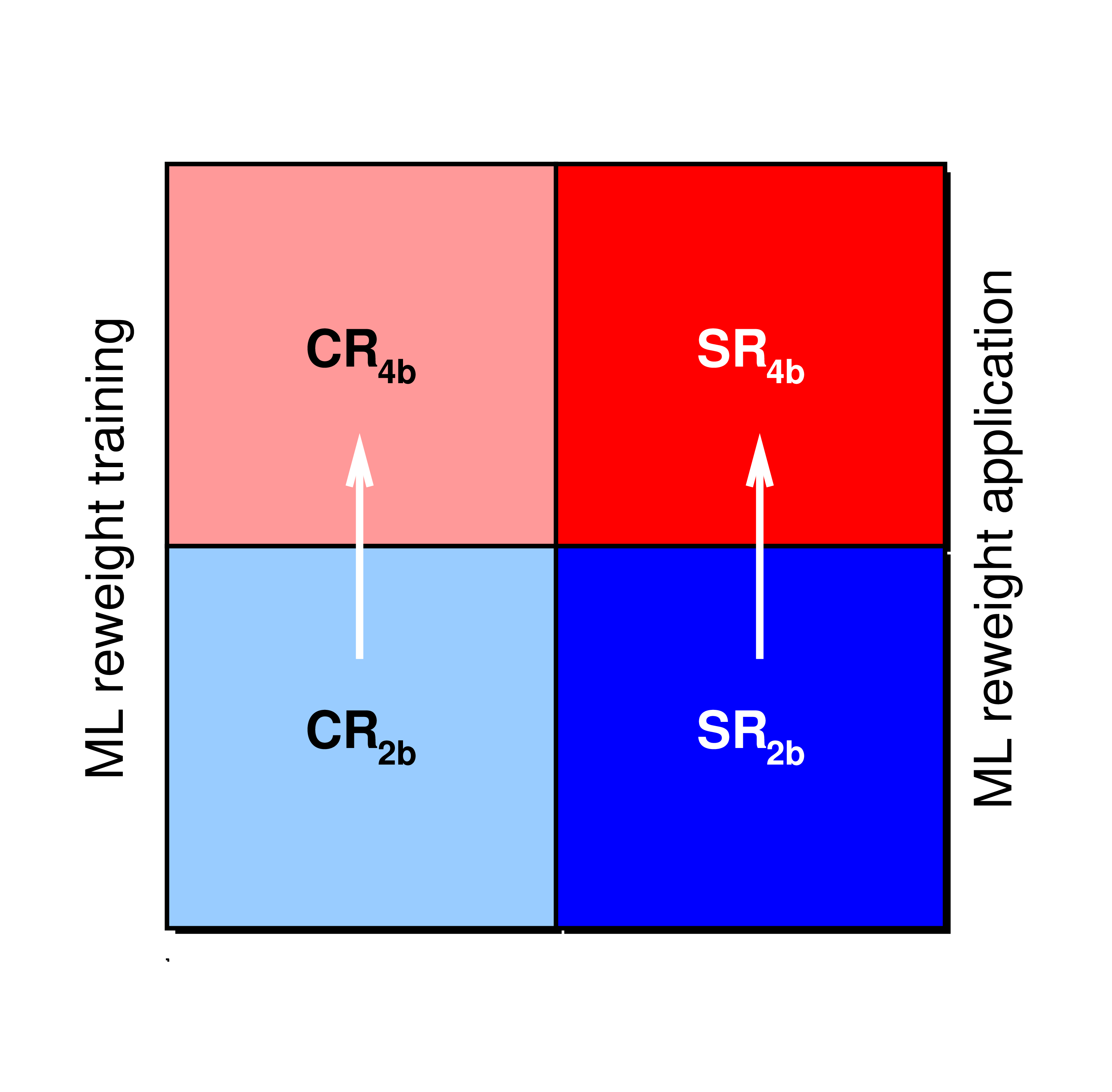
png pdf	Figure 7-b: Left: schematic diagram of the signal regions (dark shaded circles) and control regions (annular regions) in the $ m_{\mathrm{H}_1} $--$ m_{\mathrm{H}_2} $ mass plane as a function of $N_{\mathrm{b jet}}$. Right: schematic diagram showing the background estimation strategy, which applies a multidimensional reweighting of events from $ \mathrm{SR_{2\mathrm{b}}} $ to $ \mathrm{SR_{4\mathrm{b}}} $.
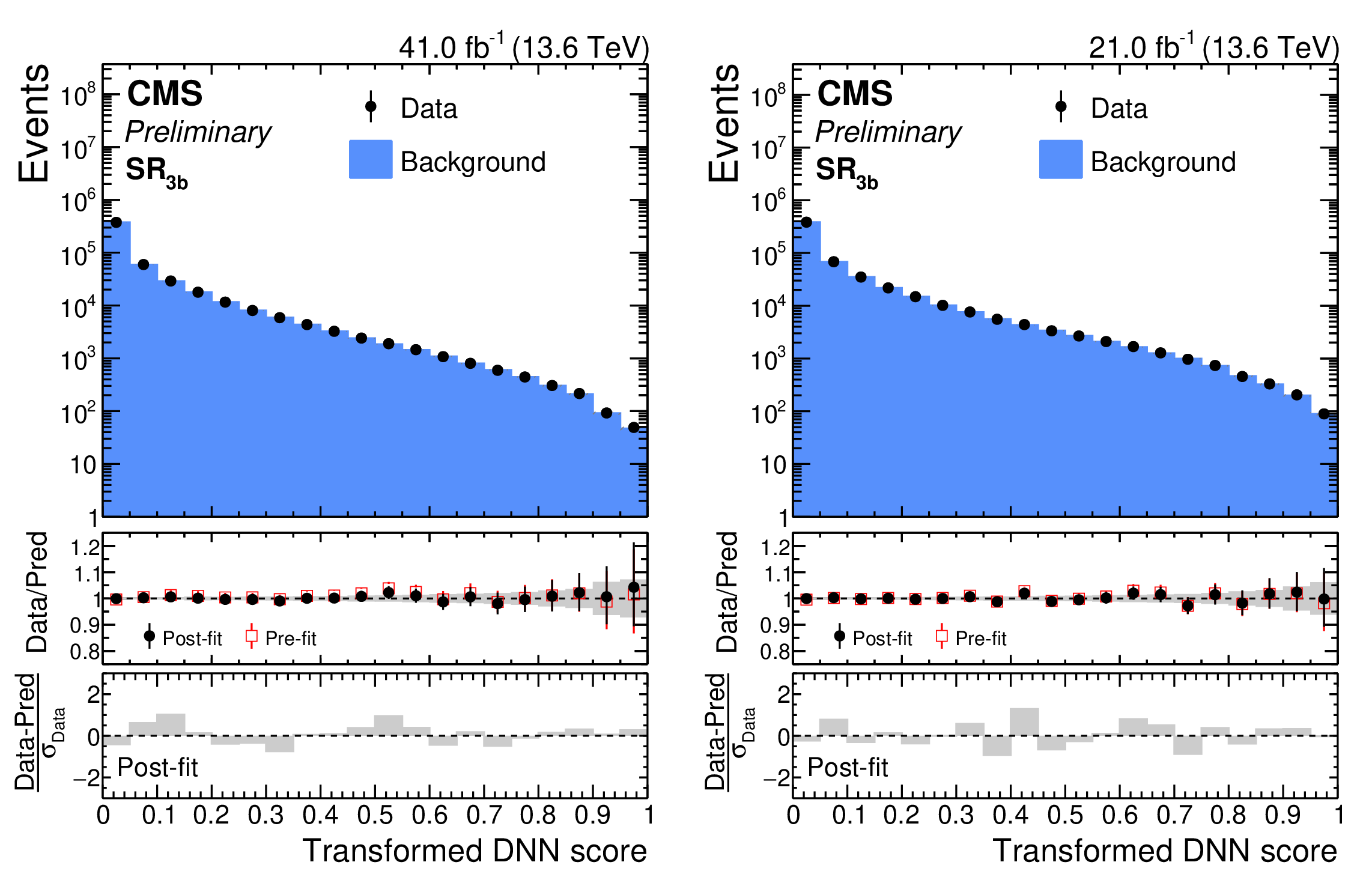
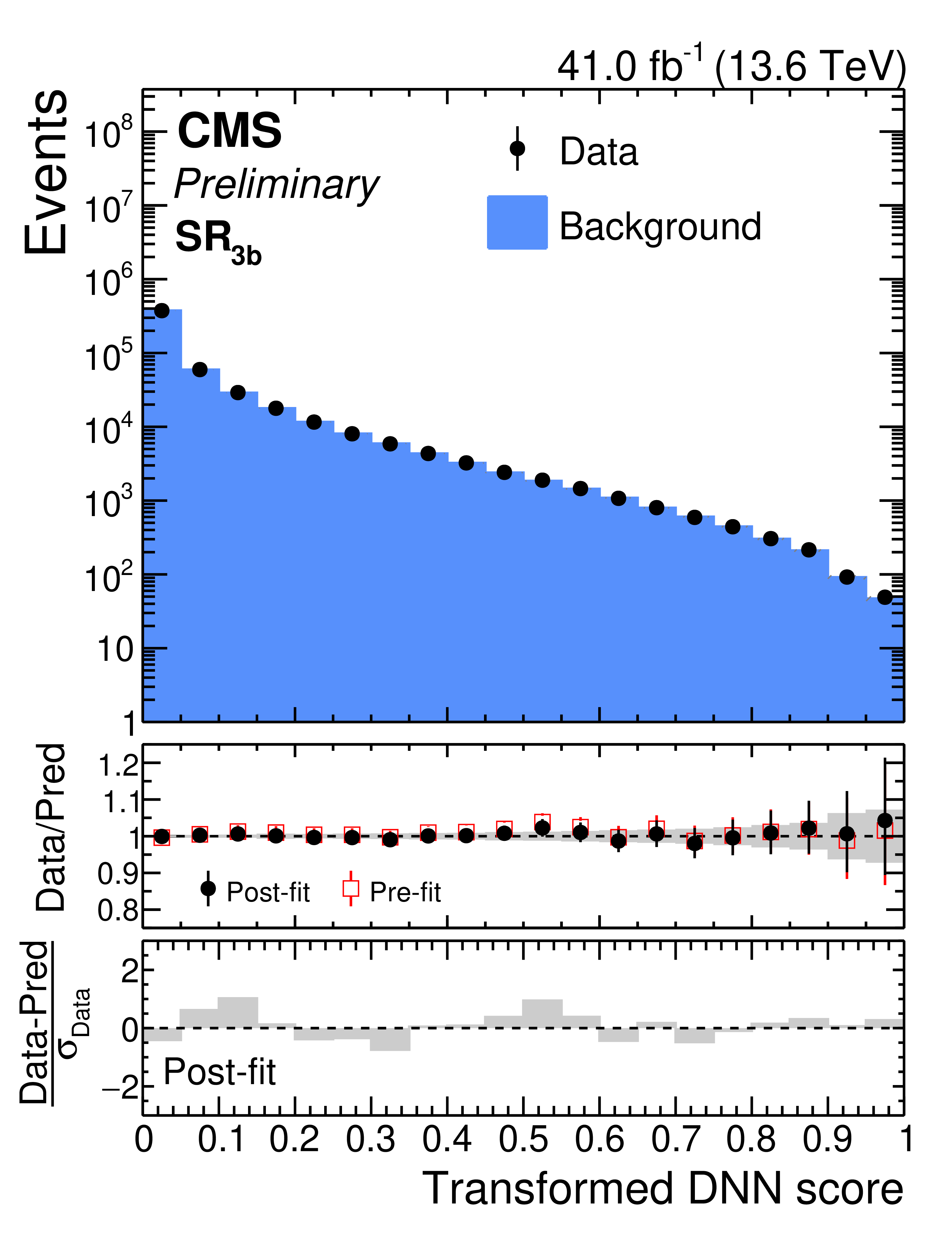
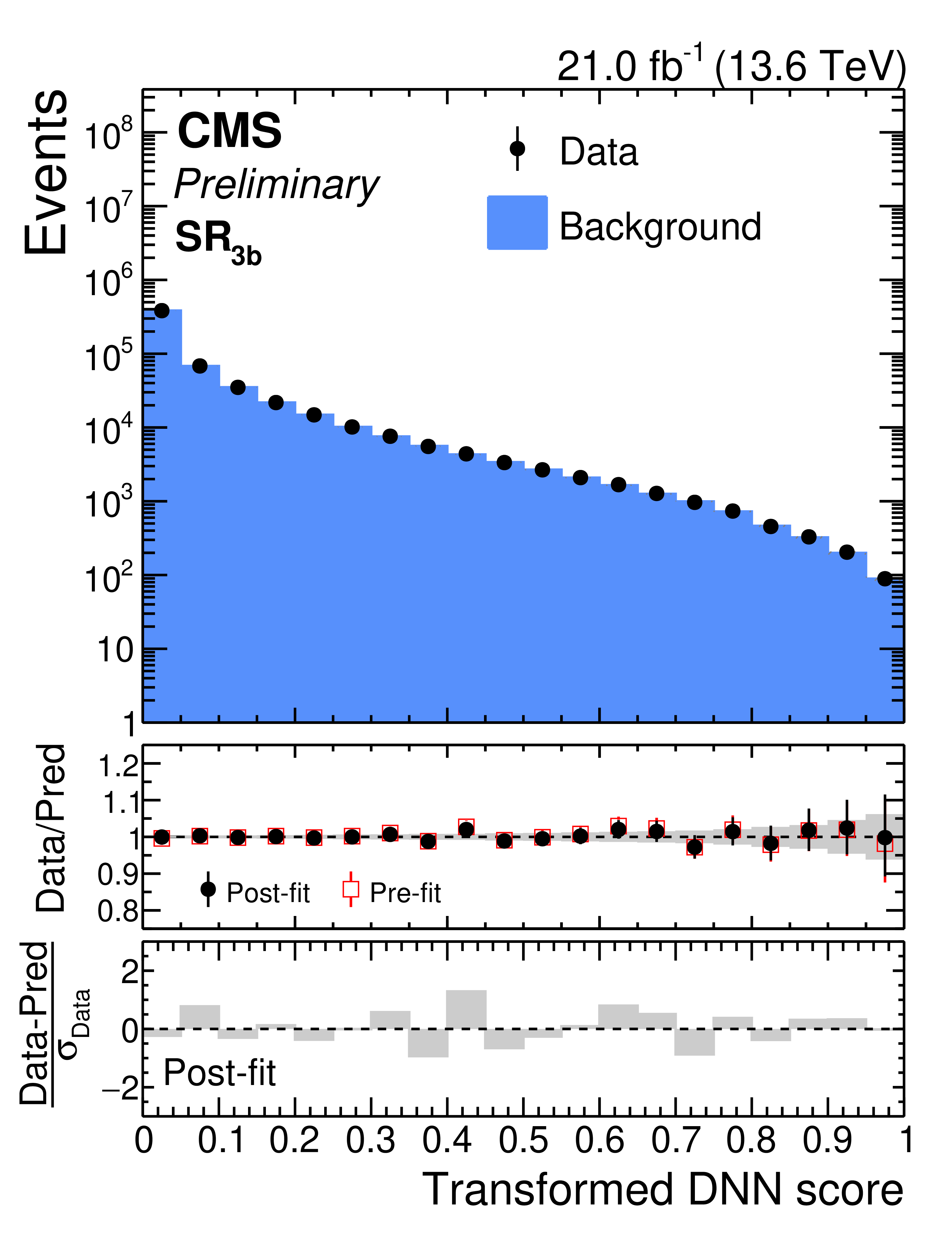
png pdf	Figure 8: Distribution of the SvsB classifier score in the $ \mathrm{g}\mathrm{g}\mathrm{H}\mathrm{H} $ category for $ \mathrm{SR_{3\mathrm{b}}} $ data (black points) compared to the data-driven background prediction (blue histogram), for the pre-ParkingHH (left) and post-ParkingHH (right) data sets. The middle panel shows the ratio of data to the pre-fit (red open markers) and post b-only fit (black solid markers) background prediction, with the gray band indicating the background post-fit uncertainty. The lower panel show the distribution of the pulls, defined as the difference between the data and the post-fit background prediction, divided by the statistical uncertainty in the data.
png pdf	Figure 8-a: Distribution of the SvsB classifier score in the $ \mathrm{g}\mathrm{g}\mathrm{H}\mathrm{H} $ category for $ \mathrm{SR_{3\mathrm{b}}} $ data (black points) compared to the data-driven background prediction (blue histogram), for the pre-ParkingHH (left) and post-ParkingHH (right) data sets. The middle panel shows the ratio of data to the pre-fit (red open markers) and post b-only fit (black solid markers) background prediction, with the gray band indicating the background post-fit uncertainty. The lower panel show the distribution of the pulls, defined as the difference between the data and the post-fit background prediction, divided by the statistical uncertainty in the data.
png pdf	Figure 8-b: Distribution of the SvsB classifier score in the $ \mathrm{g}\mathrm{g}\mathrm{H}\mathrm{H} $ category for $ \mathrm{SR_{3\mathrm{b}}} $ data (black points) compared to the data-driven background prediction (blue histogram), for the pre-ParkingHH (left) and post-ParkingHH (right) data sets. The middle panel shows the ratio of data to the pre-fit (red open markers) and post b-only fit (black solid markers) background prediction, with the gray band indicating the background post-fit uncertainty. The lower panel show the distribution of the pulls, defined as the difference between the data and the post-fit background prediction, divided by the statistical uncertainty in the data.
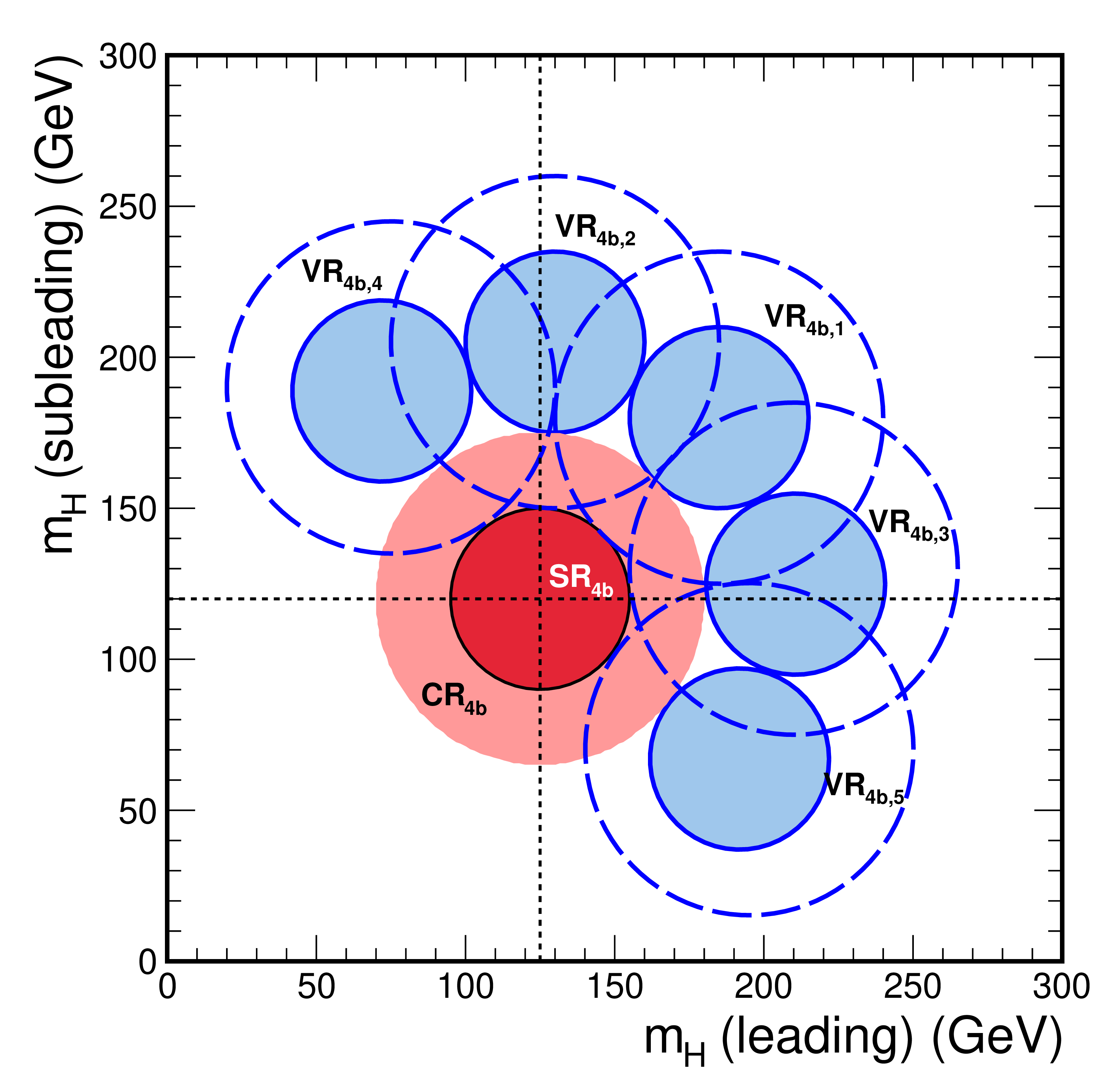
png pdf	Figure 9: A schematic diagram of the 4b validation regions defined in the $ m_{\mathrm{H}_1} $--$ m_{\mathrm{H}_2} $ mass plane and orthogonal to the $ \mathrm{SR_{4\mathrm{b}}} $. In each validation region, the solid blue area identifies the signal region, while the dashed blue lines indicate the corresponding control region. The ``leading'' H candidate is the one with largest $ p_{\mathrm{T}} $(H).
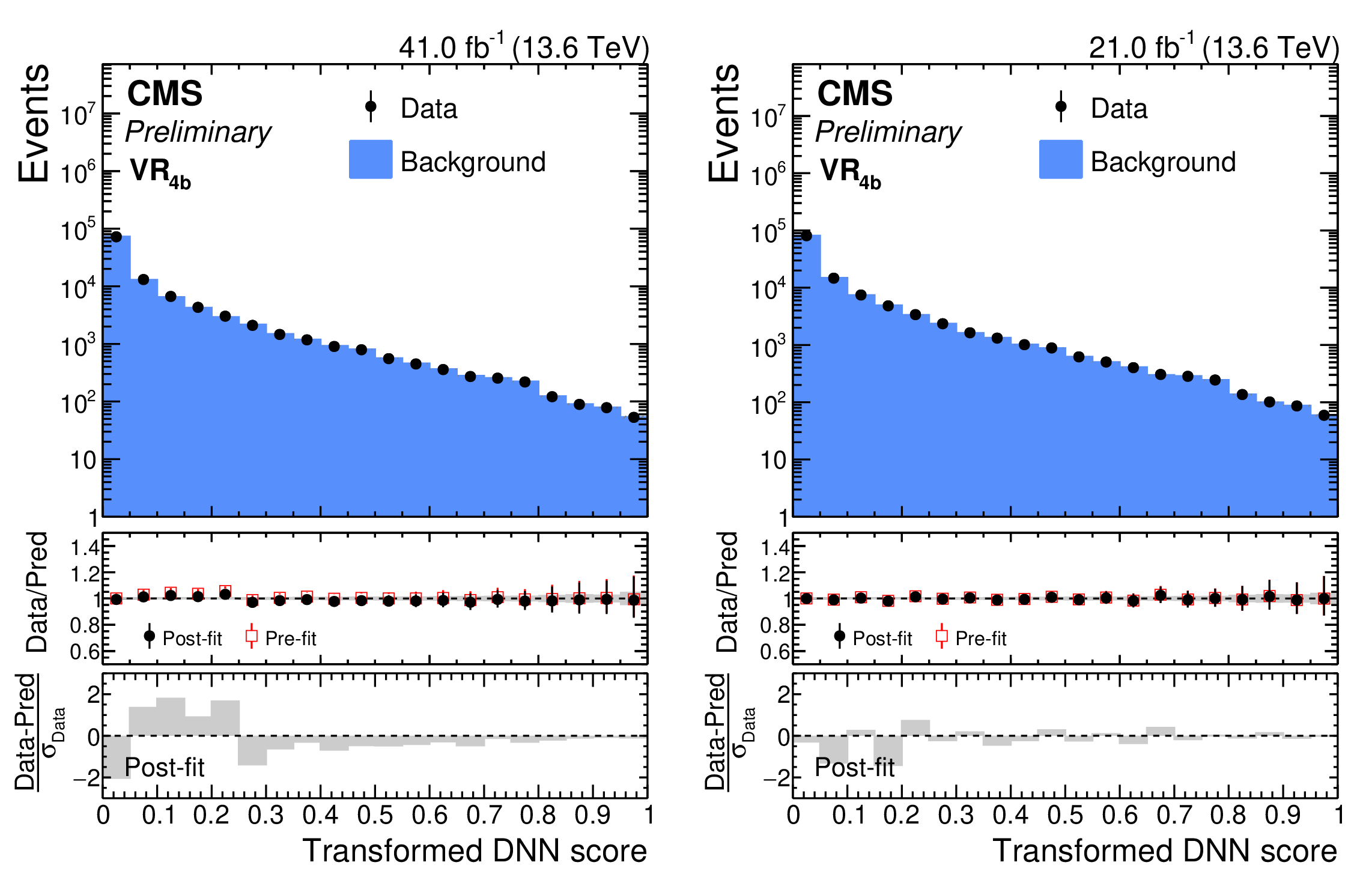
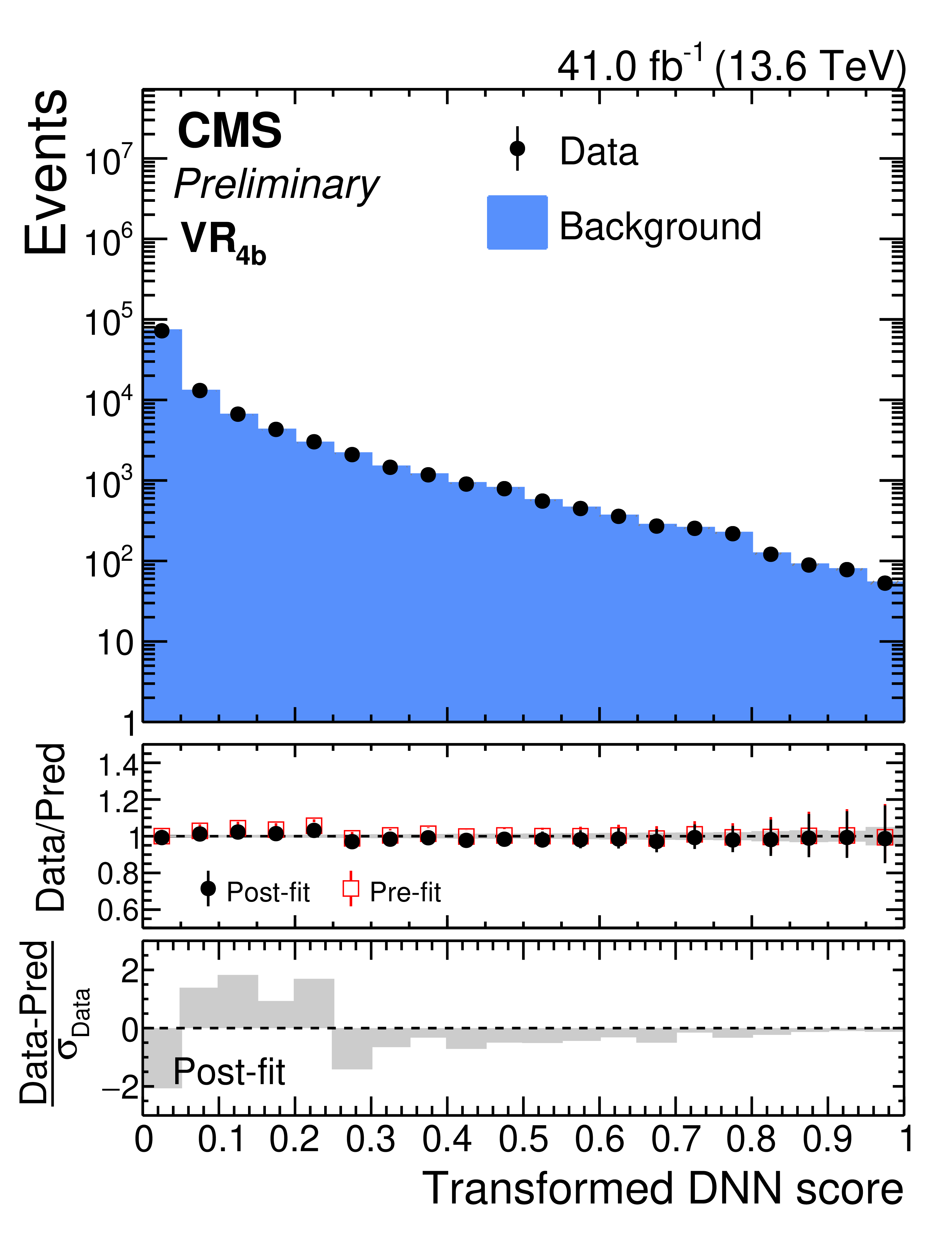
png pdf	Figure 10: Pre-fit and post b-only fit distributions of the SvsB classifier output for the sum of all 4b validation regions in pre-ParkingHH (left) and post-ParkingHH (right) data.
png pdf	Figure 10-a: Pre-fit and post b-only fit distributions of the SvsB classifier output for the sum of all 4b validation regions in pre-ParkingHH (left) and post-ParkingHH (right) data.
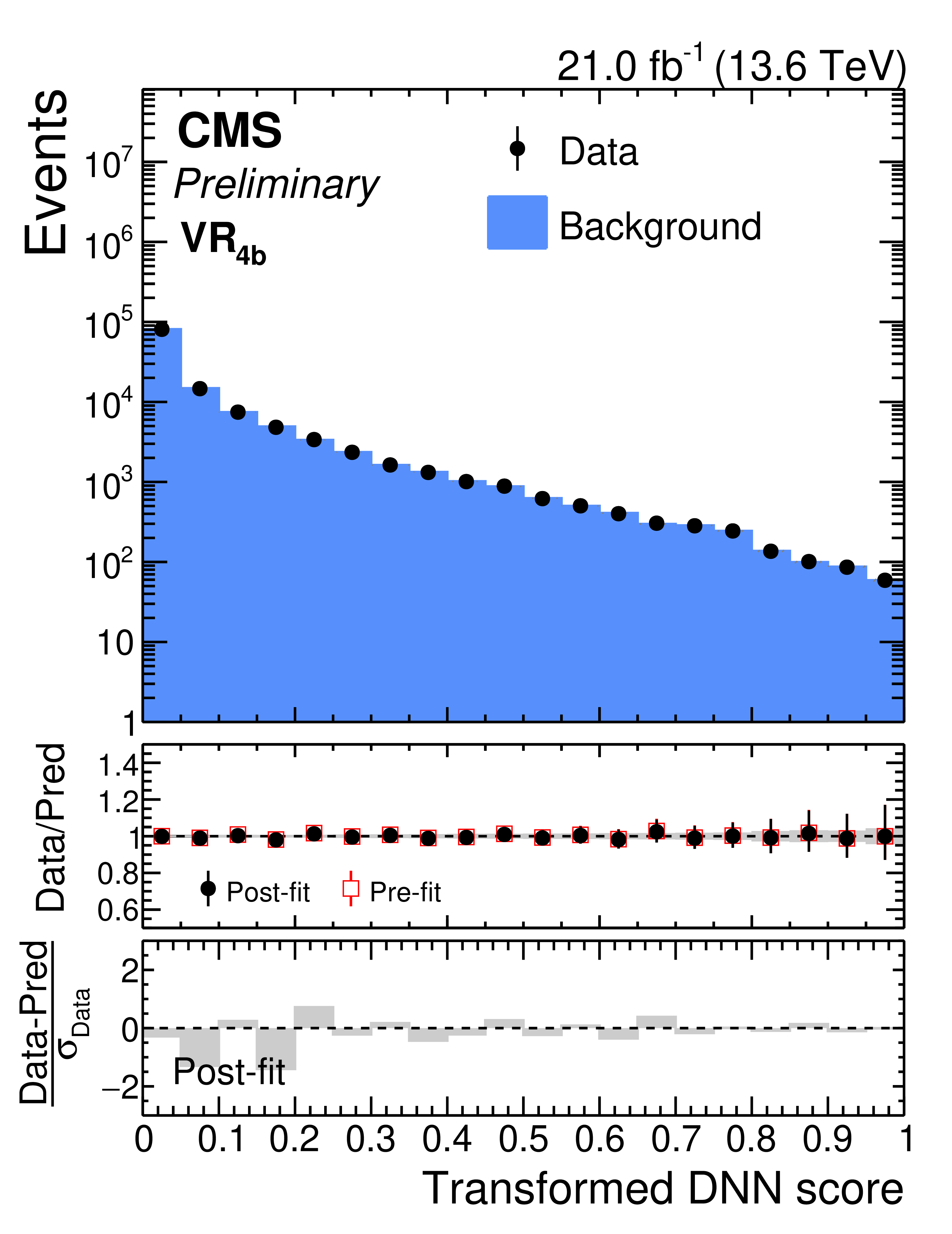
png pdf	Figure 10-b: Pre-fit and post b-only fit distributions of the SvsB classifier output for the sum of all 4b validation regions in pre-ParkingHH (left) and post-ParkingHH (right) data.
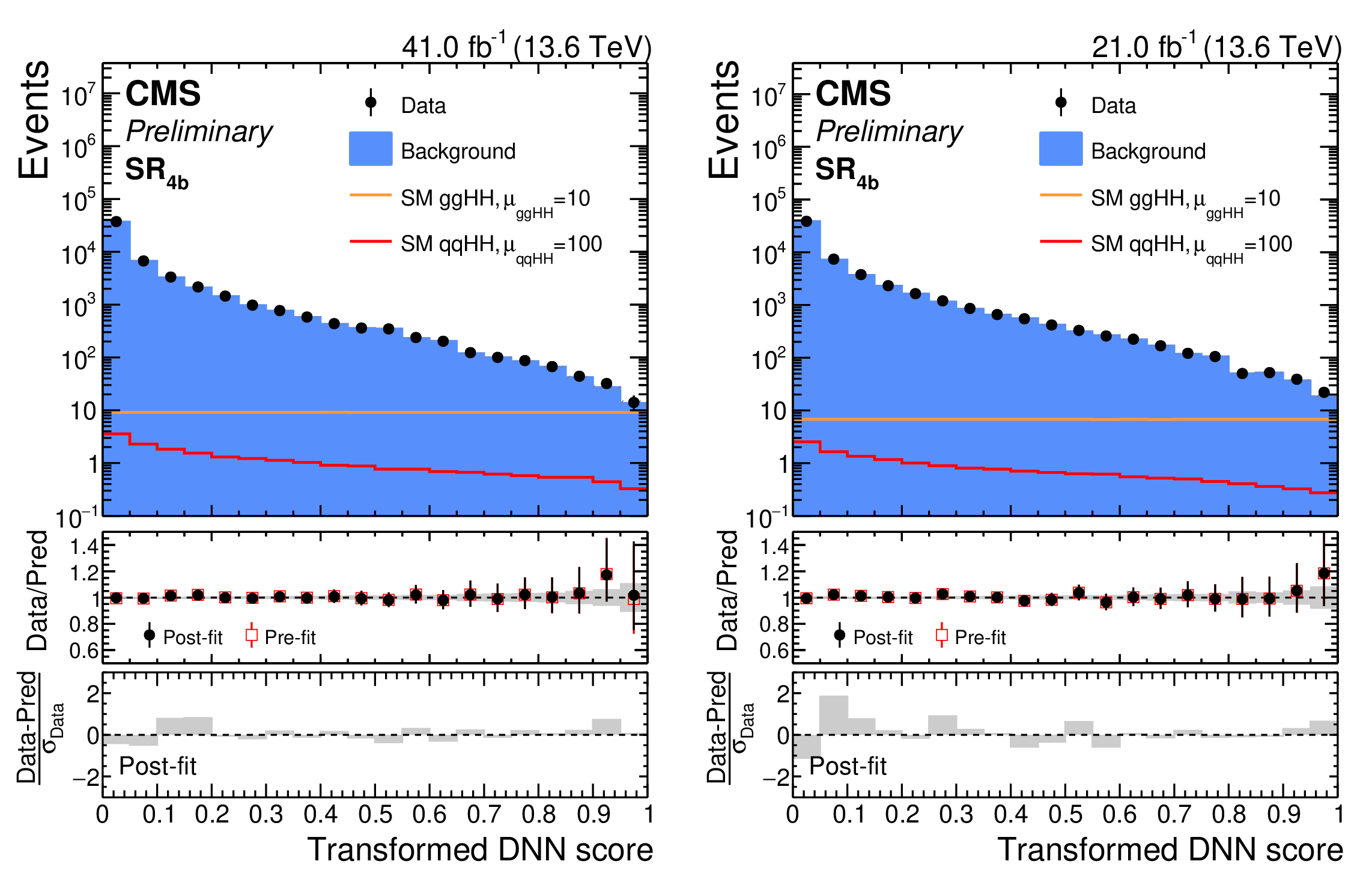
png pdf	Figure 11: Post-fit distributions of the SvsB classifier score in the $ \mathrm{SR_{4\mathrm{b}}} $ of the $ \mathrm{g}\mathrm{g}\mathrm{H}\mathrm{H} $ resolved analysis for data (black points) and the predicted background (blue filled histograms), for pre-ParkingHH (left) and post-ParkingHH (right) data. The distributions of the SM $ \mathrm{g}\mathrm{g}\mathrm{H}\mathrm{H} $ (orange line) and $ \text{qq}\mathrm{H}\mathrm{H} $ (red line) signals, scaled to improve their visibility, are overlaid.
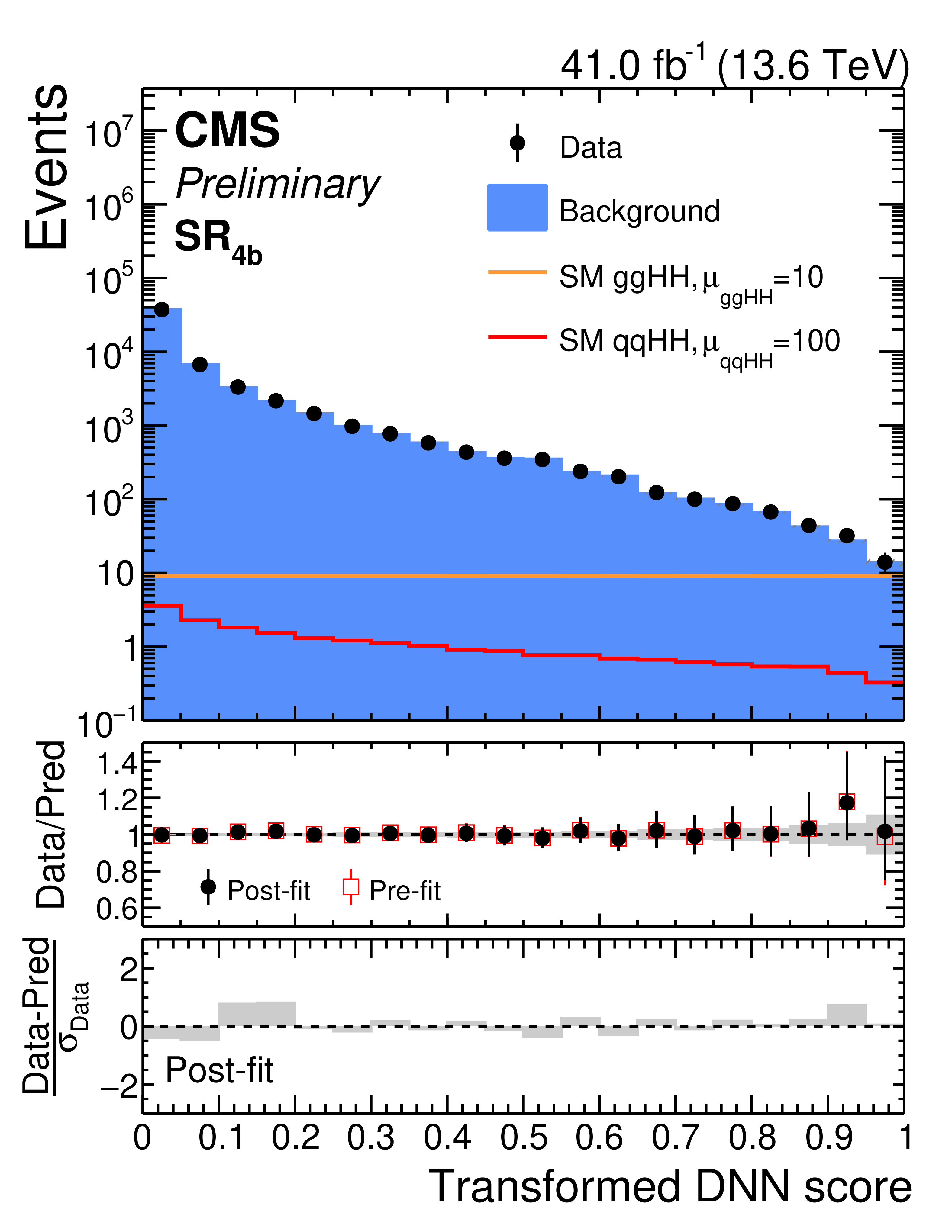
png pdf	Figure 11-a: Post-fit distributions of the SvsB classifier score in the $ \mathrm{SR_{4\mathrm{b}}} $ of the $ \mathrm{g}\mathrm{g}\mathrm{H}\mathrm{H} $ resolved analysis for data (black points) and the predicted background (blue filled histograms), for pre-ParkingHH (left) and post-ParkingHH (right) data. The distributions of the SM $ \mathrm{g}\mathrm{g}\mathrm{H}\mathrm{H} $ (orange line) and $ \text{qq}\mathrm{H}\mathrm{H} $ (red line) signals, scaled to improve their visibility, are overlaid.
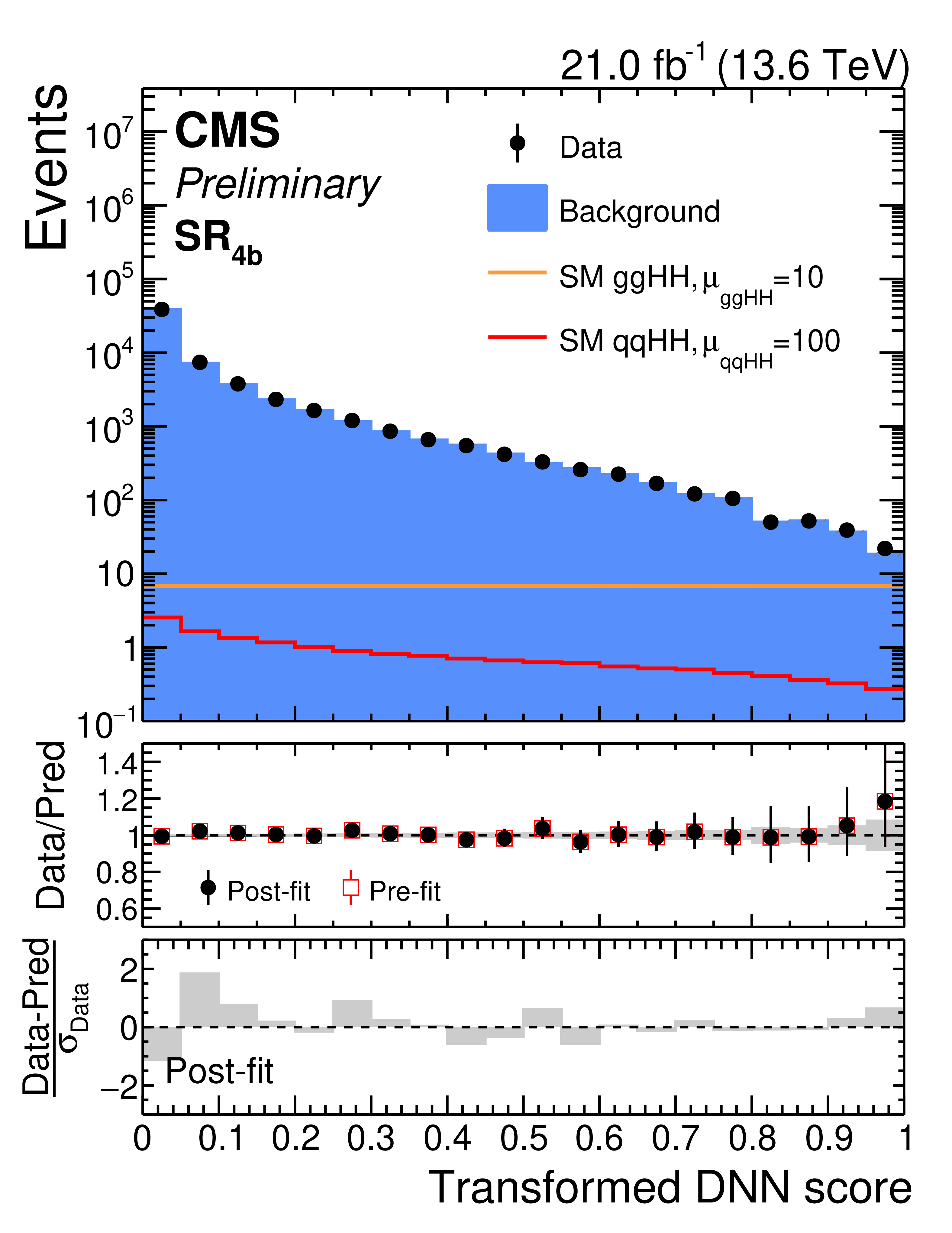
png pdf	Figure 11-b: Post-fit distributions of the SvsB classifier score in the $ \mathrm{SR_{4\mathrm{b}}} $ of the $ \mathrm{g}\mathrm{g}\mathrm{H}\mathrm{H} $ resolved analysis for data (black points) and the predicted background (blue filled histograms), for pre-ParkingHH (left) and post-ParkingHH (right) data. The distributions of the SM $ \mathrm{g}\mathrm{g}\mathrm{H}\mathrm{H} $ (orange line) and $ \text{qq}\mathrm{H}\mathrm{H} $ (red line) signals, scaled to improve their visibility, are overlaid.
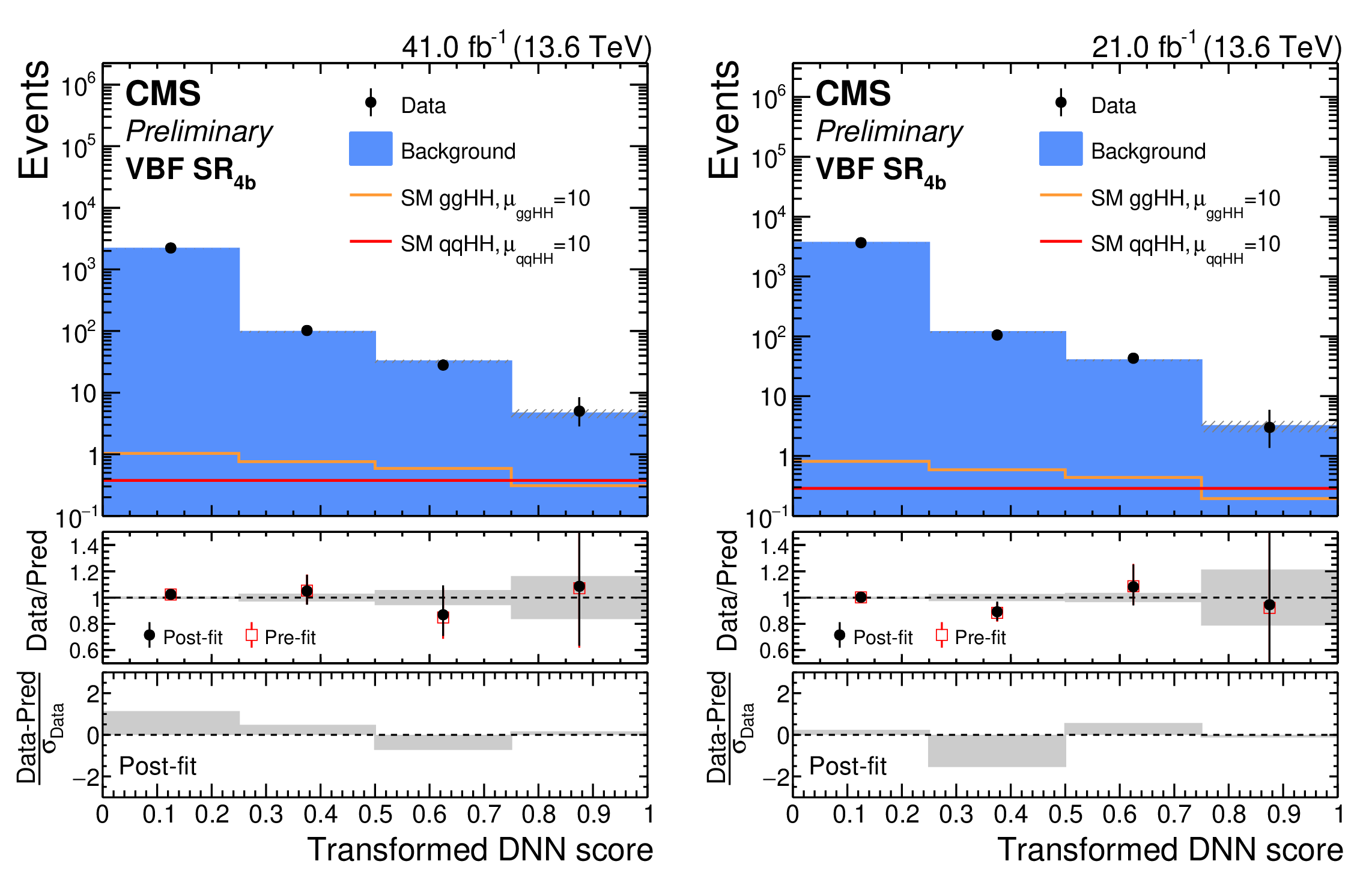
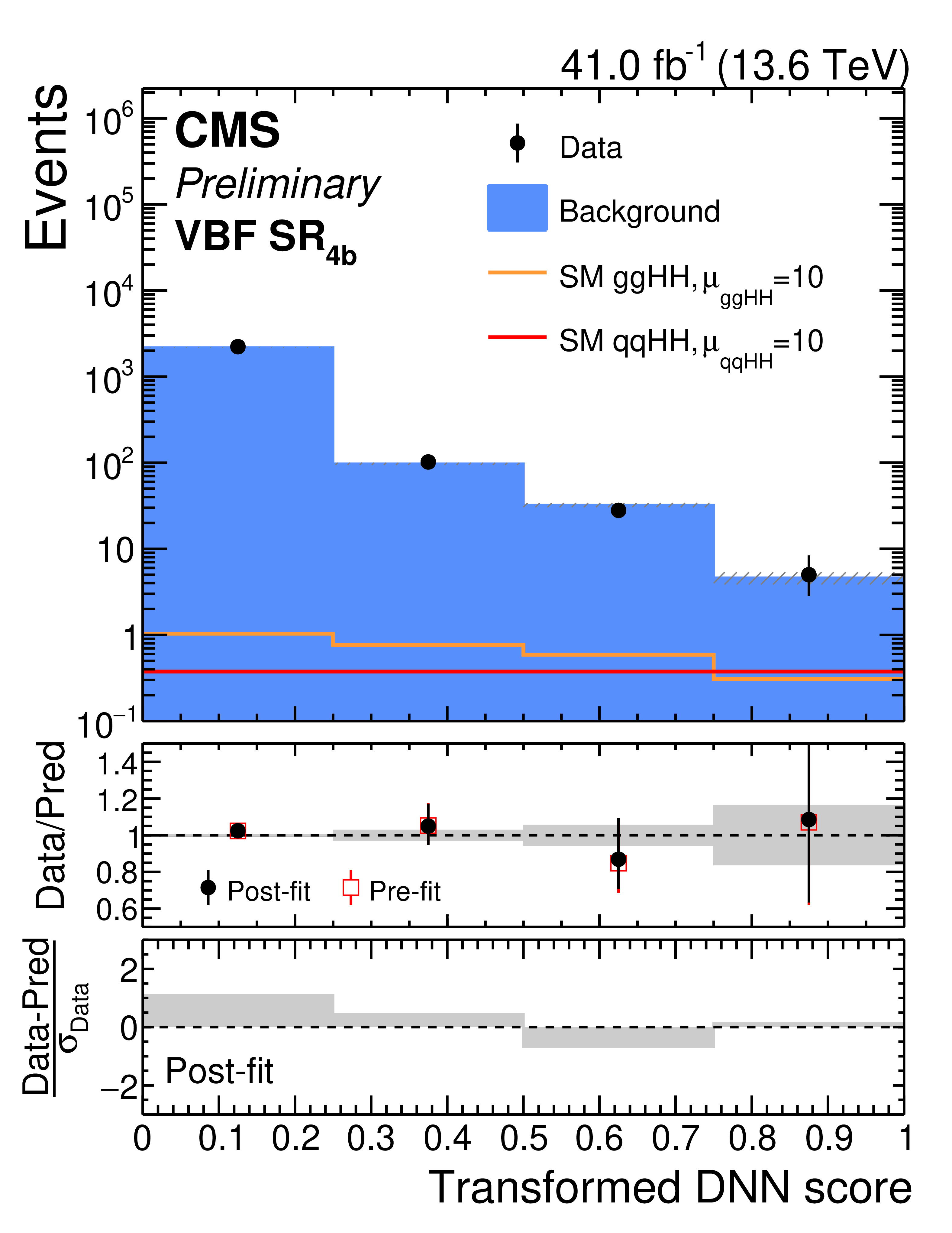
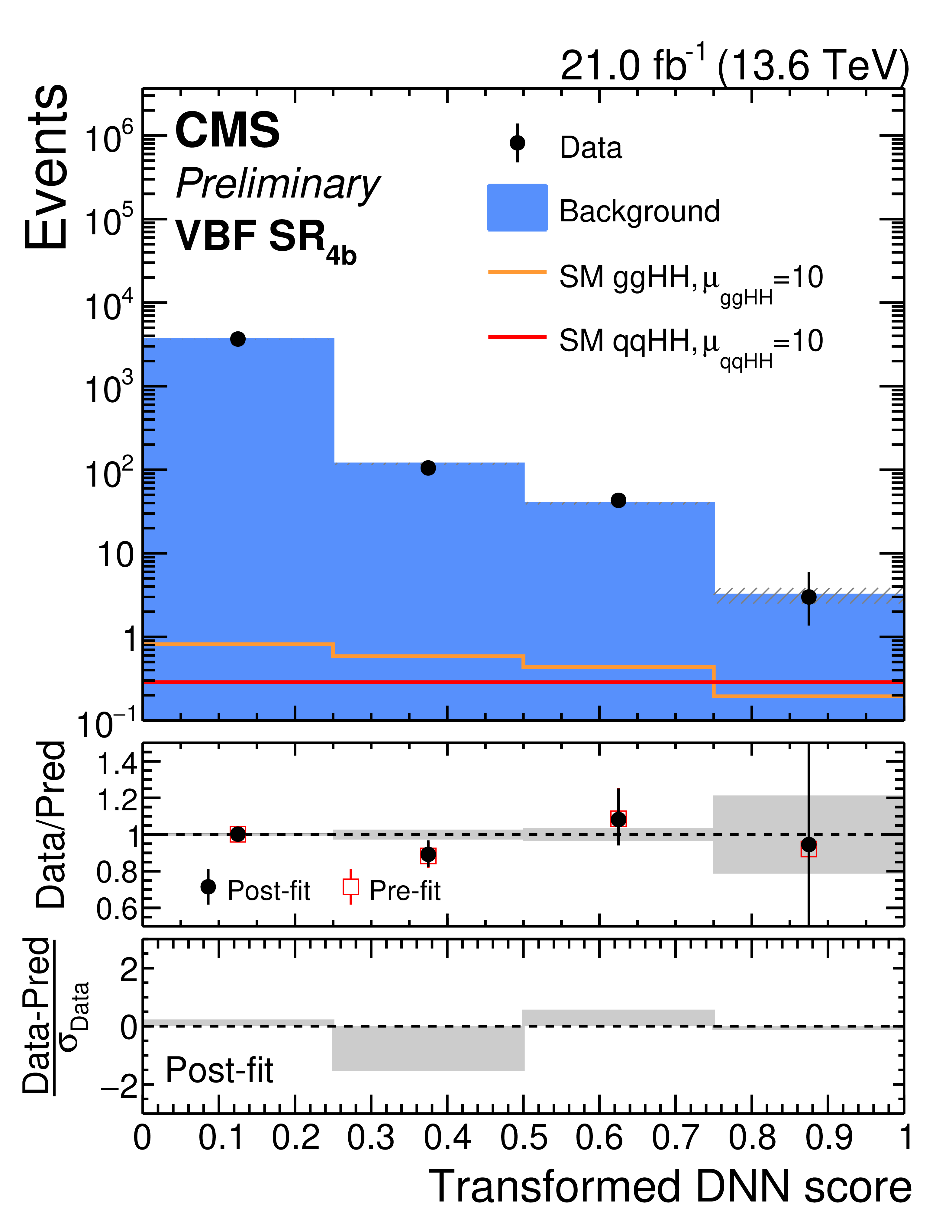
png pdf	Figure 12: Post-fit distributions of the SvsB output score in the $ \mathrm{SR_{4\mathrm{b}}} $ of the $ \text{qq}\mathrm{H}\mathrm{H} $ resolved analysis reported for data (black points) and the predicted background (blue filled histograms) for pre-ParkingHH (left) and post-ParkingHH (right) data. The distributions of the SM $ \mathrm{g}\mathrm{g}\mathrm{H}\mathrm{H} $ (orange line) and $ \text{qq}\mathrm{H}\mathrm{H} $(red line) signals, scaled to improve their visibility, are overlaid.
png pdf	Figure 12-a: Post-fit distributions of the SvsB output score in the $ \mathrm{SR_{4\mathrm{b}}} $ of the $ \text{qq}\mathrm{H}\mathrm{H} $ resolved analysis reported for data (black points) and the predicted background (blue filled histograms) for pre-ParkingHH (left) and post-ParkingHH (right) data. The distributions of the SM $ \mathrm{g}\mathrm{g}\mathrm{H}\mathrm{H} $ (orange line) and $ \text{qq}\mathrm{H}\mathrm{H} $(red line) signals, scaled to improve their visibility, are overlaid.
png pdf	Figure 12-b: Post-fit distributions of the SvsB output score in the $ \mathrm{SR_{4\mathrm{b}}} $ of the $ \text{qq}\mathrm{H}\mathrm{H} $ resolved analysis reported for data (black points) and the predicted background (blue filled histograms) for pre-ParkingHH (left) and post-ParkingHH (right) data. The distributions of the SM $ \mathrm{g}\mathrm{g}\mathrm{H}\mathrm{H} $ (orange line) and $ \text{qq}\mathrm{H}\mathrm{H} $(red line) signals, scaled to improve their visibility, are overlaid.
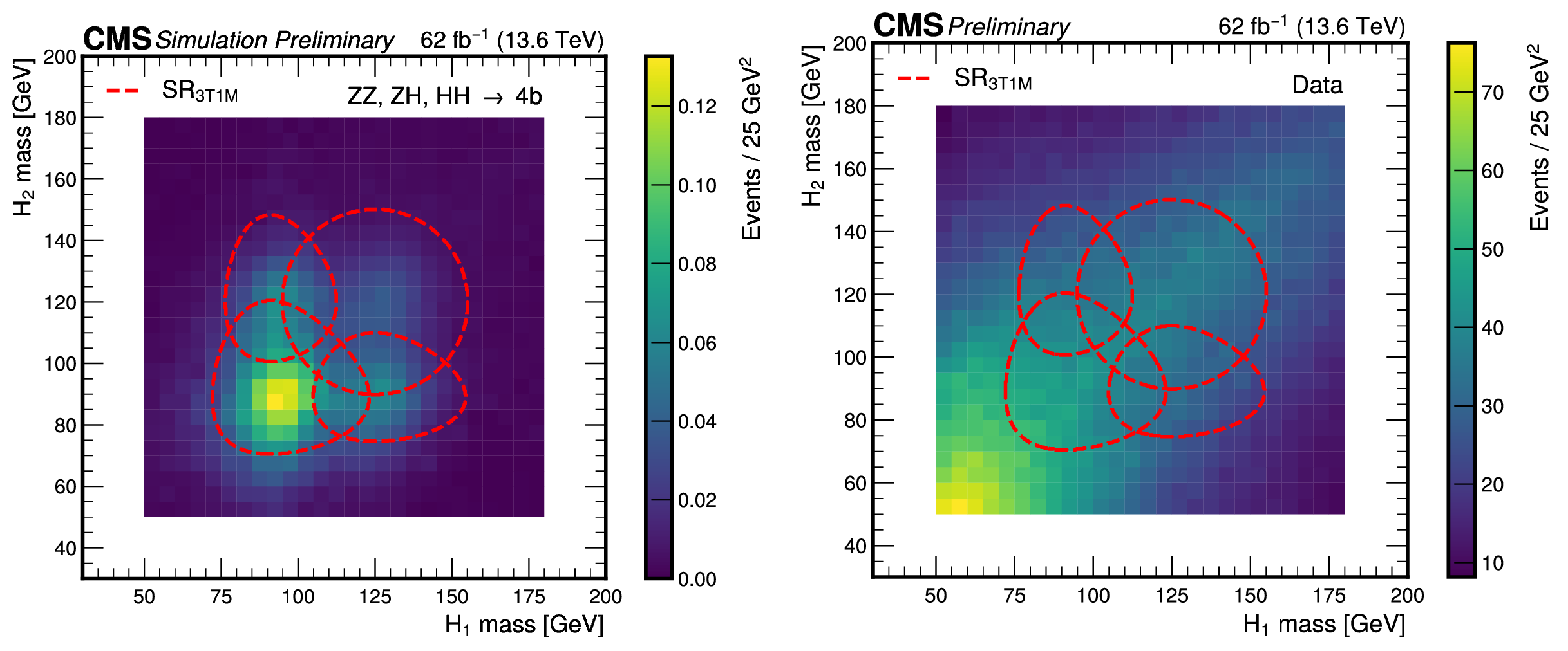
png pdf	Figure 13: The expected HH, ZH, and ZZ signal yields as estimated from simulation (left) and the observed data (right) for the Run 3 dataset, in the 3T1M region, as a function of the reconstructed masses of the leading and subleading in $ p_{\mathrm{T}} \mathrm{H} $ candidates. The signal region is defined by the union of the regions enclosed by the dashed red lines.
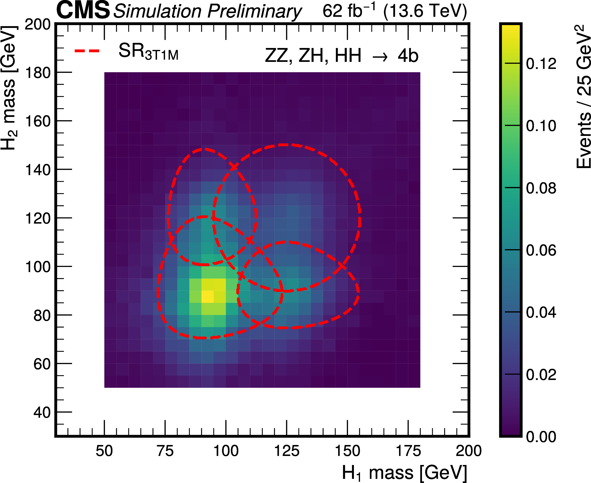
png pdf	Figure 13-a: The expected HH, ZH, and ZZ signal yields as estimated from simulation (left) and the observed data (right) for the Run 3 dataset, in the 3T1M region, as a function of the reconstructed masses of the leading and subleading in $ p_{\mathrm{T}} \mathrm{H} $ candidates. The signal region is defined by the union of the regions enclosed by the dashed red lines.
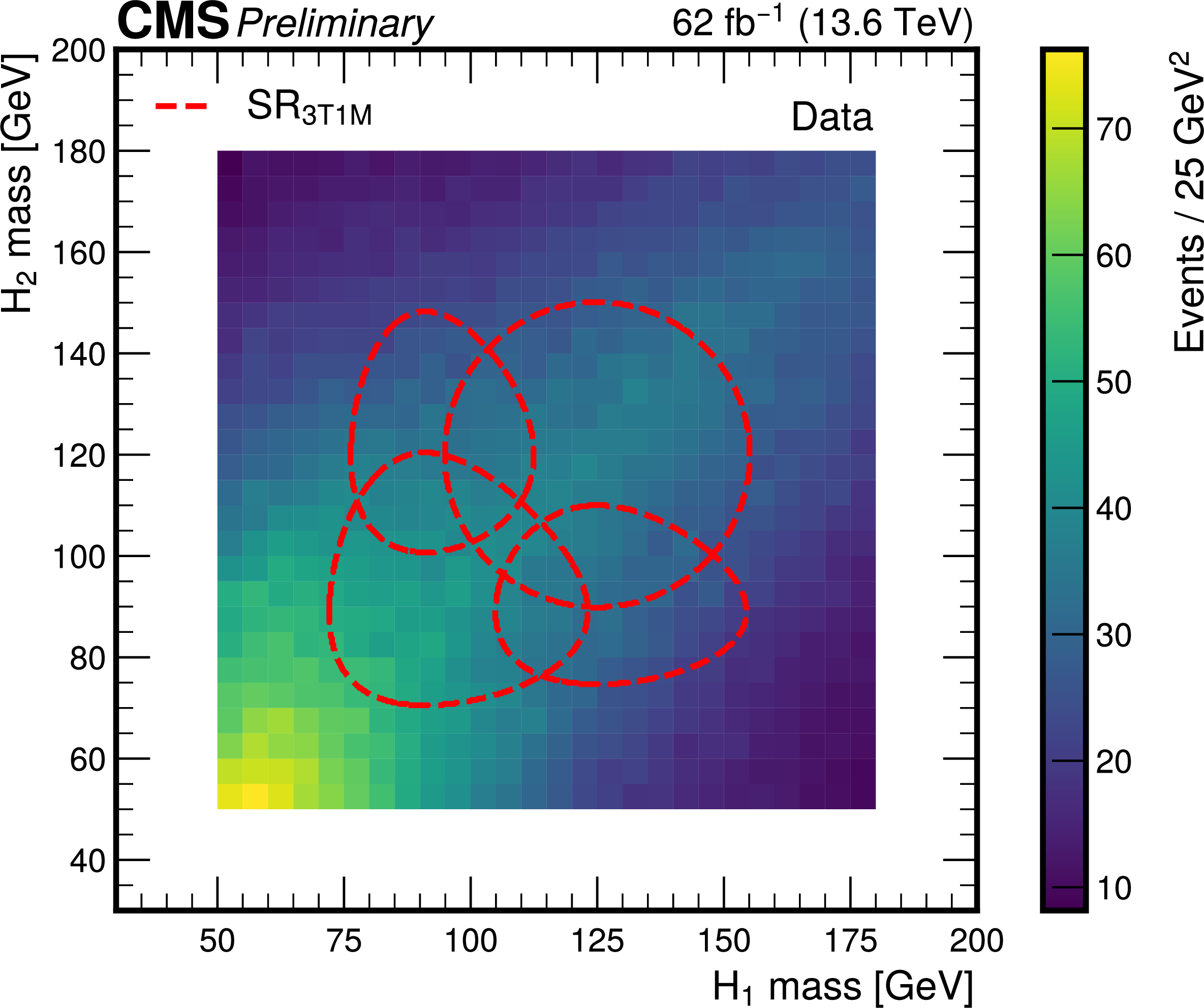
png pdf	Figure 13-b: The expected HH, ZH, and ZZ signal yields as estimated from simulation (left) and the observed data (right) for the Run 3 dataset, in the 3T1M region, as a function of the reconstructed masses of the leading and subleading in $ p_{\mathrm{T}} \mathrm{H} $ candidates. The signal region is defined by the union of the regions enclosed by the dashed red lines.
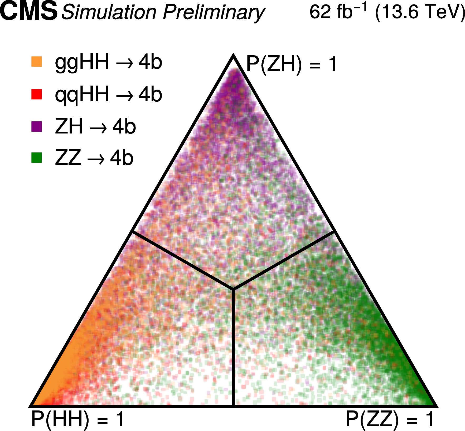
png pdf	Figure 14: Distribution of the $ \mathrm{g}\mathrm{g}\mathrm{H}\mathrm{H} $, $ \mathrm{q}\mathrm{q}\mathrm{H}\mathrm{H} $, ZZ, and ZH signal processes, normalized to unity, as a function of the three FEYNNET probability scores.
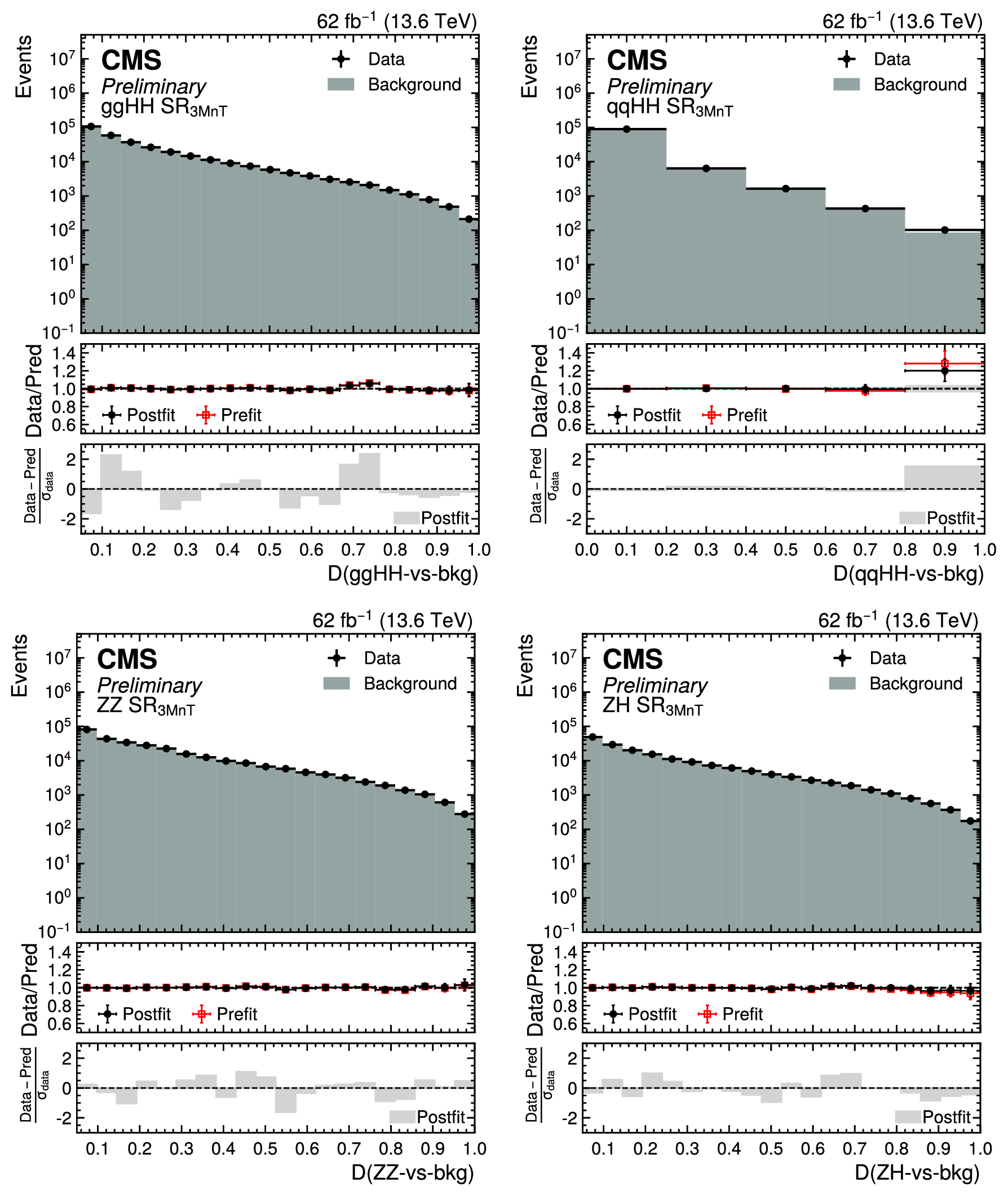
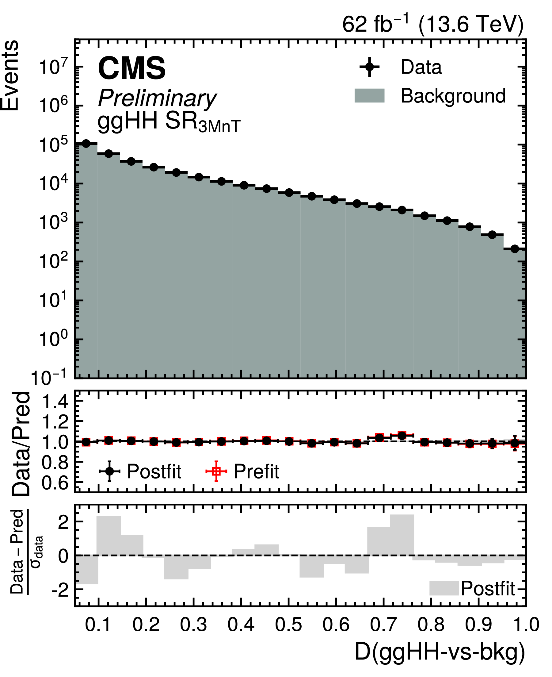
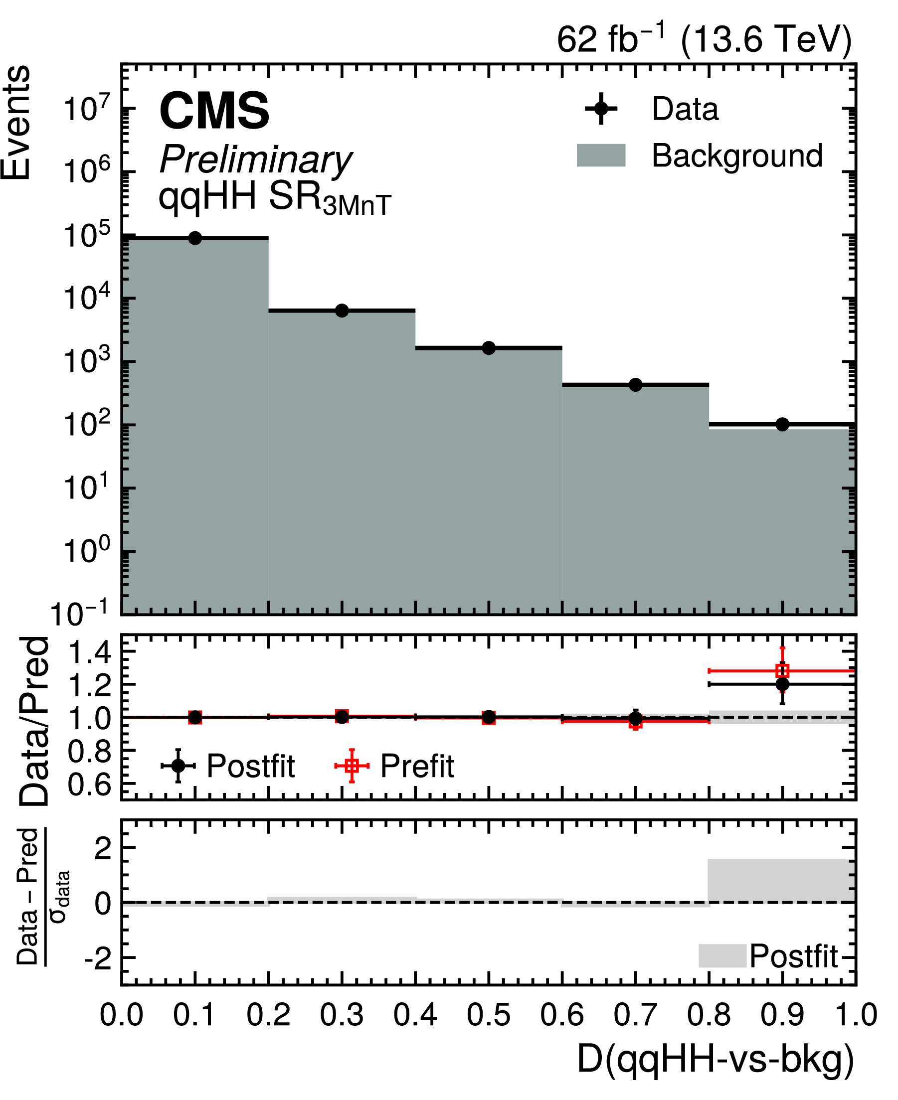
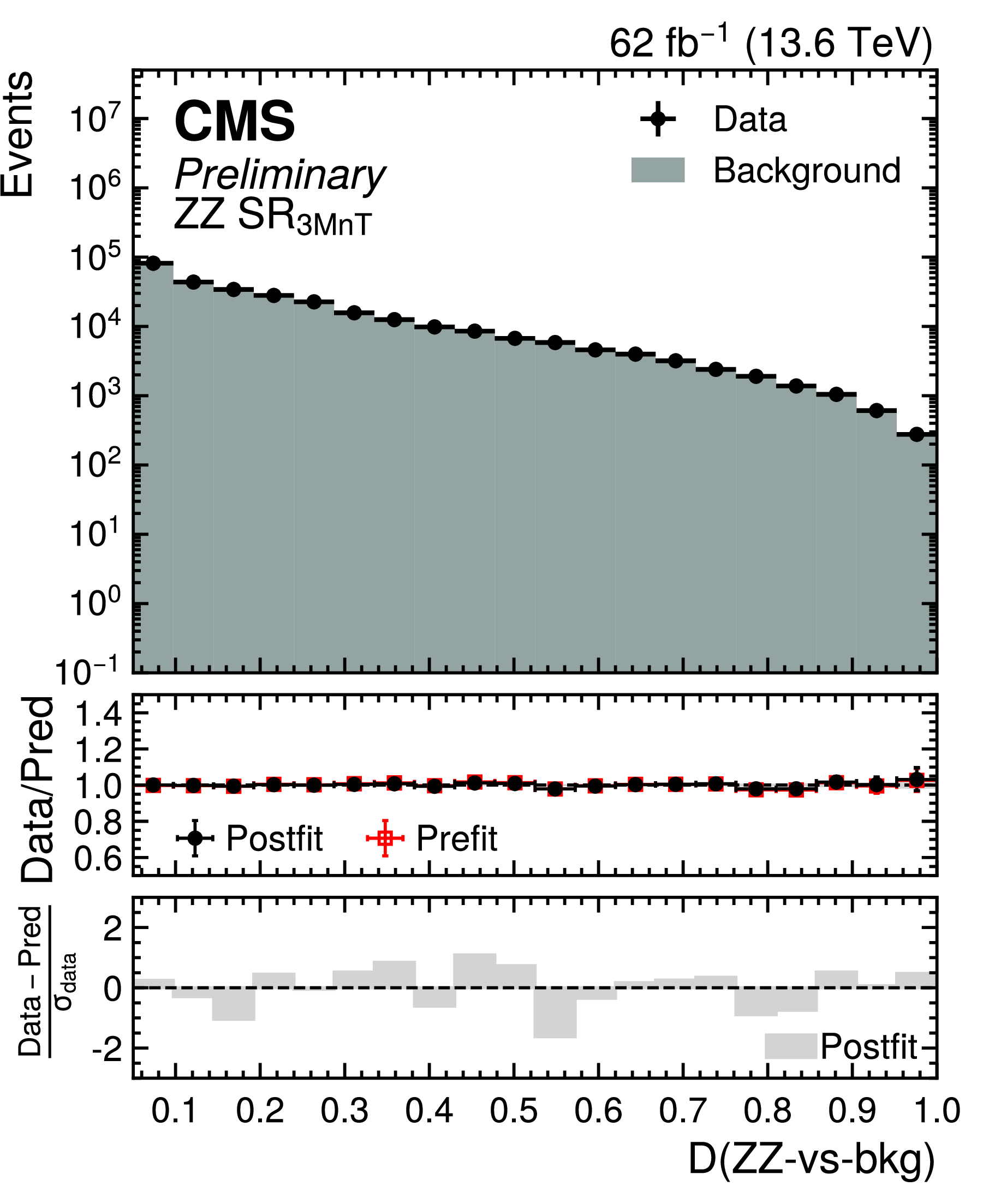
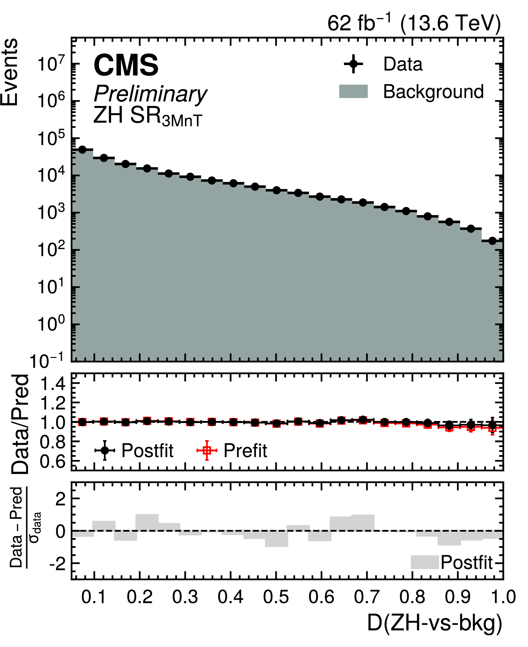
png pdf	Figure 15: Postfit distribution of the $ D $ ($\mathrm{g}\mathrm{g}\mathrm{H}\mathrm{H}$-vs-bkg) (upper left), $ D $ ($\mathrm{q}\mathrm{q}\mathrm{H}\mathrm{H}$-vs-bkg) (upper right), $ D $ ($\mathrm{Z}\mathrm{Z}$-vs-bkg) (lower left), and $ D $ ($\mathrm{Z}\mathrm{H}$-vs-bkg) (lower right) scores in the validation region $ \text{SR}_{\text{3MnT}} $ for data (black points) and the predicted background (cyan filled histograms) with the Run 3 dataset.
png pdf	Figure 15-a: Postfit distribution of the $ D $ ($\mathrm{g}\mathrm{g}\mathrm{H}\mathrm{H}$-vs-bkg) (upper left), $ D $ ($\mathrm{q}\mathrm{q}\mathrm{H}\mathrm{H}$-vs-bkg) (upper right), $ D $ ($\mathrm{Z}\mathrm{Z}$-vs-bkg) (lower left), and $ D $ ($\mathrm{Z}\mathrm{H}$-vs-bkg) (lower right) scores in the validation region $ \text{SR}_{\text{3MnT}} $ for data (black points) and the predicted background (cyan filled histograms) with the Run 3 dataset.
png pdf	Figure 15-b: Postfit distribution of the $ D $ ($\mathrm{g}\mathrm{g}\mathrm{H}\mathrm{H}$-vs-bkg) (upper left), $ D $ ($\mathrm{q}\mathrm{q}\mathrm{H}\mathrm{H}$-vs-bkg) (upper right), $ D $ ($\mathrm{Z}\mathrm{Z}$-vs-bkg) (lower left), and $ D $ ($\mathrm{Z}\mathrm{H}$-vs-bkg) (lower right) scores in the validation region $ \text{SR}_{\text{3MnT}} $ for data (black points) and the predicted background (cyan filled histograms) with the Run 3 dataset.
png pdf	Figure 15-c: Postfit distribution of the $ D $ ($\mathrm{g}\mathrm{g}\mathrm{H}\mathrm{H}$-vs-bkg) (upper left), $ D $ ($\mathrm{q}\mathrm{q}\mathrm{H}\mathrm{H}$-vs-bkg) (upper right), $ D $ ($\mathrm{Z}\mathrm{Z}$-vs-bkg) (lower left), and $ D $ ($\mathrm{Z}\mathrm{H}$-vs-bkg) (lower right) scores in the validation region $ \text{SR}_{\text{3MnT}} $ for data (black points) and the predicted background (cyan filled histograms) with the Run 3 dataset.
png pdf	Figure 15-d: Postfit distribution of the $ D $ ($\mathrm{g}\mathrm{g}\mathrm{H}\mathrm{H}$-vs-bkg) (upper left), $ D $ ($\mathrm{q}\mathrm{q}\mathrm{H}\mathrm{H}$-vs-bkg) (upper right), $ D $ ($\mathrm{Z}\mathrm{Z}$-vs-bkg) (lower left), and $ D $ ($\mathrm{Z}\mathrm{H}$-vs-bkg) (lower right) scores in the validation region $ \text{SR}_{\text{3MnT}} $ for data (black points) and the predicted background (cyan filled histograms) with the Run 3 dataset.
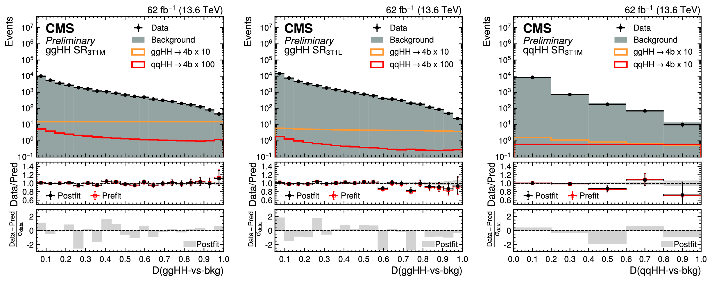
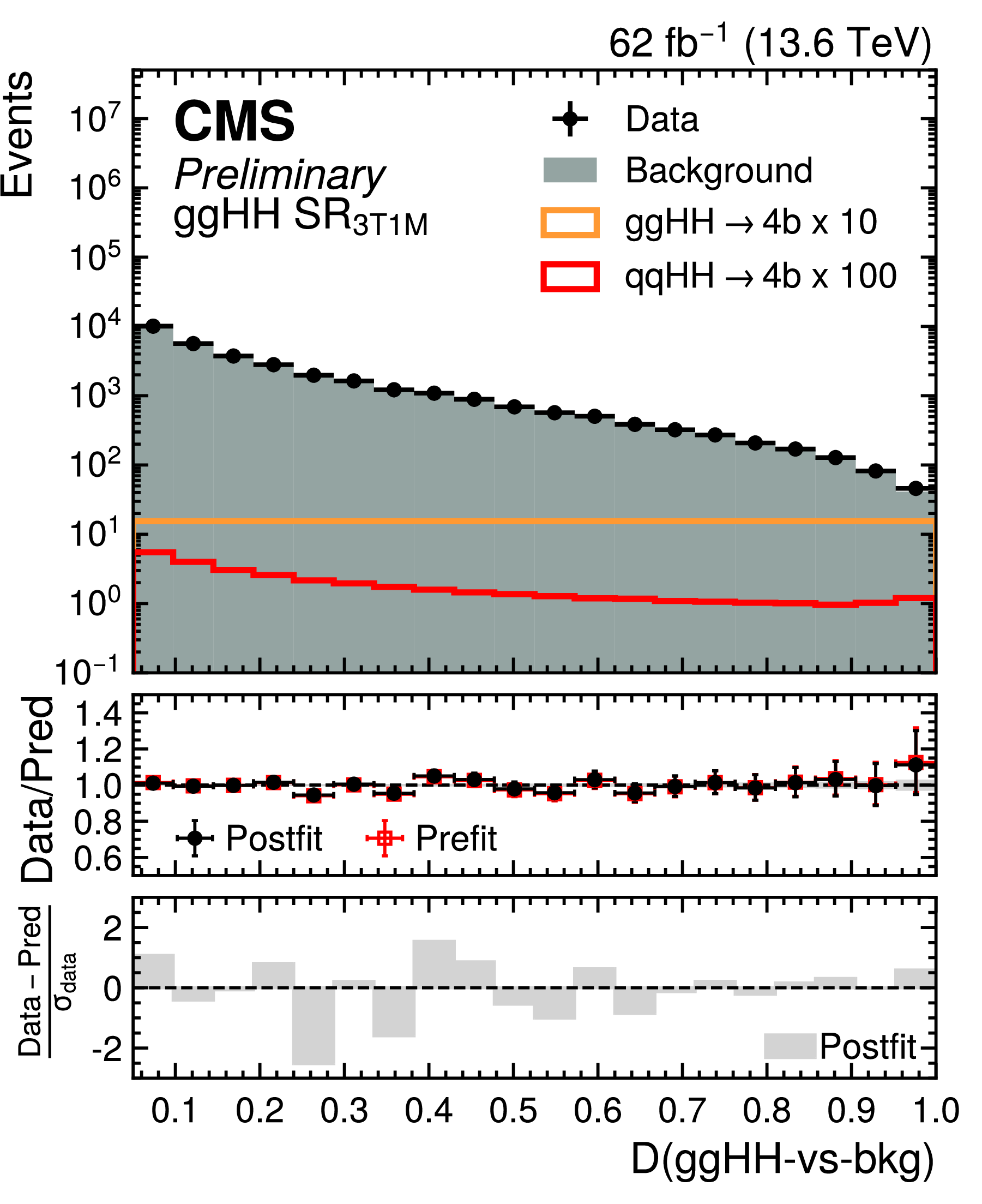
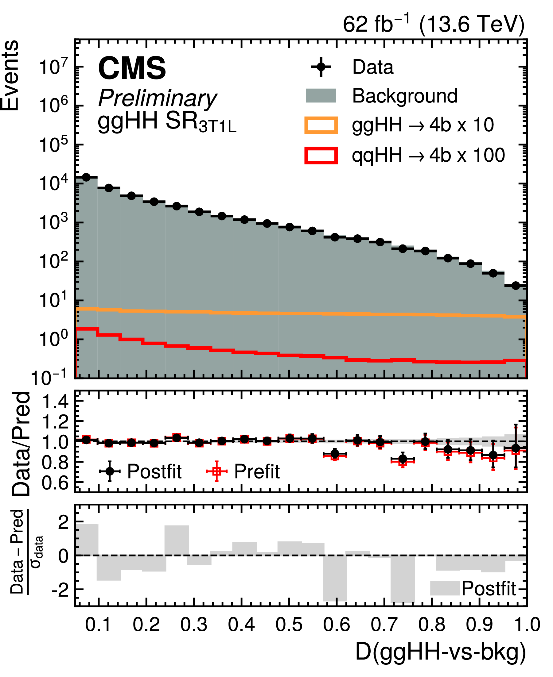
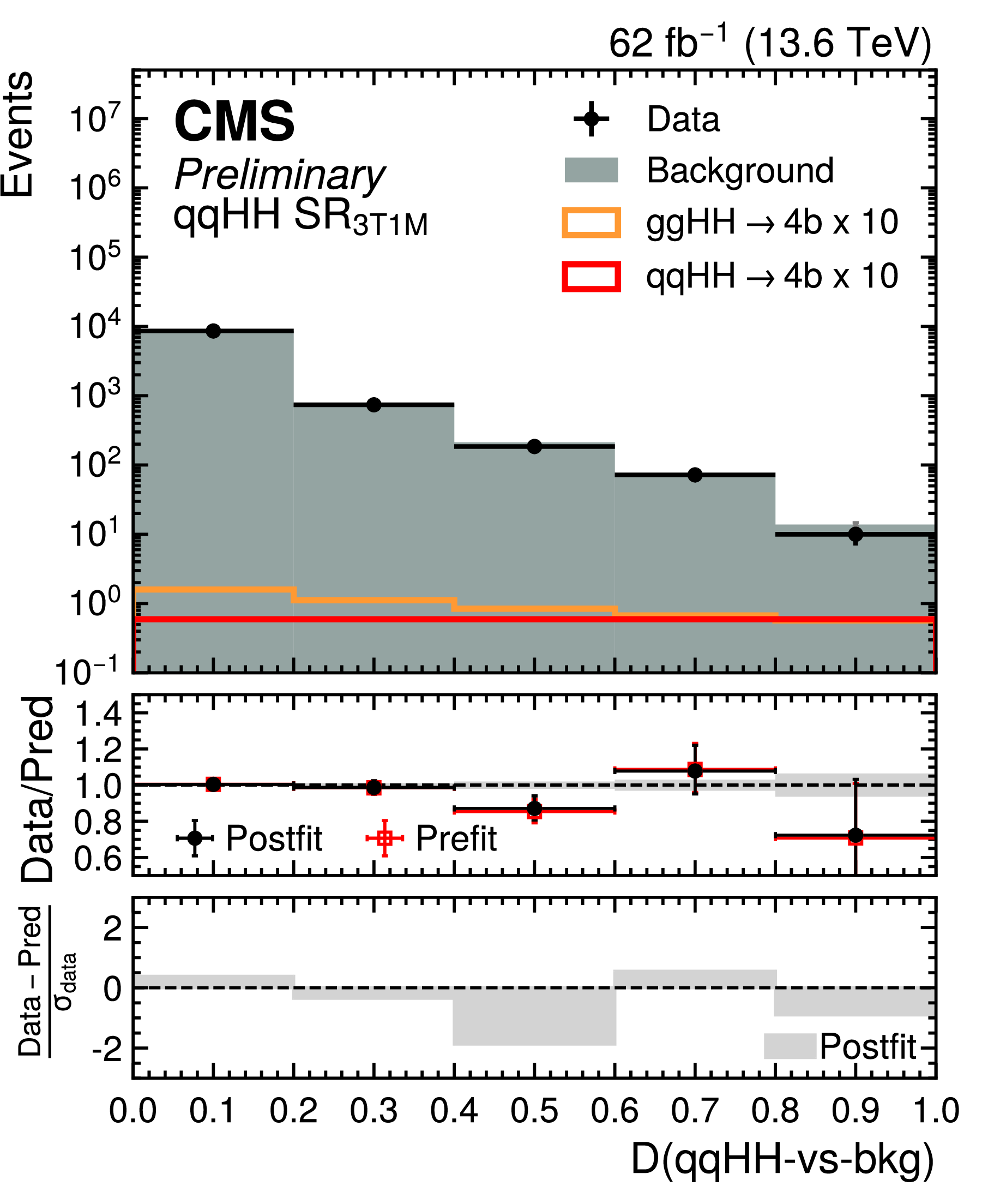
png pdf	Figure 16: Postfit distributions of the transformed $ D $ ($\mathrm{g}\mathrm{g}\mathrm{H}\mathrm{H}$-vs-bkg) score in the $ \mathrm{g}\mathrm{g}\mathrm{H}\mathrm{H} \text{SR}_{\text{3T1M}} $ (left) and $ \mathrm{g}\mathrm{g}\mathrm{H}\mathrm{H} \text{SR}_{\text{3T1L}} $ (middle) categories, and $ D $ ($\mathrm{q}\mathrm{q}\mathrm{H}\mathrm{H}$-vs-bkg) score in the $ \mathrm{q}\mathrm{q}\mathrm{H}\mathrm{H} \text{SR}_{\text{3T1M}} $ (right) category for data (black points) and the predicted background (cyan filled histograms) for the Run 3 dataset. The distributions of the SM $ \mathrm{q}\mathrm{q}\mathrm{H}\mathrm{H} $ (orange line) and $ \mathrm{q}\mathrm{q}\mathrm{H}\mathrm{H} $ (red line) signal processes, scaled to improve their visibility, are also overlaid.
png pdf	Figure 16-a: Postfit distributions of the transformed $ D $ ($\mathrm{g}\mathrm{g}\mathrm{H}\mathrm{H}$-vs-bkg) score in the $ \mathrm{g}\mathrm{g}\mathrm{H}\mathrm{H} \text{SR}_{\text{3T1M}} $ (left) and $ \mathrm{g}\mathrm{g}\mathrm{H}\mathrm{H} \text{SR}_{\text{3T1L}} $ (middle) categories, and $ D $ ($\mathrm{q}\mathrm{q}\mathrm{H}\mathrm{H}$-vs-bkg) score in the $ \mathrm{q}\mathrm{q}\mathrm{H}\mathrm{H} \text{SR}_{\text{3T1M}} $ (right) category for data (black points) and the predicted background (cyan filled histograms) for the Run 3 dataset. The distributions of the SM $ \mathrm{q}\mathrm{q}\mathrm{H}\mathrm{H} $ (orange line) and $ \mathrm{q}\mathrm{q}\mathrm{H}\mathrm{H} $ (red line) signal processes, scaled to improve their visibility, are also overlaid.
png pdf	Figure 16-b: Postfit distributions of the transformed $ D $ ($\mathrm{g}\mathrm{g}\mathrm{H}\mathrm{H}$-vs-bkg) score in the $ \mathrm{g}\mathrm{g}\mathrm{H}\mathrm{H} \text{SR}_{\text{3T1M}} $ (left) and $ \mathrm{g}\mathrm{g}\mathrm{H}\mathrm{H} \text{SR}_{\text{3T1L}} $ (middle) categories, and $ D $ ($\mathrm{q}\mathrm{q}\mathrm{H}\mathrm{H}$-vs-bkg) score in the $ \mathrm{q}\mathrm{q}\mathrm{H}\mathrm{H} \text{SR}_{\text{3T1M}} $ (right) category for data (black points) and the predicted background (cyan filled histograms) for the Run 3 dataset. The distributions of the SM $ \mathrm{q}\mathrm{q}\mathrm{H}\mathrm{H} $ (orange line) and $ \mathrm{q}\mathrm{q}\mathrm{H}\mathrm{H} $ (red line) signal processes, scaled to improve their visibility, are also overlaid.
png pdf	Figure 16-c: Postfit distributions of the transformed $ D $ ($\mathrm{g}\mathrm{g}\mathrm{H}\mathrm{H}$-vs-bkg) score in the $ \mathrm{g}\mathrm{g}\mathrm{H}\mathrm{H} \text{SR}_{\text{3T1M}} $ (left) and $ \mathrm{g}\mathrm{g}\mathrm{H}\mathrm{H} \text{SR}_{\text{3T1L}} $ (middle) categories, and $ D $ ($\mathrm{q}\mathrm{q}\mathrm{H}\mathrm{H}$-vs-bkg) score in the $ \mathrm{q}\mathrm{q}\mathrm{H}\mathrm{H} \text{SR}_{\text{3T1M}} $ (right) category for data (black points) and the predicted background (cyan filled histograms) for the Run 3 dataset. The distributions of the SM $ \mathrm{q}\mathrm{q}\mathrm{H}\mathrm{H} $ (orange line) and $ \mathrm{q}\mathrm{q}\mathrm{H}\mathrm{H} $ (red line) signal processes, scaled to improve their visibility, are also overlaid.
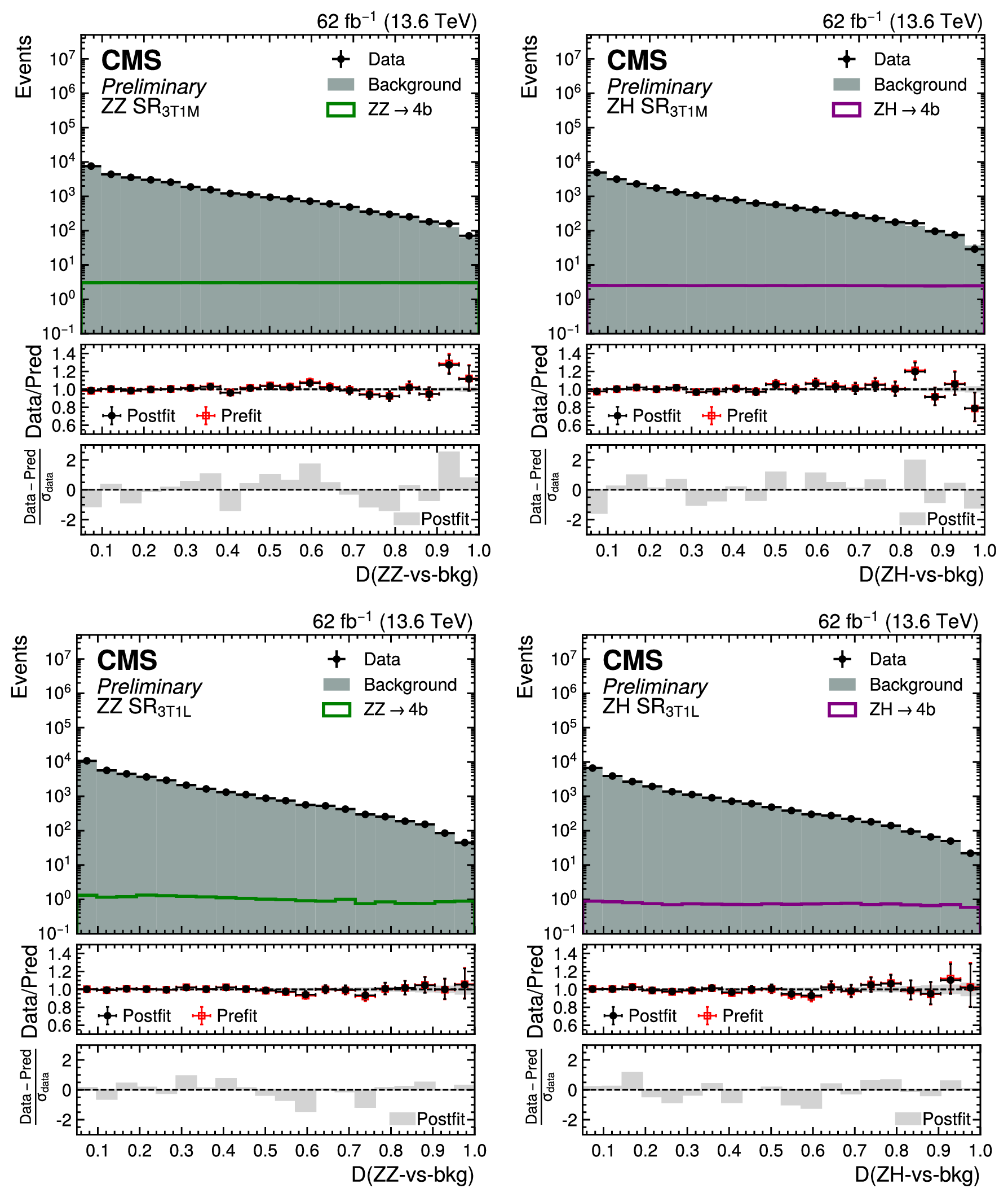
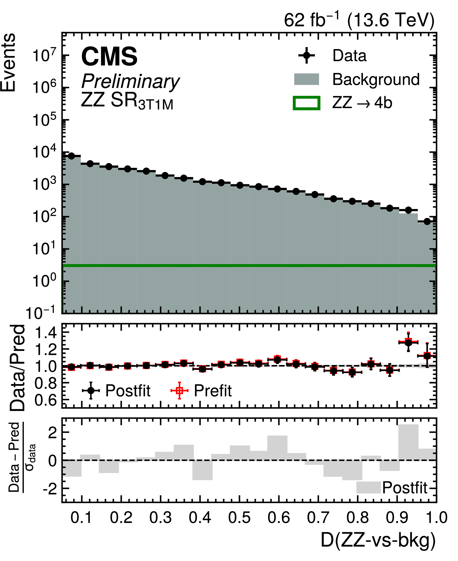
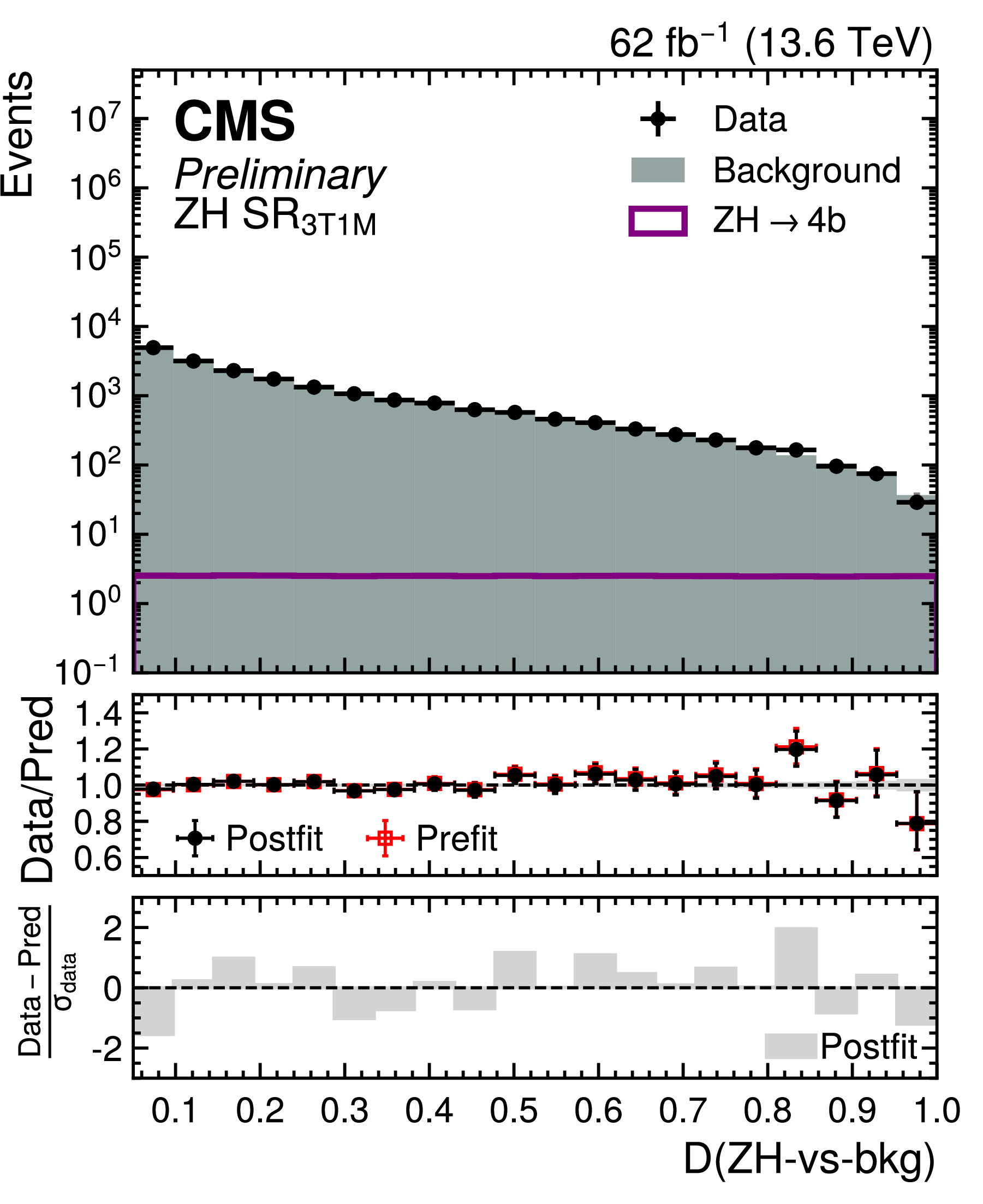
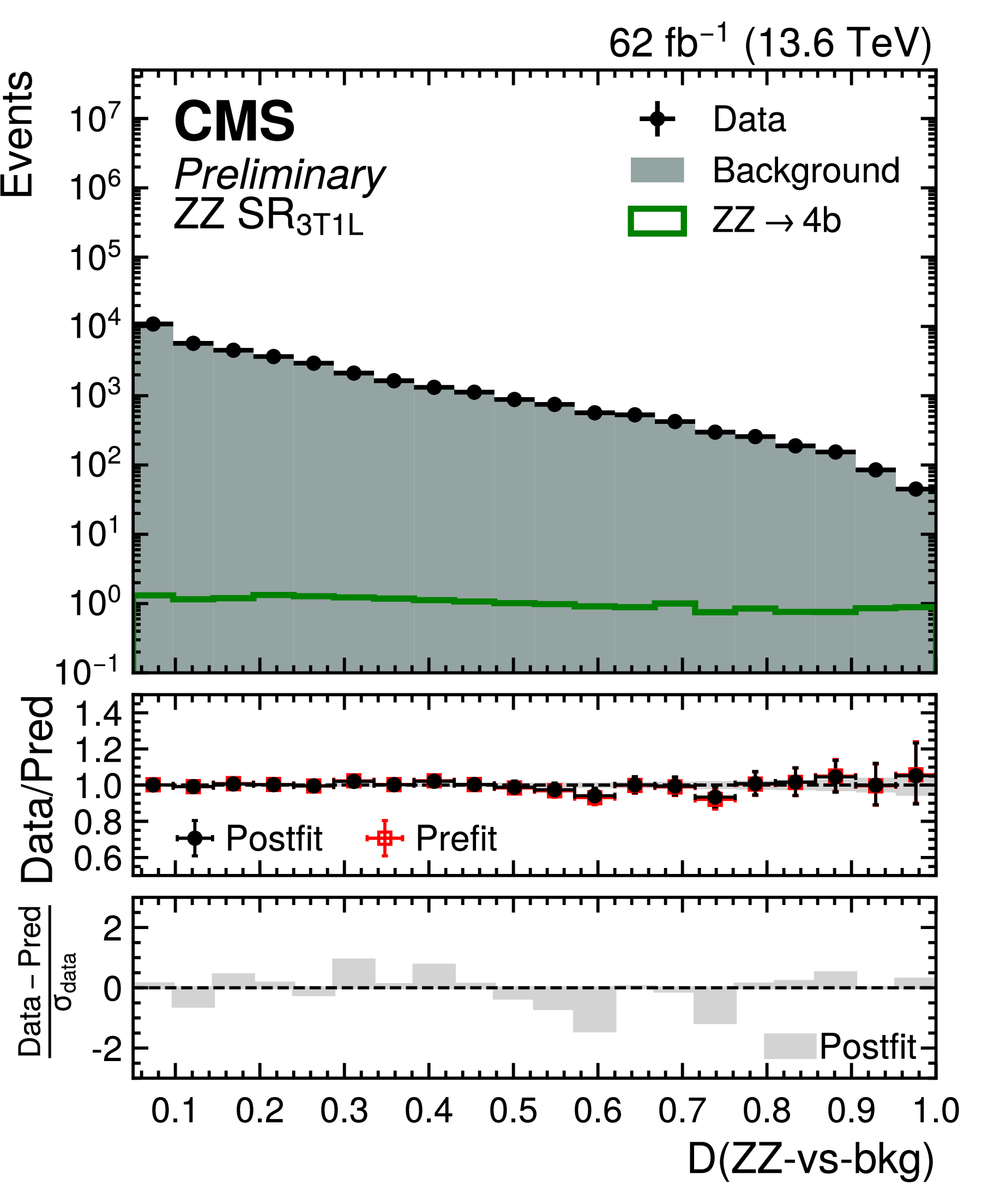
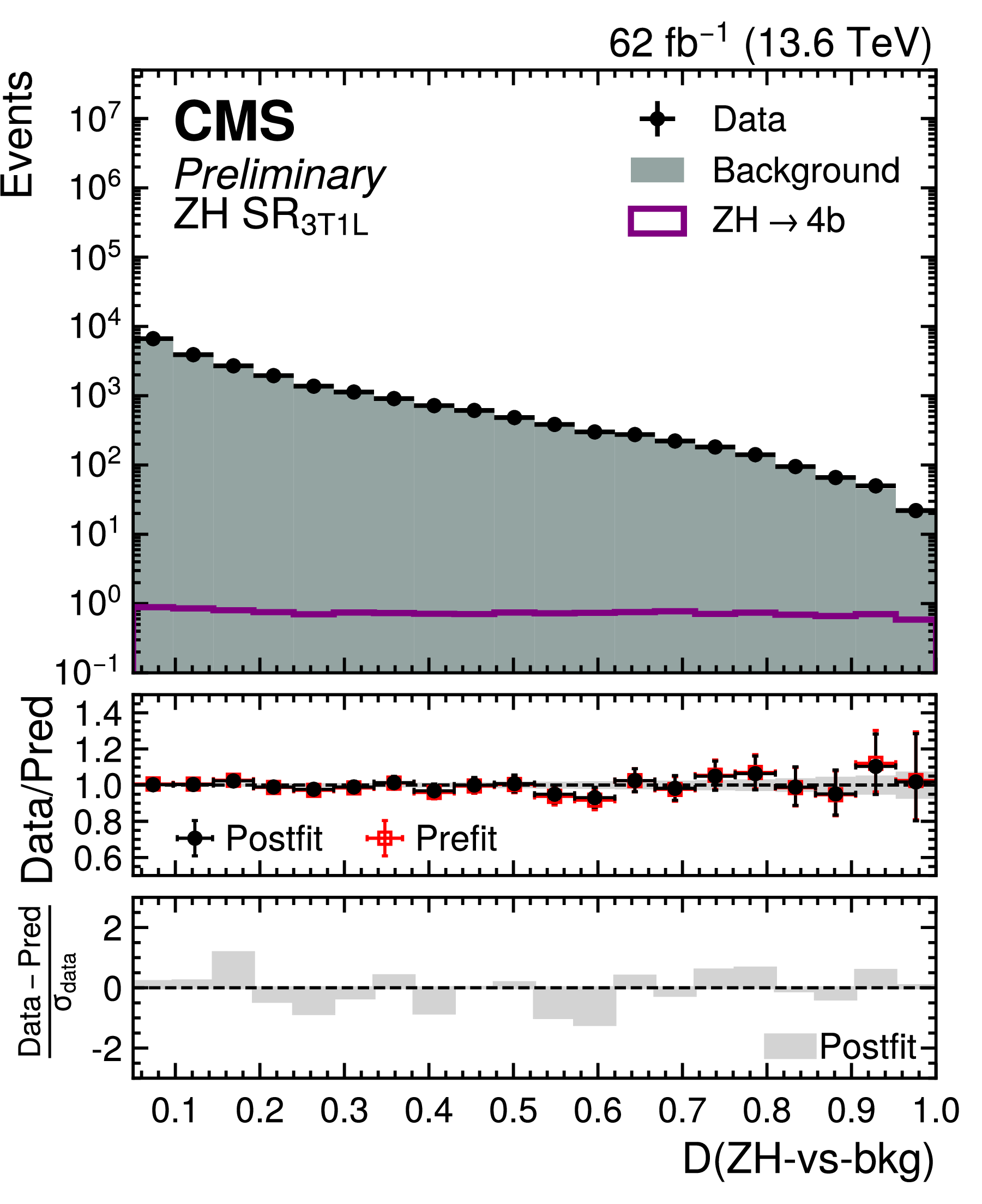
png pdf	Figure 17: Postfit distribution of the transformed $ D $ ($\mathrm{Z}\mathrm{Z}$-vs-bkg) score in the $ \mathrm{Z}\mathrm{Z} \text{SR}_{\text{3T1M}} $ (upper left) and $ \mathrm{Z}\mathrm{Z} \text{SR}_{\text{3T1L}} $ (upper right) categories, and $ D $ ($\mathrm{Z}\mathrm{H}$-vs-bkg) score in the $ \mathrm{Z}\mathrm{H} \text{SR}_{\text{3T1M}} $ (lower left) and $ \mathrm{Z}\mathrm{H} \text{SR}_{\text{3T1L}} $ (lower right) SR for data (black points) and the predicted background (cyan filled histograms) for the Run 3 dataset. The distributions of the SM ZZ (green line) and ZH (purple line) processes are also overlaid.
png pdf	Figure 17-a: Postfit distribution of the transformed $ D $ ($\mathrm{Z}\mathrm{Z}$-vs-bkg) score in the $ \mathrm{Z}\mathrm{Z} \text{SR}_{\text{3T1M}} $ (upper left) and $ \mathrm{Z}\mathrm{Z} \text{SR}_{\text{3T1L}} $ (upper right) categories, and $ D $ ($\mathrm{Z}\mathrm{H}$-vs-bkg) score in the $ \mathrm{Z}\mathrm{H} \text{SR}_{\text{3T1M}} $ (lower left) and $ \mathrm{Z}\mathrm{H} \text{SR}_{\text{3T1L}} $ (lower right) SR for data (black points) and the predicted background (cyan filled histograms) for the Run 3 dataset. The distributions of the SM ZZ (green line) and ZH (purple line) processes are also overlaid.
png pdf	Figure 17-b: Postfit distribution of the transformed $ D $ ($\mathrm{Z}\mathrm{Z}$-vs-bkg) score in the $ \mathrm{Z}\mathrm{Z} \text{SR}_{\text{3T1M}} $ (upper left) and $ \mathrm{Z}\mathrm{Z} \text{SR}_{\text{3T1L}} $ (upper right) categories, and $ D $ ($\mathrm{Z}\mathrm{H}$-vs-bkg) score in the $ \mathrm{Z}\mathrm{H} \text{SR}_{\text{3T1M}} $ (lower left) and $ \mathrm{Z}\mathrm{H} \text{SR}_{\text{3T1L}} $ (lower right) SR for data (black points) and the predicted background (cyan filled histograms) for the Run 3 dataset. The distributions of the SM ZZ (green line) and ZH (purple line) processes are also overlaid.
png pdf	Figure 17-c: Postfit distribution of the transformed $ D $ ($\mathrm{Z}\mathrm{Z}$-vs-bkg) score in the $ \mathrm{Z}\mathrm{Z} \text{SR}_{\text{3T1M}} $ (upper left) and $ \mathrm{Z}\mathrm{Z} \text{SR}_{\text{3T1L}} $ (upper right) categories, and $ D $ ($\mathrm{Z}\mathrm{H}$-vs-bkg) score in the $ \mathrm{Z}\mathrm{H} \text{SR}_{\text{3T1M}} $ (lower left) and $ \mathrm{Z}\mathrm{H} \text{SR}_{\text{3T1L}} $ (lower right) SR for data (black points) and the predicted background (cyan filled histograms) for the Run 3 dataset. The distributions of the SM ZZ (green line) and ZH (purple line) processes are also overlaid.
png pdf	Figure 17-d: Postfit distribution of the transformed $ D $ ($\mathrm{Z}\mathrm{Z}$-vs-bkg) score in the $ \mathrm{Z}\mathrm{Z} \text{SR}_{\text{3T1M}} $ (upper left) and $ \mathrm{Z}\mathrm{Z} \text{SR}_{\text{3T1L}} $ (upper right) categories, and $ D $ ($\mathrm{Z}\mathrm{H}$-vs-bkg) score in the $ \mathrm{Z}\mathrm{H} \text{SR}_{\text{3T1M}} $ (lower left) and $ \mathrm{Z}\mathrm{H} \text{SR}_{\text{3T1L}} $ (lower right) SR for data (black points) and the predicted background (cyan filled histograms) for the Run 3 dataset. The distributions of the SM ZZ (green line) and ZH (purple line) processes are also overlaid.
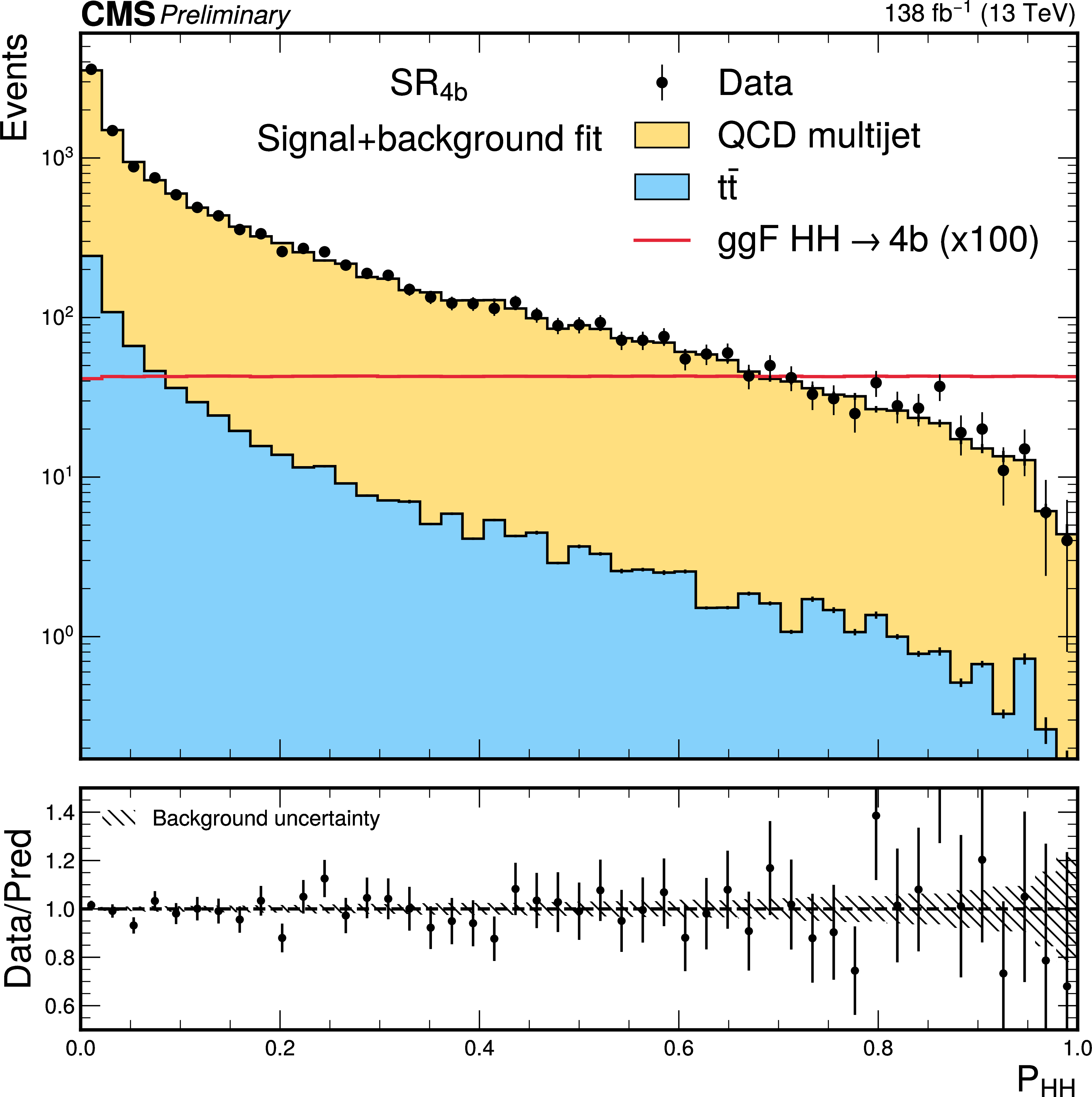
png pdf	Figure 18: The fitted signal+background distribution of the signal probability, $ \mathcal{P_{\mathrm{H}\mathrm{H}}} $, in the $ \mathrm{H}\mathrm{H} \mathrm{SR_{4\mathrm{b}}} $. The black points show the 4b events from data. The yellow and blue regions show the predictions from the QCD multijet model and the $ \mathrm{t} \overline{\mathrm{t}} $ simulation, respectively. The prediction for the SM $ \mathrm{g}\mathrm{g}\mathrm{H}\mathrm{H} $ signal distribution is given by the red histogram, multiplied by 100. The lower panel shows the data-to-background ratio, with the hatched area representing the background uncertainty.
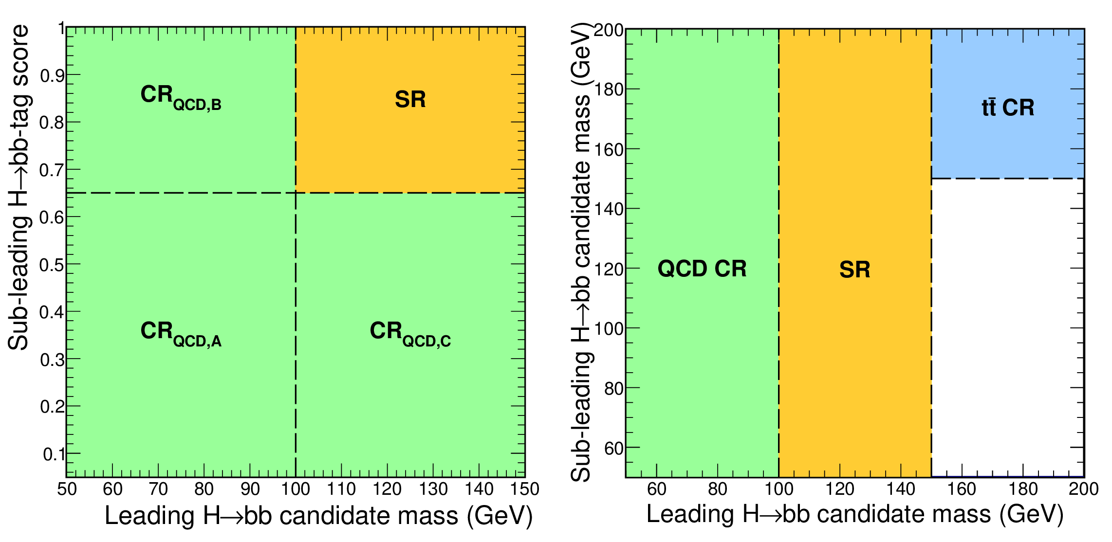
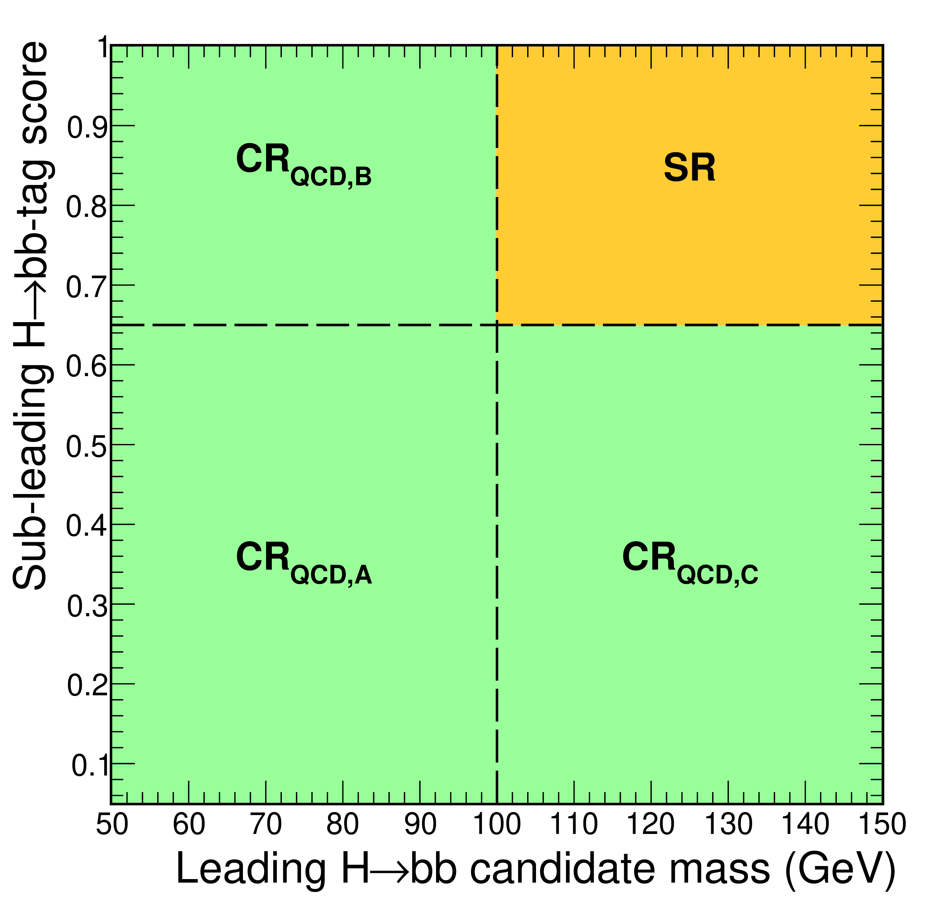
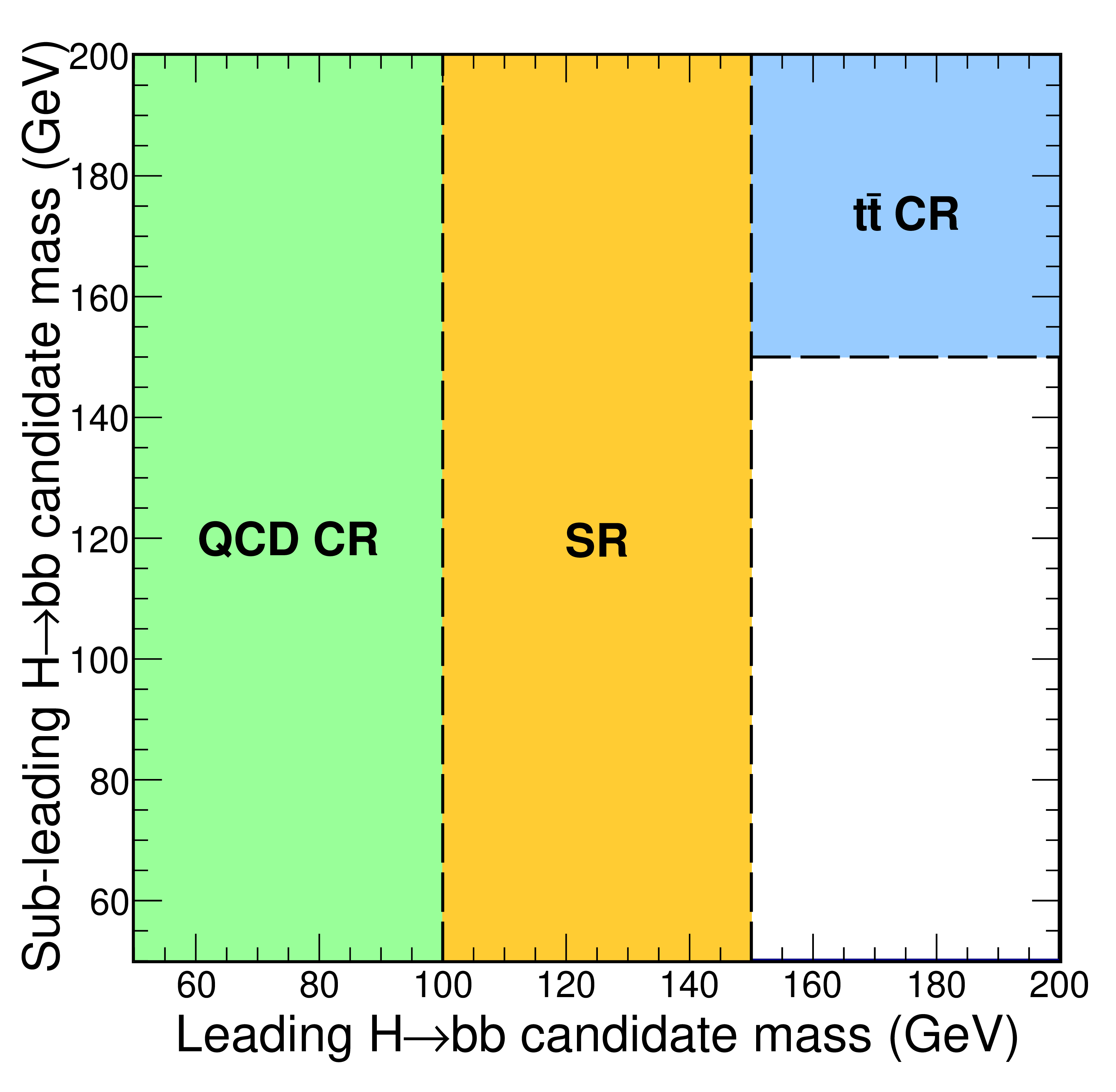
png pdf	Figure 19: Left: schematic diagram showing the regions used for the data-driven background estimation strategy used in the merged channel. The purity in QCD multijet events is reported in each of the background-enriched regions ($ \mathrm{CR_{QCD,A}} $, $ \mathrm{CR_{QCD,B}} $, and $ \mathrm{CR_{QCD,C}} $). Right: schematic diagram of the signal (orange area) and control regions (QCD in green, $ \mathrm{t} \overline{\mathrm{t}} $ in azure) in the plane defined by the $ m_\text{reg}({\mathrm{H}_1}) $ and $ m_\text{reg}({\mathrm{H}_2}) $.
png pdf	Figure 19-a: Left: schematic diagram showing the regions used for the data-driven background estimation strategy used in the merged channel. The purity in QCD multijet events is reported in each of the background-enriched regions ($ \mathrm{CR_{QCD,A}} $, $ \mathrm{CR_{QCD,B}} $, and $ \mathrm{CR_{QCD,C}} $). Right: schematic diagram of the signal (orange area) and control regions (QCD in green, $ \mathrm{t} \overline{\mathrm{t}} $ in azure) in the plane defined by the $ m_\text{reg}({\mathrm{H}_1}) $ and $ m_\text{reg}({\mathrm{H}_2}) $.
png pdf	Figure 19-b: Left: schematic diagram showing the regions used for the data-driven background estimation strategy used in the merged channel. The purity in QCD multijet events is reported in each of the background-enriched regions ($ \mathrm{CR_{QCD,A}} $, $ \mathrm{CR_{QCD,B}} $, and $ \mathrm{CR_{QCD,C}} $). Right: schematic diagram of the signal (orange area) and control regions (QCD in green, $ \mathrm{t} \overline{\mathrm{t}} $ in azure) in the plane defined by the $ m_\text{reg}({\mathrm{H}_1}) $ and $ m_\text{reg}({\mathrm{H}_2}) $.
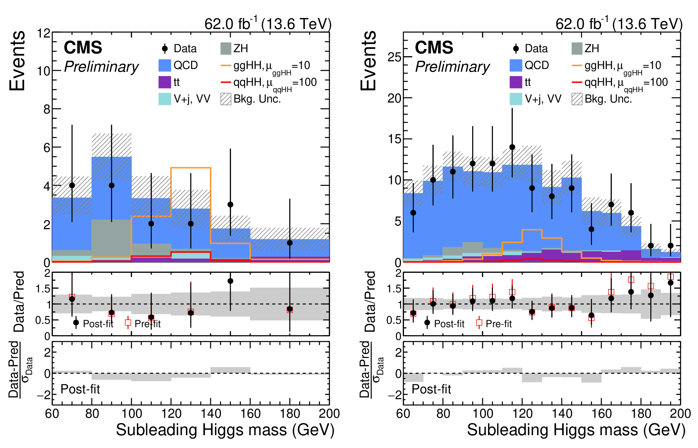
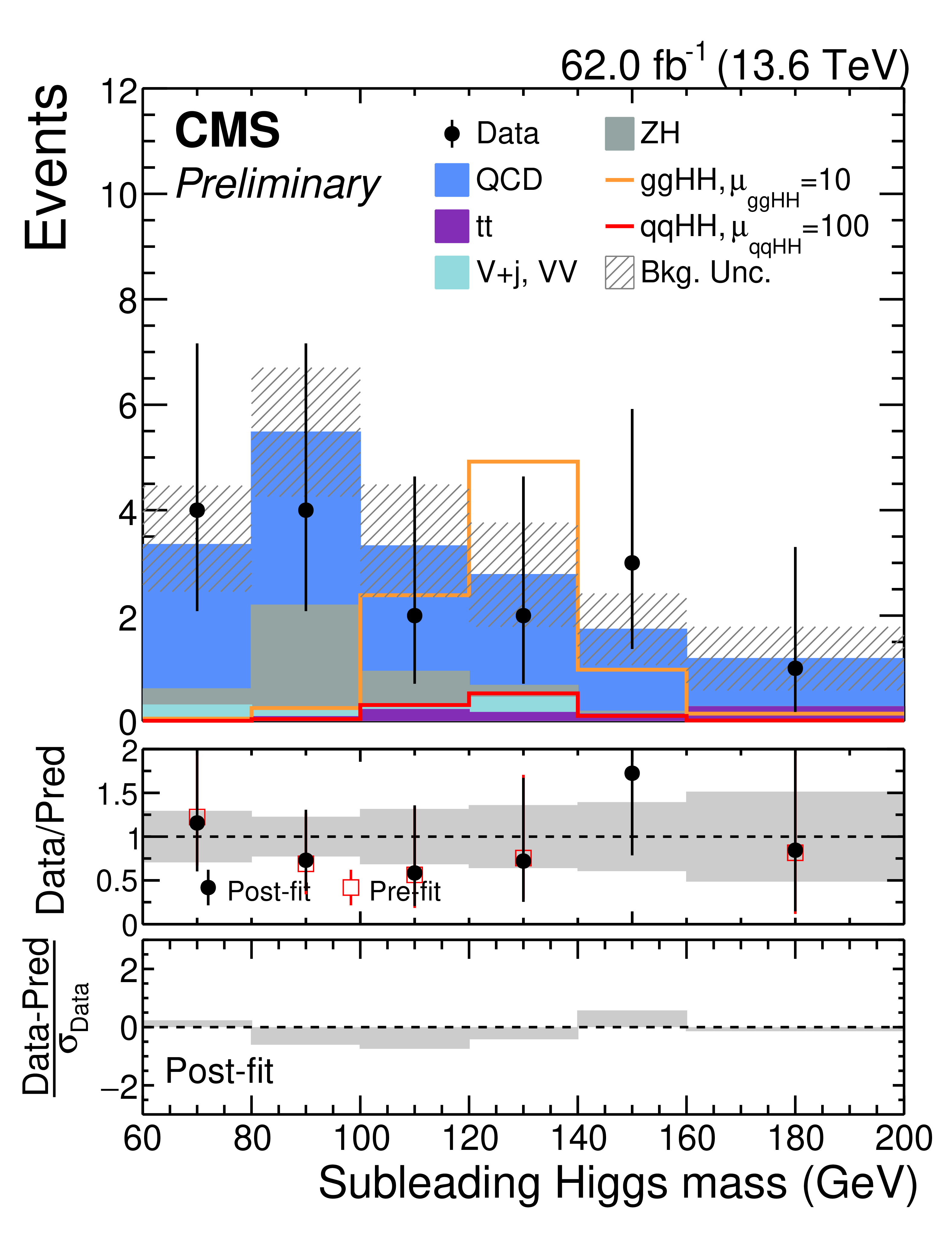
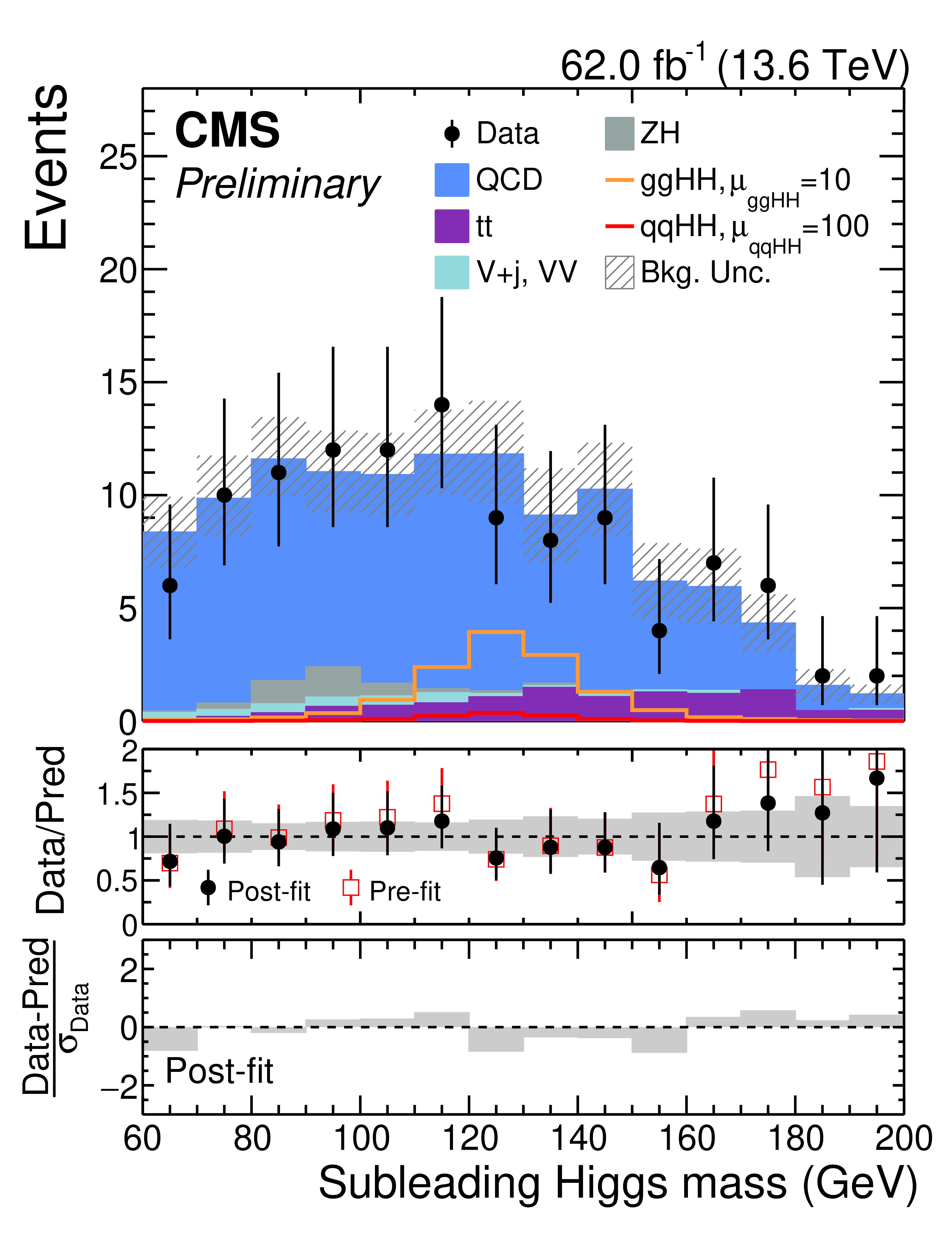
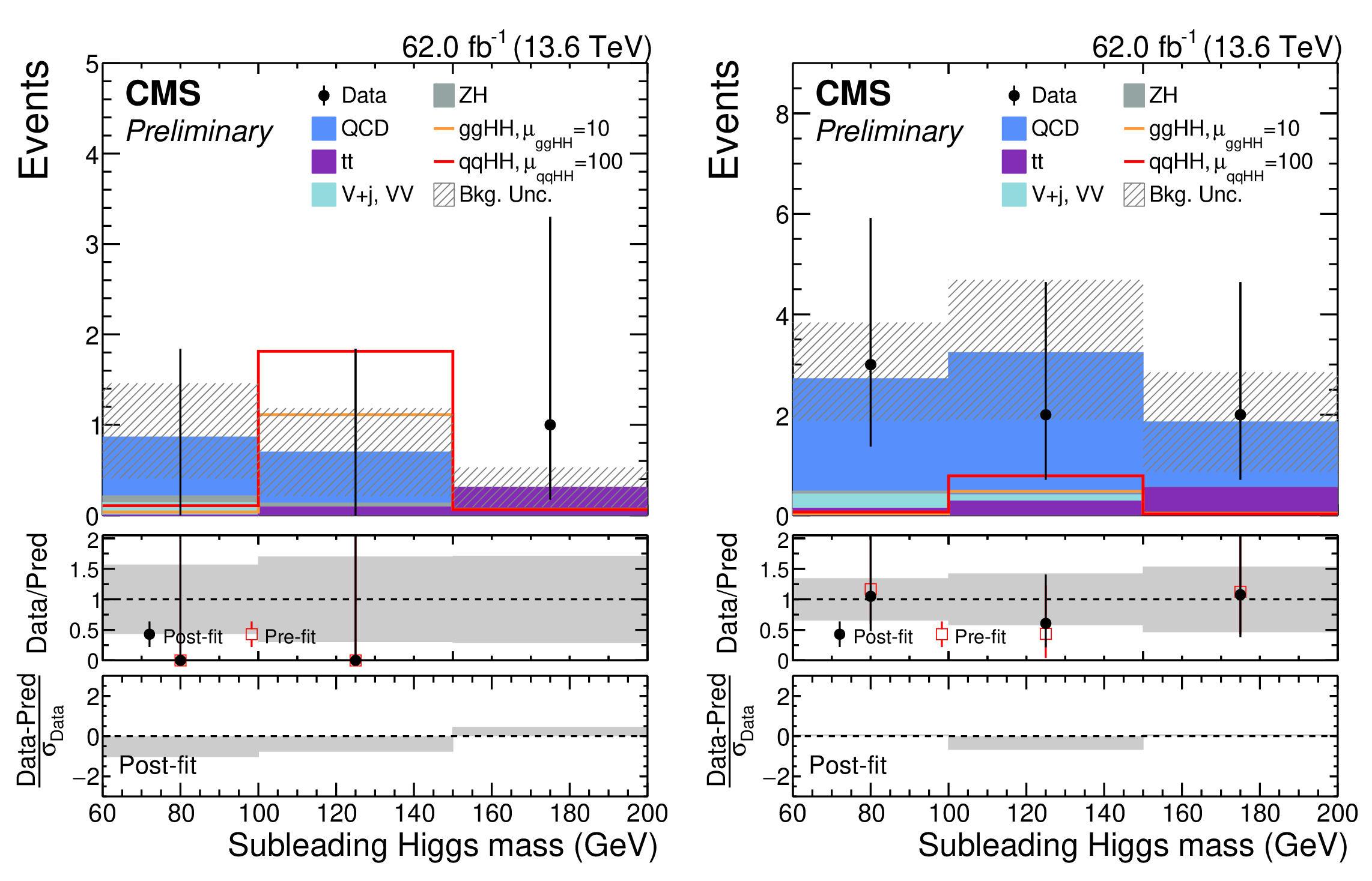
png pdf	Figure 20: Pre-fit and post-fit distributions of the fitted observables for the $ \mathrm{g}\mathrm{g}\mathrm{H}\mathrm{H} $-inclusive HPSR (left) and LPSR (right) categories of the merged analysis following the mass-fit method. Distributions are shown for data (black points) and the different background contributions from QCD multijet, $ \mathrm{t} \overline{\mathrm{t}} $, $ \mathrm{V}+\text{jets} $, dibosons, and ZH productions. The expected distributions for SM $ \mathrm{g}\mathrm{g}\mathrm{H}\mathrm{H} $ (orange) and $ \text{qq}\mathrm{H}\mathrm{H} $ (red) signals are overlaid and scaled by a multiplicative factor to improve their visibility.
png pdf	Figure 20-a: Pre-fit and post-fit distributions of the fitted observables for the $ \mathrm{g}\mathrm{g}\mathrm{H}\mathrm{H} $-inclusive HPSR (left) and LPSR (right) categories of the merged analysis following the mass-fit method. Distributions are shown for data (black points) and the different background contributions from QCD multijet, $ \mathrm{t} \overline{\mathrm{t}} $, $ \mathrm{V}+\text{jets} $, dibosons, and ZH productions. The expected distributions for SM $ \mathrm{g}\mathrm{g}\mathrm{H}\mathrm{H} $ (orange) and $ \text{qq}\mathrm{H}\mathrm{H} $ (red) signals are overlaid and scaled by a multiplicative factor to improve their visibility.
png pdf	Figure 20-b: Pre-fit and post-fit distributions of the fitted observables for the $ \mathrm{g}\mathrm{g}\mathrm{H}\mathrm{H} $-inclusive HPSR (left) and LPSR (right) categories of the merged analysis following the mass-fit method. Distributions are shown for data (black points) and the different background contributions from QCD multijet, $ \mathrm{t} \overline{\mathrm{t}} $, $ \mathrm{V}+\text{jets} $, dibosons, and ZH productions. The expected distributions for SM $ \mathrm{g}\mathrm{g}\mathrm{H}\mathrm{H} $ (orange) and $ \text{qq}\mathrm{H}\mathrm{H} $ (red) signals are overlaid and scaled by a multiplicative factor to improve their visibility.
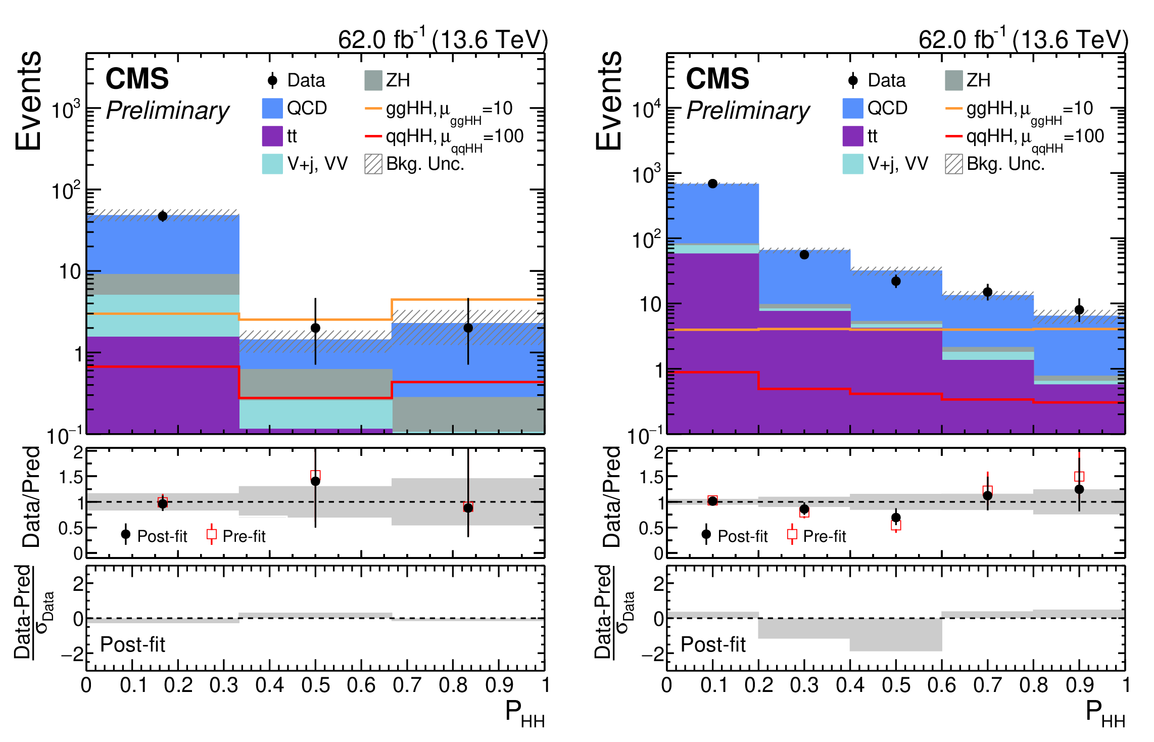
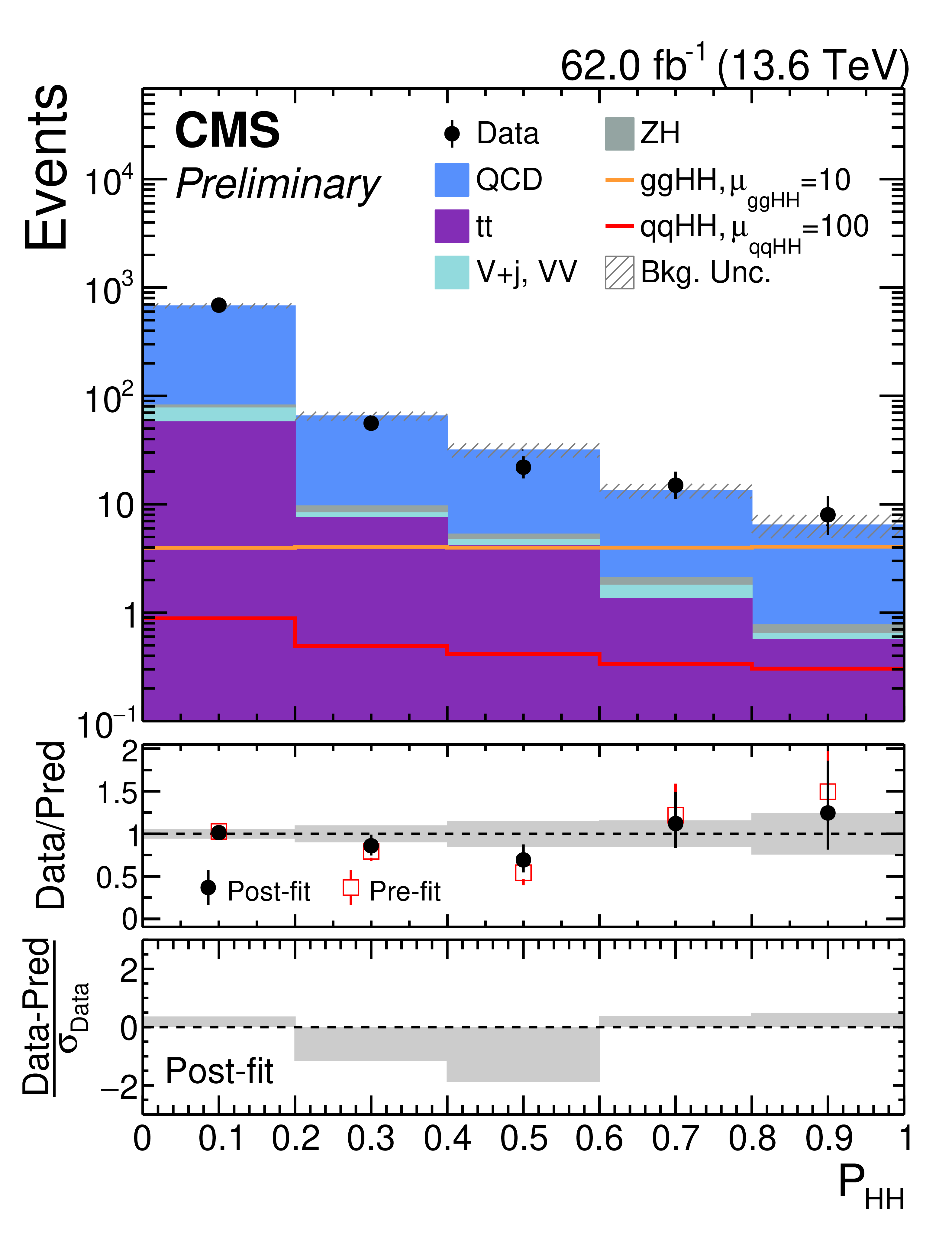
png pdf	Figure 21: Pre-fit and post-fit distributions of the fitted observables for the $ \mathrm{g}\mathrm{g}\mathrm{H}\mathrm{H} $-inclusive HPSR (left) and LPSR (right) categories of the merged analysis following the DNN-fit method. Distributions are shown for data (black points) and the different background contributions from QCD multijet, $ \mathrm{t} \overline{\mathrm{t}} $, $ \mathrm{V}+\text{jets} $, dibosons, and ZH productions. The expected distributions for SM $ \mathrm{g}\mathrm{g}\mathrm{H}\mathrm{H} $ (orange) and $ \text{qq}\mathrm{H}\mathrm{H} $ (red) signals are overlaid and scaled by a multiplicative factor to improve their visibility.
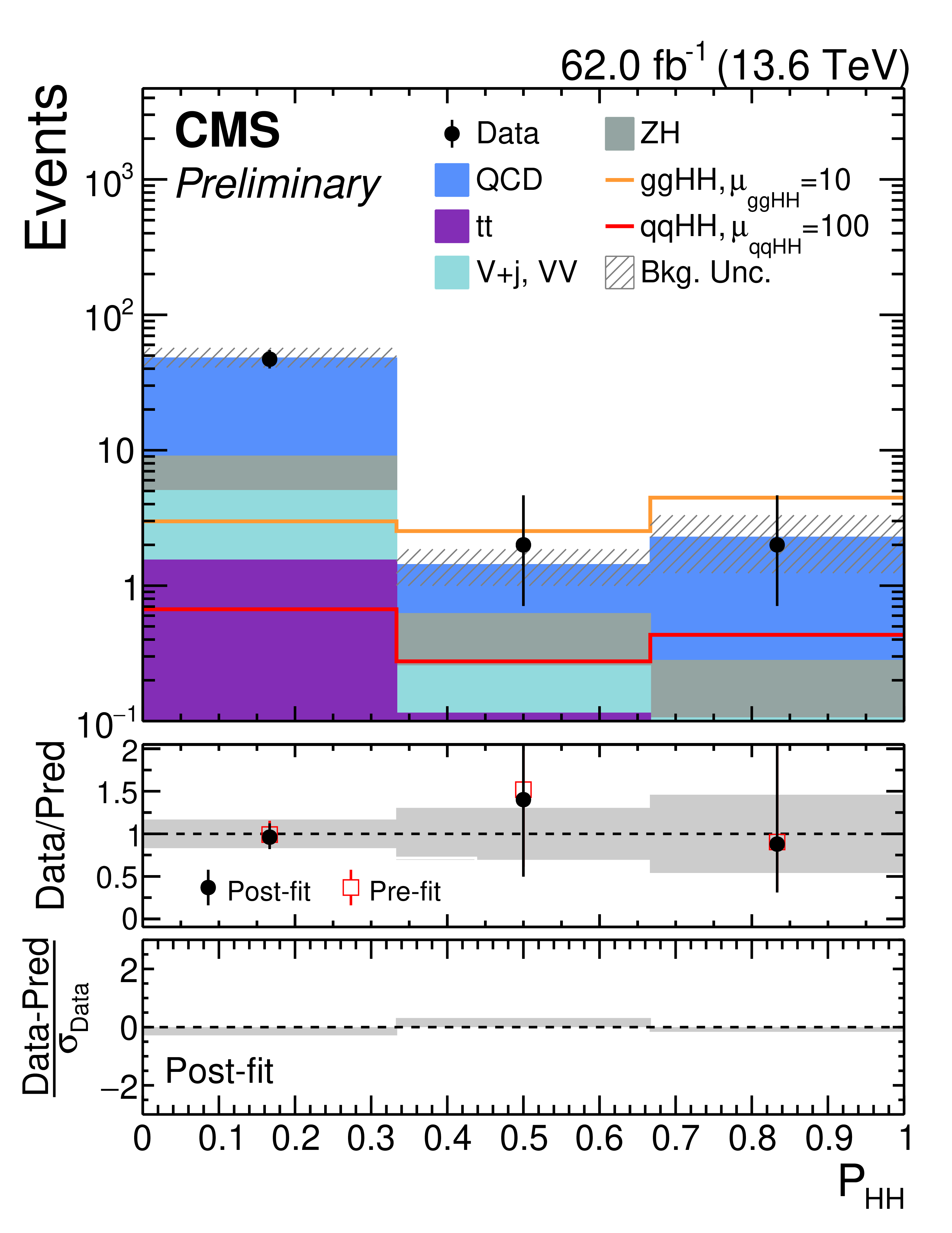
png pdf	Figure 21-a: Pre-fit and post-fit distributions of the fitted observables for the $ \mathrm{g}\mathrm{g}\mathrm{H}\mathrm{H} $-inclusive HPSR (left) and LPSR (right) categories of the merged analysis following the DNN-fit method. Distributions are shown for data (black points) and the different background contributions from QCD multijet, $ \mathrm{t} \overline{\mathrm{t}} $, $ \mathrm{V}+\text{jets} $, dibosons, and ZH productions. The expected distributions for SM $ \mathrm{g}\mathrm{g}\mathrm{H}\mathrm{H} $ (orange) and $ \text{qq}\mathrm{H}\mathrm{H} $ (red) signals are overlaid and scaled by a multiplicative factor to improve their visibility.
png pdf	Figure 21-b: Pre-fit and post-fit distributions of the fitted observables for the $ \mathrm{g}\mathrm{g}\mathrm{H}\mathrm{H} $-inclusive HPSR (left) and LPSR (right) categories of the merged analysis following the DNN-fit method. Distributions are shown for data (black points) and the different background contributions from QCD multijet, $ \mathrm{t} \overline{\mathrm{t}} $, $ \mathrm{V}+\text{jets} $, dibosons, and ZH productions. The expected distributions for SM $ \mathrm{g}\mathrm{g}\mathrm{H}\mathrm{H} $ (orange) and $ \text{qq}\mathrm{H}\mathrm{H} $ (red) signals are overlaid and scaled by a multiplicative factor to improve their visibility.
png pdf	Figure 22: Pre-fit and post-fit distributions of the fitted observables for the $ \text{qq}\mathrm{H}\mathrm{H} $ HPSR (left) and LPSR (right) categories of the merged analysis. Distributions are shown for data (black points) and the different background contributions from QCD multijet, $ \mathrm{t} \overline{\mathrm{t}} $, $ \mathrm{V}+\text{jets} $, dibosons, and ZH productions. The expected distributions for SM $ \mathrm{g}\mathrm{g}\mathrm{H}\mathrm{H} $ (orange) and $ \text{qq}\mathrm{H}\mathrm{H} $ (red) signals are overlaid and scaled by a multiplicative factor to improve their visibility.
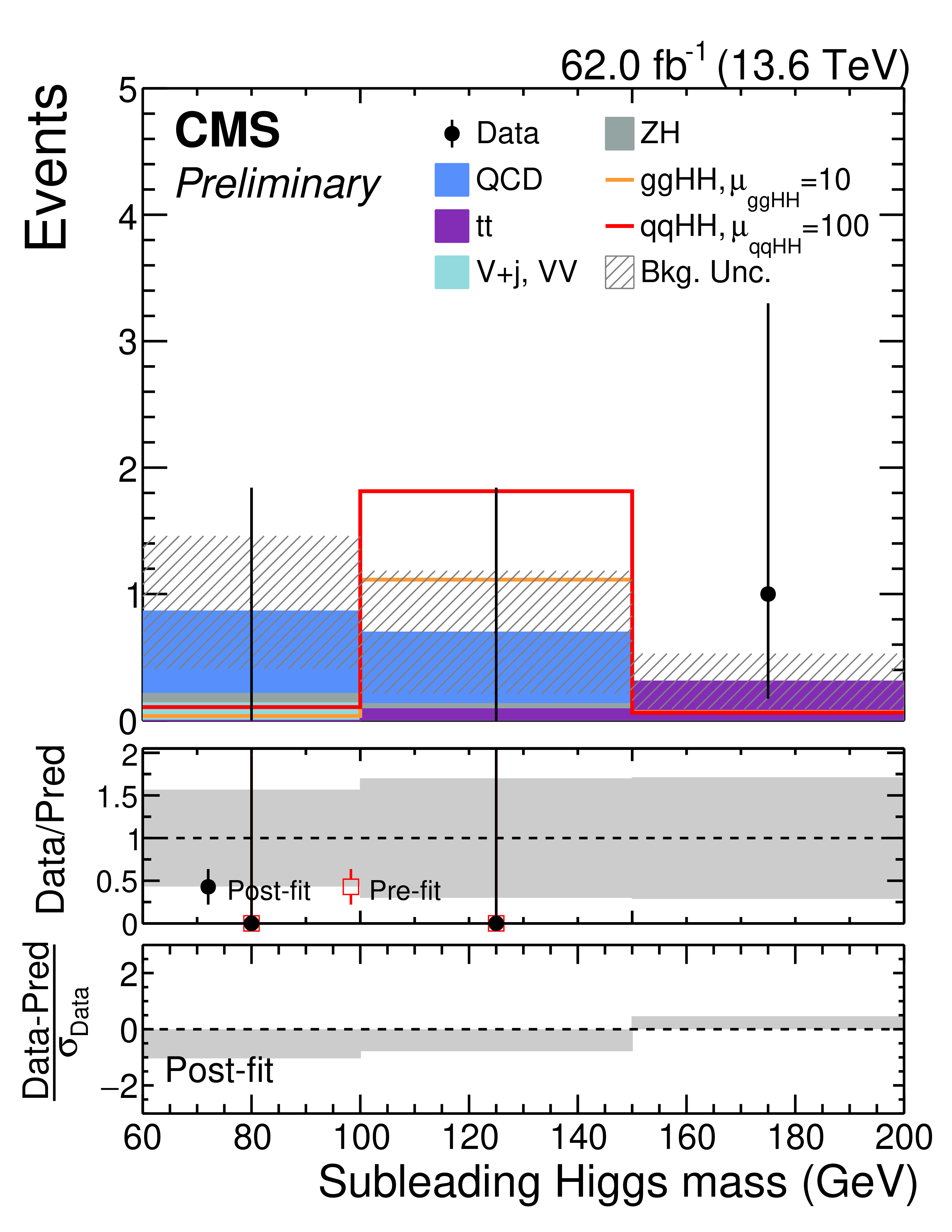
png pdf	Figure 22-a: Pre-fit and post-fit distributions of the fitted observables for the $ \text{qq}\mathrm{H}\mathrm{H} $ HPSR (left) and LPSR (right) categories of the merged analysis. Distributions are shown for data (black points) and the different background contributions from QCD multijet, $ \mathrm{t} \overline{\mathrm{t}} $, $ \mathrm{V}+\text{jets} $, dibosons, and ZH productions. The expected distributions for SM $ \mathrm{g}\mathrm{g}\mathrm{H}\mathrm{H} $ (orange) and $ \text{qq}\mathrm{H}\mathrm{H} $ (red) signals are overlaid and scaled by a multiplicative factor to improve their visibility.
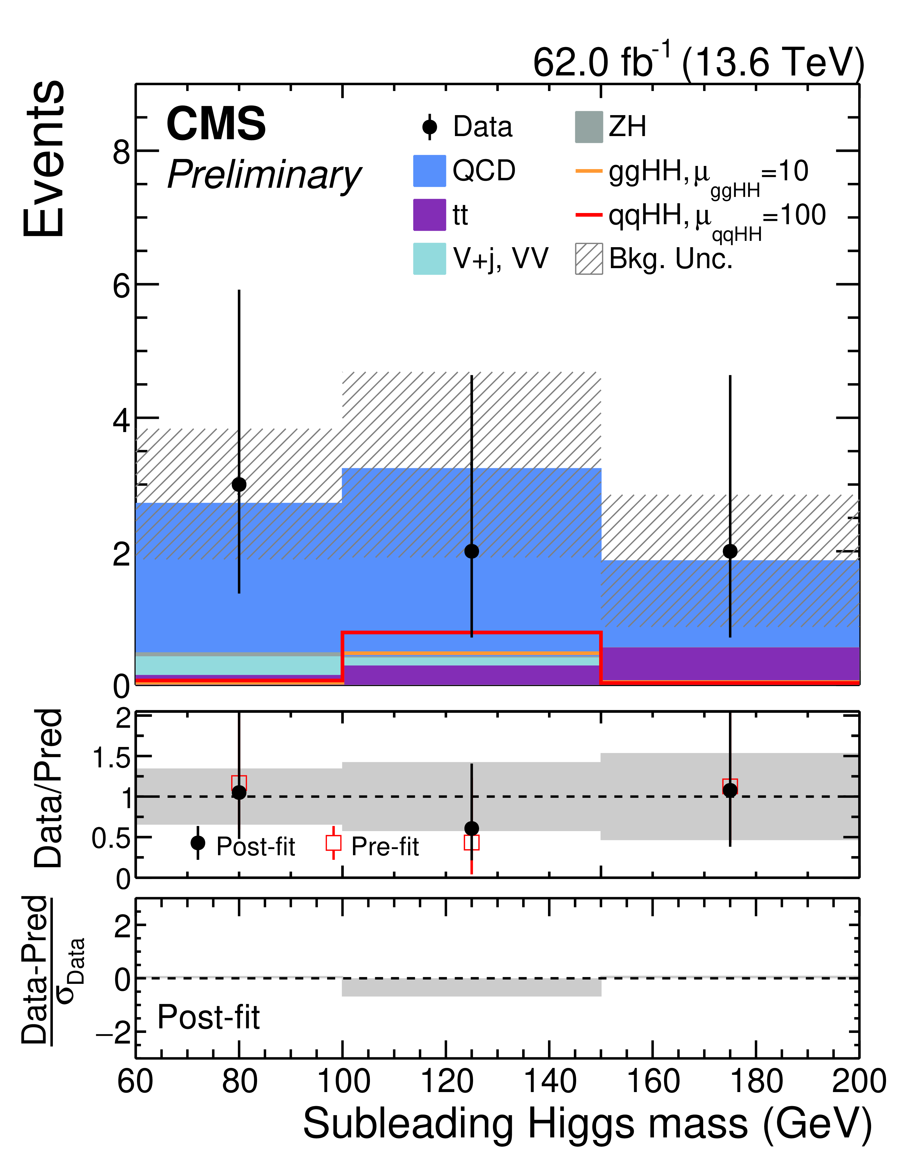
png pdf	Figure 22-b: Pre-fit and post-fit distributions of the fitted observables for the $ \text{qq}\mathrm{H}\mathrm{H} $ HPSR (left) and LPSR (right) categories of the merged analysis. Distributions are shown for data (black points) and the different background contributions from QCD multijet, $ \mathrm{t} \overline{\mathrm{t}} $, $ \mathrm{V}+\text{jets} $, dibosons, and ZH productions. The expected distributions for SM $ \mathrm{g}\mathrm{g}\mathrm{H}\mathrm{H} $ (orange) and $ \text{qq}\mathrm{H}\mathrm{H} $ (red) signals are overlaid and scaled by a multiplicative factor to improve their visibility.
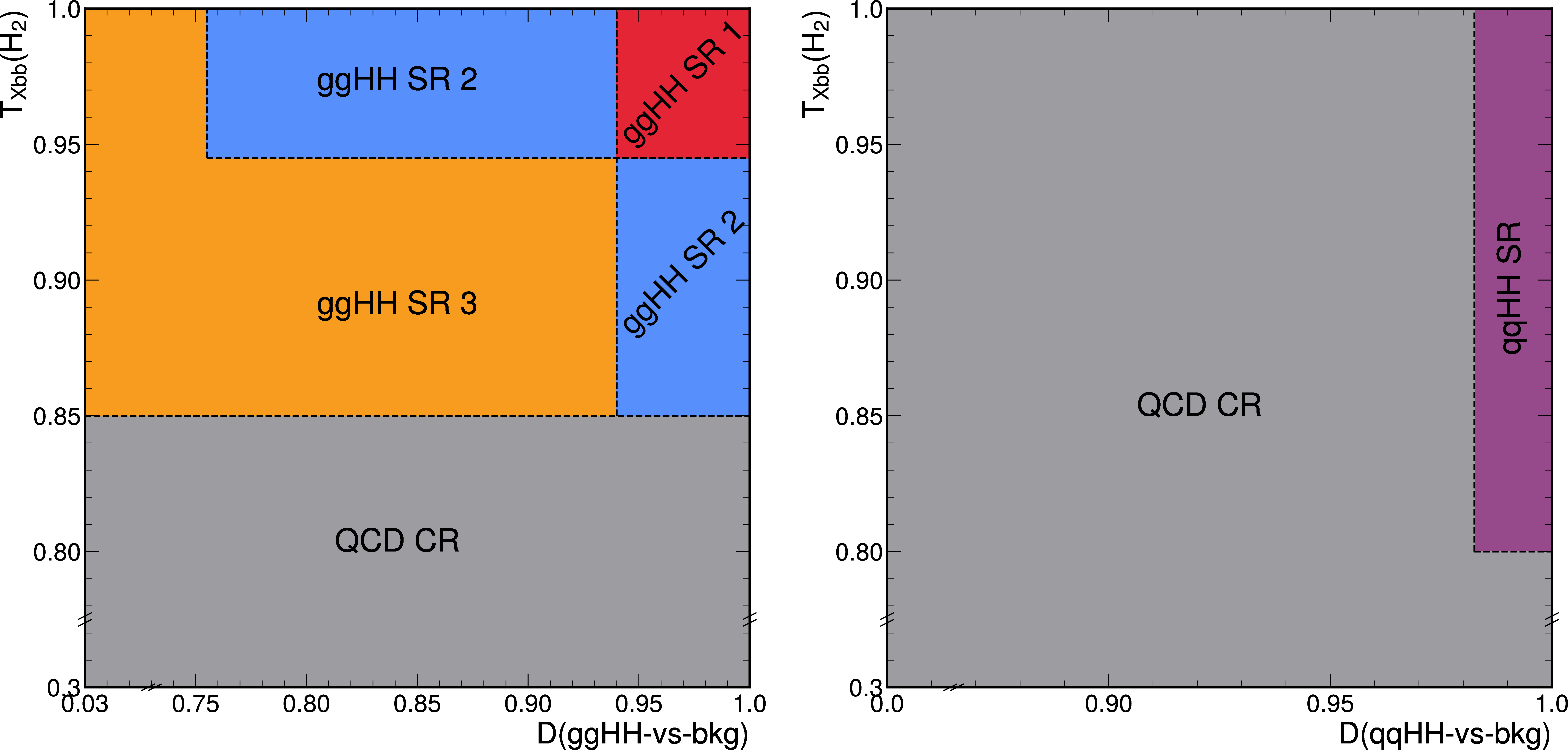
png pdf	Figure 23: Schematic diagrams showing the SRs and QCD CR (gray) used in the merged analysis described in Section 6.3. Left: the $ \mathrm{g}\mathrm{g}\mathrm{H}\mathrm{H} $ SR 1 (red), 2 (blue), and 3 (orange) are defined based on successively lower selections on the $ T_\text{Xbb} $ score of the \HepParticleHu candidate and the D(\text$ \mathrm{g}\mathrm{g}\mathrm{H}\mathrm{H} $-vs-bkg) score. Right: the $ \mathrm{q}\mathrm{q}\mathrm{H}\mathrm{H} $ SR (purple) is defined based on a Tight selection on D(\text$ \mathrm{q}\mathrm{q}\mathrm{H}\mathrm{H} $-vs-bkg) and a Loose selection on $ T_\text{Xbb} $ of the \HepParticleHu candidate.
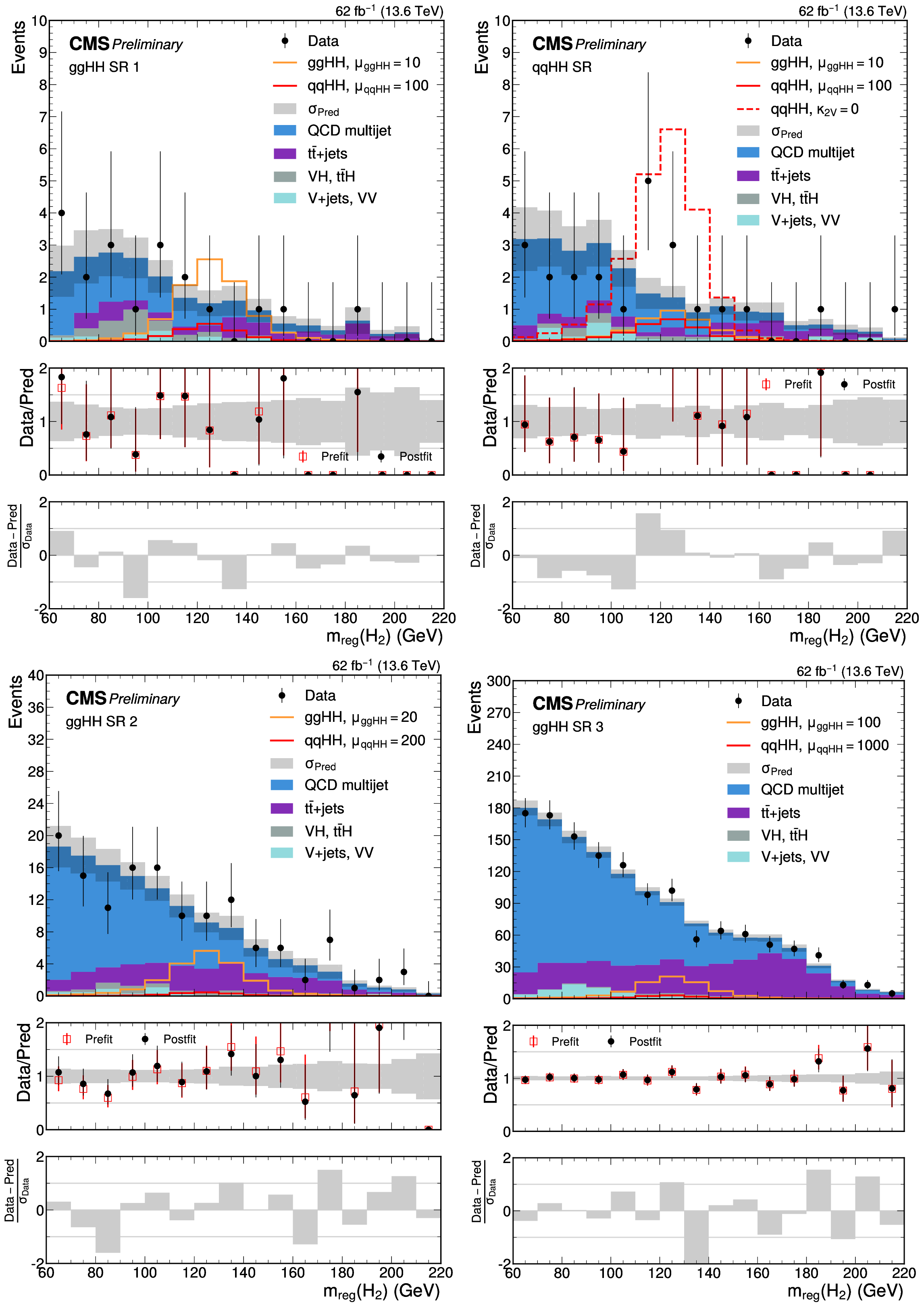
png pdf	Figure 24: The fitted signal+background distributions in the regressed mass of the secondary Higgs boson candidate $ m_\text{reg}(\mathrm{H_u}) $ in $ \mathrm{g}\mathrm{g}\mathrm{H}\mathrm{H} $ SR 1 (upper left), the $ \mathrm{q}\mathrm{q}\mathrm{H}\mathrm{H} $ SR (upper right), $ \mathrm{g}\mathrm{g}\mathrm{H}\mathrm{H} $ SR 2 (lower left), and $ \mathrm{g}\mathrm{g}\mathrm{H}\mathrm{H} $ SR 3 (lower right). The SM $ \mathrm{g}\mathrm{g}\mathrm{H}\mathrm{H} $ and $ \mathrm{q}\mathrm{q}\mathrm{H}\mathrm{H} $ signal are overlaid in the $ \mathrm{g}\mathrm{g}\mathrm{H}\mathrm{H} $ SRs scaled by different factors. The targeted $ \kappa_{2\mathrm{V}}= $ 0 $ \mathrm{q}\mathrm{q}\mathrm{H}\mathrm{H} $ signal is also overlaid in the $ \mathrm{q}\mathrm{q}\mathrm{H}\mathrm{H} $ SR.
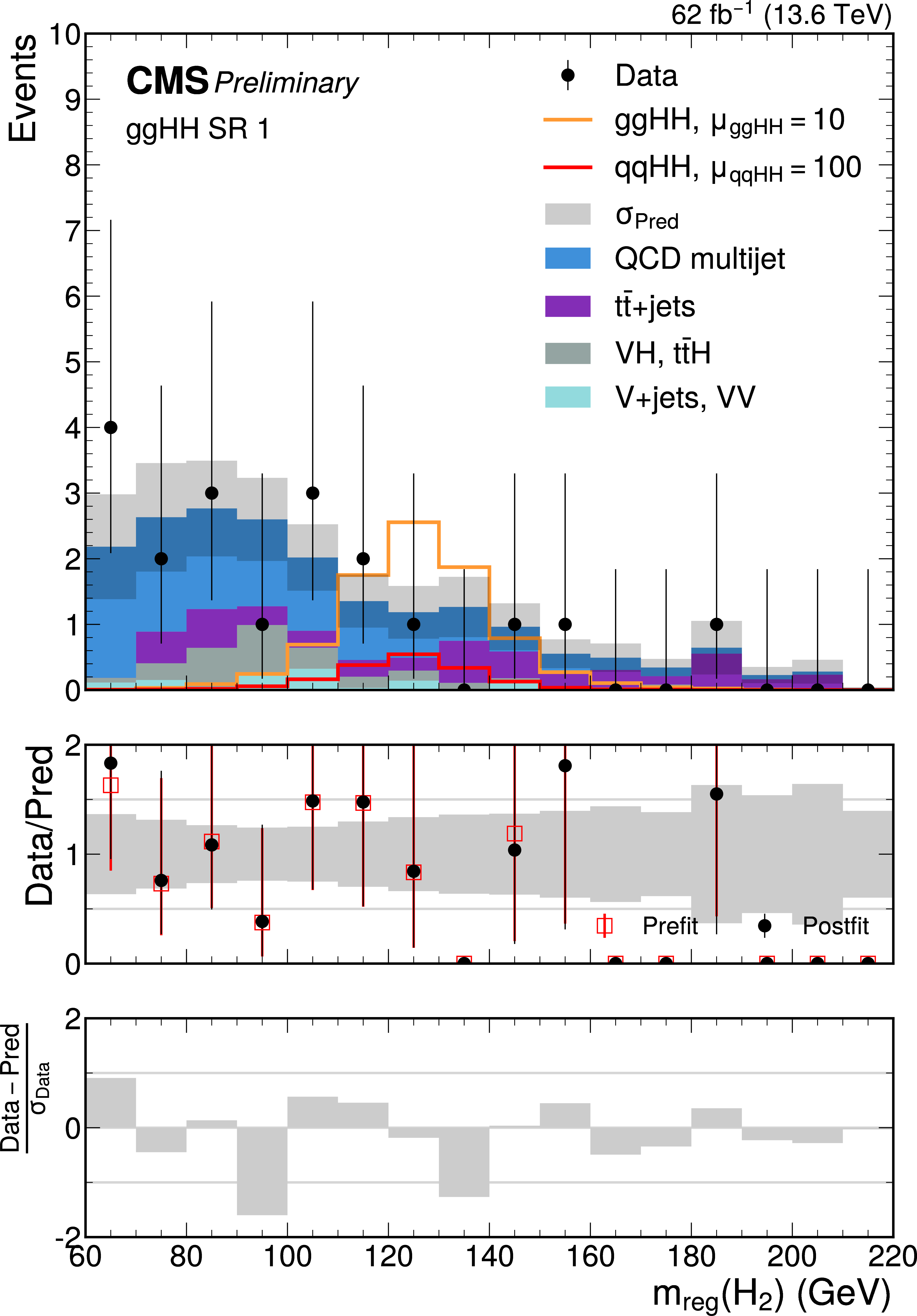
png pdf	Figure 24-a: The fitted signal+background distributions in the regressed mass of the secondary Higgs boson candidate $ m_\text{reg}(\mathrm{H_u}) $ in $ \mathrm{g}\mathrm{g}\mathrm{H}\mathrm{H} $ SR 1 (upper left), the $ \mathrm{q}\mathrm{q}\mathrm{H}\mathrm{H} $ SR (upper right), $ \mathrm{g}\mathrm{g}\mathrm{H}\mathrm{H} $ SR 2 (lower left), and $ \mathrm{g}\mathrm{g}\mathrm{H}\mathrm{H} $ SR 3 (lower right). The SM $ \mathrm{g}\mathrm{g}\mathrm{H}\mathrm{H} $ and $ \mathrm{q}\mathrm{q}\mathrm{H}\mathrm{H} $ signal are overlaid in the $ \mathrm{g}\mathrm{g}\mathrm{H}\mathrm{H} $ SRs scaled by different factors. The targeted $ \kappa_{2\mathrm{V}}= $ 0 $ \mathrm{q}\mathrm{q}\mathrm{H}\mathrm{H} $ signal is also overlaid in the $ \mathrm{q}\mathrm{q}\mathrm{H}\mathrm{H} $ SR.
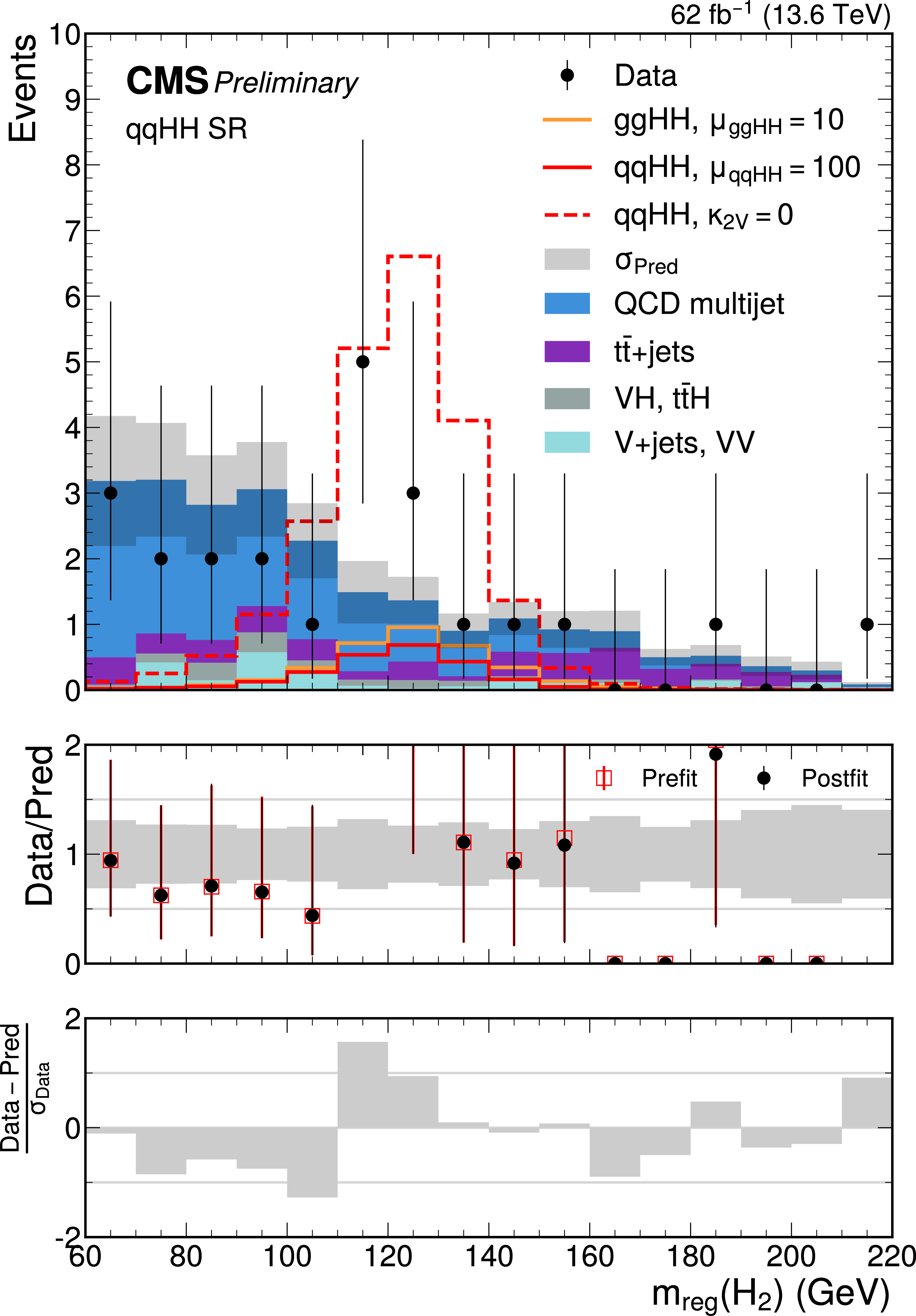
png pdf	Figure 24-b: The fitted signal+background distributions in the regressed mass of the secondary Higgs boson candidate $ m_\text{reg}(\mathrm{H_u}) $ in $ \mathrm{g}\mathrm{g}\mathrm{H}\mathrm{H} $ SR 1 (upper left), the $ \mathrm{q}\mathrm{q}\mathrm{H}\mathrm{H} $ SR (upper right), $ \mathrm{g}\mathrm{g}\mathrm{H}\mathrm{H} $ SR 2 (lower left), and $ \mathrm{g}\mathrm{g}\mathrm{H}\mathrm{H} $ SR 3 (lower right). The SM $ \mathrm{g}\mathrm{g}\mathrm{H}\mathrm{H} $ and $ \mathrm{q}\mathrm{q}\mathrm{H}\mathrm{H} $ signal are overlaid in the $ \mathrm{g}\mathrm{g}\mathrm{H}\mathrm{H} $ SRs scaled by different factors. The targeted $ \kappa_{2\mathrm{V}}= $ 0 $ \mathrm{q}\mathrm{q}\mathrm{H}\mathrm{H} $ signal is also overlaid in the $ \mathrm{q}\mathrm{q}\mathrm{H}\mathrm{H} $ SR.
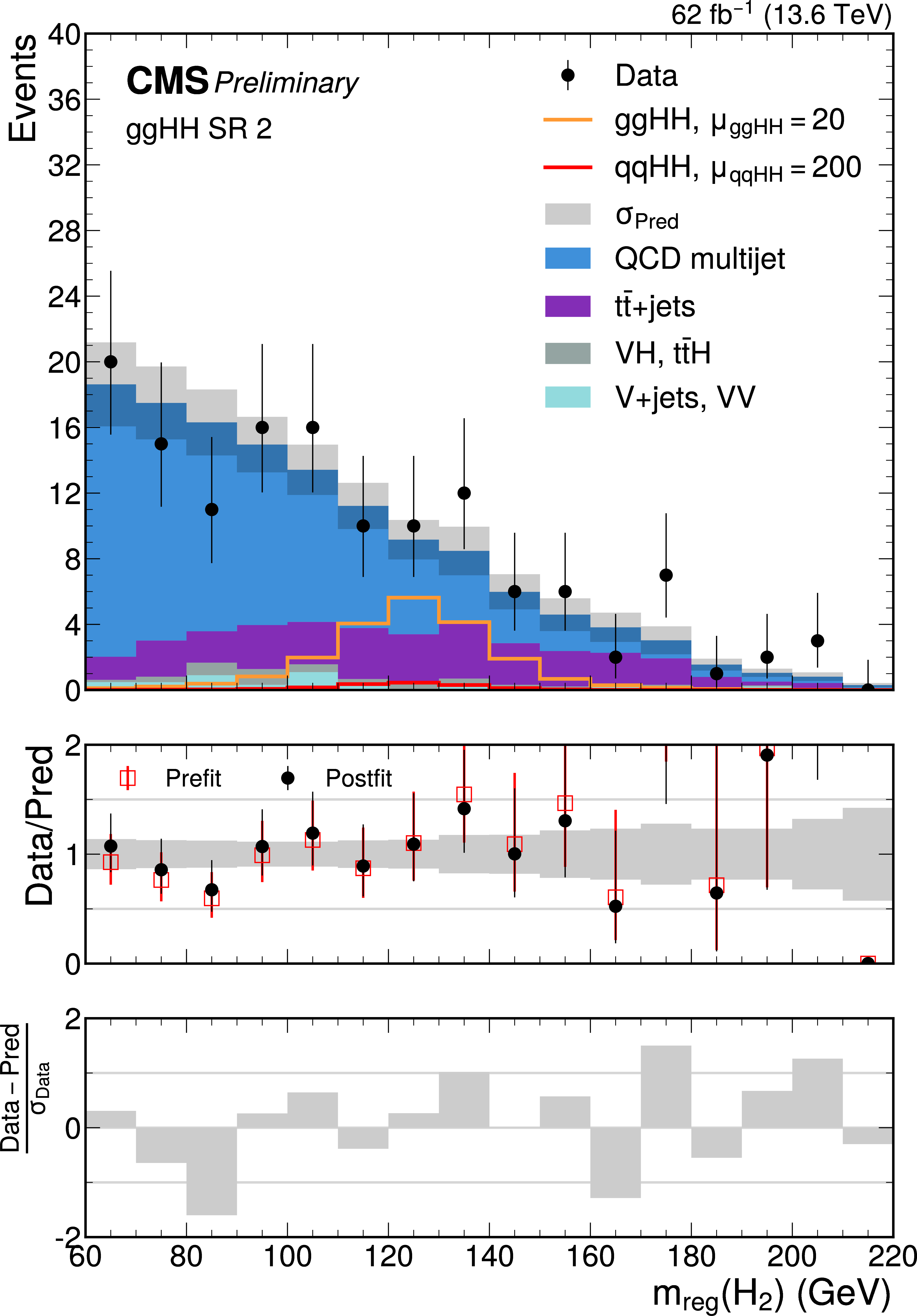
png pdf	Figure 24-c: The fitted signal+background distributions in the regressed mass of the secondary Higgs boson candidate $ m_\text{reg}(\mathrm{H_u}) $ in $ \mathrm{g}\mathrm{g}\mathrm{H}\mathrm{H} $ SR 1 (upper left), the $ \mathrm{q}\mathrm{q}\mathrm{H}\mathrm{H} $ SR (upper right), $ \mathrm{g}\mathrm{g}\mathrm{H}\mathrm{H} $ SR 2 (lower left), and $ \mathrm{g}\mathrm{g}\mathrm{H}\mathrm{H} $ SR 3 (lower right). The SM $ \mathrm{g}\mathrm{g}\mathrm{H}\mathrm{H} $ and $ \mathrm{q}\mathrm{q}\mathrm{H}\mathrm{H} $ signal are overlaid in the $ \mathrm{g}\mathrm{g}\mathrm{H}\mathrm{H} $ SRs scaled by different factors. The targeted $ \kappa_{2\mathrm{V}}= $ 0 $ \mathrm{q}\mathrm{q}\mathrm{H}\mathrm{H} $ signal is also overlaid in the $ \mathrm{q}\mathrm{q}\mathrm{H}\mathrm{H} $ SR.
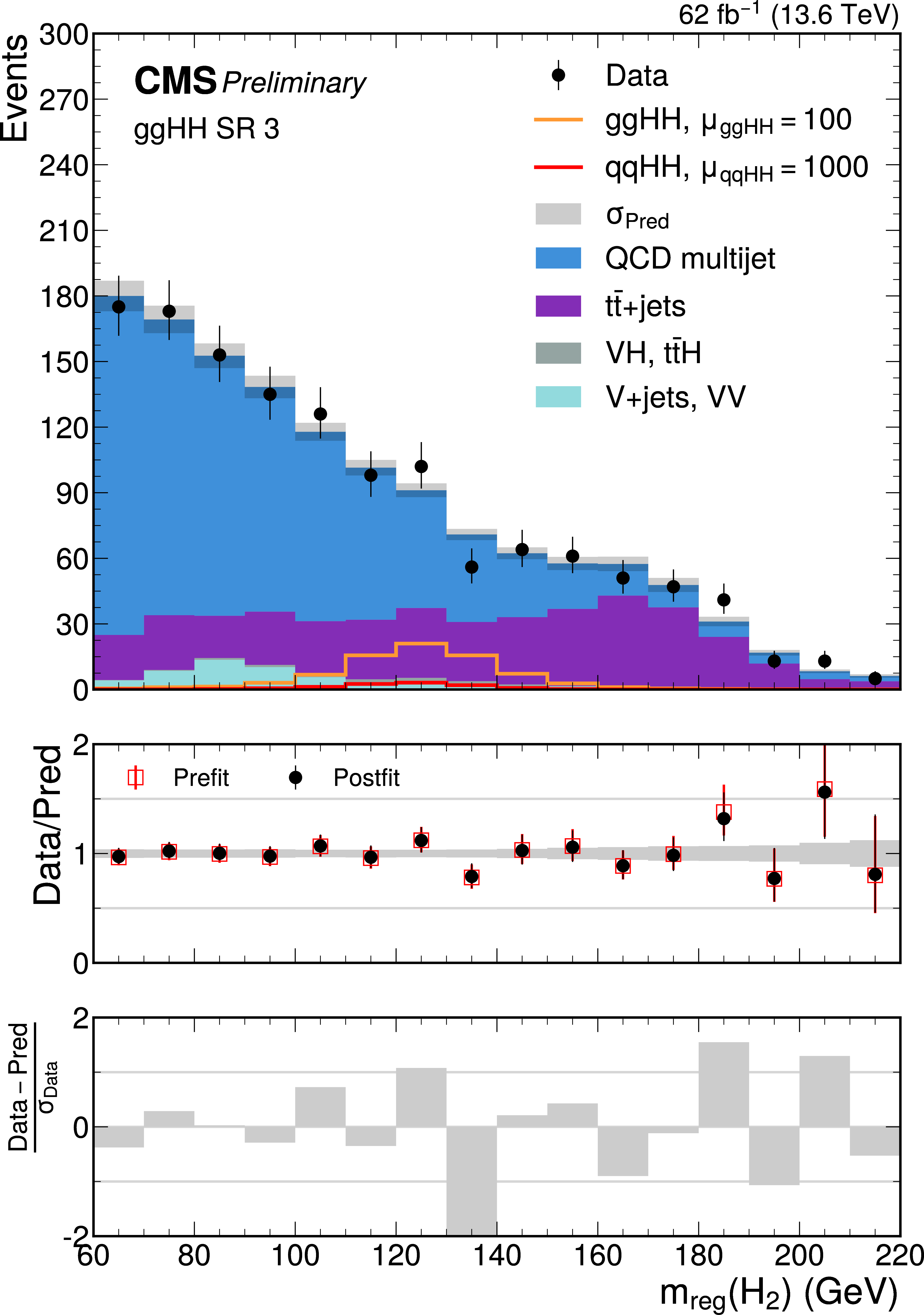
png pdf	Figure 24-d: The fitted signal+background distributions in the regressed mass of the secondary Higgs boson candidate $ m_\text{reg}(\mathrm{H_u}) $ in $ \mathrm{g}\mathrm{g}\mathrm{H}\mathrm{H} $ SR 1 (upper left), the $ \mathrm{q}\mathrm{q}\mathrm{H}\mathrm{H} $ SR (upper right), $ \mathrm{g}\mathrm{g}\mathrm{H}\mathrm{H} $ SR 2 (lower left), and $ \mathrm{g}\mathrm{g}\mathrm{H}\mathrm{H} $ SR 3 (lower right). The SM $ \mathrm{g}\mathrm{g}\mathrm{H}\mathrm{H} $ and $ \mathrm{q}\mathrm{q}\mathrm{H}\mathrm{H} $ signal are overlaid in the $ \mathrm{g}\mathrm{g}\mathrm{H}\mathrm{H} $ SRs scaled by different factors. The targeted $ \kappa_{2\mathrm{V}}= $ 0 $ \mathrm{q}\mathrm{q}\mathrm{H}\mathrm{H} $ signal is also overlaid in the $ \mathrm{q}\mathrm{q}\mathrm{H}\mathrm{H} $ SR.
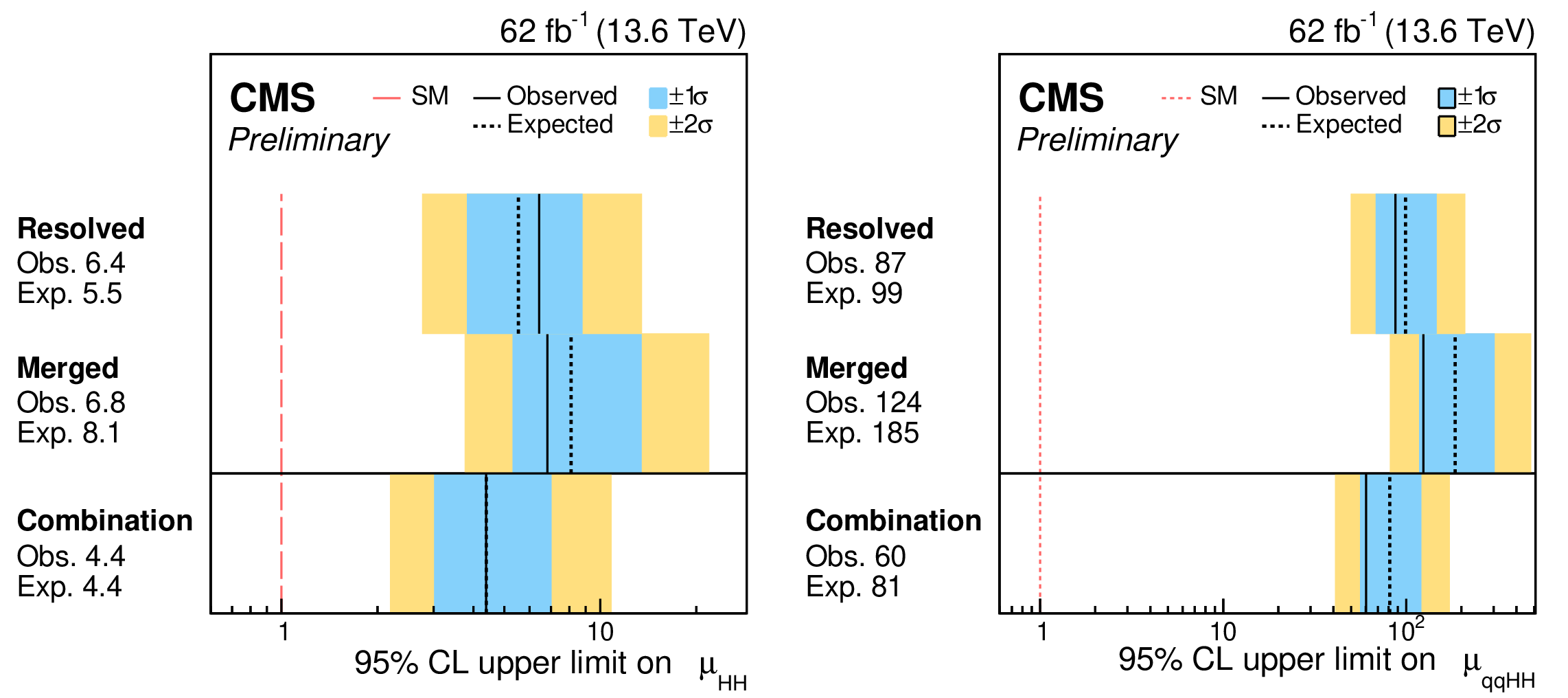
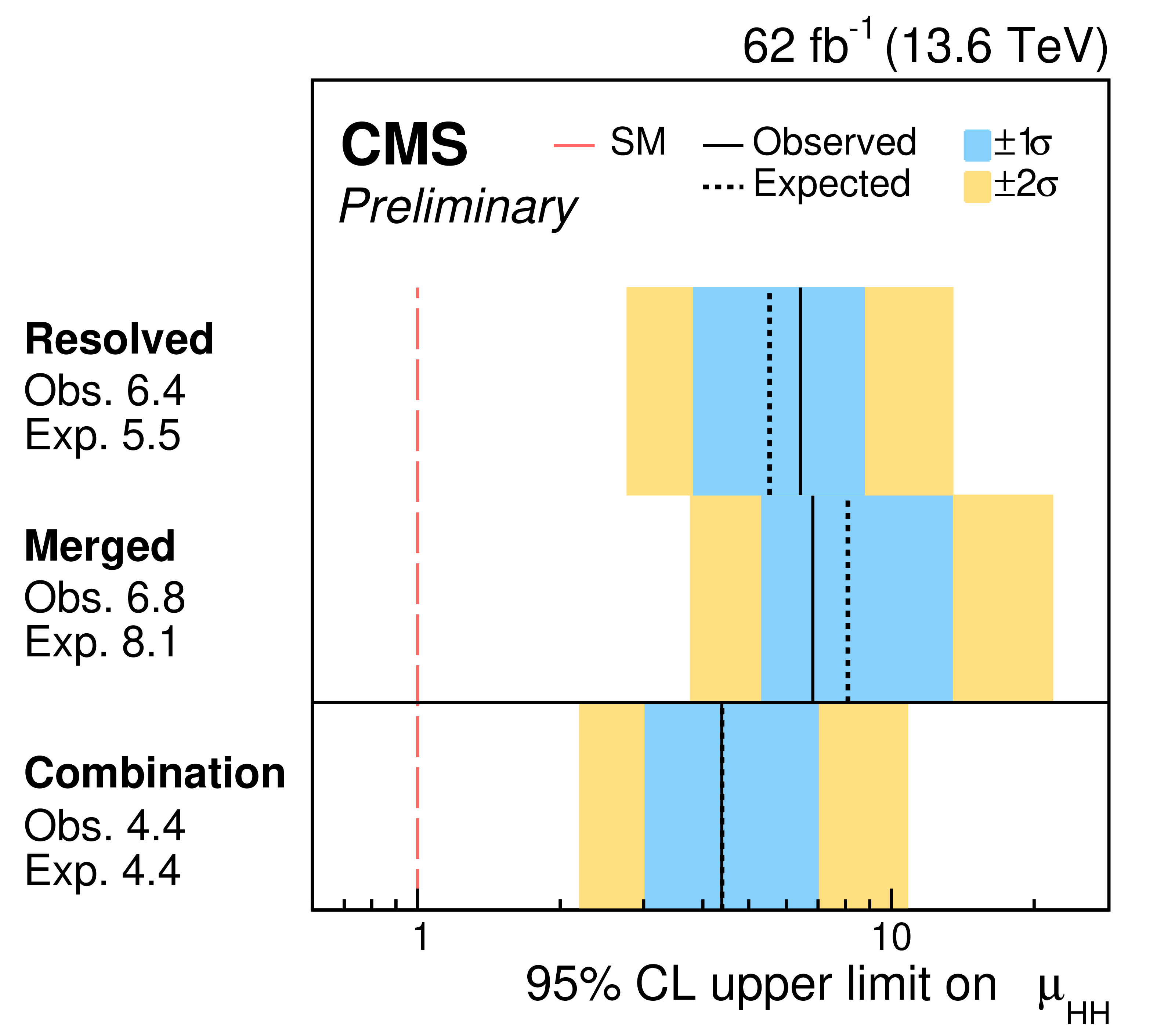
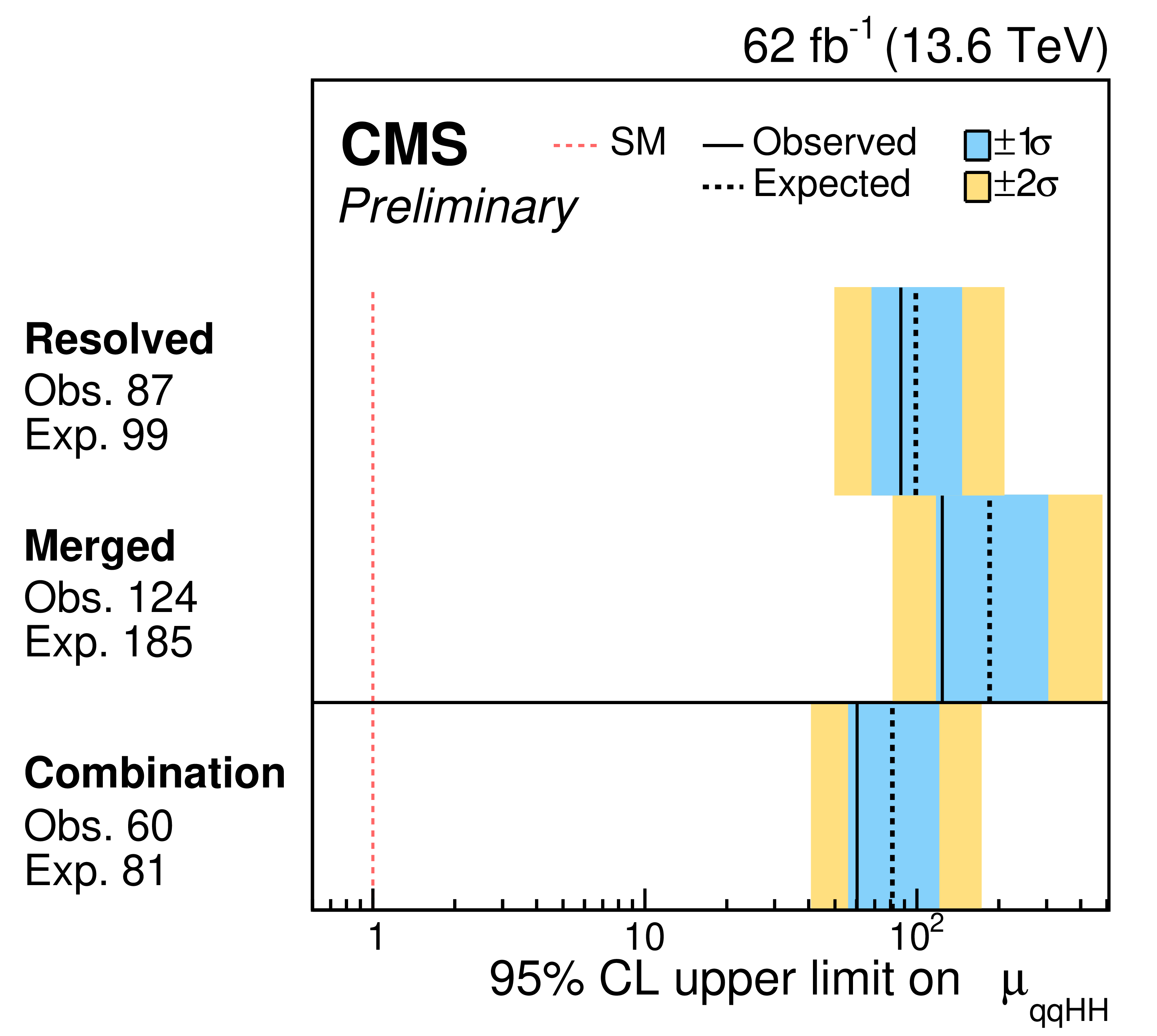
png pdf	Figure 25: Left: the observed (solid) and expected (dashed) 95% CL upper limits on the signal strength of HH production from the resolved analysis with overlap removed, the merged HPSR mass-fit category, and their combination. The cyan and blue bands represent, respectively, the 68 and 95% CL intervals around the expected limit. Right: the same breakdown of 95% CL upper limits on the signal strength of $ \text{qq}\mathrm{H}\mathrm{H} $ production.
png pdf	Figure 25-a: Left: the observed (solid) and expected (dashed) 95% CL upper limits on the signal strength of HH production from the resolved analysis with overlap removed, the merged HPSR mass-fit category, and their combination. The cyan and blue bands represent, respectively, the 68 and 95% CL intervals around the expected limit. Right: the same breakdown of 95% CL upper limits on the signal strength of $ \text{qq}\mathrm{H}\mathrm{H} $ production.
png pdf	Figure 25-b: Left: the observed (solid) and expected (dashed) 95% CL upper limits on the signal strength of HH production from the resolved analysis with overlap removed, the merged HPSR mass-fit category, and their combination. The cyan and blue bands represent, respectively, the 68 and 95% CL intervals around the expected limit. Right: the same breakdown of 95% CL upper limits on the signal strength of $ \text{qq}\mathrm{H}\mathrm{H} $ production.
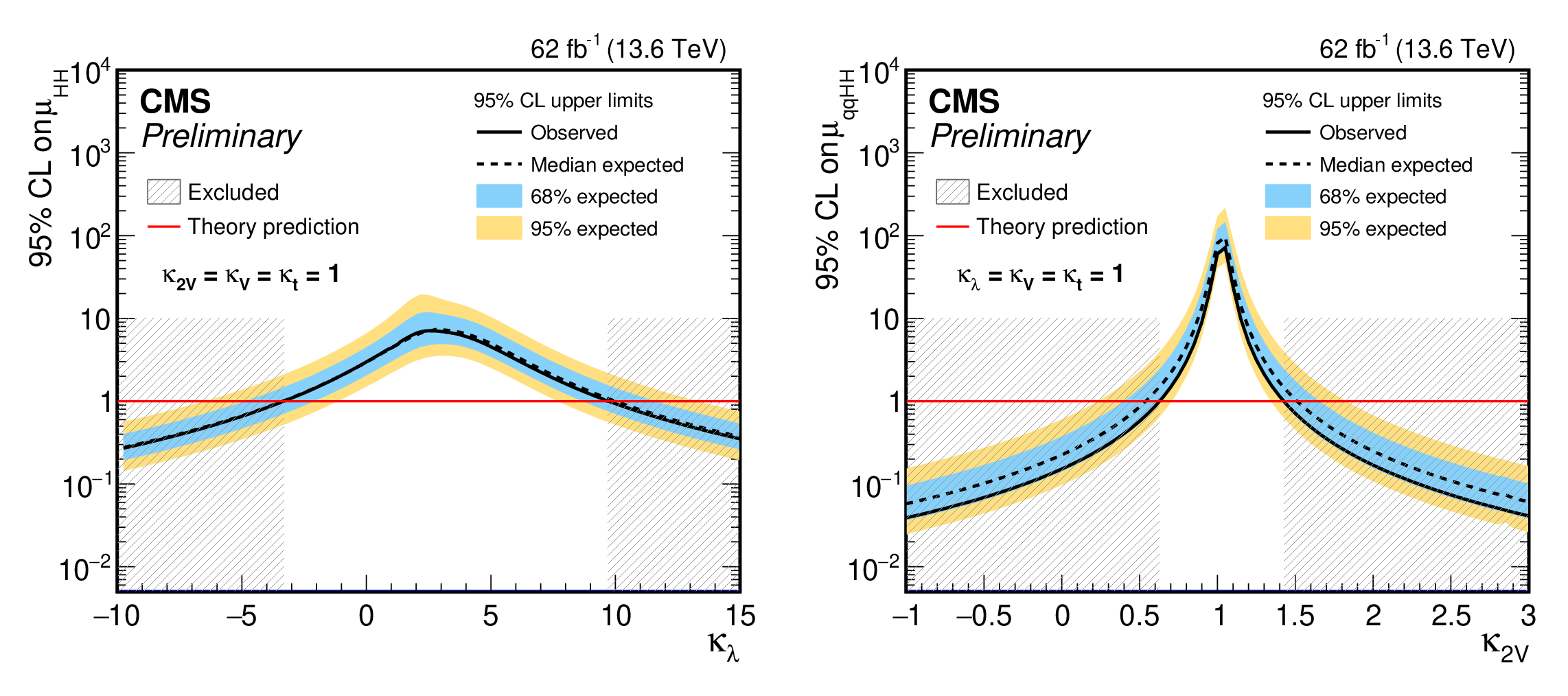
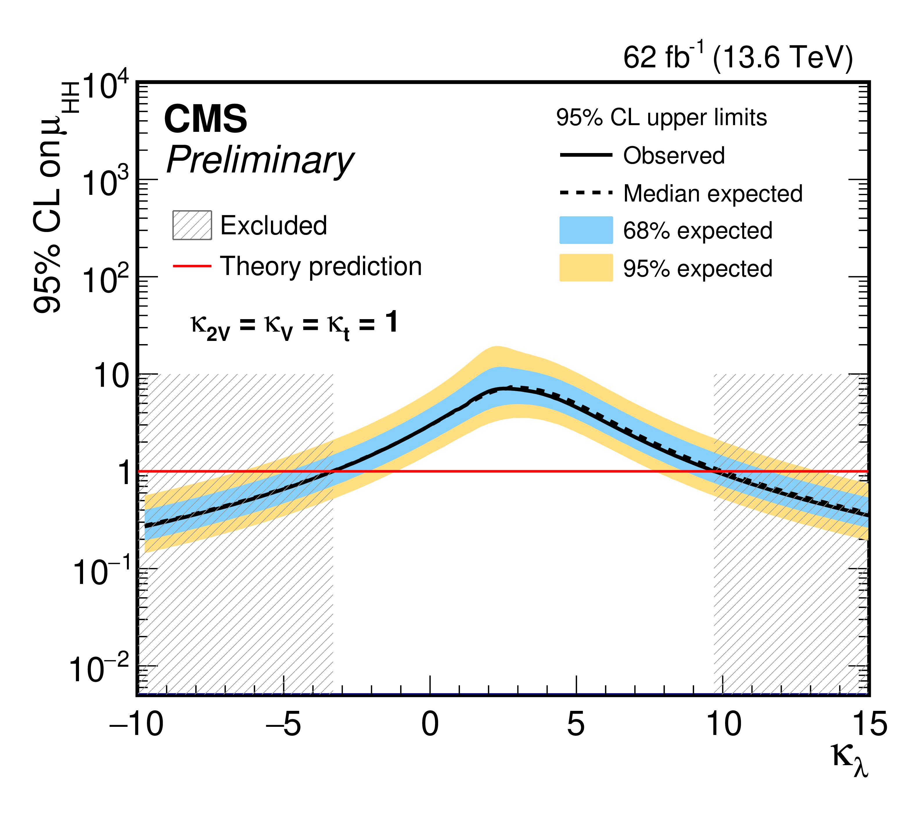
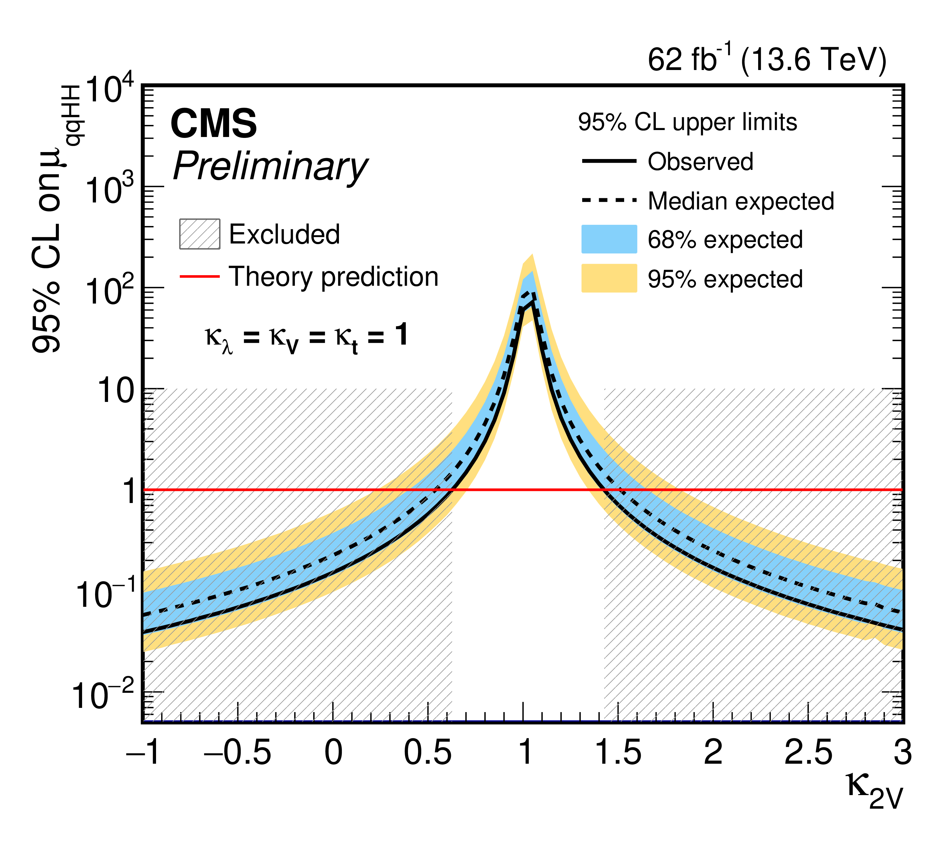
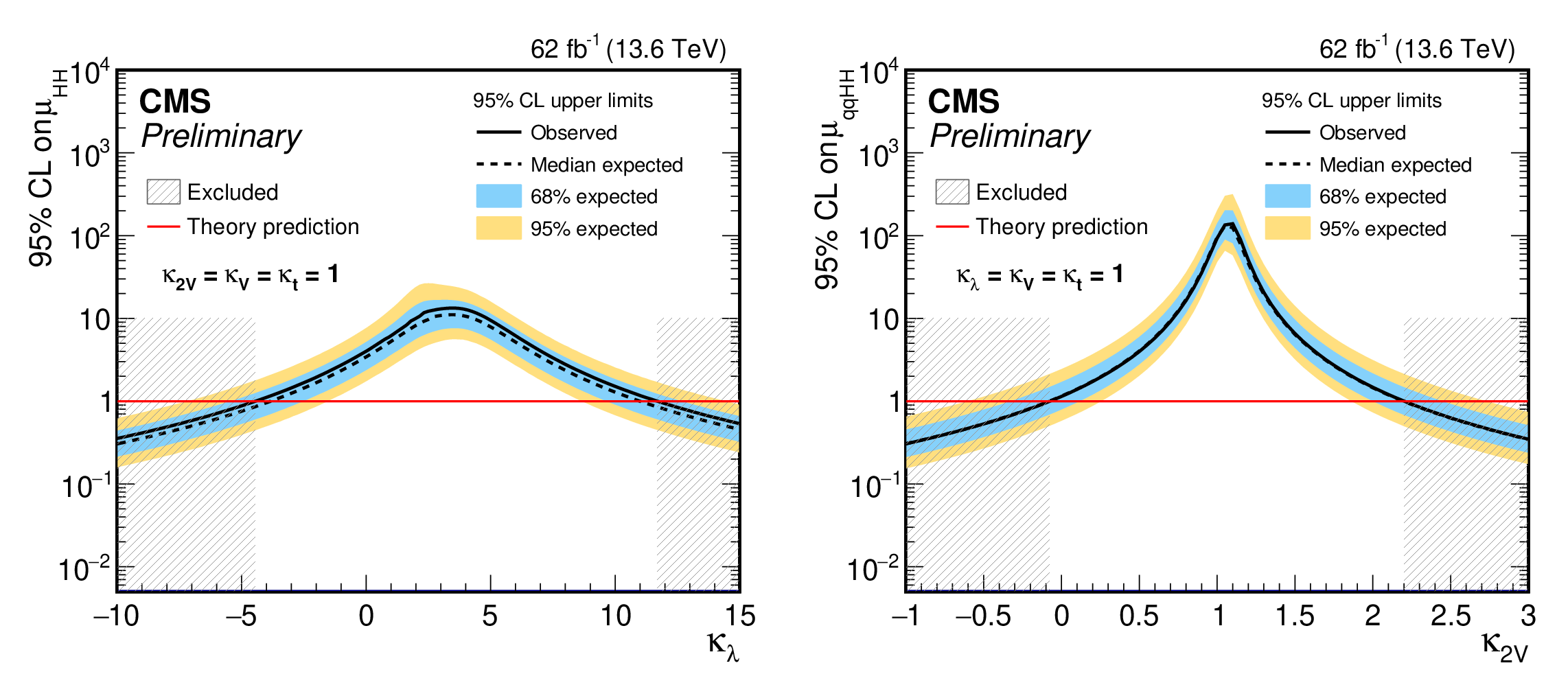
png pdf	Figure 26: The observed (solid) and expected (dashed) 95% CL upper limits on the signal strength of the HH production ($ \mu_{\mathrm{H}\mathrm{H}} $) obtained as a function of $ \kappa_{\lambda} $ (left) and $ \kappa_{\text{2V}} $ (right) for the combined fit of resolved and merged $ \mathrm{H}\mathrm{H} \to 4\mathrm{b} $ analyses. The cyan and blue bands represent, respectively, the 68 and 95% CL intervals around the expected limit. The horizontal red lines indicate the SM prediction.
png pdf	Figure 26-a: The observed (solid) and expected (dashed) 95% CL upper limits on the signal strength of the HH production ($ \mu_{\mathrm{H}\mathrm{H}} $) obtained as a function of $ \kappa_{\lambda} $ (left) and $ \kappa_{\text{2V}} $ (right) for the combined fit of resolved and merged $ \mathrm{H}\mathrm{H} \to 4\mathrm{b} $ analyses. The cyan and blue bands represent, respectively, the 68 and 95% CL intervals around the expected limit. The horizontal red lines indicate the SM prediction.
png pdf	Figure 26-b: The observed (solid) and expected (dashed) 95% CL upper limits on the signal strength of the HH production ($ \mu_{\mathrm{H}\mathrm{H}} $) obtained as a function of $ \kappa_{\lambda} $ (left) and $ \kappa_{\text{2V}} $ (right) for the combined fit of resolved and merged $ \mathrm{H}\mathrm{H} \to 4\mathrm{b} $ analyses. The cyan and blue bands represent, respectively, the 68 and 95% CL intervals around the expected limit. The horizontal red lines indicate the SM prediction.
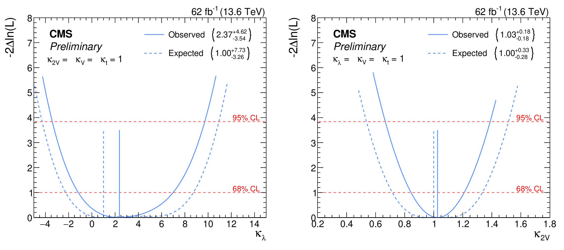
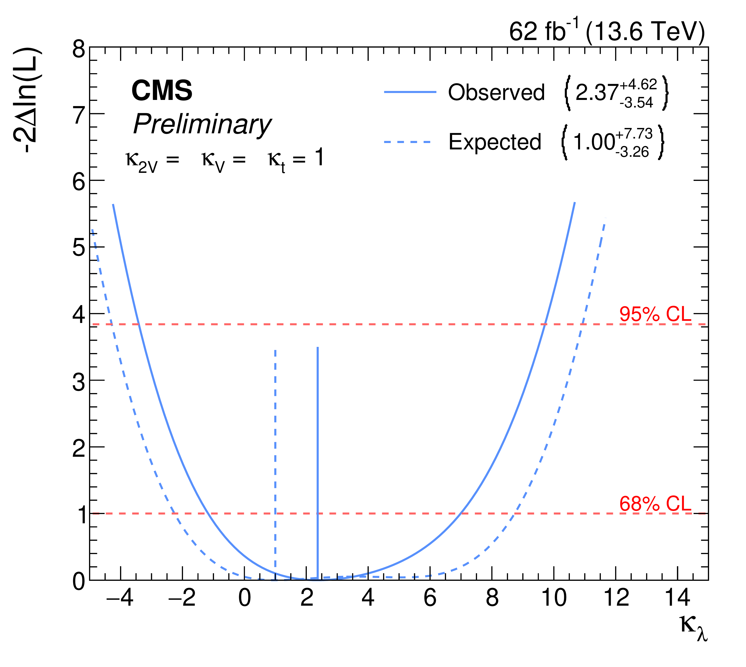
png pdf	Figure 27: The observed (solid) and expected (dashed) profile likelihood ratios as a function of $ \kappa_{\lambda} $ (left) and $ \kappa_{\text{2V}} $ (right) for the combined fit of resolved and merged $ \mathrm{H}\mathrm{H} \to 4\mathrm{b} $ analyses, where the expected is obtained from an Asimov dataset [100] defined by fixing the nuisances parameters to their maximum likelihood estimate obtained from data in which $ \mu_{\mathrm{H}\mathrm{H}}= $ 1. The 68 and 95% CL levels are indicated with the dashed red lines.
png pdf	Figure 27-a: The observed (solid) and expected (dashed) profile likelihood ratios as a function of $ \kappa_{\lambda} $ (left) and $ \kappa_{\text{2V}} $ (right) for the combined fit of resolved and merged $ \mathrm{H}\mathrm{H} \to 4\mathrm{b} $ analyses, where the expected is obtained from an Asimov dataset [100] defined by fixing the nuisances parameters to their maximum likelihood estimate obtained from data in which $ \mu_{\mathrm{H}\mathrm{H}}= $ 1. The 68 and 95% CL levels are indicated with the dashed red lines.
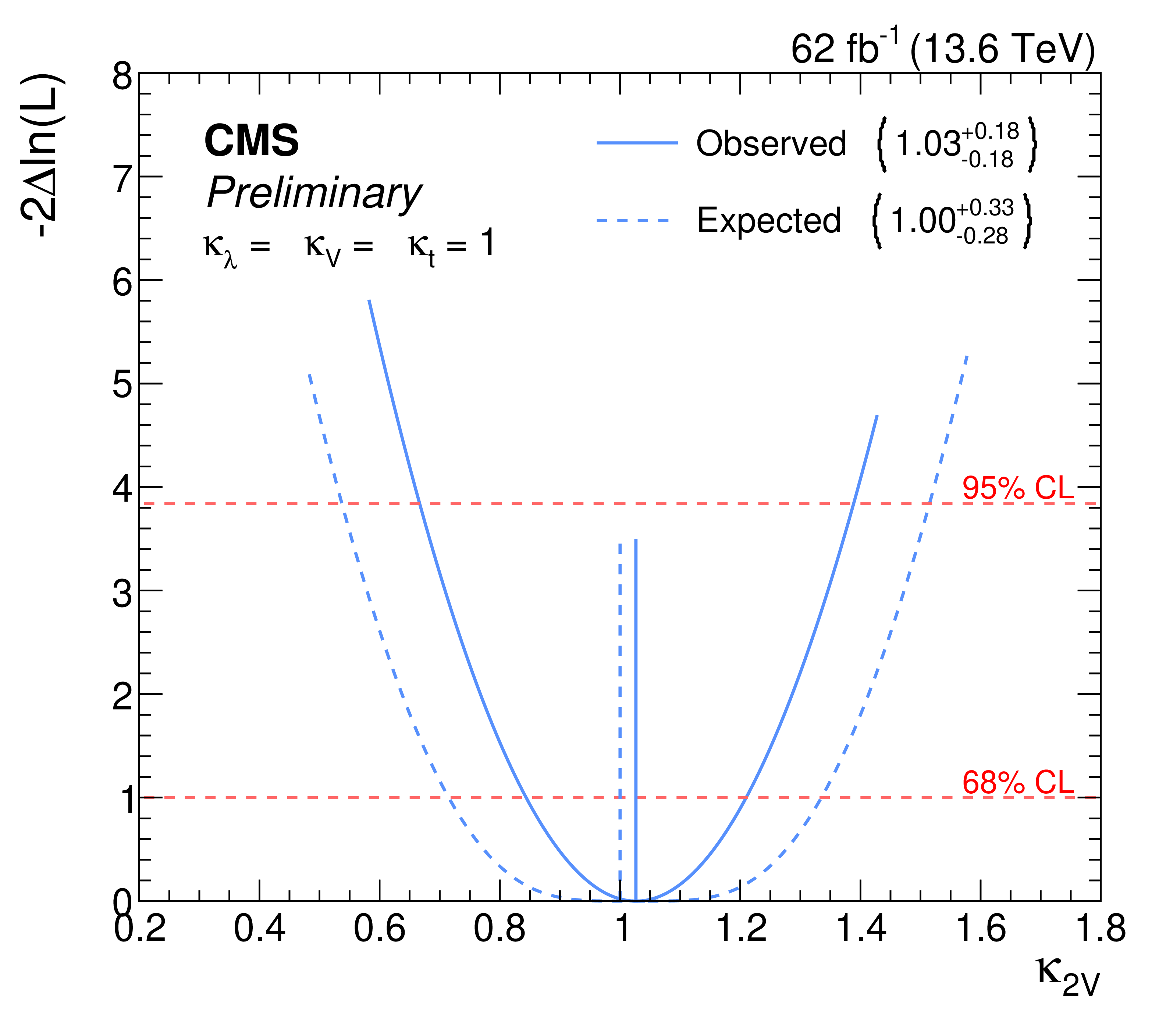
png pdf	Figure 27-b: The observed (solid) and expected (dashed) profile likelihood ratios as a function of $ \kappa_{\lambda} $ (left) and $ \kappa_{\text{2V}} $ (right) for the combined fit of resolved and merged $ \mathrm{H}\mathrm{H} \to 4\mathrm{b} $ analyses, where the expected is obtained from an Asimov dataset [100] defined by fixing the nuisances parameters to their maximum likelihood estimate obtained from data in which $ \mu_{\mathrm{H}\mathrm{H}}= $ 1. The 68 and 95% CL levels are indicated with the dashed red lines.
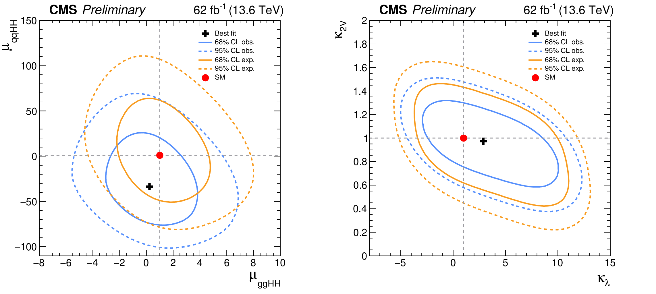
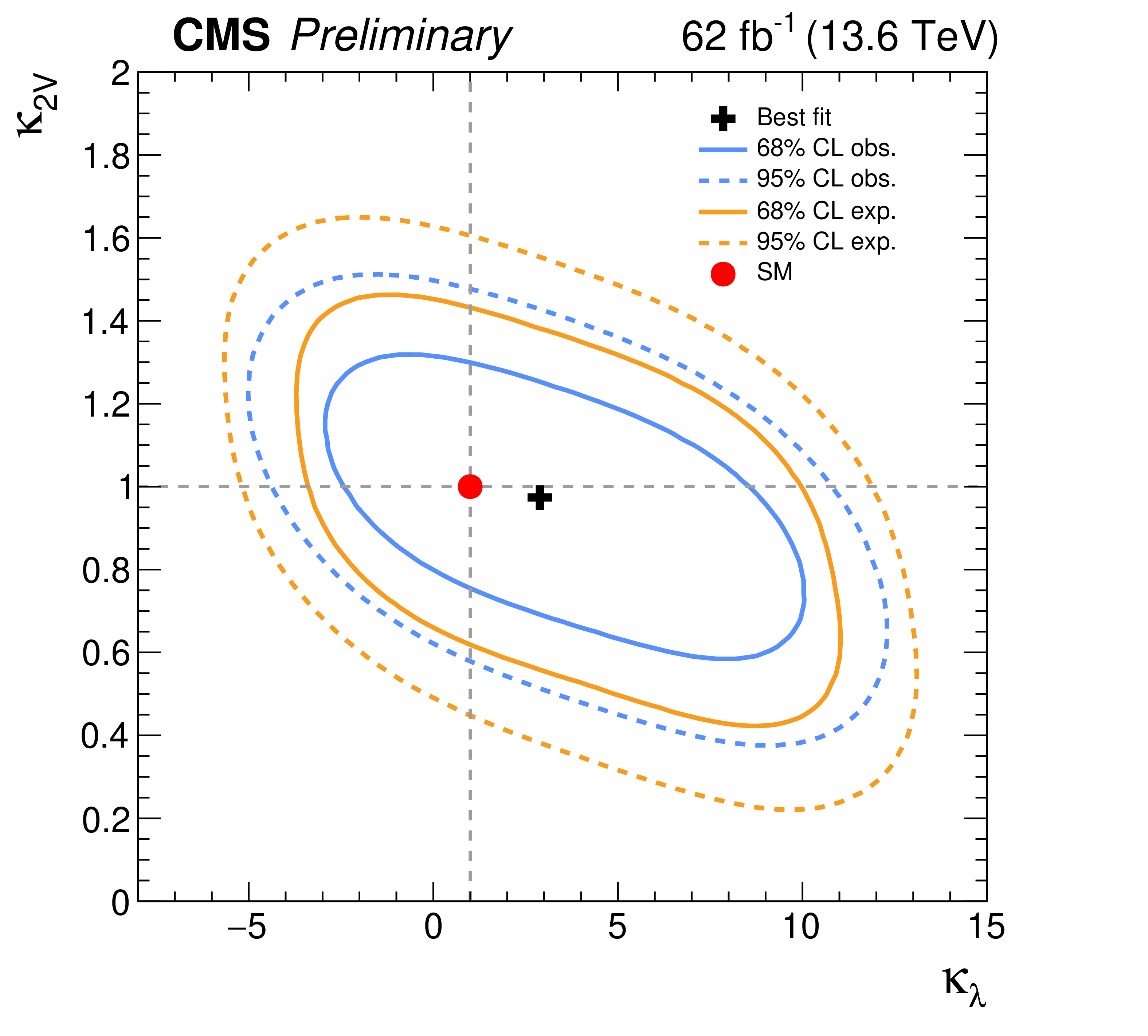
png pdf	Figure 28: The observed (blue) and expected (orange) 2D exclusion range for ($ \mu_{\mathrm{g}\mathrm{g}\mathrm{H}\mathrm{H}} $, $ \mu_{\text{qq}\mathrm{H}\mathrm{H}} $) (left) and ($ \kappa_{\lambda} $,$ \kappa_{\text{2V}} $) (right) for the combination of resolved and merged $ \mathrm{H}\mathrm{H} \to 4\mathrm{b} $ analyses. The solid and dashed lines represent the 68 and 95% CL exclusion contours, respectively. The red circle indicates the SM prediction, while the black cross shows the best-fit result.
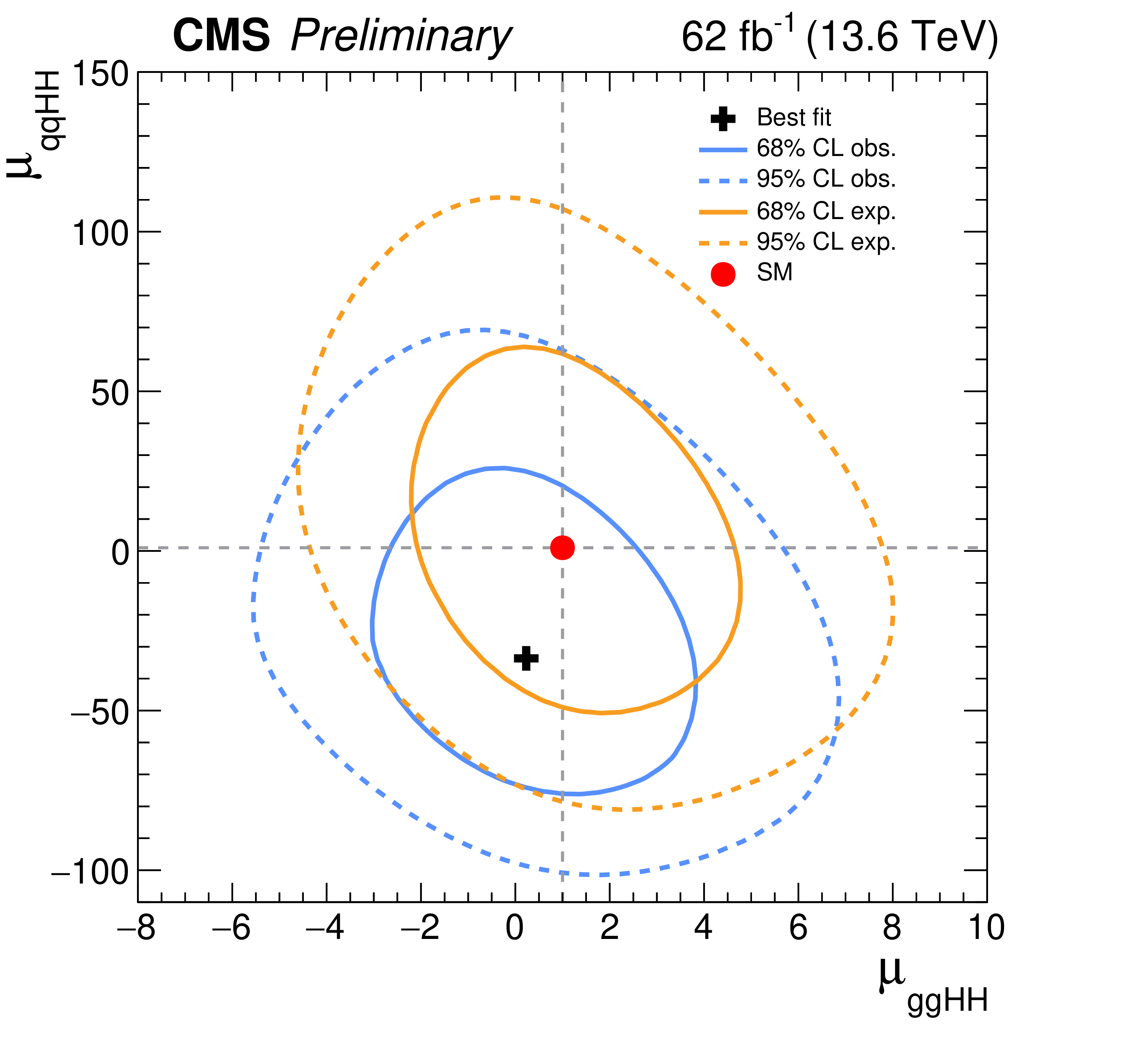
png pdf	Figure 28-a: The observed (blue) and expected (orange) 2D exclusion range for ($ \mu_{\mathrm{g}\mathrm{g}\mathrm{H}\mathrm{H}} $, $ \mu_{\text{qq}\mathrm{H}\mathrm{H}} $) (left) and ($ \kappa_{\lambda} $,$ \kappa_{\text{2V}} $) (right) for the combination of resolved and merged $ \mathrm{H}\mathrm{H} \to 4\mathrm{b} $ analyses. The solid and dashed lines represent the 68 and 95% CL exclusion contours, respectively. The red circle indicates the SM prediction, while the black cross shows the best-fit result.
png pdf	Figure 28-b: The observed (blue) and expected (orange) 2D exclusion range for ($ \mu_{\mathrm{g}\mathrm{g}\mathrm{H}\mathrm{H}} $, $ \mu_{\text{qq}\mathrm{H}\mathrm{H}} $) (left) and ($ \kappa_{\lambda} $,$ \kappa_{\text{2V}} $) (right) for the combination of resolved and merged $ \mathrm{H}\mathrm{H} \to 4\mathrm{b} $ analyses. The solid and dashed lines represent the 68 and 95% CL exclusion contours, respectively. The red circle indicates the SM prediction, while the black cross shows the best-fit result.

Tables
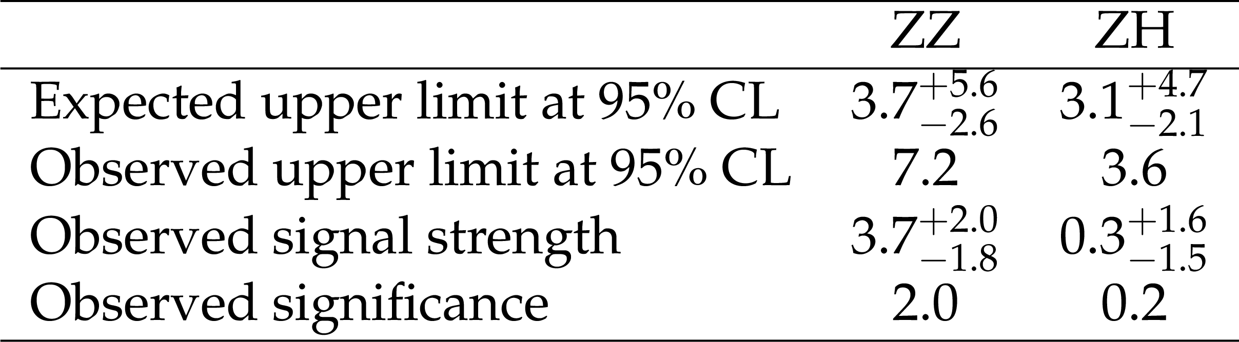
png pdf	Table 1: The observed (expected) upper limits at 95% CL on the $ \mu_{\mathrm{Z}\mathrm{Z}} $ and $ \mu_{\mathrm{Z}\mathrm{H}} $, observed signal strength and significance. The upper limits are obtained from a fit on the $ D $ ($\mathrm{Z}\mathrm{Z}$-vs-bkg) and $ D $ ($\mathrm{Z}\mathrm{H}$-vs-bkg) scores under the hypothesis of no $ \mathrm{Z}\mathrm{Z} \rightarrow4\mathrm{b} $ or $ \mathrm{Z}\mathrm{H} \rightarrow4\mathrm{b} $ signal.
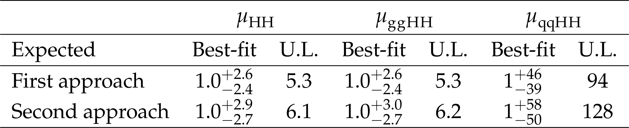
png pdf	Table 2: Expected best-fit values and 95% CL upper limits (``U.L.'') for $ \mu_{\mathrm{HH}} $, $ \mu_{\mathrm{g}\mathrm{g}\mathrm{H}\mathrm{H}} $, and $ \mu_{\text{qq}\mathrm{H}\mathrm{H}} $ in the $ \mathrm{H}\mathrm{H} \to 4\mathrm{b} $ resolved analysis following the two approaches described in Secs. 5.2 and 5.3, respectively. The uncertainties given for the best-fit signal strengths correspond to the 68% CL intervals. The best-fit signal strengths are calculated with a SM $ \mathrm{H}\mathrm{H} \to 4\mathrm{b} $ signal injected, while the upper limits are calculated in the absence of signal.
png pdf	Table 3: Observed best-fit values and 95% CL upper limits (``U.L.'') for $ \mu_{\mathrm{HH}} $, $ \mu_{\mathrm{g}\mathrm{g}\mathrm{H}\mathrm{H}} $, and $ \mu_{\text{qq}\mathrm{H}\mathrm{H}} $ in the $ \mathrm{H}\mathrm{H} \to 4\mathrm{b} $ resolved analysis following the two approaches described in Secs. 5.2 and 5.3, respectively. The uncertainties given for the best-fit signal strengths correspond to the 68% CL intervals.
png pdf	Table 4: Observed and expected, in absence of signal, 95% CL intervals for $ \kappa_{\lambda} $ and $ \kappa_{\text{2V}} $ in the $ \mathrm{H}\mathrm{H} \to 4\mathrm{b} $ resolved analysis, following the two approaches described in Secs. 5.2 and 5.3, respectively.
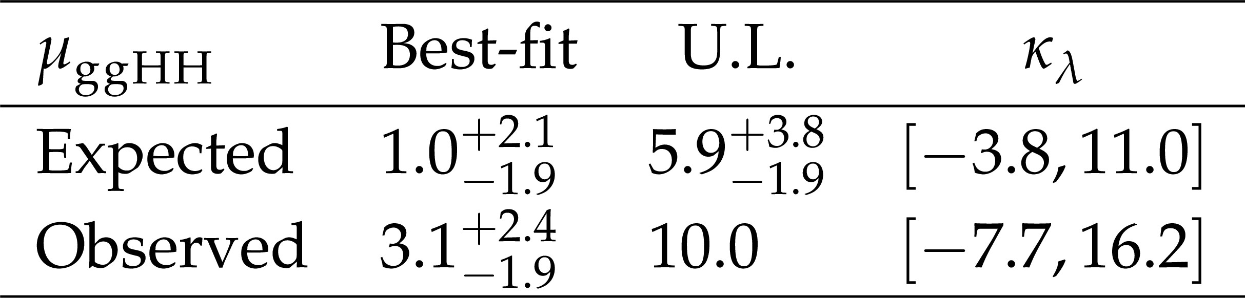
png pdf	Table 5: Expected and observed $ \mu_{\mathrm{g}\mathrm{g}\mathrm{H}\mathrm{H}} $ and their corresponding upper limits at 95% CL in the $ \mathrm{H}\mathrm{H} \to 4\mathrm{b} $ resolved channel with Run 2 data (described in Section 5.4). The observed and expected 95% CL intervals for $ \kappa_{\lambda} $ are also reported.
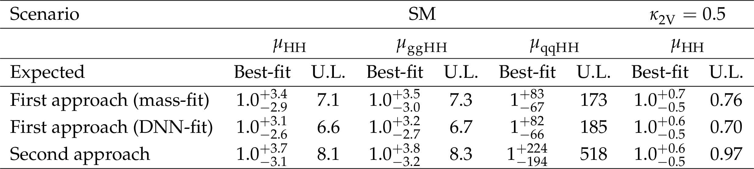
png pdf	Table 6: The expected best-fit signal strengths and 95% CL upper limits on the inclusive, $ \mathrm{g}\mathrm{g}\mathrm{H}\mathrm{H} $, and $ \mathrm{q}\mathrm{q}\mathrm{H}\mathrm{H} $ signal strengths for the SM scenario for the two approaches described in Sections 6.2 and 6.3, respectively. The expected best-fit signal strength and 95% CL upper limit on the HH signal strength for the non-SM $ \kappa_{2\mathrm{V}}= $ 0.5 scenario are also reported. The uncertainties given for the best-fit signal strengths correspond to the 68% CL intervals. The best-fit signal strengths are calculated with a SM $ \mathrm{H}\mathrm{H} \to 4\mathrm{b} $ signal injected, while the upper limits are calculated in the absence of signal.
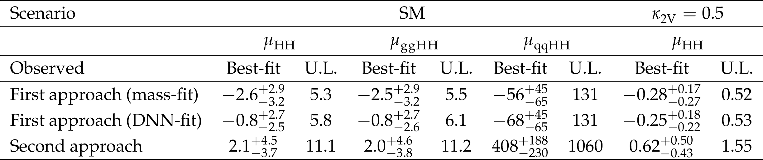
png pdf	Table 7: The observed best-fit signal strengths and 95% CL upper limits on the inclusive, $ \mathrm{g}\mathrm{g}\mathrm{H}\mathrm{H} $, and $ \mathrm{q}\mathrm{q}\mathrm{H}\mathrm{H} $ signal strengths for the SM scenario for the two approaches described in Sections 6.2 and 6.3, respectively. The best-fit and observed 95% CL upper limits on the HH signal strength for the non-SM $ \kappa_{2\mathrm{V}}= $ 0.5 are also reported. The uncertainties given for the best-fit signal strengths correspond to the 68% CL intervals.
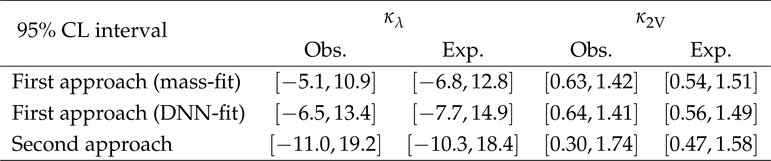
png pdf	Table 8: The observed and expected 95% CL intervals for $ \kappa_\lambda $ and $ \kappa_{2\mathrm{V}} $ in the merged channel for the two approaches described in Sections 6.2 and 6.3, respectively.
png pdf	Table 9: Expected and observed best-fit values for the signal strengths, $ \kappa_{\lambda} $, and $ \kappa_{\text{2V}} $ from the combined fit of the $ \mathrm{H}\mathrm{H} \to 4\mathrm{b} $ resolved and merged analyses. The uncertainties given correspond to the 68% CL intervals. The expected results are calculated with a SM $ \mathrm{H}\mathrm{H} \to 4\mathrm{b} $ signal injected.

Summary

Measurements of Higgs boson pair (HH) production in the four bottom quark final state are presented using a data set of proton-proton (pp) collisions at $ \sqrt{s}= $ 13.6 TeV collected by the CMS experiment during 2022-2023 and corresponding to an integrated luminosity of 62 fb$ ^{-1} $. Events in which each Higgs boson decay is separately reconstructed as a pair of small-radius jets (resolved), as well as events in which each $ \mathrm{H}\to\mathrm{b}\overline{\mathrm{b}} $ decay is reconstructed as a single large-radius jet (merged) are analyzed exclusively. Benefiting from novel analysis techniques, the combination of resolved and merged channels gives an observed (expected) upper limit at 95% confidence level (CL) on the HH signal strength $ \mu_{\mathrm{H}\mathrm{H}} $, defined as the observed HH production cross section divided by the standard model (SM) prediction, of 4.4 (4.4). Compared to previous LHC results, the expected limit with an equivalent integrated luminosity is improved by more than a factor two in the resolved topology and significantly improved in the merged topology as well. The allowed ranges at 95% CL for the Higgs trilinear self-coupling and quartic coupling between two Higgs bosons and two vector bosons, relative to the standard model expectation, are observed (expected, in absence of signal) to be $ [-3.3,9.7] $ ($ [-3.4,10.0] $) and $ [0.63,1.43] $ ($ [0.54,1.51] $), respectively. An updated analysis of the resolved topology using a 13 TeV pp collision data set corresponding to 138 fb$ ^{-1} $ and collected in 2016-2018, reports an observed (expected) 95% CL upper limit on $ \mu_{\mathrm{H}\mathrm{H}} $ of 10.0 (5.9), an improvement of about 25% in the expected limit compared to the published results using the same data.

Additional Figures
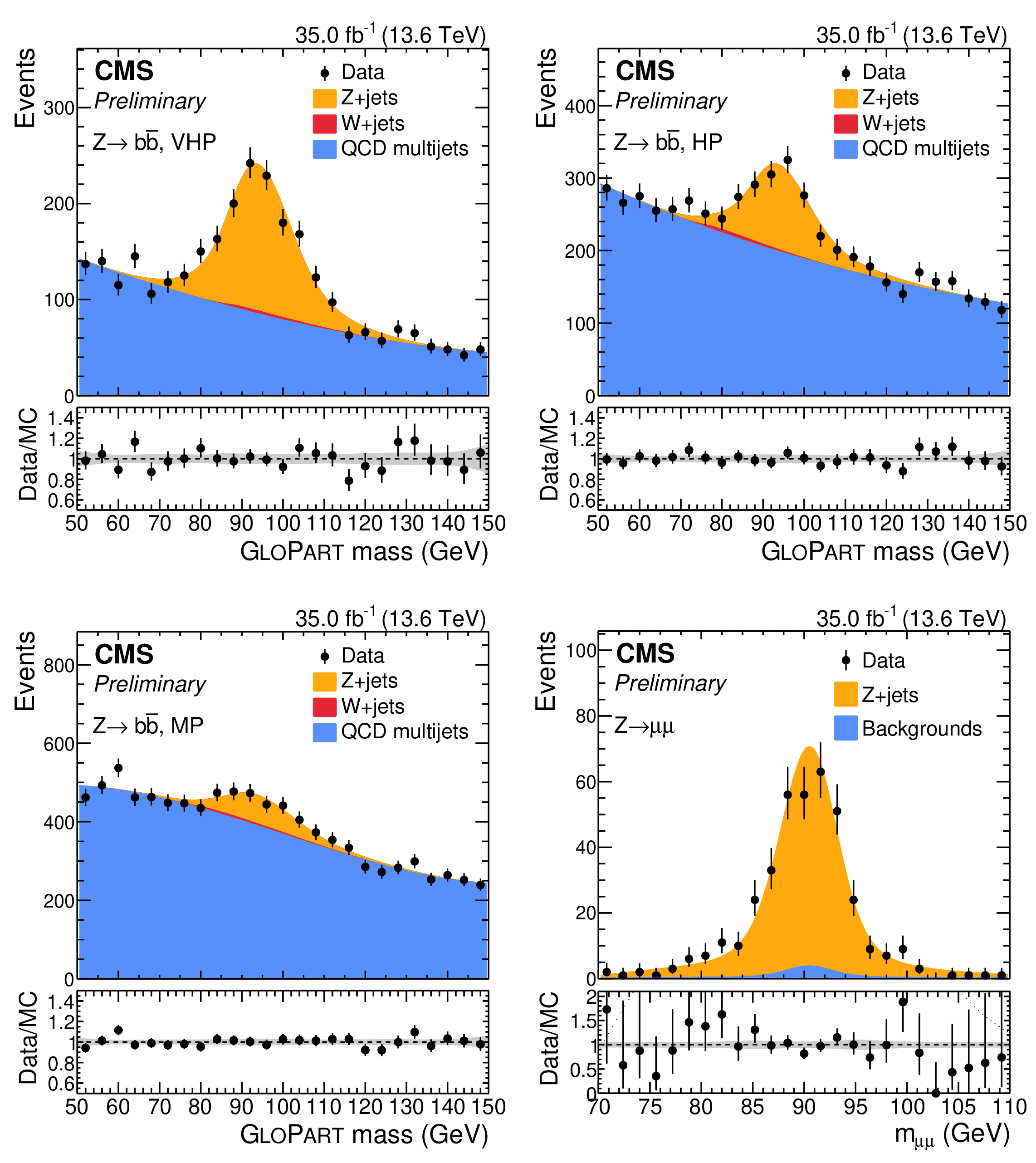
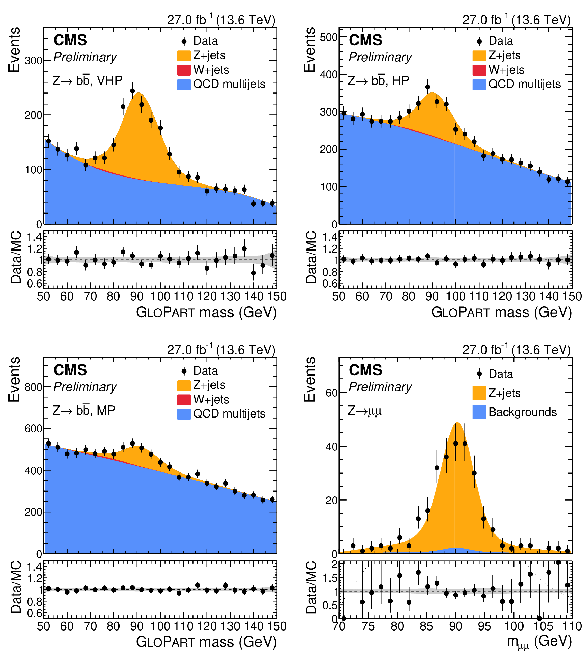
png pdf	Additional Figure 1: Comparison between data and fit prediction from a simultaneous signal-plus-background fit to the GloParT regressed jet mass distributions in $ \mathrm{Z} \to \mathrm{bb} $ VHP (top left), HP (top right), and MP (bottom left) categories. Data corresponds to the full integrated luminosity collected by the CMS detector in 2022. The same comparison is performed for the $m_{\mu\mu}$ distributions in the $ \mathrm{Z} \to \mu\mu $ region (bottom right). Each process considered in the fit is modeled via a parametric function as described in the text.
png pdf	Additional Figure 1-a: Comparison between data and fit prediction from a simultaneous signal-plus-background fit to the GloParT regressed jet mass distributions in $ \mathrm{Z} \to \mathrm{bb} $ VHP (top left), HP (top right), and MP (bottom left) categories. Data corresponds to the full integrated luminosity collected by the CMS detector in 2022. The same comparison is performed for the $m_{\mu\mu}$ distributions in the $ \mathrm{Z} \to \mu\mu $ region (bottom right). Each process considered in the fit is modeled via a parametric function as described in the text.
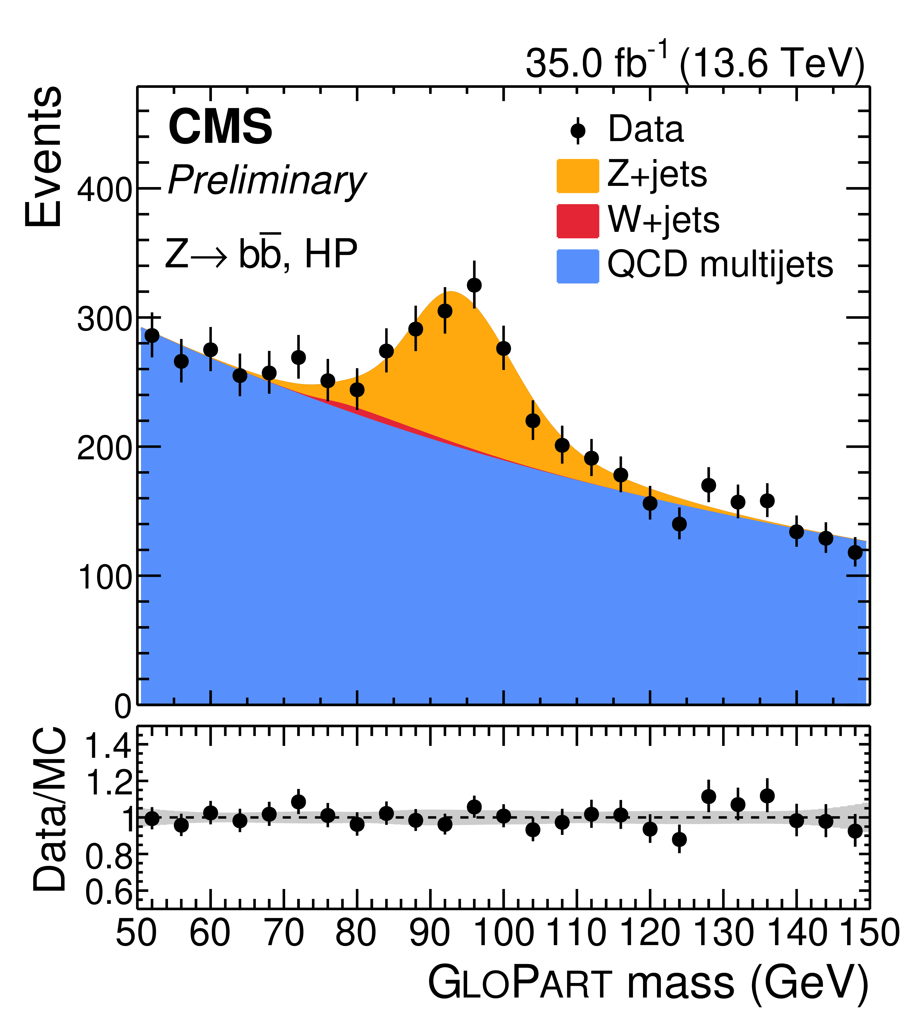
png pdf	Additional Figure 1-b: Comparison between data and fit prediction from a simultaneous signal-plus-background fit to the GloParT regressed jet mass distributions in $ \mathrm{Z} \to \mathrm{bb} $ VHP (top left), HP (top right), and MP (bottom left) categories. Data corresponds to the full integrated luminosity collected by the CMS detector in 2022. The same comparison is performed for the $m_{\mu\mu}$ distributions in the $ \mathrm{Z} \to \mu\mu $ region (bottom right). Each process considered in the fit is modeled via a parametric function as described in the text.
png pdf	Additional Figure 1-c: Comparison between data and fit prediction from a simultaneous signal-plus-background fit to the GloParT regressed jet mass distributions in $ \mathrm{Z} \to \mathrm{bb} $ VHP (top left), HP (top right), and MP (bottom left) categories. Data corresponds to the full integrated luminosity collected by the CMS detector in 2022. The same comparison is performed for the $m_{\mu\mu}$ distributions in the $ \mathrm{Z} \to \mu\mu $ region (bottom right). Each process considered in the fit is modeled via a parametric function as described in the text.
png pdf	Additional Figure 1-d: Comparison between data and fit prediction from a simultaneous signal-plus-background fit to the GloParT regressed jet mass distributions in $ \mathrm{Z} \to \mathrm{bb} $ VHP (top left), HP (top right), and MP (bottom left) categories. Data corresponds to the full integrated luminosity collected by the CMS detector in 2022. The same comparison is performed for the $m_{\mu\mu}$ distributions in the $ \mathrm{Z} \to \mu\mu $ region (bottom right). Each process considered in the fit is modeled via a parametric function as described in the text.
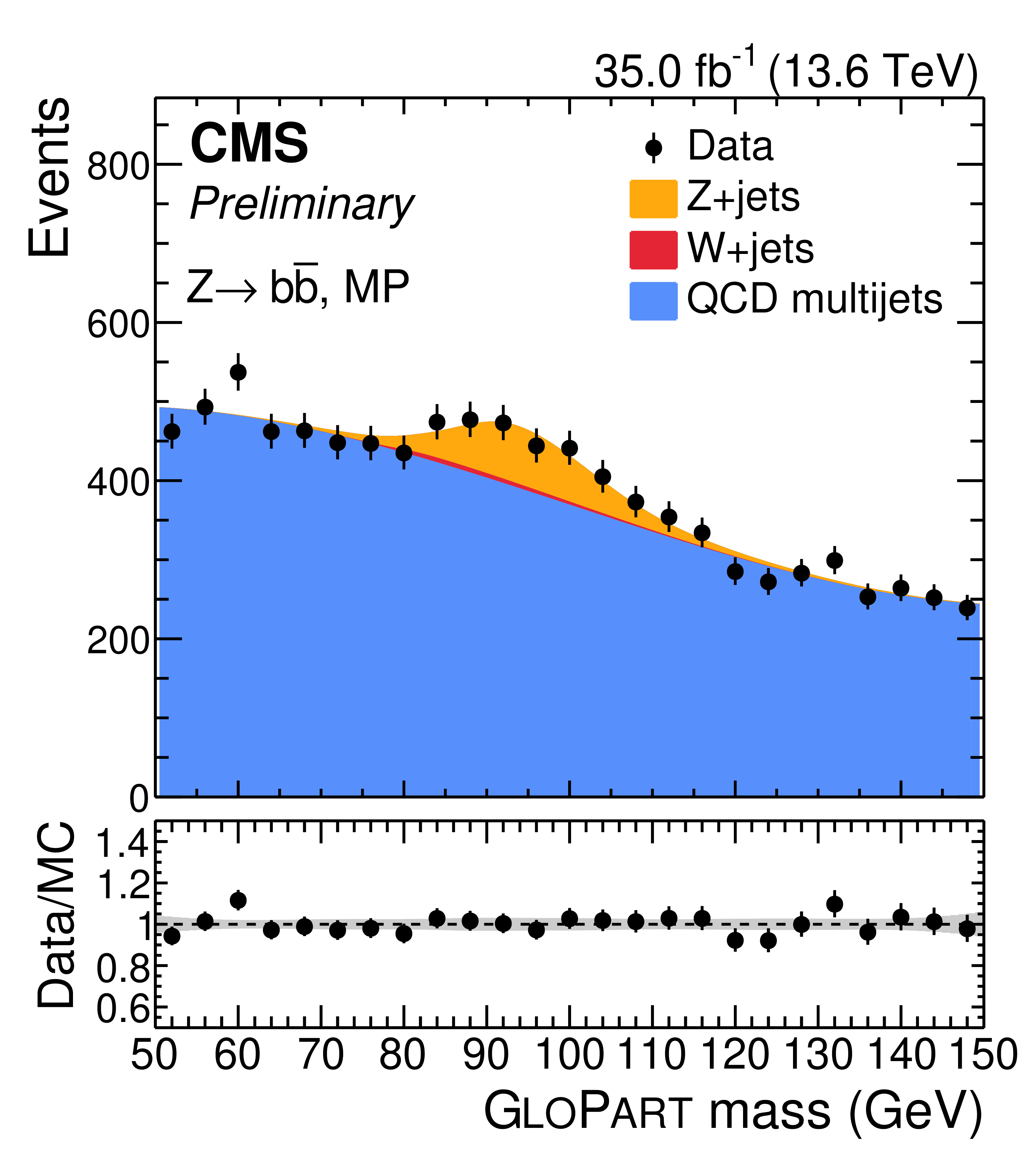
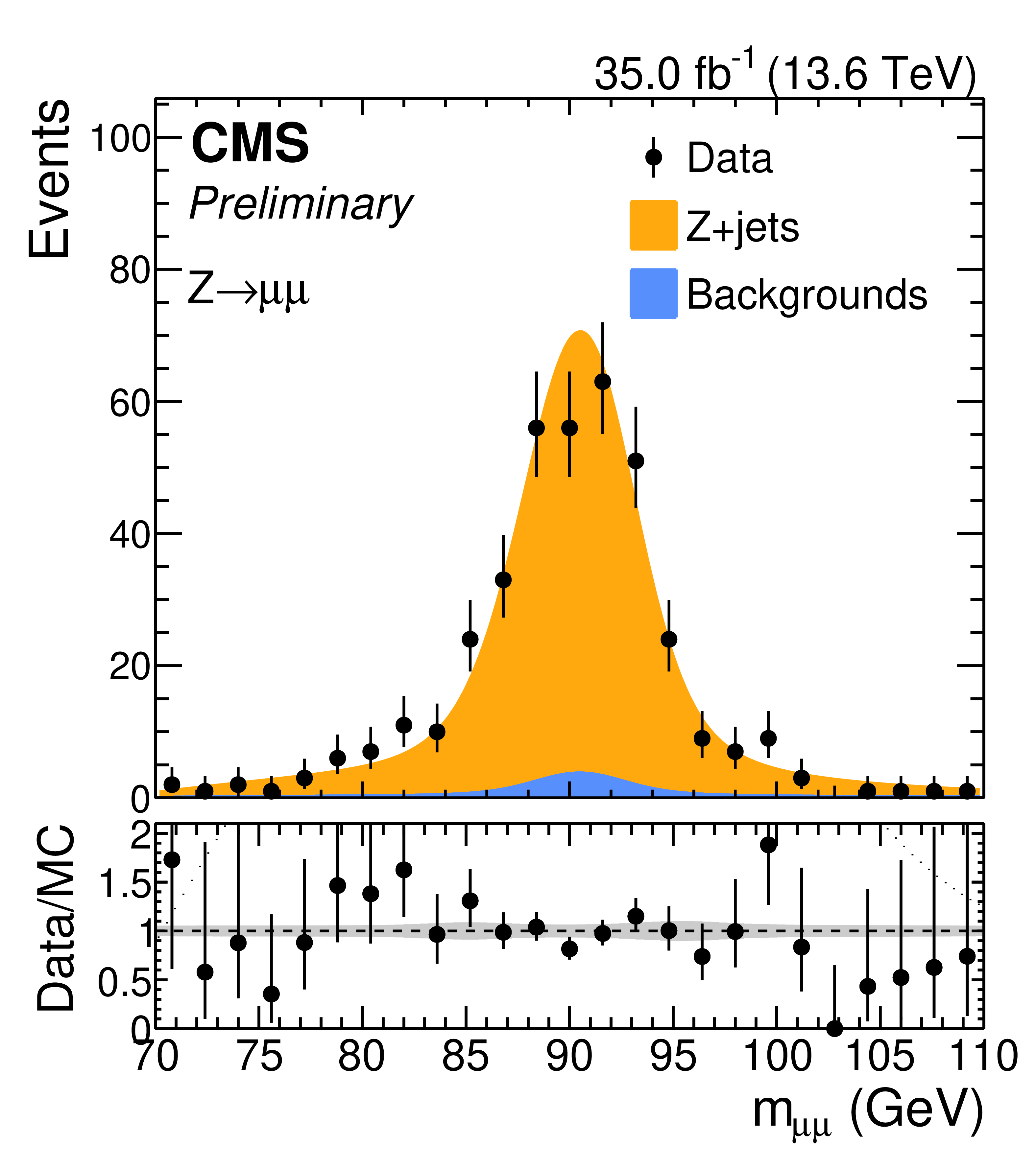
png pdf	Additional Figure 2: Comparison between data and fit prediction from a simultaneous signal-plus-background fit to the GloParT regressed jet mass distributions in $ \mathrm{Z} \to \mathrm{bb} $ VHP (top left), HP (top right), and MP (bottom left) categories. Data corresponds to the full integrated luminosity collected by the CMS detector in 2023. The same comparison is performed for the $m_{\mu\mu}$ distributions in the $ \mathrm{Z} \to \mu\mu $ region (bottom right). Each process considered in the fit is modeled via a parametric function as described in the text.
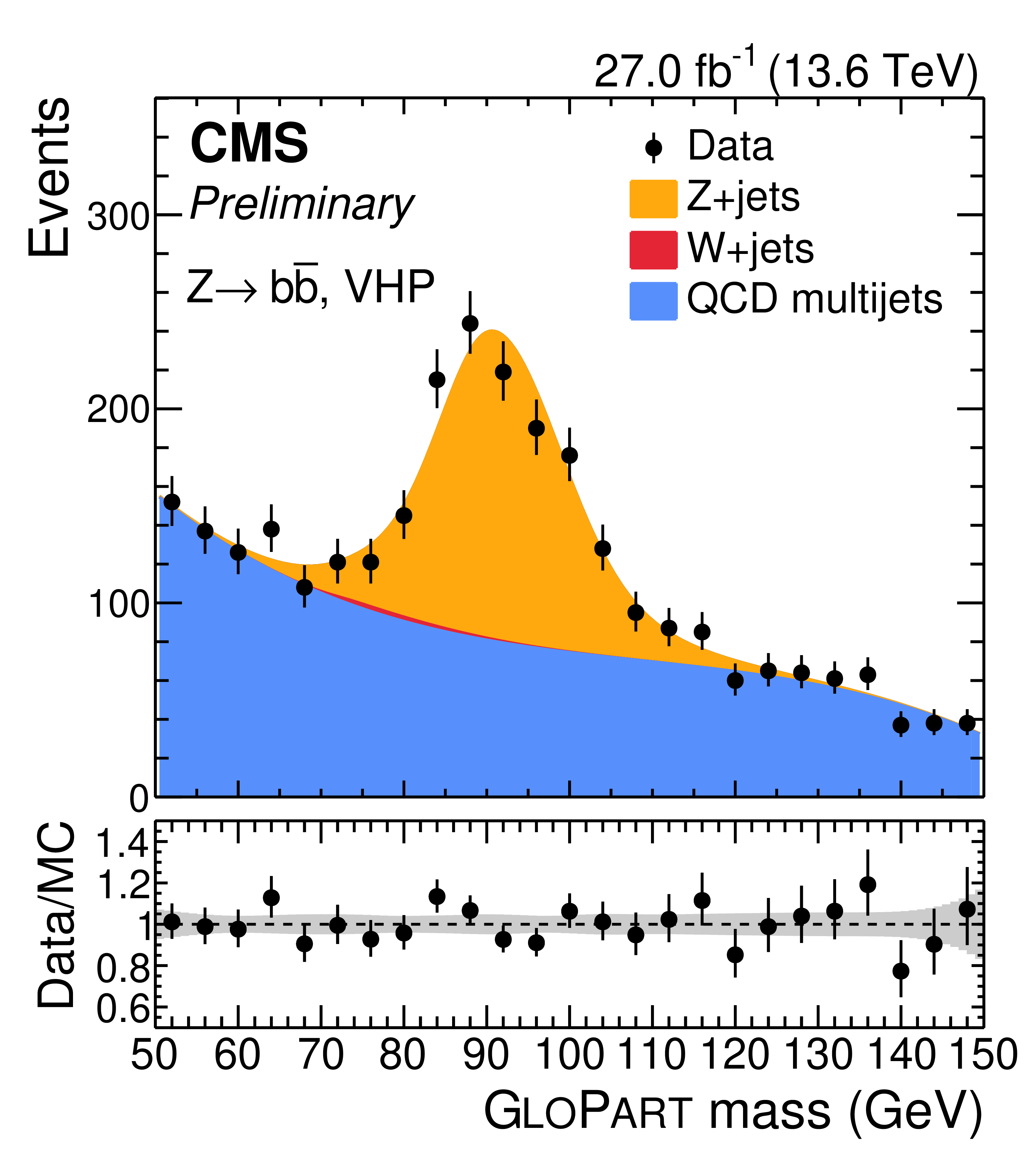
png pdf	Additional Figure 2-a: Comparison between data and fit prediction from a simultaneous signal-plus-background fit to the GloParT regressed jet mass distributions in $ \mathrm{Z} \to \mathrm{bb} $ VHP (top left), HP (top right), and MP (bottom left) categories. Data corresponds to the full integrated luminosity collected by the CMS detector in 2023. The same comparison is performed for the $m_{\mu\mu}$ distributions in the $ \mathrm{Z} \to \mu\mu $ region (bottom right). Each process considered in the fit is modeled via a parametric function as described in the text.
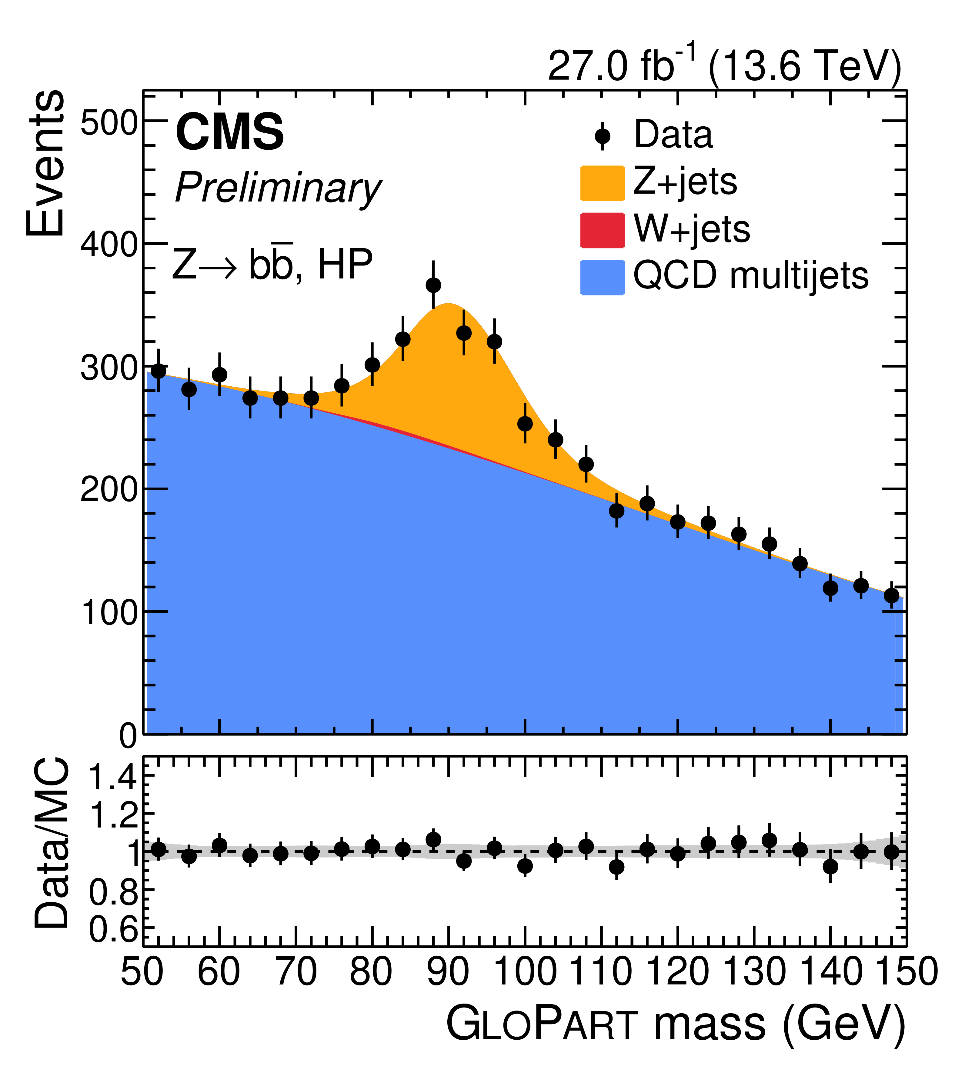
png pdf	Additional Figure 2-b: Comparison between data and fit prediction from a simultaneous signal-plus-background fit to the GloParT regressed jet mass distributions in $ \mathrm{Z} \to \mathrm{bb} $ VHP (top left), HP (top right), and MP (bottom left) categories. Data corresponds to the full integrated luminosity collected by the CMS detector in 2023. The same comparison is performed for the $m_{\mu\mu}$ distributions in the $ \mathrm{Z} \to \mu\mu $ region (bottom right). Each process considered in the fit is modeled via a parametric function as described in the text.
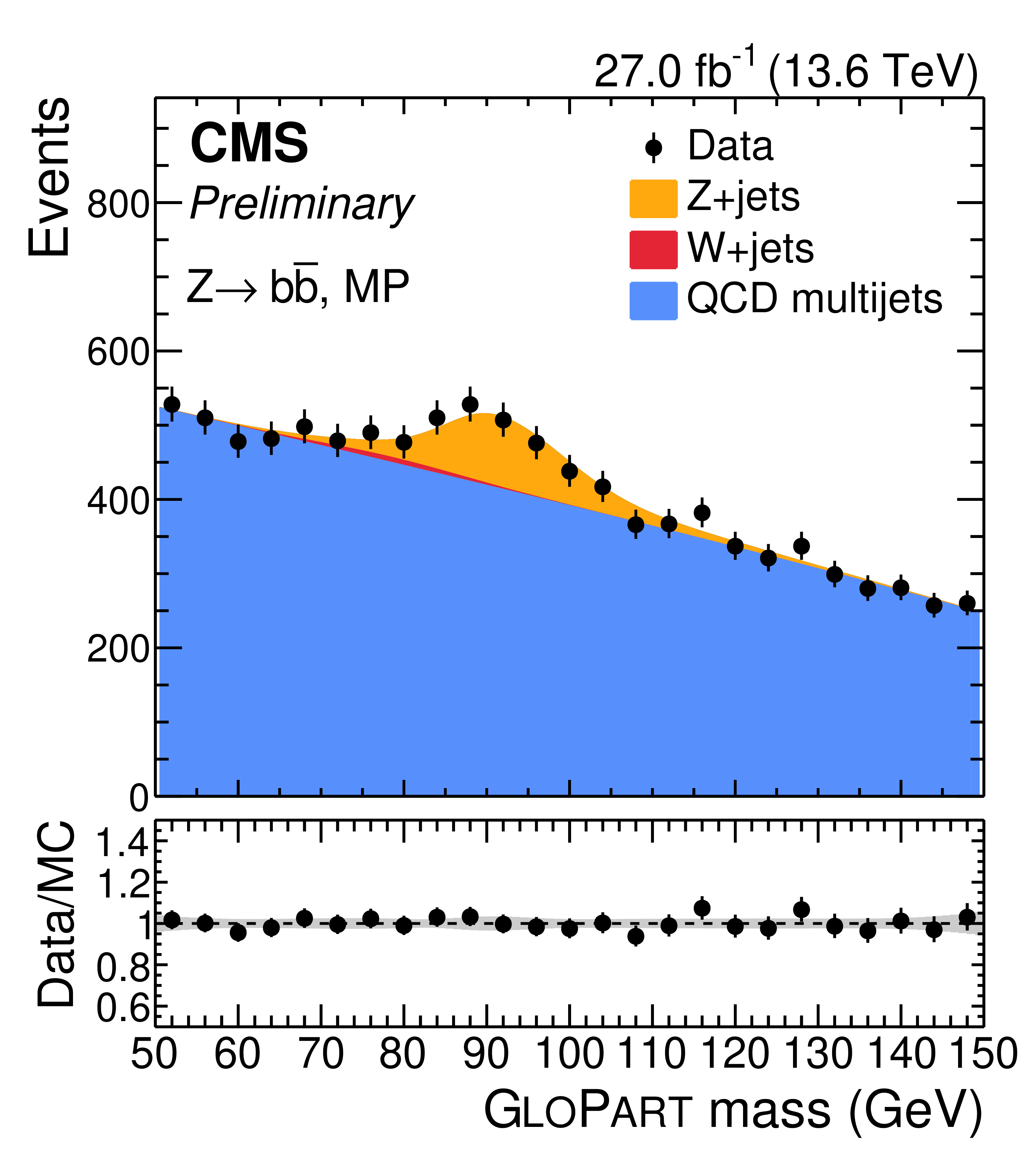
png pdf	Additional Figure 2-c: Comparison between data and fit prediction from a simultaneous signal-plus-background fit to the GloParT regressed jet mass distributions in $ \mathrm{Z} \to \mathrm{bb} $ VHP (top left), HP (top right), and MP (bottom left) categories. Data corresponds to the full integrated luminosity collected by the CMS detector in 2023. The same comparison is performed for the $m_{\mu\mu}$ distributions in the $ \mathrm{Z} \to \mu\mu $ region (bottom right). Each process considered in the fit is modeled via a parametric function as described in the text.
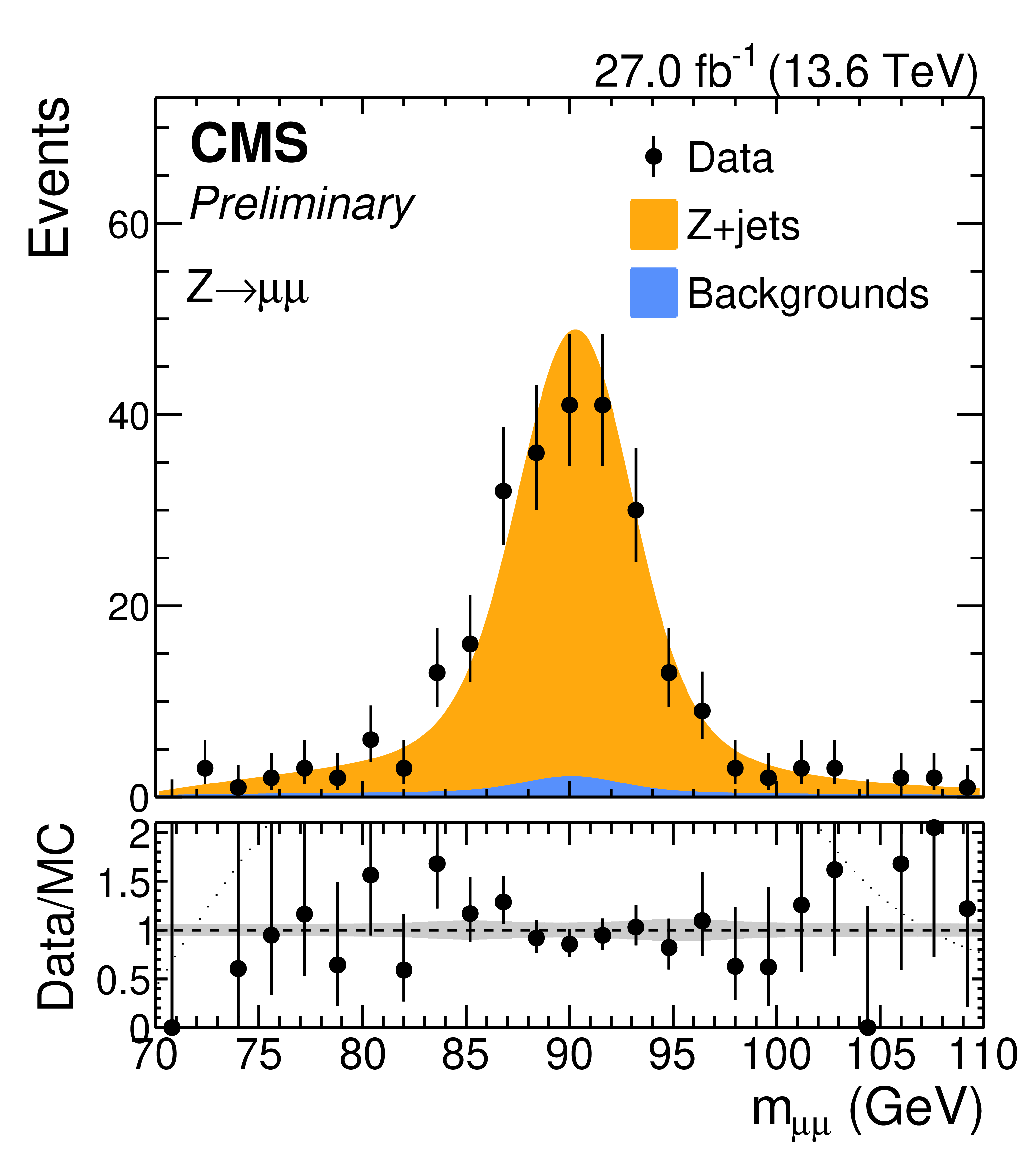
png pdf	Additional Figure 2-d: Comparison between data and fit prediction from a simultaneous signal-plus-background fit to the GloParT regressed jet mass distributions in $ \mathrm{Z} \to \mathrm{bb} $ VHP (top left), HP (top right), and MP (bottom left) categories. Data corresponds to the full integrated luminosity collected by the CMS detector in 2023. The same comparison is performed for the $m_{\mu\mu}$ distributions in the $ \mathrm{Z} \to \mu\mu $ region (bottom right). Each process considered in the fit is modeled via a parametric function as described in the text.
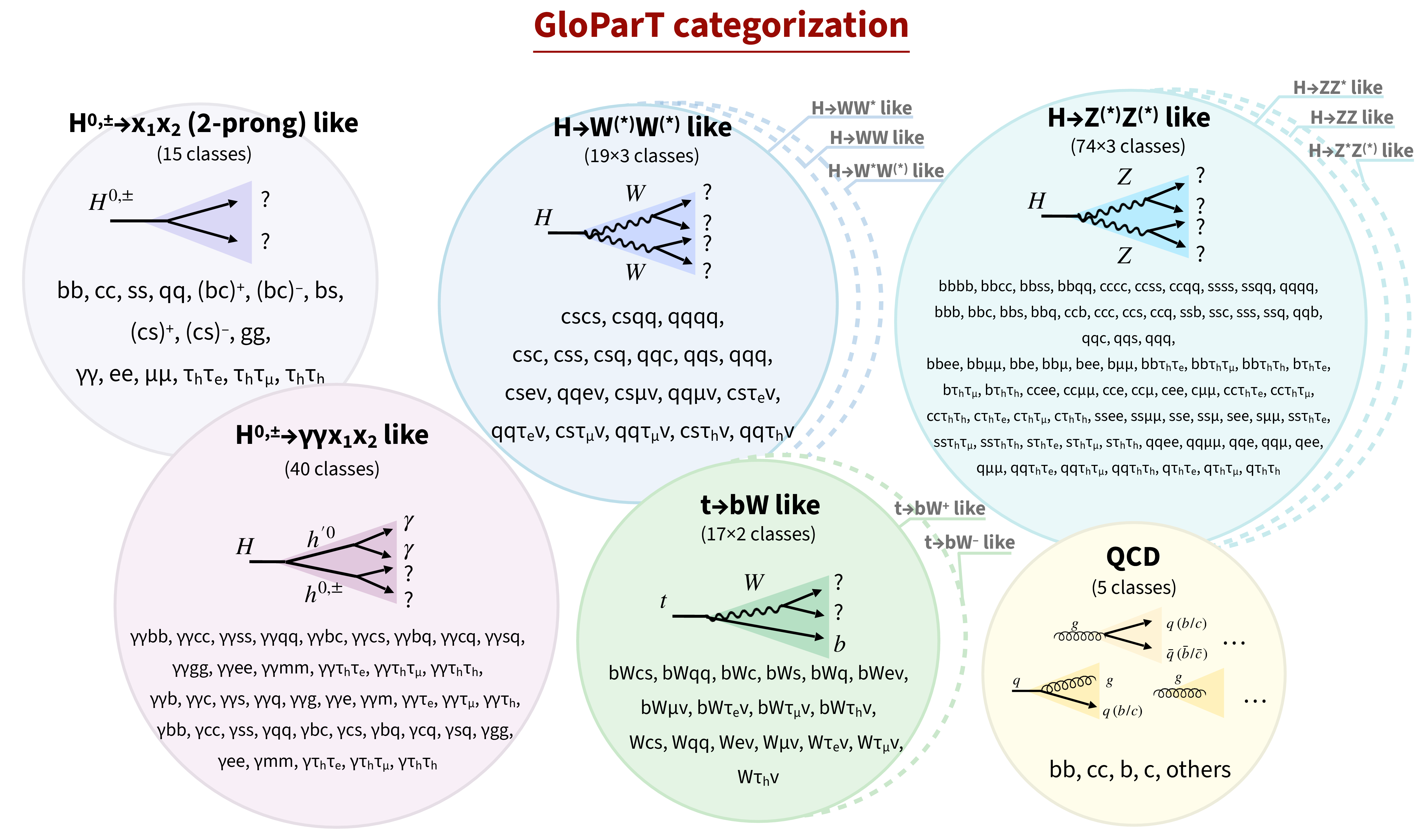
png pdf	Additional Figure 3: Full suite of AK8 jet topologies used for the GloParT model training. Jet types are first categorized by the number of quarks and leptons in the final state, and then further separated by flavor. If the decay includes a V= W or Z boson, the class is further split based on whether the vector boson is on shell, leading to three versions of each $H\to\PV^{(\ast)}\PV^{(\ast)}$ class and two versions of each $\PQt\tob\PW^{(\ast)}$ class. Diagrams illustrating the corresponding jet topologies are also shown.
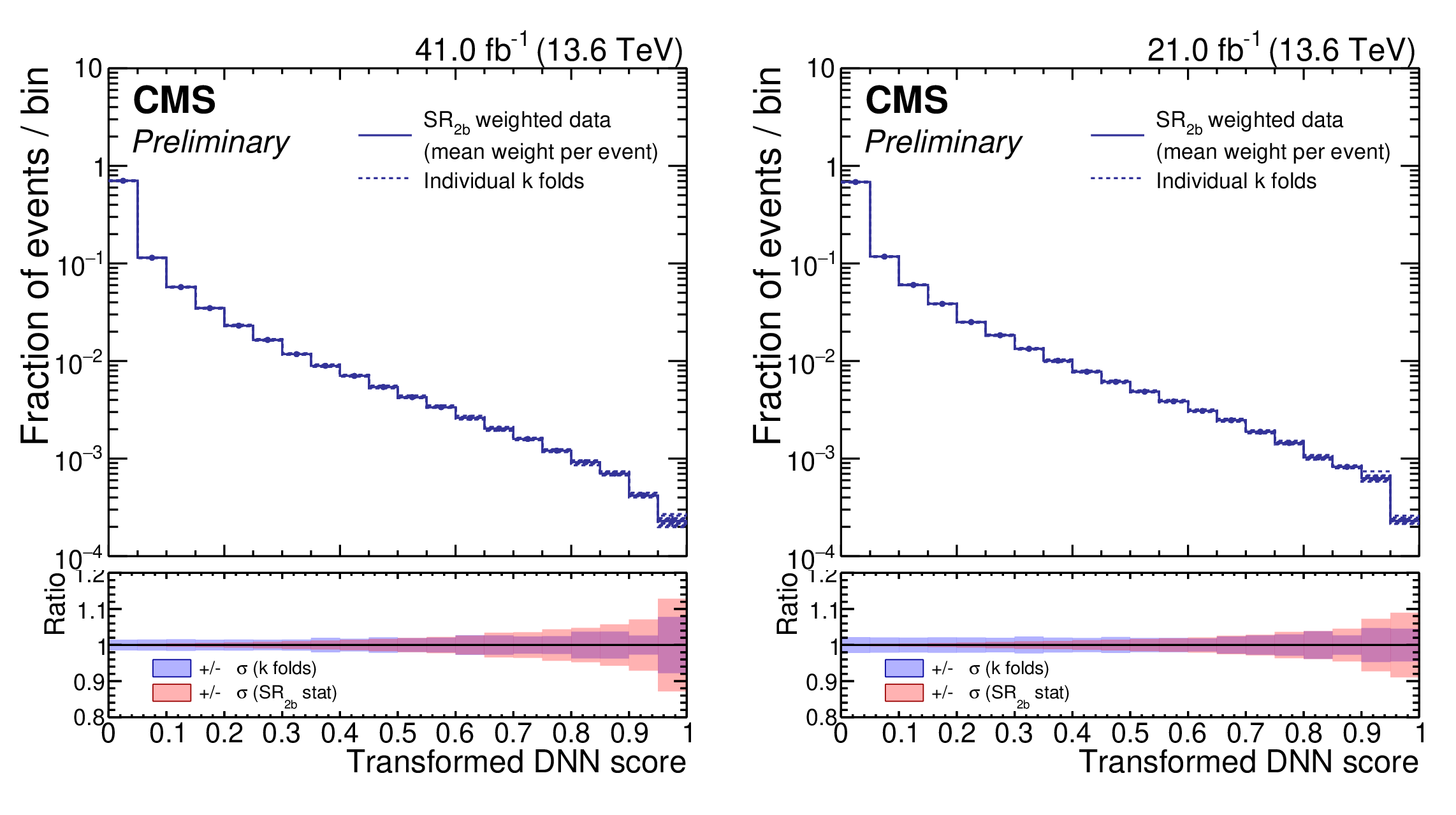
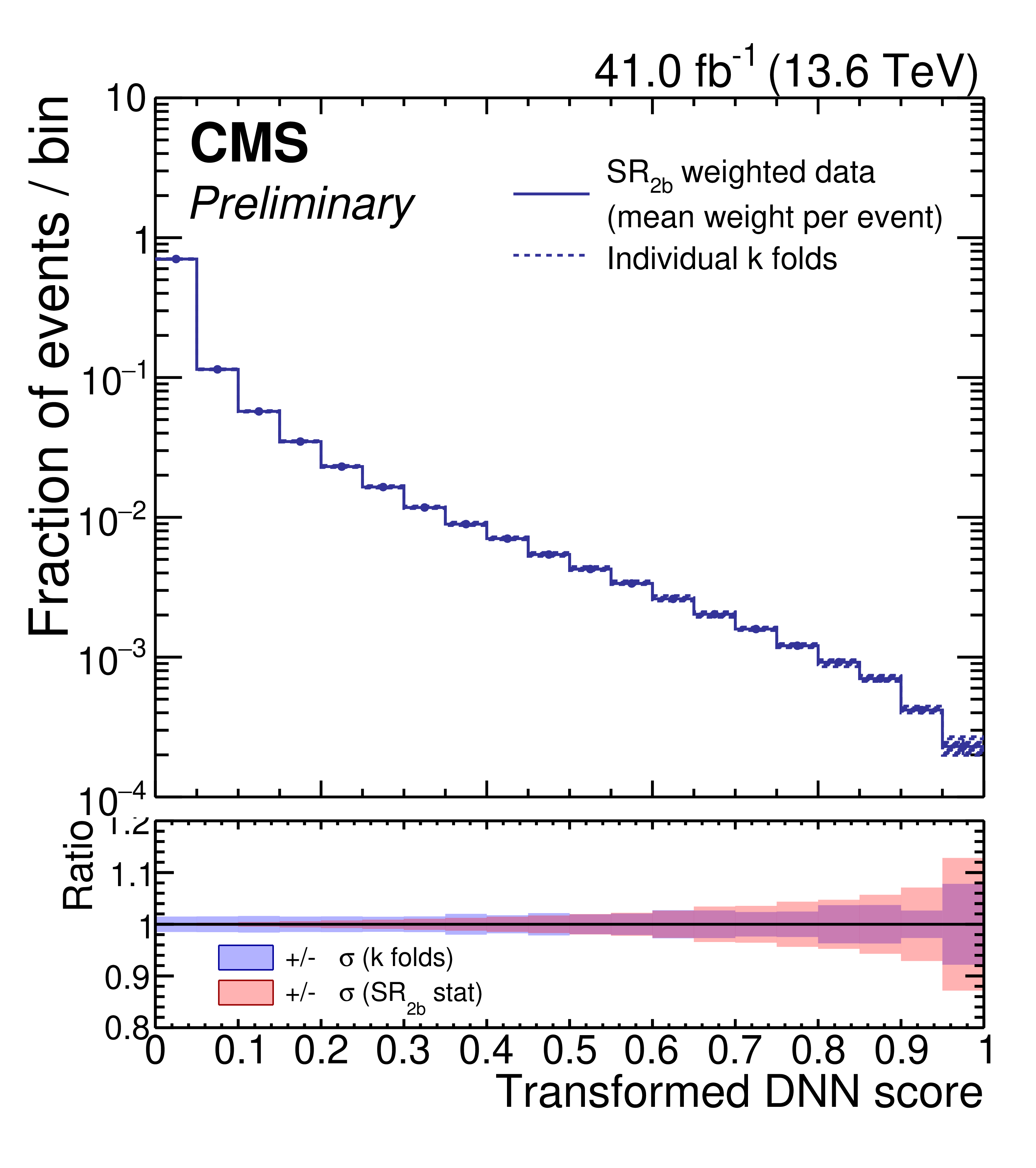
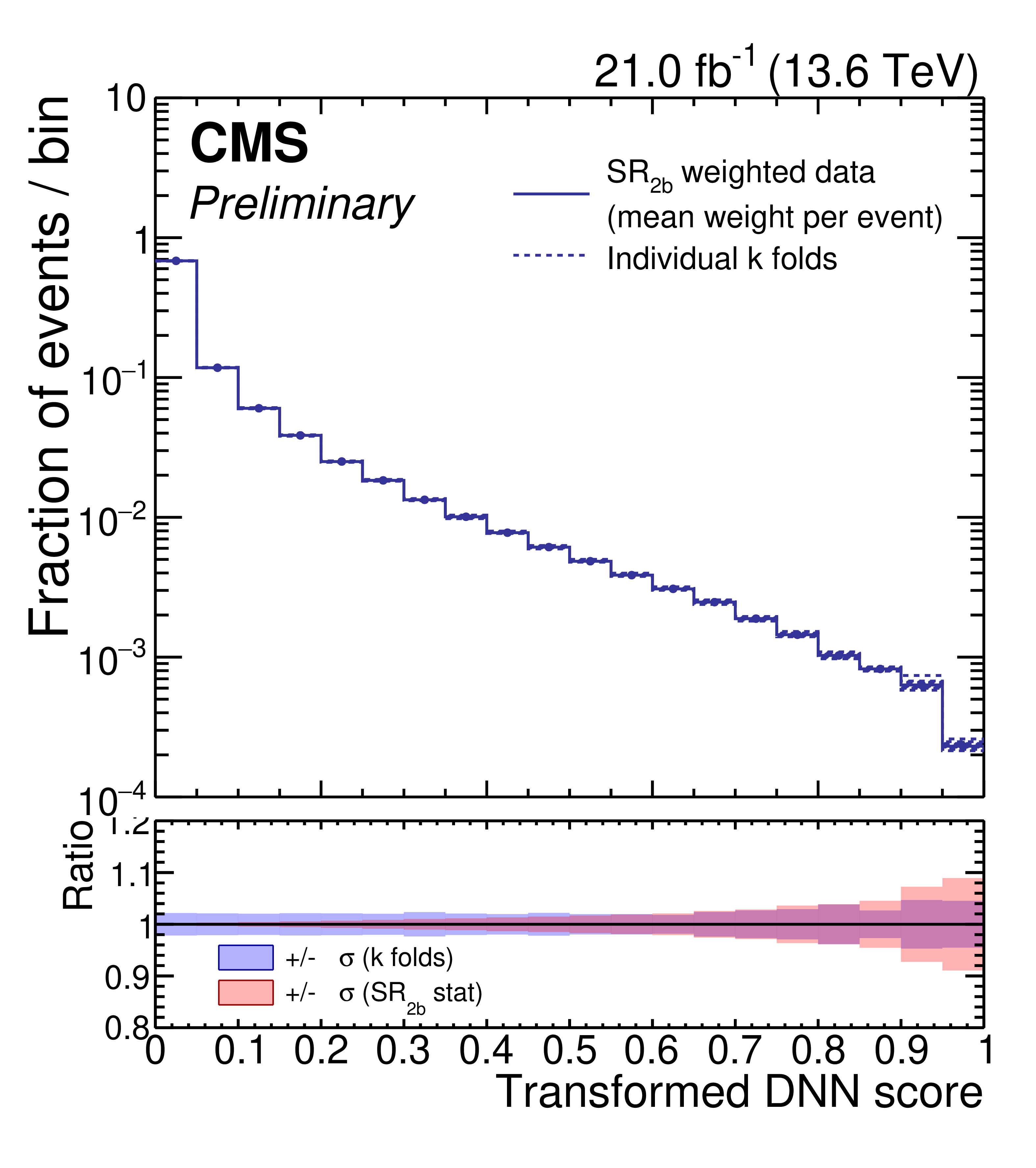
png pdf	Additional Figure 4: Transformed SvsB classifier output distribution for the reweighted $\mathrm{SR_{2b}}$ data events in the $\mathrm{SR_{4b}}$ region, shown for pre-ParkingHH (left) and post-ParkingHH (right) periods. Distributions correspond to the first analysis approach described in the note. In the upper panel, the solid blue line represents the nominal background prediction, obtained by averaging the event weights over the k-fold ensemble. The dashed lines indicate the background predictions obtained from each individual fold. In the lower panel, the red band shows the uncertainty in the $\mathrm{SR_{4b}}$ background prediction due to the limited size of the $\mathrm{SR_{2b}}$ sample, while the blue band corresponds to the symmetrized 68% CL interval around the nominal prediction as derived from the individual k-fold predictions. The statistical uncertainty from $\mathrm{SR_{2b}}$ data dominates in the highest SvsB score bins.
png pdf	Additional Figure 4-a: Transformed SvsB classifier output distribution for the reweighted $\mathrm{SR_{2b}}$ data events in the $\mathrm{SR_{4b}}$ region, shown for pre-ParkingHH (left) and post-ParkingHH (right) periods. Distributions correspond to the first analysis approach described in the note. In the upper panel, the solid blue line represents the nominal background prediction, obtained by averaging the event weights over the k-fold ensemble. The dashed lines indicate the background predictions obtained from each individual fold. In the lower panel, the red band shows the uncertainty in the $\mathrm{SR_{4b}}$ background prediction due to the limited size of the $\mathrm{SR_{2b}}$ sample, while the blue band corresponds to the symmetrized 68% CL interval around the nominal prediction as derived from the individual k-fold predictions. The statistical uncertainty from $\mathrm{SR_{2b}}$ data dominates in the highest SvsB score bins.
png pdf	Additional Figure 4-b: Transformed SvsB classifier output distribution for the reweighted $\mathrm{SR_{2b}}$ data events in the $\mathrm{SR_{4b}}$ region, shown for pre-ParkingHH (left) and post-ParkingHH (right) periods. Distributions correspond to the first analysis approach described in the note. In the upper panel, the solid blue line represents the nominal background prediction, obtained by averaging the event weights over the k-fold ensemble. The dashed lines indicate the background predictions obtained from each individual fold. In the lower panel, the red band shows the uncertainty in the $\mathrm{SR_{4b}}$ background prediction due to the limited size of the $\mathrm{SR_{2b}}$ sample, while the blue band corresponds to the symmetrized 68% CL interval around the nominal prediction as derived from the individual k-fold predictions. The statistical uncertainty from $\mathrm{SR_{2b}}$ data dominates in the highest SvsB score bins.
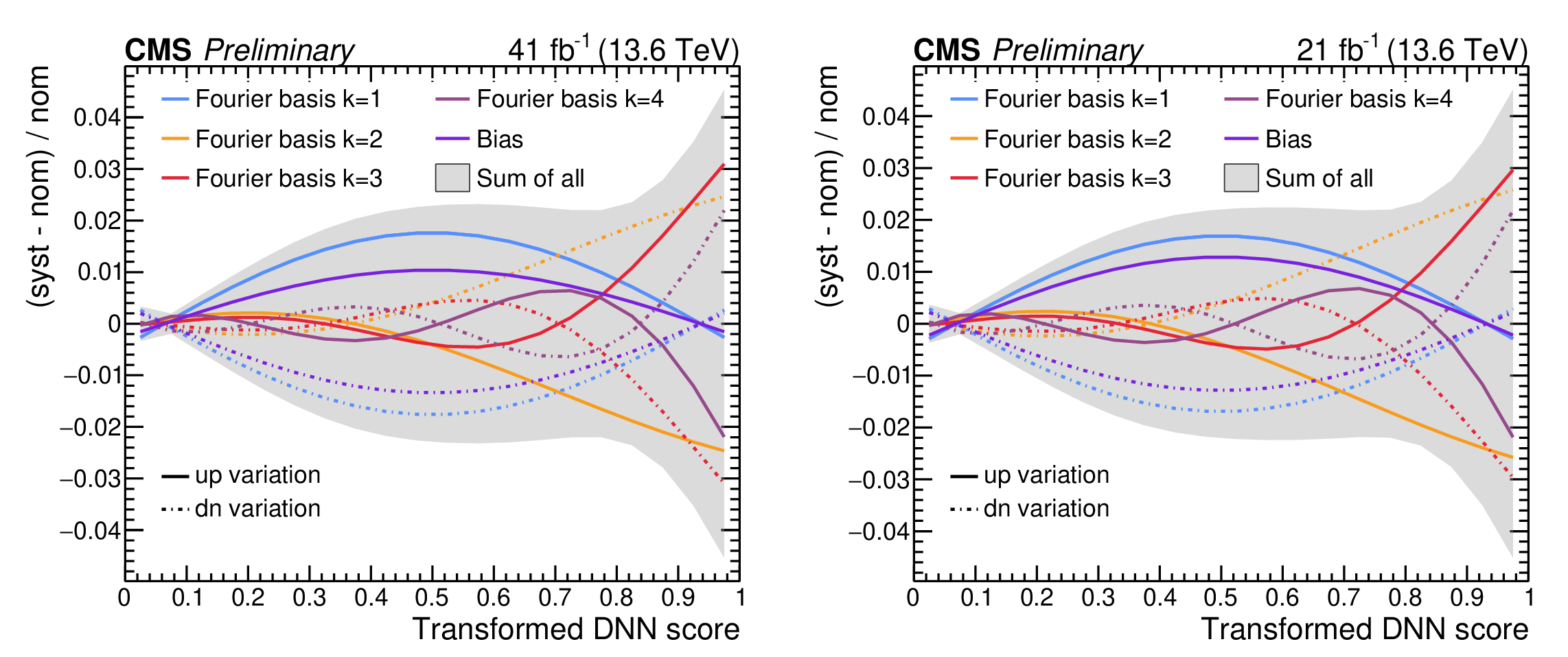
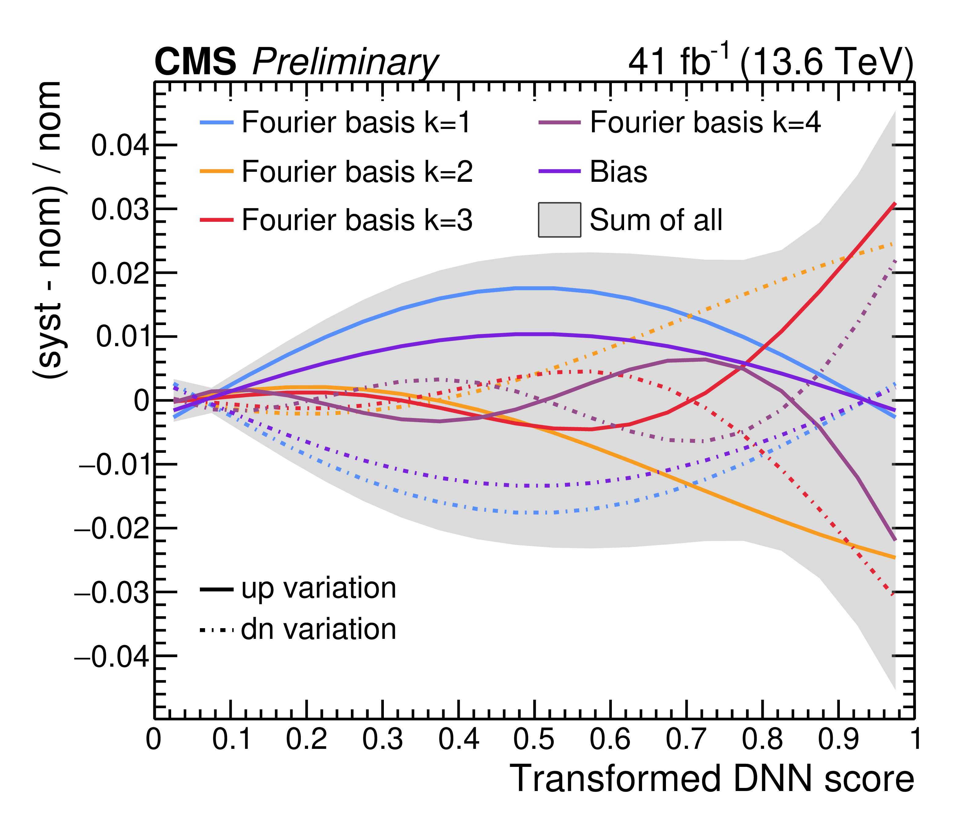
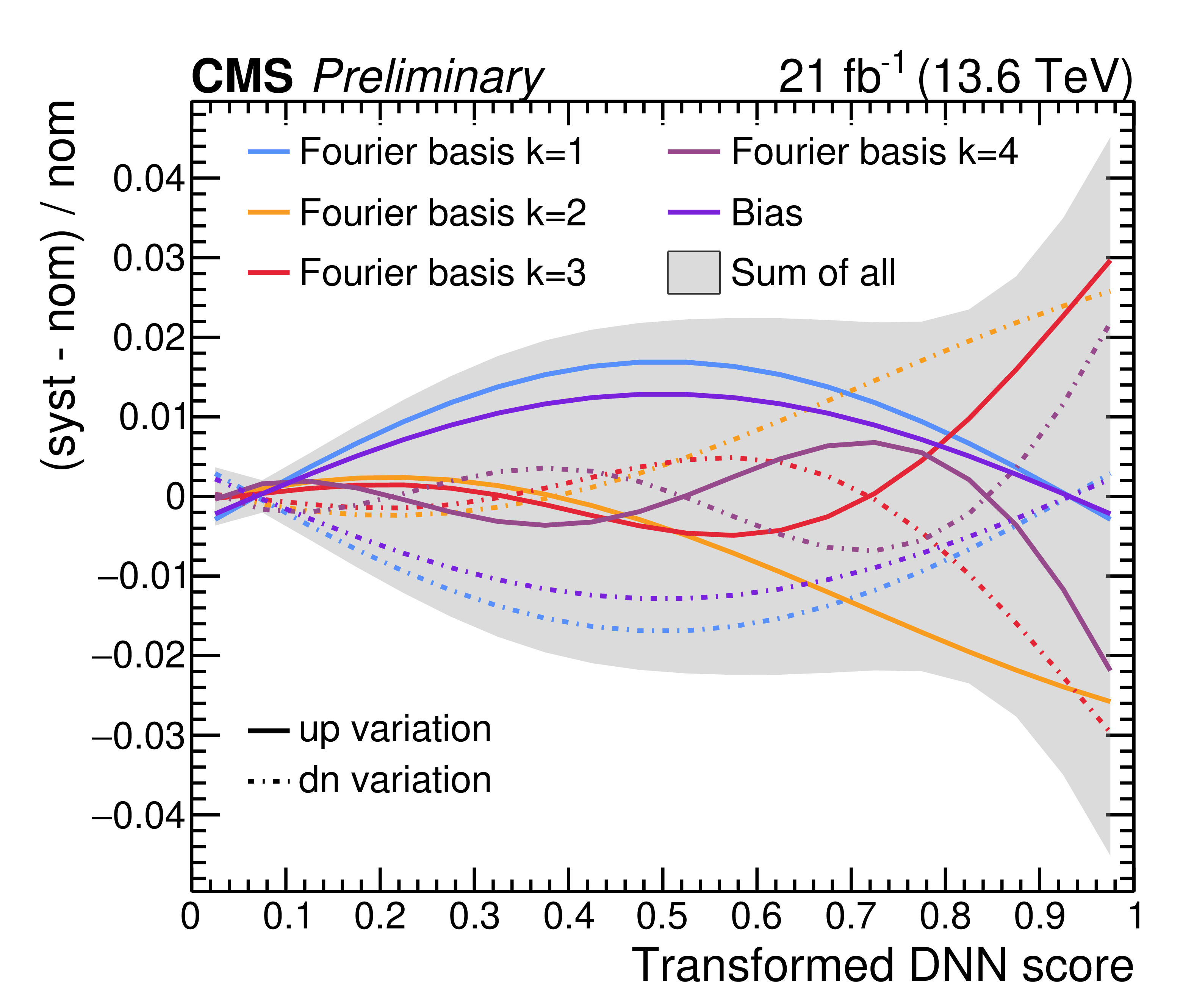
png pdf	Additional Figure 5: Data-driven shape uncertainties as a function of the SvsB classifier output for the reweighted $\mathrm{SR_{2b}}$ background events in the $\mathrm{SR_{4b}}$ region, shown for pre-ParkingHH (left) and post-ParkingHH (right) data. Distributions correspond to the first analysis approach described in the note. The solid (dashed) lines correspond to the +1$\sigma$ (-1$\sigma$) variations of the four Fourier basis components (azure, orange, red) and the bias (purple) uncertainty. The combined uncertainty, obtained by summing all components in quadrature, is shown as the solid gray filled band. Although the event selection and integrated luminosity differ between the two data-taking periods, the overall size of the shape uncertainties remains consistent. The overall uncertainty increases from 0.3% to 4.5% with increasing SvsB score.
png pdf	Additional Figure 5-a: Data-driven shape uncertainties as a function of the SvsB classifier output for the reweighted $\mathrm{SR_{2b}}$ background events in the $\mathrm{SR_{4b}}$ region, shown for pre-ParkingHH (left) and post-ParkingHH (right) data. Distributions correspond to the first analysis approach described in the note. The solid (dashed) lines correspond to the +1$\sigma$ (-1$\sigma$) variations of the four Fourier basis components (azure, orange, red) and the bias (purple) uncertainty. The combined uncertainty, obtained by summing all components in quadrature, is shown as the solid gray filled band. Although the event selection and integrated luminosity differ between the two data-taking periods, the overall size of the shape uncertainties remains consistent. The overall uncertainty increases from 0.3% to 4.5% with increasing SvsB score.
png pdf	Additional Figure 5-b: Data-driven shape uncertainties as a function of the SvsB classifier output for the reweighted $\mathrm{SR_{2b}}$ background events in the $\mathrm{SR_{4b}}$ region, shown for pre-ParkingHH (left) and post-ParkingHH (right) data. Distributions correspond to the first analysis approach described in the note. The solid (dashed) lines correspond to the +1$\sigma$ (-1$\sigma$) variations of the four Fourier basis components (azure, orange, red) and the bias (purple) uncertainty. The combined uncertainty, obtained by summing all components in quadrature, is shown as the solid gray filled band. Although the event selection and integrated luminosity differ between the two data-taking periods, the overall size of the shape uncertainties remains consistent. The overall uncertainty increases from 0.3% to 4.5% with increasing SvsB score.
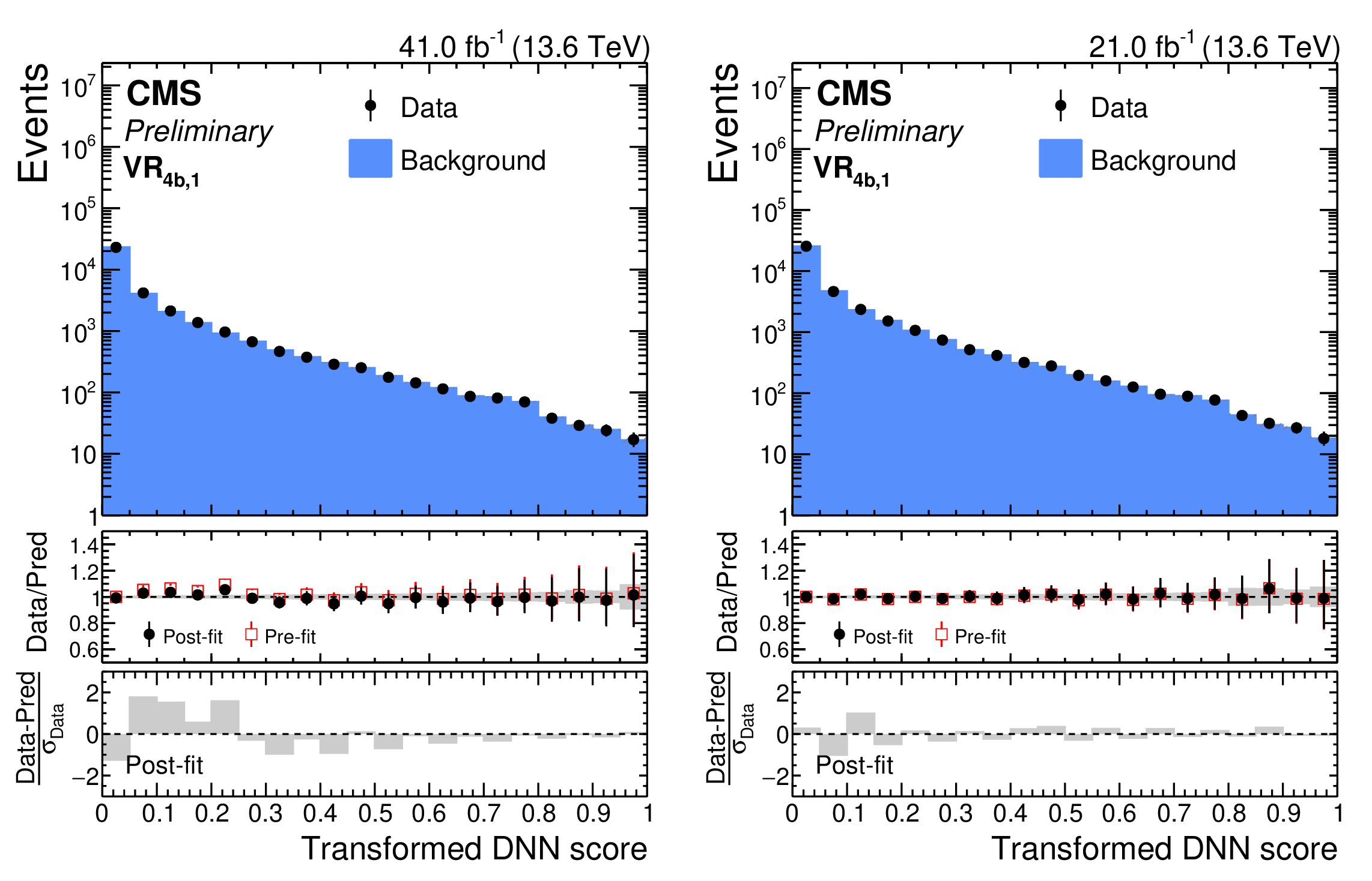
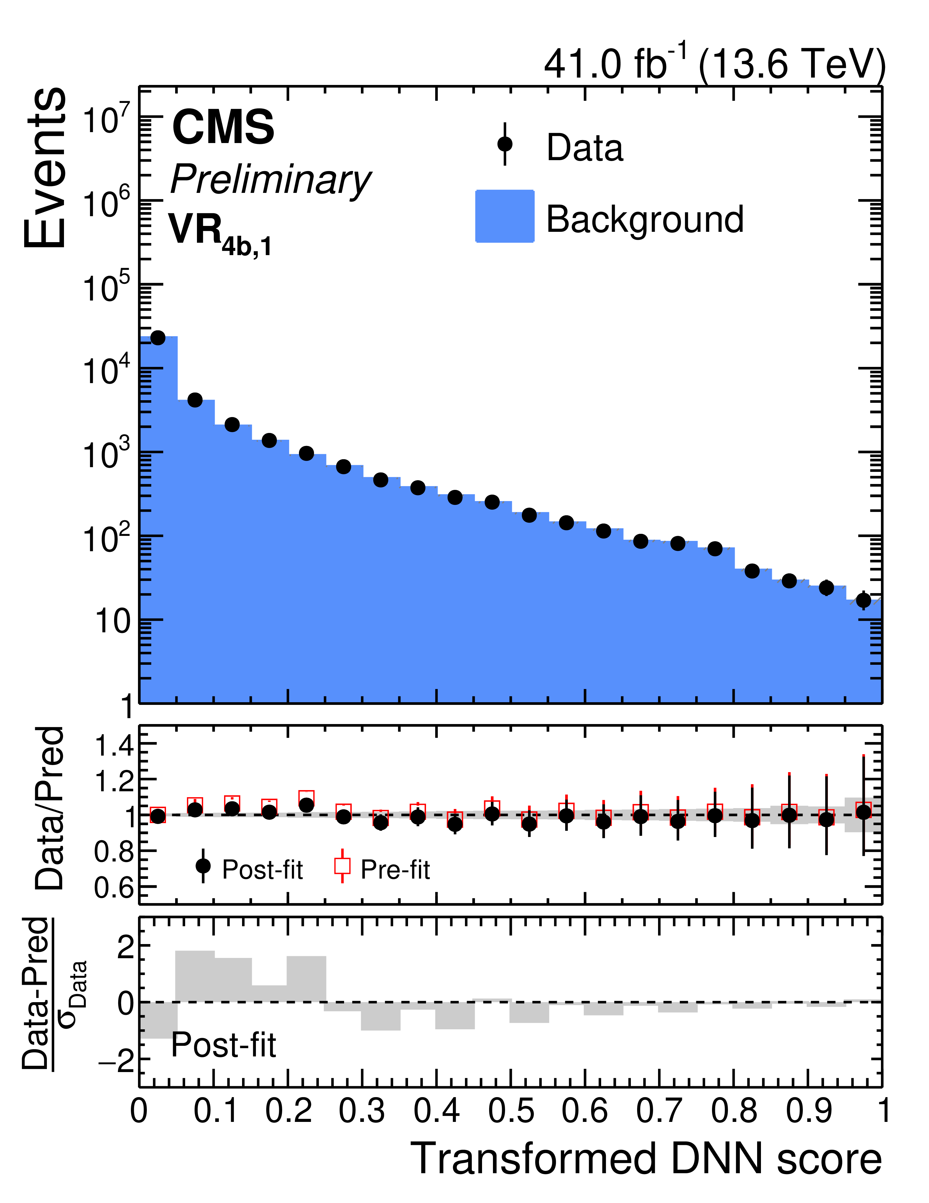
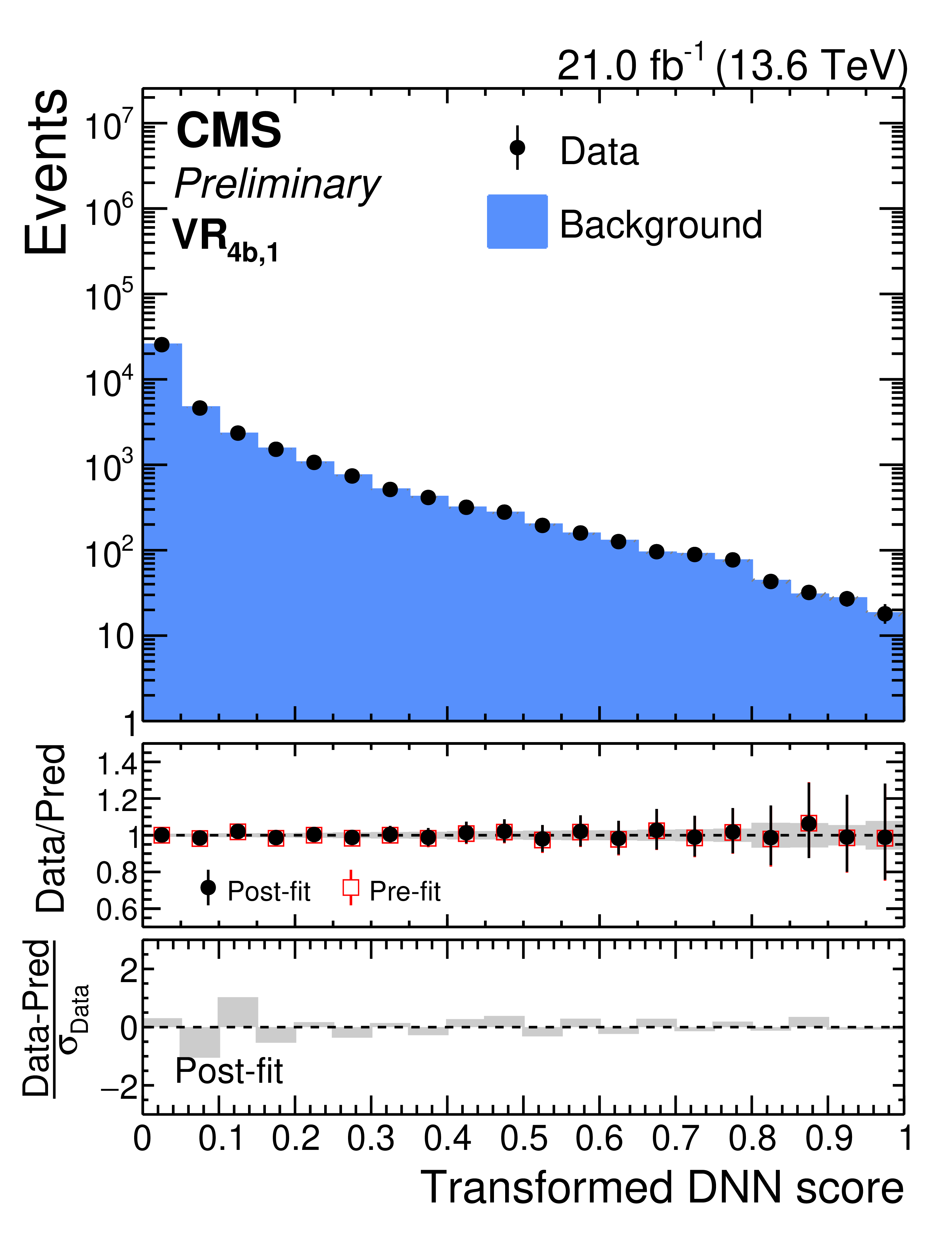
png pdf	Additional Figure 6: Pre-fit and post b-only fit distributions of the SvsB classifier output for the ${\mathrm{VR_{4b,1}}}$ validation regions in pre-ParkingHH (left) and post-ParkingHH (right) data. Distributions correspond to the first analysis approach described in the note.
png pdf	Additional Figure 6-a: Pre-fit and post b-only fit distributions of the SvsB classifier output for the ${\mathrm{VR_{4b,1}}}$ validation regions in pre-ParkingHH (left) and post-ParkingHH (right) data. Distributions correspond to the first analysis approach described in the note.
png pdf	Additional Figure 6-b: Pre-fit and post b-only fit distributions of the SvsB classifier output for the ${\mathrm{VR_{4b,1}}}$ validation regions in pre-ParkingHH (left) and post-ParkingHH (right) data. Distributions correspond to the first analysis approach described in the note.
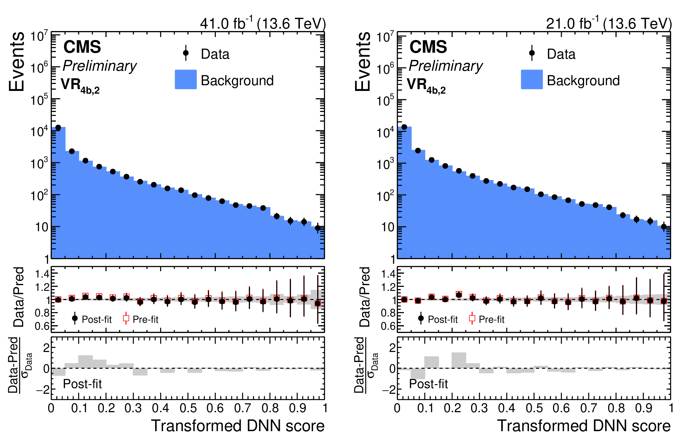
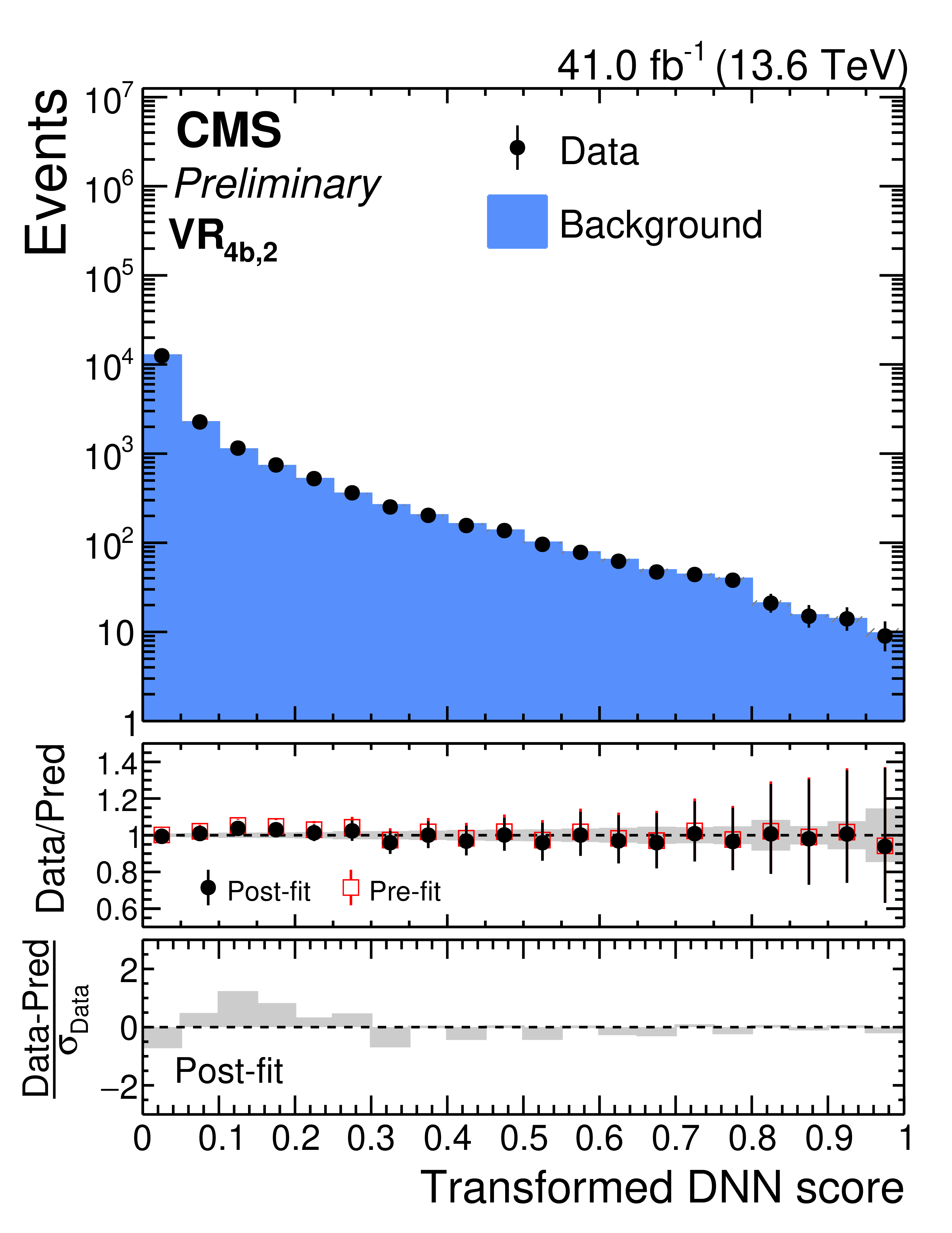
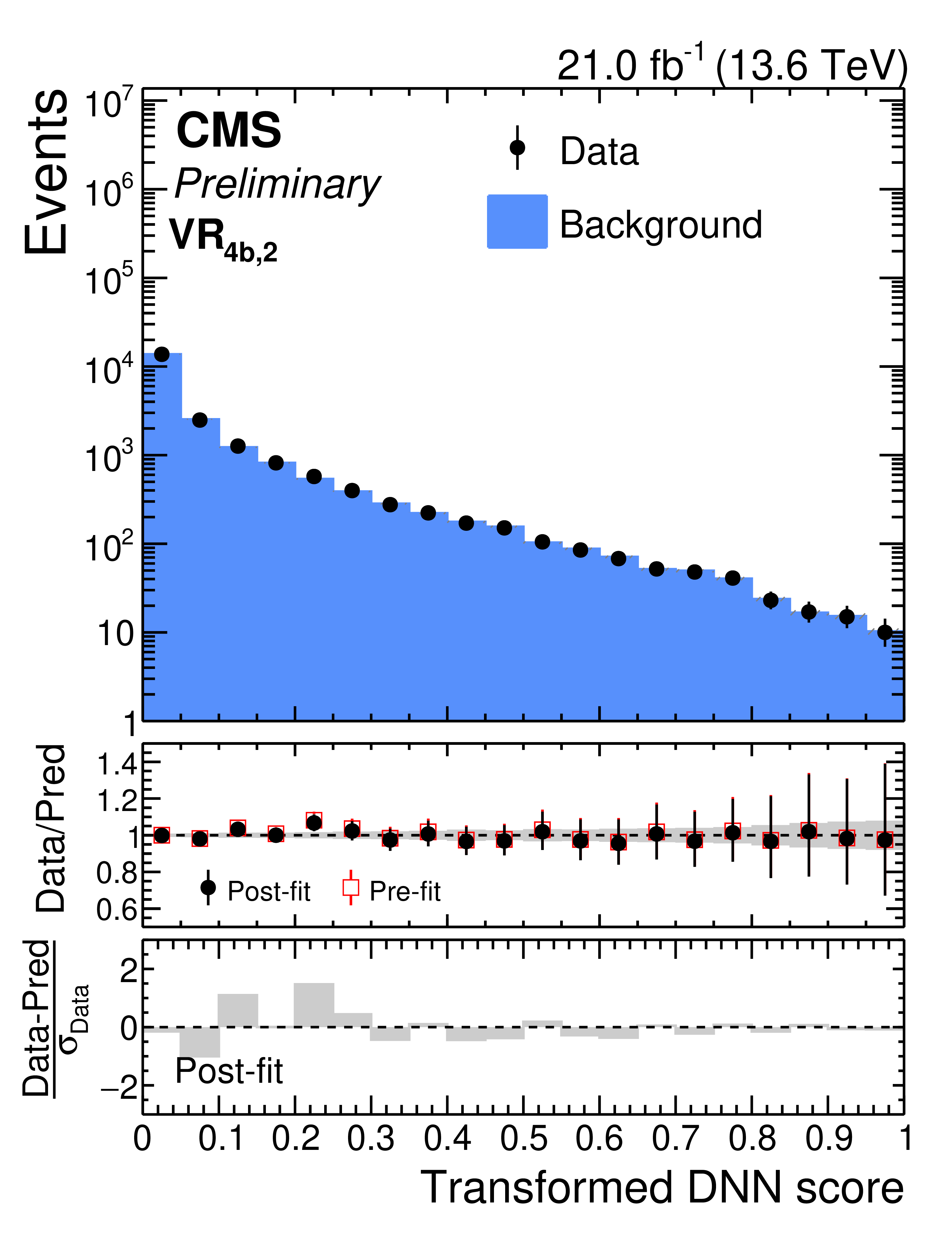
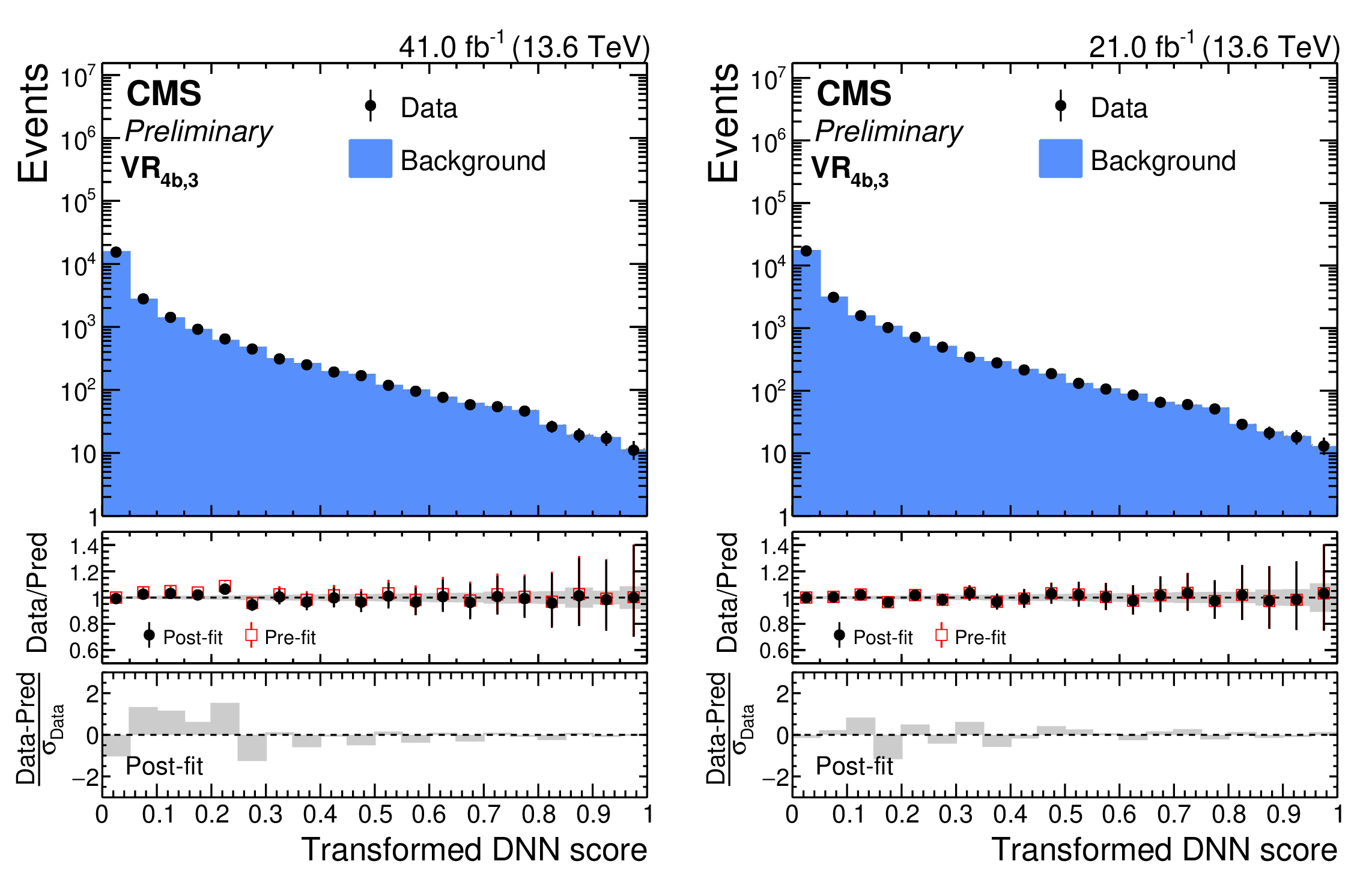
png pdf	Additional Figure 7: Pre-fit and post b-only fit distributions of the SvsB classifier output for the ${\mathrm{VR_{4b,2}}}$ validation regions in pre-ParkingHH (left) and post-ParkingHH (right) data. Distributions correspond to the first analysis approach described in the note.
png pdf	Additional Figure 7-a: Pre-fit and post b-only fit distributions of the SvsB classifier output for the ${\mathrm{VR_{4b,2}}}$ validation regions in pre-ParkingHH (left) and post-ParkingHH (right) data. Distributions correspond to the first analysis approach described in the note.
png pdf	Additional Figure 7-b: Pre-fit and post b-only fit distributions of the SvsB classifier output for the ${\mathrm{VR_{4b,2}}}$ validation regions in pre-ParkingHH (left) and post-ParkingHH (right) data. Distributions correspond to the first analysis approach described in the note.
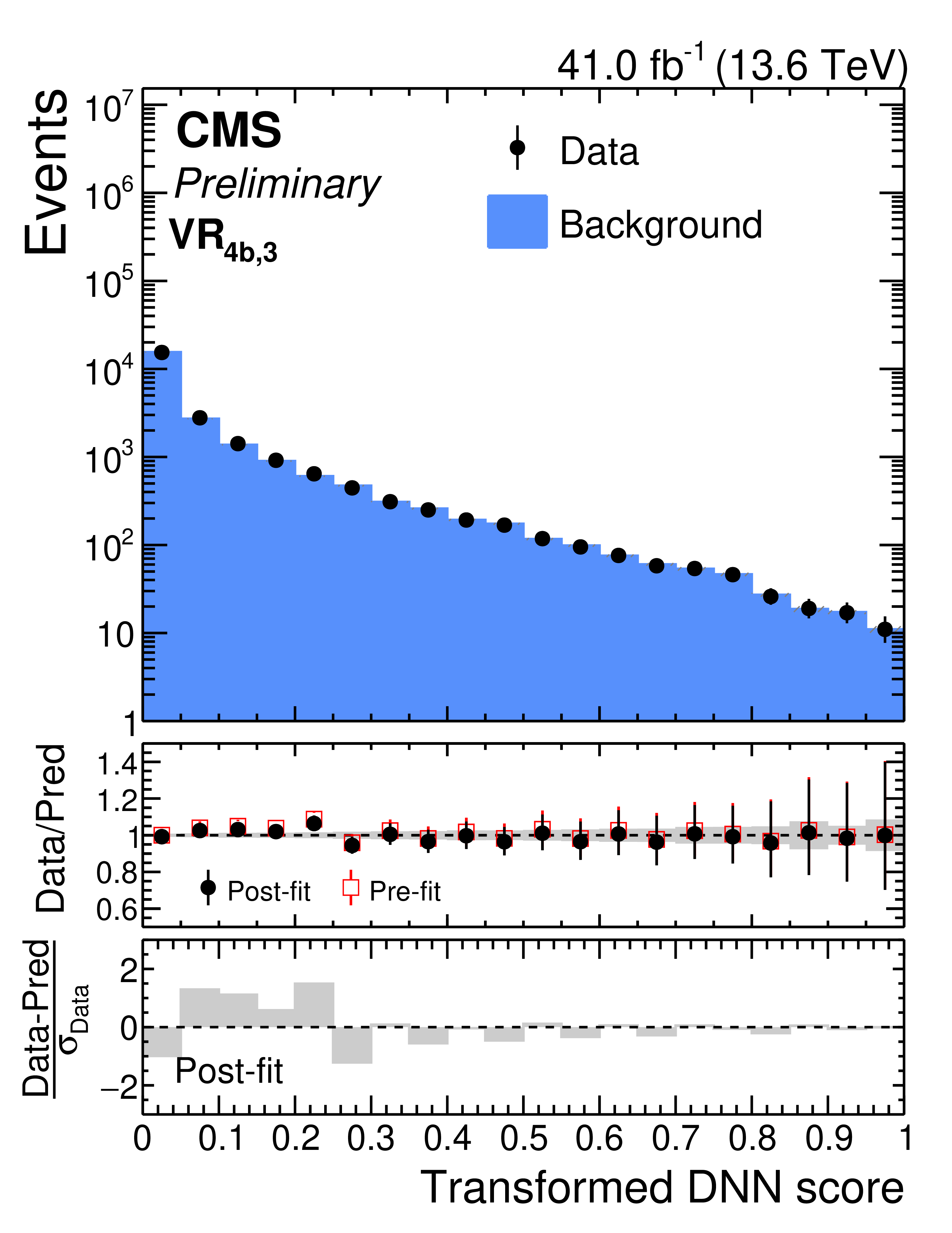
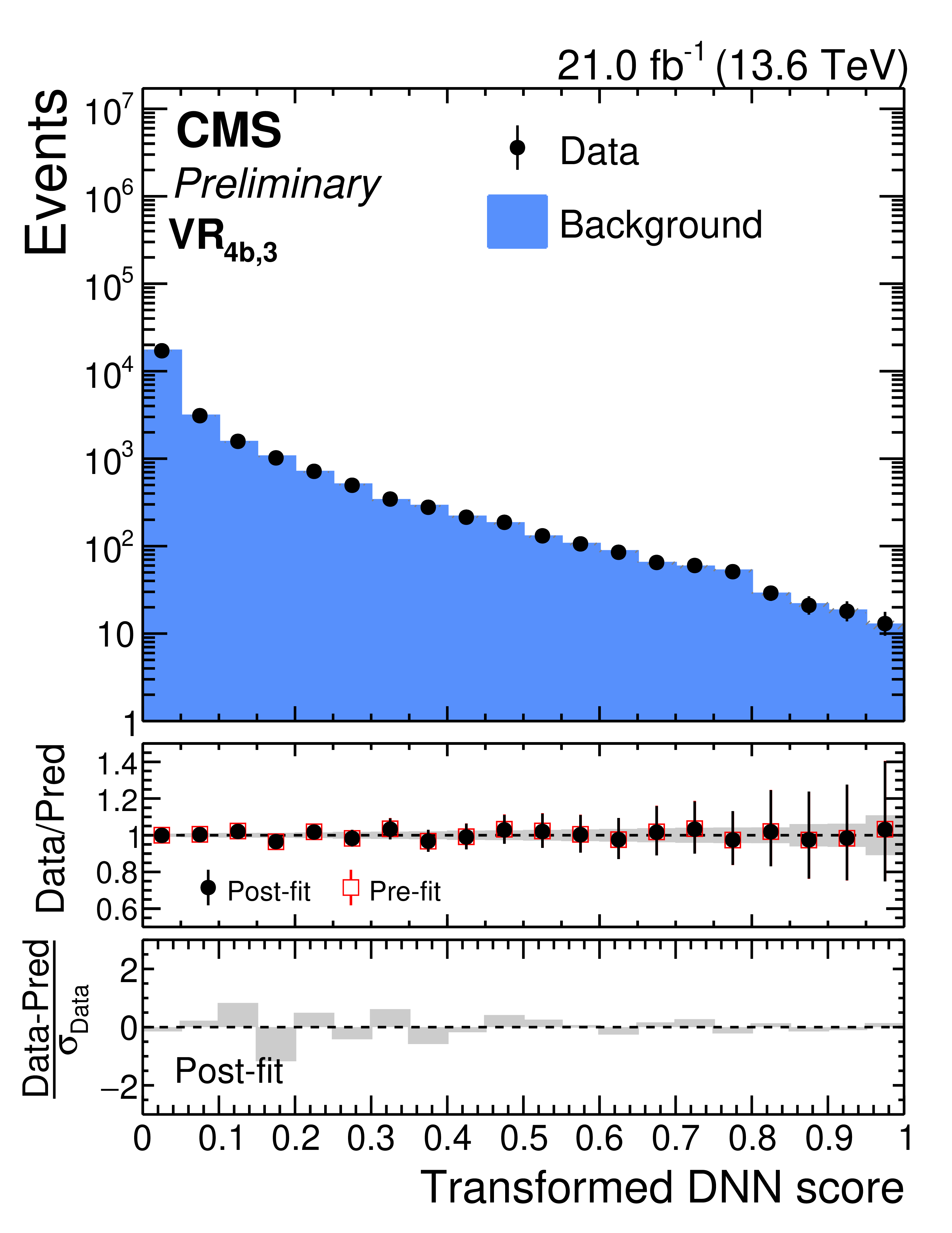
png pdf	Additional Figure 8: Pre-fit and post b-only fit distributions of the SvsB classifier output for the ${\mathrm{VR_{4b,3}}}$ validation regions in pre-ParkingHH (left) and post-ParkingHH (right) data. Distributions correspond to the first analysis approach described in the note.
png pdf	Additional Figure 8-a: Pre-fit and post b-only fit distributions of the SvsB classifier output for the ${\mathrm{VR_{4b,3}}}$ validation regions in pre-ParkingHH (left) and post-ParkingHH (right) data. Distributions correspond to the first analysis approach described in the note.
png pdf	Additional Figure 8-b: Pre-fit and post b-only fit distributions of the SvsB classifier output for the ${\mathrm{VR_{4b,3}}}$ validation regions in pre-ParkingHH (left) and post-ParkingHH (right) data. Distributions correspond to the first analysis approach described in the note.
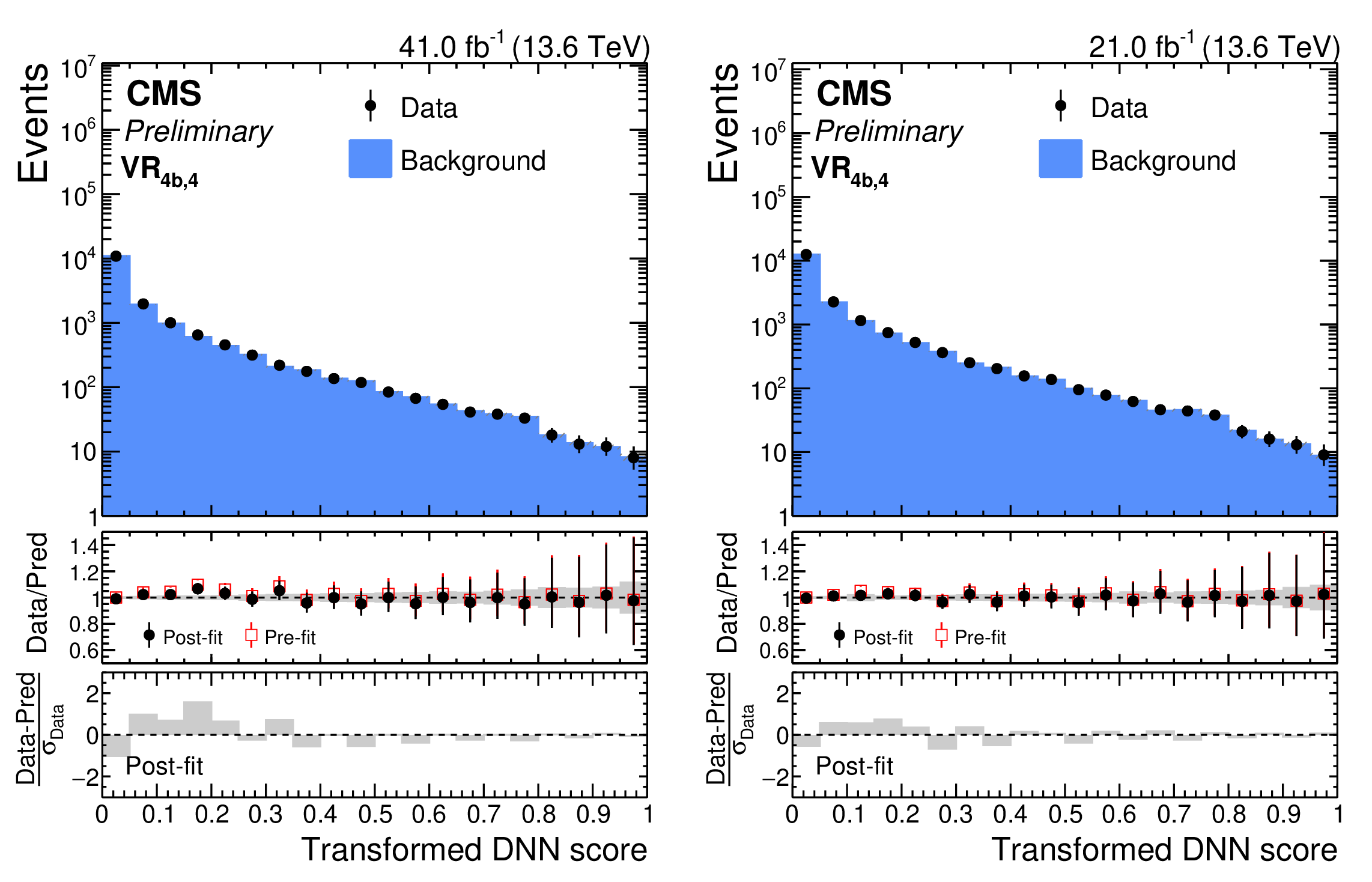
png pdf	Additional Figure 9: Pre-fit and post b-only fit distributions of the SvsB classifier output for the ${\mathrm{VR_{4b,4}}}$ validation regions in pre-ParkingHH (left) and post-ParkingHH (right) data. Distributions correspond to the first analysis approach described in the note.
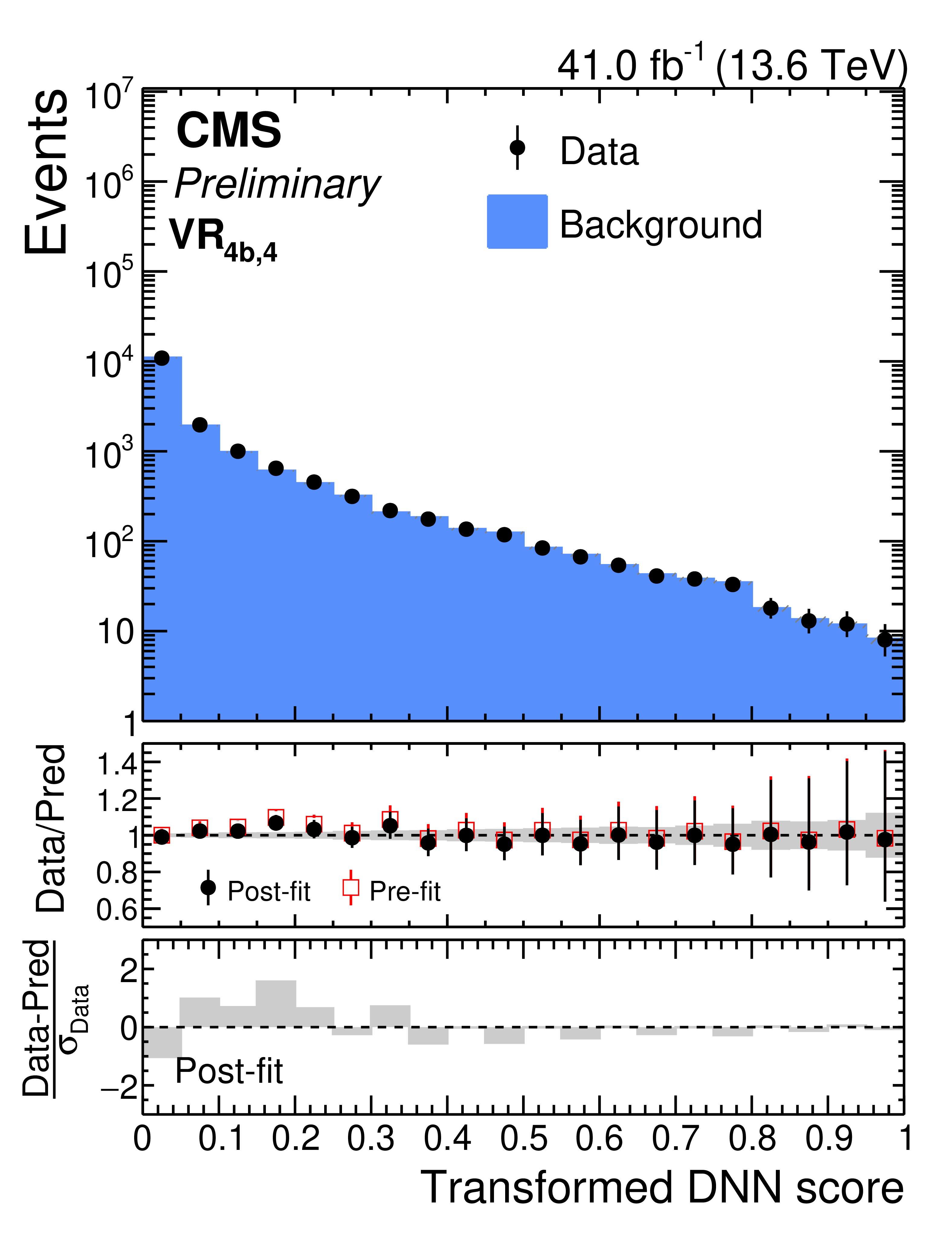
png pdf	Additional Figure 9-a: Pre-fit and post b-only fit distributions of the SvsB classifier output for the ${\mathrm{VR_{4b,4}}}$ validation regions in pre-ParkingHH (left) and post-ParkingHH (right) data. Distributions correspond to the first analysis approach described in the note.
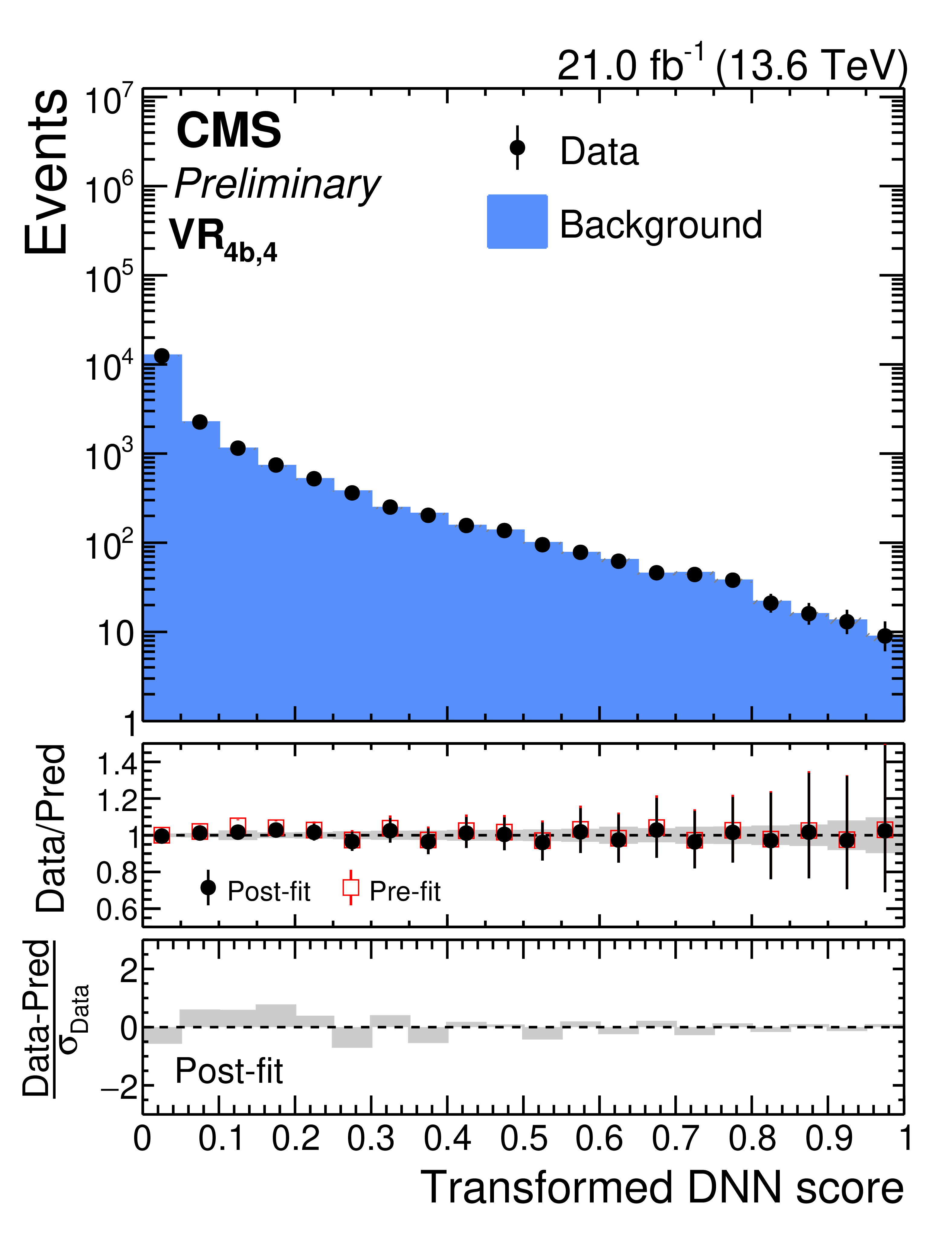
png pdf	Additional Figure 9-b: Pre-fit and post b-only fit distributions of the SvsB classifier output for the ${\mathrm{VR_{4b,4}}}$ validation regions in pre-ParkingHH (left) and post-ParkingHH (right) data. Distributions correspond to the first analysis approach described in the note.
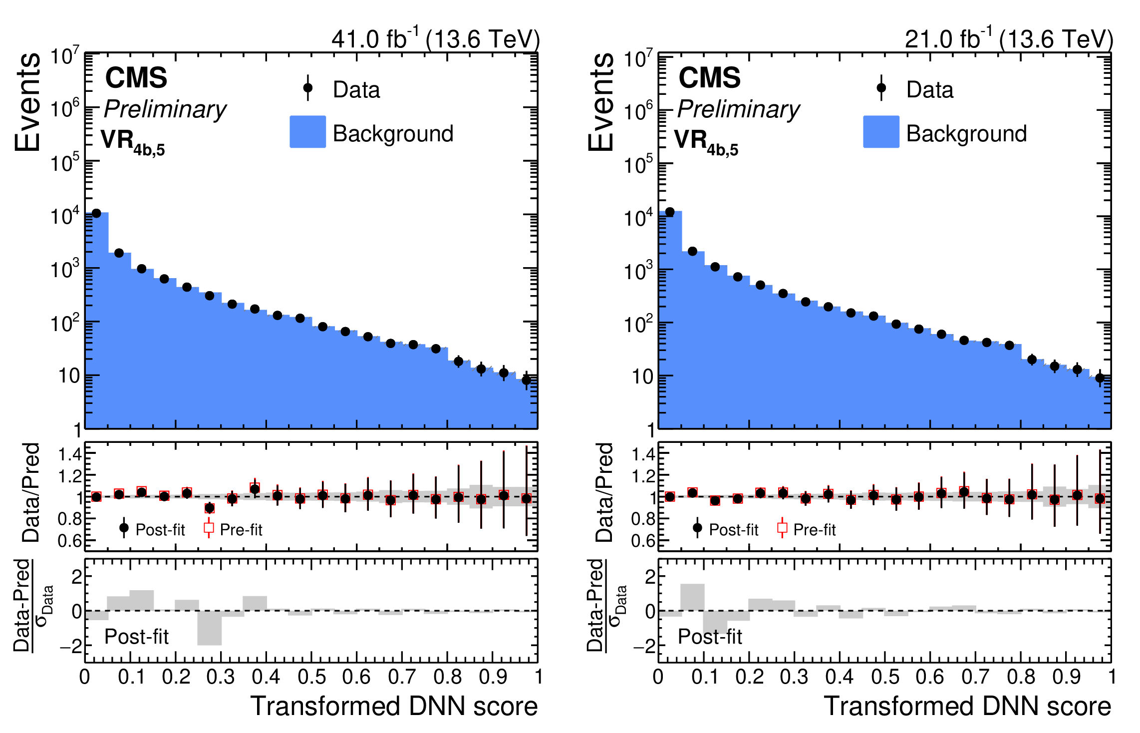
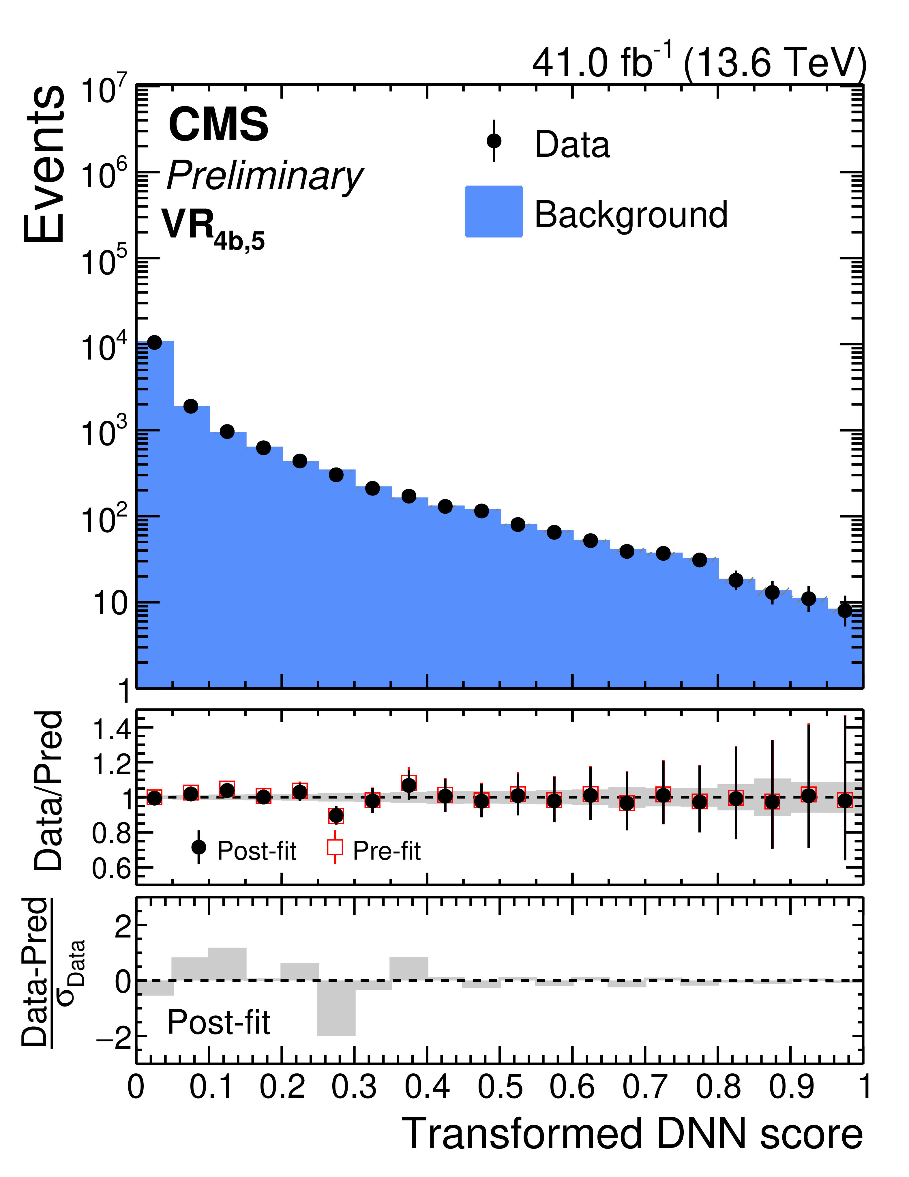
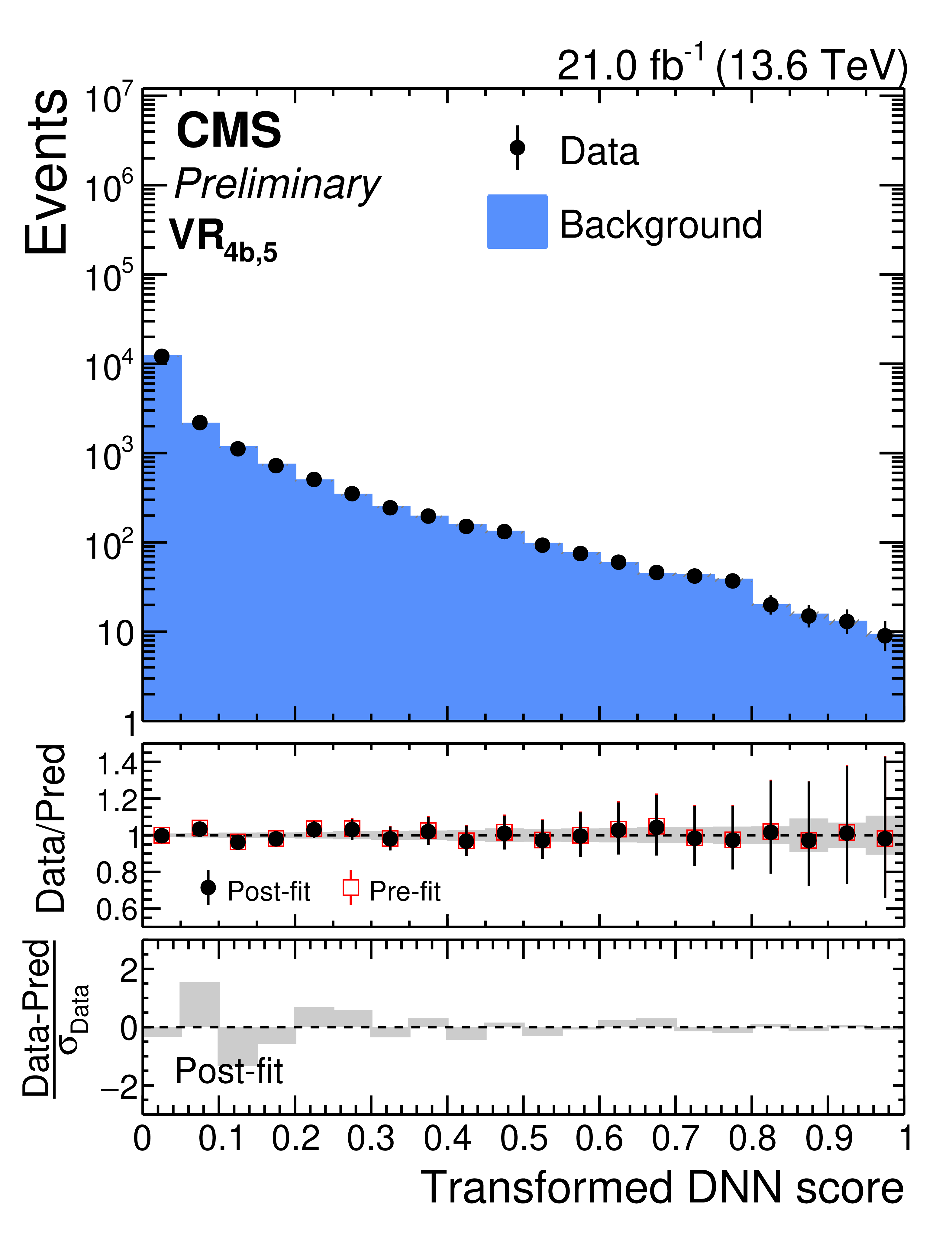
png pdf	Additional Figure 10: Pre-fit and post b-only fit distributions of the SvsB classifier output for the ${\mathrm{VR_{4b,5}}}$ validation regions in pre-ParkingHH (left) and post-ParkingHH (right) data. Distributions correspond to the first analysis approach described in the note.
png pdf	Additional Figure 10-a: Pre-fit and post b-only fit distributions of the SvsB classifier output for the ${\mathrm{VR_{4b,5}}}$ validation regions in pre-ParkingHH (left) and post-ParkingHH (right) data. Distributions correspond to the first analysis approach described in the note.
png pdf	Additional Figure 10-b: Pre-fit and post b-only fit distributions of the SvsB classifier output for the ${\mathrm{VR_{4b,5}}}$ validation regions in pre-ParkingHH (left) and post-ParkingHH (right) data. Distributions correspond to the first analysis approach described in the note.
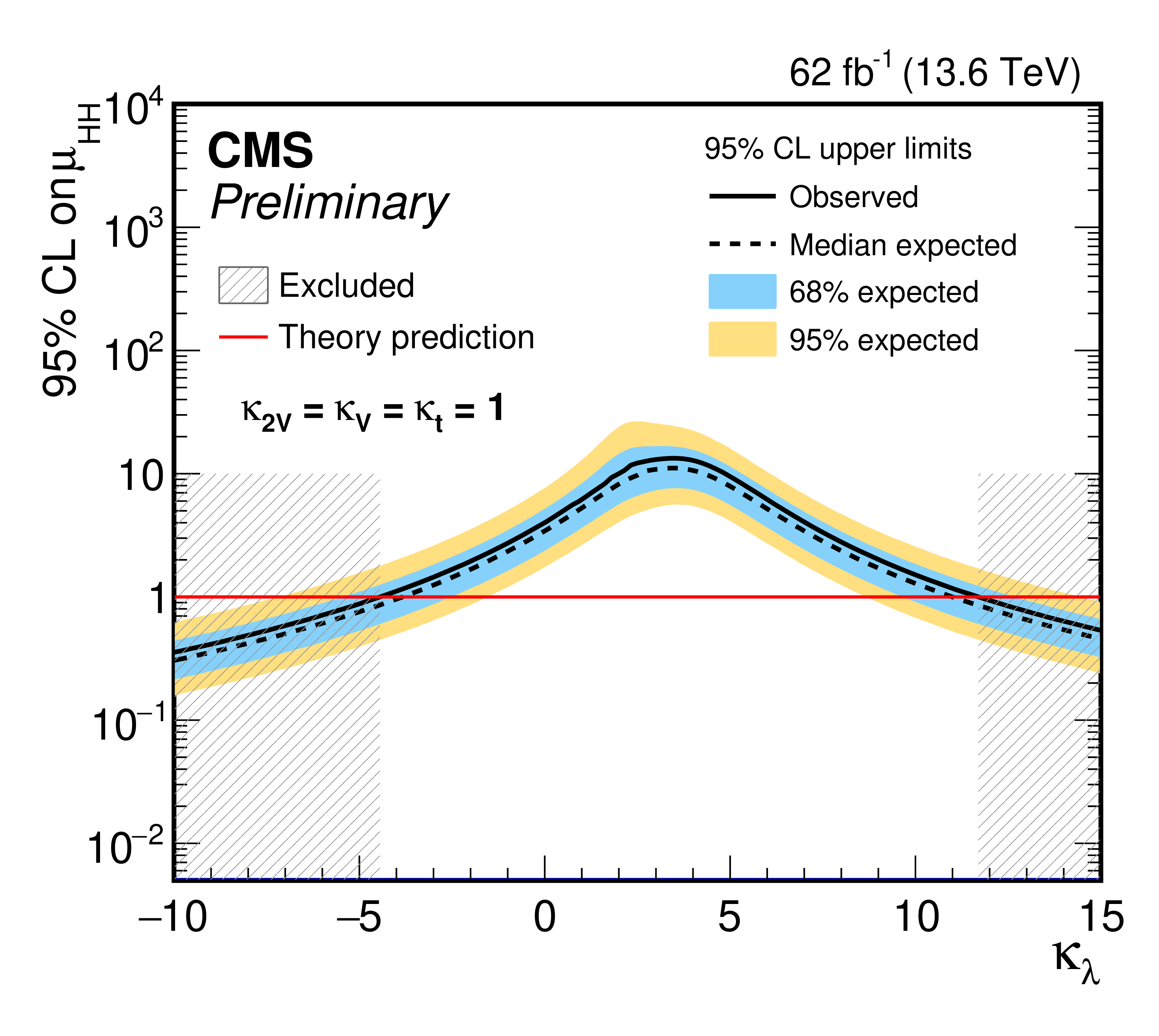
png pdf	Additional Figure 11: The observed (solid) and expected (dashed) 95% CL upper limits on the signal strength of the HH (left) and VBF (right) production (left) obtained as a function of $\mathrm{k}_{\lambda}$ (left) and $k_{VV}$(right) for the resolved $ \mathrm{H}\mathrm{H} \to 4\mathrm{b} $ analysis. The cyan and blue bands represent, respectively, the 68 and 95% CL intervals around the expected limit. The horizontal red lines indicate the SM prediction. The observed (expected) allowed range, at 95% CL, for $\mathrm{k}_{\lambda}$ is {[-4.4,11.7]}~{([-3.8,11.0])}, while that for $k_{VV}$ is {[-0.08,2.20]}~{([-0.08,2.19])}. Results correspond to the first analysis approach described in the note.
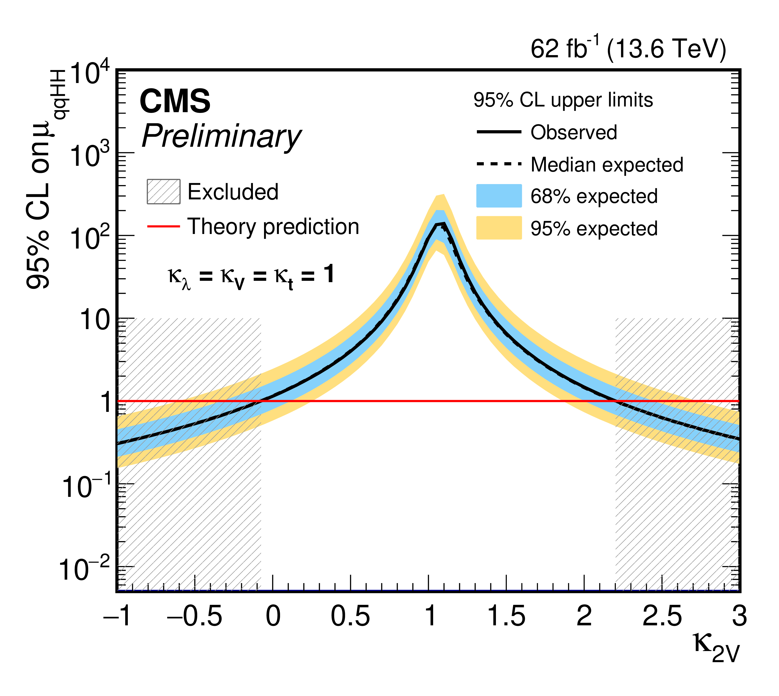
png pdf	Additional Figure 11-a: The observed (solid) and expected (dashed) 95% CL upper limits on the signal strength of the HH (left) and VBF (right) production (left) obtained as a function of $\mathrm{k}_{\lambda}$ (left) and $k_{VV}$(right) for the resolved $ \mathrm{H}\mathrm{H} \to 4\mathrm{b} $ analysis. The cyan and blue bands represent, respectively, the 68 and 95% CL intervals around the expected limit. The horizontal red lines indicate the SM prediction. The observed (expected) allowed range, at 95% CL, for $\mathrm{k}_{\lambda}$ is {[-4.4,11.7]}~{([-3.8,11.0])}, while that for $k_{VV}$ is {[-0.08,2.20]}~{([-0.08,2.19])}. Results correspond to the first analysis approach described in the note.
png pdf	Additional Figure 11-b: The observed (solid) and expected (dashed) 95% CL upper limits on the signal strength of the HH (left) and VBF (right) production (left) obtained as a function of $\mathrm{k}_{\lambda}$ (left) and $k_{VV}$(right) for the resolved $ \mathrm{H}\mathrm{H} \to 4\mathrm{b} $ analysis. The cyan and blue bands represent, respectively, the 68 and 95% CL intervals around the expected limit. The horizontal red lines indicate the SM prediction. The observed (expected) allowed range, at 95% CL, for $\mathrm{k}_{\lambda}$ is {[-4.4,11.7]}~{([-3.8,11.0])}, while that for $k_{VV}$ is {[-0.08,2.20]}~{([-0.08,2.19])}. Results correspond to the first analysis approach described in the note.
png pdf	Additional Figure 12: The observed (solid) and expected (dashed) profile likelihood ratios as a function of $\mu_{HH}$ (left) and $\mu_{VBFHH}$ (right) from the resolved $ \mathrm{H}\mathrm{H} \to 4\mathrm{b} $ analysis. The expected curves are obtained from an Asimov dataset, defined by fixing the nuisances parameters to their maximum likelihood estimate obtained from data in which $\mu_{HH}=1$. The dashed red lines indicate the 68% and 95% CL ranges, expressed in units of $-2\Delta\ln(\mathcal{L})$. Best fit values for the signal strengths, along with their 68% CL intervals, are also reported. Results correspond to the first analysis approach described in the note.
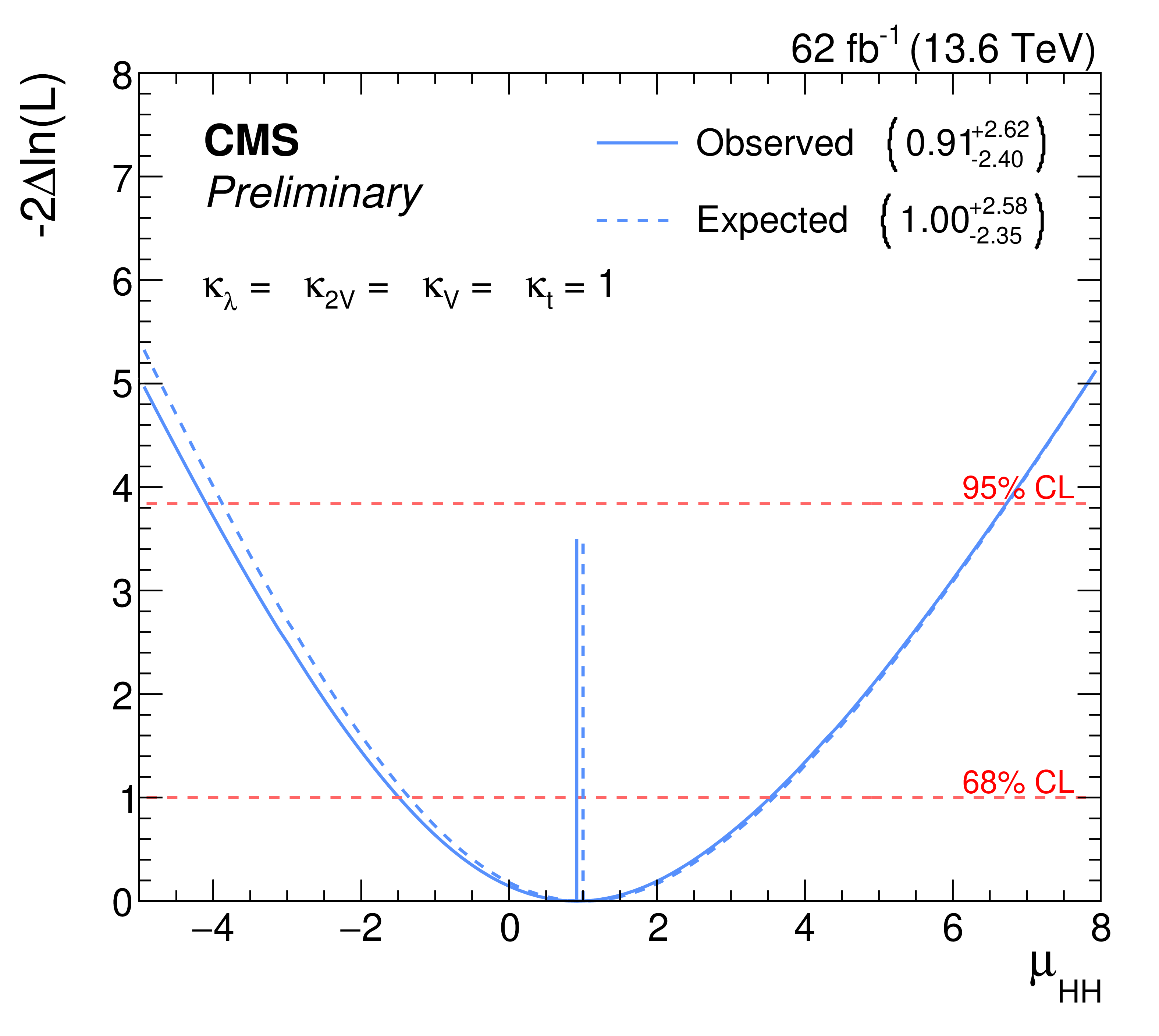
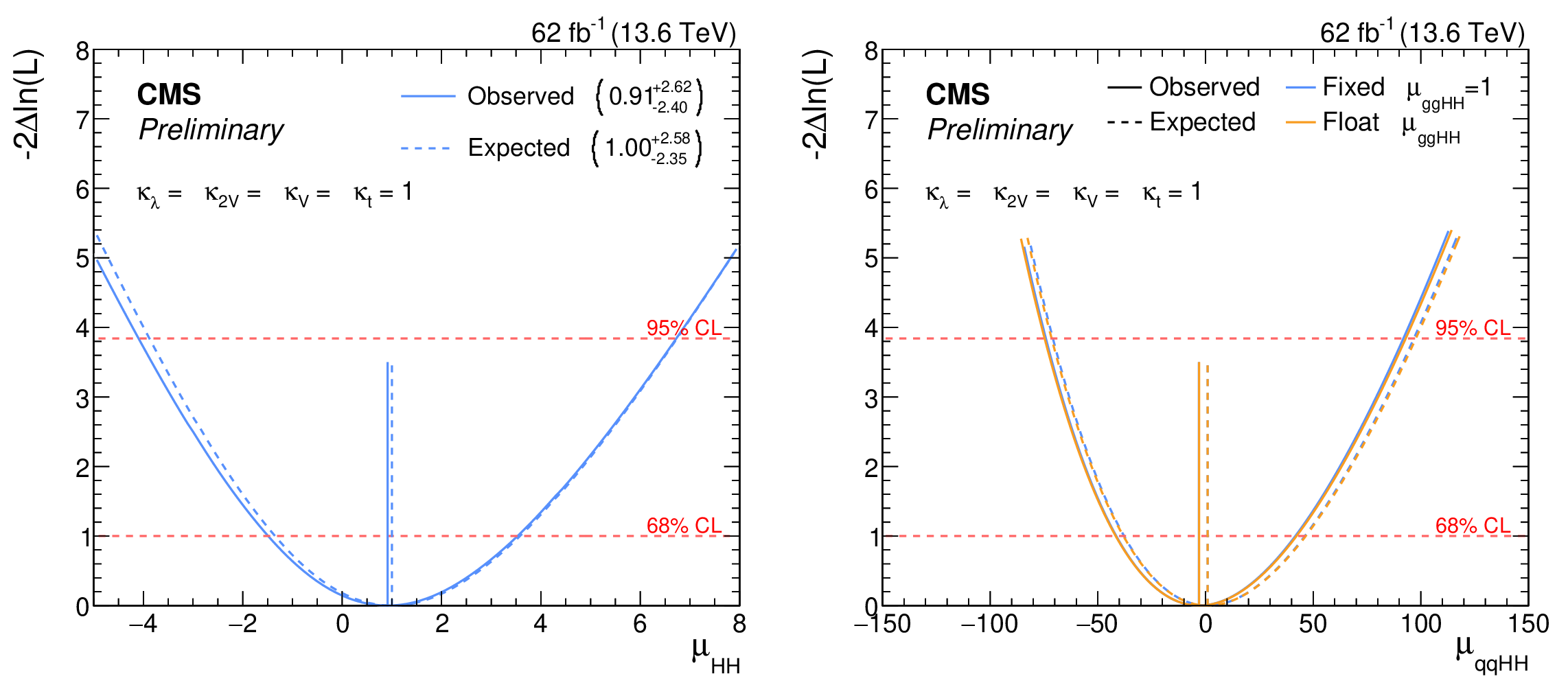
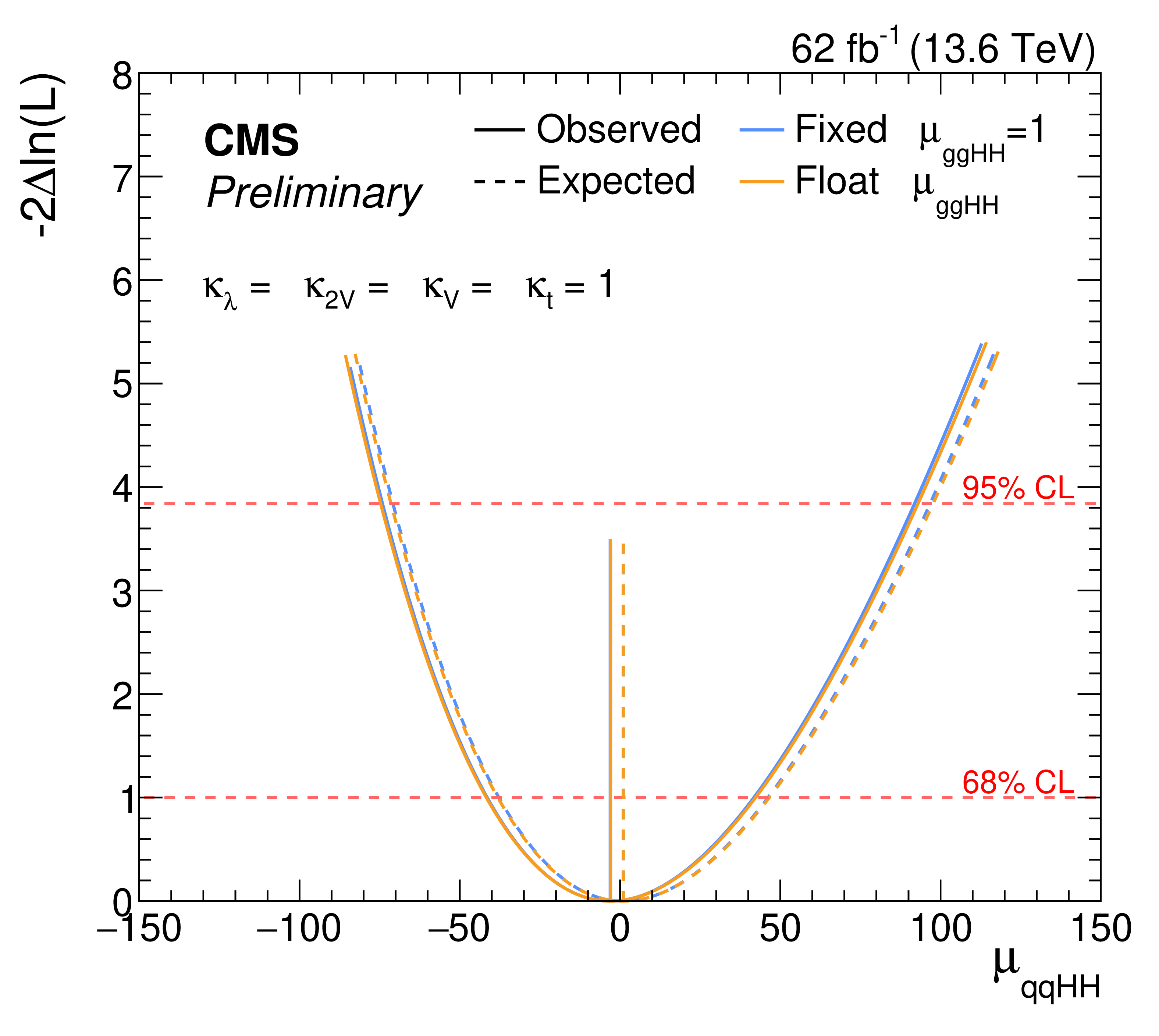
png pdf	Additional Figure 12-a: The observed (solid) and expected (dashed) profile likelihood ratios as a function of $\mu_{HH}$ (left) and $\mu_{VBFHH}$ (right) from the resolved $ \mathrm{H}\mathrm{H} \to 4\mathrm{b} $ analysis. The expected curves are obtained from an Asimov dataset, defined by fixing the nuisances parameters to their maximum likelihood estimate obtained from data in which $\mu_{HH}=1$. The dashed red lines indicate the 68% and 95% CL ranges, expressed in units of $-2\Delta\ln(\mathcal{L})$. Best fit values for the signal strengths, along with their 68% CL intervals, are also reported. Results correspond to the first analysis approach described in the note.
png pdf	Additional Figure 12-b: The observed (solid) and expected (dashed) profile likelihood ratios as a function of $\mu_{HH}$ (left) and $\mu_{VBFHH}$ (right) from the resolved $ \mathrm{H}\mathrm{H} \to 4\mathrm{b} $ analysis. The expected curves are obtained from an Asimov dataset, defined by fixing the nuisances parameters to their maximum likelihood estimate obtained from data in which $\mu_{HH}=1$. The dashed red lines indicate the 68% and 95% CL ranges, expressed in units of $-2\Delta\ln(\mathcal{L})$. Best fit values for the signal strengths, along with their 68% CL intervals, are also reported. Results correspond to the first analysis approach described in the note.
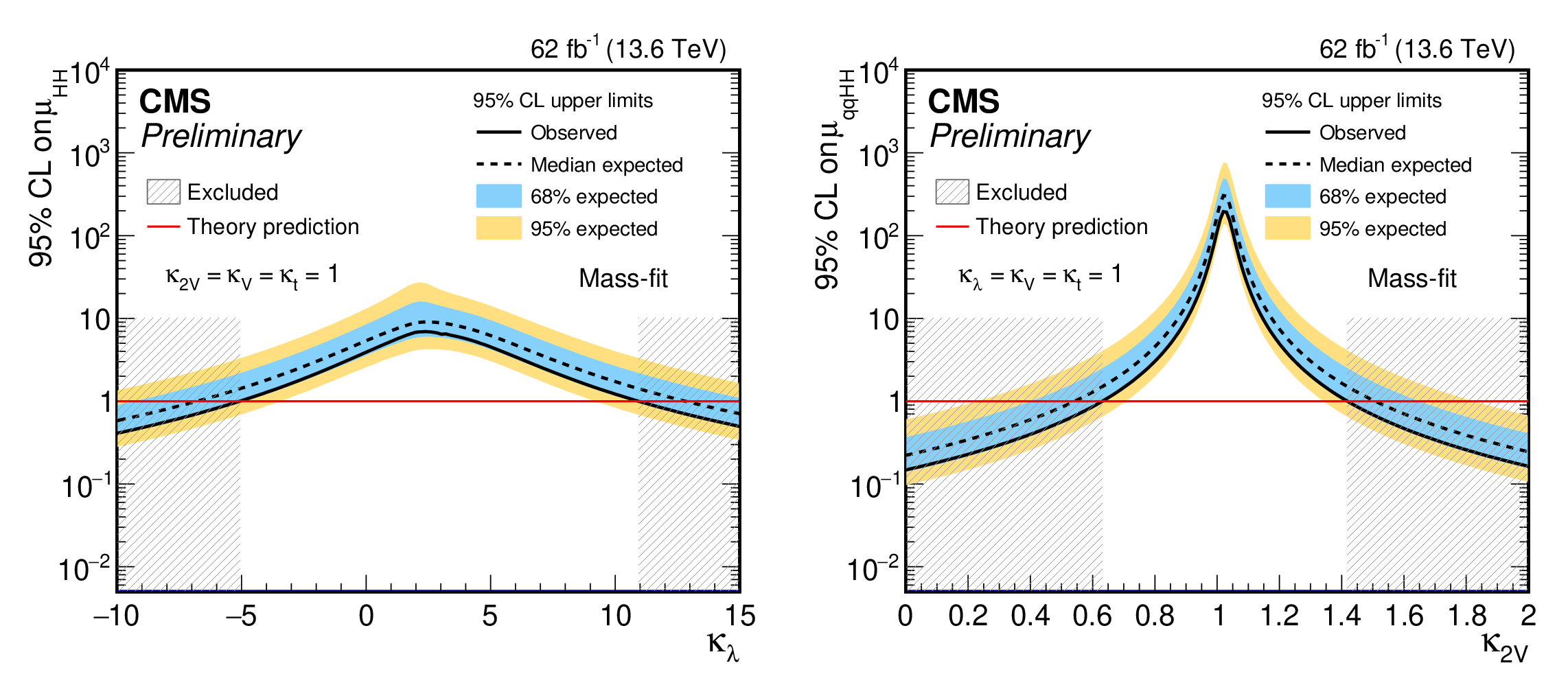
png pdf	Additional Figure 13: The observed (solid) and expected (dashed) 95% CL upper limits on the signal strength of the HH (left) and VBF (right) production (left) obtained as a function of $\mathrm{k}_{\lambda}$ (left) and $k_{VV}$ (right) for the merged mass-fit $ \mathrm{H}\mathrm{H} \to 4\mathrm{b} $ analysis. The cyan and blue bands represent, respectively, the 68 and 95% CL intervals around the expected limit. The horizontal red lines indicate the SM prediction. The observed (expected) allowed range, at 95% CL, for $\mathrm{k}_{\lambda}$ is {[-5.1,10.9]}~{([-6.8,12.8])}, while that for $k_{VV}$ is {[0.63,1.42]}~{([0.54,1.51])}. Results correspond to the first analysis approach described in the note.
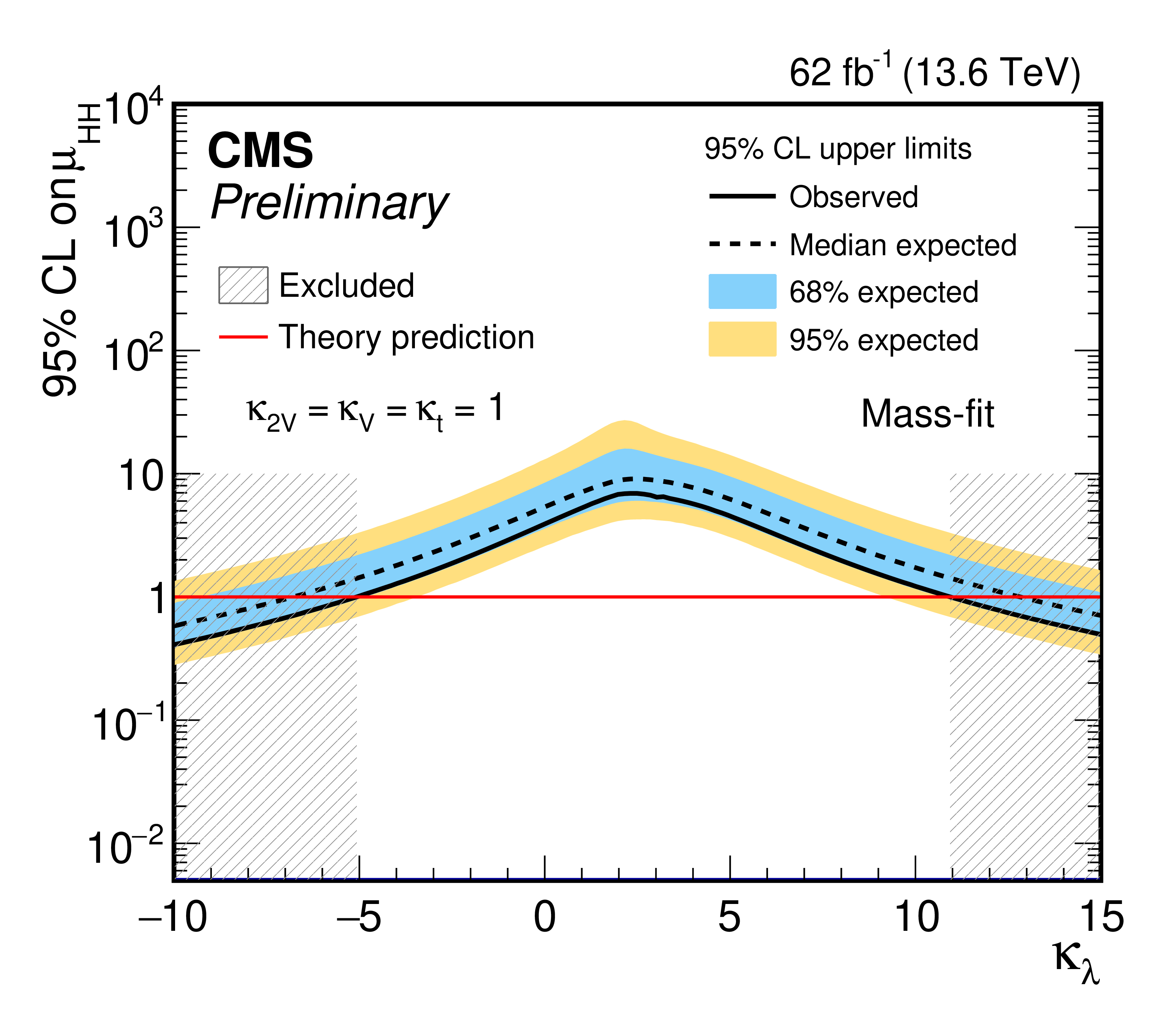
png pdf	Additional Figure 13-a: The observed (solid) and expected (dashed) 95% CL upper limits on the signal strength of the HH (left) and VBF (right) production (left) obtained as a function of $\mathrm{k}_{\lambda}$ (left) and $k_{VV}$ (right) for the merged mass-fit $ \mathrm{H}\mathrm{H} \to 4\mathrm{b} $ analysis. The cyan and blue bands represent, respectively, the 68 and 95% CL intervals around the expected limit. The horizontal red lines indicate the SM prediction. The observed (expected) allowed range, at 95% CL, for $\mathrm{k}_{\lambda}$ is {[-5.1,10.9]}~{([-6.8,12.8])}, while that for $k_{VV}$ is {[0.63,1.42]}~{([0.54,1.51])}. Results correspond to the first analysis approach described in the note.
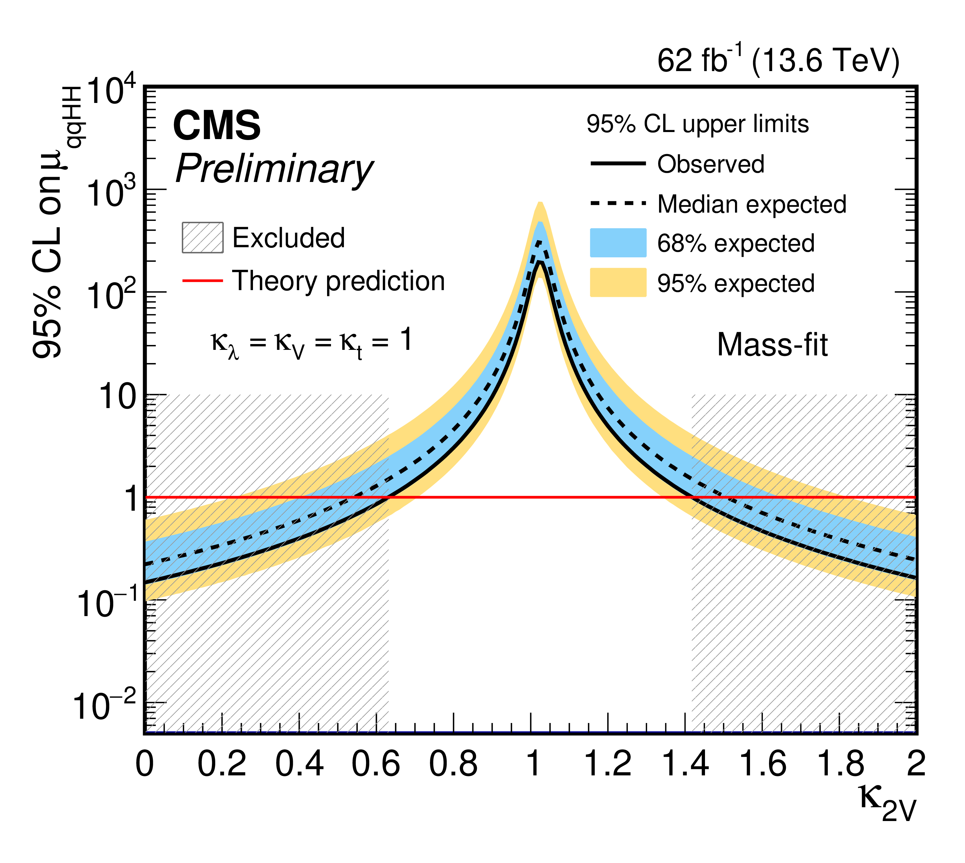
png pdf	Additional Figure 13-b: The observed (solid) and expected (dashed) 95% CL upper limits on the signal strength of the HH (left) and VBF (right) production (left) obtained as a function of $\mathrm{k}_{\lambda}$ (left) and $k_{VV}$ (right) for the merged mass-fit $ \mathrm{H}\mathrm{H} \to 4\mathrm{b} $ analysis. The cyan and blue bands represent, respectively, the 68 and 95% CL intervals around the expected limit. The horizontal red lines indicate the SM prediction. The observed (expected) allowed range, at 95% CL, for $\mathrm{k}_{\lambda}$ is {[-5.1,10.9]}~{([-6.8,12.8])}, while that for $k_{VV}$ is {[0.63,1.42]}~{([0.54,1.51])}. Results correspond to the first analysis approach described in the note.
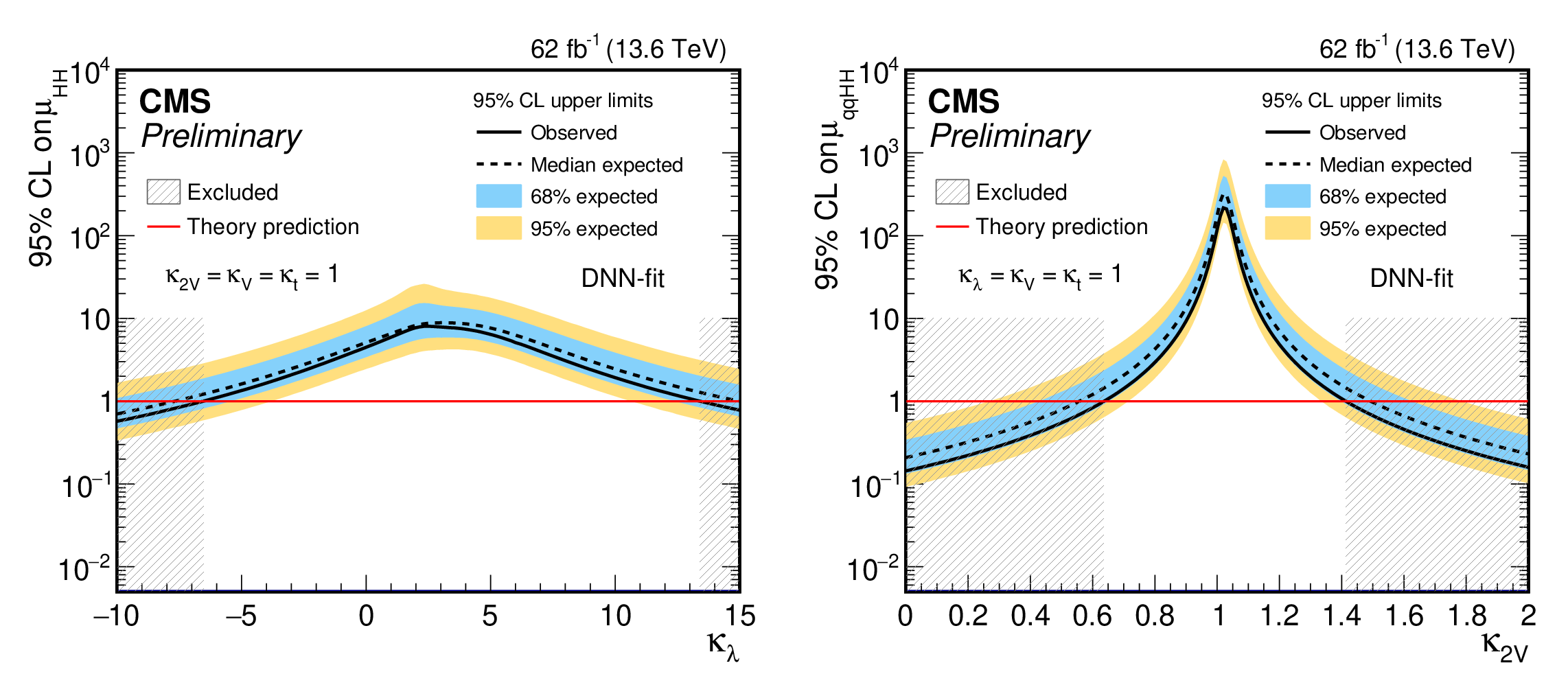
png pdf	Additional Figure 14: The observed (solid) and expected (dashed) 95% CL upper limits on the signal strength of the HH (left) and VBF (right) production (left) obtained as a function of $\mathrm{k}_{\lambda}$ (left) and $k_{VV}$ (right) for the merged DNN-fit $ \mathrm{H}\mathrm{H} \to 4\mathrm{b} $ analysis. The cyan and blue bands represent, respectively, the 68 and 95% CL intervals around the expected limit. The horizontal red lines indicate the SM prediction. The observed (expected) allowed range, at 95% CL, for $\mathrm{k}_{\lambda}$ is {[-6.5,13.4]}~{([-7.7,14.9])}, while that for $k_{VV}$is {[0.64,1.41]}~{([0.56,1.49])}. Results correspond to the first analysis approach described in the note.
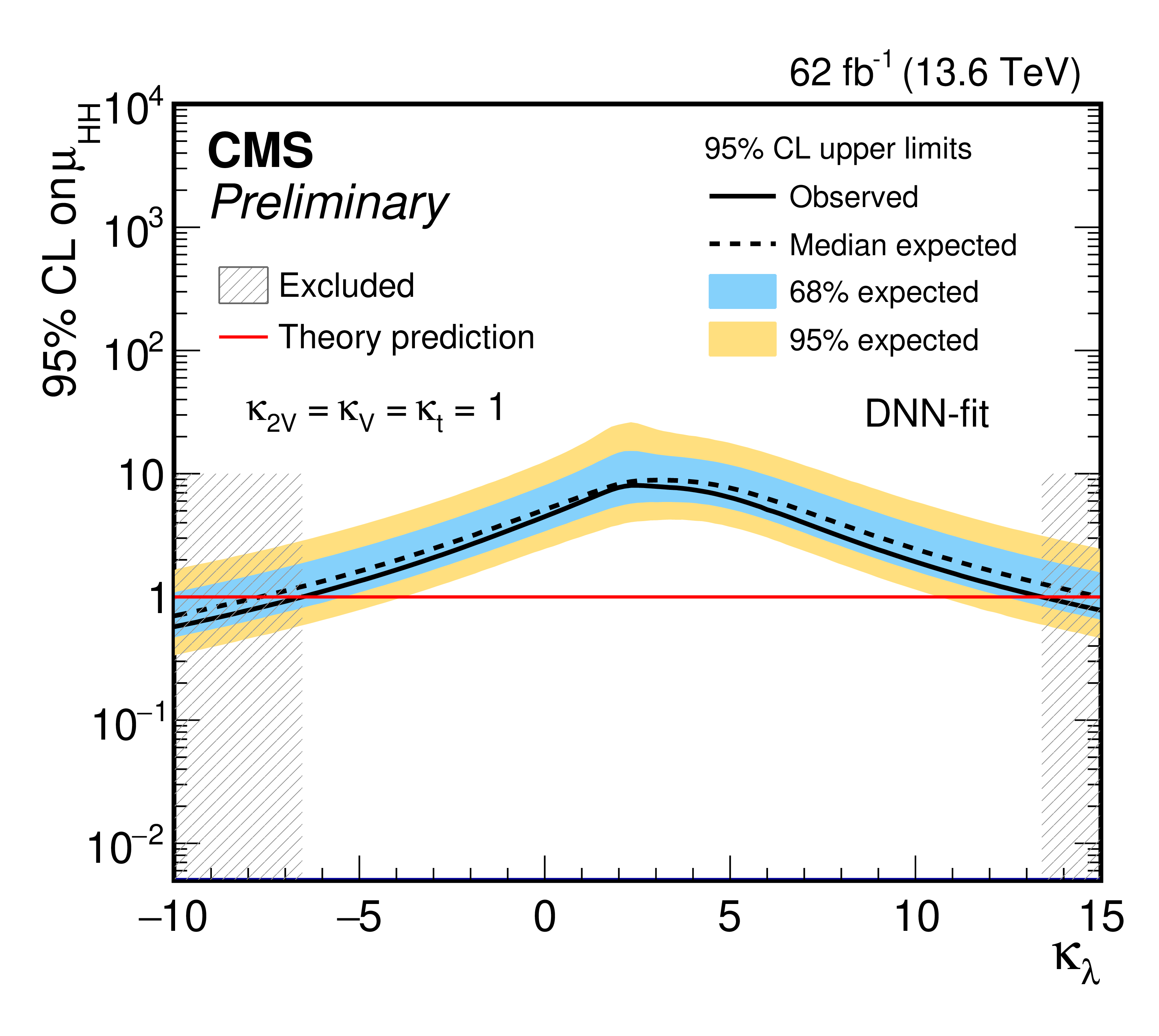
png pdf	Additional Figure 14-a: The observed (solid) and expected (dashed) 95% CL upper limits on the signal strength of the HH (left) and VBF (right) production (left) obtained as a function of $\mathrm{k}_{\lambda}$ (left) and $k_{VV}$ (right) for the merged DNN-fit $ \mathrm{H}\mathrm{H} \to 4\mathrm{b} $ analysis. The cyan and blue bands represent, respectively, the 68 and 95% CL intervals around the expected limit. The horizontal red lines indicate the SM prediction. The observed (expected) allowed range, at 95% CL, for $\mathrm{k}_{\lambda}$ is {[-6.5,13.4]}~{([-7.7,14.9])}, while that for $k_{VV}$is {[0.64,1.41]}~{([0.56,1.49])}. Results correspond to the first analysis approach described in the note.
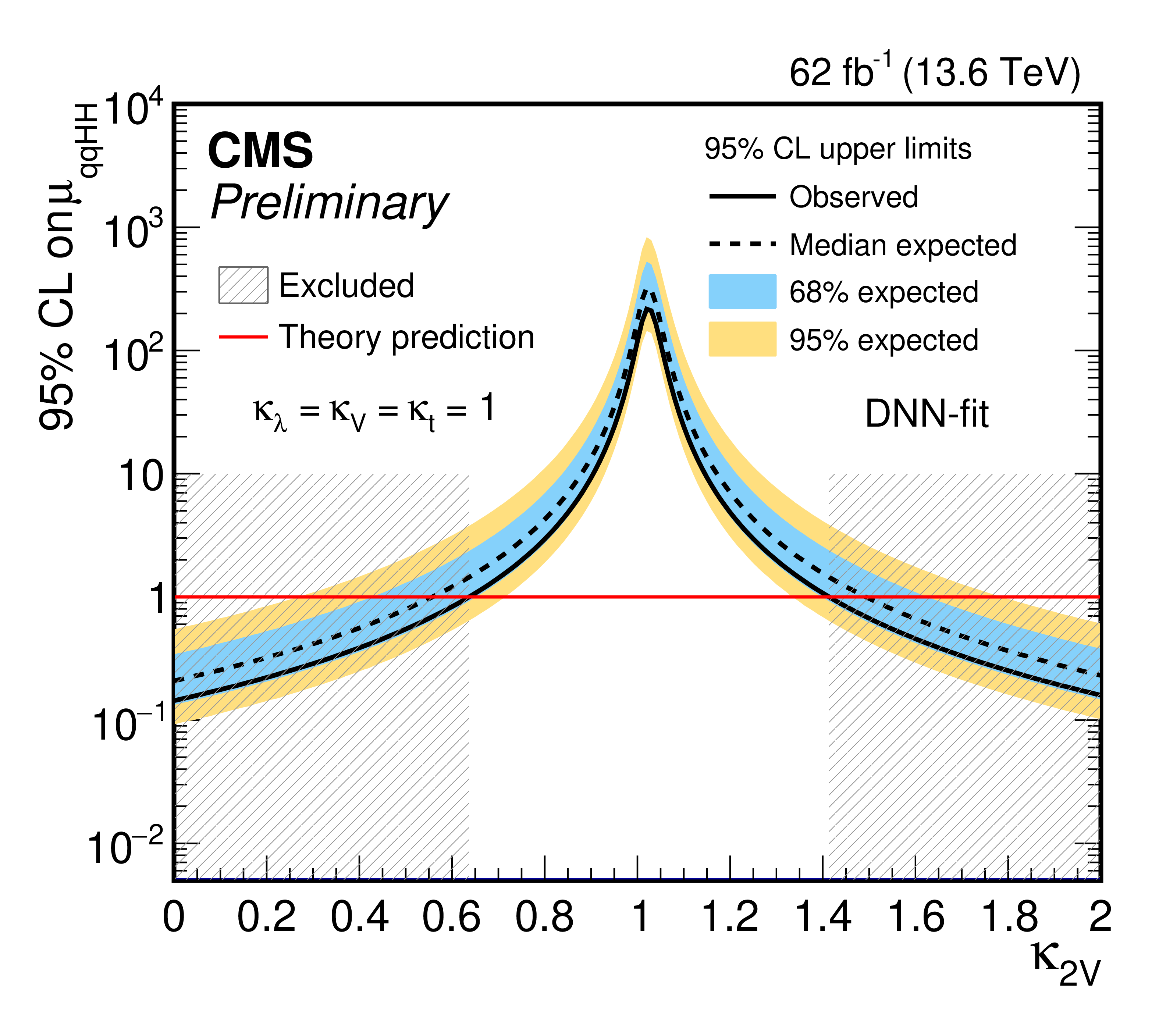
png pdf	Additional Figure 14-b: The observed (solid) and expected (dashed) 95% CL upper limits on the signal strength of the HH (left) and VBF (right) production (left) obtained as a function of $\mathrm{k}_{\lambda}$ (left) and $k_{VV}$ (right) for the merged DNN-fit $ \mathrm{H}\mathrm{H} \to 4\mathrm{b} $ analysis. The cyan and blue bands represent, respectively, the 68 and 95% CL intervals around the expected limit. The horizontal red lines indicate the SM prediction. The observed (expected) allowed range, at 95% CL, for $\mathrm{k}_{\lambda}$ is {[-6.5,13.4]}~{([-7.7,14.9])}, while that for $k_{VV}$is {[0.64,1.41]}~{([0.56,1.49])}. Results correspond to the first analysis approach described in the note.
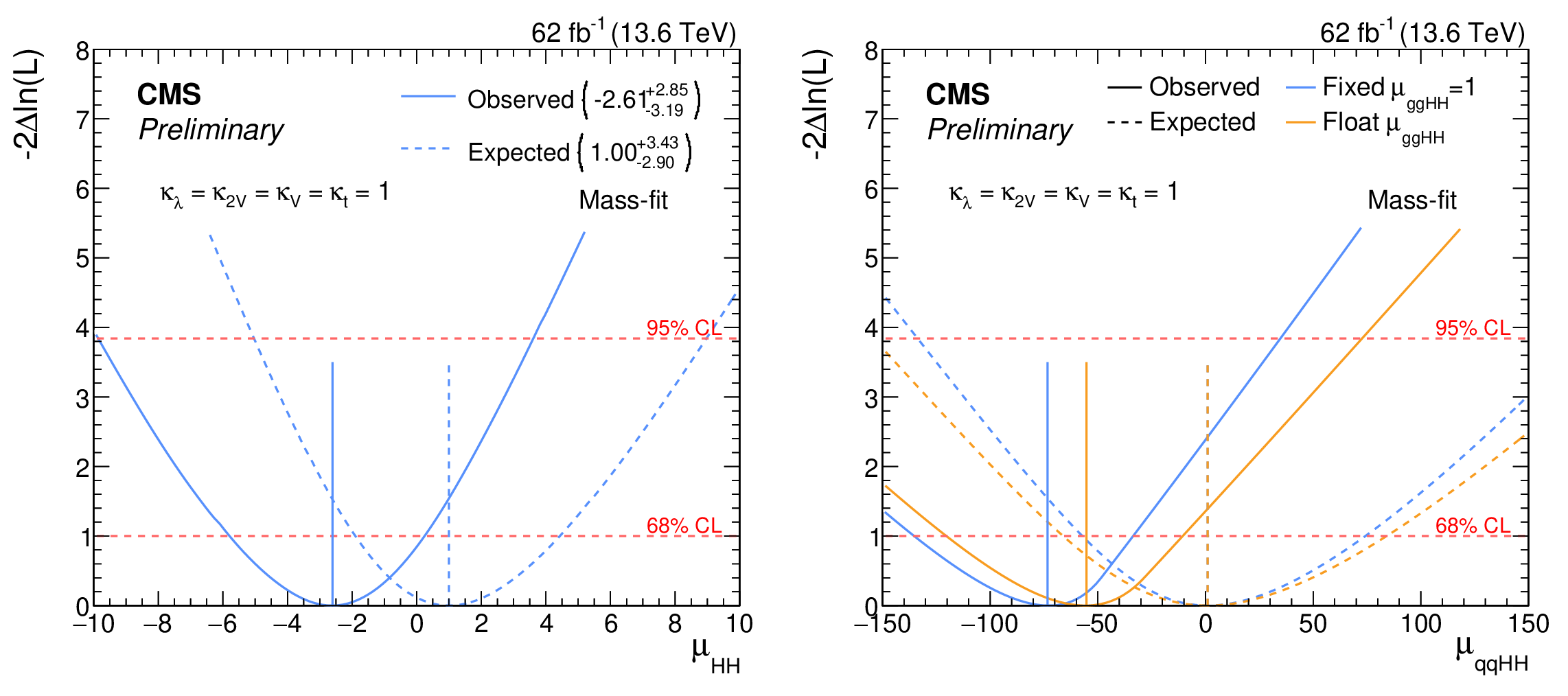
png pdf	Additional Figure 15: The observed (solid) and expected (dashed) profile likelihood ratios as a function of $\mu_{HH}$ (left) and $\mu_{qqHH}$ (right) from the merged mass-fit $ \mathrm{H}\mathrm{H} \to 4\mathrm{b} $ analysis. The $\mu_{qqHH}$ likelihood scan is shown with $\mu_{\mathrm{ggHH}}$ fixed to one (blue) and with $\mu_{\mathrm{ggHH}}$ profiled (orange). The expected curves are obtained from an Asimov dataset, defined by fixing the nuisances parameters to their maximum likelihood estimate obtained from data in which $\mu_{HH}=1$. The dashed red lines indicate the 68% and 95% CL ranges, expressed in units of $-2\Delta\ln(\mathcal{L})$. Best fit values for the signal strengths, along with their 68% CL intervals, are also reported. Results correspond to the first analysis approach described in the note.
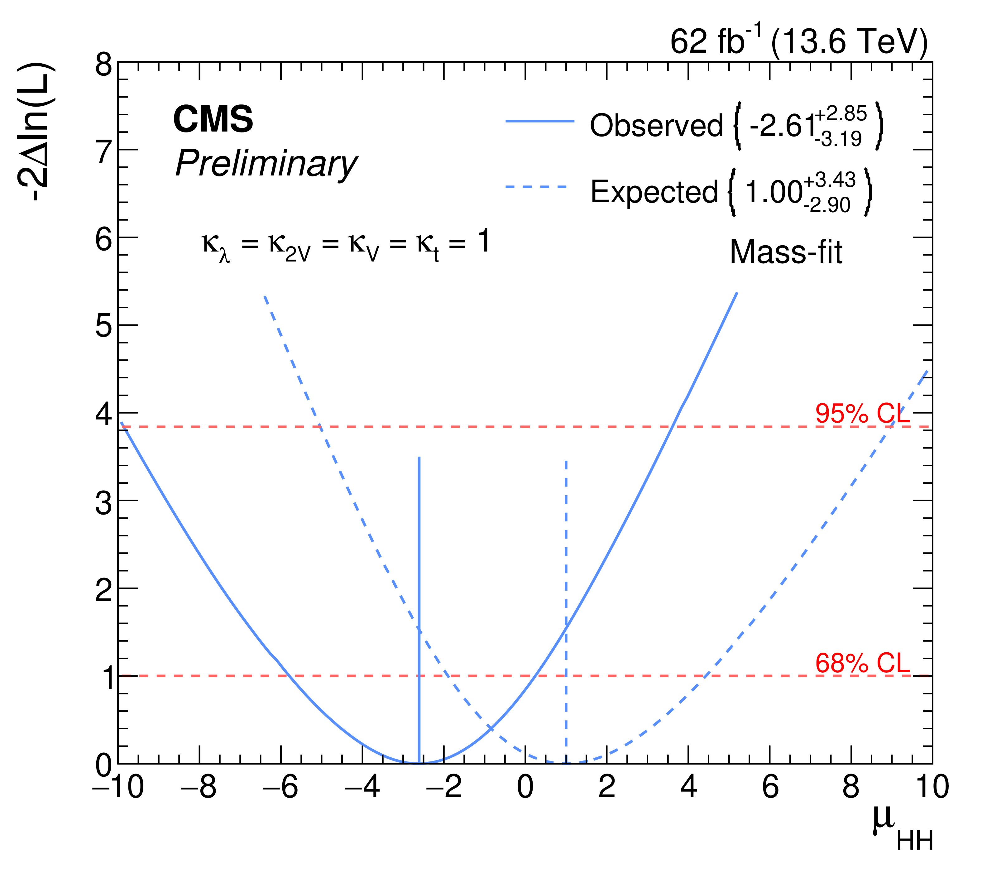
png pdf	Additional Figure 15-a: The observed (solid) and expected (dashed) profile likelihood ratios as a function of $\mu_{HH}$ (left) and $\mu_{qqHH}$ (right) from the merged mass-fit $ \mathrm{H}\mathrm{H} \to 4\mathrm{b} $ analysis. The $\mu_{qqHH}$ likelihood scan is shown with $\mu_{\mathrm{ggHH}}$ fixed to one (blue) and with $\mu_{\mathrm{ggHH}}$ profiled (orange). The expected curves are obtained from an Asimov dataset, defined by fixing the nuisances parameters to their maximum likelihood estimate obtained from data in which $\mu_{HH}=1$. The dashed red lines indicate the 68% and 95% CL ranges, expressed in units of $-2\Delta\ln(\mathcal{L})$. Best fit values for the signal strengths, along with their 68% CL intervals, are also reported. Results correspond to the first analysis approach described in the note.
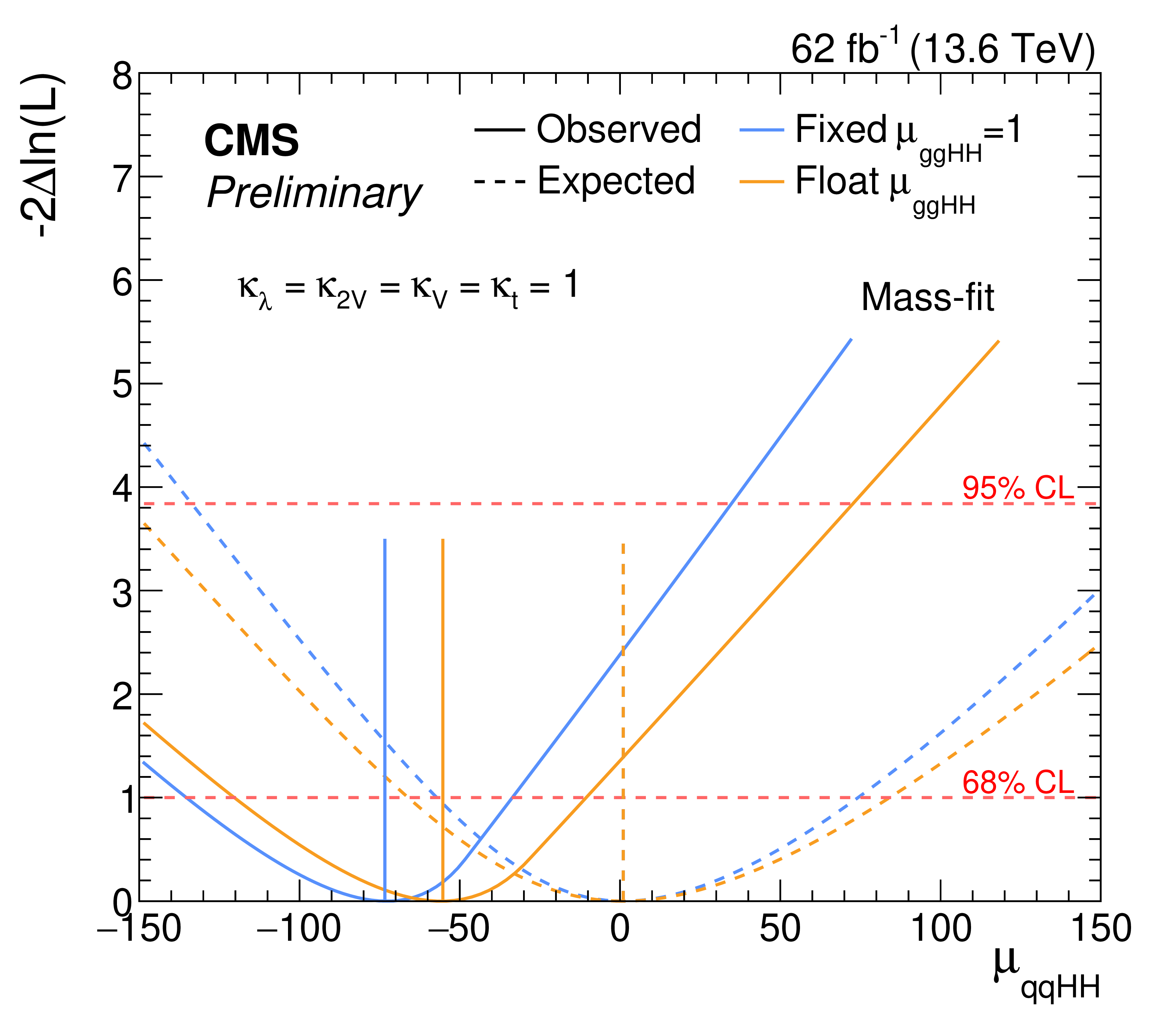
png pdf	Additional Figure 15-b: The observed (solid) and expected (dashed) profile likelihood ratios as a function of $\mu_{HH}$ (left) and $\mu_{qqHH}$ (right) from the merged mass-fit $ \mathrm{H}\mathrm{H} \to 4\mathrm{b} $ analysis. The $\mu_{qqHH}$ likelihood scan is shown with $\mu_{\mathrm{ggHH}}$ fixed to one (blue) and with $\mu_{\mathrm{ggHH}}$ profiled (orange). The expected curves are obtained from an Asimov dataset, defined by fixing the nuisances parameters to their maximum likelihood estimate obtained from data in which $\mu_{HH}=1$. The dashed red lines indicate the 68% and 95% CL ranges, expressed in units of $-2\Delta\ln(\mathcal{L})$. Best fit values for the signal strengths, along with their 68% CL intervals, are also reported. Results correspond to the first analysis approach described in the note.
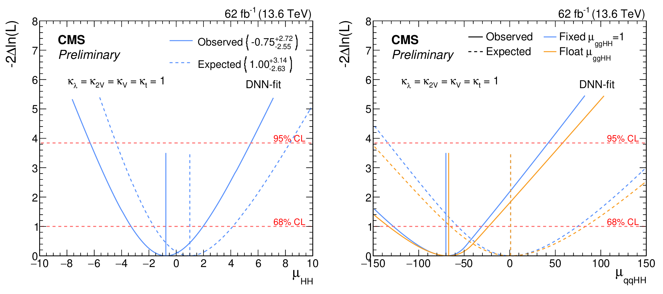
png pdf	Additional Figure 16: The observed (solid) and expected (dashed) profile likelihood ratios as a function of $\mu_{HH}$ (left) and $\mu_{qqHH}$ (right) from the merged DNN-fit $ \mathrm{H}\mathrm{H} \to 4\mathrm{b} $ analysis. The $\mu_{qqHH}$ likelihood scan is shown with $\mu_{\mathrm{ggHH}}$ fixed to one (blue) and with $\mu_{\mathrm{ggHH}}$ profiled (orange). The expected curves are obtained from an Asimov dataset, defined by fixing the nuisances parameters to their maximum likelihood estimate obtained from data in which $\mu_{HH}=1$. The dashed red lines indicate the 68% and 95% CL ranges, expressed in units of $-2\Delta\ln(\mathcal{L})$. Best fit values for the signal strengths, along with their 68% CL intervals, are also reported. Results correspond to the first analysis approach described in the note.
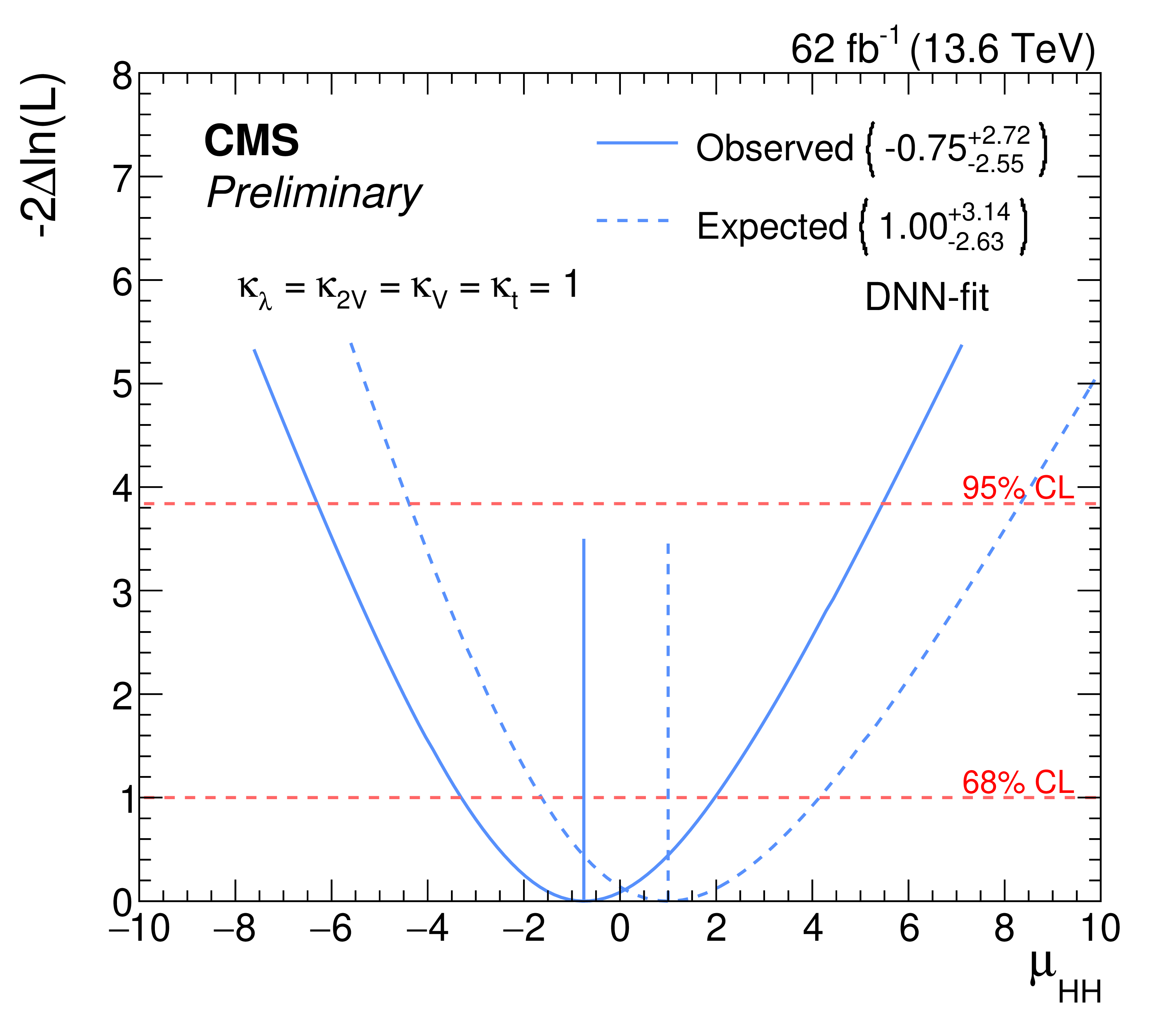
png pdf	Additional Figure 16-a: The observed (solid) and expected (dashed) profile likelihood ratios as a function of $\mu_{HH}$ (left) and $\mu_{qqHH}$ (right) from the merged DNN-fit $ \mathrm{H}\mathrm{H} \to 4\mathrm{b} $ analysis. The $\mu_{qqHH}$ likelihood scan is shown with $\mu_{\mathrm{ggHH}}$ fixed to one (blue) and with $\mu_{\mathrm{ggHH}}$ profiled (orange). The expected curves are obtained from an Asimov dataset, defined by fixing the nuisances parameters to their maximum likelihood estimate obtained from data in which $\mu_{HH}=1$. The dashed red lines indicate the 68% and 95% CL ranges, expressed in units of $-2\Delta\ln(\mathcal{L})$. Best fit values for the signal strengths, along with their 68% CL intervals, are also reported. Results correspond to the first analysis approach described in the note.
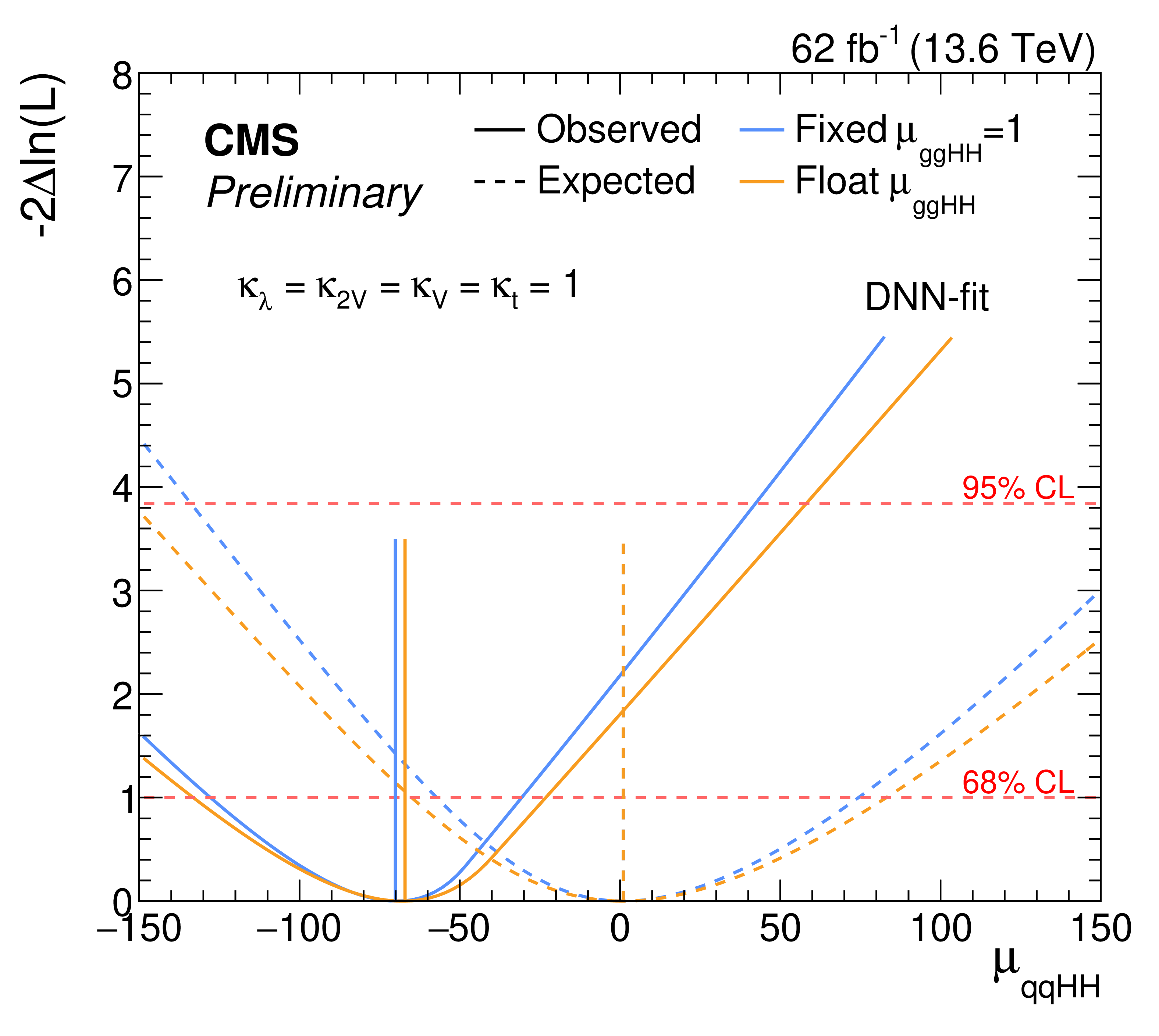
png pdf	Additional Figure 16-b: The observed (solid) and expected (dashed) profile likelihood ratios as a function of $\mu_{HH}$ (left) and $\mu_{qqHH}$ (right) from the merged DNN-fit $ \mathrm{H}\mathrm{H} \to 4\mathrm{b} $ analysis. The $\mu_{qqHH}$ likelihood scan is shown with $\mu_{\mathrm{ggHH}}$ fixed to one (blue) and with $\mu_{\mathrm{ggHH}}$ profiled (orange). The expected curves are obtained from an Asimov dataset, defined by fixing the nuisances parameters to their maximum likelihood estimate obtained from data in which $\mu_{HH}=1$. The dashed red lines indicate the 68% and 95% CL ranges, expressed in units of $-2\Delta\ln(\mathcal{L})$. Best fit values for the signal strengths, along with their 68% CL intervals, are also reported. Results correspond to the first analysis approach described in the note.
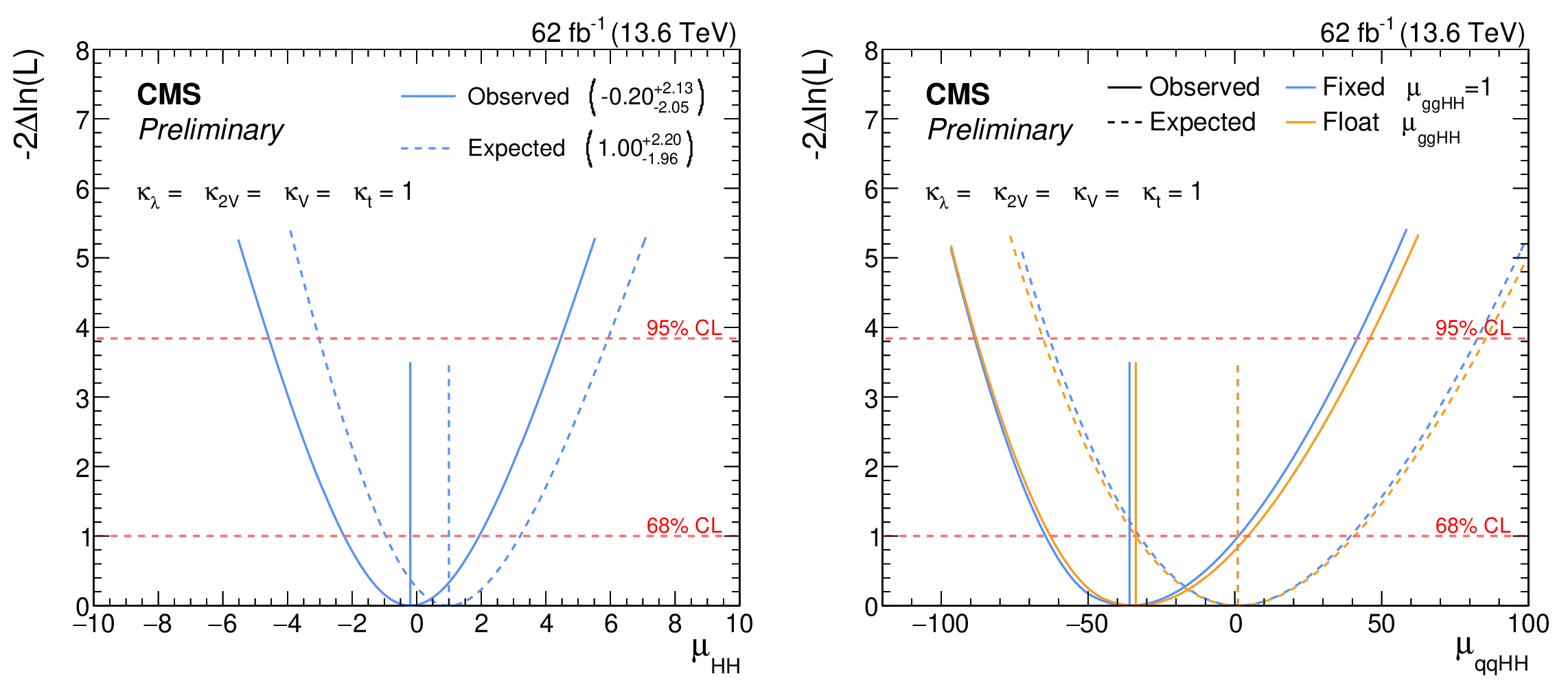
png pdf	Additional Figure 17: The observed (solid) and expected (dashed) profile likelihood ratios as a function of $\mu_{HH}$ (left) and $\mu_{qqHH}$ (right) for the combined fit of the resolved and merged $ \mathrm{H}\mathrm{H} \to 4\mathrm{b} $ analyses. The $\mu_{qqHH}$ likelihood scan is shown with $\mu_{\mathrm{ggHH}}$ fixed to one (blue) and with $\mu_{\mathrm{ggHH}}$ profiled (orange). The expected curves are obtained from an Asimov dataset, defined by fixing the nuisances parameters to their maximum likelihood estimate obtained from data in which $\mu_{HH}=1$. The dashed red lines indicate the 68% and 95% CL ranges, expressed in units of $-2\Delta\ln(\mathcal{L})$. Best fit values for the signal strengths, along with their 68% CL intervals, are also reported. Results correspond to the first analysis approach described in the note.
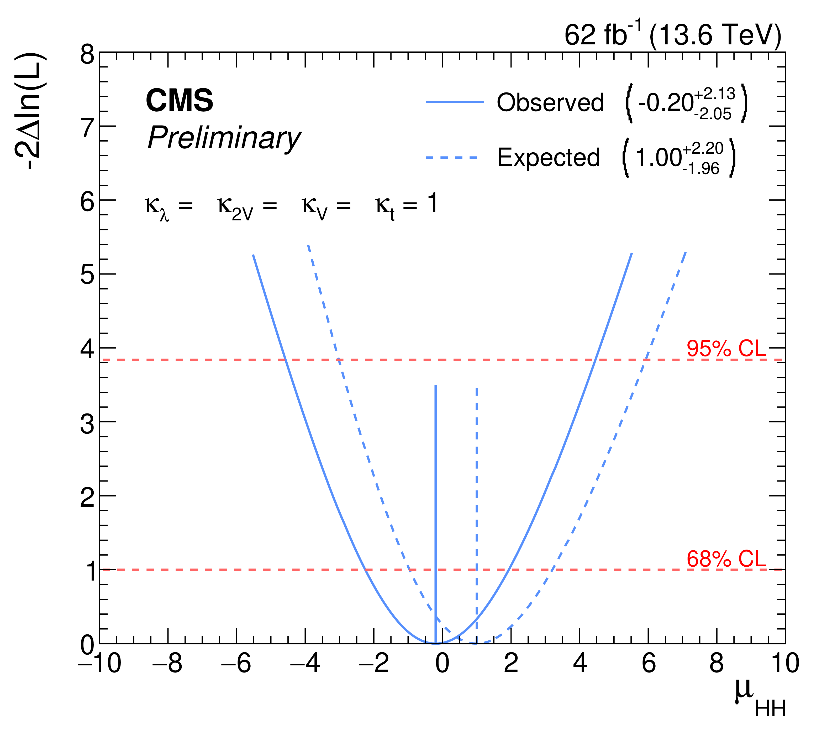
png pdf	Additional Figure 17-a: The observed (solid) and expected (dashed) profile likelihood ratios as a function of $\mu_{HH}$ (left) and $\mu_{qqHH}$ (right) for the combined fit of the resolved and merged $ \mathrm{H}\mathrm{H} \to 4\mathrm{b} $ analyses. The $\mu_{qqHH}$ likelihood scan is shown with $\mu_{\mathrm{ggHH}}$ fixed to one (blue) and with $\mu_{\mathrm{ggHH}}$ profiled (orange). The expected curves are obtained from an Asimov dataset, defined by fixing the nuisances parameters to their maximum likelihood estimate obtained from data in which $\mu_{HH}=1$. The dashed red lines indicate the 68% and 95% CL ranges, expressed in units of $-2\Delta\ln(\mathcal{L})$. Best fit values for the signal strengths, along with their 68% CL intervals, are also reported. Results correspond to the first analysis approach described in the note.
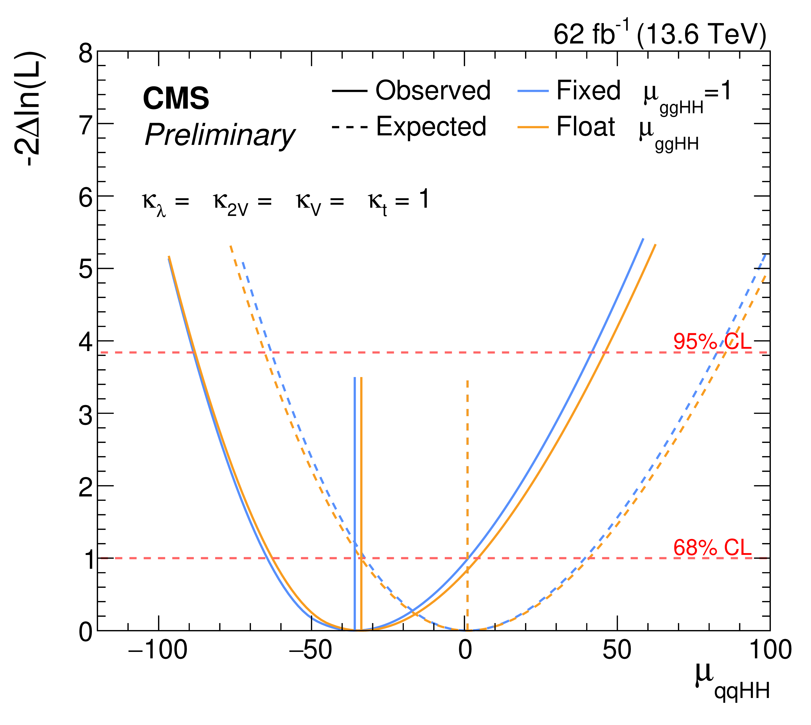
png pdf	Additional Figure 17-b: The observed (solid) and expected (dashed) profile likelihood ratios as a function of $\mu_{HH}$ (left) and $\mu_{qqHH}$ (right) for the combined fit of the resolved and merged $ \mathrm{H}\mathrm{H} \to 4\mathrm{b} $ analyses. The $\mu_{qqHH}$ likelihood scan is shown with $\mu_{\mathrm{ggHH}}$ fixed to one (blue) and with $\mu_{\mathrm{ggHH}}$ profiled (orange). The expected curves are obtained from an Asimov dataset, defined by fixing the nuisances parameters to their maximum likelihood estimate obtained from data in which $\mu_{HH}=1$. The dashed red lines indicate the 68% and 95% CL ranges, expressed in units of $-2\Delta\ln(\mathcal{L})$. Best fit values for the signal strengths, along with their 68% CL intervals, are also reported. Results correspond to the first analysis approach described in the note.
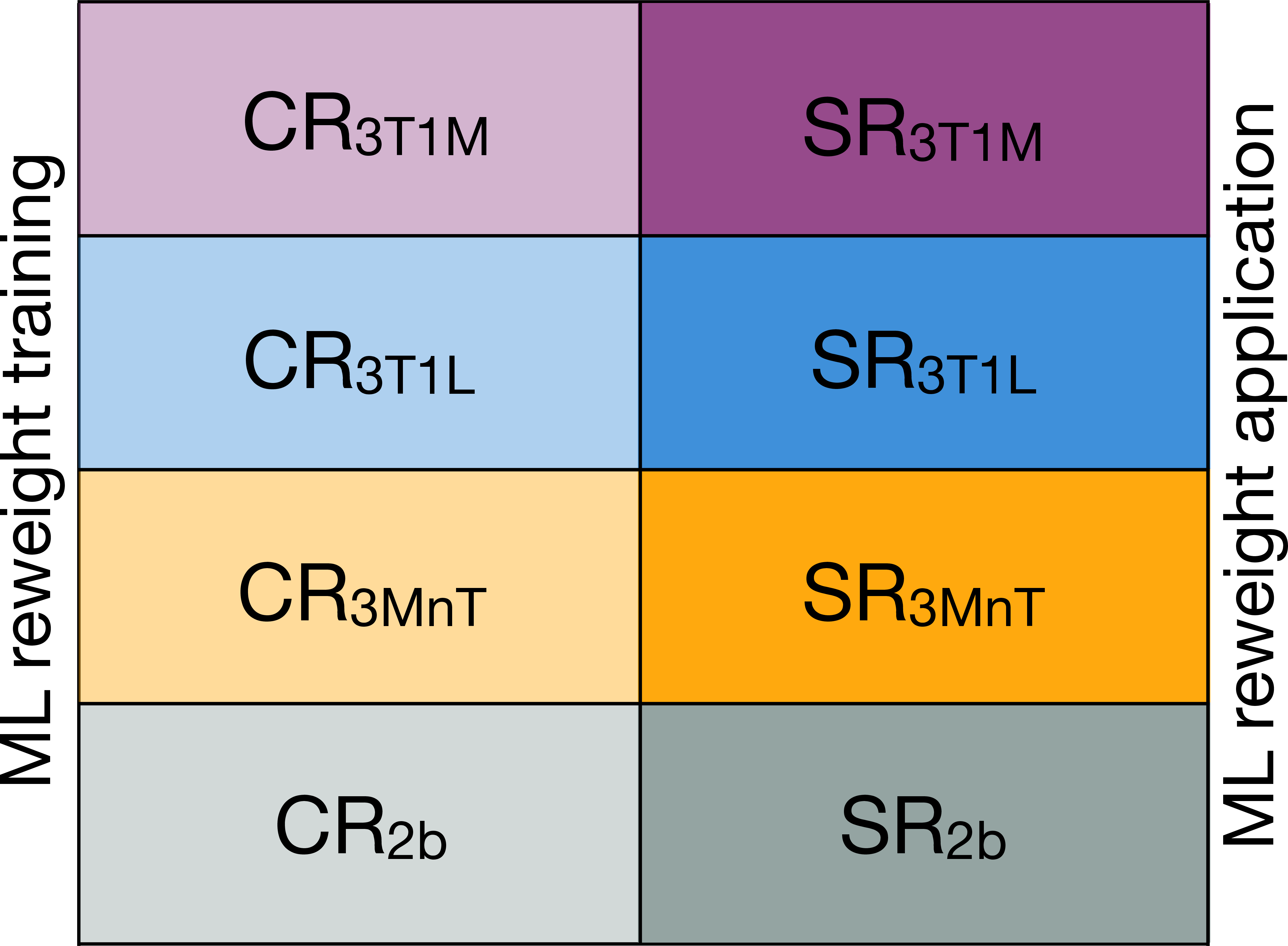
png pdf	Additional Figure 18: Schematic diagram of the signal and control regions used in the second analysis approach of the resolved topology described in the note.
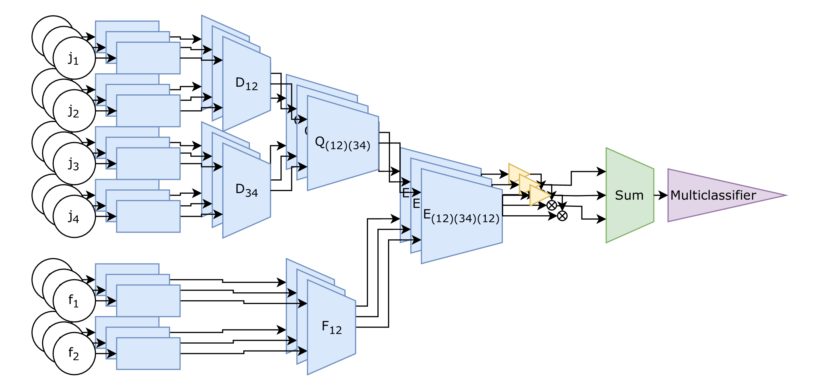
png pdf	Additional Figure 19: A schematic of the FeynNet classifier architecture used in the second analysis approach of the resolved topology described in the note. For each unique assignment of final state jets, FeynNet builds a learned embedding which is used in linear combination with the rest to derive the final output classifier score.
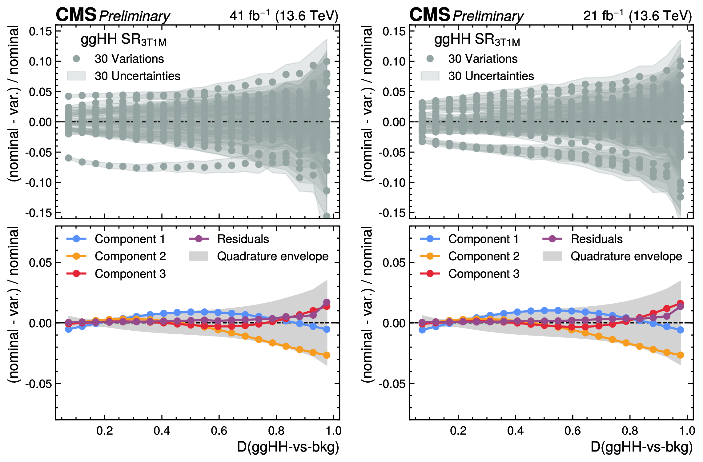
png pdf	Additional Figure 20: The upper panel shows the ratio of the difference between the nominal background model and each of the 30 background model variations over the nominal background model in the $\text{SR}_{\text{3T1M}}$, as derived by reweighting the observed data in the $\text{SR}_{\text{3T1L}}$b, for the pre-ParkingHH (left) and post-ParkingHH (right) data sets as a function of the $D(\text{ggHH-vs-bkg})$ score. The lower panel shows the first three Fourier components (blue, orange, red), and the residual (purple) systematic uncertainties. The quadrature sum of the four background systematic uncertainties are illustrated with the gray envelope. Distributions correspond to the second analysis approach of the resolved topology described in the note.
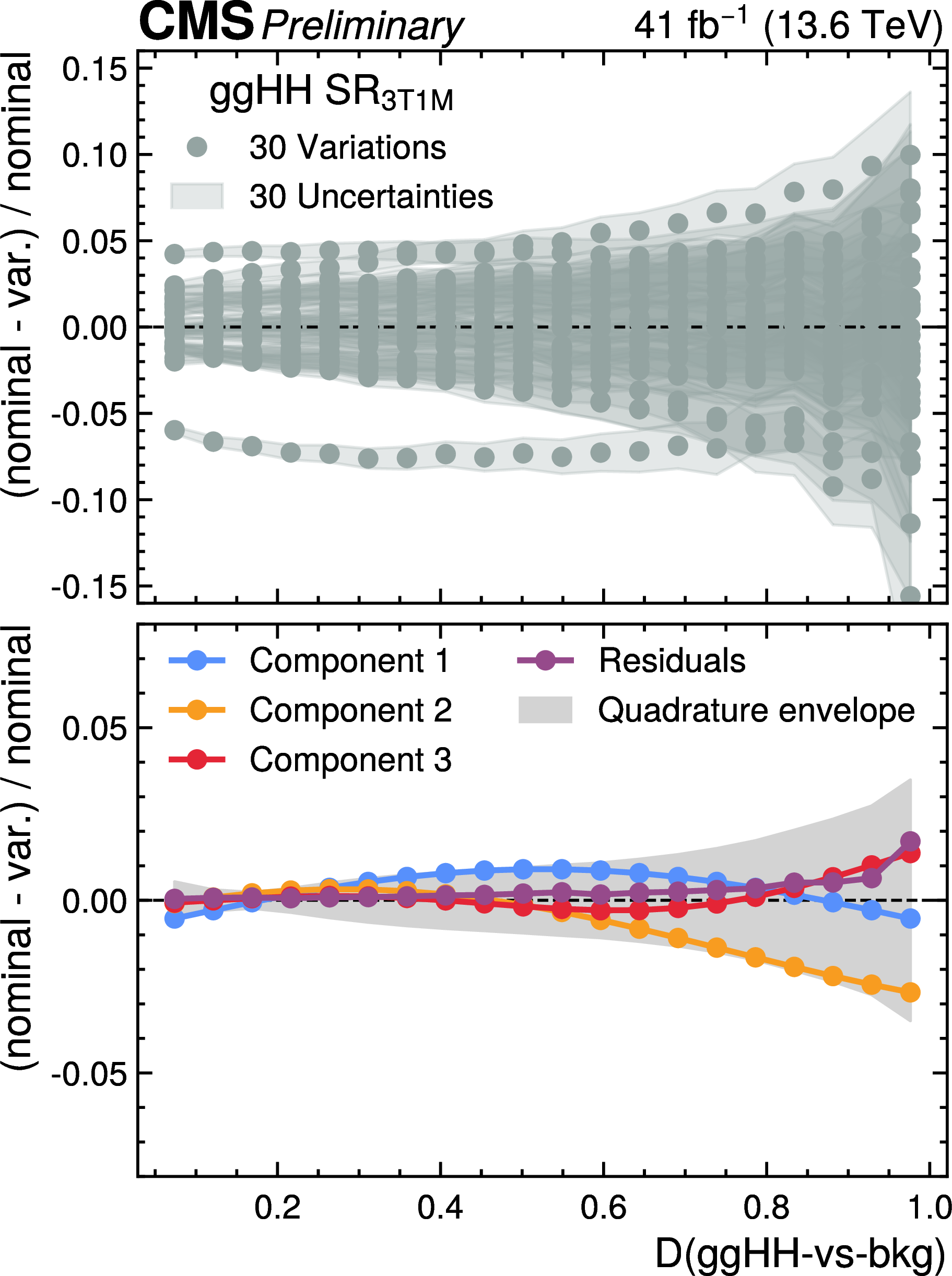
png pdf	Additional Figure 20-a: The upper panel shows the ratio of the difference between the nominal background model and each of the 30 background model variations over the nominal background model in the $\text{SR}_{\text{3T1M}}$, as derived by reweighting the observed data in the $\text{SR}_{\text{3T1L}}$b, for the pre-ParkingHH (left) and post-ParkingHH (right) data sets as a function of the $D(\text{ggHH-vs-bkg})$ score. The lower panel shows the first three Fourier components (blue, orange, red), and the residual (purple) systematic uncertainties. The quadrature sum of the four background systematic uncertainties are illustrated with the gray envelope. Distributions correspond to the second analysis approach of the resolved topology described in the note.
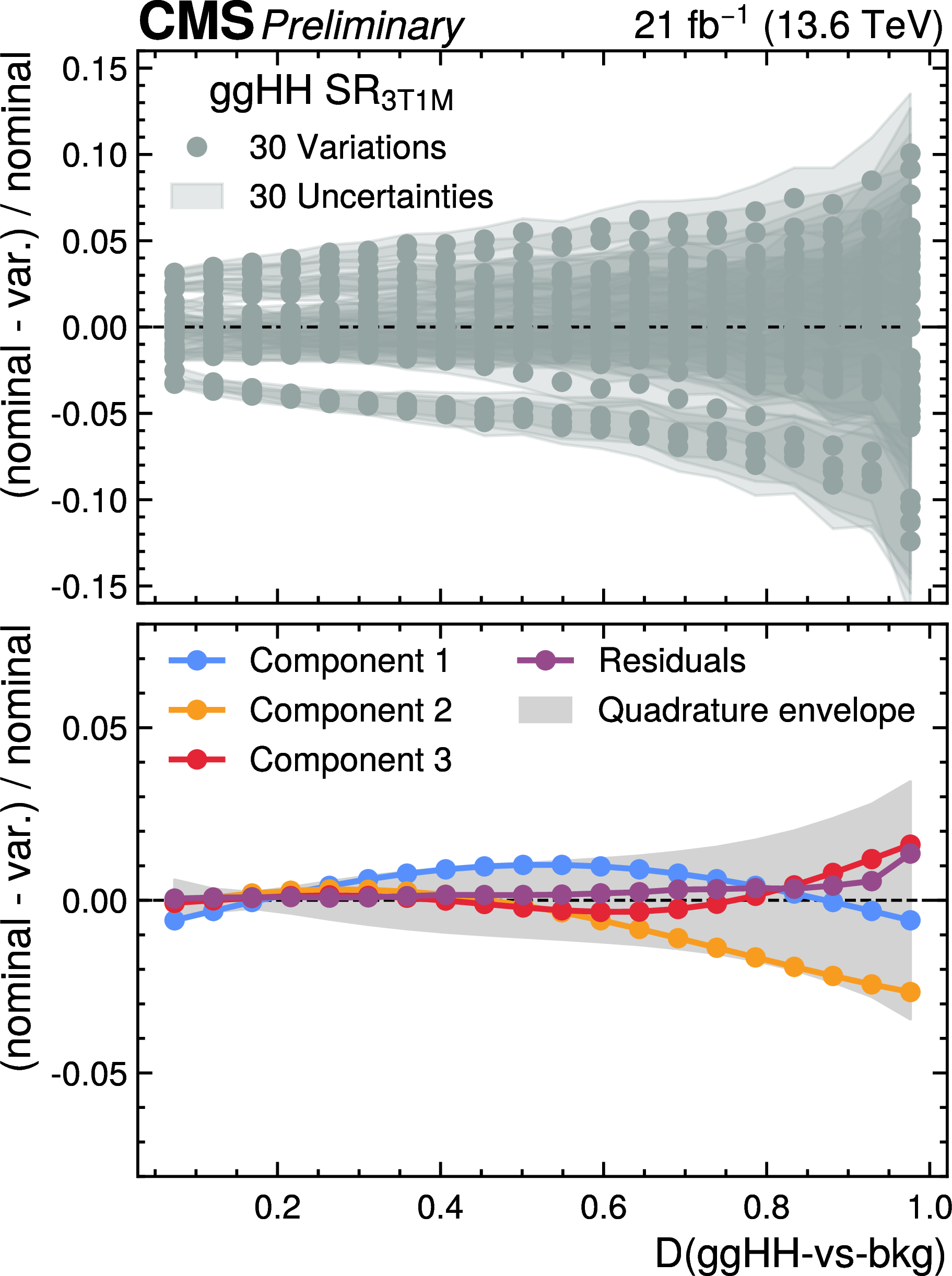
png pdf	Additional Figure 20-b: The upper panel shows the ratio of the difference between the nominal background model and each of the 30 background model variations over the nominal background model in the $\text{SR}_{\text{3T1M}}$, as derived by reweighting the observed data in the $\text{SR}_{\text{3T1L}}$b, for the pre-ParkingHH (left) and post-ParkingHH (right) data sets as a function of the $D(\text{ggHH-vs-bkg})$ score. The lower panel shows the first three Fourier components (blue, orange, red), and the residual (purple) systematic uncertainties. The quadrature sum of the four background systematic uncertainties are illustrated with the gray envelope. Distributions correspond to the second analysis approach of the resolved topology described in the note.
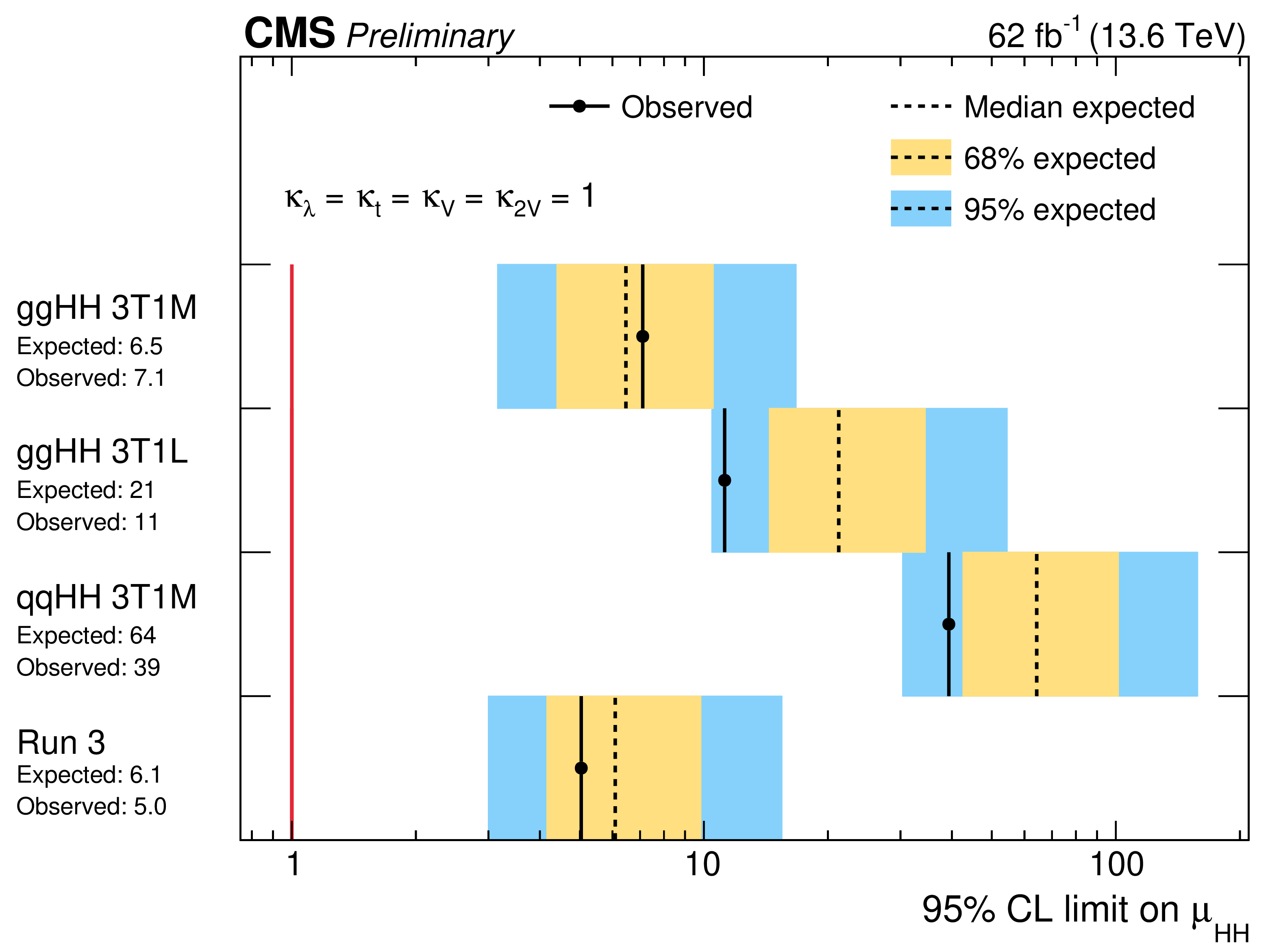
png pdf	Additional Figure 21: The observed (solid) and expected (dashed) 95% CL upper limits on the signal strength of $ \mathrm{H}\mathrm{H} $ production from the ggHH $\text{SR}_{\text{3T1M}}$, ggHH $\text{SR}_{\text{3T1L}}$, qqHH $\text{SR}_{\text{3T1M}}$, and their combination, for the resolved analysis. The yellow and cyan bands represent, respectively, the 68 and 95% CL intervals around the expected limit. Results correspond to the second analysis approach of the resolved topology described in the note.
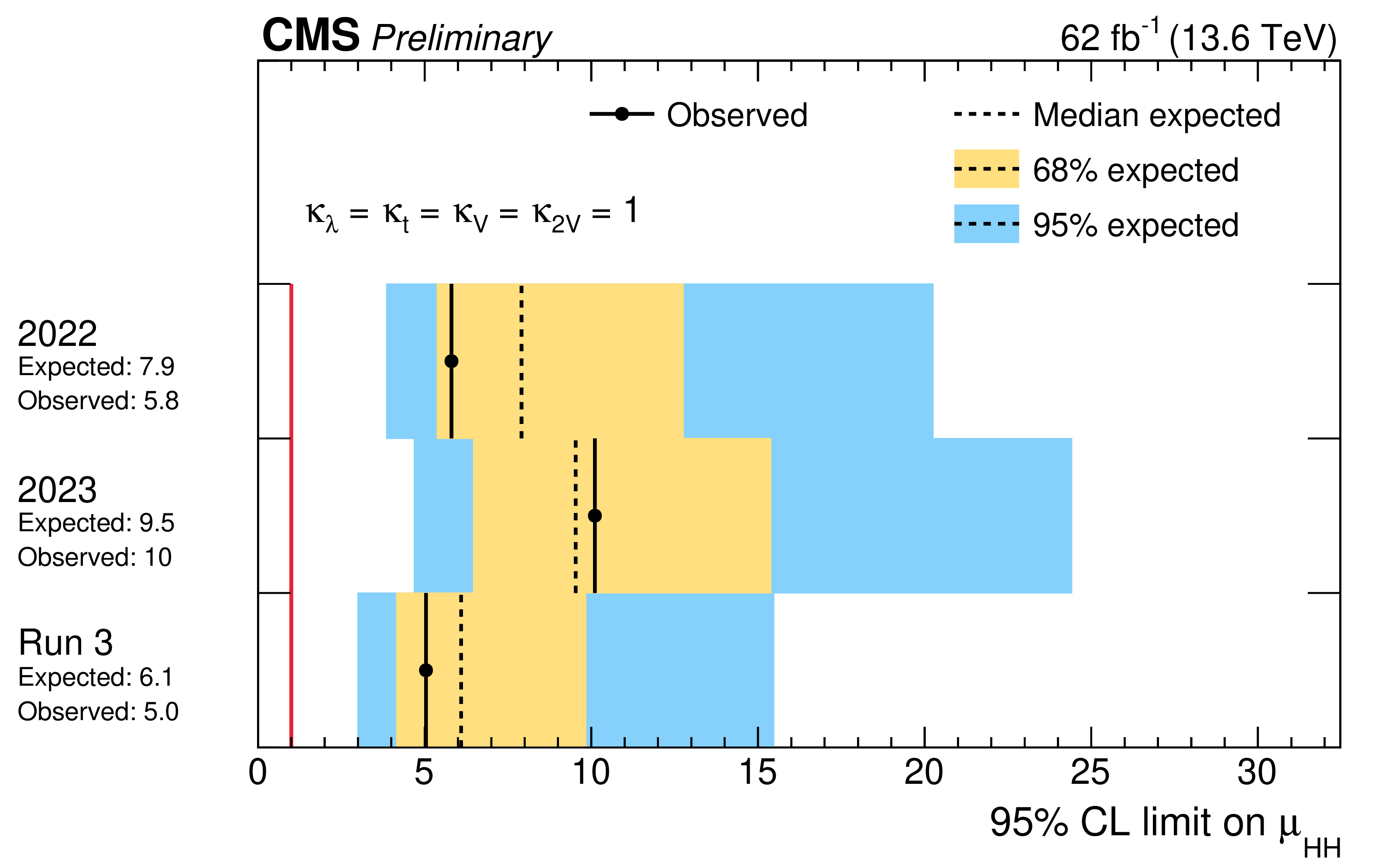
png pdf	Additional Figure 22: The observed (solid) and expected (dashed) 95% CL upper limits on the signal strength of $ \mathrm{H}\mathrm{H} $ production from the combination of the ggHH $\text{SR}_{\text{3T1M}}$, ggHH $\text{SR}_{\text{3T1L}}$, and qqHH $\text{SR}_{\text{3T1M}}$ in 2022 and 2023, for the resolved analysis. The yellow and cyan bands represent, respectively, the 68% and 95% CL intervals around the expected limit. Results correspond to the second analysis approach of the resolved topology described in the note.
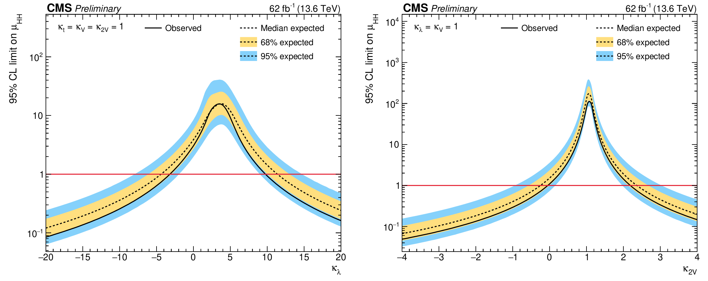
png pdf	Additional Figure 23: The observed (solid) and expected (dashed) 95% CL upper limits on the signal strength of $ \mathrm{H}\mathrm{H} $ production obtained as a function of $\mathrm{k}_{\lambda}$ (left) and \kappaVV (right) for the resolved analysis. The yellow and cyan bands represent, respectively, the 68 and 95% CL intervals around the expected limit. The horizontal red lines indicate the SM prediction. The observed (expected) allowed range, at 95% CL, for $\mathrm{k}_{\lambda}$ is [-3.19, 10.0] ([-4.38, 11.6]), and for $\mathrm{k}_{VV}$ is [-0.05, 2.24] ([-0.25, 2.4]). Results correspond to the second analysis approach of the resolved topology described in the note.
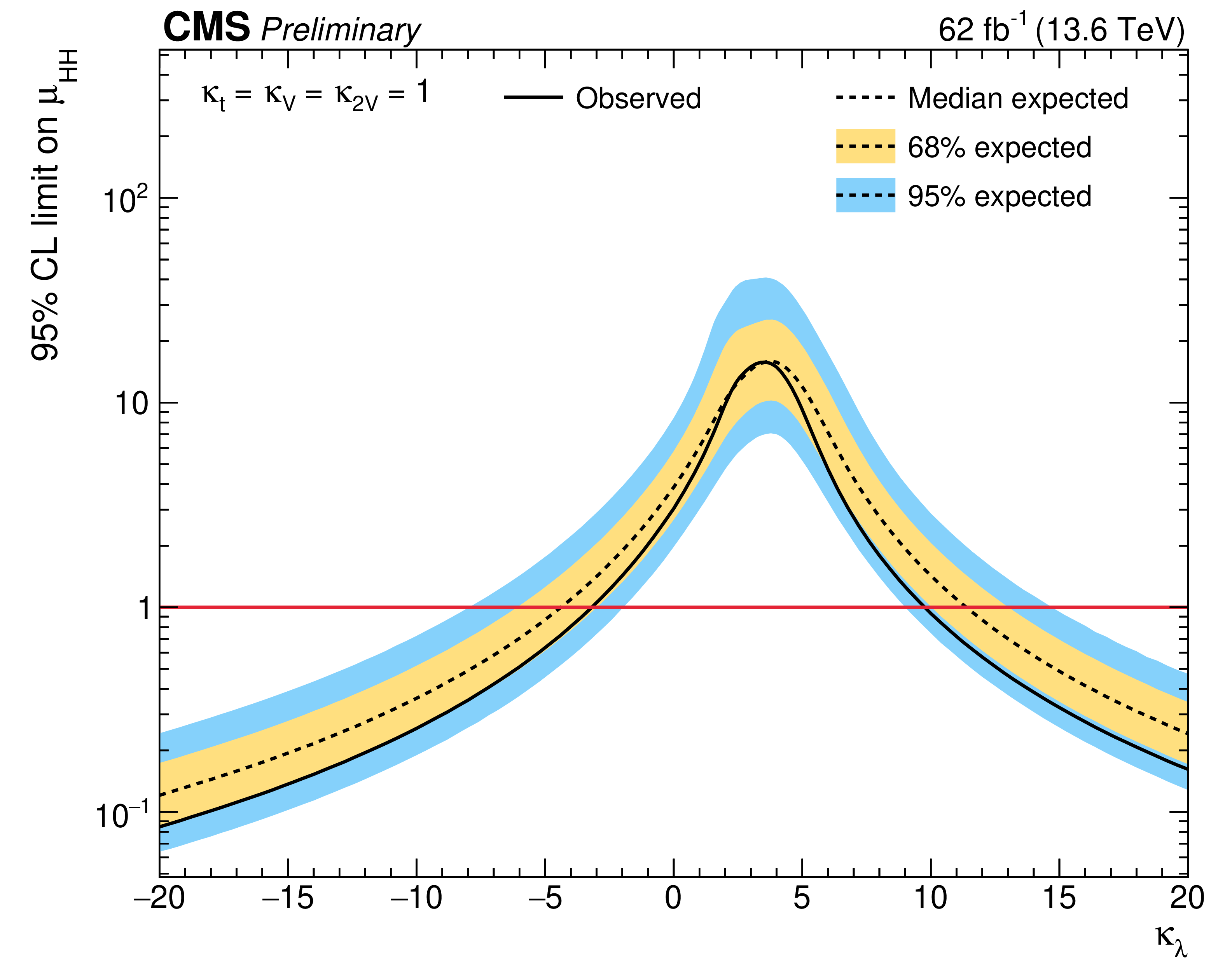
png pdf	Additional Figure 23-a: The observed (solid) and expected (dashed) 95% CL upper limits on the signal strength of $ \mathrm{H}\mathrm{H} $ production obtained as a function of $\mathrm{k}_{\lambda}$ (left) and \kappaVV (right) for the resolved analysis. The yellow and cyan bands represent, respectively, the 68 and 95% CL intervals around the expected limit. The horizontal red lines indicate the SM prediction. The observed (expected) allowed range, at 95% CL, for $\mathrm{k}_{\lambda}$ is [-3.19, 10.0] ([-4.38, 11.6]), and for $\mathrm{k}_{VV}$ is [-0.05, 2.24] ([-0.25, 2.4]). Results correspond to the second analysis approach of the resolved topology described in the note.
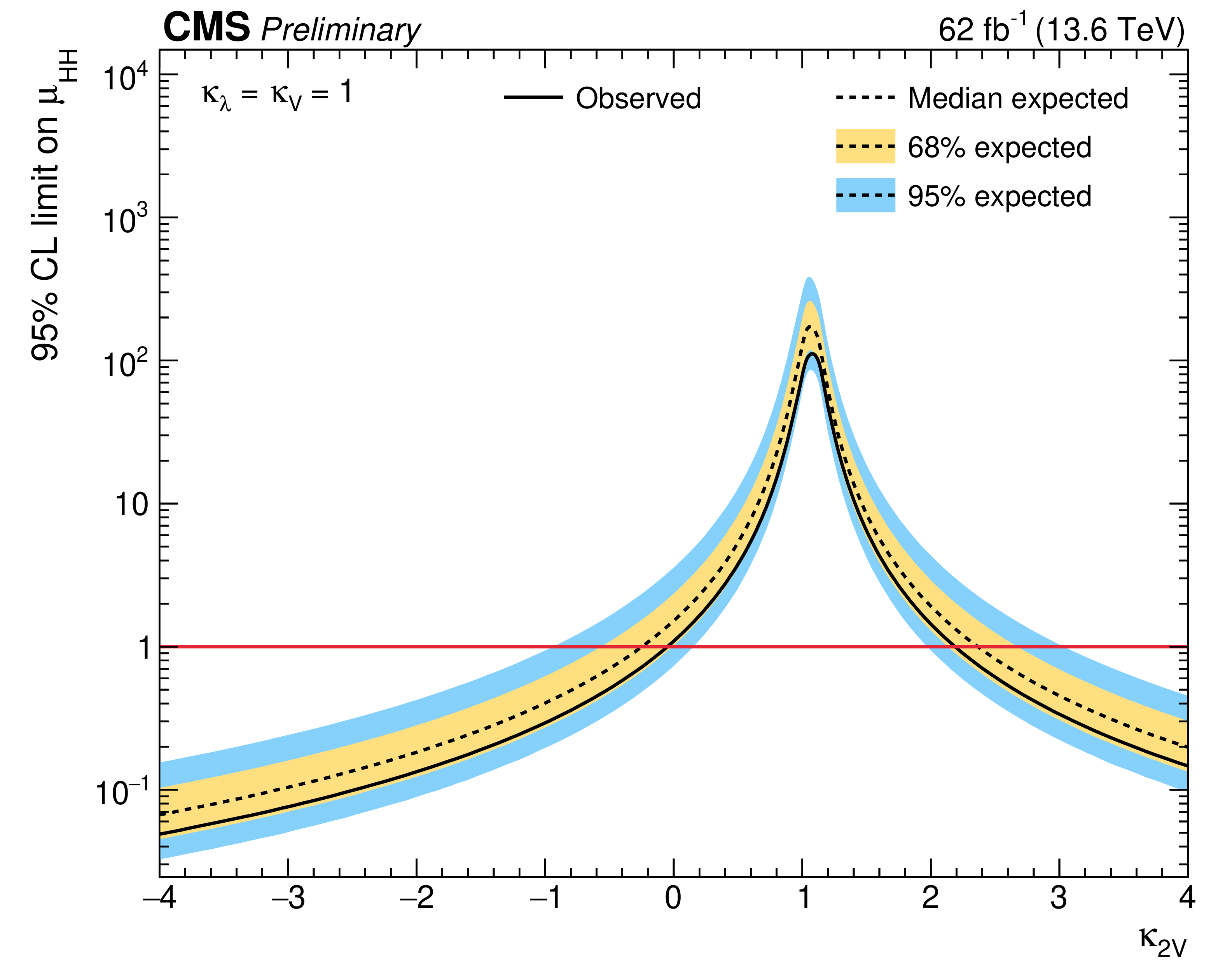
png pdf	Additional Figure 23-b: The observed (solid) and expected (dashed) 95% CL upper limits on the signal strength of $ \mathrm{H}\mathrm{H} $ production obtained as a function of $\mathrm{k}_{\lambda}$ (left) and \kappaVV (right) for the resolved analysis. The yellow and cyan bands represent, respectively, the 68 and 95% CL intervals around the expected limit. The horizontal red lines indicate the SM prediction. The observed (expected) allowed range, at 95% CL, for $\mathrm{k}_{\lambda}$ is [-3.19, 10.0] ([-4.38, 11.6]), and for $\mathrm{k}_{VV}$ is [-0.05, 2.24] ([-0.25, 2.4]). Results correspond to the second analysis approach of the resolved topology described in the note.
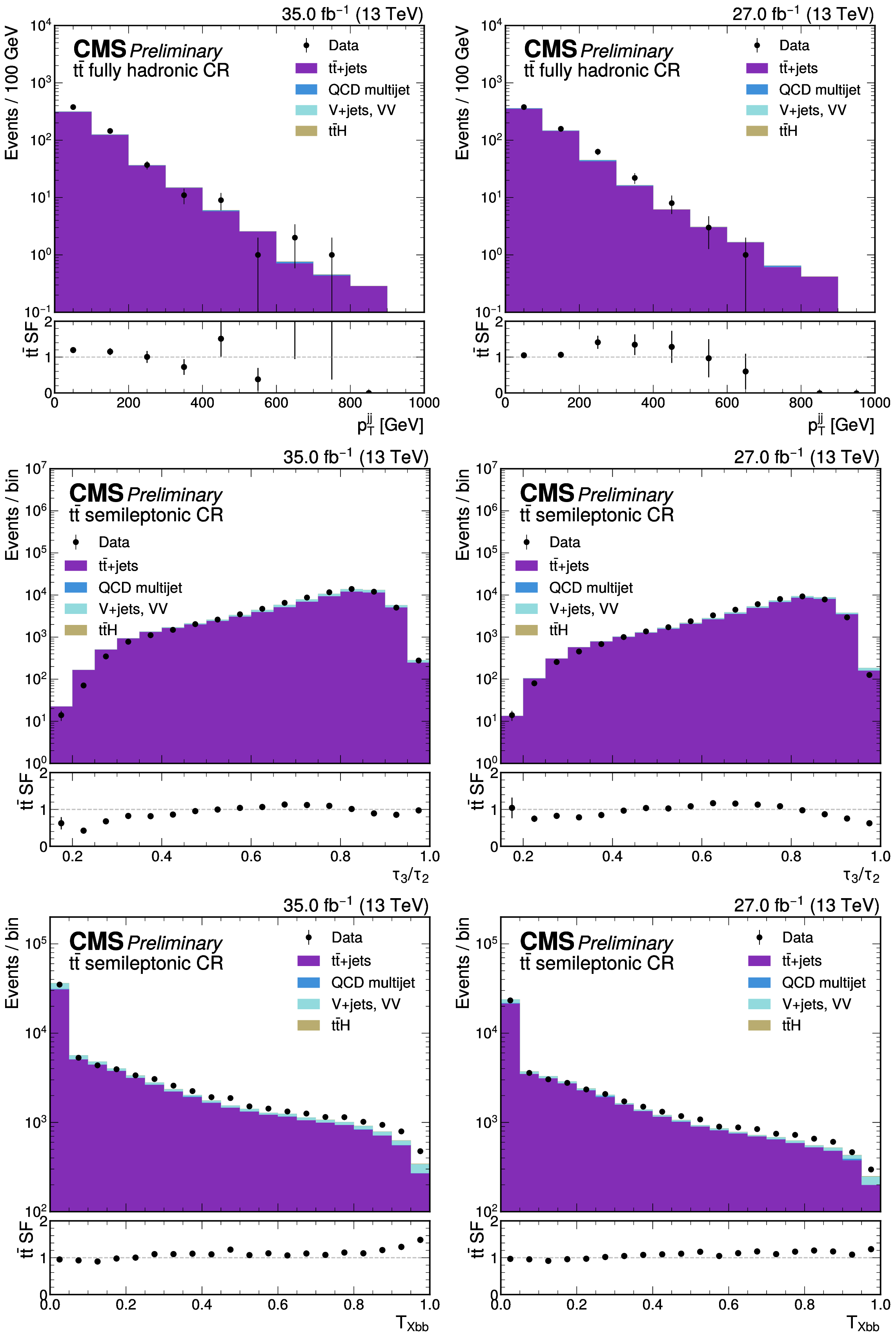
png pdf	Additional Figure 24: The derivation of the $\mathrm{t}\mathrm{\bar{t}}$ scale factors as a function of $P_t^\mathrm{jj}$ (upper) in the $\mathrm{t}\mathrm{\bar{t}}$ fully hadronic CR, and $\tau_3/\tau_2$ (middle) and \TXbb (lower) in the $\mathrm{t}\mathrm{\bar{t}}$ semileptonic CR. The scale factors are derived separately in 2022 (left) and 2023 (right) data. Distributions correspond to the second analysis approach of the merged topology described in the note.
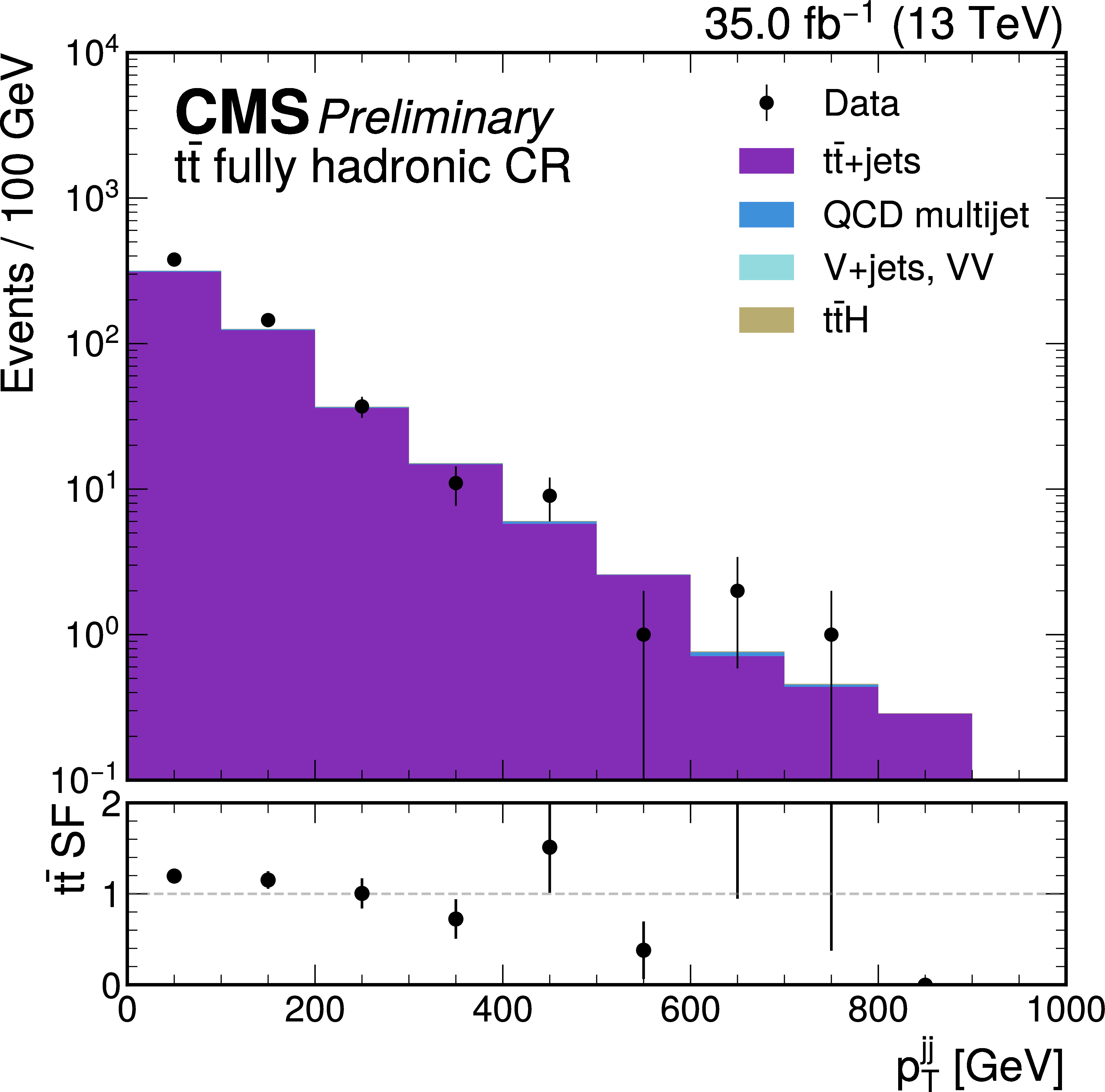
png pdf	Additional Figure 24-a: The derivation of the $\mathrm{t}\mathrm{\bar{t}}$ scale factors as a function of $P_t^\mathrm{jj}$ (upper) in the $\mathrm{t}\mathrm{\bar{t}}$ fully hadronic CR, and $\tau_3/\tau_2$ (middle) and \TXbb (lower) in the $\mathrm{t}\mathrm{\bar{t}}$ semileptonic CR. The scale factors are derived separately in 2022 (left) and 2023 (right) data. Distributions correspond to the second analysis approach of the merged topology described in the note.
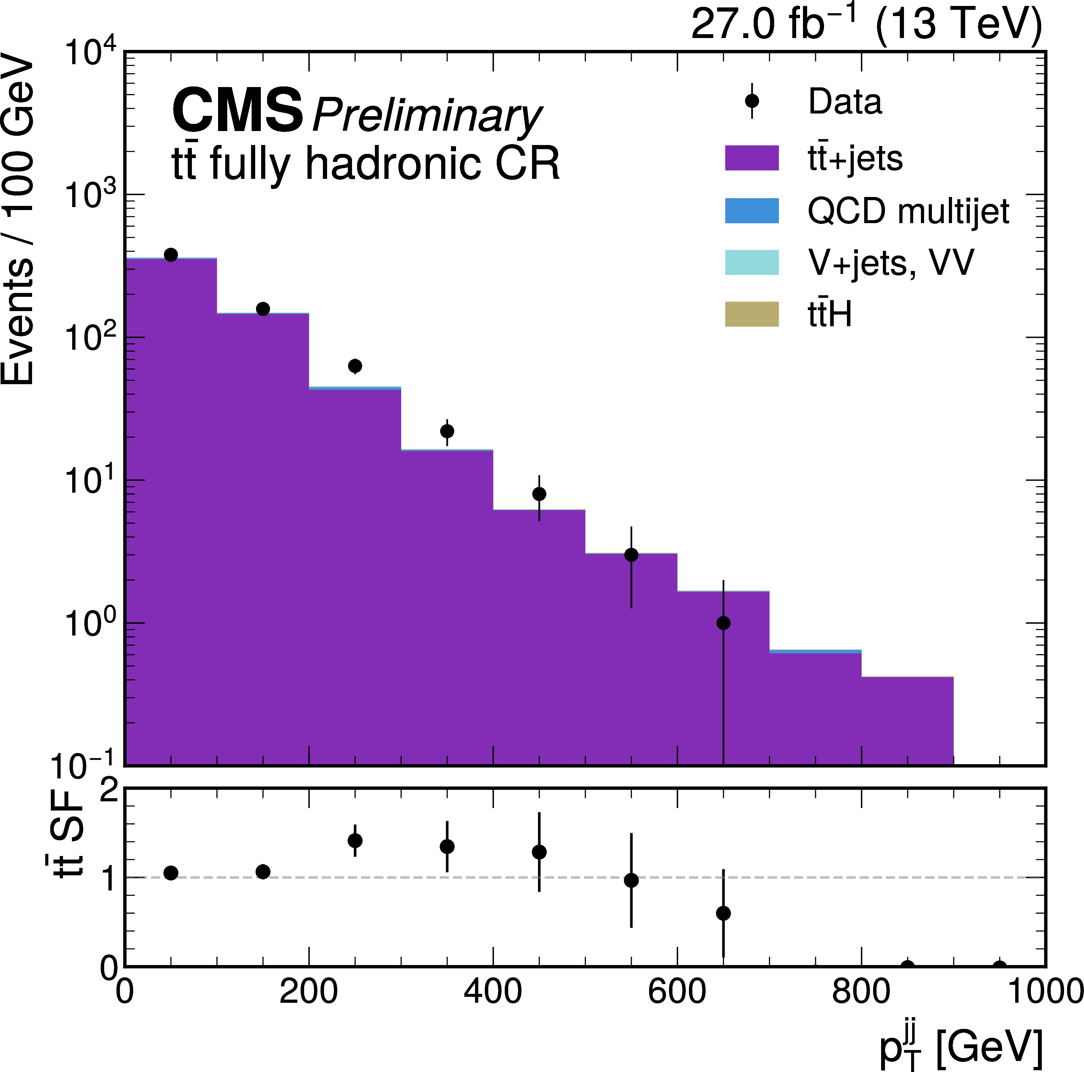
png pdf	Additional Figure 24-b: The derivation of the $\mathrm{t}\mathrm{\bar{t}}$ scale factors as a function of $P_t^\mathrm{jj}$ (upper) in the $\mathrm{t}\mathrm{\bar{t}}$ fully hadronic CR, and $\tau_3/\tau_2$ (middle) and \TXbb (lower) in the $\mathrm{t}\mathrm{\bar{t}}$ semileptonic CR. The scale factors are derived separately in 2022 (left) and 2023 (right) data. Distributions correspond to the second analysis approach of the merged topology described in the note.
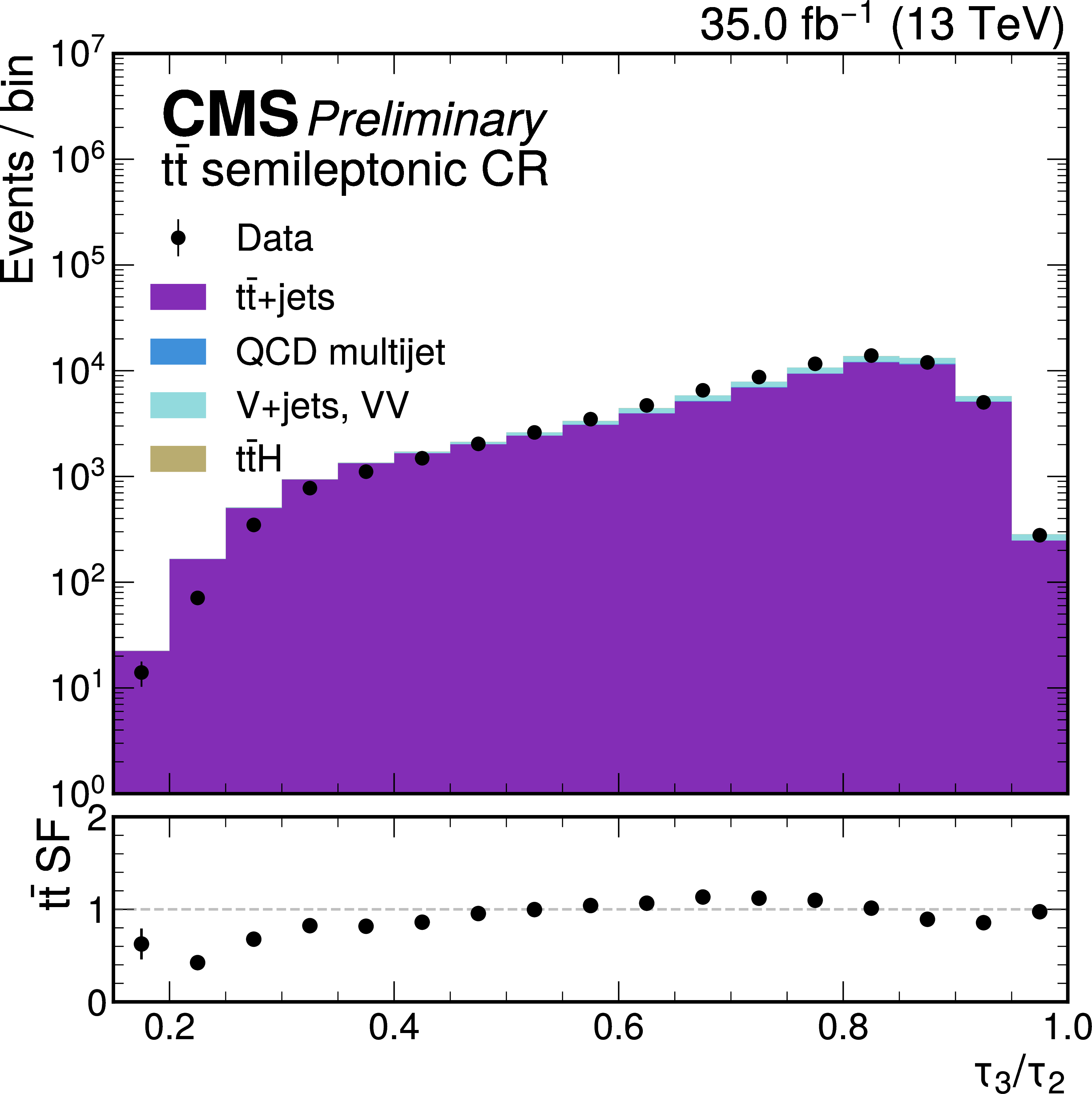
png pdf	Additional Figure 24-c: The derivation of the $\mathrm{t}\mathrm{\bar{t}}$ scale factors as a function of $P_t^\mathrm{jj}$ (upper) in the $\mathrm{t}\mathrm{\bar{t}}$ fully hadronic CR, and $\tau_3/\tau_2$ (middle) and \TXbb (lower) in the $\mathrm{t}\mathrm{\bar{t}}$ semileptonic CR. The scale factors are derived separately in 2022 (left) and 2023 (right) data. Distributions correspond to the second analysis approach of the merged topology described in the note.
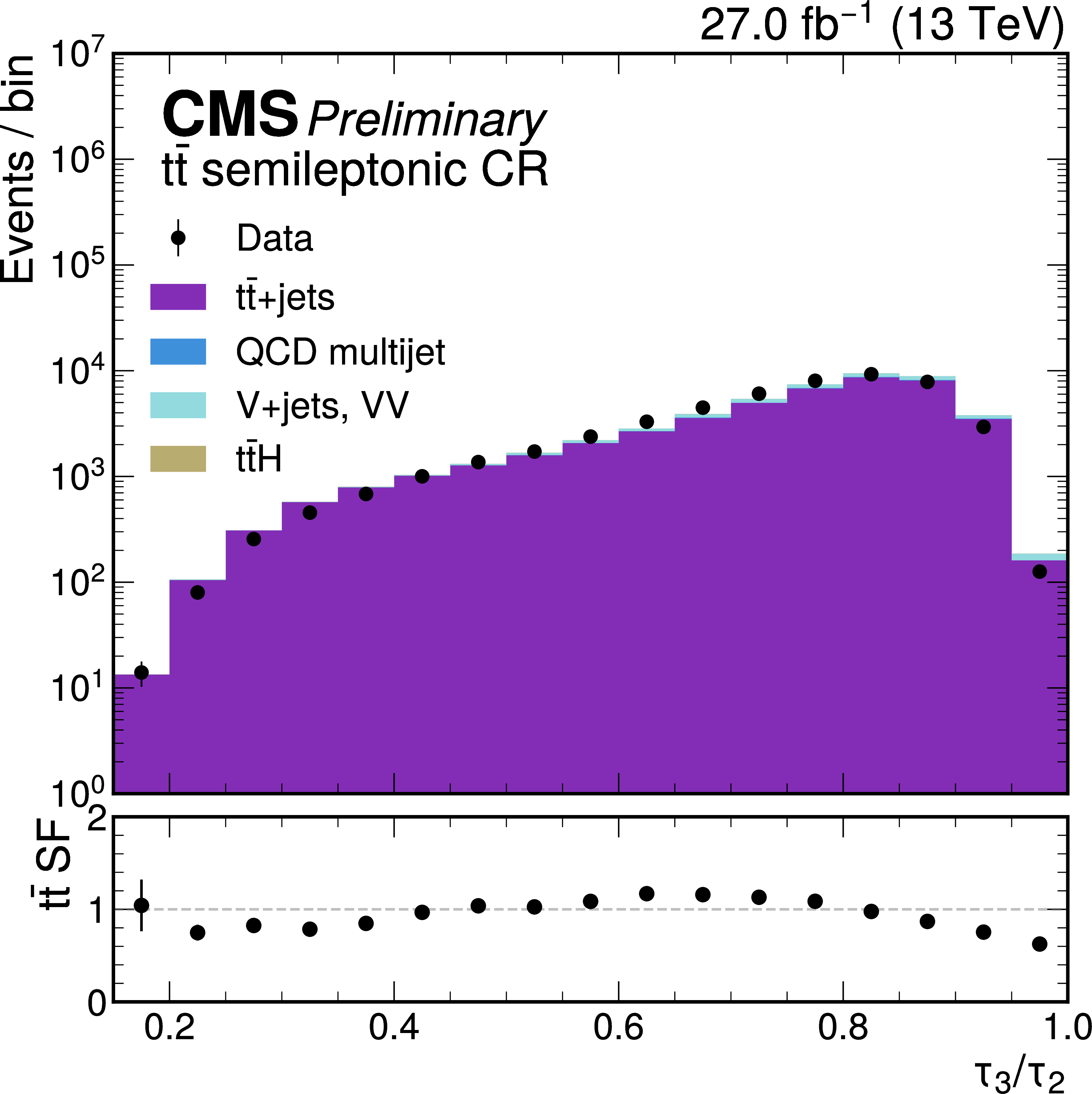
png pdf	Additional Figure 24-d: The derivation of the $\mathrm{t}\mathrm{\bar{t}}$ scale factors as a function of $P_t^\mathrm{jj}$ (upper) in the $\mathrm{t}\mathrm{\bar{t}}$ fully hadronic CR, and $\tau_3/\tau_2$ (middle) and \TXbb (lower) in the $\mathrm{t}\mathrm{\bar{t}}$ semileptonic CR. The scale factors are derived separately in 2022 (left) and 2023 (right) data. Distributions correspond to the second analysis approach of the merged topology described in the note.
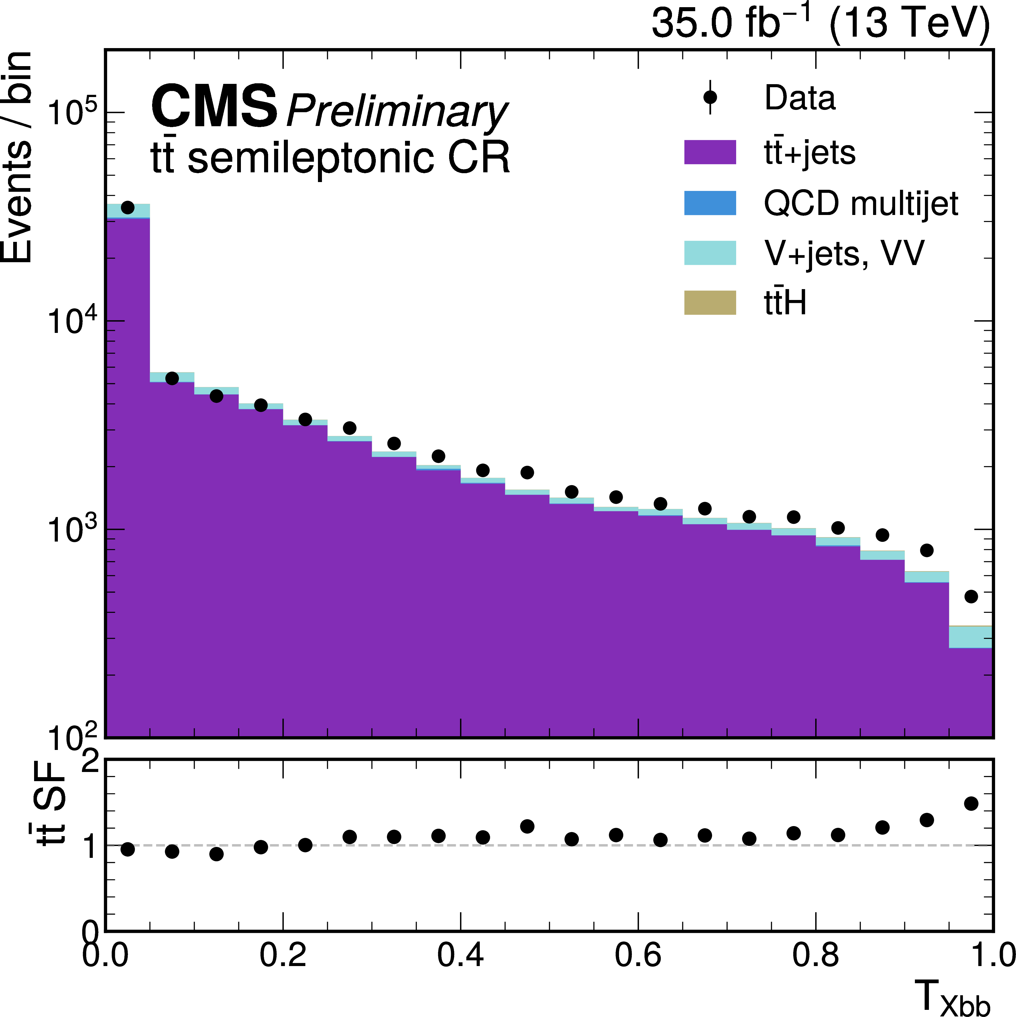
png pdf	Additional Figure 24-e: The derivation of the $\mathrm{t}\mathrm{\bar{t}}$ scale factors as a function of $P_t^\mathrm{jj}$ (upper) in the $\mathrm{t}\mathrm{\bar{t}}$ fully hadronic CR, and $\tau_3/\tau_2$ (middle) and \TXbb (lower) in the $\mathrm{t}\mathrm{\bar{t}}$ semileptonic CR. The scale factors are derived separately in 2022 (left) and 2023 (right) data. Distributions correspond to the second analysis approach of the merged topology described in the note.
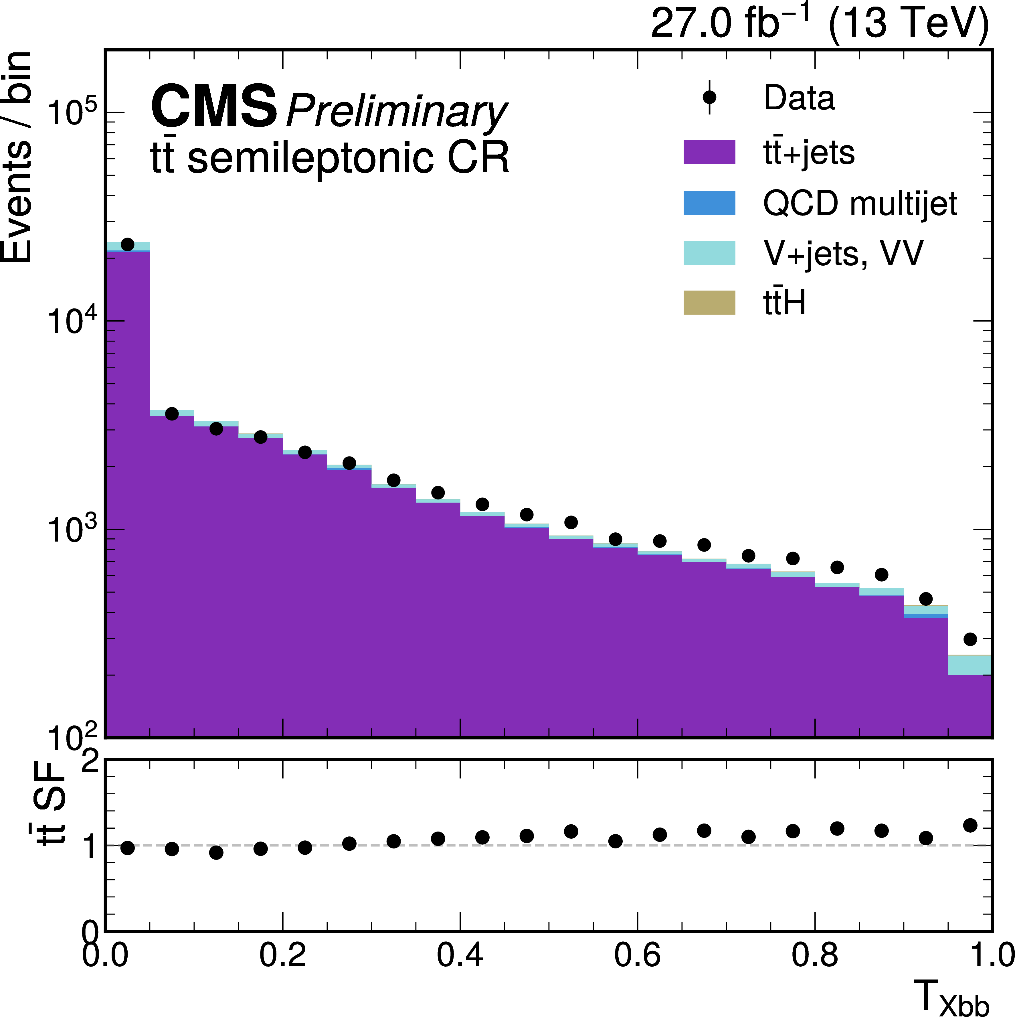
png pdf	Additional Figure 24-f: The derivation of the $\mathrm{t}\mathrm{\bar{t}}$ scale factors as a function of $P_t^\mathrm{jj}$ (upper) in the $\mathrm{t}\mathrm{\bar{t}}$ fully hadronic CR, and $\tau_3/\tau_2$ (middle) and \TXbb (lower) in the $\mathrm{t}\mathrm{\bar{t}}$ semileptonic CR. The scale factors are derived separately in 2022 (left) and 2023 (right) data. Distributions correspond to the second analysis approach of the merged topology described in the note.
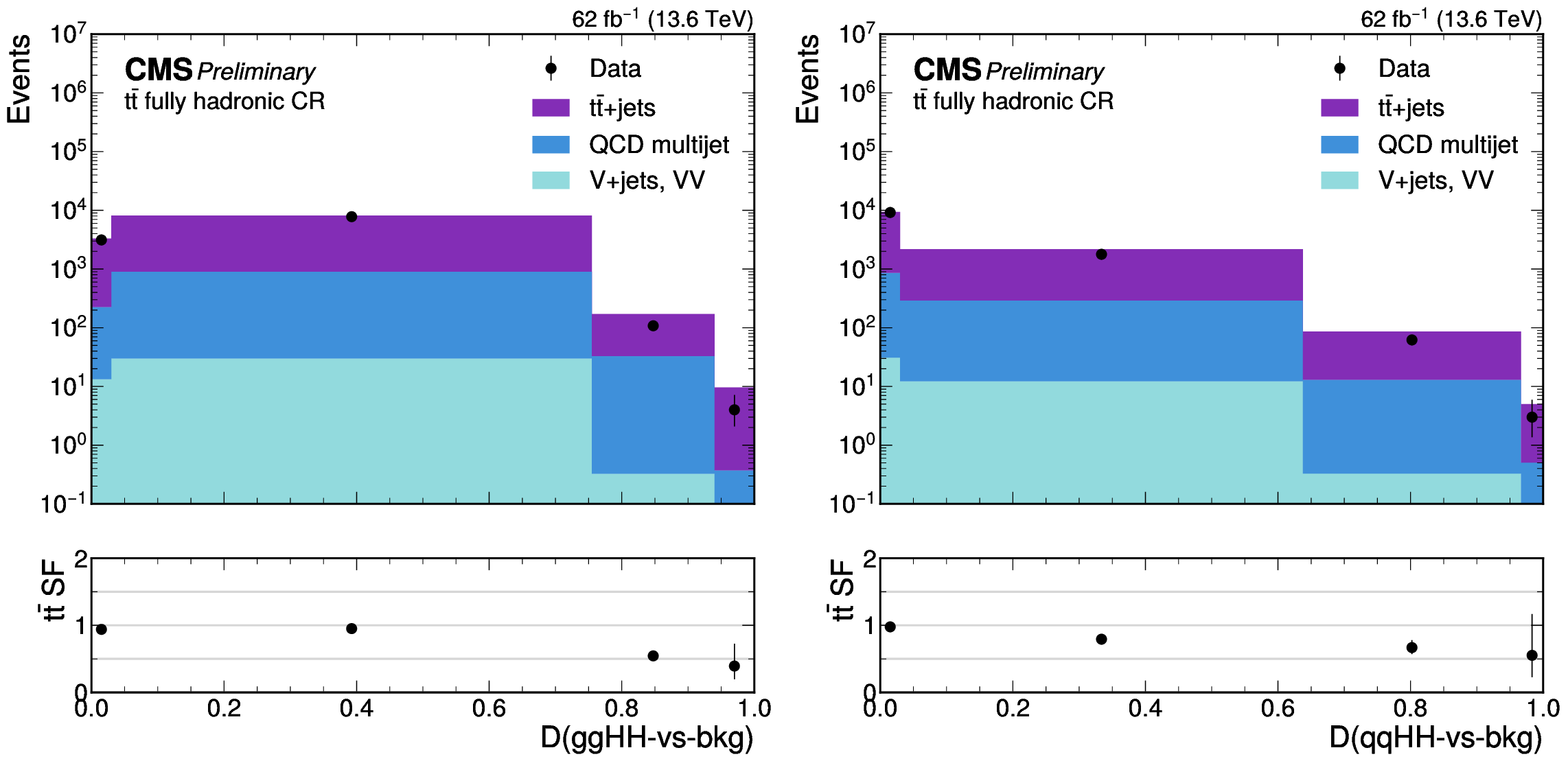
png pdf	Additional Figure 25: The $D$(ggHH-vs-bkg) (left) and $D$(qqHH-vs-bkg) (right) distributions in the $\mathrm{t}\mathrm{\bar{t}}$ fully hadronic CR for data and simulation prediction for the combined 2022 and 2023 data. The derived $\mathrm{t}\mathrm{\bar{t}}$ scale factors are shown in the bottom panel. Distributions correspond to the second analysis approach of the merged topology described in the note.
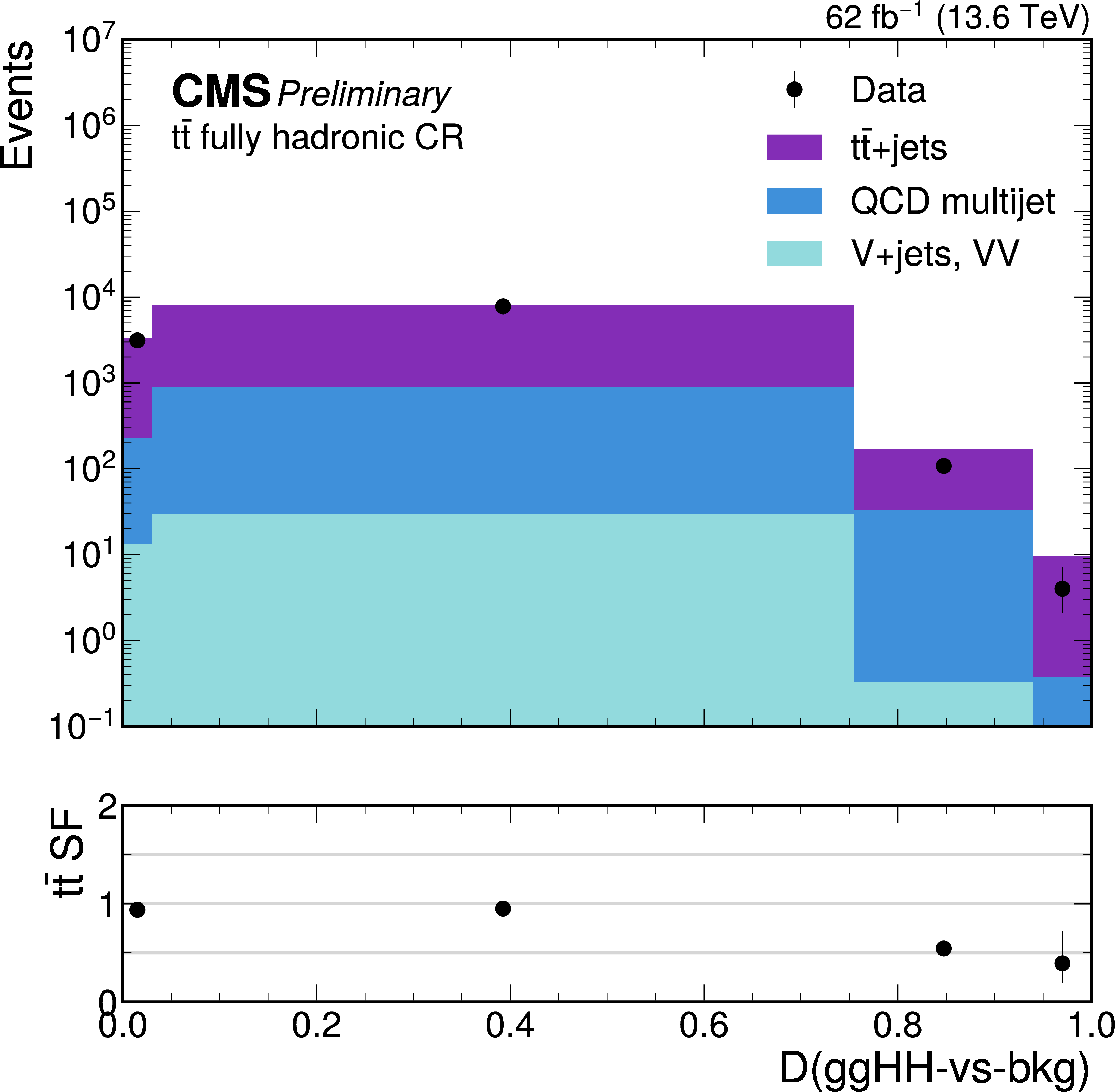
png pdf	Additional Figure 25-a: The $D$(ggHH-vs-bkg) (left) and $D$(qqHH-vs-bkg) (right) distributions in the $\mathrm{t}\mathrm{\bar{t}}$ fully hadronic CR for data and simulation prediction for the combined 2022 and 2023 data. The derived $\mathrm{t}\mathrm{\bar{t}}$ scale factors are shown in the bottom panel. Distributions correspond to the second analysis approach of the merged topology described in the note.
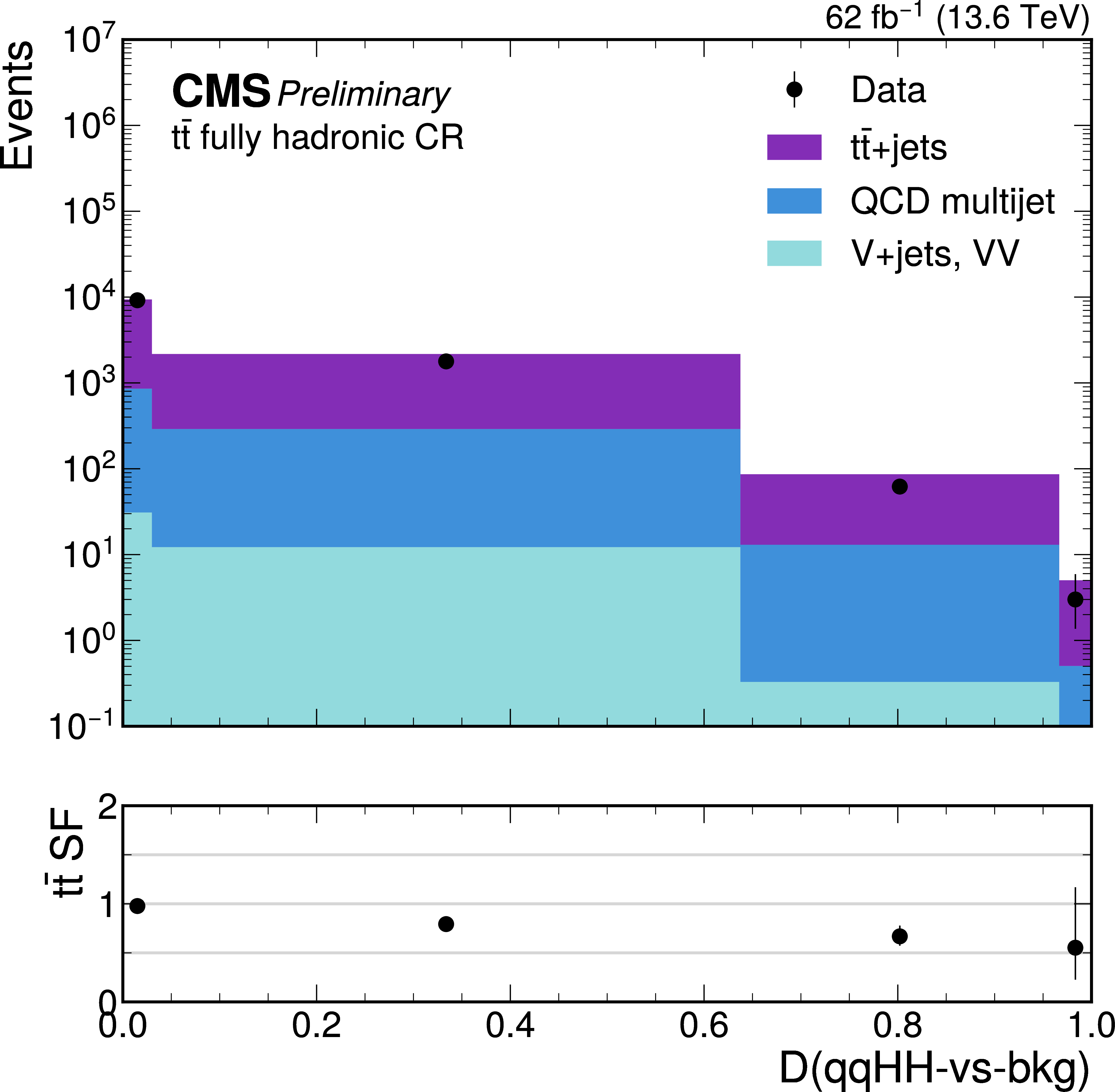
png pdf	Additional Figure 25-b: The $D$(ggHH-vs-bkg) (left) and $D$(qqHH-vs-bkg) (right) distributions in the $\mathrm{t}\mathrm{\bar{t}}$ fully hadronic CR for data and simulation prediction for the combined 2022 and 2023 data. The derived $\mathrm{t}\mathrm{\bar{t}}$ scale factors are shown in the bottom panel. Distributions correspond to the second analysis approach of the merged topology described in the note.
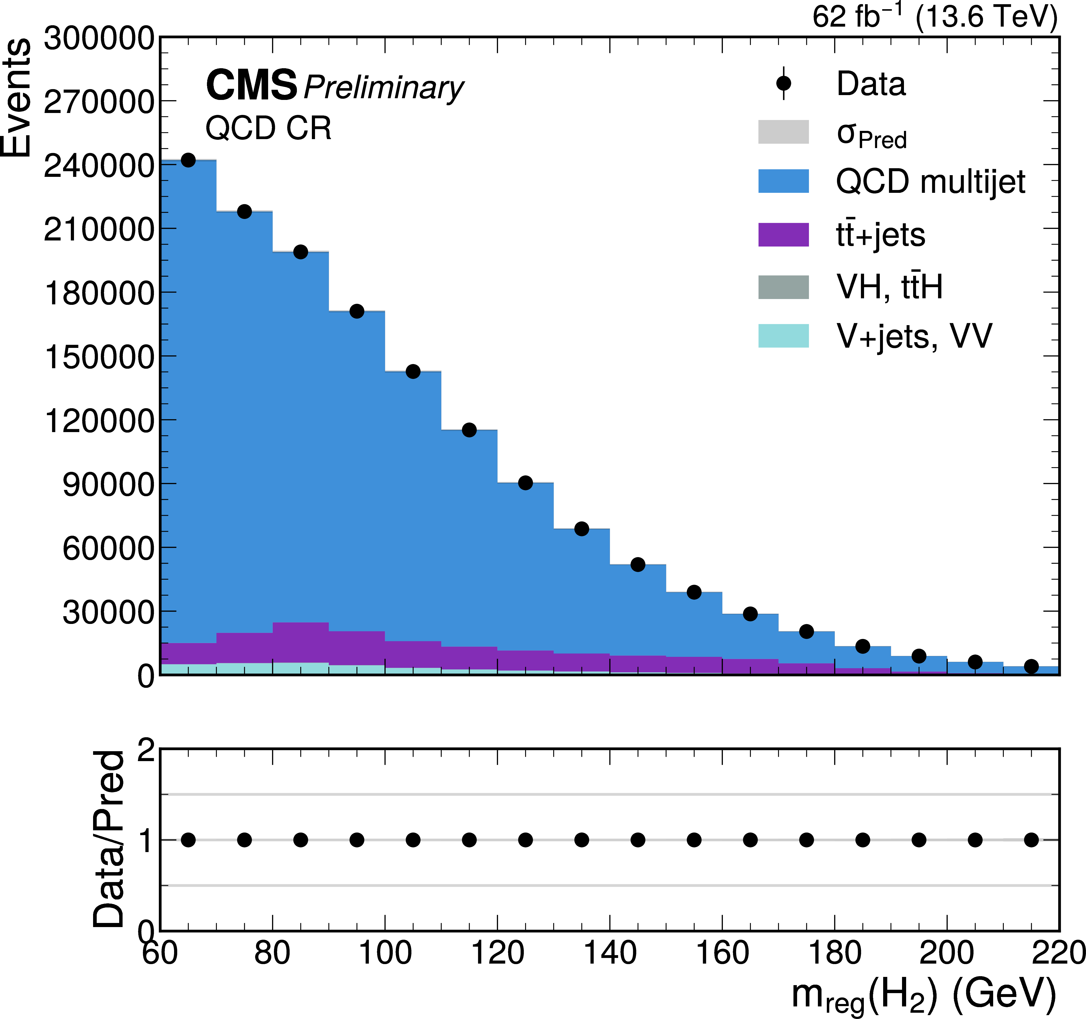
png pdf	Additional Figure 26: Postfit distribution of the regressed mass of the secondary H candidate $m_\text{reg}({H_2})$ in the QCD CR. Distribution corresponds to the second analysis approach of the merged topology described in the note.
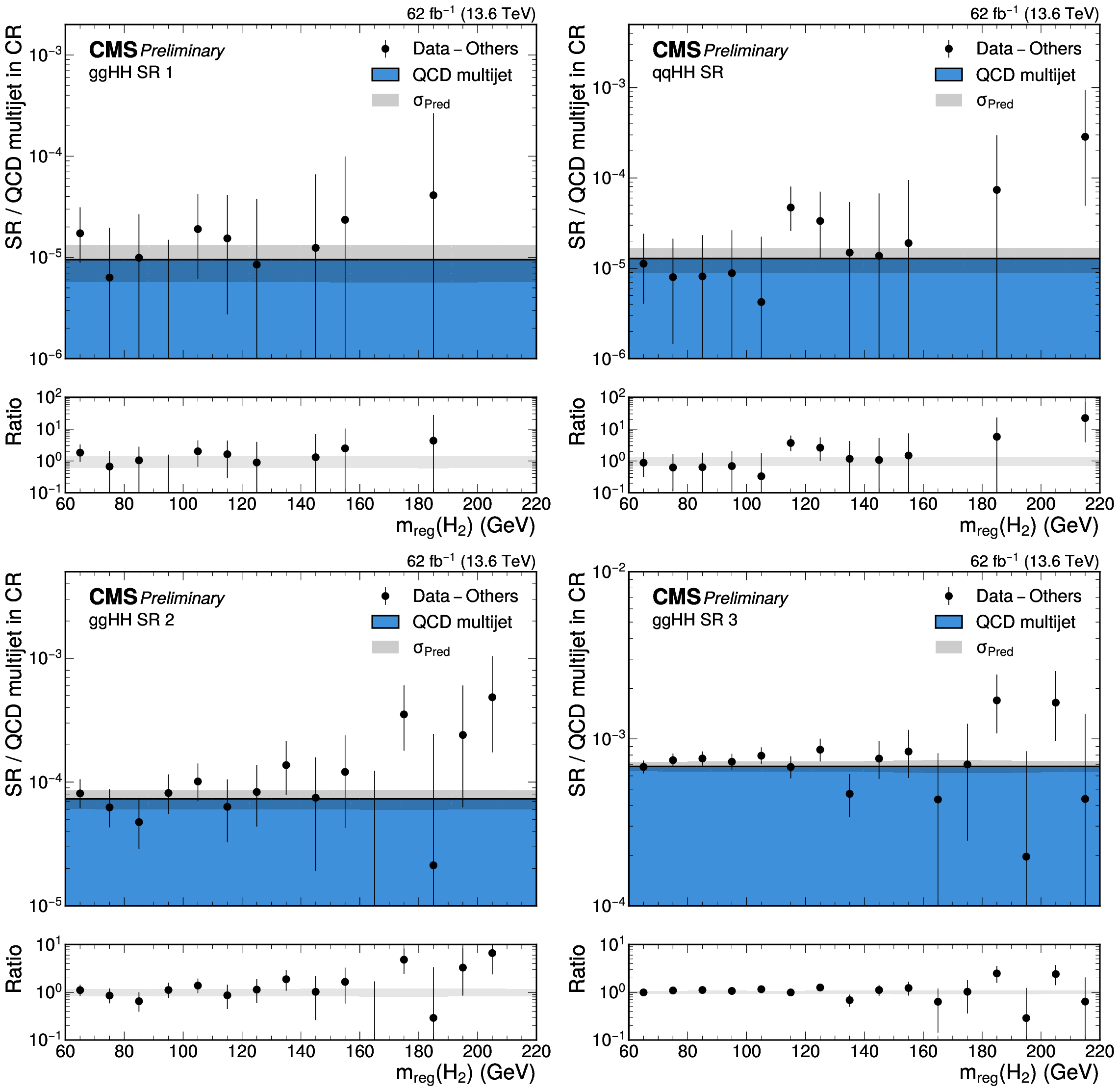
png pdf	Additional Figure 27: The data in the ggHH SR 1 (upper left), qqHHSR (upper right), ggHH SR 2 (lower left), and ggHH SR 3 (lower right) after subtracting all background processes except the QCD multijet one compared to the QCD multijet background prediction derived from the QCD CR. The fitted shape and uncertainty are derived from a simultaneous background-only fit of all four SRs. Distributions corresponds to the second analysis approach of the merged topology described in the note.
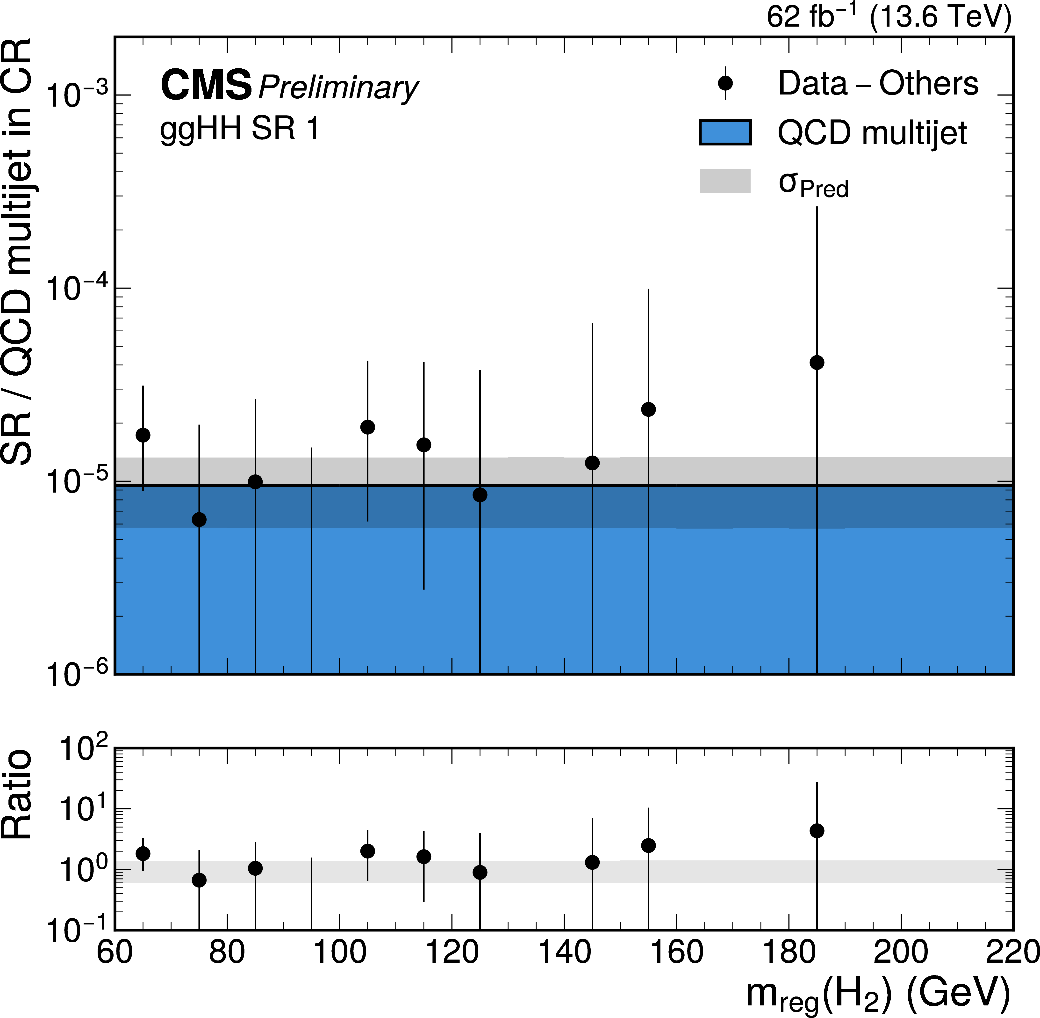
png pdf	Additional Figure 27-a: The data in the ggHH SR 1 (upper left), qqHHSR (upper right), ggHH SR 2 (lower left), and ggHH SR 3 (lower right) after subtracting all background processes except the QCD multijet one compared to the QCD multijet background prediction derived from the QCD CR. The fitted shape and uncertainty are derived from a simultaneous background-only fit of all four SRs. Distributions corresponds to the second analysis approach of the merged topology described in the note.
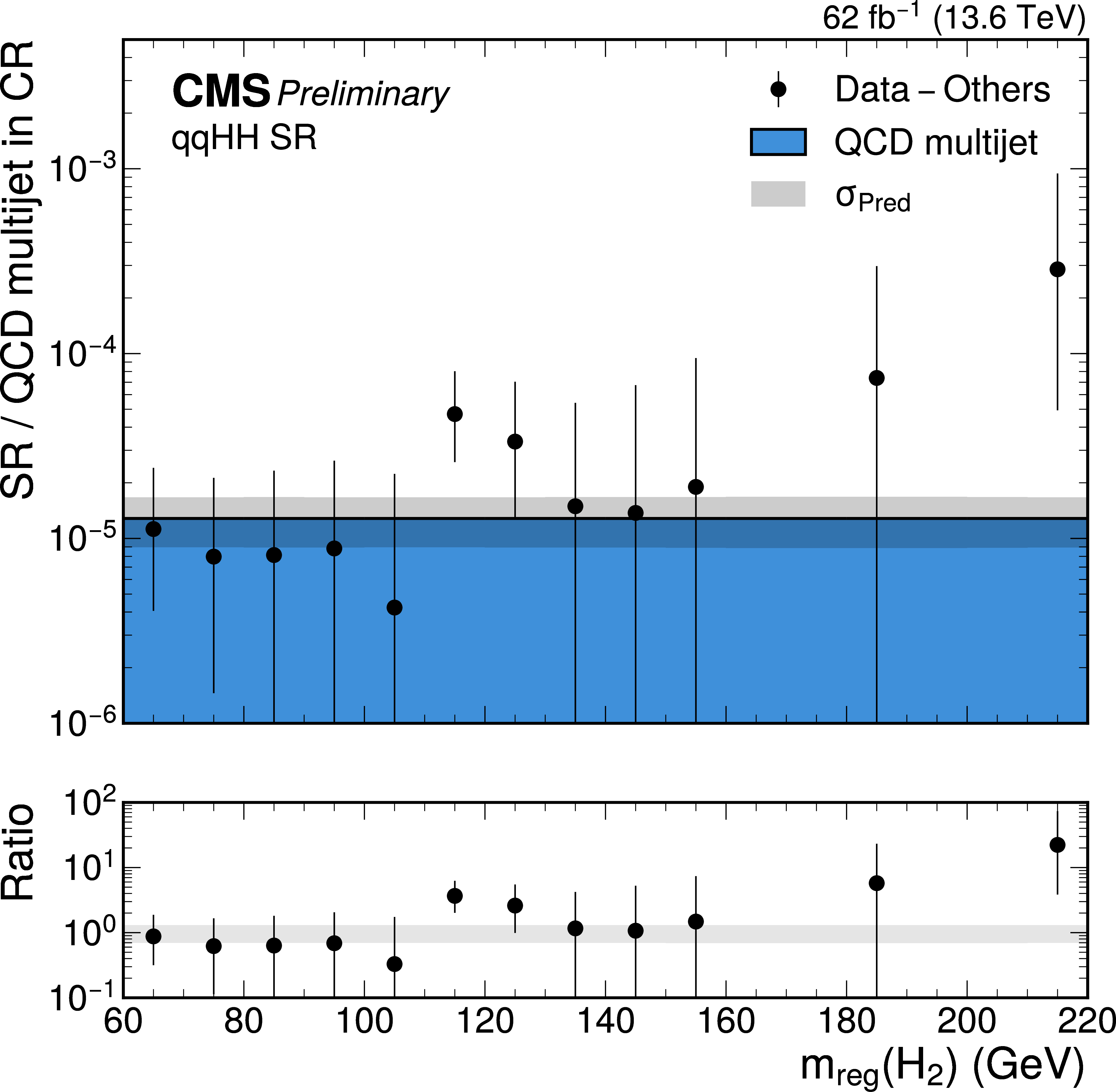
png pdf	Additional Figure 27-b: The data in the ggHH SR 1 (upper left), qqHHSR (upper right), ggHH SR 2 (lower left), and ggHH SR 3 (lower right) after subtracting all background processes except the QCD multijet one compared to the QCD multijet background prediction derived from the QCD CR. The fitted shape and uncertainty are derived from a simultaneous background-only fit of all four SRs. Distributions corresponds to the second analysis approach of the merged topology described in the note.
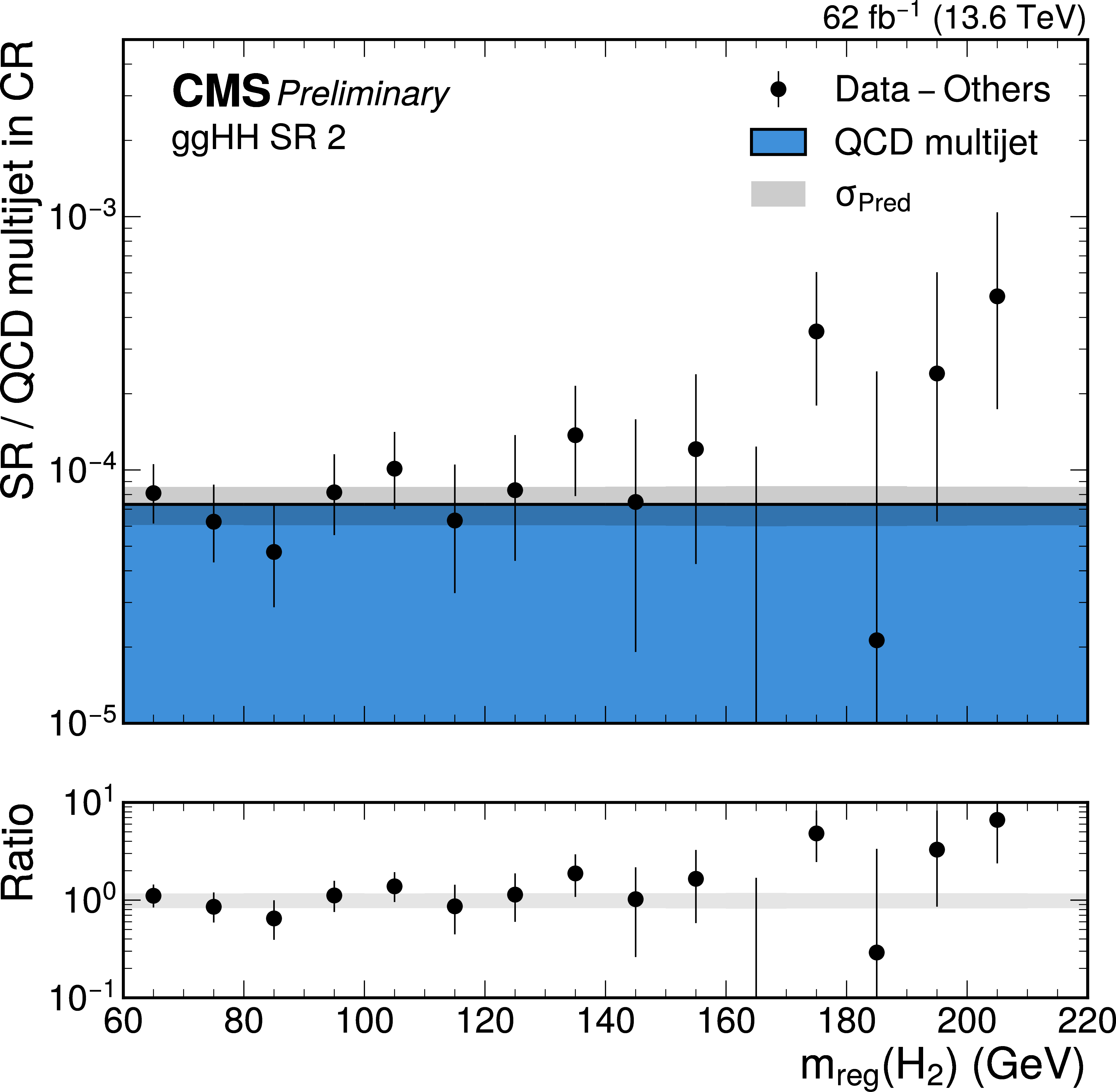
png pdf	Additional Figure 27-c: The data in the ggHH SR 1 (upper left), qqHHSR (upper right), ggHH SR 2 (lower left), and ggHH SR 3 (lower right) after subtracting all background processes except the QCD multijet one compared to the QCD multijet background prediction derived from the QCD CR. The fitted shape and uncertainty are derived from a simultaneous background-only fit of all four SRs. Distributions corresponds to the second analysis approach of the merged topology described in the note.
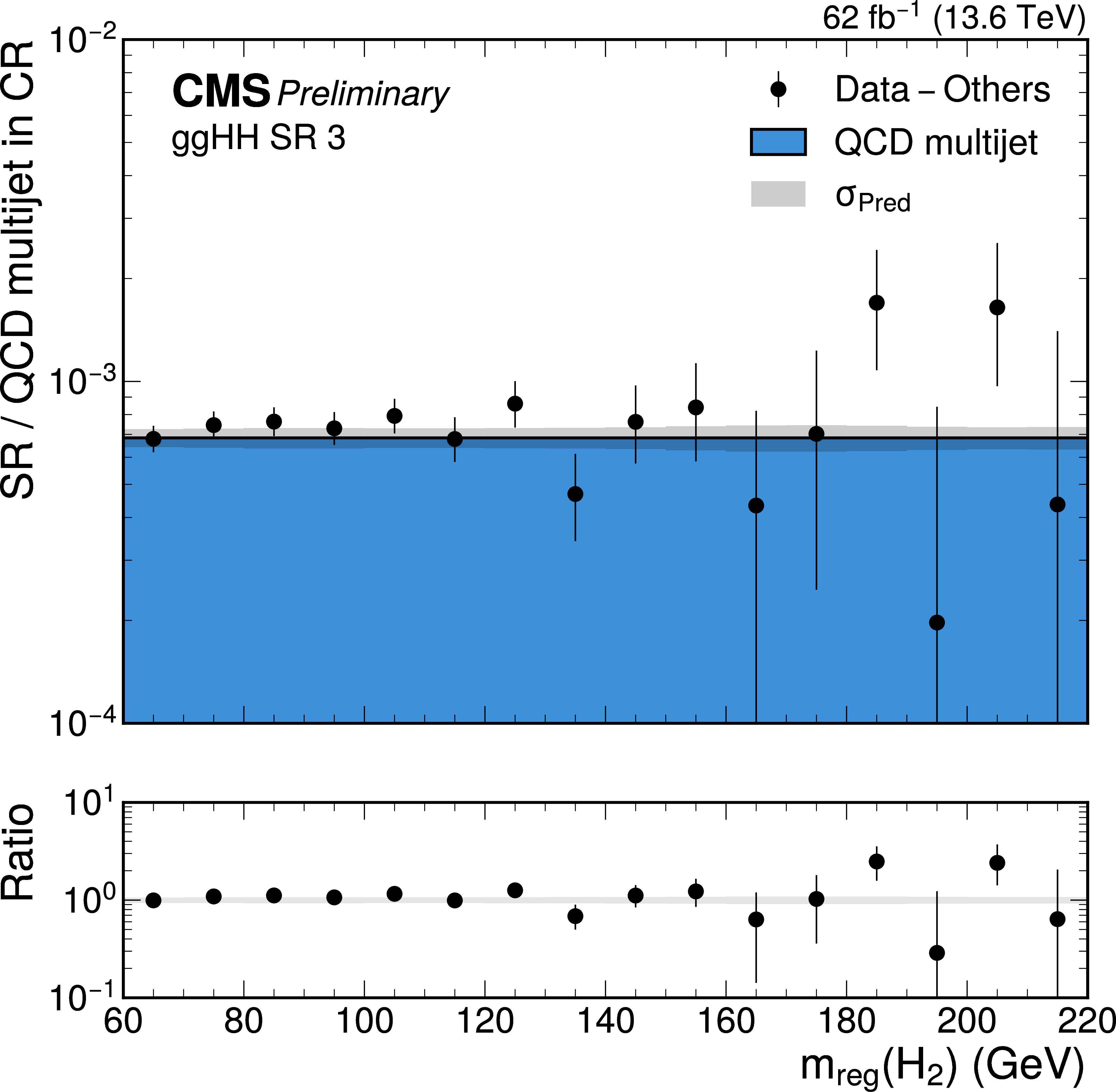
png pdf	Additional Figure 27-d: The data in the ggHH SR 1 (upper left), qqHHSR (upper right), ggHH SR 2 (lower left), and ggHH SR 3 (lower right) after subtracting all background processes except the QCD multijet one compared to the QCD multijet background prediction derived from the QCD CR. The fitted shape and uncertainty are derived from a simultaneous background-only fit of all four SRs. Distributions corresponds to the second analysis approach of the merged topology described in the note.
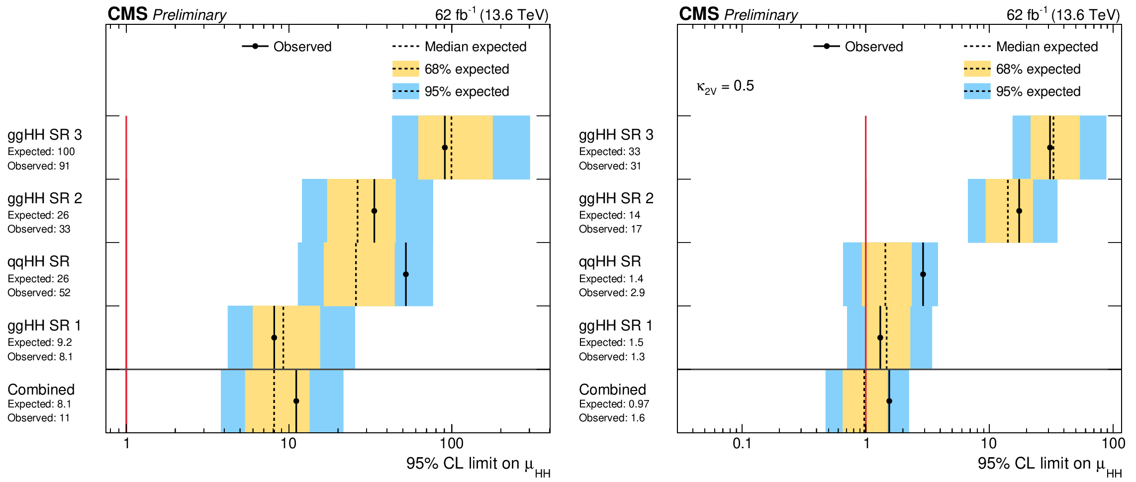
png pdf	Additional Figure 28: The observed (solid) and expected (dashed) 95% CL upper limits on $ \mathrm{H}\mathrm{H} $ production with respect to the expectation for the SM (left) and $$\mathrm{k}_{\mathrm{VV}}$=0.5$ (right) scenarios in the individual ggHH and qqHHSRs and their combination. The yellow and cyan bands represent, respectively, the 68 and 95% CL intervals around the expected limit. Results correspond to the second analysis approach of the merged topology described in the note.
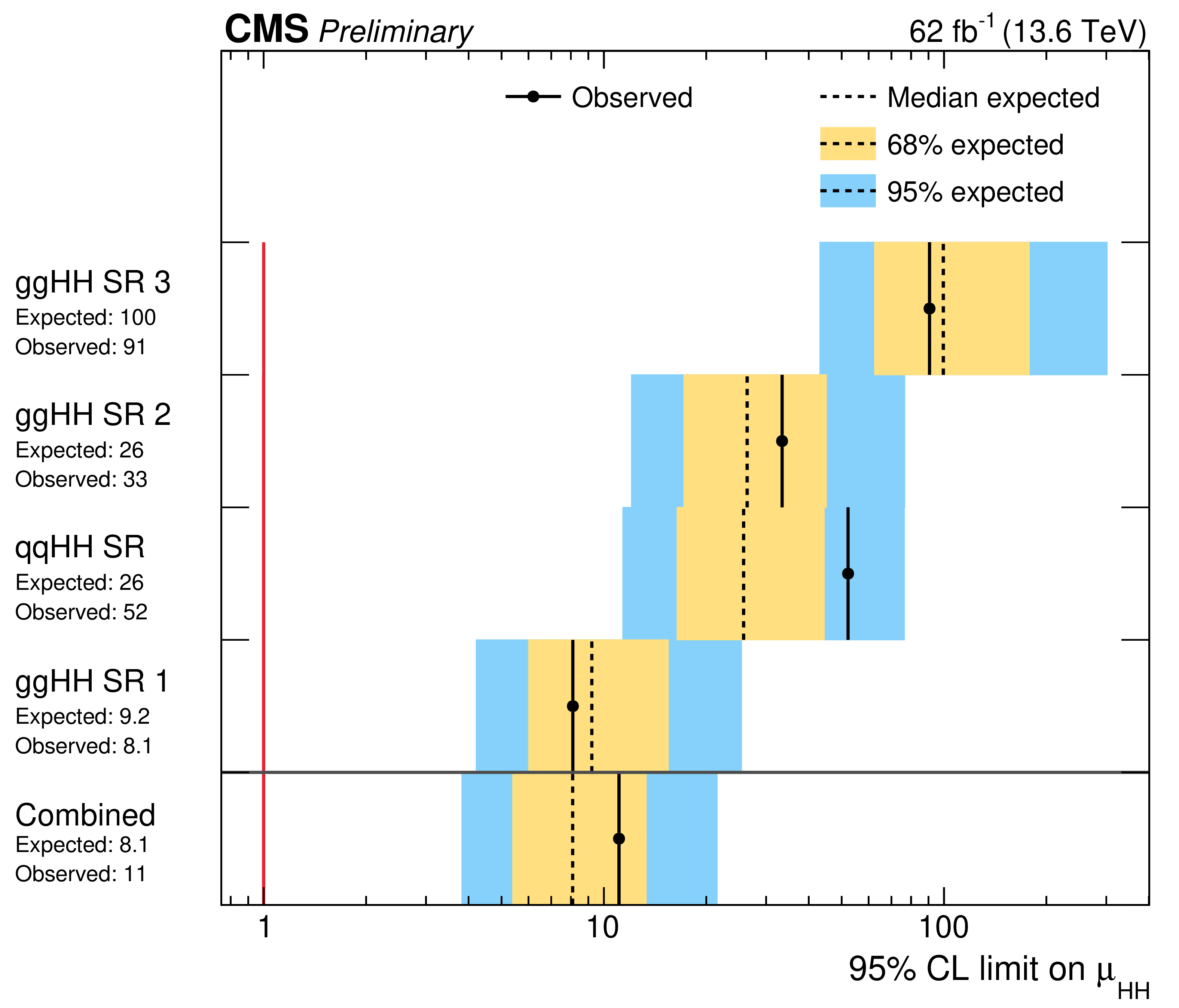
png pdf	Additional Figure 28-a: The observed (solid) and expected (dashed) 95% CL upper limits on $ \mathrm{H}\mathrm{H} $ production with respect to the expectation for the SM (left) and $$\mathrm{k}_{\mathrm{VV}}$=0.5$ (right) scenarios in the individual ggHH and qqHHSRs and their combination. The yellow and cyan bands represent, respectively, the 68 and 95% CL intervals around the expected limit. Results correspond to the second analysis approach of the merged topology described in the note.
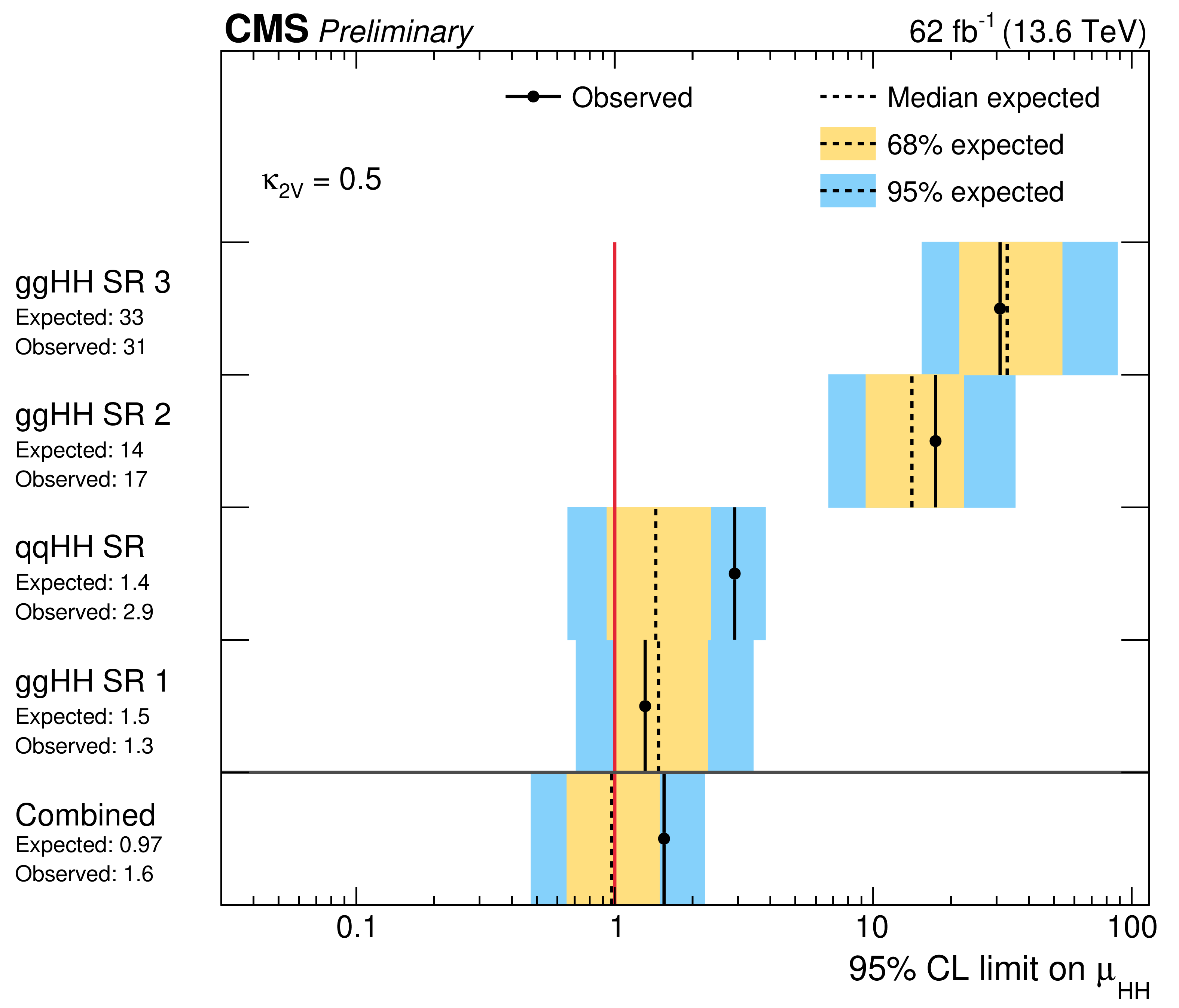
png pdf	Additional Figure 28-b: The observed (solid) and expected (dashed) 95% CL upper limits on $ \mathrm{H}\mathrm{H} $ production with respect to the expectation for the SM (left) and $$\mathrm{k}_{\mathrm{VV}}$=0.5$ (right) scenarios in the individual ggHH and qqHHSRs and their combination. The yellow and cyan bands represent, respectively, the 68 and 95% CL intervals around the expected limit. Results correspond to the second analysis approach of the merged topology described in the note.
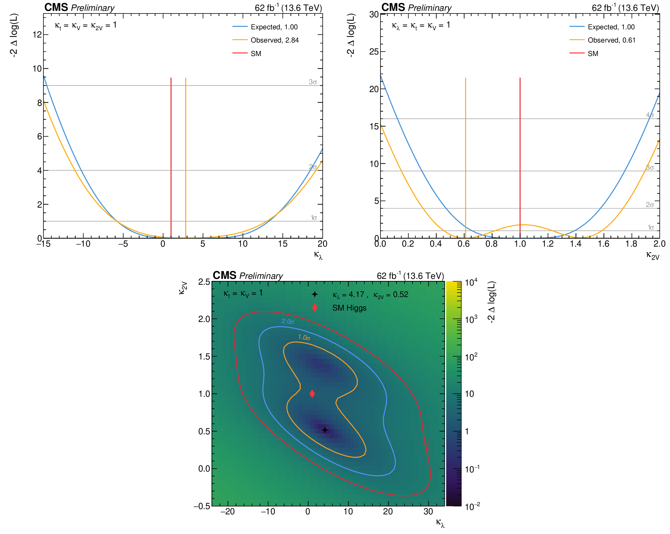
png pdf	Additional Figure 29: Profile likelihood test statistic $-2\Delta\log(L)$ scans as a function of $\mathrm{k}_{\lambda}$ (upper left), $\mathrm{k}_{\mathrm{VV}}$ (upper right), and in the ($\mathrm{k}_{\lambda}$, $\mathrm{k}_{\mathrm{VV}}$) plane (lower). Results correspond to the second analysis approach of the merged topology described in the note.
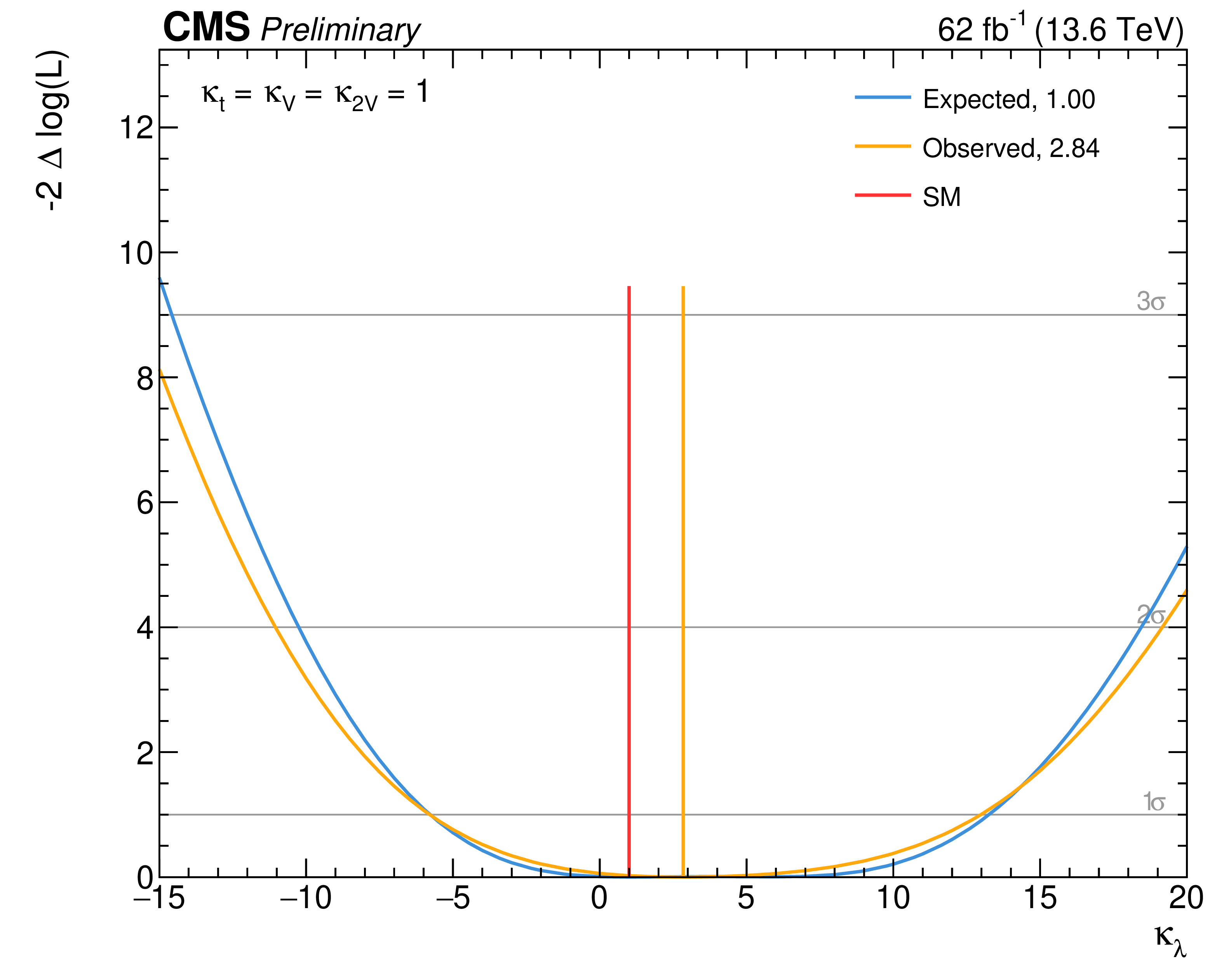
png pdf	Additional Figure 29-a: Profile likelihood test statistic $-2\Delta\log(L)$ scans as a function of $\mathrm{k}_{\lambda}$ (upper left), $\mathrm{k}_{\mathrm{VV}}$ (upper right), and in the ($\mathrm{k}_{\lambda}$, $\mathrm{k}_{\mathrm{VV}}$) plane (lower). Results correspond to the second analysis approach of the merged topology described in the note.
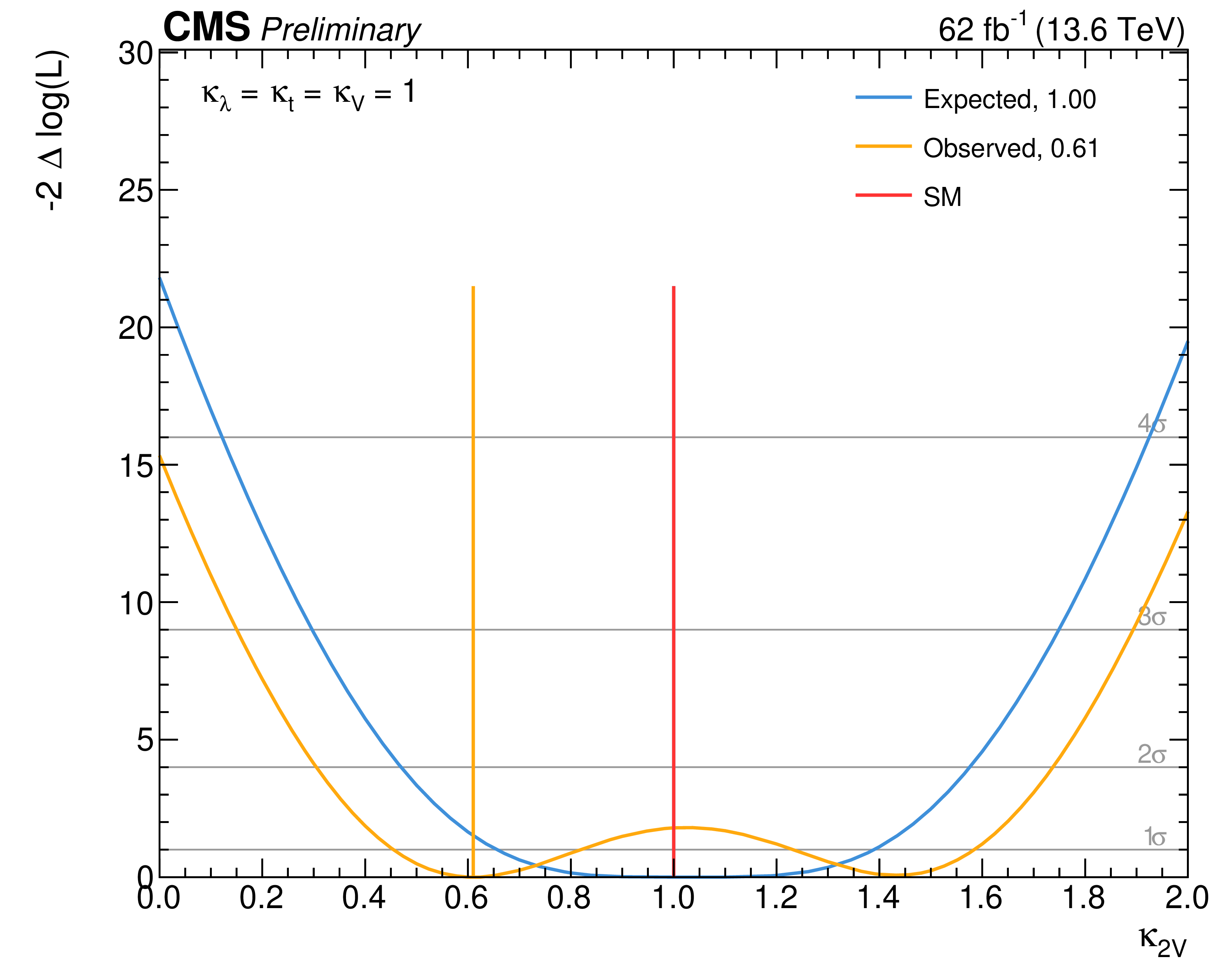
png pdf	Additional Figure 29-b: Profile likelihood test statistic $-2\Delta\log(L)$ scans as a function of $\mathrm{k}_{\lambda}$ (upper left), $\mathrm{k}_{\mathrm{VV}}$ (upper right), and in the ($\mathrm{k}_{\lambda}$, $\mathrm{k}_{\mathrm{VV}}$) plane (lower). Results correspond to the second analysis approach of the merged topology described in the note.
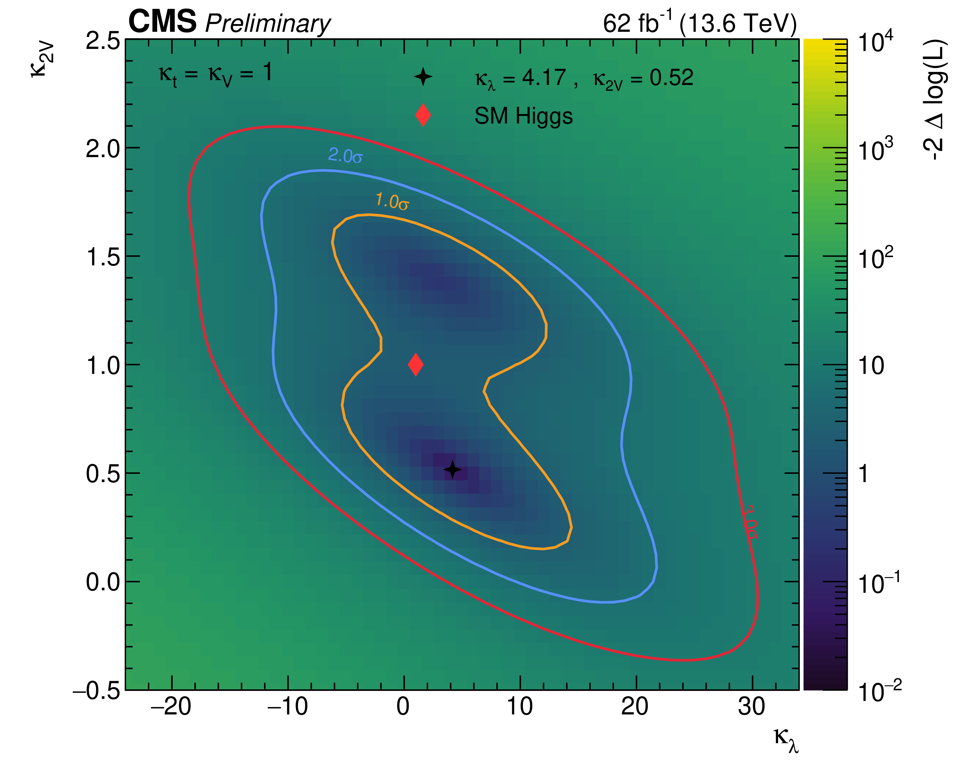
png pdf	Additional Figure 29-c: Profile likelihood test statistic $-2\Delta\log(L)$ scans as a function of $\mathrm{k}_{\lambda}$ (upper left), $\mathrm{k}_{\mathrm{VV}}$ (upper right), and in the ($\mathrm{k}_{\lambda}$, $\mathrm{k}_{\mathrm{VV}}$) plane (lower). Results correspond to the second analysis approach of the merged topology described in the note.
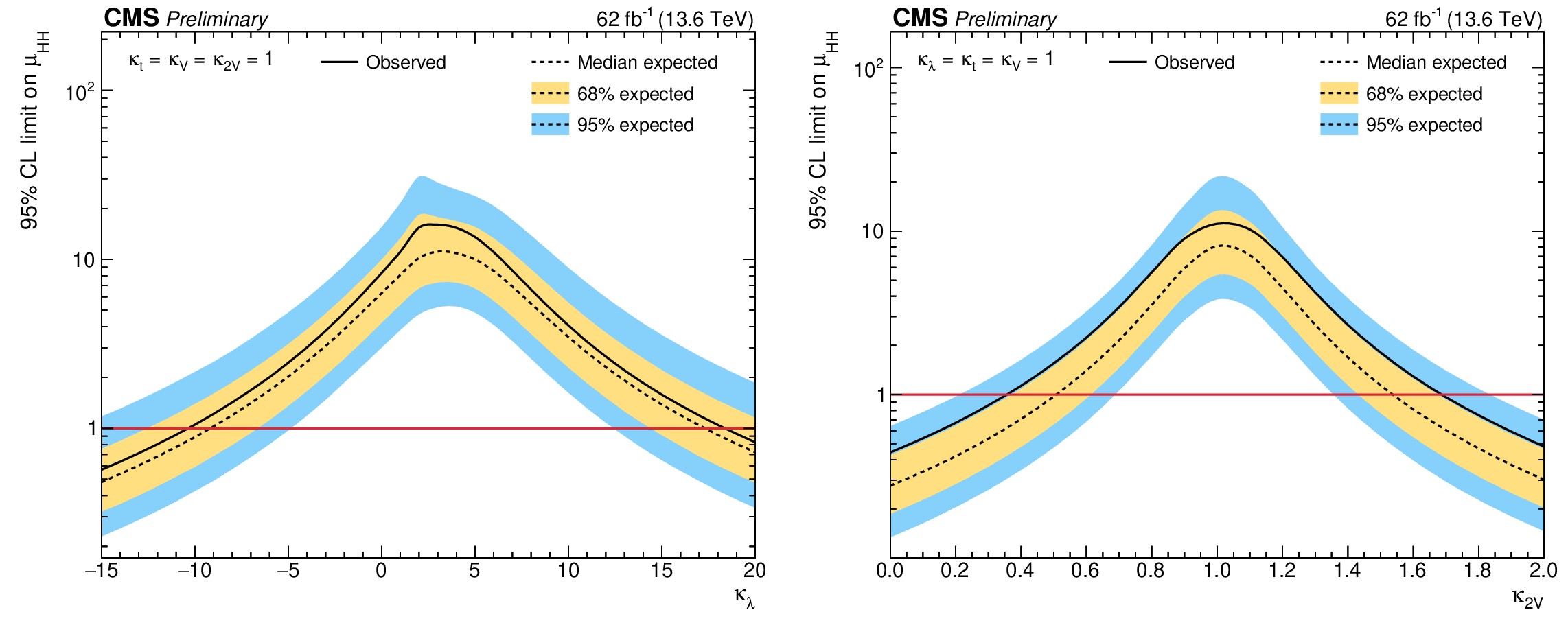
png pdf	Additional Figure 30: The observed (solid) and expected (dashed) 95% CL upper limits on the $ \mathrm{H}\mathrm{H} $ signal strength as a function of $\mathrm{k}_{\lambda}$ (left) and $\mathrm{k}_{\mathrm{VV}}$ (right). The yellow and cyan bands represent, respectively, the 68 and 95% CL intervals around the expected limit. The observed (expected) allowed range, at 95% CL for $\mathrm{k}_{\lambda}$ is [-11.0,19.2] ([-10.3,18.4]), and for $\mathrm{k}_{VV}$ is [0.30,1.74] ([0.47,1.58]). Results correspond to the second analysis approach of the merged topology described in the note.
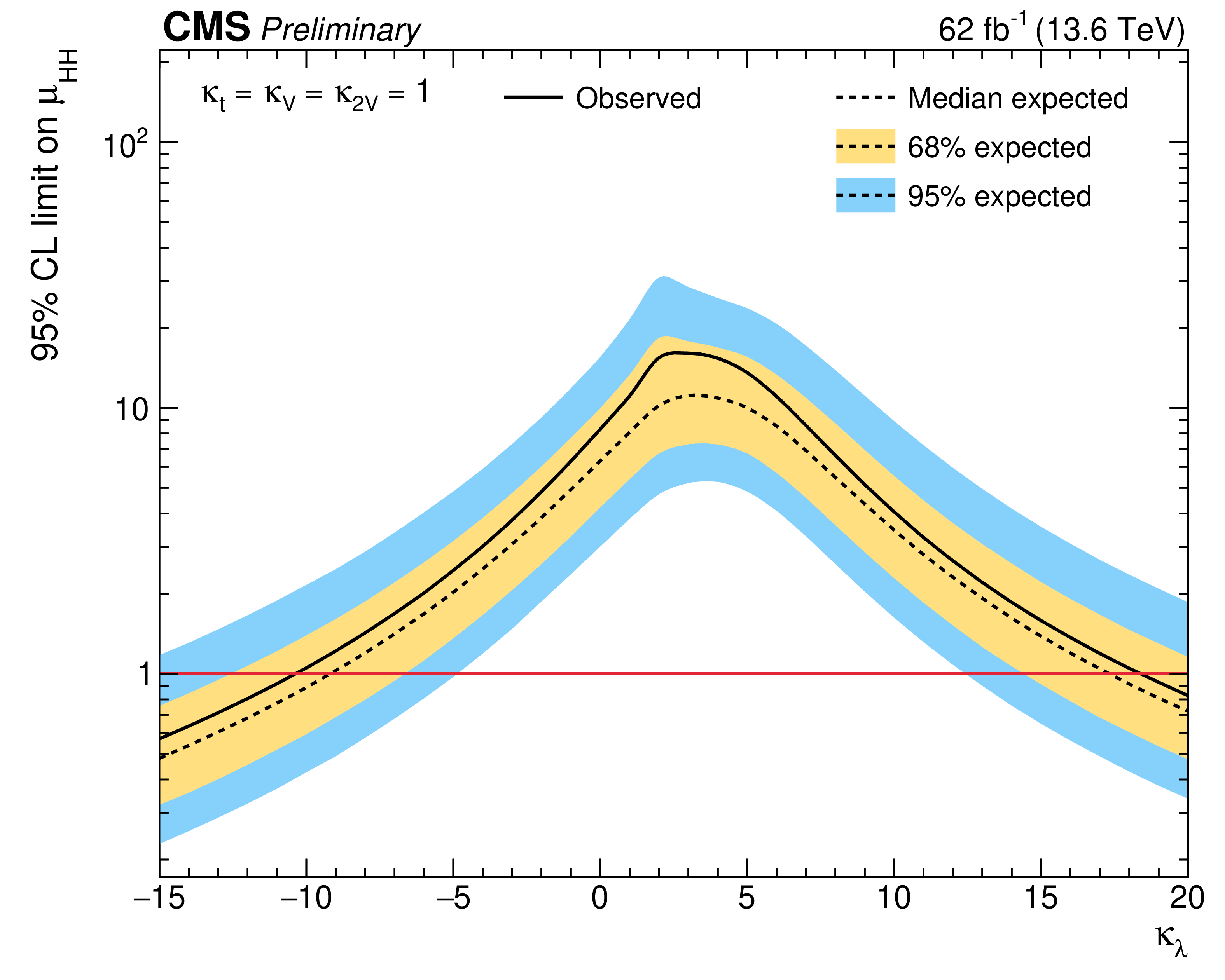
png pdf	Additional Figure 30-a: The observed (solid) and expected (dashed) 95% CL upper limits on the $ \mathrm{H}\mathrm{H} $ signal strength as a function of $\mathrm{k}_{\lambda}$ (left) and $\mathrm{k}_{\mathrm{VV}}$ (right). The yellow and cyan bands represent, respectively, the 68 and 95% CL intervals around the expected limit. The observed (expected) allowed range, at 95% CL for $\mathrm{k}_{\lambda}$ is [-11.0,19.2] ([-10.3,18.4]), and for $\mathrm{k}_{VV}$ is [0.30,1.74] ([0.47,1.58]). Results correspond to the second analysis approach of the merged topology described in the note.
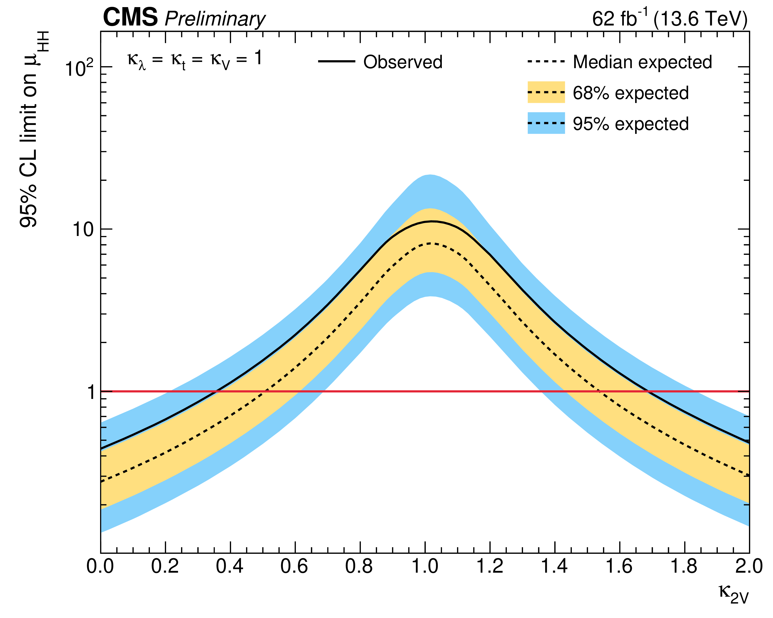
png pdf	Additional Figure 30-b: The observed (solid) and expected (dashed) 95% CL upper limits on the $ \mathrm{H}\mathrm{H} $ signal strength as a function of $\mathrm{k}_{\lambda}$ (left) and $\mathrm{k}_{\mathrm{VV}}$ (right). The yellow and cyan bands represent, respectively, the 68 and 95% CL intervals around the expected limit. The observed (expected) allowed range, at 95% CL for $\mathrm{k}_{\lambda}$ is [-11.0,19.2] ([-10.3,18.4]), and for $\mathrm{k}_{VV}$ is [0.30,1.74] ([0.47,1.58]). Results correspond to the second analysis approach of the merged topology described in the note.
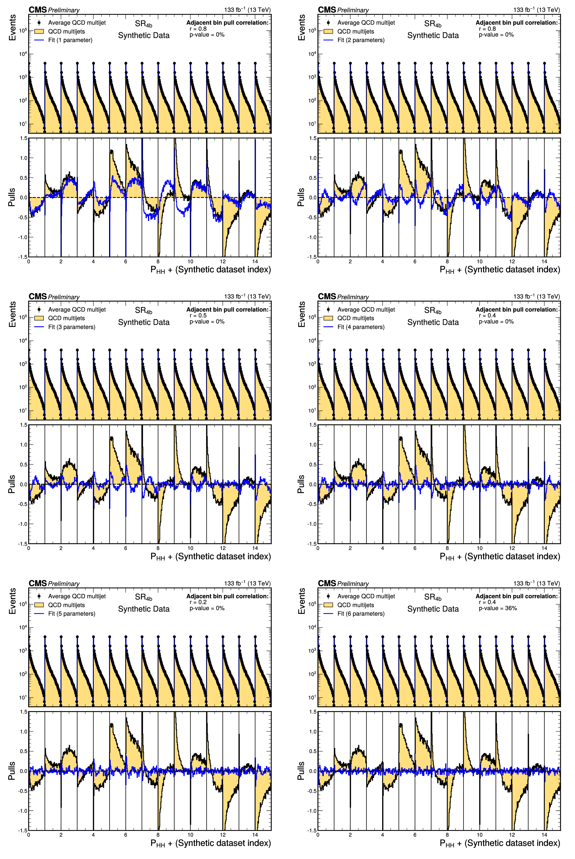
png pdf	Additional Figure 31: The predicted QCD multijet HH probability, $\mathcal{P_\mathrm{H}\mathrm{H}}$, distributions for each of the 15 synthetic datasets in the signal region (yellow regions). The distribution from each synthetic data is offset by the data sample index number. The black points give the average of the 15 data samples. The solid blue curves show a fit to the individual distributions using an increasing number of basis functions from one in the upper left plot to six in the lowest right plot. The lower panels show the pulls before (yellow histogram) and after (blue histogram) adding the basis corrections. The correlation coefficient (r) for a fit testing for correlations is given in the legend, along with the p-value used to test for lack of correlation. Basis functions are added until the p-value is greater than 5%. Distributions correspond to the Run 2 analysis in the resolved topology described in the note
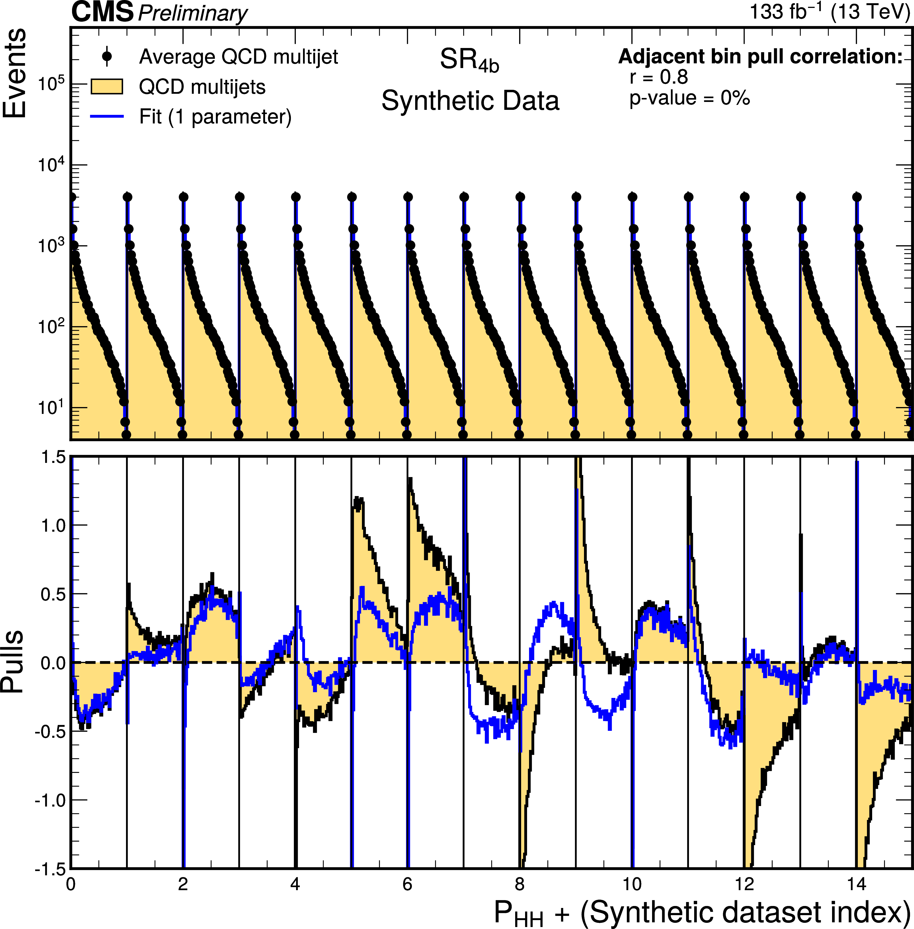
png pdf	Additional Figure 31-a: The predicted QCD multijet HH probability, $\mathcal{P_\mathrm{H}\mathrm{H}}$, distributions for each of the 15 synthetic datasets in the signal region (yellow regions). The distribution from each synthetic data is offset by the data sample index number. The black points give the average of the 15 data samples. The solid blue curves show a fit to the individual distributions using an increasing number of basis functions from one in the upper left plot to six in the lowest right plot. The lower panels show the pulls before (yellow histogram) and after (blue histogram) adding the basis corrections. The correlation coefficient (r) for a fit testing for correlations is given in the legend, along with the p-value used to test for lack of correlation. Basis functions are added until the p-value is greater than 5%. Distributions correspond to the Run 2 analysis in the resolved topology described in the note
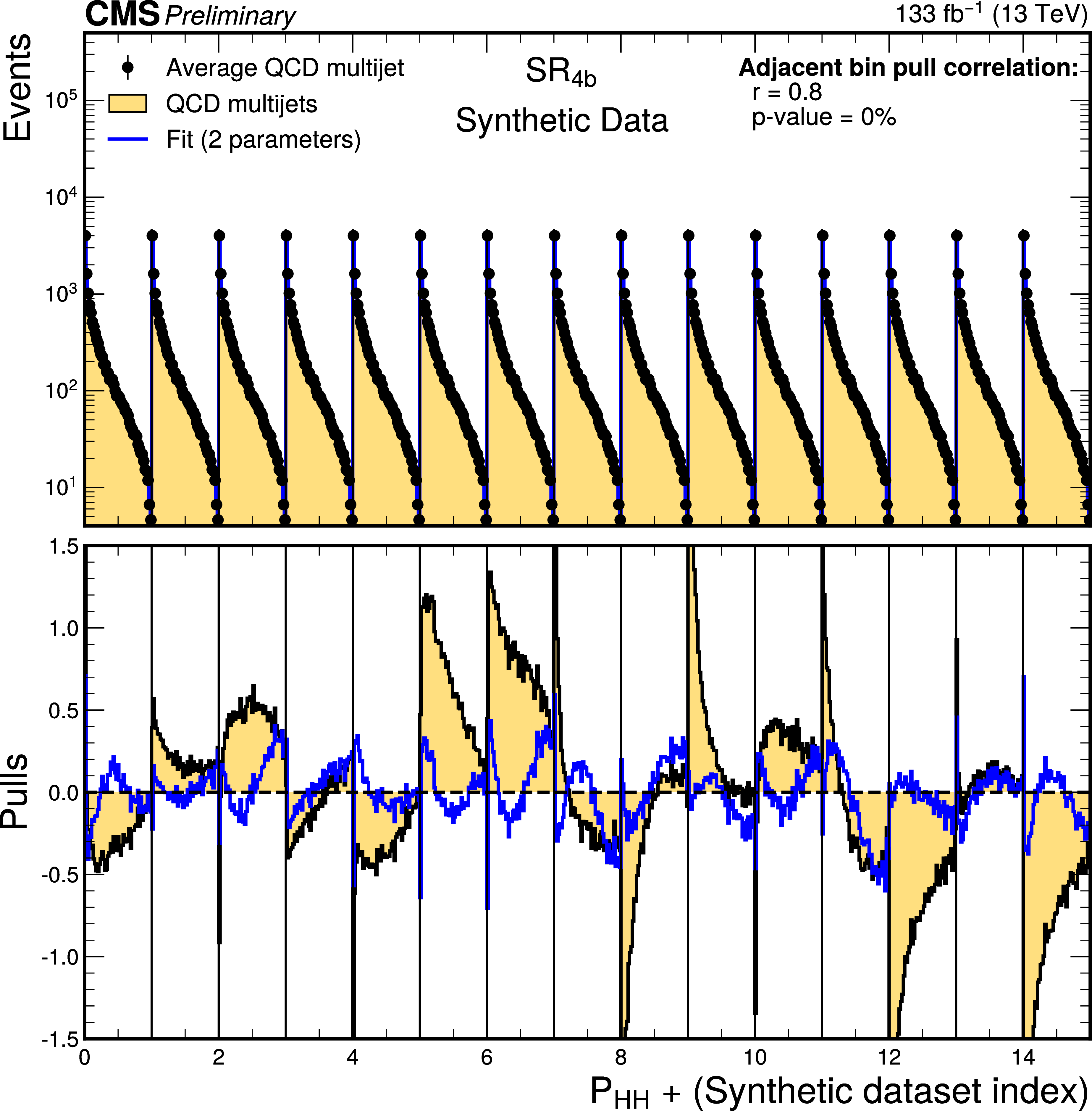
png pdf	Additional Figure 31-b: The predicted QCD multijet HH probability, $\mathcal{P_\mathrm{H}\mathrm{H}}$, distributions for each of the 15 synthetic datasets in the signal region (yellow regions). The distribution from each synthetic data is offset by the data sample index number. The black points give the average of the 15 data samples. The solid blue curves show a fit to the individual distributions using an increasing number of basis functions from one in the upper left plot to six in the lowest right plot. The lower panels show the pulls before (yellow histogram) and after (blue histogram) adding the basis corrections. The correlation coefficient (r) for a fit testing for correlations is given in the legend, along with the p-value used to test for lack of correlation. Basis functions are added until the p-value is greater than 5%. Distributions correspond to the Run 2 analysis in the resolved topology described in the note
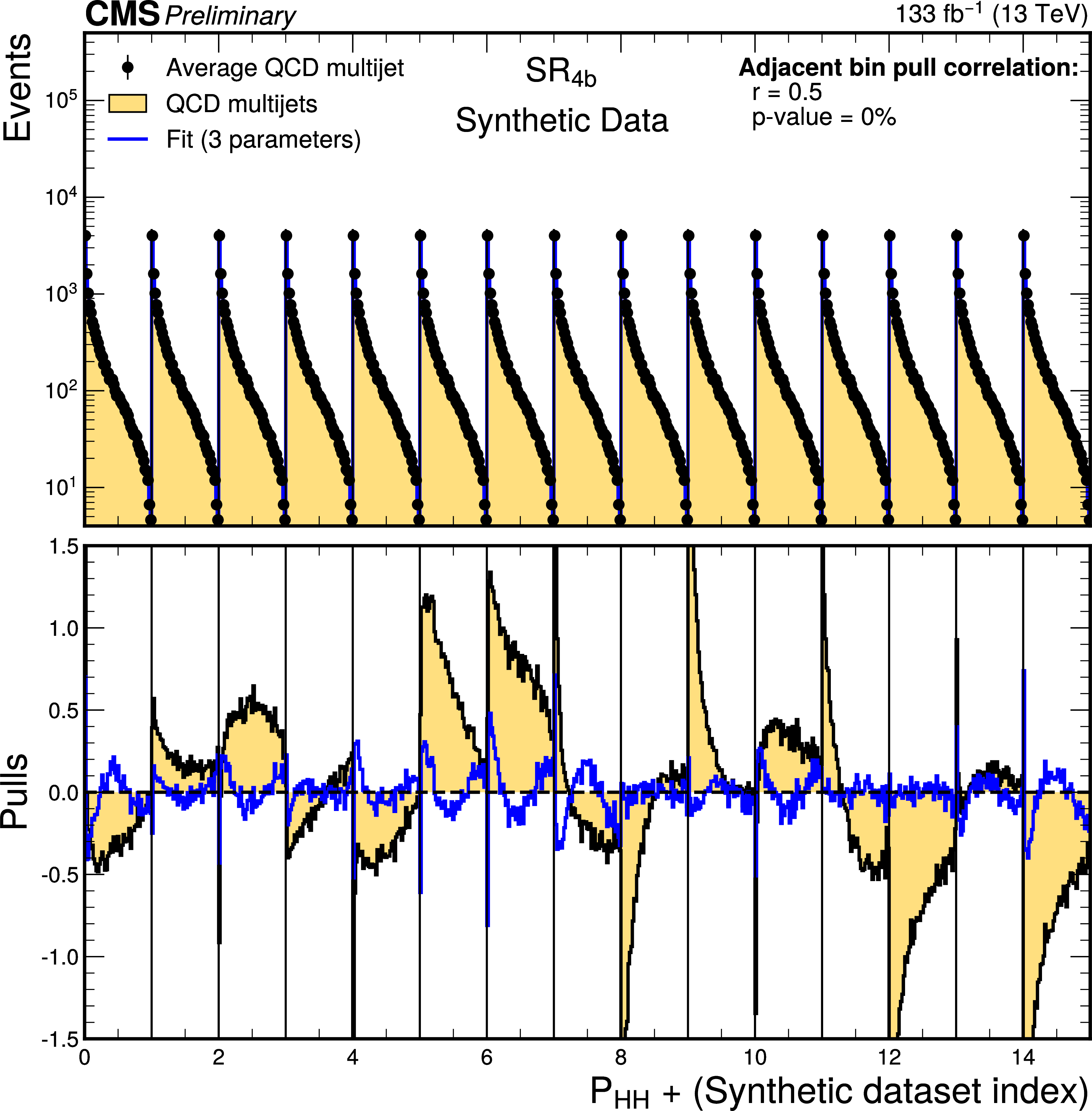
png pdf	Additional Figure 31-c: The predicted QCD multijet HH probability, $\mathcal{P_\mathrm{H}\mathrm{H}}$, distributions for each of the 15 synthetic datasets in the signal region (yellow regions). The distribution from each synthetic data is offset by the data sample index number. The black points give the average of the 15 data samples. The solid blue curves show a fit to the individual distributions using an increasing number of basis functions from one in the upper left plot to six in the lowest right plot. The lower panels show the pulls before (yellow histogram) and after (blue histogram) adding the basis corrections. The correlation coefficient (r) for a fit testing for correlations is given in the legend, along with the p-value used to test for lack of correlation. Basis functions are added until the p-value is greater than 5%. Distributions correspond to the Run 2 analysis in the resolved topology described in the note
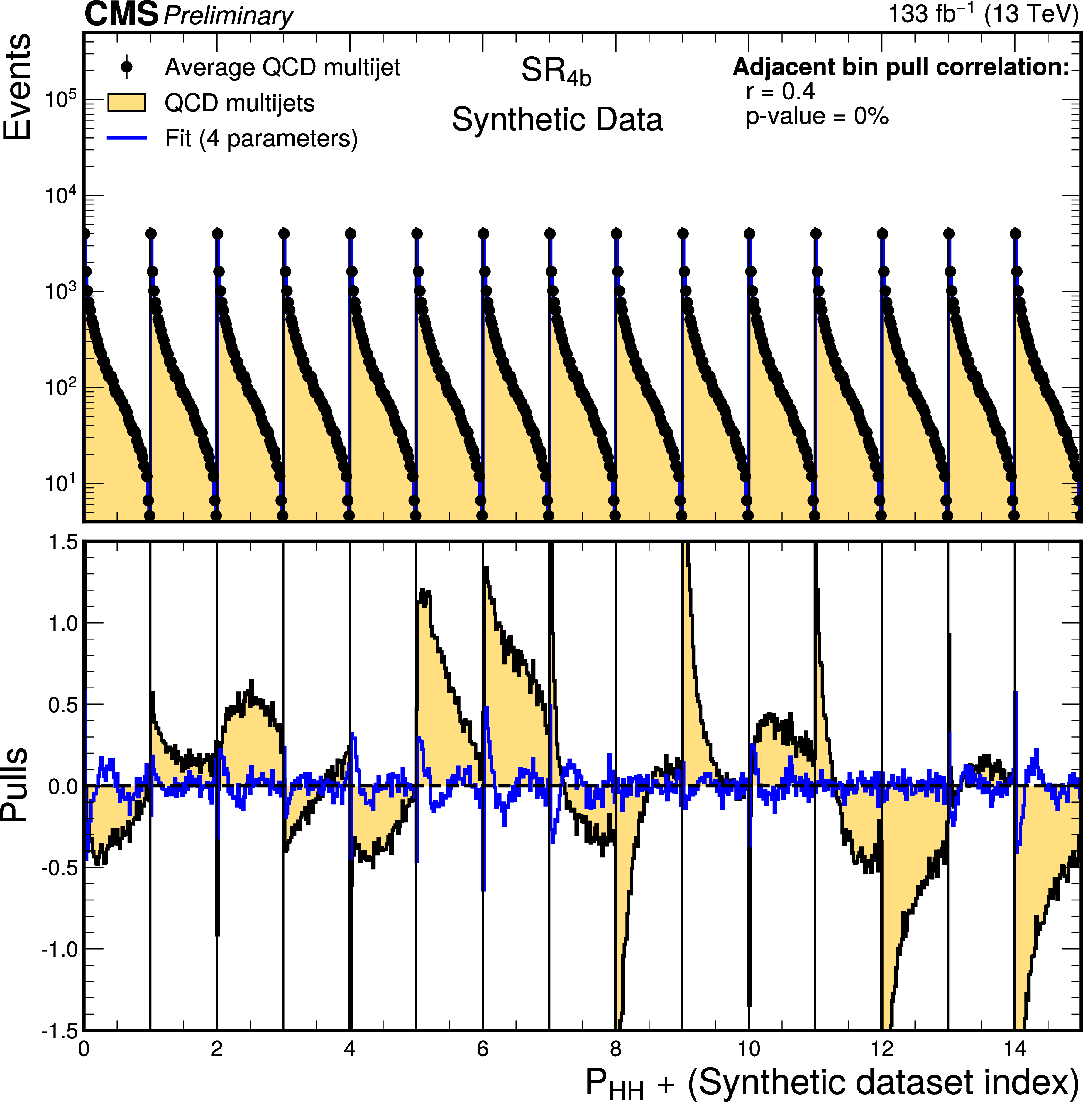
png pdf	Additional Figure 31-d: The predicted QCD multijet HH probability, $\mathcal{P_\mathrm{H}\mathrm{H}}$, distributions for each of the 15 synthetic datasets in the signal region (yellow regions). The distribution from each synthetic data is offset by the data sample index number. The black points give the average of the 15 data samples. The solid blue curves show a fit to the individual distributions using an increasing number of basis functions from one in the upper left plot to six in the lowest right plot. The lower panels show the pulls before (yellow histogram) and after (blue histogram) adding the basis corrections. The correlation coefficient (r) for a fit testing for correlations is given in the legend, along with the p-value used to test for lack of correlation. Basis functions are added until the p-value is greater than 5%. Distributions correspond to the Run 2 analysis in the resolved topology described in the note
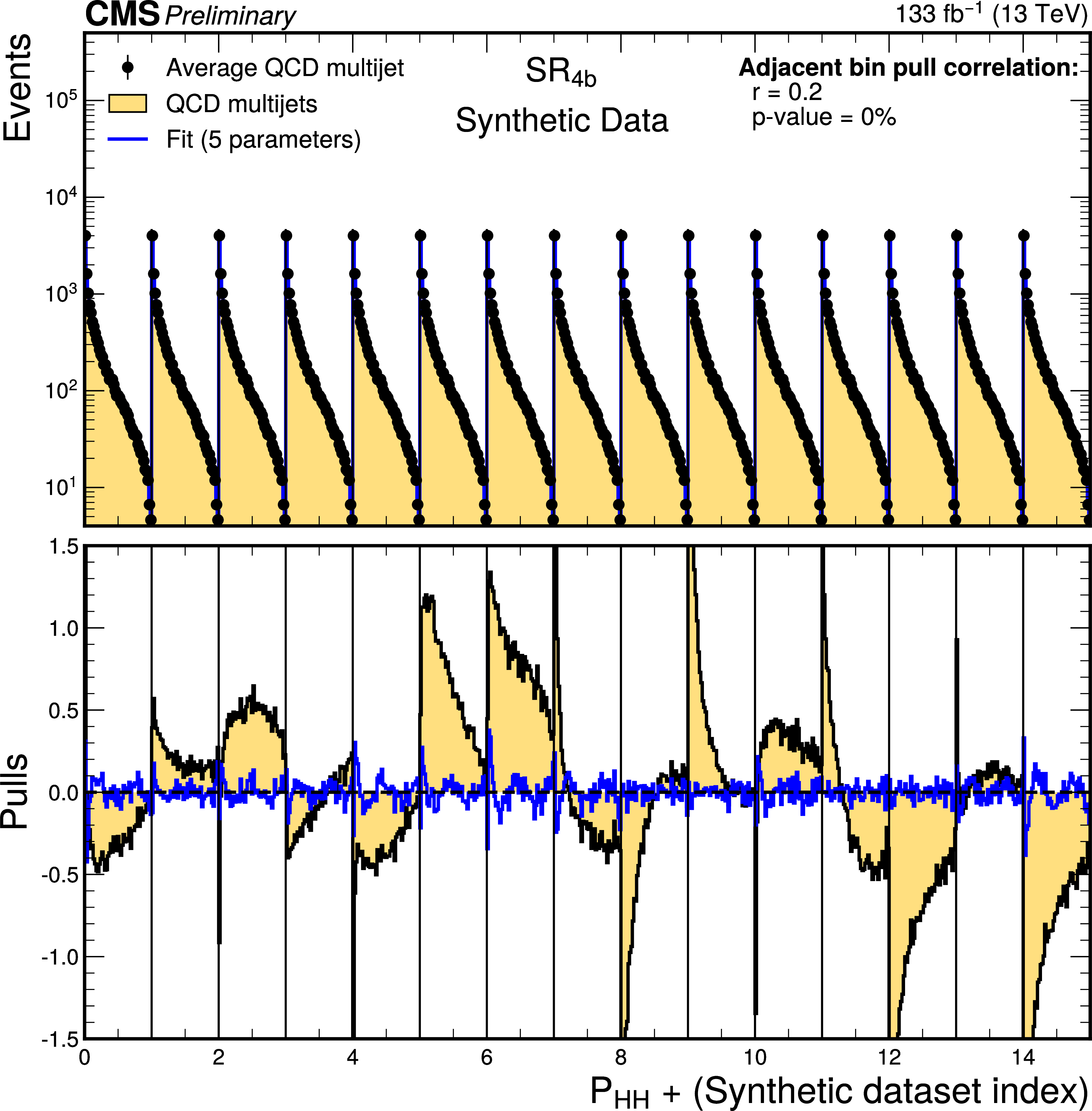
png pdf	Additional Figure 31-e: The predicted QCD multijet HH probability, $\mathcal{P_\mathrm{H}\mathrm{H}}$, distributions for each of the 15 synthetic datasets in the signal region (yellow regions). The distribution from each synthetic data is offset by the data sample index number. The black points give the average of the 15 data samples. The solid blue curves show a fit to the individual distributions using an increasing number of basis functions from one in the upper left plot to six in the lowest right plot. The lower panels show the pulls before (yellow histogram) and after (blue histogram) adding the basis corrections. The correlation coefficient (r) for a fit testing for correlations is given in the legend, along with the p-value used to test for lack of correlation. Basis functions are added until the p-value is greater than 5%. Distributions correspond to the Run 2 analysis in the resolved topology described in the note
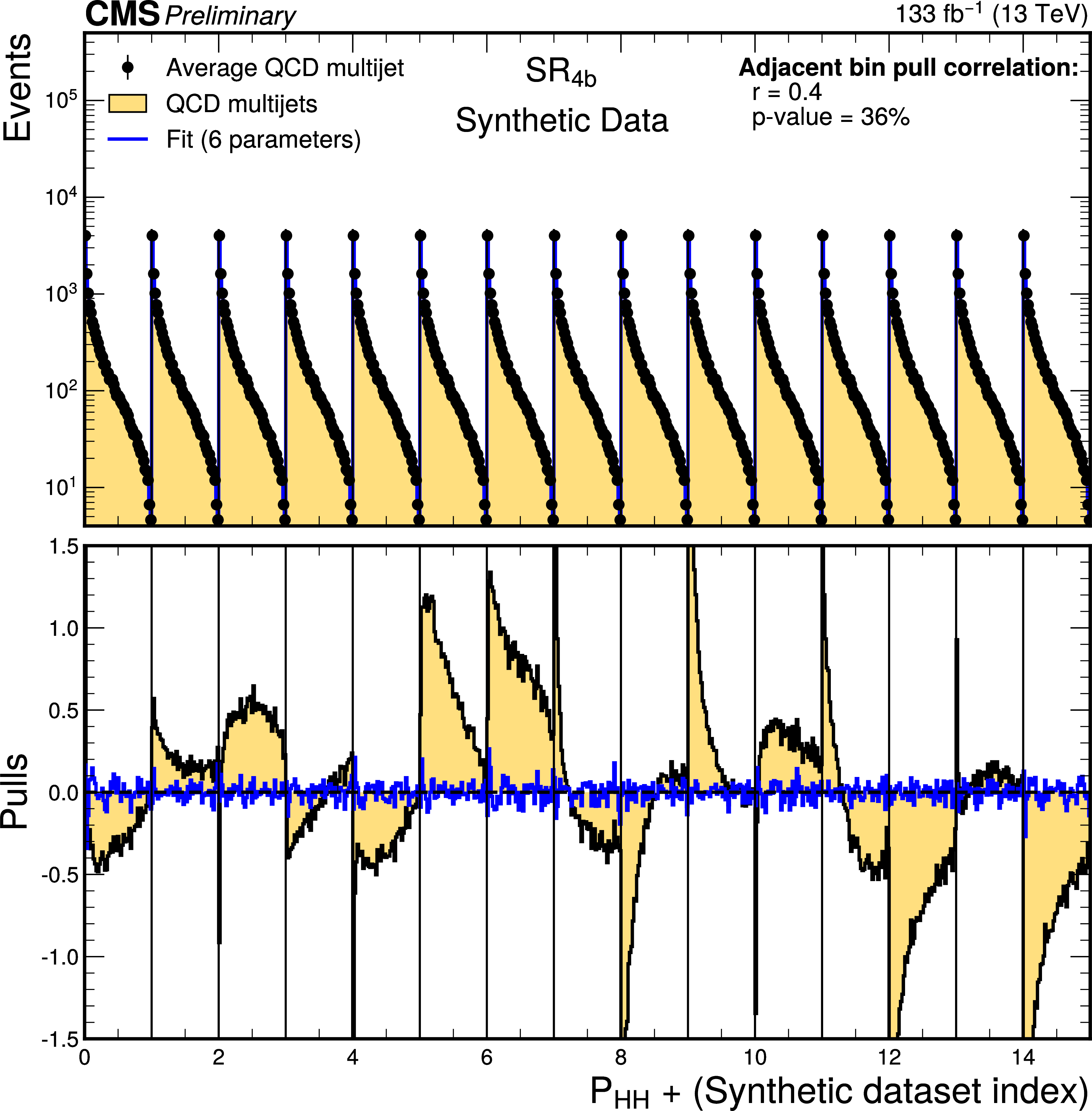
png pdf	Additional Figure 31-f: The predicted QCD multijet HH probability, $\mathcal{P_\mathrm{H}\mathrm{H}}$, distributions for each of the 15 synthetic datasets in the signal region (yellow regions). The distribution from each synthetic data is offset by the data sample index number. The black points give the average of the 15 data samples. The solid blue curves show a fit to the individual distributions using an increasing number of basis functions from one in the upper left plot to six in the lowest right plot. The lower panels show the pulls before (yellow histogram) and after (blue histogram) adding the basis corrections. The correlation coefficient (r) for a fit testing for correlations is given in the legend, along with the p-value used to test for lack of correlation. Basis functions are added until the p-value is greater than 5%. Distributions correspond to the Run 2 analysis in the resolved topology described in the note
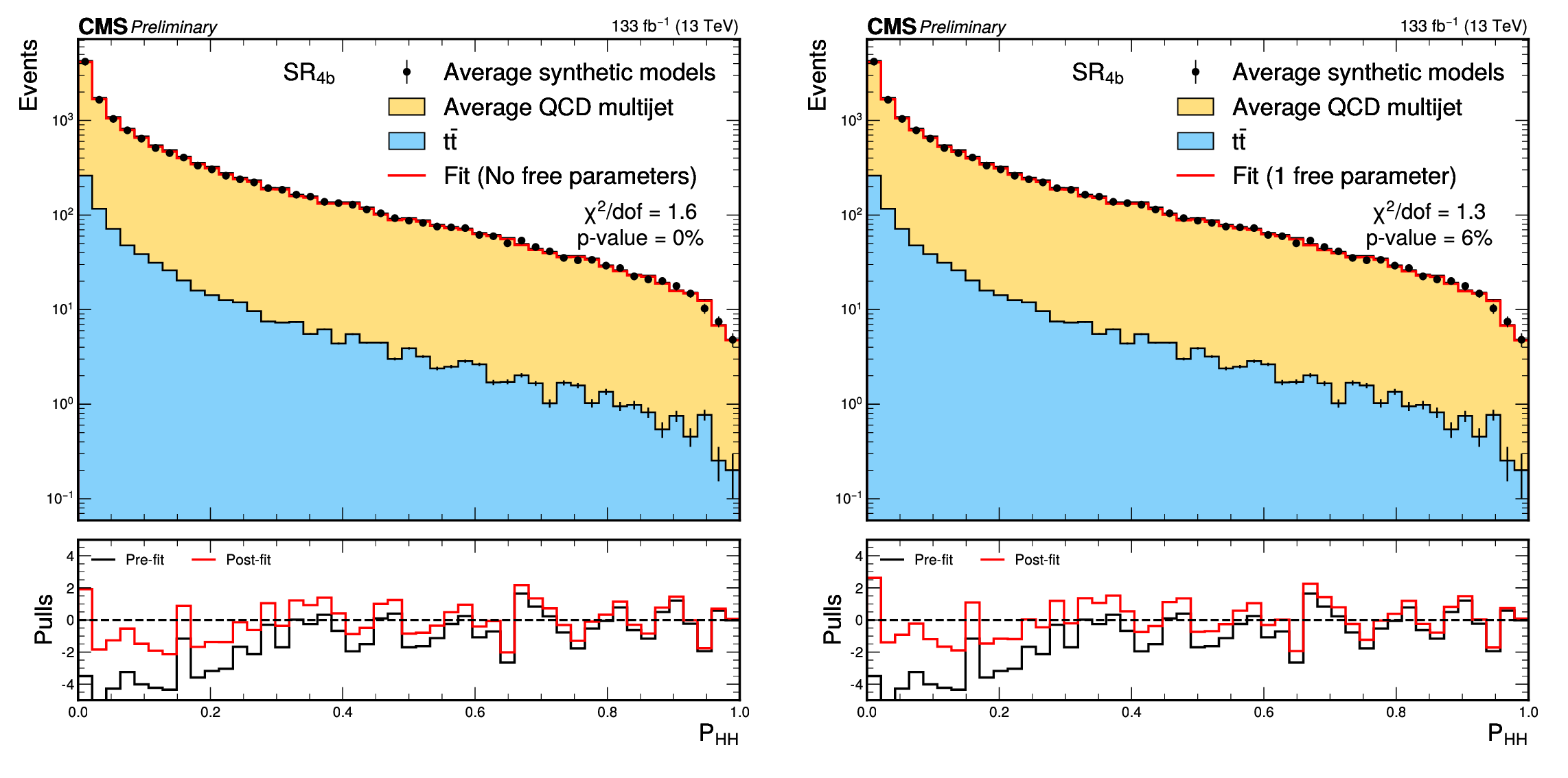
png pdf	Additional Figure 32: Distributions of the HH signal probability, $\mathcal{P_\mathrm{H}\mathrm{H}}$, for the average observed signal region yields from the synthetic dataset models. The yellow and blue regions give the distributions of the average of the QCD multijet models and the tt simulation, respectively. The red histogram displays the post-fit results of the data fit to the background model with 0 (left) and 1 unconstrained parameter (right) in the fit. The $\chi^2$ / dof and the p-value from the fit are shown in the legend. The lower panels give the pre- (black histograms) and post-fit (red histograms) pulls. Distributions correspond to the Run 2 analysis in the resolved topology described in the note.
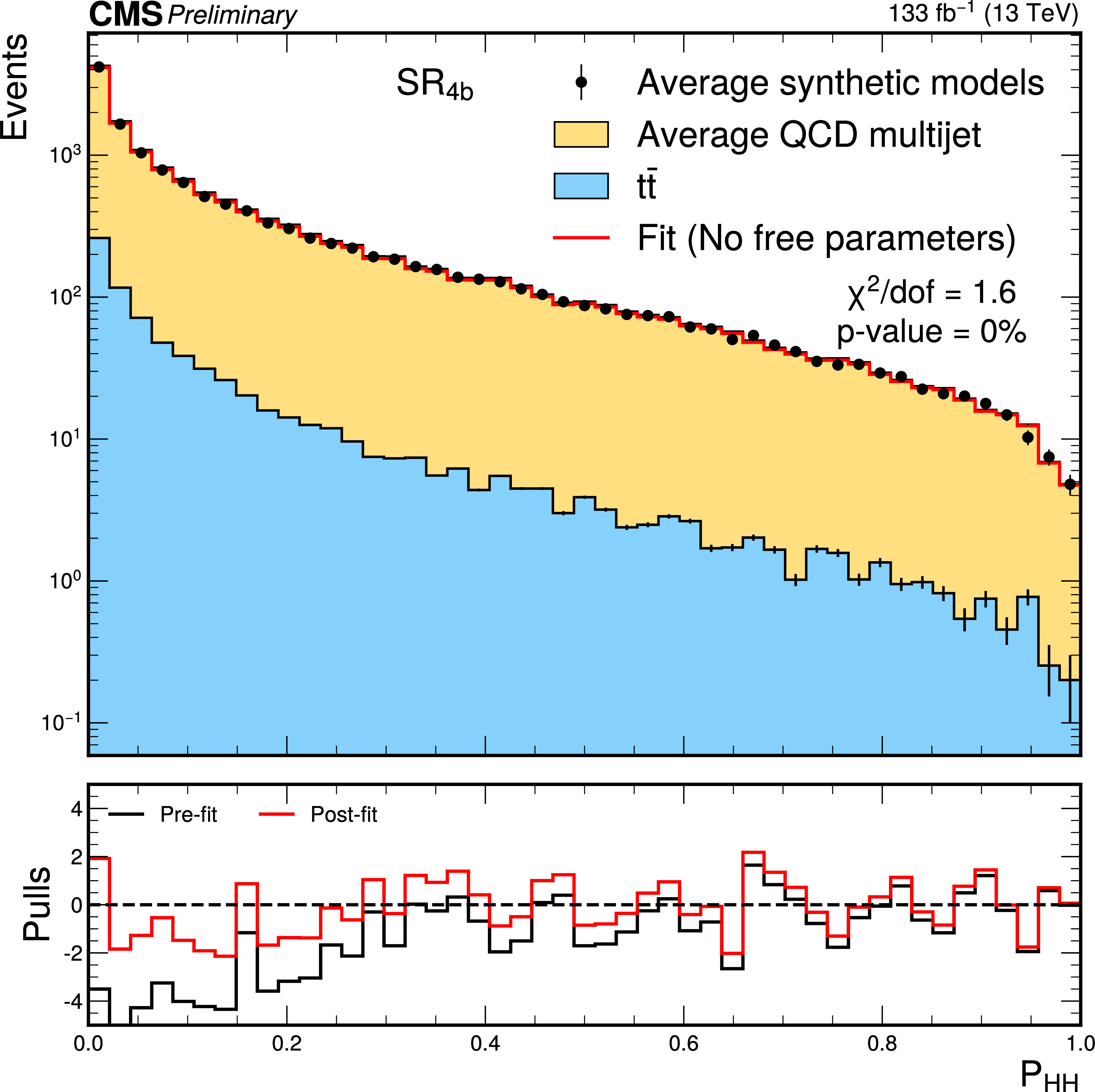
png pdf	Additional Figure 32-a: Distributions of the HH signal probability, $\mathcal{P_\mathrm{H}\mathrm{H}}$, for the average observed signal region yields from the synthetic dataset models. The yellow and blue regions give the distributions of the average of the QCD multijet models and the tt simulation, respectively. The red histogram displays the post-fit results of the data fit to the background model with 0 (left) and 1 unconstrained parameter (right) in the fit. The $\chi^2$ / dof and the p-value from the fit are shown in the legend. The lower panels give the pre- (black histograms) and post-fit (red histograms) pulls. Distributions correspond to the Run 2 analysis in the resolved topology described in the note.
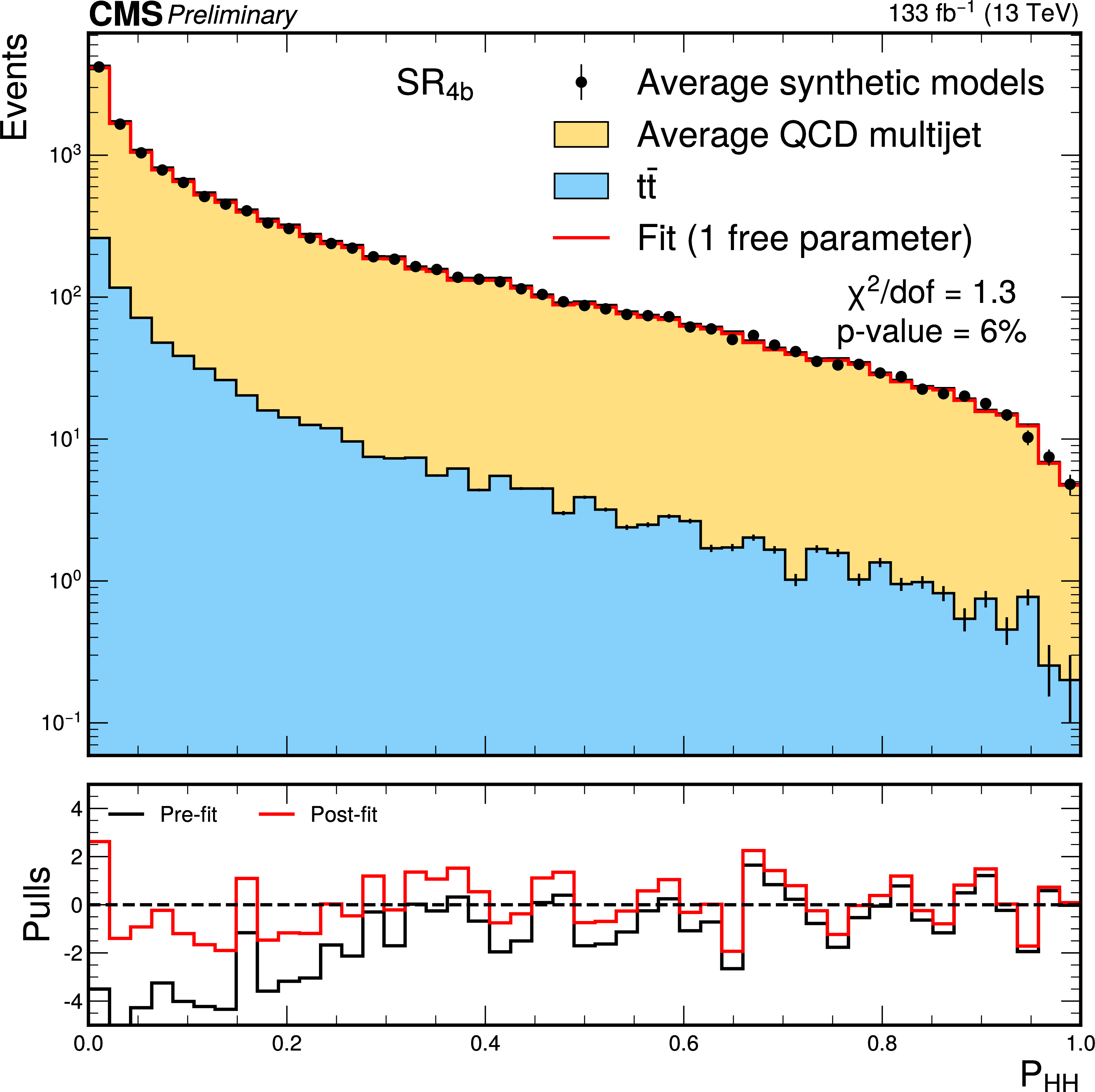
png pdf	Additional Figure 32-b: Distributions of the HH signal probability, $\mathcal{P_\mathrm{H}\mathrm{H}}$, for the average observed signal region yields from the synthetic dataset models. The yellow and blue regions give the distributions of the average of the QCD multijet models and the tt simulation, respectively. The red histogram displays the post-fit results of the data fit to the background model with 0 (left) and 1 unconstrained parameter (right) in the fit. The $\chi^2$ / dof and the p-value from the fit are shown in the legend. The lower panels give the pre- (black histograms) and post-fit (red histograms) pulls. Distributions correspond to the Run 2 analysis in the resolved topology described in the note.
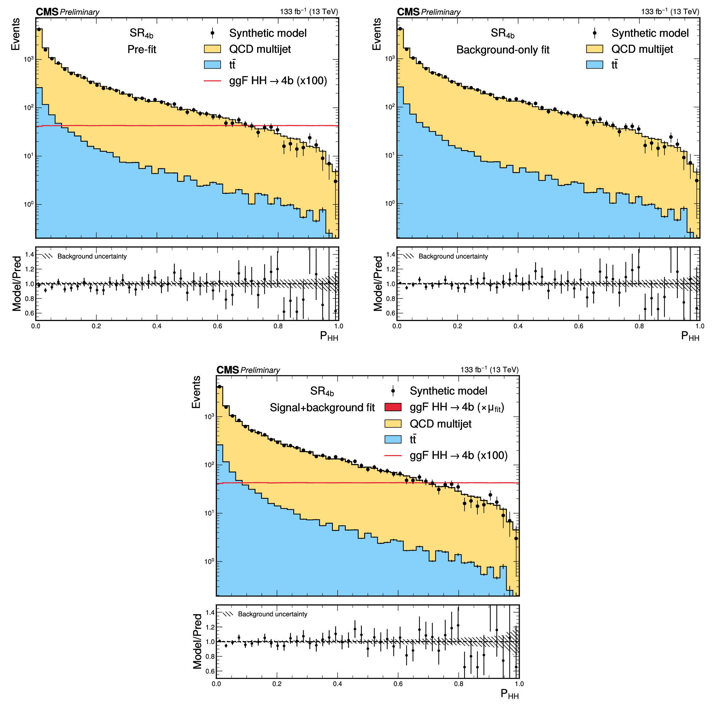
png pdf	Additional Figure 33: The prefit, background-only fit, and signal plus background distributions of the signal probability, $\mathcal{P_\mathrm{H}\mathrm{H}}$. The black points show one of the synthetic datasets. The yellow and blue regions show the predictions from the QCD multijet model and the $\mathrm{t}\mathrm{\bar{t}}$ simulation, respectively. The predictions for the $ \mathrm{H}\mathrm{H} $ signal distributions are given by the red histograms, multiplied by 100. The lower panels show the data-to-background ratio, with the hatched area representing the background uncertainty. Distributions correspond to the Run 2 analysis in the resolved topology described in the note.
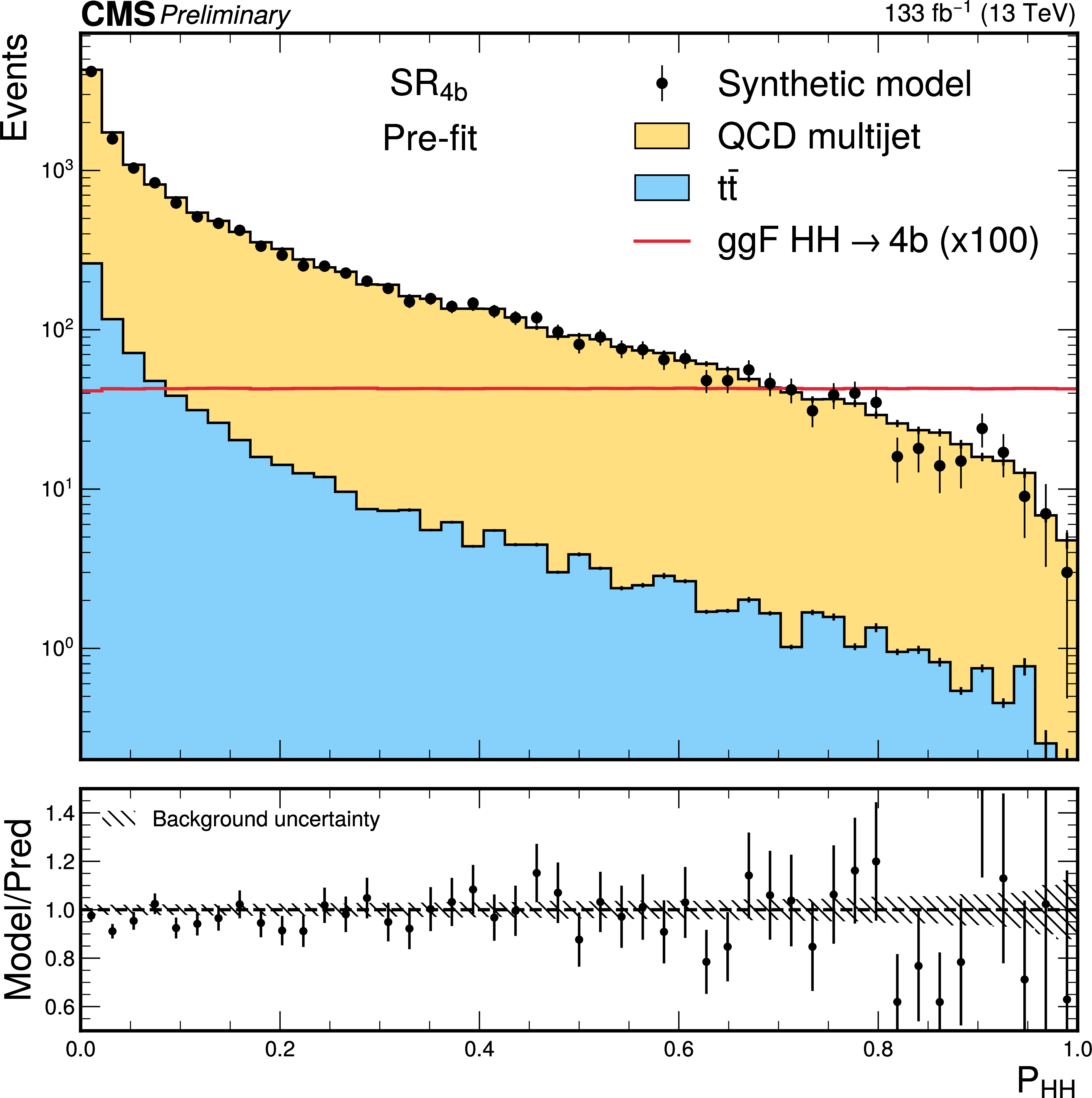
png pdf	Additional Figure 33-a: The prefit, background-only fit, and signal plus background distributions of the signal probability, $\mathcal{P_\mathrm{H}\mathrm{H}}$. The black points show one of the synthetic datasets. The yellow and blue regions show the predictions from the QCD multijet model and the $\mathrm{t}\mathrm{\bar{t}}$ simulation, respectively. The predictions for the $ \mathrm{H}\mathrm{H} $ signal distributions are given by the red histograms, multiplied by 100. The lower panels show the data-to-background ratio, with the hatched area representing the background uncertainty. Distributions correspond to the Run 2 analysis in the resolved topology described in the note.
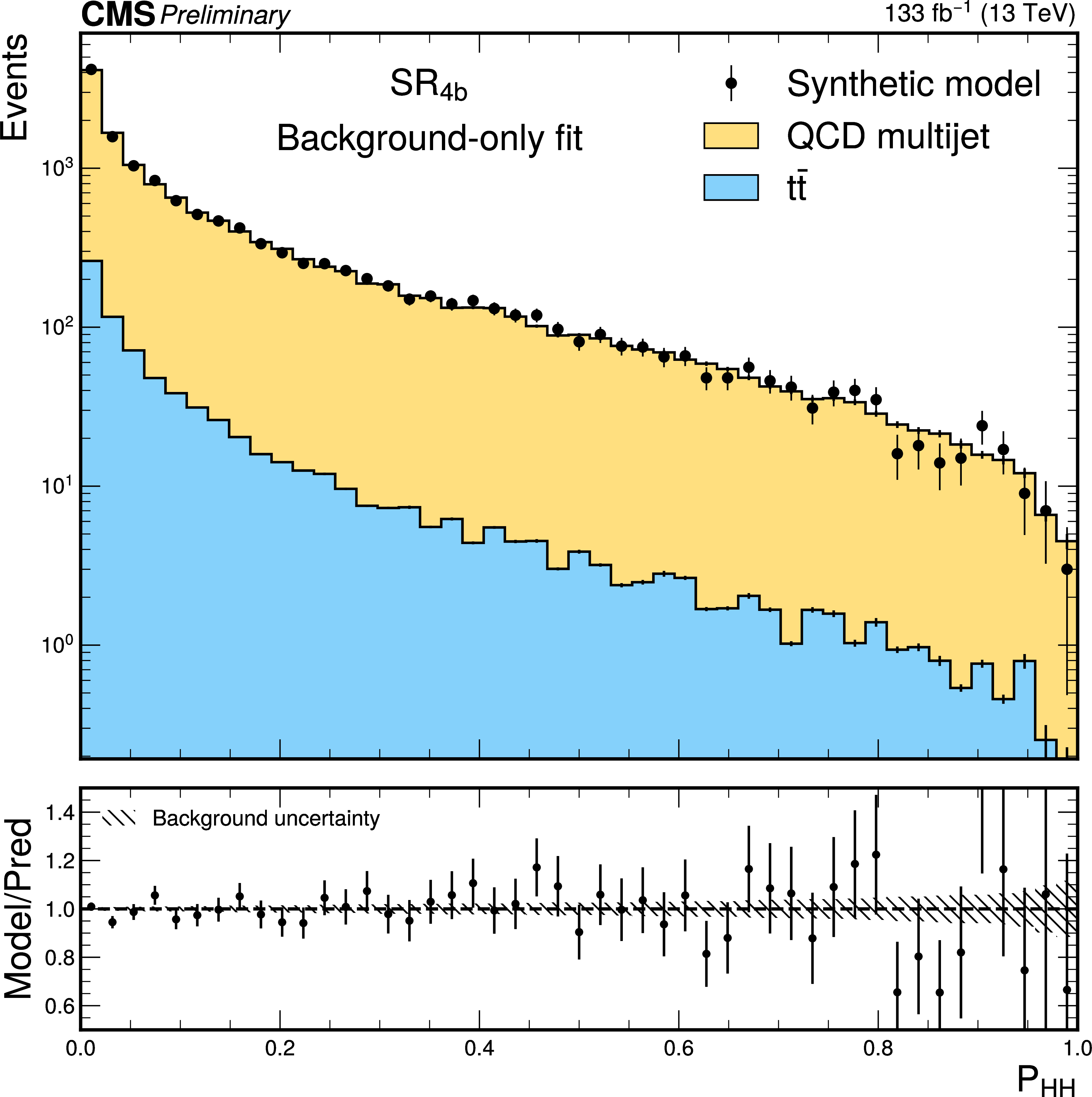
png pdf	Additional Figure 33-b: The prefit, background-only fit, and signal plus background distributions of the signal probability, $\mathcal{P_\mathrm{H}\mathrm{H}}$. The black points show one of the synthetic datasets. The yellow and blue regions show the predictions from the QCD multijet model and the $\mathrm{t}\mathrm{\bar{t}}$ simulation, respectively. The predictions for the $ \mathrm{H}\mathrm{H} $ signal distributions are given by the red histograms, multiplied by 100. The lower panels show the data-to-background ratio, with the hatched area representing the background uncertainty. Distributions correspond to the Run 2 analysis in the resolved topology described in the note.
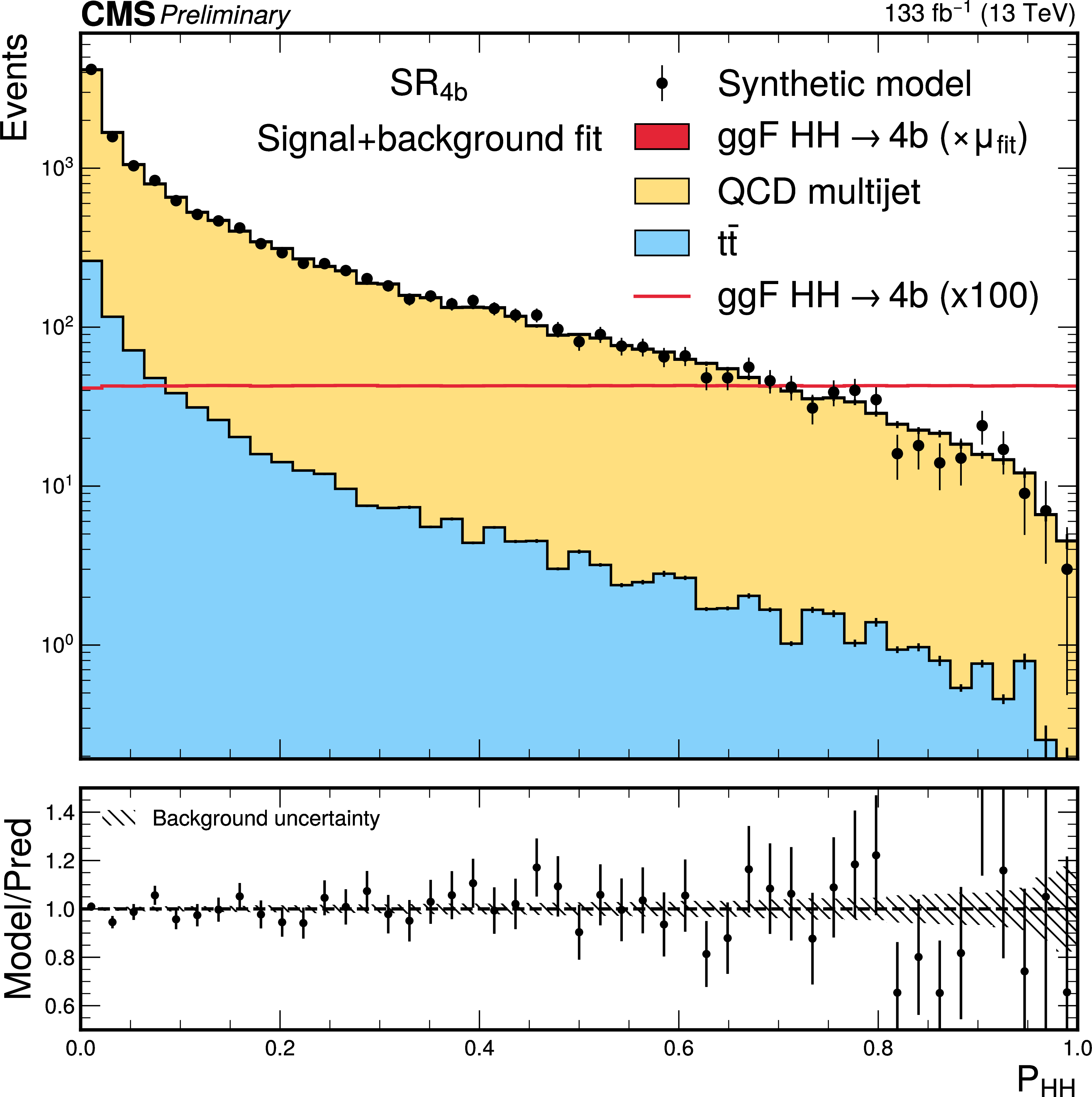
png pdf	Additional Figure 33-c: The prefit, background-only fit, and signal plus background distributions of the signal probability, $\mathcal{P_\mathrm{H}\mathrm{H}}$. The black points show one of the synthetic datasets. The yellow and blue regions show the predictions from the QCD multijet model and the $\mathrm{t}\mathrm{\bar{t}}$ simulation, respectively. The predictions for the $ \mathrm{H}\mathrm{H} $ signal distributions are given by the red histograms, multiplied by 100. The lower panels show the data-to-background ratio, with the hatched area representing the background uncertainty. Distributions correspond to the Run 2 analysis in the resolved topology described in the note.
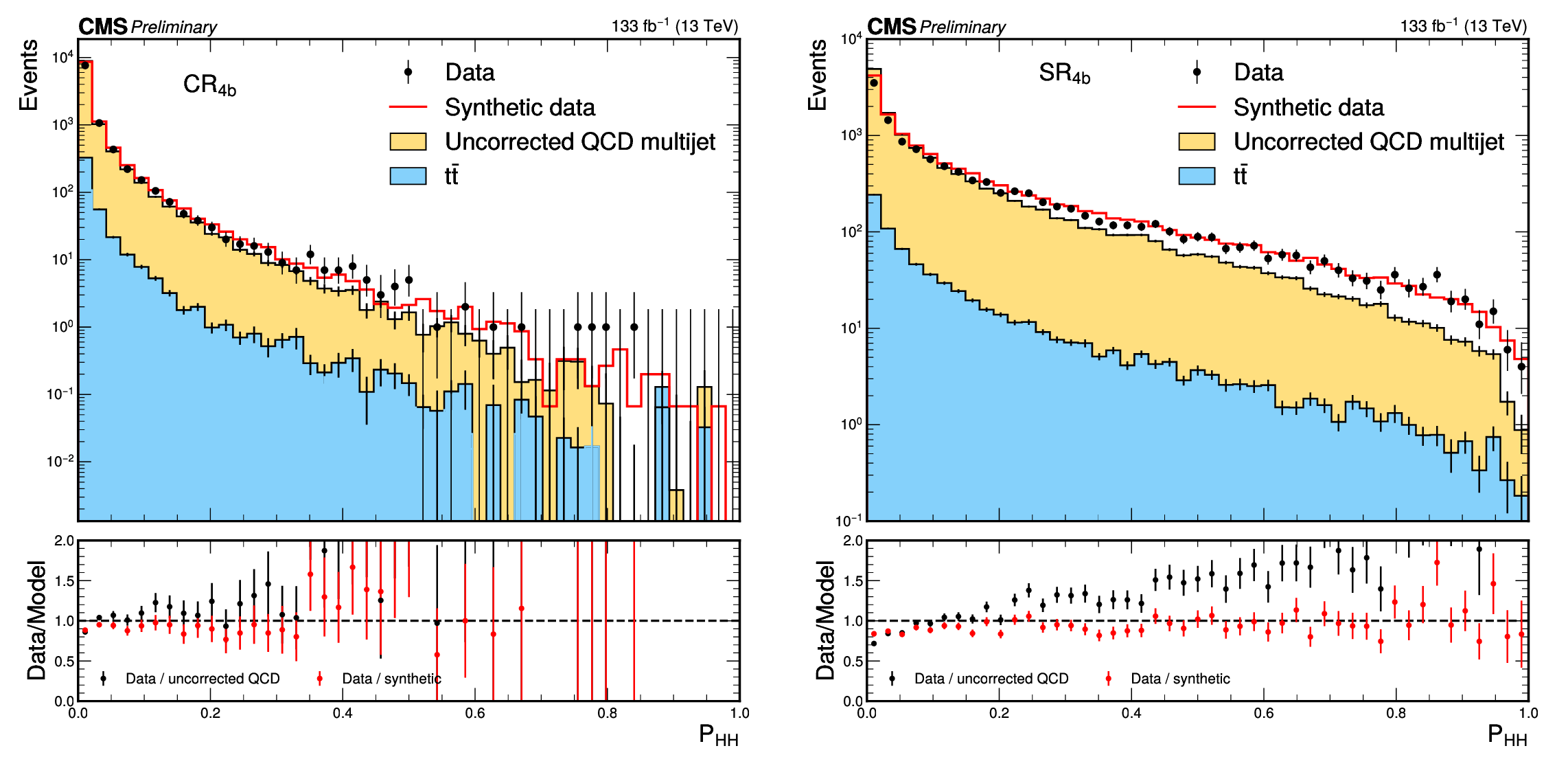
png pdf	Additional Figure 34: Distribution of the signal probability for HH, $\mathcal{P_\mathrm{H}\mathrm{H}}$, in the control region (left) and signal region (right). The 4b data events, with slightly different trigger requirements, are shown as black points. The QCD multijet distribution before kinematic corrections is shown as the yellow-filled histogram, and the simulated $\mathrm{t}\mathrm{\bar{t}}$ distribution is shown as the blue-filled histogram. The average of the synthetic datasets (red) provides a high-event-count proxy for the 4b background (black), allowing the background model to be extrapolated and tested precisely. The lower panels display the ratio of the 4b data to the average of the synthetic datasets (red) and to the QCD multijet distribution (black). Distributions correspond to the Run 2 analysis in the resolved topology described in the note.
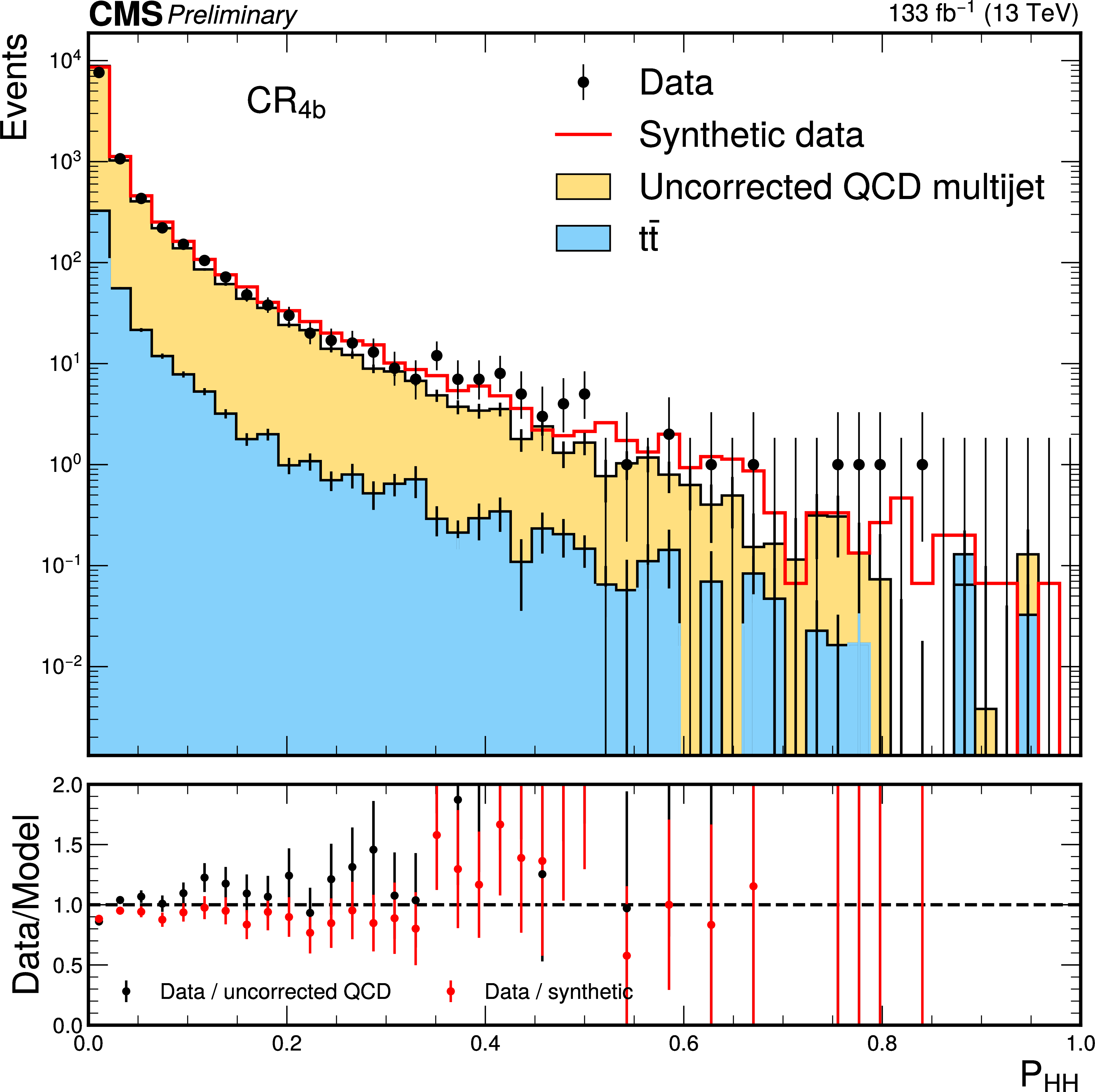
png pdf	Additional Figure 34-a: Distribution of the signal probability for HH, $\mathcal{P_\mathrm{H}\mathrm{H}}$, in the control region (left) and signal region (right). The 4b data events, with slightly different trigger requirements, are shown as black points. The QCD multijet distribution before kinematic corrections is shown as the yellow-filled histogram, and the simulated $\mathrm{t}\mathrm{\bar{t}}$ distribution is shown as the blue-filled histogram. The average of the synthetic datasets (red) provides a high-event-count proxy for the 4b background (black), allowing the background model to be extrapolated and tested precisely. The lower panels display the ratio of the 4b data to the average of the synthetic datasets (red) and to the QCD multijet distribution (black). Distributions correspond to the Run 2 analysis in the resolved topology described in the note.
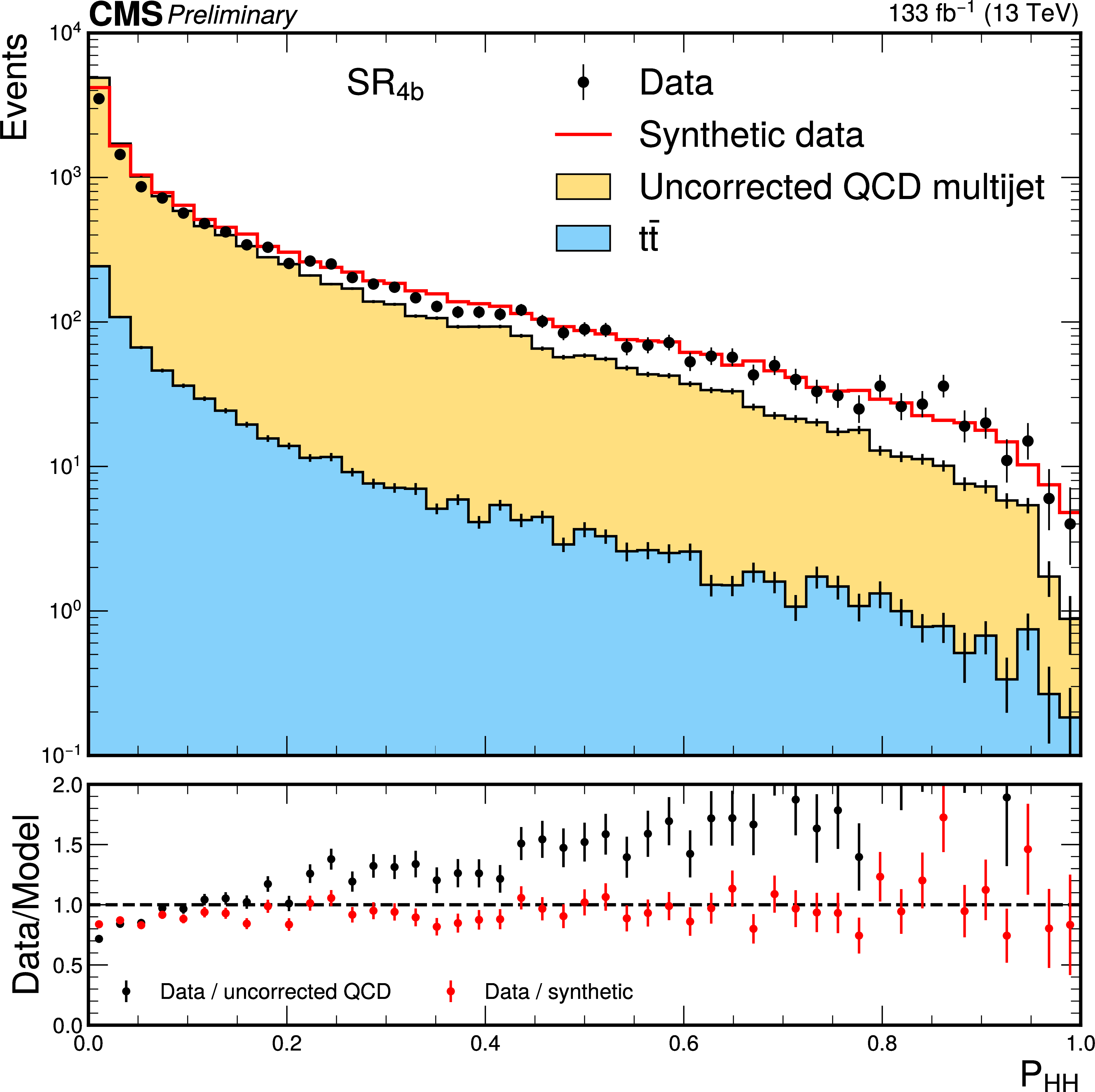
png pdf	Additional Figure 34-b: Distribution of the signal probability for HH, $\mathcal{P_\mathrm{H}\mathrm{H}}$, in the control region (left) and signal region (right). The 4b data events, with slightly different trigger requirements, are shown as black points. The QCD multijet distribution before kinematic corrections is shown as the yellow-filled histogram, and the simulated $\mathrm{t}\mathrm{\bar{t}}$ distribution is shown as the blue-filled histogram. The average of the synthetic datasets (red) provides a high-event-count proxy for the 4b background (black), allowing the background model to be extrapolated and tested precisely. The lower panels display the ratio of the 4b data to the average of the synthetic datasets (red) and to the QCD multijet distribution (black). Distributions correspond to the Run 2 analysis in the resolved topology described in the note.
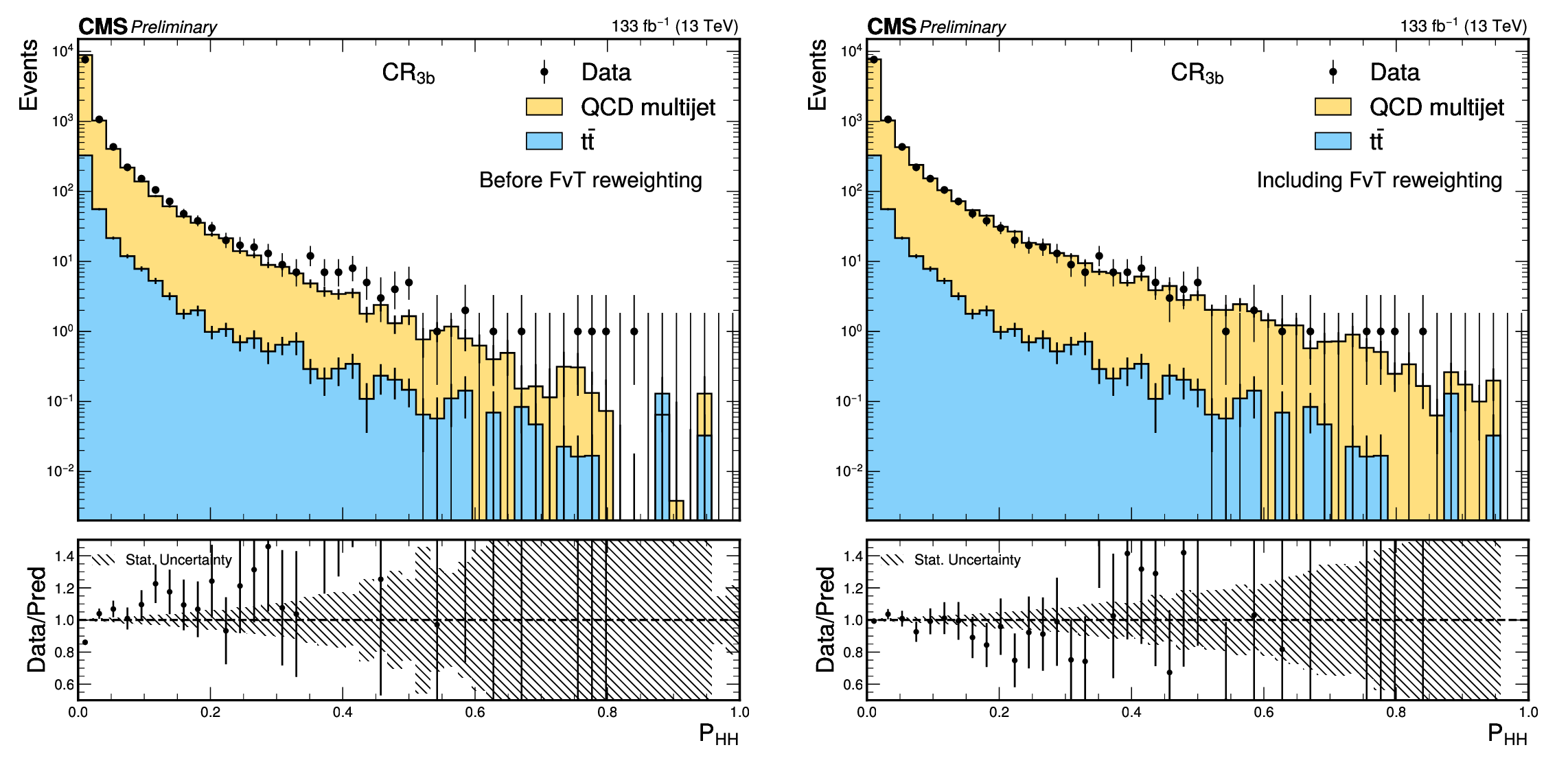
png pdf	Additional Figure 35: Distributions of the signal probabilities, $\mathcal{P_\mathrm{H}\mathrm{H}}$, in the control region. The points show the 4b events. The QCD multijet distribution (yellow region) is from the 3b data control region, before kinematic corrections (FvT reweighting) on the left and after those corrections on the right. The tt distribution (blue region) is from simulations. The lower panels display the ratio of the 4b data to the total background, which is the sum of the QCD multijet and $\mathrm{t}\mathrm{\bar{t}}$ distributions. The hatched area gives the statistical uncertainty in the background. Distributions correspond to the Run 2 analysis in the resolved topology described in the note.
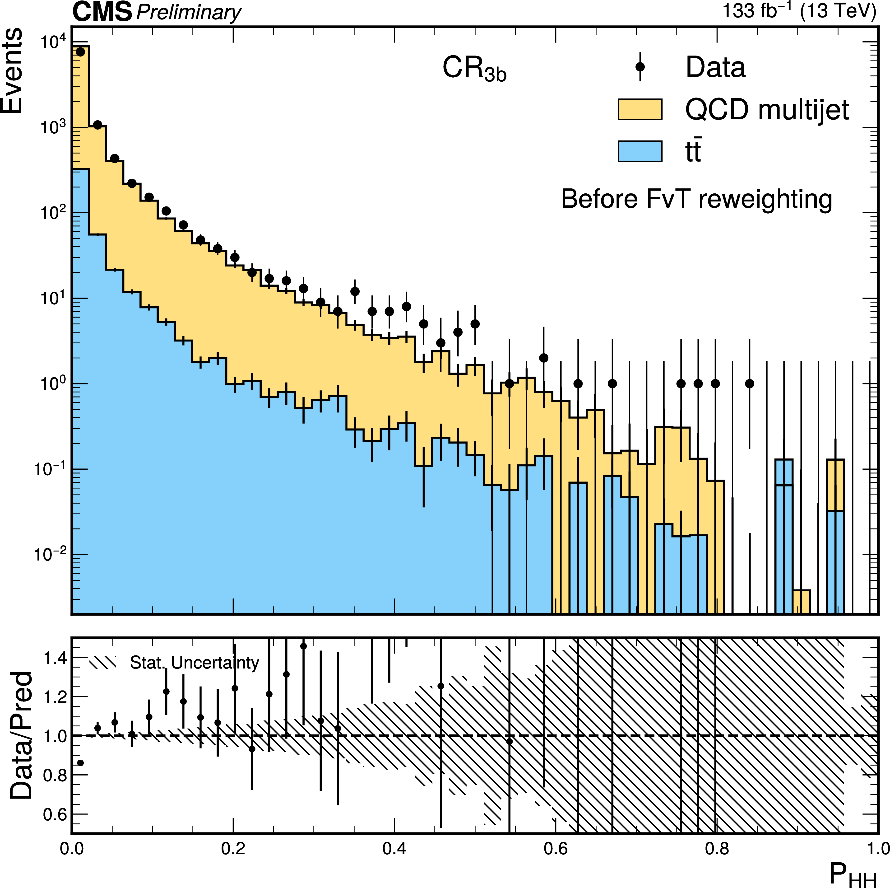
png pdf	Additional Figure 35-a: Distributions of the signal probabilities, $\mathcal{P_\mathrm{H}\mathrm{H}}$, in the control region. The points show the 4b events. The QCD multijet distribution (yellow region) is from the 3b data control region, before kinematic corrections (FvT reweighting) on the left and after those corrections on the right. The tt distribution (blue region) is from simulations. The lower panels display the ratio of the 4b data to the total background, which is the sum of the QCD multijet and $\mathrm{t}\mathrm{\bar{t}}$ distributions. The hatched area gives the statistical uncertainty in the background. Distributions correspond to the Run 2 analysis in the resolved topology described in the note.
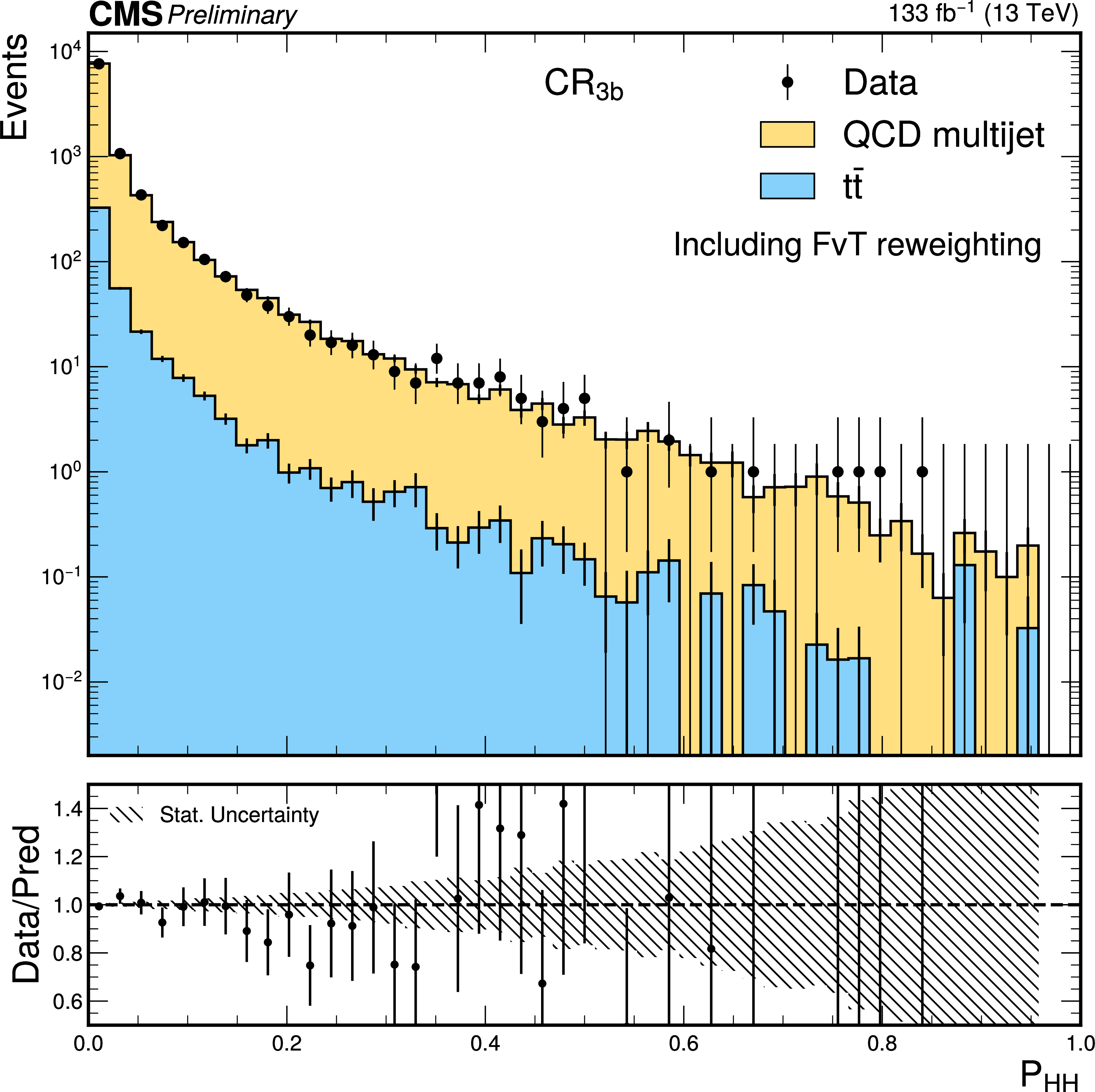
png pdf	Additional Figure 35-b: Distributions of the signal probabilities, $\mathcal{P_\mathrm{H}\mathrm{H}}$, in the control region. The points show the 4b events. The QCD multijet distribution (yellow region) is from the 3b data control region, before kinematic corrections (FvT reweighting) on the left and after those corrections on the right. The tt distribution (blue region) is from simulations. The lower panels display the ratio of the 4b data to the total background, which is the sum of the QCD multijet and $\mathrm{t}\mathrm{\bar{t}}$ distributions. The hatched area gives the statistical uncertainty in the background. Distributions correspond to the Run 2 analysis in the resolved topology described in the note.
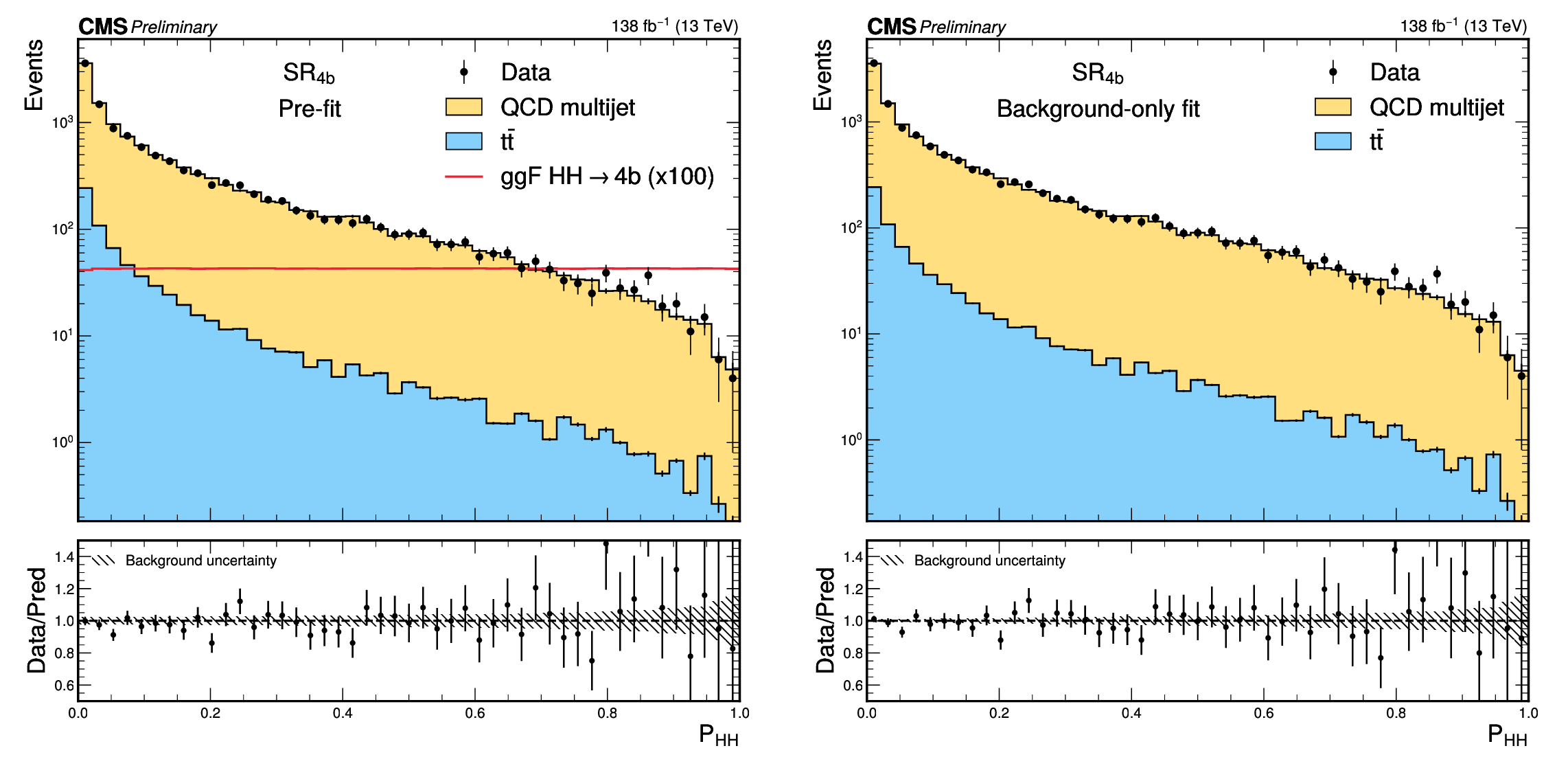
png pdf	Additional Figure 36: The prefit and background only fit signal probability, $\mathcal{P_\mathrm{H}\mathrm{H}}$, distributions. The black points show the 4b events from data. The yellow and blue regions show the predictions from the QCD multijet model and the $\mathrm{t}\mathrm{\bar{t}}$ simulation, respectively. The predictions for the $ \mathrm{H}\mathrm{H} $ signal distributions are given by the red histograms, multiplied by 100. The lower panels show the data-to-background ratio, with the hatched area representing the background uncertainty. Distributions correspond to the Run 2 analysis in the resolved topology described in the note.
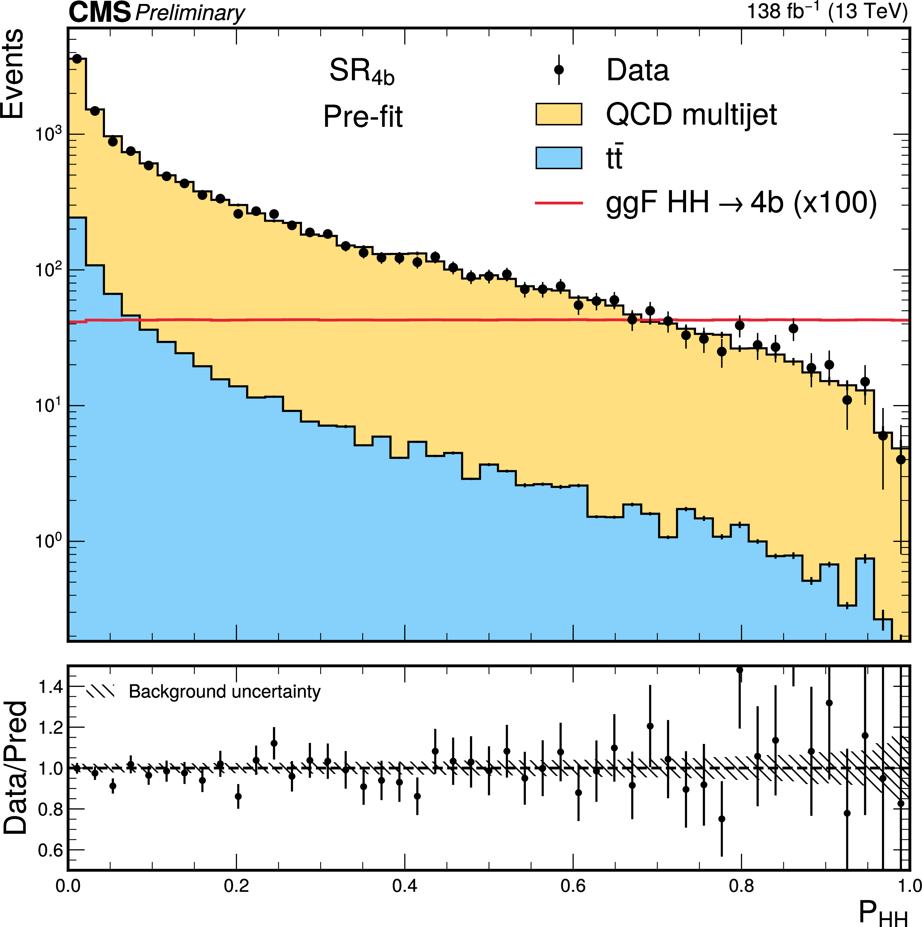
png pdf	Additional Figure 36-a: The prefit and background only fit signal probability, $\mathcal{P_\mathrm{H}\mathrm{H}}$, distributions. The black points show the 4b events from data. The yellow and blue regions show the predictions from the QCD multijet model and the $\mathrm{t}\mathrm{\bar{t}}$ simulation, respectively. The predictions for the $ \mathrm{H}\mathrm{H} $ signal distributions are given by the red histograms, multiplied by 100. The lower panels show the data-to-background ratio, with the hatched area representing the background uncertainty. Distributions correspond to the Run 2 analysis in the resolved topology described in the note.
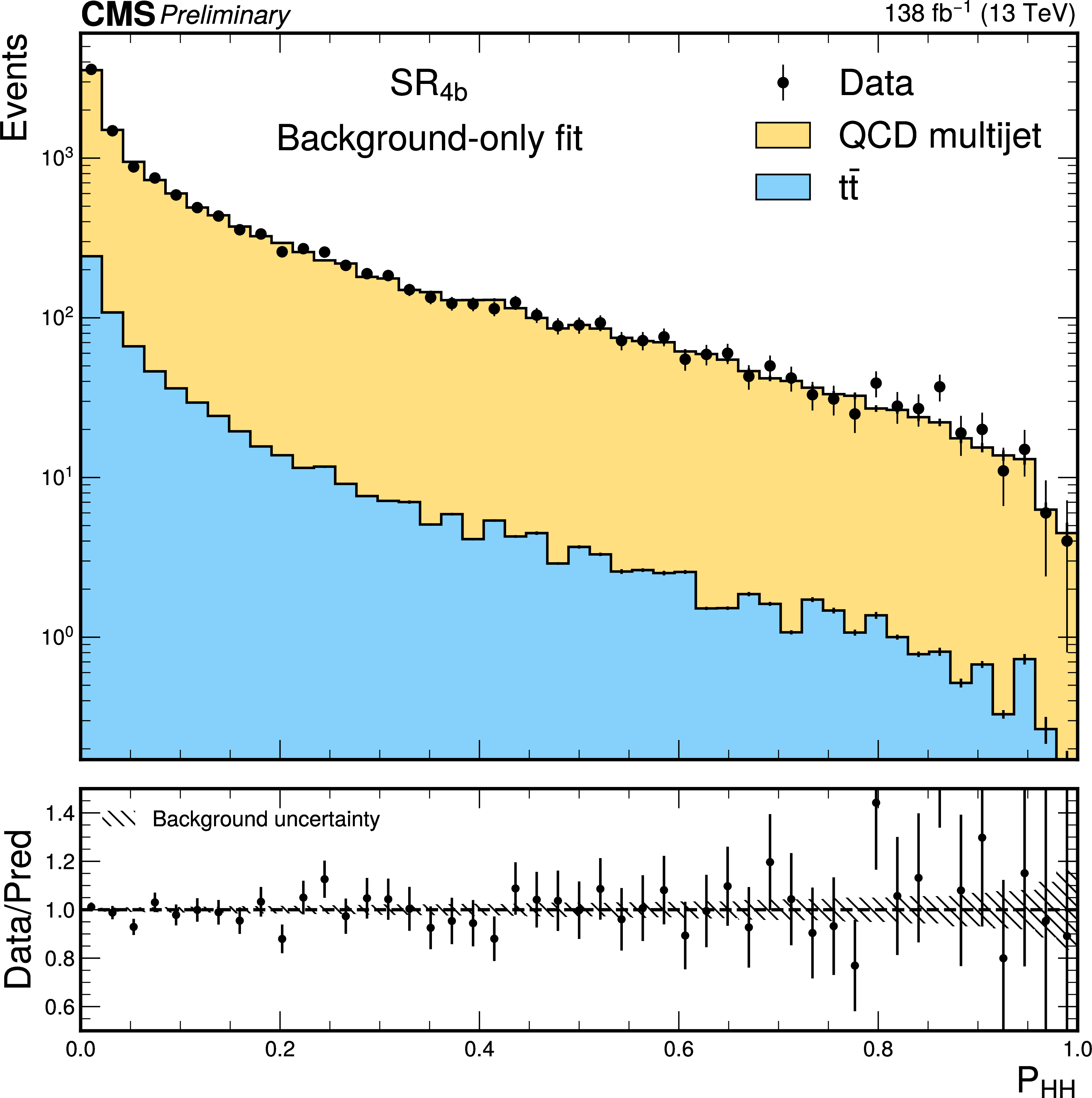
png pdf	Additional Figure 36-b: The prefit and background only fit signal probability, $\mathcal{P_\mathrm{H}\mathrm{H}}$, distributions. The black points show the 4b events from data. The yellow and blue regions show the predictions from the QCD multijet model and the $\mathrm{t}\mathrm{\bar{t}}$ simulation, respectively. The predictions for the $ \mathrm{H}\mathrm{H} $ signal distributions are given by the red histograms, multiplied by 100. The lower panels show the data-to-background ratio, with the hatched area representing the background uncertainty. Distributions correspond to the Run 2 analysis in the resolved topology described in the note.

Additional Tables
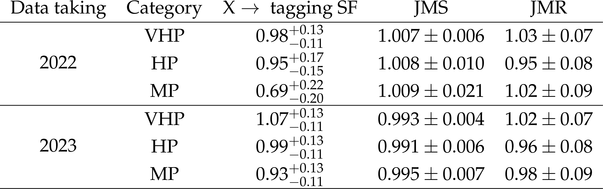
png pdf	Additional Table 1 : Efficiency, jet mass scale (JMS), and jet mass resolution (JMR) data-to-simulation scale factors measured for the GloParT mass regression separately between data collected in 2022 and 2023. Only $ \mathrm{Z} \to \mathrm{bb} $ candidates with ${P_T > 450$ GeV} are considered. Corrections for scale and resolution are applied as multiplicative factors to the predictions from simulation in the merged $ \mathrm{H}\mathrm{H} \to 4\mathrm{b} $ analysis, while efficiency scale factors are applied as per-event weights.
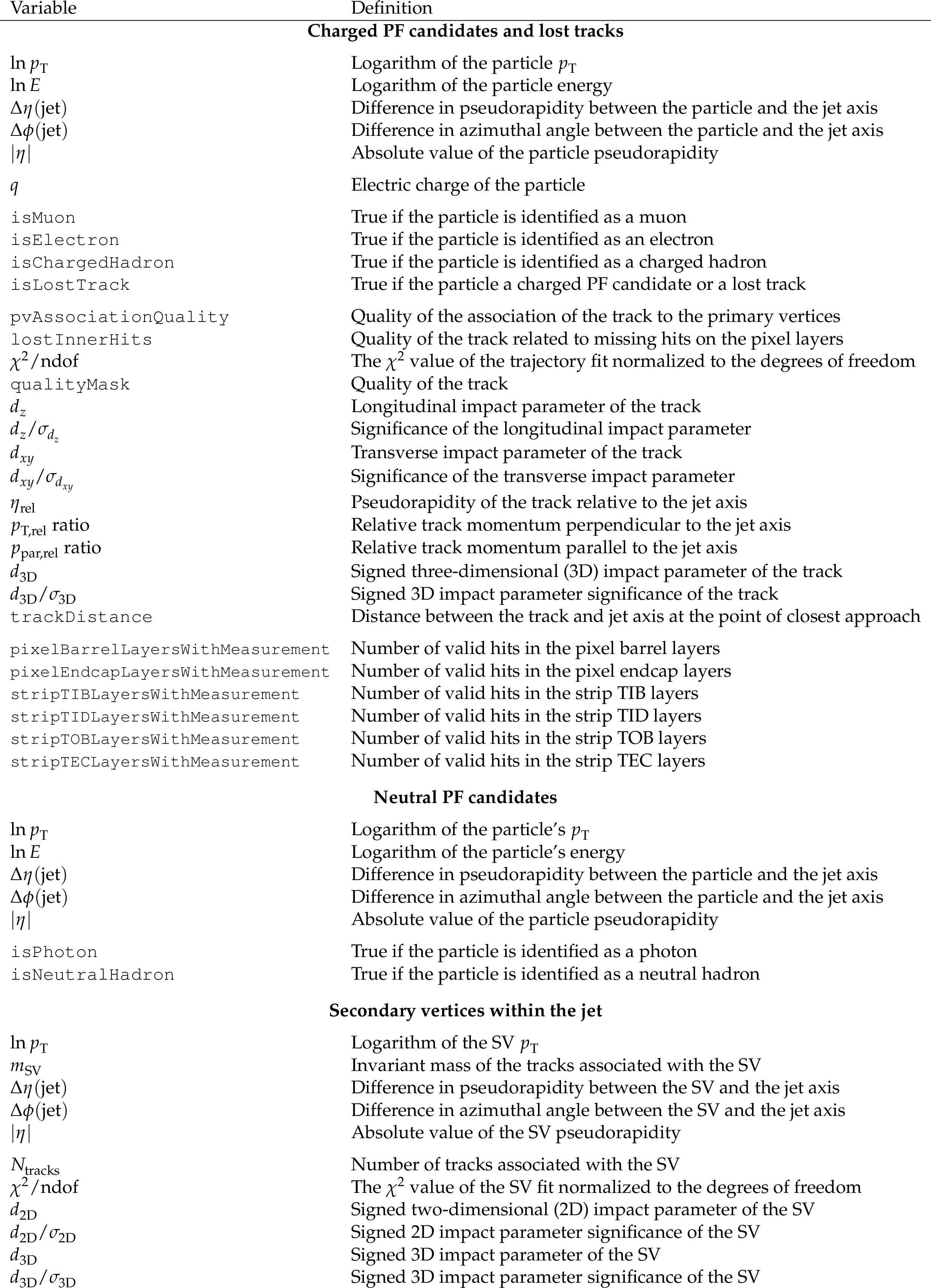
png pdf	Additional Table 2 : The complete set of input features per AK8 jet used for the GloParT model training. Three types of inputs are considered: charged PF candidates and ``lost tracks'' not associated with a charged PF candidate, neutral PF candidates, and secondary vertices (SVs)
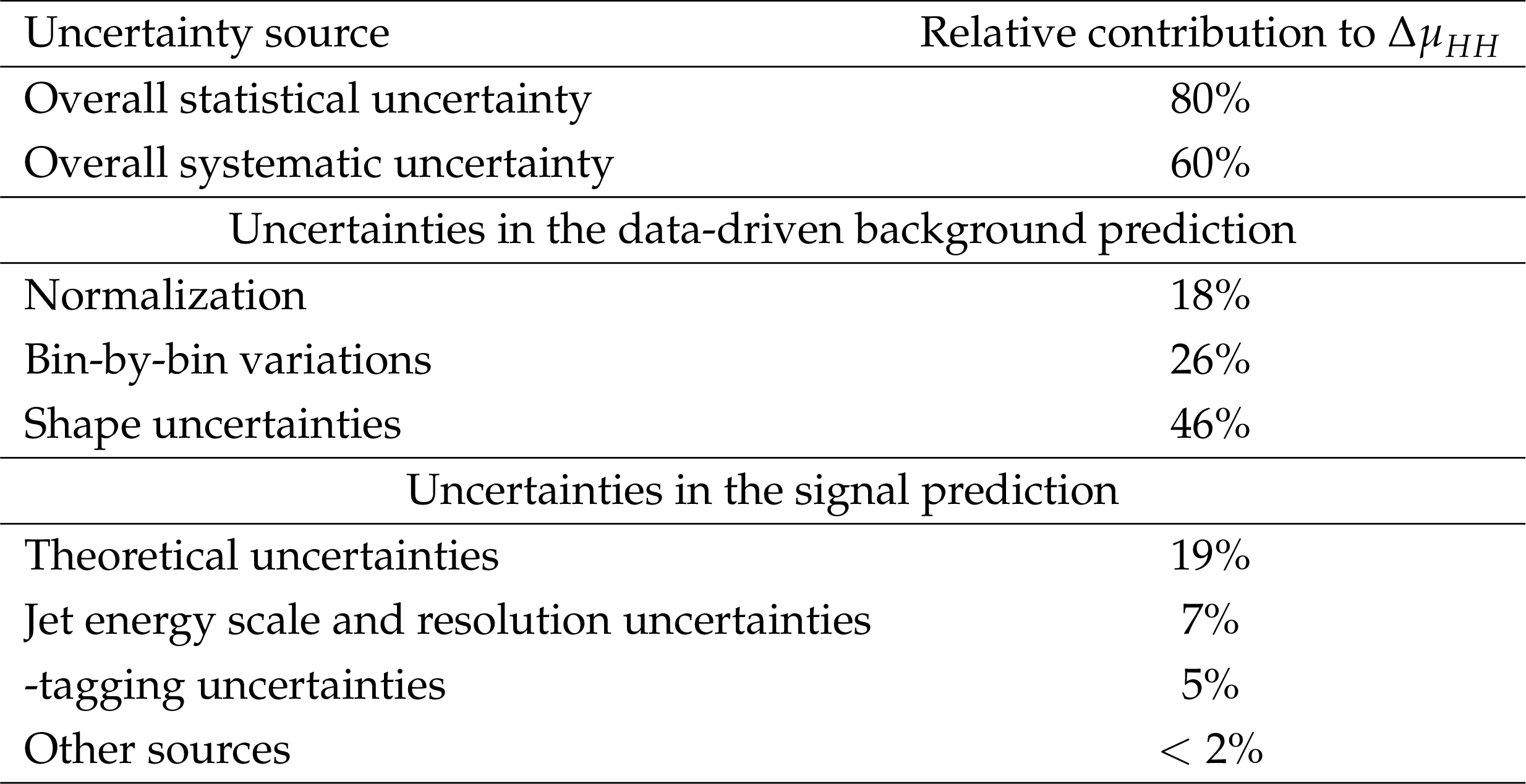
png pdf	Additional Table 3: Major sources of uncertainty in the measurement of the $\mu_{HH}$ signal strength in the resolved $ \mathrm{H}\mathrm{H} \to 4\mathrm{b} $ analysis. The post-fit uncertainty on $\mu_{HH}$ is first separated into statistical and systematic components. The systematic component is further divided into uncertainties affecting the data-driven background prediction -- primarily driven by the sample size in the regSRTwob, regCRTwob, and regCRFourb regions -- and those associated with the simulation of HH signal events. Results correspond to the first analysis approach described in the note.
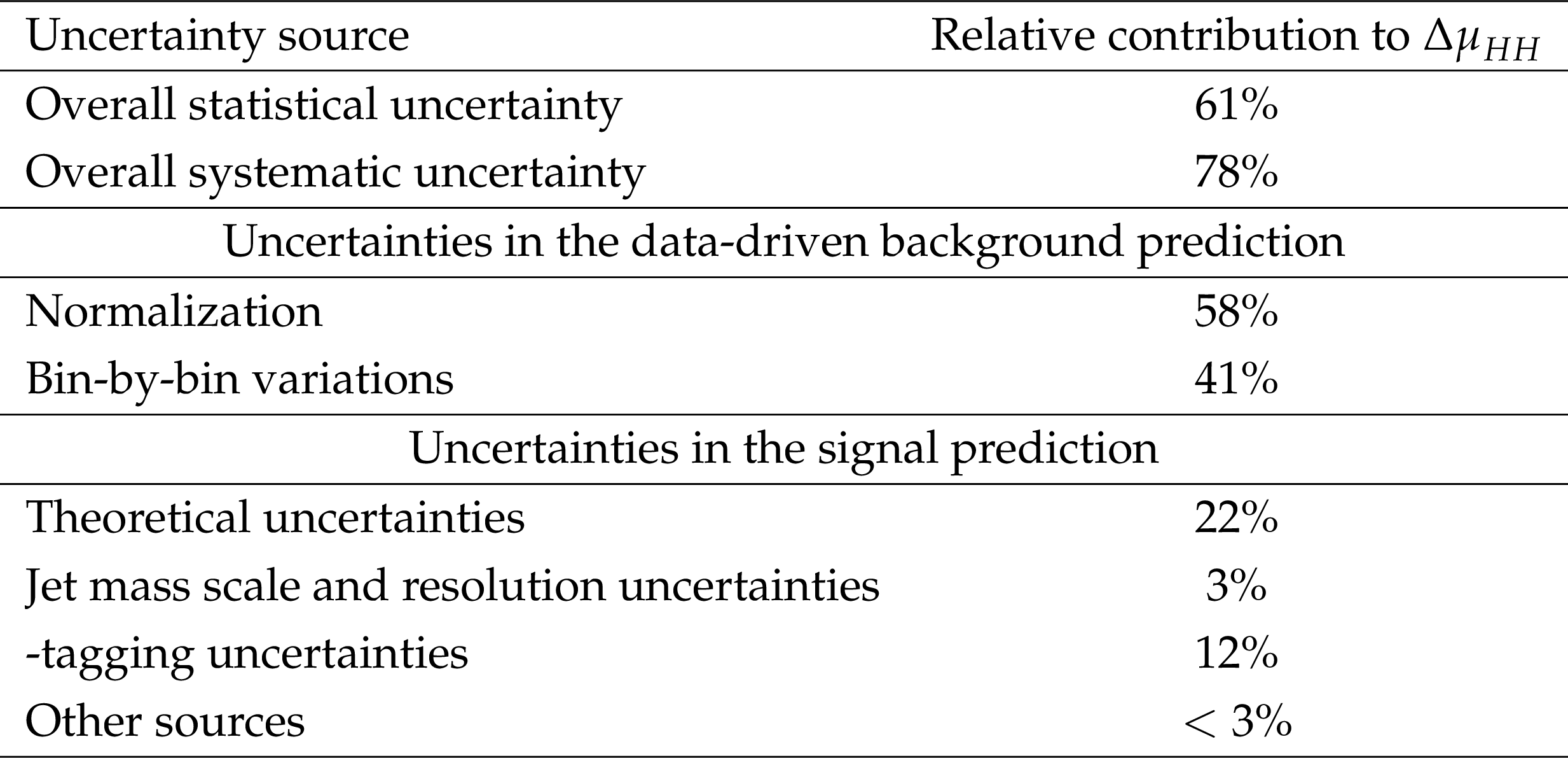
png pdf	Additional Table 4: Major sources of uncertainty in the measurement of the $\mu_{HH}$ signal strength in the merged mass-fit $ \mathrm{H}\mathrm{H} \to 4\mathrm{b} $ analysis. The post-fit uncertainty on $\mu_{HH}$ is first separated into statistical and systematic components. The systematic component is further divided into uncertainties affecting the data-driven prediction of the leading backgrounds -- primarily driven by the statistics in the QCD and $\mathrm{t}\mathrm{\bar{t}}$ control regions -- and those associated with the simulation of HH signal events. Results correspond to the first analysis approach described in the note.
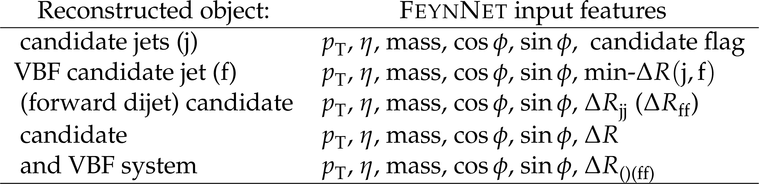
png pdf	Additional Table 5: Input observables used in the FeynNet models, for the second analysis approach of the resolved topology described in the note.
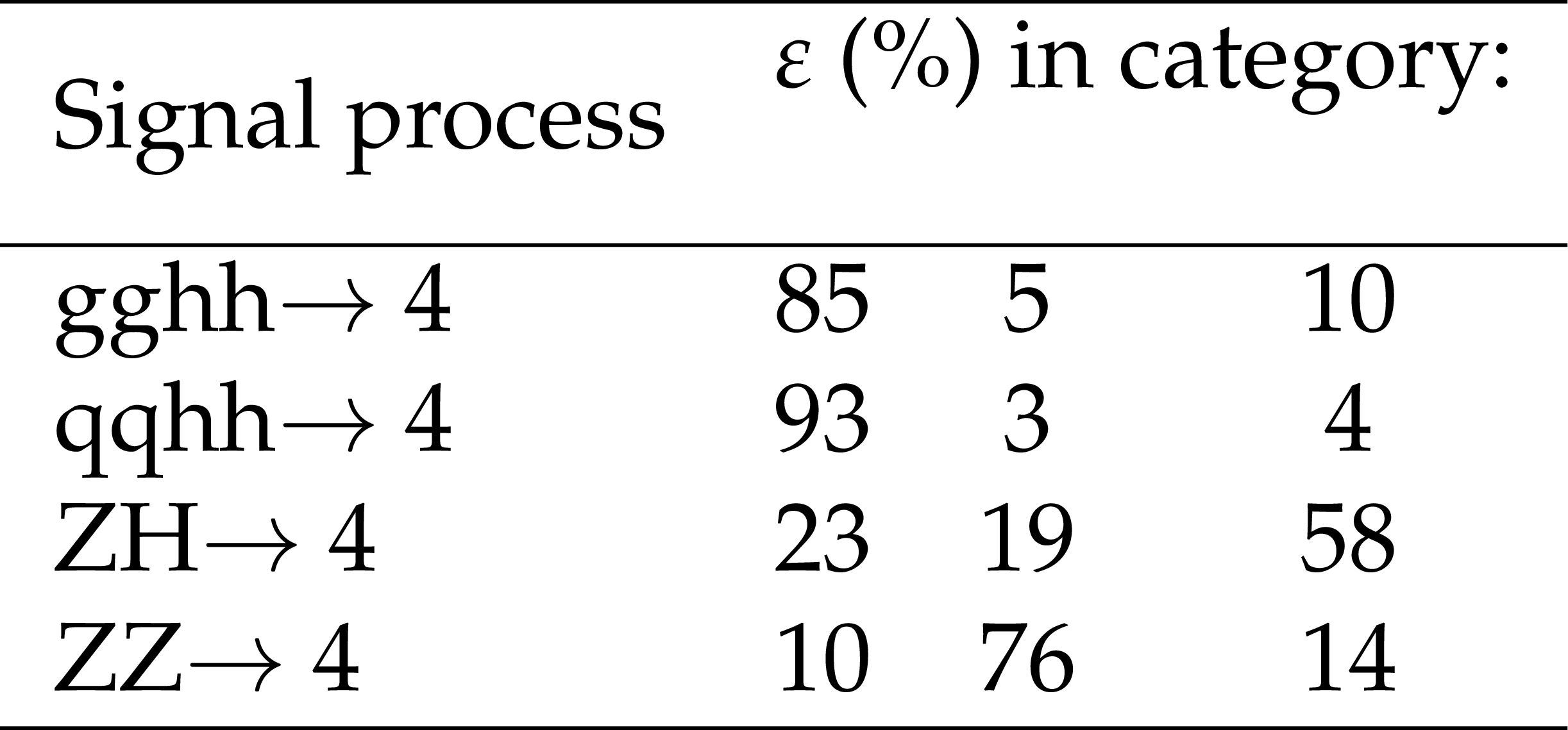
png pdf	Additional Table 6 : Efficiency of each signal process in the HH, ZZ, and ZH categories defined by the maximum FeynNet probability score in the second analysis approach of the resolved topology described in the note.
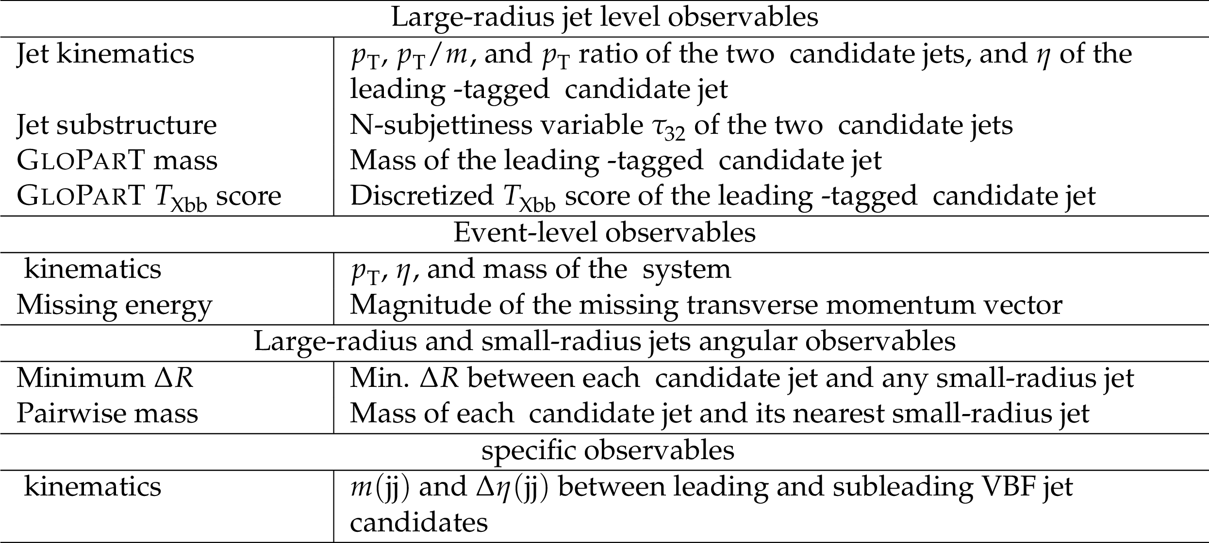
png pdf	Additional Table 7 : Input observables used in the second analysis approach of the merged topology described in the note.

References
1	F. Englert and R. Brout	Broken symmetry and the mass of gauge vector mesons	PRL 13 (1964) 321
2	P. W. Higgs	Broken symmetries, massless particles and gauge fields	PL 12 (1964) 132
3	P. W. Higgs	Broken symmetries and the masses of gauge bosons	PRL 13 (1964) 508
4	G. S. Guralnik, C. R. Hagen, and T. W. B. Kibble	Global conservation laws and massless particles	PRL 13 (1964) 585
5	P. W. Higgs	Spontaneous symmetry breakdown without massless bosons	PR 145 (1966) 1156
6	T. W. B. Kibble	Symmetry breaking in non-abelian gauge theories	PR 155 (1967) 1554
7	ATLAS Collaboration	Observation of a new particle in the search for the Standard Model Higgs boson with the ATLAS detector at the LHC	PLB 716 (2012) 1	1207.7214
8	CMS Collaboration	Observation of a New Boson at a Mass of 125 GeV with the CMS Experiment at the LHC	PLB 716 (2012) 30	CMS-HIG-12-028 1207.7235
9	CMS Collaboration	A portrait of the Higgs boson by the CMS experiment ten years after the discovery.	[Erratum: Nature 623, ()], 2022 Nature 607 (2022) 60	CMS-HIG-22-001 2207.00043
10	ATLAS Collaboration	A detailed map of Higgs boson interactions by the ATLAS experiment ten years after the discovery	[Erratum: Nature 612, E24 ()], 2022 Nature 607 (2022) 52	2207.00092
11	J. Alison et al.	Higgs boson potential at colliders: Status and perspectives	Rev. Phys. 5 (2020) 100045	1910.00012
12	F. Bishara, R. Contino, and J. Rojo	Higgs pair production in vector-boson fusion at the LHC and beyond	EPJC 77 (2017) 481	1611.03860
13	ATLAS Collaboration	Combination of Searches for Higgs Boson Pair Production in $ pp $ Collisions at $ \sqrt{s}=13\text{ }\text{ }\mathrm{TeV} $ with the ATLAS Detector	PRL 133 (2024) 101801	2406.09971
14	CMS Collaboration	Combination of searches for nonresonant Higgs boson pair production in proton-proton collisions at $ \sqrt{s} = $ 13 TeV	technical report, 2025 link	CMS-HIG-20-011 2510.07527
15	ATLAS Collaboration	Studies of new Higgs boson interactions through nonresonant HH production in the $ b\overline{b}\gamma \gamma $ final state in pp collisions at $ \sqrt{s} = $ 13 TeV with the ATLAS detector	JHEP 01 (2024) 066	2310.12301
16	ATLAS Collaboration	Search for nonresonant pair production of higgs bosons in the $ b\overline{b}b\overline{b} $ final state in $ pp $ collisions at $ \sqrt{s}=13\text{ }\text{ }\mathrm{TeV} $ with the atlas detector	PRD 108 (2023) 052003	2301.03212
17	ATLAS Collaboration	Search for the nonresonant production of higgs boson pairs via gluon fusion and vector-boson fusion in the $ b\overline{b}{\tau}^{+}{\tau}^{-} $ final state in proton-proton collisions at $ \sqrt{s}=13\text{ }\text{ }\mathrm{TeV} $ with the atlas detector	PRD 110 (2024) 032012	2404.12660
18	ATLAS Collaboration	Search for non-resonant Higgs boson pair production in final states with leptons, taus, and photons in pp collisions at $ \sqrt{s} = $ 13 TeV with the ATLAS detector	JHEP 08 (2024) 164	2405.20040
19	ATLAS Collaboration	Search for non-resonant Higgs boson pair production in the 2 $ b+2\ell +{E}_{\textrm{T}}^{\textrm{miss}} $ final state in pp collisions at $ \sqrt{s} = $ 13 TeV with the ATLAS detector	JHEP 02 (2024) 037	2310.11286
20	CMS Collaboration	Search for nonresonant Higgs boson pair production in final state with two bottom quarks and two tau leptons in proton-proton collisions at s=13 TeV	PLB 842 (2023) 137531	CMS-HIG-20-010 2206.09401
21	CMS Collaboration	Search for Higgs boson pair production with one associated vector boson in proton-proton collisions at $ \sqrt{s} = $ 13 TeV	JHEP 10 (2024) 061	CMS-HIG-22-006 2404.08462
22	CMS Collaboration	Search for Higgs boson pairs decaying to WW*WW*, WW*$ \tau\tau $, and $ \tau\tau\tau\tau $ in proton-proton collisions at $ \sqrt{s} = $ 13 TeV	JHEP 07 (2023) 095	CMS-HIG-21-002 2206.10268
23	CMS Collaboration	Search for Higgs boson pair production in the $ \textrm{b}\overline{\textrm{b}}{\textrm{W}}^{+}{\textrm{W}}^{-} $ decay mode in proton-proton collisions at $ \sqrt{s} = $ 13 TeV	JHEP 07 (2024) 293	CMS-HIG-21-005 2403.09430
24	ATLAS Collaboration	Study of Higgs boson pair production in the $ HH \rightarrow b \overline{b} \gamma\gamma $ final state with 308 fb$ ^{-1} $ of data collected at $ \sqrt{s} = $ 13 TeV and 13.6 TeV by the ATLAS experiment	technical report, 2025 link	2507.03495
25	CMS Collaboration	Search for Higgs Boson Pair Production in the Four b Quark Final State in Proton-Proton Collisions at s=13 TeV	PRL 129 (2022) 081802	CMS-HIG-20-005 2202.09617
26	ATLAS Collaboration	Search for pair production of boosted Higgs bosons via vector-boson fusion in the bbbb final state using pp collisions at s=13TeV with the ATLAS detector	PLB 858 (2024) 139007	2404.17193
27	CMS Collaboration	Search for Nonresonant Pair Production of Highly Energetic Higgs Bosons Decaying to Bottom Quarks	PRL 131 (2023) 041803	2205.06667
28	CMS Collaboration	Search for ZZ and ZH Production in the $ \mathrm{b\overline{b}b\overline{b}} $ Final State using Proton-Proton Collisions at $ \sqrt{s} = $ 13 TeV	EPJC 84 (2024) 712	CMS-HIG-22-011 2403.20241
29	CMS Collaboration	The CMS experiment at the CERN LHC	JINST 3 (2008) S08004
30	CMS Collaboration	Development of the CMS detector for the CERN LHC Run 3	JINST 19 (2024) P05064	CMS-PRF-21-001 2309.05466
31	CMS Collaboration	Performance of the CMS Level-1 trigger in proton-proton collisions at $ \sqrt{s} = $ 13 TeV	JINST 15 (2020) P10017	CMS-TRG-17-001 2006.10165
32	CMS Collaboration	The CMS trigger system	JINST 12 (2017) P01020	CMS-TRG-12-001 1609.02366
33	CMS Collaboration	Performance of the CMS high-level trigger during LHC run 2	JINST 19 (2024) P11021	CMS-TRG-19-001 2410.17038
34	CMS Collaboration	Electron and photon reconstruction and identification with the CMS experiment at the CERN LHC	JINST 16 (2021) P05014	CMS-EGM-17-001 2012.06888
35	CMS Collaboration	Performance of the CMS muon detector and muon reconstruction with proton-proton collisions at $ \sqrt{s}= $ 13 TeV	JINST 13 (2018) P06015	CMS-MUO-16-001 1804.04528
36	CMS Collaboration	Description and performance of track and primary-vertex reconstruction with the CMS tracker	JINST 9 (2014) P10009	CMS-TRK-11-001 1405.6569
37	P. Nason	A new method for combining NLO QCD with shower Monte Carlo algorithms	JHEP 11 (2004) 040	hep-ph/0409146
38	S. Frixione, P. Nason, and C. Oleari	Matching NLO QCD computations with parton shower simulations: the POWHEG method	JHEP 11 (2007) 070	0709.2092
39	S. Alioli, P. Nason, C. Oleari, and E. Re	A general framework for implementing NLO calculations in shower Monte Carlo programs: the POWHEG BOX	JHEP 06 (2010) 043	1002.2581
40	E. Bagnaschi, G. Degrassi, P. Slavich, and A. Vicini	Higgs production via gluon fusion in the POWHEG approach in the SM and in the MSSM	JHEP 02 (2012) 088	1111.2854
41	G. Heinrich et al.	NLO predictions for Higgs boson pair production with full top quark mass dependence matched to parton showers	JHEP 08 (2017) 088	1703.09252
42	S. Jones and S. Kuttimalai	Parton shower and NLO-matching uncertainties in Higgs boson pair production	JHEP 02 (2018) 176	1711.03319
43	G. Buchalla et al.	Higgs boson pair production in non-linear effective field theory with full $ m_\mathrm{t} $-dependence at NLO QCD	JHEP 09 (2018) 057	1806.05162
44	G. Heinrich et al.	Probing the trilinear Higgs boson coupling in di-Higgs production at NLO QCD including parton shower effects	JHEP 06 (2019) 066	1903.08137
45	G. Heinrich, S. P. Jones, M. Kerner, and L. Scyboz	A non-linear EFT description of $ \mathrm{g}\mathrm{g}\to\mathrm{H}\mathrm{H} $ at NLO interfaced to POWHEG	JHEP 10 (2020) 021	2006.16877
46	J. Davies et al.	Double Higgs boson production at NLO: Combining the exact numerical result and high-energy expansion	JHEP 11 (2019) 024	1907.06408
47	J. Alwall et al.	The automated computation of tree-level and next-to-leading order differential cross sections, and their matching to parton shower simulations	JHEP 07 (2014) 079	1405.0301
48	S. Dawson, S. Dittmaier, and M. Spira	Neutral Higgs boson pair production at hadron colliders: QCD corrections	PRD 58 (1998) 115012	hep-ph/9805244
49	D. Y. Shao, C. S. Li, H. T. Li, and J. Wang	Threshold resummation effects in Higgs boson pair production at the LHC	JHEP 07 (2013) 169	1301.1245
50	D. de Florian and J. Mazzitelli	Higgs Boson Pair Production at Next-to-Next-to-Leading Order in QCD	PRL 111 (2013) 201801	1309.6594
51	D. de Florian and J. Mazzitelli	Higgs pair production at next-to-next-to-leading logarithmic accuracy at the LHC	JHEP 09 (2015) 053	1505.07122
52	S. Borowka et al.	Higgs boson pair production in gluon fusion at next-to-leading order with full top-quark mass dependence	PRL 117 (2016) 012001	1604.06447
53	M. Grazzini et al.	Higgs boson pair production at NNLO with top quark mass effects	JHEP 05 (2018) 059	1803.02463
54	J. Baglio et al.	Gluon fusion into Higgs pairs at NLO QCD and the top mass scheme	EPJC 79 (2019) 459	1811.05692
55	J. Baglio et al.	$ gg\rightarrowHH $: Combined uncertainties	PRD 103 (2021) 056002	2008.11626
56	F. A. Dreyer and A. Karlberg	Vector-boson fusion Higgs pair production at N$ ^3 $LO	PRD 98 (2018) 114016	1811.07906
57	S. Frixione, P. Nason, and G. Ridolfi	A positive-weight next-to-leading-order Monte Carlo for heavy flavour hadroproduction	JHEP 09 (2007) 126	0707.3088
58	T. Je \v z o et al.	An NLO+PS generator for $ {\mathrm{t}\overline{\mathrm{t}}} $ and $ \mathrm{W}\mathrm{t} $ production and decay including non-resonant and interference effects	EPJC 76 (2016) 691	1607.04538
59	M. Czakon and A. Mitov	Top++: A program for the calculation of the top-pair cross-section at hadron colliders	Comput. Phys. Commun. 185 (2014) 2930	1112.5675
60	M. Czakon et al.	Top-pair production at the LHC through NNLO QCD and NLO EW	JHEP 10 (2017) 186	1705.04105
61	T. Sjöstrand et al.	An introduction to PYTHIA8.2	Comput. Phys. Commun. 191 (2015) 159	1410.3012
62	CMS Collaboration	Extraction and validation of a new set of CMS PYTHIA8 tunes from underlying-event measurements	EPJC 80 (2020) 4	CMS-GEN-17-001 1903.12179
63	NNPDF Collaboration	Parton distributions for the LHC Run II	JHEP 04 (2015) 040	1410.8849
64	NNPDF Collaboration	Parton distributions from high-precision collider data	EPJC 77 (2017) 663	1706.00428
65	GEANT4 Collaboration	GEANT 4---a simulation toolkit	NIM A 506 (2003) 250
66	CMS Collaboration	Particle-flow reconstruction and global event description with the CMS detector	JINST 12 (2017) P10003	CMS-PRF-14-001 1706.04965
67	M. Cacciari, G. P. Salam, and G. Soyez	The anti-$ k_{\mathrm{T}} $ jet clustering algorithm	JHEP 04 (2008) 063	0802.1189
68	M. Cacciari, G. P. Salam, and G. Soyez	FastJet user manual	EPJC 72 (2012) 1896	1111.6097
69	D. Bertolini, P. Harris, M. Low, and N. Tran	Pileup per particle identification	JHEP 10 (2014) 059	1407.6013
70	CMS Collaboration	Pileup mitigation at CMS in 13 TeV data	JINST 15 (2020) P09018	CMS-JME-18-001 2003.00503
71	CMS Collaboration	Jet energy scale and resolution in the CMS experiment in pp collisions at 8 TeV	JINST 12 (2017) P02014	CMS-JME-13-004 1607.03663
72	CMS Collaboration	Performance of missing transverse momentum reconstruction in proton-proton collisions at $ \sqrt{s} = $ 13 TeV using the CMS detector	JINST 14 (2019) P07004	CMS-JME-17-001 1903.06078
73	CMS Collaboration	Identification of heavy-flavour jets with the CMS detector in pp collisions at 13 TeV	JINST 13 (2018) P05011	CMS-BTV-16-002 1712.07158
74	H. Qu and L. Gouskos	ParticleNet: Jet Tagging via Particle Clouds	PRD 101 (2020) 056019	1902.08570
75	CMS Collaboration	Performance of the ParticleNet tagger on small and large-radius jets at High Level Trigger in Run 3	CMS Detector Performance Note CMS-DP-2023-021, CERN, 2023 CDS
76	CMS Collaboration	Novel strategy targeting HH and HHH production at High Level Trigger in Run 3	CMS Detector Performance Note CMS-DP-23-050, CERN, 2023 CDS
77	CMS Collaboration	Enriching the physics program of the CMS experiment via data scouting and data parking	Phys. Rept. 1115 (2025) 678	CMS-EXO-23-007 2403.16134
78	CMS Collaboration	Measurement of the Inclusive $ W $ and $ Z $ Production Cross Sections in $ pp $ Collisions at $ \sqrt{s}= $ 7 TeV	JHEP 10 (2011) 132	CMS-EWK-10-005 1107.4789
79	CMS Collaboration	Efficiency of the ParticleNet b-tagging algorithm used in the CMS High-Level Trigger in 2022 and 2023	CMS Detector Performance Note CMS-DP-2023-089, CERN, 2023 CDS
80	CMS Collaboration	Search for Higgs Boson Decay to a Charm Quark-Antiquark Pair in Proton-Proton Collisions at $ \sqrt{s}=13 \text{Te\hspace{-.08em}V} $	PRL 131 (2023) 061801	CMS-HIG-21-008 2205.05550
81	CMS Collaboration	Performance of heavy-flavour jet identification in boosted topologies in proton-proton collisions at sqrt(s) = 13 TeV	CMS Physics Analysis Summary, CERN, 2023 CMS-PAS-BTV-22-001	CMS-PAS-BTV-22-001
82	A. J. Larkoski, S. Marzani, G. Soyez, and J. Thaler	Soft drop	JHEP 05 (2014) 146	1402.2657
83	CMS Collaboration	Run 3 commissioning results of heavy-flavor jet tagging at $ \sqrt{s}= $13.6 TeV with CMS data using a modern framework for data processing	CMS Detector Performance Note CMS-DP-2024-024, CERN, 2024 CDS
84	E. Bols et al.	Jet Flavour Classification Using DeepJet	JINST 15 (2020) P12012	2008.10519
85	CMS Collaboration	Performance summary of AK4 jet b tagging with data from proton-proton collisions at 13 TeV with the CMS detector	CMS Detector Performance Note CMS-DP-2023-005, CERN, 2023 CDS
86	CMS Collaboration	Performance summary of AK4 jet b tagging with data from 2022 proton-proton collisions at 13.6 TeV with the CMS detector	CMS Detector Performance Note CMS-DP-2024-025, CERN, 2024 CDS
87	CMS Collaboration	A Deep Neural Network for Simultaneous Estimation of b Jet Energy and Resolution	Comput. Softw. Big Sci. 4 (2020) 10	CMS-HIG-18-027 1912.06046
88	H. Qu, C. Li, and S. Qian	Particle Transformer for Jet Tagging		2202.03772
89	CMS Collaboration	Search for highly energetic double Higgs boson production in the two bottom quark and two vector boson all-hadronic final state	CMS Physics Analysis Summary, CERN, 2024 CMS-PAS-HIG-23-012	CMS-PAS-HIG-23-012
90	CMS Collaboration	Particle transformers for identifying Lorentz-boosted Higgs bosons decaying to a pair of W bosons	CMS Physics Analysis Summary, CERN, 2025 CMS-PAS-JME-25-001	CMS-PAS-JME-25-001
91	CMS Collaboration	Identification of highly Lorentz-boosted heavy particles using graph neural networks and new mass decorrelation techniques	CMS Detector Performance Note CMS-DP-2020-002, CERN, 2020 CDS
92	CMS Collaboration	Mass regression of highly-boosted jets using graph neural networks	CMS Detector Performance Note CMS-DP-2021-017, CERN, 2021 CDS
93	J. M. Lindert et al.	Precise predictions for $ V+ $ jets dark matter backgrounds	EPJC 77 (2017) 829	1705.04664
94	ATLAS Collaboration	Efficiency corrections for a tagger for boosted $ H\rightarrow b\bar{b} $ decays in $ pp $ collisions at $ \sqrt{s}= $ 13 TeV with the ATLAS detector	technical report, CERN, Geneva, All figures including auxiliary figures are available at https://atlas.web.cern.ch/Atlas/GROUPS/PHYSICS/PUBNOTES/ATL-PHYS-PUB-2021-035, 2021
95	R. A. Fisher	On the interpretation of $ \chi^2 $ from contingency tables, and the calculation of p	Journal of the Royal Statistical Society 85 (2018) 87
96	D0 Collaboration	Search for high mass top quark production in $ p\bar{p} $ collisions at $ \sqrt{s} = $ 1.8 TeV	PRL 74 (1995) 2422	hep-ex/9411001
97	R. Kohavi	A study of cross-validation and bootstrap for accuracy estimation and model selection	in th International Joint Conference on Artificial Intelligence - Volume 2, IJCAI'95. Morgan Kaufmann Publishers Inc., San Francisco, CA, USA, 1995 Proceedings of the 1 (1995) 4
98	et al.	Attention is all you need	A. . \url https://arxiv.org/abs/1706.03762 Vaswani 202 (1900) 3
99	H. A. Panofsky and G. W. G. W. Brier	Some applications of statistics to meteorology	Mineral Industries Extension Services, College of Mineral Industries, Pennsylvania State University, 1st ed. edition, 1958
100	G. Cowan, K. Cranmer, E. Gross, and O. Vitells	Asymptotic formulae for likelihood-based tests of new physics	EPJC 71 (2011) 1554	1007.1727
101	LHC Higgs Cross Section Working Group	Handbook of LHC Higgs Cross Sections: 4. Deciphering the nature of the Higgs sector	CERN Yellow Rep. Monogr. 2 (2017)	1610.07922
102	L.-S. Ling et al.	NNLO QCD corrections to Higgs pair production via vector boson fusion at hadron colliders	PRD 89 (2014) 073001	1401.7754
103	F. A. Dreyer and A. Karlberg	Fully differential vector-boson fusion Higgs pair production at next-to-next-to-leading order	PRD 99 (2019) 074028	1811.07918
104	J. Butterworth et al.	PDF4LHC recommendations for LHC Run II	JPG 43 (2016) 023001	1510.03865
105	J. S. Conway	Incorporating Nuisance Parameters in Likelihoods for Multisource Spectra	in, 2011 PHYSTAT 201 (2011) 115	1103.0354
106	R. Barlow and C. Beeston	Fitting using finite monte carlo samples	Computer Physics Communications 77 (1993) 219
107	ATLAS, CMS, LHC Higgs Combination Group Collaboration	Procedure for the LHC Higgs boson search combination in Summer 2011	Technical Report CMS-NOTE-2011-005, ATL-PHYS-PUB-2011-11, 2011
108	A. L. Read	Presentation of search results: The $ CL_s $ technique	JPG 28 (2002) 2693
109	T. Junk	Confidence level computation for combining searches with small statistics	NIM A 434 (1999) 435	hep-ex/9902006
110	CMS Collaboration	The CMS Statistical Analysis and Combination Tool: Combine	Comput. Softw. Big Sci. 8 (2024) 19	CMS-CAT-23-001 2404.06614
111	W. Verkerke and D. P. Kirkby	The RooFit toolkit for data modeling	technical report, 2003 link	physics/0306116
112	L. Moneta et al.	The RooStats Project	PoS ACAT 057, 2010 link	1009.1003
113	CMS Collaboration	Search for Higgs Boson and Observation of Z Boson through their Decay into a Charm Quark-Antiquark Pair in Boosted Topologies in Proton-Proton Collisions at s=13 TeV	PRL 131 (2023) 041801	CMS-HIG-21-012 2211.14181
114	M. J. Dolan, C. Englert, N. Greiner, and M. Spannowsky	Production of $ \mathrm{H}\mathrm{H} jj $ at the LHC	PRL 112 (2014) 101802	1310.1084
115	M. J. Dolan et al.	$ \mathrm{H}\mathrm{H} jj $ production at the LHC	EPJC 75 (2015) 387	1506.08008
116	E. Arganda, C. Garcia-Garcia, and M. J. Herrero	Probing the Higgs self-coupling through double Higgs production in vector boson scattering at the LHC	NPB 945 (2019) 114687	1807.09736
117	J. Thaler and K. Van Tilburg	Identifying Boosted Objects with N-subjettiness	JHEP 03 (2011) 015	1011.2268
118	CMS Collaboration	Inclusive search for highly boosted Higgs bosons decaying to bottom quark-antiquark pairs in proton-proton collisions at $ \sqrt{s} = $ 13 TeV	JHEP 12 (2020) 085	CMS-HIG-19-003 2006.13251
119	CMS Collaboration	Inclusive search for a highly boosted Higgs boson decaying to a bottom quark-antiquark pair	PRL 120 (2018) 071802	CMS-HIG-17-010 1709.05543
120	CMS Collaboration	Search for low mass vector resonances decaying into quark-antiquark pairs in proton-proton collisions at $ \sqrt{s}= $ 13 TeV	JHEP 01 (2018) 097	CMS-EXO-17-001 1710.00159
121	CMS Collaboration	Search for Low Mass Vector Resonances Decaying to Quark-Antiquark Pairs in Proton-Proton Collisions at $ \sqrt{s}=13\text{ }\text{ }\mathrm{TeV} $	PRL 119 (2017) 111802	CMS-EXO-16-030 1705.10532

Compact Muon Solenoid LHC, CERN

© Copyright CERN 2024 for the benefit of the CMS Collaboration