

Compact Muon Solenoid
LHC, CERN
| CMS-TOP-23-009 ; CERN-EP-2025-143 | ||
| Probing the flavour structure of dimension-6 EFT operators in multilepton final states in proton-proton collisions at $ \sqrt{s}= $ 13 TeV | ||
| CMS Collaboration | ||
| 23 July 2025 | ||
| Submitted to J. High Energy Phys. | ||
| Abstract: An analysis of the flavour structure of dimension-6 effective field theory (EFT) operators in multilepton final states is presented, focusing on the interactions involving Z bosons. For the first time, the flavour structure of these operators is disentangled by simultaneously probing the interactions with different quark generations. The analysis targets the associated production of a top quark pair and a Z boson, as well as diboson processes in final states with at least three leptons, which can be electrons or muons. The data were recorded by the CMS experiment in the years 2016-2018 in proton-proton collisions at a centre-of-mass energy of 13 TeV and correspond to an integrated luminosity of 138 fb$ ^{-1} $. Consistency with the standard model of particle physics is observed and limits are set on the selected Wilson coefficients, split into couplings to light- and heavy-quark generations. | ||
| Links: e-print arXiv:2507.17498 [hep-ex] (PDF) ; CDS record ; inSPIRE record ; HepData record ; Physics Briefing ; CADI line (restricted) ; | ||
| Figures | |
png pdf |
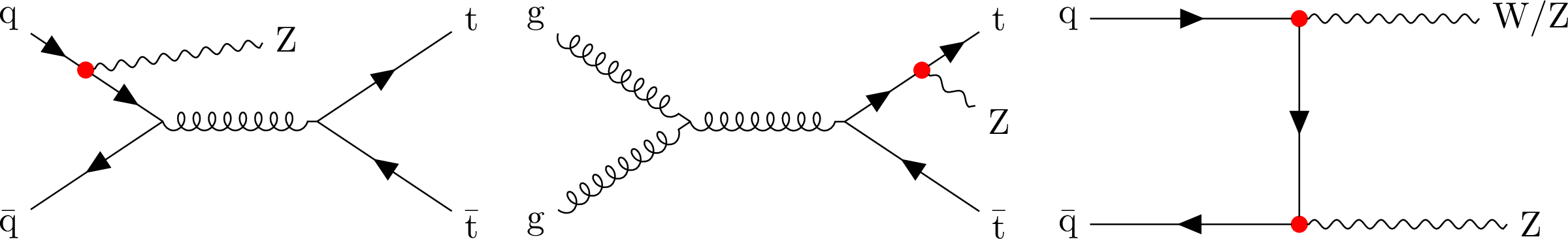
Figure 1:
Representative Feynman diagrams showing the leading-order contributions to the $ \mathrm{t}\overline{\mathrm{t}}\mathrm{Z} $ production, with the Z boson radiated from the initial-state quarks (left) and from one of the top quarks (middle). The WZ and/or ZZ production is also shown (right). The vertices affected by the EFT operators probed in this analysis are highlighted with red dots. |
png pdf |
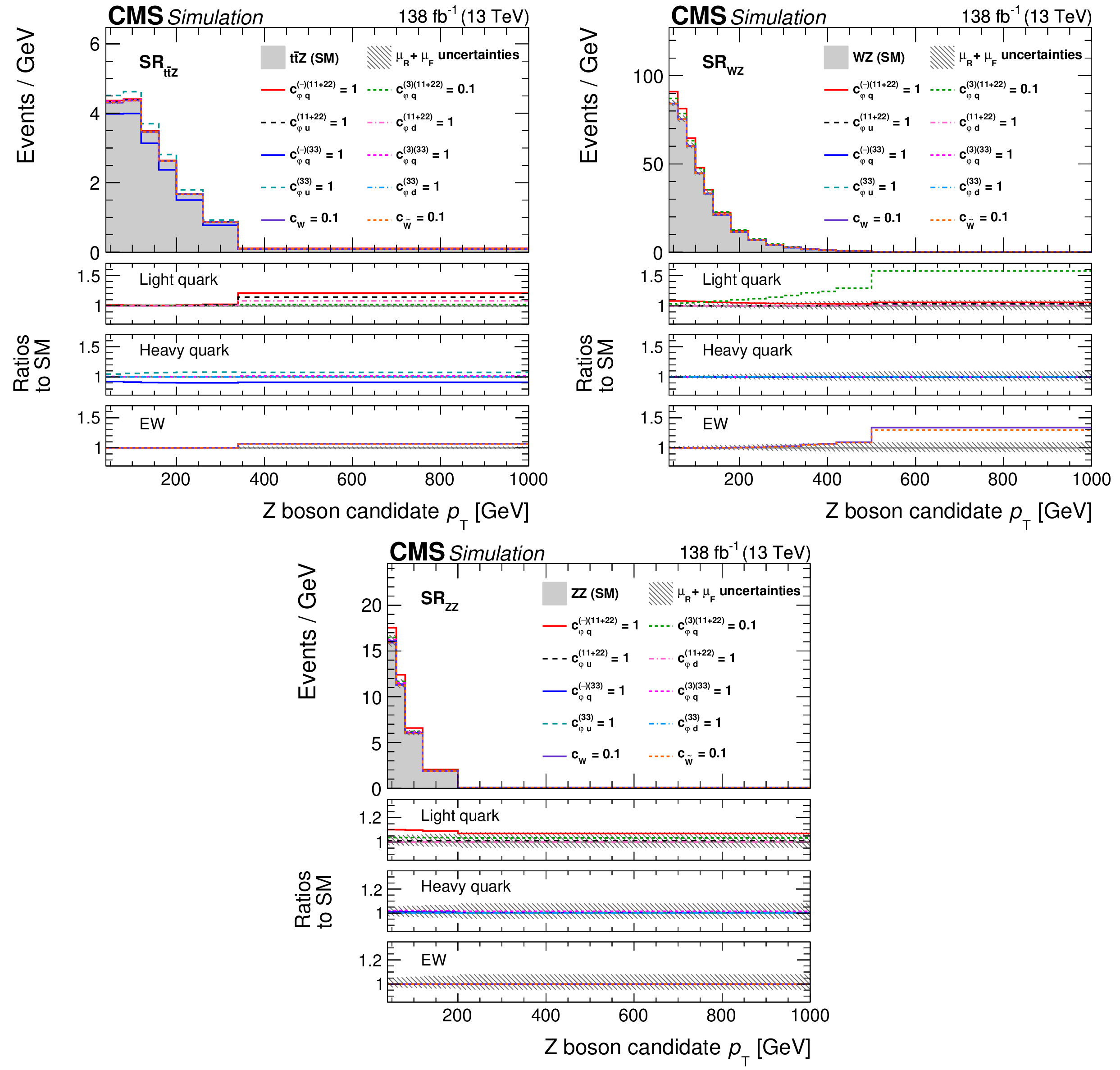
Figure 2:
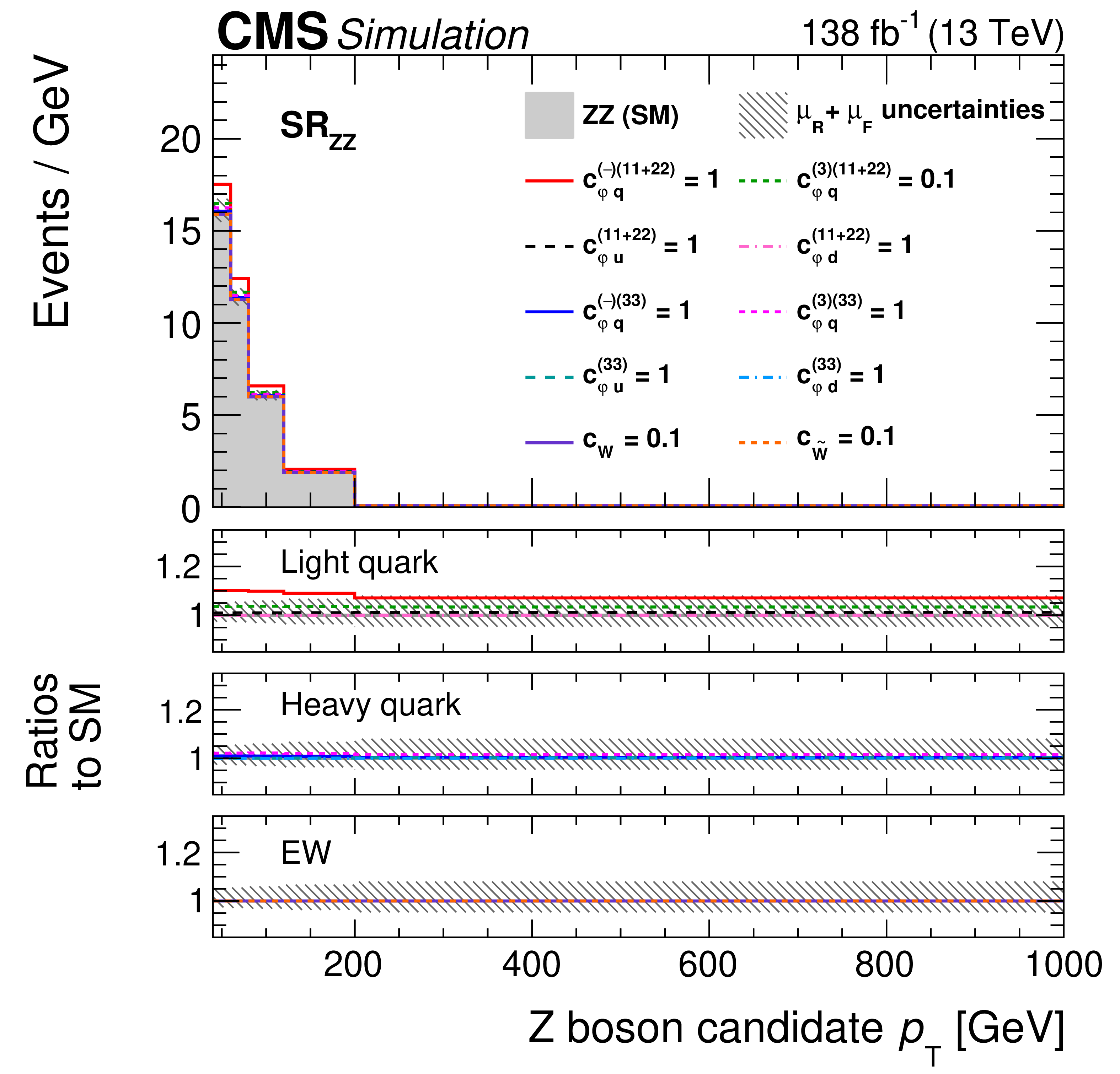
Distributions of the Z boson $ p_{\mathrm{T}} $ in the three signal regions of this analysis. Shown are $ \text{SR}_{\mathrm{t}\overline{\mathrm{t}}\mathrm{Z}} $ (upper left), $ \text{SR}_{\mathrm{W}\mathrm{Z}} $ (upper right), and $ \text{SR}_{\mathrm{Z}\mathrm{Z}} $ (lower). In each region, the target process ($ \mathrm{t}\overline{\mathrm{t}}\mathrm{Z} $, WZ, or ZZ) is shown at the SM point (coloured areas) and various EFT hypotheses (lines). The hashed band includes only uncertainties in the renormalisation and factorisation scales ($ \mu_{\text{R}} $ and $ \mu_{\text{F}} $). The upper, middle, and lower ratio panels show the ratio of EFT hypotheses for light-quark, heavy-quark, and EW boson couplings, respectively. The bin content is divided by the bin width. |
png pdf |
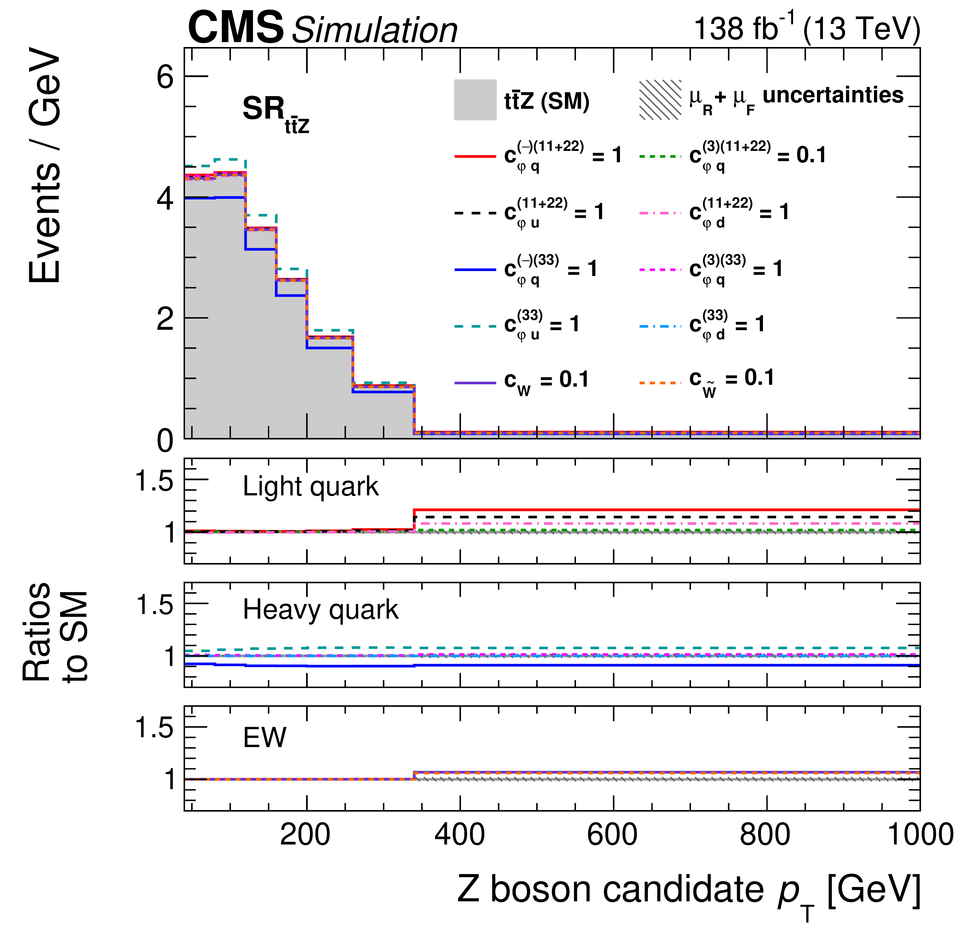
Figure 2-a:
Distributions of the Z boson $ p_{\mathrm{T}} $ in the three signal regions of this analysis. Shown are $ \text{SR}_{\mathrm{t}\overline{\mathrm{t}}\mathrm{Z}} $ (upper left), $ \text{SR}_{\mathrm{W}\mathrm{Z}} $ (upper right), and $ \text{SR}_{\mathrm{Z}\mathrm{Z}} $ (lower). In each region, the target process ($ \mathrm{t}\overline{\mathrm{t}}\mathrm{Z} $, WZ, or ZZ) is shown at the SM point (coloured areas) and various EFT hypotheses (lines). The hashed band includes only uncertainties in the renormalisation and factorisation scales ($ \mu_{\text{R}} $ and $ \mu_{\text{F}} $). The upper, middle, and lower ratio panels show the ratio of EFT hypotheses for light-quark, heavy-quark, and EW boson couplings, respectively. The bin content is divided by the bin width. |
png pdf |
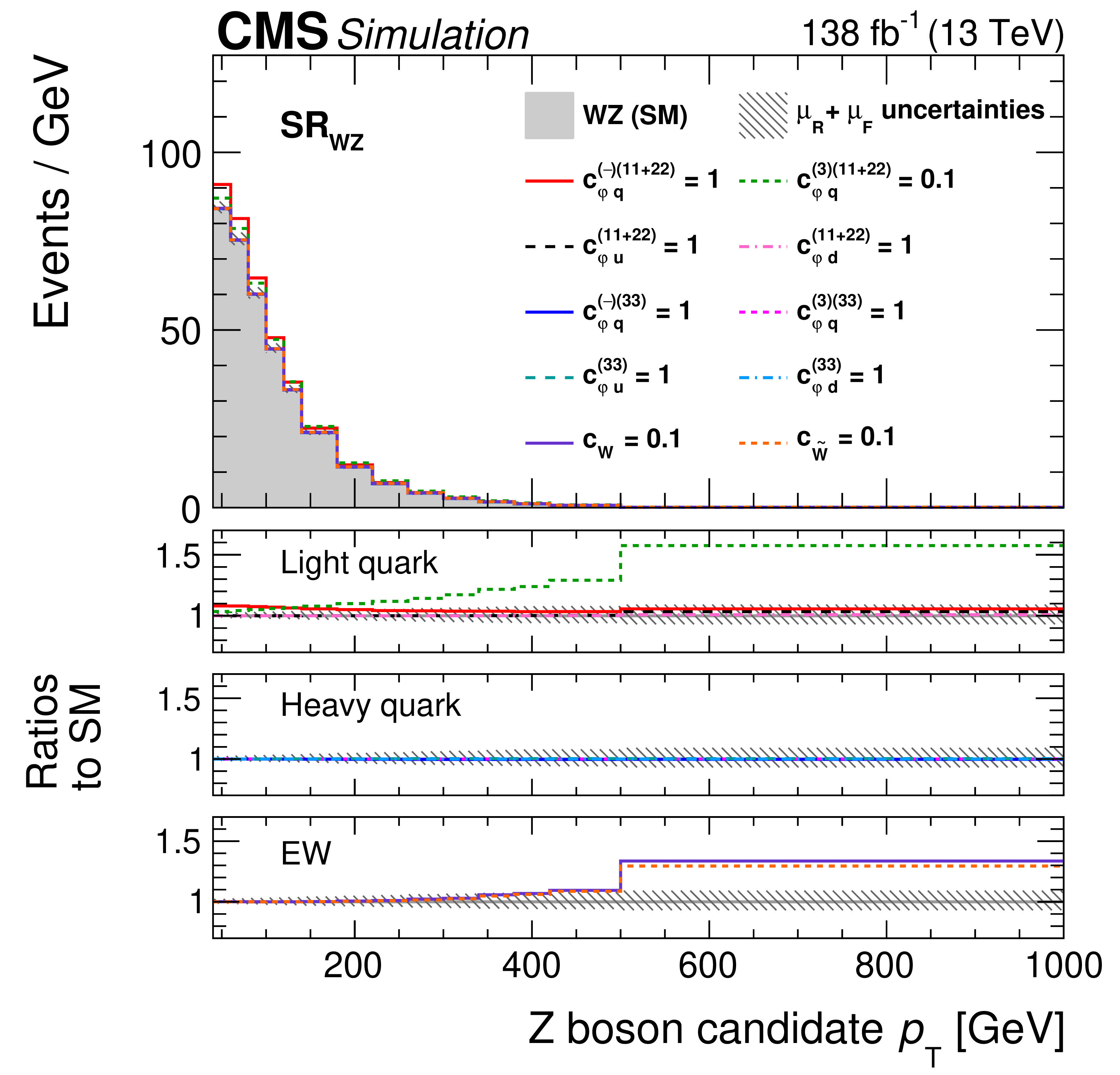
Figure 2-b:
Distributions of the Z boson $ p_{\mathrm{T}} $ in the three signal regions of this analysis. Shown are $ \text{SR}_{\mathrm{t}\overline{\mathrm{t}}\mathrm{Z}} $ (upper left), $ \text{SR}_{\mathrm{W}\mathrm{Z}} $ (upper right), and $ \text{SR}_{\mathrm{Z}\mathrm{Z}} $ (lower). In each region, the target process ($ \mathrm{t}\overline{\mathrm{t}}\mathrm{Z} $, WZ, or ZZ) is shown at the SM point (coloured areas) and various EFT hypotheses (lines). The hashed band includes only uncertainties in the renormalisation and factorisation scales ($ \mu_{\text{R}} $ and $ \mu_{\text{F}} $). The upper, middle, and lower ratio panels show the ratio of EFT hypotheses for light-quark, heavy-quark, and EW boson couplings, respectively. The bin content is divided by the bin width. |
png pdf |
Figure 2-c:
Distributions of the Z boson $ p_{\mathrm{T}} $ in the three signal regions of this analysis. Shown are $ \text{SR}_{\mathrm{t}\overline{\mathrm{t}}\mathrm{Z}} $ (upper left), $ \text{SR}_{\mathrm{W}\mathrm{Z}} $ (upper right), and $ \text{SR}_{\mathrm{Z}\mathrm{Z}} $ (lower). In each region, the target process ($ \mathrm{t}\overline{\mathrm{t}}\mathrm{Z} $, WZ, or ZZ) is shown at the SM point (coloured areas) and various EFT hypotheses (lines). The hashed band includes only uncertainties in the renormalisation and factorisation scales ($ \mu_{\text{R}} $ and $ \mu_{\text{F}} $). The upper, middle, and lower ratio panels show the ratio of EFT hypotheses for light-quark, heavy-quark, and EW boson couplings, respectively. The bin content is divided by the bin width. |
png pdf |
Figure 3:
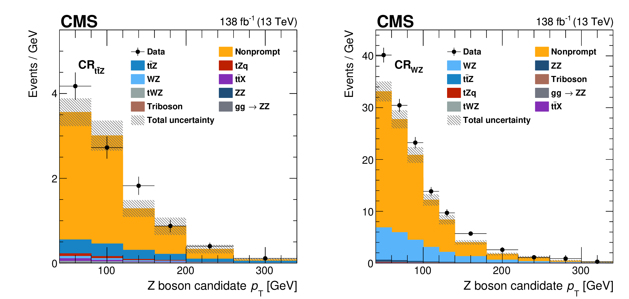
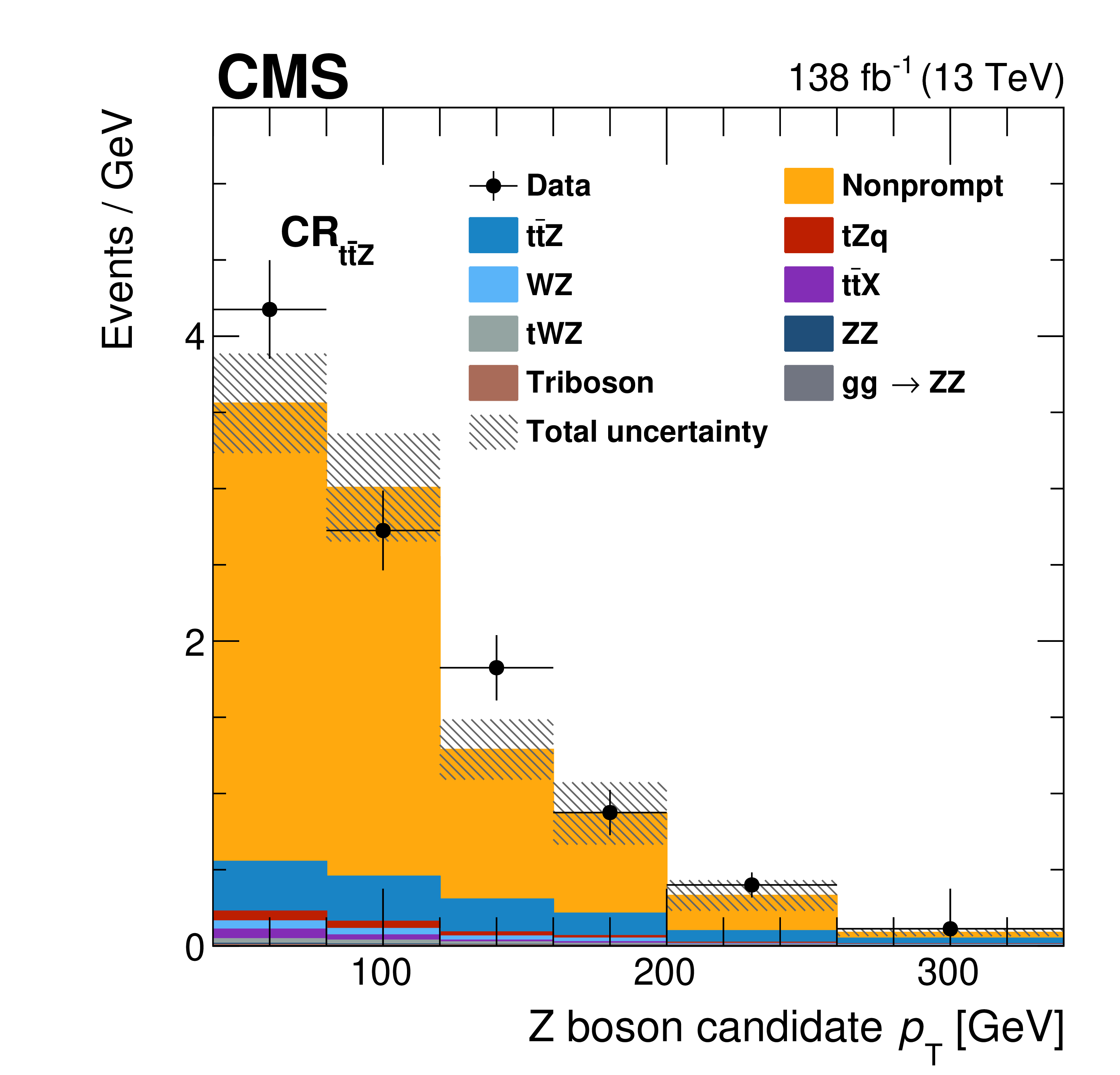
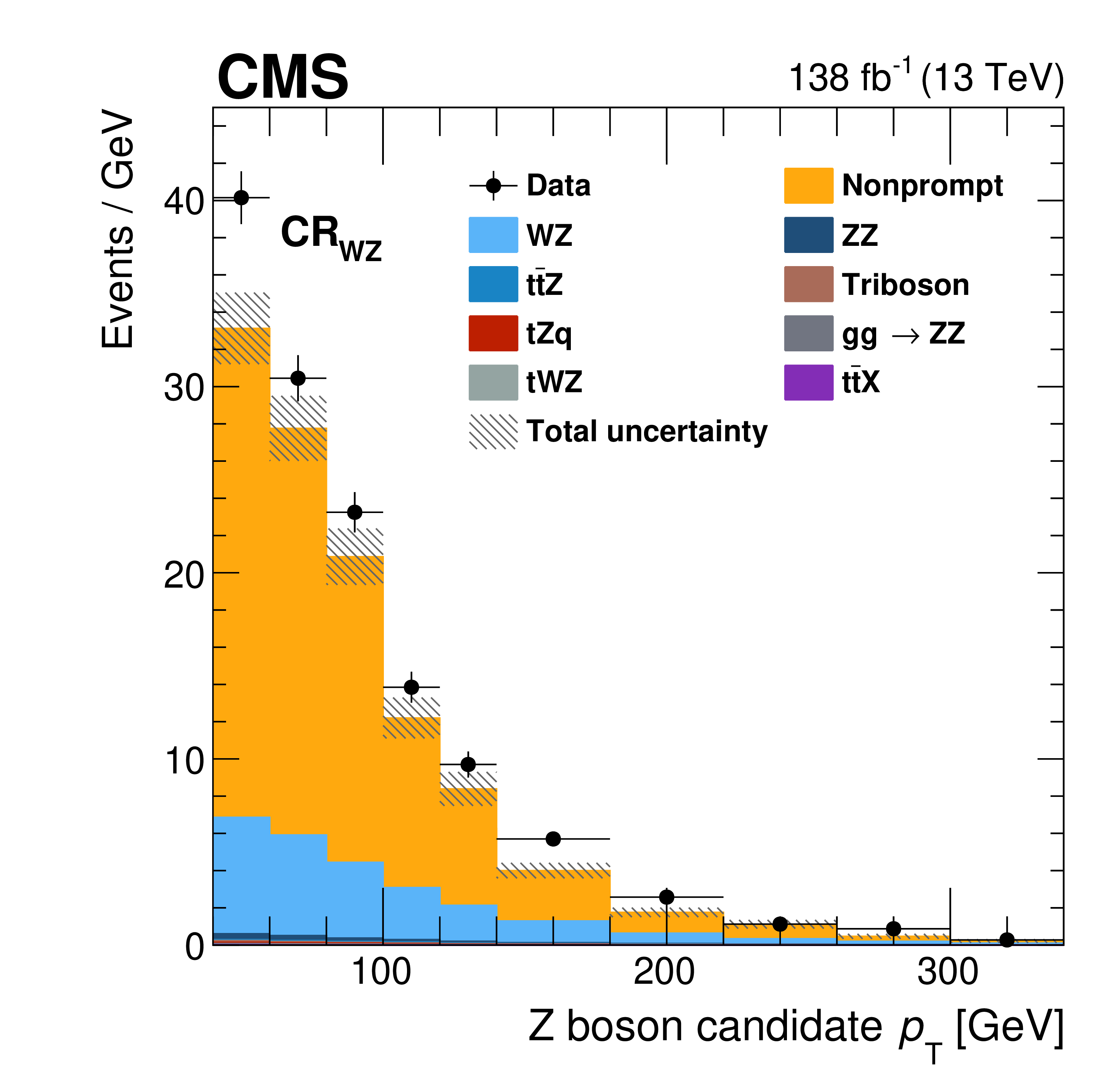
Distributions of the Z boson $ p_{\mathrm{T}} $ in the control regions of this analysis. Shown are $ \text{CR}_{\mathrm{t}\overline{\mathrm{t}}\mathrm{Z}} $ (left) and $ \text{CR}_{\mathrm{W}\mathrm{Z}} $ (right). Predictions are all obtained from simulation and are displayed as coloured areas. The hashed area shows the statistical uncertainty in the prediction. Data are displayed as markers, where the vertical bars represent the statistical uncertainty. The bin content is divided by the bin width. |
png pdf |
Figure 3-a:
Distributions of the Z boson $ p_{\mathrm{T}} $ in the control regions of this analysis. Shown are $ \text{CR}_{\mathrm{t}\overline{\mathrm{t}}\mathrm{Z}} $ (left) and $ \text{CR}_{\mathrm{W}\mathrm{Z}} $ (right). Predictions are all obtained from simulation and are displayed as coloured areas. The hashed area shows the statistical uncertainty in the prediction. Data are displayed as markers, where the vertical bars represent the statistical uncertainty. The bin content is divided by the bin width. |
png pdf |
Figure 3-b:
Distributions of the Z boson $ p_{\mathrm{T}} $ in the control regions of this analysis. Shown are $ \text{CR}_{\mathrm{t}\overline{\mathrm{t}}\mathrm{Z}} $ (left) and $ \text{CR}_{\mathrm{W}\mathrm{Z}} $ (right). Predictions are all obtained from simulation and are displayed as coloured areas. The hashed area shows the statistical uncertainty in the prediction. Data are displayed as markers, where the vertical bars represent the statistical uncertainty. The bin content is divided by the bin width. |
png pdf |
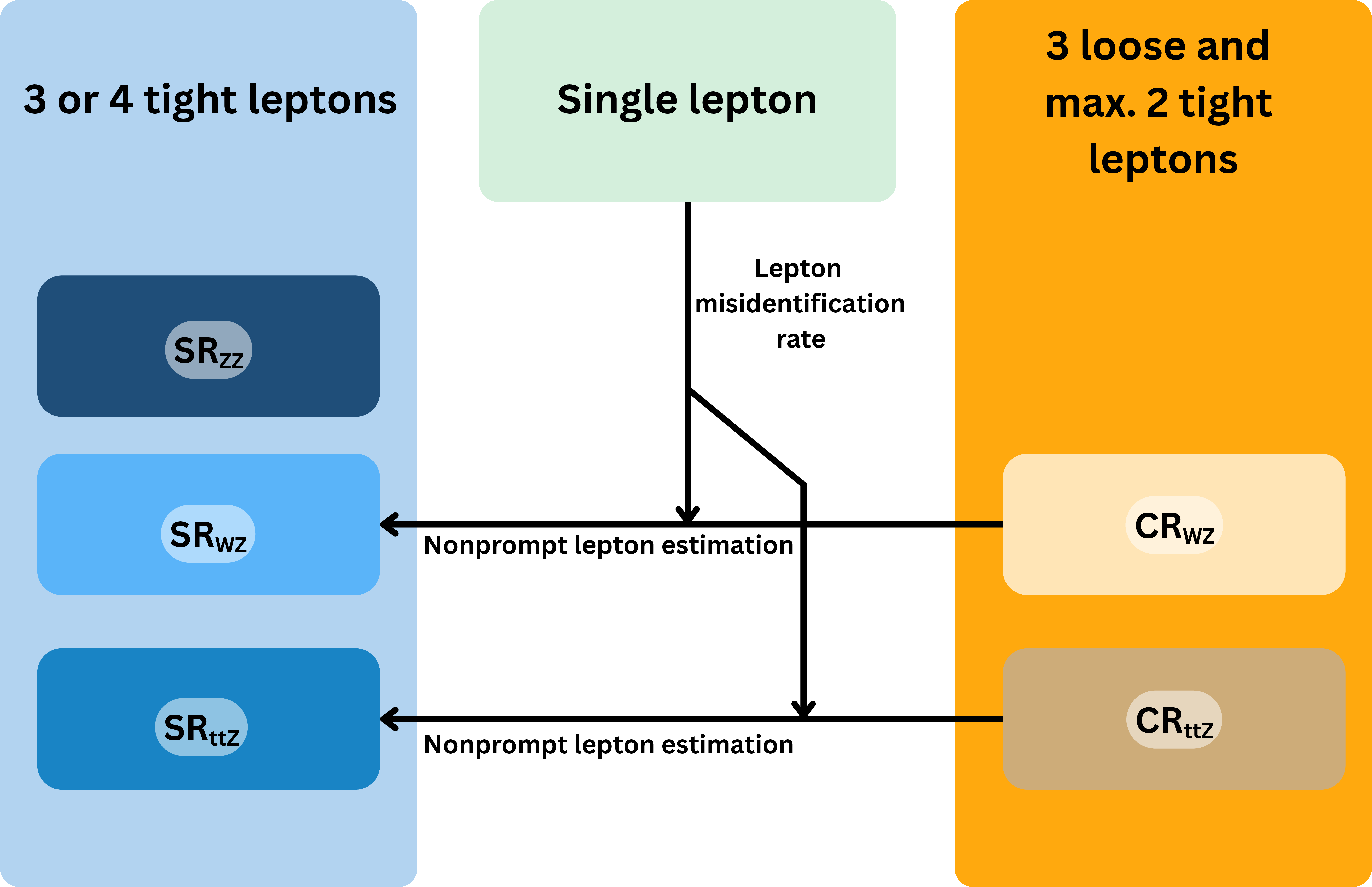
Figure 4:
Schematic representation of the SRs and CRs used in this analysis. The application of the estimated nonprompt lepton background from the CRs into the SRs is illustrated with arrows. |
png pdf |
Figure 5:
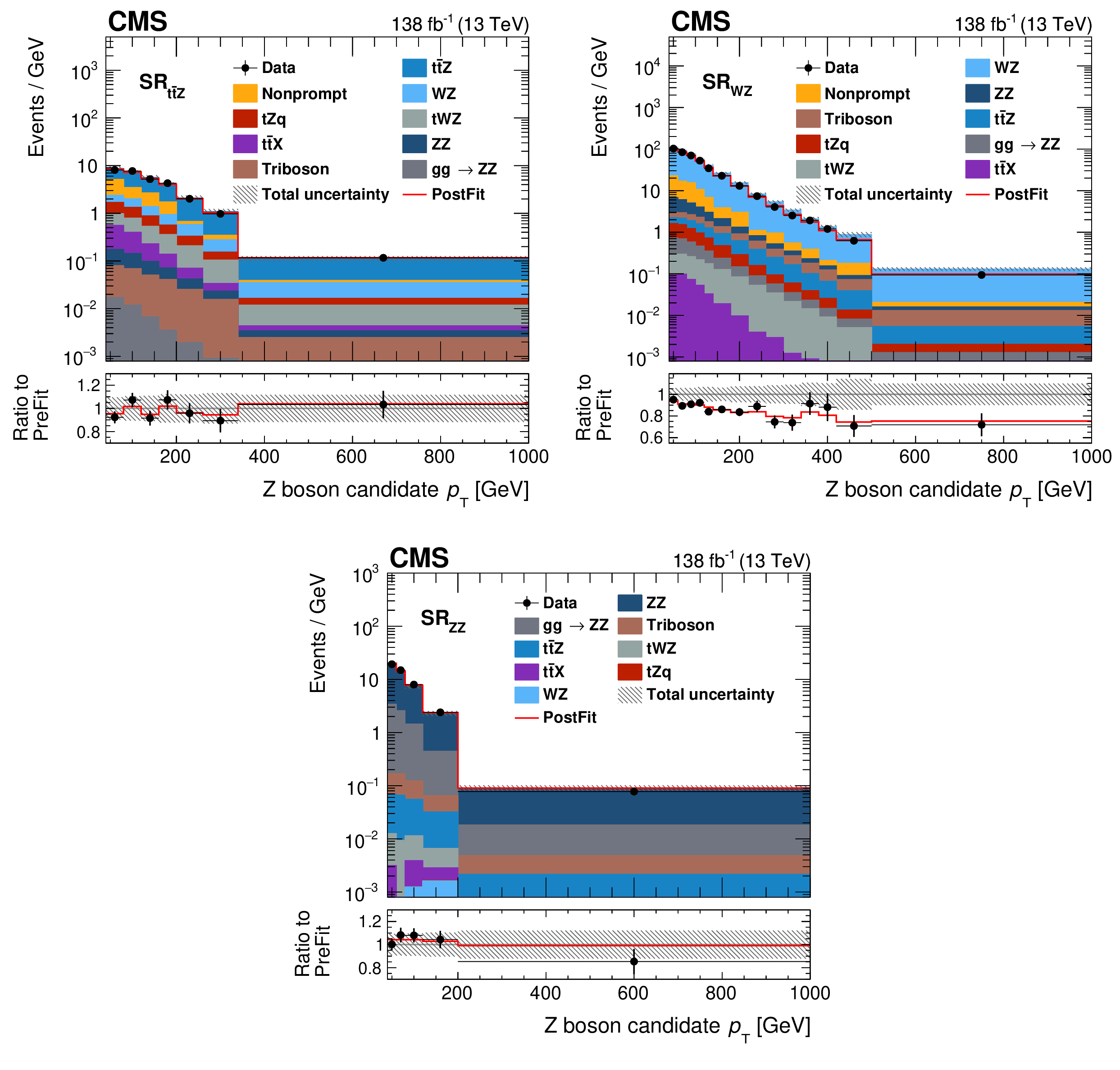
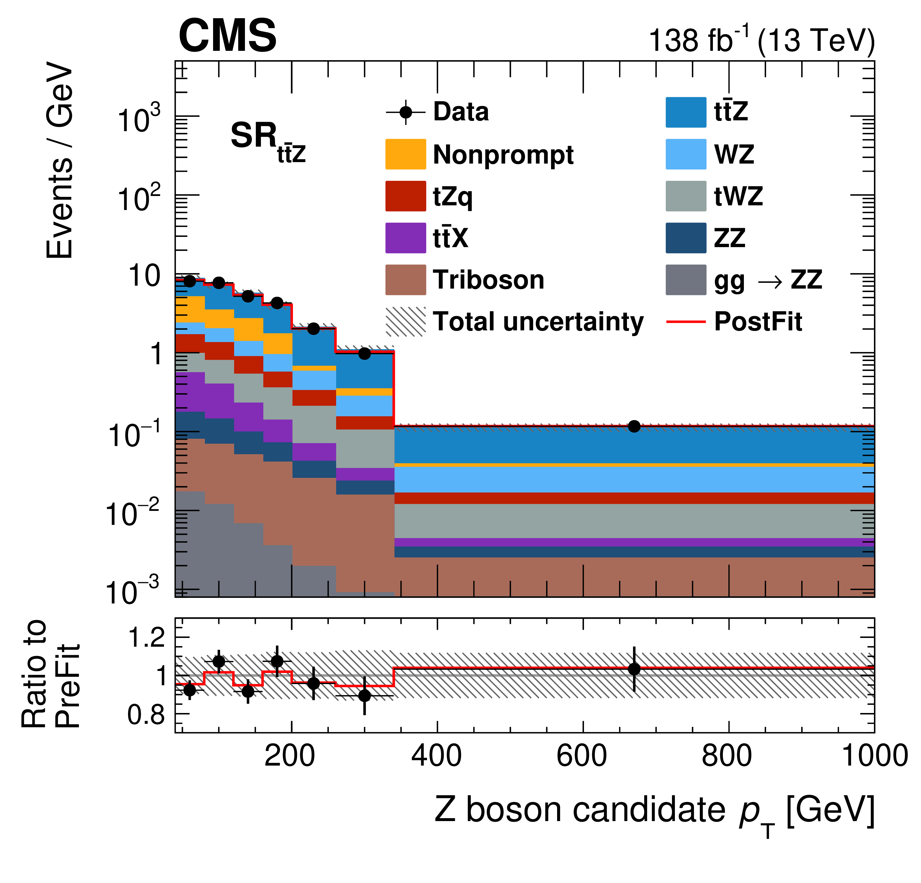
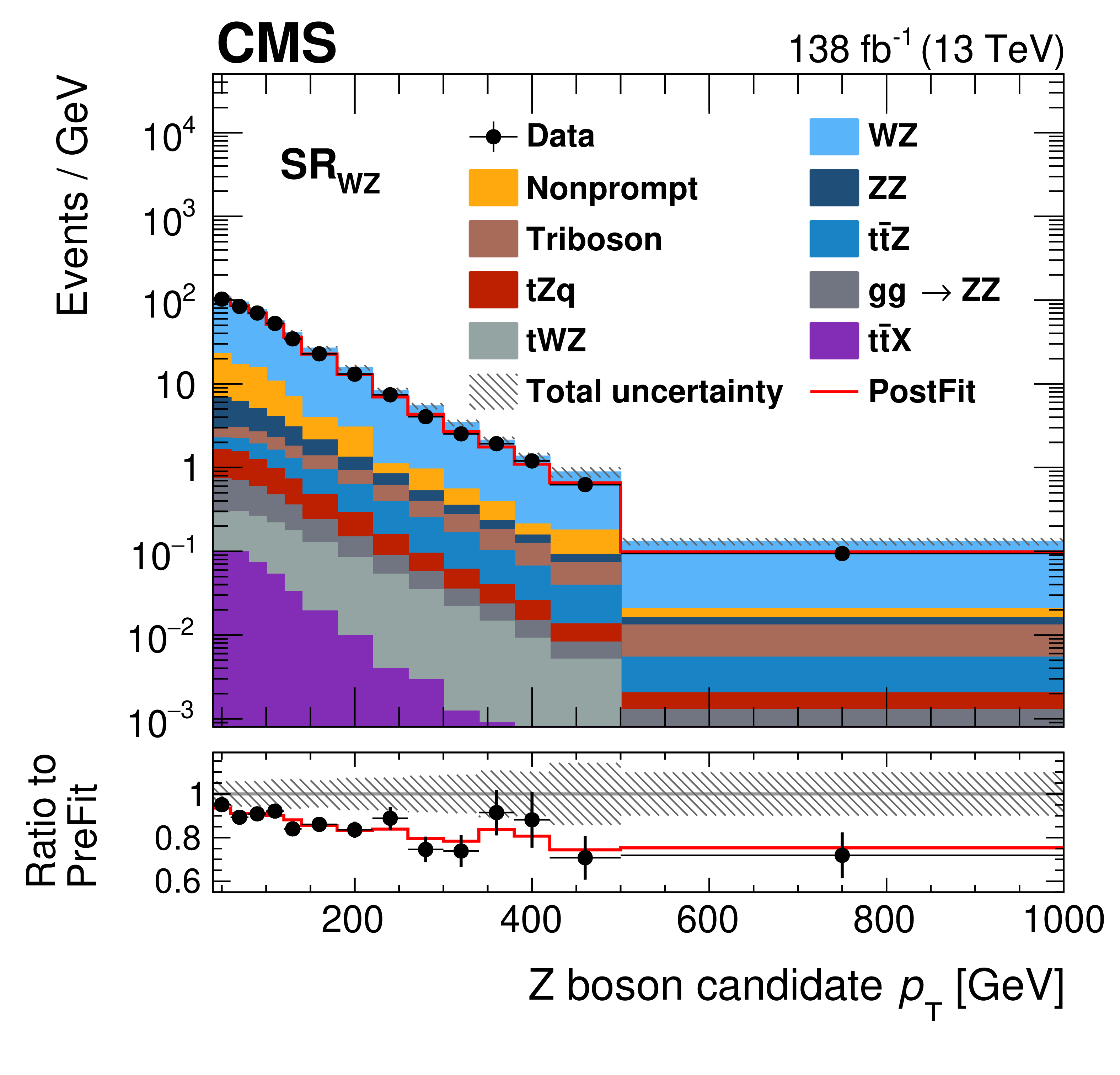
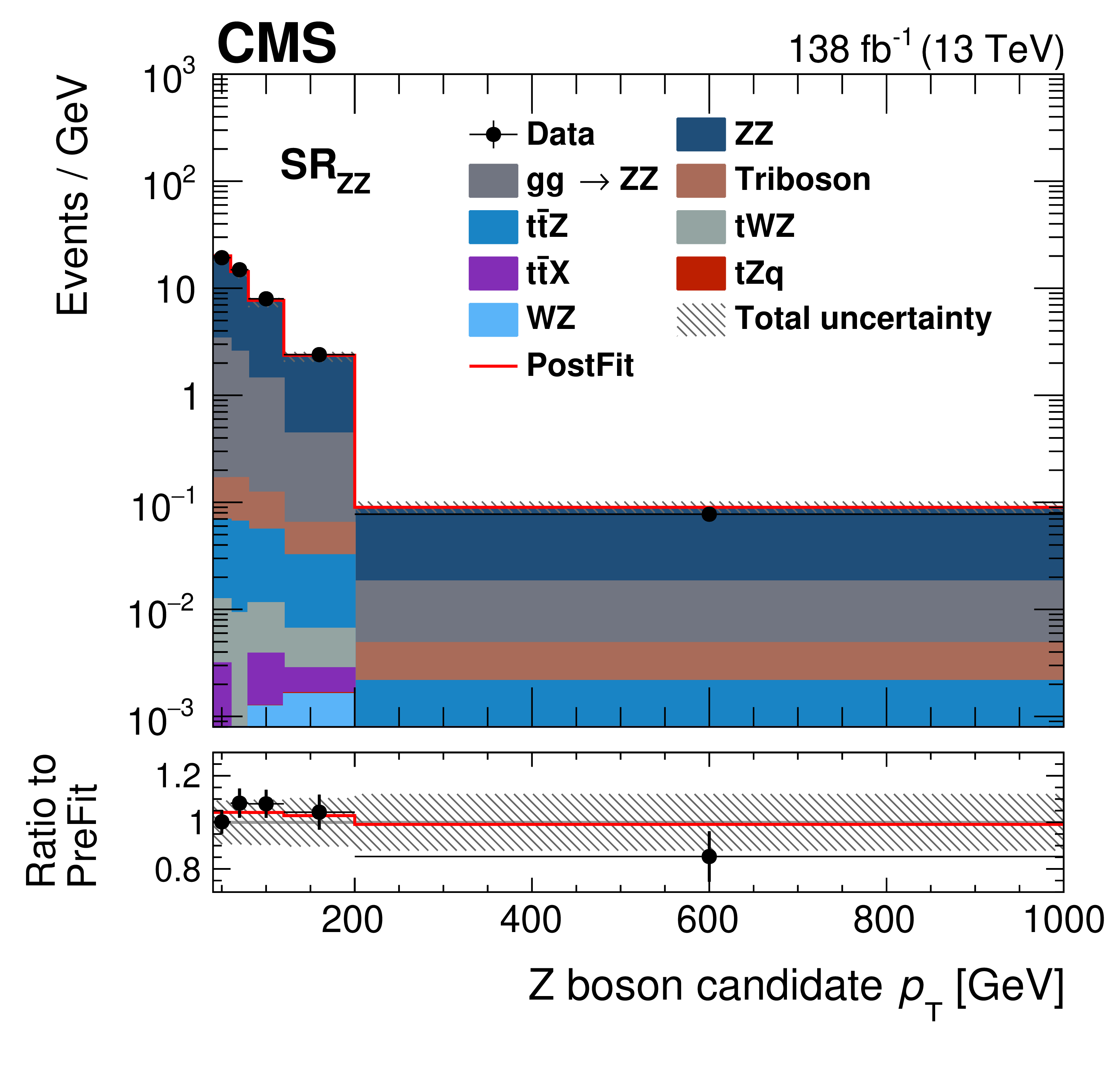
Distributions of the Z boson $ p_{\mathrm{T}} $ in the three signal regions of this analysis. Shown are the $ \text{SR}_{\mathrm{t}\overline{\mathrm{t}}\mathrm{Z}} $ (upper left), $ \text{SR}_{\mathrm{W}\mathrm{Z}} $ (upper right), and $ \text{SR}_{\mathrm{Z}\mathrm{Z}} $ (lower) regions. The data (markers) are compared to the prediction from simulation and the data-driven estimate of nonprompt leptons (coloured areas). The lower panel displays the ratio to the predictions before the fit. The hashed area displays the total uncertainties and the red line displays the best fit result in a setup with all EFT parameters. The bin content is divided by the bin width. |
png pdf |
Figure 5-a:
Distributions of the Z boson $ p_{\mathrm{T}} $ in the three signal regions of this analysis. Shown are the $ \text{SR}_{\mathrm{t}\overline{\mathrm{t}}\mathrm{Z}} $ (upper left), $ \text{SR}_{\mathrm{W}\mathrm{Z}} $ (upper right), and $ \text{SR}_{\mathrm{Z}\mathrm{Z}} $ (lower) regions. The data (markers) are compared to the prediction from simulation and the data-driven estimate of nonprompt leptons (coloured areas). The lower panel displays the ratio to the predictions before the fit. The hashed area displays the total uncertainties and the red line displays the best fit result in a setup with all EFT parameters. The bin content is divided by the bin width. |
png pdf |
Figure 5-b:
Distributions of the Z boson $ p_{\mathrm{T}} $ in the three signal regions of this analysis. Shown are the $ \text{SR}_{\mathrm{t}\overline{\mathrm{t}}\mathrm{Z}} $ (upper left), $ \text{SR}_{\mathrm{W}\mathrm{Z}} $ (upper right), and $ \text{SR}_{\mathrm{Z}\mathrm{Z}} $ (lower) regions. The data (markers) are compared to the prediction from simulation and the data-driven estimate of nonprompt leptons (coloured areas). The lower panel displays the ratio to the predictions before the fit. The hashed area displays the total uncertainties and the red line displays the best fit result in a setup with all EFT parameters. The bin content is divided by the bin width. |
png pdf |
Figure 5-c:
Distributions of the Z boson $ p_{\mathrm{T}} $ in the three signal regions of this analysis. Shown are the $ \text{SR}_{\mathrm{t}\overline{\mathrm{t}}\mathrm{Z}} $ (upper left), $ \text{SR}_{\mathrm{W}\mathrm{Z}} $ (upper right), and $ \text{SR}_{\mathrm{Z}\mathrm{Z}} $ (lower) regions. The data (markers) are compared to the prediction from simulation and the data-driven estimate of nonprompt leptons (coloured areas). The lower panel displays the ratio to the predictions before the fit. The hashed area displays the total uncertainties and the red line displays the best fit result in a setup with all EFT parameters. The bin content is divided by the bin width. |
png pdf |
Figure 6:
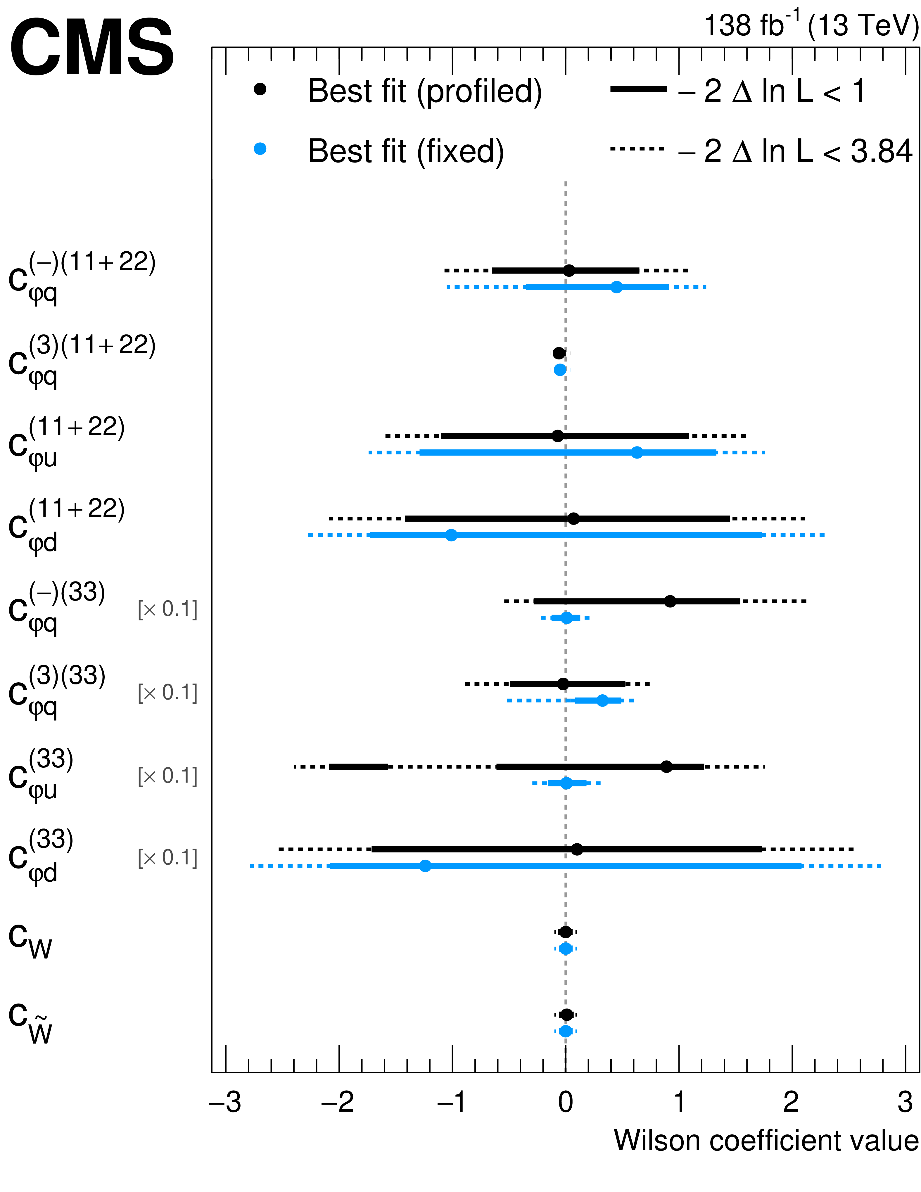
Summary of the limits obtained for the Wilson coefficients $ c_{\varphi q}^{(-)(11+22)} $, $ c_{\varphi q}^{(3)(11+22)} $, $ c_{\varphi u}^{(11+22)} $, $ c_{\varphi d}^{(11+22)} $, $ c_{\varphi q}^{(-)(33)} $, $ c_{\varphi q}^{(3)(33)} $, $ c_{\varphi u}^{(33)} $, $ c_{\varphi d}^{(33)} $, $ c_{W} $, and $ c_{\widetilde{W}} $. Shown are the best fit points and limits for scans where other Wilson coefficients are fixed to zero (`fixed') or are allowed to float (`profiled'). The points where the difference $ -2\Delta\ln L $ with respect to the best fit increases by 1 and 3.84 are shown as horizontal error bars. These points correspond to the 68 and 95% CL limits in the asymptotic approximation. For each Wilson coefficient value, the EFT energy scale is assumed to be $ \Lambda= $ 1 TeV. For better visibility, the heavy quark couplings are multiplied by a factor of 0.1. |
png pdf |
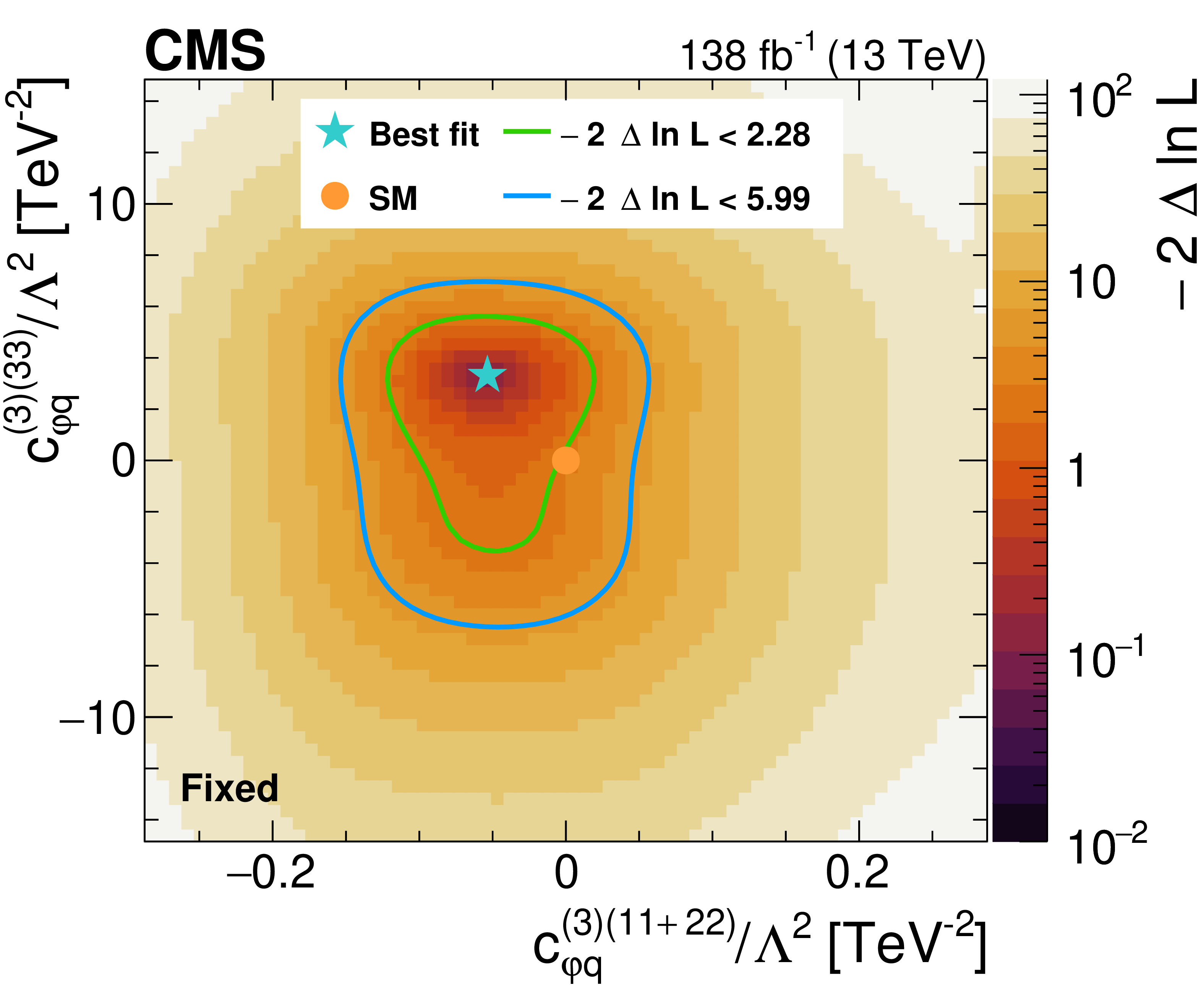
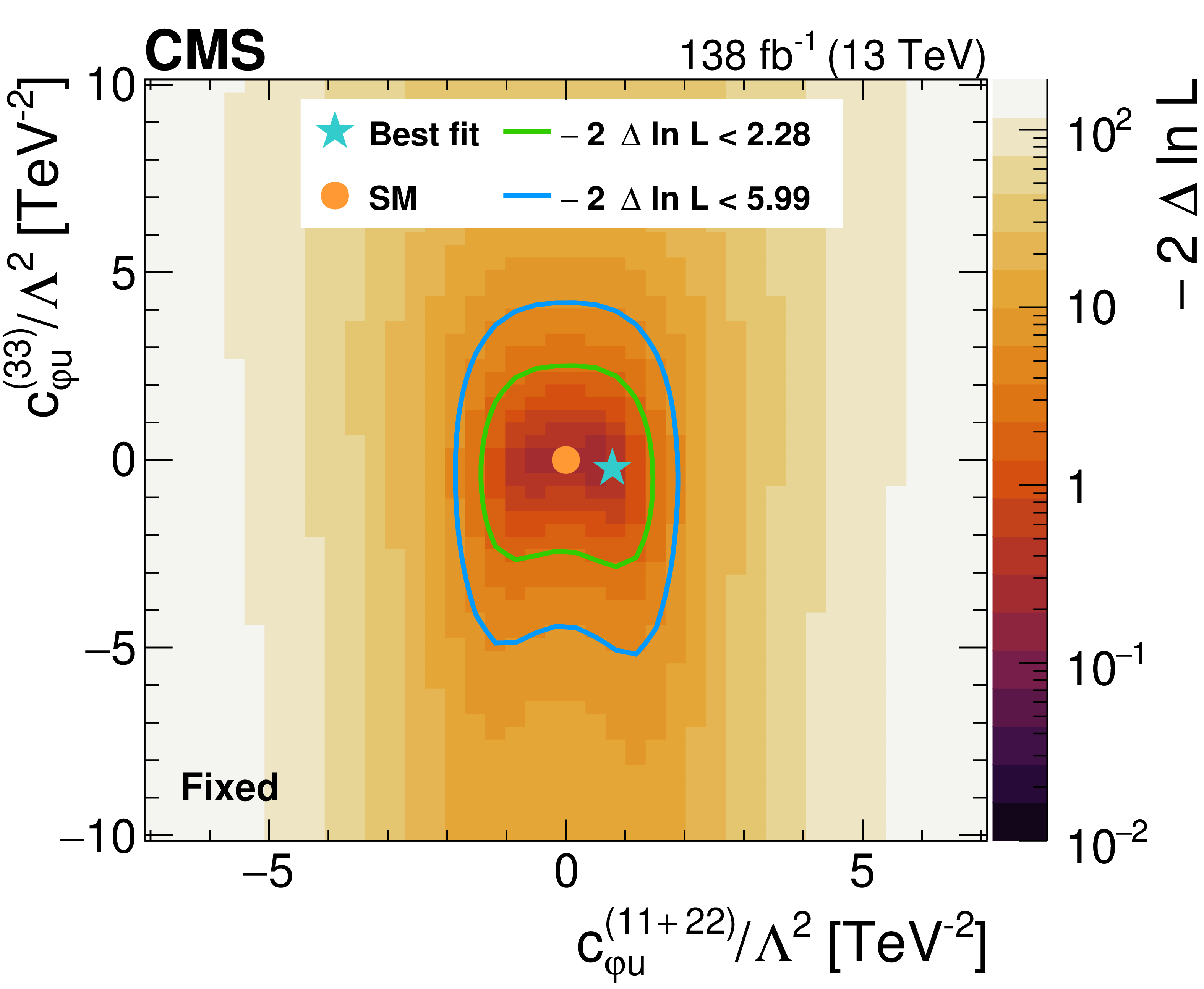
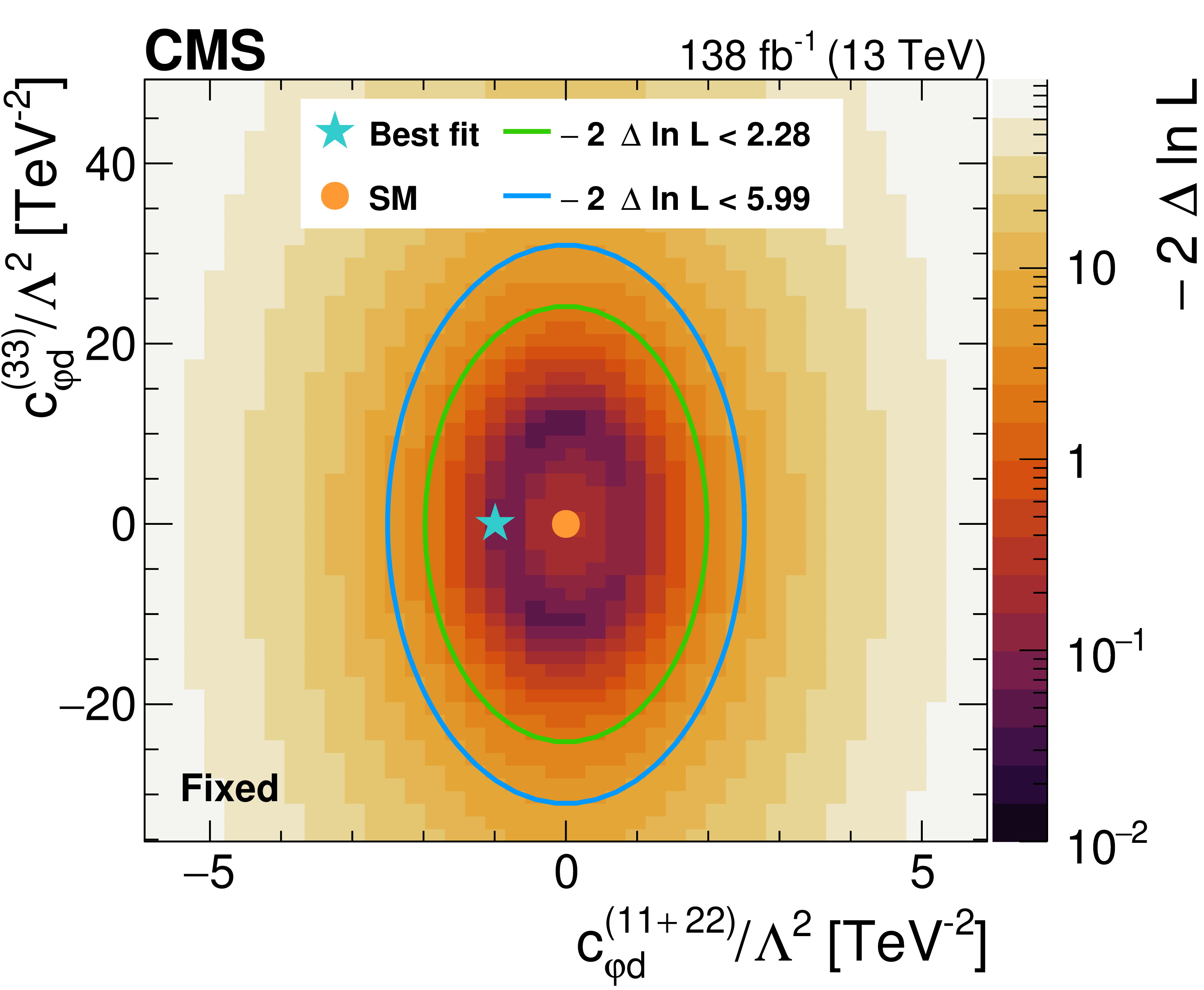
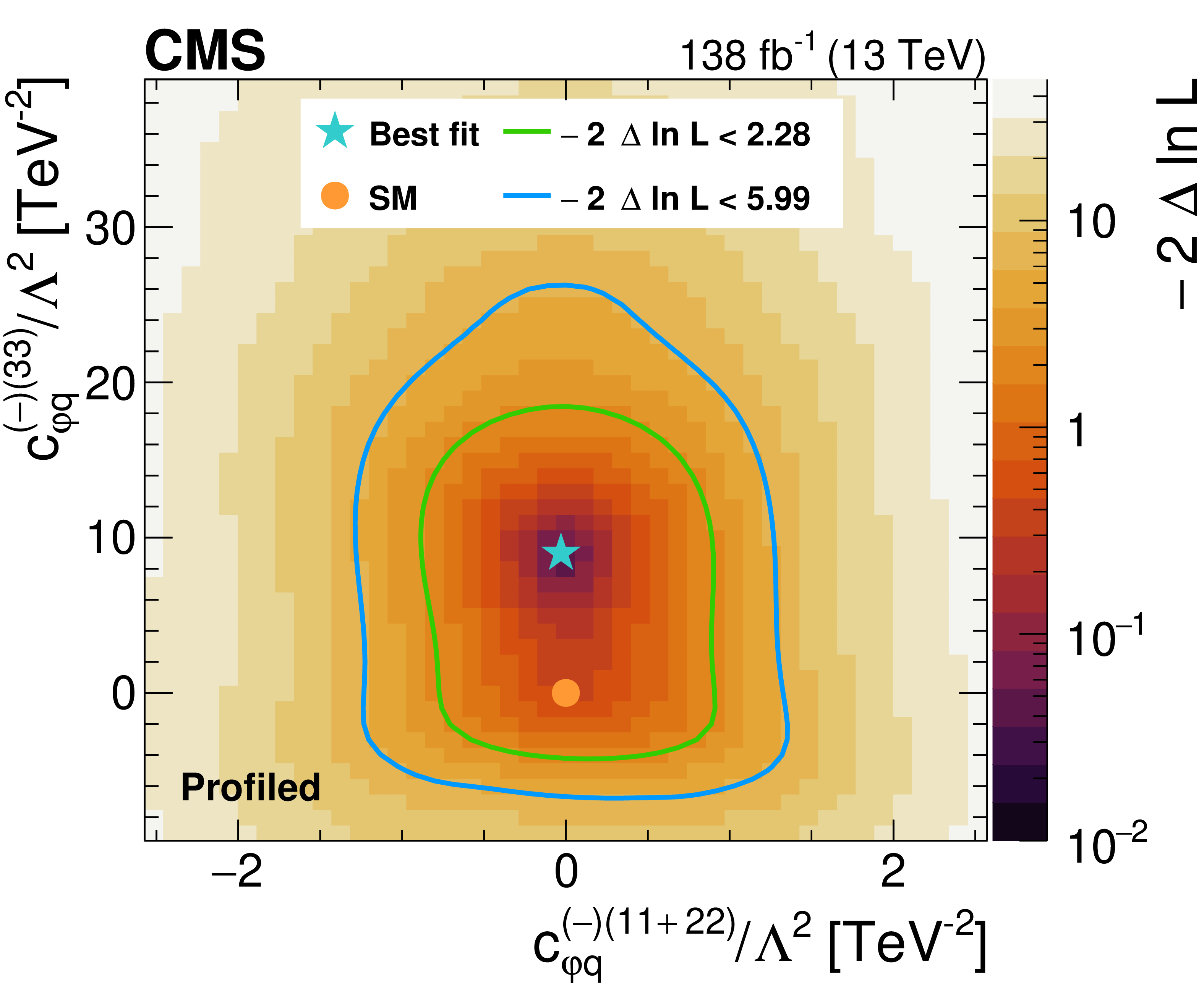
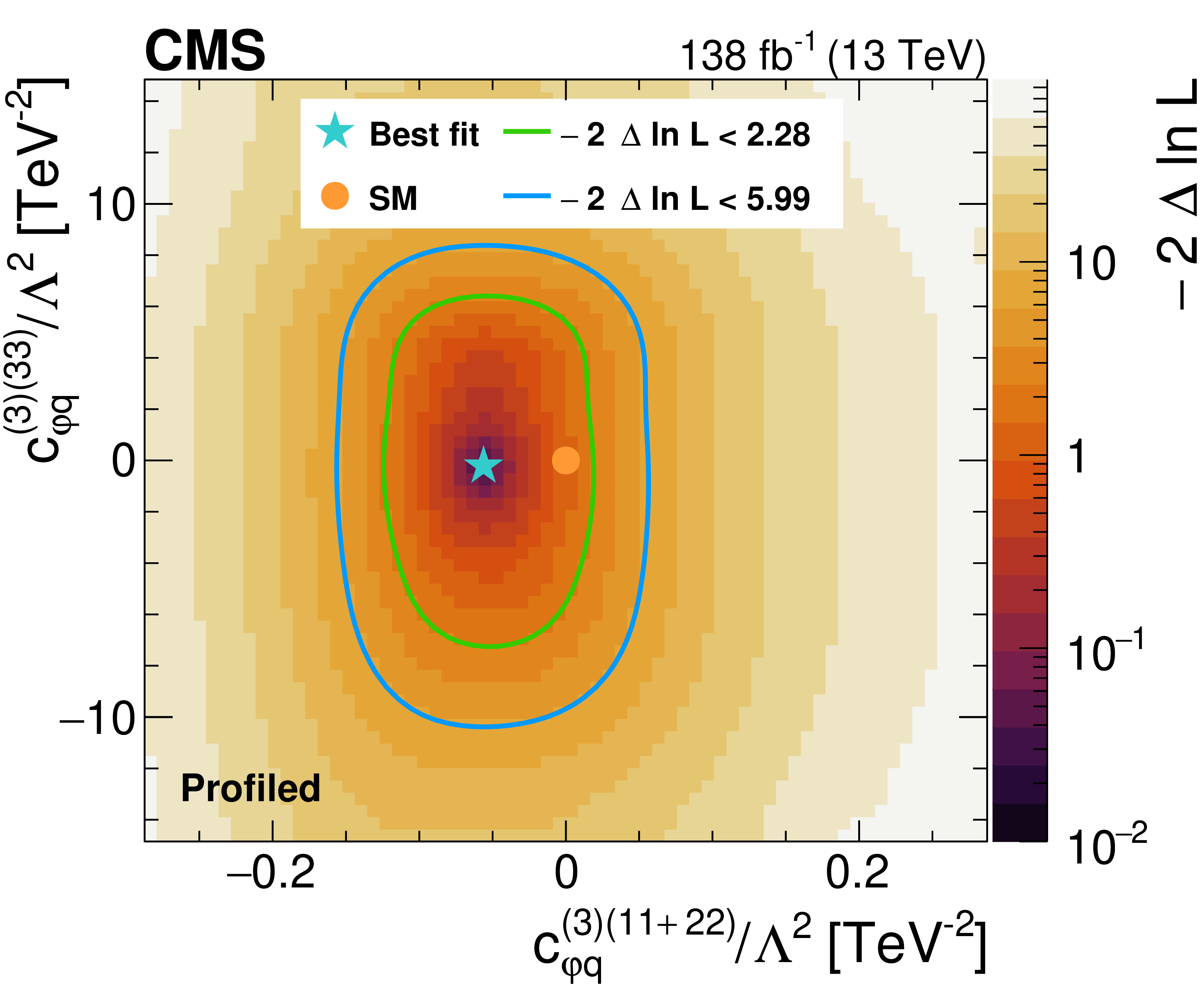
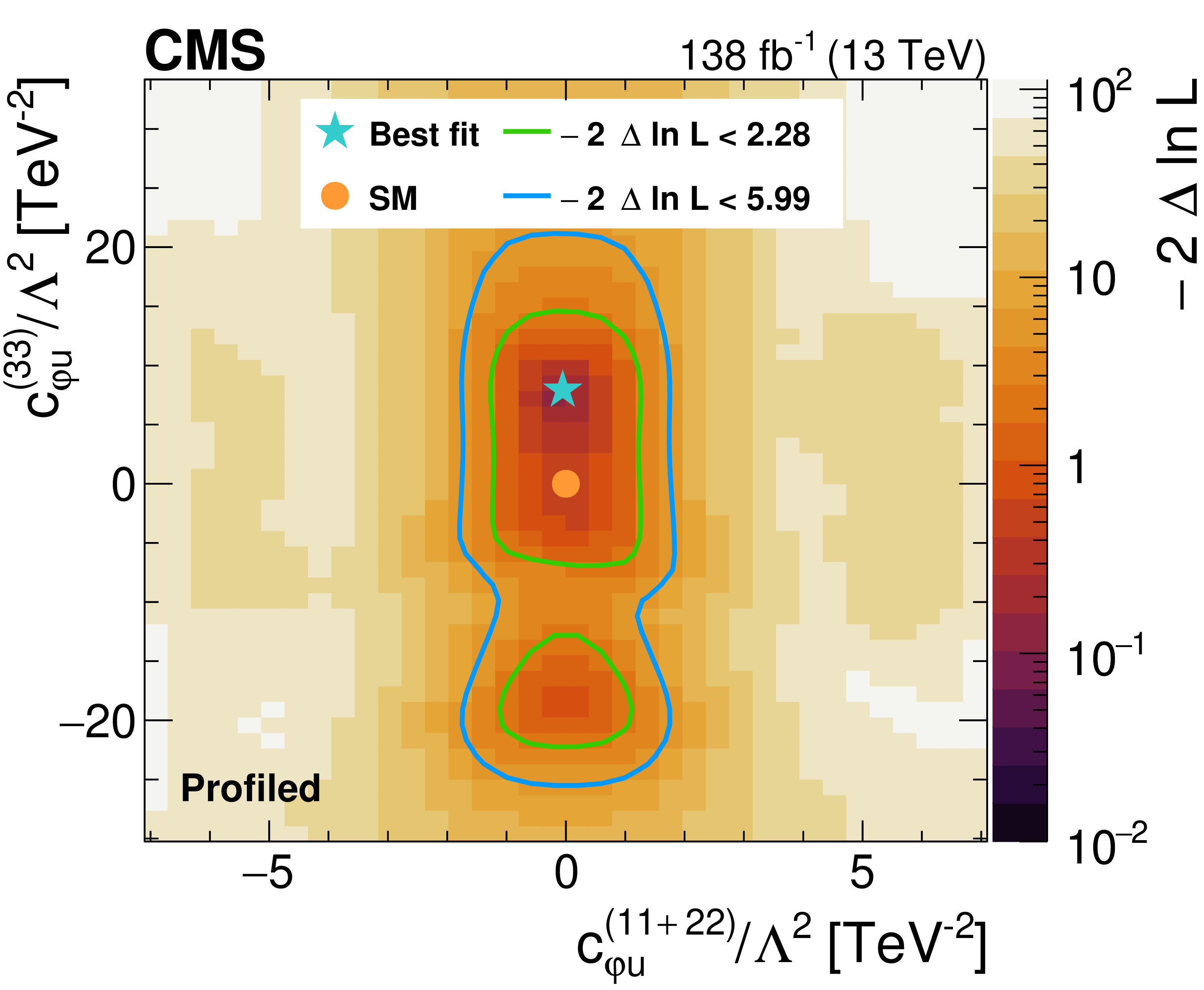
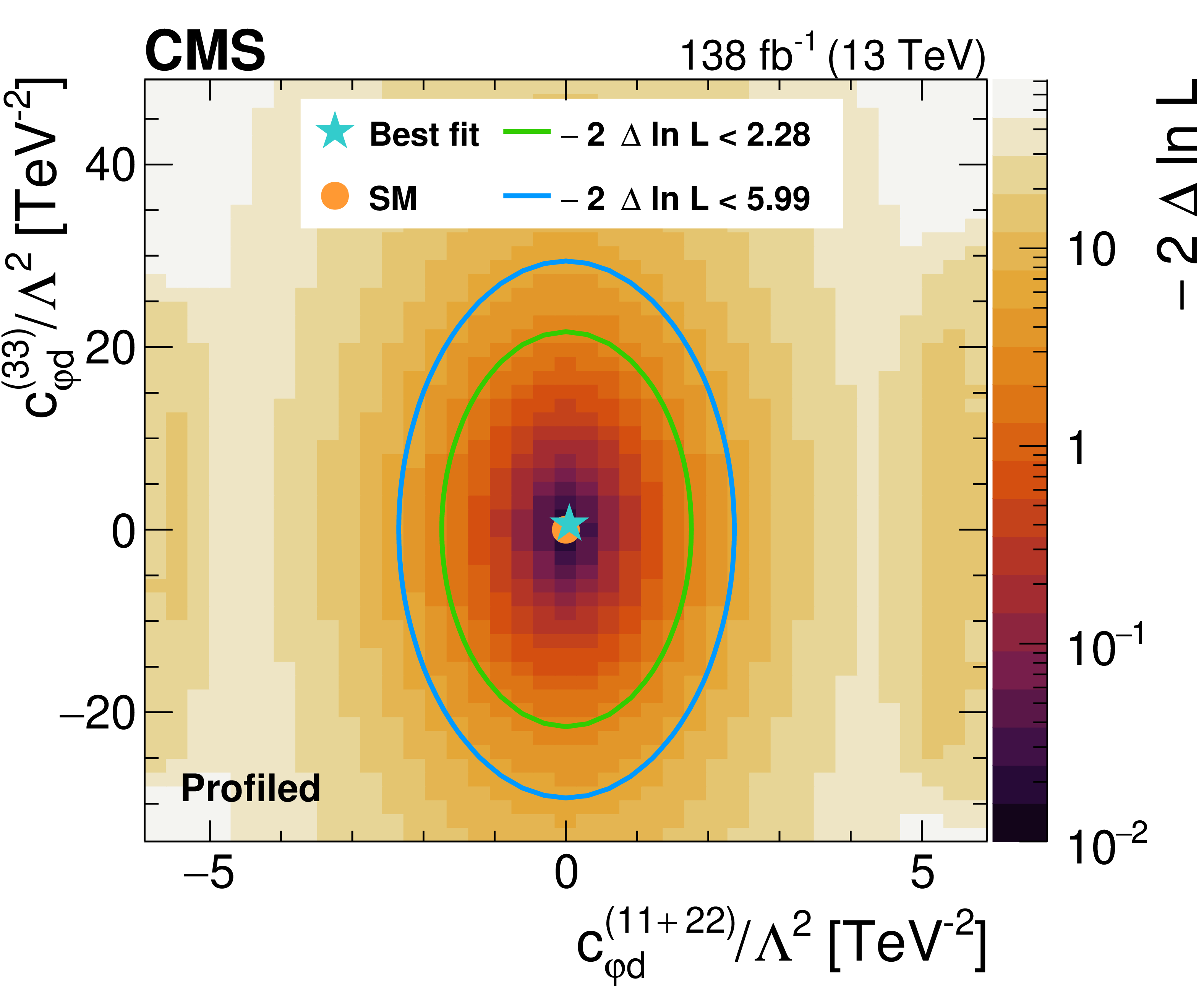
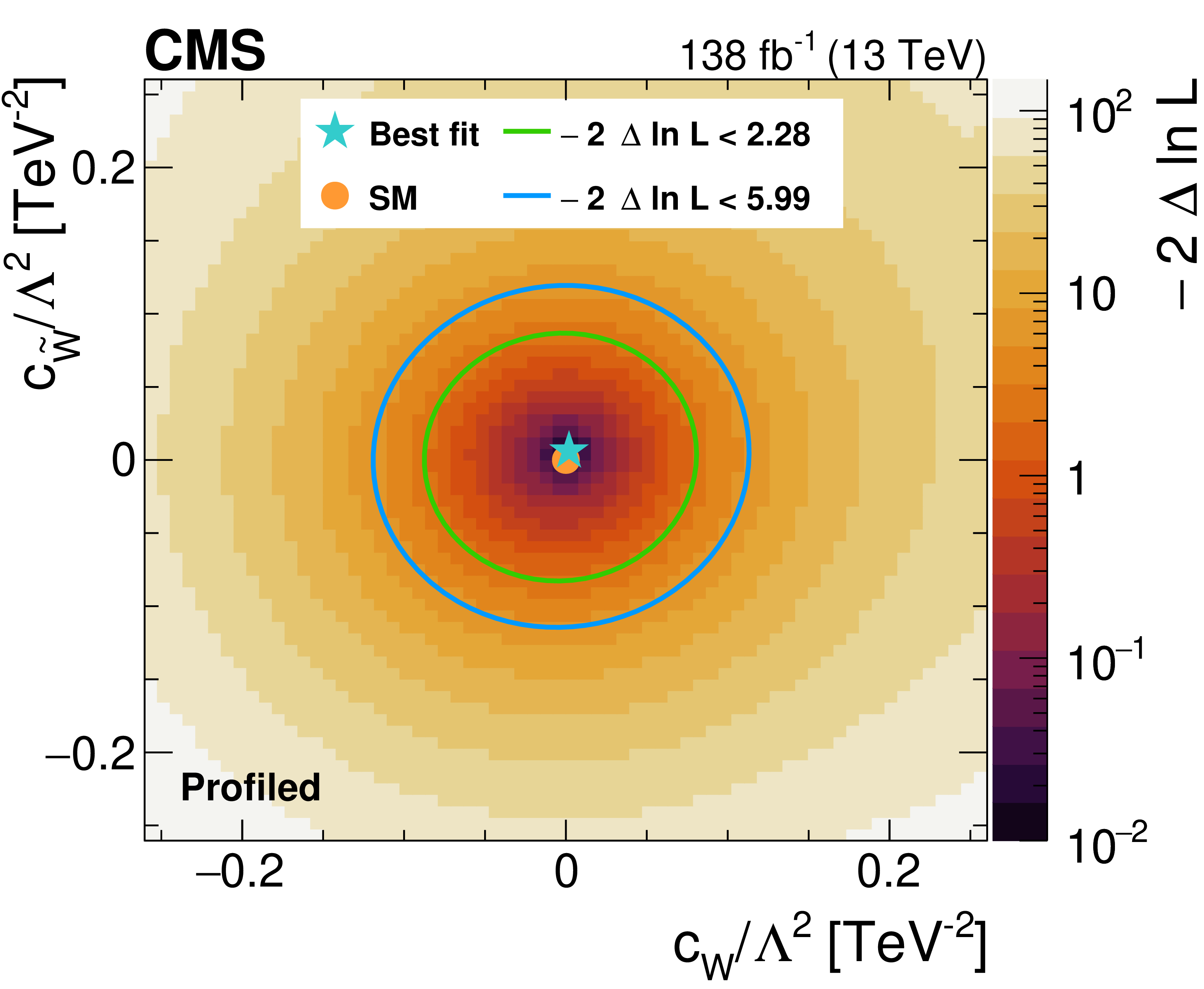
Figure 7:
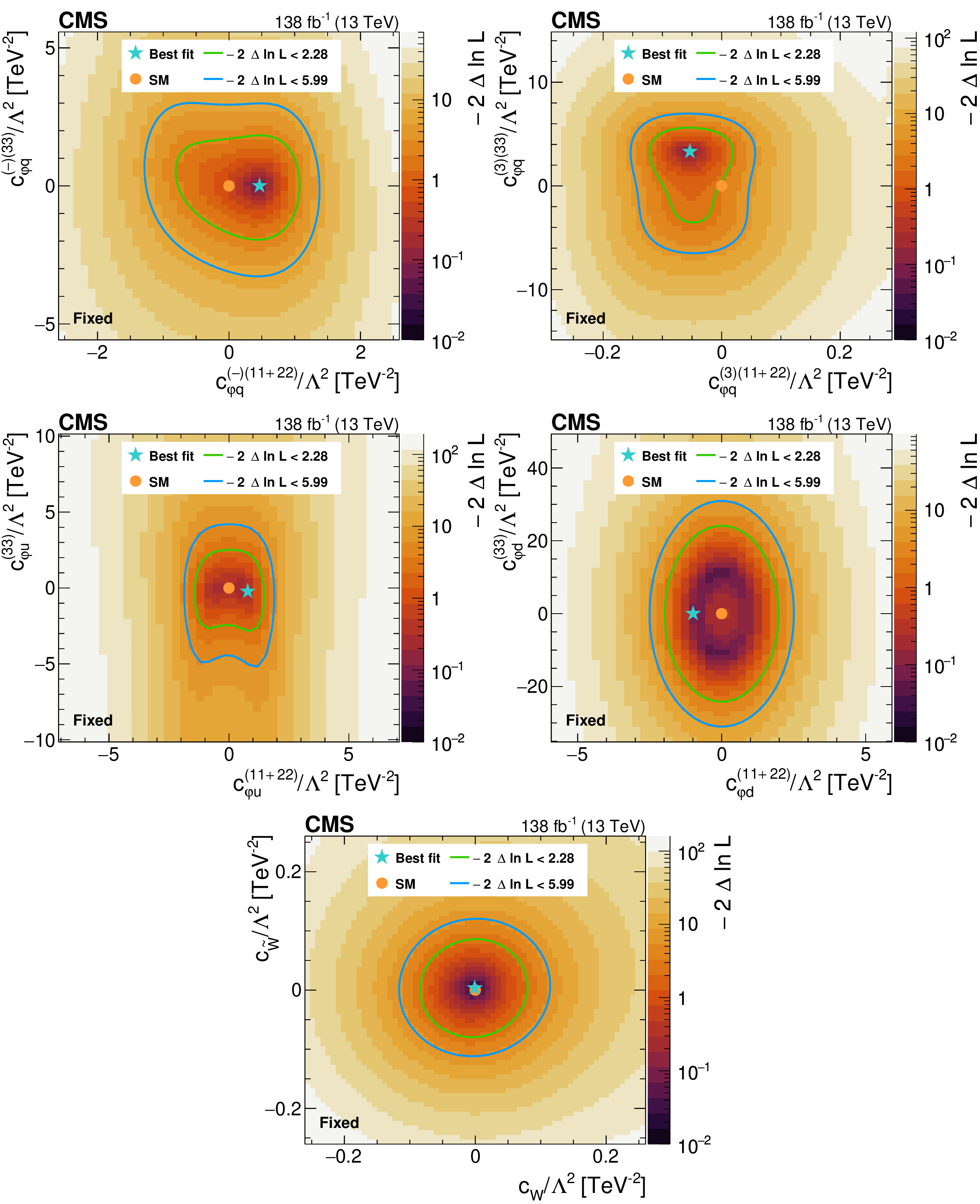
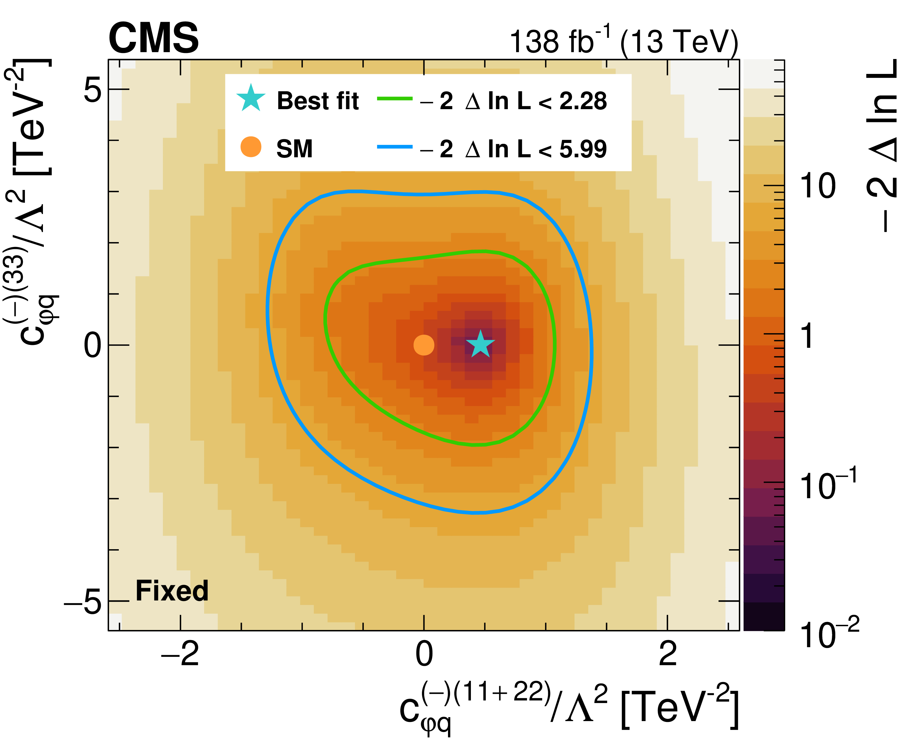
Likelihood as a function of the Wilson coefficients $ c_{\varphi q}^{(-)(11+22)} $ and $ c_{\varphi q}^{(-)(33)} $ (upper left), $ c_{\varphi q}^{(3)(11+22)} $ and $ c_{\varphi q}^{(3)(33)} $ (upper right), $ c_{\varphi u}^{(11+22)} $ and $ c_{\varphi u}^{(33)} $ (middle left), $ c_{\varphi d}^{(11+22)} $ and $ c_{\varphi d}^{(33)} $ (middle right), as well as $ c_{W} $ and $ c_{\widetilde{W}} $ (lower). All Wilson coefficients that are not scanned are fixed to zero. The best fit value is shown with a marker and the coloured lines correspond to the crossing points of $ -2\Delta\ln L $ at 2.28 and 5.99, which correspond to the 68 and 95% CL limits in the asymptotic approximation. |
png pdf |
Figure 7-a:
Likelihood as a function of the Wilson coefficients $ c_{\varphi q}^{(-)(11+22)} $ and $ c_{\varphi q}^{(-)(33)} $ (upper left), $ c_{\varphi q}^{(3)(11+22)} $ and $ c_{\varphi q}^{(3)(33)} $ (upper right), $ c_{\varphi u}^{(11+22)} $ and $ c_{\varphi u}^{(33)} $ (middle left), $ c_{\varphi d}^{(11+22)} $ and $ c_{\varphi d}^{(33)} $ (middle right), as well as $ c_{W} $ and $ c_{\widetilde{W}} $ (lower). All Wilson coefficients that are not scanned are fixed to zero. The best fit value is shown with a marker and the coloured lines correspond to the crossing points of $ -2\Delta\ln L $ at 2.28 and 5.99, which correspond to the 68 and 95% CL limits in the asymptotic approximation. |
png pdf |
Figure 7-b:
Likelihood as a function of the Wilson coefficients $ c_{\varphi q}^{(-)(11+22)} $ and $ c_{\varphi q}^{(-)(33)} $ (upper left), $ c_{\varphi q}^{(3)(11+22)} $ and $ c_{\varphi q}^{(3)(33)} $ (upper right), $ c_{\varphi u}^{(11+22)} $ and $ c_{\varphi u}^{(33)} $ (middle left), $ c_{\varphi d}^{(11+22)} $ and $ c_{\varphi d}^{(33)} $ (middle right), as well as $ c_{W} $ and $ c_{\widetilde{W}} $ (lower). All Wilson coefficients that are not scanned are fixed to zero. The best fit value is shown with a marker and the coloured lines correspond to the crossing points of $ -2\Delta\ln L $ at 2.28 and 5.99, which correspond to the 68 and 95% CL limits in the asymptotic approximation. |
png pdf |
Figure 7-c:
Likelihood as a function of the Wilson coefficients $ c_{\varphi q}^{(-)(11+22)} $ and $ c_{\varphi q}^{(-)(33)} $ (upper left), $ c_{\varphi q}^{(3)(11+22)} $ and $ c_{\varphi q}^{(3)(33)} $ (upper right), $ c_{\varphi u}^{(11+22)} $ and $ c_{\varphi u}^{(33)} $ (middle left), $ c_{\varphi d}^{(11+22)} $ and $ c_{\varphi d}^{(33)} $ (middle right), as well as $ c_{W} $ and $ c_{\widetilde{W}} $ (lower). All Wilson coefficients that are not scanned are fixed to zero. The best fit value is shown with a marker and the coloured lines correspond to the crossing points of $ -2\Delta\ln L $ at 2.28 and 5.99, which correspond to the 68 and 95% CL limits in the asymptotic approximation. |
png pdf |
Figure 7-d:
Likelihood as a function of the Wilson coefficients $ c_{\varphi q}^{(-)(11+22)} $ and $ c_{\varphi q}^{(-)(33)} $ (upper left), $ c_{\varphi q}^{(3)(11+22)} $ and $ c_{\varphi q}^{(3)(33)} $ (upper right), $ c_{\varphi u}^{(11+22)} $ and $ c_{\varphi u}^{(33)} $ (middle left), $ c_{\varphi d}^{(11+22)} $ and $ c_{\varphi d}^{(33)} $ (middle right), as well as $ c_{W} $ and $ c_{\widetilde{W}} $ (lower). All Wilson coefficients that are not scanned are fixed to zero. The best fit value is shown with a marker and the coloured lines correspond to the crossing points of $ -2\Delta\ln L $ at 2.28 and 5.99, which correspond to the 68 and 95% CL limits in the asymptotic approximation. |

png pdf |
Figure 7-e:
Likelihood as a function of the Wilson coefficients $ c_{\varphi q}^{(-)(11+22)} $ and $ c_{\varphi q}^{(-)(33)} $ (upper left), $ c_{\varphi q}^{(3)(11+22)} $ and $ c_{\varphi q}^{(3)(33)} $ (upper right), $ c_{\varphi u}^{(11+22)} $ and $ c_{\varphi u}^{(33)} $ (middle left), $ c_{\varphi d}^{(11+22)} $ and $ c_{\varphi d}^{(33)} $ (middle right), as well as $ c_{W} $ and $ c_{\widetilde{W}} $ (lower). All Wilson coefficients that are not scanned are fixed to zero. The best fit value is shown with a marker and the coloured lines correspond to the crossing points of $ -2\Delta\ln L $ at 2.28 and 5.99, which correspond to the 68 and 95% CL limits in the asymptotic approximation. |
png pdf |
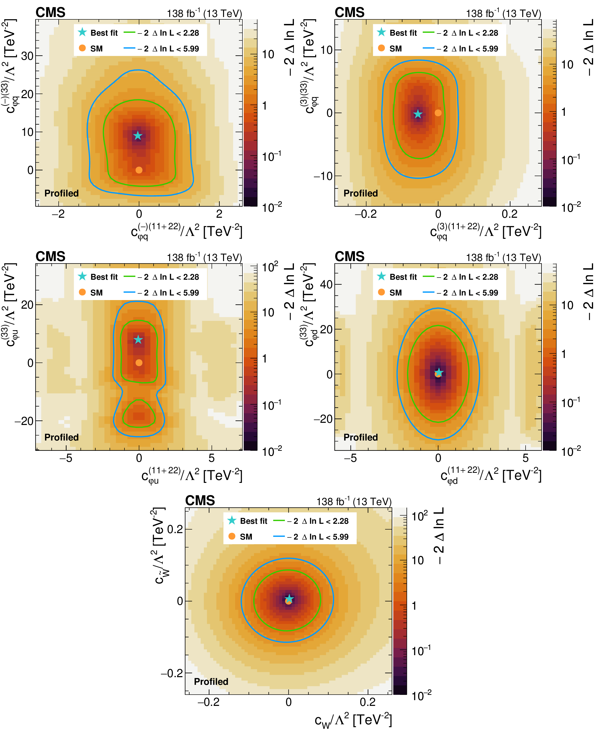
Figure 8:
Likelihood as a function of the Wilson coefficients $ c_{\varphi q}^{(-)(11+22)} $ and $ c_{\varphi q}^{(-)(33)} $ (upper left), $ c_{\varphi q}^{(3)(11+22)} $ and $ c_{\varphi q}^{(3)(33)} $ (upper right), $ c_{\varphi u}^{(11+22)} $ and $ c_{\varphi u}^{(33)} $ (middle left), $ c_{\varphi d}^{(11+22)} $ and $ c_{\varphi d}^{(33)} $ (middle right), as well as $ c_{W} $ and $ c_{\widetilde{W}} $ (lower). Other Wilson coefficients are allowed to float in the fit. The best fit value is shown with a marker and the coloured lines correspond to the crossing points of $ -2\Delta\ln L $ at 2.28 and 5.99, which correspond to the 68 and 95% CL limits in the asymptotic approximation. |
png pdf |
Figure 8-a:
Likelihood as a function of the Wilson coefficients $ c_{\varphi q}^{(-)(11+22)} $ and $ c_{\varphi q}^{(-)(33)} $ (upper left), $ c_{\varphi q}^{(3)(11+22)} $ and $ c_{\varphi q}^{(3)(33)} $ (upper right), $ c_{\varphi u}^{(11+22)} $ and $ c_{\varphi u}^{(33)} $ (middle left), $ c_{\varphi d}^{(11+22)} $ and $ c_{\varphi d}^{(33)} $ (middle right), as well as $ c_{W} $ and $ c_{\widetilde{W}} $ (lower). Other Wilson coefficients are allowed to float in the fit. The best fit value is shown with a marker and the coloured lines correspond to the crossing points of $ -2\Delta\ln L $ at 2.28 and 5.99, which correspond to the 68 and 95% CL limits in the asymptotic approximation. |
png pdf |
Figure 8-b:
Likelihood as a function of the Wilson coefficients $ c_{\varphi q}^{(-)(11+22)} $ and $ c_{\varphi q}^{(-)(33)} $ (upper left), $ c_{\varphi q}^{(3)(11+22)} $ and $ c_{\varphi q}^{(3)(33)} $ (upper right), $ c_{\varphi u}^{(11+22)} $ and $ c_{\varphi u}^{(33)} $ (middle left), $ c_{\varphi d}^{(11+22)} $ and $ c_{\varphi d}^{(33)} $ (middle right), as well as $ c_{W} $ and $ c_{\widetilde{W}} $ (lower). Other Wilson coefficients are allowed to float in the fit. The best fit value is shown with a marker and the coloured lines correspond to the crossing points of $ -2\Delta\ln L $ at 2.28 and 5.99, which correspond to the 68 and 95% CL limits in the asymptotic approximation. |
png pdf |
Figure 8-c:
Likelihood as a function of the Wilson coefficients $ c_{\varphi q}^{(-)(11+22)} $ and $ c_{\varphi q}^{(-)(33)} $ (upper left), $ c_{\varphi q}^{(3)(11+22)} $ and $ c_{\varphi q}^{(3)(33)} $ (upper right), $ c_{\varphi u}^{(11+22)} $ and $ c_{\varphi u}^{(33)} $ (middle left), $ c_{\varphi d}^{(11+22)} $ and $ c_{\varphi d}^{(33)} $ (middle right), as well as $ c_{W} $ and $ c_{\widetilde{W}} $ (lower). Other Wilson coefficients are allowed to float in the fit. The best fit value is shown with a marker and the coloured lines correspond to the crossing points of $ -2\Delta\ln L $ at 2.28 and 5.99, which correspond to the 68 and 95% CL limits in the asymptotic approximation. |
png pdf |
Figure 8-d:
Likelihood as a function of the Wilson coefficients $ c_{\varphi q}^{(-)(11+22)} $ and $ c_{\varphi q}^{(-)(33)} $ (upper left), $ c_{\varphi q}^{(3)(11+22)} $ and $ c_{\varphi q}^{(3)(33)} $ (upper right), $ c_{\varphi u}^{(11+22)} $ and $ c_{\varphi u}^{(33)} $ (middle left), $ c_{\varphi d}^{(11+22)} $ and $ c_{\varphi d}^{(33)} $ (middle right), as well as $ c_{W} $ and $ c_{\widetilde{W}} $ (lower). Other Wilson coefficients are allowed to float in the fit. The best fit value is shown with a marker and the coloured lines correspond to the crossing points of $ -2\Delta\ln L $ at 2.28 and 5.99, which correspond to the 68 and 95% CL limits in the asymptotic approximation. |
png pdf |
Figure 8-e:
Likelihood as a function of the Wilson coefficients $ c_{\varphi q}^{(-)(11+22)} $ and $ c_{\varphi q}^{(-)(33)} $ (upper left), $ c_{\varphi q}^{(3)(11+22)} $ and $ c_{\varphi q}^{(3)(33)} $ (upper right), $ c_{\varphi u}^{(11+22)} $ and $ c_{\varphi u}^{(33)} $ (middle left), $ c_{\varphi d}^{(11+22)} $ and $ c_{\varphi d}^{(33)} $ (middle right), as well as $ c_{W} $ and $ c_{\widetilde{W}} $ (lower). Other Wilson coefficients are allowed to float in the fit. The best fit value is shown with a marker and the coloured lines correspond to the crossing points of $ -2\Delta\ln L $ at 2.28 and 5.99, which correspond to the 68 and 95% CL limits in the asymptotic approximation. |
png pdf |
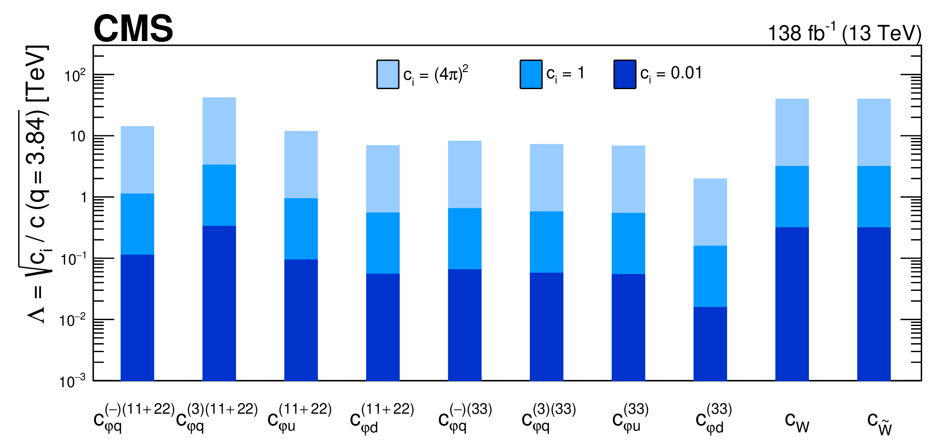
Figure 9:
Summary of the limits in the energy scale $ \Lambda $ obtained from the limits on the Wilson coefficients $ c_{\varphi q}^{(-)(11+22)} $, $ c_{\varphi q}^{(3)(11+22)} $, $ c_{\varphi u}^{(11+22)} $, $ c_{\varphi d}^{(11+22)} $, $ c_{\varphi q}^{(-)(33)} $, $ c_{\varphi q}^{(3)(33)} $, $ c_{\varphi u}^{(33)} $, $ c_{\varphi d}^{(33)} $, $ c_{W} $, and $ c_{\widetilde{W}} $. Shown are limits for scans where other Wilson coefficients are fixed to zero. The limit on $ \Lambda $ is calculated from the Wilson coefficient value at $ q = -2\Delta\ln L = $ 3.84, which corresponds to the 95% CL limit in the asymptotic approximation. The least stringent limit is chosen for each Wilson coefficient and limits are shown for three scenarios of $ c_{i} $. |
| Summary |
| An analysis of the flavour structures in effective field theory (EFT) couplings has been presented, considering the electroweak coupling to quarks of different generations in the processes $ \mathrm{t}\overline{\mathrm{t}}\mathrm{Z} $, WZ, and ZZ. Proton-proton collision data, collected at $ \sqrt{s}= $ 13 TeV in 2016-2018 by the CMS detector and corresponding to an integrated luminosity of 138 fb$ ^{-1} $ were analysed. For the first time, the flavour structures of the Z-quark couplings are disentangled by simultaneously probing the light- and heavy-quark couplings in different processes. The measured Wilson coefficients are compatible with the standard model hypothesis within their uncertainties and corresponding limits are placed using one- and two-dimensional scans of the profiled likelihood test statistic. Extracting the EFT parameters from multiple processes simultaneously makes it possible to correctly correlate EFT effects of the three processes that are often important backgrounds of each other. Thus, these results contribute to a more comprehensive EFT interpretation that preserves correlations in combinations or global fits, rather than focusing solely on individual processes. |
| References | ||||
| 1 | C. P. Burgess | Introduction to effective field theory | Cambridge University Press, . , ISBN~978-1-139-04804-0, 978-0-521-19547-8, 2020 link |
|
| 2 | W. Buchm \"u ller and D. Wyler | Effective Lagrangian analysis of new interactions and flavor conservation | NPB 268 (1986) 621 | |
| 3 | I. Brivio and M. Trott | The standard model as an effective field theory | Phys. Rept. 793 (2019) 1 | 1706.08945 |
| 4 | G. F. Giudice, C. Grojean, A. Pomarol, and R. Rattazzi | The strongly-interacting light Higgs | JHEP 06 (2007) 045 | hep-ph/0703164 |
| 5 | B. Grzadkowski, M. Iskrzynski, M. Misiak, and J. Rosiek | Dimension-six terms in the standard model Lagrangian | JHEP 10 (2010) 085 | 1008.4884 |
| 6 | A. Helset and A. Kobach | Baryon number, lepton number, and operator dimension in the SMEFT with flavor symmetries | Phys. Lett. B 800 () 135132, 2020 link |
1909.05853 |
| 7 | ATLAS Collaboration | Inclusive and differential cross-section measurements of $ {{\mathrm{t}\overline{\mathrm{t}}} \mathrm{Z}} $ production in $ {\mathrm{p}\mathrm{p}} $ collisions at $ \sqrt{s}= $ 13 TeV with the ATLAS detector, including EFT and spin-correlation interpretations | JHEP 07 (2024) 163 | 2312.04450 |
| 8 | ATLAS Collaboration | Measurements of inclusive and differential cross-sections of $ t\overline{t}\gamma $ production in pp collisions at $ \sqrt{s} $ = 13 TeV with the ATLAS detector | JHEP 10 (2024) 191 | 2403.09452 |
| 9 | CMS Collaboration | Probing effective field theory operators in the associated production of top quarks with a Z boson in multilepton final states at $ \sqrt{s}= $ 13 TeV | JHEP 12 (2021) 083 | CMS-TOP-21-001 2107.13896 |
| 10 | CMS Collaboration | Search for new physics using effective field theory in 13 TeV $ {\mathrm{p}\mathrm{p}} $ collision events that contain a top quark pair and a boosted Z or Higgs boson | PRD 108 (2023) 032008 | CMS-TOP-21-003 2208.12837 |
| 11 | CMS Collaboration | Search for new physics in top quark production with additional leptons in proton-proton collisions at $ \sqrt{s}= $ 13 TeV using effective field theory | JHEP 03 (2021) 095 | CMS-TOP-19-001 2012.04120 |
| 12 | CMS Collaboration | Search for physics beyond the standard model in top quark production with additional leptons in the context of effective field theory | JHEP 12 (2023) 068 | CMS-TOP-22-006 2307.15761 |
| 13 | S. Bi\ss mann, C. Grunwald, G. Hiller, and K. Kröninger | Top and beauty synergies in SMEFT-fits at present and future colliders | JHEP 06 (2021) 010 | 2012.10456 |
| 14 | S. Bruggisser, R. Sch ä fer, D. van Dyk, and S. Westhoff | The flavor of UV physics | JHEP 05 (2021) 257 | 2101.07273 |
| 15 | ATLAS Collaboration | Search for flavour-changing neutral current top-quark decays $ \mathrm{t}\to \mathrm{q}\mathrm{Z} $ in proton-proton collisions at $ \sqrt{s}= $ 13 TeV with the ATLAS detector | JHEP 07 (2018) 176 | 1803.09923 |
| 16 | ATLAS Collaboration | Search for flavour-changing neutral-current interactions of a top quark and a gluon in pp collisions at $ \sqrt{s}= $ 13 TeV with the ATLAS detector | EPJC 82 (2022) 334 | 2112.01302 |
| 17 | ATLAS Collaboration | Search for flavour-changing neutral-current couplings between the top quark and the photon with the ATLAS detector at $ \sqrt{s}= $ 13 TeV | PLB 842 (2023) 137379 | 2205.02537 |
| 18 | CMS Collaboration | Search for new physics in top quark production in dilepton final states in proton-proton collisions at $ \sqrt{s}= $ 13 TeV | EPJC 79 (2019) 886 | CMS-TOP-17-020 1903.11144 |
| 19 | CMS Collaboration | Measurement of the inclusive and differential $ {{\mathrm{t}\overline{\mathrm{t}}} \gamma} $ cross sections in the dilepton channel and effective field theory interpretation in proton-proton collisions at $ \sqrt{s}= $ 13 TeV | JHEP 05 (2022) 091 | CMS-TOP-21-004 2201.07301 |
| 20 | CMS Collaboration | HEPData record for this analysis | link | |
| 21 | CMS Collaboration | The CMS experiment at the CERN LHC | JINST 3 (2008) S08004 | |
| 22 | Tracker Group of the CMS Collaboration | The CMS Phase-1 pixel detector upgrade | JINST 16 (2021) P02027 | 2012.14304 |
| 23 | CMS Collaboration | Performance of the CMS Level-1 trigger in proton-proton collisions at $ \sqrt{s}= $ 13 TeV | JINST 15 (2020) P10017 | CMS-TRG-17-001 2006.10165 |
| 24 | CMS Collaboration | The CMS trigger system | JINST 12 (2017) P01020 | CMS-TRG-12-001 1609.02366 |
| 25 | CMS Collaboration | Performance of the CMS high-level trigger during LHC run 2 | JINST 19 (2024) P11021 | CMS-TRG-19-001 2410.17038 |
| 26 | J. Alwall et al. | The automated computation of tree-level and next-to-leading order differential cross sections, and their matching to parton shower simulations | JHEP 07 (2014) 079 | 1405.0301 |
| 27 | S. Frixione and B. R. Webber | Matching NLO QCD computations and parton shower simulations | JHEP 06 (2002) 029 | hep-ph/0204244 |
| 28 | O. Mattelaer | On the maximal use of Monte Carlo samples: Re-weighting events at NLO accuracy | EPJC 76 (2016) 674 | 1607.00763 |
| 29 | I. Brivio, Y. Jiang, and M. Trott | The SMEFTsim package, theory and tools | JHEP 12 (2017) 070 | 1709.06492 |
| 30 | I. Brivio | SMEFTsim 3.0---a practical guide | JHEP 04 (2021) 073 | 2012.11343 |
| 31 | T. Melia, P. Nason, R. Röntsch, and G. Zanderighi | $ {\mathrm{W^+}\mathrm{W^-}} $, $ {\mathrm{W}\mathrm{Z}} $ and $ {\mathrm{Z}\mathrm{Z}} $ production in the POWHEG \textscbox | JHEP 11 (2011) 078 | 1107.5051 |
| 32 | P. Nason and G. Zanderighi | $ {\mathrm{W^+}\mathrm{W^-}} $, $ {\mathrm{W}\mathrm{Z}} $ and $ {\mathrm{Z}\mathrm{Z}} $ production in the POWHEG -\textscbox-v2 | EPJC 74 (2014) 2702 | 1311.1365 |
| 33 | P. Nason | A new method for combining NLO QCD with shower Monte Carlo algorithms | JHEP 11 (2004) 040 | hep-ph/0409146 |
| 34 | S. Frixione, P. Nason, and C. Oleari | Matching NLO QCD computations with parton shower simulations: the POWHEG method | JHEP 11 (2007) 070 | 0709.2092 |
| 35 | S. Alioli, P. Nason, C. Oleari, and E. Re | A general framework for implementing NLO calculations in shower Monte Carlo programs: the POWHEG \textscbox | JHEP 06 (2010) 043 | 1002.2581 |
| 36 | S. Frixione, G. Ridolfi, and P. Nason | A positive-weight next-to-leading-order Monte Carlo for heavy flavour hadroproduction | JHEP 09 (2007) 126 | 0707.3088 |
| 37 | H. B. Hartanto, B. J ä ger, L. Reina, and D. Wackeroth | Higgs boson production in association with top quarks in the POWHEG \textscbox | PRD 91 (2015) 094003 | 1501.04498 |
| 38 | S. Alioli, P. Nason, C. Oleari, and E. Re | NLO single-top production matched with shower in POWHEG: $ s $- and $ t $-channel contributions | JHEP 09 (2009) 111 | 0907.4076 |
| 39 | E. Re | Single-top $ {\mathrm{W}\mathrm{t}} $-channel production matched with parton showers using the POWHEG method | EPJC 71 (2011) 1547 | 1009.2450 |
| 40 | T. Sjöstrand et al. | An introduction to PYTHIA 8.2 | Comput. Phys. Commun. 191 (2015) 159 | 1410.3012 |
| 41 | J. M. Campbell and R. K. Ellis | An update on vector boson pair production at hadron colliders | PRD 60 (1999) 113006 | hep-ph/9905386 |
| 42 | J. M. Campbell, R. K. Ellis, and C. Williams | Vector boson pair production at the LHC | JHEP 07 (2011) 018 | 1105.0020 |
| 43 | J. M. Campbell, R. K. Ellis, and W. T. Giele | A multi-threaded version of MCFM | EPJC 75 (2015) 246 | 1503.06182 |
| 44 | CMS Collaboration | Extraction and validation of a new set of CMS PYTHIA 8 tunes from underlying-event measurements | EPJC 80 (2020) 4 | CMS-GEN-17-001 1903.12179 |
| 45 | R. Frederix and S. Frixione | Merging meets matching in MC@NLO | JHEP 12 (2012) 061 | 1209.6215 |
| 46 | J. Alwall et al. | Comparative study of various algorithms for the merging of parton showers and matrix elements in hadronic collisions | EPJC 53 (2008) 473 | 0706.2569 |
| 47 | NNPDF Collaboration | Parton distributions from high-precision collider data | EPJC 77 (2017) 663 | 1706.00428 |
| 48 | GEANT4 Collaboration | GEANT 4---a simulation toolkit | NIM A 506 (2003) 250 | |
| 49 | J. Allison et al. | GEANT 4 developments and applications | IEEE Trans. Nucl. Sci. 53 (2006) 270 | |
| 50 | CMS Collaboration | Particle-flow reconstruction and global event description with the CMS detector | JINST 12 (2017) P10003 | CMS-PRF-14-001 1706.04965 |
| 51 | CMS Collaboration | Technical proposal for the Phase-II upgrade of the Compact Muon Solenoid | CMS Technical Proposal CERN-LHCC-2015-010, CMS-TDR-15-02, 2015 CDS |
|
| 52 | CMS Collaboration | Performance of missing transverse momentum reconstruction in proton-proton collisions at $ \sqrt{s}= $ 13 TeV using the CMS detector | JINST 14 (2019) P07004 | CMS-JME-17-001 1903.06078 |
| 53 | CMS Collaboration | Electron and photon reconstruction and identification with the CMS experiment at the CERN LHC | JINST 16 (2021) P05014 | CMS-EGM-17-001 2012.06888 |
| 54 | CMS Collaboration | Performance of the CMS muon detector and muon reconstruction with proton-proton collisions at $ \sqrt{s}= $ 13 TeV | JINST 13 (2018) P06015 | CMS-MUO-16-001 1804.04528 |
| 55 | CMS Collaboration | Observation of four top quark production in proton-proton collisions at $ \sqrt{s}= $ 13 TeV | PLB 847 (2023) 138290 | CMS-TOP-22-013 2305.13439 |
| 56 | CMS Collaboration | Muon identification using multivariate techniques in the CMS experiment in proton-proton collisions at $ \sqrt{s}= $ 13 TeV | JINST 19 (2024) P02031 | CMS-MUO-22-001 2310.03844 |
| 57 | M. Cacciari, G. P. Salam, and G. Soyez | The anti-$ k_{\mathrm{T}} $ jet clustering algorithm | JHEP 04 (2008) 063 | 0802.1189 |
| 58 | M. Cacciari, G. P. Salam, and G. Soyez | FASTJET user manual | EPJC 72 (2012) 1896 | 1111.6097 |
| 59 | CMS Collaboration | Jet energy scale and resolution in the CMS experiment in $ {\mathrm{p}\mathrm{p}} $ collisions at 8 TeV | JINST 12 (2017) P02014 | CMS-JME-13-004 1607.03663 |
| 60 | CMS Collaboration | Performance of b tagging algorithms in proton-proton collisions at 13 TeV with Phase 1 CMS detector | CMS Detector Performance Note CMS-DP-2018-033, 2018 CDS |
|
| 61 | E. Bols et al. | Jet flavour classification using DeepJet | JINST 15 (2020) P12012 | 2008.10519 |
| 62 | Particle Data Group , S. Navas et al. | Review of particle physics | PRD 110 (2024) 030001 | |
| 63 | CMS Collaboration | Evidence for associated production of a Higgs boson with a top quark pair in final states with electrons, muons, and hadronically decaying $ \tau $ leptons at $ \sqrt{s} = $ 13 TeV | JHEP 08 (2018) 066 | CMS-HIG-17-018 1803.05485 |
| 64 | CMS Collaboration | Measurement of the Higgs boson production rate in association with top quarks in final states with electrons, muons, and hadronically decaying tau leptons at $ \sqrt{s}= $ 13 TeV | EPJC 81 (2021) 378 | CMS-HIG-19-008 2011.03652 |
| 65 | CMS Collaboration | Identification of heavy-flavour jets with the CMS detector in $ {\mathrm{p}\mathrm{p}} $ collisions at 13 TeV | JINST 13 (2018) P05011 | CMS-BTV-16-002 1712.07158 |
| 66 | CMS Collaboration | Pileup mitigation at CMS in 13 TeV data | JINST 15 (2020) P09018 | CMS-JME-18-001 2003.00503 |
| 67 | CMS Collaboration | Precision luminosity measurement in proton-proton collisions at $ \sqrt{s} = $ 13 TeV in 2015 and 2016 at CMS | EPJC 81 (2021) 800 | CMS-LUM-17-003 2104.01927 |
| 68 | CMS Collaboration | CMS luminosity measurement for the 2017 data-taking period at $ \sqrt{s}= $ 13 TeV | CMS Physics Analysis Summary, 2018 CMS-PAS-LUM-17-004 |
CMS-PAS-LUM-17-004 |
| 69 | CMS Collaboration | CMS luminosity measurement for the 2018 data-taking period at $ \sqrt{s}= $ 13 TeV | CMS Physics Analysis Summary, 2019 CMS-PAS-LUM-18-002 |
CMS-PAS-LUM-18-002 |
| 70 | NNPDF Collaboration | Parton distributions for the LHC run II | JHEP 04 (2015) 040 | 1410.8849 |
| 71 | M. Grazzini, S. Kallweit, and M. Wiesemann | Fully differential NNLO computations with \textscmatrix | EPJC 78 (2018) 537 | 1711.06631 |
| 72 | CMS Collaboration | Measurement of the cross section of top quark-antiquark pair production in association with a W boson in proton-proton collisions at $ \sqrt{s}= $ 13 TeV | JHEP 07 (2023) 219 | CMS-TOP-21-011 2208.06485 |
| 73 | A. Kulesza et al. | Associated top quark pair production with a heavy boson: Differential cross sections at NLO+NNLL accuracy | EPJC 80 (2020) 428 | 2001.03031 |
| 74 | CMS Collaboration | Inclusive and differential cross section measurements of single top quark production in association with a Z boson in proton-proton collisions at $ \sqrt{s}= $ 13 TeV | JHEP 02 (2022) 107 | CMS-TOP-20-010 2111.02860 |
| 75 | CMS Collaboration | Measurements of production cross sections of $ {\mathrm{W}\mathrm{Z}} $ and same-sign $ {\mathrm{W}\mathrm{W}} $ boson pairs in association with two jets in proton-proton collisions at $ \sqrt{s}= $ 13 TeV | PLB 809 (2020) 135710 | CMS-SMP-19-012 2005.01173 |
| 76 | F. Cascioli et al. | $ {\mathrm{Z}\mathrm{Z}} $ production at hadron colliders in NNLO QCD | PLB 735 (2014) 311 | 1405.2219 |
| 77 | M. Grazzini et al. | NNLO QCD + NLO EW with \textscmatrix+\textscOpenLoops: precise predictions for vector-boson pair production | JHEP 02 (2020) 087 | 1912.00068 |
| 78 | CMS Collaboration | The CMS statistical analysis and combination tool: Combine | Comput. Softw. Big Sci. 8 (2024) 19 | CMS-CAT-23-001 2404.06614 |
| 79 | W. Verkerke and D. Kirkby | The \textscRooFit toolkit for data modeling | in th International Conference on Computing in High Energy and Nuclear Physics (CHEP ): La Jolla CA, United States, March 24--28,, 2003 Proc. 1 (2003) 3 |
physics/0306116 |
| 80 | L. Moneta et al. | The \textscRooStats project | in th International Workshop on Advanced Computing and Analysis Techniques in Physics Research (ACAT ): Jaipur, India, February 22--27,, 2010 Proc. 1 (2010) 3 |
1009.1003 |
| 81 | R. Barlow and C. Beeston | Fitting using finite Monte Carlo samples | Comput. Phys. Commun. 77 (1993) 219 | |
| 82 | F. U. Bernlochner, D. C. Fry, S. B. Menary, and E. Persson | Cover your bases: asymptotic distributions of the profile likelihood ratio when constraining effective field theories in high-energy physics | SciPost Phys. Core 6 (2023) 013 | 2207.01350 |
| 83 | CMS Collaboration | Measurements of $ \mathrm{p}\mathrm{p} \to \mathrm{Z}\mathrm{Z} $ production cross sections and constraints on anomalous triple gauge couplings at $ \sqrt{s} = $ 13 TeV | EPJC 81 (2021) 200 | CMS-SMP-19-001 2009.01186 |
| 84 | CMS Collaboration | Measurement of the inclusive and differential $ {\mathrm{W}\mathrm{Z}} $ production cross sections, polarization angles, and triple gauge couplings in $ {\mathrm{p}\mathrm{p}} $ collisions at $ \sqrt{s}= $ 13 TeV | JHEP 07 (2022) 032 | CMS-SMP-20-014 2110.11231 |
| 85 | CMS Collaboration | Constraints on standard model effective field theory for a Higgs boson produced in association with W or Z bosons in the H \textrightarrow$ \textrm{b}\overline{\textrm{b}} $ decay channel in proton-proton collisions at $ \sqrt{s} $ = 13 TeV | JHEP 03 (2025) 114 | CMS-HIG-23-016 2411.16907 |
| 86 | ATLAS Collaboration | Measurements of $ W^+W^-+\ge 1 $jet production cross-sections in pp collisions at $ \sqrt{s}=13 $TeV with the ATLAS detector | JHEP 06 (2021) 003 | 2103.10319 |
|
|
Compact Muon Solenoid LHC, CERN |
|

|

|

|

|

|