

Compact Muon Solenoid
LHC, CERN
| CMS-SMP-23-003 ; CERN-EP-2025-130 | ||
| Search for charged lepton flavor violating Z and Z' boson decays in proton-proton collisions at $ \sqrt{s}= $ 13 TeV | ||
| CMS Collaboration | ||
| 10 August 2025 | ||
| Phys. Rev.D 112 (2025) 112011 | ||
| Abstract: A search for flavor violating decays of the Z boson to charged leptons is performed using data from proton-proton collisions at $ \sqrt{s}= $ 13 TeV collected with the CMS detector at the LHC, corresponding to an integrated luminosity of 138 fb$ ^{-1} $. Each of the decays $ \mathrm{Z}\to\mathrm{e}\mu $, $ \mathrm{Z}\to\mathrm{e}\tau $, and $ \mathrm{Z}\to\mu\tau $ is considered. The data are consistent with the backgrounds expected from standard model processes. For the $ \mathrm{Z}\to\mathrm{e}\mu $ channel the observed (expected) 95% confidence level upper limit on the branching fraction is 1.9 (2.0)$ \times$ 10$^{-7} $, which is the most stringent direct limit to date on this process; the corresponding limits for the $ \mathrm{Z}\to\mathrm{e}\tau $ and $ \mathrm{Z}\to\mu\tau $ channels are 13.8 (11.4)$ \times$ 10$^{-6} $ and 12.0 (5.3)$ \times$ 10$^{-6} $, respectively. Additionally, the $ \mathrm{e}\mu $ final state is used to search for lepton flavor violating decays of Z' resonances in the mass range from 110 to 500 GeV. No significant excess is observed above the predicted background levels. | ||
| Links: e-print arXiv:2508.07512 [hep-ex] (PDF) ; CDS record ; inSPIRE record ; HepData record ; Physics Briefing ; CADI line (restricted) ; | ||
| Figures | |
png pdf |
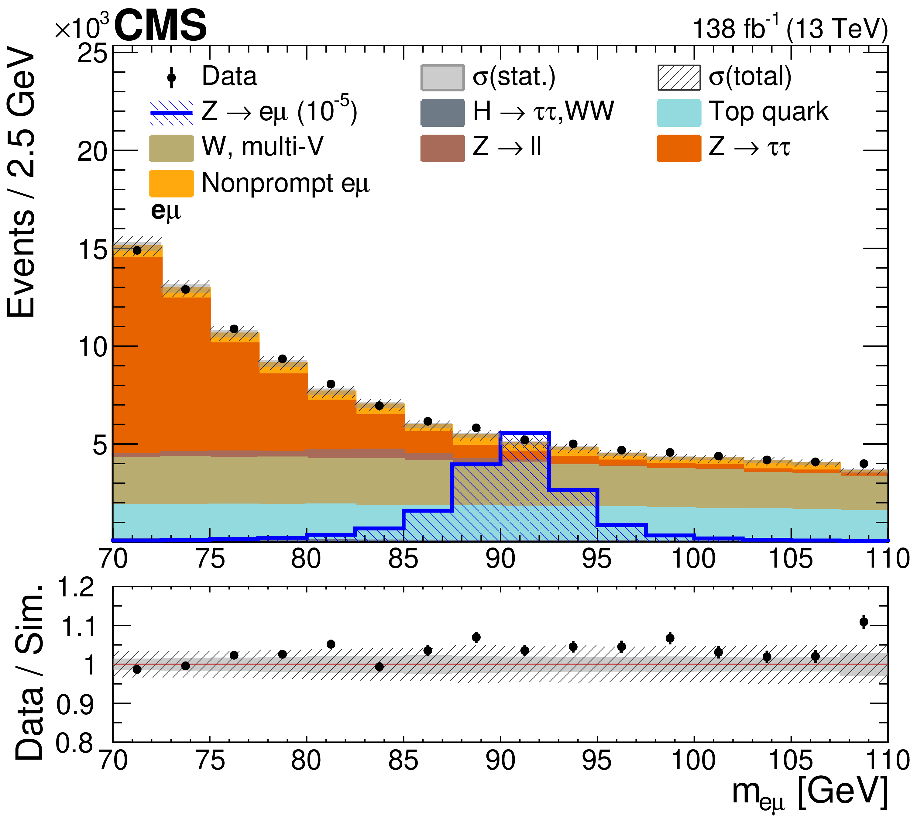
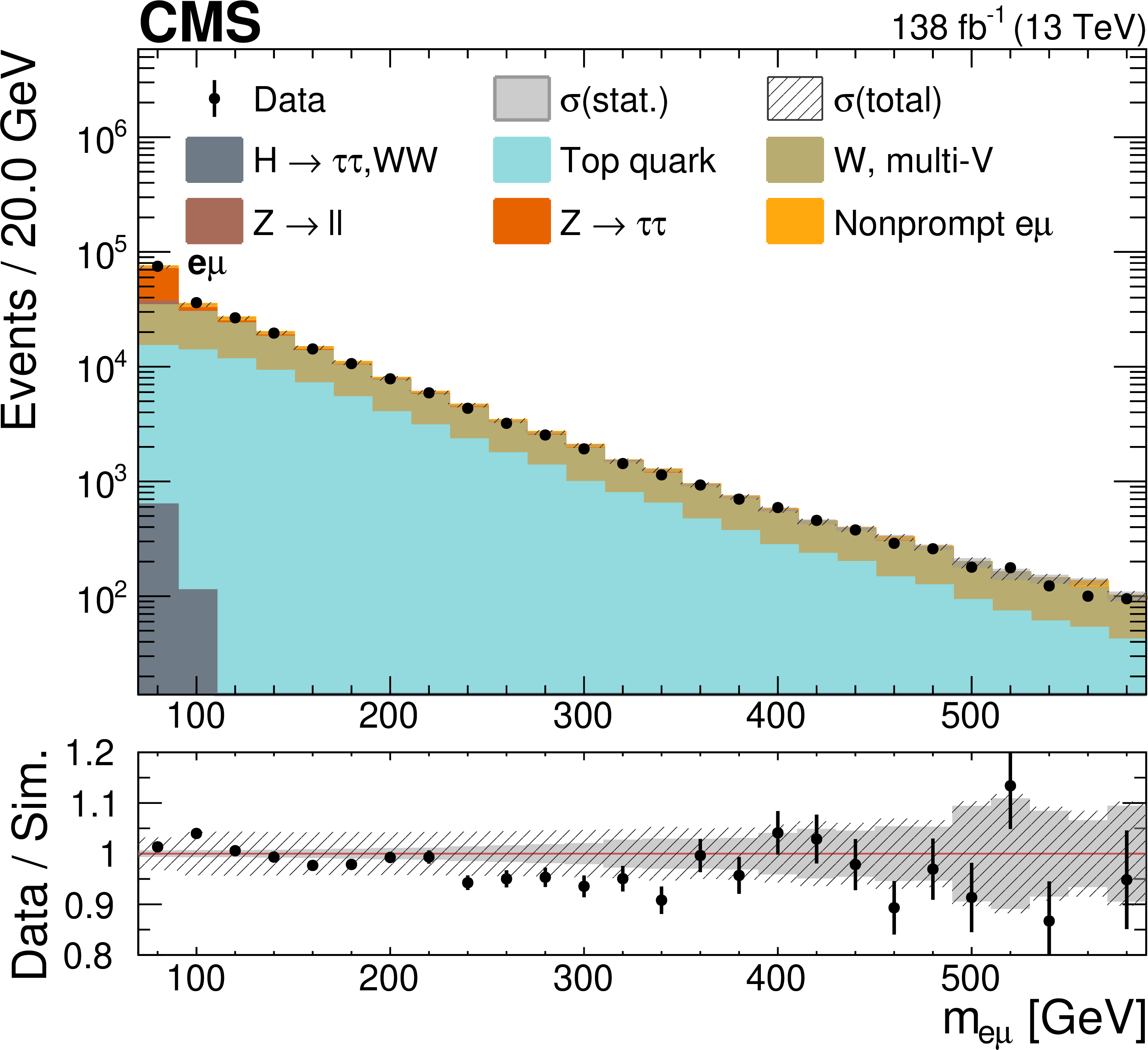
Figure 1:
Invariant mass of the $ \mathrm{e}\mu $ system for data (points, with bars denoting statistical uncertainty) and simulated background (stacked filled histograms) for events passing the baseline selection. In the legend, ``W, multi-V'' refers to W+jets events having a jet that is misidentified as a lepton, together with multiple vector boson production. The hatched histogram shows a hypothetical $ \mathrm{Z}\to\mathrm{e}\mu $ signal normalized to a branching fraction of 10$^{-5} $. The lower panel shows the ratio of the data to simulated background yields, with the statistical (combined systematic and statistical) uncertainty in the simulated yield indicated by the filled (hatched) gray band. |
png pdf |
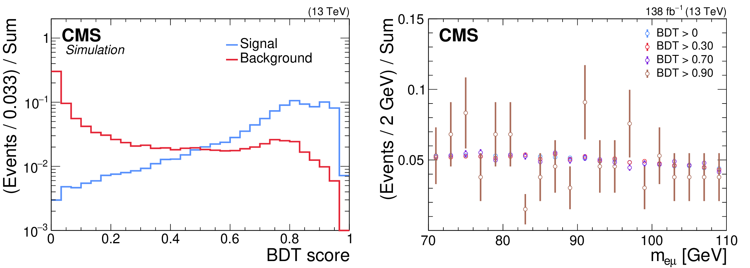
Figure 2:
The left plot shows unity-normalized distributions of the $ \mathrm{Z}\to\mathrm{e}\mu $ BDT score for simulated events from the BDT test samples satisfying 70 $ < m_{\mathrm{e}\mu} < $ 110 GeV. The blue and red histograms represent the signal and WW background, respectively. The right plot displays the unity-normalized distribution of $ m_{\mathrm{e}\mu} $ for events in the $ \mathrm{t} \overline{\mathrm{t}} $ data CR used to check for BDT mass-spectrum bias, for several BDT thresholds; the vertical bars show the statistical uncertainties. |
png pdf |
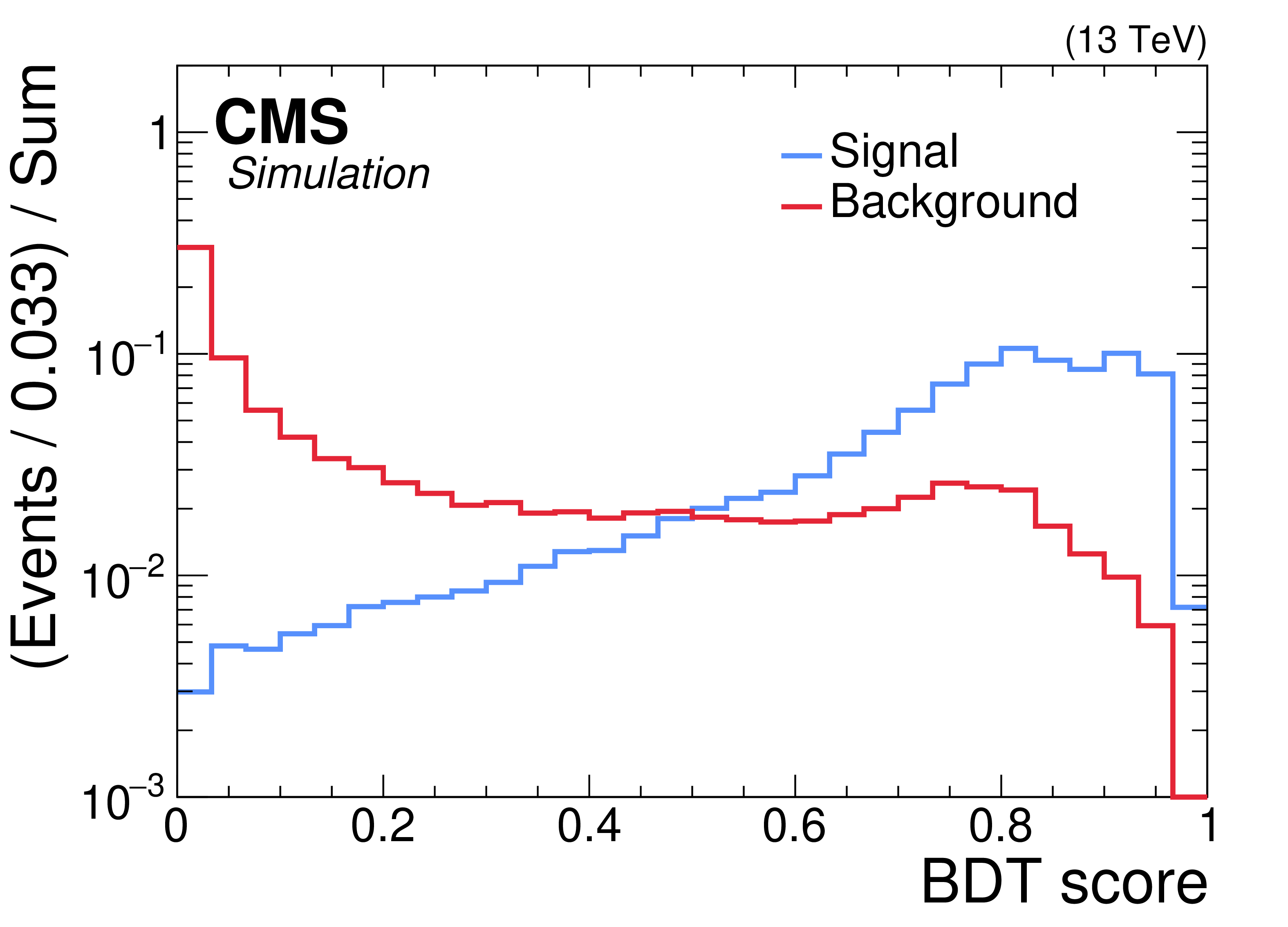
Figure 2-a:
The left plot shows unity-normalized distributions of the $ \mathrm{Z}\to\mathrm{e}\mu $ BDT score for simulated events from the BDT test samples satisfying 70 $ < m_{\mathrm{e}\mu} < $ 110 GeV. The blue and red histograms represent the signal and WW background, respectively. The right plot displays the unity-normalized distribution of $ m_{\mathrm{e}\mu} $ for events in the $ \mathrm{t} \overline{\mathrm{t}} $ data CR used to check for BDT mass-spectrum bias, for several BDT thresholds; the vertical bars show the statistical uncertainties. |
png pdf |
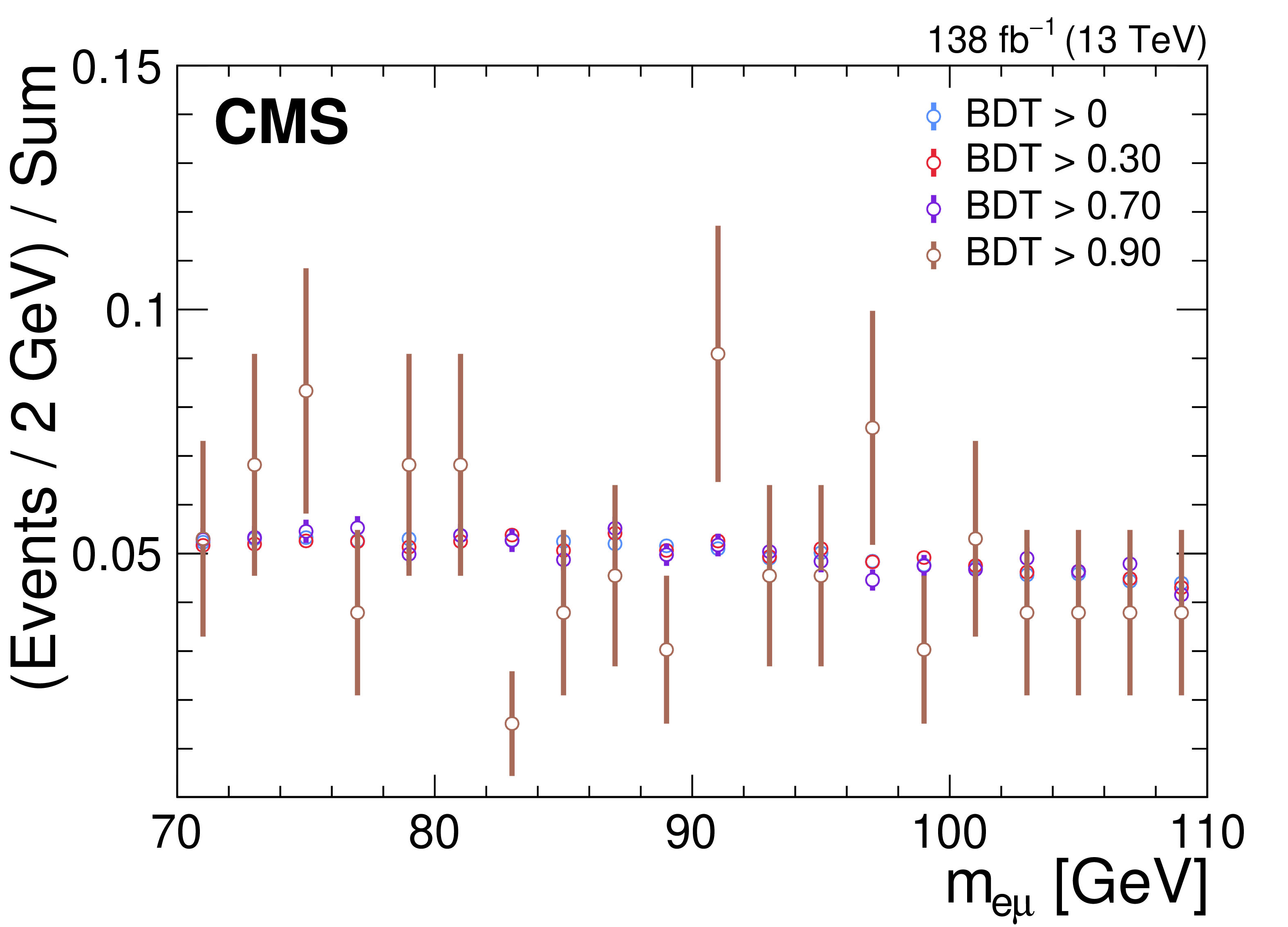
Figure 2-b:
The left plot shows unity-normalized distributions of the $ \mathrm{Z}\to\mathrm{e}\mu $ BDT score for simulated events from the BDT test samples satisfying 70 $ < m_{\mathrm{e}\mu} < $ 110 GeV. The blue and red histograms represent the signal and WW background, respectively. The right plot displays the unity-normalized distribution of $ m_{\mathrm{e}\mu} $ for events in the $ \mathrm{t} \overline{\mathrm{t}} $ data CR used to check for BDT mass-spectrum bias, for several BDT thresholds; the vertical bars show the statistical uncertainties. |
png pdf |
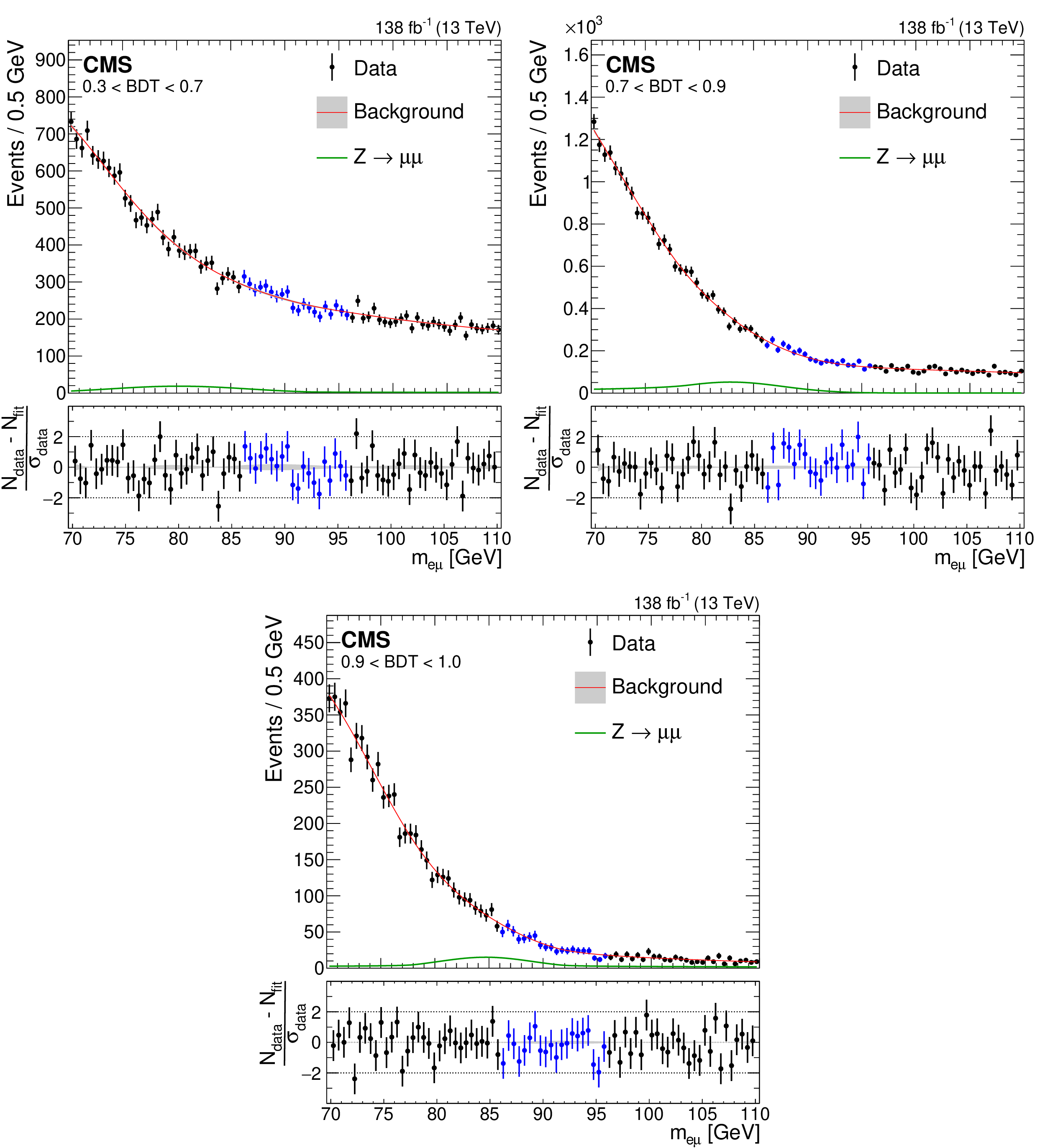
Figure 3:
Fits of the data sidebands with the background functions for the BDT score ranges 0.3-0.7 (upper left), 0.7-0.9 (upper right), and 0.9-1.0 (lower). In the upper panel of each plot, the black (blue) points with bars show the data with statistical uncertainties in the sideband (signal) region, the solid red line shows the average background prediction, and the green curve shows the $ \mathrm{Z}\to\mu\mu^*\to\mu\mu\gamma $ background component. The lower panel in each plot shows the ratio of the difference between the data and the average background prediction to the uncertainty in the data, and the gray band shows the spread of the background estimates from the separate families of parametric functions. |
png pdf |
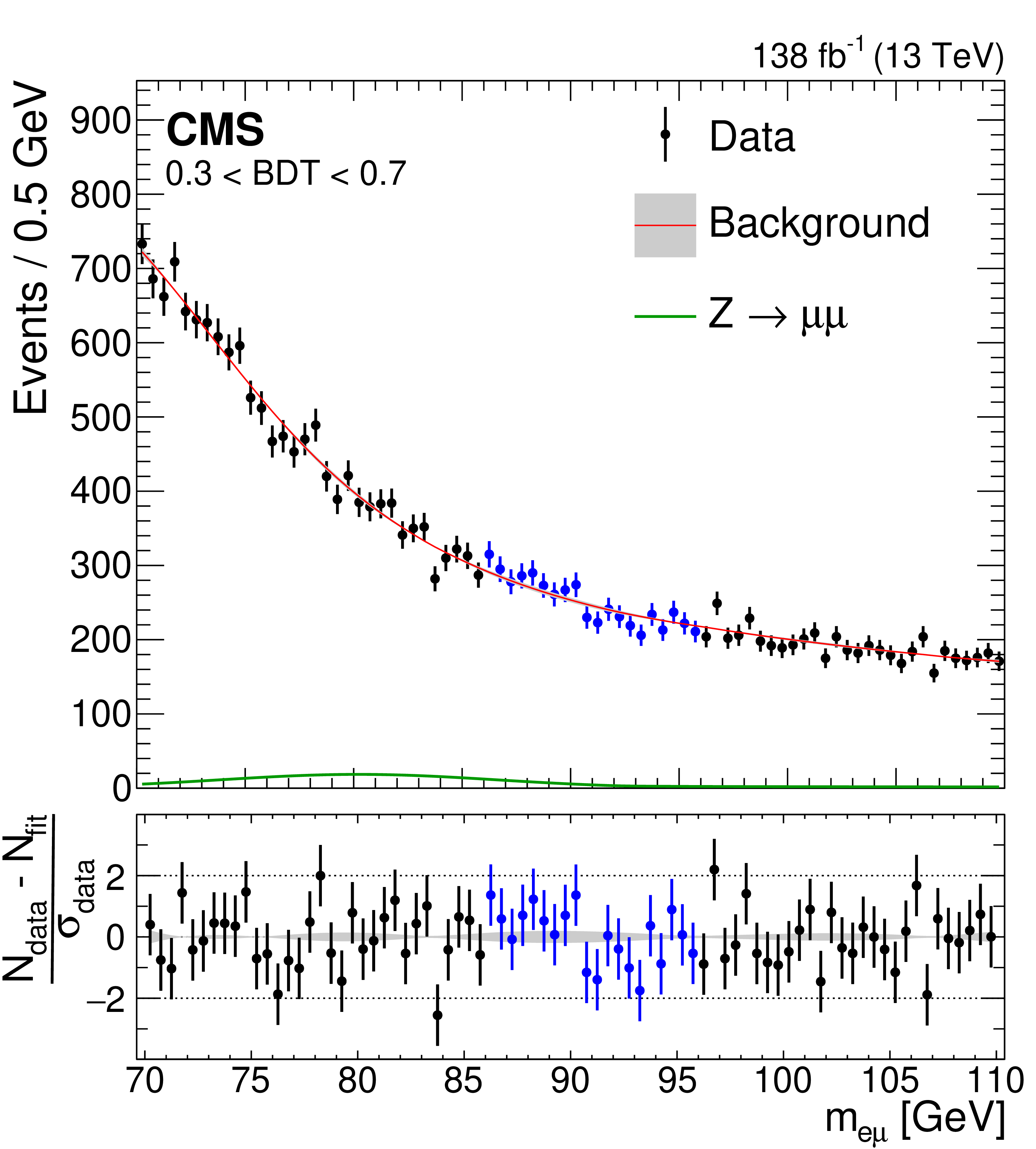
Figure 3-a:
Fits of the data sidebands with the background functions for the BDT score ranges 0.3-0.7 (upper left), 0.7-0.9 (upper right), and 0.9-1.0 (lower). In the upper panel of each plot, the black (blue) points with bars show the data with statistical uncertainties in the sideband (signal) region, the solid red line shows the average background prediction, and the green curve shows the $ \mathrm{Z}\to\mu\mu^*\to\mu\mu\gamma $ background component. The lower panel in each plot shows the ratio of the difference between the data and the average background prediction to the uncertainty in the data, and the gray band shows the spread of the background estimates from the separate families of parametric functions. |
png pdf |
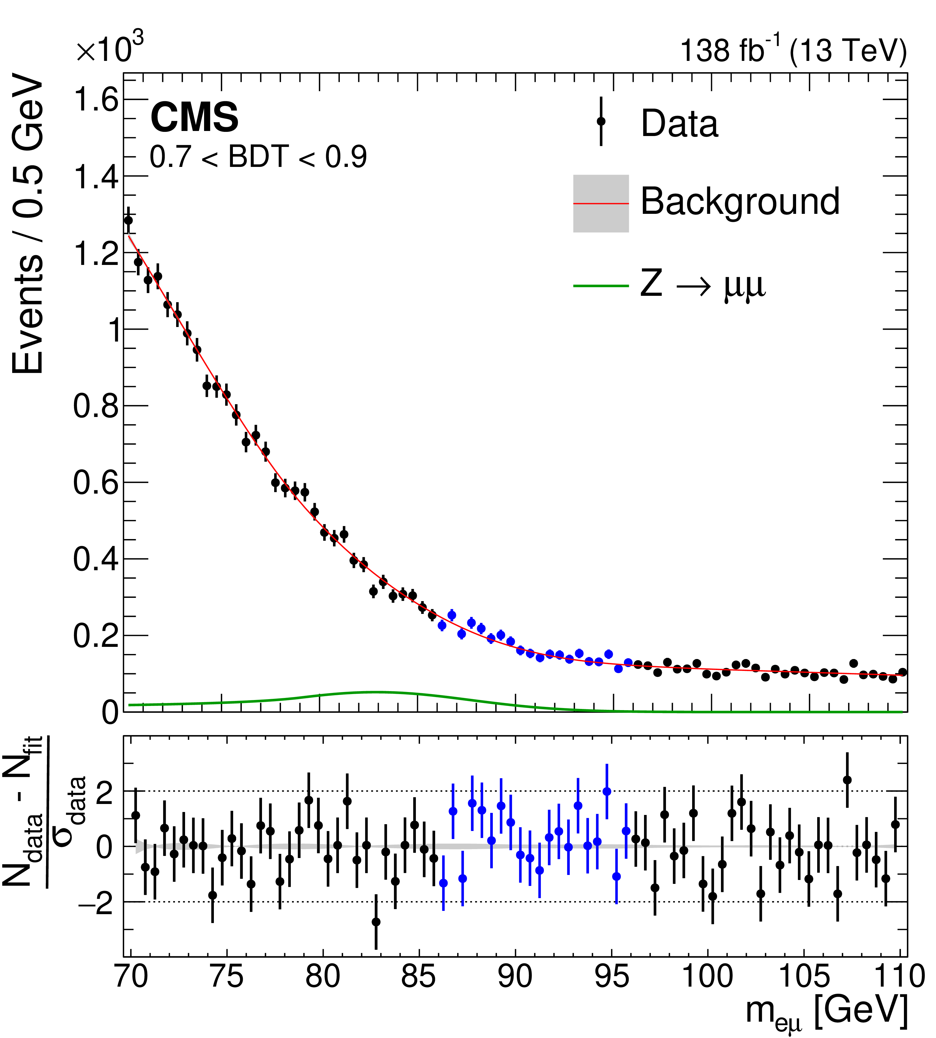
Figure 3-b:
Fits of the data sidebands with the background functions for the BDT score ranges 0.3-0.7 (upper left), 0.7-0.9 (upper right), and 0.9-1.0 (lower). In the upper panel of each plot, the black (blue) points with bars show the data with statistical uncertainties in the sideband (signal) region, the solid red line shows the average background prediction, and the green curve shows the $ \mathrm{Z}\to\mu\mu^*\to\mu\mu\gamma $ background component. The lower panel in each plot shows the ratio of the difference between the data and the average background prediction to the uncertainty in the data, and the gray band shows the spread of the background estimates from the separate families of parametric functions. |
png pdf |
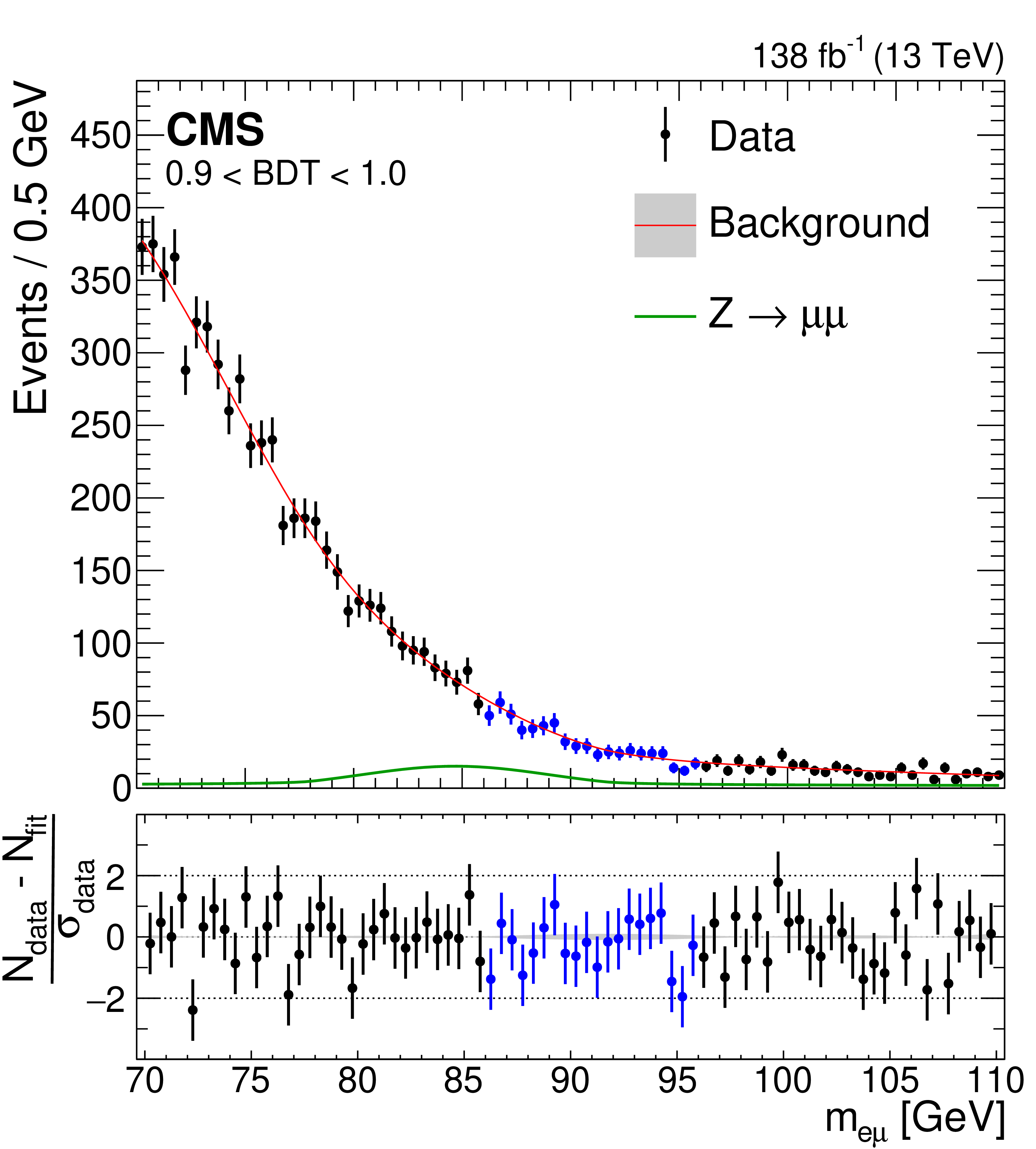
Figure 3-c:
Fits of the data sidebands with the background functions for the BDT score ranges 0.3-0.7 (upper left), 0.7-0.9 (upper right), and 0.9-1.0 (lower). In the upper panel of each plot, the black (blue) points with bars show the data with statistical uncertainties in the sideband (signal) region, the solid red line shows the average background prediction, and the green curve shows the $ \mathrm{Z}\to\mu\mu^*\to\mu\mu\gamma $ background component. The lower panel in each plot shows the ratio of the difference between the data and the average background prediction to the uncertainty in the data, and the gray band shows the spread of the background estimates from the separate families of parametric functions. |
png pdf |
Figure 4:
Invariant mass of the $ \mathrm{e}\mu $ system for data (points) and simulated background (stacked filled histograms), for events that pass the baseline selection except for that selection's upper limit on the invariant mass. The lower panel shows the ratio of the data to simulated yields, with the statistical (combined systematic and statistical) uncertainty in the simulated yield indicated by the filled (hatched) gray band. |
png pdf |
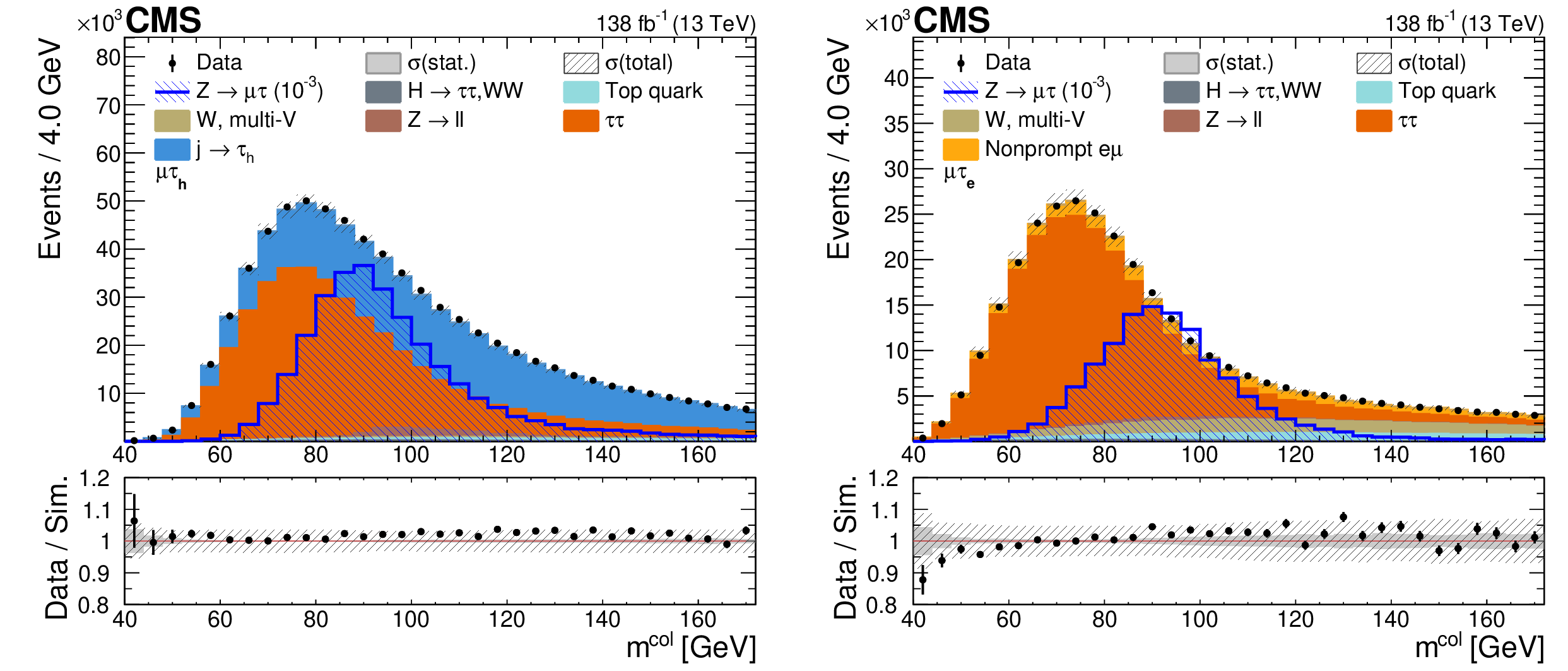
Figure 5:
The $ \mu\tau_\mathrm{h} $ (left) and $ \mu\tau_{\mathrm{e}} $ (right) $ m^{{\text{col}}} $ distributions, for the data (black markers with bars showing the statistical uncertainties) and the simulated backgrounds (filled stacked histograms). The hatched blue histogram shows the shape of the signal, normalized to a branching fraction of 10$^{-3} $, for comparison. The lower panel shows the ratio of the data to simulated yields, with the statistical (combined systematic and statistical) uncertainty in the simulated yield indicated by the filled (hatched) gray band. |
png pdf |
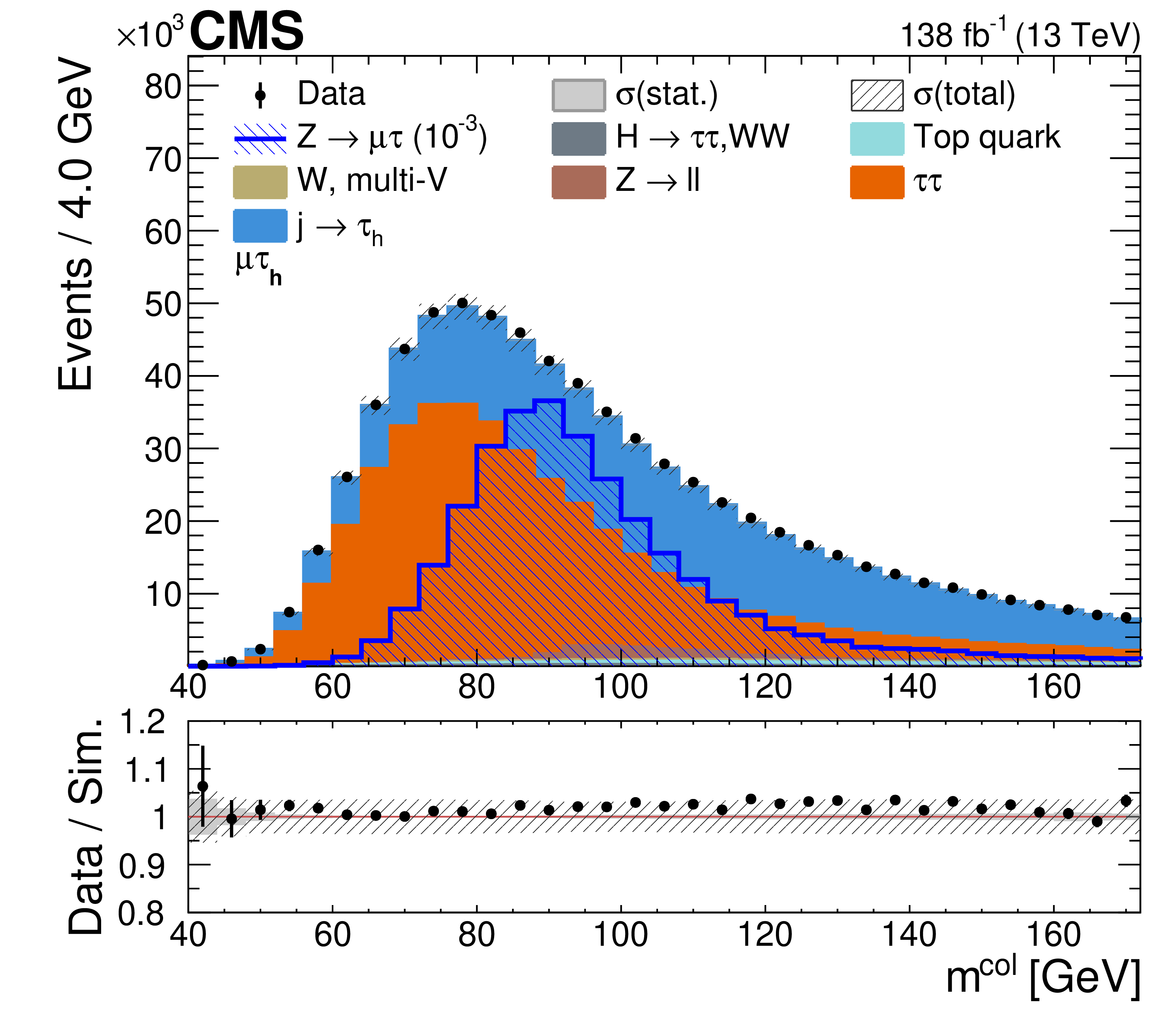
Figure 5-a:
The $ \mu\tau_\mathrm{h} $ (left) and $ \mu\tau_{\mathrm{e}} $ (right) $ m^{{\text{col}}} $ distributions, for the data (black markers with bars showing the statistical uncertainties) and the simulated backgrounds (filled stacked histograms). The hatched blue histogram shows the shape of the signal, normalized to a branching fraction of 10$^{-3} $, for comparison. The lower panel shows the ratio of the data to simulated yields, with the statistical (combined systematic and statistical) uncertainty in the simulated yield indicated by the filled (hatched) gray band. |
png pdf |
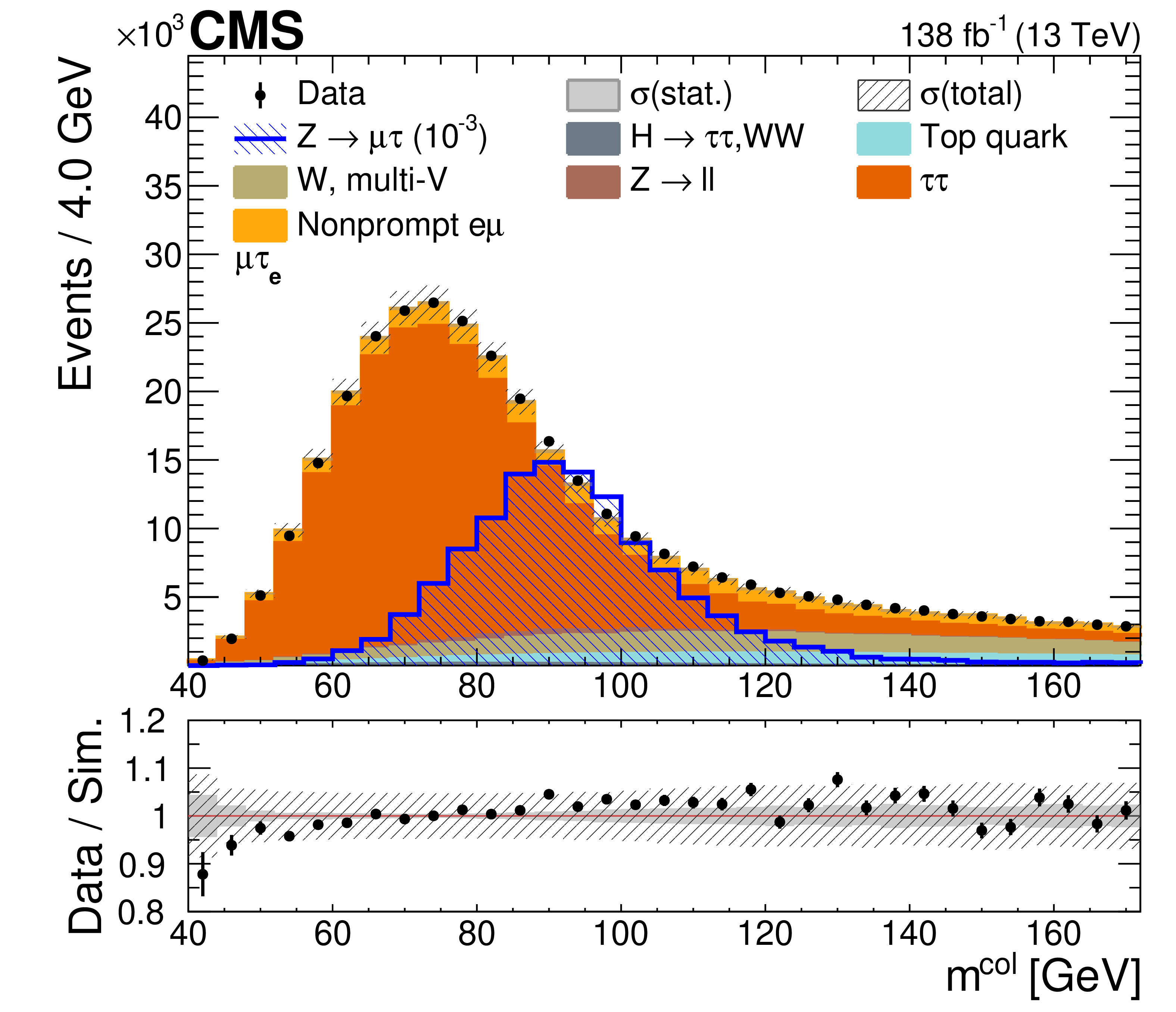
Figure 5-b:
The $ \mu\tau_\mathrm{h} $ (left) and $ \mu\tau_{\mathrm{e}} $ (right) $ m^{{\text{col}}} $ distributions, for the data (black markers with bars showing the statistical uncertainties) and the simulated backgrounds (filled stacked histograms). The hatched blue histogram shows the shape of the signal, normalized to a branching fraction of 10$^{-3} $, for comparison. The lower panel shows the ratio of the data to simulated yields, with the statistical (combined systematic and statistical) uncertainty in the simulated yield indicated by the filled (hatched) gray band. |
png pdf |
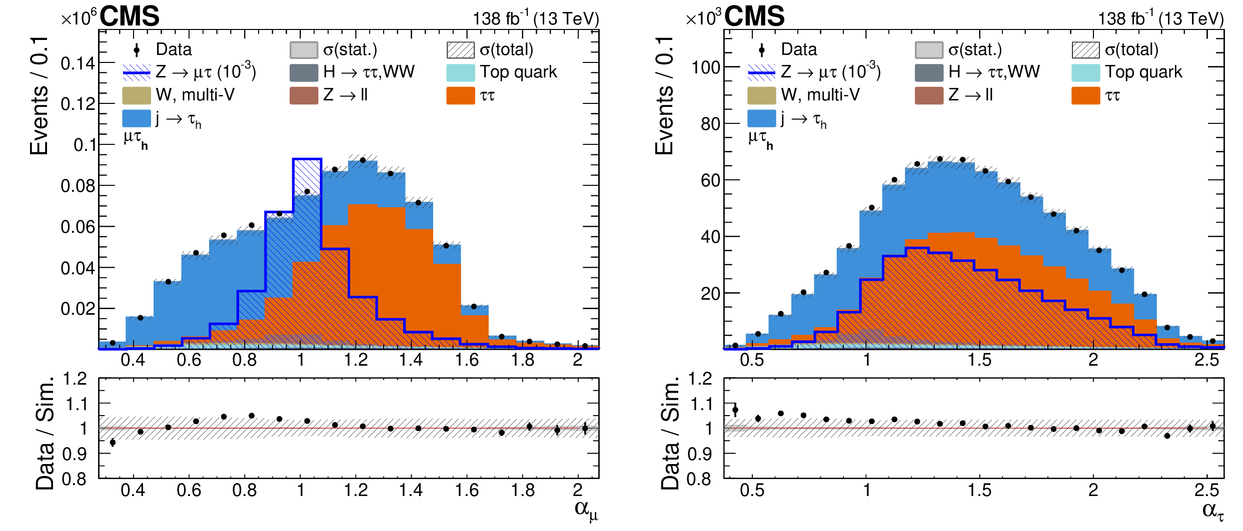
Figure 6:
Distributions of $ \mu\tau_\mathrm{h} $ signal and estimated backgrounds in $ \alpha_{\mu} $ (left), $ \alpha_{\tau} $ (right), for the data (black markers with bars showing the statistical uncertainties) and the simulated backgrounds (filled stacked histograms). The hatched blue histogram shows the shape of the signal, normalized to a branching fraction of 10$^{-3} $, for comparison. The lower panel shows the ratio of the data to simulated yields, with the statistical (combined systematic and statistical) uncertainty in the simulated yield indicated by the filled (hatched) gray band. |
png pdf |
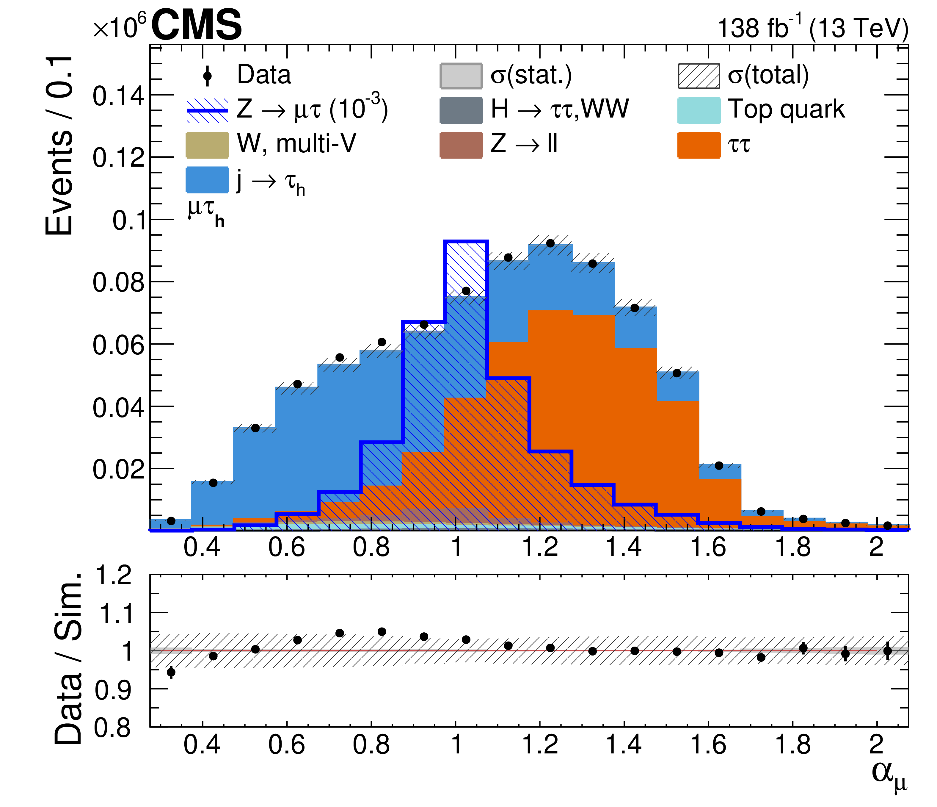
Figure 6-a:
Distributions of $ \mu\tau_\mathrm{h} $ signal and estimated backgrounds in $ \alpha_{\mu} $ (left), $ \alpha_{\tau} $ (right), for the data (black markers with bars showing the statistical uncertainties) and the simulated backgrounds (filled stacked histograms). The hatched blue histogram shows the shape of the signal, normalized to a branching fraction of 10$^{-3} $, for comparison. The lower panel shows the ratio of the data to simulated yields, with the statistical (combined systematic and statistical) uncertainty in the simulated yield indicated by the filled (hatched) gray band. |
png pdf |
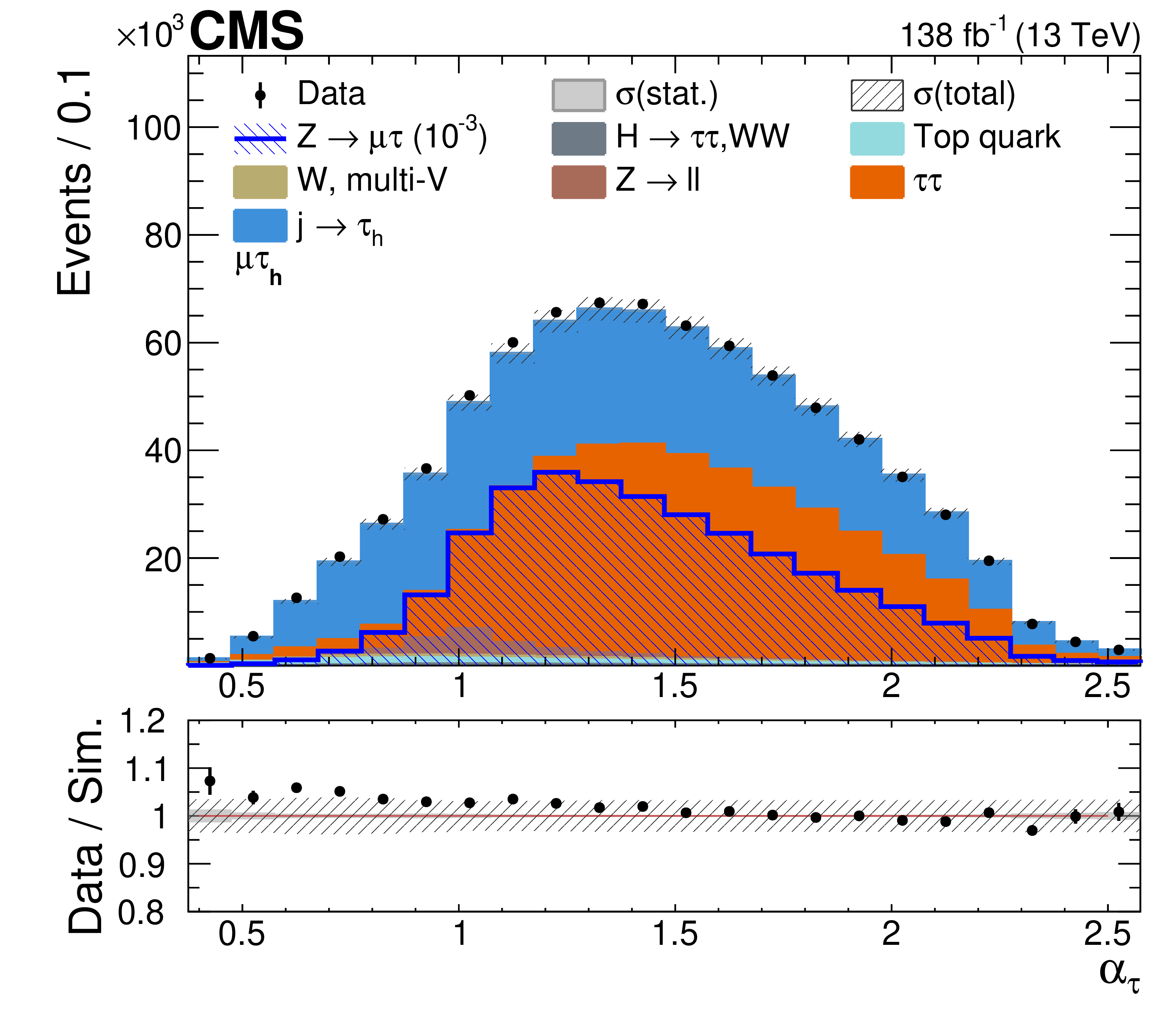
Figure 6-b:
Distributions of $ \mu\tau_\mathrm{h} $ signal and estimated backgrounds in $ \alpha_{\mu} $ (left), $ \alpha_{\tau} $ (right), for the data (black markers with bars showing the statistical uncertainties) and the simulated backgrounds (filled stacked histograms). The hatched blue histogram shows the shape of the signal, normalized to a branching fraction of 10$^{-3} $, for comparison. The lower panel shows the ratio of the data to simulated yields, with the statistical (combined systematic and statistical) uncertainty in the simulated yield indicated by the filled (hatched) gray band. |
png pdf |
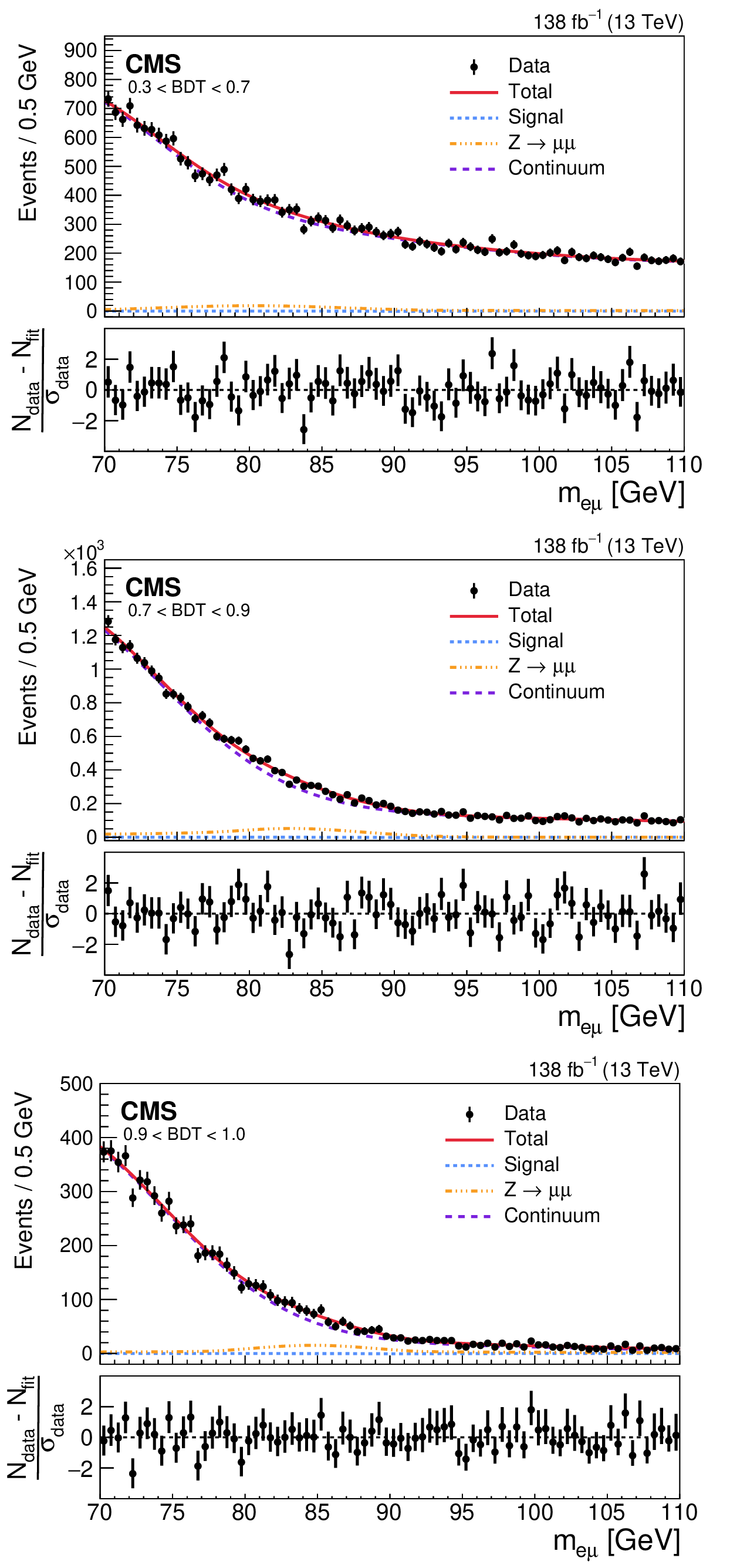
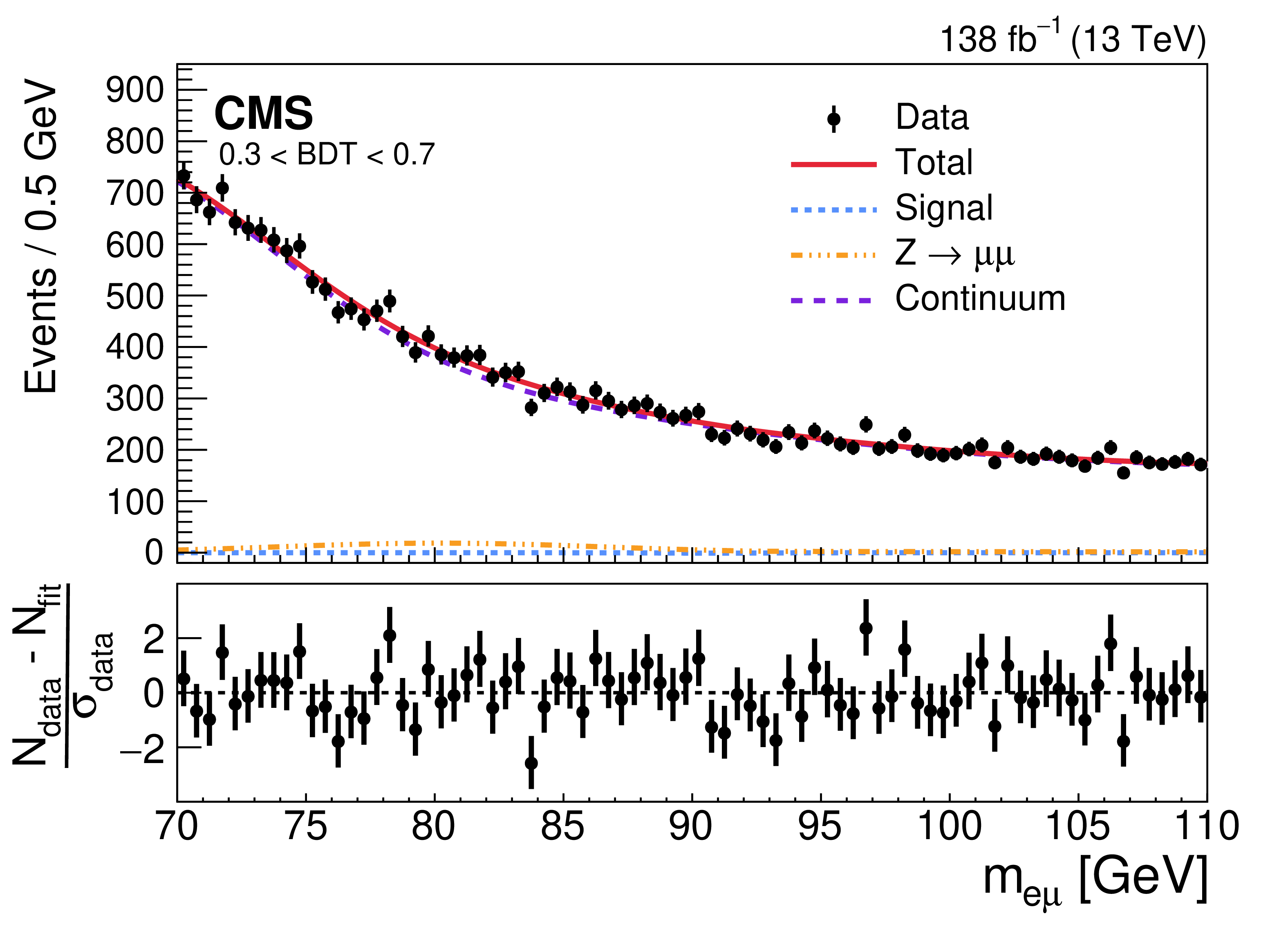
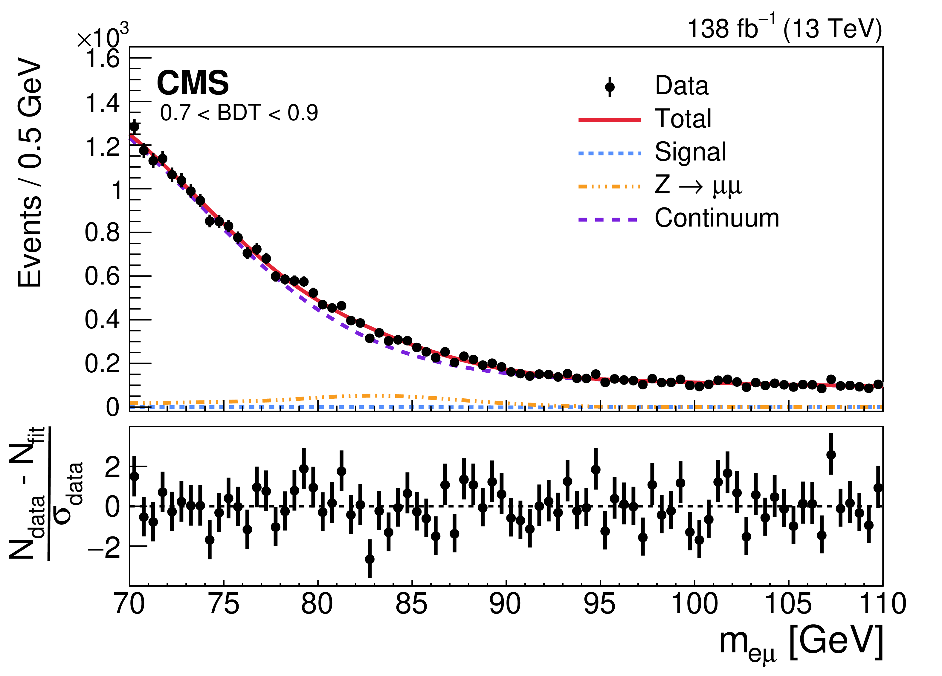
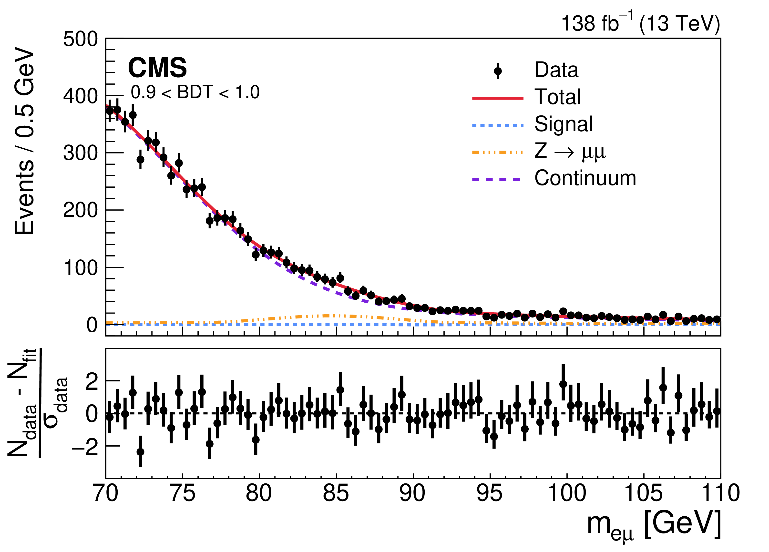
Figure 7:
For the $ \mathrm{Z}\to\mathrm{e}\mu $ search, the invariant mass fit results for the BDT score ranges 0.3-0.7 (upper), 0.7-0.9 (middle), and 0.9-1.0 (lower). In each plot, the upper panel shows the data (points with bars showing the statistical uncertainties) together with the fit distribution curve (red) and its separate signal (blue dotted) $ \mathrm{Z}\to\mu\mu $ (yellow dash-dotted) and continuum background (purple dashed) components, and the lower panel shows the deviations of the data from the fit function divided by the data uncertainty. |
png pdf |
Figure 7-a:
For the $ \mathrm{Z}\to\mathrm{e}\mu $ search, the invariant mass fit results for the BDT score ranges 0.3-0.7 (upper), 0.7-0.9 (middle), and 0.9-1.0 (lower). In each plot, the upper panel shows the data (points with bars showing the statistical uncertainties) together with the fit distribution curve (red) and its separate signal (blue dotted) $ \mathrm{Z}\to\mu\mu $ (yellow dash-dotted) and continuum background (purple dashed) components, and the lower panel shows the deviations of the data from the fit function divided by the data uncertainty. |
png pdf |
Figure 7-b:
For the $ \mathrm{Z}\to\mathrm{e}\mu $ search, the invariant mass fit results for the BDT score ranges 0.3-0.7 (upper), 0.7-0.9 (middle), and 0.9-1.0 (lower). In each plot, the upper panel shows the data (points with bars showing the statistical uncertainties) together with the fit distribution curve (red) and its separate signal (blue dotted) $ \mathrm{Z}\to\mu\mu $ (yellow dash-dotted) and continuum background (purple dashed) components, and the lower panel shows the deviations of the data from the fit function divided by the data uncertainty. |
png pdf |
Figure 7-c:
For the $ \mathrm{Z}\to\mathrm{e}\mu $ search, the invariant mass fit results for the BDT score ranges 0.3-0.7 (upper), 0.7-0.9 (middle), and 0.9-1.0 (lower). In each plot, the upper panel shows the data (points with bars showing the statistical uncertainties) together with the fit distribution curve (red) and its separate signal (blue dotted) $ \mathrm{Z}\to\mu\mu $ (yellow dash-dotted) and continuum background (purple dashed) components, and the lower panel shows the deviations of the data from the fit function divided by the data uncertainty. |
png pdf |
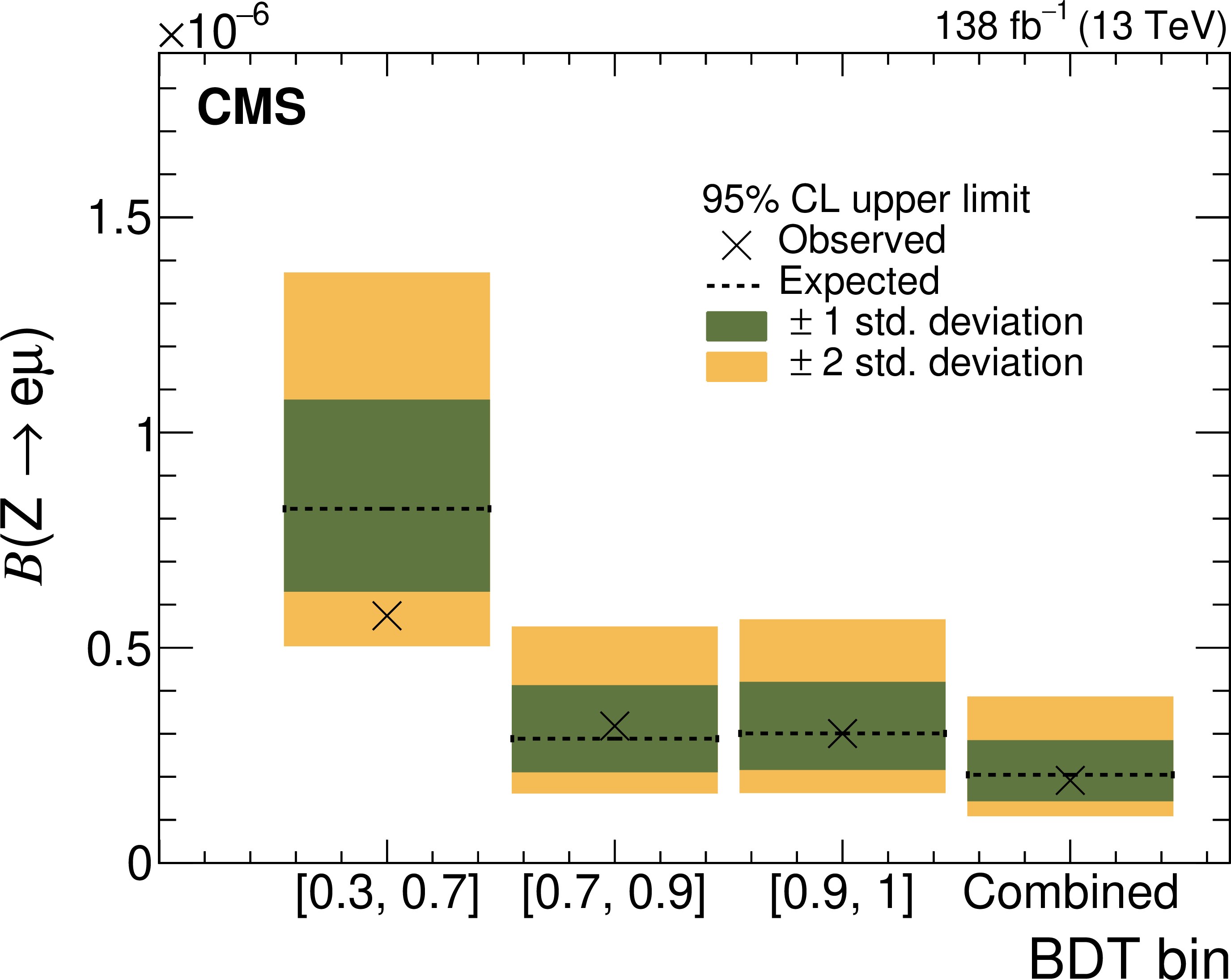
Figure 8:
Upper limits at 95% CL on the branching fraction $ \mathcal{B}(\mathrm{Z}\to\mathrm{e}\mu) $, for each BDT score range and for the final combined fit. The observed limits are denoted by the markers, while the expected limits with their 68 and 95% uncertainties are denoted by the horizontal dashed lines and green and yellow bands, respectively. |
png pdf |
Figure 9:
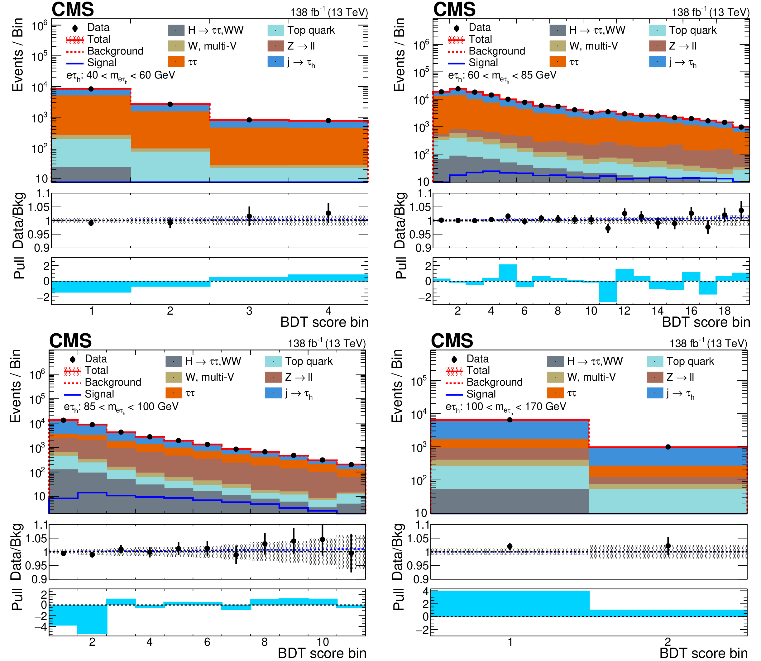
Transformed BDT score distributions for the $ \mathrm{Z}\to\mathrm{e}\tau_\mathrm{h} $ channels in the $ m_{\mathrm{e}\tau} $ ranges: (upper left) 40-60 GeV, ``$ \tau\tau $''; (upper right) 60-85 GeV, ``signal-like''; (lower left) 85-100 GeV, ``$ \mathrm{Z}\to\ell\ell $''; (lower right) 100-170 GeV, ``misID''. In each plot, the upper panel shows the data (points), the total yield from the signal + background fit (red open histogram), the signal component (blue open histogram), and the background components (stacked filled histograms). The middle panel shows the ratio to the background of the data (points with bars showing the statistical uncertainty in the data) and the combined signal + background (blue dotted histogram). The shaded band shows the systematic uncertainty in the background estimate. The lower panel shows the pull defined in the text (light-blue filled histogram). |
png pdf |
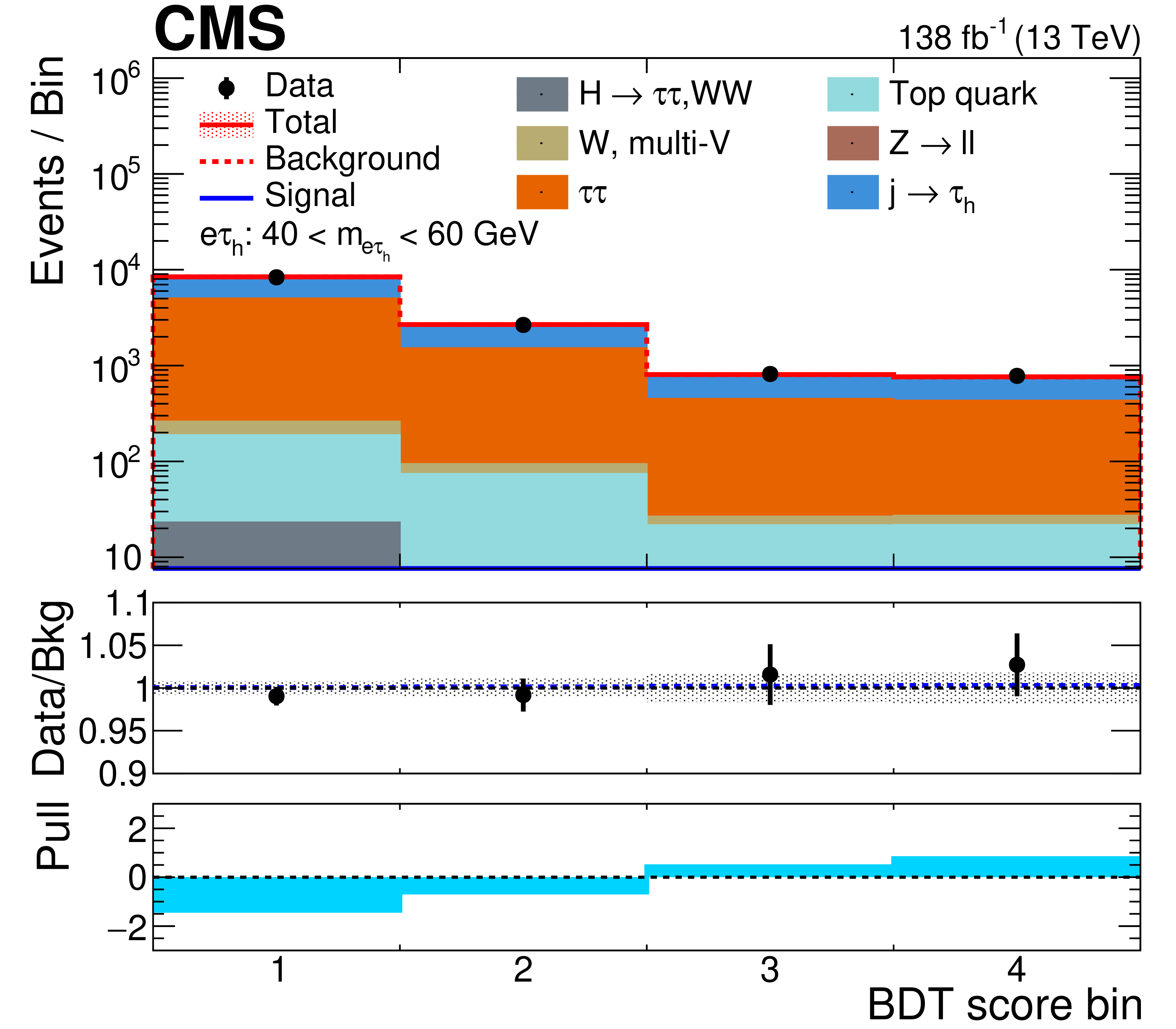
Figure 9-a:
Transformed BDT score distributions for the $ \mathrm{Z}\to\mathrm{e}\tau_\mathrm{h} $ channels in the $ m_{\mathrm{e}\tau} $ ranges: (upper left) 40-60 GeV, ``$ \tau\tau $''; (upper right) 60-85 GeV, ``signal-like''; (lower left) 85-100 GeV, ``$ \mathrm{Z}\to\ell\ell $''; (lower right) 100-170 GeV, ``misID''. In each plot, the upper panel shows the data (points), the total yield from the signal + background fit (red open histogram), the signal component (blue open histogram), and the background components (stacked filled histograms). The middle panel shows the ratio to the background of the data (points with bars showing the statistical uncertainty in the data) and the combined signal + background (blue dotted histogram). The shaded band shows the systematic uncertainty in the background estimate. The lower panel shows the pull defined in the text (light-blue filled histogram). |
png pdf |
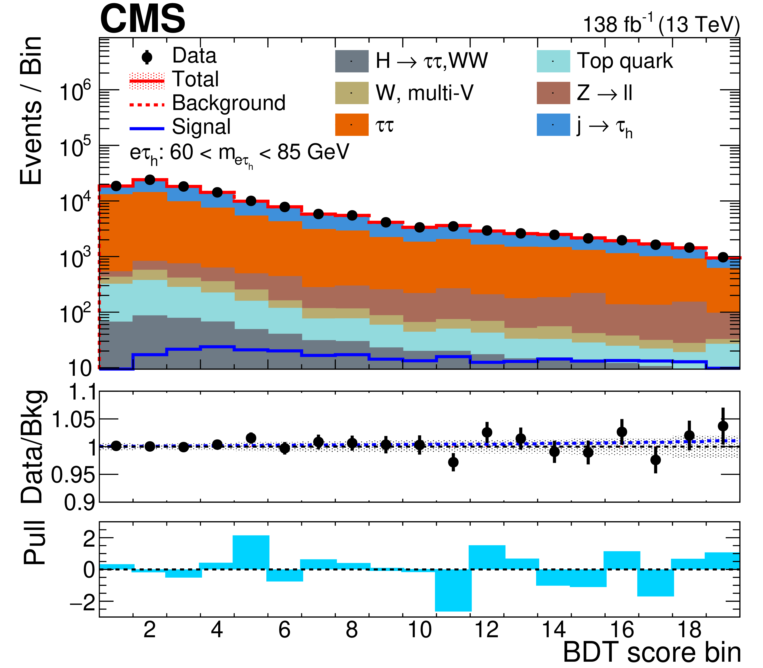
Figure 9-b:
Transformed BDT score distributions for the $ \mathrm{Z}\to\mathrm{e}\tau_\mathrm{h} $ channels in the $ m_{\mathrm{e}\tau} $ ranges: (upper left) 40-60 GeV, ``$ \tau\tau $''; (upper right) 60-85 GeV, ``signal-like''; (lower left) 85-100 GeV, ``$ \mathrm{Z}\to\ell\ell $''; (lower right) 100-170 GeV, ``misID''. In each plot, the upper panel shows the data (points), the total yield from the signal + background fit (red open histogram), the signal component (blue open histogram), and the background components (stacked filled histograms). The middle panel shows the ratio to the background of the data (points with bars showing the statistical uncertainty in the data) and the combined signal + background (blue dotted histogram). The shaded band shows the systematic uncertainty in the background estimate. The lower panel shows the pull defined in the text (light-blue filled histogram). |
png pdf |
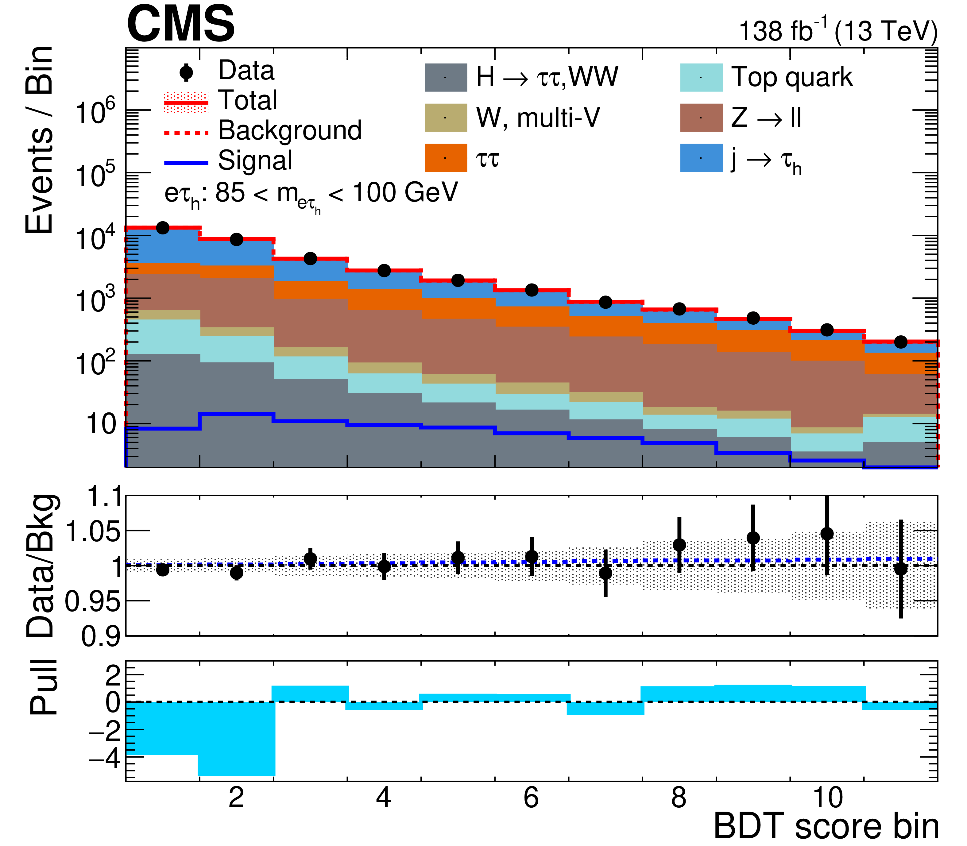
Figure 9-c:
Transformed BDT score distributions for the $ \mathrm{Z}\to\mathrm{e}\tau_\mathrm{h} $ channels in the $ m_{\mathrm{e}\tau} $ ranges: (upper left) 40-60 GeV, ``$ \tau\tau $''; (upper right) 60-85 GeV, ``signal-like''; (lower left) 85-100 GeV, ``$ \mathrm{Z}\to\ell\ell $''; (lower right) 100-170 GeV, ``misID''. In each plot, the upper panel shows the data (points), the total yield from the signal + background fit (red open histogram), the signal component (blue open histogram), and the background components (stacked filled histograms). The middle panel shows the ratio to the background of the data (points with bars showing the statistical uncertainty in the data) and the combined signal + background (blue dotted histogram). The shaded band shows the systematic uncertainty in the background estimate. The lower panel shows the pull defined in the text (light-blue filled histogram). |
png pdf |
Figure 9-d:
Transformed BDT score distributions for the $ \mathrm{Z}\to\mathrm{e}\tau_\mathrm{h} $ channels in the $ m_{\mathrm{e}\tau} $ ranges: (upper left) 40-60 GeV, ``$ \tau\tau $''; (upper right) 60-85 GeV, ``signal-like''; (lower left) 85-100 GeV, ``$ \mathrm{Z}\to\ell\ell $''; (lower right) 100-170 GeV, ``misID''. In each plot, the upper panel shows the data (points), the total yield from the signal + background fit (red open histogram), the signal component (blue open histogram), and the background components (stacked filled histograms). The middle panel shows the ratio to the background of the data (points with bars showing the statistical uncertainty in the data) and the combined signal + background (blue dotted histogram). The shaded band shows the systematic uncertainty in the background estimate. The lower panel shows the pull defined in the text (light-blue filled histogram). |
png pdf |
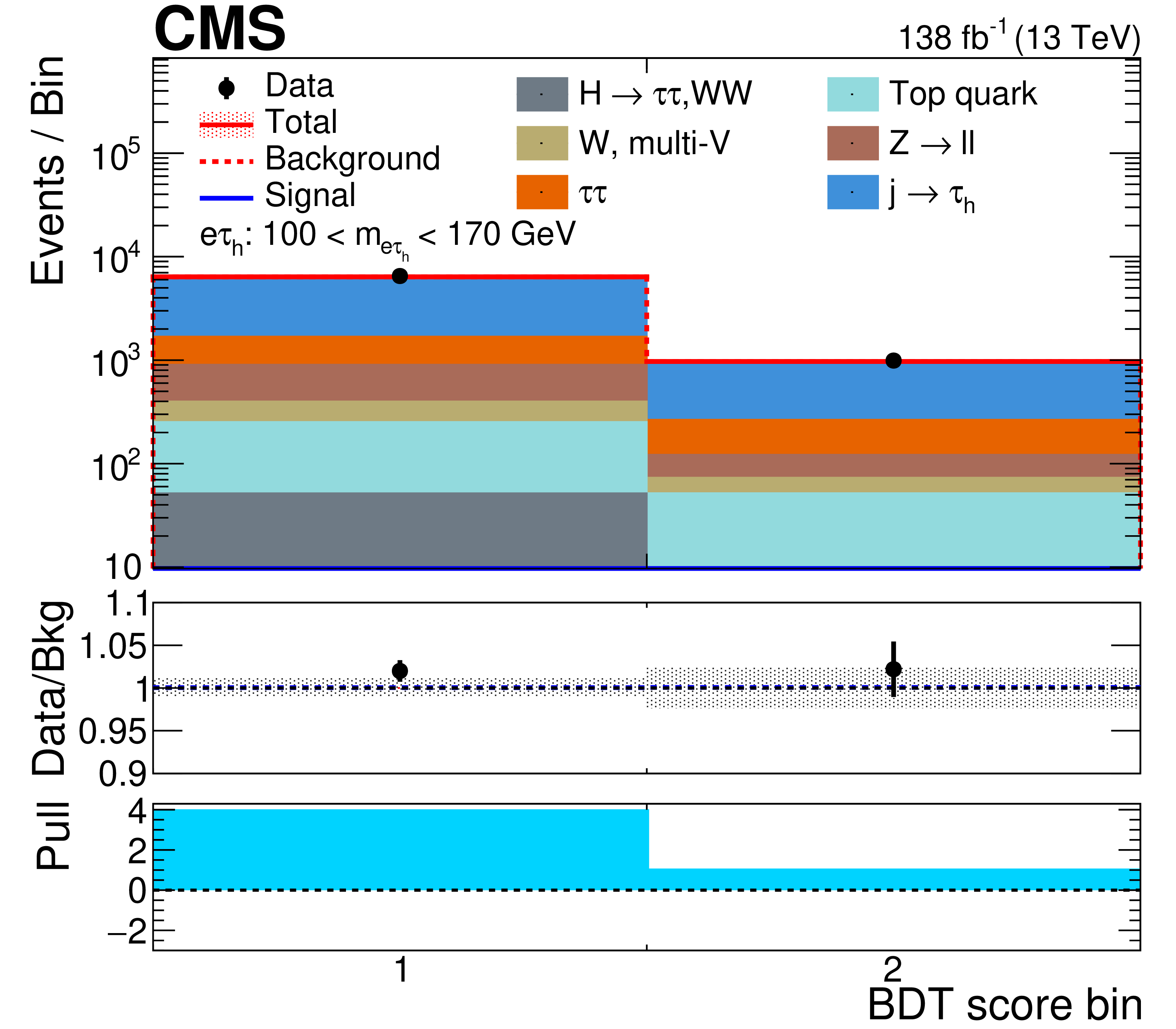
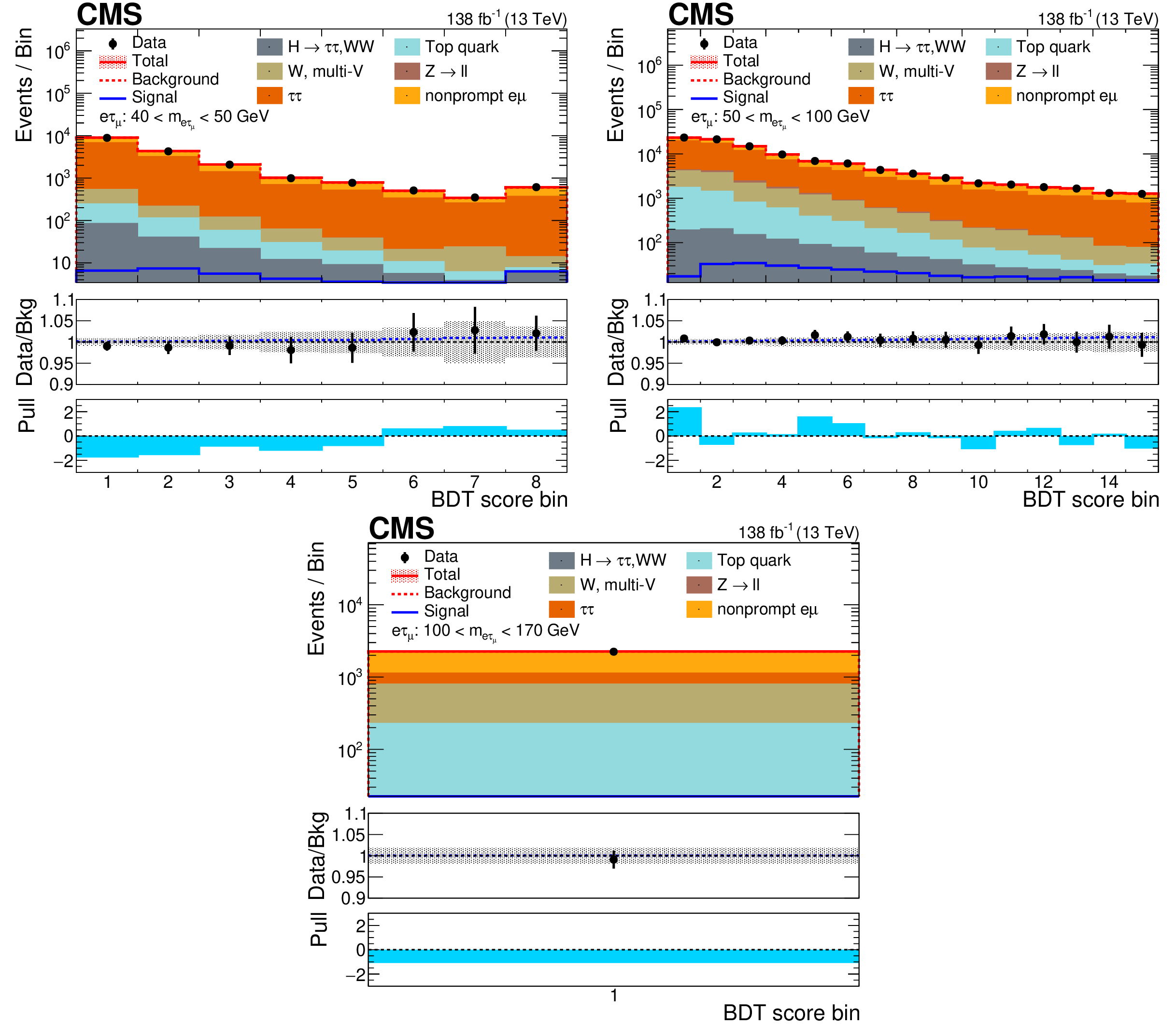
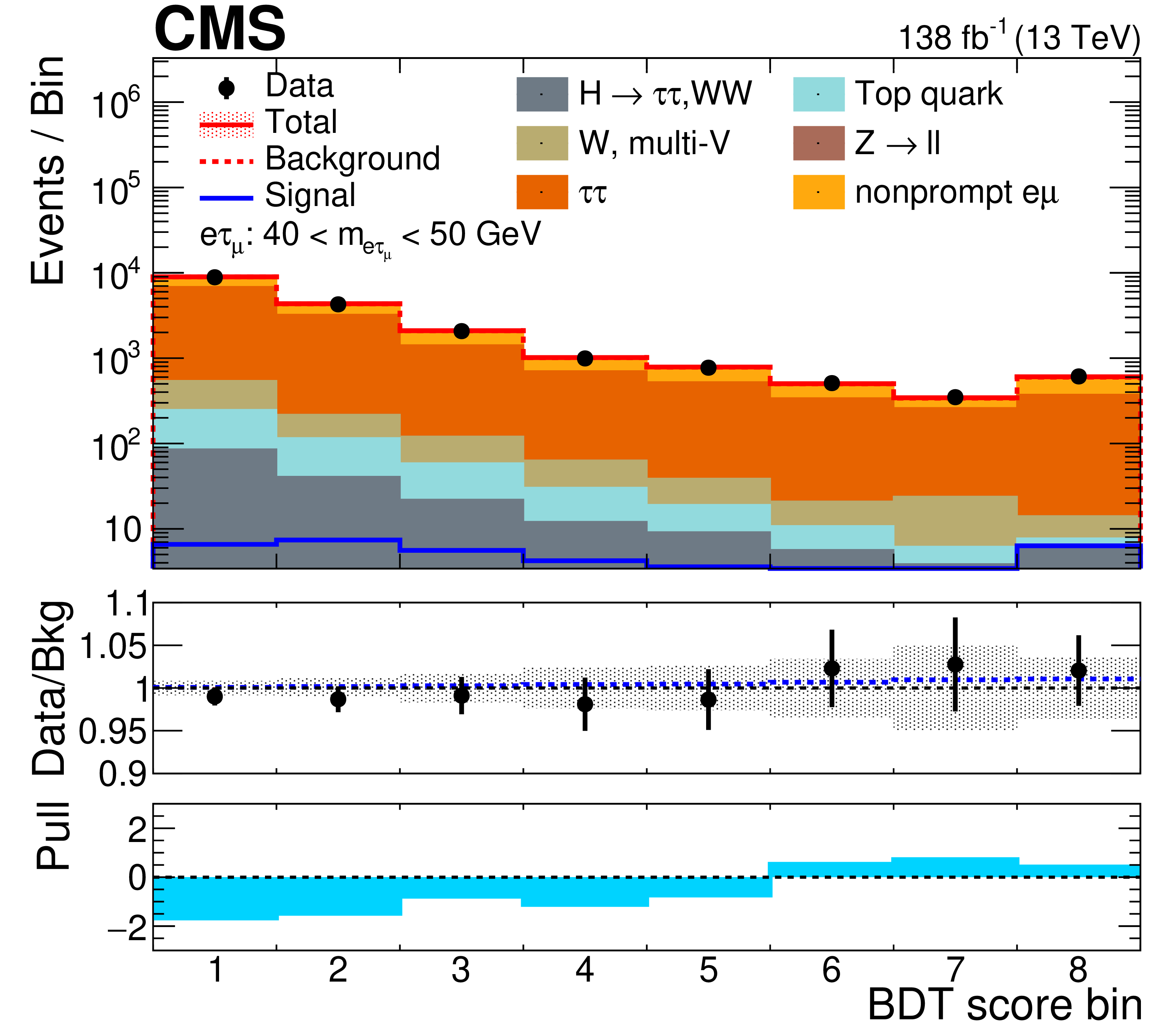
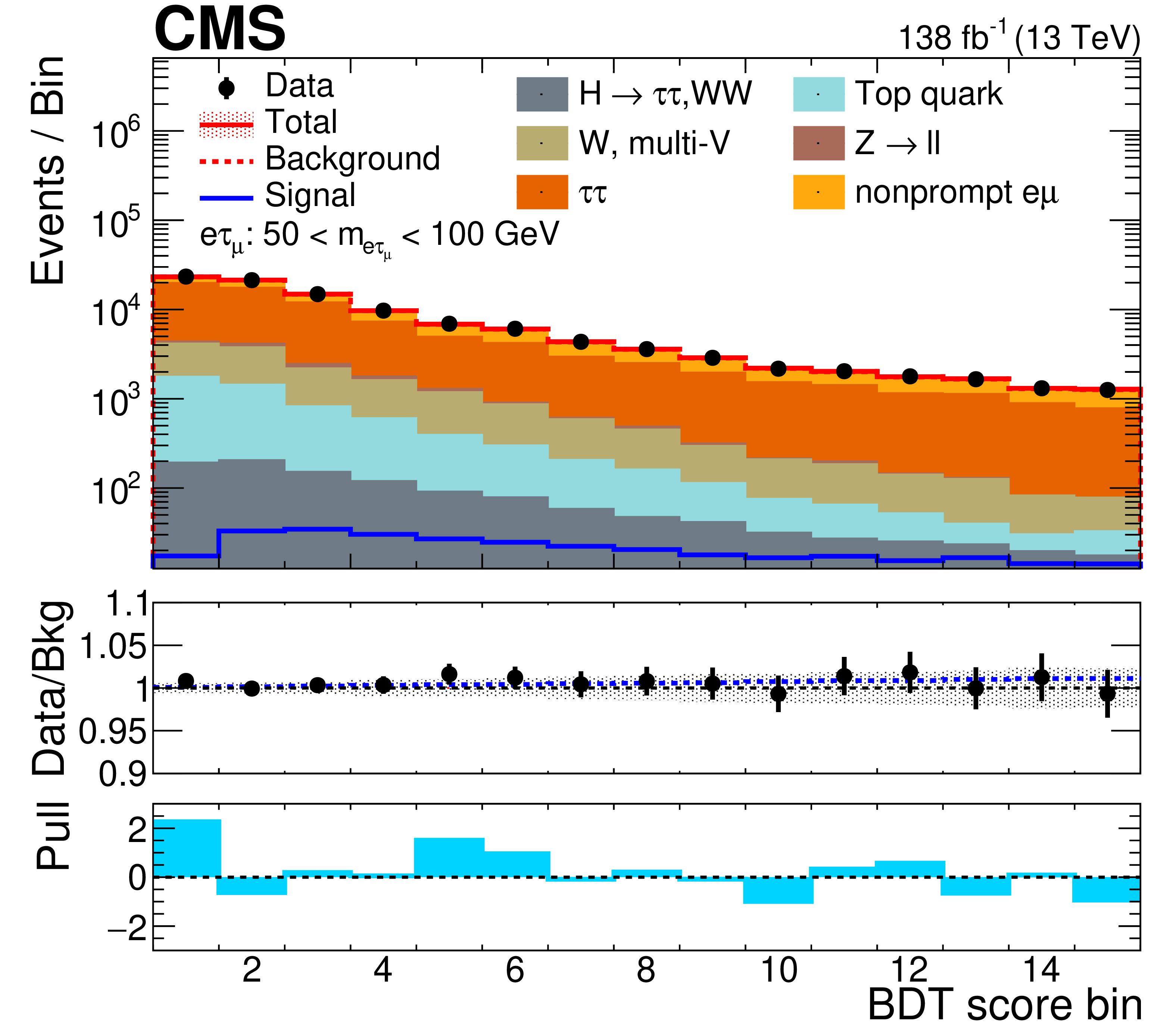
Figure 10:
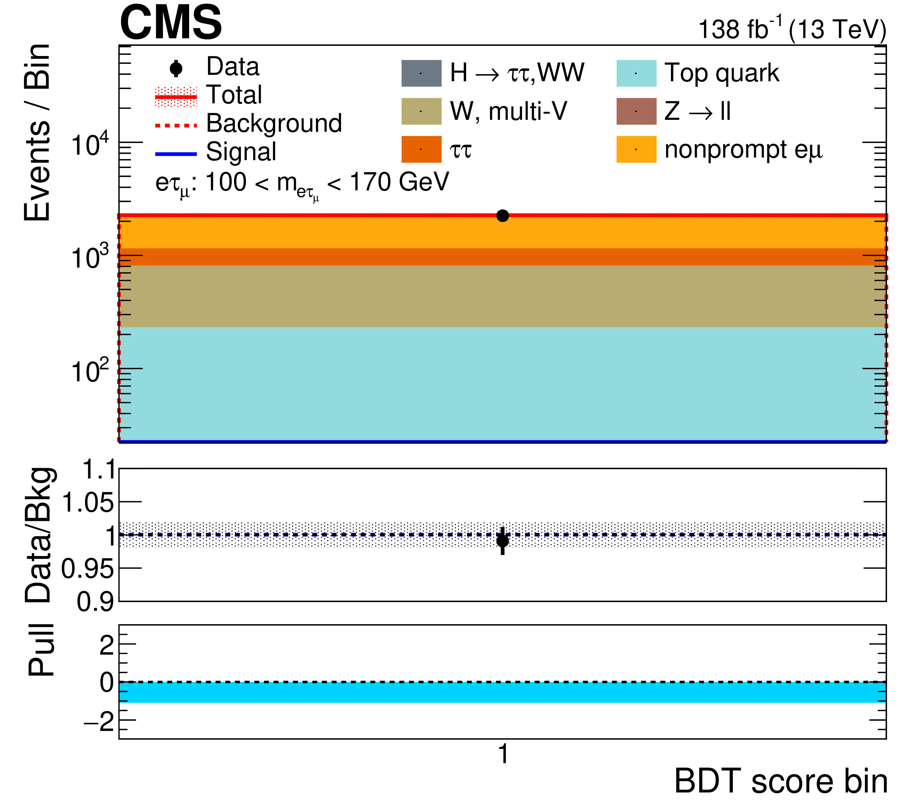
Transformed BDT score distributions for the $ \mathrm{Z}\to\mathrm{e}\tau_{\mu} $ channels in the $ m_{\mathrm{e}\tau} $ ranges: (upper left) 40-50 GeV, ``$ \tau\tau $''; (upper right) 50-100 GeV, ``signal-like''; (lower) 100-170 GeV, ``misID''. In each plot, the upper panel shows the data (points), the total yield from the signal + background fit (red open histogram), the signal component (blue open histogram), and the background components (stacked filled histograms). The middle panel shows the ratio to the background of the data (points with bars showing the statistical uncertainty in the data) and the combined signal + background (blue dotted histogram). The shaded band shows the systematic uncertainty in the background estimate. The lower panel shows the pull defined in the text (light-blue filled histogram). |
png pdf |
Figure 10-a:
Transformed BDT score distributions for the $ \mathrm{Z}\to\mathrm{e}\tau_{\mu} $ channels in the $ m_{\mathrm{e}\tau} $ ranges: (upper left) 40-50 GeV, ``$ \tau\tau $''; (upper right) 50-100 GeV, ``signal-like''; (lower) 100-170 GeV, ``misID''. In each plot, the upper panel shows the data (points), the total yield from the signal + background fit (red open histogram), the signal component (blue open histogram), and the background components (stacked filled histograms). The middle panel shows the ratio to the background of the data (points with bars showing the statistical uncertainty in the data) and the combined signal + background (blue dotted histogram). The shaded band shows the systematic uncertainty in the background estimate. The lower panel shows the pull defined in the text (light-blue filled histogram). |
png pdf |
Figure 10-b:
Transformed BDT score distributions for the $ \mathrm{Z}\to\mathrm{e}\tau_{\mu} $ channels in the $ m_{\mathrm{e}\tau} $ ranges: (upper left) 40-50 GeV, ``$ \tau\tau $''; (upper right) 50-100 GeV, ``signal-like''; (lower) 100-170 GeV, ``misID''. In each plot, the upper panel shows the data (points), the total yield from the signal + background fit (red open histogram), the signal component (blue open histogram), and the background components (stacked filled histograms). The middle panel shows the ratio to the background of the data (points with bars showing the statistical uncertainty in the data) and the combined signal + background (blue dotted histogram). The shaded band shows the systematic uncertainty in the background estimate. The lower panel shows the pull defined in the text (light-blue filled histogram). |
png pdf |
Figure 10-c:
Transformed BDT score distributions for the $ \mathrm{Z}\to\mathrm{e}\tau_{\mu} $ channels in the $ m_{\mathrm{e}\tau} $ ranges: (upper left) 40-50 GeV, ``$ \tau\tau $''; (upper right) 50-100 GeV, ``signal-like''; (lower) 100-170 GeV, ``misID''. In each plot, the upper panel shows the data (points), the total yield from the signal + background fit (red open histogram), the signal component (blue open histogram), and the background components (stacked filled histograms). The middle panel shows the ratio to the background of the data (points with bars showing the statistical uncertainty in the data) and the combined signal + background (blue dotted histogram). The shaded band shows the systematic uncertainty in the background estimate. The lower panel shows the pull defined in the text (light-blue filled histogram). |
png pdf |
Figure 11:
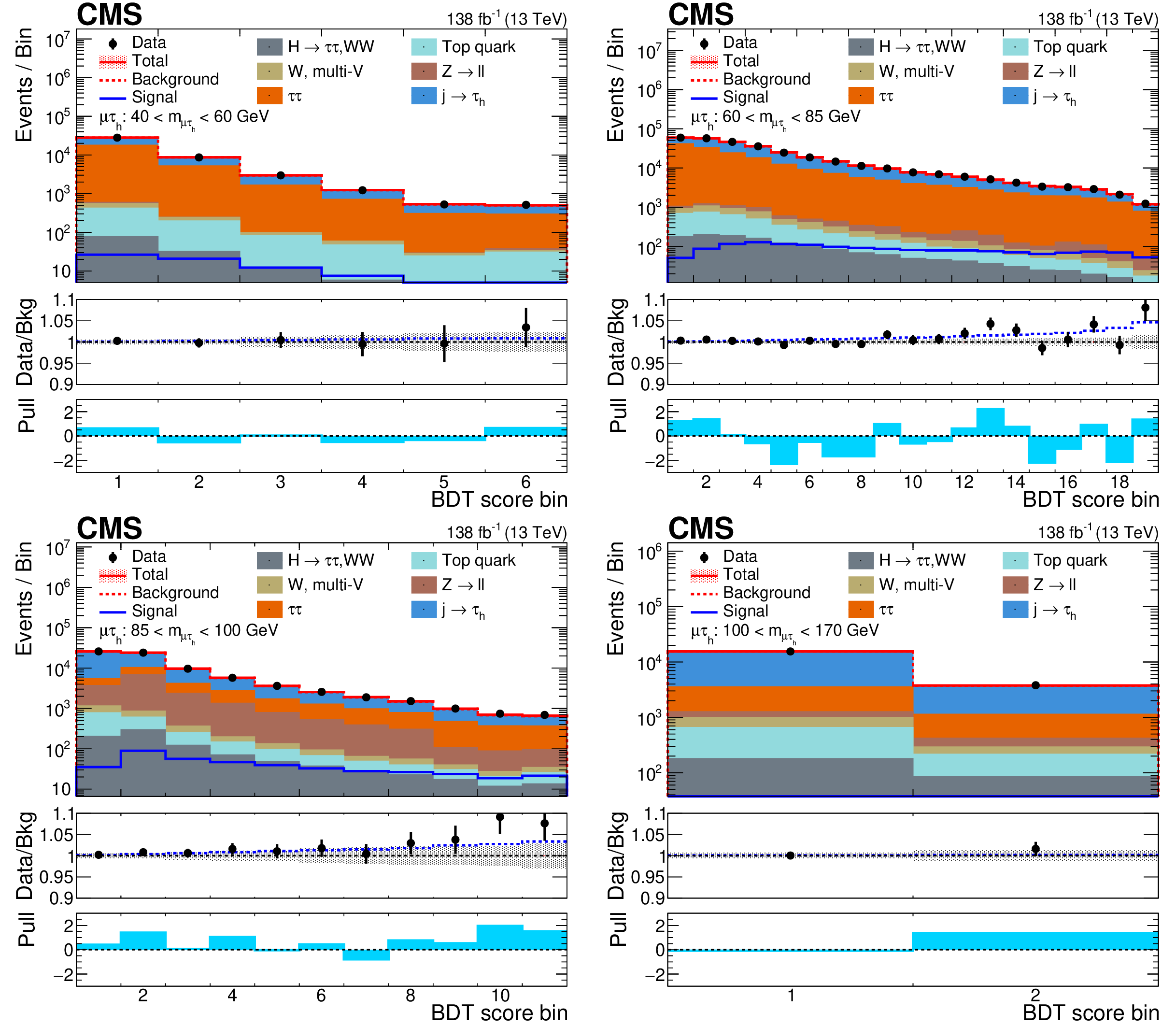
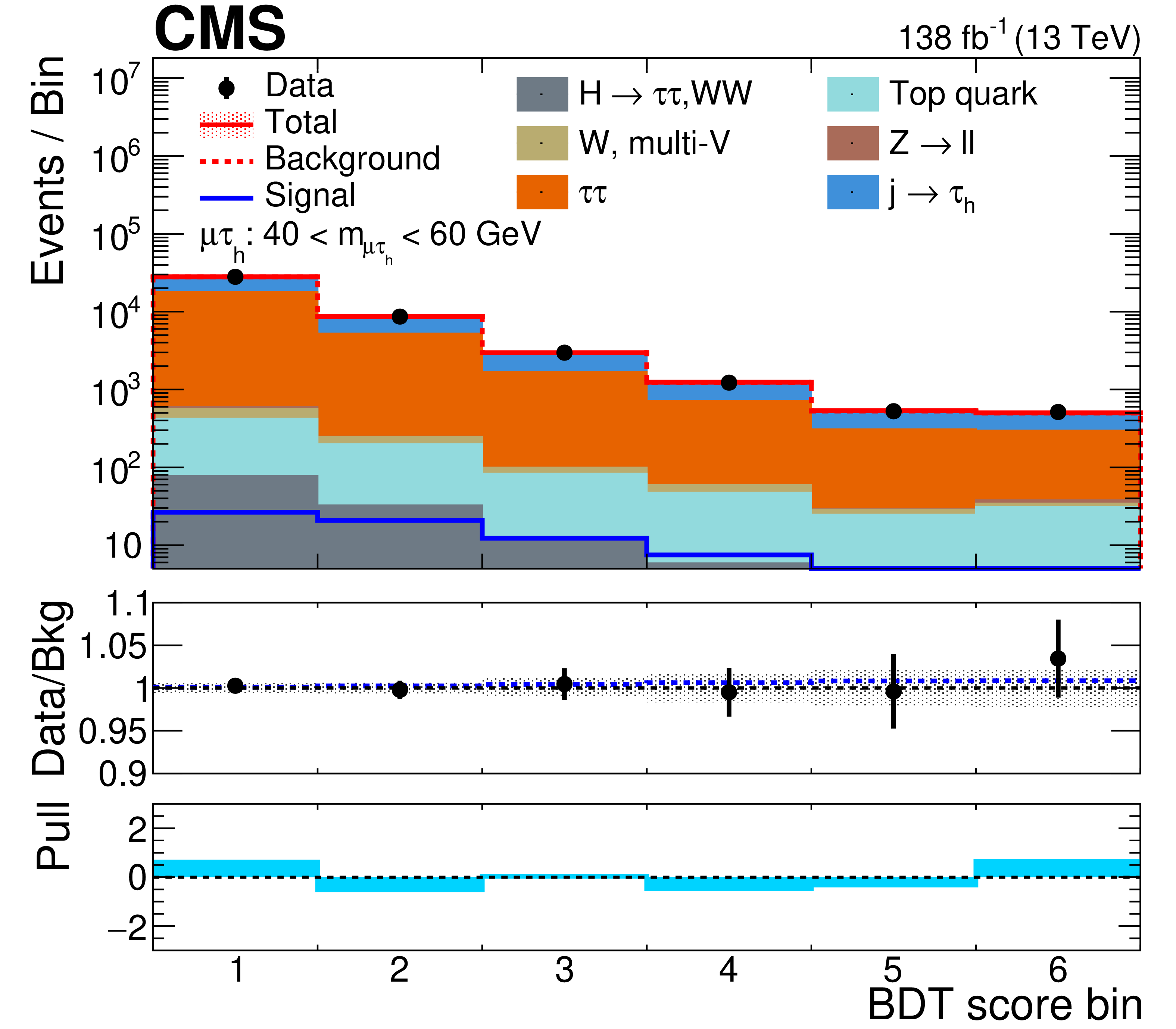
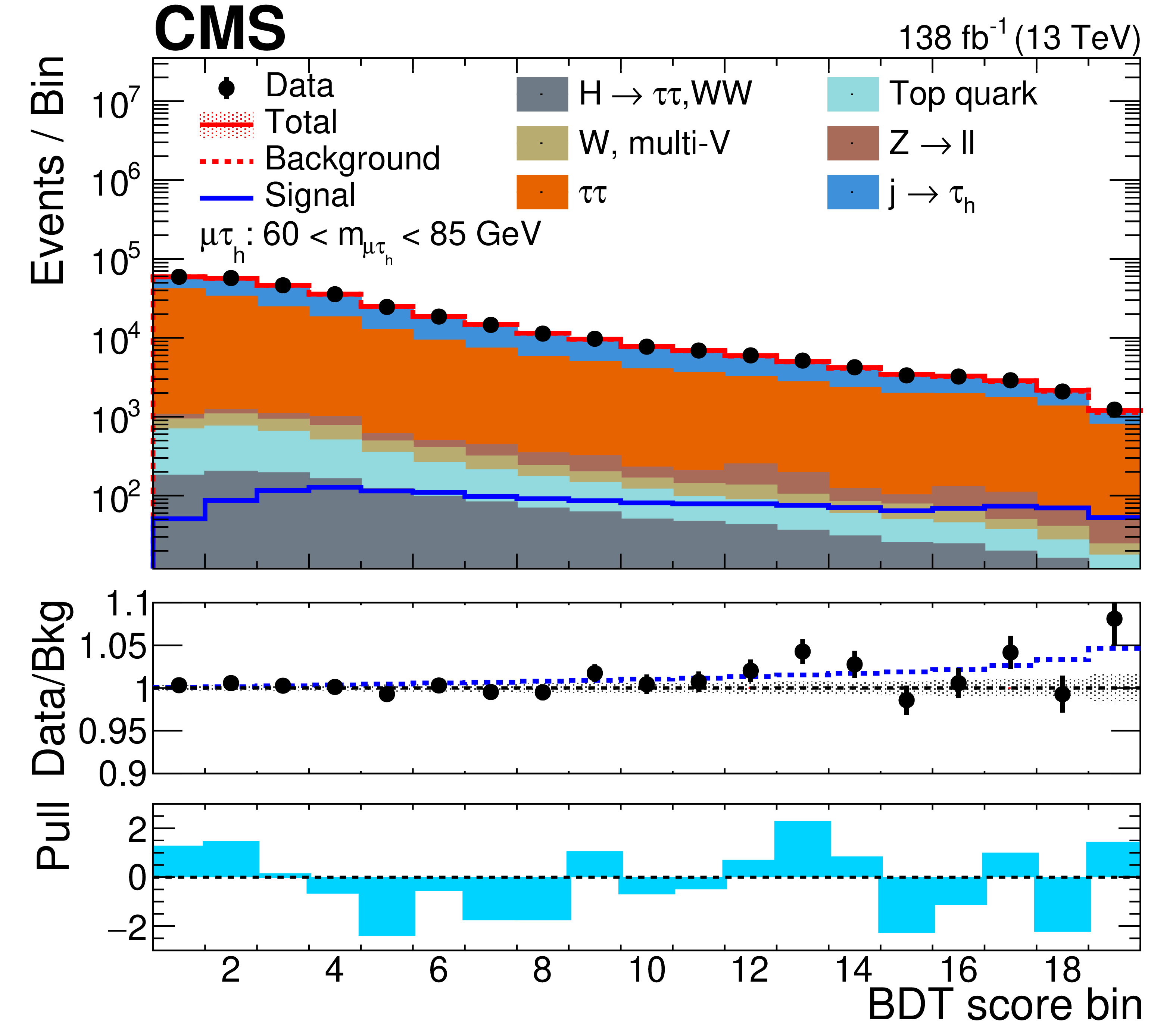
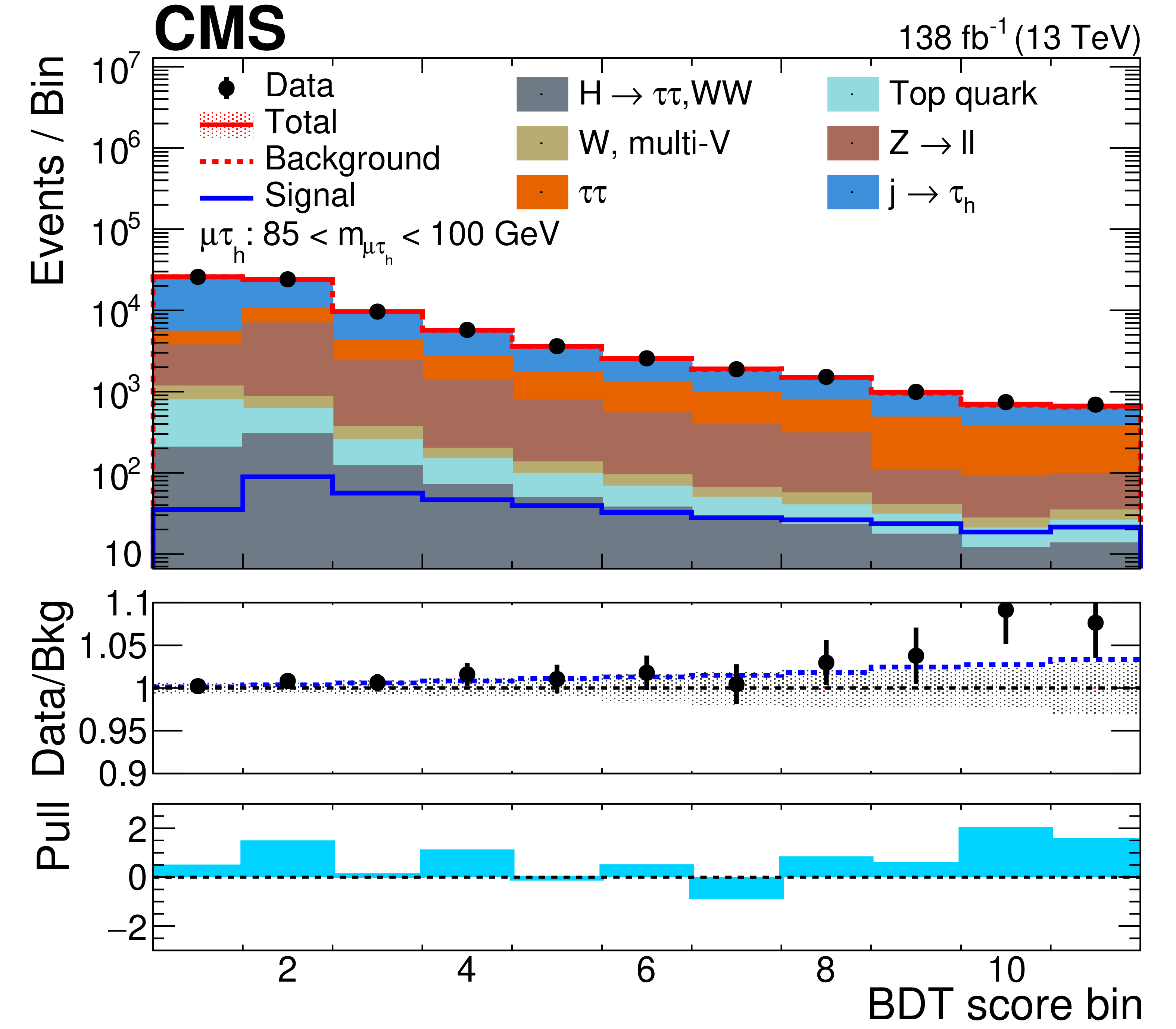
Transformed BDT score distributions for the $ \mathrm{Z}\to\mu\tau_\mathrm{h} $ channels in the $ m_{\mu\tau} $ ranges: (upper left) 40-60 GeV, ``$ \tau\tau $''; (upper right) 60-85 GeV, ``signal-like''; (lower left) 85-100 GeV, ``$ \mathrm{Z}\to\ell\ell $''; (lower right) 100-170 GeV, ``misID''. In each plot, the upper panel shows the data (points), the total yield from the signal + background fit (red open histogram), the signal component (blue open histogram), and the background components (stacked filled histograms). The middle panel shows the ratio to the background of the data (points with bars showing the statistical uncertainty in the data) and the combined signal + background (blue dotted histogram). The shaded band shows the systematic uncertainty in the background estimate. The lower panel shows the pull defined in the text (light-blue filled histogram). |
png pdf |
Figure 11-a:
Transformed BDT score distributions for the $ \mathrm{Z}\to\mu\tau_\mathrm{h} $ channels in the $ m_{\mu\tau} $ ranges: (upper left) 40-60 GeV, ``$ \tau\tau $''; (upper right) 60-85 GeV, ``signal-like''; (lower left) 85-100 GeV, ``$ \mathrm{Z}\to\ell\ell $''; (lower right) 100-170 GeV, ``misID''. In each plot, the upper panel shows the data (points), the total yield from the signal + background fit (red open histogram), the signal component (blue open histogram), and the background components (stacked filled histograms). The middle panel shows the ratio to the background of the data (points with bars showing the statistical uncertainty in the data) and the combined signal + background (blue dotted histogram). The shaded band shows the systematic uncertainty in the background estimate. The lower panel shows the pull defined in the text (light-blue filled histogram). |
png pdf |
Figure 11-b:
Transformed BDT score distributions for the $ \mathrm{Z}\to\mu\tau_\mathrm{h} $ channels in the $ m_{\mu\tau} $ ranges: (upper left) 40-60 GeV, ``$ \tau\tau $''; (upper right) 60-85 GeV, ``signal-like''; (lower left) 85-100 GeV, ``$ \mathrm{Z}\to\ell\ell $''; (lower right) 100-170 GeV, ``misID''. In each plot, the upper panel shows the data (points), the total yield from the signal + background fit (red open histogram), the signal component (blue open histogram), and the background components (stacked filled histograms). The middle panel shows the ratio to the background of the data (points with bars showing the statistical uncertainty in the data) and the combined signal + background (blue dotted histogram). The shaded band shows the systematic uncertainty in the background estimate. The lower panel shows the pull defined in the text (light-blue filled histogram). |
png pdf |
Figure 11-c:
Transformed BDT score distributions for the $ \mathrm{Z}\to\mu\tau_\mathrm{h} $ channels in the $ m_{\mu\tau} $ ranges: (upper left) 40-60 GeV, ``$ \tau\tau $''; (upper right) 60-85 GeV, ``signal-like''; (lower left) 85-100 GeV, ``$ \mathrm{Z}\to\ell\ell $''; (lower right) 100-170 GeV, ``misID''. In each plot, the upper panel shows the data (points), the total yield from the signal + background fit (red open histogram), the signal component (blue open histogram), and the background components (stacked filled histograms). The middle panel shows the ratio to the background of the data (points with bars showing the statistical uncertainty in the data) and the combined signal + background (blue dotted histogram). The shaded band shows the systematic uncertainty in the background estimate. The lower panel shows the pull defined in the text (light-blue filled histogram). |
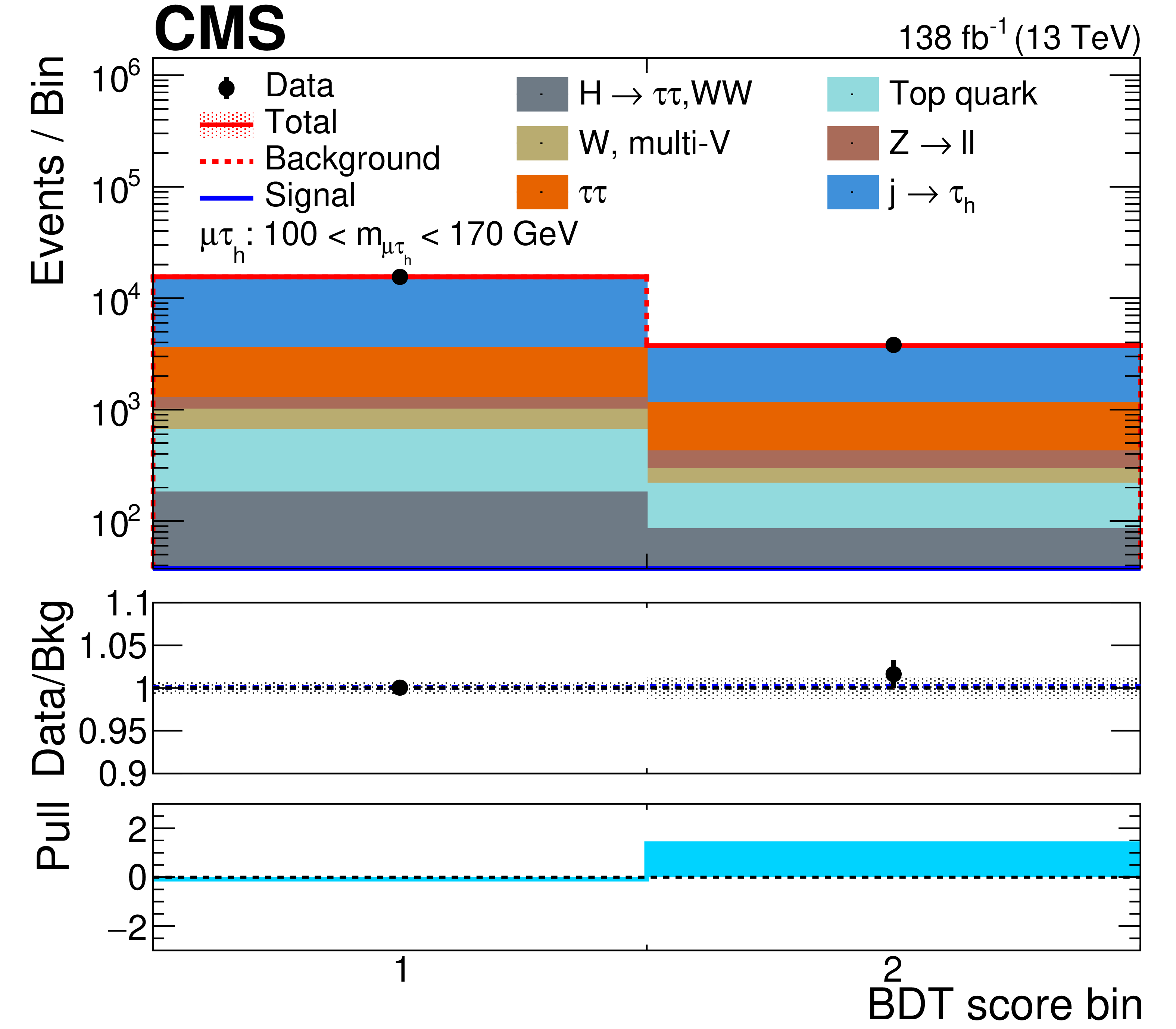
png pdf |
Figure 11-d:
Transformed BDT score distributions for the $ \mathrm{Z}\to\mu\tau_\mathrm{h} $ channels in the $ m_{\mu\tau} $ ranges: (upper left) 40-60 GeV, ``$ \tau\tau $''; (upper right) 60-85 GeV, ``signal-like''; (lower left) 85-100 GeV, ``$ \mathrm{Z}\to\ell\ell $''; (lower right) 100-170 GeV, ``misID''. In each plot, the upper panel shows the data (points), the total yield from the signal + background fit (red open histogram), the signal component (blue open histogram), and the background components (stacked filled histograms). The middle panel shows the ratio to the background of the data (points with bars showing the statistical uncertainty in the data) and the combined signal + background (blue dotted histogram). The shaded band shows the systematic uncertainty in the background estimate. The lower panel shows the pull defined in the text (light-blue filled histogram). |
png pdf |
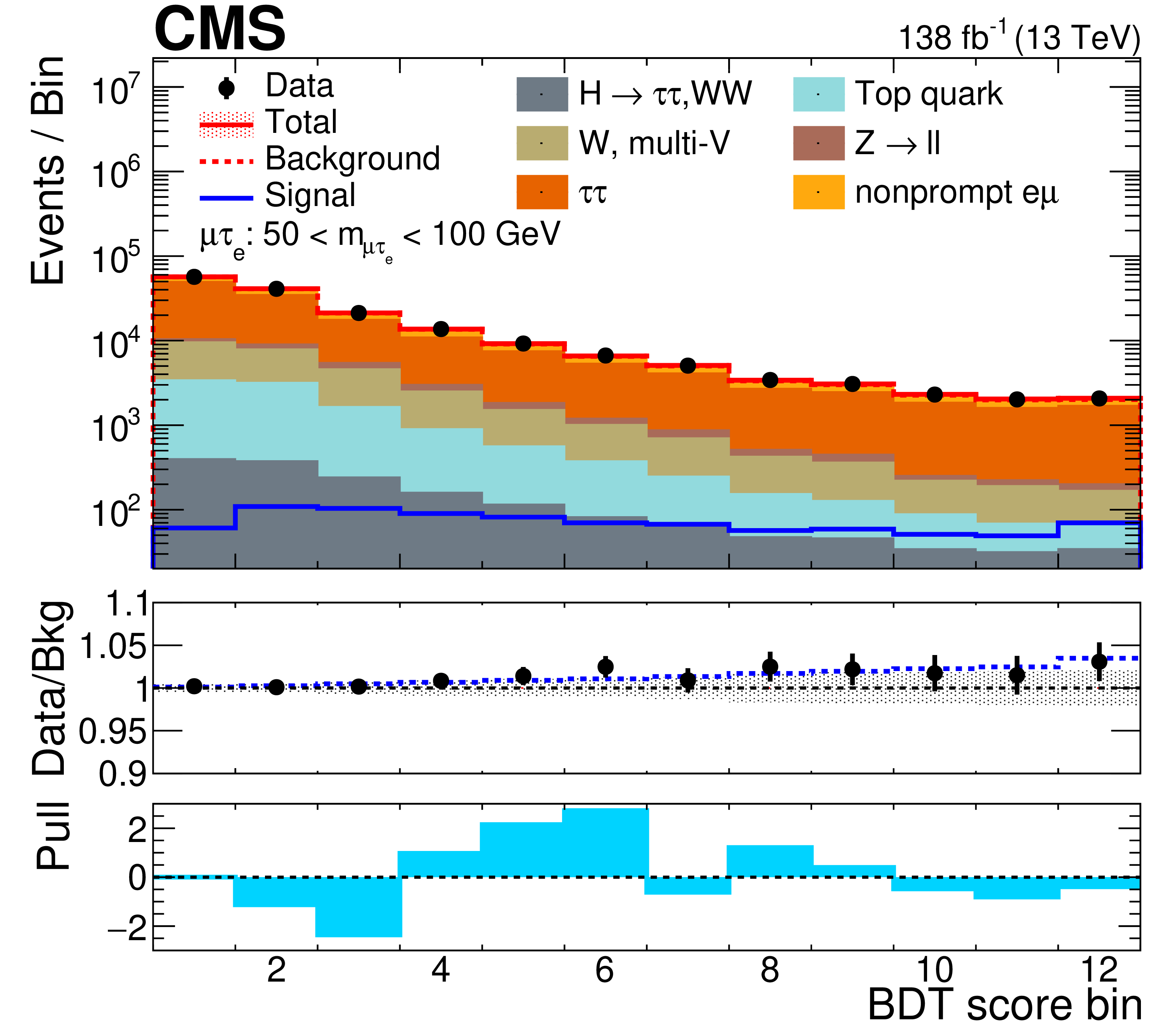
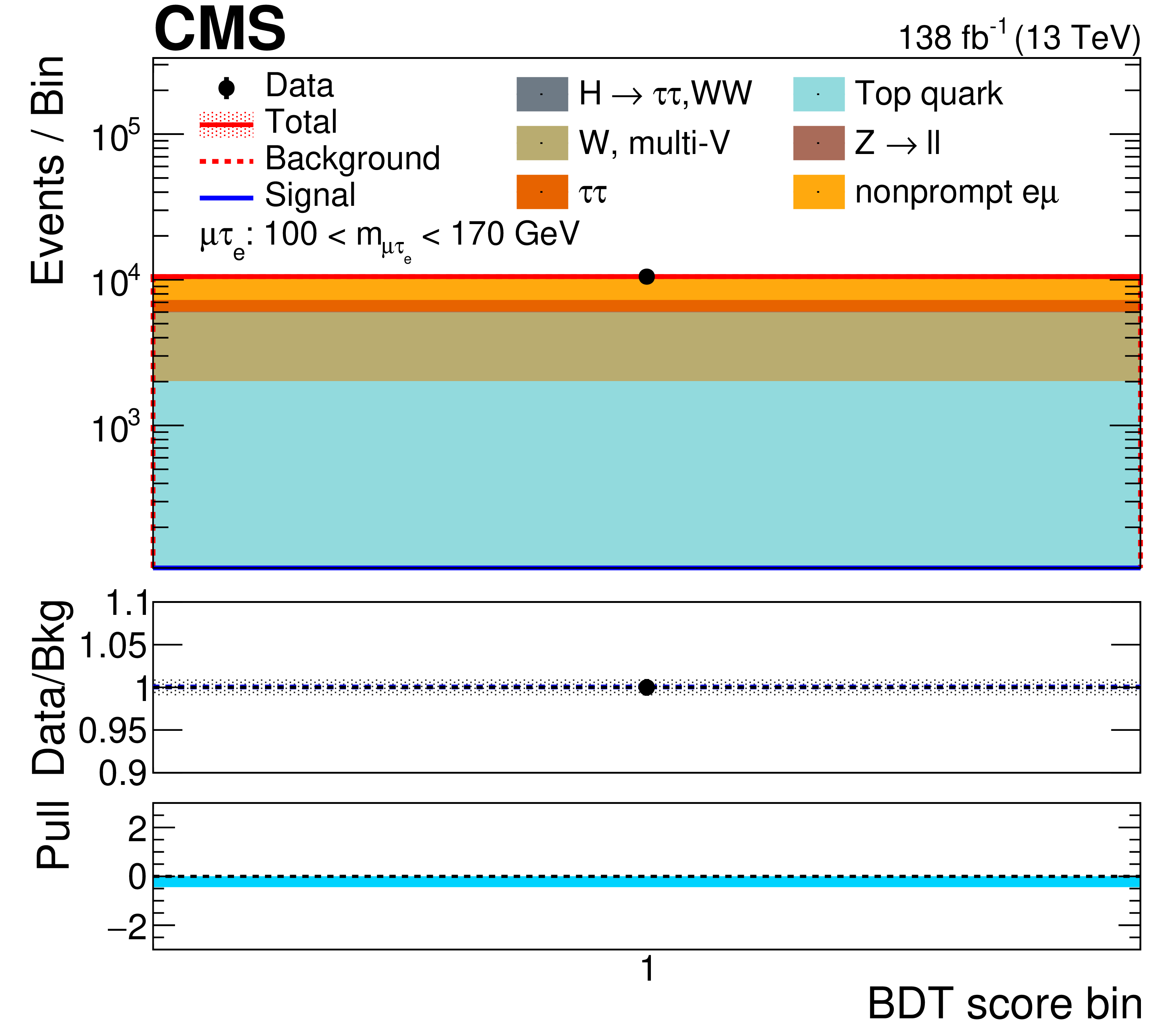
Figure 12:
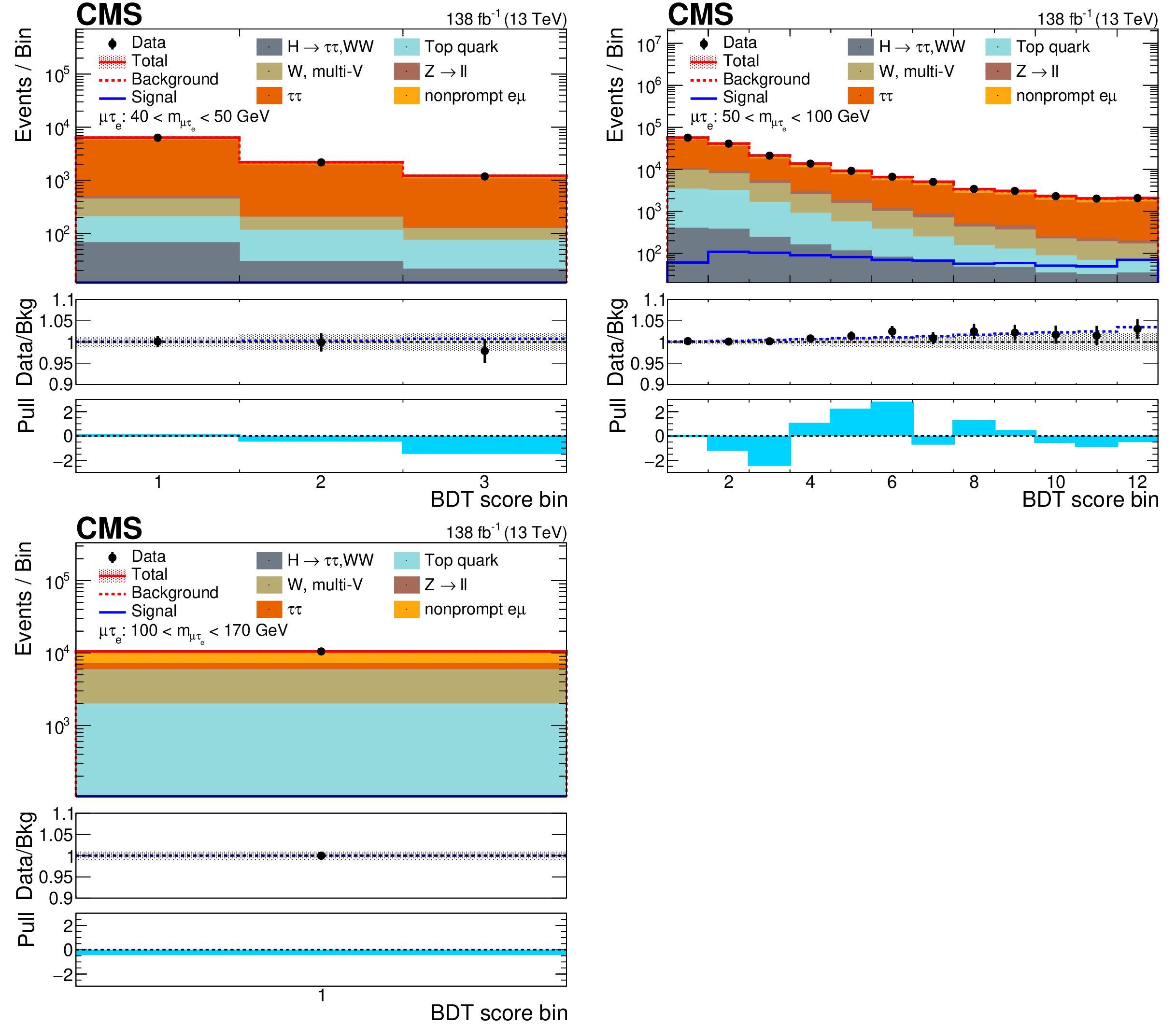
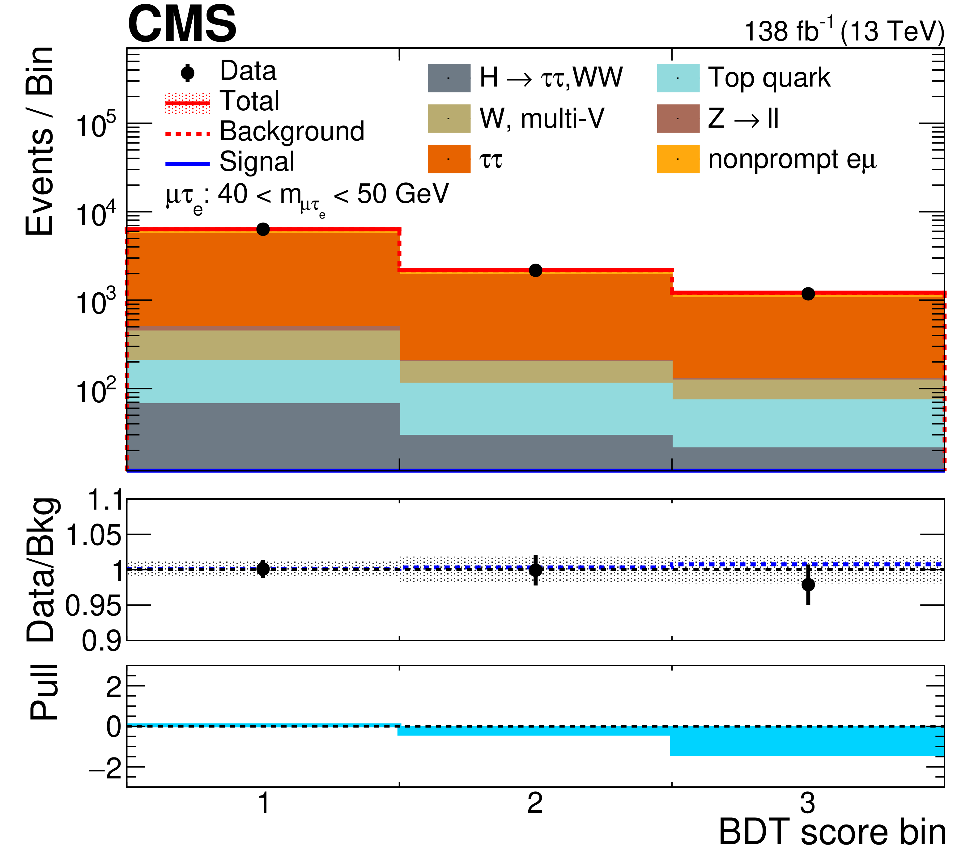
Transformed BDT score distributions for the $ \mathrm{Z}\to\mu\tau_{\mathrm{e}} $ channels in the $ m_{\mu\tau} $ ranges: (upper left) 40-50 GeV, ``$ \tau\tau $''; (upper right) 50-100 GeV, ``signal-like''; (lower) 100-170 GeV, ``misID''. In each plot, the upper panel shows the data (points), the total yield from the signal + background fit (red open histogram), the signal component (blue open histogram), and the background components (stacked filled histograms). The middle panel shows the ratio to the background of the data (points with bars showing the statistical uncertainty in the data) and the combined signal + background (blue dotted histogram). The shaded band shows the systematic uncertainty in the background estimate. The lower panel shows the pull defined in the text (light-blue filled histogram). |
png pdf |
Figure 12-a:
Transformed BDT score distributions for the $ \mathrm{Z}\to\mu\tau_{\mathrm{e}} $ channels in the $ m_{\mu\tau} $ ranges: (upper left) 40-50 GeV, ``$ \tau\tau $''; (upper right) 50-100 GeV, ``signal-like''; (lower) 100-170 GeV, ``misID''. In each plot, the upper panel shows the data (points), the total yield from the signal + background fit (red open histogram), the signal component (blue open histogram), and the background components (stacked filled histograms). The middle panel shows the ratio to the background of the data (points with bars showing the statistical uncertainty in the data) and the combined signal + background (blue dotted histogram). The shaded band shows the systematic uncertainty in the background estimate. The lower panel shows the pull defined in the text (light-blue filled histogram). |
png pdf |
Figure 12-b:
Transformed BDT score distributions for the $ \mathrm{Z}\to\mu\tau_{\mathrm{e}} $ channels in the $ m_{\mu\tau} $ ranges: (upper left) 40-50 GeV, ``$ \tau\tau $''; (upper right) 50-100 GeV, ``signal-like''; (lower) 100-170 GeV, ``misID''. In each plot, the upper panel shows the data (points), the total yield from the signal + background fit (red open histogram), the signal component (blue open histogram), and the background components (stacked filled histograms). The middle panel shows the ratio to the background of the data (points with bars showing the statistical uncertainty in the data) and the combined signal + background (blue dotted histogram). The shaded band shows the systematic uncertainty in the background estimate. The lower panel shows the pull defined in the text (light-blue filled histogram). |
png pdf |
Figure 12-c:
Transformed BDT score distributions for the $ \mathrm{Z}\to\mu\tau_{\mathrm{e}} $ channels in the $ m_{\mu\tau} $ ranges: (upper left) 40-50 GeV, ``$ \tau\tau $''; (upper right) 50-100 GeV, ``signal-like''; (lower) 100-170 GeV, ``misID''. In each plot, the upper panel shows the data (points), the total yield from the signal + background fit (red open histogram), the signal component (blue open histogram), and the background components (stacked filled histograms). The middle panel shows the ratio to the background of the data (points with bars showing the statistical uncertainty in the data) and the combined signal + background (blue dotted histogram). The shaded band shows the systematic uncertainty in the background estimate. The lower panel shows the pull defined in the text (light-blue filled histogram). |
png pdf |
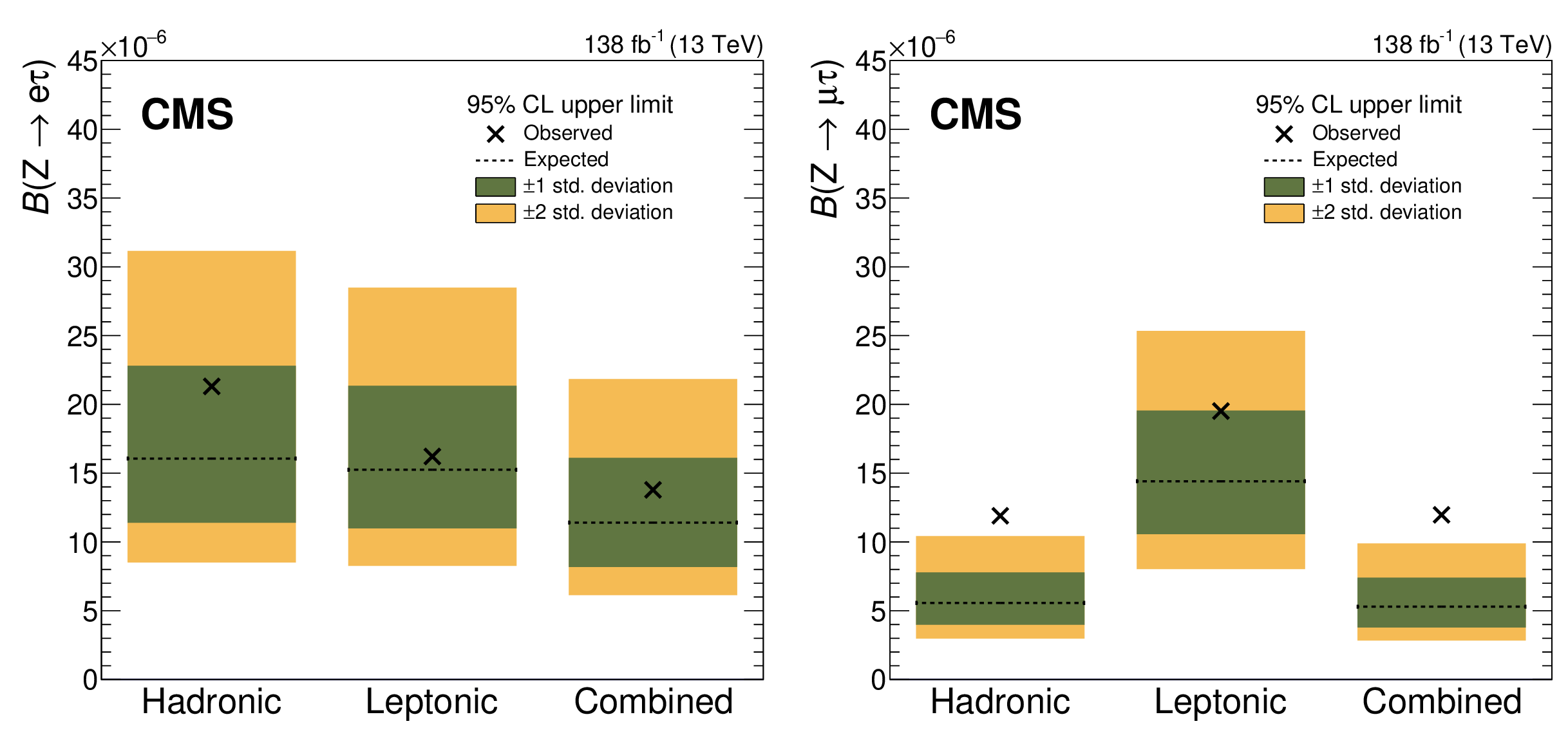
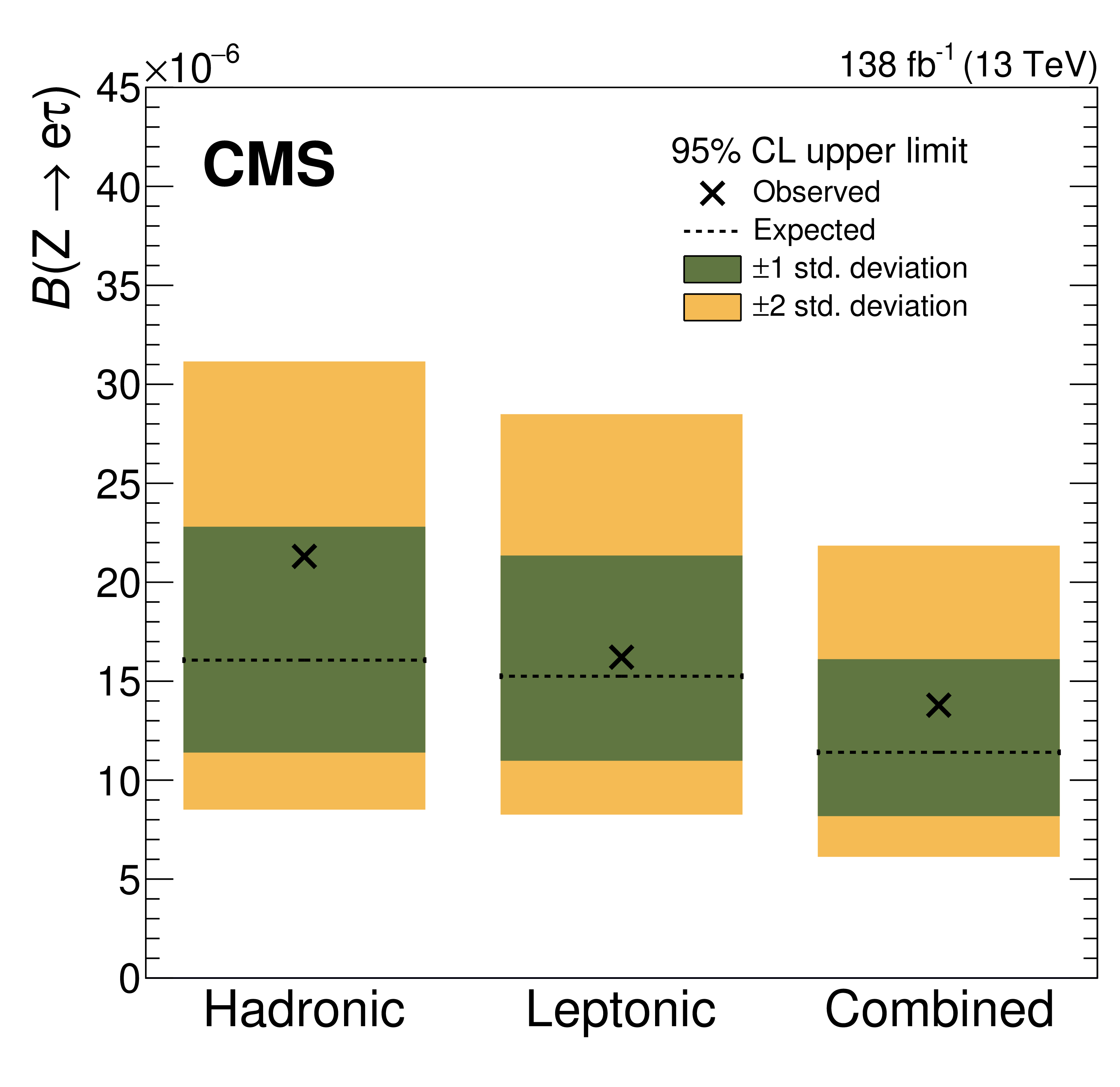
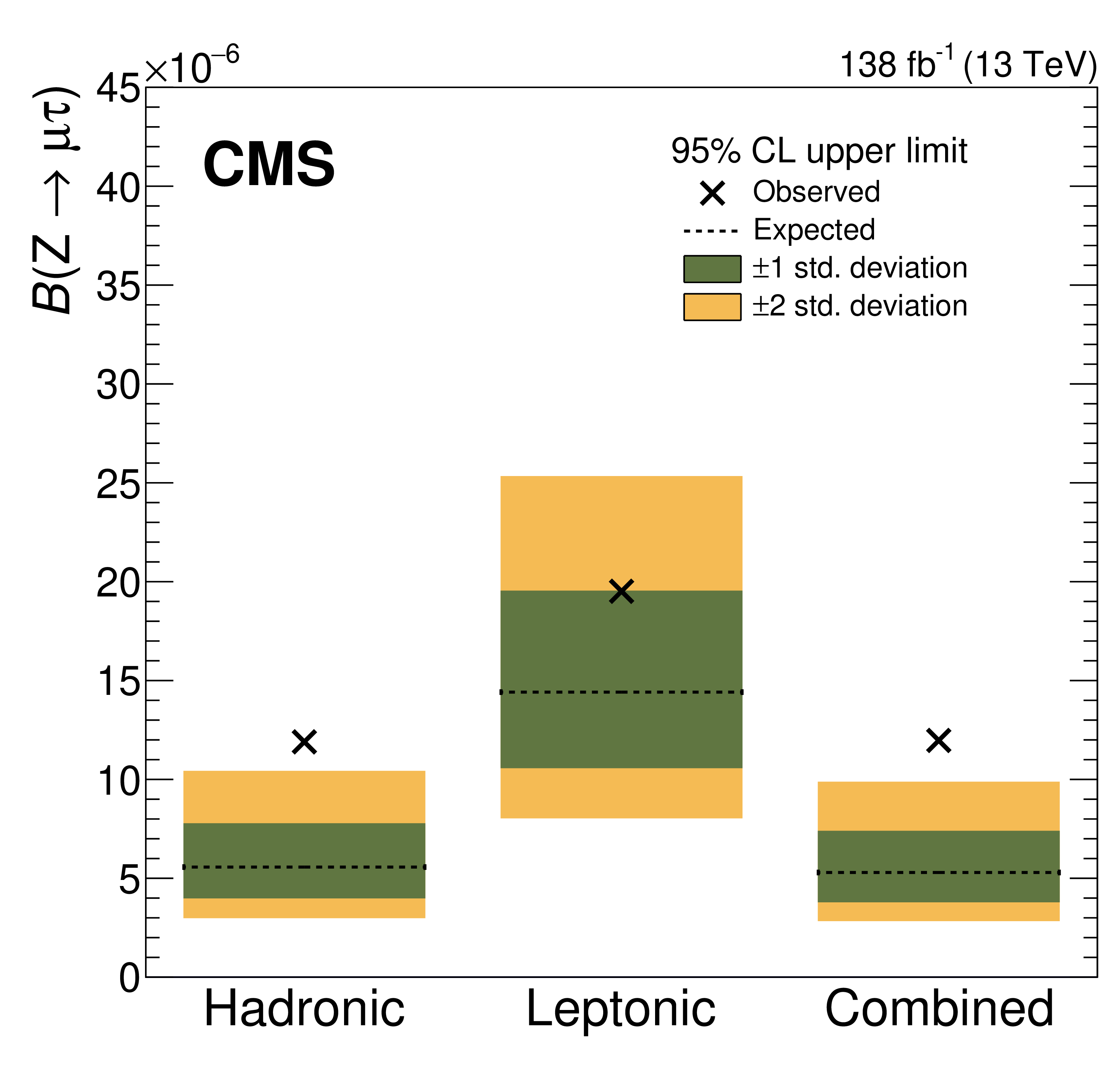
Figure 13:
Observed and expected 95% CL upper limit by category, as well as for the final combined fit, for the $ \mathrm{Z}\to\mathrm{e}\tau $ (left) and $ \mathrm{Z}\to\mu\tau $ (right) searches. The observed limits are denoted by the markers, while the expected limits with their 68 and 95% uncertainties are denoted by the horizontal dashed lines and green and yellow bands, respectively. |
png pdf |
Figure 13-a:
Observed and expected 95% CL upper limit by category, as well as for the final combined fit, for the $ \mathrm{Z}\to\mathrm{e}\tau $ (left) and $ \mathrm{Z}\to\mu\tau $ (right) searches. The observed limits are denoted by the markers, while the expected limits with their 68 and 95% uncertainties are denoted by the horizontal dashed lines and green and yellow bands, respectively. |
png pdf |
Figure 13-b:
Observed and expected 95% CL upper limit by category, as well as for the final combined fit, for the $ \mathrm{Z}\to\mathrm{e}\tau $ (left) and $ \mathrm{Z}\to\mu\tau $ (right) searches. The observed limits are denoted by the markers, while the expected limits with their 68 and 95% uncertainties are denoted by the horizontal dashed lines and green and yellow bands, respectively. |
png pdf |
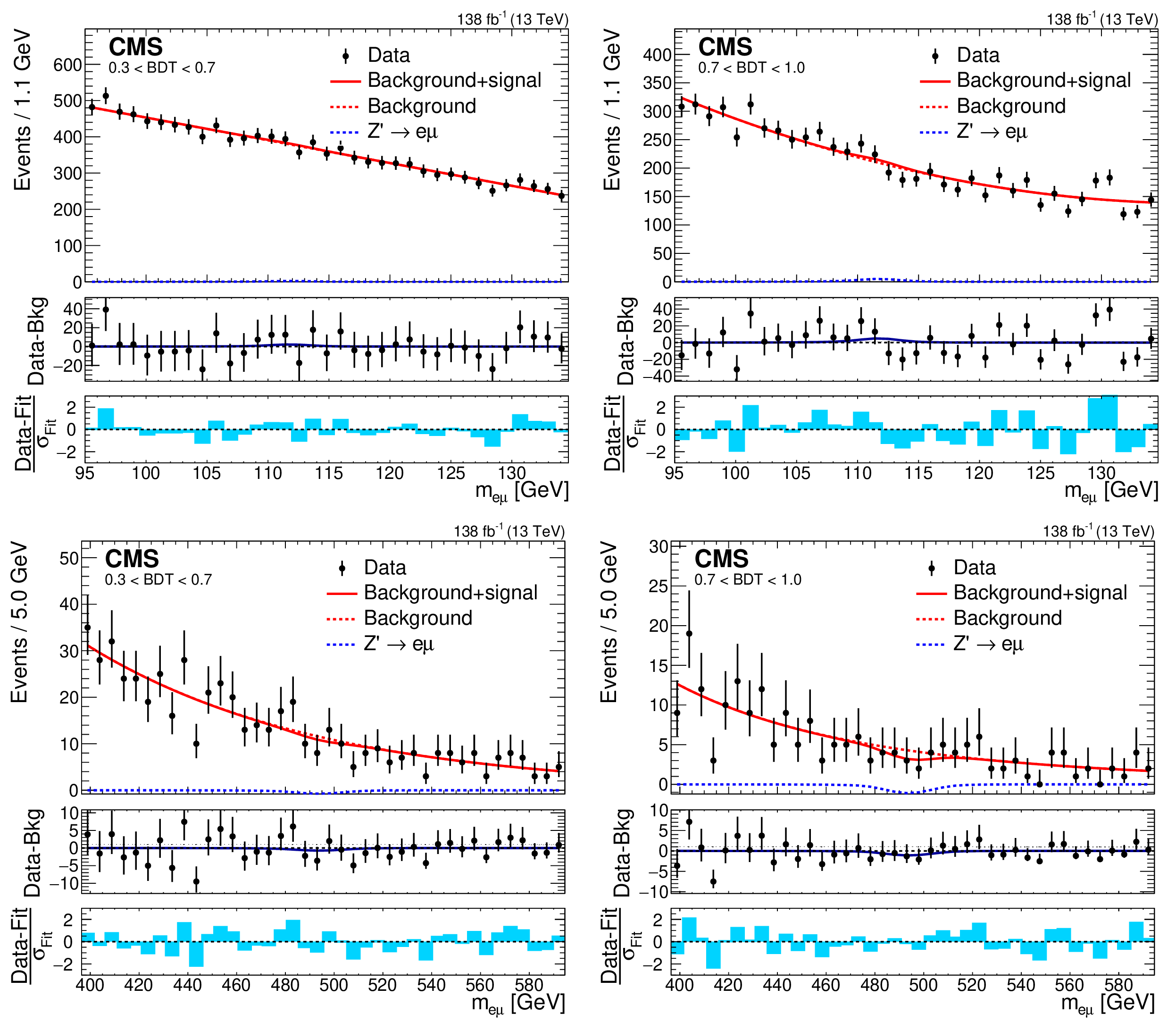
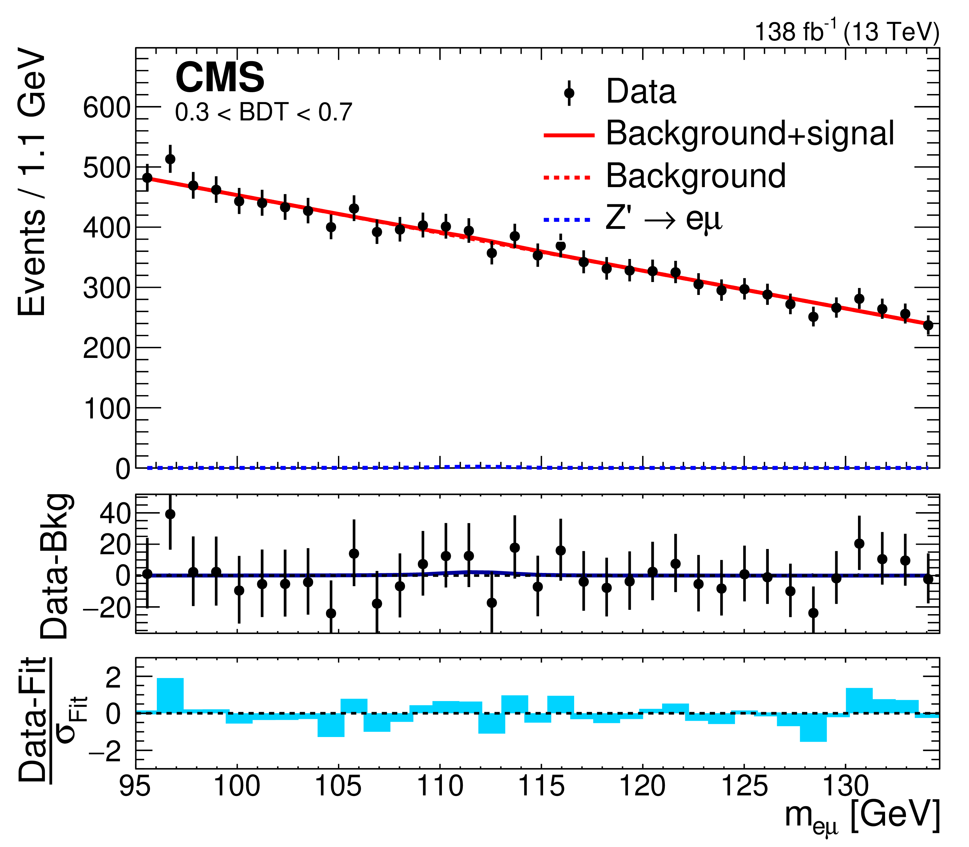
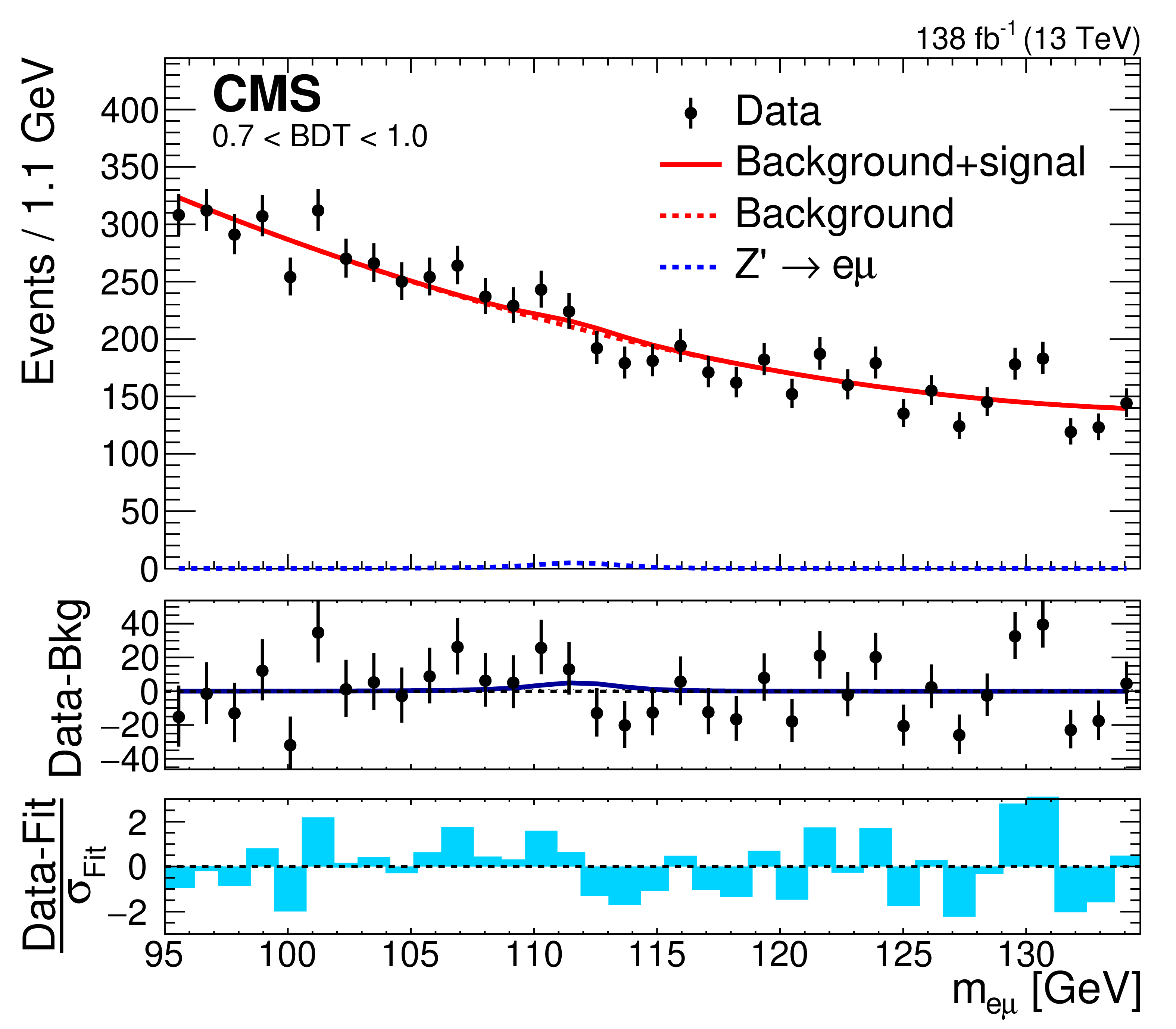
Figure 14:
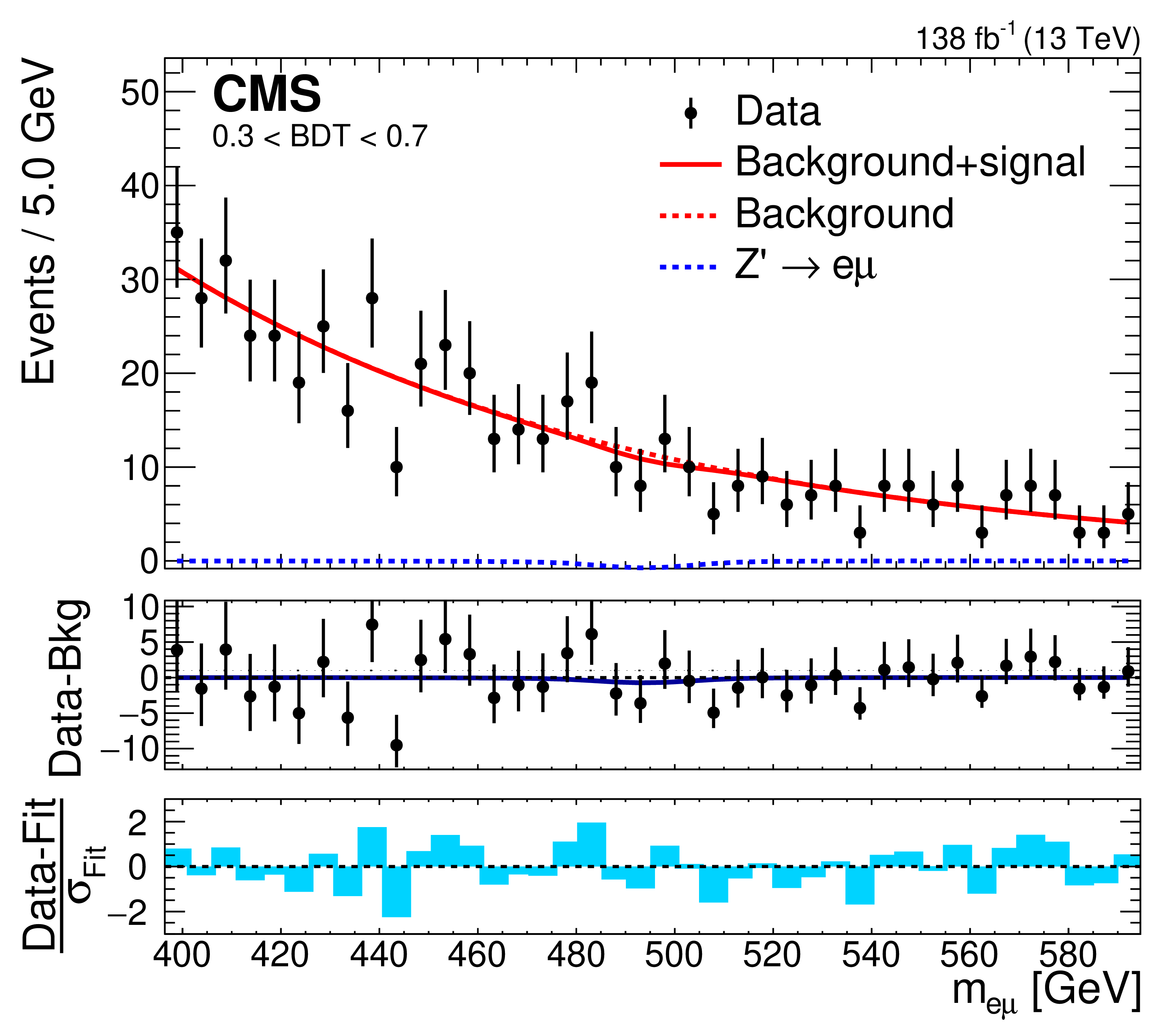
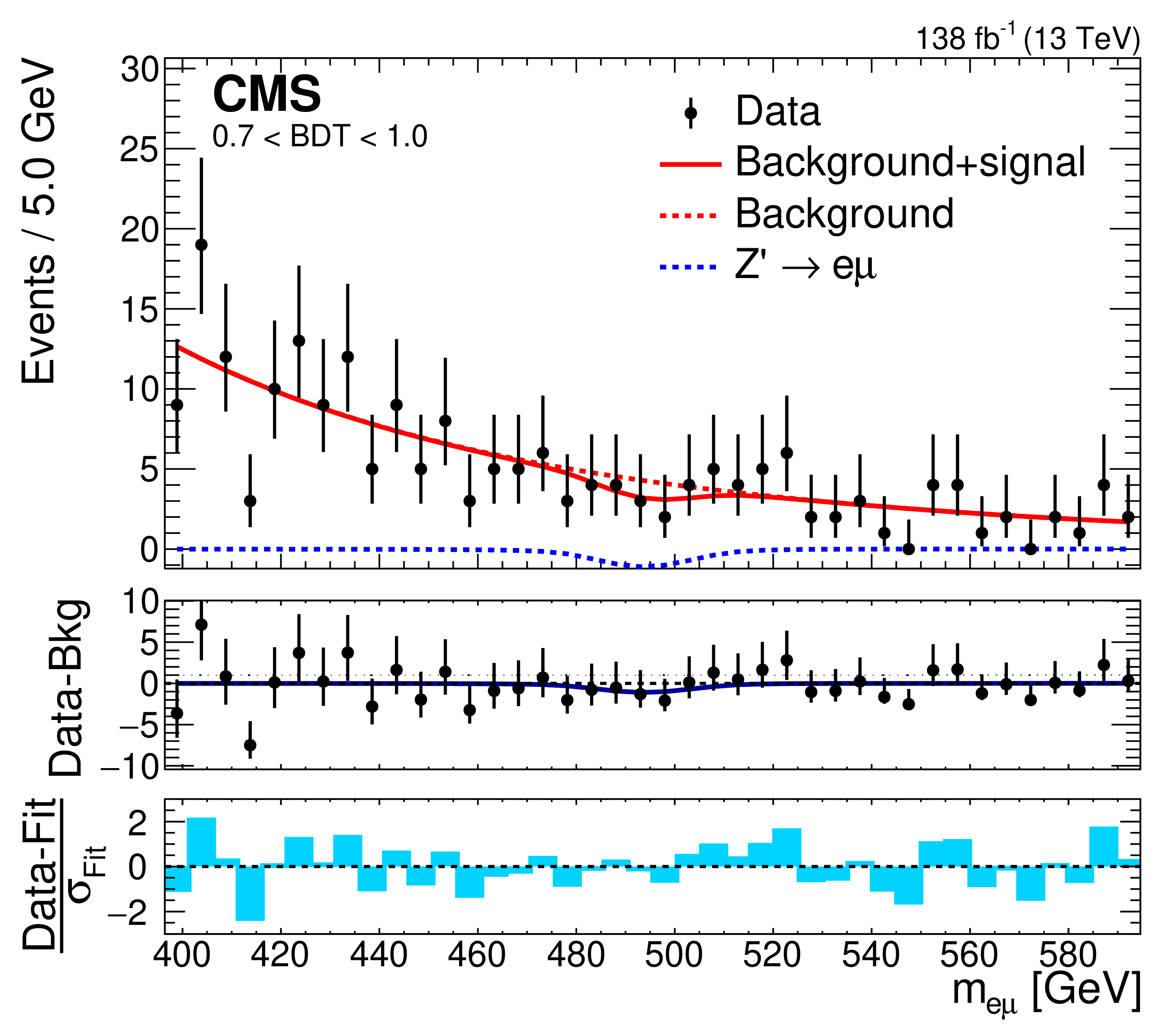
Distributions in $ m_{\mathrm{e}\mu} $ for the scan points 111 GeV (upper row) and 496 GeV (lower row) from the Z' search. In each row the BDT score range for the left (right) plot is 0.3-0.7 (0.7-1.0). In each plot, the upper panel shows the data (points with bars showing the statistical uncertainty) together with the fit distribution curve (red solid) and its separate signal (blue dotted) and background (red dotted) components, the middle panel shows the background subtracted data with the fit signal distribution, and the lower panel shows the deviations of the data from the fit function divided by the fit uncertainty. |
png pdf |
Figure 14-a:
Distributions in $ m_{\mathrm{e}\mu} $ for the scan points 111 GeV (upper row) and 496 GeV (lower row) from the Z' search. In each row the BDT score range for the left (right) plot is 0.3-0.7 (0.7-1.0). In each plot, the upper panel shows the data (points with bars showing the statistical uncertainty) together with the fit distribution curve (red solid) and its separate signal (blue dotted) and background (red dotted) components, the middle panel shows the background subtracted data with the fit signal distribution, and the lower panel shows the deviations of the data from the fit function divided by the fit uncertainty. |
png pdf |
Figure 14-b:
Distributions in $ m_{\mathrm{e}\mu} $ for the scan points 111 GeV (upper row) and 496 GeV (lower row) from the Z' search. In each row the BDT score range for the left (right) plot is 0.3-0.7 (0.7-1.0). In each plot, the upper panel shows the data (points with bars showing the statistical uncertainty) together with the fit distribution curve (red solid) and its separate signal (blue dotted) and background (red dotted) components, the middle panel shows the background subtracted data with the fit signal distribution, and the lower panel shows the deviations of the data from the fit function divided by the fit uncertainty. |
png pdf |
Figure 14-c:
Distributions in $ m_{\mathrm{e}\mu} $ for the scan points 111 GeV (upper row) and 496 GeV (lower row) from the Z' search. In each row the BDT score range for the left (right) plot is 0.3-0.7 (0.7-1.0). In each plot, the upper panel shows the data (points with bars showing the statistical uncertainty) together with the fit distribution curve (red solid) and its separate signal (blue dotted) and background (red dotted) components, the middle panel shows the background subtracted data with the fit signal distribution, and the lower panel shows the deviations of the data from the fit function divided by the fit uncertainty. |
png pdf |
Figure 14-d:
Distributions in $ m_{\mathrm{e}\mu} $ for the scan points 111 GeV (upper row) and 496 GeV (lower row) from the Z' search. In each row the BDT score range for the left (right) plot is 0.3-0.7 (0.7-1.0). In each plot, the upper panel shows the data (points with bars showing the statistical uncertainty) together with the fit distribution curve (red solid) and its separate signal (blue dotted) and background (red dotted) components, the middle panel shows the background subtracted data with the fit signal distribution, and the lower panel shows the deviations of the data from the fit function divided by the fit uncertainty. |
png pdf |
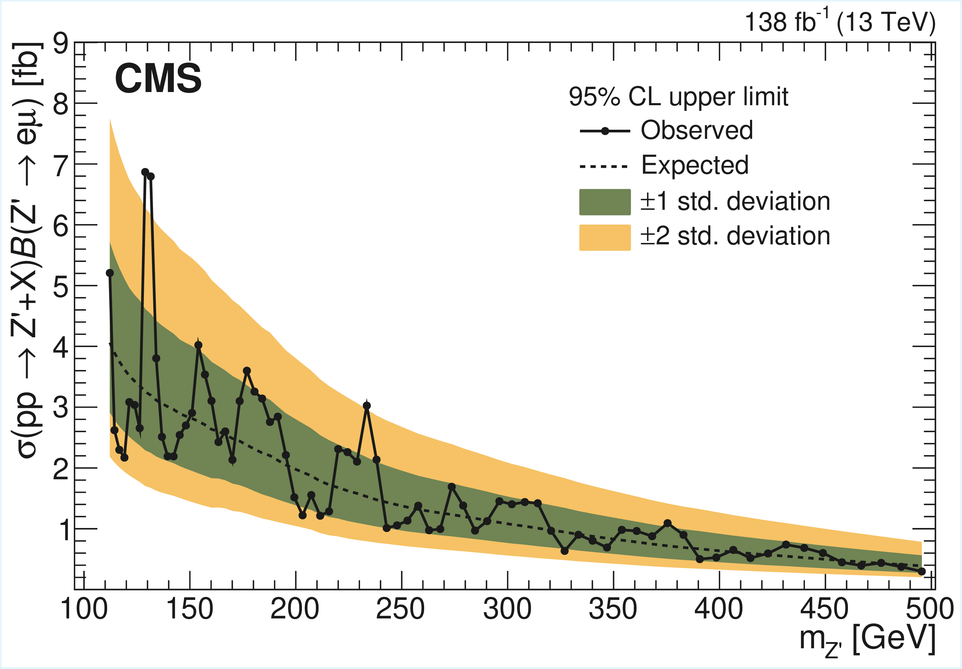
Figure 15:
Expected and observed 95% CL upper limits on $ \sigma(\mathrm{p}\mathrm{p}\to\mathrm{Z}^{'}\!+\!\mathrm{X})\mathcal{B}(\mathrm{Z}^{'}\to\mathrm{e}\mu) $ for Z' masses between 110 and 500 GeV. The solid black line connects filled circles representing the observed upper limits at the scan points, and the dashed line with filled error bands shows the expected limit. |
| Tables | |
png pdf |
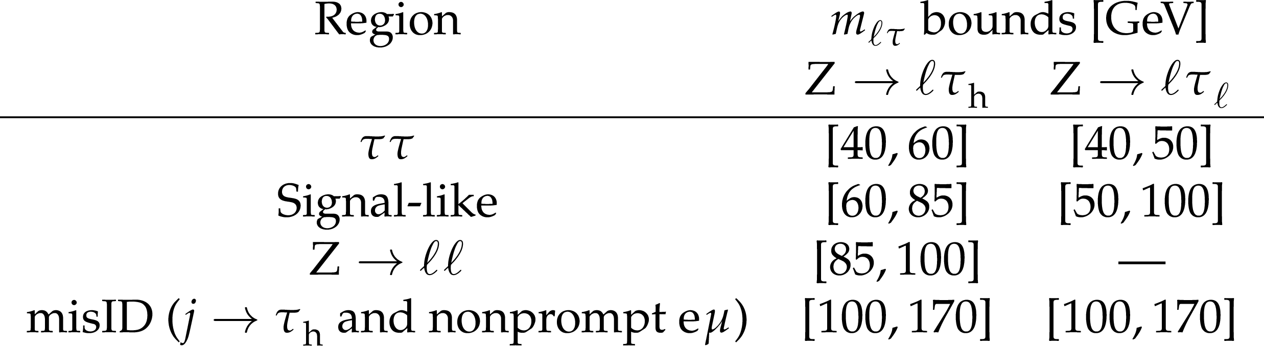
Table 1:
Regions in $ m_{\ell\tau} $ for the $ \mathrm{Z}\to\mu\tau $ and $ \mathrm{Z}\to\mathrm{e}\tau $ fits. |
png pdf |
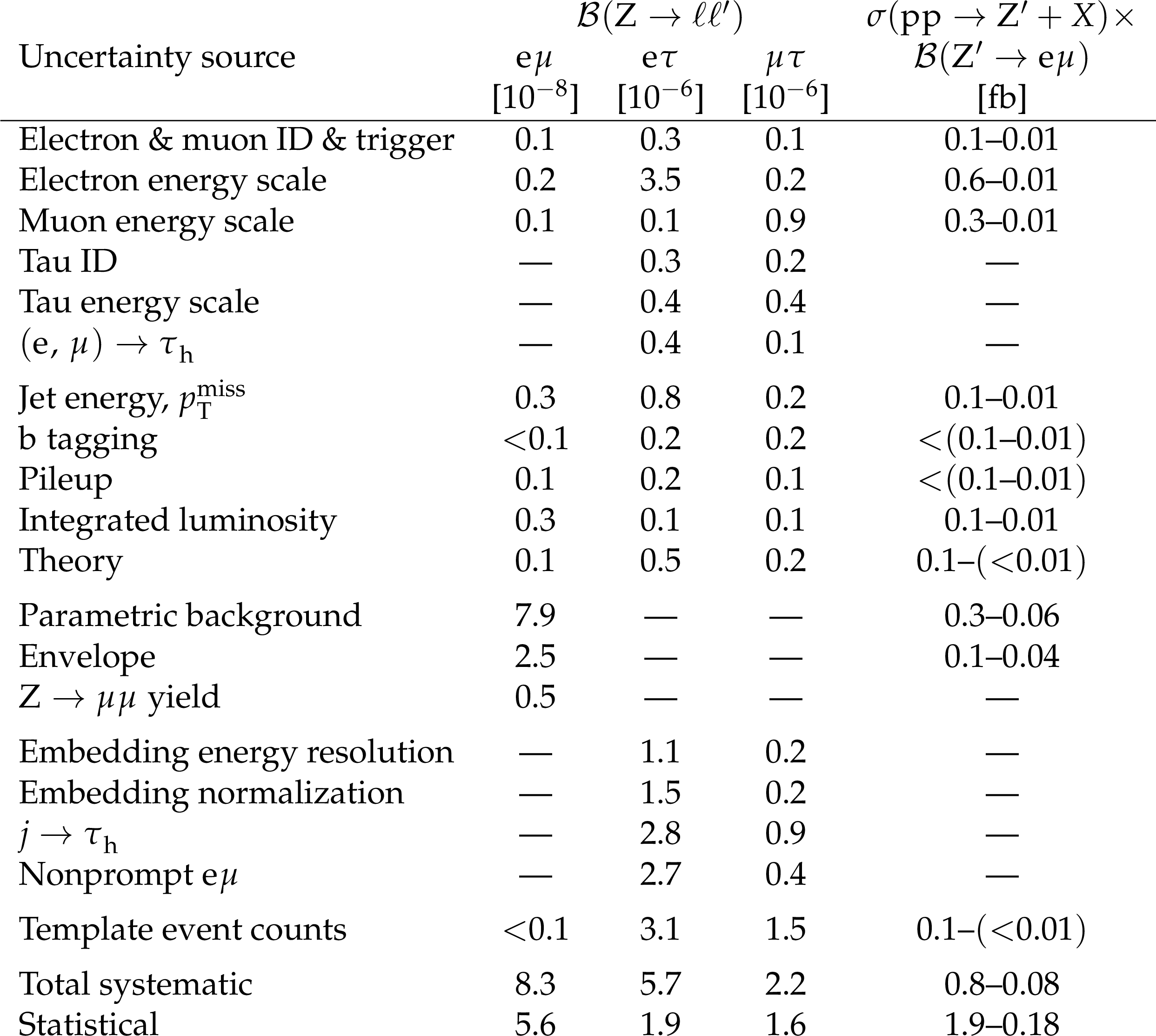
Table 2:
Sources of uncertainty and their impacts on the measured branching fraction, for each of the Z decay channels, and on the product of the production cross section and branching fraction for the Z' resonance scan. The uncertainty ranges for the Z' resonance scan are ordered from the lowest to the highest Z' mass point. Entries to which the specified uncertainty does not apply are denoted with ``$ \text{---} $''. |
png pdf |
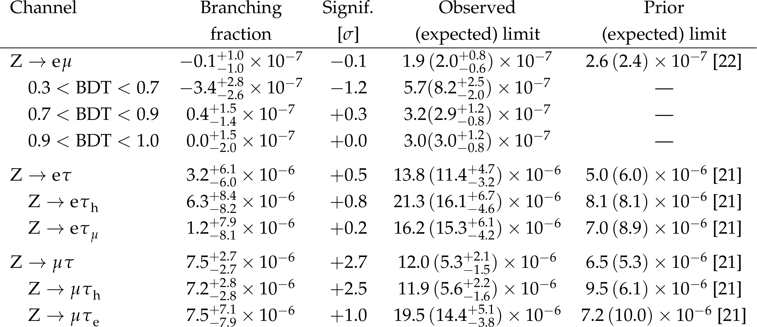
Table 3:
The measured branching fraction with its significance (signif.) and observed and expected 95% CL upper limits, for each of the $ \mathrm{Z}\to\mathrm{e}\mu $, $ \mathrm{Z}\to\mathrm{e}\tau $, and $ \mathrm{Z}\to\mu\tau $ decay channels. The prior best published limits are also given for comparison. Included are results for the separate BDT bins for $ \mathrm{Z}\to\mathrm{e}\mu $ and the separate $ \tau $ decay subchannels for $ \mathrm{Z}\to\mathrm{e}\tau $ and $ \mathrm{Z}\to\mu\tau $. |
| Summary |
| A search is presented for flavor violating decays of the Z boson to charged leptons, and for the presence of a heavier vector boson Z' exhibiting such decays. The data from proton-proton collisions at $ \sqrt{s}= $ 13 TeV were collected with the CMS detector at the LHC, and correspond to an integrated luminosity of 138 fb$^{-1}$. The specific decay modes considered are $ \mathrm{Z}^{(\prime)}\to\mathrm{e}\mu $, $ \mathrm{Z}\to\mathrm{e}\tau $, and $ \mathrm{Z}\to\mu\tau $. No significant excess of events over backgrounds from standard model processes is observed. Observed (expected) upper limits of 1.9 $ \times $ 10$^{-7} $, 1.38 $ \times $ 10$^{-5} $, and 1.20 $ \times $ 10$^{-5} $ (2.0 $ \times $ 10$^{-7} $, 1.14 $ \times $ 10$^{-5} $, and 0.53 $ \times $ 10$^{-5} $) at 95% confidence level are set on the branching fractions for $ \mathrm{Z}\to\mathrm{e}\mu $, $ \mathrm{Z}\to\mathrm{e}\tau $, and $ \mathrm{Z}\to\mu\tau $, respectively. The limit for $ \mathrm{Z}\to\mathrm{e}\mu $ is the most restrictive to date, while for $ \mathrm{Z}\to\mu\tau $ the sensitivity in terms of the expected limit is the same as that of the previous best limit. All of these limits are consistent with expectations from the standard model, and with constraints inferred from low-energy experimental limits. For Z' boson masses in the range 110-500 GeV, upper limits are set on the cross section times the branching fraction to $ \mathrm{e}\mu $ that range from 0.3 to 7 fb, and are the most restrictive to date for this mass range. Future studies can benefit from additional data, since even the systematic uncertainties arise mainly from statistical ones in control samples. |
| References | ||||
| 1 | Super-Kamiokande Collaboration | Measurement of the flux and zenith angle distribution of upward through going muons by Super-Kamiokande | PRL 82 (1999) 2644 | hep-ex/9812014 |
| 2 | Super-Kamiokande Collaboration | Solar B-8 and hep neutrino measurements from 1258 days of Super-Kamiokande data | PRL 86 (2001) 5651 | hep-ex/0103032 |
| 3 | SNO Collaboration | Direct evidence for neutrino flavor transformation from neutral current interactions in the Sudbury Neutrino Observatory | PRL 89 (2002) 011301 | nucl-ex/0204008 |
| 4 | KamLAND Collaboration | First results from KamLAND: Evidence for reactor anti-neutrino disappearance | PRL 90 (2003) 021802 | hep-ex/0212021 |
| 5 | J. I. Illana and T. Riemann | Charged lepton flavor violation from massive neutrinos in Z decays | PRD 63 (2001) 053004 | hep-ph/0010193 |
| 6 | W. J. Marciano, T. Mori, and J. M. Roney | Charged lepton flavor violation experiments | Ann. Rev. Nucl. Part. Sci. 58 (2008) 315 | |
| 7 | L. Calibbi and G. Signorelli | Charged lepton flavour violation: An experimental and theoretical introduction | Riv. Nuovo Cim. 41 (2018) 71 | 1709.00294 |
| 8 | P. Langacker | The physics of heavy Z' gauge bosons | Rev. Mod. Phys. 81 (2009) 1199 | 0801.1345 |
| 9 | C. Cornella, P. Paradisi, and O. Sumensari | Hunting for ALPs with lepton flavor violation | JHEP 01 (2020) 158 | 1911.06279 |
| 10 | M. Bauer et al. | Flavor probes of axion-like particles | JHEP 09 (2022) 056 | 2110.10698 |
| 11 | MEG II Collaboration | A search for $ \mu ^+ \rightarrow \textrm{e}^+ \gamma $ with the first dataset of the MEG II experiment | EPJC 84 (2024) 216 | 2310.12614 |
| 12 | SINDRUM Collaboration | Search for the decay $ \mu^+ \to e^+ e^+ e^- $ | NPB 299 (1988) 1 | |
| 13 | SINDRUM II Collaboration | A search for muon to electron conversion in muonic gold | EPJC 47 (2006) 337 | |
| 14 | CLEO Collaboration | Search for lepton flavor violation in Upsilon decays | PRL 101 (2008) 201601 | 0807.2695 |
| 15 | BaBar Collaboration | Search for the reactions $ e^{+} e^{-} \to \mu^{+} \tau^{-} $ and $ e^{+} e^{-} \to e^{+} \tau^{-} $ | PRD 75 (2007) 031103 | hep-ex/0607044 |
| 16 | BaBar Collaboration | Searches for lepton flavor violation in the decays $ \tau^{\pm}\to e^{\pm} \gamma $ and $ \tau^{\pm}\to \mu^{\pm} \gamma $ | PRL 104 (2010) 021802 | 0908.2381 |
| 17 | Belle Collaboration | Search for lepton flavor violating $ \tau $ decays into three leptons with 719 million produced $ \tau^+\tau^- $ pairs | PLB 687 (2010) 139 | 1001.3221 |
| 18 | S. Nussinov, R. D. Peccei, and X. M. Zhang | On unitarity based relations between various lepton family violating processes | PRD 63 (2001) 016003 | hep-ph/0004153 |
| 19 | OPAL Collaboration | A search for lepton flavor violating Z$ ^0 $ decays | Z. Phys. C 67 (1995) 555 | |
| 20 | DELPHI Collaboration | Search for lepton flavor number violating Z$ ^0 $ decays | Z. Phys. C 73 (1997) 243 | |
| 21 | ATLAS Collaboration | Search for charged-lepton-flavour violation in $ Z $-boson decays with the ATLAS detector | Nature Phys. 17 (2021) 819 | 2010.02566 |
| 22 | ATLAS Collaboration | Search for lepton-flavor-violation in $ Z $-boson decays with $ \tau $ leptons with the ATLAS detector | PRL 127 (2022) 271801 | 2105.12491 |
| 23 | ATLAS Collaboration | Search for the charged-lepton-flavor-violating decay $ Z\rightarrow e\mu $ in $ pp $ collisions at $ \sqrt{s}= $ 13 TeV with the ATLAS detector | PRD 108 (2023) 032015 | 2204.10783 |
| 24 | CMS Collaboration | HEPData record for this analysis | link | |
| 25 | CMS Collaboration | The CMS experiment at the CERN LHC | JINST 3 (2008) S08004 | |
| 26 | CMS Collaboration | Development of the CMS detector for the CERN LHC Run 3 | JINST 19 (2024) P05064 | CMS-PRF-21-001 2309.05466 |
| 27 | CMS Tracker Collaboration | Description and performance of track and primary-vertex reconstruction with the CMS tracker | JINST 9 (2014) P10009 | 1405.6569 |
| 28 | CMS Tracker Group Collaboration | The CMS phase-1 pixel detector upgrade | JINST 16 (2021) P02027 | 2012.14304 |
| 29 | CMS Collaboration | Track impact parameter resolution for the full pseudo rapidity coverage in the 2017 dataset with the CMS phase-1 pixel detector | CMS Detector Performance Summary CMS-DP-2020-049, 2020 CDS |
|
| 30 | CMS Collaboration | Technical proposal for the Phase-II upgrade of the Compact Muon Solenoid | CMS Technical Proposal CERN-LHCC-2015-010, CMS-TDR-15-02, 2015 CDS |
|
| 31 | CMS Collaboration | Particle-flow reconstruction and global event description with the CMS detector | JINST 12 (2017) P10003 | CMS-PRF-14-001 1706.04965 |
| 32 | M. Cacciari, G. P. Salam, and G. Soyez | The anti-$ k_{\mathrm{T}} $ jet clustering algorithm | JHEP 04 (2008) 063 | 0802.1189 |
| 33 | M. Cacciari, G. P. Salam, and G. Soyez | FastJet user manual | EPJC 72 (2012) 1896 | 1111.6097 |
| 34 | CMS Collaboration | Pileup mitigation at CMS in 13 TeV data | JINST 15 (2020) P09018 | CMS-JME-18-001 2003.00503 |
| 35 | CMS Collaboration | Jet energy scale and resolution in the CMS experiment in pp collisions at 8 TeV | JINST 12 (2017) P02014 | CMS-JME-13-004 1607.03663 |
| 36 | CMS Collaboration | Identification of b-quark jets with the CMS experiment | JINST 8 (2013) P04013 | CMS-BTV-12-001 1211.4462 |
| 37 | CMS Collaboration | Performance of the DeepJet b tagging algorithm using 41.9/fb of data from proton-proton collisions at 13 TeV with Phase 1 CMS detector | CMS Detector Performance Summary CMS-DP-2018-058, 2018 CDS |
|
| 38 | E. Bols et al. | Jet flavour classification using DeepJet | JINST 15 (2020) P12012 | 2008.10519 |
| 39 | CMS Collaboration | Performance of reconstruction and identification of $ \tau $ leptons decaying to hadrons and $ \nu_\tau $ in pp collisions at $ \sqrt{s}= $ 13 TeV | JINST 13 (2018) P10005 | CMS-TAU-16-003 1809.02816 |
| 40 | CMS Collaboration | Identification of hadronic tau lepton decays using a deep neural network | JINST 17 (2022) P07023 | CMS-TAU-20-001 2201.08458 |
| 41 | CMS Collaboration | ECAL 2016 refined calibration and Run 2 summary plots | CMS Detector Performance Summary CMS-DP-2020-021, 2020 CDS |
|
| 42 | CMS Collaboration | Electron and photon reconstruction and identification with the CMS experiment at the CERN LHC | JINST 16 (2021) P05014 | CMS-EGM-17-001 2012.06888 |
| 43 | CMS Collaboration | Performance of the CMS muon detector and muon reconstruction with proton-proton collisions at $ \sqrt{s}= $ 13 TeV | JINST 13 (2018) P06015 | CMS-MUO-16-001 1804.04528 |
| 44 | D. Bertolini, P. Harris, M. Low, and N. Tran | Pileup per particle identification | JHEP 10 (2014) 059 | 1407.6013 |
| 45 | CMS Collaboration | Performance of missing transverse momentum reconstruction in proton-proton collisions at $ \sqrt{s} = $ 13 TeV using the CMS detector | JINST 14 (2019) P07004 | CMS-JME-17-001 1903.06078 |
| 46 | CMS Collaboration | Performance of the CMS Level-1 trigger in proton-proton collisions at $ \sqrt{s} = $ 13 TeV | JINST 15 (2020) P10017 | CMS-TRG-17-001 2006.10165 |
| 47 | CMS Collaboration | The CMS trigger system | JINST 12 (2017) P01020 | CMS-TRG-12-001 1609.02366 |
| 48 | CMS Collaboration | Performance of the CMS high-level trigger during LHC Run 2 | JINST 19 (2024) P11021 | CMS-TRG-19-001 2410.17038 |
| 49 | J. Alwall et al. | The automated computation of tree-level and next-to-leading order differential cross sections, and their matching to parton shower simulations | JHEP 07 (2014) 079 | 1405.0301 |
| 50 | J. Alwall et al. | Comparative study of various algorithms for the merging of parton showers and matrix elements in hadronic collisions | EPJC 53 (2008) 473 | 0706.2569 |
| 51 | P. Nason | A new method for combining NLO QCD with shower Monte Carlo algorithms | JHEP 11 (2004) 040 | hep-ph/0409146 |
| 52 | S. Frixione, P. Nason, and C. Oleari | Matching NLO QCD computations with parton shower simulations: the POWHEG method | JHEP 11 (2007) 070 | 0709.2092 |
| 53 | S. Alioli, P. Nason, C. Oleari, and E. Re | A general framework for implementing NLO calculations in shower Monte Carlo programs: the POWHEG BOX | JHEP 06 (2010) 043 | 1002.2581 |
| 54 | S. Alioli, P. Nason, C. Oleari, and E. Re | NLO single-top production matched with shower in POWHEG: $ s $- and $ t $-channel contributions | JHEP 09 (2009) 111 | 0907.4076 |
| 55 | E. Re | Single-top Wt-channel production matched with parton showers using the POWHEG method | EPJC 71 (2011) 1547 | 1009.2450 |
| 56 | S. Alioli, P. Nason, C. Oleari, and E. Re | NLO Higgs boson production via gluon fusion matched with shower in POWHEG | JHEP 04 (2009) 002 | 0812.0578 |
| 57 | P. Nason and C. Oleari | NLO Higgs boson production via vector-boson fusion matched with shower in POWHEG | JHEP 02 (2010) 037 | 0911.5299 |
| 58 | T. Melia, P. Nason, R. Rontsch, and G. Zanderighi | W$^{+}$W$^{-}$, WZ and ZZ production in the POWHEG BOX | JHEP 11 (2011) 078 | 1107.5051 |
| 59 | P. Nason and G. Zanderighi | W$^{+}$W$^{-}$, WZ and ZZ production in the POWHEG-BOX-V2 | EPJC 74 (2014) 2702 | 1311.1365 |
| 60 | G. Luisoni, P. Nason, C. Oleari, and F. Tramontano | HW/HZ + 0 and 1 jet at NLO with the POWHEG BOX interfaced to GoSam and their merging within MiNLO | JHEP 10 (2013) 083 | 1306.2542 |
| 61 | T. Sjöstrand et al. | An introduction to PYTHIA 8.2 | Comput. Phys. Commun. 191 (2015) 159 | 1410.3012 |
| 62 | K. Melnikov and F. Petriello | Electroweak gauge boson production at hadron colliders through $ \mathcal{O}(\alpha_\text{s}^{2}) $ | PRD 74 (2006) 114017 | hep-ph/0609070 |
| 63 | M. Czakon and A. Mitov | Top++: A program for the calculation of the top-pair cross-section at hadron colliders | Comput. Phys. Commun. 185 (2014) 2930 | 1112.5675 |
| 64 | N. Kidonakis | Top quark production | in Helmholtz International Summer School on Physics of Heavy Quarks and Hadrons, 2014 link |
1311.0283 |
| 65 | J. M. Campbell, R. K. Ellis, and C. Williams | Vector boson pair production at the LHC | JHEP 07 (2011) 018 | 1105.0020 |
| 66 | T. Gehrmann et al. | $ \mathrm{W^+}\mathrm{W^-} $ production at hadron colliders in next to next to leading order QCD | PRL 113 (2014) 212001 | 1408.5243 |
| 67 | CMS Collaboration | Event generator tunes obtained from underlying event and multiparton scattering measurements | EPJC 76 (2016) 155 | CMS-GEN-14-001 1512.00815 |
| 68 | CMS Collaboration | Extraction and validation of a new set of CMS PYTHIA8 tunes from underlying-event measurements | EPJC 80 (2020) 4 | CMS-GEN-17-001 1903.12179 |
| 69 | R. Frederix and S. Frixione | Merging meets matching in MC@NLO | JHEP 12 (2012) 061 | 1209.6215 |
| 70 | NNPDF Collaboration | Parton distributions for the LHC Run II | JHEP 04 (2015) 040 | 1410.8849 |
| 71 | NNPDF Collaboration | Parton distributions from high-precision collider data | EPJC 77 (2017) 663 | 1706.00428 |
| 72 | NNPDF Collaboration | Parton distributions with QED corrections | NPB 877 (2013) 290 | 1308.0598 |
| 73 | GEANT4 Collaboration | GEANT4---a simulation toolkit | NIM A 506 (2003) 250 | |
| 74 | Particle Data Group , S. Navas et al. | Review of particle physics | PRD 110 (2024) 030001 | |
| 75 | T. Chen and C. Guestrin | XGBoost: A scalable tree boosting system | in Proceedings of the 22nd ACM SIGKDD International Conference on Knowledge Discovery and Data Mining, KDD '16, Association for Computing Machinery, New York, NY, USA, 2016 link |
1603.02754 |
| 76 | M. J. Oreglia | A study of the reactions $ \psi^\prime \to \gamma \gamma \psi $ | Master's thesis, Stanford University, SLAC Report SLAC-R-236, 1980 link |
|
| 77 | J. E. Gaiser | Charmonium spectroscopy from radiative decays of the $ J/\psi $ and $ \psi^\prime $ | Master's thesis, Stanford University, SLAC Report SLAC-0255, 1982 link |
|
| 78 | P. D. Dauncey, M. Kenzie, N. Wardle, and G. J. Davies | Handling uncertainties in background shapes: the discrete profiling method | JINST 10 (2015) P04015 | 1408.6865 |
| 79 | R. A. Fisher | On the mathematical foundations of theoretical statistics | Phil. Trans. Roy. Soc. Lond. 222 (1922) 309 | |
| 80 | CMS Collaboration | An embedding technique to determine $ \tau\tau $ backgrounds in proton-proton collision data | JINST 14 (2019) P06032 | CMS-TAU-18-001 1903.01216 |
| 81 | CMS Collaboration | Measurements of Higgs boson production in the decay channel with a pair of $ \tau $ leptons in proton-proton collisions at $ \sqrt{s}= $ 13 TeV | EPJC 83 (2023) 562 | CMS-HIG-19-010 2204.12957 |
| 82 | CMS Collaboration | Search for lepton-flavor violating decays of the Higgs boson in the $ \mu\tau $ and e$ \tau $ final states in proton-proton collisions at $ \sqrt{s} = $ 13 TeV | PRD 104 (2021) 032013 | CMS-HIG-20-009 2105.03007 |
| 83 | S. Davidson, S. Lacroix, and P. Verdier | LHC sensitivity to lepton flavour violating Z boson decays | JHEP 09 (2012) 092 | 1207.4894 |
| 84 | TMVA Collaboration | TMVA --- toolkit for multivariate data analysis | Technical Report CERN-OPEN-2007-007, 2007 link |
physics/0703039 |
| 85 | CMS Collaboration | Precision luminosity measurement in proton-proton collisions at $ \sqrt{s} = $ 13 TeV in 2015 and 2016 at CMS | EPJC 81 (2021) 800 | CMS-LUM-17-003 2104.01927 |
| 86 | CMS Collaboration | CMS luminosity measurement for the 2017 data-taking period at $ \sqrt{s} = $ 13 TeV | CMS Physics Analysis Summary, 2018 link |
CMS-PAS-LUM-17-004 |
| 87 | CMS Collaboration | CMS luminosity measurement for the 2018 data-taking period at $ \sqrt{s} = $ 13 TeV | CMS Physics Analysis Summary, 2019 link |
CMS-PAS-LUM-18-002 |
| 88 | CMS Collaboration | Measurement of the inelastic proton-proton cross section at $ \sqrt{s}= $ 13 TeV | JHEP 07 (2018) 161 | CMS-FSQ-15-005 1802.02613 |
| 89 | CMS Collaboration | The CMS statistical analysis and combination tool: Combine | Comput. Softw. Big Sci. 8 (2024) 19 | CMS-CAT-23-001 2404.06614 |
| 90 | J. S. Conway | Incorporating nuisance parameters in likelihoods for multisource spectra | in Proc. PHYSTAT 2011 Workshop, 2011 link |
1103.0354 |
| 91 | G. Cowan, K. Cranmer, E. Gross, and O. Vitells | Asymptotic formulae for likelihood-based tests of new physics | EPJC 71 (2011) 1554 | 1007.1727 |
| 92 | T. Junk | Confidence level computation for combining searches with small statistics | NIM A 434 (1999) 435 | hep-ex/9902006 |
| 93 | A. L. Read | Presentation of search results: the $ CL_s $ technique | JPG 28 (2002) 2693 | |
| 94 | F. E. James | Statistical Methods in Experimental Physics 2nd Edition | World Scientific Publishing Co. Pte. Ltd., Singapore, . ISBN~981-270-527-9, 2006 | |
| 95 | G. Cowan | Statistics for searches at the LHC | in LHC Phenomenology, E. Gardi, N. Glover, and R. Aidan, eds. Springer, Cham, Scottish Graduate Series, 2015 link |
|
| 96 | ATLAS Collaboration | Search for a heavy neutral particle decaying to $ e\mu $, $ e\tau $, or $ \mu\tau $ in $ pp $ collisions at $ \sqrt{s}= $ 8 TeV with the ATLAS detector | PRL 115 (2015) 031801 | 1503.04430 |
| 97 | ATLAS Collaboration | Search for new phenomena in different-flavour high-mass dilepton final states in pp collisions at $ \sqrt{s}= $ 13 Tev with the ATLAS detector | EPJC 76 (2016) 541 | 1607.08079 |
| 98 | CMS Collaboration | Search for lepton flavour violating decays of heavy resonances and quantum black holes to an e$ \mu $ pair in proton-proton collisions at $ \sqrt{s} = $ 8 TeV | EPJC 76 (2016) 317 | CMS-EXO-13-002 1604.05239 |
| 99 | CMS Collaboration | Search for heavy resonances and quantum black holes in e$\mu$, e$\tau$, and $\mu\tau$ final states in proton-proton collisions at $ \sqrt{s} = $ 13 TeV | JHEP 05 (2023) 227 | CMS-EXO-19-014 2205.06709 |
|
|
Compact Muon Solenoid LHC, CERN |
|

|

|

|

|

|